The Development of Mapping Zones to Assist in Land CoverMapping over Large Geographic Areas: A Case Study of the

Southwest ReGAP Project

GERALD MANIS1, COLLIN HOMER

2, R. DOUGLAS RAMSEY1, JOHN LOWRY

1, TODD SAJWAJ1, AND

SCOTT GRAVES3

1 Utah State University, Remote Sensing and GIS Laboratories, Logan, Utah2 EROS Data Center, Sioux Falls, South Dakota3 Ducks Unlimited, Sacramento, California

IntroductionSpectral classification of satellite imagery to map land cover across large landscapes involves theeffective identification of spectral gradients resulting from the variability of physiographic andphenologic variables, ground variability, as well as solar and atmospheric influences within andbetween remotely sensed imagery. A common method of identifying spectral gradients is tostratify landscapes into subregions of similar biophysical characteristics. This process is not newto remote sensing and has been widely used as a postprocessing method to improve accuracy(Pettinger 1982, White et al. 1995). Lillesand (1996) refers to this process as “stratifying” thestudy area, and the resulting stratification units are called “spectro-physiographic areas” or“spectrally consistent classification units (SCCUs).”

This paper outlines the development of similar stratification units, which we refer to as “mappingzones.” Our study area is comprised of the five states in the Southwest ReGAP Project (Arizona,Colorado, Nevada, New Mexico, and Utah), covering approximately 530,000 square miles andencompassing a wide variety of ecosystems.

By partitioning the five-state study area into mapping zones, we hope to maximize spectraldifferentiation within areas of uniform ecological characteristics. From a project managementand logistical standpoint, mapping zones will facilitate partitioning the workload into logicalunits. Finally, we anticipate that the development of mapping zones will simplifypostclassification modeling and improve classification accuracy. Based on previous work byBauer et al. (1994) overall classification accuracy could be improved by 10 to 15% usingphysiographic regions.

BackgroundThe underlying concept of mapping zone delineation is to divide the landscape into a finitenumber of units that represent homogeneity with respect to landform, soil, vegetation, spectralreflectance, and overall ecological physiology. Ancillary data such as Digital Elevation Models(DEMs), existing imagery, soils, and/or geologic data are the primary source of quantitativeinformation guiding the delineation of mapping zones. However, the most critical component isa familiarity with the study area and an intimate knowledge of the biophysical features of thelandscape. Delineating mapping zones requires a degree of subjective decision making to strikethe balance between affordable economic units, optimal ecological units, and reasonable spectralunits. The concept of economy helps determine mapping zone size. A large number of smallzones become uneconomic since quasi-independent mapping efforts are required for each zone.

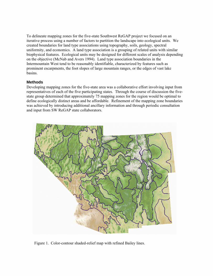
To delineate mapping zones for the five-state Southwest ReGAP project we focused on aniterative process using a number of factors to partition the landscape into ecological units. Wecreated boundaries for land type associations using topography, soils, geology, spectraluniformity, and economics. A land type association is a grouping of related units with similarbiophysical features. Ecological units may be designed for different scales of analysis dependingon the objective (McNab and Avers 1994). Land type association boundaries in theIntermountain West tend to be reasonably identifiable, characterized by features such asprominent escarpments, the foot slopes of large mountain ranges, or the edges of vast lakebasins.

MethodsDeveloping mapping zones for the five-state area was a collaborative effort involving input fromrepresentatives of each of the five participating states. Through the course of discussion the five-state group determined that approximately 75 mapping zones for the region would be optimal todefine ecologically distinct areas and be affordable. Refinement of the mapping zone boundarieswas achieved by introducing additional ancillary information and through periodic consultationand input from SW ReGAP state collaborators.

Figure 1. Color-contour shaded-relief map with refined Bailey lines.

Initial research into an ecological evaluation of the region focused on ecoregions defined byBailey et al. (1994) and Omernik (1987). These sources provided an overview of the landscapewith consideration to climate, vegetation and landform. Bailey’s ecoregion sections provided aninitial “starting point” for mapping zone boundaries. To refine the boundaries, a GIS coverageof Bailey’s ecoregions was plotted over a high-resolution, color-contour shaded-relief base map

type zones guided by Bailey’s section boundaries and was used as a starting point for discussionwith SW ReGAP collaborators.

Following comment from state collaborators, a second draft of mapping zones was created usingexisting Landsat TM images to help identify major life zones. This phase of the refinementprocess accounted for the spectral characteristics of the landscape. Interpretation of imageryimproved the delineation of major physiographic “seams,” such as escarpments and/or cleargeologic formation boundaries.

Most mapping zone boundaries are boundaries between landscape features that appear to bestdefine life zone boundaries. In areas that lack clear distinction between life zones, an attemptwas made to identify approximate boundaries by identifying spectral patterns that could berelated to vegetation communities and or geology. For example, major agricultural areas were

created from a 3-arc second DEM (Figure 1). The resulting map was an interpretation of land

used as a surrogate for natural vegetation patterns and became mapping zone boundaries in someareas to assist in the separation of natural vs. man-made environments.

A third phase of refinement involved the use of soils data. Soil is an integral component of thelandscape/vegetation relationship and provides great potential in guiding mapping zonedelineation. A soil map reflects not only edaphic conditions, but climatic conditions as well,reflecting elevation and latitude gradients over large areas. The State Soil Geographic(STATSGO) database is a nationwide digital (state-level) soil geospatial database. While theSoil Survey Geographic (SSURGO) database is more accurate and detailed than STATSGO,complete coverage for the five-state region is not available.

The original STATSGO GIS coverage for the five-state region contains approximately 2,100 soilmapping classes, each with multiple soil components. With a goal of 75 mapping zones for thefive-state region, the STATSGO database clearly had to be simplified to be useful for delineatingmapping zone boundaries. To simplify STATSGO, we developed a protocol for aggregating soilmapping classes. The protocol can be summarized as follows:

1. Component soils were re-classified based on a hierarchy of soil temperature regime,soil order, soil rooting depth classes, wetness classes, flooding regime, and broad soiltexture groups. This established a reasonable evaluation of which soil types weresimilar in their capacity to support vegetation.

2. General soil classes were sorted based on composition of similar soils, similar rangeof slopes, and similar range of non-soil components, i.e., rock outcrop, badlands,playas, etc.

3. Logical aggregations were evaluated by viewing the polygons over TM imagery, withsubsequent adjustments of slope limit and soil component differentia to preserve themost definitive delineations while merging the least definitive. Aggregations thatwere of small size, except those of unique value like dunes or playas, were mergedwith the adjacent, most similar aggregation.

4. A table was developed to describe each aggregated class, such as the range of soilgreat groups, slopes, major life zones, nonvegetated landscape features, soil textures,and a simplified mapping unit description.

Following this protocol, we generated 58 “generalized land type” classes based on soilcharacteristics. The aggregated 58-class STATSGO data layer was first used as an informal“test” of mapping zone boundaries derived in phases one and two. We found that the derivedSTATSGO data layer could be used to improve the delineation of some of the more problematicmapping zones. This was most important in areas with little topographic relief such as the plainsof eastern Colorado and New Mexico.

As a result of the refinement phases, the mapping zone GIS coverage consisted of 129 polygons.While this reflected a reasonable stratification of the landscape, it still exceeded our target of 75mapping zones. We compared this coverage to earlier drafts of the mapping zones and Bailey’secoregion sections. The smallest polygons were merged into adjoining polygons, based on thedistinctive qualities of the surrounding polygons and a general agreement or disagreement withBailey’s ecoregions. The final mapping zone coverage contained 74 polygons (Figure 2).

Figure 2. Final mapping zones for the SW ReGAP region.

DiscussionThe southwest United States provides a unique landscape with discrete mountain ranges andcomplex structural geology and soils, which helped provide a basis to delineate mapping zones.A possible limitation of using geomorphic boundaries to identify mapping zones is that thecoincidence of microclimatic and soil factors controlling vegetation will not always coincide

with geomorphology. Certain landscapes such as cuestas tend to be problematic because longdip slopes imply an unbroken elevation gradient. We have tried to resolve disagreement betweenlandscape boundaries and apparent vegetation boundaries by deferring to vegetation, asinterpreted on existing TM imagery, as the primary criteria. However, positive geomorphicboundaries took precedence over small-scale or uncertain vegetation patterns.

The amount of effort placed in deriving the soils GIS coverage from the STATSGO databasewas significant and alone did not substantially help in defining the mapping zone boundaries. Infact, a state-level geology coverage could very well be used as a surrogate for the soils dataproduced from STATSGO. What the derived STATSGO data provided was ancillaryinformation useful in verifying and refining some of the more problematic mapping zoningboundaries. The effort to aggregate the STATSGO database was not wasted as it holds greatpotential as a postclassification modeling layer.

We anticipate that well-defined mapping zones will improve image classification and, ultimately,land cover mapping. One of the important lessons learned from this effort is that delineatingmapping zones for the five-state region is an iterative process involving input from collaboratingparticipants and refinement using multiple ancillary data sources. In addition, a significantamount of personal and collective knowledge and a sound understanding of the general mappingprocess is required to interpret the ancillary data in a way that is meaningful.

Literature Cited

Bailey, R.G., P.E. Avers, T. King, W.H. McNab, editors. 1994. Ecoregions and subregions ofthe United States (1:7,500,000 map). With supplementary table of map unit descriptions,compiled and edited by W.H. McNab and R.G. Bailey. USDA Forest Service, Washington,DC.

Bauer, M.E., T.E. Burk, A.R. Ek, P.R. Coppin, S.D. Lime, T.A. Walsh, D.K. Walters, W. Befort,and D.F. Heinzen. 1994. Satellite inventory of Minnesota forest resources.Photogrammetric Engineering and Remote Sensing 60(3):287-298.

Lillesand, T.M. 1996. A protocol for satellite-based land cover classification in the UpperMidwest. Pages 103-118 in J.M. Scott, T.H. Tear, and F.W. Davis, editors. Gap Analysis: ALandscape Approach to Biodiversity Planning. ASPRS, 320 pp.

McNab, W.H., and P.E. Avers. 1994. Ecological subregions of the United States, sectiondescriptions. USDA Forest Service, Ecosystem Management Team.

Omernik, J.M. 1987. Ecoregions of the conterminous United States. Map (scale 1:7,500,000).Annals of the Association of American Geographers 77(1): 118-125

Pettinger, L.R. 1982. Digital classification of Landsat data for vegetation and land covermapping in the Blackfoot River watershed, southeastern Idaho. U.S. Geological SurveyProfessional Paper.

White, J.D., G.C. Kroh, C. Glenn, and J.E. Pinder III. 1995. Forest mapping at Lassen VolcanicNational Park, California, using Landsat TM data and a geographical information system.Photogrammetric Engineering and Remote Sensing 61:299-305.