I sdp. 336853 AQARD-U-800

ADVISORY GROUP FOR AEROSPACE RESEARCH & DEVELOPMENT 7 RUE ANCELLE, 92200 NEUILLY-SUR-SEINE, FRANCE

A \ T $ D 1

AQARD REPORT 800

The Design, Qualification and Maintenance of Vibration-Free Landing Gear .I.

Iy ' 2" ., (la Conception, la qualification et la maintenance

* des trains d'atterrissage sans vibration)

Papers presented at the 81s Meeting of the AGARD Structum d Materials Panet held in BanB Canada Octobw lH5.

/ -

by DIMS

.......... signed.

NOT kQh DESTRUCTION

NORTH ATLANTIC TREATY ORGANIZATION

I

Published March 1996

Distribution and Availability on Back Cover

AGARD-R-800

ADVISORYGROUPFORAEROSPACE RESEARCH &DEVELOPMENT

7 RUE ANCELLE, 92200 NEUILLY-SUR-SEINE, FRANCE

AGARD REPORT 800

c

The Design, Qualification and Maintenance of Vibration-Free Landing Gear (la Conception, la qualification et la maintenance des trains d’atterrissage sans vibration)

Papers presented at the 81st Meeting of the AGARD Structures and Materials Panel, held in Banff, Canada 4-5 October 1995.

- North Atlantic Treaty Organization Organisation du Traite de I’Atlantique Nord

I I

The Mission of AGARD

According to its Charter, the mission of AGARD is to bring together the leading personalities of the NATO nations in the fields of science and technology relating to aerospace for the following purposes:

- Recommending effective ways for the member nations to use their research and development capabilities for the common benefit of the NATO community;

- Providing scientific and technical advice and assistance to the Military Committee in the field of aerospace research and development (with particular regard to its military application);

- Continuously stimulating advances in the aerospace sciences relevant to strengthening the common defence posture;

- Improving the co-operation among member nations in aerospace research and development;

- Exchange of scientific and technical information;

- Providing assistance to member nations for the purpose of increasing their scientific and technical potential;

- Rendering scientific and technical assistance, as requested, to other NATO bodies and to member nations in connection with research and development problems in the aerospace field.

The highest authority within AGARD is the National Delegates Board consisting of officially appointed senior representatives from each member nation. The mission of AGARD is carried out through the Panels which are composed of experts appointed by the National Delegates, the Consultant and Exchange Programme and the Aerospace Applications Studies Programme. The results of AGARD work are reported to the member nations and the NATO Authorities through the AGARD series of publications of which this is one.

Participation in AGARD activities is by invitation only and is normally limited to citizens of the NATO nations.

The content of this publication has been reproduced directly from material supplied by AGARD or the authors.

Published March 1996

Copyright 0 AGARD 1996 All Rights Reserved

ISBN 92-836-1032-6

Printed by Canada Communication Group 45 Sacrk-Caur Blvd., Hull (Qukbec), Canada KIA OS7

ii

The Design, Qualification and Maintenance of Vibration-Free Landing Gear

(AGARD R-800)

Executive Summary

Aircraft landing gears are crucial for safety, comfort (both for passengers and pilots) and for weight considerations. As the element responsible for safely moving the aircraft on the ground, the landing gear has to fulfill several, sometimes conflicting, requirements. I Landing gears that shimmy (shimmy can be defined as a self-excited instability during take-off, landing or taxiing, involving up to three vibration motions: angular wheel motions about a vertical axis - yaw -, and a fore and aft axis - roll -, and lateral displacement of the wheel) are unacceptable. In fact, a severe occurrence of shimmy can damage the landing gear and its attaching structure, resulting in significant repair costs and airplane down time. Some assurance is therefore needed that landing gear designs will be free from shimmy under all operating conditions including the normal wear and tear experienced in service.

I - One of the difficulties of shimmy analysis is that real landing gear systems exhibit many non-linear

characteristics. Tests on life-size aircraft are obviously expensive and risky, and tests on test-rigs (namely drop-test facilities) allow only for limited information about the landing gear's dynamics; the interaction between aircraft and landing gear is especially difficult to assess. On the other hand, simulation offers a means to examine the behaviour of the landing gear as part of a complex system at a reasonable cost. Both rigid and elastic body motions can be modelled.

In view of the problems involved in correcting landing gear vibrations emerging late in the design process or even after delivery of the aircraft to service, the Workshop participants concluded that the state of the art of analyzing landing gear vibrations is not quite up to other similar subjects and that the cooperation of experts across aircraft, landing gear and tyre industry institutions is badly needed.

Workshop participants did not expect rapid progress unless there was a well planned and coordinated approach to the problem. They unanimously identified AGARD as the only institution which had enough power and authority to promote such a coordinated effort in the interest of NATO member nations.

r

"

' -

iii

L’etude, l’homologation et la maintenance des trains d’atterrissage B amortissement

(AGARD R-800)

seraient, bien entendu, trop cofiteux et trop dangereux, tandis que les essais effectuCs sur des installations fixes (et notamment les Cpreuves de chute) ne donnent que des informations limities sur les caractCristiques dynamiques du train; l’interaction entre 1’aCronef et le train d’atterrissage est particulikrement dklicate B Cvaluer. En revanche, la simulation permet d’Ctudier le comportement du train d’atterrissage en tant qu’C1Cment constitutif d’un systkme complexe, et ce, pour un coot abordable. La simulation permet la modClisation des mouvements rigides et Clastiques du fuselage.

I ‘ 1 1

S ynthkse

Le train d’atterrissage d’un aCronef est un ClCment determinant pour la sCcuritC et le confort des passagers et des Cquipages, en plus des considCrations de coefficient de chargement. C’est le train d’atterrissage qui autorise le dkplacement de l’avion au sol dans des conditions de sCcuritC acceptables. I I1 doit, par condquent, satisfaire B plusieurs critkres, qui sont parfois contradictoires. ‘ I

iv

Contents

Page

Executive Summary iii

S y n t h b e iv

Preface vi

Structures and Materials Panels vii

Technical Evaluation Report by A. Krauss

T

Reference

SESSION I: LANDING GEAR DYNAMICS

Preliminary Design Optimization of Carr ier and Land Based Fighter Landing Gears 1 by B.M. Crenshaw and S.C. Brown

A Review of Aircraft Landing Gear Dynamics by W.E. Krabacher

2

Self-Induced Oscillations of Landing Gear as an Integral Landing Gear Aircraft System Problem

3

by W. Luber, G. Kempf and A. Krauss

Analysis and Control of the Flexible Dynamics of Landing Gear in the Presence of Antiskid 4 Control Systems

by E. Denti and D. Fanteria

Fuselage Vibration Control Using Semi-Active Front Gear by H. Wentscher, W. Kortiim and W.R. Kriiger

Dynamic Behaviour of Motorbikes by F. Bohm and H.P. Willumeit

SESSION 11: LANDING GEAR SHIMMY

Landing Gear Shimmy - De Havilland’s Experience by J. Glaser and G. Hrycko

Unsteady Tire Dynamics and the Application Thereof to Shimmy and Landing Load Computations

by K. Koenig

Influence of Nonlinearity on the Shimmy Behaviour of Landing Gear by P. Woerner and 0. Noel

5

6

9

A Nonlinear Model for Landing Gear Shimmy with Applications to the McDonnell Douglas 10 FIA-18A

by J. Baumann

V

Preface

Fully reliable procedures for designing vibration-free landing gear still do not exist. This is in large part due to the absence of accurate dynamic models for describing the tyres in ground contact, the complexity of the (generally non-linear) dynamic behaviour of the structural systems involved as well as the dynamic interactions with steering and braking systems which are contributing stability factors.

‘ I

The Workshop focused on the various vibrational and stability problems (e.g. shimmy, antiskid induced vibrations) that must be considered in the early design phase of landing gear systems, thereby especially addressing problems which are related to vibrations of the combined structural system formed by the landing gear, its tyres and the flexible aircraft structure. The intention was to indicate the impact of (combined) landing geadaircraft vibration problems on aircraft design and operations. A further aim of the Workshop was to bring together specialists from aircraft, landing gear and tyre manufacturers to discuss the state-of-the-art technology in this area and to define possible future steps of development.

Dr. R. Freymann Workshop Chairman

i

vi

I - -

Structures and Materials Panel

Chairman: Prof. 0. Sensburg Deputy Chairman: Prof. S. Paipetis Chief Engineer Daimler Benz Aerospace Militaefflugzeuge LM2 Postfach 80 11 60 81663 Munich 261 10 Patras Germany Greece

Prof. of Applied Mechanics School of Engineering Dept. of Mechanical Engineering University of Patras

SUB-COMMITTEE MEMBERS

Chairman: Dr. R. Freymann Ministhe de la Force Publique, LU Bahnhofstrasse 27 85386 Eching Germany

Members: D. Chaumette - FR H. Pemer - FR L. Chesta - IT C. Perron - CA M. Curbillon - FR 0. Sensburg - GE H.H. Ottens - NE

PANEL EXECUTIVE

Dr. J.M. CARBALLAL, SP

Mail from Europe:

7, rue Ancelle PSC 116 92200 Neuilly-sur-Seine APO AE 09777 France

Mail from US and Canada: AGARD-OTAN AGARD-NATO/SMP

Tel: 33 (1) 4738 5790 & 5792 Telefax: 33 (1) 4738 5799

Telex: 610175F

v i i

Technical Evaluation Report

A. Kraw

Daimler-Benz Aerospace AG Military Aircraft LME24

8 1663 Munich GermiWJJ

INTRODUCTION

Landing gear is an invaluable aircraft system, albeit quite unpopular with most aircraft designers: In extended position. it spoils the aerodynamic shape of the aircraft. Retracted, it uses internal space which "could much better have hecn devoted to fuel or other useful things". Moreover, its dead weight impairs flight performance. Looking at landmg gear from a struchue point of view. it pro- duces large concentrated loads and provides for a lot of difficulties by requiring voluminous landing gear bays and doors interrupting the smooth flow of loads and stress. There is also the possibility that the optimal position of the landing gear with regard to e.g. nosewheel liftoff differs from that required for a satisfactory behaviour as a ground vehicle, and

structural attachment. Another stanza to this lamentation could be devoted to the themes of wheel size, brake accommodation, tyre size, tyre mechanical characteristics, and tyre pressure.

Present author has spent almost thirty years of his professional life in nircraft and landing gear design and analysis. It appeared to him that to arrive at a design satisfying straightforward and clearly written physical requirements was hard enough. It was even harder to defend such design from the particular interests of other design disciplines. However, at least in military landing gear performance and design requirements the situation with regard to "vibration-free" landing gear was even more difficult. There was not only a lack of guidance with regard to acceptable methods of design and analysis, the requirement for a vibration-free landing gear itself was compromised by accepting "shimmy" to the extent that pilots could still control the aircraft, that shimmy loads did not exceed structural limits, and that the phenomenon was ade- quately taken into account in fatigue analysis (see for instance British requirements). What wonder that budgets for shimmy analyses were limited at best and that an analytical prediction of landing gear shimmy was not considered a hard fact. Hence the landing gear designer did not get much support in striving for a landing gear free of shimmy.

, both positions might be unfavourable with regard to

especially not if this aspect would have led to aircraft interface or even rcdcs~gn problems

Therefore, the idea brought forward by AGARD S M P to perform a workshop on "THE DESIGN, QUALIFICATION AND MAINTENANCE OF VIBRATION-FREE LANDING GEAR" w a s highly appreciated and widely supported. Present author then volunteered for 'lk.corde.r", hoping to be able to draw up a fairly consistent pichue of the state of the art as well as of a viable path to be followed from early design to trouble-free operation of vibration-tke landing gear. The author's initial intention plas to arrange this technical evaluation report in parallel to the workshop title. However, having browsed tluougb the papers several times, it apparrdmo~~appropriatetoconcen~oncnrcial bchnical subjects along all tbe development process and to provide a view on more general subjects a long with a summary of the Round Tab le Discussion.

TYPE AND CAUSE OF VIBRATION

In s u m m a r y , m o s t a t t e n t i o n w a s p a i d to conventional shimmy, which implies a combined lateral I torsional I tilting motion of the wheel (3 degrrrs of freedom). In particular, [21, [81. nnd t 101 concentrate on this type of landing gcar vibration. Cases of forelaft oscil lations (1 d.0.f.) were presented at 131 and 141. Though not a cax of self- inducal oscillatiom, there was a study on the use of semi-active landing ge& technology (control of stroke damping force coefficient) to damp fuselage vertieal bending osci l la t ions o f a passenger transport aircraft [5]. A view on forced (vertical) potent ia l ly r e sonan t a i r c ra f t l l and ing g e a r oscillations on rwgb pund is given at [I 1. In one of the two classical shimmy cases presented at t71. the analytical model included a stick model of the wing which the landing gear is attached to. At [Z], there is also evidence that a predictedly stable landing gea r exh ib i t ed sh immy because o f neglecting attachment/fuselage flexibility in the analysis. Staning from isolated h n t wheel shimmy of motorcycles, [6] nlso considers oscillations of the compl*6 vehiile.

It became evident bat the classical problem of shimmy is becoming increasingly complex due to coupling with other k r a f t systems. [SI indicates that a fully active landing gear could cause stability problems in vertical (stroking) d d o n ; in view of [l]. [3], [41, f61,and 171 pnscat author expects a lot of additional problmns if a fully active landing par were to b e p r o v e n t o be v i b r a t i o n - f r e e . notwithstanding ground coupling of flight control system. The coupling of the flexible dynamics of landing gear and antiskid feedback dynamics to cause fore-aft vibrations ("gemalk")is studied at [4]. A re la ted case of s t rong braking force oscil lations (involving virtually rigid wheel suspension) is being &Mibed at [3]. At [7l then is indicated a case invalving feedback from the spning acwam.

The author's conclusion is tbat latest at the time of qualification the designer will have to substantiate tharrhe landing par is v iWon- fRa in all possibk degrees of fmdom. purrheroa he will have to show this for dl active s y w m s with direct or indirect coupling wiul me landing gear.

To prepare for this task be should have a t his disposition a wide range of proven and accepted models and he should stan to apply these models as early as possible in the design stage. However it appears that the development of vibration-free landiing ear is still far frodl th.at.

TYRE MODELS

Without any doubt, a well proven tyre model along with a r e l i i l e set of tyre parame.ters for this modcl is of vitd importance for expedient and successful development of vibrat ion-free landing gear . However there appears to be no commonly accepted. much less a validakd dynamic tyre modcl for application 10 a full-size analysis of all kind of landing gear vibration (vie. 6 d.0.f. wheel motion with arbitrary deviations from steady state). As a nafurel consequence of this situation. there is an almost complete lack of routinely measured and published (e.g. along with a tyre catalogue) tyre nrodel parameas.

[Z] is an example where linearized tyre models (3 d.0.f.) attributed to von Schlippe and Moreland arc applied to study shimmy stability of thm different aim& landing gear data sets. Both Moreland and von Schlippe tyre medels were used by [71 to represent tyre dynamic pmeertics in solution of one existing and one predicted sbimmy problem. 171 pmfers the von Schlippc medel due 10 difficlilties encountered in defining the Moreland tyre time constant. Paper [la] refers to the Moreland point-

model which in its measurement of 36

of modcl parameters is

with 9 elementary tnnsfer manufacturer dynamic tyre

motorcycles. [6] not only .o.f. but also reviews so-

nted at [4]. also including

and linearized field. As long shimmy calculations proper

n is, that of the existing ever been subject to a

i l i ty of ana ly t ica l practically all papers

Paper [Z] trea the relative influence of model parameter vari tions on shimmy stability pmdic- tions; it also p esents practical experience w.r.t.

Paper [31 treat a case of apparent shimmy (which, pndictionlnali disnepancics and reasons t h d . i

accordtng to the explanauon given i the paper. is rather a case of camouflaged gear walk), which vanishes at increased speed presumably due to nonlinearity of tyre circumferential force charac- teristics. Also in [3] there is descripted a rig test case (virmally rigid) w h m tyre and braUantiskid system nonlinurities pmhibit linear treatment. [41 deseribcs a similar phenomenon observed on aim& a& embarks on dcvaloptnsnt of a nonlinear ( t ime domain) model for calculation of tyre longitudinal force. [5] discusses feasibility of linenrimtion in context witb control optimization of a semi-active nose landing gear. Both linear and d i differential equations are developd at [61 for tbe wobble (shimmy) of a motorcycle front wheel: nonlinear effects arise from inclusion of wheel unbalance and periodic tyre radial force vpriation. In studying shimmy having occurred in f l i g h trials, nonlinear efkts were also accounted for by [7l in time domain analyses. Paper [8] p- sents a complete set of nonlinear equations of unsteady tyre dynamics. Paper [9] discusses influence of nonlincarities on shimmy, presenting models f o r typical nonlincarities as stick-slip friction and freeplay. hxldon of aoaliaearitics in a simulation model of a cantilevered landing gear g.nrrey is prrscntcd at [IO].

From a scan of the sub@ of d i t i e s , p v n t author got the impression that there is widespread concern about the reliability of linearized landing gear models. However, increased modelling e f f m and cost of computa t ion appear to impede application of nonlinear moder8 except in cases when shimmy occurred on existing hardware, notwithstanding cases whcre linearization is imp- PrOpriaD (landing, braking).

Interesting enough to present author none of the papers mentioned shimmy under nonsymmetric bas ic condi t ions, e.g. a wheel running a t a geometrically or elastically induced pre-set slip mgk ('be-in") or tilt angk.

c o ~ M R Q s u a E s

In spite of all effort spem on design of supposedly vibration-free landing gear, the workshop was pmented with some practical e&lmplcs of landing gear shimmy ([2]. [31. [71, [IO]). It was interesting

cmld not really be cured. Rather in most instances the butden had to be put on maintaining close tolerances w.r.t. f w p l a y and tyre pressure, on costly early tyrc replacement, on frrsucnt checks of tyre unbalance and out-of-round. and on pilots having to h e spccial openting proccdurcs. In somc instances there has also mass b.en added to tbe l a d i n g par, either in form of landing gear

to note that in most c m the 1andiig gem affected

reinforcement for increascd stiffness or in form of mass balance for changing vibration modes and/or frequencies.

There was not one serious attempt reported to modify geometry of a landing gear affe*ed, for in- s t ~ c e to implement a m m suitable idnation

landing gear bays are being defined to the laat millimeter a t a much too ea r ly time i n the development process. l eav ing landing gear designers at both airframe and landing gear manufacturers a t a loss to re-establish a m l y vibdon-free landing gear. This again empbasiiacs tbc necessity ofprrpsntioa and as m l y as possibly application of qualified and commonly accepted

and/or mil m. It appurs that volume end form of

methods of design for vibration-free landing gw.

ROUND TABLE DISCUSSION

Thc Workshop was concluded with a Round Table Discussion kd by Dr. R. Fnymum. The discussion was characterized by deep concern about present state and f u m development of "TEE DESIGN, QUALIFICATION AND MAMTENA" OF

C o m p a r e d w i t h e f f o r t s p e n t on a e r o - (servo)elaaticity it i s obvious that the field of ld inggwrvibrs t ioas has bccn negkctadbadlyfor a long time. Tbcro was also snse discussion about the reasona therefor. Nowcver, in view of the cost involved in correcting landing gear vibration problems emerging late in the design p r o m s or even not before aircraft del ivery to service, diseussion turned to future. It became clear tbat the state of the art of mating leading gear vibrations was not quite up to olber similar subjects and that cooperation was ncGded of expem widely diatrib- utEd across aircraft, landiig gear and tyre industry (the latter was not represented at the workshop), imtitutions, and Sum0ritie.s. Workshop participants did not expect the rapid progress needed. unless there wps a well planned and c- appmtdr to the problem. Unanimously. AGARD was identified the only instituhn which bad enough power and wtbority to promote such a c m r d b t c d effatintheinurratofNATOmMnbcrn;ltiear.The format of a Working Group was considered most suitable to acbicve the pmgrcss mmssery within a reasonrbLtim9r.Fnymnrmwasaskcdtoconvey this proposal to tbe appropriate AOARD M y . It was conaidemi useful to bave tentative 'Tmms of Rckrena" writt.n for this task. John O l w r of de Havilland. Will iam E. Krabacher of Wright Laboratory, and Amulf Krauss of Daimler-Benz Aerospace were n o m i d for an informal ''Point

VIBRATION-FREE LANDING GEAR'.

of coruct" group.

T-4

PAPERS PRESENTED AT "HE WORKSHOP

m

"Preliminary Design Optimization of Carrier and Land Based Fightcr Landing Gears", B. M. Crenshaw and Susan C. Brown. Lockheed Martin Aeronautical Systems. 86 South Cohb Drive, Marietta Ge 38063 USA

"A Review of Aircraf t Landing Gear Dynamics" , Wil l iam E . K r a b a c h e r . WLIFIVMA, Wright Laboratory, Wright plncrsoa AFB. obi 45433 USA

"Self-Induced Oscillatim of Landing Gear as an Integral LMding Gear Aircraft System Problem". W. Luber, G. Kempf, A. Krauss, Daimler-Eenz Aerospace AG, Military Ai rc ra f t LME24, D-81663 Munich . -Y

"Analysis and Control of the Flexible Dynamics of Landiig Gear in the Presence of Antiskid Control Systems", E. Denti and D. Fantsria. Dipmimento di lngegneria Aerospaziale, Univer r i t i di Pisa. Via Diotisahri 2,56126 Pisa. Italy

'Tuselage Vibration Control Using Semi- Active Front Gear", H. Wentscher. W. Kortiim. W. R. Krliger, DLR - Deutsche Forsehungsanstalt for Luft- und Raumfdut, Insaitut fiir Robot* und Sys~mdynamik. D 82234 Wcssliig. Germany

"Dynamic Behaviour of Motorbikes", F. BOhm and H. P. Willumeit, Department of T r a f f i c E n g i n e e r i n g a n d A p p l i e d Mechanics, Technical University Berlin, Germany. Paper was presented by P. Banaarie

" L a n d i n g G e a r S h i m m y - D E HAVILLAND's Experience", John Glaser and George Hrycko. Structural Dynamics Group, de Havilland Inc.. 123 Garratt Blvd., Downsview. Ontario, M3KIY5, Canada

" U n s t e a d y T i r e D y n a m i c s a n d t h e Applicat ion Thereof to Shimmy and Landing Load Computations", Klaus K a n i g , Daimler-Benz Aerospace Airbus GmbH, HiinefeldsuaSc 1-5, Bremen, -Y

[9] 'Tnfluence arity on the Shimmy g,Gear". P. Wocrner Dowty S.A., VClizy.

for Landing Gear l i c a t i o n s to t h e

as F / A - l 8 A " , Jeff ngincer, Structural

PRELIMINARY DESIGN OPTIMIZATION OF CARRIER AND LAND BASED FIGHTER

LANDING GEARS

SUMMARY

B. M. Crenshaw Susan C. Brown

Lockheed Martin Aeronautical Systems 86 South Cobb Drive, Marietta Ga. 30063 USA

The differences in requirements of land based (LB) and

with respect to landing impact and ground surface roughness. Frequently the issue of operational roughness requirements vs. “taxi” requirements arises. More often, i t seems, attention is being focused on operational runway roughness requirements. The MIL- SPEC roughness amplitudes and wavelengths may not represent the operational capability of an aircraft when combined sources of loading are considered. There are severe loads on both main and nose gears during landing rollout on a rough runway surface if braking is used; however, levels of braking and roughness combinations are not always clearly defined in procurement specifications.

The more robust landing gears sized for carrier operations are examined to determine their potential operational performance for land based roughness levels when combined loads from rollout braking are considered. While the weight penalty associated with carrier qualified landing gears is commonly recognized, and weight efficiency requirements of fighter aircraft may ultimately outweigh cost considerations for commonality of landing gear components, i t is nevertheless worthwhile to consider methods for reducing costs through multiple application designs and parts usage. Although without great previous success, multi-service application of designs has long been an attractive concept. If severe runway roughness capability is considered as an operational requirement for land based gears, the weight obstacles to common landing gears may diminish.

I carrier based (CB) aircraft landing gear are reviewed

-

A hypothetical future fighter aircraft is utilized to compare runway roughness capability of gears sized for carrier landing and arrestment loads with gears sized exclusively for land based use, to compare relative landing gear weights, and to develop concepts of landing gears with the potential of multi-service usage. A simple forward retracting vertical post strut arrangement has been examined from a conceptual standpoint for low cost production in two stroke lengths.

LIST OF SYMBOLS

g L aerodynamic lift (per strut) - Ib. N load factor - nondimensional S strut stroke - in. V sink speed - in./sec. W 8, tire deflection - in. 7 strut efficiency - nondimensional 7 tire efficiency - nondimensional

acceleration of gravity -in./sec. squared

weight per strut - Ib.

1. INTRODUCTION

An effective general approach to minimizing vibration effects on landing gear and preventing transmission of ground generated high frequency loads into other aircraft structure is to utilize the lowest practical tire pressures, and to keep the strut airspring constants low. To achieve these goals, thorough preliminary analysis is needed to avoid later “fixes” which can make the gears marginal energy absorbers for ground operations.

All too frequently, landing gears and their retractionlextension mechanisms become overly complicated or compromised because the implications of structural requirements were not studied thoroughly enough during the initial aircraft layout to lay claim to the space and volume necessary to accommodate all landing gear needs. Sometimes inevitable aircraft growth or mission changes can require a tire size change or stroke adjustment, only to have an interfering bulkhead preclude a straightforward change. In the tightly packed wheel wells of fighter aircraft, any unconservative gear sizing may even prevent such changes as slight castedcamber adjustments to improve tire wear life or trail adjustment to optimize shimmy stability. I t is therefore important to exercise all available computing and simulation techniques early in the aircraft preliminary design stage to ensure sufficient gear stroke and wheel well clearances to support the aircraft design maturing process without undue cast penalties to the landing gear or the necessity for corn promise sol ut ions.

For a long period, landing gear load/stroke characteristics were determined primarily by landing impact energy absorption requirements. Taxi loads

Paper presented at the 81st Meeting of the AGARD SMP Panel on “The Design, Qualification and Maintenance of Vibration-Free Landing Gear”, held in Ban& Canada from 4-5 October 1995, and published in R-800.

1-2

were defined by a 2.0g requirement. Presently, specifications MIL-A-8862 and MIL-A-8863 include roughness definitions in terms of (1-cosine) dips or bumps plus requirements for steps and other obstacles.

Transport aircraft designers usually concentrate on maximizing step bump capability and operations from semi-prepared surfaces. Because of the low landing and takeoff speeds of large transports, only the shorter (1-cosine) wavelengths (below perhaps 100 ft.) usually produce a speed/wavelength combination near enough to resonance to produce high gear and wing loads. At these short wavelengths, amplitudes are low. There is little published information available indicating how designers have addressed the longer wavelength roughness that becomes important at the higher landing and takeoff speeds of modem fighters. I t is particularly perplexing how gears are designed with enough damping to meet the MIL-A-8863 requirement if the aircraft is assumed to operate through resonant speed on a surface of "continuous" (l-cosine) bumps.

Conversations with procurement representatives, with design and structures personnel, with test pilots, and with potential users have not indicated a consensus of opinions with respect to "design roughness" as contrasted with "operational capability." In almost all instances, current specification wording is generally vague in this respect, in some places using the term -- "operate to and from --'I and in other places referring to taxi only, without braking.

With this uncertainty as to operational requirements vs. aircraft capability in mind, i t was decided to select two sets of landing gears, one sized for carrier operation, and one sized for conventional land based operations for studying potential roughness capability as a function of strut stroke and design load level. The ground rules for carrier based gears and land based gears have been generally followed at a preliminary design level, concentrating on vertical strut loads. Thus other load sources such as turning, pivoting, jacking, etc. have been ignored as they can be determined in connection with establishing gear strength, setting wall thicknesses, lug sizes, etc. No study of launch bar or holdback mechanisms has been made. Vertical struts have been assumed for computational simplicity. Non-vertical or articulated struts are expected to yield similar results for equivalent vertical axle strokes.

2. SINK RATES AND LANDING GEAR ENERGY ABSORPTION

The first step in sizing a landing gear is to establish the stroke length. For vertical struts, Currie, (Reference 1, p35) shows that:

W

To calculate the gear stroke required vs. sink speed and load factor, the landing impact is assumed to occur at l g wing lift, and the term:

W

goes to zero. If it is further assumed that a tire will be selected to produce 40% as much deflection as the shock strut, and that strut and.tire efficiencies are 85% and 45% respectively, Equation 1 becomes:

V 2 S = (3)

0.45

0.85 1 + 0.4(-)(2)(386)(0.85)N

V 2 S =

795.16 N (4)

Using Equation 4, a plot of stroke requirements for several load factors and sink rates can be developed as shown in Figure 1.

Figure 1 may be used as a guide in selecting strut strokes; however, a carrier based gear with a sink rate requirement of 20-25 fps. would not be designed for the lowest load factor shown because the stroke would be excessive, nor would a land based gear with a sink rate requirement of 10 fps. be designed to the highest load factor shown, because of the lack of sufficient stroke to absorb runway roughness. In keeping with current acceptable aircraft strut sizing, a preliminary design 25 inch stroke for carrier gears and a 12 inch stroke for land based gears was selected for further study.

1-3

Once preliminary stroke values are obtained, tires must be chosen. Reference 2 suggests that tires should have a deflection capability from static to fully compressed equal to the step bump height to be traversed; however, this is only practical for steps and short wavelength bumps. For longer roughness wavelengths with their large amplitudes, i t is believed to be reasonable to choose a tire with a total deflection capability of around 40 percent of the strut stroke as used in Equation 4.

During preliminary designs, i t is usually sufficient to consult tire manufacturers' handbooks and select an existing tire if possible. For single tire struts, the tire must have the required maximum static load rating. A little more freedom exists for multiple tires in that there may be more sizes available which together will have the necessary load rating. I t is desirable to utilize as much tire deflection capability as practical, yet keep the volume occupied by the tires small enough to fit in a minimal size and crowded wheel well.

For this preliminary study, an F-111 main tire was the only listed size found with both reasonable tire diameter and the required static load rating for the main gear. Dual C-130 size nose tires were selected, keeping in mind the heavy nose gear loading resulting from the carrier loading condition of free-flight engagement by the arresting cable. To maximize roughness amplitude capability of the study gears, the same tire sizes are used for both carrier and land based designs.

3. RUNWAY ROUGHNESS

Once strut stroke lengths and tire sizes have been selected, runway roughness response must be addressed. The procurement authority specifies roughness requirements, usually in terms of existing military specifications. In the future the requirements will likely be those in MIL-A-87221. Figure 2 compares portions of these specifications for (1-cosine) discrete bumps for surfaces defined as either prepared or semi-prepared at wavelengths up to 400 ft. Further breakdowns in speeds below and above 50 knots are are made in MIL-A-87221; however, only speeds above 50 knots are considered in this study. Takeoff or landing dictates responses for higher speeds; but at 50 knots and lower "taxi" conditions, speed limitations are feasible for controlling roughness induced loads. Table 1 summarizes several requirements in addition to amplitude and wavelength.

Of the three specifications considered (References 3 - 9 , only MIL-A-8863 explicitly requires combined braking simultaneously with loads from the rough surfaces; however, i t does not specify a level of braking to be used. MIL-A-8862 defines the profiles as "acceptable

runway roughness" but does not mention braking. In addition, an alternative 2.0 x MLG static load and 3.0 x NLG static load criteria is allowed by MIL-A-8862. These alternate load levels allow very little energy absorption reserve to be used for braking.

MIL-A-87221 is also considered ambiguous because it specifies taxi analysis without braking in the taxi load section, but requires consideration of runway roughness in the braking section. A review of the structural design criteria for several modem fighter aircraft did not reveal any allowance for combined braking with taxi loads.

I t should not come as a surprise, with the pressure to minimize landing gear weight, that gears designed to these specifications provide little braking capability over the defined runways, and "operational" roughness capability today remains largely an undefined quantity. It is recommended that procurement documents in the future provide more specific definitions as to the level of "operational" runway roughness capability required.

Any additional roughness capability above that achieved by current land based aircraft must come with some weight penalty. The next section of this paper attempts to quantify this penalty by comparisons with a gear sized for MIL-A-8863 carrier landing criteria based on a hypothetical aircraft. This comparison is done only at a preliminary design level and is intended to help quantify the potential weight penalty. I t remains a customer's decision to accept higher landing gear weight to achieve increased operational capability.

4. AIRCRAFT AND LANDING GEAR CONFIGURATION

A hypothetical aircraft has been configured for this landing gear comparative study. The aircraft is not representative of any existing aircraft; however, an effort was made to achieve realistic proportions, weights, and size anticipated for future fighters. In addition to landing gear characteristics, the required parameters are landing and takeoff weight, pitching moment of inertia, wheel base, and main gear tread width. Tread width was chosen to ensure turnover requirements are mel. An artist's concept of the aircraft is shown in Figure 3.

Two single tire, forward retracting main gear struts are used. A dual tire nose strut is used for compatibility with carrier nose gear catapults. These configurations are illustrated in Figure 4. Both struts have simple forward retraction mechanisms, and are mounted laterally between spherical bearings to reduce bending loads transmitted to the airframe. On each gear, one bearing is locked. The lateral positioning of the side brace should isolate any spin-up/springback and

1-4

antiskid vibrations from transmission into the aircraft structure through installed bearing tolerances. No details were considered for catapult attachment. Pertinent aircraft data is shown in Table 2.

Figure 5 shows the struts in more detail. Gas separator pistons are used in each strut to minimize any pressure loss potential from gas going into solution in the hydraulic oil. There is no significant pressure differential across this separator to cause leakage. Although metering pins are shown, computations were carried out assuming a constant orifice size. Metering pins should offer some improvement in efficiency, with resultant lower loads, but would not be expected to affect relative comparisons of gear capability. Rebound damping using a flap valve below the strut upper bearing is used in all gears. Rebound damping generally follows recommendations given in Reference 6.

Both main and nose struts are assumed to be of the same diameter for computational convenience. For a given load/stroke curve, the strut diameter does not determine vertical load, it establishes strut internal pressures.

5. LANDING LOADS

Landing impact loads for land based gears are established for 10 fps sink rates. Sink rates for carrier landing gears are based on the multivariate analysis outlined in MIL-A-8863. For the study aircraft, this analysis results in a sink rate of 24.5 fps as shown by Figure 6, based on an approach speed of approximately 125 knots. Besides the landing impact loading, allowance must be made for tire encounters with carrier deck obstructions. Thus, additional tire deflection capability equal to the deck obstruction height needs to be provided.

The main gear drop weight is calculated for an aft c.g. at design landing weight. The nose gear drop weight is calculated for the most forward c.g. plus a forward acting c.g. acceleration of 10 fps squared, to account for pitching following impact with a tail down aircraft attitude.

Carrier nose gears are very highly loaded by the "free- flight engagement" condition where the tail hook catches an arresting cable at the instant of main gear contact while at low sink speed and a high angle of attack. For this design point, the nose gear must react impact loads plus absorb a large amount of aircraft rotational energy introduced by hook loads.

Figure 7 shows landing impact load/stroke calculations for both land based and carrier based nose and main gears along with nose and main tire load deflections.

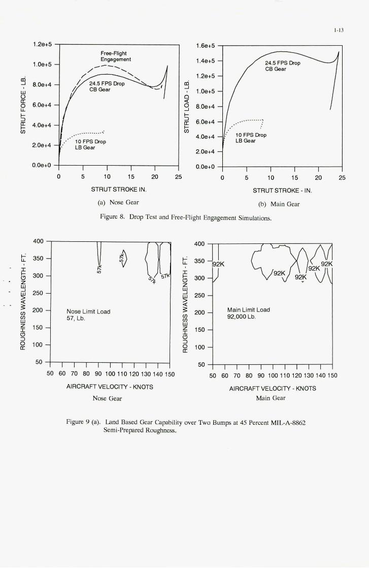
Figure 8 shows drop test simulations for nose and main gears and free flight engagement simulation loads for the nose gear. Since aerodynamic characteristics of the hypothetical aircraft were not defined, a conservative tail down angle of 16 degrees was used for the free flight engagement simulation.

6. LANDING GEAR GROUND ROUGHNESS CAPABILITY COMPARISONS

Evaluations of the roughness capability of these gears during landing rollout have been based on techniques developed for evaluating existing aircraft to operate from bomb damage repaired runways as reported in Reference 7. In this method, a matrix of aircraft velocity and roughness wavelength combinations is simulated and the maximum landing gear vertical loads are tabulated. For purposes of this comparison, the runway roughness amplitude is defined by the equations of MIL-A-8862 that express the roughness amplitude as a function of the wavelength. Velocity increments of five knots were used from 50 to 150 knots, along with wavelengths from 50 ft. to 400 ft. in 50 ft. increments. MIL-A-8862 specifies use of single and two bumps. In this study, two bumps were assumed. Also only dips were simulated as dips are usually found in other studies to produce higher loads than corresponding bumps of equal amplitude.

From the resultant 3-dimensional table of velocity, wavelength, and maximum gear load, contours of constant load level can be drawn, producing a graphical description of load trends. Contours of loads equal to or higher than limit load define combinations of roughness wavelength and airplane speed that must be avoided. For full capability over the entire speed/wavelength range, no load contour can exceed the limit vertical load of the landing gear. If limit load exceedances are found, the bump amplitude can be reduced until the gear loads are within the limit load envelope. To minimize the number of computer simulations required, the amplitudes have been reduced by an equal percentage over the entire wavelength range studied. Thus when the results are discussed in terms of a percentage of the specification roughness amplitude, the quoted percentage represents the point at which the highest load occurred, and more capability exists for other noncritical combinations of speed and wavelength.

Initial simulations were made using conventional static to compressed 3:l compression ratio strut sizing. The land based gears sized for the alternate 2g/3g criteria could not achieve more than approximately 55% of the sem i-prepared roughness requirement based on single bumps and the carrier based gear could not reach 100% of the semi-prepared surface single bump requirements. The airspring curves were then recomputed using

increased inflation pressures and lower compression ratio values. Because of high preload pressures, these modifications represent what is believed to be the maximum capability for conventional single chamber gears with these stroke lengths.

Figure 9 shows strut capability for these gears where sufficiently high roughness levels have been used to produce at least limit gear load over some portion of the speed/wavelength range studied. Unrestricted operations would require a lower roughness level where no limit loads would occur.

Figure 9 (a) shows the land based 12-inch stroke gear results without braking. The roughness level was 45% of the MIL-A-8862 semi-prepared surface. High load levels were produced for both main and nose gears in the wavelength range above 300 ft.

Since only limited semi-prepared surface roughness capability exists for the land base gear, braking simulations were made assuming only prepared surface roughness as shown in Figure 9 (b). A braking coefficient of 0.4 was assumed. Main gear loads were well below limit, but nose gear loads did exceed limit at the highest speeds around a wavelength of 100 ft.

As configured in this study, the carrier sized 25-inch stroke gear could not achieve 2-bump capability to 100% of the MIL-A-8862 roughness level at all speeds and wavelengths. Figure 9 (c) shows that limit loads are reached in the 300 ft. and above wavelength range at 75% of the semi-prepared surface roughness level without braking. The carrier sized gear does have substantial braking capability over roughness as compared to the land based design. Figure 9 (d) shows that limit loads are just reached at 50% of the MIL-A- 8862 roughness level.

Undoubtedly, additional changes could provide some improvement in the roughness tolerance of these gears; however, it is not believed that the changes would affect the relative capabilities of the carrier and land based designs. One potential method of obtaining additional roughness capability is the use of double chamber struts. In recognition of objections to double chamber struts by maintenance and gear overhaul personnel, this survey was limited to single chamber gears only.

7. WEIGHT COMPARISONS

I t is not possible to estimate accurate landing gear weights until all load components, including drag, side, and miscellaneous loads are known and the gear design has progressed at least through the detail layout task. Consequently, parametric weight estimating techniques have been used to compare these gears as shown in

Figure 10. For quantifying the weights, it is believed that the conventional land based design would be in the range of 2.2% of aircraft weight. The 0.9% relative increment shown for the carrier based design is believed to approximate the additional landing gear weight necessary for 25 inch stroke gears to achieve full takeoff/landing/RTO capability on MIL-A-8862 paved runways and limited operational capability on semi-prepared surfaces. Full operational capability with braking over MIL-A-8862 semi-prepared surfaces with two bumps or over the MIL-A-8863 continuous (l-cosine) bumps could not be achieved with these struts as configured on the hypothetical aircraft.

8. REDUCING ROUGH FIELD LANDING GEAR COSTS

Escalating costs of aircraft procurement requires that all possible methods of cost reduction be examined. For landing gears, this means design simplicity and commonality wherever possible. Cost and weight optimization must be considered jointly.

Forging costs represent as much as 5 - 10% of total cost of modem landing gears. Applying design initiatives to maximize commonality of forgings between land and carrier based gears, and possibly between nose and main gear components can reduce production costs. To do so, the general arrangements of the land based and carrier based gears should be as similar as is practical. Using the same basic geometry and trunnion attach points can facilitate commonality of components and maximize interchangeability.

Major structural components such as the shock strut cylinder and piston could perhaps be machined from common forgings. Forging dies cut to produce forgings for a 25 inch stroke gear could have excess material removed when producing 12 inch stroke gears. Common strut diameters could be achieved by machining to different wall thicknesses as necessary for higher carrier landing loads. Navy requirements now indicate Aermet 100 material, and this steel is presently a significant cost factor. Aermet 100 material removed during machining can be recovered to recoup some raw material cost.

Minor structural components such as drag and side braces may also be made from common forgings, again being sized for the heavier gear design. Allowances for wider lugs should be made during the design process. Common trunnion pins may be used with a larger inner diameter for the land based gears and a smaller diameter for the carrier based gears. Retract and steering actuators may also be made from common forgings, allowing for larger piston areas for heavier gears.

1-6

Many nonstructural components may be designed to be interchangeable from carrier based to land based designs. By using equal piston diameters, common components such as separator pistons, gland nuts, and strut bearings may be incorporated. Also, system type components such as steering valves may be completely com mon .

To benefit from design commonality, both carrier based landing gear requirements and the maximum operational runway/taxiway roughness should be considered at the beginning of the design process. History has shown that landing gears initially designed for land base use are impractical for carrier operations and entirely new designs are required. If carrier requirements are considered initially, the landing gear may be more easily adapted to multi role uses in the future and at the same time much higher roughness tolerance potential can be achieved.

9. CONCLUSIONS

Specifications for landing gear design ground loads are not always explicit in describing operational requirements on rough runways. The lack of clarity of operational requirements with respect to braking levels while on rough surfaces can lead to designs with reduced operational capability, i. e. limited to unbraked taxi or free rollout where the possibility of roughness resonance exists.

Navy carrier based aircraft specifications (MIL-A- 8863) require landinghakeoff operations from lower amplitude rough surfaces than the corresponding MIL- A-8862 surfaces; however, additional capability is inherent over corresponding Air Force gears from other requirements associated with Navy shipboard operations. When severe roughness combined with other load sources is considered, weight differences in Navy and Air Force landing gears may diminish.

Airfield roughness capability of two landing gears with different stroke lengths using MIL-A-8862 roughness specifications have been compared for a hypothetical aircraft. The landing gears were sized by Air Force and Navy Landing Impact Criteria. The landing gear weight penalty to provide operational capability with braking to Air Force gears has been estimated from this comparison at approximately 0.9 percent of aircraft weight.

10. Recommendations

Landing gear design and user technical personnel need to improve, clarify, and develop realistic ground roughness performance requirements definitions to avoid potential problems in landing gear/vehicle integration. Wheel well sizing should be based on the

maximum stroke lengths and tire sizes that could be anticipated for future, perhaps multi service usage of the airframes.

Future studies should focus on the inherent capabilities of gears designed for shipboard operations to establish benefits for use on rough runways.

Additional work is needed to rapidly quantify landing gear weight as a function of required capability through improvements in automated loads and stress analysis. Modeling tools of this type must be available and utilized from the earliest design stages.

It is recommended that cost reduction methods, including simplified gear retraction geometry, be given high priority in the initial gear design. Sizeable c a t savings might be realized, both in development and manufacturing with more progress toward standardized gear arrangements, and by reduced gear complexity which enable the use of common parts and forgings.

11.

1.

2.

3.

4.

5.

6.

7.

REFERENCES

Currie, Norman S., "Aircraft Landing Gear Design: Principles and Practices," AIAA Education Series, American Institute of Aeronautics and Astronautics, Inc. , Washington, D. C., 1988, p.35.

Williams, W. W., Williams, G. K., and Garrard, W. C. J., "Soft and Rough Field Landing Gears," SAE Paper 650844, October, - - 1965.

Airplane Strength and Rigidity, Landplane Landing and Ground Handling Loads, MIL-A- 8862A, MarchJ971.

Airplane Strength and Rigidity, Ground Loads for Navy Acquired Airplanes, MIL-A- 8863B(AS), 6 May 1987.

Aircraft Structures, General Specification For, MIL-A-87221, 28 February, 1985.

Conway, H. G., "Landing Gear Design," Chapman and Hall Ltd., London, 1958. , p. 184

Anon, "Aircraft Operation on Repaired Runways," Report of Working Group 22 of the Structures and Materials Panel, NATO/AGARD, Paris France, AGARD-R- 731, August, 1990.

1-7

MIL-SPEC Number of Bumps n Dips

8862 1 or 2

Figure 1. Stroke Requirements as a Function of Sink Rate and Load Factor.

Braking Plus Roughness

None Defmed

0 5 10 15 20 25

87221

4 4 10 m

Different Amplitude 2 Definitions: Requirements for Single and Double Bumps Braking over Roughness

Taxi without Braking

30

25

f

5

0

SINK RATE - FT.lSEG.

/

I I I I I I I 0 50 100 150 200 250 300 350 400 0 50 100 150 200 250 300 350 400

BUMP WAVELENGTH - FT.

(a) Prepared Surfaces

BUMP WAVELENGTH - FT.

@) Semi-Prepared Surfaces

Figure 2. Military Specification Roughness f a Prepared and Semi-prepared Surfaces.

TABLE 1

ADDITIONAL. RUNWAY ROUGHNESS REQUIREMENTS

Landing Impact on Roughness

I No

High Catapult and Arresting Loads

Free Flight Engagement

Deck Obstruction Loads

: I -oads

Maximum Weight 1W,ooO Lb. ~

Landing Weight

I 15Degrees I

75,000 Lb. (65,000 CB)

I Turnover Angle (Forward C. G.) I 53.819 Degrees I

Landing Weight pitch Inertia

Longitudinal Distance, Nose Gear to Main Gear

Main Gear Tread Width

Forward C. G. Position

Aft C. G. Position

C. G. Height Above Ground

Tailhmk Location

I Minimum Static Nme Gear Load I 8,121 Lb. I

0.848E+09 Lb. in?

330 in.

180 in.

61.8 in. forward of Main Gear

26.8 In. forward of Main Gear.

100.78 in.

190.76 in. aft of C. G., 32.34 in. below C. G.

I Maximum Static Nose Gear Load I 18,727Lb. I - Nose Gear Load with Braking (10 ft./sec? Deal.) 28,211 Lb.

ITEM

MIL-A-8863, Soft StNt Single Chamber, Gosoil Separated

MAIN GEAR NOSE GEAR

MIL-A-8862 Soft Strut Single Chamber, Gasoil Separated

MAIN GEAR NOSE GEAR

I Stroke I z in. I z in. I 12 in. I 12 in. I

Extended Volume

I Piston Dia.lArea I 6 in.tB.274 in?

903 in.'

I Extended Pressure 1 844 psi

Tire Static Load Rating

54,000 Lb. 24,600 Lb.fCire 54,000 Lb. 24,600 Lb.lIire

6 in.128.274 in?

426 psi

794 466 in? . 39 x 13 22PRn 47 x 18 36PRl1

6 in.tB.274 in?

(wWt.Est.j -1 6501b. 1 275 Lb. I 6ooLb. I I Orifice Coefficient I 2.65 I 1.43 I 4.6 I 2.9 I I A, Tire Coefficient I 9918.0 I 17,710 (2 Tires) I 7406.5 I 4742. (2 Tires) I I A2 Tire Coefficient I 1.259 I 1.022 11.237 11.269 I I Tire Pressure I 245 psi I 165 psi I1mps i I 60 psi I 1 Strut Preload I 23,863 Lb. I 12,045 Lb. I 25,051 Lb. I 8,8SO Lb. I I Strut Bottoming Load I 109,857 Lb. I 109,736 Lb. I 92,128 Lb. I 56,729 Lb. I

1-10

Front View

(a) Main Gear

Front View @) Nase Gear

Figure 4. Landing Gear Arrangement.

SPACER \

METERING PIN

UPPER BEARING

SEPARATOR PISTON

LOWER BEARING

AIR CHMdBER SPACER

/

Figure 5. Landing Gear Strut Concepts.

Figure 6. Carrier Based Sink Speed as a Function of Approach Speed.

20 7, 7

X

4 15 w $ f? 10

2 f n 5

0

0 5 10 15 20 25

STRUTSTROKE - IN. (a) Nose Struts

10

110 115 120 125 130 135 140 145

APPROACH SPEED - KNOTS

20 b .-

0 5 10 15 20 25

STRUTSTROKE - IN. (b) Main Struts

12

0 5 10 15 20

TIRE FORCE - LB. x io4 (c) Nme Tire Curves

0 5 10 15 20

TIRE FORCE - LB. X lo4 (d) Main Tire. Curves

Figure 7. Strut and Tire Load-Deflection Characteristics.

1-13

400

300 350 - - . ! 2

- 200 -

- 250 - 4

v) v) W $ 150 -

? g 100-

50

1.2e+5

1 . 0 ~ 5

8.0e+4

o 6 . 0 ~ 4

E 4 . 0 ~ 4 v)

2 . 0 ~ 4

w 2 5 U

\ I -i 400

350 -92K

I

z 84 '51' & 300 -

250 -

I @ ( ul h

-2

0

$ 150- U 3

Main Limit Load 92,000 Lb.

Nose Limit Load iz 200 - 3

g i o o -

57, Lb.

I I I I I I I I I 50 I I I l i I I i I

Free-Flight Engagement

____....___. ..

1 . 6 ~ 5 I

1.4et5

1 . 2 ~ 5 m J

0 1.0e+5 n 4 9 8.0et4 + 2 6.0et4 + v)

4.0e+4

2.0et4

O.OetO 0 5 10 15 20 25 0 5 10 15 20

STRUTSTROKE IN. STRUTSTROKE - IN.

(a) Nose Gear

Figure. 8. Drop Test and Free-Flight Engagement Simulations.

(b) Main Gear

50 60 70 80 90 100110120130140150

AIRCRAFTVELOCITY - KNOTS

Nose Gear

. . . . . . . . . . 50 60 70 80 90 100110120130140150

AIRCRAFTVELOCITY - KNOTS Main Gear

25

Figure 9 (a). Land Based Gear Capability over Two Bumps at 45 Percent MILA-8862 Semi-prepared Roughness.

1-14

k I 350 4001 300 4

Nose Limit Load 57,000 Lb.

I:

8 100

w $ 150

50 IIII(IIIIII 50 60 70 80 90 100110120130140150

AIRCRAFT VELOCITY - KNOTS Nose Gear

k 350 400 -I 300

$ 250 U

4

i? 200 I:

9 g 100

w $ 150

Main Limit Load 92,000 Lb.

50 - 50 60 70 80 90 100110120130140150

AIRCRAFTVELOCITY - KNOTS Main Gear

Figure 9 @). Land Based Gear Capability over MILA-8862 PrepaRd Surface Roughness with 0.4 Braking Coefficient.

400

k 350

300

$ 250

200

z 150

4

Nose LimR Load a v)

3

50 11111111111 50 60 70 80 90 100110120130140150

AIRCRAFTVELOCITY - KNOTS

Nose Gear

Second Contour: 150K . .

Main Limit Load 200

$ 150 w 180,000 Lb.

g 100

50 60 70 80 90 100110120130140150

AiRCRAFTVELOClPl - KNOTS Main Gear

Figure 9 (c). Carrier Based Gear Capability over 75 Percent MIL-A-8862 Semi-prepared Roughness.

1-15

- - - -

- -

400

350

i 300 P 250

200

W f 150

d

$

2 g 100

50

0

Second Contour: 1501

Main LImR Load 180,000 Lb.

Second Contour: 90K

Nose LImR Load 130,000 Lb.

I I I I I I I I I 50 60 70 80 90 100110120130140150

AIRCRAFTVELOCITY - KNOTS Nose Gear

400

350

E 300

250

4 d ; 200

w f 150

z g 100

50 60 70 80 90 100110120130140150

AIRCRAFTMLOCITY - KNOTS Main Gear

Figure 9 (d). Carrier Based Gear Capability over 50 Percent MILA-8862 Semi-prepared Roughness witb 0.4 Braking Coefficient.

" 1.0% a 5 1.5% w : 1.0% L

0.5%

0.0% LANDBASED CARRIu(-BASu)

Figure 10. Landing Gear Weight Comparisons.

2- 1

A REVIEW OF AIRCRAFT LANDING GEAR DYNAMICS

SUMMARY

WILLIAM E. KRABACHER WL/FIVMA Building 45

WRIGHT LABORATORY WRIGHT PATTERSON AFB

2130 Eighth Street, Suite 1 Ohio 45433-7542, USA

A review of two different landing gear shimmy mathematical models is presented. One model uses the Moreland tire model and the other model uses the Von Schlippe-Dietrich tire model. The results of a parametric study using these models is presented indicating the sensitivity of various parameters to numerical variation. An identification of stability critical parameters in the models is given. Three different aircraft landing gear shimmy data sets are reviewed and model stability predictions are discussed. A comparison is made with actual experimental results. One of these data sets indicates the nonlinear variation of various input parameters as a function of strut stroke. In the course of the presentation some design rules and cautions are

- suggested.

LIST OF SYMBOLS

The definitions of the various parameters used in the mathematical models are defined below. Except as noted, the parameters are used in both the

I 1

Moreland and the Von Schlippe-Dietrich models.

C - Tire Yaw Coefficient (radllb) (Moreland Model Only)

C, - Moreland Tire Time Constant (sec) (Moreland Model Only)

h - Half Length of the Tire Ground Contact Patch (in) (Von Schlippe-Dietrich Model Only)

L, - Tire Relaxation Length (in) (Von Schlippe-Dietrich Model Only)

C, - Structural Rotation Damping Coefficient (Rotation of Mass about the Trail Arm Axis) (in-lb-sechad)

C, - Tire Lateral Damping Coefficient (lb-sedin)

C, - Structural Lateral Damping Coefficient (lb-sec/in)

CT - Rotational Velocity Squared Damping Coefficient (Rotation about the Strut Vertical Axis) (in-lb-sec2/rad2) OR Linear Viscous Damping Coefficient (in-lb-sechad)

CFl - Friction Torque (in-lb)

CF2 - Coefficient of Friction Torque as a Function of Side Load at the Ground (in-lbAb)

FP - Peak to Peak Torsional Freeplay of the Gear about the Strut Vertical Axis (rad)

I - Mass Moment of Inertia of the Rotating Parts about the Axle (in-lb-sec*/rad)

I, - Equivalent Mass Moment of Inertia of the Lumped Mass System about the Trail Arm Axis (in-lb-sec*/rad)

I, - Equivalent Mass Moment of Inertia of the Lumped Mass System about the Strut Vertical Axis (in-lb-sec*/rad)

K, - Rotational Spring Rate about the Trail Arm Axis Measured at the Wheel/Axle Centerline (in-lb/rad)

K,

K,

- Cross Coupled Spring Rate (lb)

- Tire Lateral Spring Rate (lb/in)

K, - Lateral Spring Rate of the Structure at the Trail Arm and Strut Vertical Centerline Intersection (Ib/in)

KT - Torsional Spring Rate of the Structure about the Strut Vertical Centerline with the Damper Locked (in-lb/rad)

Paper presented ut the 8ls t Meeting of the AGARD SMP Panel on “The Design, Qualification and Maintenance of Vibration-Free Landing Gear”, held in Ban8 Canada from 4-5 October 1995, and published in R-800.

2-2

K,, - Torsional Spring Rate of the Steering Actuator about the Strut Vertical Centerline (in-lb/rad)

L - Mechanical Trail Length, defined as the Normal Distance from the Axle Centroid to the Strut Vertical Centerline (in)

La - Geometric Trail = R*sin(y)

m - Equivalent Lumped Mass of the Wheel, Tire, and Fork (Ib-sec2/in) -.

m, - Equivalent Lumped Mass of the Fork (Ib-sec2/in)

R - Rolling Radius of the Wheelnire (in)

V - Aircraft Forward Taxi Velocity (idsec)

W - Landing Gear Vertical Reaction (Ib)

p, - Tire Moment Coefficient (in-lb/rad)

y - Attitude of the Gear, Positive Wheel Forward (rad)

Other symbols used in the analysis

F, - Ground Reaction Normal to the Wheel Plane Ob)

T - Torque Moment about the Strut Vertical Axis due to Torsional Spring Rate of the Structure (in-lb)

1. INTRODUCTION

In an earlier paper (l), a rudimentary outline was presented for the development of an international standard for dealing with various types of landing gear dynamics problems such as shimmy, gear walk, judder, antiskid brake induced vibrations, dynamic response to rough runways, tire-outsf-round, and wheel imbalance. The purpose of the present paper is to sharpen the focus of the previous paper by presenting a detailed analysis of the specific problem of landing gear shimmy. The main content of this paper will be to review two different landing gear mathematical models, to present the results of a parametric study performed on a fighter aircraft nose gear indicating the sensitivity of various parameters in the model to variation', to discuss a few parameters

critical to gear stability, to review some aircraft landing gear data sets indicating in one case the non- linear variation of the various input parameters as a function of strut stroke, and to review mathematical model stability predictions for these data sets.

2. THE MATHEMATICAL MODELS

Seventeen years ago the author developed a mathematical analysis for determining the shimmy stability boundaries of an aircraft nose landing gear. Over the intervening years, this analysis has evolved into a user friendly, robust computer program that has been quite useful in the prediction of aircraft landing gear shimmy problems. In presenting these mathematical models, it should be made clear that no claim is made to these models being the best or most sophisticated ones that can be used. The only claim made is that these models have been consistently successful in the prediction of shimmy problems on the aircraft studied.

From the landing gear structural standpoint, the two models to be presented are completely identical. The only difference between the two models is that one uses the Moreland tire model (2) and the other uses the Von Schlippe-Dietrich tire model (3)(4). The mathematical equations of motion for the Moreland tire model are given by

1. m+d%/dt2 - (m - mJ+L+d20/dt2 = F, - Ks+y - K,+a - C,+dy/dt

2. Is*dzO/dt2 = T + (V/R)+I*dddt - H+\V - FN*(L + La) + (m - mJ+L*d~/d tz

- W+(A - R+a)+sin(y)

3. I,+d2ddt2 = - K,*a - K,+y - C,+dafdt - (V/R)*I*dO/dt - F,+R*cos(~)

- W*(A - R+a)+cos(y)

4. C,*d2A/dtZ = - dy/dt - dNdt + R*ddd t + (L + La)+dO/dt - V*O - Cl+dy/dtz + C,*R*d2ddtZ+ C,+(L + La)+dzO/dtz

- CI+V*dO/dt - V+C+FN

' Due to space limitations, a discussion of how each parameter in the mathematical models is obtained will be deferred to another paper.

(Note: For a general layout of the coordinate system used refer to Figure 1 below. Both models use the same coordinate system.)

2-3

5. T = - &*[ IQ - 0, I - FP]*[Q - 8, I/[ 10 - 0, I ] - [ CFI + CF2*FN]*[dQ/dt]/[ IdQ/dtl ]

6. G* de, /dt*ld@, /dtl =

- GI% &*[ IQ @I I - FPl*[Q Qi I/[ IQ Qi I 1

8. y = (IN)*[dy/dt + W d t - R*da/dt - (4 + L,,)*dQ/dt + V.6 ]

where the degrees of freedom of the model arc

y - Strut Lateral Deflection at the Intersection of the Shut Vertical Centerline and the Centerline of the Trail Arm

0 - Torsional Rotation about the Strut Vertical Centerline

8, - Torsional Rotation at the Steering Actuator /Damper

a - Tire Roll Rotation about the Fore-Aft Axis through the Trail Arm

y - Tire Torsional Rotation about the Vertical Axis through the Axle Centerline

A - Tire Contact Patch Centerline Lateral Deflection with respect to Wheel Center plsnc Intersection at the Ground

The mathematical equations of motion for the Von Schlippo-Dietrich tire d l am given by

1. m*d?/dt' - (m - mJ*L*d%/dt' = FN - K,*y - K,*a - C,*dy/dt

2. I,*d%/dt' = T + (V/R)*I*Wdt - p,*y - FN*(L + L,,) + (m - mJ*L*d?/d?

-W*@, - y + (L + L,J*Q -R*a)*sin(y)

3. I,*dza/dt' = - K,*a - K,*y - C,*da/dt - (V/R)*I*dB/dt - FN*R*cos(~) - W*@, - y + (L + L a * @ -R*a)*cos(y)

4. ([(3*L,, + h)*hT/[ 6*V3]}*d'y,,ldt3 = -yo + y - (L +Lo)*@ + (LK + h)*O

- [(2*Ln + h)/(Z*V?]*d?ddt' - [GR + W l * d Y d d t

7. FN = KO*@, - y + (L + LO)*Q) + Co*(dyddt - + (L + LO)*dWdt)

8. = [ IN]* [ dyddt - R * W d t + V*Q]

It is noted for reference (See Figure 1) that a special equation can bc derived which connects the Moreland Tire Model parameter A with ths Von Schlippe- Dietrich parameter yI. This equation is

FIGURE 1

A*cor(B) = yo - y + (L + L.,pain(s)

or, making the small angle assumptions, cos(0) = 1.0 and sin@) = 0, it follows that

The degrees of freedom of this model arc

y - Strut Lateral Deflection at the Intersection of the Strut Vertical Centerline and the Centerline of the Trail Arm

Q - Torsional Rotation about the Strut Vertical Centerline

6, - Torsional Rotation at the Steering ActuatorDamper

2-4

Q - Tire Roll Rotation about the Fore-AR Axis through the Trail Arm

- Tire Torsional Rotation about the Vertical Axis through the Axle Centerline

v,

yo - Lateral Distance from the Fore-AR Axis of Undeflected Forward Motion to the Center Point of thc Oround Contact Area

The method of initial excitation in both models is to give 8 an initial v a l q of 5.0 degrees.

In cornparins these two mathematical models, it will be noted that the only difference between them is essentially which equation is used to describe the tire motion. When this shimmy analysis was originally developed, only the Moreland Tm Model was used and most of the landing gears analysed with this analysis had Moreland tire data available. About ten years afler the original analysis was developed, a landing gear needed to be analysed for which only Von Schlippe-Dietrich tire data was available. Due to the prior suoceas of the originel analysis, it was decided to retain the original stnrctural analysis portion and only modify the tire model portion. The result is the Von Schlippe-Dietrich version presented in this paper.

An important result of obtaining this second analysis is that now a direct comparison of the accuracy of the two tire models can be obtained since all structural considerations are exactly identical for the two analyses. Recently, it becume known that an empirical procedun existed which could approximate either tire model's shimmy parameten from the LMwnr of tiro sizs and inflation pressure (5). The availability of i h i ~ procedure lenda itself to providing a h i s for a direct comparison of the two models' prediction capabilities. Some preliminary comparisons of analysis predictions have been conducted on a fighter known to have shimmy problems. However, at this time it is felt that these comparisons are too few to make any general statements on trcnds found in these comparisons.

To provide examplea of the type of output obtained from the two computer analyses based upon the above two sets of differential equations, reference is made to Figures 2, 3, 4. and 5 below. These four graphs are plots of the y - Lo@ variable for the cases of a stable landing gear. a gear in l i t cycle oscillation, a gear in divergent shimmy, and a

gear in severe divergent shimmy. The two computer analyses also output the 0. Q,, a, A or yo. and torque T variables in similar graphical plots.

SHIMMY DAMPED OUT 7 n w (SEC)

FIGURE 2

LIMIT CYCLE SHIMMY

TIME (SEC)

FIGURE 3

WVERGENTSHllvlllly

P 2 10

> -= P o -10 I

30

FIGURE 4

2-5

FIGURE S

3. SENSITIVITY ANALYSIS OF PARAMETER VARIATION

About f h e n years ago, a sensitivity analysis was conducted using some tighter nose landing gear data and the Moreland Tire Model version of the shimmy analysis. While the reaults of this study are only totally accurate for the aircraft analysed, it has been found that the general trends in this study have been a valuable guide in analysing other nose landing gear. The data d e f d g this nose landing gear from a shimmy standpoint is presented in Table 1 under the column for Fighter A.'

D e f d g the values in this table as the nominal values of the gear. the parametric study was conducted by inormumtally varying one paramctcr at a tima and increasing its value until its value was 1.5 times its nominal value. The computer output from the variation of each parameter was reviewed for stability effects and graded according to the scale: greatly increases stability, increases stability, slightly increases stability, no change, slightly decreases stability, decreases stability, greatly decreases stability. Using this scale the following results were obtained.

C - Increases Stability C, - Increases Stability C, - Slightly Increases Stability C, - Increases Stability C, - Increases Stability C, - Slightly Decreases Stability I - Decreases Stability until 1 = 1.6 and then

Increases Stability - Decreases Stability - Decreases Stability until I, = 2.25 and then

Increases Stability - Greatly Increases Stability - Decreases Stability - Increases Stability - Increases Stability - Greatly Decreases Stability

- Greatly Decreases Stability' - Greatly Increases Stability - Decreases Stability until m = ,225 and then

Neutral Stability - Increases Stability - Slightly Decreases Stability - Greatly Decreases Stability - Greatly Increases Stability - Slightly Increases Stability - Slightly Increases Stability - Decreases Stability

4. LANDING GEAR STABILW CRITICAL PARAMETERS

In one particular shimmy investigation involving a trainer nose landing gear a problem was uncovered that identified stability critical parametersu. Specifically, the vendor supplied a complete set of

' The some of the original values used in the parametric study were accidentally lost "he values listed in Table 1 arc approximately correct. However, they should not ba used in the analysis in an attempt to reconstruct the results cited here. The results of this study should be viewed simply as a general indicator of how dynamic response may change as a parameter value is altered

' Since the nominal value of L for this landing gear is 0.8 inches, the maximum value uscd in this scnsitivity study is 1.2 inches. Therefore, greatly decreasing stability makes physical sense in this case. Generally, positive trail values below 3 inches tend to be destabilizing.

' The term stability critical parameter is taken to mean that this parameter will produce greatly varying analysis prediction results for small changes in the parameter value.

' The actual experimentally measured data for this trainer is presented in Table 1.

2-6

landing gear shimmy analysis data which was entered into a data file for the shimmy analysis. When the analysis was executed, the analysis indicated the gear would shear off in the rust quarter-cycle. (Refer to Figure 5 above for a plot of the actual dynamic response predicted by the analysis.) Since this level of unstable dynamic response had never been encountered before, it was determined that something must be wrong with the data. After the vendor supplied four additional data sets. all of which also predicted the gear would-shear off in the first quarter- cycle, an investigation was conducted by comparing the values of the data in these five data sets with the data sets from other aircraft nose landing gears to determine the physical realism of the data. Using the above introduced parametric study as a guide, focus quickly narrowed onto the value of the parameter K, since its variation greatly alters the analysis predictions. The result determined was that in all five data sets supplied the value of K,, relative to the values of K, for other landing gears was in error by being two orders of magnitude too large.

It was decided to measure the stiffness values of & , Ks , K, I and K, as well as the torsional freeplay of the gear on an actual aircraft (6). The outcome of this measurement process was that in all five sets of vendor supplied data, the= four stiffnesses were grossly at odds with what was experimentilly measured on the actual aircraft. The experimentally measured values of K,, K,, and K, were approximately one order of magnitude smaller and the K, parameter was two orders of magnitude smaller than the values supplied in the data sets.

While this particular vendor did not have a f~te element analysis capability for determining these parameters, it should be pointed out tha: subsequent encounters with these parameters on other aircraft nose landing gears has generally established that finite element analyses tend to error on the high side in determining these four parameters. Therefore, since these parameters are stability critical, considerable caution should be used in determining values for them in the design stage of the gear. As an additional caution, a band around each such determined value should be established and investigated in the analysis to insure no stability boundaries are crossed within this band or in the combination of bands of these parameters.

5. SETS AND STABILITY PREDICTIONS

REVIEW OF LANDING GEAR DATA

Table 1 below provides the shimmy data sets for two different tighter (Fighter B and Fighter C) and one trainer aircraft that have been analysed for shimmy behavior. These three aircraft were selected

TABLE 1

because of a desire to provide examples of both shimmying and non-shimmying landing gear. Each of these data sets will be reviewed and their shimmy cheracteristics discussed.

The Trainer data set is an example of a stable

2-1

This procedure was repeated at increments of 0.05 degrees of torsional Geeplay from 0.5 to 1.2 degrees.

As a comparison. a static analysis of the gear was also performed to evaluate the prediction variations. The static analysis was conducted by selecting the 11 parameter values at the static stroke position of the gear and incrcmenting the taxi speed in 5 knot increments from IS to 150 knots while holding these 11 parameters constant. Again the shimmy speed was taken as the lowest speed at which the analysis indicated sustained limit cycle oscillation of the gear. The comparison between the dynamic and static analyses predictions are shown in chart 14. Also included in this charr arc the actual experimentally determined shimmy boundaries of the gear. The lower experimental boundary shows when shimmy onset occurred in the gear and the upper experimental boundary indicates strong limit cycle oscillation shimmy.

It is particularly interesting to note that the dynamic analysis boundary follows the contour of the shimmy onset boundary quite closely and consistently errors slightly on the conservative side. Whereas, the static analysis boundary lies above the shimmy onset curve below 0.85 degrees of freeplay and ermrs increasingly on the conservative side aa the torsional freeplay increaser from 0.85 degrees to 1.20 degrees. Both the dynamic and static analyses indicated the shimmy frequency to be 27 HZ and this was c o n f i i e d in experimental measurement.

landing gear when the values listed in Table 1 arc used in the shimmy analysis. An example of the typical dynamic response of this landing gear is provided in Figure 6 below for the 8 variable. (Note: 8 in this figure is in degrees.) It is noted that this gear is very stable as there is little dynamic response to the initial 5 degree deflection of 0.

Y I I

FIGURE 6

The Fighter B data sCt is one of the most complete data sets for a landing gear that the author poswsses. This set contains 11 charts that show the nonlinear variation of 11 of the input parameters to the shimmy analysis. Also included arc charts 12 and 13 which show the load stroke curve of the shock strut and the load on the gear as a function of aircraft forward ground speed.

.

.

In an earlier paper (7). an investigation was conducted to determine the overall effect of these nonlinear vuiations on the prrdiotcd stability boundaries of the analysis in comparison to the experimentally determined shimmy stability boundaries of the gear. The manner in which this investigation was conducted was to have the analysis execute 5 knot increment runs starting with 15 knots and incrementing up to 150 knots. At each speed increment, the analysis would determine the load on the gear from chart 13. Depending on the particular parameter, the analysis would either then calculate the parameter directly or it would determine the stroke position from chart 12 and then calculate the desired pwameter. After all I1 parameters were so calculated, the analysis would execute and the dynamic response of the gear would be determined. From the analysis results. the shimmy speed was then taken to be the lowest speed at which the analysis indicated sustained limit cycle oscillation of the gear.

The overall implication of these fmdmgs seems to suggest that the dynamic modelling of the gear as described above will significantly improve the

paramcter variation ir on important consideration in obtaining an accurate shimmy analysis of a landing gear.

~mcy of ths adyrir prsdiotions and that nonlinear

The Fighter C data set in Table I is provided for the 4 inch stroke position which corresponds to the static stroke position of the gear. Figures 7 . 8 . 9 , IO, 11, 12, 13, and 14 show typical dynamic response of this nose gear. Figures 7 , 8, 9, and 10 arc plots of the y - L*Q or lateral displacement variable at the point A for the taxi speeds of 80, 90, 95, and 100 knots respectively. (Note: In these figures what is called the x - L*Q variable is identical to what is referred to as the y - L*Q variable in this paper.) Figures 11. 12, 13, and 14 are the plots of the 0 or torsional rotation about the strut vertical axis variable at these same taxi speeds. (Note: C3 in degrees.)

I - + I

FIGURE 7

:: 1 ..I

FIGURE 8

Y

Y

Y

Y

1:: l - I - P *- I 1-

FIGURE 11

Y

Y

Y

.I

Y

Y

Y

FIGURE 12

FIGURE 9 FIGURE 13

FIGURE 10

2-9

In comparing these graphs it is noted that as the taxi speed increases from 80 to 90 knots a progressively longer period of time is required for the vibration to damp out. At 95 knots the gear has the onset of limit cycle shimmy. At 100 h o t s the limit cycle shimmy is definitely established. From these time histories it is seen that the shimmy oscillation frequency is about 27.06 HZ at 95 knots. When the actual aircraft was tested, it was found that the nose gear went into a sudden onset of shimmy at 92 knots and had a frequency of 27.5 HZ. Repeated testing of this landing gear, yielded reasonably consistent repeatability at this shimmy speed and frequency.

In the course of the shimmy investigation for Fighter C, one very important point came to light concerning the measurement of landing gear shimmy parameters. The vendor's original analysis consistently indicated that this landing gear was stable at all taxi speeds. The analysis provided by the author indicated the 95 knot shimmy event at 27.06 HZ. The question arose as to what was different between the two analyses. After review of the input data a primary cause of this difference was established. The stability critical parameters KT, K,, K,, and K, used in the vendor's analysis were obtained by rigidly mounting the landing gear in a fixture and measuring the resulting parameters. Whereas, the author's analysis took into consideration the softening effects of the landing gear mounted in a flexible fuselage and reduced the stiffness values supplied by the vendor. The amount of this reduction was largely based on experience with other landing gear.

- - -

- -

The reason for taking fuselage flexibility effects into consideration was based on some data obtained in another landing gear shimmy investigation.

UTLRALSCRINO RATE

S R U T ONLY IYEAWREDI

FIGURE 15

Referring to Figure 15, it is seen that the lateral stiffness values obtained for a landing gear rigidly mounted in a fixture (in the chart, strut only (measured)) vary from one and a half to three times the values of the lateral stiffness actually measured on a landing gear mounted on the aircraft. This comparison establishes the fact that backup structural flexibilities of the airframe must be taken into consideration when the four stability critical stiffness values are determined.

In addition to this primary cause of the difference between analysis predictions, a secondary cause was also established. The vendor's analysis assumed a value of 6% of critical damping as the magnitude of the structural damping available. Whereas, based upon personal experience with the variablity of available structural damping, the author decided to assume that the maximum amount of available damping was 1% of critical. At the time, the main reason for this selection was a desire to select a damping value that would expose any potential sensitivities the gear may have toward shimmying. Further support for this position was established after the fact when Denis J. Feld published his results on an analytical investigation of landing gear shimmy damping (8). The essential conclusion of the analytical investigation was that the amount of available damping at any instant during a taxi run could vary from 1% to 10% of critical viscous damping. Therefore, at the beginning of any landing gear shimmy investigation an assumption of 1% critical damping is a reasonable starting point.

Before departing from Figure 15, another subject is in need of mention. In the discussion of landing gear stability critical parameters above in section 4, it was pointed out that caution should be exercised when obtaining stability critical stiffness values because the finite element analysis predictions for these values tend to error on the high side. The proof of this error is established in the above figure for the strut only (calculated) case where it is seen that the largest error in stiffness values occurs between the calculated values and the strut mounted on an actual airframe.

6. CONCLUSIONS

In conclusion, a detailed analysis of the specific problem of landing gear shimmy was presented in which the two mathematical models described have been consistently successful in the prediction of landing gear stability characteristics to date. One of

2-10

these models uses the Moreland Tire model and the other uses the Von Schlippe-Dietrich Tire model. A classification of the various types of analysis output was given which consisted of a stable gear, a gear with limit cycle oscillation shimmy, a gear with divergent shimmy, and a gear with severe divergent shimmy. The results of a sensitivity study based on Fighter A's landing gear data was given. The parameters K,, K,, K,, and K, were identified as being stability critical in the analysis of gear shimmy. The Trainer data set described a stable landing gear. The Fighter B data set described a gear with limit cycle oscillation shimmi at a frequency of 27 HZ which was verified experimentally. Finally, the Fighter C data set analytically described a gear also with limit cycle oscillation shimmy at 95 knots with a frequency of 27.06 HZ. Experimentally, this gear went into limit cycle oscillation at 92 knots with a frequency of 27.5 HZ.

In the course of the presentation a number of important points were made. First, the Fighter B data set indicated the nonlinear variation of 11 input parameters to the shimmy analysis and suggested' that dynamic modelling of the gear will significantly improve the accuracy of the overall analysis predictions. The Fighter C data set established the importance of taking into consideration the backup fuselage flexibilities when determining the stability critical parameters KT, K,, K,, and K,. This data set also suggested that an initial assumption of 1% of critical viscous damping is a good manner in which to expose the potential senstivities of a landing gear to shimmy. Lastly, the tendency of finite element analyses to error on the high side when calculating the stability critical parameters was established.

BIBLIOGRAPHY

1. AIRCRAFT LANDING GEAR DYNAMICS PRESENT AND FUTURE, William E. Krabacher, S A E Technical Paper Series 931400 (1993).

2. Moreland, Journal of the Aeronautical Sciences,

THE STORY OF SHIMMY, William J.

pp. 793-808 (1954).

3. Von Schlippe and R. Dietrich ATI-18920 (1941) Subsequently printed as NACA TM 1365

SHIMMYING OF A PNEUMATIC WHEEL, B.

4. CORRELATION, EVALUATION, AND EXTENSION OF LMEARIZED THEORIES FOR

TIRE MOTION AND WHEEL SHIMMY, Robert F. Smiley NACA TR 1299 (1 957)

5. EMPIRICAL ESTIMATION OF TIRE PARAMETERS, Raymond J. Black, paper presented at SAE Committee A-5 Meeting, 28 April 1980, Renton, Washington

6. THE EXPERIMENTAL MEASUREMENT OF THE T-46 NOSE LANDING GEAR SHIMMY PARAMETERS, William E. Krabacher, ASDENFSL, Wright Patterson AFB, OH (1986) (In-House Publication)

7. E. Krabacher, ASDENFSL, Wright Patterson AFB OH (1981) (In-House Publication).

A DYNAMIC SHIMMY ANALYSIS, William I

8. AN ANALYTICAL INVESTIGATION OF DAMPING OF LANDING GEAR SHIMMY, Denis J. Feld, SAE Technical Paper Series 902015 (1 990).

C T I R E YAW C O E F F I C I E N T

x o . 1 f ; : ~ ~ : : : : : : , O O 2 3 4 5 6 7 8 9 1 0 1 1 1 2 1 3 1 4 NLG V E R T I C A L LOAD X10*.3 LB

C 1 T I R E TIME C O N S T A N T

4 ,

2 3 4 5 6 7 8 9 1 0 1 1 1 2 1 3 1 4

N L G V E R T I C A L L O A D X10**3 LB

2-1 1

- -

CD -TIRE LATERAL DAMPING

0 2 4 6 8 1 0 1 2 1 4 LOAD X 10**3 LB

K3 TORSIONAL STIFFNESS

c aa 0 2 4 6 8 1 0 1 2 1 4

NLG STRUT STROKE (INCHES FROM FULLY

EXTENDED)

KD TIRE LATERAL SPRING RATE

o h 0 2 4 6 8101214

NGVHTICAL LOAD X 10-3 LB

C F l FRICTIONAL TORQUE

700 T

- . . , , , . , . . . , , . 0 1 2 3 4 5 6 7 8 9101112

NLG VERTICAL LOAD XlO"3 LB

K4 CROSS COUPLED SPRING RATE

.- .

1 3 5 7 9 1 1 1 3 1 5

NLG VERTICAL LOAD XlO'"3 LB

KS LATERALSPRING RATE

0 3 x 2 c

3 q : ; : , 0

0 2 4 6 8 10 12 14 16

NLG STROKE (INCHES FROM FULLY EXTENDED)

2-12

KT T O R S I O N A L S P R I N G R A T E

8 - 0 0- 0 2 -4 6 8 10 12 14 16

NLG S T R U T S T R O K E (INCHES FROM FULLY

E X T E N DE D )

MUT TIRE MOMENT COEFFICIENT

0 2 4 6 8 1 0 1 2 1 4 NLG VERTICAL LOAD

X 10**3 LB

TAXI SPEED - LOAD CURVE

c I \

i 6 2000 ' 0

0 40 80 120 160 GROUND SPEED (KNOTS)

n

5 a U

RR TIRE ROLLING RADIUS

T\

8.5 I........ 2 4 6 8 10 12 14 16 18

NLG VERTICAL LOAD XlO"3 LES

40 35

9 30 25 b x' 20

2 5 10 5 0

0 2 4 6 8 10 12 14 16 NLQ STROKE ( INCHES FROM

FULLY E X 1 E N D ED)

1 - 1 2 I

S H I M M Y O N S E T \ 7 S T R O N G S H I M M ' I

I

- - D Y N A M I C A N A L Y S I

S T A T I C A N A L Y S I S I I

0 02 0.4 0.6 0.8 1 12 TORSIONAL FREEPLAY (DEG)

3- I

Total Length Height Wing Area

Self-Induced Oscillations of Landing Gear as an Integral Landing Gear Aircraft System Problem

10.90 m 3.91 m

15.51 m2

W.Luber, G.Kempf, A.Krauss

Gross Weight

Daimler-Benz Aerospace AG Military Aircraft LME24

8 1663 Munich Germany

3540 kg

SUMMARY

Present paper is treating three topics:

Two of the topics deal with seemingly self-induced oscillations observed during aircraft and subsystem development tests. The third topic gives a short overview on procedures to treat shimmy as a "flexible landing gear on flexible aircraft" problem. The topic treated in section 2 (Shimmy on Nose Landing Gear) presents a case observed in taxi tests of a prototype aircraft. Although specific shimmy calculations were not performed for this case, there are indications that a purely lateral/torsional tyre model would possible not have shown the instability observed. Appendix A gives some evidence therefor. Section 3 (Brake Torque Oscillations at Brake Initiation) treats a case. where quasi self-induced oscillations are caused by interaction of tyre circumferential force characteristics with the brake control system. Usual means to suppress shimmy (e.g. dampers, modification of landing gear geometry) are ineffective in this case. Landing gear vibrations may cause a variety of problems in the rest of the aircraft. Section 4 (Integral Landing Gear/Aircraft Problem) presents a summary of potential problem ramifications. It also gives a short overview on a viable approach to treat landing gear shimmy in context with aircraft structure.

-

- . -

1. INTRODUCTION

the cost of testing it is desirable to be able to predict the dynamic behaviour of landing gear systems. In the past methods were used to ca lcu la te v ia mathematical criteria, Ref. 1 - 1 and 1-2. the stability of the nose landing gear against shimmy. Since landing gear are very non-linear systems a time domain simulation code must be applied to show the behaviour of the landing gear itself and also the involved subsystems. An integrated approach to the modelling of the subsystems of the landing gear and the interaction of the elastic aircraft is required to accomplish the task. To get reliable results, which can also be validated by tests various components must be considered and introduced in the calculations like tyre, wheel, bogie, leg, oleo, braking system, anti skid control, steering and flexible aircraft. This report presents the straight forward trial to integrate the elastic aircraft into the shimmy investigation for nose landing gear of a fighter typ&aircraft development phase.

2. SHIMMY ON NOSE LANDING GEAR

A prototype training aircraft is depicted in Fig.2- 1 and the major design data are presented in the table 1 below.

I Wing SDan 1 10.46 m 1

An aircraft landing gear system has to be designed to meet various requirements covering all ground-based operations. It is a complex non-linear system which incorporates many sub-components often procured of sources which can produce structural dynamics and loading effects on the gear as well on the aircraft. The landing gear must be capable to carry heavy weight for take off operations, hard impact of the landing as well as the kinetic energy of forward motion on landing to bring the aircraft safely to rest. Due to the long terms of developing an aircraft reducing the risk of redesign and

Table 1 Technical Data Advanced Training Aircraft

The aim of the development was to take part on the competition of the next generation of the Air Force and Navy training aircraft. The design of the aircraft was

Paper presented at the 81st Meeting of the AGARD SMP Panel on "The Design, Qualification and Maintenance of Vibration-Free Landing Gear", held in Ban8 Canada from 4-5 October 1995, and published in R-800.

3-2

Mode

Elevator Rotation

therefore based on the requirements of the ' I Joint Primary Advanced Training - System ". To keep the development of the A/C in time attention was paid to a new aerodynamic design with good handling and performance quality. Reducing the risk of redesign proven components of similar aircraft were used for fast prototyping. Therefore the nose landing gear from T-46A training aircraft was used. The modified nose landing gear is shown in Fig. 2-2 with the most specific data. This paragraph describes the investigation to prove the modified nose landing gear on the advanced training aircraft is free of shimmy.

Frequency [ Hz ] 3.65

2.1 THEORETICAL ANALYSIS MODEL

~~~ ~

Rudder Rotation 3.55 Fin 1 st Bending 7.02 Wing 1 st Bending Symmetric 8.85 Fuselage 1 st Vertical Bending 12.62

Table 2 Major Eigenrnodes and Frequencies

Wing 1 st Bending Antisymmetric

2.2 NOSE LANDING GEAR

16.15

The nose landing gear strut is a single axle forward retracting gear with an oil filled, nitrogen charged shock strut. The gear was originally developed for the Fairchild Republic T-46A Trainer A/C. It was designed for a sink rate of 13 fps limit and 16.2 fps ultimate cases. To maintain the same trail of the nose landing gear as on T - 46A aircraft the original actuator rod end has been modified by Daimler Benz Aerospace. The nose landing gear wheel and tyre is from the Pilatus PC-9 and delivered via BFGoodrich, Ohio, because the original wheel and tyre was not more available.

Aileron Rotation Symmetric

2.3 TAXITEST

26.20

Several taxi tests were performed on the smooth runway at Dasa flight test centre Manching to show that the nose landing gear is free of shimmy. During the test no special equipment for shimmy excitation was installed on the runway. The aircraft was equipped with 13 transducers on wing and tail to measure the important dynamic eigen modes. Two additional transducers were installed on the nose landing gear to measure the x- and y- acceleration ( Fig. 2-2 ). The result of a low taxi test is shown in Fig. 2- 3. This time history reveals a heavy oscillation in x- and y- direction at a frequency of 25.7 Hz.

Wing 1st Torsion

2.4 EXPLANATION

36.59

Shimmy onset was measured at an aircraft speed of 35 kts during deceleration of the aircraft. The speed was stabilised and the aircraft was moving straight forward with no pilot input on the stick. Fig. 2-3 shows the time history of the measured nose landing gear transducers as well as the wing tip and ailerons. The analysed frequency is at 25.7 Hz and the maximum recorded accelerations are f log in x-direction and +7g in y-direction. From these accelerations it is suspected that a primary fore/aft oscillation induces y- oscillations due to asymmetry of nose wheel suspension (see Fig. 2-2 and Appendix). All other pick ups show no change in the time history before and during shimmy. The oscillation lasted about 2.4 seconds. The speed of the aircraft was slightly decreased to 32 kts. A more detailed sketch of the pure shimmy, only the x- and y- behaviour of the nose landing gear is depicted in Fig. 2-4. It should be mentioned that a rigid body mode of about 3 Hz is overlapped this shimmy oscillation. This aircraft mode were always measured during taxi tests and is not responsible for this landing gear oscillation. Fig. 2-5 shows the Power Spectral Density of the ailerons. The dominant frequencies are the fuselage bending , aileron rotation.

l

=

- - ~

i

2.5 SOLUTION OF THE PROBLEM

To avoid shimmy on the nose landing gear the following points were considered:

a) Change of trace line Comparison of the original nose landing gear on T-46A aircraft shows that the inclination of training aircraft landing gear leg is the same. To change the inclination of the nose landing gear either the actuator rod end or the attachments of the strut must be modified.

b) Due to the shimmy frequency of 25.7 Hz it is assumed that the eigen-modes of the fuselage, 1 st( 12.6 Hz) and

Influence of elastic fuselage modes

I

3-3

2nd (5 1 .d Hz) vertical bending are not involved in this oscillation problem.

C) Tyre Pressure Under the circumstances that the original tyre was not available and the used tyre has a different characteristic, an increase of pressure could solve the problem due to shorten the relaxation line.

d) Installation of shimmy damper The shimmy damper is a hydraulic unit which reduces the tendency of the wheel to oscillate from one side to side. This dampers are usually constructed in one of two general designs, piston type and vane type, both of which might be modified to provide power steering as well as shimmy damper actions.

e) Mounting of massbalance Tuning the eigenfrequencies of the landing gear massbalance weights have to be mounted on an arm forwards or rearwards on the strut. Massbalance is a useful tool if there is enough space to mount the weights.

f ) Landing gear torsion stiffness Possible effects of torsional backlash is a reduced effective torsional stiffness of the strut. Generally there is an undue sensitivity by reduction in torsional stiffness.

Taxi tests after increasing the tyre pressure reveals no shimmy. Fig. 2-6 shows this sufficient improvement

oscillation. No further changes were investigated.

It should be noticed that worn and cold tyres made undercarriages less stable than it was with new tyres. This was reported by pilots during taxi tests and is likely due to the change in tyre stiffness as the tread wears away. There is also a possibility that out of balance fo rces in the worn tyre induces high frequency oscillations which nullifies the effect of friction in the landing gear.

- . - because the nose landing gear is a lmost free of

- -

3. BRAKE TORQUE OSCILLATIONS AT BRAKE INITIATION

The case following demonstrates that not only unsuitable combinations of structural stiffness, damping, and pneumatic tyre characteristics may lead to unexpected vibration problems on landing gears. Rather, an unlucky combination of brake system design with the peculiarities of circumferential force development by a tyre can also produce a serious vibration problem.

3.1 THE SITUATION

In a series of development rig tests for a fighter aircraft brake system. some test, were scheduled to demonstrate

fastest possible brake force rise at high speed. A fast brake force rise was considered to yield. at least in theory. shortest possible landing ground run distance.

The test set-up "dynamometer"consisted of one main wheel with brake running within a heavy drum. where the rotational inertia of the drum was to represent respective mass per braked wheel of the aircraft. This arrangement not only gives a representative picture of aircraft deceleration by the brake but also provides correct kinetic energy to be dissipated by the brake. The brake was actuated by representative hydraulic components. Brake control was performed by one lane of the brake control computer, pilot's pedal input being replaced by a synthetic signal. Anti-skid functions of the brake control computer were implemented and active.

3.2 DESCRIPTION OF THE PHENOMENON

At brake initiation ("pilot" quasi "jumping" onto brake pedal) there was not the expected crisp yet steady rise of brake force with eventual subsequent anti-skid system activity. Rather there was a sequence of rapid on/off switching of the brake which lasted for about 1.5 seconds at a frequency of about 6 Hz. Thereafter the system stabilised to a normal behaviour.

Fig. 3-1 shows a principal sketch of those three test measurement traces which are considered essential for description and explanation of the phenomenon. From top to bottom, these are Wheel Speed. Brake Pressure (i.e. pressure on brake piston face), and Brake Torque.

The very first increase of brake pressure is needed to overcome the piston lifting spring. To arrive at the net pressure acting on the brake pad, that "spring pressure" is to be subtracted from the value measured: thus, at the first three troughs in Brake Pressure trace, brake pads are practically unloaded. This becomes apparent in Brake Torque trace, where for all practical purposes torque reduces. to zero at the corresponding non-zero troughs of Brake Pressure.

The initial phase of Brake Pressure deserves a further comment: While brake servo valve output pressure (not shown) follows solenoid current with negligible delay. this is not true for the brake pressure proper as long as brake pistons are moving to close the gaps between rotor and stator disks of the brake package. The flow of hydraulic fluid from servo valve to brake is restricted by a quite narrow Restrictor orifice which limits loss of hydraulic fluid in case of e.g. rupture of a flexible hose. The Restrictor leads to a pressure drop between servo valve output and brake piston as long as the piston is moving. This pressure drop is the larger the faster the pilot tries to actuate the brake. However, when fluid flow stops, pressure drop across the Restrictor vanishes and fu l l servo valve brake pressure gets through to brake

3-4

pistons within fractions of a second. Thus indirectly the safety feature "Restrictor" is responsible for the extremely steep brake pressure rise following on the brake filling phase.

3.3 EXPLANATIONS

From measurement traces not shown here i t became apparent that oscillations observed were produced by anti-skid system action. However, given the software and the parameters for skid identification installed in the control algorithm, the anti-skid system worked correctly. The real reason for that disagreeable and inappropriate series of anti-skid actions at brake initiation is a mismatch of brake system control and tyre physics.

3.3.1 Physics of Tyre Braking Force

Explanations following aim for a basic understanding of tyre mechanics with regard to developing circumferential force.

When a tread element of a straight-rolling tyre enters the ground contact patch it will stick to that ground element. On a tyre rolling exactly at the forward speed of the wheel axle, the position in space of tyre tread element and ground element will be practically identical at entry to and exit from ground contact patch. Nevertheless within the patch there will be slight distortion due to the tyre tread being forced from originally circular shape to straight (ground) shape. Contact patch distortion changing sign at half patch length leads to approximately zero net circumferential force on the wheel.

Non zero net circumferential force develops when wheel circumferential speed differs from axle ground speed. Due to speed difference the tread point and the ground point which coincided at entry to the contact patch depart from each other on their travel through the contact patch. As long as the relative distance of the two points is not too large. tread rubber will adhere to the original entry ground point: elastic deformation of the tread element increases on its travel through the contact patch, thereby increasing the local circumferential load on the tyre. If wheel circumferential speed is sufficiently less than ground speed, at some point along the contact patch shear force on the tread element will exceed adhesive friction capacity of the element. As a consequence, the tread element will start to slide on the ground. Sliding friction of rubber in quite complex manner depends. amongst other parameters. on sliding distance covered and sliding speed. In general it may gradually fall well below adhesive friction with increasing sliding distance and speed. This admittedly coarse view of rubber tyre mechanics leads to the following conjectures about circumferential force on a braked wheel:

a) At low speed differences, circumferential force on the tyre should be approximately proportional to the distance

between corresponding tread and ground points at exit from the ground contact patch. This "exit" distance de is. under stationary speed conditions, calculated to be

ground speed

length of ground contact patch

vg

IP

where vc wheel circumferential speed

Please note that circumferential force in this regime is dependent on a speed ratio rather than on actual speed.

b) At increasing speed difference, adhesive friction capability will be exceeded in small portions of the footprint mainly at the exit end of the ground contact patch. Within the footprint spots affected, rubber will start to slip relative to ground albeit at a very low slip speed and for very short distance. This means that circumferential force will still increase with increasing speed difference. However, rise rate will decrease with friction limited areas covering increasing portions of the tyre footprint.

c ) At speed difference approaching ground speed practically all of the rubber in the footprint will be skidding at nearly ground speed and for extended distance. Since skidding friction depends on skidding - - speed and distance covered, circumferential force of a non-rotating tyre (full skid) will be less at high ground speed than at low ground speed. Furthermore, at fixed ground speed circumferential force of a skidding tyre will also be less than the maximum achievable at a lower differential speed, where almost all of the footprint area may also be skidding yet at a higher coefficient of friction.

-

. - -

Circumferential coefficient of friction (pc) of a tyre usually is presented as a function of "Slip Ratio" (SR), where

Va - v, SR = -

This presentation compresses all tyre angular rates from rolling at ground speed (SR - 0) to full skid (SR = 1 ) into an abscissa from 0 to 1. However. as shown above pc with an increase of slip ratio becomes increasingly dependent on ground speed. Hence there will be different pc vs. SR curves for different values of ground speed. Fig. 3-2 presents a qualitative picture of this speed effect on circumferential coefficient of friction. Figures concerning tyre circumferential force are in essence modifications of figures presented at Ref. 3-2.

3-5

Ref. 3-2 treats this subject in much more detail than it is done in present paper.

3.3.2 Conclusions with Regard to Sensible Brake Control

3.3.2.1 Brake Control during Braking

Fig. 3-3 is an somewhat exaggerated variation of Fig.3-2. However, the ordinate has been renamed "Wheel Torque" after, in ideas, having multiplied circumferential friction coefficient with wheel load and ground-to-axle distance.

Best possible deceleration of the aircraft by wheel braking could certainly be achieved if retarding moment produced by the brake (!'brake torque") was just equal to the maximum driving moment achievable by the tyre ("wheel torque"). However, this maximum point will move around very quickly due to wheel load fluctuation on uneven ground, due to fluctuation of ground to tyre friction on varying ground roughness. due to variation of ground-to-axle distance. and due to other effects (e.g. side load on a braked wheel).

Although brake torque is measurable directly, wheel torque is not. Hence it is virtually impossible to exploit 100 percent of achievable wheel torque throughout the braked ground run. Therefore, brake control systems in general are aiming for a working point below the maximum wheel torque on the left (stable) branch of the wheel torque vs. slip ratio curve. However, if by chance maximum wheel torque falls below brake torque or if brake torque is increased beyond maximum achievable wheel torque, this statically unbalanced torque difference will decelerate the wheel and thereby increase slip ratio. Provided torque difference is large enough and is acting for sufficiently long time, slip ratio will be increased to the unstable part of the wheel torque curve.

-

- . .

- -

In order to avoid this critical situation it is necessary in the first place to timely recognise an incipient skid and to reduce brake torque fast enough such that slip ratio is kept on the stable side.

However, a backup procedure is needed in case that slip ratio has eventually reached the unstable side of the wheel torque vs. slip ratio curve. If this happened the wheel would continue to decelerate to an eventual standstill as long as brake torque is larger than actual wheel torque, even if maximum achievable wheel torque had meanwhile recovered beyond actual brake torque. To recover from this "deep skid" the safest way is to lift brake completely until wheel speed has returned to the stable part of the wheel torque vs. slip ratio curve.

I

For better understanding of the case presented i t is necessary to explain the principal method applied here to recognise an incipient skid: Wheel angular deceleration is the most important parameter used for skid detection.

During perfectly steady braking wheel angular dece le ra t ion is proport ional to a i r c ra f t l i nea r deceleration. Hence, on first view one could assume that any wheel deceleration beyond this value could be interpreted as an incipient skid. In theory this assumption holds only if the brake is operating at the maximum wheel torque transmittable to ground, because any loss of transmittable wheel torque will drive the working point to the right (unstable) side of the curve (Fig.3-3 and 3-4).

If the brake operates on the stable side somewhere below maximum transmittable wheel torque a reduction of transmitted wheel torque will be followed by a "useful" increment of wheel deceleration which brings transmitted wheel torque back to brake torque. Therefore, anti-skid action should only be triggered on exceedance of this "useful" wheel deceleration increment. As stated above, admittable trigger level is zero if brake torque equals transmittable wheel to rque ; t r igger leve l r i ses (progressively) with the ratio of transmittable wheel torque to brake torque.

Assumed that a brake control system in its anti-skid branch contains a fixed wheel deceleration trigger criterion, the control system should also provide for the appropriate torque reserve between brake torque and maximum transmittable wheel torque. Since maximum transmittable wheel torque is not measurable directly, anti-skid systems of the type considered here contain algorithms which reduce brake pressure output from the servo valve according to frequency and intensity of previous anti-skid actions. Brake pressure will be cautiously re-increased (eventually to the level corresponding to pilot's command) if no more anti-skid action was triggered in a sufficiently long time interval.

3.3.2.2 Brake Initiation

Up to the point of brake initiation, the wheel rolls freely at negligible wheel torque just balancing rolling drag. Therefore at brake initiation, rise of brake torque cannot immediately be counteracted by wheel torque. Rather, momentary difference between wheel torque and brake torque leads to angular deceleration of the wheel. This effects an increase of slip ratio and wheel torque. If brake to rque i s l i m i t e d to a v a l u e be low m a x i m u m transmittable wheel torque, slip ratio will eventually tune in to stationary balance of brake torque by wheel torque.

Wheel deceleration occurs during brake initiation as well as during a skid. Hence, if during brake initiation wheel deceleration exceeds the threshold set for skid detection, anti-skid control will unnecessarily l i f t the brake. The wheel will recuperate to or nearly to freely rolling conditions. When brake pressure is re-applied by anti- skid control another undue skid prevention cycle may occur.

For sake of a vibration-free brake onset it appears useful to gain insight into the factors influencing wheel angular

3-6

deceleration during brake initiation. To this end quite basic considerations may be helpful:

a ) Step increase of brake torque: If brake torque is assumed to follow a step function then extremum wheel deceleration will occur at t = 0 and will equal brake torque divided by wheel moment of inertia.

b) Creeping increase of brake torque: If brake torque is applied very slowly, this will lead to low wheel deceleration values as well. because the wheel is being given ample time to adapt to the slowly increasing demand on slip ratio.

c) Influence of "brakes on" aircraft speed: In a diagram showing wheel torque versus slip ratio (see e.g. Fig. 3-3) the initial linear part is virtually independent of ground speed. However. analysis of the equation defining slip ratio. viz.

indicates that wheel torque rise rate over time will reduce with an increase of ground speed.

Assumed wheel torque is linearly dependent on slip ratio, i.e.

v g - vc W T = K - S R = K - - R

or

then wheel torque rise rate becomes

From this equation i t is easily concluded that wheel deceleration will increase proportionally to "brakes on" g round speed (b rake torque r i s e rate a s sumed independent of speed).

It is also concluded that wheel deceleration may vary with tyre type. e.g. if different tyre construction and/or tread material changes the slope K of the wheel torque vs slip ratio, K may also change with operating conditions. e. g. dry or wet ground (Ref. 3-2)

Furtheron. wheel deceleration increases on transition from the quasilinear part of the wheel torque slope into the degressive part while approaching maximum transmittable wheel torque.

Fig. 3-5 shows simulation results of a braked wheel during brake initiation. The model used is quite simple. It contains just one degree of freedom representing rotation of a wheel moving at constant ground speed. Brake torque is assumed to form a ramp type function of time while K is assumed constant. i.e. brake torque is assumed to not exceed the linear part of wheel torque vs slip ratio function. Eventual dynamic deviations of wheel torque vs slip ratio from quasi-stationary behaviour were not taken into account.

Numerical results from simulation confirmed principal considerations presented above. Hence a systematic evaluation of simulations was performed and summarised in Fig. 3-6. This figure presents kind of a design chart. With maximum design ''brake on" speed given it shows which brake torque rise rate is at best admissible if skid detection threshold shall not be exceeded during brake initiation. This type of diagram can easily be set up for a specific aircraft using its tyre and wheel characteristics (mainly moment of inertia and wheel torque curve) in combina t ion with b rake and an t i - sk id con t ro l characteristics (primarily skid detection threshold).

In developing Fig. 3-6 it was tacitly assumed that brake torque shall not exceed the straight part of the wheel torque vs slip ratio curve. However, in reality this is rather improbable, because maximum brake torque achievable is mostly close to or even beyond maximum wheel torque achievable on dry runways. If brake torque ceiling is below maximum wheel torque achievable, - -

wheel angular deceleration will increase on the degressive slope and fall sharply off to the value corresponding to aircraft deceleration when brake torque - - ceiling is reached. If brake torque ceiling is beyond maximum wheel torque achievable , then wheel deceleration will not fall off at brake torque reaching its ceiling; rather it will progressively increase on the negative slope of the wheel torque vs slip ratio curve. Unless skid detection level had been exceeded already on the degressively positive slope of the curve, i t will be exceeded here, provided it is small enough. In addition, since brake torque rise rate is not at all perfectly controllable (e.g. due to brake temperature influence on brake torque vs brake pressure characteristics), variations of rise rate will a l so lead to variations of wheel deceleration.

~

.

Assumptions taken for Fig. 3-6 are therefore on the optimistic side. It is advisable to apply more realistic assumptions (especially on wheel torque vs slip ratio) in developing brake and anti-skid control system algorithms and parameters.

Nevertheless, the simplified approach which was taken here yields sufficient insight into the oscillation problem observed during dynamometer tests of rapid brake application at high aircraft speed.

3-7

system efficiency throughout all braked ground roll. Ground roll distance lost at soft yet non- oscillatory brake initiation is only a fraction of that which can be gained by improvement of brake efficiency by correspondingly lower skid detection threshold.

3.4 RECOMMENDATIONS AND CONCLUSIONS

In the case treated here, both brake pressure and brake torque rise at enormous rates. Brake torque rise rate alone would have been sufficient to trigger anti-skid action. In addition. presumably due to slight time delays in the system, brake torque is allowed to by far overshoot maximum wheel torque achievable. Although in the next cycle the brake torque ceiling is lowered i t is still too high due to the excessive overshoot in the previous cycle. In cycles following it is hard to decide whether sharp rises of brake torque or brake torque overstressing wheel torque capacity lead to further anti-skid actions.

In any case. a substantial reduction of brake pressure and brake torque rise rates during initial brake application would be beneficial in two ways: First, undue anti-skid action could be reliably avoided thereby. Second. eventual brake torque overshoot could be drastically reduced with the effect that brake pressure ceiling could adapt to wheel torque capacity within a single step and with significantly less pressure amplitude. In summary, reduced brake torque rise rate is suited to overcome the brake torque / brake force oscillation treated here.

From all insight gained into the problem there is no solution to be expected from any kind of bolt-on

- structural damping device.

- 3.5 POINTS OF IMPROVEMENT IN THE BRAKE SYSTEM

- - The brake torque oscillations observed in dynamometer tests at extreme "brakes on'' speed and at extreme step input to the system can be avoided through improvement

, by design as well as through improvement by operation.

Improvement by operation means that pilots are instructed to initiate brakes such that brake torque rise rate is kept below critical values. Improvement by operation is viable as long as an average pilot is not overcharged by the operation required. At best. oscillations should not occur if the pilot just avoids "jumping" onto brake pedals.

Nevertheless there are aspects of the problem rendering improvement by design a desirable alternative.

Experience shows that aircraft get heavier in course of time. As a consequence maximum "brakes on" speed shows tendencies to increase, too. If safety margins against oscillations shall be kept constant then brake torque rise rate and/or skid detection threshold must be changed. If brake torque rise rate is a hardware constant then the necessary lifting of skid detection threshold will lead to reduction of skid detection quality. In turn, reduced skid detection quality reduces anti-skid

Quickest possible brake reaction at braking onset a p p e a r s d e s i r a b l e wi th r ega rd to f l i g h t performance. However. nose diving provoked by abrupt braking will eventually produce critical loads and/or reduce aircraft capability to cope with rough ground (e.g. aircraft operation on bomb damaged and provisionally repaired runways)[Ref.3. I ] . If brake torque rise rate is reliably controlled by brake system control then this can be advantageously used in structural design (Fig. 3-7).

Adjustable control of brake torque rise rate is considered a sensible means not only to avoid oscillatory anti-skid action at brake initiation but also to improve aircraft ground handling and performance.

4. INTEGRAL LANDING GEAWAIRCRAFT PROBLEM

Sustained (e.g. self-induced) landing gear vibrations often are considered to form an exotic and rather local class of dynamic stability problems. However, the ramifications of a vibration problem on landing gear may well extend across the entire aircraft. First of all. that vibrations can present severe problems with regard to dynamic loads on landing gear and its attachments. Even if oscillatory landing gear loads do not exceed loads determined by quasi-static load cases. they may well become a problem with regard to structural fatigue (e.g. Ref. 4.1). Furtheron, landing gear vibrations may impair pilot's ability to control the aircraft. Excessive aircraft on landing gear vibrations deteriorate passenger comfort. Early and comprehensive consideration of landing gear vibration is therefore an indispensable part in the development of a successful aircraft.

"Shimmy" is not the only but one of the most frequent and most dangerous sources of landing gear vibration. Shimmy is an oscillatory wheel mode induced by a mechanism similar to that of a wing in flutter. The shimmy mode is important because it can lead to a dynamic stability problem. Primary source of the phenomenon is the flexibility between tyre footprint and the wheel plane. Other factors such as wheel speed, tyre geometry and torsional constraints have a contributing effect. From flutter calculations we know that a component investigation show general existence of instability. Total aircraft analysis reveal always the same flutter mode as component calculation but very often at lower speed.

3-8

Through interference of aerodynamic and interaction of coupled components new flutter modes are possible. Similar to this flutter behaviour it is believed that the eigenmode of the flexible aircraft can influence the stability of landing gear. The aim of the landing gear dynamic behaviour programme is to obtain dynamic data to support the design specification of an aircraft. To do this sufficiently the code must be capable to reconcile different subsystems (structure. flight control system, hydraulic etc.) and improve data with test results. At the beginning of a project the data available for sub systems are very limited. The analysis can be used to obtain preliminary results by assumed or old data and can be updated with more detailed information during the development. The analysis at Dasa is now organised as a series of individual modules for dynamic investigation for components and subsystems. This system allow easy but time intensive upgrading of modules and trend

I I calculation by using generalised modes.

Each full analytical model of the leg has about 50 eigenmodes, depending on the configuration selected. The high order of the model is a direct consequence of including all the features that are necessary to represent the interactions with other sub-systems during landing and ground roll simulation.

Lower order models are required to permit efficient time response evaluation. Reduction in modal order is achieved by removing the dynamics with the higher frequencies modes. This can be achieved by dynamic condensation of the mass and stiffness matrix. For this application, with relatively small finite element models, the method is preferable to that of R. Guyan, because the dynamic condensation or also the residual flexibility methods preserves the mode shapes very well and permits a simple procedure for the selection of modes. Up to the lowest five modes of the leg model. selected in the manner described above are retained by transforming the equations into modal coordinate system. It is also possible to determine the lowest eigenmodes on a free G r o u n d Vib ra t ion T e s t ( G V T ) wi th r e t r ac t ed undercarriage. With those derived modes a stiffness matrix can be calculated, which corresponds to the mass matrix but is not useable for static calculations. A damping matrix corresponding to the generalised co- ordinates can be easily established. because each mode is selectable. This generalised matrices are used as input to the stability criteria of R. Smiley in connection with the linearised tyre characteristic and the applicable ground force. Generally speaking it turned out that the most important parameter in the shimmy investigation is the relaxation length of the tyre, because changes of this length results in large changes of the landing gear stability. Second, the torsion (friction) damping of the piston against the cylinder, which is derived from measurement of the landing gear producer has also an imminent influence to shimmy.

Third. it turned out that the elastic fuselage modes are not important , if the leg mode frequencies are well separated from the aircraft mode frequencies.

3.2

4.1

[ 4.21

REFERENCES

Smiley R.F. Correlation, Evaluation and Extension of Linearized Theories for Tyre Motion and Wheel Shimmy NACA TR 1299; 1957

Pacejka H.B. The Wheel Shimmy Phenomenon A Theoretical and Experimental Investigation with Particular Reference to the Non Linear Problem Technical University Delft, Netherlands

Schweiger J., Weiss F., Dobbs S. Aeroelastic Design and Flight Test Evaluation of the RANGER 2000 Training Aircraft International Forum on Aeroelasticity and Structural Dynamic 1995 Manchester U.K.

Krauss, A. J. Considerations on Optimality of Landing Gear Arrangement and Design. Paper #8 from AGARD Conference Proceedings 484: Landing Gear Design Loads

Brewer, H. K. Parameters Affecting Aircraft Tire Control Forces. AIAA Paper No. 74-966

McBrearty, J. F. A Review of Landing Gear and Ground Loads Problems. AGARD Report 1 18

Gu yan,R. Reduction of Stiffness and Mass Matrices AIAA Journal February 1965

APPENDIX

Consider a wheel equipped with a pneumatic tyre. The wheel axle shall he connected to a straight guiderail by a linear springidamper element. This guiderail shall be moved across the ground at constant speed; funheron the guiderail shall be inclined against the ground.

guiderail. reality this woul landing gear leg forward rake.

3-9

nean a reduction of

Motion of the wheel axle relative to the guiderail is influenced by radial tyre force (also represented by a linear springidamper element) and by circumferential tyre force. Modeling of circumferential force depends on assumptions made.

Al. "Cog-Wheel" Assumption

The wheel is assumed to rotate at that angular velocity which is defined by the ratio of ground speed to deflected tyre radius. Circumferential force is then defined by rotational acceleration of the wheel enforced by tyre radius variations. Since this radius depends only on the coordinate of the wheel axle relative to the guiderail, the equation of motion reflecting the "Cog- Wheel" assumption has one degree of freedom. viz the linear displacement of the wheel axle on the guiderail.

With regard to potential self-induced oscillations of this system it is interesting to study the various damping terns in that equation of motion. .

. With

DC Damping coefficient of the guiderail spring DT Damping coefficient of tyre radial spring W Wheel moment of inertia VG Ground speed XB Axle displacement relative to guiderail RR Distance axle to ground p Inclination of guiderail (positive front end up)

the complete damping term reads

IW. sin p .cosp .(VG + X B .cosp) ( R R + X B . s i n p ) '

-

The damping term resulting from the "Cog-Wheel" assumption is negative (destabilizing). Since it increases approximately proportional to ground speed, the equation indicates that there might exist a critical ground speed at which overall damping becomes negative.

This critical speed can he increased by a "hardware" modification to the model by reducing inclination of the

Improvement can also be achieved by a quasi "software" modification. i.e. by pumping up the tyre to increase RR.

AZ. The "Slip Ratio" Assumption

As already discussed in present paper, circumferential force on an almost freely rolling tyre is approximately proportional to slip ratio SR.

If this assumption is introduced to the model then linear displacement of the wheel axle and rotation of the wheel are two separate degrees of freedom which are coupled by the circumferential force.

This system is not as readily analyzed as the "Cog- Wheel" system. However, from the main part of this paper it is concluded, that one and the same axle linear velocity relative to the guiderail will effect different slip ratio rates, slip ratio rates becoming smaller with increasing ground speed. That means that the ratio of circumferential force oscillation amplitude to axle displacement amplitude reduces with increasing ground speed.

Apan from any phase shift effects it is therefore expected t h a t an e v e n t u a l d e s t a b i l i z i n g e f f e c t o f t y r e circumferential force on axle foreiaft motion will cease with speed.

A3 Conclusion

Comparation of the "Cog-Wheel" model and the "Slip Ratio" model perception lead to the conclusion that sustained foreiaft bending oscillations may well occur under unfavourable landing gear design parameters. However. this type of self-induced oscillation should be limited to the low to medium aircraft speed range.

In a realistic analysis of the phenomenon, care should be taken that all important effects are included in the model. For instance, effective "guiderail" inclination can be influenced by fuselage bending and / or by stroking motion of the oleo strut.

3-10

Fig. 2-1 Advanced Training Aircraft

S T A 1 4 4 . 4 0

81 .b3

6 6 . 6 0 .

C GROUND WL 59.70

LINE

Fig. 2 - 2 Nose Landing Gear

3-11

< E

Fig. 2 - 3 Time History Nose Undercarriage . A

1 second I , . . . . .

. , . I , . 1 ....; ...............; .............. j ............... ~ _._........... ; _.__..._..

,

Fig. 2 - 4 Shimmy

3-12

X 1

Fig. 2 - 5 Power Spectral Density

..... ...............

....... f ...........

....

Fig. 2 - 6 Time History after Modification

3-13 I

BRAKE PRESS&

BRAKE TORQUE

I second

. . Fig. 3-1 Measurement Traces from Brake Dynamometer Test

U

I I I I I

0 0.1 0.h 0.6 0.8 1.0

U

Fig. 3-2 Circumferential Friction Coefficient Dependence on Slip Ratio and Speed

Fig. 3-3 Brake Working Points in Relation to Wheel Torque versus Slip Ratio

z I

Fig. 3-4 Wheel Torque Gradient K versus Slip Ratio

W.

200.

100.

0 - 1.0 1.5 2.0 0.5

TIME

Fig. 3-5 Histograms of Wheel Deceleration

RrW TORWE RISK RATE

Fig. 3-6 Design Chart for Brake Torque Rise Rate

3-15

AKE RISE TlME

BRAKING DRAG (QUALITATIVE)

1 1 I I I I i I 0.00 ' b.40 0 .m 1.20 I .CO b.00 2.40 2.@0 5.20 S.60

Fig. A-1

ANALYSIS AND CONTROL OF THE FLEXIBLE DYNAMICS OF LANDING GEAR IN THE PRESENCE OF ANTISKID CONTROL SYSTEMS

E. Denti, D. Fanteria Dipartimento di Ingegneria Aerospaziale, Universits di Pisa

Via Diotisalvi 2. 56126 PISA. Italy Tel. +39.50.550200 - Fax t39.50.553654

S U M M A R Y

This work is part of research carried out to investigate the vibration problems due to coupling between rile flrsihle dynamics of aircraji landing gear and the dynamics of antiskid control systems. The last objective is the dei~elopnrerrt of new antiskiddevices for the suppression of landing gear vibrations during braking. In the paper the above mentioned problems are described together with the models and methods available for their investigation. Preliminary results of the research are also presented. Namelv, an analytical and nwirerical model ofthe tyres in runway contact dynamics, that is one of the most critical models involved, is developed. A Iineuri,-ed nrodel of the system composed of the wheel and the landing gear is developed and the system poles are imestigoted.

LIST OF SYMBOLS

FN Vertical ground force F, Longitudinal ground force F’N Vertical ground load distribution R e Effective rolling radius sx Slip coefficient T Brakingtorque

- Vc Wheelcentrespeed V, Aircraftspeed

V, Wheel circumferential speed Vs Wheel slip speed

- Vs,. Local sliding velocity X G

- P Tyre friction coefficient 0 Theoretical slip coefficient R Wheel spin velocity

Long. deflection of landing gear leg

1. INTRODUCTION

The growth in aircraft size and landing speed has led to the development of braking control systems to protect tyres from skid damage and to reduce the stopping distance. Early antiskids were “on-off‘ systems developed only as “tyre savers” to prevent lock-up skids; later, with the introduction of the proportional servo- valve, it became possible to develop improved systems with modulated braking control. Modem antiskids are complex electronic systems that can actually improve landing performance on dry and wet runways. This performance may however be compromised by the coupling of the flexible dynamics of landing gear and antiskid feedback dynamics that may cause large wheel- hub acceleration and landing gear vibrations known as “gear walk”. The subject of the present paper is the development of mathematical and numerical models for the study of this phenomenon, with the final aim of developing new antiskid control laws for the reduction of vibrations and loads on landing gear during braking. To achieve this objective a numerical code, for the dynamic simulation of the whole system (antiskid-

landing gear-aircraft), is needed. Accurate analytical models of system components are also fundamental in order to design new control laws. In literature models and methods are mainly developed around automotive problems while few specific works on aircraft braking are available. The difference between the automotive and the aeronautical point of view is mainly in the elasticity of the link between the vehicle and the wheel; wheel-hub vibration due to the elastic motion of the aircraft’s landing gear has in fact a great influence on the dynamic behaviour of the wheels. This paper is composed of three parts. In the first part (sec. 2, 3, 4) the above mentioned problems are described, together with a review of the literature on available models and methods for their investigation. Suitable models for numerical simulation are also critically discussed. The second part (sec. 5,6) is focused on the tyres in runway contact dynamics. A “dynamic brush” numerical model, based on a Lagrangian point of view, is developed and investigated. The “Eulerian version” of the basic equations is analytically solved and a method to obtain the transfer function of braking force for small parameter variations, both at free rolling and in generic conditions, is given. Finally (sec. 7) a linearized model of the landing gear-wheel system is developed and a preliminary investigation into the system poles is presented.

2 . COUPLING PROBLEMS

On aircraft equipped with antiskid devices a dynamic instability phenomenon, known as “gear walk”. may occur. This is reported in detail in [MOSEL] and [ENRIG]. The gear walk consists in strong vibration ofthe landing gear, typically below 20 Hz, that involves large wheel- hub accelerations and seems due to a negative matching between the frequency spectrum of the longitudinal ground force and the natural frequencies of the gear. Further documentation on gear walk, collected during a braking test on a turboprop executive, is given in Fig. 2-1 and Fig. 2-2; when the antiskid current sharply decreases (and the braking torque rises) strong undamped

Paper presented at the 81st Meefrng of the AGARD SMP Panel on “The Design, Qualification and Maintenance of Vibrm’on-Free Lnndrng Gear”. held in Ban8 Canaak from 4-5 October 1995, and published in R-800.

0-2

0 IO TIME (s) 20

Fig. 2-1 An example of the gear walk phenomena

Fig. 2-2 Zoom of the critical zone

wheel-hub vibration starts. In [MOSEL] the gear walk also occurred in tests where the braking level was below the antiskid working threshold. The hypothesis put forward in [MOSEL] is that the wheel-hub fore-aft elastic motion causes high wheel angular speed variations that can be interpreted as an impending wheel skid by the antiskid system. Another problem can be the lag between the real angular speed of the tread and the angular speed measured at the rim; this lag is due to the torsional elastic mode of the tyre whose natural frequency is of the order of 30 Hz. A further possible cause of gear walk may be brake torque oscillations, due to the random behaviour of brake friction [TANNE, MOSEL]. In any case, a possible solution might be an antiskid with a feedback on aircraft and wheel-hub longitudinal acceleration, in addition to wheel spin parameters. This allows evaluation of the real slip conditions and in any case makes the synthesis of a control on landing gear acceleration possible. Investigation into these phenomena is quite difficult. The collection of experimental results is expensive and critical from the point of view of correct data measurement and interpretation. Furthermore numerical simulation needs a very accurate modelling of all system components because physical reasons for gear walk are unknown and it might be impossible to simulate gear walk if it is due to neglected details of the behaviour of these components. On the other hand accurate analytical and numerical models of system components are also

fundamental for analysis and synthesis of new antiskid laws for the suppression of gear walk.

3 . SYSTEM MODELLING

The dynamic system to be studied is composed of: aircraft, landing gear, wheels, the braking system and the antiskid control system, connected as shown in Fig. 3-1. Starting from the simulation code described in [DENTI], a computer program has been developed for the numerical simulation of the system. This program is based on the following preliminary choices. The dynamics of the aircraft is represented by a 3 degrees of freedom (DOF) rigid model. The elastic dynamics of the landing gear is represented by a 1 DOF second order linear model. The vertical and horizontal ground forces are computed as functions respectively of tyre deformation and slip coefficient; these functions are supplied to the program by tables as input data. The dynamic model of the wheel spin takes into account the horizontal ground force, the rolling friction and the braking moment. The braking system model takes into account only the servo-valve dynamics, represented by a second order linear model, while the braking moment is assumed to be proportional to the output pressure of the servo-valve. The antiskid control box implements a basic control strategy and it is possible to build other strategies of the user’s choice. The time history of the pilot’s braking command is an input datum. All these models are discussed in the following.

Fig. 3-1 Antiskid-landing gear-aircraft system

‘Aircraft dynamics has been taken into account in order to evaluate the time histories of aircraft speed and vertical ground loads, so as to consider the modifications of the working conditions of the antiskid control system. For this purpose the model chosen seems adequate. Note that the aircraft pitch model gives the vertical loads, on nose and main landing gear. as a function of the longitudinal braking force, working as a low-pass filter.

The landing gear elastic dynamics model mentioned above seems adequate for research purposes [ENRIG]. Anyhow, if previous modal analysis of the landing gear is possible, a n-DOF second order linear model based on modal superimposition can be used.

Braking system. Literature on brakes and braking systems is limited. Useful data about braking systems are to be found in [GERDE, GILES, TANNE] and about brakes in [ENRIG. MOSEL, PERRO, TARTE]. However. these papers contain little information for the system modeller, especially on the physical phenomena that

4-3

wheel hub velocity ( V, ) and spin velocity (a) , that are both measurable quantities; R , depends upon V C . vertical load on the hub ( F N ) and tyre features. In generic braking conditions, circumferential velocity ( V , ) is defined as the product R R e , while slip velocity is given by the relationship: Vs = VC - V,. (Fig. 4-1 ).

govern the dynamic generation of the braking moments. Friction is a non linear phenomenon depending upon temperature, with histeresis and random components. So a lot of work would seem necessary to improve the simple model chosen. In any case, the way of modelling this system is not essential for the present work because it does not affect the dynamics of the wheel-landing gear subsystem. However it becomes fundamental when the antiskid control loop is eventually closed.

Antiskid control box. The antiskid system is a dynamic box that allows simulation of both basic and newly designed antiskid control laws. Recent research on antiskid control systems mainly concerns ground vehicles (cars, bikes and trucks). For example new antiskid control laws are studied in [LINDO, MIYAS, WATAN], where experimental and simulation results are given, too, and in [TANCH, YEH-I, YEH-21 from a more theoretical point of view. In [HOHNO, M A W ] systems based on Fuzzy Logic and Neural Networks are presented. Practical data for car antiskid device simulation are also available in [BOWMA, FANCHI. In the aeronautical field the development of antiskid, from the early antilock “on-off” systems (1950) to the modem digital antiskid devices, is described in [CURRE, HIRZE] and NASA research on antiskid is reviewed in [TANNE]. But the strategic importance of the matter leads to a virtually total lack of recent research and detailed information and data about commercial antiskid devices. So, an accurate simulation of these devices may be difficult and may need a new synthesis based on what is known about their control logic. * Wheel. The classical wheel model adopted so far is quite good for the evaluation of the ground behaviour of aircraft, but not for the simulation of wheel transient dynamics; so, improvements are necessary for the study of gear walk phenomena. In the following a review of the literature on this subject is given and improved models are developed and examined.

4 . REVIEW OF MODELS AND METHODS

~

- .

FOR WHEEL SIMULATION

Ample literature exists in which several tyre models are developed from different points of view. Recent developments in classical models and advanced models are briefly reviewed in the following. Advanced models are divided in two classes: the first concerns models of contact forces, the second load transfer from contact patch to wheel hub. Global models resulting from the integration of the above mentioned aspects are described too.

* Classical models. In classical modelling it is assumed that tyre structure conveys the whole load, from contact patch to wheel hub, without any lag [CLARK, DUGOF, PACEZ, SAKAI]. Longitudinal forces, arising in the wheel contact patch, closely depend upon the distribution of the local sliding velocity of the tread in relation to the ground. Steady state experiments show that, at free rolling, the absolute velocity of the tread in contact is zero and the Eflective Rolling Radius ( R e ) may be defined [CLARK, PACE21 as the ratio between

Fig. 4-1 Classical model

Local sliding velocity and longitudinal global force are linked to wheel dynamic variables such as V c , R , FN , braking torque (T) and time; so, in steady state conditions, we have p = p ( F N , T , V C . R ) w i t h F , = ~ F N . Since F, , T and R are linked by the wheel spin equation of motion, the previous relationship may be writ ten again 8s p = p ( F ~ . V c , f 2 ) or p=p(FN,VC.Vs) . In literature [CLARK, PACEZ. SAKAI] global friction coefficient p is given as a function of FN , V c and slip coefficient s , ~ = Vs/Vc (or of FN , Vc and theoretical slip coefficient U= V,y/V,. ). These curves, known as “tyre stationary characteristics”. depend upon working conditions such as: inflation pressure, environmental temperature, soil status. They can be used to evaluate longitudinal forces in quasi stationary vehicle dynamics simulation, hut their experimental evaluation is heavy work and need adequate tools.

*Recent developments. In order to synthesise tyre stationary characteristics an empirical formulation has been proposed in [BAKKI, BAKKZ], whose coefficients have a physical meaning. Since this model, known nowadays as the “Magic Formula“ tyre model, gave good results and was easy to use, it has been improved upon [OOSTE, PACE11 and implemented in computer simulation facilities [SHURI]. Recently, in [SLAGM] a Magic Formula tyre model was suggested to represent wheel dynamics in computer simulation for landing gear parameter estimation and ground load prediction.

’ Contact and Force Generation Models (Brush Models) are divided into two main categories: Steady State (or quasi steady state), for slowly varying conditions, and Unsteady state, capable of simulating high frequency phenomena. - The steady s fafe brush model is an idealised representation of the tyre contact region that results from the following basic hypotheses [CLARK, PACEZ. SAKAI]:

I) the vertical ground load distribution is an input data evaluated experimentally or numerically by means of other models;

2) rolling resistance is disregarded nor is the model

4-4

itself able to predict it; 3) belt and tread are considered to be flat in the

contact zone and tread is undeformahle orthogonally to the ground;

4) the belt velocity, in the contact zone, is assumed to be uniform and equal to slip velocity Vs;

5 ) at free rolling ( Vs=O) the tread is longitudinally undeformed and no shear stress exists;

6) in generic braking conditions ( V @ ) , for the adhering part of the contact patch, the horizontal shear stress is assumed to be linearly dependent on the local longitudinal tread deformation, while for the sliding part, shear stress depends on the local sliding velocity ( V J L ) on the basis of the dynamic friction law IpAcU].

To discretize the problem the tread in contact may be regarded as a brush (Fig. 4-2) whose “bristles” are attached to the belt and move through the contact zone with the relative velocity V,. At least one bristle is always adhering at the beginning of the contact patch and the adhering zone extension is determined by the static fnction threshold. The brush model, whose fust formulation can be found in [DUGOF] (1970), gives good results and is widely used, both in its simplest form [DUGOF. PACEZ] and with experimental or empincal improvements [SAKAI, SAKAZ, SAKA3, SAKA41.

Fig. 4-2 Brush model - Unsready Models of contact force generation are rare in literature. Examples can be found in [ZANTl] and [ZANTZ] where the model adopted for computer simulation is an unsteady brush model, implemented

B elastic link between rigid belt & rim C elastic link between rigid belt & rim + residual

stiffness

A) An elastic ring tyre model was developed by [SGONG, ZEGEL] to solve the problem of correctly representing the high frequency vibrational phenomena of the tyre belt. Particularly, the need for a model capable of simulating the observed “Standing Waves” phenomena was felt [CLARK, HUANI, HUANZ]. The model consists of an elastic ring, treated as a circular elastic beam, a mass, representing the wheel rim, and radial and torsional springs, connecting the ring to the rim, whose aim is to reproduce tyre side-wall and pressurised air behaviour (“foundation stiffness”). The ring is assumed to have the radius of the belt and ground loads are concentrated at the intersection between the ring itself and a straight line perpendicular to the ground and passing by the undefomed ring centre. The model gives good results [SGONG, ZECEL] and makes it possible to take into account the fundamental elastic in- plane dynamics of the wheel. On the other hand. i f one is not interested in high frequency modes, only translational and rotational rigid displacements of the belt with respect to the rim are really important and the model becomes too sophisticated. B) In this case the ring modelling the tyre belt is linked to the rim by radial and torsional springs as in the previous model but it is assumed to be rigid [CLARK, SAKAI, ZANTI, ZANTZ]. The ring radius is assumed 10 be equal to the effective rolling radius [ZANTI, ZANTZ] to fit the kinematic relationships at free rolling [PACE21 and the previous hypotheses about load introduction are retained. The rigid ring model provides good results in wheel dynamics simulation as demonstrated in [ZANTI] and [ZANIZ]. C) Recently, an intermediate model has been proposed in [ZEGEL]. The first test results show a good agreement with experimental data for medium range frequency phenomena. The ring is rigid and it has the radius of the undeformed belt, but, between the load introduction point and the ring. more elasticity has been introduced. Such elasticity (referred to as “residual stiffness”) consists of vertical, longitudinal and torsional springs whose stiffnesses are calibrated on the basis of experimental wheel elastic properties [ZEGEL].

from an “Eulerian“ point of view, which gives very . I ~ ~ ~ ~ ~ ~ , ~ A c : ~ ~ , , ~ : ~ ~ ~ , , ~ : l ~

presentea. Finally it should be noted that all contact models and their results are closely connected to the modelling of rubber-soil friction phenomena. Reviews on this subject are to be found in [SAKAZ] and [CLARK]; furthermore in [PACE21 simplified models for analytical studies or for reducing the computational load in numerical simulation ..

extreme, there are detailed physical models with both tyre structure and tread-ground interaction represented [SAKAl, SAKAZ, SAKA3, SAKA41, while at the other, there are classical tyre and Magic formula models. In the middle asimple physical model can be found, essentially obtained by combining the wheel spin equation of motion with the above cited Brush Model. Unsteady models combining a “B” or “C“ tyre structure model with the unsteady brush model give a very good fit between simulation and unsteady experimental results [ZANTI, ZANTZ, ZEGEL]. Recently, a global dynamic

are discussed.

* Tyre Structure and Transmission Properry Models may be divided into the following main categories:

A elastic link between elastic belt & nm

tyre model Is .en orooosed in I . IEGRU]; it consists of a complex representation of the elastic and dumping features of tyre S I I U C N E (Fig. 4-3) with detailed contact modelling. It makes it possible to evaluate the vertical ground load distribution and to take into account rolling resistance phenomena disregarded in all physical models reviewed. The price to pay is in terms of computational load and complexity in the interpretation of results.

Fig. 4-3 Radial spring-damper model

Conclusions For the numerical analysis of gear walk, a " B or " C tyre structure model coupled with the unsteady brush model (Fig. 4-4) seems to give a fairly good representation of the physical phenomena. From the point of view of the analytical modelling of the system, in all the works reviewed, a constant wheel forward speed V , is assumed. Since such a hypothesis cannot be accepted if the wheel hub is connected to an elastic landing gear leg, improvements are then necessary to obtain dynamic characteristics of the system (zeroes and poles). The poles of the brush subsystem are given in [ZEGEL] but only at free rolling; so, poles in generic braking conditions must be determined in order to synthesise antiskid control systems.

5 . A

Fig. 4-4 The model selected

GRANGIAN BRUSH MODEL FOR CONTACT DYNAMICS SIMULATION

5 . 1 Bristle models

The first step in order to build a Lagrangian brush model is to make certain dynamic models of the bristles available. A sketch of the bristle is shown In Fig. 5.1-1 together with the physical model being considered. Three possible parameter choices, referred to as the "MCK Model" (with M,C,K#O), the "CK Model" (with M=O) and the "K Model" (with M=O,C=O), have been investigated by numerical simulation. The K Model is

Brush s Belt ; s p x s -

\ &-XSL -

Soil

Physical model ,,c7

Fig. 5.1-1 Bristle sketch and physical model

analogous to that usually used for brush modelling [ZANTI]. The equations governing bristle dynamics are summarised in the following table. where f l ( V . 7 ~ ) is

Non sliding

v,yr. = 0 ; 5 = v,y F, = K5

Discontinuities in bristle dynamic behaviour have been handled as shown in the flow chart in Fig. 5.1-2. The adhering bristle starts sliding, with respect to the ground, if the sum of the elastic and dumping forces becomes greater than the static friction threshold. The sliding bristle stops moving when a change in velocity sign occurs and the sum of the elastic. dumping and inertial forces (if any) is below the static friction threshold.

Stsrt I

Non sliding bristle model Sliding bristle model

I I

ffeium

Fig. 5.1-2 Bristle K-model management

44

4-6

In Fig. 5.1-3 qualitative responses to a step in slip velocity ( V,) are shown for the three models presented above. The K Model (Fig. 5.1-3 a) behaves in a rather simple way even if it is quite "unphysical": as bristle sliding happens, the sliding velocity V,, suddenly reaches its steady state value (V,), while the relative displacement of the bristle shows a discontinuity due to the fact that the spring force (proportional to the relative displacement of the bristle) must balance ground friction which decreases as VsL increases. The CK Model (Fig. 5.1-3 b) avoids the discontinuity of the kinematic quantities, by introducing a V,, dynamic transient before the steady state value V, is gained. The MCK Model (Fig. 5.1-3 c) shows very complex dynamics whose effects in a dynamic brush model simulation are not valuable a priori.

Velocity 1 7 : xsL=xs (imposed) ~

0 Time + Position

0 Time t Force I

I A- "

Time a) Mk.d.d t Velocity

I me 4 Position

Time Force

Time b) CK-Model Velocity l i s , ,q . . ,q ~

n

f Position Time - 0 I

K ( x s - x s ~ + C (Vs-Vsd Time

Time C) MCK-Model

Fig. 5.1-3 Bristle responses

5.2 Brush models and software structure

The software represents a brush built with a set of bristles behaving according to one of the three previously described models. The basic hypotheses are the same as those mentioned in sec. 4 for brush models. with the assumption of a parabolic distribution of vertical forces (see Fig. 4-2). The simulation is performed by means of a Lagrangian approach: each bristle is followed as an independent dynamic system during its motion along the contact patch. The roots of the bristles are attached to the belt and equally spaced: they move all together with the slip velocity ( V.7 ) rhat is one of the two inputs of the system, the other heing wheel centre velocity ( Vc). When a bristle exits from the contact patch, a new bristle enters, at the same time. from the other side.

5 . 3 Results from the Brush K Model

In this section the numerical results obtained with the brush model based on the bristle K Model are reponed.

Data for simulation were taken from various sources [CLARK, SAKAZ, ZEGEL] constituting a set describing a reasonable tyre. The values used for the tyre parameters are listed below while the function giving rubber friction versus sliding velocity is shown in Fig. 5.3-1:

- Vertical force ( FN ) = 3200N/m - Footprint half length ( a ) = 0.08 m - Bristle stiffness (K) = 1.0 IO6 N/m3

0.4

0.3

0.2 0.1

0 -0.1

-0.2

-0.3

-0.4

-0.5

..........

-10 -5 0 5 10

Fig. 5.3-1 Rubber-soil friction law

Braking rest. Fig. 5.3-2 shows transient responses on total longitudinal force Fx (per tyre width unit) to step inputs in V,, with constant V~=30 m/s. The unusual shapes of the transient responses are understandable if the time histories of longitudinal force distributions along the footprint shown in Fig. 5.3-3 are analyzed. Two opposite phenomena happen whose balance depends on the intensity of the braking input: increases in Fv values are due to the growth of bristle deformation in the adhering part of the contact patch, while reductions in

F, values depend upon the increase in the extension of the sliding zone. For small steps of sx ( bSr= 0.0303)

F, increases gradually to its steady state value because the sliding zone is negligible. For greater steps, the Fv time history shows an overshoot which becomes stronger as the steady state extension of the adhering part of the contact patch decreases. From the steady state values of the time histories in

4-7

occurs when the sliding zone is about fjO% of the footprint length with sx ~ 0 . 1 5 . The integral values of the graphs in Fig. 5.3-5 were analytically calculated, too, by the means of the relationships [PACEZ]:

( 1 )

nm.1.1

Fig. 5.3-2 Transient response in longitudinal force to a braking step input

Fig. 5.3-2, p(u), ~ ( 8 , ) and p(V,) curves were built for Vc=30 mls and are shown in Fig. 5.3-4. The shape of these curves is fully understandable on the basis of steady state longitudinal force distributions along the footprint shown in Fig. 5.3-5. The integral value of such distributions depends upon the extent of the sliding portion of the contact patch (where long. stress has a parabolic shape) with respect to the non sliding one (where long. stress has a linear shape). A maximum

with 2Ka2 2,r=2a(l- vu); q = - 3p o FN

solving Eq. ( I ) , the following function Fv = Fr(a) was obtained:

~=F,(3rov~(l-vu)~+p[3(11~)’ -2( ~py ] } . (3)

In Fig. 5.3-4 the results of the analytical calculation for V, = 5, IO. 15 ,20 ,25 ,30 m/s are shown. The 30 mls

curves coincide with the ones obtained by numerical simulation. It is interesting that, when plotting fi as a function of slip velocity V,, at high slip values p depends only upon V,.

. Transient response analysis. Fig. 5.3-6 shows the FI responses for small steps of s, starting from different steady state braking conditions; tests have been carried out at constant Vc=30 mls. These tests aim at deepening system behaviour for small perturbations ahout steady state conditions, both at free rolling and in any braking stationary condition whatever.

Fig. 5.3-3Transient variation of longitudinal load distribution over the contact patch for a braking step input

4-8

0 0.2 0.4 0.6 0.8 1

vc ( d S )

0.25 .. 5 ..........

0.2 . . . . 10 ......... ................... 15 ’

0.15 . . . . . . . 0.1

0.05 ....

0

0.35 I 0 0.5 1 1.5 2 2.5 3

~~~ . . . . . . . . . . . .

0 1 2 3 4 5 6 7 8

Fig. 5.3-4 Friction coeff. versus slip c0eff.s and slip vel. in steady state cond.

The steady state values of F’ variations are of course different according to the local shape of the p(s,) curve at the point corresponding to the initial steady state condition. The shape of the transient responses on F, are obviously linked to the time histories of load

m %. 0 ,ox 2- 1pi m Io* “4 ,m no* sm mm

Fig. 5.3-5 Long. load distribution over the contact patch in steady state cond.

distribution along the contact patch. In order to obtain a deeper understanding of this influence. tests for higher sx step inputs were carried out and both the transient responses and the time histories of the load distribution obtained are shown in Fig. 5.3-7. The initial down step is clearly due to the sudden variation in local friction forces on sliding bristles p ( VsL ) , caused by the sudden change of VsL from its initial value to the final one (jump from condition 1 to 2 in fig. 5.3-7). The increase and decrease in the F’ value (passing from condition 2 to 3. 4, etc. in fig. 5.3-7) is essentially due to the balance between the rise in the number of sliding bristles (due to the advance of the transition point) and the rise in the deformation of the adhering ones. The investigation carried out also shows that the F, response reaches its steady state values at a time which depends on the non sliding percentage of the contact patch. Such a time is equal to the “replacement time” necessary to replace all the bristles that are not sliding at the initial stationary state, given by:

(4) The variation of t , versus sx is shown in Fig. 5.3-8. Finally, to complete the analysis of the system dynamics, F’ responses for little steps of s , ~ , with constant V,, were evaluated, starting from the same steady state braking conditions considered above. The results are given in Fig. 5.3-9. The response starting from s,=0.3333 is not given because, at such high slip values, F, does not depend on Vc if Vs=constant (see Fig. 5.3-4).

f r = M V C - vs) .

Conclusions

The brush model presented, based on the bristle K Model, is not able to adequately represent sliding velocity VsL which, at the transition point, suddenly changes from zero to the value of slip velocity V,y. This “unphysical” behaviour does not fit in with experiments that show (at least for small sx) a linear shape variation of VsL along the sliding zone [CLARK]. However all the above does not seem to affect too much the system response on the total longitudinal force which fits experimental measurements quite well [ZANTI]. This may be due to the fact that for small s . ~ values. the sliding zone is very small, while, for larger slip coefficients, the sliding zone is larger but the badly modelled one is confined to a restricted region after the transition point. In conclusion, the model seems to be able to represent contact dynamics in a numerical simulation of wheel behaviour. Besides, the bristle K Model is simple enough to permit the development of analytical models of contact dynamics (see section 6).

5 . 4 Brush CK and MCK Models

Brush models based on the bristle MCK and CK Model, have not been investigated in detail yet. Judging from preliminary results, the CK Model seems to be interesting when a constant FN distribution is used, while, with parabolic FN distribution, it produces large sliding zones at the beginning of the contact patch that do not exist in experimental observations. The MCK

0.012 0.014 0.01s Time ($1

Fig. 5.3-6 Transient variation of the longitudinal force for small braking steps

Fig. 5.3-7 Transient responses to "non small" braking steps

4-10

Mod' ieems to give satis L :tory VsL distributions over the sliding zone even if it is very difficult to calibrate.

.........

0 0.05 0.1 0.15 0.2 s,

Fig. 5.3-8 "Replacement time" vs. slip coefficient

. . . . . . . . . . . . . . . . . . . . . . . . . . . . . . . . . . . .

,w . . . . . . . . . . . . . . . . . . . . . . . . . . . . . . . . . . . . . . . l r n [ ,66 ~ . . . . . . . . . . . . . . . . . . . . . . . . . . . . . . . .

7 1 &.La 0.k O.& o.& 0 . k o.& Drn.18,

Tim,a,o.014 0.0?8 0.018

Fig. 5.3-9 Transient variation of the long. force for small steps in wheel speed

6 . AN ANALYTICAL MODEL OF CONTACT DYNAMICS

6 . 1 p(a) model

If F, is expressed as a function of Vc and Vs by means of p curves, a linear model can be obtained as

:h in Fig. 6. In this case Fv shown in the variations are simply proportional to Vc and Vs variations; therefore to simulate the transient behaviour of Fx a more refined model is needed.

th W.., rm* en.* Uru"r.4 eenmn 4"-

Fig. 6.1-1 Contact dynamics p(a) model

6.2 Brush model

In this section the dynamics of the braking force. for small disturbances from steady state conditions, is analytically investigated. If we approach the tread as a continuum. adhering tread motion is governed by the following equation [CLARK]:

at; Jt ax -= " V , -RR, -RRe-

where c(x, t ) is the longitudinal deformation of the tread,(O; x,z)isaframeofreferencemoving with the footprint (see Fig. 4-2) and the initial and boundary conditions are:

c(. ,o)=r,,(X,O); t ; (O , t ) 'O . (6) Linearization of Eq. (5) with conditions (6) (with the assumption that R, is constant) leads to the equations:

(7) d e d e - = v C - OJR,(I + U,,) - R,, R,- a t ax

e(x,O) = 0 ; e(0,r) = 0 where the symbols with subscript "0" indicate the reference steady state condition quantities and the lower case symbols indicate small variations around the reference condition, i.e.:

e(x,t) iA{(x.t); Y C - A V C ; w * d R . Close to the free rolling condition u,,=O and the tread slidingportion can be disregarded; so Eq. (7) is valid over the whole footprint and can be solved, using the Laplace transform technique, yielding the following result:

e(s.x) = YS b){I -exp[-(xs)/(R, Q,,)]}/s (9)

where e(x,s) is the Laplace-transform of e(x.r) and v~ (s) v,-(s) - R, w(s) the Laplace-transform of the input. Now, with the same assumptions as in the K- Model, by integrating the product K e ( s . r ) along the footprint, the following transfer function for the longitudinal force (f, ) can be obtained:

with t9*2a/ReR,,. Fig. 6.2-1 shows the time response to a vs step obtained from Eq. ( IO) ; it should be noted that this response is identical to that shown in Fig. 5.3-2. evaluated numerically for an s,, variation from zero to 0.0123.

4-1 1

%+

A T -

F.,,

1.2 I f l t l t I

A i 2

A d

AFX

r . .

WHEEL DYNAMICS

1 .,( ~ . ............ I / . \ / \2 : 0.8 IF ................ / .

LANDING GEAR DYNAMICS

~G

At,

Fig. 6.2-1 Analytical response on the longitu- dinal force to a vs step at free rolling

Linearized transfer function and system poles Linearizing Eq. (10) by means of a first order Pad? technique, the following expression can be obtained:

*

which can be written in the form:

or, since 2Ka2 = *I (see Eq. (3)), in the form: as., S,,=O

Eq.s (13) and (14) give the transfer function of the contact dynamics and its correlation with the rolling tyre stationary characteristics at free rolling. It is not difficult to demonstrate that these Eq.s are equivalent to the "relaxation system" proposed in [ZEGEL].

The transfer function in generic braking conditions (a,#O) can be determined by extending the above mentioned procedure to the case of a non-negligible sliding zone, still with the same assumptions as in the K-Model. The dynamic displacement of the transition point E,,.(t) from the steady state reference position can be evaluated by linearizing the equation:

that represents the static friction threshold condition. The contribution of the adhering part to f , can then be evaluated by applying Eq. (7) between 0 and T t r ( 0 ) , the contribution of the sliding part integrating the function p( Vs)P~(x) between Y,,(t) and 2a. This procedure leads to the linear model of the contact dynamics shown in the sketch in Fig. 6.2- 1, where:

KC(x,,,t) = PU,PN(X,r) (15)

0 0 0 = o 0 0 # O

P = a,,Ks +( 0" +l)K,

0"

L I

Fig. 6.2-2 Contact dynamics brush model

Note that in a free rolling condition 2 +ca. Furthermore, K,=O and V s remain the only input of' the system (see Eq. (13)); this does not mean that the system does not respond to V c , as V, = Vc - R R , .

7 . LINEARIZED MODELS OF THE LANDING GEAR-WHEEL SYSTEM

In this section a preliminary analysis of the linear dynamics of the landing gear-wheel system shown in Fig. 7-1 is presented. Certain assumptions are made in order to simplify the analysis. Since the aim of this linearized model is to provide a tool for anti-lock system design, a constant aircraft speed V, together with a constant vertical load on the gear leg is considered. Such hypotheses seem quite reasonable, since both vertical load and aircraft speed are slowly varying with respect to gear walk frequencies. Besides, the wheel model is simplified by disregarding both foundation and rcsidual stiffness.

The transfer functions of the blocks in Fig. 7- I are:

I LANDING GEAR 2 = M ~ . S ? + C ~ . ~ + K ~ ;

WHEEL SPIN DYNAMICS AQ=L(-AT- S J , , F,,, , ,A~,.+AFJ~)

ROLLING FRICTION

For the box of the contact dynamics, both the p(o)

4-12

model and the brush model (see sec. 6. I and 6.2) may be used. In generic braking conditions, poles and zeroes of the whole landing gear-wheel system, based on the brush model of the contact dynamics, have not been investigated in detail yet. When the p(o) model is used, the presence of the wheel augments the period and the dumping of the two complex poles of the landing gear; a third real and stable pole, due to the wheel spin dynamics, is also present and moves towards the origin as (ap/ao)l0 increases, becoming unstable when (a,u/ao)lo<O. When the brush model is used, at free rolling one more pole, real and stable, due to the contact dynamics, is present. It is interesting to note that, with the simplifying hypotheses assumed, i t is possible to analytically express the poles of the wheel system as functions of system parameters.

8 . CONCLUSION

The review of the literature has shown that investigation into gear walk is difficult and few papers on specific problems of aircraft braking are available. Concerning tyre modelling, a rigid ring model with residual stiffness, for tyre structure, coupled with an unsteady brush model, seems to be a good choice for numerical investigation into gear walk. In the present paper a numerical unsteady brush model, based on a Lagrangian approach, and an analytical model of the tyre in contact dynamics have been developed. The numerical model has been extensively tested providing a good qualitative understanding of contact phenomena. The analytical model is an extension of the ones in the literature, as it is able to take velocity variations of the wheel hub into account; this is essential when such a hub is connected to an elastic landing gear leg. Furthermore the poles of the brush subsystem in generic braking conditions are given.

REFERENCES

[BAKKl] E . B a k k e r , L.Nyborg, H.B.Pacejka, Tyre Modelling for Use in Vehicle Dynamics Studies, SAE Paper no 870421, 1987, in SAE Transactions 1987.

[BAKK2] E.Bakker , H.B.Pacejka, L.Linder, A New Tyre Model with an Application in Vehicle Dynamics Studies, SAE Paper no 890087, 1989, in SAE Transactions 1989.

[BOWMA] J . E . B o w m a n , E.H.Law, A Feasibility Study of an Automotive Slip Control Braking Sys t em, SAE Paper no 930762, 1993, in SAE Transactions 1993.

[CLARK] S.K.Clark, Mechanics of Pneumatic Tires, National Bureau of Standards, Depart. of Commerce Washington D.C., 1971.

[CURRE] N.S.Currey, Aircraft Landing Gear Design: Principles and Practices, AIAA Educational Series, 1988.

[DENTI] E . D e n t i , C.Brogi, L.De Francesco,

Dynamic Simulation and Load Prediction fo r a Flexible Aircraft in Taxiing. Tuke-off and Landing, AAAF - Proc. of the Int. Forum on Aeroelasticity and Struct. Dynamics, Strasbourg, v.2, pp. 839-856, 1993.

[DOYLE] G . R . D o y l e , A Review <;f Computer Simulations fo r Aircraft-Surfcice Dynamics, AAIA Journal, v. 23, pp. 257-265, 1986

[DUGOF] H . D u g o f f , P.S.Fancher, L.Sege1, A n Analysis of Tire Tractiori Properties arid Their Influence on Vehicle Dynamic Performance, SAE Paper n o 700377, 1970, i n SAE Transactions 1970.

[ENRIG] J.J .Enright , Laboratory Siiuulation of Landing Gear Pitch-Plane Dynamics. SAE Paper no 851937, 1985, in Selected Paper SAE PT-37, Ed. by J. A. Tanner, 1989.

[FANCH] P.S.Fancher, C.C.Macadam, Computer Analysis of Antilock System Perfiormance in the Braking of Commercial Vehicles, Braking of Road Vehicles, ImechE Conf . Publications, Published by Mechanical Engineering Pub. Ltd., 1976.

[GERDE] J .C .Gerdes , D.B.Maciuca, E.Devlin, J.K.Hedrick, Brake Systeni Modelling ,for IVHS Longitudinal Control, Advances in Robust and Nonlinear Control Systems, ASME, Dynamic Syst. & Control Division DSC V. 53 pp. 119-126, 1993.

[GILES] N.A.Giles, Integrated Braking Systems, - Aerospace Design Engineering, June 1993.

[HIRZE] E.A.Hirze1, Antiskid and Modern Aircraft, SAE Paper no 720868,1972.

[HOHNO] H . 0 h n o , T . S u z u k i , K.Aoki . A. Takahasi, G.Sugimoto, Neural Netkrwrk Con t ro 1 for A u torna tic B raking Con t ro I Sys tem, Neural Networks, v. 7, n o 8, pp.

[HUANl] S.Huang , C.Su, In-Plane D~ncimics of Tyres on the Road Based on a i l

Experimentally Verified Rolling Ring Model, Vehicle System Dynamics, v. 21, pp. 247- 267, 1992.

[HUAN2] S . C . H u a n g , The Vibration of Rolling Tyres in Ground Contact, Int. J. of Vehicle Design, v. 13, no 1 , pp. 78-95, 1992.

[LINDO] W.C.Lin , D.J.Dobner, R.D.Fruechte, Design and Analysis of an Antilock Brake Control System with Electric Brake Actuator, Int. J. of Vehicle Design, v. 14, no I , pp. 13- 43, 1993.

[MAUER] G . F . M a u e r , " G . F . G i s s i n g e r , Y. Chamaillard, Fuzzy Logic Continuous unci Quantizing Control of an ADS Braking S y s t e m , SAE Paper n o 940830 i n SAE Special Publication SP- I O 18.

M.Fu kumoto , Y .Sogo

1303-1312, 1994.

I

[MIYAS] N . M i y a s a k i t

- -

I . .

i

H.Tsukinoki, Antilock Brake System ( M - ABS) Based on the Friction Coefficient Between the Wheel and the Road Su face , SAE Paper no 912174, 1991.

[MOSEL] D.D.Moseley, T. J.Carter, Performance Testing on an Electrically Actuated Aircraft Braking System, SAE Paper no 881399, 1988, in Selected Paper SAE PT-37, Ed. by J. A. Tanner, 1989.

[NEGRU] D.Negrut, J.S.Freeman, Dynamic Tyre Modelling f o r Application with Vehicle Simulation Incorporating Terrain, SAE Paper no 940223 in SAE Special Pub. SP-1016.

[OOSTE] J. J.M.van Oosten E.Bakker, Determina- tion of Magic Tyre Model Parameters, Tyre Models for Vehicle Dynamics Analysis, supplement to Vehicle System Dynamics v. 21, 1991.

[PACE11 H . B . P a c e j k a , E.Bakker, The Magic Formula Tyre Model, Tyre Models for Vehicle Dynamics Analysis, supplement to Vehicle System Dynamics. 2 1, 199 1.

[PACE21 H.B.Pacejka, R.S.Sharp, Shear Force Development by Pneumatic Tyres in Steady State Condition: A Review of Modelling Aspects, Vehicle System Dynamics, v. 20,

[ PERRO] J . M . P e r r o n n e , M . Re nne r , G . G iss i n - ger, On Line Measurement of Braking Torque Using a Strain Sensor, SAE Paper no 940333 in SAE Special Publication SP-1018.

[SAKAl] H.Sakai , Theoretical and Experimental Study on the Dynamic Property of Tyres, Part I : Review of Theories of Rubber Friction, Int. J. of Vehicle Design, v. 2, no I , pp. 78- 110, 1981.

[SAKA2] H.Sakai , Theoretical and Experimental Study on the Dynamic Property of Tyres, Part 2: Experimental Investigation of Rubber Friction and Deformation of a Tyre, Int. J. of Vehicle Design, v. 2, n o 2, pp. 182- 226,198 1.

[SAKA3] H.Sakai , Theoretical and Experimental Study on the Dynamic Property Of Tyres, Parr 3: Calculation of the Six Components of Force and Moment of a Tyre, Int. J. of Vehicle Design, v. 2, no 3, pp. 335-372, 1981

[ SAKA41 H.S a kai , Theoretical and Experimental Study on the Dynamic Property of Tyres, Part 4: Investigations of the Influences of Running Conditions By Calculation and Experiment, Int. J. of Vehicle Design, v. 3, no 3, pp. 333- 375, 1982.

[SAVKO] A.R.Savkoor , Boundary Conditions on Models f o r Predicting Tyre to Road Traction, Tyre Models for Vehicle Dynamics Analysis, supplement to Vehicle System Dynamics, v.

pp. 121-176, 1991.

4-13

21, 1991.

[ SGONG] S . G o n g , A. R . S a v koo r , H . B. Pace j k a, The Influence of Boundan Conditions oii the Vibration Transmission Properties of Tires, SAE Paper n o 931280, 1993, i n SAE Transactions 1993.

[SHURI] D. J . S h u r i n g , W.Pelz, M.G. Pottin- g e r , The Bnps Model - A n Airtoiir~itecl lniplenientation of the “Magic F o r i n i r l ~ ‘‘

Concep t , SAE Paper no 931909 in SAE Special Publication SP- 101 6.

[SLAGM] M.T.P.van Slagmaat, Tire Models i n Aircraft Landing Gear Simula t ion , Tyre Models for Vehicle Dynamics Analysis, supplement to Vehicle System Dynamics, v. 21, 1991.

[TANCH] H.Tan, Y.Chin, Vehicle Antilock Brciking and Traction Control: A Tlieorerictrl Strtd.~. Int. J. of Systems Science, v. 23, no 3. pp.

[TANNE] J . A . T a n n e r , Review of N A S A Antiskicl Braking Research, SAE Paper no 821393, 1982, in Selected Paper SAE PT-37, Ed. by J. A. Tanner, 1989.

[TARTE] J . F . T a r t e r , Electric Bruke S?:stenr Modelling and Simulation, SAE Paper n o 91 1200, I99 I , in SAE Transactions I99 I .

[WATAN] M . W a t a n a b e , N.Noguchi , A N e w Algorithm for Abs to Compensate fo r R o d - Disturbance, SAE Paper no 900205, 1990, in SAE Transactions 1990.

[YEH-I] E . C . Y e h , C.Kuo, €‘.Sun, CoirjugLite Boundary Method for Control Larv Design of Antiskid Brake Systems, In t . J . of Vehicle Design, v. 1 1 , no 1 , pp. 40-62, 1990.

[YEH-2] E.C.Yeh, G.C.Day, A Paranrerric Stird,~ of Antiskid Brake Systenis Using Poincari Map Concept, Int. J. of Vehicle Design, v. 13, no 3, pp. 210-232, 1992.

[ZANTl] A.van Zanten, R.Erhardt, A.Lutz, Measurement and Simulation of Trunsient Tire Forces, SAE Paper no 890640, 1989.

[ZANT2] A.van Zanten, R.Erhardt, A.Lutz, Measurement and Simulation qf Trunsients in Longitudinal and Lateral Tire Forces, SAE Paper no 900210, 1990, in SAE Transactions 1990.

[ZEGEL] P . W . A . Z e g e l a a r , S . G o n g , H.B . Pacejka, Tyre Models f o r the Stricly of In- Plane Dynanzics, Tyre Models for Vehicle Dynamics Analysis, supplement to Vehicle System Dynamics, v. 23, 1993.

35 1-365, 1992.

- .

5-1

Fuselage Vibration Control Using Semi-Active Front Gear

H. Wentscher, W. Kortiim, W.R. Kriiger

DLR - Deutsche Forschungsanstalt f i r Luft- und Raumfahrt Institut f i r Robotik und Systemdynamik, Posgach 11 Id

D - 82234 Wessling, Germany

Summary:

This paper presents results of research performed in the field of semi-active suspensions for advanced landing gears and opti- mization of their associated design parameters to achieve mini- mum weight, maximum comfort under strict requirements with respect to safety and even increase lifetime by reducing the loads during landing impact and taxiing.

A detailed mechanical model is derived for an existing aircraft (AIRBUS A300) which will be used for simulating the stan- dard design as well as the active optimized landing gear. The simulation is performed with SIMPACK, DLR’s prime multi- body computer code.

Results will be presented on using the multi-objective parame- ter optimization software ANDECS. The design case study will concentrate on taxiing of a flexible aircraft. Reduction of the so-called “beaming effect” (e.g. dynamic coupling of runway excitation with elastic fuselage eigenmodes) is the major design goal.

-

1. Introduction

1 . 1 Landing Gear Requirements

Among the numerous complex components that make up an aircraft the landing gear is often regarded only as a bothersome, but necessary attachment. It must not be forgotten that, while the predominant task of an aircraft is without doubt to fly with the best performance achievable, it will also spend a good part of its life on the ground. Typical cases are taxiing as well as take-off and landing. According to today’s airlines’ specifica- tions an aircraft should reach up to 90 000 take-offs and land- ings as well as 500 000 km of ground roll during its life time. Statistics also show that accidents prior to or directly after take- off and touchdown relate their fair share (more than 50%) to the overall numbers. Hence, the importance of aircraft ground handling and therefore of landing gear design should not be underestimated. Tests on life-size aircraft are obviously expensive and risky, and tests on test-rigs (namely drop-test facilities) allow only limited deduction of information about the landing gear’s dynamics; especially the interaction between aircraft and land- ing gear is difficult to assess. On the contrary, simulation offers a means to examine the behavior of the airplane as a complex system in its environment at a reasonable cost. With a modem computer mechanical systems with a large number of degrees of freedom, both for rigid and elastic body motion, can be mod- elled. The conventional landing gear type for large aircraft, consist- ing of a set of tires, sometimes a bogie, and almost always an oleo pneumatic shock absorber (often abbreviated as “oleo”) today is a highly sophisticated device that leaves only limited

room for improvement. With the advent of microelectronics both in digital computers and in controller development the idea of a controlled landing gear gained new momentum. Both systems controlling strut stiffness and damping coefficient (fully active) and controlling only the damping parameters (semi-active) are subjects of current research. As stated above, aircraft landing gears are crucial for safety, comfort (both for passengers and pilots) and for weight consid- erations. As the device responsible for safely moving the air- craft on ground, the landing gear has to fulfill several, sometimes conflicting, needs. Jenkins, [ 11 and Young, [2] have given a detailed presentation of those requirements. In short, the landing gear must on one hand absorb vertical and horizon- tal energy during landing impact, and on the other hand keep the aircraft in a stable position during ground manoeuvres. Commercial aircraft should also provide a smooth ground ride during taxiing both for passenger comfort and safety reasons.

1.2 Landing Gear Simulation

The design of a new aircraft takes a long time span which can last up to a decade from the first proposals to customer deliv- ery. The development process includes different manufacturers and suppliers who provide many components to the aircraft. Simulation has long been a necessary step in the development process. In addition to mechanical simulation (e.g. test rigs) numerical computer simulation gains more and more impor- tance and acceptance. The simulation used in the work presented in this paper was based on the Multi-Body-System (MBS) simulation tool SIM- PACK. SIMPACK is the central MBS-tool of DLR and it is being applied there for aircraft (landing gears), robots, space- craft structures, railway and road vehicles. SIMPACK offers fast numerical analysis capabilities due to an extended O(N)-algorithm for tree-configured rigid body MBS. Dealing with closed loop systems the equations of motion are accompanied by a minimal set of algebraic constraint equa- tions, resulting in a differential-algebraic description of the sys- tem. For the examination of elastic vibration control it is of course necessary to use elastic instead of rigid bodies in the model setup. In SIMPACK the kinematics of elastic bodies as well as stress stiffening effects of elastic deformations are taken into account. Extensive libraries of coupling elements like joints and force elements as well as excitations aid the engineer in setting up a model. This includes the kinematics of different suspension systems or other complex joints, force models for hydraulic components, various tire models etc.; subsystem modelling techniques enable the user to establish complex non-standard kinematic and force laws. User written subroutines extend the modelling options.

Paper presented at the 81st Meeting of the AGARD SMP Panel on “The Design, QualiJcation and Maintenance of Vibration-Free Landing Gear”, held in Ban& Canada from 4-5 October 199S, and published in R-800.

5-2

7 1 ProENGINEER

A CAD I

I NAsTRAN \

Level 1

I I

MATLAB / ANDECS

Level 2

Figure 1: SIMPACK and its Interfaces

User Code Block

SystemBuild

Figure 2: SIMPACK - MATRIXx Interface

SIMPACK Interfaces: 1.3 Landing Gear Control

One of the most important features of SIMPACK is the fact that SIMPACK is an open system which possesses various inter- faces to external standard software products (see figure 1) from the domain of finite element (FEM), computer aided design (CAD) and control system analysis (CACE) programs.

FEM: To read in arbitrary flexible geometry a file interface to FEM- programs was developed. This gives access to mass, stiffness and damping matrices and to the above mentioned terms of second order. Vice versa, loads computed by SIMPACK can be transferred to the FEM-code.

CAD: For the purpose of incorporating physical and graphical CAD- data, SIMPACK can be linked by a function call interface to CAD-packages. This means an addition to the interactive SIM- PACK model setup tool. The link enables data consistency between MBS- and CAD-data at each step of the model estab- lishing process. In general this feature is not guaranteed by just using file interfaces.

Control System Design and Analysis: Due to its ability to numerically linearize the system equations, SIMPACK can be used as a simulation block within linear con- trol design tools. SIMPACK may also be linked as a fully non- linear block into nonlinear optimization and control tools like MATRIXx, MATLAB, ANDECS, etc. (figure 2 shows these links for the connection of SIMPACK to MATRIXx). This gives the user the possibility to use SIMPACK and its parameter variation capability in a closed optimization loop to efficiently design dynamical systems.

Active control of vehicle suspensions is not only an issue in the aircraft landing gear development. Cars, trucks and railway vehicles are the major applications to profit from active suspen- sions, and great efforts are made among the respective manu- facturers to develop reliable and affordable systems.

employment. Although passive suspensions, mostly consisting of a spring and a damping device, today have a high standard, they suffer from a disadvantage that lies in their principle. Optimized to isolate the vehicle body from the ground best at a certain frequency range, their performance often diminishes at other frequencies. Additionally, the need to retain tire ground contact at all times poses a design conflict with comfort requirements. For an aircraft the implications of the phenomena mentioned above is noteworthy: designed to absorb the energy of a hard landing impact, aircraft suspensions perform quite poorly in reduction of ground-induced loads during taxi and take-off. Not surprisingly, supersonic aircraft and a new generation of stretched civil transport aircraft suffer the most under ground- induced structural vibration because of their increased struc- tural flexibility inherent in their design with slender bodies and, at supersonic aircraft, their relatively thin wings. Active and semi-active suspensions promise a solution to this problem. An active suspension can be defined as a suspension layout which controls the forces acting in the shock absorber by control of energy dissipation, or, if required by the control law, by generating additional force. The usual means of control is a closed-loop control with a control law acting with respect to measured states (often velocities or accelerations) at certain points of reference. A suspension termed “semi-active” has the restriction that it cannot input energy into the system. Usually realized as damping control, it is therefore only able to control the amount of energy dissipation. Only forces of the same direction as that of the instantaneous relative damper velocity can be generated. Nevertheless, since fully active control sys-

The principles are largely independent of the specific vehicle . - -

5-3

tems usually require a heavy and costly force generation device (for aircraft landing gears mostly pressurized oil reservoirs have been proposed) they are unlikely to be quickly introduced in production aircraft. Semi-active suspension systems offer considerable advantages of light weight and less complicated mechanical requirements without suffering a great loss in per- formance.

Summarizing, the main reasons for the introduction of semi- active landing gear control are:

1, Minimize the load on the airframe structure, minimize force peak values and vibrations that can result in fatigue and reduce the life of the airframe.

2. Minimize accelerations acting on pilot and passengers since the induced vertical and horizontal accelerations and vibrations can lead to passenger discomfort and crew disorientation.

1.3.1 Activities There have been several preceding efforts to the improvement of aircraft of ground ride. A typical measure to adopt the land- ing gear force-deflection curve toward a lower slope is the use of a two-chamber-oleo. In 1977, Somm/Straub/Kilner [4] pro- posed an adaptive landing gear system for several military transport aircraft to improve taxi performance on rough run- ways. They worked with a secondary air chamber that could be pressurized shortly after touchdown in order to generate the desired softer pneumatic spring rate as a function of aircraft weight. Today, with reliable, inexpensive and powerful elec- tronic signal processing available, research has moved toward computerized closed-loop control. In 1984 a feasibility study for a series-hydraulic active control landing gear intended for supersonic military aircraft was published by McGehee and

- - Moms, [ 5 ] . Additionally to theoretical analysis a number of tests had been performed on a test-rig to permit experimental verification of the concept. The setup is typical for a fully active control system and has before and since been investi- gated several times. The gear force applied to the airframe is regulated by the hydraulic pressure in the piston of the oleo which is used as an actuator. The results obtained led to the modification of a F106 nose landing gear which was also tested in test-rig setups, [6]. Another investigation that combined an analytical and an experimental approach was conducted by Freymann, [7]. Object of research was the simulation of a nose gear oleo. Again the force generation was realized by pressurized oil, even though the valve layout was different. A laboratory setup was used to experimentally verify the basic control concept. Even though the results obtained in both cases might be overly optimistic when it comes to application to a realistic aircraft, the investigations showed nevertheless that a fully active land- ing gear is feasible and can lead to significantly reduced air- frame loads. Another somewhat more recent approach is the analysis of improvements gained with closed loop semi-active oleo control. Studies by Kamopp [8] for automotive applica- tions show that the performance of a semi-active damper is only marginally smaller than that of a fully active system, pro- vided that an adequate control law is used. Catt/Cowling/Shep- herd [9] come to a similar result in a simulation study of aircraft suspensions. The semi-active damping device is usu- ally proposed to be an oleo with a modulated damping orifice cross-section, completely omitting the metering pin.

.

I

A study of the properties of fully and semi-active oleos led to the decision to take the semi-active damper as the system of choice (see table 1) for the work presented here, see [IO].

passive

low weight

good performance only for design case

relative low com- plexity

stable

semi-active

low weight

good performance over broad range

medium com- plexity

stable

active

high weight

good performance over broad range

high complexity

potentially un- stable

Table 1 : System Features Comparison

The semi-active damper seems to provide the best compromise between performance and additional weight handicap. The investigations of ground-load reduction are concentrated on the nose gear, since results show that this has the most potential for ride quality improvement.

1.3.2 Control LAWS Different control laws are investigated in the literature, mostly for cars and trucks. During aircraft operations, however, associ- ated parameters change during a wide range. Take-off weight will always differ drastically from landing weight, aircraft ground velocities vary between very low speed at taxi and 60 to 80 m/s at take-off and landing. Oleo and tire properties may vary depending on age and maintenance. Finally, runway qual- ity differs from airport to airport. Suitable control laws have to be robust against these changes. Several solutions to the problem exist and have been discussed thoroughly, ranging from sky-hook damping to nonlinear and adaptive control laws (for a state-of-the-art review see [ 1 I]). For many problems the algorithms have to go further than to solely observe center of gravity motion. Other points influenc- ing the results are maximum applicable actuator force and sus- pension travel limitations. For the problem discussed in this paper, the sky-hook damping approach has been chosen.

1.3.3 Hardware Since the idea of active and semi-active landing gear is rela- tively new, and no system for aircraft is as yet in the production stage, the hardware is still in the phase of concept evaluation. In the field of fully active oleo control so far heavy laboratory setups have been used to validate simulation results. For semi-active control systems, some manufacturers, espe- cially in the domain of heavy-duty trucks, have proposed and built technically feasible layouts. Other suggestions include dry friction damping (which, for large aircraft, is likely to be unre- alistic due to the large energy dissipation). A relatively new proposal is the use of electro-rheological fluids, i.e. fluids that change their viscosity in response to an electrical field. Objectives for the final choice of a system will surely be led by a consideration of performance against penalty. Surely low weight is desirable, and high safety against failure is essential. A good performance also requires a high bandwidth, low reac-

5-4

tion time actuator. The possible achievable actuator peak force might also be a decisive criterion.

2. Motivation

2.1 The Problem

2. I . I Ride Comfort Assessment In chapter 1 it could be seen that the improvement of crew and passenger ride comfort will be of growing concern for manu- facturers of large aircraft. As base measurement for ride comfort assessment the vertical accelerations are widely used. Since the individual perception is additionally influenced by other factors of the biomechanical human system, scales have been developed to weight the fact that certain frequencies are perceived to be more uncomfort- able than others for a given amplitude. In IS0 2631, [12] the frequencies between 4 and 8 Hertz are denoted as the most cru- cial for comfort (figure 3). Ride comfort improvement has

Acceleration a, (rms), lm/s21

8. --

.5 -\

I h

2 S h 4 h

8 h .+

. --

Frequency [Hertz]

Figure 3: Fatigue-Decreased Proficiency Boundary (IS0 263 1- 1974(E))

therefore to concentrate on vertical accelerations in this fre- quency range, measured in the cockpit and passenger compart- ment.

2.1.2 Airframe Eigenfrequencies Normal accelerations of the airframe originate in longitudinal rigid body modes as well as in elastic airframe eigenmodes. Rigid body eigenmodes: The important rigid body eigenmodes are found at frequencies where humans are less susceptible. The rigid airframe eigen- mode of large aircraft in vertical direction is likely to be at a frequency below one Hertz, whereas the eigenfrequency of the unsprung mass (i.e. wheels, brakes, bogies), also denoted as wheel hop frequency, is found in the range above 50 Hertz. Elastic airjrame eigenmodes: Five eigenmodes display frequencies where the human body is most sensitive, with an additional four eigenmodes in a two

Hertz band above and below the critical range. A list of the rigid and flexible eigenmodes can be found in [lo]. An active controlled landing gear introduced to improve the ride quality of a large aircraft would therefore have to concen- trate on reduction of vertical accelerations due to elastic body oscillations in the 4 to 8 Hertz frequency range. The excitation of these oscillations is caused by runway roughness either due to wear and tear or to other unavoidable reasons. Qpical exci- tations used in the simulations are presented in chapter 3.1.4.

2.2 A Proposed Solution

Recent research indicates (see chapter 1) that active gear tech- nology may pose a possible solution to the problems of aircraft ground loads and that the semi-active controlled front landing gear promises to be the most likely solution to be incorporated in a production aircraft by the aircraft industry. The proposal of this paper to solve the ride comfort problem is therefore: design the controller for a front landing gear, modify a conventional landing gear to incorporate controlled damping (thus creating a semi-active front landing gear), analyze it and compare it with the conventional gear.

2.2. I Multi-Objective Parameter Optimization using MBS Models The main part of the controller design, the optimization of the controller parameters, was performed using ANDECS, [ 131, developed also at the DLR. ANDECS is an open Computer Aided Engineering (CAE) software for the analysis and design of controlled systems. It offers interfaces with other CAE-tools, in particular with modelling environments such as SIMPACK, ACSL and DYMOLA. Besides these interfaces ANDECS pro- vides as its core design environment MOPS (Multi-Objective Programming System). Multi-objective parameter-optimization has become more and more a central design strategy for complex dynamical systems where “best” solutions are searched in the parameter space such that certain - sometimes conflicting - performance specifi- cations have to be met, [ 141. The design strategy for multi-objective parameter optimization is briefly sketched in figure 4. As usual the dynamic system is

Engineer Desision Domain I

Figure 4: Synthesis Loop of Optimization

defined by the plant and the controller models; both are com- pletely free and can be linear or nonlinear as appropriate. A number of so-called synthesis-parameters, e, are set free within certain limits; they are “tuned” to yield an optimal design. It is indeed arbitrary whether these are some (or all)

control law parameters or some parameters characterizing the mechanical system. e.g. damping or stiffness parameters of passive suspension. The various performance criteria ci. with respect to which the parameters should be optimized (mini- mized), are summarized in a criteria vector:

T “ i l c = [ C 1 ’ C 2’...’

The complete strategy exists of two imbedded loops. The outer loop is initialized by the system definition and the criteria. The inner loop stans on the basis of simulation and analysis initial- ized by a provisionary parameter vector pa with a correspond- ing criteria value CO. The desired “design-direction” is defined by a design parame- ter vector (“design director”), d:

7

d = [ d l , d 2 ’ ..., d i l l

where di is a chosen design command level corresponding to criterion ci; di are upper limits for the desired stepwise descent of the corresponding criteria:

c . ( p ) I d . i = 1 ,..., 1 (2.3) 1 - 1

As a design comparator for detecting “better” designs the max- function

C . 1 a = max-

di i = I, ..., 1 (2.4)

is chosen. The strategy is to find a minimum for this a in vary- ing the synthesis parameters p:

* a = min (a@)) (2.5) P

The implemented strategy in MOPS does not only guarantee the monotonous descent of all criteria but also tries to solve efficiently the optimization goal for which a(e) is minimal. After a sufficient number of steps within the automatic synthe- sis iteration loop, an improved design is reached which is Pareto-optimal, i.e. no criterion can be fuliher improved with- out deteriorating others. At this stage certain decisions are possible, e.g. to change the design director in order to change the design direction. Thereby the designer gains experience which criteria can be easily improved and where the critical design conflicts (within the chosen stmcture) are located. Other decisions may be the change of the criteria or of the controller stmcture or the syn- thesis parameters. Within a number of such “experiments” the potentials of the chosen stmcture is accumulated. The software modules and their interrelations as used for this paper are shown in figure 5. The overall control of the computational process is done by MOPS; time-simulation of the nonlinear model is executed by DSSIM (Dynamic Simulation Module); the generation of the MBS and controller equations is performed by SIMPACK. The end product of the optimizing process, the. satisfactory compromise, is then used to visualize the final model behavior.

The following chapter will cover the model setup, the optimal controller design as result of the optimization process will be presented in chapter 4.

Figure 5: Software Interaction in the ANDECSlSlMPACK Design Environment

3. Modelling

3.1 Aircraft Model Built-up

3.1.1 Modelling Approach The AIRBUS A300, which was selected for the model buildup, represents a configuration widely used for commercial airlin- ers: two wheel front gear, two four wheel bogie main gears, wide body fuselage, two engines and a maximum take off weight around 140 metric tons. The literally central body of the AIRBUS model is the wing sparframe, the fuselage frame situated at the connection of the aft wing spars to the fuselage. It is modelled as a rigid body without mass or geometric extent. It serves as connection point between the elastic airframe bodies and the lneliial Reference Frame. The landing gears, built up by several smaller entities. are linked up to the airframe bodies on the one side. On the other side no joints, but tire force laws form the attachment to the runway surface.

3.1.2 The Elasric Airframe Bodies For the incorporation of elastic bodies, the MBS package SIMPACK contains the possibilities to include FEM and beam- like stmctures. For the use of the BEAM preprocessor the body is divided up into several sections with piecewise constant stiff- ness, damping and distributed mass. This feature and the shape of the four airframe members modelled as elastic bodies (two wings, front and aft fuselage) made its usage feasible for the A300 model.

Fuselage: The fuselage model consists of a front fuselage pan with cnn- nection to the front landing gear and the aft fuselage part with the rigid elevator and horizontal stabilizer bodies. Both pans are linked to the wing spar frame with zero degrees of freedom joints. They are divided into five sections each. The character- istics of the fuselage were derived from design material pro- vided by the airframe manufacturer.

wings: Like the fuselage, the wing is partitioned into five sections. connected to the wing spar frame on the inner side and left free on the outer. The engine is linked rigidly to the third node, the second node includes the attachment point for the main landing gear. Only bending in z is taken into account for the wing bod- ies.

5-6

Fed with this data, the BEAM prepmcessor calculates the desired eigenmodes of the four airframe members. These eigenmodes are then used by SIMPACK to evaluate the aircraft eigenmodes implemented in the simulation. The selection of the number of eigenmodes plays an important role. High struc- tural vibrations result in small integration stepsize and thus increase CPU work. On the other hand the SHANNON theo- rem determines the maximum eigenfrequency implemented in a cenain model to be at least twice the maximum frequency under consideration ( 1151 and 1161). The eigenmodes for the taxi analysis were chosen in a way to guarantee a safe analysis up to 25Hz.

Figure 6: First and Second Fuselage Bending Eigenmode

In figure 6, the first two fuselage bending eigenmodes are. shown.

3.1.3 Force Laws To simulate the dynamical behavior of the A300 airplane, SIM- PACK had to be given a set of force laws. With the aid of the relative displacements and velocities at the specified node pints of the multi body system, the according forces were derived. The force laws are rcalizcd as user routines within SIMPACK and are explained in detail in [IO].

lire force law: The tire force model has to yield the longitudinal and lateral forces and the torque moment acting behveen the road surface and the wheel and depending on the slip between tire and ground Nevertbeless. even with a relatively simple model, computational effort has proven to be substantial for an aircraft with ten or more wheels. Lkpending on the simulation case it proved to be helpful to linearize the tire behavior if possible. For an aircraft taxiing on ground without cornering or braking, a linear spring model was incorporated. The following supposi- tions apply: * negligible slip (no braking). * no side slip, * no loss of ground contact for any tire,

* load variations small enough to allow linearization of defleo

This tire model was used for most of the taxi simulations. tion curve.

Oko-Pneumatic Shock Absorber Force Imv: Conventional (Passive) System: As primary force generating element each aircraft landing gear is equipped with one central oleo, acting on the principle of a one stage or single slope oleo like those used in the landing gears of the A300 aircraft. The passive oleo displays two sepa- rate force generating elements, the gas chamber that generates the spring force and the set of orifices responsible for the damping force. The total oleo force is composed of a gas spring part (calculated using the general gas law). a damping part and a friction part. The damping force was calculated using the squared value of the relative velocity of the sliding oleo member and the main fitting attached to the fuselage. It is dependent on the direction of the relative motion because of different damping coefficients for compression and for extension. The values for theses coeffi- cients, depending on the oleo orifice ROSS sections, were deter- mined in tests by the landing gear manufacturer. Friction forces are difficult to assess and depend on a multitude of parameters. Especially for the landing impact case, longitu- dinal forces increase. the friction and can in fact block the gear and prevent spring deflection. leading to high structural loads and even structural failure. The gas chamber pressure influ- ences the fitting pressure on the outer oleo wall, resulting also in higher friction forces. For the taxi condition the gas pressure variation and applied x-forces remain small, so a constant fric- tion term supplied by the landing gear manufacturer was incor-

Semi-Active System: The main difference between a serm-active and a conventional oleo is found in the oil orifices responsible for the damping force. To provide control over the damping force, the oil Bow and thereby the damping coefficient is regulated. This can be achieved by variable diameter orifices or by implementation of a servo valve. Since the actual design may exhibit quite differ- ent oil flow regulators, but all of them control the damping coefficient, this coefficient was chosen as control variable. The control range, i.e. the maximum and nunimum damping coeffi- cient values achievable. was deliberately chosen to lie between 20 and 500% of the original value used in the conventional A300 oleo because this range was considered to be technically feasible.

Aemdynantics Force LAW: Stationary motion of an aircraft through the air results in an aerodynamic force acting on the aircraft. Taken into account the small influence of the aetodynamic faces and moments on the overall dynamics of the system, the d y n a m i c force user routines were limited to the longitudinal motion. To account for non-stationary moments, the pitch damping coefficient was cal- culated.

poIated.

3.1.4 Runway sufme To analyze the dynamic behavior of a general nonlinear MBS model, time histories have to be evaluated for a broad range of frequencies. The excitations used on the model should include a wide frequencies range. Additionally, single frequencies of special concern might be agitated separately.

5-7

A comparison between four measured runway ZDs (thin lioes) and the PSD of the implemented model runway (solid line) is shown in figure 9.

. _

The following existing runway into account in the present investigation:

Nrbances have been taken

General roughness: Especially on older ailports and on airports in the countries of the former Warsaw Pact, the run- and taxiways display undulations of all frequencies and with higher amplitudes than those measured on air- ports in western countries, 1171. These conditions have reportedly led to dangerous situations. Pilots of aircraft equipped with Cathode Ray Displays (so called “glass cockpits”) experienced difficulties to read the instru- ments due to vertical accelerations during the take-off Nn. Concrete Plate Deforming: A widely used method to construct fortified runways is the casting of large plates using Liquid concrete. These plates are separated from each other by gaps filled with rubber. Aging of concrete runways causes the plates to settle unevenly, leading to long wavelength bumps and steps at the gaps.

Center Line Lights: All run- and taxiways are equipped with lights indicating the middle line during night time opcsation. These lamps extend a few centimeters from the ground (figure 7) and exert a shock when hit by a tire. They are spaced regularly and can induce oscilla- tions.

a: Housing Height (2 ... 5 cm) b Length (I5 ... 30cm) c: Spacing 6.. 15 m)

4 Figure 7 Center Line Light Housings in a Runway

To simulate these runway surface conditions, the following three distinct models have been programmed.

Qwi-stochastic Runwny Model Thompson [17] gave a list of a number of measured Power Spectral Densities (PSD) of runways in NATO countries. These were used to build up a deflection curve using a set of harmonic functions. The runway elevation curve resulting frnm this p m cess is displayed in figure 8.

I 40. 80. im. 160. 200

Runway x-mrdinate [ml

Figure 8: Quasi-stochastic Model Runway Surface

Power spectru~ Density [ft’/radian/ftl

‘“1 - ModelRunway - Measured Runway

10-2 I U’ iff IO’ Reduced Frequency [radianlftl

Figure 9 Power Spectral Density of Measured and Model Runway

Multiple Pulse Runway Model: Step and pulse model inputs are especially suitable to induce a broad band of frequencies into a model. In practical ground operation. pulse inputs can result from concrete plate gaps or from center line light housings. In figure 7, a light housing built into the ninway is sketched. In reality. the tire hitting the hous- ing will deform, so that the impact of the heave motion of the bottom of the tire spring will be muffled. The multiple pulse runway model uses this kind of pulse shape. Housing dimen- sions and spacing are programmed as variables and are defined in the experiment model setup.

Harmonic Wave Runway Model: The harmonic wave as excitation was included in the system analysis to perform a sort of “worst case” evaluation. With this runway model, a distinct frequency acts on the landing gear to induce potentially problematic oscillations like the main fuse- lage bending eigenfrequencies. A simple sinusoidal wave was used for the model. In figure IO, an example runway surface is

I 40. 80. i m. 160. zw

Runway x-coordinate [ml

Figure 1 0 Harmonic Model Runway Surface

5-8

given used for the excitation of the 3.6 Hertz fuselage bending eigenmode of the A3M) at a speed of 20 ds.

4. Control Concept Analysis

4.1 Control System Lay-Out

During the selection process of a control law to be imple- mented, the rigorous safety requirements in aircraft design have to be taken into consideration. Thus, low system com- plexity is one of the design drivers for the control system. A single input single output (SISO) control system requires the minimum of one sensor signal and one actuator element and was therefore chosen. Aircraft currently in commercial operation are in part already equipped with acceleration sensors. To keep additional system requirements low, a single acceleration sensor at the cockpit position was assumed and used for the feedback signal. Figure I 1 shows the resulting system layout.

Sensor

I t / / I

' Semi-active Oleo

Figure 11: Control System Sensor and Actuator Location

The block diagram in figure 12 shows the general principle of the feedback system. The Oleo Closure Rate remains the main

Olrn Closun Aircraft

Aircraft swcrurc

Sensor Signal Conmlkr Recessing

Figure 12: Control System Block Diagram

input for the Landing Gear Oleo. It determines the forces applied on the Aircrafr Sfrucrure depending on the Runway Pmfile inputs and the Damping Orifice Area Actuator. The Air- craft Response coming from the Aircraft Strucfure is fed back

using the Sensor Signal Processing and the control algorithm implemented in the Contmller. The velocity feedback used as controller input makes the cho- sen control concept a variation of the sky-hook approach.

4.2 Optimization Process

4.2. I Criteria Selection The goal of the implementation of a controlled front gear is to increase passenger and pilot comfort by reduction of fuselage vibration. The criterion vector c must take into account the nec- essary states. The aircraft state vector Y

r = (4.1)

contains the states describing the aircraft motion. Here,

Y, = [Y:], i = I , ..., nG (4.2)

denotes the position states for each of the nG joints,

stands for the velocity states of the joints.

q = [;I , i = I , ..., nK (4.4)

describes the deformation position coordinates for each elastic body nK and

(4.5)

expresses the deformation coordinates in the velocity domain. For calculation and analysis the states of several distinct loca- tions on the elastic bodies are needed. Unlike on rigid bodies. where states of any location can easily be derived if the states of the reference system of the body are known, the states of arbitrary locations on the elastic body depend on the deforma- tion position and velocity cwrdinates. To observe all interesting eigenmode shapes it is necessary to introduce measurements of suitable locations on all elastic bod- ies (fuselage and wings). For example, the first fuselage bend- ing mode can be observed by measurements in the far front or far rear end of the fuselage, whereas for the second eigenmode additional information is needed from stations between the front and the center of gravity of the aircraft. As a compromise between the resolution of high frequency eigenmodes and sim- ulation time. 16 locations have been selected on the A300 air- frame. The semi-active landing gear influences primarily the vertical motion of the aircraft. Vertical acceleration was therefore picked as criterion state to be measured. The Root Mean Square (RMS) value is calculated using

5-9

CLRMS = j(iz-Xm) dt J (4.6)

with

r, = vertical acceleration at sensor i xm= reference value for acceleration evaluation. to be set by operator ci,,+MS-criterion for s e m i 10 = start of time integration interval I, = end of time integration interval

Besides the Root Mean Square value (RMS value), which rates amplitudes and their duration time, peak values are includes as well:

cl,pe*k = max(abs(x , -xm) ) (4.7)

where cLwk denotes the peak-eriterion value. With this double criterion strategy, a trade-in of low RMS val- ues for very high but short peaks is avoided. RMS values and pealr values of all sensors were weighted equally, with slight emphasis on the fmnt fuselage part

4.2.2 Optimimtion Method The numerical procedure used to solve this nonlinear multi objective multi parameter optimization problem is based on the technique of Sequential Quadratic Rogramming (SQP) described in 1181 and [19] in an implementation in the ANDES Control Systems Design Environment ( [%I], [Zl]). ?be aim is to determine a set of parameters p in a way that min- imizes a cast function flxj under consideration of different equality and inequality constraints g(x). The general form of the cost function can be stated as

f ( x ) = min ; X E %" (4.8)

with the constraints

g,(x) = 0 ; j = 1,2 ,..., m, (4.9)

g . ( x ) > o ; j = r n , + 1 , 2 ,..., m (4.10) I - -

and the parameter domain boundaries

Cost function and constraints have to be continuous. hut no specific structure is requid. For the acceleration minimiza- tion, the cost function can now be stated as

The acceleration itself is determined as

Yith

(4.13)

(4.14)

where uft) stands for the model input, a function dependent on time I and the controller parameters p. To derive the free system parameters, the optimization strategy shown in figure 13 was used. The system was subjected to the

SIM€'ACK Simulation and Analysis I

cdtcriaq 3 * 16 RMS values of vertical accelerations 3 * 16 maximum amplituaes of vertical accelerations

m a*=min [a(p))

Figure 13: Multi Model Optimization Process

three different excitation cases which were described in chapter 3 earlier. In the following step, a complete and self-contained simulation run of the nonlinear model was performed for each excitation case. The criteria were evalmted using the steady state time response. After being weighted with the design parameters d, the optimization run was evaluated and the next optimization run initiated using changed parameters.

5. Results

5.1 Final Design Evaluation

The optimization process described above was used to derive a set of controller parameters best suited to minimize the design parameters 4. On the following pages the system performance using those controller parameters is shown for the three exdta- tion cases. The performance is subsequently compared with that of the original conventional type landing gear. A complete presentation and discussion of the results can be found in [lo].

5-10

5.2 Quasistochastic Excitation Performance

In figure 14 the vertical cockpit acceleration response of both

Vertical Cockpit Acceleration [mls21

-1 . -Conventional Nose Gear - Semi-active Nose Gear

0. 1. 2. 3. 4. 5 . lime [SI

Figure 1 4 lime Domain Response for Quasistochastic Excitation

the conventional gear (thin line) and the semi-active gear @old line) in the time domain are shown for a total simulation time of five seconds. The system state at the beginning of the simu- lation was determined by a pre-analysis time integration to guarantee a steady state response throughout the whole analy- sis period. It can be seen that no fading oscillations are present. The controlled gear performs well, the amplitudes of the accel- eration are diminished by a factor of five. The power spectral density (PSD) of the cockpit accelerations of this time history. shown in figure 15 for the frequency range

Power Specaal Density of Cockpit Acceleration [m2/ s31

-Conventional Nose Gear - Semi-active Nose Gear

10-3

I I

0 IO 20 30 Frequency [Hertz]

Figure 1 5 Power Spectral Density of Quasistochastic Excitation Response

from 0.1 to 30 Hertz, displays significant improvements over the whole frequency range. The influence of the semi-active

gear can especially be seen for the first fuselage bending eigen- mode at 3.6 Hertz and for the second symmetric and antimetric wing bending eigenmode at 5.6 and 5.7 Hertz, respectively.

5.3 Center Line Light Excitation

Figure 16 shows the system behavior for the repeated pulse excitation as exerted by center line light cases or concrete plate gaps.

Power Spectral Density of Cockpit Acceleration [mz/ s31

lo’ 7

10-31 -Conventional Nose Gear - Semi-active Nose Gear

0 IO 20 30 Frequency [Hertz]

Figure 1 6 Power Speceill Density of Center Line Light Excitation Response

While the system response of the semi-active gear remains below the one of the passive gear over the whole frequency range, two distinct peaks can be seen below lOHz for the air- craft structural eigenmodes. At those points the system perfor- mance of the semi-active oleo retains only a small advantage over the conventional system. This behavior differs from the one seen for quasistochastic excitation and may be amplified by the total absence of inputs between the bumps and on the main gears.

5.4 Harmonic Excitation

The frequency domain response for the harmonic excitation in figure 17 shows that a high level of accelerations at the fre- quency of the exciting undulations of the runway for the con- ventional gear has to be expected (thin line). Therefore the PSD in this frequency range exhibits high levels. The semi-active gear (bold line) transforms the response into small amplitudes over a wide frequency range, leading to higher PSD levels at higher frequencies than the conventiooal gear. It must be taken into account, though, that the total absence of higher frequencies in the excitation was deliberately chosen to analyze this excitation form and will be accompanied by higher or lower levels of distributed runway inputs in each real run- way excitation. Nevertheless it can be stressed that the semi-active system per- formance displays an impressive lead in the low frequency range over the conventional gear. This result is even more important bearing in mind the susceptibility of the human body with its emphasis on the low frequency range.

5-11

Power Spectral Density of Cockpit Acceleration Im2/ s31

I - Conventional Nose Gear - Semi-active Nose Gear

i 0 10 20 30

Frequency [Hertz] Figure 1 7 Power Spectral Density of Harmonic Excitation

Response (3.6Hz)

To assess the impact of the excitation of the main gears, com- parative simulations were performed. The results are presented in the next subchapter.

5.5 All-Gear Excitation

The general approach to the results obtained above was to excite the nose gear only. There are several reasons for this assumption. First, it is a contribution to the fact that the center line lights hit by the rolling aircraft would mostly be encoun- tered by the M S ~ landing gear only. The main landing gear is supposed to run on smooth surfaces. This argumentation is, with some restrictions, also valid for the harmonic excitation, due to the wide aircraft track of 9.6 m. Second, the excitation of all three landing gears adds considerably to the model size. translating into higher numerical simulation timc. The time dif- ference to the single gear simulations are substantial. since the main gears represent a highly nonlinear subsystem. Therefore it was decided that the system performance would be evaluated using the single gear excitation case for the optimization N ~ S as well as for the subsequent evaluation simulations. The following investigation was made to verify the justification of this assumption. It compares the A300 aimaft model with the conventional nose gear oleo with the model equipped with the semi-active nose gear oleo. For the main gears conventional oleos are implemented in both cases. The nose gear is subjected to the center line light excitation as described in chapter 3. the main gears are moved by the quasistochastic excitation described in the same chapter. The maximum peak values for both simulations, caused by tbe center line light bumps, appear in both responses as nearly equivalent. The difference between the excitation cases lies at the interval between two bumps. Here the single excited case experiences almost no acceleration whereas the excitation of the main gears for the all gear excitation case causes long wavelength accelerations in the cockpit region. Thus. for low Frequencies higher PSD levels can be expected. Comparing the performance of the conventional gear with the semi-active gear (see figure 18). practically no difference is found for frequencies higher than 10 Hertz. In the range between 0.1 and IO Hertz. the response to the all-gear excita-

Power Spectral Density of Cockpit Acceleration [m2/ s3]

lo’ 7

10-3 - Single Gear Excitation -All Gear Fkcitation

0 10 20 30 Frequency [Hertz]

Figure 1s: Comparison of Power Spectral Densities of Nose- Gear-Only and All-Gear Excitation Responses

tion shows higher amplitudes than the response to the single gear excitation. Nevertheless. the relative impmvements of the all-gear-excita- tion. semi-active gear against the all-gear-excitation. passive gear are at least as good as for the nosegear-only excitation case (see [IO]). This gave rise to the decision to use the single gear excitation for optimization and evaluation, reducing the computation time to levels compatible with existing hardware without risking to produce overly optimistic results.

6. Summary

In the development of newer aircrafi a tendency can be seen towards more flexible airframe structures and particularly towards smaller fuselage bending stiffness. During ground operations. this led to an increasing number of feedback prob- lems between elastic struch~re eigenmodes and landing gear dynamics, induced by runway unevenness. The aim of this work was therefore to analyze the performance potential of a semi-active nose landing gear oleo to reduce fuselage resonance motion. This oleo is derived from an exist- ing oleo for the aircraft used for the analysis, an AIRBUS A300. It consists of the original gas spring and a modified oil orifice capable of changing the damping coefficient at a high frequmy. A contmller was derived and optimized which cal- culates the necessary damping following the “sky-hook” damp- ing approach. Here the absolute fuselage vertical acceleration is measured and processed by tbe controller. The analysis was wormed using state-of-the-art simulation technology. A MultiMy Simulation (MBS) model was derived, including the highly nonlinear kinematics and force laws of the landing gears and oleos and the airframe s t~c ture elasticities. The controller was optimized using multi criteria multi objective optimization software on three models with excitations representing different runway surfaces and excita- tion cases. The performance of the semi-active system was assessed by time domain analysis with numerical integration as well as with frequency domain analysis using power spectral densities. The behavior of the proposed system showed significant improvements for all cases under consideration and for the

5-12

whole frequency range of interest. The results highlight the multi objective parameter optimization approach for finding a well performing parameter set. Since an indisputable depen- dency of the system fuselage acceleration in the frequency domain on any parameter cannot be established it seems to be difficult to come up with a satisfying controller layout by man- ually tuning ifs parameters. Both optimization and performance evaluation simulations are based on the highly nonlinear and complex MBS model. It lines out a representation of the real aircraft in many aspects affecting the dynamical behavior. Nevertheless it has to be remembered that also this complex model uses assumptions that may or may nor influence the dynamic behavior.

7. References

[I ] S.F.N. Jenkins: Lunding gear design and development. Proceedings of the Institution of Mechanicalhgi- neen, Vol203,1989

121 Donald W.S. Young: Aircraff landing gears: the post, present, andfuture. Aircrafi Lunding Gear Systems. Society of Automotive Engineers, page 179-196,1986

131 W. Kortilm and W. Rulka and A. Eichberger R e n t Enhancements of SIMPACK and Vehicle Applica- tions. European Mechanics Colloquium, EURO- MECH 320, Prague 1994

[4] P. T. Somm, H. H. Straub and J. R. Kilner: Adaptive landing gear for improved taxi performance. Boeing Aerospace CompanyJ977, APFDL-TR-77-119

[SI John R. McGehee and D. L. Moms: Active control landing gear for ground load alleviation. Active Con- trol Systems - Review, Evaluation and Projections (AGARD CP 3&1, NASA Langley R. C. ,1981

[6] W.E. Howell. J.R. Mffiehee, R.H. Daugherty, W.A. Vogler: F-106 airplane active control landing gear drop test performance. Landing Gear Design Loads (CP W), AGARD.1990

171 R. Freymann: An active control landing gear for the alleviation of aircraft taxi ground loads. Zeitschrift fiir Flugwissenschaft und Weltraumforschung, 1987

[8] D. Kamopp: Active Damping in Road Vehicle Suspen- sion Systems. Vehicle System Dynamics, 12(6), Swets & Zeithgex, Lisse, 1983

Active landing gear control for improved ride quality during ground roll. Smart Stluctures for Aircraft and Spacecraft (AGARD CP 531), Stirling Dynamics Ltd. Bristol, 1993

[IO] H. Wentscher: Design and Analysis of Semi- Active Landing Gears for Transport Aircraft. h.D. Thesis, TU MUnchen, 1995

[ll]R.V. Dukkipati, S.S. Vallurupalli,M.O.M. Osman: Adaptive Control of Active Suspension - A State of the Put Renew. The Archives of Transport. Vol. IV. 1992

[I21 International Organization for Standardization: Guide for the Evaluation of Human Exposure to Whole Body Vibration. IS0 2631-1974(E). July 1974

[9] m n e Catt, David Cowling and Alan Shepherd:

[I31 H:D. os: ANDECS ANt $is at: DEsign < Con- trolled Systems (ANDECS 1.0). Technical Report, DLR IB 515-W17.1994

[I41 Kortilm W., Lugner P.: Sysremdynamik und Regelung von Fahrzeugen. Springer Verlag Berlin, Heidelberg, New-York 1994

[IS] H. Unbehauen: RegeIungstechnik I. Meweg Verlag, Braunschweig, Wiesbaden 1989

[I61 H. Unbehauen: Regelungstechnik 11. Vieweg Verlag, Braunschweig, Wiesbaden 1989

[I71 W. E. Thompson: Measunments and Power Spectra of Runway Roughness at Airports in Countries of the North Atlantic Treaty Organization. NACA Technical Note 4303, Washington July 1958

[I81 Fletcher R.: Practical Methods of Optimization. Vol. 2. John Wiley and Sons. USA, 1981

[I91 Kraft D.: A Software Package for Sequential Qua- dratic P m g m i n g . DFVLR-FB 88-28, Oberpfaffen- hofen. Juli 1988

Design Environment for C o m l Engineering. In IFAC World Congress, Sidney, 18-23 July 1993

[21] H.-D. Joos: lnfonnafiomtechnische Behandlung des mchm'eligen opfimierungsgesfiltzten regelungstech- nischen Enrwurfs, h.D. thesis, Universilllt Stuttgart, Prof. R. RUhle, 1992

based multi-objective parameter optimization of air- craft landing gears. Pmceedings of IUTAM-Sympo- sium of Optimization of Mechanical Systems, Stuttgart 1995

[U] G. Grlibel, H.-D. Joos. M. otter: The ANDECS

[E] H. Wentscher and W. Kortilm: Multibody model-

[231 W. Kortilm and R. S. Sham (&is): Multibody Com- . - ~~

puter codes in vehicle system ~ p a m i c s . Vehicle System Dynamics, Supplement to Vol. 22. Swets & Zeitlinger, 1993

6- 1

Dynamic Behaviour of Motorbikes F. Bohm and H. P. Willumeit

Department of Traffic Engineering and Applied Mechanics Technical University Berlin, Institut fur Fahrweugtechnik

Sekr. TIB 13, Gustav-Meyer-Allee 25 13355 Berlin, Germany

Abstract Dynamic behaviour of motorcycles front wheel are not different to similar wheel suspension motion of airplanes and road vehicles. In every case self excited oscillations caused by the tire occur. Only the different design of wheel suspension produces some different coupling. The deviation of a moving wheel on a horizontal plane from straight rolling is caused by unstable lateral contact forces. The kinematical generation of such forces can be imaginated looking on the elastic tire. A first order time-depending behaviour together with inertia mass and damping of the wheel using the HURWITZ stability criterion gives important insight into the main parameters of the problem. Nevertheless the nonlinearities of the system overshadow this clear insight. Cornering force and cornering moment are nonlinear functions of cornering angle, so the use of the well known “Magic Formula” together with the black box method of control theory is a logical extension. The problem of instability arises again when thh wheel is excited from wavy surface or similar from mass unbalances of the tire. A direct time depending of the lateral tire forces can be used to show parametric instability of the system (MATHIEU equation). The rolling of the wheel on a non-smooth surface needs then to introduce methods of discrete system approach. The paper presents an overview of the problem of shimmy.

1 Introduction The pneumatic tire as a rolling suspension is intended, on the one hand, t o ensure that track unevennesses are traversed with as little vibration as possible, and, on the other, t o guarantee the driving direction and stability of the vehicle. In sharp bends, the pneumatic tire should also withstand the centrifugal forces, and it should generate the appropriate longitudinal forces during braking and acceleration. These manifold requirements, however, can only be met by means of a constructive compromise, wherein an unavoidable coupling arises, by virtue of the elasticity of the tire in all three dimensions, between the longitudinal, lateral and vertical forces and between their associated dynamic deformations. These couplings lead t o non-linearities, which complicate mathematical treatment. A first at tempt to solve the problem starts out from the premise that the track is even and the tire ideally round, and also assumes, with regard to the contact time of a tire particle with the ground, that the associated slippage between tire and ground occurs in linear fashion, from the entry point of the contact surface to the exit point thereof. If one additionally takes into consideration an average deformation g of the contact surface, due to the effective lateral force S, then a linear elastic deformation equation can in principle be written down for the lateral deformation as a function of lateral force:

s = cs g . (1)

Paper presented at the 81st Meeting of the AGARD SMP Panel on “The Design, Qualification and Maintenance of Vibration-Free Landing Gear”, held in Ban8 Canada from 4-5 October 1995, and published in R-800.

6-2

The associated lateral spring coefficient cs can be determined experimentally. The linearly increasing deformation from the entry point to the exit point, by contrast, is assigned to the travelling surface (shear deformation) and is superposed onto the deformation g. This enables one to write down a kinematic equation for the slip angle of the tire to which the lateral force S is assigned, of the form

This effective slip angle 6, j j , which is a function of the elastic lateral deformation of the tire carcase, is equal to the stationary slip angle for the case S = constant. The function S is non- linear, since it describes the partial sliding of the tire, and even progressively decreases overall once it has passed beyond the sticking state. If one only takes into consideration small slip angles in the region of zero (driving straight ahead, equation (2)), then the increase Po c' in the cornering force function at the zero point yields the following linear differential equation of first order, whose eigenvalue is negative and therefore exhibits damping behaviour. Any disturbance of the stationary rolling state is therefore damped along the direction of rolling, wherein the damping distance is approximately equal to the tire radius. Since, however, the stationary slip angle characteristic curve is largely a function of the length of the contact area, which in turn is a function of the possibly dynamic wheel load, there is automatically a coupling between the horizontal and vertical dynamics of the tire.

2 Analytical investigation of the stability of shimmy -

. - Let us now consider a wheel elastically mounted on a large mass in accordance with the examples of figure 1, and investigate the stability of small vibrations of a wheel that can be rotated around a vertical axis. In actual technical realisations the pivot point of the steering axle is always in front of the contact patch, see figure 2. Let the wheel be elastic mounted to the straight-ahead position by means of an elastic attachment (torsion spring coefficient C L ) .

There is a principal moment of inertia I about the vertical axis. For the pneumatic tracking we designate n p = !$. In the case of damping proportional to velocity (steering damping), a coefficient k~ is used. The characteristic curves for the tire are displayed in figure 3. Analytically, the use of n p has the advantage of a simpler mathematical description. The equations of motion are as follows:

'

1. Angular momentum about the steering axle:

( I + m a') + = -cL cp - kL - S (a + n p ) .

2. Lateral guiding force S for small slip angles

S = S(6ej j ) = Po C' 6 e j j = cS.

3. The effective slip angle:

(3)

(4)

( 5 )

6-3

Figure 1: Ezomples of wheel suspension: a) motorcycle, 4) motor car and c) aeroplane (after [Volk93])

S n

200

Figure 2: kinetic and dynamic quantities of the Figure 3 Lateral guiding force and pneumafic steered wheel irackinglength

After linearisation (np M no - see figure 3), it follows that:

ma') + + k L + + c e r , p + ( a + n o ) Pod = 0,

P o d (.++) aci, - c s i i = 0.

With - ex *, that leads to the characteristic determinant solutions ( I . = I + m a2):

(7)

= 0. (8)

The expansion of this gives:

pi /.

2.1 The unconstrained wheel If, for example, one sets CL = k~ = 0, the characteristic equation obtained is:

K ""'b 5 6 i- d

In the case of a wheel free to rotate around the steering axle CL = 0, k~ = 0, the ROUTH- HURWITZ stability conditions for the bow wheel of an aeroplane or for the steering of a motorcycle give

a cs -Po c' > 0. (11)

holds:

f(Acos(v t)) cos(v t ) dt = ci(A) ms(v t). x

In both of the partial domains A < yo and A 1 yo, or for a = the following equivalent torsion spring coefficients shall be

with a < 1 and a 1 1,

a < 1 : c;=o

a 2 1 : c; = CL (1 - k(a))

The shape of the function k ( a ) is given in figure 5. From the polynomial of third degree for the characteristic value X

6-5

for c: # 0 but kL = 0, we obtain the HURWITZ determinant

The determinant vanishes for cr = y, the relaxation length. For kL # 0 (and c; # 0), the HURWITZ determinant is

from which it can be gathered that there is an additional term proportional to the factor c;. From these formulae it can be seen that

1. without steering damping there can be no stabilisation and

2. if there is steering damping, sufficient stabilisation can also be provided with a dimi- nished steering stiffness c:.

3. Since in general the geometric tracking length is significantly smaller than the relaxa- tion distance, the additional terms in equation (9) must compensate for the negative effects of the stability condition (equation (15)).

Thus steering tolerance is frequently not immediately recognised, since the graph of the function k(cr) only slightly diminishes the effect of the steering damping. Thus a maintenance problem arises from the fact that, even with a very small amount of steering tolerance, vibrations are amplified.

2.3 Taking friction into consideration In order to avoid the effect of steering tolerance, therefore, friction is introduced into the steering by means of constructive measures. If one considers the effect of friction (figure 6),

Figure 6: Dependency of steering restisiance on fric- tion

this can be represented by an eqivalent linear term of the form

4 M R ' ; = .IrA(-J

6-6

where MR represents the frictional moment in the steering. For the case where CL = 0, but ki # 0, the characteristic polynomial is now:

x3 + (- v cs + f ) x2 + [ (U + no) - + + ( U + no) I, v cs - - 0. (18) U cs v cs k;

Po c‘ Ia PO I a

The HURWITZ determinant is given by:

Here one can also see that irrespective of whether A,,, i.e. the HURWITZ determinant for the case CL = k~ = 0, is positive or not, a suitably dimensioned frictional moment or ki compels st ability. This simple analytic investigation makes it clear that every rotating but elastically mounted wheel is capable of exhibiting self-excited rotational vibrations about the axis of steering. Even if wheel load variations are not taken into consideration, and thus an even ground is assumed, there is a tendency towards so-called wobble vibrations in case of a motorcycle. The effect of the non-linearity of the system on the amplitudes of vibration alone is also exhibited, wherein more exhaustive efforts with the aid of harmonic balances also take into consideration the non-linearity of the cornering curve. Unfortunately this effect is in principle non-linear, also with respect to the vertical dynamics of the wheel, leading to states of motion at several frequencies. The method of harmonic balances is thereby rendered useless for dealing with

effect [Boe77].

I

the problem. Notably the tire width and curvature of the contact area have a stabilising 4

- i 3 Steer-Shimmy of Motorcycles Instabilities of the steering system are known for several types of vehicles, e. g. the tail- or mainwheel of airplanes and the (steer-)shimmy of automobiles. This instability also accurs at single-track vehicles as bicycles, scooter, and motorcycle. It describes the resonance movements of the steering-system around the steering axis. Several authors examined this phenomenon of motorcycles (e. g. [Pac66], [Sha71], [Sha77], and [Koch80]). The modelling of the motorcycle by means of a linear differential equation system of 20. order provides the main (eigen) figures of the driver - single-track vehicle system. [Sha71] indicated the terms for three eigen-values:

0 capsize mode, as vibration-free movement of tilting (tipping) of the whole motorcycle to one side, which is stable in the lower velocity range, and constantly instable in the medium and higher velocity range.

I

0 wobble mode, which is called “shimmy” at other vehicles, and is steer motion which occurs at motorcycles as a frequency between 7 and 10 Hz almost independent from the vehicle velocity, and is good damped in the lower and medium velocity range.

0 weave mode, as vibration of the whole motorcycle around the yaw axis with an incre- asing frequency at lower driving speed and in the medium and higher velocity range movement tending towards a limit value between 2 and 3 Hz.

6-7

The linear theory, however, does in comparison with measurements on the motorcycle not come up with real-world condition results for the wobble mode, since the whole calculation model for the medium velocity range calculates a well damped vibration then, the mea- surements show that especially here just very low, respectively no damping exists. Other mechanical couplings are, therefore, effective as they are enclosed in the linear vehicle model. From the observation of a real vehicle showing that shimmy movements are very much cou- pled with the balancing condition of the wheel, [KochSO] developed a model, which contains the steering system of the motorcycle alone, without the rear frame. As a fundamental addi- tion compared to previous modelling, he encludes the periodic wheel load oscillation, which comprise a force component around the steering axis, supplying the energy for exciting the wobble mode. These wheel load oscillations occur through pitching and vertical motions of the vehicle and front wheel which are connected with the radial deformation of the tire. These oscillations are produced by road irregularities, as well as by the periodic forces of a poor balanced wheel. [Koch80], herewith, got a mechanical backup system, which encludes the radial deformation of the tire in the wobble mode. Result of this modelling is a non-linear differential equation system, which can be transformed to a MATHIEU differential equation, so that the kinetic ranges of instability of the wobble mode can be demonstrated.

1. Solution of the vertical motion Fig. 7 may be used as model. The following differential equation gives the force-balance

Figure 7: model of the vertical motion

in the vertical direction:

(mo: Mass of wheel, CR: Tire radial stiffness, y: vertical motion of wheel axis, z: vertical motion of road surface). With y = yo cos(fl t) one gets:

6-8

The reaction force coming from the road excitation results as radial force to

FR = CR (Y - 2) at the center of the tire contact.

2. Solution of the pitching motion A road irregularity at the front wheel produces a pitching motion of the vehicle. Fig. 8 may be used as model. The following differential equation for the center of gravity

~~

Figure 8: Model of ihe pitching moiion

of vehicle results from the torque balance

4 (q: pitch angle, cRV/R: front/rear wheel stiffness, z: vertical motion of road surface, u ~ : Eigenfrequency of pitch motion) so finally the solution is

q = qo cos(n t ) = Qv aG 20 ms(R t ) . 0, (U; - 521)

The following superposed movement results from the pitching and vertical motion of the whole vehicle for the front wheel

out of which the radial force can be calculated:

(33)

(34)

3. Equation of motion around the steering axis This torque balance around the steering axis gives the following differential equation, the model is shown in fig. 9

69

n

~ ~~

Figure 9 Model for ihe mofion around !he steering azis

(35)

(36)

. - .. *.. + n Fsv + Mzv C O S ~ + FR n sinX = 0,

2 8 = Ivz + mv 1, + IGz + mo 2. Linearization for small steering angles and with

results in l + 2 w ~ D ; \ + w : (39)

If the radial force from the pitching and vertical motion are introduced into the quations of motion around the steering axis the following nonlinear equation results out of it:

l + 2 w ~ D ;\+U: X (1 + 2 p cx~(S? t ) ) = 0, (41) the MATHIEU differential equation. The interesting part of this equation is that unlimited expanding solutions for particular values of its coefficients are given These values produce ranges of instability.

~

6-10

Although the solution of the MATHIEU differential equation demonstrates especially at dou- ble excitation frequency its main range of instability, the chape of the non-linear function, however, dictates what happens. The shape of this function is shown in fig. 10 using the data of a motorcycle as function of the driving speed U, respectively wheel frequency R. The shape of the front axle amplitude

Irl 4

Figure 1 0 Kinetic ranges of instability ofthe sfeenng sysfem vs vehicle speed (afler [KocheO])

as function of the driving speed, respectively wheel frequency is shown in fig. 11 showing two resonances of the vertical and pitching eigenfrequency. Since the resonance of the pitching-

I

Figure 11: Amplitude rafe of fhe vertical fmnt-arle track (afler [Koch80])

eigenfrequency (wn = 7,78 Hz) approximately coincides with the medium range of instability, also instable wobble motion is to be expected within this velocity range. The measured frequency and velocity during the wobbling of this vehicle agrees with theo- retically gained values of the nonlinear stability analysis. These results show beautifully that the wobble mode can also be determined as a characteristic value with the help of the linear theory, though it does not agree with measurements at the motorcycle, with respect to either frequency or damping. Only by including in the modelling the vertical dynamics

6-1 I

of the wheel together with the lateral dynamic characteristics, which leads to a non-linear differential equation, results in regions of instability that can be confirmed by measurements. A first- or higher-order theory of tires for the lateral characteristics and a radial tire stiffness dependent on the tire speed may further refine the results. Even if [Koch801 only used the balanced masses in its model as an excitation, the broad spec- trum of road unevennesses also provides excitations. This is also confirmed by measurements wherein greater instability arises with an unbalanced front wheel. Also G. Nybakken is engaged in work in his dissertation [Nyb73] on investigating the stability of rheolinear aeroplane landing gear.

4 Tire Magic Formulas Simulation of systems in general but also of tires can be done for two goals:

1. Description of the physical happening in a system by using physical laws:

2. Imitating the physical behaviour - in the meaning of a black-box view - by appro- ximating the behaviour.

Engineers use both methods for simulation, whereby the imitation of the physical behaviour must be done by system identification on the basis of estimated and anticipated describing rules; e.g. by theoretical control assessments. Both methods deliver also different statements. Using physical laws, precise predictions about non existing systems, and their influence by physical parameters are possible. On the other hand the computation effort is generally very high. The advantage, and very often, also the goal of the second method is the real time ability for a complex dynamic system combined with the disadvantage not to entirely comprehend the influences of physical parameters of that system. The method to imitate the physical behaviour by its approximation on the basis of behaviour equivalent formulas is called in the last time “magic formula”. On one hand in the area of vehicle development but also for driving simulators a real time ability or at least a very quick statement about the system behaviour of the total vehicle is necessary without for instance to accomplish a physically exact description of a shock absorber. In the following two of these approximating formulas are described, one could be used for calculation of the tires static and the other for the calculation of the tires dynamic behaviour.

- -

4.1 Static behaviour of tires Since the static behaviour with respeckt to side force, self aligning torque, camberforce etc. for braking and tracking forces of all tires are similar the effort to build up a physical model1 and the effort to estimate all necessary physical parameters is enormous, so the idea of using only some mathematical functions which fits the measured results by changing only some of function parameters came up. [Bak87] and (Bak891 presented a paper in which they proposed a formula with coefficients which describe some of the typifying quantities of a tire, such as slip stiffness at zero slip and force and torque values. The formula is capable of describing the characteristic of side force,

~

6-12

brake force and self aligning torque with great accurac. That mathematical representation is limited to steady-state conditions. Figure 12 shows the basic form of each characteristic G :he tire. Bakker et al. took over the

I I I Figure 12: Steady-state tire c h a r a c i e n x s (af ter [Bak87])

4

idea by Ruf [Ruf83] to approximate these tire behaviour by special angular functions. The demands for that formula was expressed - -

0 to be able to describe all steady-state tire characzistics,

0 being easily obtainable from measured dates, - \

, , 0 being physically meaningful; its parameters shoii characterize in some way the ty- I

pifying quantities of the tire,

0 being compact and easy to use,

0 contributing to a better understanding of tire beAviour, and

0 being accurate.

These demands were found for all tire characteristics i: :he expression

y(x) = D sin {C arctan [B x - E ( I L - arctan(B z))]} , (42) Y ( X ) = y(.)+S,, (43)

x = X + S h (44) I

with Y(X) standing for either side force, self aligning tcque or brake force and X denoting slip angle ( C Y ) or longitudinal slip (6). D in equation (42) is the peak value and the produc- D C B equals the slip stiffness at zero slip. The coefficient C governs the shape of the crve and the coefficient E makes it

I

I

6-13

I I possible to accomplish a local extra stretch or compression while stiffness and peak value

remain uneffected. Due to ply steer, conicity, rolling resistance and camber, the characteristics will be shifted in horizontal and/or vertical directions. These shifts are represented by Sh and S, respectively. By these approximating functions Bakker et al. got in parts excellent fitting results of measured and calculated tire behaviour as shown in Fig. 13 and 14.

c

4.2

B R A K E FORCE -Fa SIDEFORCE - F t

(NI

8,000

6,000

c.000 UCASUREMEHTS: = (7, = ODCO. b 0, - 2 DEO.

2.000

0 0 10 20 30 10 60 80 10 80 9 0 100

-LONGITUDINAL SLIP -K 111

Figure 13: Brake and side force us slip (after [Bak87])

SELF ALlONlNG TORQUE -Yz

IWm)

2oof MEASUREMENTS

-2001

.---

Figure 14: self aligning torque us break force (after [Bak87])

Measured Transfer Properties of the Tire at time varying side slip angle and its approximation by control theory trans- format ions.

~

[Wi11,3], [NastSl] and [Will951 reported about the dynamic behaviour of tires due to dynamic changes of side slip angle and wheel load.

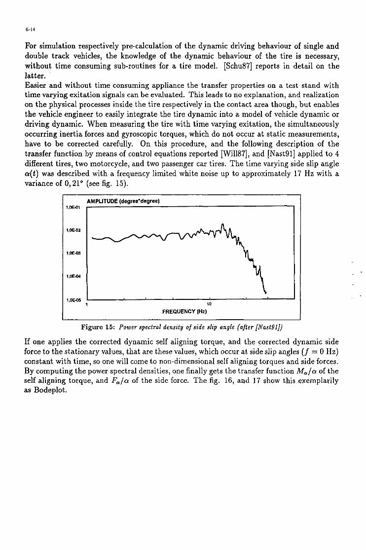
6-14 I

For simulation respectively pre-calculation of the dynamic driving behaviour of single and double track vehicles, the knowledge of the dynamic behaviour of the tire is necessary, without time consuming sub-routines for a tire model. [Schu87] reports in detail on the latter. Easier and without time consuming appliance the transfer properties on a test stand with time varying exitation signals can be evaluated. This leads to no explanation, and realization on the physical processes inside the tire respectively in the contact area though, but enables the vehicle engineer to easily integrate the tire dynamic into a model of vehicle dynamic or driving dynamic. When measuring the tire with time varying exitation, the simultaneously occurring inertia forces and gyroscopic torques, which do not occur at static measurements, have to be corrected carefully. On this procedure, and the following description of the transfer function by means of control equations reported [Wi1187], and [NastSl] applied to 4 different tires, two motorcycle, and two passenger car tires. The time varying side slip angle a(t) was described with a frequency limited white noise up to approximately 17 Hz with a variance of 0,21" (see fig. 15).

AMPLITUDE (degree'degree) 1 .E41

1 1 10

I FREQUENCY (Hz) I ~~~~

Figure 15: Power spectral density of side slip angle (after [NastSl])

If one applies the corrected dynamic self aligning torque, and the corrected dynamic side force to the stationary values, that are these values, which occur at side slip angles (f = 0 Hz) constant with time, so one will come to non-dimensional self aligning torques and side forces. By computing the power spectral densities, one finally gets the transfer function Mala of the self aligning torque, and Fa/a of the side force. The fig. 16, and 17 show this exemplarily as Bodeplot.

6-15

I - -

- -

i a

1

LMPUTUDE (lldegree)

U. I 1 10

FREQUENCY (Hz) 20

45 -

v3

-45- v* -90- vi = 5 m/s

. v2 = 20 m/s

. v3 =50m/s -135

-1 80

-

1 10 20 FREQUENCY(Hz)

Figure 16: Measured transfer function of self aligning torque relative t o side sl ip angle (af ter [NastSl])

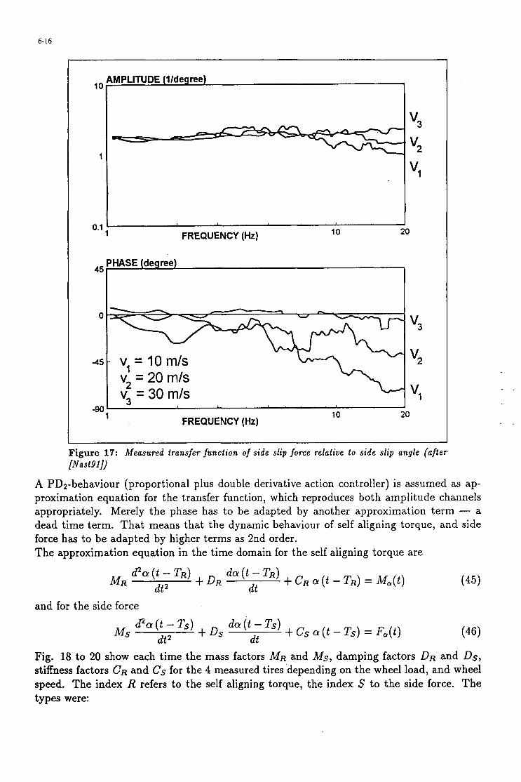
6-16

10

1

LMPLITUDE (l/degree)

I v, J

v*

1 FREQUENCY(Hz) 10 20 0.1

45

"3

-45 v*

vl

0

10 20 -90 FREQUENCY (Hz) 1

Figure 17: Measured transfer function of side slip force relative to side slip angle (after [Nast 911)

A PD2-behaviour (proportional plus double derivative action controller) is assumed as ap- proximation equation for the transfer function, which reproduces both amplitude channels appropriately. Merely the phase has to be adapted by another approximation term - a dead time term. That means that the dynamic behaviour of self aligning torque, and side force has to be adapted by higher terms as 2nd order. The approximation equation in the time domain for the self aligning torque are

and for the side force

@a ( t - Ts) da (t - Ts) + cs CY (t - Ts) = F,(t) Ms dt2 +Ds dt Fig. 18 to 20 show each time the mass factors MR and Ms, damping factors DR and Ds, stiffness factors CR and Cs for the 4 measured tires depending on the wheel load, and wheel speed. The index R refers to the self aligning torque, the index S to the side force. The types were:

6-17

I

QO

4#

Q4

QZ

etillness factor CR [Nm/deg]

U 2 2s 3

Whccl load RN]

stirneas factor Cs [N/deg]

‘.loo 0 (100

1-

m

dQ0

Y-

I. J

Whcel load [kN]

Damping factor DR [Nms/deg]

0 S I O I5 I 30 U 40 4J W

vclocity [m/s]

lyre 1; A lyre 2; X tyre 3; M tyre 4

Figure 18: Stiflness factors CR and Cs as function of wheel load; damping factors DR and Ds as func- tion of wheel speed: 1. Bridgestone 120/80 V 16 (motorcycle); 2. Bridgestone 150/80 V 16 (motorcycle); 3. Conti Contact 155 R 13 (automobile); 4. Conti Contact 175/70 R 13 (automobile) (after [NastSl])

6-18

Massfactor MR [Nms2/degr.] 0,015

0,Ol

0,005

0 0 5 10 15 20 25 30 35 4 45 5 0

Velocity [m/s]

Velocity [mls]

tyre 1; A tyre 2; X tyre 3; I tyre 4

1

Figure 19: Mass factor MR and stiffness factor CR as ixc t ion of wheel speed (af ter [NastSl])

0.02

0.01

0 0 5 10 1 5 2 0 2 5 3 4 3 5 4 0 4 5 5 0

verocrrvtw

H tyre 1; A tyre 2; X tyre 3; H tyre 4

Figure 20: Dead time as funct ion of wheel speed (after [NastSl])

As result there can be concluded:

0 the stiffness factor increases on increasing wheel load for the side force as well as for the self aligning torque.

0 the damping factors DR and Ds increase on increasing speed.

0 the dead time of the side force reduces on increasing speed.

0 CR is constant for motorcycle tires (cross bias type) over the speed, for passenger car tires (radial tires) the stiffness factor and CR increases degressively on increasing speed.

0 MR increases progressively over the speed.

0 an influence of the inflation pressure of the tire on the factors could not be measured.

On further measurements at time varying wheel load F. Sun [Sun901 also reports in his Ph.D. thesis, and reached similar results, in which he additionally determined the dynamic transfer characteristics for time varying wheel load. Since the whole transfer behaviour is still very much depending on the wheel velocity, except the stiffness factor CR for the self aligning torque of the motorcycle tire (cross bias type), one can assume that non linear effects, i.e. because of gyroscopic effects can not fully be recorded by means of the linear approximation formulation. Assuming black-box-formulas are available as break-, sideforces and torques are described in their dynamic behaviour a straight forward integration procedure is possible which will be shown here.

6-20

5 Numerical method of investigating wobble For every non-linear function S(&fr, P ) , an implicit differential equation of first order can be given-for the non-stationary process:

A stabilisation of the numerical or piecewise linear integration in the case achieved through an extension of the equation by a damping term

> 0 can be

and possibly a mass compensation term. These, however, does not render impossible the correct assessment of short-wave surface unevennesses, with regard to their effect on P ( t ) and on S(t) . As a result, the high-frequency rolling process cannot be treated further by means of analytical mechanics. Since further investigations of an analytic kind are not possible, one is compelled to resort to numerical methods. In these, the contact surface is modelled as discrete, and the sequence of contact points is investigated in discrete calculating steps. A unilateral contact condition enables the numerical representation of partial lifting and traversing of track unevennesses. In the process, the tire structure is resolved into many degrees of freedom, taking into consideration the tire mass and damping. Such a structure is geometrically non-linear in principle and has a relatively high frequency. It is guided by means of a rigid body system of low frequency, consisting of a rim and shock absorber. If, as is customary for motorcycles, one introduces a head lug angle A, then one obtains the following system of equations of motion for the steering angle p and the spring deformation s of the wheel axle (see figure 1).

JL J + kL a + CL p (49) m F d + k F i + C F S = Fy C O S X - F , sinX (50)

y, = Yf + (s - Z,) COSX (51)

= My cos X - M, sin X + a F,

In addition, there are also the lateral motion and longitudinal motion of the motor vehicle mass itself. The contact forces generated while traversing the ground unevennesses follow from the equations of motion for the tire structure, which are not given here [Boe93]. The sample calculation given in figure 21 shows the dynamic effect of wheel load variations on a stable steering system that is nevertheless capable of damped wobble. The non-linearities taken into account in the numerical integration are the deformations of finite magnitude, the unilateral contact, i.e. local lifting and settling of the running surface on rough obstacles, and the effects of traction and sliding friction. The model does not take into account the effects of tire width or of cross-sectional bending. Wobble damping, however, is markedly influenced by enlarging the tire width and increasing the length of the contact surfaces. The resultant moment of pivoting has the effect of diminishing wobble. Thus, not surprisingly, for small contact surfaces, which arise,,under low wheel loads, have an especially critical effect on wobble. A surface-oriented theory of non-stationary rolling contact has been analytically developed for perfect roadholding, taking into account the bending of the trajectories of the

6-21

. _

Example: Contact with plane including a rectangular (1x2 cm) obstacle distance 120 cm

I

i 1

I

i

f ,<

R

y = long., v = vertical

5 -_ - - 1 r

I w-' Breaker Tension Force

2x

Figure 21: Sample calculation for the steering system of the froni wheel of a moiorcycle

contact particles of a flattened tire. Wobble vibrations produced on the testing stand show that the phase angle between the amplitude of wobble and the restoring torque of the tire can certainly pass beyond go", which cannot be represented by tire behaviour of the first order. The tendency of the system to auto-excitation is thereby markedly reduced when there is a sufficient area of contact between the tire and the ground. If the ground is uneven, however,

I I

I

so that the contact surface is at times considerably reduced, one speaks of a transition to hard auto-excitation, since the stabilisation is now only produced by the kinematic terms

the air resistance of the vehicle necessarily leads to critical states of wobble, while the axial of f i s t order. At high speeds, therefore, the reduction of load on the front wheel due to

load is sufficiently large in the normal driving state. The non-linear coupling between the horizontal and vertical dynamics of the wheel also calls for numerical treatment here, since an analytic procedure only permits calculation in the case of perfect roadholding. Such a

6-22

numerical procedure, however, is very costly in term of computing time, and has only been carried out until now with coarse substitute models with few degrees of freedom. If, however, one starts out with an analytically based strategy, then the destabilisation effect can also be demonstrated here by means of numerical examples for integrating the rolling action on rough ground.

6 Conclusion Starting from that given overview furture theoretical investigation should include. It is possible to stabilise the system even in case of small contact area using the main influencing parameters found by linear theory. If the parameters are near stability border the nonlinear effects may suddenly disturb the rolling wheel and self-excitation occurs due to vanishing of vertical spin effects in contact area. In any case also for nonlinear computation the linear theory can be used as a guideline. All possible non-smooth surfaces could be taken into account using discret system modeling for the tire.

Lit erat ur [Bak87]

[Bak89]

[Boe77]

[Boe93]

[KochSO]

E. Bakker, L. Nyborg, and H. B. Pacejka: Tyre Modelling for use in vehicle dynamics studies. SAEP 87 04 21, Society of Automotive Studies, Inc., 1987.

E. Bakker, H. B. Pacejka: A new tire model wih an application in vehicle dynamics studies. SAEP 89 00 87, Society of Automotive Studies, Inc., 1989.

F. Biihm: Computing and measurements of the handling qualities of the belted Tyre. Proc. 5th VSD 2nd INTAM Symposium, Vienna, pp 85-103, Swets and Zeitlin- gen, Amsterdam and Lisse, 1978.

F. Biihm: Reifenmodell f i r hochfrequente Rollvorgfmge auf kurzwelligen Fahrbahnen. (Tire model for high-frequency rolling processes on short-wave tracks.) (Bericht Sonderforschungsbereich 181, Teilprojekt B1) VDI-Berichte Nr. 1088, pp 65-81, VDI-Verlag, Diisseldorf/Germany 1991

J. Koch Experimentelle und analytische Untersuchungen des Motorrad-Fahrer-Systems (Experimental and analytical assessment of the Motorcycle-Driver-System; PhD- Thesis 1978). Fortschr.-Ber. VDI-Z., Reihe 12, Nr. 40, 1980.

. .

[Nastg 1)

[NYb731

[Pac66]

[ Ruf831

[Schu87]

[Sha71

[ S ha771

[Sun901

[Valk93]

6-23

R. Nast, Chr. Teubert and H.-P. Willumeit: Messungen der Ubertragungseigenschaften von Luftreifen bei zeitlich verkderten Schriiglaufwinkeln und anschlieflende Nachbildung dieser Gr6flen durch Approxi- mationsgleichungen (Measurement of transfer properties of pneumatic tires under time varying side slip angle and followed by modelling using approximation equations.) VDI-Berichte Nr. 916, pp 321-344, VDI-Verlag, Dusseldorf/Germany, 1991.

G. Nybakken: Investigation of Tire Parameter Variations in Wheel Shimmy. PhD-Thesis, The University of Michigan, 1973.

H. B. Pacejka: The wheel-Shimmy phenomenon. PhD-Thesis, Technische Hogeschool, Delft, 1966

E. Ruf Theoretische Untersuchungen des Federungsverhaltens von Vierrad-StraBenfahr- zeugen. (Theoretical investigations into the suspension behaviour of four-wheel road ve- hicles. ) Fortschr.-Ber. VDI-Z., Reihe 12, Nr. 44, S. 104-105, Dusseldorf, 1983.

D. H. Schulze: Instationare Modelle des Luftreifens als Bindungselement in Mehrkorpersystemen fur fahrdynamische Untersuchungen. (Non-stationary models of the pneumatic tire as a linkage element in many-body systems for investigations into the dynamics of driving.) VDI-Fortschritt-Berichte, Reihe 12, Nr. 88, VDI-Verlag, Dusseldorf, 1987.

R. S. Sharp: The Stability and Control of Motorcycles. J. Mech. Engin. Sci., 13 No. 5, pp 316 - 329, 1971.

R. S. Sharp and C. J. Jones: The straight running stability of single track vehicles. Proc. 5th VSD 2nd INTAM Symposium, Vienna, pp 334-342, Swets and Zeitlin- gen, Amsterdam and Lisse, 1978.

F. Sun: Dynamic Properties of Motorcycle Tires. Dissertation, Beijing Institute of Technology, 1990.

R. van der Valk, H. B. Pacejka: An analysis of a civil aircraft main gear shimmy failure. Vehicle System Dynamics, 22, Swets and Zeitlingen, BV Lisse, Netherlands, 1993.

6-24

[Will871

[ W ill8 91

(Will951

H.-P. Willumeit und Ch. Teubert: Dynamische Eigenschaften von Motorradreifen bei zeitlich veriinderlichem Schriiglaufwinkel. (Dynamic properties of motorcycle tires at slip angles varying with time.) VDI-Berichte Nr. 657, pp 127-136, VDI-Verlag, Dusseldorf, 1987.

H.-P. Willumeit and F. Sun: Dynamische Eigenschaften von Motorradreifen bei zeitlich veranderlicher Radlast (Dynamic properties of motorcycle tires under time varying, wheel-load). VDI Berichte Nr. 779, pp 389401. VDI-Verlag, Diisseldorf/Germany, 1989.

H.-P. Willumeit and F. BGhm: Wheel Vibrations and Transient Tire Forces. Vehicle System Dynamics, 24, Swets and Zeitlingen, BV Lisse, Netherlands, 1995.

1

7- 1

LANDING GEAR SHIMMY - DE HAVILLAND’S EXPERIENCE

, - -

John Glaser and George Hrycko Structural Dynamics Group

de Havilland Inc. 123 Garratt Blvd.

Downsview. Ontario, M3K IY5 Canada

1. SUMMARY Landing gear shimmy is an unacceptable situation which, at the very least, leads to increased maintenance costs and at the worst could result in catastrophic failure of the gear andor the attach- ing structure. Two landing gear shimmy problems experienced by de Havilland are presented. one in service and the other pre- dicted during design. While these problems occurred over IO years ago, it is the authors’ contention that little progress has been made in this design discipline in the intervening years. I t is recommended that advisory material is needed in this important but often neglected subject.

2. LIST OF SYMBOLS tire lateral damping coefficient tire torsional damping coefficient tire cornering power damping matrix tire cornering force tire side force side force landing gear vertical force (static) vertical force on left tire vertical force on right tire gyroscopic matrix half footprint length inertia matrix polar moment of inertia of wheel assembly stiffness matrix tire lateral spring constant tire torsional spring constant tire vertical stiffness structural torsion stiffness mechanical trail geometric trail half axle length moment due to tire torsional stiffness roll moment yaw moment tire (deflected) rolling radius undeflected tire radius time displacement vector [ y, Q, yIT ground speed lateral displacement tire equator coordinate at forward end of contact patch tire equator coordinate at aft end of contacr parch tire lateral defection at forward end of contacr patch

2 A tire lateral deflection (elastic) AM0 incremental roll moment AMv incremental yaw moment Ep €& gear ti l t angle h~ yawed-rolling relaxation length p friction coefficient 5 critical damping ratio 6, structural damping ratio r, (Moreland) tire time constant r t @ roll displacement y yaw displacement y, CO circular frequency

tire lateral deflection at aft end of contact patch

pneumatic trail parallel to ground

equals T, at 100 kts (Reference 3)

tire elastic twist deflection in yaw

3. INTRODUCTION Landing gears that shimmy are unacceptable, causing consider- able discomfort and annoyance to passengers and crew. In fact, a severe occurrence of shimmy can damage the landing gear and its attaching structure, resulting in significant repair costs and air- plane down time. The prevention of shimmy on an airplane with a shimmy-prone gear increases maintenance costs and may bur- den the pilot with self-established shimmy avoidance procedures. Some assurance is therefore needed that landing gear designs will be free from shimmy under all operating conditions taking into account normal wear and tear experienced in service.

Two examples of landing gear shimmy are presented in this report; the first involving the DASH 7 nose landing gear and the second the DASH 8 main landing gear. The DASH 7 airplane is a 4-engined turboprop, seating 54 passengers, that is no longer in production but is still in service. Nose landing gear shimmy appeared early in the flight development phase of this aircraft and re-appeared again after its introduction into service.

The DASH 8 airplane is a twin turboprop that seats 36 passen- gers in its earliest version, the series 100. Landing gear shimmy did not occur physically in this case, but was predicted to occur during the design phase. What is troubling about this example is that i t took an inordinate amount of time for de Havilland and the landing gear vendor to settle on a design considered to be shimmy free. Obviously, the design process was costly and, despite the time spent, the structural efficiency of the design remains an open question: ie.. the landing gear may be heavier than necessary.

Paper presented at the 81st Meeting of the AGARD SMP Panel on “The Design, Qualification and Maintenance of Vibration-Free Landing Gear”, held in Ban& Canada from 4-5 October 1995, and published in R-800.

1-2

These examples occurred over I O years ago. While this may be considered ancient history by some standards - the computer industry, for example - i t is the authors’ opinion that there has been little progress in the state of the art of shimmy design in the intervening years.

The authors have‘reason to believe that the shimmy “problem” is perceived by many to be a “black art” with no basis in sound engineering methods. The authors disagree and are concerned that this “black art” perception has hindered progress in shimmy design unnecessarily. The shimmy “problem” is no more myste- rious than, say, aircraft flutter with which the authors have expe- rience. What is lacking is the accumulation, integration and dissemination of currently available analytical and experimental experience to support the development of practical design pro- cesses. These, in turn, would yield structurally efficient, shimmy- free designs. The authors are optimistic that practical design pro- cesses are feasible and believe that the aerospace industry would benefit if those processes were formulated and made generally available.

Presented in this report are reviews of the DASH 7 and DASH 8 shimmy problems experienced by de Havilland. The report out- lines the analysis models and methods used and presents the sta- bility results obtained from those methods. The report concludes with a recommendation for the development of advisory material on shimmy design.

4. DASH 7 NOSE LANDING GEAR SHIMMY EXPERI- ENCE

4.1 The Occurrence of Shimmy The nose landing gear on the DASH 7 airplane (see Figure I ) has two modes of operation, a castering mode with high angular damping - sometimes referred to as the “high damped mode” - and a steering mode with relatively low angular damping. Set for castering at touchdown, the nose gear automatically transitions to the steering mode by a weight-on-wheels switch.

In 1976, during the flight development trials, nose landing gear shimmy was experienced in the lower-damped steering mode. This resulted in two modifications to the design:

( 1 ) the introduction of a 0.75 second time delay between the nose wheel weight switch closure and power steering activation to allow the spin-up transient to subside before switching into the lower damped steering mode.

(2) the introduction of a 0.01 inch diameter cross bleed damper in the steering mode to increase the angular damping in that mode. Further additional damping was prohibited by steering torque requirements.

The shimmy problem was thought to have been solved by these modifications as there were no further occurrences during the flight trials. However, by the Fall of 1980, reports of nose wheei shimmy were accumulating from aircraft in service. These prob- lems took two forms, one involving feedback from the steering

actuator and the second, the more classical process addressed during airplane development.

In the first case, shimmy occurred at relatively low speed and produced alarmingly large lateral oscillations of the airplane nose. One report tells of tire marks on the runway indicating angular deflections of up to 40” from centre in one direction and up to 35”degrees in the other. This rather violent form of shimmy was caused by backlash at the tiller inpur potentiometer to the steering actuator and a modification was introduced to eliminated the backlash. This type of ‘system induced’ shimmy problem will not be discussed further.

The second type of shimmy, unlike the first, occurred at rela- tively high speed and with fairly modest amplitude oscillations of the gear assembly at a relatively high frequency (approxi- mately 20 Hz). It usually occurred with the steering system ON (ie., the mode with lower damping), but there were reports of shimmy with the steering system OFF as well.

This latter shimmy problem stimulated a broad range of immedi- ate and longer term actions, all intended to achieve an expedient and lasting solution. The actions taken were:

(1) Introduce (large) “unpaved runway” tires across the fleet because there were fewer reported incidents of shimmy involving these tires.

(2) Recommend operational procedures for curtailing shimmy onset until a solution was found; specifi- cally, that steering be left off during landing and that steering engagement be avoided at high speed.

(3) Undertake inspections of the nose landing gear to ensure that its modification status is current and its maintenance condition is to specification (e.g., wheels within balance, tires in good condition, etc.).

(4) Institute a questionnaire style reporting procedure to accumulate information on shimmy occurrences in service.

4

(5) Undertake taxi trials using a typically worn landing gear to obtain quantitative information on nose gear shimmy.

(6) Measure the frequency response characteristics of the steering actuator in an isolated test rig to estab- lish its (dynamic) stiffness and damping properties as a function of frequency.

(7) Develop an in-house analytical methodology cali- brated to the results obtained from the above tests. This analytical capability could then be used to eval- uate the benefit of design treatments; such as. a torque link damper, torsionally coupled nose wheels (live axle), changes in trail, “mass balance”, etc.

It is not the purpose of this report to review each and every action taken to resolve the DASH 7 nose gear shimmy problem: rather.

1-3

the purpose for presenting the above list is to indicate the effort required to resolve a shimmy problem when it is experienced in service. Following are some experimental and analytical results which were important in helping us develop a physical under- standing of our nose gear shimmy process and in establishing our analysis methods.

4.2 Shimmy Test Results The test results presented in Figures 2, 3 and 4 are instructive. In all cases, the ground speed is about 55 knots. Figures 2 and 3 apply to a “tight” gear for which free play in the scissors - the only significant source of free play - was removed using shims. In the case of Figure 2, the weight-on-wheels switch was deacti- vated to allow excitation by the spin-up transient and steering was ON at the outset. The result clearly shows the landing gear is fundamentally unstable at 55 kts in this low-damped configura- tion.

In Figure 3, the landing was made with the time delay circuitry operating in order to eliminate excitation by the spin-up tran- sient. With steering OFF at touchdown, the large transient oscil- lations due to spin-up are observed to attenuate quickly, due to the relatively high damping in the castering mode. While small random vibrations persist, there is no evidence of shimmy after the time delay period when steering is ON, showing that the time delay was effective in circumventing the excitation of shimmy by the wheel spin-up transient.

Figure 4a shows results for which the shims in the torque scissors were removed to produce approximately 1/8 inch of free play in the scissor apex. Again, steering was OFF at touchdown and the transient oscillations are observed to decay to limit cycle oscilla- tions within the free play range wherein, steering actuator damp- ing has negligible effect. With steering ON - activated after the 0.75 second time delay - and with torsion damping thus decreased, the oscillations within the free-play band cause the gear to go unstable, that is, to shimmy (Figure 4b).

4.3 Analysis Model The analysis model used to investigate shimmy follows the approach used by Lockheed in Reference 1. It consists of a tor- sion model defined relative to the inclined leg axis and a side dis- placement model (Figure 5). The torsion model is made up of 4 concentrated inertias to give the freedoms required to represent free play (backlash), bearing friction (coulomb damping) and torque scissor stiffness and free play (both functions of stroke). Fuselage torsion stiffness and trunnion attachment free play are also included in this model. Initially, the steering actuator stiff- ness was defined solely by the value of bulk modulus for hydrau- lic fluid which was assumed to have a value of approximately 100,000 psi (with typical air entrainment). This value was subse- quently reduced to about 34,000 psi to account for the flexibility of the steering actuator structure determined from an isolated shake test of that unit.

The side displacement model used eliminates the y independent degree of freedom by assuming an infinitely stiff leg free to roll (@ ) about an effective rotation point as illustrated in Figure 5b.

As indicated in that figure, effective values for rotation arm length, inertia, damping and frequency are dependent on the length of the shock strut. Coulomb damping or free play is not included in the side displacement model.

The equations of motion for shimmy analysis, including the von Schlippe and Moreland tire models, are presented in Appendix A. The tire coefficients used in the equations derive directly from Reference 2, except for Moreland’s tire time constant, 7, , which was selected to conform with test results. The structural damping ratio, 5 , . was assumed to lie in the range zero to 0.03.

4.4 Results Stability analysis results for both the von Schlippe and Moreland tire models are presented in Figure 6 for the case of steering sys- tem ON and no free play. As noted, all curves except one apply for a single point model of the nose gear. Also plotted in Figure 6 is the damping result obtained from the test data given in Figure 2, a single point at 55 knots ground speed with a damping value of 0.007.

The predicted frequencies are not shown but lie in the 26 Hz range. This is about 20% higher than the value measured and is attributed to mass and stiffness modelling inaccuracies. The effect of this higher torsion frequency was determined by analy- sis to increase the predicted stability by 0.01; i.e., to lower the curves in Figure 6 by that amount.

With respect to damping, three curves are indicated to give rea- sonably good agreement to the test result in the 55 knot speed range: the von Schlippe single point result for 6, = 0 , the von Schlippe distributed mass model result for 6, = 0.03 and the Moreland single point result for 5, = 0.03 and T~ * - - 0.002. Clearly, much better agreement with this single test point could have been obtained both in frequency and damping by applying arbitrary adjustments to the parameter values initially chosen. However, this was not pursued because the problem remained that no conclusion could be drawn as to which structural and tire models would give the most reliable result due to the lack of test data.

The analysis was extended to investigate the effect of free play using the distributed mass model (Figure5a) and the von Schlippe tire model. These results demonstrate why free play must be avoided in landing gear design. Its presence can result in limit cycle vibrations at speeds lower than the classical shimmy speed - the speed obtained from the solution for a tight gear.

The addition of “mass balance” to the shock strut, was investi- gated as a means for improving nose gear stability. The results presented in Figure 8 show that the forward placement of weight has a stabilizing effect and that the most effective arm length, at least for this landing gear, is equal to the tire radius. This approach ultimately led to a modification - using a 25 pound bob weight - which was made available to operators as an option. While the increase in stability is predicted to be only 0.01, i t is the authors’ opinion, based on reported performance, that the mass balance modification is more effective than predicted.

5. DASH 8 MAIN LANDING GEAR SHIMMY EXPERI- ENCE

5.1 The Occurrence of Shimmy Early in the design phase, the vendor for the main landing gear, using analysis methods which they considered reliable, reported that shimmy would occur within the operating speed range of the airplane and that torsion and side bending stiffnesses would have to be increased to achieve stability. Because of the weight increase involved, many months of intense analysis effort and debate were required before de Havilland and the landing gear vendor agreed on final design values.

5.2 Analysis Models The main landing gear for the DASH 8 airplane is shown in Fig- ure 9. The DASH 8 is a high wing aircraft with the main landing gear supported from within the nacelle. As a result, the landing gear is relatively long and flexible and therefore may be more prone to shimmy.

During the course of the shimmy investigation, a variety of gear structural models were developed ranging from simple “stick” (Figure IO), to full finite element. In all cases, except for the modal analysis discussed below, these structural models were used to define a 3x3 stiffness (or flexibility) matrix defined at the axle centreline in the single point analysis method.

In the modal analysis method, the finite element model for the landing gear and nacelle structure was extended to include a stick model for the wing with distributed mass and stiffness properties. The mode shapes and frequencies for’this system were calculated and the shimmy equations were then set up and solved in modal form.

The single point analysis method was extended to include free play. Its effect was simulated (in a global sense) by replacing the linear stiffness matrix defined at the wheel axle centreline with a non-linear stiffness matrix having low angular stiffness, kyw , within the free play range and full predicted stiffness outside that range. These equations were solved in the time domain.

Both Moreland and von Schlippe tire models were used to repre- sent tire dynamic properties. However, the Moreland model was considered less reliable for absolute stability results because there was no empirical method for defining the tire time constant, T,, (see comments in Appendix A).

For structural damping, a typical value of 6, = 0.03 was assumed in the computations. However, no allowance for this damping was given in defining stability; that is, stability curves had to have a margin of 0.03 to be considered shimmy free.

5.3 Analysis Results In January 1981, using the simpler “stick” models shown in Figure IO, de havilland confirmed that the landing gear would be unstable within the operating speed range and that the most effective way to increase the shimmy speed was to increase the torsion stiffness of the gear (at the time 1.13~10~ Ib-in/rad).

Increasing the side bending stiffness was also determined to be important but not as important as increasing the torsion stiffness. I t was also determined that shimmy stability could be improved by increasing the mechanical trail so the design was changed to increase the mechanical trail to the maximum extent possible.

I

The results from more elaborate analysis models indicated that a torsion stiffness of 2 . 2 ~ 1 0 ~ Ib-idrad and a side bending stiffness in the range of 6,000 to 8,000 Ibhn would be required to preclude shimmy. By mid 1981, these stiffness requirements grew to a high of 2 . 4 ~ 1 0 ~ Ib-idrad and 14,000 I b h . As noted above, it was only after a long, protracted period that the final design val- ues of approximately 1 . 8 ~ 1 0 ~ Ib-idrad and 7,600 I b h . with nacelle flexibility included, were agreed to by both the vendor and de Havilland.

Final analysis results are presented in Figures 1 1 and 12. Stabil- ity in the side bending mode is of little interest because the damping values in this mode are high and increasing at speeds above the no-slip speed. Regarding torsion stability, Figure 11 shows the rigid wing giving generally conservative results com- pared to the full finite element analysis. Figure 12 shows stability in the torsion mode increases with stroke. The results indicate the landing gear to be stable for the complete operating speed range of interest with a damping margin of 0.03.

Summarized in Figure 13 are the results of a non-linear analysis to establish the influence of bearing friction and free play on shimmy. These results contributed to the specification of free play limits in the main landing gear design.

6. DISCUSSION In the case of the DASH 7, it appears that the nose landing gear problem has been “contained” provided the tires are matched and in good condition, the wheels are kept in good dynamic balance, free play is limited and nose gear touchdown and taxi speeds are kept low. Nose gear mass balance is generally considered to be beneficial by those operators who elected to have that option. Obviously, the containment of nose gear shimmy has increased the maintenance cost, pilot workload and in some instances, the airplane weight.

In the case of the DASH 8, with over 400 airplanes in service, all shimmy free, it is safe to say that the main landing gear design has now been proven. However, the main concerns in this case are the time and effort required to establish the final design requirements and the degree of over-design (weight penalty) that may have been included in the final product.

I I

- -

-

7. RECOMMENDATIONS At the time the DASH 8 was being designed, there was no well established consensus on what constituted a reliable shimmy design methodology. This still appears to be the case today. For this reason. it is recommended that some guidance information be provided - similar to an advisory circular issued by aircraft airworthiness authorities. This advisory material should:

7-5

.

.

Establish standardized terminology

Give guidelines on structural modeling

Define tire models, including the assumptions and limitations

Review and update tire properties and ranges of parameter variation

Provide expressions for the tire terms appearing in the equations of motion for a variety of wheel con- figurations

Recommend design analysis guidelines taking into account free play, recommended stability margins, structural and tire parameter variability, etc. (Table 1 suggests variances for some parameters appearing in the equations of motion and indicates whether they have a stabilizing or destabilizing effect on shimmy.)

Provide guidelines on component and vehicle test procedures:

tire properties structural properties (static and dynamic) complete installed system

Provide practical design information on anti- shimmy tires, live axle, etc.

Provide standardized analysis cases for a variety of landing gear configurations

Provide information on related vibration processes and problems - sometimes confused with shimmy - such as wheel unbalance, tire out-of-round. judder. anti-skid processes, steering feedback processes, gear walk, etc. Some of these processes may warrant separate advisory material of their own.

Provide landing gear maintenance guidelines, based on analytical and experimental data, for minimizing landing gear vibrations

Provide a bibliography

8. CONCLUDING REMARKS As a consequence of the DASH 7 and DASH 8 shimmy prob- lems experienced at de Havilland, the authors were required to develop analytical tools for problem solving and design. This work was accomplished successfully despite the lack of a ‘stan- dardized’ industry accepted methodology at the time. It is the authors’ contention that reliable shimmy design procedures are required and that it is feasible to do so. Had advisory material been available during the design of the DASH 7 and DASH 8 landing gears, de Havilland may not have had the problems out-

lined herein. At the very least, their resolution would have been more expeditious.

REFERENCES (1) “Active Shimmy Control System”, AFFDL-TR-75-136.

Lockheed-California Company, Burbank California, December, 1975.

(2) Smiley, R. F., Home, W. B. “Mechanical Properties of Pneumatic Tires with Special Reference to Modem Aircraft Tires”, NASA TR-R-64, 1960

(3) Leve, H. L., “Designing Stable Dual Wheel Gears”, AlAA 69-769, July 1969

(4) Moreland, W.J., “The Story of Shimmy”, Journal of rhe Aeronautical Sciences, pp. 793 - 808 ( 1954).

(5 ) Collins, R. L., “Frequency Response of Tires using the Point Contact Theory”, J. Aircraf, June 1972.

(6) Clark, S . K., “Dynamic Properties of Aircraft Tires”, J. Air- craji, March 1974.

(7) Collins, R. L. and Black, R. J., T i r e Parameters for Land- ing-Gear Shimmy Studies”, J. Aircraft, May-June 1969

(8) Grossman, “F-15 Nose Landing Gear Shimmy, Taxi Test and correlative Analyses”, SAE Paper, No. 801 239.

(9) “Shimmy Analysis Addendum to QTR No. ATR 923, 13.5 x 6.00 - 4, DR17922T 14 PR Outrigger Tire”, Dunlop Manu- facturing, England, September 1981.

(10) von Schlippe, B., “Shimmy of a Pneumatic Wheel”, NACA TM-1365, August 1954

APPENDIX A. SHIMMY ANALYSIS MODELS

This Appendix describes the shimmy analysis methods devel- oped at de Havilland.

A.l Equations of Motion A much simplified model for a single or dual wheel landing gear is illustrated in Figure AI which shows an inclined shock strut with mechanical trail, L, measured parallel to the torsion axis and geometric trail, LG = R x sineg, where Os is the inclination angle and R is the deflected tire radius.

Also shown in Figure AI are two equally valid coordinate analy- sis systems, one located at the apex of the shock strut and the mechanical trail arm and aligned with the strut, and the other located at the wheel axle with axes orthogonal to the ground plane. The former system simplifies the mechanical terms in the equations of motion while the latter simplifies the tire force and moment terms. In order to expose more clearly the less familiar tire terms, the latter coordinate system is used in this report to

develop the equations of motion. These equations are written in terms of the lateral ( y), roll ( 4 ) and yaw (y) degrees of free- dom defined at the wheel axle;

where

and where I = inertia matrix D = damping matrix G =gyroscopic matrix K = stiffness matrix

U = [i]

A.2 Structural Terms Formulations for the left hand side terms are not given in this report but they can be found in References 1 and 3. It is impera- tive that utmost care be taken in defining and verifying the assumptions made in establishing the analysis model and in developing the data used. For instance, if a landing gear is assumed to be a uniform structure, its mass and inertia effects can be ‘lumped’ at the wheel axle and a ‘single point’ model ana- lyzed. In this case the mass and inertias of the wheel rolling assembly should be supplemented with appropriate effective masses and inertias of the supporting gear structure. The 3x3 mass matrix, M, will contain (off-diagonal) terms that couple the three degrees of freedom, y, 4 and y. If it is important to include detailed representations of bearing friction or free play (backlash), then a distributed mass model will be required to pro- vide the additional degrees of freedom needed to represent these characteristics.

The damping matrix, D, should include both structural and bear- ing friction damping terms, if appropriate. As indicated ahove, this may require the development of a more complex gear dynamic model than can be expressed by a single point formula- tion with 3x3 matrices.

The gyroscopic matrix contains roll-yaw coupling terms with coefficients IOX ( V/RT) , where 10 is the polar moment of inertia of the wheel rolling assembly, V is the ground speed and RT is the tire undeflected radius.

As in the case of the mass matrix, if the gear structure is assumed to be uniform, its stiffness properties can be represented by a 3x3 stiffness matrix, K, defined at the wheel axle. Once again, if i t is important to include detailed representation of bearing friction or free play, then additional degrees of freedom and stiffness terms will be required.

Finally, the mass, stiffness and damping effects of the landing gear’s supporting structure should be included in the equations of motion because they can have a strong effect on the stability results.

A.3 TireTerms During shimmy, the motions of the gear axle are coupled not only through the gear structure as expressed by the terms on the left hand side of equation (AI) but also through the interaction between the tire and ground, as represented by the tire forces and moments appearing on the right hand side of that equation.

Two tire models were considered, the Moreland “Point Contact” model and the von Schlippe “Stretched String” model. Both models are presented below in a coordinate system orthogonal to the ground plane. This was done in order to develop the simplest possible expressions for the tire forces and moments. Formula- tions for single and dual wheel assemblies are included.

A.4 The Moreland Point Contact Model (Single Wheel) The Moreland point contact model (Reference 4) expresses the tire contact forces and moments in terms of the tire cornering force, Fc , and pneumatic trail, E ~ , as follows (Figure A2):

= E;] (A3)

Fc = K T ~ A + C T ~ A (A41 where

and where K T ~ = tire lateral spring constant C T ~ = tire lateral damping coefficient

A = pneumatic trail parallel to ground = tire lateral deflection (elastic)

R = tire (deflected) rolling radius

To enable a solution of the shimmy equations, Moreland postu- lates an alternate expression for the tire cornering force in terms of a tire cornering power, C y , and time constant, T,, , as follows:

-

Fc = CwWt + CtyTu’$t ( ‘45)

where y, = the tire elastic twist deflection

Finally, Moreland assumes the absence of slipping or scrubbing between the tire and ground by imposing the kinematic relation- ship;

I

) i+A+V(W+Wt) = 0 (A6) I Embodied in the above kinematic relation is the assumption of no slipping or scrubbing. According to the empirical data pre- sented in References 5 and 6, this assumption is invalid and therefore, “classical” shimmy is not likely to occur at ground

(A71 wh speeds

where w is the shimmy frequency and h is half the tire footprint length. (The von Schlippe model described below also assumes that no slipping or scrubbing occurs between tire and ground and therefore it too is subject to the same speed limitation.)

v<o.8

Empirical values for the tire parameters appearing in the above equations can be obtained from Reference 2 with one notable

7-1

in terms of the yawed-rolling relaxation length, 2.0. This geo- metric relationship can also be deduced from Figure A4.

exception - the tire time constantrv. Choosing a reliable value for rY is generally a problem because no consistency can be found in the literature for this parameter as illustrated by the compiled data of Figure A3. Since r, has a strong influence on the results, it is recommended that the value used should be vali- dated in some way if the results are to be accepted in absolute terms.

Also. while empirical values for the pneumatic trail, Ep. are available. some analysts prefer to base the tire torsion moment, Mr . directly on the tire torsional stiffness K T ~ , viz;

Mt = KT,W (A8)

instead of usrng the expression proposed by Moreland Thts vari- mon has not been used in the present report.

A 5 The von SchUppe Stretched String Model (Single Wheel) The von Schlippe tire model (References IO and I) assumes that the tire equator IS represented by a "stretched string" that takes on the deflected shape shown in Figure A4 due to out-of-plane mouons In this model the tire forces and moments are: E] = E] (AS)

where F, = K T ~ A + C T ~ A

Mt = KT.N

and where the tire elastic lateral and torsional deflections are given by:

z+2 A = - 2

As before, h equals half the footprint length.

Z and 2 are defined in Figure A4 from which the following geo- metric relationships can be deduced.

Z = Y-y-R@-hW

2 = ?-y-R$+hW

Finally, the kinematic relationship that assumes no slippage between the tire and ground is given by the following expression

Empirical values for all of the parameters required by the von Schlipp tire model can be obtained from Reference 2. It might be noted that some analysts also extend the expression for MI by including the tire torsion damping term, C T ~ , viz;

Mt = K T ~ W ~ + CT~ '& ( A I 3

This variation has not been used in the present repon.

A.6 Dual Wheel G e m The Moreland and von Schlippe tire models given above apply for a landing gcar with a single wheel. The following steps extend those formulations to uual wheel landing gears:

(1) Factor the force and moment expressions by 2

(2) Add the following rolling moment term to aecount forthe vertical &round reaction forces. Assuming the total static force. Fz, is shared qually, the ground reaction force on each tire is comprised of a static force and a dynamic force due to roll displacement $.Thus.

AM$ = L ~ ( F ~ - F , R ) ( A W

where the (upward acting) ground reaction forces on the right and left tires are. respectively;

F,R = F. 2 + L ~ @ K ,

F.L = ;-L~@K. F (A171

and where LR = half axle length Kz = the tire vertical stiffness

(3) Add the following yawing moment term to account for the ground friction force;

AM^ = L ~ ~ ( F , L - F , R )

where p = tire rolling friction coefficient

E 9

7-9

7-10

.

7-1 I

. . . . . . : : - I . . . : : : : i ; : t i ; -

: r

7-12

I 1 %

3

t a

> 6

i a 5? Y

!I

8- 1

Unsteady Tire Dynamics and the Application Thereof to Shimmy and Landing Load Computations

Klaus Koenig Daimler-Benz Aerospace Airbus GmbH

HunefeldstraBe 1-5 28199 Bremen, Germany

SUMMARY A complete set of nonlinear equations of unsteady tire dy- namics for all the 6 degrees of freedom of the wheel move- ment is presented. The coefficients of these equations are based on available publications and may need some im- provements. The influence of some of the coefficients which are new or controversely discussed is shown revealing areas of caution and stressing the necessity of adequate tire tests. Nevertheless it could be demonstrated that reasonable shimmy analyses are possible with these equations and that the computation of realistic unsymmetric landing im- pacts require their inclusion as a must.

1. INTRODUCTION The wheel - without example in nature - is one of the most efficient inventions of human spirit and a fundamental ele- ment of technical constructions. The inflated tire is a rela- tively new additive to the wheel but most probably its best

Modern civilization is inconceiveable without wheels and tires. Millions of them are rolling on the streets every day and every minute . But in spite of the huge application of tires no comprehensive mathematical description of their characteristics is available. It is nearly unbelievable but it seems that all the progress of modern transportation technique was possible without a qualified theory of tire dynamics. There are early publi- cations with rather good results already 50 years ago but there is no reliable up-to-date theory available (s. ref. 8). What are the reasons? Is there really no need for a better theory? Was it too expensive to establish one? Was it just not published or available or was it too difficult for the en- gineers?

- improvement.

.

Tire dynamics is characterized as the dynamics of any or- dinary vibrator by the interaction of elasticities and masses. But superimposed in this special case is the creep- ing process within the contact area between tire and ground - the so called relaxation mechanism. One of the earliest studies of tire behavior was performed by Fromm at the German university of Danzig. The first real shimmy theory was published by von Schlippe and Dietrich (s. ref. 1). The last fundamental collection of ap- plicable data was presented by Smiley and Horne (s. ref. 2) in 1960. So what is available in 1995 can only be called a substitute or ”stopgap” but not an applicable theory of modern tires for reliable dynamic studies of dynamic structures. Therefore in the following first some thoughts are spent on how to get qualified tire data. After that published shimmy theories are compared. Based on this and together with

some amendments from other sources a complete set of equations for tire dynamics is given. Eventually, its ap- plication to shimmy and landing loads computation is stu- died.

2. GENERAL TIRE DYNAMICS The most simple way to establish reliable tire dynamics at least applicable to shimmy or linear stability studies would be to put a rolling wheel with tire on a drum to excite the wheel at its centre by frequency sweeps of deflections and to measure the load response. If this is done at a well de- fined working point of the tire and subsequently for all the 6 components of the deflection applicable at the wheel centre 36 transfer functions (frequency response func- tions) for all the 6 possible perturbations of the steady state movement of the wheel centre will be available. Each transfer function can be linearly approximated by a frac- tion of polynominals of the imaginary Fourier frequency.

If one uses as a first approximation the same denominator polynomial for the same load component and accepts that for linear systems superposition is possible, then Fourier transformation allows to establish with the polynomial co- efficients the simple matrix equation*:

n m

where PtR = LpxtR, PYtR? PZtR, Pa)tR, PetR, P V t R 1 ’ is the perturbation vector of loads and F:R its derivative to the time

rIA = [XtA, ztA, @all? V m t ] ’ is the perturbation vector of wheel centre deflections

Bn,Wm are coefficient matrices.The diagonal Bn contains the denominator and the complete Wm the nominator coefficients of the n’th or m’th order polynomials

That is all, at least for the small perturbations of shimmy.

*The more general solution would result in 36 scalar dif- ferential equations which must be solvedfirst to allow a summation of the 6 load portions of each load component caused by the 6 different excitations. By the way, f o r second order polynomials one would get 2 times 36 eigenvalues. That would allow 36 possible tire load oscillations without wheel movement perturbations and 36 wheel movement oscillations without tire load per- turbations.

Paper presented at the 81st Meeting of the AGARD SMP Panel on “The Design, Qualification and Maintenance of Vibration-Free Landing Gear”, held in Banff, Canada from 4-5 October 1995, and published in R-800.

8-2

For larger deformations as they occur at landing impact further investigations with larger amplitudes and with and without rolling velocity are necessary. But this should be a second step to be defined in detail after successful execution of the first one with small perturba- tions. Partially such studies have already been performed (s. ref. 5 ) but no complete test result is known to the author. Nevertheless, since no principle obstacle to such an ap- proach to establish reliable equations of tire dynamic is ev- ident, it can be hoped that perhaps in another 50 years such data will be available for the benefit of future engineers and of technical progress - if further progress is ever wanted at that time.

3.

The following publications will be compared:

COMPARISON OF SOME PUBLISHED TIRE EQUATIONS

- von Schlippe, and Dietrich, (s. ref. 1) I - Smiley, (s. ref. 3)

- Pacejka, (s. ref. 4) - Rogers, and Brewer, (s. ref. 5 ) with the Moreland

,

theory. If the equations of movement as given in these publica- tions are transformed to the coordinate system of Fig. 3-1 and linearized by series developments up to elements of second order coefficients for matrices B and W as defined in chapter 2 can be derived as given in table 3-1. These equations are given in their original symbols with- out further explanation of the symbols. Nevertheless some basic conclusions can be drawn:

I

- There are really only diagonal elements in the B matrices.

- B.,, = B.,, = B.,, are equal for all theories . This may mean that the tire can vibrate in itself with a single mode, showing at least 3 different load compo- nents

same places.

I - The different theories don’t place coefficients at the

- A larger portion of the matrices is non-symmetric. , - Von Schlippe and Dietrich do not study the tilt.

Pacejka does not give tilt moments .

W2,, in the theories of Smiley and Pacejka, the mis- sing coefficient W2w, WO,,, WO,,, WO,, in More- land’s theory and the missing coefficient W q , in Pacej ka’s theory.

- The absence of the elements WO,,, WO,, WO,, is caused by the relaxation mechanism. Loadings caused by sideward deflections will disappear with time.

- The theories of von Schlippe and Dietrich, Smiley and Pacejka look rather similar, they are based on equal basic thougths. The Moreland theory is funda- mentally different

- Moreland introduces a time constant C1 [sec] for de- scription of the relaxation mechanism while the other

- Remarkable are the missing coefficients Wl,,

I

theories use a relaxation length [m]. This leads to the fact that e.g. B2.. depend only on the rolling velo- city v in the Mooreland theory but on v2 in the other theories.

- Moreland originally only studied I$. The extension by y was introduced by Rogers and Brewer, and the

extension by $ by Edman (9).

4. A COMPLETE SET OF TIRE EQUATIONS For the following, Smiley’s equations as given in chapter 3 will be used as a basis. They are modified by neglection of minor unknown elements (t=O) inclusion of informa- tion from ref. 2 (WO,,, WO,,, WO,,), assumption of sym- metry (Wl,,, W2,,) and some other simplifications (WO?, : analog to Wl,, and Wl,,, W2+, : reduction to the main element). But this is not sufficient. Even for tire rolling in steady state one needs information for the x,z and 6 com- ponents. They are taken from ref. 2 and 6 and mainly based on radial tire stiffness and respectively the assumption that x loads depend on a friction coefficient and that this coeffi- cient itself depends on the slip ratio as shown in Fig. 4-1.

For the not free rolling tire in the spin up phase of landing the situation is more complicated. Nearly nothing is known. The only fact is, that for the pure sliding, all hori- zontal ground loads depend on the vertical load and a fric- tion coefficient while their direction is opposite to the movement.

To have at least something in hand a very crude assump- tion was made. It defines that during the spin up phase both types of loads are acting but the one for pure rolling with a factor between 0 and 1 increasing with the slip ratio and the other one for pure sliding decreasing in the same way down from 1 to 0 until the slip ratio reaches its zero for the first time. More details of the derivation should not be given here to avoid any boredom. But the final result is presented in table 4-1. These are rather complicated non linear equations but they should be valid for the whole landing process of horizontal landings.

5. SHIMMY ANALYSES 5.1. Tire Equations First linearized tire equations should be derived from the nonlinear set given in table 4-1. Details are given in table 5.1-1. This leads to extended equations of unsteady tire loads for all the 6 degrees of wheel freedom.

5.2. Influence of Tires on Shimmy To study this it is reasonable to look at a rigid undercar- riage to avoid coupling of structure and tire elasticity. For the most simple rigid model of Fig. 5.2-1, after some rear- rangements, one obtains the equations of motion

8-3

~

I I - : i - I -

!

o = z0 wi, , (2 - d, q,, + rr e)-Ip e

+ is, * (Wlqq-LR * (Wlqy + W1,) + L i * Wl,,) + + qst (w2qq-LR (w2qy + w2,) + Li ’ w2,,)

with

* p = pq(R1) + pq(R2) - LR (py(R1) + py(R2))

8 = 8,(R2) - 8,(R1) Iw = I, + m,

I, = radial moment of inertia of wheel including tire

I, = polar moment of inertia of wheel including tire

d, = swivel damper constant

(di + Lk)

An eigenvalue analysis of these equations delivers fre- quencies and modal dampings. Different cases were ana- lyzed and compared.

Variant S : Ki = 44145 N/m K, = 298.224 Nm/rad LI = 0.142222 m L2=5.1136. lO-3m2 I R = 0.051993 kg.m2 m, = 2.4525 kg K,= 0 WI,, = 0

These are the original data from ref. 3 case I approxima- tion B. They are based on a test performed by v. Schlippe and Dietrich. Fig. 5.2-2 shows eigenfrequencies and modal dampings over the rolling velocity for the single wheel case dR = 0, LR = 0,08m, d, = 0,06 Nm/(rad/sec).The eigenvalues of the decoupled tire mode are included. One can discern that the frequencies of the tire modes in- crease with velocity, while the frequencies of the shimmy mode remains about constant. The dampings of the tire modes are rather large. The damping of the shimmy mode crosses zero at about 3,7 m / s . At larger velocities the system is instable. Fig. 5.2-3 shows the stability areas and the shimmy fre- quencies on the stability boundary for different swivel damping values d, together with the test results of v. Schlippe and Dietrich and theoretical results from Smiley ref. 3. Smiley’s results were computed without swivel damper. The agreement is rather good. With d, = 0,6 Nm /(rad/see) the computation fits to the test results.

approach to Variant S. Used are (Variant E) : Type I11

zp = 0.02 m ro =0.13m ~0 = 0.12 m

pi = 225630 N/m2 Pr =Pi

= o

PR(O) = 1765.8 N

dR = 0.085 m

pk =0.8 sk Z0.2 m, = 2.4525 kg IR = 0.05 1993 kg m2 I, = 0.0981 kg m2 m,=O

For the single wheel case the estimation did not lead to ex- actly the same stability areas as Variant S. For the double wheel first only the wheel distance dR was introduced to show the influence of the increased swivel inertia 2.rnw.d~z. Then the polar inertia I, of the wheel was introduced and the influence of the swivel damper shown. Finally the tire coefficients W(x,e) are added. As one can see there are some influences. The shimmy ve- locity of the double wheel is smaller than that of the single wheel. Both the swivel and polar inertia contribute to this effect. For smaller trails there is no influence of the tire coeffi- cients W(x,e) while for larger trails the influence is strong and increases the shimmy velocity.

Fig. 5.2-5 shows the influence of some other coefficients. Basis is again Variant S . First W1, is studied since it was W1, #O in the More- land theory. W1, = Wlqy was tried (case a) but a corn- pletely different stability boundary occurred, absolutely not in agreement with the test results. Next by analogy with W2,,/ Wl,, it was set W1, = K1.L2/v (case b) but with the same result. Even the inclusion of a swivel dam- per did not help. Another critical element is W2,,,,+, which is not included in Moreland’s theory. But with W h q = 0 the whole stability area for smaller trails disappears. Eventually a different influence of v in W2,, and W2,, was studied (case c) to allow better comparison with the Moreland theory. It was assumed that W2,, and W& were measured at 3 m/s and that these coefficients depend only on I/v but not on l/v2. The result was not very different as one can see in Fig.5.2-5. So the final conclusion is that detailed tests are necessary to check W1, and W2,,. Caution is necessary and if nothing better is known the co- efficients given by Smiley should be chosen.

.

In Fig. 5.2-4 the influence of x and 8 movement is studied. Unfortunately no measured tire data are available to do this. So an estimation, Variant E was necessary which should

8-4

6. COMPUTATION OF THE LANDING IMPACT- For the landing impact often just the vertical stiffness of the tire and a friction coefficient are considered. But that is not adequate in our times. With modern computers equations as given in table 4-1 can be handled without problems. Of course the inclusion of such tires is only reasonable if also the elasticity of the undercarriage structure is ade- quately modelled. At least 6 degrees of freedom for each wheel centre should be available and the variation with shock absorber deflec- tion should be included. Ref. 7 gives some indications how to do this. Fig. 6-1 gives an example of a computation. Loads at the right and left main undercarriage together with shock ab- sorber deflection (U) and parameters of the aircraft move- ment are shown. The results belong to a smaller aircraft with one wheel per undercarriage. The landing conditions are 2.44 m/s sink speed (its), 69.5 m / s horizontal speed ( i s ) , 9 degrees pitch (fif,) and 8 degrees yaw (Vfl) angle. $fl is the bank angle and yts the lateral velocity of the air- craft centre of gravity. pL is the total lift. The tire loads are PX,R, py l~ , PZ~R and the undercarriage loads at the wheel centre are pxuu, pyUu, pzuu. The P.~R are measured parallel to the ground, the peUu are measured in a coordinate system of the undercarriage. The undercarriage loads include the tire loads and the wheel inertia loads.

In Fig. 6-1 one can see first of all how different the loads of the two undercarriages are. Further, one can clearly discern that the loads oscillate and that this oscillation was obviously induced by the wheel spin up / spring back effect. The large sideloads are remarkable. They reach their max- imum after spin up - on the rolling tire. They are nearly doubled on the undercarriage if compared with the loads on the tire and they don’t always decay with the vertical loads. They are mainly caused by the tire dynamics and can not be predicted without such a complete set of equa- tions as presented above in table 4-1. Since the whole movement of the aircraft in this unsymmetric landing case is determined by the sideloads one can conclude that no prediction of the unsymmetric impact loads which is in the least reliable can be computed without inclusion of the complete tire dynamics of the rolling tire under varying vertical deflections. A measurement on the flying aircraft instead comes com- paratively late and is tremendously more expensive.

REFERENCES 1.

2.

3.

4.

5.

6.

7.

8.

9.

Von Schlippe, B. and Dietrich, R. ”Zur Mechanik des Luftreifens” ZWB Verlag Oldenbourg, Miinchen, 1942

Smiley, R.F. and Horne, W.B. ”MECHANICAL PROPERTIES OF PNEUMATIC

ERN TIRES” NASA TR-64,1960 I

TIRES WITH SPECIAL REFERENCE TO MOD-

Smiley, R.F. ”CORRELATION, EVALUATION AND EXTEN- SION OF LINEARIZED THEORIES FOR TIRE MOTION AND WHEEL SHIMMY”

I

NACA-TN-3632,1956 I

Pacejka, H.B. ”THE WHEEL SHIMMY PHENOMENON” Dissertation TH Delft, 1966

Rogers, L.C. and Brewer, H.K. ”Synthesis of Tire Equations for Use in Shimmy and Other Dynamic Studies” Journal of Aircraft VoI.8 No.9, Sept.1971, p.689-697

c Horne, W.B. and Leyland, T.J.W. ”INFLUENCE OF TIRE TREAD PATTERN AND RUNWAY SURFACE CONDITION ON BRAKING FRICTION AND ROLLING RESISTANCE OF MODERN AIRCRAFT TIRE” NASA-TN-D 1376

Koenig, K. ”Die Lasten des Landesstoaes” ZFW 3 (1979) H6, p.344-360

Krabacher, W.E. ”Aircraft Landing Gear Dynamics Present and Future” SAE-paper 93 1400 (1993, Dayton Conference)

Edman,J.L. ”Experimental Study of Moreland’s Theory of Shimmy” WADC Techn. Rep. 56-197 (July 1958)

Finally it should be said that also a shimmy analysis to- gether with the landing impact may be more realistic and would cover a larger area of possible instabilities includ- ing nonlinear effects.

8-5

i I -

cn W z 0 W r k n w I cn i m 3 e U, 0 2 0 cn z

8-6

total tire loads at the centre of the wheel

pVtR = Pll, (1 - IsI * a) if zp > 0; but all ptR = 0

if z,, I 0 radial deflection load

P R = 0 ; if zpe I 0

where PRK = PR(zpc = Zpk) load portions of the rolling tire

B2 - py + B1 * py + py = Wl,,; y, + W2,, ;, - y, + WO,, Qam + Wl,, * Qm + w2,, * Qm +

+ WO,, * V m t + W1, * 3,, + W2y, Gmt B2 p$ + B1 - p 4 + pQ = Wl,, j r , + W2,,;

* Y, + WO,, * 4, + W’,, * ?am + W2,, * ?am + + WO, * V m t + W1, * V,, + W2, * V,,

B2 * p$ + B1 . pV + = Wl,, * y, + W2,, *

’ y, + WO,, Qam + Wl,, - Q, + w2,, Gam + + WO,, * V m t + W1,, * qmt + W2,, 3,,

but always by1 I I pk ’ pztR I IpQl I I Z* pk * PZ,R I Ipql I I pk - 0.44 ro pztR/6 I

so that for a new start : p. = 1p.l p. = 0 ; if sgn(p.) = sgn (p.)

p. =

sgn(p.(t - At))

t+At

- p. . dt ; if sgn(p.) # sgn (p.)

coefficients of rolling tire B2 = L2/X,

B1 = L,/X, Wl,, = -Kb * Ll/X, W2,, = -Kb - L2/X

2

2

= PR Wl,, = Wl,, = (Ky - K,. z,) * Ll/X,

W2,, = W2,, = (K, - K, * z,) . L2/X2,

WO, = K b * L, w1, = w2,, = Wl,, = w2, = 0 WO,, = - PR by Wl,, = - K, * z’, L,/X, W244 = - K, z’, L,/X2, WO, = - (K, - Kb * zW) L, Wl,, = K,/X, W2,, = K, * L, WO,, = 0.01 d i * Kx

Table 4 - 1 Complete Tire Equations

Wl,, = K, - z,/X, W2,, = K, * L1 * Z, WO,, = - K, Wl,, = - K, * L1 Xu\

W2,, = - K, * L2 /Xw 2

S t iffnesses K, = 0.8 - 2 ro * (pi + 4 - p,) - i m +

+ Kxmin (fore/aft)

K, = (pi + 0.8 * pr) * di * b, * b, + Kamin (torsion)

K, = 2 m, ro - (L,, + L, - jm/

K,, = 2.4 * (pi + 0.08 pr) . 4- (radial)

Ky = 0957 * PR

/(3 - n * (Lf + rt)) (gyroscopic)

* b, (lateral) lengths

L1 = Lr + Lh (damping length) L2 = (( 2 - L, + Lh ) . Lh / 2) (inertialength) L, = (2.8 - 0.5 pi/pr) * (1 - 4.5 zp,/(2 ro)) do

KL = bb do * (pi + 0.24 . pr) (1 - 0.7 * Zpc/do)

relaxation

Lh = 0.85 (U2 foot print)

general tire factors b, = 1 + m, Xi/(4 * x ri * do pi) centrifugal b, = 250 - zi,/(2 ro)’ (Type III and VII) torsion

2 * ro * Jzpe/(2 ro) - 2;,/(2 * ro)2

if Zpe / (2 ro) I 0.03

if zpe/ (2 . ro) > 0.03

if Zpe / (2 ro) 5 0.02

if zpe /(2 ro) > 0.02

= 15

= 475 zi,/(2 * ro)’ ( Type I)

= 19 * (zp,/(2 * ro) - 0.01)

(zp,/(2 - ro) - 0.015)

by = 0.21 (Type I); side

b, = 0.02 (Type I); vertical

by = 0.48 * do tilt bb side

deflections zpc = zp - zpx - zpy - zp, effective

2 0 zp = ro + re + z, visible

2 0 re = 0.01 m, . B,/pi centrifugal

x loading zpx = 0.1 I px,/Kx I zpy = by ’ I PY, bm/K, I y loading ZP, = 0.1 - I pq, * b, - Lh/K, I loading

friction coefficient

= 0.15 (Type I11 and VII)

= 0.03 (Type 111 and VII)

= 3 (Type I); = 2 (Type 111 and VII)

. 2

p = c1.r + (pk-pr) sk ; if-sk 5 s l Sk

= pk + (ps - pk) * (s - %)/(I - Sk) if not

slip ratio s = 1 + 6, (r0-zp/3)/i, but always Is1 5 1

indicator of spin up period a = 1 at the beginning of a horizontal landing

= 0 all time after s passed first time s = 0

8-7

wheel centre plane

wheel centre A (axle, non rotating) R (wheel, rotating)

T-

zt 20 zrn

V

plane with ground plane

bottom dew

Fig. 3-1 WHEEL COORDINATES P

A

1 slip ratio

Fig. 4-1 FRICTION COEFFICIENT DEPENDING ON SLIP RATIO

Constants (input data) TYP tire type do tire width nominal (undeflected) Kz2 mt tire mass m, wheel mass including tire

radial tire stiffness after bottoming

Pi tire pressure P' rated pressure

r0 tire radius nominal (undeflected) sk Zpk bottoming deflection

Pk maximal friction coefficient ClS full gliding friction coefficient Pr full rolling friction coefficient

slip ratio with maximal friction

definition of working point: Pr = O (free rolling) a = O (free rolling) s(0) = 0 (free rolling) y,(O) = Z,(O) = $JO) = $,,(O) = 0 (straight on)

conditions of linearization: < zpc < Zpk (no bottoming)

ro = zpx = zpy = zpv = 0 (simplification) b, = 0 (linear vertical stiffness) w .... = w.... (0) (as would be measured) B .... = B .... (0) (as would be measured) l/X, E (1 - AX,/V)/V

X,(O) = v ztA(0) - 0,25 * pR(0)/Kx(O) = zo

abbreviations:

rr = ro - zp(0)/3

additional tire coefficients for the extended unsteady tire loads

w l x x = - Pk ' pR(o)/(sk *

= - pk PR(o)/(3 sk * rr)

w l x O = - pk ' pR(O) * rr/(sk WO,, = - K,,(O) WI,, = - 0,1 ,/E wlOx = - V k pR(O) ' z(o)/(sk *

= - Pk PR(O) 2(0)/(3 sk * rr)

w l O O = - P k * pR(O) * rr zo/(sk *

Bl(x,z,8) = B2(x,z,8) = 0

Table 5.1-1 Definitions and Coefficients for Linearized Shimmy Analyses

y'A S ". 1

\ Y Fig. 5.2-1 SIMPLIFIED SHIMMY MODEL

Kxmin f 0 minimal fore/aft stiffness &,,,in f 0 minimal torsional stiffness

Table 4 - 1 Complete Tire Equations (continued)

8-8

E 30 s g 20 -

10

0

I

unstable . .. ' .

I 1, 51 shimmy mode (flutter critical yaw) + f2' 52 stable yaw (coupled tire mode) e l3 : EJ __ decoupled tire mode . - .___ ~. _ _ _ _ - _-_

Fig. 5.2-2 EIGENFREQUENCIES AND MODAL DAMPINGS

single wheel ; rigid u/c Smiley case I approx. B d, = O.OGNm/(rad/sec) ; LR = 0.08 m

stable I I

unstable - area 11 I I area I

\

Fig. 5.2-3 STABILITY DIAGRAM single wheel

0.20

- E 3 - ._ 2 0.16

0.12

0.08

0.04

0

Fig. 1 2 3 4 5 6 7 8 9

velocity v [m/sec]

5.2-4 INFLUENCE OF x AND 6 MOVEMENT

variations : 0 single wheel W(x.8) = dR = ds = 0 0 double wheel W(x.8) = Ip = d. = 0 I ' 8 W(x.8) = ds= 0 + " W(x,8) = Ip = 0; ds= 0.06 A 0) ' 8 variant E ; ds=O.oS

= s s s s s s s 0;s a b b b 0;s 0;s

Fig. 5.2-5 INFLUENCE OF y AND q~ COEFFICIENTS single wheel o test results

- I- d, = 0.6 Nm/(rad/sec)

- .

8-9

I)R (nose to the right)

‘ V

Fig. 6-la LANDING IMPACT, LEFT MAIN UNDERCARRIAGE

I .

Fig. 6-lb LANDING IMPACT, RIGHT MAIN UNDERCARRIAGE

9- 1

INFLUENCE OF NONLINEARITY ON THE SHIMMY BEHAVIOUR OF LANDING GEAR

P. WOERNER, 0. NOEL Messier-Dowty S.A.

Zone ACronautique Louis Breguet BP 10, 78142 VClizy Cedex

France

ABSTRACT One of the most critical vibratory phenomena which may occur on a landing gear is ca1led”shimmy”. It is typically unstable oscillations that could reach such a level of instability that major landing gear structural components may be damaged or destroyed.

For many years, Messier-Dowty SA. has studied this

predictions of the dynamic behaviour of landing gear. Several models have been developed taking into account many parameters, and especially the non-linear ones, in agreement with test measurements. Simulations have been performed, which show the sensitivity of shimmy stability

importance of taking account non-linearities in shimmy landing gear models.

I

, phenomenon in order to perform more accurate

I to variations of these parameters, and therefore the

Messier-Dowty SA. has performed many analyses on a landing gear which showed some instabilities under certain conditions, due to the appearance of coupling between torsion and lateral flexion. These analyses have permitted the identification of parameters that influence the phenomenon, in particular aircraft speeds and loads, and have validated the improvement achieved by increasing the stiffness of this landing gear’s torque link, to increase torsion frequency and move it away from lateral flexion frequency, thus reducing coupling tendancy.

These analyses are stil l in progress in Messier-Dowty SA., in order to take more precisely into account the non-linearities of the landing gear and to improve the knowledge of their effects, which will permit to anticipate early in the design the landing gear’s shimmy stability.

This paper describes the methods developed in order to build such a model, namely an analytical way to describe these nonlinear effects, as well as an experimental

be defined as a determinationofitsnumericcoefficients,andsimulations

1. INTRODUCTION @lane landing gear shimmy self-excited instability during take-off, landing or taxiing, involving up to three vibration motions : angular wheel motion about a vertical axis (yaw), angular motion about a fore and aft axis (roll), and lateral displacement of

and conclusions.

I -

2. GENERALITIES ABOUT MODAL ANALYSIS 1 I the wheel. AND TESTS I I

The basic cause of shimmy is an energy transfer from the contact force between the tires and the ground to the vibratory modes of the landing gear system. The vibration stability depends on the dynamic characteristics of the gear, tires and fuselage, as well as the degree of coupling that exists between the modes of these components. At certain speeds, small motions may be unstable, and in most severe cases, the pilot can not take corrective action, and failure of the gear structure may occur.

One of the difficulties of a shimmy analysis is that real landing gear systems exhibit many non-ljnear characteristics : swivel friction from the action of the upper and lower bearings of the shock strut, steering collar friction, non-linear viscous damping from the steer-damp unit, mechanical deadband associated with the strut lateral motion, and slippage of the tires : some non-linear characteristics are &pendent on landing gear wear. Nonlinear behaviour of landing gear makes the shimmy phenomenon less predictable : if a test is performed to

2.1 Concept of eigenmode for linear models

In theory, the notion of mode of a linear structure is introduced from the equation of motion :

MX” + CX + K X = F (1) - X , X , X : vectors of displacements, velocities,

- M I C , K : matrices of mass, damping and stiffness of

- F

accelerations

the structure

Eigenmodes of the structure are defined as the roots of equation (1) without righthaad term, which caracterizes the free structure :

: vector of excitation forces

Mx” + C X +Kx=o (2)

The determination of these modes constitutes an intermediate calculation to solve equation (l), whose general solution is the sum of general solution (2) and of a particular solution dependent on F.

as damped vibratory : because of damping influence, an imaginary quantity appears, from which the denomination of ”complex modes”. This damping term can be suppressed in equation (2) to obtain the equation of the conservating system associated :

It is therefore necessary to evaluate and model landing gear non-linearities in order to improve the pmiictability of the shimmy phenomenon; an accurate shimmy analysis must take into account a range of non-linearities values as wide as necessary, in order to reveal the most unstable configurations. Mx” +m=o (3)

Paper presented at the 81st Meeting of the AGARD SMP Panel on “The Design, Qualification and Maintenance of Vibration-Free Landing Gear”, held in Banfi Canada from 4-5 October 1995, and published in R-800.

9-2

Solutions of (3) correspond to pure sinusoidal motions, and are denominated ”real modes” : all the nodes of the struaure are in phase or opposite phase, whereas, for a complex mode, vibration nodes move independently from each other, and make the observation of motion more difficult.

Equation (3), which govems real modes, has a solution of the form : x = X e+”, which leads to find eigenvalues

- eigenvalues wi2 are the squares of mode pulsations ui -eigenvectors $; represent eigenshapes or mode deform

of: ( - J M + K ) ~ = o

With the variable change : X = $ q (4) - $ matrice of eigenshapes @,- - q generalized coordinates in modal basis

we obtain, after pre+multiplication by #T :

iPTM# q” + $ T C # q’ + # T K # q = #TF

M and K are symetric matrices, and modes are orthogonal relating to them ; we obtain :

m q ” + c q ’ + k q = #TF (3 - m : diagonal matrix of generalised masses mi - R : diagonal matrix of generalised stiffnesses ki with

= m i 2 m; - c : damping matrix, symetric, non diagonal in general I

I

We can assume c to be diagonal (terms e;) if the structure is weakly damped (Basile hypothesis) ; we can define a reduced damping 5;. , without dimension, as:

= I 2 mj wi

Equation (3 clearly shows the parameters to determine during a modal test : - eigen pulsations w; - eigenshapes $i

- generalised masses m; and generalised stifiesses R; - damping coefficients of matrix c, assumed to be

symetric

When those terms are known, equation (5) allows to calculate q as a function of F, then equation (4) allows to calculate motion of struuure X sollicitated by forces F: X is obtained by taking all modes into account.

Equation (5) is mahicial, but can be expressed as N scalar equations upon each eigenmode ; for the i-th mode : 4 q;” + q 4;’ + 4 qi = f;. , with the notation : f = $TF

Generalised masses mj can be normalised, and be chosen to equal I : generalised stiffnesses 4 are therefore equal to w,2

It can be expressed as Laplacian variables :

(s2 + 2 ti ui s + w2 ) qi = j

After substituting s by (for frequency response) :

(0;’ -02 + j 2 ti U; w ) qi = j

We can return to a matricial expression between q andf:

q = diag ( [Wi2 -a2 + j 2 ti U; U]-’) f = A f

We can express X as a function of excitation F : X = # q = $ A f = $ A$T F = H F

H matrix has the signification of a transfer matrix between input F and output X, whose expression is : I

i H(w)= $ A $T H(w)= # diag ( [wi2 - w2 + j 2 6 w; w ] - I ) $T I

If HQ andhi are the i- term of matrices H and$, the product of above matrices, taking into account the presence of a diagonal matrix, leads to :

I I

If the modes of the system are well spaced, this expression evaluated at a natural frequency or will be dominated by the term corresponding to that frequency, with an amplitude depending on its modal damping : I

This expression in modal basis (after variable change) leads to less voluminous calculations than a direct - method, because of the limited number of parameters : we can choose the number of modes N to be retained, which is the dimension of matrices m , c and R.

2.2 Modal tests classification in linear configuration

We first assume that the structure is linear, or weakly non-linear.

There are two main categories of modal tests : - tests with appropriation of the excitation, which allow the isolation of each mode and the direct measurement of their characteristics. - tests with transfer functions measurements, to sollicite a group of modes which are determined by means of post-processing measurement results.

2.2.1 Tests with appropriation of the excitation

The structure is loaded by the means of a sinusoidal excitation sent to an excitator, whose level is tuned in order to isolate each mode. The domain of excitation frequencies is known by the means of a previous frequency sweep to locate the interesting modes.

The theoretical e x p W o n of this method follows from solving equation (1) with a sinusoidal sollicitatioa :

W + C X + K X = F = ft@‘

9-3

The solution is of the form : X = x e@‘, which leads to :

( K - u ’ M + j w c ) x =f

Isolating an eigenmode by the means of an appropriate

kth eigen pulsation, h m tbe excitation amplitudefi. This leadsto: (K-oh)k2M+joh)kC) .q =ji

excitation CoOSists of redkbg 0 P 6&k , where 6&k is the

6&k and q are roots of the associate conservative system, &US: ( K - @ 0 k 2 M ) q = O

We deduce the expression of loading which excites the wok mode, fi, = j w k C Xk

With an appropriate excitation, the loading force compensates internal dissipation forces, and has a !”phase with the response : the criterion for appropriation is a phase criterion. For an isolated mode, all responses are in phase quadrature with excitation, which can be easily shown during testing by examination of Lissajous’s curves.

The advantage of this method is the ease of exploitation of results, which are based on a physical approach, however, experimental procedure may be delicate : phase criteria for all measures may be difficult to adjust for some modes.

I

- - -

- excited.

22.2 Tests with transferfunctions measurements

The structure is loaded on one or many excitation nodes. Tbe input signal is sinusoidal, transient, or random, and is rnulhfxquency : all the modes can be simultaneously

1 1

I

I The modal analysis is performed by aaos&r function measurement and processing : the theoretical explanation of this method follows from solving equation (4) and (5) with whatever load form :

X = # q (4) m q ” + c q ’ + k q = f = # T F (5)

According to 2.1, this can be explained as a transfer matrix between input F and output X, whose terms are of the form

#” 4% N

~ i j (0) = C,: - 0 2 + j x, U 0, r - 1

The term Hij(U) links the dynamic -LUX in the accelerometer localizsd in d.0.f. i , to the excitation applied in d0.f. j . When the transfer maaix between input and output is measured, we have to find an analytical expression such as mentioned above, which best fits the experimental result (identification process), then to deduce eigen pulsations q and damping coefficients tr . The determination of #,, tern can be ma& easier by measuring responses on tfK same points as excitation : we have i=j, thus :

The advantage of this method, as opposed to the appropriation method, is the comparative simplicity of experimental proceedings, which imposes few restraints on choice of excitation; however, this method requires a more complex method to exploit measufed results, which are based on a mathematical, rather than physical, approach, moreover, accelerometers must be located near mode antinodes, in order to achieve better measurement precision.

3. LANDING GEAR NON-LINEAWI’IES THEORETICAL DESCRIPTION

The shimmy analyses in progress in Messier-Dowry SA. show that most important non-barities are friction and freeplay along torque links, with noll-lioear effects in torsion motion. This chapter presents a theoretical description of those effects, and their experimental determination.

3.1 Theoretical descriptioa of frictioo ”Coulomb friction” or ”stickdip friction” is a nonlinear function of relative velocity between the two bodies in contact inside the landing gear. Such contact surfaces are never completely smooth : when two ”peaks” come into contact, the corresponding force is similar to a rigid mass-spring system, a funuion of position but not of velocity; on the other hand, with no contact between such peaks, slipping occurs, and this force depends only on the velocity. A good model must take both aspects into account : cf reference [l].

Elementary representation of friction as a function of relative velocity alone is shown below.

FnFl- 4

Standard stick-slipfriction modcl

There is a strong nonlinearity around &=O, with a multiple evaluation of friction between -Fh and Fh : this is unacceptable for numeric computations, which impose the linearization of such a zone.

9-4

3.2 Numerical simulation of friction

The friction nonlinear model must have a good physical interpretation of its parameters, as well as an easy implementation in numerical software : a satisfactory representation for friction is the DUM model (1%8), described in reference [2], in which friction force is the solution of following first order differential equation :

Such a system is in fact a combination of a stif6ness and a Coulomb friction, whose parameters are Kj and fo :

The significance of these parameters appears when solving the above differential equation : we obtain an hysteresis c w e F as a function of 9 :

F

ti Kf

Such a system behaves as ”stick-slip” friction, with 2 parameters Kj and fo :

- Kf is the system’s apparent stifhess, which occurs during friction initiation, which is a sticking phase (9

dF is small) ; the friction equation becomes - = Kf de around F=O: Kf is the zero point slope of above curve.

- fo is the level of sliding friction ; when F= ffo, we obtain dF = 0 : friction force depends on 8’ only, not

on 9, during this slipping phase. de

This model requires identification of parameterfo and 4 from test results.

3 3 Numerical simulation of landing gear torsion freeplay and friction

Freeplay nonlinearity is classically described as a variable stiffness, whicb poses no particular problem to model. According to above, we can model a nonlinear torsion link of a landing gear with a straightforward 1 d.0.f. model :

Fex t(t )

e

I f m is the inertia moment relative to torsion, described by wheel rnms with respect to vertical, we have a system of 2 equations with 2 unknown values F and 8, with 2 valuesf, and Kj to identify :

c(8) and 48) depend on tk angular limit of freeplay j. I

Such behaviour can be described with a non-linear model with torsion &play and friction, whose parameters are in agreement with experience, taking into account that stiffness and damping depend on torsion angle 8.

As far as I 8 I < j /2 , the system is in h e motion, with

For greater amplitudes, freeplay limits are reached, with non-zm stiffness k and damping c, coming principally from torque link flexion characteristics.

3.4 Numerical simulation of nodinemities with

c(e)=k(e)=o, SO only friction force F OCCU~S.

- - i ,

sweeping frequency. I

To characterize noblioear parameters, tests were performed by Messier-Dowfy SA. with sinusoidal excitations. Before describing these test proceedings, we show a few theoretical results from the numerical resolution of equations (6) and (7) with F-(t) = F sin wt. whicb shows a physical interpretation of such tests when 0 varies.

To make it easier, we solve separately two straightforward 1 d.0.f. models, with friction only and with freeplay only.

3.41 Nonlinear friction d e l

A + & + A B + F = ~ s i n ~ t m = 0.l ; c = OJ ; k13 ; Fo = 2 ;kj = 10

We obtain the following d t with this model :

9-5

Frequency responses o f w t i o n model for diflerud e x a t d o n levels (between 0,S and lo0 Nm)

This system has two characteristic frequencies : - the first one, associated with lower excitation levels (cf curve with 0,5 Nm), when the threshold force before sliding is not reached: the friction model is in fact a stiffness model, with value q., which is the zero point slope of the above curve. ( 6 3 3 ) . This frequency

is:f i=kJG ,therefore: f i=1.81Hz

- the second one, associated with higher excitation levels (cf c w e with 100 Nm), when sliding can appear ; the stiffness Kj does not occur any more. This

frequencyis: fa = && ,therefore: A =0.87Hz

The system gets less st i f f when excitation level grows: it progressively slides between fr ami when excitation level grows (12 fr ) .

K + k

3.4.2 Nonlinear free play model

F sin (ut)

i

We obtain the following result with this model :

I OO 0.1 1 1.6 2 28

Frequency rexponu of fieploy mods1 for diflsrunt sxcitation h l r (between 0,S and 100 Nm)

This system also has two charaaeristic frequencies : - the first ow, associated with lower excitation levels, when the threshold freeplay is not reacbed . Tbis

frequency is : fi = & $ , therefore : fi = 0.87 HZ - the second one, associated with higher excitation levels, when the Wshold heplay is reacbed. This

frequency is : fa = & & , therefore : 4 = 1.81 HZ

The system gets more stiff when excitation level grows; the frequency suddenly moves fromfi t o 6 when the excitation level grows (4 > fi ) , which is often called the "jmp" phenomenon

This freeplay behaviour is not the same as friction behaviour, whicb helps to characterize these two kinds of non-linearity during sweeping frequencies tests.

K + k

4. MEASUREMENlS AND IDENTIFICATION OF

4.1 Landing gear test descriptioa The shimmy analysis, mentioned in the introduction, has required several tests to measure dynamic characteristics of this main landing gear, in linear and noo-linear domains.

A prelimhary test campaign was performed to verify the closeness of the two frequencies set in evidence with the

one (cf introduction); insofar as the order of size of such frequencies was known, tests with appropriation were suitable.

LANDING GEAR NON-LINEARITIES

initial con6guration, and their spreading out with the new

9-6

A second test campaign was performed to obtain a more complete dynamic characterization of the landing gear, in order to validate the numerical model on many modes and to make it more accurate. Tests with transfer function measurements were well-suited, to measure many frequencies initially unknown.

4.2 Identification of non hearities with respect to tests with appropriation

4.2.1 Experimental characterization of landing gear with appropriation

Messier-Dowty SA. has performed a modal analysis on a clamped main landing gear with no contaa between wheels and ground, by means of appropriation of the excitation on a wheel center, with 10 levels of excitation force. Landing gear experimental curves show a non-linear behaviour in torsion, with dependance of frequencies and displacement on excitation amplitude : in particular, for low values of excitation, frequency decreases, but reaches an asymptote for higher values of excitation, for which the phenomenon becomes quasi-linear.

I I

i 1st ZOlK :

I

! _. i I

I I displacement J,'

/ I

Approprbfion test : tonion ampfitudes andficqucnciea

Such a curve shows 3 zones, successively reached for increasing excitation values, whose physical interpretation is : - the first zone is governed by friction : low excitation

levels do not allow the system to reach freeplay thresholds : it behaves like a 1 d0.f. oscillator with friction, which produces a frequency drop when the excitation level increases (cf nonlinear fiction model : fi >h)

- tbe second zone is governed by freeplay : dqlacement increases a lot, which shows a strong non-linearity ; friction influence is less sensitive : frequency drop noted in first zone fades. - the third zone approaches linear behaviour :

displacement increases lineary, and frequency reaches an asymptotic value. These tests with appropriation have shown that, when the studied landing gear has this linear behaviour, torsional frequency is about 16 Hz and lateral flexion frequency about 14 Hz, which are close values. This result wil l be recalled further in non-liaear simulation analyses (cf 5.3)

Furthermore, this test permits the deduction of damping C in linear behaviour from force and displacement measurements, according to relation shown in 23.1 when thewkmodeisexcited: = j q ~ k C a 4.2.2 Friction parameter identification In addition to linear characterization of landing gear, this kind of test permits the identification of non-bar parameters to be introduced in a numeric model to fit the three zones previously identified.

In panicular, we have to determine& and Kj values so that the solution of above equations (6) and (7) (cf 33) fits tests measurements with !iquency sollicitation : one possibility is to solve this equation analytically and Kf values , and looping on those 2 values to miaimize the gap between numerical solution and test result : this leads

A better way consists of finding a straightforward approximated solution of these equations, insofar as the e x t e d loading is sinusoidal : the assumption is that response wil l be h o m c too, with the same pulsation : this is the "harmonic linearization method", or "Rib averaging criterion" : cf references [3] and [8]. If Fd (t) = FuI sin ut, we have F and 8 in the form :

to relatively long computations. - - .

- -

F = F c c o s o t + F s s i n o t e = uccosut+ ussincut

m i j + c ( e @ + + e p + ~ - ~ , s i n ~ t = o (7) These expressions of F and 8 are only approximate solutions, so their substitution in equations (a) and (7) leads to non-zero values. However, according to R i b criterion, weighting factors U,, U,, F, and Fs can be determined in such a manner that, over the period 2 IL / o, the weighted averages of those non-zero values vanish, with the same weight functions cos ut and sin ut as defined in F and 8 expressions; if y = Kj lfo2, and with the above expression of F and 8, we have the conditions:

($

- - c

9-7

(%

These 4 integdons can be computed numerically by s u m F and 0 by theii appmrimw cxpnssions : they cancel out for @mi& v a l w of weighting factom U,, U ~ , F , and~.,wttichdcfine~andesol~tio~.

4.2.3 Erample of experimentalfining of nonlinear landing gear model

Theexperimeatallandinggeartorsionikquencyrespoase m e is shown as a solid line: this frequency varies between 16 Hz (in the linear mne) and 24 Hz

For ea& &on kvel, friction parameters weLe adjusted to fit the experimental m e : stars indicate the frequency level readwd from W e values.

28 I

P ~ ( W 'b .b M M .. A &-a 3- In0

I & m & n of dk. *qmimnki tonionjyurry napow

Experimental hquency evolution is well mpcted, especially amufd the asympotic frequency for higher force levek the mow importaat gap betweem the experimental m e and computed points is around the medianm, seen above as the mownooliaearune of the system, which makes it more difEcult to modcl precisely.

It is possible to improve the non-bear behaviour of this model, for example by dehiag forcefo as an expomntid fuoctiw of angular velocity : its maximum absolute valw is mater thao dipping value fo. , which represents maximum stiddng before sliding.

e'

Such an improvement will be tested io futon shimmy analysis.

4.2.24 Limitations of tests with appropriztion

Despite the relative ensiness of these test proadure. many limitations exist :

-in 0lde.r to reach asymptotic Values for frequency and damping, &on level most be sufficiently high, all the more as the landing gear has a more n 0 n - h behavioolr : as long as frequencies depend on excitation kvel, hear behsviour is not reached - if excitation level is not sufficimt. identification of friction parameters becomes less auauate.

-duringthistestcampaigu,somemodeswerediffidt to appropriate : their meammd fquencies atd

Besides, the identi6cation of fdction parameters shown above may not be accmk enough when coupling rppears between modes if coarespondhg friaion is not neglipabk,iasofarasitshypomesisisthebehavimlike a single 1 &of. model, llILcollpled with other d0.f.

damping wuc not PCCOVste enough.

4.3.1 Experimental characterization of non-lineanties with banfer%tion measmments

To reduce the limitatiws mentioned above, Mexsie4mty SA. p fanned a secord modal teat campaign on the same landing .gear with trpnsfer function mcasurrmenb, io order to obtain mom eigenfrsqueacies

par was instnunented with 19 accelerometers, whose localization allowed the measmemm of modes beywd the first One.

( ~ 1 O ) i n ~ f l e e ~ c a n d i t i W g T h c l a D d i n g

qy t &Y + >

9-8

Fnqwncy mxponurfor Bflsmnt8Xddrllon b 8 k

The following elements can be noticed fnnn this ,. experimental nault : I ..e

. * _.._ - the fust frequency peak is independent of excitation level, bot its amplitode valw, which charachxizm damping value (cf Hij (U,) expression in 2.1). depends

, I ..__ . I

*\ I '. on this excitation level, which shows a nonlinear

tchaViOUC

-thesecondfrequencypeakdependsontheexcitation

also shows a noolioear behaviour, identical to the freeplay 1 d0.f. model seen in 3.42.

! I I

level, with a "jump" between two frequencies, whic4 - Exprlnunt.IdidenU&dFRFVUL3&atndr.

As shown in 43.1. wch identification must bc made from with &&rmt &tation and diffaent

-wbenexcitingthesystemwithasinglefkxpency sweeping dinctions, asspr pry for &te&g

cornponeMS of that frequency, which should mt

other tests on this system showednodhear behaviour:

equal to this first peak, the response showed harmonic n O D - h W i t i G S .

appiarina liaearsystan. - when exciting the system with a swept sine, some

5. SAIMMY NUI)IERICAL MODEL

peak frequencies depend on the direxion of sweeping (haeasing or decreesing she), which shows -lay ,,,,* beha,+,u, with a ,*jump** pbenarmenOn

5.1 shtnmy lndd hypothesis

5.1.1 Degrees offncdom of shimmy mcdel

between the= frequency values. A wmvlete shimmy numerical ' modelhasbeendeveloved from +Vious & chnncteristics, including l&ar 43.2

function measurements Identification of non-lineanties fmm transfer and non-linear behavioor of the main landing gear, in

a p m e n t with test measmments mentioned above.

The identitication of mn-lhdties consists of linding a model whose FRP (Fkqnency Response Fundom) agree with all the experimental F W for each accelerometer : this identitication is 0btaine.d with qe&c software, integratedintothemeamwnentchaia

Them are several ways to examine the measured frequency respome function to extract these data, which are descrited in refezence 141. The numerical method used hen is called 'Tolyrefemce llme Domain Technique " (cf nfezence [SI), and allows the extraction of modal parameters, namely modal damping and Wuencies, fromexperimentaldata.

This model takes into account 3 d0.f. of the landing gear, located on the center of wheel axle : lateral displaQmeM Uy, rotation Mx about ox longhdinal axis, whicb ~ p l e ~ e n t both laanl aexion, and rotation M. h u t m vertical axis, which rrpresenrs tomion

This model must take into Dccount the following elemem:

- s k l l d descriprion of landing gear -gymwpicefkcm

-landing gear non-linearitiea -appliedexciratioll

- dylurmic tire

Insteadofusingafrequencyrrsponaefrmction,liLemany freqnency drmain algorithms, this method ia formulated from the impulse functioo (due to Dirac impulse), which may tc obtained fmm the invemeFwriertnwform of the Sepoency nsponse fuuuiow the tbeontical ideotification process is the same 88 ~wnin2.2 .2 , but expesedin the time domain. One of the advaatagea of this methodis the possibility to take many excitation mums mon easily into account. Transfer function meanurmmts are today in progress, so we have not yet 0-d all thart ChSnaLnsa ' 'cs. We

agmmeat with the first 3 modes of an experimental FRP sbow below an example of mch identiEcarioIb in

9-9

This nowlinear system is solved iteratively. with a dimetisation of the derived temporal terms (Newmark schema) and 6iction f o m (Crank-Nicholson schma).

The solution depends on airnaft velocity, which appears in the gyroscopic metrix G and in the fn?quential tire model P(s).

53 Readtn of model compntation

From the previous temporal equation, we can obtain torsion respooses of landing gear, for different non-linear parameter values and airplane velocities :

-torsional freeplay valuea : correspond to a madation freeplay measured of a staadard point of measure, whose valws are 0 ,0 .5 ,1 ,15 mm. - torsional fiction values : maximum forcefo values ive 0,25 ,50 Nm, with a constant friction slope Kj in agreement with modal tests (cf4.2.2) . - airplane velocity values : 45,55,65,75,85 mls.

The torsional damping can be deduced from logarithmic deament of temporal torsion response.

The results can be summarized in diagrams dlowing torsional damping vem airplane velocity : each diagram corresponds to one freeplay value, with the 3 fiaion values : x : ONm ; A : 25 Nm ; + : 50Nm

8 ,

5.1.2 Structural description of landing gear

Landing gear s t r u a m is taken into account with : - 2 manices 3x3 [M] and [K] obtained fmm a dynamic condeosation (Guyan method) on the center of wheel axle of the landing gear finite element model, whose calculated modes agne with modal tests with appropriation when linear behaviour is reached (cf 43.1) - a damping matrix 3x3 [C] , directly built fmm m u w n d damping coefficients with the same modal tests (cf 4.2.1)

5.1.3 Description of gyroscopic effects

We must take into Bccount gyroscopic effects due to mlling wheels of the gear,inthe form of a3x3 matrix [C] which contains a term P V I R : Jis the moment of inenia for the system ”wheel + tyre”, R is the tire radius, Vis the longibldioal airplane velocity.

5.1.4 Description of dynamic tire

A dynamic tire frequencial model was conveyed by its manufacturer, in the form :

Fpnru(s) = P(s) U 0 = P(s) /UyCs) MAS) Mz(sJ1

P(s) is a 3x3 transfer matrix (s is Laplace variable), made up with 9 elementary transfer functions, whose terms agree with manufactum dynamic tire tests, and depend explicitly on airplane velocity.

5.1.5 Landing gear non-linearities

Experimental results show more frequency variations in torsion tests than in flexion : comequently landing gear non-linearities, which are principdly fiiaicm and &play, are only locaked in torsional d.0.f. MI, with the expression described in 3.3 : cfequatiom (6) and (7) . 5.1.6 Applied excitation

An excitation in moment along the oz axis is introduced in the model, to load the landing gear in torsion : this load wil l be applied in fume shimmy tests.

5 3 Shimmy model numerical m l n t i o n

This non-linear shimmy model must be solved with a temporal analysis. Insofar as frequential analysis with a Laplace variable is limited to linear models, we must express the tire model in temporal variable, which nguires the inverse Laplace transformation of each of the niae aansfer functions of the above transfer matrix P(s): this leads to a temporal expression Fpne.(t).

The general form of the 3 d.0.f. shimmy model is :

[O 0 F j j ~ ] = Fur , with U = [Uy M. MI] M(&J U” + (C+G) U’ + &zJ U + F p d O +

M(&J and K& depend on

The scalar form of Ffiz comes from equation (6) :

because of torsional freeplay.

-2 O B 3 3 3 3 40 50 60 70 80 90

I I I I I Fn.lthyOnun

-21 I I I I I 40 50 60 70 80 90

Fneplay 0 3 mm

2 0

-7 I 40 50 60 70 80 90

FN&IUWI

9-10

10 8 6 4 2 0

-2 40 50 60 70 80 90

F w + y 13 mm

Tbc results W b e also SummPriEedindiagnms showing todmd damping vems abplam velocity : each diagmn cOmspoDds to ollc friuion value 0 or23 Nm, w i U ~ the 3 fleeplay values :

x : freeplay value 0 mm A : *lay value 0.5 mm. + :bephyvdue1oun +:freeplayvalue 13mm.

-21 I I 1 1 I 40 50 60 70 80 90

Fffctfon 0

8 , I I I I I

6 4 2 0

-2 - 40 50 60 70 80 90

F&Um 25

5.4 Influence d non-hedtiea on stab*

These diagrams show mu the linearid landing gear (fleeplay and friction equal to zero) appears to be stable, but wn-limuities lead to ZCIO damping, wahicb correspolds to limit cycled, and e v m to negative damping. which comspada to divergena in toIsioQ hetlce tk impapDce of taking wn-heaaes in0 account in shimmy models.

Ingened. this lauding geargetsmore stabk wbmfriaion inueascs. and when heeplay decrenaes: this can be exp la id h the BmuJ d t s of tk 1 do.€ nop-linear model shown in 3.4.1 and 3.4.2 , md h m flexion andmaion bquency v a l w :

-when friuion ilxWse8, thc excitation level beconlea inslImCient to reach tk limit fowfo before sliding:

friction behaves like UI dditional e $, so the torsional kquency incrrpses c m p d v e l y to its quasi-lioear d u e . - whm heeplay incnases, the excitation level becomes iosufficient to reach the fleeplay thrcsholda: this system gets less wl& 80 thc tolsiwpl flquelxy decnsses comparatively to its quui-linear ralue.

As shown in 4.2.1, the studied landing gear, wbcn behaving in a qud-lkar m m m , han dose kqucncks in torsion (16 Hz) and in llanl flexiw (14 Hz), wbicb may ccau couplins brmem t h e 2 m o b W l m

iocresses too. so the 2 Wquenciw move aside : the coupling deuepres and this knding gear gets more stabk. Inversely, wbcn wo-liocar fleeplay hcmtxs, the

more unstabk :so thislading geargeta more wrbk w h

wll-lkar friuion iwueea , the t o r s i d frqllelxy

torsional fIequency decrrarws, and becanes doser to the lateral flexion kquency, whicb lmdas thir larding gear

noIl-liIlear *lay defnnsts.

This qualitative influence of oa~-baritiea gets less dear when both heeplay and hiction become imporun, U shown in thc dingnm for 6nepl.y 15 mn : inpucicular, for a friction value of 25 Nm. the system kcows alternatively stable or UDStpbk when aircnA velocity incnases. This d t is slso shown in the f O U 0 ~ temporal curas for velocities values of 65.75 and 85 m/s

om-

9-11

i

o.O(r . 1 J/! , . . . . . . . ' . . . . . . . . . . . . . . . . . . . . . . . . . . . 1

:. . . . , . . . . . . . . , such unpredi- caused by mn-lioearities call also be fouad in thco~tical ~ramples, such as thc "D@g spring", w h behaviour is highly d t i v e to initial conditions, so far as to become chaotic, in spite of a comparstively simple behavioural eapressim :

x*+o.asx"+=7.z5c~t 4 I

-4 a S l O l s 2 0 a o S O I O * m

Dum# xplinr reax&iv@ to Idd*l eodiUowx x & h : X(0) -3 X'(0) -4 h r~ . l linr : x(o) - 3.01 xyo) - 4.01

Mo~eover, such chaotic behaviour has been expressed in pmrious landing gear nonlinear studies, in particular in refe- [61 pamgraph 4.

However. it is imponam to notice rhat this qualitative

canbe more or less dose to each other; foriastance, if Sreqoencies in linear behaviour are 10 Hz in t d o n and 15 Hz io lateral flexion, increasing fidm haeases tasim flqnency, which gas closer to lateral fquency: the system may bewme more uaatable, in opposition to this studiedlanding gear.

mente of mn-linearities CMOot apply to all landing gem, insofar as toIsiw and latael fluioll iiquencies

6. CONCLUSIONS

calcularim d t a shown above prove the importance of non4nearities io shimmy pknomm, and their ~ u e n c e o n ~ g g e a r . u a b i i t y .

Some mexk iastext. embe m to obtain, W. testa resulta, nca-linearity values to be intmduced into a shimmy model : however, thsc values are not indmic to me landing gear, iosofsr as thcy are highly dcpcDdaa on its wear.

Forthis reason. it is important to coltirme shimmy sludies by exploring non-linear parameters b i d e mcir p i b l e range of vadations, in older to de& thc most unfavourable coafisurations in terms of ddmmy stability.

Tbis is cllncntly in pm- at Mem'er4bvly SA., with of the llllldied amoreacauatenodinearchnnaarzstton

main Larding gear hnn teats with traosser fuaaion meammeas, and witb the development of a complete -Y l l lmmld ' model,insgreementwithmodaltan d t a .

Fbhm ddmmy tern on a flywheel will enable the validation of thb non-linear numeric model, cmd thc teats of Consprations able to improve landing gear stability.

Tbisimpmvedmodclizatiwofthclnndinggcarwillallow to aaalyse ita dynamic behaviour in its devdopment. At this stage, it wiU be therefom convenient to delhe and

* .

qur l i fypoas ib le~~mtof thede~ i fnecessrry to a c b i ~ the rrquestcd dynamic stability of me landing gear in its range of operaiim colrdittons.

7. REFERENCES

[l] Computer Simulation of stick-slip friction in Mechanical Dynamic Systems - D. Kamopp - Joumal of Dynamic Systems, Mwsurements and Conml - Marcb 1985. VoL 107

[2] On the modelling and simulation of HcIim - D.A. Hnessing, Jr. B. Riedlrod - Joumal of Dynamic Systems, Measmementa and coonol - TMMctl 'om of the ASME -September 1991, W. 113

[3] V i - - J ~ c o ~ S ~ I ~ , A m

[4] Modal testiDg :theory and praCtire -DJ. E h - Jdm w*y, 1984

[SI The polydea'em b e domain teclmique - F. Deblauwe, D.L. Bmwn, RJ. Allemang - MAC 1987 p. 832,845

[6l Modeling and Analysis of a Dual-Whel Nostgear : Shimmy Iostrbility and hnpaa Motions - G. Li

m Fl5 Nose Landing Gear Shimmy Taxi Test and Conelptive Adysea - D. GnwMolprm

[SI The behDvioor Of N o I I - ~ ~ Wbrptioa S m - W. SzcmpIiasLesntpnca ' - K l m A ~ & d ~ h b b &

191 Bngincerios V&dW - D. Inmao- Red= Hall

[lo] L ' d de vibration des shllc~ms imparfaiternea Lidaim - R. Dal - Revwe praaFpiSe de Mccsrdgue no 1987-3

10-1

A Nonlinear Model for Landing Gear Shimmy with

Applications to the McDonnell Douglas F/A-lSA

Jeff Baumann Senior Engineer, Structural Dynamics and Loads

McDonnell Douglas Aerospace P.O. Box 516

St. Louis, MO 63166-0516 USA

SUMMARY

This paper discusses a nonlinear shimmy model that includes components and features typically found in the nose landing gear of fighter aircraft. The gear structural model includes inertia, coulomb and viscous damping, stiffness, and torsional freeplay. Single and dual non-corotating wheels are considered. The tires are represented with the Moreland point-contact tire model.

Qualitative analytical results from modeling the nose landing gear of the McDonnell Douglas FIA-18A are presented. This landing gear, in the normal US Navy carrier-based configuration, is stable. When the launch bar and its power unit are removed for land- based versions of the aircraft, the nose gear may, under certain adverse conditions, experience shimmy. This condition can be aggravated by rotating forces due to tire unbalance or other irregularities. A number of corrective modification have been attempted with

relatively simple measures, such as increasing attention to tire maintenance, to more complicated schemes, such as adding a friction collar, adding mass dampers or even adding a dummy launch bar. For the most severe cases, the dummy launch bar seems to be required, however, the friction collar with mass dampers does show a significant improvement.

, -

- - -

I varying degrees of success. These range from

NOMENCLATURE

2 - A C

Ci CD

CPC = Cleveland Pneumatic Company C ~ D = exponential steering damper coefficient,

MSD

= acceleration, in / sec = tire coefficient of yaw, 1 / lb = tire yaw time constant, sec

= tire lateral damping, lb sec/ in

in lb sec CTL = torque link structural damping, in lb sec D DEAD = deadband function

= distance between piston bearings, in

- Fo

FA

FL

FMS = foreign military sales FP = freeplay, rad (deg)

Fu

H = overall length of the strut, in

E = angular momentum, in lb sec [Z]bod,, = effective inertia tensor for the rotating lower

= force the strut must transmit to the wheel at point 0 for dynamic equilibrium, lb

pointA, 16

lb

= force of the strut on the effective rigid body at

= resultant force in the lower piston bearing,

= resultant force in the upper piston bearing, lb

2 strut, inlbsec

ZD = diametral moment of inertia of the wheel, 2 in lb sec

Zp =polar moment of inertia of the wheel, 2 in lb sec

JCOLuR = colladlaunch bar moment of inertia, 2 in 16 sec

KO KSD = steering damper torsional stiffness, in lb

KTL =torque link torsional stiffness, in lb

Kw = tire radial stiffness, lb / in L = trailing arm length, in Lp = length of the piston, in

ii?, = moment the strut must transmit to the wheel at point 0 for dynamic equilibrium, in 16

@,, = moment of the strut on the effective rigid

MDA = McDonnell Douglas Aerospace

me

MR =rotating unbalance, lb sec

= tire lateral stiffness, lb / in

body point A, in 16

2 = effective mass of the strut, lb sec / in 2

Paper presented at the 81st Meeting of the AGARD SMP Panel on “The Design, Qualification and Maintenance of Vibration-Free Landing Gear”, held in Ban& Canada from 4-5 October 1995, and published in R-800.

10-2

MSD = steering damper exponent 2 mW =mass of the wheel, lb sec I in

R = wheel radius, in Rsr = static wheel radius, in Z = position vector, in RL RRoLL = tire rolling radius, in

& S sgn = signum function t =time, sec T, = spring torque on steering damper, in lb T2 = required torque in exponential damper, in lb TA = torque of torque Magelsteering damper at

Tcp = total Coulomb friction torque at piston, in lb TpcoN = Coulomb friction torque at piston (constant),

= lower piston bearing radius, in

= upper piston bearing radius, in = position(s) of the wheel(s) on the axle, in

point A, inlb

in lb TSD = steering damper Coulomb friction torque,

TsF = Coulomb seal friction, in lb 1; = unit vector aligned with the axle

U, = position of the CG, 5 component, in USN = United States Navy V = velocity, in I sec

V, = position of the CG, j3 component, in VTaI = taxi speed, in I sec (knots) W = aircraft weight on the strut, lb

in lb

WG X

a - a P Y A e ec O D

h P P R

PT 0

@ w R

= position of the CG, = lateral strut tip deflection, in = strut tip bending angle, rad (deg)

= angular acceleration, rad I sec = position of rotating unbalance, rad (deg) = constant strut caster angle, rad (deg) = lateral tire deflection, in = steering angle, rad (deg) = collar angle, rad (deg) = damper angle, rad (deg) = tire camber angle, rad (deg) = coefficient of friction at piston bearings = coefficient of rolling resistance = tire moment coefficient, in lb = angle between the coordinate system at the

strut tip and the one at the tire, measured about the axle, rad

component, in

2

= tire yaw angle, rad (deg) = tire drift angle, rad (deg) = wheel spin rate, rad I sec

- o = angular velocity, rad I sec

1. INTRODUCTION

As efforts are made to increase the performance and to decrease the weight of modern aircraft landing gears, shimmy problems often result. Much effort has gone into predicting the shimmy stability of landing gear designs and in studying ways to stabilize shimmy prone gears.

One of the most important factors in the shimmy model is the modeling of the tires. Two main theories have been used to describe the interaction between the tire and the ground. The ‘stretched string’ tire model, proposed by vonschlippe and Dietrich [ 13 analyzes the tire as if it were a taut string on an elastic foundation. The point-contact tire model was proposed by Moreland [2] In this model, the effects of the ground on the tire are assumed to act at a single idealized contact point. The lateral displacement of the contact point and the tire drift angle are related by the model to the lateral restoring force and the vertical restoring moment. Many researchers have since examined and compared these models. Collins [3], for example, finds that the point contact tire model is adequate for qualitative and, in most cases, quantitative studies. Also, Black [4] has shown that the point contact tire model can be derived from the stretched-string tire model. Since the point-contact tire model is much easier to implement and the required parameters are better understood, it is used for this work.

Since some of the original analysis and verification of the analysis program was related to the nose landing gear of the McDonnell Douglas F-15 it is worth special mention at this time.

The original nonlinear analysis of the F-15 nose gear was performed by Cleveland Pneumatic Company (CPC), the gear’s manufacturer. Southerland [51 describes the original analysis and computer simulation of the gear.

Both this early analysis and subsequent dynamometer testing suggested that no problems existed with the design. As aircrafi were put into service and began to wear, however, shimmy problems developed. These instabilities were traced to the presence of larger than anticipated values for the torsional freeplay. When shims were added to reduce this freeplay, the shimmy disappeared.

Grossman [6] describes experimental and analytical shimmy tests performed as part of the modification to the design of the F-15. In the first phase of the study, a series of taxi tests were performed with a specially instrumented aircraft. Vibrations were measured as the aircraft was taxied at a variety of speeds and conditions.

10-3

UPPER PISTON BEAR

STEERING MOTOR /

LOWER PISTON BEARIN

Fig. 1 a. Model Geometry for Cantilevered Landing Gear Fig. lb. Cantilevered Landing Gear

The second phase of Grossman’s study involved repeating the CPC analysis with more realistic values for the parameters. An attempt was also made to linearize the nonlinear terms in the equations.

The analysis correlated well with the shimmy speed - freeplay relations found in the taxi tests. Absolute stability was obtained for torsional freeplay less than 0.75 degrees. Also, the linearized models were shown to agree with the nonlinear model for the range of parameters tested.

2. NONLINEAR LANDING GEAR MODEL

The objective of this work was to develop software that would aid landing gear engineers in assessing the shimmy stability of a more general class of landing gear designs. With this analysis capability, potential problems could be identified early in the design process. It was also desired to be able to predict how changes to existing design would affect the shimmy stability.

Special care was taken to realistically model the torsional components that are typically found in fighter aircraft nose landing gears. Three different landing gear geometries were studied: cantilevered, fully-levered and semilevered. Only the cantilevered type, as pictured in Fig. 1, will be discussed here.

The strategy employed was to analyze the landing gear structure and the tire separately from each other. The structural model and tire model were programmed as separate computer subroutines that would share

information as the simulation ran. This made the simulation modular in that new tire or structural models could be added later.

Since the details of this analytical model have been presented elsewhere (Baumann, Barker and Koval[7] and Baumann 181, a more general description will follow. Table 1 lists the degrees of freedodstate variables used for this model.

2.1. Kinematics

2.1.1. Coordinate systems

The inertial coordinate system XoYoZo is attached to the runway (see Fig. la). The Zo axis point upwards, the Yo axis is aligned with the runway axis and points aft, the X o axis completes the right-handed triad and points to the port side of the aircraft.

A moving X I Y,Zl is fixed to the top of the aircraft strut. It is rotated away from the XoYoZo about the negative X o axis by the constant caster angle y .

The X z Y 2 Z 2 system is fixed to the bottom of the strut and accounts for bending of the strut. It is rotated away from the XIY,Zl about the Y, axis by the variable strut bending anglea . The X3Y3Z3 system is fmed to the bottom of the strut and accounts for rotations of the strut. It is rotated away from the X z Y 2 Z , about the Zz axis by the variable steering angle0 .

10-4

TABLE 1 - Degrees of Freedom

Strut Model x

dx x = - dt

a d a a = - dt

8

= lateral strut tip deflection, in

= strut tip bending angle, rad (deg)

= steering angle, rad (deg) de dt

e =-

8 c = collar angle, rad (deg)

O D = damper angle, rad (deg)

Tire Model p A w

= position of rotating unbalance, rad (deg) = lateral tire deflection, in = tire drift angle, rad (deg)

away from the X 2 Y2 Z, about the Z2 axis by the variable steering angle8 .

2.1.2. Rotational Kinematics

The angular velocity of the bottom of the strut is equal to the angular velocity of the X3Y323 coordinate system. This angular velocity accounts for the strut bending rotation a plus changes in the steering angle 8 and is given by

z3 = (a sine >5 + (a case )j3 + hi3 . The corresponding angular acceleration is

a3 = ( g s i n ~ +ci6cose)i3 +(ticose+ci6sine)j3 +hi3 -

2.1.3. Translational Kinematics

The position, velocity and acceleration of four key points on the strut are needed for this analysis. Reference is made to Fig. 1 a.

Point B is at the intersection of the strut axis and the trunnion axis. This point is assumed to remain a constant height above the runway and have a constant taxispeed VTm.

Point A, the reference point at the bottom of the strut is separated from point B by the strut of length H which is held constant over the simulation. Also, the strut may bend laterally, with the tip (Point A) deflecting a variable distance x .

Point 0, at the intersection of the strut and the axle, is separated from Point A by the trailing arm length L .

The motion of this point will also be subject-to the variable strut bending angle, a ,and steering angle,8 .

The center of mass of the effective rigid body, Point CG, of the effective rigid body which represents the swiveling mass of the landing gear is located with respect to point A by the arbitrary vector

Thus, motion of this point will also be subjected to the three flexible degrees of freedom described above.

2.2. Tire Effects

Based on a complete kinematic description of the axle, a separate tire model is used to determine the force and moment that the strut must exert on the tire(s) to maintain dynamic equilibrium. This force may include suspension, traction, rotating unbalance, and inertia effects. One such tire model is described in detail in Section 3.

For convenience, it is assumed that the force and moment act at point 0, no matter where the tire is mounted on the axle. Any transformations that are required are included in the tire model.

The force and the moment will generally be of the form

ig = FO(XO,E3)

Po = Po(Xo,,oL3)

which requires that previously defined expressions for To and E3 be substituted into the moment expressions.

2.3 Strut Forces

2.3.1. Elastic Restoring Forces and Moments.

The restoring force ( Fs ) and moment ( Ms ) due to the bending ( x , a ) of spring element AB is given by a 2x2 stiffness matrix and a 2x2 structural damping matrix. This force acts at point A in the ( & ) direction. The moment also acts at point A about the (- j 3 ) axis.

2.3.2. Shock Strut Bearing Forces

Considering the forces and moments acting on the pistonhpring at Point A (due to bending and the weight of the aircraft on the nose gear) statics can be used to determine the forces in the upper and lower piston bearings ( F, and FL , respectively). 'Ihe resulting torque exerted on the piston (and hence on

the lower strut) is

~ c p = { ~pcolv + P [ R ~ ~u + RLFL ]}sgn(8 )

where TpcoN is an additional friction torque arising from Coulomb friction between the piston and cylinder walls (independent of loading at point A).

2.4 Dynamic Analysis

At point A, the force FA and the moment

ji?, represent the force and moment of the strut on the

rigid body. At point 0, the force Fo and the moment

Eo represent the force and moment required by the wheels for static equilibrium.

2.4.1. Translational Dynamics

From Newton's second law applied to the strut rigid body,

- G = G + m , ACG

where m, is the effective translational mass of the strut.

2.4.2. Rotational Dynamics

From Newton's second law for rigid body rotations about the mass center of the strut rigid body,

Solving for ZA ,

2.4.3. Torque Models

Since shimmy involves rotations about the strut axis and since most corrective measures involve torsional components (often torsional dampers), a good torsional model is very important. Figure 2 shows how the system of Fig. lb is modeled.

Starting at the bottom of Fig. lb, the interaction between the tire and the ground plays a large role in

10-5

'1

I TA T LOWER STRUT I TIRE MODEL -

I GROUND

Fig. 2. Model for Torques

any torsional model. The modeling of the tire is discussed in Section 3.

The lower shock strut can translate along the strut axis with motion restricted by oleo-pneumatic forces within the strut. Coulomb friction will be present in the upper and lower piston bearings. This friction will oppose translation as well as rotation of the lower shock strut. Gross rotations of the lower shock strut is prevented with internal splines or with an external torque linkage, as shown in Fig. lb.

The upper arm of the torque linkage is connected to the steering collar. For carrier based aircraft, such as the F/A-l8A described below, a launch bar would also be attached to this steering collar and its effects would have to be included in the torque model.

The steering collar is driven by a steering motor. When not actively steering, this motor will serve as a shimmy damper. This damper is modeled with a spring, a Coulomb damper and an exponential damper. The exponential damper will generate a damping torque proportional to the relative angular velocity across the damper raised to some exponent. If this exponent were 1 .O, the damper would be a linear viscous damper. If this exponent were 2.0, the damper would be a "velocity-squared'' damper.

The connection between the steering collar and the damper will often have some freeplay. This freeplay, caused by gear backlash and clearance between mating parts, will allow some relative motion across the connection between the collar and the damper.

10-6

A total of three degrees of freedom are required to describe the full torsional model described above. These degrees of freedom are the collar angle 8 , its

derivative6 , and the damper angle 8 . The torque model will contain the derivatives of these three quantities as well as the torque TA which the above components will apply to the lower strut rigid body.

Since some of these components may not be present or may have only minimal effect, provisions are made to remove one or more of the degrees of freedom from the model. Six separate cases involving various combinations of degrees of freedom were analyzed. Each of these special cases are treated separately in numerical computations. Only the first of these cases, the full model as pictured in Figs. l b and 2, is discussed here.

It is first necessary to determine if the steering damper is engaged to the collar. This depends on the absolute difference between the collar angular position, 8 and the damper angle, 8 D .

a)Steering damper disengaged: lqc - qDl< FP.

The torque of the strut on the wheel, TA, is transmitted through the torque links, so that

TA = KTL (e -8 c ) + C T L ( ~ -8 c ) . .

If no structural damping is present in the torque links, CTL can be set to zero.

Summing torques in the disengaged steering damper requires

This can be solved for 6 by fust defining

= -KsD8 D

and

T2 =ITrI-Tso.

If T2 is greater than zero, then the spring torque (q ) will overcome the Coulomb friction and need to be reacted by the exponential damper. If T2 is less than zero, the Coulomb friction alone will be sufficient to react the spring torque. Summarizing:

for T2 I O

Note that the latter expression requires a nonzero steering damper coefficient, CsD . If this coefficient is

set to zero, 8 is no longer considered to be a degree of freedom and one of the other torque models would be used.

Applying Newton’s second law of motion for rotations to the collar yields

JCOLZAR

Note that this equation requires that collar rotary inertia be present ( jCOLLAR # o ). If the rotary inertia is zero, 8 is not considered to be a degree of freedom and again one of the torque models would be used.

The final state variable derivative

is already defined since it is also a state variable.

b) Steering damper engaged: le - 8 D l 2 FP.

As before, the torque of the strut on the wheel, TA , is transmitted through the torque links and is given by

TA =KTL(e-ec)+cTL(6-ec)

If no structural damping is present in the torque links, CTL can be set to zero.

Because the steering damper is connected to the collar,

Since 6

Applying Newton’s second law of motion for rotations to the collar,

is a state variable, this is already defined.

0, = $ec)

-cSDp C y sgn(6 C)] JCOLLAR

Again notice that JCoLZAR must be nonzero for this model to apply. This expression uses the deadband function to account for freeplay. This function is given by

DUD(X, FP) = (a‘ Fp for X < (-FP) for 1x1 < FP

X-FP f o r X > F P

10-7

3. MORELAND POINT-CONTACT TIRE MODEL

This model computes the effects of a single non- corotating wheel on the strut. Moreland’s point- contact theory [2] is used to describe the cornering and drift of the tire.

It is assumed that the torque about the axis of rotation is negligible. This means that no bearing friction or braking of the wheel is permitted. A rotating unbalance in the center plane of the tire is considered.

3.1 Kinematic Analysis

The following information regarding the strut axle is required by the tire model: Eo, vo, h, osTRm, S.

The acceleration of point 0 and the angular velocity of the lower strut will generally not be known to the tire model. They are assumed to be of the form:

& =A:& + A i 3 0 + Agio,

asTRm = a x & +a,jo + a , k o . -

3.1.1. Coordinate Systems

Three coordinate systems are employed in this tire model. The first XoYoZo is an inertial system aligned with the ground. The Yo axis points to the left side of the runway, the X , axis is aligned with the runway axis and points to the rear of the aircraft and the Zo axis points up. This corresponds to the XoYoZo axis of the landing gear strut model.

The second coordinate system XI & Zl is rotated from the XoYoZo about the Zo axis by the yaw angle$ (Fig. 3).

The third coordinate system X2 Y2 Z2 is rotated from the XI & Z, about the & axis by the camber angle h (Fig. 4).

Note that i. = li is the unit vector aligned with the axle. Since li is specified in the strut model, it is possible to solve for the angles g and h :

tang = uy l u x

tank = -Uz sing I u y .

3.1.2. Rotational Kinematics

The angular velocity of the axle used in this tire model accounts for changes in the yaw angle d, and changes

in the camber angle i and is

DIRECTION OF WHEEL HEADING

DIRECTION OF

Yo I

Fig. 3. Top of Wheel

Fig. 4. End View of Wheel

The angular velocity of the axle is specified by the strut model as - O S R ~ = o x i o + o y j O + o , k O .

Generally, it will not be possible to find values for d, and i that will satisfy G2 =EflRuT for all three components (there are three equations but only two unknowns). The difference between the two angular velocities is a relative rotation about the C axis. This rate 6 , and acceleration 6 can be solved and used to account for the discrepancies between the strut and wheel system.

10-8

3.1.3. Translational Kinematics

Point CG, the wheel center of mass is separated from point 0 by a distance S along the axis. Thus,

The general position, velocity and acceleration equations can be used to determine the motion of CG.

3.2. Kinematic Constraints

Three kinematic constraints must be satisfied. They are the following:

3.2.1. Tire Rolls Without Slipping

This can be used to define R , the spin rate of the wheel. This condition is

-VCG ' R R O L L ~ - A

where R R o u is the rolling radius of the tire. The left side of the equation gives the component of the wheel CG velocity in the direction of the wheel heading.

Differentiating with respect to time,

where h is the time rate of change of the wheel spin rate.

3.2.2. Vertical Constraint

This constraint sets the geometric radius, R , of the tire by requiring that the tire always maintains contact with the ground at the contact point. The appropriate equation is

Differentiating,

These two equations can be solved for R and R

3.2.3. No Side Slip

A tire under the action of a side force will drift or yaw (as it rolls) from the direction in which it is pointed (see Fig. 3). This angle is called the side-slip angle or the drift angle and is denoted by y . A standard condition is to require that as the wheel rolls and side slips, the component of the velocity normal to the path of travel becomes zero, i.e.,

vp .2, = 0

where 2, is the unit vector indicated in Fig. 3, and P is the contact point. The unit normal vector, 2, can be written as

in = cos(+ +w)i0 +sin(+ +v)jo .

The position of point P, the contact point, is given by

Rp =Eo +Si2 -k2 + A i 1 .

The velocity of P is found by differentiating. This constraint is used to solve for the unknown A .

3.3. Forces and Moments Acting on the Wheel

3.3.1. Ground Forces and Moments

The moment exerted by the tire on the ground, by virtue of side slip and the twist is given by Moreland [21 as

.

li?T = P T V i O .

There are also forces applied to the tire:

FGROUND = ~ i . d o + F N ~ ; + ~ $ 1 -

where

FmD = W - Kw ( R - R s ) = tire radial force,

FN = K D A + CDA = Moreland tire side force

and

FD = p (FmD cosh) = tire drag force.

The final element of Moreland's model relates yaw to side force:

1 \ir = - - (cF~ +w). Cl

3.3.2. Tire Unbalance

Tire unbalance forces are due to centrifugal effects of a rotating unbalance. If the product of the unbalance mass and radius is MR and the wheel spins at a rate

F~~~~~ = M R R ~ (-sin pj2 + cos pi2 ) , then the unbalance force is

-

where p is the rotation of the unbalance mass and is equal to ( a t + p is the initial wheel position. ; p

10-9

UTAW

3.4. Tire Oynamies

Summing forces by Newton's second law, the force exerted by the shut on the wheel is

Fo =mw&G-FGRouND-Gm.u

Summing Moments about the wheel's mass center and applying Newton's second law for lotations yields the moment of the shut on the wheel

-

The condition of no wheel beadng friction is imposed by requiring that

Mo-2=0

4. THE F/A-l8A

4.1. Description of the F/A-l8A

The F/A-l8A is a single place canier-based fighter attack aircraft built by McDonnell Douglas, originally for the US Navy. First fight occurred in November 1978. Since then, the F/A-18A and its two-seat variant the F/A-18B have also been sold to Canada (with the landing gear in the original USN configmtion) and to Australia and Spain (in aland- based foreign military sales, or FMS, configuration).

The landing gear is in the tricycle configuration with a dual wheel cantilevered nose landing gear (Fig. 5 ) and fully levered single wheel main landing gears.

A nose wheel steering (NWS) unit has three modes of o p t i o n : bigh gain steaing (for low speed taxiing), low gain steerinp, and off/passive damping. Thelow gain mode is automatically active'for landing and rollout but can be deselected by the pilot using a switch on the control stick.

Fig. 6. F/A-18 NLG (FMS)

4.2 Configuration Differences (USN vs. FMS)

The launch bar is used to connect the aircraft to the shuttle of a catapult and launch the airaaft off the deck of an airaaft Carrier. When the airnaft is intended to be solely land-based, weight savings and reduced maintenance expense could be realized by deleting the launch bar (about 35 pounds) and associated systems (Fig. 6). The launch bar power onit manifold, Fig. 7, is a collar thatrotates with the torque links and wheels. This manifold provides the hydraulic power necessary to raise and lower the launch bar. Seals which contain this hydraulic pressure provide a stabilizing friction torque.

FMS versions may also include taxi lights and other minor differences not relevant to the w e n t WO&

Nnmaical analysis of the FMS landing gear by the landing gear vendor prior to fabrication suggested no problems would result from removing the launch bar alone or in combination with the manifold collar.

4 3 General Observations

Most reports of shimmy in the HA-18 have been described as pilot annoyance and decreased comfort. In the most severe conditions, however, safety-of- flight concerns have been raised, primarily due to vibration levels snfiicient to make. cockpit instrumentation (excluding the head-updisplay) difficult to read.

Wide variations are found in the ages of the aircraft and the tires where shimmy is reported.

4 A. Tires

The condition of the tires appears to play a large role in shimmy. One common. apparently effective. short tenn maintenance correction is to change the tires

10-10

FIXED ADAPTER

Fig. 7. Steering Manifold

when shimmy is reprted. As this reduces the tire Life, this makes the aircraft more costly to operate.

Two specific fmrs have been observed to be important. These factors lead to cyclic forcing of the nose gear and. while this M not shimmy, it can drive similar vibrations. Ibe first effect is rotating unbalance. T%e wheels and tires are checked to insure specification compliance but the combined assembly is not. Apmduction tire-wheel assembly was tested by MDA on a commercial automotive wheel balancing machine and the unbalance was measured at 12 inch- ounces. While this is a severe unbalance, it is roughly the sum of the two unbalances allowed by the specifications. Since the tires wear qnickly with use, it would seem impractical to balance the assembly on a routine hapis.

The second factor is cold set of the rubbar redulting in flat spots. This can reanlt from loading the tire before the rubber is fully stretched by the inflation pres sur^ or by leaving the aircraft parked on the tires for s e v d days. This was observed during a winter flight test in St. Louis. The tires were inadvertently allowed to cold set and shimmy resulted.

45. Corrections

Several modifications to the FMS landing gear contlluration have been pmposed and/or attempted to correct shimmy. Ibeee will be discussed in d e r of increasing cost and complexity.

4.5.1. Increased Attention to Tire Maintenance

As earliu discussed. the condition of the tires has a big effect on shimmy and increased e m p h i s on maintenance can do a lot to mitigate shimmy.

Fig. 8. Mass Damper

While the wheels m. not balanced, the tires are marked by the manufactnm with a balance mark that m be aligned with the valve stem on the wheel to minimize static unbalance. Additionally, the tires should be inflated with dry air or nitrogen (to minimize internal moisbm) and be allowed to grow for atleast 12 homs before loading. This ensures an even stretch of the rubber. An effort should also be made to match tire diameters and pressures for the two nose gear tires. The tire predsure should be regularly checked.

To prevent formation of flat spots, the aiman should be moved evay 48 hours 01 jacked if unused for long periods of time.

-

4.5.2. Addition of a Friction Collar to Replace the Launch Bar Power Unit Manfold

The seals of the launch bar power unit manifold represent about 20% of the breakout torque and about 10% of the running torque required to swivel the wheels. This damping (along with some stabilizing mass) can be regained by adding a collar where the manifold is usually situated.

4.5.3. Addition of Simple Masses in Conjmnion with the CollarAssnnbly

Additional weights can be added to the above collar, as shown in Pig. 8, to replace some or all of the mass removed with the launch bar. Since this mass has 110 mechanical function it can be placed where it will not interfexe with gear stowage. Due to the malluradiw of gyration, this mass adds up to about 30% of the original rotational inertia The weights can be

10-1 1

modular in design and be added incrementally to correct the problem with a minimum of increased weight.

4.5.4. Reduce Freepluy

As discussed above, freeplay has previously been shown to be a significant factor in causing shimmy. Closing the tolerances in the torque links by adding special bushings has been suggested. Another possible source of freeplay is gear backlash between the steering motor/damping unit and the ring gear on the strut.

4.5.5. Addition of u Dummy h u n c h Bur

This solution is more complicated than the simple masses since it must be moved for the gear to retract. As the USN configuration is quite stable, this will solve shimmy problems.

The Spanish F/A-18 problem was corrected by incorporating a collar with a simple mass damper as described in item three, above. A flight test program was undertaken to evaluate this correction. Qualitative pilot comments were used as a basis for comparing different arrangements and to select a final design.

The Australians have had a more chronic problem. This is believed to be due, at least in part, to operating the aircraft from rougher runways. A flight test program was flown from May through October 1991 and examined the five corrective actions described above (Ranson, et al., [91). The flight test instrumentation included triaxial accelerometers attached near the bottom of the nose gear strut and on the fuselage near the nose gear trunnion. Also, high- speed motion picture cameras were mounted on the aircraft keel and at the wing tips. Nearly 300 touch- and-go landings were performed over almost 60 flights as part of this test.

In the flight test program flown by the Royal Australian Air Force, they identified a shimmy mode as well as a speed-dependent vibration mode of the gear, with a frequency equal to the wheel rotation rate. At typical landing speeds, this speed-dependent vibration mode is very close to the second harmonic of the shimmy mode, explaining why the wheel unbalance and flat spots seem to aggravate shimmy.

- . - . ’

! The NWS was deselected for about half of the landings performed. This decreased the severity of shimmy only slightly. Of the above solutions, only the addition of the dummy launch bar was found to be acceptable. The Australians are currently considering this retrofit.

4.6. Qualitative Analytical Comparison

To demonstrate the analytical model presented in sections 2 and 3, simulations of the USN and FMS F/A-18 landing gear configurations were run under identical conditions. A limited amount of correlated input data was available (much of it came from the gear vendor’s original analysis).

For this comparison, the aircraft is taxiing at 110 knoh and the gear is disturbed with an initial 40 in/sec lateral deflection rate. Figure 9 shows the lateral deflection of the axle as a function of time. As shown in Fig. 9a, the USN configuration with a launch bar is stable and the oscillations decay. When the launch bar inertia and collar damping friction are removed, as for the Spanish FMS gear (Fig. 9b), the model predicts a limit cycle oscillation will result for this condition.

5. CONCLUSIONS

Based on experiences described here with the FMS F/A-l8A, the current FMS version of the F/A-lSC/D retains the launch bar to ensure dynamic stability of the nose gear.

The analytical model described was developed partially in response to the problems encountered with the F/A-lSA. The model has demonstrated good qualitative agreement with the F-15 and F/A-l8A nose landing gears and stands ready to aid designers and dynamicists in assessing the shimmy properties of future MDA landing gear designs.

Future analytical work may center on correlating the model with quantitative test data and in developing guidelines for assigning values to the parameters. The large amount of data required by this model is regarded as a drawback. Sensitivity analysis could be used to determine the relative importance of each parameter to the final result.

ACKNOWLEDGMENTS

The author wishes to thank Prof. C. R. Barker and Prof. L. R. Koval of the University of Missouri-Rolla, who were the principal investigators in developing the analytical model described here; and Jeff Pew and Suresh Pate1 who were involved with the design and analysis of shimmy corrections for the FMS F/A-18 gear.

Thanks also to Craig Beebe, Pauline Bowermaster, Tom Burkhart, Matt Jansen, and Bill Macy of MDA who have been involved in the analysis and correction effort and who offered comments and suggestions for this paper. The encouragement of Terry Rodewald and John Coyle, both also of MDA, is acknowledged.

10-12

0 - o.5oot+oo

0.000E+00

. 0 - -o.5ooE+oo

[5] Southerland, K. F., “Shimmy Analysis for the F-15 I Nose Landing Gear Report,” McDonnell Aircraft Company Report MDC A0932, March 1971.

Shimmy, Taxi Test and Correlative Analysis,” SAE Paper 801239, October 1980.

Nonlinear Model for Landing Gear Shimmy,” presented at the ASME Winter Annual Meeting in Atlanta, GA, December 1-6, 1991.

[6] Grossman, D. T., “F-15 Nose Landing Gear

[7] Baumann, J., Barker, C. R., Koval, L. R., “A

ASME 91-WA-DSC-14

[8] Baumann, J., “Aircraft Landing Gear Shimmy,” Ph.D. Dissertation, University of Missouri-Rolla, 1992.

[9] Ranson, S . M., Jurd, K. W., and Ford, N. J., “Hornet Nose Wheel Shimmy Evaluation,” July 1992, Royal Australian Air Force Report

l l t l c - 0 . 0 0 ~ + 0 0 TIM - 0.50M+00

Fig. 9a. Simulation of F/A-l8A (USN) 0 - O.SOOE+OO

AR -00 6 -5 6 2.

O.W)OE+OO

0 - -o.5ooE+oo TI%- O.W#+W TIHE - 0.500E+OO

Fig. 9b. Simulation of F/A-l8A (FMS)

REFERENCES

[ l ] vonschlippe, B., and Dietrich, R., “Shimmying of a Pneumatic Wheel,” Papers on Shimmy and Rolling Behavior of Landing Gears presented at the Stuttgart Conference, October 16-17, 1941. NACA TM 1365, August 1954.

[2] Moreland, W. J., “The Story of Shimmy,” Journal of the Aeronautical Sciences, December 1954, pp. 793-808.

[3] Collins, R. L., Theories on the Mechanics of Tires and their Applications to Shimmy Analysis,” AIAA Journal of Aircraft, Vol. 8, No. 4, April 1971, pp. 271-277.

[4] Black, R. J., “Application of Tire Dynamics to Aircraft Landing Gear Design Analysis,” NASA CP-2264, Workshop on “Tire Modeling,” at Langley Research Center, September 7 - 9, 1982, pp. 71-93.

. *

REPORT DOCUMENTATION PAGE

1. Recipient’s Reference 2. Originator’s Reference 3. Further Reference

AGARD-R-800 ISBN 92-836-1032-6

4. Security Classification of Document

UNCLASSIFIED/ UNLIMITED

I I I ____ ____ ~_______

5. Originator Advisory Group for Aerospace Research and Development North Atlantic Treaty Organization 7 rue Ancelle, 92200 Neuilly-sur-Seine, France

6. Title The Design, Qualification and Maintenance of Vibration-Free Landing Gear

7. Presented atkponsored by The 81st Meeting of the AGARD Structures and Materials Panel, held in Banff, Canada 4-5 October 1995.

8. Author(s)/Editor(s)

Multiple

10. Author’sEditor’s Address

Multiple

12. Distribution Statement

13. KeywordsKlescriptors

Landing gear Aircraft landing Aircraft Vibration Damage

9. Date

March 1996

~

11. Pages

156

There are no restrictions on the distribution of this document. Information about the availability of this and other AGARD unclassified publications is given on the back cover.

Stability Landing simulation Design Maintenance Vibration analysis

14. Abstract

The Structures and Materials Panel of AGARD sponsored a Workshop focusing on the various vibrational and stability problems (e.g. shimmy, antiskid induced vibrations) that must be considered in the early design phase of landing gear systems, especially problems which are related to vibrations of the combined structural system formed by the landing gear, its tyres and the flexible aircraft structure. The intention was to indicate the impact of (combined) landing gear/aircraft vibration problems on aircraft design and to discuss the state-of-the-art technology in this area and to define possible future steps of development.

.

a@- NATO @ OTAN

7 RUE ANCELLE 92200 NEUILLY-SUR-SEINE

FRANCE

TBlkopie (1)47.38.57.99 TBlex 810 176

DIFFUSION DES PUBLICATIONS

AGARD NON CLASSIFIEEX

Aucun staclr de publications n'a exist€ h AGARD. A partir de 1993. AGARD d€tiendra un stack limit6 des publications awocih aux cycles de conf&ences et corn sgciaux ainsi que les AGARDographies et les rapports drs groupes de travad. o r d s et publies & panir de 1993 inclus. Les demandes de mseignements doivent etre adresseeS i AGARD par lettre ou par fax i I'adresse indiqu& ci-dessus. VeuiUez ne pes tdiphonor. La diffusion initiale de toutes les publications de I'AGARD est effectuk aup& des pays membrcs de I'OTAN par I'intWnediaire des centres de distribution nationaux indiqnh cidessous. Des exemplaires suppl~menmires peuvent pmfois €@e obhus aup& de ces centra (& I'exception des Etats-UNs). Si vous souhaitez recevoir toutes les publications de I'AGARD. ou simplement celb qui Concement cenaiaS Panels, vous pouvez demander & &e inch sur Ln liste d'envoi de I'un de ces centres. Les publications de I'AGARD son1 en vente au@s des agenw indiqUees ci-dessous. sow forme de pholocopie ou de microfiche.

CENTRES DE DIFFUSION NATIONAUX ALLEMAGNE ISLANDE

Fachinformationszentrum Karlsruhe Director of Aviation D-76344 Eeeenstein-Leowldshafen 2 cl0 Ruerad

BELoIQUE Coordonnateur AGARD-VSL Etat-major de la Force atnenne @artier Reine Elisabeth Rue d'Evere, 1140 Bmelles

CANADA Directem, Services d'informauon scientifique Ministbre de la Defense nahonale Ottawa, Ontano KIA OK2

Danish Defence Research Establishment Ryvangs AIK 1 P.O. Box 2715 DK-2100 Copenhagen 0

INTA (AGARD Puhlieations) Pintor Rosales 34 28008 Madrid

NASA Headquarters

Washinzton, D.C. 20546

DANEMARK

ESPAGNJ?

r ETATS-UNIS

. . Code JOB-I -

FRANCE O.N.E.R.A. (Dwection) 29, Avenue de la Division Leclerc 92322 Chgtillon Cedex

r -

GRECE Hellenic Air Force Air War College Scientific and Technical Library Dekelia Air Force Base Dekelia, Athens TGA IO10

Reykjacik ITALIE

Aeronautica Militare Uffcio del Delegato Nazionale all'AGARD Aero rto Ratica di Mare Cmr Pomezia (Roma)

LUXEMBOURG Voir Belgique

NORVEGE Norwegian Defence Research Establishment Attn: Bihlioteket P.O. Box 25 N-2007 Kjeller

Netherlands Delegation to AGARD National Aeros ace Laboratory NLR P.O. Box W50$ 10% BM Amsterdam

Estldo Maior da FMqa A h SDFA - Centra de DocumenwZo Alfragide 2700 Amadora

ROYAUME-UNI Defence Rescarch Information Centre Kentigern House 65 Brown Sheet Glasgow 02 SEX

M U Savunma B-lig (MSBI ARGE Dairesi Ba$kanlig (MSB) 06650 BakanliLLar-Ankara

PAYS-BAS

PORTUGAL

TURQUIE

Le centre de dismbntlan national des Etats-Unis ne detient PAS de stocks des pubtlcpaoas de I'AGARD. D6ventuelles demandes de photocopies doiveni etre formulks direaemenl auprZs du NASA Center for Aerospace Information (CASI) & I'adreme cidessous. Toute notificatian de changcment d'ladresse doit &a fail egalement suprZs de CASI.

AGENCES DE VENTE NASA Center for ESMnformation Retrieval Service The British Library

Aerospace Information (CASI) European Space Agency Document Supply Division 800 Elkridge Landing Road Lintbicum Heights. MD 21090-2934 75015 Paris West Yorkshin U 2 3 7BQ Etats-Unis France Royaume-Uni Les demandes de microfiches ou de photocopies de documents AGARD (y compris les demandes faites aup& du CAS) doivent comporter la denomination AGARD, ainsi que le numero de s&ie d'AGARD (par exemple AGARD-AG-315). Des informations analogues, telles que le titre et la date de publication son1 souhaitables. Veuiller noter qu'il y a lieu de spki i ier AGARD-R-nnn et AGARD-AR-nnn Ion de la commande des rapports AGARD et des rapports consultatifs AGARD respectivement. Des df tnnces bihliographiques complhtes ainsi que des r&sumh des publications AGARD figurent dans les journaux suivants:

10. rue Mario Nibs Boston Spa. Wetherhy

Scientific and Technical Aerospace Reports (STAR) publid par la NASA ScienWic and Technical Information Division Springfield NASA Headquarters (J'IT) Virginia 22161 Washington D.C. 20546 Etats-Unis Etats-Unis

Government Reports Announcements and Index (GRA&I) publi& par le National Technical Information Service

(accessible kgalement en mode interactif dam la base de donnks bihliographiques en ligne du NTIS, et sur CD-ROM)

ImprirnP par le Groupe Communicarion C a d 45, boul. SacrP-Crpur. Hull (Qu4bec). C& KIA OS7

NATO -@- OTAN

7 WE AMCELLE S2ZW NEUILLY-SUR-SEINE DISTWIBUTII

FRhNcE AGAlUl

Tdefax (1)47.38.57.98 TSlex610 176

WCRWAY NCWCplk€PaWR Apn: Biblioteket P.O. Box 25 N-ZOOI Kjeller

PORTUGAL EstndoMniordaFoq SDFA - Ccntro de Do

WAIN INTA (AGARD Rtbli Pintor Roslles 34 28008 Madrid

MillS Ssvunma Ea@ ARGE Dairesi Bqkat 06650 Bakanhkh -An

TURKEY

UNlTED KINGDOM Defence RLKaxh Inf< Kcntigm House 6s Bmvm Smct .. ~ . ~.~ Glasgow 0 2 8Ex

NASA Hedquatbm Coee JOB-1 Wadngton, D.C. 205

UNlTED STATES

The UaHsd States Natlo0.l DLstribntiol Cmtre dom NOT hold rtodrs Ot Applications for topics should kc made d i m t to the NASA Coara for AemSpnee lnfm . Change of address quests should also go to CASI.

SALES AGENCIES NASA Canter for Bs- . RetrievalseNice

lions)

,GARI) pObtif.nolla tim (CAS0 at the address below.

Y' ThC British Libmy Documcatsuppl Centre ,

Bmton Spa, We&y West Yorlcrhin LS23 784 United Kingdom

should indude the word 'ACARD' rb a8 title and publication d.te in ARD-R-nnn and AGARD-AR-mn,

unimi states ~ FmEe