The circumstellar environment of Wolf–Rayet stars and ...

Mon. Not. R. Astron. Soc. 367, 186–200 (2006) doi:10.1111/j.1365-2966.2005.09938.x

The circumstellar environment of Wolf–Rayet stars and gamma-rayburst afterglows

J. J. Eldridge,1� F. Genet,2,3 F. Daigne2,3 and R. Mochkovitch2,3

1Department of Physics and Astronomy, Queen’s University Belfast, Belfast BT7 1NN2Institut d’Astrophysique de Paris, 98bis Boulevard Arago, 75014 Paris, France3Universite Pierre et Marie Curie – Paris VI, 4 place Jussiey, 75005 Paris, France

Accepted 2005 November 29. Received 2005 November 18; in original form 2005 June 27

ABSTRACT

We study the evolution of the circumstellar medium of massive stars. We pay particular at-tention to Wolf-Rayet stars that are thought to be the progenitors of some long gamma-raybursts (GRBs). We detail the mass-loss rates we use in our stellar evolution models and howwe estimate the stellar wind speeds during different phases. With these details we simulate theinteractions between the wind and the interstellar medium to predict the circumstellar environ-ment around the stars at the time of core-collapse. We then investigate how the structure of theenvironment might affect the GRB afterglow. We find that when the afterglow jet encountersthe free-wind/stalled-wind interface, rebrightening occurs and a bump is seen in the afterglowlight curve. However, our predicted positions of this interface are too distant from the site ofthe GRB to reach while the afterglow remains observable. The values of the final wind density,A∗ , from our stellar models are of the same order (�1) as some of the values inferred fromobserved afterglow light curves. We do not reproduce the lowest A∗ values below 0.5 inferredfrom afterglow observations. For these cases, we suggest that the progenitors could have beena WO-type Wolf–Rayet (WR) star or a very low-metallicity star. Finally, we turn our attentionto the matter of stellar wind material producing absorption lines in the afterglow spectra. Wediscuss the observational signatures of two WR stellar types, WC and WO, in the afterglowlight curve and spectra. We also indicate how it may be possible to constrain the initial massand metallicity of a GRB progenitor by using the inferred wind density and wind velocity.

Key words: circumstellar matter – stars: evolution – stars: winds, outflows – stars: Wolf–Rayet – gamma-rays: bursts.

1 I N T RO D U C T I O N

Gamma-ray bursts (GRBs) are the most energetic and violent eventsin the Universe. While we understand the broad details of theseevents there is still much to learn. The observable details are limitedto the initial flux of gamma-rays, the light curve of radio, opticaland X-ray afterglows and the optical absorption line spectra of a fewof these afterglows. The events themselves show individuality butthere are similarities. We observe two types, long and short GRBssplit by their duration. A GRB is long if the burst lasts for a timegreater than 2 s and short otherwise. Also short bursts are observedto have a harder gamma-ray spectrum than their longer and softercounterparts. The two classes are thought to be explained by thesame physics but differ in the progenitors.

Mystery still clouds short GRBs with the first X-ray afterglowbeing only recently observed for GRB050509b (Bloom et al. 2005).

�E-mail: [email protected]

For long GRBs the first detection of an afterglow occurred forGRB970228 (van Paradijs et al. 1997). Observations of this andthe following afterglows have increased our understanding of longGRBs. It is widely believed that the progenitors are massive stars thatform a black hole at the end of their lives when nuclear reactions canno longer support the core against collapse. Then if the surroundingstellar material has enough angular momentum an accretion discwill form. This disc feeds the black hole that then produces a highlyrelativistic jet by a process that is not fully understood. If the star issmall and compact the jet will emerge from the stellar surface andproduce the GRB (Woosley 1993; MacFadyen & Woosley 1999;MacFadyen, Woosley & Heger 2001; Zhang, Weiqun & Woosley2004). After the initial event, the jet continues its motion and isdecelerated by the ambient medium producing the afterglow.

However, there are many exceptions to this standard model. Thereare some GRBs where the afterglow light curve rebrightens a fewdays after the burst. The proposed explanations are an inhomoge-neous ambient medium, late energy input from the central engineor supernova (SN) light occurring from the same stellar death that

C© 2006 The Authors. Journal compilation C© 2006 RAS

Dow

nloaded from https://academ

ic.oup.com/m

nras/article/367/1/186/1017370 by guest on 10 July 2022

The CSE of WR stars and GRB afterglows 187

gave rise to the GRB. The first example of a linked SN and GRBwas GRB980425 and SN1998bw. However, this event was peculiarwith the GRB having an energy lower than a standard GRB andthe SN being more energetic than a standard SN. The first definiterelationship between an SN and GRB was when SN2003dh was dis-covered in the afterglow optical spectrum of GRB030329 (Hjorthet al. 2003; Stanek et al. 2003).

The connection of SNe and GRBs adds weight to the argument formassive stars as the progenitors of GRBs. Therefore, the evolutionof massive stars has become vital in understanding long GRBs. In-vestigations have been split into two lines of enquiry. First has beenthe study of the progenitor stars themselves, for example, Izzard,Ramires-Ruiz & Tout (2004), Hirschi, Meynet & Maeder (2005),Petrovic et al. (2005), Yoon & Langer (2005), Fryer & Heger (2005)and Woosley & Heger (2005). The preferred progenitors are Wolf–Rayet (WR) stars. They are massive stars that lose their hydrogenenvelope to become naked helium stars. It has been suggested thatat very low metallicities WR stars might be formed by fully homo-geneous evolution, induced by rotation, during hydrogen burning(Yoon & Langer 2005). WR stars are preferred as they have a smallradius so that the relativistic jet can break out from the surface toproduce the prompt emission.

WR stars are expected to give rise to the hydrogen-deficient typeIbc SNe. The number of these stars that also/otherwise produce aGRB at the end of their lives is important to know. The branch-ing ratio of these events is uncertain but thought to be R(GRB)/R(SN Ibc) = 0.002–0.004 (van Putten 2004). If this is true thensomething extra must occur to turn an SN progenitor into a GRBprogenitor. These extra requirements for a GRB are that a black holemust form, probably directly, and the material close to the formingblack hole must have enough angular momentum to form an accre-tion disc.

Studies with rotating models indicate that the core material of WRstars can retain enough angular momentum for a disc to be formedat the time of collapse (Hirschi et al. 2005). However, the inclusionof magnetic fields introduces a mechanism to slow down the core,transferring angular momentum to the envelope. This means thatthe core can no longer from a disc around the black hole (Petrovicet al. 2005). If the star is in a binary, there are opportunities forthe star to be spun up by mass transfer or tidal forces. This makesit more likely that the GRB progenitor occurs in a binary (Izzardet al. 2004; Petrovic et al. 2005). Although models that includerotation, stellar magnetic fields and binary systems are all uncertainbecause they treat inherently three-dimensional processes by one-dimensional approximations. Also the observational evidence of theeffects of rotation and interior magnetic fields on stellar evolutionis mostly indirect.

In this study our models do not include rotation, stellar magneticfields or binary stars. By using our models however we can takethe first step to investigate the initial parameters of massive starsthat affect the circumstellar environment before we introduce theother complexities. Because of this our models will need somethingextra to turn them from SN progenitors to GRB progenitors. Thissomething extra is likely to be non-solid body rotation or a binarycompanion. We will discuss the effect of these extra factors in ourresults.

The other theme of GRB progenitor studies concerns the cir-cumstellar medium such as Ramirez-Ruiz et al. (2001, 2005),Chevalier, Li & Fransson (2004) and van Marle, Langer & Garcia-Segura (2005). These consider the environment around the starsthrough which the jet will propagate during its afterglow phase.This is a very important constraint since much more information

can be gathered on the afterglow than can be obtained from the briefprompt gamma-ray emission. These studies are useful and indicatethat some GRB afterglows are consistent with the circumstellar en-vironment around WR stars. The two pieces of evidence are someafterglow light curves where the rate of decay is explained by the jetpassing through a stellar wind environment. While in some GRBs,absorption lines have been observed that are consistent with veloc-ities from WR stars.

In this study we follow this line of enquiry, investigating the pre-SN winds and circumstellar environment around WR stars, to esti-mate the range of environments that can be expected around GRBprogenitors if they are WR stars. We begin by briefly describing themost important details of our stellar model, the mass-loss prescrip-tion and the method used to calculate the velocity of the stellar windduring different phases throughout the lifetimes of the stars.

Using these details we then simulate the evolution of the circum-stellar environment up to the point before an SN or GRB will occur.We then discuss how the circumstellar environment varies over theinitial mass and metallicity of the stars and the initial density ofthe interstellar medium (ISM). We pay particular attention to thefree-wind density through which the jet will propagate through andwhose density can be inferred from GRB afterglow light curves.

From our simulations we suggest that in afterglow simulationsa stalled-wind region should be included as well as the free-wind.The density jump between these two regions can produce rebright-ening in the afterglow as suggested by Lazzati et al. (2002). Wedemonstrate the effect on the light curve with our own afterglowcalculations, varying the free-wind density and the position of thefree-wind/stalled-wind interface.

Finally, we turn to the observations of absorption features in af-terglow spectra that may be caused by material in the stellar windof the GRB progenitor. First, we consider the ionization state of thematerial. Secondly, we determine whether the velocities inferredfrom observations are consistent with our WR star models. We thenshow how using the absorption features and inferred wind densityit is possible to constrain the initial mass and metallicity of GRBprogenitors from afterglow light curves and optical absorption linespectra.

2 WO L F – R AY E T S TA R S A N D T H E I R W I N D S

The first GRB afterglow was discovered for GRB970228 (vanParadijs et al. 1997). At the time of writing, 135 GRBs were ob-served to have optical afterglows.1 Many of these GRBs have de-tailed light curves and some have optical absorption line spectra.Mirabal et al. (2003) first noted that the absorption lines seen in theafterglow of GRB021004 were similar to the expected imprint ofa wind from a WR star. Therefore, it may be possible to directlymeasure the mass-loss rates and wind velocities of the massive starsthat are GRB progenitors and compare the values to those predictedfor stellar evolution models.

This requires the prediction of the range of wind velocities frommassive stars and the environment around the star produced by theinteraction of the wind with the ISM. This information can be ob-tained by detailed stellar evolution calculations and considerationof hydrodynamics to estimate the density structure around the star.It is also important to estimate the ionization state of this materialto calculate which ionic species will be observed. The first step isto model the massive stars themselves.

1 For an up-to-date list use the lists at: http://grad40.as.utexas.edu/tour.php and http://www.mpe.mpg.de/∼jcg/grbgen.html.

C© 2006 The Authors. Journal compilation C© 2006 RAS, MNRAS 367, 186–200

Dow


ic.oup.com/m


188 J. J. Eldridge et al.

2.1 Construction and testing of the stellar models

The stellar models we use were produced with the CambridgeSTARS stellar evolution code originally developed by Eggleton(1971) and updated most recently by Pols et al. (1995) andEldridge & Tout (2004a). Further details can be found athttp://www.ast.cam.ac.uk/∼stars. The models are available from thesame location for download. The models are the same as those de-scribed in Eldridge, Izzard & Tout (in preparation). We use 46 zero-age main-sequence models that have masses from 5 to 200 M�. Thestars have a uniform composition determined by X = 0.75 − 2.5Zand Y = 0.25 + 1.5Z , where X is the mass fraction of hydrogen, Ythat of helium and Z is the initial metallicity. This initial metallic-ity takes values from 10−3 to 0.05, equivalent to 0.05–2.5 Z�. Thecomposition is taken to be scaled solar composition.

All models have undergone carbon burning and most have startedneon burning. The latest burning stages are very short, a standardWR wind of 1000 km s−1 will only travel a distance of the order of1015 cm as the final burning stages occur. This is smaller than theinner radius taken in our circumstellar environment simulations.

The mass-loss prescription is based upon that of Dray & Tout(2003) but has been modified. We use the rates of de Jager,Nieuwenhuijzen & van der Hucht (1988) unless the mass-loss ratesare described by one of the following prescriptions. For OB starswe use the rates of Vink, de Koter & Lamers (2001) and for WRstars we use the rates of Nugis & Lamers (2000). The rates of Vinket al. (2001) include their own scaling with metallicity. For the re-maining mass-loss rates, we scale by the initial metallicity withthe factor of (Z/Z�)0.5. This is commonly used for non-WR stars(Heger et al. 2003; Eldridge & Tout 2004b); however, it has only re-cently been suggested to be included for WR stars (Vanbeveren, DeLoore & Van Rensbergen 1998; Crowther et al. 2002; Eldridge 2004;Eldridge et al. in preparation).

We must also note that while the error of the WR mass-loss ratesquoted by Nugis & Lamers (2000) is relatively small there is a largerpossible systematic error in the mass-loss rates from the effect ofclumping. The winds from hot stars are not smooth or uniformand tends to be clumped which higher- and lower-density clumps.This initially led to the WR mass-loss rates being overestimatedby a factor of 3. The problem of clumping in the winds of hotstars is still being tackled (Bouret, Lanz & Hillier 2005; Grafener& Hamann 2005) and therefore the magnitude of WR mass-lossremains uncertain by a factor of 2.

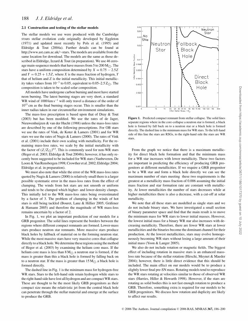
In Fig. 1, we plot an important prediction of our models for aGRB progenitor. The solid lines represent the borders between theregions where different compact remnants are formed. Lower-massstars produce neutron star remnants. More massive stars produceblack holes by fallback of material on to the forming neutron star.While the most massive stars have very massive cores that collapsedirectly to a black hole. We determine these regions using the methodof Heger et al. (2003) by examining the helium core mass. If thehelium core mass is less than 8 M� a neutron star is formed, if themass is greater than this a black hole is formed by falling back onto a neutron star. If the mass is greater than 15 M� a black hole isformed directly.

The dashed line in Fig. 1 is the minimum mass for hydrogen-freeWR stars. Stars to the left-hand side retain hydrogen while stars tothe right-hand side have lost all hydrogen and are compact WR stars.These are thought to be the most likely GRB progenitors as theircompact size means the relativistic jet from the central black holecan penetrate through the stellar material and emerge at the surfaceto produce the GRB.

Figure 1. Predicted compact remnant from stellar collapse. The solid linesseparate regions where in the core-collapse a neutron star is formed, a blackhole is formed by fall back on to a neutron star or a black hole is formeddirectly. The dashed line is the minimum mass for WR stars. To the left-handside of this line the stars are RSGs, to the right-hand side the stars are WRstars.

From the graph we notice that there is a maximum metallic-ity for direct black hole formation and that the minimum massfor a WR star increases with lower metallicity. These two factorsare important in predicting the efficiency of producing GRB pro-genitors at different metallicities. If we require a GRB progenitorto be a WR star and form a black hole directly we can see themaximum number of stars meeting these two requirements is thegreatest at a metallicity mass fraction of 0.006 assuming the initialmass fraction and star formation rate are constant with metallic-ity. At lower metallicities the number of stars decreases while athigher metallicities there is also a decrease, with a cut-off at solarmetallicity.

We note that all these stars are modelled as single stars and wedo not include binary stars. We have investigated a small sectionof binary parameter space and find that the main result is to movethe minimum mass for WR stars to lower initial masses. However,the lowest initial mass for a binary WR star also increases with de-creasing metallicity. Therefore, there are fewer WR stars at lowermetallicities and the binaries become the dominant channel for theirproduction. At the lowest metallicities, stars may evolve homoge-neously becoming WR stars without losing a large amount of theirinitial mass (Yoon & Langer 2005).

We also do not include rotation or magnetic fields. The biggesteffect of including rotation in massive stars is an enhanced mass-loss rate because of the stellar rotation (Hirschi, Meynet & Maeder2004); however, there is little direct evidence that this should beincluded. The main effect on our models would be to produce aslightly lower final pre-SN mass. Rotating models tend to reproducethe WR stars rotating at velocities similar to those of observed WRstars (Harries, Hiller & Howarth 1998). However, if the stars arerotating as solid bodies this is not fast enough rotation to produce aGRB. Therefore, something extra is required for our models to beGRB progenitors. We discuss how rotation and duplicity are likelyto affect our results.


Dow


ic.oup.com/m



2.2 The stellar wind

We have the mass-loss history for all our stellar models. We do nothave the speed of the stellar wind as it is not required to modelthe evolution of a star but it is required to model the circumstellarenvironment. There are few detailed studies of the dependence ofwind velocity on stellar parameters. Fortunately, the study of Nugis& Lamers (2000) concerns the winds of WR stars. Therefore, wecan predict the density structure that surrounds these stars with rea-sonable accuracy.

The first step in estimating stellar wind speeds is to determinethe stellar type. We define two types, WR stars and pre-WR stars.We use the same definitions as for our mass-loss rates. If the surfacehydrogen mass fraction is less than 0.4 and the surface temperatureis greater than 104 K the star is a WR star. Other stars feature alarge hydrogen envelope and are main-sequence stars or red super-giants (RSGs). We refer to these as pre-WR stars.

For pre-WR stars, we first calculate the escape velocity at thestellar surface. It is a reasonable assumption that any material es-caping from the gravitational influence of a star must be related tothis velocity. To account for the reduction of the escape velocity ofluminous stars which are close to the Eddington limit we includethe Eddington factor. Therefore

v2escape = 2G M∗

1 − �

R∗, (1)

where � = L ∗/L Edd = 7.66 × 10−5 σ e (L ∗/M ∗), and σ e = 0.401(X + Y/2 + Y/4) cm2. The escape velocity without the Edding-ton factor was taken directly as the wind velocity in the study byRamirez-Ruiz et al. (2001); this overestimates the wind speed. Fur-thermore, the physical processes that accelerate the stellar wind arecomplex (Kudritzki, Pauldrach & Puls 1987; Vink et al. 2001). Toaccount for this we relate the wind velocity and the escape velocityby using a constant to express the acceleration process uncertainty,

v2wind = βWv2

escape. (2)

For OB stars we use the βW from Vink et al. (2001) and supple-ment this with the values in Hurley, Tout & Pols (2002). We list thevalues used for βW in Table 1. To obtain βW between the rangeslisted we use linear interpolation. The wind speeds calculated arevery uncertain. There is an additional uncertainty in how changingmetallicity affects these wind speeds. Our resultant estimated windspeeds are probably correct to an order of magnitude.

WR stellar wind velocities are calculated with a similar method.We use the empirical formulae of Nugis & Lamers (2000). WRstars have unique atmospheres, their wind is optically thick and notin hydrostatic or local thermodynamic equilibrium. Because of this,models of WR stars predict smaller stellar radii and higher surfacetemperatures in comparison to the observed WR stars. Nugis &Lamers (2000) take this disparity into consideration and provide

Table 1. Value of βW used for pre-WR stars in wind speed calculations.

T eff (K) βW

<3600 0.125

6000 0.5

8000 0.7

10 000 1.3

20 000 1.3

>22 000 2.6

formulae that fit βW to the luminosity and surface composition ofWR stars.

There are two wind velocity formulae, one for WN stars andanother for WC stars. The second letter indicates which element ismost prominent in the WR star spectrum. N indicates nitrogen andC indicates carbon. The progression indicates the gradual exposureof nuclear burning products on the surface of the star. The last inthe sequence are WO stars where oxygen is the most dominantelement in the spectrum. Very few WO stars have been observed,their mass-loss rates agree with those of WC stars; however, theirwind velocities can be much higher than WC stars of equivalentluminosity. We assume WR stars to be WN stars unless all hydrogenhas been removed and (x C + x O)/y > 0.03 when we have a WCstar, where x C, x O and y are the surface number fractions of carbon,oxygen and helium.

The wind velocity of a WN star, as derived by Nugis & Lamers(2000) is

log

(vwind

vescape

)= 0.61 − 0.13 log L∗ + 0.30 log Y , (3)

with a standard deviation of 0.084 dex. For a WC star the windvelocity is given by

log

(vwind

vescape

)= −2.37 + 0.13 log L∗ − 0.07 log Z , (4)

with a standard deviation of 0.13 dex. Using these equations, one canpredict the wind velocity for our WR stars. Although as mentionedabove there is an uncertainty in greater than those listed due toclumping of the WR wind.

In our wind speeds we include a factor of (Z/Z�)0.13 as sug-gested by Vink et al. (2001). In this we are assuming that all stellarwinds are driven by radiative processes on metals. This is true forOB main-sequence stars but the processes that drives WR and RSGmass-loss are unknown even though there are some suggestions(Heger & Langer 1996). For WR stars, it is more uncertain whetherwe should include the scaling of wind velocity by initial metallicity.In radiatively driven winds it is known that the few but strong linesof carbon, nitrogen and oxygen (CNO) elements determine the windspeed while the many but weak lines of iron group elements deter-mine the mass-loss rate (Vink et al. 2001). The CNO abundance inWR stars has little relation to the initial metallicity. However, wedo include the metallicity scaling in calculating our predicted WRwind velocities.

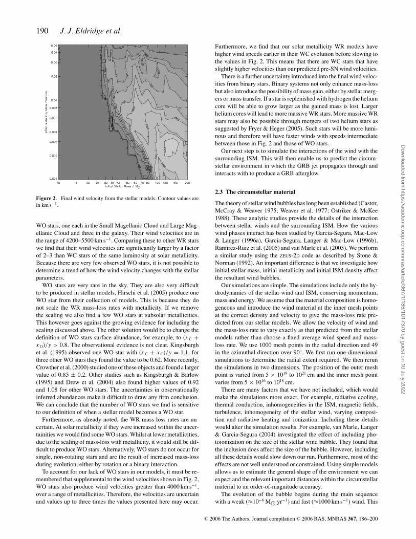
In Fig. 2, we plot the pre-SN wind velocity of our models. Duringthe evolution of the star the wind velocity varies above or belowthe values in the figure. The wind velocities indicated here willdetermine the free-wind region velocity and density. For single stars,we can see that there is a clear division between the RSGs andWR stars with them having slow and fast winds, respectively. Theevolution of pre-SN velocity with metallicity is interesting. WRstars at lower metallicity are more massive for the same initial massdue to reduced mass-loss. This makes the escape velocity largerand therefore from our calculations the wind velocity greater. Asecond contributing factor is that more massive WR stars are moreluminous, this too leads to stronger, faster wind. The wind velocitiesfrom the WN and WC star models, by construction, agree with theobserved wind velocities of WN and WC stars listed in Nugis &Lamers (2000).

It is important to note that our models only produce WN or WCstars. We find no WO stars, if we adopt the normal theorist definitionof (x C + x O)/y > 1 (Smith & Maeder 1991; Dray & Tout 2003).Kingsburgh, Barlow & Storey (1995) present observations of five


Dow


ic.oup.com/m



Figure 2. Final wind velocity from the stellar models. Contour values arein km s−1.

WO stars, one each in the Small Magellanic Cloud and Large Mag-ellanic Cloud and three in the galaxy. Their wind velocities are inthe range of 4200–5500 km s−1. Comparing these to other WR starswe find that their wind velocities are significantly larger by a factorof 2–3 than WC stars of the same luminosity at solar metallicity.Because there are very few observed WO stars, it is not possible todetermine a trend of how the wind velocity changes with the stellarparameters.

WO stars are very rare in the sky. They are also very difficultto be produced in stellar models, Hirschi et al. (2005) produce oneWO star from their collection of models. This is because they donot scale the WR mass-loss rates with metallicity. If we removethe scaling we also find a few WO stars at subsolar metallicities.This however goes against the growing evidence for including thescaling discussed above. The other solution would be to change thedefinition of WO stars surface abundance, for example, to (x C +x O)/y > 0.8. The observational evidence is not clear. Kingsburghet al. (1995) observed one WO star with (x C + x C)/y = 1.1, forthree other WO stars they found the value to be 0.62. More recently,Crowther et al. (2000) studied one of these objects and found a largervalue of 0.85 ± 0.2. Other studies such as Kingsburgh & Barlow(1995) and Drew et al. (2004) also found higher values of 0.92and 1.08 for other WO stars. The uncertainties in observationallyinferred abundances make it difficult to draw any firm conclusion.We can conclude that the number of WO stars we find is sensitiveto our definition of when a stellar model becomes a WO star.

Furthermore, as already noted, the WR mass-loss rates are un-certain. At solar metallicity if they were increased within the uncer-tainities we would find some WO stars. Whilst at lower metallicities,due to the scaling of mass-loss with metallicity, it would still be dif-ficult to produce WO stars. Alternatively, WO stars do not occur forsingle, non-rotating stars and are the result of increased mass-lossduring evolution, either by rotation or a binary interaction.

To account for our lack of WO stars in our models, it must be re-membered that supplemental to the wind velocities shown in Fig. 2,WO stars also produce wind velocities greater than 4000 km s−1,over a range of metallicities. Therefore, the velocities are uncertainand values up to three times the values presented here may occur.

Furthermore, we find that our solar metallicity WR models havehigher wind speeds earlier in their WC evolution before slowing tothe values in Fig. 2. This means that there are WC stars that haveslightly higher velocities than our predicted pre-SN wind velocities.

There is a further uncertainty introduced into the final wind veloc-ities from binary stars. Binary systems not only enhance mass-lossbut also introduce the possibility of mass gain, either by stellar merg-ers or mass transfer. If a star is replenished with hydrogen the heliumcore will be able to grow larger as the gained mass is lost. Largerhelium cores will lead to more massive WR stars. More massive WRstars may also be possible through mergers of two helium stars assuggested by Fryer & Heger (2005). Such stars will be more lumi-nous and therefore will have faster winds with speeds intermediatebetween those in Fig. 2 and those of WO stars.

Our next step is to simulate the interactions of the wind with thesurrounding ISM. This will then enable us to predict the circum-stellar environment in which the GRB jet propagates through andinteracts with to produce a GRB afterglow.

2.3 The circumstellar material

The theory of stellar wind bubbles has long been established (Castor,McCray & Weaver 1975; Weaver et al. 1977; Ostriker & McKee1988). These analytic studies provide the details of the interactionbetween stellar winds and the surrounding ISM. How the variouswind phases interact has been studied by Garcia-Segura, Mac-Low& Langer (1996a), Garcia-Segura, Langer & Mac-Low (1996b),Ramirez-Ruiz et al. (2005) and van Marle et al. (2005). We performa similar study using the ZEUS-2D code as described by Stone &Norman (1992). An important difference is that we investigate howinitial stellar mass, initial metallicity and initial ISM density affectthe resultant wind bubbles.

Our simulations are simple. The simulations include only the hy-drodynamics of the stellar wind and ISM, conserving momentum,mass and energy. We assume that the material composition is homo-geneous and introduce the wind material at the inner mesh pointsat the correct density and velocity to give the mass-loss rate pre-dicted from our stellar models. We allow the velocity of wind andthe mass-loss rate to vary exactly as that predicted from the stellarmodels rather than choose a fixed average wind speed and mass-loss rate. We use 1000 mesh points in the radial direction and 49in the azimuthal direction over 90◦. We first run one-dimensionalsimulations to determine the radial extent required. We then rerunthe simulations in two dimensions. The position of the outer meshpoint is varied from 5 × 1019 to 1021 cm and the inner mesh pointvaries from 5 × 1016 to 1018 cm.

There are many factors that we have not included, which wouldmake the simulations more exact. For example, radiative cooling,thermal conduction, inhomogeneities in the ISM, magnetic fields,turbulence, inhomogeneity of the stellar wind, varying composi-tion and radiative heating and ionization. Including these detailswould alter the simulation results. For example, van Marle, Langer& Garcia-Segura (2004) investigated the effect of including pho-toionization on the size of the stellar wind bubble. They found thatthe inclusion does affect the size of the bubble. However, includingall these details would slow down our run. Furthermore, most of theeffects are not well understood or constrained. Using simple modelsallows us to estimate the general shape of the environment we canexpect and the relevant important distances within the circumstellarmaterial to an order-of-magnitude accuracy.

The evolution of the bubble begins during the main sequencewith a weak (≈10−6 M� yr−1) and fast (≈1000 km s−1) wind. This


Dow


ic.oup.com/m



Figure 3. A representative density profile of stellar wind bubbles. The axesunits are plotted on a logarithmic scale.

creates the bubble in the ISM and is important for the overall sizeof the bubble as this wind endures the longest time. With higherISM densities, the size of this bubble can be very small as the windis not powerful enough to push out against a dense ISM. Almostimmediately after the bubble starts forming, it grows and organizesitself into the structure shown in Fig. 3 with an inner free-windregion separated from a slowly expanding stalled-wind region by ashock; there is then a thin dense shell of swept-up and shocked ISMwith the undisturbed ISM outermost. There is a contact discontinuitybetween the ISM and wind material. The flatness of the stalled-windregion depends on the initial ISM density and the inhomogeneity ofthe wind. We introduce random variation in the wind speed of theorder of 1 per cent over the azimuthal direction as in Garcia-Seguraet al. (1996a). Increasing the magnitude of this factor results in moremixing, instabilities and inhomogeneities in the wind.

After the end of core hydrogen burning most stars expand tobecome a red giant with a strong (>10−4 M� yr−1) and slow(≈100 km s−1) wind. This produces a very dense free-wind region.

Figure 4. The density of the circumstellar environment of a 70-M� star with Z = 0.004. The initial ISM density was n0 = 10 cm−3. The age of the star is3.86 Myr and the nuclear reaction in the core is neon burning. In the lower panel darker colours are less dense, lighter shades are of higher density. In the upperpanel we present cross-sections through this environment. The solid line follows the x-axis, the dotted line along the line x = y and the dashed line the y-axis.

If the mass-loss is not strong enough to remove the hydrogen enve-lope and produce a WR star, the SN occurs in this environment. Themost massive stars (�80 M�) do not experience a red giant phaseand remain blue throughout their evolution. Such stars are referredto as luminous blue variables (LBVs). They have high mass-lossrates and fast winds throughout their lifetime. Such stars producethe largest bubbles as the wind injects more kinetic energy into thebubble.

If the mass-loss is severe enough to remove most of, or all, hydro-gen from the star a further stage of WR star evolution occurs. WRstars have strong (≈10−5 M� yr−1) and fast (≈1000 km s−1) winds.This wind impacts with the slowly moving RSG wind acceleratingit to form a thin a shell travelling at a few hundred kilometres persecond (Garcia-Segura et al. 1996b; van Marle et al. 2005). If n0 �1 cm−3 the free-wind region is cleared of all this red giant material,instabilities in the shell make it mix into the stalled-wind region(Garcia-Segura et al. 1996b). If n0 � 0.1 cm−3, this material doesnot penetrate deep into the stalled-wind and instabilities do not havetime to grow so this shell is well defined at core-collapse.

The exact position and radius separating the ISM, stalled-windand free-wind varies with the initial parameters for the star and theISM. For a given stellar mass, lower initial ISM density results ina larger bubble. More massive stars produce larger bubbles whilelower metallicity stars produce smaller bubbles. Figs 4 and 5 areexamples of our simulation results. In these figures, we use the samestellar model but begin with different initial ISM density. As we cansee, the result roughly follows the simple model in Fig. 3 althoughthe inhomogeneity of the stalled-wind region can be of a few ordersof magnitude. We also find that the initial ISM density affects thestructure of the stalled-wind region. In Fig. 4, the stalled-wind/ISMinterface varies to a larger degree than that in Fig. 5. This is becausewith the higher-density ISM the shell of RSG material swept upby the WR wind can reach the interface. Instabilities in this shellmake it form into loops as it travels (Garcia-Segura et al. 1996b).When it reaches the outer interface these loops produce the variableinterface shown in Fig. 4. With lower ISM density the bubble is muchlarger and the same shell never reaches the outer interface and theinstabilities have not grown to the same level as in the higher-density


Dow


ic.oup.com/m



Figure 5. This figure is the same as Fig. 4 but the initial ISM density was n0 = 0.01 cm−3.

ISM case. This leaves a shell of material moving at a few hundredkilometres per second away from the star. The strength of theseinstabilities may be dependent on azimuthal resolution. If this wasincreased the shell may become unstable and not be as well definedas we find here.

For the GRB afterglow light curve however only the magnitudeof the stalled-wind/free-wind interface is important since once thejet encounters this interface it will slow considerably and will takeyears to reach any of the large-density variations at which pointthe afterglow will be unobservable. However, these shells will haveconsequences for the afterglow spectrum (van Marle et al. 2005),which we discuss below.

We show in Tables 2 and 3 the positions of the important interfacesin our simulations. These are the position of the free-wind/stalled-wind interface in Table 2 and the position of the stalled-wind/ISMinterface in Table 3. We calculate these values by averaging theposition of these boundaries over the azimuthal direction. Lookingat the tables we see how these distances vary with the three initialparameters of initial metallicity, initial mass and initial ISM density.The possible distances for RSW range from 2 × 1018 to 7 × 1020 cm.The value of RISM varies from 1019 to 9 × 1020 cm. These distancesare important when considering the ionization of the region aroundthe GRB progenitor. We will be able to calculate the extent of theregion ionized by the prompt GRB emission and the amount ofmaterial that remains unionized leave an imprint in the afterglowabsorption line spectra.

The most important parameter is the initial ISM density. Stellarparameters produce only slight variation in the bubble size. Thestars that lose the greatest mass produce the larger bubbles as theyinput more energy into the bubble to make it expand further. It isinteresting that the change from small bubbles to a very large free-wind regions occurs over a reasonable range of ISM densities from103 to 10−3 cm−3. The model of Weaver et al. (1977) predicts thatR ISM ∝ n−1/5

0 and that RSW ∝ n−3/100 . When we compare these trends

to those in Tables 2 and 3 by extrapolating from the n0 = 1 cm−3

column we find reasonable agreement. The difference between an-alytic and the numerical values are mostly less than 0.3 dex. Thelargest differences are at the highest or lowest ISM densities.

For RISM the main source of difference from the analytic expres-sion is from taking the average value of RISM. This introduces some

uncertainty into where we define this interface and the effect is thelargest for the smallest bubble sizes. RSW is affected by the use ofnon-constant wind velocities over the evolution of the star. With thebubbles being of different sizes the wind parameters at the interfaceschange with initial ISM density. In the cases where the wind is con-stant in nature during the final stages of evolution the simulationsreproduce the analytic expressions well. However, if the wind ischanging on a time-scale similar to the time it takes for the wind toreach the interface then the assumption made in the analytic modelsbreaks down.

The density jump at the free-wind/stalled-wind interface is be-tween a factor of 4 and ≈8. The lower value of 4 is expected fromthe conditions of an adiabatic shock. Again if the wind velocity ischanging on a time-scale similar to the time for the wind to reachthe interface the size of the jump can be increased by a small factor:an increasing wind speed will lead to a relatively less dense free-wind region and therefore a greater jump. A second reason for thisincrease is that in the shocked wind it is also not made up of materialwith a uniform velocity. Therefore, previously slower material thathas entered the wind can slow faster material entering the shock,again increasing the jump. Most of our models only have a jumpslightly higher than the pure adiabatic prediction (<5). The modelswith larger jumps are few and are confined to the models with higherinitial ISM densities (e.g. Fig. 4).

Most GRB afterglow models assume that the jet traverses eithera constant-density medium or a free-wind medium. There are alsomodels of afterglow light curves in a free-wind region followed by aconstant-density region (Dai & Lu 2002; Dai & Wu 2003; Ramirez-Ruiz et al. 2005). Afterglow calculations should include the stalled-wind region. The environment can be modelled simply with the finalwind parameters from stellar models used for the free-wind region.Then the beginning of stalled-wind region can be determined byassuming a radius for the density jump. The size of the jump isbetween a factor of 4 and ≈8 times the free-wind density at thatpoint. There are large inhomogeneities in the stalled-wind region.However, these tend to be deep in the stalled-wind. The afterglow jetis unlikely to propagate far once it has penetrated the stalled-windregion as it is decelerated by the density jump. Therefore, wheninhomogeneities are encountered the afterglow will no longer beobservable.


Dow


ic.oup.com/m



Table 2. Distance of free-wind/stalled-wind interface. n0 is the initial ISM density in particles cm−3. RSW is the radius of the free-wind/stalled-wind interface in cm.

log (n0) 3 2 1 0 −1 −2 −3Z M/M� A∗ log (RSW) log (RSW) log (RSW) log (RSW) log (RSW) log (RSW) log (RSW)

0.020 200 0.93 18.31 18.88 19.20 19.61 20.05 20.26 20.820.020 150 0.76 18.35 18.86 19.21 19.52 19.91 20.50 20.710.020 120 0.75 18.37 18.85 19.18 19.55 19.94 20.54 20.700.020 100 1.06 18.31 18.81 19.18 19.62 19.86 20.52 20.670.020 80 3.78 18.39 18.91 19.28 19.77 20.21 20.46 20.300.020 70 3.14 18.31 18.83 19.24 19.62 20.25 20.43 20.310.020 60 0.66 18.38 18.78 19.12 19.47 19.80 20.47 20.570.020 50 0.78 18.47 18.74 19.09 19.48 19.75 20.47 20.510.020 40 0.89 18.31 18.73 19.09 19.36 19.86 20.36 20.390.020 30 2.61 18.31 18.77 19.07 19.56 19.70 19.81 19.810.008 200 4.41 18.51 18.94 19.38 19.82 20.25 20.31 20.410.008 150 3.90 18.51 18.90 19.35 19.66 20.28 20.40 20.420.008 120 3.09 18.48 18.89 19.33 19.66 20.22 20.32 20.360.008 100 5.52 18.45 18.85 19.24 19.70 19.98 20.43 20.470.008 80 0.80 18.48 18.80 19.21 19.68 19.98 20.39 20.410.008 70 0.74 18.94 18.79 19.16 19.62 20.01 20.35 20.340.008 60 0.69 18.43 18.79 19.15 19.62 20.14 20.27 20.280.008 50 0.68 18.41 18.76 19.12 19.45 20.04 20.09 20.090.008 40 1.43 18.35 18.83 19.21 19.69 19.82 19.87 19.870.004 200 2.36 18.58 18.95 19.43 19.80 20.18 20.23 20.230.004 150 2.09 18.59 18.98 19.34 19.73 20.14 20.16 20.230.004 120 1.03 18.56 18.86 19.23 19.71 20.10 20.30 20.360.004 100 0.80 18.50 18.86 19.19 19.66 20.17 20.29 20.290.004 80 0.85 18.48 18.85 19.21 19.56 20.10 20.16 20.160.004 70 0.70 18.40 18.80 19.15 19.62 19.91 19.97 19.970.004 60 0.55 18.27 18.76 19.21 19.62 19.78 19.78 19.780.004 50 3.01 18.40 18.81 19.20 19.59 19.81 19.81 19.810.001 200 1.29 18.56 18.93 19.36 19.69 19.70 19.70 19.700.001 150 1.42 18.45 18.85 19.32 19.62 19.72 19.72 19.720.001 120 1.11 18.30 18.86 19.37 19.42 19.42 19.42 19.420.001 100 1.10 18.39 18.85 19.25 19.62 19.75 19.75 19.75

2.4 The free-wind density

The free-wind density is an important parameter that describesthe free-wind environment. A number of authors have modelledafterglow light curves with free-wind profiles for the circumstellarenvironment. These calculations provide an estimate of the densityin the region around the GRB progenitor. The values listed in Ta-ble 4 are taken from Chevalier et al. (2004) and Panaitescu & Kumar(2002). The wind density is defined as

ρ = Ar 2

, (5)

with

A = M4πvwind

, (6)

where M is the mass-loss rate and vwind is the wind speed. How-ever, it is more convenient to use a wind density parameter, A∗,normalized to have a value of 1 for a standard WR wind,

A∗ =(

M10−5 M� yr−1

)(1000 km s−1

vwind

). (7)

We show in Fig. 6 the A∗ values derived from our models overinitial mass and metallicity. In the figure, it is clear that for WRstars the A∗ value is relatively flat. For most WR stars A∗ ≈ 0.6–0.8, the lowest value we find here is 0.55. There is a ridge in initialmass/metallicity space of WR stars with higher A∗ values up to 3.

This region separates lower-mass stars that have an RSG phase fromthe more massive stars that move straight from the main sequence toWR evolution undergoing an LBV phase. Therefore our full rangebecomes 0.55 � A∗ � 3. Taking into consideration the uncertaintyin the mass-loss rate and wind velocity equations given by Nugis& Lamers (2000) the lowest A∗ value possible is 0.3. The valuesagree with the range of A∗ values from the WR stars in Nugis &Lamers (2000) which for WN and WC stars have a range from0.3 to 7.

This range of predicted A∗ values are of the same order, �1, asthe higher inferred values in Table 4. We do not find winds withA∗ similar in order to the very lowest values, �0.1, required forthe first three GRBs listed in the table. The GRBs with the lowerdensities in the table were first thought to be better modelled by auniform constant-density environment. The low-density wind solu-tions provide an equally good fit (Chevalier et al. 2004). There areseveral possibilities on how to obtain a lower A∗ for the circumstellarenvironment.

First, the values we present are uncertain, the WC mass-lossrates can vary by 0.15 dex and the WC wind velocities can varyby 0.13 dex. As already mentioned, the problem of clumping in thewinds of hot stars is still being tackled and the uncertainties may belarger (Bouret et al. 2005; Grafener & Hamann 2005). We estimatethat the A∗ values are perhaps uncertain by as much as a factor of 2due to the mass-loss rate uncertainty.

We have so far ignored our exclusion of WO stars. The two WOstars in Nugis & Lamers (2000) have A∗ values of 0.07 and 0.27


Dow


ic.oup.com/m



Table 3. Distance of stalled-wind to SW interface. n0 is the initial ISM density in particles cm−3. RISM is the radius of the stalled-wind/ISMinterface in cm.

log(n0) 3 2 1 0 −1 −2 −3Z M/M� A∗ log(R ISM) log(R ISM) log(R ISM) log(R ISM) log(R ISM) log(R ISM) log(R ISM)

0.020 200 0.93 19.42 19.78 20.05 20.32 20.54 20.68 20.940.020 150 0.76 19.32 19.75 20.02 20.29 20.52 20.74 20.910.020 120 0.75 19.26 19.69 19.99 20.27 20.50 20.72 20.880.020 100 1.06 19.31 19.58 19.96 20.24 20.48 20.70 20.890.020 80 3.78 19.19 19.62 19.90 20.19 20.44 20.66 20.870.020 70 3.14 19.18 19.59 19.87 20.17 20.43 20.65 20.860.020 60 0.66 19.23 19.57 19.87 20.16 20.36 20.64 20.840.020 50 0.78 17.76 19.51 19.82 20.12 20.31 20.62 20.830.020 40 0.89 19.02 19.35 19.75 20.05 20.33 20.57 20.790.020 30 2.61 18.89 19.20 19.39 19.89 20.21 20.50 20.750.008 200 4.41 19.34 19.69 19.99 20.25 20.48 20.68 20.870.008 150 3.90 19.35 19.65 19.95 20.19 20.45 20.65 20.850.008 120 3.09 19.30 19.60 19.91 20.19 20.42 20.64 20.820.008 100 5.52 19.28 19.63 19.91 20.18 20.40 20.62 20.830.008 80 0.80 19.23 19.55 19.87 20.15 20.39 20.61 20.810.008 70 0.74 19.18 19.51 19.84 20.12 20.38 20.59 20.800.008 60 0.69 18.79 19.49 19.80 20.08 20.35 20.57 20.790.008 50 0.68 18.96 19.27 19.72 20.02 20.29 20.54 20.770.008 40 1.43 18.90 19.19 19.63 19.93 20.23 20.50 20.740.004 200 2.36 19.36 19.65 19.94 20.21 20.43 20.64 20.850.004 150 2.09 19.26 19.60 19.89 20.14 20.38 20.61 20.810.004 120 1.03 19.25 19.54 19.86 20.14 20.37 20.58 20.790.004 100 0.80 19.23 19.54 19.84 20.11 20.35 20.56 20.780.004 80 0.85 19.15 19.45 19.79 20.03 20.31 20.55 20.760.004 70 0.70 19.14 19.42 19.73 20.03 20.29 20.53 20.750.004 60 0.55 18.94 19.25 19.66 19.97 20.27 20.52 20.740.004 50 3.01 18.82 19.15 19.56 19.92 20.23 20.49 20.720.001 200 1.29 19.19 19.51 19.81 20.08 20.34 20.56 20.780.001 150 1.42 19.13 19.40 19.71 19.99 20.25 20.48 20.690.001 120 1.11 18.84 19.20 19.62 19.94 20.21 20.45 20.660.001 100 1.10 18.99 19.25 19.64 19.92 20.19 20.43 20.65

Table 4. Value of A∗ for vari-ous GRBs, adapted from Chevalieret al. (2004) and Panaitescu & Kumar(2002).

GRB A∗

011121 0.02020405 <0.07021211 ∼0.015

970508 0.3, 0.39991208 0.4, 0.65991216 ∼1

000301C 0.45000418 0.69021004 0.6

which are lower than the values for WN and WC stars. This is be-cause WO stars have higher wind velocities than WC stars. There-fore if any of our WC models are in fact WO stars, either becauseour classification is wrong or they experience greater mass-loss dueto rotation of binarity, then they would have a low-density wind.With only a small sample of WO stars we do not know how low theA∗ value can be for these stars. The WO star values are much closerto the lower values in Table 4. It could be that the wind densitiesin these cases could be explained by a WO progenitor rather than aWC progenitor.

Figure 6. Final A∗ value for our models including the scaling of WR windvelocities with initial metallicity. Contour values show the value of A∗ andthe tick marks indicate the downhill direction.


Dow


ic.oup.com/m



Then we can consider processes that might affect the dynamicsof the circumstellar environment. The effect of rotation has beenstudied by Langer, Garcia-Seguar & Mac Low (1999) and Petrenz& Puls (2000). The studies tend to indicate that the density along thestellar rotation axis, where the jet is thought to propagate, will remainconstant or increase. This does not help our search for a low-densitywind. We have ourselves tested the effect on the wind structure ifthe progenitor is in a binary. The effect of binarity is discussed byRamirez-Ruiz et al. (2005). They conclude that the circumstellarmedium will not be significantly altered in most cases. The onecase that the medium may be altered will be in binaries when themasses of the two stars are close and therefore the stellar winds areof comparable strength. The outcome will be sensitive to the initialparameters of the binary and is worth investigating in the future.

Another possibility is that the low A∗ values are very similarto those produced by blue supergiants (BSGs). We know that it ispossible for evolved BSGs to explode in an SN. The stellar progen-itor of SN1987A was a BSG. It is thought that the star underwenta merger event with a binary companion that led to a single BSG(Podsiadlowski 1992). BSGs have similar wind velocities to WRstars but their mass-loss rates are usually 10–100 times lower. There-fore the typical A∗ values range from 0.1 to 0.01, agreeing with thelower values in Table 4. However, Woosley (1993) and Matzner(2003) rule out such progenitors due to the stars having too large aradius.

A final possibility is that the GRB progenitor is of very low initialmetallicity that we do not model here (Z/Z� < 1/20). Such starswill only become WR stars in binary systems due to their feeblestellar winds (Kudritzki 2002). Although, recent models by Yoon &Langer (2005) suggest that the stars might undergo homogeneousevolution during hydrogen burning.

3 M O D E L L I N G T H E G R B A F T E R G L OW

L I G H T C U RV E

After the prompt emission of gamma-rays in the GRB itself, the rel-ativistic jet continues its motion and is decelerated by the materialaround the progenitor causing a shock that transfers energy from thejet to radiation that is emitted. This is the GRB afterglow. The emis-sion slowly decays with time usually as a smooth power law. Thereare some cases however where the afterglow is far from smooth andin some cases rebrightens considerably before continuing to decay.In this section, we will not attempt to fit model light curves to ob-served GRB afterglows but will instead show the relative effects ofvarying the circumstellar environment density profile.

In our calculations we assume that the initial kinetic energy inthe relativistic jet has an isotropic equivalent value, E iso = 1053 erg.This corresponds to a true energy, E = (1 − cos θ )E iso = 4 × 1050–3 × 1051 erg, for jet opening angles in the range 5–15◦, in agreementwith observations (Frail et al. 2001; Panaitescu & Kumar 2001).

We follow the dynamical evolution of the relativistic jet usingthe simple formalism for energy and momentum conservation de-rived by Paczynski & Rhoads (1993). The calculation is stoppedjust before the jet enters the non-relativistic regime (in practice atv = 0.75c). Once the evolution of the Lorentz factor is known, thesynchrotron emission of the jet is computed following Sari, Piran& Narayan (1998). It is assumed that a fraction, εB of the internalenergy in the post-shock region is transferred into the magnetic fieldand that a fraction, ε e, is injected into a population of non-thermalrelativistic electrons, with a power-law distribution of slope, p. Wehave adopted, εB = 10−3, ε e = 0.1 and p = 2.5, which are typicalvalues found in afterglow fits. Finally, the effect of the opening angle

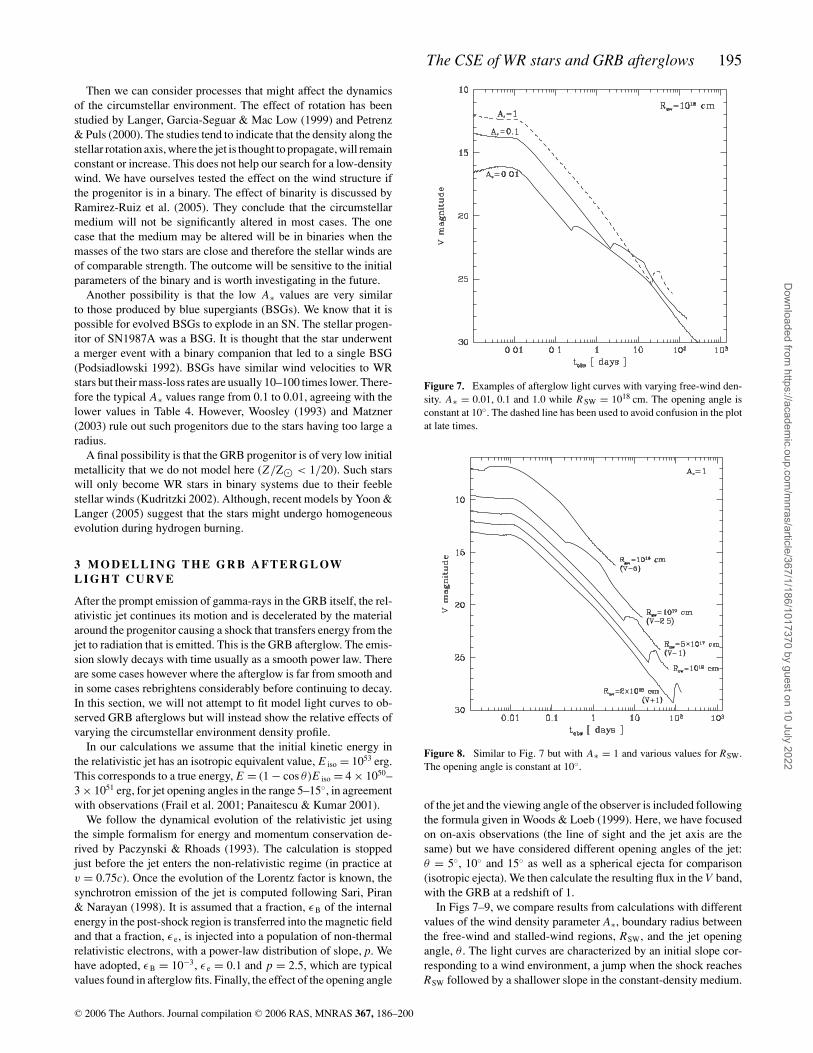
Figure 7. Examples of afterglow light curves with varying free-wind den-sity. A∗ = 0.01, 0.1 and 1.0 while RSW = 1018 cm. The opening angle isconstant at 10◦. The dashed line has been used to avoid confusion in the plotat late times.

Figure 8. Similar to Fig. 7 but with A∗ = 1 and various values for RSW.The opening angle is constant at 10◦.

of the jet and the viewing angle of the observer is included followingthe formula given in Woods & Loeb (1999). Here, we have focusedon on-axis observations (the line of sight and the jet axis are thesame) but we have considered different opening angles of the jet:θ = 5◦, 10◦ and 15◦ as well as a spherical ejecta for comparison(isotropic ejecta). We then calculate the resulting flux in the V band,with the GRB at a redshift of 1.

In Figs 7–9, we compare results from calculations with differentvalues of the wind density parameter A∗, boundary radius betweenthe free-wind and stalled-wind regions, RSW, and the jet openingangle, θ . The light curves are characterized by an initial slope cor-responding to a wind environment, a jump when the shock reachesRSW followed by a shallower slope in the constant-density medium.


Dow


ic.oup.com/m



Figure 9. Similar to Fig. 7 but with A∗ = 0.1 and RSW = 1018 cm. Wevary the opening angle.

For some of the light curves the break expected when 1/� = θ isobserved after the jump.

Fig. 7 demonstrates the effect of varying A∗ while keeping RSW

constant at 1018 cm. A denser wind has a more intense afterglow andis decelerated more quickly. Therefore, the jet takes a longer time toreach the density jump at the free-wind/stalled-wind interface. Theslight bump in the light curves occurs when the jet encounters thisinterface. In the case when A∗ = 1 the bump is observed the latestas the dense wind decelerates the jet rapidly. For a very dense wind(A∗ ≈ 10) the jet can be decelerated very quickly so that the reverseshock is efficient during the GRB. This may affect the prompt GRBemission if the emission mechanisms are internal shocks in the jet.

In Fig. 8, we show the differences introduced by moving theposition of the interface in our density profiles. For the smallestdistances the effect of the jump is hidden in the general shape ofthe light curve with only pronounced bumps at later times. Thisfigure also demonstrates that the different slopes of the light curvesoccur when the jet propagates through a constant-density or free-wind medium. Importantly when A∗ and RSW are set to the valuesin Table 2 we find that the rebrightening would occur after 10 d inmost cases. At this time the afterglow is already dim and such effectsmay be difficult to observe.

Finally, Fig. 9 shows the effect of altering the opening angle. Thepossible afterglow light curves are interesting. All follow the samepattern and all have substantial brightening a few days after the GRBdue to the jet encountering the free-wind/stalled-wind interface. Thegreatest effect on the light curve comes from the break as the jet isdecelerated and 1/� drops below the opening angle of the jet.

The most important value to fit with any calculations is the initialvalue of A∗. This will provide a solid constraint on the progenitoras it is directly related to the final mass-loss of the massive star.The position of the jump can be found from rebrightening in theafterglow but is of limited use because it is affected not only by thedetails of the progenitor but also by the initial density of the ISMand the uncertainty in the wind velocity of pre-WR stars. Althoughin the cases where the afterglow is better described by a constant-density medium this can be explained by RSW being smaller thanaround 1016 cm, so any signature of the wind profile will be in thevery early afterglow light curve.

4 A B S O R P T I O N L I N E S I N G R B A F T E R G L OW

S P E C T R A

The first GRB afterglow was observed for GRB970228 (van Paradijset al. 1997). The wait for a redshift from a GRB afterglow wasshort, one was discovered for the second observed afterglow ofGRB970508 (Metzger et al. 1997). From a spectrum the redshift ofa GRB can be determined from lines intrinsic to the host galaxy orabsorption lines within the host galaxy. In some cases there are extraabsorption lines that have a small difference to the redshift of thehost galaxy and the GRB. The inferred velocities of this materialare a few hundred and a few thousand kilometres per second. Upondiscovering these lines it has been suggested that they might becaused by absorption by the GRB progenitors stellar wind material(Holland et al. 2003; Mirabal et al. 2003; Schaefer et al. 2003;Starling et al. 2005). Although there are alternative explanationssuch as structures related to the host galaxy rather than the GRBprogenitor.

With our stellar models and simulated circumstellar environmentwe have information on the velocity profiles we can expect from thestellar wind. The predicted velocities for the free-wind region domatch well with the velocities of the absorption lines at the highestvelocity offset. In the stalled-wind region, we also predict velocitiesof a similar magnitude but we find that the exact figure depends quitesensitively on the initial ISM density and the wind velocities duringthe main-sequence and RSG phases of evolution. This agreementindicates that stellar wind material could be responsible for theseabsorption lines.

The first main question is whether the ions observed are presentin the pre-GRB wind. We verified this by modelling the environ-ment using the program CLOUDY V96.01 (Ferland 2003). We useda blackbody spectrum for the WR star emission at effective tem-perature and luminosity of WR stars. We found that the observedspecies are present in the free-wind region.

The second, and more important, question is whether the GRBcompletely ionizes the immediate environment as discussed byLazzati et al. (2002) and Starling et al. (2005). Therefore only fullyionized species will be present which cannot produce absorptionlines. In Lazzati et al. (2002), the comment is justified by calcu-lating the recombination time-scale of the material and finding thatit was much longer than the time the afterglow is observed for.While in Starling et al. (2005), they estimate this in terms whetherthere is enough energy at a certain radius to completely ionize thematerial.

We also investigate if the initial emission would be able to com-pletely ionize the surrounding medium. We start by considering theionization cross-section, σ (E), where E is the energy of the incidentphoton. We approximate the cross-sectional energy dependence as

σ (E) ≈ σi

(EEi

)−3

, (8)

where E i is the minimum energy required to ionize the species inquestion. Our next step is to estimate the number of ionizations peratom or ion at a distance R from the GRB,

ni(R) = 1

4πR2

∫ ∞

Ei

σ (E)N (E) dE, (9)

where N(E) describes the spectrum of the GRB such that N (E) dEis the number of photons produced by the source between E andE + dE . We also define Rmax such that n i(Rmax) = 1 gives themaximum distance where the atom or ion can be ionized. Before


Dow


ic.oup.com/m



we evaluate this in integral we must determine the GRB spectrum.We approximate the GRB spectrum to be

N (E) = ζ

(EEp

)α

= ζ

(EEp

)−1

E < Ep (10)

= ζ

(EEp

)−2.5

E > Ep, (11)

where Ep is the peak energy of the burst spectrum. ζ is a constantfound by normalizing with the isotropic radiated energy of the burst,ζ = E iso/(2E2

p). With these assembled formulae we evaluate equa-tion (9). The result is

ni(R) = σi Eiso

24EpπR2. (12)

We take the ion C(IV) as our example as this has been observedin some GRB afterglow spectra. We use the burst parameters fromGRB021004 which we discuss later. Therefore we have σ i = 0.66× 10−19 cm2, E iso = 2 × 1052 erg, E i = 46 eV and the rest-frame E p

= 200 keV. Using these values we find Rmax = 2.3 × 1019 cm. Fromthis we can assume that nearly all C(IV) in the free-wind materialare ionized, this argument despite being very simplistic means thatabsorption lines in the afterglow spectra are probably from materialnot associated with the GRB progenitor. But we only look at onespecies of one element, the combination of all elements present mayincrease the absorbing power of the circumstellar material. We canalso find that some of the free-wind regions in our simulations arelarger than this size if we start with a low ISM density. At initialISM densities of n0 � 1 cm−3, the RSW is greater than this ionizationradius so it is possible for some material to remain unionized andproduce absorption lines in the afterglow spectra. Comparing to theionization radii calculated in Starling et al. (2005) we can make asimilar conclusion.

There are also other details to consider. Starling et al. (2005)suggested that the jet may be structured. The jet may be formedfrom a central hyper-relativistic core surrounded by less relativisticmaterial that gives rise to the afterglow. There is a similar alternativeexplanation that uses the temporal structure to the jet. Initially the jetwill be tightly confined as its emission by the large beaming factordue to the relativistic motion. This means all the ionizing flux will betightly beamed through only a small fraction of material directly onits path. However, after the initial burst and as the fireball propagatesit will spread out. Therefore while the material down the centre ofthe jet will be ionized the material at the edge of the jet will not be.This becomes more true the larger the angle between the jet axisand the line of sight.

We conclude that the lines we see could come from the wind of theGRB progenitor in some cases. Only observations of more GRB af-terglow spectra will indicate if this is a general trend. We also predictthat there will be an evolution of the observed spectra with time. Forexample, eventually the jet will reach beyond the free-wind, at thatpoint the higher-velocity absorption lines should disappear from thespectra. If they were to remain then they must be external in origin.Although it is very improbable the afterglow will remain luminousenough at late times to allow detailed spectroscopy.

5 C O M PA R I N G TO O B S E RV E D G R B S

While there are a large number of observed GRBs and a good frac-tion with observed afterglows there are relatively few with observed

absorption line spectra. Below, we discuss three GRBs that haveobserved afterglows and compare them with our predicted circum-stellar environments.

5.1 GRB021004

The position of this burst was localized within a few minutes byHETE-2. This meant that detailed optical afterglow observationswere taken. Many different groups took spectra of the afterglow(Holland et al. 2003; Mirabal et al. 2003; Schaefer et al. 2003;Starling et al. 2005).

Starling et al. (2005) found that there were absorption lines forC(IV), Si(IV) and hydrogen, blueshifted with respect to the hostgalaxy with velocities of around 3000 and 500 km s−1. Their inter-pretation was that these lines were caused by material in the stellarwind of the GRB progenitor.

Possible resolutions of the ionization problem were discussedabove. However, the presence of hydrogen should not be possibleif the progenitor star was a WR star. Starling et al. (2005) sug-gested that the WR star was in a binary with a main-sequence Ostar companion. The O star wind would mix hydrogen into the WRwind. Both stars have similar wind velocities and the majority ofthe material in the resultant wind would still originate from the WRstar.

If we assume that the absorption lines are from material in thestellar wind we can ask, ‘what does the afterglow and absorptionlines tell us about the progenitor itself?’ Chevalier et al. (2004)estimate an A∗ value of 0.6 for this GRB. In Fig. 10, we plot theregion where A∗ = 0.6 in initial mass and metallicity space. In thesame plot we include contours of the free-wind speed determinedfrom the absorption lines of vwind = 3000 km s−1. These contoursdo not overlap. However, the mass-loss rates and the wind velocitiesare uncertain. In Fig. 11, we increase all predicted wind velocities by0.13 dex, the quoted uncertainty in the wind velocity equations, anoverlap now occurs. The inferred free-wind density and wind speedthen agrees with the predicted details of a low-metallicity WC star.It must be noted that we are only able to achieve an agreement withthe observations by exploiting that the winds are uncertain. Until

Figure 10. The solid line show where vwind = 3000 km s−1. The dashedline shows where A∗ = 0.6.


Dow


ic.oup.com/m



Figure 11. Same as Fig. 10 but the wind velocity from our models has beenincreased by 0.13 dex, the uncertainty of the predicted wind velocities. Thesolid line show where vwind = 3000 km s−1. The dashed line indicated theregion where A∗ = 0.6.

the uncertainties in WR stars and their winds are greatly reducedwe cannot make an identification in this way.

An alternative explanation is that the progenitor may be a WOstar. This is possible as while WO stars tend to have higher windvelocities and a lower free-wind density, the progenitor could havebeen a transition object with faster wind speeds than those predictedthat our solar metallicity WC stars. Although there are very few ob-served WO stars so we do not fully understand the possible windspeeds. Furthermore, we have not considered the uncertainty in theWR mass-loss rates. Altering the magnitude of the WR mass-lossrates will affect our models and change the masses, surface compo-sition and luminosity of our models and therefore change the finalvelocities and mass-loss rates. Combining all the possible uncertain-ties, it is not possible to make any conclusions about the progenitorof GRB021004 other than that its observed details agree with a widerange of WR models.

The low-velocity lines provide extra information on the windstructure around the progenitor. van Marle et al. (2005) discuss howthe lines are likely to be caused by the shell formed when the slowerRSG wind material is swept up and accelerated by the faster WRwind. We find that this occurs in all our simulations where the starsgo through an RSG phase. For initial ISM densities, n0 � 1 cm3,this shell reaches the stalled-wind region, decelerates and mixesinto the stalled-wind. At low initial densities (n0 � 0.1 cm3), wefind that the shell does not reach the stalled-wind region and re-mains in the free-wind region. The velocity is typically a few hun-dred kilometres per second, for a number of our WR stars the shellis close to the observed 500 km s−1. Therefore, the lower-velocitylines may give a qualitative indication of the initial ISM density.Although the structure of the low-velocity lines is complex andmade up of many different single lines over a range of a few hun-dred kilometres per second. Therefore no simple interpretation ispossible.

In summary, the progenitor may have been a WR star at anymetallicity. However, such stars above solar metallicity will lose toomuch mass to form a black hole directly at core-collapse, thereforesubsolar stars are favoured (Fig. 1).

5.2 GRB020813, GRB030226 and other bursts

There are two more GRBs with absorption lines slightly offset fromthe host galaxy redshift. For GRB020813, the inferred wind velocitywas 4320 km s−1 with an A∗ ≈0.01 (Barth et al. 2003). For this GRB,the case of a WO star is slightly stronger as the wind velocity andwind density agree with the typical values for observed WO stars.

For GRB030226 the velocity was 2300 km s−1 (Chornock &Filippenko 2003; Greiner et al. 2003; Price et al. 2003). There anA∗ has not been estimated. However, the wind velocity is too lowfor a WO star and is more in agreement with the wind speed of aWC star.

6 D I S C U S S I O N

The study of GRBs and their afterglows is a rapidly expanding field;it is not only of interest to those who wish to understand GRBs butalso those who wish to use GRBs as tools to solve other problems,such as investigating star formation history or the Lyman α forest.In this paper, we have both described the circumstellar environmentof possible GRB progenitors and discussed the effect of such anenvironment on the GRB afterglow.

The details of the progenitor that affects a GRB afterglow are thefinal wind velocity and mass-loss rate, these together determine theA∗ value of the free-wind region around the star. This value affectsthe slope of the afterglow light curve. For some environments theafterglow jet might encounter the density jump at the interface be-tween the free and stalled-wind while it remains observable (Dai &Lu 2002; Dai & Wu 2003; Ramirez-Ruiz et al. 2005). This densityjump is between a factor of 4 and ≈8. It is easy to use a sim-ple model density profiles of the free-wind region connected to astalled-wind region. The circumstellar environment in current after-glow calculations only considers the free-wind profiles and ignorethe stalled-wind region even though it has been known to exist forsometime (Castor et al. 1975). The environment can be described byA∗, RSW and �ρ jump. From varying these three numbers it shouldbe possible to reproduce afterglow light curves, using the values ofA∗ and RSW from our stellar models as listed in Table 2, with 4 ��ρ jump � 8.

A∗ have been inferred from observations of GRB afterglow lightcurves. The higher values (A∗ � 0.5) are similar to those from stellarevolution models of WC stars. Furthermore, using the inferred free-wind velocity from GRB afterglows we have demonstrated how itmay be possible to estimate the range of possible initial parametersfor the progenitor. No firm conclusions can be drawn as the uncer-tainty in WR wind velocities and mass-loss rates are considerable.As our understanding of these objects grows it may become possibleto use the method presented here to limit the parameter space of theprogenitor. One important question that must be answered is howthe mass-loss rate and wind velocity scales with initial metallicity.For radiatively driven winds it is known that separate elements areresponsible for determining the mass-loss rate and wind velocity.The many but weak lines of the iron group elements determine themass-loss rate while the few but strong lines of the CNO elementsdetermine the wind velocity (Vink et al. 2001). The iron group el-ements are not depleted on the surface over the lifetime of a starbut the CNO elements become enhanced as time passes. For WRstars the CNO abundance is substantially different from the initialmetallicity. The dependence on initial metallicity may therefore bevery weak.

Of further interest will be the effect of rotation and/or a binarycompanion on the progenitor star and the circumstellar environment.


Dow


ic.oup.com/m



Rotating models of GRB progenitors do retain enough angular mo-mentum to form an accretion disc around the forming black hole toproduce a GRB (Hirschi et al. 2005). Magnetic fields remove thispossibility (Petrovic et al. 2005). But binary stars can spin up a starby mass-transfer events and therefore they may be the more likelyprogenitors (Izzard et al. 2004; Petrovic et al. 2005).

The circumstellar environment is the next step to consider,it is not clear how rotation will change the details of the cir-cumstellar free-wind region (Langer et al. 1999; Petrenz & Puls2000). Ramirez-Ruiz et al. (2005) present a simulation of the cir-cumstellar environment for a rotating single star. They find thatboth the free-wind density and RSW are strongly dependent onlatitude.

A similar effect can be expected for binary stars as interactionscan spin up the stars to rotate more rapidly than might be expectedfor single stars. For binary stars, because of the many possible evo-lutionary paths, there are a number of other possible effects on theenvironment. For a wide binary interaction may shorten or removethe RSG phase by enhancing mass-loss and therefore there will onlybe a brief phase when the wind speed drops below 1000 km s−1. Forcloser binaries, common-envelope evolution may occur leading toa tight WR/O star binary where the mass-loss rate of the WR starmay be enhanced by the companion leading to larger numbers ofWO stars. The most important binary cases will be those wherethe stellar wind of the secondary is of similar strength to the WRstars when the wind density may be affected (Ramirez-Ruiz et al.2005).

7 C O N C L U S I O N

(i) Our predicted value of A∗ for single WC stars span a smallrange, 0.55 � A∗ � 3. Due to the uncertainty in WC star winds thelower value may be as low as 0.3.

(ii) All our WR models end as WC stars and we have no WO stars.WO stars have higher wind velocities than WC stars and thereforemay give rise to the lower A∗ than that we predict from our models.

(iii) The typical observed free-wind velocities inferred fromabsorption line spectra of GRB afterglows agree with predic-tions of pre-SN WR wind speeds from single non-rotatingstars.

(iv) It is possible for the free-wind region to become extremelylarge, in some cases larger than the ionization radius from the promptGRB emission. Therefore it is possible for the wind material toremain unionized and be observed in the afterglow absorption linespectrum if the initial ISM density is n0 � 1 cm−3.

(v) Rapid changes in the wind velocity during the evolution ofstars can produce small deviations in the expected dimensions ofthe circumstellar environment from analytic models.

(vi) We indicate that from limits on the value of A∗ and the finalwind speed from the GRB progenitor it may in future be possibleto estimate the initial parameters of GRB progenitors. Currently,the uncertainties in WR mass-loss are too great to draw any suchconclusions.

AC K N OW L E D G M E N T S

JJE would like to thank Chris Tout, Pierre Lesaffre and RichardAlexander for fluid conversations and Jorick Vink for windy con-versations. We would also like to thank the referees Norbert Langerand Allard-Jan van Marle for their many useful questions that led

to a greatly improved article. We also wish to thank Mike Barlowfor some details of WO stars.

R E F E R E N C E S

Barth A. J. et al., 2003, ApJ, 584, 47Bloom et al., 2005, AAS, 206, 4704Bouret J.-C., Lanz T., Hillier D. J., 2005, A&A, 438, 301Castor J., McCray R., Weaver R., 1975, ApJ, 200, 107Chevalier R. A., Li Z-Y., Fransson C., 2004, ApJ, 606, 369Chornock R., Filippenko A. V., 2003, GCN, 1897, 1Crowther P. A. et al., 2000, ApJ, 538, L51Crowther P. A., Dessart L., Hillier D. J., Abbott J. B., Fullerton A. W., 2002,

A&A, 392, 653Dai Z. G., Lu T., 2002, ApJ, 565L, 87DDai Z. G., Wu X. F., 2003, ApJ, 591, 21de Jager C., Nieuwenhuijzen H., van der Hucht K. A., 1998, A&ASS, 72,

259Dray L. M., Tout C. A., 2003, MNRAS, 341, 299Drew J. E., Barlow M. J., Unruh Y. C., Parker Q. A., Wesson R., Pierce M.

J., Masheder M. R. W., Phillipps S., 2004, MNRAS, 351, 206Eggleton P. P., 1971, MNRAS, 151, 351Eldridge J. J., 2004, PhD dissertation, Univ. Cambridge, preprint (astro-

ph/0502046)Eldridge J. J., Tout C. A., 2004a, MNRAS, 348, 201Eldridge J. J., Tout C. A., 2004b, MNRAS, 353, 87Ferland G. J., 2003, ARA&A, 41, 517Frail D. A. et al., 2001, ApJ, 562, 55Fryer C. L., Heger A., 2005, ApJ, 623, 302Garcia-Segura G., Mac Low M.-M., Langer N., 1996a, A&A, 305, 229Garcia-Segura G., Langer N., Mac Low M.-M., 1996b, A&A, 316, 133Grafener G., Hamann W.-R., 2005, A&A, 432, 633Greiner J., Guenther E., Klose S., Schwarz R., 2003, GCN, 1886, 1Harries T. J., Hiller D. J., Howarth I. D., 1998, MNRAS, 296, 1072Heger A., Langer N., 1996, A&A, 315, 421Heger A., Fryer C. L., Woosley S. E., Langer N., Hartmann D. H., 2003,

ApJ, 591, 288Hirschi R., Meynet G., Maeder A., 2004, A&A, 425, 649Hirschi R., Meynet G., Maeder A., 2005, A&A, 443, 581Hjorth J. et al., 2003, Nat, 423, 847Holland S. T. et al., 2003, AJ, 125, 2291Hurley J. R., Tout C. A., Pols O. R., 2002, MNRAS, 329, 897Izzard R. G., Ramirez-Ruiz E., Tout C. A., 2004, MNRAS, 348, 1215Kingburgh R. L., Barlow M. J., 1995, A&A, 295, 171Kingsburgh R. L., Barlow M. J., Storey P. J., 1995, A&A, 295, 75Kudritzki R. P., 2002, ApJ, 577, 389Kudritzki R. P., Pauldrach A., Puls J., 1987, A&A, 173, 293Langer N., Garcia-Segura G., Mac Low M.-M., 1999, ApJ, 520, 49Lazzati D., Rossi E., Covino S., Ghisellini G., Malesani D., 2002, A&A,

396, 5MacFadyen A. I., Woosley S. E., 1999, ApJ, 524, 262MacFadyen A. I., Woosley S. E., Heger A., 2001, ApJ, 550, 410Matzner C. D., 2003, MNRAS, 345, 575Metzger M. R., Djorgovski S. G., Kulkarni S. R., Steidel C. C., Adelberger

K. L., Frail D. A., Costa E., Frontera F., 1997, Nat, 387, 878Mirabal N. et al., 2003, ApJ, 595, 935Nugis T., Lamers H. J. G. L. M., 2000, A&A, 360, 227Ostriker J. P., McKee C. F., 1988, Rev. Mod. Phys., 60, 1OPaczynski B., Rhoads J. E., 1993, ApJ, 418, 5Panaitescu A., Kumar P., 2001, ApJ, 560, 49Panaitescu A., Kumar P., 2002, ApJ, 571, 779Petrenz P., Puls J., 2000, A&A, 358, 956Petrovic J., Langer N., Yoon S.-C., Heger A., 2005, A&A, 435, 247Podsiadlowski P., 1992, PASP, 104, 717Pols O. R., Tout C. A., Eggleton P. P., Han Z., 1995, MNRAS, 274, 964Price P. A., Fox D. W., Djorgovski S. G., West M., Cote P., Jordan A., Castro

A. J., 2003, GCN, 1889, 1


Dow


ic.oup.com/m



Ramirez-Ruiz E., Dray L. M., Madau P., Tout C. A., 2001, MNRAS, 327,829

Ramirez-Ruiz E., Garcia-Segura G., Salmonson J. D., Perez-Rendon B.,2005, ApJ, 631, 435R

Sari R., Piran T., Narayan R., 1998, ApJ, 497, 17Schaefer B. E. et al., 2003, ApJ, 588, 387Smith L. F., Maeder A., 1991, A&A, 241, 77SStanek K. Z. et al., 2003, ApJ, 591, 17Starling R. L. C., Wijers R. A. M. J., Hughes M. A., Tanvir N. R., Vreeswijk

P. M., Rol E., Salamanca I., 2005, MNRAS, 360, 305Stone J. M., Norman M. L., 1992, ApJS, 80, 753van der Hucht K. A., 2001, New Astron. Rev., 45, 135van Marle A. J., Langer N., Garcia-Segura G., 2004, Rev. Mex. Astron.

Astrofısica, 22, 136

van Marle A.-J., Langer N., Garcia-Segura G., 2005, A&A, 444, 837van Paradijs J. et al., 1997, Nat, 386, 686van Putten M. H. P. M., 2004, ApJ, 611, L81Vanbeveren D., De Loore C., Van Rensbergen W., 1998, A&AR, 9, 63VVink J. S., de Koter A., Lamers H. J. G. L. M., 2001, A&A, 369, 574Weaver R., McCray R., Castor J., Shapiro P., Moore R., 1977, ApJ, 218, 377Woods E., Loeb A., 1999, ApJ, 523, 187Woosley S. E., 1993, ApJ, 405, 273Woosley S., Heger A., 2005, preprint (astro-ph/0508175)Yoon S.-C., Langer N., 2005, A&A, 443, 643Zhang W., Woosley S. E., Heger A., 2004, ApJ, 608, 365

This paper has been typeset from a TEX/LATEX file prepared by the author.


Dow


ic.oup.com/m


The circumstellar environment of Wolf–Rayet stars and ...

Documents

Transcript of The circumstellar environment of Wolf–Rayet stars and ...