MONTANAANNUAL REPORT | 2020

& managementconservationWOLF

i

This report presents information on the status, distribution, and management of wolves in the State of Montana,

from January 1, 2019 to December 31, 2019.

This report is also available at: http://fwp.mt.gov/fishAndWildlife/management/wolf/

This report may be copied in its original form and distributed as needed.

Suggested Citation: Inman, B., K. Podruzny, A. Nelson, D. Boyd, T. Parks, T. Smucker, M. Ross, N. Lance, W. Cole, M. Parks, and S. Wells. 2019. Montana Gray Wolf Conservation and Management 2019 Annual Report. Montana Fish, Wildlife & Parks. Helena, Montana. 106 pages.

ii

Montana Gray Wolf Program 2019 Annual Report

TABLE OF CONTENTS

EXECUTIVE SUMMARY…………………………………………………………………………………………………. iv 1. BACKGROUND…………………………………………………………………………………………………………… 1 2. WOLF POPULATION MONITORING…………………………………………………………………………... 3 2.1 Wolf Distribution and Numbers …………………………………………................................. 3 Patch Occupancy Modeling Methods……………………………………………………………….. 3 Results……………………………………………………………………………………………………………… 5 Area occupied by wolves…………………………………………………………………………….. 5 Number of packs…………………………………………………………………………………………. 6 Number of wolves……………………………………………………………………………………….. 8 3. WOLF MANAGEMENT………………………………………………………………………………………………… 9 3.1 Regulated Public Hunting and Trapping …………………………………………………………….. 9 3.2 Wolf – Livestock Interactions in Montana…………………………………………………………… 11 Wolf Depredation Reports……………………………………………………………………………. 11 Wolf Depredation Incidents and Responses During 2019…………………………….. 12 Montana Livestock Loss Board Payments…………………………………………………….. 13 FWP Collaring of Livestock Packs………………………………………………………………….. 13 Proactive Prevention of Wolf Depredation…………………………………………………… 14 3.3 Total 2019 Documented Statewide Wolf Mortalities………………………………………….. 16 4. OUTREACH AND EDUCATION…………………………………………………………………………….……….. 17 5. FUNDING………………………………………………………………………………………………………….……….. 17 5.1 Montana Fish, Wildlife and Parks Funding ………………………………………………………….. 17 5.2 USDA Wildlife Services Funding ………………………………………………………………………….. 18 6. PERSONNEL AND ACKNOWLEDGEMENTS……………………………………………………….…………. 19 7. LITERATURE CITED…………………………………………………………………………………………………….. 21 APPENDIX 1: MONTANA CONTACT LIST………………………………………………………………………… 23 APPENDIX 2: RESEARCH, FIELD STUDIES, and PROJECT PUBLICATIONS…………………………. 25

A2.1. Improving estimation of wolf recruitment and abundance, and development of an adaptive harvest management program for wolves in Montana……………………………. 25

iii

LIST OF FIGURES Figure 1. Patch Occupancy Modeling (“POM”) estimated number of wolves in

Montana (including 95% confidence intervals) in relation to state wolf plan requirements along with trends in wolf harvest, confirmed livestock losses due to wolves, and total dollars generated by sales of wolf hunting licenses, 1998 – 2019…………………………………………………………………………………………………… v

Figure 2. Schematic for method of estimating the area occupied by wolves, number of

wolf packs and number of wolves in Montana, 2007 – 2019…………………………. 4 Figure 3. Model predicted probabilities of occupancy (ranging from low to high [green

to red]), verified pack centers (large dots), and harvest locations (small dots) in Montana, 2019………………………………………………………………………………………….. 8

Figure 4. Estimated wolf population size based on known mortalities anchored to

December 31 Patch Occupancy Modelling estimates, 2007 – 2019................. 10 Figure 5. License dollars generated for wolf conservation and management in

Montana, 1998 – 2019…………….….……………………………………………………………….. 10 Figure 6. Number of reports received by USDA Wildlife Services as suspected wolf

damage and the number of reports verified as wolf damage, FFY 1997 – 2019………………………………………………………………………………………………………………. 11

Figure 7. Number of cattle and sheep killed by wolves and number of wolves removed

through agency control and take by private citizens, 2000 – 2019………………… 12 Figure 8. Minimum number of wolf mortalities documented by cause for gray wolves

(2005 – 2019)……………........................................................................................ 16

iv

EXECUTIVE SUMMARY Wolf recovery in Montana began in the early 1980’s. The federal wolf recovery goal of 30 breeding pairs for 3 consecutive years in the Northern Rocky Mountains (NRM) of Montana, Idaho and Wyoming was met by 2002. Montana’s state Wolf Conservation and Management Plan of 2004 was based on the work of a citizen’s advisory council and was approved by the United States Fish and Wildlife Service (USFWS). The wolf population in the NRM tripled between the time recovery goals were met and when wolves were ultimately delisted by congressional action during 2011. At present, Montana Fish, Wildlife and Parks (FWP) implements the 2004 state management plan using a combination of sportsman license dollars and federal Pittman-Robertson funds (excise tax on firearms, ammunition, and hunting equipment) to monitor the wolf population, regulate harvest, collar packs in livestock areas, coordinate and authorize research, and direct problem wolf control under certain circumstances. The primary means of monitoring wolf distribution, numbers, and trend in Montana is now Patch Occupancy Modeling, or “POM.” The POM method uses annual hunter effort surveys, known wolf locations, habitat covariates, and estimates of wolf territory size and pack size to estimate wolf distribution and population size across the state. POM estimates of wolf population size are the preferred monitoring method due to accuracy, confidence intervals, and cost efficiency. The 2019 POM estimate of wolf population size was 833 wolves (95% C.I. = 665 – 1,021; Fig. 1). FWP is currently working with the University of Montana to refine POM by incorporating contemporary data (after initiation of a wolf hunting and trapping season) on territory and pack sizes derived with improved collar technology. Wolf hunting was recommended as a management tool in the 2004 Montana Wolf Conservation and Management Plan. Calendar year 2019 included parts of two hunting/trapping seasons for wolves. During calendar year 2019, 141 wolves were harvested during the spring, and 157 wolves were harvested during the fall for a total of 298 (Fig. 1). Sales of license year 2019/20 wolf hunting licenses generated $414,738 for wolf monitoring and management in Montana. Wildlife Services (WS) confirmed the loss of 94 livestock to wolves during 2019, including 69 cattle and 21 sheep, 2 goats, and 2 mini horses; three livestock guard dogs were also killed by wolves (Fig. 1). This total was similar to numbers during 2011-2018. During 2019 the Montana Livestock Loss Board paid $82,450 for livestock that were confirmed by WS as killed by wolves or probable wolf kills. Fifty-nine wolves were killed in response to depredation or to reduce the potential for further depredation. Of the 59 wolves, 43 were killed by WS and 16 were lawfully taken by private citizens. FWP’s Wolf Specialists radio-collared 12 wolves during 2019 to meet the legislative requirement for collaring livestock packs and to aid in population monitoring and research efforts. Montana’s wolf population grew steadily from the early 1980’s when there were less than 10 in the state. After wolf numbers approached 1,000 in 2011 and wolves were delisted, the wolf population has decreased slightly and may be stabilizing at about 850 wolves (Fig. 1). Stabilization of population size may be related to the onset of wolf hunting and trapping seasons, whereas reduced livestock depredation in recent years is most likely related to more aggressive depredation control actions (DeCesare et al. 2018). Montana’s wolf population remains well above requirements (5-6x). Wolf license sales have generated $4.2 million for wolf management and monitoring since 2009.

v

Figure 1. Patch Occupancy Modeling (“POM”) estimated number of wolves in Montana (including 95% confidence intervals) and verified minimum number of wolves residing in Montana in relation to state wolf plan requirements along with trends in wolf harvest and confirmed livestock losses due to wolves, 1998 – 2019.

1

1. BACKGROUND Wolf recovery in Montana began in the early 1980’s. Wolves increased in number and distribution because of natural emigration from Canada and successful federal and tribal efforts that reintroduced wolves into Yellowstone National Park and the wilderness areas of central Idaho. The federal wolf recovery goal of 30 breeding pairs for 3 consecutive years in Montana, Idaho and Wyoming was met during 2002, and wolves were declared to have reached biological recovery by the U.S. Fish and Wildlife Service (USFWS) that year. During 2002 there were a minimum of 663 wolves and 43 breeding pairs in the Northern Rocky Mountains (NRM). The Montana Gray Wolf Conservation and Management Plan was approved by the USFWS in 2004. Nine years after having been declared recovered and with a minimum wolf population of more than 1,600 wolves and 100 breeding pairs in the NRM, in April 2011, a congressional budget bill directed the Secretary of the Interior to reissue the final delisting rule for NRM wolves. On May 5, 2011 the USFWS published the final delisting rule designating wolves throughout the Distinct Population Segment (DPS), except Wyoming, as a delisted species. Beginning with delisting in May 2011, the wolf was reclassified as a Species in Need of Management in Montana. Montana’s laws, administrative rules, and state plan replaced the federal framework. The Montana Wolf Conservation and Management Plan is based on the work of a citizen’s advisory council. The foundations of the plan are to recognize gray wolves as a native species and a part of Montana’s wildlife heritage, to approach wolf management similar to other wildlife species such as mountain lions, to manage adaptively, and to address and resolve conflicts. As noted in the State Plan, “Long-term persistence of wolves in Montana depends on carefully balancing the complex biological, social, economic, and political aspects of wolf management.” At present, Montana Fish, Wildlife and Parks (FWP) implements the state management plan using a combination of sportsman license dollars and federal Pittman-Robertson funds (excise tax on firearms, ammunition, and hunting equipment) to monitor the wolf population, regulate sport harvest, coordinate and authorize research, and direct problem wolf control under certain circumstances. Several state statutes also guide FWP’s wolf program. FWP and partners have placed increasing emphasis on proactive prevention of livestock depredation. USDA Wildlife Services (WS) continues to investigate injured and dead livestock, and FWP works closely with them to resolve conflicts. Montana’s Livestock Loss Board compensates producers for losses to wolves and other large carnivores. Montana wolf conservation and management has transitioned to a more fully integrated program since delisting. With wolf population level securely above requirements for over a decade, FWP continues to adapt the wolf program to match resources and needs. For years, when the population was small and wolves were listed, a “wolf weekly” report was issued, detailing all depredations, collaring, control and known mortalities. That level of detail and its

2

associated expense is no longer warranted, and the information is now reported annually. This allows limited personnel time and conservation dollars to be allocated more effectively. Population monitoring techniques have also changed. Wolf packs were intensively monitored year-round beginning with their return to the northwestern part of Montana in the 1980’s. Objectives for monitoring during the period of recovery were driven by the USFWS’s recovery criteria – 30 breeding pairs for 3 consecutive years in Montana, Idaho, and Wyoming. Similar metrics of population status were used from the time recovery criteria were met in 2002, through delisting in 2011, and for the 5 years when the USFWS retained oversight after delisting. These population monitoring criteria and methods were appropriate and achievable when the wolf population was small and recovering. For instance, in 1995, when wolves were reintroduced into Yellowstone National Park and central Idaho, the end-of-year count for wolves residing in Montana was 66. In the early years, most wolf packs had radio-collared individuals and intensive monitoring was possible to identify new packs and most individuals within packs. However, in later years, the minimum count of wolves approached or exceeded 500 individuals distributed across more than 25,000 square miles of mostly rugged and remote terrain in western Montana. Therefore, the ability to count every pack, every wolf, and every breeding pair has become expensive, unrealistic, and unnecessary. Consequently, FWP has moved to more cost-effective methods for monitoring wolves. These methods can be more accurately described as population estimates that account for uncertainty (confidence intervals), as opposed to a minimum count where the end result, at this time when populations are large, reflects total effort (and dollars spent) as much as population numbers. FWP first began considering alternative approaches to monitoring the wolf population in 2006 through a collaborative effort with the University of Montana Cooperative Wildlife Research Unit. The primary objective was to find an alternative approach to wolf monitoring that would yield statistically reliable estimates of the number of wolves, the number of wolf packs, and the number of breeding pairs (Glenn et al. 2011). Ultimately, a method applicable to a sparsely distributed and elusive carnivore population was developed that used hunter observations as a cost-effective means of gathering biological data to estimate the area occupied by wolves in Montana - “Patch occupancy modelling” (POM; Rich et al. 2013a). POM is a modern, scientifically valid, and financially efficient means of monitoring wolves. POM is the best and most efficient method to document wolf population numbers and trend at this point in time. FWP is confident that the wolf population estimate and trend that POM provides is sufficient and scientifically valid evidence that can be used to assess wolf status relative to the criteria outlined in Montana’s Wolf Conservation and Management Plan. Minimum counts and pack tables are no longer reported. Instead, the more appropriate and efficient techniques that have been in development for a decade are being used. If new and improved techniques become available in the future, those methods may be implemented when appropriate.

3

2. WOLF POPULATION MONITORING 2.1 Wolf Distribution and Numbers via Patch Occupancy Modeling We used patch occupancy modeling to estimate the distribution and number of wolves in Montana (Rich et al. 2013). The general method was to 1) estimate the area occupied by wolves in packs, 2) estimate the numbers of wolf packs by dividing area occupied by average territory size and correcting for overlapping territories, and 3) estimate the numbers of wolves by multiplying the number of estimated packs by average annual pack size and accounting for lone wolves (Fig. 2). Patch Occupancy Modelling Methods To estimate the area occupied by wolf packs from 2007 to 2019, we used a multi-season false-positives occupancy model (Miller et al. 2013) using program PRESENCE (Hines 2006). First, we created an observation grid for Montana with a cell size large enough to ensure observations of packs across sample periods, yet small enough to minimize the occurrences of multiple packs in the same cell on average (cell size = 600 km2). We used locations of wolves in packs (2-25 wolves) reported by a random sample of unique deer and elk hunters during FWP annual Hunter Harvest Surveys and assigned the locations to cells. We modeled detection probability, initial occupancy, and local colonization and local extinction from 5, 1-week encounter periods along with verified locations using covariates that were summarized at the grid level. Verified wolf pack locations (centroids), were used to estimate probabilities of false detection. We estimated patch-specific estimates of occupancy and estimated the total area occupied by wolf packs by multiplying patch-specific estimates of occupancy by their respective patch size and then summing these values across all patches. Our final estimates of the total area occupied by wolf packs were adjusted for partial cells on the border of Montana and included model projections for tribal lands and national parks where no hunter survey data were available. Model covariates for detection included hunter days per km2 by hunting district per year (an index to spatial effort), proportion of wolf observations that were mapped (an correction for effort), low use forested and non-forested road densities (indices of spatial accessibility), a spatial autocovariate (the proportion of neighboring cells with wolves seen out to a mean dispersal distance of 100 km), and patch area sampled (because smaller cells on the border of Montana, parks, and tribal lands have less hunting activity and therefore less opportunity for hunters to see wolves). Model covariates for occupancy, colonization, and local extinction included a principal component constructed from several autocorrelated environmental covariates (percent forest cover, slope, elevation, latitude, percent low use forest roads, and human population density), and recency (the number of years with verified pack locations in the previous 5 years). To estimate area occupied in each year, we calculated unconditional estimates of occupancy probabilities which provided probabilities for sites that were not sampled by Montana hunters (such as national parks and tribal lands). We accounted for uncertainty in occupancy estimates

4

Figure 2. Schematic for method of estimating the number of wolves in Montana, 2007-2019. using a parametric bootstrap procedure on logit distributions of occupancy probabilities. For each set of bootstrapped estimates, we calculated area occupied. The 95% confidence intervals (C.I.s) for these values were obtained from the distribution of estimates calculated from the bootstrapping procedure.

5

To predict the total number of wolf packs in Montana from 2007 to 2019 we first established an average territory size for wolf packs in Montana. Rich et al. (2012) calculated 90% kernel home ranges from radio telemetry locations of wolves collared and tracked by FWP wolf biologists for research and/or management from 2008 to 2009. We assumed the mean estimate of territory size from these data was constant during 2007-2019. For each year, we estimated the number of wolf packs by dividing our estimates of total area occupied by the mean territory size. We then accounted for annual changes in the proportion of territories that were overlapping (non-exclusive) using the number of observed cells occupied by verified pack centers. We accounted for uncertainty in territory areas using a parametric bootstrap procedure and a log-normal distribution of territory sizes, and for each set of bootstrapped estimates we calculated mean territory size. The 95% C.I.s for these values were obtained from the distribution of estimates calculated from the bootstrapping procedure. To predict the total number of wolves in Montana from 2007 to 2019, we first calculated average pack size from the distribution of packs of known size. Pack sizes were established by FWP biologists for packs monitored for research and/or management. We used end-of-year pack counts for wolves documented in Montana from 2007 to 2019; we only used pack counts FWP biologists considered complete, i.e., good/moderate counts. Typically, intensively monitored packs with radio-collars provided complete counts more often than packs that were not radio-marked. For each year, we estimated total numbers of wolves in packs by multiplying the estimate of mean pack size by the annual predictions of number of packs. We accounted for uncertainty in pack sizes using a parametric bootstrap procedure and a Poisson distribution of pack sizes, and for each set of bootstrapped estimates we calculated mean pack size. The 95% C.I.s for these values were obtained from the distribution of estimates calculated from the bootstrapping procedure. We allowed pack sizes to vary by year but not spatially. Finally, our population estimate is for wolves in groups of 2 or more, therefore we factored in lone or dispersing wolves into the population estimate by adding 12.5%. Various studies have documented that on average 10-15% of wolf populations are composed of lone or dispersing wolves (Fuller et al. 2003). The state of Idaho adds 12.5% to account for lone wolves (Idaho Department of Fish and Game and Nez Perce Tribe 2012) and Minnesota adds 15% (Erb 2008). Results Area Occupied by Wolves in Packs From 2007 to 2019, between 50,026 and 82,375 hunters responded annually to the wolf sighting surveys. From their reported sightings, 1,064 to 3,469 locations of 2 to 25 wolves were determined each year during the 5, 1-week sampling periods. Percent of hunters reporting a wolf sighting ranged from 4.5% (2017) to 7.5% (2011). The top model of wolf occupancy showed positive associations between the initial probability that wolves occupied an area and an environmental principal component and recency. The probability that an unoccupied patch became occupied in subsequent years was positively related to an environmental principal component and recency. The probability that an occupied

6

patch became unoccupied in the following year was negatively associated with an environmental principal component. The probability that wolves were detected by a hunter during a 1-week sampling occasion was positively related to hunter days per hunting district per year, low use forest road density, low use non-forest road density, a spatial autocovariate, the proportion of observations mapped, and area sampled. The probability that wolves were falsely detected by a hunter during a 1-week sampling occasion was positively related to hunter days per hunting district per year, low use forest road density, low use non-forest road density, and a spatial autocovariate From 2007 to 2019, estimated area occupied by wolf packs in Montana ranged from 42,454 km2 (95% CI = 42,060 to 43,479) in 2007 to 78,668 km2 (95% CI = 78,391 to 79,225) in 2012 (Table 1, Fig. 2). The predicted distribution of wolves from the occupancy model closely matched the distribution of field-confirmed wolf locations (verified pack locations and harvested wolves; Fig. 3). Although the estimated area occupied nearly doubled between 2007 and 2012, the area occupied has stabilized since that time. The extent to which this stabilization represents a population responding to density dependent factors as available habitats become filled, versus a response to hunting and trapping harvest, is unknown. Number of Wolf Packs In 2008 and 2009, territory sizes from 38 monitored packs ranged from 104.70 km2 to 1771.24 km2. Mean territory size was 599.83 km2 (95% C.I. = 478.81 to 720.86; Rich et al. 2012; Table 1, Fig.2). The annual territory overlap index ranged from 1.08 in 2008 to 1.33 in 2013 (Table 1, Fig. 2). Accounting for territory overlap, estimated numbers of packs ranged from 79 (95% C.I. = 64 to 97) in 2007 to 174 (95% C.I. = 141 to 211) in 2013 (Table 1, Fig. 2). Our estimate of the number of wolf packs assumes that territory size is constant and equal across space. If territory sizes were actually larger in some years or some areas, then the estimated number of packs in those years or areas would have been biased high, and if territory sizes were actually smaller in some years or some areas, then the pack estimates would have been biased low in those years or areas. Similarly, our estimates of territory overlap were indirect indices rather than field-based observations based on high-quality telemetry data. In future applications of this technique, the assumption of constant territory sizes could be improved by modeling territory size as a flexible parameter, incorporating estimates of inter-pack buffer space or territory overlap into estimates of exclusive territory size, and incorporating spatially and temporally variable territory size predictions into estimates of pack numbers (See Appendix 2.1).

7

Table 1. Estimated area occupied by wolves, number of wolf packs, and number of wolves in Montana, 2007-2019. Annual numbers were based on best available information and were retroactively updated as patch occupancy modeling incorporated more information each year.

2007 2008 2009 2010 2011 2012 2013Estimated Area Occupied (km2) 42,454 52,540 63,064 65,123 72,700 78,668 78,084

(95% C.I.) (42,060 - 43,479) (52,248 - 53,297) (62,770 - 63,714) (64,814 - 65,764) (72,407 - 73,302) (78,391 - 79,255) (77,786 - 78,703)Territory Size (km2) 599.83 599.83 599.83 599.83 599.83 599.83 599.83

(95% C.I.) (493.36 - 740.35) (493.36 - 740.35) (493.36 - 740.35) (493.36 - 740.35) (493.36 - 740.35) (493.36 - 740.35) (493.36 - 740.35)Territory Overlap Index 1.12 1.08 1.13 1.16 1.26 1.27 1.33

Estimated Packs (600 km2 territories w/overlap) 79 94 119 126 153 166 174(95% C.I.) (64 - 97) (77 - 115) (97 - 146) (102 - 154) (124 - 187) (135 - 202) (141 - 211)

Average Pack Size (complete counts) 7.03 6.65 6.37 6.16 5.71 4.96 5.66(95% C.I.) (6.15 - 7.97) (5.96 - 7.35) (5.69 - 7.04) (5.51 - 6.86) (5.23 - 6.17) (4.49 - 5.46) (5.16 - 6.22)

Disperser/Loner Rate 12.5% 12.5% 12.5% 12.5% 12.5% 12.5% 12.5%Estimated Wolves Including Lone Wolves 629 706 854 873 983 928 1,106

(95% C.I.) (497 - 801) (563 - 886) (677 - 1,084) (688 - 1,081) (778 - 1,204) (737 - 1,143) (882 - 1,368)

2014 2015 2016 2017 2018 2019Estimated Area Occupied (km2) 72,998 75,384 71,158 69,656 71,166 71,819

(95% C.I.) (72,760 - 73,676) (75,096 - 76,004) (70,894 - 71,837) (69,414 - 70,318) (70,885 - 71,794) (71,560 - 72,450)Territory Size (km2) 599.83 599.83 599.83 599.83 599.83 599.83

(95% C.I.) (493.36 - 740.35) (493.36 - 740.35) (493.36 - 740.35) (493.36 - 740.35) (493.36 - 740.35) (493.36 - 740.35)Territory Overlap Index 1.24 1.26 1.26 1.24 1.25 1.22

Estimated Packs (600 km2 territories w/overlap) 151 158 149 144 149 146(95% C.I.) (122 - 184) (129 - 193) (121 - 181) (117 - 175) (120 - 181) (119 - 178)

Average Pack Size (complete counts) 5.39 5.61 4.96 5.38 4.98 5.08(95% C.I.) (4.86 - 5.93) (5.08 - 6.15) (4.44 - 5.44) (4.9 - 5.83) (4.55 - 5.42) (4.63 - 5.51)

Disperser/Loner Rate 12.5% 12.5% 12.5% 12.5% 12.5% 12.5%Estimated Wolves Including Lone Wolves 915 999 831 871 833 833

(95% C.I.) (728 - 1,144) (788 - 1,237) (657 - 1,036) (693 - 1,066) (673 - 1,027) (665 - 1,021)

8

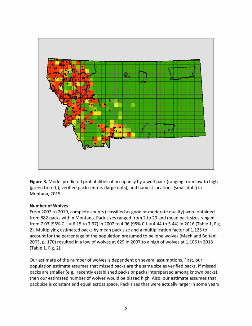
Figure 3. Model predicted probabilities of occupancy by a wolf pack (ranging from low to high [green to red]), verified pack centers (large dots), and harvest locations (small dots) in Montana, 2019. Number of Wolves From 2007 to 2019, complete counts (classified as good or moderate quality) were obtained from 882 packs within Montana. Pack sizes ranged from 2 to 29 and mean pack sizes ranged from 7.03 (95% C.I. = 6.15 to 7.97) in 2007 to 4.96 (95% C.I. = 4.44 to 5.44) in 2016 (Table 1, Fig. 2). Multiplying estimated packs by mean pack size and a multiplication factor of 1.125 to account for the percentage of the population presumed to be lone wolves (Mech and Boitani 2003, p. 170) resulted in a low of wolves at 629 in 2007 to a high of wolves at 1,106 in 2013 (Table 1, Fig. 2). Our estimate of the number of wolves is dependent on several assumptions. First, our population estimate assumes that missed packs are the same size as verified packs. If missed packs are smaller (e.g., recently established packs or packs interspersed among known packs), then our estimated number of wolves would be biased high. Also, our estimate assumes that pack size is constant and equal across space. Pack sizes that were actually larger in some years

9

or some areas would lead to underestimation of wolf numbers, and pack sizes that were smaller in some years or areas would lead to an overestimation of wolf numbers.

3. WOLF MANAGEMENT 3.1 Regulated Public Hunting and Trapping Regulated public harvest of wolves was recommended by the Governor’s Wolf Advisory Council and included in Montana’s Wolf Conservation and Management Plan that was approved by the USFWS during 2004. FWP has developed and implemented wolf harvest strategies that maintain a recovered and connected wolf population, minimize wolf-livestock conflicts, reduce wolf impacts on low or declining ungulate populations and ungulate hunting opportunities, and effectively communicate to all parties the relevance and credibility of the harvest while acknowledging the diversity of values among those parties. The Montana public has the opportunity for continuous and iterative input into specific decisions about wolf harvest throughout the public season-setting process. Wolf seasons are to be reviewed every other year by the Fish and Wildlife Commission during December (proposals) and February (final decisions). This timing allows discussion of ungulate and wolf seasons during the same Commission meetings. At the close of the 2019-20 wolf season (2019 License Year) on March 15, 2020, the harvest totaled 293 wolves taken during the 2019-20 season, including 163 taken by hunters (56%) and 130 taken by trappers (44%). Both the 2018-19 and 2019-20 wolf seasons yielded higher levels of wolf harvest than previous years. An average of 66 more wolves were harvested during each of the past two seasons than on average during the previous 6 wolf seasons when both hunting and trapping were allowed (2012-2017). Most of the increase over the 6-year average occurred in Regions 1 and 2 via trapping (Table 2). Statewide wolf population appears to have peaked in 2013 and has declined slightly since then, appearing to stabilize at around 850 wolves (Fig. 4). The total calendar-year 2019 wolf harvest in Montana was 298, including 141 wolves harvested during spring of the 2018-19 season and 157 wolves harvested during fall of the 2019-20 season. Table 2. Change in level of wolf harvest in Montana between the 2012-2017 seasons and the 2018-2019 seasons by FWP Region and type of harvest.

R1 R2 R3 R4 All R1 R2 R3 R4 All R1 R2 R3 R4 AllHunt 43 32 61 8 144 54 37 57 16 164 11 5 -4 8 20Trap 37 27 12 9 85 60 44 18 10 130 22 17 6 1 46

Total 80 59 73 17 229 114 81 75 26 294 33 22 2 9 66

2012-2017 Average Change2018-2019 Average

10

Figure 4. Estimated wolf population size based on known mortalities anchored to December 31 Patch Occupancy Modelling estimates, 2007 – 2019. During 2019, Montana sold 15,902 resident wolf hunting licenses ($19/each) and 2,252 non-resident wolf hunting licenses ($50/each). Sale of these wolf licenses generated $414,738 for wolf management and monitoring in Montana (Fig. 5). Total funding generated for wolf monitoring and management by the sale of wolf hunting licenses from 2009-2019 is over $4.1 million. Because trapping licenses for both residents and non-residents are not wolf-specific, FWP cannot quantify the financial contribution that wolf trapping generates. Figure 5. Dollars generated for wolf conservation and management through sales of wolf hunting licenses in Montana, 1998-2019.

11

3.2 Wolf – Livestock Interactions in Montana Montana wolves routinely encounter livestock on both private land and public grazing allotments. Wolves are opportunistic predators, most often seeking wild prey. However, some wolves learn to prey on livestock and teach this behavior to other wolves. The majority of cattle and sheep wolf depredation incidents confirmed by USDA Wildlife Services (WS) occur on private lands. The likelihood of detecting injured or dead livestock is probably higher on private lands where there is greater human presence than on remote public land grazing allotments. The magnitude of under-detection of loss on public allotments is unknown. Most cattle depredations occur during the spring or fall months while sheep depredations occur more sporadically throughout the year. Wolf Depredation Reports Wildlife Service’s workload increased through 2009 as the wolf population increased and distribution expanded (Fig. 6). The number of depredation reports received since those years has declined from 233 in FFY 2009 to approximately 100 or less from FFY14-FFY19. That trend held steady during FFY 2019, when 104 reports were received (Fig. 6). Since 1997, about 50% of wolf depredation reports received by WS have been verified as wolf-caused. During FFY 2019, 69% of reports were verified as wolf depredation, higher than the long-term average.

Figure 6. Number of complaints received by USDA Wildlife Services as suspected wolf damage and number of complaints verified as wolf damage, Federal Fiscal Year 1997-2019.

12

Wolf Depredation Incidents and Responses During 2019 Wildlife Services confirmed that, statewide, 69 cattle and 21 sheep, 2 goats, 2 mini horses, and 3 livestock guard dogs were killed by wolves during 2019. Wildlife Services also determined that an additional 18 cattle and 3 sheep were probable wolf kills. Total confirmed cattle and sheep losses were similar to 2011-2018 numbers, however the number of cattle has increased whereas the number of sheep has decreased (Fig. 7). Many livestock producers reported “missing” livestock and suspected wolf predation. Others reported indirect losses including poor weight gain and reduced productivity of livestock. There is no doubt that there are undocumented losses. To address livestock conflicts and to reduce the potential for further depredations, 59 wolves were killed during 2019 (Fig. 7). This was slightly lower than the average number of wolves removed due to depredation since meeting biological recovery goals in 2002 (Avg. = 70/year) and since delisting in 2011 (Avg. = 67/year). Federal and state regulations since 2009 have allowed private citizens to kill wolves seen in the act of attacking, killing, or threatening to kill livestock; from 2009-2019 an average of 12 wolves have been taken by private citizens each year. Forty-three wolves were removed in control actions by USDA Wildlife Services during 2019, and 16 wolves were killed by private citizens when wolves were seen chasing, killing, or threatening to kill livestock. The general decrease in livestock depredations since 2009 (Fig. 6) may be a result of several factors, primarily more aggressive wolf control in response to depredations (DeCesare et al. 2018).

Figure 7. Number of cattle and sheep killed by wolves and number of wolves removed through agency control and legal depredation-related take by private citizens, 2000-2019.

13

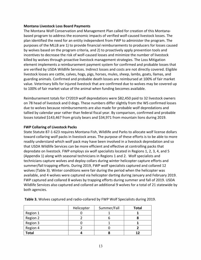
Montana Livestock Loss Board Payments The Montana Wolf Conservation and Management Plan called for creation of this Montana-based program to address the economic impacts of verified wolf-caused livestock losses. The plan identified the need for an entity independent from FWP to administer the program. The purposes of the MLLB are 1) to provide financial reimbursements to producers for losses caused by wolves based on the program criteria, and 2) to proactively apply prevention tools and incentives to decrease the risk of wolf-caused losses and minimize the number of livestock killed by wolves through proactive livestock management strategies. The Loss Mitigation element implements a reimbursement payment system for confirmed and probable losses that are verified by USDA Wildlife Services. Indirect losses and costs are not directly covered. Eligible livestock losses are cattle, calves, hogs, pigs, horses, mules, sheep, lambs, goats, llamas, and guarding animals. Confirmed and probable death losses are reimbursed at 100% of fair market value. Veterinary bills for injured livestock that are confirmed due to wolves may be covered up to 100% of fair market value of the animal when funding becomes available. Reimbursement totals for CY2019 wolf depredations were $82,450 paid to 32 livestock owners on 78 head of livestock and 0 dogs. These numbers differ slightly from the WS confirmed losses due to wolves because reimbursements are also made for probable wolf depredations and tallied by calendar year rather than federal fiscal year. By comparison, confirmed and probable losses totaled $143,467 from grizzly bears and $34,971 from mountain lions during 2019. FWP Collaring of Livestock Packs State Statute 87-1-623 requires Montana Fish, Wildlife and Parks to allocate wolf license dollars toward collaring wolf packs in livestock areas. The purpose of these efforts is to be able to more readily understand which wolf pack may have been involved in a livestock depredation and so that USDA Wildlife Services can be more efficient and effective at controlling packs that depredate on livestock. FWP employs six wolf specialists located in Regions 1, 2, 3, 4, and 5 (Appendix 1) along with seasonal technicians in Regions 1 and 2. Wolf specialists and technicians capture wolves and deploy collars during winter helicopter capture efforts and summer/fall trapping efforts. During 2019, FWP wolf specialists captured and collared 12 wolves (Table 3). Winter conditions were fair during the period when the helicopter was available, and 4 wolves were captured via helicopter darting during January and February 2019. FWP captured and collared 8 wolves by trapping efforts during summer and fall of 2019. USDA Wildlife Services also captured and collared an additional 9 wolves for a total of 21 statewide by both agencies. Table 3. Wolves captured and radio-collared by FWP Wolf Specialists during 2019.

Helicopter Summer/Fall Total Region 1 0 1 1 Region 2 2 6 8 Region 3 0 1 1 Region 4 2 0 2 Total 4 8 12

14

Proactive Prevention of Wolf Depredation In Northwest Montana, proactive depredation prevention work continued in the Trego area with the second grazing season of the Range Rider program. The Trego Range Rider Program was collaboratively funded and staffed by Natural Resources Defense Council; Defenders of Wildlife; Vital Ground; USDA AHPIS Wildlife Services; Montana Fish, Wildlife & Parks; U.S. Forest Service; and six livestock producers. The desired outcomes were to mitigate producer-predator conflicts, reduce cattle losses, reduce wolf and grizzly bear mortalities, find livestock carcasses and remove them, document presence of predators, and alert producers of predators among the herds. Ranger Rider Charlie Lytle returned for a second year, covering 6 allotments in northwestern Montana on the Kootenai National Forest and Jim Creek state lease. Cattle were present on the allotments that are within the territory of the Lydia pack in Swamp Creek drainage and the Good Pack, which has had depredations in previous years, but there were no losses in any of the allotments this year confirmed to be from wolves. The ranchers that met with FWP and NRDC in December were all very complimentary of the program, and said they believed having a Range Rider presence in the area was important. They also thought it was a large area for one person to cover and would be interested in expanding it with additional riders. FWP and WS both attempted to trap and collar wolves in that area but were not successful and have plans to collaborate on a trapline in spring 2020. The program is expected to continue in 2020. Ted North of WS is interested in starting another Ranger Rider program in 2020 in the Nirada and Hot Springs area west of Flathead Lake due to high livestock-carnivore conflicts in 2019, and is looking for funding and collaboration with the livestock producer in that area. Adam Bach of Wildlife Service continued putting up fladry in 2019, completing calving enclosures at 6 locations (most returning from previous years). In 2020 he is working with Defenders of Wildlife and NRDC to construct an experimental fence in Marion that is a 6-7 strand alternating-current permanent fence, because they have used fladry at that location for 7 years and want to make a more permanent fence solution. In West-Central Montana, FWP was involved in two collaborative proactive risk management projects in the Blackfoot Valley: the Blackfoot Challenge range rider project and carcass pickup program. This was the 12th year that the range rider project was implemented. The project employed four seasonal range riders and one permanent wildlife technician to monitor livestock and predators in areas occupied by the Arrastra Creek, Chamberlain, Morrell Mountain, Inez, and Union Peak wolf packs. The carcass pickup program removed livestock carcasses from Blackfoot Valley ranches and transported them to the carcass compost site to reduce attractants in livestock grazing and calving areas. FWP and the Blackfoot Challenge partnered with Wildlife Services for the third year to deploy fladry in the Blackfoot Valley to deter wolves from livestock calving yards. In Southwest Montana, FWP assisted with fladry deployment during calving season in Tom Miner Basin. FWP was also involved in two collaborative, proactive risk management projects in the Big Hole Valley. The first of these projects, a range rider completed its ninth season in 2019. The second project was a carcass pickup and composting program that was in its fifth year of operation.

15

In North-Central Montana, a range rider program, initiated in 2017, on private land and USFS grazing allotments west of Augusta included four livestock producers and employed one full-time and an additional part-time range rider. The program was coordinated by Kyran Kunkel, through the Conservation Science Collaborative, with funding from the Livestock Loss Board, along with several NGOs. Wildlife Services continued a full-time conflict reduction specialist position (Adam Baca) in Montana. This is a Wildlife Services employee. The position was funded collaboratively by Wildlife Services, U.S. Fish and Wildlife Service, Natural Resources Defense Council, Defenders of Wildlife and the American Prairie Reserve. Baca spent all of his time planning, coordinating, and implementing non-lethal predator damage management tools such as turbo fladry and electric fencing to protect livestock from predation. This position began in February 2018.

16

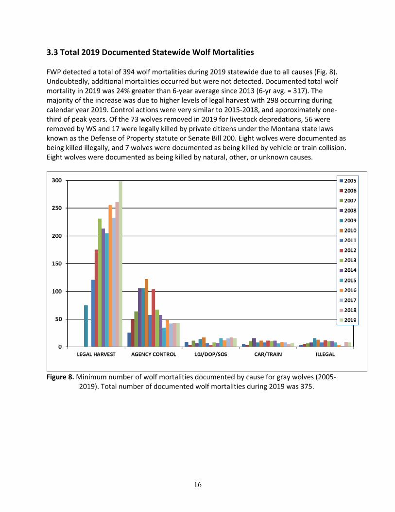
3.3 Total 2019 Documented Statewide Wolf Mortalities FWP detected a total of 394 wolf mortalities during 2019 statewide due to all causes (Fig. 8). Undoubtedly, additional mortalities occurred but were not detected. Documented total wolf mortality in 2019 was 24% greater than 6-year average since 2013 (6-yr avg. = 317). The majority of the increase was due to higher levels of legal harvest with 298 occurring during calendar year 2019. Control actions were very similar to 2015-2018, and approximately one-third of peak years. Of the 73 wolves removed in 2019 for livestock depredations, 56 were removed by WS and 17 were legally killed by private citizens under the Montana state laws known as the Defense of Property statute or Senate Bill 200. Eight wolves were documented as being killed illegally, and 7 wolves were documented as being killed by vehicle or train collision. Eight wolves were documented as being killed by natural, other, or unknown causes.

Figure 8. Minimum number of wolf mortalities documented by cause for gray wolves (2005-

2019). Total number of documented wolf mortalities during 2019 was 375.

17

4. OUTREACH AND EDUCATION FWP’s wolf program outreach and education efforts are varied, but significant. Outreach activities take a variety of forms including field site visits, phone and email conversations to share information and answer questions, presentations to school groups and other agency personnel, media interviews, and formal and informal presentations. FWP also prepared and distributed a variety of printed outreach materials and media releases to help Montanans become more familiar with the Montana wolf population and the state plan. The “Report a Wolf” application continued to generate valuable information from the public in monitoring efforts for existing packs and documenting wolf activity in new areas. Several reports were received through the website and others via postal mail and over the phone. Most wolf program staff spent some time at hunter check stations in FWP Regions 1-5 to talk with hunters about wolves, wolf management, and their hunting experiences.

5. FUNDING 5.1 Montana Fish, Wildlife & Parks Funding Funding for wolf conservation and management in Montana is controlled by laws enacted by the state legislature. State laws also provide detailed guidance on some wolf management activities. The Montana Code Annotated (MCA) is the current law, and specific sections can be viewed at http://leg.mt.gov/bills/mca/index.html. Legislative bill language and history that has created or amended MCA sections can be accessed at http://leg.mt.gov/css/bills/Default.asp. Three sections of the MCA are of primary significance to wolf management and funding. These are: MCA 87-5-132 Use of Radio-tracking Collars for Monitoring Wolf Packs MCA 87-1-623 Wolf Management Account MCA 87-1-625 Funding for Wolf Management MCA 87-5-132 was created during the 2005 legislative session by Senate Bill 461. It has been amended twice, both times during the 2011 legislative session, by House Bill 363 and Senate Bill 348. This law requires capturing and radio-collaring an individual within a wolf pack that is active in an area where livestock depredations are chronic or likely. MCA 87-1-623 was created during the 2011 Legislative Session by House Bill 363. This law requires that a wolf management account be set up and that all wolf license revenue be deposited into this account for wolf collaring and control. Specifically, it states that subject to appropriation by the legislature, money deposited in the account must be used exclusively for the management of wolves and must be equally divided and allocated for the following

18

purposes: (a) wolf-collaring activities conducted pursuant to 87-5-132; and (b) lethal action conducted pursuant to 87-1-217 to take problem wolves that attack livestock. MCA 87-1-625 was created during the 2011 Legislative Session by Senate Bill 348. This law required FWP to allocate $900,000 annually toward wolf management. "Management" in MCA 87-1-625 is defined as in MCA 87-5-102, which includes the entire range of activities that constitute a modern scientific resource program, including but not limited to research, census, law enforcement, habitat improvement, control, and education. The term also includes the periodic protection of species or populations as well as regulated taking. During the 2015 legislative session, Senate Bill 418 reduced this amount to $500,000 of spending authority. The wolf management budget for state fiscal year 2019 (July 1, 2018 – June 30, 2019) was $706,239 and consisted of $216,640 of federal PR funds, $489,599 of Montana wolf and general license dollars, and $25,001 from the Rocky Mountain Elk Foundation. Funding was used to pay for FWP’s field presence to implement population monitoring, collaring, outreach, hunting, trapping, and livestock depredation response. During state fiscal year 2019, the wolf program had 5.5 FTE wolf specialists dedicated to wolf management, and 1 total FTE for 2 seasonal technicians to increase collaring efforts in wolf packs associated with livestock. FWP also renewed the financial agreement with Wildlife Services for their role in wolf depredation management efforts. Other wolf management services provided by FWP include law enforcement, harvest/quota monitoring, legal support, public outreach, and overall program administration. Exact cost figures have not been quantified for the value of these services. 5.2 USDA Wildlife Services Funding Wildlife Services (WS) is the federal agency that assists FWP with wolf damage management. WS personnel conduct investigations of injured or dead livestock to determine if it was a predation event and, if so, what predator species was responsible for the damage. Based on WS determination, livestock owners may be eligible to receive reimbursement through the Montana Livestock Loss Program. If WS determines that the livestock depredation was a confirmed wolf kill or was a probable wolf kill, the livestock owner is eligible for 100% reimbursement on the value of the livestock killed based on USDA market value at the time of the investigation. Under an MOU with FWP, the Blackfeet Nation (BN), and the Confederated Salish and Kootenai Tribes (CSKT), WS conducts the control actions on wolves as authorized by FWP, BN, and CSKT. Control actions may include radio-collaring and/or lethal removal of wolves implicated in livestock depredation events. FWP, BN, and CSKT also authorize WS to opportunistically radio-collar wolf packs that do not have an operational radio-collar attached to a member of the pack in order to fulfill the requirements of Montana State Statute 87-1-623.

19

As a federal agency, WS receives federal appropriated funds for predator damage management activities but no federal funding directed specifically for wolf damage management. Prior to Federal Fiscal Year (FFY) 2011, the WS Program in Montana received approximately $250,000 through the Tri-State Predator Control Earmark, some of which was used for wolf damage management operations. However, that earmark was completely removed from the federal budget for FFY 2011 and not replaced in FFY 2012-2019. In FFY 2019, WS spent $314,917 conducting wolf damage management in Montana (not including administrative costs). The FFY 2019 expenditure included $204,917 Federal appropriations and $110,000 from FWP.

6. PERSONNEL AND ACKNOWLEDGEMENTS The 2019 FWP wolf specialist team was comprised of Diane Boyd, Nathan Lance, Abigail Nelson, Tyler Parks, Mike Ross, and Ty Smucker. Dr. Diane Boyd retired after more than 40 years of working with wildlife, predominantly wolves, including radio-tracking some of the first wolves to have recolonized Montana. Abby Nelson left FWP at the end of 2019 after serving as the Paradise Valley’s wolf specialist for over a decade where her knowledge, dedication and professionalism were respected by all. FWP is fortunate to have had both Abby and Diane as colleagues and we wish them both the best. Wolf specialists work closely with regional wildlife managers in FWP regions 1-5, including Neil Anderson, Howard Burt, Cory Loeker, Kevin Rose, and Mike Thompson, as well as Carnivore and Furbearer Coordinator, Bob Inman. FWP Helena and Wildlife Health Lab staff contributed time and expertise including Caryn Dearing, John Vore, Missy Erving, Justin Gude, Quentin Kujala, Greg Lemon, Ken McDonald, Adam Messer, Kevin Podruzny, Jennifer Ramsey, and Smith Wells. The wolf team is part of a much bigger team of agency professionals that make up Montana Fish, Wildlife & Parks including regional supervisors, biologists, game wardens, information officers, front desk staff, and many others who contribute their time and expertise to wolf management and administration of the program. FWP thanks Blackfoot Challenge range riders: Eric Graham, Jordan Mannix, Lindsey Mulcare, Vicki Pocha, and Sigrid Olson. The Blackfoot Challenge also worked with ranchers and landowners to reduce wildlife conflict in the Blackfoot Watershed using fladry and carcass pick-up, and they helped with wolf monitoring. USDA APHIS WS investigates all suspected wolf depredations on livestock and under the authority of FWP, carries out all livestock depredation-related wolf damage management activities in Montana. We thank them for contributing their expertise to the state’s wolf program and for their willingness to complete investigations and carry out lethal and non-lethal

20

damage management and radio-collaring activities in a timely fashion. We also thank WS for assisting with monitoring wolves in Montana. WS personnel involved in wolf management in Montana during 2019 included state director John Steuber; western district supervisor Kraig Glazier; eastern district supervisor Dalin Tidwell; western assistant district supervisor Chad Hoover; eastern assistant district supervisor Alan Brown; wildlife disease biologist Jerry Wiscomb; wildlife biologist Zack May; helicopter pilot Eric Waldorf; helicopter/airplane pilots Tim Graff and John Martin; airplane pilots Guy Terrill, Justin Ferguson, and Scott Snider; wildlife specialists Adam Baca, Glenn Hall, Finny Helske, Mike Hoggan, Cody Knoop, Jordan Linnell, Charlie Lytle, John Maetzold, Graeme McDougal, John Miedtke, Kurt Miedtke, Brian Noftsker, Ted North, Scott Olson, Jim Rost, Bart Smith, Pat Sinclair, and Danny Thomason. We acknowledge the work of the citizen-based Montana Livestock Loss Board which oversees implementation of Montana’s reimbursement program and the conflict prevention grant money, and we thank the LLB’s coordinator, George Edwards. We thank Northwest Connections for their avid interest and help in documenting wolf presence and outreach in the Swan River Valley. We thank Swan Ecosystem Center for their continued interest and support. We thank Kyran Kunkel of Conservation Science Collaborative, Inc. for his continued coordination of a range rider program on private and public land along the Southern Rocky Mountain Front. We also thank Kathy Robinson who was the range rider on this effort and was instrumental in working with local producers to monitor livestock and predator activity in the area. We thank Confederated Salish and Kootenai Tribal biologists Stacey Courville and Shannon Clairmont, and Blackfeet Tribal biologist Dustin Weatherwax for capturing and monitoring wolves in and around their respective tribal reservations. The Montana Wolf Management program field operations also benefited in a multitude of ways from the continued cooperation and collaboration of other state and federal agencies and private interests such as the USDA Forest Service, Montana Department of Natural Resources and Conservation (“State Lands”), U.S. Bureau of Land Management, Weyerhauser Company, Stimpson Lumber Company, Glacier National Park, Yellowstone National Park, Idaho Fish and Game, Wyoming Game and Fish, Nez Perce Tribe, Canadian Provincial wildlife professionals, Turner Endangered Species Fund, People and Carnivores, Wildlife Conservation Society, Keystone Conservation, Boulder Watershed Group, Big Hole Watershed Working Group, the Madison Valley Ranchlands Group, the upper Yellowstone Watershed Group, the Blackfoot Challenge, Tom Miner Basin Association, and the Granite County Headwaters Working Group. We deeply appreciate and thank our pilots whose unique and specialized skills, help us find wolves, get counts, and keep us safe in highly challenging, low altitude mountain flying situations. They include Joe Rahn (FWP Chief Pilot), Neil Cadwell (FWP Pilot), Ken Justus (FWP Pilot), Trever Throop (FWP Pilot), Mike Campbell (FWP Pilot), Rob Cherot (FWP Pilot), Jim Pierce (Red Eagle Aviation, Kalispell), Roger Stradley (Gallatin Flying Service, Belgrade), Steve Ard (Tracker Aviation Inc., Belgrade), Lowell Hanson (Piedmont Air Services, Helena), Dave Horner

21

(Red Eagle Aviation), Joe Rimensberger (Osprey Aviation, Hamilton), and Mark Duffy (Central Helicopters, Bozeman). We also thank Quicksilver Aviation for their safe and efficient helicopter capture efforts.

7. LITERATURE CITED DeCesar, N. J., S. M. Wilson, E. H. Bradley, J. A. Gude, R. M. Inman, N. J. Lance, K. Laudon, A. A.

Nelson, M. S. Ross, and T. D. Smucker. 2018. Wolf-livestock conflict and the effects of wolf management. Journal of Wildlife Management 82(4):711-722.

Erb, J. 2008. Distribution and abundance of wolves in Minnesota, 2007–08. Minnesota Department of Natural Resources, Grand Rapids, Minnesota, USA.

Fuller, T.K., L.D. Mech, and J.F. Cochrane. 2003. Wolf Population Dynamics. Pages 161-191 in LD Mech and L Boitani, editors. Wolves: behavior, ecology, and conservation. The University of Chicago Press, Chicago, Illinois, USA.

Glenn, E.S., L.N. Rich, and M.S. Mitchell. 2011. Estimating numbers of wolves, wolf packs, and breeding pairs in Montana using hunter survey data in a patch occupancy model framework: final report. Technical report, Montana Fish, Wildlife and Parks, Helena Montana.

Hines, J.E. 2006. PRESENCE- Software to estimate patch occupancy and related parameters. USGS-PWRC. http://www.mbr-pwrc.usgs.gov/software/presence.html.

Idaho Department of Fish and Game and Nez Perce Tribe. 2012. 2011 Idaho wolf monitoring progress report. Idaho Department of Fish and Game, 600 South Walnut, Boise, Idaho; Nez Perce Tribe Wolf Recovery Project, P.O. Box 365, Lapwai, Idaho. 94 pp.

Mech, D.L., and L. Boitani. 2003. Wolves: behavior, ecology, and conservation. The University of Chicago Press, Illinois, USA.

Miller, D.A.W., J.D. Nichols, J.A. Gude, K.M. Podruzny, L.N. Rich, J.E. Hines, M.S. Mitchell. 2013. Determining occurrence dynamics when false positives occur: estimating the range dynamics of wolves from public survey data. PLOS ONE 8:1-9.

Rich, L.N., R.E. Russell, E.M. Glenn, M.S. Mitchell, J.A. Gude, K.M. Podruzny, C.A. Sime, K. Laudon, D.E. Ausband, and J.D. Nichols. 2013. Estimating occupancy and predicting numbers of gray wolf packs in Montana using hunter surveys. Journal of Wildlife Management. 77:1280-1289.

Rich, L.N., M.S. Mitchell, J.A. Gude, and C.A. Sime. 2012. Anthropogenic mortality, intraspecific competition, and prey availability structure territory sizes of wolves in Montana. Journal of Mammalogy 93:722–731.

22

APPENDICES

23

TO REPORT A DEAD WOLF OR POSSIBLE ILLEGAL ACTIVITY: Montana Fish, Wildlife & Parks

• Dial 1-800-TIP-MONT (1-800-847-6668) or local game warden

TO SUBMIT WOLF REPORTS ELECTRONICALLY AND TO LEARN MORE ABOUT THE MONTANA WOLF PROGRAM, SEE:

• http://fwp.mt.gov/fishAndWildlife/management/wolf/

APPENDIX 1

MONTANA CONTACT INFORMATION

Montana Fish, Wildlife & Parks Wendy Cole FWP Wolf Management Specialist, Kalispell 406-751-4586 wendy.cole@mt.gov Tyler Parks FWP Wolf Management Specialist, Missoula 406-531-4454 tylerparks@mt.gov Nathan Lance FWP Wolf Management Specialist, Butte 406-425-3355 nlance@mt.gov Mike Ross FWP Wolf Management Specialist, Bozeman 406-581-3664 mross@mt.gov Ty Smucker FWP Wolf Management Specialist, Great Falls 406-750-4279 tsmucker@mt.gov

Bob Inman FWP Carnivore & Furbearer Coordinator 406-444-0042 bobinman@mt.gov Brian Wakeling FWP Wildlife Management Bureau Chief 406-444-3940 brian.wakeling@mt.gov USDA Wildlife Services (to request investigations of injured or dead livestock): John Steuber USDA WS State Director, Billings (406) 657-6464 (w) Kraig Glazier USDA WS West District Supervisor, Helena (406) 458-0106 (w) Dalen Tidwell USDA WS East District Supervisor, Columbus (406) 657-6464 (w)

24

MONTANA FISH WILDLIFE & PARKS ADMINISTRATIVE REGIONS

STATE REGION 3 REGION 4 REGION 6 HEADQUARTERS 1400 South 19th 4600 Giant Springs Rd 54078 US Hwy 2 W MT Fish, Wildlife & Parks Bozeman, MT 59718 Great Falls, MT 59405 Glasgow, MT 59230 1420 E 6th Avenue (406) 994-4042 (406) 454-5840 (406) 228-3700 PO Box 200701 Helena, MT 59620-0701 HELENA Area Res Office LEWISTOWN Area Res HAVRE Area Res Office (406) 444-2535 (HARO) Office (LARO) (HvARO) 930 Custer Ave W 215 W Aztec Dr 2165 Hwy 2 East REGION 1 Helena, MT 59620 PO Box 938 Havre, MT 59501 490 N Meridian Rd (406) 495-3260 Lewistown, MT 59457 (406) 265-6177 Kalispell, MT 59901 (406) 538-4658 (406) 752-5501 BUTTE Area Res Office REGION 7 (BARO) REGION 5 Industrial Site West REGION 2 1820 Meadowlark Ln 2300 Lake Elmo Dr PO Box 1630 3201 Spurgin Rd Butte, MT 59701 Billings, MT 59105 Miles City, MT 59301 Missoula, MT 59804 (406) 494-1953 (406) 247-2940 (406)234-0900 (406) 542-5500

25

APPENDIX 2

RESEARCH, FIELD STUDIES, AND PROJECT PUBLICATIONS

Each year in Montana, there are a variety of wolf-related research projects and field studies in varying degrees of development, implementation, or completion. These efforts range from wolf ecology and predator-prey relationships to wolf-livestock relationships, policy, or wolf management. In addition, the findings of some completed projects get published in the peer-reviewed literature. The 2019 efforts are summarized below, with updates or project abstracts. A2.1. IMPROVING ESTIMATION OF WOLF RECRUITMENT AND ABUNDANCE, AND DEVELOPMENT OF AN ADAPTIVE HARVEST PROGRAM FOR WOLVES IN MONTANA. Status: In Progress The full 2019 report is included on the following pages.

Federal Aid in Wildlife Restoration Grant W-161-R-1 Annual interim report, March 2020

Improving Estimation of Wolf Recruitment and Abundance, and Development of an Adaptive Harvest Management Program for Wolves in Montana

Sarah Sells Research Associate Montana Cooperative Wildlife Research Unit 205 Natural Sciences, Missoula, MT 59812 Allison Keever PhD Candidate Montana Cooperative Wildlife Research Unit 205 Natural Sciences, Missoula, MT 59812 Mike Mitchell Unit Leader Montana Cooperative Wildlife Research Unit 205 Natural Sciences, Missoula, MT 59812

Justin Gude Res & Tech Services Bureau Chief Montana Fish, Wildlife and Parks 1420 E. 6th St., Helena, MT 59620 Kevin Podruzny Biometrician Montana Fish, Wildlife and Parks 1420 E. 6th St., Helena, MT 59620

State: Montana Agency: Fish, Wildlife & Parks Grant: Montana wolf monitoring study Grant number: W-161-R-1 Time period: January 1, 2019−December 31, 2019

S. Sells

INTRODUCTION

Wolves (Canis lupus) were reintroduced into 2 areas in the southern portion of the northern Rocky Mountains (NRM) in 1995, and after rapid population growth were delisted from the endangered species list in 2011. Since that time, states in the NRM have agreed to maintain populations and breeding pairs (a male and female wolf with 2 surviving pups by December 31; USFWS 1994) above established minimums (≥150 wolves and ≥15 breeding pairs within each state). Montana estimates population size every year using patch occupancy models (POM; Miller et al. 2013; Rich et al. 2013; Bradley et al. 2015), however, these estimates are sensitive to pack size and territory size, and were developed pre-harvest. Reliability of future estimates based on POM will be contingent on accurate information on territory size, overlap, and pack size, which are expected to be strongly affected by harvest. Additionally, breeding pairs, which has proven to be an ineffective measure of recruitment, are determined via direct counts. Federal funding for wolf monitoring has ended in states where wolves are delisted, and future monitoring will not be able to rely on intensive counts of the wolf population. Furthermore, intensive, field-based monitoring has become cumbersome and less effective since the population has grown. With the implementation of harvest, predicting the effects of harvest on the wolf population and continuing to monitor the effectiveness of management actions is required to make informed decisions regarding hunting and trapping seasons.

Objectives & Deliverables

Two PhD students are addressing the 4 study objectives, as follows (Fig. 1).

Objective 1. Improve and maintain calibration of wolf abundance estimates generated through POM.

Deliverables: Models to estimate territory size and pack size that can keep POM estimates calibrated to changing environmental and management conditions for wolves in Montana (Project 1, S. Sells).

Objective 2. Improve estimation of recruitment.

Deliverables: A method to estimate recruitment for Montana’s wolf population that is more cost effective and biologically sound than the breeding pair metric (Project 2, A. Keever).

Objective 3. Develop a framework for dynamic, adaptive harvest management based on achievement of objectives 1 & 2.

Deliverables: An adaptive harvest management model that allows the formal assessment of various harvest regimes and reduces uncertainty over time to facilitate adaptive management of wolves (Project 2, A. Keever).

Objective 4. Design a targeted monitoring program to provide information needed for

Figure 1. Objectives for this project are being addressed under 2 PhD projects.

robust estimates and reduce uncertainty in the AHM paradigm over time.

Deliverables: A recommended monitoring program for wolves to maintain calibration of POM estimates, determine effectiveness of management actions, and facilitate learning in an adaptive framework (Projects 1 & 2).

Location

This study encompasses wolf distribution in Montana. Additional data for Deliverable 2 were contributed from data collected for wolves in central Idaho (Game Management Units 4, 28, 33, 34, and 35) by Idaho Department of Fish and Game as part of other research initiatives (Ausband et al. 2015, 2017; Ausband 2018).

Project Status

Project 1—S. Sells: The PhD components of this project were completed and defended in December 2019 (Fig. 2). Project deliverables included a mechanistic territory model, empirical territory and group size models, and a final dissertation (Sells 2019). As a Research Associate, S. Sells is continuing collaboration towards Deliverables 3 & 4 and is implementing the territory and group models within the existing POM framework.

Project 2—A. Keever: This project will be completed and defended in March 2020. Project deliverables will include an empirical recruitment model, a mechanistic recruitment model, a decision tool in an AHM framework, and a final dissertation.

Details are provided in subsequent sections of this report.

Acknowledgements

This project is made possible with the generous assistance of biologists and managers at Montana Fish, Wildlife and Parks, including Bob Inman, Diane Boyd, Tyler Parks, Abby Nelson, Ty Smucker, Kent Laudon, Nathan Lance, Mike Ross, Molly Parks, Brady Dunne, Liz Bradley, Jessy Coltrane, Kelly Proffitt, John Vore, Quentin Kujala, Neil Anderson, Mike Lewis, and Nick DeCesare. Biologists and managers at Idaho Fish and Game also provide generous assistance, including David Ausband and Mark Hurley. We also thank landowners for allowing access for trapping and collaring efforts. Additionally, faculty and staff at the University of Montana provide invaluable support.

Literature Cited

Ausband, D. E. 2018. Multiple breeding individuals within groups in a social carnivore. Journal of Mammalogy 99:836–844.

Figure 2. Project timeline.

Ausband, D. E., M. S. Mitchell, and L. P. Waits. 2017. Effects of breeder turnover and harvest on group composition and recruitment in a social carnivore. Journal of Animal Ecology 86:1094–1101.

Ausband, D. E., C. R. Stansbury, J. L. Stenglein, J. L. Struthers, and L. P. Waits. 2015. Recruitment in a social carnivore before and after harvest. Animal Conservation 18:415–423.

Bradley, L., J. Gude, N. Lance, K. Laudon, A. Messer, A. Nelson, G. Pauley, M. Ross, T. Smucker, and J. Steuber. 2015. Montana gray wolf conservation and management 2014 annual report. Helena, Montana.

Miller, D. A. W., J. D. Nichols, J. A. Gude, L. N. Rich, K. M. Podruzny, J. E. Hines, and M. S. Mitchell. 2013. Determining occurrence dynamics when false positives occur: estimating the range dynamics of wolves from public survey data. PloS one 8:e65808.

Rich, L. N., R. E. Russell, E. M. Glenn, M. S. Mitchell, J. A. Gude, K. M. Podruzny, C. A. Sime, K. Laudon, D. E. Ausband, and J. D. Nichols. 2013. Estimating occupancy and predicting numbers of gray wolf packs in Montana using hunter surveys. The Journal of Wildlife Management 77:1280–1289.

OBJECTIVE 1: IMPROVE AND MAINTAIN CALIBRATION OF WOLF ABUNDANCE ESTIMATES GENERATED THROUGH POM—Sarah Sells, Project 1

ABSTRACT Our goal under Objective 1 was to develop reliable methods to estimate territory size, territory overlap, and pack size to help improve the reliability of wolf abundance estimates through POM. We developed and applied a mechanistic territory model to produce predictions for the hypothesis that wolves select territories economically based on the benefits of food resources and costs of competition, travel, and predation risk. We summarized territory sizes of real wolves using location data to test the model’s predictions. As predicted, territory sizes in Montana varied inversely with prey abundance, number of nearby competitors, and pack size, and parabolically with predator density. Parameterizing the model with limited data for prey, terrain ruggedness, and human density produced spatially-explicit predictions for territory location, size, and overlap for the Montana wolf population and reliably predicted territories of specific packs, without using any empirical data for wolves. We also developed an empirical model that produced reliable estimates of territory size, which can be used to further predict and understand territorial behavior. Additionally, we aimed to test mechanisms hypothesized to influence social decisions (e.g., dispersal timing) and to develop a predictive model for pack size. Wolf pack sizes in Montana were positively related to the local abundance of prey and density of packs, and negatively related to terrain ruggedness, local mortalities, and intensity of harvest management. A predictive model for pack sizes reliably estimated the annual wolf pack sizes observed and illuminated possible underlying mechanisms influencing variation in pack sizes over space and time.

1.1 Introduction

Monitoring is a critical yet challenging management tool for gray wolves. Monitoring results help MFWP set management objectives and communicate with stakeholders and the public. Monitoring any large carnivore is challenging due to their elusive nature and low densities (Boitani et al. 2012). This is particularly true for wolves in the Northern Rocky Mountains, as federal funding for monitoring has ended and a large population spreads monitoring efforts thin. Furthermore, there is frequent turnover of packs, and behavioral dynamics may have changed with harvest.

Abundance estimates are a key component of monitoring (Bradley et al. 2015). Abundance is currently estimated in Montana using 3 parameters: area occupied, average territory size, and annual average pack size (Fig. 1.1, Bradley et al. 2015, Sells 2019). Area occupied is estimated

Figure 1.1. Example of POM results (red indicates highest occupancy probability, green lowest), and methods for calculating abundance. Graphed abundance estimates are based on minimum counts (black bars) and POM-based estimates (white bars). (From Sells 2019.)

with a Patch Occupancy Model (POM) based on hunter observations and field surveys (Miller et al. 2013, Rich et al. 2013, Bradley et al. 2015). Average territory size is assumed to be 600 km2 with minimal overlap, based on past work (Rich et al. 2012). Annual average pack size is estimated from monitoring results. Abundance is then calculated as the number of territories estimated within the area occupied, multiplied by the average pack size.

Whereas estimates of area occupied from POM are expected to be reliable (Miller et al. 2013, Bradley et al. 2015), reliability of abundance estimates hinge on assumptions about territory size and overlap (Bradley et al. 2015). Assumptions of a fixed territory size with minimal overlap are simplistic; in reality, territories vary spatiotemporally (Uboni et al. 2015). This variability is likely even greater under harvest (Brainerd et al. 2008). Furthermore, estimates of mean territory size were largely derived pre-harvest (Rich et al. 2012). If average territory size has changed, abundance estimates would be biased. Similarly, at finer spatial scales (e.g., at regional levels), where territory sizes are smaller than average, abundance estimates would be biased low, whereas the opposite would be true where territories are larger than average. Variations in territory overlap would similarly bias results.

Estimates of abundance also hinge on assumptions about pack size (Bradley et al. 2015). Pack size estimates require packs to be located and accurately counted each year, which is no longer possible due to the large number of packs and declining funding for monitoring (Bradley et al. 2015). Since implementation of recreational public harvest in 2009, several factors have further compounded these challenges and decreased accuracy of pack size estimates. First, whereas larger packs are generally easier to find and monitor, average pack size has decreased since harvest began (Bradley et al. 2015). Difficult-to-detect smaller packs may be more likely to be missed altogether, biasing estimates of average pack size high. Conversely, incomplete pack counts, especially for larger packs, could bias estimates of average pack size low. Harvest and depredation removals also affect social and dispersal behavior (Adams et al. 2008, Brainerd et al. 2008, Ausband 2015) and therefore further influence pack size.

Development of reliable methods to estimate territory size, territory overlap, and pack size could improve accuracy and precision of abundance estimates. In addition to pack counts, monitoring has relied on deploying collars; this is increasingly challenging and costly due to difficulty of capture and frequent collar loss caused by collar failures and mortalities. Given these challenges, the fact that federal funding for wolf monitoring has ended, and the number of packs to be monitored, there is need for new methods that reduce monitoring requirements and enable estimating territory size, territory overlap, and pack size. Furthermore, these methods should help keep estimates from POM calibrated into the future, which could be achieved by developing methods to predict behavioral changes under a wide range of potential future conditions.

We sought to develop reliable methods to calibrate POM by estimating territory size, territory overlap, and pack size absent costly and challenging monitoring efforts. Accordingly, our approach employed mechanistic and empirical models to maximize understanding of behavior. A mechanistic approach provided a means to test hypotheses to understand why wolves select particular territories. It furthermore enabled predicting behavior across a full range of potential present and future conditions. We also developed empirical models to understand patterns in territories and pack sizes of wolves in Montana and to provide additional tools to estimate territory and pack size.

Below, we provide overviews of each of the models developed. The dissertation produced from this research contains the full details about the mechanistic territory model (Chapters 1 and 3, Sells 2019), empirical territory size model (Chapter 2, Sells 2019), and empirical pack size model (Chapter 4, Sells 2019). Manuscripts for publication in scientific journals are currently in preparation or review. The text that follows was modified or borrowed from Sells (2019).

1.2 Wolf Location Data

A major component of this project was to collar wolves to collect location data. This effort contributed to both the mechanistic (Sect. 1.3) and empirical territory models (Sect. 1.4). Results from location data provided both a means to assess the mechanistic model’s performance and the data required to fit empirical models of territory size.

Study Area

Our study area comprised Montana (Fig. 1.2), which included the northern extent of the U.S. Rocky Mountains and elevations ranging from 554 – 3,938 m (Foresman 2001). In the northwest corner of Montana, dense forests and a maritime-influenced climate characterized the rugged, mountainous terrain of the Northern Rockies ecoregion (epa.gov). To the east, the Canadian Rockies ecoregion was characterized by higher-elevation, glaciated terrain, which transitioned to the Northwestern Glaciated Plains ecoregion characterized by level and rolling terrain with seasonal ponds and wetlands. In far southwestern Montana, the Idaho Batholith ecoregion was mountainous, granitic, and partially glaciated. To the east, the large Middle Rockies ecoregion was characterized by rolling foothills where shrubs and grasses transitioned to rugged mountains with conifers and alpine vegetation. The xeric Wyoming Basin ecoregion of south-central Montana was dominated by grasses and shrubs. The semiarid, rolling plains of

Figure 1.2. Our study area encompassed the state, which is characterized by various ecoregions (epa.gov).

Northwestern Great Plains ecoregion in southeastern Montana was interspersed with breaks and forested highlands. Wolves were found primarily in the western side of the state, but reported sightings and occasional harvests occurred in eastern Montana. Primary prey for wolves were elk (Cervus canadensis), white-tailed deer (Odocoileus virginianus), mule deer (O. hemionus), and moose (Alces alces). Other large carnivores included coyotes (C. latrans), mountain lions (Puma concolor), black bears (Ursus americanus), and grizzly bears (U. arctos). The human population in Montana was just over 1,062,000 in 2018 (census.gov). Annual depredation removals for livestock conflicts ranged 51 – 61 from 2014 – 2017 (Coltrane et al. 2015; Bradley et al. 2015; Boyd et al. 2017; Montana Fish Wildlife and Parks 2018). During this same era, harvest through hunting and trapping led to 207 – 295 mortalities per harvest season, which occurred each September 1 – March 15.

Methods

Location data were collected from 2014 – 2019 via GPS collars deployed by MFWP. Wolf captures occurred using foothold traps (EZ Grip # 7 double long spring traps, Livestock Protection Company, Alpine TX), or aerial darting. Wolf anesthetization and handling followed MFWP’s biomedical protocol for free-ranging wolves (Montana Fish, Wildlife and Parks 2005), guidelines from the Institutional Animal Care and Use Committee for the University of Montana (AUP # 070–17), and guidelines from the American Society of Mammalogists (Sikes et al. 2011). GPS collars were Lotek LifeCycle, Lotek Litetrack B 420, Telonics TGW-4400-3, Telonics TGW-4483-3, or Telonics TGW-4577-4, programmed to collect latitude and longitude every 3 – 13 hours.

MFWP wolf specialists assigned a preliminary pack identification to each collared wolf. This identification was fixed while the wolf remained a resident, i.e., its movements were in a localized cluster, including limited forays, defined as departing from and returning to the cluster. We considered the wolf to remain a resident if it did not start a new foray < 1 month after returning. If forays became more frequent or the wolf did not return, we considered it to be dispersing thereafter. Frequent forays nearly always precipitated dispersal. Upon dispersing, a wolf could either die or join a new pack by again localizing its movements. Successful dispersers were identified as a resident of the nearest pack, or given a new pack identification if the cluster did not overlap a known pack.

We estimated sizes, locations, and centroids of territories of resident, GPS-collared wolves (Figs. 1.3 – 1.4) using Program R (R Core Team 2018). We estimated 95% volume-adaptive kernel density estimates

Figure 1.3 Locations of 28 annual territories estimated for collared wolves. Darker shading represented territory overlap, and numbers were the average pack size in the 2 years post-capture. Large waterbodies and shaded relief are also shown.

(KDEs; Worton 1989) with package AdehabitatHR (Calenge 2006), with a smoothing parameter of 100% of the reference bandwidth. This smoothing parameter and a 95% KDE best prevented islands and lacunas while excluding extra-territorial forays. We also generated 90% KDEs to enable comparisons to past research in Montana (Rich et al. 2012). We generated KDEs for each year of data for each territory in which the wolf was a resident. We averaged territory size for packs with multiple KDEs, which occurred if > 1 wolf was collared in a pack or a wolf was collared for multiple years. We considered wolves to represent the same pack when their 50% KDEs (i.e., core areas) had any overlap.

For the mechanistic territory model (Sect. 1.3), we identified a territory boundary for each pack as the most recent KDE generated from fixes spanning ≥ 90% of a year. In packs with fixes spanning only 70 – 90% of a year, we used the most recent KDE. We also summarized approximate mean territory sizes for wolves with fixes spanning < 70% of a year (≥ 100 fixes required).

Results

From January 2014 – May 2019, MFWP captured and collared 92 wolves from 54 packs. Average collar deployment was 9.91 months, primarily as a result of collar failures (n = 33), harvest (n = 19), control removal (n = 8), and other mortalities (e.g., by vehicle strikes, injuries, or poaching; n = 12). Of 15 identified dispersals, 9 led to joining or forming other territories. Remaining dispersals yielded 3 mortalities, 2 emigrations to Idaho, and 1 emigration to Wyoming before returning to the wolf’s natal territory.

From data for wolves that remained a resident of a pack for ≥ 70% of a year, we estimated 43 territories of 28 packs (Fig. 1.3). After averaging by pack, arithmetic mean territory size was 582.02 km2 for 95% KDEs and 440.89 km2 for 90% KDEs (Fig. 1.4; Table 1.1). Accordingly, mean territory size decreased by 26.49% from that estimated by prior work (Rich et al. 2012).

1.3 Mechanistic Territory Model

The goal of developing a mechanistic territory model was to better understand how and why wolf territories vary over space and time. This variation could arise based on the conditions wolves encounter when selecting and defending territories, such as those related to food resources, competition, and humans. Understanding how and why territory sizes vary would help calibrate POM.

Figure 1.4. Annual territory size estimated for packs in Montana from GPS-collared wolves, 2014 – 2019.

Table 1.1. Mean sizes for wolf territories in Montana, 2014 – 2019. Measurement N

packs �̅�𝑥 territory size (km2) 1

SE (km2)

Min. Max. Geometric �̅�𝑥 (km2)

95% KDEs 28 582.02 79.41 187.71 2207.42 483.62

90% KDEs 28 440.89 58.75 137.82 1592.00 366.50

1. Arithmetic �̅�𝑥 & SE.

In general, territories that maximize benefits and minimize costs of ownership should lead to higher fitness (Brown 1964, Emlen and Oring 1977, Krebs and Kacelnik 1991). Accordingly, as a product of natural selection (Darwin 1859), animals are likely adapted to select territories economically. Based on theory and empirical precedent, territoriality should occur only when resources are economically defendable (Brown 1964), i.e., benefits outweigh costs of defense. Economical territories should also be only large enough to provide requisite resources for survival and reproduction, except in cases where additional resources increase fitness (Mitchell and Powell 2004, 2007, 2012). A primary benefit of many territories is likely exclusive access to food resources (Brown 1964, Hixon 1980, Carpenter 1987, Adams 2001) because food is essential to survival and reproduction. Primary costs are likely competition (Brown 1964, Hixon 1980, Carpenter 1987) and travel (Mitchell & Powell 2004, 2007, 2012), because competition is inherent to territoriality and energy is needed to access and defend resources. Mortality risk may also be a primary cost where predator density is high if it affects how animals select and use their territory (Sargeant et al. 1987, Whittington et al. 2005, Rich et al. 2012). Furthermore, territory holders with lower competitive ability may pay higher costs to compete against more-competitive conspecifics (Packer et al. 1990, Sillero-Zubiri and Macdonald 1998, Cassidy et al. 2015, Sells 2019).

We hypothesized that wolves are likewise adapted to select territories economically to meet resource requirements, based on the benefits of food resources and costs of competition, travel, and mortality risk. The primary food resources for wolves are ungulates (Mech and Peterson 2003, Peterson and Ciucci 2003), which have been thought to affect wolf territory size and abundance (Fuller et al. 2003; Jedrzejewski et al. 2007). The strongly territorial nature of wolves should make competition a primary cost of territorial behavior. We hypothesized that smaller packs had lower competitive ability (Cassidy et al. 2015). As coursing predators (Peterson and Ciucci 2003, Sillero-Zubiri et al. 2004), travel costs in the form of distance and terrain ruggedness are also likely to affect behavior. Humans have hunted and killed wolves for centuries (Fritts et al. 2003, Musiani and Paquet 2004), and wolves appear to associate humans with risk (Whittington et al. 2004, Hebblewhite and Merrill 2008, Latham et al. 2011). Accordingly, we hypothesized that human density affects the cost of mortality risk for wolves. We alternatively hypothesized that the cost of mortality risk was relatively unimportant to how wolves select territories.

Methods

The mechanistic territory model was developed in NetLogo 6.0 (Wilensky 1999) and entailed spatially-explicit simulations. Landscapes for simulations were grids of patches that varied in benefits and costs of ownership. We designed the model to represent the hypothesis that wolves are adapted to select territories economically based on the benefits of food resources discounted by the costs of competition, travel, and mortality risk. This meant that simulated packs employed a simple behavior rule to maintain economical territories by selecting territory patches that maximized benefits and minimized costs of ownership. Packs continued defending and modifying their territories in response to decisions made by neighboring packs as simulated wolf populations gradually increased to carrying capacity in the model.

Model application

We applied the model in two phases. In Phase 1, we produced and assessed qualitative predictions from the model for how territory size may vary in response to food, competition, pack size, and human density.

We considered the model’s predictions to match reality if the predicted trends in territory sizes in relation to food, competition, pack size, and human density reflected trends observed empirically.

In Phase 2, we parameterized the model with empirical data to produce quantitative, spatially-explicit predictions for wolves in Montana (full details in Sells 2019, Chapter 3). We used only readily-available data for prey, terrain ruggedness, and human density to test the model’s ability to make predictions absent expensive, difficult-to-collect datasets, including data for wolves (i.e., omitting data for wolf movements, pack locations, pack sizes, etc.). An ability to predict wolf space use absent wolf data would constitute a strong test of the model. We considered the model to successfully predict first-order selection (i.e., distribution; Johnson 1980) if the distributions of predicted and observed territories overlapped by > 50%, and if predicted territories overlapped < 25% of Montana not known to be part of the real distribution of wolves. We also compared patterns in predicted versus observed territory sizes across food abundances, competitor densities, human densities, and ecoregions. We then assessed the model’s ability to predict second-order territory selection (i.e., the sizes and locations of territories; Johnson 1980). After averaging predicted territory size by pack, we estimated a linear regression of the observed (Sect. 1.2) versus predicted territory sizes. We considered the model to reliably estimate territory size if the slope estimate’s 95% confidence interval overlapped 1.0 (Rich et al. 2012; Sells 2019). We compared predictions of specific locations (i.e., each 1-km2 grid patch predicted to be owned by a pack) by assessing the true positive rate (% of an empirically-observed territory [Sect. 1.2] correctly predicted). We considered the model to successfully predict second-order selection if it reliably estimated territory size and identified > 50% of the 1-km2 grid cells used by real packs.

Data inputs and outputs

Phase 1 of model simulations were conducted absent input data. We generated simple, general landscapes that varied in prey abundance and human densities (details in Sells 2019, Chapter 1). Pack sizes were randomly assigned to simulated packs. Outputs measured included territory sizes in relation to prey abundance, pack density, pack size, and human density.

For Phase 2, we developed a landscape representing Montana as a grid of 1-km2 patches. We assigned each patch a benefit of food resources and costs of travel and mortality risk (cost of competition arose during simulations). This accordingly required data inputs of food resources, terrain ruggedness, and human density, as follows.

To represent the benefit of food resources, we estimated densities of ungulates (fwp.mt.gov) in predicted seasonal habitat (Montana Natural Heritage Program). In each km2 grid cell i delineated as summer deer habitat, the density index was:

𝑑𝑑𝑑𝑑𝑑𝑑𝑑𝑑(𝑠𝑠𝑠𝑠𝑠𝑠𝑠𝑠𝑑𝑑𝑑𝑑)𝑖𝑖 = (𝑁𝑁𝑅𝑅 ÷ 𝛴𝛴𝑎𝑎𝑎𝑎𝑎𝑎𝑎𝑎) × (𝐶𝐶𝐶𝐶𝐶𝐶𝐶𝐶𝑖𝑖 ÷ 𝐶𝐶𝐶𝐶𝐶𝐶𝐶𝐶 𝑅𝑅�). 𝑁𝑁𝑅𝑅 was the 10-year average estimate of white-tailed and mule deer abundance (fwp.mt.gov) in the MFWP administrative region (𝑅𝑅) where i fell. 𝛴𝛴𝑎𝑎𝑎𝑎𝑎𝑎𝑎𝑎 was 𝑅𝑅’s estimated area of deer summer habitat. 𝐶𝐶𝐶𝐶𝐶𝐶𝐶𝐶𝑖𝑖 was the mean catch per unit effort (CPUE; buck harvest / hunter days) in the MFWP hunting district in which i fell, and 𝐶𝐶𝐶𝐶𝐶𝐶𝐶𝐶𝑅𝑅� was the regional mean CPUE, based on harvest records from 2008 – 2017 (fwp.mt.gov). We repeated these calculations for a deer winter density index, and for elk summer and winter density indices. Although CPUE positively correlates with deer and elk abundance (Dusek et al. 2006, Rich et al. 2012), regional CPUE was expected to be more comparable than statewide CPUE given

differences in factors that affect hunting success (e.g., hunting regulations, terrain, vegetation, accessibility, etc.). Relating CPUE to the regional mean modified the density estimate based on relative CPUE in the same region. We calculated a moose density index for each cell i delineated as seasonal moose habitat as:

𝑠𝑠𝑚𝑚𝑚𝑚𝑠𝑠𝑑𝑑 𝑑𝑑𝑑𝑑𝑑𝑑𝑠𝑠𝑑𝑑𝑑𝑑𝑑𝑑 (𝑠𝑠𝑑𝑑𝑠𝑠𝑠𝑠𝑚𝑚𝑑𝑑)𝑖𝑖 = 𝑁𝑁𝐻𝐻𝐻𝐻 ÷ 𝛴𝛴𝐻𝐻𝐻𝐻 𝑎𝑎𝑎𝑎𝑎𝑎𝑎𝑎. 𝑁𝑁𝐻𝐻𝐻𝐻 was the survey- and expert opinion-based estimate of moose abundance in the HD in which i fell, and 𝛴𝛴𝐻𝐻𝐻𝐻 𝑎𝑎𝑎𝑎𝑎𝑎𝑎𝑎 was the area of summer or winter moose habitat in that HD. Where densities estimates were unavailable in parks and reservations, we interpolated ungulate indices through inverse distance weighting using the gstat package in R (Pebesma 2004), and smoothed each index using weighted moving windows. We then calculated overall ungulate density indices by summing the indices for deer, elk, and moose for each season. These ungulate indices thus represented the benefit of food for wolves.

Travel cost to each patch incorporated distance and a terrain ruggedness index. Using elevation data obtained through package elevatr (Hollister and Shah 2017), we modeled terrain ruggedness per km2 as the Vector Ruggedness Measure (Sappington et al. 2007) with R package spatialEco (Evans 2018). Ruggedness was the average change in elevation between adjacent 1-km2 patches.

The cost of mortality risk for each patch was based on human density. We hypothesized that the cost of mortality risk would rise nonlinearly with the density of humans. Accordingly, from 2010 census data we calculated the square root of human density per km2.

Model outputs from Phase 2 included territory size and overlap in relation to ecoregion of Montana (Fig. 1.2), prey abundances, pack densities, and human densities. We also gathered output data on where predicted territories were in relation to territories of real wolves in Montana.

Data for testing predictions from model outputs

We measured the conditions within empirically-observed territory boundaries (Sect. 1.2) to provide a means to compare the model’s predictions with observations. We estimated the average prey densities, the number of neighboring packs (packs with centroids ≤ 25 km from the KDE boundary), and the average human densities. We also summarized the pack’s mean size in the year T and T + 1 of collar deployment.

We estimated the distribution of real wolves in Montana since recovery began (1989 – 2019) based on territory centroids reported annually by MFWP. We buffered the centroids by 12.41 km to produce circular territories 483.62 km2 in size (the geometric mean territory size for packs in Montana; Sells 2019). Dissolving the territories into a single polygon estimated the distribution of real wolves.

Results

For Phase 1, the model’s qualitative predictions aligned with trends observed empirically. Territory size was predicted by the model and observed empirically to have negative relationships with food abundance, competition, pack size, and human density (Figs. 1.5 – 1.8).

For Phase 2, the model successfully predicted first-order selection. Simulated packs overlapped 67.44% of the distribution estimated for real wolves in Montana, and 13.96% of the area beyond this estimated distribution (Sells 2019). Predictions matched trends observed empirically for the relationship of territory size with food abundance (Fig. 1.5), competitor density (Fig. 1.6), human density (Fig. 1.8), and ecoregion (Fig. 1.9).

The model successfully predicted second-order selection. The model reliably predicted territory sizes of observed packs (Fig. 1.10), as the slope of the linear regression of predicted versus observed territory size

Figure 1.5. The mechanistic territory model’s qualitative (Panel A) and quantitative (Panel B) predictions for the effects of prey abundance on territory size. Lines depict smoothed conditional means. Predictions aligned with empirical observations for wolves in Montana.

Panel A

Panel B

encompassed 1.0 (95% CI = 0.31 – 1.16; adjusted R2 = 0.29). Accuracy of exact spatial predictions varied by pack (Fig. 1.11). On average the model correctly predicted 56.14% (range 34.87 – 80.83%) of the total 1-km2 grid cells used by each real pack. Accordingly, even though second-order spatial predictions were shifted slightly from what was observed, on average the model correctly predicted over half of the 1-km2 patches included in observed territories, without using any empirical data from wolves.

Discussion

As an outcome of natural selection (Darwin 1859), animals should tend to have higher fitness if they behave economically, particularly in terms of fundamental behaviors like territory selection. We hypothesized that gray wolves select territories economically based on the benefits of food resources and costs of competition, travel, and mortality risk. Our mechanistic model for territory selection provided a means to test the hypothesis that wolves select territories economically based on these benefits and costs (Sells 2019). Absent any input data, the model predicted empirically-observed patterns for the effects of food, competition, and mortality risk, demonstrating how territory size can be expected to decrease and overlap to increase with greater densities of prey and competitors, and how territory size and overlap may respond parabolically with increasing human densities. Using limited, readily-available data for food resources, terrain ruggedness, and human density, the model predicted first- (i.e., distribution) and second-order selection (i.e., the sizes and locations of territories) for wolves in Montana. It accomplished

Figure 1.6. The mechanistic territory model’s qualitative (Panel A) and quantitative (Panel B) predictions for the effects of inter-pack competition on territory size. Lines depict smoothed conditional means. Predictions aligned with empirical observations for wolves in Montana.

Panel A

Panel B

these predictions without using empirical data for wolves. These results support the hypothesis that wolves select territories economically based on the benefits and costs of territory ownership. Understanding wolf behavior in relation to these benefits and costs will help keep POM estimates calibrated.

Model predictive capacity and support

The model had high predictive capacity. Predictions aligned with trends observed empirically for the relationships of territory size with food abundance, competition, pack size, and population density (Figs. 1.3 – 1.6) in Phase 1. In Phase 2, the model predicted first-order selection. It predicted that the majority of Montana recently occupied by real wolves would be selected for territories and areas not part of real wolf distribution would be largely avoided (Sells 2019). Predicted and observed territory sizes in relation to prey abundance, pack density, human density, and ecoregions were also well aligned. Without using data for wolves, the model successfully predicted second-order selection for specific territories (Johnson 1980) at a 1-km2 scale. The model accurately estimated individual territory sizes (Fig. 1.10) and territory locations (i.e., on average > 50% of predicted patches were used by the real pack; Fig. 1.11). Territory shapes were also more aligned than expected (Fig. 1.11) given that any empirically-observed wolf territory is a snapshot in time, and territories are in constant flux.

The predictive capacity of the model supports the hypothesis that wolves select territories economically based on the benefits of food resources and costs of competition, travel, and mortality risk. Ability to predict the location, size, and shape of individual wolf territories absent empirical data for wolves provided especially strong evidence that the model suitably captured the mechanisms driving wolf territory selection. This means that model’s predictions can be used to understand and anticipate behavioral responses of wolves to variable conditions they encounter, such as fluctuating prey or pack densities.

Effects of prey abundance

By maintaining economical territories, wolves can be expected to generally decrease their territories and increase territory overlap in response to greater prey abundances (Fig. 1.5). Smaller territories with more overlap means that densities and numbers of packs are likely to be relatively high where prey populations are high. Fluctuating prey populations can be expected to cause territory size and overlap to also fluctuate. Altogether these effects could influence the

Figure 1.7. The mechanistic territory model’s qualitative predictions for the effects of pack size on territory size. Lines depict smoothed conditional means. Predictions aligned with empirical observations for wolves in Montana.

accuracy of abundance estimates from POM (Fig. 1.1) if not unaccounted for, particularly when estimating wolf abundances at finer spatial scales than the statewide level, where local prey populations can be highly variable. Using this understanding of how territorial behavior can be expected to vary with prey populations, POM estimates can be calibrated for finer spatial scales (e.g., at MFWP regional management levels) and into the future as prey populations fluctuate.

Effects of competition

By maintaining economical territories, wolves can be expected to compress their territories and increase territory overlap in response to greater inter-pack competition (Fig. 1.6). Packs may therefore reach higher densities than would be estimated using a snapshot of average observed territory sizes alone. For example, Rich et al. (2012) reported an average territory size of 599.8 km2 for packs in 2008 – 2010. Although this mean territory size has been presumed to date to be unchanged, territory sizes have considerably declined when estimated for 2014 – 2019 using comparable methods (Sect. 1.2). Territory compression explains why the estimated distribution of wolves has not increased at comparable rates as the estimated number of packs. For example, an estimated ~65% increase in the number of packs from the years of Rich et al. (2012)’s study to ours yielded an estimated 41% increase in area occupied (Montana Fish Wildlife and Parks 2018). Packs are thus likely to have more neighboring territories in recent years than they did a decade ago, increasing the costs of competition and leading to territory compression.

Panel A

Panel B

Figure 1.8. The mechanistic territory model’s qualitative (Panel A) and quantitative (Panel B) predictions for the effects of prey abundance on territory size. Lines depict smoothed conditional means. Predictions aligned with empirical observations for wolves in Montana.

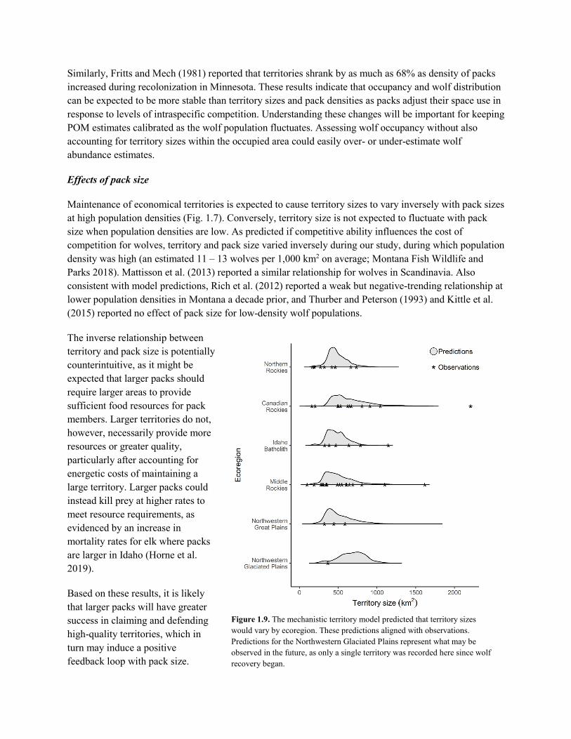
Similarly, Fritts and Mech (1981) reported that territories shrank by as much as 68% as density of packs increased during recolonization in Minnesota. These results indicate that occupancy and wolf distribution can be expected to be more stable than territory sizes and pack densities as packs adjust their space use in response to levels of intraspecific competition. Understanding these changes will be important for keeping POM estimates calibrated as the wolf population fluctuates. Assessing wolf occupancy without also accounting for territory sizes within the occupied area could easily over- or under-estimate wolf abundance estimates.

Effects of pack size

Maintenance of economical territories is expected to cause territory sizes to vary inversely with pack sizes at high population densities (Fig. 1.7). Conversely, territory size is not expected to fluctuate with pack size when population densities are low. As predicted if competitive ability influences the cost of competition for wolves, territory and pack size varied inversely during our study, during which population density was high (an estimated 11 – 13 wolves per 1,000 km2 on average; Montana Fish Wildlife and Parks 2018). Mattisson et al. (2013) reported a similar relationship for wolves in Scandinavia. Also consistent with model predictions, Rich et al. (2012) reported a weak but negative-trending relationship at lower population densities in Montana a decade prior, and Thurber and Peterson (1993) and Kittle et al. (2015) reported no effect of pack size for low-density wolf populations.

The inverse relationship between territory and pack size is potentially counterintuitive, as it might be expected that larger packs should require larger areas to provide sufficient food resources for pack members. Larger territories do not, however, necessarily provide more resources or greater quality, particularly after accounting for energetic costs of maintaining a large territory. Larger packs could instead kill prey at higher rates to meet resource requirements, as evidenced by an increase in mortality rates for elk where packs are larger in Idaho (Horne et al. 2019).

Based on these results, it is likely that larger packs will have greater success in claiming and defending high-quality territories, which in turn may induce a positive feedback loop with pack size.

Figure 1.9. The mechanistic territory model predicted that territory sizes would vary by ecoregion. These predictions aligned with observations. Predictions for the Northwestern Glaciated Plains represent what may be observed in the future, as only a single territory was recorded here since wolf recovery began.

Accordingly, where territories are estimated to be largest (e.g., through using Figs. 1.5 or 1.6), the packs within may be among the smallest observed.

Effects of mortality risk

Through maintaining economical territories, wolves may adjust their space use in relatively nuanced ways to mortality risk (Fig. 1.8). Territory size was predicted and observed empirically to increase and then decrease parabolically with an increase in human density, whereas overlap was predicted to have the opposite response. Mortality risk appears to be important for how wolves select territories; without this cost, some simulated packs attempted to settle urban areas, which they avoided when this cost contributed to the economics of territory ownership (Sells 2019). Urban areas often occur along Montana’s valley bottoms, which also attract ungulates. These areas almost certainly were once home to wolf packs until heavy habitation and mortality risk likely tipped the economic value for wolves. We expect that in areas with lower mortality risk, e.g., national parks, the risk of mortality from humans would be relatively unimportant to how wolves select territories.

Based on our results, the influence of humans on wolf behavior may be important for keeping POM estimates calibrated (Fig. 1.8). For the majority of Montana, territory sizes and resulting pack densities can be expected to vary slightly parabolically with human density (Sells 2019). Wolves can be expected to generally avoid areas with high human densities; few packs were predicted or observed to maintain territories with > 15 humans per km2. The influence of human-caused mortalities on territory size and pack size was assessed in Sections 1.4 and 1.5; however, Fig. 1.5 also provided relevant predictions: greater mortalities are likely to be associated with an increase in territory size because mortalities reduce pack size (Sect. 1.5).

General spatial trends in territory size

Economical territory selection was predicted to lead to spatial variation in means and ranges of territory sizes. Density plots of predicted territory sizes by ecoregion are expected to better depict the true variation in territories for the state of Montana than could be summarized from limited empirical observations (Fig. 1.9). Spatial variation in territories can arise through disparities in any one benefit or cost of territory ownership (e.g., prey or pack densities), or as an outcome of the interacting effects of these benefits and costs. Spatial variation in mean territory size would influence the local densities of packs, and the abundance estimates from POM. Accordingly, this spatial variation in territory sizes can be incorporated into POM to improve accuracy of abundance estimates.

Figure 1.10. The mechanistic territory model reliably predicted the sizes of specific territories compared to what was observed empirically in packs with GPS collars.

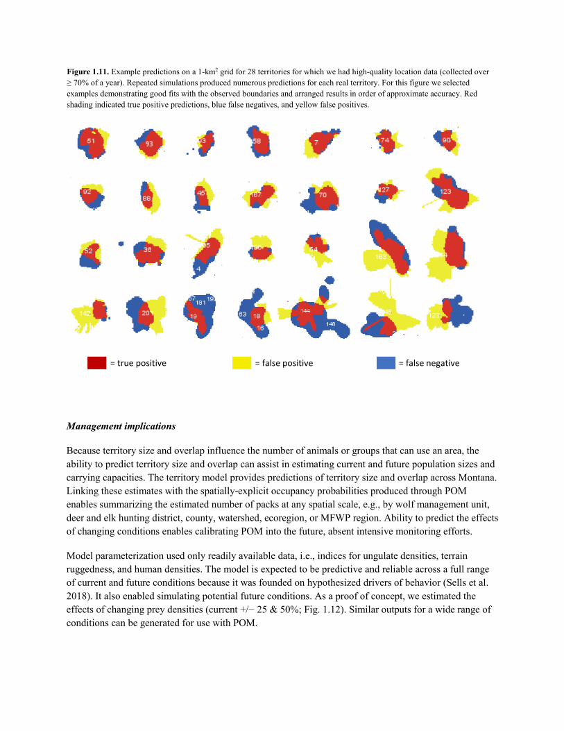
Management implications

Because territory size and overlap influence the number of animals or groups that can use an area, the ability to predict territory size and overlap can assist in estimating current and future population sizes and carrying capacities. The territory model provides predictions of territory size and overlap across Montana. Linking these estimates with the spatially-explicit occupancy probabilities produced through POM enables summarizing the estimated number of packs at any spatial scale, e.g., by wolf management unit, deer and elk hunting district, county, watershed, ecoregion, or MFWP region. Ability to predict the effects of changing conditions enables calibrating POM into the future, absent intensive monitoring efforts.

Model parameterization used only readily available data, i.e., indices for ungulate densities, terrain ruggedness, and human densities. The model is expected to be predictive and reliable across a full range of current and future conditions because it was founded on hypothesized drivers of behavior (Sells et al. 2018). It also enabled simulating potential future conditions. As a proof of concept, we estimated the effects of changing prey densities (current +/− 25 & 50%; Fig. 1.12). Similar outputs for a wide range of conditions can be generated for use with POM.

Figure 1.11. Example predictions on a 1-km2 grid for 28 territories for which we had high-quality location data (collected over ≥ 70% of a year). Repeated simulations produced numerous predictions for each real territory. For this figure we selected examples demonstrating good fits with the observed boundaries and arranged results in order of approximate accuracy. Red shading indicated true positive predictions, blue false negatives, and yellow false positives.

= true positive = false positive = false negative

1.4 Empirical Territory Size Models

We developed empirical models to further summarize and predict patterns in territory sizes of wolves in Montana. Our hypotheses were the same as outlined in Sect. 1.3 and detailed in Sells (2019, Chapter 2). We also included control removals (lethal removals of wolves in response to livestock depredations) to measure the effects of direct mortality on territory size. We hypothesized that mortality risk from humans is a primary cost of territoriality for wolves (Sect. 1.3). Wolves are intelligent and adaptable (Packard 2003), and often avoid humans (W hittington et al. 2004, Hebblewhite and Merrill 2008, Latham et al. 2011). Whether permanent or limited to specific times of day or seasons, avoidance of sites associated with mortality risk could necessitate expansion of the territory to maintain its economic value. Accordingly, we hypothesized that territory size would increase if wolves avoid areas where conspecifics were recently killed via control removals within the territory.

Methods

We generated explanatory variables for empirically-observed territory sizes (Sect. 1.2) using Program R (R Core Team 2018). To represent prey resources, we estimated densities of ungulates (deer, elk, and moose) in summer and winter (Sect. 1.3). We measured the mean prey densities within an area equivalent to the geometric mean territory size identified around the pack’s KDE centroid (Sect. 1.2). We calculated competition as the average number of neighboring packs (those with territory centroids ≤ 25 km of a pack’s KDE) in year T and T+1 per 100 km2 in territory size (Rich et al. 2012). We estimated pack size as the mean of sizes reported in year T and T+1 (Coltrane et al. 2015; Bradley et al. 2015; Boyd et al. 2017; Montana Fish Wildlife and Parks 2018). We included reported removals (harvest, dispersal, etc.) because these wolves were present for part of the year. We identified the number of control removals reported for the pack in year T and T+1 through MFWP annual reports (Coltrane et al. 2015; Bradley et al. 2015; Boyd et al. 2017; Montana Fish Wildlife and Parks 2018). Averaging data from calendar year T of collar deployment and year T+1

Figure 1.12. Example predictions from the mechanistic territory model for potential conditions wolves may encounter. In this scenario, prey densities have decreased or increased from current levels. Density plots show that the population mean territory size (Panel A) increased and overlap (Panel B) decreased as prey density declined; the range in territory sizes also increased. As prey density increased, mean territory size declined and overlap increased.

represented conditions that better matched the timing of collar deployment because collars were deployed at variable times of year. Where data for variables were unavailable in 2018 or 2019, we used the most recent year available.

We built 25 competing a priori generalized linear mixed models (GLMMs) in R package lme4 (Bates et al. 2015). Models represented different hypotheses for which benefits or costs best predicted territory size (Sells 2019). Models had multiple fixed effects plus a random effect for pack (family = Gaussian, link = log). We identified the most supported models using Akaike’s information criterion corrected for small sample size (AICc; Burnham and Anderson 2002) with a cut-off of ∆AICc = 4 (Anderson et al. 2001). Results were based on centered and scaled variables (units accordingly were standard deviations from the mean).

To evaluate the territory size model, we dropped each pack in turn, refit the model, and predicted the missing pack’s territory size. We estimated a linear regression of observed versus predicted territory sizes. If the slope estimate’s 95% CI overlapped 1.0, we considered the predictive model to reliably estimate territory size (Rich et al. 2012, Sells 2019).

Results

The top GLMM included the summer and winter ungulate indices, competition, pack size, and control removals (Fig. 1.13; Table 1.2). No others models were < 4 ∆AICc. Territory size had no relationship with the ungulate indices, negative relationships with competition and pack size, and a positive relationship with control removals. The model reliably estimated territory size (Fig. 1.14; Table 1.2). The slope from the linear regression of observed versus predicted territory sizes overlapped 1.0 (ß = 0.81, 95% CI = 0.439, 1.185, adjusted R2 = 0.30, F1,41 = 19.32, P < 0.001).

Because the top model included pack size and these data may be unavailable in the future due to decreased monitoring effort (Inman et al. 2019), we fit a second model omitting this variable. Although model support dropped (Table 1.2) and performance slightly decreased, the linear regression of observed versus predicted territory sizes also overlapped 1.0 (ß = 0.73, 95% CI = 0.386, 1.069, adjusted R2 = 0.29, F1,41 = 18.49, P < 0.001). Covariate estimates were similar to the original top model, except the winter ungulate index had a negative relationship with territory size (Fig. 1.13).

Figure 1.13. Top-supported GLMMs for territory sizes of wolves in Montana. The original top GLMM included group counts; because these data may not be available in the future, we refit a variation of this model omitting this variable. Thick bars are the 90% confidence intervals (CIs), and thinner tails the 95% CIs.

Discussion

The top empirical territory size model successfully predicted territory sizes of wolf packs in Montana. It furthermore was consistent with the hypothesis that wolves select territories economically (Fig. 1.13; Table 1.2; further details in Sells 2019, Chapter 2). This work contributes further evidence and understanding for how benefits and costs of territory ownership influence territorial behavior and resulting territory sizes.

The top model revealed interesting effects of prey (Fig. 1.13). As expected (Sect. 1.3), territory size had a negative-trending relationship with winter ungulate densities, but a positive-trending relationship with summer ungulate densities. Both these effects were uncertain. Based on conclusions from the mechanistic territory model and additional empirical analyses (Sells 2019, Chapter 2), our results suggest that wolves may optimize their territories first to prey densities that will be available in winter and secondly to those in summer. Optimization to winter ungulate densities would cause territory size to decline with increased winter ungulate densities (Sect. 1.3; Fig. 1.5). Many wolves disperse in winter (Jimenez et al. 2017), meaning they select territories when winter prey resources are a priority. Because ungulate winter range

Table 1.2. Top multi-variable models for territory sizes. Effects are reported on the log scale, and are centered and scaled. Model structure: variable × ß(2.5% CI, 97.5% CI) Log(l) ∆AICc

With pack counts

Bintercept × 6.21 (6.045, 6.383) + ungulatesummer × 0.10 (−0.045, 0.251) + ungulatewinter × −0.13 (−0.283, 0.031) + competition × −0.52 (−0.604, −0.431) + packsize × −0.16 (−0.240, −0.086) + controlremovals × 0.18 (0.140, 0.225)

−380.1 0

Without pack counts

Bintercept × 6.25 (6.054, 6.437) + ungulatesummer × 0.12 (−0.044, 0.285) + ungulatewinter × −0.25 (−0.412, −0.084) + competition × −0.63 (−0.714, −0.550) + controlremovals × 0.16 (0.115, 0.205)

−388.4 13.65

Figure 1.14. Predicted versus observed territory sizes for 28 packs in Montana. The original top GLMM included group size; because these data may not be available in the future, we tested a variation of this model omitting this variable. We considered the model reliable if the 95% confidence interval of the linear regression of predicted versus observed sizes included 1.0.

generally differs from summer range, territories optimized for winter may have fewer summer prey resources unless expanded to encompass ungulate summer range.

Results were consistent with the hypothesis that competition and mortality risk are primary costs of territorial behavior (Fig. 1.13). As predicted by the mechanistic model (Sect. 1.3) and consistent with earlier research in Montana (Rich et al. 2012), territory sizes were negatively related to the density of neighboring territories. Researchers in Scandinavia reported that territory sizes were only potentially negatively related to competition (Mattisson et al. 2013); however, we expect this uncertainty was caused by a different measure of competition (a raw number of nearby packs, whereas we scaled by the pack’s territory size). As predicted if wolves avoid areas where humans recently killed wolves, greater mortalities by control removals were associated with larger territories. Previous empirical work demonstrated that wolves avoid humans and areas associated with human hazards (Whittington et al. 2004, Hebblewhite and Merrill 2008, Latham et al. 2011). Rich et al. (2012) also reported a positive relationship between territory size and control removals for wolves in Montana a decade prior.

Management implications

By affecting the number of packs that may exist in a given area, territory size directly influences POM estimates (Fig. 1.1). Whereas estimating territory size has previously relied on deploying costly radio- and GPS-collars, our predictive model reliably estimated territory sizes absent data for wolf locations or territory boundaries. The predictive model can thus be used alongside the mechanistic territory model as an additional means to estimate territory size and keep POM estimates calibrated into the future. Ongoing work will integrate the application of both the mechanistic and empirical territory models for use with POM.

1.5 Pack Size Model

Sociality strongly shapes demographic processes. In addition to births and deaths, wolf pack size is influenced by dispersal decisions. We aimed to better understand mechanisms influencing pack size, and to develop a tool for predicting pack size for POM, absent data directly related to births and dispersals because these data will be largely unavailable to MFWP.

We hypothesized that conditions related to prey, competition, and mortality risk would influence births, deaths, and dispersals, and in turn wolf pack sizes. We expected that pack size would increase with prey abundance (Mech and Boitani 2003). If subordinates cannot meet their food requirements, they should likely disperse; additionally, dominant individuals might increase aggression or decrease subordinates’ food shares to further encourage dispersal (Mech 1999, Peterson and Ciucci 2003). Greater prey abundance conversely may increase the pack sizes that can be maintained, allowing dominants to tolerate subordinates and accept immigrants, and enticing subordinates to stay. Because wolves in Montana prey on ungulates that migrate seasonally, we further hypothesized that prey abundance either in summer or winter could have greater relative influences on pack size. Wolves produce a litter of on average 5 – 6 pups each spring (Fuller et al. 2003). Where summer prey abundance is low, this influx of new pack members could both decrease survival and influence subordinates to disperse. Alternatively, winter prey abundance may be more influential because pups reach full size and thus require greater food shares by winter (Mech and Boitani 2003). We also hypothesized that greater terrain ruggedness could negatively influence pack size by decreasing the availability of ungulates because wolves are coursing predators

(Peterson and Ciucci 2003) who may make more kills at lower elevations (McPhee et al. 2012) and may have lower hunting success in rugged terrain (Rich et al. 2012).

We hypothesized that the density of conspecific packs could affect pack size by influencing dispersal decisions. A high density of packs near an animal’s natal home range or territory could signal insufficient space for new home ranges and greater risks of mortality during dispersal, causing less dispersal and larger packs. Dominant individuals could also be more tolerant of subordinates and immigrants at high densities, when territorial disputes may increase and having a larger pack can increase the odds of winning confrontations (Cassidy et al. 2015). We expected that a low density of packs near an animal’s natal home range could signal greater odds of finding space, increasing dispersal and decreasing pack size to yield a positive relationship between pack size and density of packs (Fritts and Mech 1981, Boyd et al. 1995, Jimenez et al. 2017).

We hypothesized that mortalities and the risk of mortality influence pack size. Although mortalities can directly decrease pack size, we also hypothesized that as the risk of dying increases, subordinates may disperse to avoid this risk. If larger packs are more easily detected by humans, greater risk of mortality could likewise lead to smaller packs because dominants may tolerate subordinates less and subordinates may disperse to reduce their risk. Mortalities could also lead packs to disband in response (Brainerd et al. 2008). Alternatively, mortalities could cause pack size to increase if decreased survival leads to compensation through increased reproduction or larger litters. The risk of mortality could also lead to larger packs through decreased dispersal or greater immigration if mortality risk is diluted in larger packs.

We hypothesized that a number of factors would influence mortality risk to wolves in Montana. The local density of harvest mortalities may both directly influence survival and the perceived mortality risk of survivors. The type of harvest (hunting versus trapping) could also be influential. Control removals also directly affect pack size, and may influence survivors’ perceived mortality risk. The intensity of harvest management may further influence mortality risk. Mortality risk could also increase with low-use roads, which humans may use while hunting or otherwise recreating.

Methods

We analyzed pack size for wolves in Montana from 2005 – 2018. MFWP wolf specialists monitored packs through radio-tracking, camera-trapping, and aerial surveys from 2005 – 2018 to count pack members and estimate year-end pack sizes. They classified counts as good, moderate, or poor quality. We retained only good quality counts for our analyses (D. Boyd, A. Nelson, T. Parks, and T. Smucker, MFWP, pers. comm.). Counts considered to be of good quality were from packs documented multiple times each year using trail cameras, visual sightings, or track surveys; public reports also approximated the counts of wolf specialists. Wolf specialists estimated an annual territory centroid for each pack using either their expert knowledge or location data from wolf collars (radio or global positioning system), where available.

Data for covariates

We estimated local conditions related to prey, competition, and mortality risk using spatial data. We measured the mean value of each spatial covariate within a 483.62 km2 area (hereafter, the approximate territory, i.e., the geometric mean territory size for wolves in Montana, 2014 – 2019; Table 1.1) around

the pack’s annual territory centroid. We measured prey densities as described in Sect 1.3. For competition, we measured the mean density of territory centroids per 1000 km2 using the kernel smoothed intensity function in R package spatstat (Baddeley et al. 2015) with sigma set to 25 km. From the hunter-reported locations of harvested wolves each year, we measured mortality risk within each pack’s approximate territory as the density of harvest mortalities per 1000 km2 using the kernel smoothed intensity function in R package spatstat (Baddeley et al. 2015) with a sigma of 25 km. We derived pack-specific control removals from MFWP annual reports (fwp.mt.gov). We classified the intensity of harvest management as hunting seasons with no harvest (< 2009 and 2010), restricted harvest (2009 and 2011; when seasons were shorter, bag limits were low, and trapping was prohibited), and liberal harvest (2012 on, when seasons were longer, bag limits were higher, and trapping was allowed; fwp.mt.gov).

Analyses

We built 24 competing a priori generalized linear models (GLMs; family = Poisson) in R (R Core Team 2018), representing factors we hypothesized most influenced pack size (Sells 2019). We included variables for the density of harvest mortalities, number of control removals, and intensity of harvest management in each model because these mortality variables directly influence pack size. We avoided combining overly-correlated variables (> 0.6 Spearman’s rank correlation; Sells 2019) in the same model (Dormann et al. 2013). We identified the most supported models using Akaike’s information criterion (AIC; Burnham and Anderson 2002) with a cut-off of 4 ∆AIC (Anderson et al. 2001) and Akaike weights (𝜔𝜔𝑖𝑖; Burnham and Anderson 2002). To further understand the effects of harvest on pack size, we conducted single-variable analyses on the effects of hunting and trapping. We reported results based on centered and scaled variables, with resulting units representing standard deviations from the mean.

We tested the predictive performance of supported models by dropping each observation from the dataset in turn, refitting the model, and predicting the missing pack’s size. We then averaged annual observed and predicted pack sizes and fit a linear regression. If the regression slope estimate’s 95% CI overlapped 1.0, we considered the predictive model to reliably estimate annual mean pack size.

Results

From 2005 – 2018, MFWP monitored 46 – 152 packs per year for a total of 1531 pack-years. Of these, 26 – 68 packs per year had good quality counts, yielding 660 total pack-years for analysis. Annual mean pack size ranged 4.86 – 7.03 and overall mean pack size was 5.92 (Fig. 1.15).

Based on AIC, only the top-ranked model had support (𝜔𝜔𝑖𝑖 = 1). The model revealed positive relationships between pack size and density of prey in summer and density of packs (Fig. 1.16; Table 1.3). It revealed negative relationships between pack size and terrain ruggedness, number of control removals, intensity of harvest management, and density of low-use roads. Although the model contained the density of harvest mortalities, this variable had no effect. The model reliably estimated mean pack size (Fig. 1.17), as the slope from the linear regression of observed versus predicted annual mean pack sizes included 1.0 (ß = 1.03, 95% CI = 0.484, 1.583, adjusted R2 = 0.58, F1,12 = 16.81, P < 0.002).

Single-variable analyses revealed additional evidence for the effects of hunting and trapping (Fig. 1.18). The density of harvest mortalities (i.e., combined hunting and trapping mortalities), density of trapping mortalities, number of control removals, and intensity of harvest management had negative relationships with pack size. There was no relationship between pack size and the density of hunting mortalities.

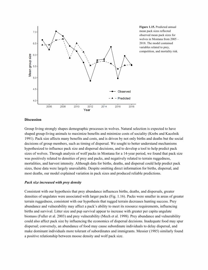
Discussion

Group living strongly shapes demographic processes in wolves. Natural selection is expected to have shaped group-living animals to maximize benefits and minimize costs of sociality (Krebs and Kacelnik 1991). Pack size affects many benefits and costs, and is driven by not only births and deaths but the social decisions of group members, such as timing of dispersal. We sought to better understand mechanisms hypothesized to influence pack size and dispersal decisions, and to develop a tool to help predict pack sizes of wolves. Through analysis of wolf packs in Montana for a 14-year period, we found that pack size was positively related to densities of prey and packs, and negatively related to terrain ruggedness, mortalities, and harvest intensity. Although data for births, deaths, and dispersal could help predict pack sizes, these data were largely unavailable. Despite omitting direct information for births, dispersal, and most deaths, our model explained variation in pack sizes and produced reliable predictions.

Pack size increased with prey density

Consistent with our hypothesis that prey abundance influences births, deaths, and dispersals, greater densities of ungulates were associated with larger packs (Fig. 1.16). Packs were smaller in areas of greater terrain ruggedness, consistent with our hypothesis that rugged terrain decreases hunting success. Prey abundance and vulnerability may affect a pack’s ability to meet its resource requirements, influencing births and survival. Litter size and pup survival appear to increase with greater per capita ungulate biomass (Fuller et al. 2003) and prey vulnerability (Mech et al. 1998). Prey abundance and vulnerability could also affect pack size by influencing the economics of dispersal decisions. Inadequate food may spur dispersal; conversely, an abundance of food may cause subordinate individuals to delay dispersal, and make dominant individuals more tolerant of subordinates and immigrants. Messier (1985) similarly found a positive relationship between moose density and wolf pack size.

Figure 1.15. Predicted annual mean pack sizes reflected observed mean pack sizes for wolves in Montana from 2005 – 2018. The model contained variables related to prey, competition, and mortality risk.

Densities of ungulates in summer were especially predictive of pack sizes in Montana (Fig. 1.16), consistent with our hypothesis that prey shortages in summer could both reduce survival and trigger dispersal as a result of an increased demand on the food supply. We expected that summer ungulate availability would be important because our summer season encompassed both the springtime influx of pups and the peak of pup food needs each fall (Mech and Boitani 2003). Previous studies have shown that wolves dispersed at greater rates in response to a lower prey base (Messier 1985), increased food stress (Peterson and Page 1988), and lower per capita ungulate biomass (Fuller et al. 2003), supporting the possibility that pack size in Montana is influenced by dispersal in response to prey abundance.

This understanding of the effects of prey density on pack size can help calibrate POM estimates. Packs can be expected to generally be larger where prey abundance is higher. Because territories were predicted to be smaller (Sect. 1.3) and pack densities higher in areas of high prey densities, altogether the densities of wolves are likely to peak where prey densities are greatest. Managing for large ungulate populations may therefore increase wolf numbers unless more wolves are harvested in the area.

Pack size increased with density of packs

A positive relationship between density of packs and pack size was consistent with our hypothesis that the density of packs may affect both survival and the economics of social decisions (Fig. 1.16). This supported our expectation that wolves could potentially maximize their fitness by dispersing at low pack densities to seek their own territories in which to breed, whereas high pack densities

Figure 1.16. The top predictive model for wolf pack sizes in Montana included variables related to prey, competition, and mortality risk. Thicker line segments represented 90% CIs, full lines represented 95% CIs, and points represented mean estimates.

Table 1.3. Variables and their 95% confidence intervals (CI)s from a predictive model for wolf pack size in Montana. Data were centered and scaled, and are reported on the log scale.

Variable β CIlower CIupper Intercept 1.92 1.844 1.992 Summer ungulate density 0.05 0.021 0.085 Density of packs 0.06 0.024 0.104 Terrain ruggedness −0.08 −0.118 −0.046 Harvest mortality density 0.00 −0.038 0.047 Control removals −0.09 −0.130 −0.049 Restricted harvest −0.13 −0.232 −0.026 Liberal harvest −0.24 −0.343 −0.130 Low-use road density −0.06 −0.093 −0.025

could cue subordinates that dispersal is uneconomical, increasing pack size as a result. High pack densities may also increase the benefit of having a large pack by strengthening its competitive ability (Cassidy et al. 2015) and success in defending its territory (Sells 2019). Larger packs at high pack densities could thus also be driven by dominants’ increased acceptance of immigrants. Our results contribute further evidence that carnivore dispersal is influenced by densities of conspecific groups. Previous research showed that wolf dispersal rates declined as did the odds of successful dispersal as density of packs increased when wolves were recolonizing Montana (Jimenez et al. 2017). Evidence of similar changes in dispersal in relation to conspecific density have been reported for lions (Panthera leo; VanderWaal et al. 2009) and Ethiopian wolves (C. simensis; Sillero-Zubiri et al. 1996).

Understanding how pack densities influence pack size can help calibrate POM. Smaller packs can be expected where pack densities are low, such as areas of recent recolonization or high mortality (e.g., through control removals). If this relationship is caused by dispersal, as hypothesized, then these same areas could have relatively rapid colonization. After the territory mosaic begins to fill in, however, pack size should generally increase and territories should compress (Sect. 1.3), causing relatively high wolf densities.

Pack size decreased with greater mortality risk

Greater control removals, harvest intensity, and low-use road densities were predictive of and negatively associated with pack sizes (Fig. 1.16; Table 1.3). These mortality-related factors may of course directly decrease pack size by decreasing survival of pack members. Smaller packs in areas of greater mortalities could also be an outcome, however, of greater dispersal among surviving pack members in response to increased mortality risk.

Trapping appeared to have a greater effect on pack size than hunting. Single-variable analyses demonstrated that general harvest (accounting for both hunting and trapping) and density of trapping mortalities were associated with decreased pack size, whereas density of hunting mortalities was not (Fig. 18). Similarly, a restricted harvest intensity (with lower bag limits and no trapping) had a weaker relationship with pack size than a liberal harvest intensity (with higher bag limits and both hunting and trapping). Hunting mortalities notably exceeded trapping mortalities each year since the advent of modern harvest management in Montana (Fig. 1.19). The lack of association between pack size and hunting mortalities and strong relationship with trapping mortalities therefore suggests there are important differences in survival and dispersal decisions in relation to type of harvest. Wolf hunters in Montana have tended to be opportunistic and often kill only one wolf per hunter, although a pack may

Figure 1.17. Predicted mean pack sizes were reliable because the 95% CI of the linear regression of predicted versus observed sizes encompassed a regression of slope 1.0 (dashed line; Rich et al. 2012).

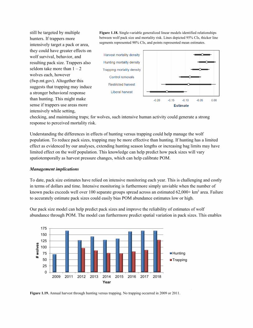
still be targeted by multiple hunters. If trappers more intensively target a pack or area, they could have greater effects on wolf survival, behavior, and resulting pack size. Trappers also seldom take more than 1 – 2 wolves each, however (fwp.mt.gov). Altogether this suggests that trapping may induce a stronger behavioral response than hunting. This might make sense if trappers use areas more intensively while setting, checking, and maintaining traps; for wolves, such intensive human activity could generate a strong response to perceived mortality risk.

Understanding the differences in effects of hunting versus trapping could help manage the wolf population. To reduce pack sizes, trapping may be more effective than hunting. If hunting has a limited effect as evidenced by our analyses, extending hunting season lengths or increasing bag limits may have limited effect on the wolf population. This knowledge can help predict how pack sizes will vary spatiotemporally as harvest pressure changes, which can help calibrate POM.

Management implications

To date, pack size estimates have relied on intensive monitoring each year. This is challenging and costly in terms of dollars and time. Intensive monitoring is furthermore simply unviable when the number of known packs exceeds well over 100 separate groups spread across an estimated 62,000+ km2 area. Failure to accurately estimate pack sizes could easily bias POM abundance estimates low or high.

Our pack size model can help predict pack sizes and improve the reliability of estimates of wolf abundance through POM. The model can furthermore predict spatial variation in pack sizes. This enables

Figure 1.18. Single-variable generalized linear models identified relationships between wolf pack size and mortality risk. Lines depicted 95% CIs, thicker line segments represented 90% CIs, and points represented mean estimates.

z

Figure 1.19. Annual harvest through hunting versus trapping. No trapping occurred in 2009 or 2011.

0255075

100125150175

2009 2011 2012 2013 2014 2015 2016 2017 2018

# w

olve

s

Year

Hunting

Trapping

estimating wolf abundances at finer scales than the statewide level, e.g., at MFWP regional scales. It also provides a means for predicting the effects of various harvest management decisions or control removal actions on pack sizes and wolf abundances.

1.6 Integration of Models with POM

Final deliverables from this work will include integrating the territory and pack size models into POM. We are currently using the predictive models to develop spatial layers for territory size, territory overlap, and pack size, which we will integrate with the occupancy model to seamlessly predict wolf abundance. The improved POM will be easily operable by MFWP. The final tools will include the ability to adjust and explore model inputs (e.g., prey abundance, harvest intensity, etc.) to predict the effects on wolf behavior and resulting wolf abundance estimates. The tools will include the ability to estimate abundance at both the state level and finer spatial scales (e.g., within each MFWP region). POM estimates will also be incorporated into the adaptive harvest management model (Study Objective #3).

Acknowledgements

For support and guidance throughout my PhD project, I thank committee members M. Mitchell, D. Ausband, D. Emlen, A. Luis, D. Pletscher, K. Podruzny, and H. Robinson. I thank MFWP wolf specialists, D. Boyd, L. Bradley, N. Lance, K. Laudon, A. Nelson, T. Parks, M. Ross, and T. Smucker, as well as technicians and volunteers, for their invaluable support and effort in trapping and collaring wolves for this work. MFWP biologists, researchers, and staff also provided support, including J. Gude, B. Inman, J. Vore, K. Proffitt, N. DeCesare, and numerous area biologists. S. Courville provided ungulate data from the Confederated Salish and Kootenai Tribes. I also thank C. Waters, S. Bassing, K. Barker, A. Keever, J. Nowak, and K. Loonam. This work was supported by revenues from the sale of Montana hunting and fishing licenses, and a Federal Aid in Wildlife Restoration grant to Montana Fish, Wildlife and Parks. It was also supported by a W. A. Franke Wildlife Biology Graduate Fellowship.

Literature Cited

Adams, E. S. 2001. Approaches to the study of territory size and shape. Annual Review of Ecology and Systematics 32:277–303.

Adams, L. G., R. O. Stephenson, B. W. Dale, R. T. Ahgook, and D. J. Demma. 2008. Population dynamics and harvest characteristics of wolves in the Central Brooks Range, Alaska. Wildlife Monographs 170:1–25.

Anderson, D. R., W. A. Link, D. H. Johnson, and K. P. Burnham. 2001. Suggestions for presenting the results of data analyses. Journal of Wildlife Management 65:373–378.

Ausband, D. E. 2015. Groups and mortality: their effects on cooperative behavior and population growth in a social carnivore. University of Montana.

Baddeley, A., E. Rubak, and R. Turner. 2015. Spatial Point Patterns: Methodology and Applications with R. Chapman and Hall/CRC Press, London, United Kingdom.

Bates, D., M. Maechler, B. Bolker, and S. Walker. 2015. lme4. <http://cran.r-project.org/package=lme4>.

Boitani, L., P. Ciucci, and A. Mortelliti. 2012. Designing carnivore surveys. Pages 8–30 in. Carnivore Ecology and Conservation A Handbook of Techniques. Oxford University Press, Oxford, United Kingdom.

Borg, B. L., S. M. Brainerd, T. J. Meier, and L. R. Prugh. 2014. Impacts of breeder loss on social structure, reproduction and population growth in a social canid. Journal of Animal Ecology.

Boyd, D., J. Gude, B. Inman, N. Lance, A. Messer, A. Nelson, T. Parks, M. Ross, T. Smucker, J. Steuber, and J. Vore. 2017. Montana Gray Wolf Conservation and Management 2016 Annual Report. <http://fwp.mt.gov/fishAndWildlife/management/wolf/>.

Boyd, D. K., P. C. Paquet, S. Donelon, R. R. Ream, D. H. Pletscher, and C. C. White. 1995. Transboundary movements of a recolonizing wolf population in the Rocky Mountains. Pages 135–140 in L. N. Carbyn, S. H. Fritts, and D. R. Seip, editors. Ecology and Conservation of Wolves in a Changing World. Canadian Circumpolar Institute, Edmonton, Alberta.

Bradley, L., J. Gude, N. Lance, K. Laudon, A. Messer, A. Nelson, G. Pauley, M. Ross, T. Smucker, J. Steuber, and J. Vore. 2015. Montana Gray Wolf Conservation and Management 2014 Annual Report. <http://fwp.mt.gov/fishAndWildlife/management/wolf/>.

Brainerd, S. M., H. Andren, E. E. Bangs, E. H. Bradley, J. A. Fontaine, W. Hall, Y. Iliopoulos, M. D. Jimenez, E. A. Jozwiak, O. Liberg, C. M. Mack, T. J. Meier, C. C. Niemeyer, H. C. Pedersen, H. Sand, R. N. Schultz, D. W. Smith, P. Wabakken, and A. P. Wydeven. 2008. The effects of breeder loss on wolves. Journal of Wildlife Management 72:89–98.

Brown, J. L. 1964. The evolution of diversity in avian territorial systems. The Wilson Bulletin 76:160–169.

Burnham, K. P., and D. R. Anderson. 2002. Model Selection and Multi-model Inference: A Practical Information–theoretic Approach. 2nd edition. Springer, New York.

Calenge, C. 2006. The package adehabitat for the R software: a tool for the analysis of space and habitat use by animals. Ecological Modelling 197:516–519.

Carpenter, F. L. 1987. Food abundance and territoriality: to defend or not to defend? American Zoologist 27:387–399.

Cassidy, K. A., D. R. MacNulty, D. R. Stahler, D. W. Smith, and L. D. Mech. 2015. Group composition effects on aggressive interpack interactions of gray wolves in Yellowstone National Park. Behavioral Ecology 26:1352–1360.

Coltrane, J., J. Gude, B. Inman, N. Lance, K. Laudon, A. Messer, A. Nelson, T. Parks, M. Ross, T. Smucker, J. Steuber, and J. Vore. 2015. Montana gray wolf conservation and management plan : 2015 annual report. <http://fwp.mt.gov/fishAndWildlife/management/wolf/>.

Darwin, C. 1859. On the Origin of the Species. John Murray, London.

Dormann, C. F., J. Elith, S. Bacher, C. Buchmann, G. Carl, G. Carré, J. R. G. Marquéz, B. Gruber, B. Lafourcade, P. J. Leitão, T. Münkemüller, C. McClean, P. E. Osborne, B. Reineking, B. Schröder, A. K. Skidmore, D. Zurell, and S. Lautenbach. 2013. Collinearity: a review of methods to deal with it and a simulation study evaluating their performance. Ecography 36:027–046.

Dusek, G., A. Wood, S. Hoekman, C. Sime, and J. Morgan. 2006. Ecology of white-tailed deer in the Salish Mountains, Northwest Montana. Final Report, Federal Aid in Wildlife Restoration project W-120-R, Montana Fish, Wildlife, and Parks. Helena, Montana, Montana.

Emlen, S. T., and L. W. Oring. 1977. Ecology, sexual selection, and the evolution of mating systems. Science 197:215–223.

Evans, J. S. 2018. spatialEco. <https://cran.r-project.org/package=spatialEco>.

Foresman, K. R. 2001. The Wild Mammals of Montana. American Society of Mammalogists, Lawrence, Kansas, Kansas.

Fritts, S. H., and L. D. Mech. 1981. Dynamics, movements, and feeding ecology of a newly protected wolf population in northwestern Minnesota. Wildlife Monographs 80:3–79.

Fritts, S. H., R. O. Stephenson, R. D. Hayes, and L. Boitani. 2003. Wolves and humans. Pages 289–316 in L. D. Mech and L Boitani, editors. Wolves: Behavior, Ecology and Conservation. University Of Chicago Press.

Fuller, T. K., L. D. Mech, and J. Fitts-Cochran. 2003. Wolf population dynamics. Pages 161–191 in L. D. Mech and L. Boitani, editors. Wolves: Behavior, Ecology and Conservation. University of Chicago Press, Chicago, Illinois.

Hebblewhite, M., and E. Merrill. 2008. Modelling wildlife-human relationships for social species with mixed-effects resource selection models. Journal of Applied Ecology 45:834–844.

Hixon, M. A. 1980. Food production and competitor density as the determinants of feeding territory size. The American Naturalist 115:510–530.

Hollister, J. W., and T. Shah. 2017. elevatr: access elevation data from various APIs. <http://github.com/usepa/elevatr>.

Inman, B., K. Podruzny, T. Smucker, A. Nelson, M. Ross, N. Lance, T. Parks, S. Boyd, and S. Wells. 2019. Montana gray wolf conservation and management 2018 annual report. Helena, Montana. <http://fwp.mt.gov/fishAndWildlife/management/wolf/>.

Jedrzejewski, W., K. Schmidt, J. Theuerkauf, J. Bogumiła, and R. Kowalczyk. 2007. Territory size of wolves Canis lupus: linking local (Białowieża Primeval Forest, Poland) and Holarctic-scale patterns. Ecography 30:66–76.

Jimenez, M. D., E. E. Bangs, D. K. Boyd, D. W. Smith, S. A. Becker, D. E. Ausband, S. P. Woodruff, E. H. Bradley, J. Holyan, and K. Laudon. 2017. Wolf dispersal in the Rocky Mountains, western United States: 1993–2008. Journal of Wildlife Management 81:581–592.

Johnson, D. H. 1980. The comparison of usage and availability measurements for evaluating resource preference. Ecology 61:65–71.

Krebs, J. R., and A. Kacelnik. 1991. Decision-making. Pages 105–136 in J. R. Krebs and N. B. Davies, editors. Behavioural Ecology: An Evolutionary Approach (Third Edition). Oxford University Press, Oxford, United Kingdom.

Latham, A. D. M., M. C. Latham, M. S. Boyce, and S. Boutin. 2011. Movement responses by wolves to industrial linear features and their effect on woodland caribou in northeastern Alberta. Ecological Applications 21:2854–2865.

Mattisson, J., H. Sand, P. Wabakken, V. Gervasi, O. Liberg, J. D. C. Linnell, G. R. Rauset, and H. C. Pedersen. 2013. Home range size variation in a recovering wolf population: evaluating the effect of environmental, demographic, and social factors. Oecologia 173:813–825.

McPhee, H. M., N. F. Webb, and E. H. Merrill. 2012. Hierarchical predation: wolf (Canis lupus) selection along hunt paths and at kill sites. Canadian Journal of Zoology 90:555–563.

Mech, L. D. 1999. Alpha status, dominance, and division of labor in wolf packs. Canadian Journal of Zoology 77:1196–1203.

Mech, L. D., L. G. Adams, T. J. Meier, J. W. Burch, and B. W. Dale. 1998. The Wolves of Denali. University of Minnesota Press, Minneapolis, Minnesota.

Mech, L. D., and L. Boitani. 2003. Wolf social ecology. Pages 1–34 in L. D. Mech and Luigi Boitani, editors. Wolves: Behavior, Ecology and Conservation. University Of Chicago Press, Chicago, IL.

Mech, L. D., and R. O. Peterson. 2003. Wolf-prey relations. Pages 131–160 in L. D. Mech and L. Boitani,

editors. Wolves: Behavior, Ecology and Conservation. University Of Chicago Press.

Messier, F. 1985. Social organization, spatial distribution, and population density of wolves in relation to moose density. Canadian Journal of Zoology 63:1068–1077.

Messier, F. 1985. Solitary living and extraterritorial movements of wolves in relation to social status and prey abundance. Canadian Journal of Zoology 63:239–245.

Miller, D. A. W., J. D. Nichols, J. A. Gude, L. N. Rich, K. M. Podruzny, J. E. Hines, and M. S. Mitchell. 2013. Determining occurrence dynamics when false positives occur: estimating the range dynamics of wolves from public survey data. PLoS ONE 8:1–9.

Mitchell, M. S., and R. A. Powell. 2004. A mechanistic home range model for optimal use of spatially distributed resources. Ecological Modelling 177:209–232.

Mitchell, M. S., and R. A. Powell. 2007. Optimal use of resources structures home ranges and spatial distribution of black bears. Animal Behaviour 74:219–230.

Mitchell, M. S., and R. A. Powell. 2012. Foraging optimally for home ranges. Journal of Mammalogy 93:917–928.

Montana Fish Wildlife and Parks. 2005. Biomedical protocol for free-ranging gray wolves (Canis lupus) in Montana: capture, anesthesia, surgery, tagging, sampling and necropsy procedures. Helena, Montana.

Montana Fish Wildlife and Parks. 2018. Montana Gray Wolf Conservation and Management 2017 Annual Report. Helena, Montana. <http://fwp.mt.gov/fishAndWildlife/management/wolf/>.

Montana Natural Heritage Program, and Montana Fish Wildlife and Parks. n.d. Montana Field Guide. <http://fieldguide.mt.gov>.

Mosser, A., and C. Packer. 2009. Group territoriality and the benefits of sociality in the African lion, Panthera leo. Animal Behaviour 78:359–370.

Musiani, M., and P. C. Paquet. 2004. The practices of wolf persecution, protection, and restoration in Canada and the United States. BioScience 54:50–60.

Packard, J. M. 2003. Wolf behavior: reproductive, social, and intelligent. Pages 35–65 in L. D. Mech and L. Boitani, editors. Wolves: Behavior, Ecology and Conservation. University Of Chicago Press.

Packer, C., D. Scheel, and A. E. Pusey. 1990. Why lions form groups: food is not enough. The American Naturalist 136:1–19. <http://www.jstor.org/stable/2556343>.

Pebesma, E. J. 2004. Multivariable geostatistics in S: the gstat package. Computers and Geosciences 683–691.

Peterson, R. O., and P. Ciucci. 2003. The wolf as a carnivore. Pages 105–130 in L. D. Mech and L. Boitani, editors. Wolves: Behavior, Ecology and Conservation. University Of Chicago Press.

Peterson, R. O., and R. E. Page. 1988. The rise and fall of Isle Royale wolves, 1975-1986. Journal of Mammalogy 69:89–99.

R Core Team. 2018. R: A language and environment for statistical computing. R Foundation for Statistical Computing, Vienna, Austria, Austria. <https://www.r-project.org/.>.

Rich, L. N., M. S. Mitchell, J. A. Gude, and C. A. Sime. 2012. Anthropogenic mortality, intraspecific competition, and prey availability influence territory sizes of wolves in Montana. Journal of Mammalogy 93:722–731.

Rich, L. N., R. E. Russell, E. M. Glenn, M. S. Mitchell, J. A. Gude, K. M. Podruzny, C. A. Sime, K. Laudon, D. E. Ausband, and J. D. Nichols. 2013. Estimating occupancy and predicting numbers of

gray wolf packs in Montana using hunter surveys. Journal of Wildlife Management 77:1280–1289.

Sappington, J. M., K. M. Longshore, and D. B. Thomson. 2007. Quantifying landscape ruggedness for animal habitat analysis: a case study using bighorn sheep in the Mojave Desert. Journal of Wildlife Management 71:1419–1426.

Sargeant, A. B., S. H. Allen, and J. O. Hastings. 1987. Spatial relations between sympatric coyotes and red foxes in North Dakota. The Journal of Wildlife Management 51:285–293.

Sells, S. N. 2019. Mechanisms driving territorial and social behavior in a cooperative carnivore. The University of Montana.

Sells, S. N., S. B. Bassing, K. J. Barker, S. C. Forshee, A. C. Keever, J. W. Goerz, and M. S. Mitchell. 2018. Increased scientific rigor will improve reliability of research and effectiveness of management. Journal of Wildlife Management 82:485–494.

Sikes, R. S., W. L. Gannon, and Animal Care and Use Committee of the American Society of Mammalogists. 2011. Guidelines of the American Society of Mammalogists for the use of wild mammals in research. Journal of Mammalogy 92:235–253.

Sillero-Zubiri, C., D. Gottelli, and D. W. Macdonald. 1996. Male philopatry, extra-pack copulations and inbreeding in Ethiopian avoidance wolves (Canis simensis). Behavioral Ecology and Sociobiology 38:331–340.

Sillero-Zubiri, C., M. Hoffmann, and D. W. Macdonald. 2004. Canids: Foxes, Wolves, Jackals and Dogs. Status Survey and Conservation Action Plan. Status Survey and Conservation Action Plan, IUCN. Gland, Switzerland and Cambridge, UK.

Sillero-Zubiri, C., and D. W. Macdonald. 1998. Scent-marking and territorial behaviour of Ethiopian wolves Canis simensis. Journal of Zoology 245:351–361.

Thurber, J. M., and R. O. Peterson. 1993. Effects of population density and pack size on the foraging ecology of gray wolves. Journal of Mammology 74:879–889.

Uboni, A., J. A. Vucetich, D. R. Stahler, and D. W. Smith. 2015. Interannual variability: a crucial component of space use at the territory level. Ecology 96:62–70.

VanderWaal, K. L., A. Mosser, and C. Packer. 2009. Optimal group size, dispersal decisions and postdispersal relationships in female African lions. Animal Behaviour 77:949–954. Elsevier Ltd.

Whittington, J., C. C. St. Clair, and G. Mercer. 2004. Path tortuosity and the permeability of roads and trails to wolf movement. Ecology and Society 9.

Whittington, J., C. C. St. Clair, and G. Mercer. 2005. Spatial responses of wolves to roads and trails in mountain valleys. Ecological Applications 15:543–553.

Wilensky, U. 1999. NetLogo. Center for Connected Learning and Computer-Based Modeling, Northwestern University, Evanston, IL. <http://ccl.northwestern.edu/netlogo/>.

Worton, B. J. 1989. Kernel methods for estimating the utilization distribution in home-range studies. Ecology 70:164–168.

OBJECTIVE 2: IMPROVE ESTIMATION OF RECRUITMENT—Allison Keever, Project 2

ABSTRACT Breeding pairs (a male and female wolf with ≥2 pups at December 31) have been documented for wolves in the NRM as a metric for recruitment. Breeding pairs, however, are an ineffective measure of recruitment. Our objectives were to develop methods to estimate recruitment that were more biologically credible without data for recruitment. We first developed and tested an empirical model to estimate the number of pups per pack and the total number of pups recruited without recruitment data. We then developed a predictive model of recruitment based on the components of recruitment: the probability a pack reproduced, the probability a pack contained > 1 breeding female, litter size, and pup survival. This model was based on empirical models of the components developed in Idaho with recruitment data, and provided an estimate of the number of pups per pack. Recruitment of wolves in Montana varied annually, and was negatively correlated with abundance and harvest, and positively correlated with pack size. With the component model, we accurately predicted recruitment for wolves in Montana. These methods provided a more effective measure of recruitment than breeding pairs, and could be implemented without recruitment data.

2.1 Introduction

Estimating recruitment (i.e., number of young produced that survive to an age at which they contribute to the population) of wolves is difficult due to the size of the wolf population and limited time and funding for monitoring. Currently, MFWP documents recruitment based on visual counts of breeding pairs (a male and female wolf with 2 surviving pups by December 31; U.S. Fish and Wildlife Service 1994). These counts, however, are incomplete due to the large number of wolves in the population. Additionally, now that states fund their own monitoring programs, future monitoring will not be able to rely on intensive counts.

Recruitment in wolves depends on their social structure. Wolves are cooperative breeders, and pack dynamics (e.g., pack tenure, breeder turnover, and number of non-breeding helpers) can affect recruitment through pup survival (e.g., Ausband et al. 2015). Cooperative breeding often relies on the presence of non-breeding individuals that help raise offspring (Solomon and French 1997), and reduction in group size can lead to decreased recruitment in cooperative breeders (Sparkman et al. 2011; Stahler et al. 2013). Human-caused mortality through both direct and indirect means (Ausband et al. 2015) and prey biomass per wolf (Boertje and Stephenson 1992) have been shown to affect recruitment. As a result, it will be important to consider the effects of harvest, pack dynamics, wolf density, and prey availability on recruitment.

Existing monitoring efforts yield insufficient data to estimate recruitment using traditional methods; therefore a new approach is needed that does not rely on extensive data. A breeding pair estimator (Mitchell et al. 2008) could be used to estimate breeding pairs, but requires knowledge of pack size; such data are hard to collect given the size of the wolf population. Additionally, the breeding pair metric is an ineffective measure of recruitment because it provides little insight into population growth rate or the level of harvest that could be sustained. Recruitment could be estimated by comparing visual counts at the den site to winter counts via aerial telemetry (Mech et al. 1998) or by marking pups at den sites (Mills et al. 2008). An alternative method could include non-invasive genetic sampling (Ausband et al. 2015) at

predicted rendezvous sites (Ausband et al. 2010). These methods, however, may not be feasible on large scales due to budget and staff constraints.

We developed an empirical recruitment model (hereafter ERM) using the framework of an integrated population model. Integrated population models can be a useful tool for demographic analyses from limited datasets, and can increase precision in estimates (Besbeas et al. 2002). Our goals were to 1) test accuracy and precision of estimates from the empirical model, 2) evaluate data requirements of the model, 3) provide estimates that are more biologically credible than the breeding pair metric, and 4) improve understanding of variation in recruitment (Sect. 2.2 and 2.3).

We also developed a predictive model of recruitment based on empirical models of the components of recruitment (Sect. 2.4). Recruitment depends on a pack’s success in breeding and giving birth, litter size, pup survival, and the number of breeders in a pack. We used the component model to produce predictions of recruitment for wolves in Montana. We compared predictions to observed recruitment spatially and temporally test the model predictions. Our goals were to 1) reduce need for data to estimate recruitment, and 2) improve understanding of variation in the components of recruitment.

2.2 Develop and Test Empirical Model of Recruitment

Introduction

We used an integrated population model framework to estimate recruitment with limited data. Integrated population models generally use time-series count data to inform changes in abundance over time, mark-recapture data to inform survival, and survey data to inform recruitment (Abadi et al. 2010; Schaub and Abadi 2011). With an integrated population model it is possible to estimate recruitment with only survival and count data, because changes in abundance over time contain information on changes in vital rates.

We adapted the integrated population model to account for the social structure of wolves. Traditional integrated population models inherently ignore social structure which can greatly affect demography (Al-Khafaji et al. 2009). For wolves, the population is a collection of packs and the packs themselves are a collection of individuals. Within a pack, wolves can survive, disperse, or be recruited. Packs similarly can dissolve and new packs can form. The processes that occur within a pack (e.g., dispersal) can affect the processes that occur among packs (e.g., pack formation).

We conducted a simulation study to determine whether the ERM would be useful to estimate recruitment of wolves. For the model to be useful for monitoring wolves in Montana, it needs to produce accurate estimates and require less field data (e.g., group counts and collars). The benefit of a simulation study is that we know the true number of wolves and their demographic rates, allowing us to compare estimates from the model to truth to assess accuracy. We also determined the accuracy of estimates with decreasing amounts of group count and collar data (i.e., considering a similar amount of data as collected in the past and less).

Methods

Model structure

We developed an ERM to estimate recruitment of wolves in Montana and evaluate factors causing spatial and temporal variation. To account for social structure of wolves we modeled the processes that occur within packs and the processes that occur among packs (Figure 2.1). We used 1) estimates of abundance from POM to inform changes in abundance over time, 2) estimates of colonization and extinction from POM to inform group formation and extinction, 3) group counts to inform changes in pack size over time, 3) GPS and VHF collar data to estimate survival, and 4) data from the literature to model dispersal (Jimenez et al. 2017). We ignored adoption of individuals into the pack because we assumed it was rare. Recruitment was the only parameter without data and could therefore be estimated.

We used POM (MacKenzie et al. 2002; Miller et al. 2013; Rich et al. 2013) to estimate the area occupied by wolves and colonization and extinction rates. Using the mean territory size estimated by Rich et al. (2012) in 2008–2009, we estimated the number of packs by dividing area occupied by mean territory size. We estimated mean group size based on group count data (Montana Fish Wildlife and Parks 2018), and multiplied mean group size by the number of packs to estimate abundance. Models from Objective 1 (territory and group size) could also be incorporated to improve estimates of abundance in this model.

We estimated survival using a discrete-time proportional hazards model with a complementary log-log (cloglog) link function. We used 4 discrete periods for analyses: the denning period (April-May), rendezvous period (June-August), the hunting-only period (September-November), and the hunting/trapping period (December-March). GPS and VHF collared adult and yearling wolves from 2007-2016 provided the known-fate data needed to estimate survival. We did not include wolves that were removed for livestock depredation in survival analysis as these have inherent sampling bias. We included a random year effect on survival to account for yearly variation.

We modeled recruitment as the number of pups per pack using generalized linear models with a log link function. The linear predictor could then be described using covariates to test hypotheses about factors influencing recruitment. For the simulation study we included a random effect of year to account for annual variation.

Figure 2.1. Diagram of ERM model structure for wolves that accounts for the hierarchy of demography in wolf population dynamics. Blue circles represent processes that occur among packs and red circles represent processes that occur within packs.

Data simulation

We simulated a wolf population for 15 years and then sampled from the population. We first generated 100 wolf packs with group counts using a Poisson distribution with an average pack size of 7 wolves. We then randomly generated survival, recruitment, and dispersal rates using a uniform distribution with a range of biologically realistic rates for each year (Murray et al. 2010; Smith et al. 2010; Ausband et al. 2015; Stenglein et al. 2015). This allowed for yearly variation in the demographic rates, which we recorded as truth. The simulated wolves in the initial 100 packs survived and reproduced based on these demographic rates. We included stochasticity using a Poisson distribution for reproduction and a binomial distribution for survival and dispersal. The number of packs was determined by generating random patch occupancy, colonization, and extinction rates from biologically realistic rates for each year and calculating the area occupied by wolves. We divided the area occupied by wolves by 600km2 (Rich et al. 2012) to determine the number of packs for our truth to which estimated could be compared.

We sampled group count data and estimates of mean group size from these packs. We summed the number of wolves in packs to calculate true total abundance. We sampled from the individual wolves to create the collar datasets. We used different amounts of data from the simulated population to evaluate the amount of data needed to get reliable estimates of recruitment. For group counts we randomly sampled 50 packs per year, which represented the maximum amount of data collection that field biologists could realistically do each year (K Podruzny, pers. comm.). Additionally, we randomly sampled 25 and 12 packs per year to create datasets representing reduced monitoring effort. We added observation error to these counts so that the data were also a sample of wolves within the pack. Because the goal of MFWP is to expend less field effort for wolf monitoring, we also tested the model without any group data. This yielded 4 total datasets (50, 25, 12, and 0 pack counts per year). For collar data we sampled 20 and 10 wolves per year to generate known-fate observations. We then sampled and created datasets for 20 and 10 collars every year, every 2 years, and every 5 years (6 datasets). We used every combination of the collar and

Table 2.1. Mean percent error and standard deviation of estimates from an integrated population model for recruitment (𝛾𝛾), mean group size (𝐺𝐺), abundance (𝑁𝑁), and survival (𝜙𝜙) from truth for a simulated wolf population with different amounts of collar and group count data. The greater the percent error, the less accurate the estimate. The mean and SD were calculated as the mean from all group count datasets for the number of collars and for group counts it is the mean from all collar datasets.

Number of collars �̅�𝛾 (𝑆𝑆𝑆𝑆) 𝐺𝐺 � (𝑆𝑆𝑆𝑆) 𝑁𝑁� (𝑆𝑆𝑆𝑆) 𝜙𝜙� (𝑆𝑆𝑆𝑆)

10 29.5% (22.90%) 5.7% (3.05%) 9.9% (8.23%) 8.6% (6.46%)

10 every 2 years 30.6% (26.35%) 5.7% (3.05%) 9.7% (8.02%) 11.3% (8.41%)

10 every 5 years 55.1% (28.99%) 5.8% (3.06%) 8.9% (7.05%) 31.6% (21.58%)

20 27.8% (22.08%) 5.7% (3.05%) 9.3% (7.95%) 8.1% (6.05%)

20 every 2 years 30.7% (21.41%) 5.7% (3.05%) 9.4% (7.98%) 10.1% (6.97%)

20 every 5 years 63.7% (29.36%) 5.8% (3.05%) 8.6% (7.68%) 36.3% (22.01%)

Group Counts

0 54.5% (33.27%) NA 15.9% (7.81%) 20.0% (18.64%)

15 39.8% (29.75%) 5.8% (3.33%) 7.3% (7.36%) 19.5% (20.16%)

25 40.8% (26.53%) 5.5% (3.15%) 6.7% (5.60%) 21.0% (20.13%)

50 23.2% (13.78%) 5.9% (2.55%) 7.2% (6.16%) 10.2% (8.61%)

group count datasets for a total of 24 scenarios. For each scenario we generated occupancy data by sampling 500 sites with 5 occasions per year. We did not evaluate the amount of occupancy data needed to provide reliable estimates because those data are relatively inexpensive to collect and those methods have been used by MFWP since 2007.

We estimated recruitment using the model for all 24 scenarios. We compared estimates of recruitment to truth and calculated the percent error for each of the scenarios. We used Markov chain Monte Carlo (MCMC; Brooks 2003) methods in a Bayesian framework to fit the ERM using program R 3.4.1 (R Core Team 2017) and package R2Jags (Su and Yajima 2015) that calls on program JAGS 4.2.0 (Plummer 2003). We ran 3 chains for 100,000 iterations. We discarded the first 50,000 iterations as a burn-in period and used a thinning rate of 2.

Results

The models for all scenarios using group count data converged and had Gelman-Rubin statistics < 1.1 for each parameter. The scenarios with 50 group counts were most accurate in estimating recruitment across collar datasets, and scenarios with 25 and 15 group counts were comparable in accuracy of estimating recruitment across collar datasets (Table 2.1). Recruitment estimates with 15 and 25 group counts and 20 or 10 collars at least every 2 years were similar to recruitment estimates with 50 group counts and the same collar data (Figure 2.2). Models for scenarios without group count data (not accounting for social structure) had trouble converging, and those that did converge were less precise and accurate than scenarios with group counts. Survival estimates for scenarios with 10 or 20 collars at least every 2 years were accurate for all amounts of group count data, and survival estimates were only inaccurate for 10 or 20 collars every 5 years and 25 group counts or less (Figure 2.3). Estimates of abundance were similarly accurate for all scenarios, however the scenarios without group counts were less precise.

Figure 2.2. Estimates of recruitment in number of pups per pack that survive 1 year (orange circles) from an integrated population model compared to truth (blue circles) for a simulated wolf population with different amounts of group count and collar data.

Discussion

Given our goal was to provide a method to estimate recruitment that is both biologically credible and cost effective, a main determinant of success would be the amount of data required. Simulations suggest that the ERM can be a viable method to estimate recruitment; however group count data greatly increase the precision and accuracy of estimates. There appears to be little benefit (accuracy of estimates) to increase monitoring efforts from 10 collars every 2 years and 15 group counts to 1) 20 collars every 2 years or 2) 10 or 20 collars every year. Similarly, there appears to be little benefit (accuracy of estimates) to increase monitoring from 15 group counts and 10 collars every 2 years to 25 group counts with the same collar data. There was an increase in accuracy, however, with 50 group counts.

The other objective of this work was to provide a method that is more biologically credible than the breeding pair metric. The breeding pair metric estimates the probability a pack contains a breeding pair. Using the breeding pair metric a manager can determine how many packs recruited at least 2 pups and a minimum of recruitment, however the ERM can estimate the number of pups recruited per pack. Further, because the model was developed in a Bayesian framework we can estimate other derived quantities of recruitment such as the total number of pups recruited to the population. Future research could also evaluate the accuracy of these quantities of recruitment. We can also use the ERM to answer biological questions about variation in the number of pups produced per pack to improve understanding of wolf population dynamics.

Figure 2.3. Estimates of survival (orange circles) from an integrated population model compared to truth (blue circles) for a simulated wolf population with different amounts of group count and collar data.

2.3 Estimate Recruitment in Montana

Introduction

Recruitment in wolves can be a driving factor of population growth. A pair of wolves that breeds produces an average of 4-6 pups per litter which can more than double the population (Fuller et al. 2003). Further, because pups tend to be the largest age class in the population (Fuller et al. 2003) future population size is mainly determined by pup recruitment. Variation in recruitment therefore can cause variation in population growth rate.

We evaluated how recruitment in wolves varied across Montana. We tested the hypothesis that variation in recruitment of wolves was driven by intrinsic factors. Intrinsic factors within a pack such as pack size and composition can affect recruitment of pups (Ausband et al. 2017a; Ausband 2018). The number of non-breeding helpers in a group influences recruitment of young in many species that cooperatively breed, including wolves (Solomon and French 1997; Courchamp et al. 2002; Stahler et al. 2013; Ausband et al. 2017a). Therefore, we predicted that recruitment would be positively correlated with pack size. Another intrinsic factor that could affect recruitment is density. Conspecific aggression can negatively affect survival (Cubaynes et al. 2014), which could decrease recruitment of pups directly or indirectly and we predicted a decrease in recruitment with population size. Gude et al. (2012) and Stenglein et al. (2015b) found evidence of density-dependence in recruitment, and density may be an important intrinsic factor driving recruitment. Accordingly, we predicted that pack size or population density would explain most of the variation in recruitment.

Alternatively, we hypothesized that extrinsic factors drive variation in recruitment. If so, we predicted that winter severity, forest cover, road density, or harvest would explain most of the variation in recruitment. Forest cover is positively associated with occupancy of wolves (Rich et al. 2013; Bassing et al. 2019), and may be associated with security cover from humans (Llaneza et al. 2012). If so, we predicted that recruitment would increase with forest cover. A proxy for availability of prey could be winter severity. Winter severity (e.g., snow depth) increases the vulnerability of ungulates to predation by wolves (Huggard 1993; Post et al. 1999; Mech and Peterson 2003). Further, fluctuations in wolf populations have been linked, via fluctuations in prey, to fluctuations in winter severity (Peterson 1974; Mech et al. 1998; Mech and Fieberg 2015). If so, we predicted that winter severity would be positively correlated with recruitment. Harvest both directly and indirectly reduces recruitment (Ausband et al. 2015, 2017a), and it could cause significant spatial and temporal variation in recruitment if harvest varies spatially or over time. Spatial variation in harvest may be difficult to quantify, however road density could be used as a proxy for spatial risk of harvest. Although wolves avoid high-use roads (Thurber et al. 1994), low-use roads may be correlated with increased risk of harvest mortality by increasing access to hunters and trappers (Person and Russell 2008). We predicted that recruitment would decrease in years with harvest and in areas of increased road density.

Methods

We used the ERM to estimate and evaluate variation in recruitment of wolves in Montana. We used three datasets that were available from ongoing monitoring in Montana: hunter surveys, global positioning system (GPS) and very-high-frequency (VHF) collars, and group counts. We used hunter surveys

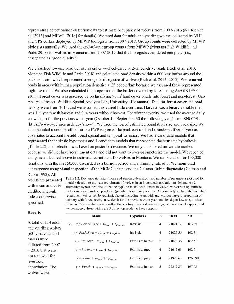
representing detection/non-detection data to estimate occupancy of wolves from 2007-2016 (see Rich et al. [2013] and MFWP [2018] for details). We used data for adult and yearling wolves collected by VHF and GPS collars deployed by MFWP biologists from 2007-2017. Group counts were collected by MFWP biologists annually. We used the end-of-year group counts from MFWP (Montana Fish Wildlife and Parks 2018) for wolves in Montana from 2007-2017 that the biologists considered complete (i.e., designated as “good quality”).

We classified low-use road density as either 4-wheel-drive or 2-wheel-drive roads (Rich et al. 2013; Montana Fish Wildlife and Parks 2018) and calculated road density within a 600 km2 buffer around the pack centroid, which represented average territory size of wolves (Rich et al. 2012, 2013). We removed roads in areas with human population densities > 25 people/km2 because we assumed these represented high-use roads. We also calculated the proportion of the buffer covered by forest using ArcGIS (ESRI 2011). Forest cover was assessed by reclassifying 90 m2 land cover pixels into forest and non-forest (Gap Analysis Project, Wildlife Spatial Analysis Lab, University of Montana). Data for forest cover and road density were from 2013, and we assumed this varied little over time. Harvest was a binary variable that was 1 in years with harvest and 0 in years without harvest. For winter severity, we used the average daily snow depth for the previous water year (October 1 – September 30 the following year) from SNOTEL (https://www.wcc.nrcs.usda.gov/snow/). We used the log of estimated population size and pack size. We also included a random effect for the FWP region of the pack centroid and a random effect of year as covariates to account for additional spatial and temporal variation. We had 2 candidate models that represented the intrinsic hypothesis and 4 candidate models that represented the extrinsic hypothesis (Table 2.2), and selection was based on posterior deviance. We only considered univariate models because we did not have recruitment data and did not want to over-parameterize the model. We repeated analyses as detailed above to estimate recruitment for wolves in Montana. We ran 3 chains for 100,000 iterations with the first 50,000 discarded as a burn-in period and a thinning rate of 3. We monitored convergence using visual inspection of the MCMC chains and the Gelman-Rubin diagnostic (Gelman and Rubin 1992). All results are presented with mean and 95% credible intervals unless otherwise specified.

Results

A total of 114 adult and yearling wolves (63 females and 51 males) were collared from 2007 – 2016 that were not removed for livestock depredation. The wolves were

Table 2.2. Deviance statistics (mean and standard deviation) and number of parameters (K) used for model selection to estimate recruitment of wolves in an integrated population model and test 2 alternative hypotheses. We tested the hypothesis that recruitment in wolves was driven by intrinsic factors such as density-dependence (population size) or pack size. Alternatively we hypothesized that recruitment was driven by extrinsic factors including years with and without harvest, proportion of territory with forest cover, snow-depth for the previous water year, and density of low-use, 4-wheel drive and 2-wheel drive roads within the territory. Lower deviance suggest more model support, and we considered those within a SD of the top model to have support.

Model Hypothesis K Mean SD

𝛾𝛾 ~ 𝑃𝑃𝑃𝑃𝑃𝑃𝑃𝑃𝑃𝑃𝑃𝑃𝑃𝑃𝑃𝑃𝑃𝑃𝑃𝑃 𝑆𝑆𝑃𝑃𝑆𝑆𝑆𝑆 + 𝜏𝜏𝑌𝑌𝑌𝑌𝑌𝑌𝑌𝑌 + 𝜏𝜏𝑅𝑅𝑌𝑌𝑅𝑅𝑅𝑅𝑅𝑅𝑅𝑅 Intrinsic 4 21021.12 163.65

𝛾𝛾 ~ 𝑃𝑃𝑃𝑃𝑃𝑃𝑃𝑃 𝑆𝑆𝑃𝑃𝑆𝑆𝑆𝑆 + 𝜏𝜏𝑌𝑌𝑌𝑌𝑌𝑌𝑌𝑌 + 𝜏𝜏𝑅𝑅𝑌𝑌𝑅𝑅𝑅𝑅𝑅𝑅𝑅𝑅 Intrinsic 4 21025.56 162.31

𝛾𝛾 ~ 𝐻𝐻𝑃𝑃𝐻𝐻𝐻𝐻𝑆𝑆𝐻𝐻𝑃𝑃 + 𝜏𝜏𝑌𝑌𝑌𝑌𝑌𝑌𝑌𝑌 + 𝜏𝜏𝑅𝑅𝑌𝑌𝑅𝑅𝑅𝑅𝑅𝑅𝑅𝑅 Extrinsic; human 5 21026.36 162.51

𝛾𝛾 ~ 𝐹𝐹𝑃𝑃𝐻𝐻𝑆𝑆𝐻𝐻𝑃𝑃 + 𝜏𝜏𝑌𝑌𝑌𝑌𝑌𝑌𝑌𝑌 + 𝜏𝜏𝑅𝑅𝑌𝑌𝑅𝑅𝑅𝑅𝑅𝑅𝑅𝑅 Extrinsic; prey 4 21642.61 162.51

𝛾𝛾 ~ 𝑆𝑆𝑃𝑃𝑃𝑃𝑆𝑆 + 𝜏𝜏𝑌𝑌𝑌𝑌𝑌𝑌𝑌𝑌 + 𝜏𝜏𝑅𝑅𝑌𝑌𝑅𝑅𝑅𝑅𝑅𝑅𝑅𝑅 Extrinsic; prey 4 21920.63 1265.98

𝛾𝛾 ~ 𝑅𝑅𝑃𝑃𝑃𝑃𝑅𝑅𝐻𝐻 + 𝜏𝜏𝑌𝑌𝑌𝑌𝑌𝑌𝑌𝑌 + 𝜏𝜏𝑅𝑅𝑌𝑌𝑅𝑅𝑅𝑅𝑅𝑅𝑅𝑅 Extrinsic; human 5 22247.85 167.08

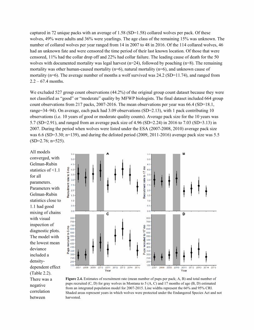
captured in 72 unique packs with an average of 1.58 (SD=1.58) collared wolves per pack. Of these wolves, 49% were adults and 36% were yearlings. The age class of the remaining 15% was unknown. The number of collared wolves per year ranged from 14 in 2007 to 48 in 2016. Of the 114 collared wolves, 46 had an unknown fate and were censored the time period of their last known location. Of those that were censored, 11% had the collar drop off and 22% had collar failure. The leading cause of death for the 50 wolves with documented mortality was legal harvest (n=24), followed by poaching (n=8). The remaining mortality was other human-caused mortality (n=6), natural mortality (n=6), and unknown cause of mortality (n=6). The average number of months a wolf survived was 24.2 (SD=11.74), and ranged from 2.2 – 67.4 months.

We excluded 527 group count observations (44.2%) of the original group count dataset because they were not classified as “good” or “moderate” quality by MFWP biologists. The final dataset included 664 group count observations from 217 packs, 2007-2016. The mean observations per year was 66.4 (SD=18.1, range=34–94). On average, each pack had 3.09 observations (SD=2.13), with 1 pack contributing 10 observations (i.e. 10 years of good or moderate quality counts). Average pack size for the 10 years was 5.7 (SD=2.91), and ranged from an average pack size of 4.96 (SD=2.24) in 2016 to 7.03 (SD=3.13) in 2007. During the period when wolves were listed under the ESA (2007-2008, 2010) average pack size was 6.6 (SD=3.30; n=139), and during the delisted period (2009, 2011-2016) average pack size was 5.5 (SD=2.76; n=525).

All models converged, with Gelman-Rubin statistics of <1.1 for all parameters. Parameters with Gelman-Rubin statistics close to 1.1 had good mixing of chains with visual inspection of diagnostic plots. The model with the lowest mean deviance included a density-dependent effect (Table 2.2). There was a negative correlation between

Figure 2.4. Estimates of recruitment rate (mean number of pups per pack; A, B) and total number of pups recruited (C, D) for gray wolves in Montana to 5 (A, C) and 17 months of age (B, D) estimated from an integrated population model for 2007-2015. Line widths represent the 66% and 95% CRI. Shaded areas represent years in which wolves were protected under the Endangered Species Act and not harvested.

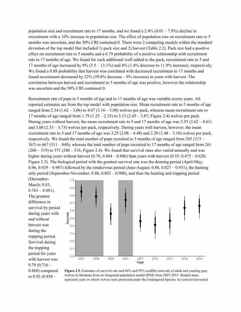
population size and recruitment rate to 17 months, and we found a 2.4% (0.01 – 7.9%) decline in recruitment with a 10% increase in population size. The effect of population size on recruitment rate to 5 months was uncertain, and the 50% CRI contained 0. There were 2 competing models within the standard deviation of the top model that included 1) pack size and 2) harvest (Table 2.2). Pack size had a positive effect on recruitment rate to 5 months and a 0.79 probability of a positive relationship with recruitment rate to 17 months of age. We found for each additional wolf added to the pack, recruitment rate to 5 and 17 months of age increased by 9% (5.5 – 13.1%) and 4% (1.4% decrease to 11.9% increase), respectively. We found a 0.88 probability that harvest was correlated with decreased recruitment to 17 months and found recruitment decreased by 22% (59.8% decrease – 9% increase) in years with harvest. The correlation between harvest and recruitment to 5 months of age was positive, however the relationship was uncertain and the 50% CRI contained 0.

Recruitment rate of pups to 5 months of age and to 17 months of age was variable across years. All reported estimates are from the top model with population size. Mean recruitment rate to 5 months of age ranged from 2.34 (1.62 – 3.06) to 4.07 (3.16 – 5.08) wolves per pack, whereas mean recruitment rate to 17 months of age ranged from 1.79 (1.25 – 2.35) to 3.13 (2.45 – 3.87; Figure 2.4) wolves per pack. During years without harvest, the mean recruitment rate to 5 and 17 months of age was 3.55 (2.62 – 4.61) and 3.00 (2.33 – 3.73) wolves per pack, respectively. During years with harvest, however, the mean recruitment rate to 5 and 17 months of age was 3.25 (2.08 – 4.48) and 2.20 (1.48 – 3.10) wolves per pack, respectively. We found the total number of pups recruited to 5 months of age ranged from 285 (213 – 367) to 667 (511 – 840), whereas the total number of pups recruited to 17 months of age ranged from 261 (206 – 319) to 371 (240 – 516; Figure 2.4). We found that survival rates also varied annually and was higher during years without harvest (0.78, 0.684 – 0.886) than years with harvest (0.55, 0.475 – 0.620; Figure 2.5). The biological period with the greatest survival rate was the denning period (April-May; 0.96, 0.929 – 0.987) followed by the rendezvous period (June-August; 0.88, 0.827 – 0.931), the hunting only period (September-November; 0.86, 0.802 – 0.900), and then the hunting and trapping period (December-March; 0.83, 0.763 – 0.881). The greatest difference in survival by period during years with and without harvest was during the trapping period. Survival during the trapping period for years with harvest was 0.79 (0.716 – 0.860) compared to 0.92 (0.858 –

Figure 2.5. Estimates of survival rate and 66% and 95% credible intervals of adult and yearling gray wolves in Montana from an integrated population model (IPM) from 2007-2015. Shaded areas represent years in which wolves were protected under the Endangered Species Act and not harvested.

0.958) during years without harvest. Mean population growth rate for our study period was 1.02 (1.00 – 1.04; Figure 2.6). We found that the correlation between population growth rate and survival (r = 0.31; Pr(r>0) = 0.86) and recruitment to 17 months of age (r = 0.23; Pr(r>0) = 0.79) was positive, whereas there was no correlation between population growth rate and recruitment to 5 months of age (r = 0.304; Pr(r>0) = 0.54). We also found a negative correlation between population growth rate and dispersal (r = -0.21; Pr(r<0) = 0.61).

Discussion

Using available data from monitoring of wolves in Montana from 2007-2016, we found that recruitment was primarily affected by intrinsic factors such as population size and pack size. Both abundance and pack size appeared to affect recruitment of pups suggesting density dependent effects of population size and pack size, however these processes had opposite effects. The negative correlation of abundance with recruitment to 17 months of age suggests a negative density dependent effect. The positive correlation of pack size with recruitment of pups to 5 and 17 months of age indicates positive density dependence within a pack. Pack size was also the main factor driving breeding pair status of wolf packs in Montana (Mitchell et al. 2008). We also found that harvest affects recruitment of wolves. Although the credible interval contained 0 for the coefficient of harvest, there was a probability of 0.88 that harvest reduced recruitment to 17 months of age. Mean recruitment to 17 months of age in years without harvest was 3 wolves per pack, and in years with harvest was 2.2 wolves per pack. These estimates align closely with findings in Idaho (Ausband et al. 2015).

Our estimates of recruitment and survival were comparable to other studies for wolves. Recruitment rate to 5 and 17 months varied over time (Figure 2.4). Recruitment estimates for wolves in Idaho averaged 3.2 and 1.6 pups per pack to 15 months without harvest and with harvest, respectively (Ausband et al. 2015). Our estimates of recruitment to 17 months of age were similar to estimates in Idaho (3.00 and 2.20 wolves per pack, without and with harvest). Survival rate for wolves in the NRM prior to harvest implementation averaged 0.75 (Smith et al. 2010), which is slightly less than we estimated for wolves in Montana during years without harvest (0.78, Figure 2.5). Similarly, survival rate for wolves in an unharvested population in Wisconsin was 0.76 (Stenglein et al. 2015). Survival rates for wolves in harvested populations in Yukon and Alaska averaged 0.56 and 0.59, respectively (Ballard et al. 1987; Hayes and Harestad 2000), which is similar to our estimates for Montana during years with harvest (0.55, Figure 2.5). We found the greatest decline in survival during the hunting and trapping period in years with harvest, suggesting that

Figure 2.6. Estimates of population growth rate and 66% and 95% credible intervals of wolves in Montana from an integrated population model (IPM) from 2007-2015. Shaded areas represent years in which wolves were protected under the Endangered Species Act and not harvested.

harvest has decreased survival in yearling and adult wolves in Montana, however we did not explicitly test this.

Our results indicate that recruitment does little to compensate for changes in survival, however the population has remained relatively stationary (mean population growth rate of 1.02). We found the correlation with population growth rate was greatest for annual survival of adults and yearlings followed by recruitment to 17 months of age. This suggests that these demographic rates have the strongest effect on population growth rate. Mean number of pups recruited to 17 months and survival of yearlings and adults decreased over time with changes in management practices (Figures 2.4 and 2.5), which is concurrent with declines in annual population growth rate (Figure 2.6). Estimated mean total human-caused mortality, which includes harvest, control removals, and other (e.g., vehicle accident), in Montana was 0.28 (SD = 0.078) during our study and is near the top of the range of human-offtake thought to result in stable or growing populations (Fuller et al. 2003). We hypothesize that immigration into or local dispersal within Montana may partially compensate for decreased survival and recruitment. Immigration of wolves is an important process in dynamics for many wolf populations (Hayes and Harestad 2000; Fuller et al. 2003). Packs may adopt unrelated individuals which can maintain pack stability in harvested populations (Rutledge et al. 2010; Bassing et al. 2019), and recolonization of unoccupied territories may occur quickly (Ballard et al. 1987; Hayes and Harestad 2000). Dispersal rates are high for wolves across the Northern Rocky Mountains (Jimenez et al. 2017) and surrounding areas may supply immigrants for the Montana wolf population. Alternatively or in conjunction with immigration, reductions in dispersal may compensate for decreased survival and recruitment and allow the Montana wolf population to remain stationary. Adams et al. (2008) found that decreased dispersal rates compensated for harvest mortality and resulted in relatively stationary densities across years in north-central Alaska.

2.4 Develop and Test a Component Model of Recruitment

Introduction

To understand variation in recruitment (offspring produced that survive to a given age), managers and researchers typically evaluate how different factors (e.g., predation or density dependence) affect the overall rate. Although recruitment is generally assessed by recruitment rate, i.e., number of offspring that survive to a certain age, it is affected by multiple demographic processes, and management decisions may differ depending on how factors affect the components of recruitment. Wolves breed cooperatively (i.e., non-breeding pack members help raise pups; Mech and Boitani 2003), and like many other cooperative breeders, they benefit from the presence of non-breeding individuals to help raise offspring (Solomon and French 1997). Although wolves reach sexual maturity around 2 years of age, the breeding pair suppresses reproduction in other pack members (Packard 2003), however some packs contain multiple breeding males and females (Ausband 2018). Recruitment in wolves is therefore a function of whether a pack successfully reproduced, the number of breeding females in a pack, litter size, and pup survival. Understanding how different factors affect the components of recruitment can better inform decisions when managing wildlife populations. For example, if increased breeder mortality is reducing the probability a pack successfully breeds, and consequently recruitment, management could alter the timing of the season so it does not coincide with breeding. Conversely, if low food availability is decreasing pup survival different management actions might be taken.

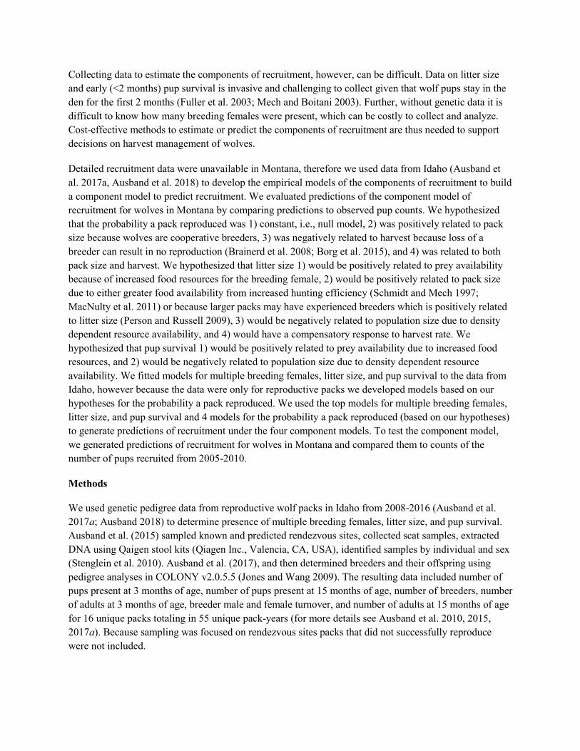
Collecting data to estimate the components of recruitment, however, can be difficult. Data on litter size and early (<2 months) pup survival is invasive and challenging to collect given that wolf pups stay in the den for the first 2 months (Fuller et al. 2003; Mech and Boitani 2003). Further, without genetic data it is difficult to know how many breeding females were present, which can be costly to collect and analyze. Cost-effective methods to estimate or predict the components of recruitment are thus needed to support decisions on harvest management of wolves.

Detailed recruitment data were unavailable in Montana, therefore we used data from Idaho (Ausband et al. 2017a, Ausband et al. 2018) to develop the empirical models of the components of recruitment to build a component model to predict recruitment. We evaluated predictions of the component model of recruitment for wolves in Montana by comparing predictions to observed pup counts. We hypothesized that the probability a pack reproduced was 1) constant, i.e., null model, 2) was positively related to pack size because wolves are cooperative breeders, 3) was negatively related to harvest because loss of a breeder can result in no reproduction (Brainerd et al. 2008; Borg et al. 2015), and 4) was related to both pack size and harvest. We hypothesized that litter size 1) would be positively related to prey availability because of increased food resources for the breeding female, 2) would be positively related to pack size due to either greater food availability from increased hunting efficiency (Schmidt and Mech 1997; MacNulty et al. 2011) or because larger packs may have experienced breeders which is positively related to litter size (Person and Russell 2009), 3) would be negatively related to population size due to density dependent resource availability, and 4) would have a compensatory response to harvest rate. We hypothesized that pup survival 1) would be positively related to prey availability due to increased food resources, and 2) would be negatively related to population size due to density dependent resource availability. We fitted models for multiple breeding females, litter size, and pup survival to the data from Idaho, however because the data were only for reproductive packs we developed models based on our hypotheses for the probability a pack reproduced. We used the top models for multiple breeding females, litter size, and pup survival and 4 models for the probability a pack reproduced (based on our hypotheses) to generate predictions of recruitment under the four component models. To test the component model, we generated predictions of recruitment for wolves in Montana and compared them to counts of the number of pups recruited from 2005-2010.

Methods

We used genetic pedigree data from reproductive wolf packs in Idaho from 2008-2016 (Ausband et al. 2017a; Ausband 2018) to determine presence of multiple breeding females, litter size, and pup survival. Ausband et al. (2015) sampled known and predicted rendezvous sites, collected scat samples, extracted DNA using Qaigen stool kits (Qiagen Inc., Valencia, CA, USA), identified samples by individual and sex (Stenglein et al. 2010). Ausband et al. (2017), and then determined breeders and their offspring using pedigree analyses in COLONY v2.0.5.5 (Jones and Wang 2009). The resulting data included number of pups present at 3 months of age, number of pups present at 15 months of age, number of breeders, number of adults at 3 months of age, breeder male and female turnover, and number of adults at 15 months of age for 16 unique packs totaling in 55 unique pack-years (for more details see Ausband et al. 2010, 2015, 2017a). Because sampling was focused on rendezvous sites packs that did not successfully reproduce were not included.

We used litter size, pup survival, and presence of multiple breeding females as response variables. We treated the number of pups at 3 months of age as the litter size. Any mortality of pups younger than this would bias litter size low and pup survival high, however the litter sizes are similar to those reported elsewhere for wolves (Fuller et al. 2003). We considered pup survival as the number of pups at 3 months of age that were still alive at 15 months of age as Ausband et al. (2017a) did. Similarly to Ausband (2018), we treated the presence of > 1 breeding female as a binary variable to estimate the probability of a pack containing multiple breeding females.

We included independent variables that represented prey availability, pack and population characteristics, and harvest. For the independent predictors of prey availability we used winter severity as an index for prey vulnerability (Mech and Peterson 2003; Mech and Fieberg 2015) and catch-per-unit-effort (CPUE) of antlered deer and elk as an index of prey abundance (Lancia et al. 1996). We used the average daily snow depth for the previous water year (October 1 – September 30 the following year) from SNOTEL (https://www.wcc.nrcs.usda.gov/snow/) for winter severity. We estimated CPUE for deer and elk in each game management unit as the number of harvested antlered deer or elk divided by the number of hunter days using harvest statistics from IDFG (idfg.idaho.gov). We used log transformed estimates of abundance of wolves from wolf monitoring by IDFG for population size (Nadeau et al. 2009; Mack et al. 2010; Holyan et al. 2011; Idaho Department of Fish and Game and Nez Perce Tribe 2012, 2013, 2014, 2015, Idaho Department of Fish and Game 2016, 2017) and the number of adults present when pups were 3 months of age as independent predictors representing pack and population characteristics. We used a binary variable to represent years with and without harvest and also harvest rate as independent predictor

Table 2.3. Candidate models and model selection for litter size (𝑃𝑃), pup survival (𝜙𝜙), and multiple breeding females (𝑚𝑚) for wolves in Idaho from 2008-2016 using leave-one-out cross-validation information criteria (LOO) and mean and standard error of the difference in the expected log predictive density (∆ELPD). Independent variables included pack size (𝑃𝑃𝑆𝑆), abundance of wolves (𝑃𝑃𝑃𝑃), winter severity (𝑊𝑊𝑆𝑆), index of deer abundance (𝑆𝑆𝑅𝑅), elk index (𝐸𝐸), harvest as a binary variable (𝐻𝐻), harvest rate (𝐻𝐻𝑅𝑅), a random effect of pack (𝛼𝛼𝑝𝑝), and a random effect of year (𝜀𝜀𝑡𝑡).

Demographic rate Model K LOO ∆LOO ∆ELPD (SE)

Litter size 𝑃𝑃 = 𝛽𝛽0 + 𝛼𝛼𝑝𝑝 2 228.50 0 0 (0) 𝑃𝑃 = 𝛽𝛽0 + 𝑃𝑃𝑆𝑆 + 𝛼𝛼𝑝𝑝 3 229.35 0.85 0.43 (0.707) 𝑃𝑃 = 𝛽𝛽0 + 𝑆𝑆𝑅𝑅 + 𝛼𝛼𝑝𝑝 3 229.96 1.46 0.73 (0.394) 𝑃𝑃 = 𝛽𝛽0 + 𝑆𝑆𝑅𝑅 + 𝑃𝑃𝑆𝑆 + 𝛼𝛼𝑝𝑝 4 230.99 2.49 1.25 (0.923) 𝑃𝑃 = 𝛽𝛽0 + 𝐻𝐻𝑅𝑅 + 𝑃𝑃𝑃𝑃 + 𝐻𝐻𝑅𝑅 ∗ 𝑃𝑃𝑃𝑃 + 𝛼𝛼𝑝𝑝 5 232.11 3.61 1.81 (0.466)

Pup Survival 𝜙𝜙 = 𝛽𝛽0 + 𝑆𝑆𝑅𝑅 + 𝑃𝑃𝑃𝑃 + 𝐻𝐻 + 𝛼𝛼𝑝𝑝 + 𝜀𝜀𝑡𝑡 6 177.55 0 0 (0) 𝜙𝜙 = 𝛽𝛽0 + 𝐻𝐻 + 𝛼𝛼𝑝𝑝 + 𝜀𝜀𝑡𝑡 4 177.57 0.02 0.01 (1.957) 𝜙𝜙 = 𝛽𝛽0 + 𝑆𝑆𝑅𝑅 + 𝐻𝐻 + 𝛼𝛼𝑝𝑝 + 𝜀𝜀𝑡𝑡 5 177.60 0.05 0.03 (0.675) 𝜙𝜙 = 𝛽𝛽0 + 𝑆𝑆𝑅𝑅 + 𝛼𝛼𝑝𝑝 + 𝜀𝜀𝑡𝑡 4 177.86 0.31 0.16 (0.998) 𝜙𝜙 = 𝛽𝛽0 + 𝑃𝑃𝑃𝑃 + 𝐻𝐻 + 𝛼𝛼𝑝𝑝 + 𝜀𝜀𝑡𝑡 5 178.23 0.68 0.34 (1.986) 𝜙𝜙 = 𝛽𝛽0 + 𝑆𝑆𝑅𝑅 + 𝑃𝑃𝑃𝑃 + 𝛼𝛼𝑝𝑝 + 𝜀𝜀𝑡𝑡 5 178.23 0.68 0.37 (1.070) 𝜙𝜙 = 𝛽𝛽0 + 𝑃𝑃𝑃𝑃 + 𝛼𝛼𝑝𝑝 + 𝜀𝜀𝑡𝑡 4 178.41 0.86 0.43 (2.180) 𝜙𝜙 = 𝛽𝛽0 + 𝛼𝛼𝑝𝑝 + 𝜀𝜀𝑡𝑡 3 179.45 1.90 0.95 (2.100) 𝜙𝜙 = 𝛽𝛽0 + 𝐻𝐻 + 𝑃𝑃𝑆𝑆 + 𝐻𝐻 ∗ 𝑃𝑃𝑆𝑆 + 𝛼𝛼𝑝𝑝 + 𝜀𝜀𝑡𝑡 6 180.70 3.15 1.58 (2.639)

Multiple breeding females

𝑚𝑚 = 𝛽𝛽0 + 𝑃𝑃𝑆𝑆 + 𝑊𝑊𝑆𝑆 + 𝑆𝑆𝑅𝑅 4 34.89 0 0 (0) 𝑚𝑚 = 𝛽𝛽0 + 𝑊𝑊𝑆𝑆 + 𝑆𝑆𝑅𝑅 3 37.30 2.41 1.21 (1.881)

𝑚𝑚 = 𝛽𝛽0 + 𝑃𝑃𝑆𝑆 2 42.42 7.53 3.76 (2.929) 𝑚𝑚 = 𝛽𝛽0 1 44.12 9.23 4.62 (3.126)

variables. We estimated harvest rates for the population using abundance estimates from IDFG and reported harvest of wolves (idfg.idaho.gov).

We fit generalized linear mixed-effects models for litter size (𝑃𝑃), pup survival (𝜙𝜙), and the probability of multiple breeding females (𝑚𝑚) with either Poisson or Bernoulli distribution. We included a random effect of pack and year to account for non-independence in litter count data and pup survival. We ran models based on our a priori hypotheses and on findings by Ausband et al. (2017a) and Ausband (2018). We considered every combination of prey availability, population and pack characteristics, and harvest which resulted in 4 competing models for litter size and multiple breeding females and 8 competing models for pup survival. Additionally, we considered a model representing the hypothesis of a compensatory response to harvest for litter size and a model for pup survival representing the hypothesis that pups in larger packs are more likely to survive. We tested for collinearity among covariates using the Pearson correlation coefficient and excluded collinear covariates within the same model (r > |0.60|; Zuur et al. 2010) in constructing our final candidate models (Table 2.3).

We fit models in a Bayesian framework using JAGS v4.2.0 (Plummer 2003) via the R2jags package (Su and Yajima 2015) in R v3.4.1 (R Core Team 2017). We ran 3 markov chains for 100,000 iterations with the first 50,000 discarded as a burn-in period and a thinning rate of 5. We continued to run an additional 50,000 interactions until chains converged. We monitored convergence using visual inspection of the chains and the Gelman-Rubin diagnostic (Gelman and Rubin 1992). We compared models using approximate leave-one-out cross-validation score (LOO; Gabry et al. 2017; Vehtari et al. 2017) and the expected log predictive density (ELPD) using Pareto-smoothed importance-sampling in the loo package (Vehtari et al. 2019). We considered models competitive if the ∆ELPD of the top model was within the standard error of the ∆ELPD of the competing models. We assessed model fit using the expected log predictive density for all demographic rates, Bayesian p-values calculated from the 𝜒𝜒2-discrepancy statistic (Gelman et al. 2004) for litter size, and the receiver operating characteristic (ROC) statistic and the corresponding area under the curve (AUC; Hosmer and Lemeshow 2000) for pup survival and the probability of multiple breeding females. We calculated the probability a coefficient was greater than or less than 0 using the MCMC samples from the posterior distribution when the CRI overlapped 0.

We combined results from multiple breeding females, litter size, and pup survival with hypotheses of whether a pack successfully reproduced to generate predictions of recruitment for wolf packs in Montana. Group counts of wolf packs were collected by MFWP biologists annually (Mech 1973; Gude et al. 2012; Coltrane et al. 2015; Inman et al. 2019). We used the end-of-year group counts for wolves in Montana that biologists considered of good quality (i.e., complete) and that included counts of pups. The data included 184 pack counts from 82 unique packs from 2005-2010. We used the average daily snow depth for the previous water year (October 1 – September 30 the following year) from SNOTEL (https://www.wcc.nrcs.usda.gov/snow/) for winter severity in Montana. We estimated CPUE for deer for each region the pack resided in as the number of harvested antlered deer divided by the number of hunter days using harvest statistics from MFWP (fwp.mt.gov).

We used the most supported model for multiple breeding females, litter size, and pup survival to predict those components of recruitment for wolves in Montana. We used 4 hypotheses to generate predictions of the probability a pack reproduced: 1) null model with a mean probability, 2) the probability a pack reproduced increased monotonically with pack size, 3) mortality during the breeding season reduced the

probability a pack reproduced due to breeder loss, and 4) pack size and mortality during the breeding season both affect the probability a pack reproduces (Figure 2.7). We generated predictions of recruitment under the 4 hypotheses for the probability a pack reproduced (𝑏𝑏) and the most supported models of multiple breeding females (𝑚𝑚), litter size (𝑃𝑃), and pup survival (𝜙𝜙) in a Bayesian hierarchical model. We assumed the probability a pack reproduced was a Bernoulli random variable and modeled the probability using a logit transformation. We used informative priors to represent our hypotheses of the probability a pack reproduced and tested the sensitivity of the results to these priors. We refit the most supported models for multiple breeding females, litter size, and pup survival and estimated recruitment (𝛾𝛾) as 𝛾𝛾 = 𝑏𝑏𝑃𝑃𝜙𝜙 + 𝑚𝑚𝑏𝑏𝑃𝑃𝜙𝜙 using the same procedures outlined above. We visually compared predictions of recruitment to observed recruitment in Montana.

Results and Discussion

All models for the probability a pack contains multiple breeding females converged with Gelman-Rubin statistics of <1.1 and had good mixing of chains. The top models for the probability of multiple breeding females included 1) prey availability (represented as winter severity and the index of deer abundance) and pack size, and 2) only prey availability (Table 2.3). Both models fitted the data well (all Pareto-k diagnostic values < 0.5; AUC ≥ 0.81). Multiple breeding females had a 0.97 probability of a positive relationship with the index of deer abundance (𝛽𝛽 = 38.02,𝐶𝐶𝑅𝑅𝐶𝐶 = −1.258− 79.446) and a positive relationship with winter severity (𝛽𝛽 = 0.28,𝐶𝐶𝑅𝑅𝐶𝐶 = 0.058 − 0.542; Figure 2.8). We found that multiple breeding females also had a positive correlation with pack size (𝛽𝛽 = 0.34,𝐶𝐶𝑅𝑅𝐶𝐶 = 0.043− 0.689).

Overall, we found that the probability a pack contained multiple breeding females was positively related to prey availability. We found that winter severity and the index of deer abundance was positively related to the probability of multiple breeding females, suggesting that packs are more likely to contain > 1 breeding female with greater prey availability. This is similar to the findings by Boertje and Stephenson (1992) that more females were reproductively active and had greater subcutaneous fat with greater ungulate biomass.

All models for litter size converged with Gelman-Rubin statistics of <1.1 and had good mixing of chains. The top models for litter size included 1) only a random effect of pack which fitted the data marginally

Figure 2.7. Hypothesized relationships between the probability a pack reproduced and pack size and harvest for gray wolves under 4 hypotheses: the null hypothesis (i.e., constant probability), the pack size hypothesis with a positive relationship between pack size and the probability a pack reproduced, the harvest hypothesis where harvest reduced the probability a pack reproduced, and the pack size + harvest hypothesis.

well (p-value = 0.78; all Pareto-k diagnostic values < 0.5), and 2) only pack size which fitted the data well (p-value = 0.76; all Pareto-k diagnostic values < 0.7). Litter size had a 0.84 probability of a positive relationship with pack size (𝛽𝛽 = 0.03,𝐶𝐶𝑅𝑅𝐶𝐶 = −0.006− 0.069). We found little variation among packs for litter size (𝑆𝑆𝑆𝑆 𝑃𝑃𝑜𝑜 𝑃𝑃𝑃𝑃𝑃𝑃𝑃𝑃𝐻𝐻 = 0.12,𝐶𝐶𝑅𝑅𝐶𝐶 = 0.006− 0.318).

Although we found support for our hypothesis that pack size was positively related to litter size, it was a small effect, and litter size was similarly explained by a mean litter size with slight variation among packs. In fact, litter size varies little in many canid species (Devenish-Nelson et al. 2013). This could indicate that biological limitations on reproduction in wolves allows for little variation in litter size. We did not find support for our hypotheses that prey availability or density was related to litter size. Boertje and Stephenson (1992) found that litter size declined with declines in ungulate biomass per wolf, however they only found declines in litter size when ungulate biomass per wolf was reduced below levels previously reported in the literature. Similarly, we did not find support for the hypothesis of a compensatory effect of harvest on litter size. Contrary to our results, Sidorovich et al. (2007) found that intensive harvest of wolves in Belarus increased litter size. The maximum reported density of wolves in Belarus during their study (36 wolves/1000 km2) was much greater than the maximum reported density of wolves in central Idaho (15 wolves/1000 km2; Bassing 2017), and therefore reproduction of wolves in Belarus may have been limited by available food resources. These results suggest that per capita prey availability may not be a limiting factor for reproduction of wolves in our study area.

All models for pup survival converged with Gelman-Rubin statistics of <1.1 and had good mixing of chains. The top model for pup survival included prey availability (represented as the index of deer abundance), abundance, and harvest followed by the harvest only model (Table 2.3). There was considerable model selection uncertainty and all models were considered competitive (Table 2.3), however the models did not fit the data well (some Pareto-k diagnostic values > 0.7 for all models; AUC ~ 0.76 for all models). Pup survival had 0.97 probability of a positive relationship with the index of deer abundance (𝛽𝛽 = 23.86,𝐶𝐶𝑅𝑅𝐶𝐶 = −1.209− 49.156) and a 0.76 probability of a positive relationship with wolf abundance (𝛽𝛽 = 2.43,𝐶𝐶𝑅𝑅𝐶𝐶 = −4.335− 7.920). We found a 0.93 probability that pup survival was less in years with harvest compared to years without harvest (𝛽𝛽 = −0.95,𝐶𝐶𝑅𝑅𝐶𝐶 = −2.307− 0.484). We found a 0.85 probability of a positive effective of pack size on pup survival (𝛽𝛽 = 0.07,𝐶𝐶𝑅𝑅𝐶𝐶 = −0.052 −0.192) in the pack size only model. When we ran the interaction model with pack size and harvest we found a 0.70 probability of a negative effect of pack size on pup survival (𝛽𝛽 = −0.06,𝐶𝐶𝑅𝑅𝐶𝐶 = −0.274−0.149) and a 0.91 probability that the interaction between harvest and pack size had a positive correlation with pup survival (𝛽𝛽 = 0.16,𝐶𝐶𝑅𝑅𝐶𝐶 = −0.075− 0.417), indicating that pups may have greater survival in larger packs during years with harvest. We found greater variation among packs (𝑆𝑆𝑆𝑆 𝑃𝑃𝑜𝑜 𝑃𝑃𝑃𝑃𝑃𝑃𝑃𝑃𝐻𝐻 =1.22,𝐶𝐶𝑅𝑅𝐶𝐶 = 0.575− 2.227) than years (𝑆𝑆𝑆𝑆 𝑃𝑃𝑜𝑜 𝑦𝑦𝑆𝑆𝑃𝑃𝐻𝐻𝐻𝐻 = 0.55,𝐶𝐶𝑅𝑅𝐶𝐶 = 0.039− 1.521) for pup survival.

We found greater variation in pup survival among packs than among years, suggesting that pack characteristics or spatial variation in food resources may be more important than temporal variation in food resources. For species that cooperatively breed, changes in group composition (number in different sex or age classes) can greatly affect recruitment (Whitman et al. 2004; Brainerd et al. 2008; Gobush et al. 2008; Ausband et al. 2017a). Loss or turnover of breeding males and females (Brainerd et al. 2008; Ausband et al. 2017b) and the number of non-breeding males and females can affect pup survival (Ausband et al. 2017a) and may explain the large variation among packs and marginal predictive ability

of the models of wolf survival. Although pup survival is affected by pack composition and breeder turnover (Ausband et al. 2017a; b), data on group composition and breeder fate are difficult to collect. Including those factors in a model would limit the ability of the model to predict recruitment only when those data were available.

For wolves in Montana, we predicted the mean probability a pack contained > 1 breeding female was 0.02 (SD = 0.012) for a pack of 5 and 0.07 (SD = 0.052) for a pack of 10 wolves. Based on the top model, we predicted a mean litter size of 4.31 (SD = 0.046). We predicted mean pup survival to be 0.59 (SD = 0.023) during years without harvest and 0.43 (SD = 0.016) during years with harvest. Based on these components, we predicted recruitment for a pack of 5 wolves to be 2.83 (SD = 0.562) and 1.91 (SD = 0.419) pups per pack during years without and with harvest, respectively, under the null hypotheses for the probability a pack reproduced.

Predictions of recruitment based on these models for packs in Montana were similar to observed recruitment (Figure 2.8). The null hypothesis for the probability a pack reproduced provided the best predictions of recruitment and the hypothesis for pack size and harvest effects performed worst (Figure 2.8, Figure 2.9). We found that 62% of all predictions fell within the 66% CRI and 71% of predictions fell within the 95% CRI under the null hypothesis. We found that 16% of observations exceeded the 95% CRI under the null model, and for all models 13% of observations were less than the 95% CRI. All predictions

Figure 2.8. Component model predictions of recruitment (wolves per pack) in gray wolf packs from Montana (2005-2010) compared to observed recruitment (X) under 4 hypotheses of the probability a pack reproduced: 1) the null hypothesis was a constant probability, 2) the pack size hypothesis was increased probability with increasing pack size, 3) the harvest hypothesis was a greater probability during years without harvest, and 4) the pack size and harvest hypothesis combined the 2 previous hypotheses. Predictions are displayed by the 50%, 66%, 80%, and 95% credible intervals. Overlap between the observed data and prediction interval indicates an accurate prediction.

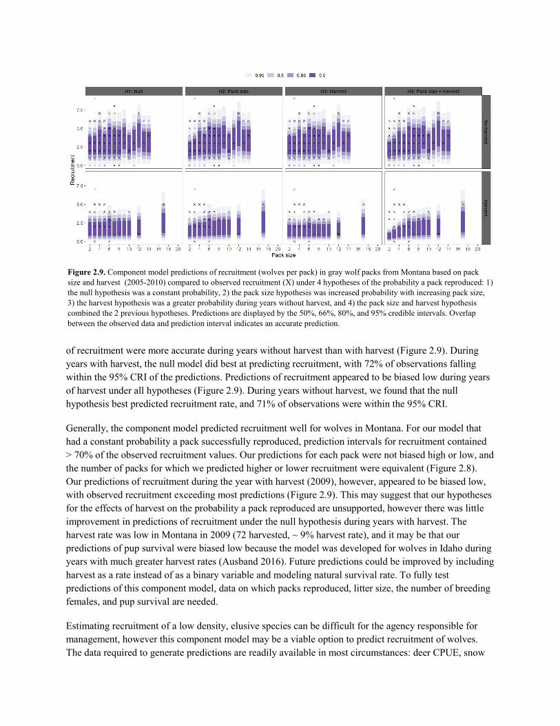
of recruitment were more accurate during years without harvest than with harvest (Figure 2.9). During years with harvest, the null model did best at predicting recruitment, with 72% of observations falling within the 95% CRI of the predictions. Predictions of recruitment appeared to be biased low during years of harvest under all hypotheses (Figure 2.9). During years without harvest, we found that the null hypothesis best predicted recruitment rate, and 71% of observations were within the 95% CRI.

Generally, the component model predicted recruitment well for wolves in Montana. For our model that had a constant probability a pack successfully reproduced, prediction intervals for recruitment contained > 70% of the observed recruitment values. Our predictions for each pack were not biased high or low, and the number of packs for which we predicted higher or lower recruitment were equivalent (Figure 2.8). Our predictions of recruitment during the year with harvest (2009), however, appeared to be biased low, with observed recruitment exceeding most predictions (Figure 2.9). This may suggest that our hypotheses for the effects of harvest on the probability a pack reproduced are unsupported, however there was little improvement in predictions of recruitment under the null hypothesis during years with harvest. The harvest rate was low in Montana in 2009 (72 harvested, ~ 9% harvest rate), and it may be that our predictions of pup survival were biased low because the model was developed for wolves in Idaho during years with much greater harvest rates (Ausband 2016). Future predictions could be improved by including harvest as a rate instead of as a binary variable and modeling natural survival rate. To fully test predictions of this component model, data on which packs reproduced, litter size, the number of breeding females, and pup survival are needed.

Estimating recruitment of a low density, elusive species can be difficult for the agency responsible for management, however this component model may be a viable option to predict recruitment of wolves. The data required to generate predictions are readily available in most circumstances: deer CPUE, snow

Figure 2.9. Component model predictions of recruitment (wolves per pack) in gray wolf packs from Montana based on pack size and harvest (2005-2010) compared to observed recruitment (X) under 4 hypotheses of the probability a pack reproduced: 1) the null hypothesis was a constant probability, 2) the pack size hypothesis was increased probability with increasing pack size, 3) the harvest hypothesis was a greater probability during years without harvest, and 4) the pack size and harvest hypothesis combined the 2 previous hypotheses. Predictions are displayed by the 50%, 66%, 80%, and 95% credible intervals. Overlap between the observed data and prediction interval indicates an accurate prediction.

depth, pack size, and whether or not the population was harvested. In instances were pack sizes are not known for all packs, an estimate of mean pack size and variance could be used to impute missing pack sizes and account for uncertainty. Because the component model focuses on individual components, one component could be updated while retaining the others to generate predictions. For example, if new data on pup survival become available, managers could update that portion of the model to generate predictions of recruitment. Further, litter size varied little and the probability a pack contained multiple breeding females was low, therefore managers wishing to alter recruitment may have more success when targeting successful reproduction and pup survival.

Literature Cited

Abadi, F., O. Gimenez, B. Ullrich, R. Arlettaz, and M. Schaub. 2010. Estimation of immigration rate using integrated population models. Journal of Applied Ecology 47:393–400.

Adams, L. G., R. O. Stephenson, B. W. Dale, R. T. Ahgook, and D. J. Demma. 2008. Population dynamics and harvest characteristics of wolves in the Central Brooks Range, Alaska. Wildlife Monographs 170:1–25.

Al-Khafaji, K., S. Tuljapurkar, J. R. Carey, and R. E. Page. 2009. Hierarchical demography: a general approach with an application to honey bees. Ecology 90:556–566.

Almberg, E. S., L. D. Mech, D. W. Smith, J. W. Sheldon, and R. L. Crabtree. 2009. A serological survey of infectious disease in Yellowstone National Park’s canid community. PloS one 4:e7042.

Ausband, D. E. 2018. Multiple breeding individuals within groups in a social carnivore. Journal of Mammalogy 99:836–844.

Ausband, D. E., M. S. Mitchell, K. Doherty, P. Zager, C. M. Mack, and J. Holyan. 2010. Surveying predicted rendezvous sites to monitor gray wolf populations. Journal of Wildlife Management 74:1043–1049.

Ausband, D. E., M. S. Mitchell, C. R. Stansbury, J. L. Stenglein, and L. P. Waits. 2017a. Harvest and group effects on pup survival in a cooperative breeder. Proceedings of the Royal Society of London B: Biological Sciences 284:20170580.

Ausband, D. E., M. S. Mitchell, and L. P. Waits. 2017b. Effects of breeder turnover and harvest on group composition and recruitment in a social carnivore. Journal of Animal Ecology 86:1094–1101.

Ausband, D. E., C. R. Stansbury, J. L. Stenglein, J. L. Struthers, and L. P. Waits. 2015. Recruitment in a social carnivore before and after harvest. Animal Conservation 18:415–423.

Ballard, W. B., J. S. Whitman, and C. L. Gardner. 1987. Ecology of an exploited wolf population in south-central Alaska. Wildlife Monographs 98:3–54.

Bassing, S. B., D. E. Ausband, M. S. Mitchell, P. Lukacs, A. C. Keever, G. Hale, and L. Waits. 2019. Stable pack abundance and distribution in a harvested wolf population. The Journal of Wildlife Management 83:577–590.

Besbeas, P., S. N. Freeman, B. J. T. Morgan, and E. A. Catchpole. 2002. Integrating mark-recapture-recovery and census data to estimate animal abundance and demographic parameters. Biometrics 58:540–547.

Boertje, R. D., and R. O. Stephenson. 1992. Effects of ungulate availability on wolf reproductive potential in Alaska. Canadian Journal of Zoology 70:2441–2443.

Borg, B. L., S. M. Brainerd, T. J. Meier, and L. R. Prugh. 2015. Impacts of breeder loss on social structure, reproduction and population growth in a social canid. The Journal of Animal Ecology

84:177–187.

Brainerd, S. M., H. Andrén, E. E. Bangs, E. H. Bradley, J. A. Fontaine, W. Hall, Y. Iliopoulos, M. D. Jimenez, E. A. Jozwiak, O. Liberg, C. M. Mack, T. J. Meier, C. C. Niemeyer, H. C. Pedersen, H. Sand, R. N. Schultz, D. W. Smith, P. Wabakken, and A. P. Wydeven. 2008. The effects of breeder loss on wolves. Journal of Wildlife Management 72:89–98.

Brooks, S. P. 2003. Bayesian computation: a statistical revolution. Philosophical Transactions of the Royal Society A 361:2681–2697.

Coltrane, J., J. A. Gude, B. Inman, N. Lance, K. Laudon, A. Messer, A. A. Nelson, T. Parks, M. Ross, T. Smucker, J. Steuber, and J. Vore. 2015. Montana gray wolf conservation and management 2015 annual report. Helena, Montana.

Courchamp, F., G. S. A. Rasmussen, and D. W. Macdonald. 2002. Small pack size imposes a trade-off between hunting and pup-guarding in the painted hunting dog Lycaon pictus. Behavioral Ecology 13:20–27.

Cubaynes, S., D. R. MacNulty, D. R. Stahler, K. A. Quimby, D. W. Smith, and T. Coulson. 2014. Density-dependent intraspecific aggression regulates survival in northern Yellowstone wolves (Canis lupus). The Journal of Animal Ecology 83:1344–1356.

ESRI. 2011. ArcGIS. Enironmental Systems Research Institute, Redlands, California.

Fuller, T. K., L. D. Mech, and J. Fitts-Cochran. 2003. Wolf population dynamics. Pages 161–191 in L. D. Mech and L. Boitani, editors. Wolves: behavior, ecology and conservation. University of Chicago Press, Chicago, Illinois.

Gabry, J., D. Simpson, A. Vehtari, M. Betancourt, and A. Gelman. 2019. Visualization in Bayesian workflow. Journal of the Royal Statistical Soceity A 182:389–402.

Gelman, A., J. B. Carlin, H. S. Stern, and D. B. Rubin. 2004. Bayesian data analysis. Second edition. Chapman and Hall/CRC Press.

Gelman, A., and D. B. Rubin. 1992. Inference from iterative simulation using multiple sequences. Statistical Science 7:457–472.

Gude, J. A., M. S. Mitchell, R. E. Russell, C. A. Sime, E. E. Bangs, L. D. Mech, and R. R. Ream. 2012. Wolf population dynamics in the U.S. Northern Rocky Mountains are affected by recruitment and human-caused mortality. The Journal of Wildlife Management 76:108–118.

Hayes, R. D., and A. S. Harestad. 2000. Demography of a recovering wolf population in the Yukon. Canadian Journal of Zoology 78:36–48.

Holyan, J., K. Holder, J. Cronce, and C. M. Mack. 2011. Wolf conservation and management in Idaho progress report 2010. Lapwaii, Idaho.

Hosmer, D. W. J., and S. Lemeshow. 2000. Applied logistic regression. 2nd edition. Wiley, New York, New York.

Huggard, D. J. 1993. Effect of snow depth on predation and scavenging by gray wolves. The Journal of Wildlife Management 57:382.

Idaho Department of Fish and Game. 2016. 2015 Idaho wolf monitoring progress report. Boise, Idaho.

Idaho Department of Fish and Game. 2017. 2016 Idaho wolf management report. Boise, Idaho.

Idaho Department of Fish and Game, and Nez Perce Tribe. 2012. 2011 Idaho wolf monitoring progress report. Boise, Idaho.

Idaho Department of Fish and Game, and Nez Perce Tribe. 2013. 2012 Idaho wolf monitoring progress

report. Boise, Idaho.

Idaho Department of Fish and Game, and Nez Perce Tribe. 2014. Idaho wolf monitoring progress report.

Idaho Department of Fish and Game, and Nez Perce Tribe. 2015. 2014 Idaho wolf monitoring progress report. Boise, Idaho.

Inman, B., K. M. Podruzny, T. D. Smucker, A. A. Nelson, M. Ross, N. Lance, T. Parks, D. K. Boyd, and S. Wells. 2019. Montana gray wolf conservation and management 2018 annual report. Helena, Montana.

Jimenez, M. D., E. E. Bangs, D. K. Boyd, D. W. Smith, S. A. Becker, D. E. Ausband, S. P. Woodruff, E. H. Bradley, J. Holyan, and K. Laudon. 2017. Wolf dispersal in the Rocky Mountains, Western United States: 1993-2008. The Journal of Wildlife Management 81:581–592.

Jones, O., and J. Wang. 2009. COLONY: a program for parentage and sibship inference from multilocus genotype data. Mol. Ecol. Resour.

Lancia, R. A., J. W. Bishir, M. C. Conner, and C. S. Rosenberry. 1996. Use of catch-effort to estimate population size. Wildlife Society Bulletin 24:731–737.

Llaneza, L., J. V. López-Bao, and V. Sazatornil. 2012. Insights into wolf presence in human-dominated landscapes: the relative role of food availability, humans and landscape attributes. Diversity and Distributions 18:459–469.

Mack, C. M., J. Rachael, J. Holyan, J. Husseman, M. Lucid, and B. Thomas. 2010. Wolf conservation and management in Idaho progress report 2009. Boise, Idaho.

MacKenzie, D. I., J. D. Nichols, G. B. Lachman, S. Droege, J. Andrew Royle, and C. A. Langtimm. 2002. Estimating site occupancy rates when detection probabilties are less than one. Ecology 83:2248–2255.

MacNulty, D. R., D. W. Smith, L. D. Mech, J. A. Vucetich, and C. Packer. 2011. Nonlinear effects of group size on the success of wolves hunting elk. Behavioral Ecology 23:75–82.

Mech, L. D. 1973. Wolf numbers in the Superior National Forest of Minnesota. Research Paper, St. Paul, MN.

Mech, L. D., L. G. Adams, T. J. Meier, J. W. Burch, and B. W. Dale. 1998. The wolves of Denali. University of Minnesota Press, Minneapolis, Minnesota.

Mech, L. D., and L. Boitani. 2003. Wolf social ecology. Pages 1–34 in L. D. Mech and L. Boitani, editors. Wolves: behavior, ecology and conservation. The University of Chicago Press, Chicago, Illinois.

Mech, L. D., and J. Fieberg. 2015. Growth rates and variances of unexploited wolf populations in dynamic equilibria. Wildlife Society Bulletin 39:41–48.

Mech, L. D., and R. O. Peterson. 2003. Wolf-prey relations. Pages 131–160 in L. D. Mech and L. Boitani, editors. Wolves: behavior, ecology and conservation. The University of Chicago Press, Chicago, Illinois.

Miller, D. A. W., J. D. Nichols, J. A. Gude, L. N. Rich, K. M. Podruzny, J. E. Hines, and M. S. Mitchell. 2013. Determining occurrence dynamics when false positives occur: estimating the range dynamics of wolves from public survey data. PloS one 8:e65808.

Mills, K. J., B. R. Patterson, and D. L. Murray. 2008. Direct estimation of early survival and movements in eastern wolf pups. Journal of Wildlife Management 72:949–954.

Mitchell, M. S., D. E. Ausband, C. A. Sime, E. E. Bangs, J. A. Gude, M. D. Jimenez, C. M. Mack, T. J.

Meier, M. S. Nadeau, and D. W. Smith. 2008. Estimation of successful breeding pairs for wolves in the Northern Rocky Mountains, USA. Journal of Wildlife Management 72:881–891.

Montana Fish Wildlife and Parks. 2018. Montana gray wolf conservation and management 2017 annual report. Helena, Montana.

Murray, D. L., D. W. Smith, E. E. Bangs, C. Mack, J. K. Oakleaf, J. Fontaine, D. Boyd, M. Jiminez, C. Niemeyer, T. J. Meier, D. Stahler, J. Holyan, and V. J. Asher. 2010. Death from anthropogenic causes is partially compensatory in recovering wolf populations. Biological Conservation 143:2514–2524.

Nadeau, M. S., Mack, Curt M, J. Holyan, J. Husseman, M. Lucid, D. Spicer, and B. Thomas. 2009. Wolf conservation and management plan in Idaho progress report 2008. Boise, Idaho.

Packard, J. M. 2003. Wolf behavior: reproductive, social, and intelligent. Pages 35–65 in L. D. Mech and L. Boitani, editors. Wolves: behavior, ecology and conservation. The University of Chicago Press, Chicago, Illinois.

Person, D. K., and A. L. Russell. 2008. Correlates of mortality in an exploited wolf population. The Journal of Wildlife Management 72:1540–1549.

Person, D. K., and A. L. Russell. 2009. Reproduction and den site selection by wolves in a disturbed landscape. Northwest Science 83:211–224.

Peterson, R. O. 1974. Wolf ecology and prey relationships on Isle Royale. Purdue University.

Plummer, M. 2003. JAGS: A program for analysis of Bayesian graphical models using Gibbs sampling.

Post, E., R. O. Peterson, N. C. Stenseth, and B. E. McLaren. 1999. Ecosystem consequences of wolf behavioural response to climate. Nature 401:905–907.

R Core Team. 2017. R: a language and environment for statistical computing. R Foundation for Statistical Computing, Vienna, Austria.

Rich, L. N., M. S. Mitchell, J. A. Gude, and C. A. Sime. 2012. Anthropogenic mortality, intraspecific competition, and prey availability influence territory sizes of wolves in Montana. Journal of Mammalogy 93:722–731.

Rich, L. N., R. E. Russell, E. M. Glenn, M. S. Mitchell, J. A. Gude, K. M. Podruzny, C. A. Sime, K. Laudon, D. E. Ausband, and J. D. Nichols. 2013. Estimating occupancy and predicting numbers of gray wolf packs in Montana using hunter surveys. The Journal of Wildlife Management 77:1280–1289.

Rutledge, L. Y., B. R. Patterson, K. J. Mills, K. M. Loveless, D. L. Murray, and B. N. White. 2010. Protection from harvesting restores the natural social structure of eastern wolf packs. Biological Conservation 143:332–339.

Schaub, M., and F. Abadi. 2011. Integrated population models: a novel analysis framework for deeper insights into population dynamics. Journal of Ornithology 152:227–237.

Schmidt, P. A., and L. D. Mech. 1997. Wolf pack size and food acquisition. The American Naturalist 150:513–517.

Smith, D. W., E. E. Bangs, J. K. Oakleaf, C. Mack, J. Fontaine, D. Boyd, M. Jimenez, D. H. Pletscher, C. C. Niemeyer, T. J. Meier, D. R. Stahler, J. Holyan, V. J. Asher, and D. L. Murray. 2010. Survival of colonizing wolves in the Northern Rocky Mountains of the United States, 1982-2004. Journal of Wildlife Management 74:620–634.

Solomon, N. G., and J. A. French, editors. 1997. Cooperative breeding in mammals. Cambridge University Press, Cambridge.

Sparkman, A. M., J. Adams, A. Beyer, T. D. Steury, L. Waits, and D. L. Murray. 2011. Helper effects on pup lifetime fitness in the cooperatively breeding red wolf (Canis rufus). Proceedings. Biological sciences / The Royal Society 278:1381–1389.

Stahler, D. R., D. R. MacNulty, R. K. Wayne, B. VonHoldt, and D. W. Smith. 2013. The adaptive value of morphological, behavioural and life-history traits in reproductive female wolves. The Journal of Animal Ecology 82:222–34.

Stenglein, J. L., L. P. Waits, D. E. Ausband, P. Zager, and C. M. Mack. 2010. Efficient, noninvasive genetic sampling for monitoring reintroduced wolves. Journal of Wildlife Management 74:1050–1058.

Stenglein, J. L., J. Zhu, M. K. Clayton, and T. R. Van Deelen. 2015. Are the numbers adding up? Exploiting discrepancies among complementary population models. Ecology and Evolution 5:368–376.

Su, Y.-S., and M. Yajima. 2015. R2jags: using R to run “JAGS.”

Thurber, J. M., R. O. Peterson, T. D. Drummer, and S. A. Thomasma. 1994. Gray wolf response to refuge boundaries and roads in Alaska. Wildlife Society Bulletin 22:61–68.

U.S. Fish and Wildlife Service. 1994. The reintroduction of gray wolves to Yellowstone National Park and central Idaho. Final Environmental Impact Statement. Denver, Colorado.

Vehtari, A., J. Gabry, Y. Yao, and A. Gelman. 2019. loo: efficient leave-one-out cross-validation and WAIC for Bayesian models.

Vehtari, A., A. Gelman, and J. Gabry. 2017. Practical Bayesian model evaluation using leave-one-out cross-validation and WAIC. Statistics and Computing 27:1413–1432.

Zuur, A. F., E. N. Ieno, and C. S. Elphick. 2010. A protocol for data exploration to avoid common statistical problems. Methods in Ecology and Evolution 1:3–14.

OBJECTIVE 3: DEVELOP ADAPTIVE HARVEST MANAGEMENT FRAMEWORK—Allison Keever, Project 2

ABSTRACT: Adaptive management (AM) incorporates scientific information and associated uncertainty in a transparent process that relates alternative management actions to explicit, quantifiable objectives to guide decisions making. Designing an AM framework requires clearly defined objectives, alternative management actions, predictive models to determine consequences of actions, an optimization algorithm to determine the management actions that best meets objectives, and monitoring data to determine the current system state and facilitate learning. Through monitoring, uncertainty can be reduced over time to improve future decisions. We developed an AM framework as a tool to guide decisions for harvest regulations for gray wolves in Montana. Our objectives were to 1) develop the AM framework for wolves to provide a decision tool to MFWP, 2) determine optimal management actions given how we quantified the components of AM, and 3) implement AM as an example of how this tool could work moving forward. As an example of the use of this AM framework, we used stochastic dynamic programing and passive adaptive learning to determine optimal management actions, given objectives and uncertainty about wolf population dynamics. The uncertainty we considered was whether immigration into Montana was partially compensating for harvest. We used the fundamental objectives developed for wolf management in 2010 that have been used as part of every season-setting process: 1) maintain positive and effective working relationships with livestock producers, hunters, and other stakeholders, 2) reduce wolf impacts on big game populations, 3) reduce wolf impacts on livestock, 4) maintain hunter opportunity for ungulates, 5) maintain a viable and connected wolf population in Montana, 6) maintain hunter opportunity for wolves, and 7) increase broad public acceptance of harvest and hunter opportunity as part of wolf conservation. We incorporated epistemic uncertainty in parameter values used in the predictive models, and also uncertainty in the relationship between regulations and harvest. Using AM, we found support for the hypothesis that net immigration into Montana was positive. This suggests that immigration may help the Montana wolf population sustain greater harvest rates than what could be expected in absence of immigration. We provide an example of how this decision tool could be implemented, and a flexible framework and tool that can be updated and adapted as uncertainty is reduced.

3.1 Introduction

Harvest is an important management tool for gray wolves in Montana. Harvest regulations for wolves are evaluated biennially and can be updated as needed, depending on the status of the population and objectives for management. Decisions on harvest regulations for wolves can be challenging, however, due to conflicting objectives from various stakeholder groups and uncertainties in the effects of harvest on wolf population dynamics.

Conflicting opinions on values of wolves and management among stakeholders (including livestock producers, hunters, tourists, and wolf conservation groups) make management decisions difficult. Federal and state agencies have legal requirements to manage the wolf population, and the Commission-approved Montana Wolf Conservation Strategy stipulates that MFWP will maintain a minimum of 15 breeding pairs and 150 wolves to have a regulated, public harvest season. Ungulate hunters have concerns that wolves affect prey populations and compete with hunters for ungulates (Ericsson and Heberlein 2003).

Livestock producers can suffer losses due to depredation events. Wolves also benefit the tourism industry in some areas (e.g., visitors to National Parks to view wolves), and conservation groups use that information to demonstrate the economic benefit of wolves (Defenders of Wildlife 2013).

A further challenge in managing wolves is uncertainty in effects of harvest on population dynamics. First, managers cannot directly control harvest rate, because changes in harvest regulations do not directly change harvest rates (Bischof et al. 2012). For example, increasing the bag limit from 1 to 5 wolves does not mean that harvest rate would increase five-fold, or even at all. Harvest rates vary based on many factors, including weather, hunter and trapper effort, hunter and trapper success, and regulations. Second, there is uncertainty in the effects of harvest on demography. There is not consensus for how harvest affects wolves (Fuller et al. 2003; Adams et al. 2008; Creel and Rotella 2010; Gude et al. 2012). Substantial variation occurs in the reported level of harvest wolf populations can sustain before growth rate decreases (Fuller et al. 2003; Adams et al. 2008; Creel and Rotella 2010; Gude et al. 2012) which could result in management actions not reaching objectives.

Despite uncertainty in the effects of harvest and the conflicting objectives and values of stakeholders MFWP must still make recommendations for harvest regulations of wolves, and the Montana Fish and Wildlife Commission still must set wolf harvest regulations. This reality creates annual controversy over wolf harvest regulations. A formal decision analysis process may help alleviate some of the technical aspects of this controversy by unifying expectations of stakeholders with divergent viewpoints.

Adaptive management (AM) provides a framework to clarify decisions while reducing uncertainty to identify the optimal strategies to meet objectives (Walters 1986, Williams et al. 2009). AM is an extension of structured decision making (SDM; Hammond et al. 1999) when decisions are iterated over time or space and uncertainty affects choices among management alternatives . Much like SDM, AM requires clearly defined objectives, alternative management actions, and models to predict outcomes of actions and evaluate tradeoffs. An essential component to AM is a monitoring program to determine the system state (e.g., population size), reduce uncertainty, and learn over time. Learning is the reduction of uncertainty and occurs when there are multiple hypotheses about how a system works, represented as multiple

Figure 3.1. Adaptive harvest management cycle. The optimal state-dependent (i.e., population size dependent) harvest strategy is based on objectives, alternatives, population models encompassing key uncertainties, and their relative support. After management is enacted, the response of the population is monitored and compared to predictions from the population models. Based on comparisons, model support is updated and uncertainty reduced.

models each with an associated probability (weight) representing the amount of support for that model (hypothesis) representing system dynamics. These model probabilities can be updated by comparing model predictions to monitoring data and provide evidence in favor of each hypothesis. When a hypothesis gains support, its model weight is increased and uncertainty is reduced, and the updated model weights can be used to make predictions. There are 2 forms of learning in AM, passive and active. The main difference between passive and active AM is that learning is anticipated and accounted for in active AM (Williams et al. 2002; Conroy and Peterson 2013). Active AM takes into account how reduction of uncertainty affects meeting objectives long-term. In passive AM, the optimal management action is selected assuming uncertainty will not change, and learning is incorporated outside of the optimization algorithm. In both passive and active AM, however, future decisions can be improved as models weights are updated and the accuracy of predictions improves. An AM framework can help guide harvest regulation decisions for wolf management while reducing uncertainty in wolf population dynamics to improve future decisions.

To address the challenges associated with managing wolves in Montana we will develop an AM framework. AM follows a general cycle: 1) Determine optimal harvest strategies dependent on objectives, alternatives, current status of the population, and the competing models (hypotheses) and their associated model probabilities, 2) enact a harvest strategy, 3) monitor changes in population size, and 4) compare monitoring data to model predictions to update model probabilities. The cycle then continues again (Figure 3.1). An AM framework for wolves will help inform current decisions while reducing uncertainty in the effects of harvest to improve future decisions. Specifically, our objectives were to 1) collaborate with MFWP to determine objectives (Sect. 3.2), 2) evaluate the relationship between harvest regulations and number harvested to predict harvest under alternative management actions (Sect. 3.3), and 3) determine optimal harvest regulations given abundance of wolves to meet objectives (Sect. 3.4). This research is still in development, and all results presented here represents progress to date.

3.2 Objectives

Introduction

Objectives are the desired outcomes from management of a system or population, and are used to measure whether management was successful (Conroy and Peterson 2013). Consequently, everything that follows in AM is largely determined by the objectives. Objectives should be quantifiable so they can be predicted and measured, and the metrics used to measure an objective are similarly important. Objectives should also reflect the values of stakeholders, and therefore stakeholders should be involved in the process of identifying objectives (Conroy and Peterson 2013).

Objectives for wolf management in Montana were developed by MFWP representatives, including regional managers, biologists, and wolf specialists, during workshops in 2009-2010 (Runge et al. 2013). The working group focused on including objectives of the different stakeholders, and developed a set of 6 fundamental objectives, 2 process objectives, and 2 strategic objectives (Runge et al. 2013 pg. 66). These objectives have guided management decisions for wolves since 2010 and were adopted by the Montana Fish and Wildlife Commission as part of every public harvest season. Although the 2010 SDM workshop provided objectives for management, formal, mathematical models relating changes in harvest regulations

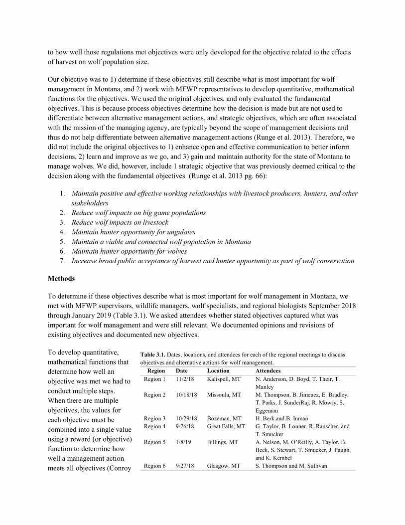
to how well those regulations met objectives were only developed for the objective related to the effects of harvest on wolf population size.

Our objective was to 1) determine if these objectives still describe what is most important for wolf management in Montana, and 2) work with MFWP representatives to develop quantitative, mathematical functions for the objectives. We used the original objectives, and only evaluated the fundamental objectives. This is because process objectives determine how the decision is made but are not used to differentiate between alternative management actions, and strategic objectives, which are often associated with the mission of the managing agency, are typically beyond the scope of management decisions and thus do not help differentiate between alternative management actions (Runge et al. 2013). Therefore, we did not include the original objectives to 1) enhance open and effective communication to better inform decisions, 2) learn and improve as we go, and 3) gain and maintain authority for the state of Montana to manage wolves. We did, however, include 1 strategic objective that was previously deemed critical to the decision along with the fundamental objectives (Runge et al. 2013 pg. 66):

1. Maintain positive and effective working relationships with livestock producers, hunters, and other stakeholders

2. Reduce wolf impacts on big game populations 3. Reduce wolf impacts on livestock 4. Maintain hunter opportunity for ungulates 5. Maintain a viable and connected wolf population in Montana 6. Maintain hunter opportunity for wolves 7. Increase broad public acceptance of harvest and hunter opportunity as part of wolf conservation

Methods

To determine if these objectives describe what is most important for wolf management in Montana, we met with MFWP supervisors, wildlife managers, wolf specialists, and regional biologists September 2018 through January 2019 (Table 3.1). We asked attendees whether stated objectives captured what was important for wolf management and were still relevant. We documented opinions and revisions of existing objectives and documented new objectives.

To develop quantitative, mathematical functions that determine how well an objective was met we had to conduct multiple steps. When there are multiple objectives, the values for each objective must be combined into a single value using a reward (or objective) function to determine how well a management action meets all objectives (Conroy

Table 3.1. Dates, locations, and attendees for each of the regional meetings to discuss objectives and alternative actions for wolf management.

Region Date Location Attendees Region 1 11/2/18 Kalispell, MT N. Anderson, D. Boyd, T. Their, T.

Manley Region 2 10/18/18 Missoula, MT M. Thompson, B. Jimenez, E. Bradley,

T. Parks, J. SunderRaj, R. Mowry, S. Eggeman

Region 3 10/29/18 Bozeman, MT H. Berk and B. Inman Region 4 9/26/18 Great Falls, MT G. Taylor, B. Lonner, R. Rauscher, and

T. Smucker Region 5 1/8/19 Billings, MT A. Nelson, M. O’Reilly, A. Taylor, B.

Beck, S. Stewart, T. Smucker, J. Paugh, and K. Kembel

Region 6 9/27/18 Glasgow, MT S. Thompson and M. Sullivan

and Peterson 2013). When the objectives are measured in different units (e.g., number of animals and dollars), the values for each objective must first be converted into common units using utility functions. In order to evaluate how well management actions met objectives listed above, we converted the values of each objective into a common metric using utility functions and then combined the utility values into a single value using a reward function that took into account the weights (relative importance) of each objective. We elicited utility functions and weights for objectives from MFWP representatives, which included supervisors, wildlife managers, and wolf specialists) to incorporate their values and knowledge. We also determined their risk attitudes as either risk averse, risk neutral, or risk tolerant (Conroy and Peterson 2013). For the reward function, we used the weighted-sum method (Conroy and Peterson 2013) to combine the utility values into a single reward value as:

𝑅𝑅𝑅𝑅𝑅𝑅𝑅𝑅𝑅𝑅𝑅𝑅 = 𝑅𝑅𝑖𝑖𝑈𝑈𝑖𝑖 + ⋯𝑅𝑅𝐼𝐼𝑈𝑈𝐼𝐼,

where 𝑅𝑅𝑖𝑖 is the weight and 𝑈𝑈𝑖𝑖 the utility value for objective i. We elicited utility functions and weights of objectives from MFWP representatives, including wildlife managers and wolf specialists, via email.

Objectives and Metrics Used for AM

The objectives that were developed in 2010 appear to still capture what is most important for wolf management and what is perceived to be important to the various stakeholders. Overall, MFWP representatives in the different regions believed the objectives developed in 2010 for wolf management were still appropriate. Minor edits/rewording and the addition of a few objectives were suggested. Because there were only minor edits, we used the originally stated objectives for the AM framework.

Weights for objectives that were evaluated were averaged from the responses by MFWP representatives from the email survey (Table 3.2). We described the metrics, utility functions, and risk attitude we used for each objective that was evaluated below and describe why 2 of the 7 objectives were not evaluated.

Reduce impacts of wolves on big game populations

Wolf impacts on big game populations are specific to local areas occupied by big game populations, which operate at a smaller scale than wolf populations, and dependent on many ecological factors. Considerable care needs to be taken in constructing a measurable attribute to reflect the process of wolf-ungulate dynamics. To simplify matters, we measured the impact of wolves on ungulates using a constructed scale from 0 (no impact) to 1 (wolves are reducing ungulate populations) across the entire state. For simplicity, we asked interviewees to assume that the impact of wolves on big game populations was only a function of the statewide number of wolves, and that the maximum impact (scale value of 1)

Table 3.2. Objectives, measurable attributes, and objective weights (relative importance) for an adaptive management framework for gray wolves in Montana. Objectives were developed in 2010 as part of a structured decision making workshop (Runge et al. 2013) and weights were assigned by MFWP representatives which included supervisors, wildlife managers, and wolf specialists.

Objective Measureable Attribute Weight Reduce wolf impacts on big game populations Scale: 0 (no impact) – 1 (reducing populations) 0.246 Reduce wolf impacts on livestock # depredation events/year 0.205 Maintain viable and connected wolf population # wolves and pups recruited 0.255 Maintain hunter opportunity for wolves # wolves, season length, bag limit 0.183 Increase acceptance of wolf harvest and opportunity Percent Montanans satisfied with regulations 0.111

was that wolves were reducing big game populations. We assumed if there were no wolves, then there was no impact on ungulates (value of 0). Second, we assumed that an increase in the statewide wolf population was associated with a greater impact on ungulates at the statewide scale. We asked interviewees to specify the shape of the relationship between the statewide wolf population size and the impact on ungulates. For the utility function, the most frequently selected risk attitude was risk tolerant, i.e., a line that decreases at an increasing rate (Figure 3.2A).

Reduce impacts of wolves on livestock

The metric we used for the objective to reduce wolf impacts on livestock was the number of depredation events each year. We estimated the number of

depredation events per year using the mean and variance of the per-wolf depredation rates for before and after harvest reported in DeCesare et al. (2018) and wolf population size. We assumed that 0 depredation events had a utility value of 1 and an increase in the number of depredation events was associated with smaller utility values. MFWP representatives most frequently selected a risk tolerant attitude (Figure 3.2B).

Maintain hunter opportunity for ungulates

We did not consider a utility function for maintaining hunter opportunity for ungulates. Maintaining hunter opportunity for big game species is integral to MFWP’s mission for providing opportunity for public enjoyment and honoring the tradition and heritage of hunting as part of Montana’s culture (mfwp.gov). However, we assumed the main effect of wolves on maintaining hunter opportunity for ungulates was through an impact on ungulate populations. Wolves likely had little effect on other factors associated with maintaining hunter opportunity for ungulates, such as public access, and therefore would likely not be influenced by decisions for wolf harvest regulations. Therefore, we assumed that reducing impacts of wolves on ungulates would maintain sufficient hunter opportunity with how management of wolves affect ungulate populations. If decisions for wolf harvest regulations can influence hunter

Figure 3.2. Utility functions elicited from MFWP representatives representing the relationship between A) wolf population size and the utility for reducing impacts of wolves on ungulates, and B) the number of depredation events and the utility for reducing impacts of wolves on livestock. Utilities are standardized from 0 (worst) to 1 (best). MFWP representatives included wildlife supervisors, managers, and wolf specialists.

opportunity for ungulates beyond a reduction in big game populations, then a metric could be developed for this objective to include in the AM framework.

Maintain a viable wolf population

We measured maintaining a viable and connected wolf population by the number of wolves and pups recruited. We assumed that 1) if there were fewer than 150 wolves or 30 pups recruited, representing the minimum state plan threshold of 150 wolves and 15 breeding pairs, then the utility value was 0, and 2) an increase in the number of wolves or pups recruited was associated with greater utility values. We created a utility function for wolf abundance and recruitment, then combined them by multiplying the utility values together. Therefore, if either abundance of wolves or the number of pups recruited was below the required minimum then the combined utility value was 0. MFWP representatives were risk averse for abundance and risk neutral for recruitment (Figure 3.3).

Maintain hunter opportunity for wolves

We used abundance of wolves, bag limit, and hunting and trapping season lengths to construct a utility function representing hunter opportunity for wolves. We assumed if abundance of wolves or the number of pups that were recruited fell below the required minimum then there was no hunter opportunity and the utility value was 0. We also assumed that an increase in abundance of wolves was associated with an increase in hunter opportunity. To convert from abundance to utilities, MFWP representatives were risk tolerant. We assumed that the utility value for hunter opportunity increased linearly for bag limit and season length, then combined the components by multiplying the utility values for abundance, bag limit, and season length together.

Increase public acceptance of wolf harvest

We used the percent Montanans satisfied with harvest regulations as the metric for acceptance of wolf harvest. We used survey data to predict the percent Montanans satisfied with regulations from hunting season length, trapping season length, and bag limit (Lewis et al. 2012, 2018). Survey data were categorized as resident private landowners, resident wolf hunting license holders, resident deer/elk license

Figure 3.3. Utility functions elicited from MFWP representatives representing the relationship between A) wolf population size and the utility for maintaining a viable wolf population, and B) the number of pups recruited and the utility for maintaining a viable wolf population. Utilities are standardized from 0 (worst) to 1 (best). MFWP representatives included wildlife supervisors, managers, and wolf specialists.

holders, and general household (Lewis et al. 2018). We developed utility functions for satisfaction with hunting season length, trapping season length, and bag limit separately for the 4 stakeholder groups. Survey data included 1) the percent of respondents that thought the season or bag limit was too short/low, suggesting they would be more satisfied with a longer/greater season or bag limit and thus a positive relationship with season length or bag limit, and 2) the percent of respondents that thought the season or bag limit was too long/high, suggesting they would be more satisfied with a shorter/smaller season or bag limit and thus a decreasing line. We used these relationships to convert the percent Montanans satisfied with hunting season length, trapping season length, and bag limits into utility values for each respondent group. To create the utility function we assumed that 1) if no Montanans were satisfied with the regulations (0%), then the utility value was 0, and 2) an increase in the percent of Montanans satisfied was associated with an increase in utility values. MFWP was risk neutral, therefore we used a linear relationship between percent Montanans satisfied and utility (Figure 3.4A). For each regulation (e.g.,

hunting season length) and survey group (e.g., private landowner), we combined the utility values for the increasing and decreasing lines using the negative squared-error loss function (Figure 3.4A). The negative squared-error loss function had small values when the utility for the increasing and decreasing lines were far apart and large values when the utility values were equal (i.e., the percent Montanans that thought the season was too long and too short were equal). Therefore, the negative squared-error loss function balances the competing interests of the respondents that want a shorter or longer season. We then combined the utility values of the 4 survey groups for each regulation type by multiplying them together (Figure 3.4). To combine the 3 regulation types we used a weighted-sum with equal weights (i.e., 1/3).

Figure 3.4. Utility functions elicited from MFWP representatives representing the relationship between B) hunting season length, C) trapping season length, and D) bag limit and the utility for increasing acceptance of harvest and hunting opportunity for wolves. Figure A demonstrates how utility functions were created from the percent Montanans that thought the season was too long and would be more satisfied with a shorter season and the percent Montanans that thought the season was too short and would be more satisfied with a longer season. They were combined using a negative squared-loss error function. Utilities are standardized from 0 (worst) to 1 (best).

Maintain positive working relationships

We did not consider a utility function for maintaining positive working relationships with stakeholders because we assumed that increasing acceptance of wolf harvest would also be positively related to positive relationships with stakeholders. Further, maintaining positive working relationships may require alternative management actions outside of harvest regulations that we did not consider.

3.3 Harvest and Alternative Management Actions

Introduction

Management actions are a set of discrete decision alternatives that can be enacted to meet objectives. The decision problem is to select the management action that is expected to best meet objectives. However, oftentimes we do not have complete control over the management actions because they can be influenced by other factors (Bischof et al. 2012; Conroy and Peterson 2013). This is known as partial controllability, and when developing an AM framework, this type of uncertainty is important to consider and incorporate. Managers cannot directly control harvest rate of wolves, because changes in harvest regulations do not necessarily change harvest rates (Bischof et al. 2012). Harvest rates for wolves can vary based on many factors, including weather, hunter and trapper effort, hunter and trapper success, regulations, and prey availability (Kapfer and Potts 2012).

Our objectives were to 1) evaluate effects of harvest regulations, social, and environmental/ecological factors on harvest of wolves, 2) determine patterns in variation of harvest, and 3) develop models to predict harvest under alternative sets of management regulations for use in an adaptive harvest management framework. For regulations, we considered season length, method type, and bag limit. For social factors, we considered number of days spent hunting by deer and elk hunters and the number of wolf tags sold. We included number of days spent hunting by deer and elk hunters because wolves are often harvested opportunisitically by deer/elk hunters. Last, we considered snow depth, snow water equivalent, and wolf density as environmental/ecological factors. We developed models for both hunting and trapping separately because we hypothesized factors would have different effects on those types of harvest. Further, because there was little variation in season length we evaluated patterns in the proportion of total annual harvest by week. We expected that the type of season (i.e., archery, general, trapping, and post trapping), the calendar week, and the hunting season week could be correlated with the proportion of wolves hunted or trapped each week.

Methods

We used the annual reported harvest from hunting and trapping (fwp.mt.gov) for the state for license years 2011-2017 to determine the number of wolves hunted and trapped each year. We took the reported number of wolves harvested from hunting and trapping each week (beginning on Monday) and divided by the total number of wolves hunted or trapped that license year to determine the proportion of wolves hunted or trapped by week.

We used reported regulations from MFWP (fwp.mt.gov) to determine independent variables related to hunting regulations. We determined season length and bag limit for each year based on the Montana hunting and trapping regulations for wolves. Hunting season lengths included the archery and general

seasons. We used the maximum annual bag limit for statewide harvest rate analyses although a bag limit of 1 was implemented in 3 of the 18 wolf management units (WMU). To evaluate the effects of hunting method on harvest we used reported weapon of harvest to classify method of harvest as either firearm/crossbow or archery. We determined the number of wolves harvested separately for the 2 method types for each year and included method as an independent predictor variable. We used reported hunting statistics from MFWP (fwp.mt.gov) to determine number of days spent hunting by deer and elk hunters and the reported wolf licenses sold for each year. We calculated snow depth and snow water equivalent (i.e., water content of snow; SWE) for each year reported from SNOTEL (https://www.wcc.nrcs.usda.gov/snow/). Additionally, we used the log transformed reported annual estimates of abundance as an index for wolf density (MFWP 2018).

We used generalized linear mixed-effects models to determine relationships between harvest regulations, social factors, and environmental/ecological and the number of wolves hunted and trapped. We modeled the linear predictor for year 𝑡𝑡 with fixed and random effects using a log link function as 𝑙𝑙𝑙𝑙𝑙𝑙(𝜇𝜇𝑡𝑡) = 𝛽𝛽0 +𝛽𝛽1𝑋𝑋1 + ⋯𝛽𝛽𝑘𝑘𝑋𝑋𝑘𝑘 + 𝛼𝛼𝑡𝑡 for independent predictor variables 𝑋𝑋𝑖𝑖 for 𝑖𝑖 = 1 to 𝐾𝐾. We then modeled the number of wolves harvested (𝑦𝑦𝑡𝑡) with a negative binomial error structure as

𝑦𝑦𝑡𝑡~𝑁𝑁𝑅𝑅𝑙𝑙𝑅𝑅𝑡𝑡𝑖𝑖𝑁𝑁𝑅𝑅𝑁𝑁𝑖𝑖𝑁𝑁𝑙𝑙𝑁𝑁𝑖𝑖𝑅𝑅𝑙𝑙 �𝑅𝑅

𝑅𝑅 + 𝜇𝜇𝑡𝑡, 𝑅𝑅�

where 𝑅𝑅 is the overdispersion parameter. We tested a random effect of year (𝛼𝛼𝑡𝑡) that was modeled using a normal distribution with mean 0 and an estimated variance parameter. We constructed 7 a priori candidate models (Table 3.3). We did not include season length for trapping because there was no variation in season length. Table 3.3. Model selection results for generalized linear mixed-effects models for the number of wolves hunted or trapped in Montana from 2011-2018. Independent predictor variables included season length (SL), method type (archery or firearm/crossbow), bag limit (bag), the number of wolf tags sold (tags), total number of days spent hunting by deer and elk hunters (elk), wolf density in wolves/1000 km2 (dens), daily average snow water equivalent (SWE), and daily average snow depth (SD) for the following water year. Models were compared using the difference in leave-one-out cross-validation information criteria (∆LOO), mean and standard error of the difference in the expected log predictive density (∆ELPD), and the deviance information criterion (DIC). Models in bold were considered competitive.

Harvest Type Model K* ∆LOO ∆ELPD (SE) DIC (pD)

Trapping

𝜷𝜷𝟎𝟎 2 0 0 49 (1.9) 𝛽𝛽0 + 𝑏𝑏𝑅𝑅𝑙𝑙 3 2.31 1.15 (0.995) 52 (3.4) 𝛽𝛽0 + 𝑡𝑡𝑅𝑅𝑙𝑙𝑡𝑡 3 2.5 1.25 (0.813) 53 (3.5)

𝛽𝛽0 + 𝑅𝑅𝑅𝑅𝑁𝑁𝑡𝑡 + 𝑆𝑆𝑆𝑆𝑆𝑆 4 3.88 1.94 (0.771) 55 (5.2) 𝛽𝛽0 + 𝑅𝑅𝑅𝑅𝑁𝑁𝑡𝑡 + 𝑆𝑆𝑆𝑆 5 6.58 3.29 (0.767) 59 (8.2)

𝛽𝛽0 + 𝑏𝑏𝑅𝑅𝑙𝑙 + 𝑅𝑅𝑅𝑅𝑁𝑁𝑡𝑡 + 𝑆𝑆𝑆𝑆 6 11.07 5.53 (1.247) 63 (11.4) 𝛽𝛽0 + 𝑏𝑏𝑅𝑅𝑙𝑙 + 𝑅𝑅𝑅𝑅𝑁𝑁𝑡𝑡 + 𝑆𝑆𝑆𝑆 + 𝑡𝑡𝑅𝑅𝑙𝑙𝑡𝑡 7 15.79 7.89 (0.241) 70 (16.3)

Hunting

𝜷𝜷𝟎𝟎 + 𝑺𝑺𝑺𝑺 + 𝒎𝒎𝒎𝒎𝒎𝒎𝒎𝒎𝒎𝒎𝒎𝒎 4 0 0 96 (4.4)

𝛽𝛽0 + 𝑆𝑆𝑆𝑆 + 𝑁𝑁𝑅𝑅𝑡𝑡ℎ𝑙𝑙𝑅𝑅 + 𝑏𝑏𝑅𝑅𝑙𝑙 5 1.61 0.81 (0.562) 98 (6.0) 𝛽𝛽0 + 𝑆𝑆𝑆𝑆 + 𝑁𝑁𝑅𝑅𝑡𝑡ℎ𝑙𝑙𝑅𝑅 + 𝑅𝑅𝑙𝑙𝑒𝑒 + 𝑆𝑆𝑆𝑆 7 4.15 2.08 (1.196) 136 (11.0)

𝛽𝛽0 + 𝑆𝑆𝑆𝑆 + 𝑁𝑁𝑅𝑅𝑡𝑡ℎ𝑙𝑙𝑅𝑅 + 𝑏𝑏𝑅𝑅𝑙𝑙 + 𝑡𝑡𝑅𝑅𝑙𝑙𝑡𝑡 + 𝑅𝑅𝑙𝑙𝑒𝑒 + 𝑅𝑅𝑅𝑅𝑁𝑁𝑡𝑡 + 𝑆𝑆𝑆𝑆 10 9.75 4.88 (2.141) 143 (16.9) 𝛽𝛽0 2 47.89 23.95 (2.438) 143 (2.2)

𝛽𝛽0 + 𝑡𝑡𝑅𝑅𝑙𝑙𝑡𝑡 + 𝑅𝑅𝑙𝑙𝑒𝑒 4 52.51 26.26 (2.944) 181 (4.8) 𝛽𝛽0 + 𝑅𝑅𝑅𝑅𝑁𝑁𝑡𝑡 + 𝑆𝑆𝑆𝑆 5 54.2 27.10 (2.982) 150 (5.6)

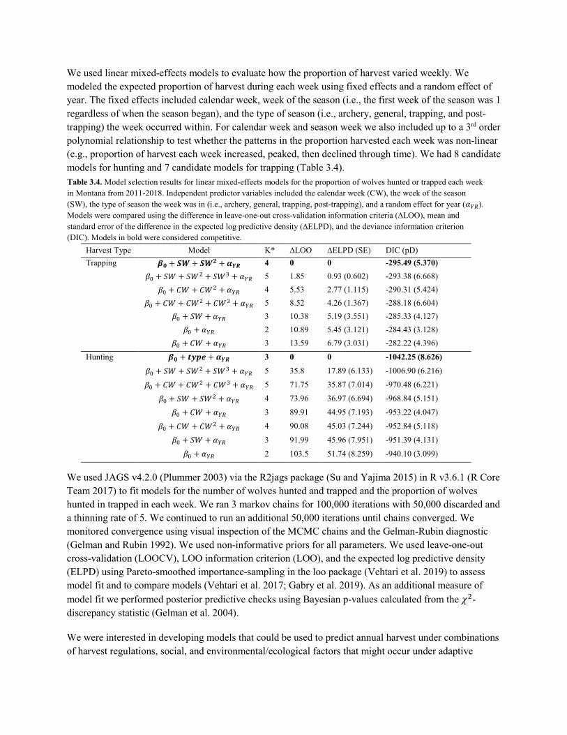
We used linear mixed-effects models to evaluate how the proportion of harvest varied weekly. We modeled the expected proportion of harvest during each week using fixed effects and a random effect of year. The fixed effects included calendar week, week of the season (i.e., the first week of the season was 1 regardless of when the season began), and the type of season (i.e., archery, general, trapping, and post-trapping) the week occurred within. For calendar week and season week we also included up to a 3rd order polynomial relationship to test whether the patterns in the proportion harvested each week was non-linear (e.g., proportion of harvest each week increased, peaked, then declined through time). We had 8 candidate models for hunting and 7 candidate models for trapping (Table 3.4).

We used JAGS v4.2.0 (Plummer 2003) via the R2jags package (Su and Yajima 2015) in R v3.6.1 (R Core Team 2017) to fit models for the number of wolves hunted and trapped and the proportion of wolves hunted in trapped in each week. We ran 3 markov chains for 100,000 iterations with 50,000 discarded and a thinning rate of 5. We continued to run an additional 50,000 iterations until chains converged. We monitored convergence using visual inspection of the MCMC chains and the Gelman-Rubin diagnostic (Gelman and Rubin 1992). We used non-informative priors for all parameters. We used leave-one-out cross-validation (LOOCV), LOO information criterion (LOO), and the expected log predictive density (ELPD) using Pareto-smoothed importance-sampling in the loo package (Vehtari et al. 2019) to assess model fit and to compare models (Vehtari et al. 2017; Gabry et al. 2019). As an additional measure of model fit we performed posterior predictive checks using Bayesian p-values calculated from the 𝜒𝜒2-discrepancy statistic (Gelman et al. 2004).

We were interested in developing models that could be used to predict annual harvest under combinations of harvest regulations, social, and environmental/ecological factors that might occur under adaptive

Table 3.4. Model selection results for linear mixed-effects models for the proportion of wolves hunted or trapped each week in Montana from 2011-2018. Independent predictor variables included the calendar week (CW), the week of the season (SW), the type of season the week was in (i.e., archery, general, trapping, post-trapping), and a random effect for year (𝛼𝛼𝑌𝑌𝑌𝑌). Models were compared using the difference in leave-one-out cross-validation information criteria (∆LOO), mean and standard error of the difference in the expected log predictive density (∆ELPD), and the deviance information criterion (DIC). Models in bold were considered competitive.

Harvest Type Model K* ∆LOO ∆ELPD (SE) DIC (pD) Trapping 𝜷𝜷𝟎𝟎 + 𝑺𝑺𝑺𝑺 + 𝑺𝑺𝑺𝑺𝟐𝟐 + 𝜶𝜶𝒀𝒀𝒀𝒀 4 0 0 -295.49 (5.370)

𝛽𝛽0 + 𝑆𝑆𝑆𝑆 + 𝑆𝑆𝑆𝑆2 + 𝑆𝑆𝑆𝑆3 + 𝛼𝛼𝑌𝑌𝑌𝑌 5 1.85 0.93 (0.602) -293.38 (6.668) 𝛽𝛽0 + 𝐶𝐶𝑆𝑆 + 𝐶𝐶𝑆𝑆2 + 𝛼𝛼𝑌𝑌𝑌𝑌 4 5.53 2.77 (1.115) -290.31 (5.424)

𝛽𝛽0 + 𝐶𝐶𝑆𝑆 + 𝐶𝐶𝑆𝑆2 + 𝐶𝐶𝑆𝑆3 + 𝛼𝛼𝑌𝑌𝑌𝑌 5 8.52 4.26 (1.367) -288.18 (6.604) 𝛽𝛽0 + 𝑆𝑆𝑆𝑆 + 𝛼𝛼𝑌𝑌𝑌𝑌 3 10.38 5.19 (3.551) -285.33 (4.127)

𝛽𝛽0 + 𝛼𝛼𝑌𝑌𝑌𝑌 2 10.89 5.45 (3.121) -284.43 (3.128) 𝛽𝛽0 + 𝐶𝐶𝑆𝑆 + 𝛼𝛼𝑌𝑌𝑌𝑌 3 13.59 6.79 (3.031) -282.22 (4.396)

Hunting 𝜷𝜷𝟎𝟎 + 𝒎𝒎𝒕𝒕𝒕𝒕𝒎𝒎 + 𝜶𝜶𝒀𝒀𝒀𝒀 3 0 0 -1042.25 (8.626)

𝛽𝛽0 + 𝑆𝑆𝑆𝑆 + 𝑆𝑆𝑆𝑆2 + 𝑆𝑆𝑆𝑆3 + 𝛼𝛼𝑌𝑌𝑌𝑌 5 35.8 17.89 (6.133) -1006.90 (6.216)

𝛽𝛽0 + 𝐶𝐶𝑆𝑆 + 𝐶𝐶𝑆𝑆2 + 𝐶𝐶𝑆𝑆3 + 𝛼𝛼𝑌𝑌𝑌𝑌 5 71.75 35.87 (7.014) -970.48 (6.221)

𝛽𝛽0 + 𝑆𝑆𝑆𝑆 + 𝑆𝑆𝑆𝑆2 + 𝛼𝛼𝑌𝑌𝑌𝑌 4 73.96 36.97 (6.694) -968.84 (5.151)

𝛽𝛽0 + 𝐶𝐶𝑆𝑆 + 𝛼𝛼𝑌𝑌𝑌𝑌 3 89.91 44.95 (7.193) -953.22 (4.047)

𝛽𝛽0 + 𝐶𝐶𝑆𝑆 + 𝐶𝐶𝑆𝑆2 + 𝛼𝛼𝑌𝑌𝑌𝑌 4 90.08 45.03 (7.244) -952.84 (5.118)

𝛽𝛽0 + 𝑆𝑆𝑆𝑆 + 𝛼𝛼𝑌𝑌𝑌𝑌 3 91.99 45.96 (7.951) -951.39 (4.131)

𝛽𝛽0 + 𝛼𝛼𝑌𝑌𝑌𝑌 2 103.5 51.74 (8.259) -940.10 (3.099)

harvest management. We used the posterior predictive distributions (Gelman et al. 2004) of the coefficient estimates from the most supported model for total wolves hunted, total wolves trapped, the proportion of wolves hunted each week, and the proportion of wolves trapped each week to generate predictions of the number of wolves harvested under 4 management actions. First, we considered the no harvest management action, which was included if the population fell below established minimums for a regulated wolf hunting season. Second, the status quo management action included the 2018-2019 harvest regulations for wolves, which have been consistent since the 2013-2014 license year. This included a bag limit of 5 wolves, 2 weeks of archery, 26 weeks of firearm, and 11 weeks of trapping. For the remaining 2 management actions we asked MFWP representatives what combination of bag limits and season lengths to include in a restricted management action and a liberal management action. Based on an average of responses, the restricted management action included a bag limit of 1, 2 weeks of archery, 5 weeks of firearm, and 2 weeks of trapping. The liberal management action was a bag limit of 10 wolves, 2 weeks of archery, 38 weeks of firearm, and 17 weeks of trapping.

Results and Management Actions Used for AM Framework

From the 2011-2018 license years there were 1833 recorded harvests (1197 hunted and 636 trapped). The sex ratio of harvest was approximately 1:1 (49% females, 51% males). Total annual harvest ranged from 128-167 for hunting and 76-129 for trapping.

All models for total number of wolves hunted and the proportion of wolves hunted each week converged with Gelman-Rubin statistics of < 1.01. The most supported model for total wolves hunted included season length and method of hunting (Table 3.3), and the model fitted the data well (Bayesian p-values ~ 0.61; all Pareto-k diagnostic values < 0.5). We found that firearm/crossbow had a positive effect (𝛽𝛽 =4.02; 𝐶𝐶𝑅𝑅𝐶𝐶 = 3.56− 4.57) and that season length had no discernable effect (𝛽𝛽 = −0.01; 55% 𝐶𝐶𝑅𝑅𝐶𝐶 =−0.07− 0.04) on the number of wolves hunted. This is likely because of the lack of variation in season length in the data. The most supported model for the proportion of wolves hunted each week was season type (Table 3.4, Figure 3.5). Most wolves were hunted during the general season (𝛽𝛽 = 0.05; 𝐶𝐶𝑅𝑅𝐶𝐶 =0.037− 0.059; Figure 3.5). The greater the coefficient, the more wolves were hunted per week during the season type.

All models for total number of wolves trapped and the proportion of wolves trapped each week converged with Gelman-Rubin statistics of < 1.01. The most supported model for total wolves trapped was the null model, or mean effect model (Table 3.3). The most supported model for the proportion of

Figure 3.5. Coefficient estimates for the effects of type of season on the proportion of wolves hunted each week in Montana from 2011-2018. The colored bands represent the 95%, 75%, and 55% credible intervals.

wolves trapped each week was a quadratic relationship with the week of the season (Table 3.4). We found that the proportion of wolves trapped increased and peaked around week 6 of the season and then declined.

For the status quo scenario, we found that predicted total wolves hunted and trapped was 142 (95% quantile: 98-197) and 83 (95% quantile: 55-118) wolves, respectively. The predicted mean annual total wolf harvest under the status quo scenario was 217 (Figure 3.6A).

For the restricted scenario, we found that predicted total wolves hunted and trapped was 42 (95% quantile: 24-65) and 11 (95% quantile: 2-24), respectively. The predited mean total wolf harvest under the restricted scneario was 54 wolves (Figure 3.6B).

For the liberal scenario, we found that predicted total wolves hunted and trapped was 175 (95% quantile: 114-252) and 97 (95% quantile: 58-150) wolves, respectively. The predicted mean total annual wolf harvest under the liberal scenario was 272 (Figure 3.6C).

3.4 AM Framework

Introduction

Not only are there multiple components to an AM framework, but also multiple phases. The deliberative or set-up phase for AM (Williams et al. 2002) consists of defining the problem and developing the

Figure 3.6. Predicted posterior distribution for the total number of wolves hunted under 3 different hunting season lengths for wolves in Montana: A) the restricted management action, B) the status quo management action, and C) the liberal management action.

components: objectives, management actions, predictive models, optimization algorithms, and monitoring (Figure 3.7). The deliberative phase provides the framework for informed management. The iterative phase is based on the components developed during the deliberative phase, and the optimization algorithm is used to identify the best managemement action based on objectives, available management actions, model predictions and utility functions, and estimates from monitoring data (Figures 3.1 and 3.7). As management actions are implemented, the measureable attributes are affected, which is estimated via monitoring. Model predictions are compared to estimates from monitoring, leading to increased support for models that predict well and decreased support for models that predicted poorly. The model support is updated and used to identify the new optimal management action, and the cycle continues (Figure 3.1). The iterative phase is thus based on current knowledge of how the population functions (model support) and current population size estimated from monitoring. The cornorstone of AM is taking advantage of iterated decision making to learn, and then use what is learned to improve future decisions.

A challenge with wolf management in Montana is general uncertainty in the effects of harvest on population dynamics of wolves. Harvest appears to be mostly an additive source of mortality for yearlings and adults (Creel and Rotella 2010; Murray et al. 2010; Horne et al. 2019) and to reduce pup survival and recruitment (Objective #2, Ausband et al. 2015, 2017). Despite the negative effects of harvest on survival and recruitment, however, wolves in Montana have sustained harvest rates from 0.17 to 0.36 and remained relatively stationary (Inman et al. 2019). This may be due to increased immigration into Montana or decreased dispersal from Montana (i.e., positive net immigration). Because wolves can travel great distances, immigration and dispersal can be important processes in dynamics of wolf populations (Hayes and Harestad 2000; Fuller et al. 2003; Adams et al. 2008; Bassing 2017). Decreased dispersal rates of wolves in Alaska partially compensated for harvest mortality and resulted in stationary densities. It is unclear, however, how net immigration into Montana affects wolf population dynamics.

We applied our simplifeid AM approach as an example of how AM could be used to guide harvest management decisions for gray wolves in Montana and test the hypothesis that net immigration partially compensates for harvest. Our objectives were to 1) develop a simplified deliberative phase for the AM framework for wolves in Montana , 2) determine optimal management actions given how we quantified the components in the simplified deliberative phase, and 3) implement the iterative phase of AM as an

Figure 3.7. Diagram of structured decision making and adaptive management showing the process to set up the decision model framework. This figure is adapted from previously published figures (Williams et al. 2007, McGowan et al. 2015). The double ended arrows demonstrate the concept of continuing to revisit past steps in the process, and the dashed arrows demonstrate the concept of revisiting all steps of AM after implementation.

example of how this tool could work moving forward. We used population models to describe changes in abundance of wolves and formalized qunatitative relationships between population size of wolves, recruitment, depredation events, impacts of wolves on ungulates, and the harvest regulations and management objectives. We considered 2 alternative models of wolf population dynamics. The first model assumed net immigration of wolves into Montana was 0 and was not partially compensating for harvest. The second model assumed net immigration into Montana was positive and was partially compensating for harvest.

Methods

For the deliberative phase, we used the objectives and mathematical functions detailed above (Sect. 3.2) to evaluate how well alternative management actions meet objectives. We evaluated the management actions elicted from MFWP representatives and incorporated uncertainty in total harvest from Section 3.3 above. For the predictive models, we used a per capita model with additive harvest mortality and density dependent recruitment. We used estimates of abundance of wolves in Montana (Inman et al. 2019) as the monitoring data.

We used stochastic dynamic programming (SDP) to compute the optimal set of management actions (Bellman 1957; Williams et al. 2002; Puterman 2014). We solved the problem for an infinite time horizon by using policy iteration in R v3.6.1 (R Core Team 2017) using package MDPtoolbox (Chadès et al. 2017). We assumed a discount factor close to 1 (i.e., 0.99999; Puterman 2014). A discount factor describes the relative value of rewards in future time periods, and a value close to 1 indicates that the value of a resource in the future is the same as the value of the resource now (Puterman 2014). The optimal management actions were state-dependent, i.e., the optimal action depended on population size and model weights (support for models). Therefore, uncertainty could be reduced by implementing the optimal management actions and then updating model weights in the iterative phase.

As an example of the iterative phase, we used a passive adaptive learning and updated model weights using Bayes’ theorem in 2 different types of simulations. First, we simulated a population following the optimal management actions to predict the median population size, number of pups recruited, number of depredation events, and the reward value for how well each management action met objectives. We ran 1000 replications of each simulation for 100 years. Each year, the optimal management action dependent on population size and model weight was selected and enacted, and the population and model weight states were updated. We updated model weights assuming model 1 was correct and then model 2 was correct. Second, we simulated the wolf population in Montana from 2011-2018, however, instead of using the optimal management actions we used the status quo management action enacted by MFWP for those years. We ran 1000 replications of each simulation. To update model weights, we compared predictions from the competing models and the estimated abundance of wolves in Montana from monitoring data (Inman et al. 2019). Again, we recorded predictions for median population size, number of pups recruited, number of depredation events, and the reward value. Additionally, we recorded changes to model weights to determine if there was support for one hypothesis over the other.

Preliminary Results and Discussion

Expected outcomes differed for the 4 management actions (no hunting, restricted hunting, status quo, and liberal hunting). No hunting had greater median number of depredation events per year for all population sizes (Figure 3.8). Restricted hunting was expected to have slightly more depredation events than the status quo or liberal hunting actions because future population size was greater under the restricted hunting regulations and we used per capita depredation rates (Figure 3.8). Total number of pups recruited was expected to be greatest under more restrictive hunting management actions (Figure 3.8). The median reward, which is how well an action meets all objectives, for each management action differed across the population sizes (Figure 3.8).

Based on the model-averaged transition probabilities under equal model weight for the 2 hypotheses (i.e., 0.5), no hunting resulted in the highest probability of increasing population size for all initial abundances. Restrictive hunting also had a high probability of increasing future population size except when the initial population was below 200 wolves. The status quo and liberal hunting management actions had the lowest probability of increasing future abundance, and when the initial population was fewer than ~700 wolves, both scenarios had a greater probability of reducing the population. An example of output from this decision tool that can be useful for management is a policy plot (Figure 3.9). A policy plot displays the optimal management action to implement for different abundances given the components of the deliberative phase of AM (i.e., objectives, management actions, population models, and optimization

Figure 3.8. Expected performance from 2 models of wolf population dynamics with equal model weight under 4 management actions: no harvest, restricted harvest, status quo, and liberal harvest. The figures show the median expected A) number of depredation events, B) number of pups recruited, C) total harvest, and D) reward or utility dependent on the current state of the population and management action.

method). AM does not produce static numbers, and when one hypothesis gains support over others, the policy plot could change. In the example figure (Figure 3.9), the optimal management action varied little with different model support (varied by ~ 50 wolves for 0.1 and 0.9 model weight). Although we found support for the hypothesis that net immigration into Montana was positive, reducing this uncertainty had little effect on the optimal management actions (Figure 3.9). When there was little to no support for the hypothesis (model 1 weight of 0.9) the population size at which to implement the liberal management action occurred at 1030 compared to 980 when there was most support for the hypothesis (model 1 weight of 0.1). Therefore, this uncertainty does not influence optimal decisions for harvest management of wolves. In general, the optimal management action was no hunting when population size was less than 440 wolves, restrictive hunting when the population was between 440 and 620 wolves, status quo hunting when population size was between 620 and 990 wolves, and liberal hunting when population size was greater than 990 wolves in the example (Figure 3.9).

When we simulated passive adaptive management for the wolf population in Montana from 2011 to 2018 for the iterative phase, we found that expected wolf population size, number of pups recruited, and depredation events declined (Figure 3.10). This follows general patterns for estimates of abundance of wolves and the number of verified depredation events in Montana (Inman et al. 2019). Over the 8 year period, weight for model 1 (net immigration = 0) declined from 0.50 to 0.36, and weight for model 2 (net immigration > 0) increased from 0.50 to 0.64 (Figure 3.10).

AM can easily account for many sources of uncertainty, including structural or model uncertainty. Using AM, we were able to find support for the hypothesis that net immigration of wolves into Montana was positive. We considered 2 competing models of wolf population dynamics. One model assumed that there was not net immigration into Montana, whereas the second model assumed that net immigration into Montana was positive. By simulating the wolf population in Montana with passive AM, we found that model uncertainty could be reduced. From 2011 to 2018, the second model gained support increasing

Figure 3.9. Example of optimal management strategies based on 2 competing models of wolf population dynamics and different model weights. Change in model weights indicates support for one hypothesis over another. Optimal policies were state-dependent on both initial wolf population size and model 1 weight. The decisions considered included no harvest, restricted harvest, the status quo harvest for wolves in Montana, and liberal harvest.

from 0.5 to 0.64. This supports the hypothesis that net immigration of wolves into Montana is positive. Dispersal rates from Yellowstone are high (Jimenez et al. 2017), and may be a source for Montana. Positive net immigration could partially compensate for harvest in the wolf population in Montana, and allow the population to sustain greater harvest rates than if net immigration was 0. In the second model we assumed that net immigration was a mean of 10%, however uncertainty in the parameter value of net immigration could also be included in passive adaptive management to reduce uncertainty in the estimate over time (Williams et al. 2002).

Learning in AM is contingent on monitoring data. Given how we set up the deliberative phase for the AM framework for wolves, monitoring only requires estimates of abundance. These estimates of abundance, however, should be reliable. Work from Objective #1 will help ensure future estimates of abundance are more accurate and precise, which will improve learning in an AM framework. With AM it is common to revisit objectives, alternatives, and even population models over time. We have developed a flexible AM framework that will allow managers to evaluate different constructions of objectives (weights and utility functions) and different management actions (combinations of bag limit, hunting season length, and trapping season length) for managing wolves with regulated public harvest. We developed a tool for FWP to alter risk attitudes for objectives, weights of objectives, and other factors related to the construction of utility functions. With this tool, managers can evaluate any combination of season lengths and bag limits to create custom management alternatives. Additionally, we added the capability to evaluate management alternatives at the regional scale (FWP regional administrative boundaries) to account for spatial variation

Figure 3.10. Expected outcomes from simulations of passive adaptive management for wolves in Montana from 2011 – 2018 based on harvest decisions implemented by Montana Fish, Wildlife and Parks. The expected performance metrics were derived from the weighted average of 2 models of wolf population dynamics (model 1: no net immigration, model 2: positive net immigration). Performance includes expected A) population size, B) number of annual depredation events, C) number of pups recruited, and D) change in model 1 (no net immigration) weight.

in the measurable attributes of the objectives. Measurable attributes and construction of quantitative functions for objectives can be revisited and revised as needed to ensure the AM framework is a useful tool for wolf management decisions.

Sensitivity analyses

To test sensitivity of recommended decisions and learning to uncertainty in estimates of abundance, we will use the upper and lower confidence limits of estimates of abundance. The AM model and recommended decision was insensitive to uncertainty in other parameter values in the models. The only component that the recommended decision was sensitive to was objective weight for maintaining hunting opportunities for wolves or for increasing public acceptance of wolf harvest. Therefore, for this framework to be effective, careful consideration of stakeholder and decision maker values should be considered to determine objective weights.

Literature Cited

Adams, L. G., R. O. Stephenson, B. W. Dale, R. T. Ahgook, and D. J. Demma. 2008. Population dynamics and harvest characteristics of wolves in the Central Brooks Range, Alaska. Wildlife Monographs 170:1–25.

Ausband, D. E., M. S. Mitchell, C. R. Stansbury, J. L. Stenglein, and L. P. Waits. 2017. Harvest and group effects on pup survival in a cooperative breeder. Proceedings of the Royal Society of London B: Biological Sciences 284:20170580.

Ausband, D. E., C. R. Stansbury, J. L. Stenglein, J. L. Struthers, and L. P. Waits. 2015. Recruitment in a social carnivore before and after harvest. Animal Conservation 18:415–423.

Bassing, S. 2017. Harvest and persistence of wolf populations: variable effects of harvest on wolf packs in the Rocky Mountains. University of Montana.

Bellman, R. E. 1957. Dynamic programming. Princeton University Press, Princeton.

Bischof, R., E. B. Nilsen, H. Brøseth, P. Männil, J. Ozoliņš, J. D. C. Linnell, and M. Bode. 2012. Implementation uncertainty when using recreational hunting to manage carnivores. The Journal of applied ecology 49:824–832.

Chadès, I., G. Chapron, M.-J. Cros, F. Garcia, and R. Sabbadin. 2017. MDPtoolbox: Markov decision processes toolbox.

Conroy, M. J., and J. T. Peterson. 2013. Decision making in natural resource management: a structured, adaptive approach. John Wiley & Sons.

Creel, S., and J. J. Rotella. 2010. Meta-analysis of relationships between human offtake, total mortality and population dynamics of gray wolves (Canis lupus). PloS one 5:e12918.

DeCesare, N. J., S. M. Wilson, E. H. Bradley, J. A. Gude, R. M. Inman, N. J. Lance, K. Laudon, A. A. Nelson, M. S. Ross, and T. D. Smucker. 2018. Wolf-livestock conflict and the effects of wolf management. The Journal of Wildlife Management 82:711–722.

Defenders of Wildlife. 2013. Wolves in the northern Rockies.

Ericsson, G., and T. A. Heberlein. 2003. Attitudes of hunters, locals, and the general public in Sweden now that the wolves are back. Biological Conservation 111:149–159.

Fuller, T. K., L. D. Mech, and J. Fitts-Cochran. 2003. Wolf population dynamics. Pages 161–191 in L. D. Mech and L. Boitani, editors. Wolves: behavior, ecology and conservation. University of Chicago Press, Chicago, Illinois.

Gabry, J., D. Simpson, A. Vehtari, M. Betancourt, and A. Gelman. 2019. Visualization in Bayesian workflow. Journal of the Royal Statistical Soceity A 182:389–402.

Gelman, A., J. B. Carlin, H. S. Stern, and D. B. Rubin. 2004. Bayesian data analysis. Second edition. Chapman and Hall/CRC Press.

Gelman, A., and D. B. Rubin. 1992. Inference from iterative simulation using multiple sequences. Statistical Science 7:457–472.

Gude, J. A., M. S. Mitchell, R. E. Russell, C. A. Sime, E. E. Bangs, L. D. Mech, and R. R. Ream. 2012. Wolf population dynamics in the U.S. Northern Rocky Mountains are affected by recruitment and human-caused mortality. The Journal of Wildlife Management 76:108–118.

Hammond, J., R. Keeney, and H. Raiffa. 1999. Smart choices: a practical guide to making better decisions. Harvard Business Review Press.

Hayes, R. D., and A. S. Harestad. 2000. Demography of a recovering wolf population in the Yukon. Canadian Journal of Zoology 78:36–48.

Horne, J. S., D. E. Ausband, M. A. Hurley, J. Struthers, J. E. Berg, and K. Groth. 2019. Integrated population model to improve knowledge and management of Idaho wolves. The Journal of Wildlife Management 83:32–42.

Inman, B., K. M. Podruzny, T. D. Smucker, A. A. Nelson, M. Ross, N. Lance, T. Parks, D. K. Boyd, and S. Wells. 2019. Montana gray wolf conservation and management 2018 annual report. Helena, Montana.

Jimenez, M. D., E. E. Bangs, D. K. Boyd, D. W. Smith, S. A. Becker, D. E. Ausband, S. P. Woodruff, E. H. Bradley, J. Holyan, and K. Laudon. 2017. Wolf dispersal in the Rocky Mountains, Western United States: 1993-2008. The Journal of Wildlife Management 81:581–592.

Kapfer, P. M., and K. B. Potts. 2012. Socioeconomic and ecological correlates of bobcat harvest in Minnesota. The Journal of Wildlife Management 76:237–242.

Lewis, M. S., A. L. Metcalf, E. C. Metcalf, C. Phelan, J. A. Gude, Q. Kujala, and B. Inman. 2018. Better understanding Montanans thoughts regarding wolves and wolf management in Montana. Helena, Montana.

Lewis, M. S., G. Pauley, Q. Kujala, J. A. Gude, Z. King, and K. Skogen. 2012. Selected results from four separate surveys of resident Montanans regarding Montana’s wolf hunt. Helena, Montana.

Montana Fish Wildlife and Parks. 2018. Montana gray wolf conservation and management 2017 annual report. Helena, Montana.

Murray, D. L., D. W. Smith, E. E. Bangs, C. Mack, J. K. Oakleaf, J. Fontaine, D. Boyd, M. Jiminez, C. Niemeyer, T. J. Meier, D. Stahler, J. Holyan, and V. J. Asher. 2010. Death from anthropogenic

causes is partially compensatory in recovering wolf populations. Biological Conservation 143:2514–2524.

Plummer, M. 2003. JAGS: A program for analysis of Bayesian graphical models using Gibbs sampling.

Puterman, M. L. 2014. Markov decision processes: discrete stochastic dynamic programming. John Wiley & Sons.

R Core Team. 2017. R: a language and environment for statistical computing. R Foundation for Statistical Computing, Vienna, Austria.

Runge, M. C., J. B. Grand, and M. S. Mitchell. 2013. Structured decision making. Pages 51–73 in P. R. Krausman and J. W. I. I. I. Cain, editors. Wildlife Management and Conservation: Contemporary Principles and Practices. The Johns Hopkins University Press, Baltimore, MD.

Su, Y.-S., and M. Yajima. 2015. R2jags: using R to run “JAGS.”

Vehtari, A., J. Gabry, Y. Yao, and A. Gelman. 2019. loo: efficient leave-one-out cross-validation and WAIC for Bayesian models.

Vehtari, A., A. Gelman, and J. Gabry. 2017. Practical Bayesian model evaluation using leave-one-out cross-validation and WAIC. Statistics and Computing 27:1413–1432.

Walters, C. 1986. Adaptive management of renewable resources. MacMillan Pub. Co.,New York, NY.

Williams, B. K., J. D. Nichols, and M. J. Conroy. 2002. Analysis and management of animal populations. Academic Press.

Williams, B. K., R. C. Szaro, and C. D. Shapiro. 2009. Adaptive management: the U.S. Department of the Interior technical guide. Adaptive Management Working Group, U.S. Department of the Interior, Washington, DC.

OBJECTIVE 4: DESIGN A TARGETED MONITORING PROGRAM—S. Sells and A. Keever, Projects 1 & 2

4.1 Introduction

Monitoring plays a central role in wildlife management. Monitoring allows managers to detect changes in wildlife populations or habitat, evaluate effectiveness of management actions for altering wildlife populations or habitat, make management decisions based on population size or status of the resource, and facilitate learning to improve future management actions (Nichols and Williams 2006). Monitoring can be most useful when it is directly linked to objectives and targets key uncertainties that impede management (Gibbs et al. 1999; Nichols and Williams 2006). Targeted monitoring can be more efficient and a better use of limited resources compared to surveillance monitoring (i.e., monitoring not guided by a priori hypotheses that include all aspects of a population’s demographic and ecological factors (Nichols and Williams 2006).

Wolves in Montana are managed through harvest. Accordingly, reliable estimates of population size are needed to make informed decisions for harvest regulations and evaluate effectives of harvest regulations in meeting objectives of wolf management. As the final step of this project, we will design a targeted monitoring program to provide reliable estimates of population size and inform decisions in the adaptive management (AM) framework.

4.2 General Approach

We will perform sensitivity analyses on the territory size, group size, recruitment, and AM models to identify factors that strongly influence results and decisions. While integrating the territory and group size models into POM, we will determine the sensitivity of POM estimates to these new models and recommend the monitoring effort to reduce uncertainty in these estimates. For the empirical recruitment model, we evaluated the sensitivity of accuracy and precision of estimates to different amounts of group count and collar data. These sensitivity results will help determine the amount of data needed to produce reliable estimates of recruitment. For the component recruitment model, we will evaluate sensitivity to uncertainty in data that are used to generate predictions of recruitment. These results will help determine which data may need to be monitored to produce reliable predictions of recruitment from the model. We are continuing to refine the AM framework; however, we evaluated sensitivity of the models in the AM framework to uncertainty in parameter estimates. In some instances, reducing uncertainty does not affect decisions (e.g., Smith et al. 2013), and may not be worth the cost of collecting the data. Therefore, if the model is sensitive to any uncertainties, we will calculate the expected value of information (Raiffa and Schlaifer 1961; Runge et al. 2011; Williams et al. 2011), which represents the increase in effectiveness of management expected if uncertainty were reduced. Additionally, as a post-hoc analysis, we will evaluate the sensitivity of decisions and learning in AM to uncertainty in estimates of abundance using the lower and upper confidence intervals.

The components which most influence the results and decisions can be targeted for monitoring to reduce uncertainty and produce robust estimates of abundance and recruitment. Based on results of sensitivity

analyses for the different models, we will develop recommendations for a unified monitoring program. Recommendations will include sampling effort, sampling distribution, and what should be monitored.

Literature Cited

Gibbs, J. P., H. L. Snell, and C. E. Causton. 1999. Effective monitoring for adaptive wildlife management: lessons from the Galapagos Islands. The Journal of Wildlife Management 63:1055–1065.

Nichols, J. D., and B. K. Williams. 2006. Monitoring for conservation. Trends in ecology & evolution 21:668–73.

Raiffa, H., and R. Schlaifer. 1961. Applied statistical decision theory. Harvard University Press, Cambridge, MA.

Runge, M. C., S. J. Converse, and J. E. Lyons. 2011. Which uncertainty? Using expert elicitation and expected value of information to design an adaptive program. Biological Conservation 144:1214–1223.

Smith, D. R., C. P. McGowan, J. P. Daily, J. D. Nichols, J. A. Sweka, and J. E. Lyons. 2013. Evaluating a multispecies adaptive management framework: must uncertainty impede effective decision-making? Journal of Applied Ecology 50:1431–1440.

Williams, B. K., M. J. Eaton, and D. R. Breininger. 2011. Adaptive resource management and the value of information. Ecological Modelling 222:3429–3436.