The Cashless Policy and Foreign Direct Investment in Nigeria: A Vector Error Correction Model (VECM)...

© 2014 Research Academy of Social Sciences

http://www.rassweb.com 43

International Journal of Financial Economics

Vol. 2, No. 2, 2014, 43-57

The Cashless Policy and Foreign Direct Investment in Nigeria: A

Vector Error Correction Model (VECM) Approach

Ezie Obumneke1, Adeniji Sesan Oluseyi

2, Oniore Jonathan Ojarikre

3

Abstract

The study undertakes an econometric research to analyze the cashless policy and its effectiveness on

attracting foreign direct investment in Nigeria using quarterly data of 2006 to 2012. The log linear vector

error correction model (VECM) was adopted to examine how automated teller machine (ATM), interbank

transfer (IBT) and Mobile money (MM) had impacted on foreign direct investment (FDI). Unit root test was

carried out on each of the variables to determine their level of stationarity. They were however found

stationary after first difference and then used for the regression analysis. From the various regression results,

we find out that the cointegration test confirmed the existence of long run relationship among the variables,

while the granger causality shows a bi-directional relationship where IBT and MM was said to granger cause

FDI in Nigeria. In the VECM model result, all the explanatory variables are positive and significant meaning

that they all contribute positively to the increase in FDI in the country. The study recommends that the use of

ATM, IBT and MM should be much more encouraged in Nigeria, with proper awareness on its benefit. Also

effective policy needs to be developed by the government through the CBN to ensure the effectiveness and

efficiency of ATM, IBT and MM.

Keywords: Automated teller machine (ATM), Interbank transfer (IBT), Mobile money (MM), Foreign direct

investment (FDI), Vector error correction model (VECM), and granger causality

1. Introduction

Foreign Direct Investment (FDI) has been debated to be an important vehicle for the transfer of

technology, contributing to growth in larger measure than domestic investment. Therefore, the need for the

Government to provide special incentives in order to motivate foreign firms to set up companies in the

country becomes an important issue. Carkovic and Levine (2002) noted that the economic rationale for

offering special incentives to attract FDI frequently derives from the belief that foreign investment produces

externalities in the form of technology transfers and spillovers. Several governments in African countries,

Nigeria inclusive, have formulated various policies towards stimulating economic activities by attracting

FDI. Unfortunately, the efforts of most countries in Africa to attract FDI have been futile in spite of the

perceived and obvious need for FDI on the continent.

The Nigerian government has been trying to provide an investment climate conducive for foreign

investments, since the inflow of foreign investments into the country has not been encouraging. The need for

foreign direct investment in Nigeria is borne out of the underdeveloped state of the country’s economy that

essentially hinders the pace of her economic development. Despite the various macroeconomic measures put

in place by the Nigerian government, there seems to be insufficient inflow of FDI into the country.

1 Department of Economics Faculty of Humanities, Social and Management Sciences Bingham University, Karu,

Nasarawa State 2 Postgraduate Student, Department of Economics Faculty of Social Sciences University of Lagos, Akoka, Lagos State

3 Department of Economics Faculty of Humanities, Social and Management Sciences Bingham University, Karu,

Nasarawa State

E. Obumneke et al.

44

The new payments system is expected to play a very crucial role in any economy, being the channel

through which financial resources flow from one segment of the economy to the other, and from investment

activities abroad. It, therefore, represents the major foundation of the modern market economy (CBN, 2011).

According to CBN, the new cash policy was introduced for a number of key reasons, including, To drive

development and modernization of our payment system in line with Nigeria‘s vision 2020 goal of being

amongst the top 20 economies by the year 2020. An efficient and modern payment system is positively

correlated with economic development, and is a key enabler for economic growth. To reduce the cost of

banking services (including cost of credit) and drive financial inclusion by providing more efficient

transaction options and greater reach and to improve the effectiveness of monetary policy in managing

inflation, attract foreign investment and driving economic growth.

In addition, the cash policy aims to curb some of the negative consequences associated with the high

usage of physical cash in the economy, including: high cost of cash: high risk of using cash, high subsidy,

informal economy and inefficiency & corruption (CBN, 2011)

According to (Cobb, 2004), the value of electronic payment goes way beyond the immediate

convenience and safety of cards to a greater sphere of contributing to overall economic development.

Against this backdrop, the study seeks or aims to analyze the positive and negative policy implications

of cash-less banking on foreign direct investment (FDI), with a view to exposing the possible benefits and

challenges poses on FDI and the economy in general.

2. Literature Review: Theoretical and Conceptual Framework/Review

Theory of Foreign Direct Investment

Renewed research interest in FDI stems from the change of perspectives among policy makers from

“hostility” to “conscious encouragement,” especially among developing countries. FDI had, until recently,

been seen as “parasitic” and retarding the development of domestic industries for export promotion(Imoudu,

2012). However, Bende-Nabende and Ford (2002) earlier submitted that the wide externalities in respect of

technology transfer, the development of human capital and the opening up of the economy to international

forces, among other factors, have served to change the former image. Caves (1996) observed that the

rationale for increase efforts to attract more FDI stems from the belief that FDI has several positive effects.

Among these are productivity gain, technology transfers, and the introduction of new processes, managerial

skills and know-how in the domestic market, employee training, international production networks, and

access to markets. Carkovic and Levine (2002) notes that the economic rationale for offering special

incentives to attract FDI frequently derives from the belief that foreign investment produces externalities in

the form of technology transfers and spill-over. According to Athukorala (2003), FDI provides much needed

resources to developing countries such as capital, technology, managerial skills, entrepreneurial ability,

brand and access to markets which are essential for developing countries to industrialize, develop, create jobs

and attack the poverty situation in their countries.

Another popular conceptualization of, and theoretical framework for, FDI determinants is the “eclectic

paradigm” attributed to Dunning (1988, 1995). It provides a framework that groups micro- and macro-level

determinants in order to analyze why and where multinational companies (MNCs) invest abroad. The

framework posits that firms invest abroad to look for three types of advantages: Ownership (O), Location

(L), and Internalization (I) advantages; hence it is called the OLI framework. The ownership-specific

advantages (of property rights/patents, expertise and other intangible assets) allow a firm to compete with

others in the markets it serves regardless of the disadvantages of being foreign because it is able to have

access to, and exploit and export natural resources and resource-based products that are available to

it(Anyanwu,2011). These advantages may arise from the firm‟s ability to coordinate complementary

activities such as manufacturing and distribution, and the ability to exploit differences between countries.

The location advantages are those that make the chosen foreign country a more attractive site (such as labor

advantages, natural resources, trade barriers that restrict imports, gains in trade costs and strategic advantages


45

through intangible assets) for FDI than the others hence the reason for the FDI is to supply the domestic

market of the recipient country through an affiliate (horizontal FDI). The location advantages may arise from

differences in country natural endowments, government regulations, transport costs, macroeconomic

stability, and cultural factors. Internalization advantages arise from exploiting imperfections in external

markets, including reduction of uncertainty and transaction costs in order to generate knowledge more

efficiently as well as the reduction of state-generated imperfections such as tariffs, foreign exchange controls,

and subsidies. In this case, the delocalization of all or a portion of the production process (e.g. production of

components/parts and/or different locations) leads to low costs benefits (vertical FDI) (Baniak et al, 2005;

Sekkat and Veganzones-Varoudakis, 2007; Pantelidis and Nikolopoulos, 2008; and Kinda, 2010). Following

on these, Dunning (1993) identified four categories of motives for FDI: resource seeking (to access raw

materials, labor force, and physical infrastructure resources), market seeking (horizontal strategy to access

the host-country domestic market), efficiency seeking (vertical strategy to take advantage of lower labor

costs, especially in developing countries), and strategic-asset seeking (to access research and development,

innovation, and advanced technology) (Cleeve, 2008).

The Theory of Money

Money plays an important role in facilitating business transactions in a modern economy. Various

theories of money has been propounded to examine the all round effect of money towards economic

transactions. The quantity theory of money is hinged on the Irvin Fisher equation of exchange that states that

the quantum of money multiplied by the velocity of money is equal to the price level multiplied by the

amount of goods sold. It is often replicated as MV= PQ, M is defined as the quantity of money, V is the

velocity of money (the number of times in a year that a currency goes around to generate a currency worth of

income), P represents the price level and Q is the quantity of real goods sold (real output). By definition, this

equation is true. It becomes a theory based on the assumptions surrounding it.

The first assumption is that velocity of money is constant. This is because the factors, often technical,

habitual and institutional, that would necessitate a faster movement in the velocity of money evolve slowly.

Such factors include population density, mode of payment (weekly, monthly), availability of credit sources

and nearness of stores to individuals. This assumption presupposes that the velocity of money is somewhat

independent of changes in the stock of money or price level. However, the Keynes liquidity preference

theory suggests that the speculative components of money demand affect money velocity.

Friedman in his modern theory of the quantity theory of money further explores the variables that could

affect the velocity of money to include human/nonhuman wealth, interest rate, and expected inflation.

The second assumption guiding the QTM is that factors affecting real output are exogenous to the

quantity theory itself. In other words, monetary factors do not influence developments in the realeconomy.

The third assumption states that causality runs from money to prices. Thus, the quantity theory of money can

be represented as

MV →PQ

In simple terms, this states that prices vary proportionally in response to changes in the quantum of

money, with velocity and real output invariant.

The Cashless Policy Concept

Cashless economy does not refer to an outright absence of cash transactions in the economic setting but

one in which the amount of cash-based transactions are kept to the barest minimum. It is an economic system

in which transactions are not done predominantly in exchange for actual cash (Daniel,Swartz, and Fermar,

2004). Vassiliou (2004) defines electronic payment as a form of financial exchange that takes place between

the buyer and seller facilitated by means of electronic communication. According to (Cobb, 2004), the value

of electronic payment goes way beyond the immediate convenience and safety of cards to a greater sphere of

contributing to overall economic development. Electronic money is also an electronic store of monetary

value on a technical device that may be widely used for making payments to undertakings other than the

issuer without necessarily involving bank accounts in the transactions, but acting as a prepaid bearer

E. Obumneke et al.

46

instrument. A cashless society possesses the following characteristics; all the money used is issued by private

financial institutions (banks, and possibly other firms). It is conceivable that the central bank continues to

operate like other banks, issuing its own deposits that could be used as money in the same way as other bank

deposits are. However, in that case the central bank has no monopoly in the issue of Money. In a cashless

society the unit of account (e.g. Dollar, euro) remains a national affair and is provided by the state. The

followings among others enhance the functioning of cashless economy; e-finance, e-banking, e-money, e-

brokering, e-exchanges etc(Shittu, 2010) In a modern economy, the use of noncash payment methods such as

cards (credit and debit) dominates the use of cash in payments. The card based payment system has several

players. On the one hand, are the providers of the card based payment system- first of which is the card

companies like MasterCard and Visa who provide their payment network for the system to function. The

second sets of providers are the banks that act as acquirers for merchants and issuers for cardholders and

reach the card payment services to the ultimate users. For these two parties, the card payment system is an

income generating initiative and they are motivated to run the system as they are able to generate adequate

profits out of their operations. On the other side of the system are the users- both merchants and cardholders.

Syanbola(2013) noted that the most outstanding cashless banking channels world over are Mobile

banking; internet banking; telephone banking; electronic card; implants; PoS terminals and ATMs. Electronic

banking is also a system by which transactions are settled electronically with the use of electronic gadgets

such as ATMs, POS terminals, GSM phones, V-cards etc, handled by e-holders, bank customers and other

stakeholders(Edet, 2008).

3. Model Specification and Analysis Techniques

The Structural Model

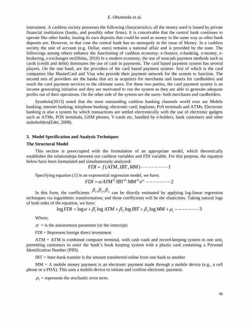
This section is preoccupied with the formulation of an appropriate model, which theoretically

establishes the relationships between our cashless variables and FDI variable. For this purpose, the equation

below have been formulated and simultaneously analyzed:

( , , ) 1FDI f ATM IBT MM

Specifying equation (1) in an exponential regression model, we have; 31 2 2tFDI ATM IBT MM e

In this form, the coefficients 1 2 3, , can be directly estimated by applying log-linear regression

techniques via logarithmic transformation; and those coefficients will be the elasticities. Taking natural logs

of both sides of the equation, we have:

1 2 3log log log log log 3tFDI ATM IBT MM

Where;

= is the autonomous parameter (or the intercept)

FDI = Represent foreign direct investment

ATM = ATM is combined computer terminal, with cash vault and record-keeping system in one unit,

permitting customers to enter the bank’s book keeping system with a plastic card containing a Personal

Identification Number (PIN).

IBT = Inter-bank transfer is the amount transferred online from one bank to another

MM = A mobile money payment is an electronic payment made through a mobile device (e.g., a cell

phone or a PDA). This uses a mobile device to initiate and confirm electronic payment.

t = represents the stochastic error term.


47

Estimation Techniques

The estimation techniques to establish the relationship between FDI variable and Cashless variables take

the following form: firstly, we employs KPSS test for the stationarity test of the variables , after which

Johansen and Juselius cointegration test will be employed to examine if there is long run relationship

between the variables, VAR modeling, impulse response function, variance decomposition and granger

causality. All this is to affirm to a reasonable extent the conclusion to be drawn from our analysis as this

work will be first of its kind to employ these sets of techniques in analyzing the relationship between FDI

and Cashless policy in Nigeria.

Stationarity Test

It is important to note that the level at which time series variables change overtime are different from

each other. Therefore, examining the linear relationship between those variables will lead to problem. Such

problem is called stationarity problem. Stationarity of a series is an important phenomenon because it can

influence its behaviour. Considering a simple model

Yt= Yt-1 + Ut 3.1

Yt is no-stationary when the mean, variance and covariance are not constant overtime. Hence, there is a

need to apply differencing operator (Δ) to it. If a non-stationary series, Yt must be differenced d times before

it becomes stationary, then it is said to be integrated of order. We write Yt ∼ I(d). Therefore, I(0) means the

series is stationary at level, I(1) means the series is stationary at first difference and I(2) shows a stationarity

of a series at second difference or integration of order (0), (1) and (2) respectively .

Three standard procedures of unit root test namely the Augmented Dickey Fuller (ADF), Phillips-Perron

(PP), and the Kwiatkowski-Phillips- Schmidt-Shin (KPSS) tests have being commonly employed in

literatures. As for this study, the KPSS tests will be employed to test the stationarity of the variables

Johnasen Cointegration Test

If two or more series are individually integrated (in the time series sense) but some linear combination

of them has a lower order of integration, then the series are said to be cointegrated.

This study uses two tests to determine the number of cointegration vectors: the Maximum

Eigenvalue test and the Trace test. The Maximum Eigenvalue statistic tests the null hypothesis of r

cointegrating relations against the alternative of r+1 cointegrating relations for r = 0, 1, 2…n-1.

This test statistics are computed as:

LRmax(r/n+1) = -T*log(1-λ) 3.2

Where λ is the Maximum Eigenvalue and T is the sample size. Trace statistics investigate the null

hypothesis of r cointegrating relations against the alternative of n cointegrating relations, where n is the

number of variables in the system for r = 0, 1, 2…n-1. Its equation is computed according to the following

formula:

LRtr (r/n) = -T* 3.3

In some cases Trace and Maximum Eigenvalue statistics may yield different results. In this case the

results of trace test should be preferred.

Vector Error Correction Model (VECM)

A vector error ccorrection model is a way to model nonstationary variables that appear to converge to a

long-run cointegrating relationship. In the VEC model the adjustment parameters show how each variable

deviates in the short-run from the long-run equilibrium relationships given by the cointegrating vectors.

Therefore, to study both the short-run and the long-run dynamics between nonstationary but cointegrated

variables and the dynamic interactions between them one should estimate a VEC model and make inferences

using this system.

E. Obumneke et al.

48

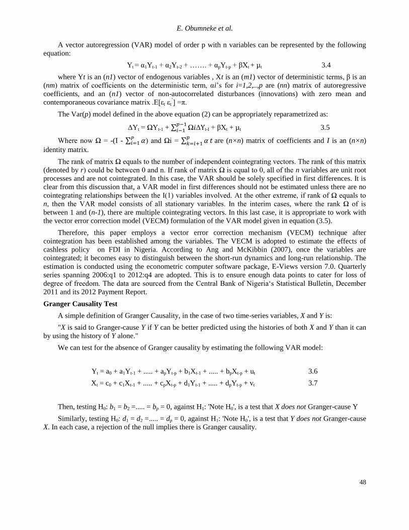
A vector autoregression (VAR) model of order p with n variables can be represented by the following

equation:

Yt = α1Yt-1 + α2Yt-2 + ……. + αpYt-p + βXt + µt 3.4

where Yt is an (n1) vector of endogenous variables , Xt is an (m1) vector of deterministic terms, β is an

(nm) matrix of coefficients on the deterministic term, αi’s for i=1,2,..,p are (nn) matrix of autoregressive

coefficients, and an (n1) vector of non-autocorrelated disturbances (innovations) with zero mean and

contemporaneous covariance matrix .E[εt εt’] =π.

The Var(p) model defined in the above equation (2) can be appropriately reparametrized as:

ΔYt = ΩYt-1 + Δ t-I + βXt + µt 3.5

Where now Ω = -(I - ) and Ωi =

are (n×n) matrix of coefficients and I is an (n×n)

identity matrix.

The rank of matrix Ω equals to the number of independent cointegrating vectors. The rank of this matrix

(denoted by r) could be between 0 and n. If rank of matrix Ω is equal to 0, all of the n variables are unit root

processes and are not cointegrated. In this case, the VAR should be solely specified in first differences. It is

clear from this discussion that, a VAR model in first differences should not be estimated unless there are no

cointegrating relationships between the I(1) variables involved. At the other extreme, if rank of Ω equals to

n, then the VAR model consists of all stationary variables. In the interim cases, where the rank Ω of is

between 1 and (n-1), there are multiple cointegrating vectors. In this last case, it is appropriate to work with

the vector error correction model (VECM) formulation of the VAR model given in equation (3.5).

Therefore, this paper employs a vector error correction mechanism (VECM) technique after

cointegration has been established among the variables. The VECM is adopted to estimate the effects of

cashless policy on FDI in Nigeria. According to Ang and McKibbin (2007), once the variables are

cointegrated; it becomes easy to distinguish between the short-run dynamics and long-run relationship. The

estimation is conducted using the econometric computer software package, E-Views version 7.0. Quarterly

series spanning 2006:q1 to 2012:q4 are adopted. This is to ensure enough data points to cater for loss of

degree of freedom. The data are sourced from the Central Bank of Nigeria‘s Statistical Bulletin, December

2011 and its 2012 Payment Report.

Granger Causality Test

A simple definition of Granger Causality, in the case of two time-series variables, X and Y is:

"X is said to Granger-cause Y if Y can be better predicted using the histories of both X and Y than it can

by using the history of Y alone."

We can test for the absence of Granger causality by estimating the following VAR model:

Yt = a0 + a1Yt-1 + ..... + apYt-p + b1Xt-1 + ..... + bpXt-p + ut 3.6

Xt = c0 + c1Xt-1 + ..... + cpXt-p + d1Yt-1 + ..... + dpYt-p + vt 3.7

Then, testing H0: b1 = b2 =..... = bp = 0, against H1: 'Note H0', is a test that X does not Granger-cause Y

Similarly, testing H0: d1 = d2 =..... = dp = 0, against H1: 'Note H0', is a test that Y does not Granger-cause

X. In each case, a rejection of the null implies there is Granger causality.


49

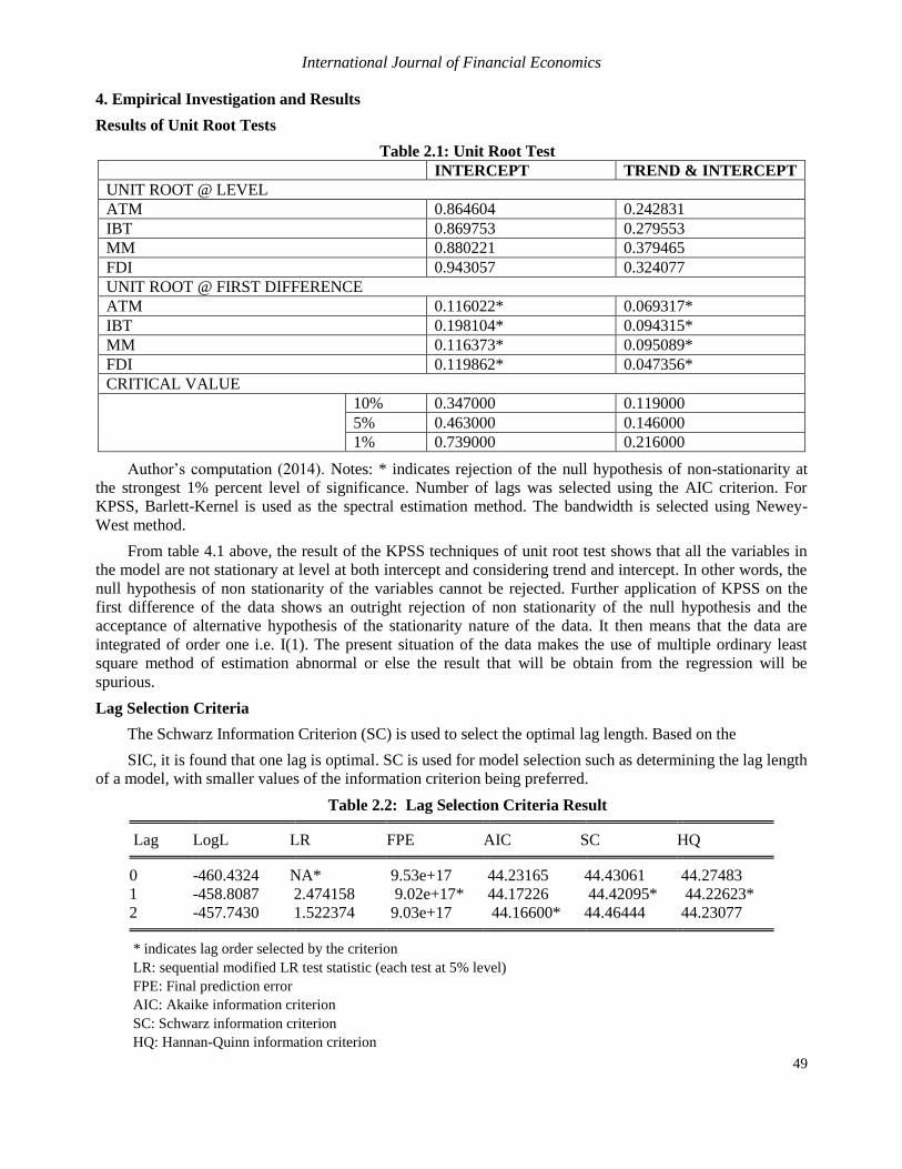
4. Empirical Investigation and Results

Results of Unit Root Tests

Table 2.1: Unit Root Test

INTERCEPT TREND & INTERCEPT

UNIT ROOT @ LEVEL

ATM 0.864604 0.242831

IBT 0.869753 0.279553

MM 0.880221 0.379465

FDI 0.943057 0.324077

UNIT ROOT @ FIRST DIFFERENCE

ATM 0.116022* 0.069317*

IBT 0.198104* 0.094315*

MM 0.116373* 0.095089*

FDI 0.119862* 0.047356*

CRITICAL VALUE

10% 0.347000 0.119000

5% 0.463000 0.146000

1% 0.739000 0.216000

Author’s computation (2014). Notes: * indicates rejection of the null hypothesis of non-stationarity at

the strongest 1% percent level of significance. Number of lags was selected using the AIC criterion. For

KPSS, Barlett-Kernel is used as the spectral estimation method. The bandwidth is selected using Newey-

West method.

From table 4.1 above, the result of the KPSS techniques of unit root test shows that all the variables in

the model are not stationary at level at both intercept and considering trend and intercept. In other words, the

null hypothesis of non stationarity of the variables cannot be rejected. Further application of KPSS on the

first difference of the data shows an outright rejection of non stationarity of the null hypothesis and the

acceptance of alternative hypothesis of the stationarity nature of the data. It then means that the data are

integrated of order one i.e. I(1). The present situation of the data makes the use of multiple ordinary least

square method of estimation abnormal or else the result that will be obtain from the regression will be

spurious.

Lag Selection Criteria

The Schwarz Information Criterion (SC) is used to select the optimal lag length. Based on the

SIC, it is found that one lag is optimal. SC is used for model selection such as determining the lag length

of a model, with smaller values of the information criterion being preferred.

Table 2.2: Lag Selection Criteria Result

Lag LogL LR FPE AIC SC HQ

0 -460.4324 NA* 9.53e+17 44.23165 44.43061 44.27483

1 -458.8087 2.474158 9.02e+17* 44.17226 44.42095* 44.22623*

2 -457.7430 1.522374 9.03e+17 44.16600* 44.46444 44.23077

* indicates lag order selected by the criterion

LR: sequential modified LR test statistic (each test at 5% level)

FPE: Final prediction error

AIC: Akaike information criterion

SC: Schwarz information criterion

HQ: Hannan-Quinn information criterion

E. Obumneke et al.

50

Cointegration Test Results

Table 2.3a Cointegration test Result @ 5% Level of Significance

Unrestricted Cointegration Rank Test (Trace)

Hypothesized Trace 0.05

No. of CE(s) Eigenvalue Statistic Critical Value Prob.**

None * 0.968426 89.37441 47.85613 0.0000

At most 1 * 0.818921 37.54322 29.79707 0.0053

At most 2 0.546404 11.91092 15.49471 0.1613

At most 3 0.003506 0.052687 3.841466 0.8184

Trace test indicates 2 cointegrating eqn(s) at the 0.05 level

* denotes rejection of the hypothesis at the 0.05 level

**MacKinnon-Haug-Michelis (1999) p-values

Unrestricted Cointegration Rank Test (Maximum Eigenvalue)

Hypothesized Max-Eigen 0.05


None * 0.968426 51.83119 27.58434 0.0000

At most 1 * 0.818921 25.63230 21.13162 0.0108

At most 2 0.546404 11.85823 14.26460 0.1161

At most 3 0.003506 0.052687 3.841466 0.8184

Max-eigenvalue test indicates 2 cointegrating eqn(s) at the 0.05 level



Table 2.3b Cointegration test Result @ 1% Level of Significance

Unrestricted Cointegration Rank Test (Trace)

Hypothesized Trace 0.01


None * 0.968426 89.37441 54.68150 0.0000

At most 1 * 0.818921 37.54322 35.45817 0.0053

At most 2 0.546404 11.91092 19.93711 0.1613

At most 3 0.003506 0.052687 6.634897 0.8184

Trace test indicates 2 cointegrating eqn(s) at the 0.01 level



Unrestricted Cointegration Rank Test (Maximum Eigenvalue)

Hypothesized Max-Eigen 0.01


None * 0.968426 51.83119 32.71527 0.0000

At most 1 0.818921 25.63230 25.86121 0.0108

At most 2 0.546404 11.85823 18.52001 0.1161

At most 3 0.003506 0.052687 6.634897 0.8184

Max-eigenvalue test indicates 1 cointegrating eqn(s) at the 0.01 level



With the unit root result depicted in table 4.1 above, there is a clear indication that all the variables are

integrated of the same order therefore show a possibility of long run relationship among the variables. This

brings a need for conducting a cointegration test i.e a test of long run relationship among the variables. The


51

Johansen-Juselius maximum likelihood procedure was applied in determining the cointegrating rank of the

system and the number of common stochastic trends driving the entire system. We reported the trace and

maximum eigen-value statistics and its critical values at both one per cent (1%) and five per cent (5%) in the

table below. The result of multivariate cointegration test based on Johansen and Juselius cointegration

technique reveal that both trace and maxi-eigen statistic shows two cointegrating equations at 5% level of

significant, while trace statistic shows two cointegrating equation and Maxi-Eigen statistic indicates one

cointeragrating equation at 1% level of significance. These results suggest that the appropriate model to use

is the VECM specification with more than one cointegrating vector in the model.

Vector Error Correction Model (VECM) Framework

The result of the long run relationship among foreign direct investment (FDI), ATM is combined

computer terminal, inter banks transfer (IBT) and mobile money (MM) in the below table:

Table 2.4 Error Correction Model (VEC) Framework

Error Correction: D(FDI) D(ATM) D(IBT) D(MM)

CointEq1 -0.493855 -0.008235 -9.19E-06 0.000204

[-1.49237] [-1.59572] [-1.25552] [ 1.60340]

D(FDI(-1)) 0.029353 0.000517 3.78E-06 3.53E-05

[0.08119] [ 0.09167] [ 0.47278] [0.25369]

D(FDI(-2)) 0.414861

0.006988 1.68E-05 0.000159

[1.25152] [1.35177] [2.29144] [1.24857]

D(ATM(-1)) 1.176903 0.157482 0.000230 0.002179

[ 0.03639] [0.31228] [0.32098] [0.17524]

D(ATM(-2)) 82.73365 0.786275 0.002139 0.031919

[ 2.71042] [ 1.65182] [ 3.16738] [ 2.71961]

D(IBT(-1)) 12162.98 316.8404 0.255336 1.078990

[ 0.74857] [ 1.25046] [ 0.71022] [ 0.17271]

D(IBT(-2)) 30317.32 82.68513 0.537338 12.54349

[1.99195] [0.34838] [1.59558] [2.14345]

D(MM(-1)) 245.0866 4.990236 0.001602 0.631406

[ 0.25896] [0.33812] [0.07650] [ 1.73512]

D(MM(-2)) 231.3158 0.024204 0.007973 0.055651

[ 0.35043] [ 0.00235] [0.54590] [ 0.21927]

C -98301407 1360250. 1771.075 -8817.763

[-0.49774] [ 0.44166] [ 0.40529] [-0.11612]

R-squared 0.776000 0.864482 0.513835 0.649577

Adj. R-squared 0.673143 0.689459 05166574 0.599274

F-statistic 10.90188 9.802929 1.479681 12.59516

E. Obumneke et al.

52

The VECM result presented above shows that long-run relationship exists between the variables, as the

error correction term is significant that is, the vector error correction term in the models should have the

required negative sign and lie within the accepted region of less than unity. The vector error correction term

in column two has the expected negative sign and is statistically significant and it shows a low speed

adjustment towards equilibrium. The results of the estimation shows positive relationship with foreign direct

investment and the R-square shows that the explanatory variables account for about 77 percent variation in

foreign direct investment in Nigeria and 23 percent can be due to other factors not captured in the model.

Taking into consideration the degree of freedom, the adjusted R-squared shows that 67 percent of the

dependent variable is explained by the explanatory variables. It is revealed from the result that a unit change

in the value of ATM first and second lag will lead to 1.2 and 82.7 increase in foreign direct investment in

Nigeria respectively. Also, a unit increase in IBT (-1) and IBT (-2) will lead raise the value of FDI by

12162.98 and 30317.32 respectively and MM in its first and second lag increase the FDI by 245.08

and 231.31.

Granger Causality Test Result

As Cointegration test did not specify the direction of a causal relation, if any, between the variables.

Economic theory guarantees that there is always Granger Causality in at least one direction(Order and

Fisher,1993). Hence, this aspect of the work seeks to verify the direction of Granger Causality between FDI,

ATM, IBT and MM. The estimation results for granger causality between the very variables are presented

below:

Table 2.5 Granger Causality Test Result

Pairwise Granger Causality Tests

Date: 12/17/13 Time: 19:14

Sample: 2006Q1 2012Q4

Lags: 2

Null Hypothesis: Obs F-Statistic Prob.

ATM does not Granger Cause FDI 26 0.11482 0.8921

FDI does not Granger Cause ATM 0.68716 0.5140

IBT does not Granger Cause FDI 26 0.32349 0.0272

FDI does not Granger Cause IBT 0.13667 0.8730

MM does not Granger Cause FDI 26 0.54848 0.0459

FDI does not Granger Cause MM 1.84854 0.1822

IBT does not Granger Cause ATM 26 0.02544 0.0249

ATM does not Granger Cause IBT 1.42593 0.2626

MM does not Granger Cause ATM 26 0.03151 0.9690

ATM does not Granger Cause MM 1.49135 0.2480

MM does not Granger Cause IBT 26 0.01906 0.9811

IBT does not Granger Cause MM 2.31273 0.0237

The above result shows a bi-directional relationship between the variables where IBT and MM granger

cause FDI in Nigeria i.e. the null hypothesis of that the variables does not granger cause FDI can be rejected

and accept the alternative hypothesis given the P-value with lesser value than 5 percent level of significance.

It was also reveal that IBT granger cause MM in Nigeria. The null hypothesis that ATM does not granger


53

cause FDI cannot be rejected which is slightly different from the positive and significant result obtained in

VECM.

Impulse Response

The impulse response describes the reaction of the system as a function of time (or possibly as a

function of some other independent variable that parameterizes the dynamic behavior of the system). It

analysis dynamic affects of the system when the model received the impulse. As our VECM model, we have

four variables, the responses between these variables are presented in the below figure, A ten-period horizon

is employed to convey a sense of the dynamics of the system i.e how far into the future we want to check the

reaction of each of the variable with another. The first figure will be explained as the base of this study:

Table 2.6: Impulse Response Functions

From figure 1 in table 4.5 above, FDI response to the shock in ATM is positive initially up to the 6th

quarter and after this period, the shock in ATM leads to a negative impact on the FDI. The response is

marked with a continuous decrease in the ATM which produced similar result on the FDI. A one standard

deviation shock in IBT initially produced a positive response of FDI but respond negatively after the 8th

quarter. One standard deviation shock in MM also affects FDI positively up to the 5th quarter and turns

negative after this period.

Variance Decomposition

The variance decomposition shows the amount of information each variable contributes to the other

variables in the autoregression. It determines how much of the forecast error variance of each of the variables

can be explained by exogenous shocks to the other variables. We employ a ten year forecasting time horizon

and observed the relevance of the variables over time.

-400,000,000

-200,000,000

0

200,000,000

400,000,000

600,000,000

800,000,000

1,000,000,000

1 2 3 4 5 6 7 8 9 10

FDI ATM IBT MM

Response of FDI to Generalized One

S.D. Innovations

0

4,000,000

8,000,000

12,000,000

16,000,000

1 2 3 4 5 6 7 8 9 10

FDI ATM IBT MM

Response of ATM to Generalized One

S.D. Innovations

-5,000

0

5,000

10,000

15,000

20,000

1 2 3 4 5 6 7 8 9 10

FDI ATM IBT MM

Response of IBT to Generalized One

S.D. Innovations

-100,000

0

100,000

200,000

300,000

400,000

1 2 3 4 5 6 7 8 9 10

FDI ATM IBT MM

Response of MM to Generalized One

S.D. Innovations

E. Obumneke et al.

54

Table 2.7 Variance Decomposition

Variance Decomposition of FDI:

Period S.E. FDI ATM IBT MM

1 8.36E+08 100.0000 0.000000 0.000000 0.000000

2 1.03E+09 93.47900 2.375960 0.376025 3.769017

3 1.35E+09 72.66763 11.55557 11.87557 4.901238

4 1.44E+09 67.82798 17.72805 13.03221 4.411758

5 1.47E+09 65.90528 19.44619 14.21176 4.436777

6 1.48E+09 64.82009 19.11220 16.49681 4.570902

7 1.49E+09 64.36567 19.02965 16.06954 4.535149

8 1.50E+09 63.56772 19.08245 18.69371 4.656113

9 1.52E+09 62.26862 19.70813 20.45435 4.568898

10 1.55E+09 60.27881 21.22291 23.09439 4.403885

Variance Decomposition of ATM:


1 13038589 60.88553 39.11447 0.000000 0.000000

2 18554349 41.52790 54.52966 0.385012 3.557428

3 26020392 26.02875 65.07622 3.143394 5.751632

4 31390450 19.86704 72.19727 2.665611 5.270082

5 35671724 15.93649 77.13457 2.064203 4.864742

6 39084289 13.36774 79.86242 1.722584 5.047263

7 42088881 11.62222 81.63886 1.490408 5.248514

8 44871984 10.43174 83.03266 1.329000 5.206604

9 47524721 9.506880 84.13910 1.196885 5.157136

10 50031949 8.756182 84.89696 1.094350 5.252512

Variance Decomposition of IBT:


1 18500.33 22.37742 25.86582 51.75676 0.000000

2 25162.20 18.24173 35.69612 42.47878 3.583366

3 34698.94 12.60023 60.57946 22.99072 3.829591

4 43093.32 8.889717 72.09658 15.72937 3.284336

5 50062.32 6.604372 74.61597 14.99547 3.784184

6 55421.58 5.389573 75.20551 14.78364 4.621281

7 60499.84 4.654475 77.05316 13.80687 4.485494

8 65668.72 4.095204 79.09029 12.61570 4.198805

9 70461.71 3.568836 80.04705 11.96294 4.421171

10 74735.14 3.208731 80.41148 11.51907 4.860726


55

Variance Decomposition of MM:


1 321482.9 10.85318 9.292862 47.36732 32.48663

2 364982.5 24.06498 7.913350 36.87083 31.15084

3 432822.5 38.88312 11.32335 27.18398 22.60955

4 468052.8 35.41561 20.96366 23.89023 19.73051

5 488626.4 33.74045 23.76470 22.92721 19.56764

6 504879.5 32.88720 22.31581 24.79839 19.99860

7 512708.5 31.97074 21.65425 26.92056 19.45445

8 520855.5 31.02575 21.45989 27.99645 19.51792

9 528474.9 30.78902 20.94113 29.26533 19.00452

10 538954.5 30.19831 20.37103 30.60685 18.82380

Cholesky Ordering: FDI ATM

IBT MM

Table above gives the fraction of the forecast error variance for each variable that is attributed to its own

innovation and to innovations in another variable. The own shocks of FDI constitute a significant source of

variation in its forecast error in the time horizon, ranging from 100% to 65.9% after five years and 60.27%

after ten years. The variation in FDI is accounted for by ATM (19.44% and 21.22%), IBT (14.2% and

23.09%), and MM (4.43% and 4.40) after five years and ten years respectively. 60.25%. it can be noticed

here that the IBT gives the highest variation in the FDI after the ten years and this is in line with the result

form the VECM model with the highest value of 12162.98 and 30317.32 than others representing how FDI

will respond to a unit change in IBT. Similar explanations hold for the variations other variables as shown in

the above tables.

5. Conclusion and Recommendation

The main objective of this study is to examine the relationship between foreign direct investment,

automated teller machine, interbank transfer and mobile money in Nigeria. Quarterly data of these variables

were collected and analyzed in turn. The analysis shot in the arm with the KPSS test of unit root test which

identified the order of integration of the variables. This was followed by the cointegration test of long run

relationship among the variables, after which the result of the unit root test and the cointegration test gives

acceptance to the suitability VECM model for further analysis. Also granger causality which was meant to

determine the direction of causality among the variables, impulse response function and variance

decomposition analysis was conducted for robustness of our analysis and verify the result obtained from the

VECM model. Hence, all these approach indicates the existence of long run relationship among the variables

under consideration and all the explanatory variables are positively related to the dependent variable.

From the various regression results, we find out that the cointegration test confirmed the existence of

long run relationship among the variables, while the granger causality shows a bi-directional relationship

where IBT and MM was said to granger cause FDI in Nigeria. In the VECM model result, all the explanatory

variables are positive and significant meaning that they all contribute positively to the increase in FDI in the

country. Among the dependent variables, IBT is said to be contributing more to FDI given the highest value

of 12162.98 and 30317.32 at first and second lag respectively of response of FDI to a unit change in IBT.

Impulse response function also depict further this relationship similar conclusion can be reach. In the same

vein, IBT accounted for the highest percentage of variation in FDI given the variance decomposition with

14.2% and 23.09% in the fifth and tenth year. Hence, given the important role foreign direct investment play

in the economy, it is imperative to identify and enhance the factors that will increase its level in the economy.

E. Obumneke et al.

56

Therefore, we recommend that the use of ATM, IBT and MM should be encouraged in Nigeria, with

proper awareness on its benefit. Also policy needs to be developed by the authority to ensure the

effectiveness and efficiency of ATM, IBT and MM.

References

Athukorala P.P.A.W (2003); “The Impact of Foreign Direct Investment on Economic Growth in Sri Lanka”

Proceedings of the Paradeniya University Research Sessions. 8(.4 pp. 40-57.

Anyanwu,J.C(2011). Determinants of Foreign Direct Investment Inflows to Africa, 1980-2007. African

Development Bank, Working Paper Series. Available online at http:/www.afdb.org/

Baniak, A., Cukrowski A. J. and Herczynski, J. (2005), “On the Determinants of Foreign Direc Investment

in Transition Economies”, Problems of Economic Transition, Vol. 48, No. 2, June 2005, 6–28.

Bende-Nabende, A., Ford, J. Sen, S and Slater, J.( 2002); “Foreign Direct Investment in East Asia:Trends

and Determinants”. Asia Pacific Journal of Economics and Business. 6 (1), pp. 4-25.

Caves, R. E(1996). "International Corporations: The Industrial Economics of Foreign Investment."

Economica 3(8) 1–27.

Carkovic, M and Levine, R. (2002) “Does Foreign Direct Investment Accelerate Economic Growth”

University of Minnesota Working Paper, Minneapolis.

CBN (2011a). Payment Systems. Retrieved on April 3rd April from http://www.cbn.gov.ng/Paymentsystem/

CBN (2011b). Cashless Lagos Implementation: New Cash Policy Stakeholder Engagement

Cleeve, E. (2008), “How Effective Are Fiscal Incentives to Attract FDI to Sub-Saharan Africa?”, The

Journal of Developing Areas, Volume 42, Number 1, Fall, 135-153.

Cobb, A (2004), cashless banking. Retrieved from: http://www.ameinfo.com/50050.html

Department of Economics and Management Sciences Nigerian Defence Academy, Kaduna. International

Journal of Business and Social Science. 3(6)

Dunning, John H. "The Eclectic Paradigm of International Production: A Restatement and Some Possible

Extensions." Journal of International Business Studies 19:1 (1988): 1–31.

Dunning, John H. "Reappraising the Eclectic Paradigm in an Age of Alliance Capitalism."Journal of

International Business Studies 26:3 (1995): 461–491.

Dunning, J.H. (1993), Multinational Enterprises and the Global Economy, Addison-Wesley. Sessions

(October)

Edet, O. (2008), “Electronic Banking in Banking Industries and its Effects”, International Journal of

Investment and Finance, 1(3), AP 10-16

Imoudu, E.C(2012). The Impact of Foreign Direct Investment on Nigeria’s Economic Growth; 1980 2009:

Evidence from the Johansen’s Cointegration Approach.

Kinda, T. (2010), “Investment Climate and FDI in Developing Countries: Firm-Level Evidence”, World

Development, Vol. 38, No. 4, 498–513.

Pantelidis, P. and Nikopoulos, E. (2008), “FDI attractiveness in Greece”, International Advances Economic

Research, Vol. 14, 90-100.

Sekkat, K. and Veganzones-Varoudakis, M-A. (2007), “Openness, Investment Climate, and FDI in

Developing Countries”, Review of Development Economics, 11(4), 607–620.

http://www.ameinfo.com/50050.html


57

Shittu,O(2010). The Impact Of Electronic Banking In Nigeria Banking System.Unpublished Masters in

Business Administration Thesis. Ladoke Akintola University Of Technology, Ogbomoso, Oyo State

Nigeria

Siyanbola,T.T(2013). The Effect Of Cashless Banking On Nigerian Economy.

Babcock University, Ilishan Remo, Ogun State, Nigeria. . eCanadian Journal of Accounting and Finance.

1(2)..9-19

The Cashless Policy and Foreign Direct Investment in Nigeria: A Vector Error Correction Model (VECM)...

Documents

Transcript of The Cashless Policy and Foreign Direct Investment in Nigeria: A Vector Error Correction Model (VECM)...