Progress in Oceanography 91 (2011) 576–592

Contents lists available at SciVerse ScienceDirect

Progress in Oceanography

journal homepage: www.elsevier .com/locate /pocean

The California Current System in relation to the Northeast Pacific Ocean circulation

Guillermo Auad a,b,⇑, Dean Roemmich a, John Gilson a

a Scripps Institution of Oceanography, University of California, San Diego, United Statesb Bureau of Ocean Energy Management, Herndon, VA, United States

a r t i c l e i n f o

Article history:Received 17 December 2010Received in revised form 14 September2011Accepted 18 September 2011Available online 2 October 2011

0079-6611/$ - see front matter Published by Elsevierdoi:10.1016/j.pocean.2011.09.004

⇑ Corresponding author at: Bureau of Ocean EnergyUnited States.

E-mail address: guillermo.auad@boem.gov (G. Aua

a b s t r a c t

The California Current System is described in its regional setting using two modern datasets. Argo provides abroadscale view of the entire eastern North Pacific Ocean for the period 2004–2010, and the High ResolutionXBT Network includes transects from Honolulu to San Francisco (1991–2010) and to Los Angeles (2008–2010). Together these datasets describe a California Current of 500–800 km width extending along the coastfrom 43�N to 23�N. The mean southward transport of the California Current is about 5 Sv off Central andSouthern California, with about 2.5 Sv of northward flow on its inshore side. Interannual variations are50% or more of the mean transports. The salinity minimum in the core of the California Current is suppliedby the North Pacific Current and by freshwater from the northern continental shelf and modified by along-shore geostrophic and across-shore Ekman advection as well as eddy fluxes and air–sea exchange. The heatand freshwater content of the California Current vary in response to the fluctuating strength of the along-shore geostrophic flow. On its offshore side, the California Current is influenced by North Pacific Intermedi-ate Waters at its deepest levels and by Eastern Subtropical Mode Waters on shallower density surfaces. Intotal, the sources of the California Current, its alongshore advection, and its strong interactions with theinshore upwelling region and the offshore gyre interior combine to make this a rich and diverse ecosystem.The present work reviews previous contributions to the regional oceanography, and uses the new datasetsto paint a spatially and temporally more comprehensive description than was possible previously.

Published by Elsevier Ltd.

1. Introduction

The California Current (CC) System (CCS) includes polewardflowing waters near the coast (the California Undercurrent, theDavidson Current and the Southern California Eddy), e.g., Hickey(1979), having boundary-current scales and upwelling dynamics,and the much broader equatorward flowing CC located farther off-shore. The latter is boundary-related in the sense of being forced bythe equatorward deflection of the zonal atmospheric circulation asit encounters the North American continent. With that causalitythe CC’s scale matches the broad atmospheric scale. The equator-ward flow of the CC is swifter than the interior flow farther tothe west because the negative wind stress curl is enhanced bythe bending of the wind approaching the continent.

Although the CC can be regarded as an enhanced eastern inte-rior circulation, several distinguishing characteristics make it animportant element of the boundary current system. Its relativelystrong geostrophic flow, Ekman transport, and eddy activity allinteract to spread near-surface waters from the coastal zone rap-idly offshore and alongshore. Beginning with the early descriptionsof the CC by Tibby (1939), Sverdrup et al. (1942) and Reid et al.(1958), and to the more recent (Hickey, 1998), interest has focused

Ltd.

Management, Herndon, VA,

d).

on the ecosystem impacts of climate variability and change in thiscomplex system (McGowan et al., 2003; Snyder et al., 2003; DiLorenzo et al., 2005; Auad et al., 2006; Rykaczewski and Dunne,2010). The CCS hosts many commercial species and an active foodchain ranging from phytoplankton to marine mammals and seabirds (Sydeman et al., 2001). The physical aspects of the oceanicCCS (Auad et al., 1991; Batteen, 1997; Gan and Allen, 2002; Batteenet al., 2003; Marchesiello et al., 2003; Di Lorenzo et al., 2005; Capetet al., 2008a,b; Moore et al., 2009), their interactions with the over-lying atmosphere (Seo et al., 2007) and with the local biology havebeen the focus of interdisciplinary observational (e.g., Roemmichand McGowan, 1995; Logerwell and Smith, 2001; McClatchieet al., 2008) and modeling studies (Powell et al., 2006; Goebelet al., 2010) while its ecosystems are highly dependent on theoccurrence and duration of upwelling events taking place on theinshore flank of the CC (Bakun et al., 1973; Barton and Argote,1980; Huyer, 1983; Schwing and Mendelssohn, 1997; Schwinget al., 2000; Chhak and Di Lorenzo, 2007; Chelton et al., 2007).Since the impacts of coastal upwelling are spread far offshore, itis necessary for the CCS study domain to be very broad. The pri-mary dataset for physical/biological studies of the region is the60-year time-series obtained by the California Co-Operative Fish-eries Investigations (CalCOFI). However, due to resource con-straints CalCOFI transects end a few hundred km from shore,near the core of the southward flow, and since the early 1980s theyhave included only waters from San Diego to just north of Point

G. Auad et al. / Progress in Oceanography 91 (2011) 576–592 577

Conception. These data do not encompass the full domain andinfluence of the CCS.

In recent few years, importance of previously unexplored smal-ler scales, i.e., mesoscale and sub-mesoscale, has been recognized.This has been possible due to advances in modeling and observa-tional arenas, with the advent of better models with increased spa-tial resolution and through new datasets including high resolutionexpendable bathythermograph data (Gilson et al., 1998), gliders(Davis et al., 2008), and high frequency radars (Emery et al.,2004). The new tools provide detailed information on the physicalstructure of small features such as squirts and filaments that areoften associated with upwelling events. In turn, the small-scalefeatures can affect the large scale oceanography of the CCS (Marc-hesiello and Estrade, 2009) since physical and biological propertiescarried offshore via upwelling-induced transport are mixed withCC waters by mesoscale and sub-mesoscale processes. Significantprogress has been made over the past few years in understandingthe role of small-scale features, especially in coupled ocean–atmo-sphere processes, e.g., Seo et al. (2007), Capet et al. (2008a,b,c),Maximenko et al. (2008), Centurioni et al. (2008), Dong et al.(2009), Levy et al. (2010).

The present study uses two modern datasets that complementthe coastal CalCOFI data by spanning a broad regional domain inthe eastern subtropical North Pacific. The region considered here(20–50�N, 150–110�W) includes a part of the eastward North PacificCurrent, its bifurcation at North America, the broad CC and a part ofthe interior farther offshore. The broad domain is chosen in order todescribe the CC’s physical boundaries, the three-dimensional struc-ture of its mean geostrophic flow and its sources and influences. Thefirst dataset is comprised of about 22,000 temperature/salinity pro-files collected by the Argo Program in this domain since 2004. Argopresently has profiling floats spaced about 3� � 3�, each obtaining aprofile every 10 days. While not resolving boundary currents orother narrow features, Argo is effective for describing the multi-yearmean and seasonal variations of large-scale property distributionsand geostrophic circulation. Second, the High Resolution XBT net-work includes two transects, each obtained quarterly. One of these,between Honolulu and San Francisco, began in 1991, while theother, between Honolulu and Los Angeles, began in 2008. Tempera-ture profiles are collected at station spacing as fine as 10 km near thecoast to resolve both the large-scale and mesoscale features occur-ring along these transects.

The present work begins with a basic description of the hydrog-raphy and circulation of the eastern subtropical North Pacific asseen in the Argo dataset, including its mean and seasonal variation.Within the broad domain, the physical boundaries of the CC arethen located using three separate definitions based on salinity, cur-rent speed, and stability. These are roughly consistent with one an-other and with historical descriptions. One of the first estimationsof the CC’s offshore boundary was given by Reid et al. (1958) whileHickey (1979) placed the CC’s core (maximum speed) at 270 kmoffshore from Point Conception. From the results published byWyllie (1966), Strub and James (2000), Marchesiello et al. (2003)and Centurioni et al. (2008), the CC width is seen ranging between500 and 900 km at different locations between San Francisco andmid Baja California.

Next, the description of the CCS is expanded to include both thealongshore and the offshore/onshore components of flow. In thesurface layer, offshore Ekman velocity is comparable in magnitudeand perpendicular to the alongshore geostrophic flow. Because theoffshore component is large in relative terms, and furtherenhanced by an energetic eddy field, the CC and the coastal upwell-ing system interact with one another strongly, creating and main-taining a rich and varied marine habitat extending well offshore. Inthis respect, several studies of the CC have focused on the climatechange-induced habitat quality variations of species found within

the CC domain (Roemmich and McGowan, 1995; McGowan et al.,1998; Chavez et al., 2003; McGowan et al., 2003; Chan et al.,2008). Beneath the surface layer, the geostrophic flow has a net on-shore component, feeding the upwelling system and bringing East-ern Subtropical Mode Water and North Pacific Intermediate Waterinto the CC domain from the west.

The presence of multiple spatial scales in the alongshore flow ofthe CC is addressed by comparing the Argo velocity field with thatof the High Resolution XBT transects. The latter reveal multiple fil-aments of flow in the CC and the nearshore California Undercurrentthat are not seen in the broadscale Argo data. Transport estimatesfor XBT and Argo are used to illustrate how these datasets can becombined in a consistent description of the CCS.

The study concludes with a preliminary look at interannual var-iability in the CC using both the Argo and High Resolution XBTdata. The Argo time-series is short, but begins to show the large-scale fluctuations in heat and freshwater content occurring in theCC. The longer time-series of geostrophic transport from the XBTdata is used to investigate the CC transport variability. These data-sets, plus other new (e.g. gliders and moorings) and ongoing (e.g.CalCOFI) measurement programs provide a wealth of informationon variability of the Northeast Pacific circulation. The present workis aimed at describing the large-scale context and establishing atemporal baseline for the Argo era, and a starting point for morecomprehensive physical and biological investigations of the CCS.

2. Data

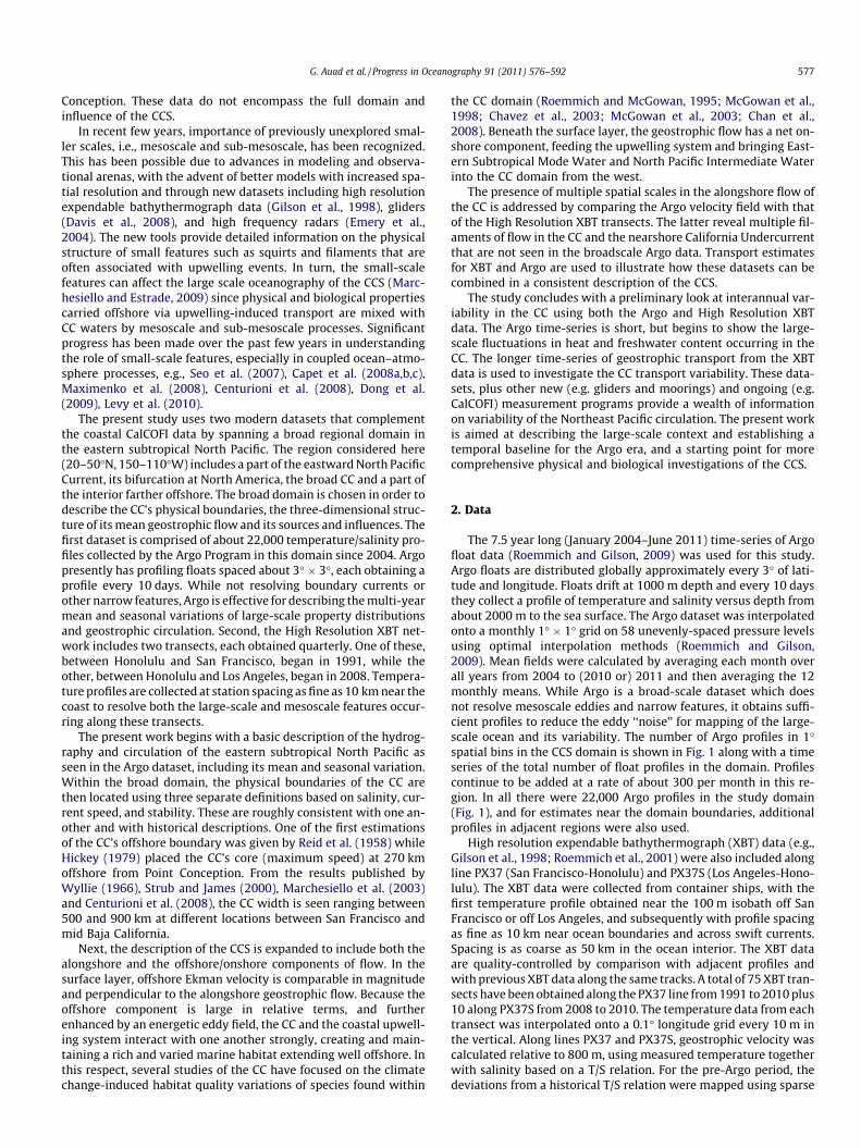
The 7.5 year long (January 2004–June 2011) time-series of Argofloat data (Roemmich and Gilson, 2009) was used for this study.Argo floats are distributed globally approximately every 3� of lati-tude and longitude. Floats drift at 1000 m depth and every 10 daysthey collect a profile of temperature and salinity versus depth fromabout 2000 m to the sea surface. The Argo dataset was interpolatedonto a monthly 1� � 1� grid on 58 unevenly-spaced pressure levelsusing optimal interpolation methods (Roemmich and Gilson,2009). Mean fields were calculated by averaging each month overall years from 2004 to (2010 or) 2011 and then averaging the 12monthly means. While Argo is a broad-scale dataset which doesnot resolve mesoscale eddies and narrow features, it obtains suffi-cient profiles to reduce the eddy ‘‘noise’’ for mapping of the large-scale ocean and its variability. The number of Argo profiles in 1�spatial bins in the CCS domain is shown in Fig. 1 along with a timeseries of the total number of float profiles in the domain. Profilescontinue to be added at a rate of about 300 per month in this re-gion. In all there were 22,000 Argo profiles in the study domain(Fig. 1), and for estimates near the domain boundaries, additionalprofiles in adjacent regions were also used.

High resolution expendable bathythermograph (XBT) data (e.g.,Gilson et al., 1998; Roemmich et al., 2001) were also included alongline PX37 (San Francisco-Honolulu) and PX37S (Los Angeles-Hono-lulu). The XBT data were collected from container ships, with thefirst temperature profile obtained near the 100 m isobath off SanFrancisco or off Los Angeles, and subsequently with profile spacingas fine as 10 km near ocean boundaries and across swift currents.Spacing is as coarse as 50 km in the ocean interior. The XBT dataare quality-controlled by comparison with adjacent profiles andwith previous XBT data along the same tracks. A total of 75 XBT tran-sects have been obtained along the PX37 line from 1991 to 2010 plus10 along PX37S from 2008 to 2010. The temperature data from eachtransect was interpolated onto a 0.1� longitude grid every 10 m inthe vertical. Along lines PX37 and PX37S, geostrophic velocity wascalculated relative to 800 m, using measured temperature togetherwith salinity based on a T/S relation. For the pre-Argo period, thedeviations from a historical T/S relation were mapped using sparse

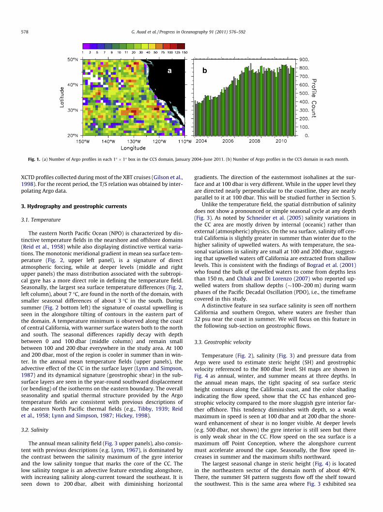
Fig. 1. (a) Number of Argo profiles in each 1� � 1� box in the CCS domain, January 2004–June 2011. (b) Number of Argo profiles in the CCS domain in each month.

578 G. Auad et al. / Progress in Oceanography 91 (2011) 576–592

XCTD profiles collected during most of the XBT cruises (Gilson et al.,1998). For the recent period, the T/S relation was obtained by inter-polating Argo data.

3. Hydrography and geostrophic currents

3.1. Temperature

The eastern North Pacific Ocean (NPO) is characterized by dis-tinctive temperature fields in the nearshore and offshore domains(Reid et al., 1958) while also displaying distinctive vertical varia-tions. The monotonic meridional gradient in mean sea surface tem-perature (Fig. 2, upper left panel), is a signature of directatmospheric forcing, while at deeper levels (middle and rightupper panels) the mass distribution associated with the subtropi-cal gyre has a more direct role in defining the temperature field.Seasonally, the largest sea surface temperature differences (Fig. 2,left column), about 7 �C, are found in the north of the domain, withsmaller seasonal differences of about 3 �C in the south. Duringsummer (Fig. 2 bottom left) the signature of coastal upwelling isseen in the alongshore tilting of contours in the eastern part ofthe domain. A temperature minimum is observed along the coastof central California, with warmer surface waters both to the northand south. The seasonal differences rapidly decay with depthbetween 0 and 100 dbar (middle column) and remain smallbetween 100 and 200 dbar everywhere in the study area. At 100and 200 dbar, most of the region is cooler in summer than in win-ter. In the annual mean temperature fields (upper panels), theadvective effect of the CC in the surface layer (Lynn and Simpson,1987) and its dynamical signature (geostrophic shear) in the sub-surface layers are seen in the year-round southward displacement(or bending) of the isotherms on the eastern boundary. The overallseasonality and spatial thermal structure provided by the Argotemperature fields are consistent with previous descriptions ofthe eastern North Pacific thermal fields (e.g., Tibby, 1939; Reidet al., 1958; Lynn and Simpson, 1987; Hickey, 1998).

3.2. Salinity

The annual mean salinity field (Fig. 3 upper panels), also consis-tent with previous descriptions (e.g. Lynn, 1967), is dominated bythe contrast between the salinity maximum of the gyre interiorand the low salinity tongue that marks the core of the CC. Thelow salinity tongue is an advective feature extending alongshore,with increasing salinity along-current toward the southeast. It isseen down to 200 dbar, albeit with diminishing horizontal

gradients. The direction of the easternmost isohalines at the sur-face and at 100 dbar is very different. While in the upper level theyare directed nearly perpendicular to the coastline, they are nearlyparallel to it at 100 dbar. This will be studied further in Section 5.

Unlike the temperature field, the spatial distribution of salinitydoes not show a pronounced or simple seasonal cycle at any depth(Fig. 3). As noted by Schneider et al. (2005) salinity variations inthe CC area are mostly driven by internal (oceanic) rather thanexternal (atmospheric) physics. On the sea surface, salinity off cen-tral California is slightly greater in summer than winter due to thehigher salinity of upwelled waters. As with temperature, the sea-sonal variations in salinity are small at 100 and 200 dbar, suggest-ing that upwelled waters off California are extracted from shallowlevels. This is consistent with the findings of Bograd et al. (2001)who found the bulk of upwelled waters to come from depths lessthan 150 m, and Chhak and Di Lorenzo (2007) who reported up-welled waters from shallow depths (�100–200 m) during warmphases of the Pacific Decadal Oscillation (PDO), i.e., the timeframecovered in this study.

A distinctive feature in sea surface salinity is seen off northernCalifornia and southern Oregon, where waters are fresher than32 psu near the coast in summer. We will focus on this feature inthe following sub-section on geostrophic flows.

3.3. Geostrophic velocity

Temperature (Fig. 2), salinity (Fig. 3) and pressure data fromArgo were used to estimate steric height (SH) and geostrophicvelocity referenced to the 800 dbar level. SH maps are shown inFig. 4 as annual, winter, and summer means at three depths. Inthe annual mean maps, the tight spacing of sea surface stericheight contours along the California coast, and the color shadingindicating the flow speed, show that the CC has enhanced geo-strophic velocity compared to the more sluggish gyre interior far-ther offshore. This tendency diminishes with depth, so a weakmaximum in speed is seen at 100 dbar and at 200 dbar the shore-ward enhancement of shear is no longer visible. At deeper levels(e.g. 500 dbar, not shown) the gyre interior is still seen but thereis only weak shear in the CC. Flow speed on the sea surface is amaximum off Point Conception, where the alongshore currentmust accelerate around the cape. Seasonally, the flow speed in-creases in summer and the maximum shifts northward.

The largest seasonal change in steric height (Fig. 4) is locatedin the northeastern sector of the domain north of about 40�N.There, the summer SH pattern suggests flow off the shelf towardthe southwest. This is the same area where Fig. 3 exhibited sea

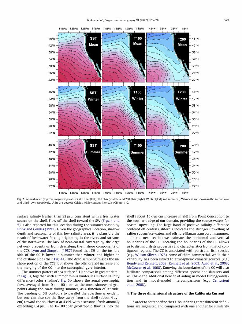
Fig. 2. Annual mean (top row) Argo temperatures at 0 dbar (left), 100 dbar (middle) and 200 dbar (right). Winter (JFM) and summer (JAS) means are shown in the second rowand third row respectively. Units are degrees Celsius while contour intervals (CI) are 1 �C.

G. Auad et al. / Progress in Oceanography 91 (2011) 576–592 579

surface salinity fresher than 32 psu, consistent with a freshwatersource on the shelf. Flow off the shelf toward the SW (Figs. 4 and5) is also reported for this location during the summer season byBrink and Cowles (1991). Given the geographical location, shallowdepth and seasonality of this low salinity area, it is plausibly theresult of freshwater forcing originating in the rivers and streamsof the northwest. The lack of near-coastal coverage by the Argonetwork prevents us from describing the inshore components ofthe CCS. Lynn and Simpson (1987) found that SH on the inshoreside of the CC is lower in summer than winter, and higher onthe offshore side (their Fig. 4a). The Argo sampling misses the in-shore portion of the CCS, but shows the offshore SH increase andthe merging of the CC into the subtropical gyre interior.

The summer pattern of sea surface SH is shown in greater detailin Fig. 5a, together with summer minus winter sea surface salinitydifference (color shading). Fig. 5b shows the zonal geostrophicflow, averaged from 0 to 100 dbar, at the most shoreward gridpoints along the coast during summer, as a function of latitude.The bending of SH contours to parallel the coastline is evident,but one can also see the flow away from the shelf (about 4 dyncm) toward the southwest at 43�N, with a seasonal fresh anomalyexceeding 0.4 psu. The 0–100 dbar geostrophic flow is into the

shelf (about 15 dyn cm increase in SH) from Point Conception tothe southern edge of our domain, providing the source waters forcoastal upwelling. The large band of positive salinity differencecentered off central California indicates the stronger upwelling ofsaltier subsurface waters and offshore Ekman transport in summer.

In the next section we estimate the horizontal and verticalboundaries of the CC. Locating the boundaries of the CC allowsus to distinguish its properties and characteristics from that of con-tiguous regions. The CC is associated with particular fish species(e.g., Wilcox-Silver, 1975), some of them commercial, while theirvariability has been linked to atmospheric climatic sources (e.g.,Hendy and Kennett, 2003; Kennett et al., 2003; Auad et al., 2003;McGowan et al., 1998). Knowing the boundaries of the CC will alsofacilitate comparisons among different epochs and datasets andwill have the additional benefit of aiding in model tuning/valida-tion and in model–model intercomparisons (e.g., Centurioniet al., 2008).

4. The three dimensional structure of the California Current

In order to better define the CC boundaries, three different defini-tions are suggested and compared with one another for similarity

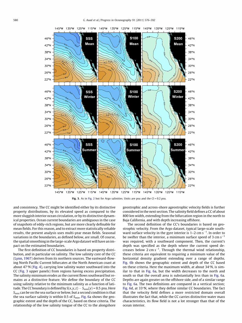
Fig. 3. As in Fig. 2 but for Argo salinities. Units are psu and the CI = 0.2 psu.

580 G. Auad et al. / Progress in Oceanography 91 (2011) 576–592

and consistency. The CC might be identified either by its distinctiveproperty distributions, by its elevated speed as compared to themore sluggish interior ocean circulation, or by its distinctive dynam-ical properties. Ocean current boundaries are ambiguous in the caseof snapshots of eddy-rich regions, but are more clearly definable formean fields. For this reason, and to extract more statistically reliableresults, the present analysis uses multi-year mean fields. Seasonalvariations in the boundaries, as defined below, are small. Of course,the spatial smoothing in the large-scale Argo dataset will have an im-pact on the estimated boundaries.

The first definition of CC boundaries is based on property distri-bution, and in particular on salinity. The low salinity core of the CC(Lynn, 1967) derives from its northern sources. The eastward-flow-ing North Pacific Current bifurcates at the North American coast atabout 47�N (Fig. 4), carrying low salinity water southward into theCC (Fig. 3 upper panels) from regions having excess precipitation.The salinity minimum erodes as the current flows southward but re-mains as a distinctive feature. We define the boundary of the CCusing salinity relative to the minimum salinity as a function of lati-tude. The CC boundary is defined by S(x, y, z) � Smin(y) = 0.5 psu. HereSmin can be on the sea surface or below, but a second condition is thatthe sea surface salinity is within 0.5 of Smin. Fig. 6a shows the geo-graphic extent and the depth of the CC, based on these criteria. Therelationship of the low salinity tongue of the CC to the alongshore

geostrophic and across-shore ageostrophic velocity fields is furtherconsidered in the next section. The salinity field defines a CC of about800 km width, extending from the bifurcation region in the north toBaja California, and with depth increasing offshore.

The second definition of the CC’s boundaries is based on geo-strophic velocity. From the Argo dataset, typical large-scale south-ward surface velocity in the gyre interior is 1–2 cm s�1. In order tobe swifter than the interior, a minimum surface speed of 3 cm s�1

was required, with a southward component. Then, the current’sdepth was specified as the depth where the current speed de-creases below 2 cm s�1. Through the thermal wind relationship,these criteria are equivalent to requiring a minimum value of thehorizontal density gradient extending over a range of depths.Fig. 6b shows the geographic extent and depth of the CC basedon these criteria. Here the maximum width, at about 34�N, is sim-ilar to that in Fig. 6a, but the width decreases to the north andsouth so that the overall area is substantially less than in Fig. 6a.Depths are again greater on the offshore side, and of a similar rangeto Fig. 6a. The two definitions are compared in a vertical section;Fig. 6d, at 33�N, where they define similar CC boundaries. The factthat the velocity field defines a more restricted domain overallillustrates the fact that, while the CC carries distinctive water masscharacteristics, its flow field is not a lot stronger than that of theocean interior.

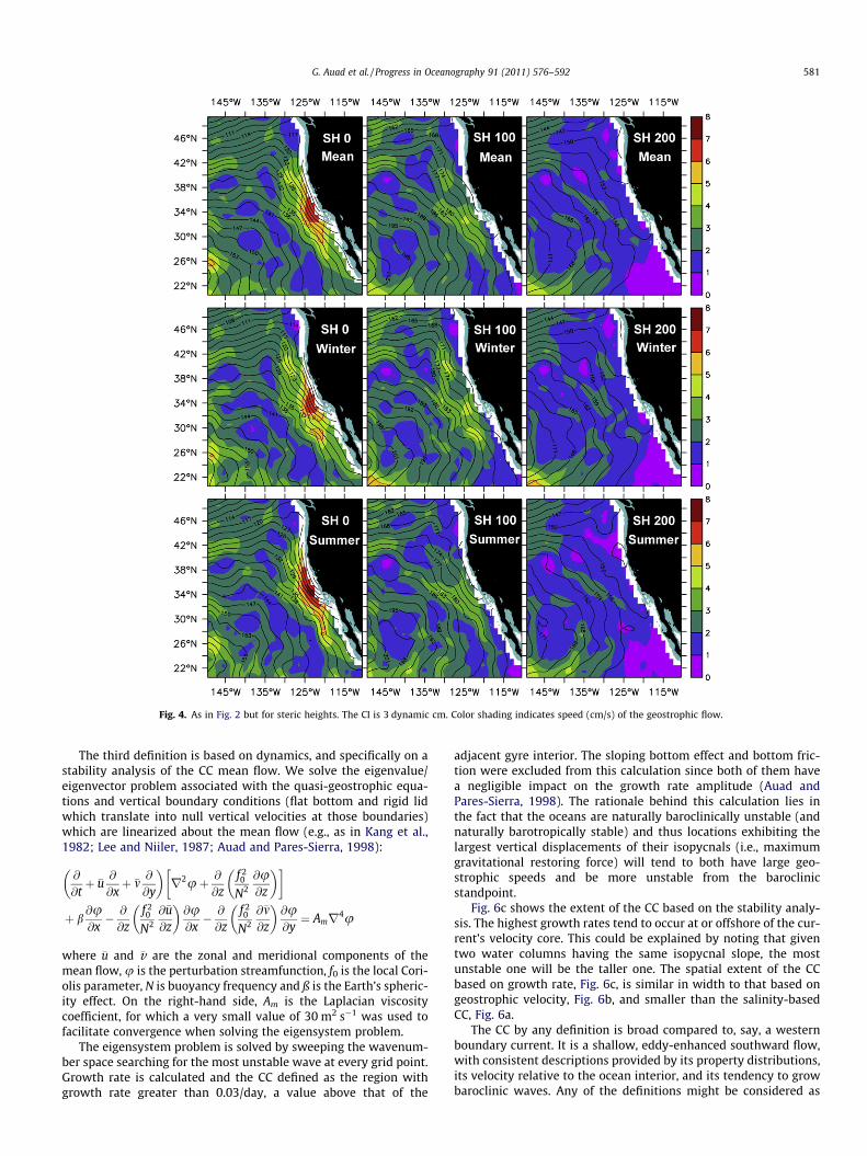
Fig. 4. As in Fig. 2 but for steric heights. The CI is 3 dynamic cm. Color shading indicates speed (cm/s) of the geostrophic flow.

G. Auad et al. / Progress in Oceanography 91 (2011) 576–592 581

The third definition is based on dynamics, and specifically on astability analysis of the CC mean flow. We solve the eigenvalue/eigenvector problem associated with the quasi-geostrophic equa-tions and vertical boundary conditions (flat bottom and rigid lidwhich translate into null vertical velocities at those boundaries)which are linearized about the mean flow (e.g., as in Kang et al.,1982; Lee and Niiler, 1987; Auad and Pares-Sierra, 1998):

@

@tþ �u

@

@xþ �m

@

@y

� �r2uþ @

@zf 20

N2

@u@z

� �� �

þ b@u@x� @

@zf 20

N2

@�u@z

� �@u@x� @

@zf 20

N2

@�m@z

� �@u@y¼ Amr4u

where �u and �v are the zonal and meridional components of themean flow, u is the perturbation streamfunction, f0 is the local Cori-olis parameter, N is buoyancy frequency and ß is the Earth’s spheric-ity effect. On the right-hand side, Am is the Laplacian viscositycoefficient, for which a very small value of 30 m2 s�1 was used tofacilitate convergence when solving the eigensystem problem.

The eigensystem problem is solved by sweeping the wavenum-ber space searching for the most unstable wave at every grid point.Growth rate is calculated and the CC defined as the region withgrowth rate greater than 0.03/day, a value above that of the

adjacent gyre interior. The sloping bottom effect and bottom fric-tion were excluded from this calculation since both of them havea negligible impact on the growth rate amplitude (Auad andPares-Sierra, 1998). The rationale behind this calculation lies inthe fact that the oceans are naturally baroclinically unstable (andnaturally barotropically stable) and thus locations exhibiting thelargest vertical displacements of their isopycnals (i.e., maximumgravitational restoring force) will tend to both have large geo-strophic speeds and be more unstable from the baroclinicstandpoint.

Fig. 6c shows the extent of the CC based on the stability analy-sis. The highest growth rates tend to occur at or offshore of the cur-rent’s velocity core. This could be explained by noting that giventwo water columns having the same isopycnal slope, the mostunstable one will be the taller one. The spatial extent of the CCbased on growth rate, Fig. 6c, is similar in width to that based ongeostrophic velocity, Fig. 6b, and smaller than the salinity-basedCC, Fig. 6a.

The CC by any definition is broad compared to, say, a westernboundary current. It is a shallow, eddy-enhanced southward flow,with consistent descriptions provided by its property distributions,its velocity relative to the ocean interior, and its tendency to growbaroclinic waves. Any of the definitions might be considered as

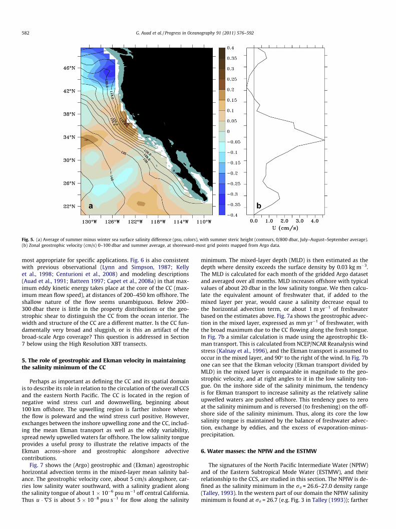
Fig. 5. (a) Average of summer minus winter sea surface salinity difference (psu, colors), with summer steric height (contours, 0/800 dbar, July–August–September average).(b) Zonal geostrophic velocity (cm/s) 0–100 dbar and summer average, at shoreward-most grid points mapped from Argo data.

582 G. Auad et al. / Progress in Oceanography 91 (2011) 576–592

most appropriate for specific applications. Fig. 6 is also consistentwith previous observational (Lynn and Simpson, 1987; Kellyet al., 1998; Centurioni et al., 2008) and modeling descriptions(Auad et al., 1991; Batteen 1997; Capet et al., 2008a) in that max-imum eddy kinetic energy takes place at the core of the CC (max-imum mean flow speed), at distances of 200–450 km offshore. Theshallow nature of the flow seems unambiguous. Below 200–300 dbar there is little in the property distributions or the geo-strophic shear to distinguish the CC from the ocean interior. Thewidth and structure of the CC are a different matter. Is the CC fun-damentally very broad and sluggish, or is this an artifact of thebroad-scale Argo coverage? This question is addressed in Section7 below using the High Resolution XBT transects.

5. The role of geostrophic and Ekman velocity in maintainingthe salinity minimum of the CC

Perhaps as important as defining the CC and its spatial domainis to describe its role in relation to the circulation of the overall CCSand the eastern North Pacific. The CC is located in the region ofnegative wind stress curl and downwelling, beginning about100 km offshore. The upwelling region is farther inshore wherethe flow is poleward and the wind stress curl positive. However,exchanges between the inshore upwelling zone and the CC, includ-ing the mean Ekman transport as well as the eddy variability,spread newly upwelled waters far offshore. The low salinity tongueprovides a useful proxy to illustrate the relative impacts of theEkman across-shore and geostrophic alongshore advectivecontributions.

Fig. 7 shows the (Argo) geostrophic and (Ekman) ageostrophichorizontal advection terms in the mixed-layer mean salinity bal-ance. The geostrophic velocity core, about 5 cm/s alongshore, car-ries low salinity water southward, with a salinity gradient alongthe salinity tongue of about 1 � 10�6 psu m�1 off central California.Thus u � rS is about 5 � 10�8 psu s�1 for flow along the salinity

minimum. The mixed-layer depth (MLD) is then estimated as thedepth where density exceeds the surface density by 0.03 kg m�3.The MLD is calculated for each month of the gridded Argo datasetand averaged over all months. MLD increases offshore with typicalvalues of about 20 dbar in the low salinity tongue. We then calcu-late the equivalent amount of freshwater that, if added to themixed layer per year, would cause a salinity decrease equal tothe horizontal advection term, or about 1 m yr�1 of freshwaterbased on the estimates above. Fig. 7a shows the geostrophic advec-tion in the mixed layer, expressed as mm yr�1 of freshwater, withthe broad maximum due to the CC flowing along the fresh tongue.In Fig. 7b a similar calculation is made using the ageostrophic Ek-man transport. This is calculated from NCEP/NCAR Reanalysis windstress (Kalnay et al., 1996), and the Ekman transport is assumed tooccur in the mixed layer, and 90� to the right of the wind. In Fig. 7bone can see that the Ekman velocity (Ekman transport divided byMLD) in the mixed layer is comparable in magnitude to the geo-strophic velocity, and at right angles to it in the low salinity ton-gue. On the inshore side of the salinity minimum, the tendencyis for Ekman transport to increase salinity as the relatively salineupwelled waters are pushed offshore. This tendency goes to zeroat the salinity minimum and is reversed (to freshening) on the off-shore side of the salinity minimum. Thus, along its core the lowsalinity tongue is maintained by the balance of freshwater advec-tion, exchange by eddies, and the excess of evaporation-minus-precipitation.

6. Water masses: the NPIW and the ESTMW

The signatures of the North Pacific Intermediate Water (NPIW)and of the Eastern Subtropical Mode Water (ESTMW), and theirrelationship to the CCS, are studied in this section. The NPIW is de-fined as the salinity minimum in the rh = 26.6–27.0 density range(Talley, 1993). In the western part of our domain the NPIW salinityminimum is found at rh = 26.7 (e.g. Fig. 3 in Talley (1993)); farther

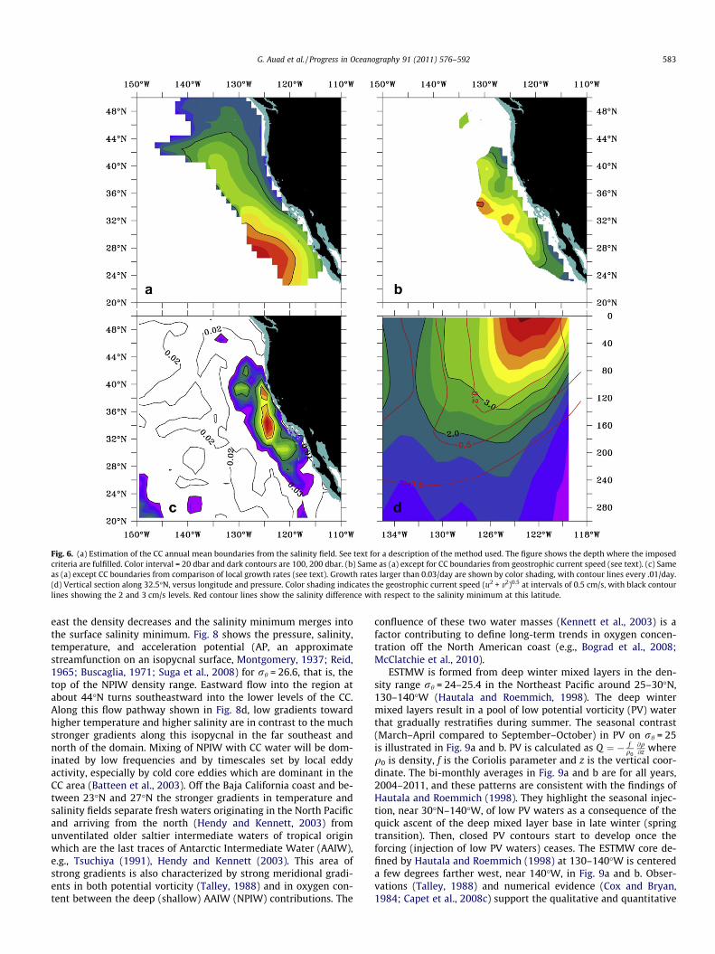
Fig. 6. (a) Estimation of the CC annual mean boundaries from the salinity field. See text for a description of the method used. The figure shows the depth where the imposedcriteria are fulfilled. Color interval = 20 dbar and dark contours are 100, 200 dbar. (b) Same as (a) except for CC boundaries from geostrophic current speed (see text). (c) Sameas (a) except CC boundaries from comparison of local growth rates (see text). Growth rates larger than 0.03/day are shown by color shading, with contour lines every .01/day.(d) Vertical section along 32.5�N, versus longitude and pressure. Color shading indicates the geostrophic current speed (u2 + v2)0.5 at intervals of 0.5 cm/s, with black contourlines showing the 2 and 3 cm/s levels. Red contour lines show the salinity difference with respect to the salinity minimum at this latitude.

G. Auad et al. / Progress in Oceanography 91 (2011) 576–592 583

east the density decreases and the salinity minimum merges intothe surface salinity minimum. Fig. 8 shows the pressure, salinity,temperature, and acceleration potential (AP, an approximatestreamfunction on an isopycnal surface, Montgomery, 1937; Reid,1965; Buscaglia, 1971; Suga et al., 2008) for rh = 26.6, that is, thetop of the NPIW density range. Eastward flow into the region atabout 44�N turns southeastward into the lower levels of the CC.Along this flow pathway shown in Fig. 8d, low gradients towardhigher temperature and higher salinity are in contrast to the muchstronger gradients along this isopycnal in the far southeast andnorth of the domain. Mixing of NPIW with CC water will be dom-inated by low frequencies and by timescales set by local eddyactivity, especially by cold core eddies which are dominant in theCC area (Batteen et al., 2003). Off the Baja California coast and be-tween 23�N and 27�N the stronger gradients in temperature andsalinity fields separate fresh waters originating in the North Pacificand arriving from the north (Hendy and Kennett, 2003) fromunventilated older saltier intermediate waters of tropical originwhich are the last traces of Antarctic Intermediate Water (AAIW),e.g., Tsuchiya (1991), Hendy and Kennett (2003). This area ofstrong gradients is also characterized by strong meridional gradi-ents in both potential vorticity (Talley, 1988) and in oxygen con-tent between the deep (shallow) AAIW (NPIW) contributions. The

confluence of these two water masses (Kennett et al., 2003) is afactor contributing to define long-term trends in oxygen concen-tration off the North American coast (e.g., Bograd et al., 2008;McClatchie et al., 2010).

ESTMW is formed from deep winter mixed layers in the den-sity range rh = 24–25.4 in the Northeast Pacific around 25–30�N,130–140�W (Hautala and Roemmich, 1998). The deep wintermixed layers result in a pool of low potential vorticity (PV) waterthat gradually restratifies during summer. The seasonal contrast(March–April compared to September–October) in PV on rh = 25is illustrated in Fig. 9a and b. PV is calculated as Q ¼ � f

q0

@q@z where

q0 is density, f is the Coriolis parameter and z is the vertical coor-dinate. The bi-monthly averages in Fig. 9a and b are for all years,2004–2011, and these patterns are consistent with the findings ofHautala and Roemmich (1998). They highlight the seasonal injec-tion, near 30�N–140�W, of low PV waters as a consequence of thequick ascent of the deep mixed layer base in late winter (springtransition). Then, closed PV contours start to develop once theforcing (injection of low PV waters) ceases. The ESTMW core de-fined by Hautala and Roemmich (1998) at 130–140�W is centereda few degrees farther west, near 140�W, in Fig. 9a and b. Obser-vations (Talley, 1988) and numerical evidence (Cox and Bryan,1984; Capet et al., 2008c) support the qualitative and quantitative

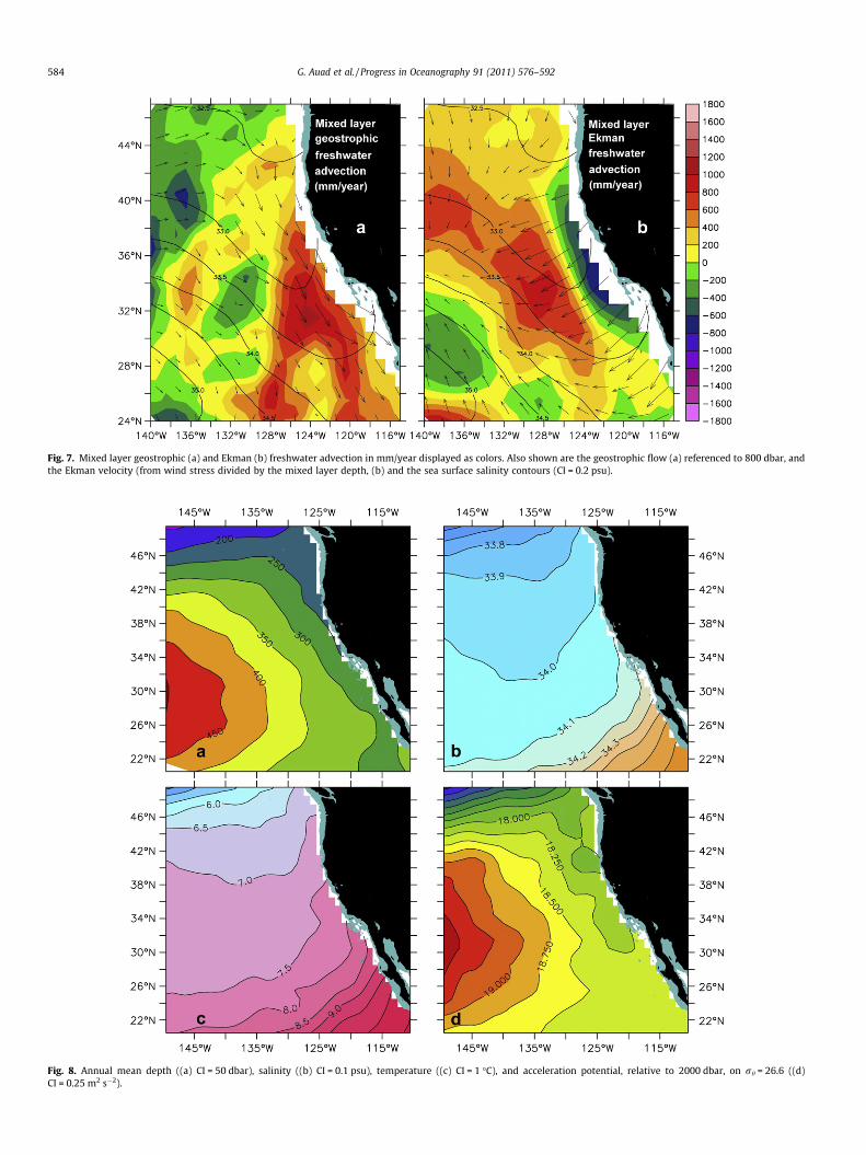
Fig. 7. Mixed layer geostrophic (a) and Ekman (b) freshwater advection in mm/year displayed as colors. Also shown are the geostrophic flow (a) referenced to 800 dbar, andthe Ekman velocity (from wind stress divided by the mixed layer depth, (b) and the sea surface salinity contours (CI = 0.2 psu).

Fig. 8. Annual mean depth ((a) CI = 50 dbar), salinity ((b) CI = 0.1 psu), temperature ((c) CI = 1 �C), and acceleration potential, relative to 2000 dbar, on rh = 26.6 ((d)CI = 0.25 m2 s�2).

584 G. Auad et al. / Progress in Oceanography 91 (2011) 576–592

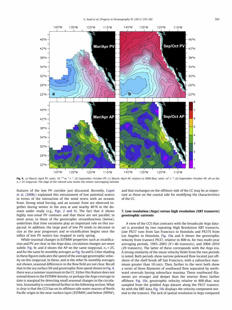
Fig. 9. (a) March–April PV, units: 10�10 m�1 s�1, (b) September–October PV, (c) March–April AP, relative to 2000 dbar, units: m2 s�2, (d) September–October AP, all on therh = 25 isopycnal. The edge of the colored area marks the winter outcropping latitude.

G. Auad et al. / Progress in Oceanography 91 (2011) 576–592 585

features of the low PV corridor just discussed. Recently, Capetet al. (2008c) explained this entrainment of low potential watersin terms of the interaction of the wind stress with an oceanicfront. Strong wind forcing, and an oceanic front are observed to-gether during winter in the area at and nearby 40�N in the do-main under study (e.g., Figs. 2 and 9). The fact that it showshighly non-zonal PV contours and that these are not parallel, inmost areas, to those of the geostrophic streamfunction (below),underlines that time variations play an important role on this iso-pycnal. In addition, the large pool of low PV tends to decrease insize as the year progresses and re-stratification begins once theinflux of low PV waters has stopped in early spring.

While seasonal changes in ESTMW properties such as stratifica-tion and PV are clear in the Argo data, circulation changes are moresubtle. Fig. 9c and d shows the AP on the same isopycnal, rh = 25,and for the same bi-monthly averages as Fig. 9a and b. Color shadingin these figures indicates the speed of the average geostrophic veloc-ity on this isopycnal. In these, and in the other bi-monthly averagesnot shown, seasonal differences in the flow field are not clear. Recallthat in the sea surface SH and geostrophic flow speed shown in Fig. 4,there was a summer maximum in the CC. Either this feature does notextend down to the ESTMW density, or perhaps the Argo coverage todate is marginal for detecting small seasonal changes in the circula-tion. Seasonality is considered further in the following section. Whatis clear is that the CCS has on its offshore side water masses of NorthPacific origin in the near-surface layer (ESTMW) and below (NPIW),

and that exchanges on the offshore side of the CC may be as impor-tant as those on the coastal side for modifying the characteristicsof the CC.

7. Low resolution (Argo) versus high resolution (XBT transects)geostrophic currents

A view of the CCS that contrasts with the broadscale Argo data-set is provided by two repeating High Resolution XBT transects.Line PX37 runs from San Francisco to Honolulu and PX37S fromLos Angeles to Honolulu. Fig. 10a and b shows the geostrophicvelocity from transect PX37, relative to 800 m, for two multi-yearaveraging periods, 1993–2003 (N = 46 transects), and 2004–2010(29 transects). The latter of these corresponds with the Argo era.A strong similarity of the mean velocity fields from the two periodsis noted. Both periods show narrow poleward flow located just off-shore of the shelf break off San Francisco, with a subsurface max-imum greater than 10 cm/s. Then, farther to the west both showa series of three filaments of southward flow separated by north-ward reversals having subsurface maxima. These southward fila-ments are stronger and deeper than the interior flows fartheroffshore. Fig. 10c, geostrophic velocity relative to 800 dbar, wassampled from the gridded Argo dataset along the PX37 transect.As with the XBT data, Fig. 10c displays the velocity component nor-mal to the transect. The lack of spatial resolution in Argo compared

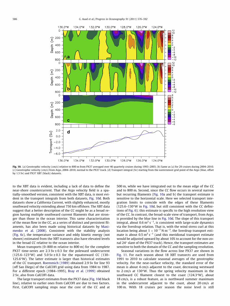
Fig. 10. (a) Geostrophic velocity (cm/s) relative to 800 m from PX37 averaged over 46 quarterly cruises during 1993–2003. (b) Same as (a) for 29 cruises during 2004–2010.(c) Geostrophic velocity (cm/s) from Argo, 2004–2010, normal to the PX37 track. (d) Transport integral (Sv) starting from the easternmost grid point of the Argo (blue, offsetby 1.5 Sv) and PX37 XBT (black) datasets.

586 G. Auad et al. / Progress in Oceanography 91 (2011) 576–592

to the XBT data is evident, including a lack of data to define thenear-shore countercurrent. That the Argo velocity field is a spa-tially-smoothed version, consistent with the XBT data, is most evi-dent in the transport integrals from both datasets, Fig. 10d. Bothdatasets show a California Current, with slightly enhanced, mostlysouthward velocity extending about 750 km offshore. The XBT datasuggest that a better description of the CC might be as a broad re-gion having multiple southward current filaments that are stron-ger than those in the ocean interior. This same characterizationof the mean flow in the CC, as a series of distinct and persistent fil-aments, has also been made using historical datasets by Maxi-menko et al. (2008). Consistent with the stability analysis(Fig. 6c), the temperature variance and eddy kinetic energy (notshown) estimated from the XBT transects also have elevated levelsin the broad CC relative to the ocean interior.

Mean transports (0–800 m relative to 800 m) for the completePX37 time-series are 2.3 Sv ± 0.3 for the poleward undercurrent(125.6–123�W) and 5.0 Sv ± 0.3 for the equatorward CC (130–125.6�W). The latter estimate is larger than historical estimatesof the CC transport. Roemmich (1989) obtained 2.9 Sv for line 93(off San Diego) of the CalCOFI grid using data from 1984 to 1987.For a different epoch (1984–1995), Bray et al. (1999) obtained2 Sv, also from CalCOFI data.

The large transport estimates from the PX37 data (Fig. 10d blackline), relative to earlier ones from CalCOFI are due to two factors.First, CalCOFI sampling stops near the core of the CC and at

500 m, while we have integrated out to the mean edge of the CCand to 800 m. Second, since the CC flow occurs in several narrowbut recurring filaments (Fig. 10a and b) the transport estimate issensitive to the horizontal scale. Here we selected transport inte-gration limits to coincide with the edges of these filaments(125.6–130�W in Fig. 10d, but still consistent with the CC defini-tions of Fig. 6); this estimate is specific to the high resolution viewof the CC. In contrast, the broad-scale view of transport, from Argo,is provided by the blue line in Fig. 10d. The slope of this transportintegral, about 0.6 m2 s�1, is consistent with large-scale dynamicsvia the Sverdrup relation. That is, with the wind stress curl at thislocation being about 1 � 10�7 N m�3, the Sverdrup transport esti-mate is about 0.5 m2 s�1 (and this meridional transport estimatewould be adjusted upward by about 10% to account for the non-zo-nal 24� slant of the PX37 track). Hence, the transport estimates aresensitive to both the domain of the CC and the sampling resolution.

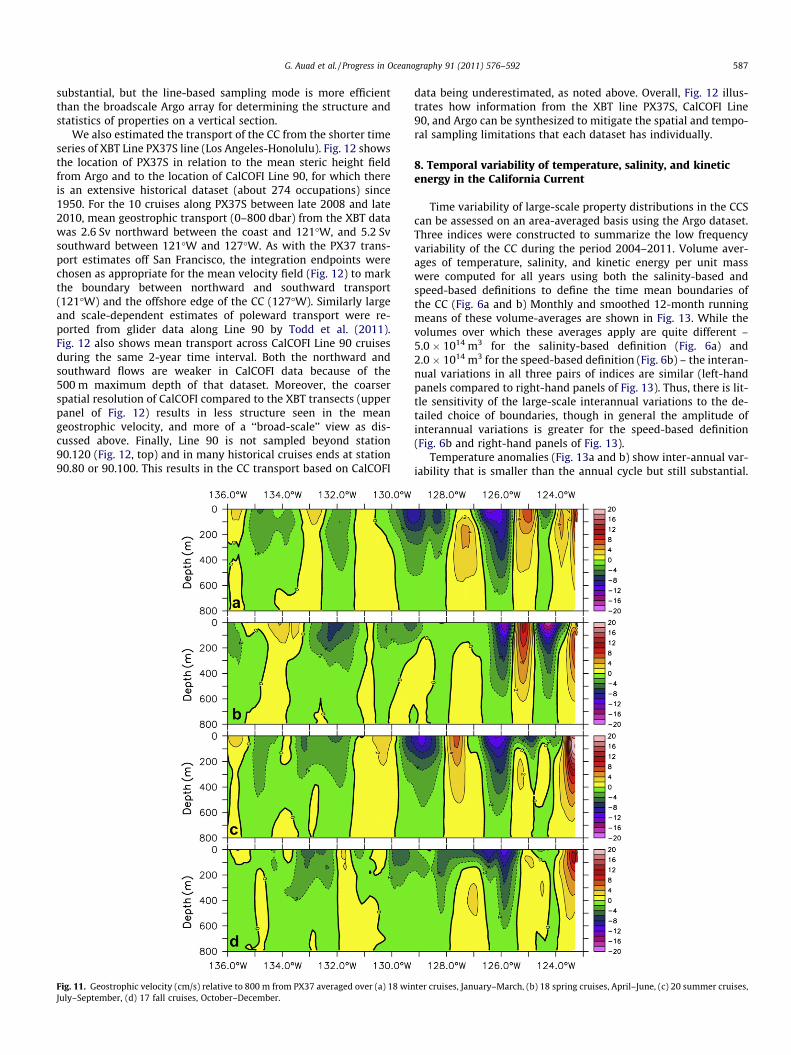
Seasonal variations in the flow across line PX37 are shown inFig. 11. For each season about 18 XBT transects are used from1991 to 2010 to calculate seasonal averages of the geostrophicvelocity. For the near-surface velocity, the standard error of themean is about 4 cm/s adjacent to the coast, decreasing westwardto 2 cm/s at 130�W. Thus the spring velocity maximum in thesouthward CC filament closest to the coast (124.3�W), about18 cm/s, is a robust feature, as is northward summer maximumin the undercurrent adjacent to the coast, about 20 cm/s at100 m. With 18 cruises per season the noise level is still

G. Auad et al. / Progress in Oceanography 91 (2011) 576–592 587

substantial, but the line-based sampling mode is more efficientthan the broadscale Argo array for determining the structure andstatistics of properties on a vertical section.

We also estimated the transport of the CC from the shorter timeseries of XBT Line PX37S line (Los Angeles-Honolulu). Fig. 12 showsthe location of PX37S in relation to the mean steric height fieldfrom Argo and to the location of CalCOFI Line 90, for which thereis an extensive historical dataset (about 274 occupations) since1950. For the 10 cruises along PX37S between late 2008 and late2010, mean geostrophic transport (0–800 dbar) from the XBT datawas 2.6 Sv northward between the coast and 121�W, and 5.2 Svsouthward between 121�W and 127�W. As with the PX37 trans-port estimates off San Francisco, the integration endpoints werechosen as appropriate for the mean velocity field (Fig. 12) to markthe boundary between northward and southward transport(121�W) and the offshore edge of the CC (127�W). Similarly largeand scale-dependent estimates of poleward transport were re-ported from glider data along Line 90 by Todd et al. (2011).Fig. 12 also shows mean transport across CalCOFI Line 90 cruisesduring the same 2-year time interval. Both the northward andsouthward flows are weaker in CalCOFI data because of the500 m maximum depth of that dataset. Moreover, the coarserspatial resolution of CalCOFI compared to the XBT transects (upperpanel of Fig. 12) results in less structure seen in the meangeostrophic velocity, and more of a ‘‘broad-scale’’ view as dis-cussed above. Finally, Line 90 is not sampled beyond station90.120 (Fig. 12, top) and in many historical cruises ends at station90.80 or 90.100. This results in the CC transport based on CalCOFI

Fig. 11. Geostrophic velocity (cm/s) relative to 800 m from PX37 averaged over (a) 18 winJuly–September, (d) 17 fall cruises, October–December.

data being underestimated, as noted above. Overall, Fig. 12 illus-trates how information from the XBT line PX37S, CalCOFI Line90, and Argo can be synthesized to mitigate the spatial and tempo-ral sampling limitations that each dataset has individually.

8. Temporal variability of temperature, salinity, and kineticenergy in the California Current

Time variability of large-scale property distributions in the CCScan be assessed on an area-averaged basis using the Argo dataset.Three indices were constructed to summarize the low frequencyvariability of the CC during the period 2004–2011. Volume aver-ages of temperature, salinity, and kinetic energy per unit masswere computed for all years using both the salinity-based andspeed-based definitions to define the time mean boundaries ofthe CC (Fig. 6a and b) Monthly and smoothed 12-month runningmeans of these volume-averages are shown in Fig. 13. While thevolumes over which these averages apply are quite different –5.0 � 1014 m3 for the salinity-based definition (Fig. 6a) and2.0 � 1014 m3 for the speed-based definition (Fig. 6b) – the interan-nual variations in all three pairs of indices are similar (left-handpanels compared to right-hand panels of Fig. 13). Thus, there is lit-tle sensitivity of the large-scale interannual variations to the de-tailed choice of boundaries, though in general the amplitude ofinterannual variations is greater for the speed-based definition(Fig. 6b and right-hand panels of Fig. 13).

Temperature anomalies (Fig. 13a and b) show inter-annual var-iability that is smaller than the annual cycle but still substantial.

ter cruises, January–March, (b) 18 spring cruises, April–June, (c) 20 summer cruises,

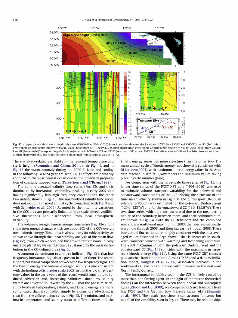
Fig. 12. (Upper panel) Mean steric height (dyn cm, 0/2000 dbar, 2004–2010) from Argo, also showing the locations of XBT Line PX37S and CalCOFI Line 90. (Left) Meangeostrophic velocity (cm/s relative to 800 m, 2008–2010) from XBT Line PX37S. (Center right) Mean geostrophic velocity (cm/s relative to 500 m, 2008–2010) from CalCOFILine 90. (Lower right) Transport integrals for Argo (relative to 800 m), XBT Line PX37S (relative to 800 m) and CalCOFI Line 90 (relative to 500 m). The latter two are set to zeroat their shoreward end. The Argo transport is integrated from a value of 2 Sv at 121�W.

588 G. Auad et al. / Progress in Oceanography 91 (2011) 576–592

There is ENSO-related variability in the regional temperature andsteric height (Roemmich and Gilson, 2011, their Fig. 1), and inFig. 13 the warm anomaly during the 2009 El Nino and coolingin the following La Nina year are seen. ENSO effects are primarilyconfined to the near coastal ocean due to the poleward propaga-tion of coastally trapped waves (Parés-Sierra and O’Brien, 1989).

The volume averaged salinity time series (Fig. 13c and d) isdominated by interannual variability, peaking in early 2007 andhaving significantly less high frequency content than the othertwo indices shown in Fig. 13. The unsmoothed salinity time seriesdoes not exhibit a marked annual cycle, consistent with Fig. 3 andwith Schneider et al. (2005). As noted by them, salinity variationsin the CCS area are primarily linked to large scale advective/diffu-sive fluctuations and disconnected from local atmosphericvariability.

The volume-averaged kinetic energy time series (Fig. 13e and f)show interannual changes which are about 30% of the CC’s overallmean kinetic energy. This index is also a proxy for eddy activity, asshown above through the linear stability analysis of the mean flow(Fig. 6c), from which we obtained the growth rates of baroclinicallyunstable planetary waves that can be sustained by the mass distri-bution in the CC-defined area (Fig. 6c).

A common denominator to all three indices in Fig. 13 is that lowfrequency interannual signals are present in all of them. The recordis short, but visual comparison between the low frequency signals ofthe kinetic energy and volume-averaged salinity is also consistentwith the findings of Schneider et al. (2005) in that the low kinetic en-ergy values in the early years of the record would contribute to re-duced advection and, increasing salinities, since low salinitywaters are advected southward by the CC. That the phase relation-ships between temperature, salinity, and kinetic energy are morecomplicated than if controlled simply by alongshore advection, isclear from the different time series in Fig. 13. The minima and max-ima in temperature and salinity occur at different times and the

kinetic energy series has more structure than the other two. Themean annual cycle of kinetic energy (not shown) is consistent withDi Lorenzo (2003), with maximum kinetic energy values in the Argodata reached in late fall (November) and minimum values takingplace in early summer (June).

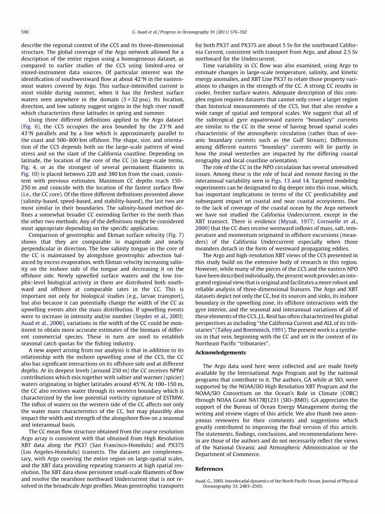
For comparison with the large-scale time series of Fig. 13, thelonger time series of the PX37 XBT data (1991–2010) was usedto estimate volume transport variability for the poleward andequatorward constituents of the CCS. Noting the structure of thetime mean velocity shown in Fig. 10a and b, transport (0–800 mrelative to 800 m) was estimated for the poleward Undercurrent(125.6–123�W) and for the equatorward CC (130–125.6�W). Thesetwo time series, which are anti-correlated due to the meanderingnature of the boundary between them, and their combined sum,are shown in Fig. 14. Both the CC transport and the combinedsum show a southward maximum in 2003, then decreasing south-ward flow through 2006, and then increasing through 2008. Theseinterannual fluctuations are roughly consistent with the area-aver-aged values described in Argo above – that is, increases in south-ward transport coincide with warming and freshening anomalies.The 2008 maximum in both the poleward Undercurrent and theequatorward CC (Fig. 14) coincides with the maximum in large-scale kinetic energy (Fig. 13c). Using the same PX37 XBT transectplus another from Honolulu to Alaska (PX38) and a data assimila-tion model, Douglass et al. (2006) associated increases in thesouthward CC and ocean interior with increases in the eastwardNorth Pacific Current.

The interannual variability seen in the CCS is likely caused bymore than one forcing agent. In the light of the recent theoreticalfindings on the interaction between the subpolar and subtropicalgyres (Zhong and Liu, 2009), we compared CCS net transport fromline PX37 and the Aleutian Low Pressure Index (ALPI) (Beamishet al., 1997). The result (not shown) can account for some butnot all of the variability seen in Fig. 14. There may be relationships

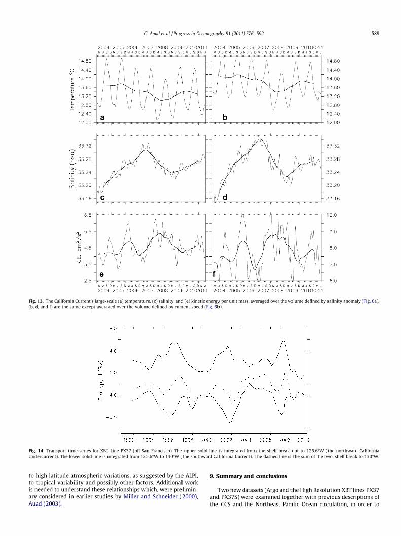
Fig. 13. The California Current’s large-scale (a) temperature, (c) salinity, and (e) kinetic energy per unit mass, averaged over the volume defined by salinity anomaly (Fig. 6a).(b, d, and f) are the same except averaged over the volume defined by current speed (Fig. 6b).

Fig. 14. Transport time-series for XBT Line PX37 (off San Francisco). The upper solid line is integrated from the shelf break out to 125.6�W (the northward CaliforniaUndercurrent). The lower solid line is integrated from 125.6�W to 130�W (the southward California Current). The dashed line is the sum of the two, shelf break to 130�W.

G. Auad et al. / Progress in Oceanography 91 (2011) 576–592 589

to high latitude atmospheric variations, as suggested by the ALPI,to tropical variability and possibly other factors. Additional workis needed to understand these relationships which, were prelimin-ary considered in earlier studies by Miller and Schneider (2000),Auad (2003).

9. Summary and conclusions

Two new datasets (Argo and the High Resolution XBT lines PX37and PX37S) were examined together with previous descriptions ofthe CCS and the Northeast Pacific Ocean circulation, in order to

590 G. Auad et al. / Progress in Oceanography 91 (2011) 576–592

describe the regional context of the CCS and its three-dimensionalstructure. The global coverage of the Argo network allowed for adescription of the entire region using a homogeneous dataset, ascompared to earlier studies of the CCS using limited-area ormixed-instrument data sources. Of particular interest was theidentification of southwestward flow at about 42�N in the eastern-most waters covered by Argo. This surface-intensified current ismost visible during summer, when it has the freshest surfacewaters seen anywhere in the domain (S < 32 psu). Its location,direction, and low salinity suggest origins in the high river runoffwhich characterizes these latitudes in spring and summer.

Using three different definitions applied to the Argo dataset(Fig. 6), the CCS occupies the area bounded by the 23�N and43�N parallels and by a line which is approximately parallel tothe coast and 500–800 km offshore. The shape, size, and orienta-tion of the CCS depends both on the large-scale pattern of windstress and on the slant of the California coastline. Depending onlatitude, the location of the core of the CC (in large-scale terms,Fig. 4, or as the strongest of several permanent filaments inFig. 10) is placed between 220 and 380 km from the coast, consis-tent with previous estimates. Maximum CC depths reach 150–250 m and coincide with the location of the fastest surface flow(i.e., the CC core). Of the three different definitions presented above(salinity-based, speed-based, and stability-based), the last two aremost similar in their boundaries. The salinity-based method de-fines a somewhat broader CC extending farther to the north thanthe other two methods. Any of the definitions might be consideredmost appropriate depending on the specific application.

Comparison of geostrophic and Ekman surface velocity (Fig. 7)shows that they are comparable in magnitude and nearlyperpendicular in direction. The low salinity tongue in the core ofthe CC is maintained by alongshore geostrophic advection bal-anced by excess evaporation, with Ekman velocity increasing salin-ity on the inshore side of the tongue and decreasing it on theoffshore side. Newly upwelled surface waters and the low tro-phic-level biological activity in them are distributed both south-ward and offshore at comparable rates in the CC. This isimportant not only for biological studies (e.g., larvae transport),but also because it can potentially change the width of the CC asupwelling events alter the mass distribution. If upwelling eventswere to increase in intensity and/or number (Snyder et al., 2003;Auad et al., 2006), variations in the width of the CC could be mon-itored to obtain more accurate estimates of the biomass of differ-ent commercial species. These in turn are used to establishseasonal catch quotas for the fishing industry.

A new aspect arising from our analysis is that in addition to itsrelationship with the inshore upwelling zone of the CCS, the CCalso has significant interactions on its offshore side and at differentdepths. At its deepest levels (around 250 m) the CC receives NPIWcontributions which mix together with saltier and warmer (spicier)waters originating in higher latitudes around 45�N. At 100–150 m,the CC also receives water through its western boundary which ischaracterized by the low potential vorticity signature of ESTMW.The influx of waters on the western side of the CC affects not onlythe water mass characteristics of the CC, but may plausibly alsoimpact the width and strength of the alongshore flow on a seasonaland interannual basis.

The CC mean flow structure obtained from the coarse resolutionArgo array is consistent with that obtained from High ResolutionXBT data along the PX37 (San Francisco-Honolulu) and PX37S(Los Angeles-Honolulu) transects. The datasets are complemen-tary, with Argo covering the entire region on large-spatial scales,and the XBT data providing repeating transects at high spatial res-olution. The XBT data show persistent small-scale filaments of flowand resolve the nearshore northward Undercurrent that is not re-solved in the broadscale Argo profiles. Mean geostrophic transports

for both PX37 and PX37S are about 5 Sv for the southward Califor-nia Current, consistent with transport from Argo, and about 2.5 Svnorthward for the Undercurrent.

Time variability in CC flow was also examined, using Argo toestimate changes in large-scale temperature, salinity, and kineticenergy anomalies, and XBT Line PX37 to relate those property vari-ations to changes in the strength of the CC. A strong CC results incooler, fresher surface waters. Adequate description of this com-plex region requires datasets that cannot only cover a larger regionthan historical measurements of the CCS, but that also resolve awide range of spatial and temporal scales. We suggest that all ofthe subtropical gyre equatorward eastern ‘‘boundary’’ currentsare similar to the CC in the sense of having broad spatial scalescharacteristic of the atmospheric circulation (rather than of oce-anic boundary currents such as the Gulf Stream). Differencesamong different eastern ‘‘boundary’’ currents will lie partly inhow the zonal westerlies are impacted by the differing coastalorography and local coastline orientation.

The role of the CC in the NPO circulation has several unresolvedissues. Among these is the role of local and remote forcing in theinterannual variability seen in Figs. 13 and 14. Targeted modelingexperiments can be designated to dig deeper into this issue, which,has important implications in terms of the CC predictability andsubsequent impact on coastal and near coastal ecosystems. Dueto the lack of coverage of the coastal ocean by the Argo networkwe have not studied the California Undercurrent, except in theXBT transect. There is evidence (Mysak, 1977; Cornuelle et al.,2000) that the CC does receive westward inflows of mass, salt, tem-perature and momentum originated in offshore excursions (mean-ders) of the California Undercurrent especially when thosemeanders detach in the form of westward propagating eddies.

The Argo and high-resolution XBT views of the CCS presented inthis study build on the extensive body of research in this region.However, while many of the pieces of the CCS and the eastern NPOhave been described individually, the present work provides an inte-grated regional view that is original and facilitates a more robust andreliable analysis of three-dimensional features. The Argo and XBTdatasets depict not only the CC, but its sources and sinks, its inshoreboundary in the upwelling zone, its offshore interactions with thegyre interior, and the seasonal and interannual variations of all ofthese elements of the CCS. J.L. Reid has often characterized his globalperspectives as including ‘‘the California Current and ALL of its trib-utaries’’ (Talley and Roemmich, 1991). The present work is a synthe-sis in that vein, beginning with the CC and set in the context of itsNortheast Pacific ‘‘tributaries’’.

Acknowledgements

The Argo data used here were collected and are made freelyavailable by the International Argo Program and by the nationalprograms that contribute to it. The authors, GA while at SIO, weresupported by the NOAA/SIO High Resolution XBT Program and theNOAA/SIO Consortium on the Ocean’s Role in Climate (CORC)through NOAA Grant NA17RJ1231 (SIO–JIMO). GA appreciates thesupport of the Bureau of Ocean Energy Management during thewriting and review stages of this article. We also thank two anon-ymous reviewers for their comments and suggestions whichgreatly contributed to improving the final version of this article.The statements, findings, conclusions, and recommendations here-in are those of the authors and do not necessarily reflect the viewsof the National Oceanic and Atmospheric Administration or theDepartment of Commerce.

References

Auad, G., 2003. Interdecadal dynamics of the North Pacific Ocean. Journal of PhysicalOceanography 33, 2483–2503.

G. Auad et al. / Progress in Oceanography 91 (2011) 576–592 591

Auad, G., Pares-Sierra, A., 1998. Mean flow stability in the eastern North PacificOcean. Geofisica Internacional 37, 113–126.

Auad, G., Pares-Sierra, A., Vallis, G.K., 1991. Circulation and energetics of a model ofthe California Current System. Journal of Physical Oceanography 21, 1534–1552.

Auad, G., Kennett, J.P., Miller, A.J., 2003. North Pacific Intermediate Water responseto a modern climate warming shift. Journal of Geophysical Research 108, 3349.doi:10.1029/2003JC001987.

Auad, G., Miller, A.J., DiLorenzo, E., 2006. Long-term forecast of oceanic conditionsoff California and their biological implications. Journal of Geophysical Research111, C09008. doi:10.1029/2005JC003219.

Bakun, A., McLain, D., Mayo, F., 1973. The mean annual cycle of coastal upwelling offwestern North America as observed from surface measurements. FisheryBulletin 72, 843–844.

Barton, E., Argote, M., 1980. Hydrographic variability in an upwelling area offnorthern Baja California in June 1976. Journal of Marine Research 38, 631–649.

Batteen, M., 1997. Wind-forced modeling studies of currents, meanders, and eddiesin the California Current System. Journal of Geophysical Research 102, 985–1010.

Batteen, M., Cipriano, N., Monroe, J., 2003. A large-scale seasonal modeling study ofthe California Current System. Journal of Oceanography 59, 545–562.

Beamish, R.J., Neville, C.E., Cass, A.J., 1997. Production of Fraser River sockeyesalmon (Oncorhynchus nerka) in relation to decadal scale changes in the climateand the ocean. Canadian Journal of Fisheries and Aquatic Science 54, 543–554.

Bograd, S.J., Chereskin, T.K., Roemmich, D., 2001. Transport of mass, heat, salt, andnutrients in the southern California Current System: annual cycle andinterannual variability. Journal of Geophysical Research 106, 9255–9275.

Bograd, S.J., Castro, C.G., Di Lorenzo, E., Palacios, D.M., Bailey, H., Gilly, W., Chavez,F.P., 2008. Oxygen declines and the shoaling of the hypoxic boundary in theCalifornia Current. Geophysical Research Letters 35, L12607. doi:10.1029/2008GL034185.

Bray, N., Keyes, A., Morawitz, W., 1999. The California Current system in theSouthern California Bight and the Santa Barbara Channel. Journal of GeophysicalResearch 104, 7695–7714.

Brink, K.H., Cowles, T.J., 1991. The coastal transition zone program. Journal ofGeophysical Research 96 (14), 637–14,647. doi:10.1029/91JC01206.

Buscaglia, J., 1971. On the circulation of the intermediate water in thesoutherwestern Atlantic Ocean. Journal of Marine Research 29, 245–255.

Capet, X., McWilliams, J.C., Molemaker, M.J., Shchepetkin, A.F., 2008a. Mesoscale tosubmesoscale transition in the California Current System. Part I: flow structure,eddy flux, and observational tests. Journal of Physical Oceanography 38, 29–43.

Capet, X., McWilliams, J.C., Molemaker, M.J., Shchepetkin, A.F., 2008b. Mesoscale tosubmesoscale transition in the California Current System. Part II: frontalprocesses. Journal of Physical Oceanography 39, 44–64.

Capet, X., McWilliams, J.C., Molemaker, M.J., Shchepetkin, A.F., 2008c. Mesoscale tosubmesoscale transition in the California Current System. Part III: energybalance and flux. Journal of Physical Oceanography 38, 2256–2269.

Centurioni, L., Ohlmann, J., Niiler, P., 2008. Permanent meanders in the CaliforniaCurrent System. Journal of Physical Oceanography 38, 1690–1710.

Chan, F., Barth, J., Lubchenco, J., Kirincich, A., Weeks, H., Peterson, W., Menge, B.,2008. Emergence of anoxia in the California current large marine ecosystem.Science 319, 920.

Chavez, F., Ryan, J., Lluch-Cota, S., Ñiquen, M., 2003. From anchovies to sardines andback: multidecadal change in the Pacific Ocean. Science 299, 217–221.

Chelton, D., Schlax, M., Samelson, R., 2007. Summertime coupling between seasurface temperature and wind stress in the California Current System. Journal ofPhysical Oceanography 37, 495–517.

Chhak, K., Di Lorenzo, E., 2007. Decadal variations in the California Currentupwelling cells. Geophysical Research Letters 34, L14604. doi:10.1029/2007GL030203.

Cornuelle, B.D., Chereskin, T.K., Niiler, P., Morris, M.Y., Musgrave, D.L., 2000.Observations and modeling of a California undercurrent eddy. Journal ofGeophysical Research 105, 1227–1243.

Cox, M., Bryan, K., 1984. A numerical model of the ventilated thermocline. Journal ofPhysical Oceanography 14, 674–687.

Davis, R.E., Ohman, M., Rudnick, D., Sherman, J., Hodges, B., 2008. Glider surveillanceof physics and biology in the southern California Current System. Limnologyand Oceanography 53, 2151–2168.

Di Lorenzo, E., 2003. Seasonal dynamics of the surface circulation in the SouthernCalifornia Current System. Deep-Sea Research II 50, 2371–2388.

Di Lorenzo, E., Miller, A.J., Schneider, N., McWilliams, J., 2005. The warming of theCalifornia Current: dynamics and ecosystem implications. Journal of PhysicalOceanography 35, 336–362.

Dong, C., Idica, E., McWilliams, J., 2009. Circulation and multiple scale variability inthe Southern California Bight. Progress in Oceanography 82, 168–190.

Douglass, E., Roemmich, D., Stammer, D., 2006. Interannual variability in NortheastPacific circulation. Journal of Geophysical Research 111, C04001. doi:10.1029/2005JC003015.

Emery, B., Washburn, L., Harlan, J., 2004. Evaluating radial current measurementsfrom CODAR high-frequency radars with moored current meters. Journal ofAtmospheric and Oceanic Technology 21, 1259–1271.

Gan, J., Allen, J.S., 2002. A modeling study of shelf circulation off northern Californiain the region of the Coastal Ocean Dynamics Experiment: response to relaxationof upwelling winds. Journal of Geophysical Research 107, 3123. doi:10.1029/2000JC000768.

Gilson, J., Roemmich, D., Cornuelle, B., 1998. Relationship of TOPEX/Poseidonaltimetric steric height and circulation in the North Pacific. Journal ofGeophysical Research 103, 27,947–27,965.

Goebel, N., Edwards, C., Zehr, J.P., Follows, M.J., 2010. An emergent communityecosystem model applied to the California Current System. Journal of MarineSystems 83, 221–241.

Hautala, S.L., Roemmich, D.H., 1998. Subtropical mode water in the NortheastPacific Basin. Journal of Geophysical Research 103, 13055–13066.

Hendy, I.L., Kennett, J.P., 2003. Tropical forcing of North Pacific intermediate waterdistribution during late Quaternary rapid climate change. Quaternary ScienceReviews 22, 673–689.

Hickey, B., 1979. The California Current, hypothesis and facts. Progress inOceanography 8, 191–279.

Hickey, B., 1998. Coastal oceanography of Western North America from the tip ofBaja California to Vancouver Island. The Sea 11, 345–393.

Huyer, A., 1983. Coastal upwelling in the California Current System. Progress inOceanography 12, 259–284.

Kalnay, E., Kanamitsu, M., Kistler, R., Collins, W., Deaven, D., Gandin, L., Iredell, M.,Saha, S., White, G., Woollen, J., Zhu, Y., Chelliah, M., Ebisuzaki, W., Higgins, W.,Janowiak, J., Mo, KC., Ropelewski, C., Wang, J., Leetmaa, A., Reynolds, R., Jenne,R., Joseph, D., 1996. The NCEP/NCAR 40-year reanalysis project. Bulletin of theAmerican Meteorological Society 77 (3), 437–471.

Kang, Y., Price, J.M., Magaard, L., 1982. On Stable and unstable Rossby waves in non-zonal oceanic shear flow. Journal of Physical Oceanography 12, 528–537.

Kelly, K., Beardsley, R., Limeburner, R., Brink, K., 1998. Variability of the near-surfaceeddy kinetic energy in the California Current based on altimetric, drifter andmoored data. Journal Geophysical Research 103, 13,067–13,083.

Kennett, J.P., Cannariato, K.G., Hendy, I.L., Behl, R.J., 2003. Methane Hydrates inQuaternary Climate Change: The Clathrate Gun Hypothesis, Special Publications54. AGU, Washington, DC, 216 pp.

Lee, D-K., Niiler, P.P., 1987. The local baroclinic instability of geostrophic spirals inthe eastern North Pacific ocean. Journal of Physical Oceanography 17, 1366–1377.

Levy, M., Klein, P., Treguier, A., Iovino, D., Madec, G., Masson, S., Takahashi, K., 2010.Modification of gyre circulation by sub-mesoscale physics. Ocean Modelling 34,1–15.

Logerwell, E.A., Smith, P.E., 2001. Mesoscale eddies and survival of late stage Pacificsardine (Sardinops sagax) larva. Fisheries Oceanography 10, 13–25.

Lynn, R.J., 1967. Seasonal variation of temperature and salinity at 10 meters in theCalifornia Current. CalCOFI Report 11, 86–157.

Lynn, R., Simpson, J., 1987. The California Current System: the seasonal variability ofits physical properties. Journal of Geophysical Research 92, 12,947–12,966.

Marchesiello, P., Estrade, P., 2009. Eddy activity and mixing in upwelling systems: acomparative study of Northwest Africa and California regions. InternationalJournal of Earth Sciences 98, 299–308.

Marchesiello, P., McWilliams, J.C., Shchepetkin, A., 2003. Equilibrium structure anddynamics of the California Current System. Journal of Physical Oceanography33, 753–783.

Maximenko, N., Melnichenko, O., Niiler, P.P., Sasaki, H., 2008. Stationary mesoscalejet-like features in the ocean. Geophysical Research Letters 35, L08603.doi:10.1029/2008GL033267.

McClatchie, S., Goericke, R., Koslow, A.J., and 24 other authors, 2008. The State of theCalifornia Current, 2007–2008: La Niña conditions and their effects on theecosystem. CalCOFI Reports 49, 39–76.

McClatchie, S., Goericke, R., Cosgrove, R., Auad, G., Vetter, R., 2010. Oxygen in theSouthern California Bight: multidecadal trends and implications for demersalfisheries. Geophysical Research Letters 37, L19602. doi:10.1029/2010GL044497.

McGowan, J., Cayan, D., Dorman, C., 1998. Climate-ocean variability and ecosystemresponse in the Northeast Pacific. Science 281, 210–217.

McGowan, J., Bograd, S., Lynn, R., Miller, A., 2003. The biological response of the1977 regime shift in the California Current. Deep-Sea Research 50, 2567–2582.

Miller, A.J., Schneider, N., 2000. Interdecadal climate regime dynamics in the NorthPacific Ocean: theories, observations and ecosystem impacts. Progress inOceanography 47, 355–379.

Montgomery, R., 1937. A suggested method for representing gradient flow inisentropic surfaces. Bulletin of the American Meteorological Society 18, 210–212.

Moore, A., Arango, H., DiLorenzo, E., Miller, A., Cornuelle, B., 2009. An adjointsensitivity analysis of the Southern California Current circulation andecosystem. Journal of Physical Oceanography 39, 702–720.

Mysak, L., 1977. On the stability of the California Undercurrent off Vancouver Island.Journal of Physical Oceanography 7, 904–917.

Parés-Sierra, A., O’Brien, J., 1989. The seasonal and interannual variability of theCalifornia Current System: a numerical model. Journal of Geophysical Research93, 3159–3180.

Powell, T.P., Lewis, C.V.W., Curchitser, E.N., Haidvogel, D.B., Hermann, A.J., Dobbins,E.L., 2006. Results from a three-dimensional, nested biological–physical modelof the California Current System and comparisons with statistics from satelliteimagery. Journal of Geophysical Research 111, C07018. doi:10.1029/2004JC002506.

Reid, J.L., 1965. Intermediate waters of the Pacific Ocean. The John HopkinsOceanographic Studies 2, 85 pp.

Reid, J.L., Roden, G., Wyllie, J., 1958. Studies of the California Current System.CalCOFI Progress Report 7-1-56 to 1-1-58, Marine Resources Committee,California Department of Fish and Game, Sacramento, pp. 27–56.

592 G. Auad et al. / Progress in Oceanography 91 (2011) 576–592

Roemmich, D., 1989. Mean transport of mass, heat, salt and nutrients in southernCalifornia coastal waters: implications for primary production and nutrientcycling. Deep-Sea Research 36, 1359–1378.

Roemmich, D., Gilson, J., 2009. The 2004–2008 mean and annual cycle oftemperature, salinity, and steric height in the global ocean from the ArgoProgram. Progress in Oceanography 82, 81–100.

Roemmich, D., Gilson, J., 2011. The global ocean imprint of ENSO. GeophysicalResearch Letters 38, L13606. doi:10.1029/2011GL047992.

Roemmich, D., McGowan, J., 1995. Climate warming and the decline of zooplanktonin the California Current. Science 267, 1324–1326.

Roemmich, D., Gilson, J., Cornuelle, B., Weller, R., 2001. The mean and time-varyingmeridional heat transport at the tropical/subtropical boundary of the NorthPacific Ocean. Journal of Geophysical Research 106, 8957–8970.

Rykaczewski, R.R., Dunne, J.P., 2010. Enhanced nutrient supply to the CaliforniaCurrent Ecosystem with global warming and increased stratification in an earthsystem model. Geophysical Research Letters 37, L21606. doi:10.1029/2010GL045019.

Schneider, N., Di Lorenzo, E., Niiler, P., 2005. Salinity variations in the CaliforniaCurrent. Journal of Physical Oceanography 35 (8), 1421–1436.

Schwing, F., Mendelssohn, R., 1997. Increased coastal upwelling in the CaliforniaCurrent System. Journal of Geophysical Research 102, 3421–3438.

Schwing, F., Moore, C., Ralston, S., Sakuma, K.A., 2000. Record Coastal Upwelling inthe California Current in 1999, CalCOFI Report 41, pp. 148–160.

Seo, H., Miller, A., Roads, J., 2007. The Scripps Coupled Ocean–Atmosphere Regional(SCOAR) model, with applications in the Eastern Pacific Sector. Journal ofClimate 20, 381–402.

Snyder, M., Sloan, L., Diffenbaugh, N., Bell, J., 2003. Future climate change andupwelling in the California Current. Geophysical Research Letters 30.doi:10,1029/2003GL017647.

Strub, P.T., James, C., 2000. Altimeter-derived variability of surface velocities in theCalifornia Current System: 2. Seasonal circulation and eddy statistics. Deep-SeaResearch II 47, 831–870.

Suga, T., Aoki, Y., Saito, H., Hanawa, K., 2008. Ventilation of the North Pacificsubtropical pycnocline and mode water formation. Progress in Oceanography77, 285–297.

Sverdrup, H.U., Johnson, M.W., Fleming, R.H., 1942. The Oceans, Their Physics,Chemistry and General Biology. Prentice Hall, 1087 pp.

Sydeman, W.J., Hester, M.M., Thayer, J.A., Gress, F., Martin, P., Buffa, J., 2001. Climatechange, reproductive performance, and diet composition of marine birds in thesouthern California Current system. Progress in Oceanography 49, 309–329.

Talley, L.D., 1988. Potential vorticity distribution in the North Pacific. Journal ofPhysical Oceanography 18, 89–106.

Talley, L.D., 1993. Distribution of North Pacific intermediate water. Journal ofPhysical Oceanography 23, 517–537.

Talley, L.D., Roemmich, D., 1991. A tribute to Joe Reid in recognition of 40 years ofcontributions to oceanography. Deep-Sea Research 38 (Suppl.), vii–viii.

Tibby, R.B., 1939. Report on Returns of Drift Bottles Released off Southern California,1937, Fish Bulletin 55, Division of Fish and Game, California, Bureau of MarineFisheries.

Todd, R., Rudnick, D., Mazloff, M., Davis, R., Cornuelle, B., 2011. Poleward flows inthe southern California Current System: glider observations and numericalsimulation. Journal of Geophysical Research 116 (116), C02026. doi:10.1029/2010JC006536.

Tsuchiya, M., 1991. Flow path of Antarctic Intermediate Water in the westernequatorial South Pacific Ocean. Deep-Sea Research I 38, S273–S279.

Wilcox-Silver, M., 1975. The habitat of Salpa fusiformis in the California Current asdefined by indicator assemblages. Limnology and Oceanography 20, 230–237.

Wyllie, J.G., 1966. Geostrophic flow of the California Current at the surface and at200 m. CalCOFI Atlas, 13 pp., and 288 charts.

Zhong, Y., Liu, Z., 2009. On the mechanism of pacific multidecadal climatevariability in CCSM3: the role of the subpolar North Pacific ocean. Journal ofPhysical Oceanography 39, 2052–2076.