The bioeconomics of controlling an African rodent pest species

Environment and Development Economics 11: 453–475 C© 2006 Cambridge University Pressdoi:10.1017/S1355770X06003044 Printed in the United Kingdom

The bioeconomics of controlling an Africanrodent pest species

ANDERS SKONHOFT∗

Department of Economics, Norwegian University of Science and Technology,N-7491 Trondheim, Norway. E-mail: [email protected]

HERWIG LEIRSDanish Pest Infestation Laboratory, Danish Institute of AgriculturalSciences, Denmark, and Department of Biology, University of Antwerp,Belgium

HARRY P. ANDREASSENDepartment of Forestry and Wildlife Management, Hedmark UniversityCollege, Norway and Department of Biology, Centre for Ecological andEvolutionary Synthesis (CEES), University of Oslo, Norway

LOTH S.A. MULUNGUSUA Pest Management Centre, Sokoine University of Agriculture,Morogoro, Tanzania

NILS CHR. STENSETHDepartment of Biology, Centre for Ecological and Evolutionary Synthesis(CEES), University of Oslo, Norway

ABSTRACT. The paper treats the economy of controlling an African pest rodent, themultimammate rat, causing major damage in maize production. An ecological populationmodel is presented and used as a basis for the economic analyses carried out at thevillage level using data from Tanzania. This model incorporates both density-dependentand density-independent (stochastic) factors. Rodents are controlled by applying poison,and the costs are made up of the cost of poison plus the damage to maize production.We analyse how the present-value costs of maize production are affected by various

∗Corresponding author

We thank the late Patrick Mwanjabe for several valuable discussions on the pestproblem treated in this paper and three referees for valuable comments. AS thanksfor support from the Norwegian Science Council. NCS and HPA thank for valuablesupport from University of Oslo and the Norwegian Science Council. NCS andHL appreciate the EU-support through the STAPLERAT project (ICA4-CT-2000-30029) and the Danish Council for Development Research (RUF). LSM appreciatesthe support from the SUA-VLIR program.

454 Anders Skonhoft et al.

rodent control strategies, by varying the duration and timing of rodenticide application.Our numerical results suggest that it is economically beneficial to control the rodentpopulation. In general, the most cost-effective duration of controlling the rodentpopulation is 3–4 months every year, and especially at the end of the dry season/beginningof rainy season. The paper demonstrates that changing from today’s practice of symp-tomatic treatment when heavy rodent damage is noticed to a practice where the calendar isemphasized, may substantially improve the economic conditions for the maize producingfarmers. This main conclusion is highly robust and not much affected by changing pricesof maize production.

1. IntroductionRodents represent major pest problems worldwide, both in the countrysideand in the cities. They do, for instance, cause serious damage to crops (suchas cereals, root crops, cotton, and sugarcane) both before and after harvest.They also damage installations and are reservoirs or vectors for seriousinfectious diseases (Fiedler, 1988; Stenseth et al., 2003).

In Africa, more than 70 rodent species have been reported to bepest species (Fiedler, 1988). Some of these exhibit irregular populationdynamics with occasional explosions, typically occurring over extensiveareas (Fiedler, 1988; Leirs et al., 1996). Within eastern Africa, multimammaterats (Mastomys natalensis) are among the most important pest rodents(Fiedler, 1988). Damage during outbreaks is profound and significantlyworsens the already unfavourable food situation on the African continent.The average rodent damage by the multimammate rat to maize in Tanzaniahas been estimated to be between 5 and 15 per cent yield loss, and forTanzania this amounts to an average of approximately 412,500 tonnes peryear (FAO statistics, 1998; Makundi et al., 1999). This corresponds to whatwould be sufficient to feed more than 2 million people for an entire year(at about 0.55 kg/day/person) or represents an estimated value of almost60 million US$ (September 1999 village market price in Tanzania, beingaround 14.5 US$ per 100 kg bag of maize). Eruptions of the multimammaterat population represent direct disasters for the subsistence farmersinvolved, but may also have national and even international politicalconsequences. Panic-stricken authorities may initiate control operations –however, often too late and typically with quite poor results. There is thusa clear need to predict and, if possible, prevent such outbreaks of rodentpopulations (Mwanjabe, 1990; Leirs, 1999).

The control of pest rodents does, however, have both an ecological andan economic component interacting dynamically with each other so asto render intuitive reasoning difficult. In this paper we consider both theecological and the economic components of rodent damage and control.This we do through the analysis of a bio-economic model – a model fallingwithin the concept of ecologically based rodent management (EBRM) (see,e.g., Singleton et al., 1999). We specifically evaluate the relations betweencontrol timing, control duration, and damage reduction. Our model is quitegeneral; hence, our analysis may illustrate pest control involving rodentsliving in highly seasonally varying environments. The model consists of awell-established stage-structured ecological model (see Leirs et al., 1997a;Leirs, 1999; Stenseth et al., 2001) and is integrated with an economic model

Environment and Development Economics 455

incorporating the crop damages by the rodents and the cost of controllingthem.

The links between the ecological and the economic components are rep-resented by the control measures affecting the mortality of the rodents aswell as the rodents’ damages on the maize crop. There is also a link throughrainfall, there being both a seasonal and stochastic component, which affectsboth the rodent population ecology and the crop yield. The timing of therodents’ breeding season is strongly related to the annual distribution ofrainfall (Leirs et al., 1993). In addition, rodent survival and maturation areaffected by precipitation in the preceding few months, as well as density-dependent factors (Leirs et al., 1997a). Thus, rainfall influences the cropyield in two ways: positively through production since more rain (withinlimits) implies higher yield, and negatively through a higher net growth ofthe rodent population following rain.

Control strategies are evaluated in terms of present-value costs, inte-grating the control cost – increases in the amount of damage control andpoison used – and the crop damage – increases in the number of rodents.Two temporal scales are included in the model, as the relevant time scalefor rodent maturation and survival is one month, while crop harvestingand the economic benefits from harvesting typically happen once a year.The double time scale results in a quite complicated ecology–economyinteraction, and the model represents an original contribution to the moregeneral literature on the economics of pest control as well as providingimportant policy implications for managing and controlling agriculturalproduction in an environment with pest populations, cf. the overview inCarlson and Wetzstein (1993). Only very few papers in the literature focuson vertebrate pest control problems with particular emphasis on smallmammals. Hone (1994) summarizes a number of simple static pest controlmodels, and presents some estimates of rodent damages as well as damagesrelated to other mammals; see also Barnett (1988). Saunders and Robards(1983) provide detailed estimates of what the damage and economic losseswere during a mouse outbreak in Australia and the costs of the controloperations. However, in all these papers, there is no dynamic link betweenthe economic considerations and the rodent population ecology, such aswhen a control strategy becomes economic efficient. This is also the case forTisdell (1982) who provides a detailed study of the damages and controlcosts of feral pigs in an Australian context. The cost and benefit of feral pigs,causing damages on Californian rangeland, is also studied in a recent paperby Zivin et al. (2000). This problem is analysed within an optimal controlframework, as they use a lumped ecological model and quite simple costand damage functions. The analysis reported in this paper is to some extentinspired by this study, as our model is built around control and damagefunctions, interacting through the ecology. However, contrary to Zivin et al.(2000), we work with a stage-structured ecological model within a stochasticframework (rainfall) with more realistic, and complex, cost functions and adouble time scale. Because of this complexity, the model is not formulatedexplicitly within an optimal programming framework. Instead we singleout some reasonable main strategies and compare the present-value costs ofthese outcomes through simulations. However, as a foundation, and guide,


for these simulations, a simplified version of the cost-minimizing model isformulated analytically.

In order to fix ideas, we consider a small village consisting of a numberof individual farmers, and that the management problem is at the levelof an agricultural officer who implements the rodent control strategy fora wide area. The model may thus be seen as a planning model, wherethe agricultural officer serves as the social planner. This social planner,presumably, will have a relatively long planning horizon and a fairly lowdiscount rate (Dasgupta and Maler, 1995). In a follow up paper, we willanalyse what happens at the farm level when there is a shorter time horizon,and where each farmer typically does not obtain the full benefit of removingthe pest from his farm; that is, externalities are present. Throughout thepresent paper, the ecological model is at the scale of one hectare. However,this does not mean that we literally assume that the village agriculturalarea is of the size of just one hectare. The area may be fairly large, justifyingthe assumption of no dispersal into the field when controlling the rats. Onehectare is also the scale used for the agricultural benefit, as well as the costsof rodent control.

The paper is organized as follows. In the next section we briefly pre-sent some background material for the analysis. The ecological model ispresented in section 3. In Section 4 the cost and damage functions of pestcontrol are outlined, while the management problem and the various controlstrategies are formulated in section 5. The results of the numerical analysesare shown in Section 6.

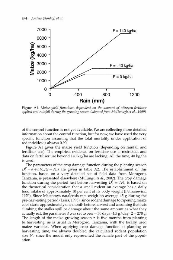
2. The studied model systemAs a basis for the analysis, we have used available insights on the multi-mammate rat population and their importance as an agricultural pestspecies, as studied in Morogoro, Tanzania, and elsewhere. In this region,62 per cent of the active population are cultivators; the large majority of thembeing subsistence farmers. The predominant crop is maize, accounting forabout 45 per cent of the hectarage under food crops and 32 per cent ofthe produced food crops (Anonymous, 2003). Irrigation is very rare andnearly all the maize crop production relies on rain. The rainy season inMorogoro is bimodal, with a first, but unreliable, peak between October andDecember and a second peak starting in February–March and continuinguntil May (Mwanjabe and Leirs, 1997). After the onset of heavy rains inFebruary–March, fields are ploughed and prepared for planting. Hence,planting of maize seeds typically takes place in March, although the exacttiming depends on rainfall. Planting is more or less synchronous in alarge area within a period of a few weeks. Field sizes are small, about0.5 ha per household. The crop yields in the region are very low withmaize production averaging 1.5 tons per hectare, going up to 2.5 tons perhectare under improved agricultural conditions (Anonymous, 2003; see alsofigure A1).

Although we have developed the model with the multimammate rat inMorogoro in mind, the model and reasoning will also be applicable to othercrop growing areas involving rodents living in highly seasonally varying


environments and with an institutional and economic structure close to theone found in rural Tanzania.

Rodent damage typically occurs immediately after planting and until themaize seedlings have reached the three-leave stage (about 2–3 weeks afterplanting). When heavy rodent damage to the seedlings becomes obvious(about ten days after the original planting), farmers may decide to replant.However, we have simplified the setting for our model by assuming thatplanting always (and only) occurs in March and that damage caused byrodents is not remedied by replanting.

Harvesting occurs in July–August. If rainfall in October–December isvery abundant, which rarely happens, then planting is possible in thatseason as well. However, farmers generally do not trust this first part of therainy season, since it is very unreliable. Hence, even though planting maybe possible, they are afraid that rainfall will not be sufficient during the restof the growing season. Thus, planting in that season only happens in someyears and even then only a part of the farmers decide to participate. Herewe ignore such a second crop.

As noted in the introduction, we consider two, overlapping time scales:one for the ecological population dynamics processes and another for theeconomic processes. The economic yearly time scale relates to the fact thatcrop harvesting normally takes place once a year, whereas the ecologicaltime scale is monthly. Since pest control actions may take place several timesa year, the control costs will also be given with a time step of one month.However, these costs are accounted for once a year, and, as a result, collapseinto the yearly time scale. We refer to the month by the index n (0, 1, . . . , 11,12, 13, . . . , 23, 24, 25, . . .) and the year by the index t (0, 1, 2, . . .). Each monthequal to 8, 20, 32, . . . (i.e. August each year) corresponds to harvesting timeand is defined so as to determine the beginning of a new production period,or ‘cropping year’.

3. The population growth under pest controlThe ecology is based on the model presented by Leirs et al. (1997a) andfurther explored by Leirs (1999), and Stenseth et al. (2001). Reproductionand survival parameters are governed by both density-dependent processesand density-independent processes (such as rainfall being treated as a time-dependent stochastic factor). The scale of the model is at one hectare, whilethe agricultural area considered may be quite large; hence, we ignore (asis typical within population dynamics modelling) dispersal. Our modelfurther describes only the female part of the population; the demographicparameter estimates are more reliable for females than for males. Moreover,it is, after all, the female part of the population that is instrumentalin generating the population dynamics through reproduction, which istypically limited by the number of breeding females. The ecological modelis a stage-structured model (see, e.g., Getz and Haight, 1989, for a generaloverview) with four stages, and where the vector Nn = (Nj0,n, Nj1,n, Nsa,n,Na,n) describes the rodent population per ha at the beginning of month n.Nj0,n is the number of juveniles in the nest, Nj1,n is the number of juvenileswhich are weaned but not yet in the trappable population, Nsa,n is the


number of sub-adult (non-reproducing) individuals, and Na,n is the numberof adult (reproducing) individuals. The total abundance at the beginning ofmonth n is then given as Nn = Nj0,n + Nj1,n+Nsa,n+Na,n.

The population dynamics is in matrix form, represented by Nn+1 = MNn,and where M is defined as (cf. Stenseth et al., 2001)

M =

⎡⎢⎢⎢⎢⎣

0 0 0 B(Vn, N(e)

n

)

s0n 0 0 0

0 s0w (1 − mn) · s1(Vn, N(e)

n

) · (1 − ψ(Vn, N(e)

n

))0

0 0 (1 − mn) · s1(Vn, N(e)

n

) · ψ(Vn, N(e)

n

)(1 − mn) · s2

(Vn, N(e)

n

)

⎤⎥⎥⎥⎥⎦

,

(1)

when B is the reproductive rate per adult female over one time step (beingone month); s0n is the monthly survival of juveniles still in the nest, ands0w is the survival of juveniles during the first month after weaning, bothassumed to be fixed irrespective of the environmental conditions; s1 is thesurvival of sub-adults, s2 is the survival of adults, and ψ is the maturationrate of sub-adults to adults (i.e., the probability that a sub-adult will matureto become a reproducing adult over the intervening month, given that itstays alive). The density relevant for defining the density-dependent struc-ture of the demographic rates is given by N(e)

n = Nsa,n + Na,n (juveniles are notyet recruited into the population and their number therefore does notaffect the demographic rates). The parameter mn, represents the reductionin natural survival (i.e., the death rate, due to pest control action duringmonth n). Consequently, by definition, when mn > 0 the population is beingaffected by the application of poison. The effect of the control is assumedto be the same for sub-adult and adult; hence, the same mn. The controlis assumed to have no effect on the juveniles, as they are just born andstill in the nest (or maybe just out of the nest) and will not eat the poison.There are therefore no control effects operating through the survival rate ofjuveniles, s0. Rainfall affects the demographic rates through the cumulativerainfall during the preceding three months Vn = (Pn–1 + Pn–2 + Pn–3), wherePn–1 represents the amount of rainfall during the month n – 1, etc. (Leirset al., 1997a). The three-month time lag is used since rainfall has an indirecteffect through vegetation (hence, the symbol Vn). The effects of density andprecipitation are non-linear: below a certain rainfall or density threshold,the demographic parameters have one value; above the threshold, theyhave another value. The parameters of the ecological model are given inthe Appendix, table A1.

Notice that rodent demography is not directly affected by crop produc-tion; the link is indirectly through rainfall. Moreover, crop production assuch has little effect on the rodents: they damage planted seeds (i.e., beforecrop production has started) and then the ripening seeds at harvest time,but, at that moment, the amount of available seeds is much larger thancan be consumed by the rodents, even in poor harvest years. During thecrop growing period, the rodents do not damage the crop but live fromalternative food in and around the fields (Makundi et al., 1999).


Stenseth et al. (2001) have explored how this ecological model behaveswhen a simple and fixed control-induced mortality is introduced. Theyshow that not only the magnitude of mn is important, but also over whichperiod the control is applied; a permanently applied control (i.e., controlevery month), may reduce the population considerably (and even drive thepopulation to extinction), while there is little effect when control is appliedat high densities only, even when there is a large increase in mortality.

Our analysis is restricted to control measures affecting survival, andwhere the effect on the control-induced reduction mn of natural survivalis assumed to result from the application of poison. Generally there is atwo-stage effect on survival. Let Xn be the amount of control measures (i.e.,some poison) applied per ha in month n. Its efficiency typically decreaseswith increasing precipitation during the month as the baits or the activeingredients degrade under humid conditions. In the present analysis, how-ever, we assume that precipitation has a negligible effect during the currentmonth. In addition, we make the reasonable assumption for the Tanzaniamultimammate rat system that after one month no effect of the poisonpersists in the environment in a form being available to the rats (Buckle,1994). Consequently, in what follows, the amount of effective control inmonth n coincides with the actual control measure the same month (andgiven by Xn).

Under these assumptions, the demographic effect of the pest control,the control or kill function (Carlson and Wetzstein, 1993), may generallybe represented by a function where the death rate increases with themanagement intensity; that is

mn = m(Xn). (2)

The reduction in natural survival, being in the domain [0, 1], is thereforegiven as ∂m/∂Xn ≥ 0 with m(0) = 0.

4. The costs and damagesThe costs of rodent control consist of two main components: the direct costof controlling the rodents and the cost through reduced yield. We startwith the yield damage cost. The crop is maize, and the yield depends onthe quality of the agricultural land, labour input, fertilizer use, and rainfall(see, e.g., Ruthenberg, 1980 and McDonagh et al., 1999). Assuming one cropper year (see above) and assuming that all production factors, except water,are optimally utilized and assumed fixed throughout the analysis, the yieldin kg per ha of agricultural land in the absence of rats may be writtenas

Yt = Y(At) (3)

where At is the amount of rainfall accumulated throughout the maize-growing season (i.e. precipitation during the five months prior harvesting,typically in August, see above). Y(At) is generally increasing in At up to somethreshold level, but at a decreasing rate; i.e. ∂Y/∂At > 0 and ∂2Y/∂2At ≤ 0(McDonagh et al., 1999). In addition, no rain means a small and negligibleharvest, hence, Y(0) = 0.


Damages caused by the rats are composed of two components, onerelating to the damage taking place during planting, expressed as a fractionof the yield, and another one relating to the damage through directconsumption of grain during harvesting, measured as absolute yield loss.Between planting and harvesting, there is essentially no damage caused bythe multimammate rat (Makundi et al., 1999). The fraction of maize plantedin month n that is damaged is directly related to the abundance of rats; thatis

Dpn = Dp(Nn) (4)

with ∂Dp/∂Nn > 0.Assuming no further rodent damage, the annual maize damage will

then be Y(At)Dpn . However, there will be a further reduction during the

harvesting period. The harvesting damage, measured in absolute loss (kgper ha), is also assumed directly related to the rodent abundance

Dhn = Dh(Nn), (5)

with ∂Dh/∂Nn > 0 and Dh(0) = 0. Consequently, the actual loss in maizeproduction in year t is

Dt = max{Y(At), [Y(At)Dp(Nn−t) + Dh(Nn)]} (6)

where the time lag τ , the length of the maize growing season (typicallyfive months), is introduced to scale the two types of damages occurring indifferent months. The economic crop loss per ha and year is therefore givenas

Kt = pDt (7)

where p is the price of the crop, assumed to be fixed over time.The direct control cost reflects basically the purchasing cost of the poison.

There may also be some costs of labour linked to the spreading of the poisonas well. If so, however, we are not explicitly considering any trade-offbetween labour uses in crop production and pest control. The control costfunction at time n (i.e., month), assumed to be fixed over time, is thereforeassumed given as

Cn = C(Xn) (8)

with ∂C/∂Xn > 0 and C(0) = 0.Having defined the control and damage cost functions, the total cost in

year t reads

Qt = Kt +∑

Cn (9)

where the summation of the control cost is taken over the year; that is, n = 8to 19 to cover the year t = 1, etc. (see above). Equation (9) implies that theeffect of discounting within the year is neglected. The total cost function alsoneglects, if any, negative poison effects on crop production. Environmentalcosts caused by the poison are not taken into account.


5. The management problem and the control strategiesWhile the crop without damage and the control cost one year is invariant ofthe crop yield without damage and control cost for the previous year, thisis obviously not so for the crop damage. Through the damage and controluse, the crop loss for one year is contingent upon the ecological state ofthe system in previous years. Hence, the cost in various years is linkedtogether through the size of the rodent population. The stochastic nature ofthe problem also makes a link through time as the rodent control consideredrefers to an environmental situation were both the crop yield and the rodentpopulation growth are subject to large fluctuations since rainfall is largelystochastic.

The management problem is therefore dynamic, and the various manage-ment strategies, given by a time sequence of the control Xn, either zero ornon-zero, is evaluated by calculating the median of the present-value cost

PC =T+1∑

1

Qt

(1 + δ)t, (10)

together with the variability (more details below). T is the control (planning)horizon in years, and δ is the (yearly) rate of discount. The basic trade-off atmonth n, as well as over time, is hence between the control cost, increasing inthe amount of poison used, and the crop damage, decreasing in the amountof poison used, and where the interaction goes through the survival rate mnof the rats.

Because of the complexity of the ecological model containing four stagesof rats, the stochastic nature of the problem and the complicated ecology–economy interaction due to the double, and partly overlapping, time scale, itis impossible to obtain any analytical solution of the management problem.However, when disregarding the stochastic element, ignoring the doubletime scale and replacing the model (1) with a biomass model, the basiceconomic trade-off may be illustrated. Under these simplified assumptionsand hence writing the population growth as Nn+1 = G(Nn, Xn), where Gis the natural growth function with dG/dXn < 0 so that Nn represents thenumber of ‘normalized’ rats at time n, it is shown in the Appendix that thecontrol condition

∂C(X)/∂ X ≥ λ[∂G(N, X)/∂ X] (11)

holds.The interpretation of the control condition is that the marginal cost of

the control, when economically rewarding to use it, should be equal to themarginal value of damage avoided by the control, evaluated at the shadowprice λ < 0 of the rodents. And, on the contrary, when it is not economicallybeneficial to use control, the marginal cost should be above the marginalvalue of the damage avoided. The shadow price changes through time,meaning that the damage cost avoided by the control changes through timeas well. In the simplified model (again, see the Appendix) it may settledown to a steady-state value, but that will definitely not happen in the fullmodel, not at least because of the fluctuations of the crop yield and rodentpopulation due to the stochastic rainfall.


Based on the above reasoning, we now single out some main strategies forcontrolling the rats that will be utilized in the numerical simulations. Con-sistent with current practice in the rural areas in Tanzania (Mwanjabe andLeirs, 1997), we assume that Xn, when applied, is fixed at some level.Keeping the dosage of the poison per application fixed, we are therefore notconsidering how much poison to use; strategies are formulated in whichmonth to apply the control measure (the timing), and for how long (theduration). We further assume the control, being either zero or non-zero ina specified sequence of months over the year, is the same from year to year.

The most trivial strategy to test is one in which rodent control is neverapplied, either because of lack of resources to apply rodenticides, or becauseit may be believed that the damage avoided by applying control willnot outweigh the cost of the rodenticide application. The more commonstrategies, however, are to apply rodenticide just before or soon afterplanting, or just before harvesting, or attempting to keep rodent populationlevels low throughout the maize growth season. These strategies aim atimmediate effects. Focusing on the negative shadow value of rodents, analternative long-term strategy could be to apply rodent control during thereproductive season, so as to minimize the birth of new animals. Again thiscould be done early, late, or throughout the reproductive season. Finally,rodent control could target the population at its usual peak late in the year,maximizing the number of rodents that would be killed.

Altogether we consider the following control strategies Xn, being eitherzero or at a fixed nonzero level, related to the calendar, and repeated in thesame way every year:

1. control for a given number of consecutive months, including no controland control every month;

2. control only for certain predetermined months (e.g., only everyFebruary or both February and March).

In addition, we have combined the above strategies with various conditionsrelated to the state of the system (such as conditioning the application ofpoison on rodent density or precipitation). As indicated above, today’spractice in Tanzania consists mainly of symptomatic treatment when heavyrodent damage is noticed. In some cases, depending on the visible presenceof many rats or issued outbreak warnings, farmers may choose to organizea prophylactic treatment at planting time. Such practices will be includedin our analysis, basically to compare the present practice with other, andbetter, strategies.

6. Results

Specific functional forms and the dataThe specific functional form of the control function (2) used in the nu-merical simulations neglects any influence through the size of the rodentpopulation. Moreover, for the given dosage Xn, we assume that the com-bined effects of natural mortality and the rodenticide-induced mortalityare constant and always 0.90. This is consistent with the field experience ofrodent control officers in Tanzania; the used poisons are effective in killing


rodents and at the used quantities they should be more than sufficient tokill all rats in the field. Usually, however, about 10 per cent of the rodents ina field survive the rodenticide application because they do not eat the bait,either accidentally or because they avoid it (Mwanjabe, personal comm-unication). Hence, with reference to the population dynamics (1),(1 − mn)si (Vn, N(e)

n ) = 0.10 is fixed every month when rodenticides areapplied, and si (Vn, N(e)

n ) in other months (see below and table A1 in theAppendix for further details).

Figure A1 in the Appendix gives the maize yield function. It includesthe use of fertiliser of 40 kg/ha, which is used and kept fixed throughoutthe simulations. The damage function during planting is specific as Dp

n =a + b Nn/(c + Nn), where a represents the background death rate of youngmaize plants (i.e. germination failure or damages not directly related to therat population), b is the maximum damage level, and c is the rat density forwhich damage is b/2. The Appendix (table A2) gives the parameter values.The damage function during the harvesting period is further specifiedlinear, Dh

n = d Nn, and where the value of d is based on information about thedaily food consumption of rats (again, see the Appendix for more details).The direct cost function is assumed to be linear as well, Cn = wXn, with was the purchasing cost of the poison (see above). Xn is fixed either at zeroor at some non-zero level (see above), and if applied, typically a treatmentwill be carried out with 2 kg of poisoned bait per ha.

As baseline value for the crop price we use p = 100 Tsh/kg maize, andw = 6500 Tsh/kg poison as the unit the control cost (table A2). The effects ofchanging economic conditions will, however, be studied. The managementproblem is, as mentioned, considered as a planning problem at the villagelevel, where the agricultural officer acts as the social planner. The planninghorizon will then be expected to be relatively long, while the rate of discountδ should reflect the social one. In the basic scenarios, we use T = 10 yearsand 7 per cent rate of discount, δ = 0.07.

Since rainfall patterns are a major component of the model’s variability,simulations have been run with a large number of different rainfallseries.1 We use monthly rainfall values (Meteorological Station, Morogoro,Tanzania) that were drawn from rainfall data obtained for that particularmonth in the period 1971–1997; that is, for each month of the run, andindependently from the values for the other months, we choose a value atrandom from the 27 years for which we had values for that month. Foreach control strategy, and set of model parameters, the model was run100 times, each time with a different random seed, resulting in 100 differentrainfall series. The model simulations always started in December with anaverage number of animals comparable to what is observed in the field inthat month. In order to reduce the effect of initial conditions, each model runran for 248 months before pest control and economic evaluation started; itthen continued for a number of years, reflecting the given planning horizon,T. Accordingly, the evaluation of each control strategy is done by calculating

1 The model was implemented numerically using Stella Research, version 5.1.1 (HighPerformance Systems, Inc., Hanover, NH, USA).


the median present-value cost (PC) of equation (10) for the 100 runs, togetherwith the variability, given by the 95 per cent range values.

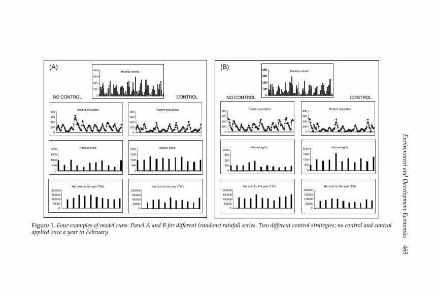
The structure of the analysesTo see the basic logic of the numerical simulations, figure 1 provides fourexamples based on two rainfall series and two different control strategies:control applied once a year in February (just before planting), and no controlat all. The two panels A and B are for different (random) rainfall series,chosen from different runs of the model; the examples are representative ofthe general pattern. As can be seen, under the rainfall pattern in panel A, therat abundance is subject to large fluctuations, both with and without control.However, the actual yearly harvest loss Dt is quite high accompanied byhigh values for the total current cost Qt when applying no control, whereasunder the February control the yield loss is smaller and the current costis lower. The same broad picture, at least for the total current cost, is alsoprovided in panel B.

For the given fertilizer use and the baseline values for the maize price andpoison cost, these results clearly indicate that pest control is economicallyrewarding, as the average yield loss is smaller and the current cost and,hence, also the PCs (not shown) are lower when control is carried out.Of course, care must be taken as figure 1 exhibits only two runs for eachstrategy. We now turn to the full-scale simulations where the results presentthe median PCs, together with the variance, for 100 simulations within eachstrategy shown.

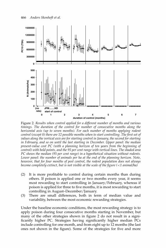
Duration and timing of the controlFigure 2 summarizes the results where we have simulated the applicationof pest control for different numbers of consecutive months. The durationof the control (i.e., number of consecutive months) is indicated along thehorizontal axis, where altogether we have included seven months as therat population goes close to extinct beyond four months (see below). Nocontrol at all is included as well, indicated by the number 0 along the axis.For each number of months applying control, except no control at all (0),there are 12 possible months to start controlling. Hence, we have generally12 medians and 95 per cent range plots within each possible duration ofcontrol as indicated by JFM . . . ND (January, February, Mars . . . , November,December). The upper panel represents the median present-value cost (PCs)with bold points, and the 95 per cent range with thin vertical lines. The PCswithout rats at all are also shown, displayed as its 95 per cent range variationas the shaded area. The lower panel gives the number of rodents at the endof the planning horizon, also as median and 95 per cent range values.

From the upper panel in figure 2, three main features should be noticed:

(1) The median present-value cost is high without control (0 months),but decreases in general for strategies with up to four consecutivemonths of control, beyond which the present-value cost (PCs) startsincreasing. Hence, the patterns only up to seven consecutive monthsare displayed. A rewarding strategy is therefore clearly to control therats for some months, but not for too long.

Environm

entandD

evelopmentE

conomics

465

(A) (B)

NO CONTROL CONTROL NO CONTROL CONTROL

Monthly rainfall

0

100

200

300

400

0

100

200

300

400

Rodent population

0

200

400

600

800

Harvest kg/ha

0

500

1000

1500

2000

Rodent population

0

200

400

600

800

Harvest kg/ha

0

500

1000

1500

2000

Net cost for the year (TSh)

0

50000

100000

150000

200000


0

50000

100000

150000

200000

Monthly rainfall

0

100

200

300

400

Rodent population

0

200

400

600

800

Harvest kg/ha

0

500

1000

1500

2000

Rodent population

0

200

400

600

800

Harvest kg/ha

0

500

1000

1500

2000


0

50000

100000

150000

200000


0

50000

100000

150000

200000

Figure 1. Four examples of model runs. Panel A and B for different (random) rainfall series. Two different control strategies; no control and controlapplied once a year in February


0

300000

600000

900000

1200000

1500000

PC

10 (

TS

h)

0

100

200

300

400

500

N (

An

imal

s/h

a)

(norats)

JFM........NDstart of control

0 1 2 3 4 5 6 7duration of control (months)

Figure 2. Results when control applied for a different number of months and varioustimings. The duration of the control for number of consecutive months along thehorizontal axis (up to seven months). For each number of months applying rodentcontrol (except 0) there are 12 possible months when to start controlling. The first set ofvalues along the vertical axis are for starting control in January, the second for startingin February, and so on until the last starting in December. Upper panel: the medianpresent-value cost PC (with a planning horizon of ten years from the beginning ofcontrol) with bold points, and the 95 per cent range with vertical lines. The shaded areaPC shows the median (95 per cent range) in a hypothetical situation without rodents.Lower panel: the number of animals per ha at the end of the planning horizon. Note,however, that for four months of pest control, the rodent population does not alwaysbecome completely extinct, but is not visible at the scale of the figure (<1 animal/ha)

(2) It is more profitable to control during certain months than duringothers. If poison is applied one or two months every year, it seemsmost rewarding to start controlling in January/February, whereas ifpoison is applied for three to five months, it is most rewarding to startcontrolling in August–December/January.

(3) There are small differences, both in term of median value andvariability, between the most economic rewarding strategies.

Under the baseline economic conditions, the most rewarding strategy is toapply poison during four consecutive months starting in November, butmany of the other strategies shown in figure 2 do not result in a signi-ficantly higher PC. Strategies having significantly higher median PCsinclude controlling for one month, and from eight up to 12 months (the lastones not shown in the figure). Some of the strategies for five and more


consecutive months may give lower PCs than strategies applied for, say, twoand three months (see also below). Strategies having significantly higherPCs also include applying controls for two to three months during thecropping season (i.e., starting in March). The timing of the control periodseems therefore to be more important than its duration, especially for controlperiods of three months or less. Hence, poisoning will be most rewardingjust before the growing season, so as to reduce the number of rodents beforethe planting of maize. Generally, the variability of the PC increases up tothree months duration of the control. After that it decreases again slightlyand stays more or less constant for five months and longer duration ofcontrol. Thus, the economic outcome of control during three months ormore is less uncertain than with shorter periods.

The lower panel in figure 2, presenting the rodent population at theend of the planning horizon, shows that some of the strategies applyingrodent control for one to two months each year do not affect populationdevelopment very much. However, if the duration of control is more thanthree months, the rodent population reduces slowly towards extinction, andfaster for longer duration of the control. The population goes close to extinctat the end of the planning horizon after four consecutive months. Hence,these graphs clearly indicate that control for more than four months is noteconomically meaningful, as more control means more control costs, butno further reduction in the number of rats, and hence, no further reductionin crop damages. It is important to notice that the patterns in the upperand lower panel are not concurrent, i.e. a small number of rats may coexisttogether with high PCs and vice versa, showing that the relation betweennumbers of rodents and economic benefit is not a trivial one. Notice alsothe high population variability.

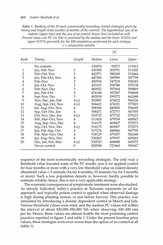
Other control strategiesFor all results presented so far we have applied rodent control duringconsecutive months and always during these months. However, theeconomic benefit of using pest control might be higher if we split thecontrol months into two (or more) periods each year separated by at leastone month. We tested this for two control periods each year with a totalof 2 (1 + 1), 4 (2 + 2), 6 (3 + 3) and 8 (4 + 4) months. For these simulations,the present-value costs (PCs) were generally lowest when rodent controlwas used during three months separated by at least one month. Hence, wealso tried all possible combinations of 3 (1 + 2), but also 4 (1 + 3) monthsseparated with at least one month. The 20 most rewarding strategies ofduration and timing of rodent control are presented in table 1. As can beseen, combinations of three to four months control in the period before thestart of the cropping season are still the most rewarding, together with atwo months control in February and November, There are, however, nosignificant present-value cost differences between the 20 strategies shownin the table; all strategies fall within the range of about four to five timesthe PC of the hypothetical case of no rodents at all. Still, compared to nocontrol at all (the bottom line), there are clear differences.

We also investigated whether an upper or lower threshold value onprecipitation or rodent density before applying poison could affect the


Table 1. Ranking of the 20 most economically rewarding control strategies given bytiming and length (total number of months of the control). The hypothetical case of no

rodents (upper line) and the case of no control (lower line) included as well.Present-value cost PC (in Tsh) is presented by the median and the lower (0.025) and

upper (0.975) percentile for the 100 simulations performed for each strategy.c = consecutive months

PC

Rank Timing Length Median Lower Upper

No rodents 103474 92073 1154131 Jan, Feb–Nov 3 430300 393791 5110202 Feb–Oct, Nov 3 442571 388248 5126643 Jan, Feb–Oct, Nov 4 447360 389589 5077994 Feb–Nov 2 450794 347518 5302435 Jan–Oct, Nov 3 453333 394788 5551386 Feb–Nov, Dec 3 460922 397604 5498697 Jan, Feb–Oct 3 474188 397287 5948488 Sep–Nov, Dec 3 492038 399272 6624889 Nov, Dec, Jan, Feb 4 (c) 502887 474022 566226

10 Aug, Sep, Oct, Nov 4 (c) 506623 474321 57700311 Jul, Aug–Oct, Nov 4 508180 480850 55669912 Sep, Oct–Dec, Jan 4 508471 472771 56755513 Oct, Nov, Dec, Jan 4 (c) 510735 477732 57921514 Feb, Mar–Oct, Nov 4 511824 479538 60006715 Aug, Sep–Nov, Dec 4 514175 469007 57257316 Sep, Oct, Nov, Dec 4 (c) 514175 469007 57257317 Jan, Feb–Sep, Oct 4 517276 480866 58779918 Feb, Mar–Nov, Dec 4 518129 479457 58244819 Jul, Aug–Nov, Dec 4 530267 479937 60926320 Dec, Jan, Feb, Mar 4 (c) 530743 484888 647072

Never control 0 820958 723460 956967

sequence of the most economically rewarding strategies. The only way athreshold value lowered some of the PC results, was if we applied controlfor four months or more with a very low threshold value on rodent density(threshold value = 5 animals/ha for 4 months, 10 animals/ha for 5 monthsor more). Such a low population density is, however, hardly possible toestimate reliably; hence, this is not a very applicable strategy.

The economic consequences of symptomatic treatment were also studied.As already indicated, today’s practice in Tanzania represents an ad hocapproach, and typically poison control is applied when observed damageis high during planting season, or just before harvest. This practice wassimulated by introducing a density dependent control in March and July.Various threshold values were tried, and the median PC values fell withinthe interval of about 830,000–856,000 Tsh when observing 100–200 ratsper ha. Hence, these values are almost double the most promising controlpractices reported in figure 2 and table 1. Under the present baseline pricevalues, these strategies were even worse than the option of no control at all(table 1).


Variations in the maize price and control costA permanent negative shift in the producer price of maize, p, will generallymake shorter duration of the control relatively more profitable. The intuitivebasis for this result is straightforward, as lower marginal crop damage costmust be compensated by lower marginal control cost (i.e. reduced durationof the control). On the other hand, the effect on the timing is quite modest.The economic conditions for the farmers may also be less favourable dueto more expensive poison, and a positive permanent shift in w also leadsin the direction of shorter duration of the control being relatively moreprofitable. Hence, instead of four months, five months, and one monthduration per year being the most economically rewarding strategies underthe base-line assumptions, we find that doubling the poison price makesduration of one month, two months, and no control the most economicallyrewarding strategies. Thus, more expensive poison means that more ratsand a higher level of crop damage will be accepted in the best strategies(cf. also inequality 11 above).

The economic consequences of symptomatic treatment were also studiedunder shifting price and cost assumptions. All the time, the best practicescompared to today’s practises of introducing density dependent controlin March and July were typically about half as costly. Finally, we alsostudied the effects of reducing the planning horizon and making theproblem more myopic by setting T = 5 years. The rate of discount δ wasalso reduced. Generally, there are small changes taking place (not reportedhere). This was also so for an increased planning horizon and a higher rate ofdiscount.

7. DiscussionThroughout this paper, we have considered a rodent pest problem where themanagement is in the hands of a social planner and where the agriculturalarea can be quite large. The control problem is specified as timing andduration strategies, where the dosage of the poison is kept fixed per monthwhenever poison is used (consistent with recent practice in Tanzania). Themost economically profitable control period seems to be just before theplanting season. The damage at planting accounts for such a large portionof the total losses due to rodents that minimizing the population duringthat short period is enough to reduce yield losses. Controlling for a longerperiod will reduce rodent populations at a time when they do not damagethe crop anyhow, and, due to the very high reproductive capacity of therodents, the population will increase rapidly as soon as control operationsare stopped, repressing any long-term effects. The simulations, however,only indicate small profitability differences among various combinationsof control months towards the start of the planting season. Although wehave not valued environmental costs of the use of poison (see, e.g., Carson1962) and negative impacts, if any, upon crop production are neglected,the small differences between the best strategies strongly suggests optingfor a strategy amongst these that uses the least poison. Hence, takingenvironmental economic considerations into account, one month or twomonths of control just before the planting season, January and February,


or eventually in November and February, seem to be the best overallstrategies.

These economically most rewarding strategies differ significantly fromtoday’s practice of symptomatic treatment when heavy rodent damage isnoticed. The economic threshold concept and the idea of adjusting thetiming of pesticide use to pest density is an old one (Carlson and Wetzstein,1993), but works poorly here because of the high reproductive rate of the ratsand the short period after sowing during which most of the damage is done.Hence, the present paper demonstrates that shifting from such practices tomore mechanistic control strategies; i.e. emphasizing the calendar instead ofthe pest abundance, can substantially improve the economic conditions forthe maize producing farmers in the present case of multimammate rats. Thebest practices compared with today’s symptomatic treatment will typicallyhalve the sum of control and damage cost. The question of how to choosebetween an economic threshold model and a mechanistic control modelis of general interest and should be examined further, but following ouranalysis it seems to be population growth characteristics of the pest ratherthan its taxonomic status that should govern that choice (see also Regev etal., 1976).

We also find that permanent changes in the crop price and control costgive effects that are more or less in line with intuition. A less valuable cropand higher poison cost make shorter duration of the control and, hence,living with more rats and nuisance relatively more profitable. On the otherhand, the optimal timing (i.e. in which months to apply poison) is onlymodestly affected by such changes. Consequently, it seems that the optimaltiming is more closely related to the ecology and the abundance of rats thanprices and costs, while the economy plays a more important role when itcomes to the optimal duration of the control. One reason for this may bethat the damage effect is far more important during some parts of the year,e.g. just before planting.

Throughout our simulations, we interpreted the pest control problemas taking place at the village level, where an agricultural officer servesas the social planner. While it mostly will remain the individual farmer’sdecision to apply control on his fields, the agricultural officer indeed playsan important role. His advice will be very influential not only to farmers,but also in ensuring timely access to rodenticides; in village shops, shelf-lifeof these poisons is limited so usually only limited quantities are availablelocally. The social planning horizon is also relevant because in case of anoutbreak coming through, the government will be required to organisecostly emergency measures (Makundi et al., 1999). When making the prob-lem more myopic through a reduced planning horizon, however, we findthat the results are only modestly influenced. For the more myopic Africanfarmer, when neglecting externalities due to various control practices withinthe management area, the above findings therefore also basically hold.When interpreting the results at the farm level, it should also be noticedthat subsistence farmers frequently face credit restrictions, and, typically, forsuch farmers, there is cash only for seed (see, e.g., Dasgupta and Maler (1995)for a general discussion). This has implications for fertiliser use which,however, has been kept fixed at a positive level throughout the analysis.


Models are only an approximation of how we conceive reality, and theyare only as good as the assumptions on which they are based. Regardingour population model, the basic building block of the present analysis, twomajor assumptions do not hold in reality. The first one is that the modeluses discrete time steps of one month; however, a lot can happen in arodent population in one month. Secondly, our model does not yet includeimmigration processes but it is obvious that these can play an importantrole, particularly when the densities after rodent control have become muchlower than in the surrounding fields. In such cases, a population may evenbe capable of recovering from a rodenticide application in the course of afew weeks (see, e.g., Leirs et al., 1997b), thus reducing the efficacy of controlactions considerably. Regarding the agricultural activities, our model doesnot yet include the common practice of replanting after rodent damage,sometimes in combination with rodenticide application, and thus partiallyremedying damage. The crop price and the control costs are also kept fixedthroughout the planning horizon, and the maize price is assumed to bethe same in years with poor and good harvest. For all these reasons, theresults should be interpreted very cautiously and the model is not yetready to be confronted with farmers and taken into practice. However, themain finding of the above analysis, emphasizes that the calendar instead ofpest abundance when controlling the rats will probably hold under morerealistic assumptions and is clearly an application rule that is quite easy toimplement.

ReferencesAnonymous (2003), Morogoro Regional Socio-economic profile, Joint Publication by

the National Bureau of Statistics (NBS) and Morogoro Regional CommissionersOffice.

Barnett, S.A. (1988), ‘Ecology and economics of rodent pest management: the needfor research’, in I. Prakash (ed.), Rodent Pest Management, Boca Raton: CRC PressInc, pp. 459–464.

Buckle, A.P. (1994), ‘Rodent control methods: chemical’, in A.P. Buckle & R.H. Smith(eds), Rodent Pests and Their Control, Wallingford: CAB International, pp. 127–160.

Carlson, G. and M. Wetzstein (1993), ‘Pesticides and pest management’, in G. Carlson,D. Zilberman, and J. Miranowski (eds), Agricultural and Environmental ResourceEconomics, New York: Oxford University Press, pp. 268–317.

Carson, R. (1962), The Silent Spring, Greenwich: Fawcett Crest Books.Dasgupta, P. and K.-G. Maler (1995), ‘Poverty, institutions, and the environmental

resource base’, in J. Behrman and T. Srinivasan (eds), Handbook of DevelopmentEconomics, Vol III, Amsterdam: Elsevier, pp. 2371–2463.

Fiedler, L.A. (1988), ‘Rodent problems in Africa’, in I. Prakash (ed.), Rodent PestManagement, Boca Raton: CRC Press Inc., pp. 35–64.

Getz, W. and R. Haight (1989), Population Harvesting, Princeton, NJ: PrincetonUniversity Press.

Hone, J. (1994), An Analysis of Vertebrate Pest Control, Cambridge: CambridgeUniversity Press.

Leirs, H. (1995), ‘Population ecology of Mastomys natalensis (Smith, 1834) multi-mammate rats: possible implications for rodent control in Africa’, AgriculturalEditions, vol. 35, Brussels: Belgian Administration for Development Cooperation.


Leirs, H. (1999), ‘Populations of African rodents: models and the real world’, inG. Singleton, L. Hinds, H. Leirs, and Z. Zhang (eds), Ecologically Based Managementof Rodent Pests, ACIAR Monograph 49, Canberra, pp. 388–408.

Leirs, H., R. Verhagen, and W. Verheyen (1993), ‘Productivity of different generationsin a population of Mastomys natalensis rats in Tanzania’, Oikos 68: 53–60.

Leirs, H., R. Verhagen, W. Verheyen, P. Mwanjabe, and T. Mbise (1996), ‘Forecastingrodent outbreaks in Africa: an ecological basis for Mastomys control in Tanzania’,Journal of Applied Ecology 39: 937–943.

Leirs, H., N.C. Stenseth, J.D. Nichols, J.E. Hines, R. Verhagen, and W.N. Verheyen(1997a), ‘Seasonality and non-linear density-dependence in the dynamics ofAfrican Mastomys rats’, Nature 389: 176–180.

Leirs, H., R. Verhagen, C.A. Sabuni, P. Mwanjabe, and W.N. Verheyen (1997b), ‘Spatialdynamics of Mastomys natalensis in a field-fallow mosaic in Tanzania’, BelgianJournal of Zoology 127: 29–38.

Makundi, R.H., N.O. Oguge, and P.S. Mwanjabe (1999), ‘Rodent pest managementin East Africa: an ecological approach’, in G. Singleton, L. Hinds, H. Leirs, and Z.Zhang (eds), Ecologically Based Management of Rodent Pests, ACIAR Monograph 49,Canberra, pp. 460–476.

McDonagh, J., R. Bernhard, J. Jensen, J. Møberg, N. Nielsen, and E. Nordbo (1999),‘Productivity of maize based cropping system under various soil-water-nutrientmanagement strategies’, Working paper, Department of Agricultural Sciences, TheRoyal Veterinary and Agricultural University, Copenhagen.

Mulungu, L.S., R.H. Makundi, H. Leirs, A.W. Massawe, S. Vibe-Petersen, and N.C.Stenseth (2002), ‘The rodent density-damage function in maize fields at an earlygrowth stage’, in G.R. Singleton, L.A. Hinds, C.J. Krebs, and D.M. Spratt (eds),Rats, Mice and People: Rodent Biology and Management. Canberra: Australian Centerfor International Agricultural Research, pp. 301–303.

Mwanjabe, P.S. (1990), ‘Outbreak of Mastomys natalensis in Tanzania’, African SmallMammal Newsletter 11: 1.

Mwanjabe, P. and H. Leirs (1997), ‘An early warning system for IPM-based rodentcontrol in smallholder farming systems in Tanzania’, Belgian Journal of Zoology 127:49–58.

Petrusewicz, K. (1970), ‘Productivity of terrestrial animals: principles and methods’,IBP Handbook, 13, Oxford: Blackwell Science.

Regev, U., A. Gutierrez, and G. Feder (1976), ‘Pests as a common property resource:A case study of alfalfa weevil control’, American Journal of Agricultural Economics58: 186–197.

Ruthenberg, H. (1980), Farming Systems in the Tropics, Oxford: Clarendon Press.Saunders, G.R. and G. Robards (1983), ‘Economic considerations of mouse-plague

control in irrigated sunflower crops’, Crop Protection 2: 153–158.Singleton, G., L. Hinds, H. Leirs, and Z. Zhang (eds) (1999), Ecologically-Based

Management of Rodent Pests. ACIAR Monograph 49, Canberra.Stenseth, N.C., H. Leirs, S. Mercelis, and P. Mwanjabe (2001), ‘Comparing strategies

of controlling African pest rodents: an empirically based theoretical study’, Journalof Applied Ecology 38: 1020–1031.

Stenseth, N.C., H. Leirs, A. Skonhoft, S.A. Davis, R.P. Pech, H.P. Andreassen, G.R.Singleton, M. Lima, R.M. Machangu, R.H. Makundi, Z. Zhang, P.B. Brown, D. Shi,and Wan Xinrong (2003), ‘Mice, rats and people: the bio-economics of agriculturalrodent pests’, Frontiers in Ecology and the Environment 1: 367–375.

Tisdell, C. (1982), Wild Pigs: Environmental Pest or Economic Resource, Sidney:Pergamon Press.

Zivin, J., B. Hueth, and D. Zilberman (2000), ‘Managing a multiple-use resource: thecase of feral pig management in Californian rangeland’, Journal of EnvironmentalEconomics and Management 39: 189–204.


Appendix

The simplified management modelWhen using a continuous time approach, the current value Hamiltonianof the (strongly!) simplified management problem reads H =−{p[Y(A)Dp(N) + Dh(N)] + C(X)}+ λ[G(N, X) − N] . The control conditionreads

∂ H/∂ X = −∂C(X)/∂ X + λ[∂G(N, X)/X] ≤ 0 (A1)

while the portfolio condition is

dλ/dt = δλ − ∂ H/∂ N = δλ + p[Y(A)(∂ Dp(N)/∂ N) + ∂ Dh(N)/∂ N]

−λ [∂G(N, X)/∂ N − 1]. (A2)

The control condition holds as equality when it is optimal to use control;that is when X > 0. (A1) directly gives condition (11) in the main text. Theportfolio equation governs the time path of the shadow price λ of therodents, and all the time we have λ< 0, as the rodent is a pest andnuisance.

Table A1. Monthly demographic parameter values for each of the combinedrainfall-density regimes in the population dynamics model. The values for s0n and s0w

are arbitrarily set, the other values were obtained from demographic analysis (fromLeirs et al., 1997a)

Regime definitionRainfall in the past3 months (mm)

Vn <200 <200 200–300 200–300 >300 >300

Density per ha N(e)n >150 <150 >150 <150 >150 <150

Demographic ratesNet reproductive rate B(Vn, N(e)

n ) 1.29 5.32 0.30 6.64 4.69 5.82Juvenile survival in

the nests0n 1.0 1.0 1.0 1.0 1.0 1.0

Juvenile survival afterweaning

s0w 0.5 0.5 0.5 0.5 0.5 0.5

Sub-adult survival S1(Vn, N(e)n ) 0.629 0.513 0.682 0.617 0.678 0.595

Sub-adult maturation ψ(Vn, N(e)n ) 0.000 0.062 0.683 0.524 0.155 1.000

Adult survival S2(Vn, N(e)n ) 0.583 0.650 0.513 0.602 0.505 0.858

The dataTable A1 summarises the demographic parameters in the ecological model.The specification of the demographic effect of the pest control equation(2) is problematic since it should include the effect of the rat abundance.Moreover, not discussed in the main text, it should also include thecombined effects of natural and poison-induced mortality and theimmediate effect of the latter on the former (through density-dependentmechanisms). Such information for a more detailed and realistic description


0

1000

2000

3000

4000

5000

6000

7000

0 400 800 1200Rain (mm)

Mai

ze (

kg/h

a)

F = 0 kg/ha

F = : 40 kg/ha

F = 140 kg/ha

Figure A1. Maize yield functions, dependent on the amount of nitrogen-fertilizerapplied and rainfall during the growing season (adopted from McDonagh et al., 1999)

of the control function is not yet available. We are collecting more detailedinformation about the control function, but for now, we have used the veryspecific function assuming that the total mortality under application ofrodenticides is always 0.90.

Figure A1 gives the maize yield function (depending on rainfall andfertiliser use). The empirical evidence on fertiliser use is restricted, anddata on fertiliser use beyond 140 kg/ha are lacking. All the time, 40 kg/hais used.

The parameters of the crop damage function during the planting seasonDp

n = a + b Nn/(c + Nn) are given in table A2. The establishment of thisfunction, based on a very detailed set of field data from Morogoro,Tanzania, is presented elsewhere (Mulungu et al., 2002). The crop damagefunction during the period just before harvesting Dh

n = d Nn is based onthe theoretical consideration that a small rodent on average has a dailyfood intake of approximately 10 per cent of its body weight (Petrusewicz,1970). Since Mastomys natalensis rats weigh on average 45 g during thepre-harvesting period (Leirs, 1995), since rodent damage to ripening maizecobs starts approximately one month before harvest and assuming that ratsclimbing the stalks spill or damage about the same amount as what theyactually eat, the parameter d was set to be d = 30 days · 4.5 g/day · 2 = 270 g.The length of the maize growing season τ is five months from plantingto harvesting, as is usual in Morogoro, Tanzania, with the locally usedmaize varieties. When applying crop damage function at planting orharvesting time, we always doubled the calculated rodent populationsize Nn since the model only represented the female part of the popul-ation.


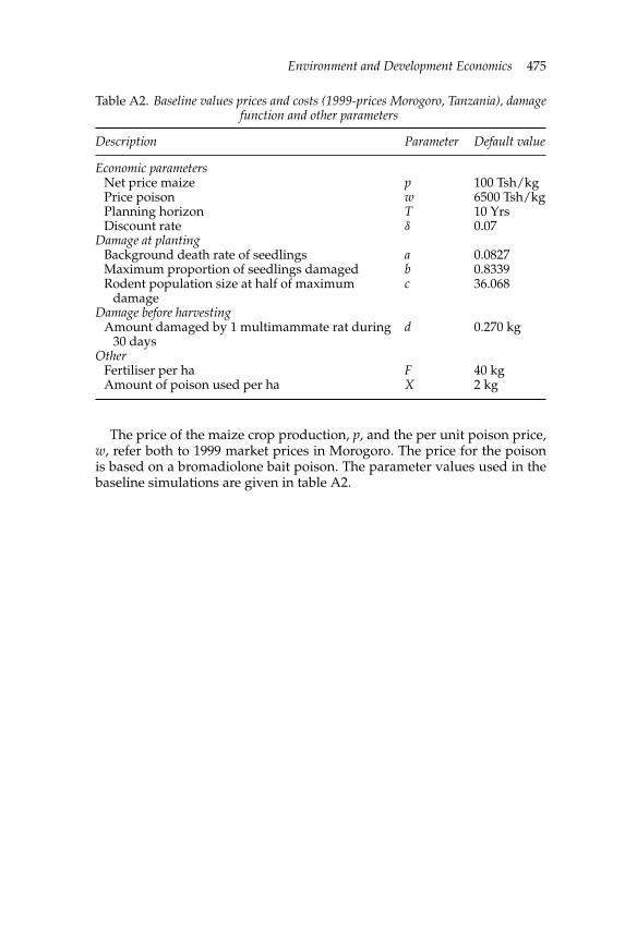
Table A2. Baseline values prices and costs (1999-prices Morogoro, Tanzania), damagefunction and other parameters

Description Parameter Default value

Economic parametersNet price maize p 100 Tsh/kgPrice poison w 6500 Tsh/kgPlanning horizon T 10 YrsDiscount rate δ 0.07

Damage at plantingBackground death rate of seedlings a 0.0827Maximum proportion of seedlings damaged b 0.8339Rodent population size at half of maximum

damagec 36.068

Damage before harvestingAmount damaged by 1 multimammate rat during

30 daysd 0.270 kg

OtherFertiliser per ha F 40 kgAmount of poison used per ha X 2 kg

The price of the maize crop production, p, and the per unit poison price,w, refer both to 1999 market prices in Morogoro. The price for the poisonis based on a bromadiolone bait poison. The parameter values used in thebaseline simulations are given in table A2.

The bioeconomics of controlling an African rodent pest species

Documents

Transcript of The bioeconomics of controlling an African rodent pest species