Policy ReseaRch WoRking PaPeR 4930

The Better You Are the Stronger It Makes You

Evidence on the Asymmetric Impact of Liberalization

Leonardo Iacovone

The World BankDevelopment Research GroupTrade and Integration TeamMay 2009

WPS4930P

ublic

Dis

clos

ure

Aut

horiz

edP

ublic

Dis

clos

ure

Aut

horiz

edP

ublic

Dis

clos

ure

Aut

horiz

edP

ublic

Dis

clos

ure

Aut

horiz

ed

Produced by the Research Support Team

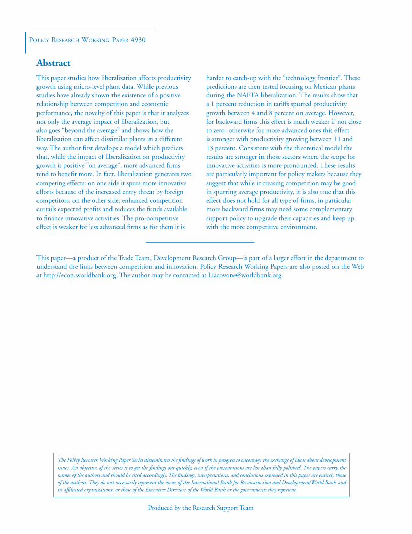
Abstract

The Policy Research Working Paper Series disseminates the findings of work in progress to encourage the exchange of ideas about development issues. An objective of the series is to get the findings out quickly, even if the presentations are less than fully polished. The papers carry the names of the authors and should be cited accordingly. The findings, interpretations, and conclusions expressed in this paper are entirely those of the authors. They do not necessarily represent the views of the International Bank for Reconstruction and Development/World Bank and its affiliated organizations, or those of the Executive Directors of the World Bank or the governments they represent.

Policy ReseaRch WoRking PaPeR 4930

This paper studies how liberalization affects productivity growth using micro-level plant data. While previous studies have already shown the existence of a positive relationship between competition and economic performance, the novelty of this paper is that it analyzes not only the average impact of liberalization, but also goes “beyond the average” and shows how the liberalization can affect dissimilar plants in a different way. The author first develops a model which predicts that, while the impact of liberalization on productivity growth is positive “on average”, more advanced firms tend to benefit more. In fact, liberalization generates two competing effects: on one side it spurs more innovative efforts because of the increased entry threat by foreign competitors, on the other side, enhanced competition curtails expected profits and reduces the funds available to finance innovative activities. The pro-competitive effect is weaker for less advanced firms as for them it is

This paper—a product of the Trade Team, Development Research Group—is part of a larger effort in the department to understand the links between competition and innovation. Policy Research Working Papers are also posted on the Web at http://econ.worldbank.org. The author may be contacted at Liacovone@worldbank.org.

harder to catch-up with the “technology frontier”. These predictions are then tested focusing on Mexican plants during the NAFTA liberalization. The results show that a 1 percent reduction in tariffs spurred productivity growth between 4 and 8 percent on average. However, for backward firms this effect is much weaker if not close to zero, otherwise for more advanced ones this effect is stronger with productivity growing between 11 and 13 percent. Consistent with the theoretical model the results are stronger in those sectors where the scope for innovative activities is more pronounced. These results are particularly important for policy makers because they suggest that while increasing competition may be good in spurring average productivity, it is also true that this effect does not hold for all type of firms, in particular more backward firms may need some complementary support policy to upgrade their capacities and keep up with the more competitive environment.

The Better You Are the Stronger It Makes You:

Evidence on the Asymmetric Impact of Liberalization∗

Leonardo Iacovone†

First Version: April 2007Current Version: May 13, 2009

∗The author is thankful to Gerardo Leyva and Abigail Duran for granting access to INEGI data at the offices of

INEGI in Aguascalientes under the commitment of complying with the confidentiality requirements set by the Mexican

Laws. I also wish to thank each one of the INEGI’s employees that helped me during the work at Aguascalientes, in

particular Gabriel Romero and Alejandro Cano. I am grateful to Alan Winters and Gustavo Crespi for their support

and guidance. Special thanks also to Gerardo Esquivel, Caroline Freund, Rafael De Hoyos, Beata Javorcik, Hiau Looi

Kee, Eric Verhoogen, Carolina Villegas, the participants at the conference on “Welfare Effects of Trade Liberalization

in Less Developed Countries” at Anahuac University, ELSNIT 2007 conference in Barcelona, World Bank Research

Group Trade seminar, and the participants to the Conference on “Organization and Performance: Understanding the

Diversity of Firms” in Tokyo for their useful comments. Finally I gratefully acknowledge the financial support from

ESRC and LENTISCO. The views expressed in this paper are those of the author and should not be attributed to the

World Bank, its Executive Directors or the countries they represent.†Development Research Group, World Bank, 1818 H Street, NW; Washington, DC, 20433, USA. Email: Liacov-

one@worldbank.org

1

1 Introduction

“Do countries with lower barriers to international trade experience faster economic progress?

Few questions have been more vigorously debated in the history of economic thought, and

none is more central to the vast literature on trade and development.” (Rodriguez and

Rodrik 1999)

The relationship between liberalization and economic performance has been strongly debated since

Adam Smith and it is still today at the center of disputes. Even more than academic economists,

policy makers consider the subject central to their concerns. In particular developing countries, that

during the 1990s have undergone profound liberalizations1 with the objective of improving their eco-

nomic performance and accelerating their growth rates, have recently started to put these policies

under discussions because of mixed results.2. In this study we will try to explain why liberalization

can result in outcomes that are different depending on the context and, more in particular, are uneven

for heterogenous firms.

In this paper we develop a model that shows how the impact of liberalization can be asymmetric for

different types of firms and test its main predictions focusing the liberalization that Mexico under-

went during NAFTA. This provides an excellent opportunity to study a deep process of liberalization

and integration with the global economy that increased the pressures from import competition and

entry threat of foreign competitors. We will analyze it and show that, consistent with our theoretical

model, the impact of NAFTA was highly asymmetric on different types of firms and, while produc-

tivity growth “on average” is larger for those firms in sectors where tariffs dropped more, at the same

time, this effect is weaker for plants more distant from the production technology frontier.

A number of previous studies using firm-level3 data have already shown that an increase in import

competition tends to have a positive impact on economic performance (Tybout and Westbrook 1995,

Lopez-Cordova 2003, Pavcnik 2002, De Hoyos and Iacovone 2006, Nickell 1996, Fernandes 2007).

However, these studies normally focused on the “average” impact of liberalization and implicitly as-

1As discussed in a recent World Bank report over the last few decades almost all developing countries have liberalized

their trade regimes (Bank 2006)2“In many developing countries, there has already been a de-industrialisation process in which lowering of tariffs

has led to imports displacing local industries” (Martin Khor 1999, Director of Third World Network)

“Some trade critics are bothered by the disappointing performance of Latin America since it slashed tariffs in the

1980s and 1990s while more protectionist China and Southeast Asia sped ahead” (“Pains from free trade spurs second

thoughts”, Wall Street Journal, 30 March 1997).3In the paper we refer interchangeably to “firm” and “plant”, however it is important to emphasize that in our

empirical analysis the unit of observation will be the plant consistently with the unit of observation of our data.

2

sume that the effect of liberalization is homogeneous for all firms.4 Differently, some recent work

from Aghion, Blundell, Griffith, Howitt, and Prantl (2004) shows that the effect of competition is

non-linear and heterogenous depending on the productivity level of the firm. Only “good firms”(e.g.

close to the productive frontier) are positively affected by competition as their innovative effort is

enhanced in response to the increased entry threat of foreign competitors. Vice-versa “bad firms”

(e.g. far from the productive frontier) are negatively affected because the intensified entry threat only

reduces their expected profits as their efficiency is too low to allow them to compete successfully with

foreign entrants(Aghion, Burgess, Redding, and Zilibotti 2004).

In this paper we contribute to the existing literature in two ways. On the theoretical front we develop

a neo-Schumpterian model that extends previous work by Aghion, Blundell, Griffith, Howitt, and

Prantl (2004) and still reaches consistent results with their model at industry-level, while generating

novel results at the firm-level. These results are more in line with much of the firm-level studies point-

ing toward a positive impact trade liberalization on firm performance “on average”. Consequently we

bring such a model to the data and test it by using plant-level data from a developing country. Our

approach, differently from much of the previous literature that analyzed the effect of liberalization

in a cross-country setting focusing mostly on outcomes (e.g. relationship between growth and open-

ness), is much more micro and concentrates on a specific mechanism through which liberalization

may influence firms’ responses (see literature review by Hallak and Levinsohn (2004)).

The paper is divided into five sections. In the next section we discuss the existing literature related to

our study. In the third one we present a set of stylized facts and sketch the theoretical model, which

generates two main predictions tested in the subsequent econometric analysis presented in section

four. The last section concludes and highlights some avenues for further research.

2 Existing Literature

This paper is related to various strands of the literature, in particular the recent works of Aghion

and Bessonova (2006) and Aghion, Burgess, Redding, and Zilibotti (2004) arguing that liberalization

boosts innovative efforts, but only for those firms that are more productive while it weakens the in-

centive to innovate for less productive ones. These models are characterized by three main elements.

First, innovation is the main driver of firm-level growth. Second, a firm innovates as long as its post-

innovation profits are larger then pre-innovation ones. Third, the effect of a successful innovation is

limited and a firm can only advance “one step a time” over the “productivity ladder”. This implies

4Schor (2004) study on Brazil and more recently Lileeva and Trefler (2007) using Canadian plants data are two

notable exceptions.

3

that if a firm is close to the productive frontier by innovating it will prevent entry of potential foreign

competitors.5 However, if a firm is far from the productive frontier then it does not have any chance

of preventing a foreign competitor from entering and taking over its market. In such a model, tariffs

reduction increases the entry threat and boosts the incentives of “advanced” firms to innovate in

order to preempt the potential foreign entry. For these firms, the increased competition reduces more

the pre-innovation profits than post-innovation profits because if the firm does not innovate it risks

losing all its market due to the entry of the foreign competitor. At the same time the consequences for

less productive firms are very different because the increased entry threat reduces the post-innovation

profits more than the pre-innovation ones. In fact, the “laggard incumbents” (i.e. less productive)

cannot prevent the entry of foreign competitors, even when able of innovating succesfully because

they are too far from the productive frontier.

Also, related to this paper is the large set of studies arguing that increased competition puts pres-

sures on “slacking managers” and pushes them to reduce the X-inefficiency (Martin 1978, Martin and

Page 1983, Leibenstein 1978). However, all these studies rely on a set of restrictive assumptions and

normally assume that firms are homogeneous (Rodrik 1988).

Our work is clearly linked to previous empirical studies analysing the effect of competition on innova-

tive activities and productivity growth even if the earlier studies could only rely on industry-level data

(Gerosky 1990, Haskel 1992). Even more relevant to our study are the more recent analysis using firm-

level data to evaluate the impact of competition on productivity and innovation (Nickell 1996, Disney,

Haskel, and Heden 2003) as well as the studies evaluating directly the impact of trade liberalization

on firm-level productivity (Tybout and Westbrook 1995, Pavcnik 2002, Fernandes 2007, De Hoyos

and Iacovone 2006). However, as previously mentioned, these studies focus on the average effect of

liberalization and do not account for the possibility that this effect could different across heterogenous

firms. Two notable exceptions, that we are aware of, are Schor (2004) Lileeva and Trefler (2007) that

allow for the impact of liberalization to be heterogenous across different firms but use a different

methodology from the one adopted in this paper.

In the same spirit of our study, a couple of recent papers analysed the impact of FDI spillovers and

5Foreign competitors are assumed to be at the frontier, therefore when they enter the domestic market they force

domestic firms that are not at the frontier to exit because they can produce the same good more efficiently. Another

possibility is that even if foreign firms don’t produce exactly the same good their entry on the domestic market can

increase the elasticity of substitution of domestic consumers and push mark-ups of domestic firms down, in this case

only more productive firms would be able to survive in the more competitive environment. The bottom line is that

increased competition will affect the elasticity of demand and therefore the markup of domestic firms. In fact, enhanced

import competition can also shift the demand for domestic varieties in and, even with fixed markups, domestic firms

are worse off as they have to spread their fixed costs over a reduced output.

4

foreign ownership exploring the possibility of heterogenous impacts on firms with different produc-

tivity levels (Griffith, Redding, and Simpson 2003, Sabirianova, Terrell, and Svejnar 2005).

This paper is very much part of the growing literature on heterogeneous firms showing how firm

heterogeneity interacts with external policy changes generating dynamics that fits much better the

empirical evidence (Jovanovic 1982, Hopenhayn 1992, Melitz and Ottaviano 2003, Melitz 2003, Help-

man, Melitz, and Yeaple 2004, Bernard, Redding, and Schott 2004, Yeaple 2005). In particular these

studies show how the impact of liberalization and globalization is highly asymmetrical depending on

the initial productivity of the firms, with more productive firms benefitting disproportionately more

from globalization than less productive ones.

3 Trade Liberalization and Productivity

3.1 The Facts

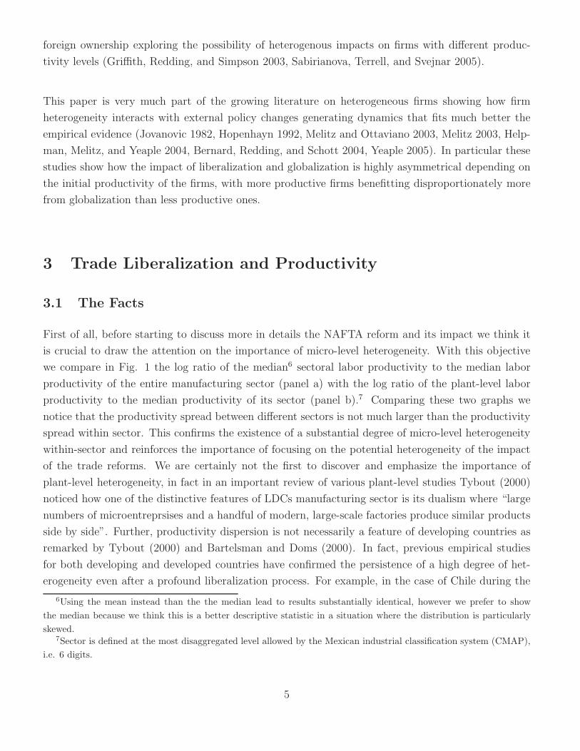
First of all, before starting to discuss more in details the NAFTA reform and its impact we think it

is crucial to draw the attention on the importance of micro-level heterogeneity. With this objective

we compare in Fig. 1 the log ratio of the median6 sectoral labor productivity to the median labor

productivity of the entire manufacturing sector (panel a) with the log ratio of the plant-level labor

productivity to the median productivity of its sector (panel b).7 Comparing these two graphs we

notice that the productivity spread between different sectors is not much larger than the productivity

spread within sector. This confirms the existence of a substantial degree of micro-level heterogeneity

within-sector and reinforces the importance of focusing on the potential heterogeneity of the impact

of the trade reforms. We are certainly not the first to discover and emphasize the importance of

plant-level heterogeneity, in fact in an important review of various plant-level studies Tybout (2000)

noticed how one of the distinctive features of LDCs manufacturing sector is its dualism where “large

numbers of microentreprsises and a handful of modern, large-scale factories produce similar products

side by side”. Further, productivity dispersion is not necessarily a feature of developing countries as

remarked by Tybout (2000) and Bartelsman and Doms (2000). In fact, previous empirical studies

for both developing and developed countries have confirmed the persistence of a high degree of het-

erogeneity even after a profound liberalization process. For example, in the case of Chile during the

6Using the mean instead than the the median lead to results substantially identical, however we prefer to show

the median because we think this is a better descriptive statistic in a situation where the distribution is particularly

skewed.7Sector is defined at the most disaggregated level allowed by the Mexican industrial classification system (CMAP),

i.e. 6 digits.

5

1980s and 1990s Crespi (2005) found that firms in the top decile have labour productivities that are

256 percent larger than those in the bottom decile, while Disney, Haskel, and Heden (2003) found a

difference of “only” 155 percent.80

.2.4

.6.8

1D

ensi

ty

−2 −1 0 1 2Log Ratio of Median Sectoral Labour Productivity to Economy−Wide Median Labour Productivity

(a) Heterogeneity Between Sectors

0.5

11.

5D

ensi

ty

−.5 0 .5 1 1.5 2Log Ratio of Plant Labour Productivity to Median Sectoral Labour Productivity within 6−digits Sector

(b) Heterogeneity Within Sectors

Figure 1: Firms Heterogeneity (Source: INEGI, Aguascalientes)

Having shown some evidence on the importance of plant-level heterogeneity, we now want to show

how after the implementation of NAFTA we observe a remarkable increase in industrial inequality

with good firms getting better, and larger firms getting larger.

If we analyze the evolution of productivity9 during the period 1993-2002 we observe two fundamental

trends: a shift in the mean productivity, as Mexican firms became on average more productive, and

an increase in the spread of the productivity distribution.10 These trends emerge from figure 3 where

8The explanations for this heterogeneity can be divided into two mayor groups. Traditionally, researchers have

pointed towards supply-side explanations such as technological efforts and uncertainty surrounding technological in-

vestments (Nelson 1981), management or ownership , human capital as well as complementary investments in organi-

zational capital, and matching between skills and organisation (Bartelsman and Doms 2000). For example the findings

that productivity ranking tends to be relatively stable seems to imply that managerial skills, or some other persistent

productivity shocks, are important determinants of this heterogeneity (Baily, Hulten, and Campbell 1992). Another

potential explanation, hard to pinpoint convincingly, points toward the existence of external economies as documented

by Krizan’s (1995) findings that there is a positive correlation between plant level productivity and regional economic

activities in various developing countries. More recently, Syverson (2004) suggested that also demand side reasons

can be important to explain this heterogeneity, in particular product heterogeneity and their substitutability plays an

important role. Finally, external to the firm, regulations and exposure to international competition can be important

in explaining part of the observed heterogeneity (Tybout 2001, Tybout 2000, Bartelsman and Doms 2000).9We use as productivity index the value added labour productivity.

10We also test the hypothesis that the productivity spread got larger more formally by regressing the coefficient of

variation, calculated within each narrowly defined sector at six digits, on a linear trend. We find that the coefficient

on the linear trend estimated with a FE model is positive and statistically significant confirming that dispersion of

6

020

4060

80M

exic

an N

AF

TA

ad

valo

rem

tarif

fs

1992 1994 1996 1998 2000 2002Year

Max Min Average

Figure 2: Import Tariffs Drop under NAFTA (Source: Secretaria de Economia, Mexico)

we plot present the distribution of the gap between each individual firm-level productivity and the

“productive frontier”, in years 1993 (dashed line), 1998 (dotted line) and 2002 (continuous line). The

gap is defined as the log of the ratio between the average productivity of the top five firms in the

sector and the individual firm labour productivity.11 A larger ratio identifies firms more distant from

the productive frontier. In figure 3 we observe the distribution moving rightward, indicating that the

gap between the average, or the median, Mexican firm and the “productive frontier” is expanding. At

the same time, we see that the right tail of the distribution is also getting fatter implying an increase

in the density of firms with larger gaps.

This expansion in productivity inequality is even more interesting if we consider that during this period

we observe the exit of a significant number of less productive firms. In fact, fig. 4 depicts the number

of number of exiting plants in Panel (a), and shows in Panel (b) that the average productivity of

exiting plants (dashed line) is always substantially smaller than the average productivity of surviving

ones (continuous line). In a nutshell, after NAFTA was implemented besides a substantial exit of less

productive plants, which should compress the productivity distribution by trimming its left tail, we

observe an increase in productivity inequality among surviving Mexican firms.

productivity among firms even within narrowly defined sectors got larger during the period under analysis.11To avoid the risk of having an excessively narrow definition of sector we define the “productive frontier” at 4 digits.

7

0.2

.4.6

.8K

erne

l Den

sity

Dis

trib

utio

n

0 1 2 3 4 5Log of Distance from Frontier

1993 1998 2002

Figure 3: Distance From Frontier (Source: INEGI, Aguascalientes)

To conclude this section we want to discuss the importance of the liberalization process under NAFTA.

During the 1990s Mexico underwent a process of deep integration with its the North-American

economies. This process marked the completion of a liberalization already started during the second

part of the 1980s. However, it is important to notice that, differently from the unilateral liberalization

of the 1980s, the liberalization under NAFTA locked in Mexican policy makers much more than the

previous reforms because of the credibility imposed by an agreement with a powerful counterpart.

Therefore, when considering the scope of the liberalization under NAFTA we need to take into ac-

count also the importance of this credibility effect (Tomz 1997, Tornell and Esquivel 1995). In this

perspective, NAFTA implied a deeper liberalisation than the drop in the average tariffs would suggest.

would appear from just looking at the drop in the average tariff. Furthermore in figure 2 we show that

the NAFTA tariffs12 drop was not negligible, while the average tariff went down from about 16% in

1993 to less than 5% in 2002, the tariff peak was reduced from about 70% in 1993 to about 20% in 2002.

12Tariff rates for commodities produced in US or Canada.

8

020

040

060

080

0su

m o

f Exi

tRev

ised

1993 1994 1995 1996 1997 1998 1999 2000 2001 2002

(a) Number of Exiting firms

22.

53

3.5

44.

5La

bour

Pro

duct

ivity

1992 1994 1996 1998 2000 2002year

Stayers Exitors

Data source: EIA

Productivity Among Exitors and Stayers

(b) Average Productivity of Exitors vs Stayers

Figure 4: Firms Demography (Source: INEGI, Aguascalientes)

3.2 The Model

In order to explain the facts presented in the previous section, in particular the increase in the in-

dustrial inequality in a period of profound liberalization we develop a model with heterogenous firms

based on neo-Schumpeterian growth models. The key intuition here is that liberalization can generate

at the same time contrasting effects on the incentives to innovate. On one side, higher competition can

hamper the innovative efforts of incumbent firms by reducing their expected profits.13 At the same

time, the liberalization may lead incumbent to increase their innovative efforts in order to “escape

competition”. The synthesis provided by the neo-Schumpeterian growth models consists exactly in

allowing these two mechanisms to coexists and interplay, and in this manner it provides us with the

theoretical basis that could explain the stylised facts presented in Section 3.1.

Now we will briefly sketch our model, which builds on the work of Aghion, Burgess, Redding, and

Zilibotti (2004) and Aghion, Bloom, Blundell, Griffith, and Howitt (2002). The principal innovation

of our model is that we relax the assumption that the impact of increased competition on backward

firms is invariably negative. Instead, we will allow also backward firms to be able to catch-up with the

productive frontier, even if this will be less likely because of their initially disadvantaged condition. We

characterize this model by discussing separately in each one of the following subsection (1) domestic

production, (2) innovation decision, (3) foreign competition, (4) equilibrium innovation.

13This effect is referred to as “Schumpeterian effect” by Aghion, Bloom, Blundell, Griffith, and Howitt (2002)

9

3.2.1 Domestic production

In the economy we have a final good y that is produced using a continuum of intermediate goods v ∈

[1, 0]. The production is described by equation 1 where xt(v) is the quantity used of the intermediate

input v and At(v) measures its productivity at time t, finally α is a parameter varying between 0 and 1.

This final good can be consumed, used to produce intermediate inputs or invested in innovation.

yt =1

α

∫ 1

0

A1−αt (v)xα

t (v)dv (1)

Each intermediate good is produced by a monopolist14 at a constant marginal cost equal to one unit

of the final good. The monopolist maximizes its profits but its monopoly power is restricted by the

existence of a set of “fringe firms” that do not operate in equilibrium but could produce the same

input using χ unit of output. Basically χ is a parameter capturing the competition intensity and

is larger than 1. Therefore the maximum price that the monopolist can charge for the intermediate

good v is pt(v) and can be expressed in terms of the output that is the numeraire

pt(v) = χ (2)

Because the final-good producing sector is perfectly competitive the price of the intermediate good v

must equal to its marginal product

MPt(v) =dyt

dxt(v)= α (xt(v)/At(v))α−1 (3)

therefore from 3 and 2 we obtain that

xt(v) = (χ/α)1

α−1 At(v) (4)

The model can be then solved and Aghion and Griffith (2005) show that the profit function15 is

inversely correlated with the strenght of th competition, proxied by χ, and positively correlated with

the productivity of the firm producing the intermediate input v as described in equation 5:

πt(v) = At(v)δ(χ) (5)

where

δ(χ) = (χ − 1)χ

α

1

α−1

(6)

3.2.2 Innovation decision

In each period the technological frontier evolves exogenously at a rate g as described by equa-

tion 7

14This assumption can be changed and have two producers competing for example under Bertrand competition.15To confirm this it is sufficient to substitute 4 and 4 in the equilibrium profit that is πt(v) = (pt − 1)xt(v)

10

At = At−1 (1 + g) (7)

and there can be two types of firms as explained by the following equation

Firm type =

Advanced or type 1 if at the end of t − 1 At−1 = At−1

Backward or type 2 if at the end of t − 1 At−1 = At−2

In order to characterise the innovation decsision we will assume that the advanced firm will success-

fully innovate, and catch up, with probability z, where z is exactly measuring its research effort.

Analogously, also the backward firm is able to innovate, however, because of its relative position with

respect to the technological frontier, when it does innovate and move “one step forward” with proba-

bility z this is not enough to catch up with the frontier.16 In fact, in order to catch up the backward

firm needs to move “two steps ahead” over the technology ladder and to do so it needs to make an extra

innovation effort. This extra effort will be succesfull only with probability s, this being smaller than z.

In the original version of the model presented by Aghion and Griffith (2005) the backward firm does not

have any chance of catching up, that is innovating and moving “two steps ahead”, so the introduction

of this extra effort and the fact that the backward firm is able to catch up with probability s is the

principal innovation of our model. However, in order to make this more realistic we will impose that

this probability s is lower than z, or in other words it is more likely that a firm is successful in moving

“one step” ahead rather than “two steps”. To simplify we can also assume that

s = θz

where θ is a parameter that we assume smaller than one but not smaller than g. Basically we want

to allow the backward firm to be able to catch up with the technological frontier.

g ≤ θ ≤ 1 (8)

Following Aghion, Burgess, Redding, and Zilibotti (2004) we assume that the cost of innovating is

quadratic in the research effort and linear in the current technological level as in equation 9. However,

for backward firms we need to take into account also the cost of the extra-effort. So the innovation

cost function is c1t for the advanced firm and c2t for the backward

Innovation Cost =

c1t = 12z2At−1(v)

c2t = 12z2At−2(v) + 1

2s2At−2(v)

(9)

16We need to remember that the backwad firm has at the end of t − 1 a productivity equal to At−2

11

At the end of every period, all firms that remain backward will then be upgraded automatically,

assuming there are spillovers from mature technology, and move up one step in the technology ladder.17

Also, at any moment t there is an exogenous probability h that any firm may exit and be replaced

by a new advanced firm at time t + 1.

3.2.3 Foreign competition

In every period foreign competitors can enter the domestic market, and their decision is done after

having observed the outcome of the innovation effort of the domestic firms. A foreign company needs

to incur in a sunk cost equal to ξ to enter the domestic market. Once it has paid this, the firm will

be able to successfully penetrate the domestic market with probability µ.18 Because, foreign firms are

assumed to be at the technological frontier, if it does enter and faces a backward domestic firm, then

it gains the entire market if, otherwise, it faces a domestic firm at the frontier then they engage in

Bertrand competition and both firms will see their profits go to zero. Consequently the entry threat

simplifies into the following condition

Entry Threatt =

0 if domestic firm is at frontier in t − 1 and innovates succesfully in t

or is backward in t − 1 but able to reach the frontier in t

µ otherwise

3.2.4 Equilibrium innovation

The solution of the expected profit maximization problem for the backward firm is obtained by solving

equation 10

maxz

E [π2t] = δ(χ)[z(1 − µ)At−1 + (1 − z) (1 − µ) At−2 + sAt + (1 − s)At−2(1 − µ)

]−

1

2

(z2 + s2

)At−2

(10)

because when, with probability z, this firm is successful in moving one step ahead and obtain a

productivity At−1, it will retain its domestic market only if the foreign firm does not enter.19 Similarly,

when it is unsuccessful at innovating with probability 1 − z and mantains productivity At−2, it will

retain its market only if the foreign firm does not enter, with probability 1 − µ. The backward firm

also engages in an extra-effort to catch-up with productive frontier and, if successful, with probability

s, obtains a productivity equal to At and retains the market. While if unsuccesful, with probability

1 − s, it mantains productivity At−2 and retains its domestic market as long as the foreign firm is

unable to enter with probability 1 − µ. Solving this maximization problem we obtain the optimal

17This allows us to have only two types of firms to deal with.18µ is a proxy capturing how difficult is to enter the domestic market, i.e. tariffs and regulations directly affect µ.19The probability that the foreign firm is unsuccessful in entering the market is exactly 1 − µ.

12

innovative effort z∗2t of the backward firm 11

z∗2t =δ

1 + θ2[g (1 + 2θ + θg) + µ (θ − g)] (11)

At the same time the advanced firm choses its optimal innovation effort z∗1t maximising its expected

profits π1t as in equation 12

maxz

E [π1t] = δ(χ)[zAt + (1 − z) (1 − µ)At−1

]−

1

2z2

t At−1 (12)

because it retains the market when it successfully innovates, with probability z, and obtains a pro-

ductivity At, in which case the foreign firm stays out of the market. The advanced firm also keeps its

market if unsuccessful at innovating, with probability 1 − z, and a resulting productivity of At−1 as

long as, with probability 1− µ, the foreign firm is unable to enter. Therefore the optimal innovation

effort of this firm is equal to

z∗1t = δ (g + µ) (13)

After having derived the optimal innovative effort for both firms, we can now determine what is the

effect of a reduction in import barriers which increases entry threat. In particular we derive two

predictions from equations 11 and 13.

dz∗2t

dµ=

δ

1 + θ2(θ − g) (14)

dz∗1t

dµ= δ (15)

Prediction 1: Liberalization by increasing entry threat (µ) increases the optimal innovative

effort of all types of firms

Prediction 2: Liberalization increases the optimal innovative effort of advanced firms more

than that of backward firms

The first prediction derives immediately from the fact that both δ and (θ−g)1+θ2 are positive. The second

prediction is a consequence of (θ−g)1+θ2 being smaller than one.

The predictions of our model are consistent with those of Aghion, Burgess, Redding, and Zilibotti

(2004) at industrial level because an increase in the foreign competition (increase in µ) expands in-

dustrial inequality as advanced firms react to it with a larger innovative effort than backward ones.

However, when we analyze the model prediction at firm level, our model implies that the effect of

liberalization is, on average, positive for both advanced and backward firms, while in Aghion, Burgess,

Redding, and Zilibotti (2004) the impact on backward firms innovative effort is always negative be-

cause the Schumpeterian effect dominates.

The predictions of our model are consistent with the basic intuition from the previous literature

on X-efficiency suggesting that increased competition is expected to spur efforts (Leibenstein 1978),

13

as well as various empirical studies analyzing the impact of trade reforms on productivity. These

studies normally found that the “average” effect of increased competition is positive (Tybout and

Westbrook 1995, Fernandes 2007, De Hoyos and Iacovone 2006, Nickell 1996). In other words, our

model extends Aghion, Burgess, Redding, and Zilibotti (2004) and Aghion and Griffith (2005) by

making their predictions more in line with previous empirical studies but mantains intact its central

feature, which is that liberalization has an unequal effect and advanced firms benefit more from

it.

4 Econometric Analysis

The econometric analysis is split into two sub-sections. In the first we briefly describe the data

while in the second section we analyzed the relationship between liberalisation and productivity. In

particular we will build or empirical model in order to explore the potential firm heterogeneity and

allow the impact of liberalization to be dissimilar for different types of firms.20

4.1 Data

The data used in this analysis are provided by INEGI and cover the entire period of NAFTA reforms,

1993-2002. The data are collected at plant level, and individual establishments are identified through

a unique key that allow us to build a panel.21 After having cleaned the dataset the number of

establishments varies between 6,500 and about 5,000 because of attrition.22 The sampling structure

of the survey is such that the data tend to be more representative of larger firms, overall the survey

covers 85% of industrial output excluding the“maquiladoras”. The survey frequency is yearly and

the variables collected cover various aspect of the firm’s operations: workers, wages, electricity usage,

intermediate inputs usage23, production, inventory, sales24, investment in different types of physical

assets, investment in R&D and in technology transfers.25

20We will focus on one specific dimension of firm heterogeneity, namely productivity.21This work was carried out while I was in Aguascalientes and in compliance with Mexican Laws protecting the

confidentiality of the data.22It is important to note that entry is not systematically captured by INEGI as the sample is refreshed only once

every ten years. However a specific department of INEGI tends to follow up on newspapers and other sources of

information the entry of new plants, in this way the most important new firms tend to be included even if this is not

systematic.23The intermediate inputs used are split into imported and domestic inputs.24As for intermediate inputs also the sales are split into domestic and foreign sales.25For more details on the data see appendix A or refer to Iacovone (2008).

14

4.2 The Asymmetric Impact of Liberalization

In this section we will address two questions aiming at testing the predictions of our model. What is

the average impact of increased import competition on productivity growth? And is this impact the

same for all firms? The implicit assumption we make here is that productivity growth is an adequate

proxy of innovative efforts.

It is a well documented feature of various firm-level studies that firms are heterogeneous in terms of

their productivity (Tybout 2000). At the same time various firm-level studies have shown that trade

liberalisation tends to influence positively the productivity of domestic firms (Pavcnik 2002, Roberts

and Tybout 1996). However, based on the theoretical model developed in section 3.2, we would also

expect the impact of increased foreign competition to be different across firms with different produc-

tivity levels.

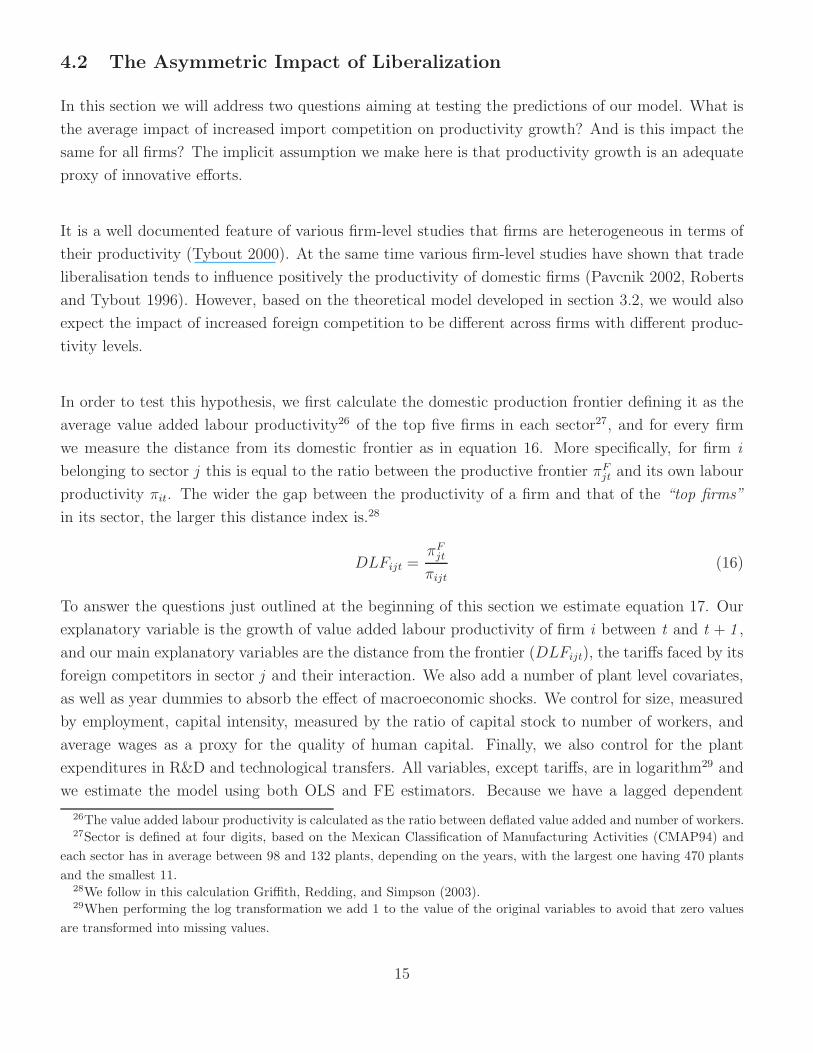
In order to test this hypothesis, we first calculate the domestic production frontier defining it as the

average value added labour productivity26 of the top five firms in each sector27, and for every firm

we measure the distance from its domestic frontier as in equation 16. More specifically, for firm i

belonging to sector j this is equal to the ratio between the productive frontier πFjt and its own labour

productivity πit. The wider the gap between the productivity of a firm and that of the “top firms”

in its sector, the larger this distance index is.28

DLFijt =πF

jt

πijt

(16)

To answer the questions just outlined at the beginning of this section we estimate equation 17. Our

explanatory variable is the growth of value added labour productivity of firm i between t and t + 1 ,

and our main explanatory variables are the distance from the frontier (DLFijt), the tariffs faced by its

foreign competitors in sector j and their interaction. We also add a number of plant level covariates,

as well as year dummies to absorb the effect of macroeconomic shocks. We control for size, measured

by employment, capital intensity, measured by the ratio of capital stock to number of workers, and

average wages as a proxy for the quality of human capital. Finally, we also control for the plant

expenditures in R&D and technological transfers. All variables, except tariffs, are in logarithm29 and

we estimate the model using both OLS and FE estimators. Because we have a lagged dependent

26The value added labour productivity is calculated as the ratio between deflated value added and number of workers.27Sector is defined at four digits, based on the Mexican Classification of Manufacturing Activities (CMAP94) and

each sector has in average between 98 and 132 plants, depending on the years, with the largest one having 470 plants

and the smallest 11.28We follow in this calculation Griffith, Redding, and Simpson (2003).29When performing the log transformation we add 1 to the value of the original variables to avoid that zero values

are transformed into missing values.

15

variable in this equation appearing on the denominator of the distance index our estimates will be

biased (Cameron and Trivedi 2005, p.764). In particular the OLS coefficient will be downward biased

while the FE coefficients will be upward bias (Arellano 2003).30

∆πijt = β0 + β1DLFijt−1 + β2Tjt−1 + β3Tjt−1 × DLFijt−1 + β4Xijt−1 + β5Y ear + µit (17)

Based on our model we expect β2 to be negative as lower tariffs should promote higher productivity

growth spurred by the increased competitive pressure. We also expect β3 to be positive, because,

as discussed in section 3.2 the impact of increased liberalisation is less positive for firms that are

more distant from the technological frontier. Finally, consistently with previous studies we expect β1

to be positive as firms lagging behind tend to catch up with their respective frontier (Alvarez and

Crespi 2007).

The main results are presented in table 7. In addition to the variables previously discussed, in the

OLS specification we also include industry, state and year fixed effects. We first present a set of

regressions where only include our main variables of interest and the fixed effects, models (1) and (2),

and then include also the plant-level controls, models (3) and (4). Consistently with our expectations

on the bias induced by the lagged dependent variable, the coefficient on the variable measuring the

distance from frontier, which contains a lagged dependent variable in its denominator, appears to be

larger in the FE than in the OLS. However it is important to underline that the qualitative results

do not change between the two models. In fact, no matter which estimate we choose, in both models

these variables are positive and significant.

Table 7 here

Our main finding is that the productivity of firms facing lower tariffs tends to grow faster but this

productivity effect is lower for firms with larger distance from the productive frontier as the coefficient

on the interaction is positive. The coefficients of the remaining variables are consistent with what

we would have expected a-priori. In particular, we find evidence of catching up as distance from

frontier positively affects subsequent productivity growth. It is also interesting to notice that the

productivity of larger and more capital intensive firms tends to grow faster. Also, as expected, the

productivity of firms paying higher wages grows faster. And finally, higher expenditures in R&D and

technology transfers promote faster productivity growth. However, these control variables are likely

to be endogenous; therefore, we do not want to push too much on their interpretation. In fact the

principal purpose of introducing them is to control for firms’ characteristics that may be correlated

with the productivity growth and therefore, if omitted, could bias our principal coefficients of interest.

30A possible extension to try to address this issue is to use a GMM estimator which makes use of the longitudinal

dimension of the data to build appropriate instruments using the lagged variables. However in our case the reduced

size of the longitudinal dimension makes the use of GMM less attractive, therefore we did not pursue this strategy.

16

For this reason in columns (1) and (2) of table 7 we exclude these regressors in order to confirm that

their inclusion is not crucial for our results.

Because of the presence of the interaction we can calculate the impact of a percentage change in tariffs

on productivity growth for different types of firms depending on their distance from the productive

frontier.31 In figure 4.2 we graph these marginal effects based on the results from column (3) and (4)

of table 7. The bottom line is that for most of the plants, except those in the top decile, e.g. the

ones that are more distant from the production frontier, the tariffs reduction spurs their productivity

growth.

Marginal Effect of % Tariff Change on % Productivity Growth

-1.5

-1

-0.5

0

0.5

1

1.5

1% 5% 10% 25% 50% Mean 75% 90% 95% 99%

Percentile - Distance from Frontier

OLS FE

Figure 5: Marginal effect of Tariffs on Productivity Growth

The results from table 7 just discussed confirm the two basic predictions of the model. After having

presented our main results, we will now discuss a set of potential concerns that may invalidate our

findings and assess if these are truly robust.

First of all, an important issue to be discussed is the possibility that tariffs could be endogenous.

Fundamentally we think this is not a major problem for two reasons. The main reason is that while it

is reasonable to expect that an entire industry is be likely to be able to influence its tariffs schedule, it

is harder for a plant alone to influence the tariffs set for its entire industry. Therefore, if our analysis

31Our β of interest is equal to β2 + β3 ∗ LogDistance.

17

was done using industry-level data we would be concerned about tariffs endogeneity while we think

this is not a major issue in our study as we focus on plant-level data.

Moreover, if we analyze the way NAFTA negotiations were carried out we can strenghten our con-

fidence about the Mexican tariffs phase out being exogenous. First, the NAFTA agreement faced

Mexico with bilateral negotiations with partners that had more influence and negotiating power.

Additionally, the negotiations were carried out in a relatively short period of time which reduces

the possibility of external interventions and interferences from individual firms. Moreover, the high

degree of uncertainty that surrounded the US Congress approval of NAFTA suggests that Mexican

negotiators focused their minds on supporting the negotiating process to increase the chances of

NAFTA being approved, rather than trying to defend the interests of individual firms.32 Indeed,

these anecdotal remarks are consistent with the findings of Kowalczyk and Davis (1996) who argue

that while for US tariffs there is evidence that higher duties and sectors with lower intra-industry

trade were characterized by slower phase out, there is not such evidence when we analyze the phase

out of Mexican tariffs except that these appear correlated with US phase-out.33

Finally, to dispel some remaining doubts we analyze the evolution of Mexican tariffs under NAFTA

and observe that, even at a rather disaggregated level (i.e. 6 digits), the rankings of the different

tariffs are rather stable. This is shown by table 3 in appendix A where we split the tariffs in deciles

and calculate the transition probabilities during the period under analysis. A similar conclusion is

reached if we observe table 4 where we calculate the Spearman rank correlation between tariffs. The

conclusion from this table is that, no matter which pair of years we consider, we can always reject the

null hypothesis that the two tariff schedules are independent. This suggests that whatever the polit-

ical economy was behind the tariffs structure this did not change much during the NAFTA period,

therefore using 6-digits industry fixed effects we control for these time-invariant industry characteris-

tics affecting the political economy of tariffs liberalization.34

In appendix B.2 we also present a set of additional regressions (see tables 8 and 9) in order to check

the robustness of our results.

First of all we exclude from our analysis the “top plants” used to calculate the productive frontier.

32NAFTA was only approved by the US Congress only on December 8th,1993, by a narrow majority of 234-200 vote

and it took effect after less than one month on January 1st, 1994.33Kowalczyk and Davis (1996) argue that empirical analysis at five-digit SITC level “suggests that from the perspec-

tive of Mexican negotiations, many other issues, including the overriding one of obtaining free trade in the near future

with its Northern neighbours, were given higher priority than the questions of how to phase duties out”34A similar argument and solution is proposed by Schor (2004) and Goldberg and Pavcnik (2005).

18

Because these plants have been used to calculate the productive frontier we can expect that there will

be some correlation, by construction, between the productive frontier and their productivity which

could bias our results. The results are reported in columns (5) to (8) of table 8 in appendix B.2 and

confirm that the exclusion of these plants does not influence our conclusions.

Secondly, because our dataset is an unbalanced panel and include plants that at some point are closed

down and exit from the sample we are concerned that exiting could influence our results. In order to

address this problem we first of all introduce a dummy variables that is equal to one when a firm will

be exiting in the year and zero otherwise. The results are reported in columns (9) and (10) of table 8

and we notice that indeed the performance of exiting firms is, in the year before exiting, clearly worse

than that of other firms. However the main coefficients of interest, i.e. the coefficient on tariffs and

on the interaction between tariffs and distance from productive frontier, are substantially unchanged.

We also repeat our estimations using a balanced panel and excluding altogether exiting plants from

the sample, the results are reported in columns (11) and (12) of table 8. In this case, even if the main

coefficients of interest are still significant and have the expected signs we observe that, differently

from previous results, the coefficient on the interaction between tariffs and distance from frontier is

larger in the OLS than in the FE model, we think this is probably a consequence of the selection bias

generated when using a balanced panel and excluding all exiting plants.

In all our discussion we have assumed that increased competition and entry threat, captured by a

reduction in Mexican tariffs under NAFTA, are having an uneven effect on firms with different pro-

ductivity level. However, it is also possible that Mexican tariffs maybe capturing some other effect.

For example, if Mexican tariffs and US tariffs under NAFTA are correlated35 the reduction in Mex-

ican tariffs may be identifying the impact of enhanced market access under NAFTA as we have not

included US tariffs in our baseline regressions. To address this problem we include US tariffs and their

interaction with distance from frontier. The results are reported in table 9 in appendix B.2, where

in columns (13) and (14) we exclude the plant-level controls while in columns (15) and (16) we also

include them36. For simplicity we will concentrate on the results reported in columns (15) and (16)

as these are substantially similar to the ones where we exclude the plant-level controls. The principal

conclusion is that the inclusion of US tariffs does not change our previous results, the coefficients on

Mexican tariffs and their interaction with distance from frontier are substantially identical. Further,

it is interesting to notice that the increased access to US markets has a similar positive effect on

productivity as the increase of domestic competition, in fact the size of the coefficients on US tariffs

is very close to that on Mexican tariffs. Additionally, it is intriguing to notice that, in line with the

predictions of recent trade models with heterogenous firms (Melitz 2003), also the expanded market

35I thank Eric Verhoogen for this remark.36Notice that in these regressions we also include a dummy to control for exiting firms

19

access affects asymmetrically domestic firms with more productive firms benefitting more.

As a further robustness check we test if our results are influenced by the 1994 peso devaluation. It

is fair to argue that, simultaneously to the NAFTA reforms, Mexican firms were also affected by

the devaluation shock which could also influence different plants asymmetrically. In order to control

for this we introduce the interaction between real exchange rate and the distance from frontier as

additional control. The results are presented in Table 10 and show that the original impact of tariffs

is somewhat attenuated and while in the OLS estimation the interaction between tariffs and distance

from frontier is still positive and significant, in the case of the fixed-effect estimation this remains

positive but becomes but marginally insignificant. At the same time, in the fixed-effect estimation

the sign of the interaction between exchange rate and distance from frontier is negative supporting

the idea that backward may have been negatively affected by the devaluation, probably because these

were less able to reap the benefits of enhanced competitiveness on the export market. Extending these

results, we restrict our sample to those products where quality differences are particularly important

as it is the case of those products that Rauch defines as “differentiated” (Rauch 1999). The reason is

that while for “homogenous products” we expect that what matters are mostly cost-cutting innova-

tion, and the scope for innovation is therefore more limited, differently for “differentiated” products

we expect that the “potential quality differences” between products give to producers more room to

introduce not only cost-cutting process innovation but also product innovation. The results presented

in Table 11 confirm our intuition and show that the impact of liberalization on productivity growth is

actually larger and, besides controlling for the interaction of exchange rate with distance from frontier,

the interaction between tariffs and distance from frontier is actually positive in all of our specifications.

To confirm these results pointing towards the importance of the “technology channel”, we split our

sample based on the average sectoral R&D intensity in the pre-NAFTA period and we re-estimate our

model just focusing on those sectors with that have an R&D intensity above the economy-wide me-

dian (in other words we focus on the top half most R&D intensive sectors). The results are reported

in Table 11 and even more confirm that our main results are stronger for those sectors where the

importance of innovative effort is particularly important which is what our model would also suggest.

In a nutshell, the patterns observed previously that liberalization spurs innovative efforts especially

in firms that are more advanced appear to be reinforced if we focus only on those sectors where the

scope for innovative activity is larger, both in terms of product and process innovation.

Finally, in order to dispel the possibility that a key driver in our results is access to finance. We include

a triple interaction in order to analyze if our results are stronger in those sectors characterized by

more pronounced dependence on external finance. We add to our main interaction between distance

20

from frontier and tariffs also the Rajan-Zingales index37 measuring the dependence from extenrnal

finance (Rajan and Zingales 1998). The results are reported in Table 13 and confirm that our main

results appear not to be driven by financial constraints as the coefficient of the triple interaction is

not statistically different from zero.

5 Conclusions

In this paper we have shown that it is important, when analyzing the impact of exogenous policy

shocks, to take into account micro-level heterogeneity. We started from a stylized fact showing an

increase in the industrial inequality after NAFTA was implemented, despite a substantial exit of less

productive plants. In order to rationalize such result we developed a neo-Schumpeterian growth model

predicting that the impact of liberalization is asymmetric across different types of firms, with “good

firms” benefitting more from the increase in competitive pressures than “bad ones”. In this model ,

the liberalization tends to generate two competing effects: on one side it spurs more innovative efforts,

because of the increased entry threat by foreign competitors. On the other side, enhanced competi-

tion curtails expected profits and reduces the resources available to nance innovative activities. The

“pro-competitive effect” is weaker for less advanced firms as for them it is harder to catch-up with

the “technology frontier”.

We tested the predictions from our theoretical model and confirm that indeed liberalization affected

asymmetrical different types of firms. In particular, a 10 percent reduction in tariffs spurred av-

erage productivity growth between 4 and 8 percent. However, while for backward firms this effect

is much weaker if not close to zero, otherwise for more advanced ones this effect is stronger with

productivity growing between 11 and 13 percent. Furthermore we showed that, as a confirmation of

the technology-channel, these results appear to be stronger in those sectors where the scope for the

innovative activities is more pronounced.

These findings have various implications. In the context of the empirical debate on the relationship

between trade liberalization and growth they suggest that we should not be surprised by evidence

that the effects of liberalization vary across countries because this could just be the consequence

that the distribution of productivity across countries before the reforms differ. Furthermore, for

policy makers being aware of the possible heterogenous effects of the reforms is potentially even

more important than knowing about the average impact of the reforms in order to devise appropriate

37This index is a proxy to characterize the degree of dependence from external funds of a specific sector (at 4

digits) and it is equal to the average ratio of capital expenditures not financed with internal funds over total capital

expenditures during the 1980-1990.

21

complementary policies and anticipate the political economy of the responses to the proposed reforms.

Finally, these findings open the avenue to further research toward better understand why identical

policies may have an asymmetric impact on heterogenous firms. In particular, we would like to

explore the mechanisms behind these heterogeneous reactions to liberalization. Are these determined

by innovative efforts, product innovation, reorganization of the productive processes and training

of the workforce? Answering these questions is particularly important for policy makers because it

may suggest that while increasing competition may be good in spurring average productivity, it is

also true that this effect may not hold for all type of firms. Therefore some complementary policies

may be needed to support weaker firms to upgrade their capacities and keep up with the enhanced

competitive environment. Clarifying these questions would help us to identify which type of policies

would be more appropriate.

22

References

Aghion, P., and E. Bessonova (2006): “On entry and growth : theory and evidence,” Revue de

l’OFCE, Special Number on Industrial Dynamics, productivity and Growth, 259.

Aghion, P., N. Bloom, R. Blundell, R. Griffith, and P. Howitt (2002): “Competition

and Innovation: An Inverted U Relationship,” Working Paper 9269, NBER.

Aghion, P., R. Blundell, R. Griffith, P. Howitt, and S. Prantl (2004): “Firm Entry,

Innovation and Growth: Theory and Micro Evidence,” Mimeo, Department of Economics, Harvard

University.

Aghion, P., R. Burgess, S. Redding, and F. Zilibotti (2004): “Entry Liberalization and

Inequality in Industrial Performance,” Mimeo, Department of Economics, Harvard University.

Aghion, P., and R. Griffith (2005): Competition and Growth: Reconciling Theory and Evidence,

Zeuthen Lecture Book Series. MIT Press.

Alvarez, R., and G. Crespi (2007): “Multinational firms and productivity catching-up: the

case of Chilean manufacturing,” International Journal of Technological Learning, Innovation and

Development, 1(2), 136–152.

Arellano, M. (2003): Panel Data Econometrics. Oxford University Press.

Baily, M. N., C. Hulten, and D. Campbell (1992): “Productivity Dynamics in Manufacturing

Plants,” Brookings Papers on Economic Activity. Microeconomics, 1992, 187–267.

Bank, W. (2006): “Assessing World Bank Support for Trade 1987-2004: An IEG Evaluatio,” Eval-

uation report, Independent Evaluation Group, World Bank.

Bartelsman, E. J., and M. Doms (2000): “Understanding Productivity: Lessons from Longitu-

dinal Microdata,” Journal of Economic Literature, 38(3), 569–594.

Bernard, A. B., S. Redding, and P. K. Schott (2004): “Comparative Advantage and Het-

erogenous Firms,” Working Paper 10668, NBER.

Cameron, C., and P. Trivedi (2005): Microeconometrics: Methods and Applications. Cambridge

University Press.

Crespi, G. (2005): “Productivity and firm heterogeneity in Chile,” .

De Hoyos, R., and L. Iacovone (2006): “Impact of NAFTA on Economic Performance: A Firm-

Level Analysis of the Trade and Productivity Channels,” Working paper, IADB.

23

Disney, R., J. Haskel, and Y. Heden (2003): “Restructuring and Productivity Growth in UK

Manufacturing,” Economic Journal, 113(489), 666–94, ISSN: 0013-0133 Available From: Pub-

lisher’s URL Journal Article.

Fernandes, A. M. (2007): “Trade Policy, Trade Volumes and Plant-Level Productivity in Colom-

bian Manufacturing Industries,” Journal of International Economics, 71(1), 52–71.

Gerosky, P. (1990): “Innovation, Technological Opportunity and Market Structure,” Oxford Eco-

nomic Papers, 42, 586–602.

Goldberg, P. K., and N. Pavcnik (2005): “Trade, Wages, and The Political Economy of Trade

Protection: Evidence From the Colombian Trade Reforms,” Journal of International Economics,

66(1), 75–105.

Griffith, R., S. Redding, and H. Simpson (2003): “Productivity Convergence and Foreign

Ownership at the Establishment Level,” Discussion Paper dp0573, CEP, LSE.

Hallak, J. C., and J. A. Levinsohn (2004): “Fooling Ourselves: Evaluating the Globalization

and Growth Debate,” NBER Working Papers 10244, National Bureau of Economic Research.

Haskel, J. (1992): “Imperfect competition, work practices and productivity growth,” Oxford Bul-

letin of Economics and Statistics, 53, 265–279.

Helpman, E., M. J. Melitz, and S. R. Yeaple (2004): “Export versus FDI with Heterogeneous

Firms,” American Economic Review, 94(1), 300–316.

Hopenhayn, H. (1992): “Entry, Exit, and Firm Dynamics in Long-Run Equilibrium,” Econometrica,

60(5), 915–938.

Iacovone, L. (2008): “Exploring Mexican Firm-Level Data,” Mimeo.

Jovanovic, B. (1982): “Selection and the Evolution of Industry,” Econometrica, 50(3), 649–670.

Kowalczyk, C., and D. Davis (1996): “Tariff Phase-Outs: Theory and Evidence from GATT and

NAFTA,” NBER Working Papers 5421, National Bureau of Economic Research.

Krizan, C. (1995): “External Economies of Scale in Chile, Mexico and Morocco: Evidence from

Plant-Level Panel Data,” .

Leibenstein, H. (1978): “On the Basic Proposition of X-Efficiency Theory,” The American Eco-

nomic Review, 68(2), 328–332.

Lileeva, A., and D. Trefler (2007): “Improved Access to Foreign Markets Raises Plant-Level

Productivity...For Some Plants,” Working Paper 13297, NBER.

Lopez-Cordova, E. (2003): “NAFTA and Manufacturing Productivity in Mexico,” Economia:

Journal of the Latin American and Caribbean Economic Association, 4(1), 55–88.

24

Martin, J. P. (1978): “X-Inefficiency, Managerial Effort and Protection,” Economica, 45(179),

273–286.

Martin, J. P., and J. M. Page (1983): “The Impact of Subsidies on X-Efficiency in LDC Industry:

Theory and an Empirical Test,” The Review of Economics and Statistics, 65(4), 608–617.

Melitz, M., and G. Ottaviano (2003): “Market Size, Trade and Productivity,” Mimeo, Depart-

ment of Economics, Harvard University.

Melitz, M. J. (2003): “The Impact of Trade on Intra-industry Reallocations and Aggregate Industry

Productivity,” Econometrica, 71(6), 1695–1725.

Nelson, R. R. (1981): “Research on Productivity Growth and Productivity Differences: Dead Ends

and New Departures,” Journal of Economic Literature, 19(3), 1029–1064.

Nickell, S. J. (1996): “Competition and Corporate Performance,” Journal of Political Economy,

104(4), 724–46.

Pavcnik, N. (2002): “Trade liberalization, exit and productivity improvements: evidence from

Chilean plants,” Review of Economic Studies, 69(1), 245–276.

Rajan, R. G., and L. Zingales (1998): “Financial Dependence and Growth,” American Economic

Review, 88(3), 559–86.

Rauch, J. E. (1999): “Networks versus markets in international trade,” Journal of International

Economics, 48(1), 7–35.

Roberts, M. J., and J. R. Tybout (1996): Industrial evolution in developing countries: Micro

patterns of turnover, productivity, and market structure. Oxford University Press for the World

Bank, Oxford and New York.

Rodriguez, F., and D. Rodrik (1999): “Trade Policy and Economic Growth: A Skeptic’s Guide

to Cross-National Evidence,” NBER Working Papers 7081, National Bureau of Economic Research.

Rodrik, D. (1988): “Imperfect Competition, Scale Economies and Trade Policy in Developing

Countries,” in Trade Policy Issues and Empirical Analysis, ed. by R. Baldwin. University of Chicago

Press and N.B.E.R.

Sabirianova, K., K. Terrell, and J. Svejnar (2005): “Distance to the efficiency frontier and

foreign direct investment spillovers,” Journal of the European Economic Association, 3(2-3), 576–

586.

Schor, A. (2004): “Heterogenous productivity response to tariff reduction. Evidence from Brazilian

manufacturing firms,” Journal of Development Economics, 75(2), 373–396.

25

Syverson, C. (2004): “Product Substitutability and Productivity Dispersion,” Review of Economics

and Statistics, 86(2), 534–550.

Tomz, M. (1997): “Do International Agreements Make Reforms More Credible? The Impact of

NAFTA on Mexican Stock Prices,” Presented at 1997 Annual Meeting of the American Political

Science Association.

Tornell, A., and G. Esquivel (1995): “The Political Economy of Mexico’s Entry to

NAFTA,” NBER Working Papers 5322, National Bureau of Economic Research, Inc, available

at http://ideas.repec.org/p/nbr/nberwo/5322.html.

Tybout, J. R. (2000): “Manufacturing Firms in Developing Countries: How Well Do They Do, and

Why?,” Journal of Economic Literature, 38(1), 11–44.

(2001): “Plant- and firm-level evidence on ”new” trade theories,” Working Paper 9418,

NBER.

Tybout, J. R., and M. D. Westbrook (1995): “Trade Liberalization and the Dimensions of

Efficiency Change in Mexican Manufacturing Industries,” Journal of International Economics,

39(1-2), 53–78.

Yeaple, S. R. (2005): “A Simple Model of Firm Heterogeneity, International Trade, and Wages,”

Journal of International Economics, 65(1), 1–20.

26

A Appendix: Data

The Encuesta Industrial Anual (EIA) is an annual industrial survey that covers the Mexican manu-

facturing sector, with the exception of “maquiladoras.” The EIA was originally started in 1963 and

then expanded in subsequent years, with the last expansion taking place in 1994 after the 1993 census.

The post-1993 EIA includes 6,867 plants spread across 205 classes of activity representing the most

important sector of manufacturing activities in Mexico based on the 1993 industrial census. In our

analysis, we use the information for the 1993-2002 period and after cleaning the number of plants is

reported in table 1

Table 1: Number of plants and exporters

Year No of plants

All Exporting

1994 6299 1586

1995 6070 1880

1996 5786 2061

1997 5572 2161

1998 5400 2106

1999 5255 1967

2000 5118 1914

2001 4952 1780

2002 4782 1696

2003 4626 1691

The sampling scheme is deterministic and based on the 1993 industrial census. For each one of the 205

selected “clase” the largest plants are selected up to the point when at least 85% of industrial output

has been covered. In those cases where the average size of plants is very small (e.g. “fragmented

classes”) up to a maximum of 120 plants are included and the coverage may fall to about 60-70%

of the total industrial output in that specific “clase”. At the same time, for those cases where the

“clase” is highly concentrated (i.e. less than 20 plants) all plants are included with a coverage of

100%.

The unit of observation is a plant described as ”the manufacturing establishment where the production

takes place”. Each plant is classified in its respective class of activity based on the basis of its

principal product. The class of activity is equivalent to the 6-digit level CMAP (Mexican System of

Classification for Productive Activities) classification.

In the EIA plants can be tracked through time thanks to a specific plant identifier.

27

A.1 Data Cleaning and Deflation

The original data have been deflated using appropriate deflators provided by Banco de Mexico. The

values of domestic sales was deflated using the domestic price producer index and the value of exports

sales was deflated using the export price index. We also deflated separately the intermediate inputs

using for the domestic inputs the price index published by Banco de Mexico38 while for the imported

inputs we used the index of exported intermediate inputs and raw materials published by the Bureau

of Labor Statistics39. We also separately deflated the wage bill using the domestic consumer price

index. Finally we deflated the value of investment in fixed assets by using four different deflators for

each one of the different types of assets kindly provided by Banco de Mexico (i.e. machineries, office

equipment, transport equipment, buildings and land).

In order to clean the data and correct for eventual inputing mistakes and outliers we trimmed the

data and eliminated the largest and smallest 1% of the observations.

Also, because the EIA only provides information on capital stock at book value, we use the information

from the Industrial Census of 1993 to obtain the exact value of capital stock at its replacement value

as the initial capital stock.

We complement the data obtained from the industrial survey with information on Mexican tariffs

obtained by Secretarıa de Economıa40 and on US tariffs obtained by Romalis41.

38www.banxico.gov.mx39www.bls.gov40www.economia.gob.mx41http://faculty.chicagogsb.edu/john.romalis/research/TariffL.ZIP

28

Table 2: Variables description

Variable Name Description

Domestic Frontier Growth Growth of the average labour productivity of top five firms in the sector

Distance from Frontier Ratio of domestic frontier to plant specific labour productivity

Employment Total number of workers (white collars and blue collars)

Average Wages Total wage bill divided by number of emplooyees

R&D Expenses in in-house research and development

Technology transfers Expenses to acquire technology (patents, engineering services, consultancy, etc.)

Exiting Plant Dummy equal to 1 if the plant will exit the sample in the following year and zero otherwize

Capital Intensity Ratio of capital stock divided by the total number of workers

US Tariffs US Tariffs applied to Mexican products agreed under NAFTA

MX NAFTA Tariff Mexican tariffs applied to US and Canadian products agreed under NAFTA

29

Table 3: Tariffs Stability - Transition Matrix

1 2 3 4 5 6 7 8 9 10 Total

1 80.82 9.59 4.57 1.83 1.37 0.91 0 0.46 0 0.46 100

2 11.92 63.58 17.88 1.99 1.99 0.66 1.99 0 0 0 100

3 5.52 7.73 58.56 20.99 2.21 1.66 2.76 0.55 0 0 100

4 4.95 1.65 12.64 49.45 27.47 1.1 2.2 0.55 0 0 100

5 2.19 3.28 3.83 16.39 51.37 16.39 3.28 2.73 0 0.55 100

6 2.86 2.86 1.71 4.57 10.86 55.43 16.57 3.43 1.14 0.57 100

7 0 1.58 0 0.53 2.63 12.11 60 18.95 4.21 0 100

8 0 0 2.86 1.71 0.57 6.86 14.29 57.14 13.71 2.86 100

9 0 1.08 0.54 0.54 2.16 2.7 3.24 14.05 66.49 9.19 100

10 0 0 0 0 0 0.57 0.57 0 12.07 86.78 100

Total 12.29 8.26 10.03 9.81 10.08 9.7 10.63 9.7 9.81 9.7 100

30

Table 4: Tariffs Stability - Spearman Rank Correlation

MXTariff93 MXTariff94 MXTariff95 MXTariff96 MXTariff97 MXTariff98 MXTariff99 MXTariff2000 MXTariff2001

MXTariff1993 1

MXTariff1994 0.7182 1

MXTariff1995 0.711 0.9943 1

MXTariff1996 0.6886 0.9693 0.9877 1

MXTariff1997 0.6488 0.9203 0.9522 0.9854 1

MXTariff1998 0.5677 0.8096 0.8576 0.9173 0.9683 1

MXTariff1999 0.4466 0.6675 0.722 0.7961 0.8705 0.9382 1

MXTariff2000 0.4451 0.6663 0.7212 0.7958 0.8706 0.937 0.9995 1

MXTariff2001 0.3129 0.4865 0.5244 0.5792 0.6344 0.6919 0.747 0.7447 1

MXTariff2002 0.3118 0.4806 0.5174 0.5708 0.6256 0.681 0.7362 0.7344 0.9975

31

Table 5: Log of the distance from productive frontier - summary statistics

Percentile Log Distance from Frontier

1% 0.61544

5% 0.8588973

10% 1.057851

25% 1.443366

Median 1.920843

Mean 2.01634

75% 2.465592

90% 3.049695

95% 3.466393

99% 4.51252

Table 6: Market Share - summary statistics

Percentile Market Shares

1% 0

5% 0.0000174

10% 0.0011921

25% 0.004464

Median 0.0129202

Mean 0.0387934

75% 0.0368139

90% 0.0952364

95% 0.1656317

99% 0.3899864

32

B Appendix: Regressions

B.1 Main Results

33

Table 7: Asymmetric effect of liberalisation

OLS FE OLS FE

(1) (2) (3) (4)

Domestic Frontier Growth 0.240*** 0.392*** 0.260*** 0.391***

(0.015) (0.014) (0.015) (0.014)

MX Tariffs NAFTA (lagged) -0.013*** -0.017*** -0.012*** -0.015***

(0.002) (0.002) (0.002) (0.002)

Distance from Frontier (lagged) 0.112*** 0.500*** 0.173*** 0.499***

(0.007) (0.011) (0.008) (0.011)

Distance x Tariffs (lagged) 0.003*** 0.006*** 0.002*** 0.006***

(0.001) (0.001) (0.001) (0.001)

Employment (lagged) 0.045*** 0.086***

(0.003) (0.013)

Capital Intensity (lagged) 0.021*** 0.004

(0.002) (0.003)

Average Wages (lagged) 0.083*** -0.026

(0.009) (0.016)

R&D (lagged) 0.004*** 0.006***

(0.001) (0.002)

Technology Transfers (lagged) 0.006*** 0.004***

(0.001) (0.002)

Industry FE (6 digits) Yes No Yes No

Location FE Yes No Yes No

Year FE Yes Yes Yes Yes

Plant FE No Yes No Yes

Plant-level controls No No Yes Yes

N 44948 44948 44176 44176

r2 0.056 0.214 0.075 0.217

34

B.2 Robustness Checks

35

Table 8: Robustness checks of asymmetric effect of liberalisation: exclude “top plants”

Exclude top plants Exclude top plants + control for exiting

OLS FE OLS FE OLS FE OLS FE

(5) (6) (7) (8) (9) (10) (11) (12)

Domestic Frontier Growth 0.232*** 0.379*** 0.251*** 0.378*** 0.254*** 0.380*** 0.268*** 0.379***

(0.016) (0.014) (0.016) (0.014) (0.016) (0.014) (0.014) (0.013)

MX Tariffs NAFTA (lagged) -0.014*** -0.018*** -0.013*** -0.016*** -0.013*** -0.015*** -0.017*** -0.014***

(0.002) (0.002) (0.002) (0.002) (0.002) (0.002) (0.002) (0.002)

Distance from Frontier (lagged) 0.132*** 0.507*** 0.193*** 0.507*** 0.201*** 0.519*** 0.217*** 0.521***

(0.007) (0.012) (0.008) (0.012) (0.008) (0.012) (0.008) (0.012)

Distance x Tariffs (lagged) 0.004*** 0.007*** 0.003*** 0.006*** 0.003*** 0.005*** 0.005*** 0.004***

(0.001) (0.001) (0.001) (0.001) (0.001) (0.001) (0.001) (0.001)

Employment (lagged) 0.052*** 0.100*** 0.046*** 0.076*** 0.037*** 0.030**

(0.003) (0.013) (0.003) (0.013) (0.003) (0.012)

Capital Intensity (lagged) 0.021*** 0.003 0.018*** 0.001 0.012*** 0.002

(0.002) (0.003) (0.002) (0.003) (0.002) (0.003)

Average Wages (lagged) 0.079*** -0.024 0.083*** -0.033** 0.079*** -0.077***

(0.009) (0.017) (0.009) (0.016) (0.008) (0.015)

R&D (lagged) 0.005*** 0.007*** 0.004*** 0.006*** 0.004*** 0.005***

(0.001) (0.002) (0.001) (0.002) (0.001) (0.002)

Technology Transfers (lagged) 0.006*** 0.004** 0.006*** 0.004** 0.007*** 0.004***

(0.001) (0.002) (0.001) (0.002) (0.001) (0.002)

Exiting Plant -0.662*** -0.661***

(0.039) (0.038)

Balanced panel No No No No No No Yes Yes

Industry FE (6 digits) Yes No Yes No Yes No Yes No

Location FE Yes No Yes No Yes No Yes No

Year FE Yes Yes Yes Yes Yes Yes Yes Yes

Plant FE No Yes No Yes No Yes No Yes

Plant-level controls No No Yes Yes Yes Yes Yes Yes

N 42872 42872 42125 42125 42125 42125 36358 36358

r2 0.069 0.220 0.089 0.224 0.113 0.245 0.134 0.252

36

Table 9: Robustness checks of asymmetric effect of liberalisation: controlling for US tariffs

OLS FE OLS FE

(13) (14) (15) (16)

Domestic Frontier Growth 0.243*** 0.387*** 0.262*** 0.386***

(0.016) (0.014) (0.016) (0.014)

MX Tariffs NAFTA (lagged) -0.013*** -0.015*** -0.012*** -0.014***

(0.002) (0.003) (0.002) (0.003)

US Nafta Tariff (lagged) -0.007* -0.015*** -0.005 -0.013***

(0.004) (0.005) (0.004) (0.005)

Distance from Frontier (lagged) 0.141*** 0.516*** 0.200*** 0.515***

(0.007) (0.012) (0.008) (0.012)

Distance x MX Tariffs (lagged) 0.003*** 0.005*** 0.003*** 0.004***

(0.001) (0.001) (0.001) (0.001)

Distance x US Tariffs (lagged) 0.003 0.005** 0.002 0.004*

(0.002) (0.002) (0.002) (0.003)

Exiting Plant -0.714*** -0.692*** -0.677*** -0.671***

(0.040) (0.038) (0.040) (0.039)

Employment (lagged) 0.046*** 0.080***

(0.003) (0.013)

Capital Intensity (lagged) 0.018*** 0.001

(0.002) (0.003)

Average Wages (lagged) 0.085*** -0.034**

(0.009) (0.017)

R&D (lagged) 0.004** 0.006***

(0.001) (0.002)

Technology Transfers (lagged) 0.006*** 0.004***

(0.001) (0.002)

Industry FE (6 digits) Yes No Yes No

Location FE Yes No Yes No

Year FE Yes Yes Yes Yes

Plant FE No Yes No Yes

Plant-level controls No No Yes Yes

N 41480 41480 40760 40760

r2 0.098 0.245 0.115 0.247

37

Table 10: Robustness checks of asymmetric effect of liberalisation: controlling also for exchange rate

OLS FE OLS FE

(17) (18) (19) (20)

Domestic Frontier Growth 0.243*** 0.389*** 0.262*** 0.387***

(0.016) (0.014) (0.016) (0.014)

MX Tariffs NAFTA (lagged) -0.012*** -0.009*** -0.011*** -0.009***

(0.002) (0.003) (0.002) (0.003)

US Nafta Tariff (lagged) -0.006 -0.008 -0.003 -0.007

(0.004) (0.005) (0.004) (0.005)

Distance from Frontier (lagged) 0.177*** 0.666*** 0.240*** 0.652***

(0.027) (0.031) (0.028) (0.032)

Distance x Exchange Rate (lagged) -0.000 -0.001*** -0.000 -0.001***

(0.000) (0.000) (0.000) (0.000)

Distance x MX Tariffs (lagged) 0.002** 0.002 0.002* 0.002

(0.001) (0.001) (0.001) (0.001)

Distance x US Tariffs (lagged) 0.002 0.002 0.001 0.001

(0.002) (0.003) (0.002) (0.003)

Exiting Plant -0.714*** -0.688*** -0.677*** -0.669***

(0.040) (0.039) (0.040) (0.039)

Employment (lagged) 0.046*** 0.074***

(0.003) (0.013)

Capital Intensity (lagged) 0.018*** 0.001

(0.002) (0.003)

Average Wages (lagged) 0.085*** -0.035**

(0.009) (0.017)

R&D (lagged) 0.004** 0.006***

(0.001) (0.002)

Technology Transfers (lagged) 0.006*** 0.004***

(0.001) (0.002)

Industry FE (6 digits) Yes No Yes No

Location FE Yes No Yes No

Year FE Yes Yes Yes Yes

Plant FE No Yes No Yes

Plant-level controls No No Yes Yes

N 41480 41480 40760 40760

r2 0.098 0.246 0.115 0.248

38

Table 11: Robustness checks of asymmetric effect of liberalisation: focus on differentiated products

OLS FE OLS FE

(21) (22) (23) (24)

Domestic Frontier Growth 0.209*** 0.353*** 0.228*** 0.351***

(0.017) (0.015) (0.017) (0.015)

MX Tariffs NAFTA (lagged) -0.013*** -0.011*** -0.013*** -0.011***

(0.003) (0.003) (0.003) (0.003)

US Nafta Tariff (lagged) 0.003 0.001 0.006 0.003

(0.005) (0.006) (0.005) (0.006)

Distance from Frontier (lagged) 0.181*** 0.657*** 0.245*** 0.636***

(0.031) (0.033) (0.031) (0.034)

Distance x Exchange Rate (lagged) -0.000 -0.001*** -0.000* -0.000***

(0.000) (0.000) (0.000) (0.000)

Distance x MX Tariffs (lagged) 0.003*** 0.003** 0.003*** 0.003*

(0.001) (0.001) (0.001) (0.002)

Distance x US Tariffs (lagged) -0.001 -0.003 -0.002 -0.004

(0.002) (0.003) (0.002) (0.003)

Exiting Plant -0.715*** -0.689*** -0.675*** -0.661***

(0.041) (0.040) (0.041) (0.040)

Employment (lagged) 0.048*** 0.095***

(0.004) (0.014)

Capital Intensity (lagged) 0.018*** 0.000

(0.002) (0.003)

Average Wages (lagged) 0.085*** -0.021

(0.010) (0.017)

R&D (lagged) 0.004** 0.005***

(0.002) (0.002)

Technology Transfers (lagged) 0.006*** 0.005***

(0.001) (0.002)

Industry FE (6 digits) Yes No Yes No

Location FE Yes No Yes No

Year FE Yes Yes Yes Yes

Plant FE No Yes No Yes

Plant-level controls No No Yes Yes

N 36392 36392 35739 35739

r2 0.099 0.246 0.116 0.248

39

Table 12: Robustness checks of asymmetric effect of liberalisation: focus on R&D intensive sectors

OLS FE OLS FE

(25) (26) (27) (28)

Domestic Frontier Growth 0.214*** 0.375*** 0.245*** 0.375***

(0.026) (0.024) (0.026) (0.024)

MX Tariffs NAFTA (lagged) -0.026*** -0.036*** -0.026*** -0.032***

(0.007) (0.007) (0.007) (0.007)

US Nafta Tariff (lagged) 0.004 0.005 0.004 0.006

(0.008) (0.008) (0.007) (0.008)

Distance from Frontier (lagged) -0.007 0.499*** 0.074 0.515***

(0.068) (0.070) (0.067) (0.071)

Distance x Exchange Rate (lagged) 0.000* 0.000 0.000* -0.000

(0.000) (0.000) (0.000) (0.000)

Distance x MX Tariffs (lagged) 0.013*** 0.015*** 0.013*** 0.013***

(0.004) (0.004) (0.004) (0.004)

Distance x US Tariffs (lagged) -0.006 -0.010* -0.006 -0.011**

(0.005) (0.005) (0.005) (0.005)

Exiting Plant -0.694*** -0.646*** -0.634*** -0.620***

(0.080) (0.087) (0.077) (0.085)

Employment (lagged) 0.054*** 0.058**

(0.006) (0.024)

Capital Intensity (lagged) 0.023*** -0.004

(0.004) (0.005)

Average Wages (lagged) 0.102*** -0.038

(0.016) (0.029)

R&D (lagged) 0.006*** 0.008***

(0.002) (0.002)

Technology Transfers (lagged) 0.004*** 0.003

(0.001) (0.003)

Industry FE (6 digits) Yes No Yes No

Location FE Yes No Yes No

Year FE Yes Yes Yes Yes

Plant FE No Yes No Yes

Plant-level controls No No Yes Yes

N 14404 14404 14206 14206

r2 0.090 0.257 0.117 0.257

40

Table 13: Robustness checks of asymmetric effect of liberalisation: exploring relevance of financial

dependence

OLS FE OLS FE

Domestic Frontier Growth 0.220*** 0.368*** 0.239*** 0.366***

(0.016) (0.014) (0.016) (0.014)

MX Tariffs NAFTA (lagged) -0.013*** -0.015*** -0.013*** -0.014***

(0.003) (0.003) (0.003) (0.003)

US Nafta Tariff (lagged) -0.004 -0.012** -0.003 -0.009*

(0.004) (0.005) (0.004) (0.005)

Distance from Frontier (lagged) 0.138*** 0.523*** 0.189*** 0.522***

(0.010) (0.016) (0.010) (0.016)

Distance x MX Tariffs (lagged) 0.003** 0.005*** 0.002** 0.004***

(0.001) (0.001) (0.001) (0.001)

Distance x US Tariffs (lagged) 0.003 0.004 0.002 0.003

(0.002) (0.002) (0.002) (0.003)

MX Tariffs x RZ -0.002 -0.003 0.001 -0.001

(0.006) (0.006) (0.006) (0.006)

Distance x RZ -0.012 -0.047 0.018 -0.043

(0.025) (0.032) (0.024) (0.032)

MX Tariff x Dist x RZ 0.002 0.001 0.002 0.000

(0.003) (0.003) (0.003) (0.003)

Exiting Plant -0.709*** -0.687*** -0.671*** -0.665***

(0.039) (0.038) (0.040) (0.039)

Employment (lagged) 0.047*** 0.085***

(0.003) (0.013)

Capital Intensity (lagged) 0.018*** 0.001

(0.002) (0.003)

Average Wages (lagged) 0.083*** -0.034**

(0.009) (0.017)

R&D (lagged) 0.004*** 0.006***

(0.001) (0.002)

Technology Transfers (lagged) 0.006*** 0.004**

(0.001) (0.002)

Industry FE Yes No Yes No

Location FE Yes No Yes No

Year FE Yes Yes Yes Yes

Plant FE No Yes No Yes

N 40739 40739 40029 40029

r2 0.096 0.241 0.113 0.244

41