THE BEST SOBOLEV TRACE CONSTANT IN PERIODICMEDIA FOR CRITICAL AND SUBCRITICAL EXPONENTS

JULIAN FERNANDEZ BONDER, RAFAEL ORIVE AND JULIO D. ROSSI

Abstract. In this paper we study homogenization problems for the Sobolev

trace embedding H1(Ω) → Lq(∂Ω) in a bounded smooth domain. Whenq = 2 this leads to a Steklov-like eigenvalue problem. We deal with the best

constant of the Sobolev trace embedding in rapidly oscillating periodic media,

we consider H1 and Lq spaces with weights that are periodic in space. We findthat extremals for these embeddings converge to a solution of an homogenized

limit problem and the best trace constant converges to a homogenized best

trace constant. Our results are in fact more general, we can also considergeneral operators of the form aε(x,∇u) with nonlinear Neumann boundary

conditions. In particular, we can deal with the embedding W 1,p(Ω) → Lq(∂Ω).

1. Introduction.

Sobolev inequalities have been studied by many authors and is by now a classicalsubject. It at least goes back to [3], for more references see [10]. Relevant for thestudy of boundary value problems for differential operators is the Sobolev traceinequality that has been intensively studied, see for example, [11, 12, 14, 15, 16].Given a bounded smooth domain Ω ⊂ RN , we deal with the best constant of theSobolev trace embedding H1(Ω) → Lq(∂Ω). When q = 2 this leads to an eigenvalueproblem of the Steklov type.

Our main goal here is to consider the Sobolev trace inequality for H1 and Lq

spaces with weights that oscillate periodically. We find that extremals for theseembeddings converge as the oscillations go to infinity to a solution of an homoge-nized limit problem and the best trace constant converges to an homogenized besttrace constant.

Let us consider the following coefficients

(1.1)

aij ∈ L∞# (T), where T = [0, 1]N , i.e., each aij is a T-periodicbounded measurable function defined on RN ,

∃α, β > 0 such that α|η|2 ≤ aij(x)ηiηj ≤ β|η|2 ∀η ∈ RN , a.e. x ∈ T,

aij = aji ∀i, j = 1, . . . , N,

(1.2)

a0 ∈ L∞# (T), i.e., a0 is T-periodic, and

∃a−, a+ ∈ R+, such that 0 < a− ≤ a0(x) ≤ a+, a.e. x ∈ T

Key words and phrases. Homogenization, Nonlinear boundary conditions, Sobolev traceembedding.

2000 Mathematics Subject Classification. 35B27, 35J65, 46E35.

1

2 J. FERNANDEZ BONDER, R. ORIVE AND J.D. ROSSI

and

(1.3)

b ∈ L∞# (T), i.e., b is T-periodic, and

∃b−, b+ ∈ R+, such that 0 < b− ≤ b(x) ≤ b+, a.e. x ∈ T.

Associated to these coefficients and a parameter ε > 0, we consider for every criticalor subcritical exponent, 1 ≤ q ≤ 2∗ := 2(N − 1)/(N − 2), the Sobolev traceinequality,

S(ε)∫

∂Ω

bε|v|qdS ≤∫

Ω

(aε

ij

∂v

∂xj

∂v

∂xi+ aε

0v2

)dx,

valid for all v ∈ H1(Ω). Here aεij(x) := aij(x/ε), aε

0(x) := a0(x/ε) and bε(x) :=b(x/ε).

The best Sobolev trace constant is the largest S(ε) such that the above inequalityholds, that is,

(1.4) S(ε) := infv∈H1(Ω)\H1

0 (Ω)

∫Ω

(aε

ij

∂v

∂xj

∂v

∂xi+ aε

0v2

)dx(∫

∂Ω

bε|v|q dS

)2/q.

For subcritical exponents, 1 ≤ q < 2∗, the embedding H1(Ω) → Lq(∂Ω) is compact,so we have existence of extremals, i.e. functions where the infimum is attained.These extremals are strictly positive in Ω (see [14]) and smooth up to the boundary(see [6]). When one normalize the extremals with

(1.5)∫

∂Ω

bε|uε|qdS = 1,

it follows that they are weak solutions of the following problem

(1.6)

∂

∂xi

(aε

ij

∂uε

∂xj

)= aε

0uε in Ω,

∂uε

∂νε:= aε

ij

∂uε

∂xjνi = S(ε)bε|uε|q−2uε on ∂Ω,

where ν is the unit outward normal vector. Of special importance is the case q = 2.In this case, (1.6) is an eigenvalue problem of Steklov type, see [20]. In the rest ofthis article we will assume that the extremals are normalized according to (1.5).

Our first result is the following:

Theorem 1. Let 1 ≤ q < 2∗. Assume that Ω is a generic domain, that is, assumethat the boundary of Ω, ∂Ω, does not contain flat pieces or that it contains finitelymany flat pieces with conormal not proportional to any m ∈ ZN . Then, the functionS(ε) converges as ε → 0 to S∗ the best Sobolev trace constant of the homogenizedproblem that is defined by

(1.7) S∗ = infv∈H1(Ω)\H1

0 (Ω)

∫Ω

(a∗ij

∂v

∂xj

∂v

∂xi+ a∗0v

2

)dx(∫

∂Ω

b∗|v|q dS

)2/q,

SOBOLEV TRACE CONSTANT 3

where the homogenized coefficients are defined by: a∗0 and b∗ are the mean value ofa0 and b respectively, i.e.,

(1.8) a∗0 :=∫

Ta0(y) dy, b∗ :=

∫T

b(y) dy.

The coefficients a∗ij are given by

a∗ij :=∫

T

(aij −

∂ai`

∂y`χj

)dy,(1.9)

where, for any k = 1, . . . , d, χk is the unique solution of the cell problem

(1.10)

−∂

∂yi

(aij

∂χk

∂yj

)=

∂ak`

∂y`in T,

χk ∈ H1#(T), m(χk) = 0.

Moreover, as ε → 0 the sequence of extremals uε of (1.4) converges (along sub-sequences) weakly in H1(Ω) to a limit u∗ that is an extremal of the homogenizedproblem (1.7) and so, it verifies

(1.11)

∂

∂xi

(a∗ij

∂u∗

∂xj

)= a∗0u

∗ in Ω,

∂u∗

∂ν∗:= a∗ij

∂v∗

∂xjνi = S∗b∗|u∗|q−2u∗ on ∂Ω.

Remark 1.1. The homogenized coefficients are related to the original coefficientsby the usual homogenization rules (see [5]). Concerning boundary terms, in [17],it is proved that for generic domains there exists a limit. However for non-genericdomains there exist different limits for different sequences of ε → 0. In Theorem 1we consider the generic case, that is, we impose that the boundary of Ω does notcontain flat pieces or that it contains finitely many flat pieces with conormal notproportional to any m ∈ ZN .

Remark 1.2. This result can be generalized using H-convergence. If we have asequence of coefficients (aε

ij) that converges to (a∗ij) in the sense of H-convergence(see [18]) then the corresponding extremals uε converge weakly in H1(Ω) to anextremal of the limit problem. To see this fact we only have to observe that, usingH-convergence, we can pass to the limit in the weak form of the equation (1.6).

Also, this result can also be seen from the Γ-convergence of functionals point ofview. The functionals describe the stored energy of the portion of the ε-periodiccomposite material occupying a region Ω of RN . The Γ-convergence provide thebehavior of the extremals and the shape of the limit of the functionals (see [9] foran extensive study of this method).

Our second result deals with the critical exponent, q = 2∗. In this case, under ageometric assumption on the domain, we have a similar result.

Theorem 2. Assume that Ω is a generic domain (see Theorem 1) and that

(1.12)α(N − 2)|B(0, 1)|1/(N−1)

2(b+)2/2∗>

|Ω|a+

|∂Ω|b−,

where the constants α, a+ and b± are given in (1.1)–(1.3).Then, the function S(ε) converges as ε → 0 to S∗ the best Sobolev trace constant

of the homogenized problem that is defined by (1.7) Moreover, as ε → 0 the sequence

4 J. FERNANDEZ BONDER, R. ORIVE AND J.D. ROSSI

of extremals uε of (1.4) converges (along subsequences) weakly in H1(Ω) to alimit u∗ that is an extremal of the homogenized problem (1.7) (and so, a solutionof (1.11)).

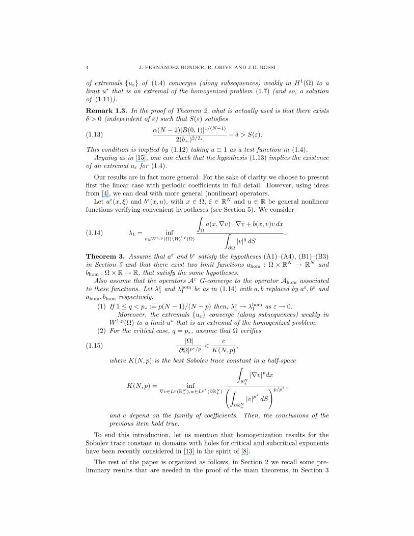
Remark 1.3. In the proof of Theorem 2, what is actually used is that there existsδ > 0 (independent of ε) such that S(ε) satisfies

(1.13)α(N − 2)|B(0, 1)|1/(N−1)

2(b+)2/2∗− δ > S(ε).

This condition is implied by (1.12) taking u ≡ 1 as a test function in (1.4).Arguing as in [15], one can check that the hypothesis (1.13) implies the existence

of an extremal uε for (1.4).

Our results are in fact more general. For the sake of clarity we choose to presentfirst the linear case with periodic coefficients in full detail. However, using ideasfrom [4], we can deal with more general (nonlinear) operators.

Let aε(x, ξ) and bε(x, u), with x ∈ Ω, ξ ∈ RN and u ∈ R be general nonlinearfunctions verifying convenient hypotheses (see Section 5). We consider

(1.14) λ1 = infv∈W 1,p(Ω)\W 1,p

0 (Ω)

∫Ω

a(x,∇v) · ∇v + b(x, v)v dx∫∂Ω

|v|q dS

.

Theorem 3. Assume that aε and bε satisfy the hypotheses (A1)–(A4), (B1)–(B3)in Section 5 and that there exist two limit functions ahom : Ω × RN → RN andbhom : Ω× R → R, that satisfy the same hypotheses.

Also assume that the operators Aε G-converge to the operator Ahom associatedto these functions. Let λε

1 and λhom1 be as in (1.14) with a, b replaced by aε, bε and

ahom, bhom respectively.(1) If 1 ≤ q < p∗ := p(N − 1)/(N − p) then, λε

1 → λhom1 as ε → 0.

Moreover, the extremals uε converge (along subsequences) weakly inW 1,p(Ω) to a limit u∗ that is an extremal of the homogenized problem.

(2) For the critical case, q = p∗, assume that Ω verifies

(1.15)|Ω|

|∂Ω|p∗/p<

c

K(N, p),

where K(N, p) is the best Sobolev trace constant in a half-space

K(N, p) = inf∇v∈Lp(RN

+ ),w∈Lp∗ (∂RN+ )

∫RN

+

|∇v|pdx(∫∂RN

+

|v|p∗dS

)p/p∗,

and c depend on the family of coefficients. Then, the conclusions of theprevious item hold true.

To end this introduction, let us mention that homogenization results for theSobolev trace constant in domains with holes for critical and subcritical exponentshave been recently considered in [13] in the spirit of [8].

The rest of the paper is organized as follows, in Section 2 we recall some pre-liminary results that are needed in the proof of the main theorems, in Section 3

SOBOLEV TRACE CONSTANT 5

we deal with the subcritical case (Theorem 1), in Section 4 with the critical case(Theorem 2) and, finally, in Section 5 we prove the extension for the nonlinear case(Theorem 3).

2. Preliminaries

In this subsection we present some results and techniques in homogenization ofperiodic media. We briefly recall the notion of two-scale convergence (see [2], [19]).

Proposition 2.1. Let Ω ⊆ RN and wε be a bounded sequence in L2(Ω) . Thereexist a subsequence, still denoted by ε, and a limit w(x, y) ∈ L2(Ω;L2

#(T)) suchthat wε two-scale converges to w in the sense that

limε→0

∫Ω

wε(x)φ(x, x/ε) dx =∫

Ω

∫T

w(x, y)φ(x, y) dxdy

for every function φ(x, y) ∈ L2(Ω; C#(T)). The two-scale convergence is denoted bywε w in 2s. Furthermore, if wε is a bounded sequence that converges weakly toa limit w in H1(Ω). Then, wε two-scale converges to w, and there exists a functionw1(x, y) ∈ L2(Ω;H1

#(T)) such that, up to a subsequence, we have the followingtwo-scale convergence

∇wε(x) ∇xw(x) +∇yw1(x, y) in 2-scale.

This two-scale convergence result is a powerful tool to deal with our problem,the study of the limit as ε → 0 in (1.4).

Another important tool is the weak star convergence in L∞(Ω). In general, ifgε, g ∈ L∞(Ω), we say that gε converges to g weak star in L∞(Ω), denoted bygε

∗ g in L∞(Ω), if ∫

Ω

gεφdx →∫

Ω

gφ dx, ∀φ ∈ L1(Ω).

We note immediately, see [8], that an εT-periodic function converges weak−∗ inL∞ to its mean value. Thus

aε0∗ a∗0 in L∞(Ω).

Moreover, if Ω is a generic domain, i.e. ∂Ω does not contain flat pieces or that itcontains finitely many flat pieces with conormal not proportional to any m ∈ ZN ,we have that

(2.1) bε ∗ b∗ in L∞(∂Ω),

where b∗ is given by (1.8), see Remark 1.1.

3. Subcritical case

In this section we assume that q is subcritical, that is 1 ≤ q < 2∗, so theimmersion H1(Ω) → Lq(∂Ω) is compact.

Proof of Theorem 1. First, let us prove that the best constants S(ε) and theextremals uε are bounded in H1 independently of ε. Indeed, by the definition ofS(ε) in (1.4) and our assumptions on the coefficients (1.1), (1.2), there exist twoconstants 0 < c < C such that

(3.1) c λ0 ≤ S(ε) ≤ C λ0,

6 J. FERNANDEZ BONDER, R. ORIVE AND J.D. ROSSI

with λ0 defined by

(3.2) λ0 = infv∈H1(Ω)\H1

0 (Ω)

∫Ω

|∇v|2 + v2 dx(∫∂Ω

|v|q dS

)2/q.

Now, we show that the extremals uε, the weak solutions of (1.6), are boundedin H1−norm independently of ε. To prove this fact recall that we have normalizedthe extremals by (1.5). By our assumptions on the coefficients (1.1), (1.2), we have

S(ε) =∫

Ω

(aε

ij

∂uε

∂xj

∂uε

∂xi+ aε

0|uε|2)

dx ≥∫

Ω

(α|∇uε|2 + a−|uε|2

)dx.

By (3.1), we obtain that uε is bounded in H1 independently of ε. Hence thereexists a subsequence (that we still call uε) and a function u0 ∈ H1(Ω) such thatuε u0 weakly in H1(Ω) and uε → u0 strongly in Lq(∂Ω) for 1 ≤ q < 2∗. By theabove mentioned convergence and (2.1) we have that∫

∂Ω

b∗|u0|q dS = 1.

Moreover, using Proposition 2.1, we obtain that uε u0 in 2-scale and there existsu1 such that

∇uε ∇xu0(x) +∇yu1(x, y), in 2-scale.

We use φ(x) + εφ1(x, x/ε) with φ ∈ H1(Ω) and φ1 ∈ H1(Ω;C#(T)) as a testfunction in the weak form of (1.6). As S(ε) is bounded, we can assume thatS(ε) → S0, for an appropriate subsequence. Then we pass to the limit the weakformulation and, by the two-scale convergence, we get∫

Ω

∫T

aij(y)(

∂u0

∂xj(x) +

∂u1

∂yj(x, y)

)(∂φ

∂xi(x) +

∂φ1

∂yi(x, y)

)dy dx

+∫

Ω

∫T

a0(y)u0(x)φ(x)dx dy = S0

∫∂Ω

∫T

b(y)|u0|q−2u0φ(x) dS dy.

Integrating by parts we obtain that (u0, u1) is the weak solution of the system

∂

∂xi

(∫T

aij(y)(

∂u0

∂xj(x) +

∂u1

∂yj(x, y)

)dy

)= a∗0 u0(x) in Ω,(3.3)

νi∂

∂xi

(∫T

aij(y)(

∂u∗

∂xj(x) +

∂u1

∂yj(x, y)

)dy

)= S0 b∗ |u0|q−2u0(x) on ∂Ω,(3.4)

∂

∂yi

(aij(y)

(∂u0

∂xi(x) +

∂u1

∂yi(x, y)

))= 0 in Ω× T,(3.5)

with a∗0 and b∗ defined in (1.8). Considering

u1(x, y) =N∑

i=1

∂u0

∂xi(x)χi(y),

SOBOLEV TRACE CONSTANT 7

we note that u1 satisfies (3.5) for any u0 since χ1 is solution of (1.10). Moreover,with this function u1 in (3.3) and (3.4), we obtain that u0 is a solution of

(3.6)

∂

∂xi

(a∗ij

∂u0

∂xj

)= a∗0u0 in Ω,

∂u0

∂ν∗= S0b

∗|u0|q−2u0 on ∂Ω,

where the coefficients a∗ij are given by (1.9) and the derivative normal ∂/∂ν∗ isdefined in (1.11). Now, since S0 satisfies (3.6), we get S0 ≥ S∗ with S∗ defined in(1.7). To conclude the proof of Theorem 1 we need to show that S0 = S∗. In fact,let u∗ be an extremal of (1.7) and consider

vε = u∗ + εχεk

∂u∗

∂xk

as a test function in (1.4), where χεk(x) = χk(x/ε). From the maximum principle

and Hopf’s Lemma we get that u∗ is strictly positive in Ω. Therefore the regularityresults of [6] are applicable and we obtain that u∗ ∈ C∞(Ω). Thus, since thefunctions χk ∈ W 1,∞ (this is a consequence of the hypotheses on the coefficients),we have immediately vε u∗ weakly in H1(Ω) and vε → u∗ strongly in Lq(∂Ω)for 1 ≤ q < 2∗. Now, we obtain∫

Ω

(aε

ij

∂vε

∂xj

∂vε

∂xi+ aε

0v2ε

)dx =

∫Ω

(aε

ij + aεik

∂χεj

∂yk

)∂u∗

∂xj

∂u∗

∂xidx

+∫

Ω

(aε

ij

∂χεk

∂yj

∂χε`

∂yi+ aε

ik

∂χε`

∂yi

)∂u∗

∂xk

∂u∗

∂x`dx

+∫

Ω

aε0(u

∗)2dx + O(ε).

Passing to the limit, using that χk is a solution of (1.10) and by the weak−∗convergence in L∞, we get

limε→0

∫Ω

(aε

ij

∂vε

∂xj

∂vε

∂xi+ aε

0v2ε

)dx =

∫Ω

(a∗ij

∂u∗

∂xj

∂u∗

∂xi+ a∗0(u

∗)2)

dx,

where a∗0 and a∗ij are defined by (1.8) and (1.9), respectively. Moreover, again bythe weak−∗ convergence in L∞, we have∫

∂Ω

bε|vε|q →∫

∂Ω

b∗|u∗|q.

Therefore, passing to the limit in (1.4) with test function vε, we prove S0 ≤ S∗ andwe conclude the proof of Theorem 1.

Remark 3.1. Results on correctors of the extremals are easily obtained with thetwo scale convergence method. Considering the solutions of the cell problem (1.10),the corrector term is defined by

uε1(x) = χk(x/ε)

∂u∗

∂xk(x),

where u∗ is an extremal of the homogenized problem (1.11). Hence, by Proposi-tion 2.1 and following the same lines as [2], (uε − u∗ − εuε

1) converges strongly tozero in H1(Ω).

8 J. FERNANDEZ BONDER, R. ORIVE AND J.D. ROSSI

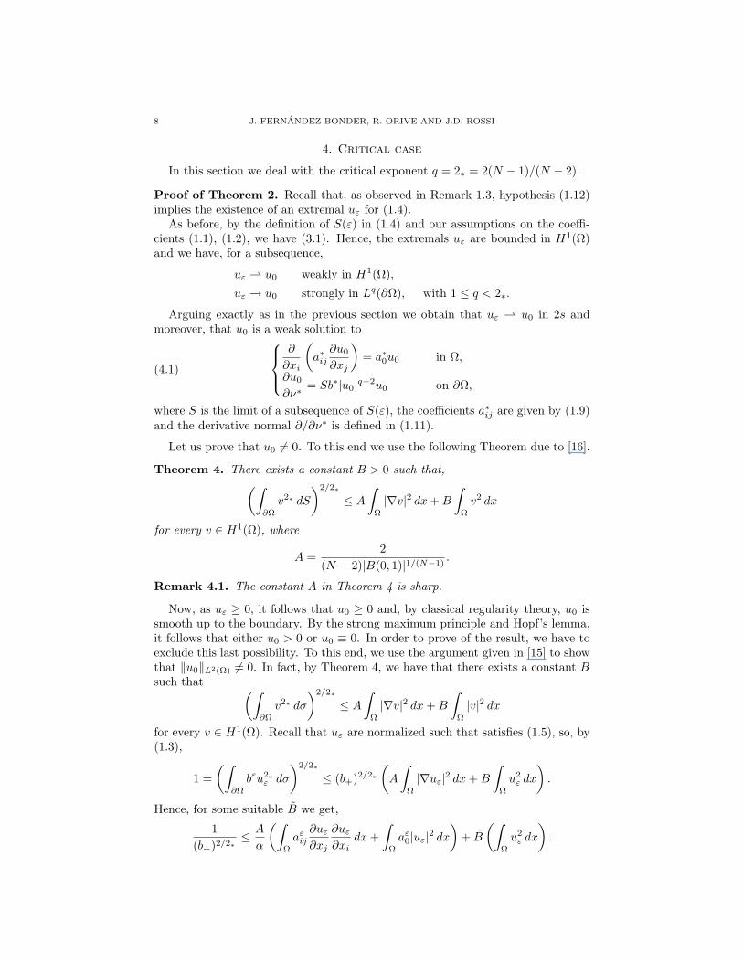
4. Critical case

In this section we deal with the critical exponent q = 2∗ = 2(N − 1)/(N − 2).

Proof of Theorem 2. Recall that, as observed in Remark 1.3, hypothesis (1.12)implies the existence of an extremal uε for (1.4).

As before, by the definition of S(ε) in (1.4) and our assumptions on the coeffi-cients (1.1), (1.2), we have (3.1). Hence, the extremals uε are bounded in H1(Ω)and we have, for a subsequence,

uε u0 weakly in H1(Ω),

uε → u0 strongly in Lq(∂Ω), with 1 ≤ q < 2∗.

Arguing exactly as in the previous section we obtain that uε u0 in 2s andmoreover, that u0 is a weak solution to

(4.1)

∂

∂xi

(a∗ij

∂u0

∂xj

)= a∗0u0 in Ω,

∂u0

∂ν∗= Sb∗|u0|q−2u0 on ∂Ω,

where S is the limit of a subsequence of S(ε), the coefficients a∗ij are given by (1.9)and the derivative normal ∂/∂ν∗ is defined in (1.11).

Let us prove that u0 6= 0. To this end we use the following Theorem due to [16].

Theorem 4. There exists a constant B > 0 such that,(∫∂Ω

v2∗ dS

)2/2∗

≤ A

∫Ω

|∇v|2 dx + B

∫Ω

v2 dx

for every v ∈ H1(Ω), where

A =2

(N − 2)|B(0, 1)|1/(N−1).

Remark 4.1. The constant A in Theorem 4 is sharp.

Now, as uε ≥ 0, it follows that u0 ≥ 0 and, by classical regularity theory, u0 issmooth up to the boundary. By the strong maximum principle and Hopf’s lemma,it follows that either u0 > 0 or u0 ≡ 0. In order to prove of the result, we have toexclude this last possibility. To this end, we use the argument given in [15] to showthat ‖u0‖L2(Ω) 6= 0. In fact, by Theorem 4, we have that there exists a constant Bsuch that (∫

∂Ω

v2∗ dσ

)2/2∗

≤ A

∫Ω

|∇v|2 dx + B

∫Ω

|v|2 dx

for every v ∈ H1(Ω). Recall that uε are normalized such that satisfies (1.5), so, by(1.3),

1 =(∫

∂Ω

bεu2∗ε dσ

)2/2∗

≤ (b+)2/2∗

(A

∫Ω

|∇uε|2 dx + B

∫Ω

u2ε dx

).

Hence, for some suitable B we get,

1(b+)2/2∗

≤ A

α

(∫Ω

aεij

∂uε

∂xj

∂uε

∂xidx +

∫Ω

aε0|uε|2 dx

)+ B

(∫Ω

u2ε dx

).

SOBOLEV TRACE CONSTANT 9

Therefore,

(4.2)1

(b+)2/2∗≤ A

αS(ε) + B

∫Ω

|uε|2 dx

Passing to the limit ε → 0 in (4.2) we arrive to

1(b+)2/2∗

≤ A

αS + B

∫Ω

|u0|2 dx

therefore, as we have assumed (1.13), that impliesα

A(b+)2/2∗> S,

we conclude u0 6= 0.Now, multiplying (4.1) by u0 and integrating by parts, we obtain∫

Ω

a∗ij∂u0

∂xj

∂u0

∂xi+ a∗0u

20 dx = S

∫∂Ω

u2∗0 dS.

As u0 6= 0 it follows that S 6= 0 and ‖u0‖L2∗ (∂Ω) 6= 0. Therefore, we conclude that

S0 ≤

∫Ω

a∗ij∂u0

∂xj

∂u0

∂xi+ a∗0u

20 dx(∫

∂Ω

u2∗0 dS

)2/2∗= S

(∫∂Ω

u2∗0 dS

)1/(N−1)

≤ S.

Now, arguing exactly as in the end of Section 3, we conclude the desired result.

5. The nonlinear case

Finally, in this section we consider the extension of our previous results to a moregeneral class of nonlinear operators, including the p−Laplacian with oscillatingcoefficients. The main ideas for these extensions are similar to the ones used beforecombined with those of [4].

We consider nonlinear monotone operators A : W 1,p(Ω) → (W 1,p(Ω))∗ of theform

Au = − div(a(x,∇u)) + b(x, u),

whose coefficients a : Ω× RN → RN belong to the class of functions satisfying thefollowing hypotheses:

(A1) a(·, ·) is of Caratheodory type.(A2) Monotonicity: 0 ≤ (a(x, ξ1)− a(x, ξ2)) · (ξ1 − ξ2) ∀ξ1, ξ2, a.e. x.(A3) Uniform ellipticity: α|ξ|p ≤ a(x, ξ) · ξ ∀ξ, a.e. x.(A4) Growth: |a(x, ξ)| ≤ β|ξ|p−1 ∀ξ, a.e. x.

and the function b : Ω× R → R satisfies the following hypotheses(B1) b(·, ·) is of Caratheodory type.(B2) Uniform α|u|p ≤ b(x, u)u ∀u, a.e. x.(B3) Growth: |b(x, u)| ≤ β|u|p−1 ∀u, a.e. x.For a and b satisfying the above hypotheses, we consider the eigenvalue problem

(5.1)div(a(x,∇u)) = b(x, u) in Ω,

a(x,∇u) · ν = λ|u|q−2u on ∂Ω.

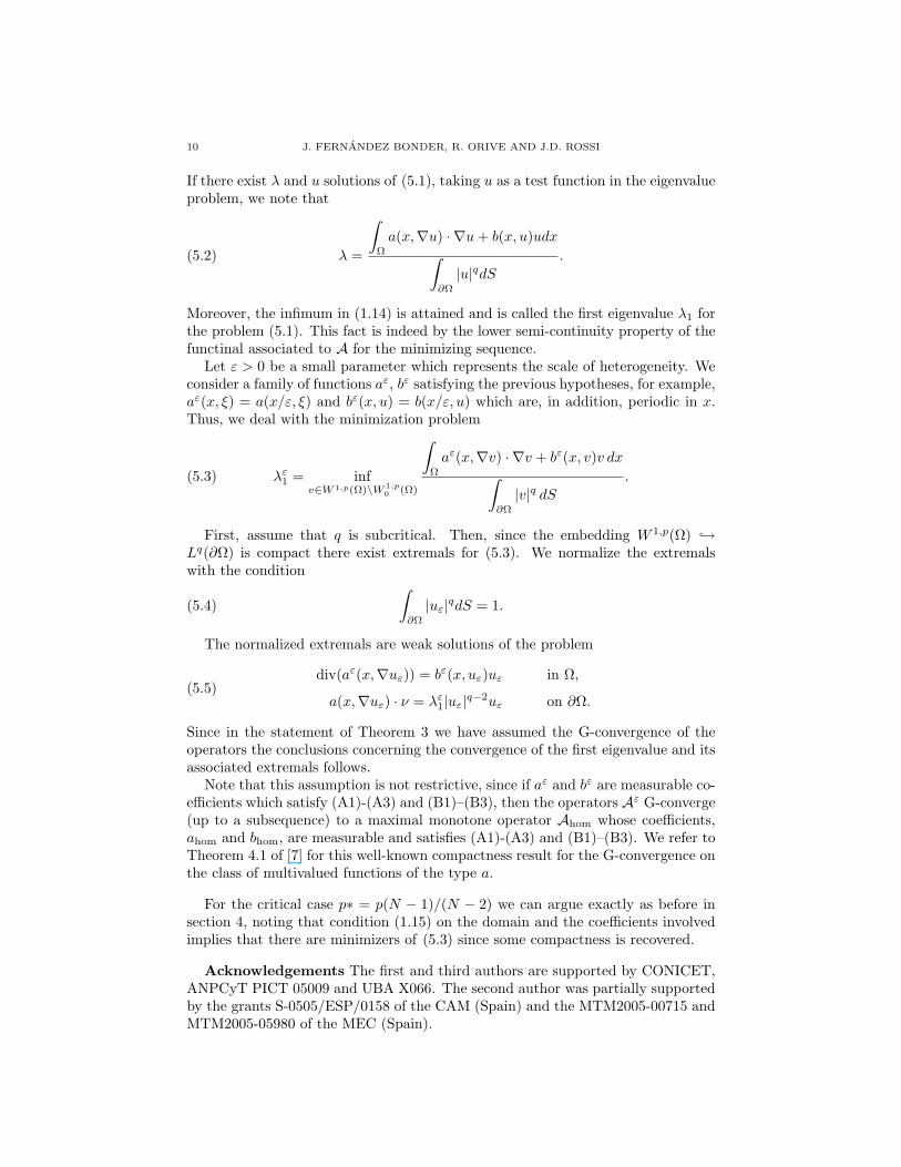
10 J. FERNANDEZ BONDER, R. ORIVE AND J.D. ROSSI

If there exist λ and u solutions of (5.1), taking u as a test function in the eigenvalueproblem, we note that

(5.2) λ =

∫Ω

a(x,∇u) · ∇u + b(x, u)udx∫∂Ω

|u|qdS

.

Moreover, the infimum in (1.14) is attained and is called the first eigenvalue λ1 forthe problem (5.1). This fact is indeed by the lower semi-continuity property of thefunctinal associated to A for the minimizing sequence.

Let ε > 0 be a small parameter which represents the scale of heterogeneity. Weconsider a family of functions aε, bε satisfying the previous hypotheses, for example,aε(x, ξ) = a(x/ε, ξ) and bε(x, u) = b(x/ε, u) which are, in addition, periodic in x.Thus, we deal with the minimization problem

(5.3) λε1 = inf

v∈W 1,p(Ω)\W 1,p0 (Ω)

∫Ω

aε(x,∇v) · ∇v + bε(x, v)v dx∫∂Ω

|v|q dS

.

First, assume that q is subcritical. Then, since the embedding W 1,p(Ω) →Lq(∂Ω) is compact there exist extremals for (5.3). We normalize the extremalswith the condition

(5.4)∫

∂Ω

|uε|qdS = 1.

The normalized extremals are weak solutions of the problem

(5.5)div(aε(x,∇uε)) = bε(x, uε)uε in Ω,

a(x,∇uε) · ν = λε1|uε|q−2uε on ∂Ω.

Since in the statement of Theorem 3 we have assumed the G-convergence of theoperators the conclusions concerning the convergence of the first eigenvalue and itsassociated extremals follows.

Note that this assumption is not restrictive, since if aε and bε are measurable co-efficients which satisfy (A1)-(A3) and (B1)–(B3), then the operators Aε G-converge(up to a subsequence) to a maximal monotone operator Ahom whose coefficients,ahom and bhom, are measurable and satisfies (A1)-(A3) and (B1)–(B3). We refer toTheorem 4.1 of [7] for this well-known compactness result for the G-convergence onthe class of multivalued functions of the type a.

For the critical case p∗ = p(N − 1)/(N − 2) we can argue exactly as before insection 4, noting that condition (1.15) on the domain and the coefficients involvedimplies that there are minimizers of (5.3) since some compactness is recovered.

Acknowledgements The first and third authors are supported by CONICET,ANPCyT PICT 05009 and UBA X066. The second author was partially supportedby the grants S-0505/ESP/0158 of the CAM (Spain) and the MTM2005-00715 andMTM2005-05980 of the MEC (Spain).

SOBOLEV TRACE CONSTANT 11

References

[1] Adimurthi, S.L. Yadava. Positive solution for Neumann problem with critical non linearityon boundary. Comm. Partial Differential Equations, 16 (11) (1991), 1733–1760.

[2] G. Allaire. Homogenization and two-scale convergence. SIAM J. Math. Anal., 23, (1992),

1482–1518.[3] T. Aubin. Equations differentielles non lineaires et le probleme de Yamabe concernant la

courbure scalaire. J. Math. Pures et Appl., 55 (1976), 269–296.

[4] L. Baffico, C. Conca, M. Rajesh. Homogenization of a class of nonlinear eigenvalue prob-lems. Proc. of the Royal Society of Edinburgh, 136A, 722, 2006

[5] A. Bensoussan, J. L. Lions and G. Papanicolaou. Asymptotic Analysis for Periodic Struc-tures. North-Holland, Amsterdam, 1978.

[6] P. Cherrier, Problemes de Neumann non lineaires sur les varietes Riemanniennes. J. Funct.

Anal. Vol. 57 (1984), 154-206.[7] V. Chiado Piat, G. Dal Maso and A. Defranceschi. G-convergence of monotone operators.

Annls Inst. H. Poincare 7 (1990), 123-160.

[8] D. Cioranescu and F. Murat. A Strange Term Coming from Nowhere, in Topics in the Math-ematical Modelling of Composite Materials, A. Cherkaev et. al. eds., Progress in Nonlinear

Differential Equations and Their Applications, 31, Birkhauser, Boston, (1997), 45–93.

[9] G. Dal Maso. An introduction to Γ-convergence. Progress in Nonlinear Differential Equationsand their Applications, 8. Birkhauser Boston, Inc., Boston, MA, 1993.

[10] O. Druet and E. Hebey. The AB program in geometric analysis: sharp Sobolev inequalities

and related problems. Mem. Amer. Math. Soc. 160 (761) (2002).[11] J. F. Escobar. Sharp constant in a Sobolev trace inequality. Indiana Math. J., 37 (3) (1988),

687–698.[12] J. Fernandez Bonder, E. Lami Dozo and J.D. Rossi. Symmetry properties for the extremals

of the Sobolev trace embedding. Ann. Inst. H. Poincare. Anal. Non Lineaire, 21 (2004), no.

6, 795–805.[13] J. Fernandez Bonder, R. Orive and J.D. Rossi. The best Sobolev trace constant in domains

with holes for critical or subcritical exponents. Submitted.

[14] J. Fernandez Bonder and J.D. Rossi. Asymptotic behavior of the best Sobolev trace constantin expanding and contracting domains. Comm. Pure Appl. Anal., 1 (3) (2002), 359–378.

[15] J. Fernandez Bonder and J.D. Rossi. On the existence of extremals for the Sobolev trace

embedding theorem with critical exponent. Bull. London Math. Soc., 37 (2005), no. 1, 119–125.

[16] Y. Li and M. Zhu. Sharp Sobolev trace inequalities on Riemannian manifolds with bound-

aries. Comm. Pure Appl. Math., 50 (1997), 449–487.[17] J.-L. Lions. Some methods in the mathematical analysis of systems and their control. Kexue

Chubanshe (Science Press), Beijing; Gordon & Breach Science Publishers, New York, 1981.

[18] F. Murat and L. Tartar, H-convergence, in Topics in the Mathematical Modelling of Com-posite Materials, A. Cherkaev et. al. eds., Progress in Nonlinear Differential Equations and

Their Applications, 31, Birkhauser, Boston, (1997), 21–43.[19] G. Nguetseng. A general convergence result for a functional related to the theory of homoge-

nization. SIAM J. Math. Anal., 20, (1989), 608–623.[20] M. W. Steklov, Sur les problemes fondamentaux en physique mathematique, Ann. Sci. Ecole

Norm. Sup., Vol. 19 (1902), 455–490.

Julian Fernandez Bonder and Julio D. Rossi

Departamento de Matematica, FCEyN, Universidad de Buenos Aires,Pabellon I, Ciudad Universitaria (1428), Buenos Aires, Argentina.E-mail address: (JFB) jfbonder@dm.uba.ar, (JDR) jrossi@dm.uba.ar

Web page: http://mate.dm.uba.ar/∼jfbonder, http://mate.dm.uba.ar/∼jrossi

Rafael Orive

Departamento de Matematicas

Universidad Autonoma de MadridCrta. Colmenar Viejo km. 15, 28049 Madrid, Spain.

E-mail address: rafael.orive@uam.es

Web page: http://www.uam.es/rafael.orive