The Analysis of Functional Brain Images - Wellcome Centre ...
664
-
Upload
khangminh22 -
Category
Documents
-
view
0 -
download
0
Transcript of The Analysis of Functional Brain Images - Wellcome Centre ...


Contents
INTRODUCTION
A short history of SPM.
Statistical parametric mapping.
Modelling brain responses.
SECTION 1: COMPUTATIONAL ANATOMY
Rigid-body Registration.
Nonlinear Registration.
Segmentation.
Voxel-based Morphometry.
SECTION 2: GENERAL LINEAR MODELS
`The General Linear Model.
Contrasts & Classical Inference.
Covariance Components.
Hierarchical models.
Random Effects Analysis.
Analysis of variance.
Convolution models for fMRI.
Efficient Experimental Design for fMRI.
Hierarchical models for EEG/MEG.
SECTION 3: CLASSICAL INFERENCE
Parametric procedures for imaging.
Random Field Theory & inference.
Topological Inference.
False discovery rate procedures.
Non-parametric procedures.
SECTION 4: BAYESIAN INFERENCE
Empirical Bayes & hierarchical models.
Posterior probability maps.
Variational Bayes.
Spatiotemporal models for fMRI.
Spatiotemporal models for EEG.
SECTION 5: BIOPHYSICAL MODELS
Forward models for fMRI.
Forward models for EEG and MEG.
Bayesian inversion of EEG models.
Bayesian inversion for induced responses.
Neuronal models of ensemble dynamics.
Neuronal models of energetics.
Neuronal models of EEG and MEG.
Bayesian inversion of dynamic models
Bayesian model selection & averaging.

SECTION 6: CONNECTIVITY
Functional integration.
Functional Connectivity.
Effective Connectivity.
Nonlinear coupling and Kernels.
Multivariate autoregressive models.
Dynamic Causal Models for fMRI.
Dynamic Causal Models for EEG.
Dynamic Causal Models & Bayesian selection.
APPENDICES
Linear models and inference.
Dynamical systems.
Expectation maximisation.
Variational Bayes under the Laplace approximation.
Kalman Filtering.
Random Field Theory.

About
STATISTICAL PARAMETRIC MAPPING: THE ANALYSIS OF FUNCTIONAL
BRAIN IMAGES
Edited By
Karl Friston, Functional Imaging Laboratory, Wellcome Department of Imaging
Neuroscience, University College London, London, UK
John Ashburner, Functional Imaging Laboratory, Wellcome Department of Imaging
Neuroscience, University College London, London, UK
Stefan Kiebel
Thomas Nichols
William Penny, Functional Imaging Laboratory, Wellcome Department of Imaging
Neuroscience, University College London, London, UK
Description
In an age where the amount of data collected from brain imaging is increasing
constantly, it is of critical importance to analyse those data within an accepted
framework to ensure proper integration and comparison of the information collected.
This book describes the ideas and procedures that underlie the analysis of signals
produced by the brain. The aim is to understand how the brain works, in terms of its
functional architecture and dynamics. This book provides the background and
methodology for the analysis of all types of brain imaging data, from functional
magnetic resonance imaging to magnetoencephalography. Critically, Statistical
Parametric Mapping provides a widely accepted conceptual framework which allows
treatment of all these different modalities. This rests on an understanding of the
brain's functional anatomy and the way that measured signals are caused
experimentally. The book takes the reader from the basic concepts underlying the
analysis of neuroimaging data to cutting edge approaches that would be difficult to
find in any other source. Critically, the material is presented in an incremental way so
that the reader can understand the precedents for each new development. This book
will be particularly useful to neuroscientists engaged in any form of brain mapping;
who have to contend with the real-world problems of data analysis and understanding
the techniques they are using. It is primarily a scientific treatment and a didactic
introduction to the analysis of brain imaging data. It can be used as both a textbook
for students and scientists starting to use the techniques, as well as a reference for
practicing neuroscientists. The book also serves as a companion to the software
packages that have been developed for brain imaging data analysis.
Audience
Scientists actively involved in neuroimaging research and the analysis of data, as well
as students at a masters and doctoral level studying cognitive neuroscience and brain
imaging.
Bibliographic Information
Hardbound, 656 pages, publication date: NOV-2006
ISBN-13: 978-0-12-372560-8
ISBN-10: 0-12-372560-7
Imprint: ACADEMIC PRESS

Elsevier UK Chapter: Prelims-P372560 30-9-2006 5:36p.m. Page:vii Trim:7.5in×9.25in
Basal Font:Palatino Margins:Top:40pt Gutter:68pt Font Size:9.5/12 Text Width:42pc Depth:55 Lines
Acknowledgements
This book was written on behalf of the SPM co-authors, who at the time of writing, include:
Jesper Andersson
John Ashburner
Nelson Trujillo-Barreto
Matthew Brett
Christian Büchel
Olivier David
Guillaume Flandin
Karl Friston
Darren Gitelman
Daniel Glaser
Volkmar Glauche
Lee Harrison
Rik Henson
Andrew Holmes
Stefan Kiebel
James Kilner
Járámie Mattout
Tom Nichols
Will Penny
Christophe Phillips
Jean-Baptise Poline
Klaas Stephan
We are also deeply indebted to many colleagues who have developed imaging methodology with us over the years.Though there are too many to name individually we would especially like to thank Keith Worsley and colleagues atMcGill. We are also very grateful to the many imaging neuroscientists who have alpha-tested implementations of ourmethodology and the many researchers who regularly make expert contributions to the SPM email list. We wouldespecially like to thank Jenny Crinion, Alex Hammers, Bas Neggers, Uta Noppeney, Helmut Laufs, Torben Lund, Marta Garrido,Christian Gaser, Marcus Gray, Andrea Mechelli, James Rowe, Karsten Specht, Marco Wilke, Alle Meije Wink and Eric Zarahn.
Finally, any endeavour of this kind is not possible without the patience and support of our families and loved ones,to whom we dedicate this book.
vii

Elsevier UK Chapter: Ch01-P372560 3-10-2006 3:01p.m. Page:3 Trim:7.5in×9.25in
Basal Font:Palatino Margins:Top:40pt Gutter:68pt Font Size:9.5/12 Text Width:42pc Depth:55 Lines
C H A P T E R
1
A short history of SPMK. Friston
INTRODUCTION
For a young person entering imaging neuroscience itmust seem that the field is very large and complicated,with numerous approaches to experimental design andanalysis. This impression is probably compounded by theabundance of TLAs (three-letter-acronyms) and obscureterminology. In fact, most of the principles behind designand analysis are quite simple and had to be establishedin a relatively short period of time at the inception ofbrain mapping. This chapter presents an anecdotal per-spective on this period. It serves to explain why someideas, like t-maps or, more technically, statistical para-metric maps, were introduced and why other issues, likeglobal normalization, were crucial, even if they are notso important nowadays.
The history of human brain mapping is probablyshorter than many people might think. Activation stud-ies depend on imaging changes in brain state within thesame scanning session. This was made possible usingshort-half-life radiotracers and positron emission tomog-raphy (PET). These techniques became available in theeighties (e.g. Herscovitch et al., 1983) and the first activa-tion maps appeared soon after (e.g. Lauter et al., 1985; Foxet al., 1986). Up until this time, regional differences amongbrain scans had been characterized using hand-drawnregions of interest (ROI), reducing hundreds of thou-sands of voxels to a handful of ROI measurements, witha somewhat imprecise anatomical validity. The idea ofmaking voxel-specific statistical inferences, through theuse of statistical parametric maps, emerged in response tothe clear need to make inferences about brain responseswithout knowing where those responses were going tobe expressed. The first t-map was used to establish func-tional specialization for colour processing in 1989 (Luecket al., 1989). The underlying methodology was describedin a paper entitled: ‘The relationship between global andlocal changes in PET scans’ (Friston et al., 1990). This
may seem an odd title to introduce statistical parametricmapping (SPM) but it belies a key motivation behind theapproach.
Statistical maps versus regions of interest
Until that time, images were usually analysed withanalysis of variance (ANOVA) using ROI averages.This approach had become established in the analy-sis of autoradiographic data in basic neuroscience andmetabolic scans in human subjects. Critically, each regionwas treated as a level of a factor. This meant that theregional specificity of a particular treatment was encodedin the region by treatment interaction. In other words,a main effect of treatment per se was not sufficient toinfer a regionally specific response. This is because sometreatments induced a global effect that was expressed inall the ROIs. Global effects were, therefore, one of thefirst major conceptual issues in the development of SPM.The approach taken was to treat global activity as a con-found in a separate analysis of covariance (ANCOVA)at each voxel, thereby endowing inference with a regionalspecificity that could not be explained by global changes.The resulting SPMs were like X-rays of region-specificchanges and, like X-rays, are still reported in maximum-intensity projection format (known colloquially as glass-brains). The issue of regional versus global changes andthe validity of global estimators were debated for severalyears, with many publications in the specialist literature.Interestingly, it is a theme that enjoyed a reprise with theadvent of functional magnetic resonance imaging (fMRI)(e.g. Aguirre et al., 1998) and still attracts some researchinterest today.
Adopting a voxel-wise ANCOVA model paved theway for a divergence between the mass-univariateapproach used by SPM (i.e. a statistic for each voxel)and multivariate models used previously. A subtle but
Statistical Parametric Mapping, by Karl Friston et al. Copyright 2007, Elsevier Ltd. All rights reserved.ISBN–13: 978-0-12-372560-8 ISBN–10: 0-12-372560-7
3

Elsevier UK Chapter: Ch01-P372560 3-10-2006 3:01p.m. Page:4 Trim:7.5in×9.25in
Basal Font:Palatino Margins:Top:40pt Gutter:68pt Font Size:9.5/12 Text Width:42pc Depth:55 Lines
4 1. A SHORT HISTORY OF SPM
important motivation for mass-univariate approacheswas the fact that a measured haemodynamic responsein one part of the brain may differ from the responsein another, even if the underlying neuronal activation wasexactly the same. This meant that the convention of usingregion-by-condition interactions as a test for regionallyspecific effects was not tenable. In other words, evenif one showed that two regions activated differently interms of measured haemodynamics, this did not meanthere was a regionally specific difference at the neuronalor computational level. This issue seems to have escapedthe electroencephalography (EEG) community, who stilluse ANOVA with region as a factor, despite the fact thatthe link between neuronal responses and channel mea-surements is even more indeterminate than for metabolicimaging. However, the move to voxel-wise, whole-brainanalysis entailed two special problems: the problem ofregistering images from different subjects so that theycould be compared on a voxel-by-voxel basis and themultiple-comparisons problem that ensued.
Spatial normalization
The pioneering work of the St Louis group had alreadyestablished the notion of a common anatomical or stereo-tactic space (Fox et al., 1988) in which to place subtractionor difference maps, using skull X-rays as a reference. Theissue was how to get images into that space efficiently.Initially, we tried identifying landmarks in the functionaldata themselves to drive the registration (Friston et al.,1989). This approach was dropped almost immediatelybecause it relied on landmark identification and was not ahundred per cent reproducible. Within a year, a more reli-able, if less accurate, solution was devised that matchedimages to a template without the need for landmarks(Friston et al., 1991a). The techniques for spatial normal-ization using template- or model-based approaches havedeveloped consistently since that time and current treat-ments regard normalization as the inversion of genera-tive models for anatomical variation that involve warp-ing templates to produce subject-specific images (e.g.Ashburner and Friston, 2005).
Topological inference
Clearly, performing a statistical test at each voxel engen-dered an enormous false positive rate when using unad-justed thresholds to declare activations significant. Theproblem was further compounded by the fact that thedata were not spatially independent and a simple Bonfer-roni correction was inappropriate (PET and SPECT (sin-gle photon emission computerized tomography) data are
inherently very smooth and fMRI had not been inventedat this stage). This was the second major theme that occu-pied people trying to characterize functional neuroimag-ing data. What was needed was a way of predicting theprobabilistic behaviour of SPMs, under the null hypothe-sis of no activation, which accounted for the smoothnessor spatial correlations among voxels. From practical expe-rience, it was obvious that controlling the false positiverate of voxels was not the answer. One could increasethe number of positive voxels by simply making the vox-els smaller but without changing the topology of theSPM. It became evident that conventional control proce-dures developed for controlling family-wise error (e.g.the Bonferroni correction) had no role in making infer-ences on continuous images. What was needed was a newframework in which one could control the false positiverate of the regional effects themselves, noting a regionaleffect is a topological feature, not a voxel.
The search for a framework for topological infer-ence in neuroimaging started in the theory of stochas-tic processes and level-crossings (Friston et al., 1991b).It quickly transpired that the resulting heuristics werethe same as established results from the theory of ran-dom fields. Random fields are stochastic processes thatconform very nicely to realizations of brain scans undernormal situations. Within months, the technology to cor-rect p-values was defined within random field theory(Worsley et al., 1992). Although the basic principles oftopological inference were established at this time, therewere further exciting mathematical developments withextensions to different sorts of SPMs and the ability toadjust the p-values for small bounded volumes of inter-est (see Worsley et al., 1996). Robert Adler, one of theworld’s contemporary experts in random field theory,who had abandoned it years before, was understandablyvery pleased and is currently writing a book with a pro-tégé of Keith Worsley (Adler and Taylor, in preparation).
Statistical parametric mapping
The name ‘statistical parametric mapping’ was chosencarefully for a number of reasons. First, it acknowledgedthe TLA of ‘significance probability mapping’, devel-oped for EEG. Significance probability mapping involvedcreating interpolated pseudo-maps of p-values to dis-close the spatiotemporal organization of evoked electricalresponses (Duffy et al., 1981). The second reason wasmore colloquial. In PET, many images are derived fromthe raw data reflecting a number of different physiolog-ical parameters (e.g. oxygen metabolism, oxygen extrac-tion fraction, regional cerebral blood flow etc.). Thesewere referred to as parametric maps. All parametricmaps are non-linear functions of the original data. The

Elsevier UK Chapter: Ch01-P372560 3-10-2006 3:01p.m. Page:5 Trim:7.5in×9.25in
Basal Font:Palatino Margins:Top:40pt Gutter:68pt Font Size:9.5/12 Text Width:42pc Depth:55 Lines
THE fMRI YEARS 5
distinctive thing about statistical parametric maps is thatthey have a known distribution under the null hypoth-esis. This is because they are predicated on a statisticalmodel of the data (as opposed to a physiological para-metric model).
One important controversy, about the statistical mod-els employed, was whether the random fluctuations orerror variance was the same from brain region to brainregion. We maintained that it was not (on common sensegrounds that the frontal operculum and ventricles werenot going to show the same fluctuations in blood flow)and adhered to voxel-specific estimates of error. For PET,the Montreal group considered that the differences invariability could be discounted. This allowed them topool their error variance estimator over voxels to givevery sensitive SPMs (under the assumption of stationaryerror variance). Because the error variance was assumedto be the same everywhere, the resulting t-maps weresimply scaled subtraction or difference maps (see Foxet al., 1988). This issue has not dogged fMRI, where it isgenerally accepted that error variance is voxel-specific.
The third motivation for the ‘statistical paramet-ric mapping’ was that it reminded people they wereusing parametric statistics that assume the errors areadditive and Gaussian. This is in contradistinction tonon-parametric approaches that are generally less sensi-tive, more computationally intensive, but do not makeany assumptions about the distribution of error terms.Although there are some important applications ofnon-parametric approaches, they are generally a spe-cialist application in the imaging community. This islargely because brain imaging data conform almostexactly to parametric assumptions by the nature ofimage reconstruction, post-processing and experimentaldesign.
THE PET YEARS
In the first few years of the nineties, many landmarkpapers were published using PET and the agenda fora functional neuroimaging programme was established.SPM proved to be the most popular way of characteriz-ing brain activation data. It was encoded in Matlab andused extensively by the MRC Cyclotron Unit at the Ham-mersmith Hospital in the UK and was then distributedto collaborators and other interested units around theworld. The first people outside the Hammersmith groupto use SPM were researchers at NIH (National Institutesof Health, UDA) (e.g. Grady et al., 1994). Within a cou-ple of years, SPM had become the community standardfor analysing PET activation studies and the assump-tions behind SPM were largely taken for granted. By
this stage, SPM was synonymous with the general lin-ear model and random field theory. Although originallyframed in terms of ANCOVA, it was quickly realizedthat any general linear model could be used to producean SPM. This spawned a simple taxonomy of experimen-tal designs and their associated statistical models. Thesewere summarized in terms of subtraction or categoricaldesigns, parametric designs and factorial designs (Fristonet al., 1995a). The adoption of factorial designs was one ofthe most important advances at this point. The first facto-rial designs focused on adaptation during motor learningand studies looking at the interaction between a psycho-logical and pharmacological challenge in psychopharma-cological studies (e.g. Friston et al., 1992). The ability tolook at the effect of changes in the level of one factor onactivations induced by another led to a rethink of cogni-tive subtraction and pure insertion and the appreciationof context-sensitive activations in the brain. The latitudeafforded by factorial designs is reflected in the fact thatmost studies are now multifactorial in nature.
THE fMRI YEARS
In 1992, at the annual meeting of the Society of CerebralBlood Flow and Metabolism in Miami, Florida, Jack Bel-liveau presented, in the first presentation of the openingsession, provisional results using photic stimulation withfMRI. This was quite a shock to the imaging commu-nity that was just starting to relax: most of the problemshad been resolved, community standards had been estab-lished and the way forward seemed clear. It was immedi-ately apparent that this new technology was going to re-shape brain mapping radically, the community was goingto enlarge and established researchers were going to haveto re-skill. The benefits of fMRI were clear, in terms of theability to take many hundreds of scans within one scan-ning session and to repeat these sessions indefinitely inthe same subject. Some people say that the main advancesin a field, following a technological breakthrough, aremade within the first few years. Imaging neurosciencemust be fairly unique in the biological sciences, in thatexactly five years after the inception of PET activationstudies, fMRI arrived. The advent of fMRI brought withit a new wave of innovation and enthusiasm.
From the point of view of SPM, there were two prob-lems, one easy and one hard. The first problem was howto model evoked haemodynamic responses in fMRI time-series. This was an easy problem to resolve because SPMcould use any general linear model, including convolu-tion models of the way haemodynamic responses werecaused (Friston et al., 1994). Stimulus functions encod-ing the occurrence of a particular event or experimental
Elsevier UK Chapter: Ch01-P372560 3-10-2006 3:01p.m. Page:6 Trim:7.5in×9.25in
Basal Font:Palatino Margins:Top:40pt Gutter:68pt Font Size:9.5/12 Text Width:42pc Depth:55 Lines
6 1. A SHORT HISTORY OF SPM
state (e.g. boxcar-functions) were simply convolved witha haemodynamic response function (HRF) to form regres-sors in a general linear model (cf multiple linear regres-sion).
Serial correlations
The second problem that SPM had to contend with wasthe fact that successive scans in fMRI time-series werenot independent. In PET, each observation was statisti-cally independent of its precedent but, in fMRI colouredtime-series, noise rendered this assumption invalid. Theexistence of temporal correlations originally met withsome scepticism, but is now established as an impor-tant aspect of fMRI time-series. The SPM communitytried a series of heuristic solutions until it arrived atthe solution presented in Worsley and Friston (1995).This procedure, also known as ‘pre-colouring’, replacedthe unknown endogenous autocorrelation by imposinga known autocorrelation structure. Inference was basedon the Satterthwaite conjecture and is formally identi-cal to the non-specificity correction developed by Geisserand Greenhouse in conventional parametric statistics. Analternative approach was ‘pre-whitening’ which tried toestimate a filter matrix from the data to de-correlatethe errors (Bullmore et al., 2001). The issue of serialcorrelations, and more generally non-sphericity, is stillimportant and attracts much research interest, particu-larly in the context of maximum likelihood techniquesand empirical Bayes (Friston et al., 2002).
New problems and old problems
The fMRI community adopted many of the develop-ments from the early days of PET. Among these werethe use of the standard anatomical space provided by theatlas of Talairach and Tournoux (1988) and conceptualissues relating to experimental design and interpretation.Many debates that had dogged early PET research wereresolved rapidly in fMRI; for example, ‘What constitutesa baseline?’ This question, which had preoccupied thewhole community at the start of PET, appeared to be anon-issue in fMRI with the use of well-controlled exper-imental paradigms. Other issues, such as global normal-ization were briefly revisited, given the different natureof global effects in fMRI (multiplicative) relative to PET(additive). However, one issue remained largely ignoredby the fMRI community. This was the issue of adjustingp-values for the multiplicity of tests performed. Whilepeople using SPM quite happily adjusted their p-valuesusing random field theory, others seemed unaware of theneed to control false positive rates. The literature now
entertained reports based on uncorrected p-values, anissue which still confounds editorial decisions today. It isinteresting to contrast this, historically, with the appear-ance of the first PET studies.
When people first started reporting PET experimentsthere was an enormous concern about the rigor and valid-ity of the inferences that were being made. Much ofthis concern came from outside the imaging communitywho, understandably, wanted to be convinced that the‘blobs’ that they saw in papers (usually Nature or Sci-ence) reflected true activations as opposed to noise. Theculture at that time was hostile to capricious reportingand there was a clear message from the broader scien-tific community that the issue of false positives had tobe resolved. This was a primary motivation for develop-ing the machinery to adjust p-values to protect againstfamily-wise false positives. In a sense, SPM was a reac-tion to the clear mandate set by the larger community,to develop a valid and rigorous framework for activa-tion studies. In short, SPM was developed in a cultureof scepticism about brain mapping that was most eas-ily articulated by critiquing its validity. This meant thatthe emphasis was on specificity and reproducibility, asopposed to sensitivity and flexibility. Current standardsfor reporting brain mapping studies are much moreforgiving than they were at its beginning, which mayexplain why recent developments have focused on sen-sitivity (e.g. Genovese et al., 2002).
The convolution model
In the mid-nineties, there was lots of fMRI research;some of it was novel, some recapitulating earlier find-ings with PET. From a methodological point of view,notable advances included the development of event-related paradigms that furnished an escape from theconstraints imposed by block designs and the use ofretinotopic mapping to establish the organization of cor-tical areas in human visual cortex. This inspired a wholesub-field of cortical surface mapping that is an importantendeavour in early sensory neuroimaging. For SPM therewere three challenges that needed to be addressed:
Temporal basis functions
The first involved a refinement of the models of evokedresponses. The convolution model had become a cor-nerstone for fMRI with SPM. The only remaining issuewas the form of the convolution kernel or haemody-namic response function that should be adopted andwhether the form changed from region to region. Thiswas resolved simply by convolving the stimulus func-tion with not one response function but several [basis

Elsevier UK Chapter: Ch01-P372560 3-10-2006 3:01p.m. Page:7 Trim:7.5in×9.25in
Basal Font:Palatino Margins:Top:40pt Gutter:68pt Font Size:9.5/12 Text Width:42pc Depth:55 Lines
THE fMRI YEARS 7
functions]. This meant that one could model condi-tion, voxel and subject-specific haemodynamic responsesusing established approaches. Temporal basis functions(Friston et al., 1995b) were important because theyallowed one to define a family of HRFs that could changetheir form from voxel to voxel. Temporal basis functionsfound an important application in the analysis of event-related fMRI. The general acceptance of the convolutionmodel was consolidated by the influential paper of Boyn-ton a year later (Boynton et al., 1996). However, at thistime, people were starting to notice some non-linearitiesin fMRI responses (Vazquez and Noll, 1998) that wereformulated, in the context of SPM, as a Volterra seriesexpansion of the stimulus function (Friston et al., 1998).This was simple because the Volterra series can be for-mulated as another linear model (compare with a Taylorexpansion). These Volterra characterizations would laterbe used to link empirical data and balloon models ofhaemodynamic responses.
Efficiency and experimental design
The second issue that concerned the developers of SPMarose from the growing number and design of event-related fMRI studies. This was the efficiency with whichresponses could be detected and estimated. Using ananalytical formulation, it was simple to show that theboxcar paradigms were much more efficient that event-related paradigms, but event-related paradigms could bemade efficient by randomizing the occurrence of partic-ular events such that they ‘bunched’ together to increaseexperimental variance. This was an interesting time inthe development of data analysis techniques because itenforced a signal processing perspective on the generallinear models employed.
Hierarchical models
The third area motivating the development of SPM wasespecially important in fMRI and reflects the fact thatmany scans can be obtained in many individuals. Unlikein PET, the within-subject scan-to-scan variability can bevery different from the between-subject variability. Thisdifference in variability has meant that inferences aboutresponses in a single subject (using within-subject vari-ability) are distinct from inferences about the populationfrom which that subject was drawn (using between-subject variability). More formally, this distinction isbetween fixed- and random-effects analyses. This distinc-tion speaks to hierarchical observation models for fMRIdata. Because SPM only had the machinery to do single-level (fixed-effects) analyses, a device was required toimplement random-effects analyses. This turned out tobe relatively easy and intuitive: subject-specific effectswere estimated in a first-level analysis and the contrasts
of parameter estimates (e.g. activations) were then re-entered into a second-level SPM analysis (Holmes andFriston, 1998). This recursive use of a single-level statis-tical model is fortuitously equivalent to multilevel hier-archical analyses (compare with the summary statisticapproach in conventional statistics).
Bayesian developments
Understanding hierarchical models of fMRI data wasimportant for another reason: these models supportempirical Bayesian treatments. Empirical Bayes was oneimportant component of a paradigm shift in SPM fromclassical inference to a Bayesian perspective. From thelate nineties, Bayesian inversion of anatomical modelshad been a central part of spatial normalization. How-ever, despite early attempts (Holmes and Ford, 1993),the appropriate priors for functional data remained elu-sive. Hierarchical models provided the answer, in theform of empirical priors that could be evaluated fromthe data themselves. This evaluation depends on the con-ditional dependence implicit in hierarchical models andbrought previous maximum likelihood schemes into themore general Bayesian framework. In short, the classi-cal schemes SPM had been using were all special casesof hierarchical Bayes (in the same way that the originalANCOVA models for PET were special cases of the gen-eral linear models for fMRI). In some instances, this con-nection was very revealing, for example, the equivalencebetween classical covariance component estimation usingrestricted maximum likelihood (i.e. ReML) and the inver-sion of two-level models with expectation maximization(EM) meant we could use the same techniques used toestimate serial correlations to estimate empirical priorson activations (Friston et al., 2002).
The shift to a Bayesian perspective had a number ofmotivations. The most principled was an appreciationthat estimation and inference corresponded to Bayesianinversion of generative models of imaging data. Thisplaced an emphasis on generative or forward models forfMRI that underpinned work on biophysical modellingof haemodynamic responses and, indeed, the frame-work entailed by dynamic causal modelling (e.g. Fris-ton et al., 2003; Penny et al., 2004). This reformulationled to more informed spatiotemporal models for fMRI(e.g. Penny et al., 2005) that effectively estimate the opti-mum smoothing by embedding spatial dependenciesin a hierarchical model. It is probably no coincidencethat these developments coincided with the arrival ofthe Gatsby Computational Neuroscience Unit next tothe Wellcome Department of Imaging Neuroscience. TheGatsby housed several experts in Bayesian inversion and

Elsevier UK Chapter: Ch01-P372560 3-10-2006 3:01p.m. Page:8 Trim:7.5in×9.25in
Basal Font:Palatino Margins:Top:40pt Gutter:68pt Font Size:9.5/12 Text Width:42pc Depth:55 Lines
8 1. A SHORT HISTORY OF SPM
machine learning and the Wellcome was home to manyof the SPM co-authors.
The second motivation for Bayesian treatments ofimaging data was to bring the analysis of EEG andfMRI data into the same forum. Source reconstructionin EEG and MEG (magnetoencephalography) is an ill-posed problem that depends explicitly on regularizationor priors on the solution. The notion of forward modelsin EEG-MEG, and their Bayesian inversion had been wellestablished for decades and SPM needed to place fMRIon the same footing.
THE MEG-EEG YEARS
At the turn of the century people had started applyingSPM to source reconstructed EEG data (e.g. Bosch-Bayardet al., 2001). Although SPM is not used widely for theanalysis of EEG-MEG data, over the past five years mostof the development work in SPM has focused on thismodality. The motivation was to accommodate differ-ent modalities (e.g. fMRI-EEG) within the same analyticand anatomical framework. This reflected the growingappreciation that fMRI and EEG could offer complemen-tary constraints on the inversion of generative models.At a deeper level, the focus had shifted from generativemodels of a particular modality (e.g. convolution mod-els for fMRI) and towards models of neuronal dynamicsthat could explain any modality. The inversion of these
TABLE 1-1 Some common TLAs
TLA Three letter acronymSPM Statistical parametric
map(ping)GLM General linear modelRFT Random field theoryVBM Voxel-based
morphometryFWE Family-wise errorFDR False discovery rateIID Independent and
identically distributedMRI Magnetic resonance
imagingPET Positron emission
tomographyEEG ElectroencephalographyMEG
MagnetoencephalographyHRF Haemodynamic responsefunctionIRF Impulse response functionFIR Finite impulse response
ERP Event-related potentialERF Event-related fieldMMN Mis-match negativityPPI Psychophysiological
interactionDCM Dynamic causal modelSEM Structural equation modelSSM State-space modelMAR Multivariate
autoregressionLTI Linear time invariantPEB Parametric empirical
BayesDEM Dynamic expectationmaximizationGEM Generalized expectation
maximizationBEM Boundary-element
methodFEM Finite-element method
models corresponds to true multimodal fusion and is theaim of recent and current developments within SPM.
In concrete terms, this period saw the application ofrandom field theory to SPMs of evoked and inducedresponses, highlighting the fact that SPMs can be appliedto non-anatomical spaces, such as space-peristimulus-time or time-frequency (e.g. Kilner et al., 2005). It has seenthe application of hierarchical Bayes to the source recon-struction problem, rendering previous heuristics, like L-curve analysis, redundant (e.g. Phillips et al., 2002) andit has seen the extension of dynamic causal modelling tocover evoked responses in EEG-MEG (David et al., 2006).
This section is necessarily short because the historyof SPM stops here. Despite this, a lot of the material inthis book is devoted to biophysical models of neuronalresponses that can, in principle, explain any modality.Much of SPM is about the inversion of these models. Inwhat follows, we try to explain the meaning of the moreimportant TLAs entailed by SPM (Table 1-1).
REFERENCES
Adler RJ, Taylor JE Random fields and geometry. In preparation -To be published by Birkhauser.
Aguirre GK, Zarahn E, D’Esposito M (1998) The inferential impactof global signal covariates in functional neuroimaging analyses.NeuroImage 8: 302–06
Ashburner J, Friston KJ (2005) Unified segmentation. NeuroImage 26:839–51
Bosch-Bayard J, Valdes-Sosa P, Virues-Alba T et al. (2001) 3Dstatistical parametric mapping of EEG source spectra by meansof variable resolution electromagnetic tomography (VARETA).Clin Electroencephalogr 32: 47–61
Boynton GM, Engel SA, Glover GH et al. (1996) Linear systemsanalysis of functional magnetic resonance imaging in human V1.J Neurosci 16: 4207–21
Bullmore ET, Long C, Suckling J et al. (2001) Colored noise and com-putational inference in neurophysiological (fMRI) time seriesanalysis: resampling methods in time and wavelet domains.Hum Brain Mapp 12: 61–78
David O, Kiebel SJ, Harrison LM et al. (2006). Dynamic causalmodeling of evoked responses in EEG and MEG. NeuroImage,30(4): 1255–7
Duffy FH, Bartels PH, Burchfiel JL (1981) Significance probabilitymapping: an aid in the topographic analysis of brain electricalactivity. Electroencephalogr Clin Neurophysiol 51: 455–62
Fox PT, Mintun MA, Raichle ME et al. (1986) Mapping human visualcortex with positron emission tomography. Nature 323: 806–9
Fox PT, Mintun MA, Reiman EM et al. (1988) Enhanced detection offocal brain responses using intersubject averaging and change-distribution analysis of subtracted PET images. J Cereb Blood FlowMetab 8: 642–53
Friston KJ, Passingham RE, Nutt JG et al. (1989) Localisation inPET images: direct fitting of the intercommissural (AC-PC) line.J Cereb Blood Flow Metab 9: 690–705
Friston KJ, Frith CD, Liddle PF et al. (1990) The relationship betweenglobal and local changes in PET scans. J Cereb Blood Flow Metab10: 458–66
Elsevier UK Chapter: Ch01-P372560 3-10-2006 3:01p.m. Page:9 Trim:7.5in×9.25in
Basal Font:Palatino Margins:Top:40pt Gutter:68pt Font Size:9.5/12 Text Width:42pc Depth:55 Lines
REFERENCES 9
Friston KJ, Frith CD, Liddle PF et al. (1991a) Plastic transformationof PET images. J Comput Assist Tomogr 15: 634–39
Friston KJ, Frith CD, Liddle PF et al. (1991b) Comparing functional(PET) images: the assessment of significant change. J Cereb BloodFlow Metab 11: 690–09
Friston KJ, Frith C, Passingham RE et al. (1992) Motor practiceand neurophysiological adaptation in the cerebellum: a positrontomography study. Proc R Soc Lond Series B 248: 223–28
Friston KJ, Jezzard PJ, Turner R (1994) Analysis of functional MRItime-series. Hum Brain Mapp 1: 153–71
Friston KJ, Holmes AP, Worsley KJ et al. (1995a) Statistical paramet-ric maps in functional imaging: a general linear approach. HumBrain Mapp 2: 189–210
Friston KJ, Frith CD, Turner R et al. (1995b) Characterizing evokedhemodynamics with fMRI. NeuroImage 2: 157–65
Friston KJ, Josephs O, Rees G et al. (1998) Nonlinear event-relatedresponses in fMRI. Magnet Reson Med 39: 41–52
Friston KJ, Glaser DE, Henson RN et al. (2002) Classical and Bayesianinference in neuroimaging: applications. NeuroImage 16: 484–512
Friston KJ, Harrison L, Penny W (2003) Dynamic causal modelling.NeuroImage 19: 1273–302
Genovese CR, Lazar NA, Nichols T (2002) Thresholding of statisticalmaps in functional neuroimaging using the false discovery rate.NeuroImage 15: 870–78
Grady CL, Maisog JM, Horwitz B et al. (1994) Age-related changes incortical blood flow activation during visual processing of facesand location. J Neurosci 14:1450–62
Herscovitch P, Markham J, Raichle ME (1983) Brain blood flow mea-sured with intravenous H2(15)O. I. Theory and error analysis.J Nucl Med 24: 782–89
Holmes A, Ford I (1993) A Bayesian approach to significance testingfor statistic images from PET. In Quantification of brain function,
tracer kinetics and image analysis in brain PET, Uemura K, LassenNA, Jones T et al. (eds). Excerpta Medica, Int. Cong. Series no.1030: 521–34
Holmes AP, Friston KJ (1998) Generalisability, random effects andpopulation inference. NeuroImage 7: S754
Kilner JM, Kiebel SJ, Friston KJ (2005) Applications of random fieldtheory to electrophysiology. Neurosci Lett 374: 174–78
Lauter JL, Herscovitch P, Formby C et al. (1985) Tonotopic organi-zation in human auditory cortex revealed by positron emissiontomography. Hear Res 20: 199–205
Lueck CJ, Zeki S, Friston KJ et al. (1989) The colour centre in thecerebral cortex of man. Nature 340: 386–89
Penny WD, Stephan KE, Mechelli A et al. (2004) Comparing dynamiccausal models. NeuroImage 22: 1157–72
Penny WD, Trujillo-Barreto NJ, Friston KJ (2005) BayesianfMRI time series analysis with spatial priors. NeuroImage 24:350–62
Phillips C, Rugg MD, Friston KJ (2002) Systematic regularization oflinear inverse solutions of the EEG source localization problem.NeuroImage 17: 287–301
Talairach P, Tournoux J (1988) A stereotactic coplanar atlas of the humanbrain. Thieme, Stuttgart
Vazquez AL, Noll DC (1998) Nonlinear aspects of the BOLDresponse in functional MRI. NeuroImage 7: 108–18
Worsley KJ, Evans AC, Marrett S et al. (1992) A three-dimensionalstatistical analysis for CBF activation studies in human brain.J Cereb Blood Flow Metab 12: 900–18
Worsley KJ, Friston KJ (1995) Analysis of fMRI time-series revis-ited – again. NeuroImage 2: 173–81
Worsley KJ, Marrett S, Neelin P et al. (1996) A unified statisticalapproach of determining significant signals in images of cerebralactivation. Hum Brain Mapp 4: 58–73

Elsevier UK Chapter: Ch10-P372560 3-10-2006 3:04p.m. Page:140 Trim:7.5in×9.25in
Basal Font:Palatino Margins:Top:40pt Gutter:68pt Font Size:9.5/12 Text Width:42pc Depth:55 Lines
C H A P T E R
10
Covariance ComponentsD. Glaser and K. Friston
INTRODUCTION
In this chapter, we take a closer look at covariancecomponents and non-sphericity. This is an importantaspect of the general linear model that we will encounterin different contexts in later chapters. The validity of F -statistics in classical inference depends on the sphericityassumption. This assumption states that the differencebetween two measurement sets (e.g. from two levels ofa particular factor) has equal variance for all pairs ofsuch sets. In practice, this assumption can be violatedin several ways, for example, by differences in varianceinduced by different experimental conditions or by serialcorrelations within imaging time-series.
A considerable literature exists in applied statistics thatdescribes and compares various techniques for dealingwith sphericity violation in the context of repeated mea-surements (see e.g. Keselman et al., 2001). The analysistechniques exploited by statistical parametrical mapping(SPM) also employ a range of strategies for dealingwith the variance structure of random effects in imag-ing data. Here, we will compare them with conventionalapproaches.
Inference in imaging depends on a detailed model ofwhat might arise by chance. If you do not know aboutthe structure of random fluctuations in your signal, youwill not know what features you should find ‘surprising’.A key component of this structure is the covariance ofthe data. That is, the extent to which different sets ofobservations depend on each other. If this structure isspecified incorrectly, one might obtain incorrect estimatesof the variability of the parameters estimated from thedata. This in turn can lead to false inferences.
Classical inference rests on the expected distribution ofa test statistic under the null hypothesis. Both the statisticand its distribution depend on hyperparameters control-ling different components of the error covariance (thiscan be just the variance, �2 in simple models). Estimates
of variance components are used to compute statisticsand variability in these estimates determines the statis-tic’s degrees of freedom. Sensitivity depends, in part,upon precise estimates of the hyperparameters (i.e. highdegrees of freedom).
In the early years of functional neuroimaging, therewas debate about whether one could ‘pool’ (errorvariance) hyperparameter estimates over voxels. Themotivation for this was an enormous increase in the pre-cision of the hyperparameter estimates that rendered theensuing t-statistics normally distributed with very highdegrees of freedom. The disadvantage was that ‘pooling’rested on the assumption that the error variance was thesame at all voxels. Although this assumption was highlyimplausible, the small number of observations in positronemission tomography (PET) renders the voxel-specifichyperparameter estimates highly variable and it was noteasy to show significant regional differences in error vari-ance. With the advent of functional magnetic resonanceimaging (fMRI) and more precise hyperparameter esti-mation, this regional heteroscedasticity was establishedand pooling was contraindicated. Consequently, mostanalyses of neuroimaging data use voxel-specific hyper-parameter estimates. This is quite simple to implement,provided there is only one hyperparameter, becauseits restricted maximum likelihood (ReML) estimate (seeChapter 22) can be obtained non-iteratively and simul-taneously through the sum of squared residuals at eachvoxel. However, in many situations, the errors have anumber of variance components (e.g. serial correlationsin fMRI or inhomogeneity of variance in hierarchicalmodels). The ensuing non-sphericity presents a poten-tial problem for mass-univariate tests of the sort imple-mented by SPM.
Two approaches to this problem can be adopted. First,departures from a simple distribution of the errors canbe modelled using tricks borrowed from the classical sta-tistical literature. This correction procedure is somewhat
Statistical Parametric Mapping, by Karl Friston et al. Copyright 2007, Elsevier Ltd. All rights reserved.ISBN–13: 978-0-12-372560-8 ISBN–10: 0-12-372560-7
140
Elsevier UK Chapter: Ch10-P372560 3-10-2006 3:04p.m. Page:141 Trim:7.5in×9.25in
Basal Font:Palatino Margins:Top:40pt Gutter:68pt Font Size:9.5/12 Text Width:42pc Depth:55 Lines
SOME MATHEMATICAL EQUIVALENCES 141
crude, but can protect against the tendency towardsliberal conclusions. This post hoc correction depends onan estimated or known non-sphericity. This estimationcan be finessed by imposing a correlation structure onthe data. Although this runs the risk of inefficient param-eter estimation, it can condition the noise to ensurevalid inference. Second, the non-sphericity, estimated interms of different covariance components, can be usedto whiten the data and effectively restore sphericity,enabling the use of conventional statistics without theneed for a post hoc correction. However, this means wehave to estimate the non-sphericity from the data.
In this chapter, we describe how the problem has beenaddressed in various implementations of SPM. We pointfirst to a mathematical equivalence between the classicalstatistical literature and how SPM treats non-sphericitywhen using ordinary least squares parameter estimates.In earlier implementations of SPM, a temporal smoothingwas employed to deal with non-sphericity in time-seriesmodels, as described in Worsley and Friston (1995). Thissmoothing ‘swamps’ any intrinsic autocorrelation andimposes a known temporal covariance structure. Whilethis structure does not correspond to the assumptionsunderlying the classical analysis, it is known and can beused to provide post hoc adjustments to the degrees offreedom of the sort used in the classical literature. Thiscorrection is mathematically identical to that employedby the Greenhouse-Geisser univariate F -test.
In the second part of the chapter, we will describea more principled approach to the problem of non-sphericity. Instead of imposing an arbitrarily covariancestructure, we will show how iterative techniques can beused to estimate the actual nature of the errors, along-side the estimation of the model. While traditional multi-variate techniques also estimate covariances, the iterativescheme allows the experimenter to ‘build in’ knowl-edge or assumptions about the covariance structure. Thiscan reduce the number of hyperparameters which mustbe estimated and can restrict the solutions to plausi-ble forms. These iterative estimates of non-sphericity useReML. In fMRI time-series, for example, these variancecomponents model the white noise component as wellas the covariance induced by, for example, an AR(1)component. In a mixed-effects analysis, the componentscorrespond to the within-subject variance (possibly dif-ferent for each subject) and the between-subject variance.More generally, when the population of subjects con-sists of different groups, we may have different resid-ual variance in each group. ReML partitions the overalldegrees of freedom (e.g. total number of fMRI scans) insuch a way as to ensure that the variance estimates areunbiased.
SOME MATHEMATICALEQUIVALENCES
Assumptions underlying repeated-measuresANOVA
Inference on imaging data under SPM proceeds by theconstruction of an F -test based on the null distribution.Our inferences are vulnerable to violations of assump-tions about the covariance structure of the data in just thesame way as, for example, in the behavioural sciences:
Specifically, ‘the conventional univariate method ofanalysis assumes that the data have been obtained frompopulations that have the well-known normal (multi-variate) form, that the degree of variability (covariance)among the levels of the variable conforms to a spheri-cal pattern, and that the data conform to independenceassumptions. Since the data obtained in many areas ofpsychological inquiry are not likely to conform to theserequirements � � � researchers using the conventional pro-cedure will erroneously claim treatment effects whennone are present, thus filling their literatures with falsepositive claims’ (Keselman et al., 2001).
It could be argued that limits on the computationalpower available to researchers led to a focus on mod-els that can be estimated without recourse to iterativealgorithms. In this account, sphericity and its associatedliterature could be considered a historically specific issue.Nevertheless, while the development of methods such asthose described in Worsley and Friston (1995) and imple-mented in SPM do not refer explicitly to repeated mea-sures designs they are, in fact, mathematically identical,as we will now show.
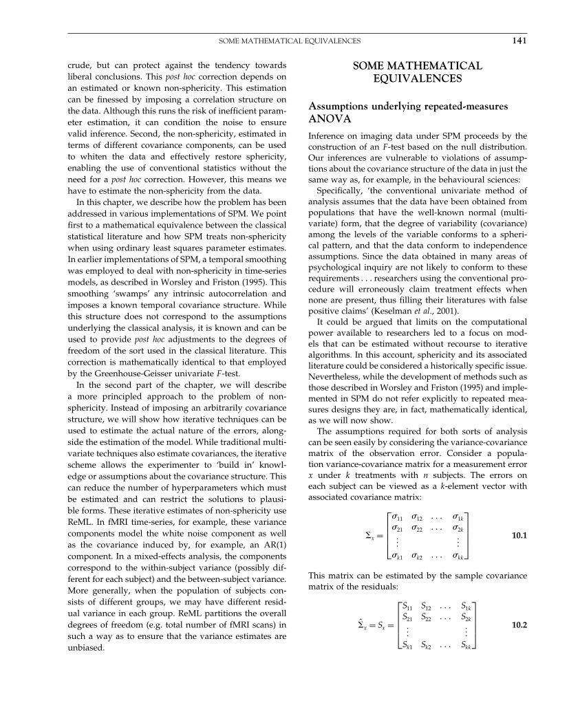
The assumptions required for both sorts of analysiscan be seen easily by considering the variance-covariancematrix of the observation error. Consider a popula-tion variance-covariance matrix for a measurement errorx under k treatments with n subjects. The errors oneach subject can be viewed as a k-element vector withassociated covariance matrix:
�x =
⎡⎢⎢⎢⎣
�11 �12 � � � �1k
�21 �22 � � � �2k
������
�k1 �k2 � � � �kk
⎤⎥⎥⎥⎦ 10.1
This matrix can be estimated by the sample covariancematrix of the residuals:
�̂x = Sx =
⎡⎢⎢⎢⎣
S11 S12 � � � S1k
S21 S22 � � � S2k
������
Sk1 Sk2 � � � Skk
⎤⎥⎥⎥⎦ 10.2
Elsevier UK Chapter: Ch10-P372560 3-10-2006 3:04p.m. Page:142 Trim:7.5in×9.25in
Basal Font:Palatino Margins:Top:40pt Gutter:68pt Font Size:9.5/12 Text Width:42pc Depth:55 Lines
142 10. COVARIANCE COMPONENTS
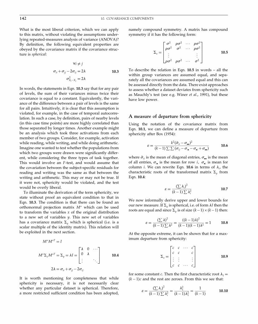
What is the most liberal criterion, which we can applyto this matrix, without violating the assumptions under-lying repeated-measures analysis of variance (ANOVA)?By definition, the following equivalent properties areobeyed by the covariance matrix if the covariance struc-ture is spherical:
∀i �= j
�ii +�jj −2�ij = 2�
�2Xi−Xj
= 2�
10.3
In words, the statements in Eqn. 10.3 say that for any pairof levels, the sum of their variances minus twice theircovariance is equal to a constant. Equivalently, the vari-ance of the difference between a pair of levels is the samefor all pairs. Intuitively, it is clear that this assumption isviolated, for example, in the case of temporal autocorre-lation. In such a case, by definition, pairs of nearby levels(in this case time points) are more highly correlated thanthose separated by longer times. Another example mightbe an analysis which took three activations from eachmember of two groups. Consider, for example, activationwhile reading, while writing, and while doing arithmetic.Imagine one wanted to test whether the populations fromwhich two groups were drawn were significantly differ-ent, while considering the three types of task together.This would involve an F -test, and would assume thatthe covariation between the subject-specific residuals forreading and writing was the same as that between thewriting and arithmetic. This may or may not be true. Ifit were not, sphericity would be violated, and the testwould be overly liberal.
To illuminate the derivation of the term sphericity, westate without proof an equivalent condition to that inEqn. 10.3. The condition is that there can be found anorthonormal projection matrix M∗ which can be usedto transform the variables x of the original distributionto a new set of variables y. This new set of variableshas a covariance matrix �y which is spherical (i.e. is ascalar multiple of the identity matrix). This relation willbe exploited in the next section.
M∗M∗T = I
M∗�xM∗T = �y = �I =
⎡⎢⎣
� 0 · · ·0 ����
� � �
⎤⎥⎦
2� = �ii +�jj −2�ij
10.4
It is worth mentioning for completeness that whilesphericity is necessary, it is not necessarily clearwhether any particular dataset is spherical. Therefore,a more restricted sufficient condition has been adopted,
namely compound symmetry. A matrix has compoundsymmetry if it has the following form:
�x =
⎡⎢⎢⎢⎣
�2 ��2 · · · ��2
��2 �2 · · · ��2
������
��2 ��2 · · · �2
⎤⎥⎥⎥⎦ 10.5
To describe the relation in Eqn. 10.5 in words – all thewithin group variances are assumed equal, and sepa-rately all the covariances are assumed equal and this canbe assessed directly from the data. There exist approachesto assess whether a dataset deviates from sphericity suchas Mauchly’s test (see e.g. Winer et al., 1991), but thesehave low power.
A measure of departure from sphericity
Using the notation of the covariance matrix fromEqn. 10.1, we can define a measure of departure fromsphericity after Box (1954):
� = k2�̄ii −�••2
k−1∑∑
�ij −�i• −�•i +�••10.6
where �̄ii is the mean of diagonal entries, �•• is the meanof all entries, �i• is the mean for row i� �•i is mean forcolumn i. We can rewrite Eqn. 10.6 in terms of �i, thecharacteristic roots of the transformed matrix �y fromEqn. 10.4:
� = ∑
�i2
k−1∑
�2i
10.7
We now informally derive upper and lower bounds forour new measure. If �y is spherical, i.e. of form �I then theroots are equal and since �y is of size k−1×k−1 then:
� = ∑
�2
k−1∑
�2= k−1�2
k−1k−1�2= 1 10.8
At the opposite extreme, it can be shown that for a max-imum departure from sphericity:
�x =
⎡⎢⎢⎢⎣
c c · · · cc c c���
������
c c · · · c
⎤⎥⎥⎥⎦ 10.9
for some constant c. Then the first characteristic root �1 =k−1c and the rest are zeroes. From this we see that:
� = ∑
�i2
k−1∑
�2i
= �21
k−1�21
= 1k−1
10.10
Elsevier UK Chapter: Ch10-P372560 3-10-2006 3:04p.m. Page:143 Trim:7.5in×9.25in
Basal Font:Palatino Margins:Top:40pt Gutter:68pt Font Size:9.5/12 Text Width:42pc Depth:55 Lines
ESTIMATING COVARIANCE COMPONENTS 143
Thus we have the following bounds:
1k−1
≤ � ≤ 1 10.11
In summary, we have seen that the measure � is well-defined using basic matrix algebra and expresses thedegree to which the standard assumptions underlyingthe distribution are violated. In the next section, weemploy this measure to protect ourselves against falselypositive inferences by correcting the parameters of theF -distribution.
Correcting degrees of freedom:the Satterthwaite approximation
Box’s motivation for using this measure for the depar-ture from sphericity was to harness an approximationdue to Satterthwaite. This deals with the fact that theactual distribution of the variance estimator is not 2
if the errors are not spherical, and thus the F -statisticused for hypothesis testing is inaccurate. The solutionadopted is to approximate the true distribution with amoment-matched scaled 2 distribution – matching thefirst and second moments. Under this approximation,in the context of repeated measures ANOVA with kmeasures and n subjects, the F -statistic is distributed asF �k−1�� n−1k−1��. To understand the eleganceof this approach, note that, as shown above, when thesphericity assumptions underlying the model are met,� = 1 and the F -distribution is then just F �k−1� n−1k − 1�, the standard degrees of freedom. In short, thecorrection ‘vanishes’ when not needed.
Finally, we note that this approximation has beenadopted for neuroimaging data in SPM. Consider theexpression for the effective degrees of freedom fromWorsley and Friston (1995):
� = trRV2
trRVRV10.12
Compare this with Eqn. 10.7 above, and see Chapter 8for a derivation. Here R is the model’s residual formingmatrix and V are the serial correlations in the errors. Inthe present context: �x = RVR. If we remember that theconventional degrees of freedom for the t-statistic arek − 1 and consider � as a correction for the degrees offreedom, then:
� = k−1� = k−1∑
�i2
k−1∑
�2i
= ∑
�i2
∑�2
i
= trRV2
trRVRV
10.13
Thus, SPM applies the Satterthwaite approximation tocorrect the F -statistic, implicitly using a measure of
sphericity violation. Next, we will see that this approachcorresponds to that employed in conventional statisticalpackages.
But which covariance matrix is usedto estimate the degrees of freedom?
Returning to the classical approach, in practice of coursewe do not know � and so it is estimated by S , thesample covariance matrix in Eqn. 10.2. From this we cangenerate an �̂ by substituting sij for the �ij in Eqn. 10.6.This correction, using the sample covariance, is oftenreferred to as the ‘Greenhouse-Geisser’ correction (e.g.Winer et al., 1991). An extensive literature treats the fur-ther steps in harnessing this correction and its variants.For example, the correction can be made more conser-vative by taking the lower bound on �̂ as derived inEqn. 10.10. This highly conservative test is [confusingly]also referred to as the ‘Greenhouse-Geisser conservativecorrection’.
The important point to note, however, is that the con-struction of the F -statistic is predicated upon a modelcovariance structure, which satisfies the assumptions ofsphericity as outlined above, but the degrees of freedomare adjusted based on the sample covariance structure.This contrasts with the approach taken in SPM whichassumes either independent and identically distributed(IID) errors (a covariance matrix which is a scalar mul-tiple of the identity matrix) or a simple autocorrelationstructure, but corrects the degrees of freedom only onthe basis of the modelled covariance structure. In the IIDcase, no correction is made. In the autocorrelation case,an appropriate correction was made, but ignoring thesample covariance matrix and assuming that the datastructure was as modelled. These strategic differences aresummarized in Table 10-1.
ESTIMATING COVARIANCECOMPONENTS
In earlier versions of SPM, the covariance structure Vwas imposed upon the data by smoothing them. Currentimplementations avoid this smoothing by modelling thenon-sphericity. This is accomplished by defining a basisset of components for the covariance structure and thenusing an iterative ReML algorithm to estimate hyper-parameters controlling these components. In this way,a wide range of sphericity violations can be modelledexplicitly. Examples include temporal autocorrelationand more subtle effects of correlations induced by taking

Elsevier UK Chapter: Ch10-P372560 3-10-2006 3:04p.m. Page:144 Trim:7.5in×9.25in
Basal Font:Palatino Margins:Top:40pt Gutter:68pt Font Size:9.5/12 Text Width:42pc Depth:55 Lines
144 10. COVARIANCE COMPONENTS
TABLE 10-1 Different approaches to modelling non-sphericity
Classical approachGreenhouse-Geisser
SPM99 SPM2/SPM5
Choice of model Assume sphericity Assume sphericityor AR(1)
Use ReML to estimatenon-sphericityparameterized witha basis set
Corrected degrees offreedom based oncovariance structure of:
Residuals Model Model
Estimation of degrees offreedom is voxel-wiseor for whole brain
Single voxel Many voxels Many voxels
several measures on each of several subjects. In all cases,however, the modelled covariance structure is used tocalculate the appropriate degrees of freedom using themoment-matching procedure described in Chapter 8. Wedo not discuss estimation in detail since this is covered inPart 4 (and Appendix 3). We will focus on the form of thecovariance structure, and look at some typical examples.We model the covariance matrix as:
�x =∑�iQi 10.14
where �I are some hyperparameters and Qi representsome basis set. The term Qi embodies the form of thecovariance components and could model different vari-ances for different blocks of data or different forms ofcorrelations within blocks. Estimation takes place usingan ReML procedure where the model coefficients andvariance estimates are re-estimated iteratively.
As will be discussed in the final section, what we in factestimate is a correlation matrix or normalized covariancefor many voxels at once. This can be multiplied by a scalarvariance estimate calculated for each voxel separately.Since this scalar does not affect the correlation structure,the corrected degrees of freedom are the same for allvoxels.
These components can be thought of as ‘design matri-ces’ for the second-order behaviour of the responsevariable and form a basis set for estimating the errorcovariance, where the hyperparameters scale the con-tribution of each constraint. Figure 10.1 illustrates twopossible applications of this technique: one for first-levelanalyses and one for random effect analyses.
Pooling non-sphericity estimates over voxels
So far we have discussed the covariance structure, draw-ing from a univariate approach. In this section, we askwhether we can harness the fact that our voxels comefrom the same brain. First, we will motivate the question
V = λ1Q1 + λ 2 Q2 + λ 3Q 3 + . . .
V = λ1Q1 + λ 2 Q2 + λ 3Q 3
FIGURE 10.1 Examples of covariance components. Top row:here we imagine that we have a number of observations over timeand a number of subjects. We decide to model the autocorrelationstructure by a sum of a simple autocorrelation AR(1) componentand a white noise component. A separately scaled combination ofthese two can approximate a wide range of actual structures, sincethe white noise component affects the ‘peakiness’ of the overallautocorrelation. For this purpose we generate two bases for eachsubject, and here we illustrate the first three. The first is an identitymatrix (no correlation) restricted to the observations from the firstsubject; the second is the same but blurred in time and with thediagonal removed. The third illustrated component is the whitenoise for the second subject and so on. Second row: in this case weimagine that we have three measures for each of several subjects. Forexample, consider a second-level analysis in which we have a scanwhile reading, while writing and while doing arithmetic for severalmembers of a population. We would like to make an inference aboutthe population from which the subjects are drawn. We want toestimate what the covariation structure of the three measures is, butwe assume that this structure is the same for each of the individuals.Here we generate three bases in total, one for all the reading scores,one for all the writing, and one for all the arithmetic. We theniteratively estimate the hyperparameters controlling each basis, andhence the covariance structure. After this has been normalized, sothat trV = rankV , it is the desired correlation.
by demonstrating that sphericity estimation involves anoisy measure, and that it might, therefore, be beneficialto pool over voxels. We will then show that under certainassumptions this strategy can be justified, and illustratean implementation.

Elsevier UK Chapter: Ch10-P372560 3-10-2006 3:04p.m. Page:145 Trim:7.5in×9.25in
Basal Font:Palatino Margins:Top:40pt Gutter:68pt Font Size:9.5/12 Text Width:42pc Depth:55 Lines
ESTIMATING COVARIANCE COMPONENTS 145
Simulating noise in sphericity measures
To assess the practicality of voxel-wise estimation of thecovariance structure we simulated 10 000 voxels drawnfrom a known population with eight measures of threelevels of a repeated measure. For each voxel we esti-mated the variance-covariance matrix using ReML anda basis set corresponding to the true distribution. Wethen calculated the � correction factor and plotted a his-togram for the distribution of this over the 10 000 voxels(Figure 10.2). Note the wide distribution, even for a uni-form underlying covariance structure. The voxel-wideestimate was 0.65, which is higher (more spherical) thanthe average of the voxel-wise estimates (i.e. 0.56). In thiscase, the � for the generating distribution was indeed0.65. This highlights the utility of pooling the estimateover many voxels to generate a correlation matrix.
Degrees of freedom reprised
As the simulation shows, to make the estimate of effectivedegrees of freedom valid, we require very precise esti-mates of non-sphericity. However, as mentioned at thestart of this chapter ‘pooling’ is problematic because thetrue error variance may change from voxel to voxel. Wewill now expand upon the form described in Eqn. 10.14to describe in detail the strategy used by current fMRIanalysis packages like SPM and multistat (Worsley et al.,2002).
Critically, we factorize the error covariance at the i-thvoxel �i = �2
i V� into a voxel-specific error variance anda voxel-wide correlation matrix. The correlation matrixis a function of hyperparameters controlling covari-
0.2 0.4 0.6 0.8 10
500
1000
1500
2000
ε
N p
ixel
s
FIGURE 10.2 Histogram illustrating voxel-wise sphericitymeasure, �, for 10 000 simulated voxels drawn from a known pop-ulation with eight measures of three levels of a repeated measure.The average of the voxel-wise estimates is 0.56. The voxel-wideestimate was 0.65, and the � for the generating distribution wasindeed 0.65.
ance components V� = �1Q1+� · · · �+�nQn that canbe estimated with high precision over a large numberof voxels. This allows one to use the reduced single-hyperparameter model and the effective degrees of free-dom as in Eqn. 10.1, while still allowing error variance tovary from voxel to voxel. Here the pooling is over ‘simi-lar’ voxels (e.g. those that activate) and that are assumedto express various error variance components in the sameproportion but not in the same amounts. In summary, wefactorize the error covariance into voxel-specific varianceand a correlation that is the same for all voxels in thesubset. For time-series, this effectively factorizes the spa-tiotemporal covariance into non-stationary spatial vari-ance and stationary temporal correlation. This enablespooling for, and only for, estimates of serial correlations.
Once the serial correlations have been estimated, infer-ence can then be based on the post hoc adjustment forthe non-sphericity described above using the Satterth-waite approximation. The Satterthwaite approximationis exactly the same as that employed in the Greenhouse-Geisser (G-G) correction for non-sphericity in commercialpackages. However, there is a fundamental distinctionbetween the SPM adjustment and the G-G correction.This is because the non-sphericity V enters as a knownconstant (or as an estimate with very high precision) inSPM. In contradistinction, the non-sphericity in G-G usesthe sample covariance matrix or multiple hyperparam-eter estimates, usually ReML, based on the data them-selves to give V̂ = �̂1Q1 +· · ·+ �̂nQn. This gives correcteddegrees of freedom that are generally too high, leadingto mildly capricious inferences. This is only a problemif the variance components interact (e.g. as with serialcorrelations in fMRI).
Compare the following with Eqn. 10.12:
vGG = trR�GG = trRV̂ 2
trRV̂RV̂ 10.15
The reason the degrees of freedom are too high is thatG-G fails to take into account the variability in theReML hyperparameter estimates and ensuing variabilityin V̂ . There are solutions to this that involve abandon-ing the single variance component model and formingstatistics using multiple hyperparameters directly (seeKiebel et al., 2003 for details). However, in SPM thisis unnecessary. The critical difference between conven-tional G-G corrections and the SPM adjustment lies inthe fact that SPM is a mass-univariate approach thatcan pool non-sphericity estimates V̂ over subsets of vox-els to give a highly precise estimate V , which can betreated as a known quantity. Conventional univariatepackages cannot do this because there is only one datasequence.

Elsevier UK Chapter: Ch10-P372560 3-10-2006 3:04p.m. Page:146 Trim:7.5in×9.25in
Basal Font:Palatino Margins:Top:40pt Gutter:68pt Font Size:9.5/12 Text Width:42pc Depth:55 Lines
146 10. COVARIANCE COMPONENTS
Non-sphericity, whitening and maximumlikelihood
In this chapter, we have introduced the concept of non-sphericity and covariance component estimation throughits impact on the distributional assumptions that under-lie classical statistics. In this context, the non-sphericityis used to make a post hoc correction to the degreesof freedom of the statistics employed. Although currentimplementations of SPM can use non-sphericity to makepost hoc adjustments to statistics based on ordinary leastsquares statistics, the default procedure is very differentand much simpler; the non-sphericity is used to whitenthe model. This renders the errors spherical and makesany correction redundant. Consider the general linearmodel (GLM) at voxel i, with non-spherical error:
yi = X�i + ei
ei ∼ N0��2i V
10.16
After V has been estimated using ReML (see below) itcan be used to pre-multiply the model by a whiteningmatrix W = V −1/2 giving:
Wyi = WX�i +wi
wi ∼ N0��2i I
wi = Wei
10.17
This new model now conforms to sphericity assump-tions and can be inverted in the usual way at each voxel.Critically, the degrees of freedom revert to their classi-cal values, without the need for any correction. Further-more, the parameter estimates of this whitened modelcorrespond to the maximum likelihood estimates of theparameters �i and are the most efficient estimates forthis model. This is used in current implementations ofSPM and entails a two-pass procedure, in which thenon-sphericity is estimated in a first pass and then thewhitened model is inverted in a second pass to givemaximum likelihood parameter and restricted maximumlikelihood variance estimates. We will revisit this issuein later chapters that consider hierarchal models and therelationship of ReML to more general model inversionschemes. Note that both the post hoc and whitening pro-cedures rest on knowing the non-sphericity. In the finalsection we take a closer look at this estimation.
Separable errors
The final issue we address is how the voxel-independenthyperparameters are estimated and how precise theseestimates are. There are many situations in which
the hyperparameters of mass-univariate observationsfactorize. In the present context, we can regard fMRItime-series as having both spatial and temporal correla-tions among the errors that factorize into a Kroneckertensor product. Consider the data matrix Y = �y1� � � � � yn�with one column, over time, for each of n voxels. Thespatiotemporal correlations can be expressed as the errorcovariance matrix in a vectorized GLM:
Y = X�+�
vecY =⎡⎢⎣
y1���
yn
⎤⎥⎦=
⎡⎢⎣
X · · · 0���
� � ����
0 · · · X
⎤⎥⎦⎡⎢⎣
�1���
�n
⎤⎥⎦+
⎡⎢⎣
�1���
�n
⎤⎥⎦
covvec� = �⊗V =⎡⎢⎣
�1V · · · �1nV���
� � ����
�n1V · · · �nnV
⎤⎥⎦ 10.18
Note that Eqn. 10.16 assumes a separable form for theerrors. This is the key assumption underlying the poolingprocedure. Here V embodies the temporal non-sphericityand � the spatial non-sphericity. Notice that the elementsof � are voxel-specific, whereas the elements of V arethe same for all voxels. We could now enter the vec-torized data into a ReML scheme, directly, to estimatethe spatial and temporal hyperparameters. However, wecan capitalize on the separable form of the non-sphericityover time and space by only estimating the hyperparam-eters of V and then use the usual estimator (Worsley andFriston, 1995) to compute a single hyperparameter �̂i foreach voxel.
The hyperparameters of V can be estimated with thealgorithm presented in Friston et al. (2002, Appendix 3).This uses a Fisher scoring scheme to maximize the loglikelihood ln pY ���� (i.e. the ReML objective function)to find the ReML estimates. In the current context thisscheme is:
� ← �+H−1g
gi = � ln pY ����
��i
= n2 tr�PQi�+ 1
2 trPT QiPY �−1Y T
Hij = −⟨
�2 ln pY ����
��2ij
⟩= n
2 trPQiPQj
P = V −1 −V −1XXT V −1X−1XT V −1
V = �1Q1 +· · ·+�nQn 10.19
This scheme is derived from basic principles inAppendix 4. Notice that the Kronecker tensor productsand vectorized forms disappear. Critically H , the preci-sion of the hyperparameter estimates, increases linearly
Elsevier UK Chapter: Ch10-P372560 3-10-2006 3:04p.m. Page:147 Trim:7.5in×9.25in
Basal Font:Palatino Margins:Top:40pt Gutter:68pt Font Size:9.5/12 Text Width:42pc Depth:55 Lines
REFERENCES 147
with the number of voxels. With sufficient voxels thisallows us to enter the resulting estimates, through V ,into Eqn. 10.16 as known quantities, because they areso precise. The nice thing about Eqn. 10.19 is that thedata enter only as Y �−1Y T whose size is determined bythe number of scans as opposed to the massive num-ber of voxels. The term Y �−1Y T is effectively the sam-ple temporal covariance matrix, sampling over voxels(after spatial whitening) and can be assembled voxel byvoxel in an efficient fashion. Eqn. 10.19 assumes thatwe know the spatial covariances. In practice, Y �−1Y T isapproximated by selecting voxels that are spatially dis-persed (so that �ij = 0) and scaling the data by an esti-mate of �−1
i obtained non-iteratively, assuming temporalsphericity.
CONCLUSION
We have shown that classical approaches do not explic-itly estimate the covariance structure of the noise in thedata but instead assume it has a tractable form, and thencorrect for any deviations from the assumptions. Thisapproximation can be based on the actual data, or on adefined structure which is imposed on the data. Moreprincipled approaches explicitly model those types ofcorrelations which the experimenter expects to find inthe data. This estimation can be noisy but, in the contextof SPM, can be finessed by pooling over many voxels.
Estimating the non-sphericity allows the experimenterto perform types of analysis which were previously ‘for-bidden’ under the less sophisticated approaches. Theseare of real interest to many researchers and include bet-ter estimation of the autocorrelation structure for fMRIdata and the ability to take more than one scan per
subject to a second level analysis and thus conduct F -tests. In event-related studies, where the exact form ofthe haemodynamic response can be critical, more thanone aspect of this response can be analysed in a random-effects context. For example, a canonical form and a mea-sure of latency or dispersion can cover a wide range ofreal responses. Alternatively, a more general basis set(e.g. Fourier or finite impulse response) can be used,allowing for non-sphericity among the different compo-nents of the set.
In this chapter, we have focused on the implications ofnon-sphericity for inference. In the next chapter we lookat a family of models that have very distinct covariancecomponents that can induce profound non-sphericity.These are hierarchical models.
REFERENCES
Box GEP (1954) Some theorems on quadratic forms applied inthe study of analysis of variance problems. Ann Math Stat 25:290–302
Friston KJ, Glaser DE, Henson RN et al. (2002) Classical andBayesian inference in neuroimaging: applications. NeuroImage16: 484–512�∗∗10�5�
Keselman HJ, Algina J, Kowalchuk RK (2001) The analysis ofrepeated measures designs: a review. Br J Math Stat Psychol54: 1–20
Kiebel SJ, Glaser DE, Friston KJ (2003) A heuristic for the degreesof freedom of statistics based on multiple hyperparameters.NeuroImage 20: 591–600
Winer BJ et al. (1991) Statistical principles in experimental design,McGraw-Hill 3rd edition, New York
Worsley KJ, Liao CH, Aston J et al. (2002) A general statistical anal-ysis for fMRI data. NeuroImage 15: 1–15
Worsley KJ, Friston KJ (1995) Analysis of fMRI time-seriesrevisited – again. NeuroImage 2: 173–81

Elsevier UK Chapter: Ch11-P372560 3-10-2006 3:05p.m. Page:148 Trim:7.5in×9.25in
Basal Font:Palatino Margins:Top:40pt Gutter:68pt Font Size:9.5/12 Text Width:42pc Depth:55 Lines
C H A P T E R
11
Hierarchical ModelsW. Penny and R. Henson
INTRODUCTION
Hierarchical models are central to many current analysesof functional imaging data including random effects anal-ysis (Chapter 12), electroencephalographic (EEG) sourcelocalization (Chapters 28 to 30) and spatiotemporal mod-els of imaging data (Chapters 25 and 26 and Friston et al.,2002b). These hierarchical models posit linear relationsamong variables with error terms that are Gaussian. Thegeneral linear model (GLM), which to date has been socentral to the analysis of functional imaging data, is aspecial case of these hierarchical models consisting of justa single layer.
Model fitting and statistical inference for hierarchicalmodels can be implemented using a parametric empiri-cal Bayes (PEB) algorithm described in Chapter 24 andin Friston et al. (2002a). The algorithm is sufficientlygeneral to accommodate multiple hierarchical levels andallows for the error covariances to take on arbitrary form.This generality is particularly appealing as it rendersthe method applicable to a wide variety of modellingscenarios. Because of this generality, however, and thecomplexity of scenarios in which the method is applied,readers wishing to learn about PEB for the first time areadvised to read this chapter first. Chapter 24 then goeson to discuss the more general case. It also shows thatthe variance components that are estimated using PEB,can also be estimated using an algorithm from classicalstatistics called restricted maximum likelihood (ReML).
In this chapter, we provide an introduction to hier-archical models and focus on some relatively simpleexamples. This chapter covers the relevant mathematicsand numerical examples are presented in the followingchapter. Each model and PEB algorithm we present isa special case of that described in Friston et al. (2002a).While there are a number of tutorials on hierarchicalmodelling (Lee, 1997; Carlin and Louis, 2000) what we
describe here has been tailored for functional imagingapplications. We also note that a tutorial on hierarchi-cal models is, to our minds, also a tutorial on Bayesianinference, as higher levels act as priors for parametersin lower levels. Readers are therefore encouraged to alsoconsult background texts on Bayesian inference, such asGelman et al. (1995).
This chapter focuses on two-level models and showshow one computes the posterior distributions over thefirst- and second-level parameters. These are derived,initially, for completely general designs and error covari-ance matrices. We then consider two special cases: (i)models with equal error variances; and (ii) separablemodels. We assume initially that the covariance compo-nents are known, and then in the section on PEB, weshow how they can be estimated. A numerical exampleis then given showing PEB in action. The chapter thendescribes how Bayesian inference can be implementedfor hierarchical models with arbitrary probability distri-butions (e.g. non-Gaussian), using the belief propagationalgorithm. We close with a discussion.
In what follows, the notation N�m��� denotes auni/multivariate normal distribution with mean m andvariance/covariance � and lower-case ps denote proba-bility densities. Upper case letters denote matrices, lowercase denote column vectors and xT denotes the trans-pose of x. We will also make extensive use of the normaldensity, i.e. if p(x)=N�m��� then:
p�x� ∝ exp(
−12
�x−m�T �−1�x−m�
)11.1
We also use Var[] to denote variance, ⊗ to denotethe Kronecker product and X+ to denote the pseudo-inverse.
Statistical Parametric Mapping, by Karl Friston et al. Copyright 2007, Elsevier Ltd. All rights reserved.ISBN–13: 978-0-12-372560-8 ISBN–10: 0-12-372560-7
148

Elsevier UK Chapter: Ch11-P372560 3-10-2006 3:05p.m. Page:149 Trim:7.5in×9.25in
Basal Font:Palatino Margins:Top:40pt Gutter:68pt Font Size:9.5/12 Text Width:42pc Depth:55 Lines
TWO-LEVEL MODELS 149
TWO-LEVEL MODELS
We consider two-level linear Gaussian models of theform:
y = Xw+ e
w = M�+z 11.2
where the errors are zero mean Gaussian with covari-ances Cov �e� = C and Cov�z� = P. The model is showngraphically in Figure 11.1. The column vectors y and whave K and N entries respectively. The vectors w and� are the first- and second-level parameters and X andM are the first- and second-level design matrices. Mod-els of this form have been used in functional imaging.For example, in random effects analysis, the second levelmodels describe the variation of subject effect sizes abouta population effect size, �. In Bayesian inference withshrinkage priors, the second-level models variation ofeffect-size over voxels around a whole-brain mean effectsize of � − 0 (i.e. for a given cognitive challenge, theresponse of a voxel chosen at random is, on average,zero). See, for example, Friston et al. (2002b).
The aim of Bayesian inference is to make inferencesabout w and � based on the posterior distributions p�w�y�and p���y�. These can be derived as follows. We first notethat the above equations specify the likelihood and priorprobability distributions:
p�y�w� ∝ exp(
−12
�y −Xw�T C−1�y −Xw�
)11.3
p�w� ∝ exp(
−12
�w−M��T P−1�w−M��
)
w
y
P
C
µ
FIGURE 11.1 Two-level hierarchical model. The data y areexplained as deriving from an effect w and a zero-mean Gaussianrandom variation with covariance C. The effects w in turn are ran-dom effects deriving from a superordinate effect � and zero-meanGaussian random variation with covariance P. The goal of Bayesianinference is to make inferences about � and w from the posteriordistributions p���y� and p�w�y�.
The posterior distribution is then:
p�w�y� ∝ p�y�w�p�w� 11.4
Taking logs and keeping only those terms that dependon w gives:
log p�w�y� = −12
�y −Xw�T C−1�y −Xw� 11.5
− 12
�w−M��T P−1�w−M��+
= −12
wT �XT C−1X +P−1�w
+wT �XT C−1y +P−1M��+
Taking logs of the Gaussian density p�x� in Eqn. 11.1 andkeeping only those terms that depend on x gives:
log p�x� = −12
xT �−1x+xT �−1m+ 11.6
Comparing Eqn. 11.5 with terms in the above equationshows that:
p�w�y� = N�m��� 11.7
�−1 = XT C−1X +P−1
m = ��XT C−1y +P−1M��
The posterior distribution over the second-level coeffi-cient is given by Bayes’ rule as:
p���y� = p�y���p���
p�y�11.8
However, because we do not have a prior p���, this poste-rior distribution becomes identical to the likelihood term,p�y���, which can be found by eliminating the first-levelparameters from our two equations, i.e. by substitutingthe second-level equation into the first giving:
y = XM�+Xz+ e 11.9
which can be written as:
y = X̃�+ ẽ 11.10
where X̃ = XM and ẽ = Xz+e. The solution to Eqn. 11.10then gives:
p���y� = N��̂���� 11.11
�̂ = �X̃T C̃−1X̃�−1X̃T C̃−1y
�� = �X̃T C̃−1X̃�−1
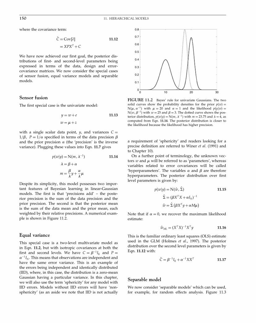
Elsevier UK Chapter: Ch11-P372560 3-10-2006 3:05p.m. Page:150 Trim:7.5in×9.25in
Basal Font:Palatino Margins:Top:40pt Gutter:68pt Font Size:9.5/12 Text Width:42pc Depth:55 Lines
150 11. HIERARCHICAL MODELS
where the covariance term:
C̃ = Cov�ẽ� 11.12
= XPXT +C
We have now achieved our first goal, the posterior dis-tributions of first- and second-level parameters beingexpressed in terms of the data, design and error-covariance matrices. We now consider the special casesof sensor fusion, equal variance models and separablemodels.
Sensor fusion
The first special case is the univariate model:
y = w+ e 11.13
w = �+z
with a single scalar data point, y, and variances C =1/� P = 1/� specified in terms of the data precision and the prior precision � (the ‘precision’ is the inversevariance). Plugging these values into Eqn. 11.7 gives
p�w�y� = N�m��−1� 11.14
� = +�
m =
�y + �
��
Despite its simplicity, this model possesses two impor-tant features of Bayesian learning in linear-Gaussianmodels. The first is that ‘precisions add’ – the poste-rior precision is the sum of the data precision and theprior precision. The second is that the posterior meanis the sum of the data mean and the prior mean, eachweighted by their relative precisions. A numerical exam-ple is shown in Figure 11.2.
Equal variance
This special case is a two-level multivariate model asin Eqn. 11.2, but with isotropic covariances at both thefirst and second levels. We have C = −1IK and P =�−1IN . This means that observations are independent andhave the same error variance. This is an example ofthe errors being independent and identically distributed(IID), where, in this case, the distribution is a zero-meanGaussian having a particular variance. In this chapter,we will also use the term ‘sphericity’ for any model withIID errors. Models without IID errors will have ‘non-sphericity’ (as an aside we note that IID is not actually
0.8
0.7
0.6
0.5
0.4
0.3
0.2
0.1
00 10 20 30
FIGURE 11.2 Bayes’ rule for univariate Gaussians. The twosolid curves show the probability densities for the prior p�w� =N����−1� with � = 20 and � = 1 and the likelihood p�y�w� =N�w�−1� with w = 25 and = 3. The dotted curve shows the pos-terior distribution, p�w�y� = N�m��−1� with m = 2375 and � = 4, ascomputed from Eqn. 11.14. The posterior distribution is closer tothe likelihood because the likelihood has higher precision.
a requirement of ‘sphericity’ and readers looking for aprecise definition are referred to Winer et al. (1991) andto Chapter 10).
On a further point of terminology, the unknown vec-tors w and � will be referred to as ‘parameters’, whereasvariables related to error covariances will be called‘hyperparameters’. The variables � and are thereforehyperparameters. The posterior distribution over firstlevel parameters is given by:
p�w�y� = N�ŵ� �̂� 11.15
�̂ = �XT X +�IN �−1
ŵ = �̂(XT y +�M�
)
Note that if � = 0, we recover the maximum likelihoodestimate:
ŵML = �XT X�−1XT y 11.16
This is the familiar ordinary least squares (OLS) estimateused in the GLM (Holmes et al., 1997). The posteriordistribution over the second level parameters is given byEqn. 11.12 with:
C̃ = −1IK +�−1XXT 11.17
Separable model
We now consider ‘separable models’ which can be used,for example, for random effects analysis. Figure 11.3
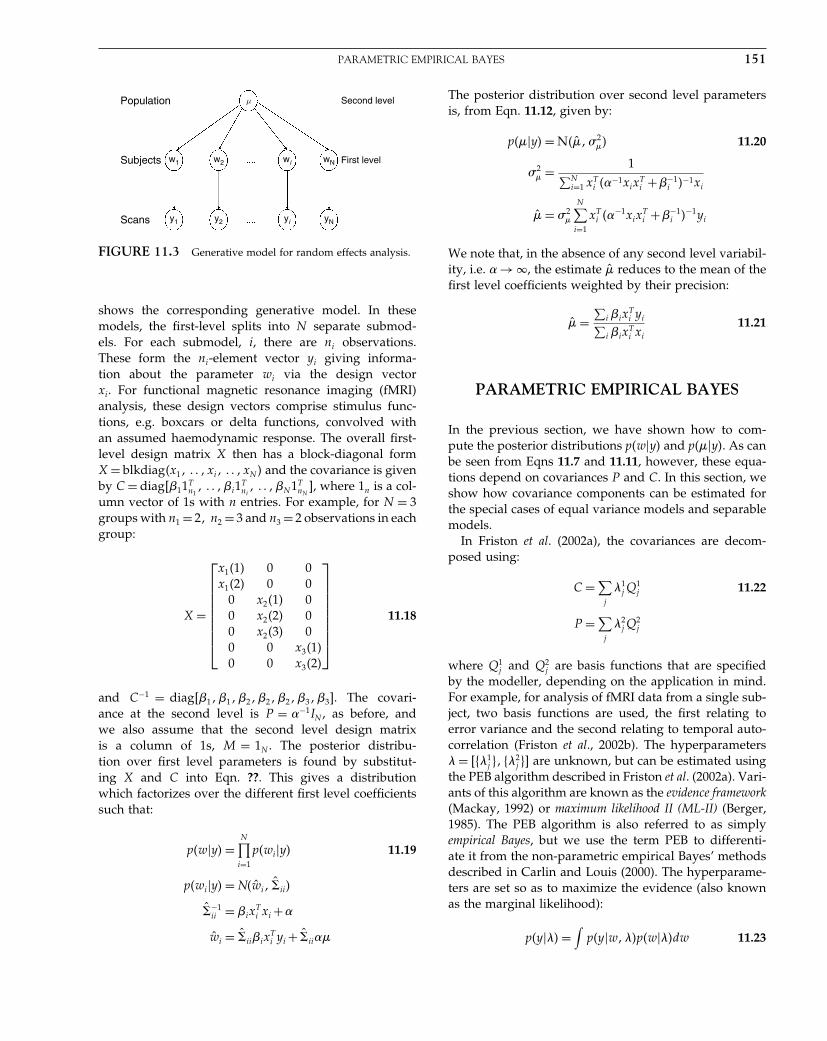
Elsevier UK Chapter: Ch11-P372560 3-10-2006 3:05p.m. Page:151 Trim:7.5in×9.25in
Basal Font:Palatino Margins:Top:40pt Gutter:68pt Font Size:9.5/12 Text Width:42pc Depth:55 Lines
PARAMETRIC EMPIRICAL BAYES 151
w1
y1 y2 yi
Population
Subjects
Scans yN
w2 wi wN First level
Second levelµ
FIGURE 11.3 Generative model for random effects analysis.
shows the corresponding generative model. In thesemodels, the first-level splits into N separate submod-els. For each submodel, i, there are ni observations.These form the ni-element vector yi giving informa-tion about the parameter wi via the design vectorxi. For functional magnetic resonance imaging (fMRI)analysis, these design vectors comprise stimulus func-tions, e.g. boxcars or delta functions, convolved withan assumed haemodynamic response. The overall first-level design matrix X then has a block-diagonal formX = blkdiag�x1� � xi� � xN � and the covariance is givenby C = diag�11T
n1� �i1T
ni� �N 1T
nN�, where 1n is a col-
umn vector of 1s with n entries. For example, for N = 3groups with n1 = 2� n2 = 3 and n3 = 2 observations in eachgroup:
X =
⎡⎢⎢⎢⎢⎢⎢⎢⎢⎣
x1�1� 0 0x1�2� 0 0
0 x2�1� 00 x2�2� 00 x2�3� 00 0 x3�1�0 0 x3�2�
⎤⎥⎥⎥⎥⎥⎥⎥⎥⎦
11.18
and C−1 = diag�1�1�2�2�2�3�3�. The covari-ance at the second level is P = �−1IN , as before, andwe also assume that the second level design matrixis a column of 1s, M = 1N . The posterior distribu-tion over first level parameters is found by substitut-ing X and C into Eqn. ??. This gives a distributionwhich factorizes over the different first level coefficientssuch that:
p�w�y� =N∏
i=1
p�wi�y� 11.19
p�wi�y� = N�ŵi� �̂ii�
�̂−1ii = ix
Ti xi +�
ŵi = �̂iiixTi yi + �̂ii��
The posterior distribution over second level parametersis, from Eqn. 11.12, given by:
p���y� = N��̂� 2�� 11.20
2� = 1∑N
i=1 xTi ��−1xix
Ti +−1
i �−1xi
�̂ = 2�
N∑i=1
xTi ��−1xix
Ti +−1
i �−1yi
We note that, in the absence of any second level variabil-ity, i.e. � → �, the estimate �̂ reduces to the mean of thefirst level coefficients weighted by their precision:
�̂ =∑
i ixTi yi∑
i ixTi xi
11.21
PARAMETRIC EMPIRICAL BAYES
In the previous section, we have shown how to com-pute the posterior distributions p�w�y� and p���y�. As canbe seen from Eqns 11.7 and 11.11, however, these equa-tions depend on covariances P and C. In this section, weshow how covariance components can be estimated forthe special cases of equal variance models and separablemodels.
In Friston et al. (2002a), the covariances are decom-posed using:
C =∑j
�1j Q
1j 11.22
P =∑j
�2j Q
2j
where Q1j and Q2
j are basis functions that are specifiedby the modeller, depending on the application in mind.For example, for analysis of fMRI data from a single sub-ject, two basis functions are used, the first relating toerror variance and the second relating to temporal auto-correlation (Friston et al., 2002b). The hyperparameters� = ���1
j �� ��2j �� are unknown, but can be estimated using
the PEB algorithm described in Friston et al. (2002a). Vari-ants of this algorithm are known as the evidence framework(Mackay, 1992) or maximum likelihood II (ML-II) (Berger,1985). The PEB algorithm is also referred to as simplyempirical Bayes, but we use the term PEB to differenti-ate it from the non-parametric empirical Bayes’ methodsdescribed in Carlin and Louis (2000). The hyperparame-ters are set so as to maximize the evidence (also knownas the marginal likelihood):
p�y��� =∫
p�y�w���p�w���dw 11.23
Elsevier UK Chapter: Ch11-P372560 3-10-2006 3:05p.m. Page:152 Trim:7.5in×9.25in
Basal Font:Palatino Margins:Top:40pt Gutter:68pt Font Size:9.5/12 Text Width:42pc Depth:55 Lines
152 11. HIERARCHICAL MODELS
This is the likelihood of the data after we have inte-grated out the first-level parameters. For the two multi-variate special cases described above, by substituting inour expressions for the prior and likelihood, integrating,taking logs and then setting the derivatives to zero, wecan derive a set of update rules for the hyperparame-ters. These derivations are provided in the following twosections.
Equal variance
For the equal variance model, the objective function is:
p�y���� =∫
p�y�w��p�w���dw 11.24
Substituting in expressions for the likelihood and priorgives:
p�y���� =(
2�
)K/2 ( �
2�
)N/2
×∫
exp(
−
2e�w�T e�w�− �
2z�w�T z�w�
)dw
where e�w� = y−Xw and z�w� = w−M�. By rearrangingthe terms in the exponent (and keeping all of them, unlikebefore where we were only interested in w-dependentterms) the integral can be written as:
I =[∫
exp(
−12
�w− ŵ�T �̂−1�w− ŵ�
)dw
]11.25
×[
exp(
−
2e�ŵ�T e�ŵ�− �
2z�ŵ�T z�ŵ�
)]
where the second term is not dependent on w. The firstfactor is then simply given by the normalizing constantof the multivariate Gaussian density:
�2��N/2��̂�1/2 11.26
Hence,
p�y���� =(
2�
)K/2
�N/2��̂�1/2
×exp(
−
2e�ŵ�T e�ŵ�− �
2z�ŵ�T z�ŵ�
)
where ��̂� denotes the determinant of �̂. Taking logs givesthe ‘log-evidence’:
F = K
2log
2�+ N
2log �+ 1
2log ��̂�
−
2e�ŵ�T e�ŵ�− �
2z�ŵ�T z�ŵ� 11.27
To find equations for updating the hyperparameters,we must differentiate F with respect to � and andset the derivative to zero. The only possibly problematicterm is the log-determinant, but this can be differentiatedby first noting that the inverse covariance is given by:
�̂−1 = XT X +�IN 11.28
If �j are the eigenvalues of the first term, then the eigen-values of �̂−1 are �j +�. Hence,
��̂−1� =∏j
��j +�� 11.29
��̂� = 1∏j��j +��
log ��̂� = −∑j
log��j +��
�
��log ��̂� = −∑
j
1�j +�
Setting the derivative �F/�� to zero then gives:
�z�ŵ�T z�ŵ� = N −∑j
�
�j +�11.30
=∑j
�j +�
�j +�−∑
j
�
�j +�
=∑j
�j
�j +�
This is an implicit equation in � which leads to the fol-lowing update rule. We first define the quantity � whichis computed from the ‘old’ value of �:
� =N∑
j=1
�j
�j +�11.31
and then let:
1�
= z�ŵ�T z�ŵ�
�11.32
The update for is derived by first noting that the eigen-values �j are linearly dependent on . Hence,
��j
�= �j
11.33
The derivative of the log-determinant is then given by:
�
�log ��̂−1� = 1
∑j
�j
�j +�11.34

Elsevier UK Chapter: Ch11-P372560 3-10-2006 3:05p.m. Page:153 Trim:7.5in×9.25in
Basal Font:Palatino Margins:Top:40pt Gutter:68pt Font Size:9.5/12 Text Width:42pc Depth:55 Lines
NUMERICAL EXAMPLE 153
which leads to the update:
1
= e�ŵ�T e�ŵ�
K −�11.35
The PEB algorithm consists of iterating the update rulesin Eqn. 11.31, Eqn. 11.32, Eqn. 11.35 and the posteriorestimates in Eqn. 11.15, until convergence.
The update rules in Eqn. 11.31, Eqn. 11.32 andEqn. 11.35 can be interpreted as follows. For every j forwhich �j >> �, the quantity � increases by 1. As � isthe prior precision and �j is the data precision (of thejth ‘eigencoefficient’), � therefore measures the numberof parameters that are determined by the data. Given Kdata points, the quantity K −� therefore corresponds tothe number of degrees of freedom in the data set. Thevariances �−1 and −1 are then updated based on thesum of squares divided by the appropriate degrees offreedom.
Separable models
For separable models, the objective function is:
p�y��� �i�� =∫
p�y�w��i��p�w���dw 11.36
Because the second-level here is the same as for the equalvariance case, so is the update for alpha. The updatesfor i are derived in a similar manner as before, but wealso make use of the fact that the first-level posteriordistribution factorizes (see Eqn. 11.19). This decouplesthe updates for each i and results in the following PEBalgorithm:
êi = yi − ŵixi 11.37
ẑi = ŵi − �̂
�i = ixTi xi
�i = �i
�i +�
� =∑i
�i
i = �ni −�i�/êTi êi
� = �/ẑT ẑ
ŵi = �ixTi yi +���/��i +��
di = ��−1xixTi +−1
i Ini�−1
2� = 1/�
∑i
xTi dixi�
�̂ = 2�
∑i
xTi diyi
ei
Predictionerrors
Predictions
w1 w2 wi
yi
wN
yN
yi
µµ
zi
y2y1
ˆˆ
ˆˆ
FIGURE 11.4 Part of the PEB algorithm for separable modelsrequires the upwards propagation of prediction errors and down-wards propagation of predictions. This passing of messages betweennodes in the hierarchy is a special case of the more general beliefpropagation algorithm referred to in Figure 11.5.
Initial values for ŵi and i are set using OLS, �̂ is ini-tially set to the mean of ŵi and � is initially set to 0.The equations are then iterated until convergence (in ourexamples in Chapter 12, we never required more thanten iterations). While the above updates may seem some-what complex, they can perhaps be better understood interms of messages passing among nodes in a hierarchicalnetwork. This is shown in Figure 11.4 for the ‘prediction’and ‘prediction error’ variables.
The PEB algorithms we have described show howBayesian inference can take place when the variancecomponents are unknown (in the previous section, weassumed the variance components were known). Anapplication of this PEB algorithm to random effects anal-ysis is provided in the next chapter. We now providea brief numerical example demonstrating the iterationswith PEB updates.
NUMERICAL EXAMPLE
This numerical example caricatures the use of PEB forestimating effect sizes from functional imaging datadescribed in Chapter 23. The approach uses a ‘globalshrinkage prior’ which embodies a prior belief that,across the brain: (i) the average effect is zero, � = 0; and(ii) the variability of responses follows a Gaussian dis-tribution with precision �. Mathematically, we can writep�wi� = N�0��−1�. Plate 5(a) (see colour plate section)shows effect sizes generated from this prior for an N =20-voxel brain and � = 1.
Chapter 23 allows for multiple effects to be expressedat each voxel and for positron emission tomography(PET)/fMRI data to be related to effect sizes using the fullflexibility of general linear models. Here, we just assumethat data at each voxel are normally distributed about
Elsevier UK Chapter: Ch11-P372560 3-10-2006 3:05p.m. Page:154 Trim:7.5in×9.25in
Basal Font:Palatino Margins:Top:40pt Gutter:68pt Font Size:9.5/12 Text Width:42pc Depth:55 Lines
154 11. HIERARCHICAL MODELS
the effect size at that voxel. That is, p�yi�wi� = N�wi�−1i �.
Plate 5(b) shows ni = 10 data points at each voxel gen-erated from this likelihood. We have allowed the obser-vation noise precision i to be different at each voxel.Voxels 2, 15 and 18, for example, have noisier data thanothers.
Effect sizes were then estimated from these data usingmaximum likelihood (ML) and PEB. ML estimates areshown in Plate 5(c) and (d). These are simply computedas the mean value observed at each voxel. PEB was imple-mented using the updates in Eqn. 11.37 with � = 0 andxi = 1ni
and initialized with � = 0 and i and ŵi set toML-estimated values.
Eqn. 11.37 was then iterated, resulting in effect sizeestimates shown in Plate 6 before iterations one, three,five and seven. These estimates seem rather stable afteronly two or three iterations. Only the effects at voxels 5and 15 seem markedly changed between iterations threeand seven. The corresponding estimates of � were 0,0.82, 0.91 and 0.95, showing convergence to the true priorresponse precision value of 1.
It is well known that PEB provides estimates that are,on average, more accurate than ML. Here, we quantifythis using, s, the standard deviation across voxels of thedifference between the true and estimated effects. ForML, s = 071 and for PEB, s = 034. That PEB estimatesare twice as accurate on average can be seen by com-paring Plate 6(a) and (d). Of course, PEB is only better‘on average’. It does better at most voxels at the expenseof being worse at a minority, for example, voxel 2. Thistrade-off is discussed further in Chapter 22.
PEB can do better than ML because it uses more infor-mation: here, the information that effects have a meanof zero across the brain and follow a Gaussian variabil-ity profile. This shows the power of Bayesian estima-tion, which combines prior information with data in anoptimal way. In this example, a key parameter in thistrade-off is the parameter �i which is computed as inEqn. 11.37. This quantity is the ratio of the data precisionto the posterior precision. A value of 1 indicates that theestimated effect is determined solely by the data, as inML. A value of 0 indicates the estimate is determinedsolely by the prior. For most voxels in our data set, wehave �i ≈ 09, but for the noisy voxels 2, 15 and 18, wehave �i ≈ 05. PEB thus relies more on prior informationwhere data are unreliable.
PEB will only do better than ML if the prior is chosenappropriately. For functional imaging data, we will neverknow what the ‘true prior’ is, just as we will never knowwhat the ‘true model’ is. But some priors and models arebetter than others, and there is a formal method for decid-ing between them. This is ‘Bayesian model selection’ andis described in Chapter 35.
Finally, we note that the prior used here does not usespatial information, i.e. there is no notion that voxel 5 is‘next to’ voxel 6. It turns out that for functional imag-ing data, spatial information is important. In Chapter 25,we describe Bayesian fMRI inference with spatial pri-ors. Bayesian model selection shows that models withspatial priors are preferred to those without (Pennyet al., 2006).
BELIEF PROPAGATION
This chapter has focused on the special case of two-level models and Gaussian distributions. It is worth-while noting that the general solution to inference intree-structured hierarchical models, which holds for alldistributions, is provided by the ‘sum-product’ or ‘beliefpropagation’ algorithm (Pearl, 1988; Jordan and Weiss,2002). This is a message passing algorithm which aimsto deliver the marginal distributions1 at each point in thehierarchy. It does this by propagating evidence up thehierarchy and marginal distributions down. If the down-ward messages are passed after the upward messageshave reached the top, then this is equivalent to propa-gating the posterior beliefs down the hierarchy. This isshown schematically in Figure 11.5.
This general solution is important as it impacts onnon-Gaussian and/or non-linear hierarchical models. Ofparticular relevance are the models of inference in cor-tical hierarchies (Friston, 2003) referred to in later chap-ters of the book. In these models, evidence flows upthe hierarchy, in the form of prediction errors, andmarginal distributions flow down, in the form of predic-tions. Completion of the downward pass explains latecomponents of event-related potentials which are cor-related with, e.g. extra-classical receptive field effects(Friston, 2003). This general solution also motivates adata analysis approach known as Bayesian model aver-aging (BMA), described further in Chapter 35, where,e.g. x3 in Figure 11.5 embodies assumptions aboutmodel structure. The downward pass of belief prop-agation then renders our final inferences independentof these assumptions. See Chapter 16 of Mackay (2003)and Ghahramani (1998) for further discussion of theseissues.
1 The probability distribution over a set of variables is known asthe joint distribution. The distribution over a subset is knownas the marginal distribution.

Elsevier UK Chapter: Ch11-P372560 3-10-2006 3:05p.m. Page:155 Trim:7.5in×9.25in
Basal Font:Palatino Margins:Top:40pt Gutter:68pt Font Size:9.5/12 Text Width:42pc Depth:55 Lines
REFERENCES 155
Inference based onupward pass
Upwardmessage
Downwardmessage
Finalinference
p (x3|y) =p (y )
p (y |x3)p (x3)
p (x2|y,x3) =p (y |x3)
p (y |x2)p (x2|x3)
p (x1 y,x2) =p (y x2)
p (y x1)p (x1 x2)
x3
x2
x1
y
p (y |x3 ) p (x3 |y )
p (x2 y) = ∫p (x2|y,x3)p (x3|y )dx3
p(y |x2)
p (y |x1)
p (x2 y)
p (x1 y) = ∫p (x1|y,x2)p (x2|y )dx2
FIGURE 11.5 Belief propagation for inferencein hierarchical models. This algorithm is used toupdate the marginal densities, i.e. to update p�xi�to p�xi�y�. Inferences based on purely the upwardpass are contingent on variables in the layer above,whereas inferences based on upward and down-ward passes are not. Completion of the downwardpass delivers the marginal density. Application ofthis algorithm to the two-level Gaussian model willproduce the update Eqn. 11.7 and Eqn. 11.11. Moregenerally, this algorithm can be used for Bayesianmodel averaging, where e.g. x3 embodies assump-tions about model structure, and as a model of infer-ence in cortical hierarchies, where e.g. completion ofthe downward pass explains extra-classical receptivefield effects (Friston, 2003).
DISCUSSION
We have described Bayesian inference for some par-ticular two-level linear-Gaussian hierarchical models.A key feature of Bayesian inference in this contextis that the posterior distributions are Gaussian withprecisions that are the sum of the data and priorprecisions. The posterior means are the sum of thedata and prior means, but each weighted accordingto their relative precision. With zero prior precision,two-level models reduce to a single-level model (i.e.a GLM) and Bayesian inference reduces to the famil-iar maximum-likelihood estimation scheme. With non-zero and, in general unknown, prior means and pre-cisions, these parameters can be estimated using PEB.These covariance components can also be estimated usingthe ReML algorithm from classical statistics. The rela-tion between PEB and ReML is discussed further inChapter 22.
We have described two special cases of the PEB algo-rithm, one for equal variances and one for separablemodels. Both algorithms are special cases of a gen-eral approach described in Friston et al. (2002a) andin Chapter 24. In these contexts, we have shown thatPEB automatically partitions the total degrees of free-dom (i.e. number of data points) into those to be usedto estimate the hyperparameters of the prior distribu-tion and those to be used to estimate hyperparametersof the likelihood distribution. The next chapter describeshow PEB can be used in the context of random effectsanalysis.
REFERENCES
Berger JO, (1985) Statistical decision theory and Bayesian analysis.Springer-Verlag, New York
Carlin BP, Louis TA (2000) Bayes and empirical Bayes methods for dataanalysis. CRC Press, USA
Friston K (2003) Learning and inference in the brain. Neural Netw16: 1325–52
Friston KJ, Penny WD, Phillips C et al. (2002a) Classical and Bayesianinference in neuroimaging: theory. NeuroImage 16: 465–83
Friston KJ, Glaser DE, Henson RNA et al. (2002b) Classical andBayesian inference in neuroimaging: applications. NeuroImage16: 484–512
Gelman A, Carlin JB, Stern HS et al. (1995) Bayesian data analysis.Chapman and Hall, Boca Raton
Ghahramani Z (1998) Learning dynamic bayesian networks. InAdaptive processing of temporal information, Giles CL, Gori M (eds).Springer-Verlag, Berlin
Holmes AP, Poline JB, Friston KJ (1997) Characterizing brainimages with the general linear model. In Human brain function,Frackowiak RSJ, Friston KJ, Frith C et al. (eds). Academic Press,London pp 59–84.
Jordan M, Weiss Y (2002) Graphical models: probabilistic inference.In The handbook of brain theory and neural networks, Arbib M (ed.).MIT Press, Cambridge
Lee PM (1997) Bayesian statistics: an introduction, 2nd edn. Arnold,London
Mackay DJC (1992) Bayesian interpolation. Neural Comput 4: 415–47Mackay DJC (2003) Information theory, inference and learning algo-
rithms. Cambridge University Press, CambridgePearl J (1988) Probabilistic reasoning in intelligent systems: networks of
plausible inference. Morgan KauffmanPenny WD, Flandin G, Trujillo-Barreto N (2006) Bayesian com-
parison of spatially regularised general linear models. HumBrain Mapp, in press
Winer BJ, Brown DR, Michels KM (1991) Statistical principles in exper-imental design. McGraw-Hill

Elsevier UK Chapter: Ch12-P372560 30-9-2006 5:13p.m. Page:156 Trim:7.5in×9.25in
Basal Font:Palatino Margins:Top:40pt Gutter:68pt Font Size:9.5/12 Text Width:42pc Depth:55 Lines
C H A P T E R
12
Random Effects AnalysisW.D. Penny and A.J. Holmes
INTRODUCTION
In this chapter, we are concerned with making statisticalinferences involving many subjects. One can envisagetwo main reasons for studying multiple subjects. The firstis that one may be interested in individual differences,as in many areas of psychology. The second, which isthe one that concerns us here, is that one is interestedin what is common to the subjects. In other words, weare interested in the stereotypical effect in the populationfrom which the subjects are drawn.
As every experimentalist knows, a subject’s responsewill vary from trial to trial. Further, this response willvary from subject to subject. These two sources of vari-ability, within-subject (also called between-scan) andbetween-subject, must both be taken into account whenmaking inferences about the population.
In statistical terminology, if we wish to take the vari-ability of an effect into account we must treat it as a‘random effect’. In a 12-subject functional magnetic res-onance imaging (fMRI) study, for example, we can viewthose 12 subjects as being randomly drawn from the pop-ulation at large. The subject variable is then a randomeffect and, in this way, we are able to take the samplingvariability into account and make inferences about thepopulation from which the subjects were drawn. Con-versely, if we view the subject variable as a ‘fixed effect’then our inferences will relate only to those 12 subjectschosen.
The majority of early studies in neuroimaging com-bined data from multiple subjects using a ‘fixed-effects’(FFX) approach. This methodology only takes intoaccount the within-subject variability. It is used to reportresults as case studies. It is not possible to make formalinferences about population effects using FFX. Random-effects (RFX) analysis, however, takes into account bothsources of variation and makes it possible to make formal
inferences about the population from which the subjectsare drawn.
In this chapter, we describe FFX and RFX analyses ofmultiple-subject data. We first describe the mathemat-ics behind RFX, for balanced designs, and show howRFX can be implemented using the computationally effi-cient ‘summary-statistic’ approach. We then describe themathematics behind FFX and show that it only takes intoaccount within-subject variance. The next section showsthat RFX for unbalanced designs is optimally imple-mented using the PEB algorithm described in the previ-ous chapter. This section includes a numerical examplewhich shows that, although not optimal, the summarystatistic approach performs well, even for unbalanceddesigns.
RANDOM EFFECTS ANALYSIS
Maximum likelihood
Underlying RFX analysis is a probability model definedas follows. We first envisage that the mean effect in thepopulation (i.e. averaged across subjects) is of size wpop
and that the variability of this effect between subjectsis �2
b . The mean effect for the ith subject (i.e. averagedacross scans), wi, is then assumed to be drawn from aGaussian with mean wpop and variance �2
b . This processreflects the fact that we are drawing subjects at randomfrom a large population. We then take into account thewithin-subject (i.e. across scan) variability by modellingthe jth observed effect in subject i as being drawn froma Gaussian with mean wi and variance �2
w. Note that�2
w is assumed to be the same for all subjects. This is arequirement of a balanced design. This two-stage processis shown graphically in Figure 12.1.
Statistical Parametric Mapping, by Karl Friston et al. Copyright 2007, Elsevier Ltd. All rights reserved.ISBN–13: 978-0-12-372560-8 ISBN–10: 0-12-372560-7
156

Elsevier UK Chapter: Ch12-P372560 30-9-2006 5:13p.m. Page:157 Trim:7.5in×9.25in
Basal Font:Palatino Margins:Top:40pt Gutter:68pt Font Size:9.5/12 Text Width:42pc Depth:55 Lines
RANDOM EFFECTS ANALYSIS 157
FIGURE 12.1 Synthetic data illustrating the probability modelunderlying random effects analysis. The dotted line is the Gaussiandistribution underlying the second-level model with mean wpop, thepopulation effect, and variance �2
b , the between-subject variance.The mean subject effects, wi, are drawn from this distribution. Thesolid lines are the Gaussians underlying the first level models withmeans wi and variances �2
w. The crosses are the observed effects yij
which are drawn from the solid Gaussians.
Given a data set of effects from N subjects with nreplications of that effect per subject, the population effectis modelled by a two-level process:
yij = wi + eij 12.1
wi = wpop +zi
where wi is the true mean effect for subject i and yij is thejth observed effect for subject i, and zi is the between-subject error for the ith subject. These Gaussian errorshave the same variance, �2
b . For the positron emissiontomography (PET) data considered below this is a differ-ential effect, the difference in activation between wordgeneration and word shadowing. The first equation cap-tures the within-subject variability and the second equa-tion the between-subject variability.
The within-subject Gaussian error eij has zero meanand variance Var�eij� = �2
w. This assumes that the errorsare independent over subjects and over replicationswithin subject. The between-subject Gaussian error zi haszero mean and variance Var�zi� = �2
b . Collapsing the twolevels into one gives:
yij = wpop +zi + eij 12.2
The maximum-likelihood estimate of the populationmean is:
ŵpop = 1Nn
N∑i=1
n∑j=1
yij 12.3
We now make use of a number of statistical relationsdefined in Appendix 12.1 to show that this estimate hasa mean E�ŵpop� = wpop and a variance given by:
Var�ŵpop� = Var
[N∑
i=1
1N
n∑j=1
1n
�wpop +zi + eij�
]12.4
= Var
[N∑
i=1
1N
zi
]+Var
[N∑
i=1
1N
n∑j=1
1n
eij
]
= �2b
N+ �2
w
Nn
The variance of the population mean estimate containscontributions from both the within-subject and between-subject variance.
Summary statistics
Implicit in the summary-statistic RFX approach is thetwo-level model:
w̄i = wi + ei 12.5
wi = wpop +zi
where wi is the true mean effect for subject i, w̄i is thesample mean effect for subject i and wpop is the true effectfor the population.
The summary-statistic (SS) approach is of interestbecause it is computationally much simpler to implementthan the full random effects model of Eqn. 12.1. This isbecause it is based on the sample mean value, w̄i, ratherthan on all of the samples yij . This is important for neu-roimaging as in a typical functional imaging group studythere can be thousands of images, each containing tensof thousands of voxels.
In the first level, we consider the variation of the sam-ple mean for each subject around the true mean foreach subject. The corresponding variance is Var�ei� =�2
w/n, where �2w is the within-subject variance. At the sec-
ond level, we consider the variation of the true subjectmeans about the population mean where Var�zi� = �2
b , thebetween-subject variance. We also have E�ei� = E�zi� = 0.Consequently:
w̄i = wpop +zi + ei 12.6
The population mean is then estimated as:
ŵpop = 1N
N∑i=1
w̄i 12.7

Elsevier UK Chapter: Ch12-P372560 30-9-2006 5:13p.m. Page:158 Trim:7.5in×9.25in
Basal Font:Palatino Margins:Top:40pt Gutter:68pt Font Size:9.5/12 Text Width:42pc Depth:55 Lines
158 12. RANDOM EFFECTS ANALYSIS
This estimate has a mean E�ŵpop� = wpop and a variancegiven by:
Var�ŵpop� = Var
[N∑
i=1
1N
w̄i
]12.8
= Var
[N∑
i=1
1N
zi
]+Var
[N∑
i=1
1N
ei
]
= �2b
N+ �2
w
Nn
Thus, the variance of the estimate of the populationmean contains contributions from both the within-subject and between-subject variances. Importantly, bothE�ŵpop� and Var�ŵpop� are identical to the maximum-likelihood estimates derived earlier. This validates thesummary-statistic approach. Informally, the validity ofthe summary-statistic approach lies in the fact that whatis brought forward to the second level is a sample mean. Itcontains an element of within-subject variability which,when operated on at the second level, produces just theright balance of within- and between-subject variance.
FIXED EFFECTS ANALYSIS
Implicit in FFX analysis is a single-level model:
yij = wi + eij 12.9
The parameter estimates for each subject are:
ŵi = 1n
n∑j=1
yij 12.10
which have a variance given by:
Var�ŵi� = Var
[n∑
j=1
1n
yij
]12.11
= �2w
n
The estimate of the group mean is then:
ŵpop = 1N
N∑i=1
ŵi 12.12
which has a variance:
Var�ŵpop� = Var
[N∑
i=1
1N
ŵi
]12.13
= 1N
Var�d̂i�
= �2w
Nn
The variance of the fixed-effects group mean estimatecontains contributions from within-subject terms only.It is not sensitive to between-subject variance. We arenot therefore able to make formal inferences about pop-ulation effects using FFX. We are restricted to informalinferences based on separate case studies or summaryimages showing the average group effect. This will bedemonstrated empirically in a later section.
PARAMETRIC EMPIRICAL BAYES
We now return to RFX analysis. We have previouslyshown how the SS approach can be used for the analy-sis of balanced designs, i.e. identical �2
w for all subjects.This section starts by showing how parametric empiricalBayes (PEB) can also be used for balanced designs. It thenshows how PEB can be used for unbalanced designs andprovides a numerical comparison between PEB and SSon unbalanced data.
Before proceeding, we note that an algorithm from clas-sical statistics, known as restricted maximum likelihood(ReML), can also be used for variance component estima-tion. Indeed, many of the papers on random effects anal-ysis use ReML instead of PEB (Friston et al., 2002, 2005).
The model described in this section is identical to theseparable model in the previous chapter but with xi = 1n
and �i = �. Given a data set of contrasts from N subjectswith n scans per subject, the population effect can bemodelled by the two-level process:
yij = wi + eij 12.14
wi = wpop +zi
where yij (a scalar) is the data from the ith subject andthe jth scan at a particular voxel. These data points areaccompanied by errors eij with wi being the size of theeffect for subject i, wpop being the size of the effect inthe population and zi being the between-subject error.This may be viewed as a Bayesian model where the firstequation acts as a likelihood and the second equationacts as a prior. That is:
p�yij�wi� = N�wi��2w� 12.15
p�wi� = N�wpop��2b �
where �2b is the between-subject variance and �2
w is thewithin-subject variance. We can make contact with thehierarchical formalism of the previous chapter by makingthe following identities. We place the yij in the columnvector y in the order – all from subject 1, all from subject 2,etc. (this is described mathematically by the vec operator

Elsevier UK Chapter: Ch12-P372560 30-9-2006 5:13p.m. Page:159 Trim:7.5in×9.25in
Basal Font:Palatino Margins:Top:40pt Gutter:68pt Font Size:9.5/12 Text Width:42pc Depth:55 Lines
PARAMETRIC EMPIRICAL BAYES 159
and is implemented in MATLAB (Mathworks, Inc.) bythe colon operator). We also let X = IN ⊗1n where ⊗ is theKronecker product and let w = �w1�w2� �wN �T . Withthese values, the first level in Eqn. 11.2 of the previouschapter is then the matrix equivalent of the first level inEqn. 12.14 (i.e. it holds for all i� j). For y = Xw + e ande.g. N = 3�n = 2 we then have:
⎡⎢⎢⎢⎢⎢⎢⎣
y11
y12
y21
y22
y31
y32
⎤⎥⎥⎥⎥⎥⎥⎦
=
⎡⎢⎢⎢⎢⎢⎢⎣
1 0 01 0 00 1 00 1 00 0 10 0 1
⎤⎥⎥⎥⎥⎥⎥⎦
⎡⎣w1
w2
w3
⎤⎦+
⎡⎢⎢⎢⎢⎢⎢⎣
e11
e12
e21
e22
e31
e32
⎤⎥⎥⎥⎥⎥⎥⎦
12.16
We then note that XT X = nIN �∑̂ = diag�Var�w1��
Var�w2�� � Var�wN �� and the ith element of XT y isequal to
∑nj=1 yij .
If we let M = 1N , then the second level in Eqn. 11.2of the previous chapter is the matrix equivalent of thesecond-level in Eqn. 12.14 (i.e. it holds for all i). Pluggingin our values for M and X and letting � = 1/�2
w and = 1/�2
b gives:
Var�ŵpop� = 1N
+�n
�n12.17
and
ŵpop = 1N
+�n
�n
�
+�n
∑i�j
yij 12.18
= 1Nn
∑i�j
yij
So the estimate of the population mean is simply theaverage value of yij . The variance can be re-written as:
Var�ŵpop� = �2b
N+ �2
w
Nn12.19
This result is identical to the maximum-likelihood andsummary-statistic results derived earlier. The equiva-lence between the Bayesian and ML results derives fromthe fact that there is no prior at the population level.Hence, p�Y ��� = p���Y�, as indicated in the previouschapter.
Unbalanced designs
The model described in this section is identical to theseparable model in the previous chapter, but with xi = 1ni
.If the error covariance matrix is non-isotropic, i.e. C �=�2
wI , then the population estimates will change. This canoccur, for example, if the design matrices are different for
different subjects (so-called unbalanced-designs), or if thedata from some of the subjects are particularly ill-fitting.In these cases, we consider the within-subject variances�2
w�i� and the number of events ni to be subject-specific.This will be the case in experimental paradigms wherethe number of events is not under experimental control,e.g. in memory paradigms where ni may refer to thenumber of remembered items.
If we let M = 1N , then the second level in Eqn. 11.2in the previous chapter is the matrix equivalent of thesecond-level in Eqn. 12.14 (i.e. it holds for all i). Pluggingin our values for M and X gives:
Var�ŵpop� =(
N∑i=1
�ini
+ni�i
)−1
12.20
and
ŵpop =(
N∑i=1
�ini
+�ini
)−1N∑
i=1
�i
+�ini
ni∑j=1
yij 12.21
This reduces to the earlier result if �i = � and ni =n. Both of these results are different to the summary-statistic approach, which we note is therefore math-ematically inexact for unbalanced designs. But as weshall see in the numerical example below, the summary-statistic approach is remarkably robust to departuresfrom assumptions about balanced designs.
Estimation
To implement the PEB estimation scheme for the unequalvariance case, we first compute the errors êij = yij −Xŵi,ẑi = ŵi − Mŵpop. We then substitute xi = 1ni
into theupdate rules derived in the PEB section of the previouschapter to obtain:
�2b ≡ 1
= 1
�
N∑i=1
ẑ2i 12.22
�2w�i� ≡ 1
�i
= 1ni −�i
ni∑j=1
ê2ij 12.23
where:
� =N∑
i=1
�i 12.24
and
�i = ni�i
+ni�i
12.25
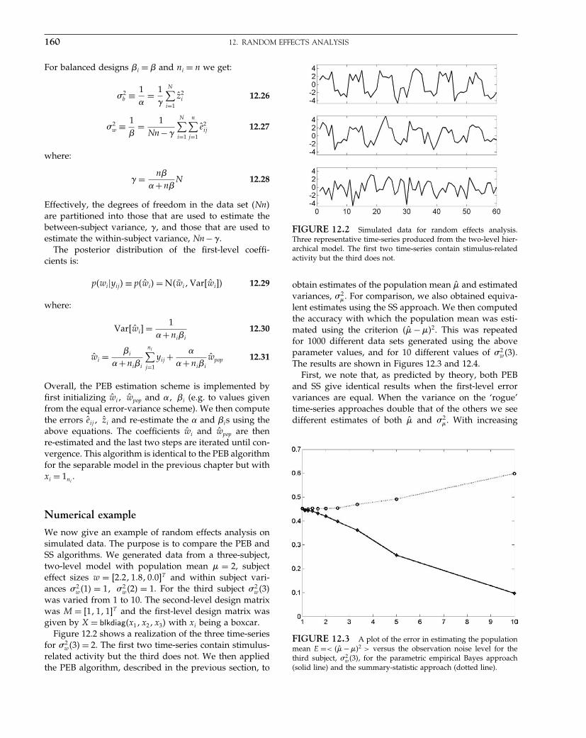
Elsevier UK Chapter: Ch12-P372560 30-9-2006 5:13p.m. Page:160 Trim:7.5in×9.25in
Basal Font:Palatino Margins:Top:40pt Gutter:68pt Font Size:9.5/12 Text Width:42pc Depth:55 Lines
160 12. RANDOM EFFECTS ANALYSIS
For balanced designs �i = � and ni = n we get:
�2b ≡ 1
= 1
�
N∑i=1
ẑ2i 12.26
�2w ≡ 1
�= 1
Nn−�
N∑i=1
n∑j=1
ê2ij 12.27
where:
� = n�
+n�N 12.28
Effectively, the degrees of freedom in the data set �Nn�are partitioned into those that are used to estimate thebetween-subject variance, �, and those that are used toestimate the within-subject variance, Nn−�.
The posterior distribution of the first-level coeffi-cients is:
p�wi�yij� ≡ p�ŵi� = N�w̄i� Var�ŵi�� 12.29
where:
Var�ŵi� = 1+ni�i
12.30
ŵi = �i
+ni�i
ni∑j=1
yij +
+ni�i
ŵpop 12.31
Overall, the PEB estimation scheme is implemented byfirst initializing ŵi� ŵpop and � �i (e.g. to values givenfrom the equal error-variance scheme). We then computethe errors êij� ẑi and re-estimate the and �is using theabove equations. The coefficients ŵi and ŵpop are thenre-estimated and the last two steps are iterated until con-vergence. This algorithm is identical to the PEB algorithmfor the separable model in the previous chapter but withxi = 1ni
.
Numerical example
We now give an example of random effects analysis onsimulated data. The purpose is to compare the PEB andSS algorithms. We generated data from a three-subject,two-level model with population mean � = 2, subjecteffect sizes w = �2 2� 1 8� 0 0�T and within subject vari-ances �2
w�1� = 1� �2w�2� = 1. For the third subject �2
w�3�was varied from 1 to 10. The second-level design matrixwas M = �1� 1� 1�T and the first-level design matrix wasgiven by X = blkdiag�x1�x2�x3� with xi being a boxcar.
Figure 12.2 shows a realization of the three time-seriesfor �2
w�3� = 2. The first two time-series contain stimulus-related activity but the third does not. We then appliedthe PEB algorithm, described in the previous section, to
FIGURE 12.2 Simulated data for random effects analysis.Three representative time-series produced from the two-level hier-archical model. The first two time-series contain stimulus-relatedactivity but the third does not.
obtain estimates of the population mean �̂ and estimatedvariances, �2
�. For comparison, we also obtained equiva-lent estimates using the SS approach. We then computedthe accuracy with which the population mean was esti-mated using the criterion ��̂ − ��2. This was repeatedfor 1000 different data sets generated using the aboveparameter values, and for 10 different values of �2
w�3�.The results are shown in Figures 12.3 and 12.4.
First, we note that, as predicted by theory, both PEBand SS give identical results when the first-level errorvariances are equal. When the variance on the ‘rogue’time-series approaches double that of the others we seedifferent estimates of both �̂ and �2
�. With increasing
FIGURE 12.3 A plot of the error in estimating the populationmean E =< ��̂ − ��2 > versus the observation noise level for thethird subject, �2
w�3�, for the parametric empirical Bayes approach(solid line) and the summary-statistic approach (dotted line).
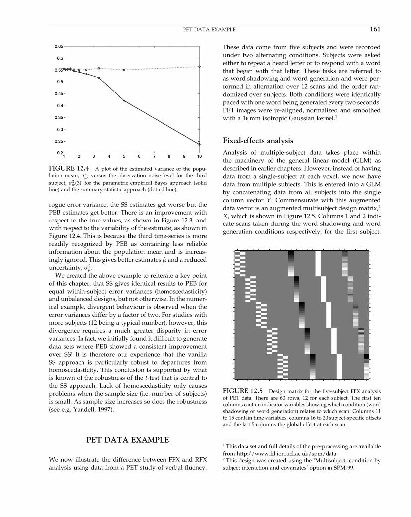
Elsevier UK Chapter: Ch12-P372560 30-9-2006 5:13p.m. Page:161 Trim:7.5in×9.25in
Basal Font:Palatino Margins:Top:40pt Gutter:68pt Font Size:9.5/12 Text Width:42pc Depth:55 Lines
PET DATA EXAMPLE 161
FIGURE 12.4 A plot of the estimated variance of the popu-lation mean, �2
�, versus the observation noise level for the thirdsubject, �2
w�3�, for the parametric empirical Bayes approach (solidline) and the summary-statistic approach (dotted line).
rogue error variance, the SS estimates get worse but thePEB estimates get better. There is an improvement withrespect to the true values, as shown in Figure 12.3, andwith respect to the variability of the estimate, as shown inFigure 12.4. This is because the third time-series is morereadily recognized by PEB as containing less reliableinformation about the population mean and is increas-ingly ignored. This gives better estimates �̂ and a reduceduncertainty, �2
�.We created the above example to reiterate a key point
of this chapter, that SS gives identical results to PEB forequal within-subject error variances (homoscedasticity)and unbalanced designs, but not otherwise. In the numer-ical example, divergent behaviour is observed when theerror variances differ by a factor of two. For studies withmore subjects (12 being a typical number), however, thisdivergence requires a much greater disparity in errorvariances. In fact, we initially found it difficult to generatedata sets where PEB showed a consistent improvementover SS! It is therefore our experience that the vanillaSS approach is particularly robust to departures fromhomoscedasticity. This conclusion is supported by whatis known of the robustness of the t-test that is central tothe SS approach. Lack of homoscedasticity only causesproblems when the sample size (i.e. number of subjects)is small. As sample size increases so does the robustness(see e.g. Yandell, 1997).
PET DATA EXAMPLE
We now illustrate the difference between FFX and RFXanalysis using data from a PET study of verbal fluency.
These data come from five subjects and were recordedunder two alternating conditions. Subjects were askedeither to repeat a heard letter or to respond with a wordthat began with that letter. These tasks are referred toas word shadowing and word generation and were per-formed in alternation over 12 scans and the order ran-domized over subjects. Both conditions were identicallypaced with one word being generated every two seconds.PET images were re-aligned, normalized and smoothedwith a 16 mm isotropic Gaussian kernel.1
Fixed-effects analysis
Analysis of multiple-subject data takes place withinthe machinery of the general linear model (GLM) asdescribed in earlier chapters. However, instead of havingdata from a single-subject at each voxel, we now havedata from multiple subjects. This is entered into a GLMby concatenating data from all subjects into the singlecolumn vector Y . Commensurate with this augmenteddata vector is an augmented multisubject design matrix,2
X, which is shown in Figure 12.5. Columns 1 and 2 indi-cate scans taken during the word shadowing and wordgeneration conditions respectively, for the first subject.
FIGURE 12.5 Design matrix for the five-subject FFX analysisof PET data. There are 60 rows, 12 for each subject. The first tencolumns contain indicator variables showing which condition (wordshadowing or word generation) relates to which scan. Columns 11to 15 contain time variables, columns 16 to 20 subject-specific offsetsand the last 5 columns the global effect at each scan.
1 This data set and full details of the pre-processing are availablefrom http://www.fil.ion.ucl.ac.uk/spm/data.2 This design was created using the ‘Multisubject: condition bysubject interaction and covariates’ option in SPM-99.
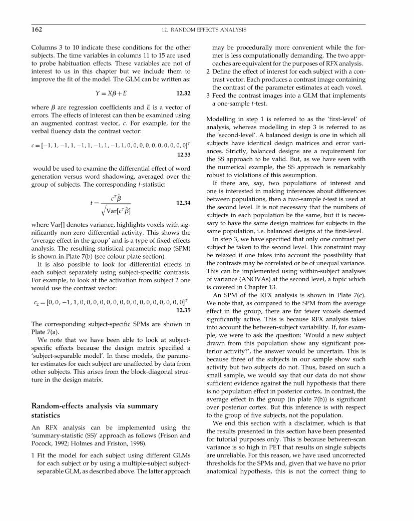
Elsevier UK Chapter: Ch12-P372560 30-9-2006 5:13p.m. Page:162 Trim:7.5in×9.25in
Basal Font:Palatino Margins:Top:40pt Gutter:68pt Font Size:9.5/12 Text Width:42pc Depth:55 Lines
162 12. RANDOM EFFECTS ANALYSIS
Columns 3 to 10 indicate these conditions for the othersubjects. The time variables in columns 11 to 15 are usedto probe habituation effects. These variables are not ofinterest to us in this chapter but we include them toimprove the fit of the model. The GLM can be written as:
Y = X�+E 12.32
where � are regression coefficients and E is a vector oferrors. The effects of interest can then be examined usingan augmented contrast vector, c. For example, for theverbal fluency data the contrast vector:
c = �−1� 1�−1� 1�−1� 1�−1� 1�−1� 1� 0� 0� 0� 0� 0� 0� 0� 0� 0� 0�T
12.33
would be used to examine the differential effect of wordgeneration versus word shadowing, averaged over thegroup of subjects. The corresponding t-statistic:
t = cT �̂√Var�cT �̂�
12.34
where Var�� denotes variance, highlights voxels with sig-nificantly non-zero differential activity. This shows the‘average effect in the group’ and is a type of fixed-effectsanalysis. The resulting statistical parametric map (SPM)is shown in Plate 7(b) (see colour plate section).
It is also possible to look for differential effects ineach subject separately using subject-specific contrasts.For example, to look at the activation from subject 2 onewould use the contrast vector:
c2 = �0� 0�−1� 1� 0� 0� 0� 0� 0� 0� 0� 0� 0� 0� 0� 0� 0� 0� 0� 0�T
12.35
The corresponding subject-specific SPMs are shown inPlate 7(a).
We note that we have been able to look at subject-specific effects because the design matrix specified a‘subject-separable model’. In these models, the parame-ter estimates for each subject are unaffected by data fromother subjects. This arises from the block-diagonal struc-ture in the design matrix.
Random-effects analysis via summarystatistics
An RFX analysis can be implemented using the‘summary-statistic (SS)’ approach as follows (Frison andPocock, 1992; Holmes and Friston, 1998).
1 Fit the model for each subject using different GLMsfor each subject or by using a multiple-subject subject-separable GLM, as described above. The latter approach
may be procedurally more convenient while the for-mer is less computationally demanding. The two appr-oaches are equivalent for the purposes of RFX analysis.
2 Define the effect of interest for each subject with a con-trast vector. Each produces a contrast image containingthe contrast of the parameter estimates at each voxel.
3 Feed the contrast images into a GLM that implementsa one-sample t-test.
Modelling in step 1 is referred to as the ‘first-level’ ofanalysis, whereas modelling in step 3 is referred to asthe ‘second-level’. A balanced design is one in which allsubjects have identical design matrices and error vari-ances. Strictly, balanced designs are a requirement forthe SS approach to be valid. But, as we have seen withthe numerical example, the SS approach is remarkablyrobust to violations of this assumption.
If there are, say, two populations of interest andone is interested in making inferences about differencesbetween populations, then a two-sample t-test is used atthe second level. It is not necessary that the numbers ofsubjects in each population be the same, but it is neces-sary to have the same design matrices for subjects in thesame population, i.e. balanced designs at the first-level.
In step 3, we have specified that only one contrast persubject be taken to the second level. This constraint maybe relaxed if one takes into account the possibility thatthe contrasts may be correlated or be of unequal variance.This can be implemented using within-subject analysesof variance (ANOVAs) at the second level, a topic whichis covered in Chapter 13.
An SPM of the RFX analysis is shown in Plate 7(c).We note that, as compared to the SPM from the averageeffect in the group, there are far fewer voxels deemedsignificantly active. This is because RFX analysis takesinto account the between-subject variability. If, for exam-ple, we were to ask the question: ‘Would a new subjectdrawn from this population show any significant pos-terior activity?’, the answer would be uncertain. This isbecause three of the subjects in our sample show suchactivity but two subjects do not. Thus, based on such asmall sample, we would say that our data do not showsufficient evidence against the null hypothesis that thereis no population effect in posterior cortex. In contrast, theaverage effect in the group (in plate 7(b)) is significantover posterior cortex. But this inference is with respectto the group of five subjects, not the population.
We end this section with a disclaimer, which is thatthe results presented in this section have been presentedfor tutorial purposes only. This is because between-scanvariance is so high in PET that results on single subjectsare unreliable. For this reason, we have used uncorrectedthresholds for the SPMs and, given that we have no prioranatomical hypothesis, this is not the correct thing to

Elsevier UK Chapter: Ch12-P372560 30-9-2006 5:13p.m. Page:163 Trim:7.5in×9.25in
Basal Font:Palatino Margins:Top:40pt Gutter:68pt Font Size:9.5/12 Text Width:42pc Depth:55 Lines
DISCUSSION 163
do (Frackowiak et al., 1997) (see Chapter 14). But as ourconcern is merely to present a tutorial on the differencebetween RFX and FFX we have neglected these otherwiseimportant points.
fMRI DATA EXAMPLE
This section compares RFX analysis as implementedusing SS versus PEB. The dataset we chose to analysecomprised 1200 images that were acquired in 10 contigu-ous sessions of 120 scans. These data have been describedelsewhere (Friston et al., 1998).
The reason we chose these data was that each of the10 sessions was slightly different in terms of design. Theexperimental design involved 30-second epochs of singleword streams and a passive listening task. The wordswere concrete, monosyllabic nouns presented at a num-ber of different rates. The word rate was varied pseudo-randomly over epochs within each session.
We modelled responses using an event-related modelwhere the occurrence of each word was modelled with adelta function. The ensuing stimulus function was con-volved with a canonical haemodynamic response func-tion and its temporal derivative to give two regressors ofinterest for each of the 10 sessions. These effects were sup-plemented with confounding and nuisance effects com-prising a mean and the first few components of a discretecosine transform, removing drifts lower than 1/128 Hz.Further details of the paradigm and analysis details aregiven in Friston et al. (2005).
The results of the SS and PEB analyses are presentedin Figure 12.6 and have been thresholded at p < 0 05,corrected for the entire search volume. These results aretaken from Friston et al. (2005) where PEB was imple-mented using the ReML formulation. It is evident that theinferences from these two procedures are almost identi-cal, with PEB being slightly more sensitive. The resultsremain relatively unchanged despite the fact that thefirst-level designs were not balanced. This contributes tonon-sphericity at the second level which is illustratedin Figure 12.7 for the SS and PEB approaches. Thisfigure shows that heteroscedasticity can vary by up to afactor of 4.
DISCUSSION
We have shown how neuroimaging data from multi-ple subjects can be analysed using fixed-effects (FFX) orrandom-effects (RFX) analysis. FFX analysis is used forreporting case studies and RFX is used to make inferences
FIGURE 12.6 SPMs showing the effect of words in the popu-lation using (a) SS and (b) PEB approaches.
about the population from which subjects are drawn. Fora comparison of these and other methods for combiningdata from multiple subjects see Lazar et al. (2002).
In neuroimaging, RFX is implemented using the com-putationally efficient summary-statistic approach. Wehave shown that this is mathematically equivalent tothe more computationally demanding maximum likeli-hood procedure. For unbalanced designs, however, thesummary-statistic approach is no longer equivalent. Butwe have shown, using a simulation study and fMRI data,that this lack of formal equivalence is not practicallyrelevant.
For more advanced treatments of random effects anal-ysis3 see e.g. Yandell (1997). These allow, for example,
3 Strictly, what in neuroimaging is known as random-effectsanalysis is known in statistics as mixed-effects analysis as thestatistical models contain both fixed and random effects.

Elsevier UK Chapter: Ch12-P372560 30-9-2006 5:13p.m. Page:164 Trim:7.5in×9.25in
Basal Font:Palatino Margins:Top:40pt Gutter:68pt Font Size:9.5/12 Text Width:42pc Depth:55 Lines
164 12. RANDOM EFFECTS ANALYSIS
(b)
0.1
0.05
0
1 2 3 4 5 6 7 8 9 101 2 3 4 5 6 7 8 9 10
(a)
0.1
0.05
01 2 3 4 5 6 7 8 9 10 1 2 3 4 5 6 7 8 9 10
FIGURE 12.7 Within-session variance as (a) assumed by SS and (b) estimated using PEB. This shows that within-session variance canvary by up to a factor of 4, although this makes little difference to the final inference (see Figure 12.6).
for subject-specific within-subject variances, unbalanceddesigns and for Bayesian inference (Carlin and Louis,2000). For a recent application of these ideas to neu-roimaging, readers are referred to Chapter 17 in whichhierarhical models are applied to single and multiple sub-ject fMRI studies. As groundwork for this more advancedmaterial readers are encouraged to first read the tutorialin Chapter 11.
A general point to note, especially for fMRI, is thatbecause the between-subject variance is typically largerthan the within-subject variance your scanning time isbest used to scan more subjects rather than to scan indi-vidual subjects for longer. In practice, this must be tradedoff against the time required to recruit and train subjects(Worsley et al., 2002).
Further points
We have so far described how to make inferences aboutunivariate effects in a single population. This is achievedin the summary-statistic approach by taking forward asingle contrast image per subject to the second level andthen using a one sample t-test.
This methodology carries over naturally to more com-plex scenarios where we may have multiple populationsor multivariate effects. For two populations, for exam-ple, we perform two-sample t-tests at the second level.An extreme example of this approach is the compari-son of a single case study with a control group. Whilethis may sound unfeasible, as one population has only asingle member, a viable test can in fact be implementedby assuming that the two populations have the samevariance.
For multivariate effects, we take forward multiple con-trast images per subject to the second level and performan analysis of variance. This can be implemented in theusual way with a GLM but, importantly, we must take
into account the fact that we have repeated measures foreach subject and that each characteristic of interest mayhave a different variability. This topic is covered in thenext chapter.
As well as testing for whether univariate populationeffects are significantly different from hypothesized val-ues (typically zero), it is possible to test whether they arecorrelated with other variables of interest. For example,one can test whether task-related activation in the motorsystem correlates with age (Ward and Frackowiak, 2003).It is also possible to look for conjunctions at the secondlevel, e.g. to test for areas that are conjointly active forpleasant, unpleasant and neutral odour valences (Got-tfried et al., 2002). For a statistical test involving con-junctions of contrasts, it is necessary that the contrasteffects be uncorrelated. This can be ensured by takinginto account the covariance structure at the second level.This is also described in the next chapter on analysis ofvariance.
The validity of all of the above approaches relies on thesame criteria that underpin the univariate single popula-tion summary-statistic approach. Namely, that the vari-ance components and estimated parameter values are, onaverage, identical to those that would be obtained by theequivalent two-level maximum likelihood model.
APPENDIX 12.1EXPECTATIONS ANDTRANSFORMATIONS
We use E�� to denote the expectation operator and Var��to denote variance and make use of the following results.Under a linear transform y = ax + b, the variance of xchanges according to:
Var�ax+ b� = a2Var�x� 12.36

Elsevier UK Chapter: Ch12-P372560 30-9-2006 5:13p.m. Page:165 Trim:7.5in×9.25in
Basal Font:Palatino Margins:Top:40pt Gutter:68pt Font Size:9.5/12 Text Width:42pc Depth:55 Lines
APPENDIX 12.1 EXPECTATIONS AND TRANSFORMATIONS 165
Secondly, if Var�xi� = Var�x� for all i then:
Var
[1N
N∑i=1
xi
]= 1
NVar�x� 12.37
For background reading on expectations, variance trans-formations and introductory mathematical statistics seeWackerley et al. (1996).
REFERENCES
Carlin BP, Louis TA (2000) Bayes and empirical Bayes methods for dataanalysis. Chapman and Hall, London
Frackowiak RSJ, Friston KJ, Frith C, et al. (1997) Human brain function.Academic Press, New York
Frison L, Pocock SJ (1992) Repeated measures in clinical trials: ananalysis using mean summary statistics and its implications fordesign. Stat Med, 11: 1685–1704
Friston KJ, Josephs O, Rees G, et al. (1998) Non-linear event-relatedresponses in fMRI. Magnet Res Med 39: 41–52
Friston KJ, Penny WD, Phillips C et al. (2002) Classical and Bayesianinference in neuroimaging: theory. NeuroImage 16: 465–83
Friston KJ, Stephan KE, Lund TE et al. (2005) Mixed-effects andfMRI studies. NeuroImage 24: 244–52
Gottfried JA, Deichmann R, Winston JS et al. (2002) Functionalheterogeneity in human olfactory cortex: an event-relatedfunctional magnetic resonance imaging study. Neurosci 22:10819–28
Holmes AP, Friston KJ (1998) Generalisability, random effects andpopulation inference. NeuroImage 7: S754
Lazar NA, Luna B, Sweeney JA et al. (2002) Combining brains: a sur-vey of methods for statistical pooling of information. Neuroimage16: 538–50
Wackerley DD, Mendenhall W, Scheaffer RL (1996) Mathematicalstatistics with applications. Duxbury Press, California
Ward NS, Frackowiak RSJ (2003) Age related changes in the neuralcorrelates of motor performance. Brain 126: 873–88
Worsley KJ, Liao CH, Aston J et al. (2002) A general statistical anal-ysis for fMRI data. NeuroImage 15(1): 1–15
Yandell BS (1997) Practical data analysis for designed experiments.Chapman and Hall, London

Elsevier UK Chapter: Ch13-P372560 30-9-2006 5:13p.m. Page:166 Trim:7.5in×9.25in
Basal Font:Palatino Margins:Top:40pt Gutter:68pt Font Size:9.5/12 Text Width:42pc Depth:55 Lines
C H A P T E R
13
Analysis of VarianceW. Penny and R. Henson
INTRODUCTION
The mainstay of many scientific experiments isthe factorial design. These comprise a number ofexperimental factors which are each expressed over anumber of levels. Data are collected for each factor/levelcombination and then analysed using analysis of vari-ance (ANOVA). The ANOVA uses F-tests to examine apre-specified set of standard effects, e.g. ‘main effects’and ‘interactions’, as described in Winer et al. (1991).
ANOVAs are commonly used in the analysis ofpositron emission tomography (PET), electroencephalog-raphy (EEG), magnetoencephalography (MEG) and func-tional magnetic resonance imaging (fMRI) data. For PET,this analysis usually takes place at the ‘first’ level. Thisinvolves direct modelling of PET scans. For EEG, MEGand fMRI, ANOVAs are usually implemented at the ‘sec-ond level’. As described in the previous chapter, firstlevel models are used to create contrast images for eachsubject. These are then used as data for a second level or‘random-effects’ analysis.
Some different types of ANOVA are tabulated inTable 13-1. A two-way ANOVA, for example, is anANOVA with 2 factors; a K1-by-K2 ANOVA is a two-wayANOVA with K1 levels of one factor and K2 levels of the
TABLE 13-1 Types of ANOVA
Factors Levels Simple Repeated measures
1 2 Two-samplet-test
Paired t-test
1 K One-wayANOVA
One-way ANOVAwithin-subject
M K1� K2� ��� KM M-wayANOVA
M-way ANOVAwithin-subject
other. A repeated measures ANOVA is one in which thelevels of one or more factors are measured from the sameunit (e.g. subjects). Repeated measures ANOVAs arealso sometimes called within-subject ANOVAs, whereasdesigns in which each level is measured from a differ-ent group of subjects are called between-subject ANOVAs.Designs in which some factors are within-subject, andothers between-subject, are sometimes called mixeddesigns.
This terminology arises because in a between-subjectdesign the difference between levels of a factor is givenby the difference between subject responses, e.g. the dif-ference between levels 1 and 2 is given by the differ-ence between those subjects assigned to level 1 and thoseassigned to level 2. In a within-subject design, the levelsof a factor are expressed within each subject, e.g. the dif-ference between levels 1 and 2 is given by the averagedifference of subject responses to levels 1 and 2. This islike the difference between two-sample t-tests and pairedt-tests.
The benefit of repeated measures is that we can matchthe measurements better. However, we must allow forthe possibility that the measurements are correlated (so-called ‘non-sphericity’ – see below).
The level of a factor is also sometimes referred to as a‘treatment’ or a ‘group’ and each factor/level combina-tion is referred to as a ‘cell’ or ‘condition’. For each type ofANOVA, we describe the relevant statistical models andshow how they can be implemented in a general linearmodel (GLM). We also give examples of how main effectsand interactions can be tested for using F-contrasts.
The chapter is structured as follows: the first sectiondescribes one-way between-subject ANOVAs. The nextsection describes one-way within-subject ANOVAs andintroduces the notion of non-sphericity. We then describetwo-way within-subject ANOVAs and make a distinction
Statistical Parametric Mapping, by Karl Friston et al. Copyright 2007, Elsevier Ltd. All rights reserved.ISBN–13: 978-0-12-372560-8 ISBN–10: 0-12-372560-7
166

Elsevier UK Chapter: Ch13-P372560 30-9-2006 5:13p.m. Page:167 Trim:7.5in×9.25in
Basal Font:Palatino Margins:Top:40pt Gutter:68pt Font Size:9.5/12 Text Width:42pc Depth:55 Lines
ONE-WAY BETWEEN-SUBJECT ANOVA 167
between models with pooled versus partitioned errors.The last section discusses issues particular to fMRI andwe end with a discussion.
Notation
In the mathematical formulations below, N�m��� denotesa uni/multivariate Gaussian with mean m and vari-ance/covariance �. IK denotes the K ×K identity matrix,XT denotes transpose, X−T the inverse transpose, X− thegeneralized-inverse, 1K is a K × 1 vector of 1s, 0K is aK×1 vector of zeroes and 0KN is a K×N matrix of zeroes.We consider factorial designs with n = 1��N subjects andm = 1��M factors where the mth factor has k = 1��Km
levels.
ONE-WAY BETWEEN-SUBJECT ANOVA
In a between-subject ANOVA, differences between levelsof a factor are given by the differences between sub-ject responses. We have one measurement per subjectand different subjects are assigned to different lev-els/treatments/groups. The response from the nth sub-ject �yn� is modelled as:
yn = �k +�+ en 13.1
where �k are the treatment effects, k = 1��K� k = g�n� andg�n� is an indicator function whereby g�n� = k means thenth subject is assigned to the kth group, e.g. g�13� = 2indicates the 13th subject being assigned to group 2. Thisis the single experimental factor that is expressed over Klevels. The variable � is sometimes called the grand meanor intercept or constant term. The random variable en is theresidual error, assumed to be drawn from a zero meanGaussian distribution.
If the factor is significant, then the above model isa significantly better model of the data than the sim-pler model:
yn = �+ en 13.2
where we just view all of the measurements as randomvariation about the grand mean. Figure 13.2 comparesthese two models on some simulated data.
In order to test whether one model is better thananother, we can use an F-test based on the extra sum ofsquares principle (see Chapter 8). We refer to Eqn. 13.1 asthe ‘full’ model and Eqn. 13.2 as the ‘reduced’ model. If
RSS denotes the residual sum of squares (i.e. the sum ofsquares left after fitting a model) then:
F = �RSSreduced −RSSfull�/�K −1�
RSSfull/�N −K�13.3
has an F-distribution with K − 1�N −K degrees of free-dom. If F is significantly non-zero then the full model hasa significantly smaller error variance than the reducedmodel. That is to say, the full model is a significantlybetter model, or the main effect of the factor is significant.
The above expression is also sometimes expressed interms of sums of squares (SS) due to treatment and dueto error:
F = SStreat/DFtreat
SSerror/DFerror
13.4
where
SStreat = RSSreduced −RSSfull 13.5
DFtreat = K −1
SSerror = RSSfull
DFerror = N −K
DFtotal = DFtreat +DFerror = N −1
Eqns 13.3 and 13.4 are therefore equivalent.
Numerical example
This subsection shows how an ANOVA can be imple-mented in a GLM. Consider a one-way ANOVA withK = 4 groups each having n = 12 subjects (i.e. N = Kn =48 subjects/observations in total). The GLM for the fullmodel in Eqn. 13.1 is:
y = X+ e 13.6
where the design matrix X = IK ⊗ 1n� 1N � is shown inFigure 13.1, where ⊗ denotes the Kronecker product(see Appendix 13.1). The vector of parameters is =�1� �2� �3� �4���T .
Eqn. 13.3 can then be implemented using the effects ofinterest F-contrast, as introduced in Chapter 9:
CT =
⎡⎢⎢⎣
1 −1/3 −1/3 −1/3 0−1/3 1 −1/3 −1/3 0−1/3 −1/3 1 −1/3 0−1/3 −1/3 −1/3 1 0
⎤⎥⎥⎦ 13.7
or equivalently:
CT =⎡⎣ 1 −1 0 0 0
0 1 −1 0 00 0 1 −1 0
⎤⎦ 13.8
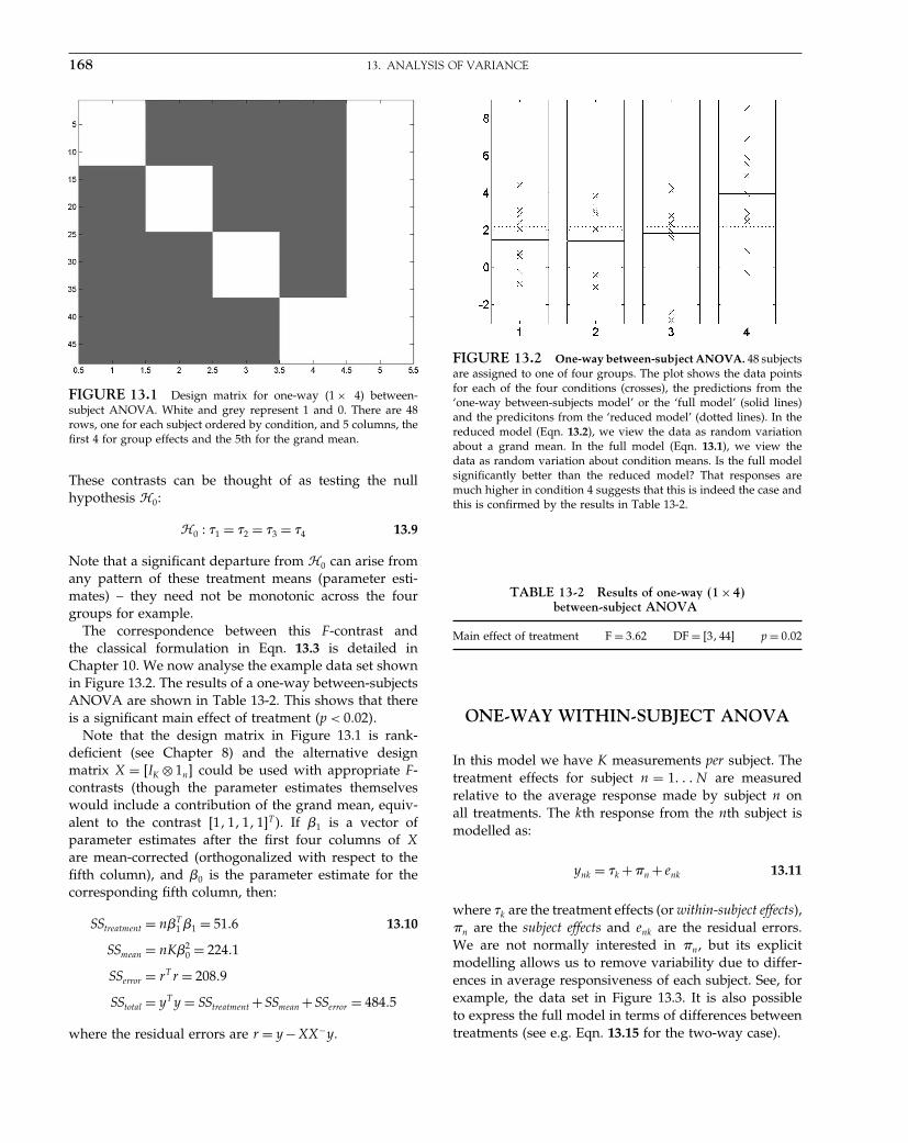
Elsevier UK Chapter: Ch13-P372560 30-9-2006 5:13p.m. Page:168 Trim:7.5in×9.25in
Basal Font:Palatino Margins:Top:40pt Gutter:68pt Font Size:9.5/12 Text Width:42pc Depth:55 Lines
168 13. ANALYSIS OF VARIANCE
FIGURE 13.1 Design matrix for one-way �1 × 4� between-subject ANOVA. White and grey represent 1 and 0. There are 48rows, one for each subject ordered by condition, and 5 columns, thefirst 4 for group effects and the 5th for the grand mean.
These contrasts can be thought of as testing the nullhypothesis �0:
�0 � �1 = �2 = �3 = �4 13.9
Note that a significant departure from �0 can arise fromany pattern of these treatment means (parameter esti-mates) – they need not be monotonic across the fourgroups for example.
The correspondence between this F-contrast andthe classical formulation in Eqn. 13.3 is detailed inChapter 10. We now analyse the example data set shownin Figure 13.2. The results of a one-way between-subjectsANOVA are shown in Table 13-2. This shows that thereis a significant main effect of treatment �p < 0�02�.
Note that the design matrix in Figure 13.1 is rank-deficient (see Chapter 8) and the alternative designmatrix X = IK ⊗ 1n� could be used with appropriate F-contrasts (though the parameter estimates themselveswould include a contribution of the grand mean, equiv-alent to the contrast 1� 1� 1� 1�T ). If 1 is a vector ofparameter estimates after the first four columns of Xare mean-corrected (orthogonalized with respect to thefifth column), and 0 is the parameter estimate for thecorresponding fifth column, then:
SStreatment = nT1 1 = 51�6 13.10
SSmean = nK20 = 224�1
SSerror = rT r = 208�9
SStotal = yT y = SStreatment +SSmean +SSerror = 484�5
where the residual errors are r = y −XX−y.
FIGURE 13.2 One-way between-subject ANOVA. 48 subjectsare assigned to one of four groups. The plot shows the data pointsfor each of the four conditions (crosses), the predictions from the‘one-way between-subjects model’ or the ‘full model’ (solid lines)and the predicitons from the ‘reduced model’ (dotted lines). In thereduced model (Eqn. 13.2), we view the data as random variationabout a grand mean. In the full model (Eqn. 13.1), we view thedata as random variation about condition means. Is the full modelsignificantly better than the reduced model? That responses aremuch higher in condition 4 suggests that this is indeed the case andthis is confirmed by the results in Table 13-2.
TABLE 13-2 Results of one-way �1×4�between-subject ANOVA
Main effect of treatment F = 3�62 DF = 3� 44� p = 0�02
ONE-WAY WITHIN-SUBJECT ANOVA
In this model we have K measurements per subject. Thetreatment effects for subject n = 1 N are measuredrelative to the average response made by subject n onall treatments. The kth response from the nth subject ismodelled as:
ynk = �k +�n + enk 13.11
where �k are the treatment effects (or within-subject effects),�n are the subject effects and enk are the residual errors.We are not normally interested in �n, but its explicitmodelling allows us to remove variability due to differ-ences in average responsiveness of each subject. See, forexample, the data set in Figure 13.3. It is also possibleto express the full model in terms of differences betweentreatments (see e.g. Eqn. 13.15 for the two-way case).
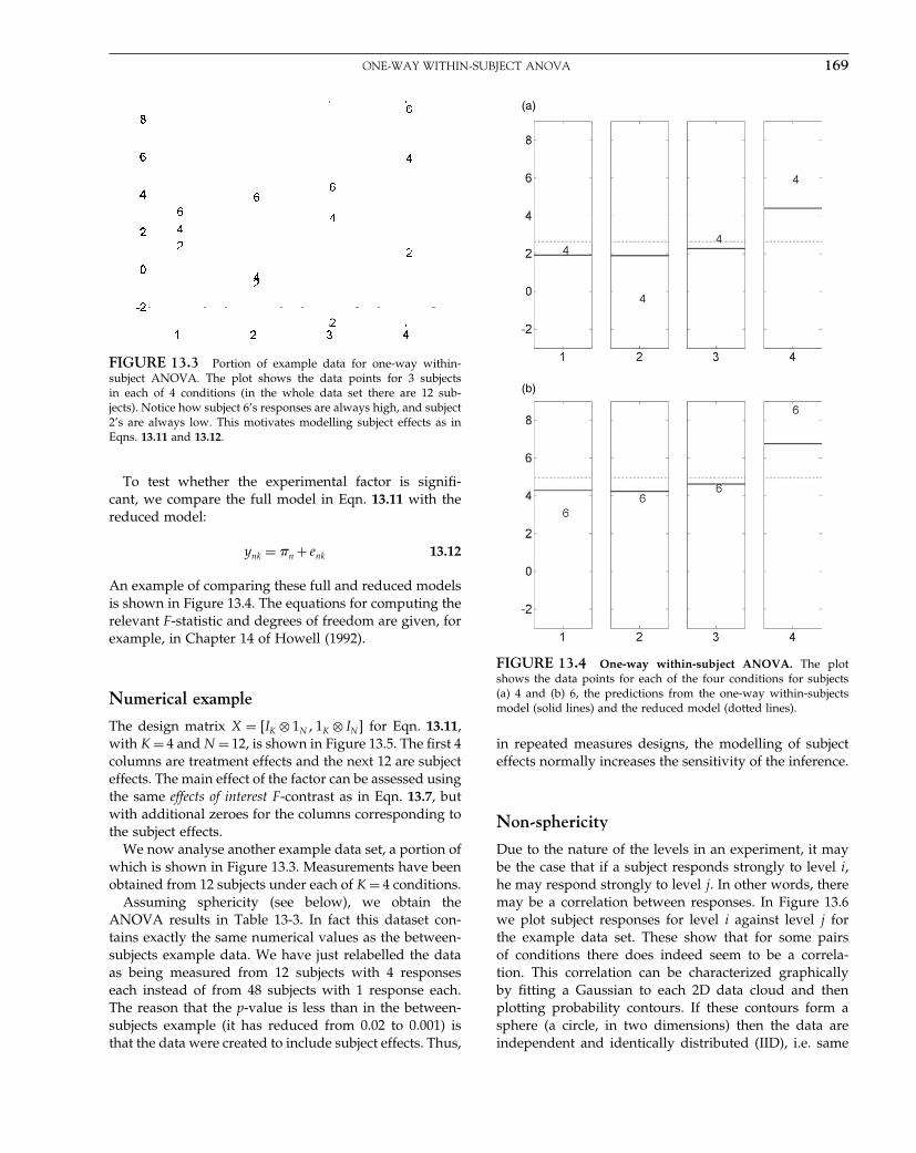
Elsevier UK Chapter: Ch13-P372560 30-9-2006 5:13p.m. Page:169 Trim:7.5in×9.25in
Basal Font:Palatino Margins:Top:40pt Gutter:68pt Font Size:9.5/12 Text Width:42pc Depth:55 Lines
ONE-WAY WITHIN-SUBJECT ANOVA 169
FIGURE 13.3 Portion of example data for one-way within-subject ANOVA. The plot shows the data points for 3 subjectsin each of 4 conditions (in the whole data set there are 12 sub-jects). Notice how subject 6’s responses are always high, and subject2’s are always low. This motivates modelling subject effects as inEqns. 13.11 and 13.12.
To test whether the experimental factor is signifi-cant, we compare the full model in Eqn. 13.11 with thereduced model:
ynk = �n + enk 13.12
An example of comparing these full and reduced modelsis shown in Figure 13.4. The equations for computing therelevant F-statistic and degrees of freedom are given, forexample, in Chapter 14 of Howell (1992).
Numerical example
The design matrix X = IK ⊗ 1N � 1K ⊗ IN � for Eqn. 13.11,with K = 4 and N = 12, is shown in Figure 13.5. The first 4columns are treatment effects and the next 12 are subjecteffects. The main effect of the factor can be assessed usingthe same effects of interest F-contrast as in Eqn. 13.7, butwith additional zeroes for the columns corresponding tothe subject effects.
We now analyse another example data set, a portion ofwhich is shown in Figure 13.3. Measurements have beenobtained from 12 subjects under each of K = 4 conditions.
Assuming sphericity (see below), we obtain theANOVA results in Table 13-3. In fact this dataset con-tains exactly the same numerical values as the between-subjects example data. We have just relabelled the dataas being measured from 12 subjects with 4 responseseach instead of from 48 subjects with 1 response each.The reason that the p-value is less than in the between-subjects example (it has reduced from 0.02 to 0.001) isthat the data were created to include subject effects. Thus,
(a)
(b)
FIGURE 13.4 One-way within-subject ANOVA. The plotshows the data points for each of the four conditions for subjects(a) 4 and (b) 6, the predictions from the one-way within-subjectsmodel (solid lines) and the reduced model (dotted lines).
in repeated measures designs, the modelling of subjecteffects normally increases the sensitivity of the inference.
Non-sphericity
Due to the nature of the levels in an experiment, it maybe the case that if a subject responds strongly to level i,he may respond strongly to level j. In other words, theremay be a correlation between responses. In Figure 13.6we plot subject responses for level i against level j forthe example data set. These show that for some pairsof conditions there does indeed seem to be a correla-tion. This correlation can be characterized graphicallyby fitting a Gaussian to each 2D data cloud and thenplotting probability contours. If these contours form asphere (a circle, in two dimensions) then the data areindependent and identically distributed (IID), i.e. same
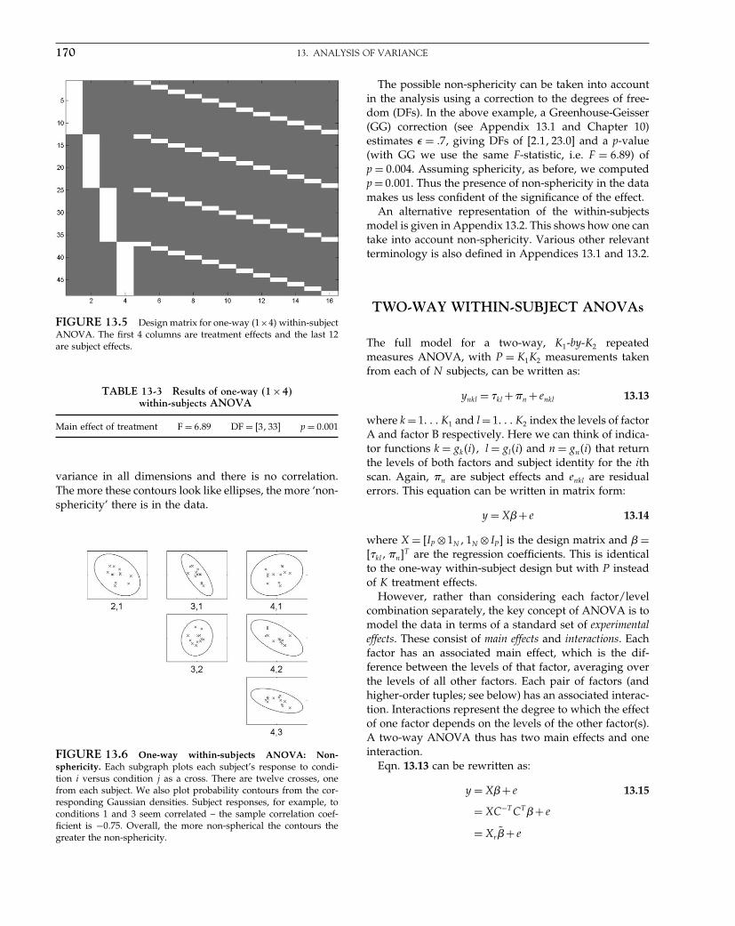
Elsevier UK Chapter: Ch13-P372560 30-9-2006 5:13p.m. Page:170 Trim:7.5in×9.25in
Basal Font:Palatino Margins:Top:40pt Gutter:68pt Font Size:9.5/12 Text Width:42pc Depth:55 Lines
170 13. ANALYSIS OF VARIANCE
FIGURE 13.5 Design matrix for one-way �1×4� within-subjectANOVA. The first 4 columns are treatment effects and the last 12are subject effects.
TABLE 13-3 Results of one-way �1×4�within-subjects ANOVA
Main effect of treatment F = 6�89 DF = 3� 33� p = 0�001
variance in all dimensions and there is no correlation.The more these contours look like ellipses, the more ‘non-sphericity’ there is in the data.
FIGURE 13.6 One-way within-subjects ANOVA: Non-sphericity. Each subgraph plots each subject’s response to condi-tion i versus condition j as a cross. There are twelve crosses, onefrom each subject. We also plot probability contours from the cor-responding Gaussian densities. Subject responses, for example, toconditions 1 and 3 seem correlated – the sample correlation coef-ficient is −0�75. Overall, the more non-spherical the contours thegreater the non-sphericity.
The possible non-sphericity can be taken into accountin the analysis using a correction to the degrees of free-dom (DFs). In the above example, a Greenhouse-Geisser(GG) correction (see Appendix 13.1 and Chapter 10)estimates � = �7, giving DFs of 2�1� 23�0� and a p-value(with GG we use the same F-statistic, i.e. F = 6�89) ofp = 0�004. Assuming sphericity, as before, we computedp = 0�001. Thus the presence of non-sphericity in the datamakes us less confident of the significance of the effect.
An alternative representation of the within-subjectsmodel is given in Appendix 13.2. This shows how one cantake into account non-sphericity. Various other relevantterminology is also defined in Appendices 13.1 and 13.2.
TWO-WAY WITHIN-SUBJECT ANOVAs
The full model for a two-way, K1-by-K2 repeatedmeasures ANOVA, with P = K1K2 measurements takenfrom each of N subjects, can be written as:
ynkl = �kl +�n + enkl 13.13
where k = 1 K1 and l = 1 K2 index the levels of factorA and factor B respectively. Here we can think of indica-tor functions k = gk�i�� l = gl�i� and n = gn�i� that returnthe levels of both factors and subject identity for the ithscan. Again, �n are subject effects and enkl are residualerrors. This equation can be written in matrix form:
y = X+ e 13.14
where X = IP ⊗1N � 1N ⊗ IP� is the design matrix and =�kl��n�T are the regression coefficients. This is identicalto the one-way within-subject design but with P insteadof K treatment effects.
However, rather than considering each factor/levelcombination separately, the key concept of ANOVA is tomodel the data in terms of a standard set of experimentaleffects. These consist of main effects and interactions. Eachfactor has an associated main effect, which is the dif-ference between the levels of that factor, averaging overthe levels of all other factors. Each pair of factors (andhigher-order tuples; see below) has an associated interac-tion. Interactions represent the degree to which the effectof one factor depends on the levels of the other factor(s).A two-way ANOVA thus has two main effects and oneinteraction.
Eqn. 13.13 can be rewritten as:
y = X+ e 13.15
= XC−T CT + e
= Xr̃+ e

Elsevier UK Chapter: Ch13-P372560 30-9-2006 5:13p.m. Page:171 Trim:7.5in×9.25in
Basal Font:Palatino Margins:Top:40pt Gutter:68pt Font Size:9.5/12 Text Width:42pc Depth:55 Lines
TWO-WAY WITHIN-SUBJECT ANOVAs 171
where Xr = XC−T is a rotated design matrix, the regres-sion coefficients are ̃ = CT , and C is a ‘contrast matrix’.This equation is important as it says that the effects ̃ canbe estimated by either (i) fitting the data using a GLMwith design matrix Xr or (ii) fitting the original GLM,with design matrix X, and applying the contrast matrix̃ = CT .
For our two-way within-subjects ANOVA we chooseC such that:
̃ = �Aq � �B
r � �ABqr �m��n�T 13.16
Here, �Aq represents the differences between each succe-
sive level q = 1 �K1 −1� of factor A (e.g. the differencesbetween levels 1 and 2, 2 and 3, 3 and 4 etc.), averagingover the levels of factor B. In other words, the main effectof A is modelled as K1 − 1 differences among K1 levels.The quantity �B
r represents the differences between eachsuccessive level r = 1 �K2 −1� of factor B, averaging overthe levels of factor A; and �AB
qr represents the differencesbetween the differences of each level q = 1 �K1 − 1�of factor A across each level r = 1 �K2 − 1� of factorB. The quantity m is the mean treatment effect. Exam-ples of contrast matrices and rotated design matrices aregiven below.
Pooled versus partitioned errors
In the above model, e is sometimes called a pooled error,since it does not distinguish between different sources oferror for each experimental effect. This is in contrast toan alternative model in which the original residual errore is split into three terms eA
nq� eBnr and eAB
nqr , each specificto a main effect or interaction. This is a different form ofvariance partitioning. Each error term is a random variableand is equivalent to the interaction between that effectand the subject variable.
The F-test for, say, the main effect of factor A is then:
F = SSk/DFk
SSnk/DFnk
13.17
where SSk is the sum of squares for the effect, SSnk isthe sum of squares for the interaction of that effect withsubjects, DFk = K1 −1 and DFnk = N�K1 −1�.
Note that, if there are no more than two levels ofevery factor in an M-way repeated measures ANOVA(i.e., Km = 2 for all m = 1 M), then the covariance of theerrors �e for each effect is a 2-by-2 matrix which neces-sarily has compound symmetry, and so there is no needfor a non-sphericity correction.1 A heuristic for this is
1 Although one could model inhomegeneity of variance.
that there is only one difference q = 1 between two levelsKm = 2. This is not necessarily the case if a pooled erroris used, as in Eqn. 13.15.
Models and null hypotheses
The difference between pooled and partitioned errormodels can be expressed by specifying the relevant mod-els and null hypotheses.
Pooled errors
The pooled error model is given by Eqn. 13.15. For themain effect of A we test the null hypothesis �0 � �A
q = 0 forall q. Similarly, for the main effect of B. For an interactionwe test the null hypothesis �0 � �AB
qr = 0 for all q� r.For example, for the 3-by-3 design shown in Figure 13.7
there are q = 1��2 differential effects for factor A and
FIGURE 13.7 In a 3×3 ANOVA there are 9 cells or conditions.The numbers in the cells correspond to the ordering of the measure-ments when rearranged as a column vector y for a single-subjectgeneral linear model. For a repeated measures ANOVA there are9 measurements per subject. The variable ynkl is the measurementat the kth level of factor A, the lth level of factor B and for the nthsubject. To implement the partitioned error models we use theseoriginal measurements to create differential effects for each subject.The differential effect �A
1 is given by row 1 minus row 2 (or cells 1, 2,3 minus cells 4, 5, 6 – this is reflected in the first row of the contrastmatrix in Eqn. 13.28). The differential effect �A
2 is given by row 2minus row 3. These are used to assess the main effect of A. Simi-larly, to assess the main effect of B we use the differential effects �B
1(column 1 minus column 2) and �B
2 (column 2 minus column 3). Toassess the interaction between A and B, we compute the four ‘sim-ple interaction’ effects �AB
11 (cells (1–4)-(2–5)), �AB12 (cells (2–5)-(3–6)),
�AB21 (cells (4–7)-(5–8)) and �AB
22 (cells (5–8)-(6–9)). These correspondto the rows of the interaction contrast matrix in Eqn. 13.30.

Elsevier UK Chapter: Ch13-P372560 30-9-2006 5:13p.m. Page:172 Trim:7.5in×9.25in
Basal Font:Palatino Margins:Top:40pt Gutter:68pt Font Size:9.5/12 Text Width:42pc Depth:55 Lines
172 13. ANALYSIS OF VARIANCE
r = 1��2 for factor B. The pooled error model thereforehas regression coefficients:
̃ = �A1 � �A
2 � �B1 � �B
2 � �AB11 � �AB
12 � �AB21 � �AB
22 �m��n�T 13.18
For the main effect of A we test the null hypothesis �0 ��A
1 = �A2 = 0. For the interaction we test the null hypothesis
�0 � �AB11 = �AB
12 = �AB21 = �AB
22 = 0.
Partitioned errors
For partitioned errors, we first transform our data setynkl into a set of differential effects for each subject andthen model these in a GLM. This set of differential effectsfor each subject is created using appropriate contrasts atthe ‘first-level’. The models that we describe below thencorrespond to a ‘second-level’ analysis. The differencebetween first and second level analyses are described inthe previous chapter on random effects analysis.
To test for the main effect of A, we first create the newdata points �nq which are the differential effects betweenthe levels in A for each subject n. We then compare thefull model:
�nq = �Aq + enq
to the reduced model �nq = enq . We are therefore testingthe null hypothesis, �0 � �A
q = 0 for all q.Similarly for the main effect of B. To test for an inter-
action, we first create the new data points �nqr which arethe differences of differential effects for each subject. Fora K1 by K2 ANOVA there will be �K1 −1��K2 −1� of these.We then compare the full model:
�nqr = �ABqr + enqr
to the reduced model �nqr = enqr . We are therefore testingthe null hypothesis, �0 � �AB
qr = 0 for all q� r.For example, for a 3-by-3 design, there are q = 1��2
differential effects for factor A and r = 1��2 for factor B.We first create the differential effects �nq . To test for themain effect of A we compare the full model:
�nq = �A1 +�A
2 + enq
to the reduced model �nq = enq . We are therefore testingthe null hypothesis, �0 � �A
1 = �A2 = 0. Similarly for the
main effect of B.To test for an interaction we first create the differences
of differential effects for each subject. There are 2×2 = 4of these. We then compare the full model:
�nqr = �AB11 +�AB
12 +�AB21 +�AB
22 + enqr
to the reduced model �nqr = enqr . We are therefore testingthe null hypothesis, �0 � �AB
11 = �AB12 = �AB
21 = �AB22 = 0� i.e.
that all the ‘simple’ interactions are zero. See Figure 13.7for an example with a 3-by-3 design.
Numerical example
Pooled error
Consider a 2 × 2 ANOVA of the same data used in theprevious examples, with K1 = K2 = 2� P = K1K2 = 4� N =12� J = PN = 48. The design matrix for Eqn. 13.15 witha pooled error term is the same as that in Figure 13.5,assuming that the four columns/conditions are ordered:
1 2 3 4A1B1 A1B2 A2B1 A2B2
13.19
where A1 represents the first level of factor A� B2 repre-sents the second level of factor B etc., and the rows areordered; all subjects data for cell A1B1; all for A1B2 etc.The basic contrasts for the three experimental effects areshown in Table 13-4 with the contrast weights for thesubject-effects in the remaining columns 5–16 set to 0.
Assuming sphericity, the resulting F-tests give theANOVA results in Table 13-5. With a Greenhouse-Geissercorrection for non-sphericity, on the other hand, � is esti-mated as 0.7, giving the ANOVA results in Table 13-6.
Main effects are not really meaningful in the presenceof a significant interaction. In the presence of an interac-tion, one does not normally report the main effects, butproceeds by testing the differences between the levels ofone factor for each of the levels of the other factor in theinteraction (so-called simple effects). In this case, the pres-ence of a significant interaction could be used to justifyfurther simple effect contrasts (see above), e.g. the effectof B at the first and second levels of A are given by thecontrasts c = 1�−1� 0� 0�T and c = 0� 0� 1�−1�T .
Equivalent results would be obtained if the designmatrix were rotated so that the first three columns reflectthe experimental effects plus a constant term in the fourthcolumn (only the first four columns would be rotated).This is perhaps a better conception of the ANOVAapproach, since it is closer to Eqn. 13.15, reflecting the
TABLE 13-4 Contrasts for experimentaleffects in a two-way ANOVA
Main effect of A [1 1 −1 −1]Main effect of B [1 −1 1 −1]Interaction, A ×B [1 −1 −1 1]
TABLE 13-5 Results of 2×2 within-subject ANOVA withpooled error assuming sphericity
Main effect of A F = 9�83 DF = 1� 33� p = 0�004Main effect of B F = 5�21 DF = 1� 33� p = 0�029Interaction, A ×B F = 5�64 DF = 1� 33� p = 0�024

Elsevier UK Chapter: Ch13-P372560 30-9-2006 5:13p.m. Page:173 Trim:7.5in×9.25in
Basal Font:Palatino Margins:Top:40pt Gutter:68pt Font Size:9.5/12 Text Width:42pc Depth:55 Lines
GENERALIZATION TO M-WAY ANOVAs 173
TABLE 13-6 Results of 2×2 within-subject ANOVA withpooled error using Greenhouse-Geisser correction
Main effect of A F = 9�83 DF = 0�7� 23�0� p = 0�009Main effect of B F = 5�21 DF = 0�7� 23�0� p = 0�043Interaction, A ×B F = 5�64 DF = 0�7� 23�0� p = 0�036
conception of factorial designs in terms of the experi-mental effects rather than the individual conditions. Thisrotation is achieved by setting the new design matrix:
Xr = X
[CT 04�12
012�4 I12
]13.20
where
CT =
⎡⎢⎢⎣
−1 −1 1 1−1 1 −1 1
1 −1 −1 11 1 1 1
⎤⎥⎥⎦ 13.21
Notice that the rows of CT are identical to the con-trasts for the main effects and interactions plus aconstant term (cf. Table 13-4). This rotated designmatrix is shown in Figure 13.8. The three experimen-tal effects can now be tested by the contrast weights1� 0� 0� 0�T � 0� 1� 0� 0�T � 0� 0� 1� 0�T (again, padded withzeroes).
In this example, each factor only has two levels whichresults in one-dimensional contrasts for testing main
FIGURE 13.8 Design matrix for 2×2 within-subject ANOVA.This design is the same as in Figure 13.5 except that the first fourcolumns are rotated. The rows are ordered all subjects for cell A1B1,all for A1B2 etc. White, grey and black represent 1, 0 and −1. Thefirst four columns model the main effect of A, the main effect of B,the interaction between A and B and a constant term. The last 12columns model subject effects. This model is a GLM instantiationof Eqn. 13.15.
TABLE 13-7 Results of ANOVA using partitioned errors
Main effect of A F = 12�17 DF = 1� 11� p = 0�005Main effect of B F = 11�35 DF = 1� 11� p = 0�006Interaction, A ×B F = 3�25 DF = 1� 11� p = 0�099
effects and interactions. The contrast weights form a vec-tor. But factors with more than two levels require multi-dimensional contrasts. Main effects, for example, can beexpressed as a linear combination of differences betweensuccessive levels (e.g. between levels 1 and 2, and 2and 3). The contrast weights therefore form a matrix. Anexample using a 3-by-3 design is given later on.
Partitioned errors
Partitioned error models can be implemented by apply-ing contrasts to the data, and then creating a separatemodel (i.e. separate GLM analysis) to test each effect.In other words, a two-stage approach can be taken, asdescribed in the previous chapter on random effects anal-ysis. The first stage is to create contrasts of the condi-tions for each subject, and the second stage is to putthese contrasts or ‘summary statistics’ into a model witha block-diagonal design matrix.
Using the example dataset, and analogous contrasts forthe main effect of B and for the interaction, we get theresults in Table 13-7. Note how (1) the degrees of free-dom have been reduced relative to Table 13-5, being splitequally among the three effects; (2) there is no need for anon-sphericity correction in this case (since K1 = K2 = 2,see above); and (3) the p-values for some of the effectshave decreased relative to Tables 13-5 and 13-6, whilethose for the other effects have increased. Whether p-values increase or decrease depends on the nature of thedata (particularly correlations between conditions acrosssubjects), but in many real data sets partitioned errorcomparisons yield more sensitive inferences. This is why,for repeated-measures analyses, the partitioning of theerror into effect-specific terms is normally preferred overusing a pooled error (Howell, 1992). But the partitionederror approach requires a new model to be specified forevery effect we want to test.
GENERALIZATION TO M-WAY ANOVAs
The above examples can be generalized to M-wayANOVAs. For a K1-by-K2-..-by-KM design, there are
P =M∏
m=1
Km 13.22
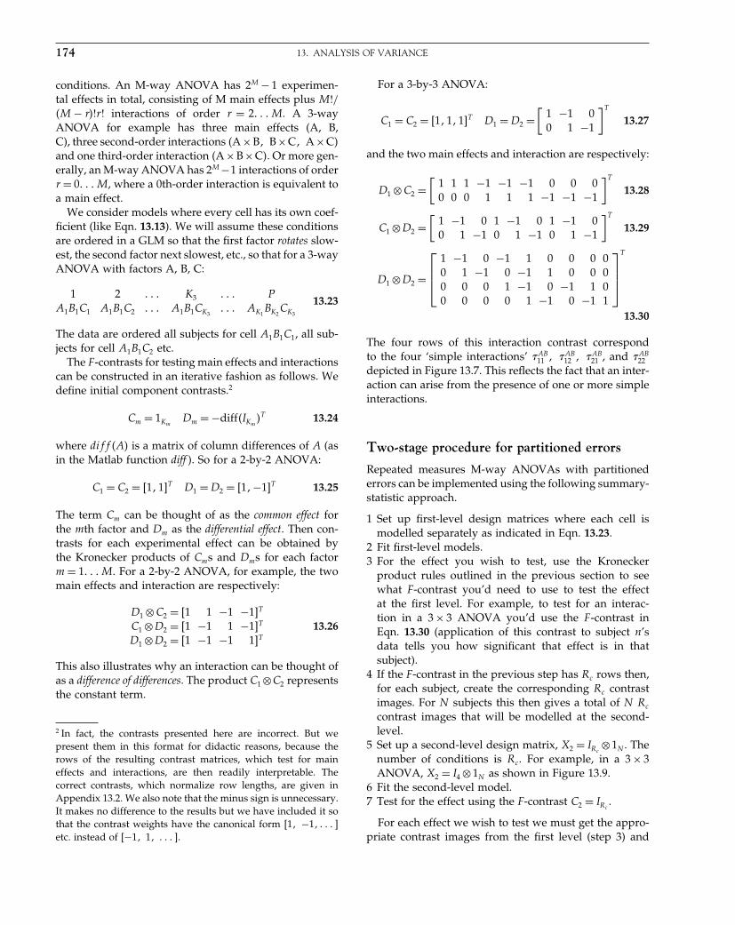
Elsevier UK Chapter: Ch13-P372560 30-9-2006 5:13p.m. Page:174 Trim:7.5in×9.25in
Basal Font:Palatino Margins:Top:40pt Gutter:68pt Font Size:9.5/12 Text Width:42pc Depth:55 Lines
174 13. ANALYSIS OF VARIANCE
conditions. An M-way ANOVA has 2M − 1 experimen-tal effects in total, consisting of M main effects plus M!/�M − r�!r! interactions of order r = 2 M . A 3-wayANOVA for example has three main effects (A, B,C), three second-order interactions �A ×B� B×C� A ×C�and one third-order interaction �A ×B×C�. Or more gen-erally, an M-way ANOVA has 2M −1 interactions of orderr = 0 M , where a 0th-order interaction is equivalent toa main effect.
We consider models where every cell has its own coef-ficient (like Eqn. 13.13). We will assume these conditionsare ordered in a GLM so that the first factor rotates slow-est, the second factor next slowest, etc., so that for a 3-wayANOVA with factors A, B, C:
1 2 K3 PA1B1C1 A1B1C2 A1B1CK3
AK1BK2
CK3
13.23
The data are ordered all subjects for cell A1B1C1, all sub-jects for cell A1B1C2 etc.
The F -contrasts for testing main effects and interactionscan be constructed in an iterative fashion as follows. Wedefine initial component contrasts.2
Cm = 1KmDm = −diff�IKm
�T 13.24
where diff�A� is a matrix of column differences of A (asin the Matlab function diff ). So for a 2-by-2 ANOVA:
C1 = C2 = 1� 1�T D1 = D2 = 1�−1�T 13.25
The term Cm can be thought of as the common effect forthe mth factor and Dm as the differential effect. Then con-trasts for each experimental effect can be obtained bythe Kronecker products of Cms and Dms for each factorm = 1 M . For a 2-by-2 ANOVA, for example, the twomain effects and interaction are respectively:
D1 ⊗C2 = 1 1 −1 −1�T
C1 ⊗D2 = 1 −1 1 −1�T
D1 ⊗D2 = 1 −1 −1 1�T
13.26
This also illustrates why an interaction can be thought ofas a difference of differences. The product C1 ⊗C2 representsthe constant term.
2 In fact, the contrasts presented here are incorrect. But wepresent them in this format for didactic reasons, because therows of the resulting contrast matrices, which test for maineffects and interactions, are then readily interpretable. Thecorrect contrasts, which normalize row lengths, are given inAppendix 13.2. We also note that the minus sign is unnecessary.It makes no difference to the results but we have included it sothat the contrast weights have the canonical form 1� −1� �etc. instead of −1� 1� �.
For a 3-by-3 ANOVA:
C1 = C2 = 1� 1� 1�T D1 = D2 =[
1 −1 00 1 −1
]T
13.27
and the two main effects and interaction are respectively:
D1 ⊗C2 =[
1 1 1 −1 −1 −1 0 0 00 0 0 1 1 1 −1 −1 −1
]T
13.28
C1 ⊗D2 =[
1 −1 0 1 −1 0 1 −1 00 1 −1 0 1 −1 0 1 −1
]T
13.29
D1 ⊗D2 =
⎡⎢⎢⎣
1 −1 0 −1 1 0 0 0 00 1 −1 0 −1 1 0 0 00 0 0 1 −1 0 −1 1 00 0 0 0 1 −1 0 −1 1
⎤⎥⎥⎦
T
13.30
The four rows of this interaction contrast correspondto the four ‘simple interactions’ �AB
11 � �AB12 � �AB
21 , and �AB22
depicted in Figure 13.7. This reflects the fact that an inter-action can arise from the presence of one or more simpleinteractions.
Two-stage procedure for partitioned errors
Repeated measures M-way ANOVAs with partitionederrors can be implemented using the following summary-statistic approach.
1 Set up first-level design matrices where each cell ismodelled separately as indicated in Eqn. 13.23.
2 Fit first-level models.3 For the effect you wish to test, use the Kronecker
product rules outlined in the previous section to seewhat F-contrast you’d need to use to test the effectat the first level. For example, to test for an interac-tion in a 3 × 3 ANOVA you’d use the F -contrast inEqn. 13.30 (application of this contrast to subject n’sdata tells you how significant that effect is in thatsubject).
4 If the F-contrast in the previous step has Rc rows then,for each subject, create the corresponding Rc contrastimages. For N subjects this then gives a total of N Rc
contrast images that will be modelled at the second-level.
5 Set up a second-level design matrix, X2 = IRc⊗1N . The
number of conditions is Rc. For example, in a 3 × 3ANOVA, X2 = I4 ⊗1N as shown in Figure 13.9.
6 Fit the second-level model.7 Test for the effect using the F-contrast C2 = IRc
.
For each effect we wish to test we must get the appro-priate contrast images from the first level (step 3) and
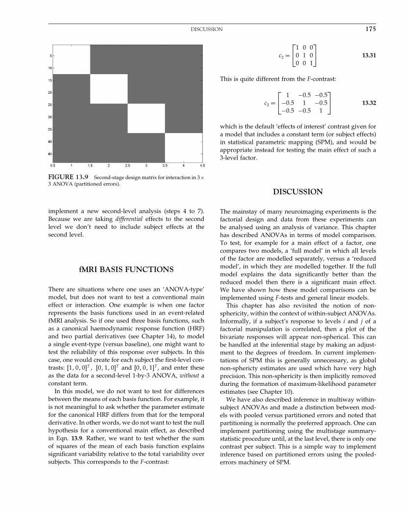
Elsevier UK Chapter: Ch13-P372560 30-9-2006 5:13p.m. Page:175 Trim:7.5in×9.25in
Basal Font:Palatino Margins:Top:40pt Gutter:68pt Font Size:9.5/12 Text Width:42pc Depth:55 Lines
DISCUSSION 175
FIGURE 13.9 Second-stage design matrix for interaction in 3×3 ANOVA (partitioned errors).
implement a new second-level analysis (steps 4 to 7).Because we are taking differential effects to the secondlevel we don’t need to include subject effects at thesecond level.
fMRI BASIS FUNCTIONS
There are situations where one uses an ‘ANOVA-type’model, but does not want to test a conventional maineffect or interaction. One example is when one factorrepresents the basis functions used in an event-relatedfMRI analysis. So if one used three basis functions, suchas a canonical haemodynamic response function (HRF)and two partial derivatives (see Chapter 14), to modela single event-type (versus baseline), one might want totest the reliability of this response over subjects. In thiscase, one would create for each subject the first-level con-trasts: 1� 0� 0�T � 0� 1� 0�T and 0� 0� 1�T , and enter theseas the data for a second-level 1-by-3 ANOVA, without aconstant term.
In this model, we do not want to test for differencesbetween the means of each basis function. For example, itis not meaningful to ask whether the parameter estimatefor the canonical HRF differs from that for the temporalderivative. In other words, we do not want to test the nullhypothesis for a conventional main effect, as describedin Eqn. 13.9. Rather, we want to test whether the sumof squares of the mean of each basis function explainssignificant variability relative to the total variability oversubjects. This corresponds to the F-contrast:
c2 =⎡⎣1 0 0
0 1 00 0 1
⎤⎦ 13.31
This is quite different from the F-contrast:
c2 =⎡⎣ 1 −0�5 −0�5
−0�5 1 −0�5−0�5 −0�5 1
⎤⎦ 13.32
which is the default ‘effects of interest’ contrast given fora model that includes a constant term (or subject effects)in statistical parametric mapping (SPM), and would beappropriate instead for testing the main effect of such a3-level factor.
DISCUSSION
The mainstay of many neuroimaging experiments is thefactorial design and data from these experiments canbe analysed using an analysis of variance. This chapterhas described ANOVAs in terms of model comparison.To test, for example for a main effect of a factor, onecompares two models, a ‘full model’ in which all levelsof the factor are modelled separately, versus a ‘reducedmodel’, in which they are modelled together. If the fullmodel explains the data significantly better than thereduced model then there is a significant main effect.We have shown how these model comparisons can beimplemented using F-tests and general linear models.
This chapter has also revisited the notion of non-sphericity, within the context of within-subject ANOVAs.Informally, if a subject’s response to levels i and j of afactorial manipulation is correlated, then a plot of thebivariate responses will appear non-spherical. This canbe handled at the inferential stage by making an adjust-ment to the degrees of freedom. In current implemen-tations of SPM this is generally unnecessary, as globalnon-sphericty estimates are used which have very highprecision. This non-sphericity is then implicitly removedduring the formation of maximum-likelihood parameterestimates (see Chapter 10).
We have also described inference in multiway within-subject ANOVAs and made a distinction between mod-els with pooled versus partitioned errors and noted thatpartitioning is normally the preferred approach. One canimplement partitioning using the multistage summary-statistic procedure until, at the last level, there is only onecontrast per subject. This is a simple way to implementinference based on partitioned errors using the pooled-errors machinery of SPM.

Elsevier UK Chapter: Ch13-P372560 30-9-2006 5:13p.m. Page:176 Trim:7.5in×9.25in
Basal Font:Palatino Margins:Top:40pt Gutter:68pt Font Size:9.5/12 Text Width:42pc Depth:55 Lines
176 13. ANALYSIS OF VARIANCE
APPENDIX 13.1THE KRONECKER PRODUCT
If A is an m1 ×m2 matrix and B is an n1 ×n2 matrix, thenthe Kronecker product of A and B is the �m1n1�× �m2n2�matrix:
A⊗B =⎡⎣ a11B a1m2
B
am11B am1m2B
⎤⎦ 13.33
Circularity
A covariance matrix � is circular if:
�ii +�jj −2�ij = 2� 13.34
for all i� j.
Compound symmetry
If all the variances are equal to �1 and all the covariancesare equal to �2 then we have compound symmetry.
Non-sphericity
If � is a K×K covariance matrix and the first K−1 eigen-values are identically equal to:
� = 0�5��ii +�jj −2�ij� 13.35
then � is spherical. Every other matrix is non-spherical orhas non-sphericity.
Greenhouse-Geisser correction
For a 1-way ANOVA between subjects with N subjectsand K levels the overall F-statistic is approximately dis-tributed as:
F �K −1��� �N −1��K −1��� 13.36
where
� = �∑K−1
i=1 �i�2
�K −1�∑K−1
i=1 �2i
13.37
and �i are the eigenvalues of the normalized matrix�z where
�z = MT �yM 13.38
and M is a K by K − 1 matrix with orthogonal columns(e.g. the columns are the first K −1 eigenvectors of �y).
APPENDIX 13.2WITHIN-SUBJECT MODELS
The model in Eqn. 13.11 can also be written as:
yn = 1K�n +� + en 13.39
where yn is now the K ×1 vector of measurements fromthe nth subject, 1K is a K ×1 vector of 1s, and � is a K ×1vector with kth entry �k and en is a K ×1 vector with kthentry enk where:
p�en� = N�0��e� 13.40
We have a choice as to whether to treat the subjecteffects �n as fixed-effects or random-effects. If we chooserandom-effects then:
p��n� = N����2�� 13.41
and overall we have a mixed-effects model as the typicalresponse for subject n� �n, is viewed as a random variablewhereas the typical response to treatment k� �k, is not arandom variable. The reduced model is:
yn = 1K�n + en 13.42
For the full model we can write:
p�y� =N∏
n=1
p�yn� 13.43
p�yn� = N�my��y�
and
my = 1K�+� 13.44
�y = 1K�2�1T
K +�e
if the subject effects are random effects, and �y = �e oth-erwise. If �e = �2
e IK then �y has compound symmetry. It isalso spherical (see Appendix 13.1). For K = 4 for example:
�y =
⎡⎢⎢⎣
�2� +�2
e �2� �2
� �2�
�2� �2
� +�2e �2
� �2�
�2� �2
� �2� +�2
e �2�
�2� �2
� �2� �2
� +�2e
⎤⎥⎥⎦ 13.45
If we let �y = ��2� +�2
e �Ry then:
Ry =
⎡⎢⎢⎣
1 � � �� 1 � �� � 1 �� � � 1
⎤⎥⎥⎦ 13.46

Elsevier UK Chapter: Ch13-P372560 30-9-2006 5:13p.m. Page:177 Trim:7.5in×9.25in
Basal Font:Palatino Margins:Top:40pt Gutter:68pt Font Size:9.5/12 Text Width:42pc Depth:55 Lines
REFERENCES 177
where
� = �2�
�2� +�2
e
13.47
For a more general �e, however, �y will be non-spherical. In this case, we can attempt to correct for thenon-sphericity. One approach is to reduce the degrees offreedom by a factor 1
K−1 ≤ � ≤ 1, which is an estimate ofthe degree of non-sphericity of �y (the Greenhouse-Geissercorrection; see Appendix 13.1). Various improvementsof this correction (e.g. Huhn-Feldt) have also been sug-gested (Howell, 1992). Another approach is to parameter-ize explicitly the error covariance matrix �e using a linearexpansion and estimate the parameters using ReML, asdescribed in Chapter 22.
Contrasts for M-way ANOVAs
The contrasts presented in the section ‘Generaliza-tion to M-way ANOVAs’ are actually incorrect. Theywere presented in a format that allowed the rows ofthe resulting contrast matrices, which test for maineffects and interactions, to be readily interpretable.We now give the correct contrasts, which derivefrom speciying the initial differential component con-trast as:
Dm = −orth�diff�IKm�T � 13.48
where orth�A� is the orthonormal basis of A (as in theMatlab function orth). This is identical to the expressionin the main text but with the addition of an orth func-tion which is necessary to ensure that the length of thecontrast vector is unity.
This results in the following contrasts for the 2-by-2ANOVA:
C1 = C2 = 1� 1�T D1 = D2 = 0�71�−0�71�T 13.49
D1 ⊗C2 = 0�71 0�71 −0�71 −0�71�T
C1 ⊗D2 = 0�71 −0�71 0�71 −0�71�T
D1 ⊗D2 = 0�71 −0�71 −0�71 0�71�T
13.50
For the 3-by-3 ANOVA:
C1 = C2 = 1� 1� 1�T D1 = D2 =[
0�41 −0�82 0�410�71 0�00 −0�71
]T
13.51
and the two main effects and interaction are respectively:
D1 ⊗C2 =[
0�41 0�41 0�41 −0�82 −0�820�71 0�71 0�71 0 0
−0�82 0�41 0�41 0�410 −0�71 −0�71 −0�71
]T
13.52
C1 ⊗D2 =[
0�41 −0�82 0�41 0�41 −0�820�71 0 −0�71 0�71 0
0�41 0�41 −0�82 0�41−0�71 0�71 0 −0�71
]T
13.53
D1 ⊗D2 =
⎡⎢⎢⎣
0�17 −0�33 0�17 −0�33 0�670�29 0 −0�29 −0�58 00�29 −0�58 0�29 0 00�5 0 −0�5 0 0
−0�33 0�17 −0�33 0�170�58 0�29 0 −0�29
0 −0�29 0�58 −0�290 −0�5 0 0�5
⎤⎥⎥⎦
T
13.54
REFERENCES
Howell DC (1992) Statistical methods for psychology. Duxbury Press,Belmont California.
Winer BJ, Brown DR, Michels KM (1991) Statistical principles inexperimental design. McGraw-Hill.

Elsevier UK Chapter: Ch14-P372560 30-9-2006 5:14p.m. Page:178 Trim:7.5in×9.25in
Basal Font:Palatino Margins:Top:40pt Gutter:68pt Font Size:9.5/12 Text Width:42pc Depth:55 Lines
C H A P T E R
14
Convolution Models for fMRIR. Henson and K. Friston
INTRODUCTION
This chapter reviews issues specific to the analysis offunctional magnetic resonance imaging (fMRI) data. Itextends the general linear model (GLM) introduced inChapter 8 to convolution models, in which the bloodoxygenation-level-dependent (BOLD) signal is modelledby neuronal causes that are expressed via a haemody-namic response function (HRF). We begin by consideringlinear convolution models and introduce the concept oftemporal basis functions. We then consider the relatedissues of temporal filtering and temporal autocorrelation.Finally, we extend the convolution model to include non-linear terms and conclude with some example analysesof fMRI data.
THE HAEMODYNAMIC RESPONSEFUNCTION (HRF)
A typical BOLD response to a single, impulsive stimula-tion (‘event’) is shown in Figure 14.1. The response peaksapproximately 5 s after stimulation, and is followed byan undershoot that lasts as long as 30 s (at high magneticfields, an initial undershoot can sometimes be observed)(Malonek and Ginvald, 1996). Early event-related studiestherefore used a long time between events (i.e. a longstimulus onset asynchrony (SOA)) to allow the responseto return to baseline between stimulations. However,although the responses to successive events will overlapat shorter SOAs, this overlap can be modelled explicitlywithin the GLM via a convolution model and an HRF,as described below. Short SOAs of a few seconds aredesirable because they are comparable to those typicallyused in behavioural and electrophysiological studies, and
because they are generally more efficient from a statisticalperspective, as we will see in the next chapter.
The shape of the BOLD impulse response appears sim-ilar across early sensory regions, such as V1 (Boyntonet al., 1996), A1 (Josephs et al., 1997) and S1 (Zarahnet al., 1997a). However, the precise shape has been shownto vary across the brain, particularly in higher corticalregions (Schacter et al., 1997), presumably due mainlyto variations in the vasculature of different regions (Leeet al., 1995). Moreover, the BOLD response appears tovary considerably across people (Aguirre et al., 1998).1
Initial dip
Undershoot
Peak
Sig
nal c
hang
e (%
)
PST (s)
Dispersion
Spe
ctra
l den
sity
Frequency (Hz)0
00.05 0.1 0.15 0.2 0.25
0
0
8 16 24 32
FIGURE 14.1 Typical (canonical) BOLD impulse response(power spectrum inset).
1 This has prompted some to use subject-specific HRFs derivedfrom a reference region known to respond to a specific task,(e.g. from central sulcus during a simple manual task performedduring a pilot scan on each subject; Aguirre et al., 1998). How-ever, while this allows for inter-subject variability, it does notallow for inter-regional variability within subjects (or potentialerror in estimation of the reference response).
Statistical Parametric Mapping, by Karl Friston et al. Copyright 2007, Elsevier Ltd. All rights reserved.ISBN–13: 978-0-12-372560-8 ISBN–10: 0-12-372560-7
178

Elsevier UK Chapter: Ch14-P372560 30-9-2006 5:14p.m. Page:179 Trim:7.5in×9.25in
Basal Font:Palatino Margins:Top:40pt Gutter:68pt Font Size:9.5/12 Text Width:42pc Depth:55 Lines
THE HAEMODYNAMIC RESPONSE FUNCTION (HRF) 179
These types of variability can be accommodated byexpressing the HRF in terms of a set of temporal basisfunctions.
A linear convolution model assumes that successiveresponses summate (superpose). However, there is goodevidence for non-linearity in the amplitude of the BOLDresponse, as a function of the stimulus duration or stim-ulus magnitude (e.g. Vasquez and Noll, 1998), and asa function of SOA (Pollmann et al., 1998; Friston et al.,1998a; Miezin et al., 2000). These non-linearities alsoappear to vary across different brain regions (Birn et al.2001; Huettel and McCarthy, 2001). The non-linearityfound as a function of SOA is typically a ‘saturation’whereby the response to a run of events is smaller thanwould be predicted by the summation of responses toeach event alone. This saturation is believed to arise inthe mapping from blood flow to BOLD signal (Fristonet al., 2000a), though may also have a neuronal locus,particularly for very short SOAs or long stimulus dura-tions (for biophysical models that incorporate such non-linearities, see Chapter 27). Saturation has been found forSOAs below approximately 8 s, and the degree of satura-tion increases as the SOA decreases. For typical SOAs of2–4 s, however, its magnitude can be small (typically lessthan 20 per cent) (Miezin et al., 2000). Later we will seehow the linear convolution model is extended to handlesuch non-linearities via a Volterra expansion.
Linear time-invariant (convolution) models
It is useful to treat a session of fMRI scans as a time-series. This is because the data tend to be correlatedacross successive scans, given that the typical measure-ment interval, TR, of 1–3 s, is less than the duration of theBOLD response. The GLM can be expressed as a functionof time (Friston et al., 1994):
y�t� = X�t��+��t� 14.1
��t� ∼ N�0��2��
where the data, y�t�, comprise the fMRI time-series, theexplanatory variables, X�t� are now functions of time, �are (time-invariant) parameters, and � is the noise auto-correlation. Though y�t� and X�t� are really discrete (sam-pled) time-series (normally represented by the vectory anddesign matrix X respectively), we will initially treat thedata and model in terms of continuous time. For simplicity,we will consider the case of a single cause or regressor.
The explanatory variables X�t� represents the predictedBOLD time course arising from neuronal activity, u�t�,up to some scaling factor. This neuronal activity (e.g. themean synaptic activity of an ensemble of neurons – seeChapter 32) is assumed to be caused by a sequence of
experimental manipulations and is usually referred to asthe stimulus function. If we assume that the BOLD sig-nal is the output of a linear time-invariant (LTI) system(Boynton et al., 1996), i.e. that the BOLD response to abrief input has a finite duration and is independent oftime, and that the responses to successive inputs super-pose in a linear fashion, then we can express X�t� as theconvolution of the stimulus function with an impulseresponse, or HRF, h�t�:
X�t� = u�t�⊗h�� =T∫
0
u�t −�h��d 14.2
where indexes the peristimulus time (PST), over whichthe BOLD impulse response is expressed. The HRF isequivalent to the first-order Volterra kernel describedbelow. The stimulus function u�t� is usually a stick-function or boxcar function encoding the occurrence ofan event or epoch. The result of convolving a randomsequence of neuronal events with a ‘canonical’ HRF (seeFigure 14.1) is shown in Figure 14.2(a). The smoothness ofthe resulting response is why the HRF is often viewed asa low-pass filter. The result of convolving more sustainedperiods of neuronal activity (called epochs in SPM) withthe canonical HRF is shown in Figure 14.2(b). Note thatthe dominant effect of increasing the duration of neu-ronal activity, up to a few seconds, is to increase the peakamplitude of the BOLD response. In other words, theBOLD response integrates neuronal activity over a fewseconds. The corollary is that a difference in the ampli-tude of the BOLD response (as tested conventionally)does not necessarily imply a difference in the mean levelof neuronal activity: the difference could reflect differ-ent durations of neuronal activity at same mean level.One way to distinguish between these scenarios is to testfor differences in the peak latency of the BOLD impulseresponse (Henson and Rugg, 2001).
In practice, the convolution must be performed in dis-crete time. Given that significant information may exist inthe predicted BOLD time course beyond that captured bytypical TRs of 1–3 s, SPM performs the convolution at ahigher temporal resolution withN time points per scan (i.e.withresolution,t = TR/N seconds).Thismeans, forexam-ple, that stimulus onsets do not need to be synchronizedwith scans (they can be specified in fractions of scans).2 Tocreate the explanatory variables, the predicted BOLD timecourse is then down-sampled every TR with reference to aspecified time point T0 (Plate 8, see colour plate section).
2 In SPM, an ‘event’ is defined as having a duration of 0, which inpractice corresponds to a single non-zero value for one time binof duration t, where the value of the stimulus function is 1/t.For epochs, the stimulus function is scaled so that it sums to oneover a second.

Elsevier UK Chapter: Ch14-P372560 30-9-2006 5:14p.m. Page:180 Trim:7.5in×9.25in
Basal Font:Palatino Margins:Top:40pt Gutter:68pt Font Size:9.5/12 Text Width:42pc Depth:55 Lines
180 14. CONVOLUTION MODELS FOR fMRI
FIGURE 14.2 Linear convolution with acanonical HRF illustrated for (a) randomlypresented events, and (b) epochs of neuronalactivity with durations increasing from 200 msto 16 s.
⊗
⊗
Time (s)
Time (s)
=
=
Time (s)
Time (s)
(a)
(b)
Peristimulus time (s)
Peristimulus time (s)
Stimulus function HRF Predicted time course
0 16 32 48 64 80 0
0 10 20 30
16 32 48 64 800 5 10 15 20 25 30
0 5 10 15 20 25 300 2 4 86 10
0
0
0
0
0
8s
4s
2s
1s
0.5s
0.2s
TEMPORAL BASIS FUNCTIONS
Given that the precise shape of the HRF may vary overbrain regions and over individuals, variability in its shapeneeds to be accommodated. The simplest way to achievethis within the GLM is via an expansion in terms of Ktemporal basis functions, fk��:
h�� =K∑
k=1
�kfk�� 14.3
If the stimulation and resulting neuronal activity were asequence of J impulses at times oj , we can construct astimulus stick-function:
u�t� =J∑
j=1
�j��t −oj� 14.4
where ��t� is the Dirac delta function. Note that vari-ations in the stimulus – for example, its magnitude �j
on each trial – can be accommodated by modulating thedelta-functions, prior to convolution with the HRF. Theseare called ‘parametric modulations’ in SPM. We will seean example of this parametric modulation in the lastsection. It is quite common to use a series of modulatedstick-functions to model a single event type by using apolynomial or other expansions of �j . For simplicity, wewill assume that �j = 1 (i.e. a zeroth-order term).
Having specified the form of the stimulus and haemo-dynamic response functions in this way, the GLM equa-tion in Eqn. 14.1 can be written:
y�t� =J∑
j=1
K∑k=1
�kfk�t −oj�+��t� 14.5
where �k are the parameters to be estimated. Severaltemporal basis sets are offered in SPM, though not allare true ‘basis’ sets in the (mathematical) sense that theyspan the space of all possible impulse response shapes(over the finite duration of that response); the term ‘basis’is used to reflect the user’s assumption that the set offunctions chosen capture BOLD impulse response shapesthat occur in reality.
FIR and Fourier sets
The most flexible basis sets are the finite impulse response(FIR) and Fourier basis sets, which make the leastassumptions about the shape of the response. The FIRset consists of contiguous boxcar functions of PST, eachlasting T/KFIR seconds (see Plate 9(a)), where T is dura-tion of the HRF. The Fourier set (see Plate 9(b)) consistsof a constant and KF sine and KF cosine functions of har-monic periods T�T/2� �T/KF seconds (i.e. K = 2 KF +1basis functions). Linear combinations of the (orthonor-mal) FIR or Fourier basis functions can capture any shapeof response up to a specified timescale (T/KFIR in thecase of the FIR) or frequency (KF /T in the case of theFourier set).
Relationship between FIR and ‘selective averaging’
In practice, there is little to choose between the FIR andFourier sets. The Fourier set can be better suited whenthe sampling of peristimulus time (as determined by therelationship between the SOA and TR) is non-uniform,whereas the parameter estimates for the FIR functionshave a more direct interpretation in terms of the ‘aver-aged’ peristimulus time histogram (PSTH). Indeed, in the

Elsevier UK Chapter: Ch14-P372560 30-9-2006 5:14p.m. Page:181 Trim:7.5in×9.25in
Basal Font:Palatino Margins:Top:40pt Gutter:68pt Font Size:9.5/12 Text Width:42pc Depth:55 Lines
TEMPORAL BASIS FUNCTIONS 181
special case when T/KFIR = TR = t, the FIR functions canbe considered as approximate delta-functions:
h�� =K∑
k=1
�k�� −k� 14.6
where ranges over post-stimulus scans. Then the modelbecomes (with some abuse of the delta-function):
y�t� =J∑
j=1
K∑k=1
�k��t −k−oj�+��t� ⇒ 14.7
y = X�+�
Xtk =J∑
j=1
��t −k−oj�
For the special case of non-overlapping responses andindependent and identically distributed (IID) error (i.e.� = 1), the maximum likelihood estimates of the FIRparameters are equivalent to the simple trial-averageddata (much like with ERPs):
�̂k = 1J
J∑j=1
y�oj +k−1� ⇒ 14.8
� = 1J
XT y
Estimating the haemodynamic response like this has beencalled ‘selective averaging’ (Dale and Buckner, 1997).However, in practice, this estimator is biased and subop-timal because it requires the information matrix (calledthe ‘overlap correction matrix’ (Dale, 1999)) to be a lead-ing diagonal matrix, i.e. XT X = JI , in which case theordinary least-squares estimates become the selectiveaverage:
�̂ = �XT X�−1XT y = 1J
XT y 14.9
With careful counterbalancing of different stimuli and theuse of variable SOAs (e.g. via null events; see Chapter 15),this requirement can be met approximately. However,selective averaging as a procedure is redundant andrepresents a special case of the general deconvolutionthat obtains when simply inverting a linear convolu-tion model. Selective averaging rests on undesirable andunnecessary constraints on the experimental design andis seldom used anymore.
Gamma functions
More parsimonious basis sets can be chosen that areinformed about the shape of the HRF. For example, since
the HRF is assumed to be bounded at zero for ≤ 0 and ≥ T , the Fourier basis functions can also be windowed(e.g. by a Hanning window) within this range. An alter-native is based on the gamma function:
f�t� =(
t −o
d
)p−1(exp�−�t −o�/d�
d�p−1�!)p−1
14.10
where o is the onset delay, d is the time-scaling, and p isan integer phase-delay (the peak delay is given by pd, andthe dispersion by pd2�. This function is bounded and pos-itively skewed (unlike a Gaussian for example). A singlegamma function has been shown to provide a reasonablygood fit to the BOLD impulse response (Boynton et al.,1996), though it lacks an undershoot (Fransson et al., 1999;Glover, 1999). A set of gamma functions of increasing dis-persions can be obtained by increasing p (see Plate 9(c)).In SPM, these functions (as with all basis functions) areorthogonalized with respect to one another. This set ismore parsimonious, in that fewer functions are requiredto capture the typical range of BOLD impulse responsesthan required by Fourier or FIR sets. This precludes over-fitting and reduces the model’s degrees of freedom, toprovide more powerful tests.
The ‘informed’ basis set and the canonicalHRF
Another more parsimonious basis set, suggested byFriston et al. (1998b), is based on a ‘canonical HRF’ andits partial derivatives (see Plate 9(d)). The canonical HRFis a ‘typical’ BOLD impulse response characterized bytwo gamma functions, one modelling the peak and onemodelling the undershoot. The canonical HRF is parame-terized by a peak delay of 6 s and an undershoot delay of16 s, with a peak-undershoot amplitude ratio of six; thesevalues were derived from a principal component analysisof the data reported in Friston et al. (1998a). To allow forvariations about the canonical form, the partial deriva-tives of the canonical HRF with respect to its delay anddispersion can be added as further basis functions. Forexample, if the real BOLD impulse response is shifted bya small amount in time , then by the first-order Taylorexpansion:
h�t +� ≈ h�t�+h′�t� 14.11
This is the same as adding a small amount of the tempo-ral derivative of h′�t�. Thus, if h�t� and h′�t� are used astwo basis functions in the GLM to estimate the param-eters �1 and �2 respectively, then small changes in thelatency of the response can be captured by the parame-ter estimate for the temporal derivative (more precisely,

Elsevier UK Chapter: Ch14-P372560 30-9-2006 5:14p.m. Page:182 Trim:7.5in×9.25in
Basal Font:Palatino Margins:Top:40pt Gutter:68pt Font Size:9.5/12 Text Width:42pc Depth:55 Lines
182 14. CONVOLUTION MODELS FOR fMRI
≈ �̂2/�̂1; see Henson et al., 2002a; Liao et al., 2002,for a fuller treatment). In SPM, the temporal derivativeis created from the finite difference between a canon-ical HRF and a canonical HRF shifted by one sec-ond. Thus, using the temporal derivative as a furtherresponse can capture differences in the latency of theBOLD response up to plus or minus a second (beyondthis range, the first-order Taylor approximation breaksdown). A similar logic applies to the use of dispersionderivative to capture [small] differences in the dura-tion of the peak response. Together, these three func-tions comprise SPM’s ‘informed’ basis set, in that theyare informed by the range of typical BOLD impulseresponse shapes observed. Subsequent work, using morebiophysically informed models of the haemodynamicresponse, revealed that the informed set is almost identi-cal to the principal components of variation, with respectto the parameters of the Balloon model described inChapter 27.
The temporal derivatives of an assumed HRF canalso be used to allow for differences in the acquisitiontimes of different slices with echo-planar imaging (EPI)sequences, in order to address the so-called slice-timingproblem (see Chapter 15). The ability of the temporalderivative to capture these latency differences is appro-priate for a TR of up to 2 s (after synchronizing themodel with the slice acquired half way though each scan),assuming that the true BOLD impulse responses matchthe canonical HRF in all brain regions (i.e. all slices;Henson et al., 1999).
Other methods
Other methods for estimating the shape of the BOLDimpulse response use non-linear (iterative) fitting tech-niques, beyond the GLM. These approaches are morepowerful, but computationally more expensive. Variousparameterizations have been used, such as a Gaussianfunction parameterized by amplitude, onset latency anddispersion (Rajapakse et al., 1998), a gamma functionparameterized by amplitude, onset latency and peaklatency (Miezin et al., 2000), or even SPM’s canonicalHRF, with the amplitude, onset latency and peak latencyparameters free to vary (Henson and Rugg, 2001). Aproblem with unconstrained iterative fitting techniques isthat the parameter estimates may not be optimal, becauseof local minima in the search space. Parameters thathave correlated effects compound this problem (oftenrequiring a re-parameterization into orthogonal compo-nents). One solution is to put priors on the parametersin a Bayesian estimation scheme (Chapter 34) in orderto ‘regularize’ the solutions (see Gossl et al., 2001, andWoolrich et al., 2004, for other examples). Indeed, more
recent Bayesian methods not only provide posterior den-sities for HRF parameters, but also provide metrics ofthe ‘goodness’ of different HRF models, using Bayesianmodel evidence (Friston, 2002; Penny et al., in press).
Which temporal basis set?
Inferences using multiple basis functions are made withF -contrasts (see Chapter 9). An example F -contrast thattests for any difference in the event-related response totwo trial-types modelled by SPM’s informed basis setis shown in Plate13(c). If the real response matches anassumed HRF, models using just that HRF are statisti-cally more powerful (Ollinger et al., 2001). In such cases,t-tests on the parameter estimate for the HRF can beinterpreted directly in terms of the ‘amplitude’ of theresponse. However, when the real response differs appre-ciably from the assumed form, tests on the HRF param-eter estimates are biased (and unmodelled structure willexist in the residuals). In such cases, the parameter esti-mate for the canonical HRF, for example, can no longernecessarily be interpreted in terms of amplitude. Theaddition of partial derivatives of the HRF can amelio-rate this problem: the inclusion of a temporal derivative,for example, can reduce the residual error by capturingsystematic delays relative to the assumed HRF. Nonethe-less, for responses that differ by more than a second intheir latency (i.e. when the first-order Taylor approxima-tion fails), different canonical HRF parameters will beestimated even when the responses have identical peakamplitudes (Henson et al., 2002a).3
An important empirical question then arises: howmuch variability exists in the BOLD impulse response?Henson et al. (2001) addressed this question for a datasetinvolving rapid motor responses to the brief presenta-tions of faces across twelve subjects. By modelling theevent-related response with a canonical HRF, its partialderivatives and an FIR basis set, the authors assessedthe contribution of the different basis functions using aseries of F -contrasts (that collapsed over subjects withina single first-level design matrix). Significant additionalvariability was captured by both the temporal deriva-tive and dispersion derivative, confirming that differentregions exhibit variations around the canonical form (see
3 Note that the inclusion of the partial derivatives of SPM’scanonical HRF does not necessarily affect the parameter esti-mate for the HRF itself, since the basis functions are orthogo-nalized (unless correlations between the regressors arise due tounder-sampling by the TR, or by temporal correlations betweenthe onsets of events of different types). Thus, their inclusiondoes not necessarily affect second-level t-tests on the canonicalHRF parameter estimate alone.

Elsevier UK Chapter: Ch14-P372560 30-9-2006 5:14p.m. Page:183 Trim:7.5in×9.25in
Basal Font:Palatino Margins:Top:40pt Gutter:68pt Font Size:9.5/12 Text Width:42pc Depth:55 Lines
TEMPORAL FILTERING AND AUTOCORRELATION 183
Plate 10(a)). Little additional variability was capturedby the FIR basis set. This suggests that the canonicalHRF and its two partial derivatives are sufficient to cap-ture the majority of experimental variability (at least inregions that were activated in this task). The same con-clusion was reached using a second-level model and thetwelve parameter estimates of a (pure) FIR model, bytesting F -contrasts that specify the ‘null-space’ of eitherthe canonical HRF or the canonical HRF plus its partialderivatives. Significant variability was not captured bythe canonical HRF alone but there was little significantvariability that could not be captured once the two partialderivatives were added (see Plate 10(b)). The latter dataand analyses can be downloaded from the SPM website(http://www.fil.ion.ucl.ac.uk/spm/data).
This sufficiency of the informed basis set may bespecific to this dataset and reflect the fact that neuronalactivity was reasonably well approximated by a deltafunction. It is unlikely to hold for more complex exper-imental trials, such as working memory trials whereinformation must be maintained for several seconds (e.g.Ollinger et al., 2001). Nonetheless, such trials may be bet-ter accommodated by more complex neuronal models.This usually entails using multiple stimulus functionsfor different components of each trial (e.g. onset, delay-period, offset, etc.) while still using an informed modelfor the HRF. This allows more direct inferences aboutstimulus, response and delay components of a trial forexample (Zarahn, 2000). More generally, the question ofwhich basis set and how may components to use becomesa problem of model selection that can be addressed sim-ply using F -contrasts or Bayesian techniques (Penny et al.,in press).
One issue arises when one wishes to use multiplebasis functions to make inferences in second-level anal-yses (e.g. in ‘random effects’ analyses over subjects;see Chapter 12). Subject-specific contrast images cre-ated after fitting an FIR model in a first-level analy-sis could, for example, enter into a second-level modelas a peristimulus time factor (differential F -contrastswhich would correspond to a condition-by-time inter-action in a conventional repeated-measures analysis ofvariance (ANOVA); Chapter 13). However, the param-eter estimates are unlikely to be independent or identi-cally distributed over subjects, violating the ‘sphericity’assumption of univariate, parametric statistical tests(Chapter 10). This is one reason why researchers havetended to stick with t-tests on (contrasts of) the parameterestimate for a single canonical HRF at the second-level.This is at the expense of potentially missing responsedifferences with a non-canonical form. One solution is touse multivariate tests (Henson et al., 2000), though theseare generally less sensitive (by virtue of making mini-mal assumptions about the data covariance) (Kiebel and
Friston, 2004). Alternatively, restricted maximum like-lihood (ReML) can be used to estimate the covariancecomponents subtending any non-sphericity (Friston et al.,2002; Chapter 22). In this case, one generally needs tomodel both unequal variances (given that different basisfunctions can have different scaling) and unequal covari-ances (given that parameter estimates for different basisfunctions are likely to be correlated across subjects). Thisallows one to make statistical inferences over multiplebasis functions at the second-level, provided one is pre-pared to assume that the basic correlational structure ofthe error is invariant across ‘activated’ voxels (the ‘pool-ing device’; see Chapter 10).
TEMPORAL FILTERING ANDAUTOCORRELATION
We can also view our time-series in terms of frequencycomponents via the Fourier transform. A schematic ofthe power spectrum, typical of a subject at rest in thescanner, is shown in Plate 11(a). This ‘noise’ spectrum isdominated by low frequencies and has been character-ized by a 1/f form when expressed in amplitude (Zarahnet al., 1997b). The noise arises from physical sources,sometimes referred to as ‘scanner drift’ (e.g. slowly vary-ing changes in ambient temperature); from physiologicalsources (e.g. biorhythms, such as ∼ 1 Hz respiratory or∼ 0�25 Hz cardiac cycles, which are aliased by the slowersampling rate); and from residual movement effects andtheir interaction with the static magnetic field (Turneret al., 1998). When the subject is performing a task,signal components are added to this noise. For example,Plate 11(b) shows the approximate signal spectruminduced by a square-wave stimulation, with a duty cycleof 64 s. When averaging over all frequencies, this signalmight be difficult to detect against background noise.However, by filtering the data with an appropriate high-pass filter (see Plate 11(c)), we can remove most of thenoise. Ideally, the remaining noise spectrum would be flat(i.e. ‘white’ noise, with equal power at all frequencies).
Highpass filtering
The choice of the highpass cut-off would ideally maxi-mize the signal-to-noise ratio. However, we cannot dis-tinguish signal from noise on the basis of the powerspectrum alone. Usually, a cut-off period of approxi-mately 128 s is used, based on observations that thenoise becomes appreciable at frequencies below approx-imately 0.008 Hz (though this may vary considerably

Elsevier UK Chapter: Ch14-P372560 30-9-2006 5:14p.m. Page:184 Trim:7.5in×9.25in
Basal Font:Palatino Margins:Top:40pt Gutter:68pt Font Size:9.5/12 Text Width:42pc Depth:55 Lines
184 14. CONVOLUTION MODELS FOR fMRI
across scanners and subjects). In other words, some lossof signal may be necessary to minimize noise. Experi-mental designs therefore try to avoid significant power atlow frequencies (i.e. conditions to be contrasted shouldbe presented too far apart in time; see Chapter 15).
In the time domain, a highpass filter can be imple-mented by a discrete cosine transform (DCT) with har-monic periods up to the cut-off. These basis functions canbe made explicit as confounds in the design matrix X0
or they can be viewed as part of a filter matrix, S (as incurrent implementations of SPM).4 This matrix is appliedto both data and model:
y = X�+X0�0 +� 14.12
⇔Sy = SX�+S�
S = I −X0X+0
The effect of applying a highpass filter to real data (takenfrom a 42 s-epoch experiment; data available from theSPM website) is illustrated in Plate 11(d). Plate 11(e)shows the fitted responses after the filter S is applied totwo boxcar models, one with and one without convo-lution with the HRF. The importance of convolving theneuronal model with an HRF is evident in the residu-als (see Plate 11(f)); had the explanatory variables beendirectly equated with the stimulus function (or neuronalactivity), significant temporal structure would remain inthe residuals (e.g. as negative deviations at the start ofeach block, i.e. at higher frequency harmonics of the box-car function).
Temporal autocorrelations
There are various reasons why the noise componentmay not be white even after highpass filtering. Theseinclude unmodelled neuronal sources that have theirown haemodynamic correlates. Because these compo-nents live in the same frequency range as the effects ofinterest, they cannot be removed by the highpass filter.These noise sources induce temporal correlation betweenthe residual errors. Such autocorrelation is a special caseof non-sphericity, which is treated more generally inChapter 10. Here, we review briefly the various (histor-ical) solutions to the specific problem of temporal auto-correlation in fMRI time-series (see Friston et al., 2000b,for a fuller treatment).
4 Though the matrix form expedites mathematical analysis, inpractice highpass filtering is implemented by the computation-ally efficient subtraction Sy = y−X0X
+0 y, where X0 is the matrix
containing the DCT.
Pre-colouring
One solution proposed by Worsley and Friston (1995)is to apply temporal smoothing. This is equivalent toadding a lowpass filter component to S (such that S,together with the highpass filter, becomes a ‘bandpass’filter). If the time-constants of the smoothing kernel aresufficiently large, the temporal autocorrelation inducedby the smoothing can be assumed to swamp any intrinsicautocorrelation, �, such that:
V = S�ST ≈ SST 14.13
The effective degrees of freedom can then be calcu-lated using the classical Satterthwaite correction (seeAppendix 8.2):
v = tr�RV�2
tr�RVRV�14.14
R = I −SX�SX�+
solely via knowledge of the filter matrix. Lowpass fil-ters derived from a Gaussian smoothing kernel with full-width at half maximum (FWHM) of 4–6 s, or derivedfrom the canonical HRF (see Figure 14.1, inset), have beensuggested (Friston et al., 2000b).
Pre-whitening
An alternative solution is to estimate the intrinsic auto-correlation directly, which can be used to create a filterto ‘pre-whiten’ the data before fitting the GLM. In otherwords, the smoothing matrix is set to S = K−1, whereKKT = � is the estimated autocorrelation matrix. If theestimation is exact, then:
V = S�ST = I 14.15
All methods for estimating the autocorrelation rest ona model of its components. These include autoregres-sive (AR) models (Bullmore et al., 1996) and 1/f models(Zarahn et al., 1997b). An AR(p) is a pth-order autore-gressive model, having the time domain form:
zt = a1zt−1 +a2zt−2 + +apzt−p +wt ⇒z = Az+w
wt ∼ N�0��w� 14.16
A =
⎡⎢⎢⎢⎣
0 0 0 a1 0 0a2 a1 0���
� � �
⎤⎥⎥⎥⎦
where wt is an IID innovation or Gaussian process andA is a lower-triangular matrix containing the coefficients

Elsevier UK Chapter: Ch14-P372560 30-9-2006 5:14p.m. Page:185 Trim:7.5in×9.25in
Basal Font:Palatino Margins:Top:40pt Gutter:68pt Font Size:9.5/12 Text Width:42pc Depth:55 Lines
TEMPORAL FILTERING AND AUTOCORRELATION 185
in its lower leading diagonals. The regression coeffi-cients ai can be estimated by ordinary least-squares. Sev-eral authors (e.g. Bullmore et al., 1996; Kruggel and vonCramon, 1999) use an AR(1) model, in which the autore-gression parameters are estimated from the residualsafter fitting the GLM. These estimates are then used tocreate the filter S = �I − A�−1 that is applied to the databefore re-fitting the GLM (a procedure that can be iter-ated until the residuals are white).
The 1/f model is a linear model with the frequency �domain form:
s��� = b1/�+ b2
g��� = s���2 14.17
where g(�) is the power spectrum, whose parameters, b1
and b2, can be estimated from the Fourier-transformeddata. The advantage of these pre-whitening methodsis that they produce the most efficient parameter esti-mates, under Gaussian assumptions (corresponding toGauss-Markov or minimum variance estimators). Tem-poral smoothing is generally less efficient because itremoves high-frequency components, which may containsignal. The disadvantage of the temporal autocorrelationmodels is that they can produce biased parameter esti-mates if the autocorrelation is not estimated accurately(i.e. they do not necessarily produce ‘minimum bias esti-mators’).
Friston et al. (2000b) argued that the AR(1) and 1/fmodels are not sufficient to estimate the typical tempo-ral autocorrelation in fMRI data. This is illustrated inPlate 12(a), which shows the power spectra and ‘autocor-relation functions’5 for the residuals of an event-relateddataset (used below). It can be seen that the AR(1)model underpredicts the intermediate-range correlations,whereas the 1/f model overpredicts the long-range cor-relations. Such a mismatch between the assumed andintrinsic autocorrelation will bias the statistics producedby pre-whitening the data.6 This mismatch can be ame-liorated by combining bandpass filtering (see Plate 12(b))and modelling the autocorrelation, in which case bothmodels provide a reasonable fit (see Plate12(c)). Indeed,highpass filtering alone (with an appropriate cut-off)is normally sufficient to allow either model to fit theremaining autocorrelation (Friston et al., 2000b).
5 An autocorrelation function plots the correlation, ��t�, as afunction of ‘lag’, t=0…n-1, and is the Fourier transform of thepower spectrum, g(�).6 More complex models of the temporal autocorrelation havesince been shown to minimize bias, such as Tukey tapers (Wool-rich et al., 2001) and autoregessive moving average (ARMA)models, a special case of the latter being an AR(1)+white noisemodel (Burock and Dale, 2000).
Estimating non-sphericity hyperparameters
The estimation of the autocovariance parameters or hyper-parameters described so far is based on the residuals ofthe time-series and represents rather ad hoc procedures.They are ad hoc and biased because they do not allow foruncertainty about the fitted components that are removedfrom the data to produce the residuals. In other words,they fail to account for the loss of degrees of freedom dueto parameter estimation per se. Current implementationsof SPM avoid this shortcoming by partitioning the datacovariance (rather than the residuals) using restrictedmaximum likelihood. This removes the bias resultingfrom correlations among the residuals induced by remov-ing modelled effects (Friston et al., 2002; though there areways of reducing this bias, Worsley et al., 2002).
Restricted maximum likelihood
Restricted maximum likelihood (ReML), allows simulta-neous estimation of model parameters and hyperparam-eters, with proper partitioning of the effective degrees offreedom (see Chapter 22 for more details). ReML can beused with any temporal autocorrelation model. Fristonet al. (2002) use an ‘AR(1)+white noise’ model (Purdonand Weisskoff, 1998) with an autoregressive error term,zt and a white noise term et:
yt = Xt�+zt + et
zt = a1zt−1 +wt 14.18
et ∼ N�0��e�
wt ∼ N�0��w�
The autocorrelation coefficient a1 = exp�−1� was fixed,leaving two unknown hyperparameters; �e and �w. Thewhite-noise component contributes to the zero-lag auto-correlation, which allows the AR(1) model to capturebetter the shape of the autocorrelation at longer lags.Note that this approach still requires a highpass filterto provide accurate fits (see Plate 12(d)), though a sub-tle difference from the residual-based approaches is thatthe highpass filter is also treated as part of the completemodel to be estimated, rather than a pre-whitening filter.
Pooled hyperparameter estimates
Iterative schemes like ReML are computationally expen-sive when performed at every voxel. Furthermore, thehyperparameter estimates from a single voxel can bequite imprecise. An expedient solution to both theseissues is to assume that the relative values of the hyper-parameters � are stationary over voxels. This allows thedata to be pooled over voxels in order to estimate the

Elsevier UK Chapter: Ch14-P372560 30-9-2006 5:14p.m. Page:186 Trim:7.5in×9.25in
Basal Font:Palatino Margins:Top:40pt Gutter:68pt Font Size:9.5/12 Text Width:42pc Depth:55 Lines
186 14. CONVOLUTION MODELS FOR fMRI
hyperparameters and implicitly ���� for all voxels con-sidered, in a single iterative procedure (see Chapter 22for details). The ensuing autocorrelation matrix ���� isextremely precise because thousands of voxel time-serieshave been used to estimate it. This means it can nowbe used to estimate the parameters in the usual way,assuming known non-sphericity. This ReML approach tomodelling serial correlations or temporal non-sphericityretains the efficiency of pre-whitening approaches, prop-erly accounts for the loss of degrees of freedom whenestimating the parameters, and allows for spatial vari-ability in the error variance. This obviates the need fortemporal smoothing, a consequence particularly impor-tant for event-related designs, in which appreciable signalcan exist at high frequencies.
It should be noted that if the temporal autocorrela-tion varies over voxels (Zarahn et al., 1997) pooling maynot be appropriate. For example, serial correlations arethought be higher in grey than white matter (Woolrichet al., 2001). This can be accommodated by estimatingvoxel-specific hyperparameters with some spatial regu-larization (Worsley et al., 2002). However, this means thatdifferent voxels can have different effective degrees offreedom, which complicates the application of randomfield theory (Chapter 17). The solution we prefer is topool over a homogeneous subset of voxels that are likelyto show the same serial correlations (e.g. all those thatrespond to the paradigm).
NON-LINEAR CONVOLUTION MODELS
The convolution model assumed thus far has been basedon a linear approximation, for which there is counter-evidence, e.g. for events close together in time (seeabove). To allow non-linearities, a generalized convolu-tion model can be used. This is based on the Volterraexpansion (Friston et al., 1998a; Josephs and Henson,1999), which can be thought of as a generalization of theTaylor series approximation to dynamic systems and hasthe form:
y�t� = h0 +�∫
−�h1�1� ·u�t −1� ·d1
+�∫
−�
�∫−�
h2�1� 2� ·u�t −1� ·u�t −2� ·d1d2 +
14.19
(with only terms up to second order shown here), wherehn is the n-th order Volterra kernel. This expansion canmodel any analytic time-invariant system, and is often
used where the state equations (e.g. biophysical model)determining that system are unknown. In the presentcontext, we assume we have a ‘causal’ system with finitememory (i.e. the integrals run from 0 to T ) and that asecond-order approximation is sufficient.
Basis functions and generalized HRFs
Again, temporal basis functions can be used to model theVolterra kernels:
h0 = f0
h�1� =K∑
k=1
��1�k fk�1� 14.20
h�1� 2� =K∑
k=1
K∑l=1
��2�kl fk�1�fl�2�
This allows us to express (linearize) the Volterra expan-sion within the GLM, with each basis function coeffi-cient associated with a column of the design matrix.The regressors for the first-order coefficients ��1�
k are sim-ply the input convolved with each basis function in theusual way. The second-order coefficients ��2�
kl have regres-sors that are the [Hadamard] products of the first-orderregressors. Friston et al. (1998a) used three gamma func-tions, leading to three columns for the first-order kernelplus a further nine columns for the second-order kernel(to model quadratic non-linearities). Using fMRI datafrom an experiment in which words were presented atdifferent rates, F -tests on the non-linear partition showedreliable effects in bilateral superior temporal regions. Theestimated first and second-order kernels are shown inFigure 14.3(a). The first-order kernel (a linear combina-tion of the three gamma functions) closely resemblesthe canonical HRF. The second-order kernel shows evi-dence of under-additivity (e.g. saturation) at short SOAsbelow 5 s (the dark region in the lower left), consistentwith other studies (see above). Interestingly, evidence ofsuper-additivity was also found for SOAs of approxi-mately 8 s (the light regions between 5 and 10 s; the kernelis necessarily symmetric).
Using these first- and second-order kernels, theresponse to any temporal pattern of word presentationscan be simulated. Using only the first-order kernel (i.e.a linear convolution model), the response to two wordspresented one second apart is simply the sum of theBOLD responses to each word alone (Figure 14.3(b), toppanel). However, adding the second-order kernel showsthe expected effect of saturation, whereby the response tothe pair of events is less than the sum of their responseswhen presented alone (Figure 14.3(b), bottom panel). In

Elsevier UK Chapter: Ch14-P372560 30-9-2006 5:14p.m. Page:187 Trim:7.5in×9.25in
Basal Font:Palatino Margins:Top:40pt Gutter:68pt Font Size:9.5/12 Text Width:42pc Depth:55 Lines
NON-LINEAR CONVOLUTION MODELS 187
2.5
1.5
0.5
–0.5
1st order kernel {h1}
2nd order kernel {h2}
Outer product of 1st order kernel
Response to a pair of stimuli
Effect of a prior stimulus
Time {seconds}
2.5 3
1.5
0.5
1
0
–0.5
2
2
1
0
2
1.5
1
0.5
0
0 5 10 15 20 25
30
20
10
00 10 20 30
30
Time {seconds}
0 5 10 15 20 25 30 35
Time {seconds}
0 5 10 15 20 25 30 35
–0.5
Time {seconds}
Time {seconds}
30
25
20
15
10
5
5 10 15 20 25 300
0
(a) (b)
FIGURE 14.3 Volterra kernels. (a) shows the first-order (upper) and second-order (lower) Volterra kernels from superior temporal cortexin an experiment in which auditory words were presented at different rates (see Friston et al., 1998a for more details). The second-order kernelshows non-linearities, resulting in both underadditivity (dark regions) and superadditivity (light regions). (b) shows the response predictedfor two stimuli 1 s apart when using a linear convolution model – i.e. the first-order kernel only (upper) – and when adding the second-orderkernel from (a), resulting in a predicted saturation of the response relative to the linear case.
principle, this saturation could be caused by neuronal fac-tors, blood-flow factors or even blood-oxygenation fac-tors. However, the fact that a PET experiment, usingthe same paradigm, showed that blood-flow increasedlinearly with word presentation rate suggests that thedominant source of saturation in these fMRI data arosein the mapping between perfusion and BOLD signal.Indeed, using a detailed biophysical, ‘balloon’ modelof the BOLD response, Friston et al. (2000a) proposedthat the reason the second stimulus is compromised,in terms of elaborating a BOLD signal, is because ofthe venous pooling, and consequent dilution of deoxy-haemoglobin, incurred by the first stimulus. This means
that less deoxyhaemoglobin can be cleared for a givenincrease in flow. The second type of non-linearity – thesuperadditivity for events presented approximately 8 sapart – was attributed to the fact that, during the flowundershoot following a first stimulus, deoxyhaemoglobinconcentration is greater than normal, thereby facilitat-ing clearance of deoxyhaemoglobin following a secondstimulus.
Although these non-linearities may be specific to thisparticular paradigm and auditory cortex, they do sug-gest caution in using event-related designs with veryshort SOAs. The saturation in particular provides impor-tant (and intuitive) limits on the statistical efficiency
Elsevier UK Chapter: Ch14-P372560 30-9-2006 5:14p.m. Page:188 Trim:7.5in×9.25in
Basal Font:Palatino Margins:Top:40pt Gutter:68pt Font Size:9.5/12 Text Width:42pc Depth:55 Lines
188 14. CONVOLUTION MODELS FOR fMRI
of event-related designs as a function of SOA (seenext chapter). Even if the significant non-linearities aresmall enough that SOAs below 5 s (but above 1 s) arestill more efficient from the statistical perspective, onecould consider adding a second-order Volterra kernel(linearized via a number of basis functions) in orderto capture systematic, event-related variability in theresiduals.
A WORKED EXAMPLE
In this section, the concepts of this chapter are illus-trated in a single-session event-related fMRI datasetfrom one of the 12 subjects reported in Hensonet al. (2002b), and freely available from the SPMwebsite http://www.fil.ion.ucl.ac.uk/spm/data. Eventscomprised 500 ms presentations of faces, to which thesubject made a famous/non-famous decision with theindex and middle fingers of their right hand. One half ofthe faces were famous, one half were novel (unfamiliar),and each face was presented twice during the session.This corresponds to a 2 × 2 factorial design consistingof first and second presentations of novel and famousfaces (conditions N1, N2, F1 and F2 respectively, eachcontaining J = 26 events). To these 104 events, 52 nullevents were added and the whole sequence permuted.This meant that the order of novel/famous faces waspseudo-randomized (given the finite sequence), thoughthe order of first and second presentations, while inter-mixed, was constrained by the fact that second presen-tations were necessarily later than first presentations onaverage. The minimum SOA �SOAmin� was 4.5 s, but var-ied near-exponentially over multiples of SOAmin due tothe null events (see next chapter). The time series com-prised 351 images acquired continuously with a TR of 2 s.The images were realigned spatially, slice-time correctedto the middle slice, normalized with a bilinear inter-polation to 3 × 3 × 3 mm voxels and smoothed with anisotropic Gaussian FWHM of 8 mm. The ratio of SOAmin
to TR ensured an effective peristimulus sampling rateof 2 Hz.
Events were modelled with K = 3 basis functions con-sisting of the canonical HRF, its temporal derivative andits dispersion derivative. The resolution of the simu-lated BOLD signal was set to 83 ms �N = 24� and theevent onsets synchronized with the middle slice �T0 =12�. Six user-specified regressors, derived from the rigid-body realignment parameters (3 translations and 3 rota-tions) were included to model residual (linear) movement
effects.7 A highpass filter with cut-off period of 120 s wasapplied to both model and data, with an AR(1) model fortemporal autocorrelations. No global scaling was used.Two different models are considered below: a ‘categori-cal’ one and a ‘parametric’ one. In the categorical model,each event-type is modelled separately. In the parametricmodel, a single event-type representing all face-trials ismodulated by their familiarity and the ‘lag’ since theirlast presentation.
Categorical model
The design matrix for the categorical model is shown inFigure 14.4(a). A (modified) effects-of-interest F -contrast,corresponding to a reduced F -test on the first 12 columnsof the design matrix (i.e. removing linear movementeffects), is shown in Figure 14.4(b) and the resultingSPM�F� in Figure 14.4(c). Several regions, most notablyin bilateral posterior inferior temporal, lateral occipi-tal, left motor and right prefrontal cortices, show someform of significant response to the events (versus base-line) at p < 0�05, corrected for whole brain. Note thatthese responses could be activations (positive amplitude)or deactivations (negative amplitude), and may differacross the event-types. A t-contrast like that inset inFigure 14.4(b) would test a more constrained hypoth-esis, namely that the response is positive when aver-aged across all event-types, and is a more powerful testfor such responses (producing more suprathreshold vox-els in this dataset). Also inset in Figure 14.4(c) is theSPM�F� from an F -contrast on the realignment parame-ters, in which movement effects can be seen at the edgeof the brain.
The parameter estimates (plotting the modifiedeffects-of-interest contrast) and best-fitting event-relatedresponses for a right fusiform voxel (close to whathas been called the ‘Fusiform Face Area’, Kanwisheret al., 1997) are shown in Plate 13(a) and 13(b). Firstpresentations of famous faces produced the greatestresponse (green fitted response). Furthermore, responsesin this region appear to be slightly earlier and narrowerthan the canonical response (indicated by the positive
7 One might also include the temporal derivatives of the realign-ment parameters, and higher-order interactions between them,in a Volterra approximation to residual movement effects(regardless of their cause). Note also that the (rare) events, forwhich the fame decision was erroneous, could be modelledas a separate event-type (since they may involve physiologicalchanges that are not typical of face recognition). This was per-formed in the demonstration on the website, but is ignored herefor simplicity.

Elsevier UK Chapter: Ch14-P372560 30-9-2006 5:14p.m. Page:189 Trim:7.5in×9.25in
Basal Font:Palatino Margins:Top:40pt Gutter:68pt Font Size:9.5/12 Text Width:42pc Depth:55 Lines
A WORKED EXAMPLE 189
(a)
(b)
(c)
SPM{F }
SPM{F }
FIGURE 14.4 Categorical model: effects of interest. (a) Design matrix. (b) F -contrast for effects of interest (inset is t-contrast that tests forpositive mean parameter estimate for canonical HRF). (c) SPM�F� MIP for effects of interest F -contrast, thresholded at p < 0�05 whole-braincorrected, together with SPM tabulated output (inset is SPM�F� for contrast on movement parameters, also at p < 0�05 corrected).
parameter estimates for the temporal and dispersionderivatives).
There are three obvious further effects of interest: themain effects of familiarity and repetition, and their inter-action. The results from an F -contrast for the repetitioneffect are shown in Plate 13(c), after inclusive maskingwith the effects-of-interest F -contrast in Figure 14.4(c).This mask restricts analysis to regions that are gener-ally responsive to faces (without needing a separate face-localizer scan, cf. Kanwisher et al., 1997), and could beused for a small-volume correction (see Chapter 17). Notethat this masking is facilitated by the inclusion of nullevents (otherwise the main effect of faces versus baselinecould not be estimated efficiently, see Chapter 15). Thecontrast of parameter estimates and fitted responses forthe single right posterior occipitotemporal region identi-fied by the repetition contrast are shown in Plate 13(d).
Differential effects were seen on all three basis functions,and represent decreased responses to repeated faces.8
Plate 14(a) shows the design matrix using a more gen-eral FIR basis set of K = 16� 2 s time bins. The effects-of-interest contrast (see Plate 14(b)) reveals a subset ofthe regions identified with the canonical basis set (cf.Plate 14(c) and Figure 14.4(c)). The absence of additionalsuprathreshold voxels when using the FIR model is likelyto reflect the reduced statistical power for this F -test todetect BOLD responses with a canonical form (and the
8 Note that this difference in the temporal derivative parameterestimates does not imply a difference in latency, given the con-current difference in canonical parameter estimates: i.e. largercanonical responses require larger temporal derivatives to shiftthem in time (Henson et al., 2002a); as mentioned previously, itis the ratio of the two parameter estimates that estimates latency.

Elsevier UK Chapter: Ch14-P372560 30-9-2006 5:14p.m. Page:190 Trim:7.5in×9.25in
Basal Font:Palatino Margins:Top:40pt Gutter:68pt Font Size:9.5/12 Text Width:42pc Depth:55 Lines
190 14. CONVOLUTION MODELS FOR fMRI
SPM{F }
(a) (c)
(b)
0
100
200
300(d)
FIGURE 14.5 Parametric model (a) Design matrix, columns ordered by basis function – canonical HRF, temporal derivative, dispersionderivative – and within each basis function by parametric effect – main effect, lag, familiarity, lag-x-familiarity. (b) F -contrasts for maineffect (top) and lag effect (bottom). (c) SPM�F� MIP for lag effect, together with SPM tabulated output, thresholded at p < 0�005 uncorrected,after inclusive masking with main effect at p < 0�05 corrected. (d) Parametric plot of fitted response from right occipitotemporal region�+45�−60�−15�, close to that in Plate 14(c), in terms of percentage signal change versus PST and lag (infinite lag values for first presentationsnot shown).
likely absence of non-canonical responses). Plate 14(d)shows the parameter estimates from a right fusiformvoxel for each of the event-types (concatenated), whichclearly demonstrate canonical-like impulse responses inall four cases. No right occipitotemporal region was iden-tified by an F -contrast testing for the repetition effect(inset in Plate 14(c)) when using the FIR basis set. Thisreflects the reduced power of this unconstrained contrast.Note that assumptions about the shape of the HRF can beimposed via appropriate contrasts within this FIR model,as illustrated by the t-contrast inset in Plate 14(b), whichcorresponds to a canonical HRF.
Parametric model
In this model, a single event-type was defined (collaps-ing the onsets for the four event-types above), which
was modulated by three parametric modulations. Thefirst modelled how the response varied according tothe recency with which a face had been seen. This wasachieved by an exponential parametric modulation of theform:
�j = exp�−Lj/50� 14.21
where Lj is the ‘lag’ for the j-th face presentation, definedas the number of stimuli between that presentation andthe previous presentation of that face. The choice ofan exponential function (rather than, say, a polyno-mial expansion) was based simply on the observationthat many biological processes have exponential time-dependency, and the half-life of the function (50 scans)was somewhat arbitrary (ideally it would be derivedempirically from separate data). Thus, as lag increases,the modulation decreases. For first presentations of faces,

Elsevier UK Chapter: Ch14-P372560 30-9-2006 5:14p.m. Page:191 Trim:7.5in×9.25in
Basal Font:Palatino Margins:Top:40pt Gutter:68pt Font Size:9.5/12 Text Width:42pc Depth:55 Lines
REFERENCES 191
Lj = � and the modulation is zero (i.e. there is no possibleadaptation or repetition suppression).
The second parametric modulation had a binary valueof 1 or −1, indicating whether the face was famous ornovel; the third modulation was the interaction betweenface familiarity and lag (i.e. the product of the first andsecond modulations, after mean-correction). Each mod-ulation was applied to the three temporal basis func-tions, producing the design matrix in Figure 14.5(a). TheF -contrast for the main effect of faces versus baseline(upper contrast in Figure 14.5(b)) identified regions sim-ilar to those identified by the effects-of-interest contrastin the categorical model above (since the models spansimilar spaces). As expected, the F -contrast for the lageffect (lower contrast in Figure 14.5(b)), after maskingwith the main effect, revealed the same right occipi-totemporal region (Figure 14.5(c)) that showed a maineffect of repetition in the categorical model. The best-fitting event-related parametric response in Figure 14.5(d)shows that the response increases with lag, suggestingthat the repetition-related decrease observed in the cate-gorical model may be transient.
These examples illustrate the use of basis functionsand the convolution model for detecting non-stationary(adapting) haemodynamic responses of unknown form inthe brain. The experimental design in this instance was asefficient as possible, under the psychological constraintsimposed by our question. In the next chapter, we use thebasic principles behind the convolution model to look atthe design of efficient experiments.
REFERENCES
Aguirre GK, Zarahn E, D’Esposito M (1998) The variabilityof human, BOLD hemodynamic responses. NeuroImage 8:360–69
Birn RM, Saad ZS, Bandettini PA (2001) Spatial heterogeneity of thenonlinear dynamics in the fMRI bold response. NeuroImage 14:817–26
Boynton GM, Engel SA, Glover GH et al. (1996) Linear systemsanalysis of functional magnetic resonance imaging in human V1.J Neurosci 16: 4207–21
Bullmore ET, Brammer MJ, Williams SCR et al. (1996) Statisticalmethods of estimation and inference for functional MR images.Mag Res Med 35: 261–77
Burock MA, Dale AM (2000) Estimation and detection ofevent-related fMRI signals with temporally correlated noise:a statistically efficient and unbiased approach. Hum Brain Mapp11: 249–60
Dale AM (1999) Optimal experimental design for event-relatedfMRI. Hum Brain Mapp 8: 109–14
Dale A, Buckner R (1997) Selective averaging of rapidly presentedindividual trials using fMRI. Hum Brain Mapp 5: 329–40
Fransson P, Kruger G, Merboldt KD et al. (1999) MRI offunctional deactivation: temporal and spatial characteristics
of oxygenation-sensitive responses in human visual cortex.NeuroImage 9: 611–18
Friston KJ (2002) Bayesian estimation of Dynamical systems: anapplication to fMRI. NeuroImage 16: 513–30
Friston KJ, Jezzard PJ, Turner R (1994) Analysis of functional MRItime-series.Hum Brain Mapp 1: 153–71
Friston KJ, Josephs O, Rees G et al. (1998a) Non-linear event-relatedresponses in fMRI. Mag Res Med 39: 41–52
Friston KJ, Fletcher P, Josephs O et al. (1998b) Event-related fMRI:characterizing differential responses. NeuroImage 7: 30–40
Friston KJ, Mechelli A, Turner R et al. (2000a) Nonlinear responsesin fMRI: the Balloon model, Volterra kernels, and other hemo-dynamics. NeuroImage 12: 466–77
Friston KJ, Josephs O, Zarahn E et al. (2000b) To smooth or notto smooth? Bias and efficiency in fMRI time-series analysis.NeuroImage 12: 196–208
Friston KJ, Glaser DE, Henson RNA et al. (2002) Classical andBayesian inference in neuroimaging: applications. NeuroImage16: 484–512
Glover GH (1999) Deconvolution of impulse response in event-related BOLD fMRI. NeuroImage 9: 416–29
Gossl C, Fahrmeir L, Auer DP (2001) Bayesian modeling of thehemodynamic response function in BOLD fMRI. NeuroImage 14:140–48
Henson R, Andersson J, Friston K (2000) Multivariate SPM: appli-cation to basis function characterisations of event-related fMRIresponses. NeuroImage 11: 468
Henson RNA, Rugg MD (2001) Effects of stimulus repeti-tion on latency of the BOLD impulse response. NeuroImage13: 683
Henson RNA, Buechel C, Josephs O et al. (1999) The slice-timingproblem in event-related fMRI. NeuroImage 9: 125
Henson RNA, Rugg MD, Friston KJ (2001) The choice of basis func-tions in event-related fMRI. NeuroImage 13: 149
Henson RNA, Price C, Rugg MD et al. (2002a) Detecting latency dif-ferences in event-related BOLD responses: application to wordsversus nonwords, and initial versus repeated face presentations.NeuroImage 15: 83–97
Henson RNA, Shallice T, Gorno-Tempini M-L et al. (2002b) Face rep-etition effects in implicit and explicit memory tests as measuredby fMRI. Cerebr Cortex 12: 178–86
Huettel SA, McCarthy G (2001) Regional differences in the refractoryperiod of the hemodynamic response: an event-related fMRIstudy. NeuroImage 14: 967–76
Josephs O, Henson RNA (1999) Event-related fMRI: modelling,inference and optimisation. Phil Trans Roy Soc London 354:1215–28
Josephs O, Turner R, Friston KJ (1997) Event-related fMRI. HumBrain Mapp 5: 243–48
Kanwisher N, McDermott J, Chun MM (1997) The fusiform facearea: a module in human extrastriate cortex specialised for faceperception. J Neurosci 17: 4302–11
Kiebel SJ, Friston KJ (2004) Statistical parametric mapping for event-related potentials. I: Generic considerations. NeuroImage 22:492–502
Kruggel F, von Cramon DY (1999) Temporal properties of thehemodynamic response in functional MRI. Hum Brain Mapp 8:259–71
Lee AT, Glover GH, Meyer CH (1995) Discrimination of largevenous vessels in time-course spiral blood-oxygenation-level-dependent magnetic-resonance functional imaging. Mag Res Med33: 745–54
Liao CH, Worsley KJ, Poline J-B et al. (2002) Estimating the delay ofthe hemodynamic response in fMRI data. NeuroImage 16: 593–606
Elsevier UK Chapter: Ch14-P372560 30-9-2006 5:14p.m. Page:192 Trim:7.5in×9.25in
Basal Font:Palatino Margins:Top:40pt Gutter:68pt Font Size:9.5/12 Text Width:42pc Depth:55 Lines
192 14. CONVOLUTION MODELS FOR fMRI
Malonek D, Grinvald A (1996) Interactions between electrical activityand cortical microcirculation revealed by imaging spectroscopy:implications for functional brain mapping. Science 272: 551–54
Miezin FM, Maccotta L, Ollinger JM et al. (2000) Characterizing thehemodynamic response: effects of presentation rate, samplingprocedure, and the possibility of ordering brain activity basedon relative timing. NeuroImage 11: 735–59
Ollinger JM, Shulman GL, Corbetta M (2001) Separating processeswithin a trial in event-related functional MRI. NeuroImage 13:210–17
Penny WD, Flandin G, Trujillo-Barreto N (in press) Bayesian com-parison of spatially regularised general linear models. Hum BrainMapp
Pollmann S, Wiggins CJ, Norris DG et al. (1998) Use of shortintertrial intervals in single-trial experiments: a 3T fMRI-study.NeuroImage 8: 327–39
Purdon PL, Weisskoff RM (1998) Effect of temporal autocorrelationdue to physiological noise and stimulus paradigm on voxel-levelfalse-positive rates in fMRI. Hum Brain Mapp 6: 239–95
Rajapakse JC, Kruggel F, Maisog JM et al. (1998) Modeling hemody-namic response for analysis of functional MRI time-series. HumBrain Mapp 6: 283–300
Schacter DL, Buckner RL, Koutstaal W et al. (1997) Late onset ofanterior prefrontal activity during true and false recognition: anevent-related fMRI study. NeuroImage 6: 259–69
Turner R, Howseman A, Rees GE et al. (1998) Functional magneticresonance imaging of the human brain: data acquisition andanalysis. Exp Brain Res 123: 5–12
Vasquez AL, Noll CD (1998) Nonlinear aspects of the BOLDresponse in functional MRI. NeuroImage 7: 108–18
Woolrich MW, Behrens TE, Smith SM (2004) Constrained linearbasis sets for HRF modelling using variational Bayes. NeuroImage21: 1748–61
Woolrich MW, Ripley BD, Brady M et al. (2001) Temporal auto-correlation in univariate linear modeling of fMRI data. NeuroIm-age 14: 1370–86
Worsley KJ, Friston KJ (1995) Analysis of fMRI time-series revis-ited – again. NeuroImage 2: 173–81
Worsley KJ, Liao, CH, Aston, J, Petre, V, Duncan, GH, Morales, F& Evans, AC (2002). A general statistical analysis for fMRI data.NeuroImage 15: 1–15
Zarahn E (2000) Testing for neural responses during tempo-ral components of trials with BOLD fMRI. NeuroImage 11:783–96
Zarahn E, Aguirre G, D’Esposito M (1997a) A trial-based experi-mental design for fMRI. NeuroImage 6: 122–38
Zarahn E, Aguirre GK, D’Esposito M (1997b) Empirical analysesof BOLD fMRI statistics: I Spatially unsmoothed datacollected under null-hypothesis conditions. NeuroImage 5:179–97

Elsevier UK Chapter: Ch15-P372560 30-9-2006 5:14p.m. Page:193 Trim:7.5in×9.25in
Basal Font:Palatino Margins:Top:40pt Gutter:68pt Font Size:9.5/12 Text Width:42pc Depth:55 Lines
C H A P T E R
15
Efficient Experimental Design for fMRIR. Henson
INTRODUCTION
This chapter begins with an overview of the varioustypes of experimental design, before proceeding to vari-ous modelling choices, such as the use of events versusepochs. It then covers some practical issues concerningthe effective temporal sampling of blood oxygenation-level-dependent (BOLD) responses and the problem ofdifferent slice acquisition times. The final and mainpart of the chapter concerns the statistical efficiency offunctional magnetic resonance imaging (fMRI) designs,as a function of stimulus onset asynchrony (SOA) andthe ordering of different stimulus-types. These consider-ations allow researchers to optimize the efficiency of theirfMRI designs.
TAXONOMY OF EXPERIMENTALDESIGN
Most experiments involve the manipulation of a numberof factors over a number of levels. For example, a factorof spatial attention might have two levels of left versusright covert attention (relative to fixation), while a secondfactor might be whether a stimulus is presented to theleft or right visual hemi-field. Orthogonal manipulationof these two factors corresponds to a ‘2 × 2’ ‘factorial’design, in which each factor-level combination consti-tutes an experimental condition (i.e. four conditions inthis case; see Chapter 13). Factors with a discrete numberof levels, as in the above example, are often called ‘cat-egorical’. Other factors may have continuous values (theduration of the stimulus for example), and may have asmany ‘levels’ as there are values. Such factors are called‘parametric’. Below, we discuss briefly different designsin the context of the general linear model (GLM) andsome of the assumptions they entail.
Single-factor subtraction designs and ‘pureinsertion’
The easiest way to illustrate different types of designis with examples. Plate 15(a) (see colour plate section)shows an example design matrix with 12 conditions and5 sessions (e.g. 5 subjects). The data could come from apositron emission tomography (PET) experiment or froma second-level analysis of contrast images from an fMRIexperiment. We use this example to illustrate a numberof designs and contrasts below. Initially, we will assumethat there was only one factor of interest, with two levels(that happened to occur six times in alternation). Thesemight be reading a visually presented cue word (‘Read’condition) and generating a semantic associate of the cue(‘Generate’ condition). If one were interested in the brainregions involved in semantic association, then one mightsubtract the Read condition from the Generate condi-tion, as shown by the t-contrast in Plate 15(a). The logicbehind this subtraction is that brain regions involved inprocesses common to both conditions (such as visual pro-cessing of the cue word) will be equally active in bothconditions, and therefore not appear in the resulting sta-tistical parametric maps (SPM). In other words, the con-trast should reveal activations related to those processesunique to generating semantic associations, relative toreading words.
A criticism often levelled at such ‘cognitive subtra-ctions’ is that the conditions may differ in ways other thanthose assumed by the specific cognitive theory underinvestigation. For example, the Generate and Read con-ditions might differ in phonological processes, as well assemantic processes (i.e. the subtraction is ‘confounded’).The assumption that tasks can be elaborated so that theycall upon a single extra process is called the ‘pure inser-tion’ assumption, and has been the source of much debatein neuroimaging (Friston et al., 1996). In fact, the debategoes back to the early days of experimental psychol-ogy, e.g. the ‘Donders’ method of subtraction and its
Statistical Parametric Mapping, by Karl Friston et al. Copyright 2007, Elsevier Ltd. All rights reserved.ISBN–13: 978-0-12-372560-8 ISBN–10: 0-12-372560-7
193

Elsevier UK Chapter: Ch15-P372560 30-9-2006 5:14p.m. Page:194 Trim:7.5in×9.25in
Basal Font:Palatino Margins:Top:40pt Gutter:68pt Font Size:9.5/12 Text Width:42pc Depth:55 Lines
194 15. EFFICIENT EXPERIMENTAL DESIGN FOR fMRI
subsequent refinements (Sternberg, 1969). In short, theconcerns about the pure insertion assumption are notunique to neuroimaging (Henson, 2005). Below we willconsider some ways to ameliorate such concerns.
Cognitive conjunctions
One way to minimize the probability that interpret-ation of activation is confounded is to isolate the pro-cess of interest using multiple different subtractions. Theprobability of each subtraction being confounded by thesame (uninteresting) differences is thus reduced. In otherwords, one only considers activation that is common toall subtractions: a method called ‘cognitive conjunction’(Price and Friston, 1997). For example, consider an exper-iment with four conditions (Plate 16): passively viewinga colour-field (Viewing Colour), naming the colour ofthat field (Naming Colour), passively viewing an object(Viewing Object), and naming an object (Naming Object).One might try to isolate the neuronal correlates of visualobject recognition by performing a conjunction of thetwo subtractions: (1) Object versus Colour Viewing and(2) Object versus Colour Naming. Both subtractions sharea difference in the stimulus (the presence or absence of anobject), but differ in the nature of the tasks (or ‘contexts’).Thus a potential confound, such as number of possiblenames, which might confound the second subtraction,would not necessarily apply to the first subtraction, andthus would not apply to the conjunction as a whole.
The precise (statistical) definition of a conjunction haschanged with the history of SPM, and different defi-nitions may be appropriate for different contexts (thedetails are beyond the present remit, but for further dis-cussion, see Friston et al., 2005; Nichols et al., 2005). In thepresent context of ‘cognitive’ conjunctions, a sufficientdefinition is that a region survives a statistical thresh-old in all component subtractions (‘inclusive’ masking),with the possible further constraint of no interactionbetween the subtractions (‘exclusive’ masking). A poste-rior temporal region shows this type of pattern in Plate 16(upper panel) and might be associated with implicitobject recognition.
A single parametric factor
To illustrate a parametric factor, let us return to theGenerate and Read experiment in Plate 15. One might beinterested whether there is any effect of time during theexperiment (e.g. activation may decrease over the experi-ment as subjects acquire more practice). In this case, atime factor can be modelled with 12 discrete levels, overwhich the effects of time could be expressed in a number
of different ways. For example, time may have a lineareffect, or it may have a greater effect towards the startthan towards the end of the experiment (e.g. an exp-onential effect). The t-contrast, testing the former lineareffect – more specifically, for regions showing a decreasein activation over time – is shown in Plate 15(b) (in fact,the plot of activity in the highlighted region suggests anexponential decrease, but with a sufficiently linear comp-onent that it is identified with the linear contrast).
When the precise function relating a parametric exper-imental factor to neuronal activity is unknown, oneoption is to express the function in terms of a polynomialexpansion, i.e.:
f�x� = �0 +�1x+�2x2 +· · · 15.1
where �i are the parameters to be estimated. For N levelsof a factor, the expansion is complete when the termsrun from 0th-order up to order N − 1. In the latter case,the corresponding design matrix is simply a rotation ofa design matrix where each level is modelled as a sep-arate column. An example design matrix for an expan-sion up to second-order, over 12 images, is shown inPlate 17(a) (e.g. for a single subject in Plate 15): the firstcolumn models linear effects, the second column modelsquadratic effects, and the third column models the 0th-order (constant) effect. An F -contrast on the second col-umn identifies a region that shows an inverted-U shapewhen activity is plotted as a function of the 12 levelsof the factor. If this factor were rate of word genera-tion, for example, one might conclude that activity in thisregion increases as the word rate increases to a certainlevel, but then decreases if that (optimal) level is sur-passed. Parametric modulations that have only one levelper value (i.e. are modelled as continuous rather thandiscrete values) can be modelled by a ‘parametric modu-lation’ in SPM. An example of a parametric modulationof event-related responses is shown in Chapter 14.
Factorial designs
Many experiments manipulate more than one factor con-currently. When each condition is associated with onelevel of every factor, it is called a ‘factorial’ design. Theseare common in experimental sciences because they allowtests of not only differences between the levels of eachfactor, collapsing over other factors (‘main effects’), butalso how the effect of one factor depends on the levelof another factor (‘interactions’). Let us return to theobject–colour experiment in Plate 16. This experimentcan be conceived as a ‘2 × 2’ design, where one fac-tor, Task, has two levels (viewing versus naming) andthe other, Stimulus, also has two levels (colour-field or

Elsevier UK Chapter: Ch15-P372560 30-9-2006 5:14p.m. Page:195 Trim:7.5in×9.25in
Basal Font:Palatino Margins:Top:40pt Gutter:68pt Font Size:9.5/12 Text Width:42pc Depth:55 Lines
EVENT-RELATED fMRI, AND RANDOMIZED VERSUS BLOCKED DESIGNS 195
object). This ‘2-way’ design, therefore, offers tests of twomain effects and one interaction (see Chapter 13 for ageneralization to ‘M-way’ factorial designs). The compo-nent subtractions considered for the cognitive conjunc-tion above are sometimes called the ‘simple effects’. Theinteraction in this design would test where the differ-ence between objects and colour-fields varies betweena naming task and a viewing task. If these conditionswere ordered: Viewing Object, Viewing Colour, NamingObject, Naming Colour (i.e. with the Task factor ‘rotat-ing’ slowest), then the interaction would have contrastweights�1 −1 −1 1�. This can be conceived as the differ-ence of two differences, i.e. difference of the two simpleeffects, i.e. �1 −1 0 0�− �0 0 1 −1�, or as the ‘product’ oftwo differences, i.e. �1 − 1� ⊗ �1 − 1�, where ⊗ is theKronecker product.
When testing one tail of the interaction (i.e. with a t-rather than F -contrast), namely where objects producegreater activation relative to colour-fields when named,rather than when viewed, a region was found in tem-poral cortex (see Plate 16 – lower SPM), anterior to thatin the conjunction (upper SPM). Given that the regionshowed little difference between objects and colour-fieldsunder passive viewing (i.e. this simple effect was notsignificant), the pattern in Plate 16 might be termed‘naming-specific object-recognition’. Note also that, if oneattempted to isolate visual object-recognition using onlya naming task, this interaction could be used as evidenceof a failure of pure insertion, i.e. that naming an object inthe visual field involves more than simply visual recog-nition (Price and Friston, 1997).
An example of an interaction involving a paramet-ric factor is shown in Plate 17(b). This contrast tests fora linear time-by-condition interaction in the Generate-Read experiment (when conceived as a 2 × 6 factorialdesign). Again, the contrast weights can be viewed asthe Kronecker product of the Generate versus Read effectand the linear time effect, i.e. �1 −1�⊗ �5 3 1 −1 −3 −5�.This t-contrast asks where in the brain the process ofsemantic association decreases (linearly) over time (asmight happen, for example, if subjects showed strongerpractice effects on the generation task than the read task).
A final example of an interaction is shown inFigure 15.1. In this case, the effects Task (Generate versusRead), Time, and their interactions have been expressedin the design matrix (for a single subject), rather thanin the contrast weights (cf. Plate 17(a)). This illustratesthe general point that one can always re-represent con-trasts by rotating both the design matrix and the contrastweights (see Chapter 13 for further discussion). Moreprecisely, the columns of the design matrix in Figure 15.1model (from left to right): effect of Task, linear thenquadratic effects of Time, linear then quadratic inter-action effects, and the constant. The F -contrast shown,
G-R Time Time G × R G × RLinLin QuadQuad
F-contrast
FIGURE 15.1 A single-subject design matrix and F -contrastshowing non-linear (linear + quadratic) interactions in a 2×6 facto-rial design.
which picks out the fourth and fifth columns, wouldtest for any type of time-by-condition interaction up tosecond order. Note that another common example of aninteraction between a categorical factor and a paramet-ric factor arises in psychophysiological interactions (PPIs;Chapter 38): in these cases, the psychological factor isoften categorical (e.g. attended versus unattended) andthe physiological factor is invariably parametric, since itreflects the continuous signal sampled by each scan fromthe source region of interest.
EVENT-RELATED fMRI, ANDRANDOMIZED VERSUS BLOCKED
DESIGNS
Event-related fMRI is simply the use of fMRI todetect responses to individual trials, in a manneranalogous to the time-locked event-related potentials(ERPs) recorded with electroencephalography (EEG). Theneuronal activity associated with each trial is normally(though not necessarily) modelled as a delta function –an ‘event’ – at the trial onset.
Historically, the advent of event-related methods (Daleand Buckner, 1997; Josephs et al., 1997; Zarahn et al., 1997),based on linear convolution models (see Chapter 14),offered several advantages. Foremost was the abilityto intermix trials of different types (so-called random-ized designs), rather than blocking them in the manner
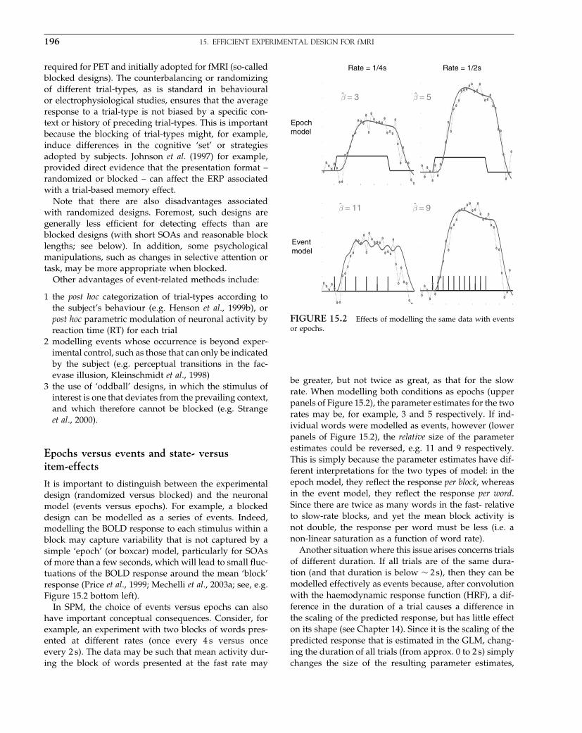
Elsevier UK Chapter: Ch15-P372560 30-9-2006 5:14p.m. Page:196 Trim:7.5in×9.25in
Basal Font:Palatino Margins:Top:40pt Gutter:68pt Font Size:9.5/12 Text Width:42pc Depth:55 Lines
196 15. EFFICIENT EXPERIMENTAL DESIGN FOR fMRI
required for PET and initially adopted for fMRI (so-calledblocked designs). The counterbalancing or randomizingof different trial-types, as is standard in behaviouralor electrophysiological studies, ensures that the averageresponse to a trial-type is not biased by a specific con-text or history of preceding trial-types. This is importantbecause the blocking of trial-types might, for example,induce differences in the cognitive ‘set’ or strategiesadopted by subjects. Johnson et al. (1997) for example,provided direct evidence that the presentation format –randomized or blocked – can affect the ERP associatedwith a trial-based memory effect.
Note that there are also disadvantages associatedwith randomized designs. Foremost, such designs aregenerally less efficient for detecting effects than areblocked designs (with short SOAs and reasonable blocklengths; see below). In addition, some psychologicalmanipulations, such as changes in selective attention ortask, may be more appropriate when blocked.
Other advantages of event-related methods include:
1 the post hoc categorization of trial-types according tothe subject’s behaviour (e.g. Henson et al., 1999b), orpost hoc parametric modulation of neuronal activity byreaction time (RT) for each trial
2 modelling events whose occurrence is beyond exper-imental control, such as those that can only be indicatedby the subject (e.g. perceptual transitions in the fac-evase illusion, Kleinschmidt et al., 1998)
3 the use of ‘oddball’ designs, in which the stimulus ofinterest is one that deviates from the prevailing context,and which therefore cannot be blocked (e.g. Strangeet al., 2000).
Epochs versus events and state- versusitem-effects
It is important to distinguish between the experimentaldesign (randomized versus blocked) and the neuronalmodel (events versus epochs). For example, a blockeddesign can be modelled as a series of events. Indeed,modelling the BOLD response to each stimulus within ablock may capture variability that is not captured by asimple ‘epoch’ (or boxcar) model, particularly for SOAsof more than a few seconds, which will lead to small fluc-tuations of the BOLD response around the mean ‘block’response (Price et al., 1999; Mechelli et al., 2003a; see, e.g.Figure 15.2 bottom left).
In SPM, the choice of events versus epochs can alsohave important conceptual consequences. Consider, forexample, an experiment with two blocks of words pres-ented at different rates (once every 4 s versus onceevery 2 s). The data may be such that mean activity dur-ing the block of words presented at the fast rate may
Rate = 1/4s Rate = 1/2s
Epochmodel
Eventmodel
β = 3 β = 5
β = 9β = 11ˆ
ˆˆ
ˆ
FIGURE 15.2 Effects of modelling the same data with eventsor epochs.
be greater, but not twice as great, as that for the slowrate. When modelling both conditions as epochs (upperpanels of Figure 15.2), the parameter estimates for the tworates may be, for example, 3 and 5 respectively. If ind-ividual words were modelled as events, however (lowerpanels of Figure 15.2), the relative size of the parameterestimates could be reversed, e.g. 11 and 9 respectively.This is simply because the parameter estimates have dif-ferent interpretations for the two types of model: in theepoch model, they reflect the response per block, whereasin the event model, they reflect the response per word.Since there are twice as many words in the fast- relativeto slow-rate blocks, and yet the mean block activity isnot double, the response per word must be less (i.e. anon-linear saturation as a function of word rate).
Another situation where this issue arises concerns trialsof different duration. If all trials are of the same dura-tion (and that duration is below ∼ 2 s), then they can bemodelled effectively as events because, after convolutionwith the haemodynamic response function (HRF), a dif-ference in the duration of a trial causes a difference inthe scaling of the predicted response, but has little effecton its shape (see Chapter 14). Since it is the scaling of thepredicted response that is estimated in the GLM, chang-ing the duration of all trials (from approx. 0 to 2 s) simplychanges the size of the resulting parameter estimates,

Elsevier UK Chapter: Ch15-P372560 30-9-2006 5:14p.m. Page:197 Trim:7.5in×9.25in
Basal Font:Palatino Margins:Top:40pt Gutter:68pt Font Size:9.5/12 Text Width:42pc Depth:55 Lines
EVENT-RELATED fMRI, AND RANDOMIZED VERSUS BLOCKED DESIGNS 197
but has no effect on statistics.1 For longer duration trials,the response begins to plateau, meaning that an ‘epochmodel’ can be a better model. More important, however,is the case of trials that vary in duration from trial to trialwithin a condition, or across conditions. Whether theseare better modelled as events, or as epochs of differentdurations (e.g. with duration equal to the RT for eachtrial), is debatable. For example, if the stimulus durationwere constant and only RTs varied, then the activity inV1 may not be expected to vary with RT, so an eventmodel might fit better (and in this case, the parameterestimate can be interpreted as the response per trial). Foractivity in premotor cortex on the other hand, greateractivity might be expected for trials with longer RTs, soa ‘varying-duration’ epoch model might fit better (andin this case, the parameter estimate can be interpretedas the response per unit time). So the choice of modeldepends on the assumptions about the duration of neu-ronal activity in the particular region of interest. If thisis unknown, trials whose durations vary over a few sec-onds (as with typical RTs) are probably best modelledwith two regressors: one modelling events, and a secondmodelling a parametric modulation of the response, bythe RT on each trial.
Finally, note that one can combine both events andepochs within the same model. A common example ofthis is when trying to distinguish between sustained(‘state’) effects and transient (‘item’) effects. Chawla et al.(1999), for example, investigated the interaction betweenselective attention (a state-effect) and transient stimu-lus changes (an item-effect) in such a ‘mixed epoch-event’ design. Subjects viewed a visual stimulus thatoccasionally changed in either colour or motion. In someblocks, they detected the colour changes, in other blocksthey detected the motion changes. By varying the inter-val between changes within a block, Chawla et al. wereable to reduce the correlation between the correspond-ing epoch- and event-related regressors (which increasesthe statistical efficiency to detect either effect alone;see below). Tests of the epoch-related effect showedthat attending to a specific visual attribute (e.g. colour)increased the baseline activity in regions selective forthat attribute (e.g. V4). Tests of the event-related effectshowed that the impulse response to the same changein visual attribute was augmented when subjects were
1 This is despite the fact that the ‘efficiency’, as calculated byEqn. 15.3, increases with greater scaling of the regressors. Thisincrease is correct, in the sense that a larger signal will be easierto detect in the presence of the same noise, but misleading inthe sense that it is the size of the signal that we are estimatingwith our model (i.e. the data are unaffected by how we modelthe trials).
attending to it (Plate 18). These combined effects of selec-tive attention – raising endogenous baseline activity andincreasing the gain of the exogenous response – couldnot be distinguished in a blocked or fully randomizeddesign.
Timing issues
There are two practical issues concerning the timingwithin randomized designs (which also apply to blockeddesigns, but to a lesser extent): the effective samplingrate of the BOLD response, and the different acquisitiontimes for different slices within a scan (i.e. volume) whenusing echo-planar imaging (EPI).
It is possible to sample the impulse response at post-stimulus intervals, TS , shorter than the inter-scan interval,TR, by dephasing event onsets with respect to scan onsets(Josephs et al., 1997). This uncoupling can be effectedby ensuring the SOA is not a simple multiple of theTR, or by adding a random trial-by-trial delay in stim-ulus onsets relative to scan onsets (Figure 15.3). In bothcases, responses at different peristimulus times (PST) aresampled over trials. The main difference between thetwo methods is simply whether the SOA is fixed or ran-dom, i.e. whether or not the stimulus onset is predictable.For example, an effective PST sampling of 0.5 Hz canbe achieved with an SOA of 6 s and a TR of 4 s; or byadding a delay of 0 or 2 s randomly to each trial (pro-ducing SOAs of 4–8 s, with a mean of 6 s). While effec-tive sampling rates higher than the TR do not necessarilyimprove response detection (since there is little powerin the canonical response above 0.2 Hz), higher sam-pling rates are important for quantifying the responseshape, such as its latency (Miezin et al., 2000; Henson andRugg, 2001).
Dephasing event onsets with respect to scan onsetsdoes not help the second practical issue concerningdifferent slice acquisition times. This ‘slice-timing’ prob-lem (Henson et al., 1999a) refers to the fact that, with adescending EPI sequence for example, the bottom sliceis acquired TR seconds later than the top slice. If a sin-gle basis function (such as a canonical HRF) were usedto model the response, and onset times were specifiedrelative to the start of each scan, the data in the bot-tom slice would be systematically delayed by TR secondsrelative to the model.2 This would produce poor (andbiased) parameter estimates for later slices, and mean
2 One solution would be to allow different event onsets for dif-ferent slices. However, slice-timing information is usually lostas soon as images are re-sliced relative to a different orientation(e.g. during spatial normalization).
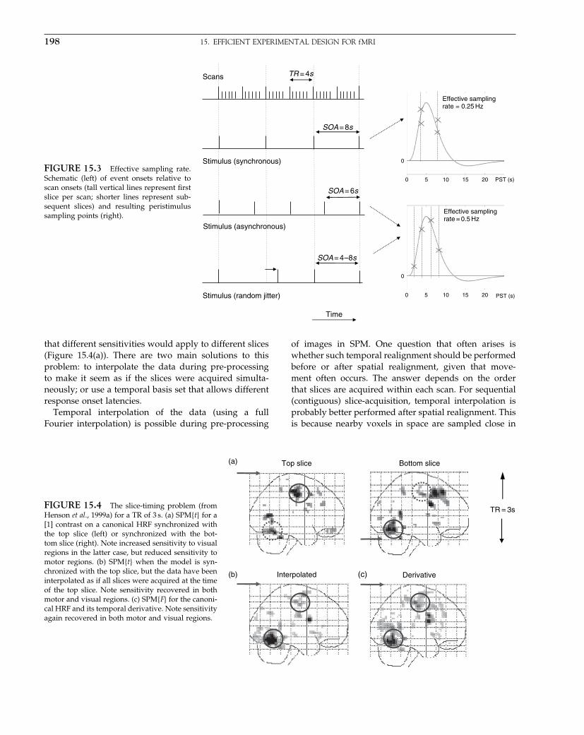
Elsevier UK Chapter: Ch15-P372560 30-9-2006 5:14p.m. Page:198 Trim:7.5in×9.25in
Basal Font:Palatino Margins:Top:40pt Gutter:68pt Font Size:9.5/12 Text Width:42pc Depth:55 Lines
198 15. EFFICIENT EXPERIMENTAL DESIGN FOR fMRI
FIGURE 15.3 Effective sampling rate.Schematic (left) of event onsets relative toscan onsets (tall vertical lines represent firstslice per scan; shorter lines represent sub-sequent slices) and resulting peristimulussampling points (right).
Effective samplingrate = 0.25 Hz
Effective samplingrate = 0.5 Hz
Stimulus (synchronous)
Scans TR = 4s
Stimulus (random jitter)
Stimulus (asynchronous)
SOA = 6s
SOA = 8s
SOA = 4– 8s
Time
0
0 5 10 15 20 PST (s)
0
0 5 10 15 20 PST (s)
that different sensitivities would apply to different slices(Figure 15.4(a)). There are two main solutions to thisproblem: to interpolate the data during pre-processingto make it seem as if the slices were acquired simulta-neously; or use a temporal basis set that allows differentresponse onset latencies.
Temporal interpolation of the data (using a fullFourier interpolation) is possible during pre-processing
of images in SPM. One question that often arises iswhether such temporal realignment should be performedbefore or after spatial realignment, given that move-ment often occurs. The answer depends on the orderthat slices are acquired within each scan. For sequential(contiguous) slice-acquisition, temporal interpolation isprobably better performed after spatial realignment. Thisis because nearby voxels in space are sampled close in
FIGURE 15.4 The slice-timing problem (fromHenson et al., 1999a) for a TR of 3 s. (a) SPM�t� for a[1] contrast on a canonical HRF synchronized withthe top slice (left) or synchronized with the bot-tom slice (right). Note increased sensitivity to visualregions in the latter case, but reduced sensitivity tomotor regions. (b) SPM�t� when the model is syn-chronized with the top slice, but the data have beeninterpolated as if all slices were acquired at the timeof the top slice. Note sensitivity recovered in bothmotor and visual regions. (c) SPM�F� for the canoni-cal HRF and its temporal derivative. Note sensitivityagain recovered in both motor and visual regions.
DerivativeInterpolated
Bottom sliceTop slice
TR = 3s
(b) (c)
(a)
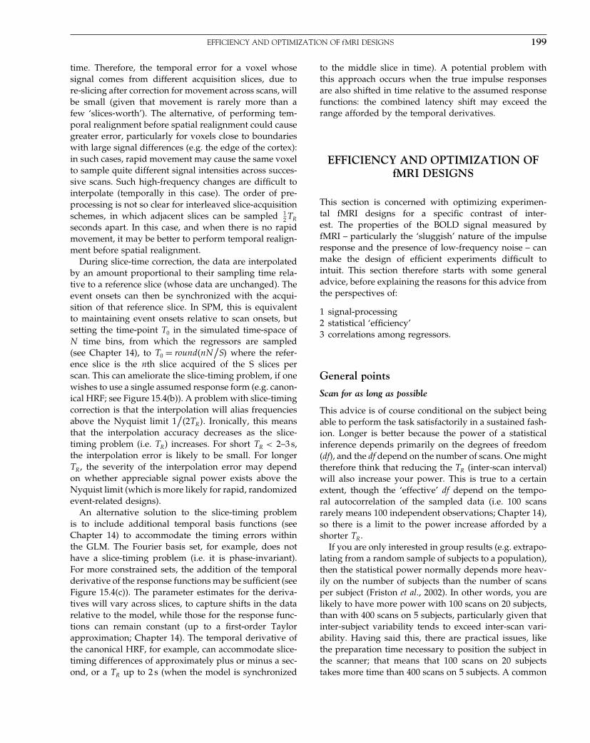
Elsevier UK Chapter: Ch15-P372560 30-9-2006 5:14p.m. Page:199 Trim:7.5in×9.25in
Basal Font:Palatino Margins:Top:40pt Gutter:68pt Font Size:9.5/12 Text Width:42pc Depth:55 Lines
EFFICIENCY AND OPTIMIZATION OF fMRI DESIGNS 199
time. Therefore, the temporal error for a voxel whosesignal comes from different acquisition slices, due tore-slicing after correction for movement across scans, willbe small (given that movement is rarely more than afew ‘slices-worth’). The alternative, of performing tem-poral realignment before spatial realignment could causegreater error, particularly for voxels close to boundarieswith large signal differences (e.g. the edge of the cortex):in such cases, rapid movement may cause the same voxelto sample quite different signal intensities across succes-sive scans. Such high-frequency changes are difficult tointerpolate (temporally in this case). The order of pre-processing is not so clear for interleaved slice-acquisitionschemes, in which adjacent slices can be sampled 1
2 TR
seconds apart. In this case, and when there is no rapidmovement, it may be better to perform temporal realign-ment before spatial realignment.
During slice-time correction, the data are interpolatedby an amount proportional to their sampling time rela-tive to a reference slice (whose data are unchanged). Theevent onsets can then be synchronized with the acqui-sition of that reference slice. In SPM, this is equivalentto maintaining event onsets relative to scan onsets, butsetting the time-point T0 in the simulated time-space ofN time bins, from which the regressors are sampled(see Chapter 14), to T0 = round�nN
/S� where the refer-
ence slice is the nth slice acquired of the S slices perscan. This can ameliorate the slice-timing problem, if onewishes to use a single assumed response form (e.g. canon-ical HRF; see Figure 15.4(b)). A problem with slice-timingcorrection is that the interpolation will alias frequenciesabove the Nyquist limit 1
/�2TR�. Ironically, this means
that the interpolation accuracy decreases as the slice-timing problem (i.e. TR) increases. For short TR < 2–3 s,the interpolation error is likely to be small. For longerTR, the severity of the interpolation error may dependon whether appreciable signal power exists above theNyquist limit (which is more likely for rapid, randomizedevent-related designs).
An alternative solution to the slice-timing problemis to include additional temporal basis functions (seeChapter 14) to accommodate the timing errors withinthe GLM. The Fourier basis set, for example, does nothave a slice-timing problem (i.e. it is phase-invariant).For more constrained sets, the addition of the temporalderivative of the response functions may be sufficient (seeFigure 15.4(c)). The parameter estimates for the deriva-tives will vary across slices, to capture shifts in the datarelative to the model, while those for the response func-tions can remain constant (up to a first-order Taylorapproximation; Chapter 14). The temporal derivative ofthe canonical HRF, for example, can accommodate slice-timing differences of approximately plus or minus a sec-ond, or a TR up to 2 s (when the model is synchronized
to the middle slice in time). A potential problem withthis approach occurs when the true impulse responsesare also shifted in time relative to the assumed responsefunctions: the combined latency shift may exceed therange afforded by the temporal derivatives.
EFFICIENCY AND OPTIMIZATION OFfMRI DESIGNS
This section is concerned with optimizing experimen-tal fMRI designs for a specific contrast of inter-est. The properties of the BOLD signal measured byfMRI – particularly the ‘sluggish’ nature of the impulseresponse and the presence of low-frequency noise – canmake the design of efficient experiments difficult tointuit. This section therefore starts with some generaladvice, before explaining the reasons for this advice fromthe perspectives of:
1 signal-processing2 statistical ‘efficiency’3 correlations among regressors.
General points
Scan for as long as possible
This advice is of course conditional on the subject beingable to perform the task satisfactorily in a sustained fash-ion. Longer is better because the power of a statisticalinference depends primarily on the degrees of freedom(df), and the df depend on the number of scans. One mighttherefore think that reducing the TR (inter-scan interval)will also increase your power. This is true to a certainextent, though the ‘effective’ df depend on the tempo-ral autocorrelation of the sampled data (i.e. 100 scansrarely means 100 independent observations; Chapter 14),so there is a limit to the power increase afforded by ashorter TR.
If you are only interested in group results (e.g. extrapo-lating from a random sample of subjects to a population),then the statistical power normally depends more heav-ily on the number of subjects than the number of scansper subject (Friston et al., 2002). In other words, you arelikely to have more power with 100 scans on 20 subjects,than with 400 scans on 5 subjects, particularly given thatinter-subject variability tends to exceed inter-scan vari-ability. Having said this, there are practical issues, likethe preparation time necessary to position the subject inthe scanner; that means that 100 scans on 20 subjectstakes more time than 400 scans on 5 subjects. A common
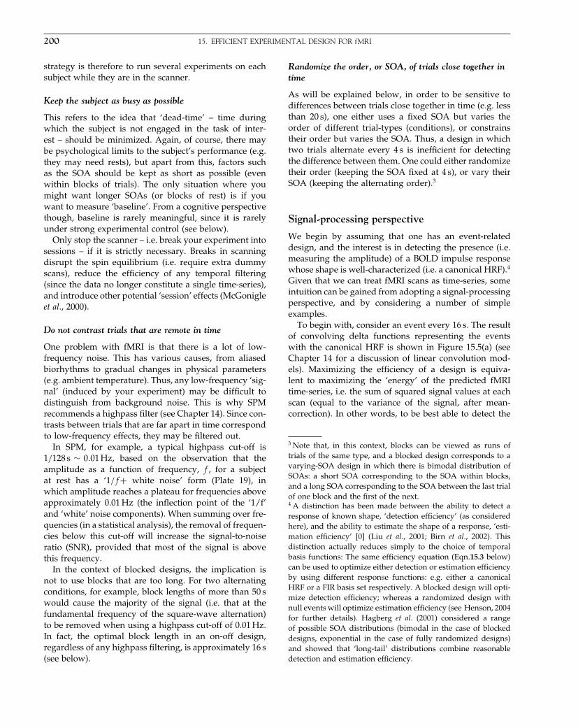
Elsevier UK Chapter: Ch15-P372560 30-9-2006 5:14p.m. Page:200 Trim:7.5in×9.25in
Basal Font:Palatino Margins:Top:40pt Gutter:68pt Font Size:9.5/12 Text Width:42pc Depth:55 Lines
200 15. EFFICIENT EXPERIMENTAL DESIGN FOR fMRI
strategy is therefore to run several experiments on eachsubject while they are in the scanner.
Keep the subject as busy as possible
This refers to the idea that ‘dead-time’ – time duringwhich the subject is not engaged in the task of inter-est – should be minimized. Again, of course, there maybe psychological limits to the subject’s performance (e.g.they may need rests), but apart from this, factors suchas the SOA should be kept as short as possible (evenwithin blocks of trials). The only situation where youmight want longer SOAs (or blocks of rest) is if youwant to measure ‘baseline’. From a cognitive perspectivethough, baseline is rarely meaningful, since it is rarelyunder strong experimental control (see below).
Only stop the scanner – i.e. break your experiment intosessions – if it is strictly necessary. Breaks in scanningdisrupt the spin equilibrium (i.e. require extra dummyscans), reduce the efficiency of any temporal filtering(since the data no longer constitute a single time-series),and introduce other potential ‘session’ effects (McGonigleet al., 2000).
Do not contrast trials that are remote in time
One problem with fMRI is that there is a lot of low-frequency noise. This has various causes, from aliasedbiorhythms to gradual changes in physical parameters(e.g. ambient temperature). Thus, any low-frequency ‘sig-nal’ (induced by your experiment) may be difficult todistinguish from background noise. This is why SPMrecommends a highpass filter (see Chapter 14). Since con-trasts between trials that are far apart in time correspondto low-frequency effects, they may be filtered out.
In SPM, for example, a typical highpass cut-off is1/128 s ∼ 001 Hz, based on the observation that theamplitude as a function of frequency, f , for a subjectat rest has a ‘1/f+ white noise’ form (Plate 19), inwhich amplitude reaches a plateau for frequencies aboveapproximately 0.01 Hz (the inflection point of the ‘1/f’and ‘white’ noise components). When summing over fre-quencies (in a statistical analysis), the removal of frequen-cies below this cut-off will increase the signal-to-noiseratio (SNR), provided that most of the signal is abovethis frequency.
In the context of blocked designs, the implication isnot to use blocks that are too long. For two alternatingconditions, for example, block lengths of more than 50 swould cause the majority of the signal (i.e. that at thefundamental frequency of the square-wave alternation)to be removed when using a highpass cut-off of 0.01 Hz.In fact, the optimal block length in an on-off design,regardless of any highpass filtering, is approximately 16 s(see below).
Randomize the order, or SOA, of trials close together intime
As will be explained below, in order to be sensitive todifferences between trials close together in time (e.g. lessthan 20 s), one either uses a fixed SOA but varies theorder of different trial-types (conditions), or constrainstheir order but varies the SOA. Thus, a design in whichtwo trials alternate every 4 s is inefficient for detectingthe difference between them. One could either randomizetheir order (keeping the SOA fixed at 4 s), or vary theirSOA (keeping the alternating order).3
Signal-processing perspective
We begin by assuming that one has an event-relateddesign, and the interest is in detecting the presence (i.e.measuring the amplitude) of a BOLD impulse responsewhose shape is well-characterized (i.e. a canonical HRF).4
Given that we can treat fMRI scans as time-series, someintuition can be gained from adopting a signal-processingperspective, and by considering a number of simpleexamples.
To begin with, consider an event every 16 s. The resultof convolving delta functions representing the eventswith the canonical HRF is shown in Figure 15.5(a) (seeChapter 14 for a discussion of linear convolution mod-els). Maximizing the efficiency of a design is equiva-lent to maximizing the ‘energy’ of the predicted fMRItime-series, i.e. the sum of squared signal values at eachscan (equal to the variance of the signal, after mean-correction). In other words, to be best able to detect the
3 Note that, in this context, blocks can be viewed as runs oftrials of the same type, and a blocked design corresponds to avarying-SOA design in which there is bimodal distribution ofSOAs: a short SOA corresponding to the SOA within blocks,and a long SOA corresponding to the SOA between the last trialof one block and the first of the next.4 A distinction has been made between the ability to detect aresponse of known shape, ‘detection efficiency’ (as consideredhere), and the ability to estimate the shape of a response, ‘esti-mation efficiency’ [0] (Liu et al., 2001; Birn et al., 2002). Thisdistinction actually reduces simply to the choice of temporalbasis functions: The same efficiency equation (Eqn.15.3 below)can be used to optimize either detection or estimation efficiencyby using different response functions: e.g. either a canonicalHRF or a FIR basis set respectively. A blocked design will opti-mize detection efficiency; whereas a randomized design withnull events will optimize estimation efficiency (see Henson, 2004for further details). Hagberg et al. (2001) considered a rangeof possible SOA distributions (bimodal in the case of blockeddesigns, exponential in the case of fully randomized designs)and showed that ‘long-tail’ distributions combine reasonabledetection and estimation efficiency.

Elsevier UK Chapter: Ch15-P372560 30-9-2006 5:14p.m. Page:201 Trim:7.5in×9.25in
Basal Font:Palatino Margins:Top:40pt Gutter:68pt Font Size:9.5/12 Text Width:42pc Depth:55 Lines
EFFICIENCY AND OPTIMIZATION OF fMRI DESIGNS 201
0 16 32 48 64 80
Time (s)
Stimulus (‘Neural’) HRF Predicted fMRI data(a)
0
0 16 32 48 64 80
Time (s)0
0 16 32 48 64 80
Time (s)0
0 16 32 48 64 80Time (s)
0
0 16 32 48 64 80
Time (s)0
0 16 32 48 64 80
Time (s)0
0 5 10 2015 25 30
Time (s)0
0 5 10 2015 25 30
Time (s)0
0 5 10 2015 25 30
Time (s)0
(b)
(c)
=
=
=
×
×
×
FIGURE 15.5 Effect of convolutionby an assumed HRF on neuronal activityevoked by (a) events every 16 s, (b) eventsevery 4 s and (c) events occurring with a50 per cent probability every 4 s.
signal in the presence of background noise, we wantto maximize the variability of that signal. A signal thatvaries little will be difficult to detect.
The above example (a fixed SOA of 16 s) is not particu-larly efficient, as we shall see later. What if we present thestimuli much faster, say every 4 s? The result is shownin Figure 15.5(b). Because the responses to successiveevents now overlap considerably, we see an initial build-up (transient) followed by small oscillations around a‘raised baseline’. Although the overall signal is high, itsvariance is low, and the majority of stimulus energy willbe lost after highpass filtering (particularly after removalof the mean, i.e. lowest frequency). So this is an even lessefficient design.
What if we vary the SOA randomly? Let’s say we havea minimal SOA of 4 s, but only a 50 per cent probability ofan event every 4 s. This is called a stochastic design (andone way to implement it is to intermix an equal numberof ‘null events’ with ‘true events’; see next section). Thisis shown in Figure 15.5(c). Though we only use half asmany stimuli as in Figure 15.5(b), this is a more efficientdesign. This is because there is a much larger variabilityin the signal.
We could also vary the SOA in a more systematicfashion. We could have runs of events, followed byruns of no (null) events. This corresponds to a blockeddesign. For example, we could have blocks of 5 stimulipresented every 4 s, alternating with 20 s of rest, as shownin Figure 15.6(a). This is even more efficient than theprevious stochastic design. To see why, we shall con-sider the Fourier transform of these time-series. First,
however, note that, with short SOAs, the predicted fMRItime-series for a blocked design is similar to what wouldobtain if neuronal activity were sustained throughoutthe block (i.e. during the Interstimulus interval (ISI)as well) as in an epoch model (Figure 15.6(b)). Now,if we take the Fourier transform of each function inFigure 15.6(b), we can plot amplitude (magnitude) asa function of frequency (Figure 15.6(c)). The amplitudespectrum of the square-wave stimulus function has adominant frequency corresponding to its ‘fundamental’frequency �Fo = 1/�20 s+20 s� = 0025 Hz�, plus a series of‘harmonics’ �3Fo 5Fo � � � etc� of progressively decreas-ing amplitude. The fundamental frequency correspondsto the frequency of a sinusoidal that best matches thebasic on-off alternation; the harmonics can be thoughtof as capturing the ‘sharper’ edges of the square-wavefunction relative to this fundamental sinusoid.
The reason for performing the Fourier transform isthat it offers a slightly different perspective. Foremost, aconvolution in time is equivalent to a multiplication infrequency space. In this way, we can regard the stim-ulus function as our original data and the HRF as a‘filter’. One can see immediately from the shape of theFourier transform of the HRF that this filter will ‘pass’low frequencies, but attenuate higher frequencies (this iswhy it is sometimes called a ‘lowpass filter’ or ‘tempo-ral smoothing kernel’). This property is why, for exam-ple, much high-frequency information was lost with thefixed SOA of 4 s in Figure 15.5(b). In the present exam-ple, the result of multiplying the amplitude spectrum ofthe stimulus function by that of the filter is that some of
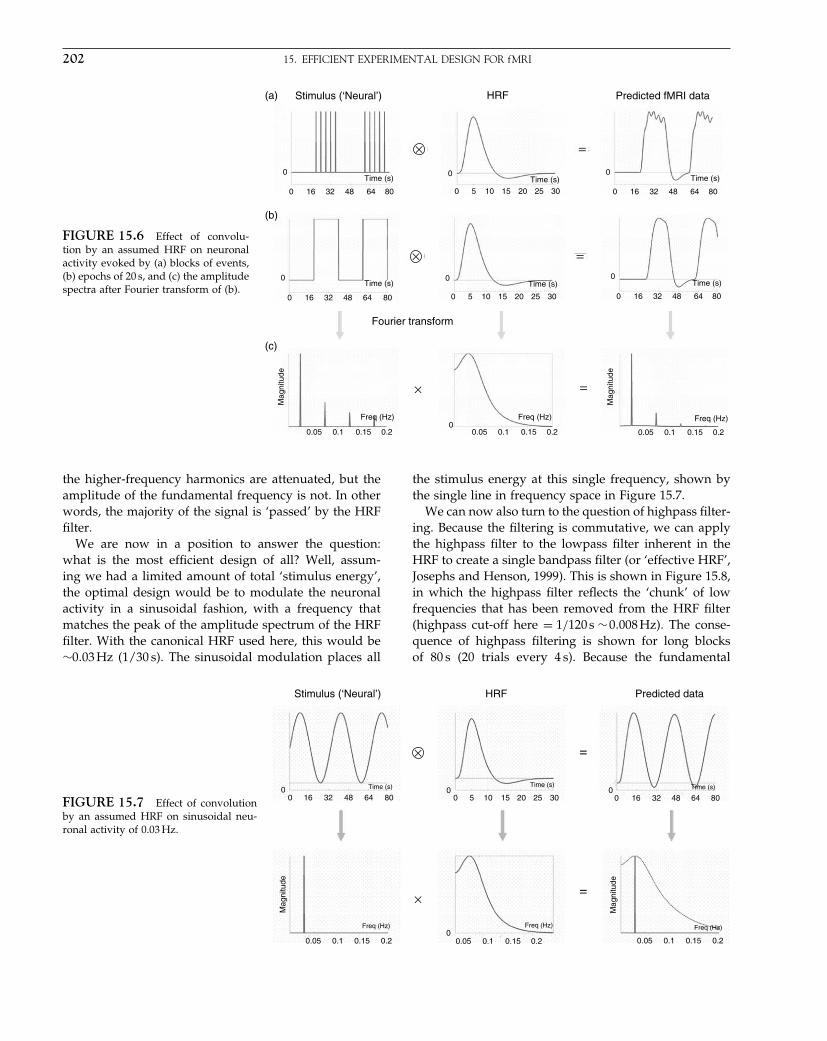
Elsevier UK Chapter: Ch15-P372560 30-9-2006 5:14p.m. Page:202 Trim:7.5in×9.25in
Basal Font:Palatino Margins:Top:40pt Gutter:68pt Font Size:9.5/12 Text Width:42pc Depth:55 Lines
202 15. EFFICIENT EXPERIMENTAL DESIGN FOR fMRI
FIGURE 15.6 Effect of convolu-tion by an assumed HRF on neuronalactivity evoked by (a) blocks of events,(b) epochs of 20 s, and (c) the amplitudespectra after Fourier transform of (b).
Stimulus (‘Neural’)(a)
(b)
(c)
0
0
0 16 32 48 64 80 0 16 32 48 64 80
0 16 32 48 64 800 0
0 0
00
5 10 15
Fourier transform
20 25 30
0 5 10 15 20 25 30
16
0.05 0.1 0.15 0.2 0.05 0.1 0.15 0.2 0.05 0.1 0.15 0.2
Freq (Hz)Freq (Hz)Freq (Hz)
Mag
nitu
de
Mag
nitu
de
0
32 48 64 80
Time (s)
Time (s) Time (s)
Time (s) Time (s)
Time (s)
HRF Predicted fMRI data
×
×
×
=
=
=
the higher-frequency harmonics are attenuated, but theamplitude of the fundamental frequency is not. In otherwords, the majority of the signal is ‘passed’ by the HRFfilter.
We are now in a position to answer the question:what is the most efficient design of all? Well, assum-ing we had a limited amount of total ‘stimulus energy’,the optimal design would be to modulate the neuronalactivity in a sinusoidal fashion, with a frequency thatmatches the peak of the amplitude spectrum of the HRFfilter. With the canonical HRF used here, this would be∼003 Hz (1/30 s). The sinusoidal modulation places all
the stimulus energy at this single frequency, shown bythe single line in frequency space in Figure 15.7.
We can now also turn to the question of highpass filter-ing. Because the filtering is commutative, we can applythe highpass filter to the lowpass filter inherent in theHRF to create a single bandpass filter (or ‘effective HRF’,Josephs and Henson, 1999). This is shown in Figure 15.8,in which the highpass filter reflects the ‘chunk’ of lowfrequencies that has been removed from the HRF filter(highpass cut-off here = 1/120 s ∼0008 Hz). The conse-quence of highpass filtering is shown for long blocksof 80 s (20 trials every 4 s). Because the fundamental
FIGURE 15.7 Effect of convolutionby an assumed HRF on sinusoidal neu-ronal activity of 0.03 Hz.
Stimulus (‘Neural’) HRF Predicted data
0 16 32Time (s)Time (s)Time (s)
48 64 8000 0
0
00 5 10 15 20 25 30
0.05 0.1 0.15 0.2 0.05 0.1
Freq (Hz) Freq (Hz)
Mag
nitu
de
Mag
nitu
de
Freq (Hz)
0.15 0.2 0.05 0.1 0.15 0.2
16 32 48 64 80
×
×
=
=
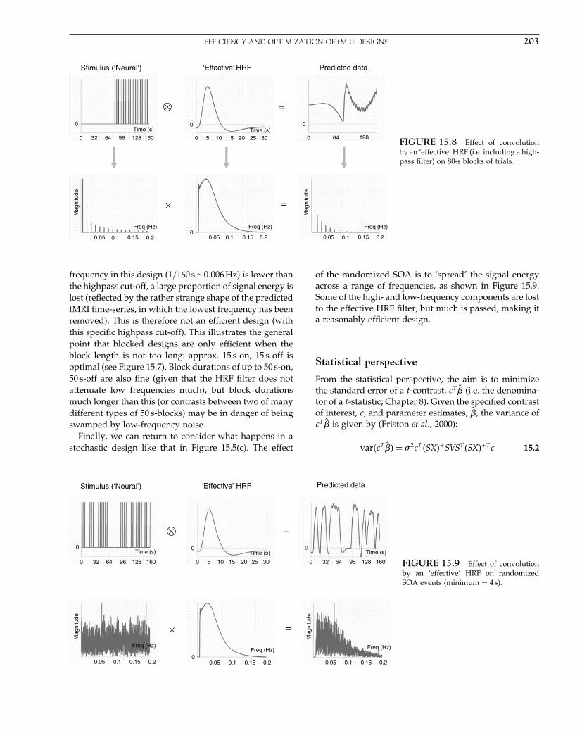
Elsevier UK Chapter: Ch15-P372560 30-9-2006 5:14p.m. Page:203 Trim:7.5in×9.25in
Basal Font:Palatino Margins:Top:40pt Gutter:68pt Font Size:9.5/12 Text Width:42pc Depth:55 Lines
EFFICIENCY AND OPTIMIZATION OF fMRI DESIGNS 203
Stimulus (‘Neural’) ‘Effective’ HRF Predicted data
128640
0.050
0.050.05 0.10.10.1 0.150.150.15 0.20.20.2
Freq (Hz)Freq (Hz)Freq (Hz)
Mag
nitu
de
Mag
nitu
de
302520151050
0
160
Time (s) Time (s)1289664320
0 0
×
×
=
=
FIGURE 15.8 Effect of convolutionby an ‘effective’ HRF (i.e. including a high-pass filter) on 80-s blocks of trials.
frequency in this design �1/160 s ∼0006 Hz� is lower thanthe highpass cut-off, a large proportion of signal energy islost (reflected by the rather strange shape of the predictedfMRI time-series, in which the lowest frequency has beenremoved). This is therefore not an efficient design (withthis specific highpass cut-off). This illustrates the generalpoint that blocked designs are only efficient when theblock length is not too long: approx. 15 s-on, 15 s-off isoptimal (see Figure 15.7). Block durations of up to 50 s-on,50 s-off are also fine (given that the HRF filter does notattenuate low frequencies much), but block durationsmuch longer than this (or contrasts between two of manydifferent types of 50 s-blocks) may be in danger of beingswamped by low-frequency noise.
Finally, we can return to consider what happens in astochastic design like that in Figure 15.5(c). The effect
of the randomized SOA is to ‘spread’ the signal energyacross a range of frequencies, as shown in Figure 15.9.Some of the high- and low-frequency components are lostto the effective HRF filter, but much is passed, making ita reasonably efficient design.
Statistical perspective
From the statistical perspective, the aim is to minimizethe standard error of a t-contrast, cT �̂ (i.e. the denomina-tor of a t-statistic; Chapter 8). Given the specified contrastof interest, c, and parameter estimates, �̂, the variance ofcT �̂ is given by (Friston et al., 2000):
var�cT �̂� = �2cT �SX�+SVST �SX�+T c 15.2
Stimulus (‘Neural’) ‘Effective’ HRF Predicted data
0
00.05 0.1 0.15 0.20.05
Mag
nitu
de
Mag
nitu
de
0.1 0.15 0.20.05 0.1 0.15 0.2
0
32 64 96 128 1600 32 64 96 128 160 0
00
5 10 15 20 25 30
Time (s)Time (s)
Freq (Hz)Freq (Hz) Freq (Hz)
Time (s)
×
×
=
=
FIGURE 15.9 Effect of convolutionby an ‘effective’ HRF on randomizedSOA events (minimum = 4 s).
Elsevier UK Chapter: Ch15-P372560 30-9-2006 5:14p.m. Page:204 Trim:7.5in×9.25in
Basal Font:Palatino Margins:Top:40pt Gutter:68pt Font Size:9.5/12 Text Width:42pc Depth:55 Lines
204 15. EFFICIENT EXPERIMENTAL DESIGN FOR fMRI
where S is a filter matrix incorporating the highpass fil-ter and any temporal smoothing, and V is the noiseautocorrelation matrix. We want to minimize this variancewith respect to the design matrix, X. If we assume thatthe filter matrix S is specified appropriately to ‘whiten’the residuals, such that SVST = I (i.e. when S = K−1, whereKKT = V ; Chapter 14), and we incorporate S into X, thenthis is equivalent to maximizing the efficiency, :
���2 cX� = ��2cT �XT X�−1c�−1 15.3
For a given contrast, c, this equation can be split into the‘noise variance’, �2, and the ‘design variance’, �XT X�−1
(Mechelli et al., 2003b). If one assumes that the noise var-iance is independent of the specific design used (whichmay not be the case, Mechelli et al., 2003b; see later),then the efficiency of a contrast for a given design isproportional to:
��cX� = �cT �XT X�−1c�−1 15.4
(For F -contrasts, where c is a matrix, the trace operatorcan be used to reduce efficiency to a single number; Dale,1999). Note that ��cX� has no units; it is a relative mea-sure. It depends on the scaling of the design matrix andthe scaling of the contrasts. Thus, all we can really say isthat one design is more efficient than another (for a givencontrast). In what follows, we use Eqn. 15.4 to evaluatethe efficiency of different sorts of design and look at howdesigns can be characterized probabilistically.
Stochastic designs
For a single event-type, the space of possibleexperimental designs can be captured by two parame-ters: the minimal SOA ��t� and the probability, pt, ofan event occurring at every �t (Friston et al., 1999). In‘deterministic’ designs, pt = 1 or pt = 0, giving a series ofevents with fixed SOA, as in Figure 15.5(a). In ‘stochas-tic’ designs 0 ≤ pt ≤ 1, producing a range of SOAs (asin Figure 15.5(c)). For ‘stationary’ stochastic designs, pt
is constant, giving an exponential distribution of SOAs;for ‘dynamic’ stochastic designs, pt changes with time.The extreme case of a dynamic stochastic design is onein which the temporal modulation of pt conforms to asquare-wave, corresponding to a blocked design. Noticethat the quantities pt and �t parameterize a space ofdesign matrices probabilistically. In other words, theyspecify the probability p�X�pt�t� of getting any par-ticular design matrix. This allows one to compute theexpected design efficiency for any class that can beparameterized in this way:
���c pt�t�� =∫
p�X�pt�t���cX�dX 15.5
This expected design efficiency can be evaluated numer-ically by generating large numbers of design matri-ces (using pt and �t) and taking the average efficiencyaccording to Eqn. 15.4. Alternatively, one can com-pute the expected efficiency analytically as described inFriston et al. (1999). This allows one to explore differentsorts of designs by treating the design matrix itself as arandom variable. For stochastic designs, efficiency is gen-erally maximal when the �t is minimal and the (mean)pt = 1
/�L+1�, where L is the number of trial types (see
Friston et al., 1999).Figure 15.10 shows the expected efficiency for detecting
canonical responses to a single event-type versus base-line, i.e. L = 1 and c = 1, for a range of possible designs.The deterministic design with �t = 8 s (top row) is leastefficient, whereas the dynamic stochastic design with asquare-wave modulation with �t = 1 s is the most effi-cient (corresponding, in this case, to a 32 s on-off blockeddesign). Intermediate between these extremes are thedynamic stochastic designs that use a sinusoidal modula-tion of pt. In other words, these designs produce clumpsof events close together in time, interspersed with peri-ods in which events are rarer. Though such designs areless efficient than the blocked (square-wave) design, theyare more efficient than the stationary stochastic designwith �t = 1 s (second row of Figure 15.10), and assum-ing that subjects are less likely to notice the ‘clumping’of events (relative to a fully blocked design), may offera good compromise between efficiency and subjectiveunpredictability.
Transition probabilities
The space of possible designs can also be characterized by�t and a ‘transition matrix’ (Josephs and Henson, 1999).This is a generalization of the above formulation thatintroduces conditional dependencies over time. For L > 1different event-types, a Lm ×L transition matrix capturesthe probability of an event being of each type, given thehistory of the last m event-types. A fully randomizeddesign with two event-types (A and B) has a simple first-order transition matrix in which each probability is a half.The efficiencies of two contrasts, the main effect of A andB (versus baseline), c = �1 1�T , and the differential effect,c = �1 −1�T , are shown as a function of �t in Plate 20(a).The optimal SOA for the main effect under these con-ditions is approximately 20 s. The efficiency of the maineffect decreases for shorter SOAs, whereas the efficiencyof the differential effect increases. Clearly, the efficiencyfor the differential contrast cannot increase indefinitelyas the SOA decreases; at some point, the BOLD responsemust saturate (see below). Nonetheless, this graph clearly

Elsevier UK Chapter: Ch15-P372560 30-9-2006 5:14p.m. Page:205 Trim:7.5in×9.25in
Basal Font:Palatino Margins:Top:40pt Gutter:68pt Font Size:9.5/12 Text Width:42pc Depth:55 Lines
EFFICIENCY AND OPTIMIZATION OF fMRI DESIGNS 205
FIGURE 15.10 Efficiency for a single event-type (from Fris-ton et al., 1999). Probability of event each SOA (left column) andexpected design efficiency (right column, increasing left-to-right) fora deterministic design with �t = 8 s �1st row�, a stationary stochastic(randomized) design with pt = 05 �2nd row� and dynamic stochasticdesigns with modulations of pt by different sinusoidal frequencies(3rd to 5th rows) and in a blocked manner every 32 s (6th row).
demonstrates how the optimal SOA depends on the spe-cific contrast of interest.5
Various experimental constraints on multiple event-type designs can also be considered. In some situations,the order of event-types might be fixed, and the designquestion relates to the optimal SOA. For a design inwhich A and B must alternate (e.g. where A and B aretransitions between two perceptual states), the optimalSOA for a differential effect is 10 s (Plate 20(b), i.e. half ofthat for the main effect). In other situations, experimental
5 The main effect, which does not distinguish A and B, is ofcourse equivalent to a deterministic design, while the differen-tial effect is equivalent to a stochastic design (from the perspec-tive of any one event-type).
constraints may limit the SOA, to at least 10 s say, and thedesign question relates to the optimal stimulus ordering.An alternating design is more efficient than a random-ized design for such intermediate SOAs. However, analternating design may not be advisable for psychologi-cal reasons (subjects’ behaviour might be influenced bythe predictable pattern). In such cases, a permuted design(in which each of trial-types is presented successivelyin a randomly-permuted order) may be a more suitablechoice (see Plate 20(b)).
A further design concept concerns ‘null events’. Theseare not real events, in that they do not differ from thebaseline and hence are not detectable by subjects (so arenot generally modelled in the design matrix). They wereintroduced by Dale and Buckner (1997) as ‘fixation tri-als’, to allow ‘selective averaging’ (see Chapter 14). Infact, they are simply a convenient means of creating astochastic design by shuffling a certain proportion of nullevents among the events of interest (producing an expo-nential distribution of SOAs). From the perspective ofmultiple event-type designs, the reason for null events isto buy efficiency for both the main effect and differentialeffect at short SOAs (at a slight cost to the efficiency forthe differential effect; see Plate 20(c)).
The efficiencies shown in Plate 20 are unlikely tomap simply (e.g. linearly) onto the size of the t-statistic.Nonetheless, if the noise variance, in Eqn. 15.3, is inde-pendent of experimental design, the relationship shouldat least be monotonic. Mechelli et al. (2003b) showedthat the noise variance can vary significantly betweena blocked and a randomized design (both modelledwith events). This suggests that the stimulus orderingdid affect (un-modelled) psychological or physiologicaleffects in this dataset, contributing to the residual error.When the data were highpass filtered however, the noisevariance no longer differed significantly between the twodesigns. In this case, the statistical results were in agree-ment with the relative efficiencies predicted from theestimation variances.
Efficiency in terms of correlations
Another way of thinking about efficiency is in terms ofthe correlation between (contrasts of) regressors withinthe design matrix. In Eqn. 15.3 the term XT X is calledthe information matrix and reflects the orthogonalityof the design matrix. High covariance between thecolumns of the design matrix introduces redundancy.This can increase the covariance of the parameter esti-mates �XT X�−1 and lead to low efficiency (depending onthe particular contrast).
Consider the earlier example of two event-types, A andB, randomly intermixed, with a short SOA. If we plot

Elsevier UK Chapter: Ch15-P372560 30-9-2006 5:14p.m. Page:206 Trim:7.5in×9.25in
Basal Font:Palatino Margins:Top:40pt Gutter:68pt Font Size:9.5/12 Text Width:42pc Depth:55 Lines
206 15. EFFICIENT EXPERIMENTAL DESIGN FOR fMRI
FIGURE 15.11 Scatter plot for two mean-corrected regressors(one point per scan) corresponding to two event-types randomlyintermixed with a short SOA.
the resulting two regressors (after convolution with anHRF) against each other, we would end up with a scatterplot something like that in Figure 15.11, where each pointreflects one scan. The high negative correlation betweenthe regressors is because whenever there is high signalfor A, there tends to be low signal for B, and vice versa.If we consider the projection of this distribution onto thex = −y direction (corresponding to a �1 − 1� contrast), itwill have a large dispersion, i.e. high experimental vari-ance, which means the difference between A and B will bedetected efficiently in this design. However, if we projectthe distribution onto the x = y direction (corresponding toa [1 1] contrast), it will have little spread, i.e. low experi-mental variance, which means that we will not detect thecommon effect of A and B versus baseline efficiently. Thisdemonstrates the markedly different efficiency for thesetwo contrasts at short SOAs that was shown in Plate 20(a).
Projection onto the x or y axes (i.e. [1 0] or [0 1] con-trasts) will have less spread than if the two regressorswere orthogonal and formed a spherical cloud of points.This shows how correlations can reduce efficiency andmakes an important general point about correlations.High correlation between two regressors means that theparameter estimate for each one will be estimated inef-ficiently, i.e. the parameter estimate itself will have highvariance. In other words, if we estimated each parametermany times we would get wildly different results. In theextreme case, that the regressors are perfectly correlated,the parameters would be inestimable (i.e. they wouldhave infinite variance). Nonetheless, we could still esti-mate efficiently the difference between them. Thus, highcorrelations within the orthogonality matrix shown bySPM should not be a cause of concern for some contrasts:what is really relevant is the correlation between the con-trasts of interest (i.e. linear combinations of columns of
the design matrix) relative to the rest of the design matrix(i.e. null space of the contrast).
In short-SOA, randomized designs with no null events,for example, we might detect brain regions showing areliable difference between event-types, yet when weplot the event-related response, we might find they areall ‘activations’ versus baseline, all ‘deactivations’ ver-sus baseline or some activations and some deactivations.However, these impressions are more apparent thanreal (and should not really be shown). If we tested thereliability of these activations or deactivations, they areunlikely to be significant. This is because we cannot esti-mate the baseline reliably in such designs. This is why,for such designs, it does not make sense to plot errorbars showing the variability of each condition alone: oneshould plot error bars pertaining to the variability of thedifference (i.e. that of the contrast actually tested).
Orthogonalizing
Another common misapprehension is that one canovercome the problem of correlated regressors by‘orthogonalizing’ one regressor with respect to the other.This rarely solves the problem. The parameter estimatesalways pertain to the orthogonal part of each regres-sor (this is an automatic property of fitting within theGLM). Thus, neither the parameter estimate for theorthogonalized regressor, nor its variance, will change.The parameter estimate for the other regressor willchange. However, this parameter estimate now reflectsthe assumption that the common variance is uniquelyattributed to this regressor. We must have an a priori rea-son for assuming this (i.e. without such prior knowledge,there is no way to determine which of the two correlatedregressors caused the common effect). In the absence ofsuch knowledge, there is no reason to orthogonalize.
The conception of efficiency in terms of correlationscan help with the design of experiments where there isnecessarily some degree of correlation among regressors.Two main experimental situations where this arises are:
1 when trials consist of two events, one of which mustfollow the other
2 blocks of events in which one wishes to distinguish‘item-’ from ‘state-’ effects (see above).
A common example of the first type of experiment are‘working memory’ designs, in which a trial consists of astimulus, a short retention interval, and then a response.We shall ignore the retention interval and concentrate onhow one can separate effects of the stimulus from thoseof the response. With short SOAs between each event-type (e.g. 4 s), the regressors for the stimulus and responsewill be negatively correlated, as shown in Figure 15.12(a).Two possible solutions to this problem are shown in
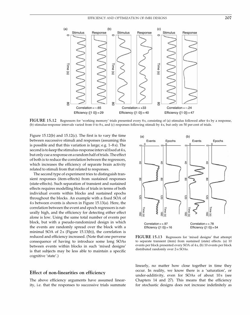
Elsevier UK Chapter: Ch15-P372560 30-9-2006 5:14p.m. Page:207 Trim:7.5in×9.25in
Basal Font:Palatino Margins:Top:40pt Gutter:68pt Font Size:9.5/12 Text Width:42pc Depth:55 Lines
EFFICIENCY AND OPTIMIZATION OF fMRI DESIGNS 207
Stimulus(a)
0T
ime (s)
Correlation = –.65
Efficiency ([1 0]) = 29
Correlation = +33
Efficiency ([1 0]) = 40
Correlation = –.24
Efficiency ([1 0]) = 47
80
0T
ime (s)
80
0T
ime (s)
80
(b) (c)Stimulus StimulusResponse Response Response
FIGURE 15.12 Regressors for ‘working memory’ trials presented every 8 s, consisting of (a) stimulus followed after 4 s by a response,(b) stimulus-response intervals varied from 0 to 8 s, and (c) responses following stimuli by 4 s, but only on 50 per cent of trials.
Figure 15.12(b) and 15.12(c). The first is to vary the timebetween successive stimuli and responses (assuming thisis possible and that this variation is large; e.g. 1–8 s). Thesecond is to keep the stimulus-response interval fixed at 4 s,but only cue a response on a random half of trials. The effectof both is to reduce the correlation between the regressors,which increases the efficiency of separate brain activityrelated to stimuli from that related to responses.
The second type of experiment tries to distinguish tran-sient responses (item-effects) from sustained responses(state-effects). Such separation of transient and sustainedeffects requires modelling blocks of trials in terms of bothindividual events within blocks and sustained epochsthroughout the blocks. An example with a fixed SOA of4 s between events is shown in Figure 15.13(a). Here, thecorrelation between the event and epoch regressors is nat-urally high, and the efficiency for detecting either effectalone is low. Using the same total number of events perblock, but with a pseudo-randomized design in whichthe events are randomly spread over the block with aminimal SOA of 2 s (Figure 15.13(b)), the correlation isreduced and efficiency increased. (Note that one perverseconsequence of having to introduce some long SOAsbetween events within blocks in such ‘mixed designs’is that subjects may be less able to maintain a specificcognitive ‘state’.)
Effect of non-linearities on efficiency
The above efficiency arguments have assumed linear-ity, i.e. that the responses to successive trials summate
0 0000
4080
120160
Tim
e (s)
Tim
e (s)
Tim
e (s)
Tim
e (s)
040
80120
160
040
80120
160
040
80120
160
Correlation = +.97Efficiency ([1 0]) = 16
Correlation = +.78Efficiency ([1 0]) = 54
Events EventsEpochs Epochs(a) (b)
FIGURE 15.13 Regressors for ‘mixed designs’ that attemptto separate transient (item) from sustained (state) effects. (a) 10events per block presented every SOA of 4 s, (b) 10 events per blockdistributed randomly over 2-s SOAs.
linearly, no matter how close together in time theyoccur. In reality, we know there is a ‘saturation’, orunder-additivity, even for SOAs of about 10 s (seeChapters 14 and 27). This means that the efficiencyfor stochastic designs does not increase indefinitely as
Elsevier UK Chapter: Ch15-P372560 30-9-2006 5:14p.m. Page:208 Trim:7.5in×9.25in
Basal Font:Palatino Margins:Top:40pt Gutter:68pt Font Size:9.5/12 Text Width:42pc Depth:55 Lines
208 15. EFFICIENT EXPERIMENTAL DESIGN FOR fMRI
the SOA decreases (e.g. for the differential effect inPlate 20(a)). By estimating non-linearity with a Volterraexpansion (Chapter 14), Friston et al. (1998) calculated theimpact of such non-linearity on evoked responses. Theresult is shown in the insert in Plate 20(a). The dotted lineshows the average response to a train of stimuli underlinear assumptions; the solid line shows the effects ofsaturation (using a second-order Volterra kernel). Whilethe solid line is below the dotted line for all SOAs (below10 s), the divergence is small until SOAs of 1–2 s. Indeed,the prediction of this calculation is that the optimal SOAcan be as low as 1 s, i.e. the advantage of short SOAscan outweigh the saturation of responses until surpris-ingly short SOAs (though it should be noted that thisprediction is based on a specific dataset, and may notgeneralize). Indeed, differential responses between ran-domized event-types have been detected with SOAs asshort as 0.5 s (Burock et al., 1998).
In this chapter, we have looked at how to detect evokedfMRI responses efficiently. Before turning to models ofevoked responses in EEG in the next chapter, we will con-clude with some common questions that exercise peopledesigning fMRI studies
COMMON QUESTIONS
What is the minimum number of events Ineed?
Unfortunately, there is no answer to this, other than ‘themore, the better’. The statistical power depends on theeffect size and variability, and this is normally unknown.Heuristics like ‘you cannot do an event-related fMRIanalysis with less than N events’ are fairly meaningless,unless one has a specific effect size in mind (which islikely to be a function of the brain region, the scannerstrength, the sequence type, etc.). Note it is possible thatfewer trials are required (for a given power) than for anequivalent contrast of behavioural data (e.g. if the noiselevel in, say, RTs exceeds that in a specific cortical regioncontributing to those RTs). Furthermore, it is not eventhe number of events per se that is relevant, it is also theSOA and event-ordering (see next question).
Do shorter SOAs mean more power simplybecause there are more trials?
It is not simply the number of trials: the temporal deploy-ment of those trials is vital (as explained above). Thus400 stimuli every 3 s is less efficient than 40 stimuli every30 s for detecting a single event-related response (since
a fixed SOA of 3 s produces little experimental variabil-ity after convolution by the HRF). Two hundred stim-uli occurring with a 50 per cent probably every 3 s (i.e.pseudo-randomly mixed with 200 null events) is muchmore efficient than either.
What is the maximum number of conditions Ican have?
A common interpretation of the rule – do not comparetrials that are too far apart in time – is not to design exper-iments with too many experimental conditions. Moreconditions necessarily mean that replications of a par-ticular condition will be further apart in time. How-ever, the critical factor is not the number of conditionsper se, but the specific contrasts performed over thoseconditions. For pair-wise comparisons of only two of, say,eight blocked conditions the above caveat would apply:if there were equal numbers of blocks of each condi-tion, blocks longer than 12.5 s (100 s/8) are likely to entaila substantial loss of signal when using a highpass cut-off of 0.01 Hz. However, this caveat would not apply ifthe contrasts of interest included (i.e. ‘spanned’) all eightconditions. This would be the case if the experimenterwere only interested in the two main effects and theinteraction within a 2 × 4 factorial design (i.e. contrastslike [1 1 1 1 −1 −1 −1 −1]). If you must compare orplot only a subset of many such blocked conditions, youshould consider presenting those blocks in a fixed order,rather than random or counterbalanced order, which willminimize the time between replications of each condition,i.e. maximize the frequency of the contrast.
Should I use null events?
Null events are simply a convenient means of achievinga stochastic distribution of SOAs, in order to allow esti-mation of the response versus inter-stimulus baseline, byrandomly intermixing them with the events of interest.However, the ‘baseline’ may not always be meaningful.It may be well defined for V1, in terms of visual flashesversus a dark background. It becomes less well definedfor ‘higher’ regions associated with cognition because itis unclear what these regions are ‘doing’ during the inter-stimulus interval. The experimenter normally has littlecontrol over this. Moreover, the baseline does not con-trol for the fact that the events of interest are impulsive(rapid changes), whereas the baseline is sustained (andmay entail adaptation or reduced attention). For this rea-son, it is often better to forget about baseline and add anextra low-level control event instead.
Elsevier UK Chapter: Ch15-P372560 30-9-2006 5:14p.m. Page:209 Trim:7.5in×9.25in
Basal Font:Palatino Margins:Top:40pt Gutter:68pt Font Size:9.5/12 Text Width:42pc Depth:55 Lines
REFERENCES 209
Another problem with null events is that, if they aretoo rare (e.g. less than approximately 33 per cent), theyactually become ‘true’ events in the sense that subjectsmay be expecting an event at the next SOA and so besurprised when it does not occur (the so-called missingstimulus effect that is well-known in event-related poten-tial (ERP) research). One solution is to replace randomlyintermixed null events with periods of baseline betweenruns of events (i.e. ‘block’ the baseline periods). This willincrease the efficiency for detecting the common effectversus baseline, at a slight cost in efficiency for detectingdifferences between the randomized event-types withineach block. Yet another problem is that the unpredictabil-ity of the occurrence of true events (caused by the ran-domly intermixed null events) can cause delayed or evenmissed processing of the events of interest, if subjectscannot prepare for them.
In summary, null events are probably only worth-while if:
1 you think the mean activity during the constant inter-stimulus interval is meaningful to contrast against
2 you do not mind null events being reasonably frequent(to avoid ‘missing stimulus’ effects)
3 you do not mind the stimulus occurrence being unpre-dictable (as far as the subject is concerned).
Having said this, some form of baseline can often serveas a useful ‘safety net’ (e.g. if you fail to detect differencesbetween two visual event-types of interest, you can atleast examine V1 responses and check that you are seeinga basic evoked response to both event-types – if not, youcan question the quality of your data or accuracy of yourmodel). Moreover, you may need randomly to inter-mixnull events if you want to estimate more precisely theshape of the BOLD impulse response (see footnote 4). It isoften the case that people include a low-level baseline ornull event to use as reference for a localizing contrast ontests for differences among true events. In other words,the contrast testing for all events versus baseline canserve as a useful constraint on the search volume forinteresting comparisons among events.
Should I generate multiple random designsand choose the most efficient?
This is certainly possible, though be wary that suchdesigns are likely to converge on designs with somestructure (e.g. blocked designs, given that they tend to beoptimal, as explained above). This may be problematicif such structure affects subjects’ behaviour (particularlyif they notice the structure). Note, however, that thereare software tools available that optimize designs at thesame time as allowing users to specify a certain level
of counterbalancing (to avoid fully blocked designs, e.g.Wager and Nichols, 2003).
REFERENCES
Birn RM, Cox RW, Bandettini PA (2002) Detection versus estimationin event-related fMRI: choosing the optimal stimulus timing.NeuroImage 15: 252–64
Burock MA, Buckner RL, Woldorff MG et al. (1998) Random-ized event-related experimental designs allow for extremelyrapid presentation rates using functional MRI. NeuroReport 9:3735–39
Chawla D, Rees G, Friston KJ (1999) The physiological basis ofattentional modulation in extrastriate visual areas. Nat Neurosci2: 671–76
Dale AM (1999) Optimal experimental design for event-relatedfMRI. Hum Brain Mapp 8: 109–14
Dale A, Buckner R (1997) Selective averaging of rapidly presentedindividual trials using fMRI. Hum Brain Mapp 5: 329–40
Friston KJ, Price CJ, Fletcher P et al. (1996) The trouble with cognitivesubtraction. NeuroImage 4: 97–104
Friston KJ, Josephs O, Rees G et al. (1998) Non-linear event-relatedresponses in fMRI. Mag Res Med 39: 41–52
Friston KJ, Zarahn E, Josephs O et al. (1999) Stochastic designs inevent-related fMRI. NeuroImage 10: 607–19
Friston KJ, Josephs O, Zarahn E et al. (2000) To smooth or notto smooth? Bias and efficiency in fMRI time-series analysis.NeuroImage 12: 196–208
Friston KJ, Glaser DE, Henson RNA et al. (2002) Classical andBayesian inference in neuroimaging: applications. NeuroImage16: 484–512
Friston KJ, Penny WD, Glaser DE (2005) Conjunction revisited.NeuroImage [15.3]
Hagberg GE, Zito G, Patria F et al. (2001) Improved detection ofevent-related functional MRI signals using probability functions.NeuroImage 14: 193–205
Henson RNA (2004) Analysis of fMRI time-series: linear time-invariant models, event-related fMRI and optimal experimentaldesign. In Human Brain Function, 2nd edn, Frackowiak RS, Fris-ton KJ, Frith CD et al. (eds). Elsevier, London, pp 793–822
Henson RNA (2005) What can functional neuroimaging tell theexperimental psychologist? Quart J Exp Psych A 58: 193–234
Henson RNA, Büchel C, Josephs O et al. (1999a) The slice-timingproblem in event-related fMRI. NeuroImage 9: 125
Henson RNA, Rugg MD, Shallice T et al. (1999b) Recollection andfamiliarity in recognition memory: an event-related fMRI study.J Neurosci 19: 3962–72
Henson RNA, Rugg MD (2001) Effects of stimulus repetition onlatency of the BOLD impulse response. NeuroImage 13: 683
Johnson MK, Nolde SF, Mather M et al. (1997) Test format can affectthe similarity of brain activity associated with true and falserecognition memory. Psychol Sci 8: 250–57
Josephs O, Henson RNA (1999) Event-related fMRI: modelling,inference and optimisation. Phil Trans Roy Soc Lond 354:1215–28
Josephs O, Turner R, Friston KJ (1997) Event-related fMRI. HumBrain Mapp 5: 243–48
Kleinschmidt A, Büchel C, Zeki S et al. (1998) Human brain activityduring spontaneously reversing perception of ambiguousfigures. Proc R Soc Lond B Biol Sci 265: 2427–33

Elsevier UK Chapter: Ch15-P372560 30-9-2006 5:14p.m. Page:210 Trim:7.5in×9.25in
Basal Font:Palatino Margins:Top:40pt Gutter:68pt Font Size:9.5/12 Text Width:42pc Depth:55 Lines
210 15. EFFICIENT EXPERIMENTAL DESIGN FOR fMRI
Liu TT, Frank LR, Wong EC et al. (2001) Detection power, estimationefficiency and predictability in event-related fMRI. NeuroImage13: 759–73
McGonigle DJ, Howseman AM, Athwal BS et al. (2000) Variabilityin fMRI: an examination of intersession differences. NeuroImage11: 708–34
Mechelli A, Henson RNA, Price CJ et al. (2003a) Comparingevent-related and epoch analysis in blocked design fMRI. Neu-roImage 18: 806–10
Mechelli A, Price CJ, Henson RNA et al. (2003b) The effectof high-pass filtering on the efficiency of response estima-tion: a comparison between blocked and randomised designs.NeuroImage 18: 798–805
Miezin FM, Maccotta L, Ollinger JM et al. (2000) Characterizing thehemodynamic response: effects of presentation rate, samplingprocedure, and the possibility of ordering brain activity basedon relative timing. NeuroImage 11: 735–59
Nichols TE, Brett M, Andersson J et al. (2005) Valid conjunctioninference with the minimum statistic. NeuroImage 25: 653–60
Price CJ, Friston KJ (1997) Cognitive conjunction: a new approachto brain activation experiments. NeuroImage 5: 261–70
Price CJ, Veltman DJ, Ashburner J et al. (1999) The critical rela-tionship between the timing of stimulus presentation and dataacquisition in blocked designs with fMRI. NeuroImage 10: 36–44
Sternberg S (1969) The discovery of processing stages: extensions ofDonders method. Acta Psychol 30: 276–315
Strange BA, Henson RN, Friston KJ et al. (2000) Brain mechanismsfor detecting perceptual, semantic, and emotional deviance.NeuroImage 12: 425–33
Wager TD, Nichols TE (2003) Optimization of experimental designin fMRI: a general framework using a genetic algorithm.NeuroImage 18: 293–309
Zarahn E, Aguirre G, D’Esposito M (1997) A trial-based experimen-tal design for fMRI. NeuroImage 6: 122–38
Elsevier UK Chapter: Ch16-P372560 30-9-2006 5:15p.m. Page:211 Trim:7.5in×9.25in
Basal Font:Palatino Margins:Top:40pt Gutter:68pt Font Size:9.5/12 Text Width:42pc Depth:55 Lines
C H A P T E R
16
Hierarchical models for EEG and MEGS. Kiebel, J. Kilner and K. Friston
INTRODUCTION
In this chapter, we will look at hierarchical linear mod-els for magneto- and electroencephalographic (M/EEG)data. Traditionally, the analysis of evoked responses isbased on analysis of variance (ANOVA) (see Chapter 13).Statistical parametric mapping (SPM) follows the sameroute, but we motivate the model within a hierarchicalframework, paying special attention to the distinctionbetween time as a factor and time as a dimension of amultivariate response variable. We describe the analysisof both event-related responses (ERR)1 and power data.
The chapter is divided into two parts. First, we discusssome fundamental modelling issues pertaining to theanalysis of M/EEG data over space and time. Equivalentconsiderations emerged in positron emission tomogra-phy/functional magnetic resonance imaging (PET/fMRI)more than a decade ago where one can treat imagingdata either in a mass-univariate (Friston et al., 1991) ormultivariate fashion (Friston et al., 1995; Worsley et al.,1997). The same considerations also apply to time binsin M/EEG data. However, the situation is different forevent-related responses, because one might want to makeinferences about the temporal form of responses. Thismeans time has to be treated as an experiential factor,as opposed to another dimension of the response space.Finely resolved temporal features in M/EEG are impor-tant, because they may contain important informationabout neuronal dynamics. The implications for modelsof M/EEG are that the data can be analysed in one oftwo ways: they can be regarded as high-dimensional
1 By ERR, we mean averaged event-related time courses (Ruggand Coles, 1995), where each of these time courses has beenaveraged within subject and trial-type (condition) to provideone peristimulus time-series for each trial-type and each subject.The modality can be either EEG or MEG.
responses in space and time, or they can be treated as atime-series at each point in space. The first section dis-closes this distinction and their relative merits. In thesecond part, we describe the analysis of M/EEG datausing linear models in which time becomes a factor. Themodels are essentially the same as those presented inChapters 8 and 13 and we recommend these chapters areread first.
We will focus on the analysis of averaged (ERR) data(Figure 16.1) and then extend the ideas to cover otherforms of M/EEG data analysis (e.g. single-trial andpower data). Source reconstruction, using informed basisfunctions and restricted maximum likelihood (ReML)covariance estimates, artefact removal or correction andaveraging are considered here to be pre-processing issues(see Chapters 28 and 29). After pre-processing, the ERRdata constitute a time-series of three-dimensional imagesover peristimulus time bins. These images may be scalarimages corresponding to current source density or three-variate images retaining information about source ori-entation. Here, we assume that we are dealing withunivariate or scalar response variables, at each voxel andtime bin.
The approaches we consider can also be applied to ERRdata which have been projected onto the scalp surface.Of course, this two-dimensional representation does notallow for a full integration with other neuroimaging data(e.g. fMRI) but might be an appropriate way to proceedwhen source reconstruction is not feasible (Plate 21; seecolour plate section).
Some key issues
After projection to voxel-space during interpolation orsource reconstruction, the data can be represented as anarray of several dimensions. These dimensions include:(i) space (in two or three dimensions); (ii) peristimulus
Statistical Parametric Mapping, by Karl Friston et al. Copyright 2007, Elsevier Ltd. All rights reserved.ISBN–13: 978-0-12-372560-8 ISBN–10: 0-12-372560-7
211

Elsevier UK Chapter: Ch16-P372560 30-9-2006 5:15p.m. Page:212 Trim:7.5in×9.25in
Basal Font:Palatino Margins:Top:40pt Gutter:68pt Font Size:9.5/12 Text Width:42pc Depth:55 Lines
212 16. HIERARCHICAL MODELS FOR EEG AND MEG
peristimulus time (ms)
Single trials
Average ERP
FIGURE 16.1 The average ERR is estimated over single trialsfor each trial type and each subject.
time or peristimulus time-frequency; and (iii) design fac-tors (e.g. group, subjects, experimental conditions, singletrials). For a given experiment, our task is to specify amodel that captures not only experimental effects, butalso the correlations between space, time and design.These correlations are important, because they allow us toassess the significance of experimentally induced effects.A failure to capture correlations properly will cause inex-act inference, which will lead to either lenient or conser-vative tests.
The three key questions addressed in the first part ofthis chapter are:
1 Shall we treat space as an experimental factor or as adimension of the data?
2 Shall we treat time as an experimental factor or as adimension of the data?
3 If time is an experimental factor, what is a good (lin-ear) model?
In the following sections we explain what these questionsmean and why they are important.
Notation
We assume that the source reconstructed data consistsof three-dimensional images with M voxels. Each imagecontains data for one time bin. In other words, each voxelin three-dimensional space has one time-series over peri-stimulus time. We assume that we have measured thesame trial types in each subject and all ERR data havethe same number of time bins.2 The number of subjects is
2 These assumptions are not strictly necessary but simplify ournotation.
Single subject Multiple subjects
Subject 1
SubjectNsubjects
Trial typeNtypes
Trial type1
Nbins
FIGURE 16.2 Data vectorization. For each voxel, one hasNsubjectsNtypes ERRs, giving N = NsubjectsNtypesNbins data points.
Nsubjects, the number of trial types is Ntypes, and the numberof time bins per ERR is Nbins. The total number of imagesis given by:
N = NsubjectsNtypesNbins
(see also Figure 16.2).
SPATIAL MODELS
In this section, we discuss the different ways one canmodel spatial correlations in the error (spatial non-sphericity). As described in Chapter 10, accounting forthese correlations is important for valid inference. Toavoid confusing this issue with temporal correlations, wewill assume that the data comprise one point in peris-timulus time. The difference between treating space (i.e.voxel) as an experimental factor and a treating it as adimension of the data array is closely related to the dif-ference between a multivariate and a mass-univariateapproach. This is the difference between treating thedata as a single M-dimensional response or M univariateobservations. In other words, we consider each image asa single observation or as a family of single-voxel obser-vations.
Multivariate models
Statistical parametric mapping (SPM) represents a mass-univariate approach, while something like a multivari-ate analysis of variance (MANOVA) would constitutea multivariate approach (cf. Yandell, 1997). These arefundamentally different because the mass-univariateapproach ignores correlations between voxels duringestimation and precludes inference about effects that areexpressed in more than one voxel. Conversely, multi-variate approaches model spatial correlations explicitly.

Elsevier UK Chapter: Ch16-P372560 30-9-2006 5:15p.m. Page:213 Trim:7.5in×9.25in
Basal Font:Palatino Margins:Top:40pt Gutter:68pt Font Size:9.5/12 Text Width:42pc Depth:55 Lines
SPATIAL MODELS 213
Furthermore, we can rearrange multivariate models andtest for voxel-times-treatment interactions. We will lookfirst at this rearrangement because it shows that conven-tional multivariate models can be treated as large univari-ate models, in which the components of the multivariateresponse become levels of an extra factor.
We can convert a multivariate observation model intoa univariate observation model by simply rearrangingthe matrix formulation. Consider the multivariate lin-ear model with a response variable y comprising Nd =Nsubjects Ntypes images (e.g. images of current source den-sity at 100 ms after presentation of a visual stimulus) overM voxels:
y = X�+� 16.1
where y is the Nd ×M data matrix, X is an Nd ×P designmatrix, � is a P ×M parameter matrix and � is an Nd ×Merror matrix, where each row of � is assumed to be sam-pled independently from the same multivariate normaldistribution with zero mean. The classical analysis of thismodel, the MANOVA, proceeds by computing samplecovariance matrices of the predicted or treatment effectsand the residuals. Wilk’s lambda (Chatfield and Collins,1980) is then used to test for treatment effects, relative tothe covariance of the residuals and, after transformation,compared with an F distribution. The important pointabout MANOVA is that the errors are assumed to be cor-related over all pairs of voxels and that this correlationis taken into account when deriving the statistic.
Vectorized forms
It is helpful to understand the implicit assumptions aboutspatio-temporal non-sphericity in MANOVA by consid-ering a more general univariate formulation: Eqn. 16.1can be rearranged into a univariate model by stackingthe columns of the response matrix on top of each otherto form a response vector and forming an augmenteddesign matrix using a Kronecker tensor product. Theparameter and error matrices are similarly vectorized:
vec�y� = �IM ⊗X�vec���+vec��� 16.2
where ⊗ denotes the Kronecker tensor product and vec(.)is the operator that stacks a matrix column-wise to pro-duce one column vector. The matrix IM is the M ×M iden-tity matrix. The essential difference between Eqn. 16.1and Eqn. 16.2, lies in the, hitherto, unspecified assump-tions about the error terms on the right hand side. Gener-ally, when using MANOVA, the covariance matrix of theerror has M ×M elements. A covariance matrix is sym-metrical and therefore contains M�M +1�/2 unknown ele-ments or, in our case, variance parameters. Each varianceparameter controls the (co)variance between the error at
voxels i and j. These variance parameters must be esti-mated. In MANOVA, this is done using the residuals ofthe fitted model.
Similarly, in Eqn. 16.2, the error covariance matrix hasdimensions NdM ×NdM and is fully specified by M�M +1�/2 variance parameters (remember that we assume thateach row of � is sampled from the same distribution):
Cov�vec���� = M∑i�j=1
�ijQij
Qij = Q̃ij ⊗ INd
16.3
where Q̃ij is an M ×M matrix with Q̃ij�k� l� = Q̃ij�k� l� =1 and zeroes elsewhere. The quantities �ij are varianceparameters (i.e. hyperparameters) that can be estimatedusing restricted maximum likelihood (ReML). However,one does not need to estimate all the variance parametersin an unconstrained way. The point made by Eqn. 16.3 isthat it can accept constraints on the variance parameters.Such constraints allow us to use (and estimate) muchfewer variance components. The use of constraints is crit-ical in neuroimaging, because the number of images N istypically much smaller than the number of voxels M . Itwould be impossible to estimate all the variance param-eters (Eqn. 16.3) from the data without using constraints.This is the reason why one cannot apply a MANOVAto neuroimaging data directly. Instead, one reduces itsdimensionality by using a principal component analysis(PCA) or a similar device (Friston et al., 1996; Worsleyet al., 1997).
In summary, multivariate models have an equivalentvectorized form. In both forms, the number of covari-ance components scales quadratically with the numberof components, in our case voxels. However, the vector-ized form offers an opportunity to specify these compo-nents explicitly and any constraints upon them. Thereis another important opportunity that is afforded bythe vectorized form; this is the specification of contraststhat span the different components of the multivari-ate response variable. One can specify these contrastsbecause the Kronecker product IM ⊗X in Eqn. 16.2 treatsthe different components (e.g. voxels) as different levelsof an additional factor. This will be an important con-sideration below when we consider whether time binsshould be treated as components of a response or asdifference of time factor.
Mass-univariate models
In contrast to multivariate approaches and their vector-ized forms, mass-univariate approaches consider the dataat each voxel i in isolation:
yi = X�i +�i 16.4
Elsevier UK Chapter: Ch16-P372560 30-9-2006 5:15p.m. Page:214 Trim:7.5in×9.25in
Basal Font:Palatino Margins:Top:40pt Gutter:68pt Font Size:9.5/12 Text Width:42pc Depth:55 Lines
214 16. HIERARCHICAL MODELS FOR EEG AND MEG
by ignoring the spatial correlations (at this stage). Notethat ordinary least squares (OLS) estimates of � are iden-tical for Eqns 16.1, 16.2 and 16.4. This enables us to esti-mate, for each voxel i� P parameters �I and one varianceparameter �i independently of other voxels.
The critical issue for mass-univariate approaches ishow to deal with the spatial covariances that have beenignored in Eqn. 16.4. The impact of spatial covariance isaccommodated at the inference stage through adjustingthe p-values associated with the SPM. This adjustment orcorrection uses random field theory (RFT) and assumesthat the error terms conform to a good lattice approxi-mation to an underlying continuous spatially extendedprocess (Chapters 17 and 18). In other words, it assumesthat the errors are continuous in space. The RFT cor-rection plays the same role as a Bonferroni correction(Yandell, 1997) for discrete data. The power of the RFTapproach is that valid inference needs only one spatialcovariance parameter for each voxel. This is the smooth-ness, which is the determinant of the covariance matrixof the spatial first partial derivatives of the error fields(Worsley et al., 1999). As with the MANOVA, these areestimated using the residuals about the fitted model. TheRFT correction does not assume spatial stationarity of theerrors or that the spatial autocovariance function is Gaus-sian. All it assumes is that the error fields are continuous(i.e. smooth). The important distinction between the SPMmass-univariate approach with RFT correction and theequivalent MANOVA approach, with a full covariancematrix, is that the former only requires 2M (M spatialand M temporal) variance parameters, whereas the latterrequires M�M +1�/2 variance parameters.
A further difference between SPM and multivariateapproaches is that SPM inferences are based on regionallyspecific effects as opposed to spatially distributed modes.In SPM, classical inference proceeds using the voxel-specific t- or F -value, whereas in multivariate statisticsinference is made about effects over all voxels. Rejec-tion of the null hypothesis in MANOVA allows one toinfer that there is a treatment effect in some voxel(s)but it does not tell one where. In principle, if the treat-ment effect was truly spatially distributed, SPM would bemuch less sensitive than MANOVA. However, the aimof functional neuroimaging is to establish regionally spe-cific responses. By definition, diffuse spatially distributedresponses are not useful in trying to characterize func-tional specialization. Furthermore, the goal of fMRI orEEG integration is to endow electrophysiological mea-sures with a spatial precision. This goal is met sufficientlyby mass-univariate approaches.
In conclusion, the special nature of neuroimaging dataand the nature of the regionally specific questions thatare asked of them, point clearly to the adoption of mass-univariate approaches and the use of RFT to accom-
modate spatial non-sphericity. This conclusion is basedupon the fact that, for spatially continuous data, we onlyneed the covariances of the first partial derivatives of theerror at each point in space, as opposed to the spatialerror covariances among all pairs of points. Secondly,the nature of the hypotheses we wish to test is inher-ently region-specific. The price we pay is that there is noopportunity to specify contrasts over different voxels asin a vectorized multivariate approach that treats voxelsas a factor.
TEMPORAL MODELS
Having motivated a mass-univariate approach for theanalysis of each voxel time-series, we now have to considerwhether time (and/or frequency) is an extra dimensionof the response variable (mass-univariate) or an experi-mental factor (vectorized-multivariate). One could simplytreat time as another dimension of the response variableto produce four-dimensional SPMs that span anatomicalspace and peristimulus time. These SPMs would have acti-vations or regions above the threshold (excursion sets)that covered a cortical region and a temporal domainfollowing the stimulus. This would allow both foranatomical and temporal specificity of inferences usingadjusted p-values. We will see an example of this later.
The appeal of this approach echoes the points made inthe previous section. The nice thing about creating four-dimensional (over space and time) SPMs is that temporalcorrelations or non-sphericity among the errors over timecan be dealt with in a parsimonious way, at the infer-ence stage, using random field corrections. This meansthat one only needs to estimate the temporal smoothnessat each time bin as opposed to the temporal correlationsover all time bins. The assumption underpinning the RFTis clearly tenable because the M/EEG data are continu-ous in time. An example of this approach is shown inFigure 16.3 (see also Kilner et al., 2006).
The alternative to treating time as a dimension is toassume that it is an experimental factor with the samenumber of levels as there are bins in peristimulus time.This is simply a time-series model at each voxel, of thesort used by fMRI. In this instance, one has to estimatethe temporal variance parameters by analogy with thespatial variance parameters in Eqn. 16.3. In other words,one has to estimate the temporal correlations of theerror to make an appropriate non-sphericity adjustmentto ensure valid inference.3 ReML estimation procedures
3 This applies if one uses OLS parameter estimates. For maxi-mum likelihood (ML) estimates, temporal correlations have tobe estimated to whiten the data.

Elsevier UK Chapter: Ch16-P372560 30-9-2006 5:15p.m. Page:215 Trim:7.5in×9.25in
Basal Font:Palatino Margins:Top:40pt Gutter:68pt Font Size:9.5/12 Text Width:42pc Depth:55 Lines
TEMPORAL MODELS 215
(a) (b)
FIGURE 16.3 Analysis of ERP data based on a spatio-temporalSPM, at the sensor level (see (Kilner et al., 2006 for details). Thetwo plots show orthogonal slices through a 3-dimensional statisticalimage SPMt, thresholded at p < 0�001 (uncorrected). In (a), thedisplay is centred on a left parietal sensor, in (b) on a right parietalsensor. In the top row, the temporal profiles are over the spatialx-axis at the two selected y-locations.
based upon expectation maximization (EM) allow thetemporal variance parameters to be specified in termsof separable covariance components (see Chapters 10and 22, and Friston et al., 2002). This technique allowsfor a flexible model of serial correlations, where the esti-mated non-sphericity is used either to whiten the data(to furnish maximum likelihood estimates) or in the esti-mation of the effective degrees of freedom (for ordinaryleast-squares estimates).
Both the mass-univariate (spatio-temporal SPM) andtime-series SPM approaches are available to us. Which isthe most suitable for a given study? The answer is thatboth approaches have their pros and cons, i.e. it dependson the data and the question.
Time-series SPM
The advantage of treating time as an experimental effectis that one can specify contrasts that cover different peri-stimulus times. It is not possible to make inferencesabout the spatial extent of activation foci in SPMs (thisis because mass-univariate approaches do not need anyspatial parameters on which they could infer). Similarly,in the context of space-time SPMs, inferences about thetemporal extent of evoked responses (e.g. differential
latencies among trial-types) are precluded. To enableinferences about the temporal form of an effect, it is nec-essary to specify contrasts that encompass many timebins. This means time has to enter as an experimentaleffect or factor.
In the spatial domain, we are interested in region- orvoxel-specific inferences because activation in one partof the brain does not have any quantitative meaningin relation to activation in a different structure. Con-versely, the relative responses over time, a given voxel,are meaningful because they define the form of theevoked transient. Therefore, in some instances, it is use-ful to compare responses over time explicitly. This meanstime is an experimental factor. An example of a ques-tion requiring a time-series SPM would be a contrasttesting for a decreased latency of the N170 under aparticular level of attention (e.g. by using a temporalderivative in a time-series model). Because the N170 isdefined by its temporal form and deployment (a compo-nent that peaks around 170 ms that is typically evoked byface stimuli) this contrast would necessarily cover manytime bins.
Spatio-temporal SPMs
Conversely, when the question cannot be framed in termseffects with an explicit temporal form, a spatio-temporalSPM may be more appropriate. These SPMs will iden-tify differences in evoked responses where and wheneverthey occur. In this context, the search for effects with aspecific temporal form or scale can be implemented bytemporally convolving the data with the desired formin accord with the match filter theorem (see Figure 16.3for an example and Kilner et al., 2006). This allowsone to search for effects, over peristimulus time, in anexploratory way. Importantly, inference using randomfield theory adjusts p-values to accommodate the fact thatone was searching over serially correlated time bins. Wehave found that treating time as a dimension is especiallyuseful for time-frequency power analyses (Kilner et al.,2005). See Figure 16.4 for an example of this approachusing time-frequency SPMs.
Summary
We have addressed some key issues about how onemodels responses in the spatial and temporal (or time-frequency) domains. These issues touch upon the under-lying question of how to model the error covarianceof spatio-temporal data. By assuming a factorizationof the spatial and temporal domain, we can separatethe modelling of the spatial and temporal correlations.
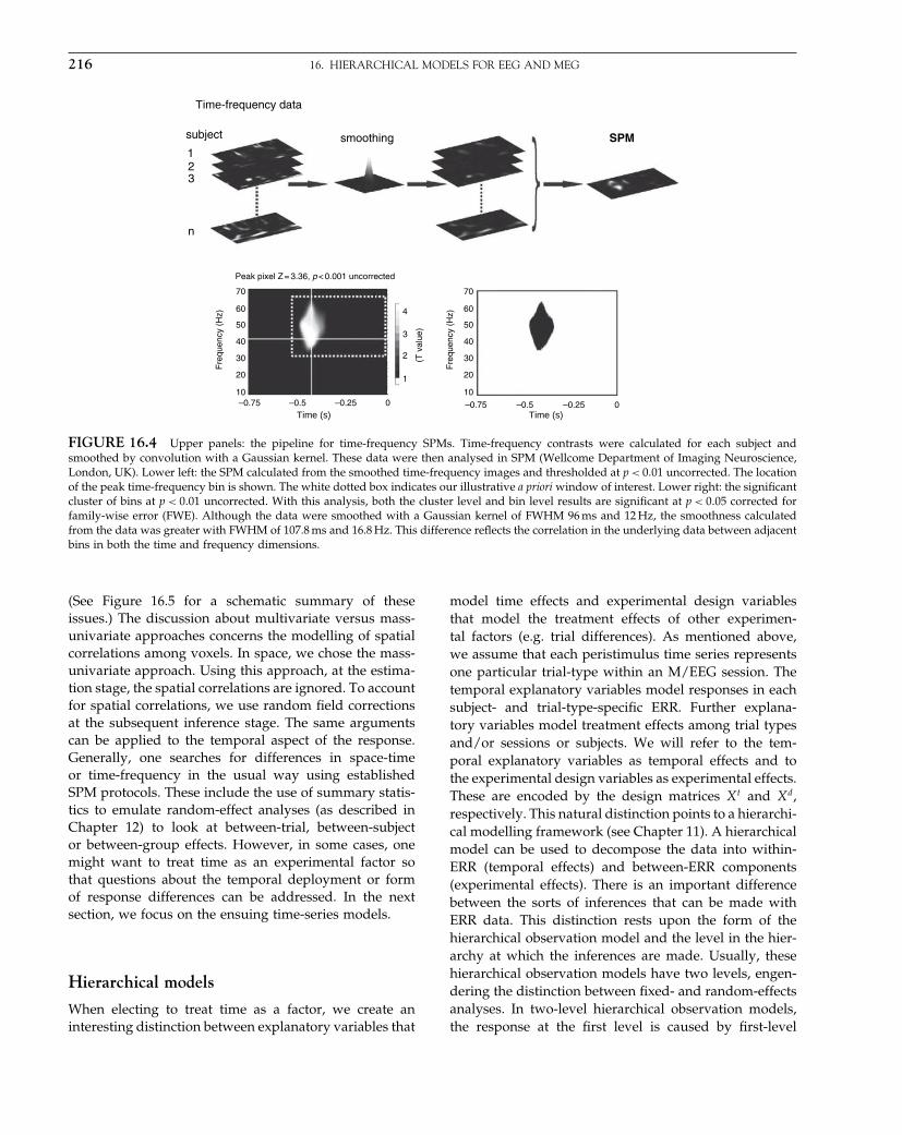
Elsevier UK Chapter: Ch16-P372560 30-9-2006 5:15p.m. Page:216 Trim:7.5in×9.25in
Basal Font:Palatino Margins:Top:40pt Gutter:68pt Font Size:9.5/12 Text Width:42pc Depth:55 Lines
216 16. HIERARCHICAL MODELS FOR EEG AND MEG
Time-frequency data
Time (s) Time (s)
subject
123
n
70
4
2
3
1
60
50
40
30
20
10–0.75 –0.5 –0.25 0
SPMsmoothing
Peak pixel Z = 3.36, p < 0.001 uncorrected
Fre
quen
cy (
Hz)
70
60
50
40
30
20
10
–0.75 –0.5 –0.25 0
Fre
quen
cy (
Hz)
(T v
alue
)
FIGURE 16.4 Upper panels: the pipeline for time-frequency SPMs. Time-frequency contrasts were calculated for each subject andsmoothed by convolution with a Gaussian kernel. These data were then analysed in SPM (Wellcome Department of Imaging Neuroscience,London, UK). Lower left: the SPM calculated from the smoothed time-frequency images and thresholded at p < 0�01 uncorrected. The locationof the peak time-frequency bin is shown. The white dotted box indicates our illustrative a priori window of interest. Lower right: the significantcluster of bins at p < 0�01 uncorrected. With this analysis, both the cluster level and bin level results are significant at p < 0�05 corrected forfamily-wise error (FWE). Although the data were smoothed with a Gaussian kernel of FWHM 96 ms and 12 Hz, the smoothness calculatedfrom the data was greater with FWHM of 107.8 ms and 16.8 Hz. This difference reflects the correlation in the underlying data between adjacentbins in both the time and frequency dimensions.
(See Figure 16.5 for a schematic summary of theseissues.) The discussion about multivariate versus mass-univariate approaches concerns the modelling of spatialcorrelations among voxels. In space, we chose the mass-univariate approach. Using this approach, at the estima-tion stage, the spatial correlations are ignored. To accountfor spatial correlations, we use random field correctionsat the subsequent inference stage. The same argumentscan be applied to the temporal aspect of the response.Generally, one searches for differences in space-timeor time-frequency in the usual way using establishedSPM protocols. These include the use of summary statis-tics to emulate random-effect analyses (as described inChapter 12) to look at between-trial, between-subjector between-group effects. However, in some cases, onemight want to treat time as an experimental factor sothat questions about the temporal deployment or formof response differences can be addressed. In the nextsection, we focus on the ensuing time-series models.
Hierarchical models
When electing to treat time as a factor, we create aninteresting distinction between explanatory variables that
model time effects and experimental design variablesthat model the treatment effects of other experimen-tal factors (e.g. trial differences). As mentioned above,we assume that each peristimulus time series representsone particular trial-type within an M/EEG session. Thetemporal explanatory variables model responses in eachsubject- and trial-type-specific ERR. Further explana-tory variables model treatment effects among trial typesand/or sessions or subjects. We will refer to the tem-poral explanatory variables as temporal effects and tothe experimental design variables as experimental effects.These are encoded by the design matrices Xt and Xd,respectively. This natural distinction points to a hierarchi-cal modelling framework (see Chapter 11). A hierarchicalmodel can be used to decompose the data into within-ERR (temporal effects) and between-ERR components(experimental effects). There is an important differencebetween the sorts of inferences that can be made withERR data. This distinction rests upon the form of thehierarchical observation model and the level in the hier-archy at which the inferences are made. Usually, thesehierarchical observation models have two levels, engen-dering the distinction between fixed- and random-effectsanalyses. In two-level hierarchical observation models,the response at the first level is caused by first-level

Elsevier UK Chapter: Ch16-P372560 30-9-2006 5:15p.m. Page:217 Trim:7.5in×9.25in
Basal Font:Palatino Margins:Top:40pt Gutter:68pt Font Size:9.5/12 Text Width:42pc Depth:55 Lines
TEMPORAL MODELS 217
FIGURE 16.5 Schematic demonstrating the different formulations of observation models implied by the multivariate versus mass-univariate and temporal dimension versus factor distinctions. The upper panels represent multivariate formulations in which there is noopportunity to place continuity constraints on the spatial or (upper left) spatio-temporal correlations. By treating each time bin or brainlocation as a separate component of the observed response, one effectively creates a model which is not informed about the continuity of theseresponses over space and time. The mass-univariate model in the lower left panel can be used to embody continuity constraints in both spaceand time through the application of random field theory. However, there would be no opportunity to assess design by time interactions. Thelower right panel represents the formulation in which time is treated as a factor but space is not.
parameters that themselves are modelled as random orstochastic variables at the second level, i.e.:
y = X�1���1� +��1�
��1� = X�2���2� +��2�
X�1� = INsubjectsNtypes⊗Xt
X�2� = Xd ⊗ INp
16.5
where the data y consists of one column vector of lengthNsubjectsNtypesNbins (see Figure 16.2). The ERR data areordered such that trial type-specific ERRs of an individ-ual subject are next to each other. This means the first-level design is X�1� = INsubjects
⊗ INtypes⊗Xt, where Xt is some
first-level design matrix, embodying temporal effects, fora single ERR. The second-level design matrix is given byX�2� = Xd ⊗ INp
, where, for example, Xd = 1Nsubjects⊗ INtypes
would be a simple averaging matrix. Np is the number ofcolumns in Xt and 1N denotes a column vector of onesof length N .
The model in Eqn. 16.5 reflects the natural hierar-chy of observed data. At the first level, the observations
are modelled in a subject- and trial-type-specific fashionwithin peristimulus time, where ��1� is the observationerror. At the second level, we model the parameters ��1�
over subjects and trial types. In other words, the ensuinghierarchy models temporal within-trial effects at the firstlevel and between-trial effects at the second. At this level,the error ��2� represents between-subject variability notmodelled in Xd.
There are several reasons why hierarchical linear mod-els are useful for characterizing ERR data. To startwith, they afford substantial latitude for modelling andhypothesis testing. Note that the first-level design matrixX�1� defines a projection onto some subspace of the data.Each parameter is associated with a specific dimensionof this subspace. One can consider many subspaces forERR data, where the Fourier transform or the wavelettransform are just two examples. The Fourier transformis useful for making inferences about power in somefrequency range. The wavelet transform is appropriatewhen making inferences about localized time-frequencyeffects. By specifying contrasts on the first- or second-level parameter estimates, we can test for effects localized

Elsevier UK Chapter: Ch16-P372560 30-9-2006 5:15p.m. Page:218 Trim:7.5in×9.25in
Basal Font:Palatino Margins:Top:40pt Gutter:68pt Font Size:9.5/12 Text Width:42pc Depth:55 Lines
218 16. HIERARCHICAL MODELS FOR EEG AND MEG
in peristimulus time and within certain frequency ranges(Kiebel and Friston, 2004). The important point about thetwo-level hierarchical model is that it enables different(linear) transforms at the first level.
A further motivation for hierarchical models is thatthey finesse the parameterization of non-sphericity. Inthis context, the error is decomposed into level-specificcomponents. From Eqn. 16.5, we see that the first-levelerror ��1� is the error about the fitted response, i.e. theobservation error. The second-level error ��2�, with anaveraging design component Xd, is the deviation ofeach first-level parameter from the average value fora particular trial-type in a specific subject. This errorarises from between-subject variability. The distinctionbetween these two components allows the decomposi-tion of the overall error into two partitions, the within-and between-subject variability. These partitions havedistinct non-sphericity structures, which can be modelledusing level-specific variance components. These facilitaterobust and accurate error estimation, which is necessaryfor valid inference.
An advantage of level-specific error components is thatone can make inferences at either level. This relates to thedistinction between fixed- and random-effects analyses(see Chapter 12). For example, in Eqn. 16.5, ��2� corre-sponds to the average response over subjects for a par-ticular trial type. The variability of ��2� (its covariance),can be derived by first collapsing the two-level model toone level:
y = X�1�X�2���2� +X�1���2� +��1� 16.6
Using an ordinary least-squares estimator, the covariancematrix of the parameter estimates is:
Cov��̂�2�� = �X�1�X�2��−Cov�X�1���2� +��1���X�1�X�2��−T 16.7
where X− denotes the generalized inverse. Eqn. 16.7says that the covariance of the estimated second-levelparameters is given by the projected error covarianceof the collapsed model. This is a mixture of the vari-ability of the errors from both levels. Therefore, �̂�2� notonly varies because of inter-subject, but also because ofwithin-subject variability.
In summary, the two-level model is useful if there isa meaningful linear projection to some low-dimensionalspace. For instance, in fMRI, the blood oxygenation-level-dependent (BOLD) response can be linearly modelledwith three basis functions. These capture a large part ofthe stimulus-induced variability. Similarly, in M/EEG,temporal basis functions in Xt allow us to summarizea response with a few parameters. At the second level,we can then test hypotheses about these parameters (i.e.differences and interactions). This dimension reductionis an efficient way of testing for effects. Note that these
basis functions can extend over peristimulus time. Theycan describe simple averages or other more complicatedshapes like damped oscillations.
An alternative is to forgo modelling the first levelcompletely and employ the identity matrix as temporaldesign matrix Xt = I . This effectively renders the two-level model (Eqn. 16.5) a one-level model, because thereis no error ��1� at the first level. This is the traditionalway of analysing evoked responses. One simply formscontrasts at the first level and models them at the second.Traditionally, researchers test for averages over a partic-ular window of peristimulus time, but one can actuallyuse any linear combination over peristimulus time. Theadvantage of this analysis is that it is simple and straight-forward and appeals to exactly the same arguments asthe summary-statistic approach to hierarchical models offMRI data.
This concludes our discussion about how we model thespatio-temporal and experimental dimensions of M/EEGdata. Next we focus on modelling the experimental fac-tors, e.g. groups or trial-types. To simplify things we willuse the identity matrix (i.e. a complete basis set) as tem-poral design matrix Xt.
HYPOTHESIS TESTING WITHHIERARCHICAL MODELS
Hierarchical models for M/EEG are the same as thoseused for other imaging modalities (see Chapter 13) andinference can proceed using the same multistage proto-col, by taking contrasts from one level to the next. Thissummary statistic approach can be used for the analysisof either evoked responses or time-frequency power data.In this section, we describe how contrasts can be specifiedto ask a wide range of questions about evoked responsesin multisubject studies, using time-series SPMs.
For ERR data, we follow the approach outlined above.First, one projects data from channel to voxel-space. Thiscan be either a two-dimensional approximation to thescalp surface or a three-dimensional source reconstruc-tion (Phillips et al., 2002; Mattout et al., 2005). These time-series of images form the input to the first level of ahierarchical model to provide estimates of the responsefor each temporal basis function (in this case each timebin), each trial-type and each subject. The inputs to thesecond level are contrasts over time bins, for each subjectand trial type. These can be simple averages over severaltime points in peristimulus time, e.g. the average between150 and 190 ms to measure the N170 component. Notethat one can choose any temporal shape as contrast, e.g.a Gaussian or damped sinusoid.
Elsevier UK Chapter: Ch16-P372560 30-9-2006 5:15p.m. Page:219 Trim:7.5in×9.25in
Basal Font:Palatino Margins:Top:40pt Gutter:68pt Font Size:9.5/12 Text Width:42pc Depth:55 Lines
SUMMARY 219
For time-frequency analyses, one first computes powerin the time-frequency domain (Kiebel et al., 2005). Incurrent software implementations of SPM, we use theMorlet wavelet transform. This renders the data 4- or5-dimensional (2 or 3 spatial dimensions, time, and fre-quency). As outlined above, there are two differentapproaches to these data. One could treat space, time, andfrequency as dimensions of a random field. This leavesonly dimensions like subject or trial-types as experimen-tal factors (see Figure 16.4 and Kilner et al., 2005). Analternative is to treat both time and frequency as fac-tors. In this case, the input to the second level is formedby subject and trial type-specific contrasts over time andfrequency (e.g. averages in windows of time-frequencyspace). In the following, we describe some commonsecond-level models for M/EEG.
Evoked responses
A typical analysis of ERRs is the one-way (repeated mea-sures) analysis of variance. For each of the n = 1� � � � �Nsubjects there are K measurements (i.e. trial-types). Thesecond-level summary statistics are contrasts over peris-timulus time, for each subject and trial type. The designmatrix in this case is X�2� = IK ⊗ 1N � 1K ⊗ IN � (see alsoChapter 13). In terms of the model’s covariance compo-nents, one could assume that the between-subject errors��2� are uncorrelated and have unequal variances for eachtrial-type. This results in K covariance components. Afterparameter estimation, one tests for main effects or inter-actions among the trial-types at the between-subject level,with the appropriate contrast. Note that this model usesa ‘pooled’ estimate of non-sphericity over voxels (seeChapter 13). An alternative is to compute the relevantcontrasts (e.g. a main effect or interaction) at the firstlevel and use a series of one-sample t-tests at the second.
Induced responses
In SPM, the time-frequency decomposition of data usesthe Morlet wavelet transform. Note that other approachesusing short-term Fourier transform, or the Hilbert trans-form on bandpassed filtered data are largely equivalentto the wavelet decomposition (Kiebel et al., 2005). Forfrequency � = 2�f and peristimulus time t, the Morletwavelet kernel is:
h�t��� = c� exp�− t2
�2t
� exp�i�t� 16.8
where c� is some normalization factor and �2t is the tem-
poral width of the kernel. The transform itself is theconvolution:
z�t���ij = h���∗ yij 16.9
where yij is the i-th (single) trial measured at the j-th channel (or voxel) and ∗ denotes convolution. Thepower is:
P�t���ij = z�t���ijz�t���∗ij 16.10
where z�t���∗ij is the complex conjugate. Induced activity
is computed by averaging Pij over trials and subtract-ing the power of the evoked response. When time andfrequency are considered experimental factors, we com-pute contrasts at the first level and pass them to thesecond. This might be an average in the time-frequencyplane (e.g. Kilner et al., 2005). Alternatively, one can com-pute, per trial type and subject, several averages in thetime-frequency plane and take them up to the secondlevel. These contrasts can be modelled using repeated-measures ANOVA, where time and frequency are bothfactors with multiple levels.
In general, we assume that the second-level errorfor contrasts of power is normally distributed, whereaspower data per se have a �2-distribution. However,in most cases, the contrasts have a near-normal dis-tribution because of averaging over time, frequencyand trials and, more importantly, taking differencesbetween peristimulus times or trial-types. These averag-ing operations render the contrasts or summary statis-tics normally distributed, by central limit theorem. Whenthere is still doubt about the normality assumption,one can apply a log or square-root transform (Kiebelet al., 2005).
SUMMARY
In this chapter, we have covered various ways ofanalysing M/EEG data, with a special focus on the dis-tinction between treating time as a factor and treat-ing it as a dimension of the response variable. Thiscorresponds to the distinction between inference basedon time-series models (of the sort using in fMRI) andspatio-temporal SPMs that span space and time. In thecase of time-series models, the hierarchical nature ofour observation models calls for a multistage summary-statistic approach, in which contrasts at each level arepassed to higher levels to enable between-trial, between-subject and between-group inferences. The central roleof hierarchal models will be taken up again in Section 4,in the context of empirical Bayes. In the next sectionwe consider, in greater depth, the nature of inferenceon SPMs.

Elsevier UK Chapter: Ch16-P372560 30-9-2006 5:15p.m. Page:220 Trim:7.5in×9.25in
Basal Font:Palatino Margins:Top:40pt Gutter:68pt Font Size:9.5/12 Text Width:42pc Depth:55 Lines
220 16. HIERARCHICAL MODELS FOR EEG AND MEG
REFERENCES
Chatfield C, Collins A (1980) Introduction to multivariate analysis.Chapman & Hall, London
Friston KJ, Frith CD, Frackowiak RS et al. (1995) Characterizingdynamic brain responses with fMRI: a multivariate approach.NeuroImage 2: 166–72
Friston KJ, Frith CD, Liddle PF et al. (1991) Comparing functional(PET) images: the assessment of significant change. J Cereb BloodFlow Metab 11: 690–99
Friston KJ, Penny W, Phillips C et al. (2002) Classical and Bayesianinference in neuroimaging: theory. NeuroImage 16: 465–83
Friston KJ, Stephan KM, Heather JD et al. (1996) A multivariateanalysis of evoked responses in EEG and MEG data. NeuroImage3: 167–74
Kiebel SJ, Friston KJ (2004) Statistical parametric mapping for event-related potentials (II): a hierarchical temporal model. NeuroImage22: 503–20
Kiebel SJ, Tallon-Baudry C, Friston KJ (2005) Parametric analysisof oscillatory activity as measured with M/EEG. Hum BrainMapp 26: 170–77
Kilner JM, Kiebel SJ, Friston KJ (2005) Applications ofrandom field theory to electrophysiology. Neurosci Lett 374:174–78
Kilner JM, Otten LJ, Friston KJ (2006) Application of random fieldtheory to EEG data in space and time. O Human Brain Mapping,Florence
Mattout J, Phillips C, Penny WD et al. (2005) MEG source localizationunder multiple constraints: an extended Bayesian framework.Neuroimage 3: 753–67
Phillips C, Rugg MD, Friston KJ (2002) Anatomically informed basisfunctions for EEG source localization: combining functional andanatomical constraints. Neuroimage 16: 678–95
Rugg MD, Coles MG (1995) Electrophysiology and mind. Oxford Uni-versity Press, Oxford
Worsley KJ, Andermann M, Koulis T et al. (1999) Detecting changesin nonisotropic images. Hum Brain Mapp 8: 98–101
Worsley KJ, Poline JB, Friston KJ et al. (1997) Characterizing theresponse of PET and fMRI data using multivariate linear models.Neuroimage 6: 305–19
Yandell BS (1997) Practical data analysis for designed experiments.Chapman & Hall, London
Elsevier UK Chapter: Ch17-P372560 30-9-2006 5:15p.m. Page:223 Trim:7.5in×9.25in
Basal Font:Palatino Margins:Top:40pt Gutter:68pt Font Size:9.5/12 Text Width:42pc Depth:55 Lines
C H A P T E R
17
Parametric proceduresM. Brett, W. Penny and S. Kiebel
INTRODUCTION
This chapter is an introduction to inference usingparametric procedures with focus on the multiple com-parison problem in functional imaging, and the way itcan be solved using random field theory (RFT).
In a standard functional imaging analysis, we fit a sta-tistical model to the data, to give us model parameters.We then use the model parameters to look for an effectwe are interested in, such as the difference between a taskand baseline. To do this, we usually calculate a statisticfor each brain voxel that tests for the effect of interest inthat voxel. The result is a large volume of statistic values.
We now need to decide if this volume shows any evi-dence of the effect. To do this, we have to take intoaccount that there are many thousands of voxels andtherefore many thousands of statistic values. This isthe multiple comparison problem in functional imaging.Random field theory is a recent branch of mathematicsthat can be used to solve this problem.
To explain the use of RFT, we will first go back tothe basics of hypothesis testing in statistics. We describethe multiple comparison problem and the usual solution,which is the Bonferroni correction. We explain why spa-tial correlation in imaging data causes problems for theBonferroni correction and introduce RFT as a solution.Finally, we discuss the assumptions underlying RFT andthe problems that arise when these assumptions do nothold. We hope this chapter will be accessible to thosewith no specific expertise in mathematics or statistics.Those more interested in mathematical details and recentdevelopments are referred to Chapters 18 and 19.
Rejecting the null hypothesis
When we calculate a statistic, we often want to decidewhether the statistic represents convincing evidence of
the effect we are interested in. Usually, we test thestatistic against the null hypothesis, which is the hypoth-esis that there is no effect. If the statistic is not compatiblewith the null hypothesis, we may conclude that there isan effect. To test against the null hypothesis, we can com-pare our statistic value to a null distribution, which is thedistribution of statistic values we would expect if thereis no effect. Using the null distribution, we can estimatehow likely it is that our statistic could have come aboutby chance. We may find that the result we found has a5 per cent chance of resulting from a null distribution.We therefore decide to reject the null hypothesis, andaccept the alternative hypothesis that there is an effect. Inrejecting the null hypothesis, we must accept a 5 per centchance that the result has in fact arisen when there is infact no effect, i.e. the null hypothesis is true. Five per centis our expected type I error rate, or the chance that we takethat we are wrong when we reject the null hypothesis.
For example, when we do a single t-test, we comparethe t-value we have found to the null distribution for thet-statistic. Let us say we have found a t-value of 2.42,and have 40 degrees of freedom. The null distribution oft-statistics with 40 degrees of freedom tells us that theprobability of observing a value greater than or equal to2.42, if there is no effect, is only 0.01. In our case, we canreject the null hypothesis with a 1 per cent risk of typeI error.
The situation is more complicated in functional imag-ing because we have many voxels and therefore manystatistic values. If we do not know where in the brain oureffect will occur, our hypothesis refers to the whole vol-ume of statistics in the brain. Evidence against the nullhypothesis would be that the whole observed volume ofvalues is unlikely to have arisen from a null distribution.The question we are asking is now a question about thevolume, or family of voxel statistics, and the risk of errorthat we are prepared to accept is the family-wise error
Statistical Parametric Mapping, by Karl Friston et al. Copyright 2007, Elsevier Ltd. All rights reserved.ISBN–13: 978-0-12-372560-8 ISBN–10: 0-12-372560-7
223
Elsevier UK Chapter: Ch17-P372560 30-9-2006 5:15p.m. Page:224 Trim:7.5in×9.25in
Basal Font:Palatino Margins:Top:40pt Gutter:68pt Font Size:9.5/12 Text Width:42pc Depth:55 Lines
224 17. PARAMETRIC PROCEDURES
rate (FWE) – which is the likelihood that this family ofvoxel values could have arisen by chance.
We can test a family-wise null hypothesis in a varietyof ways, but one useful method is to look for any statisticvalues that are larger than we would expect, if they allhad come from a null distribution. The method requiresthat we find a threshold to apply to every statistic value,so that any values above the threshold are unlikely tohave arisen by chance. This is often referred to as ‘heightthresholding’, and it has the advantage that if we findvoxels above threshold, we can conclude that there is aneffect at these voxel locations, i.e. the test has localizingpower. Alternative procedures based on cluster- and set-level inferences are discussed in the next chapter.
A height threshold that can control family-wise errormust take into account the number of tests. We saw abovethat a single t-statistic value from a null distribution with40 degrees of freedom has a 1 per cent probability ofbeing greater than 2.42. Now imagine our experiment hasgenerated 1000 t values with 40 degrees of freedom. If welook at any single statistic, then by chance it will havea 1 per cent probability of being greater than 2.42. Thismeans that we would expect 10 t values in our sample of1000 to be greater than 2.42. So, if we see one or more tvalues above 2.42 in this family of tests, this is not goodevidence against the family-wise null hypothesis, whichis that all these values have been drawn from a nulldistribution. We need to find a new threshold, such that,in a family of 1000 t statistic values, there is a 1 per centprobability of there being one or more t values above thatthreshold. The Bonferroni correction is a simple methodof setting this threshold.
THE BONFERRONI CORRECTION
The Bonferroni correction is based on simple probabilityrules. Imagine we have taken our t values and used thenull t distribution to convert them to probability values.We then apply a probability threshold � to each of our nprobability values; in our previous example � was 0.01,and n was 1000. If all the test values are drawn from anull distribution, then each of our n probability valueshas a probability � of being greater than threshold. Theprobability of all the tests being less than � is therefore�1−��n. The family-wise error rate �PFWE� is the probabil-ity that one or more values will be greater than �, whichis simply:
PFWE = 1− �1−��n 17.1
Because � is small this can be approximated by thesimpler expression:
PFWE ≤ n� 17.2
Using Eqn. 17.2, we can find a single-voxel probabilitythreshold � that will give us our required family-wiseerror rate, PFWE , such that we have a PFWE probability ofseeing any voxel above threshold in all of the n values.We simply solve Eqn. 17.2 for �:
� = PFWE/n 17.3
If we have a brain volume of 100 000 t-statistics, all with40 degrees of freedom, and we want an FWE rate of 0.05,then the required probability threshold for a single voxel,using the Bonferroni correction, would be 0�05/100� 000 =0�0000005. The corresponding t-statistic is 5.77. If anyvoxel t-statistic is above 5.77, then we can conclude thata voxel statistic of this magnitude has only a 5 per centchance of arising anywhere in a volume of 100 000 t-statistics drawn from the null distribution.
The Bonferroni procedure gives a corrected p-value; inthe case above, the uncorrected p-value for a voxel witha t-statistic of 5.77 was 0.0000005; the p-value correctedfor the number of comparisons is 0.05.
The Bonferroni correction is used for calculating FWErates for some functional imaging analyses. However, inmany cases, the Bonferroni correction is too conservativebecause most functional imaging data have some degreeof spatial correlation, i.e. there is correlation betweenneighbouring statistic values. In this case, there are fewerindependent values in the statistic volume than there arevoxels.
Spatial correlation
Some degree of spatial correlation is almost universallypresent in functional imaging data. In general, data fromany one voxel in the functional image will tend to be sim-ilar to data from nearby voxels, even after the modelledeffects have been removed. Thus the errors from the sta-tistical model will tend to be correlated for nearby voxels.The reasons for this include factors inherent in collectingand reconstructing the image, physiological signal thathas not been modelled, and spatial preprocessing appliedto the data before statistical analysis.
For positron emission tomography (PET) data, muchmore than for functional magnetic resonance imaging(fMRI), nearby voxels are related because of the way thatthe scanner collects and reconstructs the image. Thus,data that do in fact arise from a single voxel location inthe brain will also cause some degree of signal change in
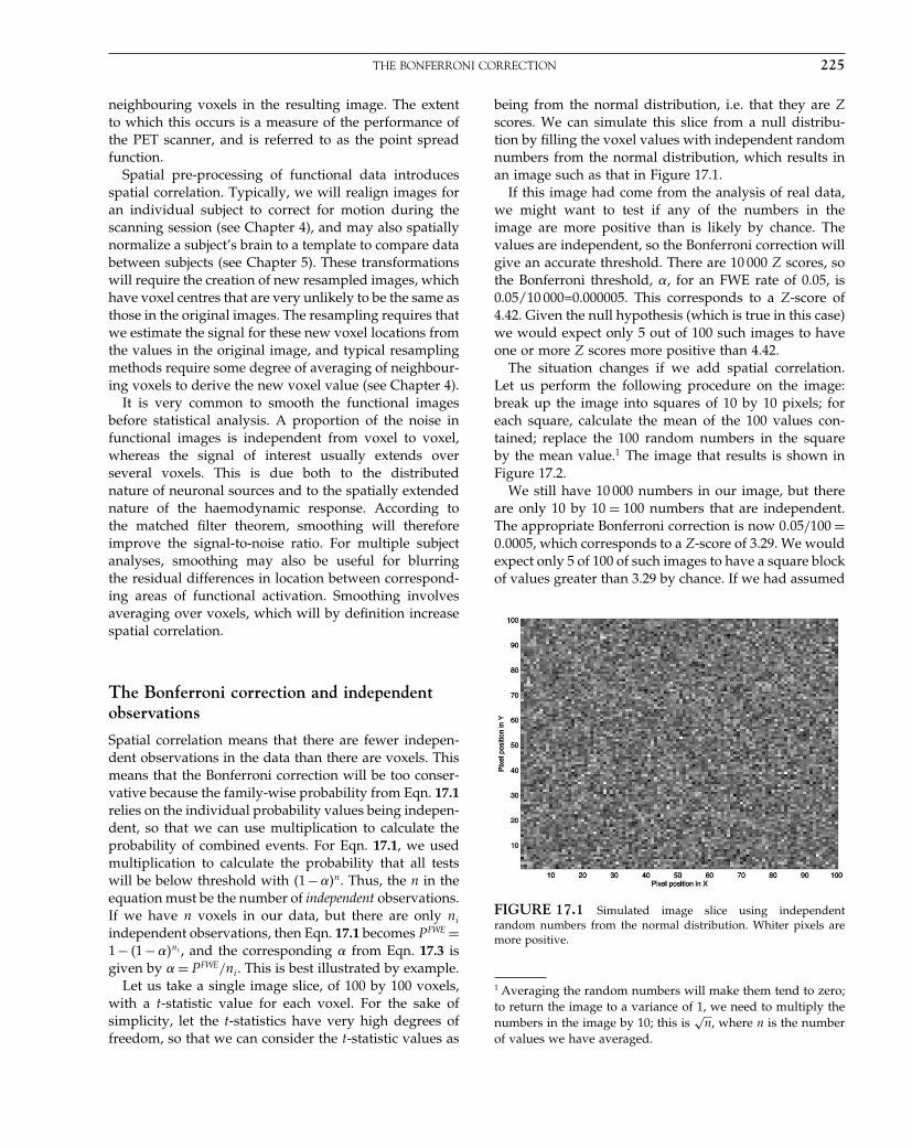
Elsevier UK Chapter: Ch17-P372560 30-9-2006 5:15p.m. Page:225 Trim:7.5in×9.25in
Basal Font:Palatino Margins:Top:40pt Gutter:68pt Font Size:9.5/12 Text Width:42pc Depth:55 Lines
THE BONFERRONI CORRECTION 225
neighbouring voxels in the resulting image. The extentto which this occurs is a measure of the performance ofthe PET scanner, and is referred to as the point spreadfunction.
Spatial pre-processing of functional data introducesspatial correlation. Typically, we will realign images foran individual subject to correct for motion during thescanning session (see Chapter 4), and may also spatiallynormalize a subject’s brain to a template to compare databetween subjects (see Chapter 5). These transformationswill require the creation of new resampled images, whichhave voxel centres that are very unlikely to be the same asthose in the original images. The resampling requires thatwe estimate the signal for these new voxel locations fromthe values in the original image, and typical resamplingmethods require some degree of averaging of neighbour-ing voxels to derive the new voxel value (see Chapter 4).
It is very common to smooth the functional imagesbefore statistical analysis. A proportion of the noise infunctional images is independent from voxel to voxel,whereas the signal of interest usually extends overseveral voxels. This is due both to the distributednature of neuronal sources and to the spatially extendednature of the haemodynamic response. According tothe matched filter theorem, smoothing will thereforeimprove the signal-to-noise ratio. For multiple subjectanalyses, smoothing may also be useful for blurringthe residual differences in location between correspond-ing areas of functional activation. Smoothing involvesaveraging over voxels, which will by definition increasespatial correlation.
The Bonferroni correction and independentobservations
Spatial correlation means that there are fewer indepen-dent observations in the data than there are voxels. Thismeans that the Bonferroni correction will be too conser-vative because the family-wise probability from Eqn. 17.1relies on the individual probability values being indepen-dent, so that we can use multiplication to calculate theprobability of combined events. For Eqn. 17.1, we usedmultiplication to calculate the probability that all testswill be below threshold with �1−��n. Thus, the n in theequation must be the number of independent observations.If we have n voxels in our data, but there are only ni
independent observations, then Eqn. 17.1 becomes PFWE =1 − �1 −��ni , and the corresponding � from Eqn. 17.3 isgiven by � = PFWE/ni. This is best illustrated by example.
Let us take a single image slice, of 100 by 100 voxels,with a t-statistic value for each voxel. For the sake ofsimplicity, let the t-statistics have very high degrees offreedom, so that we can consider the t-statistic values as
being from the normal distribution, i.e. that they are Zscores. We can simulate this slice from a null distribu-tion by filling the voxel values with independent randomnumbers from the normal distribution, which results inan image such as that in Figure 17.1.
If this image had come from the analysis of real data,we might want to test if any of the numbers in theimage are more positive than is likely by chance. Thevalues are independent, so the Bonferroni correction willgive an accurate threshold. There are 10 000 Z scores, sothe Bonferroni threshold, �, for an FWE rate of 0.05, is0.05/10 000=0.000005. This corresponds to a Z-score of4.42. Given the null hypothesis (which is true in this case)we would expect only 5 out of 100 such images to haveone or more Z scores more positive than 4.42.
The situation changes if we add spatial correlation.Let us perform the following procedure on the image:break up the image into squares of 10 by 10 pixels; foreach square, calculate the mean of the 100 values con-tained; replace the 100 random numbers in the squareby the mean value.1 The image that results is shown inFigure 17.2.
We still have 10 000 numbers in our image, but thereare only 10 by 10 = 100 numbers that are independent.The appropriate Bonferroni correction is now 0�05/100 =0�0005, which corresponds to a Z-score of 3.29. We wouldexpect only 5 of 100 of such images to have a square blockof values greater than 3.29 by chance. If we had assumed
FIGURE 17.1 Simulated image slice using independentrandom numbers from the normal distribution. Whiter pixels aremore positive.
1 Averaging the random numbers will make them tend to zero;to return the image to a variance of 1, we need to multiply thenumbers in the image by 10; this is
√n, where n is the number
of values we have averaged.

Elsevier UK Chapter: Ch17-P372560 30-9-2006 5:15p.m. Page:226 Trim:7.5in×9.25in
Basal Font:Palatino Margins:Top:40pt Gutter:68pt Font Size:9.5/12 Text Width:42pc Depth:55 Lines
226 17. PARAMETRIC PROCEDURES
FIGURE 17.2 Random number image from Figure 17.1 afterreplacing values in the 10 by 10 squares by the value of the meanwithin each square.
all the values were independent, then we would haveused the correction for 10 000 values, of � = 0�000005.Because we actually have only 100 independent observa-tions, Eqn. 17.2, with n = 100 and � = 0�000005, tells usthat we expect an FWE rate of 0.0005, which is one hun-dred times lower (i.e. more conservative) than the ratethat we wanted.
Smoothing and independent observations
In the preceding section, we replaced a block of values inthe image with their mean in order to show the effect ofreducing the number of independent observations. Thisprocedure is a very simple form of smoothing. Whenwe smooth an image with a smoothing kernel, such asa Gaussian, each value in the image is replaced with aweighted average of itself and its neighbours. Figure 17.3shows the image from Figure 17.1 after smoothing with aGaussian kernel of full width at half maximum (FWHM)of 10 pixels.2 An FWHM of 10 pixels means that, at fivepixels from the centre, the value of the kernel is halfits peak value. Smoothing has the effect of blurring theimage, and reduces the number of independent observa-tions.
2 As for the procedure where we took the mean of the 100 obser-vations in each square, the smoothed values will no longer havea variance of one, because the averaging involved in smoothingwill make the values tend to zero. As for the square example,we need to multiply the values in the smoothed image by ascale factor to return the variance to one; the derivation of thescale factor is rather technical, and not relevant to our currentdiscussion.
FIGURE 17.3 Random number image from Figure 17.1 aftersmoothing with a Gaussian smoothing kernel of full width at halfmaximum of 10 pixels.
The smoothed image contains spatial correlation,which is typical of the output from the analysis of func-tional imaging data. We now have a problem, becausethere is no simple way of calculating the number of inde-pendent observations in the smoothed data, so we can-not use the Bonferroni correction. This problem can beaddressed using random field theory.
RANDOM FIELD THEORY
Random field theory (RFT) is a recent body of mathe-matics defining theoretical results for smooth statisticalmaps. The theory has been versatile in dealing with manyof the thresholding problems that we encounter in func-tional imaging. Among many other applications, it can beused to solve our problem of finding the height thresh-old for a smooth statistical map which gives the requiredfamily-wise error rate.
The way that RFT solves this problem is by usingresults that give the expected Euler characteristic (EC) fora smooth statistical map that has been thresholded. Wewill discuss the EC in more detail below; for now it isonly necessary to note that the expected EC leads directlyto the expected number of clusters above a given thresh-old, and that this in turn gives the height threshold thatwe need.
The application of RFT proceeds in stages. First, weestimate the smoothness (spatial correlation) of our sta-tistical map. Then we use the smoothness values inthe appropriate RFT equation, to give the expected ECat different thresholds. This allows us to calculate the
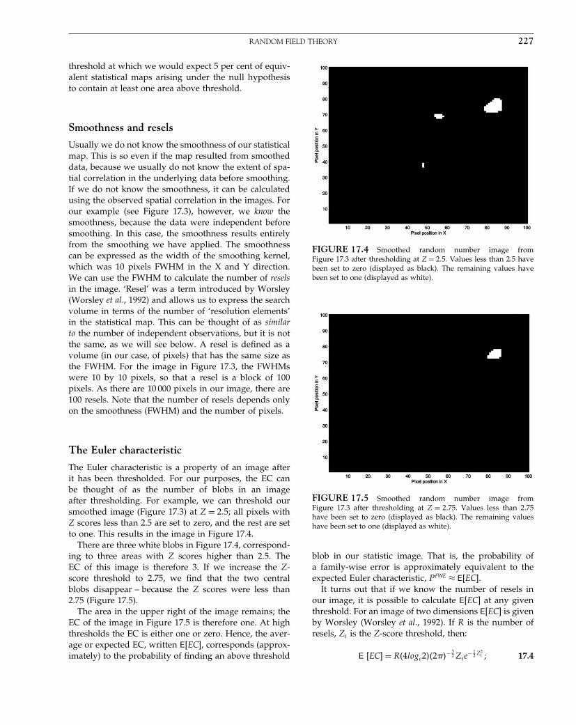
Elsevier UK Chapter: Ch17-P372560 30-9-2006 5:15p.m. Page:227 Trim:7.5in×9.25in
Basal Font:Palatino Margins:Top:40pt Gutter:68pt Font Size:9.5/12 Text Width:42pc Depth:55 Lines
RANDOM FIELD THEORY 227
threshold at which we would expect 5 per cent of equiv-alent statistical maps arising under the null hypothesisto contain at least one area above threshold.
Smoothness and resels
Usually we do not know the smoothness of our statisticalmap. This is so even if the map resulted from smootheddata, because we usually do not know the extent of spa-tial correlation in the underlying data before smoothing.If we do not know the smoothness, it can be calculatedusing the observed spatial correlation in the images. Forour example (see Figure 17.3), however, we know thesmoothness, because the data were independent beforesmoothing. In this case, the smoothness results entirelyfrom the smoothing we have applied. The smoothnesscan be expressed as the width of the smoothing kernel,which was 10 pixels FWHM in the X and Y direction.We can use the FWHM to calculate the number of reselsin the image. ‘Resel’ was a term introduced by Worsley(Worsley et al., 1992) and allows us to express the searchvolume in terms of the number of ‘resolution elements’in the statistical map. This can be thought of as similarto the number of independent observations, but it is notthe same, as we will see below. A resel is defined as avolume (in our case, of pixels) that has the same size asthe FWHM. For the image in Figure 17.3, the FWHMswere 10 by 10 pixels, so that a resel is a block of 100pixels. As there are 10 000 pixels in our image, there are100 resels. Note that the number of resels depends onlyon the smoothness (FWHM) and the number of pixels.
The Euler characteristic
The Euler characteristic is a property of an image afterit has been thresholded. For our purposes, the EC canbe thought of as the number of blobs in an imageafter thresholding. For example, we can threshold oursmoothed image (Figure 17.3) at Z = 2�5; all pixels withZ scores less than 2.5 are set to zero, and the rest are setto one. This results in the image in Figure 17.4.
There are three white blobs in Figure 17.4, correspond-ing to three areas with Z scores higher than 2.5. TheEC of this image is therefore 3. If we increase the Z-score threshold to 2.75, we find that the two centralblobs disappear – because the Z scores were less than2.75 (Figure 17.5).
The area in the upper right of the image remains; theEC of the image in Figure 17.5 is therefore one. At highthresholds the EC is either one or zero. Hence, the aver-age or expected EC, written E�EC�, corresponds (approx-imately) to the probability of finding an above threshold
FIGURE 17.4 Smoothed random number image fromFigure 17.3 after thresholding at Z = 2�5. Values less than 2.5 havebeen set to zero (displayed as black). The remaining values havebeen set to one (displayed as white).
FIGURE 17.5 Smoothed random number image fromFigure 17.3 after thresholding at Z = 2�75. Values less than 2.75have been set to zero (displayed as black). The remaining valueshave been set to one (displayed as white).
blob in our statistic image. That is, the probability ofa family-wise error is approximately equivalent to theexpected Euler characteristic, PFWE ≈ E�EC�.
It turns out that if we know the number of resels inour image, it is possible to calculate E�EC� at any giventhreshold. For an image of two dimensions E�EC� is givenby Worsley (Worsley et al., 1992). If R is the number ofresels, Zt is the Z-score threshold, then:
E �EC� = R�4loge2��2�− 32 Zte
− 12 Z2
t 17.4

Elsevier UK Chapter: Ch17-P372560 30-9-2006 5:15p.m. Page:228 Trim:7.5in×9.25in
Basal Font:Palatino Margins:Top:40pt Gutter:68pt Font Size:9.5/12 Text Width:42pc Depth:55 Lines
228 17. PARAMETRIC PROCEDURES
FIGURE 17.6 Expected EC values for an image of 100 resels.
Figure 17.6 shows E�EC� for an image of 100 resels, forZ-score thresholds between zero and five. As the thresh-old drops from one to zero, E�EC� drops to zero; this isbecause the precise definition of the EC is more complexthan simply the number of blobs (Worsley et al., 1994).This makes a difference at low thresholds but is not rel-evant for our purposes because, as explained above, weare only interested in the properties of E�EC� at highthresholds, i.e. when it approximates PFWE .
Note also that the graph in Figure 17.6 does a reason-able job of predicting the EC in our image; at a Z thresh-old of 2.5 it predicted an EC of 1.9, when we observeda value of 3; at Z = 2�75 it predicted an EC of 1.1, for anobserved EC of 1.
We can now apply RFT to our smoothed image(Figure 17.3) which has 100 resels. For 100 resels,Eqn. 17.4 gives an E�EC� of 0.049 for a Z threshold of3.8 (cf. the graph in Figure 17.6). If we have a two-dimensional image with 100 resels, then the probabilityof getting one or more blobs where Z is greater than3.8, is 0.049. We can use this for thresholding. Let x bethe Z-score threshold that gives an E�EC� of 0.05. If wethreshold our image at x, we can conclude that any blobsthat remain have a probability of less than or equal to0.05 that they have occurred by chance. From Eqn. 17.4,the threshold, x, depends only on the number of reselsin our image.
Random field thresholds and the Bonferronicorrection
The random field correction derived using the EC is notthe same as a Bonferroni correction for the number of
resels. We stated above that the resel count in an imageis not exactly the same as the number of independentobservations. If it were the same, we could use a Bonfer-roni correction based on the number of resels, instead ofusing RFT. However, these two corrections give differ-ent answers. For � = 0�05, the Z threshold according toRFT, for our 100 resel image, is Z = 3�8. The Bonferronithreshold for 100 independent tests is 0.05/100, whichequates to a Z-score of 3.3. Although the RFT maths givesus a correction that is similar in principle to a Bonferronicorrection, it is not the same. If the assumptions of RFTare met (see Section 4) then the RFT threshold is moreaccurate than the Bonferroni.
Random fields and functional imaging
Analyses of functional imaging data usually lead to three-dimensional statistical images. So far we have discussedthe application of RFT to an image of two dimensions,but the same principles apply in three dimensions. TheEC is the number of 3D blobs of Z scores above a certainthreshold and a resel is a cube of voxels of size (FWHMin x) by (FWHM in y) by (FWHM in z). The equation forE�EC� is different in the 3D case, but still depends onlyon the resels in the image.
For the sake of simplicity, we have only considered arandom field of Z-scores, i.e. numbers drawn from thenormal distribution. There are now equivalent results fort, F and �2 random fields (Worsley, 1994). For example,the statistical parametric mapping (SPM) software usesformulae for t and F random fields to calculate correctedthresholds for height.
As noted above, we usually do not know thesmoothness of a statistic volume from a functional imag-ing analysis, because we do not know the extent of spatialcorrelation before smoothing. We cannot assume that thesmoothness is the same as any explicit smoothing thatwe have applied and will need to calculate smoothnessfrom the images themselves. In practice, smoothness iscalculated using the residual values from the statisticalanalysis as described in Kiebel et al. (1999).
Small volume correction
We noted above that the results for the expected Eulercharacteristic depend only on the number of resels con-tained in the volume of voxels we are analysing. This isnot strictly accurate, although it is a very close approx-imation when the voxel volume is large compared tothe size of a resel (Worsley et al. 1996). In fact, E�EC�also depends on the shape and size of the volume. Theshape of the volume becomes important when we have

Elsevier UK Chapter: Ch17-P372560 30-9-2006 5:15p.m. Page:229 Trim:7.5in×9.25in
Basal Font:Palatino Margins:Top:40pt Gutter:68pt Font Size:9.5/12 Text Width:42pc Depth:55 Lines
RANDOM FIELD THEORY 229
a small or oddly shaped region. This is unusual if we areanalysing statistics from the whole brain, but there areoften situations where we wish to restrict our search toa smaller subset of the volume, for example where wehave a specific hypothesis as to where our signal is likelyto occur.
The reason that the shape of the volume may influ-ence the correction is best explained by example. Let usreturn to the 2D image of smoothed random numbers(Figure 17.3). We could imagine that we had reason tobelieve that signal change will occur only in the centreof the image. Our search region will not be the wholeimage, but might be a box at the image centre, with size30 by 30 pixels (Figure 17.7).
The box contains 9 resels. The figure shows a grid ofX-shaped markers; these are spaced at the width of aresel, i.e. 10 pixels. The box can contain a maximum of16 of these markers. Now let us imagine we had a moreunusually shaped search region. For some reason, wemight expect that our signal of interest will occur withina frame 2.5 pixels wide around the outside of the image.The frame contains the same number of voxels as the box,and therefore has the same volume in terms of resels.However, the frame contains many more markers (32), sothe frame is sampling from the data of more resels thanthe box. Multiple comparison correction for the framemust therefore be more stringent than for the box.
In fact, E�EC� depends on the volume, surface area, anddiameter of the search region (Worsley et al., 1996). Theseparameters can be calculated for continuous shapes forwhich formulae are available for volume, surface areaand diameter, such as spheres or boxes (see Appendix 6).
FIGURE 17.7 Smoothed random number image fromFigure 17.3 with two example search regions: a box (centre) anda frame (outer border of image). X-shaped markers are spaced atone-resel widths across the image.
FIGURE 17.8 t threshold giving an FWE rate of 0.05, forspheres of increasing radius. Smoothness was 8 mm in X Y and Zdirections, and the example analysis had 200 degrees of freedom.
Otherwise, the parameters can be estimated from anyshape that has been defined in an image. Restricting thesearch region to a small volume within a statistical mapcan lead to greatly reduced thresholds for given FWErates. For Figure 17.8, we assumed a statistical analysisthat resulted in a t-statistic map with 8 mm smoothness inthe X, Y and Z directions. The t-statistic has 200 degreesof freedom, and we have a spherical search region. Thegraph shows the t-statistic value that gives a correctedp-value of 0.05 for spheres of increasing radius.
For a sphere of zero radius, the threshold is simply thatfor a single t-statistic (uncorrected = corrected p = 0�05for t = 1�65 with 200 degrees of freedom). The correctedt threshold increases sharply as the radius increases to≈ 10 mm, and less steeply thereafter.
Uncorrected p values and regional hypotheses
When making inferences about regional effects (e.g. acti-vations) in SPMs, one often has some idea about wherethe activation should be. In this instance a correction forthe entire search volume is inappropriate.
If the hypothesized region contained a single voxel,then inference could be made using an uncorrectedp-value (as there is no extra search volume to correct for).In practice, however, the hypothesized region will usu-ally contain many voxels and can be characterized, forexample, using spheres or boxes centred on the regionof interest, and we must therefore use a p-value thathas been appropriately corrected. As described in theprevious section, this corrected p-value will depend on

Elsevier UK Chapter: Ch17-P372560 30-9-2006 5:15p.m. Page:230 Trim:7.5in×9.25in
Basal Font:Palatino Margins:Top:40pt Gutter:68pt Font Size:9.5/12 Text Width:42pc Depth:55 Lines
230 17. PARAMETRIC PROCEDURES
the size and shape of the hypothesized region, and thesmoothness of the statistic image.
Some research groups have used uncorrected p-valuethresholds, such as p < 0�001, in order to control FWEwhen there is a regional hypothesis of where the activa-tion will occur. This approach gives unquantified errorcontrol, however, because any hypothesized region islikely to contain more than a single voxel. For example,for 8 mm smoothness, a spherical region with a radiusgreater than 6.7 mm will require an uncorrected p-valuethreshold of less than 0.001 for a FWE rate ≤ 0�05. For asphere of radius 15 mm, an uncorrected p-value thresholdof 0.001 gives an E�EC� of 0.36, so there is approximatelya 36 per cent chance of seeing one or more voxels abovethreshold even if the null hypothesis is true.
DISCUSSION
In this chapter, we have focused on voxel-level infer-ence based on height thresholds to ask the question: isactivation at a given voxel significantly non-zero? Moregenerally, however, voxel-level inference can be placed ina larger framework involving cluster-level and set-levelinference. These require height and spatial extent thresh-olds to be specified by the user. Corrected p-values canthen be derived that pertain to: (i) the number of activatedregions (i.e. number of clusters above the height andvolume threshold) – set-level inferences; (ii) the numberof activated voxels (i.e. volume) comprising a particu-lar region – cluster-level inferences; and (iii) the p-valuefor each peak within that cluster – peak-level inferences.Typically, people use peak-level inferences and a spatialextent threshold of zero. This reflects the fact that char-acterizations of functional anatomy are generally moreuseful when specified with a high degree of anatomicalprecision (see Chapter 19 for more details)
There are two assumptions underlying RFT. The firstis that the error fields are a reasonable lattice approxima-tion to an underlying random field with a multivariateGaussian distribution. The second is that these fields arecontinuous, with a twice-differentiable autocorrelationfunction. A common misconception is that the autocorre-lation function has to be Gaussian, but this is not the case.
If the data have been sufficiently smoothed and thegeneral linear models correctly specified (so that theerrors are indeed Gaussian) then the RFT assumptionswill be met. If the data are not smooth; one solution isto reduce the voxel size by subsampling. Alternatively,one can turn to different inference procedures. One suchalternative is the non-parametric framework described inChapter 21.
Other inference frameworks are the false discovery rate(FDR) approach and Bayesian inference. While RFT con-trols the family-wise error, the probability of reportinga false positive anywhere in the volume, FDR controlsthe proportion of false positive voxels, among those thatare declared positive. This very different approach isdiscussed in Chapter 20. Finally, Chapter 22 introducesBayesian inference where, instead of focusing on howunlikely the data are under a null hypothesis, inferencesare made on the basis of a posterior distribution whichcharacterizes our uncertainty about the parameter esti-mates, without reference to a null distribution.
Bibliography
The mathematical basis of RFT is described in a series ofpeer-reviewed articles in statistical journals (Siegmundand Worsley, 1994; Worsley, 1994; Cao, 1999). The corepaper for RFT as applied to functional imaging is Worsleyet al., (1996) (see also Worsley et al., 2004). This providesestimates of p-values for local maxima of Gaussian, t� �2
and F fields over search regions of any shape or size inany number of dimensions. This unifies earlier resultson 2D (Friston et al., 1991) and 3D (Worsley et al., 1992)images.
The above analysis requires an estimate of the smooth-ness of the images. Poline et al. (1995) estimate thedependence of the resulting SPMs on the estimate ofthis parameter. While the applied smoothness is usu-ally fixed, Worsley et al., (1995) propose a scale-spaceprocedure for assessing significance of activations overa range of proposed smoothings. In Kiebel et al. (1999),the authors implement an unbiased smoothness estima-tor for Gaussianized t-fields and t-fields. Worsley et al.(1999) derive a further improved estimator, which takesinto account non-stationarity of the statistic field.
Another approach to assessing significance is based,not on the height of activity, but on spatial extent (Fris-ton et al., 1994), as described in the previous section. InFriston et al. (1996), the authors consider a hierarchy oftests that are regarded as peak-level, cluster-level andset-level inferences. If the approximate location of an acti-vation can be specified in advance then the significanceof the activation can be assessed using the spatial extentor volume of the nearest activated region (Friston, 1997).This test is particularly elegant as it does not require acorrection for multiple comparisons.
More recent developments in applying RFT toneuroimaging are described in the following chap-ters. Finally, we refer readers to an online resource,http://www.mrc-cbu.cam.ac.uk/Imaging/Common/randomfields.shtml, from which much of the material inthis chapter was collated.

Elsevier UK Chapter: Ch17-P372560 30-9-2006 5:15p.m. Page:231 Trim:7.5in×9.25in
Basal Font:Palatino Margins:Top:40pt Gutter:68pt Font Size:9.5/12 Text Width:42pc Depth:55 Lines
REFERENCES 231
REFERENCES
Cao J (1999) The size of the connected components of excursion setsof chi-squared, t and F fields. Adv Appl Prob 31: 577–93
Friston KJ, Frith CD, Liddle PF et al. (1991) Comparing functional(PET) images: the assessment of significant change. J Cereb BloodFlow Metab 11: 690–99
Friston KJ, Worsley KJ, Frackowiak RSJ et al. (1994) Assessing thesignificance of focal activations using their spatial extent. HumBrain Mapp 1: 214–20
Friston KJ, Holmes A, Poline J-B et al. (1996) Detecting activationsin PET and fMRI: levels of inference and power. NeuroImage 4:223–35
Friston K (1997) Testing for anatomically specified regional effects.Hum Brain Mapp 5: 133–36
Kiebel SJ, Poline JB, Friston KJ et al. (1999) Robust smooth-ness estimation in statistical parametric maps using standard-ized residuals from the general linear model. NeuroImage 10:756–66
Poline JB, Worsley KJ, Holmes AP et al. (1995) Estimatingsmoothness in statistical parametric maps: variability of p val-ues. linear model. J Comput Assist Tomogr 19: 788–96
Siegmund DO, Worsley KJ (1994) Testing for a signal with unknownlocation and scale in a stationary Gaussian random field. AnnStat 23: 608–39
Worsley KJ, Evans AC, Marrett S et al. (1992) A three-dimensionalstatistical analysis for rCBF activation studies in human brain.J Cereb Blood Flow Metab 12: 900–18
Worsley KJ (1994) Local maxima and the expected Euler characteristicof excursion sets of x2, F and t fields. Adv Appl Prob 26: 13–42
Worsley KJ, Marrett S, Neelin P et al. (1995) Searching scale spacefor activation in PET images. Hum Brain Mapp 4: 74–90
Worsley KJ, Marrett S, Neelin P et al. (1996) A unified statisticalapproach for determining significant signals in images of cere-bral activation. Hum Brain Mapp 4: 58–73
Worsley KJ, Andermann M, Koulis T et al. (1999) Detecting changesin nonisotropic images. Hum Brain Mapp 8: 98–101
Worsley KJ, Taylor JE, Tomaiuolo F et al. (2004) Unified univariateand multivariate random field theory. NeuroImage 23: 189–95

Elsevier UK Chapter: Ch18-P372560 30-9-2006 5:16p.m. Page:232 Trim:7.5in×9.25in
Basal Font:Palatino Margins:Top:40pt Gutter:68pt Font Size:9.5/12 Text Width:42pc Depth:55 Lines
C H A P T E R
18
Random Field TheoryK. Worsley
INTRODUCTION
Random field theory is used in the statistical analysisof statistical parametric maps (SPMs) whenever there isa spatial component to the inference. Most important isthe question of detecting an effect or activation at anunknown spatial location. Very often we do not know inadvance where to look for an effect, and we are inter-ested in searching the whole brain, or part of it. Thischapter presents special statistical problems related tothe problem of multiple comparisons, or multiple tests.Two methods have been proposed, the first based on themaximum of the T or F statistic, the second based on thespatial extent of the region where these statistics exceedsome threshold value. Both involve results from randomfield theory (Adler, 1981).
THE MAXIMUM TEST STATISTIC
An obvious method is to select those locations where atest statistic Z (which could be a T� �2� F or Hotelling’sT 2 statistic) is large, i.e. to threshold the image of Z ata height z. The problem is then to choose the thresholdz to exclude false positives with a high probability, say0.95. Setting z to the usual (uncorrected) p = 0�05 criti-cal value of Z (1.64 in the Gaussian case) means that 5per cent of the unactivated parts of the brain will showfalse positives. We need to raise z so that the probabilityof finding any activation in the non-activated regions is0.05. This is a type of multiple comparison problem, sincewe are testing the hypothesis of no activation at a verylarge number of voxels.
A simple solution is to apply a Bonferroni correc-tion. The probability of detecting any activation in theunactivated locations is bounded by assuming that the
unactivated locations cover the entire search region. Bythe Bonferroni inequality, the probability of detecting anyactivation is further bounded by:
P�max Z > z� ≤ N P�Z > z� 18.1
where the maximum is taken over all N voxels in thesearch region. For a p = 0�05 test of Gaussian statistics,critical thresholds of 4–5 are common. This procedure isconservative if the image is smooth, although for func-tional magnetic resonance imaging (fMRI) data it can giveaccurate thresholds in single-subject analyses in whichno smoothing has been applied.
Random field theory gives a less conservative (lower)p-value if the image is smooth:
P�max Z > z� ≈D∑
d=0
ReselsdECd�z� 18.2
where D is the number of dimensions of the searchregion, Reselsd is the number of d-dimensional resels (res-olution elements) in the search region, and ECd�z� is thed-dimensional Euler characteristic density. The approxi-mation Eqn. 18.2 is based on the fact that the left handside is the exact expectation of the Euler characteristic ofthe region above the threshold z. The Euler characteristic(EC) counts the number of clusters if the region has noholes, which is likely to be the case if z is large. Detailscan be found in Appendix 6 and Worsley et al. (1996a).
The approximation Eqn. 18.2 is accurate for searchregions of any size or shape, even a single point, but itis best for search regions that are not too concave. Some-times it is better to surround a highly convoluted searchregion, such as grey matter, by a convex hull with slightlyhigher volume but less surface area, to get a lower andmore accurate p-value. This is because the Euler charac-teristic includes terms that depend on both the volumeand surface area of the search volume.
Statistical Parametric Mapping, by Karl Friston et al. Copyright 2007, Elsevier Ltd. All rights reserved.ISBN–13: 978-0-12-372560-8 ISBN–10: 0-12-372560-7
232
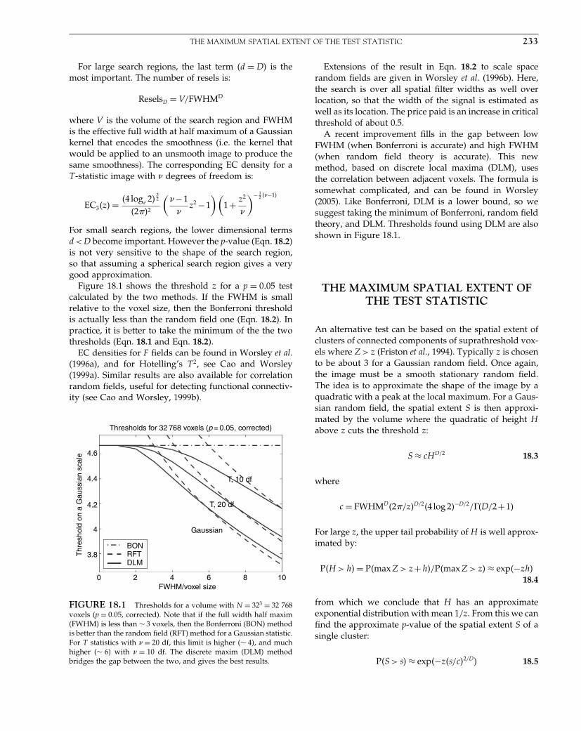
Elsevier UK Chapter: Ch18-P372560 30-9-2006 5:16p.m. Page:233 Trim:7.5in×9.25in
Basal Font:Palatino Margins:Top:40pt Gutter:68pt Font Size:9.5/12 Text Width:42pc Depth:55 Lines
THE MAXIMUM SPATIAL EXTENT OF THE TEST STATISTIC 233
For large search regions, the last term �d = D� is themost important. The number of resels is:
ReselsD = V/FWHMD
where V is the volume of the search region and FWHMis the effective full width at half maximum of a Gaussiankernel that encodes the smoothness (i.e. the kernel thatwould be applied to an unsmooth image to produce thesame smoothness). The corresponding EC density for aT -statistic image with � degrees of freedom is:
EC3�z� = �4 loge 2�32
�2��2
(� −1
�z2 −1
)(1+ z2
�
)− 12 ��−1�
For small search regions, the lower dimensional termsd < D become important. However the p-value (Eqn. 18.2)is not very sensitive to the shape of the search region,so that assuming a spherical search region gives a verygood approximation.
Figure 18.1 shows the threshold z for a p = 0�05 testcalculated by the two methods. If the FWHM is smallrelative to the voxel size, then the Bonferroni thresholdis actually less than the random field one (Eqn. 18.2). Inpractice, it is better to take the minimum of the the twothresholds (Eqn. 18.1 and Eqn. 18.2).
EC densities for F fields can be found in Worsley et al.(1996a), and for Hotelling’s T 2, see Cao and Worsley(1999a). Similar results are also available for correlationrandom fields, useful for detecting functional connectiv-ity (see Cao and Worsley, 1999b).
Thresholds for 32 768 voxels (p = 0.05, corrected)
Thr
esho
ld o
n a
Gau
ssia
n sc
ale 4.6
4.4
4.2
4
3.8
0 2 4 6 8 10FWHM/voxel size
T, 10 df
T, 20 df
Gaussian
BONRFTDLM
FIGURE 18.1 Thresholds for a volume with N = 323 = 32 768voxels (p = 0�05, corrected). Note that if the full width half maxim(FWHM) is less than ∼ 3 voxels, then the Bonferroni (BON) methodis better than the random field (RFT) method for a Gaussian statistic.For T statistics with � = 20 df, this limit is higher �∼ 4�, and muchhigher �∼ 6� with � = 10 df. The discrete maxim (DLM) methodbridges the gap between the two, and gives the best results.
Extensions of the result in Eqn. 18.2 to scale spacerandom fields are given in Worsley et al. (1996b). Here,the search is over all spatial filter widths as well overlocation, so that the width of the signal is estimated aswell as its location. The price paid is an increase in criticalthreshold of about 0.5.
A recent improvement fills in the gap between lowFWHM (when Bonferroni is accurate) and high FWHM(when random field theory is accurate). This newmethod, based on discrete local maxima (DLM), usesthe correlation between adjacent voxels. The formula issomewhat complicated, and can be found in Worsley(2005). Like Bonferroni, DLM is a lower bound, so wesuggest taking the minimum of Bonferroni, random fieldtheory, and DLM. Thresholds found using DLM are alsoshown in Figure 18.1.
THE MAXIMUM SPATIAL EXTENT OFTHE TEST STATISTIC
An alternative test can be based on the spatial extent ofclusters of connected components of suprathreshold vox-els where Z > z (Friston et al., 1994). Typically z is chosento be about 3 for a Gaussian random field. Once again,the image must be a smooth stationary random field.The idea is to approximate the shape of the image by aquadratic with a peak at the local maximum. For a Gaus-sian random field, the spatial extent S is then approxi-mated by the volume where the quadratic of height Habove z cuts the threshold z:
S ≈ cHD/2 18.3
where
c = FWHMD�2�/z�D/2�4 log 2�−D/2/�D/2+1�
For large z, the upper tail probability of H is well approx-imated by:
P�H > h� = P�max Z > z+h�/P�max Z > z� ≈ exp�−zh�18.4
from which we conclude that H has an approximateexponential distribution with mean 1/z. From this we canfind the approximate p-value of the spatial extent S of asingle cluster:
P�S > s� ≈ exp�−z�s/c�2/D� 18.5
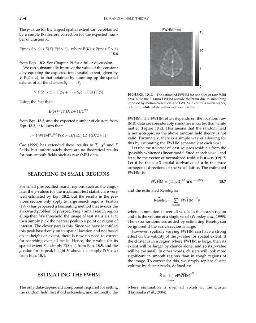
Elsevier UK Chapter: Ch18-P372560 30-9-2006 5:16p.m. Page:234 Trim:7.5in×9.25in
Basal Font:Palatino Margins:Top:40pt Gutter:68pt Font Size:9.5/12 Text Width:42pc Depth:55 Lines
234 18. RANDOM FIELD THEORY
The p-value for the largest spatial extent can be obtainedby a simple Bonferroni correction for the expected num-ber of clusters K:
P�max S > s� ≈ E�K� P�S > s�� where E�K� ≈ P�max Z > z�18.6
from Eqn. 18.2. See Chapter 19 for a fuller discussion.We can substantially improve the value of the constant
c by equating the expected total spatial extent, given byV P�Z > z�, to that obtained by summing up the spatialextents of all the clusters S1� � SK :
V P�Z > z� = E�S1 +· · ·+SK� = E�K� E�S�
Using the fact that:
E�S� ≈ c�D/2+1�/zD/2
from Eqn. 18.3, and the expected number of clusters fromEqn. 18.2, it follows that:
c ≈ FWHMDzD/2P�Z > z�/�ECD�z� �D/2+1��
Cao (1999) has extended these results to T� �2 and Ffields, but unfortunately there are no theoretical resultsfor non-smooth fields such as raw fMRI data.
SEARCHING IN SMALL REGIONS
For small prespecified search regions such as the cingu-late, the p-values for the maximum test statistic are verywell estimated by Eqn. 18.2, but the results in the pre-vious section only apply to large search regions. Friston(1997) has proposed a fascinating method that avoids theawkward problem of prespecifying a small search regionaltogether. We threshold the image of test statistics at z,then simply pick the nearest peak to a point or region ofinterest. The clever part is this. Since we have identifiedthis peak based only on its spatial location and not basedon its height or extent, there is now no need to correctfor searching over all peaks. Hence, the p-value for itsspatial extent S is simply P�S > s� from Eqn. 18.5, and thep-value for its peak height H above z is simply P�H > h�from Eqn. 18.4.
ESTIMATING THE FWHM
The only data-dependent component required for settingthe random field threshold is ReselsD, and indirectly, the
15
10
5
0
FWHM (mm)
FIGURE 18.2 The estimated FWHM for one slice of raw fMRIdata. Note the ∼ 6 mm FWHM outside the brain due to smoothingimposed by motion correction. The FWHM in cortex is much higher,∼ 10 mm, while white matter is lower ∼ 6 mm.
FWHM. The FWHM often depends on the location: rawfMRI data are considerably smoother in cortex than whitematter (Figure 18.2). This means that the random fieldis not isotropic, so the above random field theory is notvalid. Fortunately, there is a simple way of allowing forthis by estimating the FWHM separately at each voxel.
Let r be the n-vector of least-squares residuals from the(possibly whitened) linear model fitted at each voxel, andlet u be the vector of normalized residuals u = r/�r′r�1/2.Let u̇ be the n × 3 spatial derivative of u in the threeorthogonal directions of the voxel lattice. The estimatedFWHM is:
̂FWHM = �4 log 2�1/2�u̇′u̇�−1/�2D� 18.7
and the estimated ReselsD is:
̂ReselsD = ∑volume
̂FWHM−D
v
where summation is over all voxels in the search regionand v is the volume of a single voxel (Worsley et al., 1999).The extra randomness added by estimating ReselsD canbe ignored if the search region is large.
However, spatially varying FWHM can have a strongeffect on the validity of the p-value for spatial extent. Ifthe cluster is in a region where FWHM is large, then itsextent will be larger by chance alone, and so its p-valuewill be too small. In other words, clusters will look moresignificant in smooth regions than in rough regions ofthe image. To correct for this, we simply replace clustervolume by cluster resels, defined as:
S̃ = ∑cluster
v ̂FWHM−D
where summation is over all voxels in the cluster(Hayasaka et al., 2004).

Elsevier UK Chapter: Ch18-P372560 30-9-2006 5:16p.m. Page:235 Trim:7.5in×9.25in
Basal Font:Palatino Margins:Top:40pt Gutter:68pt Font Size:9.5/12 Text Width:42pc Depth:55 Lines
FALSE DISCOVERY RATE 235
There is one remaining problem: since the above sum-mation is over a small cluster, rather than a large searchregion, the randomness in estimating FWHM now makesa significant contribution to the randomness of S̃, andhence its p-value. Hayasaka et al. (2004) suggest allowingfor this by the approximation:
S̃ ≈ c̃HD/2D+1∏k=1
Xpk
k 18.8
where X1� �XD+1 are independent �2 random vari-ables. The degrees of freedom of Xk is � − k + 1 where� = n − p and p is the number of regressors in the lin-ear model, raised to the power pk = −D/2 if k = 1 andpk = 1/2 if k > 1. Again the constant c̃ is chosen so thatthe expected total resels of all clusters matches the prob-ability of exceeding the threshold times the volume ofthe search region:
c̃ ≈ zD/2P�Z > z�/�ECD�z� �D/2+1��
Combining this with the approximate distributions ofspatial extents for T� �2 and F fields from Cao (1999)requires no extra computational effort. H is replaced bya beta random variable in Eqn. 18.8, multiplied by pow-ers of yet more �2 random variables, with appropriateadjustments to c̃.
In practice, the distribution function of S̃ is best cal-culated by first taking logarithms, so that log S̃ is thena sum of independent random variables. The density ofa sum is the convolution of the densities whose Fourier
transform is the sum of the Fourier transforms. It is eas-ier to find the upper tail probability of log S̃ by replac-ing the density of one of the random variables by itsupper tail probability before doing the convolution. Theobvious choice is the exponential or beta random vari-able, since its upper tail probability has a simple closedform expression. This method has been implemented inthe stat_threshold.m function of fmristat, available fromhttp://www. math.mcgill.ca/keith/fmristat.
FALSE DISCOVERY RATE
A remarkable breakthrough in multiple testing was madeby Benjamini and Hochberg, in 1995, who took a com-pletely different approach. Instead of controlling theprobability of ever reporting a false positive, they deviseda procedure for controlling the false discovery rate (FDR),the expected proportion of false positives amongst thosevoxels declared positive (the discoveries) (Figure 18.3). Theprocedure is extremely simple to implement. Simply cal-culate the uncorrected p-value for each voxel and orderthem so that the ordered p-values are P1 ≤ P2 ≤ ≤ PN .To control the FDR at , find the largest value k so thatPk < k/N . This procedure is conservative if the voxelsare positively dependent, which is a reasonable assump-tion for most unsmoothed or smoothed imaging data. SeeChapter 20 and Genovese et al. (2002) for an applicationof this method to fMRI data, and for further references.
6
4
2
0
–2
–4
6
4
2
0
–2
–4
6
4
2
0
–2
–4
6
4
2
0
–2
–4
Signal + Gaussian white noise
FDR < 0.05, Z > 2.82 p < 0.05 (corrected), Z > 4.22
5% of volume is false +
5% probability of any false +5% of discoveries is false +
p < 0.05 (uncorrected), Z > 1.64
FIGURE 18.3 Illustration of the differencebetween false discovery rate and Bonferroni/random field methods for thresholding an image.
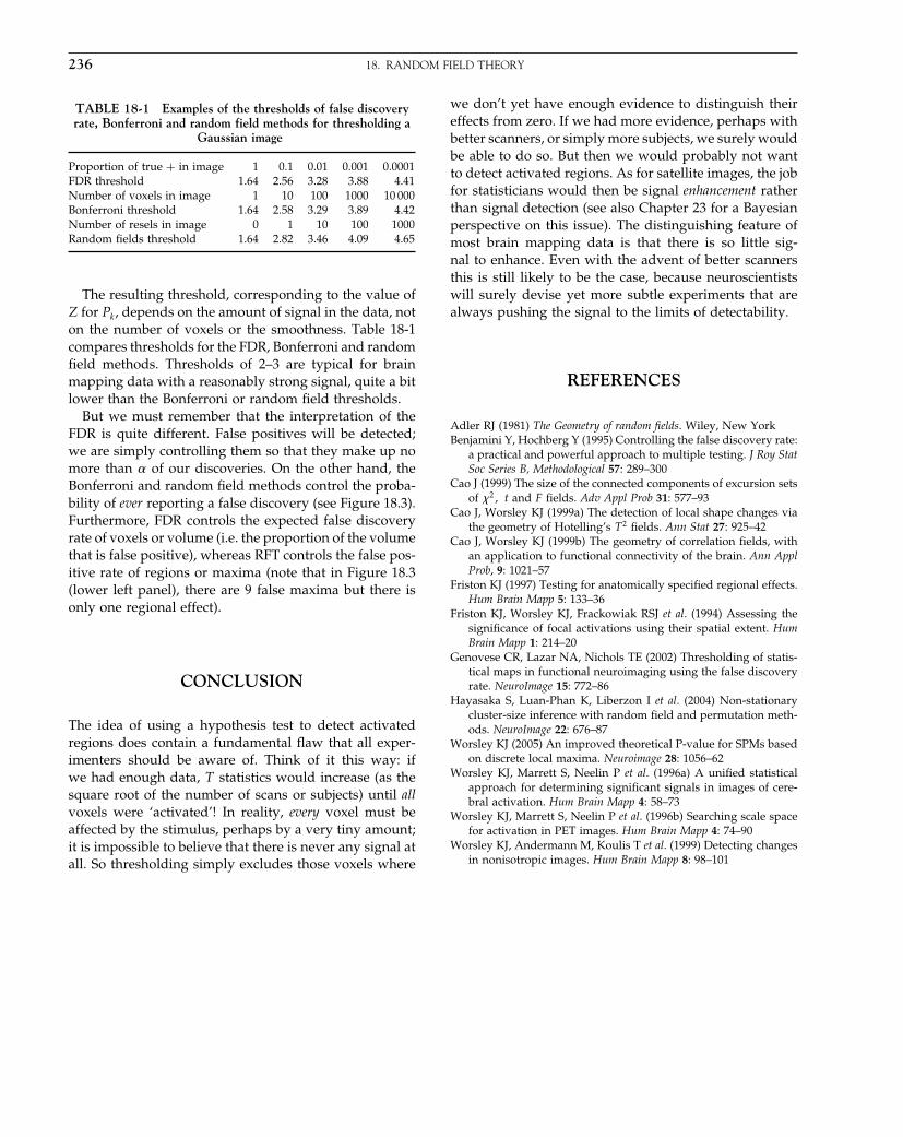
Elsevier UK Chapter: Ch18-P372560 30-9-2006 5:16p.m. Page:236 Trim:7.5in×9.25in
Basal Font:Palatino Margins:Top:40pt Gutter:68pt Font Size:9.5/12 Text Width:42pc Depth:55 Lines
236 18. RANDOM FIELD THEORY
TABLE 18-1 Examples of the thresholds of false discoveryrate, Bonferroni and random field methods for thresholding a
Gaussian image
Proportion of true + in image 1 0.1 0.01 0.001 0.0001FDR threshold 1.64 2.56 3.28 3.88 4.41Number of voxels in image 1 10 100 1000 10 000Bonferroni threshold 1.64 2.58 3.29 3.89 4.42Number of resels in image 0 1 10 100 1000Random fields threshold 1.64 2.82 3.46 4.09 4.65
The resulting threshold, corresponding to the value ofZ for Pk, depends on the amount of signal in the data, noton the number of voxels or the smoothness. Table 18-1compares thresholds for the FDR, Bonferroni and randomfield methods. Thresholds of 2–3 are typical for brainmapping data with a reasonably strong signal, quite a bitlower than the Bonferroni or random field thresholds.
But we must remember that the interpretation of theFDR is quite different. False positives will be detected;we are simply controlling them so that they make up nomore than of our discoveries. On the other hand, theBonferroni and random field methods control the proba-bility of ever reporting a false discovery (see Figure 18.3).Furthermore, FDR controls the expected false discoveryrate of voxels or volume (i.e. the proportion of the volumethat is false positive), whereas RFT controls the false pos-itive rate of regions or maxima (note that in Figure 18.3(lower left panel), there are 9 false maxima but there isonly one regional effect).
CONCLUSION
The idea of using a hypothesis test to detect activatedregions does contain a fundamental flaw that all exper-imenters should be aware of. Think of it this way: ifwe had enough data, T statistics would increase (as thesquare root of the number of scans or subjects) until allvoxels were ‘activated’! In reality, every voxel must beaffected by the stimulus, perhaps by a very tiny amount;it is impossible to believe that there is never any signal atall. So thresholding simply excludes those voxels where
we don’t yet have enough evidence to distinguish theireffects from zero. If we had more evidence, perhaps withbetter scanners, or simply more subjects, we surely wouldbe able to do so. But then we would probably not wantto detect activated regions. As for satellite images, the jobfor statisticians would then be signal enhancement ratherthan signal detection (see also Chapter 23 for a Bayesianperspective on this issue). The distinguishing feature ofmost brain mapping data is that there is so little sig-nal to enhance. Even with the advent of better scannersthis is still likely to be the case, because neuroscientistswill surely devise yet more subtle experiments that arealways pushing the signal to the limits of detectability.
REFERENCES
Adler RJ (1981) The Geometry of random fields. Wiley, New YorkBenjamini Y, Hochberg Y (1995) Controlling the false discovery rate:
a practical and powerful approach to multiple testing. J Roy StatSoc Series B, Methodological 57: 289–300
Cao J (1999) The size of the connected components of excursion setsof �2� t and F fields. Adv Appl Prob 31: 577–93
Cao J, Worsley KJ (1999a) The detection of local shape changes viathe geometry of Hotelling’s T 2 fields. Ann Stat 27: 925–42
Cao J, Worsley KJ (1999b) The geometry of correlation fields, withan application to functional connectivity of the brain. Ann ApplProb, 9: 1021–57
Friston KJ (1997) Testing for anatomically specified regional effects.Hum Brain Mapp 5: 133–36
Friston KJ, Worsley KJ, Frackowiak RSJ et al. (1994) Assessing thesignificance of focal activations using their spatial extent. HumBrain Mapp 1: 214–20
Genovese CR, Lazar NA, Nichols TE (2002) Thresholding of statis-tical maps in functional neuroimaging using the false discoveryrate. NeuroImage 15: 772–86
Hayasaka S, Luan-Phan K, Liberzon I et al. (2004) Non-stationarycluster-size inference with random field and permutation meth-ods. NeuroImage 22: 676–87
Worsley KJ (2005) An improved theoretical P-value for SPMs basedon discrete local maxima. Neuroimage 28: 1056–62
Worsley KJ, Marrett S, Neelin P et al. (1996a) A unified statisticalapproach for determining significant signals in images of cere-bral activation. Hum Brain Mapp 4: 58–73
Worsley KJ, Marrett S, Neelin P et al. (1996b) Searching scale spacefor activation in PET images. Hum Brain Mapp 4: 74–90
Worsley KJ, Andermann M, Koulis T et al. (1999) Detecting changesin nonisotropic images. Hum Brain Mapp 8: 98–101
Elsevier UK Chapter: Ch19-P372560 30-9-2006 5:16p.m. Page:237 Trim:7.5in×9.25in
Basal Font:Palatino Margins:Top:40pt Gutter:68pt Font Size:9.5/12 Text Width:42pc Depth:55 Lines
C H A P T E R
19
Topological InferenceK. Friston
INTRODUCTION
The previous two chapters have established the heuristicsbehind inference on statistical maps and how this infer-ence rests upon random field theory. In this chapter, werevisit these themes by looking at the nature of topolog-ical inference and the different ways it can be employed.The key difference between statistical parametric map-ping (SPM) and conventional statistics lies in the thingone is making an inference about. In conventional statis-tics, this is usually a scalar quantity (i.e. a model parame-ter) that generates measurements, such as reaction times.This inference is based on the size of a statistic that is afunction of scalar measurements. In contrast, in SPM onemakes inferences about the topological features of a statis-tical process that is a function of space or time. The SPMis a function of the data, which is a function of positionin the image. This renders the SPM a functional (a func-tion of a function). Put succinctly, conventional inferenceis based on a statistic, which is a function of the data. Topo-logical inference is based on an SPM which is a functionalof the data. This is important because a statistic can onlyhave one attribute – its size. Conversely, an SPM can havemany topological attributes, such as the height of a peak,the number of peaks, the volume or extent of an excur-sion set (part of the SPM above some height). All thesetopological features are quantities that have a distributionunder the null hypothesis and can be used for inference.Critically, the nature of this inference is determined by thetopological quantity used. This chapter introduces somecommon topological inferences and their relative sensitiv-ities to different sorts of treatments effects or activations.
TOPOLOGICAL INFERENCE
This chapter is about detecting activations in statisticalparametric maps and considers the relative sensitivity of
a nested hierarchy of tests that are framed in terms of thelevel of inference (peak-level, cluster-level, and set-level).These tests are based on the probability of obtaining c,or more, clusters with k, or more, voxels, above a thresh-old u. This probability has a reasonably simple form andis derived using distributional approximations from dif-ferential topology (i.e. the theory of random fields; seebelow and Chapter 18). The different levels of inferencepertain to different topological quantities, which varyin their spatial specificity: set-level inference refers tothe inference that the number of clusters comprising anobserved activation profile is unlikely to have occurredby chance. This inference pertains to the set of clusters(connected excursion sets) reaching criteria and repre-sents an inference about distributed effects. Cluster-levelinferences are a special case of set-level inferences, whichobtain when the number of clusters c is one. Similarly,peak-level inferences are special cases of cluster-levelinferences that result when the cluster is very small (i.e.k < 0). Set-level inferences are generally more powerfulthan cluster-level inferences and cluster-level inferencesare generally more powerful than peak-level inferences.The price paid for this increased sensitivity is reducedlocalizing power: peak-level tests permit individual max-ima to be identified as significant, whereas cluster andset-level inferences only allow clusters or sets of clustersto be so identified.
Peaks, clusters and sets
In what follows, we consider tests based on three topo-logical features: a peak, a cluster, and a set of clus-ters. We then consider the relative sensitivity of theensuing tests in terms of power and how that powervaries as a function of resolution and the nature ofthe underlying signal. This treatment is concerned pri-marily with distributed signals that have no a priorianatomical specification. Activations in positron emission
Statistical Parametric Mapping, by Karl Friston et al. Copyright 2007, Elsevier Ltd. All rights reserved.ISBN–13: 978-0-12-372560-8 ISBN–10: 0-12-372560-7
237
Elsevier UK Chapter: Ch19-P372560 30-9-2006 5:16p.m. Page:238 Trim:7.5in×9.25in
Basal Font:Palatino Margins:Top:40pt Gutter:68pt Font Size:9.5/12 Text Width:42pc Depth:55 Lines
238 19. TOPOLOGICAL INFERENCE
tomography (PET) and functional magnetic resonanceimaging (fMRI) are almost universally detected usingsome form of statistical mapping. The statistical processesthat ensue (i.e. statistical parametric maps) are character-ized in terms of regional excursions above some thresh-old and p-values are assigned to these excursions. Thesep-values reflect the probability of false positives or type1 error. There are two forms of control over family-wiseerror (FWE), weak and strong, which determine the levelat which departures from the null hypothesis can bereported. A test procedure controls FWE in the weaksense if the probability of false rejection is less than �.A procedure with only weak control has no localizingpower. If the null hypothesis is rejected, then all that canbe said is that there is a departure from the null hypothe-sis somewhere in the SPM. Here, the level of inference isthe whole volume analysed. A procedure controls FWEin the strong sense if the probability of a false positivepeak or cluster, for which the null hypothesis is true, isless than �, regardless of the truth of the null hypothesiselsewhere. This more stringent criterion gives localizingpower. Peaks or clusters identified by such a proceduremay be declared individually significant. Another way oflooking at this is in terms of the attributes of the topolog-ical features whose false positive rate is controlled. Con-trolling the family-wise false positive rate of peaks meansthat inference is about a peak, which has the attribute‘location’. Controlling the false positive rate of clustersenables one to infer the cluster is significant and implic-itly its spatial support. However, inferring a set of clustersis significant controls FWE in a weaker sense because itis the ensemble that is significant, not any single cluster.
As noted in Chapter 17, the simplest multiple compar-isons procedure which maintains strong control over theerror rate in a family of discrete tests is based on theBonferroni inequality. Here, the p-values belong, not topeaks, but to voxels and are adjusted for the number ofvoxels. However, for even mild dependencies betweenthe voxels, this method is excessively conservative andinappropriate. It is inappropriate because we are notinterested in controlling the false positive rate of voxels;we want to control the false positive rate of peaks. Thepeak is a topological feature, a voxel is not. Critically,for any given threshold, there will be more suprathresh-old voxels than peaks. This means the false positive rateof voxels is always greater than the false positive rateof peaks. This is why SPM uses a lower threshold thanrequired by a Bonferroni correction and why SPM is morepowerful. It is easy to see that controlling the false pos-itive rate of voxels is meaningless; imagine we simplyhalved the size of each voxel by interpolating the SPM.This would increase the false positive rate of voxels bya factor of eight. But nothing has changed. On the otherhand, the false positive rate of peaks remains constant
and the inference furnished by SPM remains exact. Thissimple example illustrates that SPM and the topologi-cal inference it entails, is central to the analysis of datathat are a function of some position in space, time, fre-quency etc.
Random field theory
The most successful approach to statistical inference onanalytic (continuous) statistical processes is predicated onthe theory of random fields. Early work was based on thetheory of level crossings (Friston et al., 1991) and differ-ential topology (Worsley et al., 1992). These approachescontrol FWE strongly, allowing for inference at the peak-level: a corrected p-value is assigned to a peak using theprobability that its height, or a higher one, could haveoccurred by chance in the volume analysed. There havebeen a number of interesting elaborations at this levelof inference (e.g. searching scale-space and other high-dimensional SPMs (e.g. Siegmund and Worsley 1994))and results for many statistics exist (e.g. Worsley, 1994).The next development, using the random field theory,was to use the spatial extent of a cluster of voxels definedby a height threshold (Friston et al., 1994; see also Polineand Mazoyer, 1993, and Roland et al., 1993). These pro-cedures control FWE strongly at the cluster-level, per-mitting inference about each cluster, and are based onthe probability of getting a cluster of the extent observed(defined by a height threshold), or a larger one, in thevolume analysed. In Friston et al. (1996) set-level infer-ence was introduced. This is based on the probability ofgetting the observed number of clusters (defined by aheight and an extent threshold), or more, in the volumeanalysed. This inference is about the set of clusters (con-tiguous regions above some height and size thresholds)or more simply about the excursion set. In this chapter,we compare the relative power of these different lev-els of inference, under different conditions. In the sensethat all these inferences are based on adjusted p-values,we consider only the case where no a priori knowledgeabout the deployment of activation is available, withinthe volume considered. This volume may be the entirecerebrum, or could be a smaller volume encompassing aregion in which one wants to focus statistical power. Theunderlying theory is exactly the same for whole brainand small volume corrections and all levels of inferenceapply.
The results in the previous two chapters and usedbelow, derive from random field theory. The assump-tions implicit in this approach are: that the SPMs are rea-sonable lattice representations of underlying continuousfields; that the components of the fields have a multivari-ate Gaussian distribution; and that the height thresholds

Elsevier UK Chapter: Ch19-P372560 30-9-2006 5:16p.m. Page:239 Trim:7.5in×9.25in
Basal Font:Palatino Margins:Top:40pt Gutter:68pt Font Size:9.5/12 Text Width:42pc Depth:55 Lines
THEORY AND DISTRIBUTIONAL APPROXIMATIONS 239
employed are high. These are reasonable assumptionsin neuroimaging as long as the voxel-size or bin-size issmall relative to the smoothness. There has been someinterest in revising cluster-level approaches in the con-text of fMRI (where the voxel sizes are larger in relationto resolution) using Monte Carlo simulations and adjust-ments to the smoothness estimators (e.g. Forman et al.,1995). Usual estimates of smoothness (e.g. Friston et al.,1991; Worsley et al., 1992; Kiebel et al., 1999) fail when thereasonable lattice assumption is violated. In our work,we sidestep this issue by interpolating the data to reducevoxel size or smoothing the data to increase smoothness.It is generally accepted that the voxel size should be lessthan half the full width at half maximum (FWHM) ofthe smoothness. The good lattice and Gaussian assump-tions can be further ensured by slight spatial smoothingof the data, which usually increases the sensitivity of theensuing analysis.
Control, levels and regional specificity
There is a fundamental difference between rejecting thenull hypothesis of no activation at a particular peak andrejecting the null hypothesis over the entire volume anal-ysed. As noted above, the former requires the strongestcontrol over FWE and the latter the weakest. One wayof thinking about this difference is to note that if acti-vation is confirmed at a particular point in the brainthen, implicitly, the hypothesis of activation somewhereis also confirmed (but the converse is not true). The dis-tinction between weak and strong control, in the contextof statistical parametric mapping, relates to the level atwhich the inference is made. The stronger the control, themore regional specificity it confers. For example, a peak-level inference is stronger than a cluster-level inferencebecause the latter disallows inferences about any peakwithin the cluster. In other words, cluster level inferencesmaintain strong control at the cluster level but only weakcontrol at the peak level. Similarly, set-level inferences areweaker than cluster-level inferences because they refer tothe set of regional effects but not any individual peak orcluster in that set. Procedures with the weakest controlhave been referred to as ‘omnibus’ tests (e.g. Fox andMintun, 1989) and frame the alternative hypothesis interms of effects anywhere in the brain. These hypothesesare usually tested using the volume above some thresh-old (e.g. exceedence proportion tests, Friston et al., 1991)or use all the SPM values (e.g. quadratic tests, Worsleyet al., 1995). A weaker control over FWE, or high-levelinference, has less regional specificity but remains a validway of establishing the significance of an activation pro-file. Intuitively, one might guess that the weaker pro-cedures provide more powerful tests because there is a
trade-off between sensitivity and regional specificity (seebelow).
Here we focus on the weaker hypotheses and considerpeak-level and cluster-level inferences subordinate to set-level inferences. This allows us to ask: which is the mostpowerful approach for detecting brain activations? Theremainder of this chapter is divided into two sections.The first section reprises the distributional approxima-tions used to make statistical inferences about an SPMand frames the results to show that all levels of inferencecan be regarded as special cases of a single probability(namely, the probability of getting c, or more, clusterswith k, or more, voxels above height u). The final sectiondeals with the relative power of voxel-level, cluster-level,and set-level inferences and its dependency on signalcharacteristics, namely, the spatial extent of the underly-ing haemodynamics and the signal-to-noise ratio.
THEORY AND DISTRIBUTIONALAPPROXIMATIONS
In this section, we review the basic results from therandom field theory that are used to provide a generalexpression for the probability of getting any excursionset defined by three quantities: a height-threshold; a spa-tial extent threshold; and a threshold on the number ofclusters. We then show that peak-level, cluster-level andset-level inferences are all special cases of this generalformulation and introduce its special cases.
A general formulation
We assume that a D-dimensional SPM conforms to a rea-sonable lattice representation of a statistical functional ofvolume R(�) expressed in resolution elements, or resels.This volume is a function of the volume’s size �, forexample radius. This measure is statistically flattened ornormalized by the smoothness W . The smoothness is,as before, W = ���1/2D = �4 ln 2�− 1
2 FWHM , where � is thecovariance matrix of the first partial derivatives of theunderlying component fields and FWHM is the full widthat half maximum. An excursion set is defined as the setof voxels that exceeds some threshold u. This excursionset comprises m clusters each with a volume of n voxels.At high thresholds, m approximates the number of max-ima and has been shown to have a Poisson distribution(Adler and Hasofer, 1981, Theorem 6.9.3):
p�m = c� = ��c�0� = 1c!0
ce−0 19.1

Elsevier UK Chapter: Ch19-P372560 30-9-2006 5:16p.m. Page:240 Trim:7.5in×9.25in
Basal Font:Palatino Margins:Top:40pt Gutter:68pt Font Size:9.5/12 Text Width:42pc Depth:55 Lines
240 19. TOPOLOGICAL INFERENCE
where 0 is the expected number of maxima (i.e. clusters).This depends on the search volume and height thresh-old. The expected number of maxima (Hasofer, 1978)would generally be approximated with the expectedEuler characteristic 0 = ECD, for the SPM in question(see Chapter 18, Appendix 6 and Figure 19.1). The vol-ume of a cluster n is distributed according to (e.g. Fristonet al., 1994):
p �n ≥ k� = exp�−k2/D�
=(
�� D2 +1�
�
)2/D 19.2
where � is the expected volume of each cluster. This issimply the total number of voxels expected by chancedivided by expected number of maxima (see Figure 19.1).This specific form for the distribution of cluster volumeis for SPM{Z} and should be replaced with more accurateexpressions for SPM{t} or SPM{F} (see Cao, 1999 andChapter 18), but serves here to illustrate the general formof topological inference. With these results it is possibleto construct an expression for the probability of getting c,or more, clusters of volume k, or more, above a thresholdu (Friston et al., 1996)
P�u�k� c� � = 1−c−1∑i=0
��i�0p�n ≥ k�� 19.3
Eqn. 19.3 can be interpreted in the following way: con-sider clusters as ‘rare events’ that occur in a volumeaccording to the Poisson distribution with expectation 0.The proportion of these rare events that meets the spatialextent criterion will be p�n ≥ k�. These criterion eventswill themselves occur according to a Poisson distribu-tion with expectation 0p�n ≥ k�. The probability that thenumber of events will be c or more is simply one minusthe probability that the number of events lies between 0and c minus one (i.e. the sum in Eqn. 19.3).
We now consider various ways in which P�u� c�k� canbe used to make inferences about brain activations. Inbrief, if the number of clusters c = 1, the probabilityreduces to that of getting one, or more, clusters with k,or more, voxels. This is the p-value for a single cluster ofvolume k. This corresponds to a cluster-level inference.Similarly if c = 1 and the number of suprathreshold vox-els k = 0, the resulting cluster-level probability (i.e. theprobability of getting one or more excursions of any vol-ume above u) is the p-value of any peak of height u. Inother words, cluster and peak-level inferences are specialcases of set-level inferences.
Peak-level inferences
Consider the situation in which the threshold u is theheight of a peak. The probability of this happening by
chance is the probability of getting one or more clusters(i.e. c = 1) with non-zero volume (i.e. k−0). The p-valueis therefore:
P�u� 0� 1� = 1−exp�−0� 19.4
This is simply the corrected probability based on theexpected number of maxima or Euler characteristic.
Cluster-level inferences
Consider now the case in which we base our inference onspatial extent k, which is defined by specifying a heightthreshold u. The probability of getting more than onecluster of volume k or more is:
P�u�k� 1� = 1−exp�−0p�n ≥ k� 19.5
This is the corrected p-value based on spatial extent(Friston et al., 1994) and has proved to be more pow-erful than peak-based inference when applied to high-resolution data (see below).
Set-level inferences
Now consider the instance where inference is based oncluster number c. In this case, both height u and extentk threshold need to be specified before the statistic cis defined. The corresponding probability is given byEqn. 19.3 and is the corrected p-value for the set ofactivation foci surviving these joint criteria. There is aconceptual relationship between set-level inferences andnon-localizing tests based on the exceedence proportion(i.e. the total number of voxels above a threshold u).Exceedence proportion tests (e.g. Friston et al., 1991) andthreshold-less quadratic tests (Worsley et al., 1995) havebeen proposed to test for activation effects over the vol-ume analysed in an omnibus sense. These tests havenot been widely used because they have no localizingpower and do not pertain to a set of well-defined activa-tions. In this sense, these tests differ from set-level testsbecause the latter do refer to a well-defined set of activa-tion foci. However, in the limiting case of a small spatialextent threshold k the set-level inference approaches anomnibus test:
P�u� 0� c� = 1−c−1∑i=0
��i�0� 19.6
This test simply compares the expected and observednumber of maxima in an SPM using the Poisson distribu-tion under the null hypothesis. These set-level inferencesare seldom employed in conventional analyses becausethey have no localizing power. However, they form a ref-erence for the sensitivity of alternative (e.g. multivariate)analyses that focus on more distributed responses.

Elsevier UK Chapter: Ch19-P372560 30-9-2006 5:16p.m. Page:241 Trim:7.5in×9.25in
Basal Font:Palatino Margins:Top:40pt Gutter:68pt Font Size:9.5/12 Text Width:42pc Depth:55 Lines
THEORY AND DISTRIBUTIONAL APPROXIMATIONS 241
Poisson Clumping Heuristic
Expected clusters Cluster volume (RESELS)
P(u,c,k) = 1 − λ(c − 1, Ψ0(u) p(n ≥ k))
12
2
Ψ0
β = ( η
p(n ≥ k) = exp(−βk D )
Γ(D/2 + 1))D
rTr
re =
WFWHM = (4 ln 2)
FWHMD
∂x∂e
∂x∂eT
≈Λ
Λ −
21
21
21
θvoxelsθ(W ) =
34 πθ 3R3 =
R2 = 2πθ 2R1 = 4θR0 = 1
(4 ln 2) (1+u 2
(2π)(1+u
2 Γ( Γ(21
21
21(
(v−1)
21
21
231
212
1
(v+1))(4 ln 22π
ρ3 =…
ρ2
=
ρ1 =
ρ0 = 1 − Φt (u)
v)−1v)−v)−
v)−
v−1)
ρ(u) = ρ0,… ,ρD
EC density Search volume (RESELS)
Smoothness
R(θ) = R0,… ,RD
⎥⎥⎥
⎦
⎤
⎢⎢⎢
⎣
⎡
⎥⎥⎥
⎦
⎤
⎢⎢⎢
⎣
⎡=
⎥⎥⎥
⎦
⎤
⎢⎢⎢
⎣
⎡n
cij =
RD
R0
…���
�
�ΨD
Ψ0
η = ρ0nRD
= (4 ln 2)
)()( 22 ΓΓ j −i +1i +1
)()( 221 ΓΓ j + 1
0
� �
��
�
ρ0c1 ρ0c1
ρ0cD
1 D
D
FIGURE 19.1 Schematic illustrating the use of random field theory in making inferences about SPMs. A fuller treatment is provided inAppendix 6. If one knew where to look exactly, then inference can be based on the value of the statistic at a specified location in the SPM,without correction. However, if one did not have an anatomical constraint a priori, then an adjustment for multiple dependent comparisons hasto be made. These corrections are usually made using distributional approximations from Gaussian random field (GRF) theory. This schematicdeals with a general case of n SPM t� whose voxels all survive a common threshold u (i.e. a conjunction of n component SPMs). The centralprobability, upon which all peak-, cluster- or set-level inferences are made, is the probability P�u� c�k� of getting c or more clusters with k ormore resels (resolution elements) above this threshold. By assuming that clusters behave like a multidimensional Poisson point process (i.e.the Poisson clumping heuristic) P�u� c�k� is simply determined. The distribution of c is Poisson with an expectation that corresponds to theproduct of the expected number of clusters, of any size, and the probability that any cluster will be bigger than k resels. The latter probabilityis shown using a form for a single Z-variate field constrained by the expected number of resels per cluster �. The expected number of reselsper cluster is simply the expected number of resels in total divided by the expected number of clusters. The expected number of clusters 0 isestimated with the Euler characteristic (EC) (effectively the number of blobs minus the number of holes). This estimate is, in turn, a functionof the EC density for the statistic in question (with degrees of freedom v) and the resel counts. The EC density is the expected EC per unit ofD-dimensional volume of the SPM where the D-dimensional volume of the search space is given by the corresponding element in the vectorof resel counts. Resel counts can be thought of as a volume metric that has been normalized by the smoothness of the SPM’s component fieldsexpressed in terms of the full width at half maximum (FWHM). This is estimated from the determinant of the variance-covariance matrixof the first spatial derivatives of e, the normalized residual fields r (from Plate 2, see colour plate section). In this example, equations for asphere of radius � are given. � denotes the cumulative density function for the statistic in question.
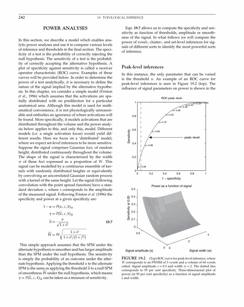
Elsevier UK Chapter: Ch19-P372560 30-9-2006 5:16p.m. Page:242 Trim:7.5in×9.25in
Basal Font:Palatino Margins:Top:40pt Gutter:68pt Font Size:9.5/12 Text Width:42pc Depth:55 Lines
242 19. TOPOLOGICAL INFERENCE
POWER ANALYSES
In this section, we describe a model which enables ana-lytic power analyses and use it to compare various levelsof inference and thresholds in the final section. The speci-ficity of a test is the probability of correctly rejecting thenull hypothesis. The sensitivity of a test is the probabil-ity of correctly accepting the alternative hypothesis. Aplot of specificity against sensitivity is called a receiveroperator characteristic (ROC) curve. Examples of thesecurves will be provided below. In order to determine thepower of a test analytically, it is necessary to define thenature of the signal implied by the alternative hypothe-sis. In this chapter, we consider a simple model (Fristonet al., 1996) which assumes that the activations are spa-tially distributed with no predilection for a particularanatomical area. Although this model is used for math-ematical convenience, it is not physiologically unreason-able and embodies an ignorance of where activations willbe found. More specifically, it models activations that aredistributed throughout the volume and the power analy-sis below applies to this, and only this, model. Differentmodels (i.e. a single activation focus) would yield dif-ferent results. Here we focus on a ‘distributed’ model,where we expect set-level inferences to be more sensitive.Suppose the signal comprises Gaussian foci, of randomheight, distributed continuously throughout the volume.The shape of the signal is characterized by the widthw of these foci expressed as a proportion of W . Thissignal can be modelled by a continuous ensemble of ker-nels with randomly distributed heights or equivalentlyby convolving an uncorrelated Gaussian random processwith a kernel of the same height. Let the signal (followingconvolution with the point spread function) have a stan-dard deviation s, where s corresponds to the amplitudeof the measured signal. Following Friston et al. (1996) thespecificity and power at a given specificity are:
1−� = P�u� c�k�W
� = P�̃u� c�k�W̃
ũ = u√1+ s2
W̃ = W
√1+ s2
1+ s2/�1+f 2�
19.7
This simple approach assumes that the SPM under thealternate hypothesis is smoother and has larger amplitudethan the SPM under the null hypothesis. The sensitivityis simply the probability of an outcome under the alter-nate hypothesis. Applying the threshold u to the alternateSPM is the same as applying the threshold ũ to a null SPMof smoothness W̃ under the null hypothesis, which means� = P�̃u� c�k�W̃ can be taken as a measure of sensitivity.
Eqn. 19.7 allows us to compute the specificity and sen-sitivity as function of thresholds, amplitude or smooth-ness of the signal. In what follows we will compare thepower of voxel-, cluster-, and set-level inferences for sig-nals of different sorts to identify the most powerful sortsof inference.
Peak-level inferences
In this instance, the only parameter that can be variedis the threshold u. An example of an ROC curve forpeak-level inferences is seen in Figure 19.2 (top). Theinfluence of signal parameters on power is shown in the
0 0.2 0.4 0.6 0.8 10
0.2
0.4
0.6
0.8
1
1 − specificity
Sen
sitiv
ity
ROC peak−level
u = 5.48
u = 4.98
u = 4.82
u = 4.72
u = 4.63
u = 4.56
u = 4.49u =4.43
u = 4.35u = 4.25
0
2
4
0
0.5
0
0.1
0.2
0.3
0.4
0.5
Signal width {w}Signal amplitude {s}
Sen
sitiv
ity a
t 0.0
5
Power as a function of signal
peak−level
FIGURE 19.2 (Top) ROC curve for peak-level inference, whereW corresponds to an FWHM of 3 voxels and a volume of 64 voxelscubed. Signal amplitude s = 0�3 and width w = 2. The dotted linecorresponds to 95 per cent specificity. Three-dimensional plot ofpower (at 95 per cent specificity) as a function of signal amplitudes and width.
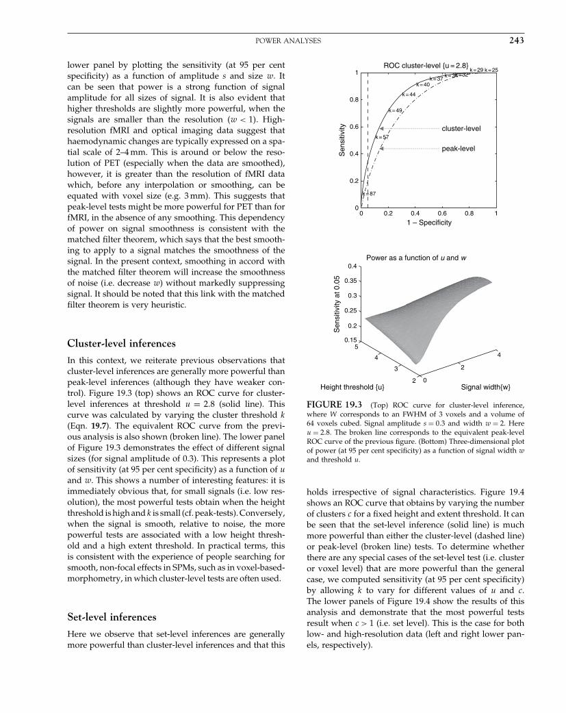
Elsevier UK Chapter: Ch19-P372560 30-9-2006 5:16p.m. Page:243 Trim:7.5in×9.25in
Basal Font:Palatino Margins:Top:40pt Gutter:68pt Font Size:9.5/12 Text Width:42pc Depth:55 Lines
POWER ANALYSES 243
lower panel by plotting the sensitivity (at 95 per centspecificity) as a function of amplitude s and size w. Itcan be seen that power is a strong function of signalamplitude for all sizes of signal. It is also evident thathigher thresholds are slightly more powerful, when thesignals are smaller than the resolution �w < 1�. High-resolution fMRI and optical imaging data suggest thathaemodynamic changes are typically expressed on a spa-tial scale of 2–4 mm. This is around or below the reso-lution of PET (especially when the data are smoothed),however, it is greater than the resolution of fMRI datawhich, before any interpolation or smoothing, can beequated with voxel size (e.g. 3 mm). This suggests thatpeak-level tests might be more powerful for PET than forfMRI, in the absence of any smoothing. This dependencyof power on signal smoothness is consistent with thematched filter theorem, which says that the best smooth-ing to apply to a signal matches the smoothness of thesignal. In the present context, smoothing in accord withthe matched filter theorem will increase the smoothnessof noise (i.e. decrease w) without markedly suppressingsignal. It should be noted that this link with the matchedfilter theorem is very heuristic.
Cluster-level inferences
In this context, we reiterate previous observations thatcluster-level inferences are generally more powerful thanpeak-level inferences (although they have weaker con-trol). Figure 19.3 (top) shows an ROC curve for cluster-level inferences at threshold u = 2�8 (solid line). Thiscurve was calculated by varying the cluster threshold k(Eqn. 19.7). The equivalent ROC curve from the previ-ous analysis is also shown (broken line). The lower panelof Figure 19.3 demonstrates the effect of different signalsizes (for signal amplitude of 0.3). This represents a plotof sensitivity (at 95 per cent specificity) as a function of uand w. This shows a number of interesting features: it isimmediately obvious that, for small signals (i.e. low res-olution), the most powerful tests obtain when the heightthreshold is high and k is small (cf. peak-tests). Conversely,when the signal is smooth, relative to noise, the morepowerful tests are associated with a low height thresh-old and a high extent threshold. In practical terms, thisis consistent with the experience of people searching forsmooth, non-focal effects in SPMs, such as in voxel-based-morphometry, in which cluster-level tests are often used.
Set-level inferences
Here we observe that set-level inferences are generallymore powerful than cluster-level inferences and that this
1
0.8
0.6
0.4
0.2
00 0.2 0.4 0.6 0.8 1
Power as a function of u and w
1 – Specificity
ROC cluster-level {u = 2.8}
cluster-level
peak-level
k = 87
k = 57
k = 49
k = 44
k = 40k = 37
k = 34k = 32k = 29 k = 25
Sen
sitiv
ity
0.4
Sen
sitiv
ity a
t 0.0
5
Height threshold {u} Signal width{w}
0.35
0.3
0.25
0.2
0.155
4
3
2 0
2
4
FIGURE 19.3 (Top) ROC curve for cluster-level inference,where W corresponds to an FWHM of 3 voxels and a volume of64 voxels cubed. Signal amplitude s = 0�3 and width w = 2. Hereu = 2�8. The broken line corresponds to the equivalent peak-levelROC curve of the previous figure. (Bottom) Three-dimensional plotof power (at 95 per cent specificity) as a function of signal width wand threshold u.
holds irrespective of signal characteristics. Figure 19.4shows an ROC curve that obtains by varying the numberof clusters c for a fixed height and extent threshold. It canbe seen that the set-level inference (solid line) is muchmore powerful than either the cluster-level (dashed line)or peak-level (broken line) tests. To determine whetherthere are any special cases of the set-level test (i.e. clusteror voxel level) that are more powerful than the generalcase, we computed sensitivity (at 95 per cent specificity)by allowing k to vary for different values of u and c.The lower panels of Figure 19.4 show the results of thisanalysis and demonstrate that the most powerful testsresult when c > 1 (i.e. set level). This is the case for bothlow- and high-resolution data (left and right lower pan-els, respectively).
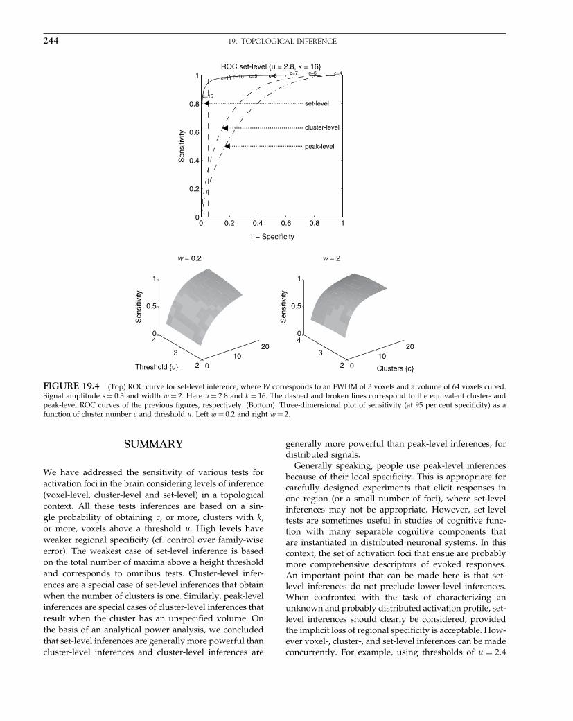
Elsevier UK Chapter: Ch19-P372560 30-9-2006 5:16p.m. Page:244 Trim:7.5in×9.25in
Basal Font:Palatino Margins:Top:40pt Gutter:68pt Font Size:9.5/12 Text Width:42pc Depth:55 Lines
244 19. TOPOLOGICAL INFERENCE
0 0.2 0.4 0.6 0.8 10
0.2
0.4
0.6
0.8 set-level
cluster-level
peak-level
1
1 − Specificity
Sen
sitiv
ity
ROC set-level {u = 2.8, k = 16}
c=15
c=11 c=10 c=9 c=8c=8 c=7 c=6 c=4
010
20
2
3
40
0.5
1
Clusters {c}
Sen
sitiv
ity
w = 2
010
20
2
3
40
0.5
1
Threshold {u}
Sen
sitiv
ity
w = 0.2
FIGURE 19.4 (Top) ROC curve for set-level inference, where W corresponds to an FWHM of 3 voxels and a volume of 64 voxels cubed.Signal amplitude s = 0�3 and width w = 2. Here u = 2�8 and k = 16. The dashed and broken lines correspond to the equivalent cluster- andpeak-level ROC curves of the previous figures, respectively. (Bottom). Three-dimensional plot of sensitivity (at 95 per cent specificity) as afunction of cluster number c and threshold u. Left w = 0�2 and right w = 2.
SUMMARY
We have addressed the sensitivity of various tests foractivation foci in the brain considering levels of inference(voxel-level, cluster-level and set-level) in a topologicalcontext. All these tests inferences are based on a sin-gle probability of obtaining c, or more, clusters with k,or more, voxels above a threshold u. High levels haveweaker regional specificity (cf. control over family-wiseerror). The weakest case of set-level inference is basedon the total number of maxima above a height thresholdand corresponds to omnibus tests. Cluster-level infer-ences are a special case of set-level inferences that obtainwhen the number of clusters is one. Similarly, peak-levelinferences are special cases of cluster-level inferences thatresult when the cluster has an unspecified volume. Onthe basis of an analytical power analysis, we concludedthat set-level inferences are generally more powerful thancluster-level inferences and cluster-level inferences are
generally more powerful than peak-level inferences, fordistributed signals.
Generally speaking, people use peak-level inferencesbecause of their local specificity. This is appropriate forcarefully designed experiments that elicit responses inone region (or a small number of foci), where set-levelinferences may not be appropriate. However, set-leveltests are sometimes useful in studies of cognitive func-tion with many separable cognitive components thatare instantiated in distributed neuronal systems. In thiscontext, the set of activation foci that ensue are probablymore comprehensive descriptors of evoked responses.An important point that can be made here is that set-level inferences do not preclude lower-level inferences.When confronted with the task of characterizing anunknown and probably distributed activation profile, set-level inferences should clearly be considered, providedthe implicit loss of regional specificity is acceptable. How-ever voxel-, cluster-, and set-level inferences can be madeconcurrently. For example, using thresholds of u = 2�4
Elsevier UK Chapter: Ch19-P372560 30-9-2006 5:16p.m. Page:245 Trim:7.5in×9.25in
Basal Font:Palatino Margins:Top:40pt Gutter:68pt Font Size:9.5/12 Text Width:42pc Depth:55 Lines
REFERENCES 245
and k = 4 allows for a set-level inference in terms of theclusters reaching criteria. At the same time, each clusterin that set has a corrected p-value based on its size andthe cluster-level inference. Similarly, each peak in thatcluster has a corrected p-value based on the voxel-levelinference (i.e. its value). The nested taxonomy presentedhere allows for all levels to be reported, each providingprotection for the lower level. As long as the levels areclearly specified, there is no reason why different levelscannot be employed, in a step-down fashion, in charac-terizing an SPM.
REFERENCES
Adler RJ, Hasofer AM (1981) The geometry of random fields. Wiley,New York
Cao J (1999) The size of the connected components of excursion setsof �2, t and F fields. Adv Appl Prob 31: 577–93
Forman SD, Cohen JD, Fitzgerald M et al. (1995) Improved assess-ment of significant activation in functional magnetic resonanceimaging (fMRI): use of a cluster-size threshold. Mag Res Med 33:636–47
Fox PT, Mintun MA (1989) Non-invasive functional brain map-ping by change distribution analysis of averaged PET images ofH15O2 tissue activity. J Nucl Med 30: 141–49
Friston KJ, Frith CD, Liddle PF et al. (1991) Comparing functional(PET) images: the assessment of significant change. J Cereb BloodFlow Metab 11: 690–99
Friston KJ, Worsley KJ, Frackowiak RSJ et al. (1994) Assessing thesignificance of focal activations using their spatial extent. HumBrain Mapp 1: 214–20
Friston KJ, Holmes A, Poline JB et al. (1996) Detecting activationsin PET and fMRI: levels of inference and power. NeuroImage 4:223–35
Hasofer AM (1978) Upcrossings of random fields. Suppl Adv ApplProb 10: 14–21
Kiebel SJ, Poline JB, Friston KJ et al. (1999) Robust smoothness esti-mation in statistical parametric maps using standardized resid-uals from the general linear model. NeuroImage 10: 756–66
Poline J-B, Mazoyer BM (1993) Analysis of individual positronemission tomography activation maps by detection of highsignal-to-noise-ratio pixel clusters. J Cereb Blood Flow Metab 13:425–37
Roland PE, Levin B, Kawashima R et al. (1993) Three dimensionalanalysis of clustered voxels in 15O-Butanol brain activationimages. Hum Brain Mapp 1: 3–19
Siegmund DO, Worsley KJ (1994) Testing for a signal with unknownlocation and scale in a stationary Gaussian random field. AnnStat 23: 608–39
Worsley KJ (1994) Local maxima and the expected Euler characteristicof excursion sets of x2, F and t fields. Adv Appl Prob 26: 13–42
Worsley KJ, Evans AC, Marrett S et al. (1992) A three-dimensionalstatistical analysis for rCBF activation studies in human brain.J Cereb Blood Flow Metab 12: 900–18
Worsley KJ, Poline J-B, Vandal AC et al. (1995) Tests for distributed,nonfocal brain activations. NeuroImage 2: 183–94

Elsevier UK Chapter: Ch02-P372560 3-10-2006 3:58p.m. Page:10 Trim:7.5in×9.25in
Basal Font:Palatino Margins:Top:40pt Gutter:68pt Font Size:9.5/12 Text Width:42pc Depth:55 Lines
C H A P T E R
2
Statistical parametric mappingK. Friston
INTRODUCTION
This chapter summarizes the ideas and procedures usedin the analysis of brain imaging data. It provides suffi-cient background to understand the principles of experi-mental design and data analysis and serves to introducethe main themes covered by subsequent chapters. Thesechapters have been organized into six parts. The firstthree parts follow the key stages of analysis: image trans-formations, modelling, and inference. These parts focuson identifying, and making inferences about, regionallyspecific effects in the brain. The final three parts addressbiophysical models of distributed neuronal responses,closing with analyses of functional and effective connec-tivity.
Characterizing a regionally specific effect rests on esti-mation and inference. Inferences in neuroimaging may beabout differences expressed when comparing one groupof subjects to another or, within subjects, changes overa sequence of observations. They may pertain to struc-tural differences (e.g. in voxel-based morphometry) (Ash-burner and Friston, 2000) or neurophysiological measuresof brain functions (e.g. fMRI or functional magnetic reso-nance imaging). The principles of data analysis are verysimilar for all of these applications and constitute thesubject of this and subsequent chapters. We will focus onthe analysis of fMRI time-series because this covers manyof the issues that are encountered in other modalities.Generally, the analyses of structural and PET (positronemission tomography) data are simpler because they donot have to deal with correlated errors from one scan tothe next. Conversely, EEG and MEG (electro- and magne-toencephalography) present special problems for modelinversion, however, many of the basic principles areshared by fMRI and EEG, because they are both causedby distributed neuronal dynamics. This chapter focuseson the design and analysis of neuroimaging studies. Inthe next chapter, we will look at conceptual and mathe-
matical models that underpin the operational issues cov-ered here.
Background
Statistical parametric mapping is used to identifyregionally specific effects in neuroimaging data and is aprevalent approach to characterizing functional anatomy,specialization and disease-related changes. The com-plementary perspective, namely functional integration,requires a different set of approaches that examine therelationship among changes in one brain region rela-tive to changes in others. Statistical parametric mappingis a voxel-based approach, employing topological infer-ence, to make some comment about regionally specificresponses to experimental factors. In order to assign anobserved response to a particular brain structure, or cor-tical area, the data are usually mapped into an anatomicalspace. Before considering statistical modelling, we dealbriefly with how images are realigned and normalizedinto some standard anatomical space. The general ideasbehind statistical parametric mapping are then describedand illustrated with attention to the different sorts ofinferences that can be made with different experimentaldesigns.
EEG, MEG and fMRI data lend themselves to a signalprocessing perspective. This can be exploited to ensurethat both the design and analysis are as efficient as pos-sible. Linear time invariant models provide the bridgebetween inferential models employed by statistical map-ping and conventional signal processing approaches. Wewill touch on these and develop them further in the nextchapter. Temporal autocorrelations in noise processesrepresent another important issue, especially in fMRI,and approaches to maximizing efficiency in the contextof serially correlated errors will be discussed. We willalso consider event and epoch-related designs in terms ofefficiency. The chapter closes by looking at the distinction
Statistical Parametric Mapping, by Karl Friston et al. Copyright 2007, Elsevier Ltd. All rights reserved.ISBN–13: 978-0-12-372560-8 ISBN–10: 0-12-372560-7
10

Elsevier UK Chapter: Ch02-P372560 3-10-2006 3:58p.m. Page:11 Trim:7.5in×9.25in
Basal Font:Palatino Margins:Top:40pt Gutter:68pt Font Size:9.5/12 Text Width:42pc Depth:55 Lines
SPATIAL TRANSFORMS AND COMPUTATIONAL ANATOMY 11
between fixed and random-effect analyses and how thisrelates to inferences about the subjects studied or thepopulation from which these subjects came.
In summary, this chapter reviews the three main stagesof data analysis: spatial or image transforms, modellingand inference; these are the areas covered in the first threeparts of this book and are summarized schematically inPlate 1 (see colour plate section). We then look at exper-imental design in light of the models covered in earlierparts. The next chapter deals with different models ofdistributed responses and previews the material coveredin the final three parts of this book.
SPATIAL TRANSFORMS ANDCOMPUTATIONAL ANATOMY
A central theme in this book is the inversion of forwardor generative models of how data are caused. We willsee this in many different contexts, from the inversionof linear models of fMRI time-series to the inversion ofdynamic causal models of distributed EEG responses.Image reconstruction, in imaging modalities like PET andfMRI, can be regarded as inverting a forward modelof how signals, deployed in anatomical space, conspireto produce measured signals. In other modalities, likeEEG and MEG, this inversion, or source reconstruction,can be a substantial problem in its own right. In mostinstances, it is expedient to decompose the inversion offorward spatiotemporal models into spatial and temporalparts. Operationally, this corresponds to reconstructingthe spatial signal at each time point and then invert-ing a temporal model of the time-series at each spatialsource (although we will consider full spatiotemporalmodels in Chapters 25 and 26). This view of source orimage reconstruction as model inversion can be extendedto cover the inversion of anatomical models describinganatomical variation within and between subjects. Theinversion of these models corresponds to registration andnormalization respectively. The aim of these anatomicalinversions or transformations is to remove or character-ize anatomical differences. Chapters 4 to 6 deal with theinversion of anatomical models for imaging modalities.Figure 2.1 shows an example of a generative model forstructural images that is presented in Chapter 6. Chap-ters 28 and 29 deal with the corresponding inversion forEEG and MEG data.
This inversion corresponds to a series of spatial trans-formations that try to reduce unwanted variance com-ponents in the voxel time-series. These components areinduced by movement or shape differences among aseries of scans. Voxel-based analyses assume that datafrom a particular voxel derive from the same part of
the brain. Violations of this assumption will introduceartefactual changes in the time-series that may obscurechanges, or differences, of interest. Even single-subjectanalyses usually proceed in a standard anatomical space,simply to enable reporting of regionally-specific effects ina frame of reference that can be related to other studies.The first step is to realign the data to undo the effectsof subject movement during the scanning session (seeChapter 4). After realignment, the data are then trans-formed using linear or non-linear warps into a standardanatomical space (see Chapters 5 and 6). Finally, the dataare usually spatially smoothed before inverting the tem-poral part of the model.
Realignment
Changes in signal intensity over time, from any onevoxel, can arise from head motion and this represents aserious confound, particularly in fMRI studies. Despiterestraints on head movement, cooperative subjects stillshow displacements of up several millimetres. Realign-ment involves estimating the six parameters of an affine‘rigid-body’ transformation that minimizes the differ-ences between each successive scan and a reference scan(usually the first or the average of all scans in thetime series). The transformation is then applied by re-sampling the data using an interpolation scheme. Esti-mation of the affine transformation is usually effectedwith a first-order approximation of the Taylor expansionof the effect of movement on signal intensity using thespatial derivatives of the images (see below). This allowsfor a simple iterative least square solution that corre-sponds to a Gauss-Newton search (Friston et al., 1995a).For most imaging modalities this procedure is sufficientto realign scans to, in some instances, a hundred micronsor so (Friston et al., 1996a). However, in fMRI, even afterperfect realignment, movement-related signals can stillpersist. This calls for a further step in which the data areadjusted for residual movement-related effects.
Adjusting for movement-related effects
In extreme cases, as much as 90 per cent of the variancein fMRI time-series can be accounted for by the effectsof movement after realignment (Friston et al., 1996a).Causes of these movement-related components are due tomovement effects that cannot be modelled using a linearmodel. These non-linear effects include: subject move-ment between slice acquisition, interpolation artefacts(Grootoonk et al., 2000), non-linear distortion due to mag-netic field inhomogeneities (Andersson et al., 2001) andspin-excitation history effects (Friston et al., 1996a). The

Elsevier UK Chapter: Ch02-P372560 3-10-2006 3:58p.m. Page:12 Trim:7.5in×9.25in
Basal Font:Palatino Margins:Top:40pt Gutter:68pt Font Size:9.5/12 Text Width:42pc Depth:55 Lines
12 2. STATISTICAL PARAMETRIC MAPPING
A generative model for images
y
p(α) = N(0,Cα)
p(β) = N(0,Cβ)
p(ci = k⏐α,γ) =
2p(ρ(β)yi⏐ci = k,μ,σ) = N(μk,σk )
j
γk b(α)ik
γj b(α)ij
Anatomical deformations α
Intensity variations
Tissue class
Data
Mixture parameters
Mixing parameters
c p(γ)
p(β)p(μ,σ)
b
β γ
μ,σ
FIGURE 2.1 A graphical model describing the generation of an image. The boxes or ‘nodes’ represent quantities required to generate animage and the lines or ‘edges’ encode conditional dependencies among these quantities. This graphical description is a useful way to describea generative model and makes all the conditional dependencies explicit. In this example, one starts by sampling some warping parameters �from their prior density p���. These are used to resample (i.e. warp) a series of tissue-class maps to give b���ik for each voxel and tissue class.The warping parameters model subject-specific anatomical deformations. Mixing parameters � are then selected from their prior density p���;these control the relative proportions of different tissue-classes over the brain. The mixing parameters scale the tissue-class maps to provide adensity from which a voxel-specific tissue-class ci is sampled. This specifies a mixture of Gaussians from which the voxel intensity is sampled.This mixture is specified in terms of the expectations � and variances � of their constituent Gaussians that are sampled from the prior densityp�����. The final stage of image construction is to scale the voxel values with some slowly varying intensity field whose parameters aresampled from their prior p��. The resulting image embodies random effects expressed at the level of anatomical deformation, amount ofdifferent tissue types, the expression of those tissues in the measurement, and image-specific inhomogeneities. Inversion of this generativemodel implicitly corrects for intensity variations, classifies each voxel probabilistically (i.e. segments) and spatially normalizes the image.Critically, this inversion accounts properly for all the conditional dependencies among the model’s parameters and provides the most likelyestimates given the data (see Chapter 6 for details of this model and its inversion).
latter can be pronounced if the repetition time approachesT1 making the current signal a function of movementhistory. These effects can render the movement-relatedsignal a non-linear function of displacement in the n-thand previous scans:
yn = f�xn�xn−1� �
By assuming a sensible form for this function, one caninclude these effects in the temporal model, so that theyare explained away when making inferences about acti-vations. This relies on accurate displacement estimatesfrom the realignment and assumes activations are notcorrelated with the movements (any component that iscorrelated will be explained away).
The form for f�xn�xn−1� �, proposed in Friston et al.(1996a), was a non-linear autoregression model that usedpolynomial expansions to second order. This model wasmotivated by spin-excitation history effects and allowed
displacement in previous scans to explain movement-related signal in the current scan. However, it is also areasonable model for other sources of movement-relatedconfounds. Generally, for repetition times (TR) of severalseconds, interpolation artefacts supersede (Grootoonket al., 2000) and first-order terms, comprising an expan-sion of the current displacement in terms of periodic basisfunctions, are sufficient.
This section has considered spatial realignment. In mul-tislice acquisition, different slices are acquired at differenttimes. This raises the possibility of temporal realignment toensure that the data from any given volume were sampledat the same time. This is usually performed using inter-polation over time and only when the TR is sufficientlysmall to permit interpolation. Generally, timing effects ofthis sort are not considered problematic because they man-ifest as artefactual latency differences in evoked responsesfrom region to region. Given that biological latency differ-ences are in the order of a few seconds, inferences about
Elsevier UK Chapter: Ch02-P372560 3-10-2006 3:58p.m. Page:13 Trim:7.5in×9.25in
Basal Font:Palatino Margins:Top:40pt Gutter:68pt Font Size:9.5/12 Text Width:42pc Depth:55 Lines
SPATIAL TRANSFORMS AND COMPUTATIONAL ANATOMY 13
these differences are only made when comparing differ-ent trial types at the same voxel. Provided the effects oflatency differences are modelled (see Chapter 14) temporalrealignment is unnecessary in most applications.
Spatial normalization
In realignment, the generative model for within-subjectmovements is a rigid-body displacement of the firstimage. The generative model for spatial normalizationis a canonical image or template that is distorted toproduce a subject-specific image. Spatial normalizationinverts this model by undoing the warp using a template-matching procedure. We focus on this simple modelhere, but note that more comprehensive models can beadopted (see Figure 2.1 and Chapter 6).
After realigning the data, a mean image of the series,or some other co-registered (e.g. a T1-weighted) image,is used to estimate some warping parameters that mapit onto a template that already conforms to some stan-dard anatomical space (e.g. Talairach and Tournoux,1988). This estimation can use a variety of models forthe mapping, including: a twelve-parameter affine trans-formation, where the parameters constitute a spatialtransformation matrix; low-frequency basis functions,usually a discrete cosine set or polynomials, where theparameters are the coefficients of the basis functionsemployed; or a vector field specifying the mapping foreach control point (e.g. voxel). In the latter case, theparameters are vast in number and constitute a vectorfield that is bigger than the image itself. Estimation ofthe parameters of all these models can be accommo-dated in a Bayesian framework, in which one is tryingto find the warping parameters � that have the maxi-mum posterior probability p���y� given the data y, wherep���y�p�y� = p�y���p���. Put simply, one wants to findthe deformation that is most likely given the data. Thisdeformation can be found by maximizing the probabil-ity of getting the data, given the current parameters,times the probability of those parameters. In practice, thedeformation is updated iteratively using a Gauss-Newtonscheme to maximize p���y�. This involves jointly minimiz-ing the likelihood and prior potentials H�y��� = ln p�y���and H��� = ln p���. The likelihood potential is generallytaken to be the sum of squared differences between thetemplate and deformed image and reflects the probabilityof actually getting that image if the transformation wascorrect. The prior potential can be used to incorporateprior information or constraints on the warp. Priors canbe determined empirically or motivated by constraintson the mappings. Priors play a more essential role as thenumber of parameters specifying the mapping increasesand are central to high-dimensional warping schemes(Ashburner et al., 1997 and see Chapter 5).
In practice, most people use an affine or spatial basisfunction warps and iterative least squares to minimize theposterior potential. A nice extension of this approach isthat the likelihood potential can be refined and taken asthe difference between the index image and a mixture oftemplates (e.g. depicting grey, white and skull tissue parti-tions). This models intensity differences that are unrelatedto registration differences and allows different modalitiesto be co-registered (see Friston et al., 1995a; Figure 2.2).
A special consideration is the spatial normalization ofbrains that have gross anatomical pathology. This pathol-ogy can be of two sorts: quantitative changes in theamount of a particular tissue compartment (e.g. corticalatrophy), or qualitative changes in anatomy involving theinsertion or deletion of normal tissue compartments (e.g.ischaemic tissue in stroke or cortical dysplasia). The for-mer case is, generally, not problematic in the sense thatchanges in the amount of cortical tissue will not affect itsoptimum spatial location in reference to some template(and, even if it does, a disease-specific template is easilyconstructed). The second sort of pathology can introducebias in the normalization (because the generative modeldoes not have a lesion) unless special precautions aretaken. These usually involve imposing constraints on thewarping to ensure that the pathology does not bias thedeformation of undamaged tissue. This involves hardconstraints implicit in using a small number of basis func-tions or soft constraints implemented by increasing therole of priors in Bayesian estimation. This can involvedecreasing the precision of the data in the region ofpathology so that more importance is afforded to the pri-ors (cf. lesion masking). An alternative strategy is to useanother modality that is less sensitive to the pathologyas the basis of the spatial normalization procedure.
Registration of functional and anatomical data
It is sometimes useful to co-register functional andanatomical images. However, with echo-planar imaging,geometric distortions of T2∗ images, relative to anatomi-cal T1-weighted data, can be a serious problem becauseof the very low frequency per point in the phase encod-ing direction. Typically, for echo-planar fMRI, magneticfield inhomogeneity, sufficient to cause de-phasing of 2�through the slice, corresponds to an in-plane distortion ofa voxel. Un-warping schemes have been proposed to cor-rect for the distortion effects (Jezzard and Balaban, 1995).However, this distortion is not an issue if one spatiallynormalizes the functional data.
Spatial smoothing
The motivations for smoothing the data are four-fold. By the matched filter theorem, the optimum
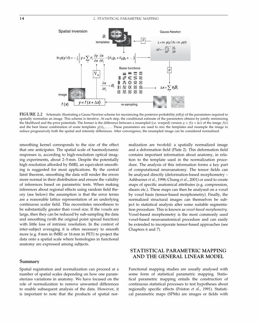
Elsevier UK Chapter: Ch02-P372560 3-10-2006 3:58p.m. Page:14 Trim:7.5in×9.25in
Basal Font:Palatino Margins:Top:40pt Gutter:68pt Font Size:9.5/12 Text Width:42pc Depth:55 Lines
14 2. STATISTICAL PARAMETRIC MAPPING
re-sampling
(θ1g1 + θ2g2 + …)−∂θi
∂x∂x∂y− 2
1ln p(y⏐θ) = y +i
θi
= Bi∂θi
∂x
y = f (x + Δx)
templates
∂θ∂L
∂θ 2
∂2L−1
Δθ = −
L = ln p(y⏐θ) + ln p(θ)
Gauss-NewtonSpatial inversion
∇xθ
f (x)
gi
Basis functions
Δx =i
θiθiBi
image
θ
FIGURE 2.2 Schematic illustrating a Gauss-Newton scheme for maximizing the posterior probability p���y� of the parameters required tospatially normalize an image. This scheme is iterative. At each step, the conditional estimate of the parameters obtains by jointly minimizingthe likelihood and the prior potentials. The former is the difference between a resampled (i.e. warped) version y = f�x+ x� of the image f�x�and the best linear combination of some templates g�x�1� . These parameters are used to mix the templates and resample the image toreduce progressively both the spatial and intensity differences. After convergence, the resampled image can be considered normalized.
smoothing kernel corresponds to the size of the effectthat one anticipates. The spatial scale of haemodynamicresponses is, according to high-resolution optical imag-ing experiments, about 2–5 mm. Despite the potentiallyhigh resolution afforded by fMRI, an equivalent smooth-ing is suggested for most applications. By the centrallimit theorem, smoothing the data will render the errorsmore normal in their distribution and ensure the validityof inferences based on parametric tests. When makinginferences about regional effects using random field the-ory (see below) the assumption is that the error termsare a reasonable lattice representation of an underlyingcontinuous scalar field. This necessitates smoothness tobe substantially greater than voxel size. If the voxels arelarge, then they can be reduced by sub-sampling the dataand smoothing (with the original point spread function)with little loss of intrinsic resolution. In the context ofinter-subject averaging it is often necessary to smoothmore (e.g. 8 mm in fMRI or 16 mm in PET) to project thedata onto a spatial scale where homologies in functionalanatomy are expressed among subjects.
Summary
Spatial registration and normalization can proceed at anumber of spatial scales depending on how one param-eterizes variations in anatomy. We have focused on therole of normalization to remove unwanted differencesto enable subsequent analysis of the data. However, itis important to note that the products of spatial nor-
malization are twofold: a spatially normalized imageand a deformation field (Plate 2). This deformation fieldcontains important information about anatomy, in rela-tion to the template used in the normalization proce-dure. The analysis of this information forms a key partof computational neuroanatomy. The tensor fields canbe analysed directly (deformation-based morphometry –Ashburner et al., 1998; Chung et al., 2001) or used to createmaps of specific anatomical attributes (e.g. compression,shears etc.). These maps can then be analysed on a voxelby voxel basis (tensor-based morphometry). Finally, thenormalized structural images can themselves be sub-ject to statistical analysis after some suitable segmenta-tion procedure. This is known as voxel-based morphometry.Voxel-based morphometry is the most commonly usedvoxel-based neuroanatomical procedure and can easilybe extended to incorporate tensor-based approaches (seeChapters 6 and 7).
STATISTICAL PARAMETRIC MAPPINGAND THE GENERAL LINEAR MODEL
Functional mapping studies are usually analysed withsome form of statistical parametric mapping. Statis-tical parametric mapping entails the construction ofcontinuous statistical processes to test hypotheses aboutregionally specific effects (Friston et al., 1991). Statisti-cal parametric maps (SPMs) are images or fields with

Elsevier UK Chapter: Ch02-P372560 3-10-2006 3:58p.m. Page:15 Trim:7.5in×9.25in
Basal Font:Palatino Margins:Top:40pt Gutter:68pt Font Size:9.5/12 Text Width:42pc Depth:55 Lines
STATISTICAL PARAMETRIC MAPPING AND THE GENERAL LINEAR MODEL 15
values that are, under the null hypothesis, distributedaccording to a known probability density function, usu-ally the Student’s t or F -distributions. These are knowncolloquially as t- or F -maps. The success of statisticalparametric mapping is due largely to the simplicity ofthe idea. Namely, one analyses each and every voxelusing any standard (univariate) statistical test. The result-ing statistical parameters are assembled into an image –the SPM. SPMs are interpreted as continuous statisticalprocesses by referring to the probabilistic behaviour ofrandom fields (Adler, 1981; Worsley et al., 1992, 1996;Friston et al., 1994). Random fields model both the uni-variate probabilistic characteristics of an SPM and anynon-stationary spatial covariance structure. ‘Unlikely’topological features of the SPM, like peaks, are inter-preted as regionally specific effects, attributable to theexperimental manipulation.
Over the years, statistical parametric mapping hascome to refer to the conjoint use of the general linear model(GLM) and random field theory (RFT) theory to analyse andmake classical inferences about topological features of thestatistical parametric maps (SPM). The GLM is used toestimate some parameters that explain continuous data inexactly the same way as in conventional analyses of dis-crete data (see Part 2). RFT is used to resolve the multiplecomparison problem that ensues when making inferencesover the volume analysed (see Part 3). RFT provides amethod for adjusting p-values for the search volume andplays the same role for continuous data (i.e. images) asthe Bonferroni correction for a number of discontinuousor discrete statistical tests.
The approach was called SPM for three reasons:
1 To acknowledge significance probability mapping,where interpolated pseudo-maps of p-values are usedto summarize the analysis of multichannel event-related potential (ERP) studies.
2 For consistency with the nomenclature of paramet-ric maps of physiological or physical parameters (e.g.parametric maps of regional cerebral blood flow (rCBF)or volume).
3 In reference to the parametric statistics that populatethe maps.
Despite its simplicity, there are some fairly subtle moti-vations for the approach that deserve mention. Usually,given a response or dependent variable, comprisingmany thousands of voxels, one would use multivari-ate analyses as opposed to the mass-univariate approachthat SPM represents. The problems with multivariateapproaches are that:
1 they do not support inferences about regionally specificeffects (i.e. topological features with a unique localizingattribute)
2 they require more observations than the dimension ofthe response variable (i.e. need more scans than voxels)
3 even in the context of dimension reduction, they areless sensitive to focal effects than mass-univariateapproaches.
A heuristic, for their relative lack of power, is that mul-tivariate approaches estimate the model’s error covari-ances using lots of parameters (e.g. the covariancebetween the errors at all pairs of voxels). Conversely,SPM characterizes spatial covariance with a smoothnessparameter, for each voxel. In general, the more parame-ters (and hyperparameters) an estimation procedure hasto deal with, the more variable the estimate of any oneparameter becomes. This renders inferences about anysingle estimate less efficient.
Multivariate approaches consider voxels as differentlevels of an experimental or treatment factor and useclassical analysis of variance, not at each voxel but byconsidering the data sequences from all voxels together,as replications over voxels. The problem here is thatregional changes in error variance, and spatial correla-tions in the data, induce profound non-sphericity1 inthe error terms. This non-sphericity would again requirelarge numbers of parameters to be estimated for eachvoxel using conventional techniques. In SPM, the non-sphericity is parameterized in a parsimonious way withjust two parameters for each voxel. These are the errorvariance and smoothness estimators (see Part 3). Thisminimal parameterization lends SPM a sensitivity thatsurpasses multivariate approaches. SPM can do thisbecause RFT implicitly harnesses constraints on the non-sphericity implied by the continuous (i.e. analytic) natureof the data. This is something that conventional mul-tivariate and equivalent univariate approaches cannotaccommodate, to their cost.
Some analyses use statistical maps based on non-parametric tests that eschew distributional assumptionsabout the data (see Chapter 21). These approaches aregenerally less powerful (i.e. less sensitive) than paramet-ric approaches (see Aguirre et al., 1998). However, theyhave an important role in evaluating the assumptions
1 Sphericity refers to the assumption of identically and indepen-dently distributed error terms (IID). Under IID assumptions theprobability density function of the errors, from all observations,has spherical iso-contours, hence sphericity. Deviations fromeither of the IID criteria constitute non-sphericity. If the errorterms are not identically distributed then different observa-tions have different error variances. Correlations among errorsreflect dependencies among the error terms (e.g. serial correla-tion in fMRI time series) and constitute the second componentof non-sphericity. In neuroimaging both spatial and temporalnon-sphericity can be quite profound.
Elsevier UK Chapter: Ch02-P372560 3-10-2006 3:58p.m. Page:16 Trim:7.5in×9.25in
Basal Font:Palatino Margins:Top:40pt Gutter:68pt Font Size:9.5/12 Text Width:42pc Depth:55 Lines
16 2. STATISTICAL PARAMETRIC MAPPING
behind parametric approaches and may supervene interms of sensitivity when these assumptions are violated(e.g. when degrees of freedom are very small and voxelsizes are large in relation to smoothness).
In Part 4 we consider Bayesian alternatives to classicalinference with SPMs. This rests on conditional inferencesabout an effect, given the data, as opposed to classi-cal inferences about the data, given the effect is zero.Bayesian inferences on continuous fields or images useposterior probability maps (PPMs). Although less com-monly used than SPMs, PPMs are potentially useful,not least because they do not have to contend with themultiple comparisons problem induced by classical infer-ence. In contradistinction to SPM, this means that infer-ences about a given regional response do not depend oninferences about responses elsewhere. Next we considerparameter estimation in the context of the GLM. Thisis followed by an introduction to the role of RFT whenmaking classical inferences about continuous data.
The general linear model
Statistical analysis of imaging data corresponds to invert-ing generative models of the data to partition observedresponses into components of interest, confounds anderror. Inferences are then pursued using statistics thatcompare interesting effects and the error. This classi-cal inference can be regarded as a direct comparison ofthe variance due to an interesting experimental manip-ulation with the error variance (compare with the F -statistic and other likelihood ratios). Alternatively, onecan view the statistic as an estimate of the response, ordifference of interest, divided by an estimate of its stan-dard deviation. This is a useful way to think about thet-statistic.
A brief review of the literature may give the impressionthat there are numerous ways to analyse PET and fMRItime-series with a diversity of statistical and conceptualapproaches. This is not the case. With very few excep-tions, every analysis is a variant of the general linearmodel. This includes simple t-tests on scans assigned toone condition or another, correlation coefficients betweenobserved responses and boxcar stimulus functions infMRI, inferences made using multiple linear regression,evoked responses estimated using linear time invariantmodels, and selective averaging to estimate event-relatedresponses in fMRI. Mathematically, they are all formallyidentical and can be implemented with the same equa-tions and algorithms. The only thing that distinguishesamong them is the design matrix encoding the temporalmodel or experimental design. The use of the correlationcoefficient deserves special mention because of its popu-larity in fMRI (Bandettini et al., 1993). The significance of
a correlation is identical to the significance of the equiv-alent t-statistic testing for a regression of the data on astimulus function. The correlation coefficient approach isuseful but the inference is effectively based on a limitingcase of multiple linear regression that obtains when thereis only one regressor. In fMRI, many regressors usuallyenter a statistical model. Therefore, the t-statistic pro-vides a more versatile and generic way of assessing thesignificance of regional effects and is usually preferredover the correlation coefficient.
The general linear model is an equation Y = X+�that expresses the observed response variable in termsof a linear combination of explanatory variables X plusa well behaved error term (Figure 2.3 and Friston et al.,1995b). The general linear model is variously known as‘analysis of covariance’ or ‘multiple regression analysis’and subsumes simpler variants, like the ‘t-test’ for a dif-ference in means, to more elaborate linear convolutionmodels such as finite impulse response (FIR) models.The matrix that contains the explanatory variables (e.g.designed effects or confounds) is called the design matrix.Each column of the design matrix corresponds to aneffect one has built into the experiment or that mayconfound the results. These are referred to as explana-tory variables, covariates or regressors. The example inPlate 1 relates to an fMRI study of visual stimulationunder four conditions. The effects on the response vari-able are modelled in terms of functions of the pres-ence of these conditions (i.e. boxcars smoothed with ahaemodynamic response function) and constitute the firstfour columns of the design matrix. There then followsa series of terms that are designed to remove or modellow-frequency variations in signal due to artefacts suchas aliased biorhythms and other drift terms. The finalcolumn is whole brain activity. The relative contributionof each of these columns is assessed using standard maxi-mum likelihood and inferences about these contributionsare made using t or F -statistics, depending upon whetherone is looking at a particular linear combination (e.g.a subtraction), or all of them together. The operationalequations are depicted schematically in Figure 2.3. Inthis scheme, the general linear model has been extended(Worsley and Friston, 1995) to incorporate intrinsic non-sphericity, or correlations among the error terms, and toallow for some temporal filtering of the data with thematrix S. This generalization brings with it the notionof effective degrees of freedom, which are less than theconventional degrees of freedom under IID assumptions(see footnote). They are smaller because the temporalcorrelations reduce the effective number of independentobservations. The statistics are constructed using theapproximation of Satterthwaite. This is the same approx-imation used in classical non-sphericity corrections suchas the Geisser-Greenhouse correction. However, in the

Elsevier UK Chapter: Ch02-P372560 3-10-2006 3:58p.m. Page:17 Trim:7.5in×9.25in
Basal Font:Palatino Margins:Top:40pt Gutter:68pt Font Size:9.5/12 Text Width:42pc Depth:55 Lines
STATISTICAL PARAMETRIC MAPPING AND THE GENERAL LINEAR MODEL 17
intrinsic correlationsintrinsic correlationsfilterfilter DataData
efficiency
SPM{t}SPM{t }...fitted data...adjusted data...residual fields...residual forming matrix
smoothness estimator
Σ−
1 − X0X0
1
21
S =
Σ(λ)
ˆ
ˆˆ
R = 1 − SX (SX )+r = RSYY * = Y + r
Y = SXβ
ˆ
ˆˆˆ
σ 2
=
tr (RVRV )
tr RV )2v =
tr (RV )rTr
V(cTβ ) = σ 2cT (SX )+V (SX )+Tc
V(cTβ ) ∝ cT(SX )+V (SX )+Tcˆ
V(cTβ)
cTβ
SY = SXβ + SεY = Xβ + ε
~tvˆ
ˆ
ε~N (0,σ 2Σ) V = S ΣST
β = (SX )+ SY
Design MatrixDesign matrix
+
ˆ ˆ
FIGURE 2.3 The general linear model. The general linear model is an equation expressing the response variable Y in terms of a linearcombination of explanatory variables in a design matrix X and an error term with assumed or known autocorrelation �. The data can befiltered with a convolution or residual forming matrix (or a combination) S, leading to a generalized linear model that includes [intrinsic]serial correlations and applied [extrinsic] filtering. Different choices of S correspond to different estimation schemes. The parameter estimatesobtain in a least squares sense using the pseudo-inverse (denoted by +) of the filtered design matrix. Generally, an effect of interest is specifiedby a vector of contrast weights c that give a weighted sum or compound of parameter estimates referred to as a contrast. The t-statistic issimply this contrast divided by its standard error (i.e. square root of its estimated variance). The ensuing t-statistic is distributed with vdegrees of freedom. The equations for estimating the variance of the contrast and the degrees of freedom are provided in the right-handpanel. Efficiency is simply the inverse of the variance of the contrast. These expressions are useful when assessing the relative efficiency ofdifferent designs encoded in X. The parameter estimates can be examined directly or used to compute the fitted responses (see lower leftpanel). Adjusted data refer to data from which fitted components (e.g. confounds) have been removed. The residuals r, obtain from applyingthe residual-forming matrix R to the data. These residual fields are used to estimate the smoothness of the component fields of the SPM andare needed by random field theory (see Figure 2.4).
Worsley and Friston (1995) scheme, this approximationis used to construct the statistics and appropriate degreesof freedom, not simply to provide a post hoc correction tothe degrees of freedom.
There is a special and important case of temporal filter-ing. This is when the filtering de-correlates (i.e. whitens)the error terms by using S = �−1/2. This is the filter-ing scheme used in current implementations of the SPMsoftware and renders the ordinary least squares (OLS)parameter estimates maximum likelihood (ML) estima-tors. These are optimal in the sense that they are the min-imum variance estimators of all unbiased estimators. Theestimation of S = �−1/2 uses expectation maximization(EM) to provide restricted maximum likelihood (ReML)estimates of � = ���� in terms of hyperparameters � cor-responding to variance components (see Chapter 11 andChapter 24 for an explanation of EM). In this case, theeffective degrees of freedom revert to the maximum thatwould be attained in the absence of temporal correlationsor non-sphericity.
Contrasts
The equations summarized in Figure 2.3 can be used toimplement a vast range of statistical analyses. The issueis therefore not the mathematics but the formulation of adesign matrix appropriate to the study design and infer-ences that are sought. The design matrix can contain bothcovariates and indicator variables. Each column has anassociated unknown or free parameter . Some of theseparameters will be of interest (e.g. the effect of a partic-ular sensorimotor or cognitive condition or the regres-sion coefficient of haemodynamic responses on reactiontime). The remaining parameters will be of no interestand pertain to confounding effects (e.g. the effect of beinga particular subject or the regression slope of voxel activ-ity on global activity). Inferences about the parameterestimates are made using their estimated variance. Thisallows one to test the null hypothesis, that all the esti-mates are zero, using the F -statistic to give an SPM�F�or that some particular linear combination (e.g. a sub-traction) of the estimates is zero using an SPM�t�. The

Elsevier UK Chapter: Ch02-P372560 3-10-2006 3:58p.m. Page:18 Trim:7.5in×9.25in
Basal Font:Palatino Margins:Top:40pt Gutter:68pt Font Size:9.5/12 Text Width:42pc Depth:55 Lines
18 2. STATISTICAL PARAMETRIC MAPPING
t-statistic obtains by dividing a contrast or compound(specified by contrast weights) of the ensuing parame-ter estimates by the standard error of that compound.The latter is estimated using the variance of the residu-als about the least-squares fit. An example of a contrastweight vector would be �−1 1 0 � �� to compare the dif-ference in responses evoked by two conditions, modelledby the first two condition-specific regressors in the designmatrix. Sometimes several contrasts of parameter esti-mates are jointly interesting. For example, when usingpolynomial (Büchel et al., 1996) or basis function expan-sions of some experimental factor. In these instances, theSPM�F� is used and is specified with a matrix of con-trast weights that can be thought of as a collection of‘t-contrasts’ (see Chapter 9 for a fuller explanation). AnF -contrast may look like:
[−1 0 0 0 0 1 0 0
]
This would test for the significance of the first or secondparameter estimates. The fact that the first weight is neg-ative has no effect on the test because the F -statistic isbased on sums of squares.
In most analyses, the design matrix contains indica-tor variables or parametric variables encoding the exper-imental manipulations. These are formally identical toclassical analysis of covariance (i.e. ANCOVA) models.An important instance of the GLM, from the perspectiveof fMRI, is the linear time-invariant (LTI) model. Mathe-matically, this is no different from any other GLM. How-ever, it explicitly treats the data-sequence as an orderedtime-series and enables a signal processing perspectivethat can be very useful (see next chapter and Chapter 14).
TOPOLOGICAL INFERENCE AND THETHEORY OF RANDOM FIELDS
Classical inferences using SPMs can be of two sorts,depending on whether one knows where to look inadvance. With an anatomically constrained hypothesis,about effects in a particular brain region, the uncorrectedp-value associated with the height or extent of that regionin the SPM can be used to test the hypothesis. With ananatomically open hypothesis (i.e. a null hypothesis thatthere is no effect anywhere in a specified volume of thebrain), a correction for multiple dependent comparisonsis necessary. The theory of random fields provides a wayof adjusting the p-value that takes into account the factthat neighbouring voxels are not independent by virtueof continuity in the original data. Provided the data aresmooth the RFT adjustment is less severe (i.e. is more
sensitive) than a Bonferroni correction for the numberof voxels. As noted above, RFT deals with the multiplecomparisons problem in the context of continuous, statis-tical fields, in a way that is analogous to the Bonferroniprocedure for families of discrete statistical tests. Thereare many ways to appreciate the difference between RFTand Bonferroni corrections. Perhaps the most intuitive isto consider the fundamental difference between an SPMand a collection of discrete t-values. When declaring apeak or cluster of the SPM to be significant, we refercollectively to all the voxels associated with that feature.The false positive rate is expressed in terms of peaksor clusters, under the null hypothesis of no activation.This is not the expected false positive rate of voxels. Onefalse positive peak may be associated with hundreds ofvoxels, if the SPM is very smooth. Bonferroni correc-tion controls the expected number of false positive vox-els, whereas RFT controls the expected number of falsepositive peaks. Because the number of peaks is alwaysless than the number of voxels, RFT can use a lowerthreshold, rendering it much more sensitive. In fact, thenumber of false positive voxels is somewhat irrelevantbecause it is a function of smoothness. The RFT correc-tion discounts voxel size by expressing the search volumein terms of smoothness or resolution elements (Resels)(Figure 2.4). This intuitive perspective is expressed for-mally in terms of differential topology using the Eulercharacteristic (Worsley et al., 1992). At high thresholds theEuler characteristic corresponds to the number of peaksabove threshold.
There are only two assumptions underlying the use ofthe RFT correction:
1 the error fields (but not necessarily the data) are a rea-sonable lattice approximation to an underlying randomfield with a multivariate Gaussian distribution
2 these fields are continuous, with a differentiable andinvertible autocorrelation function.
A common misconception is that the autocorrelationfunction has to be Gaussian. It does not. The only way inwhich these assumptions can be violated is if:
1 the data are not smooth, violating the reasonable latticeassumption or
2 the statistical model is mis-specified so that the errorsare not normally distributed.
Early formulations of the RFT correction were based on theassumption that the spatial correlation structure was wide-sense stationary. This assumption can now be relaxed dueto a revision of the way in which the smoothness estima-tor enters the correction procedure (Kiebel et al., 1999). Inother words, the corrections retain their validity, even if thesmoothness varies from voxel to voxel.

Elsevier UK Chapter: Ch02-P372560 3-10-2006 3:58p.m. Page:19 Trim:7.5in×9.25in
Basal Font:Palatino Margins:Top:40pt Gutter:68pt Font Size:9.5/12 Text Width:42pc Depth:55 Lines
TOPOLOGICAL INFERENCE AND THE THEORY OF RANDOM FIELDS 19
Poisson Clumping Heuristic
Expected clusters
R0
RD0
=...
...
...
......... ...
EC density Search volume (RESELS)
R0 = 1
R1 = 4θR2 = 2πθ
2
Smoothness
R(θ) = R0,...,RD
Cluster volume (RESELS)
P(u,c,k) = 1– λ(c –1,ψ0 (u)p(n ≥ k))
p(n ≥ k) = exp(–βk )D2
β = ( Γ(D/2 + 1))Dη12
η =ρ0
nRD 0
ρ(u) = ρ0,...,ρD
ρ0 = 1–Φt (u)
ρ0c1 ρ0c1
ρ0cD
1 n
D
ρ1 =(41n2)
12
2π (1 + u 2/v)
12– (v–1)
R3 = 43 πθ3
12
12–ρ2 = 41n2
312(2π) (1 + u
2/v)12– (v–1)Γ( ( v+1))( v) Γ( v)
–112
12
θ(W ) =FWHM
FWHM = (41n 2)
θvoxels
12 Λ 1
2D–
√e = r
r rTΛ ≈
T∂e ∂e∂x ∂x
ρ3 = ...
D
ci = j
Γ( )Γ( ) 1 j +1
2
Γ( )Γ( ) j –i+1
2i+12
2
ψ0
ψD
ψ
FIGURE 2.4 Schematic illustrating the use of random field theory (RFT) in making inferences about SPMs. If one knew precisely whereto look, then inference can be based on the value of the statistic at the specified location in the SPM. However, generally, one does not havea precise anatomical prior, and an adjustment for multiple dependent comparisons has to be made to the p-values. These corrections usedistributional approximations from RFT. This schematic deals with a general case of n SPM�t� whose voxels all survive a common thresholdu (i.e. a conjunction of n component SPMs). The central probability, upon which all peak, cluster or set-level inferences are made, is theprobability P�u� c�k� of getting c or more clusters with k or more resels (resolution elements) above this threshold. By assuming that clustersbehave like a multidimensional Poisson point-process (i.e. the Poisson clumping heuristic) P�u� c�k� is determined simply; the distributionof c is Poisson with an expectation that corresponds to the product of the expected number of clusters, of any size, and the probability thatany cluster will be bigger than k resels. The latter probability depends on the expected number of resels per cluster �. This is simply theexpected suprathreshold volume, divided by the expected number of clusters. The expected number of clusters �0 is estimated with the Eulercharacteristic (EC) (effectively the number of blobs minus the number of holes). This depends on the EC density for the statistic in question(with degrees of freedom v) and the resel counts. The EC density is the expected EC per unit of D-dimensional volume of the SPM wherethe volume of the search is given by the resel counts. Resel counts are a volume measure that has been normalized by the smoothness ofthe SPMs component fields, expressed in terms of the full width at half maximum (FWHM). This is estimated from the determinant of thevariance-covariance matrix of the first spatial derivatives of e, the normalized residual fields r (from Figure 2.3). In this example equationsfor a sphere of radius � are given. � denotes the cumulative density function for the statistic in question. (See Appendix 6 for technicaldetails.)
Anatomically closed hypotheses
When making inferences about regional effects (e.g. acti-vations) in SPMs, one often has some idea about wherethe activation should be. In this instance, a correctionfor the entire search volume is inappropriate. However,a problem remains in the sense that one would like toconsider activations that are ‘near’ the predicted location,even if they are not exactly coincident. There are twoapproaches one can adopt: pre-specify a small search vol-ume and make the appropriate RFT correction (Worsleyet al., 1996); or use the uncorrected p-value based onspatial extent of the nearest cluster (Friston, 1997). Thisprobability is based on getting the observed number ofvoxels, or more, in a given cluster (conditional on thatcluster existing). Both these procedures are based on dis-tributional approximations from RFT.
Anatomically open hypotheses and levels of inference
To make inferences about regionally specific effects,the SPM is thresholded using some height and spatialextent thresholds that are specified by the user. Correctedp-values can then be derived that pertain to:
1 The number of activated regions (i.e. number of clustersabove the height and volume threshold). These are set-level inferences.
2 The number of activated voxels (i.e. volume) compris-ing a particular region. These are cluster-level inferences.
3 The p-value for each peak within that cluster, i.e. peak-level inferences.
These p-values are corrected for the multiple depen-dent comparisons and are based on the probability ofobtaining c, or more, clusters with k, or more, voxels,

Elsevier UK Chapter: Ch02-P372560 3-10-2006 3:58p.m. Page:20 Trim:7.5in×9.25in
Basal Font:Palatino Margins:Top:40pt Gutter:68pt Font Size:9.5/12 Text Width:42pc Depth:55 Lines
20 2. STATISTICAL PARAMETRIC MAPPING
above a threshold u in an SPM of known or estimatedsmoothness. This probability has a reasonably simpleform (see Figure 2.4 for details).
Set-level refers to the inference that the number of clus-ters comprising an observed activation profile is highlyunlikely to have occurred by chance and is a statementabout the activation profile, as characterized by its con-stituent regions. Cluster-level inferences are a special caseof set-level inferences that obtain when the number ofclusters c = 1. Similarly, peak-level inferences are specialcases of cluster-level inferences that result when the clus-ter can be small (i.e. k = 0). Using a theoretical poweranalysis (see Friston et al., 1996b and Chapter 19) of dis-tributed activations, one observes that set-level inferencesare generally more powerful than cluster-level inferencesand that cluster-level inferences are generally more pow-erful than peak-level inferences. The price paid for thisincreased sensitivity is reduced localizing power. Peak-level tests permit individual maxima to be identified assignificant, whereas cluster and set-level inferences onlyallow clusters or sets of clusters to be declared signif-icant. It should be remembered that these conclusions,about the relative power of different inference levels, arebased on distributed activations. Focal activation maywell be detected with greater sensitivity using tests basedon peak height. Typically, people use peak-level infer-ences and a spatial extent threshold of zero. This reflectsthe fact that characterizations of functional anatomy aregenerally more useful when specified with a high degreeof anatomical precision.
EXPERIMENTAL AND MODEL DESIGN
This section considers the different sorts of designs thatcan be employed in neuroimaging studies. Experimen-tal designs can be classified as single factor or multifactordesigns; within this classification the levels of each factorcan be categorical or parametric. We will start by discussingcategorical and parametric designs and then deal withmultifactor designs. We then move on to some more tech-nical issues that attend the analysis of fMRI experiments.These are considered in terms of model design, using asignal processing perspective.
Categorical designs, cognitive subtraction andconjunctions
The tenet of cognitive subtraction is that the differencebetween two tasks can be formulated as a separablecognitive or sensorimotor component and that region-ally specific differences in haemodynamic responses,
evoked by the two tasks, identify the corresponding func-tionally selective area. Early applications of subtractionrange from the functional anatomy of word process-ing (Petersen et al., 1989) to functional specialization inextrastriate cortex (Lueck et al., 1989). The latter stud-ies involved presenting visual stimuli with and with-out some sensory attribute (e.g. colour, motion etc.). Theareas highlighted by subtraction were identified withhomologous areas in monkeys that showed selective elec-trophysiological responses to equivalent visual stimuli.
Cognitive conjunctions (Price and Friston, 1997) can bethought of as an extension of the subtraction technique,in the sense that they combine a series of subtractions.In subtraction, one tests a single hypothesis pertainingto the activation in one task relative to another. In con-junction analyses, several hypotheses are tested, askingwhether the activations, in a series of task pairs, are col-lectively significant (cf. an F -test). Consider the problemof identifying regionally specific activations due to a par-ticular cognitive component (e.g. object recognition). Ifone can identify a series of task pairs whose differenceshave only that component in common, then the regionwhich activates, in all the corresponding subtractions,can be associated with the common component. Con-junction analyses allow one to demonstrate the context-invariant nature of regional responses. One importantapplication of conjunction analyses is in multisubjectfMRI studies, where generic effects are identified as thosethat are jointly significant in all the subjects studied(see below).
Parametric designs
The premise behind parametric designs is that regionalphysiology will vary systematically with the degree ofcognitive or sensorimotor processing or deficits thereof.Examples of this approach include the PET experimentsof Grafton et al. (1992) that demonstrated significant cor-relations between haemodynamic responses and the per-formance of a visually guided motor tracking task. On thesensory side, Price et al. (1992) demonstrated a remark-able linear relationship between perfusion in periaudi-tory regions and frequency of aural word presentation.This correlation was not observed in Wernicke’s area,where perfusion appeared to correlate, not with the dis-criminative attributes of the stimulus, but with the pres-ence or absence of semantic content. These relationshipsor neurometric functions may be linear or non-linear. Usingpolynomial regression, in the context of the GLM, onecan identify non-linear relationships between stimulusparameters (e.g. stimulus duration or presentation rate)and evoked responses. To do this one usually uses anSPM�F� (see Büchel et al., 1996).
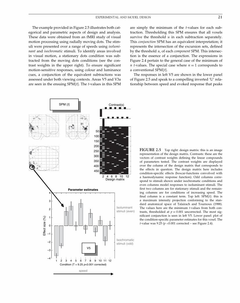
Elsevier UK Chapter: Ch02-P372560 3-10-2006 3:58p.m. Page:21 Trim:7.5in×9.25in
Basal Font:Palatino Margins:Top:40pt Gutter:68pt Font Size:9.5/12 Text Width:42pc Depth:55 Lines
EXPERIMENTAL AND MODEL DESIGN 21
The example provided in Figure 2.5 illustrates both cat-egorical and parametric aspects of design and analysis.These data were obtained from an fMRI study of visualmotion processing using radially moving dots. The stim-uli were presented over a range of speeds using isolumi-nant and isochromatic stimuli. To identify areas involvedin visual motion, a stationary dots condition was sub-tracted from the moving dots conditions (see the con-trast weights in the upper right). To ensure significantmotion-sensitive responses, using colour and luminancecues, a conjunction of the equivalent subtractions wasassessed under both viewing contexts. Areas V5 and V3aare seen in the ensuing SPM�t�. The t-values in this SPM
are simply the minimum of the t-values for each sub-traction. Thresholding this SPM ensures that all voxelssurvive the threshold u in each subtraction separately.This conjunction SPM has an equivalent interpretation; itrepresents the intersection of the excursion sets, definedby the threshold u, of each component SPM. This intersec-tion is the essence of a conjunction. The expressions inFigure 2.4 pertain to the general case of the minimum ofn t-values. The special case where n = 1 corresponds toa conventional SPM�t�.
The responses in left V5 are shown in the lower panelof Figure 2.5 and speak to a compelling inverted ‘U’ rela-tionship between speed and evoked response that peaks
SPM{t}
V5
50
100
150
200
250
300
350
400
450
2Design matrix
Parameter estimates
Effe
ct s
ize
(%)
4
3
2
1
0
–1
–2
–3
–4
SPM {t }
Isoluminantstimuli (even)
Isochromaticstimuli (odd)
speed
V5
Condition (T = 9.25 p<0.001 corrected)1 2 3 4 5 6 7 8 9 10 11 12
4 6 8 10 12
Contrast(s)
FIGURE 2.5 Top right: design matrix: this is an imagerepresentation of the design matrix. Contrasts: these are thevectors of contrast weights defining the linear compoundsof parameters tested. The contrast weights are displayedover the column of the design matrix that corresponds tothe effects in question. The design matrix here includescondition-specific effects (boxcar-functions convolved witha haemodynamic response function). Odd columns corre-spond to stimuli shown under isochromatic conditions andeven columns model responses to isoluminant stimuli. Thefirst two columns are for stationary stimuli and the remain-ing columns are for conditions of increasing speed. Thefinal column is a constant term. Top left: SPM�t�: this isa maximum intensity projection conforming to the stan-dard anatomical space of Talairach and Tournoux (1988).The values here are the minimum t-values from both con-trasts, thresholded at p = 0�001 uncorrected. The most sig-nificant conjunction is seen in left V5. Lower panel: plot ofthe condition-specific parameter estimates for this voxel. Thet-value was 9.25 (p <0�001 corrected – see Figure 2.4).

Elsevier UK Chapter: Ch02-P372560 3-10-2006 3:58p.m. Page:22 Trim:7.5in×9.25in
Basal Font:Palatino Margins:Top:40pt Gutter:68pt Font Size:9.5/12 Text Width:42pc Depth:55 Lines
22 2. STATISTICAL PARAMETRIC MAPPING
at around eight degrees per second. It is this sort of rela-tionship that parametric designs try to characterize. Inter-estingly, the form of these speed-dependent responseswas similar using both stimulus types, although lumi-nance cues are seen to elicit a greater response. From thepoint of view of a factorial design there is a main effect ofcue (isoluminant versus isochromatic), a main effect ofspeed, but no speed by cue interaction.
Clinical neuroscience studies can use parametricdesigns by looking for the neuronal correlates of clini-cal (e.g. symptom) ratings over subjects. In many cases,multiple clinical scores are available for each subject andthe statistical design can usually be seen as a multi-linear regression. In situations where the clinical scoresare correlated, principal component analysis or factoranalysis is sometimes applied to generate a new, andsmaller, set of explanatory variables that are orthogonalto each other. This has proved particularly useful in psy-chiatric studies where syndromes can be expressed overa number of different dimensions (e.g. the degree of psy-chomotor poverty, disorganization and reality distortionin schizophrenia; see Liddle et al., 1992). In this way,regionally specific correlates of various symptoms maypoint to their distinct pathogenesis in a way that tran-scends the syndrome itself. For example, psychomotorpoverty may be associated with left dorso-lateral pre-frontal dysfunction, irrespective of whether the patient issuffering from schizophrenia or depression.
Factorial designs
Factorial designs are more prevalent than single-factordesigns because they enable inferences about interac-tions. At its simplest, an interaction represents a changein a change. Interactions are associated with factorialdesigns where two or more factors are combined in thesame experiment. The effect of one factor, on the effect ofthe other, is assessed by the interaction. Factorial designshave a wide range of applications. An early application,in neuroimaging, examined adaptation and plasticityduring motor performance by assessing time by condi-tion interactions (Friston et al., 1992a). Psychopharmaco-logical activation studies are further examples of factorialdesigns (Friston et al., 1992b). In these studies, cogni-tively evoked responses are assessed before and afterbeing given a drug. The interaction term reflects the phar-macological modulation of task-dependent activations.Factorial designs have an important role in the contextof cognitive subtraction and additive factors logic byvirtue of being able to test for interactions, or context-sensitive activations, i.e. to demonstrate the fallacy ofpure-insertion (see Friston et al., 1996c). These interactioneffects can sometimes be interpreted as the integration of
the two or more [cognitive] processes or the modulationof one [perceptual] process by another. Figure 2.6 showsan example which takes an unusual perspective on themodulation of event-related responses as the interactionbetween stimulus presentation and experiential context.
From the point of view of clinical studies, interactionsare central. The effect of a disease process on sensorimo-tor or cognitive activation is simply an interaction andinvolves replicating a subtraction experiment in subjectswith and without the pathology. Factorial designs canalso embody parametric factors. If one of the factors hasa number of parametric levels, the interaction can beexpressed as a difference in regression slope of regionalactivity on the parameter, under both levels of the other[categorical] factor. An important example of factorialdesigns, that mix categorical and parameter factors, arethose looking for psychophysiological interactions. Here theparametric factor is brain activity measured in a par-ticular brain region. These designs have proven usefulin looking at the interaction between bottom-up andtop-down influences within processing hierarchies in thebrain (Friston et al., 1997). This issue will be addressedbelow and in Part 6, from the point of view of effectiveconnectivity.
Designing fMRI studies
In this section, we consider fMRI time-series from a signalprocessing perspective with particular focus on optimalexperimental design and efficiency. fMRI time-series canbe viewed as a linear admixture of signal and noise. Sig-nal corresponds to neuronally mediated haemodynamicchanges that can be modelled as a convolution of someunderlying neuronal process, responding to changes inexperimental factors, by a haemodynamic response func-tion. Noise has many contributions that render it rathercomplicated in relation to some neurophysiological mea-surements. These include neuronal and non-neuronalsources. Neuronal noise refers to neurogenic signal notmodelled by the explanatory variables and has the samefrequency structure as the signal itself. Non-neuronalcomponents have both white (e.g. Johnson noise) andcoloured components (e.g. pulsatile motion of the braincaused by cardiac cycles and local modulation of thestatic magnetic field by respiratory movement). Theseeffects are typically low-frequency or wide-band (e.g.aliased cardiac-locked pulsatile motion). The superposi-tion of all these components induces temporal correla-tions among the error terms (denoted by � in Figure 2.3)that can affect sensitivity to experimental effects. Sensi-tivity depends upon the relative amounts of signal andnoise and the efficiency of the experimental design. Effi-ciency is simply a measure of how reliable the parameter
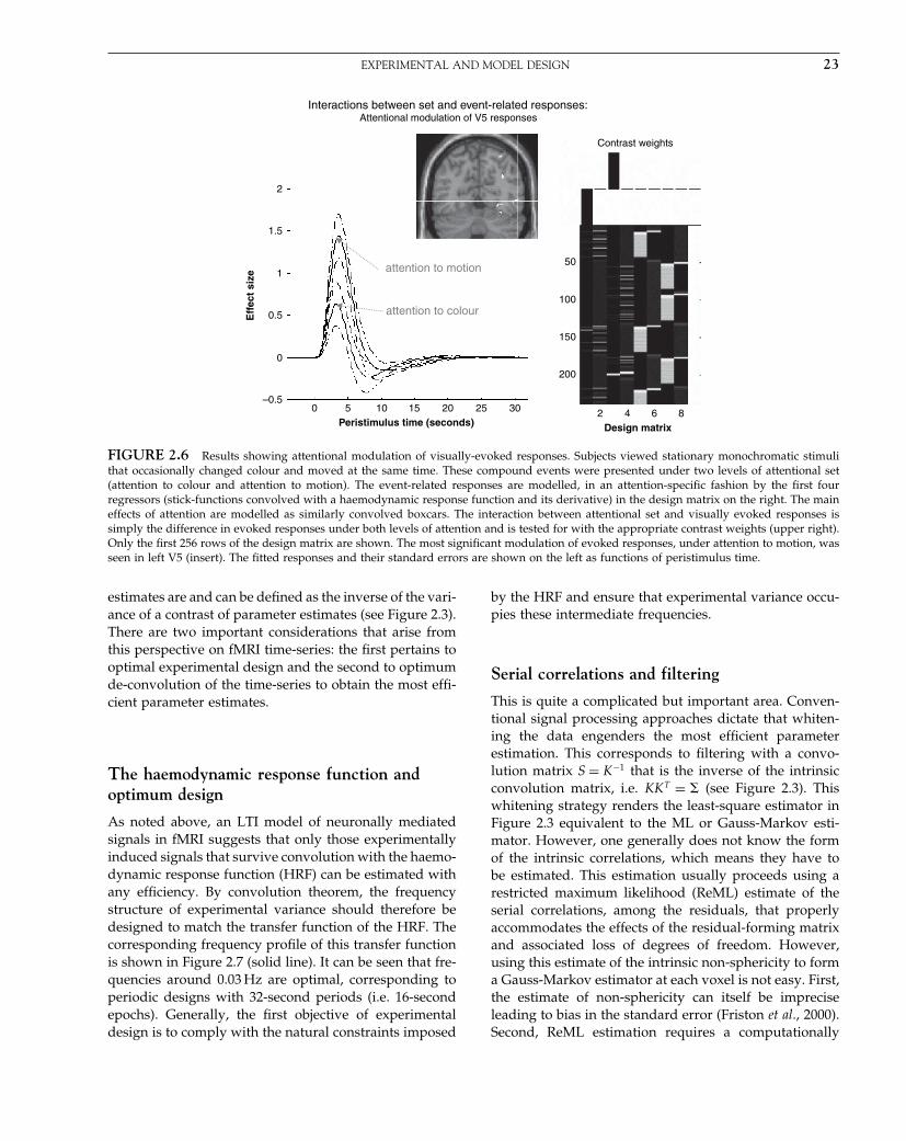
Elsevier UK Chapter: Ch02-P372560 3-10-2006 3:58p.m. Page:23 Trim:7.5in×9.25in
Basal Font:Palatino Margins:Top:40pt Gutter:68pt Font Size:9.5/12 Text Width:42pc Depth:55 Lines
EXPERIMENTAL AND MODEL DESIGN 23
attention to motion
attention to colour
2
1.5
1
0.5
0
–0.50 5 10 15
Peristimulus time (seconds)
Eff
ect
size
20 25 30
50
Contrast weights
100
150
200
2 4 6Design matrix
8
Interactions between set and event-related responses:Attentional modulation of V5 responses
FIGURE 2.6 Results showing attentional modulation of visually-evoked responses. Subjects viewed stationary monochromatic stimulithat occasionally changed colour and moved at the same time. These compound events were presented under two levels of attentional set(attention to colour and attention to motion). The event-related responses are modelled, in an attention-specific fashion by the first fourregressors (stick-functions convolved with a haemodynamic response function and its derivative) in the design matrix on the right. The maineffects of attention are modelled as similarly convolved boxcars. The interaction between attentional set and visually evoked responses issimply the difference in evoked responses under both levels of attention and is tested for with the appropriate contrast weights (upper right).Only the first 256 rows of the design matrix are shown. The most significant modulation of evoked responses, under attention to motion, wasseen in left V5 (insert). The fitted responses and their standard errors are shown on the left as functions of peristimulus time.
estimates are and can be defined as the inverse of the vari-ance of a contrast of parameter estimates (see Figure 2.3).There are two important considerations that arise fromthis perspective on fMRI time-series: the first pertains tooptimal experimental design and the second to optimumde-convolution of the time-series to obtain the most effi-cient parameter estimates.
The haemodynamic response function andoptimum design
As noted above, an LTI model of neuronally mediatedsignals in fMRI suggests that only those experimentallyinduced signals that survive convolution with the haemo-dynamic response function (HRF) can be estimated withany efficiency. By convolution theorem, the frequencystructure of experimental variance should therefore bedesigned to match the transfer function of the HRF. Thecorresponding frequency profile of this transfer functionis shown in Figure 2.7 (solid line). It can be seen that fre-quencies around 0.03 Hz are optimal, corresponding toperiodic designs with 32-second periods (i.e. 16-secondepochs). Generally, the first objective of experimentaldesign is to comply with the natural constraints imposed
by the HRF and ensure that experimental variance occu-pies these intermediate frequencies.
Serial correlations and filtering
This is quite a complicated but important area. Conven-tional signal processing approaches dictate that whiten-ing the data engenders the most efficient parameterestimation. This corresponds to filtering with a convo-lution matrix S = K−1 that is the inverse of the intrinsicconvolution matrix, i.e. KKT = � (see Figure 2.3). Thiswhitening strategy renders the least-square estimator inFigure 2.3 equivalent to the ML or Gauss-Markov esti-mator. However, one generally does not know the formof the intrinsic correlations, which means they have tobe estimated. This estimation usually proceeds using arestricted maximum likelihood (ReML) estimate of theserial correlations, among the residuals, that properlyaccommodates the effects of the residual-forming matrixand associated loss of degrees of freedom. However,using this estimate of the intrinsic non-sphericity to forma Gauss-Markov estimator at each voxel is not easy. First,the estimate of non-sphericity can itself be impreciseleading to bias in the standard error (Friston et al., 2000).Second, ReML estimation requires a computationally
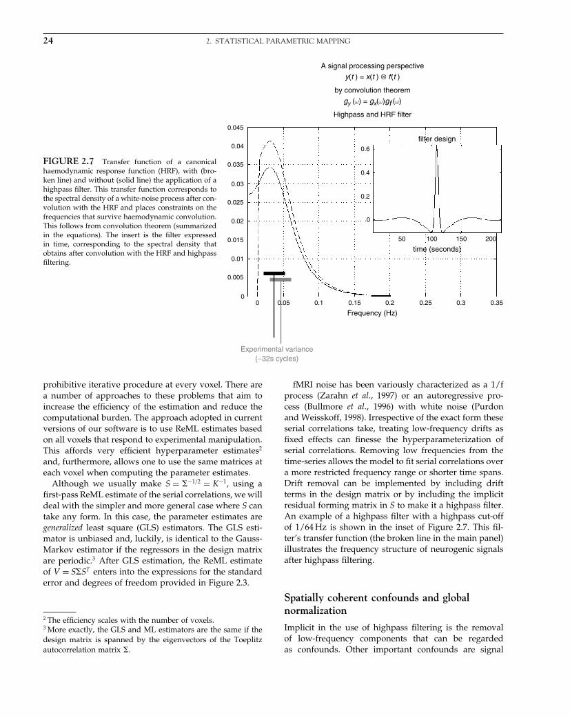
Elsevier UK Chapter: Ch02-P372560 3-10-2006 3:58p.m. Page:24 Trim:7.5in×9.25in
Basal Font:Palatino Margins:Top:40pt Gutter:68pt Font Size:9.5/12 Text Width:42pc Depth:55 Lines
24 2. STATISTICAL PARAMETRIC MAPPING
FIGURE 2.7 Transfer function of a canonicalhaemodynamic response function (HRF), with (bro-ken line) and without (solid line) the application of ahighpass filter. This transfer function corresponds tothe spectral density of a white-noise process after con-volution with the HRF and places constraints on thefrequencies that survive haemodynamic convolution.This follows from convolution theorem (summarizedin the equations). The insert is the filter expressedin time, corresponding to the spectral density thatobtains after convolution with the HRF and highpassfiltering.
A signal processing perspective
by convolution theorem
Experimental variance(~32s cycles)
gy (ω) = gx(ω)gf (ω)
y(t ) = x(t ) ⊗ f (t )
Highpass and HRF filter
Frequency (Hz)
0.045
0.04
0.035
0.03
0.025
0.02
0.015
0.01
0.005
00 0.05 0.1 0.15 0.2 0.25 0.3
0.6
0.4
0.2
0
50 100 150 200
time (seconds)
filter design
0.35
prohibitive iterative procedure at every voxel. There area number of approaches to these problems that aim toincrease the efficiency of the estimation and reduce thecomputational burden. The approach adopted in currentversions of our software is to use ReML estimates basedon all voxels that respond to experimental manipulation.This affords very efficient hyperparameter estimates2
and, furthermore, allows one to use the same matrices ateach voxel when computing the parameter estimates.
Although we usually make S = �−1/2 = K−1, using afirst-pass ReML estimate of the serial correlations, we willdeal with the simpler and more general case where S cantake any form. In this case, the parameter estimates aregeneralized least square (GLS) estimators. The GLS esti-mator is unbiased and, luckily, is identical to the Gauss-Markov estimator if the regressors in the design matrixare periodic.3 After GLS estimation, the ReML estimateof V = S�ST enters into the expressions for the standarderror and degrees of freedom provided in Figure 2.3.
2 The efficiency scales with the number of voxels.3 More exactly, the GLS and ML estimators are the same if thedesign matrix is spanned by the eigenvectors of the Toeplitzautocorrelation matrix �.
fMRI noise has been variously characterized as a 1/fprocess (Zarahn et al., 1997) or an autoregressive pro-cess (Bullmore et al., 1996) with white noise (Purdonand Weisskoff, 1998). Irrespective of the exact form theseserial correlations take, treating low-frequency drifts asfixed effects can finesse the hyperparameterization ofserial correlations. Removing low frequencies from thetime-series allows the model to fit serial correlations overa more restricted frequency range or shorter time spans.Drift removal can be implemented by including driftterms in the design matrix or by including the implicitresidual forming matrix in S to make it a highpass filter.An example of a highpass filter with a highpass cut-offof 1/64 Hz is shown in the inset of Figure 2.7. This fil-ter’s transfer function (the broken line in the main panel)illustrates the frequency structure of neurogenic signalsafter highpass filtering.
Spatially coherent confounds and globalnormalization
Implicit in the use of highpass filtering is the removalof low-frequency components that can be regardedas confounds. Other important confounds are signal

Elsevier UK Chapter: Ch02-P372560 3-10-2006 3:58p.m. Page:25 Trim:7.5in×9.25in
Basal Font:Palatino Margins:Top:40pt Gutter:68pt Font Size:9.5/12 Text Width:42pc Depth:55 Lines
EXPERIMENTAL AND MODEL DESIGN 25
components that are artefactual or have no regionalspecificity. These are referred to as global confoundsand have a number of causes. These can be dividedinto physiological (e.g. global perfusion changes in PET)and non-physiological (e.g. transmitter power calibra-tion or receiver gain in fMRI). The latter generally scalethe signal before the MRI sampling process. Other non-physiological effects may have a non-scaling effect (e.g.Nyquist ghosting, movement-related effects etc.). In PET,it is generally accepted that regional changes in rCBF,evoked neuronally, mix additively with global changes togive the measured signal. This calls for a global normal-ization procedure where the global estimator enters intothe statistical model as a confound. In fMRI, instrumen-tation effects that scale the data motivate a global nor-malization by proportional scaling, using the whole brainmean, before the data enter into the statistical model.
It is important to differentiate between global con-founds and their estimators. By definition, the globalmean over intracranial voxels will subsume all regionallyspecific effects. This means that the global estimator maybe partially collinear with effects of interest, especiallyif evoked responses are substantial and widespread. Inthese situations, global normalization may induce appar-ent deactivations in regions not expressing a physiologi-cal response. These are not artefacts in the sense that theyare real, relative to global changes, but they have lessface validity in terms of the underlying neurophysiol-ogy. In instances where regionally specific effects bias theglobal estimator, some investigators prefer to omit globalnormalization. Provided drift terms are removed fromthe time-series, this is generally acceptable because mostglobal effects have slow time constants. However, theissue of normalization-induced deactivations is better cir-cumnavigated with experimental designs that use well-controlled conditions, which elicit differential responsesin restricted brain systems.
Non-linear system identification approaches
So far, we have only considered linear models and first-order HRFs. Another signal processing perspective isprovided by non-linear system identification (Vazquezand Noll, 1998). This section considers non-linear modelsas a prelude to the next subsection on event-related fMRI,where non-linear interactions among evoked responsesprovide constraints for experimental design and analysis.We have described an approach to characterizing evokedhaemodynamic responses in fMRI based on non-linearsystem identification, in particular the use of Volterraseries (Friston et al., 1998). This approach enables one toestimate Volterra kernels that describe the relationshipbetween stimulus presentation and the haemodynamic
responses that ensue. Volterra series are essentially high-order extensions of linear convolution models. These ker-nels therefore represent a non-linear characterization ofthe HRF that can model the responses to stimuli in dif-ferent contexts and interactions among stimuli. In fMRI,the kernel coefficients can be estimated by using a sec-ond order approximation to the Volterra series to formu-late the problem in terms of a general linear model andexpanding the kernels in terms of temporal basis func-tions (see Chapter 27). This allows the use of the standardtechniques described above to estimate the kernels andto make inferences about their significance on a voxel-specific basis using SPMs.
One important manifestation of non-linear effects,captured by second order kernels, is a modulation ofstimulus-specific responses by preceding stimuli thatare proximate in time. This means that responsesat high stimulus presentation rates saturate and, insome instances, show an inverted U behaviour. Thisbehaviour appears to be specific to blood oxygenation-level-dependent (BOLD) effects (as distinct from evokedchanges in cerebral blood flow) and may represent ahaemodynamic refractoriness. This effect has importantimplications for event-related fMRI, where one may wantto present trials in quick succession.
The results of a typical non-linear analysis are givenin Figure 2.8. The results in the right panel represent theaverage response, integrated over a 32-second train ofstimuli as a function of stimulus onset asynchrony (SOA)within that train. These responses are based on the kernelestimates (left hand panels) using data from a voxel inthe left posterior temporal region of a subject obtainedduring the presentation of single words at different rates.The solid line represents the estimated response andshows a clear maximum at just less than one second.The dots are responses based on empirical data from thesame experiment. The broken line shows the expectedresponse in the absence of non-linear effects (i.e. thatpredicted by setting the second order kernel to zero). Itis clear that non-linearities become important at aroundtwo seconds leading to an actual diminution of the inte-grated response at sub-second SOAs. The implication ofthis sort of result is that SOAs should not really fall muchbelow one second and at short SOAs the assumptions oflinearity are violated. It should be noted that these datapertain to single word processing in auditory associationcortex. More linear behaviours may be expressed in pri-mary sensory cortex where the feasibility of using min-imum SOAs, as low as 500 ms, has been demonstrated(Burock et al., 1998). This lower bound on SOA is impor-tant because some effects are detected more efficientlywith high presentation rates. We now consider this fromthe point of view of event-related designs.

Elsevier UK Chapter: Ch02-P372560 3-10-2006 3:58p.m. Page:26 Trim:7.5in×9.25in
Basal Font:Palatino Margins:Top:40pt Gutter:68pt Font Size:9.5/12 Text Width:42pc Depth:55 Lines
26 2. STATISTICAL PARAMETRIC MAPPING
Non-linear saturation
2.51st order kernel {h
1}
2
1.5
1
0.5
0
–0.50
30
30
128
127
126
125
124
123
122
121
120
119
1180 1 2 3 4
Stimulus onset asynchrony (seconds)Ave
rag
e re
spo
nse
to
a 3
2s s
tim
ulu
s tr
ain
5 6 7 8 9 10
202nd order kernel {h2}
outer product of 1st order kernel
10
00 10 20 3025
20
15
10
5
0
5 10 15 20 25 30
time (seconds)
time (seconds)
0 5 10 15 20 25 30
time (seconds)
FIGURE 2.8 Left panels: Volterra kernels from a voxel in the left superior temporal gyrus at −56� −28� 12 mm. These kernel estimateswere based on a single-subject study of aural word presentation at different rates (from zero to ninety words per minute) using a secondorder approximation to a Volterra series expansion modelling the observed haemodynamic response to stimulus input (a delta function foreach word). These kernels can be thought of as a characterization of the second order haemodynamic response function. The first orderkernel (h1 – upper panel) represents the (first order) component usually presented in linear analyses. The second order kernel (h2 – lowerpanel) is presented in image format. The colour scale is arbitrary; white is positive and black is negative. The insert on the right representsh1h1
T , the second order kernel that would be predicted by a simple model that involved linear convolution with h1 followed by some staticnon-linearity. Right panel: integrated responses over a 32-second stimulus train as a function of SOA. Solid line: estimates based on thenon-linear convolution model parameterized by the kernels on the left. Broken line: the responses expected in the absence of second ordereffects (i.e. in a truly linear system). Dots: empirical averages based on the presentation of actual stimulus trains.
Event and epoch-related designs
A crucial distinction in experimental design for fMRI isthat between epoch and event-related designs. In singlephoton emission computerized tomography (SPECT) andpositron emission tomography (PET) only epoch-relatedresponses can be assessed because of the relatively longhalf-life of the radiotracers used. However, in fMRI thereis an opportunity to measure event-related responses,not unlike the paradigm used in electroencephalography(EEG) and magnetoencephalography (MEG). An impor-tant issue, in event-related fMRI, is the choice of inter-stimulus interval or more precisely SOA. The SOA, orthe distribution of SOAs, is a critical factor and is chosen,subject to psychological or psychophysical constraints, tomaximize the efficiency of response estimation. The con-straints on the SOA clearly depend upon the nature ofthe experiment but are generally satisfied when the SOAis small and derives from a random distribution. Rapidpresentation rates allow for the maintenance of a par-ticular cognitive or attentional set, decrease the latitudethat the subject has for engaging alternative strategies,
or incidental processing, and allows the integration ofevent-related paradigms using fMRI and electrophysiol-ogy. Random SOAs ensure that preparatory or anticipa-tory factors do not confound event-related responses andensure a uniform context in which events are presented.These constraints speak of the well-documented advan-tages of event-related fMRI over conventional blockeddesigns (Buckner et al., 1996; Clark et al., 1998).
In order to compare the efficiency of different designs,it is useful to have a common framework that encom-passes all of them. The efficiency can then be examinedin relation to the parameters of the designs. Designs canbe stochastic or deterministic depending on whether thereis a random element to their specification. In stochas-tic designs (Heid et al., 1997) one needs to specify theprobabilities of an event occurring at all times thoseevents could occur. In deterministic designs, the occur-rence probability is unity and the design is completelyspecified by the times of stimulus presentation or tri-als. The distinction between stochastic and determinis-tic designs pertains to how a particular realization orstimulus sequence is created. The efficiency afforded

Elsevier UK Chapter: Ch02-P372560 3-10-2006 3:58p.m. Page:27 Trim:7.5in×9.25in
Basal Font:Palatino Margins:Top:40pt Gutter:68pt Font Size:9.5/12 Text Width:42pc Depth:55 Lines
EXPERIMENTAL AND MODEL DESIGN 27
by a particular event sequence is a function of theevent sequence itself, and not of the process generatingthe sequence (i.e. deterministic or stochastic). However,within stochastic designs, the design matrix X, and asso-ciated efficiency, are random variables and the expectedor average efficiency, over realizations of X is easily com-puted.
In the framework considered here (Friston et al., 1999a),the occurrence probability p of any event occurring isspecified at each time that it could occur (i.e. everySOA or stimulus onset asynchrony). Here p is a vec-tor with an element for every SOA. This formulationengenders the distinction between stationary stochasticdesigns, where the occurrence probabilities are constantand non-stationary stochastic designs, where they changeover time. For deterministic designs, the elements of p are0 or 1, the presence of a 1 denoting the occurrence of anevent. An example of p might be the boxcars used in con-ventional block designs. Stochastic designs correspond toa vector of identical values and are therefore stationaryin nature. Stochastic designs with temporal modulation
of occurrence probability have time-dependent probabili-ties varying between 0 and 1. With these probabilities theexpected design matrices and expected efficiencies can becomputed. A useful thing about this formulation is thatby setting the mean of the probabilities p to a constant,one can compare different deterministic and stochasticdesigns given the same number of events. Some commonexamples are given in Figure 2.9 (right panel) for an SOAof one second and 32 expected events or trials over a 64second period (except for the first deterministic exam-ple with four events and an SOA of 16 seconds). It canbe seen that the least efficient is the sparse deterministicdesign (despite the fact that the SOA is roughly opti-mal for this class), whereas the most efficient is a blockdesign. A slow modulation of occurrence probabilitiesgives high efficiency while retaining the advantages ofstochastic designs and may represent a useful compro-mise between the high efficiency of block designs and thepsychological benefits and latitude afforded by stochasticdesigns. However, it is important not to generalize theseconclusions too far. An efficient design for one effect may
The design matrix as a stochastic variable
Probability
1
1
2
3
4
5
6
0 10 20 30 40 50
0 10 20 30 40 50 60
10 20 30 40 50 60
10 20 30 40 50 60
10 20 30 40 50 60
10 20 30 40 50 60
10 20 30 40 50 60
fixed deterministic
stationary stochastic
dynamic stochastic (rapid)
dynamic stochastic (intermediate)
dynamic stochastic (slow)
variable deterministic
0.5
1
005
1015
0 0.10.2 0.3
0.40.5
0
5
10
15
10
05
1015
0 0.10.2 0.3
0.40.5
0
5
10
15
10
0.5
1
0
0.5
1
0
0.5
1
0
0.5
1
0
0.5
Efficiency
SOA {sec} Probability
Probability
Efficiency-evoked responses
Efficiency-evoked differences
SOA {sec}
SBBT ST
X = SB
c)–1XT X
= pT (ST S – 1)p + diag (p)
=
=(cT –1
XT X
Efficiency
Effi
cien
cyE
ffici
ency
FIGURE 2.9 Efficiency as a function of occurrence probability p for a model X formed by post-multiplying S (a matrix containing ncolumns, modelling n possible event-related responses every SOA) by B. B is a random binary vector that determines whether the n-th responsecontributes to the design matrix X = SB where �B� = p. Right panels: a comparison of some common designs. A graphical representation ofthe occurrence probability as a function of time (seconds) is shown on the left and the corresponding efficiency is shown on the right. Theseresults assume a minimum SOA of one second, a time-series of 64 seconds and a single trial-type. The expected number of events was 32 inall cases (apart from the first). Left panels: efficiency in a stationary stochastic design with two event types both presented with increasingprobability every SOA. The upper graph is for a contrast testing for the response evoked by one trial type and the lower graph is for a contrasttesting for differential responses.
Elsevier UK Chapter: Ch02-P372560 3-10-2006 3:58p.m. Page:28 Trim:7.5in×9.25in
Basal Font:Palatino Margins:Top:40pt Gutter:68pt Font Size:9.5/12 Text Width:42pc Depth:55 Lines
28 2. STATISTICAL PARAMETRIC MAPPING
not be the optimum for another, even within the sameexperiment. This can be illustrated by comparing the effi-ciency with which evoked responses are detected and theefficiency of detecting the difference in evoked responseselicited by two sorts of trials.
Consider a stationary stochastic design with two trialtypes. Because the design is stationary, the vector ofoccurrence probabilities, for each trial type, is specifiedby a single probability. Let us assume that the two trialtypes occur with the same probability p. By varying p andSOA one can find the most efficient design dependingupon whether one is looking for evoked responses per seor differences among evoked responses. These two situ-ations are depicted in the left panels of Figure 2.9. It isimmediately apparent that, for both sorts of effects, verysmall SOAs are optimal. However, the optimal occur-rence probabilities are not the same. More infrequentevents (corresponding to a smaller p = 1/3) are requiredto estimate the responses themselves efficiently. This isequivalent to treating the baseline or control condition asany other condition (i.e. by including null events, withequal probability, as further event types). Conversely, ifwe are only interested in making inferences about thedifferences, one of the events plays the role of a nullevent and the most efficient design ensues when one orthe other event occurs (i.e. p = 1/2). In short, the mostefficient designs obtain when the events subtending thedifferences of interest occur with equal probability.
Another example of how the efficiency is sensitiveto the effect of interest is apparent when we considerdifferent parameterizations of the HRF. This issue issometimes addressed through distinguishing betweenthe efficiency of response detection and response estima-tion. However, the principles are identical and the dis-tinction reduces to how many parameters one uses tomodel the HRF for each trial type (one basis functionis used for detection and a number are required to esti-mate the shape of the HRF). Here the contrasts may bethe same but the shape of the regressors will changedepending on the temporal basis set employed. The con-clusions above were based on a single canonical HRF.Had we used a more refined parameterization of theHRF, say using three-basis functions, the most efficientdesign to estimate one basis function coefficient wouldnot be the most efficient for another. This is most easilyseen from the signal processing perspective where basisfunctions with high-frequency structure (e.g. temporalderivatives) require the experimental variance to containhigh-frequency components. For these basis functions arandomized stochastic design may be more efficient thana deterministic block design, simply because the formerembodies higher frequencies. In the limiting case of finiteimpulse response (FIR) estimation, the regressors becomea series of stick functions all of which have high fre-
quencies. This parameterization of the HRF calls for highfrequencies in the experimental variance. However, theuse of FIR models is contraindicated by model selectionprocedures (see Chapter 14) that suggest only two orthree HRF parameters can be estimated with any effi-ciency. Results that are reported in terms of FIRs shouldbe treated with caution because the inferences aboutevoked responses are seldom based on the FIR parame-ter estimates. This is precisely because they are estimatedinefficiently and contain little useful information.
INFERENCE IN HIERARCHICALMODELS
In this section, we consider some issues that are genericto brain mapping studies that have repeated measuresor replications over subjects. The critical issue is whetherwe want to make an inference about the effect in rela-tion to the within-subject variability or with respect to thebetween-subject variability. For a given group of subjects,there is a fundamental distinction between saying thatthe response is significant relative to the precision4 withwhich that response is measured and saying that it issignificant in relation to the inter-subject variability. Thisdistinction relates directly to the difference between fixed-and random-effect analyses. The following example triesto make this clear. Consider what would happen if wescanned six subjects during the performance of a taskand baseline. We then construct a statistical model wheretask-specific effects were modelled separately for eachsubject. Unknown to us, only one of the subjects activateda particular brain region. When we examine the contrastof parameter estimates, assessing the mean activationover all subjects, we see that it is greater than zero byvirtue of this subject’s activation. Furthermore, becausethat model fits the data extremely well (modelling noactivation in five subjects and a substantial activationin the sixth), the error variance, on a scan-to-scan basis,is small and the t-statistic is very significant. Can wethen say that the group shows an activation? On the onehand, we can say, quite properly, that the mean groupresponse embodies an activation but, clearly, this doesnot constitute an inference that the group’s response issignificant (i.e. that this sample of subjects shows a con-sistent activation). The problem here is that we are usingthe scan-to-scan error variance and this is not necessarilyappropriate for an inference about group responses. Tomake the inference that the group showed a significantactivation, one would have to assess the variability in
4 Precision is the inverse of the variance.
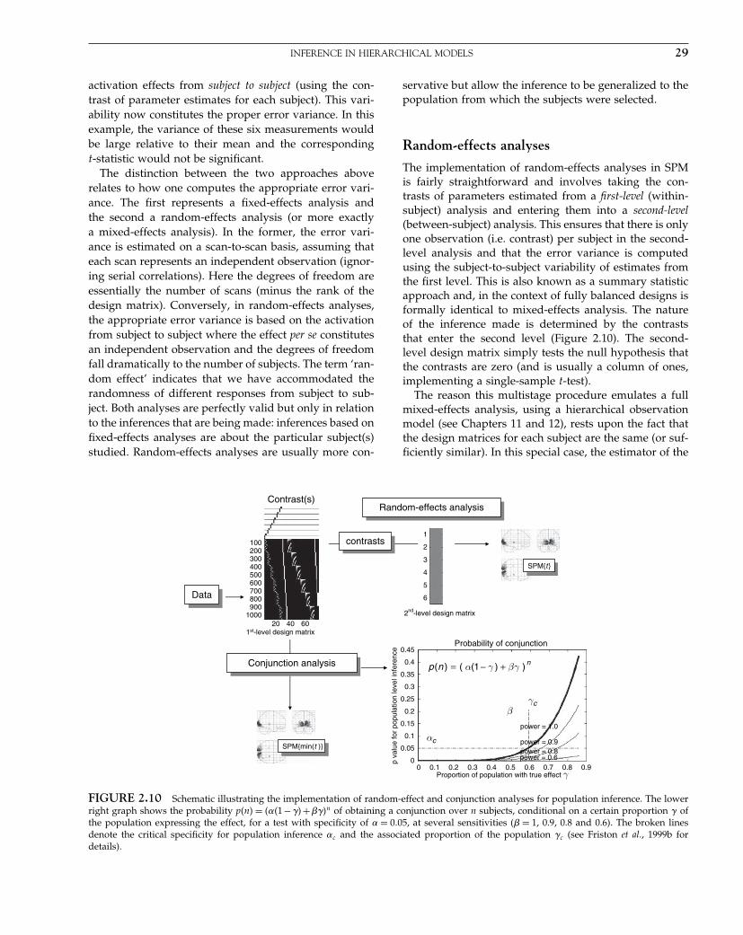
Elsevier UK Chapter: Ch02-P372560 3-10-2006 3:58p.m. Page:29 Trim:7.5in×9.25in
Basal Font:Palatino Margins:Top:40pt Gutter:68pt Font Size:9.5/12 Text Width:42pc Depth:55 Lines
INFERENCE IN HIERARCHICAL MODELS 29
activation effects from subject to subject (using the con-trast of parameter estimates for each subject). This vari-ability now constitutes the proper error variance. In thisexample, the variance of these six measurements wouldbe large relative to their mean and the correspondingt-statistic would not be significant.
The distinction between the two approaches aboverelates to how one computes the appropriate error vari-ance. The first represents a fixed-effects analysis andthe second a random-effects analysis (or more exactlya mixed-effects analysis). In the former, the error vari-ance is estimated on a scan-to-scan basis, assuming thateach scan represents an independent observation (ignor-ing serial correlations). Here the degrees of freedom areessentially the number of scans (minus the rank of thedesign matrix). Conversely, in random-effects analyses,the appropriate error variance is based on the activationfrom subject to subject where the effect per se constitutesan independent observation and the degrees of freedomfall dramatically to the number of subjects. The term ‘ran-dom effect’ indicates that we have accommodated therandomness of different responses from subject to sub-ject. Both analyses are perfectly valid but only in relationto the inferences that are being made: inferences based onfixed-effects analyses are about the particular subject(s)studied. Random-effects analyses are usually more con-
servative but allow the inference to be generalized to thepopulation from which the subjects were selected.
Random-effects analyses
The implementation of random-effects analyses in SPMis fairly straightforward and involves taking the con-trasts of parameters estimated from a first-level (within-subject) analysis and entering them into a second-level(between-subject) analysis. This ensures that there is onlyone observation (i.e. contrast) per subject in the second-level analysis and that the error variance is computedusing the subject-to-subject variability of estimates fromthe first level. This is also known as a summary statisticapproach and, in the context of fully balanced designs isformally identical to mixed-effects analysis. The natureof the inference made is determined by the contraststhat enter the second level (Figure 2.10). The second-level design matrix simply tests the null hypothesis thatthe contrasts are zero (and is usually a column of ones,implementing a single-sample t-test).
The reason this multistage procedure emulates a fullmixed-effects analysis, using a hierarchical observationmodel (see Chapters 11 and 12), rests upon the fact thatthe design matrices for each subject are the same (or suf-ficiently similar). In this special case, the estimator of the
Conjunction analysisConjunction analysis
DataData
Contrast(s)
1000
800900
700600500400300200100
4020 60
1
2
3
4
5
6
0.4
0.35
0.3
0.25
0.2
0.15
0.1
0.05
00 0.1 0.2 0.3 0.4 0.5 0.6 0.7 0.8 0.9
0.45
contrastscontrasts
Random-effects analysisRandom-effects analysis
SPM{min(t)}SPM{min(t )}
SPM{t}SPM{t }
2nd-level design matrix
Proportion of population with true effect γ
p va
lue
for
popu
latio
n le
vel i
nfer
ence
1st-level design matrix
Probability of conjunction
n
power = 1.0
power = 0.9power = 0.8power = 0.6
np ))1(( α)( + β γ− γ=
γcβ
αc
FIGURE 2.10 Schematic illustrating the implementation of random-effect and conjunction analyses for population inference. The lowerright graph shows the probability p�n� = ���1−��+��n of obtaining a conjunction over n subjects, conditional on a certain proportion � ofthe population expressing the effect, for a test with specificity of � = 0�05, at several sensitivities ( = 1, 0.9, 0.8 and 0.6). The broken linesdenote the critical specificity for population inference �c and the associated proportion of the population �c (see Friston et al., 1999b fordetails).

Elsevier UK Chapter: Ch02-P372560 3-10-2006 3:58p.m. Page:30 Trim:7.5in×9.25in
Basal Font:Palatino Margins:Top:40pt Gutter:68pt Font Size:9.5/12 Text Width:42pc Depth:55 Lines
30 2. STATISTICAL PARAMETRIC MAPPING
variance at the second level contains the right mixtureof within- and between-subject error. It is important toappreciate this because the efficiency of the design atthe first level percolates to higher levels. It is thereforeimportant to use efficient strategies at all levels in a hier-archical design.
Conjunction analyses and populationinferences
In some instances, a fixed-effects analysis is more appro-priate, particularly when reporting single-case studies.With a series of single cases, it is natural to ask what arecommon features of functional anatomy (e.g. the locationof V5) and what aspects are subject specific (e.g. the loca-tion of ocular dominance columns)? One way to addresscommonalties is to use a conjunction analysis over sub-jects. It is important to understand the nature of the infer-ence provided by conjunction analyses, because there hasbeen some confusion (see Nichols et al., 2005; Fristonet al., 2005). Imagine that, in sixteen subjects the activa-tion in V5, elicited by a motion stimulus, was greaterthan zero. The probability of this occurring by chance,in the same area, is extremely small and is the p-valuereturned by a conjunction analysis using a threshold ofp = 0�5 (i.e. t = 0) for each subject. This constitutes evi-dence that V5 is engaged by motion. However, it is notan assertion that each subject activated significantly (weonly require the t-value to be greater than zero for eachsubject). In other words, a significant conjunction is nota conjunction of significance.
The motivations for conjunction analyses, in the con-text of multisubject studies, are twofold. They providean inference, in a fixed-effects context, testing the nullhypotheses of no activation in any of the subjects, whichcan be much more sensitive than testing for the averageactivation. Second, they can be used to make inferencesabout the population in terms of confidence intervals onthe proportion of subjects showing an effect (see Fristonet al., 1999b).
CONCLUSION
In this chapter, we have reviewed the main componentsof image analysis and have introduced the tenets of sta-tistical parametric mapping. We have also consideredthe design of experiments and their statistical models,with a special focus on fMRI. This chapter has coveredthe key operational issues in identifying regionally spe-cific effects in neuroimaging. In the next chapter, we
look at models for neuroimaging from a broader perspec-tive and address the functional integration of distributedresponses in the brain.
REFERENCES
Adler RJ (1981) The geometry of random fields. Wiley, New YorkAguirre GK, Zarahn E, D’Esposito M (1998) A critique of the use of
the Kolmogorov-Smirnov (KS) statistic for the analysis of BOLDfMRI data. Mag Res Med 39: 500–05
Andersson JL, Hutton C, Ashburner J et al. (2001) Modeling geo-metric deformations in EPI time series. NeuroImage 13: 903–19
Ashburner J, Friston KJ. (2000) Voxel-based morphometry – themethods. NeuroImage 11: 805–21
Ashburner J, Neelin P, Collins DL et al. (1997) Incorporating priorknowledge into image registration. NeuroImage 6: 344–52
Ashburner J, Hutton C, Frackowiak R et al. (1998) Identifying globalanatomical differences: deformation-based morphometry. HumBrain Mapp 6: 348–57
Bandettini PA, Jesmanowicz A, Wong EC et al. (1993) Processingstrategies for time course data sets in functional MRI of thehuman brain. Mag Res Med 30: 161–73
Büchel C, Wise RJS, Mummery CJ et al. (1996) Non-linear regressionin parametric activation studies. NeuroImage 4: 60–66
Buckner R, Bandettini P, O’Craven K et al. (1996) Detection of corticalactivation during averaged single trials of a cognitive task usingfunctional magnetic resonance imaging. Proc Natl Acad Sci USA93: 14878–83
Bullmore ET, Brammer MJ, Williams SCR et al. (1996) Statisticalmethods of estimation and inference for functional MR images.Mag Res Med 35: 261–77
Burock MA, Buckner RL, Woldorff MG et al. (1998) Randomizedevent-related experimental designs allow for extremely rapidpresentation rates using functional MRI. NeuroReport 9: 3735–39
Chung MK, Worsley KJ, Paus T et al. (2001) A unified statisticalapproach to deformation-based morphometry. NeuroImage 14:595–606
Clark VP, Maisog JM, Haxby JV (1998) fMRI study of face perceptionand memory using random stimulus sequences. J Neurophysiol76: 3257–65
Friston KJ (1997) Testing for anatomical specified regional effects.Hum Brain Mapp 5: 133–36
Friston KJ, Frith CD, Liddle PF et al. (1991) Comparing functional(PET) images: the assessment of significant change. J Cereb BloodFlow Metab 11: 690–99
Friston KJ, Frith C, Passingham RE et al. (1992a) Motor practiceand neurophysiological adaptation in the cerebellum: a positrontomography study. Proc Roy Soc Lon Series B248: 223–28
Friston KJ, Grasby P, Bench C et al. (1992b) Measuring the neuro-modulatory effects of drugs in man with positron tomography.Neurosci Lett 141: 106–10
Friston KJ, Worsley KJ, Frackowiak RSJ et al. (1994) Assessing thesignificance of focal activations using their spatial extent. HumBrain Mapp 1: 214–20
Friston KJ, Ashburner J, Frith CD et al. (1995a) Spatial registrationand normalization of images. Hum Brain Mapp 2: 165–89
Friston KJ, Holmes AP, Worsley KJ et al. (1995b) Statisticalparametric maps in functional imaging: a general linearapproach. Hum Brain Mapp 2: 189–210
Friston KJ, Williams S, Howard R et al. (1996a) Movement relatedeffects in fMRI time series. Mag Res Med 35: 346–55

Elsevier UK Chapter: Ch02-P372560 3-10-2006 3:58p.m. Page:31 Trim:7.5in×9.25in
Basal Font:Palatino Margins:Top:40pt Gutter:68pt Font Size:9.5/12 Text Width:42pc Depth:55 Lines
REFERENCES 31
Friston KJ, Holmes A, Poline J-B et al. (1996b) Detecting activationsin PET and fMRI: levels of inference and power. NeuroImage 4:223–35
Friston KJ, Price CJ, Fletcher P et al. (1996c) The trouble with cogni-tive subtraction. NeuroImage 4: 97–104
Friston KJ, Büchel C, Fink GR et al. (1997) Psychophysiological andmodulatory interactions in neuroimaging. NeuroImage 6: 218–29
Friston KJ, Josephs O, Rees G et al. (1998) Non-linear event-relatedresponses in fMRI. Mag Res Med 39: 41–52
Friston KJ, Zarahn E, Josephs O et al. (1999a) Stochastic designs inevent-related fMRI. NeuroImage 10: 607–19
Friston KJ, Holmes AP, Price CJ et al. (1999b) Multisubject fMRIstudies and conjunction analyses. NeuroImage 10: 385–96
Friston KJ, Josephs O, Zarahn E et al. (2000) To smooth or notto smooth? Bias and efficiency in fMRI time-series analysis.NeuroImage 12: 196–208
Friston KJ, Penny WD and Glaser DE (2005) Conjunction revisited.NeuroImage 25(3): 661–7
Grafton S, Mazziotta J, Presty S et al. (1992) Functional anatomy ofhuman procedural learning determined with regional cerebralblood flow and PET. J Neurosci 12: 2542–48
Grootoonk S, Hutton C, Ashburner J et al. (2000) Characterizationand correction of interpolation effects in the realignment of fMRItime series. NeuroImage 11: 49–57
Heid O, Gönner F, Schroth G (1997) Stochastic functional MRI.NeuroImage 5: S476
Jezzard P, Balaban RS (1995) Correction for geometric distortion inecho-planar images from B0 field variations. Mag Res Med 34:65–73
Kiebel SJ, Poline JB, Friston KJ et al. (1999) Robust smooth-ness estimation in statistical parametric maps using standard-ized residuals from the general linear model. NeuroImage 10:756–66
Liddle PF, Friston KJ, Frith CD et al. (1992) Cerebral blood-flow andmental processes in schizophrenia. Roy Soc Med 85: 224–27
Lueck CJ, Zeki S, Friston KJ et al. (1989) The color centre in thecerebral cortex of man. Nature 340: 386–89
Nichols T, Brett M, Andersson J, Wager T, Poline JB (2004) Validconjunction interference with the minimum statistic. Neurolmage25(3): 653–60
Petersen SE, Fox PT, Posner MI et al. (1989) Positron emission tomo-graphic studies of the processing of single words. J Cog Neurosci1: 153–70
Price CJ, Friston KJ (1997) Cognitive conjunction: a new approachto brain activation experiments. NeuroImage 5: 261–70
Price CJ, Wise RJS, Ramsay S et al. (1992) Regional response dif-ferences within the human auditory cortex when listening towords. Neurosci Lett 146: 179–82
Purdon PL, Weisskoff RM (1998) Effect of temporal autocorrelationdue to physiological noise and stimulus paradigm on voxel-levelfalse-positive rates in fMRI. Hum Brain Mapp 6: 239–495
Talairach P, Tournoux J (1988) A stereotactic coplanar atlas of thehuman brain. Thieme, Stuttgart
Vazquez AL, Noll CD (1998) Non-linear aspects of the BOLDresponse in functional MRI. NeuroImage 7: 108–18
Worsley KJ, Friston KJ (1995) Analysis of fMRI time-seriesrevisited – again. NeuroImage 2: 173–81
Worsley KJ, Evans AC, Marrett S et al. (1992) A three-dimensionalstatistical analysis for rCBF activation studies in human brain.J Cereb Blood Flow Metab 12: 900–18
Worsley KJ, Marrett S, Neelin P et al. (1996) A unified statisticalapproach or determining significant signals in images of cerebralactivation. Hum Brain Mapp 4: 58–73
Zarahn E, Aguirre GK, and D’Esposito M (1997) Empirical analysesof BOLD fMRI statistics: I Spatially unsmoothed data collectedunder null-hypothesis conditions. NeuroImage 5: 179–97

Elsevier UK Chapter: Ch20-P372560 30-9-2006 5:17p.m. Page:246 Trim:7.5in×9.25in
Basal Font:Palatino Margins:Top:40pt Gutter:68pt Font Size:9.5/12 Text Width:42pc Depth:55 Lines
C H A P T E R
20
False Discovery Rate proceduresT. Nichols
INTRODUCTION
In the previous three chapters, we have seen howinferences can be made to control false positives whilesearching the brain for activations. While those chaptersconsider inferences on different types of features of astatistic image (e.g. cluster-level versus peak-level), theyall focus on a single measure of false positives, the family-wise error rate (FWE). Methods that control FWE are veryspecific: if one were to use a level 0.05 FWE thresholdthroughout one’s career, one is guaranteed that, on aver-age, no more than 1 out of 20 of the examined statisticalparametric maps (SPMs) will have any false positives. Instatistical terms, we say that a 0.05 FWE method has 95per cent confidence of producing results totally free oftype I errors. This remarkable control of false positives,however, comes with relatively poor sensitivity, or riskof false negatives.
A new perspective on the multiple testing problem isthe consideration of a different, more lenient measureof false positives. Instead of controlling the chance ofone or more false positives, one could instead controlthe fraction of false positives present. More precisely, thefalse discovery rate (FDR) is the expected proportion offalse positives among all detected voxels. A level 0.05FDR procedure allows some false positives but, on aver-age, the false positives are controlled to be no more than5 per cent of the number of voxels above the thresh-old used.
This chapter introduces FDR and related false posi-tive measures and describes methods that control FDR.We illustrate FDR control with two synthetic exam-ples and one real dataset. Throughout, we assume thatpeak or voxel-level inferences are of interest, thoughcluster-level inferences are briefly mentioned in the firstillustration.
MULTIPLE TESTING DEFINITIONS
Our starting point is a completed SPM analysis, with astatistic image that assesses evidence of an experimentalor group effect. Let a statistic image comprised of v voxelsbe denoted �Ti� = �T1�T2� � � � �Tv�, and their correspond-ing p-values be �Pi� = �P1�P2� � � � �Pv�. Consider applyinga threshold u to the image, classifying VP suprathresholdvoxels as ‘positives’ and VN = v−VP subthreshold voxelsas ‘negatives’. As shown in Table 20-1, each voxel can becross-classified according to whether or not there is trulyany signal, and whether or not the voxel is classified assignal (possibly incorrectly). When there is truly no sig-nal at a voxel, we say that the voxel’s null hypothesisis true, and here we will refer to such voxels as ‘nullvoxels’. When there is a signal present the null is false,and we call these ‘non-null voxels’. Based on thresholdu, we either reject (for Ti ≥ u) or fail to reject the nullhypothesis (for Ti < u). We say the ‘complete null’ is truewhen every voxel’s null hypothesis is true �v0 = v�.
Table 20-1 defines all of the quantities needed todefine a range of false positive measures. Note that thesemeasures are not generally observable. For example,
TABLE 20-1 Cross-classification of all v voxels in an image.For some threshold applied, VP positives are found, while v1true signal voxels actually exist in the image. Among the VP
detections, V0P are false positives, while V1N falsenegatives exist
NegativesDo not rejectHo ‘Sub-threshold’
PositivesReject Ho‘Suprathreshold’
Ho True,‘True noise’
V0N V0P v0
Ho False,‘True signal’
V1N V1P v1
VN VP v
Statistical Parametric Mapping, by Karl Friston et al. Copyright 2007, Elsevier Ltd. All rights reserved.ISBN–13: 978-0-12-372560-8 ISBN–10: 0-12-372560-7
246
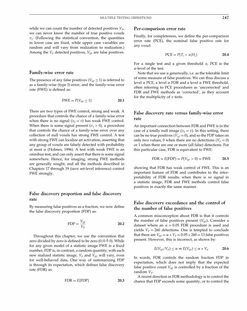
Elsevier UK Chapter: Ch20-P372560 30-9-2006 5:17p.m. Page:247 Trim:7.5in×9.25in
Basal Font:Palatino Margins:Top:40pt Gutter:68pt Font Size:9.5/12 Text Width:42pc Depth:55 Lines
MULTIPLE TESTING DEFINITIONS 247
while we can count the number of detected positives VP ,we can never know the number of true positive voxelsv1. (Following the statistical convention, the quantitiesin lower case are fixed, while upper case variables arerandom and will vary from realization to realization.)Among the VP detected positives, V0P are false positives.
Family-wise error rate
The presence of any false positives �V0P ≥ 1� is referred toas a family-wise (type I) error, and the family-wise errorrate (FWE) is defined as:
FWE = P�V0P ≥ 1� 20.1
There are two types of FWE control, strong and weak. Aprocedure that controls the chance of a family-wise errorwhen there is no signal (v0 = v) has weak FWE control.When there is some signal present (v1 > 0), a procedurethat controls the chance of a family-wise error over anycollection of null voxels has strong FWE control. A testwith strong FWE can localize an activation, asserting thatany group of voxels are falsely detected with probabilityat most � (Holmes, 1996). A test with weak FWE is anomnibus test, and can only assert that there is some signalsomewhere. Hence, for imaging, strong FWE methodsare generally sought, and all the methods described inChapters 17 through 19 (save set-level inference) controlFWE strongly.
False discovery proportion and false discoveryrate
By measuring false positives as a fraction, we now definethe false discovery proportion (FDP) as:
FDP = V0P
VP
20.2
Throughout this chapter, we use the convention thatzero divided by zero is defined to be zero �0/0� 0�. Whilefor any given model of a statistic image FWE is a fixednumber, FDP is, in contrast, a random quantity; with eachnew realized statistic image, VP and V0P will vary, evenfor well-behaved data. One way of summarizing FDPis through its expectation, which defines false discoveryrate (FDR) as:
FDR = E�FDP� 20.3
Per-comparison error rate
Finally, for completeness, we define the per-comparisonerror rate (PCE), the nominal false positive rate forany voxel:
PCE = P�Ti > u�Ho� 20.4
For a single test and a given threshold u, PCE is the�-level of the test.
Note that we use � generically, i.e. as the tolerable limitof some measure of false positives. We can thus discuss alevel � PCE, a level � FDR and a level � FWE threshold,often referring to PCE procedures as ‘uncorrected’ andFDR and FWE methods as ‘corrected’, as they accountfor the multiplicity of v tests.
False discovery rate versus family-wise errorrate
An important connection between FDR and FWE is in thecase of a totally null image (v0 = v). In this setting, therecan be no true positives (V1P = 0), and so the FDP takes ononly two values, 0 when there are no detections (VP = 0)or 1 when there are one or more (all false) detections. Forthis particular case, FDR is equivalent to FWE:
FDR = E�FDP� = P�V0P > 0� = FWE 20.5
showing that FDR has weak control of FWE. This is animportant feature of FDR and contributes to the inter-pretability of FDR results: when there is no signal ina statistic image, FDR and FWE methods control falsepositives in exactly the same manner.
False discovery exceedance and the control ofthe number of false positives
A common misconception about FDR is that it controlsthe number of false positives present �V0P�. Consider adataset where an � = 005 FDR procedure is used andyields VP = 260 detections. One is tempted to concludethat there are V0P = �×VP = 005×260 = 13 false positivespresent. However, this is incorrect, as shown by:
E�V0P/VP� ≤ �� E�V0P� ≤ �×VP 20.6
In words, FDR controls the random fraction FDP inexpectation, which does not imply that the expectedfalse positive count V0P is controlled by a fraction of therandom VP .
A recent direction in FDR methodology is to control thechance that FDP exceeds some quantity, or to control the

Elsevier UK Chapter: Ch20-P372560 30-9-2006 5:17p.m. Page:248 Trim:7.5in×9.25in
Basal Font:Palatino Margins:Top:40pt Gutter:68pt Font Size:9.5/12 Text Width:42pc Depth:55 Lines
248 20. FALSE DISCOVERY RATE PROCEDURES
false discovery exceedance (FDX). While this is a morestringent measure of false positives, it allows control onV0P . A level �� �1 −� confidence FDX procedure guar-antees that the FDP is controlled at � with probability�1−�:
P�FDP ≤ �� ≥ 1− 20.7
Inference on V0P follows:
P�FDP ≤ �� ≥ 1− ⇔ P�V0P ≤ �×VP� ≥ 1− 20.8
In words, control of the random FDP implies the falsepositive count is controlled as a fraction of the numberof detections VP .
Now consider a dataset where a level 005, 90 per centconfidence FDX procedure is used that detects 200 voxels;we could conclude with 90 per cent confidence that nomore than 200 × 005 = 10 voxels were false detections.While a few authors have proposed FDX methods (e.g.Pacifico et al., 2004; Farcomeni et al., 2005), they are notwidely used in neuroimaging, though they are mentionedto highlight a limitation of FDR.
FDR METHODS
Like FWE, FDR is simply a measure of false positives and,as with FWE, there are many different proposed meth-ods which produce thresholds that control FDR. The firstauthors who defined FDR, however, proposed a methodwhich is straightforward and consequently is the mostwidely used FDR method.
Benjamini and Hochberg (BH) FDR method
Benjamini and Hochberg (1995) introduced the FDR met-ric and proved that the Simes method, an existing weakFWE procedure, controlled their newly defined measurefor independent tests. The level � FDR threshold methodstarts by finding the p-values �Pi� for each of the teststatistics �Ti� and by ranking the p-values from smallestto largest �P�i�� = �P�i� � P�1� ≤ P�2� ≤ · · · ≤ P�v��. Next, thefollowing expression is considered for different i:
P�i� ≤ i
v� 20.9
and largest index i′ is found such that the inequalityholds. The value P�i′� can then used as a statistic threshold,and all p-values less than or equal to it can have their
null hypotheses rejected. Benjamini and Hochberg showthis procedure to control FDR conservatively:
FDR ≤ v0
v� ≤ � 20.10
with the inequality becoming equality for continu-ous �Ti�.
P-P plot interpretation
The defining inequality (Eqn. 20.9) can be plotted versusi/v, giving insight to how the FDR threshold is found(see plots in Figure 20.2). When the left side is plottedit produces a ‘P-P plot’, ordered p-values �P�i�� plottedversus i/v, a scale of their index. Plotting the right-hand-side produces a line of slope �. The FDR threshold P�i� isfound as the largest p-value below the line.
The value of this plot stems from two observations.First is the fundamental property of p-values: under thenull hypothesis, p-values follow a uniform distribution,Pi ∼ uniform�0� 1�. Thus when v0 = v the p-values shouldbe uniformly spread between 0 and 1, each with E�P�i�� =i/�v+1� ≈ i/v. This shows the P-P plot to be the orderedp-values plotted against their null-hypothesis expectedvalue (almost), and under the complete null the p-valuesshould roughly follow the identity.
The second observation is simply that, when there issignal present, we expect an excess of small p-values,causing the P-P plot to bend down at the left and belowthe slope-� line. This also shows that the exact thresh-old found will depend on the distribution of p-valuesobserved, something considered in the second illustra-tion in the next section.
Conservativeness of the BH FDR method
It may seem that the conservativeness of the method, bya factor of v0/v, would reduce its utility. However, in thecontext of brain imaging this is not a problem.
An aspect of most functional imaging experiments isthat the number of tests considered (v) is quite large andthe fraction of active voxels is quite small �v1 v�. Con-sequently, the fraction of null voxels is large �v0/v ≈ 1�and as a result the conservativeness implicit in the BHFDR method is not severe. Some authors (e.g. Benjaminiet al., 2003) propose to estimate v0 with v̂0 and replace� with � × �v/v̂0� in the BH FDR method (Eqn. 20.9),though that same work suggests these methods do notwork well under dependence and when v0/v is close to1. Hence, estimation of v0 probably will not aid mostneuroimaging applications.
BH FDR method under-dependence
An assumption of independence between voxels is unten-able in brain imaging, and so it would seem that the BH

Elsevier UK Chapter: Ch20-P372560 30-9-2006 5:17p.m. Page:249 Trim:7.5in×9.25in
Basal Font:Palatino Margins:Top:40pt Gutter:68pt Font Size:9.5/12 Text Width:42pc Depth:55 Lines
EXAMPLES AND DEMONSTRATIONS 249
FDR method would not be applicable. Fortunately, thisassumption was relaxed in a subsequent paper, in whichBenjamini and Yekutieli (2001) proved that the BH FDRprocedure is valid under positive regression dependencyon subsets (PRDS). PRDS is a very technical, generalizednotion of dependence, but can be concisely stated forGaussian data:
Corr�Ti�Tj� ≥ 0� for i = 1� � � � � v� j ∈ �0 20.11
where �0 is the set of indices for all null tests. Thiscondition requires that there must be zero or positivecorrelation between all pairs of null voxels, and betweenall pairs of null and signal voxels. No constraint is madeon the correlation between pairs of signal voxels. Forsmooth imaging data, this assumption seems reasonable,though strong physiological artefacts could induce struc-tured noise with negative correlations.
If the PRDS assumption is regarded as untenable,Benjamini and Yekutieli (2001) provide a version ofthe BH FDR method that is valid for any correlationstructure. In Eqn. 20.9 replace � with �/c�v�, wherec�v� = ∑
i=1� � � � �v 1/i ≈ log�v� + 05772. This modifiedmethod is, however, much more stringent and is muchless sensitive than the original BH FDR method.
EXAMPLES AND DEMONSTRATIONS
In the following section, we demonstrate a number ofimportant features of FDR with simulated examplesand data.
Comparison of PCE, FWE and FDR
Figure 20.1 demonstrates the application of three dif-ferent measures of false positive control. The top rowshows ten statistic images, each of which is a realizationof smooth background noise with a deterministic signalin the centre. In the bottom two rows, signal voxels areindicated by a grey line. Think of the ten images as theresults of one’s next ten experiments.
Per-comparison error rate
The second row shows the use of an uncorrected � = 01threshold, i.e., control of the per comparison error rate at10 per cent. There are many false positives: 11.3 per centof the first image’s null voxels are marked as significant,12.5 per cent of the second image, etc. Theory dictates10 per cent of the null voxels are falsely detected onaverage, but for any particular experiment it may be eitherhigher or lower. While the magnitude of false positives
FIGURE 20.1 Monte Carlo demonstration of the control ofdifferent false positive metrics.
is unacceptable, observe that such an approach is verysensitive, and most of the non-null voxels are correctlyidentified as signal.
Family-wise error rate
The third row shows the use of a 0.1-level FWE thresh-old. In nine out of ten images no false positives occur; inone image a family-wise error is visible due to the twofalse positive voxels. This illustrates how a valid FWEprocedure controls the long-run chance of any false posi-tives: over many, many experiments, no more than 1 outof 10 will have any false positives. That is, there is 90per cent confidence of the FWE thresholded image beingfalse-positive-free. This precise specificity sacrifices sen-sitivity: only a small fraction of signal voxels have beendetected in each case.
False discovery rate
The fourth row depicts the use of a 0.1-level FDRthreshold. There are fewer false positives than with PCE;measured as the false discovery proportion (FDP), falsepositives vary from image to image: 6.7 per cent of thefirst image’s significant voxels are false positives; 14.9 percent of the second image’s detections are false positives.Note that the FDP can be large at times, here as muchas 16.2 per cent over these ten realizations and could beeven larger in other realizations. As an extreme, recallthat for complete null data FDP can only be either 0 or100 per cent. A valid FDR procedure merely guaranteesthat on average FDP will not exceed the nominal 10 percent. The use of this more liberal false positive measure,though, results in more true positives than with FWE,
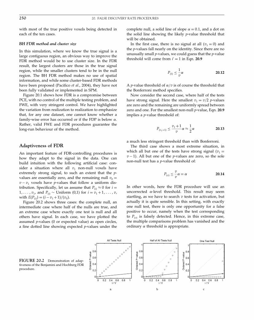
Elsevier UK Chapter: Ch20-P372560 30-9-2006 5:17p.m. Page:250 Trim:7.5in×9.25in
Basal Font:Palatino Margins:Top:40pt Gutter:68pt Font Size:9.5/12 Text Width:42pc Depth:55 Lines
250 20. FALSE DISCOVERY RATE PROCEDURES
with most of the true positive voxels being detected ineach of the ten cases.
BH FDR method and cluster size
In this simulation, where we know the true signal is alarge contiguous region, an obvious way to improve theFDR method would be to use cluster size. In the FDRresult, the largest clusters are those in the true signalregion, while the smaller clusters tend to be in the nullregion. The BH FDR method makes no use of spatialinformation, and while some cluster-based FDR methodshave been proposed (Pacifico et al., 2004), they have notbeen fully validated or implemented in SPM.
Figure 20.1 shows how FDR is a compromise betweenPCE, with no control of the multiple testing problem, andFWE, with very stringent control. We have highlightedthe variation from realization to realization to emphasizethat, for any one dataset, one cannot know whether afamily-wise error has occurred or if the FDP is below �.Rather, valid FWE and FDR procedures guarantee thelong-run behaviour of the method.
Adaptiveness of FDR
An important feature of FDR-controlling procedures ishow they adapt to the signal in the data. One canbuild intuition with the following artificial case: con-sider a situation where all v1 non-null voxels haveextremely strong signal, to such an extent that the p-values are essentially zero, and the remaining null v0 =v − v1 voxels have p-values that follow a uniform dis-tribution. Specifically, let us assume that P�i� ≈ 0 for i =1� � � � � v1, and P�i� ∼ Uniform (0,1) for i = v1 + 1� � � � � v,with E�P�i�� = �i−v1 +1�/�v0�.
Figure 20.2 shows three cases: the complete null, anintermediate case where half of the nulls are true, andan extreme case where exactly one test is null and allothers have signal. In each case, we have plotted theassumed p-values (0 or expected value) as open circles,a fine dotted line showing expected p-values under the
complete null, a solid line of slope � = 01, and a dot onthe solid line showing the likely p-value threshold thatwill be obtained.
In the first case, there is no signal at all �v1 = 0� andthe p-values fall nearly on the identity. Since there are nounusually small p-values, we could guess that the p-valuethreshold will come from i′ = 1 in Eqn. 20.9
P�1� ≤ 1v
� 20.12
A p-value threshold of �/v is of course the threshold thatthe Bonferroni method specifies.
Now consider the second case, where half of the testshave strong signal. Here the smallest v1 = v/2 p-valuesare zero and the remaining are uniformly spread betweenzero and one. For the smallest non-null p-value, Eqn. 20.9implies a p-value threshold of:
P�v1+1� ≤ v1 +1v
� ≈ 12
� 20.13
a much less stringent threshold than with Bonferroni.The third case shows a most extreme situation, in
which all but one of the tests have strong signal �v1 =v − 1�. All but one of the p-values are zero, so the solenon-null test has a p-value threshold of:
P�v� ≤ v
v� = � 20.14
In other words, here the FDR procedure will use anuncorrected �-level threshold. This result may seemstartling, as we have to search v tests for activation, butactually it is quite sensible. In this setting, with exactlyone null test, there is only one opportunity for a falsepositive to occur, namely when the test correspondingto P�v� is falsely detected. Hence, in this extreme case,the multiple comparisons problem has vanished and theordinary � threshold is appropriate.
FIGURE 20.2 Demonstration of adap-tiveness of the Benjamini and Hochberg FDRprocedure.
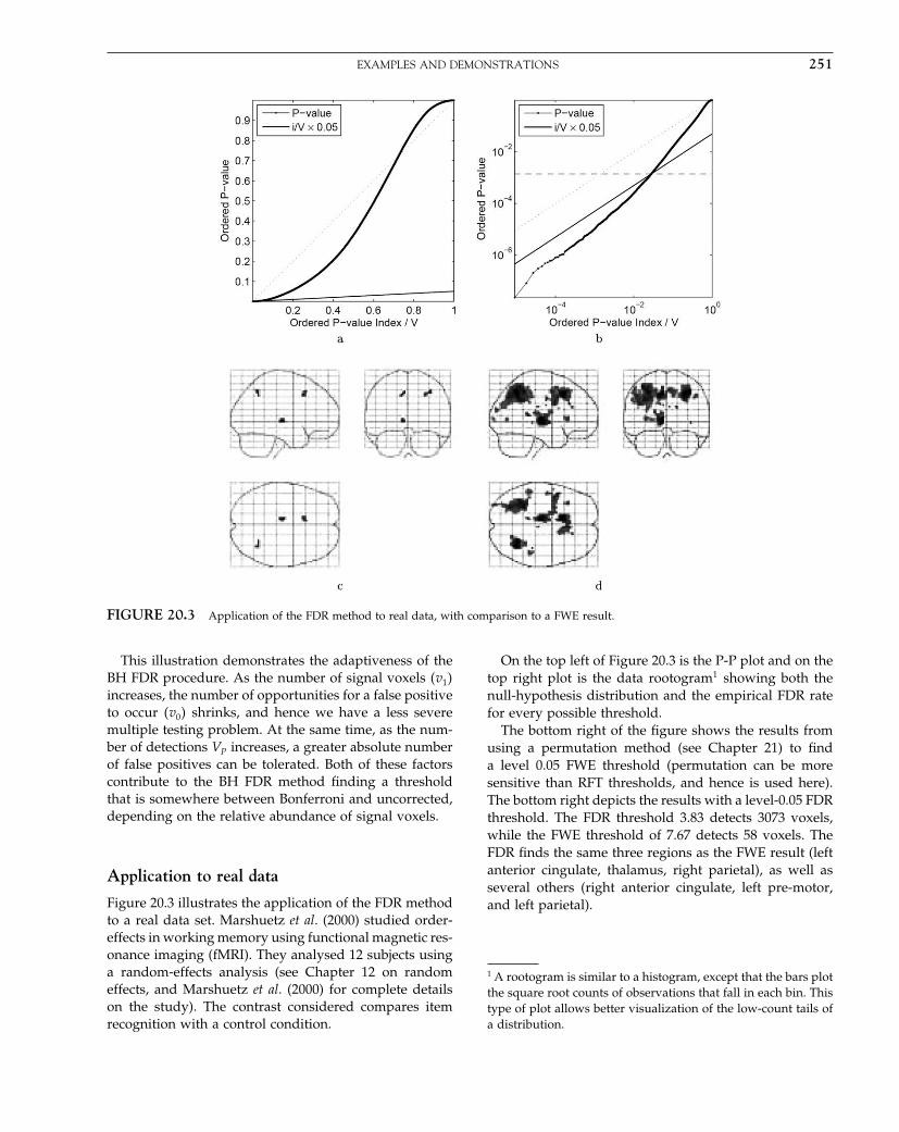
Elsevier UK Chapter: Ch20-P372560 30-9-2006 5:17p.m. Page:251 Trim:7.5in×9.25in
Basal Font:Palatino Margins:Top:40pt Gutter:68pt Font Size:9.5/12 Text Width:42pc Depth:55 Lines
EXAMPLES AND DEMONSTRATIONS 251
FIGURE 20.3 Application of the FDR method to real data, with comparison to a FWE result.
This illustration demonstrates the adaptiveness of theBH FDR procedure. As the number of signal voxels �v1�increases, the number of opportunities for a false positiveto occur �v0� shrinks, and hence we have a less severemultiple testing problem. At the same time, as the num-ber of detections VP increases, a greater absolute numberof false positives can be tolerated. Both of these factorscontribute to the BH FDR method finding a thresholdthat is somewhere between Bonferroni and uncorrected,depending on the relative abundance of signal voxels.
Application to real data
Figure 20.3 illustrates the application of the FDR methodto a real data set. Marshuetz et al. (2000) studied order-effects in working memory using functional magnetic res-onance imaging (fMRI). They analysed 12 subjects usinga random-effects analysis (see Chapter 12 on randomeffects, and Marshuetz et al. (2000) for complete detailson the study). The contrast considered compares itemrecognition with a control condition.
On the top left of Figure 20.3 is the P-P plot and on thetop right plot is the data rootogram1 showing both thenull-hypothesis distribution and the empirical FDR ratefor every possible threshold.
The bottom right of the figure shows the results fromusing a permutation method (see Chapter 21) to finda level 0.05 FWE threshold (permutation can be moresensitive than RFT thresholds, and hence is used here).The bottom right depicts the results with a level-0.05 FDRthreshold. The FDR threshold 3.83 detects 3073 voxels,while the FWE threshold of 7.67 detects 58 voxels. TheFDR finds the same three regions as the FWE result (leftanterior cingulate, thalamus, right parietal), as well asseveral others (right anterior cingulate, left pre-motor,and left parietal).
1 A rootogram is similar to a histogram, except that the bars plotthe square root counts of observations that fall in each bin. Thistype of plot allows better visualization of the low-count tails ofa distribution.
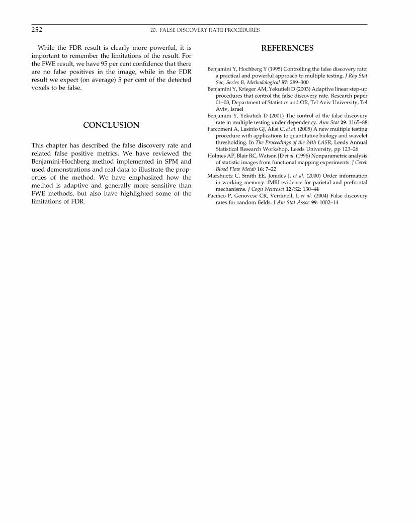
Elsevier UK Chapter: Ch20-P372560 30-9-2006 5:17p.m. Page:252 Trim:7.5in×9.25in
Basal Font:Palatino Margins:Top:40pt Gutter:68pt Font Size:9.5/12 Text Width:42pc Depth:55 Lines
252 20. FALSE DISCOVERY RATE PROCEDURES
While the FDR result is clearly more powerful, it isimportant to remember the limitations of the result. Forthe FWE result, we have 95 per cent confidence that thereare no false positives in the image, while in the FDRresult we expect (on average) 5 per cent of the detectedvoxels to be false.
CONCLUSION
This chapter has described the false discovery rate andrelated false positive metrics. We have reviewed theBenjamini-Hochberg method implemented in SPM andused demonstrations and real data to illustrate the prop-erties of the method. We have emphasized how themethod is adaptive and generally more sensitive thanFWE methods, but also have highlighted some of thelimitations of FDR.
REFERENCES
Benjamini Y, Hochberg Y (1995) Controlling the false discovery rate:a practical and powerful approach to multiple testing. J Roy StatSoc, Series B, Methodological 57: 289–300
Benjamini Y, Krieger AM, Yekutieli D (2003) Adaptive linear step-upprocedures that control the false discovery rate. Research paper01–03, Department of Statistics and OR, Tel Aviv University, TelAviv, Israel
Benjamini Y, Yekutieli D (2001) The control of the false discoveryrate in multiple testing under dependency. Ann Stat 29: 1165–88
Farcomeni A, Lasinio GJ, Alisi C, et al. (2005) A new multiple testingprocedure with applications to quantitative biology and waveletthresholding. In The Proceedings of the 24th LASR, Leeds AnnualStatistical Research Workshop, Leeds University, pp 123–26
Holmes AP, Blair RC, Watson JD et al. (1996) Nonparametric analysisof statistic images from functional mapping experiments. J CerebBlood Flow Metab 16: 7–22
Marshuetz C, Smith EE, Jonides J, et al. (2000) Order informationin working memory: fMRI evidence for parietal and prefrontalmechanisms. J Cogn Neurosci 12/S2: 130–44
Pacifico P, Genovese CR, Verdinelli I, et al. (2004) False discoveryrates for random fields. J Am Stat Assoc 99: 1002–14

Elsevier UK Chapter: Ch21-P372560 30-9-2006 5:18p.m. Page:253 Trim:7.5in×9.25in
Basal Font:Palatino Margins:Top:40pt Gutter:68pt Font Size:9.5/12 Text Width:42pc Depth:55 Lines
C H A P T E R
21
Non-parametric proceduresT. Nichols and A. Holmes
INTRODUCTION
The statistical analyses of functional mapping experi-ments usually proceed at the voxel level, involving theformation and assessment of a statistic image: at eachvoxel, a statistic indicating evidence of the experimen-tal effect of interest, at that voxel, is computed, givingan image of statistics, a statistic image or statistical para-metric map (SPM). In the absence of a priori anatomicalhypotheses, the entire statistic image must be assessedfor significant experimental effects, using a method thataccounts for the inherent multiplicity incurred by testingall voxels simultaneously.
Traditionally, this has been accomplished in a clas-sical parametric statistical framework. In the methodsdiscussed in Chapters 8 and 9 of this book, the dataare assumed to be normally distributed, with a meanparameterized by a general linear model. This flexibleframework encompasses t-tests, F -tests, paired t-tests,analysis of variance (ANOVA), correlation, linear regres-sion, multiple regression, and analysis of covariance(ANCOVA), among others. The estimated parametersof this model are contrasted to produce a test statistic ateach voxel, which has a Student’s t-distribution underthe null hypothesis. The resulting t-statistic image is thenassessed for statistical significance, using distributionalresults for continuous random fields to identify voxelsor regions where there is significant evidence against thenull hypothesis (Friston et al., 1994, 1996; Worsley et al.,1995; Worsley, 1995; Poline et al., 1997).
Holmes et al. (1996) introduced a non-parametric alter-native based on permutation test theory. This methodis conceptually simple, relies only on minimal assump-tions, deals with the multiple testing issue, and canbe applied when the assumptions of a parametricapproach are untenable. Furthermore, in some circum-stances, the permutation method outperforms parametricapproaches. Arndt et al., (1996), working independently,
also discussed the advantages of similar approaches.Subsequently, Grabrowski et al. (1996) demonstratedempirically the potential power of the approach in com-parison with other methods. Halber et al. (1997), discussedfurther by Holmes et al. (1998), also favour the permuta-tion approach. Methods to improve the computational effi-ciency of the method have been proposed by Heckel et al.(1998) and Belmonte and Yurgelun-Todd (2001).
Nichols and Holmes (2001) review the non-parametrictheory and demonstrate how multisubject functionalmagnetic resonance images (fMRI) can be analysed.One use of permutations is to evaluate methods withmore assumptions. Nichols and Hayasaka (2003; 2004)compare voxels-wise parametric to non-parametric per-formance on several multisubject datsets, as well ascluster-wise performance under stationarity and non-stationarity.
Applications of permutation testing methods to singlesubject fMRI require models of the temporal autocorre-lation in the fMRI time series. Bullmore et al. (1996) havedeveloped permutation based procedures for periodicfMRI activation designs using a simple autoregressionmoving average (ARMA) model for temporal autocor-relations, though they eschew the problem of multipletesting; later they generalized their method to multiplesubjects (Brammer et al., 1997). In later work, Bullmoreand colleagues used a wavelet transformation to accountfor more general forms of fMRI correlation (Bullmoreet al., 2001; Fadili and Bullmore, 2001), though Frimanand Westin (2005) have criticized this approach. Locascioet al. (1997) describe an application to fMRI combiningthe general linear model (Friston et al., 1995), ARMAmodelling (Bullmore et al., 1996), and a multiple testingpermutation procedure (Holmes et al., 1996). In a ran-domized experiment, Raz et al. (2003) proposed permut-ing the experimental labels instead of the data. Bullmoreet al. (1999) apply non-parametric methods to comparegroups of structural MR images.
Statistical Parametric Mapping, by Karl Friston et al. Copyright 2007, Elsevier Ltd. All rights reserved.ISBN–13: 978-0-12-372560-8 ISBN–10: 0-12-372560-7
253
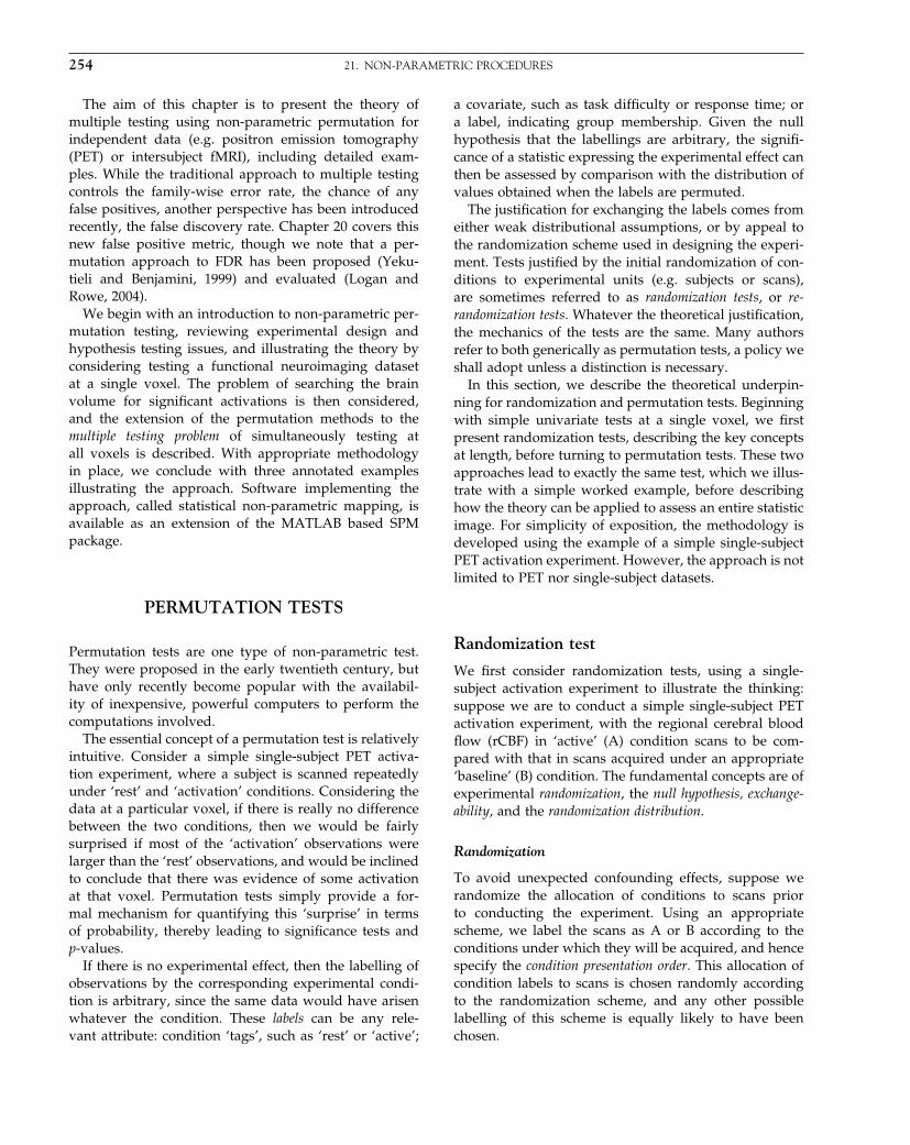
Elsevier UK Chapter: Ch21-P372560 30-9-2006 5:18p.m. Page:254 Trim:7.5in×9.25in
Basal Font:Palatino Margins:Top:40pt Gutter:68pt Font Size:9.5/12 Text Width:42pc Depth:55 Lines
254 21. NON-PARAMETRIC PROCEDURES
The aim of this chapter is to present the theory ofmultiple testing using non-parametric permutation forindependent data (e.g. positron emission tomography(PET) or intersubject fMRI), including detailed exam-ples. While the traditional approach to multiple testingcontrols the family-wise error rate, the chance of anyfalse positives, another perspective has been introducedrecently, the false discovery rate. Chapter 20 covers thisnew false positive metric, though we note that a per-mutation approach to FDR has been proposed (Yeku-tieli and Benjamini, 1999) and evaluated (Logan andRowe, 2004).
We begin with an introduction to non-parametric per-mutation testing, reviewing experimental design andhypothesis testing issues, and illustrating the theory byconsidering testing a functional neuroimaging datasetat a single voxel. The problem of searching the brainvolume for significant activations is then considered,and the extension of the permutation methods to themultiple testing problem of simultaneously testing atall voxels is described. With appropriate methodologyin place, we conclude with three annotated examplesillustrating the approach. Software implementing theapproach, called statistical non-parametric mapping, isavailable as an extension of the MATLAB based SPMpackage.
PERMUTATION TESTS
Permutation tests are one type of non-parametric test.They were proposed in the early twentieth century, buthave only recently become popular with the availabil-ity of inexpensive, powerful computers to perform thecomputations involved.
The essential concept of a permutation test is relativelyintuitive. Consider a simple single-subject PET activa-tion experiment, where a subject is scanned repeatedlyunder ‘rest’ and ‘activation’ conditions. Considering thedata at a particular voxel, if there is really no differencebetween the two conditions, then we would be fairlysurprised if most of the ‘activation’ observations werelarger than the ‘rest’ observations, and would be inclinedto conclude that there was evidence of some activationat that voxel. Permutation tests simply provide a for-mal mechanism for quantifying this ‘surprise’ in termsof probability, thereby leading to significance tests andp-values.
If there is no experimental effect, then the labelling ofobservations by the corresponding experimental condi-tion is arbitrary, since the same data would have arisenwhatever the condition. These labels can be any rele-vant attribute: condition ‘tags’, such as ‘rest’ or ‘active’;
a covariate, such as task difficulty or response time; ora label, indicating group membership. Given the nullhypothesis that the labellings are arbitrary, the signifi-cance of a statistic expressing the experimental effect canthen be assessed by comparison with the distribution ofvalues obtained when the labels are permuted.
The justification for exchanging the labels comes fromeither weak distributional assumptions, or by appeal tothe randomization scheme used in designing the experi-ment. Tests justified by the initial randomization of con-ditions to experimental units (e.g. subjects or scans),are sometimes referred to as randomization tests, or re-randomization tests. Whatever the theoretical justification,the mechanics of the tests are the same. Many authorsrefer to both generically as permutation tests, a policy weshall adopt unless a distinction is necessary.
In this section, we describe the theoretical underpin-ning for randomization and permutation tests. Beginningwith simple univariate tests at a single voxel, we firstpresent randomization tests, describing the key conceptsat length, before turning to permutation tests. These twoapproaches lead to exactly the same test, which we illus-trate with a simple worked example, before describinghow the theory can be applied to assess an entire statisticimage. For simplicity of exposition, the methodology isdeveloped using the example of a simple single-subjectPET activation experiment. However, the approach is notlimited to PET nor single-subject datasets.
Randomization test
We first consider randomization tests, using a single-subject activation experiment to illustrate the thinking:suppose we are to conduct a simple single-subject PETactivation experiment, with the regional cerebral bloodflow (rCBF) in ‘active’ (A) condition scans to be com-pared with that in scans acquired under an appropriate‘baseline’ (B) condition. The fundamental concepts are ofexperimental randomization, the null hypothesis, exchange-ability, and the randomization distribution.
Randomization
To avoid unexpected confounding effects, suppose werandomize the allocation of conditions to scans priorto conducting the experiment. Using an appropriatescheme, we label the scans as A or B according to theconditions under which they will be acquired, and hencespecify the condition presentation order. This allocation ofcondition labels to scans is chosen randomly accordingto the randomization scheme, and any other possiblelabelling of this scheme is equally likely to have beenchosen.
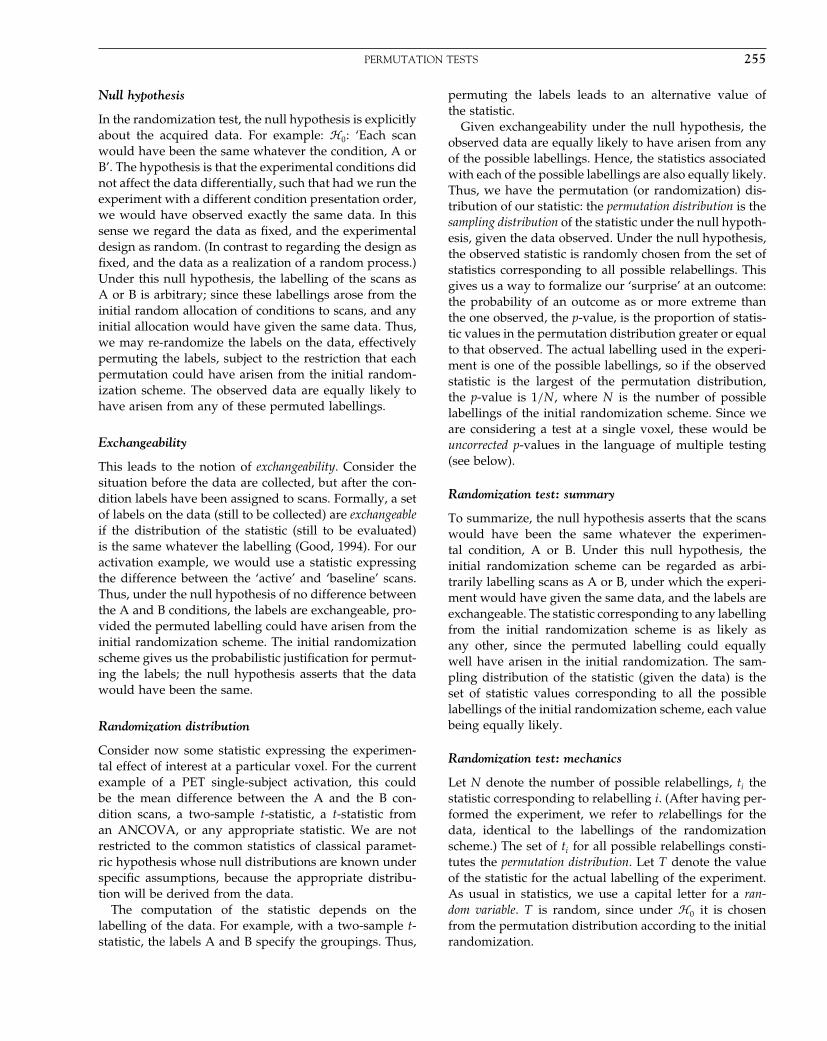
Elsevier UK Chapter: Ch21-P372560 30-9-2006 5:18p.m. Page:255 Trim:7.5in×9.25in
Basal Font:Palatino Margins:Top:40pt Gutter:68pt Font Size:9.5/12 Text Width:42pc Depth:55 Lines
PERMUTATION TESTS 255
Null hypothesis
In the randomization test, the null hypothesis is explicitlyabout the acquired data. For example: �0: ‘Each scanwould have been the same whatever the condition, A orB’. The hypothesis is that the experimental conditions didnot affect the data differentially, such that had we run theexperiment with a different condition presentation order,we would have observed exactly the same data. In thissense we regard the data as fixed, and the experimentaldesign as random. (In contrast to regarding the design asfixed, and the data as a realization of a random process.)Under this null hypothesis, the labelling of the scans asA or B is arbitrary; since these labellings arose from theinitial random allocation of conditions to scans, and anyinitial allocation would have given the same data. Thus,we may re-randomize the labels on the data, effectivelypermuting the labels, subject to the restriction that eachpermutation could have arisen from the initial random-ization scheme. The observed data are equally likely tohave arisen from any of these permuted labellings.
Exchangeability
This leads to the notion of exchangeability. Consider thesituation before the data are collected, but after the con-dition labels have been assigned to scans. Formally, a setof labels on the data (still to be collected) are exchangeableif the distribution of the statistic (still to be evaluated)is the same whatever the labelling (Good, 1994). For ouractivation example, we would use a statistic expressingthe difference between the ‘active’ and ‘baseline’ scans.Thus, under the null hypothesis of no difference betweenthe A and B conditions, the labels are exchangeable, pro-vided the permuted labelling could have arisen from theinitial randomization scheme. The initial randomizationscheme gives us the probabilistic justification for permut-ing the labels; the null hypothesis asserts that the datawould have been the same.
Randomization distribution
Consider now some statistic expressing the experimen-tal effect of interest at a particular voxel. For the currentexample of a PET single-subject activation, this couldbe the mean difference between the A and the B con-dition scans, a two-sample t-statistic, a t-statistic froman ANCOVA, or any appropriate statistic. We are notrestricted to the common statistics of classical paramet-ric hypothesis whose null distributions are known underspecific assumptions, because the appropriate distribu-tion will be derived from the data.
The computation of the statistic depends on thelabelling of the data. For example, with a two-sample t-statistic, the labels A and B specify the groupings. Thus,
permuting the labels leads to an alternative value ofthe statistic.
Given exchangeability under the null hypothesis, theobserved data are equally likely to have arisen from anyof the possible labellings. Hence, the statistics associatedwith each of the possible labellings are also equally likely.Thus, we have the permutation (or randomization) dis-tribution of our statistic: the permutation distribution is thesampling distribution of the statistic under the null hypoth-esis, given the data observed. Under the null hypothesis,the observed statistic is randomly chosen from the set ofstatistics corresponding to all possible relabellings. Thisgives us a way to formalize our ‘surprise’ at an outcome:the probability of an outcome as or more extreme thanthe one observed, the p-value, is the proportion of statis-tic values in the permutation distribution greater or equalto that observed. The actual labelling used in the experi-ment is one of the possible labellings, so if the observedstatistic is the largest of the permutation distribution,the p-value is 1/N , where N is the number of possiblelabellings of the initial randomization scheme. Since weare considering a test at a single voxel, these would beuncorrected p-values in the language of multiple testing(see below).
Randomization test: summary
To summarize, the null hypothesis asserts that the scanswould have been the same whatever the experimen-tal condition, A or B. Under this null hypothesis, theinitial randomization scheme can be regarded as arbi-trarily labelling scans as A or B, under which the experi-ment would have given the same data, and the labels areexchangeable. The statistic corresponding to any labellingfrom the initial randomization scheme is as likely asany other, since the permuted labelling could equallywell have arisen in the initial randomization. The sam-pling distribution of the statistic (given the data) is theset of statistic values corresponding to all the possiblelabellings of the initial randomization scheme, each valuebeing equally likely.
Randomization test: mechanics
Let N denote the number of possible relabellings, ti thestatistic corresponding to relabelling i. (After having per-formed the experiment, we refer to relabellings for thedata, identical to the labellings of the randomizationscheme.) The set of ti for all possible relabellings consti-tutes the permutation distribution. Let T denote the valueof the statistic for the actual labelling of the experiment.As usual in statistics, we use a capital letter for a ran-dom variable. T is random, since under �0 it is chosenfrom the permutation distribution according to the initialrandomization.

Elsevier UK Chapter: Ch21-P372560 30-9-2006 5:18p.m. Page:256 Trim:7.5in×9.25in
Basal Font:Palatino Margins:Top:40pt Gutter:68pt Font Size:9.5/12 Text Width:42pc Depth:55 Lines
256 21. NON-PARAMETRIC PROCEDURES
Under �0, all of the ti are equally likely, so wedetermine the significance of our observed statistic T bycounting the proportion of the permutation distributionas or more extreme than T , giving us our p-value. Wereject the null hypothesis at significance level � if thep-value is less than �. Equivalently, T must be greaterthan or equal to the 100�1 −�� percentile of the permu-tation distribution. Thus, the critical value is the �c +1�thlargest member of the permutation distribution, wherec = ��N�� �N rounded down. If T exceeds this criticalvalue then the test is significant at level �.
Permutation test
In many situations, it is impractical randomly to allocateexperimental conditions, or perhaps we are presentedwith data from an experiment that was not random-ized. For instance, we cannot randomly assign subjectsto be patients or normal controls. Or, for example, con-sider a multisubject fMRI second-level analysis wherea covariate is measured for each subject, and we seekbrain regions whose activation appears to be related tothe covariate value.
In the absence of an explicit randomization of con-ditions to scans, we must make weak distributionalassumptions to justify permuting the labels on the data.Typically, all that is required is that distributions havethe same shape, or are symmetric. The actual permu-tations that are performed again depend on the degreeof exchangeability which, in turn, depend on the actualassumptions made. With the randomization test, theexperimenter designs the initial randomization schemecarefully to avoid confounds. The randomization schemereflects an implicitly assumed degree of exchangeability.With the permutation test, the degree of exchangeabilitymust be assumed post hoc. Usually, the reasoning thatwould have led to a particular randomization scheme canbe applied post hoc to an experiment, leading to a per-mutation test with the same degree of exchangeability.Given exchangeability, computation proceeds as for therandomization test.
Permutation test: summary
Weak distributional assumptions are made, whichembody the degree of exchangeability. The exact form ofthese assumptions depends on the experiment at hand,as illustrated in the following section and in the examplessection.
For a simple single-subject activation experiment, wemight typically assume the following: for a particularvoxel, ‘active’ and ‘baseline’ scans within a given blockhave a distribution with the same shape, though possi-bly different means. The null hypothesis asserts that the
distributions for the ‘baseline’ and ‘active’ scans havethe same mean, and hence are the same. Then the labelsare arbitrary within the chosen blocks, which are thusthe exchangeability blocks. Any permutation of the labelswithin the exchangeability blocks leads to an equallylikely statistic. (Note, if this were a multisubject dataset,the exchangeability block would be the entire dataset, assubjects are regarded as independent.)
The mechanics are then the same as with the random-ization test: for each of the possible relabellings, computethe statistic of interest; for relabelling i, call this statisticti. Under the null hypothesis each of the ti are equallylikely, so the p-value is the proportion of the tis greaterthan or equal to the statistic T corresponding to the cor-rectly labelled data.
Single voxel example
To make these concepts concrete, consider assessing theevidence of an activation effect at a single voxel of asingle-subject PET activation experiment consisting of sixscans, three in each of the ‘active’ (A) and ‘baseline’ (B)conditions. Suppose that the conditions were presentedalternately, starting with rest, and that the observed dataat this voxel are {90.48, 103.00, 87.83, 99.93, 96.06, 99.76}to 2 decimal places. (These data are from a voxel in theprimary visual cortex of the second subject in the PETvisual activation experiment presented in the examplessection.)
As mentioned before, any statistic can be used, so forsimplicity of illustration we use the ‘mean difference’, i.e.T = 1
3
∑3j=1�Aj − Bj� where Bj and Aj indicate the value
of the jth scan at the particular voxel of interest, underthe baseline and active conditions respectively. Thus, weobserve statistic T = 9�45.
Randomization test
Suppose that the condition presentation order was ran-domized, the actual ordering of BABABA having beenselected randomly from all allocations of three As andthree Bs to the six available scans, a simple balanced ran-domization within a single randomization block of sizesix. By combinatorics, or some counting, we find thatthis randomization scheme has twenty �6C3 = 20� possibleoutcomes.
Then we can justify permuting the labels on the basisof this initial randomization. Under the null hypothe-sis �0: ‘The scans would have been the same what-ever the experimental condition, A or B’, the labels areexchangeable, and the statistics corresponding to the
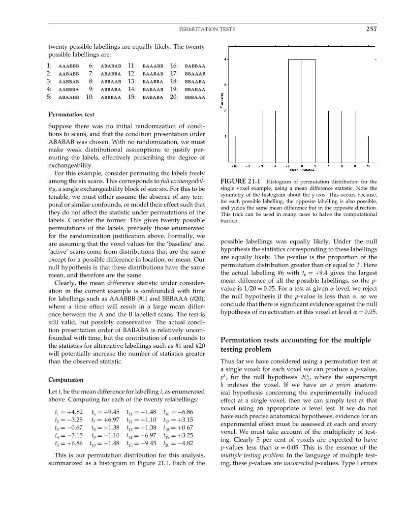
Elsevier UK Chapter: Ch21-P372560 30-9-2006 5:18p.m. Page:257 Trim:7.5in×9.25in
Basal Font:Palatino Margins:Top:40pt Gutter:68pt Font Size:9.5/12 Text Width:42pc Depth:55 Lines
PERMUTATION TESTS 257
twenty possible labellings are equally likely. The twentypossible labellings are:
1: aaabbb 6: ababab 11: baaabb 16: babbaa
2: aababb 7: ababba 12: baabab 17: bbaaab
3: aabbab 8: abbaab 13: baabba 18: bbaaba
4: aabbba 9: abbaba 14: babaab 19: bbabaa
5: abaabb 10: abbbaa 15: bababa 20: bbbaaa
Permutation test
Suppose there was no initial randomization of condi-tions to scans, and that the condition presentation orderABABAB was chosen. With no randomization, we mustmake weak distributional assumptions to justify per-muting the labels, effectively prescribing the degree ofexchangeability.
For this example, consider permuting the labels freelyamong the six scans. This corresponds to full exchangeabil-ity, a single exchangeability block of size six. For this to betenable, we must either assume the absence of any tem-poral or similar confounds, or model their effect such thatthey do not affect the statistic under permutations of thelabels. Consider the former. This gives twenty possiblepermutations of the labels, precisely those enumeratedfor the randomization justification above. Formally, weare assuming that the voxel values for the ‘baseline’ and‘active’ scans come from distributions that are the sameexcept for a possible difference in location, or mean. Ournull hypothesis is that these distributions have the samemean, and therefore are the same.
Clearly, the mean difference statistic under consider-ation in the current example is confounded with timefor labellings such as AAABBB (#1) and BBBAAA (#20),where a time effect will result in a large mean differ-ence between the A and the B labelled scans. The test isstill valid, but possibly conservative. The actual condi-tion presentation order of BABABA is relatively uncon-founded with time, but the contribution of confounds tothe statistics for alternative labellings such as #1 and #20will potentially increase the number of statistics greaterthan the observed statistic.
Computation
Let ti be the mean difference for labelling i, as enumeratedabove. Computing for each of the twenty relabellings:
t1 = +4�82 t6 = +9�45 t11 = −1�48 t16 = −6�86t2 = −3�25 t7 = +6�97 t12 = +1�10 t17 = +3�15t3 = −0�67 t8 = +1�38 t13 = −1�38 t18 = +0�67t4 = −3�15 t9 = −1�10 t14 = −6�97 t19 = +3�25t5 = +6�86 t10 = +1�48 t15 = −9�45 t20 = −4�82
This is our permutation distribution for this analysis,summarized as a histogram in Figure 21.1. Each of the
FIGURE 21.1 Histogram of permutation distribution for thesingle voxel example, using a mean difference statistic. Note thesymmetry of the histogram about the y-axis. This occurs because,for each possible labelling, the opposite labelling is also possible,and yields the same mean difference but in the opposite direction.This trick can be used in many cases to halve the computationalburden.
possible labellings was equally likely. Under the nullhypothesis the statistics corresponding to these labellingsare equally likely. The p-value is the proportion of thepermutation distribution greater than or equal to T . Herethe actual labelling #6 with t6 = +9�4 gives the largestmean difference of all the possible labellings, so the p-value is 1/20 = 0�05. For a test at given � level, we rejectthe null hypothesis if the p-value is less than �, so weconclude that there is significant evidence against the nullhypothesis of no activation at this voxel at level � = 0�05.
Permutation tests accounting for the multipletesting problem
Thus far we have considered using a permutation test ata single voxel: for each voxel we can produce a p-value,pk, for the null hypothesis � k
0 , where the superscriptk indexes the voxel. If we have an a priori anatom-ical hypothesis concerning the experimentally inducedeffect at a single voxel, then we can simply test at thatvoxel using an appropriate � level test. If we do nothave such precise anatomical hypotheses, evidence for anexperimental effect must be assessed at each and everyvoxel. We must take account of the multiplicity of test-ing. Clearly 5 per cent of voxels are expected to havep-values less than � = 0�05. This is the essence of themultiple testing problem. In the language of multiple test-ing, these p-values are uncorrected p-values. Type I errors
Elsevier UK Chapter: Ch21-P372560 30-9-2006 5:18p.m. Page:258 Trim:7.5in×9.25in
Basal Font:Palatino Margins:Top:40pt Gutter:68pt Font Size:9.5/12 Text Width:42pc Depth:55 Lines
258 21. NON-PARAMETRIC PROCEDURES
must be controlled overall, such that the probability offalsely declaring any region as significant is less thanthe nominal test level �. This is known as controllingthe family-wise error rate, the family being the collectionof tests performed over the entire brain. Formally, werequire a test procedure maintaining strong control overfamily-wise type I error, giving adjusted p-values, p-valuescorrected for the multiplicity of tests examined.
The construction of suitable multiple testing pro-cedures for the problem of assessing statistic imagesfrom functional mapping experiments within paramet-ric frameworks has occupied many authors e.g. Fristonet al., 1991, 1994, 1996; Worsley et al., 1992, 1995; Polineand Mazoyer, 1993; Roland et al. 1993; Worsley, 1994;Forman et al. 1995; Poline et al. 1997; Cao, 1999). In con-trast to these parametric and simulation based methods, anon-parametric resampling based approach provides anintuitive and easily implemented solution (Westfall andYoung, 1993). The key realization is that the reasoningpresented above for permutation tests at a single voxelrelies on relabelling entire images, so the arguments canbe extended to image-level inference by considering anappropriate maximal statistic. If, under the omnibus nullhypothesis, the labels are exchangeable with respect tothe voxel statistic under consideration, then the labels areexchangeable with respect to any statistic summarizingthe voxel statistics, such as their maxima.
We consider two popular types of test, single thresholdand suprathreshold cluster size tests, but note again theability of these methods to use any statistic.
Single threshold test
With a single threshold test, the statistic image is thresh-olded at a given critical threshold, and voxels with statisticvalues exceeding this threshold have their null hypothe-ses rejected. Rejection of the omnibus hypothesis (that allthe voxel hypotheses are true) occurs if any voxel valueexceeds the threshold, a situation clearly determined bythe value of the maximum value of the statistic image.Thus, consideration of the maximum voxel statistic dealswith the multiple testing problem. For a valid omnibustest, the critical threshold is such that the probability thatit is exceeded by the maximal statistic is less than �; there-fore, we require the distribution of the maxima of thenull statistic image. Approximate parametric derivationsbased on the theory of strictly stationary continuous ran-dom fields are given by Friston et al. (1991) and Worsleyet al. (1992, 1995); Worsley, 1994.
The permutation approach can furnish the distribu-tion of the maximal statistic in a straightforward manner:Rather than compute the permutation distribution of thestatistic at a particular voxel, we compute the permuta-tion distribution of the maximal voxel statistic over the
volume of interest. We reject the omnibus hypothesis atlevel � if the maximal statistic for the actual labelling ofthe experiment is in the top 100� per cent of the permu-tation distribution for the maximal statistic. The criticalvalue is the �c +1�th largest member of the permutationdistribution, where c = ��N�� �N rounded down. Fur-thermore, we can reject the null hypothesis at any voxelwith a statistic value exceeding this threshold: the criticalvalue for the maximal statistic is the critical threshold fora single threshold test over the same volume of inter-est. This test can be shown to have strong control overexperiment-wise type I error. A formal proof is given byHolmes et al. (1996).
The mechanics of the test are as follows: for each pos-sible relabelling i = 1� � � � �N , note the maximal statistictmaxi , the maximum of the voxel statistics for relabelling i �
tmaxi = maxti
Ni=1. This gives the permutation distribution
for T max, the maximal statistic. The critical threshold isthe c+1 largest member of the permutation distributionfor T max, where c = ��N�� �N rounded down. Voxelswith statistics exceeding this threshold exhibit evidenceagainst the corresponding voxel hypotheses at level �.The corresponding corrected p-value for each voxel is theproportion of the permutation distribution for the max-imal statistic that is greater than or equal to the voxelstatistic.
Suprathreshold cluster tests
Suprathreshold cluster tests start by thresholding thestatistic image at a predetermined primary threshold, andthen assess the resulting pattern of suprathreshold activ-ity. Suprathreshold cluster size tests assess the size of con-nected suprathreshold regions for significance, declaringregions greater than a critical size as activated. Thus, thedistribution of the maximal suprathreshold cluster size(for the given primary threshold) is required. Simulationapproaches have been presented by Poline and Mazoyer(1993) and Roland et al. (1993) for PET, Forman et al.(1995) for fMRI. Friston et al. (1994) give a theoreticalparametric derivation for Gaussian statistic images basedon the theory of continuous Gaussian random fields; Cao(1999) gives results for �2� t and F fields.
Again, as noted by Holmes et al. (1996), a non-parametric permutation approach is simple to derive.Simply construct the permutation distribution of themaximal suprathreshold cluster size. For the statisticimage corresponding to each possible relabelling, notethe size of the largest suprathreshold cluster above theprimary threshold. The critical suprathreshold clustersize for this primary threshold is the ���N�+1�th largestmember of this permutation distribution. Corrected p-values for each suprathreshold cluster in the observedstatistic image are obtained by comparing their size tothe permutation distribution.

Elsevier UK Chapter: Ch21-P372560 30-9-2006 5:18p.m. Page:259 Trim:7.5in×9.25in
Basal Font:Palatino Margins:Top:40pt Gutter:68pt Font Size:9.5/12 Text Width:42pc Depth:55 Lines
PERMUTATION TESTS 259
In general, such suprathreshold cluster tests are morepowerful for functional neuroimaging data than the sin-gle threshold approach (see Chapter 19 and Friston et al.,1995 for a fuller discussion). However, it must be remem-bered that this additional power comes at the price ofreduced localizing power: the null hypotheses for vox-els within a significant cluster are not tested, so indi-vidual voxels cannot be declared significant. Only theomnibus null hypothesis for the cluster can be rejected.Further, the choice of primary threshold dictates thepower of the test in detecting different types of deviationfrom the omnibus null hypothesis. With a low thresh-old, large suprathreshold clusters are to be expected, sointense focal ‘signals’ will be missed. At higher thresh-olds these focal activations will be detected, but lowerintensity diffuse ‘signals’ may go undetected below theprimary threshold.
Poline et al. (1997) addressed these issues within aparametric framework by considering the suprathresholdcluster size and height jointly. A non-parametric varia-tion could be to consider the exceedance mass, the excessmass of the suprathreshold cluster, defined as the integralof the statistic image above the primary threshold withinthe suprathreshold cluster (Holmes, 1994; Bullmore et al.,1999). Calculation of the permutation distribution andp-values proceeds exactly as before.
Considerations
Before turning to example applications of thenon-parametric permutation tests described above, wenote some relevant theoretical issues. The statisticalliterature (referenced below) should be consulted foradditional theoretical discussion. For issues related tothe current application to functional neuroimaging, seealso Holmes (1994), Holmes et al. (1996), and Arndtet al. (1996).
Non-parametric statistics
First, it should be noted that these methods are neithernew nor contentious: originally expounded by Fisher(1935), Pitman (1937a,b,c), and later Edgington (1964,1969a,b), these approaches are enjoying a renaissance ascomputing technology makes the requisite computationsfeasible for practical applications. Had R.A. Fisher andhis peers had access to similar resources, it is possiblethat large areas of parametric statistics would have goneundeveloped! Modern texts on the subject include Good’sPermutation Tests (1994), Edgington’s Randomization Tests(1995), and Manly’s Randomization, Bootstrap and Monte-Carlo Methods in Biology (1997). Recent interest in moregeneral resampling methods, such as the bootstrap, has
further contributed to the field. For a treatise on resam-pling based multiple testing procedures, see Westfall andYoung (1993).
Many standard statistical tests are essentially permuta-tion tests: The ‘classic’ non-parametric tests, such as theWilcoxon and Mann-Whitney tests, are permutation testswith the data replaced by appropriate ranks, such thatthe critical values are only a function of sample size andcan therefore be tabulated. Fisher’s exact test (1990), andtests of Spearman and Kendall correlations (Kendall andGibbons 1990), are all permutation/randomization based.
Assumptions
The only assumptions required for a valid permutationtest are those to justify permuting the labels. Clearly, theexperimental design, model, statistic and permutationsmust also be appropriate for the question of interest. Fora randomization test, the probabilistic justification fol-lows directly from the initial randomization of conditionlabels to scans. In the absence of an initial randomiza-tion, permutation of the labels can be justified via weakdistributional assumptions. Thus, only minimal assump-tions are required for a valid test. (The notable case whenexchangeability under the null hypothesis is not tenableis fMRI time-series, due to temporal autocorrelation.)
In contrast to parametric approaches where the statis-tic must have a known null distributional form, thepermutation approach is free to consider any statisticsummarizing evidence for the effect of interest at eachvoxel. The consideration of the maximal statistic over thevolume of interest then deals with the multiple testingproblem.
However, there are additional considerations whenusing the non-parametric approach with a maximalstatistic to account for multiple testing. In order for thesingle threshold test to be equally sensitive at all vox-els, the (null) sampling distribution of the chosen statisticshould be similar across voxels. For instance, the simplemean difference statistic used in the single voxel examplecould be considered as a voxel statistic, but areas wherethe mean difference is highly variable will dominate thepermutation distribution for the maximal statistic. Thetest will still be valid, but will be less sensitive at thosevoxels with lower variability. So, although for an indi-vidual voxel, a permutation test on group mean differ-ences is equivalent to one using a two-sample t-statistic(Edgington, 1995), this is not true in the multiple testingsetting using a maximal statistic.
One approach to this problem is to consider multisteptests, which iteratively identify activated areas, cut themout, and continue assessing the remaining volume. Theseare described below, but are additionally computation-ally intensive. A preferable solution is to use a voxel

Elsevier UK Chapter: Ch21-P372560 30-9-2006 5:18p.m. Page:260 Trim:7.5in×9.25in
Basal Font:Palatino Margins:Top:40pt Gutter:68pt Font Size:9.5/12 Text Width:42pc Depth:55 Lines
260 21. NON-PARAMETRIC PROCEDURES
statistic with approximately homogeneous null permuta-tion distribution across the volume of interest, such as anappropriate t-statistic. A t-statistic is essentially a meandifference normalized by a variance estimate, effectivelymeasuring the reliability of an effect. Thus, we considerthe same voxel statistics for a non-parametric approachas we would for a comparable parametric approach.
Pseudo t-statistics
Nonetheless, we can still do a little better than a straightt-statistic, particularly at low degrees of freedom. A t-statistic is a change divided by the square root of theestimated variance of that change. When there are fewdegrees of freedom available for variance estimation, say,less than 20, this variance is estimated poorly. Errors inestimation of the variance from voxel to voxel appearas high (spatial) frequency noise in images of the esti-mated variance or near-zero variance estimates, whichin either case cause noisy t-statistic images. Given thatPET and fMRI measure (or reflect) blood flow, physio-logical considerations would suggest that the variancebe roughly constant over small localities. This suggestspooling the variance estimate at a voxel with those of itsneighbours to give a locally pooled variance estimate asa better estimate of the actual variance. Since the modelis of the same form at all voxels, the voxel variance esti-mates have the same degrees of freedom, and the locallypooled variance estimate is simply the average of thevariance estimates in the neighbourhood of the voxel inquestion. More generally, weighted locally pooled voxelvariance estimates can be obtained by smoothing theraw variance image. The filter kernel then specifies theweights and neighbourhood for the local pooling. Thepseudo t-statistic images formed with smoothed varianceestimators are smooth. In essence the noise (from thevariance image) has been smoothed, but not the signal.A derivation of the parametric distribution of the pseudot requires knowledge of the variance-covariances of thevoxel-level variances, and has so far proved elusive. Thisprecludes parametric analyses using a pseudo t-statistic,but poses no problems for a non-parametric approach.
Number of relabellings and test size
A constraint on the permutation test is the number of pos-sible relabellings. Since the observed labelling is alwaysone of the N possible labellings, the smallest p-valueattainable is 1/N . Thus, for a level � = 0�05 test poten-tially to reject the null hypothesis, there must be at leasttwenty possible relabellings.
More generally, the permutation distribution is discrete,consisting of a finite set of possibilities correspondingto the N possible relabellings. Hence, any p-values pro-duced will be multiples of 1/N . Further, the 100�1−��th
percentile of the permutation distribution, the criticalthreshold for a level � test, may lie between two values.Equivalently, � may not be a multiple of 1/N , such thata p-value of exactly � cannot be attained. In these cases,an exact test with size exactly � is not possible. It is forthis reason that the critical threshold is computed as the�c+1�th largest member of the permutation distribution,where c = ��N�� �N rounded down. The test can bedescribed as almost exact, since the size is at most 1/Nless than �.
Monte Carlo tests
A large number of possible relabellings is also prob-lematic, due to the computations involved. In situationswhere it is not feasible to compute the statistic images forall the relabellings, a random subsample of relabellingscan be used (Dwass, 1957) (see also Edgington, 1969a fora less mathematical description). The set of N possiblerelabellings is reduced to a more manageable N ′ con-sisting of the true labelling and N ′ −1 randomly chosenfrom the set of N −1 possible relabellings. The test thenproceeds as before.
Such a test is sometimes known as an approximate orMonte Carlo permutation test, since the permutation distri-bution is approximated by a random selection of all possi-ble values. The p-values found are random, and will varybetween Monte Carlo realizations. Despite the name, theresulting test is still exact. However, as might be expectedfrom the previous section, using an approximatepermutation distribution results in a test that is less pow-erful than one using the full permutation distribution.
Fortunately, as few as 1000 permutations can yieldan effective approximate permutation test (Edgington,1969a). However, for a Monte Carlo test with minimalloss of power in comparison to the full test (i.e. withhigh efficiency), one should consider rather more (Jöckel,1986). A margin of error can characterize the degree towhich the p-values vary. When N is large and N ′ � N theapproximate 95 per cent margin of error is 2
√p�1−p�/N ′
where p is the true p-value found with all N permuta-tions. This result shows that, if one is to limit the marginof error at 10 per cent of a nominal 0.05 p-value, an N ′ ofapproximately 7500 is required.
Power
Generally, non-parametric approaches are less power-ful than equivalent parametric approaches when theassumptions of the latter are true. The assumptionsprovide the parametric approach with additional infor-mation, which the non-parametric approach must ‘dis-cover’. The more relabellings, the better the power ofthe non-parametric approach relative to the parametricapproach. In a sense, the method has more information
Elsevier UK Chapter: Ch21-P372560 30-9-2006 5:18p.m. Page:261 Trim:7.5in×9.25in
Basal Font:Palatino Margins:Top:40pt Gutter:68pt Font Size:9.5/12 Text Width:42pc Depth:55 Lines
WORKED EXAMPLES 261
from more relabellings, and ‘discovers’ the null distribu-tion assumed in the parametric approach. However, if theassumptions required for a parametric analysis are notcredible, a non-parametric approach provides the onlyvalid method of analysis.
In the current context of assessing statistic imagesfrom functional neuroimaging experiments, the preva-lent statistical parametric mapping techniques require anumber of assumptions and involve some approxima-tions. Experience suggests that the permutation meth-ods described here do at least as well as the parametricmethods, at least on real (PET) data (Arndt et al., 1996).For noisy statistic images, such as t-statistic images withlow degrees of freedom, the ability to consider pseudot-statistics constructed with locally pooled (smoothed)variance estimates affords the permutation approachadditional power (Holmes, 1994; Holmes et al., 1996, andexamples below).
Multistep tests
The potential for confounds to affect the permutation dis-tribution via the consideration of unsuitable relabellingshas already been considered. Recall also the above com-ments regarding the potential for the maximum-basedpermutation test to be differentially sensitive acrossthe volume of interest if the null permutation distri-bution varies dramatically from voxel to voxel. Thereis also the prospect that departures from the nullhypothesis influence the permutation distribution. Thusfar, our non-parametric multiple testing permutationtesting technique has consisted of a single-step: the nullsampling distribution (given the data), is the permuta-tion distribution of the maximal statistic computed overall voxels in the volume of interest, potentially includ-ing voxels where the null hypothesis is not true. A largedeparture from the null hypothesis will give a large statis-tic, not only in the actual labelling of the experiment, butalso in other relabellings, similar to the true labelling.This does not affect the overall validity of the test, butmay make it more conservative for voxels other than thatwith the maximum observed statistic.
One possibility is to consider step-down tests, wheresignificant regions are iteratively identified and cut out,and the remaining volume is reassessed. The resultingprocedure still maintains strong control over family-wisetype I error, our criteria for a test with localizing power,but will be more powerful (at voxels other than that withthe maximal statistic). However, the iterative nature ofthe procedure multiplies the computational burden of analready intensive procedure. Holmes et al. (1996), give adiscussion and efficient algorithms, developed further inHolmes (1998), but find that the additional power gainedwas negligible for the cases studied.
Recall also the motivations for using a normalizedvoxel statistic, such as the t-statistic: an inappropriatelynormalized voxel statistic will yield a test that is differ-entially sensitive across the image. In these situations thestep-down procedures may be more beneficial.
Generalizability
Questions often arise about the scope of inference,or generalizability of non-parametric procedures. Forparametric tests, when a collection of subjects have beenrandomly selected from a population of interest andintersubject variability is considered, the inference is onthe sampled population and not just the sampled sub-jects. The randomization test, in contrast, only makesinference on the data at hand: a randomization testregards the data as fixed and uses the randomness of theexperimental design to justify exchangeability. A permu-tation test, while operationally identical to the random-ization test, can make inference on a sampled population:a permutation test also regards the data as fixed but itadditionally assumes the presence of a population distri-bution to justify exchangeability, and hence can be usedfor population inference. The randomization test is trulyassumption free, but has a limited scope of inference.
In practice, since subjects rarely constitute a ran-dom sample of the population of interest, we findthe issue of little practical concern. Scientists routinelygeneralize results, integrating prior experience, otherfindings, existing theories, and common sense in a waythat a simple hypothesis test does not admit.
WORKED EXAMPLES
The following sections illustrate the application of thetechniques described above to three common experimen-tal designs: single-subject PET ‘parametric’, multisubjectPET activation, and multisubject fMRI activation. In eachexample we will illustrate the key steps in performing apermutation analysis:
1 Null hypothesisSpecify the null hypothesis
2 ExchangeabilitySpecify exchangeability of observations under the nullhypothesis
3 StatisticSpecify the statistic of interest, usually broken downinto specifying a voxel-level statistic and a summarystatistic
4 RelabellingsDetermine all possible relabellings given the exchange-ability scheme under the null hypothesis

Elsevier UK Chapter: Ch21-P372560 30-9-2006 5:18p.m. Page:262 Trim:7.5in×9.25in
Basal Font:Palatino Margins:Top:40pt Gutter:68pt Font Size:9.5/12 Text Width:42pc Depth:55 Lines
262 21. NON-PARAMETRIC PROCEDURES
5 Permutation distributionCalculate the value of the statistic for each relabelling,building the permutation distribution
6 SignificanceUse the permutation distribution to determine signif-icance of correct labelling and threshold for statis-tic image.
The first three items follow from the experimentaldesign and must be specified by the user; the last three arecomputed by the software, though we will still addressthem here. When comparable parametric analyses areavailable (within SPM), we will compare the permutationresults to the parametric results.
Single-subject PET: parametric design
The first study will illustrate how covariate analyses areimplemented and how the suprathreshold cluster sizestatistic is used. This example also shows how random-ization in the experimental design dictates the exchange-ability of the observations.
Study description
The data come from a study of Silbersweig et al. (1994).The aim of the study was to validate a novel PET method-ology for imaging transient, randomly occurring events,specifically events that were shorter than the durationof a PET scan. This work was the foundation for laterwork imaging hallucinations in schizophrenics (Silber-sweig et al., 1995). We consider one subject from thestudy, who was scanned 12 times. During each scan thesubject was presented with brief auditory stimuli. Theproportion of each scan over which stimuli were deliv-ered was chosen randomly, within three randomizationblocks of size four. A score was computed for each scan,indicating the proportion of activity infused into the brainduring stimulation. This scan activity score is our covari-ate of interest, which we shall refer to as Duration. This isa type of parametric design, though in this context para-metric refers not to a set of distributional assumptions,but rather an experimental design where an experimentalparameter is varied continuously. This is in contradistinc-tion to a factorial design where the experimental probeis varied over a small number of discrete levels.
We also have to consider the global cerebral bloodflow (gCBF), which we account for here by includingit as a nuisance covariate in our model. This gives amultiple regression, with the slope of the Duration effectbeing of interest. Note that regressing out gCBF like thisrequires an assumption that there is no linear dependencebetween the score and global activity; examination of ascatter plot and a correlation coefficient of 0.09 confirmed
this as a tenable assumption (see Chapter 8 for furtherdiscussion of global effects in PET).
Null hypothesis
Since this is a randomized experiment, the test will bea randomization test, and the null hypothesis pertainsdirectly to the data, and no assumptions are required:
�0 � The data would be the same whatever the Duration�
Exchangeability
Since this experiment was randomized, our choice of EB(i.e. exchangeability block) matches the randomizationblocks of the experimental design, which was chosenwith temporal effects in mind. The values of Durationwere grouped into three blocks of four, such that eachblock had the same mean and similar variability, andthen randomized within block. Thus we have three EBsof size four.
Statistic
We decompose our statistic of interest into two statistics:one voxel-level statistic that generates a statistic image,and a maximal statistic that summarizes that statisticimage in a single number. An important considerationwill be the degrees of freedom. We have one parameterfor the grand mean, one parameter for the slope withDuration, and one parameter for confounding covariategCBF. Hence 12 observations less three parameters leavesjust nine degrees of freedom to estimate the error vari-ance at each voxel.
Voxel-level statistic With only nine degrees of free-dom, this study shows the characteristic noisy varianceimage (Figure 21.2). The high frequency noise from poorvariance estimates propagates into the t-statistic image,when one would expect an image of evidence against�0 to be smooth (as is the case for studies with greaterdegrees of freedom) since the raw images are smooth.
We address this situation by smoothing the varianceimages (see pseudo t-statistics), replacing the varianceestimate at each voxel with a weighted average of itsneighbours. We use weights from an 8 mm sphericalGaussian smoothing kernel. The statistic image consist-ing of the ratio of the slope and the square root of thesmoothed variance estimate is smoother than that com-puted with the raw variance. At the voxel level, theresulting statistic does not have a Student’s t-distributionunder the null hypothesis, so we refer to it as a pseudot-statistic.
Figure 21.3 shows the effect of variance smoothing.The smoothed variance image creates a smoother statis-tic image, the pseudo t-statistic image. The key here

Elsevier UK Chapter: Ch21-P372560 30-9-2006 5:18p.m. Page:263 Trim:7.5in×9.25in
Basal Font:Palatino Margins:Top:40pt Gutter:68pt Font Size:9.5/12 Text Width:42pc Depth:55 Lines
WORKED EXAMPLES 263
10
5
0
Slo
pe o
f dur
atio
nsq
rt (
Var
ianc
e of
slo
pe)
t-st
atis
tic
–5
50
0
x y–50
–500
50
–100
500
0.5
1
1.5
2
2.5
3
0
x y–50
–500
50
–100
50
–2
0
2
4
0
x y–50
–500
50
–100
FIGURE 21.2 Mesh plots of parametric analysis, z = 0 mm. Upper left: slope estimate. Lower left: standard deviation of slope estimate.Right: t image for Duration. Note how the standard deviation image is much less smooth than the slope image, and how the t image iscorrespondingly less smooth than the slope image.
10
5
0
Slo
pe o
f dur
atio
n
sqrt
(S
moo
thed
Var
ianc
e of
Slo
pe)
pseu
do t-
stat
istic
–5
50
0
x y–50
–500
50
–100
50
0
0.5
1
1.5
2
2.5
3
0
x y–50
–500
50
–100
50
–2
0
2
4
6
8
0
x y–50
–50
050
–100
FIGURE 21.3 Mesh plots of permutation analysis, z = 0 mm. Upper left: slope estimate. Lower left: square root of smoothed variance ofslope estimate. Right: pseudo t image for Duration. Note that the smoothness of the pseudo t image is similar to that of the slope image (cf.Figure 21.2).
is that the parametric t-statistic introduces high spa-tial frequency noise via the poorly estimated standarddeviation – by smoothing the variance image we are mak-ing the statistic image more like the ‘signal’.
Summary statistic We summarize evidence against �0
for each relabelling with the maximum statistic and,in this example, consider the maximum suprathresholdcluster size (max STCS).
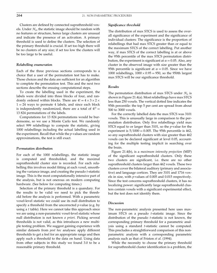
Elsevier UK Chapter: Ch21-P372560 30-9-2006 5:18p.m. Page:264 Trim:7.5in×9.25in
Basal Font:Palatino Margins:Top:40pt Gutter:68pt Font Size:9.5/12 Text Width:42pc Depth:55 Lines
264 21. NON-PARAMETRIC PROCEDURES
Clusters are defined by connected suprathreshold vox-els. Under �0, the statistic image should be random withno features or structure, hence large clusters are unusualand indicate the presence of an activation. A primarythreshold is used to define the clusters. The selection ofthe primary threshold is crucial. If set too high there willbe no clusters of any size; if set too low the clusters willbe too large to be useful.
Relabelling enumeration
Each of the three previous sections corresponds to achoice that a user of the permutation test has to make.Those choices and the data are sufficient for an algorithmto complete the permutation test. This and the next twosections describe the ensuing computational steps.
To create the labelling used in the experiment, thelabels were divided into three blocks of four, and ran-domly ordered within blocks. There are 4! = 4 × 3 × 2 ×1 = 24 ways to permute 4 labels, and since each blockis independently randomized, there are a total of 4!3 =13 824 permutations of the labels.
Computations for 13 824 permutations would be bur-densome, so we use a Monte Carlo test. We randomlyselect 999 relabellings to compute the statistic, giving1000 relabellings including the actual labelling used inthe experiment. Recall that while the p-values are randomapproximations, the test is still exact.
Permutation distribution
For each of the 1000 relabellings, the statistic imageis computed and thresholded, and the maximalsuprathreshold cluster size is recorded. For each rela-belling this involves model fitting at each voxel, smooth-ing the variance image, and creating the pseudo t-statisticimage. This is the most computationally intensive part ofthe analysis, but is not onerous on modern computinghardware. (See below for computing times.)
Selection of the primary threshold is a quandary. Forthe results to be valid we need to pick the thresh-old before the analysis is performed. With a parametricvoxel-level statistic we could use its null distribution tospecify a threshold from the uncorrected p-value (e.g. byusing a t table). Here we cannot take this approach sincewe are using a non-parametric voxel-level statistic whosenull distribution is not known a priori. Picking severalthresholds is not valid, as this introduces a new multi-ple testing problem. We suggest gaining experience withsimilar datasets from post hoc analyses: apply differentthresholds to get a feel for an appropriate range and thenapply such a threshold to the data on hand. Using datafrom other subjects in this study we found 3.0 to be areasonable primary threshold.
Significance threshold
The distribution of max STCS is used to assess the over-all significance of the experiment and the significance ofindividual clusters: The significance is the proportion ofrelabellings that had max STCS greater than or equal tothe maximum STCS of the correct labelling. Put anotherway, if max STCS of the correct labelling is at or abovethe 95th percentile of the max STCS permutation distri-bution, the experiment is significant at � = 0�05. Also, anycluster in the observed image with size greater than the95th percentile is significant at � = 0�05. Since we have1000 relabellings, 1000 × 0�95 = 950, so the 950th largestmax STCS will be our significance threshold.
Results
The permutation distribution of max STCS under �0 isshown in Figure 21.4(a). Most relabellings have max STCSless than 250 voxels. The vertical dotted line indicates the95th percentile: the top 5 per cent are spread from about500 to 3000 voxels.
For the correctly labelled data the max STCS was 3101voxels. This is unusually large in comparison to the per-mutation distribution. Only five relabellings yield maxSTCS equal to or larger than 3101, so the p-value for theexperiment is 5/1000 = 0�005. The 95th percentile is 462,so any suprathreshold clusters with size greater than 462voxels can be declared significant at level 0.05, account-ing for the multiple testing implicit in searching overthe brain.
Figure 21.4(b), is a maximum intensity projection (MIP)of the significant suprathreshold clusters. Only thesetwo clusters are significant, i.e. there are no othersuprathreshold clusters larger than 462 voxels. These twoclusters cover the bilateral auditory (primary and associa-tive) and language cortices. They are 3101 and 1716 vox-els in size, with p-values of 0.005 and 0.015 respectively.Since the test concerns suprathreshold clusters, it has nolocalizing power: significantly large suprathreshold clus-ters contain voxels with a significant experimental effect,but the test does not identify them.
Discussion
The non-parametric analysis presented here uses max-imum STCS on a pseudo t-statistic image. Since thedistribution of the pseudo t-statistic is not known, thecorresponding primary threshold for a parametric anal-ysis using a standard t-statistic cannot be computed.This precludes a straightforward comparison of this non-parametric analysis with a corresponding parametricanalysis such as that of Friston et al. (1994).
While the necessity to choose the primary thresholdfor suprathreshold cluster identification is a problem, the
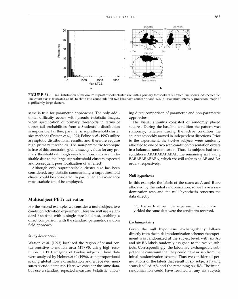
Elsevier UK Chapter: Ch21-P372560 30-9-2006 5:18p.m. Page:265 Trim:7.5in×9.25in
Basal Font:Palatino Margins:Top:40pt Gutter:68pt Font Size:9.5/12 Text Width:42pc Depth:55 Lines
WORKED EXAMPLES 265
FIGURE 21.4 (a) Distribution of maximum suprathreshold cluster size with a primary threshold of 3. Dotted line shows 95th percentile.The count axis is truncated at 100 to show low-count tail; first two bars have counts 579 and 221. (b) Maximum intensity projection image ofsignificantly large clusters.
same is true for parametric approaches. The only addi-tional difficulty occurs with pseudo t-statistic images,when specification of primary thresholds in terms ofupper tail probabilities from a Students’ t-distributionis impossible. Further, parametric suprathreshold clustersize methods (Friston et al., 1994; Poline et al., 1997) utilizeasymptotic distributional results, and therefore requirehigh primary thresholds. The non-parametric techniqueis free of this constraint, giving exact p-values for any pri-mary threshold (although very low thresholds are unde-sirable due to the large suprathreshold clusters expectedand consequent poor localization of an effect).
Although only suprathreshold cluster size has beenconsidered, any statistic summarizing a suprathresholdcluster could be considered. In particular, an exceedancemass statistic could be employed.
Multisubject PET: activation
For the second example, we consider a multisubject, twocondition activation experiment. Here we will use a stan-dard t-statistic with a single threshold test, enabling adirect comparison with the standard parametric randomfield approach.
Study description
Watson et al. (1993) localized the region of visual cor-tex sensitive to motion, area MT/V5, using high reso-lution 3D PET imaging of twelve subjects. These datawere analysed by Holmes et al. (1996), using proportionalscaling global flow normalization and a repeated mea-sures pseudo t-statistic. Here, we consider the same data,but use a standard repeated measures t-statistic, allow-
ing direct comparison of parametric and non-parametricapproaches.
The visual stimulus consisted of randomly placedsquares. During the baseline condition the pattern wasstationary, whereas during the active condition thesquares smoothly moved in independent directions. Priorto the experiment, the twelve subjects were randomlyallocated to one of two scan condition presentation ordersin a balanced randomization. Thus six subjects had scanconditions ABABABABABAB, the remaining six havingBABABABABABA, which we will refer to as AB and BAorders respectively.
Null hypothesis
In this example, the labels of the scans as A and B areallocated by the initial randomization, so we have a ran-domization test, and the null hypothesis concerns thedata directly:
�o: For each subject, the experiment would haveyielded the same data were the conditions reversed.
Exchangeability
Given the null hypothesis, exchangeability followsdirectly from the initial randomization scheme: the exper-iment was randomized at the subject level, with six ABand six BA labels randomly assigned to the twelve sub-jects. Correspondingly, the labels are exchangeable sub-ject to the constraint that they could have arisen from theinitial randomization scheme. Thus we consider all per-mutations of the labels that result in six subjects havingscans labelled AB, and the remaining six BA. The initialrandomization could have resulted in any six subjects
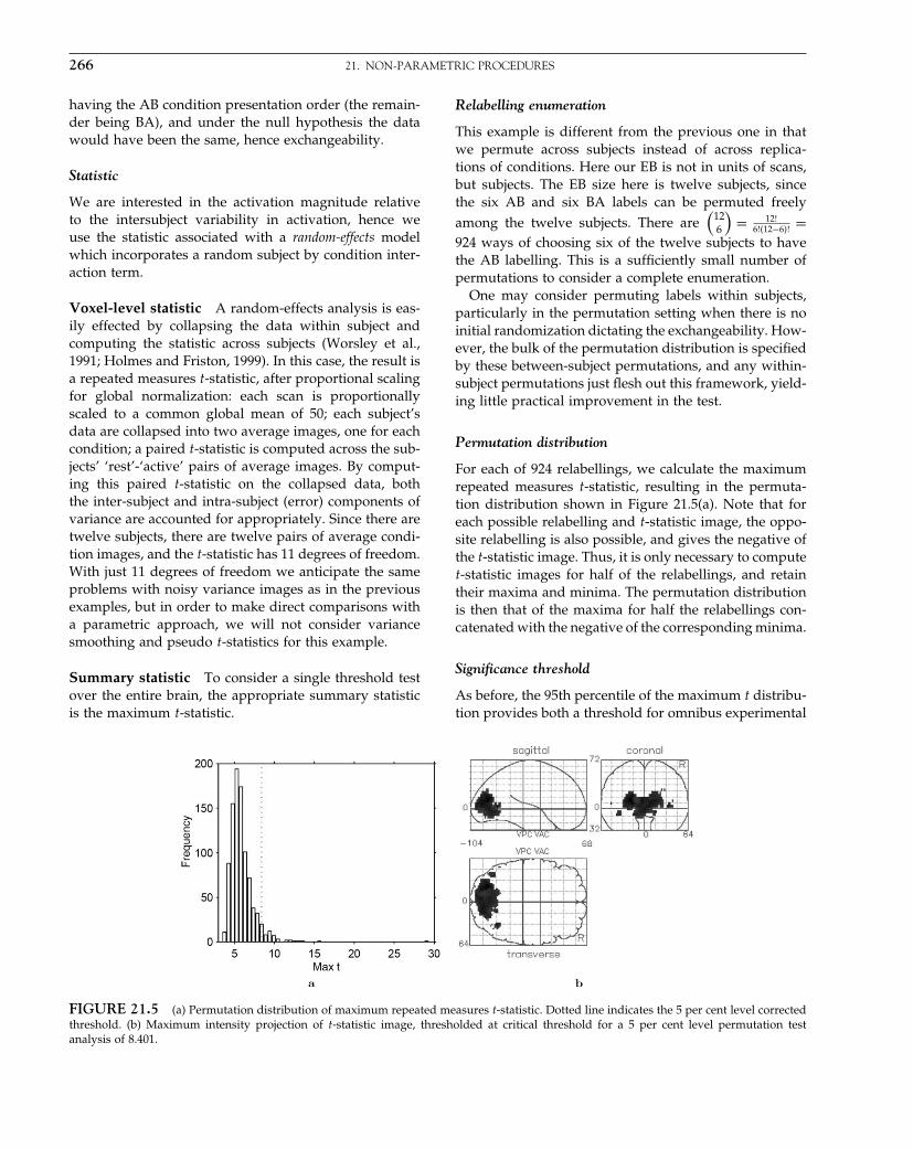
Elsevier UK Chapter: Ch21-P372560 30-9-2006 5:18p.m. Page:266 Trim:7.5in×9.25in
Basal Font:Palatino Margins:Top:40pt Gutter:68pt Font Size:9.5/12 Text Width:42pc Depth:55 Lines
266 21. NON-PARAMETRIC PROCEDURES
having the AB condition presentation order (the remain-der being BA), and under the null hypothesis the datawould have been the same, hence exchangeability.
Statistic
We are interested in the activation magnitude relativeto the intersubject variability in activation, hence weuse the statistic associated with a random-effects modelwhich incorporates a random subject by condition inter-action term.
Voxel-level statistic A random-effects analysis is eas-ily effected by collapsing the data within subject andcomputing the statistic across subjects (Worsley et al.,1991; Holmes and Friston, 1999). In this case, the result isa repeated measures t-statistic, after proportional scalingfor global normalization: each scan is proportionallyscaled to a common global mean of 50; each subject’sdata are collapsed into two average images, one for eachcondition; a paired t-statistic is computed across the sub-jects’ ‘rest’-‘active’ pairs of average images. By comput-ing this paired t-statistic on the collapsed data, boththe inter-subject and intra-subject (error) components ofvariance are accounted for appropriately. Since there aretwelve subjects, there are twelve pairs of average condi-tion images, and the t-statistic has 11 degrees of freedom.With just 11 degrees of freedom we anticipate the sameproblems with noisy variance images as in the previousexamples, but in order to make direct comparisons witha parametric approach, we will not consider variancesmoothing and pseudo t-statistics for this example.
Summary statistic To consider a single threshold testover the entire brain, the appropriate summary statisticis the maximum t-statistic.
Relabelling enumeration
This example is different from the previous one in thatwe permute across subjects instead of across replica-tions of conditions. Here our EB is not in units of scans,but subjects. The EB size here is twelve subjects, sincethe six AB and six BA labels can be permuted freelyamong the twelve subjects. There are
(126
)= 12!
6!�12−6�! =924 ways of choosing six of the twelve subjects to havethe AB labelling. This is a sufficiently small number ofpermutations to consider a complete enumeration.
One may consider permuting labels within subjects,particularly in the permutation setting when there is noinitial randomization dictating the exchangeability. How-ever, the bulk of the permutation distribution is specifiedby these between-subject permutations, and any within-subject permutations just flesh out this framework, yield-ing little practical improvement in the test.
Permutation distribution
For each of 924 relabellings, we calculate the maximumrepeated measures t-statistic, resulting in the permuta-tion distribution shown in Figure 21.5(a). Note that foreach possible relabelling and t-statistic image, the oppo-site relabelling is also possible, and gives the negative ofthe t-statistic image. Thus, it is only necessary to computet-statistic images for half of the relabellings, and retaintheir maxima and minima. The permutation distributionis then that of the maxima for half the relabellings con-catenated with the negative of the corresponding minima.
Significance threshold
As before, the 95th percentile of the maximum t distribu-tion provides both a threshold for omnibus experimental
FIGURE 21.5 (a) Permutation distribution of maximum repeated measures t-statistic. Dotted line indicates the 5 per cent level correctedthreshold. (b) Maximum intensity projection of t-statistic image, thresholded at critical threshold for a 5 per cent level permutation testanalysis of 8.401.
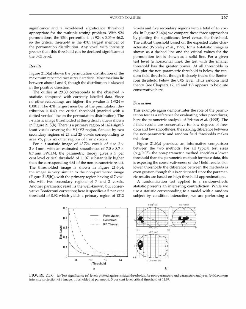
Elsevier UK Chapter: Ch21-P372560 30-9-2006 5:18p.m. Page:267 Trim:7.5in×9.25in
Basal Font:Palatino Margins:Top:40pt Gutter:68pt Font Size:9.5/12 Text Width:42pc Depth:55 Lines
WORKED EXAMPLES 267
significance and a voxel-level significance thresholdappropriate for the multiple testing problem. With 924permutations, the 95th percentile is at 924 × 0�05 = 46�2,so the critical threshold is the 47th largest member ofthe permutation distribution. Any voxel with intensitygreater than this threshold can be declared significant atthe 0.05 level.
Results
Figure 21.5(a) shows the permutation distribution of themaximum repeated measures t-statistic. Most maxima liebetween about 4 and 9, though the distribution is skewedin the positive direction.
The outlier at 29.30 corresponds to the observed t-statistic, computed with correctly labelled data. Sinceno other relabellings are higher, the p-value is 1/924 =0�0011. The 47th largest member of the permutation dis-tribution is 8.40, the critical threshold (marked with adotted vertical line on the permutation distribution). Thet-statistic image thresholded at this critical value is shownin Figure 21.5(b). There is a primary region of 1424 signif-icant voxels covering the V1/V2 region, flanked by twosecondary regions of 23 and 25 voxels corresponding toarea V5, plus six other regions of 1 or 2 voxels.
For a t-statistic image of 43 724 voxels of size 2 ×2 × 4 mm, with an estimated smoothness of 7�8 × 8�7 ×8�7 mm FWHM, the parametric theory gives a 5 percent level critical threshold of 11.07, substantially higherthan the corresponding 4.61 of the non-parametric result.The thresholded image is shown in Figure 21.6(b);the image is very similar to the non-parametric image(Figure 21.5(b)), with the primary region having 617 vox-els, with two secondary regions of 7 and 2 voxels.Another parametric result is the well-known, but conser-vative Bonferroni correction; here it specifies a 5 per centthreshold of 8.92 which yields a primary region of 1212
voxels and five secondary regions with a total of 48 vox-els. In Figure 21.6(a) we compare these three approachesby plotting the significance level versus the threshold.The critical threshold based on the expected Euler char-acteristic (Worsley et al., 1995) for a t-statistic image isshown as a dashed line and the critical values for thepermutation test is shown as a solid line. For a giventest level (a horizontal line), the test with the smallerthreshold has the greater power. At all thresholds inthis plot the non-parametric threshold is below the ran-dom field threshold, though it closely tracks the Bonfer-roni threshold below the 0.05 level. Thus random fieldtheory (see Chapters 17, 18 and 19) appears to be quiteconservative here.
Discussion
This example again demonstrates the role of the permu-tation test as a reference for evaluating other procedures,here the parametric analysis of Friston et al. (1995). Thet field results are conservative for low degrees of free-dom and low smoothness; the striking difference betweenthe non-parametric and random field thresholds makesthis clear.
Figure 21.6(a) provides an informative comparisonbetween the two methods. For all typical test sizes�� ≤ 0�05�, the non-parametric method specifies a lowerthreshold than the parametric method: for these data, thisis exposing the conservativeness of the t field results. Forlower thresholds the difference between the methods iseven greater, though this is anticipated since the paramet-ric results are based on high threshold approximations.
A randomization test applied to a random-effectsstatistic presents an interesting contradiction. While weuse a statistic corresponding to a model with a randomsubject by condition interaction, we are performing a
FIGURE 21.6 (a) Test significance ��� levels plotted against critical thresholds, for non-parametric and parametric analyses. (b) Maximumintensity projection of t image, thresholded at parametric 5 per cent level critical threshold of 11.07.

Elsevier UK Chapter: Ch21-P372560 30-9-2006 5:18p.m. Page:268 Trim:7.5in×9.25in
Basal Font:Palatino Margins:Top:40pt Gutter:68pt Font Size:9.5/12 Text Width:42pc Depth:55 Lines
268 21. NON-PARAMETRIC PROCEDURES
randomization test that technically excludes inference ona population. However, if we assume that the subjects ofthis study constitute a random sample of the populationof interest, we can ignore the experimental randomiza-tion and perform a permutation test, as we do in the nextexample.
Multisubject fMRI: activation
For this third and final example, consider a multisub-ject fMRI activation experiment. Here we will performa permutation test so that we can make inference on apopulation. We will use a smoothed variance t-statisticwith a single threshold test and will make qualita-tive and quantitative comparisons with the parametricresults.
Before discussing the details of this example, we notethat fMRI data present a special challenge for non-parametric methods. Since fMRI data exhibit temporalautocorrelation (Smith et al., 1999), an assumption ofexchangeability of scans within subjects is not tenable.However, to analyse a group of subjects for populationinference, we need only assume exchangeability of sub-jects. Hence, while intrasubject fMRI analyses are notstraightforward with the permutation test, multisubjectanalyses are.
Study description
Marshuetz et al. (2000) studied order effects in workingmemory using fMRI. The data were analysed using arandom-effects procedure (Holmes and Friston, 1999), asin the last example. For fMRI, this procedure amounts toa generalization of the repeated measures t-statistic.
There were 12 subjects, each participating in eightfMRI acquisitions. There were two possible presenta-tion orders for each block, and there was randomizationacross blocks and subjects. The TR was two seconds, atotal of 528 scans collected per condition. Of the study’sthree conditions we consider only two, item recognitionand control. For item recognition, the subject was pre-sented with five letters and, after a two second interval,presented with a probe letter. They were to respond ‘yes’if the probe letter was among the five letters and ‘no’ ifit was not. In the control condition, they were presentedwith five Xs and, two seconds later, presented with eithera ‘y’ or an ‘n’; they were to press ‘yes’ for y and ‘no’for n.
Each subject’s data were analysed, creating a differ-ence image between the item recognition and controleffects. These images were analysed with a one-samplet-test, yielding a random-effects analysis that accountsfor intersubject differences.
Null hypothesis
While this study used randomization within and acrosssubject and hence permits the use of a randomizationtest, we will use a permutation approach to generalizethe results to a population (see above).
Again using a random-effects statistic, we only analyseeach subject’s item versus control difference image. Wemake the weak distributional assumption that the valuesof a subject’s difference images at any given voxel (acrosssubjects) are drawn from a symmetric distribution. (Thedistribution may be different at different voxels, so longas it is symmetric.) The null hypothesis is that these dis-tributions are centred on zero:
�o: The symmetric distributions of the (voxel valuesof the) subjects’ difference images have zero mean.
Exchangeability
The conventional assumption of independent subjectsimplies exchangeability, and hence a single EB consistingof all subjects.
Exchanging the item and control labels has exactlythe effect of flipping the sign of the difference image.So we consider subject labels of ‘+1’ and ‘−1’, indicat-ing an unflipped or flipped sign of the data. Under thenull hypothesis, we have data symmetric about zero, andhence can randomly flip the signs of a subject’s differenceimages.
Statistic
In this example we focus on statistic magnitude.
Voxel-level statistic As noted above, this analysisamounts to a one-sample t-test on the first level differenceimages, testing for a zero-mean effect across subjects.We use a pseudo t-test, with a variance smoothing of4 mm FWHM, comparable to the original within-subjectsmoothing. In our experience, the use of any variancesmoothing is more important than the particular magni-tude (FWHM) of the smoothing.
Summary statistic Again we are interested in search-ing over the whole brain for significant changes, hencewe use the maximum pseudo t.
Relabelling enumeration
Based on our exchangeability under the null hypothesis,we can flip the sign on some or all of our subjects’ data.There are 212 = 4096 possible ways of assigning either ‘+1’or ‘−1’ to each subject. We consider all 4096 relabellings.

Elsevier UK Chapter: Ch21-P372560 30-9-2006 5:18p.m. Page:269 Trim:7.5in×9.25in
Basal Font:Palatino Margins:Top:40pt Gutter:68pt Font Size:9.5/12 Text Width:42pc Depth:55 Lines
WORKED EXAMPLES 269
Permutation distribution
For each relabelling we found the maximum pseudot-statistic, yielding the distribution in Figure 21.7(a). Asin the last example, we have a symmetry in these labels;we need only compute 2048 statistic images and saveboth the maxima and minima.
Significance threshold
With 4096 permutations, the 95th percentile is 4096 ×0�05 = 452�3, and hence the 453rd largest maxima definesthe 0.05 level corrected significance threshold.
Results
The permutation distribution of the maximum pseudot-statistic under �0 is shown in Figure 21.7(a). It is cen-
tred around 4.5 and is slightly positively skewed; allmaxima found were between about 3 and 8.
The correctly labelled data yielded the largest maxi-mum, 8.471. Hence the overall significance of the exper-iment is 1/4096 = 0�0002. The dotted line indicates the0.05 corrected threshold, 5.763. Figure 21.7(b) shows thethresholded maximum intensity projection (MIP) of sig-nificant voxels. There are 312 voxels in eight distinctregions; in particular there are bilateral posterior parietalregions, a left thalamic region and an anterior cingu-late region; these are typical of working memory studies(Marshuetz et al., 2000).
It is informative to compare this result to the traditionalt-statistic, using both a non-parametric and parametricapproach to obtain corrected thresholds. We reran thisnon-parametric analysis using no variance smoothing.The resulting thresholded data is shown in Figure 21.7(c);
FIGURE 21.7 (a) Permutation distribution of maximum repeated-measures t-statistic. Dotted line indicates the 5 per cent level correctedthreshold. (b) Maximum intensity projection of pseudo t-statistic image threshold at 5 per cent level, as determined by permutation distribution.(c) Maximum intensity projection of t-statistic image threshold at 5 per cent level as determined by permutation distribution. (d) Maximumintensity projection of t-statistic image threshold at 5 per cent level as determined by random field theory.

Elsevier UK Chapter: Ch21-P372560 30-9-2006 5:18p.m. Page:270 Trim:7.5in×9.25in
Basal Font:Palatino Margins:Top:40pt Gutter:68pt Font Size:9.5/12 Text Width:42pc Depth:55 Lines
270 21. NON-PARAMETRIC PROCEDURES
TABLE 21-1 Comparison of four inference methods for the item recognition fMRI data. The minimum corrected p-value andnumber of significant voxels give an overall measure of sensitivity; corrected thresholds can only be compared within statistic type.For these data, the Bonferroni and random field results are very similar, and the non-parametric methods are more powerful; thenon-parametric t method detects 10 times as many voxels as the parametric method, and the non-parametric pseudo t detects 60
times as many
StatisticInferencemethod
Corrected threshold Minimumcorrected
Number ofsignificant
t Pseudo t p-value voxels
t Random field 9�870 0�0062 5t Bonferroni 9�802 0�0025 5t Permutation 7�667 0�0002 58Pseudo t Permutation 5�763 0�0002 312
there are only 58 voxels in three regions that exceededthe corrected threshold of 7.667. Using standard para-metric random field methods produced the result inFigure 21.7(d). For 110 776 voxels of size 2 × 2 × 2 mm,with an estimated smoothness of 5�1 × 5�8 × 6�9 mmFWHM, the parametric theory finds a threshold of 9.870;there are only five voxels in three regions above thisthreshold. Note that only the pseudo t-statistic detectsthe bilateral parietal regions. Table 21-1 summarizes thethree analyses along with the Bonferroni result.
Discussion
In this example, we have demonstrated the utility of thenon-parametric method for intersubject fMRI analyses.Based only on independence of the subjects and sym-metric distribution of difference images under the nullhypothesis, we can create a permutation test that yieldsinferences on a population.
Multiple subject fMRI studies often have few subjects,many fewer than 20 subjects. By using the smoothed vari-ance t-statistic we have gained sensitivity, relative to thestandard t-statistic. Even with the standard t-statistic, thenon-parametric test proved more powerful, detecting fivetimes as many voxels as active. Although the smoothedvariance t is statistically valid, it does not overcome anylimitations of face validity of an analysis based on only12 subjects.
We note that this relative ranking of sensitivity (non-parametric pseudo t, non-parametric t, parametric t) isconsistent with the other second-level data sets we haveanalysed. We believe this is due to a conservativeness ofthe random t-field results under low degrees of freedom.
Discussion of examples
These examples have demonstrated the non-parametricpermutation test for PET and fMRI with a variety ofexperimental designs and analyses. We have addressed
each of the steps in sufficient detail to follow the algo-rithmic steps that the SPM software performs. We haveshown that the ability to utilize smoothed variances viaa pseudo t-statistic can offer increased power over a cor-responding standard t-statistic image. Using standard t-statistics, we have seen how the permutation test can beused as a reference against which parametric results canbe validated.
However, note that the comparison between paramet-ric and non-parametric results must be made very care-fully. Comparable models and statistics must be used,and multiple testing procedures with the same degreeof control over image-wise type I error used. Further,since the permutation distributions are derived from thedata, critical thresholds are specific to the data set underconsideration. Although the examples presented aboveare compelling, it should be remembered that these areonly a few specific examples. However, the points notedfor these specific examples are indicative of our generalexperience with these methods.
Finally, while we have noted that the non-parametricmethod has greater computational demands than para-metric methods, they are reasonable on modern hard-ware. The PET examples presented here would takeabout 5 minutes on a typical desktop PC, while the fMRIexample could take longer, as much as 20 minutes due tomore permutations (2048 versus. 500) and larger images.
CONCLUSIONS
In this chapter, the theory and practicalities of non-parametric randomization and permutation tests forfunctional neuroimaging experiments have been pre-sented and illustrated with worked examples.
As has been demonstrated, the permutation approachoffers various advantages. The methodology is intuitiveand accessible. With suitable maximal summary statis-tics, the multiple testing problem can be accounted for
Elsevier UK Chapter: Ch21-P372560 30-9-2006 5:18p.m. Page:271 Trim:7.5in×9.25in
Basal Font:Palatino Margins:Top:40pt Gutter:68pt Font Size:9.5/12 Text Width:42pc Depth:55 Lines
REFERENCES 271
easily; only minimal assumptions are required for validinference, and the resulting tests are almost exact, withsize at most 1/N less than the nominal test level �, whereN is the number of relabellings.
The non-parametric permutation approaches describedgive results similar to those obtained from a com-parable statistical parametric mapping approach usinga general linear model with multiple testing correc-tions derived from random field theory. In this respect,these non-parametric techniques can be used to verifythe validity of less computationally expensive paramet-ric approaches. When the assumptions required for aparametric approach are not met, the non-parametricapproach described provides a viable alternative.
In addition, the approach is flexible. Choice of voxeland summary statistic are not limited to those whose nulldistributions can be derived from parametric assump-tions. This is particularly advantageous at low degreesof freedom, when noisy variance images lead to noisystatistic images and multiple testing procedures basedon the theory of continuous random fields are conserva-tive. By assuming a smooth variance structure, and usinga pseudo t-statistic computed with smoothed variances,the permutation approach gains considerable power.
Therefore, the non-parametric permutation approachshould be considered for experimental designs withlow degrees of freedom. These include small-samplesize problems, such as single-subject PET/SPECT (sin-gle photon emission computed tomography), but alsoPET/SPECT and fMRI multisubject and between-groupanalyses involving small numbers of subjects, whereanalysis must be conducted at the subject level to accountfor intersubject variability. It is our hope that this chapter,and the accompanying software, will encourage appro-priate application of these non-parametric techniques.
REFERENCES
Arndt S, Cizadlo T, Andreasen NC et al. (1996) Tests for compar-ing images based on randomization and permutation methods.J Cereb Blood Flow Metab 16: 1271–79
Belmonte M, Yurgelun-Todd D (2001) Permutation testing madepractical for functional magnetic resonance image analysis. IEEETrans Med Imag 20: 243–48
Brammer MJ, Bullmore ET, Simmons A et al. (1997) Generic brainactivation mapping in functional magnetic resonance imaging:a nonparametric approach. Mag Res Med 15: 763–70
Bullmore E, Brammer M, Williams SCR et al. (1996) Statistical meth-ods of estimation and inference for functional MR image analy-sis. Mag Res Med 35: 261–77
Bullmore E, Long C, Suckling J (2001) Colored noise and com-putational inference in neurophysiological (fMRI) time seriesanalysis: resampling methods in time and wavelet domains.Hum Brain Mapp 12: 61–78
Bullmore ET, Suckling J, Overmeyer S et al. (1999) Global, voxel,and cluster tests, by theory and permutation, for a differencebetween two groups of structural MR images of the brain. IEEETrans Med Imag 18: 32–42
Cao J (1999) The size of the connected components of excursion setsof �2� t and f fields. Adv Appl Prob 31: 577–93
Dwass M (1957) Modified randomization tests for nonparametrichypotheses. Ann Math Stat 28: 181–87
Edgington ES (1964) Randomization tests. J Psychol 57: 445–49Edgington ES (1969a) Approximate randomization tests. J Psychol
72: 143–49Edgington ES (1969b) Statistical inference: the distribution free approach.
McGraw-Hill, New YorkEdgington ES (1995) Randomization tests, 3rd edn. Marcel Dekker,
New YorkFadili J, Bullmore ET (2001) Wavelet-generalised least squares: a
new blu estimator of regression models with long-memoryerrors. NeuroImage 15: 217–32
Fisher RA (1935) The design of experiments. Oliver, Boyd, EdinburghFisher RA, Bennett JH (1990) Statistical methods, experimental design,
and scientific inference. Oxford University Press, OxfordForman SD, Cohen JD, Fitzgerald M et al. (1995) Improved assess-
ment of significant activation in functional magnetic resonanceimaging (fMRI): use of a cluster-size threshold. Mag Res Med 33:636–47
Friman O, Westin CF (2005) Resampling FMRI time series. NeuroIm-age 25: 859–67
Friston KJ, Frith CD, Liddle PF et al. (1991) Comparing functional(PET) images: the assessment of significant change. J Cereb BloodFlow Metab 11: 690–99
Friston KJ, Holmes AP, Poline J-B et al. (1996) Detecting activationsin PET and fMRI: levels of inference and power. NeuroImage 4:223–35
Friston KJ, Holmes AP, Worsley KJ et al. (1995) Statistical parametricmaps in functional imaging: a general linear approach. HumBrain Mapp 2: 189–210
Friston KJ, Worsley KJ, Frackowiak RSJ et al. (1994) Assessing thesignificance of focal activations using their spatial extent. HumBrain Mapp 1: 214–20
Good P (1994) Permutation tests. A practical guide to resampling methodsfor testing hypotheses. Springer-Verlag, New York
Grabowski TJ, Frank RJ, Brown CK et al. (1996) Reliability of PETactivation across statistical methods, subject groups, and samplesizes. Hum Brain Mapp, 4: 23–46
Halber M, Herholz K, Wienhard K et al. (1997) Performance of arandomization test for single-subject 15-O-water PET activationstudies. J Cereb Blood Flow Metab 17: 1033–39
Heckel D, Arndt S, Cizadlo T et al. (1998) An efficient procedurefor permutation tests in imaging research. Comput Biomed Res31: 164–71
Holmes AP (1994) Statistical issues in functional brain mapping.PhD thesis, University of Glasgow, Glasgow. Available fromhttp://www.fil.ion.ucl.ac.uk/spm/papers/APH_thesis
Holmes AP, Blair RC, Watson JDG et al. (1996) Nonparametric anal-ysis of statistic images from functional mapping experiments.J Cereb Blood Flow Metab 16: 7–22
Holmes AP, Friston KJ (1999) Generalisability, random effects &population inference. NeuroImage 7: S754
Elsevier UK Chapter: Ch21-P372560 30-9-2006 5:18p.m. Page:272 Trim:7.5in×9.25in
Basal Font:Palatino Margins:Top:40pt Gutter:68pt Font Size:9.5/12 Text Width:42pc Depth:55 Lines
272 21. NON-PARAMETRIC PROCEDURES
Holmes AP, Watson JDG, Nichols TE (1998) Holmes & Watson, on‘Sherlock’. Cereb Blood Flow Metab 18: S697 Letter to the editor,with reply.
Jöckel K-H (1986) Finite sample properties and asymptotic efficiencyof monte-carlo tests. Ann Stat 14: 336–47
Kendall M, Gibbons JD (1990) Rank correlation methods, 5th edn.Edward Arnold, London
Locascio JJ, Jennings PJ, Moore CI et al. (1997) Time series analy-sis in the time domain and resampling methods for studies offunctional magnetic resonance brain imaging. Hum Brain Mapp5: 168–93
Logan BR, Rowe DB (2004) An evaluation of thresholding tech-niques in FMRI analysis. NeuroImage 22: 95–108
Manly BFJ (1997) Randomization, bootstrap and Monte-Carlo methodsin biology. Chapman & Hall, London
Marshuetz C, Smith EE, Jonides J et al. (2000) Order informationin working memory: fMRI evidence for parietal and prefrontalmechanisms. J Cogn Neurosci 12/S2: 130–44
Nichols TE, Hayasaka S (2003) Controlling the familywise error ratein functional neuroimaging: a comparative review. Stat MethMed Res 12: 419–46
Nichols TE, Holmes AP (2001) Nonparametric permutation tests forfunctional neuroimaging: a primer with examples. Hum BrainMapp 15: 1–25
Pitman EJG (1937a) Signficance tests which may be applied to sam-ples from any population. J R Stat Soc (Suppl) 4: 119–30
Pitman EJG (1937b) Signficance tests which may be applied to sam-ples from any population. II. The correlation coefficient test.J R Stat Soc (Suppl) 4: 224–32
Pitman EJG (1937c) Signficance tests which may be applied to sam-ples from any population. III. The analysis of variance test.Biometrika 29: 322–35
Poline JB, Mazoyer BM (1993) Analysis of individual positron emis-sion tomography activation maps by detection of high signal-to-noise-ratio pixel clusters. J Cereb Blood Flow Metab 13: 425–37
Poline JB, Worsley KJ, Evans AC et al. (1997) Combining spatialextent and peak intensity to test for activations in functionalimaging. NeuroImage 5: 83–96
Raz J, Zheng H, Ombao H et al. (2003) Statistical tests for FMRIbased on experimental randomization. NeuroImage 19: 226–32
Roland PE, Levin B, Kawashima R et al. (1993) Three-dimensionalanalysis of clustered voxels in 15-o-butanol brain activationimages. Hum Brain Mapp 1: 3–19
Silbersweig DA, Stern E, Frith C et al. (1995) A functional neu-roanatomy of hallucinations in schizophrenia. Nature 378: 167–69
Silbersweig DA, Stern E, Schnorr L et al. (1994) Imaging tran-sient, randomly occurring neuropsychological events in single-subjects with positron emission tomography: an event-relatedcount rate correlational analysis. J Cereb Blood Flow Metab 14:771–82
Smith AM, Lewis BK, Ruttimann UE et al. (1999) Investigation oflow frequency drift in FMRI signal. NeuroImage 9: 526–33
Watson JDG, Myers R, Frackowiak RSJ et al. (1993) Area v5 of thehuman brain: evidence from a combined study using positronemission tomography and magnetic resonance imaging. CerebCort 3: 79–94
Westfall PH, Young SS (1993) Resampling-based multiple testing: exam-ples and methods for p-value adjustment. John Wiley & Sons Inc,New York
Worsley KJ (1994) Local maxima and the expected Euler charac-teristic of excursion sets of �2, f and t fields. Adv Appl Prob26: 13–42
Worsley KJ (1996) The geometry of random images. Chance 9: 27–40Worsley KJ, Evans AC, Marrett S et al. (1992) A three-dimensional
statistical analysis for CBF activation studies in human brain.J Cereb Blood Flow Metab 12: 1040–42. See comment in J CerebBlood Flow Metab 13: 1040–42.
Worsley KJ, Evans AC, Strother SC et al. (1991) A linear spatialcorrelation model, with applications to positron emission tomog-raphy. J Am Stat Assoc 86: 55–67
Worsley KJ, Marrett S, Neelin P et al. (1995) A unified statisticalapproach for determining significant signals in images of cere-bral activation. Hum Brain Mapp 4: 58–73
Yekutieli D, Benjamini Y (1999) Resampling-based false discov-ery rate controlling multiple test procedures for correlated teststatistics. J Stat Plann Inference 82: 171–96
Elsevier UK Chapter: Ch22-P372560 30-9-2006 5:20p.m. Page:275 Trim:7.5in×9.25in
Basal Font:Palatino Margins:Top:40pt Gutter:68pt Font Size:9.5/12 Text Width:42pc Depth:55 Lines
C H A P T E R
22
Empirical Bayes and hierarchical modelsK. Friston and W. Penny
INTRODUCTION
Bayesian inference plays a central role in many imagingneuroscience applications. Empirical Bayes is the estima-tion and inference framework associated with a Bayesiantreatment of hierarchical models. Empirical Bayes and theinversion of hierarchical models can almost be regardedas the same thing. Empirical Bayes is important becausenearly all the models we use in neuroimaging have someexplicit or implicit hierarchical structure. Bayesian infer-ence will play an increasing role in subsequent chaptersand rests on the equality:
p���y� = p�y���p��� 22.1
The first term specifies a generative model and an asso-ciated energy function, which we usually try to optimizewith respect to the parameters of the model �, given somedata y. The model is specified in terms of the second twoterms; the likelihood p�y��� and prior p(�). However, inhierarchical models there are conditional independencesamong the model parameters that mean the probabilitieson the right factorize:
p���y� = p�y���1��p���1����2��� � � � � p���n�� 22.2
There are many examples of these models, ranging fromMarkov models of hidden states that evolve over timeto complicated graphical models, in which the parame-ters at one level control the distribution of parametersat lower levels, sometimes in a non-linear and possiblytime-varying fashion. In this chapter, we will be lookingat relatively simple hierarchical linear models. Irrespec-tive of the exact form of hierarchical models, they allhave intermediate terms p���i����i+1��. These are empiricalpriors. They have an ambiguous role that is intermedi-ate between the likelihood and priors (i.e. the first andlast terms). On the one hand, like a full prior, they pro-vide constraints on ��i�, on the other, they specify the
likelihood of ��i�, given ��i+1�. This means the empiricalpriors depend on ��i+1�, which has to be inferred from thedata, hence empirical Bayes. Empirical Bayes is criticalto model specification and inversion because empiricalpriors embody formal constraints on the generation ofobserved data and these constraints can be used in apowerful way. The chapters in this section try to illus-trate this point, starting with simple hierarchies of lin-ear models and ending with complicated and informedspatio-temporal models of functional magnetic resonanceimaging (fMRI) time-series.
This chapter revisits hierarchical observation models(see Chapter 11) used in functional neuroimaging. Itemphasizes the common ground shared by classical andBayesian methods to show that conventional analysesof neuroimaging data can be usefully extended withinan empirical Bayesian framework. In particular, we for-mulate the procedures used in conventional data analy-sis in terms of hierarchical linear models and establisha connection between classical inference and paramet-ric empirical Bayes (PEB) through covariance componentestimation. This estimation is based on expectation max-imization or EM (see Appendix 3). Hierarchical modelsnot only provide for inference at the highest level, butallow one to revisit lower levels, to make Bayesian infer-ences. Bayesian inferences eschew many of the difficul-ties encountered with classical inference and characterizebrain responses in a way that is more directly related towhat one is interested in.
We start with a theoretical summary and then dealwith applications of the theory to a range of issues inneuroimaging. These include: estimating non-sphericityor variance components in fMRI time-series that can arisefrom serial correlations within subject, or are inducedby multisubject (i.e. hierarchical) studies; Bayesian mod-els for imaging data, in which effects at one voxel areconstrained by responses in others (see Chapters 23 and25); and Bayesian estimation of dynamic models of brain
Statistical Parametric Mapping, by Karl Friston et al. Copyright 2007, Elsevier Ltd. All rights reserved.ISBN–13: 978-0-12-372560-8 ISBN–10: 0-12-372560-7
275

Elsevier UK Chapter: Ch22-P372560 30-9-2006 5:20p.m. Page:276 Trim:7.5in×9.25in
Basal Font:Palatino Margins:Top:40pt Gutter:68pt Font Size:9.5/12 Text Width:42pc Depth:55 Lines
276 22. EMPIRICAL BAYES AND HIERARCHICAL MODELS
responses (see Chapter 34). Although diverse, all theseestimation and inference problems are accommodated bythe framework described next.
Classical and Bayesian inference
Since its inception, statistical parametric mapping (SPM)has proved useful for characterizing neuroimaging datasequences. However, SPM is limited because it is basedon classical inference procedures. In this chapter, weintroduce a more general framework, which places SPMin a broader context and points to alternative ways ofcharacterizing and making inferences about regionallyspecific effects in neuroimaging. In particular, we formu-late the procedures used in conventional data analysis interms of hierarchical linear models and establish the con-nection between classical inference and empirical Bayesianinference through covariance component estimation. Thisestimation is based on the expectation maximization (orEM) algorithm.
Statistical parametric mapping entails the use of thegeneral linear model and classical statistics, under para-metric assumptions, to create a statistic (usually thet-statistic) at each voxel. Inferences about regionally spe-cific effects are based on the ensuing image of t-statistics,the SPM�t�. The requisite distributional approximationsfor the peak height, or spatial extent, of voxel clus-ters, surviving a specified threshold, are derived usingGaussian random field theory (see Part 3). Random fieldtheory enables the use of classical inference procedures,and the latitude afforded by the general linear model,to give a powerful and flexible approach to continuous,spatially extended data. It does so by protecting againstfamily-wise false positives over all the voxels that consti-tute a search volume, i.e. it provides a way of adjustingthe p-values, in the same way that a Bonferroni correc-tion does for discrete data (Worsley, 1994; Friston et al.,1995).
Despite its success, statistical parametric mapping hasa number of limitations: the p-value, ascribed to a topo-logical feature of the SPM, does not reflect the likelihoodthat the effect is present but simply the probability ofgetting the feature in the effect’s absence. There are sev-eral shortcomings to this classical approach. First, onecan never reject the alternate hypothesis (i.e. say that anactivation has not occurred) because the probability thatan effect is exactly zero is itself zero. This is problem-atic, for example, in trying to establish double dissocia-tions or indeed functional segregation; one can never sayone area responds to colour but not motion and anotherresponds to motion but not colour. Secondly, because theprobability of an effect being zero is vanishingly small,given enough scans or subjects one can always demon-
strate a significant effect at every voxel. This fallacy ofclassical inference is relevant practically, with the thou-sands of scans that enter some fixed-effect analyses offMRI data. The issue here is that trivially small activa-tions can be declared significant if there are sufficientdegrees of freedom to render their estimated variabilitysmall enough. A third problem, which is specific to SPM,is the correction or adjustment applied to the p-valuesto resolve the multiple comparison problem. This hasthe somewhat nonsensical effect of changing the infer-ence about one part of the brain in a way that dependson whether another part is examined. Put simply, thethreshold increases with search volume, rendering infer-ence very sensitive to what it encompasses. Clearly, theprobability that any voxel has activated does not changewith the search volume and yet the p-value does.
All these problems would be eschewed by using theprobability that a voxel had activated, or indeed its acti-vation was greater than some threshold. This sort of infer-ence is precluded by classical approaches, which simplygive the likelihood of getting the data, given no effect. Whatone would like is the probability of the effect given thedata. This is the posterior probability used in Bayesianinference. The Bayesian approach to significance testingin functional neuroimaging was introduced by AndrewHolmes and Ian Ford (Holmes and Ford, 1993) four yearsafter SPM was invented. The Bayesian approach requiresboth the likelihood, afforded by assumptions about thedistribution of errors, and the prior probability of acti-vation. These priors can enter as known values or canbe estimated from the data, provided we have observedmultiple instances of the effect we are interested in. Thelatter is referred to as empirical Bayes and rests upon ahierarchical observation model. In many situations we doassess the same effect over different subjects, or indeeddifferent voxels, and are in a position to adopt empiri-cal Bayes. This chapter describes one such approach. Incontrast to other proposals, this approach is not a novelway of analysing neuroimaging data. The use of Bayesfor fMRI data has been usefully explored elsewhere (e.g.spatio-temporal Markov field models, Descombes et al.,1998; and mixture models, Everitt and Bullmore, 1999).See also Hartvig and Jensen (2000) who combine boththese approaches and Højen-Sørensen et al. (2000) whofocus on temporal aspects with hidden Markov models.Generally, these approaches assume that voxels are eitheractive or not and use the data to infer their status. Becauseof this underlying assumption, there is little connectionwith conventional models that allow for continuous orparametric responses. Our aim here is to highlight thefact that conventional models we use routinely conformto hierarchical observation models that can be treated ina Bayesian fashion. The importance of this rests on theconnection between classical and Bayesian inference and

Elsevier UK Chapter: Ch22-P372560 30-9-2006 5:20p.m. Page:277 Trim:7.5in×9.25in
Basal Font:Palatino Margins:Top:40pt Gutter:68pt Font Size:9.5/12 Text Width:42pc Depth:55 Lines
THEORETICAL BACKGROUND 277
the use of Bayesian procedures that are overlooked froma classical perspective. For example, random-effect anal-yses of fMRI data (Holmes and Friston, 1998, and seeChapter 12) adopt two-level hierarchical models. In thiscontext, people generally focus on classical inference atthe second level, unaware that the same model can sup-port Bayesian inference at the first. Revisiting the firstlevel, within a Bayesian framework, provides a muchbetter characterization of single-subject responses, bothin terms of the estimated effects and the nature of theinference. We will see an example of this later.
Overview
The aim of the first section below is to describe hier-archical observation models and establish the relation-ship between classical maximum likelihood (ML) andempirical Bayes estimators. Parametric empirical Bayescan be formulated in terms of covariance componentestimation (e.g. within-subject versus between-subjectcontributions to error). The covariance component for-mulation is important because it is ubiquitous in fMRIand electroencephalography (EEG). Different sources ofvariability in the data induce non-sphericity that has tobe estimated before any inferences about an effect canbe made. Important sources of non-sphericity includeserial or temporal correlations among errors in single-subject studies, or in multisubject studies, the differencesbetween within- and between-subject variability. Theseissues are used in the second section to emphasize boththe covariance component estimation and Bayesian per-spectives, in terms of the difference between responseestimates based on classical maximum likelihood estima-tors and the conditional expectations or modes, using aBayesian approach.
In the next chapter, we use the same theory to elaboratehierarchical models that allow the construction of pos-terior probability maps. Again, this employs two-levelmodels but focuses on Bayesian inference at the firstlevel. It complements the preceding fMRI application byshowing how global shrinkage priors can be estimatedusing observations over voxels at the second level. Thisis a special case of more sophisticated hierarchical mod-els of fMRI data presented in Chapter 25, which uselocal shrinkage priors to enforce spatial constraints onthe inversion.
THEORETICAL BACKGROUND
In this section, we focus on theory and procedures. Thekey points are reprised in subsequent sections where
they are illustrated using real and simulated data. Thissection describes how the parameters and hyperparame-ters of a hierarchical model can be estimated given data.The distinction between a parameter and a hyperparam-eter depends on the context established by the infer-ence. Here, parameters are quantities that determine theexpected response, which is observed. Hyperparameterspertain to the probabilistic behaviour of the parameters.Perhaps the simplest example is provided by a single-sample t-test. The parameter of interest is the true effectcausing the observations to differ from zero. The hyper-parameter corresponds to the variance of the observa-tion error (usually denoted by 2). Note that one canestimate the parameter, with the sample mean, withoutknowing the hyperparameter. However, if one wantedto make an inference about the estimate, it is necessary toknow (or estimate using the residual sum of squares) thehyperparameter. In this chapter, all the hyperparametersare simply variances of different quantities that causethe measured response (e.g. within-subject variance andbetween-subject variance).
The aim of this section is to show the close relationshipbetween Bayesian and maximum likelihood estimationimplicit in conventional analyses of imaging data, usingthe general linear model. Furthermore, we want to placeclassical and Bayesian inference within the same frame-work. In this way, we show that conventional analysesare special cases of a more general parametric empiricalBayes (PEB) approach. First, we reprise hierarchical lin-ear observation models that form the cornerstone of theensuing estimation procedures. These models are thenreviewed from the classical perspective of estimating themodel parameters using maximum likelihood (ML) andstatistical inference using the t-statistic. The same modelis then considered in a Bayesian light to make an impor-tant point: the estimated error variances, at any level,play the role of priors on the variability of the parame-ters in the level below. At the highest level, the ML andBayes estimators are the same.
Both classical and Bayesian approaches rest uponcovariance component estimation using EM. This isdescribed briefly and presented in detail in Appendix 3.The EM algorithm is related to that described inDempster et al. (1981), but extended to cover hierarchicalmodels with any number of levels. For an introductionto EM in generalized linear models, see Fahrmeir andTutz (1994). This text provides an exposition of EM andPEB in linear models, usefully relating EM to classicalmethods (e.g. restricted maximum likelihood (ReML)).For an introduction to Bayesian statistics see Lee (1997).This text adopts a more explicit Bayesian perspectiveand again usefully connects empirical Bayes with classi-cal approaches, e.g. the Stein ‘shrinkage’ estimator andempirical Bayes estimators used below (Lee, 1997). In

Elsevier UK Chapter: Ch22-P372560 30-9-2006 5:20p.m. Page:278 Trim:7.5in×9.25in
Basal Font:Palatino Margins:Top:40pt Gutter:68pt Font Size:9.5/12 Text Width:42pc Depth:55 Lines
278 22. EMPIRICAL BAYES AND HIERARCHICAL MODELS
many standard texts the hierarchical models consideredhere are referred to as random-effects models.
Hierarchical linear models
We will deal with hierarchical linear observation modelsof the form:
y = X�1���1� +�1�
��1� = X�2���2� +�2�
���
��n−1� = X�n���n� +�n�
22.3
under Gaussian assumptions about the errors �i� ∼N�0�C�i�
�. The response variable, y, is usually observedboth within units over time and over several units (e.g.subject or voxels). X�i� are specified [design] matricescontaining explanatory variables or constraints on theparameters ��i−1� of the level below. If the hierarchicalmodel has only one level, it reduces to the familiar gen-eral linear model employed in conventional data anal-ysis (see Chapter 8). Two-level models will be familiarto readers who use mixed- or random-effects analyses.In this instance, the first-level design matrix models theactivation effects, over scans within subjects, in a subject-separable fashion (i.e. in partitions constituting the blocksof a block diagonal matrix). The second-level designmatrix models the subject-specific effects over subjects.Usually, but not necessarily, the design matrices are blockdiagonal matrices where each block models the observa-tions in each unit at that level (e.g. session, subject orgroup).
X�i� =
⎡⎢⎢⎢⎢⎣
X�i�1 0 · · · 00 X�i�
2���
� � �
0 X�i�J
⎤⎥⎥⎥⎥⎦ 22.4
Some examples are shown in Figure 22.1 (these examplesare used in the next section). The design matrix at anylevel has as many rows as the number of columns inthe design matrix of the level below. One can envisagethree-level models, which embody activation effects inscans modelled for each session, effects expressed in eachsession modelled for each subject and, finally, effects oversubjects.
The Gaussian or parametric assumptions, implicit inthese models, imply that all the random sources ofvariability, in the observed response, have a Gaussiandistribution. This is appropriate for most models in neu-roimaging and makes the relationship between classical
Hierarchical form
1st level y X (1)
2nd level θ (1) θ
(2)
θ (1)
ε (2)
ε (1)
= X
(2) +
y = + ε (1)
θ(2)
ε(2)
Non-hierarchical form
],[ )2()1()1( XXX
+=
FIGURE 22.1 Schematic showing the form of the design matri-ces in a two-level model and how the hierarchical form (upperpanel) can be reduced to a non-hierarchical form (lower panel).The design matrices are shown in image format with an arbitrarycolour scale. The response variable, parameters and error terms aredepicted as plots. In this example there are four subjects or unitsobserved at the first level. Each subject’s response is modelled withthe same three effects, one of these being a constant term. Thesedesign matrices are part of those used in Friston et al. (2002b) togenerate simulated fMRI data and are based on the design matricesused in the subsequent empirical event-related fMRI analyses.
approaches and Bayesian treatments (that can be general-ized to non-Gaussian densities) much more transparent.
Technically, models that conform to Eqn. 22.3 fallinto the class of conditionally independent hierarchi-cal models when the response variables and parame-ters are independent across units, conditionally on thehyperparameters controlling the error terms (Kass andSteffey, 1989). These models are also called parametricempirical Bayes (PEB) models because the obvious inter-pretation of the higher-level densities as priors led tothe development of PEB methodology (Efron and Mor-ris, 1973). Although the procedures considered in thischapter accommodate general models that are not condi-tionally independent, we refer to the Bayesian proceduresbelow as PEB because the motivation is identical and
Elsevier UK Chapter: Ch22-P372560 30-9-2006 5:20p.m. Page:279 Trim:7.5in×9.25in
Basal Font:Palatino Margins:Top:40pt Gutter:68pt Font Size:9.5/12 Text Width:42pc Depth:55 Lines
THEORETICAL BACKGROUND 279
most of the examples assume conditional independence.Having posited a model with a hierarchical form, the aimis to estimate its parameters and make some inferencesabout these estimates using their estimated variabilityor, more generally, find the posterior or conditional den-sity of its parameters. In classical inference, one is usu-ally only interested in inference about the parameters atthe highest level to which the model is specified. In aBayesian context, the highest level is regarded as provid-ing constraints or empirical priors that enable posteriorinferences about the parameters in lower levels. Identi-fying the system of equations in Eqn. 22.3 can proceedunder two perspectives that are formally identical: a clas-sical statistical perspective and a Bayesian one.
After recursive substitution, to eliminate all but thefinal level parameters, Eqn. 22.3 can be written as:
y = �1� +X�1��2� +· · ·+X�1�� � � X�n−1��n� +X�1�� � � X�n���n�
22.5
In this non-hierarchical form the components of theresponse comprise linearly separable contributions fromall levels. Those components are referred to as randomeffects C̃ where the last-level parameters enter as fixedeffects. The covariance partitioning implied by Eqn. 22.5is:
E�yyT � = C̃ +X�1�� � � X�n���n���n�T X�n�T � � � X�1�T
C̃ =C�1� +· · ·+X�1�� � � X�n−1�C�i�
X�n−1�T � � � X�1�T22.6
where C�i� is the covariance of ��i�. If only one level is spec-
ified, the random effects vanish and a fixed-effect analysisensues. If n is greater than one, the analysis correspondsto a random-effect analysis (or more exactly a mixed-effectanalysis that includes random terms). Eqn. 22.5 can beinterpreted in two ways that form respectively the basisfor a classical:
y = X̃��n� + ̃
X̃ =X�1�X�2�� � � X�n� 22.7
̃ =�1� +X�1��2� +· · ·+X�1�X�2�� � � X�n−1��n�
and Bayesian estimation:
y =X� +�1�
X = [X�1�� � � � �X�1�X�2�� � � X�n−1��X�1�X�2�� � � X�n�]
22.8
� =
⎡⎢⎢⎢⎣
�2�
����n�
��n�
⎤⎥⎥⎥⎦
In the first formulation, the random effects are lumpedtogether and treated as a compound error, rendering
the last-level parameters the only parameters to appearexplicitly. Inferences about n-th level parameters areobtained by simply specifying the model to the orderrequired. In contradistinction, the second formulationtreats the error terms as parameters, so that � comprisesthe errors at all levels and the final-level parameters. Herewe have effectively collapsed the hierarchical model intoa single level by treating the error terms as parameters(see Figure 22.1 for a graphical depiction).
A classical perspective
From a classical perceptive, Eqn. 22.7 represents an obser-vation model with response variable y, design matrixX̃ and parameters ��n�. Classically, estimation proceedsusing the maximum likelihood (ML) estimator of thefinal-level parameters. Under our model assumptions,this is the Gauss-Markov estimator:
ML = My
M = �X̃T C−1̃ X̃�−1X̃T C−1
̃
22.9
where M is a matrix that projects the data onto the esti-mate. Inferences about this estimate are based upon itscovariance, against which any contrast (i.e. linear mix-ture specified by the contrast weight vector c) can becompared using the t-statistic:
t = cT ML√cT Cov� ML�c
Cov� ML� = MC̃MT = �X̃T C̃−1
X̃�−1
22.10
The covariance of the ML estimator represents a mixtureof covariances of lower-level errors projected to the high-est level. To implement this classical procedure we needthe random effects C̃ = Cov�̃� projected down the hier-archy onto the response or observation space. In otherwords, we need the error covariance components of themodel, C�i�
from Eqn. 22.6. To estimate these one hasto turn to the second formulation, Eqn. 22.8, and someiterative procedure (i.e. EM). This covariance componentestimation reflects the underlying equivalence betweenclassical and empirical Bayes methods. There are spe-cial cases where one does not need to resort to iterativecovariance component estimation, e.g. single-level mod-els. With balanced designs, where X�i�
1 = X�i�j for all i and
j, one can replace the response variable with the ML esti-mates at the penultimate level and proceed as if one hada single-level model. This is used in summary-statisticimplementation of random-effect analyses (Holmes andFriston, 1998, see Chapter 12).
In summary, parameter estimation and inference, inhierarchical models, can proceed given estimates of the

Elsevier UK Chapter: Ch22-P372560 30-9-2006 5:20p.m. Page:280 Trim:7.5in×9.25in
Basal Font:Palatino Margins:Top:40pt Gutter:68pt Font Size:9.5/12 Text Width:42pc Depth:55 Lines
280 22. EMPIRICAL BAYES AND HIERARCHICAL MODELS
hierarchical covariance components. The reason for intro-ducing inference based on ML is to establish the cen-tral role of covariance component estimation. In the nextsection, we take a Bayesian approach to the same issue.
A Bayesian perspective
Bayesian inference is based on the conditional probabil-ity of the parameters given the data p���i��y�. Under theassumptions above, this conditional density is Gaussianand the problem reduces to finding its first two moments,the conditional mean �i�
��y and covariance C�i���y . These den-
sities are determined for all levels, enabling inference atany level, using the same hierarchical model. Given theposterior density we can work out the maximum a poste-riori (MAP) estimate of the parameters (a point estimatorequivalent to �i�
��y for the linear systems considered here)or the probability that the parameters exceed some spec-ified value. Consider Eqn. 22.3 from a Bayesian pointof view. Here, level i can be thought of as providingprior constraints on the expectation and covariances ofthe parameters below:
E���i−1�� = �i−1�� = X�i���i�
Cov���i−1�� = C�i−1�� = C�i�
22.11
In other words, the parameters at any level play the roleof hyperparameters for the subordinate level that con-trol the prior expectation under the constraints specifiedby X�i�. Similarly, the prior covariances are specified bythe error covariances of the level above. For example,given several subjects, we can use information about thedistribution of activations, over subjects, to inform anestimate pertaining to any single subject. In this case, thebetween-subject variability, from the second level, entersas a prior on the parameters of the first level. In manyinstances, we measure the same effect repeatedly in dif-ferent contexts. The fact that we have some handle onthis effect’s inherent variability means that the estimatefor a single instance can be constrained by knowledgeabout others. At the final level we can treat the parame-ters as unknown, in which case their priors are flat1 (cf.fixed effects) giving an empirical Bayesian approach, orknown. In the latter case, the connection with the classi-cal formulation is lost because there is nothing to makean inference about at the final level.
The objective is to estimate the conditional means andcovariances of lower-level parameters in a way that isconsistent with information from higher levels. All the
1 Flat or uniform priors denote a probability distribution that isthe same everywhere, reflecting a lack of any predilection forspecific value. In the limit of very high variance, a Gaussiandistribution becomes flat.
information we require is contained in the conditionalmean and covariance of � from Eqn. 22.8. From Bayes’rule, the posterior probability is proportional to the like-lihood of obtaining the data, conditional on �, times theprior probability of �:
p���y� ∝ p�y���p��� 22.12
where the Gaussian priors p��� are specified in terms oftheir expectation and covariance:
� = E��� =
⎡⎢⎢⎢⎣
0���0
�n��
⎤⎥⎥⎥⎦ C� = Cov��� =
⎡⎢⎢⎢⎢⎣
C�2� · · · 0 0���
� � ����
���
0 · · · C�n� 0
0 · · · 0 C�n��
⎤⎥⎥⎥⎥⎦
22.13
Under Gaussian assumptions the likelihood and priorsare given by:
p �y��� ∝ exp�−12
�X� −y�T C�1�−1 �X� −y�� 22.14
p��� ∝ exp�−12
�� − ��T C−1
� �� − ���
Substituting Eqn. 22.14 into Eqn. 22.12 gives a posteriordensity with a Gaussian form:
p ���y� ∝ exp�−12
�� − ��y�T C−1
��y�� − ��y�� 22.15
C��y = �XT C�1�−1 X +C−1
� �−1
��y = C��y�XT C�1�−1
y +C−1� ��
Note that when we adopt an empirical Bayesian schemeC�n�
� = � and C−1� � = 0. This means we never have to
specify the prior expectation at the last level because itnever appears explicitly in Eqn. 22.15.
The solution Eqn. 22.15 is ubiquitous in the estimationliterature and is presented under various guises in differ-ent contexts. If the priors are flat, i.e. C−1
� = 0, the expres-sion for the conditional mean reduces to the minimumvariance linear estimator, referred to as the Gauss-Markovestimator. The Gauss-Markov estimator is identical tothe ordinary least square (OLS) estimator that obtainsafter pre-whitening. If the errors are assumed to be inde-pendently and identically distributed, i.e. C�1�
= I , thenEqn. 22.15 reduces to the ordinary least square estimator.With non-flat priors, the form of Eqn. 22.15 is identicalto that employed by ridge regression and [weighted] min-imum norm solutions (e.g. Tikhonov and Arsenin, 1977)commonly found in the inverse solution literature. TheBayesian perspective is useful for minimum norm for-mulations because it motivates plausible forms for theconstraints that can be interpreted in terms of priors.
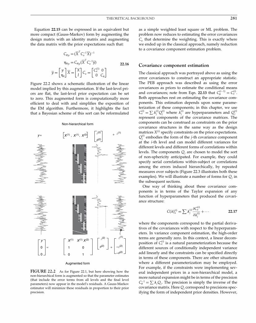
Elsevier UK Chapter: Ch22-P372560 30-9-2006 5:20p.m. Page:281 Trim:7.5in×9.25in
Basal Font:Palatino Margins:Top:40pt Gutter:68pt Font Size:9.5/12 Text Width:42pc Depth:55 Lines
THEORETICAL BACKGROUND 281
Equation 22.15 can be expressed in an equivalent butmore compact (Gauss-Markov) form by augmenting thedesign matrix with an identity matrix and augmentingthe data matrix with the prior expectations such that:
C��y = �XTC−1
X�−1
��y =C��y�XTC−1
y�
y =[
y �
]X =
[XI
]C =
[C�1�
00 C�
] 22.16
Figure 22.2 shows a schematic illustration of the linearmodel implied by this augmentation. If the last-level pri-ors are flat, the last-level prior expectation can be setto zero. This augmented form is computationally moreefficient to deal with and simplifies the exposition ofthe EM algorithm. Furthermore, it highlights the factthat a Bayesian scheme of this sort can be reformulated
Augmented form
Non-hierarchical form
ε(2)
ε(2)
θ(2)
ε(1)
θ(2) –ε(2)
–θ(2)
+
ε(1)
10
01 =
0
0
y
+, ,y =
X (1)X
(1) X (2)
X (1) X
(1) X (2)
FIGURE 22.2 As for Figure 22.1, but here showing how thenon-hierarchical form is augmented so that the parameter estimates(that include the error terms from all levels and the final levelparameters) now appear in the model’s residuals. A Gauss-Markovestimator will minimize these residuals in proportion to their priorprecision.
as a simple weighted least square or ML problem. Theproblem now reduces to estimating the error covariancesC that determine the weighting. This is exactly wherewe ended up in the classical approach, namely reductionto a covariance component estimation problem.
Covariance component estimation
The classical approach was portrayed above as using theerror covariances to construct an appropriate statistic.The PEB approach was described as using the errorcovariances as priors to estimate the conditional meansand covariances; note from Eqn. 22.13 that C�i−1�
� = C�i� .
Both approaches rest on estimating the covariance com-ponents. This estimation depends upon some parame-terization of these components; in this chapter, we useC�i�
=∑��i�
j Q�i�j where ��i�
j are hyperparameters and Q�i�j
represent components of the covariance matrices. Thecomponents can be construed as constraints on the priorcovariance structures in the same way as the designmatrices X�i� specify constraints on the prior expectations.Q�i�
j embodies the form of the j-th covariance componentat the i-th level and can model different variances fordifferent levels and different forms of correlations withinlevels. The components Qj are chosen to model the sortof non-sphericity anticipated. For example, they couldspecify serial correlations within-subject or correlationsamong the errors induced hierarchically, by repeatedmeasures over subjects (Figure 22.3 illustrates both theseexamples). We will illustrate a number of forms for Qj inthe subsequent sections.
One way of thinking about these covariance com-ponents is in terms of the Taylor expansion of anyfunction of hyperparameters that produced the covari-ance structure:
C����i� =∑
��i�j
�C�i�
���i�j
+· · · 22.17
where the components correspond to the partial deriva-tives of the covariances with respect to the hyperparam-eters. In variance component estimation, the high-orderterms are generally zero. In this context, a linear decom-position of C�i�
is a natural parameterization because thedifferent sources of conditionally independent varianceadd linearly and the constraints can be specified directlyin terms of these components. There are other situationswhere a different parameterization may be employed.For example, if the constraints were implementing sev-eral independent priors in a non-hierarchical model, amore natural expansion might be in terms of the precisionC−1
� =∑�jQj . The precision is simply the inverse of the
covariance matrix. Here Qj correspond to precisions spec-ifying the form of independent prior densities. However,
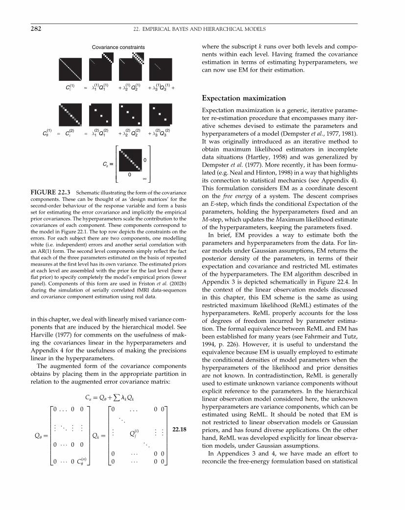
Elsevier UK Chapter: Ch22-P372560 30-9-2006 5:20p.m. Page:282 Trim:7.5in×9.25in
Basal Font:Palatino Margins:Top:40pt Gutter:68pt Font Size:9.5/12 Text Width:42pc Depth:55 Lines
282 22. EMPIRICAL BAYES AND HIERARCHICAL MODELS
Covariance constraints
= Cε + λ 2 Q 2
+ λ 3 Q 3
+
= =
0
0
∞
=θC =
(1) (1) (1) (1) (1) (1)
(1) (2)
λ 1 Q 1
+ λ 2 Q 2
+ λ 3 Q 3
(2) (2) (2) (2) (2) (2)λ 1
Q 1 CεCθ
(1)
FIGURE 22.3 Schematic illustrating the form of the covariancecomponents. These can be thought of as ‘design matrices’ for thesecond-order behaviour of the response variable and form a basisset for estimating the error covariance and implicitly the empiricalprior covariances. The hyperparameters scale the contribution to thecovariances of each component. These components correspond tothe model in Figure 22.1. The top row depicts the constraints on theerrors. For each subject there are two components, one modellingwhite (i.e. independent) errors and another serial correlation withan AR(1) form. The second level components simply reflect the factthat each of the three parameters estimated on the basis of repeatedmeasures at the first level has its own variance. The estimated priorsat each level are assembled with the prior for the last level (here aflat prior) to specify completely the model’s empirical priors (lowerpanel). Components of this form are used in Friston et al. (2002b)during the simulation of serially correlated fMRI data-sequencesand covariance component estimation using real data.
in this chapter, we deal with linearly mixed variance com-ponents that are induced by the hierarchical model. SeeHarville (1977) for comments on the usefulness of mak-ing the covariances linear in the hyperparameters andAppendix 4 for the usefulness of making the precisionslinear in the hyperparameters.
The augmented form of the covariance componentsobtains by placing them in the appropriate partition inrelation to the augmented error covariance matrix:
C = Q� +∑�kQk
Q� =
⎡⎢⎢⎢⎢⎢⎢⎢⎢⎢⎢⎣
0 � � � 0 0
���� � �
������
0 · · · 0 0
0 · · · 0 C�n��
⎤⎥⎥⎥⎥⎥⎥⎥⎥⎥⎥⎦
Qk =
⎡⎢⎢⎢⎢⎢⎢⎢⎢⎢⎢⎣
0 � � � 0 0� � �
��� Q�i�j
������
� � �
0 · · · 0 00 · · · 0 0
⎤⎥⎥⎥⎥⎥⎥⎥⎥⎥⎥⎦
22.18
where the subscript k runs over both levels and compo-nents within each level. Having framed the covarianceestimation in terms of estimating hyperparameters, wecan now use EM for their estimation.
Expectation maximization
Expectation maximization is a generic, iterative parame-ter re-estimation procedure that encompasses many iter-ative schemes devised to estimate the parameters andhyperparameters of a model (Dempster et al., 1977, 1981).It was originally introduced as an iterative method toobtain maximum likelihood estimators in incompletedata situations (Hartley, 1958) and was generalized byDempster et al. (1977). More recently, it has been formu-lated (e.g. Neal and Hinton, 1998) in a way that highlightsits connection to statistical mechanics (see Appendix 4).This formulation considers EM as a coordinate descenton the free energy of a system. The descent comprisesan E-step, which finds the conditional Expectation of theparameters, holding the hyperparameters fixed and anM-step, which updates the Maximum likelihood estimateof the hyperparameters, keeping the parameters fixed.
In brief, EM provides a way to estimate both theparameters and hyperparameters from the data. For lin-ear models under Gaussian assumptions, EM returns theposterior density of the parameters, in terms of theirexpectation and covariance and restricted ML estimatesof the hyperparameters. The EM algorithm described inAppendix 3 is depicted schematically in Figure 22.4. Inthe context of the linear observation models discussedin this chapter, this EM scheme is the same as usingrestricted maximum likelihood (ReML) estimates of thehyperparameters. ReML properly accounts for the lossof degrees of freedom incurred by parameter estima-tion. The formal equivalence between ReML and EM hasbeen established for many years (see Fahrmeir and Tutz,1994, p. 226). However, it is useful to understand theequivalence because EM is usually employed to estimatethe conditional densities of model parameters when thehyperparameters of the likelihood and prior densitiesare not known. In contradistinction, ReML is generallyused to estimate unknown variance components withoutexplicit reference to the parameters. In the hierarchicallinear observation model considered here, the unknownhyperparameters are variance components, which can beestimated using ReML. It should be noted that EM isnot restricted to linear observation models or Gaussianpriors, and has found diverse applications. On the otherhand, ReML was developed explicitly for linear observa-tion models, under Gaussian assumptions.
In Appendices 3 and 4, we have made an effort toreconcile the free-energy formulation based on statistical
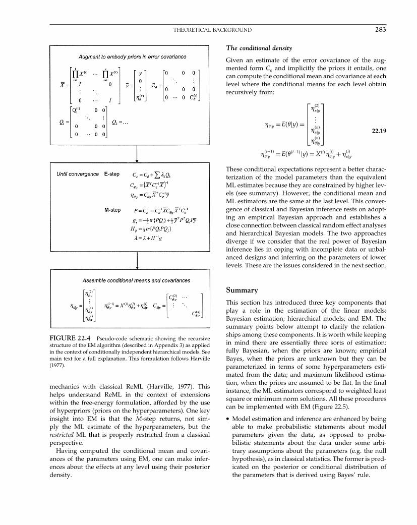
Elsevier UK Chapter: Ch22-P372560 30-9-2006 5:20p.m. Page:283 Trim:7.5in×9.25in
Basal Font:Palatino Margins:Top:40pt Gutter:68pt Font Size:9.5/12 Text Width:42pc Depth:55 Lines
THEORETICAL BACKGROUND 283
FIGURE 22.4 Pseudo-code schematic showing the recursivestructure of the EM algorithm (described in Appendix 3) as appliedin the context of conditionally independent hierarchical models. Seemain text for a full explanation. This formulation follows Harville(1977).
mechanics with classical ReML (Harville, 1977). Thishelps understand ReML in the context of extensionswithin the free-energy formulation, afforded by the useof hyperpriors (priors on the hyperparameters). One keyinsight into EM is that the M-step returns, not sim-ply the ML estimate of the hyperparameters, but therestricted ML that is properly restricted from a classicalperspective.
Having computed the conditional mean and covari-ances of the parameters using EM, one can make infer-ences about the effects at any level using their posteriordensity.
The conditional density
Given an estimate of the error covariance of the aug-mented form C and implicitly the priors it entails, onecan compute the conditional mean and covariance at eachlevel where the conditional means for each level obtainrecursively from:
��y =E���y� =
⎡⎢⎢⎢⎢⎢⎣
�2��y���
�n��y
�n���y
⎤⎥⎥⎥⎥⎥⎦
�i−1���y =E���i−1��y� = X�i� �i�
��y + �i��y
22.19
These conditional expectations represent a better charac-terization of the model parameters than the equivalentML estimates because they are constrained by higher lev-els (see summary). However, the conditional mean andML estimators are the same at the last level. This conver-gence of classical and Bayesian inference rests on adopt-ing an empirical Bayesian approach and establishes aclose connection between classical random effect analysesand hierarchical Bayesian models. The two approachesdiverge if we consider that the real power of Bayesianinference lies in coping with incomplete data or unbal-anced designs and inferring on the parameters of lowerlevels. These are the issues considered in the next section.
Summary
This section has introduced three key components thatplay a role in the estimation of the linear models:Bayesian estimation; hierarchical models; and EM. Thesummary points below attempt to clarify the relation-ships among these components. It is worth while keepingin mind there are essentially three sorts of estimation:fully Bayesian, when the priors are known; empiricalBayes, when the priors are unknown but they can beparameterized in terms of some hyperparameters esti-mated from the data; and maximum likelihood estima-tion, when the priors are assumed to be flat. In the finalinstance, the ML estimators correspond to weighted leastsquare or minimum norm solutions. All these procedurescan be implemented with EM (Figure 22.5).
• Model estimation and inference are enhanced by beingable to make probabilistic statements about modelparameters given the data, as opposed to proba-bilistic statements about the data under some arbi-trary assumptions about the parameters (e.g. the nullhypothesis), as in classical statistics. The former is pred-icated on the posterior or conditional distribution ofthe parameters that is derived using Bayes’ rule.
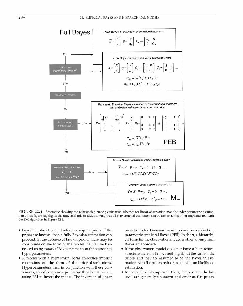
Elsevier UK Chapter: Ch22-P372560 30-9-2006 5:20p.m. Page:284 Trim:7.5in×9.25in
Basal Font:Palatino Margins:Top:40pt Gutter:68pt Font Size:9.5/12 Text Width:42pc Depth:55 Lines
284 22. EMPIRICAL BAYES AND HIERARCHICAL MODELS
FIGURE 22.5 Schematic showing the relationship among estimation schemes for linear observation models under parametric assump-tions. This figure highlights the universal role of EM, showing that all conventional estimators can be cast in terms of, or implemented with,the EM algorithm in Figure 22.4.
• Bayesian estimation and inference require priors. If thepriors are known, then a fully Bayesian estimation canproceed. In the absence of known priors, there may beconstraints on the form of the model that can be har-nessed using empirical Bayes estimates of the associatedhyperparameters.
• A model with a hierarchical form embodies implicitconstraints on the form of the prior distributions.Hyperparameters that, in conjunction with these con-straints, specify empirical priors can then be estimated,using EM to invert the model. The inversion of linear
models under Gaussian assumptions corresponds toparametric empirical Bayes (PEB). In short, a hierarchi-cal form for the observation model enables an empiricalBayesian approach.
• If the observation model does not have a hierarchicalstructure then one knows nothing about the form of thepriors, and they are assumed to be flat. Bayesian esti-mation with flat priors reduces to maximum likelihoodestimation.
• In the context of empirical Bayes, the priors at the lastlevel are generally unknown and enter as flat priors.

Elsevier UK Chapter: Ch22-P372560 30-9-2006 5:20p.m. Page:285 Trim:7.5in×9.25in
Basal Font:Palatino Margins:Top:40pt Gutter:68pt Font Size:9.5/12 Text Width:42pc Depth:55 Lines
THEORETICAL BACKGROUND 285
This is equivalent to treating the parameters at the lastlevel as fixed effects (i.e. effects with no intrinsic orrandom variability). One consequence of this is thatthe conditional mean and the ML estimate, at the lastlevel, are identical.
• At the last level, PEB and classical approaches are for-mally identical. At subordinate levels PEB can use theposterior densities for Bayesian inference about theeffects of interest. This is precluded in classical treat-ments because there are no empirical priors.
• EM provides a generic framework in which full Bayes,PEB or ML estimation can proceed. Its critical utility inthis context is the estimation of covariance components,given some data, through the ReML estimation ofhyperparameters mixing these covariance components.EM can be applied to hierarchical models by augment-ing the design matrix and data (see Figures 22.2 and22.4) to convert a hierarchical inverse problem into anon-hierarchical form. We will see later (Appendix 4)that EM is a special case of variational Bayes and thatReML is a special case of EM.
• In the absence of priors, or hierarchical constraints,EM can be used in an ML setting to estimatethe error covariance for Gauss-Markov estimates(see Figure 22.5). These estimators are the optimumweighted least square estimates in the sense they havethe minimum variance of all unbiased linear estima-tors. In the limiting case that the covariance constraintsreduce to a single basis (synonymous with known cor-relations or a single hyperparameter), the EM schemeconverges in a single iteration and emulates a classicalsum of square estimation of error variance. When thissingle basis is the identity matrix, EM simply imple-ments ordinary least squares.
In this section, we have reviewed hierarchical obser-vation models of the sort commonly encountered inneuroimaging. Their hierarchical nature induces differentsources of variability in the observations at different lev-els (i.e. variance components) that can be estimated usingEM. The use of EM, for variance component estimation,is not limited to hierarchical models, but finds a use-ful application whenever non-sphericity of the errors isspecified with more than one hyperparameter (e.g. serialcorrelations in fMRI). This application will be illustratednext. The critical thing about hierarchical models is thatthey enable empirical Bayes, where variance estimatesat higher levels can be used as constraints on the esti-mation of effects at lower levels. This perspective restsupon exactly the same mathematics that pertains to vari-ance component estimation in non-hierarchical models,but allows one to frame the estimators in conditional orBayesian terms. An intuitive understanding of the con-ditional estimators, at a given level, is that they ‘shrink’
towards their average, in proportion to the error varianceat that level, relative to their intrinsic variability (errorvariance at the supraordinate level). See Lee (1997: 232)for a discussion of PEB and Stein ‘shrinkage’ estimators.
In what sense are these Bayes predictors a better char-acterization of the model parameters than the equiva-lent ML estimates? In other words, what is gained inusing a shrinkage estimator? This is a topic that has beendebated at great length in the statistics literature andeven in the popular press (see the Scientific American arti-cle ‘Stein’s paradox in statistics’, Efron and Morris, 1977).The answer depends on one’s definition of ‘better’, or intechnical terms, the loss function. If the aim is to find thebest predictor for a specific subject, then one can do nobetter than the ML estimator for that subject. Here theloss function is simply the squared difference betweenthe estimated and real effects for the subject in question.Conversely, if the loss function is averaged over sub-jects then the shrinkage estimator is best. This has beenneatly summarized in a discussion chapter read beforethe Royal Statistical Society entitled ‘Regression, predic-tion and shrinkage’ by Copas (1983). The vote of thankswas given by Dunsmore, who said:
Suppose I go to the doctor with some complaint andask him to predict the time, y, to remission. He willtake some explanatory measurements x and providesome prediction for y. What I am interested in is aprediction for my x, not for any other x that I mighthave had – but did not. Nor am I really interested inhis necessarily using a predictor which is ‘best’ overall possible xs. Perhaps rather selfishly, but I believejustifiably, I want the best predictor for my x. Doesit necessarily follow that the best predictor for myx should take the same form as for some other x?Of course, this can cause problems for the esteem ofthe doctor or his friendly statistician. Because we areconcerned with actual observations, the goodness orotherwise of the prediction will eventually becomeapparent. In this case, the statistician will not be ableto hide behind the screen provided by averaging overall possible future xs.
Copas then replied:
Dr Dunsmore raises two general points that repaycareful thought. First, he questions the assumptionmade at the very start of the chapter that predictionsare to be judged in the context of a population offuture xs and not just at some specific x. To pursue theanalogy of the doctor and the patient, all I can say isthat the chapter is written from the doctor’s point ofview and not from the patient’s! No doubt the doctorwill feel he is doing a better job if he cures 95 per centof patients rather than only 90 per cent, even though

Elsevier UK Chapter: Ch22-P372560 30-9-2006 5:20p.m. Page:286 Trim:7.5in×9.25in
Basal Font:Palatino Margins:Top:40pt Gutter:68pt Font Size:9.5/12 Text Width:42pc Depth:55 Lines
286 22. EMPIRICAL BAYES AND HIERARCHICAL MODELS
a particular patient (Dr Dunsmore) might do better inthe latter situation than the former. As explained inthe chapter, pre-shrunk predictors do better than leastsquares for most xs at the expense of doing worse ata minority of xs. Perhaps if we think our symptomsare unusual we should seek a consultant who is pre-pared to view our complaint as an individual researchproblem rather than rely on the blunt instrument ofconventional wisdom.
The implication for Bayesian estimators, in the contextof neuroimaging, is that they are the best for each subject[or voxel] on average over subjects [or voxels]. In this sense,Bayesian or conditional estimates of individual effects areonly better, on average, over the individual effects esti-mated. The issues, framed by Keith Worsley above, speakto the important consideration that Bayesian estimates,of the sort discussed in this chapter, are only ‘better’ ina collective sense. One example of this collective contextis presented in the next chapter, where between-voxeleffects are used to ‘shrink’ within-voxel estimates thatare then reported together in a posterior probability map(PPM).
The estimators and inference from a PEB approachdo not inherently increase the sensitivity or specificityof the analysis. The most appropriate way to do thiswould be simply to increase sample size. PEB method-ology can be better regarded as providing a set of esti-mates or predictors that are internally consistent withinand over hierarchies of the observation model. Further-more, they enable Bayesian inference (comments aboutthe likelihood of an effect given the data) that com-plements classical inference (comments about the likeli-hood of the data). Bayesian inference does not necessarilydecide whether activation is present or not, it simply esti-mates the probability of activation, specified in terms ofthe size of the effect. Conversely, classical inference ispredicated on a decision (is the null hypothesis true or isthe size of the effect different from zero?). The productof classical inference is a decision or declaration, whichinduces a sensitivity and specificity of the inference. Onemotivation, behind Bayesian treatments, is to circumventthe difficult compromise between sensitivity and speci-ficity engendered by classical inference in neuroimaging.
EM AND COVARIANCE COMPONENTESTIMATION
In this section we present a series of models that exem-plify the diverse issues that can be addressed with EM. Inhierarchical linear observation models, both classical andempirical Bayesian approaches can be framed in terms
of covariance component estimation (e.g. variance partition-ing). To illustrate the use of EM in covariance componentestimation, we focus on two important problems in fMRI:non-sphericity induced by serial or temporal correlationsamong errors and variance components caused by thehierarchical nature of multisubject studies. In hierarchicalobservation models, variance components at higher lev-els can be used as constraints on the parameter estimatesof lower levels. This enables the use of PEB estimators,as distinct from classical ML estimates. We develop thisdistinction to address the difference between responseestimates based on ML and conditional estimators.
As established in the previous section, empirical Bayesenables the estimation of a model’s parameters (e.g. acti-vations) and hyperparameters that specify the model’svariance components (e.g. within- and between-subject-variability). The estimation procedures conform to EM,which, considering just the hyperparameters in linearmodels, is formally identical to ReML. If there is onlyone variance component, these iterative schemes simplifyto conventional, non-iterative sum of squares varianceestimates. However, there are many situations when sev-eral hyperparameters have to be estimated: for example,when the correlations among errors are unknown but canbe parameterized with a small number of hyperparame-ters (cf. serial correlations in fMRI time-series). Anotherimportant example, in fMRI, is the multisubject design, inwhich the hierarchical nature of the observation inducesdifferent variance components at each level. The aim ofthis section is to illustrate how variance component esti-mation can proceed in both single-level and hierarchi-cal models. In particular, the examples emphasize that,although the mechanisms inducing non-sphericity can bevery different, the variance component estimation prob-lems they represent, and the analytic approaches calledfor, are identical.
We will use two fMRI examples. In the first, we dealwith the issue of variance component estimation usingserial correlations in single-subject fMRI studies. Becausethere is no hierarchical structure to this problem there isno Bayesian aspect. However, in the second example, weadd a second level to the observation model for the firstto address inter-subject variability. Endowing the modelwith a second level invokes empirical Bayes. This enablesa quantitative comparison of classical and conditionalsingle-subject response estimates.
Variance component estimation in asingle-level model
In this section, we review serial correlations in fMRIand use simulated data to compare ReML estimates toestimates of correlations based simply on the model

Elsevier UK Chapter: Ch22-P372560 30-9-2006 5:20p.m. Page:287 Trim:7.5in×9.25in
Basal Font:Palatino Margins:Top:40pt Gutter:68pt Font Size:9.5/12 Text Width:42pc Depth:55 Lines
EM AND COVARIANCE COMPONENT ESTIMATION 287
residuals. The importance of modelling temporal corre-lations for classical inference based on the t-statistic isdiscussed in terms of correcting for non-sphericity infMRI time-series. This section concludes with a quantita-tive assessment of serial correlations within and betweensubjects.
Serial correlations in fMRI
In this section, we restrict ourselves to a single-levelmodel and focus on the covariance component estima-tion afforded by EM. We have elected to use a simplebut important covariance estimation problem to illus-trate one of the potential uses of the scheme described inthe previous section. Namely, serial correlations in fMRIembodied in the error covariance matrix for the first (andonly) level of this model C�1�
. Serial correlations have along history in the analysis of fMRI time-series. fMRItime-series can be viewed as a linear admixture of sig-nal and noise. Noise has many contributions that renderit rather complicated in relation to other neurophysio-logical measurements. These include neuronal and non-neuronal sources. Neuronal noise refers to neurogenicsignal not modelled by the explanatory variables and hasthe same frequency structure as the signal itself. Non-neuronal components have both white (e.g. RF noise)and coloured components (e.g. pulsatile motion of thebrain caused by cardiac cycles and local modulation ofthe static magnetic field B0 by respiratory movement).These effects are typically low frequency or wide-bandand induce long-range correlations in the errors overtime. These serial correlations can be used to provide MLestimates of the parameters (see previous section), whitenthe data (Bullmore et al., 1996; Purdon and Weisskoff,1998) or enter the non-sphericity corrections describedin Worsley and Friston (1995). These approaches dependupon an accurate estimation of the serial correlations. Toestimate correlations C���, in terms of some hyperpa-rameters, �, one needs both the residuals of the model, r,and the conditional covariance of the parameter estimatesthat produced those residuals. These combine to give therequired error covariance (cf. Eqn.A3.5 in Appendix 3).
C��� = rrT +XC��yXT 22.20
The term XC��yXT represents the conditional covarianceof the parameter estimates C��y ‘projected’ onto the mea-surement space, by the design matrix X. The problemis that the covariance of the parameter estimates is itselfa function of the error covariance. This circular problem issolved by the recursive parameter re-estimation implicitin EM. It is worth noting that estimators of serial corre-lations based solely on the residuals (produced by anyestimator) will be biased. This bias results from ignoringthe second term in Eqn. 22.20, which accounts for the
component of error covariance due to uncertainty aboutthe parameter estimates themselves. It is likely that anyvalid recursive scheme for estimating serial correlationsin fMRI time-series conforms to EM (or ReML), even if theconnection is not made explicit. See Worsley et al. (2002)for a non-iterative approach to autoregressive models.
In summary, the covariance estimation afforded by EMcan be used to estimate serial correlations in fMRI time-series that coincidentally provide the most efficient (i.e.Gauss-Markov) estimators of the effect one is interestedin. In this section, we apply EM as described in Fristonet al. (2002a) to simulated fMRI data sequences and takethe opportunity to establish the connections among somecommonly employed inference procedures based uponthe t-statistic. This example concludes with an applica-tion to empirical data to demonstrate quantitatively therelative variability in serial correlations over voxels andsubjects.
Estimating serial correlations
For each fMRI session, we have a single-level observationmodel that is specified by the design matrix X�1� andconstraints on the observation’s covariance structure Q�1�
i ,in this case serial correlations among the errors.
y = X�1���1� +�1�
Q�1�1 = I 22.21
Q�1�2 = KKT � kij =
{ej−i i > j
0 i ≤ j
The measured response y has errors �1� ∼ N�0�C�1� �. I is
the identity matrix. Here Q�1�1 and Q�1�
2 represent covari-ance components of C�1�
that model a white noise andan autoregressive AR(1) process with an AR coefficientof 1/e = 0�3679. Notice that this is a very simple modelof autocorrelations; by fixing the AR coefficient thereare just two hyperparameters that allow for differentmixtures of an AR(1) process and white-noise (cf. the3 hyperparameters needed for a full AR(1) plus whitenoise model). The AR(1) component is modelled as anexponential decay of correlations over non-zero lag.
These components were chosen given the popularityof AR plus white-noise models in fMRI (Purdon andWeisskoff, 1998). Clearly, this basis set can be extendedin any fashion using Taylor expansions to model devia-tions of the AR coefficient from 1/e or, indeed, model anyother form of serial correlations. Non-stationary autocor-relations can be modelled by using non-Toeplitz formsfor the bases that allow the elements in the diagonalsof Q�1�
i to vary over observations. This might be useful,for example, in the analysis of event-related potentials,where the structure of errors may change with peristim-ulus time.

Elsevier UK Chapter: Ch22-P372560 30-9-2006 5:20p.m. Page:288 Trim:7.5in×9.25in
Basal Font:Palatino Margins:Top:40pt Gutter:68pt Font Size:9.5/12 Text Width:42pc Depth:55 Lines
288 22. EMPIRICAL BAYES AND HIERARCHICAL MODELS
FIGURE 22.6 Top panel: true response (activation plus ran-dom low frequency components) and that based on the OLS andML estimators for a simulated fMRI experiment. The insert showsthe similarity between the OLS and ML predictions. Lower panel:true (dashed) and estimated (solid) autocorrelation functions. Thesample autocorrelation function of the residuals (dotted line) andthe best fit in terms of the covariance components (dot-dashed) arealso shown. The insert shows the true covariance hyperparameters(black), those obtained using just the residuals (grey) and those esti-mated by EM (white). Note, in relation to the EM estimates, thosebased directly on the residuals severely underestimate the actualcorrelations. The simulated data comprised 128 observations withan inter-scan interval of 2 s. The activations were modelled with aboxcar (duty cycle 64 s) convolved with a canonical haemodynamicresponse function and scaled to a peak height of two. The con-stant terms and low frequency components were simulated witha linear combination of the first sixteen components of a discretecosine set, each scaled by a random unit Gaussian variate. Seriallycorrelated noise was formed by filtering unit Gaussian noise witha convolution kernel based on covariance hyperparameters of 1.0[uncorrelated or white component] and 0.5 [AR(1) component].
In the examples below, the covariance constraints werescaled to a maximum of one. This means that the sec-ond hyperparameter can be interpreted as the correlationbetween one scan and the next. The components enter,along with the data, into the EM algorithm in Figure 22.4to provide ML estimates of the parameters ��1� and ReMLestimates of the hyperparameters ��1�. An example, basedon simulated data, is shown in Figure 22.6. In this exam-
ple, the design matrix comprised a boxcar regressor andthe first sixteen components of a discrete cosine set.The simulated data corresponded to a compound of thisdesign matrix (see figure legend) plus noise, colouredusing hyperparameters of one and a half for the whiteand AR(1) components respectively. The top panel showsthe data (dots), the true and fitted effects (broken andsolid lines). For comparison, fitted responses based onboth ML and OLS (ordinary least squares) are provided.The insert in the upper panel shows these estimators aresimilar but not identical. The lower panel shows the true(dashed) and estimated (solid) autocorrelation functionbased on C
�1� = ��1�
1 Q�1�1 +��1�
2 Q�1�2 . They are nearly identi-
cal. For comparison the sample autocorrelation function(dotted line) and an estimate based directly on the resid-uals, i.e. ignoring the second term of Eqn. 22.20 (dot-dash line) are provided. The underestimation that ensuesusing the residuals is evident in the insert that shows thetrue hyperparameters (black), those estimated properlyusing ReML (white) and those based on the residualsalone (grey). By failing to account for the uncertaintyabout the parameters, the hyperparameters based onlyon the residuals are severe underestimates. The sampleautocorrelation function even shows negative correla-tions. This is a result of fitting the low frequency com-ponents of the design matrix. One way of understandingthis is to note that the autocorrelations among the resid-uals are not unbiased estimators of C
�1� but of RC�1�
RT ,where R is the residual-forming matrix. In other words,the residuals are not the true errors but what is left afterprojecting them onto the null space of the design matrix.The full details of this simulated single-session, boxcardesign fMRI study are provided in the figure legend.
Inference in the context of non-sphericity2
This subsection reprises why covariance component esti-mation is so important for inference. In short, althoughthe parameter estimates may not depend on spheric-ity, the standard error, and ensuing inference, does. Theimpact of serial correlations on inference was noted earlyin the fMRI analysis literature (Friston et al., 1994) and ledto the generalized least squares (GLS) scheme describedin Worsley and Friston (1995). In this scheme one startswith any observation model that is pre-multiplied bysome weighting or convolution matrix S to give:
Sy = SX�1���1� +S�1� 22.22
2 An IID process is identically and independently distributedand has a probability distribution whose iso-contours conformto a sphere. Any departure from this is referred to as non-sphericity.
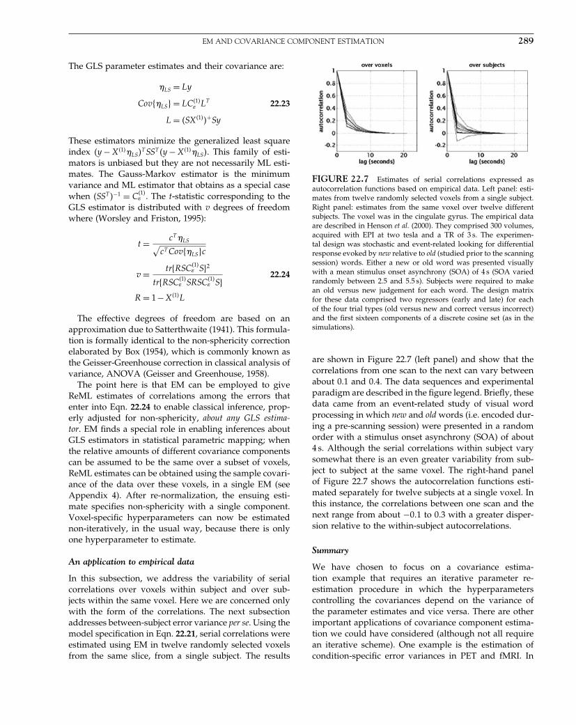
Elsevier UK Chapter: Ch22-P372560 30-9-2006 5:20p.m. Page:289 Trim:7.5in×9.25in
Basal Font:Palatino Margins:Top:40pt Gutter:68pt Font Size:9.5/12 Text Width:42pc Depth:55 Lines
EM AND COVARIANCE COMPONENT ESTIMATION 289
The GLS parameter estimates and their covariance are:
LS = Ly
Cov� LS� = LC�1� LT 22.23
L = �SX�1��+Sy
These estimators minimize the generalized least squareindex �y − X�1� LS�
T SST �y − X�1� LS�. This family of esti-mators is unbiased but they are not necessarily ML esti-mates. The Gauss-Markov estimator is the minimumvariance and ML estimator that obtains as a special casewhen �SST �−1 = C�1�
. The t-statistic corresponding to theGLS estimator is distributed with v degrees of freedomwhere (Worsley and Friston, 1995):
t = cT LS√cT Cov� LS�c
v = tr�RSC�1� S�2
tr�RSC�1� SRSC�1�
S�22.24
R = 1−X�1�L
The effective degrees of freedom are based on anapproximation due to Satterthwaite (1941). This formula-tion is formally identical to the non-sphericity correctionelaborated by Box (1954), which is commonly known asthe Geisser-Greenhouse correction in classical analysis ofvariance, ANOVA (Geisser and Greenhouse, 1958).
The point here is that EM can be employed to giveReML estimates of correlations among the errors thatenter into Eqn. 22.24 to enable classical inference, prop-erly adjusted for non-sphericity, about any GLS estima-tor. EM finds a special role in enabling inferences aboutGLS estimators in statistical parametric mapping; whenthe relative amounts of different covariance componentscan be assumed to be the same over a subset of voxels,ReML estimates can be obtained using the sample covari-ance of the data over these voxels, in a single EM (seeAppendix 4). After re-normalization, the ensuing esti-mate specifies non-sphericity with a single component.Voxel-specific hyperparameters can now be estimatednon-iteratively, in the usual way, because there is onlyone hyperparameter to estimate.
An application to empirical data
In this subsection, we address the variability of serialcorrelations over voxels within subject and over sub-jects within the same voxel. Here we are concerned onlywith the form of the correlations. The next subsectionaddresses between-subject error variance per se. Using themodel specification in Eqn. 22.21, serial correlations wereestimated using EM in twelve randomly selected voxelsfrom the same slice, from a single subject. The results
FIGURE 22.7 Estimates of serial correlations expressed asautocorrelation functions based on empirical data. Left panel: esti-mates from twelve randomly selected voxels from a single subject.Right panel: estimates from the same voxel over twelve differentsubjects. The voxel was in the cingulate gyrus. The empirical dataare described in Henson et al. (2000). They comprised 300 volumes,acquired with EPI at two tesla and a TR of 3 s. The experimen-tal design was stochastic and event-related looking for differentialresponse evoked by new relative to old (studied prior to the scanningsession) words. Either a new or old word was presented visuallywith a mean stimulus onset asynchrony (SOA) of 4 s (SOA variedrandomly between 2.5 and 5.5 s). Subjects were required to makean old versus new judgement for each word. The design matrixfor these data comprised two regressors (early and late) for eachof the four trial types (old versus new and correct versus incorrect)and the first sixteen components of a discrete cosine set (as in thesimulations).
are shown in Figure 22.7 (left panel) and show that thecorrelations from one scan to the next can vary betweenabout 0.1 and 0.4. The data sequences and experimentalparadigm are described in the figure legend. Briefly, thesedata came from an event-related study of visual wordprocessing in which new and old words (i.e. encoded dur-ing a pre-scanning session) were presented in a randomorder with a stimulus onset asynchrony (SOA) of about4 s. Although the serial correlations within subject varysomewhat there is an even greater variability from sub-ject to subject at the same voxel. The right-hand panelof Figure 22.7 shows the autocorrelation functions esti-mated separately for twelve subjects at a single voxel. Inthis instance, the correlations between one scan and thenext range from about −0�1 to 0.3 with a greater disper-sion relative to the within-subject autocorrelations.
Summary
We have chosen to focus on a covariance estima-tion example that requires an iterative parameter re-estimation procedure in which the hyperparameterscontrolling the covariances depend on the variance ofthe parameter estimates and vice versa. There are otherimportant applications of covariance component estima-tion we could have considered (although not all requirean iterative scheme). One example is the estimation ofcondition-specific error variances in PET and fMRI. In
Elsevier UK Chapter: Ch22-P372560 30-9-2006 5:20p.m. Page:290 Trim:7.5in×9.25in
Basal Font:Palatino Margins:Top:40pt Gutter:68pt Font Size:9.5/12 Text Width:42pc Depth:55 Lines
290 22. EMPIRICAL BAYES AND HIERARCHICAL MODELS
conventional SPM analyses, one generally assumes thatthe error variance expressed in one condition is the sameas that in another. This represents a sphericity assump-tion over conditions and allows one to pool several con-ditions when estimating the error variance. Assumptionsof this sort, and related sphericity assumptions in mul-tisubject studies, can be easily addressed in unbalanceddesigns, or even in the context of missing data, using EM.
Variance component estimation in fMRI intwo-level models
In this subsection, we augment the model above with asecond level. This engenders a number of issues, includ-ing the distinction between fixed- and random-effectmodels of subject responses and the opportunity to makeBayesian inferences about single-subject responses. Asabove, we start with model specification, proceed tosimulated data and conclude with an empirical exam-ple. In this example, the second level represents obser-vations over subjects. Analyses of simulated data areused to illustrate the distinction between fixed- andrandom-effect inferences by looking at how their respec-tive t-values depend on the variance components anddesign factors. The fMRI data are the same as used aboveand comprise event-related time-series from twelve sub-jects. We chose a dataset that would be difficult to analyserigorously using routine software. These data not onlyevidence serial correlations but also the number of trial-specific events varied from subject to subject, giving anunbalanced design.
Model specification
The observation model here comprises two levels withthe opportunity for subject-specific differences in errorvariance and serial correlations at the first level andparameter-specific variance at the second. The estimationmodel here is simply an extension of that used in the pre-vious subsection to estimate serial correlations. Here itembodies a second level that accommodates observationsover subjects.
Level one y = X�1���1� +�1�
⎡⎢⎣
y1���ys
⎤⎥⎦=
⎡⎢⎢⎣
X�1�1 · · · 0���
� � ����
0 · · · X�1�s
⎤⎥⎥⎦⎡⎢⎢⎣
��1�1���
��1�s
⎤⎥⎥⎦+�1�
Q�1�1 =
⎡⎢⎣
It · · · 0���
� � ����
0 · · · 0
⎤⎥⎦ � � � � �Q�1�
s =⎡⎢⎣
0 · · · 0���
� � ����
0 · · · It
⎤⎥⎦
Q�1�s+1 =
⎡⎢⎣
KKT · · · 0���
� � ����
0 · · · 0
⎤⎥⎦ � � � � �Q
�1�2s =
⎡⎢⎣
0 · · · 0���
� � ����
0 · · · KKT
⎤⎥⎦
Level two ��1� = X�2���2� +�2�
X�2� = 1s ⊗ Ip
Q�2�1 = Is ⊗
⎡⎢⎣
1 · · · 0���
� � ����
0 · · · 0
⎤⎥⎦ � � � � �Q�2�
p = Is ⊗⎡⎢⎣
0 · · · 0���
� � ����
0 · · · 1
⎤⎥⎦
22.25
for s subjects each scanned on t occasions and p parame-ters. The Kronecker tensor product A⊗B simply replacesthe element of A with AijB. An example of these designmatrices and covariance constraints are shown, respec-tively, in Figures 22.1 and 22.3. Note that there are 2 × serror covariance constraints, one set for the white noisecomponents and one for AR(1) components. Similarly,there are as many prior covariance constraints as thereare parameters at the second level.
Simulations
In the simulations we used 128 scans for each of twelvesubjects. The design matrix comprised three effects, mod-elling an event-related haemodynamic response to fre-quent but sporadic trials (in fact the instances of correctlyidentified ‘old’ words from the empirical example below)and a constant term. Activations were modelled with tworegressors, constructed by convolving a series of deltafunctions with a canonical haemodynamic response func-tion (HRF)3 and the same function delayed by three sec-onds. The delta functions indexed the occurrence of eachevent. These regressors model event-related responseswith two temporal components, which we will refer toas ‘early’ and ‘late’ (cf. Henson et al., 2000). Each subject-specific design matrix therefore comprised three columnsgiving a total of thirty-six parameters at the first leveland three at the second (the third being a constant term).The HRF basis functions were scaled so that a parameterestimate of one corresponds to a peak response of unity.After division by the grand mean, and multiplication by100, the units of the response variable and parameterestimates were rendered adimensional and correspond toper cent whole brain mean over all scans. The simulateddata were generated using Eqn. 22.25 with unit Gaussian
3 The canonical HRF was the same as that employed by SPM. Itcomprises a mixture of two gamma variates modelling peak andundershoot components and is based on a principal componentanalysis of empirically determined haemodynamic responses,over voxels, as described in Friston et al. (1998)

Elsevier UK Chapter: Ch22-P372560 30-9-2006 5:20p.m. Page:291 Trim:7.5in×9.25in
Basal Font:Palatino Margins:Top:40pt Gutter:68pt Font Size:9.5/12 Text Width:42pc Depth:55 Lines
EM AND COVARIANCE COMPONENT ESTIMATION 291
noise coloured using a temporal, convolution matrix withfirst-level hyperparameters 0.5 and −0�1 for each subject’swhite and AR(1) error covariance components respec-tively. The second-level parameters and hyperparameterswere ��2� = �0�5� 0� 0�T ���2� = �0�02� 0�006� 0�T . These val-ues model substantial early responses, with an expectedvalue of 0.5 per cent and a standard deviation over sub-jects of 0.14 per cent (i.e. square root of 0.02). The latecomponent was trivial with zero expectation and a stan-dard deviation of 0.077 per cent. The third or constantterms were discounted with zero mean and variance.These values were chosen because they are typical of realdata (see below).
Figures 22.8 and 22.9 show the results after subject-ing the simulated data to EM to estimate the conditional
FIGURE 22.8 The results of an analysis of simulated event-related responses in a single voxel. Parameter and hyperparameterestimates based on a simulated fMRI study are shown in relation totheir true values. The simulated data comprised 128 scans for eachof twelve subjects with a mean peak response over subjects of 0.5per cent. The construction of these data is described in the maintext. Stimulus presentation conformed to the presentation of ‘old’words in the empirical analysis described in the main text. Serialcorrelations were modelled as in the main text. Upper left: first-level hyperparameters. The estimated subject-specific values (black)are shown alongside the true values (white). The first twelve corre-spond to the ‘white’ term or variance. The second twelve control thedegree of autocorrelation and can be interpreted as the correlationbetween one scan and the next. Upper right: hyperparameters forthe early and late components of the evoked response. Lower-left:the estimated subject-specific parameters pertaining to the early-and late-response components are plotted against their true values.Lower right: the estimated and true parameters at the second level,representing the conditional mean of the distribution from whichthe subject-specific effects are drawn.
FIGURE 22.9 Response estimates and inferences about theestimates presented in Figure 22.8. Upper panel: true (dotted) andML (solid) estimates of event-related responses to a stimulus over12 subjects. The units of activation are adimensional and corre-spond to per cent of whole-brain mean. The insert shows the cor-responding subject-specific t-values for contrasts testing for earlyand late responses. Lower panel: the equivalent estimates based onthe conditional means. It can be seen that the conditional estimatesare much ‘tighter’ and reflect better the inter-subject variability inresponses. The insert shows the posterior probability that the acti-vation was greater than 0.1 per cent. Because the responses weremodelled with early and late components (basis functions corre-sponding to canonical haemodynamic response functions, separatedby 3 s) separate posterior probabilities could be computed for each.The simulated data comprised only early responses as reflected inthe posterior probabilities.
mean and covariances of the subject-specific evokedresponses. Figure 22.8 shows the estimated hyperpa-rameters and parameters (black) alongside the true val-ues (white). The first-level hyperparameters controllingwithin-subject error (i.e. scan to scan variability) areestimated in a reasonably reliable fashion, but notethat these estimates show a degree of variation aboutthe veridical values (see Conclusion). In this example,the second-level hyperparameters are over-estimated butremarkably good, given only twelve subjects. The param-eter estimates at the first and second levels are again very

Elsevier UK Chapter: Ch22-P372560 30-9-2006 5:20p.m. Page:292 Trim:7.5in×9.25in
Basal Font:Palatino Margins:Top:40pt Gutter:68pt Font Size:9.5/12 Text Width:42pc Depth:55 Lines
292 22. EMPIRICAL BAYES AND HIERARCHICAL MODELS
FIGURE 22.10 Estimation of differential event-relatedresponses using real data. The format of this figure is identicalto that of Figure 22.8. The only differences are that these resultsare based on real data and the response is due to the differencebetween studied or familiar (old) words and novel (new) words.In this example we used the first 128 scans from twelve subjects.Clearly, in this figure, we cannot include true effects.
reasonable, correctly attributing the majority of the exper-imental variance to an early effect. Figure 22.8 should becompared with Figure 22.10, which shows the equivalentestimates for real data.
The top panel in Figure 22.9 shows the ML estimatesthat would have been obtained if we had used a single-level model. These correspond to response estimates froma conventional fixed-effects analysis. The insert showsthe classical fixed-effect t-values, for each subject, forcontrasts testing early and late response components.Although these t-values properly reflect the prominenceof early effects, their variability precludes any thresholdthat could render the early components significant andyet exclude false positives pertaining to the late compo-nent. The lower panel highlights the potential of revisit-ing the first level in the context of a hierarchical model.It shows the equivalent responses based on the condi-tional mean and the posterior inference (insert) basedon the conditional covariance. This allows us to reiter-ate some points made in the previous section. First, theparameter estimates and ensuing response estimates areinformed by information abstracted from higher levels.Second, these empirical priors enable Bayesian inferenceabout the probability of an activation that is specified inneurobiological terms.
In Figure 22.9 the estimated responses are shown (solidlines) with the actual responses (broken lines). Note howthe conditional estimates show a regression or ‘shrinkage’to the conditional mean. In other words, their varianceshrinks to reflect, more accurately, the variability in realresponses. In particular, the spurious variability in theapparent latency of the peak response in the ML estimatesdisappears when using the conditional estimates. This isbecause the contribution of the late component, whichcauses latency differences, is suppressed in the condi-tional estimates. This, in turn, reflects the fact that thevariability in its expression over subjects is small relativeto that induced by the observation error. Simulations likethese suggest that characterizations of inter-subject vari-ability using ML approaches can severely overestimatethe true variability. This is because the ML estimates areunconstrained and simply minimize observation errorwithout considering how likely the ensuing inter-subjectvariability is.
The posterior probabilities (insert) are a function ofthe conditional mean
�1���y and covariance C�1�
��y and a sizethreshold � = 0�1 that specifies what we consider a bio-logically meaningful effect.
1−�
⎛⎜⎝� − cT �1�
��y√cT C�1�
��yc
⎞⎟⎠ 22.26
The contrast weight vectors were c = �1� 0� 0�T for theearly effect and c = �0� 1� 0�T for a late effect. As expected,the probability of the early response being greater than� = 0�1 was uniformly high for all subjects, whereas theequivalent probability for the late component was neg-ligible. Note that, in contrast to the classical inference,there is now a clear indication that each subject expressedan early response but no late response.
An empirical analysis
Here the analysis is repeated using real data and theresults are compared to those obtained using simulateddata. The empirical data are described in Henson et al.(2000). Briefly, they comprised 128+ scans in twelve sub-jects. Only the first 128 scans were used below. The exper-imental design was stochastic and event-related, lookingfor differential responses evoked by new relative to old(studied prior to the scanning session) words. Either anew or old word was presented every 4 seconds or so(SOA varied between 2.5 and 5.5 s). In this design oneis interested only in the differences between responsesevoked by the two stimulus types. This is because theefficiency of the design to detect the effect of stimuliper se is negligible with such a short SOA. Subjects wererequired to make an old versus new judgement for eachword. Drift (the first 8 components of a discrete cosine

Elsevier UK Chapter: Ch22-P372560 30-9-2006 5:20p.m. Page:293 Trim:7.5in×9.25in
Basal Font:Palatino Margins:Top:40pt Gutter:68pt Font Size:9.5/12 Text Width:42pc Depth:55 Lines
EM AND COVARIANCE COMPONENT ESTIMATION 293
set) and the effects of incorrect trials were treated asconfounds and removed using linear regression.4 Thefirst-level subject-specific design matrix partitions com-prised four regressors with early and late effects for bothold and new words.
The analysis proceeded in exactly the same way asabove. The only difference was that the contrast testedfor differences between the two word types, i.e. c =�1� 0�−1� 0�T for an old minus new early effect. Thehyperparameter and parameter estimates, for a voxelin the cingulate gyrus (BA 31; −3�−33, 39 mm), areshown in Figure 22.10, adopting the same format as inFigure 22.8. Here we see that the within-subject errorvaries much more in the empirical data, with the lastsubject showing almost twice the error variance of thefirst. As above, serial correlations vary considerably fromsubject to subject and are not consistently positive ornegative. The second-level hyperparameters showed theearly component of the differential response to be morereliable over subjects than the late component (0.007 and0.19, respectively). All but two subjects had a greaterearly response, relative to late, which on average wasabout 0.28 per cent. In other words, activation differen-tials, in the order of 0.3 per cent, occurred in the contextof an observation error with a standard deviation of 0.5per cent (see Figure 22.10). The inter-subject variabilitywas about 30 per cent of the mean response amplitude.A component of the variability in within-subject error isdue to uncertainty in the ReML estimates of the hyperpa-rameters (see below), but this degree of inhomogeneity issubstantially more than in the simulated data (where sub-jects had equal error variances). It is interesting to notethat, despite the fact that the regressors for the early andlate components had exactly the same form, the between-subject error for one was less than half that of the other.Results of this sort speak of the prevalence of non-sphericity (in this instance heteroscedasticity or unequalvariances) and a role for the analyses illustrated here.
The response estimation and inference are shown inFigure 22.11. Again we see the characteristic ‘shrinkage’when comparing the ML to the conditional estimates. Itcan be seen that all subjects, apart from the first and third,had over a 95 per cent chance of expressing an earlydifferential of 0.1 per cent or more. The late differentialresponse was much less consistent, although one subjectexpressed a difference with about 84 per cent confidence.
4 Strictly speaking the projection matrix implementing thisadjustment should also be applied to the covariance constraintsbut this would render the components singular and ruin theirsparsity structure. We therefore omitted this and ensured, insimulations, that the adjustment had a negligible effect on thehyperparameter estimates.
FIGURE 22.11 The format of this figure is identical to that ofFigure 22.9. The only differences are that these results are basedon real data and the response is due to the difference betweenstudied or familiar (old) words and novel (new) words. The sameregression of conditional responses to the conditional mean is seenon comparing the ML and conditional estimates. In relation to thesimulated data, there is more evidence for a late component but nolate activation could be inferred for any subject with any degree ofconfidence. The voxel from which these data were taken was in thecingulate gyrus (BA 31) at −3�−33, 39 mm.
Summary
The examples presented above allow us to reprise a num-ber of important points made in the previous section (seealso Friston et al., 2002a). In conclusion, the main pointsare:
• There are many instances when an iterative parame-ter re-estimation scheme is required (e.g. dealing withserial correlations or missing data). These schemes aregenerally variants of EM.
• Even before considering the central role of covari-ance component estimation in hierarchical models orempirical Bayes, it is an important aspect of model esti-mation in its own right, particularly in estimating non-sphericity. Parameter estimates can either be obtained
Elsevier UK Chapter: Ch22-P372560 30-9-2006 5:20p.m. Page:294 Trim:7.5in×9.25in
Basal Font:Palatino Margins:Top:40pt Gutter:68pt Font Size:9.5/12 Text Width:42pc Depth:55 Lines
294 22. EMPIRICAL BAYES AND HIERARCHICAL MODELS
directly from an EM algorithm, in which case they cor-respond to the ML or Gauss-Markov estimates, or thehyperparameters can be used to determine the errorcorrelations which re-enter a generalized least-squarescheme, as a non-sphericity correction.
• Hierarchical models enable a collective improvementin response estimates by using conditional, as opposedto maximum-likelihood, estimators. This improvementensues from the constraints derived from higher levelsthat enter as empirical priors on lower levels.
In the next chapter, we revisit two-level modelsbut consider hierarchical observations over voxels asopposed to subjects.
REFERENCES
Box GEP (1954) Some theorems on quadratic forms applied in thestudy of analysis of variance problems, I. Effect of inequalityof variance in the one-way classification. Ann Math Stats 25:290–302
Bullmore ET, Brammer MJ, Williams SCR et al. (1996) Statisticalmethods of estimation and inference for functional MR images.Mag Res Med 35: 261–77
Copas JB (1983) Regression prediction and shrinkage. J Roy Stat SocSeries B 45: 311–54
Dempster AP, Laird NM, Rubin DB (1977) Maximum likelihoodfrom incomplete data via the EM algorithm. J Roy Stat Soc SeriesB 39: 1–38
Dempster AP, Rubin DB, Tsutakawa RK (1981) Estimation in covari-ance component models. J Am Stat Assoc 76: 341–53
Descombes X, Kruggel F, von Cramon DY (1998) fMRI signalrestoration using a spatio-temporal Markov random field pre-serving transitions. NeuroImage 8: 340–49
Efron B, Morris C (1973) Stein’s estimation rule and its com-petitors – an empirical Bayes approach. J Am Stat Assoc 68:117–30
Efron B, Morris C (1977) Stein’s paradox in statistics. Sci Am May:119–27
Everitt BS, Bullmore ET (1999) Mixture model mapping of brainactivation in functional magnetic resonance images. Hum BrainMapp 7: 1–14
Fahrmeir L, Tutz G (1994) Multivariate statistical modelling basedon generalised linear models. Springer-Verlag Inc., New York,pp 355–56
Friston KJ, Josephs O, Rees G et al. (1998) Nonlinear event-relatedresponses in fMRI. Magn Reson Med 39: 41–52
Friston KJ, Jezzard PJ, Turner R (1994) Analysis of functional MRItime-series. Hum Brain Mapp 1: 153–71
Friston KJ, Holmes AP, Worsley KJ et al. (1995) Statistical parametricmaps in functional imaging: a general linear approach. HumBrain Map 2: 189–210
Friston KJ, Penny W, Phillips C et al. (2002a) Classical and Bayesianinference in neuroimaging: theory. NeuroImage 16: 465–83
Friston KJ, Glaser DE, Henson RNA et al. (2002b) Classical andBayesian inference in neuroimaging: applications. NeuroImage16: 484–512
Geisser S, Greenhouse SW (1958) An extension of Box’s results onthe use of the F distribution in multivariate analysis. Ann MathStats 29: 885–91
Hartley H (1958) Maximum likelihood estimation from incompletedata. Biometrics 14: 174–94
Hartvig NV, Jensen JL (2000) Spatial mixture modelling of fMRIdata. Hum Brain Mapp 11: 233–48
Harville DA (1977) Maximum likelihood approaches to variancecomponent estimation and to related problems. J Am Stat Assoc72: 320–38
Henson RNA, Rugg MD, Shallice T et al. (2000) Confidence in recog-nition memory for words: dissociating right prefrontal roles inepisodic retrieval. J Cog Neurosci 12: 913–23
Højen-Sørensen P, Hansen LK, Rasmussen CE (2000) Bayesian mod-elling of fMRI time-series. In Advances in neural information pro-cessing systems 12, Solla SA, Leen TK, Muller KR (eds). MIT Press,pp 754–60
Holmes A, Ford I (1993) A Bayesian approach to significance testingfor statistic images from PET. In Quantification of brain function,tracer kinetics and image analysis in brain PET, Uemura K, LassenNA, Jones T et al. (eds). Excerpta Medica, Int. Cong. Series No.1030: 521–34
Holmes AP, Friston KJ (1998) Generalisability, random effects andpopulation inference. NeuroImage S754
Kass RE, Steffey D (1989) Approximate Bayesian inference in condi-tionally independent hierarchical models (parametric empiricalBayes models). J Am Stat Assoc 407: 717–26
Lee PM (1997) Bayesian Statistics an Introduction. John Wiley andSons Inc., New York
Neal RM, Hinton GE (1998) A view of the EM algorithm that justifiesincremental, sparse and other variants. In Learning in graphi-cal models, Jordan MI (ed.). Kluwer Academic Press, Dordrecht,pp 355–68
Purdon PL, Weisskoff R (1998) Effect of temporal autocorrelationsdue to physiological noise stimulus paradigm on voxel-levelfalse positive rates in fMRI. Hum Brain Mapp 6: 239–49
Satterthwaite EF (1941) Synthesis of variance. Psychometrika 6:309–16
Tikhonov AN, Arsenin VY (1977) Solution of ill posed problems.Washington and Sons, Washington
Worsley KJ (1994) Local maxima and the expected Euler character-istic of excursion sets of chi squared, F and t fields. Adv ApplProb 26: 13–42
Worsley KJ, Friston. KJ (1995) Analysis of fMRI time-series revis-ited – again. NeuroImage 2: 173–81
Worsley KJ, Liao C, Aston J et al. (2002) A general statistical analysisfor fMRI data. NeuroImage 15: 1–14

Elsevier UK Chapter: Ch23-P372560 30-9-2006 5:20p.m. Page:295 Trim:7.5in×9.25in
Basal Font:Palatino Margins:Top:40pt Gutter:68pt Font Size:9.5/12 Text Width:42pc Depth:55 Lines
C H A P T E R
23
Posterior probability mapsK. Friston and W. Penny
INTRODUCTION
This chapter describes the construction of posterior prob-ability maps that enable conditional or Bayesian infer-ences about regionally specific effects in neuroimaging.Posterior probability maps are images of the proba-bility or confidence that an activation exceeds somespecified threshold, given the data. Posterior probabil-ity maps (PPMs) represent a complementary alternativeto statistical parametric maps (SPMs) that are used tomake classical inferences. However, a key problem inBayesian inference is the specification of appropriate pri-ors. This problem can be finessed using empirical Bayesin which prior variances are estimated from the data,under some simple assumptions about their form. Empir-ical Bayes requires a hierarchical observation model, inwhich higher levels can be regarded as providing priorconstraints on lower levels. In neuroimaging, observa-tions of the same effect over voxels provide a natural,two-level hierarchy that enables an empirical Bayesianapproach. In this section, we present the motivation andthe operational details of a simple empirical Bayesianmethod for computing posterior probability maps. Wethen compare Bayesian and classical inference throughthe equivalent PPMs and SPMs testing for the same effectin the same data. The approach adopted here is a natu-ral extension of parametric empirical Bayes described inthe previous chapter. The resulting model entails globalshrinkage priors to inform the estimation of effects ateach voxel or bin in the image. These global priors canbe regarded as a special case of spatial priors in the moregeneral spatiotemporal models for functional magneticresonance imaging (fMRI) introduced in Chapter 25.
To date, inference in neuroimaging has been restrictedlargely to classical inferences based upon statistical para-metric maps (SPMs). The alternative approach is touse Bayesian or conditional inference based upon theposterior distribution of the activation given the data
(Holmes and Ford, 1993). This necessitates the spec-ification of priors (i.e. the probability distribution ofthe activation). Bayesian inference requires the posteriordistribution and therefore rests upon a posterior den-sity analysis. A useful way to summarize this posteriordensity is to compute the probability that the activa-tion exceeds some threshold. This computation repre-sents a Bayesian inference about the effect, in relation tothe specified threshold. We now describe an approachto computing posterior probability maps for activationeffects or, more generally, treatment effects in imagingdata sequences. This approach represents the simplestand most computationally expedient way of constructingPPMs.
As established in the previous chapter, the motivationfor using conditional or Bayesian inference is that it hashigh face-validity. This is because the inference is aboutan effect, or activation, being greater than some specifiedsize that has some meaning in relation to underlying neu-rophysiology. This contrasts with classical inference, inwhich the inference is about the effect being significantlydifferent from zero. The problem for classical inferenceis that trivial departures from the null hypothesis can bedeclared significant, with sufficient data or sensitivity.Furthermore, from the point of view of neuroimaging,posterior inference is especially useful because it eschewsthe multiple-comparison problem. Posterior inferencedoes not have to contend with the multiple-comparisonproblem because there are no false-positives. The prob-ability that activation has occurred, given the data, atany particular voxel is the same, irrespective of whetherone has analysed that voxel or the entire brain. For thisreason, posterior inference using PPMs may represent arelatively more powerful approach than classical infer-ence in neuroimaging. The reason that there is no needto adjust the p-values is that we assume independentprior distributions for the activations over voxels. In thissimple Bayesian model, the Bayesian perspective is sim-ilar to that of the frequentist who makes inferences on a
Statistical Parametric Mapping, by Karl Friston et al. Copyright 2007, Elsevier Ltd. All rights reserved.ISBN–13: 978-0-12-372560-8 ISBN–10: 0-12-372560-7
295
Elsevier UK Chapter: Ch23-P372560 30-9-2006 5:20p.m. Page:296 Trim:7.5in×9.25in
Basal Font:Palatino Margins:Top:40pt Gutter:68pt Font Size:9.5/12 Text Width:42pc Depth:55 Lines
296 23. POSTERIOR PROBABILITY MAPS
per-comparison basis (see Berry and Hochberg, 1999 fora detailed discussion).
Priors and Bayesian inference
PPMs require the posterior distribution or conditionaldistribution of the activation (a contrast of conditionalparameter estimates) given the data. This posterior den-sity can be computed, under Gaussian assumptions,using Bayes’ rule. Bayes’ rule requires the specificationof a likelihood function and the prior density of themodel’s parameters. The models used to form PPMs, andthe likelihood functions, are exactly the same as in clas-sical SPM analyses. The only extra bit of informationthat is required is the prior probability distribution ofthe parameters of the general linear model employed.Although it would be possible to specify these in termsof their means and variances using independent data, orsome plausible physiological constraints, there is an alter-native to this fully Bayesian approach. The alternative isempirical Bayes, in which the variances of the prior dis-tributions are estimated directly from the data. EmpiricalBayes requires a hierarchical observation model, wherethe parameters and hyperparameters at any particularlevel can be treated as priors on the level below. There arenumerous examples of hierarchical observation models.For example, the distinction between fixed- and mixed-effects analyses of multisubject studies relies upon atwo-level hierarchical model. However, in neuroimag-ing, there is a natural hierarchical observation model thatis common to all brain mapping experiments. This isthe hierarchy induced by looking for the same effects atevery voxel within the brain (or grey matter). The firstlevel of the hierarchy corresponds to the experimentaleffects at any particular voxel and the second level of thehierarchy comprises the effects over voxels. Put simply,the variation in a particular contrast, over voxels, can beused as the prior variance of that contrast at any particu-lar voxel. A caricature of the approach presented in thischapter appears as a numerical example in Chapter 11on hierarchical models.
The model used here is one in which the spatial rela-tionship among voxels is discounted. The advantage oftreating an image like a ‘gas’ of unconnected voxels isthat the estimation of between-voxel variance in activa-tion can be finessed to a considerable degree (see belowand Appendix 4). This renders the estimation of posteriordensities tractable because the between-voxel variancecan then be used as a prior variance at each voxel. Wetherefore focus on this simple and special case and on the‘pooling’ of voxels to give precise [ReML] estimates ofthe variance components required for Bayesian inference.The main focus of this chapter is the pooling procedure
that affords a computational saving necessary to producePPMs of the whole brain. In what follows, we describehow this approach is implemented and provide someexamples of its application.
THEORY
Conditional estimators and the posteriordensity
Here we describe how the posterior distribution of theparameters of any general linear model can be estimatedat each voxel from imaging data sequences. Under Gaus-sian assumptions about the errors � ∼ N�0�C�� of a gen-eral linear model with design matrix X, the responses aremodelled as:
y = X� +� 23.1
The conditional or posterior covariances and mean ofthe parameters � are given by (Friston et al., 2002a):
C��y =�XT C−1� X +C−1
� �−1
��y =C��yXT C−1
� y23.2
where C� is the prior covariance (assuming a prior expec-tation of zero). Once these moments are known, the pos-terior probability that a particular effect or contrast speci-fied by a contrast weight vector c exceeds some threshold is computed easily:
p = 1−�
⎛⎜⎝ − cT ��y√
cT C��yc
⎞⎟⎠ 23.3
��·� is the cumulative density function of the unit normaldistribution. An image of these posterior probabilitiesconstitutes a PPM.
Estimating the error covariance
Clearly, to compute the conditional moments above oneneeds to know the error and prior covariances C� and C�.In the next section, we will describe how the prior covari-ance C� can be estimated. In this section, we describehow the error covariance can be estimated in terms of ahyperparameter �� where C� = ��V , and V is the corre-lation or non-sphericity matrix of the errors (see below).This hyperparameter is estimated simply using restricted
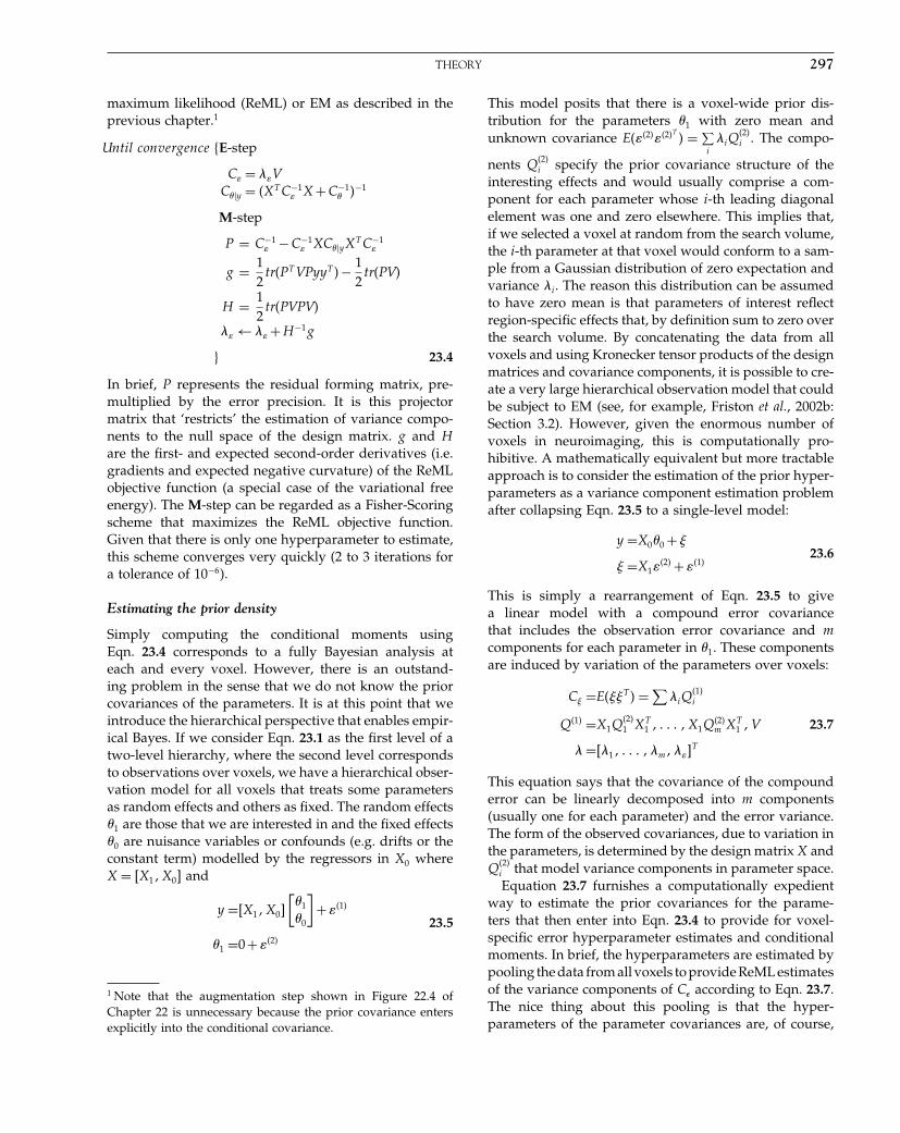
Elsevier UK Chapter: Ch23-P372560 30-9-2006 5:20p.m. Page:297 Trim:7.5in×9.25in
Basal Font:Palatino Margins:Top:40pt Gutter:68pt Font Size:9.5/12 Text Width:42pc Depth:55 Lines
THEORY 297
maximum likelihood (ReML) or EM as described in theprevious chapter.1
Until convergence �E-step
C� = ��VC��y = �XT C−1
� X +C−1� �−1
M-step
P = C−1� −C−1
� XC��yXT C−1�
g = 12
tr�PT VPyyT �− 12
tr�PV�
H = 12
tr�PVPV�
�� ← �� +H−1g
� 23.4
In brief, P represents the residual forming matrix, pre-multiplied by the error precision. It is this projectormatrix that ‘restricts’ the estimation of variance compo-nents to the null space of the design matrix. g and Hare the first- and expected second-order derivatives (i.e.gradients and expected negative curvature) of the ReMLobjective function (a special case of the variational freeenergy). The M-step can be regarded as a Fisher-Scoringscheme that maximizes the ReML objective function.Given that there is only one hyperparameter to estimate,this scheme converges very quickly (2 to 3 iterations fora tolerance of 10−6).
Estimating the prior density
Simply computing the conditional moments usingEqn. 23.4 corresponds to a fully Bayesian analysis ateach and every voxel. However, there is an outstand-ing problem in the sense that we do not know the priorcovariances of the parameters. It is at this point that weintroduce the hierarchical perspective that enables empir-ical Bayes. If we consider Eqn. 23.1 as the first level of atwo-level hierarchy, where the second level correspondsto observations over voxels, we have a hierarchical obser-vation model for all voxels that treats some parametersas random effects and others as fixed. The random effects�1 are those that we are interested in and the fixed effects�0 are nuisance variables or confounds (e.g. drifts or theconstant term) modelled by the regressors in X0 whereX = X1�X0� and
y = X1�X0�
[�1
�0
]+��1�
�1 =0+��2�
23.5
1 Note that the augmentation step shown in Figure 22.4 ofChapter 22 is unnecessary because the prior covariance entersexplicitly into the conditional covariance.
This model posits that there is a voxel-wide prior dis-tribution for the parameters �1 with zero mean andunknown covariance E���2���2�T � = ∑
i�iQ
�2�i . The compo-
nents Q�2�i specify the prior covariance structure of the
interesting effects and would usually comprise a com-ponent for each parameter whose i-th leading diagonalelement was one and zero elsewhere. This implies that,if we selected a voxel at random from the search volume,the i-th parameter at that voxel would conform to a sam-ple from a Gaussian distribution of zero expectation andvariance �i. The reason this distribution can be assumedto have zero mean is that parameters of interest reflectregion-specific effects that, by definition sum to zero overthe search volume. By concatenating the data from allvoxels and using Kronecker tensor products of the designmatrices and covariance components, it is possible to cre-ate a very large hierarchical observation model that couldbe subject to EM (see, for example, Friston et al., 2002b:Section 3.2). However, given the enormous number ofvoxels in neuroimaging, this is computationally pro-hibitive. A mathematically equivalent but more tractableapproach is to consider the estimation of the prior hyper-parameters as a variance component estimation problemafter collapsing Eqn. 23.5 to a single-level model:
y =X0�0 +�
� =X1��2� +��1�
23.6
This is simply a rearrangement of Eqn. 23.5 to givea linear model with a compound error covariancethat includes the observation error covariance and mcomponents for each parameter in �1. These componentsare induced by variation of the parameters over voxels:
C� =E���T � =∑�iQ
�1�i
Q�1� =X1Q�2�1 XT
1 � � � � �X1Q�2�m XT
1 �V 23.7
� = �1� � � � ��m����T
This equation says that the covariance of the compounderror can be linearly decomposed into m components(usually one for each parameter) and the error variance.The form of the observed covariances, due to variation inthe parameters, is determined by the design matrix X andQ�2�
i that model variance components in parameter space.Equation 23.7 furnishes a computationally expedient
way to estimate the prior covariances for the parame-ters that then enter into Eqn. 23.4 to provide for voxel-specific error hyperparameter estimates and conditionalmoments. In brief, the hyperparameters are estimated bypooling the data from all voxels to provide ReML estimatesof the variance components of C� according to Eqn. 23.7.The nice thing about this pooling is that the hyper-parameters of the parameter covariances are, of course,
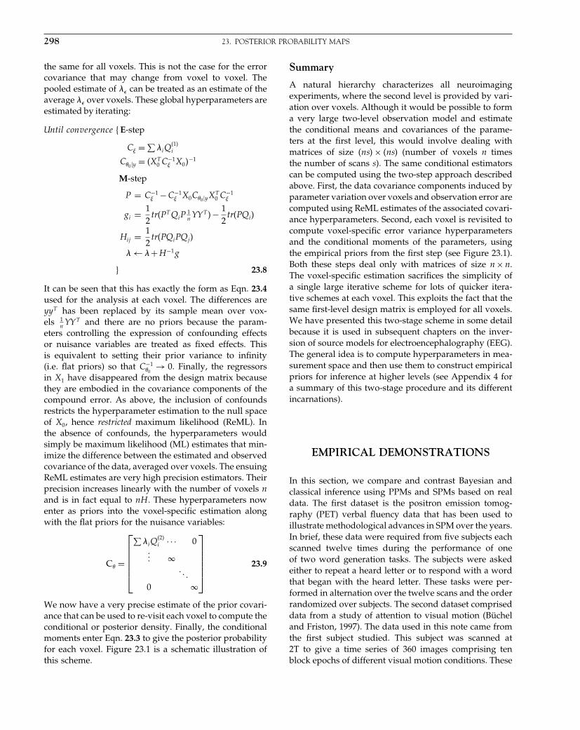
Elsevier UK Chapter: Ch23-P372560 30-9-2006 5:20p.m. Page:298 Trim:7.5in×9.25in
Basal Font:Palatino Margins:Top:40pt Gutter:68pt Font Size:9.5/12 Text Width:42pc Depth:55 Lines
298 23. POSTERIOR PROBABILITY MAPS
the same for all voxels. This is not the case for the errorcovariance that may change from voxel to voxel. Thepooled estimate of �� can be treated as an estimate of theaverage �� over voxels. These global hyperparameters areestimated by iterating:
Until convergence � E-step
C� =∑�iQ
�1�i
C�0�y = �XT0 C−1
� X0�−1
M-step
P = C−1� −C−1
� X0C�0�yXT0 C−1
�
gi = 12
tr�PT QiP1nYY T �− 1
2tr�PQi�
Hij = 12
tr�PQiPQj�
� ← �+H−1g
� 23.8
It can be seen that this has exactly the form as Eqn. 23.4used for the analysis at each voxel. The differences areyyT has been replaced by its sample mean over vox-els 1
nYY T and there are no priors because the param-
eters controlling the expression of confounding effectsor nuisance variables are treated as fixed effects. Thisis equivalent to setting their prior variance to infinity(i.e. flat priors) so that C−1
�0→ 0. Finally, the regressors
in X1 have disappeared from the design matrix becausethey are embodied in the covariance components of thecompound error. As above, the inclusion of confoundsrestricts the hyperparameter estimation to the null spaceof X0, hence restricted maximum likelihood (ReML). Inthe absence of confounds, the hyperparameters wouldsimply be maximum likelihood (ML) estimates that min-imize the difference between the estimated and observedcovariance of the data, averaged over voxels. The ensuingReML estimates are very high precision estimators. Theirprecision increases linearly with the number of voxels nand is in fact equal to nH . These hyperparameters nowenter as priors into the voxel-specific estimation alongwith the flat priors for the nuisance variables:
C� =
⎡⎢⎢⎢⎢⎢⎣
∑�iQ
�2�i · · · 0
��� �� � �
0 �
⎤⎥⎥⎥⎥⎥⎦
23.9
We now have a very precise estimate of the prior covari-ance that can be used to re-visit each voxel to compute theconditional or posterior density. Finally, the conditionalmoments enter Eqn. 23.3 to give the posterior probabilityfor each voxel. Figure 23.1 is a schematic illustration ofthis scheme.
Summary
A natural hierarchy characterizes all neuroimagingexperiments, where the second level is provided by vari-ation over voxels. Although it would be possible to forma very large two-level observation model and estimatethe conditional means and covariances of the parame-ters at the first level, this would involve dealing withmatrices of size �ns� × �ns� (number of voxels n timesthe number of scans s). The same conditional estimatorscan be computed using the two-step approach describedabove. First, the data covariance components induced byparameter variation over voxels and observation error arecomputed using ReML estimates of the associated covari-ance hyperparameters. Second, each voxel is revisited tocompute voxel-specific error variance hyperparametersand the conditional moments of the parameters, usingthe empirical priors from the first step (see Figure 23.1).Both these steps deal only with matrices of size n × n.The voxel-specific estimation sacrifices the simplicity ofa single large iterative scheme for lots of quicker itera-tive schemes at each voxel. This exploits the fact that thesame first-level design matrix is employed for all voxels.We have presented this two-stage scheme in some detailbecause it is used in subsequent chapters on the inver-sion of source models for electroencephalography (EEG).The general idea is to compute hyperparameters in mea-surement space and then use them to construct empiricalpriors for inference at higher levels (see Appendix 4 fora summary of this two-stage procedure and its differentincarnations).
EMPIRICAL DEMONSTRATIONS
In this section, we compare and contrast Bayesian andclassical inference using PPMs and SPMs based on realdata. The first dataset is the positron emission tomog-raphy (PET) verbal fluency data that has been used toillustrate methodological advances in SPM over the years.In brief, these data were required from five subjects eachscanned twelve times during the performance of oneof two word generation tasks. The subjects were askedeither to repeat a heard letter or to respond with a wordthat began with the heard letter. These tasks were per-formed in alternation over the twelve scans and the orderrandomized over subjects. The second dataset compriseddata from a study of attention to visual motion (Bücheland Friston, 1997). The data used in this note came fromthe first subject studied. This subject was scanned at2T to give a time series of 360 images comprising tenblock epochs of different visual motion conditions. These
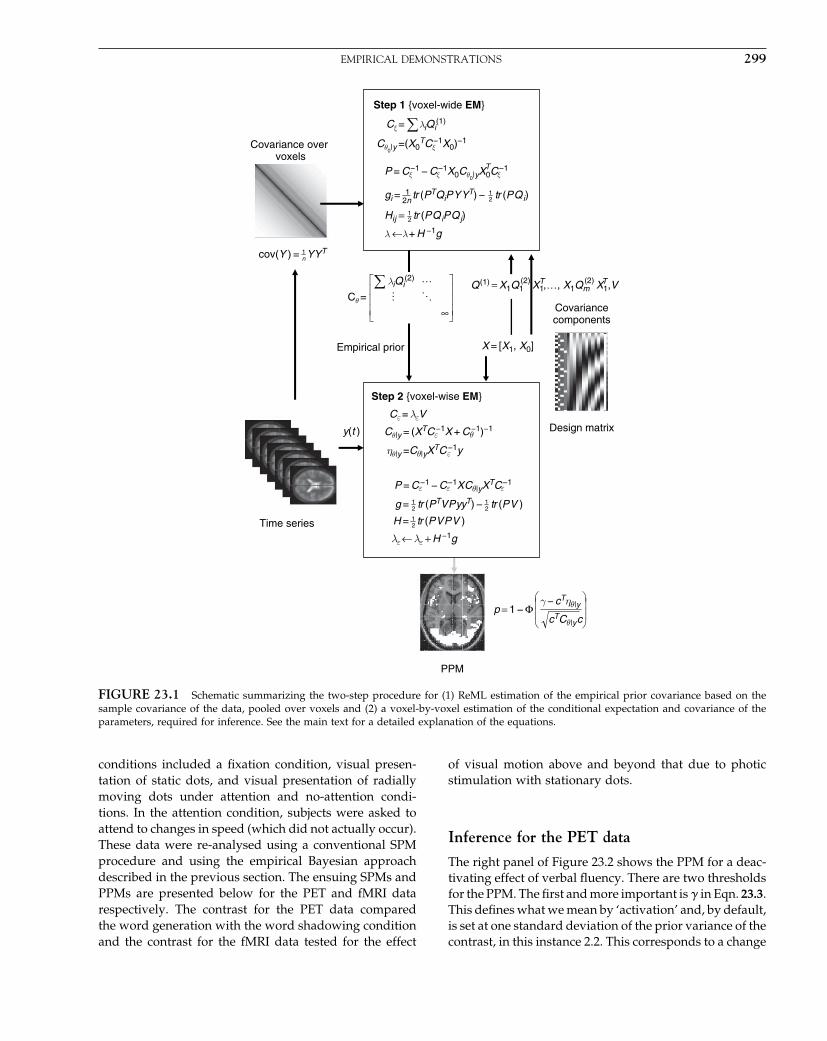
Elsevier UK Chapter: Ch23-P372560 30-9-2006 5:20p.m. Page:299 Trim:7.5in×9.25in
Basal Font:Palatino Margins:Top:40pt Gutter:68pt Font Size:9.5/12 Text Width:42pc Depth:55 Lines
EMPIRICAL DEMONSTRATIONS 299
Time series
Q
(1) = X1Q1 X1T T, X1Qm X1,V,(2) (2)
∞Cθ =
X = [X1, X0]
γ − cTηθ|y
cTCθ|y c
p = 1 − Φ
n YYT1cov(Y ) =
Covariancecomponents
y(t )
Empirical prior
PPM
Covariance over voxels
Cθ0|y =(X0TC
−1X0)−1
Cξ = λiQi(1)
tr (PQiPQj)Hij = 21
tr (PQi)tr (PTQiPYYT) −gi = 21
2n1
λ ←λ + H −1g
Step 1 {voxel-wide EM}
tr (PVPV )H =
tr (PV )tr (PTVPyyT) −g =
P = C −1 − C
−1XCθ|yXTC
−1
Cθ|y = (XTC
−1X + C −1)−1
ηθ|y =Cθ|yXTC
−1y
Cε = λεV
21
21
21
Step 2 {voxel-wise EM}
Design matrix
ξ
ε
ε
ε ε ε
θ
P = C −1
− C −1X0Cθ0|y
X0C −1T
ξ ξ ξ
λiQi(2)
λε ← λε + H −1g
FIGURE 23.1 Schematic summarizing the two-step procedure for (1) ReML estimation of the empirical prior covariance based on thesample covariance of the data, pooled over voxels and (2) a voxel-by-voxel estimation of the conditional expectation and covariance of theparameters, required for inference. See the main text for a detailed explanation of the equations.
conditions included a fixation condition, visual presen-tation of static dots, and visual presentation of radiallymoving dots under attention and no-attention condi-tions. In the attention condition, subjects were asked toattend to changes in speed (which did not actually occur).These data were re-analysed using a conventional SPMprocedure and using the empirical Bayesian approachdescribed in the previous section. The ensuing SPMs andPPMs are presented below for the PET and fMRI datarespectively. The contrast for the PET data comparedthe word generation with the word shadowing conditionand the contrast for the fMRI data tested for the effect
of visual motion above and beyond that due to photicstimulation with stationary dots.
Inference for the PET data
The right panel of Figure 23.2 shows the PPM for a deac-tivating effect of verbal fluency. There are two thresholdsfor the PPM. The first and more important is in Eqn. 23.3.This defines what we mean by ‘activation’ and, by default,is set at one standard deviation of the prior variance of thecontrast, in this instance 2.2. This corresponds to a change
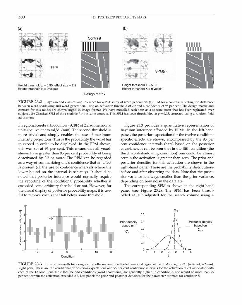
Elsevier UK Chapter: Ch23-P372560 30-9-2006 5:20p.m. Page:300 Trim:7.5in×9.25in
Basal Font:Palatino Margins:Top:40pt Gutter:68pt Font Size:9.5/12 Text Width:42pc Depth:55 Lines
300 23. POSTERIOR PROBABILITY MAPS
Height threshold p = 0.95, effect size = 2.2Extent threshold K = 0 voxels
Design matrix
Contrast
PPM
(a)
Height threshold T = 5.50Extent threshold K = 0 voxels
SPM(t1)
(b)
FIGURE 23.2 Bayesian and classical and inference for a PET study of word generation. (a) PPM for a contrast reflecting the differencebetween word-shadowing and word-generation, using an activation threshold of 2.2 and a confidence of 95 per cent. The design matrix andcontrast for this model are shown (right) in image format. We have modelled each scan as a specific effect that has been replicated oversubjects. (b) Classical SPM of the t-statistic for the same contrast. This SPM has been thresholded at p = 0�05, corrected using a random-fieldadjustment.
in regional cerebral blood flow (rCBF) of 2.2 adimensionalunits (equivalent to ml/dl/min). The second threshold ismore trivial and simply enables the use of maximumintensity projections. This is the probability the voxel hasto exceed in order to be displayed. In the PPM shown,this was set at 95 per cent. This means that all voxelsshown have greater than 95 per cent probability of beingdeactivated by 2.2 or more. The PPM can be regardedas a way of summarizing one’s confidence that an effectis present (cf. the use of confidence intervals where thelower bound on the interval is set at ). It should benoted that posterior inference would normally requirethe reporting of the conditional probability whether itexceeded some arbitrary threshold or not. However, forthe visual display of posterior probability maps, it is use-ful to remove voxels that fall below some threshold.
Figure 23.3 provides a quantitative representation ofBayesian inference afforded by PPMs. In the left-handpanel, the posterior expectation for the twelve condition-specific effects are shown, encompassed by the 95 percent confidence intervals (bars) based on the posteriorcovariance. It can be seen that in the fifth condition (thethird word-shadowing condition) one could be almostcertain the activation is greater than zero. The prior andposterior densities for this activation are shown in theright-hand panel. These are the probability distributionsbefore and after observing the data. Note that the poste-rior variance is always smaller than the prior variance,depending on how noisy the data are.
The corresponding SPM is shown in the right-handpanel (see Figure 23.2). The SPM has been thresh-olded at 0.05 adjusted for the search volume using a
Prior densitybased on
–6 –4 –2 0 2 4 60
0.1
0.2
0.3
0.4
0.5
Posterior density based on
yηθ
yCθCθ
2 4 6 8 10 12–2
–1
0
1
2
3
Condition
yηθ
Con
tras
t est
imat
e at
[–54
, –4,
–2]
θ
FIGURE 23.3 Illustrative results for a single voxel – the maximum in the left temporal region of the PPM in Figure 23.3 (−54�−4�−2 mm).Right panel: these are the conditional or posterior expectations and 95 per cent confidence intervals for the activation effect associated witheach of the 12 conditions. Note that the odd conditions (word shadowing) are generally higher. In condition 5, one would be more than 95per cent certain the activation exceeded 2.2. Left panel: the prior and posterior densities for the parameter estimate for condition 5.
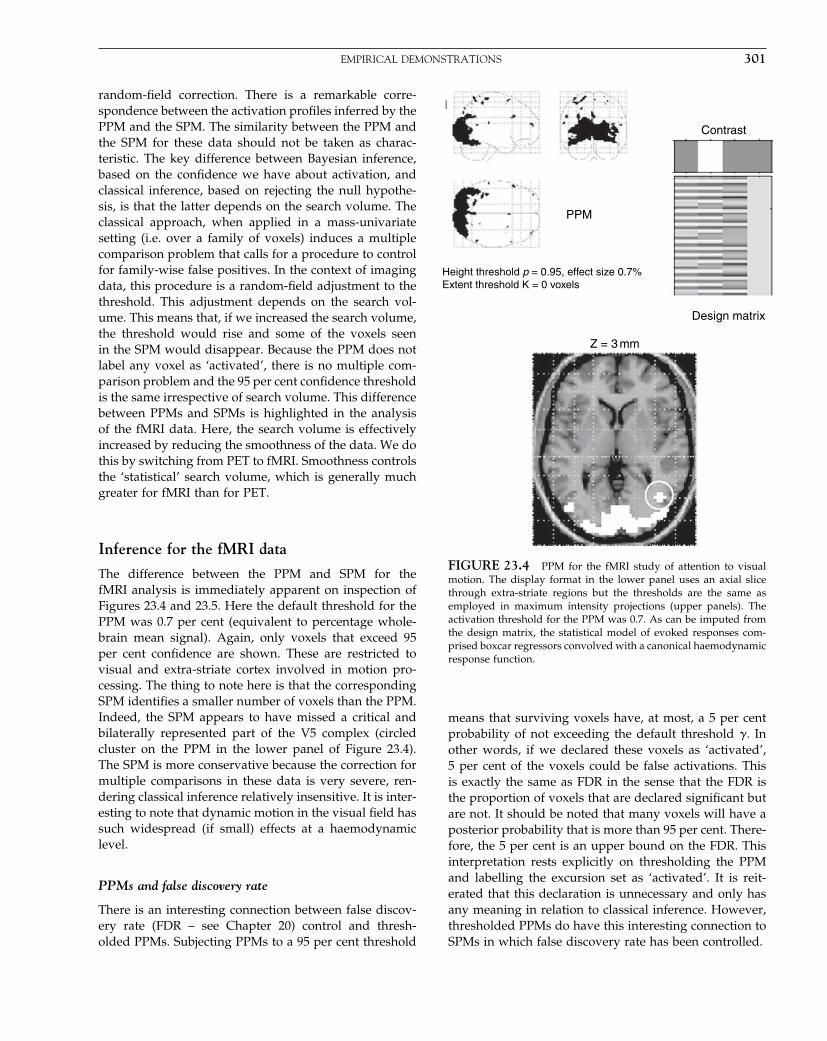
Elsevier UK Chapter: Ch23-P372560 30-9-2006 5:20p.m. Page:301 Trim:7.5in×9.25in
Basal Font:Palatino Margins:Top:40pt Gutter:68pt Font Size:9.5/12 Text Width:42pc Depth:55 Lines
EMPIRICAL DEMONSTRATIONS 301
random-field correction. There is a remarkable corre-spondence between the activation profiles inferred by thePPM and the SPM. The similarity between the PPM andthe SPM for these data should not be taken as charac-teristic. The key difference between Bayesian inference,based on the confidence we have about activation, andclassical inference, based on rejecting the null hypothe-sis, is that the latter depends on the search volume. Theclassical approach, when applied in a mass-univariatesetting (i.e. over a family of voxels) induces a multiplecomparison problem that calls for a procedure to controlfor family-wise false positives. In the context of imagingdata, this procedure is a random-field adjustment to thethreshold. This adjustment depends on the search vol-ume. This means that, if we increased the search volume,the threshold would rise and some of the voxels seenin the SPM would disappear. Because the PPM does notlabel any voxel as ‘activated’, there is no multiple com-parison problem and the 95 per cent confidence thresholdis the same irrespective of search volume. This differencebetween PPMs and SPMs is highlighted in the analysisof the fMRI data. Here, the search volume is effectivelyincreased by reducing the smoothness of the data. We dothis by switching from PET to fMRI. Smoothness controlsthe ‘statistical’ search volume, which is generally muchgreater for fMRI than for PET.
Inference for the fMRI data
The difference between the PPM and SPM for thefMRI analysis is immediately apparent on inspection ofFigures 23.4 and 23.5. Here the default threshold for thePPM was 0.7 per cent (equivalent to percentage whole-brain mean signal). Again, only voxels that exceed 95per cent confidence are shown. These are restricted tovisual and extra-striate cortex involved in motion pro-cessing. The thing to note here is that the correspondingSPM identifies a smaller number of voxels than the PPM.Indeed, the SPM appears to have missed a critical andbilaterally represented part of the V5 complex (circledcluster on the PPM in the lower panel of Figure 23.4).The SPM is more conservative because the correction formultiple comparisons in these data is very severe, ren-dering classical inference relatively insensitive. It is inter-esting to note that dynamic motion in the visual field hassuch widespread (if small) effects at a haemodynamiclevel.
PPMs and false discovery rate
There is an interesting connection between false discov-ery rate (FDR – see Chapter 20) control and thresh-olded PPMs. Subjecting PPMs to a 95 per cent threshold
Height threshold p = 0.95, effect size 0.7%Extent threshold K = 0 voxels
Z = 3 mm
Design matrix
Contrast
PPM
FIGURE 23.4 PPM for the fMRI study of attention to visualmotion. The display format in the lower panel uses an axial slicethrough extra-striate regions but the thresholds are the same asemployed in maximum intensity projections (upper panels). Theactivation threshold for the PPM was 0.7. As can be imputed fromthe design matrix, the statistical model of evoked responses com-prised boxcar regressors convolved with a canonical haemodynamicresponse function.
means that surviving voxels have, at most, a 5 per centprobability of not exceeding the default threshold . Inother words, if we declared these voxels as ‘activated’,5 per cent of the voxels could be false activations. Thisis exactly the same as FDR in the sense that the FDR isthe proportion of voxels that are declared significant butare not. It should be noted that many voxels will have aposterior probability that is more than 95 per cent. There-fore, the 5 per cent is an upper bound on the FDR. Thisinterpretation rests explicitly on thresholding the PPMand labelling the excursion set as ‘activated’. It is reit-erated that this declaration is unnecessary and only hasany meaning in relation to classical inference. However,thresholded PPMs do have this interesting connection toSPMs in which false discovery rate has been controlled.
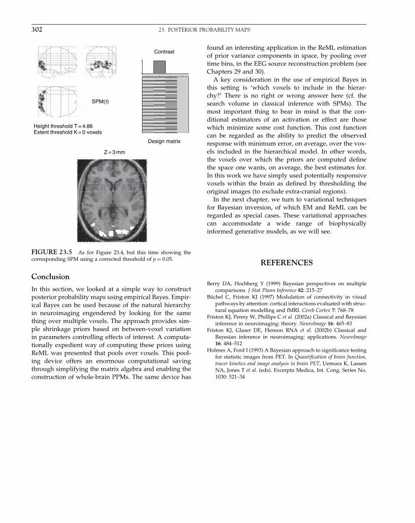
Elsevier UK Chapter: Ch23-P372560 30-9-2006 5:20p.m. Page:302 Trim:7.5in×9.25in
Basal Font:Palatino Margins:Top:40pt Gutter:68pt Font Size:9.5/12 Text Width:42pc Depth:55 Lines
302 23. POSTERIOR PROBABILITY MAPS
Height threshold T = 4.86Extent threshold K = 0 voxels
Design matrix
SPM(t )
Contrast
Z = 3 mm
FIGURE 23.5 As for Figure 23.4, but this time showing thecorresponding SPM using a corrected threshold of p = 0�05.
Conclusion
In this section, we looked at a simple way to constructposterior probability maps using empirical Bayes. Empir-ical Bayes can be used because of the natural hierarchyin neuroimaging engendered by looking for the samething over multiple voxels. The approach provides sim-ple shrinkage priors based on between-voxel variationin parameters controlling effects of interest. A computa-tionally expedient way of computing these priors usingReML was presented that pools over voxels. This pool-ing device offers an enormous computational savingthrough simplifying the matrix algebra and enabling theconstruction of whole-brain PPMs. The same device has
found an interesting application in the ReML estimationof prior variance components in space, by pooling overtime bins, in the EEG source reconstruction problem (seeChapters 29 and 30).
A key consideration in the use of empirical Bayes inthis setting is ‘which voxels to include in the hierar-chy?’ There is no right or wrong answer here (cf. thesearch volume in classical inference with SPMs). Themost important thing to bear in mind is that the con-ditional estimators of an activation or effect are thosewhich minimize some cost function. This cost functioncan be regarded as the ability to predict the observedresponse with minimum error, on average, over the vox-els included in the hierarchical model. In other words,the voxels over which the priors are computed definethe space one wants, on average, the best estimates for.In this work we have simply used potentially responsivevoxels within the brain as defined by thresholding theoriginal images (to exclude extra-cranial regions).
In the next chapter, we turn to variational techniquesfor Bayesian inversion, of which EM and ReML can beregarded as special cases. These variational approachescan accommodate a wide range of biophysicallyinformed generative models, as we will see.
REFERENCES
Berry DA, Hochberg Y (1999) Bayesian perspectives on multiplecomparisons. J Stat Plann Inference 82: 215–27
Büchel C, Friston KJ (1997) Modulation of connectivity in visualpathways by attention: cortical interactions evaluated with struc-tural equation modelling and fMRI. Cereb Cortex 7: 768–78
Friston KJ, Penny W, Phillips C et al. (2002a) Classical and Bayesianinference in neuroimaging: theory. NeuroImage 16: 465–83
Friston KJ, Glaser DE, Henson RNA et al. (2002b) Classical andBayesian inference in neuroimaging: applications. NeuroImage16: 484–512
Holmes A, Ford I (1993) A Bayesian approach to significance testingfor statistic images from PET. In Quantification of brain function,tracer kinetics and image analysis in brain PET, Uemura K, LassenNA, Jones T et al. (eds). Excerpta Medica, Int. Cong. Series No.1030: 521–34
Elsevier UK Chapter: Ch24-P372560 30-9-2006 5:21p.m. Page:303 Trim:7.5in×9.25in
Basal Font:Palatino Margins:Top:40pt Gutter:68pt Font Size:9.5/12 Text Width:42pc Depth:55 Lines
C H A P T E R
24
Variational BayesW. Penny, S. Kiebel and K. Friston
INTRODUCTION
Bayesian inference can be implemented for arbitraryprobabilistic models using Markov chain Monte Carlo(MCMC) (Gelman et al., 1995). But MCMC is compu-tationally intensive and so not practical for most brainimaging applications. This chapter describes an alterna-tive framework called ‘variational Bayes (VB)’ which iscomputationally efficient and can be applied to a largeclass of probabilistic models (Winn and Bishop, 2005).
The VB approach, also known as ‘ensemble learning’,takes its name from Feynmann’s variational free energymethod developed in statistical physics. VB is a devel-opment from the machine learning community (Petersonand Anderson, 1987; Hinton and van Camp, 1993) and hasbeen applied in a variety of statistical and signal processingdomains (Bishop et al., 1998; Jaakola et al., 1998; Ghahra-maniandBeal,2001;WinnandBishop, 2005). It is now alsowidely used in the analysis of neuroimaging data (Pennyet al., 2003; Sahani and Nagarajan, 2004; Sato et al., 2004;Woolrich, 2004; Penny et al., 2006; Friston et al., 2006).
This chapter is structured as follows. We describe thefundamental relationship between model evidence, freeenergy and Kullback-Liebler (KL) divergence that lies attheheartofVB.Before this,wereviewthesalientpropertiesof the KL-divergence. We then describe how VB learningdelivers a factorized, minimum KL-divergence approxi-mation to the true posterior density in which learning isdriven by an explicit minimization of the free energy. Thetheoretical section is completed by relating VB to Laplaceapproximations and describing how the free energy canalso be used as a surrogate for the model evidence, allow-ing for Bayesian model comparison. Numerical examplesare then given showing how VB differs from Laplace andproviding simulation studies using models of functionalmagnetic resonance imaging (fMRI) data (Penny et al.,2003). These are based on a general linear model withautoregressive errors, or GLM-AR model.
THEORY
In what follows we use upper-case letters to denote matri-ces and lower-case to denote vectors. N�m��� denotesa uni/multivariate Gaussian with mean m and vari-ance/covariance �. XT denotes the matrix transpose andlog x denotes the natural logarithm.
Kullback-Liebler divergence
For densities q��� and p��� the relative entropy orKullback-Liebler (KL) divergence from q to p is (Coverand Thomas, 1991):
KL�q�p� =∫
q��� logq���
p���d� 24.1
The KL-divergence satisfies the Gibb’s inequality(Mackay, 2003):
KL�q�p� ≥ 0 24.2
with equality only if q = p. In general KL�q�p� �= KL�p�q�,so KL is not a distance measure. Formulae for computingKL, for both Gaussian and gamma densities, are given inAppendix, 24.1.
Model evidence and free energy
Given a probabilistic model of some data, the log of the‘evidence’ or ‘marginal likelihood’ can be written as:
log p�Y� =∫
q��� log p�Y�d�
=∫
q��� logp�Y���
p���Y�d�
Statistical Parametric Mapping, by Karl Friston et al. Copyright 2007, Elsevier Ltd. All rights reserved.ISBN–13: 978-0-12-372560-8 ISBN–10: 0-12-372560-7
303

Elsevier UK Chapter: Ch24-P372560 30-9-2006 5:21p.m. Page:304 Trim:7.5in×9.25in
Basal Font:Palatino Margins:Top:40pt Gutter:68pt Font Size:9.5/12 Text Width:42pc Depth:55 Lines
304 24. VARIATIONAL BAYES
=∫
q��� log[
p�Y���q���
q���p���Y�
]d�
= F +KL�q����p���Y�� 24.3
where q��� is considered, for the moment, as an arbitrarydensity. We have:
F =∫
q��� logp�Y���
q���d� 24.4
which, in statistical physics is known as the negativefree energy. The second term in Eqn. 24.3 is the KL-divergence between the density q��� and the true poste-rior p���Y�. Eqn. 24.3 is the fundamental equation of theVB-framework and is shown graphically in Figure 24.1.
Because KL is always positive, due to the Gibbsinequality, F provides a lower bound on the model evi-dence. Moreover, because KL is zero when two densitiesare the same, F will become equal to the model evidencewhen q��� is equal to the true posterior. For this reasonq��� can be viewed as an approximate posterior.
The aim of VB-learning is to maximize F and so makethe approximate posterior as close as possible to the trueposterior. This approximate posterior will be the one thatbest approximates the true posterior in the sense of min-imizing KL-divergence. We should point out that thisdivergence cannot be minimized explicitly because p���y�is only known up to a constant. Instead, it is minimizedimplicitly by maximizing F and by virtue of Eqn. 24.3.Of course, maximizing F , the negative free energy, is thesame as minimizing −F , the free energy.
Factorized approximations
To obtain a practical learning algorithm we must alsoensure that the integrals in F are tractable. One genericprocedure for attaining this goal is to assume that the
log p(Y )
KL
F
FIGURE 24.1 The negative free energy, F , provides a lowerbound on the log-evidence of the model with equality when theapproximate posterior equals the true posterior.
approximating density factorizes over groups of param-eters. In physics, this is known as the mean field approx-imation. Thus, we consider:
q��� =∏i
q��i� 24.5
where �i is the ith group of parameters. We can also writethis as:
q��� = q��i�q��\i� 24.6
where �\i denotes all parameters not in the ith group. Thedistributions q��i� which maximize F can then be derivedas follows:
F =∫
q��� log[
p�Y���
q���
]d� 24.7
=∫ ∫
q��i�q��\i� log[
p�Y���
q��i�q��\i�
]d�\id�i
=∫
q��i�[∫
q��\i� log p�Y���d�\i
]d�i
−∫
q��i� log q��i�d�i +C
=∫
q��i�I��i�d�i −∫
q��i� log q��i�d�i +C
where the constant C contains terms not dependent onq��i� and:
I��i� =∫
q��\i� log p�Y���d�\i 24.8
Writing I��i� = log exp I��i� gives:
F =∫
q��i� log[
exp�I��i��
q��i�
]d�i +C 24.9
= KL�q��i��exp�I��i���+C
This is minimized when:
q��i� = exp�I��i��
Z24.10
where Z is the normalization factor needed to make q��i�a valid probability distribution. Importantly, this meanswe are often able to determine the optimal analytic form ofthe component posteriors. This results in what is knownas a ‘free-form’ approximation.
For example, Mackay (1995) considers the case of linearregression models with gamma priors over error preci-sions, , and Gaussian priors over regression coefficients, with a factorized approximation q��� = q��q��.Application of Eqn. 24.10 then leads to an expression inwhich I�� has terms in and log only. From this wecan surmise that the optimal form for q�� is a gammadensity (see Appendix 24.1).
Elsevier UK Chapter: Ch24-P372560 30-9-2006 5:21p.m. Page:305 Trim:7.5in×9.25in
Basal Font:Palatino Margins:Top:40pt Gutter:68pt Font Size:9.5/12 Text Width:42pc Depth:55 Lines
THEORY 305
More generally, free-form approximations can bederived for models from the ‘conjugate-exponential’ fam-ily (Attias, 1999; Ghahramani and Beal, 2001; Winn andBishop, 2005). Exponential family distributions includeGaussians and discrete multinomials and conjugacyrequires the posterior (over a factor) to have the samefunctional form as the prior.
This allows free-form VB to be applied to arbitrarydirected acyclic graphs comprising discrete multinomialvariables with arbitrary subgraphs of univariate and mul-tivariate Gaussian variables. Special cases include hid-den Markov models, linear dynamical systems, principalcomponent analysers, as well as mixtures and hier-archical mixtures of these. Moreover, by introducingadditional variational parameters, free-form VB can beapplied to models containing non-conjugate distribu-tions. This includes independent component analysis(Attias, 1999) and logistic regression (Jaakola and Jordan,1997).
Application of Eqn. 24.10 also leads to a set of updateequations for the parameters of the component posteriors.This is implemented for the linear regression exampleby equating the coefficients of and log with the rele-vant terms in the gamma density (see Appendix 24.1). Inthe general case, these update equations are coupled asthe solution for each q��i� depends on expectations withrespect to the other factors q��\i�. Optimization proceedsby initializing each factor and then cycling through eachfactor in turn and replacing the current distribution withthe estimate from Eqn. 24.10. Examples of these updateequations are provided in the following chapter, whichapplies VB to spatio-temporal models of fMRI data.
Laplace approximations
Laplace’s method approximates the integral of a function∫f���d� by fitting a Gaussian at the maximum �̂ of f���,
and computing the volume of the Gaussian. The covari-ance of the Gaussian is determined by the Hessian matrixof log f��� at the maximum point �̂ (Mackay, 1998).
The term ‘Laplace approximation’ is used for themethod of approximating a posterior distribution witha Gaussian centred at the maximum a posteriori (MAP)estimate. This is the application of Laplace’s method withf��� = p�Y ���p���. This can be justified by the fact thatunder certain regularity conditions, the posterior distri-bution approaches a Gaussian as the number of sam-ples grows (Gelman et al., 1995). This approximation isderived in detail in Chapter 35.
Despite using a full distribution to approximate theposterior, instead of a point estimate, the Laplace approx-imation still suffers from most of the problems of MAPestimation. Estimating the variances at the end of iter-
ated learning does not help if the procedure has alreadyled to an area of low probability mass. This point will beillustrated in the results section.
This motivates a different approach where, for non-linear models, the Laplace approximation is used ateach step of an iterative approximation process. This isdescribed in Chapters 22 and 35. In fact, this method is anexpectation maximization (EM) algorithm, which isknown to be a special case of VB (Beal, 2003). This is clearfrom the fact that, at each step of the approximation, wehave an ensemble instead of a point estimate.
The relations between VB, EM, iterative Laplaceapproximations, and an algorithm from classical statisticscalled restricted maximum likelihood (ReML) are dis-cussed in Appendix 4 and Friston et al. (2006). This algo-rithm uses a ‘fixed-form’ for the approximating ensemble,in this case being a full-covariance Gaussian. This is to becontrasted with the ‘free-form’ VB algorithms describedin the previous section, where the optimal form for q���is derived from p�Y��� and the assumed factorization.
Model inference
As we have seen earlier, the negative free energy, F , isa lower bound on the model evidence. If this bound istight then F can be used as a surrogate for the modelevidence and so allow for Bayesian model selection andaveraging.1 This provides a mechanism for fine-tuningmodels. In neuroimaging, F has been used to optimizethe choice of haemodynamic basis set (Penny et al., 2006),the order of autoregressive models (Penny et al., 2003)(see also Chapter 40), and the spatial diffusivity of EEGsources (see Chapter 26).
Earlier, the negative free energy was written:
F =∫
q��� logp�Y���
q���d� 24.11
By using p�Y��� = p�Y ���p��� we can express it as the sumof two terms:
F��� =∫
q��� log p�Y ���d� −KL�q����p���� 24.12
where the first term is the average likelihood of the dataand the second term is the KL between the approximat-ing posterior and the prior. This is not to be confused withthe KL in Eqn. 24.3 which was between the approximateposterior and the true posterior. In Eqn. 24.12, the KL
1 Throughout this chapter our notation has, for brevity, omittedexplicit dependence on the choice of model, m. But strictly,e.g. p�Y�, F , p���Y� and q��� should be written as p�Y �m�, F�m�,p���Y�m� and q���m�.

Elsevier UK Chapter: Ch24-P372560 30-9-2006 5:21p.m. Page:306 Trim:7.5in×9.25in
Basal Font:Palatino Margins:Top:40pt Gutter:68pt Font Size:9.5/12 Text Width:42pc Depth:55 Lines
306 24. VARIATIONAL BAYES
term grows with the number of model parameters and sopenalizes more complex models. Thus, F contains bothaccuracy and complexity terms, reflecting the two con-flicting requirements of a good model, that it fit the datayet be as simple as possible. Model selection principlesare also discussed in Chapter 35.
In the very general context of probabilistic graphicalmodels, Beal and Ghahramani (2003) have shown thatthe above VB approximation of model evidence is con-siderably more accurate than the Bayesian informationcriterion (BIC), while incurring little extra computationalcost. Chapter 35 discusses the utility of the BIC in thecontext of fixed priors. Moreover, it is of comparableaccuracy to a much more computationally demandingmethod based on annealed importance sampling (AIS)(Beal and Ghahramani, 2003).
EXAMPLES
This section first provides an idealized example whichillustrates the difference between Laplace and VB approx-imations. We then present some simulation results show-ing VB applied to a model of fMRI data. In what follows‘Laplace approximation’ refers to a Gaussian centred atthe MAP estimate and VB uses either a fixed-form approx-imation (see ‘univariate densities’ below) or a free-formapproximation (see ‘factorized approximation’ below).
Univariate densities
Figure 24.2 and Plate 22 (see colour plate section) pro-vide an example showing what it means to minimizeKL for univariate densities. The solid lines in Figure 24.2show a posterior distribution p which is a Gaussian mix-ture density comprising two modes. The first containsthe maximimum a posteriori (MAP) value and the secondcontains the majority of the probability mass.
The Laplace approximation to p is therefore given bya Gaussian centred around the first, MAP mode. Thisis shown in Figure 24.2(a). This approximation does nothave high probability mass, so the model evidence willbe underestimated.
Figure 24.2(b) shows a Laplace approximation to thesecond mode, which could arise if MAP estimationfound a local, rather than a global, maximum. Finally,Figure 24.2(c) shows the minimum KL-divergence approx-imation, assuming that q is a Gaussian. This is a fixed-formVBapproximation,aswehavefixedtheformof theapprox-imating density (i.e. q is a Gaussian). This VB solution cor-responds to a density q which is moment-matched to p.
FIGURE 24.2 Probability densities p��� (solid lines) and q���(dashed lines) for a Gaussian mixture p��� = 0�2×N�m1��2
1 �+0�8×N�m2��2
2 � with m1 = 3�m2 = 5, �1 = 0�3��2 = 1�3, and a singleGaussian q��� = N� ��2� with (a) = 1�� = �1 which fits thefirst mode, (b) = 2�� = �2 which fits the second mode and (c) = 4�6�� = 1�4 which is moment-matched to p���.
Plate 22 plots KL�q�p� as a function of the mean andstandard deviation of q, showing a minimum aroundthe moment-matched values. These KL values werecomputed by discretizing p and q and approximatingEqn. 24.1 by a discrete sum. The MAP mode, maximummass mode and moment-matched solutions have KL�q�p�
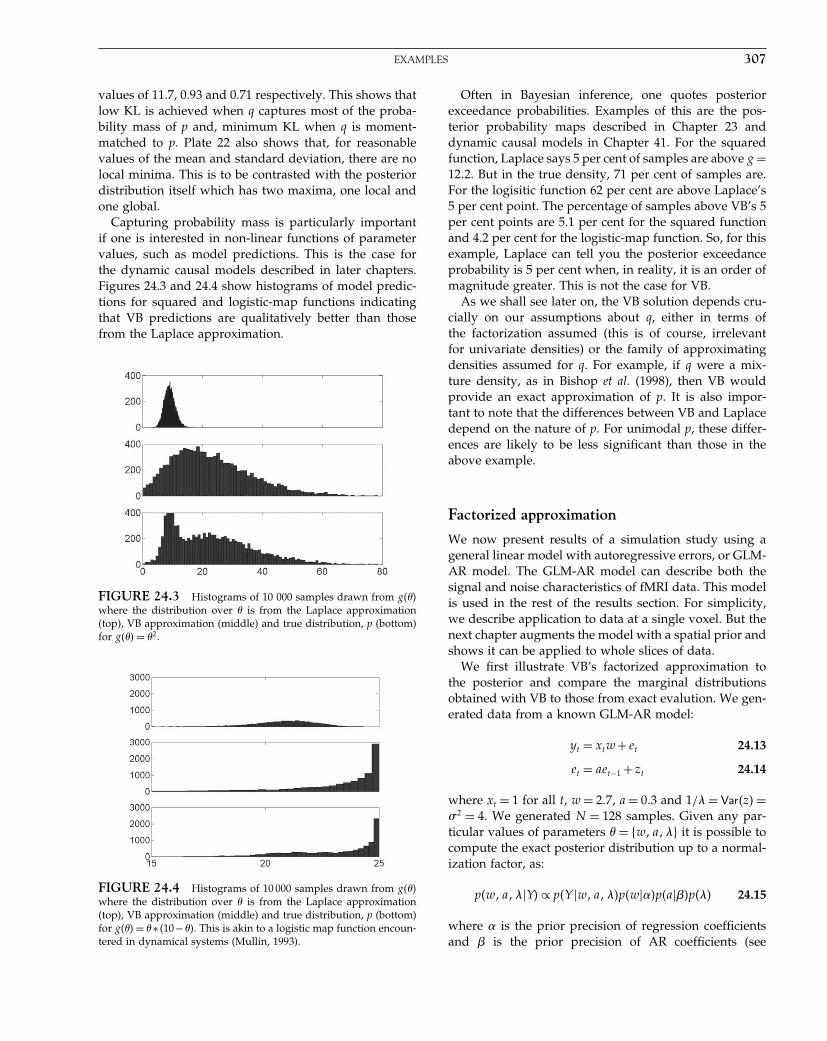
Elsevier UK Chapter: Ch24-P372560 30-9-2006 5:21p.m. Page:307 Trim:7.5in×9.25in
Basal Font:Palatino Margins:Top:40pt Gutter:68pt Font Size:9.5/12 Text Width:42pc Depth:55 Lines
EXAMPLES 307
values of 11.7, 0.93 and 0.71 respectively. This shows thatlow KL is achieved when q captures most of the proba-bility mass of p and, minimum KL when q is moment-matched to p. Plate 22 also shows that, for reasonablevalues of the mean and standard deviation, there are nolocal minima. This is to be contrasted with the posteriordistribution itself which has two maxima, one local andone global.
Capturing probability mass is particularly importantif one is interested in non-linear functions of parametervalues, such as model predictions. This is the case forthe dynamic causal models described in later chapters.Figures 24.3 and 24.4 show histograms of model predic-tions for squared and logistic-map functions indicatingthat VB predictions are qualitatively better than thosefrom the Laplace approximation.
FIGURE 24.3 Histograms of 10 000 samples drawn from g���where the distribution over � is from the Laplace approximation(top), VB approximation (middle) and true distribution, p (bottom)for g��� = �2.
FIGURE 24.4 Histograms of 10 000 samples drawn from g���where the distribution over � is from the Laplace approximation(top), VB approximation (middle) and true distribution, p (bottom)for g��� = �∗ �10−��. This is akin to a logistic map function encoun-tered in dynamical systems (Mullin, 1993).
Often in Bayesian inference, one quotes posteriorexceedance probabilities. Examples of this are the pos-terior probability maps described in Chapter 23 anddynamic causal models in Chapter 41. For the squaredfunction, Laplace says 5 per cent of samples are above g =12�2. But in the true density, 71 per cent of samples are.For the logisitic function 62 per cent are above Laplace’s5 per cent point. The percentage of samples above VB’s 5per cent points are 5.1 per cent for the squared functionand 4.2 per cent for the logistic-map function. So, for thisexample, Laplace can tell you the posterior exceedanceprobability is 5 per cent when, in reality, it is an order ofmagnitude greater. This is not the case for VB.
As we shall see later on, the VB solution depends cru-cially on our assumptions about q, either in terms ofthe factorization assumed (this is of course, irrelevantfor univariate densities) or the family of approximatingdensities assumed for q. For example, if q were a mix-ture density, as in Bishop et al. (1998), then VB wouldprovide an exact approximation of p. It is also impor-tant to note that the differences between VB and Laplacedepend on the nature of p. For unimodal p, these differ-ences are likely to be less significant than those in theabove example.
Factorized approximation
We now present results of a simulation study using ageneral linear model with autoregressive errors, or GLM-AR model. The GLM-AR model can describe both thesignal and noise characteristics of fMRI data. This modelis used in the rest of the results section. For simplicity,we describe application to data at a single voxel. But thenext chapter augments the model with a spatial prior andshows it can be applied to whole slices of data.
We first illustrate VB’s factorized approximation tothe posterior and compare the marginal distributionsobtained with VB to those from exact evalution. We gen-erated data from a known GLM-AR model:
yt = xtw+ et 24.13
et = aet−1 +zt 24.14
where xt = 1 for all t, w = 2�7, a = 0�3 and 1/ = Var�z� =�2 = 4. We generated N = 128 samples. Given any par-ticular values of parameters � = �w�a�� it is possible tocompute the exact posterior distribution up to a normal-ization factor, as:
p�w�a��Y� ∝ p�Y �w�a��p�w���p�a��p�� 24.15
where � is the prior precision of regression coefficientsand is the prior precision of AR coefficients (see
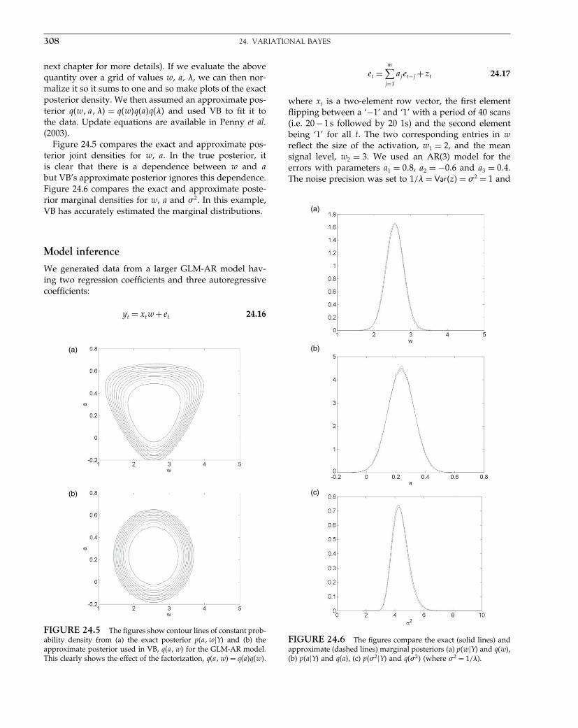
Elsevier UK Chapter: Ch24-P372560 30-9-2006 5:21p.m. Page:308 Trim:7.5in×9.25in
Basal Font:Palatino Margins:Top:40pt Gutter:68pt Font Size:9.5/12 Text Width:42pc Depth:55 Lines
308 24. VARIATIONAL BAYES
next chapter for more details). If we evaluate the abovequantity over a grid of values w, a, , we can then nor-malize it so it sums to one and so make plots of the exactposterior density. We then assumed an approximate pos-terior q�w�a�� = q�w�q�a�q�� and used VB to fit it tothe data. Update equations are available in Penny et al.(2003).
Figure 24.5 compares the exact and approximate pos-terior joint densities for w, a. In the true posterior, itis clear that there is a dependence between w and abut VB’s approximate posterior ignores this dependence.Figure 24.6 compares the exact and approximate poste-rior marginal densities for w, a and �2. In this example,VB has accurately estimated the marginal distributions.
Model inference
We generated data from a larger GLM-AR model hav-ing two regression coefficients and three autoregressivecoefficients:
yt = xtw+ et 24.16
(a)
(b)
FIGURE 24.5 The figures show contour lines of constant prob-ability density from (a) the exact posterior p�a�w�Y� and (b) theapproximate posterior used in VB, q�a�w� for the GLM-AR model.This clearly shows the effect of the factorization, q�a�w� = q�a�q�w�.
et =m∑
j=1
ajet−j +zt 24.17
where xt is a two-element row vector, the first elementflipping between a ‘−1’ and ‘1’ with a period of 40 scans(i.e. 20 − 1 s followed by 20 1s) and the second elementbeing ‘1’ for all t. The two corresponding entries in wreflect the size of the activation, w1 = 2, and the meansignal level, w2 = 3. We used an AR(3) model for theerrors with parameters a1 = 0�8, a2 = −0�6 and a3 = 0�4.The noise precision was set to 1/ = Var�z� = �2 = 1 and
(a)
(b)
(c)
FIGURE 24.6 The figures compare the exact (solid lines) andapproximate (dashed lines) marginal posteriors (a) p�w�Y� and q�w�,(b) p�a�Y� and q�a�, (c) p��2�Y� and q��2� (where �2 = 1/).

Elsevier UK Chapter: Ch24-P372560 30-9-2006 5:21p.m. Page:309 Trim:7.5in×9.25in
Basal Font:Palatino Margins:Top:40pt Gutter:68pt Font Size:9.5/12 Text Width:42pc Depth:55 Lines
DISCUSSION 309
(a)
(b)
F(m)
m
FIGURE 24.7 The figures show (a) an example time-seriesfrom a GLM-AR model with AR model order m = 3 and (b) a plotof the average negative free energy F�m�, with error bars, versus m.This shows that F�m� picks out the correct model order.
we initially generated N = 400 samples. This is a largermodel than in the previous example as we have moreAR and regression coefficients. An example time seriesproduced by this process is shown in Figure 24.7(a).
We then generated 10 such time-series and fitted GLM-AR(p) models to each using the VB algorithm. In eachcase, the putative model order was varied between m = 0and m = 5 and we estimated the model evidence foreach. Formulae for the model evidence approximationare available in Penny et al. (2003). Figure 24.7(b) showsa plot of the average value of the negative free energy,F�m� as a function of m, indicating that the maximumoccurs at the true model order.
Gibbs sampling
While it is possible, in principle, to plot the exact poste-riors using the method described previously, this wouldrequire a prohibitive amount of computer time for this
larger model. We therefore validated VB by comparing itwithGibbssampling(Gelmanetal., 1995;Pennyetal., 2003).
We generated a number of datasets containing eitherN = 40, N = 160 or N = 400 scans. At each dataset sizewe compared Gibbs and VB posteriors for each of theregression coefficients. For the purpose of these compar-isons the model order was kept fixed at m = 3. Figure 24.8shows representative results indicating a better agree-ment with increasing number of scans. We also note thatVB requires more iterations for fewer scans (typically 4iterations for N = 400, 5 iterations for N = 160 and 7iterations for N = 40). This is because the algorithm wasinitialized with an ordinary least squares (OLS) solutionwhich is closer to the VB estimate if there is a large num-ber of scans.
Estimation of effect size
Finally, we generated a number of data sets of varioussizes to compare VB and OLS estimates of activation sizewith the true value of w1 = 2. This comparison was madeusing a paired t-test on the absolute estimation error. ForN > 100, the VB estimation error was significantly smallerfor VB than for OLS �p < 0�05�. For N = 160, for example,the VB estimation error was 15 per cent smaller than theOLS error �p < 0�02�.
DISCUSSION
Variational Bayes delivers a factorized, minimum KL-divergence approximation to the true posterior densityand model evidence. This provides a computationallyefficient implementation of Bayesian inference for a largeclass of probabilistic models (Winn and Bishop, 2005).It allows for parameter inference, based on the approx-imating density q���m� and model inference based on afree energy approximation, F�m� to the model evidence,p�y�m�.
The quality of inference provided by VB depends onthe nature of the approximating distribution. There aretwo distinct approaches here. Fixed-form approximationsfix the form of q to be, for example, a diagonal (Hin-ton and van Camp, 1993) or full-covariance Gaussianensemble (Friston et al., 2006). Free-form approximationschoose a factorization that depends on p�Y���. Theserange from fully factorized approximations, where thereare no dependencies in q, to structured approximations.These identify substructures in p�Y���, such as trees ormixtures of trees, in which exact inference is possible.Variational methods are then used to handle interactionsbetween them (Ghahramani, 2002).

Elsevier UK Chapter: Ch24-P372560 30-9-2006 5:21p.m. Page:310 Trim:7.5in×9.25in
Basal Font:Palatino Margins:Top:40pt Gutter:68pt Font Size:9.5/12 Text Width:42pc Depth:55 Lines
310 24. VARIATIONAL BAYES
(a) (b)
(c) (d)
(e) (f)
FIGURE 24.8 The figures show the posterior distributions from Gibbs sampling (solid lines) and variational Bayes (dashed lines) fordata sets containing 40 scans (top row), 160 scans (middle row) and 400 scans (bottom row). The distributions in the left column are for thefirst regression coefficient (size of activation) and in the right column for the second regression coefficient (offset). The fidelity of the VBapproximation increases with number of scans.
VB also delivers an approximation to the modelevidence, allowing for Bayesian model comparison.However, it turns out that model selections based on VBare systematically biased towards simpler models (Bealand Ghahramani, 2003). Nevertheless, they have beenshown empirically to be more accurate than BIC approx-imations and faster than sampling approximations (Bealand Ghahramani, 2003). Bayesian model selection is dis-cussed further in Chapter 35.
Chapter 22 described a parametric empirical Bayes(PEB) algorithm for inference in hierarchical linear
Gaussian models. This algorithm may be viewed as a spe-cial case of VB with a fixed-form full-covariance Gaussianensemble (Friston et al., 2006). More generally, however,VB can be applied to models with discrete as well ascontinuous variables.
A classic example here is the Gaussian mixture model.This has been applied to an analysis of intersubject vari-ability in fMRI data. Model comparisons based on VBidentified two overlapping degenerate neuronal systemsin subjects performing a cross-modal priming task (Nop-peney et al., 2006).
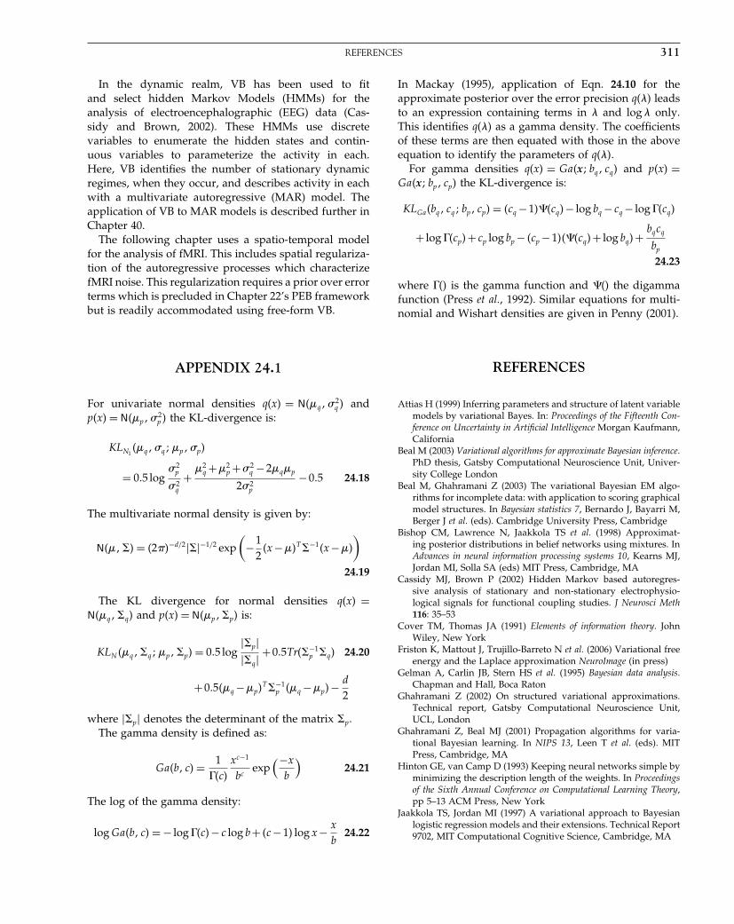
Elsevier UK Chapter: Ch24-P372560 30-9-2006 5:21p.m. Page:311 Trim:7.5in×9.25in
Basal Font:Palatino Margins:Top:40pt Gutter:68pt Font Size:9.5/12 Text Width:42pc Depth:55 Lines
REFERENCES 311
In the dynamic realm, VB has been used to fitand select hidden Markov Models (HMMs) for theanalysis of electroencephalographic (EEG) data (Cas-sidy and Brown, 2002). These HMMs use discretevariables to enumerate the hidden states and contin-uous variables to parameterize the activity in each.Here, VB identifies the number of stationary dynamicregimes, when they occur, and describes activity in eachwith a multivariate autoregressive (MAR) model. Theapplication of VB to MAR models is described further inChapter 40.
The following chapter uses a spatio-temporal modelfor the analysis of fMRI. This includes spatial regulariza-tion of the autoregressive processes which characterizefMRI noise. This regularization requires a prior over errorterms which is precluded in Chapter 22’s PEB frameworkbut is readily accommodated using free-form VB.
APPENDIX 24.1
For univariate normal densities q�x� = N� q��2q � and
p�x� = N� p��2p � the KL-divergence is:
KLN1� q��q� p��p�
= 0�5 log�2
p
�2q
+ 2q + 2
p +�2q −2 q p
2�2p
−0�5 24.18
The multivariate normal density is given by:
N� ��� = �2��−d/2���−1/2 exp(
−12
�x− �T �−1�x− �
)
24.19
The KL divergence for normal densities q�x� =N� q��q� and p�x� = N� p��p� is:
KLN � q��q� p��p� = 0�5 log��p���q�
+0�5Tr��−1p �q� 24.20
+0�5� q − p�T �−1
p � q − p�− d
2
where ��p� denotes the determinant of the matrix �p.The gamma density is defined as:
Ga�b� c� = 1��c�
xc−1
bcexp
(−x
b
)24.21
The log of the gamma density:
log Ga�b� c� = − log ��c�− c log b+ �c−1� log x− x
b24.22
In Mackay (1995), application of Eqn. 24.10 for theapproximate posterior over the error precision q�� leadsto an expression containing terms in and log only.This identifies q�� as a gamma density. The coefficientsof these terms are then equated with those in the aboveequation to identify the parameters of q��.
For gamma densities q�x� = Ga�x� bq� cq� and p�x� =Ga�x� bp� cp� the KL-divergence is:
KLGa�bq� cq� bp� cp� = �cq −1���cq�− log bq − cq − log ��cq�
+ log ��cp�+ cp log bp − �cp −1����cq�+ log bq�+ bqcq
bp
24.23
where ��� is the gamma function and ��� the digammafunction (Press et al., 1992). Similar equations for multi-nomial and Wishart densities are given in Penny (2001).
REFERENCES
Attias H (1999) Inferring parameters and structure of latent variablemodels by variational Bayes. In: Proceedings of the Fifteenth Con-ference on Uncertainty in Artificial Intelligence Morgan Kaufmann,California
Beal M (2003) Variational algorithms for approximate Bayesian inference.PhD thesis, Gatsby Computational Neuroscience Unit, Univer-sity College London
Beal M, Ghahramani Z (2003) The variational Bayesian EM algo-rithms for incomplete data: with application to scoring graphicalmodel structures. In Bayesian statistics 7, Bernardo J, Bayarri M,Berger J et al. (eds). Cambridge University Press, Cambridge
Bishop CM, Lawrence N, Jaakkola TS et al. (1998) Approximat-ing posterior distributions in belief networks using mixtures. InAdvances in neural information processing systems 10, Kearns MJ,Jordan MI, Solla SA (eds) MIT Press, Cambridge, MA
Cassidy MJ, Brown P (2002) Hidden Markov based autoregres-sive analysis of stationary and non-stationary electrophysio-logical signals for functional coupling studies. J Neurosci Meth116: 35–53
Cover TM, Thomas JA (1991) Elements of information theory. JohnWiley, New York
Friston K, Mattout J, Trujillo-Barreto N et al. (2006) Variational freeenergy and the Laplace approximation NeuroImage (in press)
Gelman A, Carlin JB, Stern HS et al. (1995) Bayesian data analysis.Chapman and Hall, Boca Raton
Ghahramani Z (2002) On structured variational approximations.Technical report, Gatsby Computational Neuroscience Unit,UCL, London
Ghahramani Z, Beal MJ (2001) Propagation algorithms for varia-tional Bayesian learning. In NIPS 13, Leen T et al. (eds). MITPress, Cambridge, MA
Hinton GE, van Camp D (1993) Keeping neural networks simple byminimizing the description length of the weights. In Proceedingsof the Sixth Annual Conference on Computational Learning Theory,pp 5–13 ACM Press, New York
Jaakkola TS, Jordan MI (1997) A variational approach to Bayesianlogistic regression models and their extensions. Technical Report9702, MIT Computational Cognitive Science, Cambridge, MA

Elsevier UK Chapter: Ch24-P372560 30-9-2006 5:21p.m. Page:312 Trim:7.5in×9.25in
Basal Font:Palatino Margins:Top:40pt Gutter:68pt Font Size:9.5/12 Text Width:42pc Depth:55 Lines
312 24. VARIATIONAL BAYES
Jaakola TS, Jordan MI, Ghahramani Z et al. (1998) An introduction tovariational methods for graphical models. In Learning in graphicalmodels, Jordan MI (ed.). Kluwer Academic Press, Dordrecht
Mackay DJC (1995) Ensemble learning and evidence maximization.Technical report, Cavendish Laboratory, University of Cam-bridge, Cambridge
MacKay DJC (1998) Choice of basis for Laplace approximations.Machine Learning 33: 77–86
Mackay DJC (2003) Information theory, inference and learning algo-rithms. Cambridge University Press, Cambridge
Mullin T (1993) The nature of chaos. Oxford Science Publications,Oxford
Noppeney U, Penny WD, Price CJ et al. (2006) Identification ofdegenerate neuronal systems based on intersubject variability.NeuroImage 30: 885–90
Penny WD (2001) Kullback-Liebler divergences of normal, gamma,Dirichlet and Wishart densities. Technical report, WellcomeDepartment of Imaging Neuroscience, London
Penny WD, Kiebel SJ, Friston KJ (2003) Variational Bayesian infer-ence for fMRI time series. NeuroImage 19: 727–41
Penny WD, Flandin G, Trujillo-Barreto N (2006) Bayesiancomparison of spatially regularised general linear models. HumBrain Mapp in press
Peterson C, Anderson J (1987) A mean field theory learn-ing algorithm for neural networks. Complex Syst 1:995–1019
Press WH, Teukolsky SA, Vetterling WT et al. (1992) NumericalRecipes in C. Cambridge University Press
Sahani M, Nagarajan SS (2004) Reconstructing MEG sources withunknown correlations. In Advances in neural information process-ing systems, Saul L, Thrun S, Schoelkopf B (eds), volume 16. MIT,Cambridge, MA
Sato M, Yoshioka T, Kajihara S et al. (2004) HierarchicalBayesian estimation for MEG inverse problem. NeuroImage 23:806–26
Winn J, Bishop C (2005) Variational message passing. J MachineLearning Res 6: 661–94
Woolrich MW, Behrens TE, Smith SM (2004) Constrained linearbasis sets for HRF modelling using variational Bayes. NeuroImage21: 1748–61
Elsevier UK Chapter: Ch25-P372560 30-9-2006 5:22p.m. Page:313 Trim:7.5in×9.25in
Basal Font:Palatino Margins:Top:40pt Gutter:68pt Font Size:9.5/12 Text Width:42pc Depth:55 Lines
C H A P T E R
25
Spatio-temporal models for fMRIW. Penny, G. Flandin and N. Trujillo-Barreto
INTRODUCTION
Functional magnetic resonance imaging (fMRI) usingblood oxygen-level-dependent (BOLD) contrast is anestablished method for making inferences about region-ally specific activations in the human brain (Frackowiaket al., 2003). From measurements of changes in blood oxy-genation one can use various statistical models, such asthe general linear model (GLM) (Friston et al., 1995), tomake inferences about task-specific changes in underly-ing neuronal activity.
This chapter reviews previous work (Penny et al., 2003,2005, 2006; Penny and Flandin, 2005a) on the devel-opment of spatially regularized general linear models(SRGLMs) for the analysis of fMRI data. These modelsallow for the characterization of subject and regionallyspecific effects using spatially regularized posterior prob-ability maps (PPMs). This spatial regularization has beenshown (Penny et al., 2005) to increase the sensitivity ofinferences one can make.
The chapter is structured as follows. The theoreti-cal section describes the generative model for SRGLM.This is split into descriptions of the prior and likeli-hood. We show how the variational Bayes (VB) algo-rithm, described in the previous chapter, can be used forapproximate inference. We describe how these inferencesare implemented for uni- and multivariate contrasts,and discuss the rationale for thresholding the resultingPPMs. We also discuss the spatio-temporal nature of themodel and compare it with standard approaches. Theresults section looks at null fMRI data, synthetic dataand fMRI from functional activation studies of audi-tory and face processing. The chapter finishes with adiscussion.
Notation
Lower case variable names denote vectors and scalars.Whether the variable is a vector or scalar should be clearfrom the context. Upper case names denote matricesor dimensions of matrices. In what follows N�x�����denotes a multivariate normal density over x, havingmean � and covariance �. The precision of a Gaussianvariate is the inverse (co)variance. A gamma densityover the scalar random variable x is written as Ga�x�a� b�.Normal and gamma densities are defined in Chapter 24.We also use ��x��2 = xT x, denote the trace operator asTr�X�, X+ for the pseudo-inverse, and use diag�x� todenote a diagonal matrix with diagonal entries given bythe vector x.
THEORY
We denote an fMRI data set consisting of T time points atN voxels as the T ×N matrix Y . In mass-univariate mod-els (Friston et al., 1995), these data are explained in termsof a T × K design matrix X, containing the values of Kregressors at T time points, and a K×N matrix of regres-sion coefficients W , containing K regression coefficientsat each of the N voxels. The model is written:
Y = XW +E 25.1
where E is a T×N error matrix.It is well known that fMRI data are contaminated with
artefacts. These stem primarily from low-frequency driftsdue to hardware instabilities, aliased cardiac pulsationand respiratory sources, unmodelled neuronal activityand residual motion artefacts not accounted for by rigidbody registration methods (Woolrich et al., 2001). This
Statistical Parametric Mapping, by Karl Friston et al. Copyright 2007, Elsevier Ltd. All rights reserved.ISBN–13: 978-0-12-372560-8 ISBN–10: 0-12-372560-7
313
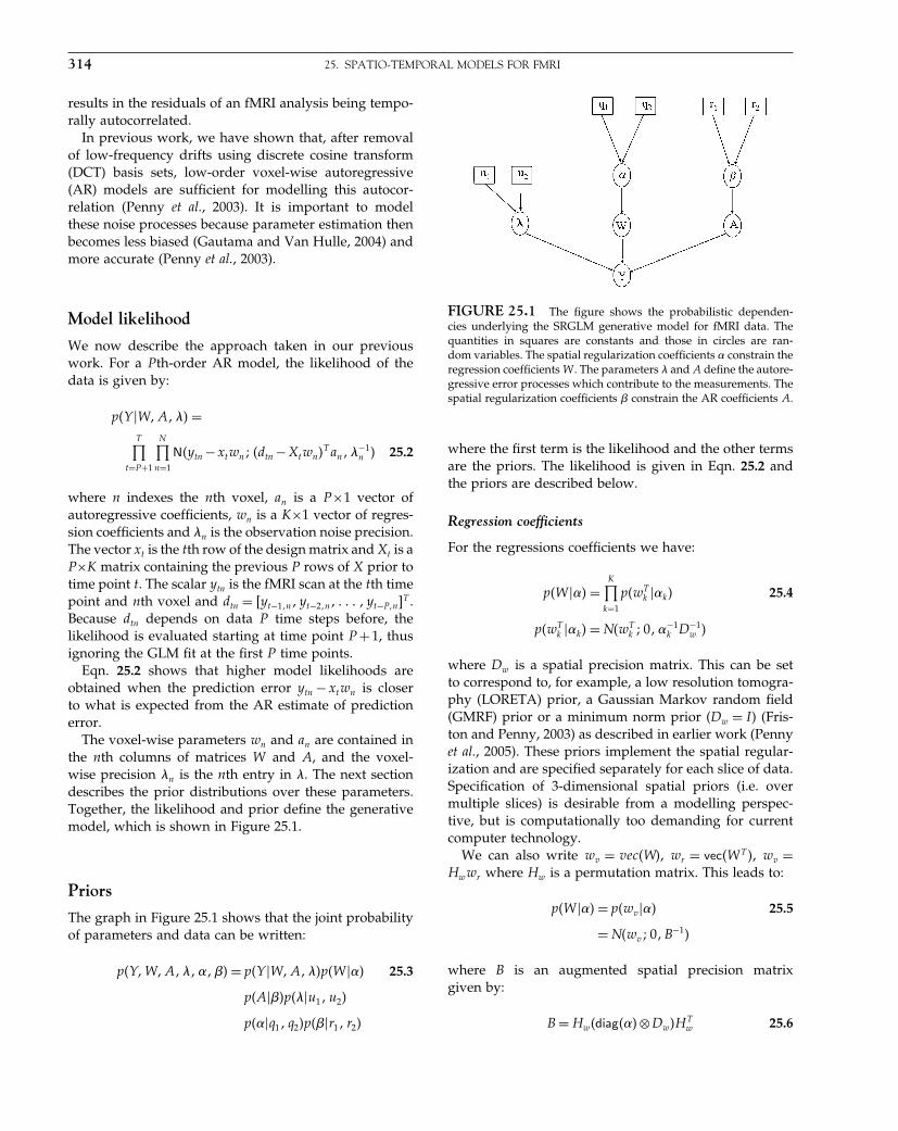
Elsevier UK Chapter: Ch25-P372560 30-9-2006 5:22p.m. Page:314 Trim:7.5in×9.25in
Basal Font:Palatino Margins:Top:40pt Gutter:68pt Font Size:9.5/12 Text Width:42pc Depth:55 Lines
314 25. SPATIO-TEMPORAL MODELS FOR FMRI
results in the residuals of an fMRI analysis being tempo-rally autocorrelated.
In previous work, we have shown that, after removalof low-frequency drifts using discrete cosine transform(DCT) basis sets, low-order voxel-wise autoregressive(AR) models are sufficient for modelling this autocor-relation (Penny et al., 2003). It is important to modelthese noise processes because parameter estimation thenbecomes less biased (Gautama and Van Hulle, 2004) andmore accurate (Penny et al., 2003).
Model likelihood
We now describe the approach taken in our previouswork. For a Pth-order AR model, the likelihood of thedata is given by:
p�Y �W�A��� =T∏
t=P+1
N∏n=1
N�ytn −xtwn� �dtn −Xtwn�T an��−1n � 25.2
where n indexes the nth voxel, an is a P×1 vector ofautoregressive coefficients, wn is a K×1 vector of regres-sion coefficients and �n is the observation noise precision.The vector xt is the tth row of the design matrix and Xt is aP×K matrix containing the previous P rows of X prior totime point t. The scalar ytn is the fMRI scan at the tth timepoint and nth voxel and dtn = yt−1�n� yt−2�n� � yt−P�n�T .Because dtn depends on data P time steps before, thelikelihood is evaluated starting at time point P + 1, thusignoring the GLM fit at the first P time points.
Eqn. 25.2 shows that higher model likelihoods areobtained when the prediction error ytn − xtwn is closerto what is expected from the AR estimate of predictionerror.
The voxel-wise parameters wn and an are contained inthe nth columns of matrices W and A, and the voxel-wise precision �n is the nth entry in �. The next sectiondescribes the prior distributions over these parameters.Together, the likelihood and prior define the generativemodel, which is shown in Figure 25.1.
Priors
The graph in Figure 25.1 shows that the joint probabilityof parameters and data can be written:
p�Y�W�A����� � = p�Y �W�A���p�W ��� 25.3
p�A� �p���u1�u2�
p���q1� q2�p� �r1� r2�
FIGURE 25.1 The figure shows the probabilistic dependen-cies underlying the SRGLM generative model for fMRI data. Thequantities in squares are constants and those in circles are ran-dom variables. The spatial regularization coefficients � constrain theregression coefficients W . The parameters � and A define the autore-gressive error processes which contribute to the measurements. Thespatial regularization coefficients constrain the AR coefficients A.
where the first term is the likelihood and the other termsare the priors. The likelihood is given in Eqn. 25.2 andthe priors are described below.
Regression coefficients
For the regressions coefficients we have:
p�W ��� =K∏
k=1
p�wTk ��k� 25.4
p�wTk ��k� = N�wT
k � 0��−1k D−1
w �
where Dw is a spatial precision matrix. This can be setto correspond to, for example, a low resolution tomogra-phy (LORETA) prior, a Gaussian Markov random field(GMRF) prior or a minimum norm prior (Dw = I) (Fris-ton and Penny, 2003) as described in earlier work (Pennyet al., 2005). These priors implement the spatial regular-ization and are specified separately for each slice of data.Specification of 3-dimensional spatial priors (i.e. overmultiple slices) is desirable from a modelling perspec-tive, but is computationally too demanding for currentcomputer technology.
We can also write wv = vec�W�, wr = vec�W T �, wv =Hwwr where Hw is a permutation matrix. This leads to:
p�W ��� = p�wv��� 25.5
= N�wv� 0�B−1�
where B is an augmented spatial precision matrixgiven by:
B = Hw�diag���⊗Dw�HTw 25.6
Elsevier UK Chapter: Ch25-P372560 30-9-2006 5:22p.m. Page:315 Trim:7.5in×9.25in
Basal Font:Palatino Margins:Top:40pt Gutter:68pt Font Size:9.5/12 Text Width:42pc Depth:55 Lines
THEORY 315
where ⊗ is the Kronecker product. This form of the prioris useful as our specification of approximate posteriors isbased on similar quantities. It can be seen that � encodesthe spatial precision of the regression coefficients.
The above Gaussian priors underly GMRFs andLORETA and have been used previously in fMRI(Woolrich et al., 2004) and electroencephalography (EEG)(Pascal Marqui et al., 1994). They are by no means, how-ever, the optimal choice for imaging data. In EEG, forexample, much interest has focused on the use of Lp-norm priors (Auranen et al. 2005) instead of the L2-normimplicit in the Gaussian assumption. Additionally, weare currently investigating the use of wavelet priors. Thisis an active area of research and will be the topic of futurepublications.
AR coefficients
We also define a spatial prior for the AR coefficients sothat they too can be spatially regularized. We have:
p�A� � =P∏
p=1
p�ap� p� 25.7
p�ap� p� = N�ap� 0� −1p D−1
a �
Again, Da is a user-defined spatial precision matrix, av =vec�A�, ar = vec�AT � and av = Haar , where Ha is a permu-tation matrix. This prior is used to implement the spatialregularization of the AR coefficients. We can write:
p�A� � = p�av� � 25.8
= N�av� 0� J−1�
where J is an augmented spatial precision matrix:
J = Ha �diag� �⊗Da�HTa 25.9
This form of the prior is useful as our specification ofapproximate posteriors is based on similar quantities.The parameter plays a similar role to � and controlsthe spatial regularization of the temporal autoregressioncoefficients.
We have also investigated ‘tissue-type’ priors whichconstrain AR estimates to be similar for voxels in thesame tissue-type, e.g. grey matter, white matter or cere-brospinal fluid. Bayesian model selection (Penny et al.,2006), however, favours the smoothly varying priorsdefined in Eqn. 25.7.
Precisions
We use gamma priors on the precisions �, and �:
p���u1�u2� =N∏
n=1
Ga��n�u1�u2� 25.10
p���q1� q2� =K∏
k=1
Ga��k� q1� q2�
p� �r1� r2� =P∏
p=1
Ga� p� r1� r2�
where the gamma density is defined in Chapter 24.Gamma priors were chosen as they are the conjugate pri-ors for Gaussian error models. The parameters are set toq1 = r1 = u1 = 10 and q2 = r2 = u2 = 0�1. These parame-ters produce gamma densities with a mean of 1 and avariance of 10. The robustness of, for example, modelselection to the choice of these parameters is discussedin Penny et al. (2003).
Approximate posteriors
Inference for SRGLMs has been implemented using thevariational Bayes (VB) approach described in the previ-ous chapter. In this section, we describe the algorithmdeveloped in previous work (Penny et al., 2005) where weassumed that the approximate posterior factorizes overvoxels and subsets of parameters.
Because of the spatial priors, the regression coefficientsin the true posterior p�W �Y� will clearly be correlated.Our perspective, however, is that this is too computation-ally burdensome for current personal computers to takeaccount of. Moreover, as we shall see later, updates forthe approximate factorized densities q�wn� do encouragethe approximate posterior means to be similar at nearbyvoxels, thereby achieving the desired effect of the prior.
Our approximate posterior is given by:
q�W�A����� � =∏n
q�wn�q�an�q��n� 25.11
∏k
q��k�∏p
q� p�
and each component of the approximate posterioris described below. These update equations are self-contained except for a number of quantities that aremarked out using the ‘tilde’ notation. These are Ãn� b̃n�C̃n� d̃n and G̃n, which are all defined in Appendix 25.1.
Regression coefficients
We have:
q�wn� = N�wn� ŵn� �̂n� 25.12
�̂n =(�̄nÃn + B̄nn
)−1
ŵn = �̂n
(�̄nb̃T
n + rn
)
rn = −N∑
i=1�i �=n
B̄niŵi
Elsevier UK Chapter: Ch25-P372560 30-9-2006 5:22p.m. Page:316 Trim:7.5in×9.25in
Basal Font:Palatino Margins:Top:40pt Gutter:68pt Font Size:9.5/12 Text Width:42pc Depth:55 Lines
316 25. SPATIO-TEMPORAL MODELS FOR FMRI
where ŵn is the estimated posterior mean and �̂n isthe estimated posterior covariance. The quantity B̄ isdefined as in Eqn. 25.6 but uses �̄ instead of �. Thequantities Ãn and b̃n are expectations related to autore-gressive processes and are defined in Appendix 25.1. Inthe absence of temporal autocorrelation we have Ãn =XT X and b̃T
n = XT yn.
AR coefficients
We have:
q�an� = N�an�mn�Vn�
where
Vn =(�̄nC̃n + J̄nn
)−125.13
mn = Vn��̄nd̃n + jn�
jn = −N∑
i=1�i �=n
J̄nimi
and mn is the estimated posterior mean and Vn is theestimated posterior covariance. The quantity J̄ is definedas in Eqn. 25.9 but ̄ is used instead of . The subscriptsin J̄ni denote that part of J̄ relevant to the nth and ithvoxels. The quantities C̃n and d̃n are expectations that aredefined in Appendix 25.1.
Precisions
The approximate posteriors over the precision variablesare gamma densities. For the precisions on the observa-tion noise we have:
q��n� = Ga��n� bn� cn� 25.14
1bn
= G̃n
2+ 1
u1
cn = T
2+u2
�̄n = bc
where G̃n is the expected prediction error defined inAppendix 25.1. For the precisions of the regression coef-ficients we have:
q��k� = Ga��k�gk�hk� 25.15
1gk
= 12
(Tr��̂kDw�+ ŵT
k Dwŵk
)+ 1
q1
hk = N
2+ q2
�̄k = gkhk
For the precisions of the AR coefficients we have:
q� p� = Ga� p� r1p� r2p� 25.16
1r1p
= 12
(Tr�VpDa�+mT
p Damp
)+ 1
r1
r2p = N
2+ r2
̄p = r1pr2p
Practicalities
Our empirical applications use spatial precision matricesDa and Dw, defined above, which produce GMRF priors.Also, we use AR models of order P = 3. Model selectionusing VB showed that this model order was sufficient forall voxels in a previous analysis of fMRI (Penny et al.,2003).
The VB algorithm is initialized using ordinary leastsquare (OLS) estimates for regression and autoregressiveparameters as described in Penny et al. (2003). Quantitiesare then updated using Eqns. 25.12, 25.13, 25.14, 25.15,25.16.
As described in the previous chapter, the aim of VBis to match an approximate posterior to the true poste-rior density in the sense of minimizing Kullback-Liebler(KL) divergence. This is implemented implicitly by max-imizing the quantity F , known in statistical physics asthe negative free energy. In the implemention of VB forSRGLMs, F is monitored during optimization. Conver-gence is then defined as less than a 1 per cent increasein F .
Expressions for computing F are given in Penny et al.(2006). This is an important quantity as it can also beused for model comparison. This is described at length inPenny et al. (2006) and reviewed in Chapters 24 and 35.
The algorithm we have described is implemented inSPM version 5 and can be downloaded from SPM Soft-ware (2006). Computation of a number of quantites (e.g.C̃n, d̃n and G̃n) is now much more efficient than in previ-ous versions (Penny et al., 2005). These improvements aredescribed in a separate document (Penny and Flandin,2005b). To analyse a single session of data (e.g. the facefMRI data) takes about 30 minutes on a typical personalcomputer.
Spatio-temporal deconvolution
The central quantity of interest in fMRI analysis isour estimate of effect sizes, embodied in contrasts ofregression coefficients. A key update equation in ourVB scheme is, therefore, the approximate posterior for

Elsevier UK Chapter: Ch25-P372560 30-9-2006 5:22p.m. Page:317 Trim:7.5in×9.25in
Basal Font:Palatino Margins:Top:40pt Gutter:68pt Font Size:9.5/12 Text Width:42pc Depth:55 Lines
THEORY 317
the regression coefficients. This is given by Eqn. 25.12.For the special case of temporally uncorrelated data wehave:
�̂n = (�̄nXT X + B̄nn
)−125.17
ŵn = �̂n
(�̄nXT yn + rn
)
where B̄ is a spatial precision matrix and rn is theweighted sum of neighbouring regression coefficient esti-mates.
This update indicates that the estimate at a given voxelregresses towards those at nearby voxels. This is thedesired effect of the spatial prior and is preserved despitethe factorization over voxels in the approximate poste-rior (see Eqn. 25.11). Eqn. 25.17 can be thought of as thecombination of a temporal prediction XT yn and a spatialprediction from rn. Each prediction is weighted by itsrelative precision to produce the optimal estimate ŵn. Inthis sense, VB provides a spatio-temporal deconvolutionof fMRI data. Moreover, the parameters controlling therelative precisions, �̄n and �̄, are estimated from the data.The effect size estimates therefore derive from an auto-matically regularized spatio-temporal deconvolution.
Contrasts
After having estimated a model, we will be interested incharacterizing a particular effect, c, which can usually beexpressed as a linear function or ‘contrast’ of parameters,w. This is described at length in Chapter 9. That is,
cn = CT wn 25.18
where C is a contrast vector or matrix. For example,the contrast vector CT = 1�−1� computes the differencebetween two experimental conditions.
Our statistical inferences are based on the approximatedistribution q�W�, which implies a distribution on c, q�c�.Because q�W� factorizes over voxels we can write:
q�c� =N∏
n=1
q�cn� 25.19
where cn is the effect size at voxel n. Given a contrastmatrix C we have:
q�cn� = N�cn��n�Sn� 25.20
with mean and covariance:
�n = CT ŵn 25.21
Sn = CT �̂nC
Bayesian inference based on this posterior can then takeplace using confidence intervals (Box and Tiao, 1992). Forunivariate contrasts we have suggested the use of poste-rior probability maps (PPMs), as described in Chapter 23.
If cn is a vector, then we have a multivariate contrast.Inference can then proceed as follows. The probability �that the zero vector lies on the 1 − � confidence regionof the posterior distribution at each voxel must then becomputed. We first note that this probability is the sameas the probability that the vector �n lies on the edge of the1 −� confidence region for the distribution N��n� 0� Sn�.This latter probability can be computed by forming thetest statistic:
dn = �Tn S−1
n �n 25.22
which will be the sum of rn = rank�Sn� independent,squared Gaussian variables. As such, it has a �2 distribu-tion:
p�dn� = �2�rn� 25.23
This procedure is identical to that used for making infer-ences in Bayesian multivariate autoregressive models(Harrison et al., 2003). We can also use this procedureto test for two-sided effects, i.e., activations or deactiva-tions. Though, strictly, these contrasts are univariate wewill use the term ‘multivariate contrasts’ to cover thesetwo-sided effects.
Thresholding
In previous work (Friston and Penny, 2003), we havesuggested deriving PPMs by applying two thresholds tothe posterior distributions: (i) an effect size threshold,�; and (ii) a probability threshold pT . Voxel n is thenincluded in the PPM if q�cn > �� > pT . This approach wasdescribed in Chapter 23.
If voxel n is to be included, then the posteriorexceedance probability q�cn > �� is plotted. It is alsopossible to plot the effect size itself, cn. The followingexploratory procedure can be used for exploring the pos-terior distribution of effect sizes. First, plot a map of effectsizes using the thresholds � = 0 and pT = 1−1/N whereN is the number of voxels. We refer to these values asthe ‘default thresholds’. Then, after visual inspection ofthe resulting map use a non-zero �, the value of whichreflects effect sizes in areas of interest. It will then bepossible to reduce pT to a value such as 0.95. Of course,if previous imaging analyses have indicated what effectsizes are physiologically relevant then this exploratoryprocedure is unnecessary.
Elsevier UK Chapter: Ch25-P372560 30-9-2006 5:22p.m. Page:318 Trim:7.5in×9.25in
Basal Font:Palatino Margins:Top:40pt Gutter:68pt Font Size:9.5/12 Text Width:42pc Depth:55 Lines
318 25. SPATIO-TEMPORAL MODELS FOR FMRI
False positive rates
If we partition effect-size values into two hypothesisspaces H0 � c ≤ � and H1 � c > �, then we can character-ize the sensitivity and specificity of our algorithm. Thisis different to classical inference which uses H0 � c = 0.A false positive (FP) occurs if we accept H1 when H0 istrue.
If we use the default threshold, and the approximateposterior were exact, then the distribution of FPs isbinomial with rate 1/N . The expected number of falsepositives in each PPM is therefore N ×1/N = 1. The vari-ance is N ×1/N × �1−1/N� which is approximately 1. Wewould therefore expect 0, 1 or 2 false positives per PPM.
Of course, the above result only holds if the approxi-mate posterior is equal to the true posterior. But, giventhat all of our computational effort is aimed at this goal,it would not be surprising if the above analysis wereindicative of actual FP rates. This issue will be investi-gated using null fMRI data in the next section.
RESULTS
Null data
This section describes the analysis of a null dataset to findout how many false positives are obtained using PPMswith default thresholds.
Images were acquired from a 1.5T Sonata (Siemens,Erlangen, Germany) which produced T2∗-weightedtransverse echo-planar images (EPIs) with BOLD con-trast, while a subject was lying in the scanner, asked torest and was not provided with any experimental stimu-lus. These data are thus collected under the null hypoth-esis, H0, that experimental effects are zero. This shouldhold whatever the design matrix and contrast we con-ceive. Any observed activations will be false positives.
Whole brain EPIs consisting of 48 transverse slices wereacquired every TR = 4�32 s resulting in a total of T = 98scans. The voxel size is 3 × 3 × 3 mm. All images wererealigned to the first image using a six-parameter rigid-body transformation to account for subject movement.These data were not spatially smoothed. While spatialsmoothing is necessary for the standard application ofclassical inference (see e.g. Chapter 2), it is not necessaryfor the spatio-temporal models described in this chapter.Indeed, the whole point of SRGLM is that the optimalsmoothness can be inferred from the data.
We then implemented a standard whole volume anal-ysis on images comprising N = 59 945 voxels. We usedthe design matrix shown in the left panel of Figure 25.2.Use of the default thresholds resulted in no spuriousactivations in the PPM.
We then repeated the above analysis but with a numberof different design matrices. First, we created a numberof epoch designs. These were based on the design inFigure 25.2, but epoch onsets were jittered by a numberbetween plus or minus 9 scans. This number was drawnfrom a uniform distribution, and the epoch durationswere drawn from a uniform distribution between 4 and10 scans. Five such design matrices were created andVB models fitted with each to the null data. For everyanalysis, the number of false positives was 0.
Secondly, we created a number of event-relateddesigns by sampling event onsets with inter-stimulusintervals drawn from a poisson distribution with rate fivescans. These event streams were then convolved with acanonical HRF (Henson, 2003). Again, five such designmatrices were created and VB models fitted with each tothe null data. Over the five analyses, the average numberof false positives was 9.4. The higher false positive rate forevent-related designs is thought to occur because event-related regressors are more similar than epoch regressorsto fMRI noise.
Synthetic data
We then added three synthetic activations to a slice ofnull data �z = −13 mm�. These were created using thedesign matrix and regression coefficient image shownin Figure 25.2 (the two regression coefficient images, i.e.for the activation and the mean, were identical). Theseimages were formed by placing delta functions at threelocations and then smoothing with Gaussian kernels hav-ing full width at half maxima (FWHMs) of 2, 3 and 4pixels (going clockwise from the top-left blob). Imageswere then rescaled to make the peaks unity.
In principle, smoothing with a Gaussian kernel rendersthe true effect size greater than zero everywhere becausea Gaussian has infinite spatial support. In practice, how-ever, when implemented on a digital computer withfinite numerical precision, most voxels will be numer-ically zero. Indeed, our simulated data contained 299‘activated’ voxels, i.e. voxels with effect sizes numericallygreater than zero.
This slice of data was then analysed using VB. The con-trast CT = 1� 0� was then used to look at the estimatedactivation effect, which is shown in the left panel ofFigure 25.3. For comparison, we also show the effect asestimated using OLS. Clearly, OLS estimates are muchnoisier than VB estimates.
Figure 25.4 shows plots of the exceedance probabilitiesfor two different effect-size thresholds, � = 0 and � = 0�3.Figure 25.5 shows thresholded versions of these images.These are PPMs. Neither of these PPMs contains anyfalse positives. That is, the true effect size is greater than
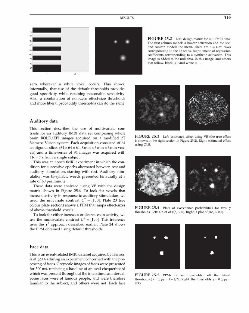
Elsevier UK Chapter: Ch25-P372560 30-9-2006 5:22p.m. Page:319 Trim:7.5in×9.25in
Basal Font:Palatino Margins:Top:40pt Gutter:68pt Font Size:9.5/12 Text Width:42pc Depth:55 Lines
RESULTS 319
FIGURE 25.2 Left: design matrix for null fMRI data.The first column models a boxcar activation and the sec-ond column models the mean. There are n = 1��98 rowscorresponding to the 98 scans. Right: image of regressioncoefficients corresponding to a synthetic activation. Thisimage is added to the null data. In this image, and othersthat follow, black is 0 and white is 1.
zero wherever a white voxel occurs. This shows,informally, that use of the default thresholds providesgood specificity while retaining reasonable sensitivity.Also, a combination of non-zero effect-size thresholdsand more liberal probability thresholds can do the same.
Auditory data
This section describes the use of multivariate con-trasts for an auditory fMRI data set comprising wholebrain BOLD/EPI images acquired on a modified 2TSiemens Vision system. Each acquisition consisted of 64contiguous slices (64×64×64, 3 mm×3 mm×3 mm vox-els) and a time-series of 84 images was acquired withTR = 7 s from a single subject.
This was an epoch fMRI experiment in which the con-dition for successive epochs alternated between rest andauditory stimulation, starting with rest. Auditory stim-ulation was bi-syllabic words presented binaurally at arate of 60 per minute.
These data were analysed using VB with the designmatrix shown in Figure 25.6. To look for voxels thatincrease activity in response to auditory stimulation, weused the univariate contrast CT = 1� 0�. Plate 23 (seecolour plate section) shows a PPM that maps effect-sizesof above-threshold voxels.
To look for either increases or decreases in activity, weuse the multivariate contrast CT = 1� 0�. This inferenceuses the �2 approach described earlier. Plate 24 showsthe PPM obtained using default thresholds.
Face data
This is an event-related fMRI data set acquired by Hensonet al. (2002) during an experiment concerned with the pro-cessing of faces. Greyscale images of faces were presentedfor 500 ms, replacing a baseline of an oval chequerboardwhich was present throughout the interstimulus interval.Some faces were of famous people, and were thereforefamiliar to the subject, and others were not. Each face
FIGURE 25.3 Left: estimated effect using VB (the true effectis shown in the right section in Figure 25.2). Right: estimated effectusing OLS.
FIGURE 25.4 Plots of exceedance probabilities for two �thresholds. Left: a plot of p�cn > 0�. Right: a plot of p�cn > 0�3�.
FIGURE 25.5 PPMs for two thresholds. Left: the defaultthresholds (� = 0, pT = 1−1/N ) Right: the thresholds � = 0�3, pT =0�95.
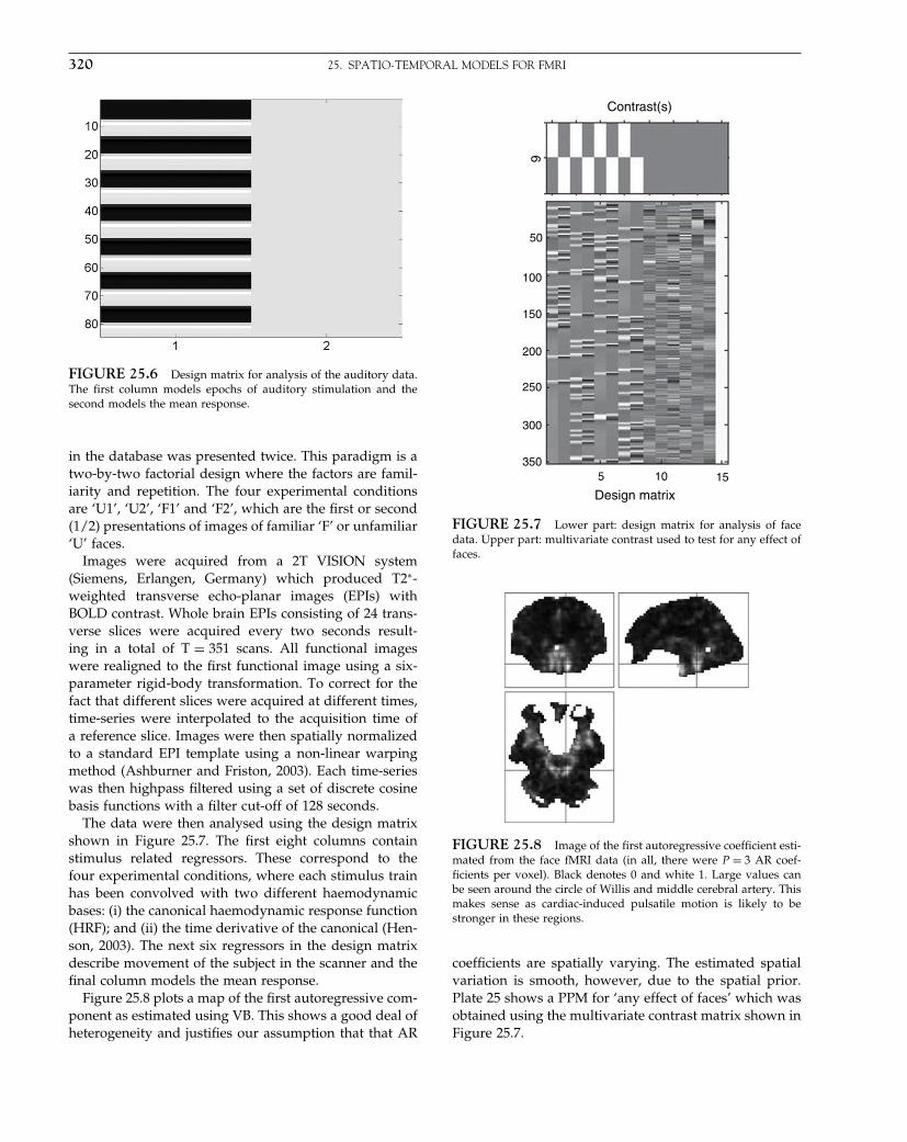
Elsevier UK Chapter: Ch25-P372560 30-9-2006 5:22p.m. Page:320 Trim:7.5in×9.25in
Basal Font:Palatino Margins:Top:40pt Gutter:68pt Font Size:9.5/12 Text Width:42pc Depth:55 Lines
320 25. SPATIO-TEMPORAL MODELS FOR FMRI
FIGURE 25.6 Design matrix for analysis of the auditory data.The first column models epochs of auditory stimulation and thesecond models the mean response.
in the database was presented twice. This paradigm is atwo-by-two factorial design where the factors are famil-iarity and repetition. The four experimental conditionsare ‘U1’, ‘U2’, ‘F1’ and ‘F2’, which are the first or second(1/2) presentations of images of familiar ‘F’ or unfamiliar‘U’ faces.
Images were acquired from a 2T VISION system(Siemens, Erlangen, Germany) which produced T2∗-weighted transverse echo-planar images (EPIs) withBOLD contrast. Whole brain EPIs consisting of 24 trans-verse slices were acquired every two seconds result-ing in a total of T = 351 scans. All functional imageswere realigned to the first functional image using a six-parameter rigid-body transformation. To correct for thefact that different slices were acquired at different times,time-series were interpolated to the acquisition time ofa reference slice. Images were then spatially normalizedto a standard EPI template using a non-linear warpingmethod (Ashburner and Friston, 2003). Each time-serieswas then highpass filtered using a set of discrete cosinebasis functions with a filter cut-off of 128 seconds.
The data were then analysed using the design matrixshown in Figure 25.7. The first eight columns containstimulus related regressors. These correspond to thefour experimental conditions, where each stimulus trainhas been convolved with two different haemodynamicbases: (i) the canonical haemodynamic response function(HRF); and (ii) the time derivative of the canonical (Hen-son, 2003). The next six regressors in the design matrixdescribe movement of the subject in the scanner and thefinal column models the mean response.
Figure 25.8 plots a map of the first autoregressive com-ponent as estimated using VB. This shows a good deal ofheterogeneity and justifies our assumption that that AR
50
100
150
200
250
300
3505 10 15
Design matrix
9
Contrast(s)
FIGURE 25.7 Lower part: design matrix for analysis of facedata. Upper part: multivariate contrast used to test for any effect offaces.
FIGURE 25.8 Image of the first autoregressive coefficient esti-mated from the face fMRI data (in all, there were P = 3 AR coef-ficients per voxel). Black denotes 0 and white 1. Large values canbe seen around the circle of Willis and middle cerebral artery. Thismakes sense as cardiac-induced pulsatile motion is likely to bestronger in these regions.
coefficients are spatially varying. The estimated spatialvariation is smooth, however, due to the spatial prior.Plate 25 shows a PPM for ‘any effect of faces’ which wasobtained using the multivariate contrast matrix shown inFigure 25.7.

Elsevier UK Chapter: Ch25-P372560 30-9-2006 5:22p.m. Page:321 Trim:7.5in×9.25in
Basal Font:Palatino Margins:Top:40pt Gutter:68pt Font Size:9.5/12 Text Width:42pc Depth:55 Lines
REFERENCES 321
DISCUSSION
We have reviewed a framework for the analysis of fMRIdata based on spatially regularized GLMs. This modelembodies prior knowledge that evoked responses arespatially homogeneous and locally contiguous.
As compared to standard approaches based onspatially smoothing the imaging data itself, the spatialregularization procedure has been shown to result ininferences with higher sensitivity (Penny et al., 2005). Theapproach may be viewed as an automatically regularizedspatio-temporal deconvolution scheme.
Use of PPMs with default thresholds resulted in lowfalse positive rates for null fMRI data, and physiologicallyplausible activations for auditory and face fMRI datasets. We have recently developed a similar approach forsource localization of EEG/MEG, which is described inthe following chapter.
APPENDIX 25.1
This appendix provides a number of formulae requiredfor updating the approximate posteriors. These have beenderived in Penny et al. (2003). First, auxiliary quantitiesfor updating q�wn� are:
Ãn =∑t
xTt xt +XT
t �mTn mn +Vn�Xt
−xTt mnXt −XT
t mTn xt 25.24
b̃n =∑t
ytnxt −mndtnxt −ytnmnXt
+dTtn�mT
n mn +Vn�Xt 25.25
For the special case in which the errors are uncorrelated,i.e. P = 0, we have Ãn = XT X and b̃n = XT yn. If we alsohave no spatial prior on the regression coefficients, i.e.� = 0, we then recover the least squares update:
ŵn = �XT X�−1XT yn 25.26
Secondly, auxiliary quantities for updating q�an� are:
C̃n =∑t
dtndTtn +Xt�ŵnŵT
n + �̂n�XTt 25.27
−dtnŵTn XT
t −XtŵndTtn
d̃n =∑t
ytndTtn −xtŵndT
tn −ytnŵTn X̃T +xt�ŵnŵT
n + �̂n�XTt
Thirdly, the auxiliary quantity for updating q��n� is:
G̃n = G̃n1 + G̃n2 + G̃n3 25.28
where
G̃n1 =∑t
y2tn +dT
tn�mTn mn +Vn�dtn −2ytndT
tnmn 25.29
G̃n2 =∑t
xt�ŵnŵTn + �̂�xT
t +Tr�XTt �mT
n mn +Vn�Xt�̂n�
+ŵTn XT
t �mTn mn +Vn�Xtŵn −2xt�ŵnŵT
n + �̂n�XtmTn
G̃n3 =∑t
−2ytnxtŵn +2mndtnxtŵn
+2ytnmnXtŵn −2dTtn�mT
n mn +Vn�Xtŵn
Many terms in the above equations do not depend onmodel parameters and so can be pre-computed for effi-cient implementation. See Penny and Flandin (2005b) formore details.
REFERENCES
Ashburner J, Friston KJ (2003) Spatial normalization using basisfunctions. In Human brain function, 2nd edn, Frackowiak RSJ,Friston KJ, Frith C et al. (eds). Academic Press, London
Auranen T, Nummenmaa A, Hammalainen M et al. (2005) Bayesiananalysis of the neuromagnetic inverse problem with lp normpriors. NeuroImage 26: 70–84
Box GEP, Tiao GC (1992) Bayesian inference in statistical analysis. JohnWiley, New York
Frackowiak RSJ, Friston KJ, Frith C et al. (2003) Human brain function,2nd edn. Academic Press, London
Friston KJ, Holmes AP, Worsley KJ et al. (1995). Statistical parametricmaps in functional imaging: a general linear approach. HumBrain Mapp 2: 189–210
Friston KJ, Penny WD (2003) Posterior probability maps and SPMs.NeuroImage 19: 1240–49
Gautama T, Van Hulle MM (2004) Optimal spatial regularisationof autocorrelation estimates in fMRI analysis. NeuroImage 23:1203–16
Harrison L, Penny WD, Friston KJ (2003) Multivariate autoregres-sive modelling of fMRI time series. NeuroImage 19: 1477–91
Henson RNA. (2003) Analysis of fMRI time series. In Human brainfunction, 2nd edn, Frackowiak RSS, Friston KJ, Frith C et al. (eds).Academic Press, London
Henson RNA, Shallice T, Gorno-Tempini ML et al. (2002) Face rep-etition effects in implicit and explicit memory tests as measuredby fMRI. Cereb Cortex 12: 178–86
Pascual Marqui R, Michel C, Lehman D (1994) Low resolution elec-tromagnetic tomography: a new method for localizing electricalactivity of the brain. Int J Psychophysiol 18: 49–65
Penny WD, Kiebel SJ, Friston KJ (2003) Variational Bayesian infer-ence for fMRI time series. NeuroImage 19: 727–41
Penny WD, Flandin G (2005a) Bayesian analysis of fMRI data withspatial priors. In Proceedings of the Joint Statistical Meeting (JSM),Section on Statistical Graphics (CDROM), 2005. American Statisti-cal Association, Alexandria, VA
Penny WD, Flandin G (2005b) Bayesian analysis of single-subjectfMRI: SPM implementation. Technical report, Wellcome Depart-ment of Imaging Neuroscience, London
Penny WD, Trujillo-Barreto N, Friston KJ (2005) Bayesian fMRI timeseries analysis with spatial priors. NeuroImage, 24: 350–62

Elsevier UK Chapter: Ch25-P372560 30-9-2006 5:22p.m. Page:322 Trim:7.5in×9.25in
Basal Font:Palatino Margins:Top:40pt Gutter:68pt Font Size:9.5/12 Text Width:42pc Depth:55 Lines
322 25. SPATIO-TEMPORAL MODELS FOR FMRI
Penny WD, Flandin G, Trujillo-Barreto N (2006) Bayesian com-parison of spatially regularised general linear models. HumBrain Mapp (in press)
SPM Software (2006) Wellcome Department of Imaging Neu-roscience. Available from http://www.fil.ion.ucl.ac.uk/spm/software/
Woolrich MW, Ripley BD, Brady M et al. (2001) Temporal autocor-relation in univariate linear modelling of fMRI data. NeuroImage14: 1370–86
Woolrich MW, Behrens TE, Smith SM (2004) Constrained linearbasis sets for HRF modelling using variational Bayes. NeuroImage21: 1748–61
Elsevier UK Chapter: Ch26-P372560 30-9-2006 5:23p.m. Page:323 Trim:7.5in×9.25in
Basal Font:Palatino Margins:Top:40pt Gutter:68pt Font Size:9.5/12 Text Width:42pc Depth:55 Lines
C H A P T E R
26
Spatio-temporal models for EEGW. Penny, N. Trujillo-Barreto and E. Aubert
INTRODUCTION
Imaging neuroscientists have at their disposal a vari-ety of imaging techniques for investigating human brainfunction (Frackowiak et al., 2003). Among these, theelectroencephalogram (EEG) records electrical voltagesfrom electrodes placed on the scalp, the magnetoen-cephalogram (MEG) records the magnetic field from sen-sors placed just above the head and functional magneticresonance imaging (fMRI) records magnetization changesdue to variations in blood oxygenation.
However, as the goal of brain imaging is to obtaininformation about the neuronal networks that supporthuman brain function, one must first transform mea-surements from imaging devices into estimates of intra-cerebral electrical activity. Brain imaging methodologistsare therefore faced with an inverse problem, ‘How canone make inferences about intracerebral neuronal pro-cesses given extracerebral or vascular measurements?’
We argue that this problem is best formulated asa model-based spatio-temporal deconvolution problem.For EEG and MEG, the required deconvolution is pri-marily spatial, and for fMRI it is primarily temporal.Although one can make minimal assumptions about thesource signals by applying ‘blind’ deconvolution meth-ods (McKeown et al., 1998; Makeig et al., 2002), knowledgeof the underlying physical processes can be used to greateffect. This information can be implemented in a forwardmodel that is inverted during deconvolution. In M/EEG,forward models make use of Maxwell’s equations gov-erning propagation of electromagnetic fields (Baillet et al.,2001) and in fMRI haemodynamic models link neuralactivity to ‘balloon’ models of vascular dynamics (Fristonet al., 2000).
To implement a fully spatio-temporal deconvolution,time-domain fMRI models must be augmented with aspatial component and spatial-domain M/EEG models
with a temporal component. The previous chaptershowed how this could be implemented for fMRI. Thischapter describes a model-based spatio-temporal decon-volution method for M/EEG.
The underlying forward or ‘generative’ model incor-porates two mappings. The first specifies a time-domaingeneral linear model (GLM) at each point in source space.This relates effects of interest at each voxel to sourceactivity at that voxel. This is identical to the ‘mass-univariate’ approach that is widely used in the analysisof fMRI (Frackowiak et al., 2003). The second mappingrelates source activity to sensor activity at each timepoint using the usual spatial-domain lead-field matrix(see Chapter 28).
Our model therefore differs from the standard genera-tive model implicit in source reconstruction by having anadditional level that embodies temporal priors. There aretwo potential benefits of this approach. First, the use oftemporal priors can result in more sensitive source recon-structions. This may allow signals to be detected thatcannot be detected otherwise. Second, it provides an anal-ysis framework for M/EEG that is very similar to thatused in fMRI. The experimental design can be coded ina design matrix, the model fitted to data, and variouseffects of interest can be characterized using ‘contrasts’(Frackowiak et al., 2003). These effects can then be testedfor statistically using posterior probability maps (PPMs),as described in previous chapters. Importantly, the modeldoes not need to be refitted to test for multiple experi-mental effects that are potentially present in any singledata set. Sources are estimated once only using a spatio-temporal deconvolution rather than separately for eachtemporal component of interest.
The chapter is organized as follows. In the theorysection, we describe the model and relate it to exist-ing distributed solutions. The success of the approachrests on our ability to characterize neuronal responses,and task-related differences in them, using GLMs.
Statistical Parametric Mapping, by Karl Friston et al. Copyright 2007, Elsevier Ltd. All rights reserved.ISBN–13: 978-0-12-372560-8 ISBN–10: 0-12-372560-7
323
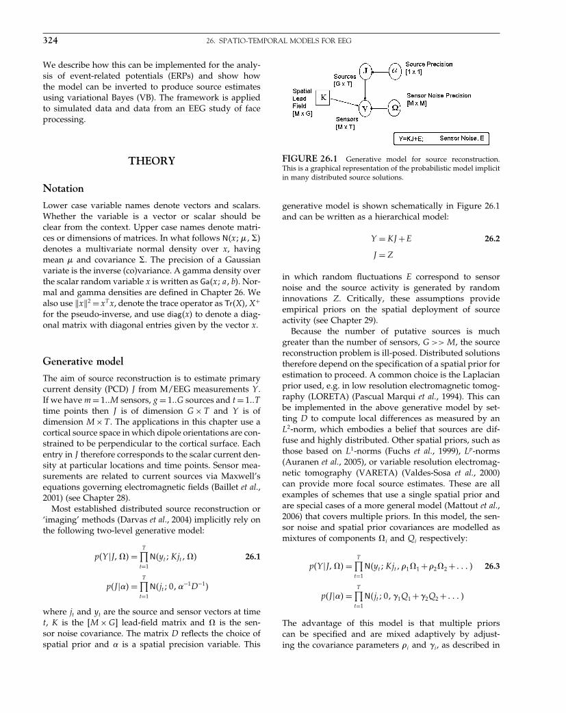
Elsevier UK Chapter: Ch26-P372560 30-9-2006 5:23p.m. Page:324 Trim:7.5in×9.25in
Basal Font:Palatino Margins:Top:40pt Gutter:68pt Font Size:9.5/12 Text Width:42pc Depth:55 Lines
324 26. SPATIO-TEMPORAL MODELS FOR EEG
We describe how this can be implemented for the analy-sis of event-related potentials (ERPs) and show howthe model can be inverted to produce source estimatesusing variational Bayes (VB). The framework is appliedto simulated data and data from an EEG study of faceprocessing.
THEORY
Notation
Lower case variable names denote vectors and scalars.Whether the variable is a vector or scalar should beclear from the context. Upper case names denote matri-ces or dimensions of matrices. In what follows N�x�����denotes a multivariate normal density over x, havingmean � and covariance �. The precision of a Gaussianvariate is the inverse (co)variance. A gamma density overthe scalar random variable x is written as Ga�x�a� b�. Nor-mal and gamma densities are defined in Chapter 26. Wealso use �x�2 = xT x, denote the trace operator as Tr�X�, X+
for the pseudo-inverse, and use diag�x� to denote a diag-onal matrix with diagonal entries given by the vector x.
Generative model
The aim of source reconstruction is to estimate primarycurrent density (PCD) J from M/EEG measurements Y .If we have m = 1��M sensors, g = 1��G sources and t = 1��Ttime points then J is of dimension G × T and Y is ofdimension M ×T . The applications in this chapter use acortical source space in which dipole orientations are con-strained to be perpendicular to the cortical surface. Eachentry in J therefore corresponds to the scalar current den-sity at particular locations and time points. Sensor mea-surements are related to current sources via Maxwell’sequations governing electromagnetic fields (Baillet et al.,2001) (see Chapter 28).
Most established distributed source reconstruction or‘imaging’ methods (Darvas et al., 2004) implicitly rely onthe following two-level generative model:
p�Y �J�� =T∏
t=1
N�yt�Kjt�� 26.1
p�J �� =T∏
t=1
N�jt� 0�−1D−1�
where jt and yt are the source and sensor vectors at timet, K is the �M × G� lead-field matrix and is the sen-sor noise covariance. The matrix D reflects the choice ofspatial prior and is a spatial precision variable. This
FIGURE 26.1 Generative model for source reconstruction.This is a graphical representation of the probabilistic model implicitin many distributed source solutions.
generative model is shown schematically in Figure 26.1and can be written as a hierarchical model:
Y = KJ +E 26.2
J = Z
in which random fluctuations E correspond to sensornoise and the source activity is generated by randominnovations Z. Critically, these assumptions provideempirical priors on the spatial deployment of sourceactivity (see Chapter 29).
Because the number of putative sources is muchgreater than the number of sensors, G >> M , the sourcereconstruction problem is ill-posed. Distributed solutionstherefore depend on the specification of a spatial prior forestimation to proceed. A common choice is the Laplacianprior used, e.g. in low resolution electromagnetic tomog-raphy (LORETA) (Pascual Marqui et al., 1994). This canbe implemented in the above generative model by set-ting D to compute local differences as measured by anL2-norm, which embodies a belief that sources are dif-fuse and highly distributed. Other spatial priors, such asthose based on L1-norms (Fuchs et al., 1999), Lp-norms(Auranen et al., 2005), or variable resolution electromag-netic tomography (VARETA) (Valdes-Sosa et al., 2000)can provide more focal source estimates. These are allexamples of schemes that use a single spatial prior andare special cases of a more general model (Mattout et al.,2006) that covers multiple priors. In this model, the sen-sor noise and spatial prior covariances are modelled asmixtures of components i and Qi respectively:
p�Y �J�� =T∏
t=1
N�yt�Kjt� 11 + 22 + � � � � 26.3
p�J �� =T∏
t=1
N�jt� 0��1Q1 +�2Q2 + � � � �
The advantage of this model is that multiple priorscan be specified and are mixed adaptively by adjust-ing the covariance parameters i and �i, as described in

Elsevier UK Chapter: Ch26-P372560 30-9-2006 5:23p.m. Page:325 Trim:7.5in×9.25in
Basal Font:Palatino Margins:Top:40pt Gutter:68pt Font Size:9.5/12 Text Width:42pc Depth:55 Lines
THEORY 325
Chapter 29. One can also use Bayesian model selectionto compare different combinations of priors, as describedin Chapter 35. For simplicity, we will deal with a singlespatial prior component because we want to focus ontemporal priors. However, it would be relatively simpleto extend the approach to cover multiple prior covariance(or precision) components.
Also, in Chapter 35 we will describe a prior over amodel class that, when used with Bayesian model aver-aging (BMA), can automatically provide either focal ordistributed solutions depending on the reconstructionat hand. The applications in this chapter use Laplacianpriors.
Whatever the choice of spatial prior, the majority ofsource reconstruction applications follow a single-passserial processing strategy. Either (i) spatial processingfirst proceeds to create source estimates at each time pointand then (ii) temporal models are applied at these ‘virtualdepth electrodes’ (Brookes et al., 2004; Darvas et al., 2004;Kiebel and Friston, 2004). Or (ii) time series methodsare applied in sensor space to identify components ofinterest using, e.g. time windowing (Rugg and Coles,1995) or time-frequency estimation and then (iii) sourcereconstructions are based on these components.
In this chapter, we review a multiple-pass strategyin which temporal and spatial parameter estimates areimproved iteratively to provide an optimized and mutu-ally constrained solution. It is based on the followingthree-level generative model:
p�Y �J�� =T∏
t=1
N�yt�Kjt�� 26.4
p�J �W��� =T∏
t=1
N�jTt � xtW��−1IG� 26.5
p�W �� =K∏
k=1
N�wk� 0�−1D−1� 26.6
The first level, Eqn. 26.4, is identical to the standardmodel. In the second level, however, source activity ateach voxel is constrained using a �T ×K� matrix of tem-poral basis functions, X. The tth row of X is xt. Thegenerative model is shown schematically in Figure 26.2.
The precision of the source noise is given by �. In thischapter, � is a scalar; and we will apply the framework toanalyse event-related potentials (ERPs) (Rugg and Coles,1995). Event-related source activity is described by thetime domain GLM and remaining source activity willcorrespond to spontaneous activity. The quantity �−1 cantherefore be thought of as the variance of spontaneousactivity in source space.
The regression coefficients W determine the weightingof the temporal basis functions. The third level of themodel is a spatial prior that reflects our prior uncertainty
FIGURE 26.2 Generative model for source reconstructionwith temporal priors. This is a hierarchical model with regressioncoefficients at the ‘top’ and M/EEG data at the ‘bottom’.
about W . Each regression coefficient map, wk (row of W ),is constrained by setting D to correspond to the usualL2-norm spatial prior. The spatial prior that is usually onthe sources now, therefore, appears at a superordinatelevel.
Different choices of D result in different weights anddifferent neighbourhood relations. The applications inthis paper use D = LT L, where L is the surface Laplaciandefined as:
Lij =
⎧⎪⎪⎨⎪⎪⎩
1� if i = j
− 1Nij
� if i and j are geodesic neighbours
0� otherwise�
where Nij is the geometric mean of the number of neigh-bors of i and j. This prior has been used before in thecontext of fMRI with Euclidean neighbours (Woolrichet al., 2001; Penny and Flandin, 2005).
The first level of the model assumes that there isGaussian sensor noise, et, with zero mean and covariance. This covariance can be estimated from pre-stimulusor baseline periods when such data are available (Sahaniand Nagarajan, 2004). Alternatively, we assume that =diag��−1� where the mth element of �−1 is the noisevariance on the mth sensor. We provide a scheme forestimating �m, should this be necessary.
We also place gamma priors on the precision variables� , � and :
p��� =M∏
m=1
Ga��m�b�prior� c�prior
� 26.7
p��� = Ga��� b�prior� c�prior
�
p�� =K∏
k=1
Ga�k� bprior� cprior
�
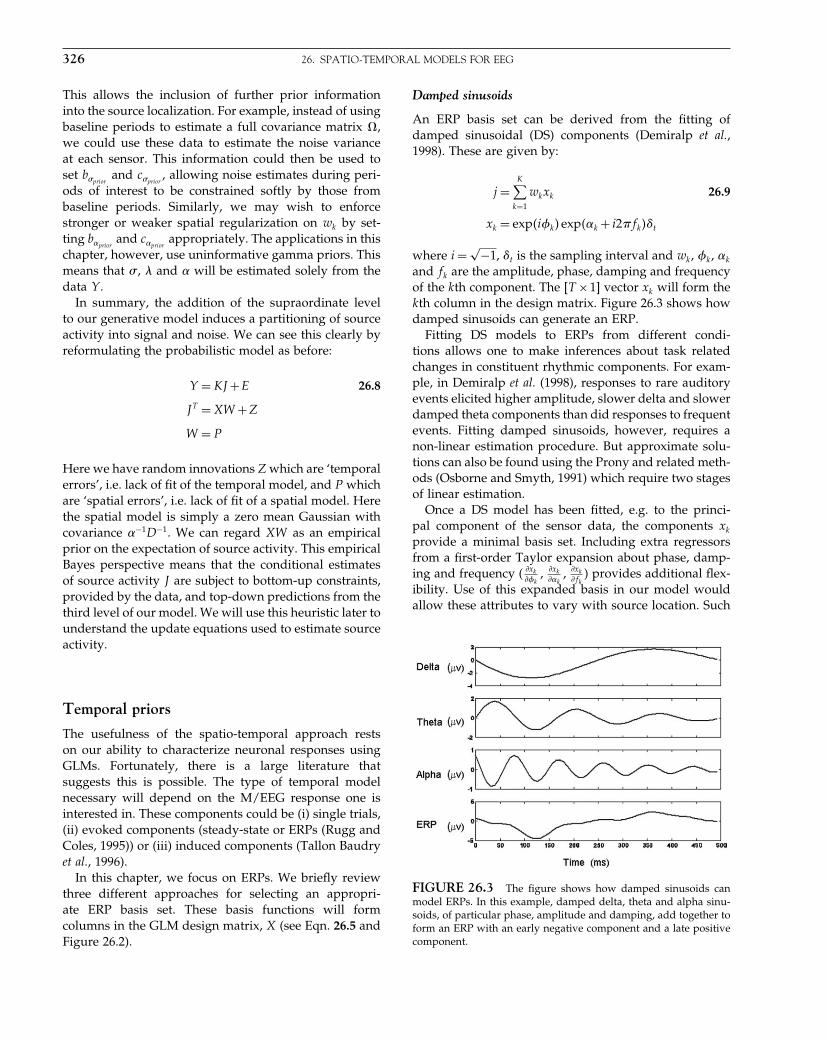
Elsevier UK Chapter: Ch26-P372560 30-9-2006 5:23p.m. Page:326 Trim:7.5in×9.25in
Basal Font:Palatino Margins:Top:40pt Gutter:68pt Font Size:9.5/12 Text Width:42pc Depth:55 Lines
326 26. SPATIO-TEMPORAL MODELS FOR EEG
This allows the inclusion of further prior informationinto the source localization. For example, instead of usingbaseline periods to estimate a full covariance matrix ,we could use these data to estimate the noise varianceat each sensor. This information could then be used toset b�prior
and c�prior, allowing noise estimates during peri-
ods of interest to be constrained softly by those frombaseline periods. Similarly, we may wish to enforcestronger or weaker spatial regularization on wk by set-ting bprior
and cpriorappropriately. The applications in this
chapter, however, use uninformative gamma priors. Thismeans that � , � and will be estimated solely from thedata Y .
In summary, the addition of the supraordinate levelto our generative model induces a partitioning of sourceactivity into signal and noise. We can see this clearly byreformulating the probabilistic model as before:
Y = KJ +E 26.8
JT = XW +Z
W = P
Here we have random innovations Z which are ‘temporalerrors’, i.e. lack of fit of the temporal model, and P whichare ‘spatial errors’, i.e. lack of fit of a spatial model. Herethe spatial model is simply a zero mean Gaussian withcovariance −1D−1. We can regard XW as an empiricalprior on the expectation of source activity. This empiricalBayes perspective means that the conditional estimatesof source activity J are subject to bottom-up constraints,provided by the data, and top-down predictions from thethird level of our model. We will use this heuristic later tounderstand the update equations used to estimate sourceactivity.
Temporal priors
The usefulness of the spatio-temporal approach restson our ability to characterize neuronal responses usingGLMs. Fortunately, there is a large literature thatsuggests this is possible. The type of temporal modelnecessary will depend on the M/EEG response one isinterested in. These components could be (i) single trials,(ii) evoked components (steady-state or ERPs (Rugg andColes, 1995)) or (iii) induced components (Tallon Baudryet al., 1996).
In this chapter, we focus on ERPs. We briefly reviewthree different approaches for selecting an appropri-ate ERP basis set. These basis functions will formcolumns in the GLM design matrix, X (see Eqn. 26.5 andFigure 26.2).
Damped sinusoids
An ERP basis set can be derived from the fitting ofdamped sinusoidal (DS) components (Demiralp et al.,1998). These are given by:
j =K∑
k=1
wkxk 26.9
xk = exp�i�k� exp�k + i2�fk��t
where i = √−1, �t is the sampling interval and wk, �k, k
and fk are the amplitude, phase, damping and frequencyof the kth component. The �T ×1� vector xk will form thekth column in the design matrix. Figure 26.3 shows howdamped sinusoids can generate an ERP.
Fitting DS models to ERPs from different condi-tions allows one to make inferences about task relatedchanges in constituent rhythmic components. For exam-ple, in Demiralp et al. (1998), responses to rare auditoryevents elicited higher amplitude, slower delta and slowerdamped theta components than did responses to frequentevents. Fitting damped sinusoids, however, requires anon-linear estimation procedure. But approximate solu-tions can also be found using the Prony and related meth-ods (Osborne and Smyth, 1991) which require two stagesof linear estimation.
Once a DS model has been fitted, e.g. to the princi-pal component of the sensor data, the components xk
provide a minimal basis set. Including extra regressorsfrom a first-order Taylor expansion about phase, damp-ing and frequency ( �xk
��k� �xk
�k� �xk
�fk) provides additional flex-
ibility. Use of this expanded basis in our model wouldallow these attributes to vary with source location. Such
FIGURE 26.3 The figure shows how damped sinusoids canmodel ERPs. In this example, damped delta, theta and alpha sinu-soids, of particular phase, amplitude and damping, add together toform an ERP with an early negative component and a late positivecomponent.

Elsevier UK Chapter: Ch26-P372560 30-9-2006 5:23p.m. Page:327 Trim:7.5in×9.25in
Basal Font:Palatino Margins:Top:40pt Gutter:68pt Font Size:9.5/12 Text Width:42pc Depth:55 Lines
THEORY 327
Taylor series expansions have been particularly usefulin GLM characterizations of haemodynamic responses infMRI (Frackowiak et al., 2003).
Wavelets
ERPs can also be modelled using wavelets:
j =K∑
k=1
wkxk 26.10
where xk are wavelet basis functions and wk are waveletcoefficients. Wavelets provide a tiling of time-frequencyspace that gives a balance between time and frequencyresolution. The Q-factor of a filter or basis function isdefined as the central frequency to bandwidth ratio.
Wavelet bases are chosen to provide constant Q (Unserand Aldroubi, 1996). This makes them good models ofnon-stationary signals, such as ERPs and induced EEGcomponents (Tallon Baudry et al., 1996). Wavelet basissets are derived by translating and dilating a motherwavelet. Figure 26.4 shows wavelets from two differ-ent basis sets, one based on Daubechies wavelets andone based on Battle-Lemarie (BL) wavelets. These basissets are orthogonal. Indeed the BL wavelets have beendesigned from an orthogonalization of cubic B-splines(Unser and Aldroubi, 1996).
If K = T , then the mapping j → w is referred toas a wavelet transform, and for K > T we have anovercomplete basis set. More typically, we have K ≤ T . Inthe ERP literature, the particular subset of basis functions
0.5
0.4
0.3
0.2
0.1
0
0
–0.1
–0.2
–0.4
–0.6
–0.8
0
–0.2
–0.4
–0.6
–0.8
0.5
0.2
0.4
0.6
0.2
0.4
0.6
0.4
0.4
0.3
0.3
0.2
0.2
0.2
0.4
0.6
0.8
1
0.1
0.1
0
–0.1–0.2
0
0
–0.1
–0.2
–0.2
–0.3
–0.4
–0.4
0 100 200 300 400
0 100 200 300 400
0 100 200 300 400 0 100 200 300 400
0 100 200 300 400
0 100 200 300 400
FIGURE 26.4 The graphs show wavelets from a Daubechies set of order 4 (left) and a Battle-Lemarie basis set of order 3 (right). Thewavelets in the lower panels are higher frequency translations of the wavelets in the top panels. Each full basis set comprises multiplefrequencies and translations covering the entire time domain.

Elsevier UK Chapter: Ch26-P372560 30-9-2006 5:23p.m. Page:328 Trim:7.5in×9.25in
Basal Font:Palatino Margins:Top:40pt Gutter:68pt Font Size:9.5/12 Text Width:42pc Depth:55 Lines
328 26. SPATIO-TEMPORAL MODELS FOR EEG
used is chosen according to the type of ERP componentone wishes to model. Popular choices are wavelets basedon B-splines (Unser and Aldroubi, 1996).
In statistics, however, it is well known that an appro-priate subset of basis functions can be automaticallyselected using a procedure known as ‘wavelet shrinkage’or ‘wavelet denoising’. This relies on the property thatnatural signals, such as images, speech or neuronal activ-ity, can be represented using a sparse code comprisingjust a few large wavelets coefficients. Gaussian noise sig-nals, however, produce Gaussian noise in wavelet space.This comprises a full set of wavelet coefficients whosesize depends on the noise variance. By ‘shrinking’ thesenoise coefficients to zero using a thresholding proce-dure (Donoho and Johnstone, 1994; Clyde et al., 1998),and transforming back into signal space, one can denoisedata. This amounts to defining a temporal model. Wewill use this approach for the empirical work reportedlater on.
PCA
A suitable basis can also be derived from principal com-ponents analysis (PCA). Trejo and Shensa (1999), forexample, applied PCA and varimax rotation to the clas-sification of ERPs in a signal detection task. They found,however, that better classification was more accuratewith a Daubechies wavelet basis.
PCA decompositions are also used in the multiple sig-nal classification (MUSIC) approach (Mosher and Leahy,1998). The dimension of the basis set is chosen to sepa-rate the signal and noise subspaces. Source reconstructionis then based on the signal, with information about thenoise used to derive statistical maps based on pseudo-z scores. In Friston et al. (2006), a temporal basis set isdefined using the principal eigenvectors of a full-rankprior temporal covariance matrix. This approach makesthe link between signal subspace and prior assumptionstransparent.
Dimensionality
Whatever the choice of basis, it is crucial that the dimen-sion of the signal subspace is less than the dimensionof the original time series. That is, K < T . This is neces-sary for the temporal priors to be effective, from both astatistical and computational perspective.
Theoretically, one might expect the dimensionality ofERP generators to be quite small. This is because of thelow-dimensional synchronization manifolds that arisewhen non-linear dynamical systems are coupled into anensemble (Breakspear and Terry, 2002).
In practice, the optimal reduced dimensionality canbe found automatically using a number of methods. For
wavelets this can be achieved using shrinkage methods(Donoho and Johnstone 1994; Clyde et al., 1998) and, forPCA, using various model order selection criteria (Minka,2000); for damped sinusoids, Prony-based methods canuse AR model order criteria (Roberts and Penny, 2002).Moreover, it is also possible to compute the model evi-dence of the source reconstruction model we have pro-posed, as shown in the following section. This can thenbe used to optimize the basis set.
Bayesian inference
To make inferences about the sources underling M/EEG,we need to invert our probabilistic model to produce theposterior density p�J �Y�. This is straightforward in princi-ple and can be achieved using standard Bayesian methods(Gelman et al., 1995). For example, one could use Markovchain Monte Carlo (MCMC) to produce samples fromthe posterior. This has been implemented efficiently fordipole-like inverse solutions (Schmidt et al., 1999) in whichsources are parameterized as spheres of unknown num-ber, extent and location. It is, however, computationallydemanding for distributed source solutions, taking severalhours for source spaces comprising G>1000 voxels (Aura-nen et al., 2005). In this work, we adopt the computationallyefficient approximate inference framework called varia-tional Bayes (VB), which was reviewed in Chapter 24.
Approximate posteriors
For our source reconstruction model we assume the fol-lowing factorization of the approximate posterior:
q�J�W������ = q�J�q�W�q��q���q��� 26.11
We also assume that the approximate posterior for theregression coefficients factorizes over voxels:
q�W� =G∏
g=1
q�wg� 26.12
This approximation was used in the spatio-temporalmodel for fMRI described in the previous chapter.
Because of the spatial prior (Eqn. 26.6), the regressioncoefficients in the true posterior p�W �Y� will clearly becorrelated. Our perspective, however, is that this is toocomputationally burdensome for current personal com-puters to take account of. Moreover, as we shall seebelow, updates for our approximate factorized densitiesq�wg� do encourage the approximate posterior means tobe similar at nearby voxels, thereby achieving the desiredeffect of the prior.

Elsevier UK Chapter: Ch26-P372560 30-9-2006 5:23p.m. Page:329 Trim:7.5in×9.25in
Basal Font:Palatino Margins:Top:40pt Gutter:68pt Font Size:9.5/12 Text Width:42pc Depth:55 Lines
THEORY 329
Now that we have defined the probabilistic model andour factorization of the approximate posterior, we can usethe procedure described in Chapter 24 to derive expres-sions for each component of the approximate posterior.We do not present details of these derivations in thischapter. Similar derivations have been published else-where (Penny et al., 2005). The following sections describeeach distribution and the updates of its sufficient statis-tics required to maximize the lower bound on the modelevidence, F .
Sources
Updates for the sources are given by:
q�J� =T∏
t=1
q�jt� 26.13
q�jt� = N�jt� ĵt� �̂jt� 26.14
�̂jt=(KT ̂K + �̂IG
)−126.15
ĵt = �̂jt
(KT ̂yt + �̂Ŵ T xT
t
)26.16
where ĵt is the tth column of Ĵ and ̂, �̂ and Ŵ areestimated parameters defined in the following sections.Eqn. 26.16 shows that our source estimates are the resultof a spatio-temporal deconvolution. The spatial contribu-tion to the estimate is KT yt and the temporal contributionis Ŵ T xT
t . From the perspective of the hierarchical model,shown in Figure 26.5, these are the ‘bottom-up’ and‘top-down’ predictions. Importantly, each prediction isweighted by its relative precision. Moreover, the param-eters controlling the relative precisions, �̂ and ̂, are
FIGURE 26.5 Probabilistic inversion of the generative modelleads to a source reconstruction based on a spatio-temporal decon-volution in which bottom-up and top-down predictions, from sensordata and temporal priors, are optimally combined using Bayesianinference.
estimated from the data. This means that our source esti-mates derive from an automatically regularized spatio-temporal deconvolution. This property is shared by thespatio-temporal model for fMRI, described in the previ-ous chapter.
An alternative perspective on this computation is givenby ignoring the regularization term in Eqn. 26.16. We thensee that �̂jt
KT ̂ = �KT ̂K�+KT ̂ = BTw, which is equiv-
alent to a beamformer (Darvas et al., 2004). Eqn. 26.16then shows that our source estimates use beamformerpredictions BT
wyt that are modified using a temporalmodel. Beamformers cannot localize temporally corre-lated sources. But, as we shall see later, the spatio-temporal model can.
We end this section by noting that statistical infer-ences about current sources are more robust than pointpredictions. This property has been used to great effectwith pseudo-z beamformer statistics (Robinson and Vrba,1999), sLORETA (Pascual Marqui, 2002) and VARETA(Valdes-Sosa et al., 2000) source reconstructions, whichdivide current source estimates by their standard devia-tions. This approach can be adopted in the current frame-workasthestandarddeviationsarereadilycomputedfromthe diagonal elements of �̂jt
using Eqn. 26.23. Moreover,we can threshold these statistic images to create posteriorprobability maps (PPMs), as introduced in Chapter 25.
Regression coefficients
Updates for the regression coefficients are given by:
q�wg� = N�wg� ŵg� �̂wg� 26.17
�̂wg=(�̂XT X +dggdiag�̂�
)−1
ŵg = �̂wg
(�̂XT ĵT
g +diag�̂�rg
)
where ̂ is defined in Eqn. 26.21, dij is the i� jth elementof D and rg is given by:
rg =G∑
g′=1�g′ �=g
dgg′ŵg′ 26.18
As shown in the previous chapter, rg is the weighted sumof neighbouring regression coefficient estimators.
The update for ŵg in Eqn. 26.17 therefore indicatesthat the regression coefficient estimates at a given voxelregress towards those at nearby voxels. This is the desiredeffect of the spatial prior and it is preserved despite thefactorization in the approximate posterior. This equationcan again be thought of in terms of the hierarchical modelwhere the regression coefficient estimate is a combinationof a bottom-up prediction from the level below, XT ĵT
g ,and a top-down prediction from the prior, rg. Again, eachcontribution is weighted by its relative precision.

Elsevier UK Chapter: Ch26-P372560 30-9-2006 5:23p.m. Page:330 Trim:7.5in×9.25in
Basal Font:Palatino Margins:Top:40pt Gutter:68pt Font Size:9.5/12 Text Width:42pc Depth:55 Lines
330 26. SPATIO-TEMPORAL MODELS FOR EEG
The update for the covariance in Eqn 26.17 shows thatthe only off-diagonal contributions are due to the designmatrix. If the temporal basis functions are therefore cho-sen to be orthogonal then this posterior covariance will bediagonal, thus making a potentially large saving of com-puter memory. One benefit of the proposed framework,however, is that non-orthogonal bases can be accommo-dated. This may allow for a more natural and compactdescription of the data.
Precision of temporal models
Updates for the precision of the temporal model aregiven by:
q��� = Ga��� b�post� c�post
� 26.19
1b�post
= 1b�prior
+ 12
∑t
(�ĵt − Ŵ T xT
t �2 +Tr(�̂jt
)
+G∑
g=1
xt�̂wgxT
t
)
c�post= c�prior
+ GT
2
�̂ = b�postc�post
In the context of ERP analysis, these expressions amountto an estimate of the variance of spontaneous activity insource space, �̂−1, given by the squared error betweenthe ERP estimate, Ŵ T xT
t , and source estimate, ĵt, aver-aged over time and space and the other approximateposteriors.
Precision of forward model
Updates for the precision of the sensor noise are given by:
q��� = =M∏
m=1
q��m� 26.20
q��m� = Ga��m�b�post� c�post
�
1bm
= 1b�prior
+ 12
∑t
(ymt −kT
mĵt
)2 + 12
kTm�̂jt
km
cm = c�prior+ T
2�̂m = bmcm
̂−1 = diag��̂�
These expressions amount to an estimate of observationnoise at the mth sensor, �̂m
−1, given by the squared errorbetween the forward model and sensor data, averagedover time and the other approximate posteriors.
Precision of spatial prior
Updates for the precision of the spatial prior are given by:
q�� =K∏
k=1
q�k� 26.21
q�k� = Ga�k� bpost� cpost
�
1bpost
= 1bprior
+�DŵTk �2 +
G∑g=1
dgsgk
cpost= cprior
+ G
2̂k = bpost
cpost
where sgk is the kth diagonal element of �̂wg. These
expressions amount to an estimate of the ‘spatial noisevariance’, ̂−1
k , given by the discrepancy between neigh-bouring regression coefficients, averaged over space andthe other approximate posteriors.
Implementation details
A practical difficulty with the update equations for thesources is that the covariance matrix �̂jt
is of dimen-sion G×G where G is the number of sources. Even lowresolution source grids typically contain G > 1000 ele-ments. This therefore presents a problem. A solution isfound, however, with use of a singular value decomposi-tion (SVD). First, we define a modified lead field matrixK̄ = ̂1/2K and compute its SVD:
K̄ = USV T 26.22
= UV̄
where V̄ is an M×G matrix, the same dimension as thelead field, K. It can then be shown using the matrix inver-sion lemma (Golub and Van Loan, 1996) that:
�̂jt= �̂−1 �IG −RG� 26.23
RG = V̄ T ��̂IM +SST �−1V̄
which is simple to implement computationally, as it onlyrequires inversion of an M×M matrix.
Source estimates can be computed as shown inEqn. 26.16. In principle, this means the estimated sourcesover all time points and source locations are given by:
Ĵ = �̂jtKT ̂Y + �̂�̂jt
Ŵ T XT
In practice, however, it is inefficient to work with sucha large matrix during estimation. We therefore do notimplement Eqns 26.15 and 26.16 but, instead, work in thereduced space ĴX = ĴX which are the sources projected

Elsevier UK Chapter: Ch26-P372560 30-9-2006 5:23p.m. Page:331 Trim:7.5in×9.25in
Basal Font:Palatino Margins:Top:40pt Gutter:68pt Font Size:9.5/12 Text Width:42pc Depth:55 Lines
RESULTS 331
onto the design matrix. These projected source estimatesare given by:
ĴX = ĴX 26.24
= �̂jtKT ̂YX + �̂�̂jt
Ŵ T XT X
= AKYX + �̂AW XT X
where YX and XT X can be pre-computed and theintermediate quantities are given by:
AK = �̂jtKT ̂ 26.25
= �̂−1(KT −RGKT
)AW = �̂jt
Ŵ T
= �̂−1(Ŵ T −RGŴ T
)
Because these matrices are only of dimension G×M andG×K respectively, ĴX can be efficiently computed. Theterm XT ĵT
g in Eqn. 26.17 is then given by the gth row of ĴX .The intermediate quantities can also be used to com-
pute model predictions as:
Ŷ = KĴ 26.26
= KAKY + �̂KAW XT
The m�tth entry in Ŷ then corresponds to the kTmĵt term in
Eqn. 26.20. Other computational savings are as follows.For Eqn. 26.20 we use the result:
kTm�̂jt
km = 1�̂m
M∑m′=1
s2m′m′u2
mm′
s2m′m′ + �̂
26.27
where sij and uij are the i� jth entries in S and U respec-tively. For Eqn. 26.19 we use the result:
Tr��̂jt� =
M∑i=1
1
s2ii + �̂
+ G−M
�̂26.28
To summarize, our source reconstruction model is fit-ted to data by iteratively applying the update equa-tions until the change in the negative free energy (seeChapter 24), F , is less than some user-specified toler-ance. This procedure is summarized in the pseudo-codein Figure 26.6. This amounts to a process in which sen-sor data are spatially deconvolved, time-series modelsare fitted in source space, and then the precisions (accu-racy) of the temporal and spatial models are estimated.This process is then iterated and results in a spatio-temporal deconvolution in which all aspects of the modelare optimized to maximize a lower bound on the modelevidence.
FIGURE 26.6 Pseudo-code for spatio-temporal deconvolutionof M/EEG. The parameters of the model � = �J�W����� areestimated by updating the approximate posteriors until the negativefree energy is maximized to within a certain tolerance (left panel).At this point, because the log evidence L = log p�Y� is fixed, theapproximate posteriors will best approximate the true posteriors inthe sense of KL-divergence (right panel), as described in Chapter 24.The equations for updating the approximate posteriors are given inthe theory section.
RESULTS
This section presents some preliminary qualitativeresults. In what follows we refer to the spatio-temporalapproach as ‘VB-GLM’.
Comparison with LORETA
We generated data from our model as follows. First, wecreated two regressors consisting of a 10 Hz and 20 Hzsinewave with amplitudes of 10 and 8 respectively. Theseformed the two columns of a design matrix shown inFigure 26.7. We generated 600 ms of activity with a sam-ple period of 5 ms, giving 120 time points.
FIGURE 26.7 Simulations that compare VB-GLM withLORETA use the above design matrix, X. The columns in this matrixcomprise a 10 Hz and a 20 Hz sinewave.
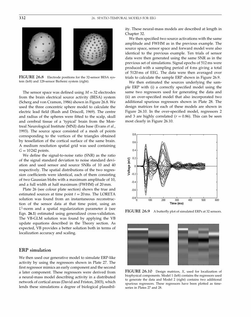
Elsevier UK Chapter: Ch26-P372560 30-9-2006 5:23p.m. Page:332 Trim:7.5in×9.25in
Basal Font:Palatino Margins:Top:40pt Gutter:68pt Font Size:9.5/12 Text Width:42pc Depth:55 Lines
332 26. SPATIO-TEMPORAL MODELS FOR EEG
FIGURE 26.8 Electrode positions for the 32-sensor BESA sys-tem (left) and 128-sensor BioSemi system (right).
The sensor space was defined using M = 32 electrodesfrom the brain electrical source activity (BESA) system(Scherg and von Cramon, 1986) shown in Figure 26.8. Weused the three concentric sphere model to calculate theelectric lead field (Rush and Driscoll, 1969). The centreand radius of the spheres were fitted to the scalp, skulland cerebral tissue of a ‘typical’ brain from the Mon-treal Neurological Institute (MNI) data base (Evans et al.,1993). The source space consisted of a mesh of pointscorresponding to the vertices of the triangles obtainedby tessellation of the cortical surface of the same brain.A medium resolution spatial grid was used containingG = 10 242 points.
We define the signal-to-noise ratio (SNR) as the ratioof the signal standard deviation to noise standard devi-ation and used sensor and source SNRs of 10 and 40respectively. The spatial distributions of the two regres-sion coefficients were identical, each of them consistingof two Gaussian blobs with a maximum amplitude of 10,and a full width at half maximum (FWHM) of 20 mm.
Plate 26 (see colour plate section) shows the true andestimated sources at time point t = 20 ms. The LORETAsolution was found from an instantaneous reconstruc-tion of the sensor data at that time point, using anL2-norm and a spatial regularization parameter ̂ (seeEqn. 26.1) estimated using generalized cross-validation.The VB-GLM solution was found by applying the VBupdate equations described in the Theory section. Asexpected, VB provides a better solution both in terms oflocalization accuracy and scaling.
ERP simulation
We then used our generative model to simulate ERP-likeactivity by using the regressors shown in Plate 27. Thefirst regressor mimics an early component and the seconda later component. These regressors were derived froma neural-mass model describing activity in a distributednetwork of cortical areas (David and Friston, 2003), whichlends these simulations a degree of biological plausibil-
ity. These neural-mass models are described at length inChapter 32.
We then specified two source activations with the sameamplitude and FWHM as in the previous example. Thesource space, sensor space and forward model were alsoidentical to the previous example. Ten trials of sensordata were then generated using the same SNR as in theprevious set of simulations. Signal epochs of 512 ms wereproduced with a sampling period of 4 ms giving a totalof 5120 ms of EEG. The data were then averaged overtrials to calculate the sample ERP shown in Figure 26.9.
We then estimated the sources underlying the sam-ple ERP with (i) a correctly specified model using thesame two regressors used for generating the data and(ii) an over-specified model that also incorporated twoadditional spurious regressors shown in Plate 28. Thedesign matrices for each of these models are shown inFigure 26.10. In the over-specified model, regressors 2and 3 are highly correlated (r = 0�86). This can be seenmost clearly in Figure 26.10.
FIGURE 26.9 A butterfly plot of simulated ERPs at 32 sensors.
FIGURE 26.10 Design matrices, X, used for localization ofbiophysical components. Model 1 (left) contains the regressors usedto generate the data and Model 2 (right) contains two additionalspurious regressors. These regressors have been plotted as time-series in Plates 27 and 28.

Elsevier UK Chapter: Ch26-P372560 30-9-2006 5:23p.m. Page:333 Trim:7.5in×9.25in
Basal Font:Palatino Margins:Top:40pt Gutter:68pt Font Size:9.5/12 Text Width:42pc Depth:55 Lines
RESULTS 333
The models were then fitted to the data using theVB update rules. As shown in Plates 29 and 30, thetrue effects (regression coefficients) are accurately recov-ered even for the over-specified model. The spuriousregression coefficients are shrunk towards zero. This is aconsequence of the spatial prior and the iterative spatio-temporal deconvolution. This also shows that sourcereconstruction with temporal priors is robust to modelmis-specification.
We then performed a second simulation with the set ofregressors shown in Plate 28, and identical specificationsof source space, sensor space, forward model and SNR.But in this example we generated data from the regres-sion coefficients shown in Plate 31, regression coefficients1 and 4 being set to zero. These data therefore comprisethree distributed sources: (i) a right-lateralized sourcehaving time-series given by a scaled, noise-corruptedregressor 2; (ii) a frontal source given by a scaled, noise-corrupted regressor 3; and (iii) a left-lateralized sourcecomprising a noisy, scaled mixture of regressors 2 and 3.These sources are therefore highly correlated.
The VB-GLM model, using a full design matrix com-prising all four regressors, was then fitted to thesedata. The estimated regression coefficients are shown inPlate 32. Regressors 1 and 4 have been correctly estimatedto be close to zero, whereas regressors 2 and 3 bear a close
resemblance to the true values. This shows that VB-GLM,in contrast to, for example beamforming approaches, iscapable of localizing temporally correlated sources.
Face ERPs
This section presents an analysis of a face processingEEG data set from Henson et al. (2003). The experimentinvolved presentation of images of faces and scrambledfaces, as described in Figure 26.11.
The EEG data were acquired on a 128-channel BioSemiActiveTwo system, sampled at 1024 Hz. The data werereferenced to the average of left and right earlobe elec-trodes and epoched from −200 ms to +600 ms. Theseepochs were then examined for artefacts, defined as time-points that exceeded an absolute threshold of 120 micro-volts. A total of 29 of the 172 trials were rejected. Theepochs were then averaged to produce condition specificERPs at each electrode.
The first clear difference between faces and scram-bled faces is maximal around 160 ms, appearing as anenhancement of a negative component (peak ‘N160’)at occipito-temporal channels (e.g. channel ‘B8’), orenhancement of a positive peak at Cz (e.g. channel ‘A1’).
Phase 1
500 ms
Time
O
O
+
+
HighSymmetry
Sb
Sa
Ub
Fa
LowSymmetry
LowAsymmetry
HighAsymmetry
600 ms
700 ms
2456 ms
FIGURE 26.11 Face paradigm. The experiment involved randomized presentation of images of 86 faces and 86 scrambled faces. Halfof the faces belong to famous people, half are novel, creating three conditions in total. In this chapter, we consider just two conditions: (i)faces (famous or not); and (ii) scrambled faces. The scrambled faces were created by 2D Fourier transformation, random phase permutation,inverse transformation and outline-masking. Thus faces and scrambled faces are closely matched for low-level visual properties such as spatialfrequency. The subject judged the left-right symmetry of each image around an imaginary vertical line through the centre of the image. Faceswere presented for 600 ms, every 3600 ms.

Elsevier UK Chapter: Ch26-P372560 30-9-2006 5:23p.m. Page:334 Trim:7.5in×9.25in
Basal Font:Palatino Margins:Top:40pt Gutter:68pt Font Size:9.5/12 Text Width:42pc Depth:55 Lines
334 26. SPATIO-TEMPORAL MODELS FOR EEG
These effects are shown as a differential topography inPlate 33 and as time-series in Plate 34.
A temporal model was then fitted using waveletshrinkage (Donoho and Johnstone, 1994). Before applyingthe model, the data were first downsampled and the 128samples following stimulus onset were extracted. Thesesteps were taken as we used WaveLab1 to generate thewavelet bases. This uses a pyramid algorithm to computecoefficients, so requiring the number of samples to be apower of two.
We then extracted the first eigenvector of the sensordata using a singular value decomposition (SVD) andfitted wavelet models to this time-series. A number ofwavelet bases were examined, two samples of whichare shown in Figure 26.4. These are the Daubechies-4and Battle-Lemarie-3 wavelets. Plate 35 shows the corre-sponding time-series estimates. These employed K = 28and K = 23 basis functions respectively, as determined byapplication of the wavelet shrinkage algorithm (Donohoand Johnstone, 1994). We used the smaller Battle-Lemariebasis set in the source reconstruction that follows.
ERPs for faces and scrambled faces were then con-catenated to form a vector of 256 elements at each elec-trode. The overall sensor matrix Y was then of dimension256×128. The design matrix, of dimension 256×46, wascreated by having identical block diagonal elements eachcomprising the Battle-Lemarie basis. This is shown inFigure 26.12. The source space was then defined using amedium resolution cortical grid defined using the typicalMNI brain, as in the previous sections. Current source
FIGURE 26.12 Design matrix for source reconstruction ofERPs from face data. Each block contains a 23-element Batte-Lemariebasis set. The first components, forming diagonals in the picture, arelow frequency wavelets. The high frequency wavelets are concen-trated around the N160, where the signal is changing most quickly.
1 WaveLab is available from http://www-stat.stanford.edu/wavelab.
orientations were assumed perpendicular to the corticalsurface. Constraining current sources based on a differentindividual anatomy is clearly suboptimal, but neverthe-less allows us to report some qualitative results.
We then applied the source reconstruction algorithmand obtained a solution after 20 minutes of processing.Plate 36 shows differences in the source estimates forfaces minus scrambled faces at time t = 160 ms. Theimages show differences in absolute current at eachvoxel. They have been thresholded at 50 per cent ofthe maximum difference at this time point. The max-imum difference is plotted in red and 50 per cent ofthe maximum difference in blue. At this threshold fourmain clusters of activation appear at (i) right fusiform,(ii) right anterior temporal, (iii) frontal and (iv) superiorcentroparietal.
These activations are consistent with previous fMRI(Henson et al., 2003) and MEG analyses of faces minusscrambled faces in that face processing is lateralizedto the right hemisphere and, in particular, to fusiformcortex. Additionally, the activations in temporal andfrontal regions, although not significant in group ran-dom effects analyses, are nonetheless compatible withobserved between-subject variability on this task.
DISCUSSION
This chapter has described a model-based spatio-temporal deconvolution approach to source reconstruc-tion. Sources are reconstructed by inverting a forwardmodel comprising a temporal process as well as a spatialprocess. This approach relies on the fact that EEG andMEG signals are extended in time as well as in space.
It rests on the notion that MEG and EEG reflect theneuronal activity of a spatially distributed dynamical sys-tem. Depending on the nature of the experimental task,this activity can be highly localized or highly distributedand the dynamics can be more, or less, complex. At oneextreme, listening, for example to simple auditory stim-uli produces brain activations that are highly localizedin time and space. This activity is well described by asingle dipole located in brainstem and reflecting a sin-gle burst of neuronal activity at, for example t = 20 mspost-stimulus. More complicated tasks, such as odd-ball paradigms, elicit spatially distributed responses andmore complicated dynamics that can appear in the ERPas damped sinusoidal responses. In this chapter, we havetaken the view that, by explictly modelling these dynam-ics, one can obtain better source reconstructions.
This view is not unique within the source reconstruc-tion community. Indeed, there have been a number ofapproaches that also make use of temporal priors. Baillet
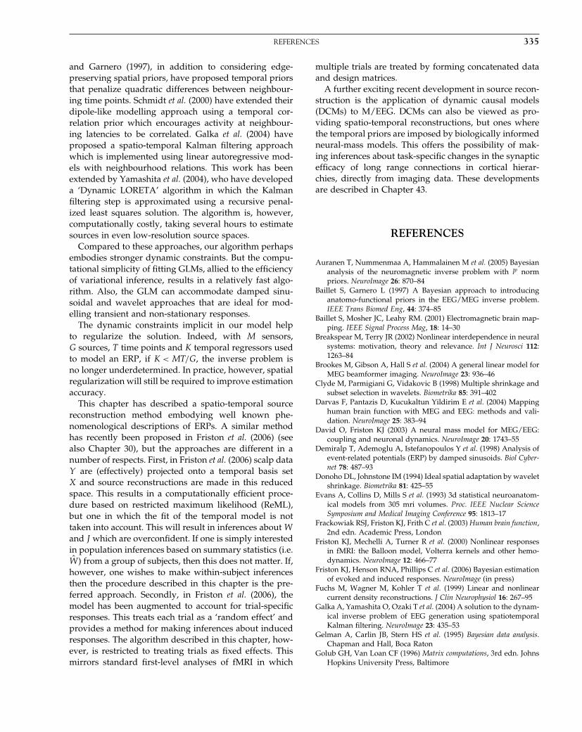
Elsevier UK Chapter: Ch26-P372560 30-9-2006 5:23p.m. Page:335 Trim:7.5in×9.25in
Basal Font:Palatino Margins:Top:40pt Gutter:68pt Font Size:9.5/12 Text Width:42pc Depth:55 Lines
REFERENCES 335
and Garnero (1997), in addition to considering edge-preserving spatial priors, have proposed temporal priorsthat penalize quadratic differences between neighbour-ing time points. Schmidt et al. (2000) have extended theirdipole-like modelling approach using a temporal cor-relation prior which encourages activity at neighbour-ing latencies to be correlated. Galka et al. (2004) haveproposed a spatio-temporal Kalman filtering approachwhich is implemented using linear autoregressive mod-els with neighbourhood relations. This work has beenextended by Yamashita et al. (2004), who have developeda ‘Dynamic LORETA’ algorithm in which the Kalmanfiltering step is approximated using a recursive penal-ized least squares solution. The algorithm is, however,computationally costly, taking several hours to estimatesources in even low-resolution source spaces.
Compared to these approaches, our algorithm perhapsembodies stronger dynamic constraints. But the compu-tational simplicity of fitting GLMs, allied to the efficiencyof variational inference, results in a relatively fast algo-rithm. Also, the GLM can accommodate damped sinu-soidal and wavelet approaches that are ideal for mod-elling transient and non-stationary responses.
The dynamic constraints implicit in our model helpto regularize the solution. Indeed, with M sensors,G sources, T time points and K temporal regressors usedto model an ERP, if K < MT/G, the inverse problem isno longer underdetermined. In practice, however, spatialregularization will still be required to improve estimationaccuracy.
This chapter has described a spatio-temporal sourcereconstruction method embodying well known phe-nomenological descriptions of ERPs. A similar methodhas recently been proposed in Friston et al. (2006) (seealso Chapter 30), but the approaches are different in anumber of respects. First, in Friston et al. (2006) scalp dataY are (effectively) projected onto a temporal basis setX and source reconstructions are made in this reducedspace. This results in a computationally efficient proce-dure based on restricted maximum likelihood (ReML),but one in which the fit of the temporal model is nottaken into account. This will result in inferences about Wand J which are overconfident. If one is simply interestedin population inferences based on summary statistics (i.e.Ŵ ) from a group of subjects, then this does not matter. If,however, one wishes to make within-subject inferencesthen the procedure described in this chapter is the pre-ferred approach. Secondly, in Friston et al. (2006), themodel has been augmented to account for trial-specificresponses. This treats each trial as a ‘random effect’ andprovides a method for making inferences about inducedresponses. The algorithm described in this chapter, how-ever, is restricted to treating trials as fixed effects. Thismirrors standard first-level analyses of fMRI in which
multiple trials are treated by forming concatenated dataand design matrices.
A further exciting recent development in source recon-struction is the application of dynamic causal models(DCMs) to M/EEG. DCMs can also be viewed as pro-viding spatio-temporal reconstructions, but ones wherethe temporal priors are imposed by biologically informedneural-mass models. This offers the possibility of mak-ing inferences about task-specific changes in the synapticefficacy of long range connections in cortical hierar-chies, directly from imaging data. These developmentsare described in Chapter 43.
REFERENCES
Auranen T, Nummenmaa A, Hammalainen M et al. (2005) Bayesiananalysis of the neuromagnetic inverse problem with lp normpriors. NeuroImage 26: 870–84
Baillet S, Garnero L (1997) A Bayesian approach to introducinganatomo-functional priors in the EEG/MEG inverse problem.IEEE Trans Biomed Eng, 44: 374–85
Baillet S, Mosher JC, Leahy RM. (2001) Electromagnetic brain map-ping. IEEE Signal Process Mag, 18: 14–30
Breakspear M, Terry JR (2002) Nonlinear interdependence in neuralsystems: motivation, theory and relevance. Int J Neurosci 112:1263–84
Brookes M, Gibson A, Hall S et al. (2004) A general linear model forMEG beamformer imaging. NeuroImage 23: 936–46
Clyde M, Parmigiani G, Vidakovic B (1998) Multiple shrinkage andsubset selection in wavelets. Biometrika 85: 391–402
Darvas F, Pantazis D, Kucukaltun Yildirim E et al. (2004) Mappinghuman brain function with MEG and EEG: methods and vali-dation. NeuroImage 25: 383–94
David O, Friston KJ (2003) A neural mass model for MEG/EEG:coupling and neuronal dynamics. NeuroImage 20: 1743–55
Demiralp T, Ademoglu A, Istefanopoulos Y et al. (1998) Analysis ofevent-related potentials (ERP) by damped sinusoids. Biol Cyber-net 78: 487–93
Donoho DL, Johnstone IM (1994) Ideal spatial adaptation by waveletshrinkage. Biometrika 81: 425–55
Evans A, Collins D, Mills S et al. (1993) 3d statistical neuroanatom-ical models from 305 mri volumes. Proc. IEEE Nuclear ScienceSymposium and Medical Imaging Conference 95: 1813–17
Frackowiak RSJ, Friston KJ, Frith C et al. (2003) Human brain function,2nd edn. Academic Press, London
Friston KJ, Mechelli A, Turner R et al. (2000) Nonlinear responsesin fMRI: the Balloon model, Volterra kernels and other hemo-dynamics. NeuroImage 12: 466–77
Friston KJ, Henson RNA, Phillips C et al. (2006) Bayesian estimationof evoked and induced responses. NeuroImage (in press)
Fuchs M, Wagner M, Kohler T et al. (1999) Linear and nonlinearcurrent density reconstructions. J Clin Neurophysiol 16: 267–95
Galka A, Yamashita O, Ozaki T et al. (2004) A solution to the dynam-ical inverse problem of EEG generation using spatiotemporalKalman filtering. NeuroImage 23: 435–53
Gelman A, Carlin JB, Stern HS et al. (1995) Bayesian data analysis.Chapman and Hall, Boca Raton
Golub GH, Van Loan CF (1996) Matrix computations, 3rd edn. JohnsHopkins University Press, Baltimore
Elsevier UK Chapter: Ch26-P372560 30-9-2006 5:23p.m. Page:336 Trim:7.5in×9.25in
Basal Font:Palatino Margins:Top:40pt Gutter:68pt Font Size:9.5/12 Text Width:42pc Depth:55 Lines
336 26. SPATIO-TEMPORAL MODELS FOR EEG
Henson RNA, Goshen-Gottstein Y, Ganel T et al. (2003) Electro-physiological and hemodynamic correlates of face perception,recognition and priming. Cerebr Cort 13: 793–805
Kiebel SJ, Friston KJ (2004) Statistical parametric mapping for event-related potentials II: a hierarchical temporal model. NeuroImage22: 503–20
Makeig S, Westerfield M, Jung T-P et al. (2002) Dynamic brainsources of visual evoked responses. Science 295: 690–94
Mattout J, Phillips C, Penny WD (2006) MEG source localisationunder multiple constraints: an extended Bayesian framework.NeuroImage 30: 753–67
McKeown MJ, Makeig S, Brown GG et al. (1998) Analysis of fMRIdata by blind separation into independent spatial components.Hum Brain Mapp 6: 160–88
Minka TP (2000) Automatic choice of dimensionality for PCA. Tech-nical Report 514, MIT Media Laboratory, Perceptual ComputingSection, Cambridge, MA
Mosher JC, Leahy RM (1998) Recursive MUSIC: a framework foreeg and meg source localization. IEEE Trans Biomed Eng 47:332–40
Osborne MR, Smyth GK (1991) A modified Prony algorithm for fit-ting functions defined by difference equations. J Sci Stat Comput12: 362–82
Pascual Marqui R (2002) Standardized low resolution electromag-netic tomography (sLORETA): technical details. Meth Find ExpClin Pharmacol 24: 5–12
Pascual Marqui R, Michel C, Lehman D (1994) Low resolution elec-tromagnetic tomography: a new method for localizing electricalactivity of the brain. Int J Psychophysiol 18: 49–65
Penny WD, Flandin G (2005) Bayesian analysis of single-subjectfMRI: SPM implementation. Technical report, Wellcome Depart-ment of Imaging Neuroscience, London
Penny WD, Trujillo-Barreto N, Friston KJ (2005) Bayesian fMRItime series analysis with spatial priors. NeuroImage 24:350–62
Roberts SJ, Penny WD (2002) Variational Bayes for gener-alised autoregressive models. IEEE Trans Signal Process 50:2245–57
Robinson S, Vrba J (1999) Functional neuroimaging by syntheticaperture magnetometry (SAM). In Recent advances in biomag-netism. Tohoku University Press, Sendai
Rugg MD, Coles MGH (1995) Electrophysiology of mind: event-relatedpotentials and cognition. Oxford University Press, Oxford
Rush S, Driscoll D (1969) EEG electrode sensitivity – an applicationof reciprocity. IEEE Trans Biomed Eng 16: 15–22
Sahani M, Nagarajan SS (2004) Reconstructing MEG sources withunknown correlations. In Advances in neural information process-ing systems, Saul L, Thrun S, Schoelkopf B (eds), volume 16. MIT,Cambridge, MA
Scherg M, von Cramon D (1986) Evoked dipole source potentials ofthe human auditory cortex. Electroencephalogr Clin Neurophysiol65: 344–60
Schmidt DM, George JS, Wood CC (1999) Bayesian inference appliedto the electromagnetic inverse problem. Hum Brain Mapp 7:195–212
Schmidt DM, Ranken DM, George JS (2000) Spatial-temporalBayesian inference for MEG/EEG. In 12th International Confer-ence on Biomagnetism, Helsinki, Finland, August
Tallon Baudry C, Bertrand O, Delpuech C et al. (1996) Stimulusspecificity of phase-locked and non phase-locked 40 Hz visualresponses in human. J Neurosci 16: 4240–49
Trejo L, Shensa MJ (1999) Feature extraction of event-related poten-tials using wavelets: an application to human performance mon-itoring. Brain Lang 66: 89–107
Unser M, Aldroubi A (1996) A review of wavelets in biomedicalapplications. Proc IEEE 84: 626–38
Valdes-Sosa P, Marti F, Garcia F et al. (2000) Variable resolu-tion electric-magnetic tomography. In Proceedings of the 10thInternational Conference on Biomagnetism, volume 2, 373–76,Springer-Verlag, New York
Woolrich MW, Ripley BD, brady M et al. (2001) Temporal autocor-relation in univariate linear modelling of fMRI data. NeuroImage14: 1370–86
Yamashita O, Galka A, Ozaki T et al. (2004) Recursive penalisedleast squares solution for dynamical inverse problems of EEGgeneration. Hum Brain Mapp 21: 221–35

Elsevier UK Chapter: Ch27-P372560 30-9-2006 5:23p.m. Page:339 Trim:7.5in×9.25in
Basal Font:Palatino Margins:Top:40pt Gutter:68pt Font Size:9.5/12 Text Width:42pc Depth:55 Lines
C H A P T E R
27
Forward models for fMRIK. Friston and D. Glaser
INTRODUCTION
Part 6 is concerned with biophysical models of neu-ronal responses and the inversion of these models tomake inferences about their parameters. In relation tothe previous chapters, there is a greater focus on howsignals observed with neuroimaging are generated andthe underlying physical and physiological mechanisms.In this chapter, we look at haemodynamics. In the nextchapter, we turn to electrical and magnetic sources thatgenerate electroencephalography (EEG) and magnetoen-cephalography (MEG) signals. These chapters start withconventional electromagnetic forward models. In thesubsequent chapters, we consider physiology in moredepth, through mean-field models of neuronal popula-tions or ensembles and how these provide a motivationfor neural-mass models of event-related potentials. In thefinal chapters, we consider some general issues encoun-tered during model inversion and selection.
There is a growing appreciation of the importance ofnon-linearities in evoked responses in functional mag-netic resonance imaging (fMRI), particularly with theadvent of event-related fMRI. These non-linearities arecommonly expressed as interactions among stimuli thatcan lead to the suppression and increased latency ofresponses to stimuli that are incurred by a precedingstimulus. We presented previously a model-free char-acterization of these effects using generic techniquesfrom non-linear system identification, namely a Volterraseries formulation. At the same time, Buxton et al. (1998)described a plausible and compelling dynamical modelof haemodynamic signal transduction in fMRI. Subse-quent work by Mandeville et al. (1999) provided impor-tant theoretical and empirical constraints on the form ofthe dynamic relationship between blood flow and vol-ume that underpins the evolution of the fMRI signal.In this chapter, we combine these system identificationand model-based approaches and ask whether the Bal-
loon model is sufficient to account for the non-linearbehaviours observed in real time-series. We conclude thatit can and, furthermore, the model parameters that ensueare biologically plausible. This conclusion is based on theobservation that the Balloon model can produce Volterrakernels that emulate empirical kernels.
To enable this evaluation we have had to embed theBalloon model in a haemodynamic input-state-outputmodel that included the dynamics of perfusion changesthat are contingent on underlying synaptic activation.This chapter presents the haemodynamic model, its asso-ciated Volterra kernels and addresses the model’s valid-ity in relation to empirical characterizations of evokedresponses in fMRI and other neurophysiological con-straints.
Background
This chapter is about modelling the relationship betweenneural activity and the BOLD (blood oxygenation-level-dependent) fMRI signal. The link between blood supplyand brain activity has been established for over a hun-dred years. In their seminal paper, Roy and Sherring-ton (1890) concluded that functional activity increasedblood flow and inferred that there was a coupling thatincreased blood flow in response to increased metabolicdemand. Interestingly, their observation of the conse-quences of metabolic demand came before the demon-stration of the increase in demand itself. It was morethan seventy years later that the regional measurementof metabolic changes was convincingly achieved usingautoradiographic techniques. These used a substitute forglucose, called deoxyglucose (2DG) radioactively labelledwith C14. 2DG enters the cells by the same route as glu-cose but is not metabolized and thus accumulates insidethe cells at a rate that depends on their metabolic activity.By examining the density of labelled 2DG in brain slices,
Statistical Parametric Mapping, by Karl Friston et al. Copyright 2007, Elsevier Ltd. All rights reserved.ISBN–13: 978-0-12-372560-8 ISBN–10: 0-12-372560-7
339
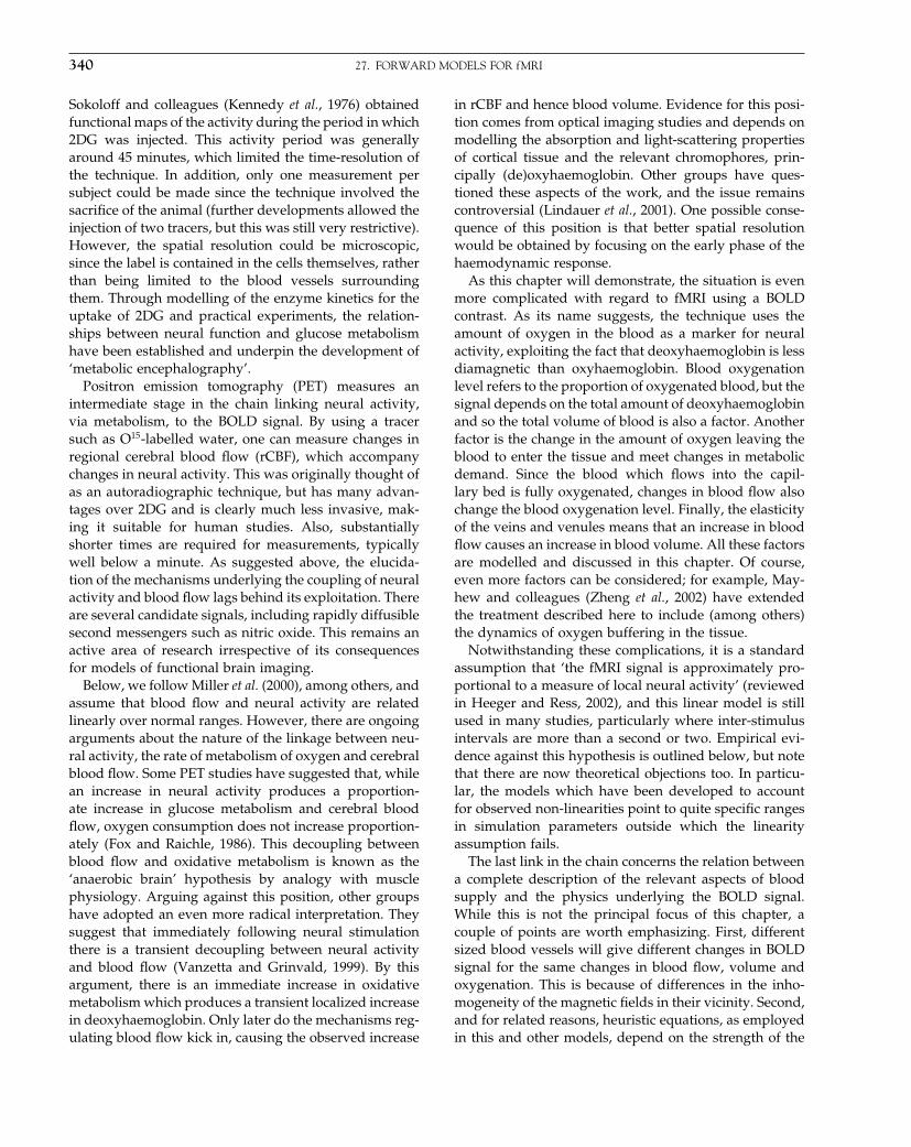
Elsevier UK Chapter: Ch27-P372560 30-9-2006 5:23p.m. Page:340 Trim:7.5in×9.25in
Basal Font:Palatino Margins:Top:40pt Gutter:68pt Font Size:9.5/12 Text Width:42pc Depth:55 Lines
340 27. FORWARD MODELS FOR fMRI
Sokoloff and colleagues (Kennedy et al., 1976) obtainedfunctional maps of the activity during the period in which2DG was injected. This activity period was generallyaround 45 minutes, which limited the time-resolution ofthe technique. In addition, only one measurement persubject could be made since the technique involved thesacrifice of the animal (further developments allowed theinjection of two tracers, but this was still very restrictive).However, the spatial resolution could be microscopic,since the label is contained in the cells themselves, ratherthan being limited to the blood vessels surroundingthem. Through modelling of the enzyme kinetics for theuptake of 2DG and practical experiments, the relation-ships between neural function and glucose metabolismhave been established and underpin the development of‘metabolic encephalography’.
Positron emission tomography (PET) measures anintermediate stage in the chain linking neural activity,via metabolism, to the BOLD signal. By using a tracersuch as O15-labelled water, one can measure changes inregional cerebral blood flow (rCBF), which accompanychanges in neural activity. This was originally thought ofas an autoradiographic technique, but has many advan-tages over 2DG and is clearly much less invasive, mak-ing it suitable for human studies. Also, substantiallyshorter times are required for measurements, typicallywell below a minute. As suggested above, the elucida-tion of the mechanisms underlying the coupling of neuralactivity and blood flow lags behind its exploitation. Thereare several candidate signals, including rapidly diffusiblesecond messengers such as nitric oxide. This remains anactive area of research irrespective of its consequencesfor models of functional brain imaging.
Below, we follow Miller et al. (2000), among others, andassume that blood flow and neural activity are relatedlinearly over normal ranges. However, there are ongoingarguments about the nature of the linkage between neu-ral activity, the rate of metabolism of oxygen and cerebralblood flow. Some PET studies have suggested that, whilean increase in neural activity produces a proportion-ate increase in glucose metabolism and cerebral bloodflow, oxygen consumption does not increase proportion-ately (Fox and Raichle, 1986). This decoupling betweenblood flow and oxidative metabolism is known as the‘anaerobic brain’ hypothesis by analogy with musclephysiology. Arguing against this position, other groupshave adopted an even more radical interpretation. Theysuggest that immediately following neural stimulationthere is a transient decoupling between neural activityand blood flow (Vanzetta and Grinvald, 1999). By thisargument, there is an immediate increase in oxidativemetabolism which produces a transient localized increasein deoxyhaemoglobin. Only later do the mechanisms reg-ulating blood flow kick in, causing the observed increase
in rCBF and hence blood volume. Evidence for this posi-tion comes from optical imaging studies and depends onmodelling the absorption and light-scattering propertiesof cortical tissue and the relevant chromophores, prin-cipally (de)oxyhaemoglobin. Other groups have ques-tioned these aspects of the work, and the issue remainscontroversial (Lindauer et al., 2001). One possible conse-quence of this position is that better spatial resolutionwould be obtained by focusing on the early phase of thehaemodynamic response.
As this chapter will demonstrate, the situation is evenmore complicated with regard to fMRI using a BOLDcontrast. As its name suggests, the technique uses theamount of oxygen in the blood as a marker for neuralactivity, exploiting the fact that deoxyhaemoglobin is lessdiamagnetic than oxyhaemoglobin. Blood oxygenationlevel refers to the proportion of oxygenated blood, but thesignal depends on the total amount of deoxyhaemoglobinand so the total volume of blood is also a factor. Anotherfactor is the change in the amount of oxygen leaving theblood to enter the tissue and meet changes in metabolicdemand. Since the blood which flows into the capil-lary bed is fully oxygenated, changes in blood flow alsochange the blood oxygenation level. Finally, the elasticityof the veins and venules means that an increase in bloodflow causes an increase in blood volume. All these factorsare modelled and discussed in this chapter. Of course,even more factors can be considered; for example, May-hew and colleagues (Zheng et al., 2002) have extendedthe treatment described here to include (among others)the dynamics of oxygen buffering in the tissue.
Notwithstanding these complications, it is a standardassumption that ‘the fMRI signal is approximately pro-portional to a measure of local neural activity’ (reviewedin Heeger and Ress, 2002), and this linear model is stillused in many studies, particularly where inter-stimulusintervals are more than a second or two. Empirical evi-dence against this hypothesis is outlined below, but notethat there are now theoretical objections too. In particu-lar, the models which have been developed to accountfor observed non-linearities point to quite specific rangesin simulation parameters outside which the linearityassumption fails.
The last link in the chain concerns the relation betweena complete description of the relevant aspects of bloodsupply and the physics underlying the BOLD signal.While this is not the principal focus of this chapter, acouple of points are worth emphasizing. First, differentsized blood vessels will give different changes in BOLDsignal for the same changes in blood flow, volume andoxygenation. This is because of differences in the inho-mogeneity of the magnetic fields in their vicinity. Second,and for related reasons, heuristic equations, as employedin this and other models, depend on the strength of the

Elsevier UK Chapter: Ch27-P372560 30-9-2006 5:23p.m. Page:341 Trim:7.5in×9.25in
Basal Font:Palatino Margins:Top:40pt Gutter:68pt Font Size:9.5/12 Text Width:42pc Depth:55 Lines
NON-LINEAR EVOKED RESPONSES 341
magnet. In particular, the equations used here may berelevant only for 1.5 T scanners, although other versionsfor different field strength have been developed.
Finally, a word about ‘neural activity’. So far, we havedeliberately not specified what type of neural activity weare considering. First, it is worth remembering that dif-ferent electrophysiological measures can emphasize dif-ferent aspects of neural activity. In particular, recordingof multiple single units, with an intracortical microelec-trode, can tend to sample action potentials from largepyramidal output neurons. Such studies are frequentlyreferred to when characterizing the response proper-ties of a primate cortical area. However, the metabolicdemands of various cellular processes suggest that spik-ing is not the major drain on the resources of a cell butrather synaptic transmission, restoration of postsynapticpotentials and cytoskeletal turnover dominate (Attwelland Laughlin, 2001). The processes are just as importantas spiking, whether in interneurons and whether excita-tory or inhibitory. An example that shows the importanceof this distinction is feed-forward (spike-dependent) ver-sus feed-back (modulatory) activity in low-level visualcortex. BOLD fMRI experiments in humans have shown agood agreement with studies of spiking in V1 in responseto modulating the contrast of a visual stimulus, however,attentional (top-down) modulation effects in V1 haveproved elusive in monkey electrophysiology but robustwith BOLD studies in humans. Aside from their neuro-biological significance, these issues should be borne inmind when considering the neural activity disclosed byBOLD.
A further subtlety relates to the modelled time courseof neural activity; a typical set of spike- or block-functionsused to model neural activity will fail to capture adapta-tion and response transients which are well known fromthe neurophysiological literature. Note that the adapta-tion paradigm deliberately exploits these effects (Grill-Spector and Malach, 2001). Studies using simultaneousfMRI and intracortical electrical recording in monkeyshave empirically validated many of the theoretical pointsconsidered above (Logothetis et al., 2001). In particular,the closeness of the BOLD signal to local field potentials(LFP) and multiunit activity (MUA) rather than spik-ing activity was emphasized. These studies also demon-strated that the linear assumption can predict up to 90 percent of the variance in BOLD responses in some corticalregions. However, there was considerable variability inthe accuracy of prediction. In Chapter 32, we will revisitsome of these themes in a more abstract way using asimple dimensional analysis of the energetics entailed byneuronal dynamics and the implications for electrical andhaemodynamic responses.
Having surveyed the general issues surrounding thecoupling of neural activity and the BOLD signal, we will
now consider a specific and detailed model. This couldbe considered as an instantiation of current knowledgeand further extensions of this model have already beenproposed, which incorporate new data. What follows islargely a reprise of Friston et al. (2000), and contains somemathematical material.
NON-LINEAR EVOKED RESPONSES
In this section, we focus on the non-linear aspectsof evoked responses in functional neuroimaging andpresent a dynamical approach to modelling and charac-terizing event-related signals in fMRI. We will show thatthe Balloon-Windkessel model (Buxton and Frank, 1997;Buxton et al., 1998; Mandeville et al., 1999) can account fornon-linearities in event-related responses that are seenempirically and describe a non-linear dynamical modelthat couples changes in synaptic activity to fMRI signals.This haemodynamic model obtains by combining theBalloon-Windkessel model (henceforth Balloon model)with a model of how synaptic activity causes changes inregional flow.
In Friston et al. (1994), we presented a linear model ofhaemodynamic responses in fMRI time-series, whereinunderlying neuronal activity (inferred on the basis ofchanging stimulus or task conditions) is convolved, orsmoothed with a haemodynamic response function. InFriston et al. (1998) we extended this model to covernon-linear responses using a Volterra series expansion.At the same time, Buxton and colleagues developed amechanistic model of how evoked changes in blood flowwere transformed into a BOLD signal (Buxton et al.,1998). A component of the Balloon model, namely therelationship between blood flow and volume, was thenelaborated in the context of standard Windkessel theoryby Mandeville et al. (1999). The Volterra approach, incontradistinction to other non-linear characterization ofhaemodynamic responses (cf. Vazquez and Noll, 1996),is model-independent, in the sense that Volterra seriescan model the behaviour of any non-linear time-invariantdynamical system.1 The principal aim of the work pre-sented below was to see if the Balloon model would be
1 In principle Volterra series can represent any dynamical input-state-output system and in this sense a characterization in termsof Volterra kernels is model-independent. However, by usingbasis functions to constrain the solution space, constraints areimposed on the form of the kernels and, implicitly, the under-lying dynamical system (i.e. state-space representation). Thecharacterization is therefore only assumption free to the extentthe basis set is sufficiently comprehensive.
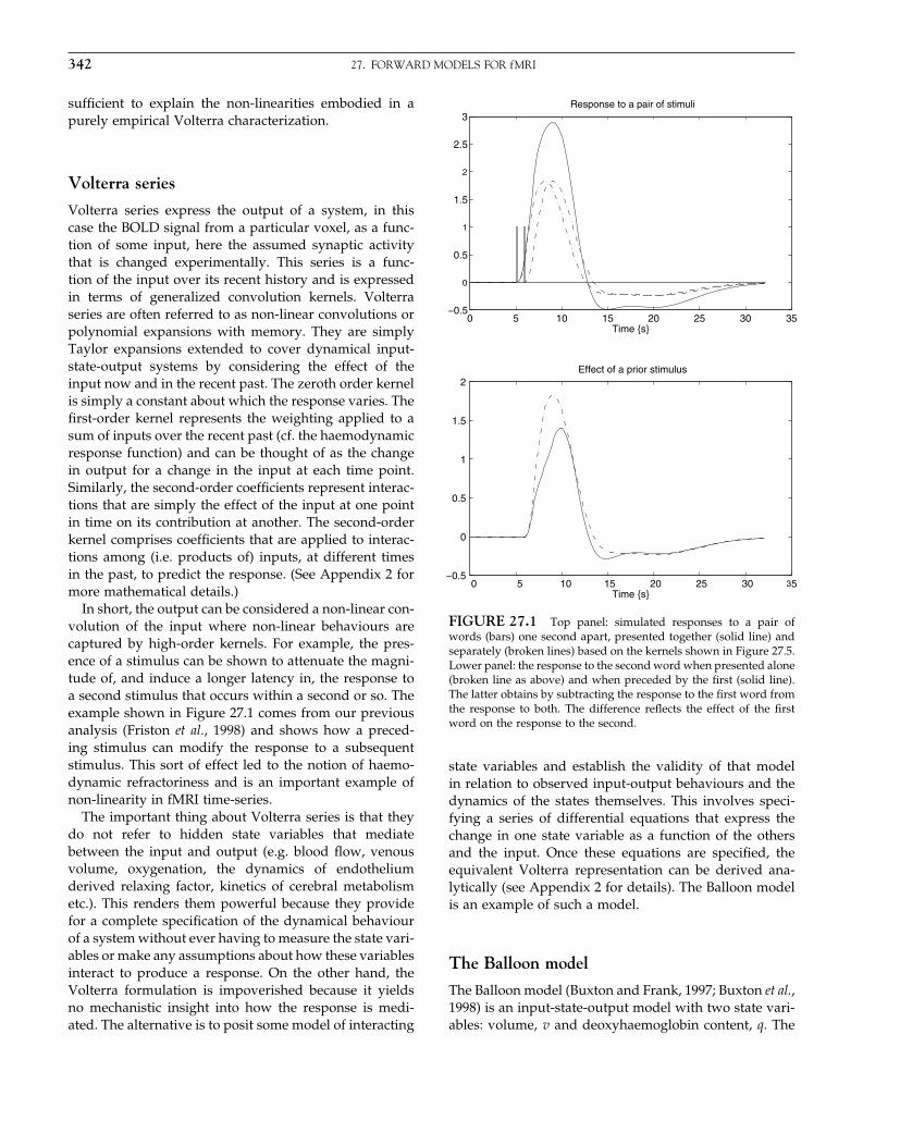
Elsevier UK Chapter: Ch27-P372560 30-9-2006 5:23p.m. Page:342 Trim:7.5in×9.25in
Basal Font:Palatino Margins:Top:40pt Gutter:68pt Font Size:9.5/12 Text Width:42pc Depth:55 Lines
342 27. FORWARD MODELS FOR fMRI
sufficient to explain the non-linearities embodied in apurely empirical Volterra characterization.
Volterra series
Volterra series express the output of a system, in thiscase the BOLD signal from a particular voxel, as a func-tion of some input, here the assumed synaptic activitythat is changed experimentally. This series is a func-tion of the input over its recent history and is expressedin terms of generalized convolution kernels. Volterraseries are often referred to as non-linear convolutions orpolynomial expansions with memory. They are simplyTaylor expansions extended to cover dynamical input-state-output systems by considering the effect of theinput now and in the recent past. The zeroth order kernelis simply a constant about which the response varies. Thefirst-order kernel represents the weighting applied to asum of inputs over the recent past (cf. the haemodynamicresponse function) and can be thought of as the changein output for a change in the input at each time point.Similarly, the second-order coefficients represent interac-tions that are simply the effect of the input at one pointin time on its contribution at another. The second-orderkernel comprises coefficients that are applied to interac-tions among (i.e. products of) inputs, at different timesin the past, to predict the response. (See Appendix 2 formore mathematical details.)
In short, the output can be considered a non-linear con-volution of the input where non-linear behaviours arecaptured by high-order kernels. For example, the pres-ence of a stimulus can be shown to attenuate the magni-tude of, and induce a longer latency in, the response toa second stimulus that occurs within a second or so. Theexample shown in Figure 27.1 comes from our previousanalysis (Friston et al., 1998) and shows how a preced-ing stimulus can modify the response to a subsequentstimulus. This sort of effect led to the notion of haemo-dynamic refractoriness and is an important example ofnon-linearity in fMRI time-series.
The important thing about Volterra series is that theydo not refer to hidden state variables that mediatebetween the input and output (e.g. blood flow, venousvolume, oxygenation, the dynamics of endotheliumderived relaxing factor, kinetics of cerebral metabolismetc.). This renders them powerful because they providefor a complete specification of the dynamical behaviourof a system without ever having to measure the state vari-ables or make any assumptions about how these variablesinteract to produce a response. On the other hand, theVolterra formulation is impoverished because it yieldsno mechanistic insight into how the response is medi-ated. The alternative is to posit some model of interacting
0 5 10 15 20 25 30 35−0.5
0
0.5
1
1.5
2
2.5
3
Time {s}
Response to a pair of stimuli
0 5 10 15 20 25 30 35−0.5
0
0.5
1
1.5
2
Time {s}
Effect of a prior stimulus
FIGURE 27.1 Top panel: simulated responses to a pair ofwords (bars) one second apart, presented together (solid line) andseparately (broken lines) based on the kernels shown in Figure 27.5.Lower panel: the response to the second word when presented alone(broken line as above) and when preceded by the first (solid line).The latter obtains by subtracting the response to the first word fromthe response to both. The difference reflects the effect of the firstword on the response to the second.
state variables and establish the validity of that modelin relation to observed input-output behaviours and thedynamics of the states themselves. This involves speci-fying a series of differential equations that express thechange in one state variable as a function of the othersand the input. Once these equations are specified, theequivalent Volterra representation can be derived ana-lytically (see Appendix 2 for details). The Balloon modelis an example of such a model.
The Balloon model
The Balloon model (Buxton and Frank, 1997; Buxton et al.,1998) is an input-state-output model with two state vari-ables: volume, v and deoxyhaemoglobin content, q. The

Elsevier UK Chapter: Ch27-P372560 30-9-2006 5:23p.m. Page:343 Trim:7.5in×9.25in
Basal Font:Palatino Margins:Top:40pt Gutter:68pt Font Size:9.5/12 Text Width:42pc Depth:55 Lines
THE HAEMODYNAMIC MODEL 343
input to the system is blood flow, fand the output is theBOLD signal, y. The BOLD signal is partitioned into anextra- and intravascular component, weighted by theirrespective volumes. These signal components depend onthe deoxyhaemoglobin content and render the signal anon-linear function of v and q. The effect of flow onv and q (see below) determines the output and it isthese effects that are the essence of the Balloon model:increases in flow effectively inflate a venous ‘balloon’such that deoxygenated blood is diluted and expelledat a greater rate. The clearance of deoxyhaemoglobinreduces intra-voxel dephasing and engenders an increasein signal. Before the balloon has inflated sufficiently theexpulsion and dilution may be insufficient to counter-act the increased delivery of deoxygenated blood to thevenous compartment and an ‘early dip’ in signal may beexpressed. After the flow has peaked, and the balloon hasrelaxed again, reduced clearance and dilution contributeto the post-stimulus undershoot commonly observed.This is a simple and plausible model that is predicatedon a minimal set of assumptions and relates closely tothe Windkessel formulation of Mandeville et al. (1999).Furthermore, the predictions of the Balloon model concurwith the steady-state models of Hoge and colleagues, andtheir elegant studies of the relationship between bloodflow and oxygen consumption in human visual cortex(e.g. Hoge et al., 1999).
The Balloon model is inherently non-linear and mayaccount for the sorts of non-linear interactions revealedby the Volterra formulation. One simple test of thishypothesis is to see if the Volterra kernels associated withthe Balloon model compare with those derived empir-ically. The Volterra kernels estimated in Friston et al.(1998) clearly did not use flow as input because flowis not measurable with BOLD fMRI. The input com-prised a stimulus function as an index of synaptic activ-ity. In order to evaluate the Balloon model in terms ofVolterra kernels, it has to be extended to accommodatethe dynamics of how flow is coupled to synaptic activityencoded in the stimulus function. This chapter presentsone such extension.
In summary, the Balloon model deals with the linkbetween flow and BOLD signal. By extending the modelto cover the coupling of synaptic activity and flow, a com-plete model, relating experimentally induced changes inneuronal activity to BOLD signal, obtains. The input-output behaviour of this model can be compared to thereal brain in terms of their respective Volterra kernels.
The remainder of this chapter is divided into threesections. In the next section, we present a haemody-namic model of the coupling between synaptic activityand BOLD response that builds upon the Balloon model.The second section presents an empirical evaluation ofthis model by comparing its Volterra kernels with those
obtained using real fMRI data. This is not a trivial exer-cise because there is no guarantee that the Balloon modelcould produce the complicated forms of the kernels seenempirically and, even if it could, the parameters neededto do so may be biologically implausible. This section pro-vides estimates of these parameters, which allow somecomment on the face validity of the model, in relation toknown physiology. The final section presents a discus-sion of the results in relation to known biophysics andneurophysiology. This chapter is concerned with the val-idation and evaluation of the Balloon model in relationto the Volterra characterizations, and the haemodynamicmodel presented below in relation to real haemodynam-ics. In Chapter 34, we will use the haemodynamic modelto illustrate Bayesian inversion of dynamic models andsubsequent chapters will use the model as part of largerdynamic causal models for fMRI (see Chapter 41).
THE HAEMODYNAMIC MODEL
In this section, we describe a haemodynamic model thatmediates between synaptic activity and measured BOLDresponses. This model essentially combines the Balloonmodel and a simple linear dynamical model of changesin regional cerebral blood flow (rCBF) caused by neu-ronal activity. The model architecture is summarized inFigure 27.2. To motivate the model components moreclearly we will start at the output and work towards theinput.
The Balloon component
This component links rCBF and the BOLD signal asdescribed in Buxton et al. (1998). All variables areexpressed in normalized form, relative to resting values.The BOLD signal is taken to be a static non-linear func-tion of normalized venous volume v, normalized totaldeoxyhaemoglobin voxel content q and resting net oxy-gen extraction fraction by the capillary bed E0:
y = g�v� q� = V0�k1�1− q�+k2�1− q/v�+k3�1−v��
k1 = 7E0
k1 = 2
k1 = 2E0 −0�2
27.1
where V0 is resting blood volume fraction. This signalcomprises a volume-weighted sum of extra- and intravas-cular signals that are functions of volume and deoxy-haemoglobin content. The latter are the state variables
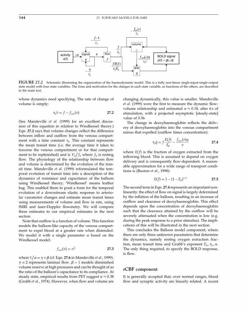
Elsevier UK Chapter: Ch27-P372560 30-9-2006 5:23p.m. Page:344 Trim:7.5in×9.25in
Basal Font:Palatino Margins:Top:40pt Gutter:68pt Font Size:9.5/12 Text Width:42pc Depth:55 Lines
344 27. FORWARD MODELS FOR fMRI
s
signal
ƒflow
q
dHb
BOLD signaly(t ) = g(ν,q)
activityu(t )
s
0
)(τ
νƒout−
0τƒ
00E
ƒE(ƒ )
τ
ν
volume
νƒout(ν)q
0τ−
f
ƒ−1τ
−
s
s
τ−
εu
FIGURE 27.2 Schematic illustrating the organization of the haemodynamic model. This is a fully non-linear single-input-single-outputstate model with four state variables. The form and motivation for the changes in each state variable, as functions of the others, are describedin the main text.
whose dynamics need specifying. The rate of change ofvolume is simply:
�0v̇ = f −fout�v� 27.2
(See Mandeville et al. (1999) for an excellent discus-sion of this equation in relation to Windkessel theory.)Eqn. 27.2 says that volume changes reflect the differencebetween inflow and outflow from the venous compart-ment with a time constant �0. This constant representsthe mean transit time (i.e. the average time it takes totraverse the venous compartment or for that compart-ment to be replenished) and is V0
/f0 where f0 is resting
flow. The physiology of the relationship between flowand volume is determined by the evolution of the tran-sit time. Mandeville et al. (1999) reformulated the tem-poral evolution of transit time into a description of thedynamics of resistance and capacitance of the balloonusing Windkessel theory; ‘Windkessel’ means leatherbag. This enabled them to posit a form for the temporalevolution of a downstream elastic response to arterio-lar vasomotor changes and estimate mean transit timesusing measurements of volume and flow in rats, usingfMRI and laser-Doppler flowmetry. We will comparethese estimates to our empirical estimates in the nextsection.
Note that outflow is a function of volume. This functionmodels the balloon-like capacity of the venous compart-ment to expel blood at a greater rate when distended.We model it with a single parameter � based on theWindkessel model:
fout�v� = v1� 27.3
where 1/
� = �+ (cf. Eqn. 27.6 in Mandeville et al., 1999).� = 2 represents laminar flow. > 1 models diminishedvolume reserve at high pressures and can be thought of asthe ratio of the balloon’s capacitance to its compliance. Atsteady state, empirical results from PET suggest � ≈ 0�38(Grubb et al., 1974). However, when flow and volume are
changing dynamically, this value is smaller. Mandevilleet al. (1999) were the first to measure the dynamic flow-volume relationship and estimated � ≈ 0�18, after 6 s ofstimulation, with a projected asymptotic [steady-state]value of 0.36.
The change in deoxyhaemoglobin reflects the deliv-ery of deoxyhaemoglobin into the venous compartmentminus that expelled (outflow times concentration):
�0q̇ = fE�f�
E0− fout�v�q
v27.4
where E�f� is the fraction of oxygen extracted from theinflowing blood. This is assumed to depend on oxygendelivery and is consequently flow-dependent. A reason-able approximation for a wide range of transport condi-tions is (Buxton et al., 1998):
E�f� = 1− �1−E0�1/f 27.5
The second term in Eqn. 27.4 represents an important non-linearity: the effect of flow on signal is largely determinedby the inflation of the balloon, resulting in an increase ofoutflow and clearance of deoxyhaemoglobin. This effectdepends upon the concentration of deoxyhaemoglobinsuch that the clearance attained by the outflow will beseverely attenuated when the concentration is low (e.g.during the peak response to a prior stimulus). The impli-cations of this will be illustrated in the next section.
This concludes the Balloon model component, wherethere are only three unknown parameters that determinethe dynamics, namely resting oxygen extraction frac-tion, mean transit time and Grubb’s exponent E0� �0��.The only thing required, to specify the BOLD response,is flow.
rCBF component
It is generally accepted that, over normal ranges, bloodflow and synaptic activity are linearly related. A recent

Elsevier UK Chapter: Ch27-P372560 30-9-2006 5:23p.m. Page:345 Trim:7.5in×9.25in
Basal Font:Palatino Margins:Top:40pt Gutter:68pt Font Size:9.5/12 Text Width:42pc Depth:55 Lines
THE HAEMODYNAMIC MODEL 345
empirical verification of this assumption can be foundin Miller et al. (2000), who used MRI perfusion imagingto address this issue in visual and motor cortices. Aftermodelling neuronal adaptation they were able to con-clude: ‘Both rCBF responses are consistent with a lineartransformation of a simple non-linear neural responsemodel’. Furthermore, our own work using PET and fMRIreplications of the same experiments suggested that theobserved non-linearities enter into the translation of rCBFinto a BOLD response (as opposed to a non-linear rela-tionship between synaptic activity and rCBF) in the audi-tory cortices (see Friston et al., 1998). Under the constraintthat the dynamical system linking synaptic activity andrCBF is linear we will use the most parsimonious model:
ḟ = s 27.6
where s is some flow inducing signal. Although it mayseem more natural to express the effect of this signaldirectly on vascular resistance (r), e.g. ṙ = −s, Eqn. 27.6has the more plausible form. This is because the effectof signal is much smaller when r is small (when thearterioles are fully dilated, signals such as endothelium-derived relaxing factor or nitric oxide will cause relativelysmall decrements in resistance). This can be seen by not-ing Eqn. 27.6 is equivalent to ṙ = −r2s, where f = 1/r .
The signal is assumed to subsume many neurogenicand diffusive signal sub-components and is generated byneuronal activity u(t):
ṡ = u− s/
�s − �f −1�/
�f 27.7
The unknown parameters here represent the efficacy withwhich neuronal activity causes an increase in signal ,the time-constant for signal decay or elimination �s andthe time-constant for autoregulatory feedback �f fromblood flow. The existence of this feedback term can beinferred from post-stimulus undershoots in rCBF (e.g.Irikura et al., 1994) and the well-characterized vasomo-tor signal in optical imaging (Mayhew et al., 1998). Thecritical aspect of the latter oscillatory �∼ 0�1 Hz� compo-nent of intrinsic signals is that it shows variable phaserelationships from region to region, supporting stronglythe notion of local closed-loop feedback mechanisms asmodelled in Eqn. 27.6 and Eqn. 27.7.
There are three unknown parameters for each of thetwo components of the haemodynamic model above (seealso Figure 27.2 for a schematic summary). Figure 27.3illustrates the behaviour of the haemodynamic modelfor typical values of the six parameters; = 0�5� �s = 0�8��f = 0�4� �0 = 1�� = 0�2�E0 = 0�8 and assuming V0 = 0�02here and throughout. We have used a very high valuefor oxygen extraction to accentuate the early dip (seediscussion).
FIGURE 27.3 Dynamics of the haemodynamic model. Upperleft panel: the time-dependent changes in the neuronally inducedperfusion signal that causes an increase in blood flow. Lower leftpanel: the resulting changes in normalized blood flow f . Upperright panel: the concomitant changes in normalized venous volumev (solid line) and normalized deoxyhaemoglobin content q (brokenline). Lower right panel: the per cent change in BOLD signal that iscontingent on v and q. The broken line is inflow normalized to thesame maximum as the BOLD signal. This highlights the fact thatBOLD signal lags the rCBF signal by about a second.
Following a short-lived neuronal transient, signalis generated and starts to decay immediately. Thissignal induces an increase in flow that itself aug-ments signal decay, to the extent the signal is sup-pressed below resting levels (see the upper left panelin Figure 27.3). This behaviour corresponds to a damp-ened oscillator. Increases in flow (lower-left panel) dilatethe venous balloon, which responds by ejecting deoxy-haemoglobin. In the first few hundred milliseconds thenet deoxyhaemoglobin q increases with an acceleratingflow-dependent delivery. It is then cleared by volume-dependent outflow expressing a negative peak a secondor so after the positive volume v peak (the broken andsolid lines in the upper right panel correspond to q andv respectively). This results in an early dip in the BOLDsignal followed by a pronounced positive peak at about4 s (lower right panel) that reflects the combined effectsof reduced net deoxyhaemoglobin, increased venous vol-ume and consequent dilution of deoxyhaemoglobin. Notethat the rise and peak in volume (solid line in the upperright panel) lags flow by about a second. This is verysimilar to the predictions of the Windkessel formulationand the empirical results presented in Mandeville et al.
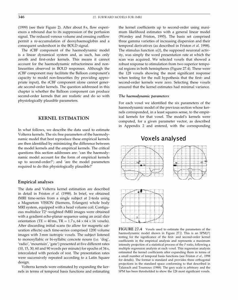
Elsevier UK Chapter: Ch27-P372560 30-9-2006 5:23p.m. Page:346 Trim:7.5in×9.25in
Basal Font:Palatino Margins:Top:40pt Gutter:68pt Font Size:9.5/12 Text Width:42pc Depth:55 Lines
346 27. FORWARD MODELS FOR fMRI
(1999) (see their Figure 2). After about 8 s, flow experi-ences a rebound due to its suppression of the perfusionsignal. The reduced venous volume and ensuing outflowpermit a re-accumulation of deoxyhaemoglobin and aconsequent undershoot in the BOLD signal.
The rCBF component of the haemodynamic modelis a linear dynamical system and, as such, has onlyzeroth and first-order kernels. This means it cannotaccount for the haemodynamic refractoriness and non-linearities observed in BOLD responses. Although therCBF component may facilitate the Balloon component’scapacity to model non-linearities (by providing appro-priate input), the rCBF component alone cannot gener-ate second-order kernels. The question addressed in thischapter is whether the Balloon component can producesecond-order kernels that are realistic and do so withphysiologically plausible parameters.
KERNEL ESTIMATION
In what follows, we describe the data used to estimateVolterra kernels. The six free parameters of the haemody-namic model that best reproduce these empirical kernelsare then identified by minimizing the difference betweenthe model kernels and the empirical kernels. The criticalquestions this section addresses are: ‘can the haemody-namic model account for the form of empirical kernelsup to second-order?’; and ‘are the model parametersrequired to do this physiologically plausible?’
Empirical analyses
The data and Volterra kernel estimation are describedin detail in Friston et al. (1998). In brief, we obtainedfMRI time-series from a single subject at 2-tesla usinga Magnetom VISION (Siemens, Erlangen) whole bodyMRI system, equipped with a head volume coil. Contigu-ous multislice T2∗-weighted fMRI images were obtainedwith a gradient echo-planar sequence using an axial sliceorientation �TE = 40 ms� TR = 1�7 s� 64 × 64 × 16 voxels).After discarding initial scans (to allow for magnetic sat-uration effects) each time-series comprised 1200 volumeimages with 3 mm isotropic voxels. The subject listenedto monosyllabic or bi-syllabic concrete nouns (i.e. ‘dog’,‘radio’, ‘mountain’, ‘gate’) presented at five different rates(10, 15, 30, 60 and 90 words per minute) for epochs of 34 s,intercalated with periods of rest. The presentation rateswere successively repeated according to a Latin Squaredesign.
Volterra kernels were estimated by expanding the ker-nels in terms of temporal basis functions and estimating
the kernel coefficients up to second-order using maxi-mum likelihood estimates with a general linear model(Worsley and Friston, 1995). The basis set comprisedthree gamma varieties of increasing dispersion and theirtemporal derivatives (as described in Friston et al. 1998).The stimulus function u�t�, the supposed neuronal activ-ity, was simply the word presentation rate at which thescan was acquired. We selected voxels that showed arobust response to stimulation from two superior tempo-ral regions in both hemispheres (Figure 27.4). These werethe 128 voxels showing the most significant responsewhen testing for the null hypothesis that the first- andsecond-order kernels were zero. Selecting these voxelsensured that the kernel estimates had minimal variance.
The haemodynamic parameters
For each voxel we identified the six parameters of thehaemodynamic model of the previous section whose ker-nels corresponded, in a least squares sense, to the empir-ical kernels for that voxel. The model’s kernels werecomputed, for a given parameter vector, as describedin Appendix 2 and entered, with the corresponding
FIGURE 27.4 Voxels used to estimate the parameters of thehaemodynamic model shown in Figure 27.2. This is an SPM�F�testing for the significance of the first- and second-order kernelcoefficients in the empirical analysis and represents a maximumintensity projection of a statistical process of the F -ratio, following amultiple regression analysis at each voxel. This regression analysisestimated the kernel coefficients after expanding them in terms ofa small number of temporal basis functions (see Friston et al., 1998for details). The format is standard and provides three orthogonalprojections in the standard space conforming to that described inTalairach and Tournoux (1988). The grey scale is arbitrary and theSPM has been thresholded to show the 128 most significant voxels.

Elsevier UK Chapter: Ch27-P372560 30-9-2006 5:23p.m. Page:347 Trim:7.5in×9.25in
Basal Font:Palatino Margins:Top:40pt Gutter:68pt Font Size:9.5/12 Text Width:42pc Depth:55 Lines
RESULTS AND DISCUSSION 347
empirical estimates, into the objective function thatwas minimized.
RESULTS AND DISCUSSION
The model-based and empirical kernels for the first voxelare shown in Figure 27.5. It can be seen that there is aremarkable agreement in terms of the first- and second-order kernels. This is important because it suggests thatthe non-linearities inherent in the Balloon componentof the haemodynamic model are sufficient to accountfor the non-linear responses observed in real time-series.The first-order kernel corresponds to the conventionalhaemodynamic response function and shows the char-acteristic peak at about 4 s and the post-stimulus under-shoot. The empirical undershoot appears more protractedthan the model’s prediction, suggesting that the model
FIGURE 27.5 The first- and second-order Volterra kernelsbased on parameter estimates from a voxel in the left superior tem-poral gyrus at −56, −28, 12 mm. These kernels can be thought ofas a second-order haemodynamic response function. The first-orderkernels (upper panels) represent the (first-order) component usu-ally presented in linear analyses. The second-order kernels (lowerpanels) are presented in image format. The colour scale is arbitrary;white is positive and black is negative. The left-hand panels arekernels based on parameter estimates from the analysis describedin Figure 27.4. The right-hand panels are the kernels associatedwith the haemodynamic model using parameter estimates that bestmatch the empirical kernels.
is not perfect in every respect. The second-order kernelhas a pronounced negativity on the upper left, flankedby two smaller positivities. This negativity accounts forthe refractoriness seen when two stimuli are temporallyproximate; from the perspective of the Balloon model, thesecond stimulus is compromised in terms of elaboratinga BOLD signal, because of the venous pooling, and conse-quent dilution of deoxyhaemoglobin incurred by the firststimulus. This means that less deoxyhaemoglobin can becleared for a given increase in flow. More interesting arethe positive regions, which suggest stimuli separated byabout 8 s should show super-additive effects. This can beattributed to the fact that, during the flow undershootfollowing the first stimulus, deoxyhaemoglobin concen-tration is greater than normal (see the upper right panelin Figure 27.3), thereby facilitating clearance of deoxy-haemoglobin following the second stimulus.
Figure 27.6 shows the various functions implied bythe haemodynamic model parameters averaged over all
FIGURE 27.6 Functions implied by the (mean) haemody-namic model parameters over the voxels shown in Figure 27.4.Upper left panel: outflow as a function of venous volume fout�v�.Upper right panel: oxygen extraction as a function of inflow. Thesolid line is extraction per se E�f � and the broken line is the netnormalized delivery of deoxyhaemoglobin to the venous compart-ment f E�f �/E0. Lower panel: this is a plot of the non-linear func-tion of volume and deoxyhaemoglobin that represents BOLD signaly�t� = g�v� q�.

Elsevier UK Chapter: Ch27-P372560 30-9-2006 5:23p.m. Page:348 Trim:7.5in×9.25in
Basal Font:Palatino Margins:Top:40pt Gutter:68pt Font Size:9.5/12 Text Width:42pc Depth:55 Lines
348 27. FORWARD MODELS FOR fMRI
voxels. These include outflow as a function of venousvolume fout�v� and oxygen extraction fraction as a func-tion of inflow. The solid line in the upper right panelis extraction E�f � and the broken line is the net nor-malized delivery of deoxyhaemoglobin to the venouscompartment fE�f �
/E0. Note that, although the fraction
of oxygen extracted decreases with flow, the net deliv-ery of deoxygenated haemoglobin increases with flow.In other words, flow increases per se actually reduce sig-nal. It is only the secondary effects of flow on dilutionand volume-dependent outflow that cause an increasein BOLD signal. The lower panel depicts the non-linearfunction of volume and deoxyhaemoglobin that repre-sents BOLD signal y�t� = g�v� q�. Here one observes thatpositive BOLD signals are expressed only when deoxy-haemoglobin is low. The effect of volume is much lessmarked and tends to affect signal predominantly throughdilution.
The distributions of the parameters over voxels areshown in Figure 27.7 with their mean in brackets at thetop of each panel. It should be noted that the data fromwhich these estimates came were not independent. How-ever, given they came from four different brain regionsthey are remarkably consistent. In the next section wewill discuss each of these parameters and the effect itexerts on the BOLD response.
DISCUSSION
The main point is that the Balloon model, suitablyextended to incorporate the dynamics of rCBF induc-tion by synaptic activity, can reproduce the same form ofVolterra kernels that are seen empirically. As such, theBalloon model is sufficient to account for the more impor-tant non-linearities observed in evoked fMRI responses.The remainder of this section deals with the validity ofthe haemodynamic model in terms of the plausibilityof the parameter estimates from the previous section.The role of each parameter in shaping the haemody-namic response is illustrated in the associated panel inFigure 27.8 and is discussed in the following subsections.
Neuronal efficacy
This represents the increase in signal elicited by neuronalactivity, expressed in terms of event density (i.e. num-ber of evoked transients per second). From a biophysicalperspective it is not very interesting because it reflectsboth the potency of the stimulus in eliciting a neuronalresponse and the efficacy of the ensuing synaptic activityto induce the signal. It is interesting to note, however, that
FIGURE 27.7 Histograms of the distribution of the six freeparameters of the haemodynamic model estimated over the voxelsshown in Figure 27.4. The number in brackets at the top of each his-togram is the mean value for the parameters in question: neuronalefficacy is , signal decay is �s , autoregulation is �f , transit time is�0, stiffness is � and oxygen extraction is E0.
one word per second invokes an increase in normalizedrCBF of unity (i.e. in the absence of regulatory effects,a doubling of blood flow over a second). As might beexpected, changes in this parameter simply modulate theevoked haemodynamic responses (see the first panel inFigure 27.8).
Signal decay
This parameter reflects signal decay or elimination.Transduction of neuronal activity into perfusion changes,over a few 100 , has a substantial neurogenic component(that may be augmented by electrical conduction alongthe vascular endothelium). However, at spatial scales ofseveral millimetres it is likely that rapidly diffusing spa-tial signals mediate increases in rCBF through relaxation
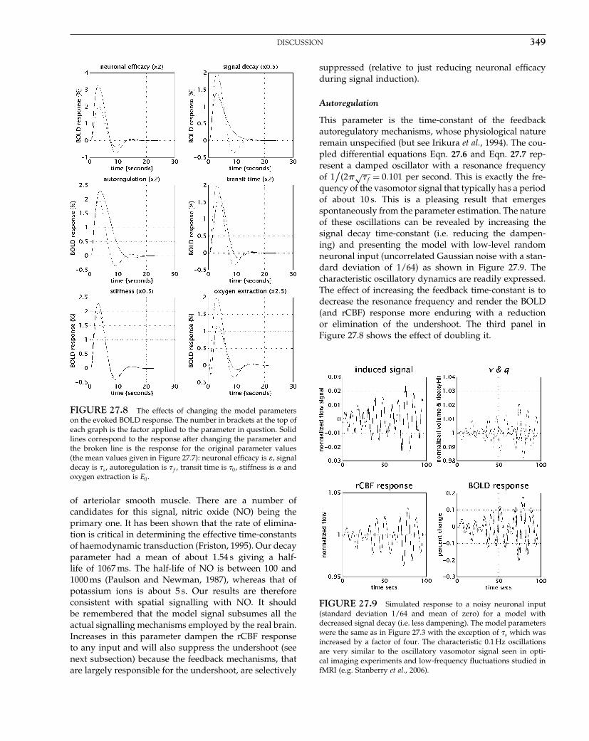
Elsevier UK Chapter: Ch27-P372560 30-9-2006 5:23p.m. Page:349 Trim:7.5in×9.25in
Basal Font:Palatino Margins:Top:40pt Gutter:68pt Font Size:9.5/12 Text Width:42pc Depth:55 Lines
DISCUSSION 349
FIGURE 27.8 The effects of changing the model parameterson the evoked BOLD response. The number in brackets at the top ofeach graph is the factor applied to the parameter in question. Solidlines correspond to the response after changing the parameter andthe broken line is the response for the original parameter values(the mean values given in Figure 27.7): neuronal efficacy is , signaldecay is �s , autoregulation is �f , transit time is �0, stiffness is � andoxygen extraction is E0.
of arteriolar smooth muscle. There are a number ofcandidates for this signal, nitric oxide (NO) being theprimary one. It has been shown that the rate of elimina-tion is critical in determining the effective time-constantsof haemodynamic transduction (Friston, 1995). Our decayparameter had a mean of about 1.54 s giving a half-life of 1067 ms. The half-life of NO is between 100 and1000 ms (Paulson and Newman, 1987), whereas that ofpotassium ions is about 5 s. Our results are thereforeconsistent with spatial signalling with NO. It shouldbe remembered that the model signal subsumes all theactual signalling mechanisms employed by the real brain.Increases in this parameter dampen the rCBF responseto any input and will also suppress the undershoot (seenext subsection) because the feedback mechanisms, thatare largely responsible for the undershoot, are selectively
suppressed (relative to just reducing neuronal efficacyduring signal induction).
Autoregulation
This parameter is the time-constant of the feedbackautoregulatory mechanisms, whose physiological natureremain unspecified (but see Irikura et al., 1994). The cou-pled differential equations Eqn. 27.6 and Eqn. 27.7 rep-resent a damped oscillator with a resonance frequencyof 1
/�2�
√�f = 0�101 per second. This is exactly the fre-
quency of the vasomotor signal that typically has a periodof about 10 s. This is a pleasing result that emergesspontaneously from the parameter estimation. The natureof these oscillations can be revealed by increasing thesignal decay time-constant (i.e. reducing the dampen-ing) and presenting the model with low-level randomneuronal input (uncorrelated Gaussian noise with a stan-dard deviation of 1/64) as shown in Figure 27.9. Thecharacteristic oscillatory dynamics are readily expressed.The effect of increasing the feedback time-constant is todecrease the resonance frequency and render the BOLD(and rCBF) response more enduring with a reductionor elimination of the undershoot. The third panel inFigure 27.8 shows the effect of doubling it.
FIGURE 27.9 Simulated response to a noisy neuronal input(standard deviation 1/64 and mean of zero) for a model withdecreased signal decay (i.e. less dampening). The model parameterswere the same as in Figure 27.3 with the exception of �s which wasincreased by a factor of four. The characteristic 0.1 Hz oscillationsare very similar to the oscillatory vasomotor signal seen in opti-cal imaging experiments and low-frequency fluctuations studied infMRI (e.g. Stanberry et al., 2006).

Elsevier UK Chapter: Ch27-P372560 30-9-2006 5:23p.m. Page:350 Trim:7.5in×9.25in
Basal Font:Palatino Margins:Top:40pt Gutter:68pt Font Size:9.5/12 Text Width:42pc Depth:55 Lines
350 27. FORWARD MODELS FOR fMRI
Transit time
This is an important parameter that determines thedynamics of the signal. It is effectively resting venousvolume divided by resting flow and, in our data, is esti-mated at about 1 s (0.98 s). The transit time through the ratbrain is roughly 1.4 s at rest and, according to the asymp-totic projections for rCBF and volume, falls to 0.73 s dur-ing stimulation (Mandeville et al., 1999). In other words, ittakesaboutasecondfor a blood cell to traverse the venouscompartment. The effect of increasing mean transit timeis to slow down the dynamics of the BOLD signal withrespect to the flow changes. The shape of the responseremains the same but it is expressed more slowly. In thefourth panel of Figure 27.8 a doubling of the mean transittime is seen to retard the peak BOLD response by abouta second and the undershoot by about 2 s.
Stiffness parameter
Under steady state conditions this would be about 0.38.The mean over voxels considered above was about0.33. This discrepancy, in relation to steady state lev-els, is anticipated by the Windkessel formulation and isattributable to the fact that volume and flow are in a stateof continuous flux during the evoked responses. Recallfrom Eqn. 27.3 that 1/� = �+ = 3�03, in our data. Underthe assumption of laminar flow, � = 2 ⇒ ≈ 1, whichis less than Mandeville et al. (1999) found for rats dur-ing forepaw stimulation, but is certainly in a plausiblerange. Increasing this parameter increases the degree ofnon-linearity in the flow-volume behaviour of the venousballoon that underpins the non-linear behaviour we aretrying to account for. However, its direct effect on evokedresponses to single stimuli is not very marked. The fifthpanel of Figure 27.8 shows the effects when it is decreasedby 50 per cent.
Resting oxygen extraction
This is about 34 per cent and the range observed inour data fits exactly with known values for resting oxy-gen extraction fraction (between 20 and 55 per cent).Oxygen extraction fraction is a potentially important fac-tor in determining the nature of evoked fMRI responsesbecause it may be sensitive to the nature of the baselinethat defines the resting state. Increases in this parame-ter can have quite profound effects on the shape of theresponse that bias it towards an early dip. In the exampleshown (last panel in Figure 27.8) the resting extractionhas been increased to 78 per cent. This is a potentiallyimportant observation that may explain why the initialdip has been difficult to observe in all studies. Accordingto the results presented in Figure 27.8, the initial dip isvery sensitive to resting oxygen extraction fraction, which
should be high before the dip is expressed. Extractionfraction will be high in regions with very low blood flow,or in tissue with endogenously high extraction. It may bethat cytochrome oxidase rich cortex, like the visual cor-tices, has a higher fraction and is more likely to evidenceearly dips.
In summary, the parameters of the haemodynamicmodel that best reproduce empirically derived Volterrakernels are all biologically plausible and lend the modela construct validity (in relation to the Volterra formu-lation) and face validity (in relation to other physio-logical characterizations of the cerebral haemodynamicsreviewed here). In this extended haemodynamic model,non-linearities, inherent in the Balloon model, and outputnon-linearity have been related directly to non-linearitiesin responses. Their role in mediating the post-stimulusundershoot is emphasized less here because the rCBFcomponent cannot model undershoots.
CONCLUSION
In conclusion, we have described an input-state-outputmodel of the haemodynamic response to changes insynaptic activity that combines the Balloon model offlow to BOLD signal coupling and a dynamical modelof the transduction of neuronal activity into perfusionchanges. This model has been characterized in terms ofits Volterra kernels and easily reproduces empirical ker-nels with parameters that are biologically plausible. Thismeans that the non-linearities inherent in the Balloonmodel are sufficient to account for haemodynamic refrac-toriness and other non-linear aspects of evoked responsesin fMRI.
In the next chapter, we consider the mapping fromneuronal activity to measurements made with EEG andMEG. Here the dynamics are less important, but the spa-tial aspect of the forward model becomes much morecomplicated.
REFERENCES
Attwell D, Laughlin SB (2001) An energy budget for signaling inthe grey matter of the brain. J Cereb Blood Flow Metab 21: 1133–45
Buxton RB, Frank LR (1997) A model for the coupling betweencerebral blood flow and oxygen metabolism during neural stim-ulation. J Cereb Blood Flow Metab 17: 64–72
Buxton RB, Wong EC, Frank LR (1998) Dynamics of blood flow andoxygenation changes during brain activation: the Balloon model.Mag Res Med 39: 855–64

Elsevier UK Chapter: Ch27-P372560 30-9-2006 5:23p.m. Page:351 Trim:7.5in×9.25in
Basal Font:Palatino Margins:Top:40pt Gutter:68pt Font Size:9.5/12 Text Width:42pc Depth:55 Lines
REFERENCES 351
Fox PT, Raichle ME (1986) Focal physiological uncoupling of cere-bral blood flow and oxidative metabolism during somatosen-sory stimulation in human subjects. Proc Natl Acad Sci USA 83:1140–44
Friston KJ (1995) Regulation of rCBF by diffusible signals: an analy-sis of constraints on diffusion and elimination. Hum Brain Mapp3: 56–65
Friston KJ, Jezzard P, Turner R (1994) Analysis of functional MRItime series. Hum Brain Mapp 1: 153–71
Friston KJ, Josephs O, Rees G et al. (1998) Nonlinear event-relatedresponses in fMRI. Mag Res Med 39: 41–52
Friston KJ, Mechelli A, Turner R et al. (2000) Nonlinear responsesin fMRI: the Balloon model, Volterra kernels, and other hemo-dynamics. NeuroImage 12: 466–77
Grill-Spector K, Malach R (2001) fMR-adaptation: a tool for studyingthe functional properties of human cortical neurons. Acta Psychol(Amst) 107: 293–321
Grubb RL, Rachael ME, Euchring JO et al. (1974) The effects ofchanges in PCO2 on cerebral blood volume, blood flow andvascular mean transit time. Stroke 5: 630–39
Heeger DJ, Ress D (2002) What does fMRI tell us about neuronalactivity? Nat Rev Neurosci 3: 142–51
Hoge RD, Atkinson J, Gill B et al. (1999) Linear coupling betweencerebral blood flow and oxygen consumption in activatedhuman cortex. Proc Natl Acad Sci USA 96: 9403–08
Irikura K, Maynard KI, Moskowitz MA (1994) Importance of nitricoxide synthase inhibition to the attenuated vascular responsesinduced by topical l-nitro-arginine during vibrissal stimulation.J Cereb Blood Flow Metab 14: 45–48
Kennedy C, Des Rosiers MH, Sakurada O et al. (1976) Metabolicmapping of the primary visual system of the monkey by meansof the autoradiographic [14C]deoxyglucose technique. Proc NatlAcad Sci USA 73: 4230–34
Lindauer U, Royl G, Leithner C et al. (2001) No evidence for earlydecrease in blood oxygenation in rat whisker cortex in responseto functional activation. NeuroImage 13: 988–1001
Logothetis NK, Pauls J, Augath MT et al. (2001) Neurophysiologicalinvestigation of the basis of the fMRI signal. Nature 412: 150–57
Mandeville JB, Marota JJ, Ayata C et al. (1999) Evidence of a cere-brovascular postarteriole Windkessel with delayed compliance.J Cereb Blood Flow Metab 19: 679–89
Mayhew J, Hu D, Zheng Y et al. (1998) An evaluation of linear mod-els analysis techniques for processing images of microcirculationactivity. NeuroImage 7: 49–71
Miller KL, Luh WM, Liu TT et al. (2000) Characterizing the dynamicperfusion response to stimuli of short duration. Proc ISRM 8: 580
Paulson OB, Newman EA (1987) Does the release of potassium fromastrocyte endfeet regulate cerebral blood? Science 237: 896–98
Roy CS, Sherrington CS (1890) On the regulation of the blood supplyof the brain. J Physiol Lond 11: 85–108
Stanberry LI, Richards TL, Berninger VW et al. (2006). Low-frequency signal changes reflect differences in functional con-nectivity between good readers and dyslexics during continuousphoneme mapping. Mag Res Imag 24: 217–29
Talairach J, Tournoux P (1988) A co-planar stereotaxic atlas of a humanbrain. Thieme, Stuttgart
Vanzetta I, Grinvald A (1999) Increased cortical oxidativemetabolism due to sensory stimulation: implications for func-tional brain imaging. Science 286: 1555–58
Vazquez AL, Noll DC (1996) Non-linear temporal aspects of theBOLD response in fMRI. Proc Int Soc Mag Res Med 3: S1765
Worsley KJ, Friston KJ (1995) Analysis of fMRI time-seriesrevisited – again. NeuroImage 2: 173–81
Zheng Y, Martindale J, Johnston D et al. (2002) A model of the hemo-dynamic response and oxygen delivery to brain. NeuroImage 16:617–37

Elsevier UK Chapter: Ch28-P372560 30-9-2006 5:25p.m. Page:352 Trim:7.5in×9.25in
Basal Font:Palatino Margins:Top:40pt Gutter:68pt Font Size:9.5/12 Text Width:42pc Depth:55 Lines
C H A P T E R
28
Forward models for EEGC. Phillips, J. Mattout and K. Friston
INTRODUCTION
In this chapter, we turn to forward models for electricaland magnetic measurements v of neuronal activity j. Theform of such models is very simple,
v = Lj 28.1
where L is called a lead field. We will refer to thelead field repeatedly in subsequent chapters, where itis treated as a simple linear mapping. However, as wewill see below, it entails a substantial amount of theoryand forward modelling: electroencephalography (EEG)and magnetoencephalography (MEG) involves record-ing the electric potential (or magnetic field) produced byneuronal activity, at the surface of the scalp. The advan-tage of M/EEG lies in its excellent temporal resolution,as activity is seen in ‘real time’. However, non-invasivemeasurements of the electromagnetic field can only beobtained from a limited number of sensors placed on, oraround, the scalp.
In EEG (and MEG), the forward problem entails comput-ing the electromagnetic field at the scalp given a sourceconfiguration and volume conductor. The inverse problemdescribes the opposite problem: given the volume con-ductor and the electromagnetic field at the scalp, whatis the location and time course of the sources? The solu-tion of the forward problem, even if approximate, isrequired to solve the inverse problem. The forward prob-lem itself is a ‘simple electromagnetic problem’ that canbe expressed and solved with Maxwell’s equations. Thedifficult aspect lies in modelling the volume conductor, ahuman head, and the sources, the neuronal activity of thebrain. To do this, it is necessary to understand cerebralanatomy and the nature of neuronal activity.
To be detected, neural activity must sum coherently.Because of their very short time course, synchronous fir-ing of action potentials, APs, is unlikely but the longer
time course of postsynaptic potentials (PSPs) allowsthem to superpose temporally. Moreover the electromag-netic field generated by a dipolar source (like a PSP)decreases with distance – approximately as 1/r2, moreslowly than the 1/r3-dependent field of a quadrupolarsource (like an AP). Therefore, even though APs are muchlarger in amplitude than PSPs, it is generally acceptedthat postsynaptic potentials are the generators of scalpfields usually recorded in EEG and MEG (Nunez, 1981;Hämäläinen et al., 1993). If the dendrites supporting PSPsare oriented randomly or radially on a complete sphericalsurface (or small closed surface), no net electromagneticfield can be detected outside the immediate vicinity ofthe active neurons; this is called a ‘closed field’ config-uration. Because of the uniform spatial organization oftheir dendrites (perpendicular to the cortical surface), thepyramidal cells are the only neurons that can generate anet macroscopic current dipole over the cortical surface,whose field is detectable on the scalp. This is named an‘open field’ configuration. The brain’s electrical activity isthus generally modelled as small current dipoles, locatedin the grey matter.
The overall structure of the head is rather complicated.The brain, skull, scalp and other parts of the head (eyes,vessels, nerves, cerebrospinal fluid, etc.) comprise vari-ous tissues and cavities of different electrical conductiv-ity. Moreover, the electrical conductivity of brain tissue ishighly anisotropic: in the white matter, conduction is 10times greater along an axon fibre than in the transversedirection. These complications are generally ignored; atthe present time, it is impossible to measure accurately invivo the detailed conductivity of all tissues and to accountfor them in the solution of the forward problem (Marinet al., 1998; Huiskamp et al., 1999). Therefore, the headis usually modelled as a set of concentric homogeneousvolume conductors: the brain (comprising the white andgrey matter), the skull and the scalp. Once the relation-ship between brain electrical activity and electromagnetic
Statistical Parametric Mapping, by Karl Friston et al. Copyright 2007, Elsevier Ltd. All rights reserved.ISBN–13: 978-0-12-372560-8 ISBN–10: 0-12-372560-7
352

Elsevier UK Chapter: Ch28-P372560 30-9-2006 5:25p.m. Page:353 Trim:7.5in×9.25in
Basal Font:Palatino Margins:Top:40pt Gutter:68pt Font Size:9.5/12 Text Width:42pc Depth:55 Lines
ANALYTICAL FORMULATION 353
scalp fields has been established, the inverse problem canbe addressed. Non-invasive measurements of the elec-tromagnetic field can only be obtained from the scalpsurface, and the spatial configuration of neuronal activitycannot be determined uniquely if based on EEG and/orMEG recordings alone (von Helmholtz, 1853; Nunez,1981).
In summary, estimates of electromagnetic activitydepend on cortical anatomy: cellular-level structuresdetermine how neuronal electrical activity producesmacroscopic current sources detectable outside the head,the local electrical conductivity influences the solution ofthe forward problem, and the anatomy of the brain at thesulcal level can be used to constrain the inverse solution.
ANALYTICAL FORMULATION
Maxwell’s equations
For the forward problem, the electromagnetic propertiesof the head (or at least its simplified model) and the loca-tion of the electric current generators in the brain areassumed to be known. Maxwell’s equations can then beused to calculate the electric (and magnetic) field on thesurface of the scalp or inside the head volume if neces-sary. In differential equation form, Maxwell’s equationscan be expressed as (Ramo et al., 1984):
�� �E = �
�28.2a
�� �B = 0 28.2b
�� × �E = −��B�t
28.2c
�� × �B = ��j +����E�t
28.2d
where �E is the electric field, �B is the magnetic field, �j is thecurrent density, � is the charge density, � is the electricpermittivity, and � is the magnetic permeability.
These are the basic set of equations of classical electro-magnetism. Together with two auxiliary relations, Ohm’slaw �j = � �E and the continuity equation ���j = ��/�t, theydescribe all electromagnetic phenomena. In the case ofbioelectric phenomena such as electro- and magnetoen-cephalography (M/EEG), we are only interested in theelectric (and magnetic) field �E (and �B). The treatment ofMaxwell’s equations can be simplified significantly bynoting that the media comprising the head have no sig-nificant capacitance: they are either purely resistive or thefrequency of activity is sufficiently low that the capac-itance can be neglected. This means there are no elec-
tromagnetic wave propagation phenomena (Hämäläinenet al., 1993; He, 1998).
This allows us to adopt a quasistatic approximationof Maxwell’s equations, which means that, in the calcu-lation of �E (and �B), ��E/�t and ��B/�t can be ignored assource terms. Physically, these assumptions mean thatthe instantaneous current density depends only on theinstantaneous current sources and conforms to the super-position theorem. Eqn. 28.2c then becomes �� × �E = 0 andthe electric field �E can be expressed as the negative gra-dient of a scalar field, the electric potential V :
�E = −��V 28.3
‘Current sources’ are, by definition, a distribution offorced current density �jf . The current sources �jf can beseen as the summed coherent electric activity of activatedcell membranes, i.e. the current density produced directlyby neural activity, with arbitrarily close sink and sourcecurrents. The total current density �jtot flowing throughthe media is equal to the sum of the imposed sources�jf and the return current �jr . The latter is the result ofthe macroscopic electric field on charge carriers in theconducting medium, as expressed by Ohm’s law. WithOhm’s law and 28.3, we have:
�jtot = �jr +�jf = � �E +�jf = −� ��V +�jf 28.4
By neglecting the capacitance of head tissues, chargedoes not accumulate in the volume or on tissue interfaces,i.e. the charges are redistributed in negligible time. Thistranslates mathematically into zero divergence of the cur-rent density ���jtot = 0. And, by taking the divergence of28.4, we obtain the simplified Maxwell’s equation:
���� ��V = ���jf 28.5
This equation is at the heart of the forward problem inEEG: it links explicitly the current sources �jf and theelectric potential V .
Equation 28.5 can be solved for V in various ways,depending on the geometry of the model, the form ofthe conductivity � and the location of the sources �jf .An analytical solution is possible only for particularcases: a highly symmetrical geometry (e.g. concentricspheres or cubes) and homogeneous isotropic conduc-tivity. For other more general cases, numerical methodsare required. Common methods include the ‘finite ele-ment method’ (FEM) (Chari and Silvester, 1980; van denBroek et al., 1996; Awada et al., 1997; Buchner et al.,1997; Klepfer et al., 1997), the ‘finite difference method’(FDM) (Rosenfeld et al., 1996; Saleheen and Ng, 1997,1998) and the ‘boundary element method’ (BEM) (Becker,1992; Ferguson and Stroink, 1997; Mosher et al., 1999).

Elsevier UK Chapter: Ch28-P372560 30-9-2006 5:25p.m. Page:354 Trim:7.5in×9.25in
Basal Font:Palatino Margins:Top:40pt Gutter:68pt Font Size:9.5/12 Text Width:42pc Depth:55 Lines
354 28. FORWARD MODELS FOR EEG
The FEM and FDM make no assumptions about theshape of the volume conductivity and allow the estima-tion of V at any location in the volume. The volume is tes-sellated into small volume elements in which Maxwell’sequations are solved locally. As each volume element ischaracterized by its own conductivity (isotropic or not),any configuration of conductive volume can be modelled.With the FEM, the volume elements are of arbitrary shape(usually tetrahedron or regular polyhedron), while thevolume elements are cubic with the FDM. In contrast,the BEM is based on the hypothesis that the volume isdivided into subvolumes of homogeneous and isotropicconductivity, and the potential V is estimated only onthe surfaces separating these subvolumes.
The FEM and FDM offer a more general solution ofthe forward problem but the complexity of the numer-ical problem and the computing time needed to solveit are increased greatly, compared with the BEM. More-over, the conductivity throughout the volume, necessaryto make full use of the FEM and FDM, cannot be esti-mated for individual subjects. Therefore, a simple ‘threesphere shell’ model with an analytical solution is stillused generally for M/EEG source localization. A moreanatomically realistic but still tractable approach uses theBEM to solve the forward problem. We will focus on theBEM from now on.
The BEM approach for EEG
One way of solving Eqn. 28.5 is the boundary elementmethod, which relies on one major assumption: the vol-ume is divided into subvolumes of homogeneous andisotropic conductivity. The solution of the forward prob-lem then can be obtained with the help of some boundaryconditions and Green’s theorem.
Boundary conditions
Consider Sl the surface separating two volumes, vol−
and vol+, of conductivity �− and �+. Let’s define dSl
an infinitesimal element of this surface and let �n be theunit vector normal to the surface oriented from the insidetowards the outside or, by convention, from vol− to vol+,as shown in Figure 28.1.
There are no sources located on the surfaces betweenhomogeneous volumes and the current normal to thesurfaces is continuous, so on surface Sl, we have �jtot =−� ��V and
�− ��V − →dSl = �+ ��V + →
dSl 28.6
FIGURE 28.1 The surface Sl separates the two homogeneousvolumes vol− and vol+ of isotropic conductivity �− and �+. dSl isan infinitesimal element of the surface Sl and �n is the unit vectornormal to Sl, oriented from vol− to vol+.
where �dsl = �ndSl is the oriented infinitesimal element ofthis surface. Moreover, the potential V must also be con-tinuous on Sl:
V −�Sl = V +�Sl 28.7
The Eqns 28.6 and 28.7 provide the two boundary condi-tions necessary to solve the quasistatic form of Maxwell’sequations as expressed in Eqn. 28.5.
Green’s theorem
Let dvk be an element of the homogeneous regional vol-ume volk (where k = 1 � � � Nv and Nv is the number ofhomogeneous volumes) and let �dSl be an oriented ele-ment, �dsl = �ndSl, of the surface Sl separating two regionsof homogeneous conductivity (where l = 1 � � � NS andNS is the number of such surfaces). Take two well-behaved functions � and in each region volk; thenGreen’s theorem states (Smythe, 1950):
NS∑l
∫Sl
[�−
l ��− �� − − − ���−− ��+l ��+ �� + − + ���+
] →dSl
28.8
=Nv∑k
∫volk
[� ����k
�� − ����k���
]dvk
where the sums run over the Nv volumes and the NS
surfaces, and the symbols − and + refer to the volumesinside and outside surface Sl.
The forward problem entails evaluating the electricpotential V from the current sources distribution �jf withthe quasistatic form of Maxwell’s equation, Eqn. 28.5 andthe boundary conditions Eqn. 28.6 and Eqn. 28.7, usingGreen’s theorem, Eqn. 28.8.
Analytical BEM equation
In Eqn. 28.8, if we take � = 1/r , where r is the dis-tance between an arbitrary point �r and the origin �o, then,

Elsevier UK Chapter: Ch28-P372560 30-9-2006 5:25p.m. Page:355 Trim:7.5in×9.25in
Basal Font:Palatino Margins:Top:40pt Gutter:68pt Font Size:9.5/12 Text Width:42pc Depth:55 Lines
ANALYTICAL FORMULATION 355
for smooth surfaces, Eqn. 28.8 becomes, as shown byGeselowitz (1967):
NS∑l
∫Sl
[��−
l�� − −�+
l�� +
1r
− ��−l − −�+
l +��(
1r
)]�dSl
28.9
= 4�� +Nv∑k
∫volk
1r
��(�k
�� )
dvk
where, � and in the first term of the right hand side, areevaluated at the origin �o, i.e. for r = 0. Consider = V andsuppose that �jf is distributed in only one homogeneousvolume, the brain volume volbr ; then, thanks to the sim-plified Maxwell’s equation, Eqn. 28.5 and the boundaryconditions, Eqn. 28.6 and Eqn. 28.7, Eqn. 28.9 becomes:
−NS∑l
��−l −�+
l ∫
Sl
V ��(
1r
)�dSl = 4��V +
∫volbr
1r
���jf dvbr
28.10
By the divergence theorem and the definition of
the divergence operator �� , we have:∫
vol��(
�jfr
)dv =
∫S
�jfr�dS = ∫
vol
[�jf �� ( 1r
)+ 1r���jf]
dv. And, as there are no
sources �jf on any surface Sl�jf �Sl = 0, then∫
vol1r���jf dv =
− ∫vol
�jf �� ( 1r
)dv. Therefore, Eqn. 28.10 becomes:
4��V =∫
volbr
�jf ��(
1r
)dvbr −
NS∑l
��−l −�+
l ∫
Sl
V ��(
1r
)�dSl
28.11
On the left hand side of Eqn. 28.11, V is still evaluatedat the origin �o of space (an arbitrary point) and r is thedistance from that origin to a point on the surface Sl
(in the surface integrals) or in the volume volbr (in thevolume integral).
Let us consider �x the point where V is evaluated, �s′
a point on the surface Sl and �r ′ a point in the volumevolbr . The distance r between the point �x where V isevaluated and any point �s′ on the surface S′
l (or �r ′ in thevolume volbr ) will be expressed by ��x −�s′� (or ��x − �r ′�).Thus Eqn. 28.11 is rewritten (Sarvas, 1987) like this:
4����xV��x =∫
Volbr
�jf ��r ′�� ′(
1��x−�r ′�
)dvbr
−NS∑l
��−l −�+
l ∫
S′l
V��s′�� ′(
1��x−�s′�
)�dS′
l
28.12
where �� ′ means that the gradient is with respect to �r ′ or�s′. The potential V should be evaluated on the surfacesSl but, if �x approaches the point �s on a surface Sk, the kth
surface integral becomes singular in Eqn. 28.12.
Consider now Fk��x the integral on the smooth surfaceSk in Eqn. 28.12, Fk��x = ∫
S′kV��s′���1/��x −�s′��dS′
k; then itfollows from Vladimirov (1971):
lim�x→�s
Fk��x = −2�V��s+Fk��s 28.13
where �x approaches the point �s on the surface Sk fromthe inside, so in the volume of conductivity �−
k . WithEqn. 28.13, the point �x can be placed on any surface Sk
and, with �x → �s, Eqn. 28.12 becomes:
4��−k V��s =
∫Volbr
�jf ��r ′�� ′(
1��s −�r ′�
)dvbr
−NS∑l
��−l −�+
l ∫
S′l
V��s′�� ′(
1��s −�s′�
)�dS′
l
+2���−k −�+
k V��s 28.14
and eventually:
V��s = V���s− 12�
NS∑l
�−l −�+
l
�−k +�+
k
∫S′
l
V��s′�� ′(
1��s −�s′�
)�n��s′ dS′
l
28.15
where V���s is the potential due to �jf in a conductorof infinite extent and homogeneous conductivity ��−
k +�+
k /2:
V���s = 12���−
k +�+k
∫v
�jf ��r ′�� ′(
1��s −�r ′�
)dv 28.16
and
• the sum∑NS
l runs over all the surfaces separating vol-umes of homogeneous isotropic conductivity.
• �−l and �+
l are the conductivity inside and outside thesurface Sl.• �s and �s′ are points on the surfaces Sk and Sl respectively.
• �n��s′ is a unit vector normal to the surface Sl at the point�s′ and oriented from the inside towards the outsideof Sl.
This is an explicit relationship between the currentsources �jf and the surface potential V . As V is present onboth sides of this integral equation, V can only be eval-uated in closed form for particular geometries, such asconcentric spheres. For more general cases, i.e. realistichead models, numerical methods are required to solvethis integral equation.
The BEM approach for MEG
Magnetoencephalographic (MEG) signals are not verydifferent from EEG data because they represent comple-mentary effects generated by neuronal activity. Both EEG

Elsevier UK Chapter: Ch28-P372560 30-9-2006 5:25p.m. Page:356 Trim:7.5in×9.25in
Basal Font:Palatino Margins:Top:40pt Gutter:68pt Font Size:9.5/12 Text Width:42pc Depth:55 Lines
356 28. FORWARD MODELS FOR EEG
and MEG are related to the imposed current sources �jfby Maxwell’s equations, through �E and V for EEG and �Bfor MEG.
As with the derivations above for V (Eqn. 28.15), anintegral form of Maxwell’s equation can be derived forthe magnetic field �B (Hämäläinen et al., 1993):
�B��r = �B���r+ �0
4�
NS∑l
��−l −�+
l ∫
S′l
V��s′�r −�s′
��r −�s′�3 × �n��s′ dS′l
28.17
where
�B���r = �0
4�
∫volbr
�jf ��r ′× �r −�r ′
��r −�r ′�3 dv 28.18
Importantly, the potential distribution V over the sur-faces is assumed to be known. As with EEG, an analyticalsolution exists only for highly symmetric models; other-wise, numerical methods are used to solve this equation.
NUMERICAL SOLUTION OF THE BEMEQUATION
The main task now, in solving the BEM forward problem,is to evaluate accurately the integrals on the right handside of Eqn. 28.15.
Approximation of the BEM analyticalequation
The volume integral over the continuous sources dis-tribution �jf can be calculated easily by approximating�jf with a superposition of independent point sourcesof known location and orientation. On the other hand,the surface integrals are more difficult to calculate: theyrun on different and irregular surfaces and, moreover,they involve the potential V��s that we want to solve for.Therefore, it is necessary to express the surface integralsin terms of the value of the unknown function V at somediscrete set of points on the surfaces, and to tessellate thesurfaces into sets of regular patches. The most obviousapproximation for the surfaces is to model each of themby a set of plane triangles. With this surface tessellation,the surface integrals of Eqn. 28.15 can be expressed as asum of integrals over triangles:
V��s = V���s− 12�
NS∑l=1
�−l −�+
l
�−k +�+
k
N�ltr∑
m=1
∫��l
m
V��s′�� ′(
1��s −�s′�
)�n��s′ dS′ 28.19
where the surface Sl has been modelled by a set of N �ltr
triangles ��lm . The function V is rendered discrete by
choosing on which nodal points V is evaluated and howthe function V behaves on each individual plane triangle.This would allow an explicit calculation of the integralsover the triangles and Eqn. 28.19 could eventually be sim-plified to a sum of known or, at least, easily evaluatedfunctions.
Three different approximations of V over a triangleare usually considered. First, one could evaluate V at thecentre of gravity of each triangle and consider this valueconstant over the triangle: one value is thus obtainedfor each triangle. This approximation is referred as the‘centre of gravity’ (or CoG) method (Hämäläinen andSarvas, 1989; Meijs et al., 1989). The function V couldalso be evaluated on the vertices of the triangles; this isgenerally called a ‘vertex’ approximation (one value pervertex). If the potential over the triangle is supposed tobe constant and equal to the mean of the potential at itsvertices, this approximation will be called the ‘constantpotential at vertices’ (or CPV) method (Schlitt et al., 1995).A better approximation would be to consider that thepotential varies linearly over the triangle. We will callthis approximation the ‘linear potential at vertices’ (orLPV) method (Schlitt et al., 1995). In what follows, wewill consider only the CoG and LPV approximations.
The CoG and LPV approaches differ mainly in thechoice of the nodal points where the unknown potentialfunction V is calculated. It is important to note that for aclosed tessellated surface there are about twice as manytriangles as vertices. The number and arrangement of thetriangles determine how well the true surface is approx-imated spatially. The choice of the potential approxima-tion method determines the number of equations to besolved (one per triangle or vertex) and how well thetrue potential is modelled over each triangle (constant orlinear approximation).
Current source model
In Eqn. 28.16, the source function �jf ��r is a continuousfunction throughout the volume. The source function�jf ��r can be approximated by a distribution of Nj inde-pendent dipole sources of known location �ri:
�jf ��r =Nj∑i=1
�jf ��ri���r −�ri 28.20
where �jf ��ri = ∫vi
�jf ��r ′ dvi is the summed activity, in thesmall volume vi around the location �ri, modelled as apunctate current source, and ���r is the discrete Dirac
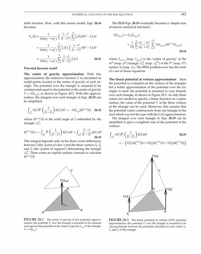
Elsevier UK Chapter: Ch28-P372560 30-9-2006 5:25p.m. Page:357 Trim:7.5in×9.25in
Basal Font:Palatino Margins:Top:40pt Gutter:68pt Font Size:9.5/12 Text Width:42pc Depth:55 Lines
NUMERICAL SOLUTION OF THE BEM EQUATION 357
delta function. Now, with this source model, Eqn. 28.16becomes:
V���s = 12���−
k +�+k
∫v
�s −�r ′
��s −�r ′�3Nj∑i=1
�jf ��ri���r ′ − �ri dv
= 12���−
k +�+k
Nj∑i=1
�jf ��ri∫
v
�s −�r ′
��s −�r ′�3 ���r ′ − �ri dv
= 12���−
k +�+k
Nj∑i=1
�s −�ri
��s −�ri�3�jf ��ri 28.21
Potential function model
The centre of gravity approximation With thisapproximation, the unknown function V is calculated onnodal points located at the centre of gravity of each tri-angle. The potential over the triangle is assumed to beconstant and equal to the potential at the centre of gravityV = V��scog, as shown in Figure 28.2. With this approxi-mation, the integral over each triangle in Eqn. 28.19 canbe simplified:
∫��l
m
V��s′�� ′(
1��s −�s′�
)�n��s′ dS′ = −V��s′
cog��lm��s 28.22
where ��lm��s is the solid angle at �s subtended by thetriangle ��l
m :
��lm��s = −∫��l
m
�� ′(
1��s −�s′�
)�n��s′ dS′ =
∫��l
m
�s′ −�s��s′ −�s�3 �n��s′ dS′
28.23This integral depends only on the three vector differencesbetween �s (the ‘point of view’) and the three vertices �s′
1, �s′2
and �s′3 (the ‘points of support’) determining the triangle
��lm . There exists an explicit analytic formula to calculate
��lm��s.
FIGURE 28.2 The centre of gravity (CoG) potential approxi-mation: the potential V over the triangle is assumed to be constantand equal to the potential at the centre of gravity �scog of the triangle,V = V��scog.
The BEM Eqn. 28.19 eventually becomes a ‘simple sumof known analytical functions’:
V��scogp = V���scogp
+ 12�
NS∑l=1
�−l −�+
l
�−k +�+
k
N�ltr∑
m=1
V��scogm��lm��scogp
28.24
where �scogm (resp. �scogp) is the ‘centre of gravity’ of themth (resp. pth) triangle ��l
m (resp. ��kp ) of the lth (resp. kth)
surface Sl (resp. Sk). The BEM problem now has the formof a set of linear equations.
The linear potential at vertices approximation Herethe potential is evaluated on the vertices of the trianglesbut a better approximation of the potential over the tri-angles is used: the potential is assumed to vary linearlyover each triangle, as shown in Figure 28.3. As only threevalues are needed to specify a linear function on a planesurface, the value of the potential V at the three verticesof the triangle can be used. Moreover, this ensures thatthe potential varies continuously from one triangle to thenext which was not the case with the CoG approximation.
The integral over each triangle in Eqn. 28.19 can besimplified to give a weighted sum of the potential at thevertices:
∫��l
m
V��s′�� ′(
1��s −�s′�
)�n��s′dS′ 28.25
= −(V��s′
1��lm1 ��s+V��s′
2��lm2 ��s+V��s′
3��lm3 ��s
)
FIGURE 28.3 The linear potential at vertices (LPV) potentialapproximation: the potential V over the triangle is assumed to bevarying linearly between the potential calculated at each vertex �s1,�s2 and �s3 of the triangle.

Elsevier UK Chapter: Ch28-P372560 30-9-2006 5:25p.m. Page:358 Trim:7.5in×9.25in
Basal Font:Palatino Margins:Top:40pt Gutter:68pt Font Size:9.5/12 Text Width:42pc Depth:55 Lines
358 28. FORWARD MODELS FOR EEG
The three ��lm• ��s are also purely geometric quantities
depending on the vector differences between the ‘pointof view’ �s and the vertices �s′
• of the triangle. An analyticformula to calculate the ��lm
• ��s from �s and �s′• exists. With
this approximation the BEM Eqn. 28.19 simplifies to:
V��s• = V���s•+ 12�
NS∑l=1
�−l −�+
l
�−k +�+
k
28.26
N�ltr∑
m=1
(V��s′
1m��lm1 ��s•+V��s′
2m��lm2 ��s•+V��s′
3m��lm3 ��s•
)
where �s• is one of the three vertices of a triangle of the kth
surface Sk and �s′im is the ith vertex of the mth triangle ��l
m
of the lth surface Sl. Again, the BEM problem is reducedto a set of linear equations.
Solid angles and potential approximation
As shown in the previous section, to solve the BEM equa-tions, it is necessary to calculate solid angles, i.e. purelygeometrical quantities.
Solid angle calculation
For the CoG approximation, the solid angle ��lm��s sub-tended by a plane triangle ��l
m at some point �s has tobe calculated. Without loss of generality, the observationpoint �s can be placed at the origin �o∗. The three vertices�s1, �s2 and �s3 of the plane triangle are then specified by thevectors �v1 = �s1 −�o∗, �v2 = �s2 −�o∗ and �v3 = �s3 −�o∗ relative tothis origin �o∗, as shown in Figure 28.4. The solid angle �can be expressed analytically as a function of �v1, �v2 and
FIGURE 28.4 Solid angle supported by a plane triangle: thesolid angle � supported at the point �o∗ by the plane triangle (greyshade) depends only on the three vectors �v1, �v2 and �v3 and can beeasily calculated by Eqn. 28.27.
�v3 by the formula taken from van Oosterom and Strackee(1983):
tan(
12
�
)= �v1��v2 × �v3
��v1� ��v2� ��v3�+ ��v1�v2��v3�+ ��v1�v3��v2�+ ��v2�v3��v1�28.27
For the LPV approximation, three geometric quanti-ties �i�i = 1 2 3 have to be calculated for each triangle,under the assumption that the potential V varies linearlyover this triangle. There also exists an analytic formulafor �i (de Munck, 1992; Schlitt et al., 1995):
�i = 12A
(�zi�n�+���vj − �vk ��
)28.28
where
• A is the surface of the plane triangle• �zi = �vj × �vk with �i j k a cyclic permutation of �1 2 3• �n is a unit vector normal to the triangle• � is the solid angle subtended by the plane triangle at
the origin as expressed in Eqn. 28.27• � = �n�vi is equal to the perpendicular distance from the
origin to the triangle
• �� is a vector defined by �� = 3∑i=1
��j − �i�vj with
�i = 1��vj−�vi� ln
( ��vj−�vi� ��vj �+��vj−�vi�vj
��vj−�vi� ��vi�+��vj−�vi�vi
).
The �i also satisfy the equality: �1 +�2 +�3 = �.
Solid angle properties
An important property of solid angles concerns theirintegral over a single closed surface. We know fromEqn. 28.23 that the infinitesimal solid angle d�′ sub-tended by the infinitesimal surface dS′ around the point�s′ at the point of view �s is expressed by: d�′��s�s′ =�n��s′ �s′−�s
��s′−�s�3 dS′. Then the integral of d�′��s�s′ over a smoothclosed surface is:
�S��s =∫
Sd�′��s�s′ =
⎡⎣ 0
2�4�
⎤⎦ for �s
⎡⎣outside
oninside
⎤⎦ the surface�
28.29
The BEM Eqn. 28.15 contains an integral of the form:∫Sd�′��s�s′V��s′ which is converted into a discrete sum,
of the form:∑M
m=1 �nm Vm. It is therefore important thatthe �nm satisfy Eqn. 28.29, i.e.
�nS =M∑
m=1
�nm =⎡⎣ 0
2�4�
⎤⎦ for �s
⎡⎣outside
oninside
⎤⎦ the surface�
28.30
When �s is outside or inside the surface, these equalitiesare satisfied: all the �nm can be calculated unambiguously

Elsevier UK Chapter: Ch28-P372560 30-9-2006 5:25p.m. Page:359 Trim:7.5in×9.25in
Basal Font:Palatino Margins:Top:40pt Gutter:68pt Font Size:9.5/12 Text Width:42pc Depth:55 Lines
NUMERICAL SOLUTION OF THE BEM EQUATION 359
with Eqn. 28.27 or Eqn. 28.28. But when �s is on the surfaceitself we meet the ‘auto-solid angle’ (ASA) problem: thesolid angle subtended by a triangle which contains thepoint of view is zero and the second equality of Eqn. 28.30may not be satisfied automatically.
The ASA problem for the CoG approximation
In the CoG approximation, as the potential is evaluatedat the ‘centre of gravity’ of each triangle, there will beonly one null solid angle: �mm = 0, as can be seen inFigure 28.5. Since the rest of the solid angle subtendedby the closed surface is already 2�, there is no missingangle and the second equality of Eqn. 28.30 is satisfied.
Nevertheless, in reality the surface modelled by thetriangle is not plane, and it should thus support somenon-zero solid angle. There is no obvious way to improvethe solution, but to use a finer meshing of the surface.
The ASA problem for the LPV approximation
With the LPV approximation, all the adjacent triangles(grey triangles in Figure 28.6) containing the ‘point ofview’ are supporting an estimated null solid angle. Thesolid angle subtended by the rest of the surface will notbe equal to 2� because the adjacent triangles do not rep-resent a flat surface.
�miss = 2� −M∑
m=1
�nm = 0 28.31
There are two main problems here: (1) how do wedivide up the missing solid angle �miss between the adja-cent triangles, and (2) within each of them, how do weshare between its vertices the missing part, as illustrated
FIGURE 28.5 The auto-solid angle problem for the CoGapproximation: the solid angle subtended by the grey triangle fromits centre of gravity (the black dot) is zero and the total solid anglesubtended by the rest of the surface (white triangles) is equal to 2�.
FIGURE 28.6 The auto-solid angle problem for the LPVapproximation: the estimated solid angle supported by the ‘central’point and the adjacent grey triangles is zero but the total solid anglesupported by the remaining white triangles is less than 2�.
in Figure 28.7. An analytic solution exists (Heller, 1990)but it requires each triangle around the point of view �s0
be approximated by a portion of sphere of centre �rc andradius R. If the surface is regular and smooth comparedto the density of the mesh, this local spherical approxi-mation will hold as R will be much larger than the lengthof the edges of the triangles.
Since three points do not determine a sphere, a fourthpoint must be chosen. A suitable point would be the nextadjacent vertex, e.g. the sphere that passes through thetriplet [�s0�s1�s2] could be required to pass through �s3 as well.A better and anatomically more tenable approximationcan be obtained, if, at the tessellation stage, the centre ofgravity �scog of each triangle is projected perpendicular tothe triangular plane onto the actual surface of the volume�s⊥
cog. A sphere can now be fitted easily to four points:the three vertices defining the triangle and its projectedcentre of gravity, as shown in Figure 28.8.
Once the spheres have been fitted for �s0 and its adja-cent vertices �s1, �s2, � � � , �sNadj
, an approximate valuefor the solid angle subtended by each triplet [�s0�s1�s2],[�s0�s2�s3], � � � , [�s0�sNadj
�s1] at �s0 can be calculated. Usingspherical coordinates for the vertices, as shown in
FIGURE 28.7 The surface defined by �s1, �s2, � � � , �s5 around �s0supports a non-zero solid angle. Each triangle, defined by a triplet ofvertices ([�s0�s1�s2], [�s0�s2�s3], � � � , [�s0�s5�s1]), supports a part of the missingsolid angle, which in turn must be shared between its vertices. Eachtriangle can be locally approximated by a portion of sphere.

Elsevier UK Chapter: Ch28-P372560 30-9-2006 5:25p.m. Page:360 Trim:7.5in×9.25in
Basal Font:Palatino Margins:Top:40pt Gutter:68pt Font Size:9.5/12 Text Width:42pc Depth:55 Lines
360 28. FORWARD MODELS FOR EEG
FIGURE 28.8 Spherical approximation of an adjacent planetriangle: the triplet of vertices [�s0�s1�s2] and the projection �s⊥
cog of thecentre of gravity �scog of the triangle onto the actual surface determinea sphere, with centre �rc and radius R, that approximates the actualsurface.
Figure 28.9, the solid angle ���s0�s1�s2� subtended at �s0
by the spherical region bounded by �s0, �s1 and �s2, isapproximated by: ���s0�s1�s2� = �1+�2
4 12 where �1 and �2
are easily obtained and sin 122 = ��sb−�s2�
2R sin �2with �sb = �rc +
1sin �1
[sin��1 −�2��s0 −�rc+ sin �2��s1 −�rc
].
FIGURE 28.9 Auto-solid angle approximation: the triangledefined by the triplet [�s0�s1�s2] is approximated by a portion of asphere. The solid angle subtended at �s0 by the curved surface (boldline) can be calculated using the spherical coordinates of �s1 and �s2:�1, �2 and 12.
The fraction f�•� of missing solid angle �miss to beassigned to each triangle �•�, e.g., ��s0�s1�s2�, is obtained by:
f��s0�s1�s2� = ���s0�s1�s2�
���s0�s1�s2� +���s0�s2�s3� +· · ·+���s0�sNadj�s1�
28.32
Note that, even though these equations entail approxima-tions, since they only involve ratios, the total solid anglesubtended by the region around �s0 will sum to �miss, andthe total solid angle subtended by the entire surface at �s0
will be exactly 2�. Now, it is necessary to share furtherthis portion of missing solid angle between the verticesof the adjacent triangles.
Assuming that �1, �2 and 12 are small and that thepotential V varies linearly with distance on the sphere,Heller (1990) showed that it is possible to share the solidangle f��s0�s1�s2��miss between the three vertices �s0, �s1 and�s2 such that ��s0��s0�s1�s2� +��s1��s0�s1�s2� +��s2��s0�s1�s2� = f��s0�s1�s2��miss,where:
��s0��s0�s1�s2� = 112��1 +�2
(7�1 +7�2 − �2
1
�2− �2
2
�1
)f��s0�s1�s2��miss
28.33a
��s1��s0�s1�s2� = 112��1 +�2
(3�1 +2�2 + �2
2
�1
)f��s0�s1�s2��miss
28.33b
��s2��s0�s1�s2� = 112��1 +�2
(2�1 +3�2 + �2
1
�2
)f��s0�s1�s2��miss
28.33c
Matrix form of the BEM equation
A simple realistic head model can be obtained by consid-ering three concentric volumes of homogeneous conduc-tivity: the brain, skull and scalp volumes, of conductivity�br , �sk and �sc respectively, as depicted in Figure 28.10.The three interfaces: ‘brain-skull’, ‘skull-scalp’ and ‘scalp-air’ separating the three volumes are numbered 1, 2 and 3.With this convention, the conductivity inside and outsideeach surface is defined by:
�−1 = �br
�+1 = �−
2 = �sk
�+2 = �−
3 = �sc
�+3 = 0
28.34
With the discrete approximation of the source term(Eqn. 28.21) and the approximation of the boundary ele-ment equation: CoG approximation (Eqn. 28.24) or LPV

Elsevier UK Chapter: Ch28-P372560 30-9-2006 5:25p.m. Page:361 Trim:7.5in×9.25in
Basal Font:Palatino Margins:Top:40pt Gutter:68pt Font Size:9.5/12 Text Width:42pc Depth:55 Lines
NUMERICAL SOLUTION OF THE BEM EQUATION 361
FIGURE 28.10 Simple realistic head model: three concentricvolumes of homogeneous conductivity, brain (�br ), skull (�sk) andscalp (�sc), separated by the three surfaces S1, S2 and S3, comprisethe head model.
approximation (Eqn. 28.27), the BEM problem can beexpressed in matrix form:
⎡⎣v1
v2
v3
⎤⎦=
⎡⎣B11 B12 B13
B21 B22 B23
B31 B32 B33
⎤⎦⎡⎣v1
v2
v3
⎤⎦+
⎡⎣G1
G2
G3
⎤⎦ �j� ⇔ v = B v+G j
28.35where:
• vk, an Nvk× 1 vector, contains the potential at the Nvk
nodal points of surface Sk: centre of gravity of eachtriangle for the CoG approximation or vertices of thetriangles for the LPV approximation. v is Nv ×1 vectorwith Nv = Nv1
+Nv2+Nv3
.• Bkl, an Nvk
×Nvlmatrix, represents the influence of the
potential of surface Sl on the potential of surface Sk.Its elements depend on the conductivity inside andoutside the surfaces Sk and Sl, and on the solid anglesused in the BEM Eqn. 28.24. B is an Nv ×Nv matrix.
• j = ��jt1
�jt2 � � � �jNj
t�t, a 3Nj × 1 vector, is the source dis-
tribution vector, where each �jn = �jnx jny jnz �t is anorientation-free source vector.
• Gk, an Nvk× 3Nj matrix, is the free space potential
matrix depending on the location �rn of the sources �jn,the nodal points on surface Sk and the conductivityinside and outside surface Sk (�−
k and �+k ). G is an
Nv ×3Nj matrix.
Constructing the matrices B and G
The matrices B and G can be constructed directly asfollows.
Matrix B with the CoG approximation The element�p q of the matrix Bkl is:
B�pqkl = 1
2�
(�−
l −�+l
�−k +�+
k
)�pq 28.36
where p (resp. q) is the index of the nodal point on thesurface Sk (resp. Sl), and �pq is the solid angle at the
centre of gravity of the pth triangle of Sk subtended bythe qth triangle of Sl.
Matrix B with the LPV approximation The element�p q of the matrix Bkl is:
B�pqkl = 1
2�
(�−
l −�+l
�−k +�+
k
) Nq∑n
�qpn 28.37
where p (resp. q) is the index of the nodal point on thesurface Sk (resp. Sl), Nq is the number of triangles com-prising the qth vertex, and �
qpn is the portion of solid angle
attributed to the qth vertex and subtended by the nth tri-angle (containing the qth vertex) of Sl at the pth vertex ofthe surface Sk.
Free potential matrix G The elements �p 3q − 2,�p 3q −1 and �p 3q of the matrix Gk is:
[G�p3q−2
k G�p3q−1k G�p3q
k
]= ��sp −�rq
t
2���−k +�+
k ��sp −�rq�328.38
where �sp is the pth nodal point of the surface Sk, and �rq isthe location of the qth current source �jq .
Solving the numerical BEM equation
The solution of the forward problem now rests on estab-lishing a linear relationship between the source distribu-tion j and the potential on the surfaces v (or at least onthe scalp v3) of the form:
v = L j 28.39
An obvious solution of Eqn. 28.35 would be simply tosolve the system of equations:
�INv−Bv = G j 28.40
by inverting the matrix �INv− B. However, we are
dealing here with a problem of electric potential and apotential function can only be measured relative to somereference point, i.e. calculated to within a constant. Thesystems of Eqn. 28.40 therefore rank deficient and thematrix �INv
− B cannot be inverted.1 The only way to
1 As va = v and vb = v + c 1Nv(with c = 0) must both satisfy
Eqn. 28.35 and Eqn. 28.40, it follows:
v = B v +G j�v + c1Nv
= B�v + c1Nv+G j c = 0
}⇒ c1Nv
= B c 1Nv c = 0
⇒ B 1Nv= 1Nv
⇒ �INv−B1Nv
= 0
The matrix �INv− B has a null eigenvalue associated with the
eigenvector 1Nv, i.e. B has a unit eigenvalue associated with the
eigenvector 1Nv.

Elsevier UK Chapter: Ch28-P372560 30-9-2006 5:25p.m. Page:362 Trim:7.5in×9.25in
Basal Font:Palatino Margins:Top:40pt Gutter:68pt Font Size:9.5/12 Text Width:42pc Depth:55 Lines
362 28. FORWARD MODELS FOR EEG
solve Eqn. 28.40 is to use a ‘deflation technique’ (Lynnand Timlake, 1968a, b; Chan, 1984).
Deflation technique
By assuming that the unit eigenvalue of B is simple, it caneasily be shown that any other solution will only differby an additive constant, i.e., a scalar multiple of 1Nv
. Letp be any vector such that 1t
Nvp = 1 and suppose that we
seek the solution of Eqn. 28.35 such that pt v = 0. Thenlooking for this particular solution, Eqn. 28.35 becomes:
v = �B−1Nvptv +G j 28.41
Under the assumption that pt v = 0, the matrix C = �B−1Nv
pt is a deflation of B and has no unit eigenvalue, sothat �INv
−C−1 = �INv−B−1Nv
pt−1 exists. Eqn. 28.35 canbe rewritten as:
⎡⎣v1
v2
v3
⎤⎦=
⎡⎣C11 C12 C13
C21 C22 C23
C31 C32 C33
⎤⎦⎡⎣v1
v2
v3
⎤⎦+
⎡⎣G1
G2
G3
⎤⎦ �j� 28.42
and this system of equations can be solved by calculating:
v = �INv−C−1G j = �INv
−B−1Nvpt−1G j 28.43
where v satisfies pt v = 0.Each vector v• is of size Nv• ×1, so if, for example, p is
defined by:
p = �0 0 � � � 0︸ ︷︷ ︸Nv1
0 0 � � � 0︸ ︷︷ ︸Nv2
p p � � � p︸ ︷︷ ︸Nv3
�t 28.44
with p = 1/Nv3, then pt v = 0 simply means that the mean
of v3 is zero. Therefore Eqn. 28.43 provides us with thesolution that is mean corrected over the scalp surface.
Partial solution for the scalp
The number of equations �Nv to solve in Eqn. 28.42 israther large, but only the direct relationship between thesource distribution j and the potential on the scalp v3,i.e. the lead field between the sources and the scalp L,is of interest in the EEG problem. After some algebraicmanipulations, Eqn. 28.42 can be rewritten as:
�1v3 = �2j 28.45
where
�1 = −(�C33 − INv3
+�5C13 +�6C23
)28.46a
�2 = G3 +�5G1 +�6G2 28.46b
and
�6 = �4�2 −�3 28.47a
�5 = �3�1 −�4 28.47b
�4 = C31
(−�2C21 + �C11 − INv1
)−1
28.47c
�3 = C32
(−�1C12 + �C22 − INv2
)−1
28.47d
�2 = C12
(C22 − INv2
)−128.47e
�1 = C21
(C11 − INv1
)−128.47f
By proceeding carefully, one has only to solve four sys-tems of equations (28.47f, 28.47e, 28.47d and 28.47c) toobtain �1 and �2. The matrices to invert are only of sizeNv1
and Nv2, thus the calculation of �1 and �2 require
much less computational effort than inverting C, directly,which is of size Nv = Nv1
+Nv2+Nv3
. The lead field for allnodal points on the scalp surface can then be obtainedfrom Eqn. 28.45 by calculating:
v3 = �−11 �2j = L j 28.48
where �1 is only of size Nv3. It would of course be possible
to obtain a relation such as Eqn. 28.45 for the other twosurfaces.
It is important to note that �1 depends only on thematrix C, i.e. on the geometry and the conductivity ofthe volumes, but not on the source distribution j. Bypre-calculating and saving �−1
1 , �5 and �6, the lead fieldmatrix L can be calculated very easily for any sourcedistribution, using Eqns 28.46b and 28.48.
Partial solution for the electrode sites
In general, it is not necessary to calculate the potential Vover the entire scalp surface as the EEG is recorded froma limited number of electrodes. Therefore, only the leadfield for the electrode sites, Lel is required:
v3el = Lelj 28.49
In a realistic head model, the location of the electrodesis defined relative to the triangular mesh of the scalp.As the electrodes typically have a diameter of a few mil-limetres, their location of can be approximated with thenodal point directly underneath.
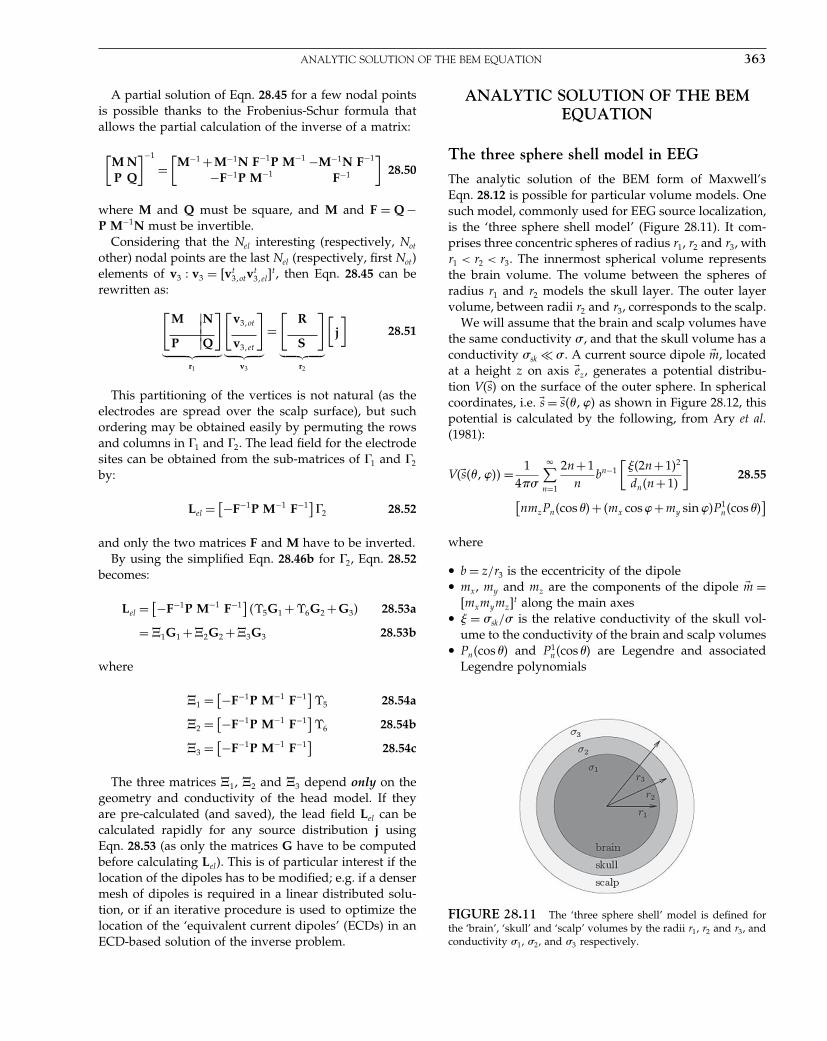
Elsevier UK Chapter: Ch28-P372560 30-9-2006 5:25p.m. Page:363 Trim:7.5in×9.25in
Basal Font:Palatino Margins:Top:40pt Gutter:68pt Font Size:9.5/12 Text Width:42pc Depth:55 Lines
ANALYTIC SOLUTION OF THE BEM EQUATION 363
A partial solution of Eqn. 28.45 for a few nodal pointsis possible thanks to the Frobenius-Schur formula thatallows the partial calculation of the inverse of a matrix:
[M NP Q
]−1
=[
M−1 +M−1N F−1P M−1 −M−1N F−1
−F−1P M−1 F−1
]28.50
where M and Q must be square, and M and F = Q −P M−1N must be invertible.
Considering that the Nel interesting (respectively, Not
other) nodal points are the last Nel (respectively, first Not)elements of v3 � v3 = �vt
3otvt3el�
t, then Eqn. 28.45 can berewritten as:
[M �N��P �Q
]
︸ ︷︷ ︸r1
[v3ot
v3et
]
︸ ︷︷ ︸v3
=[
R
S
]
︸ ︷︷ ︸r2
[j
]28.51
This partitioning of the vertices is not natural (as theelectrodes are spread over the scalp surface), but suchordering may be obtained easily by permuting the rowsand columns in �1 and �2. The lead field for the electrodesites can be obtained from the sub-matrices of �1 and �2
by:
Lel = [−F−1P M−1 F−1]�2 28.52
and only the two matrices F and M have to be inverted.By using the simplified Eqn. 28.46b for �2, Eqn. 28.52
becomes:
Lel = [−F−1P M−1 F−1]��5G1 +�6G2 +G3 28.53a
= �1G1 +�2G2 +�3G3 28.53b
where
�1 = [−F−1P M−1 F−1]�5 28.54a
�2 = [−F−1P M−1 F−1]�6 28.54b
�3 = [−F−1P M−1 F−1]
28.54c
The three matrices �1, �2 and �3 depend only on thegeometry and conductivity of the head model. If theyare pre-calculated (and saved), the lead field Lel can becalculated rapidly for any source distribution j usingEqn. 28.53 (as only the matrices G have to be computedbefore calculating Lel). This is of particular interest if thelocation of the dipoles has to be modified; e.g. if a densermesh of dipoles is required in a linear distributed solu-tion, or if an iterative procedure is used to optimize thelocation of the ‘equivalent current dipoles’ (ECDs) in anECD-based solution of the inverse problem.
ANALYTIC SOLUTION OF THE BEMEQUATION
The three sphere shell model in EEG
The analytic solution of the BEM form of Maxwell’sEqn. 28.12 is possible for particular volume models. Onesuch model, commonly used for EEG source localization,is the ‘three sphere shell model’ (Figure 28.11). It com-prises three concentric spheres of radius r1, r2 and r3, withr1 < r2 < r3. The innermost spherical volume representsthe brain volume. The volume between the spheres ofradius r1 and r2 models the skull layer. The outer layervolume, between radii r2 and r3, corresponds to the scalp.
We will assume that the brain and scalp volumes havethe same conductivity � , and that the skull volume has aconductivity �sk � . A current source dipole �m, locatedat a height z on axis �ez, generates a potential distribu-tion V��s on the surface of the outer sphere. In sphericalcoordinates, i.e. �s = �s��� as shown in Figure 28.12, thispotential is calculated by the following, from Ary et al.(1981):
V��s��� = 14��
�∑n=1
2n+1n
bn−1
[��2n+12
dn�n+1
]28.55
[nmzPn�cos �+ �mx cos �+my sin �P1
n�cos �]
where
• b = z/r3 is the eccentricity of the dipole• mx, my and mz are the components of the dipole �m =
�mxmymz�t along the main axes
• � = �sk/� is the relative conductivity of the skull vol-ume to the conductivity of the brain and scalp volumes
• Pn�cos � and P1n�cos � are Legendre and associated
Legendre polynomials
FIGURE 28.11 The ‘three sphere shell’ model is defined forthe ‘brain’, ‘skull’ and ‘scalp’ volumes by the radii r1, r2 and r3, andconductivity �1, �2, and �3 respectively.
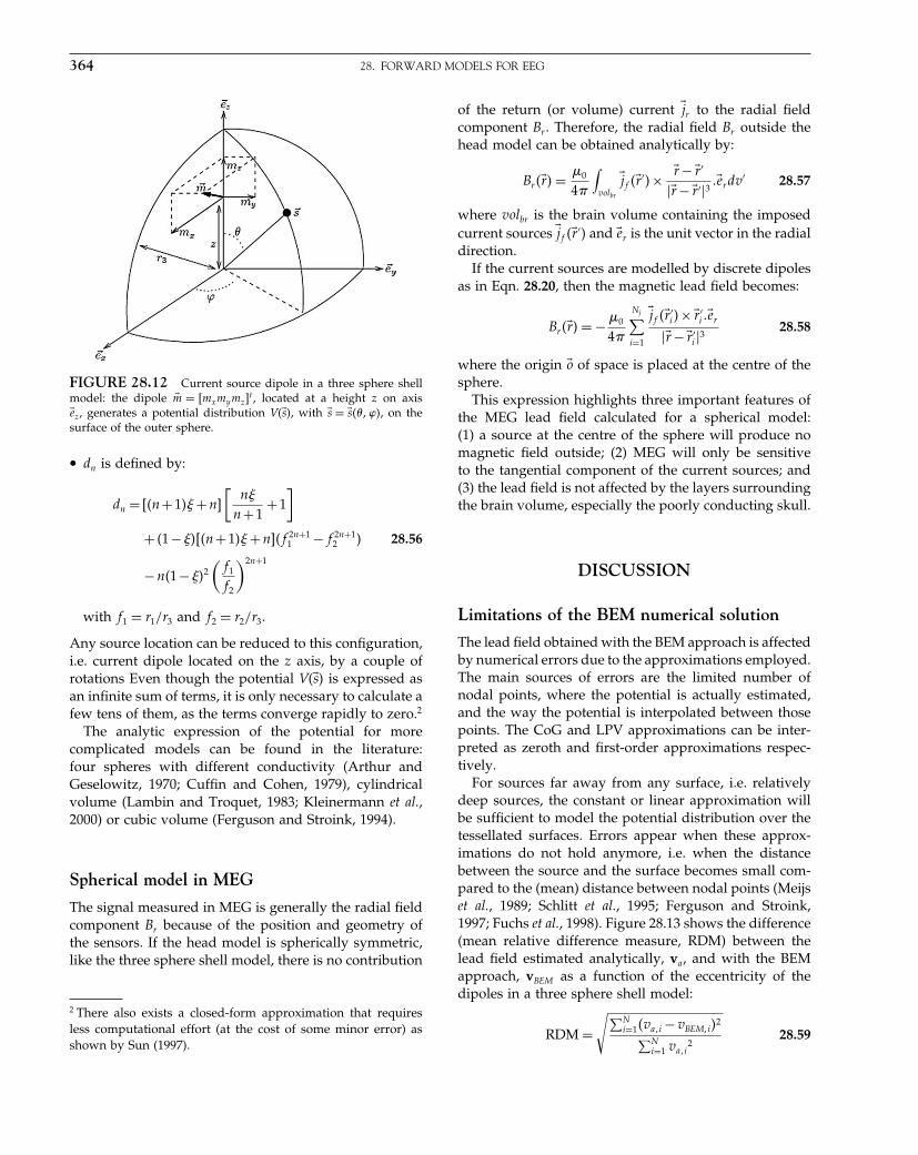
Elsevier UK Chapter: Ch28-P372560 30-9-2006 5:25p.m. Page:364 Trim:7.5in×9.25in
Basal Font:Palatino Margins:Top:40pt Gutter:68pt Font Size:9.5/12 Text Width:42pc Depth:55 Lines
364 28. FORWARD MODELS FOR EEG
FIGURE 28.12 Current source dipole in a three sphere shellmodel: the dipole �m = �mxmymz�
t , located at a height z on axis�ez, generates a potential distribution V��s, with �s = �s���, on thesurface of the outer sphere.
• dn is defined by:
dn = ��n+1� +n�
[n�
n+1+1
]
+ �1−���n+1� +n��f 2n+11 −f 2n+1
2 28.56
−n�1−�2
(f1
f2
)2n+1
with f1 = r1/r3 and f2 = r2/r3.
Any source location can be reduced to this configuration,i.e. current dipole located on the z axis, by a couple ofrotations Even though the potential V��s is expressed asan infinite sum of terms, it is only necessary to calculate afew tens of them, as the terms converge rapidly to zero.2
The analytic expression of the potential for morecomplicated models can be found in the literature:four spheres with different conductivity (Arthur andGeselowitz, 1970; Cuffin and Cohen, 1979), cylindricalvolume (Lambin and Troquet, 1983; Kleinermann et al.,2000) or cubic volume (Ferguson and Stroink, 1994).
Spherical model in MEG
The signal measured in MEG is generally the radial fieldcomponent Br because of the position and geometry ofthe sensors. If the head model is spherically symmetric,like the three sphere shell model, there is no contribution
2 There also exists a closed-form approximation that requiresless computational effort (at the cost of some minor error) asshown by Sun (1997).
of the return (or volume) current �jr to the radial fieldcomponent Br . Therefore, the radial field Br outside thehead model can be obtained analytically by:
Br��r = �0
4�
∫volbr
�jf ��r ′× �r −�r ′
��r −�r ′�3 ��erdv′ 28.57
where volbr is the brain volume containing the imposedcurrent sources �jf ��r ′ and �er is the unit vector in the radialdirection.
If the current sources are modelled by discrete dipolesas in Eqn. 28.20, then the magnetic lead field becomes:
Br��r = − �0
4�
Nj∑i=1
�jf ��r ′i ×�r ′
i ��er
��r −�r ′i �3
28.58
where the origin �o of space is placed at the centre of thesphere.
This expression highlights three important features ofthe MEG lead field calculated for a spherical model:(1) a source at the centre of the sphere will produce nomagnetic field outside; (2) MEG will only be sensitiveto the tangential component of the current sources; and(3) the lead field is not affected by the layers surroundingthe brain volume, especially the poorly conducting skull.
DISCUSSION
Limitations of the BEM numerical solution
The lead field obtained with the BEM approach is affectedby numerical errors due to the approximations employed.The main sources of errors are the limited number ofnodal points, where the potential is actually estimated,and the way the potential is interpolated between thosepoints. The CoG and LPV approximations can be inter-preted as zeroth and first-order approximations respec-tively.
For sources far away from any surface, i.e. relativelydeep sources, the constant or linear approximation willbe sufficient to model the potential distribution over thetessellated surfaces. Errors appear when these approx-imations do not hold anymore, i.e. when the distancebetween the source and the surface becomes small com-pared to the (mean) distance between nodal points (Meijset al., 1989; Schlitt et al., 1995; Ferguson and Stroink,1997; Fuchs et al., 1998). Figure 28.13 shows the difference(mean relative difference measure, RDM) between thelead field estimated analytically, va, and with the BEMapproach, vBEM as a function of the eccentricity of thedipoles in a three sphere shell model:
RDM =√∑N
i=1�vai −vBEMi2∑Ni=1 vai
228.59

Elsevier UK Chapter: Ch28-P372560 30-9-2006 5:25p.m. Page:365 Trim:7.5in×9.25in
Basal Font:Palatino Margins:Top:40pt Gutter:68pt Font Size:9.5/12 Text Width:42pc Depth:55 Lines
DISCUSSION 365
FIGURE 28.13 In a three sphere shell model, both analyticaland BEM solutions are calculated for sources placed at differenteccentricities. The lead fields obtained are compared using a relativedifference measure (RDM). The mean RDM is plotted as a functionof the sources eccentricity.
The difference between the exact analytic solution andthe approximated BEM solution increases abruptly whenthe source is placed close to the inner skull surface. Notethat this problem is also the same with other numericalapproaches such as the FEM (Marin et al., 1998).
Accuracy could be improved by higher order approx-imation of the potential on the tessellated surface, atthe cost of increased computational load and complex-ity. Other improvements have been suggested, such asthe ‘linear Galerkin’ approximation (Mosher et al., 1999),or the ‘isolated skull approach’ (Hämäläinen and Sarvas,1989). Still, whatever the complexity of the mesh ele-ments, there will always be errors caused by replacing asmooth surface with a polyhedron.
Anatomically constrained spherical headmodel
The three sphere shell model can be used directly tomodel a subject’s head. If images of the subject’s headand/or the electrode locations are not available, then astandard spherical model can be used. The electrode loca-tions are fixed according to the system used, for examplethe classic 10-20 system. If anatomical information andthe electrode locations are available, then the sphericalmodel can be adjusted to the subject’s head. The sphericalmodel can be either fitted to the overall head shape (or toall the electrodes simultaneously), or fitted locally to thearea with the largest EEG activity. The former ensuresa global fit of the model to the subject’s anatomy, whilethe latter offers a better fit just for the area of interest.
Whatever the approach adopted, the human headis clearly not spherical and the brain volume, i.e. the
source space, will not fit in some areas. For example (seePlate 37, colour plate section), when globally fitting thethree sphere shell model to the scalp surface, the frontaland occipital lobes protrude beyond the sphere model,and the temporal lobes are too deep within. To over-come these modelling errors, an anatomically constrainedspherical head model was proposed by Spinelli et al.(2000). In order to retain the simplicity of the three sphereshell model, the anatomy of the head is itself transformedto a best fitting sphere. The spherical transformation andthe lead field of the sources are obtained as follows:
1 From an anatomical image, the scalp surface (it couldalso be the inner skull surface or both) is extracted andtessellated with a regular mesh.
2 The best fitting sphere is estimated with this scalpmesh. The spherical model is defined by its centre �csphere
and radius Rsphere.3 The source locations inside the brain volume can be
expressed in spherical coordinates �Rsb �� aroundthe best fitting sphere centre. The radius of eachsource depends on its longitude and latitude, i.e. Rsb =Rsb���. Similarly, the radius of the scalp surface inthe direction ��� of any source is given by Rscalp =Rscalp���.
4 Then the brain volume, i.e. source space, can be ren-dered spherical by scaling the radius of all the sourcelocations (Plate 38) like this:
Rsbsphere��� = Rsb���Rsphere
Rscalp���28.60
5 The lead field for the re-located sources �Rsbsphere ��,can then be estimated in the spherical model in theusual way.
This process clearly modifies the solution space, intro-ducing discrepancies between the anatomy of the subjectand the model. However, compared to the simple bestfitting sphere model and the BEM numerical approach,the anatomically constrained spherical head model offerstwo main advantages. First, even though the solutionspace is warped, the relative depth of sources is pre-served: superficial (resp. deep) sources remain close to(resp. far from) the scalp surface and the electrodes. Thisis crucial, as the strength of the lead field depends on thedistance between the source and the electrodes. Second,the analytic solution of the forward problem can be usedto calculate the lead field. This provides a fast and accu-rate estimation, free from numerical errors that attendthe BEM equations. The anatomically constrained spher-ical head model may be a good compromise betweenanatomical accuracy and computational efficiency.
This concludes our treatment of the forward model forM/EEG. In the next chapter, we look at the inversion ofthis model to estimate distributed sources in the brain.

Elsevier UK Chapter: Ch28-P372560 30-9-2006 5:25p.m. Page:366 Trim:7.5in×9.25in
Basal Font:Palatino Margins:Top:40pt Gutter:68pt Font Size:9.5/12 Text Width:42pc Depth:55 Lines
366 28. FORWARD MODELS FOR EEG
REFERENCES
Arthur RM, Geselowitz DB (1970) Effect of inhomogeneities on theapparent location and magnitude of a cardiac current dipolesource. IEEE Trans Biomed Eng 17: 141–46
Ary JP, Klein SA, Fender DH (1981) Location of sources of evokedscalp potentials: Corrections for skull and scalp thickness. IEEETrans Biomed Eng 28: 447–52
Awada KA, Jackson DR, Williams JT et al. (1997) Computationalaspects of finite element modeling in EEG source localization.IEEE Trans Biomed Eng 44: 736–52
Becker A (1992) The boundary element method in engineering. A completecourse. McGraw-Hill Book Company, London
Buchner H, Knoll G, Fuchs M et al. (1997) Inverse localization ofelectric dipole current sources in finite element models of thehuman head. Electroencephalogr Clin Neurophysiol 102: 267–78
Chan TF (1984) Deflated decomposition of solutions of nearly sin-gular systems. SIAM J Numeric Anal 21: 738–54
Chari M, Silvester P (1980) Finite elements in electrical and magneticfield problems. Chichester John Wiley & Sons
Cuffin BN, Cohen D (1979) Comparison of the magnetoencephalo-gram and electroencephalogram. Electroencephalogr Clin Neuro-physiol 47: 132–46
de Munck JC (1992) A linear discretization of the volume con-ductor boundary integral equation using analytically integratedelements. IEEE Trans Biomed Eng 39: 986–90
Ferguson A, Stroink G (1997) Factors affecting the accuracy of theboundary element method in the forward problem – I: calculat-ing surface potential. IEEE Trans Biomed Eng 44: 1139–55
Ferguson AS, Stroink G (1994) The potential generated by currentsources located in an insulated rectangular volume conductor.J Appl Phys 76: 7671–76
Fuchs M, Wagner M, Wischmann HA et al. (1998) Improving sourcereconstructions by combining bioelectric and biomagnetic data.Electroencephalogr Clin Neurophysiol 107: 93–111
Geselowitz DB (1967) On bioelectric potentials in an inhomogeneousvolume conductor. Biophys J 7: 1–11
Hämäläinen MS, Hari R, Ilmoniemi RJ et al. (1993) Magnetoen-cephalography – theory, instrumentation, and applications tononinvasive studies of the working human brain. Rev Mod Phys65: 413–97
Hämäläinen MS, Sarvas J (1989) Realistic conductivity geometrymodel of the human head for interpretation of neuromagneticdata. IEEE Trans Biomed Eng 36: 165–71
He S (1998) Frequency series expansion of an explicit solution for adipole inside a conducting sphere at low frequency. IEEE TransBiomed Eng 45: 1249–58
Heller L (1990) Computation of the return current in encephalogra-phy: the auto solid angle. SPIE Digit Image Synth Inverse Optics1351: 376–90
Huiskamp G, Vroeijenstijn M, van Dijk R et al. (1999) The needfor correct realistic geometry in the inverse EEG problem. IEEETrans Biomed Eng 46: 1281–87
Kleinermann F, Avis N, Alhargan F (2000) Analytical solution tothe three-dimensional electrical forward problem for a circularcylinder. Inverse Probl 16: 461–68
Klepfer RN, Johnson CR, Macleod RS (1997) The effect of inhomo-geneities and anisotropies on electrocardiographic fields: a 3-Dfinite-element study. IEEE Trans Biomed Eng 44: 706–19
Lambin P, Troquet J (1983) Complete calculation of the electricpotential produced by a pair of current source and sink energiz-ing a circular finite-length cylinder. J Appl Phys 54: 4174–84
Lynn MS, Timlake WP (1968a) The numerical solution of singularintegral equation of potential theory. Numer Math 11: 77–98
Lynn MS, Timlake WP (1968b) The use of multiple deflations inthe numerical solution of singular systems of equations, withapplication to potential theory. SIAM J Numer Anal 5: 303–22
Marin G, Guerin C, Baillet S et al. (1998) Influence of skull anisotropyfor the forward and inverse problem in EEG: simulations studiesusing fem on realistic head models. Hum Brain Mapp 6: 250–69
Meijs JWH, Weier OW, Peters MJ et al. (1989) On the numericalaccuracy of the boundary element method. IEEE Trans BiomedEng 36: 1038–49
Mosher JC, Leahy RM, Lewis PS (1999) EEG and MEG: forwardsolutions for inverse methods. IEEE Trans Biomed Eng 46: 245–59
Nunez PL (1981) Electric fields of the brain: the neurophysics of EEG.Oxford University Press, New York
Ramo S, Whinnery JR, van Duze T (1984) Fields and Waves in Com-munication Electronics. John Wiley & Sons, New York
Rosenfeld M, Tanami R, Abboud S (1996) Numerical solution ofthe potential due to dipole sources in volume conductors witharbitrary geometry and conductivity. IEEE Trans Biomed Eng 43:679–89
Saleheen HI, Ng KT (1997) New finite difference formulations forgeneral inhomogeneous anisotropic bioelectric problems. IEEETrans Biomed Eng 44: 800–09
Saleheen HI, Ng KT (1998) A new three-dimensional finite-difference bidomain formulation for inhomogeneous anisotropiccardiac tissues. IEEE Trans Biomed Eng 45: 15–25
Sarvas J (1987) Basic mathematical and electromagnetic concepts ofthe biomagnetic inverse problem. Phys Med Biol 32: 11–22
Schlitt HA, Heller L, Aaron R et al. (1995) Evaluation of boundaryelement methods for the eeg forward problem: effect of linearinterpolation. IEEE Trans Biomed Eng 42: 52–58
Smythe WR (1950) Static and dynamic electricity. MacGraw Hill, NewYork
Spinelli L, Andino SG, Lantz G et al. (2000) Electromagnetic inversesolutions in anatomically constrained spherical heads models.Brain Topogr 13: 115–25
Sun M (1997) An efficient algorithm for computing multishell spher-ical volume conductor models in eeg dipole source localization.IEEE Trans Biomed Eng 44: 1243–52
van den Broek S, Zhou H, Peters M (1996) Computation of neu-romagnetic fields using finite-element method and Biot-Savartlaw. Med Biol Eng Comput 34: 21–26
van Oosterom A, Strackee J (1983) The solid angle of a plane triangle.IEEE Trans Biomed Eng 30: 125–26
Vladimirov VS (1971) Equations of mathematical physics. MarcelDekker, New York
Von Helmholtz HL (1853) Ueber einige Gesetze der Vertheilungelektrischer Ströme in Koperlichen Leitern mit Anwendung aufdie thierisch-elektrischen Versuche. Ann Phys Chem 89: 211–33,354–77.
Elsevier UK Chapter: Ch29-P372560 30-9-2006 5:26p.m. Page:367 Trim:7.5in×9.25in
Basal Font:Palatino Margins:Top:40pt Gutter:68pt Font Size:9.5/12 Text Width:42pc Depth:55 Lines
C H A P T E R
29
Bayesian inversion of EEG modelsJ. Mattout, C. Phillips, J. Daunizeau and K. Friston
INTRODUCTION
In this chapter, we consider a generative model forevoked neuronal responses as observed with elec-troencephalography (EEG) and magnetoencephalogra-phy (MEG). Because of its linear and hierarchical nature,this model can be estimated efficiently using empiricalBayes. Importantly, multiple constraints on the sourcedistribution can be incorporated in terms of variancecomponents that are estimated from the data. A dualestimation is obtained via an expectation maximization(EM) scheme to give the restricted maximum likelihood(ReML) estimate of the prior covariance components (interms of hyperparameters) and the maximum a posteri-ori (MAP) estimate of the sources. The Bayesian formal-ism yields a generic approach to source reconstructionunder multiple constraints, which is extended to coverspatio-temporal models for induced responses in the nextchapter.
Background
The problem of recovering volume current sources fromsuperficial electromagnetic measurement is intrinsicallyill-posed. This means the spatial configuration of neu-ronal activity cannot be determined uniquely, basedon EEG and/or MEG recordings alone (Nunez, 1981).To resolve the non-uniqueness of this inverse prob-lem, assumptions about the solution are necessary for aunique solution. There are two approaches to this:
• Equivalent current dipole (ECD) approaches, wherethe M/EEG signals are assumed to be generated by arelatively small number of focal sources (Miltner et al.,
1994; Scherg and Ebersole, 1994; Scherg et al., 1999;Aine et al., 2000).
• Distributed linear (DL) approaches, where all pos-sible source locations are considered simultaneously(Backus and Gilbert, 1970; Sarvas, 1987; Hamalainenand Ilmoniemi, 1994; Grave de Peralta Menendez andGonzalez Andino, 1999; Pascual-Marqui, 1999; Uutelaet al., 1999).
In the context of distributed models, constraints orpriors can be introduced probabilistically using Bayes.The major problem here is the handling of multiple con-straints and their appropriate weighting, in relation toeach other and observation noise (Gonzalez Andino et al.,2001). In Phillips et al. (2002a), we introduced a simplerestricted maximum likelihood (ReML) procedure to esti-mate a single hyperparameter, i.e. the balance betweenfitting the data and conforming to the priors. Here,we reformulate the implicit weighted minimum norm(WMN) solution in terms of a hierarchical linear model.With this approach, any number of constraints (or priors)on the source or noise covariance matrices can be intro-duced. An expectation maximization (EM) algorithm isused to obtain an ReML estimate of the hyperparametersassociated with each constraint. This enables the MAPsolution for the sources to be calculated uniquely andefficiently.
This chapter is divided into five sections. In the firstthree sections, the theoretical background and opera-tional details of the approach are described. The firstsection introduces the WMN solution in a Bayesianframework, while the second and third sections intro-duce the hierarchical parametric empirical Bayes (PEB)framework and ReML approach, respectively. The twolast sections give some examples of the application ofReML in comparison with classical approaches, usingEEG and MEG data.
Statistical Parametric Mapping, by Karl Friston et al. Copyright 2007, Elsevier Ltd. All rights reserved.ISBN–13: 978-0-12-372560-8 ISBN–10: 0-12-372560-7
367
Elsevier UK Chapter: Ch29-P372560 30-9-2006 5:26p.m. Page:368 Trim:7.5in×9.25in
Basal Font:Palatino Margins:Top:40pt Gutter:68pt Font Size:9.5/12 Text Width:42pc Depth:55 Lines
368 29. BAYESIAN INVERSION OF EEG MODELS
THE BAYESIAN FORMULATION OFCLASSICAL REGULARIZATION
The instantaneous source localization problem in EEGcan be summarized as:
v = F�r� j�+� 29.1
where v, a vector of size Ne ×1, is the potential at Ne elec-trodes; r and j are the 3×1 vectors of source location andmoment; � is the additive noise. F is a function linkingthe source �r� j� and the potential v. The function F is thesolution of the forward problem (i.e. the forward model)and depends only on the head model (conductivities andspatial configuration).
For Nd sources defined by ri and ji�I = 1�K�Nd�, thesource localization problem Eqn. 29.1 can be rewritten,by appeal to the superposition theorem, as:
v =Nd∑i=1
F�ri� ji�+� 29.2
In this chapter, sources of the M/EEG signal are mod-elled using current dipoles, either on a three-dimensionalgrid throughout the brain (see fourth section) or on adiscrete three-dimensional manifold that corresponds tothe cortical surface (see fifth section). This represents adistributed linear approach where Nd is much smallerthan Ne. Because the location ri of each current source iis now fixed, Eqn. 29.1 becomes an underdetermined butlinear problem:
v = Lj +� 29.3
where j now indicates a vector of current dipoles atNd locations and L is the lead field matrix linking thesource amplitudes j to the electrical potential v. If thesource orientation is free, then j = �j1� j2� � � � � jNd
�T , whereji = �jx�i� jy�i� jz�i�
T encodes both orientation and ampli-tude of the i-th dipole. Otherwise, for oriented sources,j = �j1� j2� � � � � jNd
�t, where each ji specifies only the ampli-tude. For discrete data, with Nt time bins, Eqn. 29.3 canbe expressed as a multivariate linear model:
V = LJ +� 29.4
with V = �v1�v2� � � � � vNt�, J = �j1� j2� � � � � jNt
� and � =��1��2� � � � � �Nt
� where vi, ji and �i are the potential,source parameters and additive noise at the ith timesample.
Weighted minimum norm and Bayesiansolutions
As mentioned above, the source localization problem isintrinsically ill posed. With the DL approach, we facethe linear but under-determined problem expressed inEqn. 29.4. One common approach to this problem is theweighted minimum norm (WMN) solution or Tikhonovregularization method (Tikhonov and Arsenin, 1977),in which the a priori regularization constraints have aBayesian interpretation.
The WMN solution constrains the reconstructed sourcedistribution by minimizing a linear mixture of someweighted norm �Hj� of the source amplitudes j andthe residuals of the fit. Assuming noise is Gaussian � ∼N�0�C�� with a known covariance matrix C�, the regular-ized problem is expressed as:
ĵ = minj
(∥∥C−1/2� �Lj −v�
∥∥2 +�Hj�2)
= minj
(�Lj −v�T C−1
� �Lj −v�+jT HT Hj) 29.5
where the hyperparameter expresses the balancebetween fitting the model
∥∥C−1/2� �Lj −v�
∥∥ and minimiz-ing the a priori constraint �Hj�. The solution of Eqn. 29.5for a given is:
ĵ = Tv 29.6
where, using the matrix inversion Lemma:
T = �LT C−1� L+HT H�−1LT C−1
�
= �HT H�−1LT �L�HT H�−1LT +C��−1
29.7
The important connection with Bayesian estimatesrests on Gaussian assumptions, under which the condi-tional expectation of the source amplitudes j is:
ĵ = �LT C−1� L+C−1
j �−1LT C−1� v
= CjLT �LCjL
T +C��−1v
29.8
where Cj is the prior covariance of the sources. Compar-ing Eqn. 29.8 with Eqn. 29.7 provides the motivation forchoosing forms of H , where:
HT H = C−1j 29.9
In other words, H specifies the form of the precision orour prior belief on where sources are expressed (precisionis the inverse of the variance).
In summary, the WMN solution depends on the hyper-parameter that balances the relative contribution offitting the model (or likelihood of the data) and the con-straint on the solution (or prior). As varies, the regular-ized solution ĵ also changes. Therefore, the choice of is
Elsevier UK Chapter: Ch29-P372560 30-9-2006 5:26p.m. Page:369 Trim:7.5in×9.25in
Basal Font:Palatino Margins:Top:40pt Gutter:68pt Font Size:9.5/12 Text Width:42pc Depth:55 Lines
RESTRICTED MAXIMUM LIKELIHOOD 369
crucial. A heuristic way to understand the properties ofĵ is to plot the weighted norm of the regularized solution∥∥∥Hĵ
∥∥∥, against the norm of the residuals∥∥∥C−1/2
� �Lĵ −v�∥∥∥
for different values of . The ensuing curve has an Lshape (in ordinary or double logarithmic scale), henceits name L-curve (see Appendix 29.1). A satisfactory would lie close to the inflection of the L-curve (Hansen,1992). A major disadvantage of the L-curve approach isthat solutions must be calculated for a large number ofvalues of to find an appropriate level of regularization.Moreover, the L-curve approach cannot be extended toestimate multiple hyperparameters. This would requirean extensive search in hyperparameter space to deter-mine the inflection in a hyperplane (Brooks et al., 1999).
In Phillips et al. (2002a) we introduced an iterativerestricted ML (ReML) procedure to estimate while cal-culating ĵ for the simple case of one hyperparameter. Inthe following section, we extend the approach to solvethe generalized WMN problem with multiple hyperpa-rameters, thereby determining the relative contributionof different priors to the solution.
A HIERARCHICAL OR PARAMETRICEMPIRICAL BAYES APPROACH
The source localization problem can be expressed in thecontext of a two-level hierarchical parametric empiricalBayes (PEB) model:
v = Lj +��1�
j = 0+��2�29.10
where both random terms have a Gaussian distributionwith zero mean:
��1� ∼ N�0�C��
��2� ∼ N�0�Cj�29.11
Within this framework, the covariance matrices C andCj , which are equivalent to those in Eqn. 29.5, can bemodelled as a linear combination of covariance compo-nents:
C� = �1�1 Q�1�
1 +�1�2 Q�1�
2 + � � �
Cj = �2�1 Q�2�
1 1 +�2�2 Q�2�
2 + � � �29.12
where the [restricted] maximum likelihood estimates of = �1�
1 ��1�2 � � � � ��2�
1 ��3�2 can be identified using expec-
tation maximization (EM) (see Appendix 3 for the oper-ational details). This allows one to compute C��� and
C��j , and the conditional expectation of the sourcesĵ using Eqn. 29.8.
In this hierarchical model, the unknown parameters jare assumed to be Gaussian variables with zero mean(i.e. have shrinkage priors). Regional variance can beincreased to render sources at some locations more likely.A source with a larger prior variance is less constrainedand is more likely to be different from zero. Eqn. 29.12furnishes a better approximation of the sources’ covari-ance Cj when its exact form is not known a priori.A variety of components can be used simultaneously, butthe relative weight of each constraint is not fixed. This isparticularly important when, for instance, spatial coher-ence and explicit location priors are used together. Forexample, some sources can be specified as a priori moreactive: this can be based on prior knowledge or derivedfrom functional magnetic resonance imaging (fMRI) mea-sures of brain activity. Introducing priors from fMRI interms of covariance components is natural because fMRIprovides only spatial information at the temporal scale ofM/EEG. Note that specifying priors in terms of covari-ance components means that sources can be expressedpreferentially in different parts of the brain. This shouldbe contrasted with a prior specification in terms of pre-cision components, where sources are precluded frombeing expressed in areas of high precision. The formeris more appropriate because it enables permissive pri-ors as opposed to restrictive priors. For example, eachfMRI activation blob could be used as a prior covariancecomponent, which means sources can be expressed ineach blob.
Similarly, the noise covariance matrix C� can be mod-elled more accurately with a mixture of components. Forexample, an independent and uniform noise componentover electrodes can be introduced by defining Q�1�
1 asthe identity matrix. Covariances among electrodes can beintroduced in Q�1�
2 , which is generally estimated from thedata (e.g. within the prestimulus interval of the event-related potential (ERP)). If a subset of electrodes picksup more noise than the others, this can also be modelledin Q�1�
2 .By selecting the EEG episode carefully, during which
the hyperparameters are stationary, the EM algorithmfavours the relevant priors by increasing their hyperpa-rameters and suppresses the others by rendering theirhyperparameters very small.
RESTRICTED MAXIMUM LIKELIHOOD
In practice, the hierarchical model is inverted byminimizing the ReML objective function with respectto the hyperparameters (see Appendix 3). The critical
Elsevier UK Chapter: Ch29-P372560 30-9-2006 5:26p.m. Page:370 Trim:7.5in×9.25in
Basal Font:Palatino Margins:Top:40pt Gutter:68pt Font Size:9.5/12 Text Width:42pc Depth:55 Lines
370 29. BAYESIAN INVERSION OF EEG MODELS
aspect of this inversion is that it can proceed in channelspace. This means the size of the matrices are relativelysmall and the inversion is extremely quick. The two-levelmodel in Eqn. 29.10 can be collapsed into a single equa-tion:
v = L��2� +��1� 29.13
This means the covariance Cv of the channel data1 hasthe following components:
Cv = LCjLT +C�
= �1�1 Q�1�
1 +�1�2 Q�1�
2 +· · ·+�2�1 LQ�2�
1 LT +�2�2 LQ�2�
2 LT +· · ·29.14
where only the hyperparameters are unknown and canbe estimated using restricted maximum likelihood, asdescribed in Appendix 4. This gives the same [restricted]maximum likelihood estimate as the M-step of the EMalgorithm, but does so in a computationally expedientway, by variance partitioning in sensor-space. To get veryprecise estimates of the hyperparameters one can usemultiple observations to calculate the covariance matrixCv ≈ vvT . This sample covariance can be based on succes-sive time bins, assuming that the noise and prior covari-ances are locally stationary. Although not pursued here,it is also possible to use instantaneous estimates of Cv
sampled from the same time bin of multiple trials.
APPLICATION TO SYNTHETICMEG DATA
In this section, we illustrate the ReML scheme usingsimulated MEG data. Further details about thesesimulations and results can be found in Mattout et al.(2006) and Chapter 35.
The simulated data
To simulate MEG data, a 3D high resolution (voxelsize: 0�9375 mm×0�9375 mm×1�5 mm) MRI volume froma healthy volunteer was segmented. The boundarybetween white and grey matter was approximated withsmall triangles whose vertices provided about 7000dipole locations spread uniformly over the cortex. We
1 We refer to Cv as a covariance matrix but, strictly speaking, it isjust a second order matrix. Covariance matrices are second ordermatrices of mean corrected variables, whereas our variables areusually baseline corrected.
computed the forward operator L for this dipole mesh,using a single-shell spherical head model (Sarvas, 1987).
MEG data were simulated over 130 sensors, by acti-vating two extended sources. Each source was a clus-ter comprising one randomly chosen dipole and its fournearest neighbours. The extent of each simulated sourcewas about 5 mm in radius. The activation was mod-elled with a half-period sine function (over 15 time bins).A delay of two time bins was applied to waveforms ofthe two sources. After projection onto sensor space, whiteGaussian noise was added �SNR = 20 dB�.2 Five hundreddata sets were simulated to compare the ReML approachwith the classical WMN estimation based on the L-curveapproach and to study the performance of the ReMLscheme under various combinations of priors.
The priors
At the sensor level, we consider a single measurementnoise component defined by Q�1�
1 = INe, i.e. independent
measurement noise on each sensor with identical vari-ance. INe
is the Ne ×Ne identity matrix. At the source level,three types of priors are considered, either individuallyor together.
Smoothness constraint
This is defined by the covariance component:
Q�1�S �i� j� = exp�−d2
ij
/2s2� 29.15
where dij is the distance3 between dipoles i and j.The spatial smoothness parameter was s = 8 mm. LikeLORETA (Pascual-Marqui et al., 1994), this prior enforcescorrelation among neighbouring sources.
Intrinsic functional constraint
Multivariate source prelocalization (MSP) provides, fromthe normalized MEG data itself, an estimate �i of thelikelihood of activation at each source location (Mattoutet al., 2005). These estimates can be incorporated as quan-titative priors. They can also provide a substantial reduc-tion of the inverse solution space by only considering thedipoles that are most likely to be active. For each simu-lated source configuration we restrict the solution space
2 SNR stands for signal-to-noise ratio and is here expressed indecibels, i.e. SNR = log10�As/An�, where As (resp. An) refers tothe maximum absolute signal (resp. noise) value. An SNR of20 dB thus corresponds to a 10 per cent noise level.3 The Euclidian distance was used for these simulations. How-ever, the smoothness constraint as implemented in SPM5 usesthe geodesic distance over the cortical surface.

Elsevier UK Chapter: Ch29-P372560 30-9-2006 5:26p.m. Page:371 Trim:7.5in×9.25in
Basal Font:Palatino Margins:Top:40pt Gutter:68pt Font Size:9.5/12 Text Width:42pc Depth:55 Lines
APPLICATION TO SYNTHETIC MEG DATA 371
to the 1500 dipoles with the highest likelihood of acti-vation. Within this subset, the intrinsic prior covariancecomponent is the leading diagonal matrix:
Q�2�i �i� i� = �i 29.16
Extrinsic functional constraints
The third constraint we consider is based on data fromother imaging modalities, typically fMRI, and enters sim-ply as a binary mask. This mask distinguishes quali-tatively between a priori active and non-active corticalareas. The corresponding prior source variance compo-nent is defined by the leading diagonal matrix:
Q�2�e �i� i� = 1 29.17
when the source is part of an active area, and zero oth-erwise. We modelled two sorts of extrinsic priors – validQ�2�
e and invalid Q̃�2�e (Figure 29.1) – because we were
interested in the impact of invalid priors, particularly inthe context of multiple priors. In this instance, there is anopportunity to discount invalid priors in favour of validpriors.
Results
Since the L-curve approach can only accommodate a sin-gle constraint, the classical WMN provides only foursolutions for each data set, one per source prior, whereasReML provides nineteen, corresponding to all possiblemixtures of priors. Here we use the receiver operatingcharacteristic (ROC) to evaluate and compare the varioussource estimates. The ROC characterizes inverse meth-ods in terms of correctly classifying each dipole, as eitheractive or not. For each estimate of the source distribution,a ROC curve represents the true positive rate (sensitiv-ity) versus the false positive rate (1−specificity). The areaunder the curve (AUC) quantifies the overall power. TheAUC ranges between 0 and 1, indicating the probabilityof correct separation of an active source from a non-activeone. Comparing the AUC of different inverse modelsallows one to assess the relative performance of methodsand sets of priors.
Table 29-1 shows the averaged AUC value over our sim-ulations. We analysed the AUC using analysis of vari-ance (ANOVA). The main effect of method (ReML versus
FIGURE 29.1 Synthetic EEG data: data without noise (top left). Same data with added noise, at different SNRs: 4 (top right), 12 (bottomleft), 100 (bottom right).

Elsevier UK Chapter: Ch29-P372560 30-9-2006 5:26p.m. Page:372 Trim:7.5in×9.25in
Basal Font:Palatino Margins:Top:40pt Gutter:68pt Font Size:9.5/12 Text Width:42pc Depth:55 Lines
372 29. BAYESIAN INVERSION OF EEG MODELS
TABLE 29-1 Mean values of the AUC for the WMN andReML approaches and different priors
AUC Prior models ReML WMN
1 constraint Q�2�s 0�7833 0�777
Q�2�i 0�7944 0�7746
Q�2�e 0�8560 0�8560
Q̃�2�e 0�4994 0�4994
2 constraints Q�2�s 0�7999
Q�2�i
Q�2�s 0�8211
Q�2�e
Q�2�s 0�7931
Q̃�2�e
Q�2�i 0�8211
Q�2�e
Q�2�i 0�7962
Q̃�2�e
Q�2�i 0�8536
Q̃�2�e
3 constraints Q�2�s 0�8211
Q�2�i
Q�2�e
Q�2�s 0�7972
Q�2�i
Q̃�2�e
Q�2�s 0�8211
Q�2�e
Q̃�2�e
Q�2�i 0�8211
Q�2�e
Q̃�2�e
4 constraints Q�2�s 0�8206
Q�2�i
Q�2�e
Q̃�2�e
WMN) proves highly significant (F�1� 499� = 1�01; p <0�001), implying a much better source detection profilewith ReML. Since the ReML and WMN approaches dif-fer only in the way they estimate the hyperparameters,these results suggest that the ReML estimates of the bal-ance between the priors and data fit are significantly betterthan obtained with the traditional L-curve approach.
When using ReML, the effect of the valid extrinsic priorcan be assessed by a two-by-seven ANOVA, whose factorsare the inclusion or not of the valid extrinsic prior and theseven possible prior models. The main effect on the validextrinsic prior was highly significant (F�1� 499� = 2565�272;p < 0�001). This shows that relevant priors are properlyassigned a high weight, even in the context of invalidor irrelevant priors. Conversely, any deterioration in thereconstruction,duetotheinclusionoftheinvalidprior,was
insignificant (F�1� 499� = 0�140 p < 0�708). Again, this isimportant because it shows that irrelevant priors are prop-erly discounted by the inversion.
APPLICATION TO SYNTHETICEEG DATA
The simulated data
We used a simplified head model that comprises 1716dipoles distributed uniformly on a horizontal grid (witha maximum of 24 sources along a radius), within a three-sphere shell model. Twenty-seven electrodes were placedon the upper hemisphere according to a pseudo 10–20electrode setup. The orientation of each source was fixedand the lead-field for all sources was calculated ana-lytically (Ary et al., 1981). Two hundred locations wereselected randomly to assess the efficiency of the ReMLapproach. At each of these locations an instantaneous dis-tributed source set j0 was generated as a set of connecteddipoles within a 1.5 grid-size radius of a ‘central’ dipole.On average, each source comprised about nine dipoles.Each source vector j0 was modulated over time to gen-erate a time series J0. Data with different SNRs wereobtained by adding scaled white noise ��1� to the noise-free data V = LJ0 +�. Three levels of noise were used byadopting an SNR of 4, 12 and 100. The electrical potentialat electrodes, over time, with these three SNRs are shownin Figure 29.1.
The priors
We considered three kinds of priors on the sources.
Spatial coherence
This component was constructed using anatomicallyinformed basis functions (IBFs) based on grey matterdensity and a spatial smoothness kernel (Phillips et al.,2002b, 2005). It comprised a leading diagonal matrix ofeigenvalues of the principal IBFs that was rotated intosource space (and then projected onto channel space).This prior implies that the basis functions in source space,with the highest eigenvalues, are more likely to representthe source activity, ensuring a smooth solution.
Depth constraint
To ensure that sources contribute to the solution equally,irrespective of their depth (Ioannanides et al., 1990;Gorodnitsky et al., 1995; Grave de Peralta Menendezand Gonzales Andino, 1998), deeper sources are given a

Elsevier UK Chapter: Ch29-P372560 30-9-2006 5:26p.m. Page:373 Trim:7.5in×9.25in
Basal Font:Palatino Margins:Top:40pt Gutter:68pt Font Size:9.5/12 Text Width:42pc Depth:55 Lines
APPLICATION TO SYNTHETIC EEG DATA 373
larger prior variance than superficial sources. The depthis indexed by the norm of the gain vector for each source.This covariance component is defined by the leadingdiagonal matrix diag�LT L�−1.
Location priors
These were introduced as leading diagonal matriceswhose elements encode the prior probability of whetherthe source is active or not. As above, these extrinsic func-tional priors take values of zero (the prior variance is notaffected), or one (the prior variance increases with the cor-respondinghyperparameter).Threedifferent typesof loca-tion priors are considered, either separately or together:
1 accurate priors, centred on the active source set2 close inaccurate priors, located between 6 and 16 grid-
size from the truly active source3 distant inaccurate priors, located between 24 and 48
grid-size from the truly active source.
Each simulation condition (SNR, priors) was assessedfor the 200 different source configurations.
Results
Figure 29.2 and Plate 39 (see colour plate section) showthe reconstructions obtained with the various constraints
FIGURE 29.2 Example of a source configuration used in thesimulations (top left) and the corresponding priors; accurate locationpriors (top right), and inaccurate location priors (close, bottom left,and distant, bottom right).
TABLE 29-2 Localization error (mm) for the three SNRsand the four location priors (none, accurate, inaccurate and
both accurate and inaccurate)
Localization error Low Medium High
No priors 6 4 10Accurate priors 4 4 4Close inaccurate
priors12 15 13
Distant inaccuratepriors
34 32 32
Accurate and closeinaccurate priors
4 4 4
Accurate and distantinaccurate priors
4 4 4
described above. To evaluate the performance of theinversion we used a lower bound on the localizationerror such that 80 per cent of the sources are recov-ered within this bound (Table 29-2). Table 29-3 providesthe mean and standard deviation of the hyperparame-ter of the noise component. This estimate is relativelystable over simulations. It reflects accurately the actualvariance of noise, i.e. 2.3 (low SNR), 0.26 (mediumSNR) and 0.0037 (high SNR). Although the estimatednoise variance is accurate, the standard deviation of itsestimate is much smaller when accurate location pri-ors are used. The inclusion of accurate location priorsseems to help the partitioning of signal variance intoits components, namely, source activity and additivenoise. For some sources, the noise variance was greatlyover-estimated.
Finally, Table 29-4 gives the mean and standard devi-ation of the hyperparameters pertaining to the sourcevariance components. Note that some hyperparametersare negative. This simply means that the correspondingcovariance component is used to reduce the (co)varianceof the sources. The combination of all the covariancecomponents should always lead to a positive definite(co)variance matrix estimate. In general, the hyperparam-eters decrease as the SNR increases, except when inac-curate location priors are used in isolation. The use ofaccurate location priors has a large influence on the otherpriors. Indeed, the hyperparameter corresponding to theaccurate location priors is several orders larger than anyother hyperparameter (i.e. the spatial coherence, depthor inaccurate location priors). Apart from the hyperpa-rameter corresponding to the accurate location priors, thehyperparameters vary over a relatively large range andcan have positive or negative values depending on thesource, the noise and the priors. Generally, the standarddeviation of the hyperparameters estimates decreases asthe SNR increases.

Elsevier UK Chapter: Ch29-P372560 30-9-2006 5:26p.m. Page:374 Trim:7.5in×9.25in
Basal Font:Palatino Margins:Top:40pt Gutter:68pt Font Size:9.5/12 Text Width:42pc Depth:55 Lines
374 29. BAYESIAN INVERSION OF EEG MODELS
TABLE 29-3 Mean and standard deviation of the hyperparameters of the noise component∗
Hyperparameters Low SNR Medium SNR High SNR
Without accurate location priors 2�3 ± 0�15 0�26 ± 0�038 0�0082±0�047With accurate location priors 2�3 ± 0�04 0�26±0�0065 0�0037 ±0�00012
∗The precision of this estimate depends mainly on the presence or absence of accurate location priors. Therefore, thesimulations without any location priors and with inaccurate location priors are pooled in the category ‘Without accuratelocation priors’. Similarly, results obtained ‘With accurate location priors’ cover simulations with accurate location priors,with and without inaccurate location priors.
TABLE 29-4 Mean and standard deviation of the hyperparameters pertaining to the sources’ prior variance components
Hyperparameters SNR Spatial coherence Depth constraint Accurate location Inaccurate location
No location priors Low −0�5±1�9 6�8±14�0 – –Medium −0�35±1�7 5�6±12�0 – –High −0�058±1�3 3�1±8�8 – –
Accurate location priors Low 0�016±0�043 −0�2±0�32 16±4�1 –Medium 0�0073±0�0097 −0�72±0�076 9�1±1�9 –High 0�00016±0�00032 −0�0016±0�0026 6�9±1�6 –
Inaccurate location priors Low −0�39±1�7 5�6±1�3 – 4�7 ±1�9Medium −0�41±1�5 5�5±11 – 18±72High −0�092±1�2 2�9±7�9 – 70±300
Accurate and inaccurate Low 0�021±0�064 −0�23±0�49 16±4�4 −0�15±0�36location priors Medium 0�088±0�014 −0�082±0�11 9�4±2�1 −0�076±0�14
High 0�00017 ±0�00034 −0�0016±00�0029 6�9±1�6 −0�0021±0�013
CONCLUSION
The hierarchical PEB-ReML approach presented hereprovides efficient and optimal estimators of M/EEGevoked responses. Our analyses of synthetic EEG andMEG data show that: the noise variance estimate is accu-rate and consistent; localization and detection error isgreatly reduced by the introduction of valid locationpriors; and the further introduction of invalid priors hadno effect on the reconstruction.
Combining data obtained from different modalitieswithin the same framework can overcome the intrinsiclimitations (on temporal or spatial resolution) of any onemodality. In this chapter, we have outlined a way inwhich structural and functional MRI data can be used aspriors in the estimation of M/EEG sources. Crucially, wehave illustrated the role of ReML hyperparameter esti-mates in modelling the relative contributions of M/EEGresiduals and fMRI-based priors to the estimation.
Classical approaches to noise regularization ofdistributed linear solutions are usually empirical andproceed on a trial-and-error basis: the level of regular-ization is adapted manually such that the ensuing solu-tion and assumed noise component seem reasonable. Incontrast, the ReML procedure successfully controls thenoise regularization by a hyperparameter in a principled
and unique way. Even at constant SNR, the values ofthe hyperparameters vary over a wide range. The valueof the hyperparameters depends on the source config-uration and the distribution of potentials it generatesover the scalp. Therefore, any fixed value of the hyper-parameters can lead to suboptimal solutions. This is animportant point and a fundamental motivation for theadaptative ReML estimates proposed here. For example,some sources may arise in cortical regions where priorscan be specified very precisely leading to large hyperpa-rameters. In other regions, priors may be less informativerendering a smaller value of the hyperparameter moreappropriate. The flexibility afforded by parameterizingthe priors in terms of hyperparameters lies in being ableto specify the components of the noise and prior sourcecovariances without fixing their relative contributions.These contributions are scaled by the hyperparametersthat we estimated using ReML. The advantage of thisapproach is that the relative importance of the likeli-hood of, and priors on, the solution can be determinedempirically. In other words, they can shape themselvesin relation to observation error and each other.
In this chapter, we have focused on the face validityof Bayesian inversion (i.e. showing that the scheme doeswhat it is supposed to do). It is also fairly easy to estab-lish the construct validity in terms of neurobiological
Elsevier UK Chapter: Ch29-P372560 30-9-2006 5:26p.m. Page:375 Trim:7.5in×9.25in
Basal Font:Palatino Margins:Top:40pt Gutter:68pt Font Size:9.5/12 Text Width:42pc Depth:55 Lines
REFERENCES 375
plausibility. The example in Plate 40 shows that the ReMLscheme localizes face-selective responses to the appropri-ate part of the fusiform gyrus. In this instance, intrinsicfunctional priors produced the best results. Clearly, onecannot assess the intrinsic quality of the priors basedon the solution. However, the ReML objective function(which is also the variational free energy – see Chapter 24)can be used for model comparison and selection, i.e.to evaluate different reconstructions obtained from dif-ferent sets of priors (Mattout et al., 2006). This willbe the subject of Chapter 35. In the next chapter, weextend the instantaneous model described above to coverperistimulus time and generalize the inversion to pro-vide conditional estimates of both evoked and inducedresponses.
APPENDIX 29.1THE L-CURVE APPROACH
The L-curve heuristic involves estimating the WMNsolution for various values of hyperparameter (seeEqn. 29.5 and Eqn. 29.7). A plot of the norm of the priorterm against the norm of the data fit leads to an L-shapecurve whose inflection point indicates an optimal hyper-parameter. This amounts to maximizing the following:
−12
�v−Lĵ�T C−1� �v−Lĵ�− 1
2ĵT C−1
j j 29.A1
A precise estimation entails an exhaustive scanningof hyperparameter space. This is one drawback of theapproach, namely, the need for a large number of esti-mations to find an appropriate level of regularization.We use L-curve analysis as a reference for the estimationof single hyperparameters in the WMN simulations.Practically, we use:
= �
∥∥LLT∥∥
Ne
29.A2
with thirty values of �. This ensures an L-curve with arelatively fine sampling in the vicinity of its inflection.Note that the L-curve minimization criterion is a poorapproximation to the ReML (EM) objective function (seeAppendix 3):
F = p�v��
= −12
�v−Lĵ�T C−1� �v−Lĵ�− 1
2ĵT C−1
j j − 12
log �C��
− 12
ln �Cj�+12
ln �Cv�y�+ � � � 29.A3
which accounts properly for uncertainty in the sourceestimates.
REFERENCES
Aine C, Huang M, Stephen J et al. (2000) Multistart algorithms forMEG empirical data analysis reliably characterize locations andtime courses of multiple sources. NeuroImage 12: 159–72
Ary JP, Klein SA, Fender DH (1981) Location of sources of evokedscalp potentials: corrections for skull and scalp thickness. IEEETrans Biomed Eng 28: 447–52
Backus GE, Gilbert JF (1970) Uniqueness in the inversion of inaccu-rate gross earth data. Philos Trans R Soc 266: 123–92
Brooks DH, Ahmad GF, MacLeod RS et al. (1999) Inverse electrocar-diography by simultaneous imposition of multiple constraints.IEEE Trans Biomed Eng 46: 3–17
Gorodnitsky L, George JS, Rao BD (1995) Neuromagnetic sourceimaging with FOCUSS: a recursive weighted minimum normalgorithm. Electroencephalogr Clin Neurophysiol 95: 231–51
Gonzales Andino SL, Blanke O, Lantz G et al. (2001) The use of func-tional constraints for the neuroelectromagnetic inverse problem:Alternatives and caveats. Int J Bioelectromagnetism 3: 1–17
Grave de Peralta Menendez R, Gonzales Andino SL (1998) A criticalanalysis of linear inverse solutions to the neuroelectromagneticinverse problem. IEEE Trans Biomed Eng 45: 440–48
Grave de Peralta Menendez R, Gonzales Andino SL (1999) Backusand Gilbert method for vector fields. Hum Brain Mapp 7:161–65
Hamalainen MS, Ilmoniemi RJ (1994) Interpreting magnetic fieldsof the brain – minimum norm estimates. Med Biol Eng Comput32: 35–42
Hansen PC (1992) Analysis of discrete ill-posed problems by meansof the L-curve. SIAM Rev 34: 561–80
Ionnanides AA, Bolton JPR, Clarke CJS (1990) Continuous prob-abilistic solutions to the biomagnetic inverse problem. InverseProbl 6: 523–43
Mattout J, Pélégrini-Issac M, Garnero L et al. (2005) Multivariatesource prelocalization (MSP): use of functionally informed basisfunctions for better conditioning the MEG inverse problem. Neu-roImage 26: 356–73
Mattout J, Phillips C, Penny WD et al. (2006) MEG source localizationunder multiple constraints: an extended Bayesian framework.NeuroImage 30: 753–67
Miltner W, Braun C, Johnson R et al. (1994) A test of brain electricalsource analysis (BESA): a simulation study. ElectroencephalogrClin Neurophysiol 91: 295–310
Nunez PL (1981) Electric fields of the brain: the neurophysics of EEG.Oxford University Press, New York
Pascual-Marqui RD (1999) Review of methods for solving the EEGinverse problem. Int J Bioelectromag 1: 75–86
Pascual-Marqui RD, Michel CM, Lehmann D (1994) Low reso-lution electromagnetic tomography: a new method for local-izing electrical activity in the brain. IEEE Trans Biomed Eng418: 49–65
Phillips C, Rugg MD, Friston KJ (2002a) Anatomicallyinformed basis functions for EEG source localization: com-bining functional and anatomical constraints. NeuroImage 16:678–95
Phillips C, Rugg MD, Friston KJ (2002b) Systematic regularisation oflinear inverse solution of the EEG source localisation problem.NeuroImage 17: 287–301
Phillips C, Mattout J, Rugg MD et al. (2005) An empirical Bayesiansolution to the source reconstruction problem in EEG. NeuroIm-age 24: 997–1011
Sarvas J (1987) Basic mathematical and electromagnetic concepts ofthe biomagnetic inverse problem. Phys Med Biol 32: 11–22

Elsevier UK Chapter: Ch29-P372560 30-9-2006 5:26p.m. Page:376 Trim:7.5in×9.25in
Basal Font:Palatino Margins:Top:40pt Gutter:68pt Font Size:9.5/12 Text Width:42pc Depth:55 Lines
376 29. BAYESIAN INVERSION OF EEG MODELS
Scherg M, Ebersole JS (1994) Brain source imaging of focal andmultifocal epileptiform EEG activity. Clin Neurophysiol 24: 51–60
Scherg M, Bast T, Berg P (1999) Multiple source analysis of interictalspikes: goals, requirements, and clinical value. J Clin Neurophysiol16: 214–24
Tikhonov AN, Arsenin VY (1977) Solutions of ill-posed problems. JohnWiley, New York
Uutela K, Hamalainen MS, Somersolo E (1999) Visualization of mag-netoencephalographic data using minimum current estimates.NeuroImage 10: 173–80

Elsevier UK Chapter: Ch03-P372560 3-10-2006 3:01p.m. Page:32 Trim:7.5in×9.25in
Basal Font:Palatino Margins:Top:40pt Gutter:68pt Font Size:9.5/12 Text Width:42pc Depth:55 Lines
C H A P T E R
3
Modelling brain responsesK. Friston and K. Stephan
INTRODUCTION
In the previous chapter, we focused on the practicalissues encountered in the analysis of neuroimaging data.In this chapter, we look at modelling in a more principledway; placing statistical parametric mapping in the largercontext of modelling distributed brain responses. Infer-ences about the functional organization of the brain reston models of how measurements of evoked responsesare caused. These models can be quite diverse, rangingfrom conceptual models of functional anatomy to math-ematical models of neuronal and haemodynamics. Theaim of this chapter is to introduce the key models usedin imaging neuroscience and how they relate to eachother. We start with anatomical models of functionalbrain architectures, which motivate some of the funda-ments of neuroimaging. We then reprise basic statisticalmodels (e.g. the general linear model) used for makingclassical and Bayesian inferences about where neuronalresponses are expressed. By incorporating biophysicalconstraints, these basic models can be finessed and, in adynamic setting, rendered causal. This allows us to inferhow interactions among brain regions are mediated. Thechapter serves to introduce the themes covered in thefinal three parts of this book.
We will review models of brain responses startingwith the general linear model of functional magneticresonance imaging (fMRI) data discussed in the pre-vious chapter. This model is successively refined untilwe arrive at neuronal mass models of electroencephalo-graphic (EEG) responses. The latter models afford mecha-nistic inferences about how evoked responses are caused,at the level of neuronal subpopulations and the couplingamong them.
Overview
Neuroscience depends on conceptual, anatomical,statistical and causal models that link ideas about howthe brain works to observed neuronal responses. Herewe highlight the relationships among the sorts of modelsthat are employed in imaging. We will show how simplestatistical models, used to identify where evoked brainresponses are expressed (cf. neo-phrenology) can be elab-orated to provide models of how neuronal responses arecaused (e.g. dynamic causal modelling). We will reviewa series of models that cover conceptual models, motivat-ing experimental design, to detailed biophysical modelsof coupled neuronal ensembles that enable questions tobe asked at a physiological and computational level.
Anatomical models of functional brain architecturesmotivate the fundaments of neuroimaging. In the firstsection, we review the distinction between functionalspecialization and integration and how these principlesserve as the basis for most models of neuroimagingdata. The next section turns to simple statistical models(e.g. the general linear model) used for making classi-cal and Bayesian inferences about functional specializa-tion in terms of where neuronal responses are expressed.By incorporating biological constraints, simple obser-vation models can be made more realistic and, in adynamic framework, causal. This section concludes byconsidering the biophysical modelling of haemodynamicresponses. All the models considered in this sectionpertain to regional responses. In the final section, wefocus on models of distributed responses, where theinteractions among cortical areas or neuronal subpopu-lations are modelled explicitly. This section covers thedistinction between functional and effective connectivityand reviews dynamic causal modelling of functional
Statistical Parametric Mapping, by Karl Friston et al. Copyright 2007, Elsevier Ltd. All rights reserved.ISBN–13: 978-0-12-372560-8 ISBN–10: 0-12-372560-7
32

Elsevier UK Chapter: Ch03-P372560 3-10-2006 3:01p.m. Page:33 Trim:7.5in×9.25in
Basal Font:Palatino Margins:Top:40pt Gutter:68pt Font Size:9.5/12 Text Width:42pc Depth:55 Lines
ANATOMICAL MODELS 33
integration, using fMRI and EEG. We conclude withan example from ERP (event-related potential) researchand show how the mismatch negativity (MMN) canbe explained by changes in coupling among neuronalsources that may underlie perceptual learning.
ANATOMICAL MODELS
Functional specialization and integration
From a historical perspective, the distinction betweenfunctional specialization and functional integrationrelates to the dialectic between localizationism and connec-tionism that dominated thinking about brain function inthe nineteenth century. Since the formulation of phrenol-ogy by Gall, who postulated fixed one-to-one relationsbetween particular parts of the brain and specific mentalattributes, the identification of a particular brain regionwith a specific function has become a central theme inneuroscience. Somewhat ironically, the notion that dis-tinct brain functions could, at least to some degree, belocalized in the brain was strengthened by early scien-tific attempts to refute the phrenologists’ claims. In 1808,a scientific committee of the Athénée at Paris, chairedby Cuvier, declared that phrenology was an unscientificand invalid theory (Staum, 1995). This conclusion, whichwas not based on experimental results, may have beenenforced by Napoleon Bonaparte (who, allegedly, wasnot amused after Gall’s phrenological examination of hisown skull did not give the flattering results he expected).During the following decades, lesion and electrical stim-ulation paradigms were developed to test whether func-tions could indeed be localized in animal models. Initiallesion experiments on pigeons by Flourens gave resultsthat were incompatible with phrenologist predictions,but later experiments, including stimulation experimentsin dogs and monkeys by Fritsch, Hitzig and Ferrier, sup-ported the idea that there was a relation between distinctbrain regions and certain cognitive or motor functions.Additionally, clinicians like Broca and Wernicke showedthat patients with focal brain lesions in particular loca-tions showed specific impairments. However, it was real-ized early on that, in spite of these experimental findings,it was generally difficult to attribute a specific functionto a cortical area, given the dependence of cerebral activ-ity on the anatomical connections between distant brainregions; for example, a meeting that took place on August4th 1881 addressed the difficulties of attributing functionto a cortical area, given the dependence of cerebral activ-ity on underlying connections (Phillips et al., 1984). Thismeeting was entitled ‘Localisation of function in the cor-tex cerebri’. Goltz (1881), although accepting the results
of electrical stimulation in dog and monkey cortex, con-sidered that the excitation method was inconclusive, inthat the movements elicited might have originated inrelated pathways, or current could have spread to distantcentres. In short, the excitation method could not be usedto infer functional localization because localizationismdiscounted interactions, or functional integration amongdifferent brain areas. It was proposed that lesion stud-ies could supplement excitation experiments. Ironically,it was observations on patients with brain lesions someyears later (see Absher and Benson, 1993) that led to theconcept of disconnection syndromes and the refutation oflocalizationism as a complete or sufficient explanation ofcortical organization. Functional localization implies thata function can be localized in a cortical area, whereasspecialization suggests that a cortical area is specializedfor some aspects of perceptual or motor processing, andthat this specialization is anatomically segregated withinthe cortex. The cortical infrastructure supporting a sin-gle function may then involve many specialized areaswhose union is mediated by the functional integrationamong them. In this view, functional specialization isonly meaningful in the context of functional integrationand vice versa.
Functional specialization and segregation
The functional role of any component (e.g. cortical area,sub-area or neuronal population) of the brain is definedlargely by its connections. Certain patterns of cortical pro-jections are so common that they could amount to rulesof cortical connectivity. ‘These rules revolve around one,apparently, overriding strategy that the cerebral cortexuses – that of functional segregation’ (Zeki, 1990). Func-tional segregation demands that cells with common func-tional properties be grouped together. This architecturalconstraint necessitates both convergence and divergenceof cortical connections. Extrinsic connections among cor-tical regions are not continuous but occur in patchesor clusters. This patchiness has, in some instances, aclear relationship to functional segregation. For exam-ple, V2 has a distinctive cytochrome oxidase architecture,consisting of thick stripes, thin stripes and inter-stripes.When recordings are made in V2, directionally selective(but not wavelength or colour selective) cells are foundexclusively in the thick stripes. Retrograde (i.e. back-ward) labelling of cells in V5 is limited to these thickstripes. All the available physiological evidence suggeststhat V5 is a functionally homogeneous area that is special-ized for visual motion. Evidence of this nature supportsthe notion that patchy connectivity is the anatomicalinfrastructure that mediates functional segregation andspecialization. If it is the case that neurons in a given
Elsevier UK Chapter: Ch03-P372560 3-10-2006 3:01p.m. Page:34 Trim:7.5in×9.25in
Basal Font:Palatino Margins:Top:40pt Gutter:68pt Font Size:9.5/12 Text Width:42pc Depth:55 Lines
34 3. MODELLING BRAIN RESPONSES
cortical area share a common responsiveness, by virtueof their extrinsic connectivity, to some sensorimotor orcognitive attribute, then this functional segregation is alsoan anatomical one.
In summary, functional specialization suggests thatchallenging a subject with the appropriate sensorimo-tor attribute or cognitive process should lead to activitychanges in, and only in, the specialized areas. This isthe anatomical and physiological model upon which thesearch for regionally specific effects is based. We willdeal first with models of regionally specific responsesand return to models of functional integration later.
STATISTICAL MODELS
Statistical parametric mapping
Functional mapping studies are usually analysed withsome form of statistical parametric mapping. Asdescribed in the previous chapter, statistical parametricmapping entails the construction of continuous statisti-cal processes to test hypotheses about regionally specificeffects (Friston et al., 1991). Statistical parametric map-ping uses the general linear model (GLM) and randomfield theory (RFT) to analyse and make classical infer-ences. Parameters of the GLM are estimated in exactlythe same way as in conventional analysis of discrete data.RFT is used to resolve the multiple-comparisons prob-lem induced by making inferences over a volume of thebrain. RFT provides a method for adjusting p-values forthe search volume of a statistical parametric map (SPM)to control false positive rates. It plays the same role forcontinuous data (i.e. images or time-series) as the Bonfer-roni correction for a family of discontinuous or discretestatistical tests.
We now consider the Bayesian alternative to classi-cal inference with SPMs. This rests on conditional infer-ences about an effect, given the data, as opposed toclassical inferences about the data, given the effect iszero. Bayesian inferences about effects that are contin-uous in space use posterior probability maps (PPMs).Although less established than SPMs, PPMs are poten-tially very useful, not least because they do not have tocontend with the multiple-comparisons problem inducedby classical inference (see Berry and Hochberg, 1999).In contradistinction to SPM, this means that inferencesabout a given regional response do not depend oninferences about responses elsewhere. Before looking atthe models underlying Bayesian inference, we brieflyreview estimation and classical inference in the contextof the GLM.
The general linear model
Recall from Chapter 2 that the general linear model:
y = X�+� 3.1
expresses an observed response y in terms of a linearcombination of explanatory variables in the design matrixX plus a well-behaved error term. The general linearmodel is variously known as analysis of variance ormultiple regression and subsumes simpler variants, likethe t-test for a difference in means, to more elaboratelinear convolution models. Each column of the designmatrix models a cause of the data. These are referred toas explanatory variables, covariates or regressors. Some-times the design matrix contains covariates or indicatorvariables that take values of zero or one to indicate thepresence of a particular level of an experimental factor (cf.analysis of variance – ANOVA). The relative contributionof each of these columns to the response is controlled bythe parameters �. Inferences about the parameter esti-mates are made using t or F -statistics, as described in theprevious chapter.
Having computed the statistic, RFT is used to assignadjusted p-values to topological features of the SPM, suchas the height of peaks or the spatial extent of blobs. Thisp-value is a function of the search volume and smooth-ness. The intuition behind RFT is that it controls the falsepositive rate of peaks corresponding to regional effects.A Bonferroni correction would control the false positiverate of voxels, which is inexact and unnecessarily severe.The p-value is the probability of getting a peak in theSPM, or higher, by chance over the search volume. If suf-ficiently small (usually less than 0.05) the regional effectis declared significant.
Classical and Bayesian inference
Inference in neuroimaging is restricted largely to clas-sical inferences based upon statistical parametric maps.The statistics that comprise these SPMs are essentiallyfunctions of the data. The probability distribution of thechosen statistic, under the null hypothesis (i.e. the nulldistribution) is used to compute a p-value. This p-valueis the probability of obtaining the statistic, or the data,given that the null hypothesis is true. If sufficiently small,the null hypothesis is rejected and an inference is made.The alternative approach is to use Bayesian or condi-tional inference based upon the posterior distributionof the activation given the data. This necessitates thespecification of priors (i.e. the probability distributionof the activation). Bayesian inference requires the pos-terior distribution and therefore rests upon a posterior

Elsevier UK Chapter: Ch03-P372560 3-10-2006 3:01p.m. Page:35 Trim:7.5in×9.25in
Basal Font:Palatino Margins:Top:40pt Gutter:68pt Font Size:9.5/12 Text Width:42pc Depth:55 Lines
STATISTICAL MODELS 35
density analysis. A useful way to summarize this poste-rior density is to compute the probability that the activa-tion exceeds some threshold. This represents a Bayesianinference about the effect, in relation to the specifiedthreshold. By computing posterior probability for eachvoxel, we can construct PPMs that are a useful comple-ment to classical SPMs.
The motivation for using conditional or Bayesian infer-ence is that it has high face validity. This is because theinference is about an effect, or activation, being greaterthan some specified size that has some meaning in rela-tion to underlying neurophysiology. This contrasts withclassical inference, in which the inference is about theeffect being significantly different from zero. The prob-lem for classical inference is that trivial departures fromthe null hypothesis can be declared significant, with suf-ficient data or sensitivity. From the point of view ofneuroimaging, posterior inference is especially usefulbecause it eschews the multiple-comparisons problem. Inclassical inference, one tries to ensure that the probabilityof rejecting the null hypothesis incorrectly is maintainedat a small rate, despite making inferences over large vol-umes of the brain. This induces a multiple-comparisonsproblem that, for spatially continuous data, requires anadjustment or correction to the p-value using RFT asmentioned above. This correction means that classicalinference becomes less sensitive or powerful with largesearch volumes. In contradistinction, posterior inferencedoes not have to contend with the multiple-comparisonsproblem because there are no false positives. The prob-ability that activation has occurred, given the data, atany particular voxel is the same, irrespective of whetherone has analysed that voxel or the entire brain. For thisreason, posterior inference using PPMs represents a rel-atively more powerful approach than classical inferencein neuroimaging.
Hierarchical models and empirical Bayes
PPMs require the posterior distribution or conditionaldistribution of the activation (a contrast of conditionalparameter estimates) given the data. This posterior den-sity can be computed, under Gaussian assumptions,using Bayes’ rule. Bayes’ rule requires the specifica-tion of a likelihood function and the prior density ofthe model parameters. The models used to form PPMsand the likelihood functions are exactly the same asin classical SPM analyses, namely the GLM. The onlyextra information that is required is the prior probabil-ity distribution of the parameters. Although it wouldbe possible to specify those using independent dataor some plausible physiological constraints, there is analternative to this fully Bayesian approach. The alterna-tive is empirical Bayes in which the prior distributions
are estimated from the data. Empirical Bayes requiresa hierarchical observation model where the parametersand hyperparameters at any particular level can betreated as priors on the level below. There are numerousexamples of hierarchical observation models in neu-roimaging. For example, the distinction between fixed-and mixed-effects analyses of multisubject studies reliesupon a two-level hierarchical model. However, in neu-roimaging, there is a natural hierarchical observationmodel that is common to all brain mapping experiments.This is the hierarchy induced by looking for the sameeffects at every voxel within the brain (or grey mat-ter). The first level of the hierarchy corresponds to theexperimental effects at any particular voxel and the sec-ond level comprises the effects over voxels. Put sim-ply, the variation in a contrast, over voxels, can be usedas the prior variance of that contrast at any particu-lar voxel. Hierarchical linear models have the followingform:
y = X�1���1� +��1�
��1� = X�2���2� +��2�
��2� = � � �
3.2
This is exactly the same as Eqn. 3.1, but now the param-eters of the first level are generated by a supraordi-nate linear model and so on to any hierarchical depthrequired. These hierarchical observation models are animportant extension of the GLM and are usually esti-mated using expectation maximization (EM) (Dempsteret al., 1977). In the present context, the response vari-ables comprise the responses at all voxels and ��1� are thetreatment effects we want to make an inference about.Because we have invoked a second level, the first-levelparameters embody random effects and are generatedby a second-level linear model. At the second level, ��2�
is the average effect over voxels and ��2� its voxel-to-voxel variation. By estimating the variance of ��2� one isimplicitly estimating an empirical prior on the first-levelparameters at each voxel. This prior can then be usedto estimate the posterior probability of ��1� being greaterthan some threshold at each voxel. An example of theensuing PPM is provided in Figure 3.1 along with theclassical SPM.
In summary, we have seen how the GLM can beused to test hypotheses about brain responses and how,in a hierarchical form, it enables empirical Bayesian orconditional inference. Next, we deal with dynamic sys-tems and how they can be formulated as GLMs. Thesedynamic models take us closer to how brain responsesare actually caused by experimental manipulations andrepresent the next step towards causal models of brainresponses.
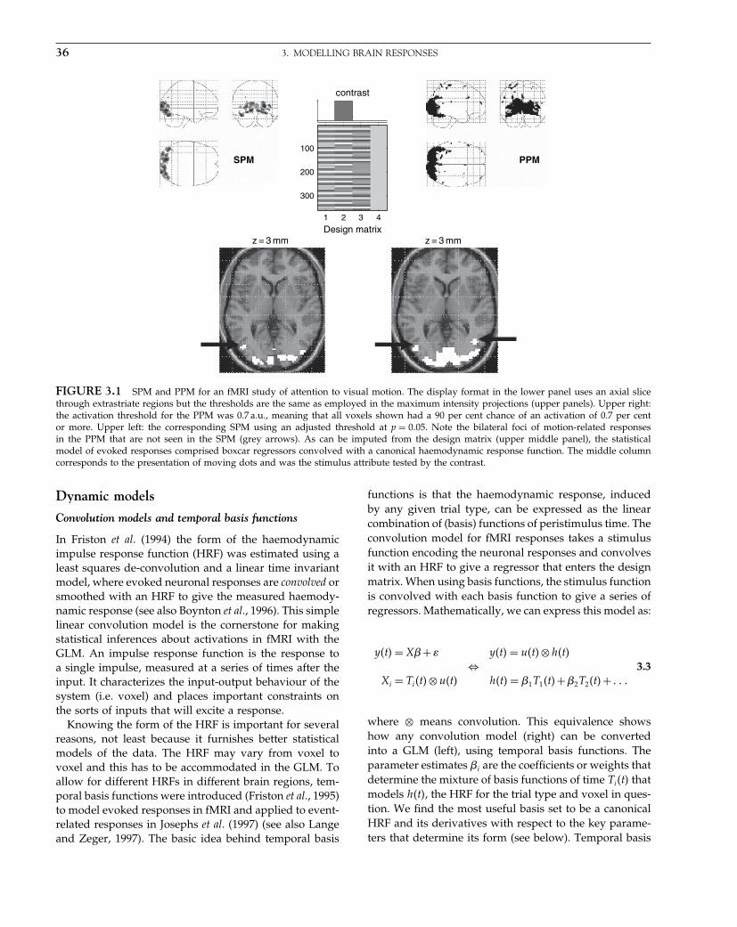
Elsevier UK Chapter: Ch03-P372560 3-10-2006 3:01p.m. Page:36 Trim:7.5in×9.25in
Basal Font:Palatino Margins:Top:40pt Gutter:68pt Font Size:9.5/12 Text Width:42pc Depth:55 Lines
36 3. MODELLING BRAIN RESPONSES
Design matrix1 2 3 4
100
200
300
contrast
z = 3 mm z = 3 mm
PPMSPM
FIGURE 3.1 SPM and PPM for an fMRI study of attention to visual motion. The display format in the lower panel uses an axial slicethrough extrastriate regions but the thresholds are the same as employed in the maximum intensity projections (upper panels). Upper right:the activation threshold for the PPM was 0.7 a.u., meaning that all voxels shown had a 90 per cent chance of an activation of 0.7 per centor more. Upper left: the corresponding SPM using an adjusted threshold at p = 0�05. Note the bilateral foci of motion-related responsesin the PPM that are not seen in the SPM (grey arrows). As can be imputed from the design matrix (upper middle panel), the statisticalmodel of evoked responses comprised boxcar regressors convolved with a canonical haemodynamic response function. The middle columncorresponds to the presentation of moving dots and was the stimulus attribute tested by the contrast.
Dynamic models
Convolution models and temporal basis functions
In Friston et al. (1994) the form of the haemodynamicimpulse response function (HRF) was estimated using aleast squares de-convolution and a linear time invariantmodel, where evoked neuronal responses are convolved orsmoothed with an HRF to give the measured haemody-namic response (see also Boynton et al., 1996). This simplelinear convolution model is the cornerstone for makingstatistical inferences about activations in fMRI with theGLM. An impulse response function is the response toa single impulse, measured at a series of times after theinput. It characterizes the input-output behaviour of thesystem (i.e. voxel) and places important constraints onthe sorts of inputs that will excite a response.
Knowing the form of the HRF is important for severalreasons, not least because it furnishes better statisticalmodels of the data. The HRF may vary from voxel tovoxel and this has to be accommodated in the GLM. Toallow for different HRFs in different brain regions, tem-poral basis functions were introduced (Friston et al., 1995)to model evoked responses in fMRI and applied to event-related responses in Josephs et al. (1997) (see also Langeand Zeger, 1997). The basic idea behind temporal basis
functions is that the haemodynamic response, inducedby any given trial type, can be expressed as the linearcombination of (basis) functions of peristimulus time. Theconvolution model for fMRI responses takes a stimulusfunction encoding the neuronal responses and convolvesit with an HRF to give a regressor that enters the designmatrix. When using basis functions, the stimulus functionis convolved with each basis function to give a series ofregressors. Mathematically, we can express this model as:
y�t� = X�+� y�t� = u�t�⊗h�t�⇔
Xi = Ti�t�⊗u�t� h�t� = �1T1�t�+�2T2�t�+ � � �3.3
where ⊗ means convolution. This equivalence showshow any convolution model (right) can be convertedinto a GLM (left), using temporal basis functions. Theparameter estimates �i are the coefficients or weights thatdetermine the mixture of basis functions of time Ti�t� thatmodels h�t�, the HRF for the trial type and voxel in ques-tion. We find the most useful basis set to be a canonicalHRF and its derivatives with respect to the key parame-ters that determine its form (see below). Temporal basis
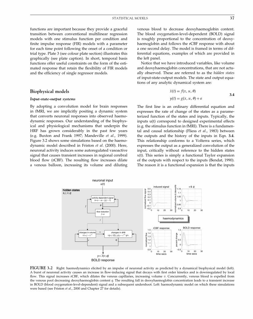
Elsevier UK Chapter: Ch03-P372560 3-10-2006 3:01p.m. Page:37 Trim:7.5in×9.25in
Basal Font:Palatino Margins:Top:40pt Gutter:68pt Font Size:9.5/12 Text Width:42pc Depth:55 Lines
STATISTICAL MODELS 37
functions are important because they provide a gracefultransition between conventional multilinear regressionmodels with one stimulus function per condition andfinite impulse response (FIR) models with a parameterfor each time point following the onset of a condition ortrial type. Plate 3 (see colour plate section) illustrates thisgraphically (see plate caption). In short, temporal basisfunctions offer useful constraints on the form of the esti-mated response that retain the flexibility of FIR modelsand the efficiency of single regressor models.
Biophysical models
Input-state-output systems
By adopting a convolution model for brain responsesin fMRI, we are implicitly positing a dynamic systemthat converts neuronal responses into observed haemo-dynamic responses. Our understanding of the biophys-ical and physiological mechanisms that underpin theHRF has grown considerably in the past few years(e.g. Buxton and Frank 1997; Mandeville et al., 1999).Figure 3.2 shows some simulations based on the haemo-dynamic model described in Friston et al. (2000). Here,neuronal activity induces some autoregulated vasoactivesignal that causes transient increases in regional cerebralblood flow (rCBF). The resulting flow increases dilatea venous balloon, increasing its volume and diluting
venous blood to decrease deoxyhaemoglobin content.The blood oxygenation-level-dependent (BOLD) signalis roughly proportional to the concentration of deoxy-haemoglobin and follows the rCBF response with abouta one second delay. The model is framed in terms of dif-ferential equations, examples of which are provided inthe left panel.
Notice that we have introduced variables, like volumeand deoxyhaemoglobin concentrations, that are not actu-ally observed. These are referred to as the hidden statesof input-state-output models. The state and output equa-tions of any analytic dynamical system are:
ẋ�t� = f�x�u��
y�t� = g�x�u��+�3.4
The first line is an ordinary differential equation andexpresses the rate of change of the states as a parame-terized function of the states and inputs. Typically, theinputs u(t) correspond to designed experimental effects(e.g. the stimulus function in fMRI). There is a fundamen-tal and causal relationship (Fliess et al., 1983) betweenthe outputs and the history of the inputs in Eqn. 3.4.This relationship conforms to a Volterra series, whichexpresses the output as a generalized convolution of theinput, critically without reference to the hidden statesx(t). This series is simply a functional Taylor expansionof the outputs with respect to the inputs (Bendat, 1990).The reason it is a functional expansion is that the inputs
flow inductionƒ= s
y = λ(ν,q)
u(t )
s
ν
ƒ
hidden states
neuronal input
hidden states
BOLD response
ν
s,ƒ,ν,q
changes in dHbτq = ƒ E(ƒ,ρ)/ρ – ν1/α q/ν
changes in volumeτν = ƒ – ν1/α
ƒ
q
activity-dependent signals = u – κs – γ (ƒ – 1)
hemodynamics
⋅
⋅
⋅ ⋅
00.9 –0.5
0.5
01
1
1.1
1.2
1.3
1.4
1.5 1.5
10time secs
rCBF response BOLD response
haemodynamics
norm
aliz
ed fl
owno
rmal
ized
flow
sig
nal
norm
aliz
ed v
olum
e &
deo
xyH
bpe
rcen
t cha
nge
time secs20 30 0 10 20 30
0–0.2 0.9
0.95
1
1.05
1.1
1.15
–0.1
00.10.20.30.40.5
10 20
induced signal v & q
30 0 10 20 30
FIGURE 3.2 Right: haemodynamics elicited by an impulse of neuronal activity as predicted by a dynamical biophysical model (left).A burst of neuronal activity causes an increase in flow-inducing signal that decays with first order kinetics and is downregulated by localflow. This signal increases rCBF, which dilates the venous capillaries, increasing volume v. Concurrently, venous blood is expelled fromthe venous pool decreasing deoxyhaemoglobin content q. The resulting fall in deoxyhaemoglobin concentration leads to a transient increasein BOLD (blood oxygenation-level-dependent) signal and a subsequent undershoot. Left: haemodynamic model on which these simulationswere based (see Friston et al., 2000 and Chapter 27 for details).

Elsevier UK Chapter: Ch03-P372560 3-10-2006 3:01p.m. Page:38 Trim:7.5in×9.25in
Basal Font:Palatino Margins:Top:40pt Gutter:68pt Font Size:9.5/12 Text Width:42pc Depth:55 Lines
38 3. MODELLING BRAIN RESPONSES
are a function of time. (For simplicity, here and in andEqn. 3.7, we deal with only one experimental input.)
y�t� =∑i
t∫0
� � �
t∫0
i��1� � � � ��i�
×u�t −�1�� � � � �u�t −�i�d�1� � � � � d�i
i��1� � � � ��i� = �iy�t�
�u�t −�1�� � � � � �u�t −�i�3.5
where i��1� K��i) is the i-th order kernel. In Eqn. 3.5the integrals are restricted to the past. This renders thesystem causal. The key thing here is that Eqn. 3.5 is sim-ply a convolution and can be expressed as a GLM, asin Eqn. 3.3. This means that we can take a neurophysio-logically realistic model of haemodynamic responses anduse it as an observation model to estimate parametersusing observed data. Here the model is parameterizedin terms of kernels that have a direct analytic relation tothe original parameters of the biophysical system. Thefirst-order kernel is simply the conventional HRF. High-order kernels correspond to high-order HRFs and can beestimated using basis functions as described above. Infact, by choosing basis functions according to:
A���i = ����1
�i
3.6
one can estimate the biophysical parameters because, toa first-order approximation, �i = i. The critical step wehave taken here is to start with a dynamic causal modelof how responses are generated and construct a generallinear observation model that allows us to estimate andinfer things about the parameters of that model. This is incontrast to the conventional use of the GLM with designmatrices that are not informed by a forward model ofhow data are caused. This approach to modelling brainresponses has a much more direct connection with under-lying physiology and rests upon an understanding of theunderlying system.
Non-linear system identification
Once a suitable causal model has been established (e.g.Figure 3.2), we can estimate second-order kernels. Thesekernels represent a non-linear characterization of theHRF that can model interactions among stimuli in caus-ing responses. One important manifestation of the non-linear effects, captured by the second-order kernels, isa modulation of stimulus-specific responses by preced-ing stimuli that are proximate in time. This means thatresponses at high stimulus presentation rates saturateand, in some instances, show an inverted U behaviour.This behaviour appears to be specific to BOLD effects(as distinct from evoked changes in cerebral blood flow)
and may represent a haemodynamic refractoriness. Thiseffect has important implications for event-related fMRI,where one may want to present trials in quick succession.(See Figure 2.8 in the previous chapter for an example ofsecond-order kernels and the implications for haemody-namic responses.)
In summary, we started with models of regionally spe-cific responses, framed in terms of the general linearmodel, in which responses were modelled as linear mix-tures of designed changes in explanatory variables. Hier-archical extensions to linear observation models enablerandom-effects analyses and, in particular, empiricalBayes. The mechanistic utility of these models is real-ized though the use of forward models that embodycausal dynamics. Simple variants of these are the linearconvolution models used to construct explanatory vari-ables in conventional analyses of fMRI data. These are aspecial case of generalized convolution models that aremathematically equivalent to input-state-output systemscomprising hidden states. Estimation and inference withthese dynamic models tells us something about how theresponse was caused, but only at the level of a singlevoxel. The next section retains the same perspective onmodels, but in the context of distributed responses andfunctional integration.
MODELS OF FUNCTIONALINTEGRATION
Functional and effective connectivity
Imaging neuroscience has firmly established functionalspecialization as a principle of brain organization inhumans. The integration of specialized areas has provenmore difficult to assess. Functional integration is usu-ally inferred on the basis of correlations among mea-surements of neuronal activity. Functional connectivity isdefined as statistical dependencies or correlations amongremote neurophysiological events. However, correlations canarise in a variety of ways: for example in multiunit elec-trode recordings, they can result from stimulus-lockedtransients evoked by a common input or reflect stimulus-induced oscillations mediated by synaptic connections(Gerstein and Perkel, 1969). Integration within a dis-tributed system is usually better understood in terms ofeffective connectivity; effective connectivity refers explic-itly to the influence that one neural system exerts over another,either at a synaptic (i.e. synaptic efficacy) or populationlevel. It has been proposed that ‘the [electrophysiological]notion of effective connectivity should be understood asthe experiment- and time-dependent, simplest possible

Elsevier UK Chapter: Ch03-P372560 3-10-2006 3:01p.m. Page:39 Trim:7.5in×9.25in
Basal Font:Palatino Margins:Top:40pt Gutter:68pt Font Size:9.5/12 Text Width:42pc Depth:55 Lines
MODELS OF FUNCTIONAL INTEGRATION 39
circuit diagram that would replicate the observed tim-ing relationships between the recorded neurons’ (Aert-sen and Preißl, 1991). This speaks of two importantpoints: effective connectivity is dynamic, i.e. activity-dependent and it depends upon a model of the interac-tions. The estimation procedures employed in functionalneuroimaging can be divided into linear non-dynamicmodels (e.g. McIntosh and Gonzalez-Lima, 1994) or non-linear dynamic models.
There is a necessary link between functional integra-tion and multivariate analyses because the latter arenecessary to model interactions among brain regions.Multivariate approaches can be divided into thosethat are inferential in nature and those that are data-led or exploratory. We will first consider multivariateapproaches that look at functional connectivity or covari-ance patterns (and are generally exploratory) and thenturn to models of effective connectivity (that allow forinference about their parameters).
Eigenimage analysis and related approaches
In Friston et al. (1993), we introduced voxel-basedprincipal component analysis (PCA) of neuroimagingtime-series to characterize distributed brain systemsimplicated in sensorimotor, perceptual or cognitive pro-cesses. These distributed systems are identified withprincipal components or eigenimages that correspond tospatial modes of coherent brain activity. This approachrepresents one of the simplest multivariate characteri-zations of functional neuroimaging time-series and fallsinto the class of exploratory analyses. Principal compo-nent or eigenimage analysis generally uses singular valuedecomposition (SVD) to identify a set of orthogonal spa-tial modes that capture the greatest amount of varianceexpressed over time. As such, the ensuing modes embodythe most prominent aspects of the variance-covariancestructure of a given time-series. Noting that covarianceamong brain regions is equivalent to functional connec-tivity renders eigenimage analysis particularly interest-ing because it was among the first ways of addressingfunctional integration (i.e. connectivity) with neuroimag-ing data. Subsequently, eigenimage analysis has beenelaborated in a number of ways. Notable among these iscanonical variate analysis (CVA) and multidimensionalscaling (Friston et al., 1996a, b). Canonical variate analy-sis was introduced in the context of MANCOVA (mul-tiple analysis of covariance) and uses the generalizedeigenvector solution to maximize the variance that canbe explained by some explanatory variables relative toerror. CVA can be thought of as an extension of eigen-image analysis that refers explicitly to some explanatoryvariables and allows for statistical inference.
In fMRI, eigenimage analysis (e.g. Sychra et al., 1994)is generally used as an exploratory device to characterizecoherent brain activity. These variance components may,or may not, be related to experimental design. For exam-ple, endogenous coherent dynamics have been observedin the motor system at very low frequencies (Biswal et al.,1995). Despite its exploratory power, eigenimage analy-sis is limited for two reasons. First, it offers only a lineardecomposition of any set of neurophysiological measure-ments and second, the particular set of eigenimages orspatial modes obtained is determined by constraints thatare biologically implausible. These aspects of PCA conferinherent limitations on the interpretability and useful-ness of eigenimage analysis of biological time-series andhave motivated the exploration of non-linear PCA andneural network approaches.
Two other important approaches deserve mentionhere. The first is independent component analysis (ICA).ICA uses entropy maximization to find, using itera-tive schemes, spatial modes or their dynamics that areapproximately independent. This is a stronger require-ment than orthogonality in PCA and involves removinghigh-order correlations among the modes (or dynam-ics). It was initially introduced as spatial ICA (McKeownet al., 1998) in which the independence constraint wasapplied to the modes (with no constraints on their tem-poral expression). More recent approaches use, by anal-ogy with magneto- and electrophysiological time-seriesanalysis, temporal ICA where the dynamics are enforcedto be independent. This requires an initial dimensionreduction (usually using conventional eigenimage anal-ysis). Finally, there has been an interest in cluster anal-ysis (Baumgartner et al., 1997). Conceptually, this can berelated to eigenimage analysis through multidimensionalscaling and principal coordinate analysis.
All these approaches are interesting, but they are notused very much. This is largely because they tell younothing about how the brain works nor allow one toask specific questions. Simply demonstrating statisticaldependencies among regional brain responses or endoge-nous activity (i.e. demonstrating functional connectivity)does not address how these responses were caused. Toaddress this one needs explicit models of integration ormore precisely, effective connectivity.
Dynamic causal modelling withbilinear models
This section is about modelling interactions among neu-ronal populations, at a cortical level, using neuroimagingtime-series and dynamic causal models that are informedby the biophysics of the system studied. The aim ofdynamic causal modelling is to estimate, and make infer-ences about, the coupling among brain areas and how
Elsevier UK Chapter: Ch03-P372560 3-10-2006 3:01p.m. Page:40 Trim:7.5in×9.25in
Basal Font:Palatino Margins:Top:40pt Gutter:68pt Font Size:9.5/12 Text Width:42pc Depth:55 Lines
40 3. MODELLING BRAIN RESPONSES
that coupling is influenced by experimental changes (e.g.time or cognitive set). The basic idea is to construct areasonably realistic neuronal model of interacting corti-cal regions or nodes. This model is then supplementedwith a forward model of how neuronal or synaptic activ-ity translates into a measured response (see previoussection). This enables the parameters of the neuronalmodel (i.e. effective connectivity) to be estimated fromobserved data.
Intuitively, this approach regards an experiment asa designed perturbation of neuronal dynamics thatare promulgated and distributed throughout a systemof coupled anatomical nodes to change region-specificneuronal activity. These changes engender, through ameasurement-specific forward model, responses that areused to identify the architecture and time constants ofthe system at a neuronal level. This represents a depar-ture from conventional approaches (e.g. structural equa-tion modelling and autoregression models; McIntoshand Gonzalez-Lima, 1994; Büchel and Friston, 1997), inwhich one assumes the observed responses are drivenby endogenous or intrinsic noise (i.e. innovations). Incontrast, dynamic causal models assume the responsesare driven by designed changes in inputs. An impor-tant conceptual aspect of dynamic causal models per-tains to how the experimental inputs enter the model andcause neuronal responses. Experimental variables canelicit responses in one of two ways. First, they can elicitresponses through direct influences on specific anatom-ical nodes. This would be appropriate, for example, inmodelling sensory evoked responses in early visual cor-tices. The second class of input exerts its effect vicar-iously, through a modulation of the coupling amongnodes. These sorts of experimental variables would nor-mally be more enduring; for example attention to a par-ticular attribute or the maintenance of some perceptualset. These distinctions are seen most clearly in relationto particular forms of causal models used for estimation,e.g. the bilinear approximation:
ẋ = f�x�u�
= Ax+uBx+Cu
y = g�x�+�
A = �f
�xB = �2f
�x�uC = �f
�u
3.7
where ẋ = �x/�t. This is an approximation to any modelof how changes in neuronal activity in one region xi arecaused by activity in the other regions. Here the outputfunction g�x� embodies a haemodynamic convolution,linking neuronal activity to BOLD, for each region (e.g.that in Figure 3.2). The matrix A represents the couplingamong the regions in the absence of input u�t�. This can
be thought of as the latent coupling in the absence ofexperimental perturbations. The matrix B is effectivelythe change in latent coupling induced by the input. Itencodes the input-sensitive changes in A or, equivalently,the modulation of coupling by experimental manipula-tions. Because B is a second-order derivative it is referredto as bilinear. Finally, the matrix C embodies the extrinsicinfluences of inputs on neuronal activity. The parameters = A�B�C are the connectivity or coupling matrices thatwe wish to identify and define the functional architectureand interactions among brain regions at a neuronal level.
Because Eqn. 3.7 has exactly the same form as Eqn. 3.4,we can express it as a GLM and estimate the parame-ters using EM in the usual way (see Friston et al., 2003).Generally, estimation in the context of highly parameter-ized models like DCMs requires constraints in the formof priors. These priors enable conditional inference aboutthe connectivity estimates. The sorts of questions that canbe addressed with DCMs are now illustrated by lookingat how attentional modulation is mediated in sensoryprocessing hierarchies in the brain.
DCM and attentional modulation
It has been established that the superior posterior parietalcortex (SPC) exerts a modulatory role on V5 responsesusing Volterra-based regression models (Friston andBüchel, 2000) and that the inferior frontal gyrus (IFG)exerts a similar influence on SPC using structural equa-tion modelling (Büchel and Friston, 1997). The examplehere shows that DCM leads to the same conclusions butstarting from a completely different construct. The exper-imental paradigm and data acquisition are described inFigure 3.3. This figure also shows the location of theregions that entered the DCM. These regions were basedon maxima from conventional SPMs testing for the effectsof photic stimulation, motion and attention. Regionaltime courses were taken as the first eigenvariate of 8 mmspherical volumes of interest centred on the maximashown in the figure. The inputs, in this example, compriseone sensory perturbation and two contextual inputs. Thesensory input was simply the presence of photic stimula-tion and the first contextual one was presence of motionin the visual field. The second contextual input, encodingattentional set, was one during attention to speed changesand zero otherwise. The outputs corresponded to thefour regional eigenvariates in (Figure 3.3, left panel). Theintrinsic connections were constrained to conform to ahierarchical pattern in which each area was reciprocallyconnected to its supraordinate area. Photic stimulationentered at, and only at, V1. The effect of motion in thevisual field was modelled as a bilinear modulation ofthe V1 to V5 connectivity and attention was allowed tomodulate the backward connections from IFG and SPC.

Elsevier UK Chapter: Ch03-P372560 3-10-2006 3:01p.m. Page:41 Trim:7.5in×9.25in
Basal Font:Palatino Margins:Top:40pt Gutter:68pt Font Size:9.5/12 Text Width:42pc Depth:55 Lines
MODELS OF FUNCTIONAL INTEGRATION 41
V1
SPC
IFG
Motion
Photic
Attention
.42(100%)
.37(90%)
.56(99%)
.74(100%).82
(100%)
.69 (100%)
.65 (100%)
.52 (98%)
V5
V1
V 5
SPC
IFG
SPC
IFGVI
200 1000800600400
time {seconds}
time {seconds}
200 1000800600400
time {seconds}
200 600400
resp
onse
10
8
6
4
2
0
–2
resp
onse
10
8
6
4
2
0
–2re
spon
se
10
8
6
4
2
0
–2
resp
onse
10
8
6
4
2
0
–2
10.80.60.40.2
010.80.60.40.2
0
10.80.60.40.2
0
time {seconds}
FIGURE 3.3 Results of a DCM analysis of attention to visual motion with fMRI. Right panel: functional architecture based upon theconditional estimates shown alongside their connections, with the per cent confidence that they exceeded threshold in brackets. The mostinteresting aspects of this architecture involve the role of motion and attention in exerting bilinear effects. Critically, the influence of motionis to enable connections from V1 to the motion-sensitive area V5. The influence of attention is to enable backward connections from theinferior frontal gyrus (IFG) to the superior parietal cortex (SPC). Furthermore, attention increases the influence of SPC on V5. Dotted arrowsconnecting regions represent significant bilinear effects in the absence of a significant intrinsic coupling. Left panel: fitted responses basedupon the conditional estimates and the adjusted data are shown for each region in the DCM. The insert (upper left) shows the location of theregions.
Subjects were studied with fMRI under identical stimulus conditions (visual motion subtended by radially moving dots) while manipulatingthe attentional component of the task (detection of velocity changes). The data were acquired from a normal subject at 2 Tesla. Each subjecthad four consecutive 100-scan sessions comprising a series of 10-scan blocks under five different conditions, D F A F N F A F N S. The firstcondition (D) was a dummy condition to allow for magnetic saturation effects. F (Fixation) corresponds to a low-level baseline where thesubjects viewed a fixation point at the centre of a screen. In condition A (Attention), subjects viewed 250 dots moving radially from the centreat 4.7 degrees per second and were asked to detect changes in radial velocity. In condition N (No attention), the subjects were asked simplyto view the moving dots. In condition S (Stationary), subjects viewed stationary dots. The order of A and N was swapped for the last twosessions. In all conditions subjects fixated the centre of the screen. During scanning there were no speed changes. No overt response wasrequired in any condition.
The results of the DCM are shown in Figure 3.3 (rightpanel). Of primary interest here is the modulatory effectof attention that is expressed in terms of the bilinearcoupling parameters for this input. As expected, we canbe highly confident that attention modulates the back-ward connections from IFG to SPC and from SPC to V5.Indeed, the influences of IFG on SPC are negligible inthe absence of attention (dotted connection). It is impor-tant to note that the only way that attentional manipu-lation can affect brain responses is through this bilineareffect. Attention-related responses are seen throughoutthe system (attention epochs are marked with arrows inthe plot of IFG responses in the left panel). This atten-tional modulation is accounted for, sufficiently, by chang-ing just two connections. This change is, presumably,instantiated by instructional set at the beginning of eachepoch.
The second thing this analysis illustrates is how func-tional segregation is modelled in DCM. Here one canregard V1 as ‘segregating’ motion from other visual infor-mation and distributing it to the motion-sensitive area,V5. This segregation is modelled as a bilinear ‘enabling’of V1 to V5 connections when, and only when, motion
is present. Note that, in the absence of motion, the latentV1 to V5 connection was trivially small (in fact the esti-mate was −0�04). The key advantage of entering motionthrough a bilinear effect, as opposed to a direct effect onV5, is that we can finesse the inference that V5 showsmotion-selective responses with the assertion that theseresponses are mediated by afferents from V1. The twobilinear effects above represent two important aspects offunctional integration that DCM is able to characterize.
Structural equation modelling as a special case of DCM
The central idea behind dynamic causal modelling isto treat the brain as a deterministic non-linear dynamicsystem that is subject to inputs and produces outputs.Effective connectivity is parameterized in terms of cou-pling among unobserved brain states (e.g. neuronal activ-ity in different regions). The objective is to estimatethese parameters by perturbing the system and measur-ing the response. This is in contradistinction to estab-lished methods for estimating effective connectivity fromneurophysiological time-series, which include structuralequation modelling and models based on multivariate

Elsevier UK Chapter: Ch03-P372560 3-10-2006 3:01p.m. Page:42 Trim:7.5in×9.25in
Basal Font:Palatino Margins:Top:40pt Gutter:68pt Font Size:9.5/12 Text Width:42pc Depth:55 Lines
42 3. MODELLING BRAIN RESPONSES
autoregressive processes. In these models, there is nodesigned perturbation and the inputs are treated asunknown and stochastic. Furthermore, the inputs areoften assumed to express themselves instantaneouslysuch that, at the point of observation the change in statesis zero. From Eqn. 3.7, in the absence of bilinear effectswe have:
ẋ = 0
= Ax+Cu
x = −A−1Cu
3.8
This is the regression equation used in structural equa-tion modelling (SEM) where A = D− I and D contains theoff-diagonal connections among regions. The key pointhere is that A is estimated by assuming u�t� is somerandom innovation with known covariance. This is notreally tenable for designed experiments when u�t� repre-sent carefully structured experimental inputs. AlthoughSEM and related autoregressive techniques are useful forestablishing dependence among regional responses, theyare not surrogates for informed causal models based onthe underlying dynamics of these responses.
In this section, we have covered multivariate tech-niques ranging from eigenimage analysis that does nothave an explicit forward or causal model to DCMthat does. The bilinear approximation to any DCM hasbeen illustrated through its use with fMRI to studyattentional modulation. The parameters of the bilinearapproximation include first-order effective connectivityA and its experimentally-induced changes B. Althoughthe bilinear approximation is useful, it is possible tomodel coupling among neuronal subpopulations explic-itly. We conclude with a DCM that embraces a num-ber of neurobiological facts and takes us much closerto a mechanistic understanding of how brain responsesare generated. This example uses responses measuredwith EEG.
Dynamic causal modelling withneural-mass models
Event-related potentials (ERPs) have been used fordecades as electrophysiological correlates of perceptualand cognitive operations. However, the exact neuro-biological mechanisms underlying their generation arelargely unknown. In this section, we use neuronally plau-sible models to understand event-related responses. Ourexample shows that changes in connectivity are suffi-cient to explain certain ERP components. Specifically, wewill look at the MMN, a component associated with rareor unexpected events. If the unexpected nature of rare
stimuli depends on learning which stimuli are frequent,then the MMN must be due to plastic changes in con-nectivity that mediate perceptual learning. We concludeby showing that advances in the modelling of evokedresponses now afford measures of connectivity amongcortical sources that can be used to quantify the effectsof perceptual learning.
Neural-mass models
The minimal model we have developed (David et al.,2006) uses the connectivity rules described in Fellemanand Van Essen (1992) to assemble a network of coupledsources. These rules are based on a partitioning of thecortical sheet into supra-, infra-granular layers and gran-ular layer (layer 4). Bottom-up or forward connectionsoriginate in agranular layers and terminate in layer 4.Top-down or backward connections target agranular lay-ers. Lateral connections originate in agranular layers andtarget all layers. These long-range or extrinsic cortico-cortical connections are excitatory and arise from pyra-midal cells.
Each region or source is modelled using a neural massmodel described in David and Friston (2003), based onthe model of Jansen and Rit (1995). This model emu-lates the activity of a cortical area using three neuronalsubpopulations, assigned to granular and agranular lay-ers. A population of excitatory pyramidal (output) cellsreceives inputs from inhibitory and excitatory popula-tions of interneurons, via intrinsic connections (intrinsicconnections are confined to the cortical sheet). Withinthis model, excitatory interneurons can be regarded asspiny stellate cells found predominantly in layer 4 andin receipt of forward connections. Excitatory pyrami-dal cells and inhibitory interneurons are considered tooccupy agranular layers and receive backward and lat-eral inputs (Figure 3.4).
To model event-related responses, the networkreceives inputs via input connections. These connectionsare exactly the same as forward connections and deliverinputs to the spiny stellate cells in layer 4. In the presentcontext, inputs u�t� model sub-cortical auditory inputs.The vector C controls the influence of the input on eachsource. The lower, upper and leading diagonal matricesAF �AB�AL encode forward, backward and lateral con-nections respectively. The DCM here is specified in termsof the state equations shown in Figure 3.4 and a linearoutput equation:
ẋ = f�x�u�
y = Lx0 +�3.9

Elsevier UK Chapter: Ch03-P372560 3-10-2006 3:01p.m. Page:43 Trim:7.5in×9.25in
Basal Font:Palatino Margins:Top:40pt Gutter:68pt Font Size:9.5/12 Text Width:42pc Depth:55 Lines
MODELS OF FUNCTIONAL INTEGRATION 43
spinystellate
cells
inhibitoryinterneurons
pyramidalcells
γ4 γ3
γ4S(x7) −2x6 x3Hix6 =
x0 = x5 − x6
x2 = x5
x3 = x6
−
γ1 γ2
AFS(x0)
AL S(x0)
AB S(x0)
Extrinsicforward
connections
Extrinsicbackwardconnections
Intrinsicconnections
Neuronal model
Extrinsiclateralconnections
2x8
τe((AB + AL + γ3I )S(x0)) – 2τe
x7
τe
Hex8 =
x7 = x8
–
2x4
τe
((AF + AL + γ1I )S(x0) + Cu) –
2τe
x1
τe
Hex4 =
x1 = x4
–
2x5
τe((AB + AL
)S(x0) + γ2
S(X1)) – 2τe
x2
τe
Hex5 = –
τi τi τi2
⋅
⋅
⋅
⋅
⋅
⋅
⋅
⋅
⋅
FIGURE 3.4 Schematic of the DCM used to model electrical responses. This schematic shows the state equations describing the dynamicsof sources or regions. Each source is modelled with three subpopulations (pyramidal, spiny stellate and inhibitory interneurons) as describedin Jansen and Rit (1995) and David and Friston (2003). These have been assigned to granular and agranular cortical layers which receiveforward and backward connections respectively.
where x0 represents the transmembrane potential of pyra-midal cells and L is a lead field matrix coupling electricalsources to the EEG channels. This should be comparedto the DCM above for haemodynamics; here the equa-tions governing the evolution of neuronal states are muchmore complicated and realistic, as opposed to the bilin-ear approximation in Eqn. 3.7. Conversely, the outputequation is a simple linearity, as opposed to the non-linear observer used for fMRI. As an example, the stateequation for the inhibitory subpopulation is:
ẋ7 = x8
ẋ8 = He
e
��AB +AL +�3I�S�x0��− 2x8
e
− x7
2e
3.10
Propagation delays on the extrinsic connections havebeen omitted for clarity here and in Figure 3.4.
Within each subpopulation, the evolution of neuronalstates rests on two operators. The first transforms theaverage density of presynaptic inputs into the averagepostsynaptic membrane potential. This is modelled by alinear transformation with excitatory and inhibitory ker-nels parameterized by He�i and e�i� He�i control the max-imum postsynaptic potential and e�i represent a lumpedrate-constant. The second operator S transforms the aver-age potential of each subpopulation into an average firingrate. This is assumed to be instantaneous and is a sigmoidfunction. Interactions among the subpopulations depend
on constants �1�2�3�4, which control the strength of intrin-sic connections and reflect the total number of synapsesexpressed by each subpopulation. In Eqn. 3.10, the topline expresses the rate of change of voltage as a functionof current. The second line specifies how current changesas a function of voltage, current and presynaptic inputfrom extrinsic and intrinsic sources. Having specified theDCM in terms of these equations, one can estimate thecoupling parameters from empirical data using EM asdescribed above.
Perceptual learning and the MMN
The example shown in Figure 3.5 is an attempt to modelthe MMN in terms of changes in backward and lateralconnections among cortical sources. In this example, two[averaged] channels of EEG data were modelled withthree cortical sources. Using this generative or forwardmodel, we estimated differences in the strength of theseconnections for rare and frequent stimuli. As expected,we could account for detailed differences in the ERPs(the MMN) by changes in connectivity (see Figure 3.5 fordetails). Interestingly, these differences were expressedselectively in the lateral connections. If this model is a suf-ficient approximation to the real sources, these changesare a non-invasive measure of plasticity, mediating per-ceptual learning, in the human brain.

Elsevier UK Chapter: Ch03-P372560 3-10-2006 3:01p.m. Page:44 Trim:7.5in×9.25in
Basal Font:Palatino Margins:Top:40pt Gutter:68pt Font Size:9.5/12 Text Width:42pc Depth:55 Lines
44 3. MODELLING BRAIN RESPONSES
0.5
spinystellatecells
pyramidalcells
IntrinsicForward
BackwardLateral time
input
.56/
.61
.59/
.87
.05/
.04
.00/.09
.01/3.68
inhibitoryinterneurons
P300 Real andmodelled
frequentrare
Time {s}
0
–2
0
2
4
–4–2024
0.5 1 1.5
0 1 1.5Time {s}
FIGURE 3.5 Summary of a DCM analysis of event-relatedpotentials (ERPs) elicited during an auditory oddball paradigm,employing rare and frequent pure tones. Upper panel: schematicshowing the architecture of the neuronal model used to explain theempirical data. Sources were coupled with extrinsic cortico-corticalconnections following the rules of Felleman and van Essen (1992).The free parameters of this model included intrinsic and extrinsicconnection strengths that were adjusted best to explain the data.In this example, the lead field was also estimated, with no spatialconstraints. The parameters were estimated for ERPs recorded dur-ing the presentation of rare and frequent tones and are reportedbeside their corresponding connection (frequent/rare). The mostnotable finding was that the mismatch response could be explainedby a selective increase in lateral connection strength from 0.1 to3.68 Hz (highlighted in bold). Lower panel: the channel positions(left) and ERPs (right) averaged over two subsets of channels (cir-cled on the left). Note the correspondence between the measuredERPs and those generated by the model (see David et al., 2006 fordetails).
Auditory stimuli, 1000 or 2000 Hz tones with 5 ms rise and falltimes and 80 ms duration, were presented binaurally. The toneswere presented for 15 minutes, every 2 s in a pseudo-randomsequence with 2000 Hz tones occurring 20 per cent of the time and1000 Hz tones occurring 80 per cent of the time. The subject wasinstructed to keep a mental record of the number of 2000 Hz tones(non-frequent target tones). Data were acquired using 128 EEG elec-trodes with 1000 Hz sample frequency. Before averaging, data werereferenced to mean earlobe activity and band-pass filtered between1 and 30 Hz. Trials showing ocular artefacts and bad channels wereremoved from further analysis.
CONCLUSION
In this chapter, we have reviewed some key models thatunderpin image analysis and have touched briefly onways of assessing specialization and integration in thebrain. These models can be regarded as a succession ofmodelling endeavours that draw more and more on ourunderstanding of how brain-imaging signals are gener-ated, both in terms of biophysics and the underlying neu-ronal interactions. We have seen how hierarchical linearobservation models encode the treatment effects elicitedby experimental design. General linear models based onconvolution models imply an underlying dynamic input-state-output system. The form of these systems can beused to constrain convolution models and explore someof their simpler non-linear properties. By creating obser-vation models based on explicit forward models of neu-ronal interactions, one can model and assess interactionsamong distributed cortical areas and make inferencesabout coupling at the neuronal level. The next years willprobably see an increasing realism in the dynamic causalmodels introduced above. These endeavours are likely toencompass fMRI signals enabling the conjoint modelling,or fusion, of different modalities and the marriage ofcomputational neuroscience with the modelling of brainresponses.
REFERENCES
Absher JR, Benson DF (1993) Disconnection syndromes: an overviewof Geschwind’s contributions. Neurology 43: 862–67
Aertsen A, Preißl H (1991) Dynamics of activity and connectiv-ity in physiological neuronal networks. In Non linear dynamicsand neuronal networks, Schuster HG (ed.). VCH Publishers Inc.,New York, pp 281–302
Baumgartner R, Scarth G, Teichtmeister C et al. (1997) Fuzzy cluster-ing of gradient-echo functional MRI in the human visual cortex.Part 1: reproducibility. J Mag Res Imaging 7: 1094–101
Bendat JS (1990) Nonlinear system analysis and identification from ran-dom data. John Wiley and Sons, New York
Berry DA, Hochberg Y (1999) Bayesian perspectives on multiplecomparisons. J Stat Plann Inference 82: 215–227
Biswal B, Yetkin FZ, Haughton VM et al. (1995) Functional connec-tivity in the motor cortex of resting human brain using echo-planar MRI. Mag Res Med 34: 537–41
Boynton GM, Engel SA, Glover GH et al. (1996) Linear systemsanalysis of functional magnetic resonance imaging in human V1.J Neurosci 16: 4207–21
Büchel C, Friston KJ (1997) Modulation of connectivity in visualpathways by attention: cortical interactions evaluated withstructural equation modelling and fMRI. Cereb Cortex 7:768–78
Buckner RL, Koutstaal W, Schacter DL, et al. (1998) Functional-anatomic study of episodic retrieval. II. Selective averaging ofevent-related fMRI trials to test the retrieval success hypothesis.NeuroImage 7: 163–75
Elsevier UK Chapter: Ch03-P372560 3-10-2006 3:01p.m. Page:45 Trim:7.5in×9.25in
Basal Font:Palatino Margins:Top:40pt Gutter:68pt Font Size:9.5/12 Text Width:42pc Depth:55 Lines
REFERENCES 45
Buxton RB, Frank LR (1997) A model for the coupling betweencerebral blood flow and oxygen metabolism during neuralstimulation. J Cereb Blood Flow Metab 17: 64–72
David O, Friston KJ (2003) A neural mass model for MEG/EEG:coupling and neuronal dynamics. NeuroImage 20: 1743–55
David O, Kiebel SJ, Harrison LM et al. (2006) Dynamic causal mod-elling of evoked responses in EEG and MEG. Neuroimage. Feb 8;(Epub ahead of print)
Dempster AP, Laird NM, Rubin DB (1977) Maximum likelihoodfrom incomplete data via the EM algorithm. J Roy Stat Soc Series B39: 1–38
Felleman DJ, Van Essen DC (1992) Distributed hierarchical process-ing in the primate cerebral cortex. Cerebr Cortex 1: 1–47
Fliess M, Lamnabhi M, Lamnabhi-Lagarrigue F (1983) An algebraicapproach to nonlinear functional expansions. IEEE Trans CircuitsSyst 30: 554–70
Friston KJ, Büchel C (2000) Attentional modulation of effectiveconnectivity from V2 to V5/MT in humans. Proc Natl Acad SciUSA 97: 7591–96
Friston KJ, Frith CD, Liddle PF et al. (1991) Comparing functional(PET) images: the assessment of significant change. J Cereb BloodFlow Metab 11: 690–99
Friston KJ, Frith CD, Liddle PF et al. (1993). Functional connectivity:the principal component analysis of large data sets. J Cereb BloodFlow Metab 13: 5–14
Friston KJ, Jezzard P, Turner M (1994) Analysis of functional MRItime-series. Human Brain Mapping 1(2): 153–71
Friston KJ, Frith CD, Turner R et al. (1995) Characterising evokedhemodynamics with fMRI. NeuroImage 2: 157–65
Friston KJ, Poline J-B, Holmes AP et al. (1996a) A multivariate ana-lysis of PET activation studies. Hum Brain Mapp 4: 140–51
Friston KJ, Frith CD, Fletcher P et al. (1996b) Functional topogra-phy: multidimensional scaling and functional connectivity in thebrain. Cereb Cortex 6: 156–64
Friston KJ, Mechelli A, Turner R et al. (2000) Nonlinear responsesin fMRI: the Balloon model, Volterra kernels, and other hemo-dynamics. NeuroImage 12: 466–77
Friston KJ, Harrison L, Penny W. (2003) Dynamic causal modelling.NeuroImage 19:1273–302
Gerstein GL, Perkel DH, Taylor JG (2001) Neural modellingand functional brain imaging: an overview. Neural Netw 13:829–46
Gerstein GL, Perkel DH (1969) Simultaneously recorded trains ofaction potentials: analysis and functional interpretation. Science16: 828–30
Jansen BH, Rit VG (1995). Electroencephalogram and visual evokedpotential generation in a mathematical model of coupled corticalcolumns. Biol Cybern 73: 357–66
Josephs O, Turner R, Friston K (1997) Event-related fMRI. HumanBrain Mapping 5(4): 243–8
Lange N, Zeger SL (1997) Non-linear Fourier time series ana-lysis for human brain mapping by functional magnetic res-onance imaging (with discussion) J Roy Stat Soc Ser C46: 1–29
Mandeville JB, Marota JJ, Ayata C et al. (1999) Evidence of a cere-brovascular postarteriole Windkessel with delayed compliance.J Cereb Blood Flow Metab 19: 79–89
McIntosh AR, Gonzalez-Lima F (1994) Structural equation mod-elling and its application to network analysis in functional brainimaging. Hum Brain Mapp 2: 2–22
McKeown M, Jung T-P, Makeig S et al. (1998) Spatially independentactivity patterns in functional MRI data during the Stroop colournaming task. Proc Natl Acad Sci 95: 803–10
Phillips CG, Zeki S, Barlow HB (1984) Localisation of functionin the cerebral cortex. Past present and future. Brain 107:327–61
Staum M (1995) Physiognomy and phrenology at the Paris Athénée.J Hist Ideas 56: 443–62
Sychra JJ, Bandettini PA, Bhattacharya N et al. (1994) Syntheticimages by subspace transforms. I Principal component imagesand related filters. Med Physics 21: 193–201
Zeki S (1990) The motion pathways of the visual cortex. In Vision:coding and efficiency, Blakemore C (ed.). Cambridge UniversityPress, Cambridge, pp 321–45

Elsevier UK Chapter: Ch30-P372560 30-9-2006 5:26p.m. Page:377 Trim:7.5in×9.25in
Basal Font:Palatino Margins:Top:40pt Gutter:68pt Font Size:9.5/12 Text Width:42pc Depth:55 Lines
C H A P T E R
30
Bayesian inversion for induced responsesJ. Mattout, C. Phillips, J. Daunizeau and K. Friston
INTRODUCTION
Electroencephalography (EEG) and magnetoencephalog-raphy (MEG) provide a non-invasive and instantaneousmeasure of the whole brain activity. These measuresreflect synchronous postsynaptic potentials of corticalpopulations of neurons (Nunez and Silberstein, 2000).Unfortunately, localizing these electromagnetic sourcesrepresents an ill-posed inverse problem that, in theabsence of constraints, does not admit a unique solution.Consequently, deriving a realistic and unique solutionrests on prior knowledge, in addition to the observedmeasurements.
Any source reconstruction approach comprises threecomponents. The first relates to the definition of the solu-tion space and a parametric representation of the sources.The second embodies information about the physical andgeometrical properties of the head; this models the propa-gation of brain electromagnetic fields through the varioustissues (i.e. a forward model). Together, these two com-ponents constitute a generative model of the EEG/MEGdata. By nature, a generative model can be used for bothsimulating synthetic datasets and estimating the param-eters of local neuronal activity from experimental data.Finally, the generative model is inverted to provide con-ditional estimates of the sources (Baillet and Garnero,1997; Schmidt et al., 1999; Phillips et al., 2002; Amblardet al., 2004; Daunizeau et al., 2006).
Two types of inverse methods can be distinguishedby their respective source model: the equivalent currentdipole (ECD) and distributed modelling (DM). Althoughother source models have been used, such as multipoles(Jerbi et al., 2004) or continuous current densities (Rieraet al., 1998), both approaches usually rely upon a dipolarrepresentation of cortical sources, which are parameter-ized in terms of location, orientation and intensity. AnECD models the activity of a large cortical area. MEG and
EEG data are then explained by few ECDs (usually lessthan five). Distributed models consider a large number(a few thousands) of dipoles deployed at fixed locationsover the cortical surface. Although the underlying para-metric models are the same, the parameterization of thesolution space is very different, calling for different for-ward calculations as well as different inverse operatorsand solutions. In this chapter, we focus on distributedmodels.
In contradistinction to most ECD approaches, DM usesthe subject’s anatomy, usually derived from high res-olution anatomical magnetic resonance imaging (MRI)(Dale and Sereno, 1993). The solution space and asso-ciated forward models can then be made as realistic asallowed by computational constraints and the precisionof head tissue conductivity measures. Moreover, due tothe use of fixed dipole locations, the forward computa-tion only need be computed once, prior to any inverseoperation. DM yields a highly under-determined but lin-ear system which is formally similar to those encoun-tered in signal and image processing. These problems canbe treated in a Bayesian way, using priors to furnish aunique solution. Prior constraints are needed due to theunder-determinacy of the system.
In the context of DM, priors based on mathemati-cal, anatomical, physiological and functional heuristicshave been considered (Hamalainen and Ilmoniemi, 1994;Pascual-Marqui et al., 1994; Gorodnitsky et al., 1995;Baillet and Garnero, 1997; Dale et al., 2000; Phillipset al., 2002; Babiloni et al., 2004; Mattout et al., 2005).Although these approaches involve different constraintsand inverse criteria, they all obtain a unique solution byoptimizing a goodness of fit term and a prior term in acarefully balanced way. Most can be framed in terms of aweighted minimum norm (WMN) criterion, which repre-sents the classical and most popular distributed approach(Hauk, 2004).
Statistical Parametric Mapping, by Karl Friston et al. Copyright 2007, Elsevier Ltd. All rights reserved.ISBN–13: 978-0-12-372560-8 ISBN–10: 0-12-372560-7
377
Elsevier UK Chapter: Ch30-P372560 30-9-2006 5:26p.m. Page:378 Trim:7.5in×9.25in
Basal Font:Palatino Margins:Top:40pt Gutter:68pt Font Size:9.5/12 Text Width:42pc Depth:55 Lines
378 30. BAYESIAN INVERSION FOR INDUCED RESPONSES
However, a critical outstanding issue lies in the relativeweighting of the accuracy and regularization criteriaupon which the solution depends. Usually, in the con-text of Tikhonov regularization or WMN solutions, thisweighting is fixed arbitrarily, or by using the L-curveheuristic. The latter case, which we will refer to as the(classical) WMN, is limited because it can only accommo-date a single constraint on the source parameters. Thismeans that multiple constraints (e.g. spatial and tempo-ral) (Baillet and Garnero, 1997) have to be mixed into asingle prior term, using ad hoc criteria.
The inverse approach considered in this chapter is ageneralization of the approach described in the previouschapter. This inversion uses a hierarchical (general) linearmodel that embraces, under the assumption of Gaussianerrors, multiple constraints specified in terms of variancecomponents. These constraints can be formulated in sen-sor or source space. The optimal weight associated witheach constraint is estimated from the data using empiri-cal Bayes and is computed iteratively using expectation–maximization (EM) (Friston et al., 2002). These weightsare equivalent to restricted maximum likelihood (ReML)estimates of the prior covariance components.
Using temporal basis functions, the same approachcan be extended to estimate both evoked and inducedresponses. This chapter shows how one can estimateevoked responses which are phase-locked to the stim-ulus, and induced responses that are not. For a singletrial, the model is exactly the same. However, in the con-text of multiple trials, the inherent distinction betweenevoked and induced responses calls for different treat-ments of a hierarchical multitrial model. This is becausethere is a high correlation between the response evokedin one trial and that of the next. Conversely, inducedresponses have a random phase-relationship over tri-als and are, a priori, independent. In what follows, wederive the respective models and show how they canbe estimated efficiently using ReML. This enables theBayesian estimation of evoked and induced changes inpower.
This chapter comprises four sections. The first sectiondescribes the ReML identification operators based oncovariances, over time, for a single trial. We then con-sider an extension of this scheme that accommodates con-straints on the temporal expression of responses usingtemporal basis functions. In the third section, we showhow the same conditional operator can be used to esti-mate response energy or power. In the fourth section,we consider extensions to the model that cover mul-tiple trials and show that evoked responses are basedon the covariance of the average response over trials,whereas induced responses are based on the averagecovariance.
THE BASIC ReML APPROACH TODISTRIBUTED SOURCE
RECONSTRUCTION
Hierarchical linear models
Inversion of hierarchical models for M/EEG was coveredin the previous chapter, so we focus here on the structureof the problem and on the nature of the variables thatenter the ReML scheme. The empirical Bayes approach tomultiple priors, in the context of unknown observationnoise, rests on the hierarchical observation model:
y = Lj +��1�
j = ��2�
Cov�vec���1��� = V �1� ⊗C�1�
Cov�vec���2��� = V �2� ⊗C�2�
C�1� =∑��1�
i Q�1�i
C�2� =∑��2�
i Q�2�i
30.1
where y represents a c× t data matrix of channels × timebins. L is a c× s lead-field matrix, linking the channels tothe s sources, and j is an s × t matrix of source activityover peristimulus time. ��1� and ��2� are random effects,representing observation error or noise and unknownsource activity respectively. V �1� and V �2� are the tem-poral correlation matrices of these random effects. Mostapproaches, including our previous work, have assumedthem to be the identity matrix. However, they could eas-ily model serial correlations and, indeed, non-stationarycomponents. C�1� and C�2� are the spatial covariances fornoise and sources respectively; they are linear mixturesof covariance components Q�1�
i and Q�2�i , which embody
spatial constraints on the solution. V �1� ⊗C�1� representsa parametric noise covariance model (Huizenga et al.,2002) in which the temporal and spatial components fac-torize. Here the spatial component can have multiplecomponents estimated through ��1�
i , whereas the tem-poral form is fixed. At the second level, V �2� ⊗ C�2� canbe regarded as spatio-temporal priors on the sourcesp(j) = N�0�V �2� ⊗C�2��, whose spatial components areestimated empirically in terms of ��2�
i .The ReML scheme described here is based on the two
main results for vec operators and Kronecker tensor prod-ucts:
vec�ABC� = �CT ⊗A�vec�B�
tr�AT B� = vec�A�T vec�B�30.2
The vec operator stacks the columns of a matrix on topof each other to produce a long column vector. The trace
Elsevier UK Chapter: Ch30-P372560 30-9-2006 5:26p.m. Page:379 Trim:7.5in×9.25in
Basal Font:Palatino Margins:Top:40pt Gutter:68pt Font Size:9.5/12 Text Width:42pc Depth:55 Lines
THE BASIC ReML APPROACH TO DISTRIBUTED SOURCE RECONSTRUCTION 379
operator tr(A) sums the leading diagonal elements of amatrix A and the Kronecker tensor product A⊗B replaceseach element Aij of A with AijB to produce a largermatrix. These equalities enable us to express the forwardmodel in Eqn. 30.1 as:
vec�y� = �I ⊗L�vec�j�+vec���1��
vec�j� = vec���2��30.3
and express the conditional mean ĵ and covariance �̂ as:
vec�ĵ� = �̂�V �1�−1 ⊗LT C�1�−1�vec�y�
= �V �2� ⊗C�2�LT ��V �2� ⊗LC�2�LT +V �1� ⊗C�1��−1vec�y�
�̂ = �V �2�−1 ⊗C�2�−1 +V �1�−1 ⊗LT C�1�−1L�−1
30.4
The first and second lines of Eqn. 30.4 are equivalentby the matrix inversion lemma. The conditional meanvec�ĵ� or maximum a posteriori (MAP) estimate is the mostlikely source, given the data. The conditional covariance�̂ encodes uncertainty about vec(j) and can be regardedas the dispersion of a distribution over an ensemble ofsolutions centred on the conditional mean.
In principle, Eqn. 30.4 provides a way of computingconditional means of the sources and their conditionalcovariances. However, it entails pre-multiplying a verylong vector with an enormous (st×ct) matrix. Things aremuch simpler when the temporal correlations of noiseand signal are the same, i.e. V �1� = V �2� = V . In this specialcase, we can compute the conditional mean and covari-ances using much smaller matrices:
ĵ = My
�̂ = V ⊗ Ĉ
M = C�2�LT C−1
C = LC�2�LT +C�1�
Ĉ = �LT C�1�−1L+C�2�−1�−1
30.5
Here M is an �s × c� matrix that corresponds to a MAPoperator that maps the data to the conditional mean.This compact form depends on assuming the temporalcorrelations V of the observation error and the sourcesare the same. This ensures the covariance of the datacov�vec�y�� = �, and of the sources conditioned on thedata �̂, factorize into separable spatial and temporal com-ponents:
� = V ⊗C
�̂ = V ⊗ Ĉ30.6
This is an important point because Eqn. 30.6 is notgenerally true if the temporal correlations of the errorand sources are different, i.e. V �1� �= V �2�. Even if, a priori,there is no interaction between the temporal and spa-tial responses, a difference in the temporal correlations,from the two levels, induces conditional spatio-temporaldependencies. This means that the conditional estimateof the spatial distribution changes with time. This depen-dency precludes the factorization implicit in Eqn. 30.5and enforces a full-vectorized spatio-temporal analysis(Eqn. 30.4), which is computationally expensive.
For the moment, we will assume the temporal correla-tions are the same and then generalize the approach inthe next section for some special cases of V �1� �= V �2�.
Estimating the covariances
Under the assumption that V �1� = V �2� = V , the only quan-tities that need to be estimated are the covariance compo-nents in Eqn. 30.1. This proceeds using an iterative ReMLscheme in which the covariance parameters maximize thelog-likelihood or log-evidence:
� = max�
ln p�y���Q�
= REML�vec�y�vec�y�T �V ⊗Q�30.7
In brief, the � = REML�A�B� operator decomposes asample covariance matrix A into a number of speci-fied components B = B1� � � � so that A ≈∑
i�iBi (see pre-
vious chapter and Appendix 4). The ensuing covari-ance parameters � = �i� � � � render the sample covari-ance the most likely. In our application, the samplecovariance is simply the outer product of the vectorizeddata vec�y�vec�y�T and the components are V ⊗Qi. Here,Q = Q�1�
1 � � � � LQ�2�1 LT � � � � are the spatial covariance com-
ponents from the first level of the model and the secondlevel, after projection onto channel space through thelead-field.
ReML was originally formulated in terms of covari-ance component analysis, but is now appreciated as aspecial case of expectation maximization (EM). The useof the ReML estimate properly accounts for the degreesof freedom lost in estimating the model parameters (i.e.sources), when estimating the covariance components.The ‘restriction’ means that the covariance componentestimated is restricted to the null space of the model.This ensures that uncertainty about the source estimatesis accommodated in the covariance estimates. The key
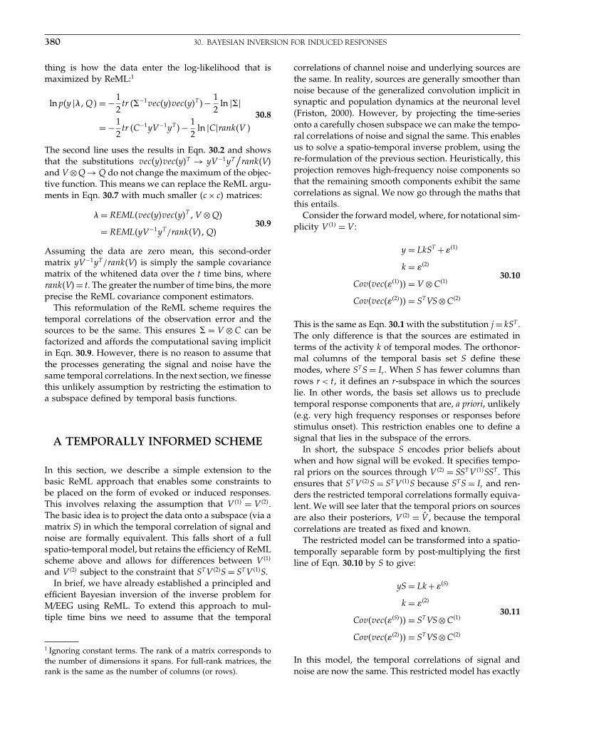
Elsevier UK Chapter: Ch30-P372560 30-9-2006 5:26p.m. Page:380 Trim:7.5in×9.25in
Basal Font:Palatino Margins:Top:40pt Gutter:68pt Font Size:9.5/12 Text Width:42pc Depth:55 Lines
380 30. BAYESIAN INVERSION FOR INDUCED RESPONSES
thing is how the data enter the log-likelihood that ismaximized by ReML:1
ln p�y ���Q� = −12
tr ��−1vec�y�vec�y�T �− 12
ln ���
= −12
tr �C−1yV −1yT �− 12
ln �C�rank�V �
30.8
The second line uses the results in Eqn. 30.2 and showsthat the substitutions vec�y�vec�y�T → yV −1yT
/rank�V�
and V ⊗Q → Q do not change the maximum of the objec-tive function. This means we can replace the ReML argu-ments in Eqn. 30.7 with much smaller �c× c� matrices:
� = REML�vec�y�vec�y�T �V ⊗Q�
= REML�yV −1yT /rank�V��Q�30.9
Assuming the data are zero mean, this second-ordermatrix yV −1yT /rank�V� is simply the sample covariancematrix of the whitened data over the t time bins, whererank�V� = t. The greater the number of time bins, the moreprecise the ReML covariance component estimators.
This reformulation of the ReML scheme requires thetemporal correlations of the observation error and thesources to be the same. This ensures � = V ⊗ C can befactorized and affords the computational saving implicitin Eqn. 30.9. However, there is no reason to assume thatthe processes generating the signal and noise have thesame temporal correlations. In the next section, we finessethis unlikely assumption by restricting the estimation toa subspace defined by temporal basis functions.
A TEMPORALLY INFORMED SCHEME
In this section, we describe a simple extension to thebasic ReML approach that enables some constraints tobe placed on the form of evoked or induced responses.This involves relaxing the assumption that V �1� = V �2�.The basic idea is to project the data onto a subspace (via amatrix S) in which the temporal correlation of signal andnoise are formally equivalent. This falls short of a fullspatio-temporal model, but retains the efficiency of ReMLscheme above and allows for differences between V �1�
and V �2� subject to the constraint that ST V �2�S = ST V �1�S.In brief, we have already established a principled and
efficient Bayesian inversion of the inverse problem forM/EEG using ReML. To extend this approach to mul-tiple time bins we need to assume that the temporal
1 Ignoring constant terms. The rank of a matrix corresponds tothe number of dimensions it spans. For full-rank matrices, therank is the same as the number of columns (or rows).
correlations of channel noise and underlying sources arethe same. In reality, sources are generally smoother thannoise because of the generalized convolution implicit insynaptic and population dynamics at the neuronal level(Friston, 2000). However, by projecting the time-seriesonto a carefully chosen subspace we can make the tempo-ral correlations of noise and signal the same. This enablesus to solve a spatio-temporal inverse problem, using there-formulation of the previous section. Heuristically, thisprojection removes high-frequency noise components sothat the remaining smooth components exhibit the samecorrelations as signal. We now go through the maths thatthis entails.
Consider the forward model, where, for notational sim-plicity V �1� = V :
y = LkST +��1�
k = ��2�
Cov�vec���1��� = V ⊗C�1�
Cov�vec���2��� = ST VS ⊗C�2�
30.10
This is the same as Eqn. 30.1 with the substitution j = kST .The only difference is that the sources are estimated interms of the activity k of temporal modes. The orthonor-mal columns of the temporal basis set S define thesemodes, where ST S = Ir . When S has fewer columns thanrows r < t� it defines an r-subspace in which the sourceslie. In other words, the basis set allows us to precludetemporal response components that are, a priori, unlikely(e.g. very high frequency responses or responses beforestimulus onset). This restriction enables one to define asignal that lies in the subspace of the errors.
In short, the subspace S encodes prior beliefs aboutwhen and how signal will be evoked. It specifies tempo-ral priors on the sources through V �2� = SST V �1�SST . Thisensures that ST V �2�S = ST V �1�S because ST S = Ir and ren-ders the restricted temporal correlations formally equiva-lent. We will see later that the temporal priors on sourcesare also their posteriors, V �2� = V̂ , because the temporalcorrelations are treated as fixed and known.
The restricted model can be transformed into a spatio-temporally separable form by post-multiplying the firstline of Eqn. 30.10 by S to give:
yS = Lk+��S�
k = ��2�
Cov�vec���S��� = ST VS ⊗C�1�
Cov�vec���2��� = ST VS ⊗C�2�
30.11
In this model, the temporal correlations of signal andnoise are now the same. This restricted model has exactly
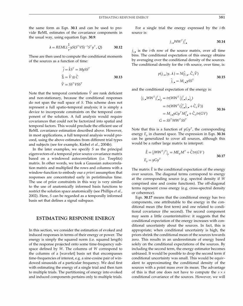
Elsevier UK Chapter: Ch30-P372560 30-9-2006 5:26p.m. Page:381 Trim:7.5in×9.25in
Basal Font:Palatino Margins:Top:40pt Gutter:68pt Font Size:9.5/12 Text Width:42pc Depth:55 Lines
ESTIMATING RESPONSE ENERGY 381
the same form as Eqn. 30.1 and can be used to pro-vide ReML estimates of the covariance components inthe usual way, using equation Eqn. 30.9:
� = REML�1r
yS�ST VS�−1ST yT �Q� 30.12
These are then used to compute the conditional momentsof the sources as a function of time:
ĵ = k̂ST = MySST
�̂ = V̂ ⊗ Ĉ 30.13
V̂ = SST VSST
Note that the temporal correlations V̂ are rank deficientand non-stationary, because the conditional responsesdo not span the null space of S. This scheme does notrepresent a full spatio-temporal analysis; it is simply adevice to incorporate constraints on the temporal com-ponent of the solution. A full analysis would requirecovariances that could not be factorized into spatial andtemporal factors. This would preclude the efficient use ofReML covariance estimation described above. However,in most applications, a full temporal analysis would pro-ceed, using the above estimates from different trial typesand subjects (see for example, Kiebel et al., 2004b).
In the later examples, we specify S as the principaleigenvectors of a temporal prior source covariance matrixbased on a windowed autocorrelation (i.e. Toeplitz)matrix. In other words, we took a Gaussian autocorrela-tion matrix and multiplied the rows and columns with awindow-function to embody our a priori assumption thatresponses are concentrated early in peristimulus time.The use of prior constraints in this way is very similarto the use of anatomically informed basis functions torestrict the solution space anatomically (see Phillips et al.,2002). Here, S can be regarded as a temporally informedbasis set that defines a signal subspace.
ESTIMATING RESPONSE ENERGY
In this section, we consider the estimation of evoked andinduced responses in terms of their energy or power. Theenergy is simply the squared norm (i.e. squared length)of the response projected onto some time-frequency sub-space defined by W . The columns of W correspond tothe columns of a [wavelet] basis set that encompassestime-frequencies of interest, e.g. a sine-cosine pair of win-dowed sinusoids of a particular frequency. We deal firstwith estimating the energy of a single trial and then turnto multiple trials. The partitioning of energy into evokedand induced components pertains only to multiple trials.
For a single trial the energy expressed by the i-thsource is:
ji�•WW T jTi�• 30.14
ji�• is the i-th row of the source matrix, over all timebins. The conditional expectation of this energy obtainsby averaging over the conditional density of the sources.The conditional density for the i-th source, over time, is:
p�ji�• �y��� = N�ĵi�•� ĈiiV̂ �
ĵi�• = Mi�•ySST30.15
and the conditional expectation of the energy is:
⟨ji�•WW T jT
i�•⟩p= tr�WW T
⟨jTi�•ji�•
⟩p�
= tr�WW T �ĵTi�• ĵi�• + ĈiiV̂ ��
= Mi�•yGyT MTi�• + Ĉiitr�GV�
G = SST WW T SST
30.16
Note that this is a function of yGyT , the correspondingenergy Ey in channel space. The expression in Eqn. 30.16can be generalized to cover all sources, although thiswould be a rather large matrix to interpret:
Ê = ⟨jWW T jT
⟩p= MEyM
T + Ĉtr�GV �
Ey = yGyT30.17
The matrix Ê is the conditional expectation of the energyover sources. The diagonal terms correspond to energyat the corresponding source (e.g. spectral density if Wcomprised sine and cosine functions). The off-diagonalterms represent cross energy (e.g. cross-spectral densityor coherence).
Eqn. 30.17 means that the conditional energy has twocomponents, one attributable to the energy in the con-ditional mean (the first term) and one related to condi-tional covariance (the second). The second componentmay seem a little counterintuitive: it suggests that theconditional expectation of the energy increases with con-ditional uncertainty about the sources. In fact, this isappropriate; when conditional uncertainty is high, thepriors shrink the conditional mean of the sources towardszero. This results in an underestimate of energy basedsolely on the conditional expectations of the sources. Byincluding the second term, the energy estimator becomesunbiased. It would be possible to drop the second term ifconditional uncertainty was small. This would be equiv-alent to approximating the conditional density of thesources with a point mass over its mean. The advantageof this is that one does not have to compute the s × sconditional covariance of the sources. However, we will
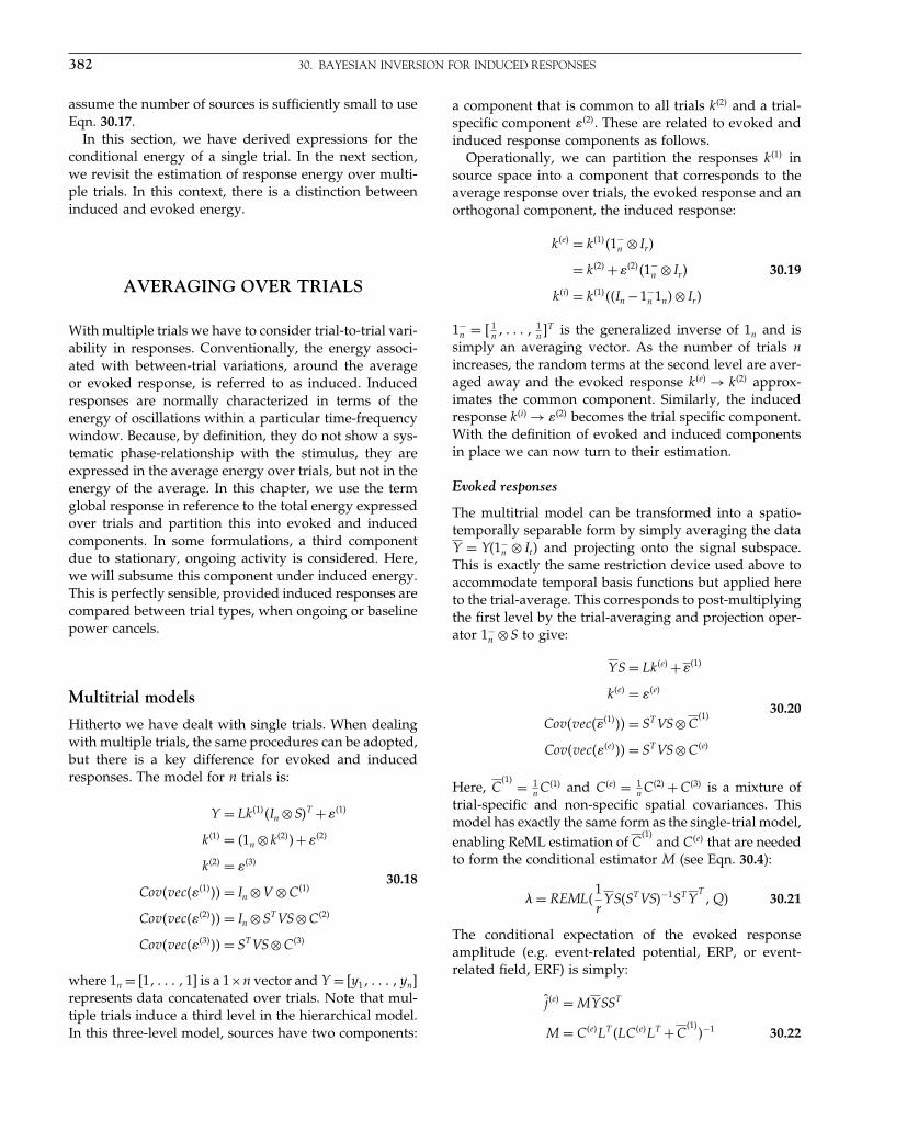
Elsevier UK Chapter: Ch30-P372560 30-9-2006 5:26p.m. Page:382 Trim:7.5in×9.25in
Basal Font:Palatino Margins:Top:40pt Gutter:68pt Font Size:9.5/12 Text Width:42pc Depth:55 Lines
382 30. BAYESIAN INVERSION FOR INDUCED RESPONSES
assume the number of sources is sufficiently small to useEqn. 30.17.
In this section, we have derived expressions for theconditional energy of a single trial. In the next section,we revisit the estimation of response energy over multi-ple trials. In this context, there is a distinction betweeninduced and evoked energy.
AVERAGING OVER TRIALS
With multiple trials we have to consider trial-to-trial vari-ability in responses. Conventionally, the energy associ-ated with between-trial variations, around the averageor evoked response, is referred to as induced. Inducedresponses are normally characterized in terms of theenergy of oscillations within a particular time-frequencywindow. Because, by definition, they do not show a sys-tematic phase-relationship with the stimulus, they areexpressed in the average energy over trials, but not in theenergy of the average. In this chapter, we use the termglobal response in reference to the total energy expressedover trials and partition this into evoked and inducedcomponents. In some formulations, a third componentdue to stationary, ongoing activity is considered. Here,we will subsume this component under induced energy.This is perfectly sensible, provided induced responses arecompared between trial types, when ongoing or baselinepower cancels.
Multitrial models
Hitherto we have dealt with single trials. When dealingwith multiple trials, the same procedures can be adopted,but there is a key difference for evoked and inducedresponses. The model for n trials is:
Y = Lk�1��In ⊗S�T +��1�
k�1� = �1n ⊗k�2��+��2�
k�2� = ��3�
Cov�vec���1��� = In ⊗V ⊗C�1�
Cov�vec���2��� = In ⊗ST VS ⊗C�2�
Cov�vec���3��� = ST VS ⊗C�3�
30.18
where 1n = 1� � � � � 1 is a 1×n vector and Y = y1� � � � � ynrepresents data concatenated over trials. Note that mul-tiple trials induce a third level in the hierarchical model.In this three-level model, sources have two components:
a component that is common to all trials k�2� and a trial-specific component ��2�. These are related to evoked andinduced response components as follows.
Operationally, we can partition the responses k�1� insource space into a component that corresponds to theaverage response over trials, the evoked response and anorthogonal component, the induced response:
k�e� = k�1��1−n ⊗ Ir �
= k�2� +��2��1−n ⊗ Ir � 30.19
k�i� = k�1���In −1−n 1n�⊗ Ir �
1−n = 1
n� � � � � 1
nT is the generalized inverse of 1n and is
simply an averaging vector. As the number of trials nincreases, the random terms at the second level are aver-aged away and the evoked response k�e� → k�2� approx-imates the common component. Similarly, the inducedresponse k�i� → ��2� becomes the trial specific component.With the definition of evoked and induced componentsin place we can now turn to their estimation.
Evoked responses
The multitrial model can be transformed into a spatio-temporally separable form by simply averaging the dataY = Y�1−
n ⊗ It� and projecting onto the signal subspace.This is exactly the same restriction device used above toaccommodate temporal basis functions but applied hereto the trial-average. This corresponds to post-multiplyingthe first level by the trial-averaging and projection oper-ator 1−
n ⊗S to give:
YS = Lk�e� +��1�
k�e� = ��e�
Cov�vec���1��� = ST VS ⊗C�1�
Cov�vec���e��� = ST VS ⊗C�e�
30.20
Here, C�1� = 1
nC�1� and C�e� = 1
nC�2� + C�3� is a mixture of
trial-specific and non-specific spatial covariances. Thismodel has exactly the same form as the single-trial model,enabling ReML estimation of C
�1�and C�e� that are needed
to form the conditional estimator M (see Eqn. 30.4):
� = REML�1r
YS�ST VS�−1ST YT�Q� 30.21
The conditional expectation of the evoked responseamplitude (e.g. event-related potential, ERP, or event-related field, ERF) is simply:
ĵ�e� = MYSST
M = C�e�LT �LC�e�LT +C�1�
�−1 30.22

Elsevier UK Chapter: Ch30-P372560 30-9-2006 5:26p.m. Page:383 Trim:7.5in×9.25in
Basal Font:Palatino Margins:Top:40pt Gutter:68pt Font Size:9.5/12 Text Width:42pc Depth:55 Lines
SOME EXAMPLES 383
C�1� =∑
��1�i Q�1�
i
C�e� =∑��e�
i Q�e�i
The conditional expectation of evoked power is then:
Ê�e� = ME�e�y MT + Ĉtr�GV�
E�e�y = YGY
T
Ĉ = �LT C�1�−1
L+C�e�−1�−1
30.23
where E�e�y is the evoked cross-energy in channel space.
In short, this is exactly the same as a single-trial analysisbut using the channel-data averaged over trials. How-ever, this averaging is not appropriate for the inducedresponses considered next.
Induced responses
To isolate and characterize induced responses, we effec-tively subtract the evoked response from all trials to giveỸ = Y��In − 1−
n 1n� ⊗ It�, and project this mean-correcteddata onto the signal subspace. The average covariance ofthe ensuing data is then decomposed using ReML. Thisentails post-multiplying the first level of the multi-trialmodel by �In −1−
n 1n�⊗S to give:
Ỹ �In ⊗S� = Lk�i� + �̃�1�
k�i� = ��i�
Cov�vec��̃�1��� = In ⊗ST VS ⊗ C̃�1�
Cov�vec���i��� = In ⊗ST VS ⊗C�i�
30.24
In this transformation k�i� is a large s × nr matrix thatcovers all trials. Again, this model has the same spatio-temporally separable form as the previous models,enabling an efficient ReML estimation of the covariancecomponents of C̃�1� and C�i�:
� = REML�1nr
Ỹ �In ⊗S�ST VS�−1ST �Ỹ T �Q� 30.25
The first argument of the ReML function is just the covari-ance of the whitened, mean-corrected data averaged overtrials. The conditional expectation of induced energy, pertrial, is then:
�i� = 1n
MỸ �In ⊗G�Ỹ T MT + 1n
Ĉtr�In ⊗GV�
= ME�i�y MT + Ĉtr�GV�
E�i�y = 1
nỸ �In ⊗G�Ỹ T
30.26
where E�i�y is the induced cross-energy per trial, in channel
space. The spatial conditional projector M and covari-ance Ĉ are defined as above (Eqn. 30.22 and Eqn. 30.23).
Although it would be possible to estimate the amplitudeof induced responses for each trial, this is seldominteresting.
Summary
The key thing to take from this section is that the esti-mation of evoked responses involves averaging overtrials and estimating the covariance components. Con-versely, the analysis of induced responses involves esti-mating covariance components and then averaging. Inboth cases, the iterative ReML scheme operates on smallc× c matrices.
The various uses of the ReML scheme and conditionalestimators are shown schematically in Figure 30.1. Notethat all applications, be they single-trial or trial-average,estimates of evoked responses or induced energy, reston a two-stage procedure in which ReML covariancecomponent estimators are used to form conditional esti-mators of the sources. The second thing to take fromthis figure is that the distinction between evoked andinduced responses only has meaning in the context ofmultiple trials. This distinction rests on an operationaldefinition, established in the decomposition of responseenergy in channel space. The corresponding decomposi-tion in source space affords the simple and efficient esti-mation of evoked and induced power described in thissection. However, it is interesting to note that conditionalestimators of evoked and induced components are notestimates of the fixed k�2� and random ��2� effects in thehierarchical model. These estimates would require a fullmixed-effects analysis. Another interesting issue is thatevoked and induced responses in channel space (wherethere is no estimation per se) represent a bi-partitioning ofglobal responses. This is not the case for their conditionalestimates in source space. In other words, the conditionalestimate of global power is not necessarily the sum of theconditional estimates of evoked and induced power.
SOME EXAMPLES
In this section, we illustrate the above procedures usingtoy and real data. The objective of the toy example isto clarify the nature of the operators and matrices, tohighlight the usefulness of restricting the signal spaceand to show, algorithmically, how evoked and inducedresponses are recovered. The real data are presented toestablish a degree of face validity, given that face-relatedresponses have been fully characterized in terms of theirfunctional anatomy. The toy example deals with the

Elsevier UK Chapter: Ch30-P372560 30-9-2006 5:26p.m. Page:384 Trim:7.5in×9.25in
Basal Font:Palatino Margins:Top:40pt Gutter:68pt Font Size:9.5/12 Text Width:42pc Depth:55 Lines
384 30. BAYESIAN INVERSION FOR INDUCED RESPONSES
FIGURE 30.1 ReML scheme: schematic showing the various applications of the ReML scheme in estimating evoked and inducedresponses in multiple trials. See main text for an explanation of the variables.
single-trial case and the real data, looking for face-specificresponses, illustrates the multi-trial case.
Toy example
We generated data according to the model in Eqn. 30.10using s = 128 sources, c = 16 channels and t = 64 timebins. The lead field L was a matrix of random Gaussianvariables. The spatial covariance components comprised:
Q�1�1 = Ic
Q�2�1 = DDT
Q�2�2 = DFDT 30.27
where D was a spatial convolution or dispersion opera-tor, using a Gaussian kernel with a standard deviation
of four voxels. This can be considered a smoothness orspatial coherence constraint. F represents structural orfunctional MRI constraints and was a leading diagonalmatrix encoding the prior probability of a source at eachvoxel. This was chosen randomly by smoothing a ran-dom Gaussian sequence raised to the power four. Thenoise was assumed to be identically and independentlydistributed, V �1� = V = It. The signal subspace in timeS was specified by the first r = 8 principal eigenvectorsof a Gaussian autocorrelation matrix of standard devia-tion two, windowed with a function of peristimulus timet2 exp�−t/8�. This constrains the prior temporal correla-tion structure of the sources V �2� = SST VSST , which aresmooth and restricted to earlier time bins by the window-function.
The hyperparameters were chosen to emphasize theMRI priors � = ��1�
1 ���2�1 ���2�
2 = 1� 0� 8 and provide asignal to noise of about one, measured as the ratio of the
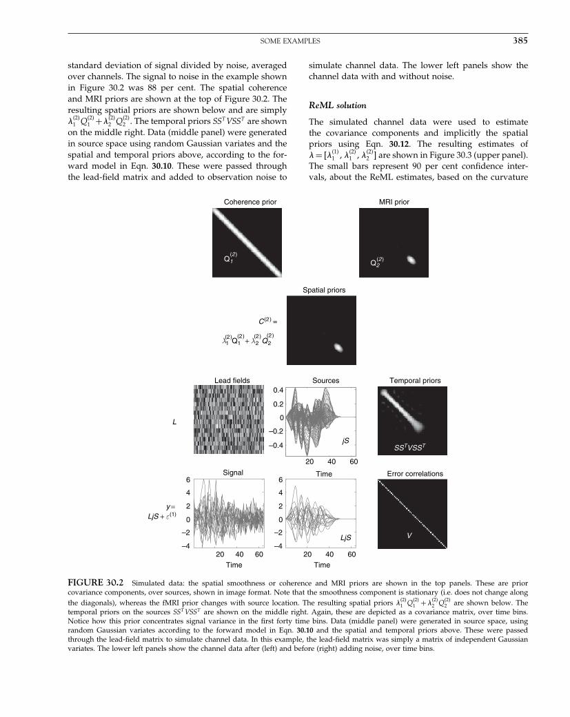
Elsevier UK Chapter: Ch30-P372560 30-9-2006 5:26p.m. Page:385 Trim:7.5in×9.25in
Basal Font:Palatino Margins:Top:40pt Gutter:68pt Font Size:9.5/12 Text Width:42pc Depth:55 Lines
SOME EXAMPLES 385
standard deviation of signal divided by noise, averagedover channels. The signal to noise in the example shownin Figure 30.2 was 88 per cent. The spatial coherenceand MRI priors are shown at the top of Figure 30.2. Theresulting spatial priors are shown below and are simply��2�
1 Q�2�1 +��2�
2 Q�2�2 . The temporal priors SST VSST are shown
on the middle right. Data (middle panel) were generatedin source space using random Gaussian variates and thespatial and temporal priors above, according to the for-ward model in Eqn. 30.10. These were passed throughthe lead-field matrix and added to observation noise to
simulate channel data. The lower left panels show thechannel data with and without noise.
ReML solution
The simulated channel data were used to estimatethe covariance components and implicitly the spatialpriors using Eqn. 30.12. The resulting estimates of� = ��1�
1 ���2�1 ���2�
2 are shown in Figure 30.3 (upper panel).The small bars represent 90 per cent confidence inter-vals, about the ReML estimates, based on the curvature
Coherence prior MRI prior
–0.4
–0.2
0
0.2
0.4Sources Temporal priorsLead fields
Error correlations
Spatial priors
20 40 60–4
–2
0
2
4
6
Time
–4
–2
0
2
4
6Signal
20 40 60
Time
Q1 Q2
C
(2 ) =
SSTVSST
V
L
y =
LjS + ε
(1)
jS
LjS
20 40 60
Time
(2 )
(2 )
λ1 Q1 + λ 2 Q 2(2 ) (2 ) (2 ) (2 )
FIGURE 30.2 Simulated data: the spatial smoothness or coherence and MRI priors are shown in the top panels. These are priorcovariance components, over sources, shown in image format. Note that the smoothness component is stationary (i.e. does not change alongthe diagonals), whereas the fMRI prior changes with source location. The resulting spatial priors �
�2�1 Q
�2�1 + �
�2�2 Q
�2�2 are shown below. The
temporal priors on the sources SST VSST are shown on the middle right. Again, these are depicted as a covariance matrix, over time bins.Notice how this prior concentrates signal variance in the first forty time bins. Data (middle panel) were generated in source space, usingrandom Gaussian variates according to the forward model in Eqn. 30.10 and the spatial and temporal priors above. These were passedthrough the lead-field matrix to simulate channel data. In this example, the lead-field matrix was simply a matrix of independent Gaussianvariates. The lower left panels show the channel data after (left) and before (right) adding noise, over time bins.

Elsevier UK Chapter: Ch30-P372560 30-9-2006 5:26p.m. Page:386 Trim:7.5in×9.25in
Basal Font:Palatino Margins:Top:40pt Gutter:68pt Font Size:9.5/12 Text Width:42pc Depth:55 Lines
386 30. BAYESIAN INVERSION FOR INDUCED RESPONSES
True prior spatial covariance
–5
0
5
10
True and estimated covariance parameters
Estimated prior spatial covariance
λ1 λ1 λ 2
C
(2) =
λ1 Q1 +λ 2 Q2
(1) (2) (2)
(2) (2) (2) (2)
FIGURE 30.3 ReML solution: the ReML estimates of � =�
�1�1 ��
�2�1 ��
�2�2 are shown in the upper panel. The small bars rep-
resent 90 per cent confidence intervals about the ReML estimates,based on the curvature of the log likelihood. The large bars are thetrue values. The ReML scheme correctly assigns more weight tothe MRI priors to provide the empirical prior in the lower panel(left). This ReML estimate is virtually indistinguishable from thetrue prior (right).
of the log-likelihood in Eqn. 30.7. The large bars are thetrue values. The ReML scheme correctly assigns muchmore weight to the MRI priors to provide the empiricalprior in the lower panel (left). This ReML estimate (left)is virtually indistinguishable from the true prior (right).
Conditional estimates of responses
The conditional expectations of sources, over time, areshown in Figure 30.4 using the expression in Eqn. 30.13.The upper left panel shows the true and estimated spa-tial profile at the time bin expressing the largest activ-ity (maximal deflection). The equivalent source estimate,over time, is shown on the right. One can see the charac-teristic shrinkage of the conditional estimators, in relationto the true values. The full spatio-temporal profiles areshown in the lower panels.
Conditional estimates of response energy
To illustrate the estimation of energy, we defined atime-frequency window W = w�t� sin��t��w�t� cos��t�for one frequency, �, over a Gaussian time window, w�t�.
20 40 60 80 100 120
-0.1
0
0.1
0.2
0.3
0.4
True and estimated signal
Source20 40 60
-0.4
-0.2
0
0.2
0.4
True and estimated signal
Time
trueMAP
Dip
ole
Time
Estimated source
20 40 60
20
40
60
80
100
120
Dip
ole
Time
True source
20 40 60
20
40
60
80
100
120
Sĵ jS
FIGURE 30.4 Conditional estimates of responses: the upperpanel shows the true and estimated spatial profile at the time binexpressing the largest activity (upper left). The equivalent profile,over time, is shown on the upper right for the source expressingthe greatest response. These graphs correspond to sections (dottedlines) though the full spatio-temporal profiles shown in image for-mat (lower panels). Note the characteristic shrinkage of the MAPestimates, relative to the true values, that follows from the use ofshrinkage priors (that shrink the conditional expectations to theprior mean of zero).
This time-frequency subspace is shown in the upper pan-els of Figure 30.5. The corresponding energy was esti-mated using Eqn. 30.17 and is shown, with the true val-ues, in the lower panels. The agreement is evident.
Analysis of real data
We used MEG data from a single subject while theymade symmetry judgements on faces and scrambledfaces (for a detailed description of the paradigm seeHenson et al., 2003). MEG data were sampled at 625 Hzfrom a 151-channel CTF Omega system at the WellcomeTrust Laboratory for MEG Studies, Aston University,UK. The epochs (80 face trials, collapsing across famil-iar and unfamiliar faces, and 84 scrambled trials) were

Elsevier UK Chapter: Ch30-P372560 30-9-2006 5:26p.m. Page:387 Trim:7.5in×9.25in
Basal Font:Palatino Margins:Top:40pt Gutter:68pt Font Size:9.5/12 Text Width:42pc Depth:55 Lines
SOME EXAMPLES 387
0 20 40 60 80
Time-frequency subspace
Time (ms)
Time-frequency subspace
10
20
30
40
50
60
W
Estimated [cross] energy True [cross] energy
)(ˆˆ GVtrCMMyGyE TT +=TjGjE =
20 40 60 80 100 1200
0.005
0.01
0.015
0.02
Source
EstimatedTrue energy
Diag (E )ˆ
FIGURE 30.5 Conditional estimates of response energy: atime-frequency subspace W is shown in the upper panels as func-tions of time (left) and in image format (right). This subspace definesthe time-frequency response of interest. In this example, we are test-ing for frequency-specific responses between 10 and 20 time bins.The corresponding energy estimates are shown over sources, withthe true values, in the middle panel. Note the remarkable corre-spondence. The lower panels show the cross-energy over sources,with estimates on the left and true values on the right. The energiesin the middle panel are the leading diagonals of the cross-energymatrices, shown as images below. Again, note the formal similaritybetween the true and estimated cross-energies.
baseline-corrected from −100 ms to 0 ms. The 500 ms,after stimulus onset, of each trial entered the analysis.A T1-weighted MRI was also obtained with a resolu-tion 1×1×1 mm3. Head-shape was digitized with a 3-DPolhemus Isotrak and used to co-register the MRI andMEG data. A segmented cortical mesh was created usingAnatomist (Mangin et al., 2004), with approximately 4000dipoles oriented normal to the grey matter. Finally, asingle-shell spherical head model was constructed using
BrainStorm (Baillet et al., 2004) to compute the forwardoperator L.
The spatial covariance components comprised:
Q�1�1 = Ic
Q�2�1 = DDT
30.28
where spatial smoothness operator D was defined onthe cortical mesh, using a Gaussian kernel with a stan-dard deviation of 8 mm. Note we used only one, rathersmooth, spatial component in this analysis. This was forsimplicity. A more thorough analysis would use multiplecomponents and Bayesian model selection to choose theoptimum number of components (Mattout et al., 2006).As with the simulated data analysis, the noise correla-tions were assumed to be identical and independentlydistributed, V �1� = It, and the signal subspace in time Swas specified by the first r = 50 principal eigenvectors ofthe windowed autocorrelation matrix used above.
We focused our analysis on the earliest reliable differ-ence between faces and scrambled faces, as characterizedby the M170 component in the ERF (Plate 41(c) – seecolour plate section). A frequency band of 10–15 Hz waschosen on the basis of reliable differences (p < 0 01; cor-rected) in a statistical parametric map (time-frequencySPM) of the global energy differences (Plate 41(b)) aroundthe M170 latency (Henson et al., 2005a). The ensuing time-frequency subspace was centred at 170 ms (Plate 41(c)).
Results
Plate 41(d) shows evoked and induced power in chan-nel space as defined in Eqn. 30.23 and Eqn. 30.26respectively. Power maps were normalized to the samemaximum for display. In both conditions, maximumpower is located over the right temporal regions. How-ever, the range of power values is much wider for theevoked response. Moreover, whereas scalp topographiesof induced responses are similar between conditions,the evoked energy is clearly higher for faces, relative toscrambled faces. This suggests that the M170 is mediatedby differences in phase-locked activity.
This is confirmed by the power analysis in source space(Plate 42), using Eqn. 30.23 and Eqn. 30.26. Evoked andinduced responses are generated by the same set of corti-cal regions. However, the differences between faces andscrambled faces, in terms of induced power, are weakcompared to the equivalent differences in evoked power(see the scale bars in Plate 42). Furthermore, the varia-tion in induced energy over channels and conditions issmall, relative to evoked power. This non-specific profilesuggests that ongoing activity may contribute substan-tially to the induced component. As mentioned above,the interesting aspect of induced power usually resides in

Elsevier UK Chapter: Ch30-P372560 30-9-2006 5:26p.m. Page:388 Trim:7.5in×9.25in
Basal Font:Palatino Margins:Top:40pt Gutter:68pt Font Size:9.5/12 Text Width:42pc Depth:55 Lines
388 30. BAYESIAN INVERSION FOR INDUCED RESPONSES
trial-specific differences. A full analysis of induced differ-ences will be presented elsewhere. Here we focus on thefunctional anatomy implied by evoked differentials. Thefunctional anatomy of evoked responses, in this context,is sufficiently well known to establish the face validity ofour conditional estimators:
The upper panel of Plate 43 shows the cortical projec-tion of the difference between the conditional expecta-tions of evoked energy, for faces versus scrambled faces.The largest changes were expressed in the right infe-rior occipital gyrus (IOG), the right orbitofrontal cortex(OFC) and the horizontal posterior segment of the rightsuperior temporal sulcus (STS). Plate 44 shows the co-registration of these energy changes with the subject’sstructural MRI. Happily, the ‘activation’ of these regionsis consistent with the equivalent comparison of fMRIresponses (Henson et al., 2003).
The activation of the ventral and lateral occipitotempo-ral regions is also consistent with recent localizations ofthe evoked M170 (Henson et al., 2005b; Tanskanen et al.,2005). This is to be expected, given that most of the energychange appears to be phase-locked (Henson et al., 2005a).Indeed, the conditional estimates of evoked responsesat the location of the maximum of energy change inthe right IOG and right posterior STS show a deflectionaround 170 ms that is greater for faces than scrambledfaces (Plate 43, lower panel).
Note we have not made any inferences about theseeffects. SPMs of energy differences would normallybe constructed using conditional estimates of powerchanges over subjects (see Plate 40).
DISCUSSION
We have described an empirical Bayes approach toM/EEG source reconstruction that covers both evokedand induced responses. The estimation scheme is basedon classical covariance component estimation usingrestricted maximum likelihood (ReML). We used tempo-ral basis functions to place constraints on the temporalform of the responses and showed how one can esti-mate evoked responses, which are phase-locked to thestimulus, and induced responses that are not. This inher-ent distinction calls for different transformations of ahierarchical model of multiple trial responses to provideBayesian estimates of power.
Oscillatory activity is well known to be related toneural coding and information processing in the brain(Hari et al., 1997; Tallon-Baudry et al., 1999; Fries et al.,2001). Oscillatory activity refers to signals generated ina particular frequency band time-locked but not neces-sary phase-locked to the stimulus. Classical data aver-
aging approaches may not capture this activity, whichcalls for trial-to-trial analyses. However, localizing thesources of oscillatory activity on a trial-by-trial basisis computationally demanding and requires data withlow SNR. This is why early approaches were limited tochannel space (e.g. Tallon-Baudry et al., 1997). Recently,several inverse algorithms have been proposed to esti-mate the sources of induced oscillations. Most are dis-tributed (or imaging) methods, since equivalent currentdipole models are not suitable for explaining a few hun-dreds of milliseconds of non-averaged activity. Amongdistributed approaches, two main types can be distin-guished: the beam-former (Gross et al., 2001; Sekiharaet al., 2001; Cheyne et al., 2003) and minimum-norm-basedtechniques (David et al., 2002; Jensen and Vanni, 2002),although both can be formulated as (weighted) minimumnorm estimators (Hauk, 2004). A strict minimum normsolution obtains when no weighting matrix is involved(Hamalainen et al., 1993), but constraints such as fMRI-derived priors have been shown to condition the inversesolution (Lin et al., 2004). Beam-former approaches imple-ment a constrained inverse using a set of spatial fil-ters (see Huang et al., 2004 for an overview). The basicprinciple employed by beam-formers is to estimate theactivity at each putative source location while suppress-ing the contribution of other sources. This means thatbeam-formers look explicitly for uncorrelated sources.Although some robustness has been reported in the con-text of partially correlated sources (Van Veen et al., 1997),this aspect of beam-forming can be annoying when tryingto characterize coherent or synchronized cortical sources(Gross et al., 2001).
In this chapter, we have looked at a generalizationof the weighted minimum norm approach based onhierarchical linear models and empirical Bayes, whichcan accommodate multiple priors in an optimal fash-ion (Phillips et al., 2005). The approach involves a par-titioning of the data covariance matrix into noise andprior source variance components, whose relative con-tributions are estimated using ReML. Each model (i.e.set of partitions or components) can be evaluated usingBayesian model selection (Mattout et al., 2006). Moreover,the ReML scheme is computationally efficient, requir-ing only the inversion of small matrices. With tempo-ral constraints, the scheme offers a general Bayesianframework that can incorporate all kind of spatial pri-ors such as beam-former-like spatial filters and/or fMRI-derived constraints (Friston et al., 2006). Furthermore,basis functions enable both the use of computationallyefficient ReML-based variance component estimation andthe definition of priors on the temporal form of theresponse. This implies a separation of the temporal andspatial dependencies, at both the sensor and source lev-els, using a Kronecker formulation (Huizenga et al., 2002).

Elsevier UK Chapter: Ch30-P372560 30-9-2006 5:26p.m. Page:389 Trim:7.5in×9.25in
Basal Font:Palatino Margins:Top:40pt Gutter:68pt Font Size:9.5/12 Text Width:42pc Depth:55 Lines
REFERENCES 389
Thanks to this spatio-temporal approximation, the esti-mation of induced responses, from multi-trial data, doesnot require a computationally demanding trial-by-trialapproach (Jensen et al., 2002) or drastic dimension reduc-tion of the solution space (David et al., 2002).
The approach described in this chapter allows forspatio-temporal modelling of evoked and inducedresponses under the assumption that there is a subspaceS, in which temporal correlations among the data andsignal have the same form. Clearly, this subspace shouldencompass as much of the signal as possible. In this work,we used the principal eigenvariates of a prior covariancebased on smooth signals, concentrated early in peristim-ulus time. This subspace is therefore informed by priorassumptions about how and when signal is expressed. Akey issue here is what would happen if the prior subspacedid not coincide with the true signal subspace. In thisinstance, there may be a loss of efficiency as experimen-tal variance is lost to the null space of S. However, therewill be no bias in the [projected] response estimates. Sim-ilarly, the estimate of the error covariance componentswill be unbiased but lose efficiency as high frequencynoise components are lost in the restriction. Put simply,this means the variability in the covariance parameterestimates will increase, leading to a slight overconfidencein conditional inference. The overconfidence problem isnot an issue here because we are only interested in theconditional expectations, which would normally be takento a further (between-subject) level for inference.
Importantly, statistical parametric mapping of the esti-mated power changes in a particular time-frequency win-dow, over conditions and/or over subjects, can now beachieved at the cortical level (Brookes et al., 2004; Kiebelet al., 2004a). Finally, with the appropriate wavelet trans-formation, instantaneous power and phase could also beestimated in order to study cortical synchrony.
In the previous three chapters, we considered theinversion of electromagnetic models to estimate currentsources. In the next three chapters, we turn to modelsof how neuronal dynamics generate the activity in thesesources. The neuronal and electromagnetic models of thissection are combined later (Chapter 42) in the dynamiccausal modelling of measured M/EEG responses.
REFERENCES
Amblard C, Lapalme E, Lina JM (2004) Biomagnetic source detectionby maximum entropy and graphical models. IEEE Trans BiomedEng 51: 427–42
Babiloni F, Babiloni C, Carducci F et al. (2004) Multimodal integra-tion of EEG and MEG data: a simulation study with variablesignal-to-noise ratio and number of sensors. Hum Brain Mapp 14:197–209
Baillet S, Garnero L (1997) A Bayesian approach to introducinganatomo-functional priors in the EEG/MEG inverse problem.IEEE Trans Biomed Eng 44: 374–85
Baillet S, Mosher JC, Leahy RM (2004) Electromagnetic brain imag-ing using Brainstorm. Proceedings of the IEEE InternationalSymposium on Biomedical Imaging (ISBI) 1: 652–5
Brookes MJ, Gibson AM, Hall SD et al. (2005) A general linear modelfor MEG beam former imaging. NeuroImage 23: 936-46
Cheyne D, Gaetz W, Garnero L et al. (2003) Neuromagnetic imagingof cortical oscillations accompanying tactile stimulation. CognBrain Res 17: 599–611
Dale AM, Sereno M (1993) Improved localization of cortical activityby combining EEG and MEG with MRI surface reconstruction:a linear approach. J Cogn Neurosci 5: 162–76
Dale AM, Liu AK, Fischl BR et al. (2000) Dynamic statistical para-metric mapping: combining fMRI and MEG for high-resolutionimaging of cortical activity. Neuron 26: 55–67
Daunizeau J, Mattout J, Clonda D, et al. (2006) Bayesian spatio-temporal approach for EEG-source reconstruction: conciliatingECD and distributed models. IEEE Trans Biomed Eng 53: 503–16
David O, Garnero L, Cosmelli D et al. (2002) Estimation of neuraldynamics from MEG/EEG cortical current density maps: appli-cation to the reconstruction of large-scale cortical synchrony.IEEE Trans Biomed Eng 49: 975–87
Dietterich TG (2000) Ensemble methods in machine learning. Pro-ceedings of the First International Workshop on Multiple ClassifierSystems, Lecture Notes in Computer Science, Springer-Verlag
Fries P, Reynolds JH, Rorie AE et al. (2001) Modulation of oscillatoryneuronal synchronization by selective visual attention. Science291: 1506–07
Friston KJ (2000) The labile brain I. Neuronal transients and nonlin-ear coupling. Phil Trans R Soc Lond B 355: 215–36
Friston KJ, Penny W, Phillips C et al. (2002) Classical and Bayesianinference in neuroimaging: theory. NeuroImage 16: 465–83
Friston KJ, Mattout J, Trujillo-Barreto N et al. (2006) Variational freeenergy and the Laplace approximation, NeuroImage (in Press)
Gorodnitsky LF, George JS, Rao BD (1995) Neuromagnetic sourceimaging with FOCUSS: a recursive weighted minimum normalgorithm. Electroencephalogr Clin Neurophysiol 95: 231–51
Gross J, Kujala J, Hamalainen M et al. (2001) Dynamic imagingof coherent sources: studying neural interactions in the humanbrain. Proc Natl Acad Sci 98: 694–99
Hamalainen MS, Hari R, Ilmoniemi R et al. (1993) Magnetoen-cephalography: theory, instrumentation and applications to non-invasive study of human brain functions. Rev Mod Phys 65:413–97
Hamalainen MS, Ilmoniemi RJ (1994) Interpreting magnetic fieldsof the brain – minimum norm estimates. Med Biol Eng Comput32: 35–42
Hari R, Salmelin R (1997) Human cortical oscillations: a neuromag-netic view through the skull. Trends Neurosci 20: 44–49
Hauk O (2004) Keep it simple: a case for using classical mini-mum norm estimation in the analysis of EEG and MEG data.NeuroImage 21: 1612–21
Henson RN, Goshen-Gottstein Y, Ganel T et al. (2003) Electrophysi-ological and haemodynamic correlates of face perception, recog-nition and priming. Cereb Cortex 13: 793–805
Henson R, Kiebel S, Kilner J et al. (2005a) Time-frequency SPMs forMEG data on face perception: power changes and phase-locking.Human Brain Mapping Conference (HBM’05)
Henson R, Mattout J, Friston K et al. (2005b) Distributed source local-ization of the M170 using multiple constraints. Human BrainMapping Conference (HBM’05)
Elsevier UK Chapter: Ch30-P372560 30-9-2006 5:26p.m. Page:390 Trim:7.5in×9.25in
Basal Font:Palatino Margins:Top:40pt Gutter:68pt Font Size:9.5/12 Text Width:42pc Depth:55 Lines
390 30. BAYESIAN INVERSION FOR INDUCED RESPONSES
Huang M-X, Shih JJ, Lee DL et al. (2004) Commonalities and differ-ences among vectorized beamformers in electromagnetic sourceimaging. Brain Topogr 16: 139–58
Huizenga HM, de Munk JC, Waldorp LJ et al. (2002) Spatio-temporalEEG/MEG source analysis based on a parametric noise covari-ance model. IEEE Trans Biomed Eng 49: 533–39
Jensen O, Vanni S (2002) A new method to identify sources of oscil-latory activity from magnetoencephalographic data. NeuroImage15: 568–74
Jerbi K, Baillet S, Mosher JC et al. (2004) Localization of realisticcortical activity in MEG using current multipoles. NeuroImage22: 779–93
Kiebel SJ, Friston KJ (2004a) Statistical parametric mapping forevent-related potentials: I. Generic considerations. NeuroImage22: 492–502
Kiebel SJ, Friston KJ (2004b) Statistical parametric mapping forevent-related potentials: II. A hierarchical temporal model. Neu-roImage 22: 503–20
Kilner JM, Kiebel SJ, Friston KJ (2005) Applications of random fieldtheory to electrophysiology. Neurosci Lett 374: 174–78
Lin F-H, Witzel T, Hamalainen MS et al. (2004) Spectral spatio-temporal imaging of cortical oscillations and interactions in thehuman brain. NeuroImage 23: 582–95
Mangin JF, Riviere D, Cachia A et al. (2004) A framework to studythe cortical folding patterns. NeuroImage 23: 129–38
Mattout J, Pélégrini-Issac M, Garnero L et al. (2005) Multivariatesource prelocalization (MSP): use of functionally informed basisfunctions for better conditioning the MEG inverse problem. Neu-roImage 26: 356–73
Mattout J, Phillips C, Penny WD et al. (2006) MEG source localizationunder multiple constraints: an extended Bayesian framework.NeuroImage 30: 753–67
Nunez PL, Silberstein RB (2000) On the relationship of synapticactivity to macroscopic measurements: does co-registration ofEEG with fMRI make sense? Brain Topogr 13: 79–96
Pascual-Marqui RD, Michel CM, Lehmann D (1994) Low resolu-tion electromagnetic tomography: a new method for localizingelectrical activity in the brain. IEEE Trans Biomed Eng 418: 49–65
Phillips C, Rugg MD, Friston KJ (2002) Anatomically informed basisfunctions for EEG source localization: combining functional andanatomical constraints. NeuroImage 16: 678–95
Phillips C, Mattout J, Rugg MD et al. (2005) An empirical Bayesiansolution to the source reconstruction problem in EEG. NeuroIm-age 24: 997–1011
Riera JJ, Fuentes ME, Valdes PA et al. (1998) EEG distributed inversesolutions for a spherical head model. Inverse Problems 14: 1009–19
Schmidt D, George J, Wood C (1999) Bayesian inference appliedto the electromagnetic inverse problem. Hum Brain Mapp 7:195–212
Sekihara K, Nagarajan SS, Poeppel D et al. (2001) Reconstructingspatio-temporal activities of neural sources using an MEG vectorbeamformer technique. IEEE Trans Biomed Eng 48: 760–71
Tallon-Baudry C, Bertrand O (1999) Oscillatory gamma activity inhumans and its role in object representation. Trends Cogn Sci 3:151–62
Tallon-Baudry C, Bertrand O, Delpuech C et al. (1997) Oscillatory�-band (30–70 Hz) activity induced by a visual search task inhumans. J Neurosci 17: 722–34
Tanskanen T, Nasanen R, Montez T et al. (2005) Face recognitionand cortical responses show similar sensitivity to noise spatialfrequency. Cereb Cortex 15: 526–34
Van Veen BD, van Drongelen W, Yuchtman M et al. (1997) Localiza-tion of brain electrical activity via linearly constrained minimumvariance spatial filtering. IEEE Trans Biomed Eng 44: 867–80

Elsevier UK Chapter: Ch31-P372560 30-9-2006 5:26p.m. Page:391 Trim:7.5in×9.25in
Basal Font:Palatino Margins:Top:40pt Gutter:68pt Font Size:9.5/12 Text Width:42pc Depth:55 Lines
C H A P T E R
31
Neuronal models of ensemble dynamicsL. Harrison, O. David and K. Friston
INTRODUCTION
In this chapter, we introduce some of the basis princi-ples behind modelling ensemble or population dynam-ics. In particular, we focus on mean-field approximationsthat allow one to model the evolution of states aver-aged over large numbers of neurons that are assumed torespond similarly to external influences. This is the basisof the neural mass models used in subsequent chaptersto model interactions among subpopulations that consti-tute sources of measured brain signals. These models areimportant because they are parameterized in biologicalterms. This means their inversion allows one to ask ques-tions that are framed in terms of biological processes,rather than at a purely phenomenological level.
Neuronal responses are the product of coupling amongneuronal populations. Sensory information is encodedand distributed among neuronal ensembles in a way thatdepends on biophysical parameters that control this cou-pling. Because coupling can be modulated by experimen-tal factors, estimates of coupling parameters provide asystematic way to parameterize experimentally inducedresponses. This chapter is about biologically informedmodels that embed this coupling.
The electrical properties of nervous tissue derivefrom the electrochemical activity of coupled neu-rons that generate current sources within the cortex,which can be estimated from multiple scalp electrodeelectroencephalography (EEG) recordings. These electri-cal traces express large-scale coordinated patterns of elec-trical activity. There are two commonly used methodsto characterize event-related changes in these signals:averaging over many traces to form event-related poten-tials (ERP) and calculating the spectral profile of ongoingoscillatory activity (cf. evoked and induced responses).The assumption implicit in the averaging procedure isthat the evoked signal has a fixed temporal relationshipto the stimulus, whereas the latter procedure relaxes this
assumption (Pfurtscheller and Lopes da Silva, 1999). Wewill return to this distinction, using neural-mass models,in Chapter 33.
Particular characteristics of ERPs are associated withcognitive states, e.g. the mismatch negativity in auditoryoddball paradigms (Winkler et al., 2001). The changes inERP evoked by an ‘event’ are assumed to reflect event-dependent changes in cortical processing. In a similarway, spectral peaks of ongoing oscillations are generallythought to reflect the degree of synchronization amongoscillating neuronal populations, with specific changesin the spectral profile being associated with variouscognitive states. These changes have been called event-related desynchronization (ERD) and event-related syn-chronization (ERS). ERD is associated with an increasein processing information, e.g. voluntary hand move-ment (Pfurtscheller, 2001), whereas ERS is associatedwith reduced processing, e.g. during little or no motorbehaviour. These observations led to the thesis that ERDrepresents increased cortical excitability and converselythat ERS reflects deactivation. We will look at this fromthe point of view neuronal energetics and relationship tometabolic activation in the next chapter.
The conventional approach to interpreting the EEGin terms of computational processes (Churchland andSejnowski, 1994), is to correlate task-dependent changesin the ERP or time-frequency profiles of ongoing activ-ity with cognitive or pathological states. A comple-mentary strategy is to invert a generative model ofhow data are caused and estimate its parameters. Thisapproach goes beyond associating particular activitieswith cognitive states to model the self-organization ofneuronal systems during functional processing. Candi-date models, developed in theoretical neuroscience, canbe divided into mathematical and computational (Dayan,1994). Mathematical models entail the biophysical mech-anisms behind neuronal activity, such as the Hodgkin-Huxley model neuron of action potential generation(Dayan and Abbott, 2001). Computational models are
Statistical Parametric Mapping, by Karl Friston et al. Copyright 2007, Elsevier Ltd. All rights reserved.ISBN–13: 978-0-12-372560-8 ISBN–10: 0-12-372560-7
391
Elsevier UK Chapter: Ch31-P372560 30-9-2006 5:26p.m. Page:392 Trim:7.5in×9.25in
Basal Font:Palatino Margins:Top:40pt Gutter:68pt Font Size:9.5/12 Text Width:42pc Depth:55 Lines
392 31. NEURONAL MODELS OF ENSEMBLE DYNAMICS
concerned with how a computational device could imple-ment a particular task, e.g. representing saliency ina hazardous environment. Both approaches have pro-duced compelling models, which speaks to the use ofbiologically and computationally informed forward orgenerative models in neuroimaging. We focus here onmathematical models.
The two broad classes of generative models are neural-mass models (NMM) (Jansen and Rit, 1995; Valdes et al.,1999; David and Friston, 2003) and population den-sity models (Knight, 2000; Gerstner and Kistler, 2002).NMMs were developed as parsimonious models of themean activity (firing rate or membrane potential) of neu-ronal populations and have been used to generate awide range of oscillatory behaviours associated with theERP/EEG. The model equations for a population are aset of non-linear differential equations forming a closedloop between the influence neuronal firing has on meanmembrane potential and how this potential changes theconsequent firing rate of a population. Usually, two oper-ators are required – linking membrane responses to inputfrom afferent neurons (pulse-to-wave) and the depen-dence of action potential density on membrane potential(wave-to-pulse) (see Jirsa, 2004 for a review). They aredivided into lumped models, where populations of neu-rons are modelled as discrete nodes that interact throughcortico-cortical connections, or as continuous neuronalfields (Jirsa and Haken, 1996; Rennie et al., 2002), wherethe cortical sheet is modelled as a continuum on whichthe cortical dynamics unfold. Frank (2005) has extendedthe continuum model to include stochastic effects withan application to magnetoencephalography (MEG) data.David et al. (2006) have recently extended an NMM pro-posed by Jansen and Rit (1995) and implemented it asa forward model to analyse ERP data. In doing this,they were able to infer changes in effective connectiv-ity, defined as the influence one region exerts on another(Friston et al., 2003). We will deal with this NMM modelin the next chapter and its inversion in Chapter 41.
Analyses of effective connectivity in the neuroimag-ing community were first used with positron emissiontomography (PET) and later with functional magneticresonance imaging (fMRI) data. The latter applicationsled to the development of dynamic causal modelling(DCM). DCM for neuroimaging data (see Chapter 41)embodies organizational principles of cortical hierarchiesand neurophysiological knowledge (e.g. time constantsof biophysical processes) to constrain a parameterizednon-linear dynamic model of observed responses. Aprincipled way of incorporating these constraints is inthe context of Bayesian estimation (Friston et al., 2002).Furthermore, established Bayesian model comparisonand selection techniques can be used to disambiguatedifferent models and their implicit assumptions. The
development of this methodology by David et al. (2006)for NMMs of ERP/EEG was an obvious extension. Inthis chapter, we apply the same treatment to populationdensity models of interacting neuronal subpopulations.
An alternative to NMMs are population density mod-els. These model the effect of stochastic influences (e.g.variability of presynaptic spike-time arrivals) by con-sidering how the probability density of neuronal statesevolves over time. In contradistinction, NMMs con-sider only the evolution of the density’s mode or mass.Stochastic effects are important for many phenomena,e.g. stochastic resonance (Wiesenfeld and Moss, 1995).The probability density is over trajectories through state-space. The ensuing densities can be used to generatemeasurements, such as the mean firing rate or membranepotential of an average neuron within a population. Akey tool for modelling population densities is the Fokker-Planck equation (FPE) (Risken, 1996). This equation hasa long history in the physics of transport processes andhas been applied to a wide range of physical phenom-ena, e.g. Brownian motion, chemical oscillations, laserphysics and biological self-organization (Kuramoto, 1984;Haken, 1996). The beauty of the FPE is that, given con-straints on the smoothness of stochastic forces (Kloedenand Platen, 1999), stochastic effects are equivalent to adiffusive process. This can be modelled by a deterministicequation in the form of a partial differential equation. TheFokker-Planck formalism uses notions from mean-fieldtheory, but is dynamic and can model transitions fromnon-equilibrium to equilibrium states. The key point hereis that all the random fluctuations and forces that shapeneuronal dynamics at a microscopic level can be sum-marized in terms of a deterministic (i.e. non-random)evolution of probability densities using the FPE.
Local field potentials (LFPs) and ERPs represent theaverage response over millions of neurons, which meansit is sufficient to model their population density to gen-erate responses. This means the FPE is a good candidatefor a forward or generative model of LFPs and ERPs.Because the population dynamics entailed by the FPE aredeterministic, established Bayesian techniques for invert-ing deterministic dynamical systems (Chapter 34) can beapplied directly.
Overview
In the first section, we review the theory of integrate-and-fire neurons with synaptic dynamics and its for-mulation as an FPE of interacting populations mediatedthrough mean-field quantities (see Risken, 1996; Dayanand Abbott, 2001 for further details). The model encom-passes four basic characteristics of neuronal activity andorganization – neurons are: dynamic, driven by stochastic
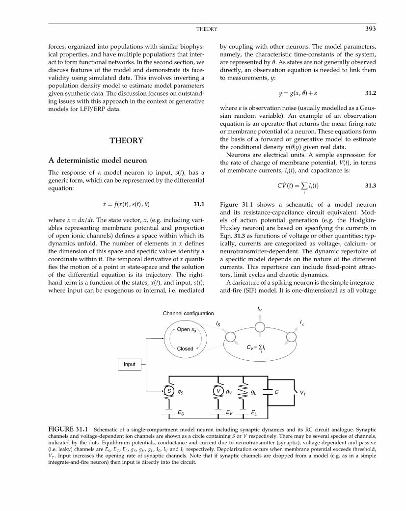
Elsevier UK Chapter: Ch31-P372560 30-9-2006 5:26p.m. Page:393 Trim:7.5in×9.25in
Basal Font:Palatino Margins:Top:40pt Gutter:68pt Font Size:9.5/12 Text Width:42pc Depth:55 Lines
THEORY 393
forces, organized into populations with similar biophys-ical properties, and have multiple populations that inter-act to form functional networks. In the second section, wediscuss features of the model and demonstrate its face-validity using simulated data. This involves inverting apopulation density model to estimate model parametersgiven synthetic data. The discussion focuses on outstand-ing issues with this approach in the context of generativemodels for LFP/ERP data.
THEORY
A deterministic model neuron
The response of a model neuron to input, s�t�, has ageneric form, which can be represented by the differentialequation:
ẋ = f�x�t�� s�t�� �� 31.1
where ẋ = dx/dt. The state vector, x, (e.g. including vari-ables representing membrane potential and proportionof open ionic channels) defines a space within which itsdynamics unfold. The number of elements in x definesthe dimension of this space and specific values identify acoordinate within it. The temporal derivative of x quanti-fies the motion of a point in state-space and the solutionof the differential equation is its trajectory. The right-hand term is a function of the states, x�t�, and input, s�t�,where input can be exogenous or internal, i.e. mediated
by coupling with other neurons. The model parameters,namely, the characteristic time-constants of the system,are represented by �. As states are not generally observeddirectly, an observation equation is needed to link themto measurements, y:
y = g�x���+� 31.2
where � is observation noise (usually modelled as a Gaus-sian random variable). An example of an observationequation is an operator that returns the mean firing rateor membrane potential of a neuron. These equations formthe basis of a forward or generative model to estimatethe conditional density p���y� given real data.
Neurons are electrical units. A simple expression forthe rate of change of membrane potential, V�t�, in termsof membrane currents, Ii�t�, and capacitance is:
CV̇ �t� =∑i
Ii�t� 31.3
Figure 31.1 shows a schematic of a model neuronand its resistance-capacitance circuit equivalent. Mod-els of action potential generation (e.g. the Hodgkin-Huxley neuron) are based on specifying the currents inEqn. 31.3 as functions of voltage or other quantities; typ-ically, currents are categorized as voltage-, calcium- orneurotransmitter-dependent. The dynamic repertoire ofa specific model depends on the nature of the differentcurrents. This repertoire can include fixed-point attrac-tors, limit cycles and chaotic dynamics.
A caricature of a spiking neuron is the simple integrate-and-fire (SIF) model. It is one-dimensional as all voltage
Input
Open xs
Closed
Channel configuration
LI
IV
IS
iCV = ∑Ii
gS gV gL C VT
ELEVES
S V
.
FIGURE 31.1 Schematic of a single-compartment model neuron including synaptic dynamics and its RC circuit analogue. Synapticchannels and voltage-dependent ion channels are shown as a circle containing S or V respectively. There may be several species of channels,indicated by the dots. Equilibrium potentials, conductance and current due to neurotransmitter (synaptic), voltage-dependent and passive(i.e. leaky) channels are ES , EV , EL, gS , gV , gL, IS , IV and IL respectively. Depolarization occurs when membrane potential exceeds threshold,VT . Input increases the opening rate of synaptic channels. Note that if synaptic channels are dropped from a model (e.g. as in a simpleintegrate-and-fire neuron) then input is directly into the circuit.
Elsevier UK Chapter: Ch31-P372560 30-9-2006 5:26p.m. Page:394 Trim:7.5in×9.25in
Basal Font:Palatino Margins:Top:40pt Gutter:68pt Font Size:9.5/12 Text Width:42pc Depth:55 Lines
394 31. NEURONAL MODELS OF ENSEMBLE DYNAMICS
and synaptic channels are ignored. Instead, current ismodelled as a constant passive leak of charge, therebyreducing the right-hand side of Eqn. 31.3 to ‘leakage’ andinput currents:
CV̇ = gL�EL −V�+ s�t� 31.4
where gL and EL are the conductance and equilibriumpotential of the leaky channel respectively. This modeldoes not incorporate the biophysics needed to gener-ate action potentials. Instead, spiking is modelled as athreshold process, i.e. once membrane potential exceedsa threshold value, VT , a spike is generated and mem-brane potential is reset to VR, where VR ≤ EL < VT . Nospike is actually emitted; only subthreshold dynamics aremodelled.
Modelling suprathreshold dynamics
First, we will augment a simple integrate-and-fire modelwith an additional variable T , inter-spike time (IST). Typ-ically, as described above, the threshold potential is mod-elled as an absorbing boundary condition with re-entryat the reset voltage. However, we will model the IST as astate variable for a number of reasons. First, it constrainsthe neuronal trajectory to a finite region of state-space,which only requires natural boundary conditions, i.e. theprobability mass decays to zero as state-space extends toinfinity. This makes our later treatment generic, becausewe do not have to consider model-specific boundaryconditions when, for example, formulating the FPE orderiving its eigensystem. Another advantage is that thetime between spikes can be calculated directly from thedensity on IST. Finally, having an explicit representa-tion of the time since the last spike allows us to modeltime-dependent changes in the system’s parameters (e.g.relative refractoriness), which would be much more dif-ficult in conventional formulations. The resulting modelis two-dimensional and automates renewal to reset volt-age once threshold has been exceeded. We will refer tothis as a temporally augmented (TIF) model. With thisadditional state-variable, we have:
V̇ = 1C
�gL�EL −V�+ s�t��+��VR −V��
Ṫ = 1−�TH�V�
� = exp�−T 2/22�
H�V� ={
1 V ≥ VT
0 V < VT
31.5
A characteristic feature of this deterministic model is thatthe input has to reach a threshold before spikes are gen-erated, after which firing rate increases monotonically.
This is in contrast to a stochastic model that has non-zeroprobability of firing, even with low input. We will see anexample of this later. Given a suprathreshold input to theTIF neuron, membrane voltage is reset to VR using theHeaviside function (last term in Eqn. 31.5). This ensuresthat once V > VT the rate of change of T with respect totime is large and negative �� = 104�, reversing the pro-gression of inter-spike time and returning it to zero, afterwhich it increases constantly for VR < V < VT . Membranepotential is coupled to T , via an expression involving�, which is a Gaussian function, centred at T = 0 witha small dispersion � = 1 ms�. During the first few mil-liseconds following a spike, this term provides a briefimpulse to clamp membrane potential near to VR (cf. therefractory period).
Modelling spike-rate adaptation and synapticdynamics
The TIF model can be extended to include ion-channeldynamics, i.e. to model spike-rate adaptation and synap-tic transmission. We will call this channel model a CIFmodel.
V̇ = 1C
�gL�EL −V�+g1x1�E1 −V�
+g2x2�E2 −V�+g3x3�E3 −V�
+g4x4�E4 −V�/�1+exp�−�V −a�/b��+��VR −V��
Ṫ =1−�TH�V� 31.6
1ẋ1 =�1−x1�4�−x1
2ẋ2 =�1−x2��p2 + s�t��−x2
3ẋ3 =�1−x3�p3 −x3
4ẋ4 =�1−x4�p4 −x4
(Table 31-1 gives a list of variables used throughoutthis chapter.) These equations model spike-rate adapta-tion and synaptic dynamics (fast excitatory AMPA, slowexcitatory NMDA and inhibitory GABA channels) bya generic synaptic channel mechanism, which is illus-trated in Figure 31.1. The proportion of open channelsis modelled by x1� � � � � x4; these correspond to K (slowpotassium), AMPA, GABA or NMDA channels, where0 ≤ xi ≤ 1. Given no input, the proportion of open chan-nels relaxes to an equilibrium state, e.g. pi/�1+pi� forGABA and NMDA channels. The rate at which channelsclose is proportional to xi. Conversely, the rate of open-ing is proportional to 1−xi. External input now enters byincreasing the opening rate of AMPA channels (see theRC circuit of Figure 31.1).

Elsevier UK Chapter: Ch31-P372560 30-9-2006 5:26p.m. Page:395 Trim:7.5in×9.25in
Basal Font:Palatino Margins:Top:40pt Gutter:68pt Font Size:9.5/12 Text Width:42pc Depth:55 Lines
THEORY 395
TABLE 31-1 Variables and symbols
Description Symbol
Membrane potential VInter-spike time TProportion of open channels: K, AMPA,
GABA and NMDAx1� � � � � x4
State vector x = �x1� � � � � x4�V� T T
Probability density �Probability mode coefficients �Dynamic operator QRight eigenvector matrix RLeft eigenvector matrix LEigenvalue matrix DObservations yObservation operator M
Stochastic dynamics
The response of a deterministic system to input is knownfrom its dynamics and initial conditions as it followsa well-defined trajectory in state-space. The additionof system noise, i.e. random input, to the determinis-tic equation turns it into a stochastic differential equa-tion. If the random input is Langevin, it is referredto as a Langevin equation (Frank, 2005). In contrastto deterministic systems, the Langevin equation has anensemble of solutions. The effect of stochastic terms,e.g. variable spike-time arrival, is to disperse trajectoriesthrough state-space. A simple example of this is shownin Figure 31.2. Three trajectories are shown, each with thesame initial condition. The influence of stochastic inputis to disperse the trajectories.
Under smoothness constraints on the random input,the ensemble of solutions are described exactly bythe Fokker-Planck equation (Risken, 1996; Kloeden andPlaten, 1999). The FPE frames the evolution of the ensem-
Dispersive effect of stochastic forces
Mem
bran
e po
tent
ial (
mV
)
...500 ms0..... Time
–55
–60
–65
–70
–75
–80
–85
FIGURE 31.2 Dispersive effect of stochastic input on trajecto-ries. Three trajectories of the CIF model (Eqn. 31.6) are shown, onein bold to emphasize the dispersion of trajectories despite the sameinitial position. Once threshold is exceeded V is reset to VR.
ble of solutions as a deterministic process, which modelsthe dispersive effect of stochastic input as a diffusive pro-cess. This leads to a parsimonious description in termsof a probability density over state space, represented by��x� t�. This is important, as stochastic effects can have asubstantial influence on dynamic behaviour, as we willsee in the next section.
Population density methods have received much atten-tion over the past few decades as a means of mod-elling efficiently the activity of thousands of similar neu-rons. Knight and Sirovich (Sirovich, 2003) describe aneigenfunction approach to solving these equations andextend the method to a time-dependent perturbationsolution. Comparative studies by (Omurtag et al., 2000;Haskell et al., 2001) have demonstrated the efficiency andaccuracy of population density methods using MonteCarlo simulations of neuronal populations. The effects ofsynaptic dynamics have been explored and applied toorientation tuning (Nykamp and Tranchina, 2000, 2001).Furthermore, Casti et al. (2002) have modelled burstingactivity in the lateral geniculate nucleus. Below, we intro-duce the FPE and its eigensolution. We have adoptedsome terminology of Knight and others for consistency.We start with an intuitive derivation of the FPE for ran-dom inputs that are Poisson in nature. This is a goodmodel for input that comprises random spike trains.
The Fokker-Planck formalism
To simplify the description, we will deal with a simpleintegrate-and-fire model with one excitatory input. Con-sider a one-dimensional system with equations of motiondescribed by Eqn. 31.1, but now with s�t� as a randomvariable encoding the stochastic arrival of spikes:
ẋ = f�x�+ s�t�
s�t� = h∑n
��t − tn�31.7
where h represents a discrete change in postsynapticmembrane potential due to each spike and tn representsthe time of the nth spike. If we consider the input over ashort time interval the mean spike-rate and the associatedinput are:
r�t� = 1T
T∫0
∑n
�� − tn�d
s�t� = hr�t�
31.8
The input is now a Poisson process whose expectationand variance scales with firing rate. How does this vari-ability affect the evolution of the density? The masterequation (Risken, 1996), detailing the rate of change of

Elsevier UK Chapter: Ch31-P372560 30-9-2006 5:26p.m. Page:396 Trim:7.5in×9.25in
Basal Font:Palatino Margins:Top:40pt Gutter:68pt Font Size:9.5/12 Text Width:42pc Depth:55 Lines
396 31. NEURONAL MODELS OF ENSEMBLE DYNAMICS
FIGURE 31.3 The master equation of asimple integrate-and-fire model with excitatoryinput (no synaptic dynamics). Three values of thestate x (x and x ± h) and transition rates (f�x�,f�x +h� and r�t�) are shown. The rate of changeof ��x� t� with time is attained by considering therates in and out of x (formulas at the top left andright respectively).
ρ(x)in = ρ(x + h)f(x + h) + ρ(x − h)r (t ) ρ(x)out = –ρ(x)r (t) − ρ(x)f (x )
f(x + h)
r (t)
r (t)
f (x )
[f (x)ρ(x)] + r (t)(ρ(x − h)−ρ(x))∂x∂= −
x
x + h
x − h
Master equation
ρ(x) = ρ(x)in − ρ(x)out
��x� t� with time, can be intuited from the ladder diagramof Figure 31.3:
�̇�x� = − �
�x�f�x���x� + r�t����x−h�−��x�� 31.9
The first term is due to leakage current and generatesa steady flow towards EL. The second expression is dueto input and is composed of two terms, which can beconsidered as replenishing and depleting terms respec-tively. Given an impulse of input the probability massbetween x−h and x will flow to x, whereas the probabil-ity mass at x flows away from it. The replenishing termin Eqn. 33.9 can be approximated using the second-orderTaylor expansion:
��x−h� ≈ ��x�−h��
�x+ h2
2�2�
�x231.10
Substituting into Eqn. 31.9 and using Eqn. 31.8 we get:
�̇ = − �
�x��f + s�� + w2
2�2�
�x2
w2 = rh2
31.11
where w2 is the strength or variance of the stochastic fluc-tuations. This is also known as the diffusion coefficientc = w2/2. This equation can be written more simply by:
�̇ = Q�x� s�� 31.12
where Q�x� s� contains all the dynamic informationentailed by the differential equations of the model. Thisis the Fokker-Planck or dynamic operator (Knight, 2000).The first term of Eqn. 31.11, known as the advection term,describes movement of the probability density due to thesystems’ deterministic dynamics. The second describes
dispersion of density brought about by stochastic varia-tions in the input. Inherent in this approximation is theassumption that h is small, i.e. the accuracy of the Taylorseries increases as h → 0. Comparisons between the diffu-sion approximation and direct simulations have demon-strated its accuracy in the context of neuronal models.The FPE above generalizes easily to cover models withmultiple states, such as the TIF and CIF models of theprevious section. We can see this with an alternativederivation of Eqn. 31.11 in terms of scalar and vectorfields.
Derivation in terms of vector fields
For an alternative perspective on Eqn. 31.11, we can thinkof the density dynamics in terms of scalar and vectorfields. The probability density, ��x� t�, is a scalar functionwhich specifies the probability mass at x, correspondingto the number of neurons with state x. This quantity willchange if the states are acted on by a force whose influ-ence is quantified by a vector field J�x�. This field rep-resents the flow of probability mass within state-space.The net flux at any point is given by the divergence ofthe vector field � · J (where � is the divergence opera-tor). The net flux is a scalar field and contains all theinformation needed to determine the rate of change ofprobability with time:
�̇ = −� · J 31.13
is the continuity equation. The negative sign ensures thatprobability mass flows from high to low densities. Thetwo forces in our simplified model are the leakage currentand excitatory input. The former moves a neuron towardsits equilibrium potential, EL, while excitatory input drives

Elsevier UK Chapter: Ch31-P372560 30-9-2006 5:26p.m. Page:397 Trim:7.5in×9.25in
Basal Font:Palatino Margins:Top:40pt Gutter:68pt Font Size:9.5/12 Text Width:42pc Depth:55 Lines
THEORY 397
voltage towards VT . Each force generates its flux, whichare in opposite directions. The overall flux is:
J�x� = f��x�+ r�t�
x∫x−h
��x′� t�dx′
x∫x−h
��x′� t�dx′ ≈ h�1− h
2� �� ⇒
�̇ = −� · J
= −� · ��f + s�− w2
2� ��
31.14
which is the same as Eqn. 31.11, but has been formulatedfor a vector of states as opposed to a single state.
A general formulation
In the derivations so far, we have dealt with excitatoryinput that is Poisson in nature, where the expectation andvariance of the process scale with each other. A more gen-eral formulation of the FPE considers deterministic inputs�t� and stochastic input w��t� as separate quantities. Thisgives the Langevin and non-linear Fokker-Planck equa-tions (ensemble dynamics):
ẋ = f�x� s�+w�x� s���t�
�̇ = � · �−f�x� s�+ w2
2���
= −n∑
i=1
�
�xi
�f + s��+ 12
n∑i�k=1
�2
�xi�xk
w2ik�x� s��
31.15
Zero mean, Langevin fluctuation, ��t� (cf. a Weinerprocess) of unit variance, is scaled by w�x� s�. The lastexpression in Eqn. 31.15 has been written in a way thatseparates the two parts of the advection-diffusion equa-tion. The deterministic input contributes to flow, whichconfers structure on the density. An example of f�x� s�is Eqn. 31.6, where x = �x1� � � � � x4�V� T T and n = 6. Theadvection or flow changes the local density in propor-tion to its gradient; clearly, if the density is flat, flow willhave no effect. The second term is a diffusion term thattends to smooth the density; in other words, the densitywill decrease when it is peaked and has a high negativecurvature (the curvature is the second partial derivative).This dispersion or diffusion reflects the stochastic fluctu-ations that dispel states from areas of high density. In theexample above, w�x� s� = √
hs; however, if w�x� s� is fixedand diagonal the dispersion or diffusion of each state isisotropic. In what follows, we will use input in referenceto deterministic inputs that shape density dynamics inthe context of random fluctuations where w�x� s� is diag-onal and constant (see Table 31-2 for values).
TABLE 31-2 Parameter values used in simulations
Parameter description Symbol Value/units
Firing threshold VT −53 mVReset voltage VR −90 mVEquilibrium potential EL −73 mVEquilibrium potential:
K, AMPA, GABAand NMDA
E1� � � � � E4 −90, 0, −70 and 0 mV
Passive conductance gL 25 nSActive conductance: K,
AMPA, GABA andNMDA
g1� � � � � g4 128, 24, 64 and 8 nS
Membrane capacitance C 0.375 nFTime constant: K,
AMPA, GABA andNMDA
1� � � � � 4 80, 2.4, 7 and 100 ms
Background openingcoefficient: AMPA,GABA and NMDA
p1� � � � � p3 0.875, 0.0625 and0.0625 a.u.
Diffusion coefficient:V�T�K, AMPA,GABA and NMDA
w21� � � � �w2
6 4, 0, 0.125, 0.125,0.125 and 0�125 ms−1
Solving the Fokker-Planck equation
Generally, the FPE is difficult to solve using analytic tech-niques. Exact solutions exist for only a limited numberof models (Risken, 1996). However, approximate analyticand numerical techniques offer ways of solving a generalequation. We have chosen a solution based on projec-tion onto a bi-orthogonal set. This results in a system ofuncoupled equations that approximate the original sys-tem and enables an important dimension reduction ofthe original set of equations.
The dynamic operator, Q�s�, is generally input-dependent and non-symmetric. By diagonalizing Q�s�,we implicitly reformulate the density dynamics in termsof probability modes. Two sets of eigenvectors (right andleft) are associated with the dynamic operator, forming abi-orthogonal set. This set encodes modes or patterns ofprobability over state-space. The right eigenvectors arecolumn vectors of the matrix R, where QR = RD and lefteigenvectors are row vectors of matrix L, where LQ = DL.Both sets of eigenvectors share the same eigenvalues inthe diagonal matrix D, which are sorted so that �0 > �1 >�2� � � . The left-eigenvector matrix is simply the general-ized inverse of the right-eigenvector matrix. The numberof eigenvectors and values, n, is equal to the dimension-ality of Q. After normalization Q can be diagonalized:
LQR = D 31.16
Assume for the moment that input is constant, i.e. s = 0.Projecting the probability density ��x� t� onto the spaceL generates an equivalent representation, but within a

Elsevier UK Chapter: Ch31-P372560 30-9-2006 5:26p.m. Page:398 Trim:7.5in×9.25in
Basal Font:Palatino Margins:Top:40pt Gutter:68pt Font Size:9.5/12 Text Width:42pc Depth:55 Lines
398 31. NEURONAL MODELS OF ENSEMBLE DYNAMICS
TABLE 31-3 State variable ranges and number of binsused to grid state-space
State variable Number of bins Range of values
V 16 �−92�−48 mVT 8 [0,0.1] sx1 4 [0,1] a.u.x2 2 [0,1] a.u.x3 2 [0,1] a.u.x4 2 [0,1] a.u.
different coordinate system. Conversely, R projects backto the original coordinate system:
� = L�� � = R� 31.17
Substituting Q = RDL and the right expression ofEqn. 31.17 into Eqn. 31.12 gives a diagonalized system,�̇ = D�, which has the solution:
��t� = exp�Dt���0� 31.18
where ��0� is a vector of initial conditions. This solu-tion can be framed in terms of independent modes, i.e.columns of R, each of which contributes linearly to theevolution of the density. The expression of each modeis encoded by the elements of �. The modes are inde-pendent in the sense that the changes in one mode donot affect the changes in another. This is because wehave uncoupled the differential equations when project-ing onto the bi-orthogonal set.
The rate of exponential decay of the i-th mode is char-acterized by its eigenvalue according to i = −1
/�i, where
i is its characteristic time-constant. The key thing hereis that, in many situations, most modes decay rapidly tozero, i.e. they have large negative eigenvalues. Heuris-tically, these modes dissipate very quickly because dis-persion smoothes them away. The contribution of theseunstable modes, to the dynamics at longer time-scales, isnegligible. This is the rationale for reducing the dimen-sion of the solution by ignoring them. Another advantageis that the equilibrium solution, i.e. the probability den-sity that the system relaxes to (given constant input), isgiven by the principal mode, whose eigenvalue is zero.An approximate solution can then be written as:
��x� t� = Rm exp�Dmt�Lm��x� 0� 31.19
where ��x� 0� is the initial density profile, Rm and Lm
are the principal m modes and Dm contains the first meigenvalues, where m ≤ n. The benefit of an approximatesolution is that computational demand is greatly reducedwhen modelling the population dynamics. From now on,we will drop the subscript m and assume the eigensystemhas been reduced.
Time-dependent solutions
The dynamic operator, Q�s�, is input-dependent and ide-ally needs calculating for each new input vector. Thisis time consuming and can be circumvented by usinga perturbation expansion around a solution we alreadyknow, i.e. for s = 0. Approximating Q�s� with a Taylorexpansion about s = 0:
Q�s� ≈ Q�0�+∑i
si
�Q
�si
31.20
where Q�0� is evaluated at zero input and �Q/
�si is ameasure of its dependency on si. Substituting this intothe above equations and using D�0� = LQ�0�R gives thedynamic equation for the coefficients �, in terms of thebi-orthogonal set of Q�0�:
�̇ =(
D�0�+∑i
siL�Q
�si
R
)� = D̂�s�� 31.21
We are assuming here that the inputs can be treated asconstant during the small time interval over which thesystem is integrated. Eqn. 31.21 provides a simple set oflocally linear equations that can be integrated to emulatethe density dynamics of any ensemble.
So far, density dynamics have been presented asdescribing a statistical ensemble of solutions of a singleneuron’s response to input. An alternative interpretationis that ��x� t� represents an ensemble of trajectoriesdescribing a population of neurons. The shift from a sin-gle neuron to an ensemble interpretation entails addi-tional constraints on the population dynamics. An ensem-ble or mean-field type population equation assumes thatneurons within an ensemble are indistinguishable. Thismeans that each neuron ‘feels’ the same influence frominternal interactions and external input. We will assumethat this approximation holds for a subpopulation of neu-rons. However, for this to be a useful assumption, weneed some mechanism for coupling different subpopula-tions that are acted upon by different inputs.
Multiple populations and their coupling
Interactions within a network of ensembles are mod-elled by coupling activities among populations withmean-field terms, such as average activity or spikerate. Coupled populations have been considered byNykamp and Tranchina (2000) in modelling orientationtuning in the visual cortex. Coupling among popula-tions, each described by standard Fokker-Planck dynam-ics, via mean-field quantities, induces non-linearities andthereby extends the networks’ dynamic repertoire. This

Elsevier UK Chapter: Ch31-P372560 30-9-2006 5:26p.m. Page:399 Trim:7.5in×9.25in
Basal Font:Palatino Margins:Top:40pt Gutter:68pt Font Size:9.5/12 Text Width:42pc Depth:55 Lines
THEORY 399
can result in a powerful set of equations that have beenused to model physical, biological and social phenomena.
To model influences among populations, we simplytreat an average state of an ensemble s�i� = M��i� as aninput. The linear operator M acts on the density of the i-th population to provide an expected state (or some othermoment) such as mean firing rate. A simple exampleis self-feedback, where the mean of an ensemble cou-ples to its own dynamics as an input. The mean-fieldnow depends on the population’s own activity and hasbeen described as a dynamic mean-field. This notion ofmean-field coupling can be extended to cover multiplepopulations. A schematic of two interacting populationsof the CIF model (Eqn. 31.6) is shown in Figure 31.4.
Generally, coupling is modelled as a modulation ofthe parameters of the target population i, by inputs fromthe source k. The effect of a small perturbation of theseparameters is used to approximate the time-dependentoperator, which leads to a further term in Eqn. 31.21. Toa first-order approximation, for the i-th ensemble with jexternal inputs:
�̇�i� = D̂�i���i�
D̂�i��s���1����2�� � � � �� = D�i��0�+∑j
sjL�Q�i�
�sj
R
+∑k�l
��k�l L
�Q�i�
���k�l
R 31.22
The effect of the l-th mode of the k-th ensemble ��k�l on
the i-th ensemble follows from the chain rule:
�Q�i�
���k�l
= −� ·(
��̇�i�
���i�
���i�
�s�k�
�s�k�
���k�l
)31.23
where ���i�/
�s�k� specifies the mechanism whereby theinput from the k-th ensemble affects the i-th by changing
its parameters. The derivative �s�k�/
���k�l encodes how
the input changes with the l-th mode of the source. Forexample, evolution of the probability modes in the sourceregion causes a change in its average firing rate, whichmodulates synaptic AMPA channel opening dynamics inthe target region, parameterized by ��i� = p�i�
2 in Eqn. 31.6.This leads to a change in the flux of the target region �̇�i�
and a change in its density.Once Eqn. 31.22 has been integrated, the measured
output of the i-th region can be calculated in the sameway that mean-field effects are calculated:
y�i� = MR�i���i� 31.24
Estimation and inference of mean field models
The formulation above furnishes a relatively sim-ple dynamic model for measured electrophysiologicalresponses reflecting population dynamics. This modelcan be summarized using Eqn. 31.22 and Eqn. 31.24:
�̇�i� = D̂�i���i�
y�i� = MR�i���i� +��i�31.25
This is a deterministic input-state-output system withhidden states ��i� controlling the expression of probabil-ity density modes of the i-th population. Notice that thestates no longer refer to biophysical or neuronal states(e.g. depolarization) but to the densities over states. Theinputs are known deterministic perturbations s�t� andthe outputs are y�i�. The architecture and mechanisms ofthis system are encoded in its parameters. In Chapter 34,we will see how this class of model can be inverted toprovide conditional estimates of the parameters. In theremainder of this chapter, we focus on the sorts of sys-tems that can be modelled and how inversion of these
Open
Closed
s
(1)
θ(2)
IleakIsK
IAMPA
IGABAINMDA
μ(1)
∂s
(1)
∂s
(1)
∂θ(2)
∂θ(2) μ(2)
IleakIsK
IAMPA
IGABAINMDA
Population 2Population 1
⋅
∂μ(2)⋅
–∇ =∂Q (2)
∂μl(1)
∂μl(1) ∂s
(1)
∂θ(2)
∂θ(2)
∂μ(2)⋅ ∂s
(1)
∂μl(1)
FIGURE 31.4 Schematic of interacting subpopulations.The rate of change of density over time, �̇�2�, depends on ��1�
due to coupling. The density in population 1 leads to a firingrate s�1� which modulates the synaptic channel opening rate ofpopulation 2, parameterized by ��2�, which in turn modulates�̇�2�. The coupling is calculated using the chain rule.
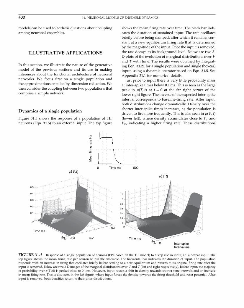
Elsevier UK Chapter: Ch31-P372560 30-9-2006 5:26p.m. Page:400 Trim:7.5in×9.25in
Basal Font:Palatino Margins:Top:40pt Gutter:68pt Font Size:9.5/12 Text Width:42pc Depth:55 Lines
400 31. NEURONAL MODELS OF ENSEMBLE DYNAMICS
models can be used to address questions about couplingamong neuronal ensembles.
ILLUSTRATIVE APPLICATIONS
In this section, we illustrate the nature of the generativemodel of the previous sections and its use in makinginferences about the functional architecture of neuronalnetworks. We focus first on a single population andthe approximations entailed by dimension reduction. Wethen consider the coupling between two populations thatcomprise a simple network.
Dynamics of a single population
Figure 31.5 shows the response of a population of TIFneurons (Eqn. 31.5) to an external input. The top figure
shows the mean firing rate over time. The black bar indi-cates the duration of sustained input. The rate oscillatesbriefly before being damped, after which it remains con-stant at a new equilibrium firing rate that is determinedby the magnitude of the input. Once the input is removed,the rate decays to its background level. Below are two 3-D plots of the evolution of marginal distributions over Vand T with time. The results were obtained by integrat-ing Eqn. 31.21 for a single population and single (boxcar)input, using a dynamic operator based on Eqn. 31.5. SeeAppendix 31.1 for numerical details.
Just prior to input there is very little probability massat inter-spike times below 0.1 ms. This is seen as the largepeak in ��T� t� at t = 0 at the far right corner of thelower right figure. The inverse of the expected inter-spikeinterval corresponds to baseline-firing rate. After input,both distributions change dramatically. Density over theshorter inter-spike times increases, as the population isdriven to fire more frequently. This is also seen in ��V� t�(lower left), where density accumulates close to VT andVR, indicating a higher firing rate. These distributions
0
500
Time ms
ρ(V,t )ρ(Τ,t )
Time ms0 500
–53
–90
mV
0
500Time ms
0
0.1
Inter-spikeInterval ms
Mea
n fir
ing
rate
Hz
0.1
0.2
0.2
0.3
0.4
0.4
0.6
0.8
1
1.2
0
0.5
FIGURE 31.5 Response of a single population of neurons (FPE based on the TIF model) to a step rise in input, i.e. a boxcar input. Thetop figure shows the mean firing rate per neuron within the ensemble. The horizontal bar indicates the duration of input. The populationresponds with an increase in firing that oscillates briefly before settling to a new equilibrium and returns to its original firing rate after theinput is removed. Below are two 3-D images of the marginal distributions over V and T (left and right respectively). Before input, the majorityof probability over ��T� 0� is peaked close to 0.1 ms. However, input causes a shift in density towards shorter time intervals and an increasein mean firing rate. This is also seen in the left figure, where input forces the density towards the firing threshold and reset potential. Afterinput is removed, both densities return to their prior distributions.
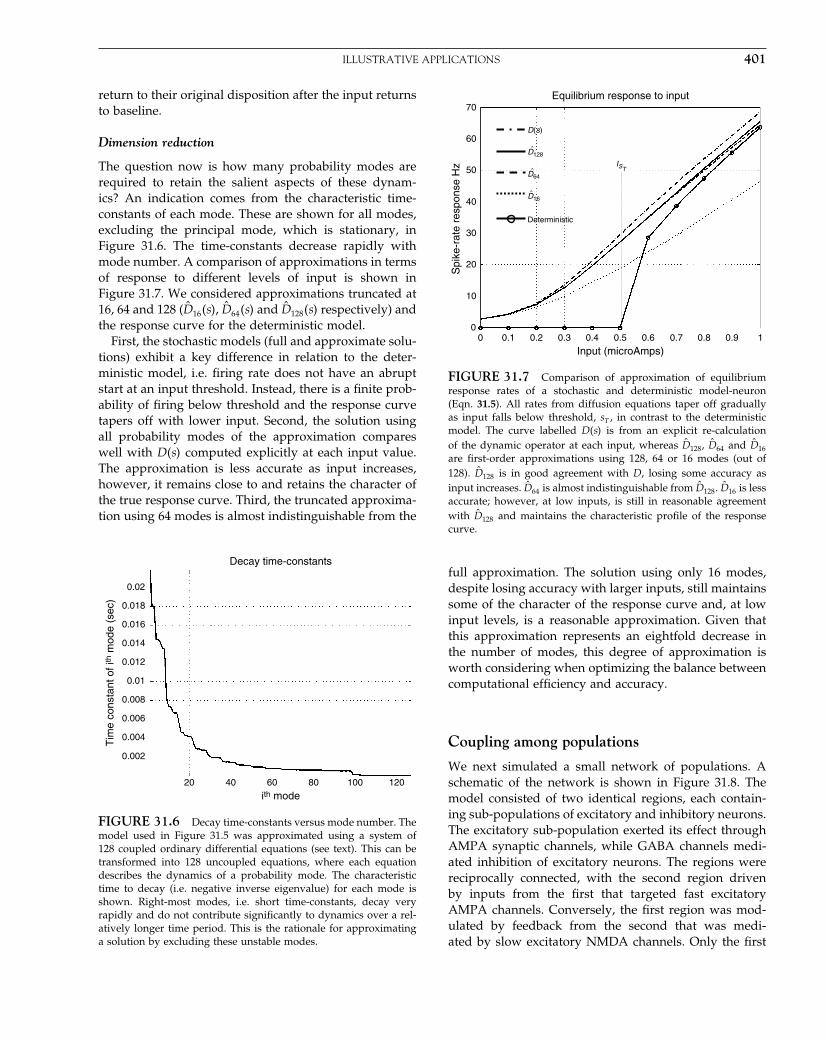
Elsevier UK Chapter: Ch31-P372560 30-9-2006 5:26p.m. Page:401 Trim:7.5in×9.25in
Basal Font:Palatino Margins:Top:40pt Gutter:68pt Font Size:9.5/12 Text Width:42pc Depth:55 Lines
ILLUSTRATIVE APPLICATIONS 401
return to their original disposition after the input returnsto baseline.
Dimension reduction
The question now is how many probability modes arerequired to retain the salient aspects of these dynam-ics? An indication comes from the characteristic time-constants of each mode. These are shown for all modes,excluding the principal mode, which is stationary, inFigure 31.6. The time-constants decrease rapidly withmode number. A comparison of approximations in termsof response to different levels of input is shown inFigure 31.7. We considered approximations truncated at16, 64 and 128 (D̂16�s�, D̂64�s� and D̂128�s� respectively) andthe response curve for the deterministic model.
First, the stochastic models (full and approximate solu-tions) exhibit a key difference in relation to the deter-ministic model, i.e. firing rate does not have an abruptstart at an input threshold. Instead, there is a finite prob-ability of firing below threshold and the response curvetapers off with lower input. Second, the solution usingall probability modes of the approximation compareswell with D�s� computed explicitly at each input value.The approximation is less accurate as input increases,however, it remains close to and retains the character ofthe true response curve. Third, the truncated approxima-tion using 64 modes is almost indistinguishable from the
Tim
e co
nsta
nt o
f ith
mod
e (s
ec)
ith mode
Decay time-constants
20
0.002
0.004
0.006
0.008
0.01
0.012
0.014
0.016
0.018
0.02
40 60 80 100 120
FIGURE 31.6 Decay time-constants versus mode number. Themodel used in Figure 31.5 was approximated using a system of128 coupled ordinary differential equations (see text). This can betransformed into 128 uncoupled equations, where each equationdescribes the dynamics of a probability mode. The characteristictime to decay (i.e. negative inverse eigenvalue) for each mode isshown. Right-most modes, i.e. short time-constants, decay veryrapidly and do not contribute significantly to dynamics over a rel-atively longer time period. This is the rationale for approximatinga solution by excluding these unstable modes.
Spi
ke-r
ate
resp
onse
Hz
D̂16
D̂64
D̂128
D(s)
Equilibrium response to input
Deterministic
IST
70
60
50
40
30
20
10
00 0.1 0.2 0.3 0.4 0.5
Input (microAmps)0.6 0.7 0.8 0.9 1
FIGURE 31.7 Comparison of approximation of equilibriumresponse rates of a stochastic and deterministic model-neuron(Eqn. 31.5). All rates from diffusion equations taper off graduallyas input falls below threshold, sT , in contrast to the deterministicmodel. The curve labelled D�s� is from an explicit re-calculationof the dynamic operator at each input, whereas D̂128, D̂64 and D̂16are first-order approximations using 128, 64 or 16 modes (out of128). D̂128 is in good agreement with D, losing some accuracy asinput increases. D̂64 is almost indistinguishable from D̂128. D̂16 is lessaccurate; however, at low inputs, is still in reasonable agreementwith D̂128 and maintains the characteristic profile of the responsecurve.
full approximation. The solution using only 16 modes,despite losing accuracy with larger inputs, still maintainssome of the character of the response curve and, at lowinput levels, is a reasonable approximation. Given thatthis approximation represents an eightfold decrease inthe number of modes, this degree of approximation isworth considering when optimizing the balance betweencomputational efficiency and accuracy.
Coupling among populations
We next simulated a small network of populations. Aschematic of the network is shown in Figure 31.8. Themodel consisted of two identical regions, each contain-ing sub-populations of excitatory and inhibitory neurons.The excitatory sub-population exerted its effect throughAMPA synaptic channels, while GABA channels medi-ated inhibition of excitatory neurons. The regions werereciprocally connected, with the second region drivenby inputs from the first that targeted fast excitatoryAMPA channels. Conversely, the first region was mod-ulated by feedback from the second that was medi-ated by slow excitatory NMDA channels. Only the first
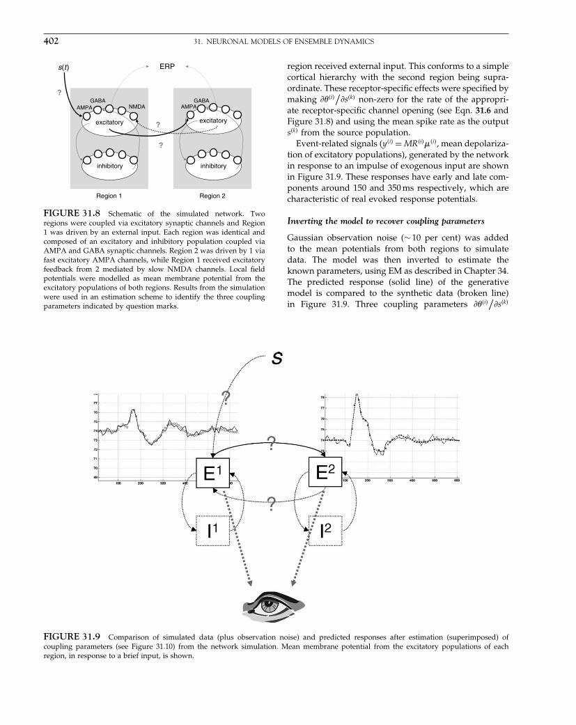
Elsevier UK Chapter: Ch31-P372560 30-9-2006 5:26p.m. Page:402 Trim:7.5in×9.25in
Basal Font:Palatino Margins:Top:40pt Gutter:68pt Font Size:9.5/12 Text Width:42pc Depth:55 Lines
402 31. NEURONAL MODELS OF ENSEMBLE DYNAMICS
s(t )
GABA
excitatory
inhibitory
?
?
?
ERP
Region 2Region 1
inhibitory
excitatory
AMPAGABA
NMDAAMPA
FIGURE 31.8 Schematic of the simulated network. Tworegions were coupled via excitatory synaptic channels and Region1 was driven by an external input. Each region was identical andcomposed of an excitatory and inhibitory population coupled viaAMPA and GABA synaptic channels. Region 2 was driven by 1 viafast excitatory AMPA channels, while Region 1 received excitatoryfeedback from 2 mediated by slow NMDA channels. Local fieldpotentials were modelled as mean membrane potential from theexcitatory populations of both regions. Results from the simulationwere used in an estimation scheme to identify the three couplingparameters indicated by question marks.
region received external input. This conforms to a simplecortical hierarchy with the second region being supra-ordinate. These receptor-specific effects were specified bymaking ���i�
/�s�k� non-zero for the rate of the appropri-
ate receptor-specific channel opening (see Eqn. 31.6 andFigure 31.8) and using the mean spike rate as the outputs�k� from the source population.
Event-related signals (y�i� = MR�i���i�, mean depolariza-tion of excitatory populations), generated by the networkin response to an impulse of exogenous input are shownin Figure 31.9. These responses have early and late com-ponents around 150 and 350 ms respectively, which arecharacteristic of real evoked response potentials.
Inverting the model to recover coupling parameters
Gaussian observation noise (∼10 per cent) was addedto the mean potentials from both regions to simulatedata. The model was then inverted to estimate theknown parameters, using EM as described in Chapter 34.The predicted response (solid line) of the generativemodel is compared to the synthetic data (broken line)in Figure 31.9. Three coupling parameters ���i�
/�s�k�
FIGURE 31.9 Comparison of simulated data (plus observation noise) and predicted responses after estimation (superimposed) ofcoupling parameters (see Figure 31.10) from the network simulation. Mean membrane potential from the excitatory populations of eachregion, in response to a brief input, is shown.

Elsevier UK Chapter: Ch31-P372560 30-9-2006 5:26p.m. Page:403 Trim:7.5in×9.25in
Basal Font:Palatino Margins:Top:40pt Gutter:68pt Font Size:9.5/12 Text Width:42pc Depth:55 Lines
CONCLUSION 403
Parameter values
21 3Parameter
Estimate
True
0.1
0.2
0.3
0.4
0.5
<P
>
0.6
0.7
0.8
0.9
1
0
FIGURE 31.10 The conditional expectations of the three cou-pling parameters between input to Region 1, Region 1 to 2 andbackward coupling from 2 to 1 (parameter indices 1–3 respectively)are shown next to the known parameters of the simulation.
mediating exogenous input and the extrinsic connectionsbetween regions (bold connections with question marksin Figures 31.8 and 31.9) were given uninformative priors.These represent unknown parameters that the estimationscheme was trying to identify. Their conditional expec-tations are shown with the true values in Figure 31.10.They show good agreement and speak to the possibilityof inverting mean-field models using real data.
CONCLUSION
The aim of this chapter was to demonstrate the feasibilityof using the FPE in a generative model for LFP/ERPs. Theensuing model embodies salient features of real neuronalsystems: neurons are dynamic units, driven by stochas-tic forces and organized into populations with similarresponse characteristics; and multiple populations inter-act to form functional networks. Despite the stochasticnature of neuronal dynamics, the FPE formulates thesolution in terms of a deterministic process, where thedispersive effect of noise is modelled as a diffusive pro-cess. The motivation for using such a model is that itsassociated parameters have a clear biological meaning,enabling unambiguous and mechanistic interpretations.
We have reviewed well-known material on integrate-and-fire model neurons with synaptic dynamics, whichincluded fast excitatory AMPA, slow excitatory NMDAand inhibitory GABA mediated currents. The FPE was
used to model the effect of stochastic input, or systemnoise, on population dynamics. Its time-dependent solu-tion was approximated using a perturbation expansionabout zero input. Decomposition into a bi-orthogonal setenabled a dimension reduction of the system of coupledequations, due to the rapid dissipation of unstable proba-bility modes. Interactions among populations were mod-elled as a change in the parameters of a target populationthat depended on the average state of source populations.
To show that the model produces realistic responsesand, furthermore, it could be used as an estimation orforward model, separate ensembles were coupled to forma small network of two regions. The coupled model wasused to simulate ERP data, i.e. mean potentials fromexcitatory subpopulations in each region. Signals werecorrupted by Gaussian noise and subject to expectationmaximization (EM). Three parameters were estimated –input, forward and backward connection strengths – andwere shown to compare well to the known values. It ispleasing to note that the stochastic model produces sig-nals that exhibit salient features of real ERP data and theestimation scheme was able to recover its parameters.
The key aspect of the approach presented here isthe use of population density dynamics as a forwardmodel of observed data. These models have been usedto explore the cortical dynamics underlying orientationtuning in the visual cortex. These models may also finda place in LFP/ERP data analysis. In these models, ran-dom effects are absorbed into the FPE and the pop-ulation dynamics become deterministic. This is a crit-ical point because it means system identification hasonly to deal with observation noise. Heuristically, thedeterministic noise induced by stochastic effects is effec-tively ‘averaged away’ by measures like ERPs. However,the effect of stochastic influence is still expressed andmodelled, deterministically, at the level of populationdynamics.
There are many issues invoked by this modellingapproach. The dimensionality of solutions for large sys-tems can become extremely large in probability space.Given an N-dimensional dynamic system, dividing eachdimension into M bins results in an approximation to theFPE with a total of MN ordinary differential equations.The model used to simulate a network of populationsused 4096 equations to approximate the dynamics ofone population. Dimension reduction, by using a trun-cated bi-orthogonal set, is possible. However, as wasdemonstrated in Figure 31.7, there is a trade-off betweenaccuracy and dimension reduction. Generally, a morerealistic model requires more variables, so there is a bal-ance between biological realism and what we can expectfrom current computational capabilities.
The model neuron used in this chapter is just one ofmany candidates. Much can be learnt from comparing

Elsevier UK Chapter: Ch31-P372560 30-9-2006 5:26p.m. Page:404 Trim:7.5in×9.25in
Basal Font:Palatino Margins:Top:40pt Gutter:68pt Font Size:9.5/12 Text Width:42pc Depth:55 Lines
404 31. NEURONAL MODELS OF ENSEMBLE DYNAMICS
models. For instance, is modelling the inter-spike time asa state variable an efficient use of dimensions? This mayeschew the need for detailed boundary conditions; how-ever, it may well be an extravagant use of dimensionsgiven computational limitations. The current modellingapproach is not limited to electrophysiological data. Anymeasurement which is coupled to electrical activity of aneuronal population could, in principle, also be includedin the generative model, which could be used to com-bine measurements of electrical and metabolic origin,e.g. fMRI.
The use of Bayesian system identification enables theformal inclusion of additional information when estimat-ing model parameters from data. We have not given thetopic of priors much consideration in this chapter, but it isan important issue. Analytic priors derived from stabilityor bifurcation analyses could be used to ensure parame-ter values which engender dynamics characteristic of thesignals measured, i.e. stable fixed point, limit cycle orchaotic attractors. Empirical priors derived from data alsohave great potential in constraining system identification.A Bayesian framework also facilitates model comparisonthrough quantifying the ‘evidence’ that a data set has fora number of different models (Penny et al., 2004).
In the next two chapters, we turn to neural-mass mod-els of EEG data. Neural-mass models are a special caseof mean-field models in which the ensemble densitiesare approximated with a single mode or point mass.In other words, the density is summarized with a statevector that encodes the most likely or expected stateof each ensemble. This can be thought of as a dimen-sion reduction to the smallest number of modes (i.e.one) or can be regarded as approximating the full den-sity with a point mass over its expectation. Clearly,neural-mass models lose the ability properly to modelrandom fluctuations, however, the computational sav-ing enables a much greater number of biophysical statesto be modelled with a large repertoire of dynamicalbehaviours.
APPENDIX 31.1 NUMERICAL SOLUTIONOF FOKKER-PLANCK EQUATION
The equation we wish to integrate is:
�̇�x� t� = Q� 31.A1
First, vectorize and grid up the n-D state-space xi = ih,where i = 1� � � � �N and evaluate ẋ = f�x� s� at all gridpoints. Calculate the operators −� ·f and �2, where �2 =
� · � is the Laplace operator, required to construct anapproximation to the dynamic operator:
Q = −� · �f + s�+ w2
2�2 31.A2
Eqn. 31.A1 is a system of coupled differential equationswith the solution:
��x� t +�t� = exp��tQ���x� t� 31.A3
This system is reduced and integrated over small timesteps using the eigenvectors of Q, where for the i-thensemble or population:
��i��t +�t� = exp�D�i��t���i��t�
D̂�i� = D�i�0 +∑
j
sjD�i�j +∑
k�l
��k�l D�i�
kl
y�i��t� = MR�i���i��t�
31.A4
The Jacobian matrices are pre-computed using Q�i� from31.A2:
D�i�0 = LQ�i�R D�i�
j = L�Q�i�
�sj
R D�i�kl = L
�Q�i�
���k�l
R 31.A5
After discretizing state-space and approximating Q�i� forone population, the eigenvectors and values can be cal-culated using the Matlab function ‘eig.m’ (or ‘eigs.m’for specific eigenvector/values) and saved. Given these,a reduced or full model can be used to model a networkof populations by specifying the connectivity amongensembles. The exponential matrix of the reduced orfull model can be calculated using the Matlab function‘expm’ (Moler and Van Loan, 2003). This uses a (6,6) Padeapproximation. Explicit and implicit numerical integra-tion schemes can be reformulated into a Pade approxi-mation, e.g. (0,1) approximation of order 1 is a forwardEuler scheme, whereas (1,1) approximation of order 2 is aCrank-Nicolson implicit scheme. As the ‘expm’ functionuses an implicit approximation the scheme is accurateand unconditionally stable (Smith, 1985).
REFERENCES
Casti AR, Omurtag A, Sornborger A et al. (2002) A population studyof integrate-and-fire-or-burst neurons. Neural Comput 14: 957–86
Churchland PS and Sejnowski TJ (1994) The computational brain. MITPress, Cambridge, MA
David O, Friston KJ (2003) A neural mass model for MEG/EEG:coupling and neuronal dynamics. NeuroImage 20: 1743–55
David O, Kiebel SJ, Harrison LM et al. (2006) Dynamic causal mod-eling of evoked responses in EEG and MEG. NeuroImage 30:1255–72
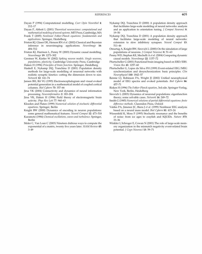
Elsevier UK Chapter: Ch31-P372560 30-9-2006 5:26p.m. Page:405 Trim:7.5in×9.25in
Basal Font:Palatino Margins:Top:40pt Gutter:68pt Font Size:9.5/12 Text Width:42pc Depth:55 Lines
REFERENCES 405
Dayan P (1994) Computational modelling. Curr Opin Neurobiol 4:212–17
Dayan P, Abbott L (2001) Theoretical neuroscience: computational andmathematical modeling of neural systems. MIT Press, Cambridge, MA
Frank T (2005) Nonlinear Fokker-Planck equations: fundamentals andapplications. Springer, Heidelberg
Friston KJ, Glaser DE, Henson RN et al. (2002) Classical and Bayesianinference in neuroimaging: applications. NeuroImage 16:484–512
Friston KJ, Harrison L, Penny W (2003) Dynamic causal modelling.NeuroImage 19: 1273–302
Gerstner W, Kistler W (2002) Spiking neuron models. Single neurons,populations, plasticity. Cambridge University Press, Cambridge
Haken H (1996) Principles of brain function. Springer, HeidelbergHaskell E, Nykamp DQ, Tranchina D (2001) Population density
methods for large-scale modelling of neuronal networks withrealistic synaptic kinetics: cutting the dimension down to size.Network 12: 141–74
Jansen BH, Rit VG (1995) Electroencephalogram and visual evokedpotential generation in a mathematical model of coupled corticalcolumns. Biol Cybern 73: 357–66
Jirsa VK (2004) Connectivity and dynamics of neural informationprocessing. Neuroinformatics 2: 183–204
Jirsa VK, Haken H (1996) Field theory of electromagnetic brainactivity. Phys Rev Lett 77: 960–63
Kloeden and Platen (1999) Numerical solution of stochastic differentialequations. Springer, Berlin
Knight BW (2000) Dynamics of encoding in neuron populations:some general mathematical features. Neural Comput 12: 473–518
Kuramoto (1984) Chemical oscillations, waves and turbulence. Springer,Berlin
Moler C, Van Loan C (2003) Nineteen dubious ways to compute theexponential of a matrix, twenty five years later. SIAM Review 45:3–49
Nykamp DQ, Tranchina D (2000) A population density approachthat facilitates large-scale modeling of neural networks: analysisand an application to orientation tuning. J Comput Neurosci 8:19–50
Nykamp DQ, Tranchina D (2001) A population density approachthat facilitates large-scale modeling of neural networks:extension to slow inhibitory synapses. Neural Comput 13:511–46
Omurtag A, Knight BW, Sirovich L (2000) On the simulation of largepopulations of neurons. J Comput Neurosci 8: 51–63
Penny WD, Stephan KE, Mechelli A et al. (2004) Comparing dynamiccausal models. NeuroImage 22: 1157–72
Pfurtscheller G (2001) Functional brain imaging based on ERD/ERS.Vision Res 41: 1257–60
Pfurtscheller G, Lopes da Silva FH (1999) Event-related EEG/MEGsynchronization and desynchronization: basic principles. ClinNeurophysiol 110: 1842–57
Rennie CJ, Robinson PA, Wright JJ (2002) Unified neurophysicalmodel of EEG spectra and evoked potentials. Biol Cybern 86:457–71
Risken H (1996) The Fokker-Planck equation, 3rd edn. Springer-Verlag,New York, Berlin, Heidelberg
Sirovich L (2003) Dynamics of neuronal populations: eigenfunctiontheory; some solvable cases. Network 14: 249–72
Smith G (1985) Numerical solutions of partial differential equations: finitedifference methods. Clarendon Press, Oxford
Valdes PA, Jimenez JC, Riera J et al. (1999) Nonlinear EEG analysisbased on a neural mass model. Biol Cybern 81: 415–24
Wiesenfeld K, Moss F (1995) Stochastic resonance and the benefitsof noise: from ice ages to crayfish and SQUIDs. Nature 373:33–36
Winkler I, Schroger E, Cowan N (2001) The role of large-scale mem-ory organization in the mismatch negativity event-related brainpotential. J Cogn Neurosci 13: 59–71

Elsevier UK Chapter: Ch32-P372560 30-9-2006 5:27p.m. Page:406 Trim:7.5in×9.25in
Basal Font:Palatino Margins:Top:40pt Gutter:68pt Font Size:9.5/12 Text Width:42pc Depth:55 Lines
C H A P T E R
32
Neuronal models of energeticsJ. Kilner, O. David and K. Friston
INTRODUCTION
In this chapter, we will describe a simple biophysicalmodel that links neuronal dynamics to functional mag-netic resonance imaging (fMRI) and electroencephalog-raphy (EEG) measurements. The previous chapterdescribed mean-field models and the next chapter willcover neural-mass approaches to modelling EEG sig-nals. Here, we look at a simple mean-field model thatwas developed with the specific aim of relating neuronalactivity recorded with EEG and the neuronal activity thatleads to a modulation of the blood oxygenation-level-dependent (BOLD) signal recorded with fMRI.
The chapter is divided into three sections. First, we willdescribe the motivation for relating the different measuresof brain activity afforded by EEG and fMRI and reviewdifferent approaches that have been adopted for multi-modal fusion. Second, we will outline the neuronal model,starting with a dimensional analysis. In brief, this modelsuggests that neuronal activity causes an accelerationof temporal dynamics leading to: increased energy dis-sipation; decreased effective membrane time-constants;increased coupling among neuronal ensembles; and ashift in the EEG spectral profile to higher frequencies.Finally, we will show that these predictions are consis-tent with empirical observations of how changes in theEEG spectrum are expressed haemodynamically.
EEG AND fMRI INTEGRATION
It is now generally accepted that the integration offMRI and electromagnetic measures of brain activityhas an important role in characterizing evoked brainresponses. These measures are both related to theunderlying neural activity. However, electromagnetic
measures are direct and capture neuronal activity withmillisecond temporal resolution, while fMRI providesan indirect measure with poor temporal resolution,in the order of seconds. Conversely, fMRI has excel-lent spatial resolution, in the order of millimetres,compared to EEG-MEG (electroencephalography-magnetoencephalography). Therefore, the obviousmotivation for integrating these two measures is toprovide a composite recording that has high temporaland spatial resolution. The possibility of integratingthese two measures in humans is supported by the studyof Logothetis et al. (2001). In this study, the authorsdemonstrated that within the macaque monkey visualcortex, intracortical recordings of the local field potential(LFP) and the BOLD signal were linearly related.
Approaches to integration can be classified intothree sorts: integration through prediction; integrationthrough constraints; and integration through fusion.These are depicted schematically in Figure 32.1. Inte-gration through prediction (dotted line) uses tempo-rally resolved EEG signals as a predictor of changes inconcurrently recorded fMRI. The ensuing region-specifichaemodynamic correlates can then be characterizedwith high spatial resolution with conventional imagingmethodology (Lovblad et al., 1999; Lemieux et al., 2001;Czisch et al., 2004). Several studies of this type (Goldmanet al., 2002; Laufs et al., 2003a, b; Martinez-Montes, 2004)have focused on correlating modulations in ongoingoscillatory activity measured by EEG with the haemody-namic signal. They have demonstrated that modulationsin alpha rhythms (oscillations at ∼10Hz) are negativelycorrelated with modulations in the BOLD signal, i.e. anincrease in alpha power is associated with a decreasein BOLD. Studies employing integration through con-straints (dashed line), have used the spatial resolution offocal fMRI activations to constrain equivalent dipole ordistributed estimates of EEG-MEG sources (Dale et al.,2000; Phillips et al., 2002). However, neither of these
Statistical Parametric Mapping, by Karl Friston et al. Copyright 2007, Elsevier Ltd. All rights reserved.ISBN–13: 978-0-12-372560-8 ISBN–10: 0-12-372560-7
406

Elsevier UK Chapter: Ch32-P372560 30-9-2006 5:27p.m. Page:407 Trim:7.5in×9.25in
Basal Font:Palatino Margins:Top:40pt Gutter:68pt Font Size:9.5/12 Text Width:42pc Depth:55 Lines
A HEURISTIC FOR EEG-fMRI INTEGRATION 407
EEG
Neuralactivity
i
ii
iii iii
BOLD
FIGURE 32.1 Schematic showing the approaches toEEG/fMRI integration. (i) Integration through prediction. (ii)Integration through constraints. (iii) Integration through fusionwith forward models.
schemes can be considered as true integration of mul-timodal data in the sense that there is no common for-ward model that links the underlying neuronal dynamicsof interest to measured haemodynamic and electricalresponses (solid black lines).
The characterization of the relationship between theelectrophysiology of neuronal systems and their slowerhaemodynamics is crucial from a number of perspectives:not only for forward models of electrical and haemo-dynamic data, but also for the utility of spatial priors,derived from fMRI, in the inverse EEG/MEG sourcereconstruction problem, and for the disambiguation ofinduced, relative to evoked, brain responses using bothmodalities.
In the next section, we will describe perhaps the sim-plest of all models which helps to explain some empiricalobservations from EEG-fMRI integration, using a dimen-sional analysis and a biophysical model.
A HEURISTIC FOR EEG-fMRIINTEGRATION
A dimensional analysis
Given the assumption that haemodynamics reflect theenergetics of underlying neuronal changes (Jueptner andWeiller, 1995; Shulman and Rothman, 1998; Hoge et al.,1999; Magistretti et al., 1999; Magistretti and Pellerin,1999; Shin, 2000), we assume here that the BOLD sig-nal b, at any point in time, is proportional to the rateof energy dissipation, induced by transmembrane cur-rents. It is important to note that we are not assumingthe increase in blood flow, which is the major contributorto the BOLD signal, is a direct consequence of the rateof energy dissipation, but rather that these two measures
are proportional (see Hoge et al., 1999). Although recentwork has suggested that the neurovascular coupling isdriven by glutamate release (see Lauritzen, 2001; Attwelland Iadecola, 2002), glutamate release, BOLD signal andenergy usage are correlated and therefore the assump-tion here that the BOLD signal is proportional to therate of energy dissipation is tenable. This dissipation isexpressed in terms of Joules per second and correspondsto the product of transmembrane potential (V, joules percoulomb) and transmembrane current (I , coulombs persecond):
b ∝ ⟨V T I
⟩32.1
where V = �V1� � � � �Vk�T corresponds to a [large] col-
umn vector of potentials for each neuronal compart-ment k within a voxel, similarly for the currents. Clearly,Eqn. 32.1 will not be true instantaneously, because itmay take some time for the energy cost to be expressedin terms of increased oxygen delivery, extraction andperfusion. However, over a suitable timescale, of orderseconds, Eqn. 32.1 will be approximately correct. Assum-ing a single-compartment model, currents are related tochanges in membrane potential though their capacitanceC, which we will assume is constant (see Dayan andAbbott, 2001: 156). By convention, the membrane currentis defined as positive when positive ions leave the neuronand negative when positive ions enter the neuron:
I = −CV̇ 32.2
then
b ∝ V⟨V T V̇
⟩32.3
To relate changes in membrane potential to the BOLDsignal, we need to adopt some model of a neuronalsystem and how it activates. A simple integrate-and-fire model of autonomous neuronal dynamics can beexpressed in the form:
V̇k = −Vk/�k +uk
= fk�V�32.4
for the k-th compartment or unit (See Eqn. 31.1 of theprevious chapter). We have assumed here that synapticcurrents are caused by some non-linear function of thedepolarization status of all units in the population (cf. amean-field effect as described in the previous chapter):i.e. uk = gk�V�. For a system of this form we can approx-imate the dynamics of perturbations with the first-ordersystem:
V̇ �t� = −JV
J = f
v
32.5
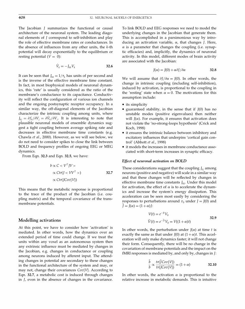
Elsevier UK Chapter: Ch32-P372560 30-9-2006 5:27p.m. Page:408 Trim:7.5in×9.25in
Basal Font:Palatino Margins:Top:40pt Gutter:68pt Font Size:9.5/12 Text Width:42pc Depth:55 Lines
408 32. NEURONAL MODELS OF ENERGETICS
The Jacobian J summarizes the functional or causalarchitecture of the neuronal system. The leading diago-nal elements of J correspond to self-inhibition and playthe role of effective membrane rates or conductances. Inthe absence of influences from any other units, the k-thpotential will decay exponentially to the equilibrium orresting potential �V = 0�:
V̇k = −JkkVk 32.6
It can be seen that Jkk = 1/�k has units of per second andis the inverse of the effective membrane time constant.In fact, in most biophysical models of neuronal dynam-ics, this ‘rate’ is usually considered as the ratio of themembrane’s conductance to its capacitance. Conductiv-ity will reflect the configuration of various ion channelsand the ongoing postsynaptic receptor occupancy. In asimilar way, the off-diagonal elements of the Jacobiancharacterize the intrinsic coupling among units, whereJkj = fk/Vj = V̇k/Vj . It is interesting to note thatplausible neuronal models of ensemble dynamics sug-gest a tight coupling between average spiking rate anddecreases in effective membrane time constants (e.g.Chawla et al., 2000). However, as we will see below, wedo not need to consider spikes to close the link betweenBOLD and frequency profiles of ongoing EEG or MEGdynamics.
From Eqn. 32.3 and Eqn. 32.5, we have:
b ∝ C < V T JV >
∝ Ctr�J < VV T >� 32.7
∝ Ctr�JCovV��
This means that the metabolic response is proportionalto the trace of the product of the Jacobian (i.e. cou-pling matrix) and the temporal covariance of the trans-membrane potentials.
Modelling activations
At this point, we have to consider how ‘activation’ ismediated. In other words, how the dynamics over anextended period of time could change. If we treat theunits within any voxel as an autonomous system thenany extrinsic influence must be mediated by changes inthe Jacobian, e.g. changes in conductance or couplingamong neurons induced by afferent input. The attend-ing changes in potential are secondary to these changesin the functional architecture of the system and may, ormay not, change their covariances CovV�. According toEqn. 32.7, a metabolic cost is induced through changesin J , even in the absence of changes in the covariance.
To link BOLD and EEG responses we need to model theunderlying changes in the Jacobian that generate them.This is accomplished in a parsimonious way by intro-ducing an activation variable, �, that changes J . Here,� is a parameter that changes the coupling (i.e. synap-tic efficacies) and, implicitly, the dynamics of neuronalactivity. In this model, different modes of brain activityare associated with the Jacobian:
J��� = J�0�+�J/� 32.8
We will assume that J/� = J�0�. In other words, thechange in intrinsic coupling (including self-inhibition),induced by activation, is proportional to the coupling inthe ‘resting’ state when � = 0. The motivations for thisassumption include:
• its simplicity• guaranteed stability, in the sense that if J�0� has no
unstable modes (positive eigenvalues) then neitherwill J���. For example, it ensures that activation doesnot violate the ‘no-strong-loops hypothesis’ (Crick andKoch, 1998)
• it ensures the intrinsic balance between inhibitory andexcitatory influences that underpins ‘cortical gain con-trol’ (Abbott et al., 1998)
• it models the increases in membrane conductance asso-ciated with short-term increases in synaptic efficacy.
Effect of neuronal activation on BOLD
These considerations suggest that the coupling Jkj amongneurons (positive and negative) will scale in a similar wayand that these changes will be reflected by changes ineffective membrane time constants Jkk. Under this modelfor activation, the effect of � is to accelerate the dynam-ics and increase the system’s energy dissipation. Thisacceleration can be seen most easily by considering theresponses to perturbations around v0 under J = J�0� andJ̃ = J��� = �1+��J :
V�t� = e−JtV0
Ṽ �t� = e−J̃ tV0 = V��1+��t�32.9
In other words, the perturbation under J��� at time t isexactly the same as that under J�0� at �1+��t. This accel-eration will only make dynamics faster; it will not changetheir form. Consequently, there will be no change in thecovariation of membrane potentials and the impact on thefMRI responses is mediated by, and only by, changes in J :
b̃
b∝ tr�J̃CovV��
tr�JCovV��= �1+�� 32.10
In other words, the activation � is proportional to therelative increase in metabolic demands. This is intuitive
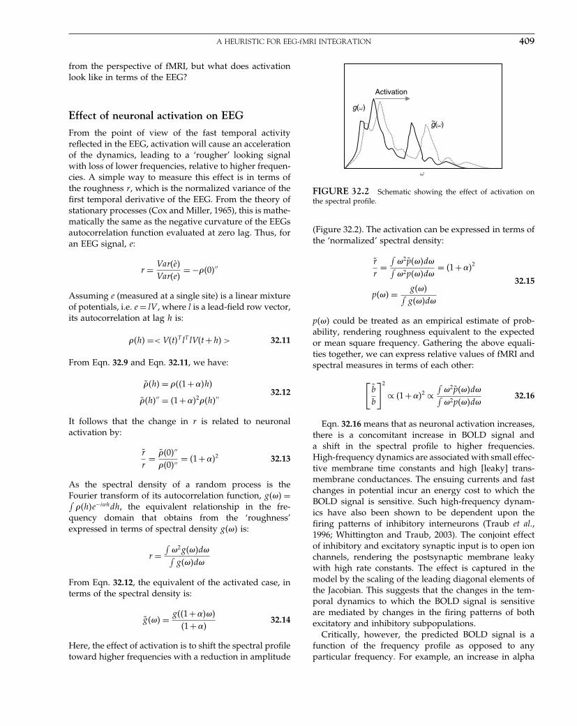
Elsevier UK Chapter: Ch32-P372560 30-9-2006 5:27p.m. Page:409 Trim:7.5in×9.25in
Basal Font:Palatino Margins:Top:40pt Gutter:68pt Font Size:9.5/12 Text Width:42pc Depth:55 Lines
A HEURISTIC FOR EEG-fMRI INTEGRATION 409
from the perspective of fMRI, but what does activationlook like in terms of the EEG?
Effect of neuronal activation on EEG
From the point of view of the fast temporal activityreflected in the EEG, activation will cause an accelerationof the dynamics, leading to a ‘rougher’ looking signalwith loss of lower frequencies, relative to higher frequen-cies. A simple way to measure this effect is in terms ofthe roughness r, which is the normalized variance of thefirst temporal derivative of the EEG. From the theory ofstationary processes (Cox and Miller, 1965), this is mathe-matically the same as the negative curvature of the EEGsautocorrelation function evaluated at zero lag. Thus, foran EEG signal, e:
r = Var�ė�
Var�e�= − �0�′′
Assuming e (measured at a single site) is a linear mixtureof potentials, i.e. e = lV , where l is a lead-field row vector,its autocorrelation at lag h is:
�h� =< V�t�T lT lV�t +h� > 32.11
From Eqn. 32.9 and Eqn. 32.11, we have:
̃�h� = ��1+��h�
̃�h�′′ = �1+��2 �h�′′ 32.12
It follows that the change in r is related to neuronalactivation by:
r̃
r= ̃�0�′′
�0�′′ = �1+��2 32.13
As the spectral density of a random process is theFourier transform of its autocorrelation function, g��� =∫
�h�e−iwhdh, the equivalent relationship in the fre-quency domain that obtains from the ‘roughness’expressed in terms of spectral density g��� is:
r =∫
�2g���d�∫g���d�
From Eqn. 32.12, the equivalent of the activated case, interms of the spectral density is:
g̃��� = g��1+����
�1+��32.14
Here, the effect of activation is to shift the spectral profiletoward higher frequencies with a reduction in amplitude
g(ω)
Activation
~g(ω)
ω
FIGURE 32.2 Schematic showing the effect of activation onthe spectral profile.
(Figure 32.2). The activation can be expressed in terms ofthe ‘normalized’ spectral density:
r̃
r=∫
�2p̃���d�∫�2p���d�
= �1+��2
p��� = g���∫g���d�
32.15
p��� could be treated as an empirical estimate of prob-ability, rendering roughness equivalent to the expectedor mean square frequency. Gathering the above equali-ties together, we can express relative values of fMRI andspectral measures in terms of each other:
[b̃
b
]2
∝ �1+��2 ∝∫
�2p̃���d�∫�2p���d�
32.16
Eqn. 32.16 means that as neuronal activation increases,there is a concomitant increase in BOLD signal anda shift in the spectral profile to higher frequencies.High-frequency dynamics are associated with small effec-tive membrane time constants and high [leaky] trans-membrane conductances. The ensuing currents and fastchanges in potential incur an energy cost to which theBOLD signal is sensitive. Such high-frequency dynam-ics have also been shown to be dependent upon thefiring patterns of inhibitory interneurons (Traub et al.,1996; Whittington and Traub, 2003). The conjoint effectof inhibitory and excitatory synaptic input is to open ionchannels, rendering the postsynaptic membrane leakywith high rate constants. The effect is captured in themodel by the scaling of the leading diagonal elements ofthe Jacobian. This suggests that the changes in the tem-poral dynamics to which the BOLD signal is sensitiveare mediated by changes in the firing patterns of bothexcitatory and inhibitory subpopulations.
Critically, however, the predicted BOLD signal is afunction of the frequency profile as opposed to anyparticular frequency. For example, an increase in alpha

Elsevier UK Chapter: Ch32-P372560 30-9-2006 5:27p.m. Page:410 Trim:7.5in×9.25in
Basal Font:Palatino Margins:Top:40pt Gutter:68pt Font Size:9.5/12 Text Width:42pc Depth:55 Lines
410 32. NEURONAL MODELS OF ENERGETICS
g(ω )
g(ω )
Deactivation
∫ω 2p(ω )d ω
∫ω 2p(ω)d ω
~
ω
ω
FIGURE 32.3 Schematic showing the effect of deactivation onmean square frequency.
(low-frequency), without a change in total power, wouldreduce the mean square frequency and suggest deactiva-tion. Conversely, an increase in gamma (high-frequency)would increase the mean square frequency and speak toactivation (Figure 32.3).
EMPIRICAL EVIDENCE
The model described in this chapter ties togetherexpected changes in BOLD and EEG measures and makesa clear prediction about the relationship between the dif-ferent frequency components of ongoing EEG or MEGactivity and the expected BOLD response. Accordingto the model, any modulations in the degree of low-frequency relative to the high-frequency components inthe EEG signal will be inversely correlated with theBOLD signal. This is largely in agreement with the empir-ical data available. It is now generally accepted that mod-ulations in the ongoing alpha rhythm, 8–12 Hz, when theeyes are shut, are inversely correlated with the BOLDsignal at voxels within the parietal, parieto-occipital andfrontal cortices (Goldman et al., 2002; Laufs et al., 2003a, b;Moosmann et al., 2003; Martinez-Montes, 2004). Further-more, during low-frequency visual entrainment, usinga periodic checkerboard stimulus, the BOLD signal isreduced compared to an aperiodic stimulus (Parkes et al.,
2004). The model presented here also predicts that a shiftin the frequency profile of the EEG to high-frequencycomponents should be correlated with an increase in theBOLD signal. Although there is a much smaller liter-ature on high-frequency EEG-BOLD correlations, whathas been published is broadly in agreement with thisprediction. Laufs et al. (2003b) report predominantly pos-itive correlations between the BOLD signal and the EEGpower in the 17–23 Hz and the 24–30 Hz bandwidth andParkes et al. (2004) demonstrate that an aperiodic checker-board stimulus induces a greater BOLD signal than alow-frequency periodic stimulus. However, perhaps themost convincing empirical data that support the pre-diction of the model described here come not from ahuman study but from a study on anaesthetized adultcats by Niessing et al. (2005). In this study, Niessingand colleagues recorded a measure of the electrical activ-ity, the local field potential (LFP), which is analogousto the EEG signal, directly from primary visual cortexusing implanted electrodes. They recorded the BOLDsignal simultaneously, using optical imaging, while thecats were shown moving whole field gratings of differ-ent orientations. Niessing et al. showed that, in trials inwhich the optical signal was strong, the neural responsetended to oscillate at higher frequencies. In other words,an increase in the BOLD signal was associated with ashift in the spectral mass of the electrical signal to higherfrequencies, in agreement with the analysis describedhere.
However, there are a number of observations that arenot captured by the model. First, the model does notaddress very slow changes in potentials, < 0�1 Hz, thatare unlikely to contribute to the event-related response.As such it does not capture the very slow modulationsin LFP that have been shown previously to be relatedto the BOLD response (Leopold et al., 2003). Secondly,and most notably, it does not explain the positive cor-relation of the BOLD signal with alpha oscillations inthe thalamus (Goldman et al., 2002; Martinez-Montes,2004). This discrepancy could reflect the unique neuronaldynamics of the thalamus. Thalamic neurons are charac-terized by complex intrinsic firing properties, which mayrange from the genesis of high-frequency bursts of actionpotentials to tonic firing (Steriade et al., 1993). However,it could also reflect the fact that the model is based onseveral assumptions that are wrong:
• The first assumption is that the dynamics of transmem-brane potentials conform to an autonomous ordinarydifferential equation (ODE). The shortcomings of thisassumption are that there is no opportunity for deter-ministic noise. However, this is a fairly mild restrictionin relation to the autonomy, which precludes extrinsicinput. This enforces afferent inputs outside the voxel

Elsevier UK Chapter: Ch32-P372560 30-9-2006 5:27p.m. Page:411 Trim:7.5in×9.25in
Basal Font:Palatino Margins:Top:40pt Gutter:68pt Font Size:9.5/12 Text Width:42pc Depth:55 Lines
EMPIRICAL EVIDENCE 411
or source to exert their influence vicariously throughchanges in the systems’ parameters, encoded by theJacobian. This can be seen as a limitation, given thedriving nature of [forward] extrinsic connections insensory cortex, but does fit comfortably with other per-spectives on functional integration in the brain (seebelow and Chapter 36).
• The use of an autonomous ODE precludes hiddenstates that mediate changes in conductance and lim-its the model to a simple integrate-and-fire-like sum-mary of neuronal behaviour. A more general form forEqn. 32.2 would require:
V̇ = fV �V�x�
ẋ = fx�V�x�32.17
where, other hidden states x might correspond toconductances and channel gating terms as in moredetailed biophysical models of neurons (see Dayan andAbbott, 2001 and Eqn. 31.6 in the previous chapter).The only argument that can be offered in defence ofEqn. 32.2 is that it may be sufficient to capture impor-tant behaviours by appeal to mean field approxima-tions (see Chapter 31).
• The activation is modelled effectively by a scaling ofthe Jacobian. Functionally, this is a severe assumptionbecause it precludes the selective enabling of particu-lar connections. The consequence of this assumptionis that any neuronal system can vary its rate or speedof computation, but can only do one thing. In real-ity, a better approximation would be bilinear with amultidimensional activation denoted by the vector � =��1� � � � �:
J̃ = J +∑�kBk
Bk = J
�k
32.18
However, this model is too unconstrained to make anygeneric comments, without assuming a particular formfor the bilinear terms Bk.
Having briefly deconstructed the model, it is worth not-ing that it highlights some important conceptual issues.These include:
• First, it reframes the notion of ‘activation’ in dynamicterms, suggesting that activation is not simply anexcess of spikes, or greater power in any particularEEG frequency band; activation may correspond to anacceleration of dynamics, subserving more rapid com-putations. This sort of activation can manifest with nooverall change in power but a change in the frequenciesat which power is expressed. Because more rapid or
dissipative dynamics are energetically more expensive,it may be that they are reserved for ‘functionally’ adap-tive or necessary neuronal processing.
• Secondly, under the generative model of activation, aspeeding up of the dynamics corresponds to a decreasein the width of the cross-correlation functions betweenall pairs of units in the population. At the macroscopiclevel of EEG recordings, considered here, the synchro-nization between pairs of units, as measured by thecross-correlation function, is captured in the width ofthe autocorrelation of the EEG signal, because the EEGsignal is a measure of synchronous neural activity.This width is a ubiquitous measure of synchroniza-tion that transcends any frequency-specific changes incoherence. In short, activation as measured by fMRIis caused, in this model, by increased synchronizationand, implicitly, a change in the temporal structure ofneuronal dynamics.
• Thirdly, our analysis suggests that the underlying ‘acti-vation’ status of neuronal systems is not expressedin any single frequency, but is exhibited across thespectral profile. This has implications for use of classi-cal terms like ‘event-related desynchronization’. If oneonly considered modulations in spectral density at onefrequency, as in the classical use of the term desyn-chronization, one would conclude that the effect ofactivation was a desynchronization of low-frequencycomponents. According to the model, however, theeffect of activation is a shift in the entire spectral pro-file to higher frequencies with a concomitant atten-uation in amplitude of all frequencies. This generalconclusion does not preclude the selective expressionof certain frequencies during specific cognitive opera-tions (e.g. increases in theta oscillations during men-tal arithmetic (Mizuhara et al., 2004)). However, themodel suggests that the context in which these fre-quencies are expressed is an important determinantof the BOLD response. In other words, it is not theabsolute power of any frequency but the profile whichdetermines expected metabolic cost.
• Fourthly, as introduced above, one of the assumptionstreats neuronal systems as autonomous, such that theevolution of their states is determined in an autonomousfashion. This translates into the assumption that thepresynaptic influence of intrinsic connections com-pletely overshadows extrinsic inputs. This may seem anodd assumption. However, it is the basis of non-linearcoupling in the brain and may represent, quantitatively,a much more important form of integration than sim-ple linear coupling. We have addressed this issue bothempirically and theoretically in Friston (2000) and inChapter 39; in brief, if extrinsic inputs affect the excitabil-ity of neurons, as opposed to simply driving a response,the coupling can be understood in terms of changes
Elsevier UK Chapter: Ch32-P372560 30-9-2006 5:27p.m. Page:412 Trim:7.5in×9.25in
Basal Font:Palatino Margins:Top:40pt Gutter:68pt Font Size:9.5/12 Text Width:42pc Depth:55 Lines
412 32. NEURONAL MODELS OF ENERGETICS
in the system parameters, namely the Jacobian. Thismeans the response to input will be non-linear. Quanti-tative analyses (a simple form of bi-coherence analysis)of MEG data suggest this form of non-linear couplingcan account for much more variation in power thanlinear coupling, i.e. coherence (see Chapter 39).
SUMMARY
The integration of EEG and fMRI data is likely to playan important role in our understanding of brain func-tion. Through multimodal fusion it should be possible toharness the temporal resolution of EEG and the spatialresolution of fMRI in characterizing neural activity. Themajority of the studies integrating EEG and fMRI to datehave focused on directly correlating the two measures,after first transforming the data so that they are on the sametemporal scale (usually by convolution of the EEG time-series with a canonical haemodynamic response function).This approach has proved successful in demonstrating thatmultimodal fusion is feasible and that regionally specificdependencies between the two measures exist. However,this approach to characterizing the relationship betweenthe EEG and the fMRI is limited as it does not character-ize the integration in terms of the underlying neuronalcauses. Full EEG-fMRI integration rests on understandingthe relationship between the underlying neuronal activityand the BOLD and EEG signals through their respectiveforward models. Although the model discussed in thischapter falls a long way short of this, it can explain thenature of some of the previously reported correlationsbetween EEG and fMRI by considering the integration interms of the underlying neuronal dynamics.
We have proposed a simple model that relates BOLDchanges to the relative spectral density of an EEG traceand the roughness of the EEG time-series. Neuronal acti-vation affects the relative contribution of high and lowEEG frequencies. This model accommodates the obser-vations that BOLD signal correlates negatively with theexpression of alpha power and positively with the expres-sion of higher frequencies. Clearly, many of the assump-tions are not correct in detail, but the overall pictureafforded may provide a new perspective on some impor-tant issues in neuroimaging. In the next chapter, we gobeyond the quantitative heuristics entailed by the dimen-sional analysis of this chapter and look at neural-massmodels with a much more detailed form. These modelsembed constraints on synaptic physiology and connec-tivity and can reproduce many of the phenomena seen inEEG recordings. In Chapter 39, we will again use detailedneural-mass models to help understand the mechanisticbasis of non-linear coupling in the brain.
REFERENCES
Abbott LF, Varela JA, Karmel Sen S et al. (1997) Synaptic depressionand cortical gain control. Science 275: 220–23
Attwell D, Iadecola C (2002) The neural basis of functional imagingbrain signals. Trends Neurosci 25: 621–25
Chawla D, Lumer ED, Friston KJ (2000) Relating macroscopic mea-sures of brain activity to fast, dynamic neuronal interactions.Neural Comput 12: 2805–21
Cox DR, Miller HD (1965) The theory of stochastic processes. Chapmanand Hall, London
Crick F, Koch C (1998) Constraints on cortical and thalamic projec-tions: the no-strong-loops hypothesis. Nature 39: 245–50
Czisch M, Wehrle R, Kaufmann C et al. (2004) Functional MRI dur-ing sleep: BOLD signal decreases and their electrophysiologicalcorrelates. Eur J Neurosci 20: 566–74
Dale AM, Liu AK, Fischl BR et al. (2000) Dynamic statistical para-metric mapping: combining fMRI and MEG for high-resolutionimaging of cortical activity. Neuron 26: 55–67
Dayan P, Abbott LF (2001). Theoretical neuroscience. computational andmathematical modelling of neural systems. MIT Press, Cambridge,MA
Friston KJ (2000) The labile brain I. Neuronal transients and nonlin-ear coupling. Phil Trans R Soc Lond B 355: 215–36
Goldman R, Stern JM, Engel J Jr et al. (2002) Simultaneous EEG andfMRI of the alpha rhythm. Neuroreport 13: 2487–92
Hoge RD, Atkinson J, Gill B et al. (1999) Linear coupling betweencerebral blood flow and oxygen consumption in activatedhuman cortex. Proc Natl Acad Sci USA 96: 9403–08
Jueptner M, Weiller C (1995) Review: does measurement of regionalcerebral blood flow reflect synaptic activity? Implications forPET and fMRI. NeuroImage 2: 148–56
Laufs H, Krakow K, Sterzer P et al. (2003a) Electroencephalographicsignatures of attentional and cognitive default modes in sponta-neous brain activity fluctuations at rest. Proc Natl Acad Sci 100:11053–58
Laufs H, Kleinschmidt A, Beyerle A et al. (2003b) EEG-correlatedfMRI of human alpha activity. NeuroImage 19: 1463–76
Lauritzen M (2001) Relationship of spikes, synaptic activity, andlocal changes of cerebral blood flow. J Cereb Blood Flow Metab 21:1367–83
Lemieux L, Krakow K, Fish DR (2001) Comparison of spike-triggered functional MRI BOLD activation and EEG dipolemodel localization. NeuroImage 14: 1097–104
Leopold DA, Murayama Y, Logothetis NK (2003) Very slow activityfluctuations in monkey visual cortex: implications for functionalbrain imaging. Cereb Cortex 13: 422–33
Logothetis NK, Pauls J, Augath M et al. (2001) Neurophysiologicalinvestigation of the basis of the fMRI signal. Nature 412: 150–57
Lovblad KO, Thomas R, Jakob PM et al. (1999) Silent functionalmagnetic resonance imaging demonstrates focal activation inrapid eye movement sleep. Neurology 53: 2193–95
Magistretti PJ, Pellerin L (1999) Cellular mechanisms of brain energymetabolism and their relevance to functional brain imaging. Phi-los Trans R Soc Lond B Biol Sci 354: 1155–63
Magistretti PJ, Pellerin L, Rothman DL et al. (1999) Energy ondemand. Science 283: 496–97
Martinez-Montes E, Valdes-Sosa PA, Miwakeichi F et al. (2004) Con-current EEG/fMRI analysis by multiway Partial Least Squares.NeuroImage 22: 1023–34
Mizuhara H, Wang LQ, Kobayashi K et al. (2004) A long-rangecortical network emerging with theta oscillation in a mental task.Neuroreport 15: 1233–38

Elsevier UK Chapter: Ch32-P372560 30-9-2006 5:27p.m. Page:413 Trim:7.5in×9.25in
Basal Font:Palatino Margins:Top:40pt Gutter:68pt Font Size:9.5/12 Text Width:42pc Depth:55 Lines
REFERENCES 413
Moosmann M, Ritter P, Krastel I et al. (2003) Correlates of alpharhythm in functional magnetic resonance imaging and nearinfrared spectroscopy. NeuroImage 20: 145–58
Niessing J, Ebisch B, Schmidt KE et al. (2005) Hemodynamic signalscorrelate tightly with synchronized gamma oscillations. Science309: 948–51
Parkes LM, Fries P, Kerskens CM et al. (2004) Reduced BOLDresponse to periodic visual stimulation. NeuroImage 21: 236–43
Phillips C, Rugg MD, Friston KJ (2002) Anatomically informed basisfunctions for EEG source localization: combining functional andanatomical constraints. NeuroImage 16: 678–95
Shin C (2000) Neurophysiologic basis of functional neuroimaging:animal studies. J Clin Neurophysiol 17: 2–9
Shulman RG, Rothman DL (1998) Interpreting functional imagingstudies in terms of neurotransmitter cycling. Proc Natl Acad SciUSA 95: 11993–98
Steriade M, McCormick DA, Sejnowski T (1993) Thalamocorti-cal oscillations in the sleeping and aroused brain. Science 262:679–85
Traub RD, Whittington MA, Stanford IM et al. (1996)A mechanism for generation of long-range syn-chronous fast oscillations in the cortex. Nature 383:621–24
Whittington MA, Traub RD (2003) Interneuron diversity series:inhibitory interneurons and network oscillations in vitro. TrendsNeurosci 26: 676–82

Elsevier UK Chapter: Ch33-P372560 30-9-2006 5:28p.m. Page:414 Trim:7.5in×9.25in
Basal Font:Palatino Margins:Top:40pt Gutter:68pt Font Size:9.5/12 Text Width:42pc Depth:55 Lines
C H A P T E R
33
Neuronal models of EEG and MEGO. David, L. Harrison and K. Friston
INTRODUCTION
This chapter considers the mechanisms that shapeevoked electroencephalographic (EEG) and magnetoen-cephalographic (MEG) responses. We introduce neural-mass models and focus on a particular model ofhierarchically arranged areas, defined with three kinds ofinter-area connections (forward, backward and lateral).Using this model, we will investigate the role of connec-tions or coupling on the generation of oscillations andevent-related activity. Neural-mass models can repro-duce nearly all the characteristics of event-related activityobserved with M/EEG. Critically, they enforce a neuro-biological perspective on ERPs (even-related potentials).This chapter uses neural-mass models to emulate com-mon M/EEG phenomena and, in doing so, addressestheir underlying mechanisms. In Chapter 42, we willshow how the parameters of these models can be esti-mated from real data. This is the goal of dynamiccausal modelling, where differences in ERP compo-nents, between conditions, are explained by connectivitychanges within the brain.
Overview
This chapter gathers together the ideas and results pre-sented in a series of papers (David and Friston, 2003;David et al., 2004, 2006b) describing the developmentof neural-mass models for dynamic causal modelling(DCM). These neural-mass models are used in statisticalparametric mapping (SPM) as the basis of DCM forevent-related potentials (ERP) and event-related fields(ERFs) (see Chapter 42). In this chapter, we describewhat a neural-mass model is; we then construct, a pos-teriori, the model used in later chapters, starting with asingle neuronal population and ending with hierarchi-
cal cortical models. Finally, we illustrate how this modelcan be used to understand the basis of key phenomenaobserved with EEG and MEG.
NEURAL-MASS MODELS
M/EEG signals result mainly from extracellular currentflow, associated with summed postsynaptic potentials insynchronously activated and vertically oriented neurons(i.e. the dendritic activity of macrocolumns of pyramidalcells in the cortical sheet) (see Chapter 28). Often, signalsmeasured in MEG and EEG are decomposed into dis-tinct frequency bands (delta: 1–4 Hz; theta: 4–8 Hz; alpha:8–12 Hz; beta: 12–30 Hz; gamma: 30–70 Hz) (Nunez andSrinivasan, 2005). These rhythms exhibit robust correlatesof behavioural states but often with no obvious functionalrole. The exact neurophysiological mechanisms, whichconstrain synchronization to a given frequency band,remain obscure, however, the generation of oscillationsappears to depend on interactions between inhibitoryand excitatory populations, whose kinetics determinetheir oscillation frequency.
ERPs and ERFs are obtained by averaging EEG andMEG signals in reference to some change in stimulusor task (Coles and Rugg, 1995). They show transientactivity that lasts a second or so and which is corre-lated with changes in the state of the subject. ERPsand ERFs have been used for decades as putative elec-trophysiological correlates of perceptual and cognitiveoperations. However, like M/EEG oscillations, the exactneurobiological mechanisms underlying their generationare largely unknown. Recently, there has been a growinginterest in the distinction between evoked and inducedresponses (see Chapter 30). Evoked responses are dis-closed by conventional averaging procedures (classical
Statistical Parametric Mapping, by Karl Friston et al. Copyright 2007, Elsevier Ltd. All rights reserved.ISBN–13: 978-0-12-372560-8 ISBN–10: 0-12-372560-7
414

Elsevier UK Chapter: Ch33-P372560 30-9-2006 5:28p.m. Page:415 Trim:7.5in×9.25in
Basal Font:Palatino Margins:Top:40pt Gutter:68pt Font Size:9.5/12 Text Width:42pc Depth:55 Lines
NEURAL-MASS MODELS 415
ERPs/ERFs), whereas the latter usually call for single-trial analyses of induced oscillations (Tallon-Baudry andBertrand, 1999). Understanding the mechanistic relation-ship between evoked and induced responses could bea key for revealing how the electrical activity reacts toexperimental changes. In other words, generative mod-els of both M/EEG and ERP/ERF could be importantfor revealing how information is coded and processed inneural networks.
What is a neural-mass model?
There are several ways to model neural signals (Whit-tington et al., 2000): by using either a detailed model, inwhich it is difficult to determine the influence of eachmodel parameter, or a simplified one, in which realismis sacrificed for a more parsimonious description of keymechanisms. The complexity of neural networks gen-erating M/EEG signals (Thomson and Deuchars, 1997;DeFelipe et al., 2002) is considerable and usually makesthe second approach more viable. Neural-mass mod-els (Lopes da Silva et al., 1974; Freeman, 1978; VanRotterdam et al., 1982; Stam et al., 1999; Valdes et al.,1999; Wendling et al., 2000; Robinson et al., 2001; Davidand Friston, 2003) are examples of simplified models,which usually model cortical macrocolumns as surro-gates for cortical areas and, sometimes, thalamic nuclei.They use only one or two state variables to repre-sent the mean activity of neuronal populations. Thesestates summarize the behaviour of millions of inter-acting neurons. This procedure, sometimes referred toloosely as a mean-field approximation, is very efficientfor determining the steady-state behaviour of neuronalsystems, but its utility in a dynamic or non-stationarycontext is less established (Haskell et al., 2001) (seeChapter 31 for a detailed discussion). In what follows,we will assume that the mean-field approximation is suf-ficient for our purposes. Figure 33.1 shows a schematicthat tries to convey the intuition behind mean-fieldapproximations.
As we saw in Chapter 31, the mean-field approxi-mation involves partitioning the neuronal system intoseparable ensembles. Each ensemble or population isthen coupled with mean-field quantities like average fir-ing rate. In neural-mass models, we make the furtherapproximation that the density of each ensemble can bedescribed as a point mass. In other words, we ignorethe variability in the states of neurons in an ensem-ble and assume that their collective behaviour can beapproximated with a single value (i.e. the density‘s mode)for each state variable (e.g. voltage, current, conduc-tance etc.).
w
wn
w2
ν1
u1
0
1ν1
u1
w1
ν2
u2
0
1ν2
u2
νn
un
0
1νn
un
.
.
.ν
u
0
1
u, ν
r
FIGURE 33.1 Mean-field approximation (MFA). Left: considera neuronal population comprising n neurons. vi, mi and wi denotethe membrane potential, the normalized firing rate and the firingthreshold of the i-th neuron, respectively. The input-output step-functions show that, in this example, the neurons fire at 1 or donot fire, depending on the threshold of firing which may varybetween neurons. Right: the MFA of the neural-mass models stipu-lates that the dynamics of the neuronal ensemble, or neuronal mass,is described sufficiently by the mean of the state variables (v and m),using the mean relationship between v and m (the step function istransformed into a sigmoid function by averaging). Thus the effectof the MFA is that it reduces a huge system into a small one.
Neural-mass models of M/EEG
M/EEG signals are generated by the massively syn-chronous dendritic activity of pyramidal cells (Nunezand Srinivasan, 2005), but modelling M/EEG signals isseldom tractable using realistic models because of thecomplexity of real neural networks. Since the 1970s, thepreferred approach has been neural-mass models, i.e.models which describe the average activity with a smallnumber of state variables (see Figure 33.1). Basically,these models use two conversion operations (Jirsa andHaken, 1997; Robinson et al., 2001): a wave-to-pulse oper-ator at the soma of neurons, which is generally a staticsigmoid function; and a linear pulse-to-wave conversionimplemented at a synaptic level. The first operator relatesthe mean firing rate to average postsynaptic depolariza-tion. This is assumed to be instantaneous. The secondoperator depends on synaptic kinetics and models theaverage postsynaptic response as a linear convolution ofincoming spike rate. The shape of the convolution ker-nels embodies the synaptic and dendritic kinetics of thepopulation (Figures 33.2 and 33.3).
The majority of neural-mass models of M/EEG havebeen designed to generate alpha rhythms (Lopes da Silvaet al., 1974; Van Rotterdam et al., 1982; Jansen and Rit, 1995;Stam et al., 1999). Recent studies have shown that it ispossible to reproduce the whole spectrum of M/EEG oscil-lations, using appropriate model parameters (Robinson
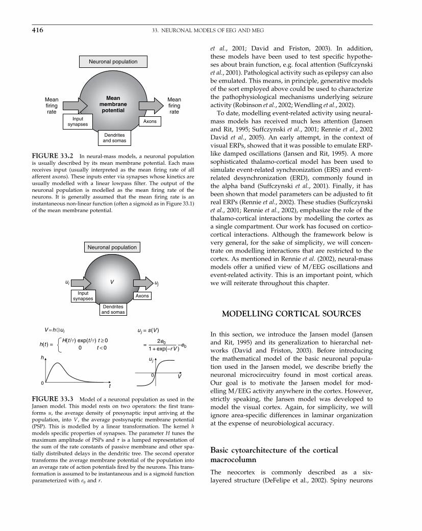
Elsevier UK Chapter: Ch33-P372560 30-9-2006 5:28p.m. Page:416 Trim:7.5in×9.25in
Basal Font:Palatino Margins:Top:40pt Gutter:68pt Font Size:9.5/12 Text Width:42pc Depth:55 Lines
416 33. NEURONAL MODELS OF EEG AND MEG
Meanmembranepotential
Meanfiringrate
Meanfiringrate
Neuronal population
Inputsynapses
Dendritesand somas
Axons
FIGURE 33.2 In neural-mass models, a neuronal populationis usually described by its mean membrane potential. Each massreceives input (usually interpreted as the mean firing rate of allafferent axons). These inputs enter via synapses whose kinetics areusually modelled with a linear lowpass filter. The output of theneuronal population is modelled as the mean firing rate of theneurons. It is generally assumed that the mean firing rate is aninstantaneous non-linear function (often a sigmoid as in Figure 33.1)of the mean membrane potential.
V
Neuronal population
Inputsynapses
Dendritesand somas
Axons
H(t /τ) exp(t /τ) t ≥ 0h(t ) =
V = h ui u j = s (V )
V
h
t0
0
ujui
0 t < 02e0
1 + exp(–r V )–e0=
u j
FIGURE 33.3 Model of a neuronal population as used in theJansen model. This model rests on two operators: the first trans-forms u, the average density of presynaptic input arriving at thepopulation, into V , the average postsynaptic membrane potential(PSP). This is modelled by a linear transformation. The kernel hmodels specific properties of synapses. The parameter H tunes themaximum amplitude of PSPs and � is a lumped representation ofthe sum of the rate constants of passive membrane and other spa-tially distributed delays in the dendritic tree. The second operatortransforms the average membrane potential of the population intoan average rate of action potentials fired by the neurons. This trans-formation is assumed to be instantaneous and is a sigmoid functionparameterized with e0 and r.
et al., 2001; David and Friston, 2003). In addition,these models have been used to test specific hypothe-ses about brain function, e.g. focal attention (Suffczynskiet al., 2001). Pathological activity such as epilepsy can alsobe emulated. This means, in principle, generative modelsof the sort employed above could be used to characterizethe pathophysiological mechanisms underlying seizureactivity (Robinson et al., 2002; Wendling et al., 2002).
To date, modelling event-related activity using neural-mass models has received much less attention (Jansenand Rit, 1995; Suffczynski et al., 2001; Rennie et al., 2002David et al., 2005). An early attempt, in the context ofvisual ERPs, showed that it was possible to emulate ERP-like damped oscillations (Jansen and Rit, 1995). A moresophisticated thalamo-cortical model has been used tosimulate event-related synchronization (ERS) and event-related desynchronization (ERD), commonly found inthe alpha band (Suffczynski et al., 2001). Finally, it hasbeen shown that model parameters can be adjusted to fitreal ERPs (Rennie et al., 2002). These studies (Suffczynskiet al., 2001; Rennie et al., 2002), emphasize the role of thethalamo-cortical interactions by modelling the cortex asa single compartment. Our work has focused on cortico-cortical interactions. Although the framework below isvery general, for the sake of simplicity, we will concen-trate on modelling interactions that are restricted to thecortex. As mentioned in Rennie et al. (2002), neural-massmodels offer a unified view of M/EEG oscillations andevent-related activity. This is an important point, whichwe will reiterate throughout this chapter.
MODELLING CORTICAL SOURCES
In this section, we introduce the Jansen model (Jansenand Rit, 1995) and its generalization to hierarchal net-works (David and Friston, 2003). Before introducingthe mathematical model of the basic neuronal popula-tion used in the Jansen model, we describe briefly theneuronal microcircuitry found in most cortical areas.Our goal is to motivate the Jansen model for mod-elling M/EEG activity anywhere in the cortex. However,strictly speaking, the Jansen model was developed tomodel the visual cortex. Again, for simplicity, we willignore area-specific differences in laminar organizationat the expense of neurobiological accuracy.
Basic cytoarchitecture of the corticalmacrocolumn
The neocortex is commonly described as a six-layered structure (DeFelipe et al., 2002). Spiny neurons

Elsevier UK Chapter: Ch33-P372560 30-9-2006 5:28p.m. Page:417 Trim:7.5in×9.25in
Basal Font:Palatino Margins:Top:40pt Gutter:68pt Font Size:9.5/12 Text Width:42pc Depth:55 Lines
MODELLING CORTICAL SOURCES 417
(pyramidal cells and spiny stellate cells) and smoothneurons comprise the two major groups of corticalneurons. The majority of cortical neurons are pyrami-dal cells that are found in layers 2 to 6. Most spinystellate cells are interneurons that are located in themiddle cortical layers. Smooth neurons are essentiallyGABA (�-aminobutyric acid)-ergic interneurons that aredistributed in all layers. In general, cortical neuronsare thought to be organized into multiple, repeatingmicrocircuits. In spite of cortical heterogeneity, a basicmicrocircuit has emerged: its skeleton is formed by apyramidal cell, which receives excitatory inputs fromextrinsic afferents and spiny cells. Inhibitory inputsoriginate mostly from GABAergic interneurons. Thesemicroanatomical characteristics have been found in allcortical areas and species examined so far and can be con-sidered as fundamental aspects of cortical organization(DeFelipe et al., 2002).
These canonical microcircuits are commonly referredto as cortical minicolumns (∼ 50 �m diameter, containingabout 400 principal cells), which are themselves groupedinto cortical macrocolumns (∼ 900 �m diameter) (Jones,2000). A cortical area (∼ 1–2 cm diameter) is composed ofmany cortical macrocolumns. Depending upon the levelof integration one is interested in, each of these struc-tures (cortical minicolumn, macrocolumn or area) can beconsidered as the functional unit, whose behavioural isapproximated by neural-mass models. As we are inter-ested here in cognitive neuroscience, using macroscopicmeasurements, we will consider the highest level of orga-nization and build a neural-mass model (GeneralizedJansen Model) reflecting the activity of cortical areas.
Modelling a neuronal population
A cortical area, macrocolumn or minicolumn, comprisesseveral neuronal subpopulations. In this section, wedescribe the mathematical model of one area, which spec-ifies the evolution of the dynamics of each subpopulation.This evolution rests on two operators (see Figure 33.3):the first transforms u�t�, the average density of pre-synaptic input arriving at the population, into V�t�, theaverage postsynaptic membrane potential (PSP). This ismodelled by the linear transformation:
V = h⊗u 33.1
where ⊗ denotes the convolution operator in the timedomain and h is the impulse response or first-order kernel:
h�t� ={
H�t/�� exp�−t/�� t ≥ 0
0 t < 033.2
The kernel h is parameterized by H and � that modelspecific properties of synapses: the parameter H tunes
the maximum amplitude of PSPs and � is a lumpedrepresentation of the sum of the rate constants of passivemembrane and other spatially distributed delays in thedendritic tree. Eqn. 33.1 and Eqn. 33.2 are mathematicallyequivalent to the following state equations:
ġ = H
�u− 2
�g − 1
�2V
V̇ = g
⇒ V̈ = H
�u− 2
�V̇ − 1
�2V
33.3
Note that this has the same form as Eqn. 32.2 in theprevious chapter; I = −CV̇ , if we assume g = −I/C isproportional to transmembrane current. When the exter-nal input to the population u�t� is known, it is possibleto obtain the membrane potential v�t� by integratingEqn. 33.3 (see Kloeden and Platen, 1999 for a descriptionof various numerical solutions of differential equations).Eqn. 33.3 is effectively a second-order differential equa-tion governing the evolution of postsynaptic potential inresponse to input and is formally similar to the equationsof motion in Chapter 31 (e.g. Eqn. 31.6) for integrate-and-fire neurons.
The second operator transforms the average membranepotential of the population into the average rate of actionpotentials fired by the neurons. This transformation isassumed to be instantaneous and is described by thesigmoid function:
s�V� = 2e0
1+exp�−rV�− e0 33.4
where e0 and r are parameters that determine its shape(e.g. voltage sensitivity). It is this function that endowsthe model with non-linear behaviours that are criticalfor phenomena like phase-resetting of the M/EEG (seebelow). Note that the form of s�V� specifies implicitly thatthe resting state for the mean membrane potential v andthe mean firing rate u = s�V� is zero. This means that weare modelling variations of v around its resting value,which is usually negative (tens of mV) but unknown.In other words, states are treated as small perturbationsaround their resting values, which are set to zero.
Neural-mass versus mean-field models
The sigmoid function in Eqn. 33.4 is quite important forneural-mass models because it summarizes the effects ofvariability, over the population, considered in full mean-field treatments. In Chapter 31, we coupled populationswith the mean-field quantities s�i� = M��i�, where M wasa linear operator that returned the mean firing rate and��i� was the population density of the i-th population.In neural-mass models we only use the mode of thisdensity, i.e. V �i� = maxV ��i��V�. This means we have to
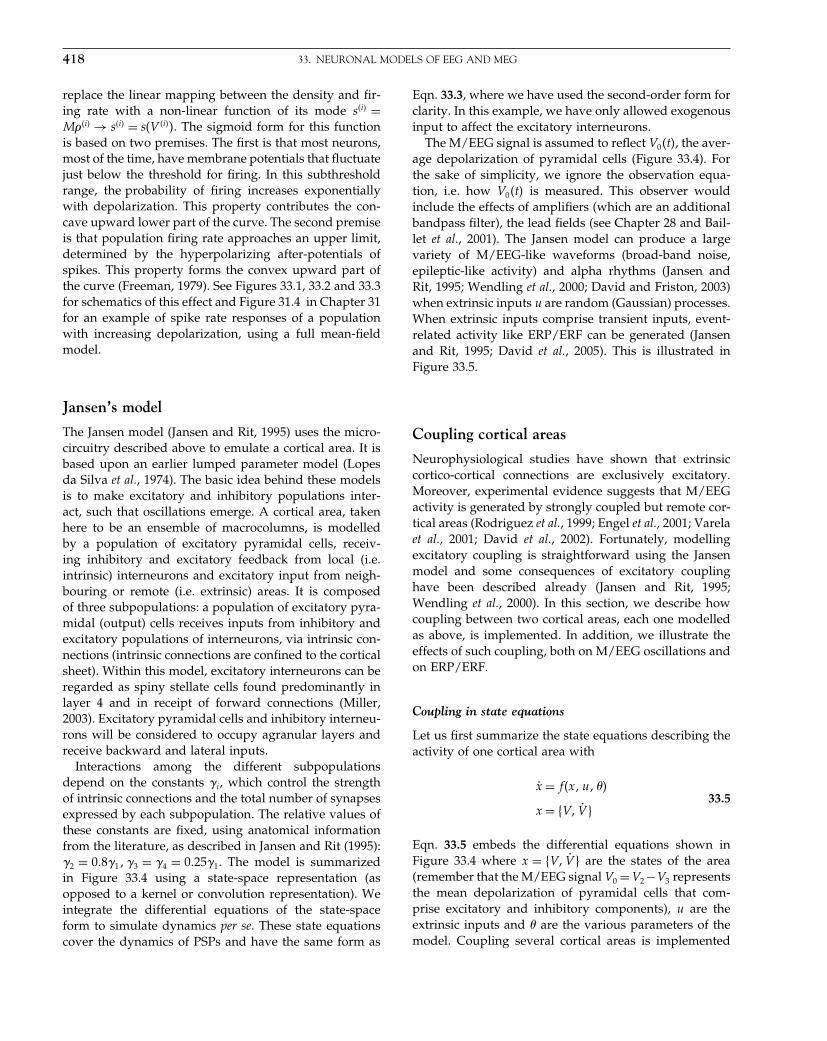
Elsevier UK Chapter: Ch33-P372560 30-9-2006 5:28p.m. Page:418 Trim:7.5in×9.25in
Basal Font:Palatino Margins:Top:40pt Gutter:68pt Font Size:9.5/12 Text Width:42pc Depth:55 Lines
418 33. NEURONAL MODELS OF EEG AND MEG
replace the linear mapping between the density and fir-ing rate with a non-linear function of its mode s�i� =M��i� → s�i� = s�V �i��. The sigmoid form for this functionis based on two premises. The first is that most neurons,most of the time, have membrane potentials that fluctuatejust below the threshold for firing. In this subthresholdrange, the probability of firing increases exponentiallywith depolarization. This property contributes the con-cave upward lower part of the curve. The second premiseis that population firing rate approaches an upper limit,determined by the hyperpolarizing after-potentials ofspikes. This property forms the convex upward part ofthe curve (Freeman, 1979). See Figures 33.1, 33.2 and 33.3for schematics of this effect and Figure 31.4 in Chapter 31for an example of spike rate responses of a populationwith increasing depolarization, using a full mean-fieldmodel.
Jansen’s model
The Jansen model (Jansen and Rit, 1995) uses the micro-circuitry described above to emulate a cortical area. It isbased upon an earlier lumped parameter model (Lopesda Silva et al., 1974). The basic idea behind these modelsis to make excitatory and inhibitory populations inter-act, such that oscillations emerge. A cortical area, takenhere to be an ensemble of macrocolumns, is modelledby a population of excitatory pyramidal cells, receiv-ing inhibitory and excitatory feedback from local (i.e.intrinsic) interneurons and excitatory input from neigh-bouring or remote (i.e. extrinsic) areas. It is composedof three subpopulations: a population of excitatory pyra-midal (output) cells receives inputs from inhibitory andexcitatory populations of interneurons, via intrinsic con-nections (intrinsic connections are confined to the corticalsheet). Within this model, excitatory interneurons can beregarded as spiny stellate cells found predominantly inlayer 4 and in receipt of forward connections (Miller,2003). Excitatory pyramidal cells and inhibitory interneu-rons will be considered to occupy agranular layers andreceive backward and lateral inputs.
Interactions among the different subpopulationsdepend on the constants �i, which control the strengthof intrinsic connections and the total number of synapsesexpressed by each subpopulation. The relative values ofthese constants are fixed, using anatomical informationfrom the literature, as described in Jansen and Rit (1995):�2 = 0�8�1�3 = �4 = 0�25�1. The model is summarizedin Figure 33.4 using a state-space representation (asopposed to a kernel or convolution representation). Weintegrate the differential equations of the state-spaceform to simulate dynamics per se. These state equationscover the dynamics of PSPs and have the same form as
Eqn. 33.3, where we have used the second-order form forclarity. In this example, we have only allowed exogenousinput to affect the excitatory interneurons.
The M/EEG signal is assumed to reflect V0�t�, the aver-age depolarization of pyramidal cells (Figure 33.4). Forthe sake of simplicity, we ignore the observation equa-tion, i.e. how V0�t� is measured. This observer wouldinclude the effects of amplifiers (which are an additionalbandpass filter), the lead fields (see Chapter 28 and Bail-let et al., 2001). The Jansen model can produce a largevariety of M/EEG-like waveforms (broad-band noise,epileptic-like activity) and alpha rhythms (Jansen andRit, 1995; Wendling et al., 2000; David and Friston, 2003)when extrinsic inputs u are random (Gaussian) processes.When extrinsic inputs comprise transient inputs, event-related activity like ERP/ERF can be generated (Jansenand Rit, 1995; David et al., 2005). This is illustrated inFigure 33.5.
Coupling cortical areas
Neurophysiological studies have shown that extrinsiccortico-cortical connections are exclusively excitatory.Moreover, experimental evidence suggests that M/EEGactivity is generated by strongly coupled but remote cor-tical areas (Rodriguez et al., 1999; Engel et al., 2001; Varelaet al., 2001; David et al., 2002). Fortunately, modellingexcitatory coupling is straightforward using the Jansenmodel and some consequences of excitatory couplinghave been described already (Jansen and Rit, 1995;Wendling et al., 2000). In this section, we describe howcoupling between two cortical areas, each one modelledas above, is implemented. In addition, we illustrate theeffects of such coupling, both on M/EEG oscillations andon ERP/ERF.
Coupling in state equations
Let us first summarize the state equations describing theactivity of one cortical area with
ẋ = f�xu�
x = �V V̇ �33.5
Eqn. 33.5 embeds the differential equations shown inFigure 33.4 where x = �V V̇ � are the states of the area(remember that the M/EEG signal V0 = V2 −V3 representsthe mean depolarization of pyramidal cells that com-prise excitatory and inhibitory components), u are theextrinsic inputs and are the various parameters of themodel. Coupling several cortical areas is implemented

Elsevier UK Chapter: Ch33-P372560 30-9-2006 5:28p.m. Page:419 Trim:7.5in×9.25in
Basal Font:Palatino Margins:Top:40pt Gutter:68pt Font Size:9.5/12 Text Width:42pc Depth:55 Lines
MODELLING CORTICAL SOURCES 419
γ 2γ 1
γ 4 γ 3
u
1c
c 2
c 3
He = 3.25 e0 = 2.5
r = 0.56δ = 10 ms
Hi = 29.3τe = 10 msτi = 15 ms
γ1
= 50γ
2 = 40
γ3
= 12γ
4 = 12
Inhibitoryinterneurons
Spinystellate
cells
Pyramidalcells
Intrinsicconnections
Extrinsicconnections
V4 =.. He
τe
2V4
.
τe
V4τe
γ3S(V0 ) – –
V2 =.. He
τe
γ2S(V1 ) –
2V2
.
τe
V2
τe
–2
2V3 =
V0 = V2 – V3
.. Hi
τi
2V3
.
τi
V3
τi
γ4S(V4 ) – –
V1 =.. He
τe
2V1
.
τe
V1
.
τe
(γ1S(V0) + cu ) – –2
2
FIGURE 33.4 State-space representation of Jansen’s model of a cortical area. Three neuronal subpopulations are considered to model acortical area. Pyramidal cells interact with both excitatory and inhibitory interneurons with the connectivity constants �2 = 0�8�1�3 = �4 =0�25�1. The parameters H and � control the expression of postsynaptic potentials (see previous figure). Subscripts e and i denote excitatoryand inhibitory, respectively. We assume the average depolarization of pyramidal cells V0 is proportional to cortical current densities obtainedwith source reconstruction algorithms using M/EEG scalp data. The insert provides the values of parameters used for all the simulations inthis chapter: refers to propagation delays on extrinsic connections.
Spinystellate
cells
Inhibitoryinterneurons
u(t )
v (t )
v (t )
u(t )
Pyramidalcells
Spinystellate
cells
Inhibitoryinterneurons
Pyramidalcells
4
2
0
0 100 200 300 400 500 600 700 800 900 1000
–2
–4
6
4
2
0 100 200 300 400 500 600 700 800 900 1000
0
Time (ms)
Time (ms)
FIGURE 33.5 Effect of the nature ofextrinsic inputs u on the responses of a corti-cal area (Jansen model). Upper: M/EEG-likeoscillations are obtained when u is stochas-tic (Gaussian in this simulation). Lower:ERP/ERF-like waveforms are obtained whenu contains a fast transient (a delta functionin this simulation). This simulation used themodel described in Figure 33.4.
by treating the outputs of one cortical area as the extrin-sic input to another. The input aijs�V
�j�� to the i-th is themean firing of pyramidal cells in the j-th, multiplied bythe strength of the connection or coupling aij .
For several areas with states x�I�, we can expressthe dynamics as a set of coupling differential
equations where, ignoring propagation delays forsimplicity:
ẋ�1� = f�x�1� a12S�V �2�0 �+a13S�V �3�
0 �+· · ·+ c1u�1��
ẋ�2� = f�x�2� a21S�V �1�0 �+a23S�V �3�
0 �+· · ·+ c2u�2��
ẋ�2� = � � � 33.6
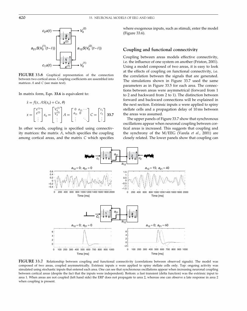
Elsevier UK Chapter: Ch33-P372560 30-9-2006 5:28p.m. Page:420 Trim:7.5in×9.25in
Basal Font:Palatino Margins:Top:40pt Gutter:68pt Font Size:9.5/12 Text Width:42pc Depth:55 Lines
420 33. NEURONAL MODELS OF EEG AND MEG
2
1
x
c 2u(t )
c 1u(t )
a 21S(V0 (t – δ ))(1)
a 12S(V0 (t – δ ))(2)
(1)
x(2)
(1)V0
(2)V0
FIGURE 33.6 Graphical representation of the connectionbetween two cortical areas. Coupling coefficients are assembled intomatrices A and C (see main text).
In matrix form, Eqn. 33.6 is equivalent to:
ẋ = f�xAS�x0�+Cu�
x =⎡⎣
x�1�
x�2�
���
⎤⎦x0 =
⎡⎢⎣
V �1�0
V �2�0���
⎤⎥⎦A =
⎡⎣
0 a12 · · ·a21 0���
� � �
⎤⎦C =
⎡⎣
c1c2���
⎤⎦ 33.7
In other words, coupling is specified using connectiv-ity matrices: the matrix A, which specifies the couplingamong cortical areas, and the matrix C which specifies
where exogenous inputs, such as stimuli, enter the model(Figure 33.6).
Coupling and functional connectivity
Coupling between areas models effective connectivity,i.e. the influence of one system on another (Friston, 2001).Using a model composed of two areas, it is easy to lookat the effects of coupling on functional connectivity, i.e.the correlation between the signals that are generated.The simulations shown in Figure 33.7 used the sameparameters as in Figure 33.5 for each area. The connec-tions between areas were asymmetrical (forward from 1to 2 and backward from 2 to 1). The distinction betweenforward and backward connections will be explained inthe next section. Extrinsic inputs u were applied to spinystellate cells and a propagation delay of 10 ms betweenthe areas was assumed.
The upper panels of Figure 33.7 show that synchronousoscillations appear when neuronal coupling between cor-tical areas is increased. This suggests that coupling andthe synchrony of the M/EEG (Varela et al., 2001) areclosely related. The lower panels show that coupling can
1
1
2
2c1
a12 = 0; a21 = 0 a12 = 0; a21 = 60
a12 = 15; a21 = 40a12 = 0; a21 = 00.60.40.2
0–0.2–0.4
0
0
2
4
6
0
2
4
6
–2
0 100 200 300 400 500 600 700 800 900 1000 0 100 200 300 400 500 600 700 800 900 1000
200 400 600 800 1000 1200 1400 1600 1800 2000 0
–1.5
1.5
–1–0.5
00.5
1
200 400 600 800 1000 12001400 1600 1800 2000
Time [ms]
Time [ms] Time [ms]
Time [ms]
a21
a21
a12
a12
c2c1
FIGURE 33.7 Relationship between coupling and functional connectivity (correlations between observed signals). The model wascomposed of two areas, coupled asymmetrically. Extrinsic inputs u were applied to spiny stellate cells only. Top: ongoing activity wassimulated using stochastic inputs that entered each area. One can see that synchronous oscillations appear when increasing neuronal couplingbetween cortical areas (despite the fact that the inputs were independent). Bottom: a fast transient (delta function) was the extrinsic input toarea 1. When areas are not coupled (left hand side) the ERP does not propagate to area 2, whereas one can observe a late response in area 2when coupling is present.

Elsevier UK Chapter: Ch33-P372560 30-9-2006 5:28p.m. Page:421 Trim:7.5in×9.25in
Basal Font:Palatino Margins:Top:40pt Gutter:68pt Font Size:9.5/12 Text Width:42pc Depth:55 Lines
HIERARCHICAL MODELS OF CORTICAL NETWORKS 421
propagateneuronal transientssuchasERP/ERF.Thistopicwillbediscussed in more depth later. The important pointhere is that changes in coupling can explain many aspectsof synchronization and ERP/ERFs and are in a positionto bridge the study of evoked and induced or ongoingM/EEG activity. We will come back to this issue later.
So far, we have been introducing the different compo-nents and key ideas behind neural-mass models. In thenext section, we describe the model which we have usedto simulate several aspects of cortical responses and useas the generative model for DCM in later chapters. Thekey feature of this model is its hierarchal architecture thatarises from the distinction between forward, backwardand lateral extrinsic connections.
HIERARCHICAL MODELS OF CORTICALNETWORKS
It is well known that the cortex has a hierarchical organi-zation (Felleman and Van Essen, 1991; Crick and Koch,1998), comprising bottom-up, top-down and lateral pro-cesses that can be understood from an anatomical andcognitive perspective (Engel et al., 2001). We have dis-cussed previously the importance of hierarchical pro-cesses, in relation to perceptual inference in the brain,using the intimate relationship between hierarchicalmodels and empirical Bayes (Friston, 2002). Using a hier-archical neural-mass model, the work described in Davidet al. (2005) and reprised here, was more physiologicallymotivated. We were primarily interested in the effects, onevent-related M/EEG activity, of connections strengths,and how these effects were expressed at different hier-archical levels. In addition, we were interested in hownon-linearities in these connections might be expressedin observed responses. In this section, we describe thearchitecture and the state equations of the neural-massmodel which is used in DCM (David et al., 2006a; Kiebelet al., 2006; and Chapter 42). The subsequent sections in
this chapter explore the emergent properties of the modeland the mechanistic insights provided.
Forward, backward and lateral connections
Although neural-mass models originated in the early1970s (Wilson and Cowan, 1972; Lopes da Silva et al.,1974; Freeman, 1978), none has addressed the hierarchicalnature of cortical organization. The minimal model wepropose, which accounts for directed extrinsic connec-tions, uses the rules described in Felleman and Van Essen(1991). Extrinsic connections are connections that traversewhite matter and connect cortical regions (and subcorti-cal structures). These rules, based upon a tri-partitioningof the cortical sheet (into supra-, infra-granular layers andgranular layer 4), have been derived from experimentalstudies of cat visual cortex. We will assume that they canbe generalized to the whole cortex. The ensuing modelis general, and can be used to model various corticalnetworks (David et al., 2006a; Kiebel et al., 2006), wherevariability among different cytoarchitectonic regions ismodelled by different area-specific parameters, under thesame microcircuitry. Under this simplifying assumption,the connections can be defined as in Figure 33.8: bottom-up or forward connections originate in agranular layersand terminate in layer 4. Top-down or backwardconnections only connect agranular layers. Lateral con-nections originate in agranular layers and target all lay-ers. All these long-range or extrinsic cortico-cortical con-nections are excitatory and are mediated through theaxons of pyramidal cells. For schematic reasons, we lumpthe superficial and deep pyramidal layers into the infra-granular layer in our model.
Although the thalamo-cortical connections have beenthe focus of several modelling studies, they represent aminority of extrinsic connections: in contrast, it is thoughtthat at least 99 per cent of axons in white matter link cor-tical areas of the same hemisphere (Abeles, 1991). For thisreason, and for simplicity, we do not include the thalamic
Supra-granular
Infra-granular
Layer 4
Bottom-up Top-down Lateral
FIGURE 33.8 Connection rules adopted for the construction of hierarchical models. These rules are a simplified version of those proposedby Felleman and Van Essen (1991). The cortical sheet is divided into two components: the granular layer (layer 4) and the agranular layers(supra- and infra-granular layers). Bottom-up connections originate in agranular layers and terminate in layer 4. Top-down connections onlyengage agranular layers. Lateral connections originate in agranular layers and target all layers.

Elsevier UK Chapter: Ch33-P372560 30-9-2006 5:28p.m. Page:422 Trim:7.5in×9.25in
Basal Font:Palatino Margins:Top:40pt Gutter:68pt Font Size:9.5/12 Text Width:42pc Depth:55 Lines
422 33. NEURONAL MODELS OF EEG AND MEG
nuclei in our model. However, they can be included ifthe role of the thalamus (or other subcortical structure)is thought important.
State equations
Using the connection rules above, it is straightforwardto construct hierarchical cortico-cortical networks usingJansen models of cortical areas. The different types ofconnections are shown in Figure 33.9, in terms of con-nections among the three subpopulations. To modelevent-related responses, the network receives inputsvia exogenous input connections. These connections areexactly the same as forward connections delivering fixedor stochastic inputs u to the spiny stellate cells in layer 4.In the present context, they can be regarded as connectionsfrom thalamic or geniculate nuclei. Inputs u can modelincoming stimuli and stochastic background activity.
Connections among areas are mediated by long-range excitatory (glutaminergic) pathways. As discussedabove, we consider three types of extrinsic connec-tions (Figure 33.9): forward, backward, and lateral. Thestrength of each type of connection is controlled by acoupling parameter a � aF for forward, aB for backwardand aL for lateral. We model propagation delays for theseconnections. The state equations for a single area areshown in Figure 33.10. It can be seen that the distinctionbetween forward, backward and lateral connections ismodelled in terms of which subpopulation is affected byinput from the pyramidal cells of another area. The insertshows the values of the intrinsic parameters �i� used inall the simulations of this chapter.
Using these connections, hierarchical cortical modelsfor M/EEG can be constructed to test various hypothe-ses, and represent examples of dynamic causal models(Friston et al., 2003). The causal model here is a multiple-input multiple-output system that comprises m inputsand l outputs with one output per region. The m inputscorrespond to designed causes (e.g. stimulus functionsencoding the occurrence of events) or stochastic pro-cesses modelling background activity. In principle, eachinput could have direct access to every region. However,in practice the effects of inputs are usually restricted toa single input region, usually the lowest in the hierar-chy. Each of the l regions produces a measured outputthat corresponds to the M/EEG signal. Each region hasfive �Hei �ei �1� intrinsic parameters that correspondto the time constants described above. These play acrucial role in generating regional responses. However,we will consider them fixed and focus on the extrinsiccoupling parameters or effective connectivity. These arethe matrices CAF AB and AL that contain the couplingparameters c aF aB and aL. The values of these parame-ters, used in the following simulations, are provided inthe figure legends. These are the parameters that are esti-mated from the data in DCM using the expectation andmaximization (EM) (Friston et al., 2002).
The neuronal model described above embodies manyneuroanatomical and physiological constraints whichlend it a neuronal plausibility. It has been designedto explore emergent behaviours that may help under-stand empirical phenomena and, critically, as the basis ofdynamic observation models. Although the model com-prises coupled systems, the coupling is highly asymmet-ric and heterogeneous. This contrasts with homogeneous
Excitatoryinterneurons
PyramidalCells
InhibitoryInterneurons
ExcitatoryInterneurons
PyramidalCells
InhibitoryInterneurons
Bottom-up
ExcitatoryInterneurons
PyramidalCells
InhibitoryInterneurons
ExcitatoryInterneurons
PyramidalCells
InhibitoryInterneurons
Top-down
ExcitatoryInterneurons
PyramidalCells
InhibitoryInterneurons
ExcitatoryInterneurons
PyramidalCells
InhibitoryInterneurons
Lateral
a F
Excitatory connection
Inhibitory connection
a B a
L
FIGURE 33.9 Hierarchical connections among Jansen units based on simplified Felleman and van Essen rules (Figure 33.8). Long rangeconnectivity is mediated by pyramidal cells axons. Their targets depend upon the type of connections. Coupling or connectivity parameterscontrol the strength of each type of connection: aF for forward, aB for backward, and aL for lateral.

Elsevier UK Chapter: Ch33-P372560 30-9-2006 5:28p.m. Page:423 Trim:7.5in×9.25in
Basal Font:Palatino Margins:Top:40pt Gutter:68pt Font Size:9.5/12 Text Width:42pc Depth:55 Lines
MECHANISMS OF ERP GENERATION 423
γ4 γ3
γ2γ1Intrinsicconnections
Output
Extrinsiclateralconnections
Extrinsicbackwardconnections
Extrinsicforward
connections
S(x0) =
V4 =.. He
τe
2V4.
τe
V4
τe(γ3S(V0) + (AB + AL)S(x0))– – 2
V0 = V2–V3
V2 =.. He
τe
2V2.
τe
V2
τe(γ
2S(V1) + (AB + AL)S(x0))– – 2
..V3 =
Hi
τi
2V3.
τi
V3
τiγ
4S(V4)– – 2
V1 =.. He
τe
2V1
.
τe
V1
τe(γ1S(V0) + (AF + AL)S(x0) + Cu) – –
2
[S(V0(1) (t – δ ))...]T
AFS(x0)+Cu
ALS(x0)
ABS(x0)
FIGURE 33.10 Schematic of the modelof a single source with its extrinsic connec-tions. This schematic includes the (simplified)differential equations describing the dynam-ics of the source or regions states. Each sourceis modelled with three subpopulations (pyra-midal, spiny-stellate and inhibitory interneu-rons) as described in Jansen and Rit (1995).These have been assigned to granular andagranular cortical layers, which receive for-ward and backward connection respectively.
and symmetrically coupled map lattices (CML) andglobally coupled maps (GCMs) encountered in more ana-lytic treatments. Using the concepts of chaotic dynami-cal systems, GCMs have motivated a view of neuronaldynamics that is cast in terms of high-dimensional tran-sitory dynamics among ‘exotic’ attractors (Tsuda, 2001).Much of this work rests on uniform coupling, whichinduces a synchronization manifold, around which thedynamics play. The ensuing chaotic itinerancy has manyintriguing aspects that can be related to neuronal systems(Breakspear et al., 2003; Kaneko and Tsuda, 2003). How-ever, the focus of the work presented below is not chaoticitinerancy but chaotic transience (the transient dynamicsevoked by perturbations to the systems state), in systemswith asymmetric coupling. This focus precludes much ofthe analytic treatment available for GCMs; but see Jirsaand Kelso (2000) for an analytical description of coherentpattern formation in a spatially continuous neural systemwith a heterogeneous connection topology. However, aswe hope to show, simply integrating the model, to sim-ulate responses, can be a revealing exercise. This is whatwe will pursue in subsequent sections.
MECHANISMS OF ERP GENERATION
In this section, we characterize the input-outputbehaviour of a series of canonical networks in terms oftheir impulse response functions. This is effectively theresponse (mean depolarization of pyramidal subpopu-lations) to a delta-function-input or impulse. The sim-
ulations of this section can be regarded as modellingevent-related responses to events of short duration, in theabsence of spontaneous activity or stochastic input. In thenext section, we will use more realistic inputs that com-prise both stimulus-related and stochastic components.
The effects of inputs
Inputs u act directly on the spiny stellate neurons oflayer 4. Their influence is mediated by the forward con-nections parameterized by the matrix C. When theseconnections are sufficiently strong, the output of thespiny stellate subpopulation saturates, due to the non-linear sigmoid function in Eqn. 33.4. This non-linearityhas important consequences for event-related responsesand the ensuing dynamics. In brief, the form of theimpulse response function changes qualitatively withinput strength. To illustrate this point, we modelled asingle area, which received an impulse at time zero, andcalculated the corresponding response for different val-ues of c (Figure 33.11). With weak inputs, the responseis linear, leading to a linear relationship between c andpeak M/EEG responses. However, with large valuesof c, neuronal activity leaves the linear domain of thesigmoid function, the spiking saturates and the shape ofthe evoked response changes.
This behaviour is not surprising and simply reflectsthe non-linear relationship between firing rates and post-synaptic depolarization, modelled by the non-linearity.This non-linearity causes saturation in the responses ofunits to intrinsic and extrinsic inputs. For example, whenthe input is strong enough to saturate spiny stellate

Elsevier UK Chapter: Ch33-P372560 30-9-2006 5:28p.m. Page:424 Trim:7.5in×9.25in
Basal Font:Palatino Margins:Top:40pt Gutter:68pt Font Size:9.5/12 Text Width:42pc Depth:55 Lines
424 33. NEURONAL MODELS OF EEG AND MEG
FIGURE 33.11 The strength of input modulates the shape of the M/EEG signal. The output of one area has been calculated for differentvalues of c, the strength of forward connections mediating input u (delta function). When c is small �c = 1 c = 1000�, the output is notsaturated and the M/EEG amplitude is linearly related to c. For large values of c�c = 106 c = 109�, spiny stellate cells saturate and the shapeof event-related M/EEG response changes substantially.
spiking, the pyramidal response exhibits a short plateau(right panel in Figure 33.11). This saturation persists untilthe membrane potential of spiny stellate cells returns toits resting state. The sigmoid function models phenom-ena at the single unit level, like refractoriness and spikerate adaptation and aspects of neuronal ensembles atthe population level, like the distribution of thresholdsinvolved in the generation of action potentials. The ensu-ing behaviour confers an inherent stability on dynamicsbecause it is recapitulated in the response to all bottom-up influences, as shown next.
Bottom-up effects
The targets of forward connections and extrinsic inputsare identical. Therefore, the effects of c and aF onevent-related responses are exactly the same. Figure 33.12shows the simplest case of two areas (area 1 drives
area 2). The difference, in relation to the previousconfiguration, is that area 1 has a gating effect. This isbasically a lowpass filter, which leads to greater vari-ation of the response in area 2, relative to responseselicited by direct input to area 2 (cf. Figure 33.11). Forinstance, the small negative response component in area1, which follows the first positive deflection, is dramat-ically enhanced in area 2 for strong forward couplings.Again, this reflects the non-linear behaviour of subpop-ulations responding to synaptic inputs.
As mentioned above, activity is subject to lowpass fil-tering, by synaptic processes, each time it encounters acortical region. A simple and intuitive consequence ofthis is that the form of event-related responses changeswith each successive convolution in the hierarchy. Toillustrate this point, consider a feed-forward configura-tion composed of five regions (Figure 33.13). We seein Figure 33.13 that, in addition to the propagation lag
FIGURE 33.12 The M/EEG signal of area 1 (black) and area 2 (grey) is plotted as a function of the forward connectivity aF . Bottom-upconnectivity has the same effect as input connectivity c: high values cause a saturation of spiny stellate cells (input cells), with a dramatic effecton M/EEG event-related responses. Non-linear effects are particularly strong for the largest value of aF (right panel) as the small negativecomponent of area 1 (seen best in the left panel) induces a huge negative response in area 2.
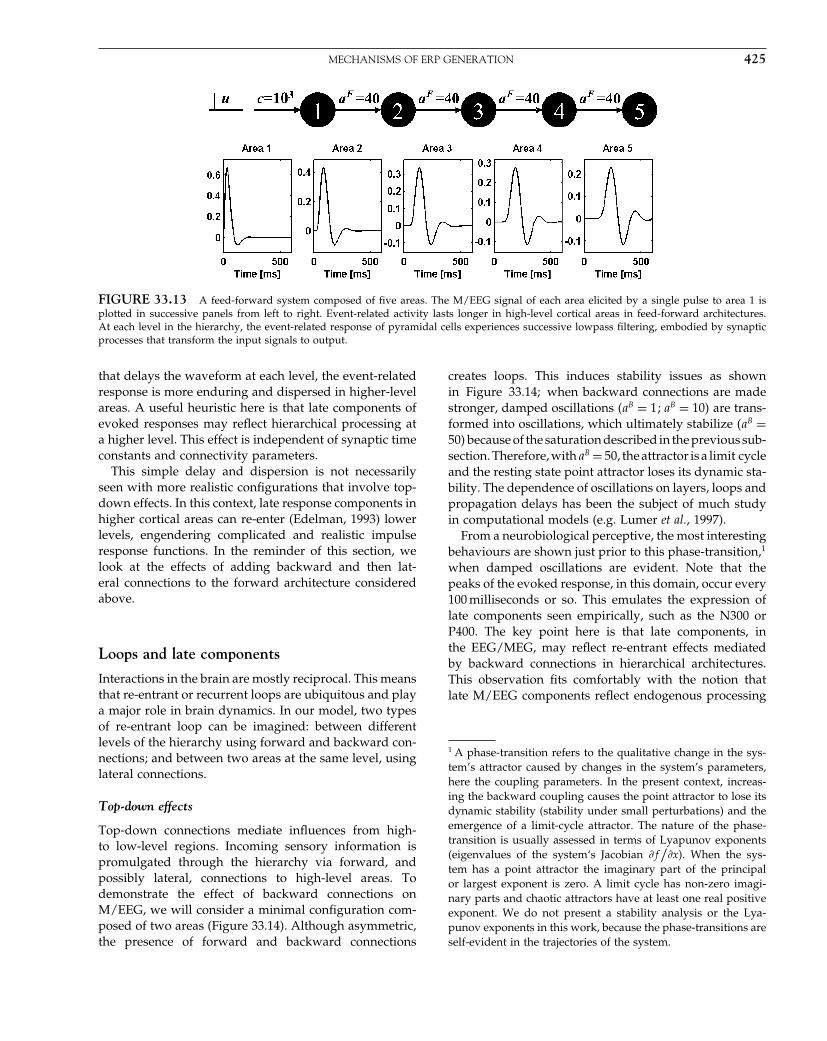
Elsevier UK Chapter: Ch33-P372560 30-9-2006 5:28p.m. Page:425 Trim:7.5in×9.25in
Basal Font:Palatino Margins:Top:40pt Gutter:68pt Font Size:9.5/12 Text Width:42pc Depth:55 Lines
MECHANISMS OF ERP GENERATION 425
FIGURE 33.13 A feed-forward system composed of five areas. The M/EEG signal of each area elicited by a single pulse to area 1 isplotted in successive panels from left to right. Event-related activity lasts longer in high-level cortical areas in feed-forward architectures.At each level in the hierarchy, the event-related response of pyramidal cells experiences successive lowpass filtering, embodied by synapticprocesses that transform the input signals to output.
that delays the waveform at each level, the event-relatedresponse is more enduring and dispersed in higher-levelareas. A useful heuristic here is that late components ofevoked responses may reflect hierarchical processing ata higher level. This effect is independent of synaptic timeconstants and connectivity parameters.
This simple delay and dispersion is not necessarilyseen with more realistic configurations that involve top-down effects. In this context, late response components inhigher cortical areas can re-enter (Edelman, 1993) lowerlevels, engendering complicated and realistic impulseresponse functions. In the reminder of this section, welook at the effects of adding backward and then lat-eral connections to the forward architecture consideredabove.
Loops and late components
Interactions in the brain are mostly reciprocal. This meansthat re-entrant or recurrent loops are ubiquitous and playa major role in brain dynamics. In our model, two typesof re-entrant loop can be imagined: between differentlevels of the hierarchy using forward and backward con-nections; and between two areas at the same level, usinglateral connections.
Top-down effects
Top-down connections mediate influences from high-to low-level regions. Incoming sensory information ispromulgated through the hierarchy via forward, andpossibly lateral, connections to high-level areas. Todemonstrate the effect of backward connections onM/EEG, we will consider a minimal configuration com-posed of two areas (Figure 33.14). Although asymmetric,the presence of forward and backward connections
creates loops. This induces stability issues as shownin Figure 33.14; when backward connections are madestronger, damped oscillations �aB = 1�aB = 10� are trans-formed into oscillations, which ultimately stabilize �aB =50� because of the saturation described in the previous sub-section. Therefore, with aB = 50, the attractor is a limit cycleand the resting state point attractor loses its dynamic sta-bility. The dependence of oscillations on layers, loops andpropagation delays has been the subject of much studyin computational models (e.g. Lumer et al., 1997).
From a neurobiological perceptive, the most interestingbehaviours are shown just prior to this phase-transition,1
when damped oscillations are evident. Note that thepeaks of the evoked response, in this domain, occur every100 milliseconds or so. This emulates the expression oflate components seen empirically, such as the N300 orP400. The key point here is that late components, inthe EEG/MEG, may reflect re-entrant effects mediatedby backward connections in hierarchical architectures.This observation fits comfortably with the notion thatlate M/EEG components reflect endogenous processing
1 A phase-transition refers to the qualitative change in the sys-tem’s attractor caused by changes in the system’s parameters,here the coupling parameters. In the present context, increas-ing the backward coupling causes the point attractor to lose itsdynamic stability (stability under small perturbations) and theemergence of a limit-cycle attractor. The nature of the phase-transition is usually assessed in terms of Lyapunov exponents(eigenvalues of the system‘s Jacobian �f
/�x). When the sys-
tem has a point attractor the imaginary part of the principalor largest exponent is zero. A limit cycle has non-zero imagi-nary parts and chaotic attractors have at least one real positiveexponent. We do not present a stability analysis or the Lya-punov exponents in this work, because the phase-transitions areself-evident in the trajectories of the system.

Elsevier UK Chapter: Ch33-P372560 30-9-2006 5:28p.m. Page:426 Trim:7.5in×9.25in
Basal Font:Palatino Margins:Top:40pt Gutter:68pt Font Size:9.5/12 Text Width:42pc Depth:55 Lines
426 33. NEURONAL MODELS OF EEG AND MEG
FIGURE 33.14 Backward connections have a key influence on the stability of M/EEG event-related activity as demonstrated by thissimple model composed of two areas (area 1 coded in black and area 2 coded in grey). The forward connectivity aF has been fixed at 40 andbackward connectivity aB varies between 1 and 50 from left to right. When top-down effects are small, their re-entry leads to longer lastingevent-related responses characterized by damped oscillations (aB = 1; aB = 10). However, over a critical threshold of aB (which depends uponaF ), the system undergoes a phase-transition, loses its point attractor and expresses oscillatory dynamics (aB = 25; aB = 50).
and depend explicitly on top-down effects. In short, latecomponents may depend on backward connections andreflect a re-entry of dynamics to hierarchically lower pro-cessing areas. This dependency can be seen clearly bycomparing the two left-hand panels in Figure 33.14 thatshow the emergence of late components on increasingthe backward connection from one to ten.
The phase transition from damped late components tooscillations is critical. Before the transition the system iscontrollable. This means that the response can be deter-mined analytically given the input. As discussed in Fris-ton (2000a), long impulse responses endow the brain witha ‘memory’ of past inputs that enables perceptual pro-cessing of temporally extended events. In Friston (2000b),this was demonstrated using a Volterra kernel formula-tion and the simulation of spatiotemporal receptive fieldsin the visual system (see also Chapter 39). However,after the transition, it is no longer possible to determinewhen the input occurred given the output. This violatesthe principle of maximum information transfer (Linsker,1990) and precludes this sort of response in the brain. Inshort, it is likely that re-entrant dynamics prolong neu-ronal transients but will stop short of incurring a phasetransition. If this phase transition occurs it is likely tobe short-lived or pathological (e.g. photosensitive seizureactivity).
It should be noted that the oscillations in the righthand panels of Figure 33.14 do not represent a mech-anism for induced oscillations. The oscillations hereare deterministic components of the system’s impulseresponse function and are time-locked to the stimulus.Induced oscillations, by definition, are not time-locked tothe stimulus and probably arise from a stimulus-relatedchange in the system’s control parameters (i.e. short-termchanges in connectivity). We will return to this point later.
Lateral connections
Lateral connections link different regions at the samelevel in the hierarchy. They can be unidirectional or bidi-rectional as shown for the model in Figure 33.15 withtwo areas. The main difference between forward andunidirectional lateral connections is that the latter targetpyramidal cells. This means that the M/EEG signal is notso constrained by non-linear saturation in layer 4 units.Therefore, as shown in Figure 33.15(a), the event-relatedresponse does not saturate for strong lateral connectiv-ity values aL. On the other hand, bilateral connectionsare completely symmetric, which enables them to createa synchronization manifold (Breakspear, 2002; Breaks-pear and Terry, 2002b). A comparison of Figure 33.15(b)and Figure 33.14 shows that a special aspect of bilateralconnections is their ability to support dynamics that arein phase. This sort of zero-lag phase-synchronization iscommonplace in the brain. Its mediation by lateral con-nections in this model concurs with previous modellingstudies of zero-lag coupling in triplets of cortical areasthat involve at least one set of bilateral or reciprocal con-nections (Chawla et al., 2001). For very large values of aL,architectures with bilateral connections are highly non-linear and eventually undergo a second phase transition(see Figure 33.15(b)).
In this section, we have provided a deterministiccharacterization of simple hierarchical models in terms oftheir impulse responses. We have tried to show that themodel exhibits a degree of face validity in relation to realevoked responses and have related certain mechanisticaspects to previous modelling work to provide some con-struct validity. We now turn to another biological issue,namely the plausibility of non-linear mechanisms thatmight explain ERP/ERF components.
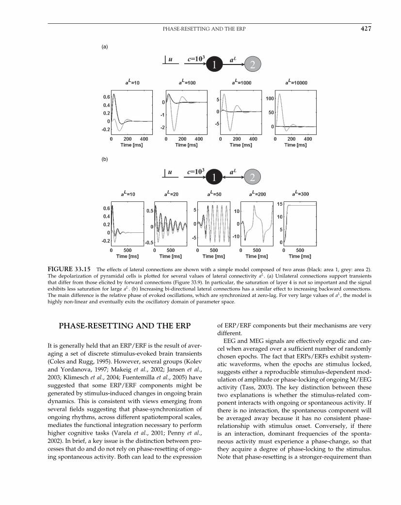
Elsevier UK Chapter: Ch33-P372560 30-9-2006 5:28p.m. Page:427 Trim:7.5in×9.25in
Basal Font:Palatino Margins:Top:40pt Gutter:68pt Font Size:9.5/12 Text Width:42pc Depth:55 Lines
PHASE-RESETTING AND THE ERP 427
(a)
(b)
FIGURE 33.15 The effects of lateral connections are shown with a simple model composed of two areas (black: area 1, grey: area 2).The depolarization of pyramidal cells is plotted for several values of lateral connectivity aL. (a) Unilateral connections support transientsthat differ from those elicited by forward connections (Figure 33.9). In particular, the saturation of layer 4 is not so important and the signalexhibits less saturation for large aL. (b) Increasing bi-directional lateral connections has a similar effect to increasing backward connections.The main difference is the relative phase of evoked oscillations, which are synchronized at zero-lag. For very large values of aL, the model ishighly non-linear and eventually exits the oscillatory domain of parameter space.
PHASE-RESETTING AND THE ERP
It is generally held that an ERP/ERF is the result of aver-aging a set of discrete stimulus-evoked brain transients(Coles and Rugg, 1995). However, several groups (Kolevand Yordanova, 1997; Makeig et al., 2002; Jansen et al.,2003; Klimesch et al., 2004; Fuentemilla et al., 2005) havesuggested that some ERP/ERF components might begenerated by stimulus-induced changes in ongoing braindynamics. This is consistent with views emerging fromseveral fields suggesting that phase-synchronization ofongoing rhythms, across different spatiotemporal scales,mediates the functional integration necessary to performhigher cognitive tasks (Varela et al., 2001; Penny et al.,2002). In brief, a key issue is the distinction between pro-cesses that do and do not rely on phase-resetting of ongo-ing spontaneous activity. Both can lead to the expression
of ERP/ERF components but their mechanisms are verydifferent.
EEG and MEG signals are effectively ergodic and can-cel when averaged over a sufficient number of randomlychosen epochs. The fact that ERPs/ERFs exhibit system-atic waveforms, when the epochs are stimulus locked,suggests either a reproducible stimulus-dependent mod-ulation of amplitude or phase-locking of ongoing M/EEGactivity (Tass, 2003). The key distinction between thesetwo explanations is whether the stimulus-related com-ponent interacts with ongoing or spontaneous activity. Ifthere is no interaction, the spontaneous component willbe averaged away because it has no consistent phase-relationship with stimulus onset. Conversely, if thereis an interaction, dominant frequencies of the sponta-neous activity must experience a phase-change, so thatthey acquire a degree of phase-locking to the stimulus.Note that phase-resetting is a stronger-requirement than

Elsevier UK Chapter: Ch33-P372560 30-9-2006 5:28p.m. Page:428 Trim:7.5in×9.25in
Basal Font:Palatino Margins:Top:40pt Gutter:68pt Font Size:9.5/12 Text Width:42pc Depth:55 Lines
428 33. NEURONAL MODELS OF EEG AND MEG
induced oscillations. It requires any induced dynamicsto be phase-locked in peristimulus time. In short, phase-resetting is explicitly non-linear and implies an inter-action between stimulus-related response and ongoingactivity. Put simply, this means that the event-relatedresponse depends on ongoing activity. This dependencycan be assessed with the difference between responseselicited with and without the stimulus (if we could repro-duce exactly the same ongoing activity). In the absenceof interactions there will be no difference. Any differenceimplies non-linear interactions. Clearly, this cannot bedone empirically but it can be pursued using simulations.
We will show next that phase-resetting is an emergentphenomenon and a plausible candidate for causingERPs/ERFs. Phase-resetting is used in this chapter asan interesting example of non-linear responses that havebeen observed empirically. We use it to show thatnon-linear mechanisms can be usefully explored withneuronal models of the sort developed here. In particu-lar, static non-linearities, in neuronal mass models, aresufficient to explain phase-resetting. Phase-resetting rep-resents non-linear behaviour because, in the absence ofamplitude changes, phase-changes can only be mediatedin a non-linear way. This is why phase-synchronizationplays a central role in detecting non-linear couplingamong sources (Breakspear, 2002; Tass, 2003).
Simulations
In this section, we investigate the effect of ongoingactivity on stimulus-dependent responses to reconcileapparently contradictory conclusions from studies ofevent-related potentials. On one hand, classical studieshave shown that event-related potentials are associatedwith amplitude changes in the M/EEG signal that rep-resent a linear summation of an impulse response andongoing activity (Arieli et al., 1996; Shah et al., 2004). Inthis scheme, the variability at the single-trial level is dueto, and only to, ongoing activity, which is removed afteraveraging to estimate the impulse response. On the otherhand, it has been hypothesized that event-related wave-forms, obtained after averaging, could be due to a phase-resetting of ongoing activity with no necessary change inthe amplitude (i.e. power) of any stimulus-locked tran-sient (Makeig et al., 2002; Jansen et al., 2003). Althoughmathematically well defined, the neural mechanisms thatcould instantiate phase-resetting of ongoing activity areunknown.
We will take phase-resetting to imply a non-linearinteraction between ongoing activity and stimulus-related input that results in phase-locking to stimulusonset. Although phase-locking can be produced by evok-ing oscillatory transients (i.e. amplitude modulation),
this mechanism involves no change or resetting of theongoing dynamics. To assess the contribution of phase-resetting in our simulations, we therefore need to lookfor interactions between ongoing and stimulus-relatedinputs that produced phase-locking in the outputs. Wecan address this, in a simple way, by subtracting theresponse to ongoing activity alone from the responseto a mixture of ongoing activity and stimulus input. Inthe absence of interactions, this difference (the evokedresponse) should be the same. On the other hand, ifinteractions are prevalent, the difference should changewith each realization of ongoing activity. We performedthese analyses with different levels of input and assessedthe degree of phase-locking in the outputs with thephase-locking value (PLV) (Tallon-Baudry et al., 1996;Lachaux et al., 1999): PLV�t� = ∣∣�exp�j��t���trials
∣∣where theinstantaneous phase ��t� was obtained from the Hilberttransform (Le Van Quyen et al., 2001).
To evaluate the effect of background activity on single-trial event-related responses, we used the two area hier-archical model above, with aB = 1 (see Figure 33.14). Thefirst area was driven by an impulse function (stimu-lus) and Gaussian random noise (background activity) ofstandard deviation of 0.05. The output of this region canbe considered a mixture of evoked response and ongoingactivity. We considered two conditions: one with low lev-els of mixed input �c = 102� and another with high levels�c = 2�104�. These values were chosen to emphasize thesystem’s nonlinear properties; with the smaller value ofc, neuronal responses remain largely in the linear regime.The larger value of c was chosen so that excursions ofthe states encroached on the non-linear regime, to pro-duce neuronal saturation in some trials. In both cases, thestimulus was a delta-function. The simulated responses,for 100 trials, are shown in Figure 33.16.
When input levels are low (left hand side ofFigure 33.16), event-related activity, at the single-triallevel, shows a relatively reproducible waveform afterstimulus onset (Figure 33.16(b)). This transient is reflectedin the ERP/ERF after averaging (Figure 33.16(c)). To con-firm the experimental results of Arieli et al. (1996), wedecomposed each event-related response into two com-ponents. First, the stochastic component (the responseto ongoing activity alone – Figure 33.16(d)) and second,an extra component elicited by adding the stimulus(Figure 33.16(e)). This is the difference between theresponse elicited by the stochastic component alone(Figure 33.16(d)) and the response to the mixed input(Figure 33.16(b)). If the system was linear, these differ-ences should not exhibit any variability over trials, andthus define the ‘reproducible response’ (Arieli et al., 1996).Effectively, the stimulus-dependent component shows novariability and we can conclude that the response com-ponents due to stimulus and ongoing activity are linearly
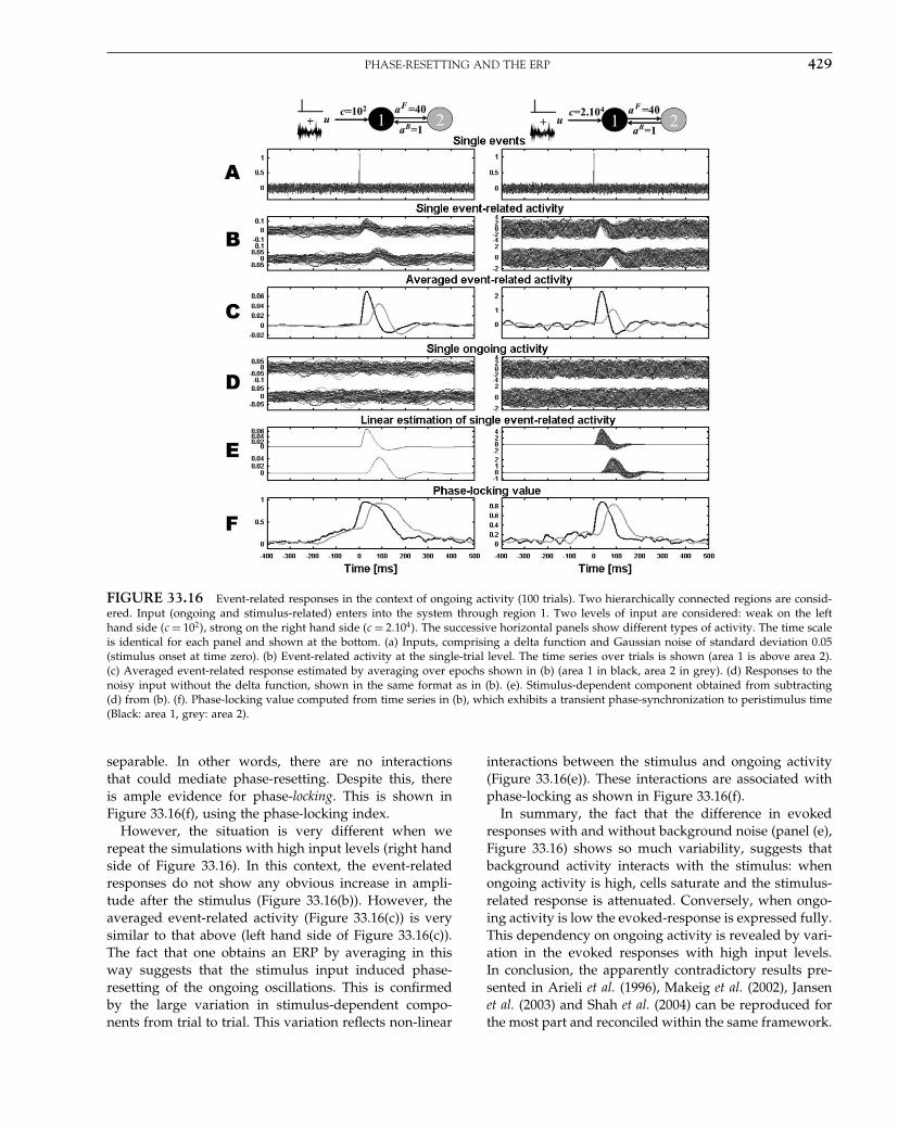
Elsevier UK Chapter: Ch33-P372560 30-9-2006 5:28p.m. Page:429 Trim:7.5in×9.25in
Basal Font:Palatino Margins:Top:40pt Gutter:68pt Font Size:9.5/12 Text Width:42pc Depth:55 Lines
PHASE-RESETTING AND THE ERP 429
FIGURE 33.16 Event-related responses in the context of ongoing activity (100 trials). Two hierarchically connected regions are consid-ered. Input (ongoing and stimulus-related) enters into the system through region 1. Two levels of input are considered: weak on the lefthand side (c = 102�, strong on the right hand side (c = 2�104�. The successive horizontal panels show different types of activity. The time scaleis identical for each panel and shown at the bottom. (a) Inputs, comprising a delta function and Gaussian noise of standard deviation 0.05(stimulus onset at time zero). (b) Event-related activity at the single-trial level. The time series over trials is shown (area 1 is above area 2).(c) Averaged event-related response estimated by averaging over epochs shown in (b) (area 1 in black, area 2 in grey). (d) Responses to thenoisy input without the delta function, shown in the same format as in (b). (e). Stimulus-dependent component obtained from subtracting(d) from (b). (f). Phase-locking value computed from time series in (b), which exhibits a transient phase-synchronization to peristimulus time(Black: area 1, grey: area 2).
separable. In other words, there are no interactionsthat could mediate phase-resetting. Despite this, thereis ample evidence for phase-locking. This is shown inFigure 33.16(f), using the phase-locking index.
However, the situation is very different when werepeat the simulations with high input levels (right handside of Figure 33.16). In this context, the event-relatedresponses do not show any obvious increase in ampli-tude after the stimulus (Figure 33.16(b)). However, theaveraged event-related activity (Figure 33.16(c)) is verysimilar to that above (left hand side of Figure 33.16(c)).The fact that one obtains an ERP by averaging in thisway suggests that the stimulus input induced phase-resetting of the ongoing oscillations. This is confirmedby the large variation in stimulus-dependent compo-nents from trial to trial. This variation reflects non-linear
interactions between the stimulus and ongoing activity(Figure 33.16(e)). These interactions are associated withphase-locking as shown in Figure 33.16(f).
In summary, the fact that the difference in evokedresponses with and without background noise (panel (e),Figure 33.16) shows so much variability, suggests thatbackground activity interacts with the stimulus: whenongoing activity is high, cells saturate and the stimulus-related response is attenuated. Conversely, when ongo-ing activity is low the evoked-response is expressed fully.This dependency on ongoing activity is revealed by vari-ation in the evoked responses with high input levels.In conclusion, the apparently contradictory results pre-sented in Arieli et al. (1996), Makeig et al. (2002), Jansenet al. (2003) and Shah et al. (2004) can be reproduced forthe most part and reconciled within the same framework.

Elsevier UK Chapter: Ch33-P372560 30-9-2006 5:28p.m. Page:430 Trim:7.5in×9.25in
Basal Font:Palatino Margins:Top:40pt Gutter:68pt Font Size:9.5/12 Text Width:42pc Depth:55 Lines
430 33. NEURONAL MODELS OF EEG AND MEG
With high activity levels, the ongoing and stimulus-dependent components interact, through non-linearitiesin the population dynamics, to produce phase-resettingand a classical ERP on averaging. When activity is lower,the stimulus and endogenous dynamics do not interactand the ERP simply reflects the transient evoked by stim-uli that is linearly separable from ongoing dynamics.
We have shown that non-linear mechanisms due tothe saturation of neuronal outputs can be important inmeasured EPR/ERF. In the next section, we take anotherperspective on event-related activity (ERPs are a particu-lar type of event-related activity) and focus on the mod-ulation of ongoing activity by the experimental context.
ONGOING AND EVENT-RELATEDACTIVITY
Ongoing activity, i.e. oscillations in the M/EEG signalthat share no phase relationship with the stimulus, refersto dynamics that are regarded as random fluctuations, orautonomous dynamics with a high complexity. Ongoingactivity is shaped by the same non-linear convolutionexperienced by deterministic inputs. In the context ofstationary inputs, the outputs can be characterized interms of their spectral properties, which are determinedby the generalized transfer functions of the Volterra ker-nels (see Chapter 39) associated with any controllableanalytic system. The impulse response function is thefirst-order kernel. As soon as the connectivity parametersof a hierarchical network change, the principal modesof this network, defined by the principal frequencies ofoscillations, are modulated (David and Friston, 2003). Asan illustration, consider the simple hierarchical model of
two cortical areas established in the previous sectionswith two configurations, which differ in the strength ofbackward connections (aB = 1 and aB = 10) (Figure 33.17).The corresponding frequency spectra, of pyramidal celldepolarization of the two areas, show that the changein connectivity induces a profound modulation of theirspectral profile. As one might intuit, strong backwardconnections induce a peak at the same frequency of thedamped oscillations in the impulse response function.This is an important aspect of ongoing activity in thesense that its spectral behaviour may be very close to thatof evoked transients as shown in (Makeig et al., 2002).
Induced versus evoked responses
This modulation of oscillatory dynamics, by the system’scoupling parameters, provides a natural model for event-related changes in rhythmic activity. This phenomenonis known as event-related synchronization (ERS) in fre-quency bands showing an evoked increase in power,or conversely, event-related desynchronization (ERD)for decreases (Basar, 1980; Pfurtscheller and Lopes daSilva, 1999). In light of the above connectivity-dependentchanges in power, ERD and ERS may reflect the dynam-ics induced by evoked changes in short-term plasticity. Thekey difference between evoked and induced transientsrelates to the presence or absence of changes in the sys-tem’s control parameters, here coupling or synaptic effi-cacy. Evoked changes are not necessarily associated withparameter changes and any complicated response can beascribed to transients that arise as the systems trajectoryreturns to its attractor. Conversely, induced responsesarise from perturbation of the attractor manifold itself,by changes in the parameters and ensuing changes in
FIGURE 33.17 The modulation of backward connectivity (aB = 1 or aB = 10) has huge effect on the power spectrum of ongoing M/EEGdynamics (responses are plotted in black for area 1 and in grey for area 2). When aB increases from 1 to 10, there is loss of power below3 Hz, and an excess between 3 and 7 Hz. The amplitude spectra in the right panel were obtained by averaging the modulus of the fast Fouriertransform of pyramidal cell depolarization, over 100 epochs of 2.5 s (examples are shown in the two left-hand panels, black: first area, grey:second area).

Elsevier UK Chapter: Ch33-P372560 30-9-2006 5:28p.m. Page:431 Trim:7.5in×9.25in
Basal Font:Palatino Margins:Top:40pt Gutter:68pt Font Size:9.5/12 Text Width:42pc Depth:55 Lines
INDUCED RESPONSES AND ERPs 431
the dynamics. This distinction was discussed in Friston(1997a) in relation to MEG dynamics and modelled usingasymmetric connections between two areas in Friston(2000a) and Chapter 39.
Empirically, the ERS/ERD approach is used to look forM/EEG power changes of rhythmic activity induced byexternal events. This phenomenon has been modelled, inthe case of alpha rhythms, by a computational model ofthalamocortical networks (Suffczynski et al., 2001). It hasbeen shown that a key mechanism is the modulation offunctional interaction between populations of thalamo-cortical cells and the reticular nucleus. In the last appli-cation of neural-mass models for ERPs in this chapter,we consider the differences between induced and evokedresponses in more depth. Our goal is to look at the gen-erative mechanisms behind induced responses. The nextsection is a summary of David et al. (2006b).
INDUCED RESPONSES AND ERPs
Cortical oscillatory activity, as disclosed by local fieldpotentials (LFPs), EEG and MEG recordings, can be cat-egorized as ongoing, evoked or induced (Tallon-Baudryand Bertrand, 1999). Evoked and induced oscillations dif-fer in their phase-relationships to the stimulus. Evokedoscillations are phase-locked to the stimulus, whereasinduced oscillations are not. Operationally, these twophenomena are revealed by the order of trial-averagingand spectral analysis (see Chapter 30). To estimateevoked power, the M/EEG signal is first averaged overtrials and then subject to time-frequency analysis to givean event-related response (ERR). To estimate inducedoscillations, the time-frequency decomposition is appliedto each trial and the ensuing power is averaged acrosstrials. The power of evoked and background componentsis subtracted from this total power to reveal inducedpower. In short, evoked responses can be characterizedas the power of the average, while induced responses arethe average power that cannot be explained by the powerof the average.
A common conception is that evoked oscillationsreflect a stimulus-locked event-related response in time-frequency space and that induced oscillations are gen-erated by some distinct high-order process. FollowingSinger and Gray (1995), this process is often describedin terms of ‘binding’ and/or neuronal synchronization.The tenet of the binding hypothesis is that coherent fir-ing patterns can induce large fluctuations in the mem-brane potential of neighbouring neurons which, in turn,facilitate synchronous firing and information transfer (asdefined operationally in Varela, 1995). Oscillations areinduced because their self-organized emergence is not
evoked directly by the stimulus, but induced vicariouslythrough non-linear and possibly autonomous mecha-nisms.
Our treatment of induced responses is divided intothree parts. In the first, we establish a key distinctionbetween dynamic mechanisms, normally associated withclassical evoked responses like the ERP and structuralmechanisms, implicit in the genesis of induced responses.Dynamic effects are simply the effect of inputs on a sys-tem‘s response. Conversely, structural mechanisms entaila transient change in the system‘s causal structure, i.e. itsparameters (e.g. synaptic coupling). These changes couldbe mediated by non-linear effects of input. We relatethe distinction between dynamic and structural mecha-nisms to series of dichotomies in dynamical system the-ory and neurophysiology. These include the distinctionbetween driving and modulatory effects in the brain. Thispart concludes with a review of how neuronal responsesare characterized operationally, in terms of evoked andinduced power, and how these characterizations relate todynamic and structural perturbations. In the second part,we show that structural mechanisms can indeed produceinduced oscillations. In the example provided, responsesare induced by a stimulus-locked modulation of the back-ward connections from one source to another. However,we show that this structural effect is also expressed inevoked oscillations when dynamic and structural effectsinteract. In the final part, we show the converse, namelythat dynamic mechanisms can produce induced oscil-lations, even in the absence of structural effects. Thiscan occur when trial-to-trial variations in input suppresshigh-frequency responses after averaging. Our discussionfocuses on the rather complicated relationship betweenthe two types of mechanisms that can cause responsesin M/EEG and the ways in which evoked and inducedresponses are measured. We introduce adjusted power asa complement to induced power that resolves some ofthese ambiguities.
Dynamic and structural mechanisms
From Eqn. 33.5, it is immediately clear that the states andimplicitly the system’s response, can only be changed byperturbing u�t� or . We will refer to these as dynamicand structural effects respectively. This distinction arisesin a number of different contexts. From a purely dynam-ical point of view, transients elicited by dynamic effectsare the system’s response to input changes, e.g. the pre-sentations of a stimulus in an ERP study. If the sys-tem is dissipative and has a stable fixed point, then theresponse is a generalized convolution of the input withassociated kernels. The duration and form of the result-ing dynamics effect depends on the dynamical stability of
Elsevier UK Chapter: Ch33-P372560 30-9-2006 5:28p.m. Page:432 Trim:7.5in×9.25in
Basal Font:Palatino Margins:Top:40pt Gutter:68pt Font Size:9.5/12 Text Width:42pc Depth:55 Lines
432 33. NEURONAL MODELS OF EEG AND MEG
the system to perturbations of its states (i.e. how the sys-tem’s trajectories change with the state). Structural effectsdepend on structural stability (i.e. how the system’s trajec-tories change with the parameters). Systematic changesin the parameters can produce systematic changes inthe response, even in the absence of input. For systemsthat show autonomous (i.e. periodic or chaotic) dynam-ics, changing the parameters is equivalent to changingthe attractor manifold, which induces a change in thesystem’s states. We have discussed this in the contextof non-linear coupling and classical neuromodulation(Friston, 1997b; Breakspear et al., 2003). For systems withfixed points and Volterra kernels, changing the param-eters is equivalent to changing the kernels and trans-fer functions. This changes the spectral density relation-ships between the inputs and outputs. As such, structuraleffects are clearly important in the genesis of inducedoscillations because they can produce frequency modula-tion of ongoing activity that does not entail phase-lockingto any event. In summary, dynamic effects are expresseddirectly on the states and conform to a convolution ofinputs to form responses. Structural effects are expressedindirectly, through the Jacobian (see Appendix 2), and areinherently non-linear, inducing high-order kernels andassociated transfer functions.
Drivers and modulators
The distinction between dynamic and structural inputsspeaks immediately of the difference between ‘drivers’and ‘modulators’ (Sherman and Guillery, 1998). In sen-sory systems, a driver ensemble can be identified as thetransmitter of receptive field properties. For instance,neurons in the lateral geniculate nuclei drive primaryvisual area responses in the cortex, so that retinotopicmapping is conserved. Modulatory effects are expressedas changes in certain aspects of information transfer,by the changing responsiveness of neuronal ensemblesin a context-sensitive fashion. A common example isattentional gain. Other examples involve extra-classicalreceptive field effects that are expressed beyond theclassical receptive field. Generally, these are thought tobe mediated by backward and lateral connections. Interms of synaptic processes, it has been proposed thatthe postsynaptic effects of drivers are fast (ionotropicreceptors), whereas those of modulators are slower andmore enduring (e.g. metabotropic receptors). The mech-anisms of action of drivers refer to classical neuronaltransmission, either biochemical or electrical, and arewell understood. Conversely, modulatory effects canengage a complex cascade of highly non-linear cellularmechanisms (Turrigiano and Nelson, 2004). Modulatoryeffects can be understood as transient departures from
homeostatic states, lasting hundreds of milliseconds, dueto synaptic changes in the expression and function ofreceptors and intracellular messaging systems.
Classical examples of modularity mechanisms involvevoltage-dependent receptors, such as NMDA receptors.These receptors do not cause depolarization directly (cf.a dynamic effect) but change the unit’s sensitivity todepolarization (i.e. a structural effect). It is interesting tonote that backward connections, usually associated withmodulatory influences, target supragranular layers in thecortex where NMDA receptors are expressed in greaterproportion. Having established the difference betweendynamics and structural effects and their relationshipto driving and modulatory afferents in the brain, wenow turn to the characterization of evoked and inducedresponses in terms of time-frequency analyses.
Evoked and induced power
The criterion that differentiates induced and evokedresponses is the degree to which oscillatory activity isphase-locked to the stimulus over trials. An ERR is thewaveform that is expressed in the EEG signal after everyrepetition of the same stimulus. Due to physiological andmeasurement noise, the ERR is often only evident afteraveraging over trials. More formally, the evoked responsey�t�e to a stimulus is defined as the average of measuredresponses in each trial y�t�:
y�t�e = �y�t�� 33.8
where t is peristimulus time. A time-frequency represen-tation s�� t� of a response y�t� obtains by successivelyfiltering y�t� using a kernel or filter-bank parameterizedby frequencies �j = 2�vj , over the frequency range ofinterest:
s�� t� =⎡⎢⎣
k��1 t�⊗y�t����
k��J t�⊗y�t�
⎤⎥⎦ 33.9
k��j t� can take several forms (Kiebel et al., 2005). Thetotal power, averaged over trials and the power of theaverage are respectively:
g�� t�T = �s�� t�s�� t�∗�g�� t�e = �s�� t�� �s�� t�∗�
33.10
where ∗ denotes the complex conjugate. g�� t�e is evokedpower and is simply the power of y�t�e. Induced powerg�� t�i is defined as the component of total power that

Elsevier UK Chapter: Ch33-P372560 30-9-2006 5:28p.m. Page:433 Trim:7.5in×9.25in
Basal Font:Palatino Margins:Top:40pt Gutter:68pt Font Size:9.5/12 Text Width:42pc Depth:55 Lines
INDUCED RESPONSES AND ERPs 433
cannot be explained by baseline and evoked power.2 Thisimplicitly partitions total power into three orthogonalcomponents (induced, baseline and evoked):
g�� t�T = g�� t�i +g�� t�e +g���b 33.11
Baseline power g���b is a frequency-specific constant dueto ongoing activity and experimental noise, both of whichare assumed to be stationary. This component is usu-ally calculated over a period of time preceding stimuluspresentation.
Mechanisms of generation
In this subsection, we establish how dynamic and struc-tural mechanisms are expressed in terms of evoked andinduced power. As illustrated in Figure 33.18, the inputsfor the i-th trial u�i� can be decomposed into a determinis-tic stimulus-related component � and trial-specific back-ground activity ��i�, which is stochastic and unrelated tothe stimulus:
u�i� = �+��i� 33.12
For simplicity, we will assume that the state-spacedefined by Eqn. 33.4 operates largely in its linear regime,
2
1
(2)u (t )D
u (t )M
(2)V0
(1)V0
β(t )(2)
θ(t )
=
(1)u (t)D α (t ) β (t )(1)= +
FIGURE 33.18 Neuronal model used in the simulations. Twocortical areas interact with forward and backward connections. Bothareas receive a stochastic input, which simulates ongoing activityfrom other brain areas. In addition, area 1 receives a stimulus, mod-elled as a delta function. A single modulatory effect is considered. Itsimulates a stimulus-related slow modulation of extrinsic backwardconnectivity. The outputs of the neuronal system are the pyramidaldepolarizations of both areas.
2 A different definition is sometimes used, where inducedresponses are based on the difference in amplitude betweensingle-trials and the ERR: y�t�−y�t�e (Truccolo et al., 2002). Thearguments in this work apply to both formulations. However, itis simpler for us to use Eqn. 33.11 because it discounts ongoingactivity. This allows us to develop the arguments by consideringjust one trial-type (opposed to differences between trial-types)
as suggested by studies which have found only weaknon-linearities in EEG oscillations (Stam et al., 1999;Breakspear and Terry, 2002a). This allows us to focuson the first-order kernels and transfer functions. We willalso assume the background activity is stationary. In thisinstance, the total power is:
g�� t�T = ��� t�2g�� t�u
g�� t�u = g�� t�� +g����
33.13
In words, the total power is the power of the input, mod-ulated by the transfer function ��� t�2 (see Appendix 2).The power of the input is simply the power of the deter-ministic component, at time t, plus the power of ongoingactivity. The evoked power is simply the power of theinput, because the noise and background terms are sup-pressed by averaging:
g�� t�e = ��� t�2 �s�� t��� �s�� t�∗��
= ��� t�2g�� t��
33.14
The baseline power at t = t0 is:
g���b = ��� t0�2g���� 33.15
This means that induced power is:
g�� t�i = ���� t�2 −��� t0�2�g���� 33.16
This is an important result. It means that the only wayinduced power can be expressed is if the transfer func-tion ��� t � changes at time t. This can only happenif the parameters of the neuronal system change. Inother words, only structural effects can mediate inducedpower. However, this does not mean to say that struc-tural effects are expressed only in induced power. Theycan also be expressed in the evoked power: Eqn. 33.14shows clearly that evoked power at a particular point inperistimulus time depends on both g�� t�� and ��� t �.This means that structural effects mediated by changes inthe transfer function can be expressed in evoked power,provided g�� t�� > 0. In other words, structural effectscan modulate the expression of stationary componentsdue to ongoing activity and also deterministic compo-nents elicited dynamically. To summarize so far:
• Dynamic effects (of driving inputs) conform to a gen-eralized convolution of inputs to form the system’sresponse.
• Structural effects can be formulated as a time-dependent change in the parameters (that may bemediated by modulatory inputs). This translates intotime-dependent change in the convolution kernels andensuing response.

Elsevier UK Chapter: Ch33-P372560 30-9-2006 5:28p.m. Page:434 Trim:7.5in×9.25in
Basal Font:Palatino Margins:Top:40pt Gutter:68pt Font Size:9.5/12 Text Width:42pc Depth:55 Lines
434 33. NEURONAL MODELS OF EEG AND MEG
• If the ongoing activity is non-zero and stationary, onlystructural effects can mediate induced power.
• If stimulus-related input is non-zero, structural effectscan also mediate evoked power, i.e. dynamic and struc-tural effects can conspire to produce evoked power.
In the next subsection, we demonstrate these theoreti-cal considerations in a practical setting, using the neural-mass model of event-related responses. In this sectionand in the simulations below, we only consider a sin-gle trial-type. In practice, one would normally comparethe responses evoked and induced by two trial types.However, the conclusions are exactly the same in bothcontexts. One can regard the simulations below as a com-parison of one trial-type to a baseline that caused noresponse (and had no baseline power).
Modelling induced oscillations
We consider a simple model composed of two sources,inter-connected with forward and backward connec-tions (Figure 33.18). The sources receive two types ofinputs. The first u�t�D, models afferent activity thatdelivers dynamic perturbations to the system’s states(by changing postsynaptic currents). This dynamic per-turbation had stochastic and deterministic components:background inputs ��i� comprised Gaussian noise thatwas delivered to both sources. The deterministic partmodelled a stimulus with an impulse ��t� = �0�, deliv-ered to the first source at the beginning of each trial. Thesecond sort of input u�t�M induced a structural change bymodulating extrinsic connections. As one might expect,the effects of these two input classes differ considerably.On the one hand, synaptic inputs perturb the systemnearly instantaneously and the deterministic part evokesresponses that are phase-locked to the stimulus. On theother hand, modulatory inputs modify the manifold thatattracts ongoing activity, without necessarily resetting itsphase. For simplicity, we restrict our modulatory effectsto a modulation of the extrinsic backward connection,thus encompassing various synaptic mechanisms whichmodify the gain of excitatory synapses (Salinas and Thier,2000). We chose the backward connection because back-ward connections are associated with modulatory effects,both in terms of physiology (e.g. the mediation of extra-classical receptive field effects) (see also Allman et al.,1985; Murphy et al., 1999) and anatomy (e.g. they termi-nate in supragranular layers that expressed large numberof voltage-dependent NMDA receptors) (see also Maun-sell and Van, 1983; Angelucci et al., 2002). There maybe many other modulatory mechanisms that will pro-duce the same pattern of oscillatory activity and it willbe an interesting endeavour to disambiguate the locusof structural changes using these sorts of models andempirical data.
Structural perturbation and induced oscillations
To illustrate the points of the previous section, we willconsider two scenarios in which the modulatory effectarrives at the same time as the driving input and onein which it arrives after the dynamic perturbation hasdissipated. Let us assume that the modulatory input hasa slow time-constant � = 150 ms compared to the mainfrequency of ongoing oscillations (10 Hz). The modula-tory effects can be expressed with stimulus onset, or aftersome delay. In the first case, evoked oscillations will bemodulated and these effects will be visible in the ERR.In the second case, phase-locking with the stimulus willhave been lost and no effect will be seen in the ERR.However, in both cases, structural changes will appearas induced oscillations.
This is illustrated in Plate 45 (see colour plate section)using 500 trial-averages. In the upper panel we con-sider a modulatory input immediately after stimulusonset. As expected, evoked responses are much more pro-nounced relative to delayed modulation (lower panel).The induced power (c) shows that increases in the back-ward connection induce oscillations in the alpha andgamma band. The induced power in Plate 45 has beenfrequency normalized (by removing the mean and divid-ing by the standard deviation at t = 0) to show increasedpower in the gamma band more clearly. These simula-tions provide a nice model for induced responses usinga structural perturbation, in this instance a slow modu-lation of the efficacy of backward connections in a sim-ple hierarchy of neuronal populations. Critically, thesesimulations also show that responses can be evokedstructurally by a modulation of dynamic perturbations.This dual mechanism depends on driving and modula-tory effects occurring at the same time, causing evokedand induced responses in the same time-frequency win-dow. Having established that evoked responses can alsobe mediated by structural mechanisms we now showthat induced responses can be mediated by dynamicmechanisms.
Induced oscillations and trial-to-trial variability
Above we considered the stimulus as a deterministicinput. Here we consider what would happen if thestimulus-related input was stochastic. This randomnessis most easily understood in terms of trial-to-trial vari-ability in the inputs. As suggested in Truccolo et al. (2002),we consider two types of variability in the input. Thefirst relates to a trial-to-trial gain, or amplitude varia-tions. For an identical stimulus, early processing mayintroduce variations in the amplitude of driving inputs toa source. Gain modulation is a ubiquitous phenomenonin the central nervous system (Salinas and Thier, 2000),but its causes are not completely understood. Two

Elsevier UK Chapter: Ch33-P372560 30-9-2006 5:28p.m. Page:435 Trim:7.5in×9.25in
Basal Font:Palatino Margins:Top:40pt Gutter:68pt Font Size:9.5/12 Text Width:42pc Depth:55 Lines
INDUCED RESPONSES AND ERPs 435
neurophysiological mechanisms that may mediate gainmodulation include fluctuations of extracellular calciumconcentration (Smith et al., 2002) and/or of the overalllevel of synaptic input to a neuron (Chance et al., 2002).These may act as a gain control signal that modulatesresponsiveness to excitatory drive. A common example ofgain effects, in a psychophysiological context, is the effectof attention (McAdams and Maunsell, 1999; Treue andMartinez Trujillo, 1999). The second commonly observedsource of variability is in the latency of input onset, i.e.the time between the presentation of the stimulus andthe peak response of early processing. Azouz and Gray(1999) have investigated the sources of such latency vari-ations at the neuronal level. Basically, they describe twomajor phenomena: coherent fluctuations in cortical activ-ity preceding the onset of a stimulus have an impacton the latency of neuronal responses (spikes). This indi-cates that the time needed to integrate activity to reachaction potential threshold varies between trials. The othersource of latency variability is fluctuations in the actionpotential threshold itself.
Both types of trial-to-trial variability, gain modulationand latency, can be modelled by introducing appropriaterandom variables. The theoretical analysis described inDavid et al. (2006b) shows that:
• High frequency components are lost in the evokedresponses when latency varies randomly over tri-als. This means that ERR will be estimated badly athigh frequencies. This variation effectively blurs orsmoothes the average, and suppresses fast oscillationsin the evoked response. However, the total powerremains unchanged, because the power expressed ineach trial does not depend on latency. Therefore, thehigh frequencies lost from the evoked responses nowappear in the induced response. In summary, theinduced power has now acquired a stimulus-lockedcomponent. Note that this dynamically induced powercan only be expressed in frequencies that show evokedresponses. This is illustrated in Plate 46 as a transferof power from the evoked component to the inducedcomponent.
• Gain variations also allow non-structural mechanismsto induce power. Here the time-dependent changes instimulus-dependent power again contribute to inducedresponses. In this instance, the contribution is not fre-quency specific, as with latency variations, but pro-portional to the variance in gain. This is illustrated inPlate 47.
Summary
In summary, we have made a distinction betweendynamic and structural mechanisms that underlie tran-
sient responses to perturbations. We then consideredhow responses are measured in time-frequency in termsof evoked and induced responses. Theoretical predic-tions (see David et al., 2006b), confirmed by simulations,show that there is no simple relationship between thetwo mechanisms causing responses and the two waysin which they are characterized. Specifically, evokedresponses can be mediated both structurally and dynami-cally. Similarly, if there is trial-to-trial variability, inducedresponses can be mediated by both mechanisms (seeFigure 33.19 for a schematic summary).
For evoked responses this is not really an issue. The factthat evoked responses reflect both dynamic and struc-tural perturbations is sensible, if one allows for the factthat any input can have dynamic and structural effects. Inother words, the input perturbs the states of the neuronalsystem and, at the same time, modulates interactionsamong the states. The structural component here can beviewed as a non-linear (e.g. bilinear) effect that simplyinvolves interactions between the input and parameters(e.g. synaptic status). Generally, the structurally medi-ated component of evoked responses will occur at thesame time and frequency as the dynamically mediatedcomponents. This precludes ambiguity when interpret-ing evoked responses, if one allows for both dynamicand structural causes.
The situation is more problematic for inducedresponses. In the absence of trial-to-trial variabil-ity, induced responses must be caused by structuralperturbations. Furthermore, there is no necessary co-localization of evoked and induced responses in time-frequency, because induced responses are disclosed byongoing activity. However, if trial-to-trial variability issufficient, induced responses with no structural com-ponent will be expressed. This means that induced
Structural causes
Dynamic causes
Evokedresponses
Inducedresponses
Modulation of evokedresponses
Modulation of ongoingactivity
Evoked responses lost dueto latency variations
Evoked responses thatsurvive averaging
FIGURE 33.19 Schematic illustrating the many-to-many map-ping between dynamic versus structural causes and evoked versusinduced responses.
Elsevier UK Chapter: Ch33-P372560 30-9-2006 5:28p.m. Page:436 Trim:7.5in×9.25in
Basal Font:Palatino Margins:Top:40pt Gutter:68pt Font Size:9.5/12 Text Width:42pc Depth:55 Lines
436 33. NEURONAL MODELS OF EEG AND MEG
responses that occur at the same time as evokedresponses have an ambiguity in relation to their cause.Happily, this can be addressed at two levels. First,induced responses that do not overlap in peristimulustime cannot be attributed to dynamic mechanisms andare therefore structural in nature. Second, one can re-visitthe operational definition of induced responses to derivea measure that is immune to the effects of trial-to-trialvariability.
Adjusted power
Here we introduce the notion of adjusted power as acomplementary characterization of structurally mediatedresponses. Adjusted power derives from a slightly moreexplicit formulation of induced responses as that compo-nent of total power that cannot be explained by evokedor ongoing activity. The adjusted response is simplythe total power, orthogonalized, at each frequency, withrespect to baseline and evoked power:
g�� t�a = g�� t�T −g�� t��̂
�̂ = g�� t�+g�� t�T
g�� t� =⎡⎢⎣
1 g�� t1�e
������
1 g�� tT �e
⎤⎥⎦
33.17
+ denotes the pseudoinverse. Eqn. 33.17 is implicitly esti-mating baseline power and the contribution from evokedpower and removing them from the total power. In otherwords, �̂ is a 2-vector estimate of g���b and �1+��. Afterthese components have been removed the only compo-nents left must be structural in nature:
g�� t�a ≈ ���� t�2 −��� t0�2�g���� 33.18
Plate 48 shows that the effect of trial-to-trial variabilityon induced responses disappears when using adjustedpower. This means one can unambiguously attributeadjusted responses to structural mechanisms. The ERP-adjusted response removes evoked response compo-nents, including those mediated by structural changes.However, structurally mediated induced componentswill not be affected unless they have the same tempo-ral expression. The usefulness of adjusted power in anempirical setting will be addressed in future work.
DISCUSSION
We have divided neuronal mechanisms into dynamicand structural, which may correspond to driving and
modularity neurotransmitter systems respectively. Thesetwo sorts of effects are related to evoked and inducedresponses in M/EEG. By definition, evoked responsesexhibit phase-locking to a stimulus whereas inducedresponses do not. Consequently, averaging over trialsdiscounts both ongoing and induced components andevoked responses are defined by the response averagedover trials. Evoked responses may be mediated primar-ily by driving inputs. In M/EEG, driving inputs affectthe state of measured neuronal assemblies, i.e. the den-dritic currents in thousands of pyramidal cells. In con-tradistinction, structural effects, mediated by modulatoryinputs, engage neural mechanisms which affect neuronalstates, irrespective of whether they are phase-locked tothe stimulus or not. These inputs are expressed formallyas time-varying parameters of the state equations mod-elling the systems. Although the ensuing changes in theparameters may be slow and enduring, their effects onongoing or evoked dynamics may be expressed as fast orhigh-frequency dynamics. We have considered a furthercause of induced oscillations, namely trial-to-trial vari-ability of driving inputs. As suggested in Truccolo et al.(2002), these can modelled by varying latency and gain.We have shown that gain variations have no effect onthe ERR but increase induced responses in proportion toevoked responses. Secondly, we show that jitter in latencyeffectively smoothes the evoked responses and transfersenergy from evoked to induced power, preferentially athigher frequencies.
The conclusions of this work, summarized inFigure 33.19, provide constraints on the interpretation ofevoked and induced responses in relation to their medi-ation by dynamic and structural mechanisms. This isillustrated by the work of Tallon-Baudry and colleagues,who have looked at non-phase-locked episodes of syn-chronization in the gamma-band (30–60 Hz). They haveemphasized the role of induced responses in feature-binding and top-down mechanisms of perceptual syn-thesis. The top-down aspect is addressed by their earlystudies of illusory perception (Tallon-Baudry et al., 1996),where the authors, ‘tested the stimulus specificity ofhigh-frequency oscillations in humans using three typesof visual stimuli: two coherent stimuli (a Kanizsa anda real triangle) and a non-coherent stimulus’. Theyfound an early phase-locked 40 Hz component, whichdid not vary with stimulation type and a second 40 Hzcomponent, appearing around 28 ms, which was notphase-locked to stimulus onset. This shows a nice disso-ciation between early evoked and late induced responses.The induced component was stronger in response to acoherent triangle, whether real or illusory and: ‘couldreflect, therefore, a mechanism of feature binding basedon high-frequency synchronization’. Because it was late,the induced response can only be caused by structural
Elsevier UK Chapter: Ch33-P372560 30-9-2006 5:28p.m. Page:437 Trim:7.5in×9.25in
Basal Font:Palatino Margins:Top:40pt Gutter:68pt Font Size:9.5/12 Text Width:42pc Depth:55 Lines
CONCLUSION 437
mechanisms (see Figure 33.19). This is consistent with therole of top-down influences and the modulatory mech-anisms employed by backward connections in visualsynthesis (Maunsell and Van, 1983; Bullier et al., 2001;Albright and Stoner, 2002).
Classical ERP/ERF research has focused on dynamicperturbations (Coles and Rugg, 1995). On the otherhand, studies of event-related synchronization (ERS) ordesynchronization (ERD) are more concerned with struc-tural effects that may be mediated by modulatory sys-tems (Pfurtscheller and Lopes da Silva, 1999). Practicallyspeaking, we have shown that it is not always possibleto distinguish between dynamic and structural effectswhen inferring the causes of evoked and induced oscil-lations. However, certain features of induced oscillationsmight provide some hints: (i) induced oscillations in highfrequencies concomitant with evoked responses in lowfrequencies may indicate a jittering of inputs; (ii) inducedoscillations that are temporally dissociated from evokedresponses are likely to be due to modulatory or struc-tural effects. Finally, we have introduced the notion ofadjusted power that can be unambiguously associatedwith structural effects.
CONCLUSION
Neural-mass models afford a straightforward approachto modelling the activity of populations of neurons. Theirmain assumption is that the state of the population can beapproximated using very few state variables (generallylimited to mean membrane currents, potentials and firingrates). Given a macroscopic architecture, describing theoverall connectivity between populations of a given corti-cal area and between different cortical areas, it is possibleto simulate the steady-state dynamics of the system oreven the transient response to a perturbation of extrinsicinput or connectivity. Consequently, neural-mass modelsare useful to describe and predict the macroscopic electri-cal activity of the brain. Since the early 1970s, they havebeen used to address several important issues, e.g. alpharhythms (Lopes da Silva et al., 1997), olfactory responses(Freeman, 1987), and focal attention (Suffczynski et al.,2001). They are now being introduced into neuroimag-ing to understand the underlying neuronal mechanismsof fMRI and PET data (Horwitz and Tagamets, 1999;Almeida and Stetter, 2002; Aubert and Costalat, 2002).
Despite their relative simplicity, neural-mass modelscan exhibit complex dynamical behaviour reminiscentof the real brain. In David and Friston (2003), we haveshown that physiologically plausible synaptic kineticslead to the emergence of oscillatory M/EEG-like signalscovering the range of theta to gamma bands. To emulate
more complex oscillatory M/EEG dynamics, we haveproposed a generalization of the Jansen model that incor-porates several distinct neural populations that resonateat different frequencies. Changing the composition ofthese populations induces a modulation of the spectrumof simulated M/EEG signals.
We have investigated the consequence of coupling tworemote cortical areas. It appears that the rhythms gener-ated depend critically upon both the strength of the cou-pling and the propagation delay. As the coupling directlymodulates the contribution of one area to another, thespectrum of the driven area, in the case of a unidirec-tional coupling, is obviously a mixture of the source andtarget spectra. More interestingly, a reciprocal couplingengenders more marked modifications of the M/EEGspectrum, which can include strong oscillatory activity.Bi-directional coupling is important because of the highproportion of reciprocal connections in the brain. Themost robust consequence of coupling is phase synchro-nization of remote oscillations.
Obviously neural-mass models do not describe exactlyhow neural signals interact. These models represent asummary of underlying neurophysiological processesthat cannot be modelled in complete detail becauseof their complexity. In particular, the model we useddoes not accommodate subcortical structures such asthe reticular nuclei of the thalamus, which is thoughtto be involved in the genesis of delta and alphaoscillations of the EEG (Steriade, 2001). Despite theselimitations, neural-mass models are useful in helpingto understand some macroscopic properties of M/EEGsignals, such as non-linearities (Stam et al., 1999) andcoupling characteristics (Wendling et al., 2000). They canalso be used to reconstruct a posteriori the scenario ofinhibition/excitation balance during epileptic seizures(Wendling et al., 2002). Moreover, fitting simple modelsto actual M/EEG data, as described above, allows one todetermine empirically likely ranges for some importantphysiological parameters (Valdes et al., 1999).
In David et al. (2004), we investigated the sensitivity ofmeasures of regional interdependencies in M/EEG data,illustrating an important practical use of neural-massmodels. It is known that some interactions among corti-cal areas are reflected in M/EEG signals. In the literature,numerous analytic tools are used to reveal these statisticaldependencies. These methods include cross-correlation,coherence (Clifford Carter, 1987), mutual information(Roulston, 1999), non-linear correlation (Pijn et al., 1992),non-linear interdependencies or generalized synchro-nization (Arnhold et al., 1999), neural complexity (Tononiet al., 1994), synchronization likelihood (Stam and vanDijk, 2002), phase synchronization (Tass et al., 1998;Lachaux et al., 1999), etc. These interdependencies areestablished in a way that allows one to make inferences

Elsevier UK Chapter: Ch33-P372560 30-9-2006 5:28p.m. Page:438 Trim:7.5in×9.25in
Basal Font:Palatino Margins:Top:40pt Gutter:68pt Font Size:9.5/12 Text Width:42pc Depth:55 Lines
438 33. NEURONAL MODELS OF EEG AND MEG
about the nature of the coupling. However, it is notclear which aspects of neuronal interactions are criticalfor causing the frequency-specific linear and non-lineardependencies observed. Using the model described inthis chapter, we have estimated how synaptic activityand neuronal interactions are expressed in M/EEG dataand establish the construct validity of various indices ofnon-linear coupling. This particular topic has not beenaddressed in this chapter because we have focused moreon emergent behaviour and mechanisms.
Another important application of neural-mass mod-els is the study of event-related dynamics, which hasbeen the focus of this chapter. We have shown that itis possible to construct hierarchical models for M/EEGsignals. To that end, we have assumed an architecturefor cortical regions and their connections. In particular,we have used the Jansen model (Jansen and Rit, 1995)for each source, and a simplified version of the connec-tion rules of (Felleman and Van Essen, 1991) to couplethese sources. We have shown that neural-mass models(Nunez, 1974; Jansen and Rit, 1995; Lopes da Silva et al.,1997; Stam et al., 1999; Valdes et al., 1999; Robinson et al.,2001; Suffczynski et al., 2001; Rennie et al., 2002; Wendlinget al., 2002; David and Friston, 2003) can reproduce alarge variety of M/EEG signal characteristics: ongoing(oscillatory) activity, event-related activity (ERP/ERF,ERS/ERD). We have tried to highlight the relationshipsthat exist between ERP/ERF and M/EEG oscillations onthe one hand, evoked and induced responses on the otherhand. One utility of neural-mass models is their abil-ity to pinpoint specific neuronal mechanisms underlyingnormal or pathological activity. Effort is needed to incor-porate them, more systematically, in M/EEG analyses toenable enquiry into mechanistic questions about macro-scopic neuronal processes.
In the next chapter, we look at the inversion of dynamicmodels, using relatively simple models for fMRI. Laterwe will apply the same inversion to the models describedin this chapter. The resulting approach to M/EEG data(David et al., 2006a; Kiebel et al., 2006) means we canframe our questions in a mechanistic and biologicallygrounded way, using neural-mass models.
REFERENCES
Abeles M (1991) Corticonics: neural circuits of the cerebral cortex.Cambridge University Press, Cambridge
Albright TD, Stoner GR (2002) Contextual influences on visual pro-cessing. Annu Rev Neurosci 25: 339–79
Allman J, Miezin F, McGuinness E (1985) Stimulus specificresponses from beyond the classical receptive field: neurophys-iological mechanisms for local-global comparisons in visualneurons. Annu Rev Neurosci 8: 407–30
Almeida R, Stetter M (2002) Modelling the link between functionalimaging and neuronal activity: synaptic metabolic demand andspike rates. NeuroImage 17: 1065–79
Angelucci A, Levitt JB, Lund JS (2002) Anatomical origins of theclassical receptive field and modulatory surround field of singleneurons in macaque visual cortical area V1. Prog Brain Res 136:373–88
Arieli A, Sterkin A, Grinvald A et al. (1996) Dynamics of ongoingactivity: explanation of the large variability in evoked corticalresponses. Science 273: 1868–71
Arnhold J, Grassberger P, Lehnertz K et al. (1999) A robust methodfor detecting interdependences: application to intracraniallyrecorded EEG. Physica D 134: 419–30
Aubert A, Costalat R (2002) A model of the coupling between brainelectrical activity, metabolism, and hemodynamics: applicationto the interpretation of functional neuroimaging. NeuroImage 17:1162–81
Azouz R, Gray CM (1999) Cellular mechanisms contributing toresponse variability of cortical neurons in vivo. J Neurosci 19:2209–23
Baillet S, Mosher JC, Leahy RM (2001) Electromagnetic brain map-ping. IEEE Signal Process Mag 14–30
Basar E (1980) EEG-brain dynamics: relation between EEG and brainevoked potentials. Elsevier, New York
Breakspear M (2002) Nonlinear phase desynchronization in humanelectroencephalographic data. Hum Brain Mapp 15: 175–98
Breakspear M, Terry JR (2002a) Detection and description of non-linear interdependence in normal multichannel human EEGdata. Clin Neurophysiol 113: 735–53
Breakspear M, Terry JR (2002b) Nonlinear interdependence in neu-ral systems: motivation, theory, and relevance. Int J Neurosci 112:1263–84
Breakspear M, Terry JR, Friston KJ (2003) Modulation of excita-tory synaptic coupling facilitates synchronization and complexdynamics in a biophysical model of neuronal dynamics. Network14: 703–32
Bullier J, Hupe J, James AC et al. (2001) The role of feedback connec-tions in shaping the responses of visual cortical neurons. ProgBrain Res 134: 193–204
Chance FS, Abbott LF, Reyes AD (2002) Gain modulation frombackground synaptic input. Neuron 35: 773–82
Chawla D, Friston KJ, Lumer ED (2001) Zero-lag synchronousdynamics in triplets of interconnected cortical areas. Neural Netw14: 727–35
Clifford Carter G (1987) Coherence and time delay estimation. ProcIEEE 75: 236–55
Coles MGH, Rugg MD (1995) Event-related brain potentials: anintroduction. In Electrophysiology of mind, Rugg MD, Coles MGH(eds). Oxford University Press, Oxford, pp 1–26
Crick F, Koch C (1998) Constraints on cortical and thalamic projec-tions: the no-strong-loops hypothesis. Nature 391: 245–50
David O, Cosmelli D, Friston KJ (2004) Evaluation of different mea-sures of functional connectivity using a neural-mass model. Neu-roImage 21: 659–73
David O, Friston KJ (2003) A neural-mass model for M/EEG: cou-pling and neuronal dynamics. NeuroImage 20: 1743–55
David O, Garnero L, Cosmelli D et al. (2002) Estimation of neuraldynamics from M/EEG cortical current density maps: applica-tion to the reconstruction of large-scale cortical synchrony. IEEETrans Biomed Eng 49: 975–87
David O, Harrison L, Friston KJ (2005) Modelling event-relatedresponses in the brain. NeuroImage 25: 756–70
David O, Kiebel SJ, Harrison LM et al. (2006a) Dynamic causalmodelling of evoked responses in EEG and MEG. NeuroImage30: 1255–72

Elsevier UK Chapter: Ch33-P372560 30-9-2006 5:28p.m. Page:439 Trim:7.5in×9.25in
Basal Font:Palatino Margins:Top:40pt Gutter:68pt Font Size:9.5/12 Text Width:42pc Depth:55 Lines
REFERENCES 439
David O, Kilner JM, Friston KJ (2006b) Mechanisms of evoked andinduced responses in M/EEG. NeuroImage 15: 1580–91
DeFelipe J, Alonso-Nanclares L, Arellano JI (2002) Microstructureof the neocortex: comparative aspects. J Neurocytol 31: 299–316
Edelman GM (1993) Neural Darwinism: selection and re-entrantsignaling in higher brain function. Neuron 10: 115–25
Engel AK, Fries P, Singer W (2001) Dynamic predictions: oscilla-tions and synchrony in top-down processing. Nat Rev Neurosci2: 704–16
Felleman DJ, Van Essen DC (1991) Distributed hierarchical process-ing in the primate cerebral cortex. Cereb Cortex 1: 1–47
Freeman WJ (1978) Models of the dynamics of neural populations.Electroencephalogr Clin Neurophysiol Suppl 34: 9–18
Freeman WJ (1979) Nonlinear gain mediating cortical stimulus-response relations. Biol Cybernet 33: 237–47
Freeman WJ (1987) Simulation of chaotic EEG patterns with adynamic model of the olfactory system. Biol Cybernet 56: 139–50
Friston K (2002) Functional integration and inference in the brain.Prog Neurobiol 68: 113–43
Friston KJ (1997a) Another neural code? NeuroImage 5: 213–20Friston KJ (1997b) Transients, metastability, and neuronal dynamics.
NeuroImage 5: 164–71Friston KJ (2000a) The labile brain. I. Neuronal transients and non-
linear coupling. Philos Trans R Soc Lond B Biol Sci 355: 215–36Friston KJ (2000b) The labile brain. III. Transients and spatio-
temporal receptive fields. Philos Trans R Soc Lond B Biol Sci 355:253–65
Friston KJ (2001) Brain function, nonlinear coupling, and neuronaltransients. Neuroscientist 7: 406–18
Friston KJ, Harrison L, Penny W (2003) Dynamic causal modelling.NeuroImage 19: 1273–302
Friston KJ, Penny W, Phillips C et al. (2002) Classical and Bayesianinference in neuroimaging: theory. NeuroImage 16: 465–83
Fuentemilla L, Marco-Pallares J, Grau C (2005) Modulation of spec-tral power and of phase resetting of EEG contributes differ-entially to the generation of auditory event-related potentials.NeuroImage 30: 909–16
Haskell E, Nykamp DQ, Tranchina D (2001) Population densitymethods for large-scale modelling of neuronal networks withrealistic synaptic kinetics: cutting the dimension down to size.Network 12: 141–74
Horwitz B, Tagamets MA (1999) Predicting human functional mapswith neural net modeling. Hum Brain Mapp 8: 137–42
Jansen BH, Agarwal G, Hegde A et al. (2003) Phase synchronizationof the ongoing EEG and auditory EP generation. Clin Neurophys-iol 114: 79–85
Jansen BH, Rit VG (1995) Electroencephalogram and visual evokedpotential generation in a mathematical model of coupled corticalcolumns. Biol Cybernet 73: 357–66
Jirsa VK, Haken H (1997) A derivation of a macroscopic field theoryof the brain from the quasi-microscopic neural dynamics. PhysicaD 99: 503–26
Jirsa VK, Kelso JA (2000) Spatiotemporal pattern formation in neuralsystems with heterogeneous connection topologies. Phys Rev EStat Phys Plasmas Fluids Relat Interdiscip Topics 62: 8462–65
Jones EG (2000) Microcolumns in the cerebral cortex. Proc Natl AcadSci USA 97: 5019–21
Kaneko K, Tsuda I (2003) Chaotic itinerancy. Chaos 13: 926–36Kiebel SJ, David O, Friston KJ (2006) Dynamic causal modelling of
evoked responses in M/EEG with lead field parameterization.NeuroImage 30: 1273–84
Kiebel SJ, Tallon-Baudry C, Friston KJ (2005) Parametric analysisof oscillatory activity as measured with EEG/MEG. Hum BrainMapp 26: 170–77
Klimesch W, Schack B, Schabus M et al. (2004) Phase-locked alphaand theta oscillations generate the P1-N1 complex and arerelated to memory performance. Brain Res Cogn Brain Res 19:302–16
Kloeden PE, Platen E (1999) Numerical solution of stochastic differentialequations. Springer Verlag, Berlin
Kolev V, Yordanova J (1997) Analysis of phase-locking is informa-tive for studying event-related EEG activity. Biol Cybernet 76:229–35
Lachaux J-P, Rodriguez E, Martinerie J et al. (1999) Measuring phasesynchrony in brain signals. Hum Brain Mapp 8: 194–208
Le Van Quyen M, Foucher J, Lachaux J et al. (2001) Comparisonof Hilbert transform and wavelet methods for the analysis ofneuronal synchrony. J Neurosci Methods 111: 83–98
Linsker R (1990) Perceptual neural organization: some approachesbased on network models and information theory. Annu RevNeurosci 13: 257–81
Lopes da Silva FH, Hoeks A, Smits H et al. (1974) Model of brainrhythmic activity. The alpha-rhythm of the thalamus. Kybernetik15: 27–37
Lopes da Silva FH, Pijn JP, Velis D et al. (1997) Alpha rhythms:noise, dynamics and models. Int J Psychophysiol 26: 237–49
Lumer ED, Edelman GM, Tononi G (1997) Neural dynamics in amodel of the thalamocortical system. I. Layers, loops and theemergence of fast synchronous rhythms. Cereb Cortex 7: 207–27
Makeig S, Westerfield M, Jung TP et al. (2002) Dynamic brain sourcesof visual evoked responses. Science 295: 690–94
Maunsell JH, Van E (1983) The connections of the middle temporalvisual area (MT) and their relationship to a cortical hierarchy inthe macaque monkey. J Neurosci 3: 2563–86
McAdams CJ, Maunsell JH (1999) Effects of attention on orientation-tuning functions of single neurons in macaque cortical area V4.J Neurosci 19: 431–41
Miller KD (2003) Understanding layer 4 of the cortical circuit: amodel based on cat V1. Cereb Cortex 13: 73–82
Murphy PC, Duckett SG, Sillito AM (1999) Feedback connections tothe lateral geniculate nucleus and cortical response properties.Science 286: 1552–54
Nunez PL (1974) The brain wave equation: a model for the EEG.Math Biosci 21: 279–97
Nunez PL, Srinivasan R (2005) Electric fields of the brain, 2nd edn.Oxford University Press, New York
Penny WD, Kiebel SJ, Kilner JM et al. (2002) Event-related braindynamics. Trends Neurosci 25: 387–89
Pfurtscheller G, Lopes da Silva FH (1999) Event-related M/EEGsynchronization and desynchronization: basic principles. ClinNeurophysiol 110: 1842–57
Pijn JP, Velis DN, Lopes da Silva FH (1992) Measurement of inter-hemispheric time differences in generalised spike-and-wave.Electroencephalogr Clin Neurophysiol 83: 169–71
Rennie CJ, Robinson PA, Wright JJ (2002) Unified neurophysicalmodel of EEG spectra and evoked potentials. Biol Cybernet 86:457–71
Robinson PA, Rennie CJ, Rowe DL (2002) Dynamics of large-scalebrain activity in normal arousal states and epileptic seizures.Phys Rev E Stat Nonlin Soft Matter Phys 65: 041924
Robinson PA, Rennie CJ, Wright JJ et al. (2001) Prediction of elec-troencephalographic spectra from neurophysiology. Phys Rev E63: 021903
Rodriguez E, George N, Lachaux JP et al. (1999) Perception’sshadow: long-distance synchronization of human brain activity.Nature 397: 430–33
Roulston MS (1999) Estimating the errors on measured entropy andmutual information. Physica D 125: 285–94

Elsevier UK Chapter: Ch33-P372560 30-9-2006 5:28p.m. Page:440 Trim:7.5in×9.25in
Basal Font:Palatino Margins:Top:40pt Gutter:68pt Font Size:9.5/12 Text Width:42pc Depth:55 Lines
440 33. NEURONAL MODELS OF EEG AND MEG
Salinas E, Thier P (2000) Gain modulation: a major computationalprinciple of the central nervous system. Neuron 27: 15–21
Shah AS, Bressler SL, Knuth KH et al. (2004) Neural dynamics andthe fundamental mechanisms of event-related brain potentials.Cereb Cortex 14: 476–83
Sherman SM, Guillery RW (1998) On the actions that one nerve cellcan have on another: distinguishing ‘drivers’ from ‘modulators’.Proc Natl Acad Sci USA 95: 7121–26
Singer W, Gray CM (1995) Visual feature integration and the tem-poral correlation hypothesis. Annu Rev Neurosci 18: 555–86
Smith MR, Nelson AB, Du LS (2002) Regulation of firing responsegain by calcium-dependent mechanisms in vestibular nucleusneurons. J Neurophysiol 87: 2031–42
Stam CJ, Pijn JP, Suffczynski P et al. (1999) Dynamics of the humanalpha rhythm: evidence for non-linearity? Clin Neurophysiol 110:1801–13
Stam CJ, van Dijk BW (2002) Synchronization likelihood: an unbi-ased measure of generalized synchronization in multivariatedata sets. Physica D 163: 236–51
Steriade M (2001) Impact of network activities on neuronal proper-ties in corticothalamic systems. J Neurophysiol 86: 1–39
Suffczynski P, Kalitzin S, Pfurtscheller G et al. (2001) Computa-tional model of thalamo-cortical networks: dynamical control ofalpha rhythms in relation to focal attention. Int J Psychophysiol 43:25–40
Tallon-Baudry C, Bertrand O (1999) Oscillatory gamma activity inhumans and its role in object representation. Trends Cogn Sci 3:151–62
Tallon-Baudry C, Bertrand O, Delpuech C et al. (1996) Stimulusspecificity of phase-locked and non-phase-locked 40 Hz visualresponses in human. J Neurosci 16: 4240–49
Tass P, Wienbruch C, Weule J et al. (1998) Detection of n:m phaselocking from noisy data: application to magnetoencephalogra-phy. Phys Rev Lett 81: 3291–94
Tass PA (2003) Stochastic phase resetting of stimulus-lockedresponses of two coupled oscillators: transient response clus-tering, synchronization, and desynchronization. Chaos 13:364–76
Thomson AM, Deuchars J (1997) Synaptic interactions in neocorticallocal circuits: dual intracellular recordings in vitro. Cereb Cortex7: 510–22
Tononi G, Sporns O, Edelman GM (1994) A measure for brain com-plexity: relating functional segregation and integration in thenervous system. Proc Natl Acad Sci USA 91: 5033–37
Treue S, Martinez Trujillo JC (1999) Feature-based attention influ-ences motion processing gain in macaque visual cortex. Nature399: 575–79
Truccolo WA, Ding M, Knuth KH et al. (2002) Trial-to-trial variabil-ity of cortical evoked responses: implications for the analysis offunctional connectivity. Clin Neurophysiol 113: 206–26
Tsuda I (2001) Toward an interpretation of dynamic neural activ-ity in terms of chaotic dynamical systems. Behav Brain Sci 24:793–810
Turrigiano GG, Nelson SB (2004) Homeostatic plasticity in the devel-oping nervous system. Nat Rev Neurosci 5: 97–107
Valdes PA, Jimenez JC, Riera J et al. (1999) Nonlinear EEG analysisbased on a neural-mass model. Biol Cybernet 81: 415–24
Van Rotterdam A, Lopes da Silva FH, van den EJ et al. (1982)A model of the spatial-temporal characteristics of the alpharhythm. Bull Math Biol 44: 283–305
Varela F (1995) Resonant cell assemblies: a new approach to cogni-tive functions and neuronal synchrony. Biol Res 28: 81–95
Varela F, Lachaux J-P, Rodriguez E et al. (2001) The brainweb: phasesynchronization and large-scale integration. Nat Rev Neurosci 2:229–39
Wendling F, Bartolomei F, Bellanger JJ et al. (2002) Epileptic fastactivity can be explained by a model of impaired GABAergicdendritic inhibition. Eur J Neurosci 15: 1499–508
Wendling F, Bellanger JJ, Bartolomei F et al. (2000) Relevance ofnonlinear lumped-parameter models in the analysis of depth-EEG epileptic signals. Biol Cybernet 83: 367–78
Whittington MA, Traub RD, Kopell N et al. (2000) Inhibition-basedrhythms: experimental and mathematical observations on net-work dynamics. Int J Psychophysiol 38: 315–36
Wilson HR, Cowan JD (1972) Excitatory and inhibitory interactionsin localized populations of model neurons. Biophys J 12: 1–24

Elsevier UK Chapter: Ch34-P372560 30-9-2006 5:29p.m. Page:441 Trim:7.5in×9.25in
Basal Font:Palatino Margins:Top:40pt Gutter:68pt Font Size:9.5/12 Text Width:42pc Depth:55 Lines
C H A P T E R
34
Bayesian inversion of dynamic modelsK. Friston and W. Penny
INTRODUCTION
In this chapter, we look at the inversion of dynamicmodels. We use, as an example, the haemodynamicmodel presented in Chapter 27. The inversion schemeis an extension of the Bayesian treatments reviewedin Part 4. Inverting haemodynamic models of neuronalresponses is clearly central to functional magnetic reso-nance imaging (fMRI) and forms the basis for dynamiccausal models for fMRI based on neuronal networks (seeChapter 41). However, the principles of the inversiondescribed in this chapter can be applied to any analytic,deterministic dynamic system and we will use exactlythe same scheme for dynamic models of magnetoen-cephalography/electroencephalography (M/EEG) later.In this chapter, we focus on the inversion of a singlemodel to find the conditional density of the model’sparameters that can then be used for inference, on param-eter space. In the next chapter, we will focus on inferenceabout models themselves (i.e. inference on model space),in terms of Bayesian model comparison, selection andaveraging.
This chapter is about estimating the conditional orposterior distribution of the parameters of determin-istic dynamical systems. The scheme conforms to anEM search for the maximum of the conditional or pos-terior density. The inclusion of priors in the estima-tion procedure ensures robust and rapid convergenceand the resulting conditional densities enable Bayesianinference about the model parameters. The approachis demonstrated using an input-state-output model ofthe haemodynamic coupling between experimentallydesigned causes or factors in fMRI studies and the ensu-ing blood oxygenation-level-dependent (BOLD) response(see Chapter 27). This example represents a generaliza-tion of current fMRI analysis models that accommodatesnon-linearities and in which the parameters have anexplicit physical interpretation.
We focus on the identification of deterministicnon-linear dynamical models. Deterministic here refersto models where the dynamics are completely deter-mined by the state of the system. Random fluctuationsor stochastic effects enter only at the point that the sys-tem’s outputs or responses are observed.1 By consideringa voxel as an input-state-output system one can model theeffects of an input (i.e. stimulus function) on some statevariables (e.g. flow, volume, deoxyhaemoglobin contentetc.) and the output (i.e. BOLD response) engendered bythe changing state of the voxel. The aim is to identify theposterior or conditional distribution of the parameters,given the data. Knowing the posterior distribution allowsone to characterize an observed system in terms of theparameters that maximize their posterior probability (i.e.those parameters that are most likely given the data) or,indeed, make inferences about whether the parametersare bigger or smaller than some specified value.
By demonstrating the inversion of haemodynamicmodels, we establish the key role of biophysical modelsof evoked brain responses in making Bayesian inferencesabout experimentally induced effects. Including param-eters that couple experimentally changing stimulus ortask conditions to the system’s states enables this infer-ence. The posterior or conditional distribution of theseparameters can then be used to make inferences aboutthe efficacy of experimental inputs in eliciting measuredresponses. Because the parameters we want to make aninference about have an explicit physical interpretation,in the context of the haemodynamic model used, the facevalidity of the ensuing inference is grounded in physi-ology. Furthermore, because the experimental effects areparameterized in terms of processes that have natural
1 There is another important class of models where stochasticprocesses enter at the level of the state variables themselves(i.e. deterministic noise). These are referred to as stochasticdynamical models.
Statistical Parametric Mapping, by Karl Friston et al. Copyright 2007, Elsevier Ltd. All rights reserved.ISBN–13: 978-0-12-372560-8 ISBN–10: 0-12-372560-7
441
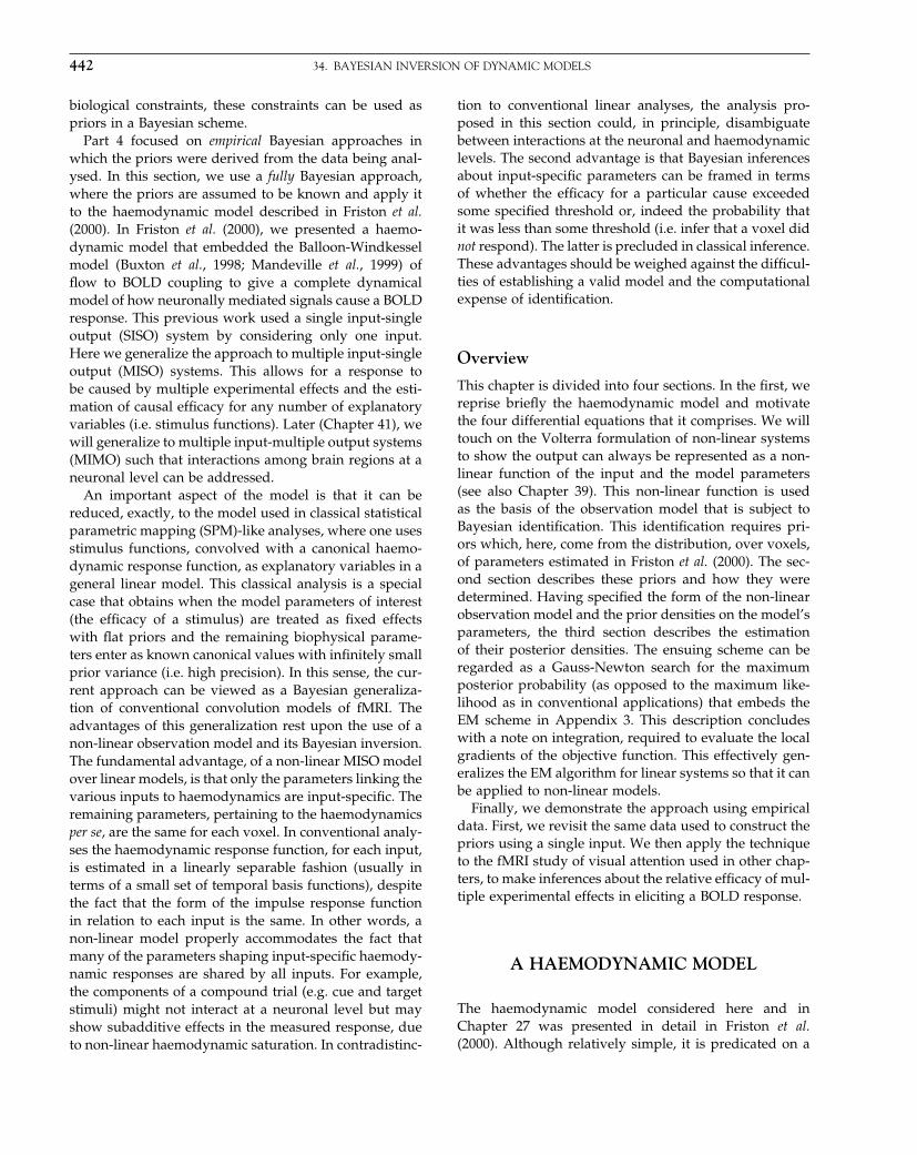
Elsevier UK Chapter: Ch34-P372560 30-9-2006 5:29p.m. Page:442 Trim:7.5in×9.25in
Basal Font:Palatino Margins:Top:40pt Gutter:68pt Font Size:9.5/12 Text Width:42pc Depth:55 Lines
442 34. BAYESIAN INVERSION OF DYNAMIC MODELS
biological constraints, these constraints can be used aspriors in a Bayesian scheme.
Part 4 focused on empirical Bayesian approaches inwhich the priors were derived from the data being anal-ysed. In this section, we use a fully Bayesian approach,where the priors are assumed to be known and apply itto the haemodynamic model described in Friston et al.(2000). In Friston et al. (2000), we presented a haemo-dynamic model that embedded the Balloon-Windkesselmodel (Buxton et al., 1998; Mandeville et al., 1999) offlow to BOLD coupling to give a complete dynamicalmodel of how neuronally mediated signals cause a BOLDresponse. This previous work used a single input-singleoutput (SISO) system by considering only one input.Here we generalize the approach to multiple input-singleoutput (MISO) systems. This allows for a response tobe caused by multiple experimental effects and the esti-mation of causal efficacy for any number of explanatoryvariables (i.e. stimulus functions). Later (Chapter 41), wewill generalize to multiple input-multiple output systems(MIMO) such that interactions among brain regions at aneuronal level can be addressed.
An important aspect of the model is that it can bereduced, exactly, to the model used in classical statisticalparametric mapping (SPM)-like analyses, where one usesstimulus functions, convolved with a canonical haemo-dynamic response function, as explanatory variables in ageneral linear model. This classical analysis is a specialcase that obtains when the model parameters of interest(the efficacy of a stimulus) are treated as fixed effectswith flat priors and the remaining biophysical parame-ters enter as known canonical values with infinitely smallprior variance (i.e. high precision). In this sense, the cur-rent approach can be viewed as a Bayesian generaliza-tion of conventional convolution models of fMRI. Theadvantages of this generalization rest upon the use of anon-linear observation model and its Bayesian inversion.The fundamental advantage, of a non-linear MISO modelover linear models, is that only the parameters linking thevarious inputs to haemodynamics are input-specific. Theremaining parameters, pertaining to the haemodynamicsper se, are the same for each voxel. In conventional analy-ses the haemodynamic response function, for each input,is estimated in a linearly separable fashion (usually interms of a small set of temporal basis functions), despitethe fact that the form of the impulse response functionin relation to each input is the same. In other words, anon-linear model properly accommodates the fact thatmany of the parameters shaping input-specific haemody-namic responses are shared by all inputs. For example,the components of a compound trial (e.g. cue and targetstimuli) might not interact at a neuronal level but mayshow subadditive effects in the measured response, dueto non-linear haemodynamic saturation. In contradistinc-
tion to conventional linear analyses, the analysis pro-posed in this section could, in principle, disambiguatebetween interactions at the neuronal and haemodynamiclevels. The second advantage is that Bayesian inferencesabout input-specific parameters can be framed in termsof whether the efficacy for a particular cause exceededsome specified threshold or, indeed the probability thatit was less than some threshold (i.e. infer that a voxel didnot respond). The latter is precluded in classical inference.These advantages should be weighed against the difficul-ties of establishing a valid model and the computationalexpense of identification.
Overview
This chapter is divided into four sections. In the first, wereprise briefly the haemodynamic model and motivatethe four differential equations that it comprises. We willtouch on the Volterra formulation of non-linear systemsto show the output can always be represented as a non-linear function of the input and the model parameters(see also Chapter 39). This non-linear function is usedas the basis of the observation model that is subject toBayesian identification. This identification requires pri-ors which, here, come from the distribution, over voxels,of parameters estimated in Friston et al. (2000). The sec-ond section describes these priors and how they weredetermined. Having specified the form of the non-linearobservation model and the prior densities on the model’sparameters, the third section describes the estimationof their posterior densities. The ensuing scheme can beregarded as a Gauss-Newton search for the maximumposterior probability (as opposed to the maximum like-lihood as in conventional applications) that embeds theEM scheme in Appendix 3. This description concludeswith a note on integration, required to evaluate the localgradients of the objective function. This effectively gen-eralizes the EM algorithm for linear systems so that it canbe applied to non-linear models.
Finally, we demonstrate the approach using empiricaldata. First, we revisit the same data used to construct thepriors using a single input. We then apply the techniqueto the fMRI study of visual attention used in other chap-ters, to make inferences about the relative efficacy of mul-tiple experimental effects in eliciting a BOLD response.
A HAEMODYNAMIC MODEL
The haemodynamic model considered here and inChapter 27 was presented in detail in Friston et al.(2000). Although relatively simple, it is predicated on a

Elsevier UK Chapter: Ch34-P372560 30-9-2006 5:29p.m. Page:443 Trim:7.5in×9.25in
Basal Font:Palatino Margins:Top:40pt Gutter:68pt Font Size:9.5/12 Text Width:42pc Depth:55 Lines
A HAEMODYNAMIC MODEL 443
substantial amount of careful theoretical work and empir-ical validation (e.g. Buxton et al., 1998; Mayhew et al.,1998; Hoge et al., 1999; Mandeville et al., 1999). The modelis a SISO system with a stimulus function as input (that issupposed to elicit a neuronally mediated flow-inducingsignal) and BOLD response as output. The model has sixparameters and four state variables each with its corre-sponding differential equation. The differential or stateequations express how each state variable changes overtime as a function of the others. These state equationsand the output non-linearly (a static non-linear functionof the state variables) specify the form of the forward orgenerative model. The parameters determine any specificrealization of the model. In what follows we review thestate equations, the output non-linearity, extension to aMISO system and the Volterra representation.
The state equations
Assuming that the dynamical system linking synapticactivity and rCBF is linear (Miller et al., 2000) we startwith:
ḟ = s 34.1
where f�t� is inflow and s�t� is some flow inducing sig-nal. The signal is assumed to subsume many neurogenicand diffusive signal subcomponents and is generatedby neuronal responses to the input (the stimulus func-tion) u�t�:
ṡ = �u�t�−�ss−�f �fin −1� 34.2
�, �s and �f are parameters that represent the efficacywith which input causes an increase in signal, the rate-constant for signal decay or elimination and the rate-constant for autoregulatory feedback from blood flow.The existence of this feedback term can be inferredfrom post-stimulus undershoots in rCBF and the well-characterized vasomotor signal (V-signal) in opticalimaging (Mayhew et al., 1998). Inflow determines the rateof change of volume through:
�v̇ = f −f0�v�
f0�v� = v1/�34.3
This says that normalized venous volume changes reflectthe difference between inflow f�t� and outflow f0�t� fromthe venous compartment with a time constant (transit-time) �. Outflow is a function of volume that modelsthe balloon-like capacity of the venous compartment toexpel blood at a greater rate when distended (Buxtonet al., 1998). It can be modelled with a single parameter
(Grubb et al., 1974) � based on the Windkessel model(Mandeville et al., 1999). The change in normalized totaldeoxyhaemoglobin voxel content q�t� reflects the deliv-ery of deoxyhaemoglobin into the venous compartmentminus that expelled (outflow times concentration):
�q̇ = fE�f�
E0− f0q
v
E�f� = 1− �1−E0�1/f
34.4
where E�f� is the fraction of oxygen extracted frominflowing blood. This is assumed to depend on oxygendelivery and is consequently flow-dependent. This con-cludes the state equations, where there are six unknownparameters, namely efficacy �, signal decay �s, autoregu-lation �f , transit time �, Grubb’s exponent � and restingnet oxygen extraction by the capillary bed E0.
The output non-linearity
The BOLD signal y�t� = g�v� q� is taken to be a staticnon-linear function of volume and deoxyhaemoglobincontent:
y�t� = g�v� q� = V0 �k1�1− q�+k2�1− q/v�+k3�1−v��
k1 = 7E0
k2 = 2
k3 = 2E0 −02
34.5
where V0 is resting blood volume fraction. This sig-nal comprises a volume-weighted sum of extra- andintravascular signals that are functions of volume anddeoxyhaemoglobin content. A critical term in the out-put equation is the concentration term k2�1−q/v�, whichaccounts for most of the non-linear behaviour of thehaemodynamic model. The architecture of this model issummarized in Figure 34.1.
Extension to a MISO
The extension to a multiple input system is trivial andinvolves extending Eqn. 34.2 to cover n inputs:
ṡ = �1u�t�1 +· · ·+�nu�t�n −�ss−�f �f −1� 34.6
The model now has 5+n parameters: five biophysicalparameters �s, �f , �, � and E0 and n efficacies �1� �n.Although all these parameters have to be estimated,we are only interested in making inferences about theefficacies. Note that the biophysical parameters are thesame for all inputs.

Elsevier UK Chapter: Ch34-P372560 30-9-2006 5:29p.m. Page:444 Trim:7.5in×9.25in
Basal Font:Palatino Margins:Top:40pt Gutter:68pt Font Size:9.5/12 Text Width:42pc Depth:55 Lines
444 34. BAYESIAN INVERSION OF DYNAMIC MODELS
ƒ = sflow induction
s
ƒ
vτq = ƒE(ƒ)/E0−v1/αq /v
changes in dHb
τv = ƒ−v1/α
changes in volume
ƒ
q
s = εu−κss − κƒ (ƒ −1)activity-dependent signal
u(t)
y(t ) = g(v,q) = V0(k1(1−q) + k2(1−q /v) + k3(1−v ))
Output: a mixture of intra- and extra-vascular signal
Input: mean synaptic activity
The haemodynamic model
Voxel
v
3.5
3
2.5
2
1.5
3
0.5
0
–0.5
–1–5 0 5 10
PST {secs}15 20 25 30
FIGURE 34.1 Schematic illustrating the architecture of the haemodynamic model. This is a fully non-linear single-input u�t�, single-output y�t� state model with four state variables s, f , v and q. The form and motivation for the changes in each state variable, as functions ofthe others, are described in the main text.
The Volterra formulation
In our haemodynamic model, the state variables arex = x1� · · · �x4 = s� f�v� q and the parameters are � =�s��f � ����E0��1� � �n. The state equations and out-put non-linearity specify a multiple input-single output(MISO) model:
ẋ = f�x�u�
y = g�x�
ẋ1 = f1�x�u� = �1u�t�1 +· · ·+�nu�t�n −�sx1 −�f �x2 −1�
ẋ2 = f2�x�u� = x1
ẋ3 = f3�x�u� = 1�
�x2 −x1/�3 �
ẋ4 = f4�x�u� = x21− �1−E0�1/x2
�E0− x1/�
3 x4
�x3
y�t� = g�x� = V0�k1�1−x4�+k2�1−x4/x3�+k3�1−x3��34.7
This is the state-space representation. The alternativeVolterra formulation represents the output as a non-linear convolution of the input, critically without refer-ence to the state variables (see Bendat, 1990). This seriescan be considered a non-linear convolution that obtainsfrom a functional Taylor expansion of the response oroutputs. The reason this is a functional expansion is thatthe inputs are a function of time. This means the coeffi-cients of the expansion are also functions of time. These

Elsevier UK Chapter: Ch34-P372560 30-9-2006 5:29p.m. Page:445 Trim:7.5in×9.25in
Basal Font:Palatino Margins:Top:40pt Gutter:68pt Font Size:9.5/12 Text Width:42pc Depth:55 Lines
PRIORS 445
are the system’s generalized kernels; for a single inputthis expansion can be expressed as:
y�t� = h���u�
= �0 +�∑
i=1
�∫0
�∫0
�i��1� �i�u�t −�1�
u�t −�i�d�1 d�i 34.8
�i��1� �i� = iy�t�
u�t −�1� u�t −�i�
where �i��1� �i� is the i-th generalized convolutionkernel (Fliess et al., 1983). Eqn. 34.8 expresses the out-put as a function of the input and the parameters whoseposterior distribution we require. In other words, the ker-nels represent a re-parameterization of the system. Thekernels are a time-invariant characterization of the input-output behaviour of the system and can be thought ofas generalized high-order convolution kernels that areapplied to a stimulus function to produce the observedBOLD response. Integrating Eqn. 34.7 and applying theoutput non-linearity to the state variables is the same asconvolving the inputs with the kernels as in Eqn. 34.8.Both give the system’s response in terms of the output.In what follows, the response is evaluated by integratingEqn. 34.7. This means the kernels are not required. How-ever, the Volterra formulation is introduced for severalreasons. First, it demonstrates that the output is a non-linear function of the inputs y�t� = h���u�. This is criti-cal for the generality of the estimation scheme describedhere. Secondly, it provides an important connection withconventional analyses using general linear convolutionmodels (see below). Finally, we can use the kernels tocharacterize evoked responses.
PRIORS
Bayesian inversion requires informative priors on theparameters. Under Gaussian assumptions, these priordensities can be specified in terms of their expectationand covariance. These moments are taken here to bethe sample mean and covariance, over voxels, of theparameter estimates reported in Friston et al. (2000). Nor-mally, priors play a critical role in inference; indeedthe traditional criticism levelled at Bayesian inferencereduces to reservations about the validity of the priorsemployed. However, in the application considered here,this criticism can be discounted. This is because thepriors, on those parameters about which inferences aremade, are relatively flat. Only the five biophysical param-eters have informative priors.
In Friston et al. (2000), the parameters were identi-fied as those that minimized the sum of squared dif-ferences between the Volterra kernels implied by theparameters and those derived directly from the data. Thisderivation used ordinary least square estimators, exploit-ing the fact that Volterra formulation is linear in theunknowns, namely the kernel coefficients. The kernelscan be thought of as a re-parameterization of the modelthat does not refer to the underlying state representation.In other words, for every set of parameters, there is acorresponding set of kernels (see Friston et al., 2000 andbelow for the derivation of the kernels as a function ofthe parameters). The data and Volterra kernel estimationare described in detail in Friston et al. (1998). In brief,we obtained long fMRI time-series from a single subjectat 2 tesla and a short TR of 1.7 s. After discarding ini-tial scans (to allow for magnetic saturation effects) eachtime-series comprised 1200 volume images with 3 mmisotropic voxels. The subject listened to monosyllabic orbi-syllabic concrete nouns (i.e. ‘dog’, ‘radio’, ‘mountain’,‘gate’) presented at five different rates (10, 15, 30, 60and 90 words per minute) for epochs of 34 s, intercalatedwith periods of rest. The presentation rates were repeatedaccording to a Latin Square design.
The distribution of the five biophysical parameters,over 128 voxels, was computed to give our prior expec-tation �� and covariance C�. Signal decay �s had amean of about 0.65 per second giving a half-life t1/2 =ln 2/�s ≈ 1 s. Mean feedback rate �f was about 0.4 persecond. Mean transit time � was 0.98 s. Under steadystate conditions Grubb’s parameter � is about 0.38. Themean over voxels was 0.326. Mean resting oxygen extrac-tion E0 was about 34 per cent and the range observedconformed exactly to known values for resting oxy-gen extraction fraction (between 20 and 55 per cent).Figure 34.2 shows the covariances among the biophys-ical parameters along with the correlation matrix (left-hand insert). The correlations suggest a high correlationbetween transit time and the rate constants for signalelimination and autoregulation.
The priors for the efficacies are taken to be rela-tively flat with an expectation of zero and a varianceof 16 per second. Here, the efficacies are assumed tobe independent of the biophysical parameters with zerocovariance. A variance of 16, or standard deviation of 4,corresponds to time constants in the range of 250 ms. Inother words, inputs can elicit flow-inducing signal overa wide range of time constants from infinitely slowly tovery fast (250 ms) with about the same probability. A‘strong’ activation usually has an efficacy of about 0.5 persecond. Notice that, from a dynamical perspective, a largeresponse depends upon the speed of the response not thepercentage change. Equipped with these priors we can
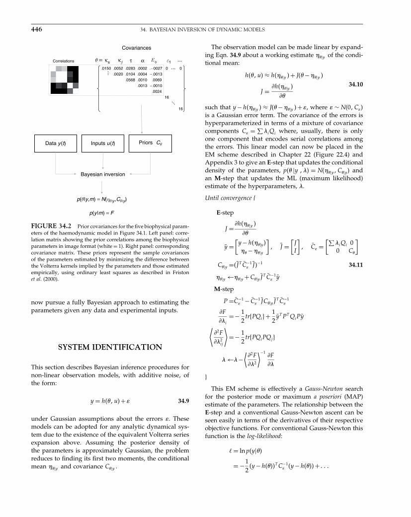
Elsevier UK Chapter: Ch34-P372560 30-9-2006 5:29p.m. Page:446 Trim:7.5in×9.25in
Basal Font:Palatino Margins:Top:40pt Gutter:68pt Font Size:9.5/12 Text Width:42pc Depth:55 Lines
446 34. BAYESIAN INVERSION OF DYNAMIC MODELS
Priors Cθ
Correlations
Bayesian inversion
−
−−
16
16
0024.
0010.0013.
0069.0010.0568.
0013.0004.0104.0020.
000027.0002.0283.0052.0150.
...
Covariances
ε10s Εƒ=
Data y (t) Inputs u (t)
p(y |m) = F
p(θ|y,m) = N(ηθ |y ,Cθ |y)
θ κ κ τ ......
...
α
FIGURE 34.2 Prior covariances for the five biophysical param-eters of the haemodynamic model in Figure 34.1. Left panel: corre-lation matrix showing the prior correlations among the biophysicalparameters in image format (white = 1). Right panel: correspondingcovariance matrix. These priors represent the sample covariancesof the parameters estimated by minimizing the difference betweenthe Volterra kernels implied by the parameters and those estimatedempirically, using ordinary least squares as described in Fristonet al. (2000).
now pursue a fully Bayesian approach to estimating theparameters given any data and experimental inputs.
SYSTEM IDENTIFICATION
This section describes Bayesian inference procedures fornon-linear observation models, with additive noise, ofthe form:
y = h���u�+� 34.9
under Gaussian assumptions about the errors �. Thesemodels can be adopted for any analytic dynamical sys-tem due to the existence of the equivalent Volterra seriesexpansion above. Assuming the posterior density ofthe parameters is approximately Gaussian, the problemreduces to finding its first two moments, the conditionalmean ���y and covariance C��y .
The observation model can be made linear by expand-ing Eqn. 34.9 about a working estimate ���y of the condi-tional mean:
h���u� ≈ h����y �+ J�� −���y �
J = h����y �
�
34.10
such that y −h����y � ≈ J�� −���y �+�, where � ∼ N�0�C��is a Gaussian error term. The covariance of the errors ishyperparameterized in terms of a mixture of covariancecomponents C� = ∑
�iQi where, usually, there is onlyone component that encodes serial correlations amongthe errors. This linear model can now be placed in theEM scheme described in Chapter 22 (Figure 22.4) andAppendix 3 to give an E-step that updates the conditionaldensity of the parameters, p�� �y ��� = N����y�C��y� andan M-step that updates the ML (maximum likelihood)estimate of the hyperparameters, �.
Until convergence {
E-step
J = h����y �
�
ȳ =[y −h����y��� −���y
]� J̄ =
[JI
]� C̄� =
[∑�iQi 00 C�
]
C��y =�J̄ T C̄−1� J̄ �−1 34.11
���y ←���y +C��yJ̄T C̄−1
� ȳ
M-step
P =C̄−1� − C̄−1
� J̄C��yJ̄T C̄−1
�
F
�i
=− 12
tr�PQi�+ 12
ȳT PT QiPȳ
⟨ 2F
�2ij
⟩=− 1
2tr�PQiPQj�
� ←�−⟨ 2F
�2
⟩−1 F
�
}
This EM scheme is effectively a Gauss-Newton searchfor the posterior mode or maximum a poseriori (MAP)estimate of the parameters. The relationship between theE-step and a conventional Gauss-Newton ascent can beseen easily in terms of the derivatives of their respectiveobjective functions. For conventional Gauss-Newton thisfunction is the log-likelihood:
� = ln p�y���
= −12
�y −h����T C−1� �y −h����+

Elsevier UK Chapter: Ch34-P372560 30-9-2006 5:29p.m. Page:447 Trim:7.5in×9.25in
Basal Font:Palatino Margins:Top:40pt Gutter:68pt Font Size:9.5/12 Text Width:42pc Depth:55 Lines
SYSTEM IDENTIFICATION 447
�
�= JT C−1
� �y −h��ML��
− 2�
�2= JT C−1
� J
�ML ← �ML + �JT C−1� J�−1JT C−1
� �y −h��ML�� 34.12
This is a conventional Gauss-Newton scheme. By simplyaugmenting the log-likelihood with the log prior we get:
L = ln p�y��� = ln p�y���+ ln p���
= −12
�y −h����T C−1� �y −h����
− 12
��� −��T C−1� ��� −��+
L
�= JT C−1
� �y −h����y��+C−1� ��� −���y� 34.13
− 2L
�2= JT C−1
� J +C−1�
���y ← ���y + �JT C−1� J +C−1
� �−1�JT C−1� �y −h����y��
+C−1� ��� −���y��
This is identical to the update for the conditional expec-tation in the E-step.
In short, the only difference between the E-step anda conventional Gauss-Newton ML search is that priorsare included in the objective function converting it fromlog-likelihood into L = ln p�y��� = p���y�+p�y�, which isproportional to the log-posterior. In the special contextof EM, L = ln p���y� is the same as the variational energyoptimized in variational Bayes (see Appendix 4).
The use of EM rests upon the need to find not onlythe conditional mean but also the hyperparameters ofunknown variance components. The E-step finds the cur-rent MAP estimate that provides the next expansion pointfor the Gauss-Newton search and the conditional covari-ance required by the M-step. The M-step then updatesthe ReML (restricted maximum likelihood) estimates ofthe covariance hyperparameters that are required to com-pute the conditional moments in the E-step. Technically,Eqn. 34.11 is a generalized EM (GEM) because the M-stepincreases the log-likelihood of the hyperparameter esti-mates, as opposed to maximizing it.
Relationship to other procedures
The procedure presented above represents a fairly obvi-ous extension to conventional Gauss-Newton searchesfor the parameters of non-linear observation models. Theextension has two components: first, maximization ofthe posterior density that embodies priors, as opposed tothe likelihood. This allows for the incorporation of prior
information into the solution and ensures uniquenessand convergence. Second, it covers the estimation ofunknown covariance components. This is importantbecause it accommodates unknown and non-sphericalerrors. The overall approach furnishes a relatively simpleway of obtaining Bayes estimators for non-linear systemswith unknown additive observation error. Technically,the algorithm represents a posterior mode analysis for non-linear observation models using EM. It can be regardedas approximating the posterior density of the parame-ters by replacing the conditional mean with the modeand the conditional precision with the curvature of theenergy (at the current expansion point). This is known asthe Laplace approximation. Covariance hyperparametersare then estimated, which maximize the expected log-likelihood of the data under this posterior density. Thisquantity is known as the variational free energy in statis-tical physics and is the quantity optimized in variationalBayes. This is important from two perspectives. First, thevariational free energy is a lower bound approximation tothe marginal log-likelihood or log-evidence for a model(e.g. model m; see Figure 34.2). The log-evidence plays acentral role in comparing different models, as we will seein the next chapter. Second, the EM scheme above can beconsidered a special case of variational Bayes, in whichone assumes the conditional density of the hyperparam-eters is a point mass. This perspective is developed morefully in Appendix 4.
Posterior mode estimation is an alternative to full pos-terior density analysis, which avoids numerical integra-tion (Fahrmeir and Tutz, 1994: 58) and has been discussedextensively in the context of generalized linear models (e.g.Santner and Duffy, 1989). The departure from Gaussianassumptions in generalized linear models comes fromnon-Gaussian likelihoods, as opposed to non-linearitiesin the observation model considered here, but the issuesare similar. Posterior mode estimation usually assumesthe error covariances and priors are known. If the pri-ors are unknown constants then empirical Bayes can beemployed to estimate the required hyperparameters.
It is important not to confuse this application of EMwith Kalman filtering. Although Kalman filtering canbe formulated in terms of EM and, indeed, posteriormode estimation, Kalman filtering is used with com-pletely different observation models – state-space models.State-space models comprise a transition equation andan observation equation (cf. the state equation and out-put non-linearity above) and cover systems in which theunderlying state is hidden and is treated as a stochasticvariable. This is not the sort of model considered here, inwhich the inputs (experimental design) and the ensuingstates are known. This means that the conditional densi-ties can be computed for the entire time series simultane-ously (Kalman filtering updates the conditional density

Elsevier UK Chapter: Ch34-P372560 30-9-2006 5:29p.m. Page:448 Trim:7.5in×9.25in
Basal Font:Palatino Margins:Top:40pt Gutter:68pt Font Size:9.5/12 Text Width:42pc Depth:55 Lines
448 34. BAYESIAN INVERSION OF DYNAMIC MODELS
recursively, by stepping through the time series). If wetreated the inputs as unknown and random, then thestate equation could be re-written as a stochastic differ-ential equation (SDE) and a transition equation derivedfrom it, using local linearity assumptions (see Appendix 2for details). This would form the basis of a state-spacemodel. This approach may be useful for accommodat-ing deterministic noise in the haemodynamic model but,in this treatment, we consider the inputs to be fixed.This means that the only random effects enter at thelevel of the observation or output non-linearity. In otherwords, we are assuming that the measurement error infMRI is the principal source of random fluctuations inour measurements and that the haemodynamic responseper se is determined by known inputs. This is the sameassumption used in conventional analyses of fMRI data.
A note on integration
To iterate the EM, the local gradients J = h/ � have tobe evaluated. This involves evaluating h���u� around thecurrent expansion point with the generalized convolu-tion of the inputs for the current conditional parameterestimates according to Eqn. 34.8 or, equivalently, the inte-gration of Eqn. 34.7. The latter can be accomplished effi-ciently by capitalizing on the fact that stimulus functionsare usually sparse. In other words, inputs arrive as infre-quent events (e.g. event-related paradigms) or changes ininput occur sporadically (e.g. boxcar designs). We can usethis to evaluate y�t� = h����y�u� at the times the data weresampled using a bilinear approximation to Eqn. 34.7. TheTaylor expansion of ẋ�t� about x�0� = x0 = �0� 1� 1� 1�T :
ẋ ≈ f�x0� 0�+ f
X�x−x0�
+∑i
ui
( 2f
X ui
�x−x0�+ f
ui
)34.14
has a bilinear form, following a change of variables(equivalent to adding an extra state variable, which is acontact term):
Ẋ�t� ≈ AX +∑i
u�t�iBiX
X =[
1x
]
A =[
0 0(f�x0� 0�− f
xx0
) f
x
]34.15
Bi =[
0 0( f
ui− 2f
x uiX0
) 2f
x ui
]
This bilinear approximation is important because theVolterra kernels of bilinear systems have closed-formexpressions (see Appendix 2; Eqn. A2.8). This means thatthe kernels can be derived analytically, and quickly, toprovide a characterization of the impulse response prop-erties of the system. The integration of Eqn. 34.15 is pred-icated on its solution over periods �t = tk+1 − tk withinwhich the inputs are constant:
X�tk+1� = exp�J�t�X�tk�
y�tk+1� = g�x�tk+1�� 34.16
J = A+∑i
u�tk�iBi
This quasi-analytical integration scheme can be an orderof magnitude quicker than straightforward numericalintegration, depending on the sparsity of inputs.
Relation to conventional fMRI analyses
Note that, if we treated the five biophysical parametersas known canonical values and discounted all but thefirst order terms in the Volterra expansion, the followinglinear model would result:
h�u��� = �0 +n∑
i=1
t∫0
�1���u�t −��id� =n∑
i=1
�1 ∗u�t�i
≈ �0 +n∑
i=1
�i
�1
�i
∗u�t�i
34.17
where * denotes convolution and the second expressionis a first-order Taylor expansion around the expected val-ues of the parameters. This is exactly the same as thegeneral linear model adopted in conventional analysis offMRI time series, if we elect to use just one (canonical)haemodynamic response function (HRF) to convolve ourstimulus functions with. In this context the HRF playsthe role of �1/ �i in Eqn. 34.17. This partial derivative isshown in Figure 34.3 (upper panel) using the prior expec-tations of the parameters and conforms closely to the sortof HRF used in practice. Now, by treating the efficaciesas fixed effects (i.e. with flat priors), the MAP and MLestimators reduce to the same thing and the conditionalexpectation reduces to the Gauss-Markov estimator:
�ML = �JT C−1� J�−1JT C−1
� y 34.18
where J is the design matrix. This is precisely the esti-mator used in conventional analyses when whiteningstrategies are employed.
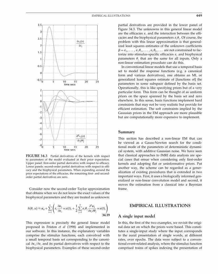
Elsevier UK Chapter: Ch34-P372560 30-9-2006 5:29p.m. Page:449 Trim:7.5in×9.25in
Basal Font:Palatino Margins:Top:40pt Gutter:68pt Font Size:9.5/12 Text Width:42pc Depth:55 Lines
EMPIRICAL ILLUSTRATIONS 449
∂εi
∂κ1(σ)
∂εi ∂θj
∂2κ1(σ)
FIGURE 34.3 Partial derivatives of the kernels with respectto parameters of the model evaluated at their prior expectation.Upper panel: first-order partial derivative with respect to efficacy.Lower panels: second-order partial derivatives with respect to effi-cacy and the biophysical parameters. When expanding around theprior expectations of the efficacies, the remaining first- and second-order partial derivatives are zero.
Consider now the second-order Taylor approximationthat obtains when we do not know the exact values of thebiophysical parameters and they are treated as unknown:
h���u� ≈ �0 +n∑
i=1
(�i
�1
�i
∗u�t�i +12
5∑j=1
�i�j
2�1
�i �j
∗u�t�i
)
34.19
This expression is precisely the general linear modelproposed in Friston et al (1998) and implemented inour software. In this instance, the explanatory variablescomprise the stimulus functions, each convolved witha small temporal basis set corresponding to the canoni-cal �1/ �i and its partial derivatives with respect to thebiophysical parameters. Examples of these second-order
partial derivatives are provided in the lower panel ofFigure 34.3. The unknowns in this general linear modelare the efficacies �i and the interaction between the effi-cacies and the biophysical parameters �i�j . Of course, theproblem with this linear approximation is that general-ized least squares estimates of the unknown coefficients� = �1� � �1�1� � �1�2� are not constrained to fac-torize into stimulus-specific efficacies �i and biophysicalparameters �j that are the same for all inputs. Only anon-linear estimation procedure can do this.
In conventional linear models that use a temporal basisset to model the response functions (e.g. a canonicalform and various derivatives), one obtains an ML orgeneralized least squares estimate of [functions of] theparameters in some subspace defined by the basis set.Operationally, this is like specifying priors but of a veryparticular form. This form can be thought of as uniformpriors on the space spanned by the basis set and zeroelsewhere. In this sense, basis functions implement hardconstraints that may not be very realistic but provide forefficient estimation. The soft constraints implied by theGaussian priors in the EM approach are more plausiblebut are computationally more expensive to implement.
Summary
This section has described a non-linear EM that canbe viewed as a Gauss-Newton search for the condi-tional mode of the parameters of deterministic dynami-cal system, with additive Gaussian noise. We have seenthat classical approaches to fMRI data analysis are spe-cial cases that ensue when considering only first-orderkernels and adopting flat or uninformative priors. Putanother way, the scheme can be regarded as a gener-alization of existing procedures that is extended in twoimportant ways. First, it uses a biologically informed gen-eralized or non-linear convolution model and second, itmoves the estimation from a classical into a Bayesianframe.
EMPIRICAL ILLUSTRATIONS
A single input model
In this, the first of the two examples, we revisit the origi-nal data set on which the priors were based. This consti-tutes a single-input study where the input correspondsto the aural presentation of single words, at differentrates, over epochs. The data were subject to a conven-tional event-related analysis, where the stimulus functioncomprised trains of spikes indexing the presentation of

Elsevier UK Chapter: Ch34-P372560 30-9-2006 5:29p.m. Page:450 Trim:7.5in×9.25in
Basal Font:Palatino Margins:Top:40pt Gutter:68pt Font Size:9.5/12 Text Width:42pc Depth:55 Lines
450 34. BAYESIAN INVERSION OF DYNAMIC MODELS
each word. The stimulus function was convolved witha canonical HRF and its temporal derivative. The datawere highpass filtered by removing low-frequency com-ponents modelled by a discrete cosine set. The resultingSPM{t}, testing for activations due to words, is shownin Figure 34.4 (left-hand panel) thresholded at p = 005(corrected).
A single region in the left superior temporal gyrus wasselected for analysis. The input comprised the same stim-ulus function used in the conventional analysis and theoutput was the first eigenvariate of highpass filtered timeseries, of all voxels, within a 4 mm sphere, centred onthe most significant voxel in the SPM{t} (marked by anarrow in Figure 34.4). The error covariance componentsQ comprised an identity matrix modelling white or anindependent and identically distributed (IID) componentand a second with exponentially decaying off-diagonal
elements modelling an AR(1) component (see Fristonet al. (2002) and Chapter 10). This models serial correla-tions among the errors. The results of the estimation pro-cedure are shown in the right-hand panel in terms of theconditional distribution of the parameters and the condi-tional expectation of the first- and second-order kernels.The kernels are a function of the parameters and theirderivation using a bilinear approximation is describedin Friston et al. (2000) and Appendix 2. The upper-rightpanel shows the first-order kernels for the state variables(signal, inflow, deoxyhaemoglobin content and volume).These can be regarded as impulse response functionsdetailing the response to a transient input. The first- andsecond-order output kernels for the BOLD response areshown in the lower-right panels. They concur with thosederived empirically in Friston et al. (2000). Note the char-acteristic undershoot in the first-order kernel and the
fMRI study of single word processing at different rates
FIGURE 34.4 An SISO example: Left panel: conventional SPM{t} testing for an activating effect of word presentation. The arrow showsthe centre of the region (a sphere of 4 mm radius) whose response entered into the Bayesian inversion. The results for this region are shown inthe right-hand panel in terms of the conditional distribution of the parameters and the conditional expectation of the first- and second-orderkernels. The upper-right panel shows the first-order kernels for the state variables (signal, inflow, deoxyhaemoglobin content and volume).The first- and second-order output kernels for the BOLD response are shown in the lower-right panels. The left-hand panels show theconditional or posterior distributions. The conditional density for efficacy is presented in the upper panel and those for the five biophysicalparameters in the lower panel. The shading corresponds to the probability density and the bars to 90 per cent confidence intervals.

Elsevier UK Chapter: Ch34-P372560 30-9-2006 5:29p.m. Page:451 Trim:7.5in×9.25in
Basal Font:Palatino Margins:Top:40pt Gutter:68pt Font Size:9.5/12 Text Width:42pc Depth:55 Lines
EMPIRICAL ILLUSTRATIONS 451
pronounced negativity in the upper left of the second-order kernel, flanked by two off-diagonal positive regionsat around 8 s. These lend the haemodynamics a degree ofrefractoriness when presenting paired stimuli less thana few seconds apart and a superadditive response withabout 8 s separation. The left-hand panels show the con-ditional or posterior distributions. The density for theefficacy is presented in the upper panel and those forthe five biophysical parameters are shown in the lowerpanel. The shading corresponds to the probability den-sity and the bars to 90 per cent confidence intervals. Thevalues of the biophysical parameters are all within a veryacceptable range. In this example, the signal eliminationand decay appears to be slower than normally encoun-tered, with the rate constants being significantly largerthan their prior expectations. Grubb’s exponent here iscloser to the steady state value of 0.38 than the priorexpectation of 0.32. Of greater interest is the efficacy. Itcan be seen that the efficacy lies between 0.4 and 0.6 andis clearly greater than zero. This would be expected givenwe chose the most significant voxel from the conven-tional analysis. Notice there is no null hypothesis hereand we do not even need a p-value to make the inferencethat words evoke a response in this region. An importantfacility, with inferences based on the conditional distri-bution and precluded in classical analyses, is that onecan infer a cause did not elicit a response. This is demon-strated next.
A multiple input model
In this example, we turn to a data set used in previoussections, in which there are three experimental causes orinputs. This was a study of attention to visual motion.Subjects were studied with fMRI under identical stimulusconditions (visual motion subtended by radially movingdots) while manipulating the attentional component ofthe task (detection of velocity changes). The data wereacquired from normal subjects at 2 tesla using a VISION(Siemens, Erlangen) whole body MRI system, equippedwith a head volume coil. Here we analyse data fromthe first subject. Contiguous multislice fMRI images wereobtained with a gradient echo-planar sequence (TE =40 ms, TR = 322 s, matrix size = 64 × 64 × 32, voxel size3×3×3 mm). Each subject had four consecutive 100-scansessions comprising a series of 10-scan blocks under fivedifferent conditions D F A F N F A F N S. The first con-dition (D) was a dummy condition to allow for magneticsaturation effects. F (Fixation) corresponds to a low-levelbaseline where the subjects viewed a fixation point at thecentre of a screen. In condition A (Attention), subjectsviewed 250 dots moving radially from the centre at 4.7
degrees per second and were asked to detect changes inradial velocity. In condition N (No-attention), the subjectswere asked simply to view the moving dots. In conditionS (Stationary), subjects viewed stationary dots. The orderof A and N was swapped for the last two sessions. Inall conditions, subjects fixated the centre of the screen.In a pre-scanning session the subjects were given fivetrials with five speed changes (reducing to 1 per cent).During scanning there were no speed changes. No overtresponse was required in any condition.
This design can be reformulated in terms of threepotential causes, photic stimulation, visual motion anddirected attention. The F-epochs have no associated causeand represent a baseline. The S-epochs have just photicstimulation. The N-epochs have both photic stimulationand motion, whereas the A-epochs encompass all threecauses. We performed a conventional analysis using box-car stimulus functions encoding the presence or absenceof each of the three causes, during each epoch. Thesefunctions were convolved with a canonical HRF and itstemporal derivative to give two repressors for each cause.The corresponding design matrix is shown in the leftpanel of Figure 34.5. We selected a region that showeda significant attentional effect in the lingual gyrus. Thestimulus functions modelling the three inputs were thebox functions used in the conventional analysis. The out-put corresponded to the first eigenvariate of highpassfiltered time-series from all voxels in a 4 mm sphere cen-tred on 0, −66, −3 mm (Talairach and Tournoux, 1988).The error covariance basis was the identity matrix (i.e.ignoring serial correlations because of the relatively longTR). The results are shown in the right-hand panel ofFigure 34.5 using the same format as Figure 34.4. Thecritical thing here is that there are three conditional den-sities, one for each input efficacy. Attention has a clearactivating effect with more than a 90 per cent probabil-ity of being greater than 0.25 per second. However, inthis region neither photic stimulation nor motion in thevisual field evokes any real response. The efficacies ofboth are less than 0.1 and are centred on zero. This meansthat the time constants of the visually evoked responsecould range from about 10 s to never. Consequently, thesecauses can be discounted from a dynamical perspec-tive. In short, this visually unresponsive area respondssubstantially to attentional manipulation showing a truefunctional selectivity. This is a crucial statement becauseclassical inference does not allow one to infer any regiondoes not respond and therefore precludes inference aboutthe specificity of regional responses. The only reason onecan say ‘this region responds selectively to attention’ isbecause Bayesian inference allows one to say ‘it doesnot response to photic stimulation with random dots ormotion’.
Elsevier UK Chapter: Ch34-P372560 30-9-2006 5:29p.m. Page:452 Trim:7.5in×9.25in
Basal Font:Palatino Margins:Top:40pt Gutter:68pt Font Size:9.5/12 Text Width:42pc Depth:55 Lines
452 34. BAYESIAN INVERSION OF DYNAMIC MODELS
Extension to MISO
fMRI study of attention to visual motion
Design matrix
Photic motion attention
{ { {
FIGURE 34.5 A MISO example using visual attention to motion. The left panel shows the design matrix used in the conventionalanalysis and the right panel shows the results of the Bayesian analysis of a lingual extrastriate region. This panel has the same format asFigure 34.4.
CONCLUSION
In this chapter, we have looked at an EM implemen-tation of the Gauss-Newton method for estimating theconditional or posterior distribution of the parametersof a deterministic dynamical system. The inclusion ofpriors in the estimation procedure ensures robust andrapid convergence and the resulting conditional densitiesenable Bayesian inference about the model’s parame-ters. We have examined the coupling between experi-mentally designed causes or factors in fMRI studies andthe ensuing BOLD response. This application representsa generalization of existing linear models to accommo-date dynamics and non-linearities in the transductionof experimental causes to measured output in fMRI.Because the model is predicated on biophysical processesthe parameters have a physical interpretation. Further-more, the approach extends classical inference about thelikelihood of the data to more plausible inferences aboutthe parameters of the model given the data. This infer-ence provides confidence intervals based on the condi-tional density.
Perhaps the most important extension of the schemedescribed in this chapter is to MIMO systems where wedeal with multiple regions or voxels at the same time. Theimportance of this extension is that one can incorporateinteractions among brain regions at the neuronal level.This furnishes a framework for the dynamic causal mod-elling of functional integration in the brain (see Chap-ters 41 and 42). This chapter focused on inference onthe space of parameters. In the next chapter, we look atinference on the space of models.
REFERENCES
Bendat JS (1990) Nonlinear System Analysis and Identification fromRandom Data. John Wiley and Sons, New York
Buxton RB, Wong EC, Frank LR (1998) Dynamics of blood flowand oxygenation changes during brain activation: The Balloonmodel. Mag Res Med 39: 855–64
Fahrmeir L, Tutz G (1994) Multivariate statistical modelling basedon generalised linear models. Springer Verlag Inc., New York,pp 355–56

Elsevier UK Chapter: Ch34-P372560 30-9-2006 5:29p.m. Page:453 Trim:7.5in×9.25in
Basal Font:Palatino Margins:Top:40pt Gutter:68pt Font Size:9.5/12 Text Width:42pc Depth:55 Lines
REFERENCES 453
Fliess M, Lamnabhi M, Lamnabhi-Lagarrigue F (1983) An algebraicapproach to nonlinear functional expansions. IEEE Trans CircuitsSyst 30: 554–70
Friston KJ, Glaser DE, Henson RNA et al. (2002) Classical and Bayesianinference in neuroimaging: applications. NeuroImage 16: 484–512
Friston KJ, Josephs O, Rees G et al. (1998) Non-linear event-relatedresponses in fMRI. Mag Res Med 39: 41–52
Friston KJ, Mechelli A, Turner R et al. (2000) Nonlinear responsesin fMRI: the Balloon model, Volterra kernels and other hemo-dynamics. NeuroImage 12: 466–77
Grubb RL, Rachael ME, Euchring JO et al. (1974) The effects ofchanges in PCO2 on cerebral blood volume, blood flow andvascular mean transit time. Stroke 5: 630–39
Hoge RD, Atkinson J, Gill B et al. (1999) Linear cou-pling between cerebral blood flow and oxygen consump-
tion in activated human cortex. Proc Natl Acad Sci 96:9403–08
Mandeville JB, Marota JJ, Ayata C et al. (1999) Evidence of a cere-brovascular postarteriole windkessel with delayed compliance.J Cereb Blood Flow Metab 19: 679–89
Mayhew J, Hu D, Zheng Y et al. (1998) An evaluation of linear mod-els analysis techniques for processing images of microcirculationactivity. NeuroImage 7: 49–71
Miller KL, Luh WM, Liu TT et al. (2000) Characterizing the dynamicperfusion response to stimuli of short duration. Proc ISRM8: 580
Santner TJ, Duffy DE (1989) The statistical analysis of discrete data.Springer, New York
Talairach J, Tournoux P (1988) A Co-planar stereotaxic atlas of a humanbrain. Thieme, Stuttgart

Elsevier UK Chapter: Ch35-P372560 30-9-2006 5:30p.m. Page:454 Trim:7.5in×9.25in
Basal Font:Palatino Margins:Top:40pt Gutter:68pt Font Size:9.5/12 Text Width:42pc Depth:55 Lines
C H A P T E R
35
Bayesian model selection and averagingW.D. Penny, J. Mattout and N. Trujillo-Barreto
INTRODUCTION
In Chapter 11, we described how Bayesian inference canbe applied to hierarchical models. In this chapter, weshow how the members of a model class, indexed bym, can also be considered as part of a hierarchy. Modelclasses might be general linear models (GLMs) where mindexes different choices for the design matrix, dynamiccausal models (DCMs) where m indexes connectivity orinput patterns, or source reconstruction models where mindexes functional or anatomical constraints. Explicitlyincluding model structure in this way will allow us tomake inferences about that structure.
Figure 35.1 shows the generative model we have inmind. First, a member of the model class is chosen.Then model parameters � and finally the data y are gen-erated. Bayesian inference for hierarchical models canbe implemented using the belief propagation algorithm.Figure 35.2 shows how this can be applied for modelselection and averaging. It comprises three stages thatwe will refer to as: (i) conditional parameter inference;(ii) model inference; and (iii) model averaging. Thesestages can be implemented using the equations shown inFigure 35.2.
Conditional parameter inference is based on Bayes’rule whereby, after observing data y, prior beliefs aboutmodel parameters are updated to posterior beliefs. Thisupdate requires the likelihood p�y���m�. It allows one tocompute the density p���y�m�. The term conditional isused to highlight the fact that these inferences are basedon model m. Of course, being a posterior density, it isalso conditional on the data y.
Model inference is based on Bayes’ rule whereby, afterobserving data y, prior beliefs about model structureare updated to posterior beliefs. This update requiresthe evidence p�y�m�. Model selection is then imple-mented by picking the model that maximizes the pos-
terior probability p�m�y�. If the model priors p�m� areuniform then this is equivalent to picking the modelwith the highest evidence. Pairwise model compar-isons are based on Bayes factors, which are ratios ofevidences.
Model averaging, as depicted in Figure 35.2, alsoallows for inferences to be made about parameters. Butthese inferences are based on the distribution p���y�,rather than p���y�m�, and so are free from assumptionsabout model structure.
FIGURE 35.1 Hierarchical generative model in which mem-bers of a model class, indexed by m, are considered as partof the hierarchy. Typically, m indexes the structure of themodel. This might be the connectivity pattern in a dynamiccausal model or set of anatomical or functional constraints ina source reconstruction model. Once a model has been chosenfrom the distribution p�m�, its parameters are generated from theparameter prior p���m� and finally data are generated from thelikelihood p�y���m�.
Statistical Parametric Mapping, by Karl Friston et al. Copyright 2007, Elsevier Ltd. All rights reserved.ISBN–13: 978-0-12-372560-8 ISBN–10: 0-12-372560-7
454
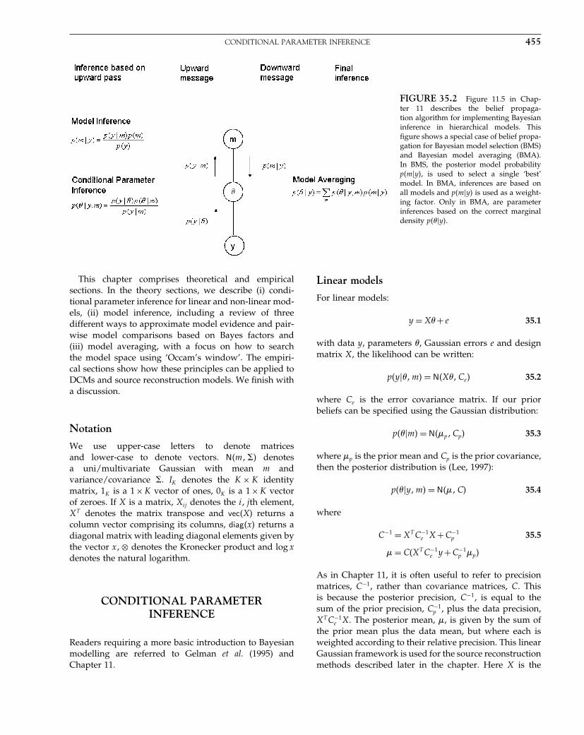
Elsevier UK Chapter: Ch35-P372560 30-9-2006 5:30p.m. Page:455 Trim:7.5in×9.25in
Basal Font:Palatino Margins:Top:40pt Gutter:68pt Font Size:9.5/12 Text Width:42pc Depth:55 Lines
CONDITIONAL PARAMETER INFERENCE 455
FIGURE 35.2 Figure 11.5 in Chap-ter 11 describes the belief propaga-tion algorithm for implementing Bayesianinference in hierarchical models. Thisfigure shows a special case of belief propa-gation for Bayesian model selection (BMS)and Bayesian model averaging (BMA).In BMS, the posterior model probabilityp�m�y�, is used to select a single ‘best’model. In BMA, inferences are based onall models and p�m�y� is used as a weight-ing factor. Only in BMA, are parameterinferences based on the correct marginaldensity p���y�.
This chapter comprises theoretical and empiricalsections. In the theory sections, we describe (i) condi-tional parameter inference for linear and non-linear mod-els, (ii) model inference, including a review of threedifferent ways to approximate model evidence and pair-wise model comparisons based on Bayes factors and(iii) model averaging, with a focus on how to searchthe model space using ‘Occam’s window’. The empiri-cal sections show how these principles can be applied toDCMs and source reconstruction models. We finish witha discussion.
Notation
We use upper-case letters to denote matricesand lower-case to denote vectors. N�m��� denotesa uni/multivariate Gaussian with mean m andvariance/covariance �. IK denotes the K × K identitymatrix, 1K is a 1 ×K vector of ones, 0K is a 1 ×K vectorof zeroes. If X is a matrix, Xij denotes the i� jth element,XT denotes the matrix transpose and vec�X� returns acolumn vector comprising its columns, diag�x� returns adiagonal matrix with leading diagonal elements given bythe vector x�⊗ denotes the Kronecker product and log xdenotes the natural logarithm.
CONDITIONAL PARAMETERINFERENCE
Readers requiring a more basic introduction to Bayesianmodelling are referred to Gelman et al. (1995) andChapter 11.
Linear models
For linear models:
y = X� + e 35.1
with data y, parameters �, Gaussian errors e and designmatrix X, the likelihood can be written:
p�y���m� = N�X��Ce� 35.2
where Ce is the error covariance matrix. If our priorbeliefs can be specified using the Gaussian distribution:
p���m� = N��p�Cp� 35.3
where �p is the prior mean and Cp is the prior covariance,then the posterior distribution is (Lee, 1997):
p���y�m� = N���C� 35.4
where
C−1 = XT C−1e X +C−1
p 35.5
� = C�XT C−1e y +C−1
p �p�
As in Chapter 11, it is often useful to refer to precisionmatrices, C−1, rather than covariance matrices, C. Thisis because the posterior precision, C−1, is equal to thesum of the prior precision, C−1
p , plus the data precision,XT C−1
e X. The posterior mean, �, is given by the sum ofthe prior mean plus the data mean, but where each isweighted according to their relative precision. This linearGaussian framework is used for the source reconstructionmethods described later in the chapter. Here X is the
Elsevier UK Chapter: Ch35-P372560 30-9-2006 5:30p.m. Page:456 Trim:7.5in×9.25in
Basal Font:Palatino Margins:Top:40pt Gutter:68pt Font Size:9.5/12 Text Width:42pc Depth:55 Lines
456 35. BAYESIAN MODEL SELECTION AND AVERAGING
lead-field matrix which transforms measurements fromsource space to sensor space (Baillet et al., 2001).
Our model assumptions, m, are typically embodiedin different choices for the design or prior covariancematrices. These allow for the specification of GLMs withdifferent regressors or different covariance components.
Variance components
Bayesian estimation, as described in the previous section,assumed that we knew the prior covariance, Cp, anderror covariance, Ce. This information is, however, rarelyavailable. In Friston et al. (2002) these covariances areexpressed as:
Cp =∑i
�iQi 35.6
Ce =∑j
�jQj
where Qi and Qj are known as ‘covariance components’and �i��j are hyperparameters. Chapter 24 and Fristonet al. (2002) show how these hyperparameters can beestimated using parametric empirical Bayes (PEB). It isalso possible to represent precision matrices, rather thancovariance matrices, using a linear expansion as shownin Appendix 4.
Non-linear models
For non-linear models, we have:
y = h���+ e 35.7
where h��� is a non-linear function of parameter vector �.We assume Gaussian prior and likelihood distributions:
p���m� = N��p�Cp� 35.8
p�y���m� = N�h����Ce�
where m indexes model structure, �p is the prior mean,Cp the prior covariance and Ce is the error covariance.
The linear framework described in the previous sectioncan be applied by locally linearizing the non-linearity,about a ‘current’ estimate �i, using a first order Taylorseries expansion:
h��� = h��i�+ h��i�
��� −�i� 35.9
Substituting this into Eqn. 35.7 and defining r ≡y −h��i�� J ≡ h��i�
�and � ≡ � −�i gives
r = J� + e 35.10
which now conforms to a GLM (cf. Eqn. 35.1). The ‘prior’(based on starting estimate �i), likelihood and posteriorare now given by:
p���m� = N��p −�i�Cp� 35.11
p�r���m� = N�J��Ce�
p���r�m� = N���Ci+1�
The quantities � and Ci+1 can be found using the resultfor the linear case (substitute r for y and J for X inEqn. 35.5). If we define our ‘new’ parameter estimate as�i+1 = �i +� then:
C−1i+1 = JT C−1
e J +C−1p 35.12
�i+1 = �i +Ci+1�JT C−1
e r +C−1p ��p −�i��
This update is applied iteratively, in that the estimate�i+1 becomes the starting point for a new Taylor seriesexpansion. It can also be combined with hyperparameterestimates, to characterize Cp and Ce, as described inFriston (2002). This then corresponds to the PEB algo-rithm described in Chapter 22. This algorithm is used,for example, to estimate parameters of dynamic causalmodels. For DCM, the non-linearity h��� corresponds tothe integration of a dynamic system.
As described, in Chapter 24, this PEB algorithm isa special case of variational Bayes with a fixed-formfull-covariance Gaussian ensemble. When the algorithmhas converged, it provides an estimate of the posteriordensity:
p���y�m� = N��PEB�CPEB� 35.13
which can then be used for parameter inference andmodel selection.
The above algorithm can also be viewed as the E-step of an expectation maximization (EM) algorithm,described in section 3.1 of Friston (2002) and Appendix 3.The M-step of this algorithm, which we have notdescribed, updates the hyperparameters. This E-step canalso be viewed as a Gauss-Newton optimization wherebyparameter estimates are updated in the direction of thegradient of the log-posterior by an amount proportionalto its curvature (see e.g. Press et al., 1992).
MODEL INFERENCE
Given a particular model class, we let the variable m indexmembers of that class. Model classes might be GLMs wherem indexes design matrices, DCMs where m indexes con-nectivity or input patterns, or source reconstruction mod-els where m indexes functional or anatomical constraints.

Elsevier UK Chapter: Ch35-P372560 30-9-2006 5:30p.m. Page:457 Trim:7.5in×9.25in
Basal Font:Palatino Margins:Top:40pt Gutter:68pt Font Size:9.5/12 Text Width:42pc Depth:55 Lines
MODEL INFERENCE 457
Explicitly including model structure in this way willallow us to make inferences about model structure.
We may, for example, have prior beliefs p�m�. In theabscence of any genuine prior information here, a uni-form distribution will suffice. We can then use Bayes’rule which, in light of observed data y, will update thesemodel priors into model posteriors:
p�m�y� = p�y�m�p�m�
p�y�35.14
Model inference can then proceed based on this distri-bution. This will allow for Bayesian model comparisons(BMCs). In Bayesian model selection (BMS), a model isselected which maximizes this probability:
mMP = argmaxm
�p�m�y��
If the prior is uniform, p�m� = 1/M then this is equivalentto picking the model with the highest evidence:
mME = argmaxm
�p�y�m��
If we have uniform priors then BMC can be implementedwith Bayes factors. Before covering this in more detail,we emphasize that all of these model inferences requirecomputation of the model evidence. This is given by:
p�y�m� =∫
p�y���m�p���m�d� 35.15
The model evidence is simply the normalization termfrom parameter inference, as shown in Figure 35.2. Thisis the ‘message’ that is passed up the hierachy duringbelief propagation, as shown in Figure 35.2. For linearGaussian models, the evidence can be expressed analyt-ically. For non-linear models there are various approxi-mations which are discussed in later subsections.
Bayes factors
Given models m = i and m = j, the Bayes factor compar-ing model i to model j is defined as (Kass and Raftery,1993, 1995):
Bij = p�y�m = i�
p�y�m = j�
where p�y�m = j� is the evidence for model j. When Bij > 1,the data favour model i over model j, and when Bij < 1,the data favour model j. If there are more than two mod-els to compare then we choose one of them as a referencemodel and calculate Bayes factors relative to that refer-ence. When model i is an alternative model and model j a
null model, Bij is the likelihood ratio upon which classicalstatistics are based (see Appendix 1).
A classic example here is the analysis of vari-ance for factorially designed experiments, described inChapter 13. To see if there is a main effect of a factor,one compares two models in which the levels of the fac-tor are described by (i) a single variable or (ii) separatevariables. Evidence in favour of model (ii) allows one toinfer that there is a main effect.
In this chapter, we will use Bayes factors to comparedynamic causal models. In these applications, often themost important inference is on model space. For exam-ple, whether or not experimental effects are mediated bychanges in feedforward or feedback pathways. This par-ticular topic is dealt with in greater detail in Chapter 43.
The Bayes factor is a summary of the evidenceprovided by the data in favour of one scientific theory,represented by a statistical model, as opposed to another.Raftery (1995) presents an interpretation of Bayes factors,shown in Table 35-1. Jefferys (1935) presents a similargrading for the comparison of scientific theories. Thesepartitionings are somewhat arbitrary but do providedescriptive statements.
Table 35-1 also shows the equivalent posterior proba-bility of hypothesis i:
p�m = i�y� = p�y�m = i�p�m = i�
p�y�m = i�p�m = i�+p�y�m = j�p�m = j�35.16
assuming equal model priors p�m = i� = p�m = j� = 0 5.If we define the ‘prior odds ratio’ as p�m = i�/p�m = j�
and the ‘posterior odds ratio’ as:
Oij = p�m = i�y�
p�m = j�y�35.17
then the posterior odds are given by the prior odds mul-tiplied by the Bayes factor. For prior odds of unity theposterior odds are therefore equal to the Bayes factor.Here, a Bayes factor of Bij = 100, for example, correspondsto odds of 100-to-1. In betting shop parlance this is 100-to-1 ‘on’. A value of Bij = 0 01 is 100-to-1 ’against’.
TABLE 35-1 Interpretation of Bayes factors. Bayes factorscan be interpreted as follows. Given candidate hypotheses i andj, a Bayes factor of 20 corresponds to a belief of 95 per cent inthe statement ‘hypothesis i is true’. This corresponds to strong
evidence in favour of i.
Bij p�m = i�y��%� Evidence in favour of model i
1 to 3 50–75 Weak3 to 20 75–95 Positive20 to 150 95–99 Strong≥ 150 ≥ 99 Very strong

Elsevier UK Chapter: Ch35-P372560 30-9-2006 5:30p.m. Page:458 Trim:7.5in×9.25in
Basal Font:Palatino Margins:Top:40pt Gutter:68pt Font Size:9.5/12 Text Width:42pc Depth:55 Lines
458 35. BAYESIAN MODEL SELECTION AND AVERAGING
Bayes factors in Bayesian statistics play a similar roleto p-values in classical statistics. In Raftery (1995), how-ever, Raftery argues that p-values can give misleadingresults, especially in large samples. The background tothis assertion is that Fisher originally suggested the use ofsignificance levels (the p-values beyond which a result isdeemed significant) � = 0 05 or 0.01 based on his experi-ence with small agricultural experiments having between30 and 200 data points. Subsequent advice, notably fromNeyman and Pearson, was that power and significanceshould be balanced when choosing �. This essentiallycorresponds to reducing � for large samples (but they didnot say how � should be reduced). Bayes factors providea principled way to do this.
The relation between p-values and Bayes factors is wellillustrated by the following example (Raftery, 1995). Forlinear regression models, one can use Bayes factors orp-values to decide whether to include an extra regressor.For a sample size of Ns = 50, positive evidence in favourof inclusion (say, B12 = 3) corresponds to a p-value of0.019. For Ns = 100 and 1000 the corresponding p-valuesreduce to 0.01 and 0.003. If one wishes to decide whetherto include multiple extra regressors the correspondingp-values drop more quickly.
Importantly, unlike p-values, Bayes factors can be usedto compare models that cannot be nested.1 This providesan optimal inference framework that can, for example, beapplied to determine which haemodynamic basis func-tions are appropriate for functional magnetic resonanceimaging (fMRI) (Penny et al., 2006). They also allow oneto quantify evidence in favour of a null hypothesis.
Computing the model evidence
This section shows how the model evidence can be com-puted for non-linear models. The evidence for linearmodels is then given as a special case. The prior andlikelihood of the non-linear model can be expanded as:
p���m� = �2��−p/2�Cp�−1/2 exp�−12
e���T C−1p e���� 35.18
p�y���m� = �2��−Ns/2�Ce�−1/2 exp�−12
r���T C−1e r����
where
e��� = � −�p 35.19
r��� = y −h���
are the ‘parameter errors’ and ‘prediction errors’.
1 Model selection using classical inference requires nestedmodels. Inference is made using step-down procedures and the‘extra sum of squares’ principle, as described in Chapter 8.
Substituting these expressions into Eqn. 35 andrearranging allows the evidence to be expressed as:
p�y�m� = �2��−p/2�Cp�−1/2�2��−Ns/2�Ce�−1/2I��� 35.20
where
I��� =∫
exp�−12
r���T C−1e r���− 1
2e���T C−1
p e����d� 35.21
For linear models this integral can be expressed analyti-cally. For non-linear models, it can be estimated using aLaplace approximation.
Laplace approximation
The Laplace approximation was introduced inChapter 24. It makes use of the first order Taylor seriesapproximation referred to in Eqn. 35.9, but this timeplaced around the solution, �L, found by an optimizationalgorithm.
Usually, the term ‘Laplace approximation’ refers toan expansion around the maximum a posteriori (MAP)solution:
�MAP = argmax�
�p�y���m�p���m�� 35.22
Thus �L = �MAP .But, more generally, one can make an expansion
around any solution, for example the one provided byPEB. In this case �L = �PEB. As we have described inChapter 24, PEB is a special case of VB with a fixed-form Gaussian ensemble, and so does not deliver theMAP solution. Rather, PEB maximizes the negative freeenergy and so implicitly minimizes the Kullback-Liebler(KL)-divergence between the true posterior and a full-covariance Gaussian approximation to it. This differenceis discussed in Chapter 24.
Whatever the expansion point, the model non-linearityis approximated using:
h��� = h��L�+ J�� −�L� 35.23
where J = h��L��
. We also make use of the knowledge thatthe posterior covariance is given by:
C−1L = JT C−1
e J +C−1p 35.24
For CL = CPEB this follows directly from Eqn. 35.12.By using the substitutions e��� = ��−�L�+ ��L −�p� and
r��� = �y−h��L��+�h��L�−h����, making use of the abovetwo expressions, and removing terms not dependent on�, we can write:
I��� =[∫
exp�−12
�� −�L�T C−1L �� −�L��d�
]35.25
×[
exp�−12
r��L�T C−1e r��L�− 1
2e��L�T C−1
p e��L��
]
35.26

Elsevier UK Chapter: Ch35-P372560 30-9-2006 5:30p.m. Page:459 Trim:7.5in×9.25in
Basal Font:Palatino Margins:Top:40pt Gutter:68pt Font Size:9.5/12 Text Width:42pc Depth:55 Lines
MODEL INFERENCE 459
where the first factor is the normalizing term of the mul-tivariate Gaussian density. The algebraic steps involvedin the above substitutions are detailed in Stephan et al.(2005). Hence:
I��� = �2��p/2�CL�1/2 exp(
−12
r��L�T C−1e r��L � 35.27
− 12
e��L�T C−1p e��L�
)
Substituting this expression into Eqn. 35.20 and takinglogs gives the Laplace approximation to the log-evidence:
log p�y�m�L = −Ns
2log 2� − 1
2log �Ce�−
12
log �Cp� 35.28
+ 12
log �CL�−12
r��L�T C−1e r��L�
− 12
e��L�T C−1p e��L�
When comparing the evidence for different models, wecan ignore the first term as it will be the same for allmodels. Dropping the first term and rearranging gives:
log p�y�m�L = Accuracy�m�−Complexity�m� 35.29
where
Accuracy�m� = −12
log �Ce�−12
r��L�T C−1e r��L� 35.30
Complexity�m� = 12
log �Cp�−12
log �CL�+12
e��L�T C−1p e��L�
Use of base-e or base-2 logarithms leads to the log-evidence being measured in ‘nats’ or ‘bits’ respectively.Models with high evidence optimally trade-off two con-flicting requirements of a good model, that it fit the dataand be as simple as possible.
The complexity term depends on the prior covari-ance, Cp, which determines the ‘cost’ of parameters. Thisdependence is worrisome if the prior covariances arefixed a priori, as the parameter cost will also be fixeda priori. This will lead to biases in the resulting modelcomparisons. For example, if the prior (co)variances areset to large values, model comparison will consistentlyfavour models that are less complex than the true model.
In DCM for fMRI (Friston et al., 2003), prior variancesare set to fixed values so as to enforce dynamic stability,with high probability. Use of the Laplace approximation inthis context could therefore lead to biases in model com-parison. A second issue in this context is that, to enforcedynamic stability, models with different numbers of con-nections will employ different prior variances. There-fore the priors change from model to model. This meansthat model comparison entails a comparison of the priors.
To overcome these potential problems with DCM forfMRI, alternative approximations to the model evidenceare used instead. These are the Bayesian information cri-terion (BIC) and Akaike information criterion (AIC) intro-duced below. They also use fixed parameter costs, butthey are fixed between models and are different for BICthan AIC. It is suggested in Penny et al. (2004) that, ifthe two measures provide consistent evidence, a modelselection can be made.
Finally, we note that, if prior covariances are estimatedfrom data, then the parameter cost will also have beenestimated from data, and this source of bias in modelcomparison is removed. In this case, the model evi-dence also includes terms which account for uncertaintyin the variance component estimation, as described inChapter 10 of Bishop (1995).
Bayesian information criterion
An alternative approximation to the model evidence isgiven by the Bayesian information criterion (Schwarz,1978). This is a special case of the Laplace approximationwhich drops all terms that do not scale with the numberof data points, and can be derived as follows.
Substituting Eqn. 35.27 into Eqn. 35.20 gives:
p�y�m�L = p�y��L�m�p��L�m��2��p/2�CL�1/2 35.31
Taking logs gives:
log p�y�m�L = log p�y��L�m�+ log p��L�m�
+ p
2log 2� + 1
2log �CL� 35.32
The dependence of the first three terms on the numberof data points is O�Ns��O�1� and O�1�. For the 4th term,entries in the posterior covariance scale linearly with N−1
s :
limNs→�
12
log �CL� = 12
log �CL�0�
Ns
� 35.33
= −p
2log Ns +
12
log �CL�0��
where CL�0� is the posterior covariance based on Ns = 0data points (i.e. the prior covariance). This last term there-fore scales as O�1�. Schwarz (1978) notes that in the limitof large Ns, Eqn. 35.32 therefore reduces to:
BIC = limNs→�
log p�y�m�L 35.34
= log p�y��L�m�− p
2log Ns
This can be re-written as:
BIC = Accuracy�m�− p
2log Ns 35.35
Elsevier UK Chapter: Ch35-P372560 30-9-2006 5:30p.m. Page:460 Trim:7.5in×9.25in
Basal Font:Palatino Margins:Top:40pt Gutter:68pt Font Size:9.5/12 Text Width:42pc Depth:55 Lines
460 35. BAYESIAN MODEL SELECTION AND AVERAGING
where p is the number of parameters in the model. InBIC, the cost of a parameter, −0 5 log Ns bits, thereforereduces with an increasing number of data points.
Akaike’s information criterion
The second criterion we use is Akaike’s information cri-terion (AIC)2 (Akaike, 1973). AIC is maximized when theapproximating likelihood of a novel data point is clos-est to the true likelihood, as measured by the Kullback-Liebler divergence (this is shown in Ripley (1995)). TheAIC is given by:
AIC = Accuracy�m�−p 35.36
Though not originally motivated from a Bayesian per-spective, model comparisons based on AIC are asymp-totically equivalent (i.e. as Ns → �) to those based onBayes factors (Akaike, 1983), i.e. AIC approximates themodel evidence.
Empirically, BIC is biased towards simple models andAIC to complex models (Kass and Raftery, 1993). Indeed,inspection of Eqns 35.35 and 35.36 shows that for valuesappropriate for, e.g. DCM for fMRI, where p ≈ 10 andNs ≈ 200, BIC pays a heavier parameter penalty than AIC.
MODEL AVERAGING
The parameter inferences referred to in previous sectionsare based on the distribution p���y�m�. That m appears asa dependent variable, makes it explicit that these infer-ences are contingent on assumptions about model struc-ture. More generally, however, if inferences about modelparameters are paramount one would use a Bayesianmodel averaging (BMA) approach. Here, inferences arebased on the distribution:
p���y� =∑m
p���y�m�p�m�y� 35.37
where p�m�y� is the posterior probability of model m.
p�m�y� = p�y�m�p�m�
p�y�35.38
As shown in Figure 35.2, only when these ‘messages’,p�m�y�, have been passed back down the hierarchy isbelief propagation complete. Only then do we have thetrue marginal density p���y�. Thus, BMA allows for cor-rect Bayesian inferences, whereas what we have previ-ously described as ‘parameter inferences’ are conditional
2 Strictly, AIC should be referred to as an information criterion.
on model structure. Of course, if our model spacecomprises just one model there is no distribution.
BMA accounts for uncertainty in the model selec-tion process, something which classical statistical analy-sis neglects. By averaging over competing models, BMAincorporates model uncertainty into conclusions aboutparameters. BMA has been successfully applied to manystatistical model classes including linear regression, gen-eralized linear models, and discrete graphical models, inall cases improving predictive performance (see Hoetinget al. 1999 for a review).3 In this chapter, we describethe application of BMA to electroencephalography (EEG)source reconstruction.
There are, however, several practical difficulties withEqn. 35.37 when the number of models and number ofvariables in each model are large. In neuroimaging, mod-els can have tens of thousands of parameters. This issuehas been widely treated in the literature (Draper, 1995),and the general consensus has been to construct searchstrategies to find a set of models that are ‘worth tak-ing into account’. One of these strategies is to generatea Markov chain to explore the model space and thenapproximate Eqn. 35.37 using samples from the posteriorp�m�y� (Madigan and York, 1992). But this is computa-tionally very expensive.
In this chapter, we will instead use the Occam’swindow procedure for nested models described inMadigan and Raftery (1994). First, a model that is N0
times less likely a posteriori than the maximum posteriormodel is removed (in this chapter we use N0 = 20). Sec-ond, complex models with posterior probabilities smallerthan their simpler counterparts are also excluded. Theremaining models fall in Occam’s window. This leads tothe following approximation to the posterior density:
p���y� = ∑m�C
p���y�m�p�m�y� 35.39
where the set C identifies ‘Occam’s window’. Modelsfalling in this window can be identified using the searchstrategy defined in Madigan and Raftery (1994).
DYNAMIC CAUSAL MODELS
The term ‘causal’ in DCM arises because the brain istreated as a deterministic dynamical system (see e.g.section 1.1 in Friston et al. (2003) in which external inputscause changes in neuronal activity which, in turn, cause
3 Software is also available from http://www.research.att.com/volinsky/bma.html.

Elsevier UK Chapter: Ch35-P372560 30-9-2006 5:30p.m. Page:461 Trim:7.5in×9.25in
Basal Font:Palatino Margins:Top:40pt Gutter:68pt Font Size:9.5/12 Text Width:42pc Depth:55 Lines
DYNAMIC CAUSAL MODELS 461
changes in the resulting fMRI, MEG or EEG signal. DCMsfor fMRI comprise a bilinear model for the neurodynam-ics and an extended Balloon model (Buxton, 1998; Friston,2002) for the haemodynamics. These are described indetail in Chapter 41.
The effective connectivity in DCM is characterized bya set of ‘intrinsic connections’ that specify which regionsare connected and whether these connections are unidi-rectional or bidirectional. We also define a set of inputconnections that specify which inputs are connected towhich regions, and a set of modulatory connections thatspecify which intrinsic connections can be changed bywhich inputs. The overall specification of input, intrinsicand modulatory connectivity comprise our assumptionsabout model structure. This, in turn, represents a sci-entific hypothesis about the structure of the large-scaleneuronal network mediating the underlying cognitivefunction. Examples of DCMs are shown in Figure 35.5.
Attention to visual motion
In previous work we have established that attentionmodulates connectivity in a distributed system of corticalregions that subtend visual motion processing (Bucheland Friston, 1997; Friston and Buchel, 2000). Thesefindings were based on data acquired using the follow-ing experimental paradigm. Subjects viewed a computerscreen which displayed either a fixation point, stationarydots or dots moving radially outward at a fixed velocity.For the purpose of our analysis we can consider threeexperimental variables. The ‘photic stimulation’ variableindicates when dots were on the screen, the ‘motion’variable indicates that the dots were moving and the‘attention’ variable indicates that the subject was attend-ing to possible velocity changes. These are the three inputvariables that we use in our DCM analyses and are shownin Figure 35.3.
In this chapter, we model the activity in three regionsV1, V5 and superior parietal cortex (SPC). The original360-scan time series were extracted from the data set of asingle subject using a local eigendecomposition and areshown in Figure 35.4.
We initially set up three DCMs, each embodying dif-ferent assumptions about how attention modulates con-nections to V5. Model 1 assumes that attention modulatesthe forward connection from V1 to V5, model 2 assumesthat attention modulates the backward connection fromSPC to V5 and model 3 assumes attention modulatesboth connections. These models are shown in Figure 35.5.Each model assumes that the effect of motion is to mod-ulate the connection from V1 to V5 and uses the samereciprocal hierarchical intrinsic connectivity.
FIGURE 35.3 The ‘photic’, ‘motion’ and ‘attention’ variablesused in the DCM analysis of the attention to visual motion data (seeFigures 35.4 and 35.5).
FIGURE 35.4 Attention data. fMRI time series (rough solidlines) from regions V1, V5 and SPC and the corresponding estimatesfrom DCM model 1 (smooth solid lines).
We fitted the models and computed Bayes factors,shown in Table 35-2. We did not use the Laplace approx-imation to the model evidence, as DCM for fMRI usesfixed prior variances which compound model compari-son. Instead, we computed both AIC and BIC and madean inference only if the two resulting Bayes factors wereconsistent (Penny et al., 2004).
Table 35-2 shows that the data provide consistent evi-dence in favour of the hypothesis embodied in model 1,i.e. that attention modulates solely the forward connec-tion from V1 to V5.
We now look more closely at the comparison of model1 with model 2. The estimated connection strengths ofthe attentional modulation were 0.23 for the forward

Elsevier UK Chapter: Ch35-P372560 30-9-2006 5:30p.m. Page:462 Trim:7.5in×9.25in
Basal Font:Palatino Margins:Top:40pt Gutter:68pt Font Size:9.5/12 Text Width:42pc Depth:55 Lines
462 35. BAYESIAN MODEL SELECTION AND AVERAGING
FIGURE 35.5 Attention models. In all models, photic stimu-lation enters V1 and the motion variable modulates the connectionfrom V1 to V5. Models 1, 2 and 3 have reciprocal and hierarchi-cally organized intrinsic connectitivty. They differ in how attentionmodulates the connectivity to V5, with model 1 assuming modu-lation of the forward connection, model 2 assuming modulation ofthe backward connection and model 3 assuming both. Solid arrowsindicate input and intrinsic connections and dotted lines indicatemodulatory connections.
TABLE 35-2 Attention data – comparing modulatoryconnectivities. Bayes factors provide consistent evidence in
favour of the hypothesis embodied in model 1, that attentionmodulates (solely) the bottom-up connection from V1 to V5.Model 1 is preferred to models 2 and 3. Models 1 and 2 have
the same number of connections so AIC and BIC giveidentical values
B12 B13 B32
AIC 3 56 2 81 1 27BIC 3 56 19 62 0 18
connection in model 1 and 0.55 for the backward con-nection in model 2. This shows that attentional modu-lation of the backward connection is stronger than theforward connection. However, a breakdown of the Bayesfactor B12 in Table 35-3 shows that the reason model 1is favoured over model 2 is because it is more accurate.In particular, it predicts superior parietal cortex (SPC)
TABLE 35-3 Attention data. Breakdown of contributions tothe Bayes factor for model 1 versus model 2. The largest single
contribution to the Bayes factor is the increased modelaccuracy in region SPC, where 8.38 fewer bits are required to
code the prediction errors. The overall Bayes factor B12 of3.56 provides consistent evidence in favour of model 1
SourceModel 1 versus model 2relative cost (bits)
Bayes factorB12
V1 accuracy 7 32 0 01V5 accuracy −0 77 1 70SPC accuracy −8 38 333 36
Complexity (AIC) 0 00 1 00Complexity (BIC) 0 00 1 00
Overall (AIC) −1 83 3 56Overall (BIC) −1 83 3 56
activity much more accurately. Thus, although model 2does show a significant modulation of the SPC-V5 con-nection, the required change in its prediction of SPCactivity is sufficient to compromise the overall fit of themodel. If we assume models 1 and 2 are equally likelya priori then our posterior belief in model 1 is 0.78 (from3.56/(3.56+1)). Thus, model 1 is the favoured model eventhough the effect of attentional modulation is weaker.
This example makes an important point. Two modelscan only be compared by computing the evidence foreach model. It is not sufficient to compare values of singleconnections. This is because changing a single connectionchanges overall network dynamics and each hypothesisis assessed (in part) by how well it predicts the data,and the relevant data are the activities in a distributednetwork.
We now focus on model 3 that has both modulation offorward and backward connections. First, we make a sta-tistical inference to see if, within model 3, modulation ofthe forward connection is larger than modulation of thebackward connection. For these data, the posterior distri-bution of estimated parameters tells us that this is the casewith probability 0.75. This is a different sort of inferenceto that made above. Instead of inferring which is morelikely, modulation of a forward or of a backward con-nection, we are making an inference about which effectis stronger when both are assumed present.
However, this inference is contingent on theassumption that model 3 is a good model. It is based onthe density p���y�m = 3�. The Bayes factors in Table 35-2, however, show that the data provide consistent evi-dence in favour of the hypothesis embodied in model1, that attention modulates only the forward connection.Table 35-4 shows a breakdown of B13. Here the largestcontribution to the Bayes factor (somewhere between 2.72and 18.97) is the increased parameter cost for model 3.

Elsevier UK Chapter: Ch35-P372560 30-9-2006 5:30p.m. Page:463 Trim:7.5in×9.25in
Basal Font:Palatino Margins:Top:40pt Gutter:68pt Font Size:9.5/12 Text Width:42pc Depth:55 Lines
MULTIPLE CONSTRAINTS 463
TABLE 35-4 Attention data. Breakdown of contributions tothe Bayes factor for model 1 versus model 3. The largest single
contribution to the Bayes factor is the cost of coding theparameters. The table indicates that both models are similarlyaccurate but model 1 is more parsimonious. The overall Bayes
factor B13 provides consistent evidence in favour of the(solely) bottom-up model
SourceModel 1 versus model 3relative cost (bits)
Bayes factorB13
V1 accuracy −0 01 1 01V5 accuracy 0 02 0 99SPC accuracy −0 05 1 04
Complexity (AIC) −1 44 2 72Complexity (BIC) −4 25 18 97
Overall (AIC) −1 49 2 81Overall (BIC) −4 29 19 62
The combined use of Bayes factors and DCM providesus with a formal method for evaluating competing sci-entific theories about the forms of large-scale neural net-works and the changes in them that mediate perceptionand cognition. These issues are pursued in Chapter 43in which DCMs are compared so as to make inferencesabout inter-hemispheric integration from fMRI data.
SOURCE RECONSTRUCTION
A comprehensive introduction to source reconstruction isprovided in Baillet et al. (2001). For more recent develop-ments see Michel et al. (2004) and Chapters 28 to 30. Theaim of source reconstruction is to estimate sources, �,from sensors, y, where:
y = X� + e 35.40
e is an error vector and X defines a lead-field matrix.Distributed source solutions usually assume a Gaussianprior for:
p��� = N��p�Cp� 35.41
Parameter inference for source reconstruction can thenbe implemented as described in the section above onlinear models. Model inference can be implementedusing the expression in Eqn. 35.29. For the numericalresults in this chapter, we augmented this expression toaccount for uncertainty in the estimation of the hyper-parameters. The full expression for the log-evidence ofhyperparameterized models under the Laplace approx-imation is described in Trujillo-Barreto et al. (2004) andAppendix 4.
MULTIPLE CONSTRAINTS
This section considers source reconstruction with mul-tiple constraints. This topic is covered in greater detailand from a different perspective in Chapters 29 and 30.The constraints are implemented using a decompositionof the prior covariance into distinct components:
Cp =∑i
�iQi 35.42
The first type of constraint is a smoothness constraint, Qsc,based on the usual L2-norm. The second is an intrinsicfunctional constraint, Qint, based on multivariate sourceprelocalization (MSP) (Mattout et al., 2005). This pro-vides an estimate, based on a multivariate characteriza-tion of the M/EEG data themselves. Thirdly, we usedextrinsic functional constraints which were considered as‘valid’, Qv
ext, or ‘invalid’, Qiext. These extrinsic constraints
are derived from other imaging modalities such as fMRI.We used invalid constraints to test the robustness of thesource reconstructions.
To test the approach, we generated simulated sourcesfrom the locations shown in Plate 49(a) (see colour platesection). Temporal activity followed a half-period sinefunction with a period of 30 ms. This activity was pro-jected onto 130 virtual MEG sensors and Gaussian noisewas then added. Further details on the simulations aregiven in Mattout et al. (2006).
We then reconstructed the sources using all combina-tions of the various constraints. Plate 50 shows a sampleof source reconstructions. Table 35-5 shows the evidencefor each model which we computed using the Laplace
TABLE 35-5 Log-evidence of models with differentcombinations of smoothness constraints, Qsc, intrinsicconstraints, Qint, valid, Qv
ext and invalid, Qiext, extrinsic
constraints
Log-evidence
1 constraint
Qsc 205.2Qint 208.4Qv
ext 215.6Qi
ext 131.5
2 constraints
Qsc�Qint 207.4Qsc�Qv
ext 214.1Qsc�Qi
ext 204.9Qint�Qv
ext 214.9Qint�Qi
ext 207.4Qv
ext�Qiext 213.2
3 constraints
Qsc�Qint�Qvext 211.5
Qsc�Qint�Qiext 207.2
Qsc�Qvext�Qi
ext 214.7Qint�Qv
ext�Qiext 212.7
4 constraints Qsc�Qint�Qvext�Qi
ext 211.3

Elsevier UK Chapter: Ch35-P372560 30-9-2006 5:30p.m. Page:464 Trim:7.5in×9.25in
Basal Font:Palatino Margins:Top:40pt Gutter:68pt Font Size:9.5/12 Text Width:42pc Depth:55 Lines
464 35. BAYESIAN MODEL SELECTION AND AVERAGING
TABLE 35-6 Bayes factors for models with and withoutvalid location priors, B21, and with and without invalid
location priors, B31. Valid location priors make the modelssignificantly better, whereas invalid location priors do not
make them significantly worse
Bayes factor
Model 1 Model 2 Model 3 B21 B31
Qsc Qsc�Qvext Qsc�Qi
ext 7047 0.8Qint Qint�Qv
ext Qint�Qiext 655 0.4
Qsc�Qint Qsc�Qint�Qvext Qsc�Qint�Qi
ext 60 0.8
approximation (which is exact for these linear Gaussianmodels). As expected, the model with the single validlocation prior had the highest evidence.
Further, any model which contains the valid locationprior has high evidence. The table also shows that anymodel which contains both valid and invalid locationpriors does not show a dramatic decrease in evidence,compared to the same model without the invalid loca-tion prior. These trends can be assessed more formallyby computing the relevant Bayes factors, as shown inTable 35-6. This shows significantly enhanced evidencein favour of models including valid location priors. It alsosuggests that the smoothness and intrinsic location priorscan ameliorate the misleading effect of invalid priors.
MODEL AVERAGING
In this section, we consider source localizations withanatomical constraints. A class of source reconstructionmodels is defined where, for each model, activity isassumed to derive from a particular anatomical ‘com-partment’ or combination of compartments. Anatomicalcompartments are defined by taking 71 brain regions,obtained from a 3D segmentation of the probabilisticMRI atlas (PMA) (Evans et al., 1993) shown in Plate 51.These compartments preserve the hemispheric symme-try of the brain, and include deep areas like thalamus,basal ganglia and brainstem. Simple activations may belocalized to single compartments and more complex acti-vations to combinations of compartments. These combi-nations define a nested family of source reconstructionmodels which can be searched using the Occam’s win-dow approach described above.
The source space consists of a 3D-grid of points thatrepresent the possible generators of the EEG/MEG insidethe brain, while the measurement space is defined bythe array of sensors where the EEG/MEG is recorded.We used a 4.25 mm grid spacing and different arrays ofelectrodes/coils are placed in registration with the PMA.
The 3D-grid is further clipped by the grey matter, whichconsists of all brain regions segmented and shown inPlate 51.
Three arrays of sensors were used and are depicted inPlate 52. For EEG simulations a first set of 19 electrodes(EEG-19) from the 10/20 system is chosen. A secondconfiguration of 120 electrodes (EEG-120) is also usedin order to investigate the dependence of the results onthe number of sensors. Here, electrode positions weredetermined by extending and refining the 10/20 system.For MEG simulations, a dense array of 151 sensors wereused (MEG-151). The physical models constructed in thisway, allow us to compute the electric/magnetic lead fieldmatrices that relate the primary current density (PCD)inside the head, to the voltage/magnetic field measuredat the sensors.
We now present the results of two simulation studies.In the first study, two distributed sources were simulated.One source was located in the right occipital pole, andthe other in the thalamus. This simulation is referred toas ‘OPR+TH’. The spatial distribution of PCD (i.e. thetrue � vector) was generated using two narrow Gaussianfunctions of the same amplitude shown in Figure 35.6(a).
The temporal dynamics were specified using a linearcombination of sine functions with frequency compo-nents evenly spaced in the alpha band (8–12 Hz). Theamplitude of the oscillation as a function of frequenciesis a narrow Gaussian peaked at 10 Hz. That is, activity isgiven by:
j�t� =N∑
i=1
exp�−8�fi −10�2� sin�2�fit� 35.43
where 8 ≤ fi ≤ 12 Hz. Here, fi is the frequency and tdenotes time. These same settings are then used for thesecond simulation study, in which only the thalamic(TH) source was used (see Figure 35.6(b)). This second
FIGURE 35.6 Spatial distributions of the simulated primarycurrent densities. (a) Simultaneous activation of two sources atdifferent depths: one in the right occipital pole and the other inthe thalamus (OPR+TH). (b) Simulation of a single source in thethalamus (TH).
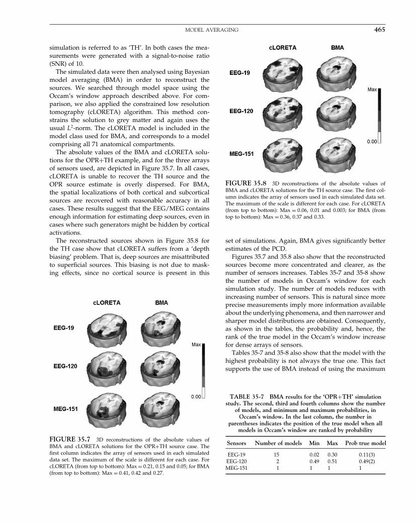
Elsevier UK Chapter: Ch35-P372560 30-9-2006 5:30p.m. Page:465 Trim:7.5in×9.25in
Basal Font:Palatino Margins:Top:40pt Gutter:68pt Font Size:9.5/12 Text Width:42pc Depth:55 Lines
MODEL AVERAGING 465
simulation is referred to as ‘TH’. In both cases the mea-surements were generated with a signal-to-noise ratio(SNR) of 10.
The simulated data were then analysed using Bayesianmodel averaging (BMA) in order to reconstruct thesources. We searched through model space using theOccam’s window approach described above. For com-parison, we also applied the constrained low resolutiontomography (cLORETA) algorithm. This method con-strains the solution to grey matter and again uses theusual L2-norm. The cLORETA model is included in themodel class used for BMA, and corresponds to a modelcomprising all 71 anatomical compartments.
The absolute values of the BMA and cLORETA solu-tions for the OPR+TH example, and for the three arraysof sensors used, are depicted in Figure 35.7. In all cases,cLORETA is unable to recover the TH source and theOPR source estimate is overly dispersed. For BMA,the spatial localizations of both cortical and subcorticalsources are recovered with reasonable accuracy in allcases. These results suggest that the EEG/MEG containsenough information for estimating deep sources, even incases where such generators might be hidden by corticalactivations.
The reconstructed sources shown in Figure 35.8 forthe TH case show that cLORETA suffers from a ‘depthbiasing’ problem. That is, deep sources are misattributedto superficial sources. This biasing is not due to mask-ing effects, since no cortical source is present in this
FIGURE 35.7 3D reconstructions of the absolute values ofBMA and cLORETA solutions for the OPR+TH source case. Thefirst column indicates the array of sensors used in each simulateddata set. The maximum of the scale is different for each case. ForcLORETA (from top to bottom): Max = 0 21, 0.15 and 0.05; for BMA(from top to bottom): Max = 0 41, 0.42 and 0.27.
FIGURE 35.8 3D reconstructions of the absolute values ofBMA and cLORETA solutions for the TH source case. The first col-umn indicates the array of sensors used in each simulated data set.The maximum of the scale is different for each case. For cLORETA(from top to bottom): Max = 0 06, 0.01 and 0.003; for BMA (fromtop to bottom): Max = 0 36, 0.37 and 0.33.
set of simulations. Again, BMA gives significantly betterestimates of the PCD.
Figures 35.7 and 35.8 also show that the reconstructedsources become more concentrated and clearer, as thenumber of sensors increases. Tables 35-7 and 35-8 showthe number of models in Occam’s window for eachsimulation study. The number of models reduces withincreasing number of sensors. This is natural since moreprecise measurements imply more information availableabout the underlying phenomena, and then narrower andsharper model distributions are obtained. Consequently,as shown in the tables, the probability and, hence, therank of the true model in the Occam’s window increasefor dense arrays of sensors.
Tables 35-7 and 35-8 also show that the model with thehighest probability is not always the true one. This factsupports the use of BMA instead of using the maximum
TABLE 35-7 BMA results for the ‘OPR+TH’ simulationstudy. The second, third and fourth columns show the number
of models, and minimum and maximum probabilities, inOccam’s window. In the last column, the number in
parentheses indicates the position of the true model when allmodels in Occam’s window are ranked by probability
Sensors Number of models Min Max Prob true model
EEG-19 15 0 02 0 30 0 11�3�EEG-120 2 0 49 0 51 0 49�2�MEG-151 1 1 1 1
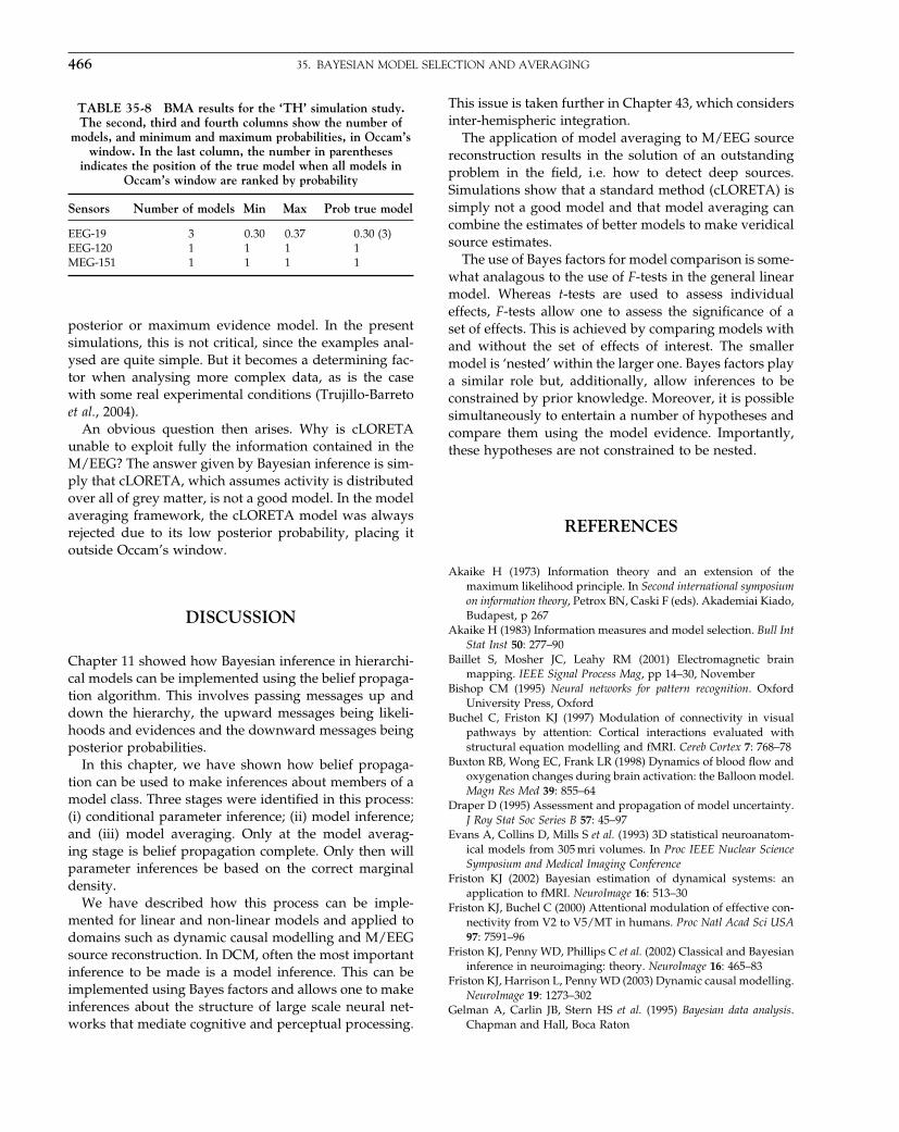
Elsevier UK Chapter: Ch35-P372560 30-9-2006 5:30p.m. Page:466 Trim:7.5in×9.25in
Basal Font:Palatino Margins:Top:40pt Gutter:68pt Font Size:9.5/12 Text Width:42pc Depth:55 Lines
466 35. BAYESIAN MODEL SELECTION AND AVERAGING
TABLE 35-8 BMA results for the ‘TH’ simulation study.The second, third and fourth columns show the number of
models, and minimum and maximum probabilities, in Occam’swindow. In the last column, the number in parentheses
indicates the position of the true model when all models inOccam’s window are ranked by probability
Sensors Number of models Min Max Prob true model
EEG-19 3 0 30 0 37 0 30 �3�EEG-120 1 1 1 1MEG-151 1 1 1 1
posterior or maximum evidence model. In the presentsimulations, this is not critical, since the examples anal-ysed are quite simple. But it becomes a determining fac-tor when analysing more complex data, as is the casewith some real experimental conditions (Trujillo-Barretoet al., 2004).
An obvious question then arises. Why is cLORETAunable to exploit fully the information contained in theM/EEG? The answer given by Bayesian inference is sim-ply that cLORETA, which assumes activity is distributedover all of grey matter, is not a good model. In the modelaveraging framework, the cLORETA model was alwaysrejected due to its low posterior probability, placing itoutside Occam’s window.
DISCUSSION
Chapter 11 showed how Bayesian inference in hierarchi-cal models can be implemented using the belief propaga-tion algorithm. This involves passing messages up anddown the hierarchy, the upward messages being likeli-hoods and evidences and the downward messages beingposterior probabilities.
In this chapter, we have shown how belief propaga-tion can be used to make inferences about members of amodel class. Three stages were identified in this process:(i) conditional parameter inference; (ii) model inference;and (iii) model averaging. Only at the model averag-ing stage is belief propagation complete. Only then willparameter inferences be based on the correct marginaldensity.
We have described how this process can be imple-mented for linear and non-linear models and applied todomains such as dynamic causal modelling and M/EEGsource reconstruction. In DCM, often the most importantinference to be made is a model inference. This can beimplemented using Bayes factors and allows one to makeinferences about the structure of large scale neural net-works that mediate cognitive and perceptual processing.
This issue is taken further in Chapter 43, which considersinter-hemispheric integration.
The application of model averaging to M/EEG sourcereconstruction results in the solution of an outstandingproblem in the field, i.e. how to detect deep sources.Simulations show that a standard method (cLORETA) issimply not a good model and that model averaging cancombine the estimates of better models to make veridicalsource estimates.
The use of Bayes factors for model comparison is some-what analagous to the use of F-tests in the general linearmodel. Whereas t-tests are used to assess individualeffects, F-tests allow one to assess the significance of aset of effects. This is achieved by comparing models withand without the set of effects of interest. The smallermodel is ‘nested’ within the larger one. Bayes factors playa similar role but, additionally, allow inferences to beconstrained by prior knowledge. Moreover, it is possiblesimultaneously to entertain a number of hypotheses andcompare them using the model evidence. Importantly,these hypotheses are not constrained to be nested.
REFERENCES
Akaike H (1973) Information theory and an extension of themaximum likelihood principle. In Second international symposiumon information theory, Petrox BN, Caski F (eds). Akademiai Kiado,Budapest, p 267
Akaike H (1983) Information measures and model selection. Bull IntStat Inst 50: 277–90
Baillet S, Mosher JC, Leahy RM (2001) Electromagnetic brainmapping. IEEE Signal Process Mag, pp 14–30, November
Bishop CM (1995) Neural networks for pattern recognition. OxfordUniversity Press, Oxford
Buchel C, Friston KJ (1997) Modulation of connectivity in visualpathways by attention: Cortical interactions evaluated withstructural equation modelling and fMRI. Cereb Cortex 7: 768–78
Buxton RB, Wong EC, Frank LR (1998) Dynamics of blood flow andoxygenation changes during brain activation: the Balloon model.Magn Res Med 39: 855–64
Draper D (1995) Assessment and propagation of model uncertainty.J Roy Stat Soc Series B 57: 45–97
Evans A, Collins D, Mills S et al. (1993) 3D statistical neuroanatom-ical models from 305 mri volumes. In Proc IEEE Nuclear ScienceSymposium and Medical Imaging Conference
Friston KJ (2002) Bayesian estimation of dynamical systems: anapplication to fMRI. NeuroImage 16: 513–30
Friston KJ, Buchel C (2000) Attentional modulation of effective con-nectivity from V2 to V5/MT in humans. Proc Natl Acad Sci USA97: 7591–96
Friston KJ, Penny WD, Phillips C et al. (2002) Classical and Bayesianinference in neuroimaging: theory. NeuroImage 16: 465–83
Friston KJ, Harrison L, Penny WD (2003) Dynamic causal modelling.NeuroImage 19: 1273–302
Gelman A, Carlin JB, Stern HS et al. (1995) Bayesian data analysis.Chapman and Hall, Boca Raton

Elsevier UK Chapter: Ch35-P372560 30-9-2006 5:30p.m. Page:467 Trim:7.5in×9.25in
Basal Font:Palatino Margins:Top:40pt Gutter:68pt Font Size:9.5/12 Text Width:42pc Depth:55 Lines
REFERENCES 467
Hoeting JA, Madigan D, Raftery AE et al. (1999) Bayesian modelaveraging: a tutorial. Stat Sci 14: 382–417
Jefferys H (1935) Some tests of significance, treated by the theory ofprobability. Proc Camb Philos Soc 31: 203–22
Kass RE, Raftery AE (1993) Bayes factors and modeluncertainty. Technical Report 254, University of Washington.http://www.stat.washington.edu/tech.reports/tr254.ps.
Kass RE, Raftery AE (1995) Bayes factors. J Am Stat Assoc 90: 773–95Lee PM (1997) Bayesian statistics: an introduction, 2nd edn. Arnold,
LondonMadigan D, Raftery A (1994) Model selection and accounting
for uncertainty in graphical models using Occam’s window.J Am Stat Assoc 89: 1535–46
Madigan D, York J (1992) Bayesian graphical models for discretedata. Technical report, Department of Statistics, University ofWashington, Report number 259
Mattout J, Pelegrini-Isaac M, Garnero L et al. (2005) Multivari-ate source prelocalisation: use of functionally informed basisfunctions for better conditioning the MEG inverse problem.NeuroImage 26: 356–73
Mattout J, Phillips C, Penny WD et al. (2006) MEG source localisationunder multiple constraints: an extended Bayesian framework.NeuroImage 30: 753–67
Michel CM, Marraya MM, Lantza G et al. (2004) EEG source imaging.Clin Neurophysiol 115: 2195–22
Penny WD, Stephan KE, Mechelli A et al. (2004) Comparing dynamiccausal models. NeuroImage 22: 1157–72
Penny WD, Flandin G, Trujillo-Barreto N (2006) Bayesian compar-ison of spatially regularised general linear models. Hum BrainMapp (in press)
Press WH, Teukolsky SA, Vetterling WT et al. (1992) NumericalRecipes in C. Cambridge University Press, Cambridge
Raftery AE (1995) Bayesian model selection in social research.In Sociological methodology, Marsden PV (ed.). Cambridge, MA,pp 111–96
Ripley B (1995) Pattern recognition and neural networks. CambridgeUniversity Press, Cambridge
Schwarz G (1978) Estimating the dimension of a model. Ann Stat 6:461–64
Stephan KE, Friston KJ, Penny WD (2005) Computing the objectivefunction in DCM. Technical report, Wellcome Department ofImaging Neuroscience, ION, UCL, London
Trujillo-Barreto N, Aubert-Vazquez E, Valdes-Sosa P (2004)Bayesian model averaging in EEG/MEG imaging. NeuroImage21: 1300–19

Elsevier UK Chapter: Ch36-P372560 30-9-2006 5:30p.m. Page:471 Trim:7.5in×9.25in
Basal Font:Palatino Margins:Top:40pt Gutter:68pt Font Size:9.5/12 Text Width:42pc Depth:55 Lines
C H A P T E R
36
Functional integrationK. Friston
INTRODUCTION
The next chapters are about functional integration in thebrain. This chapter reviews the neurobiology of func-tional integration, in terms of neuronal information pro-cessing and frames the sorts of question that can beaddressed with analyses of functional and effective con-nectivity. In fact, we use empirical Bayes (see Part 4) asthe basis for understanding integration among the lev-els of hierarchically organized cortical areas. The nexttwo chapters (Chapters 37 and 38) deal with functionaland effective connectivity. Chapters 39 and 40 deal withcomplementary models of functional integration, namelythe Volterra or generalized convolution formulation andstate-space representations. The final chapters in thissection cover dynamic causal modelling. For a moremathematical treatment of these models and their inter-relationships, see Appendix 2.
In this chapter, we will review the empirical evidencefor functional specialization and integration, with a spe-cial focus on extrinsic connections among cortical areasand how they define cortical hierarchies. We will thenlook at these hierarchical architectures, using ideas fromtheoretical neurobiology, which clarify the potential roleof forward and backward connections. Finally, we seehow neuroimaging can be used to test hypotheses thatarise from this theoretical treatment. Specifically, weshow that functional neuroimaging can be used to test forinteractions between bottom-up and top-down influenceson an area and to make quantitative inferences aboutchanges in connectivity. This chapter is quite theoreticaland is used to introduce constraints from neurobiologyand computational neuroscience that provide a contextfor the models of functional integration presented in thesubsequent chapters.
Interactions and context-sensitivity
In concert with the growing interest in contextual andextra-classical receptive field effects in electrophysiology(i.e. how the receptive fields of sensory neurons changeaccording to the context a stimulus is presented in), asimilar shift is apparent in imaging. Namely, the appre-ciation that functional specialization can exhibit similarextra-classical phenomena, in which a cortical area maybe specialized for one thing in one context but somethingelse in another (see McIntosh, 2000). These extra-classicalphenomena have implications for theoretical ideas abouthow the brain might work. This chapter uses theoreticalmodels of representational or perceptual inference as avehicle to illustrate how imaging can be used to addressimportant questions about functional brain architectures.
Many models of perceptual learning and inferencerequire prior assumptions about the distribution of sen-sory causes. However, as seen in the previous chapters,empirical Bayes suggests that priors can be learned in ahierarchical context. The main point made in this chapteris that backward connections, mediating internal or gen-erative models of how sensory data are caused, can con-struct empirical priors and are essential for perception.Moreover, non-linear generative models require theseconnections to be modulatory so that causes in highercortical levels can interact to predict responses in lowerlevels. This is important in relation to functional asym-metries in forward and backward connections that havebeen demonstrated empirically.
Overview
We start by reviewing the two fundamental principlesof brain organization, namely functional specialization
Statistical Parametric Mapping, by Karl Friston et al. Copyright 2007, Elsevier Ltd. All rights reserved.ISBN–13: 978-0-12-372560-8 ISBN–10: 0-12-372560-7
471
Elsevier UK Chapter: Ch36-P372560 30-9-2006 5:30p.m. Page:472 Trim:7.5in×9.25in
Basal Font:Palatino Margins:Top:40pt Gutter:68pt Font Size:9.5/12 Text Width:42pc Depth:55 Lines
472 36. FUNCTIONAL INTEGRATION
and functional integration and how they rest upon theanatomy and physiology of cortico-cortical connectionsin the brain. The second section deals with the nature andlearning of representations from a theoretical or compu-tational perspective. The key focus of this section is onthe functional architectures implied by the theory. Gen-erative models based on predictive coding rest on hierar-chies of backward and lateral projections and, critically,confer a necessary role on backward connections. Thetheme of context-sensitive responses is used in the sub-sequent section to preview different ways of measuringconnectivity with functional neuroimaging. The focus ofthis section is evidence for the interaction of bottom-upand top-down influences and establishing the presenceof backward connections. The final section reviews someof the implications for lesion studies and neuropsychol-ogy. Dynamic diaschisis is introduced, in which aberrantneuronal responses can be observed following damageto distal brain areas that provide enabling or modulatoryafferents.
FUNCTIONAL SPECIALIZATION ANDINTEGRATION
The brain appears to adhere to two fundamentalprinciples of functional organization, functional integra-tion and functional specialization, where the integra-tion within and among specialized areas is mediatedby effective connectivity. The distinction relates to thatbetween ‘localizationism’ and ‘connectionism’ that dom-inated thinking about cortical function in the nineteenthcentury. Since the early anatomic theories of Gall, theidentification of a particular brain region with a specificfunction has become a central theme in neuroscience.However, functional localization per se was not easy todemonstrate: for example, a meeting that took place on4 August 1881 addressed the difficulties of attributingfunction to a cortical area, given the dependence of cere-bral activity on underlying connections (Phillips et al.,1984). This meeting was entitled ‘Localization of func-tion in the cortex cerebri’. Goltz, although accepting theresults of electrical stimulation in dog and monkey cortex,considered that the excitation method was inconclusive,in that the behaviours elicited might have originated inrelated pathways, or current could have spread to dis-tant centres. In short, the excitation method could notbe used to infer functional localization because localiza-tionism discounted interactions, or functional integrationamong different brain areas. It was proposed that lesionstudies could supplement excitation experiments. Ironi-cally, it was observations on patients with brain lesionssome years later (see Absher and Benson, 1993) that
led to the concept of ‘disconnection syndromes’ and therefutation of localizationism as a complete or sufficientexplanation of cortical organization. Functional localiza-tion implies that a function can be localized in a corticalarea, whereas specialization suggests that a cortical areais specialized for some aspects of perceptual or motorprocessing, where this specialization can be anatomicallysegregated within the cortex. The cortical infrastructuresupporting a single function may then involve many spe-cialized areas whose union is mediated by the functionalintegration among them. Functional specialization andintegration are not exclusive, they are complementary.Functional specialization is only meaningful in the con-text of functional integration and vice versa.
Functional specialization and segregation
The functional role, played by any component (e.g. cor-tical area, sub-area, neuronal population or neuron) ofthe brain, is defined largely by its connections. Certainpatterns of cortical projections are so common that theyamount to rules of cortical connectivity. ‘These rulesrevolve around one, apparently, overriding strategy thatthe cerebral cortex uses – that of functional segregation’(Zeki, 1990). Functional segregation demands that cellswith common functional properties be grouped together.This architectural constraint necessitates both conver-gence and divergence of cortical connections. Extrinsicconnections, between cortical regions, are not continu-ous but occur in patches or clusters. This patchiness hasa clear relationship to functional segregation. For exam-ple, the secondary visual area, V2, has a cytochromeoxidase architecture, consisting of thick, thin and inter-stripes. When recordings are made in V2, directionallyselective (but not wavelength or colour selective) cellsare found exclusively in the thick stripes. Retrograde(i.e. backward) labelling of cells in V5 is limited to thesethick stripes. All the available physiological evidencesuggests that V5 is a functionally homogeneous areathat is specialized for visual motion. Evidence of thisnature supports the notion that patchy connectivity is theanatomical infrastructure that underpins functional seg-regation and specialization. If it is the case that neurons ina given cortical area share a common responsiveness (byvirtue of their extrinsic connectivity) to some sensorimo-tor or cognitive attribute, then this functional segregationis also an anatomical one. Challenging a subject with theappropriate sensorimotor attribute or cognitive processshould lead to activity changes in, and only in, the areasof interest. This is the model upon which the search forregionally specific effects with functional neuroimagingis based.
Elsevier UK Chapter: Ch36-P372560 30-9-2006 5:30p.m. Page:473 Trim:7.5in×9.25in
Basal Font:Palatino Margins:Top:40pt Gutter:68pt Font Size:9.5/12 Text Width:42pc Depth:55 Lines
FUNCTIONAL SPECIALIZATION AND INTEGRATION 473
The anatomy and physiology ofcortico-cortical connections
If specialization rests upon connectivity then importantorganizational principles should be embodied in theneuroanatomy and physiology of extrinsic connections.Extrinsic connections couple different cortical areas,whereas intrinsic connections are confined to the corticalsheet. There are certain features of cortico-cortical con-nections that provide strong clues about their functionalrole. In brief, there appears to be a hierarchical organiza-tion that rests upon the distinction between forward andbackward connections. The designation of a connection asforward or backward depends primarily on its corticallayers of origin and termination. Some characteristics ofcortico-cortical connections are presented below and aresummarized in Table 36-1. The list is not exhaustive butserves to introduce some important principles that haveemerged from empirical studies of visual cortex:
• Hierarchical organization – the organization of the visualcortices can be considered as a hierarchy of cortical lev-els with reciprocal extrinsic cortico-cortical connectionsamong the constituent cortical areas (Felleman and VanEssen, 1991). The notion of a hierarchy depends upon adistinction between reciprocal forward and backwardextrinsic connections (see Figure 36.1).
• Reciprocal connections – although reciprocal, forwardand backward connections show both a microstruc-tural and functional asymmetry. The terminations ofboth show laminar specificity. Forward connections(from a low to a high level) have sparse axonal bifurca-tions and are topographically organized, originating insupra-granular layers and terminating largely in layerIV. Backward connections, on the other hand, showabundant axonal bifurcation and a more diffuse topog-raphy. Their origins are bilaminar-infragranular andthey terminate predominantly in supra-granular layers(Rockland and Pandya, 1979; Salin and Bullier, 1995).
Extrinsic connections show an orderly convergenceand divergence of connections from one cortical levelto the next. At a macroscopic level, one point in agiven cortical area will connect to a region 5–8 mm indiameter in another. An important distinction betweenforward and backward connections is that backwardconnections are more divergent. For example, thedivergence region of a point in V5 (i.e. the regionreceiving backward afferents from V5) may includethick and inter-stripes in V2, whereas the convergenceregion (i.e. the region providing forward afferents toV5) is limited to the thick stripes (Zeki and Shipp,1988). Backward connections are more abundant thanforward connections and transcend more levels. Forexample, the ratio of forward efferent connections tobackward afferents in the lateral geniculate is about oneto ten. Another important distinction is that backwardconnections will traverse a number of hierarchical lev-els, whereas forward connections are more restricted.For example, there are backward connections from TEand TEO to V1 but no monosynaptic connections fromV1 to TE or TEO (Salin and Bullier, 1995).
• Functionally asymmetric forward and backward connec-tions – functionally, reversible inactivation (e.g. Sandelland Schiller, 1982; Girard and Bullier, 1989) and neu-roimaging (e.g. Büchel and Friston, 1997) studies sug-gest that forward connections are driving and alwayselicit a response, whereas backward connections can bemodulatory. In this context, modulatory means back-ward connections modulate responsiveness to otherinputs. At the single cell level, ‘inputs from drivers canbe differentiated from those of modulators. The drivercan be identified as the transmitter of receptive fieldproperties; the modulator can be identified as alteringthe probability of certain aspects of that transmission’(Sherman and Guillery, 1998).
The notion that forward connections are concernedwith the segregation of sensory information is consistent
TABLE 36-1 Some key characteristics of extrinsic cortico-cortical connections
• The organization of the visual cortices can be considered as a hierarchy (Felleman and Van Essen, 1991)• The notion of a hierarchy depends upon a distinction between forward and backward extrinsic connections• This distinction rests upon laminar specificity (Rockland and Pandya, 1979; Salin and Bullier, 1995)• Backward connections are more numerous and transcend more levels• Backward connections are more divergent than forward connections (Zeki and Shipp, 1988)
Forward connections Backward connections
Sparse axonal bifurcations Abundant axonal bifurcationTopographically organized Diffuse topographyOriginate in supra-granular layers Originate in bi-laminar/infra-granular layersTerminate largely in layer IV Terminate predominantly in supra-granular layersPostsynaptic effects through fast AMPA (1.3–2.4 msdecay) and GABAA (6 ms decay) receptors
Modulatory afferents activate slow (50 ms decay) voltage-sensitive NMDA receptors
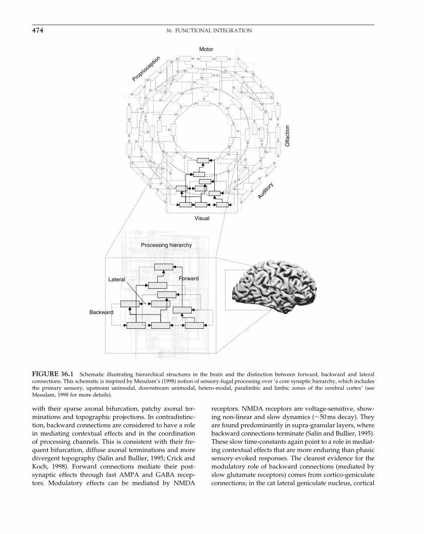
Elsevier UK Chapter: Ch36-P372560 30-9-2006 5:30p.m. Page:474 Trim:7.5in×9.25in
Basal Font:Palatino Margins:Top:40pt Gutter:68pt Font Size:9.5/12 Text Width:42pc Depth:55 Lines
474 36. FUNCTIONAL INTEGRATION
Backward
ForwardLateral
Processing hierarchy
Visual
Audito
ry
Olfa
ctio
n
Motor
Propr
iocep
tion
FIGURE 36.1 Schematic illustrating hierarchical structures in the brain and the distinction between forward, backward and lateralconnections. This schematic is inspired by Mesulam’s (1998) notion of sensory-fugal processing over ‘a core synaptic hierarchy, which includesthe primary sensory, upstream unimodal, downstream unimodal, hetero-modal, paralimbic and limbic zones of the cerebral cortex’ (seeMesulam, 1998 for more details).
with their sparse axonal bifurcation, patchy axonal ter-minations and topographic projections. In contradistinc-tion, backward connections are considered to have a rolein mediating contextual effects and in the coordinationof processing channels. This is consistent with their fre-quent bifurcation, diffuse axonal terminations and moredivergent topography (Salin and Bullier, 1995; Crick andKoch, 1998). Forward connections mediate their post-synaptic effects through fast AMPA and GABA recep-tors. Modulatory effects can be mediated by NMDA
receptors. NMDA receptors are voltage-sensitive, show-ing non-linear and slow dynamics (∼50 ms decay). Theyare found predominantly in supra-granular layers, wherebackward connections terminate (Salin and Bullier, 1995).These slow time-constants again point to a role in mediat-ing contextual effects that are more enduring than phasicsensory-evoked responses. The clearest evidence for themodulatory role of backward connections (mediated byslow glutamate receptors) comes from cortico-geniculateconnections; in the cat lateral geniculate nucleus, cortical
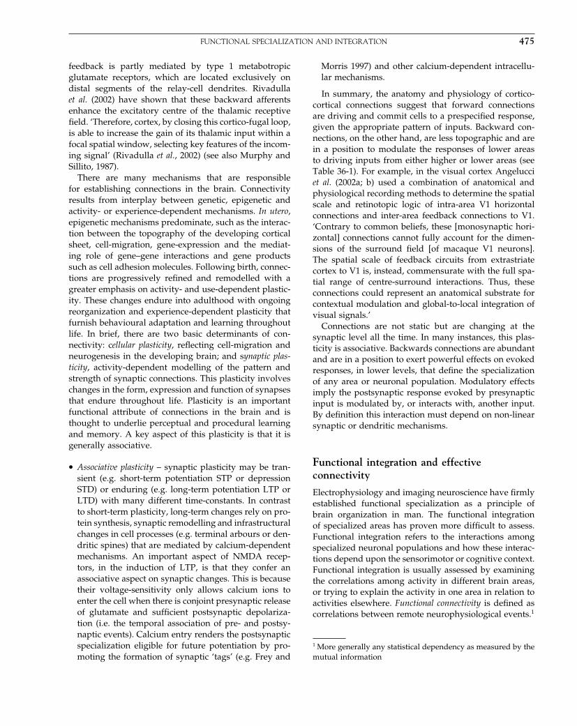
Elsevier UK Chapter: Ch36-P372560 30-9-2006 5:30p.m. Page:475 Trim:7.5in×9.25in
Basal Font:Palatino Margins:Top:40pt Gutter:68pt Font Size:9.5/12 Text Width:42pc Depth:55 Lines
FUNCTIONAL SPECIALIZATION AND INTEGRATION 475
feedback is partly mediated by type 1 metabotropicglutamate receptors, which are located exclusively ondistal segments of the relay-cell dendrites. Rivadullaet al. (2002) have shown that these backward afferentsenhance the excitatory centre of the thalamic receptivefield. ‘Therefore, cortex, by closing this cortico-fugal loop,is able to increase the gain of its thalamic input within afocal spatial window, selecting key features of the incom-ing signal’ (Rivadulla et al., 2002) (see also Murphy andSillito, 1987).
There are many mechanisms that are responsiblefor establishing connections in the brain. Connectivityresults from interplay between genetic, epigenetic andactivity- or experience-dependent mechanisms. In utero,epigenetic mechanisms predominate, such as the interac-tion between the topography of the developing corticalsheet, cell-migration, gene-expression and the mediat-ing role of gene–gene interactions and gene productssuch as cell adhesion molecules. Following birth, connec-tions are progressively refined and remodelled with agreater emphasis on activity- and use-dependent plastic-ity. These changes endure into adulthood with ongoingreorganization and experience-dependent plasticity thatfurnish behavioural adaptation and learning throughoutlife. In brief, there are two basic determinants of con-nectivity: cellular plasticity, reflecting cell-migration andneurogenesis in the developing brain; and synaptic plas-ticity, activity-dependent modelling of the pattern andstrength of synaptic connections. This plasticity involveschanges in the form, expression and function of synapsesthat endure throughout life. Plasticity is an importantfunctional attribute of connections in the brain and isthought to underlie perceptual and procedural learningand memory. A key aspect of this plasticity is that it isgenerally associative.
• Associative plasticity – synaptic plasticity may be tran-sient (e.g. short-term potentiation STP or depressionSTD) or enduring (e.g. long-term potentiation LTP orLTD) with many different time-constants. In contrastto short-term plasticity, long-term changes rely on pro-tein synthesis, synaptic remodelling and infrastructuralchanges in cell processes (e.g. terminal arbours or den-dritic spines) that are mediated by calcium-dependentmechanisms. An important aspect of NMDA recep-tors, in the induction of LTP, is that they confer anassociative aspect on synaptic changes. This is becausetheir voltage-sensitivity only allows calcium ions toenter the cell when there is conjoint presynaptic releaseof glutamate and sufficient postsynaptic depolariza-tion (i.e. the temporal association of pre- and postsy-naptic events). Calcium entry renders the postsynapticspecialization eligible for future potentiation by pro-moting the formation of synaptic ‘tags’ (e.g. Frey and
Morris 1997) and other calcium-dependent intracellu-lar mechanisms.
In summary, the anatomy and physiology of cortico-cortical connections suggest that forward connectionsare driving and commit cells to a prespecified response,given the appropriate pattern of inputs. Backward con-nections, on the other hand, are less topographic and arein a position to modulate the responses of lower areasto driving inputs from either higher or lower areas (seeTable 36-1). For example, in the visual cortex Angelucciet al. (2002a; b) used a combination of anatomical andphysiological recording methods to determine the spatialscale and retinotopic logic of intra-area V1 horizontalconnections and inter-area feedback connections to V1.‘Contrary to common beliefs, these [monosynaptic hori-zontal] connections cannot fully account for the dimen-sions of the surround field [of macaque V1 neurons].The spatial scale of feedback circuits from extrastriatecortex to V1 is, instead, commensurate with the full spa-tial range of centre-surround interactions. Thus, theseconnections could represent an anatomical substrate forcontextual modulation and global-to-local integration ofvisual signals.’
Connections are not static but are changing at thesynaptic level all the time. In many instances, this plas-ticity is associative. Backwards connections are abundantand are in a position to exert powerful effects on evokedresponses, in lower levels, that define the specializationof any area or neuronal population. Modulatory effectsimply the postsynaptic response evoked by presynapticinput is modulated by, or interacts with, another input.By definition this interaction must depend on non-linearsynaptic or dendritic mechanisms.
Functional integration and effectiveconnectivity
Electrophysiology and imaging neuroscience have firmlyestablished functional specialization as a principle ofbrain organization in man. The functional integrationof specialized areas has proven more difficult to assess.Functional integration refers to the interactions amongspecialized neuronal populations and how these interac-tions depend upon the sensorimotor or cognitive context.Functional integration is usually assessed by examiningthe correlations among activity in different brain areas,or trying to explain the activity in one area in relation toactivities elsewhere. Functional connectivity is defined ascorrelations between remote neurophysiological events.1
1 More generally any statistical dependency as measured by themutual information
Elsevier UK Chapter: Ch36-P372560 30-9-2006 5:30p.m. Page:476 Trim:7.5in×9.25in
Basal Font:Palatino Margins:Top:40pt Gutter:68pt Font Size:9.5/12 Text Width:42pc Depth:55 Lines
476 36. FUNCTIONAL INTEGRATION
However, correlations can arise in a variety of ways. Forexample, in multiunit electrode recordings they can resultfrom stimulus-locked transients, evoked by a commoninput or reflect stimulus-induced oscillations mediated bysynaptic connections (Gerstein and Perkel, 1969). Inte-gration within a distributed system is better understoodin terms of effective connectivity. Effective connectivityrefers explicitly to the influence that one neuronal sys-tem exerts over another, either at a synaptic (i.e. synapticefficacy) or population level. It has been proposed that‘the [electrophysiological] notion of effective connectiv-ity should be understood as the experiment- and time-dependent, simplest possible circuit diagram that wouldreplicate the observed timing relationships between therecorded neurons’ (Aertsen and Preil, 1991). This meanseffective connectivity is dynamic, i.e. activity-dependent,and depends upon a model of the interactions. Recentmodels of effective connectivity accommodate the mod-ulatory or non-linear effects mentioned above. A moredetailed discussion of these models is provided in subse-quent chapters. In this chapter, the terms modulatory andnon-linear are used almost synonymously. Modulatoryeffects imply the postsynaptic response evoked by oneinput is modulated, or interacts with, another. By defini-tion this interaction must depend on non-linear synapticmechanisms.
In summary, the brain can be considered as an ensem-ble of functionally specialized areas that are coupled in anon-linear fashion by effective connections. Empirically,it appears that connections from lower to higher areas arepredominantly driving, whereas backward connectionsthat mediate top-down influences are more diffuse andare capable of exerting modulatory influences. In the nextsection, we describe a theoretical perspective that high-lights the functional importance of backward connectionsand non-linear interactions.
LEARNING AND INFERENCE IN THEBRAIN
This section describes the heuristics behind self-supervised learning based on empirical Bayes. Thisapproach is considered within the framework of genera-tive models and follows Dayan and Abbott (2001: 359–397)to which the reader is referred for background reading.A more detailed discussion of these issues can be foundin Friston (2005).
First, we will reprise empirical Bayes in the contextof brain function per se. Having established the requisitearchitecture for learning and inference, neuronal imple-mentation is considered in sufficient depth to make pre-dictions about the structural and functional anatomy that
would be needed to implement empirical Bayes in thebrain. We conclude by relating theoretical predictionswith the four neurobiological principles listed in the pre-vious section.
Causes, perception and sensation
Causes are simply the states of processes generating sen-sory data. It is not easy to ascribe meaning to these stateswithout appealing to the way that we categorize things.Causes may be categorical in nature, such as the identityof a face or the semantic category of an object. Othersmay be parametric, such as the position of an object. Eventhough causes may be difficult to describe, they are easyto define operationally. Causes are quantities or statesthat are necessary to specify the products of a processgenerating sensory information. To keep things simple,let us frame the problem of representing causes in termsof a deterministic non-linear function:
u = g�v��� 36.1
where v is a vector of causes in the environment (e.g. thevelocity of a particular object, direction of radiant lightetc.), and u represents sensory input. g�v��� is a functionthat generates data from the causes. � are the parametersof the generative model. Unlike the causes, they are fixedquantities that have to be learned. We shall see later thatthe parameters correspond to connection strengths in thebrain’s model of how data are caused. Non-linearitiesin Eqn. 36.1 represent interactions among the causes.These can often be viewed as contextual effects, wherethe expression of a particular cause depends on the con-text established by another. A ubiquitous example, fromearly visual processing, is the occlusion of one object byanother; in a linear world the visual sensation, causedby two objects, would be a transparent overlay or super-position. Occlusion is a non-linear phenomenon becausethe sensory input from one object (occluded) interacts, ordepends on, the other (occluder). This interaction is anexample of non-linear mixing of causes to produce sen-sory data. At a higher level, the cause associated with theword ‘hammer’ depends on the semantic context (thatdetermines whether the word is a verb or a noun).
The problem the brain has to contend with is to find afunction of the data that recognizes the underlying causes.To do this, the brain must undo the interactions to dis-close contextually invariant causes. In other words, thebrain must perform a non-linear un-mixing of causes andcontext. The key point here is that the non-linear mixingmay not be invertible and recognition may be a funda-mentally ill-posed problem. For example, no amount ofun-mixing can recover the parts of an object that are

Elsevier UK Chapter: Ch36-P372560 30-9-2006 5:30p.m. Page:477 Trim:7.5in×9.25in
Basal Font:Palatino Margins:Top:40pt Gutter:68pt Font Size:9.5/12 Text Width:42pc Depth:55 Lines
LEARNING AND INFERENCE IN THE BRAIN 477
occluded by another. The corresponding indeterminacy,in probabilistic learning, rests on the combinatorial explo-sion of ways in which stochastic generative models cangenerate input patterns (Dayan et al., 1995). In what fol-lows, we consider the implications of this problem. Putsimply, recognition of causes from sensory data is theinverse of generating data from causes. If the generativemodel is not invertible, then recognition can only proceedif there is an explicit generative model in the brain.
The specific model considered here rests on empiricalBayes. This model can be regarded as a mathematical for-mulation of the long-standing notion (Locke, 1690) that:‘our minds should often change the idea of its sensa-tion into that of its judgement, and make one serve onlyto excite the other’. In a similar vein, Helmholtz (1860)distinguishes between perception and sensation: ‘It mayoften be rather hard to say how much from perceptionsas derived from the sense of sight is due directly to sensa-tion, and how much of them, on the other hand, is due toexperience and training’ (see Pollen, 1999). In short, thereis a distinction between a percept, which is the product ofrecognizing the causes of sensory input, and sensation perse. Recognition, i.e. inferring causes from sensation, is theinverse of generating sensory data from their causes. Itfollows that recognition rests on models, learned throughexperience, of how sensations are caused.
Conceptually, empirical Bayes and generative mod-els are related to ‘analysis-by–synthesis’ (Neisser, 1967).This approach to perception, from cognitive psychol-ogy, involves adapting an internal model of the worldto match sensory input and was suggested by Mum-ford (1992) as a way of understanding hierarchical neu-ronal processing. The idea is reminiscent of Mackay’sepistemological automata (MacKay, 1956) which perceiveby comparing expected and actual sensory input, (Rao,1999). These models emphasize the role of backward con-nections in mediating predictions of lower level input,based on the activity of higher cortical levels.
Generative models and perception
This section introduces a basic framework for under-standing learning and inference. This framework restsupon generative and recognition models, which are func-tions that map causes to sensory input and vice versa.Generative models afford a generic formulation of repre-sentational learning and inference in a supervised or self-supervised context. There are many forms of generativemodels that range from conventional statistical models(e.g. factor and cluster analysis) to those motivated byBayesian inference and learning (e.g. Dayan et al., 1995;Hinton et al., 1995). The goal of generative models is: ‘tolearn representations that are economical to describe but
allow the input to be reconstructed accurately’ (Hintonet al., 1995). The distinction between reconstructing dataand learning efficient representations relates directly tothe distinction between inference and learning.
Inference vs. learning
Generative models relate unknown causes v andunknown parameters � to observed sensory data u. Theobjective is to make inferences about the causes and learnthe parameters. Inference may be simply estimating themost likely cause and is based on estimates of the param-eters from learning. A generative model is specified interms of a prior distribution over the causes p�v��� andthe generative distribution or likelihood of the data giventhe causes p�u�v���. Together, these define the marginaldistribution of data implied by a generative model:
p�u��� =∫
p�u�v���p�v���dv 36.2
The conditional density of the causes, given the data, aregiven by the recognition model, which is defined in termsof the recognition or conditional distribution:
p�v�u��� = p�u�v���p�v���
p�u���36.3
However, as considered above, the generative model maynot be inverted easily and it may not be possible toparameterize this recognition distribution. This is crucialbecause the endpoint of learning is the acquisition of auseful recognition model that can be applied to sensorydata. One solution is to posit an approximate recogni-tion or conditional density q�v� that is consistent with thegenerative model and that can be parameterized. Esti-mating the moments (e.g. expectation) of this densitycorresponds to inference. Estimating the parameters ofthe underlying generative model corresponds to learn-ing. This distinction maps directly onto the two steps ofexpectation–maximization (EM) (Dempster et al., 1977).
Expectation maximization
To keep things simple, assume that we are only inter-ested in the first moment or expectation of q�v� whichwe will denote by �. This is the conditional mean orexpected cause. EM is a coordinate ascent scheme thatcomprises an E-step and an M-step. In the present con-text, the E-step finds the conditional expectation of thecauses (i.e. inference), while the M-step identifies themaximum likelihood value of the parameters (i.e. learn-ing). Critically, both adjust the conditional causes andparameters to maximize the same thing.

Elsevier UK Chapter: Ch36-P372560 30-9-2006 5:30p.m. Page:478 Trim:7.5in×9.25in
Basal Font:Palatino Margins:Top:40pt Gutter:68pt Font Size:9.5/12 Text Width:42pc Depth:55 Lines
478 36. FUNCTIONAL INTEGRATION
The free energy formulation
EM provides a useful procedure for density estimationthat has direct connections with statistical mechanics.Both steps of the EM algorithm involve maximizing afunction of the densities above. This function correspondsto the negative free energy in physics (see Chapter 24and the Appendices for more details):
F = ln p�u���−KL�q�v�� p�v�u��� 36.4
This objective function has two terms. The first is themarginal likelihood of the data under the generativemodel. The second term is the Kullback-Leibler diver-gence2 between the approximate and true recognitiondensities. Critically, the second term is always positive,rendering F a lower-bound on the expected log-likelihood of the data. This means maximizing the objec-tive function (i.e. minimizing the free energy) is simplyminimizing our surprise about the data. The E-stepincreases F with respect to the expected cause, ensur-ing a good approximation to the recognition distributionimplied by the parameters �. This is inference. TheM-step changes �, enabling the generative model tomatch the likelihood of the data and corresponds tolearning:
Inference E � = max�
F
Learning M � = max�
F36.5
The remarkable thing is that both inference and learningare driven in exactly the same way, namely to minimize thefree energy. This is effectively the same as minimizingsurprise about sensory data encountered. The implica-tion, as we will see below, is that the same principle canexplain phenomena as wide ranging as the mis-matchnegativity (MMN) in evoked electrical brain responses toHebbian plasticity during perceptual learning.
Predictive coding
We have now established an objective function that ismaximized to enable inference and learning in E- andM-steps respectively. Here, we consider how that max-imization might be implemented. In particular, we willlook at predictive coding, which is based on minimiz-ing prediction error (Rao and Ballard, 1998). Predictionerror is the difference between the data observed andthat predicted by the inferred causes. We will see that
2 A measure of the distance or difference between two probabilitydensities.
minimizing the free energy is equivalent to minimizingprediction error. Consider any static non-linear genera-tive model under Gaussian assumptions:
u = g�v���+��1�
v = �+��2�36.6
where Cov���1�� = �1� is the covariance of random fluc-tuations in the sensory data. Priors on the causes arespecified in terms of their expectation � and covari-ance Cov���2�� = �2�. This form will be useful in the nextsection when we generalize to hierarchical models. Forsimplicity, we will approximate the recognition densitywith a point mass. From Eqn. 36.4:
F = −12
��1�T ��1� − 12
��2�T ��2� − 12
ln � �1��− 12
ln � �2��
��1� = �1�−1/2�u−g������ 36.7
��2� = �2�−1/2��−��
The first term in Eqn. 37.7 is the prediction error that isminimized in predictive coding. The second correspondsto a prior term that constrains or regularizes conditionalestimates of the causes. The need for this term stems fromthe ill-posed nature of recognition discussed above andis a ubiquitous component of inverse solutions.
Predictive coding schemes can be seen in the context offorward and inverse models adopted in machine vision(Ballard et al., 1983; Kawato et al., 1993). Forward mod-els generate data from causes (cf. generative models),whereas inverse models approximate the reverse trans-formation of data to causes (cf. recognition models). Thisdistinction embraces the ill-posed nature of inverse prob-lems. As with all underdetermined inverse problems, therole of constraints is central. In the inverse literature, apriori constraints usually enter in terms of regularizedsolutions. For example: ‘Descriptions of physical prop-erties of visible surfaces, such as their distance and thepresence of edges, must be recovered from the primaryimage inputs. Computational vision aims to understandhow such descriptions can be obtained from inherentlyambiguous and noisy inputs. A recent development inthis field sees early vision as a set of ill-posed prob-lems, which can be solved by the use of regulariza-tion methods’ (Poggio et al., 1985). The architecturesthat emerge from these schemes suggest that: ‘Feed-forward connections from the lower visual cortical areato the higher visual cortical area provide an approxi-mated inverse model of the imaging process (optics)’.Conversely: ‘while the back-projection connection fromthe higher area to the lower area provides a forwardmodel of the optics’ (Kawato et al., 1993). This perspectivehighlights the importance of backward connections andthe role of priors in enabling predictive coding schemes.

Elsevier UK Chapter: Ch36-P372560 30-9-2006 5:30p.m. Page:479 Trim:7.5in×9.25in
Basal Font:Palatino Margins:Top:40pt Gutter:68pt Font Size:9.5/12 Text Width:42pc Depth:55 Lines
LEARNING AND INFERENCE IN THE BRAIN 479
Predictive coding and Bayes
Predictive coding is a strategy that has some compelling[Bayesian] underpinnings. To finesse the inverse problemposed by non-invertible generative models, constraintsor priors are required. These resolve the ill-posed prob-lems that confound recognition based on purely forwardarchitectures. It has long been assumed that sensory unitsadapt to the statistical properties of the signals to whichthey are exposed (see Simoncelli and Olshausen, 2001for review). In fact, the Bayesian framework for percep-tual inference has its origins in Helmholtz’s notion ofperception as unconscious inference. Helmholtz realizedthat retinal images are ambiguous and that prior knowl-edge was required to account for perception (Kerstenet al., 2004). Kersten et al. (2004) provide an excellentreview of object perception as Bayesian inference andask a fundamental question: ‘Where do the priors comefrom. Without direct input, how does image-independentknowledge of the world get put into the visual system?’In the next section, we answer this question and showhow empirical Bayes allows priors to be learned andinduced online, during inference.
Cortical hierarchies and empirical Bayes
The problem with fully Bayesian inference is that thebrain cannot construct the prior expectation and vari-ability, � and �2� de novo. They have to be learnedand, furthermore, adapted to the current experientialcontext. This calls for empirical Bayes, in which priorsare estimated from data. Empirical Bayes harnesses thehierarchical structure of a generative model, treating theestimates at one level as priors on the subordinate level(Efron and Morris, 1973). Empirical Bayes provides a nat-ural framework within which to treat cortical hierarchiesin the brain, each level providing constraints on the levelbelow. This approach models the world as a hierarchy ofsystems where supraordinate causes induce, and moder-ate, changes in subordinate causes. Empirical priors offercontextual guidance towards the most likely cause of thedata. Note that predictions at higher levels are subjectto the same constraints; only the highest level, if there isone in the brain, is unconstrained.
Next, we extend the generative model to cover empir-ical priors. This means that constraints, required by pre-dictive coding, are absorbed into the learning scheme.This hierarchical extension induces extra parameters thatencode the variability or precision of the causes. These arereferred to as hyperparameters in the classical covariancecomponent literature. Hyperparameters are updated inthe M-step and are treated in exactly the same way asthe parameters.
Hierarchical models
Consider any level i in a hierarchy whose causes v�i� areelicited by causes in the level above v�i+1�. The hierarchicalform of the generative model is:
u =v�1� = g�v�2�� ��1��+��1�
v�2� = g�v�3�� ��2��+��2�
v�3� = � � �
36.8
Technically, these models fall into the class of condition-ally independent hierarchical models, when the stochas-tic terms are independent (Kass and Steffey, 1989). Thesemodels are also called parametric empirical Bayes (PEB)models because the obvious interpretation of the higher-level densities as priors led to the development of PEBmethodology (Efron and Morris, 1973). Often, in statis-tics, these hierarchical models comprise just two levels,which is a useful way to specify simple shrinkage pri-ors on the parameters of single-level models. We willassume the stochastic terms are Gaussian with covariance �i�. Therefore, the means and covariances determine thelikelihood at each level:
p�v�i��v�i+1�� ��i�� = N�g�i�� �i�� 36.9
This likelihood also plays the role of an empirical prior onv�i� at the level below, where it is jointly maximized withthe likelihood p�v�i−1��v�i�� ��i−1��. This is the key to under-standing the utility of hierarchical models; by inferringthe generative distribution of level i one is implicitly esti-mating the prior for level i−1. This enables the learningof prior densities. The hierarchical nature of these modelslends an important context-sensitivity to recognition den-sities not found in single-level models. Because high-levelcauses determine the prior expectation of causes in the sub-ordinate level, they change the distributions upon whichinference is based, in a data and context-dependent way.
Implementation
The biological plausibility of empirical Bayes in the braincan be established fairly simply. The objective functionis now:
F = −12
��1�T ��1� − 12
��2�T ��2� − � � �
− 12
ln � �1��− 12
ln � �2��− � � �
��i� = ��i� −g���i+1�� ��i��−��i���i�
= �I +��i��−1���i� −g���i+1�� ��i���
�i� = �I +��i��2 36.10

Elsevier UK Chapter: Ch36-P372560 30-9-2006 5:30p.m. Page:480 Trim:7.5in×9.25in
Basal Font:Palatino Margins:Top:40pt Gutter:68pt Font Size:9.5/12 Text Width:42pc Depth:55 Lines
480 36. FUNCTIONAL INTEGRATION
In neuronal models, the prediction error is encoded bythe activities of units denoted by ��i�. These error unitsreceive a prediction from units in the level above3 viabackward connections and lateral influences from the rep-resentational units ��i� being predicted. Horizontal inter-actions among the error units serve to de-correlate them(cf. Foldiak 1990), where the symmetric lateral connec-tion strengths ��i� hyperparameterize the covariances �i�,which are the prior covariances for level i−1.
The conditional causes and parameters perform a gra-dient ascent on the objective function:4
E �̇�i� = �F
���i�= −���i−1�T
���i���i−1� − ���i�T
���i���i�
��i� = ��i� −g���i+1�� ��i��−��i���i�
M �̇�i� = �F
���i�= −
⟨���i�T
���i���i�
⟩u
36.11
�̇�i� = �F
���i�= −
⟨���i�T
���i���i�
⟩u
− �1+��i��−1
Inferences, mediated by the E-step, rest on changes inunits encoding expected causes ��i� that are mediated byforward connections from error units in the level belowand lateral interactions with error units in the same level.Similarly, prediction error is constructed by comparingthe activity of these units with the activity predicted bybackward connections.
This is the simplest version of a very general learningalgorithm. It is general in the sense that it does not requirethe parameters of either the generative or prior distribu-tions. It can learn non-invertible, non-linear generativemodels and encompasses complicated hierarchical pro-cesses. Furthermore, each of the learning components hasa relatively simple neuronal interpretation (see below).
IMPLICATIONS FOR CORTICALINFRASTRUCTURE AND PLASTICITY
The scheme implied by Eqn. 36.11 has four clear impli-cations for the functional architecture required to imple-ment it. We review these in relation to cortical organiza-tion in the brain. A schematic summarizing these pointsis provided in Figure 36.2. In short, we arrive at exactly
3 Clearly, in the brain, backward connections are not inhibitorybut, after mediation by inhibitory interneurons, their effectiveinfluence could be rendered so.4 For simplicity, we have ignored conditional uncertainty aboutthe causes that would otherwise induce further terms in theM-step.
the same four points presented at the end of the firstsection.
• Hierarchical organization – hierarchical models enableempirical Bayesian estimation of prior densities andprovide a plausible model for sensory data. Modelsthat do not show conditional independence (e.g. thoseused by connectionist and infomax schemes) dependon prior constraints for inference and do not invoke ahierarchical cortical organization. The nice thing aboutthe architecture in Figure 36.2 is that the responses ofunits at the i-th level ��i� depend only on the error atthe current level and the immediately preceding level.Similarly the error units ��i� are only connected to unitsin the current level and the level above. This hierar-chical organization follows from conditional indepen-dence and is important because it permits a biologicallyplausible implementation, where the connections driv-ing inference run only between neighbouring levels.
• Reciprocal connections – in the hierarchical scheme, thedynamics of units ��i+1� are subject to two, locally avail-able, influences: a likelihood or recognition term medi-ated by forward afferents from the error units in thelevel below and an empirical prior conveyed by errorunits in the same level. Critically, the influences of theerror units in both levels are mediated by linear con-nections with strengths that are exactly the same as the[negative] reciprocal connections from ��i+1� to ��i� and��i+1�. From Eqn. 36.11:
��̇�i+1�
���i�= − ���i�
���i+1�
T
��̇�i+1�
���i+1�= − ���i+1�
���i+1�
T36.12
Functionally, forward and lateral connections arereciprocated, where backward connections generatepredictions of lower-level responses. Forward connec-tions allow prediction error to drive units in supraor-dinate levels. Lateral connections, within each level,mediate the influence of error units on the predictingunits and intrinsic connections ��i� among the errorunits de-correlate them, allowing competition amongprior expectations with different precisions (precisionis the inverse of variance). In short, lateral, forwardand backward connections are all reciprocal, consistentwith anatomical observations.
• Functionally asymmetric forward and backward connec-tions – although the connections are reciprocal, thefunctional attributes of forward and backward influ-ences are different. The top-down influences of units��i+1� on error units in the lower level ��i� = ��i� −g���i+1�� ��i�� − ��i���i� instantiate the forward model.These can be non-linear, where each unit in the higher
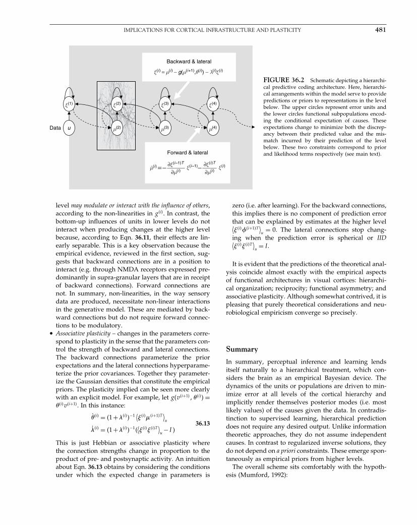
Elsevier UK Chapter: Ch36-P372560 30-9-2006 5:30p.m. Page:481 Trim:7.5in×9.25in
Basal Font:Palatino Margins:Top:40pt Gutter:68pt Font Size:9.5/12 Text Width:42pc Depth:55 Lines
IMPLICATIONS FOR CORTICAL INFRASTRUCTURE AND PLASTICITY 481
Data
ξ (1) ξ
(2)
μ(2)u
Backward & lateral
ξ (i ) = μ(i ) − g(μ(i +1),θ(i )) − λ(i )ξ
(i )
Forward & lateral
−∂μ(i )
∂ξ (i –1)T
−=∂μ(i )
∂ξ (i )T
ξ (i )ξ
(i –1)μ(i )
μ(3)
ξ (3) ξ
(4)
μ(4)
.
FIGURE 36.2 Schematic depicting a hierarchi-cal predictive coding architecture. Here, hierarchi-cal arrangements within the model serve to providepredictions or priors to representations in the levelbelow. The upper circles represent error units andthe lower circles functional subpopulations encod-ing the conditional expectation of causes. Theseexpectations change to minimize both the discrep-ancy between their predicted value and the mis-match incurred by their prediction of the levelbelow. These two constraints correspond to priorand likelihood terms respectively (see main text).
level may modulate or interact with the influence of others,according to the non-linearities in g�i�. In contrast, thebottom-up influences of units in lower levels do notinteract when producing changes at the higher levelbecause, according to Eqn. 36.11, their effects are lin-early separable. This is a key observation because theempirical evidence, reviewed in the first section, sug-gests that backward connections are in a position tointeract (e.g. through NMDA receptors expressed pre-dominantly in supra-granular layers that are in receiptof backward connections). Forward connections arenot. In summary, non-linearities, in the way sensorydata are produced, necessitate non-linear interactionsin the generative model. These are mediated by back-ward connections but do not require forward connec-tions to be modulatory.
• Associative plasticity – changes in the parameters corre-spond to plasticity in the sense that the parameters con-trol the strength of backward and lateral connections.The backward connections parameterize the priorexpectations and the lateral connections hyperparame-terize the prior covariances. Together they parameter-ize the Gaussian densities that constitute the empiricalpriors. The plasticity implied can be seen more clearlywith an explicit model. For example, let g�v�i+1�� ��i�� =��i�v�i+1�. In this instance:
�̇�i� = �1+��i��−1 ⟨��i���i+1�T⟩u
�̇�i� = �1+��i��−1�⟨��i���i�T
⟩u− I �
36.13
This is just Hebbian or associative plasticity wherethe connection strengths change in proportion to theproduct of pre- and postsynaptic activity. An intuitionabout Eqn. 36.13 obtains by considering the conditionsunder which the expected change in parameters is
zero (i.e. after learning). For the backward connections,this implies there is no component of prediction errorthat can be explained by estimates at the higher level⟨��i���i+1�T
⟩u
= 0. The lateral connections stop chang-ing when the prediction error is spherical or IID⟨��i���i�T
⟩u= I .
It is evident that the predictions of the theoretical anal-ysis coincide almost exactly with the empirical aspectsof functional architectures in visual cortices: hierarchi-cal organization; reciprocity; functional asymmetry; andassociative plasticity. Although somewhat contrived, it ispleasing that purely theoretical considerations and neu-robiological empiricism converge so precisely.
Summary
In summary, perceptual inference and learning lendsitself naturally to a hierarchical treatment, which con-siders the brain as an empirical Bayesian device. Thedynamics of the units or populations are driven to min-imize error at all levels of the cortical hierarchy andimplicitly render themselves posterior modes (i.e. mostlikely values) of the causes given the data. In contradis-tinction to supervised learning, hierarchical predictiondoes not require any desired output. Unlike informationtheoretic approaches, they do not assume independentcauses. In contrast to regularized inverse solutions, theydo not depend on a priori constraints. These emerge spon-taneously as empirical priors from higher levels.
The overall scheme sits comfortably with the hypoth-esis (Mumford, 1992):

Elsevier UK Chapter: Ch36-P372560 30-9-2006 5:30p.m. Page:482 Trim:7.5in×9.25in
Basal Font:Palatino Margins:Top:40pt Gutter:68pt Font Size:9.5/12 Text Width:42pc Depth:55 Lines
482 36. FUNCTIONAL INTEGRATION
on the role of the reciprocal, topographic pathwaysbetween two cortical areas, one often a ‘higher’ areadealing with more abstract information about theworld, the other ‘lower’, dealing with more concretedata. The higher area attempts to fit its abstractionsto the data it receives from lower areas by sendingback to them from its deep pyramidal cells a templatereconstruction best fitting the lower level view. Thelower area attempts to reconcile the reconstruction ofits view that it receives from higher areas with whatit knows, sending back from its superficial pyrami-dal cells the features in its data which are not pre-dicted by the higher area. The whole calculation isdone with all areas working simultaneously, but withorder imposed by synchronous activity in the varioustop-down, bottom-up loops.
We have tried to show that this sort of hierarchicalprediction can be implemented in brain-like architec-tures using mechanisms that are biologically plausible(Figure 36.3).
Backward or feedback connections?
There is something slightly counterintuitive about empir-ical Bayes in the brain. In this view, cortical hierar-chies are trying to generate sensory data from high-levelcauses. This means the causal structure of the world isembodied in the backward connections. Forward connec-tions simply provide feedback by conveying predictionerror to higher levels. In short, forward connections arethe feedback connections. This is why we have been carefulnot to ascribe a functional label like feedback to backwardconnections. Perceptual inference emerges from recurrenttop-down and bottom-up processes that enable sensa-tion to constrain perception. This self-organizing processis distributed throughout the hierarchy. Similar perspec-tives have emerged in cognitive neuroscience on the basisof psychophysical findings. For example, Reverse Hierar-chy Theory distinguishes between early explicit perceptionand implicit low level vision, where: ‘our initial consciouspercept – vision at a glance – matches a high-level,generalized, categorical scene interpretation, identifying
Forward recognition effects
Backward generation effects
Spiny stellate and small basket neurons in layer 4
Superficialpyramidal
cells
Double bouquet cells
Deep pyramidal cells
L4
SG
IG
ξ(i ) = μ (i ) −g(μ
(i +1), θ(i ))−λ(i )ξ(i )
ξ (i –1)
ξ (i –1) ξ
(i)
μ(i –1)
μ(i –1)
μ(i +1)μ(i)
ξ (i )
μ (i )
FIGURE 36.3 A more detailed picture of the influences among units. Here, we have associated various cells with different roles in thescheme described in the main text. The key constraint on this sort of association is that superficial pyramidal cells are the source of forwardconnections, which, according to the theory, should encode prediction error.
Elsevier UK Chapter: Ch36-P372560 30-9-2006 5:30p.m. Page:483 Trim:7.5in×9.25in
Basal Font:Palatino Margins:Top:40pt Gutter:68pt Font Size:9.5/12 Text Width:42pc Depth:55 Lines
ASSESSING FUNCTIONAL ARCHITECTURES WITH BRAIN IMAGING 483
‘ “forest before trees” ’ (Hochstein and Ahissar, 2002). Onthe other hand, backward connections are responsible forpredicting; lower level responses embed the generative orforward model. The effect of these predictions on lower-level responses is the focus of the next section.
ASSESSING FUNCTIONALARCHITECTURES WITH BRAIN
IMAGING
In the previous section, we have seen one approach tounderstanding the nature of functional integration in thebrain. We will use this framework to preview the differ-ent ways in which integration can be measured empir-ically, with a special focus on the interaction betweenforward and backward connections. The examples usedwill appear again in later chapters that take us fromsimple measure of statistical correlations among differentbrain areas though to dynamic causal models of corticalhierarchies.
Clearly, it would be nice to demonstrate the existenceof top-down influences with neuroimaging. This is aslightly deeper problem than might be envisaged. This isbecause making causal inferences about effective connec-tivity is not straightforward (see Pearl, 2000). It is not suf-ficient to show regional activity is partially predicted byactivity in a higher level to confirm the existence of back-ward connections because statistical dependency does, initself, not permit causal inference. Statistical dependen-cies could easily arise in a purely forward architecturebecause the higher-level activity is caused by activityin the lower level. Although there are causal modellingtechniques (i.e. dynamic causal modelling (DCM)) thatcan address this problem, we will start with a simplerapproach and note that interactions between bottom-upand top-down influences cannot be explained by purelyfeed-forward architectures. An interaction, in this con-text, can be construed as an effect of backward connec-tions on the driving efficacy of forward connections. Inother words, the response evoked by the same drivingbottom-up influence depends upon the context estab-lished by top-down influence. This interaction is usedbelow simply as evidence for the existence of backwardinfluences. There are instances of predictive coding thatemphasize this phenomenon. For example, the ‘Kalmanfilter model demonstrates how certain forms of attentioncan be viewed as an emergent property of the interactionbetween top-down expectations and bottom-up signals’(Rao, 1999).
This section focuses on the evidence for these interac-tions. From the point of view of functionally specialized
responses, these interactions manifest as context-sensitiveor contextual specialization, where modality-, category-or exemplar-specific responses, driven by bottom-upinput are modulated by top-down influences induced byperceptual set. The first half of this section adopts thisperceptive. The second part of this section uses measure-ments of effective connectivity to establish interactionsbetween bottom-up and top-down influences. All theexamples presented below rely on attempts to establishinteractions by trying to change sensory-evoked neuronalresponses through putative manipulations of top-downinfluences. These include inducing independent changesin perceptual set, cognitive [attentional] set, perceptuallearning and, in the last section, through the study ofpatients with brain lesions
Context-sensitive specialization
If functional specialization is context-dependent then oneshould be able to find evidence for functionally spe-cific responses, using neuroimaging, that are expressedin one context and not in another. The first empiricalexample provides such evidence. If the contextual natureof specialization is mediated by backwards connectionsthen it should be possible to find cortical regions in whichfunctionally specific responses, elicited by the same stim-uli, are modulated by activity in higher areas. The secondexample shows that this is, indeed, possible. Both of theseexamples depend on factorial experimental designs.
Multifactorial designs
Factorial designs combine two or more factors within atask or tasks. Factorial designs can be construed as per-forming subtraction experiments in two or more differentcontexts. The differences in activations, attributable to theeffects of context, are simply the interaction. Consideran implicit object recognition experiment, for examplenaming (of the object’s name or the non-object’s colour)and simply saying ‘yes’ during passive viewing of objectsand non-objects. The factors in this example are implicitobject recognition with two levels (objects versus non-objects) and phonological retrieval (naming versus say-ing ‘yes’). The idea here is to look at the interactionbetween these factors, or the effect that one factor hason the responses elicited by changes in the other. Inour experiment, object-specific responses are elicited (byasking subjects to view objects relative to meaninglessshapes), with and without phonological retrieval. This‘two-by-two’ design allows one to look at the interactionbetween phonological retrieval and object recognition.This analysis identifies not regionally specific activationsbut regionally specific interactions. When we performedthis experiment, these interactions were evident in the left

Elsevier UK Chapter: Ch36-P372560 30-9-2006 5:30p.m. Page:484 Trim:7.5in×9.25in
Basal Font:Palatino Margins:Top:40pt Gutter:68pt Font Size:9.5/12 Text Width:42pc Depth:55 Lines
484 36. FUNCTIONAL INTEGRATION
posterior, inferior temporal region and can be associatedwith the integration of phonology and object recogni-tion (see Figure 36.4 and Friston et al., 1996 for details).Alternatively, this region can be thought of as express-ing recognition-dependent responses that are realized in,and only in, the context of having to name the object.These results can be construed as evidence of contextualspecialization for object-recognition that depends uponmodulatory afferents (possibly from temporal and pari-etal regions) that are implicated in naming a visuallyperceived object. There is no empirical evidence in theseresults to suggest that the temporal or parietal regionsare the source of this top-down influence but, in the nextexample, the source of modulation is addressed explicitlyusing psychophysiological interactions.
Psychophysiological interactions
Psychophysiological interactions speak directly to theinteractions between bottom-up and top-down influ-ences, where one is modelled as an experimental factorand the other constitutes a measured brain response. Inan analysis of psychophysiological interactions, one istrying to explain a regionally specific response in termsof an interaction between the presence of a sensorimotoror cognitive process and activity in another part of thebrain (Friston et al., 1997). The supposition here is thatthe remote region is the source of backward modulatoryafferents that confer functional specificity on the targetregion. For example, by combining information aboutactivity in the posterior parietal cortex, mediating atten-tional or perceptual set pertaining to a particular stimulusattribute, can we identify regions that respond to thatstimulus when, and only when, activity in the parietalsource is high? If such an interaction exists, then one
might infer that the parietal area is modulating responsesto the stimulus attribute for which the area is selective.This has clear ramifications in terms of the top-downmodulation of specialized cortical areas by higher brainregions.
The statistical model employed in testing for psy-chophysiological interactions is a simple regressionmodel of effective connectivity that embodies non-linear(second-order or modulatory effects). As such, this classof model speaks directly to functional specialization ofa non-linear and contextual sort. Figure 36.5 illustrates aspecific example (see Dolan et al., 1997 for details). Sub-jects were asked to view degraded face and non-face con-trol stimuli. The interaction between activity in the pari-etal region and the presence of faces was expressed mostsignificantly in the right infero-temporal region not farfrom the homologous left infero-temporal region impli-cated in the object naming experiment above. Changesin parietal activity were induced experimentally by pre-exposure to un-degraded stimuli before some scans butnot others. The data in the right panel of Figure 36.5 sug-gest that the infero-temporal region shows face-specificresponses, relative to non-face objects, when, and onlywhen, parietal activity is high. These results can be inter-preted as a priming-dependent face-specific response, ininfero-temporal regions that are mediated by interactionswith medial parietal cortex. This is a clear example of con-textual specialization that depends on top-down effects.
Effective connectivity
The previous examples, demonstrating contextual spe-cialization, are consistent with functional architectures
Object-specific activations
No naming
Adj
uste
d rC
BF
Naming
FIGURE 36.4 This example of regionally specific interactions comes from an experiment where subjects were asked to view colourednon-object shapes or coloured objects and say ‘yes’, or to name either the coloured object or the colour of the shape. Left: a regionally specificinteraction in the left infero-temporal cortex. The SPM (statistical parametric map) threshold is p < 0�05 (uncorrected). Right: the correspondingactivities in the maxima of this region are portrayed in terms of object recognition-dependent responses with and without naming. It is seenthat this region shows object recognition responses when, and only when, there is phonological retrieval. The ‘extra’ activation with namingcorresponds to the interaction. These data were acquired from six subjects scanned 12 times using PET.
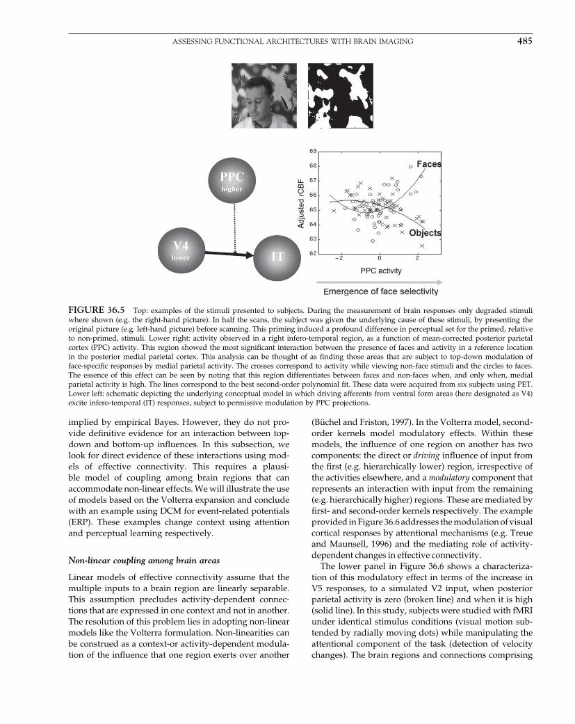
Elsevier UK Chapter: Ch36-P372560 30-9-2006 5:30p.m. Page:485 Trim:7.5in×9.25in
Basal Font:Palatino Margins:Top:40pt Gutter:68pt Font Size:9.5/12 Text Width:42pc Depth:55 Lines
ASSESSING FUNCTIONAL ARCHITECTURES WITH BRAIN IMAGING 485
EA
FIGURE 36.5 Top: examples of the stimuli presented to subjects. During the measurement of brain responses only degraded stimuliwhere shown (e.g. the right-hand picture). In half the scans, the subject was given the underlying cause of these stimuli, by presenting theoriginal picture (e.g. left-hand picture) before scanning. This priming induced a profound difference in perceptual set for the primed, relativeto non-primed, stimuli. Lower right: activity observed in a right infero-temporal region, as a function of mean-corrected posterior parietalcortex (PPC) activity. This region showed the most significant interaction between the presence of faces and activity in a reference locationin the posterior medial parietal cortex. This analysis can be thought of as finding those areas that are subject to top-down modulation offace-specific responses by medial parietal activity. The crosses correspond to activity while viewing non-face stimuli and the circles to faces.The essence of this effect can be seen by noting that this region differentiates between faces and non-faces when, and only when, medialparietal activity is high. The lines correspond to the best second-order polynomial fit. These data were acquired from six subjects using PET.Lower left: schematic depicting the underlying conceptual model in which driving afferents from ventral form areas (here designated as V4)excite infero-temporal (IT) responses, subject to permissive modulation by PPC projections.
implied by empirical Bayes. However, they do not pro-vide definitive evidence for an interaction between top-down and bottom-up influences. In this subsection, welook for direct evidence of these interactions using mod-els of effective connectivity. This requires a plausi-ble model of coupling among brain regions that canaccommodate non-linear effects. We will illustrate the useof models based on the Volterra expansion and concludewith an example using DCM for event-related potentials(ERP). These examples change context using attentionand perceptual learning respectively.
Non-linear coupling among brain areas
Linear models of effective connectivity assume that themultiple inputs to a brain region are linearly separable.This assumption precludes activity-dependent connec-tions that are expressed in one context and not in another.The resolution of this problem lies in adopting non-linearmodels like the Volterra formulation. Non-linearities canbe construed as a context-or activity-dependent modula-tion of the influence that one region exerts over another
(Büchel and Friston, 1997). In the Volterra model, second-order kernels model modulatory effects. Within thesemodels, the influence of one region on another has twocomponents: the direct or driving influence of input fromthe first (e.g. hierarchically lower) region, irrespective ofthe activities elsewhere, and a modulatory component thatrepresents an interaction with input from the remaining(e.g. hierarchically higher) regions. These are mediated byfirst- and second-order kernels respectively. The exampleprovided in Figure 36.6 addresses the modulation of visualcortical responses by attentional mechanisms (e.g. Treueand Maunsell, 1996) and the mediating role of activity-dependent changes in effective connectivity.
The lower panel in Figure 36.6 shows a characteriza-tion of this modulatory effect in terms of the increase inV5 responses, to a simulated V2 input, when posteriorparietal activity is zero (broken line) and when it is high(solid line). In this study, subjects were studied with fMRIunder identical stimulus conditions (visual motion sub-tended by radially moving dots) while manipulating theattentional component of the task (detection of velocitychanges). The brain regions and connections comprising
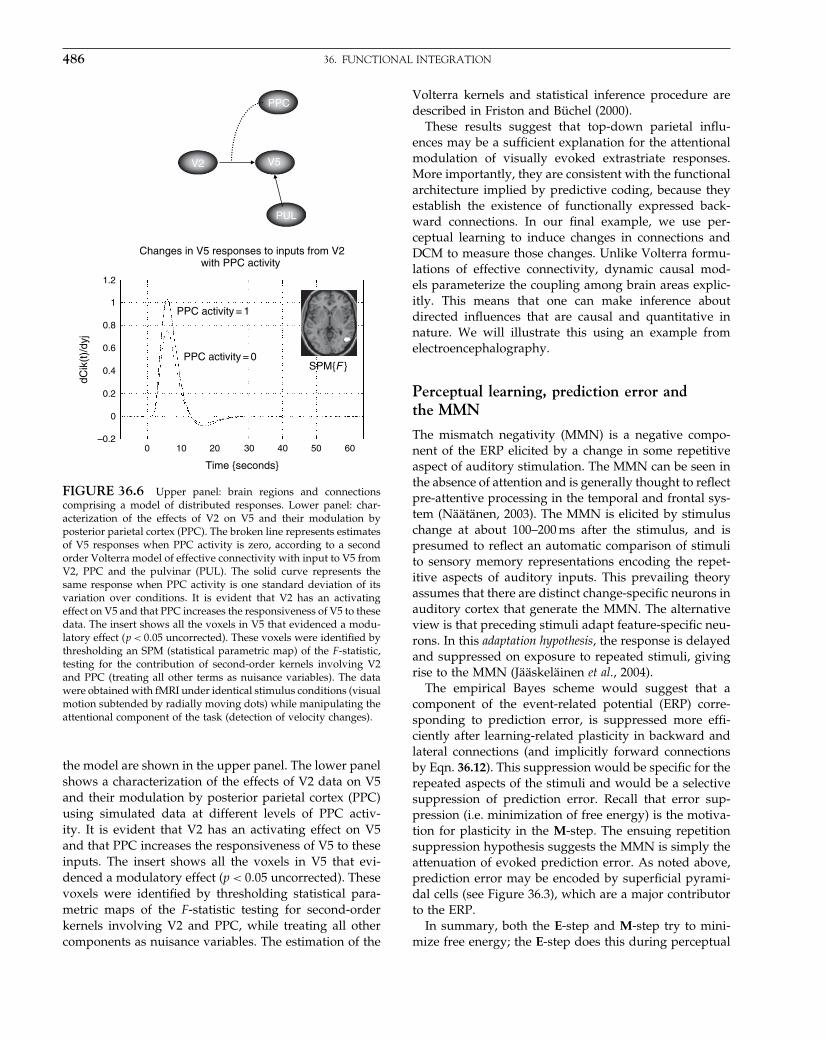
Elsevier UK Chapter: Ch36-P372560 30-9-2006 5:30p.m. Page:486 Trim:7.5in×9.25in
Basal Font:Palatino Margins:Top:40pt Gutter:68pt Font Size:9.5/12 Text Width:42pc Depth:55 Lines
486 36. FUNCTIONAL INTEGRATION
PPC
V5
PUL
V2
Changes in V5 responses to inputs from V2with PPC activity
SPM{F }
PPC activity = 1
PPC activity = 0
0 10 20 30 40 50 60
Time {seconds}
dCik
(t)/
dyj
1.2
1
0.8
0.6
0.4
0.2
0
–0.2
FIGURE 36.6 Upper panel: brain regions and connectionscomprising a model of distributed responses. Lower panel: char-acterization of the effects of V2 on V5 and their modulation byposterior parietal cortex (PPC). The broken line represents estimatesof V5 responses when PPC activity is zero, according to a secondorder Volterra model of effective connectivity with input to V5 fromV2, PPC and the pulvinar (PUL). The solid curve represents thesame response when PPC activity is one standard deviation of itsvariation over conditions. It is evident that V2 has an activatingeffect on V5 and that PPC increases the responsiveness of V5 to thesedata. The insert shows all the voxels in V5 that evidenced a modu-latory effect (p < 0�05 uncorrected). These voxels were identified bythresholding an SPM (statistical parametric map) of the F -statistic,testing for the contribution of second-order kernels involving V2and PPC (treating all other terms as nuisance variables). The datawere obtained with fMRI under identical stimulus conditions (visualmotion subtended by radially moving dots) while manipulating theattentional component of the task (detection of velocity changes).
the model are shown in the upper panel. The lower panelshows a characterization of the effects of V2 data on V5and their modulation by posterior parietal cortex (PPC)using simulated data at different levels of PPC activ-ity. It is evident that V2 has an activating effect on V5and that PPC increases the responsiveness of V5 to theseinputs. The insert shows all the voxels in V5 that evi-denced a modulatory effect (p < 0�05 uncorrected). Thesevoxels were identified by thresholding statistical para-metric maps of the F-statistic testing for second-orderkernels involving V2 and PPC, while treating all othercomponents as nuisance variables. The estimation of the
Volterra kernels and statistical inference procedure aredescribed in Friston and Büchel (2000).
These results suggest that top-down parietal influ-ences may be a sufficient explanation for the attentionalmodulation of visually evoked extrastriate responses.More importantly, they are consistent with the functionalarchitecture implied by predictive coding, because theyestablish the existence of functionally expressed back-ward connections. In our final example, we use per-ceptual learning to induce changes in connections andDCM to measure those changes. Unlike Volterra formu-lations of effective connectivity, dynamic causal mod-els parameterize the coupling among brain areas explic-itly. This means that one can make inference aboutdirected influences that are causal and quantitative innature. We will illustrate this using an example fromelectroencephalography.
Perceptual learning, prediction error andthe MMN
The mismatch negativity (MMN) is a negative compo-nent of the ERP elicited by a change in some repetitiveaspect of auditory stimulation. The MMN can be seen inthe absence of attention and is generally thought to reflectpre-attentive processing in the temporal and frontal sys-tem (Näätänen, 2003). The MMN is elicited by stimuluschange at about 100–200 ms after the stimulus, and ispresumed to reflect an automatic comparison of stimulito sensory memory representations encoding the repet-itive aspects of auditory inputs. This prevailing theoryassumes that there are distinct change-specific neurons inauditory cortex that generate the MMN. The alternativeview is that preceding stimuli adapt feature-specific neu-rons. In this adaptation hypothesis, the response is delayedand suppressed on exposure to repeated stimuli, givingrise to the MMN (Jääskeläinen et al., 2004).
The empirical Bayes scheme would suggest that acomponent of the event-related potential (ERP) corre-sponding to prediction error, is suppressed more effi-ciently after learning-related plasticity in backward andlateral connections (and implicitly forward connectionsby Eqn. 36.12). This suppression would be specific for therepeated aspects of the stimuli and would be a selectivesuppression of prediction error. Recall that error sup-pression (i.e. minimization of free energy) is the motiva-tion for plasticity in the M-step. The ensuing repetitionsuppression hypothesis suggests the MMN is simply theattenuation of evoked prediction error. As noted above,prediction error may be encoded by superficial pyrami-dal cells (see Figure 36.3), which are a major contributorto the ERP.
In summary, both the E-step and M-step try to mini-mize free energy; the E-step does this during perceptual
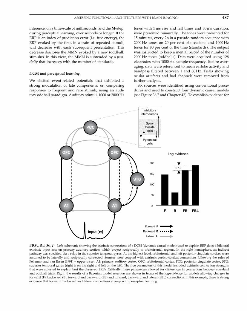
Elsevier UK Chapter: Ch36-P372560 30-9-2006 5:30p.m. Page:487 Trim:7.5in×9.25in
Basal Font:Palatino Margins:Top:40pt Gutter:68pt Font Size:9.5/12 Text Width:42pc Depth:55 Lines
ASSESSING FUNCTIONAL ARCHITECTURES WITH BRAIN IMAGING 487
inference, on a time-scale of milliseconds, and the M-step,during perceptual learning, over seconds or longer. If theERP is an index of prediction error (i.e. free energy), theERP evoked by the first, in a train of repeated stimuli,will decrease with each subsequent presentation. Thisdecrease discloses the MMN evoked by a new (oddball)stimulus. In this view, the MMN is subtended by a posi-tivity that increases with the number of standards.
DCM and perceptual learning
We elicited event-related potentials that exhibited astrong modulation of late components, on comparingresponses to frequent and rare stimuli, using an audi-tory oddball paradigm. Auditory stimuli, 1000 or 2000 Hz
tones with 5 ms rise and fall times and 80 ms duration,were presented binaurally. The tones were presented for15 minutes, every 2 s in a pseudo-random sequence with2000 Hz tones on 20 per cent of occasions and 1000 Hztones for 80 per cent of the time (standards). The subjectwas instructed to keep a mental record of the number of2000 Hz tones (oddballs). Data were acquired using 128electrodes with 1000 Hz sample-frequency. Before aver-aging, data were referenced to mean earlobe activity andbandpass filtered between 1 and 30 Hz. Trials showingocular artefacts and bad channels were removed fromfurther analysis.
Six sources were identified using conventional proce-dures and used to construct four dynamic causal models(see Figure 36.7 and Chapter 42). To establish evidence for
A1 A1
OFC OFC
PCC
STG
Input (w)Forward F
Backward B
Lateral L
Spinystellate
cells
Inhibitoryinterneurons
Pyramidalcells
0
50
100
150
200
F
Log evidence
27.9
FBLFBB
FIGURE 36.7 Left: schematic showing the extrinsic connections of a DCM (dynamic causal model) used to explain ERP data; a bilateralextrinsic input acts on primary auditory cortices which project reciprocally to orbitofrontal regions. In the right hemisphere, an indirectpathway was specified via a relay in the superior temporal gyrus. At the highest level, orbitofrontal and left posterior cingulate cortices wereassumed to be laterally and reciprocally connected. Sources were coupled with extrinsic cortico-cortical connections following the rules ofFelleman and van Essen (1991) – upper insert. A1: primary auditory cortex, OFC: orbitofrontal cortex, PCC: posterior cingulate cortex, STG:superior temporal gyrus (right is on the right and left on the left). The free parameters of this model included extrinsic connection strengthsthat were adjusted to explain best the observed ERPs. Critically, these parameters allowed for differences in connections between standardand oddball trials. Right: the results of a Bayesian model selection are shown in terms of the log-evidence for models allowing changes inforward �F�, backward �B�, forward and backward �FB� and forward, backward and lateral �FBL� connections. In this example, there is strongevidence that forward, backward and lateral connections change with perceptual learning.

Elsevier UK Chapter: Ch36-P372560 30-9-2006 5:30p.m. Page:488 Trim:7.5in×9.25in
Basal Font:Palatino Margins:Top:40pt Gutter:68pt Font Size:9.5/12 Text Width:42pc Depth:55 Lines
488 36. FUNCTIONAL INTEGRATION
changes in backward and lateral connections, above andbeyond changes in forward connections, we employedBayesian model selection (see Chapter 35). This entailedspecifying four models that allowed for changes in for-ward, backward, forward and backward and in all con-nections. These, and only these, changes in extrinsicconnectivity could explain the differences in the ERP,elicited by standard relative to oddball stimuli. The mod-els were compared using the negative free energy asan approximation to the log-evidence for each model:if, after inversion, we assume the approximating con-ditional density is the true conditional density, the freeenergy reduces to the log-evidence (see Eqn. 36.4). InBayesian model selection, a difference in log-evidenceof three or more can be considered as strong evidencefor the model with the greater evidence, relative to theone with less. The log evidences for the four modelsare shown in Figure 36.7. The model with the highestevidence (by a margin of 27.9) is the DCM that allowsfor learning-related changes in forward, backward andlateral connections. These results provide clear evidencethat changes in backward and lateral connections areneeded to explain the observed differences in corticalresponses.
In the final section, the implications of hierarchicallyorganized connections are considered from the point ofview of the lesion-deficit model and neuropsychology.
FUNCTIONAL INTEGRATION ANDNEUROPSYCHOLOGY
If functional specialization depends on interactionsamong cortical areas, then one might predict changesin functional specificity in cortical regions that receiveenabling or modulatory afferents from a damaged area.A simple consequence is that aberrant responses willbe elicited in regions hierarchically below the lesion if,and only if, these responses depend upon input fromthe lesion site. However, there may be other contextsin which the region’s responses are perfectly normal(relying on other, intact, afferents). This leads to thenotion of a context-dependent region-specific abnormal-ity, caused by, but remote from, a lesion (i.e. an abnormalresponse that is elicited by some tasks but not others). Wehave referred to this phenomenon as ‘dynamic diaschisis’(Price et al., 2001).
Dynamic diaschisis
Classical diaschisis, demonstrated by early anatomicalstudies and more recently by neuroimaging studies of
resting brain activity, refers to regionally specific reduc-tions in metabolic activity at sites that are remote from,but connected to, damaged regions. The clearest exam-ple is ‘crossed cerebellar diaschisis’ (Lenzi et al., 1982),in which abnormalities of cerebellar metabolism areseen following cerebral lesions involving the motor cor-tex. Dynamic diaschisis describes the task-specific effectsthat a lesion can have on the evoked responses of a dis-tant cortical region. The basic idea is that an other-wise viable cortical region expresses aberrant neuronalresponses when, and only when, those responses dependupon interactions with a damaged region. This can arisebecause normal responses in any given region dependupon reciprocal interactions with other regions. Theregions involved will depend on the cognitive and sen-sorimotor operations engaged at any particular time. Ifthese regions include one that is damaged, then abnor-mal responses may ensue. However, there may be sit-uations when the same region responds normally, forinstance when its dynamics depend only upon integra-tion with undamaged regions. If the region can respondnormally in some situations then forward driving compo-nents must be intact. This suggests that dynamic diaschi-sis will only present itself when the lesion involves ahierarchically equivalent or higher area.
An example from neuropsychology
We investigated this possibility in a functional imagingstudy of four aphasic patients, all with damage to theleft posterior inferior frontal cortex, classically known asBroca’s area (Figure 36.8; upper panels). These patientshad speech output deficits but relatively preserved com-prehension. Generally, functional imaging studies canonly make inferences about abnormal neuronal responseswhen changes in cognitive strategy can be excluded. Weensured this by engaging the patients in an explicit taskthat they were able to perform normally. This involveda key-press response when a visually presented letterstring contained a letter with an ascending visual feature(e.g. h, k, l, or t). While the task remained constant, thestimuli presented were either words or consonant letterstrings. Activations detected for words, relative to letters,were attributed to implicit word processing. Each patientshowed normal activation of the left posterior middletemporal cortex that has been associated with semanticprocessing (Price, 1998). However, none of the patientsactivated the left posterior inferior frontal cortex (dam-aged by the stroke), or the left posterior inferior tempo-ral region (undamaged by the stroke) (see Figure 36.4).These two regions are crucial for word production (Price,1998). Examination of individual responses in this arearevealed that all the normal subjects showed increasedactivity for words relative to consonant letter strings,
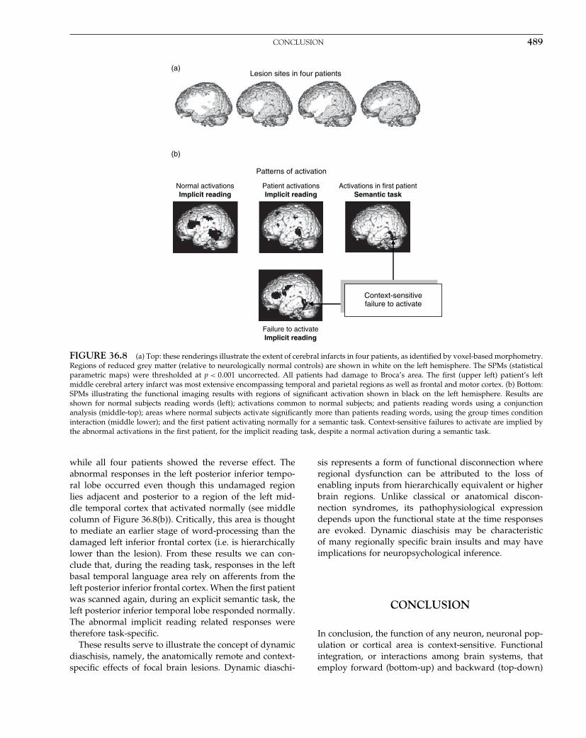
Elsevier UK Chapter: Ch36-P372560 30-9-2006 5:30p.m. Page:489 Trim:7.5in×9.25in
Basal Font:Palatino Margins:Top:40pt Gutter:68pt Font Size:9.5/12 Text Width:42pc Depth:55 Lines
CONCLUSION 489
(a)Lesion sites in four patients
(b)
Normal activationsImplicit reading
Failure to activateImplicit reading
Context - sensitivefailure to activate
Context-sensitivefailure to activate
Patterns of activation
Patient activationsImplicit reading
Activations in first patientSemantic task
FIGURE 36.8 (a) Top: these renderings illustrate the extent of cerebral infarcts in four patients, as identified by voxel-based morphometry.Regions of reduced grey matter (relative to neurologically normal controls) are shown in white on the left hemisphere. The SPMs (statisticalparametric maps) were thresholded at p < 0�001 uncorrected. All patients had damage to Broca’s area. The first (upper left) patient’s leftmiddle cerebral artery infarct was most extensive encompassing temporal and parietal regions as well as frontal and motor cortex. (b) Bottom:SPMs illustrating the functional imaging results with regions of significant activation shown in black on the left hemisphere. Results areshown for normal subjects reading words (left); activations common to normal subjects; and patients reading words using a conjunctionanalysis (middle-top); areas where normal subjects activate significantly more than patients reading words, using the group times conditioninteraction (middle lower); and the first patient activating normally for a semantic task. Context-sensitive failures to activate are implied bythe abnormal activations in the first patient, for the implicit reading task, despite a normal activation during a semantic task.
while all four patients showed the reverse effect. Theabnormal responses in the left posterior inferior tempo-ral lobe occurred even though this undamaged regionlies adjacent and posterior to a region of the left mid-dle temporal cortex that activated normally (see middlecolumn of Figure 36.8(b)). Critically, this area is thoughtto mediate an earlier stage of word-processing than thedamaged left inferior frontal cortex (i.e. is hierarchicallylower than the lesion). From these results we can con-clude that, during the reading task, responses in the leftbasal temporal language area rely on afferents from theleft posterior inferior frontal cortex. When the first patientwas scanned again, during an explicit semantic task, theleft posterior inferior temporal lobe responded normally.The abnormal implicit reading related responses weretherefore task-specific.
These results serve to illustrate the concept of dynamicdiaschisis, namely, the anatomically remote and context-specific effects of focal brain lesions. Dynamic diaschi-
sis represents a form of functional disconnection whereregional dysfunction can be attributed to the loss ofenabling inputs from hierarchically equivalent or higherbrain regions. Unlike classical or anatomical discon-nection syndromes, its pathophysiological expressiondepends upon the functional state at the time responsesare evoked. Dynamic diaschisis may be characteristicof many regionally specific brain insults and may haveimplications for neuropsychological inference.
CONCLUSION
In conclusion, the function of any neuron, neuronal pop-ulation or cortical area is context-sensitive. Functionalintegration, or interactions among brain systems, thatemploy forward (bottom-up) and backward (top-down)

Elsevier UK Chapter: Ch36-P372560 30-9-2006 5:30p.m. Page:490 Trim:7.5in×9.25in
Basal Font:Palatino Margins:Top:40pt Gutter:68pt Font Size:9.5/12 Text Width:42pc Depth:55 Lines
490 36. FUNCTIONAL INTEGRATION
connections, mediate this adaptive specialization. A criti-cal consequence is that hierarchically organized neuronalresponses, in any given cortical area, can represent dif-ferent things at different times. Although most models ofperceptual learning and inference require priors on thecauses of sensation, empirical Bayes suggests that theseassumptions can be relaxed and that priors can be learnedin a hierarchical context. We have tried to show that thishierarchical prediction can be implemented in brain-likearchitectures and in a biologically plausible fashion. Thearguments in this chapter were developed under empir-ical or hierarchal Bayes models of brain function, wherehigher levels provide a prediction of the inputs to lowerlevels. Conflict between the two is resolved by changesin the higher-level representations, which are driven bythe ensuing error in lower regions, until the mismatch isexplained away. From this perspective, the specializationof any region is determined both by bottom-up inputsand by top-down predictions. Specialization is thereforenot an intrinsic property of any region, but depends onboth forward and backward connections with other areas.Because the latter have access to the context in which thedata are generated they are in a position to modulate theselectivity of lower areas.
The theoretical neurobiology in this chapter has beenused to motivate the importance of measuring effectiveconnectivity, especially modulatory or non-linear cou-pling in the brain. These non-linear aspects will be arecurrent theme in subsequent chapters that discuss func-tional and effective connectivity from a conceptual andoperational point of view.
REFERENCES
Absher JR, Benson DF (1993) Disconnection syndromes: an overviewof Geschwind’s contributions. Neurology 43: 862–67
Aertsen A, Preil H (1991) Dynamics of activity and connectivityin physiological neuronal networks. In Non linear dynamics andneuronal networks, Schuster HG (ed.). VCH Publishers Inc., NewYork, pp 281–302
Angelucci A, Levitt JB, Walton EJ et al. (2002a) Circuits for local andglobal signal integration in primary visual cortex. J Neurosci 22:8633–46
Angelucci A, Levitt JB, Lund JS (2002b) Anatomical origins of theclassical receptive field and modulatory surround field of singleneurons in macaque visual cortical area V1. Prog Brain Res 136:373–88
Ballard DH, Hinton GE, Sejnowski TJ (1983) Parallel visual compu-tation. Nature 306: 21–26
Büchel C, Friston KJ (1997) Modulation of connectivity in visualpathways by attention: cortical interactions evaluated with struc-tural equation modelling and fMRI. Cerebr Cortex 7: 768–78
Crick F, Koch C (1998) Constraints on cortical and thalamic projec-tions: the no-strong-loops hypothesis. Nature 391: 245–50
Dayan P, Abbott LF (2001) Theoretical neuroscience. Computational andmathematical modelling of neural systems. MIT Press, [∗∗36.3]
Dayan P, Hinton GE, Neal RM (1995) The Helmholtz machine. Neu-ral Comput 7: 889–904
Dempster AP, Laird NM, Rubin DB (1977) Maximum likelihoodfrom incomplete data via the EM algorithm. J Roy Stat Soc SeriesB 39: 1–38
Dolan RJ, Fink GR, Rolls E et al. (1997) How the brain learns to seeobjects and faces in an impoverished context. Nature 389: 596–98
Efron B, Morris C (1973) Stein’s estimation rule and its competitors –an empirical Bayes approach. J Am Stat Assoc 68: 117–30
Felleman DJ, Van Essen DC (1991) Distributed hierarchical process-ing in the primate cerebral cortex. Cereb Cortex 1: 1–47
Foldiak P (1990) Forming sparse representations by local anti-Hebbian learning. Biol Cybern. 64: 165–70
Frey U, Morris RGM (1997) Synaptic tagging and long-term poten-tiation. Nature 385: 533–36
Friston KJ, Price CJ, Fletcher P et al. (1996) The trouble with cognitivesubtraction. NeuroImage 4: 97–104
Friston KJ, Büchel C, Fink et al. (1997) Psychophysiological andmodulatory interactions in neuroimaging. NeuroImage 6: 218–29
Friston KJ, Büchel C (2000) Attentional modulation of V5 in human.Proc Natl Acad Sci USA 97: 7591–96
Friston KJ (2005) A theory of cortical responses. Philos Trans R SocLond B Biol Sci 360: 815–36
Gerstein GL, Perkel DH (1969) Simultaneously recorded trains ofaction potentials: analysis and functional interpretation. Science164: 828–30
Girard P, Bullier J (1989) Visual activity in area V2 during reversibleinactivation of area 17 in the macaque monkey. J Neurophysiol62: 1287–301
Helmholtz H (1860/1962) Handbuch der physiologischen optik (Englishtranslation, Southall JPC, ed.), Vol. 3. Dover, New York
Hinton GE, Dayan P, Frey BJ et al. (1995) The ‘Wake-Sleep’ algorithmfor unsupervised neural networks. Science 268: 1158–61
Hochstein S, Ahissar M (2002) View from the top: hierarchies andreverse hierarchies in the visual system. Neuron 36: 791–804
Jääskeläinen IP, Ahveninen J, Bonmassar G et al. (2004) Humanposterior auditory cortex gates novel sounds to consciousness.Proc Natl Acad Sci 101: 6809–14
Kass RE, Steffey D (1989) Approximate Bayesian inference in condi-tionally independent hierarchical models (parametric empiricalBayes models). J Am Stat Assoc 407: 717–26
Kawato M, Hayakawa H, Inui T (1993) A forward-inverse opticsmodel of reciprocal connections between visual cortical areas.Network 4: 415–22
Kersten D, Mamassian P, Yuille A (2004) Object perception asBayesian inference. Annu Rev Psychol 55: 271–304
Lenzi GL, Frackowiak RSJ, Jones T (1982) Cerebral oxygenmetabolism blood flow in human cerebral ischaemic infarction.J Cereb Blood Flow Metab 2: 321–35
Locke J (1690/1976) An essay concerning human understanding. Dent,London
MacKay DM (1956) The epistemological problem for automata. InAutomata studies, Shannon CE, McCarthy J (eds). Princeton Uni-versity Press, Princeton, pp 235–51
McIntosh AR (2000) Towards a network theory of cognition. NeuralNetworks 13: 861–70
Mesulam MM (1998) From sensation to cognition. Brain 121: 1013–52Mumford D (1992) On the computational architecture of the neocor-
tex. II. The role of cortico-cortical loops. Biol Cybernet 66: 241–51Murphy PC, Sillito AM (1987) Corticofugal feedback influences the
generation of length tuning in the visual pathway. Nature 329:727–29
Elsevier UK Chapter: Ch36-P372560 30-9-2006 5:30p.m. Page:491 Trim:7.5in×9.25in
Basal Font:Palatino Margins:Top:40pt Gutter:68pt Font Size:9.5/12 Text Width:42pc Depth:55 Lines
REFERENCES 491
Näätänen R (2003) Mismatch negativity: clinical research andpossible applications. Int J Psychophysiol 48: 179–88
Neisser U (1967) Cognitive psychology. Appleton-Century-Crofts,New York
Pearl J (2000) Causality, models, reasoning and inference. CambridgeUniversity Press, Cambridge
Phillips CG, Zeki S, Barlow HB (1984) Localisation of functionin the cerebral cortex: past present and future. Brain 107:327–61
Poggio T, Torre V, Koch C (1985) Computational vision and regu-larisation theory. Nature 317: 314–19
Pollen DA (1999) On the neural correlates of visual perception. CerebCortex 9: 4–19
Price CJ (1998) The functional anatomy of word comprehension andproduction. T rends Cogn Sci 2: 281–88
Price CJ, Warburton EA, Moore CJ et al. (2001) Dynamic diaschisis:anatomically remote and context-sensitive human brain lesions.J Cogn Neurosci 13: 419–29
Rao RP (1999) An optimal estimation approach to visual perceptionand learning. Vision Res 39: 1963–89
Rao RP, Ballard DH (1998) Predictive coding in the visual cortex:a functional interpretation of some extra-classical receptive fieldeffects. Nature Neurosci 2: 79–87
Rivadulla C, Martinez LM, Varela C et al. (2002) Completing thecorticofugal loop: a visual role for the corticogeniculate type1 metabotropic glutamate receptor. J Neurosci 22: 2956–62
Rockland KS, Pandya DN (1979) Laminar origins and terminationsof cortical connections of the occipital lobe in the rhesus monkey.Brain Res 179: 3–20
Salin P-A, Bullier J (1995) Corticocortical connections in the visualsystem: structure and function. Psychol Bull 75: 107–54
Sandell JH, Schiller PH (1982) Effect of cooling area 18 on striatecortex cells in the squirrel monkey.J Neurophysiol 48: 38–48
Sherman SM, Guillery RW (1998) On the actions that one nerve cellcan have on another: distinguishing ‘drivers’ from ‘modulators’.Proc Natl Acad Sci USA 95: 7121–26
Simoncelli EP, Olshausen BA (2001) Natural image statistics andneural representation. Annu Rev Neurosci 24: 1193–216
Treue S, Maunsell HR (1996) Attentional modulation of visualmotion processing in cortical areas MT and MST. Nature382: 539–41
Zeki S (1990) The motion pathways of the visual cortex. In Vision:coding and efficiency, Blakemore C (ed.). Cambridge UniversityPress, Cambridge, pp 321–45
Zeki S, Shipp S (1988) The functional logic of cortical connections.Nature 335: 311–17

Elsevier UK Chapter: Ch37-P372560 30-9-2006 5:31p.m. Page:492 Trim:7.5in×9.25in
Basal Font:Palatino Margins:Top:40pt Gutter:68pt Font Size:9.5/12 Text Width:42pc Depth:55 Lines
C H A P T E R
37
Functional connectivity: eigenimages andmultivariate analyses
K. Friston and C. Büchel
INTRODUCTION
This chapter deals with imaging data from a multivari-ate perspective. This means that the observations at eachvoxel are considered jointly with explicit reference tothe interactions among brain regions. The concept offunctional connectivity is reviewed and is used as thebasis for interpreting eigenimages. Having consideredthe nature of eigenimages and variations on their appli-cations, we then turn to a related approach that, unlikeeigenimage analysis, is predicated on a statistical model.This approach is called multivariate analysis of vari-ance (MANCOVA) and uses canonical variate analysis tocreate canonical images. The integrated and distributednature of neurophysiological responses to sensorimotoror cognitive challenge makes a multivariate perspectiveparticularly appropriate, indeed necessary, for functionalintegration.
Functional integration and connectivity
A landmark meeting that took place on the morning of4 August 1881 highlighted the difficulties of attributingfunction to a cortical area, given the dependence of cere-bral activity on underlying connections (Phillips et al.,1984). Goltz, although accepting the results of electricalstimulation in dog and monkey cortex, considered theexcitation method inconclusive, in that the movementselicited might have originated in related pathways, orcurrent could have spread to distant centres. Despiteadvances over the past century, the question remains:are the physiological changes elicited by sensorimotoror cognitive challenges explained by functional segrega-tion, or by integrated and distributed changes mediatedby neuronal connections? The question itself calls for a
framework within which to address these issues. Func-tional and effective connectivity are concepts that are criticalto this framework.
Origins and definitions
In the analysis of neuroimaging time-series, functionalconnectivity is defined as the statistical dependencies amongspatially remote neurophysiologic events. This definitionprovides a simple characterization of functional inter-actions. The alternative is effective connectivity (i.e.the influence one neuronal system exerts over another).These concepts originated in the analysis of separablespike trains obtained from multiunit electrode record-ings (Gerstein and Perkel, 1969). Functional connectiv-ity is simply a statement about the observed depen-dencies or correlations; it does not comment on howthese correlations are mediated. For example, at thelevel of multiunit microelectrode recordings, correlationscan result from stimulus-locked transients, evoked by acommon afferent input, or reflect stimulus-induced oscil-lations, phasic coupling of neuronal assemblies, medi-ated by synaptic connections. Effective connectivity iscloser to the notion of a connection and can be definedas the influence one neural system exerts over another,either at a synaptic (cf. synaptic efficacy) or corticallevel. Although functional and effective connectivity canbe invoked at a conceptual level in both neuroimag-ing and electrophysiology, they differ fundamentally ata practical level. This is because the time-scales andnature of neurophysiological measurements are verydifferent (seconds versus milliseconds and haemody-namic versus spike trains). In electrophysiology, it isoften necessary to remove the confounding effects ofstimulus-locked transients (that introduce correlationsnot causally mediated by direct neuronal interactions)to reveal an underlying connectivity. The confounding
Statistical Parametric Mapping, by Karl Friston et al. Copyright 2007, Elsevier Ltd. All rights reserved.ISBN–13: 978-0-12-372560-8 ISBN–10: 0-12-372560-7
492

Elsevier UK Chapter: Ch37-P372560 30-9-2006 5:31p.m. Page:493 Trim:7.5in×9.25in
Basal Font:Palatino Margins:Top:40pt Gutter:68pt Font Size:9.5/12 Text Width:42pc Depth:55 Lines
EIGENIMAGES, MULTIDIMENSIONAL SCALING AND OTHER DEVICES 493
effect of stimulus-evoked transients is less problematicin neuroimaging because propagation of dynamics fromprimary sensory areas onwards is mediated by neu-ronal connections (usually reciprocal and interconnect-ing). However, it should be remembered that functionalconnectivity is not necessarily due to effective connectiv-ity (e.g. common neuromodulatory input from ascendingaminergic neurotransmitter systems or thalamo-corticalafferents) and, where it is, effective influences may beindirect (e.g. polysynaptic relays through multiple areas).
EIGENIMAGES, MULTIDIMENSIONALSCALING AND OTHER DEVICES
In what follows, we introduce a number of techniques(eigenimage analysis, multidimensional scaling, partialleast squares and generalized eigenimage analysis) usingfunctional connectivity as a reference. Emphasis is placedon the relationship among these techniques. For example,eigenimage analysis is equivalent to principal componentanalysis and the variant of multidimensional scaling con-sidered here is equivalent to principal coordinates anal-ysis. Principal components and coordinates analyses arepredicated on exactly the same eigenvector solution and,from a mathematical perspective, are the same thing.
Measuring a pattern of correlated activity
Here we introduce a simple way of measuring theamount a pattern of activity (representing a connectedbrain system) contributes to the functional connectiv-ity or variance-covariances observed in imaging data.Functional connectivity is defined in terms of statisticaldependencies among neurophysiological measurement.If we assume these measurements conform to Gaus-sian assumptions, then we need only characterize theircorrelations or covariance (correlations are normalizedcovariances).1 The point-to-point functional connectivitybetween one voxel and another is not usually of greatinterest. The important aspect of a covariance structure isthe pattern of correlated activity subtended by (an enor-mous number of) pair-wise covariances. In measuringsuch patterns, it is useful to introduce the concept of anorm. Vector and matrix norms serve the same purposeas absolute values for scalar quantities. In other words,
1 Clearly neuronal processes are not necessarily Gaussian. How-ever, we can still characterize the second-order dependen-cies with the correlations. Higher-order dependencies wouldinvolve computing cumulants as described in Appendix 2.
they furnish a measure of distance. One frequently usednorm is the 2-norm, which is the length of a vector. Thevector 2-norm can be used to measure the degree towhich a particular pattern of brain activity contributesto a covariance structure. If a pattern is described by acolumn vector p, with an element for each voxel, then thecontribution of that pattern to the covariance structurecan be measured by the 2-norm of Mp = �Mp�. M is a(mean-corrected) matrix of data with one row for eachsuccessive scan and one column for each voxel:
�Mp�2 = pT MT Mp 37.1
T denotes transposition. Put simply, the 2-norm is a num-ber that reflects the amount of variance-covariance orfunctional connectivity that can be accounted for by aparticular distributed pattern. It should be noted that the2-norm only measures the pattern of interest. There maybe many other important patterns of functional connec-tivity. This fact begs the question: ‘what are the mostprevalent patterns of coherent activity?’ To answer thisquestion one turns to eigenimages or spatial modes.
Eigenimages and spatial modes
In this section, the concept of eigenimages or spatialmodes is introduced in terms of patterns of activitydefined above. We show that spatial modes are sim-ply those patterns that account for the most variance-covariance (i.e. have the largest 2-norm).
Eigenimages or spatial modes are most commonlyobtained using singular value decomposition (SVD). SVDis an operation that decomposes an original time-series,M , into two sets of orthogonal vectors (patterns in spaceand patterns in time) V and U where:
�U�S�V� = SVD�M�
M = USV T37.2
U and V are unitary orthogonal matrices UT U = I , V T V =I and V T U = 0 (the sum of squares of each column isunity and all the columns are uncorrelated) and S isa diagonal matrix (only the leading diagonal has non-zero values) of decreasing singular values. The singularvalue of each eigenimage is simply its 2-norm. BecauseSVD maximizes the first singular value, the first eigenim-age is the pattern that accounts for the greatest amountof the variance-covariance structure. In summary, SVDand equivalent devices are powerful ways of decom-posing an imaging time-series into a series of orthogo-nal patterns that embody, in a step-down fashion, thegreatest amounts of functional connectivity. Each eigen-vector (column of V ) defines a distributed brain system
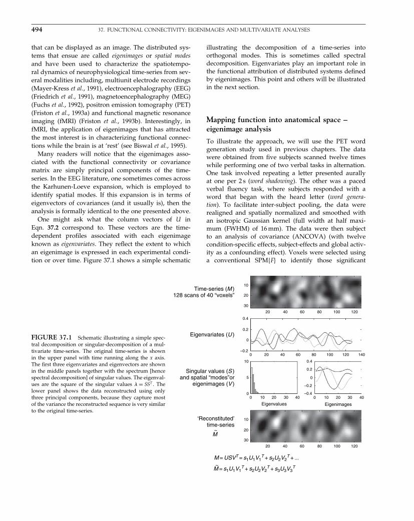
Elsevier UK Chapter: Ch37-P372560 30-9-2006 5:31p.m. Page:494 Trim:7.5in×9.25in
Basal Font:Palatino Margins:Top:40pt Gutter:68pt Font Size:9.5/12 Text Width:42pc Depth:55 Lines
494 37. FUNCTIONAL CONNECTIVITY: EIGENIMAGES AND MULTIVARIATE ANALYSES
that can be displayed as an image. The distributed sys-tems that ensue are called eigenimages or spatial modesand have been used to characterize the spatiotempo-ral dynamics of neurophysiological time-series from sev-eral modalities including, multiunit electrode recordings(Mayer-Kress et al., 1991), electroencephalography (EEG)(Friedrich et al., 1991), magnetoencephalography (MEG)(Fuchs et al., 1992), positron emission tomography (PET)(Friston et al., 1993a) and functional magnetic resonanceimaging (fMRI) (Friston et al., 1993b). Interestingly, infMRI, the application of eigenimages that has attractedthe most interest is in characterizing functional connec-tions while the brain is at ‘rest’ (see Biswal et al., 1995).
Many readers will notice that the eigenimages asso-ciated with the functional connectivity or covariancematrix are simply principal components of the time-series. In the EEG literature, one sometimes comes acrossthe Karhunen-Loeve expansion, which is employed toidentify spatial modes. If this expansion is in terms ofeigenvectors of covariances (and it usually is), then theanalysis is formally identical to the one presented above.
One might ask what the column vectors of U inEqn. 37.2 correspond to. These vectors are the time-dependent profiles associated with each eigenimageknown as eigenvariates. They reflect the extent to whichan eigenimage is expressed in each experimental condi-tion or over time. Figure 37.1 shows a simple schematic
illustrating the decomposition of a time-series intoorthogonal modes. This is sometimes called spectraldecomposition. Eigenvariates play an important role inthe functional attribution of distributed systems definedby eigenimages. This point and others will be illustratedin the next section.
Mapping function into anatomical space –eigenimage analysis
To illustrate the approach, we will use the PET wordgeneration study used in previous chapters. The datawere obtained from five subjects scanned twelve timeswhile performing one of two verbal tasks in alternation.One task involved repeating a letter presented aurallyat one per 2 s (word shadowing). The other was a pacedverbal fluency task, where subjects responded with aword that began with the heard letter (word genera-tion). To facilitate inter-subject pooling, the data wererealigned and spatially normalized and smoothed withan isotropic Gaussian kernel (full width at half maxi-mum (FWHM) of 16 mm). The data were then subjectto an analysis of covariance (ANCOVA) (with twelvecondition-specific effects, subject-effects and global activ-ity as a confounding effect). Voxels were selected usinga conventional SPM�F� to identify those significant
FIGURE 37.1 Schematic illustrating a simple spec-tral decomposition or singular-decomposition of a mul-tivariate time-series. The original time-series is shownin the upper panel with time running along the x axis.The first three eigenvariates and eigenvectors are shownin the middle panels together with the spectrum [hencespectral decomposition] of singular values. The eigenval-ues are the square of the singular values = SST . Thelower panel shows the data reconstructed using onlythree principal components, because they capture mostof the variance the reconstructed sequence is very similarto the original time-series.
M = USVT = s1U1V1
T + s2U2V2
T + ...
M = s1U1V1T
+ s2U2V2T
+ s3U3V3T~
Time-series (M )128 scans of 40 “voxels”
Eigenvariates (U )
Singular values (S )and spatial “modes”or
eigenimages (V )
‘Reconstituted’time-series
M~
20 40 60 80 100 120
20 40 60 80 100 120
200–0.2
0
00 10 20
Eigenvalues Eigenimages
30 40 0 10 20 30 40
5
10
0.2
0.4
–0.2
–0.4
0
0.2
0.4
40 60 80 100 120 140
10
20
30
10
20
30
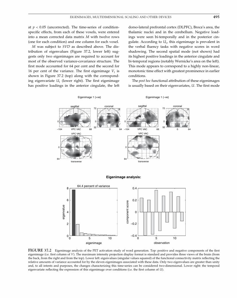
Elsevier UK Chapter: Ch37-P372560 30-9-2006 5:31p.m. Page:495 Trim:7.5in×9.25in
Basal Font:Palatino Margins:Top:40pt Gutter:68pt Font Size:9.5/12 Text Width:42pc Depth:55 Lines
EIGENIMAGES, MULTIDIMENSIONAL SCALING AND OTHER DEVICES 495
at p < 005 (uncorrected). The time-series of condition-specific effects, from each of these voxels, were enteredinto a mean corrected data matrix M with twelve rows(one for each condition) and one column for each voxel.
M was subject to SVD as described above. The dis-tribution of eigenvalues (Figure 37.2, lower left) sug-gests only two eigenimages are required to account formost of the observed variance-covariance structure. Thefirst mode accounted for 64 per cent and the second for16 per cent of the variance. The first eigenimage V1 isshown in Figure 37.2 (top) along with the correspond-ing eigenvariate U1 (lower right). The first eigenimagehas positive loadings in the anterior cingulate, the left
dorso-lateral prefrontal cortex (DLPFC), Broca’s area, thethalamic nuclei and in the cerebellum. Negative load-ings were seen bi-temporally and in the posterior cin-gulate. According to U1, this eigenimage is prevalent inthe verbal fluency tasks with negative scores in wordshadowing. The second spatial mode (not shown) hadits highest positive loadings in the anterior cingulate andbi-temporal regions (notably Wernicke’s area on the left).This mode appears to correspond to a highly non-linear,monotonic time effect with greatest prominence in earlierconditions.
The post hoc functional attribution of these eigenimagesis usually based on their eigenvariates, U . The first mode
Eigenimage analysis:
com
pone
nt s
core
observation
0 5 10
–0.2
–0.4
0.2
0
0.4
eigenimage
eige
nval
ue
64.4 percent of variance
00 5 10
2
4
6
8
Eigenimage 1 {+ve} Eigenimage 1 {–ve}
sagittal
VPC VAC
0
–104 68
VPC VAC
transverse
0
64R
32
0
0 64
R72coronal
transverse
0
64R
VPC VAC
–104 68VPC VAC
sagittal
640
R
32
0
72coronal
0
FIGURE 37.2 Eigenimage analysis of the PET activation study of word generation. Top: positive and negative components of the firsteigenimage (i.e. first column of V ). The maximum intensity projection display format is standard and provides three views of the brain (fromthe back, from the right and from the top). Lower left: eigenvalues (singular values squared) of the functional connectivity matrix reflecting therelative amounts of variance accounted for by the eleven eigenimages associated with these data. Only two eigenvalues are greater than unityand, to all intents and purposes, the changes characterizing this time-series can be considered two-dimensional. Lower right: the temporaleigenvariate reflecting the expression of this eigenimage over conditions (i.e. the first column of U ).
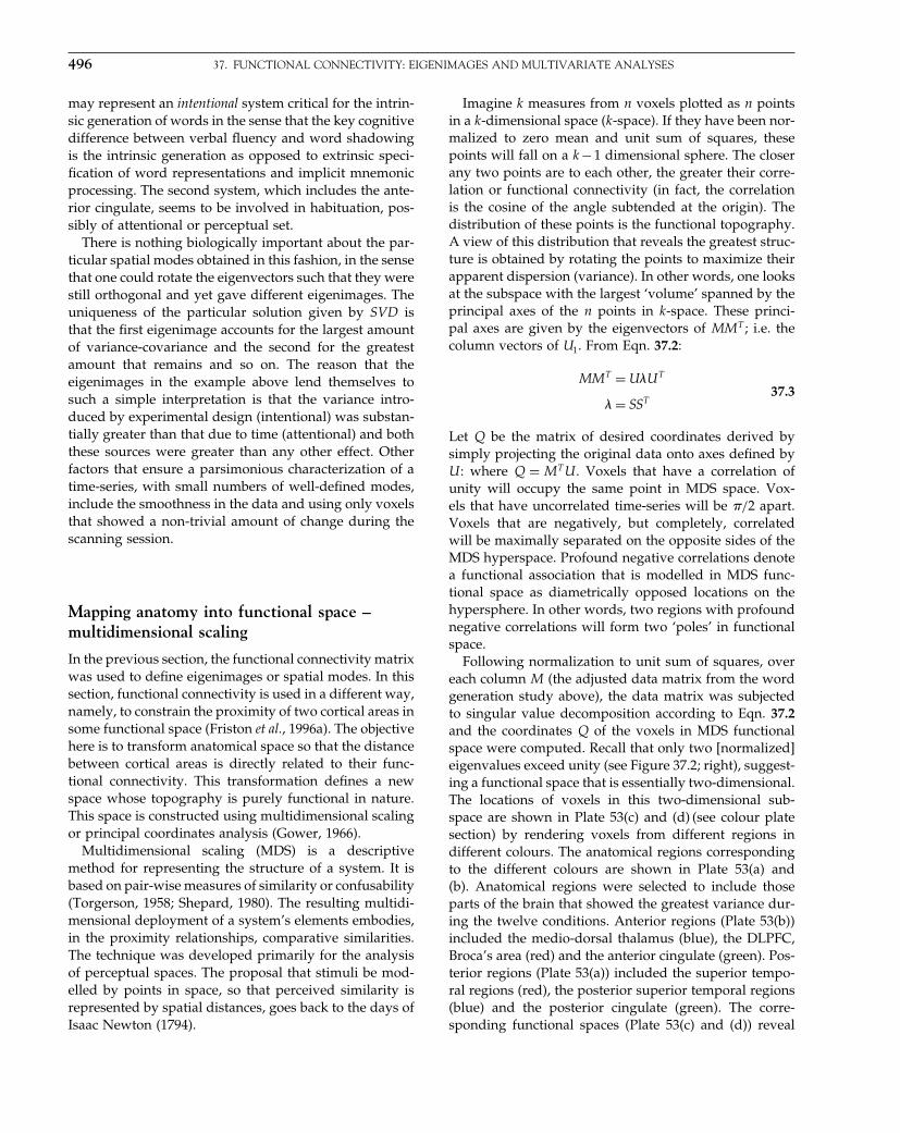
Elsevier UK Chapter: Ch37-P372560 30-9-2006 5:31p.m. Page:496 Trim:7.5in×9.25in
Basal Font:Palatino Margins:Top:40pt Gutter:68pt Font Size:9.5/12 Text Width:42pc Depth:55 Lines
496 37. FUNCTIONAL CONNECTIVITY: EIGENIMAGES AND MULTIVARIATE ANALYSES
may represent an intentional system critical for the intrin-sic generation of words in the sense that the key cognitivedifference between verbal fluency and word shadowingis the intrinsic generation as opposed to extrinsic speci-fication of word representations and implicit mnemonicprocessing. The second system, which includes the ante-rior cingulate, seems to be involved in habituation, pos-sibly of attentional or perceptual set.
There is nothing biologically important about the par-ticular spatial modes obtained in this fashion, in the sensethat one could rotate the eigenvectors such that they werestill orthogonal and yet gave different eigenimages. Theuniqueness of the particular solution given by SVD isthat the first eigenimage accounts for the largest amountof variance-covariance and the second for the greatestamount that remains and so on. The reason that theeigenimages in the example above lend themselves tosuch a simple interpretation is that the variance intro-duced by experimental design (intentional) was substan-tially greater than that due to time (attentional) and boththese sources were greater than any other effect. Otherfactors that ensure a parsimonious characterization of atime-series, with small numbers of well-defined modes,include the smoothness in the data and using only voxelsthat showed a non-trivial amount of change during thescanning session.
Mapping anatomy into functional space –multidimensional scaling
In the previous section, the functional connectivity matrixwas used to define eigenimages or spatial modes. In thissection, functional connectivity is used in a different way,namely, to constrain the proximity of two cortical areas insome functional space (Friston et al., 1996a). The objectivehere is to transform anatomical space so that the distancebetween cortical areas is directly related to their func-tional connectivity. This transformation defines a newspace whose topography is purely functional in nature.This space is constructed using multidimensional scalingor principal coordinates analysis (Gower, 1966).
Multidimensional scaling (MDS) is a descriptivemethod for representing the structure of a system. It isbased on pair-wise measures of similarity or confusability(Torgerson, 1958; Shepard, 1980). The resulting multidi-mensional deployment of a system’s elements embodies,in the proximity relationships, comparative similarities.The technique was developed primarily for the analysisof perceptual spaces. The proposal that stimuli be mod-elled by points in space, so that perceived similarity isrepresented by spatial distances, goes back to the days ofIsaac Newton (1794).
Imagine k measures from n voxels plotted as n pointsin a k-dimensional space (k-space). If they have been nor-malized to zero mean and unit sum of squares, thesepoints will fall on a k−1 dimensional sphere. The closerany two points are to each other, the greater their corre-lation or functional connectivity (in fact, the correlationis the cosine of the angle subtended at the origin). Thedistribution of these points is the functional topography.A view of this distribution that reveals the greatest struc-ture is obtained by rotating the points to maximize theirapparent dispersion (variance). In other words, one looksat the subspace with the largest ‘volume’ spanned by theprincipal axes of the n points in k-space. These princi-pal axes are given by the eigenvectors of MMT ; i.e. thecolumn vectors of U1. From Eqn. 37.2:
MMT = UUT
= SST37.3
Let Q be the matrix of desired coordinates derived bysimply projecting the original data onto axes defined byU : where Q = MT U . Voxels that have a correlation ofunity will occupy the same point in MDS space. Vox-els that have uncorrelated time-series will be �/2 apart.Voxels that are negatively, but completely, correlatedwill be maximally separated on the opposite sides of theMDS hyperspace. Profound negative correlations denotea functional association that is modelled in MDS func-tional space as diametrically opposed locations on thehypersphere. In other words, two regions with profoundnegative correlations will form two ‘poles’ in functionalspace.
Following normalization to unit sum of squares, overeach column M (the adjusted data matrix from the wordgeneration study above), the data matrix was subjectedto singular value decomposition according to Eqn. 37.2and the coordinates Q of the voxels in MDS functionalspace were computed. Recall that only two [normalized]eigenvalues exceed unity (see Figure 37.2; right), suggest-ing a functional space that is essentially two-dimensional.The locations of voxels in this two-dimensional sub-space are shown in Plate 53(c) and (d) (see colour platesection) by rendering voxels from different regions indifferent colours. The anatomical regions correspondingto the different colours are shown in Plate 53(a) and(b). Anatomical regions were selected to include thoseparts of the brain that showed the greatest variance dur-ing the twelve conditions. Anterior regions (Plate 53(b))included the medio-dorsal thalamus (blue), the DLPFC,Broca’s area (red) and the anterior cingulate (green). Pos-terior regions (Plate 53(a)) included the superior tempo-ral regions (red), the posterior superior temporal regions(blue) and the posterior cingulate (green). The corre-sponding functional spaces (Plate 53(c) and (d)) reveal

Elsevier UK Chapter: Ch37-P372560 30-9-2006 5:31p.m. Page:497 Trim:7.5in×9.25in
Basal Font:Palatino Margins:Top:40pt Gutter:68pt Font Size:9.5/12 Text Width:42pc Depth:55 Lines
EIGENIMAGES, MULTIDIMENSIONAL SCALING AND OTHER DEVICES 497
a number of things about the functional topographyelicited by this set of activation tasks. First, each anatom-ical region maps into a relatively localized portion offunctional space. This preservation of local contiguityreflects the high correlations within anatomical regions,due in part to smoothness of the original data and tohigh degrees of intra-regional functional connectivity.Second, the anterior regions are almost in juxtaposition,as are posterior regions. However, the confluence ofanterior and posterior regions forms two diametricallyopposing poles (or one axis). This configuration suggestsan anterior-posterior axis with prefronto-temporal andcingulo-cingulate components. One might have predictedthis configuration by noting that the anterior regionshad high positive loadings on the first eigenimage (seeFigure 37.2), while the posterior regions had high neg-ative loadings. Thirdly, within the anterior and poste-rior sets of regions certain generic features are evident.The most striking is the particular ordering of functionalinteractions. For example, the functional connectivitybetween posterior cingulate (green) and superior tempo-ral regions (red) is high and similarly for the superiortemporal (red) and posterior temporal regions (blue). Yetthe posterior cingulate and posterior temporal regionsshow very little functional connectivity (they are �/2apart or, equivalently, subtend 90 degrees at the origin).
These results are consistent with known anatomicalconnections. For example, DLPFC – anterior cingu-late connections, DLPFC – temporal connections, bi-temporal commissural connections and medio-dorsalthalamic – DLPFC projections have all been demon-strated in non-human primates (Goldman-Rakic, 1988).The medio-dorsal thalamic region and DLPFC are so cor-related that one is embedded within the other (purplearea). This is pleasing given the known thalamo-corticalprojections to DLPFC.
Functional connectivity between systems –partial least squares
Hitherto, we have been dealing with functional con-nectivity between two voxels. The same notion can beextended to functional connectivity between two sys-tems by noting that there is no fundamental differencebetween the dynamics of one voxel and the dynamics ofa distributed system or mixture of voxels. The functionalconnectivity between two systems is simply the correla-tion or covariance between their time-dependent activi-ties. The time-dependent activity of a system or patternpi is given by:
vi = Mpi
Cij = vTi vj = pT
i MT Mpj
37.4
where Cij is the functional connectivity between the sys-tems described by vectors pi and pj . Consider functionalconnectivity between two systems in separate parts of thebrain, for example the right and left hemispheres. Herethe data matrices Mi and Mj derive from different sets ofvoxels and Eqn. 37.4 becomes:
Cij = vTi vj = pT
i MTi Mjpj 37.5
If one wanted to identify the intra-hemispheric sys-tems that showed the greatest inter-hemispheric func-tional connectivity (i.e. covariance), one would need toidentify the pair of vectors pi and pj that maximize Cij
in Eqn. 37.5. SVD finds another powerful application indoing just this:
�U�S�V� = SVD�MTi Mj�
MTi Mj = USV T 37.6
UT MTi MjV = S
The first columns of U and V represent the singularimages that correspond to the two systems with thegreatest amount of functional connectivity (the singularvalues in the diagonal matrix S). In other words, SVDof the (generally asymmetric) cross-covariance matrix,based on time-series from two anatomically separateparts of the brain, yields a series of paired vectors (pairedcolumns of U and V ) that, in a step-down fashion,define pairs of brain systems that show the greatest func-tional connectivity. This particular application of SVDis also know as partial least squares and has been pro-posed for analysis of designed activation experimentswhere the two data matrices comprise an image time-series and a set of behavioural or task parameters, i.e.the design matrix (McIntosh et al., 1996). In this appli-cation, the paired singular vectors correspond to a sin-gular image and a set of weights that give the linearcombination of task parameters that show the maxi-mal covariance with the corresponding singular image.This is conceptually related to canonical image analysis(see next section) based on the generalized eigenvaluesolution.
Differences in functional connectivity –generalized eigenimages
Here, we introduce an extension of eigenimage analysisusing the solution to the generalized eigenvalue problem.This problem involves finding the eigenvector solutionthat involves two covariance matrices and can be usedto find the eigenimage that is maximally expressed inone time-series relative to another. In other words, it can

Elsevier UK Chapter: Ch37-P372560 30-9-2006 5:31p.m. Page:498 Trim:7.5in×9.25in
Basal Font:Palatino Margins:Top:40pt Gutter:68pt Font Size:9.5/12 Text Width:42pc Depth:55 Lines
498 37. FUNCTIONAL CONNECTIVITY: EIGENIMAGES AND MULTIVARIATE ANALYSES
find a pattern of distributed activity that is most preva-lent in one data set and least expressed in another. Theexample used to illustrate this idea is fronto-temporalfunctional disconnection in schizophrenia (see Fristonet al., 1996b).
The notion that schizophrenia represents a disintegra-tion or fractionation of the psyche is as old as its name,introduced by Bleuler (1913) to convey a ‘splitting’ ofmental faculties. Many of Bleuler’s primary processes,such as ‘loosening of associations’ emphasize a fragmen-tation and loss of coherent integration. In what follows,we assume that this mentalist ‘splitting’ has a physio-logical basis and, furthermore, that both the mentalistand physiological disintegration have precise and spe-cific characteristics that can be understood in terms offunctional connectivity.
The idea is that, although localized pathophysiologyin cortical areas may be a sufficient explanation for somesigns of schizophrenia, it does not suffice as an explana-tion for the symptoms of schizophrenia. The conjectureis that symptoms, such as hallucinations and delusions,are better understood in terms of abnormal interactionsor impaired integration between different cortical areas.This dysfunctional integration, expressed at a physiolog-ical level as abnormal functional connectivity, is measur-able with neuroimaging and observable at a cognitivelevel as a failure to integrate perception and action thatmanifests as clinical symptoms. The distinction betweena regionally specific pathology and a pathology of inter-action can be seen in terms of a first-order effect (e.g.hypofrontality) and a second-order effect that only existsin the relationship between activity in the prefrontal cor-tex and some other (e.g. temporal) region. In a similarway, psychological abnormalities can be regarded as firstorder (e.g. a poverty of intrinsically cued behaviour inpsychomotor poverty) or second order (e.g. a failure tointegrate intrinsically cued behaviour and perception inreality distortion).
The generalized eigenvalue solution
Suppose that we want to find a pattern embodying thegreatest amount of functional connectivity in controlsubjects, relative to schizophrenic subjects (e.g. fronto-temporal covariance). To achieve this, we identify aneigenimage that reflects the most functional connectiv-ity in control subjects relative to a schizophrenic group,d. This eigenimage is obtained by using a generalizedeigenvector solution:
C−1i Cjd = d
Cjd = Cid37.7
where Ci and Cj are the two functional connectivity matri-ces. The generalized eigenimage d is essentially a pat-tern that maximizes the ratio of the 2-norm measures(see Eqn. 37.1) when applied to Ci and Cj . Generallyspeaking, these matrices could represent data from two[groups of] subjects or from the same subject(s) scannedunder different conditions. In the present example, weuse connectivity matrices from control subjects and peo-ple with schizophrenia showing pronounced psychomo-tor poverty.
The data were acquired from two groups of six sub-jects. Each subject was scanned six times during the per-formance of three word generation tasks (A B C C BA). Task A was a verbal fluency task, requiring subjectsto respond with a word that began with a heard letter.Task B was a semantic categorization task in which sub-jects responded ‘man-made’ or ‘natural’, depending on aheard noun. Task C was a word-shadowing task in whichsubjects simply repeated what was heard. In the presentcontext, the detailed nature of the tasks is not important.They were used to introduce variance and covariancein activity that could support an analysis of functionalconnectivity.
The groups comprised six control subjects and sixschizophrenic patients. The schizophrenic subjects pro-duced fewer than 24 words on a standard (one minute)FAS verbal fluency task (generating words beginningwith the letters ‘F’, ‘A’ and ‘S’). The results of a gener-alized eigenimage analysis are presented in Figure 37.3.As expected, the pattern that best captures group dif-ferences involves prefrontal and temporal cortices andencodes negative correlations between left DLPFC andbilateral superior temporal regions (Figure 37.3; upperpanels). The amount to which this pattern was expressedin each subject is shown in the lower panel using theappropriate 2-norm
∥∥dT Cid∥∥. It is seen that this eigen-
image, while prevalent in control subjects, is uniformlyreduced in schizophrenic subjects.
Summary
In the preceding section, we have seen how eigenim-ages can be framed in terms of functional connectivityand the relationships among eigenimage analysis, mul-tidimensional scaling, partial least squares and general-ized eigenimage analysis. In the next section, we use thegenerative models perspective, described in the previouschapter, to take component analysis into the non-lineardomain. In the subsequent section, we return to general-ized eigenvalue solutions and their role in classificationand canonical image analysis.

Elsevier UK Chapter: Ch37-P372560 30-9-2006 5:31p.m. Page:499 Trim:7.5in×9.25in
Basal Font:Palatino Margins:Top:40pt Gutter:68pt Font Size:9.5/12 Text Width:42pc Depth:55 Lines
NON-LINEAR PRINCIPAL AND INDEPENDENT COMPONENT ANALYSIS (PCA AND ICA) 499
Positive
Eigenimage analysis
2 no
rm
120
100
80
60
40
20
controls schizophrenics0
sagittal
VPC VAC
0
104 68
VPC VAC
Transverse
0
64 R
32
0
0 64
R72
coronal
Transverse
0
64 R
VPC VAC
0
104 68VPC VAC
sagittal
640
R
32
0
72coronal
Negative
FIGURE 37.3 Generalized eigenimage analysis of schizophrenic and control subjects. Top left and right: positive and negative loadingsof the first eigenimage that is maximally expressed in the control group and minimally expressed in the schizophrenic group. This analysisused PET activation studies of word generation with six scans per subject and six subjects per group. The activation study involved threeword generation conditions (word shadowing, semantic categorization and verbal fluency), each of which was presented twice. The greyscale is arbitrary and each image has been normalized to the image maximum. The display format is standard and represents a maximumintensity projection. This eigenimage is relatively less expressed in the schizophrenic data. This point is made by expressing the amount offunctional connectivity attributable to the eigenimage in (each subject in) both groups, using the appropriate 2-norm (lower panel).
NON-LINEAR PRINCIPAL ANDINDEPENDENT COMPONENT
ANALYSIS (PCA AND ICA)
Generative models
Recall from the previous chapter how generative modelsof data could be framed in terms of a prior distributionover causes p�v��� and a generative distribution or likeli-hood of the inputs given the causes p�u�v ��. For exam-ple, factor analysis corresponds to the generative model:
p�v �� = N�0� 1�
p�u �v �� = N��v���37.8
Namely, the underlying causes of inputs are independentnormal variates that are mixed linearly and added toGaussian noise to form inputs. In the limiting case of� → 0, the model becomes deterministic and conformsto PCA. By simply assuming non-Gaussian priors onecan specify generative models for sparse coding:
p�v �� =∏p�vi ��
p�u �v �� = N��v���37.9
where p�vi� �� are chosen to be suitably sparse (i.e.heavy-tailed), with a cumulative density function thatcorresponds to the squashing function below. Thedeterministic equivalent of sparse coding is ICA that

Elsevier UK Chapter: Ch37-P372560 30-9-2006 5:31p.m. Page:500 Trim:7.5in×9.25in
Basal Font:Palatino Margins:Top:40pt Gutter:68pt Font Size:9.5/12 Text Width:42pc Depth:55 Lines
500 37. FUNCTIONAL CONNECTIVITY: EIGENIMAGES AND MULTIVARIATE ANALYSES
obtains when � → 0. These formulations allow usto consider simple extensions of PCA by looking atnon-linear versions of the underlying generative model.
Non-linear PCA
Despite its exploratory power, eigenimage analysis isfundamentally limited because the particular modesobtained are uniquely determined by constraints thatare biologically implausible. This represents an inher-ent limitation on the interpretability and usefulness ofeigenimage analysis. The two main limitations of conven-tional eigenimage analysis are that the decomposition ofany observed time-series is in terms of linearly separablecomponents. Secondly, the spatial modes are somewhatarbitrarily constrained to be orthogonal and account, suc-cessively, for the largest amount of variance. From a bio-logical perspective, the linearity constraint is a severe onebecause it precludes interactions among brain systems.This is an unnatural restriction on brain activity, whereone expects to see substantial interactions that render theexpression of one mode sensitive to the expression of oth-ers. Non-linear PCA attempts to circumvent these sortsof limitations.
The generative model implied by Eqn. 37.8, when � →0, is linear and deterministic:
p�v �� = N�0� 1�
u = �v37.10
Here the causes v correspond to the eigenvariates and themodel parameters to scaled eigenvectors � = VS. u is theobserved data or image that comprised each row of Mabove. This linear generative model g�v��� = �v can nowbe generalized to any static non-linear model by takinga second-order approximation:
p�v �� = N�0� 1�
u = g�v���
=∑i
Vivi +12
∑ij
Vijvivj + � � � 37.11
Vi = �g
�v
Vij = �2g
�vi�vj
This non-linear model has two sorts of modes; first-order modes Vi that mediate the effect of any orthogonalcause on the response (i.e. map the causes onto voxelsdirectly) and second-order modes Vij , which map inter-actions among causes onto the measured response. These
second-order modes could represent the distributed sys-tems implicated in the interaction between various exper-imentally manipulated causes. See the example below.
The identification of the first- and second-ordermodes proceeds using expectation maximization (EM) asdescribed in the previous chapter. In this instance, thealgorithm can be implemented as a simple neural netwith forward connections from the data to the causesand backward connections from the causes to the pre-dicted data. The E-step corresponds to recognition of thecauses by the forward connections using the current esti-mate of the first-order modes and the M-step adjuststhese connections to minimize the prediction error ofthe generative model in Eqn. 37.11, using the recognizedcauses. These schemes (e.g. Kramer, 1991; Karhunen andJoutsensalo, 1994; Friston et al., 2000) typically employ a‘bottleneck’ architecture that forces the inputs through asmall number of nodes (see the insert in Plate 54). Theoutput from these nodes then diverges to produce thepredicted inputs. After learning, the activity of the bot-tleneck nodes can be treated as estimates of the causes.In short, these representations obtain by projection of theinput onto a low-dimensional curvilinear manifold thatis defined by the activity of the bottleneck. Before lookingat an empirical example we will briefly discuss ICA.
Independent component analysis
ICA represents another way of generalizing the linearmodel used by PCA. This is achieved, not through non-linearities, but by assuming non-Gaussian priors. Thenon-Gaussian form can be specified by a non-linear trans-formation of the causes ṽ = ��v� that renders them nor-mally distributed, such that when � → 0, in Eqn. 37.9we get:
p�ṽ �� = N�0� 1�
v = �−1�ṽ� 37.12
u = �v
This is not the conventional way to present ICA, butis used here to connect the models for PCA and ICA.The form of the non-linear squashing function ṽ = ��v�embodies our prior assumptions about the marginal dis-tribution of the causes. These are usually supra-Gaussian.There exist simple algorithms that implicitly minimizethe objective function F (see previous chapter) using thecovariances of the data. In neuroimaging, this enforcesan ICA of independent spatial modes, because there aremore voxels than scans (McKeown et al., 1998). In EEG,there are more time bins than channels and the indepen-dent components are temporal in nature. The distinction

Elsevier UK Chapter: Ch37-P372560 30-9-2006 5:31p.m. Page:501 Trim:7.5in×9.25in
Basal Font:Palatino Margins:Top:40pt Gutter:68pt Font Size:9.5/12 Text Width:42pc Depth:55 Lines
NON-LINEAR PRINCIPAL AND INDEPENDENT COMPONENT ANALYSIS (PCA AND ICA) 501
between spatial and temporal ICA depends on whetherone regards Eqn. 37.12 as generating data over space ortime (see Friston, 1998 for a discussion of their relativemerits). The important thing about ICA, relative to PCA,is that the prior densities model independent causes notjust uncorrelated causes. This difference is expressed interms of statistical dependencies beyond second-order(see Stone, 2002 for an introduction to these issues).
An example
This example comes from Friston et al. (2000)2 and isbased on an fMRI study of visual processing that wasdesigned to address the interaction between colour andmotion systems.
We had expected to demonstrate that a ‘colour’ modeand ‘motion’ mode would interact to produce a second-order mode reflecting: (i) reciprocal interactions betweenextrastriate areas functionally specialized for colour andmotion; (ii) interactions in lower visual areas mediated byconvergent backwards connections; or (iii) interactions inthe pulvinar mediated by cortico-thalamic loops.
Data acquisition and experimental design
A subject was scanned under four different conditions,in six scan epochs, intercalated with a low-level (visualfixation) baseline condition. The four conditions wererepeated eight times in a pseudo-random order giving384 scans in total or 32 stimulation/baseline epoch pairs.The four experimental conditions comprised the presen-tation of moving and stationary dots, using luminanceand chromatic contrast, in a two by two-factorial design.Luminance contrast was established using isochromaticstimuli (red dots on a red background or green dots on agreen background). Hue contrast was obtained by usingred (or green) dots on a green (or red) background andestablishing iso-luminance with flicker photometry. Inthe two movement conditions, the dots moved radiallyfrom the centre of the screen, at eight degrees per sec-ond to the periphery, where they vanished. This createsthe impression of optical flow. By using these stimuli wehoped to excite activity in a visual motion system andone specialized for colour processing. Any interactionbetween these systems would be expressed in terms ofmotion-sensitive responses that depended on the hue orluminance contrast subtending that motion.
2 Although an example of non-linear PCA, the generative modelactually used augmented Eqn. 37.11 with a non-linear functionof the second- order terms: u = G�v� = ∑
iVivi + 1
2
∑ij
Vij��vivj�.
This endows the causes with unique scaling.
Non-linear PCA
The data were reduced to an eight-dimensional subspaceusing SVD and entered into a non-linear PCA using twocauses. The functional attribution of the resulting sourceswas established by looking at the expression of thecorresponding first-order modes over the four conditions(right lower panels in Plate 54). This expression is simplythe score on the first principal component over all 32epoch-related responses for each cause. The first mode isclearly a motion-sensitive mode but one that embodiessome colour preference, in the sense that the motion-dependent responses of this system are accentuated in thepresence of colour cues. This was not quite what we hadanticipated; the first-order effect contains what wouldfunctionally be called an interaction between motion andcolour processing. The second first-order mode appearsto be concerned exclusively with colour processing. Thecorresponding anatomical profiles are shown in Plate 54(left panels). The first-order mode, which shows bothmotion and colour-related responses, shows high load-ings in bilateral motion sensitive complex V5 (Brodmannareas 19 and 37 at the occipito-temporal junction) andareas traditionally associated with colour processing(V4 – the lingual gyrus). The second first-order mode ismost prominent in the hippocampus, parahippocampaland related lingual cortices on both sides. In summary,the two first-order modes comprise: an extrastriatecortical system including V5 and V4 that responds tomotion, and preferentially so when motion is supportedby colour cues; and a [para]hippocampus-lingual systemthat is concerned exclusively with colour processing,above and beyond that accounted for by the first system.The critical question is where do these modes interact?
The interaction between the extrastriate and[para]hippocampus-lingual systems conforms to thesecond-order mode in the lower panels. This mode high-lights the pulvinar of the thalamus and V5 bilaterally.This is a pleasing result in that it clearly implicatesthe thalamus in the integration of extrastriate and[para]hippocampal systems. This integration is mediatedby recurrent cortico-thalamic connections. It is alsoa result that would not have been obtained from aconventional SPM analysis. Indeed, we looked for aninteraction between motion and colour processing anddid not see any such effect in the pulvinar.
Summary
We have reviewed eigenimage analysis and general-izations based on non-linear and non-Gaussian gener-ative models. All the techniques above are essentiallydescriptive, in that they do not allow one to make any sta-tistical inferences about the characterizations that obtain.

Elsevier UK Chapter: Ch37-P372560 30-9-2006 5:31p.m. Page:502 Trim:7.5in×9.25in
Basal Font:Palatino Margins:Top:40pt Gutter:68pt Font Size:9.5/12 Text Width:42pc Depth:55 Lines
502 37. FUNCTIONAL CONNECTIVITY: EIGENIMAGES AND MULTIVARIATE ANALYSES
In the second half of this chapter, we turn to multi-variate techniques that enable statistical inference andhypothesis testing. We will introduce canonical images thatcan be thought of as statistically informed eigenimages,pertaining to effects introduced by experimental design.We have seen that patterns can be identified usingthe generalized eigenvalue solution that are maximallyexpressed in one covariance structure, relative to another.Consider now using this approach where the first covari-ance matrix reflected the effects we were interested in,and the second embodied covariances due to error. Thiscorresponds to canonical image analysis, and is consid-ered in the following section.
MANCOVA AND CANONICAL IMAGEANALYSES
In this section, we review multivariate approaches tothe analysis of functional imaging studies. The analy-ses described use standard multivariate techniques tomake statistical inferences about activation effects and todescribe their important features. Specifically, we intro-duce multivariate analysis of covariance (MANCOVA)and canonical variates analysis (CVA) to characterizeactivation effects. This approach characterizes the brain’sresponse in terms of functionally connected and dis-tributed systems in a similar fashion to eigenimage anal-ysis. Eigenimages figure in the current analysis in thefollowing way: a problematic issue in multivariate anal-ysis of functional imaging data is that the number ofsamples (i.e. scans) is usually very small in relation to thenumber of components (i.e. voxels) of the observations.This issue is resolved by analysing the data, not in termsof voxels, but in terms of eigenimages, because the num-ber of eigenimages is much smaller than the number ofvoxels. The importance of the multivariate analysis thatensues can be summarized as follows:
• Unlike eigenimage analysis, it provides for statisti-cal inferences (based on classical p-values) about thesignificance of the brain’s response in terms of somehypothesis.
• The approach implicitly takes account of spatial corre-lations in the data without making any assumptions.
• The canonical variate analysis produces generalizedeigenimages (canonical images) that capture the acti-vation effects, while suppressing the effects of noise orerror.
• The theoretical basis is well established and can befound in most introductory texts on multivariate anal-ysis (see also Friston et al., 1996c).
Although useful, in a descriptive sense, eigenimageanalysis and related approaches are not generally con-sidered as ‘statistical’ methods that can be used to makestatistical inferences; they are mathematical devices thatsimply identify prominent patterns of correlations orfunctional connectivity. In what follows, we observe thatmultivariate analysis of covariance (MANCOVA) withcanonical variate analysis combines some features ofstatistical parametric mapping and eigenimage analy-sis. Unlike statistical parametric mapping, MANCOVAis multivariate. In other words, it considers all voxels ina single scan as one observation. The importance of thismultivariate approach is that effects, due to activations,confounding effects and error effects, are assessed both interms of effects at each voxel and interactions among voxels.This means one does not have to assume anything aboutspatial correlations (cf. smoothness with random fieldmodels) to assess the significance of an activation effect.Unlike statistical parametric mapping, these correlationsare explicitly included in the analysis. The price one paysfor adopting a multivariate approach is that inferencescannot be made about regionally specific changes (cf. sta-tistical parametric mapping). This is because the inferencepertains to all the components (voxels) of a multivariatevariable (not a particular voxel or set of voxels). Fur-thermore, because the spatial non-sphericity has to beestimated, without knowing the observations came fromcontinuous spatially extended processes, the estimatesare less efficient and inferences are less powerful.
Usually, multivariate analyses are implemented in twosteps. First, the significance of hypothesized effects isassessed in terms of a p-value and secondly, if justi-fied, the quantitative nature of the effect is determined.The analysis here conforms to this two-stage procedure.When the brain’s response is assessed to be significantusing MANCOVA, the nature of this response remains tobe characterized. Canonical variate analysis is an appro-priate way to do this. The canonical images obtainedwith CVA are similar to eigenimages, but are based onboth the activation and error. CVA is closely related tode-noising techniques in EEG and MEG time-series anal-yses that use a generalized eigenvalue solution. Anotherway of looking at canonical images is to think of themas eigenimages that reflect functional connectivity due toactivations, when spurious correlations due to error areexplicitly discounted.
Dimension reduction and eigenimages
The first step in multivariate analysis is to ensure thatthe dimensionality (number of components or voxels)of the data is smaller than the number of observations.Clearly, this is not the case for images, because there are

Elsevier UK Chapter: Ch37-P372560 30-9-2006 5:31p.m. Page:503 Trim:7.5in×9.25in
Basal Font:Palatino Margins:Top:40pt Gutter:68pt Font Size:9.5/12 Text Width:42pc Depth:55 Lines
MANCOVA AND CANONICAL IMAGE ANALYSES 503
more voxels than scans; therefore the data have to betransformed. The dimension reduction proposed here isstraightforward and uses the scan-dependent expression,Y , of eigenimages as a reduced set of components foreach multivariate observation (scan). Where:
�U�S�V� = SVD�M�
Y = US37.13
As above, M is a large matrix of adjusted voxel-valueswith one column for each voxel and one row foreach scan. Here, ‘adjusted’ implies mean correction andremoval of any confounds using linear regression. Theeigenimages constitute the columns of U , another uni-tary orthonormal matrix, and their expression over scanscorresponds to the columns of the matrix Y . Y has onecolumn for each eigenimage and one row for each scan.In our work, we use only the j columns of Y and Uassociated with eigenvalues greater than unity (after nor-malizing each eigenvalue by the average eigenvalue).
The general linear model revisited
Recall the general linear model from previous chapters:
Y = X�+� 37.14
where the errors are assumed to be independent andidentically normally distributed. The design matrix X hasone column for every effect (factor or covariate) in themodel. The design matrix can contain both covariates andindicator variables reflecting an experimental design. � isthe parameter matrix with one column vector of param-eters for each mode. Each column of X has an associatedunknown parameter. Some of these parameters will beof interest, the remaining parameters will not. We willpartition the model accordingly:
Y = X1�1 +X0�0 +� 37.15
where X1 represents a matrix of zeros or ones depend-ing on the level or presence of some interesting condi-tion or treatment effect (e.g. the presence of a particularcognitive component) or the columns of X1 might con-tain covariates of interest that could explain the observedvariance in Y (e.g. dose of apomorphine or ‘time on tar-get’). X0 corresponds to a matrix of indicator variablesdenoting effects that are not of any interest (e.g. of beinga particular subject or block effect) or covariates of nointerest (i.e. ‘nuisance variables’, such as global activityor confounding time effects).
Statistical inference
Significance is assessed by testing the null hypothesisthat the effects of interest do not significantly reduce theerror variance when compared to the remaining effectsalone (or alternatively the null hypothesis that �1 is zero).The null hypothesis is tested in the following way. Thesum of squares and products matrix (SSPM) due to erroris obtained from the difference between actual and esti-mated values of the response:
SR = �Y −X�̂�T �Y −X�̂� 37.16
where the sums of squares and products due to effectsof interest is given by:
ST = �X1�̂1�T �X1�̂1� 37.17
The error sum of squares and products under the nullhypothesis, i.e. after discounting the effects of interest aregiven by:
S0 = �Y −X0�̂0�T �Y −X0�̂0� 37.18
The significance can now be tested with:
� = SR
S037.19
This is Wilk’s statistic (known as Wilk’s Lambda). Aspecial case of this test is Hotelling‘s T -square test andapplies when one simply compares one condition withanother, i.e. X1 has only one column (Chatfield andCollins, 1980). Under the null hypothesis, after transfor-mation, � has chi-squared distribution with degrees offreedom jh. The transformation is given by:
−�v− �j −h+1�/2� ln � ∼ �2jh 37.20
where v are the degrees of freedom associated with errorterms, equal to the number of scans, n, minus the numberof effects modelled, rank�X�. j is the number of eigen-images in the j-variate response variable and h is thedegrees of freedom associated with the effects of interest,rank�X1�. Eqn. 37.20 enables one to compute a p-value forsignificance testing in the usual way.
Characterizing the effect with CVA
Having established that the effects of interest are sig-nificant (e.g. differences among two or more activationconditions), the final step is to characterize these effectsin terms of their spatial topography. This characteriza-tion employs canonical variates analysis or CVA. The
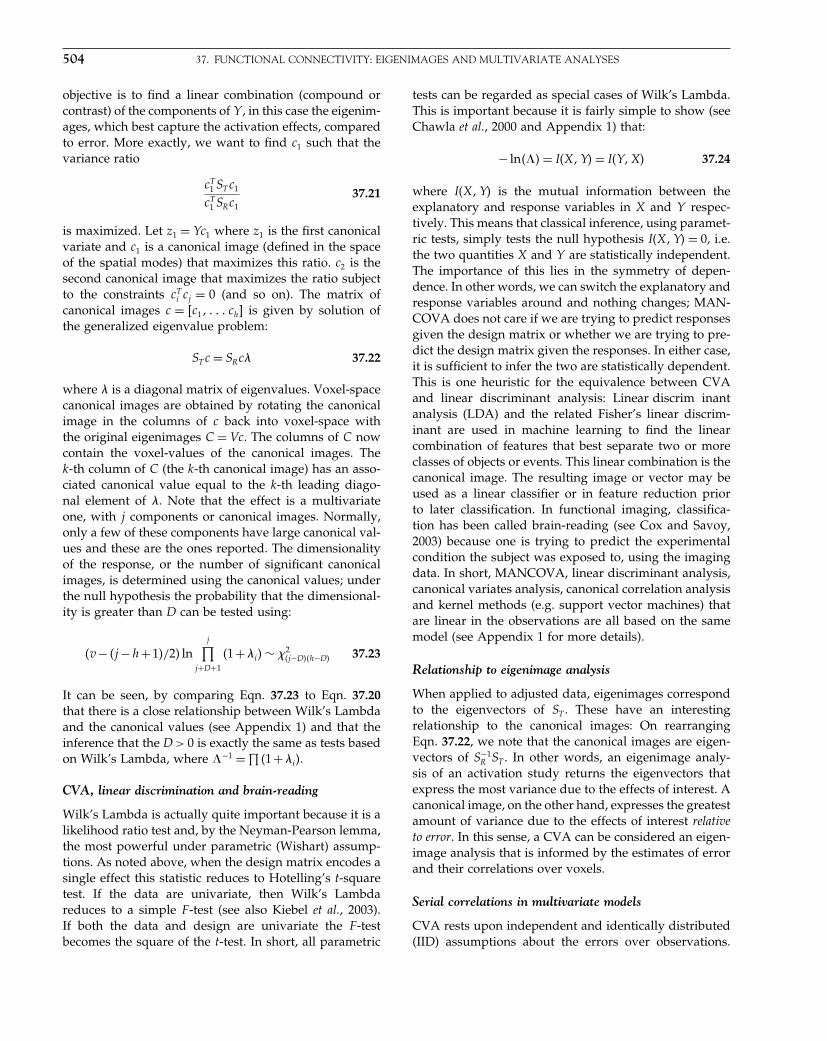
Elsevier UK Chapter: Ch37-P372560 30-9-2006 5:31p.m. Page:504 Trim:7.5in×9.25in
Basal Font:Palatino Margins:Top:40pt Gutter:68pt Font Size:9.5/12 Text Width:42pc Depth:55 Lines
504 37. FUNCTIONAL CONNECTIVITY: EIGENIMAGES AND MULTIVARIATE ANALYSES
objective is to find a linear combination (compound orcontrast) of the components of Y , in this case the eigenim-ages, which best capture the activation effects, comparedto error. More exactly, we want to find c1 such that thevariance ratio
cT1 ST c1
cT1 SRc1
37.21
is maximized. Let z1 = Yc1 where z1 is the first canonicalvariate and c1 is a canonical image (defined in the spaceof the spatial modes) that maximizes this ratio. c2 is thesecond canonical image that maximizes the ratio subjectto the constraints cT
i cj = 0 (and so on). The matrix ofcanonical images c = �c1� � � � ch� is given by solution ofthe generalized eigenvalue problem:
ST c = SRc 37.22
where is a diagonal matrix of eigenvalues. Voxel-spacecanonical images are obtained by rotating the canonicalimage in the columns of c back into voxel-space withthe original eigenimages C = Vc. The columns of C nowcontain the voxel-values of the canonical images. Thek-th column of C (the k-th canonical image) has an asso-ciated canonical value equal to the k-th leading diago-nal element of . Note that the effect is a multivariateone, with j components or canonical images. Normally,only a few of these components have large canonical val-ues and these are the ones reported. The dimensionalityof the response, or the number of significant canonicalimages, is determined using the canonical values; underthe null hypothesis the probability that the dimensional-ity is greater than D can be tested using:
�v− �j −h+1�/2� lnj∏
j+D+1
�1+i� ∼ �2�j−D��h−D� 37.23
It can be seen, by comparing Eqn. 37.23 to Eqn. 37.20that there is a close relationship between Wilk’s Lambdaand the canonical values (see Appendix 1) and that theinference that the D > 0 is exactly the same as tests basedon Wilk’s Lambda, where �−1 =∏
�1+i�.
CVA, linear discrimination and brain-reading
Wilk’s Lambda is actually quite important because it is alikelihood ratio test and, by the Neyman-Pearson lemma,the most powerful under parametric (Wishart) assump-tions. As noted above, when the design matrix encodes asingle effect this statistic reduces to Hotelling’s t-squaretest. If the data are univariate, then Wilk’s Lambdareduces to a simple F -test (see also Kiebel et al., 2003).If both the data and design are univariate the F -testbecomes the square of the t-test. In short, all parametric
tests can be regarded as special cases of Wilk’s Lambda.This is important because it is fairly simple to show (seeChawla et al., 2000 and Appendix 1) that:
− ln��� = I�X�Y� = I�Y�X� 37.24
where I�X�Y� is the mutual information between theexplanatory and response variables in X and Y respec-tively. This means that classical inference, using paramet-ric tests, simply tests the null hypothesis I�X�Y� = 0, i.e.the two quantities X and Y are statistically independent.The importance of this lies in the symmetry of depen-dence. In other words, we can switch the explanatory andresponse variables around and nothing changes; MAN-COVA does not care if we are trying to predict responsesgiven the design matrix or whether we are trying to pre-dict the design matrix given the responses. In either case,it is sufficient to infer the two are statistically dependent.This is one heuristic for the equivalence between CVAand linear discriminant analysis: Linear discrim inantanalysis (LDA) and the related Fisher’s linear discrim-inant are used in machine learning to find the linearcombination of features that best separate two or moreclasses of objects or events. This linear combination is thecanonical image. The resulting image or vector may beused as a linear classifier or in feature reduction priorto later classification. In functional imaging, classifica-tion has been called brain-reading (see Cox and Savoy,2003) because one is trying to predict the experimentalcondition the subject was exposed to, using the imagingdata. In short, MANCOVA, linear discriminant analysis,canonical variates analysis, canonical correlation analysisand kernel methods (e.g. support vector machines) thatare linear in the observations are all based on the samemodel (see Appendix 1 for more details).
Relationship to eigenimage analysis
When applied to adjusted data, eigenimages correspondto the eigenvectors of ST . These have an interestingrelationship to the canonical images: On rearrangingEqn. 37.22, we note that the canonical images are eigen-vectors of S−1
R ST . In other words, an eigenimage analy-sis of an activation study returns the eigenvectors thatexpress the most variance due to the effects of interest. Acanonical image, on the other hand, expresses the greatestamount of variance due to the effects of interest relativeto error. In this sense, a CVA can be considered an eigen-image analysis that is informed by the estimates of errorand their correlations over voxels.
Serial correlations in multivariate models
CVA rests upon independent and identically distributed(IID) assumptions about the errors over observations.

Elsevier UK Chapter: Ch37-P372560 30-9-2006 5:31p.m. Page:505 Trim:7.5in×9.25in
Basal Font:Palatino Margins:Top:40pt Gutter:68pt Font Size:9.5/12 Text Width:42pc Depth:55 Lines
MANCOVA AND CANONICAL IMAGE ANALYSES 505
Violation of these assumptions in fMRI has motivatedthe study of multivariate linear models (MLMs) for neu-roimaging that allow for temporal non-sphericity (seeWorsley et al., 1997). Although this is an interesting issue,it should be noted that conventional CVA (with dimen-sion reduction) can be applied after pre-whitening thetime-series.
An example
We will consider an application of the above proce-dures to the word generation study in normal subjects,used above. We assessed the significance of condition-dependent effects by treating each of the twelve scansas a different condition. Note that we do not considerthe word generation (or word shadowing) conditions asreplications of the same condition. In other words, thefirst time one performs a word generation task is a dif-ferent condition from the second time and so on. The(alternative) hypothesis adopted here states that thereis a significant difference among the twelve conditions,but that this does not constrain the nature of this differ-ence to a particular form. The most important differenceswill emerge from the CVA. Clearly, one might hope thatthese differences will be due to word generation, but theymight not be. This hypothesis should be compared witha more constrained hypothesis that considers the condi-tions as six replications of word shadowing and wordgeneration. This latter hypothesis is more directed andexplicitly compares word shadowing with word genera-tion. This comparison could be tested in a single subject.The point is that the generality afforded by the cur-rent framework allows one to test very constrained (i.e.specific) hypotheses or rather general hypotheses aboutsome unspecified activation effect.3 We choose the lattercase here because it places more emphasis on canoni-cal images as descriptions of what has actually occurredduring the experiment. Had we chosen the former, wewould have demonstrated significant mutual informationbetween the data and the classification of each scan aseither word shadowing or generation (cf. brain-readingfor word generation).
The design matrix partition for effects of interest X1
had twelve columns representing the conditions. We des-ignated subject effects, time and global activity as unin-teresting confounds X0. The adjusted data were reducedto 60 eigenvectors as described above. The first 14 eigen-vectors had (normalized) eigenvalues greater than unity
3 This is in analogy to the use of the SPM�F�, relative to more con-strained hypotheses tested with SPM�t�, in conventional mass-univariate approaches.
and were used in the subsequent analysis. The result-ing matrix data Y , with 60 rows (one for each scan)and 14 columns (one for each eigenimage) was subjectto MANCOVA. The significance of the condition effectswas assessed with Wilk’s Lambda. The threshold forcondition or activation effects was set at p = 002. Inother words, the probability of there being no differencesamong the 12 conditions was 2 per cent.
Canonical variates analysis
The first canonical image and its canonical variate areshown in Figure 37.4. The upper panels show this sys-tem to include anterior cingulate and Broca’s area, withmore moderate expression in the left posterior inferotem-poral regions (right). The positive components of thiscanonical image (left) implicate ventro-medial prefrontalcortex and bi-temporal regions (right greater than left).One important aspect of these canonical images is theirhighly distributed yet structured nature, reflecting thedistributed integration of many brain areas. The canoni-cal variate expressed in terms of mean condition effectsis seen in the lower panel of Figure 37.4. It is pleasingto note that the first canonical variate corresponds to thedifference between word shadowing and verbal fluency.
Recall that the eigenimage in Figure 37.2 reflects themain pattern of correlations evoked by the mean con-dition effects and should be compared with the firstcanonical image in Figure 37.4. The differences betweenthese characterizations of activation effects are informa-tive: the eigenimage is totally insensitive to the reliabil-ity or error attributable to differential activation fromsubject to subject, whereas the canonical image reflectsthese variations. For example, the absence of the pos-terior cingulate in the canonical image and its relativeprominence in the eigenimage suggests that this regionis implicated in some subjects but not in others. The sub-jects that engaged the posterior cingulate must do soto some considerable degree because the average effects(represented by the eigenimage) are quite substantial.Conversely, the medial prefrontal cortical deactivationsare a more pronounced feature of activation effects thanwould have been inferred on the basis of the eigenimageanalysis. These observations beg the question: ‘which isthe best characterization of functional anatomy?’ Obvi-ously, there is no simple answer but the question speaksof an important point. A canonical image characterizesa response relative to error, by partitioning the observedvariance into effects of interest and a residual variationabout these effects. Experimental design, a hypothesis,and the inferences that are sought determine this parti-tioning. An eigenimage does not entail any concept oferror and is not constrained by any hypothesis.

Elsevier UK Chapter: Ch37-P372560 30-9-2006 5:31p.m. Page:506 Trim:7.5in×9.25in
Basal Font:Palatino Margins:Top:40pt Gutter:68pt Font Size:9.5/12 Text Width:42pc Depth:55 Lines
506 37. FUNCTIONAL CONNECTIVITY: EIGENIMAGES AND MULTIVARIATE ANALYSES
sagittal72
32
0 0 0
32
68–104
0
04
72 R
R4F4
P
0
–104
0
R04
68VPC VAC
VPC VAC VPC VAC
VPC VAC
transversetransverse
corona sagittal coronal
Canonical image 1 {+ve} Canonical image 1 {–ve}
FIGURE 37.4 Top: the first canonical image displayed as maximum intensity projections of the positive and negative components. Thedisplay format is standard and provides three views of the brain from the front, the back and the right hand side. The grey scale is arbitraryand the space conforms to that described in the atlas of Talairach and Tournoux (1988). Bottom: the expression of the first canonical image(i.e. the canonical variate) averaged over conditions. The odd conditions correspond to word shadowing and the even conditions correspondto word generation. This canonical variate is clearly sensitive to the differences evoked by these two tasks.
Multivariate versus univariate models
Although multivariate linear models are important, thisbook focuses more on univariate models. There is a sim-ple reason for this: any multivariate model can be refor-mulated as a univariate model by vectorizing the model.For example:
Y = X�+�
�y1� � � � � yj� = X��1� � � � ��j�+ ��1� � � � � �j�37.25
can be rearranged to give a univariate model:
vec�Y� = �I ⊗X�vec���+vec���⎡⎢⎣
y1yj
⎤⎥⎦=
⎡⎢⎣
X
X
⎤⎥⎦⎡⎢⎣
y1yj
⎤⎥⎦+
⎡⎢⎣
�1�j
⎤⎥⎦ 37.26
where ⊗ denotes the Kronecker tensor product. Here,cov�vec���� = � ⊗ V , where � is the covariance amongcomponents and V encodes the serial correlations. InMLMs � is unconstrained and requires full estimation (interms of SR above). Therefore, any MLM and its univari-ate form are exactly equivalent, if we place constraintson the non-sphericity of the errors that ensure it hasthe form �⊗V . This speaks to an important point: anymultivariate analysis can proceed in a univariate settingwith appropriate constraints on the non-sphericity. Infact, MLMs are special cases that assume the covariancefactorizes into � ⊗ V and � is unconstrained. In neu-roimaging there are obvious constraints on the form of �
because this embodies the spatial covariances. Randomfield theory harnesses these constraints. MLMs do notand are therefore less sensitive.
Elsevier UK Chapter: Ch37-P372560 30-9-2006 5:31p.m. Page:507 Trim:7.5in×9.25in
Basal Font:Palatino Margins:Top:40pt Gutter:68pt Font Size:9.5/12 Text Width:42pc Depth:55 Lines
REFERENCES 507
Summary
This chapter has described multivariate approaches tothe analysis of functional imaging studies. These usestandard multivariate techniques to describe or makestatistical inferences about distributed activation effectsand characterize important features of functional connec-tivity. The multivariate approach differs fundamentallyfrom statistical parametric mapping, because the conceptof a separate voxel or region of interest ceases to havemeaning. In this sense, inference is about the whole imagevolume, not any component. This feature precludes sta-tistical inferences about regional effects made withoutreference to changes elsewhere in the brain. This funda-mental difference ensures that mass-univariate and mul-tivariate approaches are likely to be treated as distinctand complementary approaches to functional imagingdata (see Kherif et al., 2002).
In this chapter, we have used correlations amongbrain measurements to identify systems that respondin a coherent fashion. This identification proceeds with-out reference to the mechanisms that may mediate dis-tributed and integrated responses. In the next chapter,we turn to models of effective connectivity that groundthe nature of these interactions.
REFERENCES
Biswal B, Yetkin FZ, Haughton VM et al. (1995) Functional connec-tivity in the motor cortex of resting human brain using echo-planar MRI. Mag Res Med 34: 537–41
Bleuler E (1913) Dementia Praecox or the group of schizophrenias.Translated into English in The clinical roots of the schizophrenia con-cept, Cutting J, Shepherd M, (eds) (1987). Cambridge UniversityPress, Cambridge
Chatfield C, Collins AJ (1980) Introduction to multivariate analysis.Chapman and Hall, London, pp 189–210
Chawla D, Lumer ED, Friston KJ (2000) Relating macroscopic mea-sures of brain activity to fast, dynamic neuronal interactions.Neural Comput 12: 2805–21
Friedrich R, Fuchs A, Haken H (1991) Modelling of spatio-temporalEEG patterns. In Mathematical approaches to brain functioning diag-nostics, Dvorak I, Holden AV (eds). Manchester University Press,New York
Fuchs A, Kelso JAS, Haken H (1992) Phase transitions in the humanbrain: spatial mode dynamics. Int J Bifurcation Chaos 2: 917–39
Friston KJ, Frith CD, Liddle PF et al. (1993a) Functional connectivity:the principal component analysis of large (PET) data sets. J CerebBlood Flow Metab 13: 5–14
Friston KJ, Jezzard P, Frackowiak RSJ et al. (1993b) Characterisingfocal and distributed physiological changes with MRI and PET.In Functional MRI of the brain. Society of Magnetic Resonance inMedicine, Berkeley, pp 207–16
Friston KJ, Frith CD, Fletcher P et al. (1996a) Functional topogra-phy: multidimensional scaling and functional connectivity in thebrain. Cereb Cortex 6: 156–64
Friston KJ, Herold S, Fletcher P et al. (1996b) Abnormal fronto-temporal interactions in schizophrenia. In Biology of schizophre-nia and affective disease, Watson SJ (ed.). ARNMD Series 73:421–29
Friston KJ, Poline J-B, Holmes AP et al. (1996c) A multivariate anal-ysis of PET activation studies. Hum Brain Mapp 4: 140–51
Friston KJ (1998) Modes or models: a critique on independent com-ponent analysis for fMRI. Trends Cogn Sci 2: 373–74
Friston KJ, Phillips J, Chawla D et al. (2000) Nonlinear PCA: charac-terising interactions between modes of brain activity. Phil TransR Soc Lond B 355: 135–46
Gerstein GL, Perkel DH (1969) Simultaneously recorded trains ofaction potentials: analysis and functional interpretation. Science164: 828–30
Goldman-Rakic PS (1988) Topography of cognition: parallel dis-tributed networks in primate association cortex. Annv Rev Neu-rosci 11: 137–56
Gower JC (1966) Some distance properties of latent root and vectormethods used in multivariate analysis. Biometrika 53: 325–28
Karhunen J, Joutsensalo J (1994) Representation and separation ofsignals using nonlinear PCA type learning. Neural Networks 7:113–27
Kherif F, Poline JB, Flandin G et al. (2002) Multivariate model spec-ification for fMRI data. NeuroImage 16: 1068–83
Kiebel SJ, Glaser DE, Friston KJ (2003) A heuristic for the degreesof freedom of statistics based on multiple variance parameters.NeuroImage 20: 591–600
Kramer MA (1991) Nonlinear principal component analysis usingauto-associative neural networks. AIChE J 37: 233–43
Mayer-Kress G, Barczys C, Freeman W (1991) Attractor reconstruc-tion from event-related multi-electrode EEG data. In Mathemat-ical approaches to brain functioning diagnostics, Dvorak I, HoldenAV (eds). Manchester University Press, New York
McIntosh AR, Bookstein FL, Haxby JV et al. (1996) Spatial patternanalysis of functional brain images using partial least squares.NeuroImage 3: 143–57
McKeown MJ, Makeig S, Brown GG et al. (1998) Analysis of fMRIdata by blind separation into independent spatial components.Hum Brain Mapp 6: 160–88
Newton I (1794) Opticks. Book 1, part 2, prop. 6. Smith and Walford,London
Phillips CG, Zeki S, Barlow HB (1984) Localisation of func-tion in the cerebral cortex. Past, present and future. Brain107: 327–61
Shepard RN (1980) Multidimensional scaling, tree-fitting and clus-tering. Science 210: 390–98
Stone JV (2002) Independent component analysis: an introduction.Trends Cogn Sci 6: 59–64
Talairach P, Tournoux J (1988) A stereotactic coplanar atlas of the humanbrain. Thieme, Stuttgart
Torgerson WS (1958) Theory and methods of scaling. Wiley,New York
Worsley KJ, Poline JB, Friston KJ et al. (1997) Characterizing theresponse of PET and fMRI data using multivariate linear models.NeuroImage 6: 305–19
Elsevier UK Chapter: Ch38-P372560 30-9-2006 5:32p.m. Page:508 Trim:7.5in×9.25in
Basal Font:Palatino Margins:Top:40pt Gutter:68pt Font Size:9.5/12 Text Width:42pc Depth:55 Lines
C H A P T E R
38
Effective ConnectivityL. Harrison, K. Stephan and K. Friston
INTRODUCTION
In the previous chapter, we dealt with functional connec-tivity and different ways of summarizing patterns of cor-relations among brain systems. In this chapter, we turn toeffective connectivity and mechanistic models that mightmediate these correlations. This chapter can be regardedas an introduction to different models of effective con-nectivity covered in the remaining chapters of this Part.
Brain function depends on interactions among its com-ponents that range from individual cell compartmentsto neuronal populations. As described in Chapter 36,anatomical and physiological in vivo studies of connectiv-ity suggest a hierarchy of specialized regions that processincreasingly abstract features, e.g. from simple edges inV1, through colour and motion in V4 and V5 respec-tively, to faces in the fusiform gyrus. These specializedregions are connected, allowing distributed and recur-rent neuronal information processing. This means theirselective responses, or specialization, are a function ofconnectivity. An important theme in this chapter is thatconnections can change in a context-sensitive way. Werefer to these changes as plasticity, to describe changes inthe influence different brain systems have on each other.The formation of distributed networks, through dynamicinteractions, is the basis of functional integration, whichis time- and context-dependent. Changes in connectivityare important for development, learning, perception andadaptive response to injury.
Given the importance of changes in connectivity, wewill distinguish between two classes of experimental fac-tors or input to the brain. The first class evokes responsesdirectly, whereas the second has a more subtle effect andinduces input-dependent changes in connectivity thatmodulate responses to the first. We will refer to the sec-ond class as ‘contextual’. For example, augmented neu-ronal responses associated with attending to a stimulus
can be attributed to the changes induced in connectivityby attention. The distinction between inputs that evokeresponses and those that modulate effective connectivityis the motivation for developing non-linear models thataccommodate contextual changes in connection strength.We will focus on the simplest non-linear models, namelybilinear models.
This chapter is divided into three sections. In the first,we introduce a system identification approach, wherebrain responses are parameterized within the frameworkof a mathematical model. A bilinear model is derived toapproximate generic non-linear dynamics. This is usedto highlight the different ways in which experimentaleffects can be modelled and how the notion of effectiveconnectivity emerges as a natural measure. We describethe different approaches to estimating functional integra-tion, starting with static models in the second section anddynamic models in the third. We conclude with remarkson strategies and the features of models that have proveduseful in modelling connectivity to date.
IDENTIFICATION OF DYNAMICSYSTEMS
System identification is the use of observed data to esti-mate parameters of a model that represents a physicalsystem. The model may be linear or non-linear, formu-lated in discrete or continuous time and parameterizedin the time or frequency domain. The aim is to constructa mathematical description of a system’s response toinput. Models may be divided into two main categories:those that invoke hidden states and those that quantifyrelationships between inputs and outputs without hid-den states, effectively treating the system as a black box(see Juang, 2001). Examples of the former include state-space models (SSM) and hidden Markov models (HMM),
Statistical Parametric Mapping, by Karl Friston et al. Copyright 2007, Elsevier Ltd. All rights reserved.ISBN–13: 978-0-12-372560-8 ISBN–10: 0-12-372560-7
508

Elsevier UK Chapter: Ch38-P372560 30-9-2006 5:32p.m. Page:509 Trim:7.5in×9.25in
Basal Font:Palatino Margins:Top:40pt Gutter:68pt Font Size:9.5/12 Text Width:42pc Depth:55 Lines
IDENTIFICATION OF DYNAMIC SYSTEMS 509
whereas the latter include generalized convolution mod-els (see Chapter 39) and autoregressive models (Chat-field, 1996 and Chapter 40).
There are two main requirements of biologically plau-sible models of functional integration: that they aredynamic and non-linear. They have to be dynamic,because the brain is a physical system whose stateevolves continuously in time. This means that the cur-rent state of the brain affects its state in the future (wewill see the issues involved in relaxing this requirementlater). Models have to be non-linear, because biologi-cal systems depend on non-linear phenomena for muchof their characteristic behaviour (Scott, 1999). Exam-ples include the neuronal dynamics of action poten-tials (Dayan and Abbott, 2001), population dynamicsin co-evolutionary systems (Glass and Kaplan, 2000)and limit cycles in physiological systems (Glass, 2001).The motivation for non-linear dynamic models is thattheir non-additive characteristics enable them to repro-duce sufficiently complex behaviour, of the sort observedin biological systems. However, non-linear models areoften mathematically intractable, calling for approxima-tion techniques.
On the other hand, linear dynamic models can beanalysed in closed form. Consequently, there exists alarge body of theory for handling them: linear modelsadhere to the principle of superposition, which meansthat the system’s response to input is additive. Thereare no interactions between different inputs or betweeninputs and the intrinsic states of the system. This meansthe response is a linear mixture of inputs. A systemthat violates this principle responds in a non-additivemanner, i.e. with more or less than a linear mixture.Such a system is, by definition, non-linear. However,there is a price for the ease with which linear modelscan be analysed, because their behavioural repertoire islimited to exponential decay and growth, linear oscilla-tion or a combination of these. Examples of subadditiveresponses are ubiquitous in physiology, e.g. saturation,where the effect of increasing input reaches a satura-tion point and further input does not generate an addi-tional response (e.g. biochemical reactions or synapticinput).
A useful compromise is to make linear approximationsto a generic non-linear model. These models have theadvantage that they capture some essential non-linearfeatures, while remaining mathematically tractable. Thisstrategy has engendered bilinear models (Rao, 1992),where non-linear terms are limited to interactions thatcan be modelled as the product of two variables (inputsand states). Despite constraints on high-order non-linearities, bilinear models can easily model plasticity ineffective connections. We will use a bilinear model to
illustrate the concepts of linear and bilinear coupling andhow they are used to model effective connectivity.
Approximating functions
We start with some basic concepts about approximatingnon-linear functions: consider a scalar, x, and a suffi-ciently smooth function f�x�. This function can be approx-imated in the neighbourhood of an expansion point, x0,using the Taylor series expansion:
f�x� ≈ f�x0�+ df
dx�x−x0�+ d2f
dx2
�x−x0�2
2! + · · ·
+ dnf
dxn
�x−x0�n
n! 38.1
where the nth order derivatives are evaluated at x0.These values are coefficients that scale the contributionof their respective terms. The derivatives are used asthey map a local change in �x − x0�
n onto a change inf�x�. The degree of non-linearity of f determines therate of convergence, weakly non-linear functions con-verging, rapidly. The series converges to the exact func-tion as n goes to infinity. A simple example is shown inFigure 38.1.
Consider now bivariate non-linear functions, wheref�x�u� depends on two quantities x and u, thecorresponding Taylor series including high-order termsinvolving products of x and u. The linear and bilinearapproximations are given by fL and fB:
fL�x�u� = ax+ cu
a = �f
�x
c = �f
�u
fB�x�u� = ax+ bxu+ cu
b = �2f
�x�u
38.2
For clarity, the expansion point x0 = 0 and the serieshave been centred so that f�x0� = f�u0� = 0. The approx-imation, fL depends on linear terms in x and u scaledby coefficients a and c, calculated from the first-orderderivatives. The first-order terms of fB are the same asfL, however, a third term includes the product of x andu, which is scaled by b, a second-order derivative withrespect to both variables. This term introduces the non-linearity. Note, we have not included quadratic terms inx or u. The resulting approximation has the appealingproperty of being both linear in x and u, but allowing fora modulation of x by u.
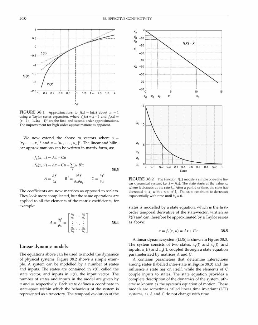
Elsevier UK Chapter: Ch38-P372560 30-9-2006 5:32p.m. Page:510 Trim:7.5in×9.25in
Basal Font:Palatino Margins:Top:40pt Gutter:68pt Font Size:9.5/12 Text Width:42pc Depth:55 Lines
510 38. EFFECTIVE CONNECTIVITY
x0
fL(x)
ln(x)
fB (x)
1
–0.5
–1
–1.5
–2
–2.5
0.5
0
0 0.2 0.4 0.6 0.8 1 1.2 1.4 1.6 1.8 2
FIGURE 38.1 Approximations to f�x� = ln�x� about x0 = 1using a Taylor series expansion, where fL�x� = x − 1 and fB�x� =�x−1�−1/2�x−1�2 are the first- and-second-order approximations.The improvement for high-order approximations is apparent.
We now extend the above to vectors where x =�x1� � � � � xn�T and u = �u1� � � � �um�T . The linear and bilin-ear approximations can be written in matrix form, as:
fL�x�u� = Ax+Cu
fB�x�u� = Ax+Cu+∑j
ujBjx
A = �f
�xB j = �2f
�x�uj
C = �f
�u
38.3
The coefficients are now matrices as opposed to scalars.They look more complicated, but the same operations areapplied to all the elements of the matrix coefficients, forexample:
A = �f
�x=
⎡⎢⎢⎣
�f1�x1
· · · �f1�xn
�fn
�x1· · · �fn
�xn
⎤⎥⎥⎦ 38.4
Linear dynamic models
The equations above can be used to model the dynamicsof physical systems. Figure 38.2 shows a simple exam-ple. A system can be modelled by a number of statesand inputs. The states are contained in x�t�, called thestate vector, and inputs in u�t�, the input vector. Thenumber of states and inputs in the model are given byn and m respectively. Each state defines a coordinate instate-space within which the behaviour of the system isrepresented as a trajectory. The temporal evolution of the
x0
xn x3 x2 x1 x0
x2
x1
x3
xn
x0
x1
x2
x3
xn
f (X ) = X
0
0 5 10 15
–10
–20
–30
–40
–50
–60
–70
–80
Time
15
10
5
00 0.1 0.2 0.3 0.4 0.5 0.6 0.7 0.8 0.9 1
FIGURE 38.2 The function f�x� models a simple one-state lin-ear dynamical system, i.e. ẋ = f�x�. The state starts at the value x0where it decreases at the rate ẋ0. After a period of time, the state hasdecreased to x1 with a rate of ẋ1. The state continues to decreasesexponentially with time until ẋn = 0.
states is modelled by a state equation, which is the first-order temporal derivative of the state-vector, written asẋ�t� and can therefore be approximated by a Taylor seriesas above:
ẋ = fL�x�u� = Ax+Cu 38.5
A linear dynamic system (LDS) is shown in Figure 38.3.The system consists of two states, x1�t� and x2�t�, andinputs, u1�t� and u2�t�, coupled through a state equationparameterized by matrices A and C.
A contains parameters that determine interactionsamong states (labelled inter-state in Figure 38.3) and theinfluence a state has on itself, while the elements of Ccouple inputs to states. The state equation provides acomplete description of the dynamics of the system, oth-erwise known as the system’s equation of motion. Thesemodels are sometimes called linear time invariant (LTI)systems, as A and C do not change with time.

Elsevier UK Chapter: Ch38-P372560 30-9-2006 5:32p.m. Page:511 Trim:7.5in×9.25in
Basal Font:Palatino Margins:Top:40pt Gutter:68pt Font Size:9.5/12 Text Width:42pc Depth:55 Lines
IDENTIFICATION OF DYNAMIC SYSTEMS 511
Inputu1
Inputu2
c 22
c 22
a12
a12
Intrinsicconnectivity
Connectivity toextrinsic input
Inter-state & self
a 21
a 21
c 11
c 11+=
x = Ax + Cu
0
0 u 2
u 1
x2
x1
x1
x1 = a11x1 + a12x2 + c11u1
x2
x1 = a22x2 + a21x1 + c22u2
x2
x1
a 11
a 11
a 22
a 22
.
.
.
. .
FIGURE 38.3 System with two states, x1 and x2, and inputs,u1 and u2, whose dynamics are determined by the time invari-ant matrices A and C in the state equation. The matrices describethe intrinsic connectivity and how states are connected to externalinputs.
Bilinear dynamic models
Linear models are useful because they are a good first-order approximation to many phenomena. However,they furnish rather restricted descriptions of non-linearsystems. The model in Figure 38.4 has been augmentedto illustrate how a bilinear model is formulated. The stateequation adopts the same form as fB, whose essential fea-ture is the bilinear interaction between inputs and states:
ẋ = fB�x�u�
=(
A +m∑
j=1
ujBj
)x+Cu 38.6
= Ãx+Cu
The key difference is the addition of Bj . These scale theinteraction among states and inputs when added to Aand model input-dependent changes to the intrinsic con-nectivity of the network. This is illustrated in Figure 38.4where the coupling coefficient a12 is modulated by theproduct b2
12u2. The modified matrix à operates on thestate vector and determines the response of the model.However, now à changes with time because it is a func-tion of time-varying input. This distinguishes it from theLTI model above.
These systems are simple to integrate over short peri-ods of time, during which the input can be regarded as
Inputu1
Inputu2
a12
b12
a 21
u 2
c 11 c 22
x1
x1 = a11x1 + (a12 + b12u2(t ))x 2+ c11u1
x2 = a22x2 + a21x 1 + c22u2
x2
a 11 a 22
c 22
a12
a 21
c 11++=
0
0 u 2
u 1
x2
x1
x2
x1a 11
a 22 0
0
0
.
. .
x = Ã x + Cu .
.b 12
2
Inducedconnectivity
2
2
à (u ) = A + uj B jΣ
j = 1
m
FIGURE 38.4 A bilinear model. Input u2 interacts with x2,rendering the matrix �u� state-dependent. This induces input-dependent modulation of the coupling parameters, and differentresponses to other inputs, i.e. u1. All connections that are not showncorrespond to zero in the coupling matrices.
constant. In this context, the bilinear form reduces to alocal linear form and Eqn. 38.6 can be re-written as:
ż = Jz
J = M +Nu
z =[
1x
]M =
[0 00 A
]N =
[0 0C B
] 38.7
Here x�t� has been augmented with a constant, whichallows the inputs and states to be treated collectively. Thisequation can be solved using standard linear techniques(Boas, 1983), such as the matrix exponential method (seeAppendix 2).
It helps to consider a specific example. If u2 is binary,the model in Figure 38.4 effectively comprises two LTImodels. The model’s behaviour can be characterized as aswitching between two linear systems. The switch fromone linear mode to the other will be determined byu2. For instance, if the two linear models were linearlydamped harmonic oscillators, each with different periodsof oscillation, a switch from one state to another would beaccompanied by changes in the oscillation of the states.
In bilinear models, inputs can be divided into twoclasses: perturbing and contextual. Perturbing inputsinfluence states directly (e.g. u1 in Figure 38.4). The effectsof these inputs are distributed according to the intrinsicconnections of the model. Conversely, contextual inputs(e.g. u2 in Figure 38.4) reconfigure the response of the
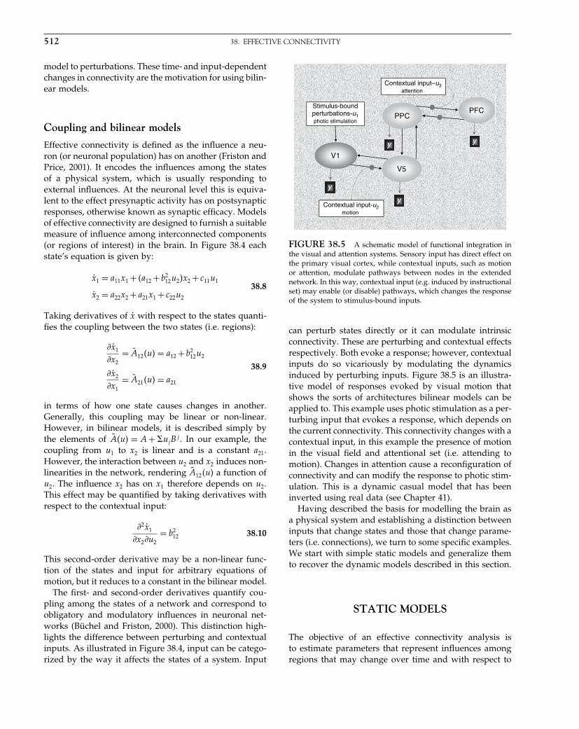
Elsevier UK Chapter: Ch38-P372560 30-9-2006 5:32p.m. Page:512 Trim:7.5in×9.25in
Basal Font:Palatino Margins:Top:40pt Gutter:68pt Font Size:9.5/12 Text Width:42pc Depth:55 Lines
512 38. EFFECTIVE CONNECTIVITY
model to perturbations. These time- and input-dependentchanges in connectivity are the motivation for using bilin-ear models.
Coupling and bilinear models
Effective connectivity is defined as the influence a neu-ron (or neuronal population) has on another (Friston andPrice, 2001). It encodes the influences among the statesof a physical system, which is usually responding toexternal influences. At the neuronal level this is equiva-lent to the effect presynaptic activity has on postsynapticresponses, otherwise known as synaptic efficacy. Modelsof effective connectivity are designed to furnish a suitablemeasure of influence among interconnected components(or regions of interest) in the brain. In Figure 38.4 eachstate’s equation is given by:
ẋ1 = a11x1 + �a12 + b212u2�x2 + c11u1
ẋ2 = a22x2 +a21x1 + c22u2
38.8
Taking derivatives of ẋ with respect to the states quanti-fies the coupling between the two states (i.e. regions):
�ẋ1
�x2= Ã12�u� = a12 + b2
12u2
�ẋ2
�x1= Ã21�u� = a21
38.9
in terms of how one state causes changes in another.Generally, this coupling may be linear or non-linear.However, in bilinear models, it is described simply bythe elements of �u� = A + ujB
j . In our example, thecoupling from u1 to x2 is linear and is a constant a21.However, the interaction between u2 and x2 induces non-linearities in the network, rendering Ã12�u� a function ofu2. The influence x2 has on x1 therefore depends on u2.This effect may be quantified by taking derivatives withrespect to the contextual input:
�2ẋ1
�x2�u2= b2
12 38.10
This second-order derivative may be a non-linear func-tion of the states and input for arbitrary equations ofmotion, but it reduces to a constant in the bilinear model.
The first- and second-order derivatives quantify cou-pling among the states of a network and correspond toobligatory and modulatory influences in neuronal net-works (Büchel and Friston, 2000). This distinction high-lights the difference between perturbing and contextualinputs. As illustrated in Figure 38.4, input can be catego-rized by the way it affects the states of a system. Input
V5
PFC
V1
PPCStimulus-boundperturbations-u1photic stimulation
y
y
y y
Contextual input-u2motion
Contextual input–u3attention
FIGURE 38.5 A schematic model of functional integration inthe visual and attention systems. Sensory input has direct effect onthe primary visual cortex, while contextual inputs, such as motionor attention, modulate pathways between nodes in the extendednetwork. In this way, contextual input (e.g. induced by instructionalset) may enable (or disable) pathways, which changes the responseof the system to stimulus-bound inputs.
can perturb states directly or it can modulate intrinsicconnectivity. These are perturbing and contextual effectsrespectively. Both evoke a response; however, contextualinputs do so vicariously by modulating the dynamicsinduced by perturbing inputs. Figure 38.5 is an illustra-tive model of responses evoked by visual motion thatshows the sorts of architectures bilinear models can beapplied to. This example uses photic stimulation as a per-turbing input that evokes a response, which depends onthe current connectivity. This connectivity changes with acontextual input, in this example the presence of motionin the visual field and attentional set (i.e. attending tomotion). Changes in attention cause a reconfiguration ofconnectivity and can modify the response to photic stim-ulation. This is a dynamic casual model that has beeninverted using real data (see Chapter 41).
Having described the basis for modelling the brain asa physical system and establishing a distinction betweeninputs that change states and those that change parame-ters (i.e. connections), we turn to some specific examples.We start with simple static models and generalize themto recover the dynamic models described in this section.
STATIC MODELS
The objective of an effective connectivity analysis isto estimate parameters that represent influences amongregions that may change over time and with respect to

Elsevier UK Chapter: Ch38-P372560 30-9-2006 5:32p.m. Page:513 Trim:7.5in×9.25in
Basal Font:Palatino Margins:Top:40pt Gutter:68pt Font Size:9.5/12 Text Width:42pc Depth:55 Lines
STATIC MODELS 513
experimental tasks. This rests on the inversion of a causalmodel. Identifying a complete and biologically plausiblemathematical model requires a high level of sophistica-tion. However, some progress can be made by modellingrelationships in the data alone (among voxels or regions),without invoking hidden states and ignoring the conse-quent dynamics. This makes the maths much easier butdiscounts temporal information and is biologically unre-alistic. We will call these models ‘static’ as they modelinstantaneous interactions among regions and ignore theinfluence previous states have on current responses.
Linear models
Linear models assume that each time sample is inde-pendent of the next. This is tenable for positron emis-sion tomography (PET) data because the nature of themeasurement is essentially steady state. Usually, PETdata are acquired while holding brain states constant,using an appropriate task or stimulus and waiting untilsteady-state radiotracer kinetics can be assumed. Math-ematically, this means the rate of change of the states iszero. However, in functional magnetic resonance imag-ing (fMRI), this assumption is generally violated (andcertainly for electrophysiological measurements); this isthe motivation for dynamic models of fMRI and elec-troencephalography (EEG) responses.
In static linear models, the activity of each voxel ismodelled as a linear mixture of activity in all voxels plussome error. This can be expressed as a multivariate linearmodel:
Y = Y�+�
Y =⎡⎢⎣
y1
yT
⎤⎥⎦ 38.11
where yt is a row vector containing all regional measure-ments at time t. The problem with this formulation isthat the trivial solution � = 1 completely accounts for thedata. We will see later how structural equation modellingdeals with this by fixing some connections. Althoughunconstrained linear models cannot address connectivityper se, if we include non-linearities, they can be used toassess changes in connectivity.
Bilinear models
Bilinear models can be used to estimate changes inconnectivity if the bilinear term includes a measure ofneuronal activity. If the bilinear term represents an inter-action between activity and an experimental factor, it can
model the effects of contextual input. If the bilinear termis an interaction between neuronal activities, it can modelmodulatory interactions among populations of neurons.We will focus on the former: the model in Plate 55 (left-hand panel) (see colour plate section) is a simple bilinearmodel. It consists of an input u, which generates an out-put y. The non-linearity is due to an interaction betweenthe input and output. This model comprises a linear andbilinear term parameterized by b1 and b2 respectively.
y = ub1 +uyb2 38.12
If the model contained the first term only, it would belinear and the relationship between input and outputwould be a straight line. The addition of the secondterm introduces non-linear behaviour. Plotting u and yfor different values of b2 demonstrates this. The input-output behaviour depends on b2 and is revealed by thetwo curves in Plate 55 (right-hand panel). It can be seenthat the sensitivity of changes in y to changes in u (i.e.the slope) depends on y. This sort of dependency wasused in Friston et al. (1995) to demonstrate asymmetricalnon-linear interactions between V1 and V2 during visualstimulation. In this example, the bilinear term comprisedfMRI measures of neuronal activity in V1 and V2, corre-sponding to y and u respectively.
The bilinear term in Eqn. 38.12 contains the productof input and activity uy. This is referred to as a psy-chophysiological interaction (PPI). Although we will focuson psychophysiological interaction terms, all that followscan be applied to any bilinear effect. As noted above,these include the interactions between two physiologicalvariates.
Psychophysiological interactions
Büchel et al. (1996) discuss a series of increasingly high-order interaction terms in general linear models. Theseare introduced as new explanatory variables enablingstatistical parametric mapping (SPM) to estimate themagnitude and significance of non-linear effects directly.A special example of this is a psychophysiological inter-action (Friston et al., 1997) where the bilinear termrepresents an interaction between an input or psycholog-ical variable and a response or physiological variable yi
measured at the i-th brain region. Any linear model canbe augmented to include a PPI:
Y = �X u×yi��+� 38.13
The design matrix partition X = �u�yi� � � � � normally con-tains the main effect of experimental input and regionalresponse. The PPI is the Hadamard product u×yi and is

Elsevier UK Chapter: Ch38-P372560 30-9-2006 5:32p.m. Page:514 Trim:7.5in×9.25in
Basal Font:Palatino Margins:Top:40pt Gutter:68pt Font Size:9.5/12 Text Width:42pc Depth:55 Lines
514 38. EFFECTIVE CONNECTIVITY
obtained by multiplying the input and response vectorselement by element. Both the main effects and interactionterms are included because the main effects have to bemodelled to assess properly the additional explanatorypower afforded by the bilinear or PPI term. Standardhypothesis testing can be used to estimate the significanceof the PPI at any point in the brain with an SPM.
Plate 56 illustrates bilinear effects in real data. Thesedata come from an fMRI study of the modulatory effectsof attention on visual responses to radial motion (seeBüchel and Friston, 1998 for experimental details). Theaim was to quantify the top-down modulatory effect ofattention on V1 to V5 connectivity. The model combinespsychological data (attentional set) with physiologicaldata (V1 activity) to model the interaction. The right-handpanel in Plate 56 show a regression analysis of the samedata, divided according to attentional set, to demonstratethe difference in regression slopes subtending this PPI.
In this example, attention was modelled as a ‘con-textual’ variable, while visual stimulation perturbed thesystem. The latter evoked a response within the con-text of the former, i.e. visual stimuli evoke differentresponses depending on attentional set, modelled as achange in connectivity. Here, attention reconfigures con-nection strengths among prefrontal and primary corticalareas (Mesulam, 1998). This bilinear effect may take anyappropriate form in PPI models, including, for example,psychological, physiological or pharmacological indices.These models emphasize the use of factorial experimen-tal designs (Friston et al., 1997) and allow us to considerexperimental inputs in a different light, distinguishingcontextual input (one factor) from direct perturbation(another factor). PPI models have provided importantevidence for the interactions among distributed brainsystems and enabled inferences about task-dependentplasticity using a relatively simple procedure. The modelwe consider next was developed explicitly with effec-tive connectivity or path analysis in mind, but adopts adifferent approach to the estimation of model parame-ters. This approach rests on specifying constraints on theconnectivity.
Structural equation modelling
Structural equation modelling (SEM), or path analysis, isa multivariate method used to test hypotheses regard-ing the influences among interacting variables. Its rootsgo back to the 1920s, when path analysis was developedto quantify unidirectional causal flow in genetic dataand developed further by social scientists in the 1960s(Maruyama, 1998). It was criticized for the limitationsinherent in the least squares method of estimating modelparameters, which motivated a general linear modelling
approach from the 1970s onwards. It is now available incommercial software packages, including LISREL, EQSand AMOS. See Maruyama (1998) for an introduction tothe basic ideas. Researchers in functional imaging startedto use it in the early 1990s (McIntosh and Gonzalez-Lima, 1991, 1992a, b, 1994). It was applied first to ani-mal autoradiographic data and later to human PET datawhere, among other experiments, it was used to iden-tify task-dependent differential activation of the dorsaland ventral visual pathways (McIntosh et al., 1994). Manyinvestigators have used SEM since then. An example ofits use to identify attentional modulation of effective con-nectivity between prefrontal and premotor cortices canbe found in Rowe et al. (2002).
An SEM is a linear model with a number of modifica-tions, which are illustrated in Figure 38.6: the couplingmatrix, �, is ‘pruned’ to include only paths of inter-est. Critically, self-connections are precluded. The datamatrix, Y , contains responses from regions of interest andpossibly experimental or bilinear terms. The underlyingmodel is a general linear model:
Y = Y�+� 38.14
where the free parameters, �, are constrained, accordingto the specified pruning or sparsity structure of connec-tions. To simplify the model, the residuals � are assumedto be independent. They are interpreted as driving eachregion stochastically from one measurement to anotherand are sometimes called innovations.
ε 3
ε 1 ε
2
y
1
y 3
y
2b 12
b 13 b 32
0
0
0 0
0 0
b13b 12
b 32
[ y t
y t = y t β + ε t
1 y t2 y t ] = 3 [ y t
1 y t2 y t ]
3 + ε t
ε t ~ N (0, Σ)
FIGURE 38.6 An SEM is used to estimate path coefficients fora specific network of connections, after ‘pruning’ the connectivitymatrix. The graphic illustrates a particular sparsity structure, whichis usually based on prior anatomical knowledge. yt may containphysiological or psychological data or bilinear terms (to estimatethe influence of ‘contextual’ input). The innovations � are assumedto be independent, and can be interpreted as driving inputs to eachnode.

Elsevier UK Chapter: Ch38-P372560 30-9-2006 5:32p.m. Page:515 Trim:7.5in×9.25in
Basal Font:Palatino Margins:Top:40pt Gutter:68pt Font Size:9.5/12 Text Width:42pc Depth:55 Lines
STATIC MODELS 515
Instead of minimizing the sum of squared errors, thefree parameters are estimated using the sample covari-ance structure of the data. The rationale for this is thatthe covariance reflects the global behaviour of the data,i.e. capturing relationships among variables, in contrastto the former, which reflects the goodness of fit fromthe point of view of each region. Practically, an objectivefunction is constructed from the sampled and impliedcovariance, which is optimized with respect to the param-eters. The implied covariance, ���, is computed easilyby rearranging Eqn. 38.14 and assuming some value forthe covariance of the innovations,
⟨�T �
⟩:
Y�I −�� = �
Y = ��1−��−1
= ⟨Y T Y
⟩= �1−��−T
⟨�T �
⟩�1−��−1
38.15
The sample covariance is:
S = 1n−1
Y T Y
where n is the number of observations and the maximumlikelihood objective function is:
FML = ln � �− tr�S−1�− ln �S� 38.16
This is simply the Kullback-Leibler divergence betweenthe sample and the covariance implied by the free param-eters. A gradient descent, such as a Newton-Raphsonscheme, is generally used to estimate the parameters,which minimize this divergence. The starting values canbe estimated using ordinary least square (OLS) (McIntoshand Gonzalez-Lima, 1994).
Inferences about changes in the parameters or pathcoefficients rest on the notion of nested, or stacked, mod-els. A nested model consists of a free-model within whichany number of constrained models is ‘nested’. In a freemodel, all parameters are free to take values that opti-mize the objective function, whereas a constrained modelhas one, or a number of parameters omitted, constrainedto be zero or equal across models (i.e. attention andnon-attention). By comparing the goodness of fit of eachmodel against the others, �2 statistics can be derived(Bollen, 1989). Hypotheses testing proceeds using thisstatistic. For example, given a constrained model, whichis defined by the omission of a pathway, evidence foror against the pathway can be tested by ‘nesting’ it inthe free model. If the difference in goodness of fit isunlikely to have occurred by chance, the connection canbe declared significant. An example of a nested model
V1 PPC
NAb21
Ab32
Ab32PPC
PPC
PPC
vs.
Constrained-modelFree-model
V5
V1 V5
V1 V5
V1 V5
Ab21
Ab21Ab21
Ab32
Ab32
Ab21NAb21H0 : =
FIGURE 38.7 Inference about changes in connection strengthsproceeds using nested models. Parameters from free and con-strained models are compared with a �2 statistic. This examplecompares path coefficients during attention (A) and non-attention(NA), testing the null hypothesis that the V1 to V5 connections arethe same under both levels of attention.
that was tested by Büchel and Friston (1997) is shown inFigure 38.7.
SEM can accommodate bilinear effects by includingthem as an extra node. A significant connection from abilinear term represents a modulatory effect in exactlythe same way as in a PPI. Büchel and Friston (1997) usedbilinear terms in an SEM of the visual attention data set,to establish the modulation of connections by prefrontalcortex. In this example, the bilinear term comprised mea-surements of activity in two brain regions. An interestingextension of SEM has been to look at models of connec-tivity over multiple brains (i.e. subjects). The nice thingabout this is that there are no connections between brains,which provide sparsity constraints on model inversion(see Mechelli et al., 2002).
SEM shares the same limitations as the linear modelapproach described above, i.e. temporal information isdiscounted.1 However, it has enjoyed relative success andbecome established over the past decade due, in part, toits commercial availability as well as its intuitive appeal.However, it usually requires a number of rather ad hocprocedures, such as partitioning the data to create nestedmodels, or pruning the connectivity matrix to render thesolution tractable. These problems are confounded withan inability to capture non-linear features and tempo-ral dependencies. By moving to dynamic models, weacknowledge the effect of an input’s history and embeda priori knowledge into models at a more plausible andmechanistic level. These issues will be addressed in thefollowing section.
1 There are extensions of SEM that model dynamic informationby using temporal embedding. However, these are formally thesame as the multivariate autoregressive models discussed in thenext section.

Elsevier UK Chapter: Ch38-P372560 30-9-2006 5:32p.m. Page:516 Trim:7.5in×9.25in
Basal Font:Palatino Margins:Top:40pt Gutter:68pt Font Size:9.5/12 Text Width:42pc Depth:55 Lines
516 38. EFFECTIVE CONNECTIVITY
DYNAMIC MODELS
The static models described above discount temporalinformation. Consequently, permuted data sets producethe same path coefficients as the original data. Modelsthat use the order in which data are produced are morenatural candidates for neuronal dynamics. In this sectionwe will review Kalman filtering, autoregressive and gen-eralized convolution models (see Chapters 39 and 40).
The Kalman filter
The Kalman filter is used in engineering to model dynam-ics (Juang, 2001). It is based on a state-space model thatinvokes an extra set of [hidden] variables to generatedata. These models are useful because long-range tem-poral order, within observed data, is modelled throughinteractions among hidden states, instead of mappinginput directly onto output (see below). The Kalman filteris an ‘online’ procedure consisting of two steps: predic-tion and correction (or update). The hidden states areestimated (prediction step) using the information up untilthe present, which is updated (correction step) on receiptof each new measurement. These two steps are repeatedrecursively as new information arrives. A simple exam-ple demonstrates intuitively how the filter works. Thisexample is taken from Ghahramani (2002).
Consider a series of data, which are received sequen-tially. Say we wanted to calculate a running average witheach new data point. The estimate of the mean (whichwe will call the ‘state’) after t values of x is x̂t, where:
x̂t = 1t
∑t
xt and x̂t−1 = 1t −1
∑t−1
xt−1 ⇒
x̂t = t −1t
x̂t−1 + 1txt
= x̂t−1 +K �xt − x̂t−1�
38.17
where K is the Kalman Gain = 1/t. This example givesthe basic idea behind Kalman filtering and illustrates itsgeneral form: a prediction and a weighted correction (fora less heuristic introduction, see Appendix 5). The fil-ter balances two types of information from a prediction(based on previous data) and an observation, weightedby their respective precisions using Bayes’ rule. If themeasured data are not reliable, K goes to zero, weightingthe prediction error less and relying more on the preced-ing prediction. Conversely, if sequential dependence islow, then K is large, emphasizing information providedby the data when constructing an estimate of the currentstate. The quantities required in the forward recursionare the Kalman Gain and the mean and covariance of the
prediction. A backward recursive algorithm called theKalman Smoother calculates the mean and covariance ofthe states using data from the future, which is a post hocprocedure to improve estimates.
Kalman filtering and smoothing are generally appliedto state-space models in discrete time (see Appendix 5).To understand how the filter is applied we start with thefamiliar linear observation model:
yt = xt�t +�t
�t ∼ N�0�R�38.18
Here y and x are univariate and are both known, e.g.blood oygenation-level-dependent (BOLD) activity fromV1 and V5. However, � is now a variable parame-ter or state that is observed vicariously through BOLDresponses and changes with time according to the updateequation:
�t = �t−1 +�t
�t ∼ N�0�Q�38.19
�t is a further innovation. Given this model, the Kalmanfilter can be used to estimate the evolution of the hiddenstate or variable parameter, �. Note that if �t = 0 then�t = �t−1. This is the static estimate from an ordinaryregression analysis. In this form of states-space model,the states play the role of variable parameters. This iswhy this application of Kalman filtering is also knownas variable parameter regression.
Büchel and Friston (1998) used Kalman filtering tomeasure effective connectivity between V1 and V5: bymodelling the path coefficient as a hidden state, the filterdisclosed fluctuations in the coupling, which changed withattention (even though attentional status did not enter themodel).Figure38.8 illustrates themodelandplots the time-dependent estimate, �t, for V1 to V5 connectivity (lowerpanel). This reveals fluctuations that match changes inattentional set; the light grey bars indicate periods of atten-tion to visual motion and the dark grey bars, periods with-out attention. The connection is clearly much strongerduring attention, suggesting that attention to motion hasenabled the forward connections from V1 to V5. Theresults of this analysis show that there is task-dependentvariation in inter-regional connectivity. Critically, thisvariation was estimated from the data. However, in gen-eral, these changes in connectivity are induced experi-mentally by known and deterministic causes.
In Chapter 41, we return to hidden-state models andre-analyse the attentional data set in a way that allowsdesigned manipulations of attention to affect the hiddenstates of a causal model. In dynamic casual modelling, thestates are dynamic variables (e.g. neuronal activity) and

Elsevier UK Chapter: Ch38-P372560 30-9-2006 5:32p.m. Page:517 Trim:7.5in×9.25in
Basal Font:Palatino Margins:Top:40pt Gutter:68pt Font Size:9.5/12 Text Width:42pc Depth:55 Lines
DYNAMIC MODELS 517
States (variable parameters)
Output (observations)
Update equation:
Observation equation:
Time (scans)
Tim
e-va
ryin
g re
gres
sion
0.5
0.8
βt – 2
y t – 2 y t – 1 y t y t + 1
βt – 1 βt
βt = βt – 1 + ηt
βt + 1
ηt ~ N (0,Q )
yt = xt βt + εt εt ~ N (0,R )
βt
FIGURE 38.8 State-space model of the path coefficientbetween V1 and V5. Connection strengths are modelled as a hiddenstate (or variable parameter) that changes with time, according tothe update equation (upper panel). Its evolution is estimated usingthe Kalman filter. This empirical example reveals fluctuations thatmatch changes in attentional set (lower panel). The light grey barsindicate periods of attention to visual motion and the dark grey bars,periods without attention. The connection is clearly much strongerduring attention, suggesting that attention to motion has enabledthe forward connections from V1 to V5.
the effective connectivity corresponds to fixed parametersthat can interact with time-varying states and inputs.2
The remainder of this chapter focuses on approaches thatdo not refer to hidden states, such as autoregressive andgeneralized convolution models.
Multivariate autoregressive models
Sequential measurements often contain temporal infor-mation that can provide insight into the physical mecha-nisms generating them. A simple and intuitive model oftemporal order is an autoregressive (AR) model, where
2 This should be contrasted with Kalman filtering, in which theconnectivity itself was presumed to be a time-varying state.
the value of a variable at a particular time depends onpreceding values.
The parameters of AR models comprise regressioncoefficients, at successive time lags, that encode sequen-tial dependencies of the system in a simple and effectivemanner. This model can be extended to include sev-eral variables with dependencies among variables at dif-ferent lags. These dependencies may be interpreted asthe influence of one variable on another and can, withsome qualification, be regarded as measures of effec-tive connectivity. Models involving many variables arecalled multivariate autoregressive (MAR) models andhave been used to measure dependencies among regionalactivities as measured with fMRI (Goebel et al., 2003;Harrison et al., 2003).
MAR models do not invoke hidden states. Instead,correlations among measurements at different time lagsare used to quantify coupling. This incorporates historyinto the model in a similar way to the Volterra approachdescribed below. MAR models are linear, but can beextended to include bilinear interaction terms (Pennyet al., 2005). To understand MAR we will build up amodel from a univariate AR model and show that MARmodels conform to general linear models (GLMs) withtime-lagged explanatory variables.
Consider data at voxel i at time t modelled as a linearcombination of previous values, plus an innovation:
yit = �yi
t−1� � � � � yit−p�
⎡⎢⎣
w1
wp
⎤⎥⎦+�t 38.20
w is a p×1 column vector containing the model param-eters (AR coefficients). Here the explanatory variablesare now preceding values over different time lags. Wecan extend the model to d-regions contained in the rowvector:
yt =p∑
j=1
�y1t−j� � � � � yd
t−j �
⎡⎢⎣
w11j · · · w1d
j
wd1j wdd
j
⎤⎥⎦+ ��1� � � � � �d�
=p∑
j=1
yt−jWj +� 38.21
which has d×d parameters Wj at each time lag, describ-ing interactions among all pairs of variables. This is sim-ply a GLM whose parameters can be estimated in theusual way to give W , which is a p × d × d array of ARcoefficients (see Figure 38.9 for a schematic of the model).There are no inputs to the model, except for the errors,which play the role of innovations (cf. SEM). This meansthat experimentally designed effects have no explicit role(unless they enter through bilinear terms). However, themodel attempts to identify relations between variables
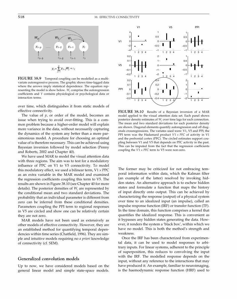
Elsevier UK Chapter: Ch38-P372560 30-9-2006 5:32p.m. Page:518 Trim:7.5in×9.25in
Basal Font:Palatino Margins:Top:40pt Gutter:68pt Font Size:9.5/12 Text Width:42pc Depth:55 Lines
518 38. EFFECTIVE CONNECTIVITY
y t – p
W p W 2 W 1
y t – 2
ε t – 3 ε t – 2 ε t – 1 ε t
y t – 1 y t
y t – jWj + ε t y t = Σj = 1
p
. . . .
FIGURE 38.9 Temporal coupling can be modelled as a multi-variate autoregressive process. The graphic shows time-lagged datawhere the arrows imply statistical dependence. The equation rep-resenting the model is show below. Wj comprise the autoregressioncoefficients and Y contains physiological or psychological data orinteraction terms.
over time, which distinguishes it from static models ofeffective connectivity.
The value of p, or order of the model, becomes anissue when trying to avoid over-fitting. This is a com-mon problem because a higher-order model will explainmore variance in the data, without necessarily capturingthe dynamics of the system any better than a more par-simonious model. A procedure for choosing an optimalvalue of is therefore necessary. This can be achieved usingBayesian inversion followed by model selection (Pennyand Roberts, 2002 and Chapter 40).
We have used MAR to model the visual attention datawith three regions. The aim was to test for a modulatoryinfluence of PPC on V1 to V5 connectivity. To modelthis modulatory effect, we used a bilinear term, V1×PPCas an extra variable in the MAR model and examinedthe regression coefficients coupling this term to V5. Theresults are shown in Figure 38.10 (see Chapter 40 for moredetails). The posterior densities of Wj are represented bythe conditional mean and two standard deviations. Theprobability that an individual parameter is different fromzero can be inferred from these conditional densities.Parameters coupling the PPI term to regional responsesin V5 are circled and show one can be relatively certainthey are not zero.
MAR models have not been used as extensively asother models of effective connectivity. However, they arean established method for quantifying temporal depen-dencies within time series (Chatfield, 1996). They are sim-ple and intuitive models requiring no a priori knowledgeof connectivity (cf. SEM).
Generalized convolution models
Up to now, we have considered models based on thegeneral linear model and simple state-space models.
V1
V1
V5
V5
PPI
PPI
4
2
0
1 2 3 4 1 2 3 4 1 2 3 4
1 2 3 41 2 3 4
1 2 3 4 1 2 3 4 1 2 3 4
1 2 3 4
–2
–4
2
1
0
–1
–2
2
1
0
–1
–2
1
0.5
0
–0.5
–1
1
0.5
0
–0.5
–1
1
0.5
0
–0.5
–1
0.2
0.1
0
–0.1
–0.2
0.2
0.1
0
–0.1
–0.2
0.2
0
–0.2
–0.4
0.4
FIGURE 38.10 Results of a Bayesian inversion of a MARmodel applied to the visual attention data set. Each panel showsposterior density estimates of Wj over time lags for each connection.The mean and two standard deviations for each posterior densityare shown. Diagonal elements quantify autoregression and off diag-onals crossregressions. The variates used were: V1, V5 and PPI; thePPI term was the Hadamard product V1 × PFC of activity in V1and the prefrontal cortex (PFC). The circled estimates support cou-pling between V1 and V5 that depends on PFC activity in the past.This can be imputed from the fact that the regression coefficientscoupling the V1×PFC term to V5 were non-zero.
The former may be criticized for not embracing tem-poral information within data, which the Kalman filter(an example of the latter) resolved by invoking hid-den states. An alternative approach is to eschew hiddenstates and formulate a function that maps the historyof input directly onto output. This can be achieved bycharacterizing the response (output) of a physical systemover time to an idealized input (an impulse), called animpulse response function (IRF) or transfer function (TF).In the time domain, this function comprises a kernel thatquantifies the idealized response. This is convenient asit bypasses any hidden states generating the data. How-ever, it renders the system a ‘black box’, within which wehave no model. This is both the method’s strength andweakness.
Once the IRF has been characterized from experimen-tal data, it can be used to model responses to arbi-trary inputs. For linear systems, adherent to the principleof superposition, this reduces to convolving the inputwith the IRF. The modelled response depends on theinput, without any reference to the interactions that mayhave produced it. An example, familiar to neuroimaging,is the haemodynamic response function (HRF) used to
Elsevier UK Chapter: Ch38-P372560 30-9-2006 5:32p.m. Page:519 Trim:7.5in×9.25in
Basal Font:Palatino Margins:Top:40pt Gutter:68pt Font Size:9.5/12 Text Width:42pc Depth:55 Lines
DYNAMIC MODELS 519
model the haemodynamic response of the brain to stim-ulus functions. However, we would like to cover non-linear models, which obtain by generalizing the notionof convolution models to include high-order interac-tions among inputs, an approach originally developed byVolterra in 1930 (Rieke et al., 1997).
The generalized non-linear state and observation equa-tions of any analytic system are, respectively:
ẋ�t� = f�x�t��u�t��
y�t� = g�x�t��u�t��38.22
These can be reformulated to relate output to input,y�t� = h�u�t−��� without reference to the states x�t�. Thismapping is a non-linear functional Taylor expansion:
y�t� = h0 +�∫
−�h1��1�u�t −�1�d�1
+�∫
−�
�∫−�
h2��1� �2�u�t −�1�u�t −�2�d�1d�2 +· · ·
+�∫
−�� � �
�∫−�
hn��1� · · · � �n�u�t −�1� · · ·u�t −�n�d�1 · · ·d�n
38.23
where n is the order of the series and may take any posi-tive integer to infinity. This is known as a Volterra series.Under certain conditions, h converges as n increases(Fliess et al., 1983) and can provide a complete descrip-tion of a system, given enough terms. To understandthis we need to consider the Taylor series expansionas a means of approximating a general non-linear func-tion (see Figure 38.1). Any sufficiently smooth non-linearfunction can be approximated, within the neighbourhoodof an expansion point x0, by scaling increasingly high-order terms, computed from derivatives of the functionabout x0 (see Eqn. 38.1). The Volterra series is a Tay-lor series expansion, where high-order terms are con-structed from variables modelling interactions and scaledby time-varying coefficients. The Volterra series is apower-series expansion where the coefficients are nowfunctions, known as kernels. The kernels are functions oftime and, as the series involves functions of functions,they are known as functionals.
An increase in accuracy of the approximation isachieved by considering higher order terms, as demon-
strated by deriving linear and bilinear models. The sameis true of the linear and bilinear convolution models:
y�t� ≈ h0 +�∫
0
h1��1�u�t −�1���1
y�t� ≈ h0 +�∫
0
h1��1�u�t −�1���1
+�∫
0
�∫0
h2��1� �2�u�t −�1�u�t −�2���1��2
38.24
Note that the integrals in Eqn. 38.24 are from zero toinfinity. This means the response depends only on pastinputs. This renders the system casual (cf. the acausalsystem in Eqn. 38.23). The HRF derives from a linear con-volution model. The system’s IRF and the occurrencesof experimental trials are therefore h1 and u�t� respec-tively. The linear model complies with the principle ofsuperposition: given two, the response is simply thesum of the two responses. By including the second-orderkernel, non-additive responses can be modelled. Practi-cally, this means that the timing of inputs is importantin that different pairs of inputs may produce differentresponses. The Volterra formulation is a generalizationof the convolution model, which convolves increasinglyhigh-order interactions with multidimensional kernels toapproximate the non-additive components of a system’sresponse.
Kernels scale the effect each input, in the past, hashad on the current response. As such, Volterra serieshave been described as ‘power series with memory’.Sequential terms embody increasingly complex interac-tions among inputs up to arbitrary order. The seriesconverges with increasing terms which, for weakly non-linear systems, is assumed to occur after the second-orderterm. A schematic, showing how two inputs can producean output in a bilinear convolution model, is shown inFigure 38.11.
The first and second-order kernels quantify the linearand bilinear responses; this means they encode first- andsecond-order effective connectivity respectively (Friston,2000). More specifically, the kernels map the input in thepast to the current response:
h1��1� = �y�t�
�u�t −�1�
h2��1� �2� = �2y�t�
�u�t −�1��u�t −�2�38.25
� � �
Having established the Volterra kernel as a measureof effective connectivity, we need to estimate them from

Elsevier UK Chapter: Ch38-P372560 30-9-2006 5:32p.m. Page:520 Trim:7.5in×9.25in
Basal Font:Palatino Margins:Top:40pt Gutter:68pt Font Size:9.5/12 Text Width:42pc Depth:55 Lines
520 38. EFFECTIVE CONNECTIVITY
u1(t )
y (t )
u2(t )
12h2
h11
h12
FIGURE 38.11 Schematic showing how two inputs can pro-duce an output. Linear contributions from each input are formed byconvolution with their respective first-order kernels h1. In addition,non-additive responses, due to non-linear interactions between thetwo inputs and hidden states, are modelled by convolution with thesecond-order kernel, h2. Note that the second-order kernel is twodimensional.
experimental data. By reformulating the model usingan appropriate basis set, kernels can be reconstructedfrom estimated coefficients. The HRF is modelled well bygamma functions and this is the reason for choosing themto approximate Volterra kernels. Generally, the Volterrakernels for an arbitrarily non-linear dynamic system aredifficult to compute unless the underlying generativeprocess leading to the data is fairly well characterized.
A bilinear convolution model can be reformulated byconvolving the inputs with the basis set bi and using theset of convolved inputs in a GLM:
y�t� = �0 +n∑
i=1
�ixi�t�+n∑
i=1
n∑j=1
�ijxi�t�xj�t�
xi�t� =∫
bi��1�u�t −�1���1
38.26
The kernels are then recovered by:
h0 = �0
h1��1� =n∑
i=1
�ibi��1� 38.27
h2��1� �2� =n∑
i=1
n∑j=1
�ijbi��1�bj��2�
This method was applied to the attentional data set usedpreviously. The model consisted of inputs from threeregions: putamen, V1 complex and posterior parietal cor-tex (PPC), to V5, as shown in Figure 38.12. BOLD record-ings from these regions were used as an index of neuronalactivity, representing input to V5. The lower panel illus-trates responses to simulated inputs, using the empiri-cally determined kernels. It shows the response of V5 to
PPC activity = 0 SPM{F }
PPC activity = 1
V1 Pul.
V5
PPC
Res
pons
e of
V5
to im
puls
e fr
om V
1
Time (s)0 10 20 30 40 50 60
1.2
1
0.8
0.6
0.4
0.2
0
–0.2
FIGURE 38.12 Top: brain regions and connections compris-ing a Volterra model of visually evoked responses. Bottom: char-acterization of the effects of V1 inputs on V5 and their modulationby posterior parietal cortex (PPC). Broken lines represent estimatesof V5 responses when PPC activity is zero, according to a second-order Volterra model of effective connectivity with inputs to V5from V1, PPC and the pulvinar (Pul.). The solid curve represents thesame response when PPC activity is one standard deviation of itsbetween-condition variation. It is evident that V1 has an activatingeffect on V5 and that PPC increases the responsiveness of V5 to theseinputs. The insert shows all the voxels in V5 that evidenced a modu-latory effect (p < 005 uncorrected). These voxels were identified bythresholding a statistical parametric map of the F -statistic, testingfor the contribution of second-order kernels involving V1 and PPC(treating all other terms as nuisance variables). The fMRI data wereobtained under identical stimulus conditions (visual motion sub-tended by radially moving dots) while manipulating the attentionalcomponent of the task (detection of velocity changes).
an impulse from V1 and provides a direct comparison ofV5 responses to the same input from V1, with and with-out prefrontal cortex (PFC) activity. The influence of PFCis clear and reflects its enabling of V1 to V5 connectivity.This is an example of second-order effective connectivity.
The Volterra method has many useful qualities. Itapproximates non-linear behaviour within the familiarframework of a generalized convolution model. Ker-nels can be estimated using a GLM and inferencesmade under parametric assumptions. Furthermore, ker-nels contain the dynamic information we require to mea-sure effective connectivity. However, kernels characterize
Elsevier UK Chapter: Ch38-P372560 30-9-2006 5:32p.m. Page:521 Trim:7.5in×9.25in
Basal Font:Palatino Margins:Top:40pt Gutter:68pt Font Size:9.5/12 Text Width:42pc Depth:55 Lines
REFERENCES 521
an ideal response, generalized to accommodate non-linear behaviour, which is effectively a summary ofinput-output behaviour. It should also be noted thatVolterra series are only local approximations aroundan expansion point. Although they may be extremelygood approximations for some systems, they may not befor others. For instance, Volterra series cannot capturethe behaviour of periodic or chaotic dynamics (i.e. non-controllable systems). A major weakness of the methodis that we have no notion of the internal mechanisms thatgenerated the data, and this is one motivation for turningto dynamic causal models.
CONCLUSION
This chapter has described different methods of mod-elling inter-regional coupling using neuroimaging data.The development and application of these methods ismotivated by the importance of changes in effective con-nectivity in development, cognition and pathology. Wehave portrayed the models incrementally, starting withlinear regression models and ending with bilinear convo-lution models. In the next three chapters we will revisitbilinear models. Bilinear models cover plasticity inducedby environmental and neurophysiological changes, whileretaining mathematical tractability of linear models.
REFERENCES
Boas ML (1983) Mathematical models in the physical sciences. JohnWiley & Sons, New York
Bollen KA (1989) Structural equations with latent variables. John Wiley& Sons, New York
Büchel C, Friston K (2000) Assessing interactions among neuronalsystems using functional neuroimaging. Neural Netw 13: 871–82
Büchel C, Friston KJ (1997) Modulation of connectivity in visualpathways by attention: cortical interactions evaluated with struc-tural equation modelling and fMRI. Cereb Cortex 7: 768–78
Büchel C, Friston KJ (1998) Dynamic changes in effective connectiv-ity characterized by variable parameter regression and Kalmanfiltering. Hum Brain Mapp 6: 403–08
Büchel C, Wise RJ, Mummery CJ et al. (1996) Nonlinear regressionin parametric activation studies. NeuroImage 4: 60–66
Chatfield C (1996) The analysis of time series: an introduction. CRCPress, Florida
Dayan P, Abbott L (2001) Theoretical Neuroscience. MIT, Cambridge,MA
Fliess M, Lamnabhi M, Lamnabhi-Lagarrigue F (1983) An algebraicapproach to nonlinear functional expansions. IEEE Trans CircSyst 30: 554–70
Friston KJ (2000) The labile brain. I. Neuronal transients and non-linear coupling. Philos Trans R Soc Lond B Biol Sci 355: 215–36
Friston KJ, Buechel C, Fink GR et al. (1997) Psychophysiologicaland modulatory interactions in neuroimaging. NeuroImage 6:218–29
Friston KJ, Price CJ (2001) Dynamic representations and generativemodels of brain function. Brain Res Bull 54: 275–85
Friston KJ, Ungerleider LG, Jezzard P et al. (1995) Characterizingmodulatory interactions between areas V1 and V2 in humancortex: a new treatment of functional MRI data. Hum Brain Mapp2: 211–24
Ghahramani Z (2002) Unsupervised learning course (lecture 4).www.gatsby.ucl.ac.uk/∼zoubin/index.html
Glass L (2001) Synchronization and rhythmic processes in physiol-ogy. Nature 410: 277–84
Glass L, Kaplan D (2000) Understanding nonlinear dynamics. SpringerVerlag, New York
Goebel R, Roebroeck A, Kim DS et al. (2003) Investigating directedcortical interactions in time-resolved fMRI data using vectorautoregressive modeling and Granger causality mapping. MagRes Imag 21: 1251–61
Harrison L, Penny WD, Friston K (2003) Multivariate autoregressivemodeling of fMRI time series. NeuroImage 19: 1477–91
Juang J-N (2001) Identification and control of mechanical systems. Cam-bridge University Press, Cambridge
Maruyama GM (1998) Basics of structural equation modelling. SagePublications, Inc., California
McIntosh AR, Gonzalez-Lima F (1991) Structural modelling of func-tional neural pathways mapped with 2-deoxyglucose: effects ofacoustic startle habituation on the auditory system 7. Brain Res547: 295–302
McIntosh AR, Gonzalez-Lima F (1992a) The application of structuralequation modelling to metabolic mapping of functional neu-ral systems. In Advances in metabolic mapping techniques for brainimaging of behavioural and learning functions. Kluwer AcademicPublishers, Dordrecht, pp 219–55
McIntosh AR, Gonzalez-Lima F (1992b) Structural modelling offunctional visual pathways mapped with 2-deoxyglucose: effectsof patterned light and footshock. Brain Res 578: 75–86
McIntosh AR, Gonzalez-Lima F (1994) Structural equation mod-elling and its application to network analysis in functional brainimaging. Hum Brain Mapp 2: 2–22
McIntosh AR, Grady CL, Ungerleider LG et al. (1994) Network anal-ysis of cortical visual pathways mapped with PET. J Neurosci 14:655–66
Mechelli A, Penny WD, Price CJ et al. (2002) Effective connectivityand intersubject variability: using a multisubject network to testdifferences and commonalities. NeuroImage 17: 1459–69
Mesulam MM (1998) From sensation to cognition. Brain 121:1013–52
Penny W, Ghahramani Z, Friston K (2005) Bilinear dynamical sys-tems. Philos Trans R Soc Lond B Biol Sci 360: 983–93
Penny W, Roberts SJ (2002) Bayesian multivariate autoregressivemodels with structured priors. IEE Proc-Vis Image Signal Process149: 33–41
Rao TS (1992) Identification of bilinear time series models 5. StatSinica 2: 465–78
Rieke F, Warland D, de Ruyter van Steveninck R et al. (1997) Foun-dations. In Spikes: exploring the neural code. MIT, Cambridge, MA,pp 38–48
Rowe J, Friston K, Frackowiak R et al. (2002) Attention to action:specific modulation of corticocortical interactions in humans.NeuroImage 17: 988–98
Scott A (1999) Nonlinear science: emergence & dynamics of coherentstructures. Oxford University Press, Oxford

Elsevier UK Chapter: Ch39-P372560 30-9-2006 5:33p.m. Page:522 Trim:7.5in×9.25in
Basal Font:Palatino Margins:Top:40pt Gutter:68pt Font Size:9.5/12 Text Width:42pc Depth:55 Lines
C H A P T E R
39
Non-linear coupling and kernelsK. Friston
INTRODUCTION
This chapter revisits the Volterra formulation of effectiveconnectivity from a conceptual and neurobiological pointof view. Recall from the previous chapter that the gener-alized convolution representation, afforded by Volterraexpansions, is just a way of describing the input-outputbehaviour of dynamic systems that have an equivalentstate-space representation. In subsequent chapters, wewill deal with state-space representations in more detail.Before proceeding to explicit input-state-output models,we will look at why the Volterra formulation is a usefulsummary of input-output relationships in this chapterand the role of multivariate autoregression models ofoutput-output relationships in the next chapter.
The brain as a dynamic system
The brain can be regarded as an ensemble of con-nected dynamical systems and, as such, conforms tosome simple principles relating the inputs and out-puts of its constituent parts. The implications for theway we think about and measure neuronal interactionscan be quite profound. These range from implicationsfor which aspects of neuronal activity are important tomeasure and how to characterize coupling among neu-ronal populations, to implications pertaining to dynamicinstability and complexity that is necessary for adaptiveself-organization.
This chapter focuses on the first issue by looking atneuronal interactions, coupling and implicit neuronalcodes from a dynamical perspective. In brief, by consid-ering the brain in this light one can show that a sufficientdescription of neuronal activity must comprise activityat the current time and its recent history. This history
constitutes a neuronal transient. Such transients repre-sent an essential metric of neuronal interactions and,implicitly, a code employed in the functional integra-tion of brain systems. The nature of transients, expressedcoincidently in different neuronal populations, reflectstheir underlying coupling. A complete description ofthis coupling, or effective connectivity, can be expressedin terms of generalized convolution [Volterra] kernelsthat embody high-order or non-linear interactions. Thiscoupling may be synchronous, and possibly oscillatory,or asynchronous. A critical distinction between syn-chronous and asynchronous coupling is that the for-mer is essentially linear and the latter is non-linear.The non-linear nature of asynchronous coupling enablescontext-sensitive interactions that characterize real braindynamics, suggesting that it plays an important role infunctional integration.
Brain states are inherently labile, with a complexity anditinerancy that renders their invariant characteristics elu-sive. The basic idea pursued here is that the dynamics ofneuronal systems can be viewed as a succession of tran-sient spatiotemporal patterns of activity. These transientsare shaped by the brain’s infrastructure, principally con-nections, which have been selected to ensure the adap-tive nature of the resulting dynamics. Although ratherobvious, this formulation embodies a fundamental point,namely, that any description of brain state should havean explicit temporal dimension. In other words, mea-sures of brain activity are only meaningful when speci-fied over periods of time. This is particularly importantin relation to fast dynamic interactions among neuronalpopulations that are characterized by synchrony. Syn-chronization has become a central theme in neuroscience(e.g. Gray and Singer, 1989; Eckhorn et al., 1988; Engelet al., 1991) and yet represents only one possible sort ofinteraction.
Statistical Parametric Mapping, by Karl Friston et al. Copyright 2007, Elsevier Ltd. All rights reserved.ISBN–13: 978-0-12-372560-8 ISBN–10: 0-12-372560-7
522
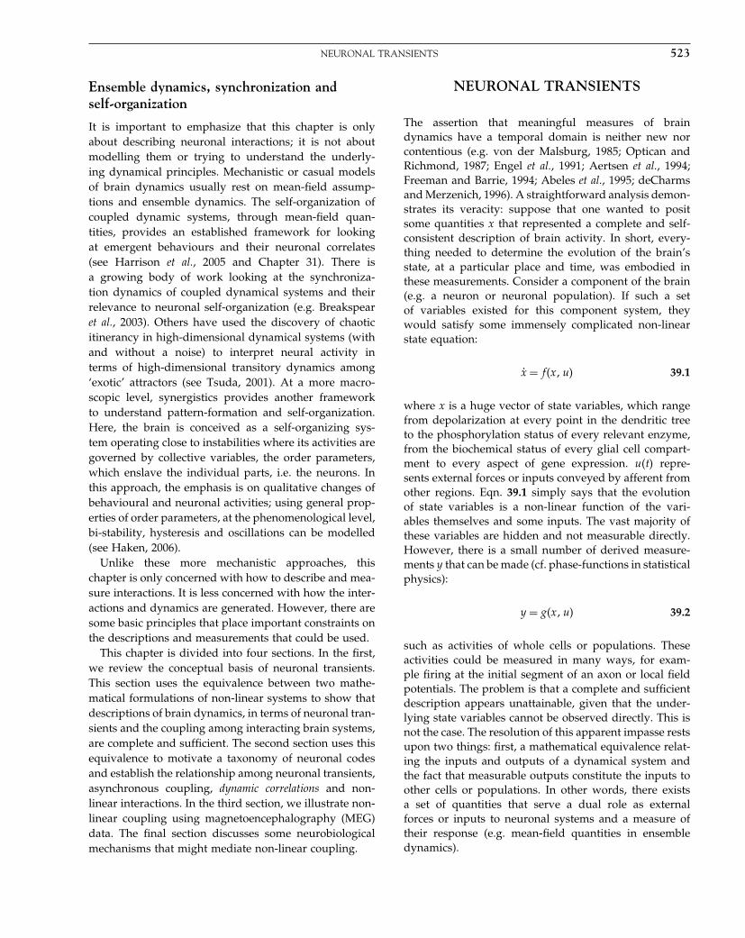
Elsevier UK Chapter: Ch39-P372560 30-9-2006 5:33p.m. Page:523 Trim:7.5in×9.25in
Basal Font:Palatino Margins:Top:40pt Gutter:68pt Font Size:9.5/12 Text Width:42pc Depth:55 Lines
NEURONAL TRANSIENTS 523
Ensemble dynamics, synchronization andself-organization
It is important to emphasize that this chapter is onlyabout describing neuronal interactions; it is not aboutmodelling them or trying to understand the underly-ing dynamical principles. Mechanistic or casual modelsof brain dynamics usually rest on mean-field assump-tions and ensemble dynamics. The self-organization ofcoupled dynamic systems, through mean-field quan-tities, provides an established framework for lookingat emergent behaviours and their neuronal correlates(see Harrison et al., 2005 and Chapter 31). There isa growing body of work looking at the synchroniza-tion dynamics of coupled dynamical systems and theirrelevance to neuronal self-organization (e.g. Breakspearet al., 2003). Others have used the discovery of chaoticitinerancy in high-dimensional dynamical systems (withand without a noise) to interpret neural activity interms of high-dimensional transitory dynamics among‘exotic’ attractors (see Tsuda, 2001). At a more macro-scopic level, synergistics provides another frameworkto understand pattern-formation and self-organization.Here, the brain is conceived as a self-organizing sys-tem operating close to instabilities where its activities aregoverned by collective variables, the order parameters,which enslave the individual parts, i.e. the neurons. Inthis approach, the emphasis is on qualitative changes ofbehavioural and neuronal activities; using general prop-erties of order parameters, at the phenomenological level,bi-stability, hysteresis and oscillations can be modelled(see Haken, 2006).
Unlike these more mechanistic approaches, thischapter is only concerned with how to describe and mea-sure interactions. It is less concerned with how the inter-actions and dynamics are generated. However, there aresome basic principles that place important constraints onthe descriptions and measurements that could be used.
This chapter is divided into four sections. In the first,we review the conceptual basis of neuronal transients.This section uses the equivalence between two mathe-matical formulations of non-linear systems to show thatdescriptions of brain dynamics, in terms of neuronal tran-sients and the coupling among interacting brain systems,are complete and sufficient. The second section uses thisequivalence to motivate a taxonomy of neuronal codesand establish the relationship among neuronal transients,asynchronous coupling, dynamic correlations and non-linear interactions. In the third section, we illustrate non-linear coupling using magnetoencephalography (MEG)data. The final section discusses some neurobiologicalmechanisms that might mediate non-linear coupling.
NEURONAL TRANSIENTS
The assertion that meaningful measures of braindynamics have a temporal domain is neither new norcontentious (e.g. von der Malsburg, 1985; Optican andRichmond, 1987; Engel et al., 1991; Aertsen et al., 1994;Freeman and Barrie, 1994; Abeles et al., 1995; deCharmsand Merzenich, 1996). A straightforward analysis demon-strates its veracity: suppose that one wanted to positsome quantities x that represented a complete and self-consistent description of brain activity. In short, every-thing needed to determine the evolution of the brain’sstate, at a particular place and time, was embodied inthese measurements. Consider a component of the brain(e.g. a neuron or neuronal population). If such a setof variables existed for this component system, theywould satisfy some immensely complicated non-linearstate equation:
ẋ = f�x�u� 39.1
where x is a huge vector of state variables, which rangefrom depolarization at every point in the dendritic treeto the phosphorylation status of every relevant enzyme,from the biochemical status of every glial cell compart-ment to every aspect of gene expression. u�t� repre-sents external forces or inputs conveyed by afferent fromother regions. Eqn. 39.1 simply says that the evolutionof state variables is a non-linear function of the vari-ables themselves and some inputs. The vast majority ofthese variables are hidden and not measurable directly.However, there is a small number of derived measure-ments y that can be made (cf. phase-functions in statisticalphysics):
y = g�x�u� 39.2
such as activities of whole cells or populations. Theseactivities could be measured in many ways, for exam-ple firing at the initial segment of an axon or local fieldpotentials. The problem is that a complete and sufficientdescription appears unattainable, given that the under-lying state variables cannot be observed directly. This isnot the case. The resolution of this apparent impasse restsupon two things: first, a mathematical equivalence relat-ing the inputs and outputs of a dynamical system andthe fact that measurable outputs constitute the inputs toother cells or populations. In other words, there existsa set of quantities that serve a dual role as externalforces or inputs to neuronal systems and a measure oftheir response (e.g. mean-field quantities in ensembledynamics).

Elsevier UK Chapter: Ch39-P372560 30-9-2006 5:33p.m. Page:524 Trim:7.5in×9.25in
Basal Font:Palatino Margins:Top:40pt Gutter:68pt Font Size:9.5/12 Text Width:42pc Depth:55 Lines
524 39. NON-LINEAR COUPLING AND KERNELS
Input-state-output systems and Volterra series
Neuronal systems are inherently non-linear and lendthemselves to modelling with non-linear dynamical sys-tems. However, due to the complexity of biological sys-tems, it is difficult to find analytic equations that describethem adequately. Even if these equations were known,the state variables are often not observable. An alter-native approach to identification is to adopt a verygeneral model (Wray and Green, 1994) and focus onthe inputs and outputs. The Fliess fundamental for-mula (Fliess et al., 1983) describes the causal relation-ship between the outputs and the recent history of theinputs. This relationship can be expressed as a Volterraseries which expresses the output as a non-linear con-volution of the inputs, critically without reference to thestates. This series is simply a functional Taylor expansionof Eqn. 39.2:
y�t� = h�u�t −��� = �∑i=0
�∫0
� � ��∫0
�i��1� � � � �i�u�t −�1�� � �
u�t −�i�d�1� � � d�i
�i��1� � � � ��i� = �iy�t�
�u�t−�1� � � � �u�t−�i�39.3
where �i��1� � � � ��i� is the i-th order kernel. Volterraseries have been described as a ‘power series with mem-ory’ and are generally thought of as a high-order or ‘non-linear convolution’ of the inputs to provide an output(see Bendat, 1990 for a fuller discussion).
Convolution and state-space representations
The Volterra expansion means that the output of anyneuronal system is a function of the recent history of itsinputs. The critical thing here is that we never need toknow the hidden variables that describe the details ofeach cell’s electrochemical and biochemical status. Weonly need to know the history of its inputs which, ofcourse, are the outputs of other cells. Eqn. 39.3 is, inprinciple, a sufficient description of brain dynamics andrequires the inputs u�t − �� at all times preceding themoment in question. These are simply neuronal tran-sients. The degree of transience depends on how far backin time it is necessary to go fully to capture the brain’sdynamics. For example, if we wanted to determine thebehaviour of a cell in V1 (primary visual cortex) then wewould need to know the activity of all connected cells inthe immediate vicinity over the last millisecond or so toaccount for propagation delays down afferent axons. Wewould also need to know the activity in distant sources,like the lateral geniculate nucleus and higher corticalareas, some ten or more milliseconds ago. In short, weneed the recent history of all inputs.
Transients can be expressed in terms of firing rates(e.g. chaotic oscillations, Freeman and Barrie, 1994) orindividual spikes (e.g. syn-fire chains, Abeles et al., 1995).Transients are not just a mathematical abstraction, theyhave real implications at a number of levels. For exam-ple, the emergence of fast oscillatory interactions amongsimulated neuronal populations depends upon the time-delays implicit in axonal transmission and the time-constants of postsynaptic responses. Another slightlymore subtle aspect of this formulation is that changesin synaptic efficacy, such as short-term potentiation ordepression, take some time to be mediated by intracellu-lar mechanisms. This means that the interaction betweeninputs at different times that models these activity-dependent effects, again depends on the relevant historyof activity.
Levels of description
The above arguments lead to a conceptual model ofthe brain as a collection of dynamical systems (e.g.cells or populations of cells), each represented as aninput-state-output model, where the state remains hidden.However, the inputs and outputs are accessible and arecausally related where the output of one system consti-tutes the input toanother.Acompletedescriptionthereforecomprises the nature of these relationships (the Volterrakernels) and the neuronal transients that mediate them(the inputs). This constitutes a mesoscopic level of descrip-tion that ignores the dynamics that are intrinsic to eachsystem, but entails no loss of information about theirinteractions.
The equivalence, in terms of specifying the behaviourof a neuronal system, between microscopic and meso-scopic levels of description is critical. In short, theequivalence means that all the information inherent inunobservable microscopic variables that determine theresponse of a neuronal system is embedded in the his-tory of its observable inputs and outputs. Although themicroscopic level of description may be more mechanis-tically informative, neuronal transients are an equivalentdescription.1
1 We have focused on the distinction between microscopicand mesoscopic levels of description. The macroscopic level isreserved for approaches, exemplified by synergistics (Haken,1983), that characterize the spatiotemporal evolution of braindynamics in terms of a small number of macroscopic orderparameters (see Kelso, 1995 for an engaging exposition). Orderparameters are created and determined by the cooperation ofmicroscopic quantities and yet, at the same time, govern thebehaviour of the whole system. See Jirsa et al. (1995) for a niceexample.

Elsevier UK Chapter: Ch39-P372560 30-9-2006 5:33p.m. Page:525 Trim:7.5in×9.25in
Basal Font:Palatino Margins:Top:40pt Gutter:68pt Font Size:9.5/12 Text Width:42pc Depth:55 Lines
NEURONAL CODES 525
Effective connectivity and Volterra kernels
The first conclusion so far is that neuronal transients arenecessary to specify brain dynamics. The second con-clusion is that a complete model of the influence oneneuronal population exerts over another should take theform of a Volterra series.2 This implies that a completecharacterization of these influences (i.e. effective connec-tivity) comprises the Volterra kernels that are appliedto the inputs to yield the outputs. Effective connec-tivity refers to: ‘the influence that one neural systemexerts over another, either at a synaptic [i.e. synaptic effi-cacy] or population level’ (Friston, 1995a). It has beenproposed (Aertsen and Preißl, 1991) that: ‘the notionof effective connectivity should be understood as theexperiment- and time-dependent, simplest possible cir-cuit diagram that would replicate the observed timingrelationships between the recorded neurons’ (see theprevious chapter).
Volterra kernels and effective connectivity
Volterra kernels are essential in characterizing theeffective connectivity, because they represent the causalinput-output characteristics of the system in question. Inneurobiological terms they are synonymous with effectiveconnectivity. From Eqn. 39.3:
�1��1� = �y�t�
�u�t −�1��2��1��2� = �2y�t�
�u�t −�1��u�t −�2�� � �
39.4
It is evident that the first-order kernel embodies theresponse evoked by a change in input at t −�1. In otherwords, it is a time-dependent measure of driving efficacy.Similarly, the second order kernel reflects the modulatoryinfluence of the input at t − �1 on the response evokedby input at t −�2. And so on for higher orders.
If effective connectivity is the influence that one neu-ral system exerts over another, it should be possible,given the effective connectivity and the input, to predictthe response of a recipient population. This is preciselywhat Volterra kernels do. Any model of effective con-nectivity can be expressed as a Volterra series and any
2 An important qualification here is that each system is ‘control-lable’. Systems which are not ‘controlled’ have quasi-periodicor chaotic behaviours that are maintained by autonomous inter-actions among the states of the system. Although an importantissue at the microscopic level, it is fairly easy to show that themean field approximation to any ensemble of subsystems is con-trollable. This is because the Fokker-Planck equation governingensemble dynamics has a point attractor (see Chapter 31).
measure of effective connectivity can be reduced to a setof Volterra kernels. An important aspect of effective con-nectivity is its context-sensitivity. Effective connectivityis simply the ‘effect’ that input has on the output of atarget system. This effect will be sensitive to other inputs,its own history and, of course, the microscopic state andcausal architecture intrinsic to the target population. Thisintrinsic dynamical structure is embodied in the Volterrakernels. In short, Volterra kernels are synonymous witheffective connectivity because they characterize the mea-surable effect that an input has on its target. An exampleof using Volterra kernels to characterize context-sensitivechanges in effective connectivity was provided in theprevious chapter (see Figure 38.12). This example usedhaemodynamic responses to changes in neuronal activityas measured with functional magnetic resonance imaging(fMRI).
NEURONAL CODES
Functional integration refers to the concerted interactionsamong neuronal populations that mediate perceptualbinding, sensorimotor integration and cognition. It per-tains to the mechanisms of, and constraints under which,the state of one population influences that of another.It has been suggested by many that functional integra-tion among neuronal populations uses transient dynam-ics that represent a temporal code. A compelling proposalis that population responses, encoding a percept, becomeorganized in time, through reciprocal interactions, to dis-charge in synchrony (von der Malsburg, 1985; Singer,1994). The use of the term ‘encoding’ speaks directly ofthe notion of codes. Here, a neuronal code is taken tobe a metric that reveals interactions among neuronal sys-tems by enabling some prediction of the response in onepopulation given the same sort of measure in another.3
Clearly, from the previous section, neuronal transientsrepresent the most generic form of code because, giventhe Volterra kernels, the output can, in principle, be pre-dicted exactly. Neuronal transients have a number ofattributes (e.g. inter-spike interval, duration, mean levelof firing, predominant frequency etc.) and any of thesecould be contenders for a more parsimonious code. Theproblem of identifying possible codes can be reduced to
3 Although the term code is not being used to denote anythingthat ‘codes’ for something in the environment, it could be usedto define some aspect of an evoked transient that has highmutual information with a stimulus parameter (e.g. Optican andRichmond, 1987; Tovee et al., 1993).
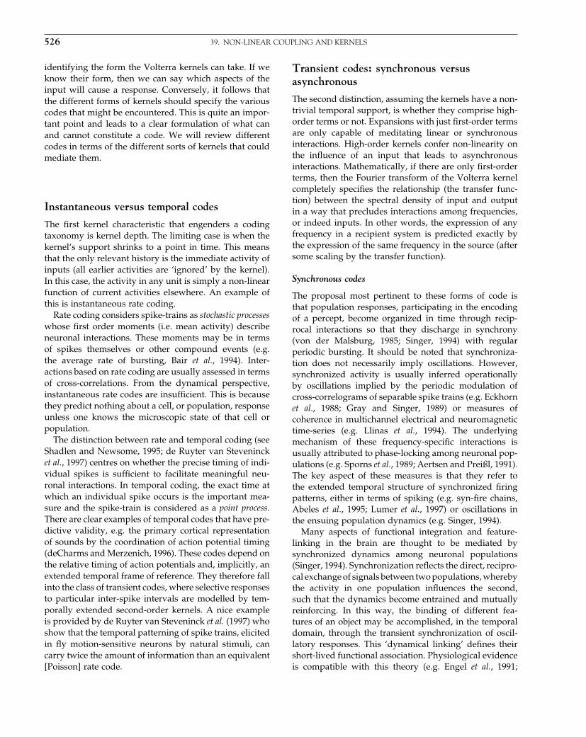
Elsevier UK Chapter: Ch39-P372560 30-9-2006 5:33p.m. Page:526 Trim:7.5in×9.25in
Basal Font:Palatino Margins:Top:40pt Gutter:68pt Font Size:9.5/12 Text Width:42pc Depth:55 Lines
526 39. NON-LINEAR COUPLING AND KERNELS
identifying the form the Volterra kernels can take. If weknow their form, then we can say which aspects of theinput will cause a response. Conversely, it follows thatthe different forms of kernels should specify the variouscodes that might be encountered. This is quite an impor-tant point and leads to a clear formulation of what canand cannot constitute a code. We will review differentcodes in terms of the different sorts of kernels that couldmediate them.
Instantaneous versus temporal codes
The first kernel characteristic that engenders a codingtaxonomy is kernel depth. The limiting case is when thekernel‘s support shrinks to a point in time. This meansthat the only relevant history is the immediate activity ofinputs (all earlier activities are ‘ignored’ by the kernel).In this case, the activity in any unit is simply a non-linearfunction of current activities elsewhere. An example ofthis is instantaneous rate coding.
Rate coding considers spike-trains as stochastic processeswhose first order moments (i.e. mean activity) describeneuronal interactions. These moments may be in termsof spikes themselves or other compound events (e.g.the average rate of bursting, Bair et al., 1994). Inter-actions based on rate coding are usually assessed in termsof cross-correlations. From the dynamical perspective,instantaneous rate codes are insufficient. This is becausethey predict nothing about a cell, or population, responseunless one knows the microscopic state of that cell orpopulation.
The distinction between rate and temporal coding (seeShadlen and Newsome, 1995; de Ruyter van Stevenincket al., 1997) centres on whether the precise timing of indi-vidual spikes is sufficient to facilitate meaningful neu-ronal interactions. In temporal coding, the exact time atwhich an individual spike occurs is the important mea-sure and the spike-train is considered as a point process.There are clear examples of temporal codes that have pre-dictive validity, e.g. the primary cortical representationof sounds by the coordination of action potential timing(deCharms and Merzenich, 1996). These codes depend onthe relative timing of action potentials and, implicitly, anextended temporal frame of reference. They therefore fallinto the class of transient codes, where selective responsesto particular inter-spike intervals are modelled by tem-porally extended second-order kernels. A nice exampleis provided by de Ruyter van Steveninck et al. (1997) whoshow that the temporal patterning of spike trains, elicitedin fly motion-sensitive neurons by natural stimuli, cancarry twice the amount of information than an equivalent[Poisson] rate code.
Transient codes: synchronous versusasynchronous
The second distinction, assuming the kernels have a non-trivial temporal support, is whether they comprise high-order terms or not. Expansions with just first-order termsare only capable of meditating linear or synchronousinteractions. High-order kernels confer non-linearity onthe influence of an input that leads to asynchronousinteractions. Mathematically, if there are only first-orderterms, then the Fourier transform of the Volterra kernelcompletely specifies the relationship (the transfer func-tion) between the spectral density of input and outputin a way that precludes interactions among frequencies,or indeed inputs. In other words, the expression of anyfrequency in a recipient system is predicted exactly bythe expression of the same frequency in the source (aftersome scaling by the transfer function).
Synchronous codes
The proposal most pertinent to these forms of code isthat population responses, participating in the encodingof a percept, become organized in time through recip-rocal interactions so that they discharge in synchrony(von der Malsburg, 1985; Singer, 1994) with regularperiodic bursting. It should be noted that synchroniza-tion does not necessarily imply oscillations. However,synchronized activity is usually inferred operationallyby oscillations implied by the periodic modulation ofcross-correlograms of separable spike trains (e.g. Eckhornet al., 1988; Gray and Singer, 1989) or measures ofcoherence in multichannel electrical and neuromagnetictime-series (e.g. Llinas et al., 1994). The underlyingmechanism of these frequency-specific interactions isusually attributed to phase-locking among neuronal pop-ulations (e.g. Sporns et al., 1989; Aertsen and Preißl, 1991).The key aspect of these measures is that they refer tothe extended temporal structure of synchronized firingpatterns, either in terms of spiking (e.g. syn-fire chains,Abeles et al., 1995; Lumer et al., 1997) or oscillations inthe ensuing population dynamics (e.g. Singer, 1994).
Many aspects of functional integration and feature-linking in the brain are thought to be mediated bysynchronized dynamics among neuronal populations(Singer, 1994). Synchronization reflects the direct, recipro-cal exchange of signals between two populations, wherebythe activity in one population influences the second,such that the dynamics become entrained and mutuallyreinforcing. In this way, the binding of different fea-tures of an object may be accomplished, in the temporaldomain, through the transient synchronization of oscil-latory responses. This ‘dynamical linking’ defines theirshort-lived functional association. Physiological evidenceis compatible with this theory (e.g. Engel et al., 1991;

Elsevier UK Chapter: Ch39-P372560 30-9-2006 5:33p.m. Page:527 Trim:7.5in×9.25in
Basal Font:Palatino Margins:Top:40pt Gutter:68pt Font Size:9.5/12 Text Width:42pc Depth:55 Lines
EVIDENCE FOR NON-LINEAR COUPLING 527
Fries et al., 1997). Synchronization of oscillatory responsesoccurs within as well as among visual areas, e.g. betweenhomologous areas of the left and right hemispheres andbetween areas at different levels of the visuomotor path-way (e.g. Engel et al., 1991). Synchronization in the visualcortex appears to depend on stimulus properties, such ascontinuity, orientation and motion coherence.
The problem with synchronization is that there is noth-ing essentially dynamic about synchronous interactionsper se. As argued by Erb and Aertsen (1992): ‘the ques-tion might not be so much how the brain functions byvirtue of oscillations, as most researchers working oncortical oscillations seem to assume, but rather how itmanages to do so in spite of them’. In order to estab-lish dynamic cell assemblies, it is necessary to createand destroy synchrony (see Breakspear et al., 2003 forone mechanism). It is precisely these dynamic aspectsthat speak of changes in synchrony (e.g. Desmedt andTomberg, 1994; Tass, 2005) and the asynchronous tran-sitions between synchronous states as the more perti-nent phenomenon. In other words, it is the successivereformulation of dynamic cell assemblies, through non-linear or asynchronous interactions, that is at the heart ofdynamical linking (Singer, 1994).
Asynchronous codes
An alternative perspective on neuronal codes is providedby dynamic correlations (Aertsen et al., 1994) as exempli-fied in Vaadia et al. (1995). A fundamental phenomenon,observed by Vaadia et al. (1995), is that, followingbehaviourally salient events, the degree of coherent fir-ing between two neurons can change profoundly andsystematically over the ensuing second or so (cf. inducedresponses in the EEG, Tallon-Baudry et al., 1999; Lachauxet al., 2000). One implication is that a complete modelof neuronal interactions has to accommodate dynamicchanges in correlations, modulated on time-scales of100–1000 ms. Neuronal transients provide a simple expla-nation for temporally modulated coherence or dynamiccorrelation. Imagine that two neurons respond to anevent with a similar transient. For example, if two neu-rons respond to an event with decreased firing for 400 ms,and this decrease was correlated over epochs, then pos-itive correlations between the two firing rates would beseen for the first 400 of the epoch, and then fade away,exhibiting a dynamic modulation of coherence. In otherwords, the expression transient covariance can be for-mulated as covariance in the expression of transients.The generality of this equivalence can be establishedusing singular value decomposition (SVD) of the joint-peristimulus time histogram (J-PSTH) as described inFriston (1995b). This is simply a mathematical device toshow that dynamic changes in coherence are equivalent
to the coherent expression of neural transients. In itselfit is not important, in the sense that dynamic correla-tions are just as valid a characterization as neuronal tran-sients and, indeed, may provide more intuitive insightsinto how this phenomenon is mediated (e.g. Riehle et al.,1997). A more important observation is that J-PSTHs canbe asymmetric about the leading diagonal. This meansthat coupled transients in two units can have a differenttemporal pattern of activity. This can only be explainedby asynchronous or non-linear coupling.
Summary
In summary, the critical distinction between synchronousand asynchronous coupling is the difference betweenlinear and non-linear interactions among units or pop-ulations.4 This difference reduces to the existence ofhigh-order Volterra kernels in mediating the input-outputbehaviour of coupled cortical regions. There is a close con-nection between asynchronous-non-linear coupling andthe expression of distinct transients in two brain regions:both would be expressed as dynamic correlations or,in the EEG, as event-related changes in synchronization(e.g. induced oscillations (Friston et al., 1997)). If the tran-sient model is correct, then important transactions amongcortical areas will be overlooked by techniques that arepredicated on rate coding (e.g. correlations, covariancepatterns, spatial modes etc.) or synchronization models(e.g. coherence analysis and cross-correlograms). Clearly,the critical issue is whether there is direct evidence fornon-linear or asynchronous coupling that would renderhigh-order Volterra kernels necessary.
EVIDENCE FOR NON-LINEARCOUPLING
Why is asynchronous coupling so important? The reasonis that asynchronous interactions embody all the non-linear interactions implicit in functional integration andit is these that mediate the context-sensitive nature of
4 The term ‘generalized synchrony’ has been introduced toinclude non-linear inter-dependencies (see Schiff et al., 1996).Generalized synchrony subsumes synchronous and asyn-chronous coupling. An elegant method for making inferencesabout generalized synchrony is described in Schiff et al. (1996).This approach is particularly interesting from our point of viewbecause it calls upon the recent history of the dynamics throughthe use of temporal embedding to reconstruct the attractorsanalysed.

Elsevier UK Chapter: Ch39-P372560 30-9-2006 5:33p.m. Page:528 Trim:7.5in×9.25in
Basal Font:Palatino Margins:Top:40pt Gutter:68pt Font Size:9.5/12 Text Width:42pc Depth:55 Lines
528 39. NON-LINEAR COUPLING AND KERNELS
neuronal interactions. Non-linear interactions among cor-tical areas render the effective connectivity among theminherently dynamic and contextual. Examples of context-sensitive interactions include the attentional modulationof evoked responses in functionally specialized sensoryareas (e.g. Treue and Maunsell, 1996) and other con-textually dependent dynamics (see Phillips and Singer,1997). Whole classes of empirical phenomena, such asextra-classical receptive field effects, rely on non-linearor asynchronous interactions.
Non-linear coupling and asynchronousinteractions
If the temporal structures of recurring transients in twoparts of the brain are distinct, then the expression ofcertain frequencies in one cortical area should predictthe expression of different frequencies in another. Incontrast, synchronization posits the expression of thesame frequencies. Correlations among different frequen-cies therefore provide a basis for discriminating betweensynchronous and asynchronous coupling.
Consider time-series from two neuronal populationsor cortical areas. Synchrony requires that the expres-sion of a particular frequency (e.g. 40 Hz) in one time-series will be coupled with the expression of the samefrequency in the other. In other words, the modula-tion of this frequency in one area can be explained orpredicted by its modulation in the second. Conversely,asynchronous coupling suggests that the power at a ref-erence frequency, say 40 Hz, can be predicted by thespectral density in the second time-series at frequenciesother than 40 Hz. These predictions can be tested empiri-cally using standard time-frequency and regression anal-yses as described in Friston (2000). Figure 39.1 shows anexample of this sort of analysis, revealing the dynamicchanges in spectral density between 8 and 64 Hz over16 s. The cross-correlation matrix of the time-dependentexpression of different frequencies in the parietal andprefrontal regions is shown in the lower left panel. Thereis anecdotal evidence for both synchronous and asyn-chronous coupling. Synchronous coupling, based uponthe co-modulation of the same frequencies, is mani-fest as hot-spots along, or near, the leading diagonal ofthe cross-correlation matrix (e.g. around 20 Hz). Moreinteresting, are correlations between high frequenciesin one time-series and low frequencies in another. Inparticular, note that the frequency modulation at about34 Hz in the parietal region (second time-series) couldbe explained by several frequencies in the prefrontalregion. The most profound correlations are with lowerfrequencies in the first time-series (26 Hz). Using a simpleregression framework, statistical inferences can be made
about the coupling within and between different frequen-cies (see Friston, 2000 for details). A regression analysisshows that coupling at 34 Hz has significant synchronousand asynchronous components, whereas the coupling at48 Hz is purely asynchronous (middle and right peaks inthe graphs), i.e. a coupling between beta dynamics in thepre-motor region and gamma dynamics in the parietalregion.
THE NEURAL BASIS OF NON-LINEARCOUPLING
In Friston (1997), it was suggested that, from a neurobio-logical perspective, the distinction between non-linear[asynchronous] and linear [synchronous] interactionscould be viewed in the following way. Synchroniza-tion emerges from the reciprocal exchange of signalsbetween two populations, where each drives the other,such that the dynamics become entrained and mutuallyreinforcing. In asynchronous coding, the afferents fromone population exert a modulatory influence, not on theactivity of the second, but on the interactions within it(e.g. a modulation of effective connectivity or synapticefficacies within the target population) leading to changesin the dynamics intrinsic to the second population. Inthis model, there is no necessary synchrony betweenthe intrinsic dynamics that ensue and the temporal pat-tern of modulatory input. To test this hypothesis onewould need to demonstrate that asynchronous couplingemerges when extrinsic connections are changed fromdriving connections to modulatory connections. Clearly,this cannot be done in the real brain. However, we canuse computational techniques to create a biologicallyrealistic model of interacting populations and test thishypothesis directly.
Interactions between simulated populations
Two populations were simulated using the neural-massmodel described in Friston (2000). This model simu-lates entire neuronal populations in a deterministic fash-ion based on known neurophysiological mechanisms(see also Chapter 31). In particular, we modelled threesorts of synapse, fast inhibitory (GABA), fast excita-tory (AMPA) and slower voltage-dependent synapses(NMDA). Connections intrinsic to each populationused only GABA and AMPA-like synapses. Simulatedglutaminergic extrinsic connections between popula-tions used either driving AMPA-like synapses ormodulatory NMDA-like synapses. Transmission delays
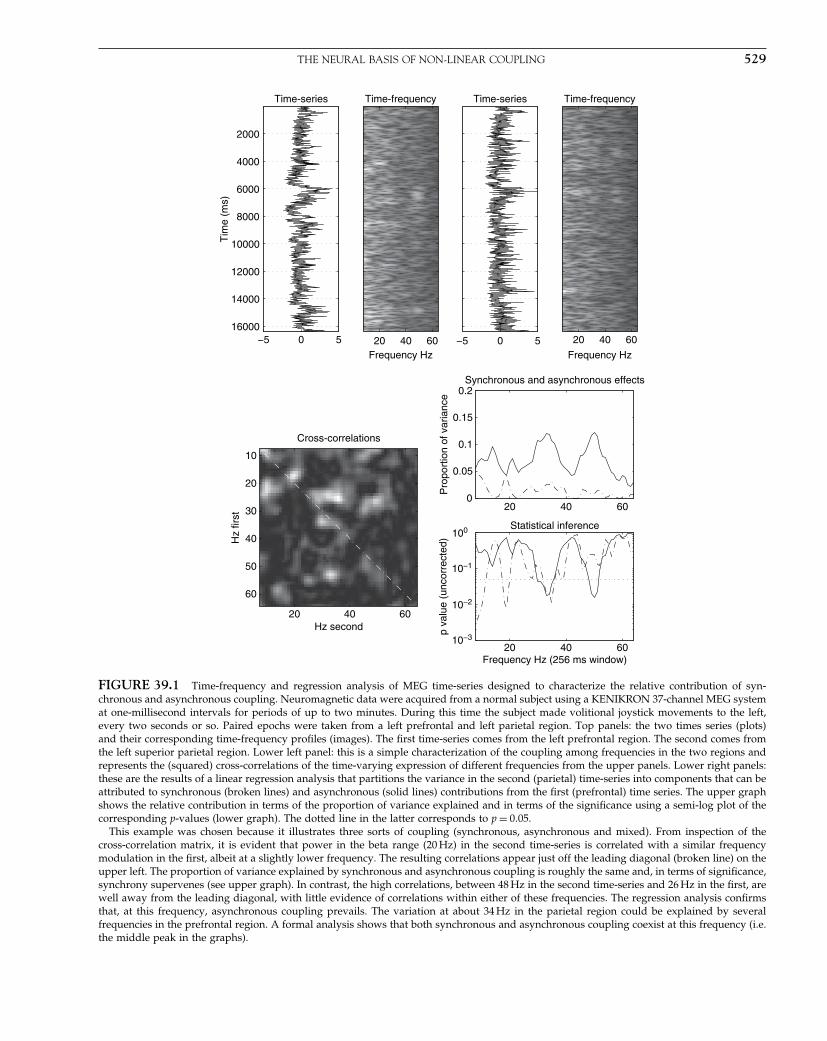
Elsevier UK Chapter: Ch39-P372560 30-9-2006 5:33p.m. Page:529 Trim:7.5in×9.25in
Basal Font:Palatino Margins:Top:40pt Gutter:68pt Font Size:9.5/12 Text Width:42pc Depth:55 Lines
THE NEURAL BASIS OF NON-LINEAR COUPLING 529
2000
4000
6000
8000
10000
12000
14000
16000−5 0 5
Tim
e (m
s)
Time-series
Frequency Hz
Time-frequency
20 40 60 −5 0 5
Time-series
Frequency Hz
Time-frequency
20 40 60
Hz
first
Hz second
Cross-correlations
20 40 60
10
20
30
40
50
60
20 40 600
0.05
0.1
0.15
0.2
Pro
port
ion
of v
aria
nce
Synchronous and asynchronous effects
20 40 6010−3
10−2
10−1
100
Frequency Hz (256 ms window)
p va
lue
(unc
orre
cted
)
Statistical inference
FIGURE 39.1 Time-frequency and regression analysis of MEG time-series designed to characterize the relative contribution of syn-chronous and asynchronous coupling. Neuromagnetic data were acquired from a normal subject using a KENIKRON 37-channel MEG systemat one-millisecond intervals for periods of up to two minutes. During this time the subject made volitional joystick movements to the left,every two seconds or so. Paired epochs were taken from a left prefrontal and left parietal region. Top panels: the two times series (plots)and their corresponding time-frequency profiles (images). The first time-series comes from the left prefrontal region. The second comes fromthe left superior parietal region. Lower left panel: this is a simple characterization of the coupling among frequencies in the two regions andrepresents the (squared) cross-correlations of the time-varying expression of different frequencies from the upper panels. Lower right panels:these are the results of a linear regression analysis that partitions the variance in the second (parietal) time-series into components that can beattributed to synchronous (broken lines) and asynchronous (solid lines) contributions from the first (prefrontal) time series. The upper graphshows the relative contribution in terms of the proportion of variance explained and in terms of the significance using a semi-log plot of thecorresponding p-values (lower graph). The dotted line in the latter corresponds to p = 005.
This example was chosen because it illustrates three sorts of coupling (synchronous, asynchronous and mixed). From inspection of thecross-correlation matrix, it is evident that power in the beta range (20 Hz) in the second time-series is correlated with a similar frequencymodulation in the first, albeit at a slightly lower frequency. The resulting correlations appear just off the leading diagonal (broken line) on theupper left. The proportion of variance explained by synchronous and asynchronous coupling is roughly the same and, in terms of significance,synchrony supervenes (see upper graph). In contrast, the high correlations, between 48 Hz in the second time-series and 26 Hz in the first, arewell away from the leading diagonal, with little evidence of correlations within either of these frequencies. The regression analysis confirmsthat, at this frequency, asynchronous coupling prevails. The variation at about 34 Hz in the parietal region could be explained by severalfrequencies in the prefrontal region. A formal analysis shows that both synchronous and asynchronous coupling coexist at this frequency (i.e.the middle peak in the graphs).

Elsevier UK Chapter: Ch39-P372560 30-9-2006 5:33p.m. Page:530 Trim:7.5in×9.25in
Basal Font:Palatino Margins:Top:40pt Gutter:68pt Font Size:9.5/12 Text Width:42pc Depth:55 Lines
530 39. NON-LINEAR COUPLING AND KERNELS
for extrinsic connections were fixed at 8 ms. By usingrealistic time constants the characteristic oscillatorydynamics of each population were expressed in thegamma range.
The results of coupling two populations with uni-directional AMPA-like connections are shown in thetop of Figure 39.2 in terms of the simulated local fieldpotentials (LFP). Occasional transients in the drivingpopulation were evoked by injecting a depolarizingcurrent at random intervals (dotted lines). The tight
synchronized coupling that ensues is evident. This exam-ple highlights the point that near-linear coupling canarise even in the context of loosely coupled, highlynon-linear neuronal oscillators of the sort modelled here.Contrast these entrained dynamics under driving connec-tions with those that emerge when the connection is mod-ulatory or NMDA-like (lower panel in Figure 39.2). Here,there is no synchrony and, as predicted, fast transients ofan oscillatory nature are facilitated by the low-frequencyinput from the first population (cf. the MEG analyses
200 400 600 800 1000 1200 1400 1600 1800 2000−70
−60
−50
−40
−30
−20
−10
0Synchronous (AMPA) coupling
Time (ms)
Tra
nsm
embr
ane
pote
ntia
l (m
V)
200 400 600 800 1000 1200 1400 1600 1800 2000−70
−60
−50
−40
−30
−20
−10
0Asynchronous (NMDA) coupling
Time (ms)
Tra
nsm
embr
ane
pote
ntia
l (m
V)
FIGURE 39.2 Simulated local field potentials (LFP) of two coupled populations using two different sorts of postsynaptic responses(AMPA and NMDA-like) to inputs from the first to the target population. The dotted line shows the depolarization effected by sporadicinjections of current into the first population. The key thing to note is that, under AMPA-like or driving connections, the second populationis synchronously entrained by the first. When the connections are modulatory or voltage-dependent (NMDA), the effects are much moresubtle and resemble a frequency modulation. These data were simulated using a biologically plausible model of excitatory and inhibitorysubpopulations. The model was deterministic with variables pertaining to the collective, probabilistic, behaviour of the subpopulations (cf. amean-field treatment) (see Friston, 2000 for details).

Elsevier UK Chapter: Ch39-P372560 30-9-2006 5:33p.m. Page:531 Trim:7.5in×9.25in
Basal Font:Palatino Margins:Top:40pt Gutter:68pt Font Size:9.5/12 Text Width:42pc Depth:55 Lines
THE NEURAL BASIS OF NON-LINEAR COUPLING 531
1000
2000
3000
4000
5000
6000
7000
8000−5 0 5
Tim
e m
s
Time−series
Frequency Hz
Time−frequency
20 40 60 −5 0 5
Time−series
Frequency Hz
Time−frequency
20 40 60
Hz
first
Hz second
Cross−correlations
20 40 60
10
20
30
40
50
60
20 40 600
0.2
0.4
0.6
0.8
Pro
port
ion
of v
aria
nce
Synchronous and asynchronous effects
20 40 6010−15
10−10
10−5
100
Frequency Hz (256 ms window)
P v
alue
(un
corr
ecte
d)
Statistical inference
FIGURE 39.3 As for Figure 39.1, but here using the simulated data employing voltage-dependent NMDA-like connections. The couplinghere includes some profoundly asynchronous [non-linear] components involving frequencies in the gamma range implicated in the analysesof real (MEG) data shown in Figure 39.1. In particular, note the asymmetrical cross-correlation matrix and the presence of asynchronous andmixed coupling implicit in the p-value plots on the lower right.
above). This is a nice example of asynchronous couplingthat is underpinned by non-linear modulatory interac-tions between neuronal populations. The nature of thecoupling can be characterized using the time-frequencyanalysis (identical in every detail) applied to the neu-romagnetic data of the previous section. The results forthe NMDA simulation are presented in Figure 39.3. Thecross-correlation matrix resembles that obtained with the
MEG data in Figure 39.1. Both in terms of the variance,and inference, asynchronous coupling supervenes atmost frequencies but, as in the real data, mixed cou-pling is also evident. These results can be taken as aheuristic confirmation of the notion that modulatory, inthis case voltage-dependent, interactions are sufficientlynon-linear to account for the emergence of asynchronouscoupling.

Elsevier UK Chapter: Ch39-P372560 30-9-2006 5:33p.m. Page:532 Trim:7.5in×9.25in
Basal Font:Palatino Margins:Top:40pt Gutter:68pt Font Size:9.5/12 Text Width:42pc Depth:55 Lines
532 39. NON-LINEAR COUPLING AND KERNELS
Modulatory interactions and non-linearcoupling
In summary, asynchronous coupling is synonymous withnon-linear coupling. Non-linear coupling can be framedin terms of the modulation of intrinsic interactions,within a cortical area or neuronal population, by extrinsicinput offered by afferents from other parts of the brain.This mechanism predicts that the modulation of fast (e.g.gamma) activity in one cortical area can be predicted bymuch slower changes in other areas. This form of cou-pling is very different from coherence or other measuresof synchronous coupling and concerns the relationshipbetween the first-order dynamics in one area and thesecond-order dynamics (spectral density) expressed inanother. In terms of the above NMDA simulation, tran-sient depolarization in the modulating population causesa short-lived increased input to the second. These affer-ents impinge on voltage-sensitive NMDA-like synapseswith time constants (in the model) of about 100 ms.These synapses open and slowly close again, remain-ing open long after an afferent volley. Because of theirvoltage-sensitive nature, this input will have no effect onthe dynamics intrinsic to the second population unlessthere is already a substantial degree of depolarization.If there is then, through self-excitation and inhibition,the concomitant opening of fast excitatory and inhibitorychannels, this will generally increase membrane conduc-tance, decrease the effective membrane time constantsand lead to fast oscillatory transients. This is what weobserve in the lower panel of Figure 39.2. In relationto the MEG analyses, the implied modulatory mecha-nisms that may underpin this effect are entirely consistentwith the anatomy, laminar specificity and functional roleattributed to prefrontal efferents (Rockland and Pandya,1979; Selemon and Goldman-Rakic, 1988).
CONCLUSION
In this chapter, we have dealt with some interestingand interrelated aspects of effective connectivity, neu-ronal codes, non-linear coupling, neuronal transients anddynamic correlations (e.g. induced oscillations). The keypoints can be summarized as follows:
• Starting with the premise that the brain can be repre-sented as an ensemble of connected input-state-outputsystems (e.g. cellular compartments, cells or popula-tions of cells), there is an equivalent input-output for-mulation in terms of a Volterra series. This is simplya functional expansion of each system’s inputs that
produces its outputs (where the outputs of one systemare the inputs to another).
• The existence of this expansion suggests that the his-tory of inputs, or neuronal transients, and the Volterrakernels are a complete and sufficient description ofbrain dynamics. This is the primary motivation forframing dynamics in terms of neuronal transients andusing Volterra kernels to model effective connectivity.
• The Volterra formulation provides constraints on theform that neuronal interactions and implicit codesmust conform to. There are two limiting cases: whenthe kernel decays very quickly; and when high-orderkernels disappear. The first case corresponds to instan-taneous codes (e.g. rate codes) and the second to syn-chronous interactions (e.g. synchrony codes).
• High-order kernels in the Volterra formulation speak tonon-linear interactions and implicitly to asynchronouscoupling. Asynchronous coupling implies couplingamong the expression of different frequencies.
• Coupling among different frequencies is easy todemonstrate using neuromagnetic measurements ofreal brain dynamics. This implies that non-linear, asyn-chronous coupling is a prevalent component of func-tional integration.
• High-order kernels correspond to modulatory inter-actions that can be construed as a non-linear effectof inputs that interact with the intrinsic states of therecipient system. This implies that driving connectionsmay be linear and engender synchronous interactions.Conversely, modulatory connections, being non-linear,may be revealed by asynchronous coupling and inducehigh-order kernels.
In the next chapter, we look at another way of sum-marizing and quantifying temporal dependencies amongmeasured brain responses, using multivariate autoregres-sion models. These models are formulated in discretetime, as opposed to the continuous time formulation usedfor generalized convolution models.
REFERENCES
Abeles M, Bergman H, Gat I et al. (1995) Cortical activity flips amongquasi-stationary states. Proc Natl Acad Sci USA 92: 8616–20
Aertsen A, Erb M, Palm G (1994) Dynamics of functional coupling inthe cerebral cortex: an attempt at a model-based interpretation.Physica D 75: 103–28
Aertsen A, Preißl H (1991) Dynamics of activity and connectivityin physiological neuronal networks. In Non linear dynamics andneuronal networks, Schuster HG (ed.). VCH publishers Inc., NewYork, pp 281–302
Bair W, Koch C, Newsome W et al. (1994) Relating temporal prop-erties of spike trains from area MT neurons to the behaviour of
Elsevier UK Chapter: Ch39-P372560 30-9-2006 5:33p.m. Page:533 Trim:7.5in×9.25in
Basal Font:Palatino Margins:Top:40pt Gutter:68pt Font Size:9.5/12 Text Width:42pc Depth:55 Lines
REFERENCES 533
the monkey. In Temporal coding in the brain, Buzsaki G, Llinas R,Singer W et al. (eds). Springer Verlag, Berlin, pp 221–50
Bendat JS (1990) Nonlinear system analysis and identification from ran-dom data. John Wiley and Sons, New York
Breakspear M, Terry JR, Friston KJ (2003). Modulation of excita-tory synaptic coupling facilitates synchronization and complexdynamics in a biophysical model of neuronal dynamics. Network14: 703–32
deCharms RC, Merzenich MM (1996) Primary cortical representa-tion of sounds by the co-ordination of action potential timing.Nature 381: 610–13
de Ruyter van Steveninck RR, Lewen GD, Strong SP et al. (1997)Reproducibility and variability in neural spike trains. Science275: 1085–88
Desmedt JE, Tomberg C (1994) Transient phase-locking of 40 Hzelectrical oscillations in prefrontal and parietal human cortexreflects the process of conscious somatic perception. NeurosciLett 168: 126–29
Eckhorn R, Bauer R, Jordan W et al. (1988) Coherent oscillations:a mechanism of feature linking in the visual cortex? Multipleelectrode and correlation analysis in the cat. Biol Cybernet 60:121–30
Engel AK, Konig P, Singer W (1991) Direct physiological evidencefor scene segmentation by temporal coding. Proc Natl Acad SciUSA 88: 9136–40
Erb M, Aertsen A (1992) Dynamics of activity in biology-orientedneural network models: stability analysis at low firing rates. InInformation processing in the cortex. Experiments and theory, AertsenA, Braitenberg V (eds). Springer-Verlag, Berlin, pp 201–23
Fliess M, Lamnabhi M, Lamnabhi-Lagarrigue F (1983) An algebraicapproach to nonlinear functional expansions. IEEE Transactionson Circuits and Systems 30: 554–70
Freeman W, Barrie J (1994) Chaotic oscillations and the genesisof meaning in cerebral cortex. In Temporal coding in the brain,Buzsaki G, Llinas R, Singer W et al. (eds). Springer Verlag, Berlin,pp 13–38
Fries P, Roelfsema PR, Engel A et al. (1997) Synchronisation of oscil-latory responses in visual cortex correlates with perception ininter-ocular rivalry. Proc Natl Acad Sci USA 94: 12699–704
Friston KJ (1995a) Functional and effective connectivity in neuro-imaging: a synthesis. Hum Brain Mapp 2: 56–78
Friston KJ (1995b) Neuronal transients. Proc Roy Soc Series B 261:401–05
Friston KJ (1997) Transients metastability and neuronal dynamics.NeuroImage 5: 164–71
Friston KJ (2000) The labile brain I: Neuronal transients and non-linear coupling. Philos Trans R Soc (Lond) 355: 215–36
Friston KJ, Stephan KM and Frackowiak RSJ (1997) Transient phase-locking and dynamic correlations: are they the same thing?Human Brain Mapping 5: 48–57
Gray CM, Singer W (1989) Stimulus specific neuronal oscillations inorientation columns of cat visual cortex. Proc Natl Acad Sci USA86: 1698–1702
Haken H (1983) Synergistics: an introduction, 3rd edn. Springer, BerlinHaken H (2006) Synergetics of brain function. Int J Psychophysiol
Mar 7; (Epub ahead of print)Harrison LM, David O, Friston KJ (2005) Stochastic models
of neuronal dynamics. Philos Trans R Soc Lond B Biol Sci360: 1075–91
Jirsa VK, Friedrich R, Haken H (1995) Reconstruction of the spatio-temporal dynamics of a human magnetoencephalogram. PhysicaD 89: 100–22
Kelso JAS (1995) Dynamic patterns: the self-organisation of brain andbehaviour. MIT Press, Cambridge, MA
Lachaux JP, Rodriguez E, Martinerie J et al. (2000) A quantitativestudy of gamma-band activity in human intracranial recordingstriggered by visual stimuli. Eur J Neurosci 12: 2608–22
Llinas R, Ribary U, Joliot M et al. (1994) Content and context intemporal thalamocortical binding. In Temporal coding in the brain,Buzsaki G, Llinas R, Singer W et al. (eds). Springer Verlag, Berlin,pp 251–72
Lumer ED, Edelman GM, Tononi G (1997) Neural dynamics ina model of the thalamocortical System II. The role of neuralsynchrony tested through perturbations of spike timing. CerebCortex 7: 228–36
Optican L, Richmond BJ (1987) Temporal encoding of two-dimensional patterns by single units in primate inferior cortex.II Information theoretic analysis. J Neurophysiol 57: 132–46
Phillips WA, Singer W (1997) In search of common foundations forcortical computation. Behav Brain Sci 20: 57–83
Riehle A, Grun S, Diesmann M et al. (1997) Spike synchronisationand rate modulation differentially involved in motor corticalfunction. Science 278: 1950–53
Rockland KS, Pandya DN (1979) Laminar origins and terminationsof cortical connections of the occipital lobe in the rhesus monkey.Brain Res 179: 3–20
Schiff SJ, So P, Chang T et al. (1996) Detecting dynamical inter-dependence and generalised synchrony though mutual predic-tion in a neuronal ensemble. Phys Rev E 54: 6708–24
Selemon LD, Goldman-Rakic PS (1988) Common cortical and sub-cortical targets of the dorsolateral prefrontal and posterior pari-etal cortices in the rhesus monkey: evidence for a distributedneural network subserving spatially guided behavior. J Neurosci8: 4049–68
Shadlen MN, Newsome WT (1995) Noise, neural codes and corticalorganisation. Curr Opin Neurobiol 4: 569–79
Singer W (1994) Time as coding space in neocortical processing: ahypothesis. In Temporal coding in the brain, Buzsaki G, Llinas R,Singer W et al. (eds). Springer Verlag, Berlin, pp 51–80
Sporns O, Gally, JA, Reeke GN et al. (1989) Reentrant signallingamong simulated neuronal groups leads to coherence in theiroscillatory activity Proc Natl Acad Sci USA 86: 7265–69
Tallon-Baudry C, Kreiter A, Bertrand O (1999) Sustained and tran-sient oscillatory responses in the gamma and beta bands ina visual short-term memory task in humans. Vis Neurosci. 16:449–59
Tass PA (2005) Estimation of the transmission time of stimulus-locked responses: modelling and stochastic phase resetting anal-ysis. Philos Trans R Soc Lond B Biol Sci 360: 995–99
Tovee MJ, Rolls ET, Treves A et al. (1993) Information encoding andthe response of single neurons in the primate temporal visualcortex. J Neurophysiology 70: 640–54
Treue S, Maunsell HR (1996) Attentional modulation of visual motionprocessing in cortical areas MT and MST. Nature 382: 539–41
Tsuda I (2001) Toward an interpretation of dynamic neural activity interms of chaotic dynamical systems. Behav Brain Sci 24: 793–810
Vaadia E, Haalman I, Abeles M et al. (1995) Dynamics of neuronalinteractions in monkey cortex in relation to behavioural events.Nature 373: 515–18
von der Malsburg C (1985) Nervous structures with dynamical links.Ber Bunsenges Phys Chem 89: 703–10
Wray J, Green GGR (1994) Calculation of the Volterra kernels of non-linear dynamic systems using an artificial neuronal network. BiolCybernet 71: 187–95
Elsevier UK Chapter: Ch04-P372560 3-10-2006 3:02p.m. Page:49 Trim:7.5in×9.25in
Basal Font:Palatino Margins:Top:40pt Gutter:68pt Font Size:9.5/12 Text Width:42pc Depth:55 Lines
C H A P T E R
4
Rigid Body RegistrationJ. Ashburner and K. Friston
INTRODUCTION
Rigid body registration is one of the simplest formsof image registration, so this chapter provides an idealframework for introducing some of the concepts thatwill be used by the more complex registration methodsdescribed later. The shape of a human brain changesvery little with head movement, so rigid body transfor-mations can be used to model different head positionsof the same subject. Registration methods described inthis chapter include within modality, or between dif-ferent modalities such as positron emission tomography(PET). and magnetic resonance imaging (MRI). Matchingof two images is performed by finding the rotations andtranslations that optimize some mutual function of theimages. Within-modality registration generally involvesmatching the images by minimizing the mean squareddifference between them. For between-modality registra-tion, the matching criterion needs to be more complex.
Image registration is important in many aspects offunctional image analysis. In imaging neuroscience, par-ticularly for functional MRI (fMRI), the signal changesdue to any haemodynamic response can be small com-pared to apparent signal differences that can result fromsubject movement. Subject head movement in the scan-ner cannot be completely eliminated, so retrospectivemotion correction is performed as a preprocessing step.This is especially important for experiments where sub-jects may move in the scanner in a way that is corre-lated with the different conditions (Hajnal et al., 1994).Even tiny systematic differences can result in a significantsignal accumulating over numerous scans. Without suit-able corrections, artefacts arising from subject movementcorrelated with the experimental paradigm may appearas activations. A second reason why motion correctionis important is that it increases sensitivity. The t-test isbased on the signal change relative to the residual vari-ance. The residual variance is computed form the sum
of squared differences between the data and the linearmodel to which it is fitted. Movement artefacts add tothis residual variance, and so reduce the sensitivity ofthe test to true activations.
For studies of a single subject, sites of activation canbe accurately localized by superimposing them on a highresolution structural image of the subject (typically a T1-weighted MRI). This requires registration of the func-tional images with the structural image. As in the case ofmovement correction, this is normally performed by opti-mizing a set of parameters describing a rigid body trans-formation, but the matching criterion needs to be morecomplex because the structural and functional imagesnormally look very different. A further use for this reg-istration is that a more precise spatial normalization canbe achieved by computing it from a more detailed struc-tural image. If the functional and structural images arein register, then a warp computed from the structuralimage can be applied to the functional images.
Another application of rigid registration is within thefield of morphometry, and involves identifying shapechanges within single subjects by subtracting coregis-tered images acquired at different times. The changescould arise for a number of different reasons, but mostare related to pathology. Because the scans are of thesame subject, the first step for this kind of analysisinvolves registering the images together by a rigid bodytransformation.
At its simplest, image registration involves estimat-ing a mapping between a pair of images. One imageis assumed to remain stationary (the reference image),whereas the other (the source image) is spatially trans-formed to match it. In order to transform the sourceto match the reference, it is necessary to determinea mapping from each voxel position in the referenceto a corresponding position in the source. The sourceis then resampled at the new positions. The mappingcan be thought of as a function of a set of estimated
Statistical Parametric Mapping, by Karl Friston et al. Copyright 2007, Elsevier Ltd. All rights reserved.ISBN–13: 978-0-12-372560-8 ISBN–10: 0-12-372560-7
49

Elsevier UK Chapter: Ch04-P372560 3-10-2006 3:02p.m. Page:50 Trim:7.5in×9.25in
Basal Font:Palatino Margins:Top:40pt Gutter:68pt Font Size:9.5/12 Text Width:42pc Depth:55 Lines
50 4. RIGID BODY REGISTRATION
transformation parameters. A rigid body transformationin three dimensions is defined by six parameters: threetranslations and three rotations.
There are two steps involved in registering a pair ofimages together. There is the registration itself, wherebythe set of parameters describing a transformation is esti-mated. Then there is the transformation, where one of theimages is transformed according to the estimated param-eters. Performing the registration normally involves iter-atively transforming the source image many times, usingdifferent parameters, until some matching criterion isoptimized.
First of all, this chapter will explain how images aretransformed via the process of resampling. This chapteris about rigid registration of images, so the next sectiondescribes the parameterization of rigid body transforma-tions as a subset of the more general affine transforma-tions. The final two sections describe methods of rigidbody registration, in both intra- and inter-modality con-texts. Intra-modality registration implies registration ofimages acquired using the same modality and scanningsequence or contrast agent, whereas inter-modality regis-tration allows the registration of different modalities (e.g.T1- to T2-weighted MRI, or MRI to PET).
RE-SAMPLING IMAGES
An image transformation is usually implemented as a‘pulling’ operation (where pixel values are pulled fromthe original image into their new location) rather thana ‘pushing’ one (where the pixels in the original imageare pushed into their new location). This involves deter-mining for each voxel in the transformed image, the cor-responding intensity in the original image. Usually, thisrequires sampling between the centres of voxels, so someform of interpolation is needed.
Simple interpolation
The simplest approach is to take the value of the clos-est voxel to the desired sample point. This is referredto as nearest neighbour or zero-order hold resampling. Thishas the advantage that the original voxel intensities arepreserved, but the resulting image is degraded quite con-siderably, resulting in the resampled image having a‘blocky’ appearance.
Another approach is to use trilinear interpolation (first-order hold) to resample the data. This is slower than near-est neighbour, but the resulting images are less ‘blocky’.However, trilinear interpolation has the effect of losingsome high frequency information from the image.
FIGURE 4.1 Illustration of image interpolation in two dimen-sions. Points a through to p represent the original regular grid ofpixels. Point u is the point whose value is to be determined. Pointsq to t are used as intermediates in the computation.
Figure 4.1 will now be used to illustrate bilinear inter-polation (the two dimensional version of trilinear inter-polation). Assume that there is a regular grid of pixels atcoordinates xa�ya to xp�yp, having intensities va to vp, andthat the point to re-sample is at u. The value at points rand s are first determined (using linear interpolation) asfollows:
vr = �xg −xr�vf + �xr −xf �vg
xg −xf
vs = �xk −xs�vj + �xs −xj�vk
xk −xj
4.1
Then vu is determined by interpolating between vr andvs:
vu = �yu −ys�vr + �yr −yu�vs
yr −ys
4.2
The extension of the approach to three dimensions istrivial.
Windowed sinc interpolation
The optimum method of applying rigid body transfor-mations to images with minimal interpolation artefact isto do it in Fourier space. In real space, the interpolationmethod that gives results closest to a Fourier interpola-tion is sinc interpolation. This involves convolving the

Elsevier UK Chapter: Ch04-P372560 3-10-2006 3:02p.m. Page:51 Trim:7.5in×9.25in
Basal Font:Palatino Margins:Top:40pt Gutter:68pt Font Size:9.5/12 Text Width:42pc Depth:55 Lines
RE-SAMPLING IMAGES 51
FIGURE 4.2 Sinc function in two dimensions, both with (right) and without (left) a Hanning window.
image with a sinc function centred on the point to bere-sampled. To perform a pure sinc interpolation, everyvoxel in the image should be used to sample a singlepoint. This is not feasible due to speed considerations,so an approximation using a limited number of nearestneighbours is used. Because the sinc function extends toinfinity, it is often truncated by modulation with a Han-ning window (Figure 4.2). Because the function is sepa-rable, the interpolation is performed sequentially in thethree dimensions of the volume. For one dimension thewindowed sinc function using the I nearest neighbourswould be:
I∑i=1
vi
sin��di�
�di
12
�1+ cos�2�di/I��
∑Ij=1
sin��dj�
�dj
12
�1+ cos�2�dj/I��
4.3
where di is the distance from the centre of the ith voxelto the point to be sampled, and vi is the value of theith voxel.
Generalized interpolation
The methods described so far are all classical interpola-tion methods that locally convolve the image with someform of interpolant. Much more efficient re-sampling canbe performed using generalized interpolation (Thévenazet al., 2000). Generalized interpolation methods model animage as a linear combination of basis functions withlocal support, typically B-splines or o-Moms (maximal-order interpolation of minimal support) basis functions(Figure 4.3). Before resampling begins, an image of basisfunction coefficients is produced, which involves a veryfast deconvolution (Unser et al., 1993a,b). The separabil-ity of the basis functions allow this to be done sequen-tially along each of the dimensions. Resampling at eachnew point then involves computing the appropriate lin-ear combination of basis functions, which can be thoughtof as a local convolution of the basis function coefficients.Again, this is done sequentially because of the separabil-ity of the bases.
B-splines are a family of functions of varying degree.Interpolation using B-splines of degree 0 or 1 (first and
second order) is identical to nearest neighbour1 or lin-ear interpolation respectively. B-splines of degree n aregiven by:
�n�x� =n∑
j=0
�−1�j�n+1�
�n+1− j�!j! max(
n+12
+x− j� 0)n
4.4
An nth degree B-spline has a local support of n + 1,which means that during the final resampling step, alinear combination of n + 1 basis functions are neededto compute an interpolated value. o-Moms are derivedfrom B-splines, and consist of a linear combination ofthe B-spline and its derivatives. They produce the mostaccurate interpolation for the least local support, but lacksome of the B-splines’ advantages. Unlike the o-Moms’functions, a B-spline of order n is n−1 times continuouslydifferentiable.
2 4 6 8 10 12 14 16–1
0
1
2
3
4
5
FIGURE 4.3 This figure illustrates a one dimensional B-splinerepresentation of an image, where the image is assumed to be com-posed of a linear combination of B-spline basis functions. The dottedlines are the individual basis functions, which sum to produce theinterpolated function (solid line).
1 Except with a slightly different treatment exactly in the centreof two voxels.
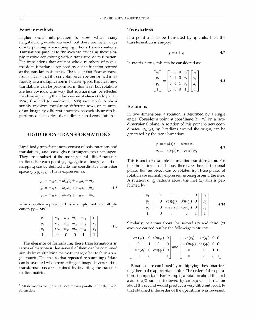
Elsevier UK Chapter: Ch04-P372560 3-10-2006 3:02p.m. Page:52 Trim:7.5in×9.25in
Basal Font:Palatino Margins:Top:40pt Gutter:68pt Font Size:9.5/12 Text Width:42pc Depth:55 Lines
52 4. RIGID BODY REGISTRATION
Fourier methods
Higher order interpolation is slow when manyneighbouring voxels are used, but there are faster waysof interpolating when doing rigid body transformations.Translations parallel to the axes are trivial, as these sim-ply involve convolving with a translated delta function.For translations that are not whole numbers of pixels,the delta function is replaced by a sinc function centredat the translation distance. The use of fast Fourier trans-forms means that the convolution can be performed mostrapidly as a multiplication in Fourier space. It is clear howtranslations can be performed in this way, but rotationsare less obvious. One way that rotations can be effectedinvolves replacing them by a series of shears (Eddy et al.,1996; Cox and Jesmanowicz, 1999) (see later). A shearsimply involves translating different rows or columnsof an image by different amounts, so each shear can beperformed as a series of one dimensional convolutions.
RIGID BODY TRANSFORMATIONS
Rigid body transformations consist of only rotations andtranslations, and leave given arrangements unchanged.They are a subset of the more general affine2 transfor-mations. For each point �x1�x2�x3� in an image, an affinemapping can be defined into the coordinates of anotherspace �y1�y2�y3�. This is expressed as:
y1 = m11x1 +m12x2 +m13x3 +m14
y2 = m21x1 +m22x2 +m23x3 +m24 4.5
y3 = m31x1 +m32x2 +m33x3 +m34
which is often represented by a simple matrix multipli-cation �y = Mx�:
⎡⎢⎢⎢⎣
y1
y2
y3
1
⎤⎥⎥⎥⎦=
⎡⎢⎢⎢⎣
m11 m12 m13 m14
m21 m22 m23 m24
m31 m32 m33 m34
0 0 0 1
⎤⎥⎥⎥⎦
⎡⎢⎢⎢⎣
x1
x2
x3
1
⎤⎥⎥⎥⎦ 4.6
The elegance of formulating these transformations interms of matrices is that several of them can be combinedsimply by multiplying the matrices together to form a sin-gle matrix. This means that repeated re-sampling of datacan be avoided when reorienting an image. Inverse affinetransformations are obtained by inverting the transfor-mation matrix.
2 Affine means that parallel lines remain parallel after the trans-formation.
Translations
If a point x is to be translated by q units, then thetransformation is simply:
y = x +q 4.7
In matrix terms, this can be considered as:
⎡⎢⎢⎢⎣
y1
y2
y3
1
⎤⎥⎥⎥⎦=
⎡⎢⎢⎢⎣
1 0 0 q1
0 1 0 q2
0 0 1 q3
0 0 0 1
⎤⎥⎥⎥⎦
⎡⎢⎢⎢⎣
x1
x2
x3
1
⎤⎥⎥⎥⎦ 4.8
Rotations
In two dimensions, a rotation is described by a singleangle. Consider a point at coordinate �x1�x2� on a two-dimensional plane. A rotation of this point to new coor-dinates �y1�y2�, by � radians around the origin, can begenerated by the transformation:
y1 = cos���x1 + sin���x2
y2 = −sin���x1 + cos���x2
4.9
This is another example of an affine transformation. Forthe three-dimensional case, there are three orthogonalplanes that an object can be rotated in. These planes ofrotation are normally expressed as being around the axes.A rotation of q1 radians about the first �x� axis is per-formed by:
⎡⎢⎢⎢⎢⎣
y1
y2
y3
1
⎤⎥⎥⎥⎥⎦=
⎡⎢⎢⎢⎢⎣
1 0 0 0
0 cos�q1� sin�q1� 0
0 −sin�q1� cos�q1� 0
0 0 0 1
⎤⎥⎥⎥⎥⎦
⎡⎢⎢⎢⎢⎣
x1
x2
x3
1
⎤⎥⎥⎥⎥⎦ 4.10
Similarly, rotations about the second �y� and third �z�axes are carried out by the following matrices:
⎡⎢⎢⎢⎢⎣
cos�q2� 0 sin�q2� 0
0 1 0 0
−sin�q2� 0 cos�q2� 0
0 0 0 1
⎤⎥⎥⎥⎥⎦and
⎡⎢⎢⎢⎢⎣
cos�q3� sin�q3� 0 0
−sin�q3� cos�q3� 0 0
0 0 1 0
0 0 0 1
⎤⎥⎥⎥⎥⎦ �
Rotations are combined by multiplying these matricestogether in the appropriate order. The order of the opera-tions is important. For example, a rotation about the firstaxis of �/2 radians followed by an equivalent rotationabout the second would produce a very different result tothat obtained if the order of the operations was reversed.
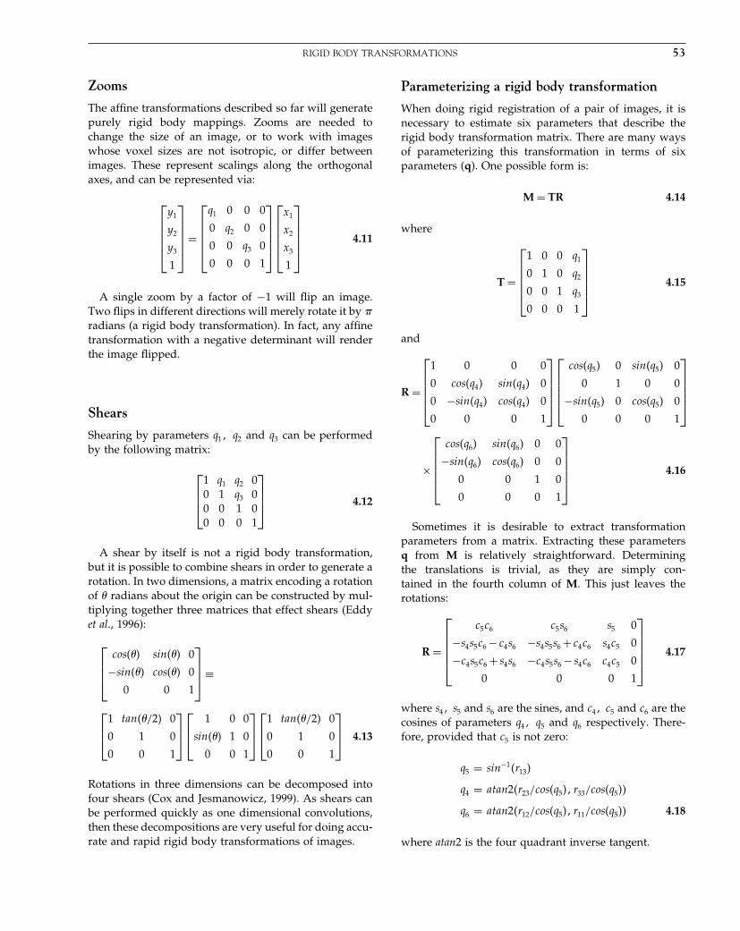
Elsevier UK Chapter: Ch04-P372560 3-10-2006 3:02p.m. Page:53 Trim:7.5in×9.25in
Basal Font:Palatino Margins:Top:40pt Gutter:68pt Font Size:9.5/12 Text Width:42pc Depth:55 Lines
RIGID BODY TRANSFORMATIONS 53
Zooms
The affine transformations described so far will generatepurely rigid body mappings. Zooms are needed tochange the size of an image, or to work with imageswhose voxel sizes are not isotropic, or differ betweenimages. These represent scalings along the orthogonalaxes, and can be represented via:
⎡⎢⎢⎢⎢⎣
y1
y2
y3
1
⎤⎥⎥⎥⎥⎦=
⎡⎢⎢⎢⎢⎣
q1 0 0 0
0 q2 0 0
0 0 q3 0
0 0 0 1
⎤⎥⎥⎥⎥⎦
⎡⎢⎢⎢⎢⎣
x1
x2
x3
1
⎤⎥⎥⎥⎥⎦ 4.11
A single zoom by a factor of −1 will flip an image.Two flips in different directions will merely rotate it by �radians (a rigid body transformation). In fact, any affinetransformation with a negative determinant will renderthe image flipped.
Shears
Shearing by parameters q1� q2 and q3 can be performedby the following matrix:
⎡⎢⎢⎣
1 q1 q2 00 1 q3 00 0 1 00 0 0 1
⎤⎥⎥⎦ 4.12
A shear by itself is not a rigid body transformation,but it is possible to combine shears in order to generate arotation. In two dimensions, a matrix encoding a rotationof � radians about the origin can be constructed by mul-tiplying together three matrices that effect shears (Eddyet al., 1996):
⎡⎢⎢⎣
cos��� sin��� 0
−sin��� cos��� 0
0 0 1
⎤⎥⎥⎦≡
⎡⎢⎣
1 tan��/2� 0
0 1 0
0 0 1
⎤⎥⎦⎡⎢⎣
1 0 0
sin��� 1 0
0 0 1
⎤⎥⎦⎡⎢⎣
1 tan��/2� 0
0 1 0
0 0 1
⎤⎥⎦ 4.13
Rotations in three dimensions can be decomposed intofour shears (Cox and Jesmanowicz, 1999). As shears canbe performed quickly as one dimensional convolutions,then these decompositions are very useful for doing accu-rate and rapid rigid body transformations of images.
Parameterizing a rigid body transformation
When doing rigid registration of a pair of images, it isnecessary to estimate six parameters that describe therigid body transformation matrix. There are many waysof parameterizing this transformation in terms of sixparameters (q). One possible form is:
M = TR 4.14
where
T =
⎡⎢⎢⎢⎢⎣
1 0 0 q1
0 1 0 q2
0 0 1 q3
0 0 0 1
⎤⎥⎥⎥⎥⎦ 4.15
and
R =
⎡⎢⎢⎢⎢⎣
1 0 0 0
0 cos�q4� sin�q4� 0
0 −sin�q4� cos�q4� 0
0 0 0 1
⎤⎥⎥⎥⎥⎦
⎡⎢⎢⎢⎢⎣
cos�q5� 0 sin�q5� 0
0 1 0 0
−sin�q5� 0 cos�q5� 0
0 0 0 1
⎤⎥⎥⎥⎥⎦
×
⎡⎢⎢⎢⎢⎣
cos�q6� sin�q6� 0 0
−sin�q6� cos�q6� 0 0
0 0 1 0
0 0 0 1
⎤⎥⎥⎥⎥⎦ 4.16
Sometimes it is desirable to extract transformationparameters from a matrix. Extracting these parametersq from M is relatively straightforward. Determiningthe translations is trivial, as they are simply con-tained in the fourth column of M. This just leaves therotations:
R =
⎡⎢⎢⎢⎢⎣
c5c6 c5s6 s5 0
−s4s5c6 − c4s6 −s4s5s6 + c4c6 s4c5 0
−c4s5c6 + s4s6 −c4s5s6 − s4c6 c4c5 0
0 0 0 1
⎤⎥⎥⎥⎥⎦ 4.17
where s4� s5 and s6 are the sines, and c4� c5 and c6 are thecosines of parameters q4� q5 and q6 respectively. There-fore, provided that c5 is not zero:
q5 = sin−1�r13�
q4 = atan2�r23/cos�q5�� r33/cos�q5��
q6 = atan2�r12/cos�q5�� r11/cos�q5�� 4.18
where atan2 is the four quadrant inverse tangent.
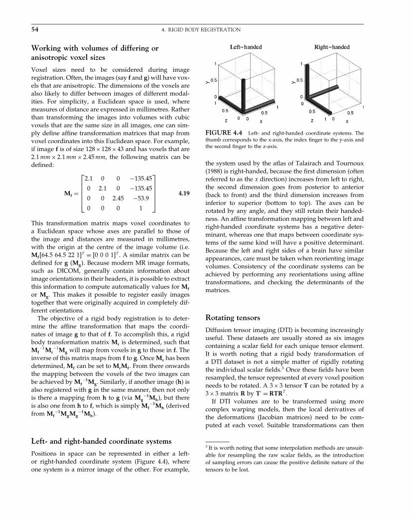
Elsevier UK Chapter: Ch04-P372560 3-10-2006 3:02p.m. Page:54 Trim:7.5in×9.25in
Basal Font:Palatino Margins:Top:40pt Gutter:68pt Font Size:9.5/12 Text Width:42pc Depth:55 Lines
54 4. RIGID BODY REGISTRATION
Working with volumes of differing oranisotropic voxel sizes
Voxel sizes need to be considered during imageregistration. Often, the images (say f and g) will have vox-els that are anisotropic. The dimensions of the voxels arealso likely to differ between images of different modal-ities. For simplicity, a Euclidean space is used, wheremeasures of distance are expressed in millimetres. Ratherthan transforming the images into volumes with cubicvoxels that are the same size in all images, one can sim-ply define affine transformation matrices that map fromvoxel coordinates into this Euclidean space. For example,if image f is of size 128×128×43 and has voxels that are2�1 mm × 2�1 mm × 2�45 mm, the following matrix can bedefined:
Mf =
⎡⎢⎢⎢⎢⎣
2�1 0 0 −135�45
0 2�1 0 −135�45
0 0 2�45 −53�9
0 0 0 1
⎤⎥⎥⎥⎥⎦ 4.19
This transformation matrix maps voxel coordinates toa Euclidean space whose axes are parallel to those ofthe image and distances are measured in millimetres,with the origin at the centre of the image volume (i.e.Mf64�5 64�5 22 1T = 0 0 0 1T . A similar matrix can bedefined for g �Mg�. Because modern MR image formats,such as DICOM, generally contain information aboutimage orientations in their headers, it is possible to extractthis information to compute automatically values for Mf
or Mg. This makes it possible to register easily imagestogether that were originally acquired in completely dif-ferent orientations.
The objective of a rigid body registration is to deter-mine the affine transformation that maps the coordi-nates of image g to that of f. To accomplish this, a rigidbody transformation matrix Mr is determined, such thatMf
−1Mr−1Mg will map from voxels in g to those in f. The
inverse of this matrix maps from f to g. Once Mr has beendetermined, Mf can be set to MrMf. From there onwardsthe mapping between the voxels of the two images canbe achieved by Mf
−1Mg. Similarly, if another image (h) isalso registered with g in the same manner, then not onlyis there a mapping from h to g (via Mg
−1Mh), but thereis also one from h to f, which is simply Mf
−1Mh (derivedfrom Mf
−1MgMg−1Mh).
Left- and right-handed coordinate systems
Positions in space can be represented in either a left-or right-handed coordinate system (Figure 4.4), whereone system is a mirror image of the other. For example,
FIGURE 4.4 Left- and right-handed coordinate systems. Thethumb corresponds to the x-axis, the index finger to the y-axis andthe second finger to the z-axis.
the system used by the atlas of Talairach and Tournoux(1988) is right-handed, because the first dimension (oftenreferred to as the x direction) increases from left to right,the second dimension goes from posterior to anterior(back to front) and the third dimension increases frominferior to superior (bottom to top). The axes can berotated by any angle, and they still retain their handed-ness. An affine transformation mapping between left andright-handed coordinate systems has a negative deter-minant, whereas one that maps between coordinate sys-tems of the same kind will have a positive determinant.Because the left and right sides of a brain have similarappearances, care must be taken when reorienting imagevolumes. Consistency of the coordinate systems can beachieved by performing any reorientations using affinetransformations, and checking the determinants of thematrices.
Rotating tensors
Diffusion tensor imaging (DTI) is becoming increasinglyuseful. These datasets are usually stored as six imagescontaining a scalar field for each unique tensor element.It is worth noting that a rigid body transformation ofa DTI dataset is not a simple matter of rigidly rotatingthe individual scalar fields.3 Once these fields have beenresampled, the tensor represented at every voxel positionneeds to be rotated. A 3×3 tensor T can be rotated by a3×3 matrix R by T′ = RTRT .
If DTI volumes are to be transformed using morecomplex warping models, then the local derivatives ofthe deformations (Jacobian matrices) need to be com-puted at each voxel. Suitable transformations can then
3 It is worth noting that some interpolation methods are unsuit-able for resampling the raw scalar fields, as the introductionof sampling errors can cause the positive definite nature of thetensors to be lost.

Elsevier UK Chapter: Ch04-P372560 3-10-2006 3:02p.m. Page:55 Trim:7.5in×9.25in
Basal Font:Palatino Margins:Top:40pt Gutter:68pt Font Size:9.5/12 Text Width:42pc Depth:55 Lines
WITHIN-MODALITY RIGID REGISTRATION 55
be extracted from these derivatives, and applied to eachelement of the re-sampled tensor field (Alexander et al.,1999, 2001).
WITHIN-MODALITY RIGIDREGISTRATION
Whenever several images of the same subject have beenacquired, it is extremely useful to have them all in regis-ter. Some of the simple benefits of this include allowingimages to be averaged in order to increase signal to noise,or to subtract one image from another to emphasize dif-ferences between the images. Rigid4 registration is nor-mally used for retrospectively registering images of thesame subject that have been collected at different times.Even if images were acquired during the same scanningsession, the subject may have moved slightly betweenacquisitions.
The most common application of within-modality reg-istration in functional imaging is to reduce motion arte-facts by realigning the volumes in image time-series.The objective of realignment is to determine the rigidbody transformations that best map the series of func-tional images to the same space. This can be achieved byminimizing the mean squared difference between eachof the images and a reference image, where the refer-ence image could be one of the images in the series. Forslightly better results, this procedure could be repeated,but instead of matching to one of the images from theseries, the images would be registered to the mean ofall the realigned images. Because of the non-stationaryvariance in the images, a variance image could be com-puted at the same time as the mean, in order to providebetter weighting for the registration. Voxels with a lot ofvariance should be given lower weighting, whereas thosewith less variance should be weighted more highly.
Within-modality image registration is also useful forlooking at shape differences of brains. Morphometricstudies sometimes involve looking at changes in brainshape over time, often to study the progression of a dis-ease such as Alzheimer’s, or to monitor tumour growthor shrinkage. Differences between structural MR scansacquired at different times are identified, by first coreg-istering the images and then looking at the differencebetween the registered images. Rigid registration canalso be used as a preprocessing step before using non-linear registration methods for identifying shape changes(Freeborough and Fox, 1998).
4 Or affine registration if voxel sizes are not accurately known.
Image registration involves estimating a set ofparameters describing a spatial transformation that ‘best’match the images together. The goodness of the matchis based on an objective function, which is maximized orminimized using some optimization algorithm. This sectiondeals with registering images that have been collectedusing the same (or similar) modalities, allowing a rela-tively simple objective function to be used. In this case,the objective function is the mean squared differencebetween the images. The more complex task of regis-tering images with different contrasts will be dealt withlater.
Optimization
The objective of optimization is to determine the val-ues for a set of parameters for which some function ofthe parameters is minimized (or maximized). One of thesimplest cases involves determining the optimum param-eters for a model in order to minimize the mean squareddifference between a model and a set of real world data.Normally there are many parameters and it is not possi-ble to search exhaustively through the whole parameterspace. The usual approach is to make an initial parame-ter estimate, and begin iteratively searching from there.At each iteration, the model is evaluated using the cur-rent parameter estimates, and the objective function com-puted. A judgement is then made about how the parame-ter estimates should be modified, before continuing on tothe next iteration. The optimization is terminated whensome convergence criterion is achieved (usually whenthe objective function stops decreasing, or its derivativeswith respect to the parameters become sufficiently small).
The registration approach described here is essentiallyan optimization. One image (the source image) is spa-tially transformed so that it matches another (the ref-erence image) by minimizing the mean squared differ-ence. The parameters that are optimized are those thatdescribe the spatial transformation (although there areoften other nuisance parameters required by the model,such as intensity scaling parameters). A good algorithmto use for rigid registration (Friston et al., 1995; Woodset al., 1998) is Gauss-Newton optimization, and it is illus-trated here.
Suppose that bi�q� is the function describing the differ-ence between the source and reference images at voxeli, when the vector of model parameters have values q.For each voxel, a first approximation of Taylor’s theoremcan be used to estimate the value that this difference willtake if the parameters q are decreased by t:
bi�q − t� � bi�q�− t1�bi�q�
�q1− t2
�bi�q�
�q2� � � 4.20
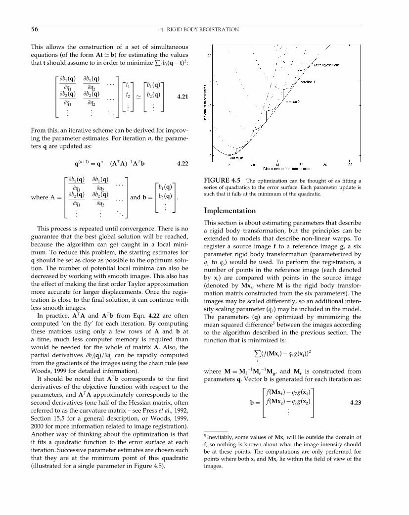
Elsevier UK Chapter: Ch04-P372560 3-10-2006 3:02p.m. Page:56 Trim:7.5in×9.25in
Basal Font:Palatino Margins:Top:40pt Gutter:68pt Font Size:9.5/12 Text Width:42pc Depth:55 Lines
56 4. RIGID BODY REGISTRATION
This allows the construction of a set of simultaneousequations (of the form At � b) for estimating the valuesthat t should assume to in order to minimize
∑i bi�q − t�2:
⎡⎢⎢⎢⎢⎢⎣
�b1�q�
�q1
�b1�q�
�q2� � �
�b2�q�
�q1
�b2�q�
�q2� � �
������
� � �
⎤⎥⎥⎥⎥⎥⎦
⎡⎢⎢⎣
t1
t2
���
⎤⎥⎥⎦�
⎡⎢⎢⎣
b1�q�
b2�q�
���
⎤⎥⎥⎦ 4.21
From this, an iterative scheme can be derived for improv-ing the parameter estimates. For iteration n, the parame-ters q are updated as:
q�n+1� = qn − �AT A�−1AT b 4.22
where A =
⎡⎢⎢⎢⎢⎢⎣
�b1�q�
�q1
�b1�q�
�q2� � �
�b2�q�
�q1
�b2�q�
�q2� � �
������
� � �
⎤⎥⎥⎥⎥⎥⎦
and b =
⎡⎢⎢⎣
b1�q�
b2�q����
⎤⎥⎥⎦.
This process is repeated until convergence. There is noguarantee that the best global solution will be reached,because the algorithm can get caught in a local mini-mum. To reduce this problem, the starting estimates forq should be set as close as possible to the optimum solu-tion. The number of potential local minima can also bedecreased by working with smooth images. This also hasthe effect of making the first order Taylor approximationmore accurate for larger displacements. Once the regis-tration is close to the final solution, it can continue withless smooth images.
In practice, AT A and AT b from Eqn. 4.22 are oftencomputed ‘on the fly’ for each iteration. By computingthese matrices using only a few rows of A and b ata time, much less computer memory is required thanwould be needed for the whole of matrix A. Also, thepartial derivatives �bi�q�/�qj can be rapidly computedfrom the gradients of the images using the chain rule (seeWoods, 1999 for detailed information).
It should be noted that AT b corresponds to the firstderivatives of the objective function with respect to theparameters, and AT A approximately corresponds to thesecond derivatives (one half of the Hessian matrix, oftenreferred to as the curvature matrix – see Press et al., 1992,Section 15.5 for a general description, or Woods, 1999,2000 for more information related to image registration).Another way of thinking about the optimization is thatit fits a quadratic function to the error surface at eachiteration. Successive parameter estimates are chosen suchthat they are at the minimum point of this quadratic(illustrated for a single parameter in Figure 4.5).
FIGURE 4.5 The optimization can be thought of as fitting aseries of quadratics to the error surface. Each parameter update issuch that it falls at the minimum of the quadratic.
Implementation
This section is about estimating parameters that describea rigid body transformation, but the principles can beextended to models that describe non-linear warps. Toregister a source image f to a reference image g, a sixparameter rigid body transformation (parameterized byq1 to q6) would be used. To perform the registration, anumber of points in the reference image (each denotedby xi) are compared with points in the source image(denoted by Mxi, where M is the rigid body transfor-mation matrix constructed from the six parameters). Theimages may be scaled differently, so an additional inten-sity scaling parameter �q7� may be included in the model.The parameters (q) are optimized by minimizing themean squared difference5 between the images accordingto the algorithm described in the previous section. Thefunction that is minimized is:
∑i
�f�Mxi�− q7g�xi��2
where M = Mf−1Mr
−1Mg, and Mr is constructed fromparameters q. Vector b is generated for each iteration as:
b =
⎡⎢⎢⎣
f�Mx1�− q7g�x1�
f�Mx2�− q7g�x2����
⎤⎥⎥⎦ 4.23
5 Inevitably, some values of Mxi will lie outside the domain off, so nothing is known about what the image intensity shouldbe at these points. The computations are only performed forpoints where both xi and Mxi lie within the field of view of theimages.

Elsevier UK Chapter: Ch04-P372560 3-10-2006 3:02p.m. Page:57 Trim:7.5in×9.25in
Basal Font:Palatino Margins:Top:40pt Gutter:68pt Font Size:9.5/12 Text Width:42pc Depth:55 Lines
WITHIN-MODALITY RIGID REGISTRATION 57
Each column of matrix A is constructed by differentiatingb with respect to parameters q1 to q7:
A =
⎡⎢⎢⎢⎢⎢⎣
�f�Mx1�
�q1
�f�Mx1�
�q2� � �
�f�Mx1�
�q6−g�x1�
�f�Mx2�
�q1
�f�Mx2�
�q2� � �
�f�Mx2�
�q6−g�x2�
������
� � ����
���
⎤⎥⎥⎥⎥⎥⎦4.24
Because non-singular affine transformations are easilyinvertible, it is possible to make the registration morerobust by also considering what happens with the inversetransformation. By swapping around the source andreference image, the registration problem also becomesone of minimizing:
∑j
�g�M−1yj�− q−17 f�yj��
2
In theory, a more robust solution could be achieved bysimultaneously including the inverse transformation tomake the registration problem symmetric (Woods et al.,1998). The objective function would then be:
1
∑i
�f�Mxi�− q7g�xi��2 + 2
∑j
�g�M−1yj�− q−17 f�yj��
2
4.25
Normally, the intensity scaling of the image pair will besimilar, so equal values for the weighting factors ( 1 and 2) can be used. Matrix A and vector b would then beformulated as:
b =
⎡⎢⎢⎢⎢⎢⎢⎢⎢⎢⎢⎢⎢⎢⎣
�121 �f�Mx1�− q7g�x1��
�121 �f�Mx2�− q7g�x2��
���
�122 �g�M−1 −y1�− q−1
7 f�y1��
�122 �g�M−1 −y2�− q−1
7 f�y2��
���
⎤⎥⎥⎥⎥⎥⎥⎥⎥⎥⎥⎥⎥⎥⎦
4.26
and
A =
⎡⎢⎢⎢⎢⎢⎢⎢⎢⎢⎢⎢⎢⎢⎢⎢⎣
�121
�f�Mx1�
�q1· · · �
121
�f�Mx1�
�q6−�
121 g�x1�
�121
�f�Mx2�
�q1· · · �
121
�f�Mx2�
�q6−�
121 g�x2�
���� � �
������
�122
�f�M−1y1�
�q1· · · �
122
�g�M−1y1�
�q6�
121 q−2
7 f�y1�
�122
�g�M−1y2�
�q1· · · �
122
�g�M−1y2�
�q6�
122 q−2
7 f�y2�
���� � �
������
⎤⎥⎥⎥⎥⎥⎥⎥⎥⎥⎥⎥⎥⎥⎥⎥⎦
4.27
Residual artefacts from PET and fMRI
Even after realignment, there may still be some motionrelated artefacts remaining in functional data. After ret-rospective realignment of PET images with large move-ments, the primary source of error is due to incorrectattenuation correction. In emission tomography methods,many photons are not detected because they are atten-uated by the subject’s head. Normally, a transmissionscan (using a moving radioactive source external to thesubject) is acquired before collecting the emission scans.The ratio of the number of detected photon pairs fromthe source, with and without a head in the field of view,produces a map of the proportion of photons that areabsorbed along any line-of-response. If a subject movesbetween the transmission and emission scans, then theapplied attenuation correction is incorrect because theemission scan is no longer aligned with the transmis-sion scan. There are methods for correcting these errors(Andersson et al., 1995), but they are beyond the scope ofthis book.
In fMRI, there are many sources of motion related arte-facts. The most obvious ones are:
• Interpolation error from the re-sampling algorithmused to transform the images can be one of the mainsources of motion related artefacts.
• When MR images are reconstructed, the final imagesare usually the modulus of the initially complex data.This results in voxels that should be negative being ren-dered positive. This has implications when the imagesare re-sampled, because it leads to errors at the edgeof the brain that cannot be corrected however good theinterpolation method is. Possible ways to circumventthis problem are to work with complex data, or applya low pass filter to the complex data before taking themodulus.
• The sensitivity (slice selection) profile of each slice alsoplays a role in introducing artefacts (Noll et al., 1997).
• fMRI images are spatially distorted, and the amount ofdistortion depends partly upon the position of the sub-ject’s head within the magnetic field. Relatively largesubject movements result in the brain images changingshape, and these shape changes cannot be corrected bya rigid body transformation (Jezzard and Clare, 1999;Andersson et al., 2001).
• Each fMRI volume of a series is currently acquired aplane at a time over a period of a few seconds. Subjectmovement between acquiring the first and last planeof any volume is another reason why the images maynot strictly obey the rules of rigid body motion.
• After a slice is magnetized, the excited tissue takestime to recover to its original state, and the amount ofrecovery that has taken place will influence the inten-sity of the tissue in the image. Out of plane movement

Elsevier UK Chapter: Ch04-P372560 3-10-2006 3:02p.m. Page:58 Trim:7.5in×9.25in
Basal Font:Palatino Margins:Top:40pt Gutter:68pt Font Size:9.5/12 Text Width:42pc Depth:55 Lines
58 4. RIGID BODY REGISTRATION
will result in a slightly different part of the brain beingexcited during each repeat. This means that the spinexcitation will vary in a way that is related to headmotion, and so leads to more movement related arte-facts (Friston et al., 1996).
• Nyquist ghost artefacts in MR images do not obey thesame rigid body rules as the head, so a rigid rotationto align the head will not mean that the ghosts arealigned. The same also applies to other image artefacts,such as those arising due to chemical shifts.
• The accuracy of the estimated registration parametersis normally in the region of tens of microns. This isdependent upon many factors, including the effectsjust mentioned. Even the signal changes elicited by theexperiment can have a slight effect (a few microns) onthe estimated parameters (Freire and Mangin, 2001).
These problems cannot be corrected by simple imagerealignment and so may be sources of possible stimuluscorrelated motion artefacts. Systematic movement arte-facts resulting in a signal change of only one or two percent can lead to highly significant false positives over anexperiment with many scans. This is especially impor-tant for experiments where some conditions may causeslight head movements (such as motor tasks, or speech),because these movements are likely to be highly corre-lated with the experimental design. In cases like this,it is difficult to separate true activations from stimuluscorrelated motion artefacts. Providing there are enoughimages in the series and the movements are small, someof these artefacts can be removed by using an analysis ofcovariation (ANCOVA) model to remove any signal thatis correlated with functions of the movement parame-ters (Friston et al., 1996). However, when the estimates ofthe movement parameters are related to the experimentaldesign, it is likely that much of the true fMRI signal willalso be lost. These are still unresolved problems.
BETWEEN-MODALITY RIGIDREGISTRATION
The combination of multiple imaging modalities can pro-vide enhanced information that is not readily apparenton inspection of individual image modalities. For studiesof a single subject, sites of activation can be accuratelylocalized by superimposing them on a high resolutionstructural image of the subject (typically a T1-weightedMRI). This requires registration of the functional imageswith the structural image. A further possible use for thisregistration is that a more precise spatial normalizationcan be achieved by computing it from a more detailedstructural image. If the functional and structural images
are in register, then a warp computed from the struc-tural image can be applied to the functional images. Nor-mally a rigid body model is used for registering imagesof the same subject, but because fMRI images are usu-ally severely distorted – particularly in the phase encodedirection (Jezzard and Clare, 1999; Jezzard, 2000) – it isoften preferable to do non-linear registration (Kybic et al.,2000; Studholme et al., 2000). Rigid registration modelsrequire voxel sizes to be accurately known. This is a prob-lem that is particularly apparent when registering imagesfrom different scanners.
Two images from the same subject acquired usingthe same modality or scanning sequences generally looksimilar, so it suffices to find the rigid body transfor-mation parameters that minimize the sum of squareddifferences between them. However, for coregistrationbetween modalities there is nothing quite so obvious tominimize, as there is no linear relationship between theimage intensities (Figure 4.6).
FIGURE 4.6 An example of T1- and T2-weighted MR imagesregistered using mutual information. The two registered images areshown interleaved in a chequered pattern.

Elsevier UK Chapter: Ch04-P372560 3-10-2006 3:02p.m. Page:59 Trim:7.5in×9.25in
Basal Font:Palatino Margins:Top:40pt Gutter:68pt Font Size:9.5/12 Text Width:42pc Depth:55 Lines
BETWEEN-MODALITY RIGID REGISTRATION 59
Older methods of registration involved the manualidentification of homologous landmarks in the images.These landmarks are aligned together, thus bringing theimages into registration. This is time-consuming, requiresa degree of experience, and can be rather subjective.One of the first widely used semiautomatic coregistra-tion methods was that known as the ‘head-hat’ approach(Pelizzari et al., 1988). This method involved extractingbrain surfaces of the two images, and then matchingthe surfaces together. There are also a number of otherbetween-modality registration methods that involve par-titioning the images, or finding common features, andthen registering them together, but they are beyond thescope of this chapter.
The first intensity based inter-modal registrationmethod was AIR (Woods et al., 1993), which has beenwidely used for a number of years for registering PETand MR images. This method uses a variance of intensityratios (VIR) objective function, and involves dividing theMR images into a number of partitions based on intensity.The registration is approximately based on minimizingthe variance of the corresponding PET voxel intensitiesfor each partition. It makes a number of assumptionsabout how the PET intensity varies with the MRI inten-sity, which are generally valid within the brain, but donot work when non-brain tissue is included. Becauseof this, the method has the disadvantage of requiringthe MR images to be edited to remove non-brain tissue.For reviews of a number of inter-modality registrationapproaches, see Zuk and Atkins, 1996 and Hill et al., 2001.
Information theoretic approaches
The most recent voxel-similarity measures to be used forinter-modal (as well as intra-modal (Holden et al., 2000))registration have been based on information theory. Thesemeasures are based on joint probability distributions ofintensities in the images, usually discretely representedin the form of 2D joint histograms, which are normalizedto sum to one.
The first information theoretic measure to be pro-posed was the entropy of the joint probability distribu-tion (Studholme et al., 1995), which should be minimizedwhen the images are in register:
H�f� g� = −∫ �
−�
∫ �
−�P�f� g� log P�f� g�dfdg 4.28
The discrete representation of the probability distribu-tions is from a joint histogram, which can be consideredas an I by J matrix P. The entropy is then computed fromthe histogram according to:
H�f� g� =∑J
j=1
∑I
i=1pij log pij 4.29
In practice, the entropy measure was found to producepoor registration results, but shortly afterwards, a morerobust measure of registration quality was introduced.This was based on mutual information (MI) (Collignonet al., 1995; Wells et al., 1996) (also known as Shannoninformation), which is given by:
I�f� g� = H�f�+H�g�−H�f� g� 4.30
where H�f� g� is the joint entropy of the images, and H�f�and H�g� are their marginalized entropies given by:
H�f� = −∫ �
−�P�f� log P�f�df 4.31
H�g� = −∫ �
−�P�g� log P�g�dg 4.32
MI is a measure of dependence of one image onthe other, and can be considered as the distance(Kullback-Leibler divergence) between the joint distri-bution �P�f� g�� and the distribution assuming completeindependence �P�f�P�g��. When the two distributions areidentical, this distance (and the mutual information) iszero. After rearranging, the expression for MI becomes:
I�f� g� = KL�P�f� g���P�f�P�g��
=∫ �
−�
∫ �
−�P�f� g� log
(P�f� g�
P�f�P�g�
)dfdg 4.33
It is assumed that the MI between the images is max-imized when they are in register (Figure 4.7). Anotherinformation theoretic measure (Studholme et al., 1999)that can be used for registration is:
Ĩ �f� g� = H�f�+H�g�
H�f� g�4.34
Another useful measure (Maes et al., 1997) is:
Ĩ �f� g� = 2H�f� g�−H�f�−H�g� 4.35
and also the entropy correlation coefficient (Maes et al., 1997)(see Press et al., 1992, for more information):
U�f� g� = 2H�f�+H�g�−H�f� g�
H�f�+H�g�4.36
Implementation details
Generating a joint histogram involves scanning throughthe voxels of the reference image and finding the cor-responding points of the source. The appropriate bin inthe histogram is incremented by one for each of these

Elsevier UK Chapter: Ch04-P372560 3-10-2006 3:02p.m. Page:60 Trim:7.5in×9.25in
Basal Font:Palatino Margins:Top:40pt Gutter:68pt Font Size:9.5/12 Text Width:42pc Depth:55 Lines
60 4. RIGID BODY REGISTRATION
FIGURE 4.7 An illustration of how the joint histogram of animage pair changes as they are displaced relative to each other (notethat the pictures show log�1 + N�, where N is the count in eachhistogram bin). The MI of the images is also shown.
point pairs. Pairs are ignored if the corresponding voxelis unavailable because it lies outside the image volume.The coordinate of the corresponding point rarely liesat an actual voxel centre, meaning that interpolation isrequired.
Many developers use partial volume interpolation (Col-lignon et al., 1995), rather than interpolating the imagesthemselves, but this can make the MI objective func-tion particularly susceptible to interpolation artefact(Figure 4.8). The MI tends to be higher when voxel centresare sampled, where one is added to a single histogrambin. MI is lower when sampling in the centre of the eightneighbours, as an eighth is added to eight bins. Theseartefacts are especially prominent when fewer point pairsare used to generate the histograms.
A simpler alternative is to interpolate the images them-selves, but this can lead to new intensity values in thehistograms, which also cause interpolation artefact. Thisartefact largely occurs because of aliasing after integerrepresented images are rescaled so that they have valuesbetween zero and I −1, where I is the number of bins inthe histogram (Figure 4.9). If care is taken at this stage,then interpolation of the image intensities becomes lessof a problem. Another method of reducing these artefactsis to not sample the reference image on a regular grid, by(for example) introducing a random jitter to the sampledpoints (Likar and Pernuš, 2001).
Histograms contain noise, especially if a relativelysmall number of points are sampled in order to gen-erate them. The optimum binning to use is still notfully resolved, and is likely to vary from application toapplication, but most researchers use histograms rangingbetween about 16 × 16 and 256 × 256. Smoothing a his-togram has a similar effect to using fewer bins. Another
FIGURE 4.8 The mutual information objective function can be particularly susceptible to interpolation artefacts. This figure shows aplot of the MI between two images when they are translated with respect to each other. The dotted and dot-dashed lines show it computedusing partial volume interpolation at high and lower sampling densities respectively. The solid and dashed lines show MI computed byinterpolating the images themselves (solid indicates high sampling density, dashed indicates lower density).

Elsevier UK Chapter: Ch04-P372560 3-10-2006 3:02p.m. Page:61 Trim:7.5in×9.25in
Basal Font:Palatino Margins:Top:40pt Gutter:68pt Font Size:9.5/12 Text Width:42pc Depth:55 Lines
REFERENCES 61
FIGURE 4.9 Rescaling an image can lead to aliasing artefacts in its histogram. Above: histogram based on original integer intensityvalues, simulated to have a Gaussian distribution. Below: the histogram after the intensities are rescaled shows aliasing artefacts.
alternative is to use a continuous representation of thejoint probability distribution, such as a Parzen windowdensity estimate (Wells et al., 1996), or possibly even aGaussian mixture model representation.
A method of optimization based on the first and secondderivatives of the objective function was introduced ear-lier. Similar principles have been applied to minimizingthe VIR objective function (Woods et al., 1993), and also tomaximizing MI (Thévenaz and Unser, 2000).6 However,the most widely adopted scheme for maximizing MI isPowell’s method (see Press et al., 1992), which involvesa series of successive line searches. Failures occasion-ally arise if the voxel similarity measure does not varysmoothly with changes to the parameter estimates. Thiscan happen because of interpolation artefact, or if insuffi-cient data contribute to the joint histogram. Alternatively,the algorithm can get caught within a local optimum, soit is important to assign starting estimates that approxi-mately register the images. The required accuracy of thestarting estimates depends on the particular images, butan approximate figure for many brain images with a good
6 This paper uses Levenberg-Marquardt optimization (Presset al., 1992), which is a stabilized version of the Gauss-Newtonmethod.
field of view would be in the region of about 5 cm fortranslations and 15° for rotations.
REFERENCES
Alexander DC, Gee JC, Bajcsy R (1999) Strategies for data reori-entation during non-rigid transformations of diffusion tensorimages. In Proc Medical Image Computing and Computer-AssistedIntervention (MICCAI), Taylor C, Colchester A (eds), vol. 1679of Lecture Notes in Computer Science. Springer-Verlag, Berlin andHeidelberg, pp. 463–72
Alexander DC, Pierpaoli C, Basser PJ et al. (2001) Spatial transfor-mations of diffusion tensor magnetic resonance images. IEEETrans Med Imag 20: 1131–39
Andersson JLR, Hutton C, Ashburner J et al. (2001) Modeling geo-metric deformations in EPI time series. NeuroImage 13: 903–19
Andersson JLR, Vagnhammar BE, Schneider H (1995) Accurateattenuation correction despite movement during PET imaging.J Nucl Med 36: 670–78
Collignon A, Maes F, Delaere D et al. (1995) Automated multi-modality image registration based on information theory. InProc Information Processing in Medical Imaging (IPMI), Bizais Y,Barillot C, Di Paola R (eds). Kluwer Academic Publishers, Dor-drecht
Cox RW, Jesmanowicz A (1999) Real-time 3D image registration forfunctional MRI. Magn Res Med 42: 1014–18
Eddy WF, Fitzgerald M, Noll DC (1996) Improved image registra-tion by using Fourier interpolation. Mag Res Med 36: 923–31

Elsevier UK Chapter: Ch04-P372560 3-10-2006 3:02p.m. Page:62 Trim:7.5in×9.25in
Basal Font:Palatino Margins:Top:40pt Gutter:68pt Font Size:9.5/12 Text Width:42pc Depth:55 Lines
62 4. RIGID BODY REGISTRATION
Freeborough PA, Fox NC (1998) Modelling brain deformations inalzheimer disease by fluid registration of serial MR images.J Comput Assist Tomogr 22: 838–43
Freire L, Mangin J-F (2001) Motion correction algorithms of the brainmapping community create spurious functional activations. InProc Information Processing in Medical Imaging (IPMI), Insana MF,Leahy RM (eds), vol. 2082 of Lecture Notes in Computer Science.Springer-Verlag, Berlin and Heidelberg, pp 246–58
Friston KJ, Ashburner J, Frith CD et al. (1995) Spatial registrationand normalization of images. Hum Brain Mapp 2: 165–89
Friston KJ, Williams S, Howard R et al. (1996) Movement-relatedeffects in fMRI time-series. Mag Res Med 35: 346–55
Hajnal JV, Mayers R, Oatridge A et al. (1994) Artifacts due to stim-ulus correlated motion in functional imaging of the brain. MagRes Med 31: 289–91
Hill DLG, Batchelor PG, Holden M et al. (2001) Medical image reg-istration. Phys Med Biol 46: R1–R45
Holden M, Hill DLG, Denton ERE et al. (2000) Voxel similaritymeasures for 3-D serial MR brain image registration. IEEE TransMed Imag 19(2): 94–102
Jezzard P (2000) Handbook of medical imaging, Chap. 26. AcademicPress, San Diego, pp 425–38
Jezzard P, Clare S (1999) Sources of distortion in functional MRIdata. Hum Brain Mapp 8(2): 80–85
Kybic J, Theévenaz P, Nirkko A et al. (2000) Unwarping of uni-directionally distorted EPI images. IEEE Trans Med Imag 19(2):80–93
Likar B, Pernuš F (2001) A heirarchical approach to elastic registra-tion based on mutual information. Image Vision Comput 19: 33–44
Maes F, Collignon A, Vandermeulen D et al. (1997) Multimodalityimage registration by maximisation of mutual information. IEEETrans Med Imag 16: 187–97
Noll DC, Boada FE, Eddy WF (1997) A spectral approach toanalyzing slice selection in planar imaging: optimization forthrough-plane interpolation. Mag Res Med 38: 151–60
Pelizzari CA, Chen GTY, Spelbring DR et al. (1988) Accurate three-dimensional registration of CT, PET and MR images of the brain.Comput Assist Tomogr 13: 20–26
Press WH, Teukolsky SA, Vetterling WT et al. (1992) NumericalRecipes in C, 2nd edn. Cambridge University Press, Cambridge
Studholme C, Constable RT, Duncan JS (2000) Accurate alignmentof functional EPI data to anatomical MRI using a physics-baseddistortion model. IEEE Trans Med Imag 19(11): 1115–27
Studholme C, Hill DLG, Hawkes DJ (1995) Multiresolution voxelsimilarity measures for MR-PET coregistration. In Proc Informa-tion Processing in Medical Imaging (IPMI), Bizais Y, Barillot C,Di Paola R (eds). Kluwer Academic Publishers, Dordrecht.
Studholme C, Hill DLG, Hawkes DJ (1999) An overlap invariantentropy measure of 3D medical image alignment. Pattern Recog-nit 32: 71–86
Talairach J, Tournoux P (1988) Coplanar stereotaxic atlas of the humanbrain. Thieme Medical, New York
Thévenaz P, Blu T, Unser M (2000) Interpolation revisited. IEEETrans Med Imag 19(7): 739–58
Thévenaz P, Unser M (2000) Optimization of mutual informationfor multiresolution image registration. IEEE Trans Image Process9(12): 2083–99
Unser M, Aldroubi A, Eden M (1993a) B-spline signal processing:Part I – theory. IEEE Trans Signal Process 41(2): 821–33
Unser M, Aldroubi A, Eden M (1993b) B-spline signal processing:Part II – efficient design and applications. IEEE Transact SignalProcess 41(2): 834–48
Wells WM III, Viola P, Atsumi H et al. (1996) Multi-modal volumeregistration by maximisation of mutual information. Med ImageAnal 1(1): 35–51
Woods RP (1999) Brain Warping, chap. 20. Academic Press, SanDiego, pp 365–76
Woods RP (2000) Handbook of Medical Imaging, chap. 33. AcademicPress, San Diego, pp 529–36
Woods RP, Grafton ST, Holmes CJ et al. (1998) Automated imageregistration: I. General methods and intrasubject, intramodalityvalidation. Comput Assist Tomogr 22: 139–52
Woods RP, Mazziotta JC, Cherry SR (1993) MRI-PET registrationwith automated algorithm. Comput Assist Tomogr 17: 536–46
Zuk TD, Atkins MS (1996) A comparison of manual and automaticmethods for registering scans of the head. IEEE Trans Med Imag15(5): 732–44

Elsevier UK Chapter: Ch40-P372560 30-9-2006 5:34p.m. Page:534 Trim:7.5in×9.25in
Basal Font:Palatino Margins:Top:40pt Gutter:68pt Font Size:9.5/12 Text Width:42pc Depth:55 Lines
C H A P T E R
40
Multivariate autoregressive modelsW. Penny and L. Harrison
INTRODUCTION
Functional neuroimaging has been used to corroboratefunctional specialization as a principle of organizationin the human brain. However, disparate regions of thebrain do not operate in isolation and, more recently, neu-roimaging has been used to characterize the networkproperties of the brain under specific cognitive states(Buchel and Friston, 1997a; Buchel and Friston, 2000).These studies address a complementary principle of orga-nization, functional integration.
Functional magnetic resonance imaging (fMRI) pro-vides a unique opportunity to observe simultaneousrecordings of activity throughout the brain evoked bycognitive and sensorimotor challenges. Each voxel withinthe brain is represented by a time-series of neurophys-iological activity that underlies the measured bloodoxygen-level-dependent (BOLD) response. Given thesemultivariate, voxel-based time-series, can we infer large-scale network behaviour among functionally specializedregions?
A number of methods have been proposed to answerthis question including regression models (McIntoshet al., 1994; Friston et al., 1993, 1995, 1997), convolu-tion models (Friston and Buchel, 2000; Friston, 2001) andstate-space models (Buchel and Friston, 1998). Regressiontechniques, underlying for example the analysis of psy-chophysiological interactions (PPIs), are useful becausethey are easy to fit and can test for the modulatory inter-actions of interest (Friston et al., 1997). However, this isat the expense of excluding temporal information, i.e.the history of an input or physiological variable. This isimportant as interactions within the brain, whether overshort or long distances, take time and are not instan-taneous. Structural equation modelling (SEM), as usedby the neuroimaging community (McIntosh et al., 1994;
Buchel and Friston, 1997b) has similar problems.1 Con-volution models, such as the Volterra approach, modeltemporal effects in terms of an idealized response char-acterized by the kernels of the model (Friston, 2000). Acriticism of the Volterra approach is that it treats thesystem as a black box, meaning that it has no model ofthe internal mechanisms that may generate data. State-space models account for correlations within the data byinvoking state variables whose dynamics generate data.Recursive algorithms, such as the Kalman filter, may beused to estimate these states through time, given the data(Buchel and Friston, 1998).
This chapter describes an approach based onmultivariate autoregressive (MAR) models. These arelinear multivariate time-series models which have along history of application in econometrics. The MARmodel characterizes interregional dependencies withindata, specifically in terms of the historical influence onevariable has on another. This is distinct from regressiontechniques that quantify instantaneous correlations. Weuse MAR models to make inferences about functionalintegration from fMRI data.
The chapter is divided into three sections. First, wedescribe the theory of MAR models, parameter esti-mation, model order selection and statistical inference.We have used a Bayesian technique for model orderselection and parameter estimation, which is introducedin Chapter 24 and is described fully in Penny andRoberts (2002). Secondly, we model neurophysiologicaldata taken from an fMRI experiment addressing atten-tional modulation of cortical connectivity during a visualmotion task (Buchel and Friston, 1997b). The modula-tory effect of one region upon the responses to otherregions is a second order interaction which is precluded
1 There exist versions of SEM that do model dynamic informa-tion, see Cudeck (2002) for details of dynamic factor analysis.
Statistical Parametric Mapping, by Karl Friston et al. Copyright 2007, Elsevier Ltd. All rights reserved.ISBN–13: 978-0-12-372560-8 ISBN–10: 0-12-372560-7
534

Elsevier UK Chapter: Ch40-P372560 30-9-2006 5:34p.m. Page:535 Trim:7.5in×9.25in
Basal Font:Palatino Margins:Top:40pt Gutter:68pt Font Size:9.5/12 Text Width:42pc Depth:55 Lines
THEORY 535
in linear models. To circumvent this we have introducedbilinear terms (Friston et al., 1997). Thirdly, we discuss theadvantages and disadvantages of MAR models, their usein spectral estimation and possible future developments.
THEORY
Multivariate autoregressive models
Given a univariate time-series, its consecutive measure-ments contain information about the process that gener-ated it. An attempt at describing this underlying ordercan be achieved by modelling the current value of thevariable as a weighted linear sum of its previous val-ues. This is an autoregressive (AR) process and is a verysimple, yet effective, approach to time-series character-ization (Chatfield, 1996). The order of the model is thenumber of preceding observations used, and the weightscharacterize the time-series.
Multivariate autoregressive models extend thisapproach to multiple time-series so that the vector of cur-rent values of all variables is modelled as a linear sumof previous activities. Consider d time-series generatedfrom d variables within a system, such as a functionalnetwork in the brain, and where m is the order of themodel. An MAR(m) model predicts the next value in ad-dimensional time-series, yn as a linear combination ofthe m previous vector values:
yn =m∑
i=1
yn−iA�i�+ en 40.1
where yn = �yn�1�� yn�2�� � � � � yn�d�� is the nth sample ofa d-dimensional time-series, each A�i� is a d-by-d matrixof coefficients (weights) and en = �en�1�� en�2�� � � � � en�d��is additive Gaussian noise with zero mean and covari-ance R. We have assumed that the data mean has beensubtracted from the time-series.
The model can be written in the standard form of amultivariate linear regression model as follows:
yn = xnW + en 40.2
where xn = �yn−1�yn−2� � � � � yn−m� are the m previous mul-tivariate time-series samples and W is a �m × d�-by-dmatrix of MAR coefficients (weights). There are thereforea total of k = m×d×d MAR coefficients.
If the nth rows of Y , X and E are yn, xn and en respec-tively and there are n = 1��N samples then we can write:
Y = XW +E 40.3
where Y is an �N − m�-by-d matrix, X is an �N − m�-by-�m × d� matrix and E is an (N − m)-by-d matrix. The
number of rows N −m (rather than N ) arises as samplesat time points before m do not have sufficient precedingsamples to allow prediction.
MAR models are fully connected in that each region is,by default, assumed connected to all others. However, byfitting the model to data and testing to see which connec-tions are signficantly non-zero, one can infer a sub-networkthat mediates the observed dynamics. This can be imple-mented using Bayesian inference as described below.
These sub-networks are related to the concept of‘Granger causality’ (Granger, 1969), which is definedoperationally as follows. Activity in region X ‘Granger’causes activity in region Y if any of the connections fromX to Y, over all time lags, are non-zero. These causalityrelationships can be summarized by directed graphs asdescribed in Eichler (2005). An example will be presentedlater on in the chapter.
Non-linear autoregressive models
Given a network model of the brain, we can think of twofundamentally different types of coupling: linear and non-linear. The model discussed so far is linear. Linear systemsare described by the principle of superposition, which isthat inputs have additive effects on the response that areindependent of each other. Non-linear systems are charac-terized by inputs which interact to produce a response.
In Buchel and Friston (1997b), non-linear interac-tions were modelled using ‘bilinear terms’. This is theapproach adopted in this chapter. Specifically, to modela hypothesized interaction between variables yn�j� andyn�k� one can form the new variable:
In�j� k� = yn�j�yn�k� 40.4
This is a ‘bilinear variable’. This is orthogonalized withrespect to the original time-series and placed in an aug-mented MAR model with connectivity matrices Ã�i�.
�yn� In�j� k�� =m∑
i=1
�yn−i� In−i�j� k��Ã�i�+ en 40.5
The relevant entries in �i� then reflect modulatory influ-ences, e.g. a change of the connection strength betweeny�j� and other time-series due to the influence of y�k�.
It should be noted that each bilinear variable intro-duces only one of many possible sources of non-linearbehaviour into the model. The example above specificallymodels non-linear interactions between yn�j� and yn�k�,however, other bilinear terms could involve, for instance,the time-series yn�j� and inputs u�t�. The inclusion ofthese terms is guided by the hypothesis of interest, e.g.does ‘time’ change the connectivity between earlier andlater stages of processing in the dorsal visual pathway?Here u�t� would model time.
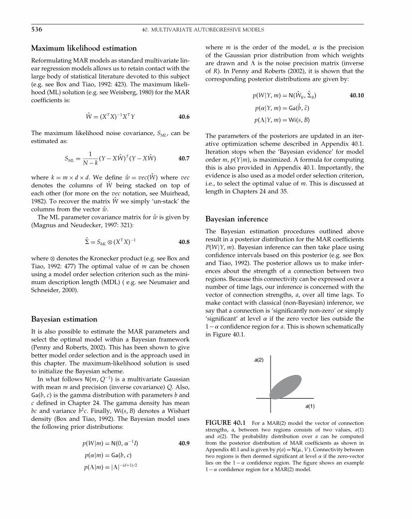
Elsevier UK Chapter: Ch40-P372560 30-9-2006 5:34p.m. Page:536 Trim:7.5in×9.25in
Basal Font:Palatino Margins:Top:40pt Gutter:68pt Font Size:9.5/12 Text Width:42pc Depth:55 Lines
536 40. MULTIVARIATE AUTOREGRESSIVE MODELS
Maximum likelihood estimation
Reformulating MAR models as standard multivariate lin-ear regression models allows us to retain contact with thelarge body of statistical literature devoted to this subject(e.g. see Box and Tiao, 1992: 423). The maximum likeli-hood (ML) solution (e.g. see Weisberg, 1980) for the MARcoefficients is:
Ŵ = �XT X�−1XT Y 40.6
The maximum likelihood noise covariance, SML, can beestimated as:
SML = 1N −k
�Y −XŴ�T �Y −XŴ� 40.7
where k = m × d × d. We define ŵ = vec�Ŵ � where vecdenotes the columns of Ŵ being stacked on top ofeach other (for more on the vec notation, see Muirhead,1982). To recover the matrix Ŵ we simply ‘un-stack’ thecolumns from the vector ŵ.
The ML parameter covariance matrix for ŵ is given by(Magnus and Neudecker, 1997: 321):
̂ = SML ⊗ �XT X�−1 40.8
where ⊗ denotes the Kronecker product (e.g. see Box andTiao, 1992: 477) The optimal value of m can be chosenusing a model order selection criterion such as the mini-mum description length (MDL) ( e.g. see Neumaier andSchneider, 2000).
Bayesian estimation
It is also possible to estimate the MAR parameters andselect the optimal model within a Bayesian framework(Penny and Roberts, 2002). This has been shown to givebetter model order selection and is the approach used inthis chapter. The maximum-likelihood solution is usedto initialize the Bayesian scheme.
In what follows N�m�Q−1� is a multivariate Gaussianwith mean m and precision (inverse covariance) Q. Also,Ga�b� c� is the gamma distribution with parameters b andc defined in Chapter 24. The gamma density has meanbc and variance b2c. Finally, Wi�s�B� denotes a Wishartdensity (Box and Tiao, 1992). The Bayesian model usesthe following prior distributions:
p�W �m� = N�0�−1I� 40.9
p��m� = Ga�b� c�
p���m� = ���−�d+1�/2
where m is the order of the model, is the precisionof the Gaussian prior distribution from which weightsare drawn and � is the noise precision matrix (inverseof R). In Penny and Roberts (2002), it is shown that thecorresponding posterior distributions are given by:
p�W �Y�m� = N�ŴB� ̂B� 40.10
p��Y�m� = Ga�b̂� ĉ�
p���Y�m� = Wi�s�B�
The parameters of the posteriors are updated in an iter-ative optimization scheme described in Appendix 40.1.Iteration stops when the ‘Bayesian evidence’ for modelorder m, p�Y �m�, is maximized. A formula for computingthis is also provided in Appendix 40.1. Importantly, theevidence is also used as a model order selection criterion,i.e., to select the optimal value of m. This is discussed atlength in Chapters 24 and 35.
Bayesian inference
The Bayesian estimation procedures outlined aboveresult in a posterior distribution for the MAR coefficientsP�W �Y�m�. Bayesian inference can then take place usingconfidence intervals based on this posterior (e.g. see Boxand Tiao, 1992). The posterior allows us to make infer-ences about the strength of a connection between tworegions. Because this connectivity can be expressed over anumber of time lags, our inference is concerned with thevector of connection strengths, a, over all time lags. Tomake contact with classical (non-Bayesian) inference, wesay that a connection is ‘significantly non-zero’ or simply‘significant’ at level if the zero vector lies outside the1− confidence region for a. This is shown schematicallyin Figure 40.1.
a(2)
a(1)
FIGURE 40.1 For a MAR(2) model the vector of connectionstrengths, a, between two regions consists of two values, a�1�and a�2�. The probability distribution over a can be computedfrom the posterior distribution of MAR coefficients as shown inAppendix 40.1 and is given by p�a� = N���V �. Connectivity betweentwo regions is then deemed significant at level if the zero-vectorlies on the 1 − confidence region. The figure shows an example1− confidence region for a MAR(2) model.
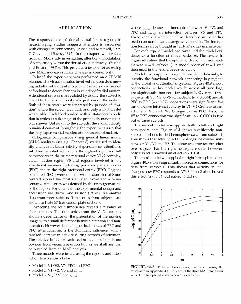
Elsevier UK Chapter: Ch40-P372560 30-9-2006 5:34p.m. Page:537 Trim:7.5in×9.25in
Basal Font:Palatino Margins:Top:40pt Gutter:68pt Font Size:9.5/12 Text Width:42pc Depth:55 Lines
APPLICATION 537
APPLICATION
The responsiveness of dorsal visual brain regions inneuroimaging studies suggests attention is associatedwith changes in connectivity (Assad and Maunsell, 1995;O’Craven and Savoy, 1995). In this chapter, we use datafrom an fMRI study investigating attentional modulationof connectivity within the dorsal visual pathways (Bucheland Friston, 1997b). This provides a testbed for assessinghow MAR models estimate changes in connectivity.
In brief, the experiment was performed on a 2T MRIscanner. The visual stimulus involved random dots mov-ing radially outwards at a fixed rate. Subjects were trainedbeforehand to detect changes in velocity of radial motion.Attentional set was manipulated by asking the subject toattend to changes in velocity or to just observe the motion.Both of these states were separated by periods of ‘fixa-tion’ where the screen was dark and only a fixation dotwas visible. Each block ended with a ‘stationary’ condi-tion in which a static image of the previously moving dotswas shown. Unknown to the subjects, the radial velocityremained constant throughout the experiment such thatthe only experimental manipulation was attentional set.
Categorical comparisons using general linear model(GLM) analyses (see e.g. Chapter 8) were used to iden-tify changes in brain activity dependent on attentionalset. This revealed activations throughout right and lefthemispheres in the primary visual cortex V1/2 complex,visual motion region V5 and regions involved in theattentional network including posterior parietal cortex(PPC) and in the right prefrontal cortex (PFC). Regionsof interest (ROI) were defined with a diameter of 8 mmcentred around the most significant voxel and a repre-sentative time-series was defined by the first eigenvariateof the region. For details of the experimental design andacquisition see Buchel and Friston (1997b). We analysedata from three subjects. Time-series from subject 1 areshown in Plate 57 (see colour plate section).
Inspecting the four time-series reveals a number ofcharacteristics. The time-series from the V1/2 complexshows a dependence on the presentation of the movingimage with a small difference between attention and non-attention. However, in the higher brain areas of PPC andPFC, attentional set is the dominant influence, with amarked increase in activity during periods of attention.The relative influence each region has on others is notobvious from visual inspection but, as we shall see, canbe revealed from an MAR analysis.
Three models were tested using the regions and inter-action terms shown below:
• Model 1: V1/V2, V5, PPC and PFC• Model 2: V1/V2, V5 and Iv1�ppc
• Model 3: V5, PPC and Iv5�pfc
where Iv1�ppc denotes an interaction between V1/V2 andPPC and Iv5�pfc an interaction between V5 and PFC.These variables were created as described in the earliersection on non-linear autoregressive models. The interac-tion terms can be thought as ‘virtual’ nodes in a network.
For each type of model, we computed the model evi-dence as a function of model order m. The results inFigure 40.2 show that the optimal order for all three mod-els was m = 4 (subject 1). A model order of m = 4 wasthen used in the results reported below.
Model 1 was applied to right hemisphere data only, toidentify the functional network connecting key regionsin the visual and attentional systems. Figure 40.3 showsconnections in this model which, across all time lags,are significantly non-zero for subject 1. Over the threesubjects, all V1/V2 to V5 connections ( < 0�0004) and allPFC to PPC ( < 0�02) connections were significant. Wecan therefore infer that activity in V1/V2 Granger causesactivity in V5, and PFC Granger causes PPC. Also, theV5 to PPC connection was significant ( < 0�0009) in twoout of three subjects.
The second model was applied both to left and righthemisphere data. Figure 40.4 shows significantly non-zero connections for left hemisphere data from subject 1.This shows that activity in PPC changes the connectivitybetween V1/V2 and V5. The same was true for the othertwo subjects. For the right hemisphere data, however,only subject 1 showed an effect ( < 0�03).
The third model was applied to right hemisphere data.Figure 40.5 shows significantly non-zero connections fordata from subject 1. This shows that activity in PFCchanges how PPC responds to V5. Subject 2 also showedthis effect ( < 0�03) but subject 3 did not.
FIGURE 40.2 Plots of log-evidence, computed using theexpression in Appendix 40.1, for each of the three MAR models forsubject 1. The optimal order is m = 4 in each case.

Elsevier UK Chapter: Ch40-P372560 30-9-2006 5:34p.m. Page:538 Trim:7.5in×9.25in
Basal Font:Palatino Margins:Top:40pt Gutter:68pt Font Size:9.5/12 Text Width:42pc Depth:55 Lines
538 40. MULTIVARIATE AUTOREGRESSIVE MODELS
FIGURE 40.3 Inferred connectivity for model 1. Arrows indi-cate Granger causal relations. Thin arrows indicate 0�001 ≤ ≤ 0�05and thick, ≤ 0�001.
FIGURE 40.4 Inferred connectivity for model 2. Arrows showGranger causal relations (0�001 ≤ ≤ 0�05). The model supports thenotion that PPC modulates the V1/V2 to V5 connection.
FIGURE 40.5 Inferred connectivity for model 3. Arrows showGranger causal relations (0�001 ≤ ≤ 0�05). The model supports thenotion that PFC modulates the V5 to PPC connection.
DISCUSSION
We have proposed the use of MAR models for mak-ing inferences about functional integration using fMRItime-series. One motivation for this is that the previ-ously dominant model used for making such inferencesin the existing fMRI/PET (positron emission tomogra-phy) literature, namely structural equation modelling, asused in McIntosh et al. (1994) and Buchel and Friston(1997b), is not a time-series model. Indeed, inferences arebased solely on the instantaneous correlations betweenregions – if the series were randomly permuted overtime, SEM would give the same results. Thus SEM throwsaway temporal information.
Further, MAR models may contain loops and self-connections, yet parameter estimation can proceed in apurely linear framework, i.e. there is an analytic solutionthat can be found via linear algebra. In contradistinction,SEM models with loops require non-linear optimization.The reason for this is that MAR models do not containinstantaneous connections. The between-region connec-tivity arises from connections between regions at differ-ent time lags. Due to temporal persistence in the activityof each region, this captures much the same effect, but ina computationally simpler manner.
In this chapter, we applied Bayesian MAR modelsto fMRI data. Bayesian inferences about connectionswere then made on the basis of the estimated poste-rior distribution. This allows for the identification of asub-network of connections that mediate the observeddynamics. These connections describe causal relations, inthe sense of Granger (Granger, 1969).
This is in the spirit of how general linear models areused for characterizing functional specialization; all con-ceivable factors are placed in one large model and thendifferent hypotheses are tested using t- or F-contrasts(Frackowiak et al., 1997). We note that this approach isfundamentally different from the philosophy underlyingSEM. In SEM, only a few connections are modelled. Theseare chosen on the basis of prior anatomical or functionalknowledge and are interpreted as embodying causal rela-tions. Thus, with SEM, causality is ascribed a priori (Pearl,1998), but with MAR, causality can be inferred from data.
MAR models can also be used for spectral estima-tion. In particular, they enable parsimonious estima-tion of coherences (correlation at particular frequen-cies), partial coherences (the coherence between twotime-series after the effects of others have been takeninto account), phase relationships (Marple, 1987; Cas-sidy and Brown, 2000) and directed transfer functions(Kaminski et al., 1997). MAR models have been usedin this way to investigate functional integration fromelectroencephalography (EEG) and Electrocorticogram

Elsevier UK Chapter: Ch40-P372560 30-9-2006 5:34p.m. Page:539 Trim:7.5in×9.25in
Basal Font:Palatino Margins:Top:40pt Gutter:68pt Font Size:9.5/12 Text Width:42pc Depth:55 Lines
APPENDIX 40.1 539
(ECOG) recordings (Bressler et al., 1999). This providesa link with a recent analysis of fMRI data (Muller et al.,2001) which looks for sets of voxels that are highly coher-ent. MAR models provide a parametric way of estimatingthis coherence, although in this chapter we have reportedthe results in the time domain.
A further aspect of MAR models is that they captureonly linear relations between regions. Following Bucheland Friston (1997b), we have extended their capabili-ties by introducing bilinear terms. This allows one toinfer that activity in one region modulates connectivitybetween two other regions. Such inferences are beyondthe current capabilities of dynamic causal models forfMRI (see Chapter 41).
It is also possible to include further higher-order terms,for instance, second-order interactions across differentlags. Frequency domain characterization of the resultingmodels would then allow us to report bi-spectra (Priest-ley, 1988). These describe the correlations between differ-ent frequencies which may be important for the study offunctional integration (Friston, 2000, see also Chapter 39).
A key aspect of our approach has been the use ofa mature Bayesian estimation framework (Penny andRoberts, 2002). This has allowed us to select the optimalMAR model order. One promising direction for extend-ing the model is to replace Gaussian priors with sparsepriors. This would effectively remove most connections,allowing the model to be applied to a very large num-ber of regions. This approach has been investigated ina non-Bayesian framework using penalized regressionand pruning based on false discovery rates (Valdes-Sosaet al., 2005).
APPENDIX 40.1
Bayesian estimation
Following the algorithm developed in Penny andRoberts, (2002), the parameters of the posterior distribu-tions are updated iteratively as follows:
�D = �̂⊗ �XT X� 40.11
̂B = ��D + ̂I�−1
ŴB = ̂B�DŴ
1
b̂= 1
2Ŵ T
B ŴB + 12Tr�̂B�+ 1
b
ĉ = k
2+ c
̂ = b̂ĉ
s = N
B = 12
�Y −XŴB�T �Y −XŴB�
+∑n
�I ⊗xn�̂B�I ⊗xn�T
�̂ = sB−1
The updates are initialized using the maximum-likelihood solution. Iteration terminates when theBayesian log-evidence increases by less than 0.01 per cent.The log-evidence is computed as follows:
log p�Y �m� = N
2log �B�−KLN �p�W �m��p�W �Y�m�� 40.12
−KLGa�p��m��p��Y�m��+ log d�N/2�
where KLN and KLGa denote the Kullback-Liebler (KL)divergences for normal and gamma densities defined inChapter 24. Essentially, the first term in the above equa-tion is an accuracy term and the KL terms act as a penaltyfor model complexity (see Chapters 24 and 35 for moreon model comparison).
Testing the significance of connections
The connectivity between two regions can be expressedover a number of time lags. Therefore, to see if the con-nectivity is significantly non-zero, we make an inferenceabout the vector of coefficients a, where each element ofthat vector is the value of a MAR coefficient at a differenttime lag. First, we specify �k × k� (k = m × d × d) sparsematrix C such that
a = CT w 40.13
returns the estimated weights for connections betweenthe two regions of interest. For an MAR(m) model, thisvector has m entries, one for each time lag. The probabil-ity distribution is given by p�a� = N���V� and is shownschematically in Figure 40.1. The mean and covarianceare given by:
� = CT ŵ 40.14
V = CT ̂BC
where ŵ = vec�ŴB� and ̂B are the Bayesian estimates ofthe parameters of the posterior distribution of regressioncoefficients from the previous section. In fact, p�a� is justthat part of p�w� that we are interested in.
The probability that the zero vector lies on the 1−confidence region for this distribution is then computedas follows. We first note that this probability is the sameas the probability that the vector m lies on the edge of
Elsevier UK Chapter: Ch40-P372560 30-9-2006 5:34p.m. Page:540 Trim:7.5in×9.25in
Basal Font:Palatino Margins:Top:40pt Gutter:68pt Font Size:9.5/12 Text Width:42pc Depth:55 Lines
540 40. MULTIVARIATE AUTOREGRESSIVE MODELS
the 1 − region for the distribution N�0�V�. This latterprobabilitiy can be computed by forming the test statistic:
d = �T V −1� 40.15
which will be the sum of r = rank�V� independent,squared Gaussian variables. As such it has a �2 distribu-tion:
p�d� = �2�r� 40.16
This results in the same test for multivariate effects ingeneral linear models described in Chapter 25. In thepresent context, if a are the autoregressive coefficientsfrom region X to region Y, and the above test finds themto be significantly non-zero, then we can conclude that XGranger causes Y (Eichler, 2005).
REFERENCES
Assad JA, Maunsell RM (1995) Neuronal correlates of inferredmotion in primate posterior parietal cortex. Nature 373: 518–21
Box GEP, Tiao GC (1992) Bayesian inference in statistical analysis. JohnWiley, New York
Bressler SL, Ding M, Yang W (1999) Investigation of cooperativecortical dynamics by multivariate autoregressive modeling ofevent-related local field potentials. Neurocomputing 26–27: 625–31
Buchel C, Friston KJ (1997a) Characterizing functional integration.In Human Brain Function, Frackowiak RSJ, Friston KJ, Frith CD,et al. (eds). Academic Press, London, pp 127–40
Buchel C, Friston KJ (1997b) Modulation of connectivity in visualpathways by attention: cortical interactions evaluated with struc-tural equation modelling and fMRI. Cereb Cortex 7: 768–78
Buchel C, Friston KJ (1998) Dynamic changes in effective connectiv-ity characterized by variable parameter regression and Kalmanfiltering. Hum Brain Mapp 6: 403–08
Buchel C, Friston KJ (2000) Assessing interactions among neuronalsystems using functional neuroimaging. Neural Netw 13: 871–82
Cassidy MJ, Brown P (2002) Stationary and non-stationary autore-gressive models for electrophysiological signal analysis andfunctional coupling studies. IEEE Trans Biomed Eng 49: 1142–52
Chatfield C (1996) The analysis of time series. Chapman and Hall,London
Cudeck R (2002) Structural Equation Modeling: Present and Future.Scientific Software International, Lincolnwood
Eichler M (2005) Evaluating effective connectivity. Phil Trans R SocB 360: 953–67
Frackowiak RSJ, Friston KJ, Frith CD et al. (1997) Human Brain Func-tion. Academic Press
Friston KJ (2000) The labile brain.I. neuronal transients and nonlin-ear coupling. Phil Trans R Soc London B 355: 215–36
Friston KJ (2001) Brain function, nonlinear coupling, and neuronaltransients. Neuroscientist 7: 406–18
Friston KJ, Buchel C (2000) Attentional modulation of effective con-nectivity from V2 to V5/MT in humans. Proc Natl Acad Sci USA97: 7591–96
Friston KJ, Buchel C, Fink GR et al. (1997) Psychophysiological andmodulatory interactions in neuroimaging. NeuroImage 6: 218–29
Friston KJ, Frith CD, Frackowiak RSJ (1993) Time-dependentchanges in effective connectivity measured with PET. Hum BrainMapp 1: 69–79
Friston KJ, Ungerleider LG, Jezzard P (1995) Charcterizing modu-latory interactions between V1 and V2 in human cortex: a newtreatment of functional MRI data. Hum Brain Mapp 2: 211–24
Granger C (1969) Investigating causal relations by econometric mod-els and cross-spectral methods. Econometrika 37: 424–38
Kaminski M, Blinowska K, Szelenberger W (1997) Topographicanalysis of coherence and propagation of EEG activity duringsleep and wakefulness. Electroencephalogr Clin Neurophysiol 102:216–27
Magnus JR, Neudecker H (1997) Matrix differential calculus with appli-cations in statistics and econometrics. John Wiley
Marple SL (1987) Digital spectral analysis with applications. Prentice-Hall
McIntosh AR, Grady CL, Underleider LG et al. (1994) Networkanalysis of cortical visual pathways mapped with PET. J Neurosci14: 655–66
Muirhead RJ (1982) Aspects of multivariate statistical theory. JohnWiley
Muller K, Lohmann G, Blosch V et al. (2001) On multivariate spectralanalysis of fMRI time series. NeuroImage, 14: 347–56
Neumaier A, Schneider T (2000) Estimation of parameters andeigenmodes of multivariate autoregressive models. ACM TransMath Softw 27: 27–57
O’Craven KM, Savoy RL (1995) Voluntary attention can modulatefmri activity in human MT/MST. Neuron 18: 591–8
Pearl J (1998) Graphs, causality, and structural equation modelsSociol Meth Res 27: 226–84
Penny WD, Roberts SJ (2002) Bayesian multivariate autoregressivemodels with structured priors. IEE Proc Vis Image Signal Process149: 33–41
Priestley MB (1988) Nonlinear and non-stationary time series analysis.Harcourt Brace Jovanovich
Valdes-Sosa PA, Sanchez-Bornot J, Lage-Castellanos A et al. (2005)Estimating brain functional connectivity with sparse multivari-ate autoregression. Phil Trans R Soc B 360: 969–81
Weisberg S (1980) Applied linear regression. John Wiley
Elsevier UK Chapter: Ch41-P372560 30-9-2006 5:35p.m. Page:541 Trim:7.5in×9.25in
Basal Font:Palatino Margins:Top:40pt Gutter:68pt Font Size:9.5/12 Text Width:42pc Depth:55 Lines
C H A P T E R
41
Dynamic Causal Models for fMRIK. Friston
INTRODUCTION
In this chapter, we apply the system identification tech-niques described in Chapter 34 to the dynamic modelsof effective connectivity introduced in Chapter 38. In thischapter, we consider simple bilinear models for haemo-dynamic time-series (i.e. functional magnetic resonanceimaging, fMRI). In the next chapter, we describe moreelaborate models for electrical and magnetic responsesas measured with electroencephalography and mag-netoencephalography (EEG-MEG). By using a bilinearapproximation, to any system’s equations of motion, theparameters of the implicit causal model reduce to threesets. These comprise parameters that: mediate the influ-ence of extrinsic inputs on the states; mediate regionalcoupling among the states; and [bilinear] parameters thatallow the inputs to modulate that coupling.
We use this bilinear model for the analysis of effec-tive connectivity using experimentally designed inputsand fMRI responses. In this context, the coupling param-eters determine effective connectivity and the bilinearparameters reflect the changes in connectivity inducedby inputs. The ensuing framework allows one to char-acterize fMRI experiments, conceptually, as an experi-mental manipulation of integration among brain regions(by contextual or trial-free inputs, like time or attentionalset) that is disclosed using evoked responses (to per-turbations or trial-bound inputs like stimuli). As withprevious analyses of effective connectivity, the focusis on experimentally induced changes in coupling (cf.psychophysiological interactions). However, unlike pre-vious approaches in neuroimaging, the causal modelascribes responses to designed deterministic inputs, asopposed to treating inputs as unknown and stochas-tic. To date, dynamic causal modelling (DCM) has beenapplied to a wide range of issues; ranging from category-effects (Mechelli et al., 2003) through to affective prosody(Ethofer et al., 2006) and rhyming (Bitan et al., 2005).
Background
This chapter is about modelling interactions among neu-ronal populations, at a cortical level, using neuroimaging(haemodynamic) time-series. It presents the motivationand procedures for dynamic causal modelling of evokedbrain responses. The aim of this modelling is to esti-mate, and make inferences about, the coupling amongbrain areas and how that coupling is influenced bychanges in experimental context (e.g. time or cognitiveset). Dynamic causal modelling represents a fundamentaldeparture from existing approaches to effective connec-tivity because it employs a more plausible generativemodel of measured brain responses that embraces theirnon-linear and dynamic nature.
The basic idea is to construct a reasonably realisticneuronal model of interacting cortical regions or nodes.This model is then supplemented with a forward modelof how neuronal or synaptic activity is transformedinto a measured response. This enables the parame-ters of the neuronal model (i.e. effective connectivity)to be estimated from observed data. These supplemen-tary models may be forward models of electromagneticmeasurements or haemodynamic models of fMRI mea-surements. In this chapter, we will focus on fMRI.Responses are evoked by known deterministic inputs thatembody designed changes in stimulation or context. Thisis accomplished by using a dynamic input-state-outputmodel with multiple inputs and outputs. The inputs cor-respond to conventional stimulus functions that encodeexperimental manipulations. The state variables coverboth the neuronal activities and other neurophysiologicalor biophysical variables needed to form the outputs. Theoutputs are measured electromagnetic or haemodynamicresponses over the brain regions considered.
Intuitively, this scheme regards an experiment as adesigned perturbation of neuronal dynamics that aredistributed throughout a system of coupled anatomicalnodes to change region-specific neuronal activity. These
Statistical Parametric Mapping, by Karl Friston et al. Copyright 2007, Elsevier Ltd. All rights reserved.ISBN–13: 978-0-12-372560-8 ISBN–10: 0-12-372560-7
541
Elsevier UK Chapter: Ch41-P372560 30-9-2006 5:35p.m. Page:542 Trim:7.5in×9.25in
Basal Font:Palatino Margins:Top:40pt Gutter:68pt Font Size:9.5/12 Text Width:42pc Depth:55 Lines
542 41. DYNAMIC CAUSAL MODELS FOR fMRI
changes engender, through a measurement-specific for-ward model, responses that are used to identify thearchitecture and time-constants of the system at the neu-ronal level. This represents a departure from conven-tional approaches (e.g. structural equation modelling andautoregression models, McIntosh and Gonzalez-Lima,1994; Büchel and Friston 1997), in which one assumes theobserved responses are driven by endogenous or intrinsicnoise (i.e. innovations). In contrast, dynamic causal mod-els assume the responses are driven by designed changesin inputs. An important aspect of dynamic causal mod-els, for neuroimaging, pertains to how the experimentalinputs enter the model and cause neuronal responses.We have established in previous chapters that experi-mental variables can elicit responses in one of two ways.First, they can elicit responses through direct influenceson specific anatomical nodes. This would be appropri-ate, for example, in modelling sensory evoked responsesin early visual cortices. The second class of input exertsits effect vicariously, through a modulation of the cou-pling among nodes. These sorts of experimental variableswould normally be more enduring, for example, atten-tion to a particular attribute or the maintenance of someperceptual set. These distinctions are seen most clearly inrelation to existing analyses and experimental designs.
DCM and existing approaches
The central ideal DCM is to treat the brain as a deter-ministic non-linear dynamic system that is subject toinputs and produces outputs. Effective connectivity isparameterized in terms of coupling among unobservedbrain states (e.g. neuronal activity in different regions).The objective is to estimate these parameters by per-turbing the system and measuring the response. Thisis in contradistinction to established methods, for esti-mating effective connectivity from neurophysiologicaltime-series, which include structural equation modellingand models based on multivariate autoregressive pro-cesses. In these models, there is no designed perturbationand the inputs are treated as unknown and stochastic.Multivariate autoregression models and their spectralequivalents like coherence analysis, not only assumethe system is driven by stochastic innovations, but areusually restricted to linear interactions. Structural equa-tion modelling assumes the interactions are linear and,furthermore, instantaneous in the sense that structuralequation models are not time-series models. In short,dynamic causal modelling is distinguished from alter-native approaches not just by accommodating the non-linear and dynamic aspects of neuronal interactions, butby framing the estimation problem in terms of perturba-tions that accommodate experimentally designed inputs.
This is a critical departure from conventional approachesto causal modelling in neuroimaging and, importantly,brings the analysis of effective connectivity much closerto the analysis of region-specific effects: dynamic causalmodelling calls upon the same experimental design prin-ciples to elicit region-specific interactions that we usein conventional experiments to elicit region-specific acti-vations. In fact, as shown later, the convolution model,used in the standard analysis of fMRI time-series, is aspecial and simple case of DCM that arises when thecoupling among regions is discounted. In DCM, thecausal or explanatory variables that comprise the conven-tional design matrix become the inputs and the param-eters become measures of effective connectivity.Although DCM can be framed as a generalization ofthe linear models used in conventional analyses to coverbilinear models (see below), it also represents an attemptto embed more plausible forward models of how neu-ronal dynamics respond to inputs and produce measuredresponses. This reflects the growing appreciation of therole that neuronal models may have to play in under-standing measured brain responses (see Horwitz et al.,2001 for a discussion).
This chapter can be regarded as an extension of pre-vious work on the Bayesian identification of haemody-namic models (Friston 2002) to cover multiple regions. InChapter 34, we focused on the biophysical parameters ofa haemodynamic response in a single region. The mostimportant parameter was the efficacy with which experi-mental inputs could elicit an activity-dependent vasodila-tory signal. In this chapter, neuronal activity is modelledexplicitly, allowing for interactions among the activitiesof multiple regions in generating the observed haemody-namic response. The estimation procedure employed forDCM is formally identical to that described in Chapter 34(see also Appendix 4).
DCM and experimental design
DCM is used to test the specific hypothesis that moti-vated the experimental design. It is not an exploratorytechnique, as with all analyses of effective connectivitythe results are specific to the tasks and stimuli employedduring the experiment. In DCM, designed inputs canproduce responses in one of two ways. Inputs can elicitchanges in the state variables (i.e. neuronal activity)directly. For example, sensory input could be modelledas causing direct responses in primary visual or auditoryareas. The second way in which inputs affect the systemis through changing the effective connectivity or inter-actions. Useful examples of this sort of effect would bethe attentional modulation of connections between pari-etal and extrastriate areas. Another ubiquitous example

Elsevier UK Chapter: Ch41-P372560 30-9-2006 5:35p.m. Page:543 Trim:7.5in×9.25in
Basal Font:Palatino Margins:Top:40pt Gutter:68pt Font Size:9.5/12 Text Width:42pc Depth:55 Lines
INTRODUCTION 543
of contextual effects would be time. Time-dependentchanges in connectivity correspond to plasticity. It is use-ful to regard experimental factors as inputs that belongto the class that produce evoked responses or to the classof contextual factors that induce changes in coupling(although, in principle, all inputs could do both). The firstclass comprises trial- or stimulus-bound perturbations,whereas the second establishes a context in which effectsof the first sort evoke responses. This second class is typ-ically trial-free and induced by task instructions or othercontextual changes. Measured responses in high-ordercortical areas are mediated by interactions among brainareas elicited by trial-bound perturbations. These inter-actions can be modulated by other set-related or contex-tual factors that modulate the latent or regional couplingamong areas. Figure 41.1 illustrates this schematically.The important implication here, for experimental designin DCM, is that it should be multifactorial, with at leastone factor controlling sensory perturbation and anotherfactor manipulating the context in which the responsesare evoked (cf. psychophysiological interactions).
In this chapter, we use bilinear approximations to anyDCM. The bilinear approximation reduces the parame-ters to three sets that control three distinct things: first,the direct or extrinsic influence of inputs on brain statesin any particular area; second, the regional or latent
coupling of one area to another; and finally, changes inthis coupling that are induced by input. Although, insome instances, the relative strengths of coupling may beof interest, most analyses of DCMs focus on the changesin coupling embodied in the bilinear parameters. Thefirst class of parameters is generally of little interest inthe context of DCM, but is the primary focus in classicalanalyses of regionally specific effects. In classical analy-ses, the only way experimental effects can be expressedis though a direct or extrinsic influence on each voxelbecause mass-univariate models (e.g. statistical paramet-ric mapping, SPM) preclude coupling among voxels orits modulation.
Questions about the modulation of effective connec-tivity are addressed through inference about the bilin-ear parameters described above. They are bilinear in thesense that an input-dependent change in connectivity canbe construed as a second-order interaction between theinput and activity in the source, when causing a responsein a target region. The key role of bilinear terms reflectsthe fact that the more interesting applications of effectiveconnectivity address changes in connectivity induced byset or time. In short, DCM with a bilinear approxima-tion allows one to claim that an experimental manipula-tion has ‘activated a pathway’ as opposed to a corticalregion. Bilinear terms correspond to psychophysiological
V1
V4
BA37
STG
BA39
Stimulus-boundperturbations - u1
{e.g. visual words}
y
y
y
y
y
Stimulus-free context - u2{e.g. cognitive set or time}
FIGURE 41.1 This is a schematic illustrating the concepts underlying dynamic causal modelling. In particular, it highlights the twodistinct ways in which inputs or perturbations can elicit responses in the regions or nodes that comprise the model. In this example, there arefive nodes, including visual areas V1 and V4 in the fusiform gyrus, areas 39 and 37 and the superior temporal gyrus (STG). Stimulus-boundperturbations designated u1 act as extrinsic inputs to the primary visual area V1. Stimulus-free or contextual inputs u2 mediate their effectsby modulating the coupling between V4 and BA39 and between BA37 and V4. For example, the responses in the angular gyrus (BA39)are caused by inputs to V1 that are transformed by V4, where the influences exerted by V4 are sensitive to the second input. The darksquare boxes represent the components of the DCM that transform the state variables zi in each region (neuronal activity) into a measured[haemodynamic] response yi.
Elsevier UK Chapter: Ch41-P372560 30-9-2006 5:35p.m. Page:544 Trim:7.5in×9.25in
Basal Font:Palatino Margins:Top:40pt Gutter:68pt Font Size:9.5/12 Text Width:42pc Depth:55 Lines
544 41. DYNAMIC CAUSAL MODELS FOR fMRI
interaction terms in conventional regression analysesof effective connectivity (Friston et al., 1997) and thoseformed by moderator variables (Kenny and Judd, 1984)in structural equation modelling (Büchel and Friston,1997). Their bilinear aspect speaks again of the impor-tance of multifactorial designs that allow these interac-tions to be measured and the central role of the contextin which region-specific responses are formed (seeMcIntosh, 2000).
DCM and inference
Because DCMs are not restricted to linear or instanta-neous systems, they are necessarily complicated and,potentially, need a large number of free parameters.This is why they have greater biological plausibility inrelation to alternative approaches. However, this makesmodel inversion more dependent upon constraints. Anatural way to embody the requisite constraints is withina Bayesian framework. Consequently, dynamic causalmodels are inverted using Bayesian schemes to furnishconditional estimators and inferences about the connec-tions. In other words, the estimation procedure providesthe probability distribution of a coupling parameter interms of its mean and standard deviation. Having estab-lished this posterior density, the probability that theconnection exceeds some specified threshold is easilycomputed. Bayesian inferences like this are more straight-forward than corresponding classical inferences andeschew the multiple comparisons problem. The posteriordensity is computed using the likelihood and prior den-sities. The likelihood of the data, given some parameters,is specified by the forward model or DCM (in one senseall models are simply ways of specifying the likelihoodof an observation). The prior densities on the couplingparameters offer suitable constraints to ensure robust andefficient estimation. These priors harness some naturalconstraints about the dynamics of coupled systems (seebelow), but also allow the user to specify which con-nections are present and which are not. An importantuse of prior constraints of this sort is the restriction ofwhere inputs can elicit extrinsic responses. It is inter-esting to reflect that conventional analyses suppose thatall inputs have unconstrained access to all brain regions.This is because classical models assume activations arecaused directly by experimental factors, as opposed tobeing mediated by afferents from other brain areas.
Additional constraints on the intrinsic connections andtheir modulation by contextual inputs can also be spec-ified, but they are not necessary. These additional con-straints can be used to make a model more parsimonious,allowing one to focus on a particular connection. Wewill provide examples of this below. Unlike structural
equation modelling, there are no limits on the number ofconnections that can be modelled because the assump-tions and estimation scheme used by dynamic causalmodelling are completely different, relying upon knowninputs.
Overview
This chapter comprises a theoretical section and threesections demonstrating the use and validity of DCM. Inthe theoretical section, we present the concepts used inthe remaining sections. The later sections address theface, predictive and construct validity of DCM respec-tively. Face validity entails the estimation, and infer-ence procedure identifies what it is supposed to. Thesubsequent section on predictive validity uses empiri-cal data from an fMRI study of single-word processingat different rates. These data were obtained consecu-tively in a series of contiguous sessions. This allowedus to repeat the DCM using independent realizations ofthe same paradigm. Predictive validity over the multi-ple sessions was assessed in terms of the consistencyof the coupling estimates and their posterior densities.The final section on construct validity revisits changesin connection strengths among parietal and extrastriateareas induced by attention to optic flow stimuli. We haveestablished previously attentionally mediated increasesin effective connectivity using both structural equationmodelling and a Volterra formulation of effective con-nectivity (Büchel and Friston, 1997; Friston and Büchel,2000). Here we show that dynamic causal modellingleads to the same conclusions. This chapter ends with abrief discussion of dynamic causal modelling, its limita-tions and potential applications.
THEORY
In this section, we present the theoretical motivation andoperational details upon which DCM rests. In brief, DCMis a fairly standard non-linear system identification pro-cedure using Bayesian inversion of deterministic input-state-output dynamic models. In this chapter, the systemcan be construed as a number of interacting brain regions.We will focus on a particular form for the dynamics thatcorresponds to a bilinear approximation to any analyticsystem. However, the idea behind DCM is not restrictedto bilinear forms, as we will see in the next chapter.
This section is divided into three parts. First, wedescribe the DCM itself, then consider the nature of pri-ors on the parameters of the DCM and finally summarizethe inference procedure. The estimation conforms to the

Elsevier UK Chapter: Ch41-P372560 30-9-2006 5:35p.m. Page:545 Trim:7.5in×9.25in
Basal Font:Palatino Margins:Top:40pt Gutter:68pt Font Size:9.5/12 Text Width:42pc Depth:55 Lines
THEORY 545
posterior density analysis under Gaussian assumptionsdescribed in Chapter 34. In Chapter 34, we were primar-ily concerned with estimating the efficacy with whichinput elicits a vasodilatory signal, presumably mediatedby neuronal responses to the input. The causal modelshere can be regarded as a collection of haemodynamicmodels, one for each area, in which the experimentalinputs are supplemented with neural activity from otherareas. The parameters of interest now cover not only thedirect efficacy of experimental inputs, but also the effi-cacy of neuronal input from distal regions, i.e. effectiveconnectivity (see Figure 41.1).
The Bayesian inversion finds the maximum or modeof the posterior density of the parameters (i.e. the mostlikely coupling parameters given the data) by performinga gradient assent on the log-posterior. The log-posteriorrequires both likelihood and prior terms. The likelihoodobtains from Gaussian assumptions about the errors inthe observation model supplied by the DCM. This like-lihood or forward model is described in the next sub-section. By combining the likelihood with priors on thecoupling and haemodynamic parameters, described inthe second subsection, one can form an expression forthe posterior density that is used in the estimation.
Dynamic causal models
The dynamic causal model is a multiple-input multiple-output (MIMO) system that comprises m inputs andl outputs with one output per region. The m inputs corre-spond to designed causes (e.g. boxcar or stick stimulus-functions). The inputs are exactly the same as thoseused to form design matrices in conventional analysesof fMRI and can be expanded in the usual way whennecessary (e.g. using polynomials or temporal basis func-tions). In principle, each input could have direct access toevery region. However, in practice, the extrinsic effectsof inputs are usually restricted to a single input region.Each of the l regions produces a measured output thatcorresponds to the observed blood oxygenation-level-dependent (BOLD) signal. These l time-series would nor-mally be taken as the average or first eigenvariate of keyregions, selected on the basis of a conventional analy-sis. Each region has five state variables. Four of theseare of secondary importance and correspond to the statevariables of the haemodynamic model first presented inFriston et al. (2000) and described in previous chapters.These haemodynamic states comprise a vasodilatory sig-nal, normalized flow, normalized venous volume, andnormalized deoxyhaemoglobin content. These biophys-ical states are required to compute the observed BOLDresponse and are not influenced by the states of otherregions.
Central to the estimation of coupling parameters isthe neuronal state of each region. This corresponds toaverage neuronal or synaptic activity and is a function ofthe neuronal states of other brain regions. We will dealfirst with the equations for the neuronal states and thenbriefly reprise the differential equations that constitutethe haemodynamic model for each region.
Neuronal state equations
Restricting ourselves to the neuronal states z =�z1� � � � � zl�
T one can posit any arbitrary form or modelfor effective connectivity:
ż = F�z�u��� 41.1
where F is some non-linear function describing the neu-rophysiological influences exerted by inputs u�t� and theactivity in all brain regions on the evolution of the neu-ronal states. � are the parameters of the model whoseposterior density we require for inference. It is not nec-essary to specify the form of this equation because itsbilinear approximation provides a natural and useful re-parameterization in terms of coupling parameters.
ż ≈ Az+∑ujBjz+Cu
= (A+∑ujB
j)z+Cu
A = F
z
∣∣∣∣u=0
Bj = 2F
zuj
= A
uj
C = F
u
∣∣∣∣z=0
41.2
The Jacobian or connectivity matrix A represents the first-order coupling among the regions in the absence of input.This can be thought of as the regional coupling in theabsence of experimental perturbations. Notice that thestate, which is perturbed, depends on the experimen-tal design (e.g. baseline or control state) and thereforethe regional coupling is specific to each experiment. Thematrices Bj are effectively the change in regional couplinginduced by the j-th input. Because Bj are second-orderderivatives these terms are referred to as bilinear. Finally,the matrix C encodes the extrinsic influences of inputson neuronal activity. The parameters �c = A�Bj�C� arethe coupling matrices we wish to identify and definethe functional architecture and interactions among brainregions at a neuronal level. Figure 41.2 shows an exampleof a specific architecture to demonstrate the relationshipbetween the matrix form of the bilinear model and theunderlying state equations for each region. Notice thatthe units of coupling are per unit time and therefore cor-respond to rates. Because we are in a dynamical setting,a strong connection means an influence that is expressedquickly or with a small time constant. It is useful toappreciate this when interpreting estimates and thresh-olds quantitatively. This will be illustrated below.

Elsevier UK Chapter: Ch41-P372560 30-9-2006 5:35p.m. Page:546 Trim:7.5in×9.25in
Basal Font:Palatino Margins:Top:40pt Gutter:68pt Font Size:9.5/12 Text Width:42pc Depth:55 Lines
546 41. DYNAMIC CAUSAL MODELS FOR fMRI
Setu2
Stimuliu1
a23
z5
z3
y4
y5
y3
z1 a11a21 a22 a23
a33
a44a53 a54 a55
a45
a35 u2
a42
z4
c11
z1z2
y1y2
latent connectivity induced connectivity
Forward, backward & self
++=
00
0
00
00
0
0
The bilinear model
a45z5 + (a42 + u2b242)z2
z4 = a44z4 +
z2 = a22z2 +
z = (A + ∑ ujB j )z + Cu
z1 = a11z1 + c11u1
z5 = a55x5 +a53z3 + a54z4
z3 = a33z3 + a35z5
.
.
z5
..
b242
b223
g(v5,q5)
g(v4,q4)
g(v3,q3)
g(v2,q2)g(v1,q1)
a21z1 + (a23 + u2b223)z3
z1 c11
u1u2
z5
j
.
.
a54
a21
b223
b242
FIGURE 41.2 This schematic (upper panel) recapitulates the architecture in Figure 41.1 in terms of the differential equations impliedby a bilinear approximation. The equations in each of the white areas describe the changes in neuronal activity zi in terms of linearlyseparable components that reflect the influence of other regional state variables. Note particularly, how the second contextual inputs enterthese equations. They effectively increase the intrinsic coupling parameters, aij , in proportion to the bilinear coupling parameters, bk
ij . In thisdiagram, the haemodynamic component of the DCM illustrates how the neuronal states enter a region-specific haemodynamic model toproduce the outputs yi that are a function of the region’s biophysical states reflecting deoxyhaemoglobin content and venous volume (qi andvi). The lower panel reformulates the differential equations in the upper panel into a matrix format. These equations can be summarizedmore compactly in terms of coupling parameter matrices A, Bj and C. This form is used in the main text and shows how it relates to theunderlying differential equations that describe the state dynamics.
The evolution of neuronal activity in each region causeschanges in volume and deoxyhaemoglobin to engenderthe observed BOLD response y as described next.
Haemodynamic state equations
The remaining state variables of each region are bio-physical states (s, f , v, q), which form the BOLD sig-nal and mediate the translation of neuronal activityinto haemodynamic responses. Haemodynamic statesare a function of, and only of, the neuronal state ofeach region. The state equations have been describedin Chapters 27 and 34. These constitute a haemody-namic model that embeds the Balloon-Windkessel model
(Buxton et al., 1998; Mandeville et al., 1999). In brief, anactivity-dependent vasodilatory signal s increases flow f .Flow increases volume and dilutes deoxyhaemoglobin (vand q). The last two haemodynamic states enter an out-put non-linearity to give the observed BOLD response.A list of the biophysical parameters �h = �� ������ isprovided in Table 41-1 and a schematic of the haemody-namic model is shown in Figure 41.3.
The likelihood model
Combining the neuronal and haemodynamic statesx = z� s� f�v� q gives us a full forward model specified by

Elsevier UK Chapter: Ch41-P372560 30-9-2006 5:35p.m. Page:547 Trim:7.5in×9.25in
Basal Font:Palatino Margins:Top:40pt Gutter:68pt Font Size:9.5/12 Text Width:42pc Depth:55 Lines
THEORY 547
TABLE 41-1 Priors on biophysical parameters
Parameter Description Prior mean �� Prior variance C�
� Rate of signaldecay
0.65 per second 0�015
Rate of flow-dependentelimination
0.41 per second 0�002
� Haemodynamictransit time
0.98 second 0�0568
� Grubb’sexponent
0.32 0�0015
� Resting oxygenextractionfraction
0.34 0�0024
Neuronal input
Haemodynamic response
The hemodynamic model ),( qvg
z
y
flow
z
s
ν
f
State variables
νq
x = z,s,f,ν,q
f
q
signals = z – κs – γ(f – 1)
y = g(ν,q)
volume
τν = f – ν I/α
dHbτq = f E(f,ρ)/ρ – ν
I/αq /ν
f = s
FIGURE 41.3 This schematic shows the architecture of thehaemodynamic model for a single region (regional subscripts havebeen dropped for clarity). Neuronal activity induces a vasodila-tory and activity-dependent signal s that increases the flow f . Flowcauses changes in volume and deoxyhaemoglobin (v and q). Thesetwo haemodynamic states enter an output non-linearity to givethe observed BOLD response y. This transformation from neuronalstates zi to haemodynamic response yi is encoded graphically bythe dark-grey boxes in the previous figure and in the insert above.
the neuronal bilinear state equation (Eqn. 41.2) and thehaemodynamic equations in Figure 41.3:
ẋ = f�x�u���
y = g�x���41.3
with parameters � = �c� �h�. For any set of parametersand inputs, the state equation can be integrated andpassed through the output non-linearity to give the pre-dicted response h�u���. This integration can be madequite expedient by capitalizing on the sparsity of stimu-lus functions commonly employed in fMRI designs (seeChapter 34; Eqn. 34.16). Integrating Eqn. 41.3 is equiv-alent to a generalized convolution of the inputs withthe system’s Volterra kernels. These kernels are easilyderived from the Volterra expansion of Eqn. 41.3 (Bendat,1990 and Appendix 2):
hi�u��� =∑k
t∫0
� � �
t∫0
�ki ��1� � � � ��k�u�t −�1�� � � � �
u�t −�k�d�1� � � � � d�k
�ki ��1� � � � ��k� = kyi�t�
u�t −�1�� � � � � u�t −�k�41.4
either by numerical differentiation or analyticallythrough bilinear approximations (see Friston, 2002). �k
i
is the k-th order kernel for region i. For simplicity,Eqn. 41.4 is for a single input. The kernels are simply a re-parameterization of the model. We will use these kernelsto characterize regional impulse responses at neuronaland haemodynamic levels later.
The dynamic model can be made into a likelihoodmodel by adding errors and confounding or nuisanceeffects X�t� to give y = h�u��� + X� + �. Here � arethe unknown coefficients for confounds. In the exam-ples below, X�t� comprises a low-order discrete cosineset, modelling low-frequency drifts and a constant term.The likelihood model specifies p�y�����u� = N�h�u���+X�������, where � are some hyperparameters control-ling the covariance of the errors ����. To completethe specification of the generative model p�y�����u� =p�y�����u�p���p��� we need the priors p��� and p���. Wewill treat confounds as fixed effects, which means thesehave flat priors. The priors on the coupling and haemo-dynamic parameters are described next.
Priors
In this application, we use a fully Bayesian approachbecause there are clear and necessary constraints on neu-ronal dynamics that can be used to motivate priors on thecoupling parameters and empirically determined priorson the biophysical haemodynamic parameters are rela-tively easy to specify. We will deal first with the couplingparameters.
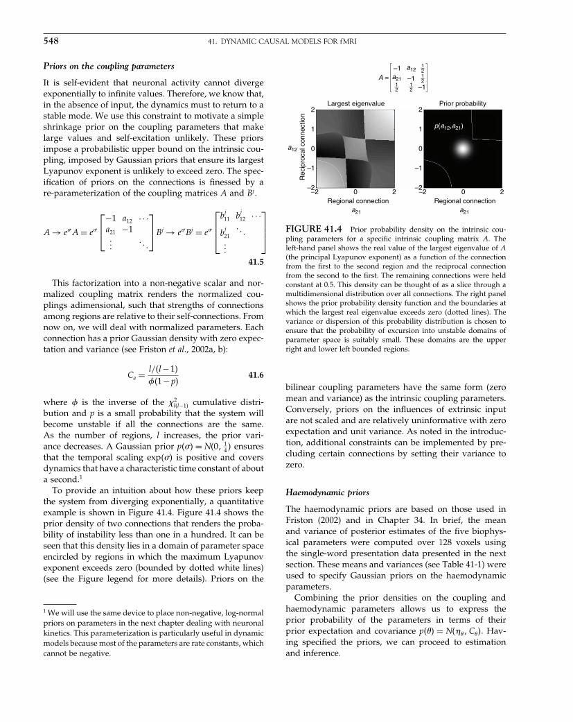
Elsevier UK Chapter: Ch41-P372560 30-9-2006 5:35p.m. Page:548 Trim:7.5in×9.25in
Basal Font:Palatino Margins:Top:40pt Gutter:68pt Font Size:9.5/12 Text Width:42pc Depth:55 Lines
548 41. DYNAMIC CAUSAL MODELS FOR fMRI
Priors on the coupling parameters
It is self-evident that neuronal activity cannot divergeexponentially to infinite values. Therefore, we know that,in the absence of input, the dynamics must to return to astable mode. We use this constraint to motivate a simpleshrinkage prior on the coupling parameters that makelarge values and self-excitation unlikely. These priorsimpose a probabilistic upper bound on the intrinsic cou-pling, imposed by Gaussian priors that ensure its largestLyapunov exponent is unlikely to exceed zero. The spec-ification of priors on the connections is finessed by are-parameterization of the coupling matrices A and Bj .
A → e�A = e�
⎡⎢⎣
−1 a12 · · ·a21 −1���
� � �
⎤⎥⎦Bj → e�Bj = e�
⎡⎢⎢⎣
bj11 b
j12 · · ·
bj21
� � ����
⎤⎥⎥⎦
41.5
This factorization into a non-negative scalar and nor-malized coupling matrix renders the normalized cou-plings adimensional, such that strengths of connectionsamong regions are relative to their self-connections. Fromnow on, we will deal with normalized parameters. Eachconnection has a prior Gaussian density with zero expec-tation and variance (see Friston et al., 2002a, b):
Ca = l/�l−1�
��1−p�41.6
where � is the inverse of the �2l�l−1� cumulative distri-
bution and p is a small probability that the system willbecome unstable if all the connections are the same.As the number of regions, l increases, the prior vari-ance decreases. A Gaussian prior p��� = N�0� 1
4 � ensuresthat the temporal scaling exp��� is positive and coversdynamics that have a characteristic time constant of abouta second.1
To provide an intuition about how these priors keepthe system from diverging exponentially, a quantitativeexample is shown in Figure 41.4. Figure 41.4 shows theprior density of two connections that renders the proba-bility of instability less than one in a hundred. It can beseen that this density lies in a domain of parameter spaceencircled by regions in which the maximum Lyapunovexponent exceeds zero (bounded by dotted white lines)(see the Figure legend for more details). Priors on the
1 We will use the same device to place non-negative, log-normalpriors on parameters in the next chapter dealing with neuronalkinetics. This parameterization is particularly useful in dynamicmodels because most of the parameters are rate constants, whichcannot be negative.
a21
a21 a21
a12
a12
A =
Prior probabilityLargest eigenvalue
Regional connection Regional connection
Rec
ipro
cal c
onne
ctio
n
2
1
0
–1
–2
2
1
0
–1
–2–2 0 2 –2 0 2
p(a12,a21)
–1
–1–11
212
1212
FIGURE 41.4 Prior probability density on the intrinsic cou-pling parameters for a specific intrinsic coupling matrix A. Theleft-hand panel shows the real value of the largest eigenvalue of A(the principal Lyapunov exponent) as a function of the connectionfrom the first to the second region and the reciprocal connectionfrom the second to the first. The remaining connections were heldconstant at 0.5. This density can be thought of as a slice through amultidimensional distribution over all connections. The right panelshows the prior probability density function and the boundaries atwhich the largest real eigenvalue exceeds zero (dotted lines). Thevariance or dispersion of this probability distribution is chosen toensure that the probability of excursion into unstable domains ofparameter space is suitably small. These domains are the upperright and lower left bounded regions.
bilinear coupling parameters have the same form (zeromean and variance) as the intrinsic coupling parameters.Conversely, priors on the influences of extrinsic inputare not scaled and are relatively uninformative with zeroexpectation and unit variance. As noted in the introduc-tion, additional constraints can be implemented by pre-cluding certain connections by setting their variance tozero.
Haemodynamic priors
The haemodynamic priors are based on those used inFriston (2002) and in Chapter 34. In brief, the meanand variance of posterior estimates of the five biophys-ical parameters were computed over 128 voxels usingthe single-word presentation data presented in the nextsection. These means and variances (see Table 41-1) wereused to specify Gaussian priors on the haemodynamicparameters.
Combining the prior densities on the coupling andhaemodynamic parameters allows us to express theprior probability of the parameters in terms of theirprior expectation and covariance p��� = N����C��. Hav-ing specified the priors, we can proceed to estimationand inference.
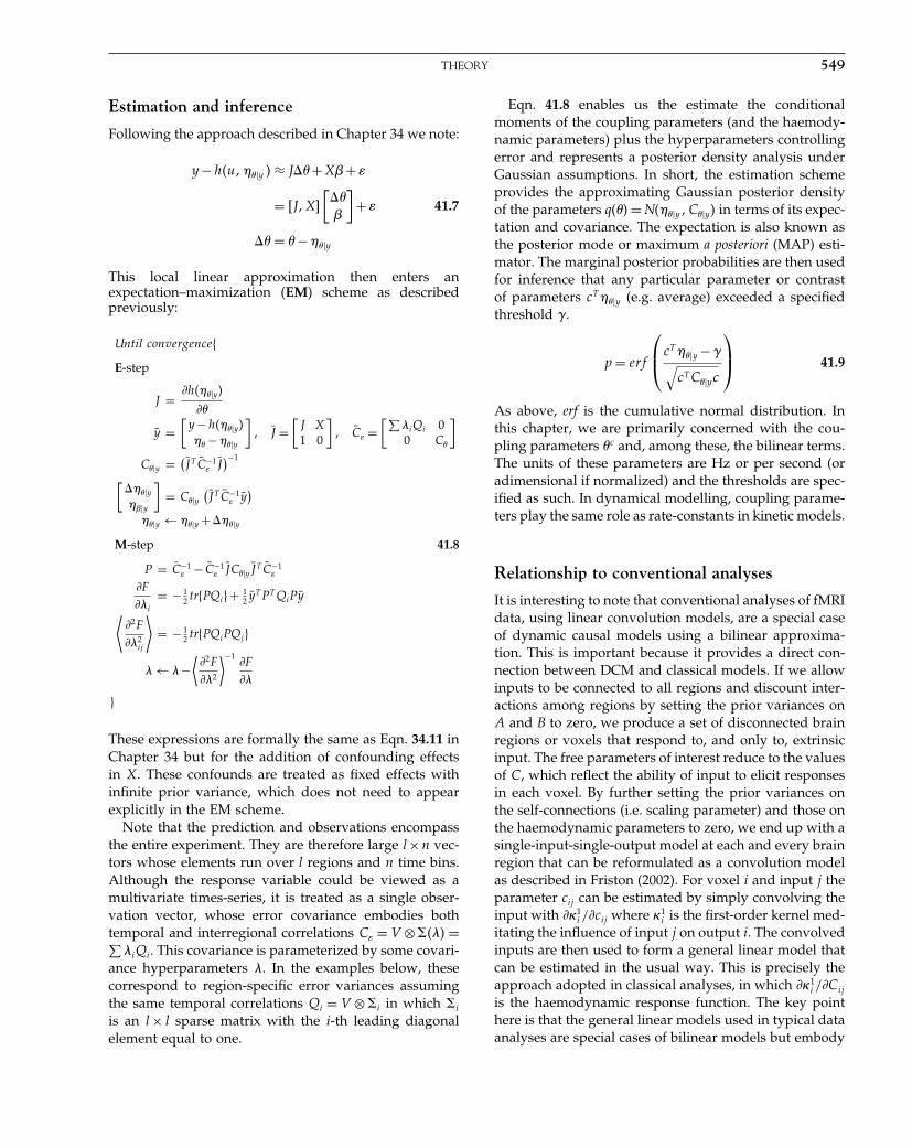
Elsevier UK Chapter: Ch41-P372560 30-9-2006 5:35p.m. Page:549 Trim:7.5in×9.25in
Basal Font:Palatino Margins:Top:40pt Gutter:68pt Font Size:9.5/12 Text Width:42pc Depth:55 Lines
THEORY 549
Estimation and inference
Following the approach described in Chapter 34 we note:
y −h�u����y � ≈ J�� +X�+�
= �J�X�
[���
]+�
�� = � −���y
41.7
This local linear approximation then enters anexpectation–maximization �EM� scheme as describedpreviously:
Until convergence
E-step
J = h����y�
�
ȳ =[
y −h����y��� −���y
]� J̄ =
[J X1 0
]� C̄� =
[∑�iQi 00 C�
]
C��y = (J̄ T C̄−1
� J̄)−1
[����y���y
]= C��y
(J̄ T C̄−1
� ȳ)
���y ← ���y +����y
M-step 41.8
P = C̄−1� − C̄−1
� J̄C��yJ̄ T C̄−1�
F
�i
= − 12 trPQi�+ 1
2 ȳT PT QiPȳ
⟨2F
�2ij
⟩= − 1
2 trPQiPQj�
� ← �−⟨2F
�2
⟩−1F
�
�
These expressions are formally the same as Eqn. 34.11 inChapter 34 but for the addition of confounding effectsin X. These confounds are treated as fixed effects withinfinite prior variance, which does not need to appearexplicitly in the EM scheme.
Note that the prediction and observations encompassthe entire experiment. They are therefore large l×n vec-tors whose elements run over l regions and n time bins.Although the response variable could be viewed as amultivariate times-series, it is treated as a single obser-vation vector, whose error covariance embodies bothtemporal and interregional correlations C� = V ⊗���� =∑
�iQi. This covariance is parameterized by some covari-ance hyperparameters �. In the examples below, thesecorrespond to region-specific error variances assumingthe same temporal correlations Qi = V ⊗�i in which �i
is an l × l sparse matrix with the i-th leading diagonalelement equal to one.
Eqn. 41.8 enables us the estimate the conditionalmoments of the coupling parameters (and the haemody-namic parameters) plus the hyperparameters controllingerror and represents a posterior density analysis underGaussian assumptions. In short, the estimation schemeprovides the approximating Gaussian posterior densityof the parameters q��� = N����y�C��y� in terms of its expec-tation and covariance. The expectation is also known asthe posterior mode or maximum a posteriori (MAP) esti-mator. The marginal posterior probabilities are then usedfor inference that any particular parameter or contrastof parameters cT ���y (e.g. average) exceeded a specifiedthreshold .
p = erf
⎛⎜⎝cT ���y − √
cT C��yc
⎞⎟⎠ 41.9
As above, erf is the cumulative normal distribution. Inthis chapter, we are primarily concerned with the cou-pling parameters �c and, among these, the bilinear terms.The units of these parameters are Hz or per second (oradimensional if normalized) and the thresholds are spec-ified as such. In dynamical modelling, coupling parame-ters play the same role as rate-constants in kinetic models.
Relationship to conventional analyses
It is interesting to note that conventional analyses of fMRIdata, using linear convolution models, are a special caseof dynamic causal models using a bilinear approxima-tion. This is important because it provides a direct con-nection between DCM and classical models. If we allowinputs to be connected to all regions and discount inter-actions among regions by setting the prior variances onA and B to zero, we produce a set of disconnected brainregions or voxels that respond to, and only to, extrinsicinput. The free parameters of interest reduce to the valuesof C, which reflect the ability of input to elicit responsesin each voxel. By further setting the prior variances onthe self-connections (i.e. scaling parameter) and those onthe haemodynamic parameters to zero, we end up with asingle-input-single-output model at each and every brainregion that can be reformulated as a convolution modelas described in Friston (2002). For voxel i and input j theparameter cij can be estimated by simply convolving theinput with �1
i /cij where �1i is the first-order kernel med-
itating the influence of input j on output i. The convolvedinputs are then used to form a general linear model thatcan be estimated in the usual way. This is precisely theapproach adopted in classical analyses, in which �1
i /Cij
is the haemodynamic response function. The key pointhere is that the general linear models used in typical dataanalyses are special cases of bilinear models but embody

Elsevier UK Chapter: Ch41-P372560 30-9-2006 5:35p.m. Page:550 Trim:7.5in×9.25in
Basal Font:Palatino Margins:Top:40pt Gutter:68pt Font Size:9.5/12 Text Width:42pc Depth:55 Lines
550 41. DYNAMIC CAUSAL MODELS FOR fMRI
more assumptions. These assumptions enter through theuse of highly precise priors that discount interactionsamong regions and prevent any variation in biophysi-cal responses. Having described the theoretical aspectsof DCM, we now turn to applications and its validity.
FACE VALIDITY – SIMULATIONS
In this section, we use simulated data to establish theutility of the bilinear approximation and the robust-ness of the estimation scheme described in the previ-ous section. We deliberately chose an architecture thatwould be impossible to characterize using existing meth-ods based on regression models (e.g. structural equationmodelling). This architecture embodies loops and recip-rocal connections and poses the problem of vicariousinput, the ambiguity between the direct influences of onearea and influences that are mediated through others.
A toy system
The simulated architecture is depicted in Figure 41.5 andhas been labelled so that it is consistent with the DCMcharacterized empirically in the next section. The modelcomprises three regions: a primary (A1) and secondary�A2� auditory area and a higher-level region �A3�. Thereare two inputs. The first is a sensory input u1 encodingthe presentation of epochs of words at different frequen-cies. The second input u2 is contextual in nature and issimply an exponential function of the time elapsed sincethe start of each epoch (with a time constant of 8 s). Theseinputs were based on a real experiment and are the sameas those used in the empirical analyses of the next section.The scaling of the inputs is important for the quanti-tative evaluation of the bilinear and extrinsic couplingparameters. The convention adopted here is that inputsencoding events approximate delta functions such thattheir integral over time corresponds to the number ofevents that have occurred. For event-free inputs, like themaintenance of a particular instructional set, the input isscaled to a maximum of unity, so that the integral reflectsthe number of seconds over which the input was prevalent.The inputs were specified in time bins that were a sixteenthof the interval between scans (repetition time; TR = 1�7 s).
The auditory input is connected to the primary area;the second input has no direct effect on activity but mod-ulates the forward connections from A1 to A2 so thatits influence shows adaptation during the epoch. The sec-ond auditory area receives input from the first and sendssignals to the higher area �A3�. In addition to reciprocalbackward connections, in this simple auditory hierarchya connection from the lowest to the highest area has
A2
A1.4
.4
.8
.4
–.4
.4
.8
Context{adaptation}
1 10
8
6
4
2
5
6
4
2
0
–2
4
3
2
1
0
6
4
2
0
–2
–4
–1
0
0.8
0.6
0.4
0.2
00 200 400 600
0 200 400 600
0 200 400 600
0 200 400 600
0 200 400 600
Output
simulated response
Drifts and noise
Time {seconds}
Time {seconds}
Neuronalsaturation
Sensory input
A3
Simulatedresponse
FIGURE 41.5 This is a schematic of the architecture used togenerate simulated data. Non-zero regional connections are shownas directed black arrows with the strength or true parameter along-side. Here, the perturbing input is the presentation of words (sen-sory inputs) and acts as an intrinsic influence on A1. In addition, thisinput modulates the self-connection of A3 to emulate saturation-like effects (see main text and Figure 41.6). The contextual input isa decaying exponential of within-epoch time and positively modu-lates the forward connection from A1 to A2. The lower panel showshow responses were simulated by mixing the output of the systemdescribed above with drifts and noise as described in the main text.
been included. Finally, the first input (word presentation)modulates the self-connections of the third region. Thisinfluence has been included to show how bilinear effectscan emulate non-linear responses. A bilinear modulationof the self-connection can augment or attenuate decayof synaptic activity, rendering the average response to

Elsevier UK Chapter: Ch41-P372560 30-9-2006 5:35p.m. Page:551 Trim:7.5in×9.25in
Basal Font:Palatino Margins:Top:40pt Gutter:68pt Font Size:9.5/12 Text Width:42pc Depth:55 Lines
FACE VALIDITY – SIMULATIONS 551
streams of stimuli rate-dependent. This is because thebilinear effect will only be expressed if sufficient synap-tic activity persists after the previous stimulus. This, inturn, depends on a sufficiently fast presentation rate. Theresulting response emulates a saturation at high presen-tation rates or small stimulus onset asynchronies that hasbeen observed empirically. Critically, we are in a positionto disambiguate between neuronal saturation, modelledby this bilinear term, and haemodynamic saturation,modelled by non-linearities in the haemodynamic com-ponent of this DCM. A significant bilinear self-connectionimplies neuronal saturation above and beyond thatattributable to haemodynamics. Figure 41.6 illustratesthis neuronal saturation by plotting the simulatedresponse of A3 in the absence of saturation B1 = 0 againstthe simulated response with b1
3�3 = −0�4. It is evident thatthere is a non-linear sub-additive effect at high responselevels. It should be noted that true neuronal saturation ofthis sort is mediated by second-order interactions amongthe states (i.e. neuronal activity). However, as shown inFigure 41.6, we can emulate these effects by using thefirst extrinsic input as a surrogate for neuronal inputsfrom other areas in the bilinear component of the model.
Using this model we simulated responses using thevalues for A�B1�B2 and C given in Figure 41.7 and the
Bilinear effects8
8 10
7
6
6
5
4
4
3
2
2
1
0
0–1
Response with no saturation
Res
pons
e w
ith s
atur
atio
n
FIGURE 41.6 This is a plot of the simulated response withsaturation against the equivalent response with no saturation. Thesesimulated responses were obtained by setting the bilinear couplingparameter b1
33 labelled ‘neuronal saturation’ in Figure 41.5 to −0�4and zero respectively. The key thing to observe is a saturationof responses at high levels. The broken line depicts the responseexpected in the absence of saturation. This illustrates how bilineareffects can introduce non-linearities into the response.
Values of Aconditionalestimates
true
true
A {latent}
1
12
3to from
B {input–dependent}
0.5
0
1
12
3to from
0.5
0p(
A >
log(
2)/4
)
esimated
A {latent}
1
12
3to from
0.5
0
p(A
> lo
g(2)
/4)
p(B
> lo
g(2)
/4)
B {input–dependent}
1
12
3to from
0.5
0
p(B
> lo
g(2)
/4)
esimated
Values of B 2
conditionalestimates
ηθ|y
ηθ|y
FIGURE 41.7 Results summarizing the conditional estimationbased upon the simulated data of Figure 41.5. The upper panelsshow the conditional estimates and posterior probabilities pertain-ing to the regional coupling parameters. The lower panels showthe equivalent results for bilinear coupling parameters mediatingthe effect of within-epoch time. Conditional or MAP estimates ofthe parameters are shown in image format with arbitrary scal-ing. The posterior probabilities that these parameters exceeded athreshold of ln(2)/4 per second are shown as three-dimensional barcharts. True values and probabilities are shown on the left, whereasthe estimated values and posterior probabilities are shown on theright. This illustrates that the conditional estimates are a reasonableapproximation to the true values and, in particular, the posteriorprobabilities conform to the true probabilities, if we consider valuesof 90 per cent or more.
prior expectations for the biophysical parameters givenin Table 41-1. The values of the coupling parameters werechosen to match those seen typically in practice. Thisensured the simulated responses were realistic in relationto simulated noise. After down-sampling these determin-istic responses every 1.7 s (the TR of the empirical dataused in the next section), we added known noise to pro-duce simulated data. These data comprised time-series of256 observations with independent or serially correlatedGaussian noise based on an AR(1) process. Unless other-wise stated, the noise had standard deviation of one half
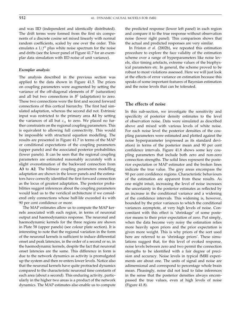
Elsevier UK Chapter: Ch41-P372560 30-9-2006 5:35p.m. Page:552 Trim:7.5in×9.25in
Basal Font:Palatino Margins:Top:40pt Gutter:68pt Font Size:9.5/12 Text Width:42pc Depth:55 Lines
552 41. DYNAMIC CAUSAL MODELS FOR fMRI
and was IID (independent and identically distributed).The drift terms were formed from the first six compo-nents of a discrete cosine set mixed linearly with normalrandom coefficients, scaled by one over the order. Thisemulates a 1/f 2 plus white noise spectrum for the noiseand drifts (see the lower panel of Figure 41.7 for an exem-plar data simulation with IID noise of unit variance).
Exemplar analysis
The analysis described in the previous section wasapplied to the data shown in Figure 41.5. The priorson coupling parameters were augmented by setting thevariance of the off-diagonal elements of B1 (saturation)and all but two connections in B2 (adaptation) to zero.These two connections were the first and second forwardconnections of this cortical hierarchy. The first had sim-ulated adaptation, whereas the second did not. Extrinsicinput was restricted to the primary area A1 by settingthe variances of all but c11 to zero. We placed no fur-ther constraints on the regional coupling parameters. Thisis equivalent to allowing full connectivity. This wouldbe impossible with structural equation modelling. Theresults are presented in Figure 41.7 in terms of the MAPor conditional expectations of the coupling parameters(upper panels) and the associated posterior probabilities(lower panels). It can be seen that the regional couplingparameters are estimated reasonably accurately with aslight overestimation of the backward connection fromA3 to A2. The bilinear coupling parameters modellingadaptation are shown in the lower panels and the estima-tors have correctly identified the first forward connectionas the locus of greatest adaptation. The posterior proba-bilities suggest inferences about the coupling parameterswould lead us to the veridical architecture if we consid-ered only connections whose half-life exceeded 4 s with90 per cent confidence or more.
The MAP estimates allow us to compute the MAP ker-nels associated with each region, in terms of neuronaloutput and haemodynamics response. The neuronal andhaemodynamic kernels for the three regions are shownin Plate 58 (upper panels) (see colour plate section). It isinteresting to note that the regional variation in the formof the neuronal kernels is sufficient to induce differentialonset and peak latencies, in the order of a second or so, inthe haemodynamic kernels, despite the fact that neuronalonset latencies are the same. This difference in form isdue to the network dynamics as activity is promulgatedup the system and then re-enters lower levels. Notice alsothat the neuronal kernels have quite protracted dynamicscompared to the characteristic neuronal time constants ofeach area (about a second). This enduring activity, partic-ularly in the higher two areas is a product of the networkdynamics. The MAP estimates also enable us to compute
the predicted response (lower left panel) in each regionand compare it to the true response without observationnoise (lower right panel). This comparison shows thatthe actual and predicted responses are very similar.
In Friston et al. (2002b), we repeated this estimationprocedure to explore the face validity of the estimationscheme over a range of hyperparameters like noise lev-els, slice timing artefacts, extreme values of the biophys-ical parameters etc. In general, the scheme proved to berobust to most violations assessed. Here we will just lookat the effects of error variance on estimation because thisspeaks of some important features of Bayesian estimationand the noise levels that can be tolerated.
The effects of noise
In this sub-section, we investigate the sensitivity andspecificity of posterior density estimates to the levelof observation noise. Data were simulated as describedabove and mixed with various levels of white noise.For each noise level the posterior densities of the cou-pling parameters were estimated and plotted against thenoise hyperparameter (expressed as its standard devi-ation) in terms of the posterior mean and 90 per centconfidence intervals. Figure 41.8 shows some key cou-pling parameters that include both zero and non-zeroconnection strengths. The solid lines represent the poste-rior expectation or MAP estimator and the broken linesindicate the true value. The grey areas encompass the90 per cent confidence regions. Characteristic behavioursof the estimation are apparent from these results. Asone might intuit, increasing the level of noise increasesthe uncertainty in the posterior estimates as reflected byan increase in the conditional variance and a wideningof the confidence intervals. This widening is, however,bounded by the prior variances to which the conditionalvariances asymptote, at very high levels of noise. Con-comitant with this effect is ‘shrinkage’ of some poste-rior means to their prior expectation of zero. Put simply,when the data become very noisy the estimation reliesmore heavily upon priors and the prior expectation isgiven more weight. This is why priors of the sort usedhere are referred to as ‘shrinkage priors’. These simu-lations suggest that, for this level of evoked response,noise levels between zero and two permit the connectionstrengths to be identified with a fair degree of preci-sion and accuracy. Noise levels in typical fMRI experi-ments are about one. The units of signal and noise areadimensional and correspond to percentage whole brainmean. Pleasingly, noise did not lead to false inferencesin the sense that the posterior densities always encom-passed the true values, even at high levels of noise(Figure 41.8).
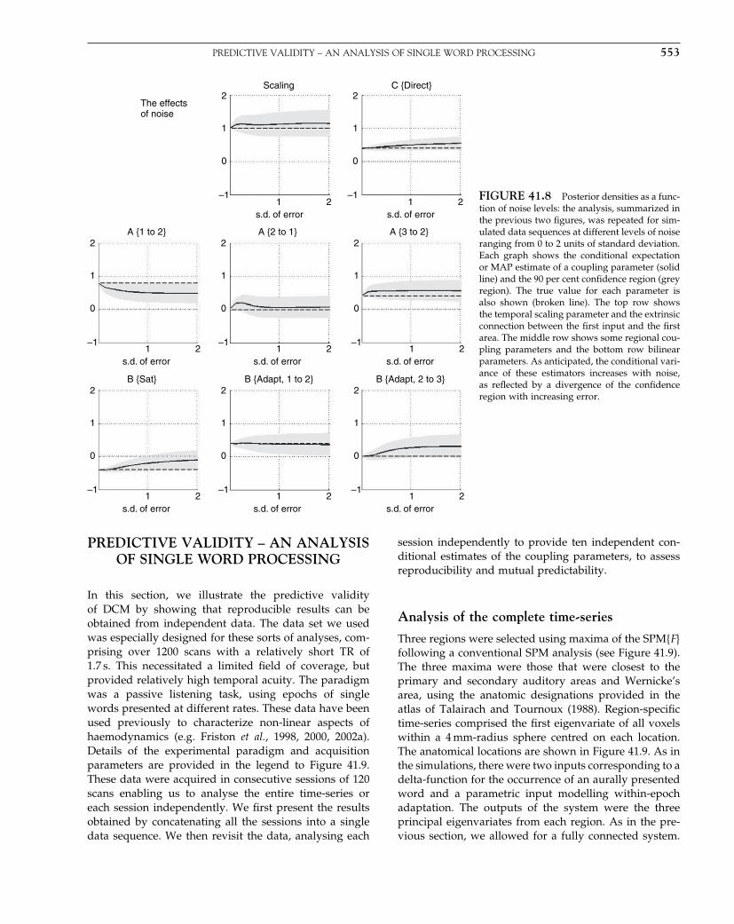
Elsevier UK Chapter: Ch41-P372560 30-9-2006 5:35p.m. Page:553 Trim:7.5in×9.25in
Basal Font:Palatino Margins:Top:40pt Gutter:68pt Font Size:9.5/12 Text Width:42pc Depth:55 Lines
PREDICTIVE VALIDITY – AN ANALYSIS OF SINGLE WORD PROCESSING 553
The effects of noise
Scaling
A {1 to 2}
s.d. of error
s.d. of error
s.d. of error
2
1 1
0
–1
2
1
0
–1
2
1 2
1 2
A {2 to 1} A {3 to 2}
s.d. of error
2
1
0
–11 2
s.d. of error
2
1
0
–11 2
B {Sat}
s.d. of error
2
1
0
–11 2
B {Adapt, 1 to 2} B {Adapt, 2 to 3}
s.d. of error
2
1
0
–11 2
s.d. of error
2
1
0
–11 2
1 2
0
–1
C {Direct}
FIGURE 41.8 Posterior densities as a func-tion of noise levels: the analysis, summarized inthe previous two figures, was repeated for sim-ulated data sequences at different levels of noiseranging from 0 to 2 units of standard deviation.Each graph shows the conditional expectationor MAP estimate of a coupling parameter (solidline) and the 90 per cent confidence region (greyregion). The true value for each parameter isalso shown (broken line). The top row showsthe temporal scaling parameter and the extrinsicconnection between the first input and the firstarea. The middle row shows some regional cou-pling parameters and the bottom row bilinearparameters. As anticipated, the conditional vari-ance of these estimators increases with noise,as reflected by a divergence of the confidenceregion with increasing error.
PREDICTIVE VALIDITY – AN ANALYSISOF SINGLE WORD PROCESSING
In this section, we illustrate the predictive validityof DCM by showing that reproducible results can beobtained from independent data. The data set we usedwas especially designed for these sorts of analyses, com-prising over 1200 scans with a relatively short TR of1.7 s. This necessitated a limited field of coverage, butprovided relatively high temporal acuity. The paradigmwas a passive listening task, using epochs of singlewords presented at different rates. These data have beenused previously to characterize non-linear aspects ofhaemodynamics (e.g. Friston et al., 1998, 2000, 2002a).Details of the experimental paradigm and acquisitionparameters are provided in the legend to Figure 41.9.These data were acquired in consecutive sessions of 120scans enabling us to analyse the entire time-series oreach session independently. We first present the resultsobtained by concatenating all the sessions into a singledata sequence. We then revisit the data, analysing each
session independently to provide ten independent con-ditional estimates of the coupling parameters, to assessreproducibility and mutual predictability.
Analysis of the complete time-series
Three regions were selected using maxima of the SPMF�following a conventional SPM analysis (see Figure 41.9).The three maxima were those that were closest to theprimary and secondary auditory areas and Wernicke’sarea, using the anatomic designations provided in theatlas of Talairach and Tournoux (1988). Region-specifictime-series comprised the first eigenvariate of all voxelswithin a 4 mm-radius sphere centred on each location.The anatomical locations are shown in Figure 41.9. As inthe simulations, there were two inputs corresponding to adelta-function for the occurrence of an aurally presentedword and a parametric input modelling within-epochadaptation. The outputs of the system were the threeprincipal eigenvariates from each region. As in the pre-vious section, we allowed for a fully connected system.
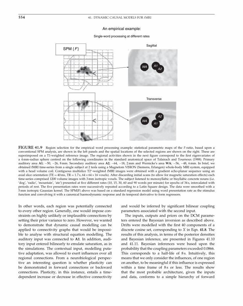
Elsevier UK Chapter: Ch41-P372560 30-9-2006 5:35p.m. Page:554 Trim:7.5in×9.25in
Basal Font:Palatino Margins:Top:40pt Gutter:68pt Font Size:9.5/12 Text Width:42pc Depth:55 Lines
554 41. DYNAMIC CAUSAL MODELS FOR fMRI
SPM { F }Sagittal
Transverse
WA
WA
A1
A1
A2
A2
An empirical example:
Single-word processing at different rates
FIGURE 41.9 Region selection for the empirical word processing example: statistical parametric maps of the F -ratio, based upon aconventional SPM analysis, are shown in the left panels and the spatial locations of the selected regions are shown on the right. These aresuperimposed on a T1-weighted reference image. The regional activities shown in the next figure correspond to the first eigenvariates ofa 4 mm-radius sphere centred on the following coordinates in the standard anatomical space of Talairach and Tournoux (1988). Primaryauditory area A1; −50, −26, 8 mm. Secondary auditory area A2; −64, −18, 2 mm and Wernicke’s area WA; −56, −48, 6 mm. In brief, weobtained fMRI time-series from a single subject at 2 tesla using a Magnetom VISION (Siemens, Erlangen) whole-body MRI system, equippedwith a head volume coil. Contiguous multislice T2∗-weighted fMRI images were obtained with a gradient echo-planar sequence using anaxial slice orientation �TE = 40 ms� TR = 1�7 s� 64×64×16 voxels). After discarding initial scans (to allow for magnetic saturation effects) eachtime-series comprised 1200 volume images with 3 mm isotropic voxels. The subject listened to monosyllabic or bisyllabic concrete nouns (i.e.‘dog’, ‘radio’, ‘mountain’, ‘ate’) presented at five different rates (10, 15, 30, 60 and 90 words per minute) for epochs of 34 s, intercalated withperiods of rest. The five presentation rates were successively repeated according to a Latin Square design. The data were smoothed with a5 mm isotropic Gaussian kernel. The SPM{F} above was based on a standard regression model using word presentation rate as the stimulusfunction and convolving it with a canonical haemodynamic response and its temporal derivative to form regressors.
In other words, each region was potentially connectedto every other region. Generally, one would impose con-straints on highly unlikely or implausible connections bysetting their prior variance to zero. However, we wantedto demonstrate that dynamic causal modelling can beapplied to connectivity graphs that would be impossi-ble to analyse with structural equation modelling. Theauditory input was connected to A1. In addition, audi-tory input entered bilinearly to emulate saturation, as inthe simulations. The contextual input, modelling puta-tive adaptation, was allowed to exert influences over allregional connections. From a neurobiological perspec-tive an interesting question is whether plasticity canbe demonstrated in forward connections or backwardconnections. Plasticity, in this instance, entails a time-dependent increase or decrease in effective connectivity
and would be inferred by significant bilinear couplingparameters associated with the second input.
The inputs, outputs and priors on the DCM parame-ters entered the Bayesian inversion as described above.Drifts were modelled with the first 40 components of adiscrete cosine set, corresponding to X in Eqn. 41.8. Theresults of this analysis, in terms of the posterior densitiesand Bayesian inference, are presented in Figures 41.10and 41.11. Bayesian inferences were based upon theprobability that the coupling parameters exceeded 0.0866.This corresponds to a half-life of 8 s. Intuitively, thismeans that we only consider the influences, of one regionon another, to be meaningful if this influence is expressedwithin a time frame of 8 s or less. The results showthat the most probable architecture, given the inputsand data, conforms to a simple hierarchy of forward

Elsevier UK Chapter: Ch41-P372560 30-9-2006 5:35p.m. Page:555 Trim:7.5in×9.25in
Basal Font:Palatino Margins:Top:40pt Gutter:68pt Font Size:9.5/12 Text Width:42pc Depth:55 Lines
PREDICTIVE VALIDITY – AN ANALYSIS OF SINGLE WORD PROCESSING 555
Estimated architecture
WA
A1
A2
Input {stimulus}
Input {context}
.92(100%)
.38(94%)
.47(98%)
.37 (91%)
–.62 (99%)
–.51 (99%)
.37 (100%)
10
8
6
4
2
0100 200 400 500300
Time {seconds}
100
1
0
0.8
0.6
0.4
0.2
200 400 500300Time {seconds}
FIGURE 41.10 Results of a DCM anal-ysis applied to the data described in the pre-vious figure. The display format follows thatof Figure 41.5. The coupling parameters areshown alongside the corresponding connec-tions. The values in brackets are the percent-age confidence that these values exceed athreshold of ln(2)/8 per second.
connections where A1 influences A2 and WA, whereasA2 sends connections just to WA (Figure 41.10). Althoughbackward connections between WA and A2 were esti-mated to be greater than our threshold with 82 per centconfidence they are not shown in Figure 41.11 (whichis restricted to posterior probabilities of 90 per centor more). Saturation could be inferred in A1 and WAwith a high degree of confidence with b1
11 and b133 being
greater than 0.5. Significant plasticity or time-dependentchanges were expressed predominantly in the forwardconnections, particularly that between A1 and A3, i.e.b2
13 = 0�37. The conditional estimates are shown in moredetail in Figure 41.11, along with the conditional fittedresponses and associated kernels. A full posterior densityanalysis for a particular contrast of effects is shown inFigure 41.11(a) (lower panel). This contrast tested for theaverage plasticity over all forward and backward connec-tions and demonstrates that we can be virtually certainplasticity was greater than zero.
This analysis illustrates three things. First, the DCMhas defined a hierarchical architecture that is the mostlikely given the data. This hierarchical structure wasnot part of the prior constraints because we allowedfor a fully connected system. Second, the significant
bilinear effects of auditory stimulation suggest thereis measurable neuronal saturation above and beyondthat attributable to haemodynamic non-linearities. This isquite significant because such disambiguation is usuallyimpossible given just haemodynamic responses. Finally,we were able to show time-dependent decreases ineffective connectivity in forward connections from A1.Although this experiment was not designed to test forplasticity, the usefulness of DCM, in studies of learningand priming, should be self-evident.
Reproducibility
The analysis above was repeated identically for each 120-scan session to provide ten sets of Bayesian estimators.Drifts were modelled with the first four components of adiscrete cosine set. The estimators are presented graphi-cally in Figure 41.12 and demonstrate extremely consis-tent results. In the upper panels, the intrinsic connectionsare shown to be very similar; again reflecting a hierarchi-cal architecture. The conditional means and 90 per centconfidence regions for two connections are shown inFigure 41.12(a). These connections included the forward

Elsevier UK Chapter: Ch41-P372560 30-9-2006 5:35p.m. Page:556 Trim:7.5in×9.25in
Basal Font:Palatino Margins:Top:40pt Gutter:68pt Font Size:9.5/12 Text Width:42pc Depth:55 Lines
556 41. DYNAMIC CAUSAL MODELS FOR fMRI
A {latent}
from
B {saturation}
post
erio
r de
nsity
B {adaptation}
to to to
A1 A2
5
4
2
3
1
00
1.5 0.35
0.3
0.25
0.20.15
0.10.05
00–1000 1000 2000
0.5
–0.5
1
0
0 10 20
10.5
WAfrom
A1 A2 WAfrom
A1 A2 WA
A2
A1
KernelsResponses
hemodynamic kernels1s
t ord
er r
espo
nse
1st o
rder
res
pons
eseconds
mean adaptation (Hz)
time {seconds}
resp
onse
milliseconds
neuronal kernels
WA
100
–2
0
2
4
6
8
–2
0
2
2
4
6
8
200 300 400 500
00 200 300 400 500
100 200 300 400
p(cTθ y)
MAP estimates ηθ |y
(a)
(b)
FIGURE 41.11 This figure provides a more detailed characterization of the conditional estimates. The images in the top row are theMAP estimates for the regional and bilinear coupling parameters, pertaining to saturation and adaptation. The middle panel shows theposterior density of a contrast of all bilinear terms mediating adaptation, namely the modulation of regional connections by the secondtime-dependent experimental effect. The predicted responses based upon the conditional estimators are shown for each of the three regionson the lower left (solid lines) with the original data (dots) after removal of confounds. A re-parameterization of the conditional estimates, interms of the first-order kernels, is shown on the lower right. The haemodynamic (left) and neuronal (right) kernels should be compared withthe equivalent kernels for the simulated data in Plate 58.
connection from A1 to A2 that is consistently strong. Thebackward connection from WA to A2 was weaker, butwas certainly greater than zero in every analysis. Equiv-alent results were obtained for the modulatory effects orbilinear terms, although the profile was less consistent(Figure 41.12(b)). However, the posterior density of thecontrast testing for average time-dependent adaptationor plasticity is relatively consistent and again almost cer-tainly greater than zero, in each analysis.
To illustrate the stability of hyperparameter estimates,the standard deviations of observation error are presentedfor each session over the three areas in Figure 41.13. Astypical of studies at this field strength the standard devi-ation of noise is about 0.8–1 per cent whole brain mean. Itis pleasing to note that the session-to-session variability inhyperparameter estimates was relatively small, in relationto region-to-region differences.
In summary, independent analyses of data acquiredunder identical stimulus conditions, on the same subject,in the same scanning session, yield remarkably similarresults. These results are biologically plausible and speakof time-dependent changes, following the onset of a streamof words, in forward connections among auditory areas.
CONSTRUCT VALIDITY – ANANALYSIS OF ATTENTIONAL EFFECTS
ON CONNECTIONS
In this final section, we address the construct validity ofDCM. In previous chapters, we have seen that attentionpositively modulates the backward connections in a dis-tributed system of cortical regions mediating attention
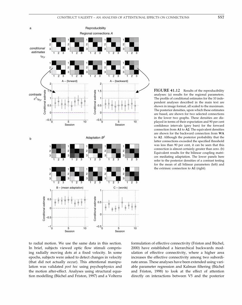
Elsevier UK Chapter: Ch41-P372560 30-9-2006 5:35p.m. Page:557 Trim:7.5in×9.25in
Basal Font:Palatino Margins:Top:40pt Gutter:68pt Font Size:9.5/12 Text Width:42pc Depth:55 Lines
CONSTRUCT VALIDITY – AN ANALYSIS OF ATTENTIONAL EFFECTS ON CONNECTIONS 557
Reproducibility
Regional connections A
Adaptation B2
contrasts
conditionalestimates
a
b
1
1
2
2
3
1
2
3
1
2
3
1
2
3
1
2
3
1
2
3
1
2
3
1
2
3
1
2
3
1
2
3
3 1 2 3 1 2 3 1 2 3 1 2 3
1 2 31 2 31 2 31 22
A – {forward} A – {backward}
31
2
1
1.5 1.5
0.5
Con
ditio
nal e
stim
ate
–0.5
0
0 5Session
10
2
1
0.5
Con
ditio
nal e
stim
ate
–0.5
0
0 5Session
10
B – {mean adaptation} C – {words}1
0
0.50.5
–0.5
Con
ditio
nal e
stim
ate
–10 5
Session10
1
Con
ditio
nal e
stim
ate
–0.5
0
0 5Session
10
3
1
2
2
3
1
2
3
1
2
3
1
2
3
1
2
3
1 2 31 2 31 2 31 2 31 3
1
2
2
3
1
2
3
1
2
3
1
2
3
1
2
3
1 2 31 2 31 2 31 2 31 3
ηθ | y
cTηθ | y
FIGURE 41.12 Results of the reproducibilityanalyses: (a) results for the regional parameters.The profile of conditional estimates for the 10 inde-pendent analyses described in the main text areshown in image format, all scaled to the maximum.The posterior densities, upon which these estimatesare based, are shown for two selected connectionsin the lower two graphs. These densities are dis-played in terms of their expectation and 90 per centconfidence intervals (grey bars) for the forwardconnection from A1 to A2. The equivalent densitiesare shown for the backward connection from WAto A2. Although the posterior probability that thelatter connections exceeded the specified thresholdwas less than 90 per cent, it can be seen that thisconnection is almost certainly greater than zero. (b)Equivalent results for the bilinear coupling matri-ces mediating adaptation. The lower panels hererefer to the posterior densities of a contrast testingfor the mean of all bilinear parameters (left) andthe extrinsic connection to A1 (right).
to radial motion. We use the same data in this section.In brief, subjects viewed optic flow stimuli compris-ing radially moving dots at a fixed velocity. In someepochs, subjects were asked to detect changes in velocity(that did not actually occur). This attentional manipu-lation was validated post hoc using psychophysics andthe motion after-effect. Analyses using structural equa-tion modelling (Büchel and Friston, 1997) and a Volterra
formulation of effective connectivity (Friston and Büchel,2000) have established a hierarchical backwards mod-ulation of effective connectivity, where a higher areaincreases the effective connectivity among two subordi-nate areas. These analyses have been extended using vari-able parameter regression and Kalman filtering (Bücheland Friston, 1998) to look at the effect of attentiondirectly on interactions between V5 and the posterior
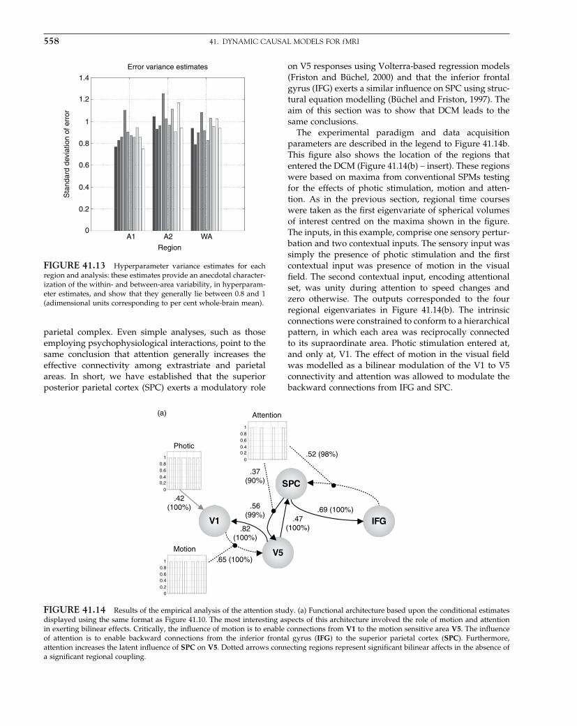
Elsevier UK Chapter: Ch41-P372560 30-9-2006 5:35p.m. Page:558 Trim:7.5in×9.25in
Basal Font:Palatino Margins:Top:40pt Gutter:68pt Font Size:9.5/12 Text Width:42pc Depth:55 Lines
558 41. DYNAMIC CAUSAL MODELS FOR fMRI
Error variance estimatesS
tand
ard
devi
atio
n of
err
or
1.4
1.2
0.8
0.6
0.4
0.2
0A1 A2 WA
Region
1
FIGURE 41.13 Hyperparameter variance estimates for eachregion and analysis: these estimates provide an anecdotal character-ization of the within- and between-area variability, in hyperparam-eter estimates, and show that they generally lie between 0.8 and 1(adimensional units corresponding to per cent whole-brain mean).
parietal complex. Even simple analyses, such as thoseemploying psychophysiological interactions, point to thesame conclusion that attention generally increases theeffective connectivity among extrastriate and parietalareas. In short, we have established that the superiorposterior parietal cortex (SPC) exerts a modulatory role
on V5 responses using Volterra-based regression models(Friston and Büchel, 2000) and that the inferior frontalgyrus (IFG) exerts a similar influence on SPC using struc-tural equation modelling (Büchel and Friston, 1997). Theaim of this section was to show that DCM leads to thesame conclusions.
The experimental paradigm and data acquisitionparameters are described in the legend to Figure 41.14b.This figure also shows the location of the regions thatentered the DCM (Figure 41.14(b) – insert). These regionswere based on maxima from conventional SPMs testingfor the effects of photic stimulation, motion and atten-tion. As in the previous section, regional time courseswere taken as the first eigenvariate of spherical volumesof interest centred on the maxima shown in the figure.The inputs, in this example, comprise one sensory pertur-bation and two contextual inputs. The sensory input wassimply the presence of photic stimulation and the firstcontextual input was presence of motion in the visualfield. The second contextual input, encoding attentionalset, was unity during attention to speed changes andzero otherwise. The outputs corresponded to the fourregional eigenvariates in Figure 41.14(b). The intrinsicconnections were constrained to conform to a hierarchicalpattern, in which each area was reciprocally connectedto its supraordinate area. Photic stimulation entered at,and only at, V1. The effect of motion in the visual fieldwas modelled as a bilinear modulation of the V1 to V5connectivity and attention was allowed to modulate thebackward connections from IFG and SPC.
V1 IFG
V5
SPC
Motion
Photic
Attention
.82(100%)
.42(100%)
.37(90%)
10.80.60.40.2
010.80.60.40.2
0
10.80.60.4
0.20
.69 (100%).47
(100%)
.65 (100%)
.52 (98%)
.56(99%)
(a)
FIGURE 41.14 Results of the empirical analysis of the attention study. (a) Functional architecture based upon the conditional estimatesdisplayed using the same format as Figure 41.10. The most interesting aspects of this architecture involved the role of motion and attentionin exerting bilinear effects. Critically, the influence of motion is to enable connections from V1 to the motion sensitive area V5. The influenceof attention is to enable backward connections from the inferior frontal gyrus (IFG) to the superior parietal cortex (SPC). Furthermore,attention increases the latent influence of SPC on V5. Dotted arrows connecting regions represent significant bilinear affects in the absence ofa significant regional coupling.

Elsevier UK Chapter: Ch41-P372560 30-9-2006 5:35p.m. Page:559 Trim:7.5in×9.25in
Basal Font:Palatino Margins:Top:40pt Gutter:68pt Font Size:9.5/12 Text Width:42pc Depth:55 Lines
CONSTRUCT VALIDITY – AN ANALYSIS OF ATTENTIONAL EFFECTS ON CONNECTIONS 559
FIGURE 41.14 (Continued) (b) Fitted responses based upon the conditional estimates and the adjusted data are shown using the sameformat as in Figure 41.11. The insert shows the location of the regions, again adopting the same format in previous figures. The location ofthese regions centred on the primary visual cortex V1; 6, −84, −6 mm: motion-sensitive area V5; 45, −81, 5 mm. Superior parietal cortex, SPC;18, −57, 66 mm. Inferior frontal gyrus, IFG, 54, 18, 30 mm. The volumes from which the first eigenvariates were calculated corresponded to8 mm-radius spheres centred on these locations.
Subjects were studied with fMRI under identical stimulus conditions (visual motion subtended by radially moving dots) while manipulatingthe attentional component of the task (detection of velocity changes). The data were acquired from normal subjects at 2 tesla using aMagnetom VISION (Siemens, Erlangen) whole-body MRI system, equipped with a head volume coil. Here we analyse data from the firstsubject. Contiguous multislice T2∗-weighted fMRI images were obtained with a gradient echo-planar sequence (TE = 40 ms� TR = 3�22 s,matrix size = 64×64×32, voxel size 3×3×3 mm). Each subject had four consecutive 100-scan sessions comprising a series of 10-scan blocksunder five different conditions D F A F N F A F N S. The first condition (D) was a dummy condition to allow for magnetic saturation effects.F (Fixation) corresponds to a low-level baseline where the subjects viewed a fixation point at the centre of a screen. In condition A (Attention),subjects viewed 250 dots moving radially from the centre at 4.7 degrees per second and were asked to detect changes in radial velocity. Incondition N (No attention), the subjects were asked simply to view the moving dots. In condition S (Stationary), subjects viewed stationarydots. The order of A and N was swapped for the last two sessions. In all conditions, subjects fixated the centre of the screen. In a pre-scanningsession the subjects were given five trials with five speed changes (reducing to 1 per cent). During scanning there were no speed changes.No overt response was required in any condition.
The results of the DCM are shown in Figure 41.14(a).Of primary interest here is the modulatory effect of atten-tion that is expressed in terms of the bilinear couplingparameters for this third input. As hoped, we can behighly confident that attention modulates the backwardconnections from IFG to SPC and from SPC to V5. Indeed,the influences of IFG on SPC are negligible in the absenceof attention (dotted connection in Figure 41.14(a)). Itis important to note that the only way that attentionalmanipulation can affect brain responses was throughthis bilinear effect. Attention-related responses are seenthroughout the system (attention epochs are marked witharrows in the plot of IFG responses in Figure 41.14(b)).This attentional modulation is accounted for by chang-ing just two connections. This change is, presumably,instantiated by instructional set at the beginning of each
epoch. The second thing this analysis illustrates is howfunctional segregation is modelled in DCM. Here onecan regard V1 as a ‘segregating’ motion from othervisual information and distributing it to the motion-sensitive area V5. This segregation is modelled as a bilin-ear ‘enabling’ of V1 to V5 connections when, and onlywhen, motion is present. Note that, in the absence ofmotion, the V1 to V5 connection was trivially small (infact the MAP estimate was −0�04). The key advantage ofentering motion through a bilinear effect, as opposed to adirect effect on V5, is that we can finesse the inference thatV5 shows motion-selective responses with the assertionthat these responses are mediated by afferents from V1.The two bilinear effects above represent two importantaspects of functional integration that DCM was designedto characterize.

Elsevier UK Chapter: Ch41-P372560 30-9-2006 5:35p.m. Page:560 Trim:7.5in×9.25in
Basal Font:Palatino Margins:Top:40pt Gutter:68pt Font Size:9.5/12 Text Width:42pc Depth:55 Lines
560 41. DYNAMIC CAUSAL MODELS FOR fMRI
CONCLUSION
In this chapter, we have presented dynamic causalmodelling. DCM is a causal modelling procedure fordynamical systems in which causality is inherent in thedifferential equations that specify the model. The basicidea is to treat the system of interest, in this case thebrain, as an input-state-output system. By perturbing thesystem with known inputs, measured responses are usedto estimate various parameters that govern the evolutionof brain states. Although there are no restrictions on theparameterization of the model, a bilinear approximationaffords a simple re-parameterization in terms of effectiveconnectivity. This effective connectivity can be latent or,through bilinear terms, model input-dependent changesin coupling. Parameter estimation proceeds using fairlystandard approaches to system identification that restupon Bayesian inference.
Dynamic causal modelling represents a fundamentaldeparture from conventional approaches to modellingeffective connectivity in neuroscience. The critical dis-tinction between DCM and other approaches, such asstructural equation modelling or multivariate autoregres-sive techniques, is that the input is treated as known,as opposed to stochastic. In this sense, DCM is muchcloser to conventional analyses of neuroimaging time-series because the causal or explanatory variables enter asknown fixed quantities. The use of designed and knowninputs in characterizing neuroimaging data with the gen-eral linear model or DCM is a more natural way to anal-yse data from designed experiments. Given that the vastmajority of imaging neuroscience relies upon designedexperiments, we consider DCM a potentially useful com-plement to existing techniques. We develop this pointand the relationship of DCM to other approaches inAppendix 2.
In the next chapter, we consider DCMs for EEG. Herethe electromagnetic model mapping neuronal states tomeasurements is simpler than the haemodynamic mod-els used in fMRI. Conversely, the neuronal componentof the model is much more complicated and realis-tic. This is because there is more temporal informationin EEG.
REFERENCES
Bendat JS (1990) Nonlinear system analysis and identification from ran-dom data. John Wiley and Sons, New York
Bitan T, Booth JR, Choy J et al. (2005) Shifts of effective connec-tivity within a language network during rhyming and spelling.J Neurosci 25: 5397–403
Büchel C, Friston KJ (1997) Modulation of connectivity in visualpathways by attention: cortical interactions evaluated with struc-tural equation modelling and fMRI. Cereb Cortex 7: 768–78
Büchel C, Friston KJ (1998) Dynamic changes in effective connectiv-ity characterised by variable parameter regression and Kalmanfiltering. Hum Brain Mapp 6: 403–08
Buxton RB, Wong EC, Frank LR (1998) Dynamics of blood flow andoxygenation changes during brain activation: the Balloon model.Mag Res Med 39: 855–64
Ethofer T, Anders S, Erb M et al. (2006) Cerebral pathways in pro-cessing of affective prosody: a dynamic causal modeling study.NeuroImage 30: 580–87
Friston KJ (2002) Bayesian estimation of dynamical systems: anapplication to fMRI. NeuroImage 16: 513–30
Friston KJ, Büchel C (2000) Attentional modulation of effective con-nectivity from V2 to V5/MT in humans. Proc Natl Acad Sci USA97: 7591–96
Friston KJ, Büchel C, Fink GR et al. (1997) Psychophysiological andmodulatory interactions in neuroimaging. NeuroImage 6: 218–29
Friston KJ, Josephs O, Rees G et al. (1998) Nonlinear event-relatedresponses in fMRI. Mag Res Med 39: 41–52
Friston KJ, Mechelli A, Turner R et al. (2000) Nonlinear responsesin fMRI: the Balloon model, Volterra kernels and other hemo-dynamics. NeuroImage 12: 466–77
Friston KJ, Penny W, Phillips C et al. (2002a) Classical and Bayesianinference in neuroimaging: theory. NeuroImage 16: 465–83
Friston KJ, Harrison L, Penny W (2002b) Dynamic causal modelling.NeuroImage 19:1273–302
Horwitz B, Friston KJ, Taylor JG (2001) Neural modeling and func-tional brain imaging: an overview. Neural Netw 13: 829–46
Kenny DA, Judd CM (1984) Estimating nonlinear and interactiveeffects of latent variables. Psychol Bull 96: 201–10
Mandeville JB, Marota JJ, Ayata C et al. (1999) Evidence of a cere-brovascular postarteriole Windkessel with delayed compliance.J Cereb Blood Flow Metab 19: 679–89
McIntosh AR (2000) Towards a network theory of cognition. NeuralNetw 13: 861–70
McIntosh AR, Gonzalez-Lima F (1994) Structural equation mod-elling and its application to network analysis in functional brainimaging. Hum Brain Mapp 2: 2–22
Mechelli A, Price CJ, Noppeney U et al. (2003) A dynamic causalmodeling study on category effects: bottom-up or top-downmediation? J Cogn Neurosci 15: 925–34
Talairach J, Tournoux P (1988) A co-planar stereotaxic atlas of a humanbrain. Thieme, Stuttgart

Elsevier UK Chapter: Ch42-P372560 30-9-2006 5:35p.m. Page:561 Trim:7.5in×9.25in
Basal Font:Palatino Margins:Top:40pt Gutter:68pt Font Size:9.5/12 Text Width:42pc Depth:55 Lines
C H A P T E R
42
Dynamic causal models for EEGK. Friston, S. Kiebel, M. Garrido and O. David
INTRODUCTION
Neuronally plausible, generative or forward models areessential for understanding how event-related fields(ERFs) and potentials (ERPs) are generated. In thischapter, we describe the dynamic causal modelling(DCM) of event-related responses measured with elec-troencephalography (EEG) or magnetoencephalography(MEG). This approach uses a biologically informed causalmodel to make inferences about the underlying neu-ronal networks generating responses. The approach canbe regarded as a neurobiologically constrained sourcereconstruction scheme, in which the parameters ofthe reconstruction have an explicit neuronal interpreta-tion. Specifically, these parameters encode, among otherthings, the coupling among sources and how that cou-pling depends upon stimulus attributes or experimentalcontext. The basic idea is to supplement conventionalelectromagnetic forward models, of how sources areexpressed in measurement space, with a model of howsource activity is generated by neuronal dynamics. Asingle inversion of this extended forward model enablesinference about both the spatial deployment of sourcesand the underlying neuronal architecture generatingthem. Critically, this inference covers long-range connec-tions among well-defined neuronal subpopulations.
In Chapter 33, we simulated ERPs using a hierarchicalneural-mass model that embodied bottom-up, top-downand lateral connections among remote regions. In thischapter, we describe a Bayesian procedure to estimatethe parameters of this model using empirical data. Wedemonstrate this procedure by characterizing the roleof changes in cortico-cortical coupling, in the genesis ofERPs using two examples. In brief, in the first example,ERPs recorded during the perception of faces and housesare modelled as distinct cortical sources in the ventralvisual pathway. We will see that category-selectivity,as indexed by the face-selective N170, can be explained
by category-specific differences in forward connectionsfrom sensory to higher areas in the ventral stream. Thesechanges allow one to identify where, in the processingstream, category-selectivity emerges. The second exam-ple uses an auditory oddball paradigm to show thatmismatch negativity can be explained by changes in con-nectivity. Specifically, using Bayesian model selection,we will assess changes in backward connections, aboveand beyond changes in forward connections. In accordwith theoretical predictions, we will see strong evidencefor learning-related changes in both forward and back-ward coupling. These examples illustrate DCM for ERPsto address category- or context-specific coupling amongcortical regions.
Background
ERFs and ERPs have been used for decades as magneto-and electrophysiological correlates of perceptual andcognitive operations. However, the exact neurobiologi-cal mechanisms underlying their generation are largelyunknown. Previous studies have shown that ERP-likeresponses can be reproduced by perturbations of modelcortical networks (Jansen and Rit, 1995; Rennie et al.,2002; Jirsa, 2004; David et al., 2005). Here we show thatchanges in connectivity, among distinct cortical sources,are sufficient to explain stimulus- or set-specific ERPdifferences.
Functional versus effective connectivity
The aim of dynamic causal modelling (Friston et al., 2003)is to make inferences about the coupling among brainregions or sources and how that coupling is influencedby experimental factors. DCM uses the notion of effectiveconnectivity, defined as the influence one neuronal systemexerts over another. DCM represents a departure fromexisting approaches to connectivity because it employs
Statistical Parametric Mapping, by Karl Friston et al. Copyright 2007, Elsevier Ltd. All rights reserved.ISBN–13: 978-0-12-372560-8 ISBN–10: 0-12-372560-7
561

Elsevier UK Chapter: Ch42-P372560 30-9-2006 5:35p.m. Page:562 Trim:7.5in×9.25in
Basal Font:Palatino Margins:Top:40pt Gutter:68pt Font Size:9.5/12 Text Width:42pc Depth:55 Lines
562 42. DYNAMIC CAUSAL MODELS FOR EEG
an explicit generative model of measured brain responsesthat embraces their non-linear causal architecture. Thealternative to causal modelling is simply to establish sta-tistical dependencies between activity in one brain regionand another. This is referred to as functional connectiv-ity. Functional connectivity is useful because it rests onan operational definition and eschews any argumentsabout how dependencies are caused. Most approaches inthe EEG and MEG literature address functional connec-tivity, with a focus on dependencies that are expressedat a particular frequency of oscillations (i.e. coherence)(see Schnitzler and Gross, 2005 for a nice review).Recent advances have looked at non-linear or general-ized synchronization in the context of chaotic oscilla-tors (e.g. Rosenblum et al., 2002) and stimulus-lockedresponses of coupled oscillators (see Tass, 2004). Thesecharacterizations often refer to phase-synchronizationas a useful measure of non-linear dependency. Anotherexciting development is the reformulation of coherencein terms of autoregressive models. A compelling exampleis reported in Brovelli et al. (2004), who were able showthat: ‘synchronized beta oscillations bind multiple sen-sorimotor areas into a large-scale network during motormaintenance behaviour and carry Granger causal influ-ences from primary somatosensory and inferior posteriorparietal cortices to motor cortex’. Similar developmentshave been seen in functional neuroimaging with fMRI(e.g. Harrison et al., 2003; Roebroeck et al., 2005).
These approaches generally entail a two-stage proce-dure. First, an electromagnetic forward model is invertedto estimate the activity of sources in the brain. Then,a post-hoc analysis is used to establish statistical depen-dencies (i.e. functional connectivity) using coherence,phase-synchronization, Granger influences or relatedanalyses such as (linear) directed transfer functions and(non-linear) generalized synchrony. DCM takes a verydifferent approach and uses a forward model that explic-itly includes long-range connections among neuronalsubpopulations underlying measured sources. A singleBayesian inversion allows one to infer on the couplingparameters of the model (i.e. effective connectivity) thatmediate functional connectivity. This is like performing abiological informed source reconstruction with the addedconstraint that the activity in one source has to be causedby activity in others, in a biologically plausible fashion.This approach is much closer in sprit to the work ofRobinson et al. (2004) who show that, ‘model-based elec-troencephalographic (EEG) methods can quantify neu-rophysiologic parameters that underlie EEG generationin ways that are complementary to and consistent withstandard physiologic techniques’. DCM also speaks ofthe interest in neuronal modelling of ERPs in specificsystems. See, for example, Melcher and Kiang (1996), whoevaluate a detailed cellular model of brainstem auditory
evoked potentials (BAEP) and conclude: ‘it should nowbe possible to relate activity in specific cell populationsto psychophysical performance since the BAEP can berecorded in behaving humans and animals’ (see also Dau,2003). Although the models presented in this chapterare more generic than those invoked to explain theBAEP, they share the same ambition of understandingthe mechanisms of response generation and move awayfrom phenomenological or descriptive quantitative EEGmeasures.
Dynamic causal modelling
The central idea behind DCM is to treat the brain as adeterministic non-linear dynamical system that is subjectto inputs, and produces outputs. Effective connectivity isparameterized in terms of coupling among unobservedbrain states, i.e. neuronal activity in different regions.Coupling is estimated by perturbing the system and mea-suring the response. This is in contradistinction to estab-lished methods for estimating effective connectivity fromneurophysiological time-series, which include structuralequation modelling and models based on multivariateautoregressive processes (Mcintosh and Gonzalez-Lima,1994; Büchel and Friston, 1997; Harrison et al., 2003). Inthese models, there is no designed perturbation and theinputs are treated as unknown and stochastic. Althoughthe principal aim of DCM is to explain responses in termsof context-dependent coupling, it can also be viewed asa biologically informed inverse solution to the sourcereconstruction problem. This is because estimating theparameters of a DCM rests on estimating the hiddenstates of the modelled system. In ERP studies, these statescorrespond to the activity of the sources that comprise themodel. In addition to biophysical and coupling parame-ters, the DCM’s parameters cover the spatial expressionof sources at the sensor level. This means that invert-ing the DCM entails a simultaneous reconstruction of thesource configuration and their dynamics.
Implicit in the use of neural-mass models is theassumption that the data can be explained by ran-dom fluctuations around population dynamics that areapproximated with a point mass (i.e. the mean orexpected state of a population). This is usually inter-preted in relation to the dynamics of an ensemble ofneurons that constitute sources of signal. However, inthe context of modelling ERPs and ERFs, there is alsoan ensemble of trials that are averaged to form the data.The mean-field-like assumptions that motivate neural-mass models can be extended to cover ensembles oftrials. This sidesteps questions about the trial-to-trial gen-esis of ERPs. However, we have previously addressedthese questions using the same neural-mass model usedin this chapter (David et al., 2005), by dissociating
Elsevier UK Chapter: Ch42-P372560 30-9-2006 5:35p.m. Page:563 Trim:7.5in×9.25in
Basal Font:Palatino Margins:Top:40pt Gutter:68pt Font Size:9.5/12 Text Width:42pc Depth:55 Lines
THEORY 563
‘the components of event-related potentials (ERPs) orevent-related fields (ERFs) that can be explained by alinear superposition of trial-specific responses and thoseengendered non-linearly (e.g. by phase-resetting)’ (seeDavid et al., 2005 and Chapter 33 for further details).
DCM has been validated previously with functionalmagnetic resonance imaging (fMRI) time-series (Fristonet al., 2003; Riera et al., 2004). fMRI responses depend onhaemodynamic processes that effectively lowpass filterneuronal dynamics. However, with ERPs this is not thecase and there is sufficient information, in the temporalstructure of evoked responses, to enable precise condi-tional identification of quite complicated DCMs. We willuse a model (David et al., 2005 and Chapter 33) thatembeds cortical sources, with several source-specific neu-ronal subpopulations, into hierarchical cortico-corticalnetworks.
This chapter is structured as follows. In the theorysection, we review the neural-mass model used to gener-ate M/EEG-like evoked responses. This section summa-rizes Chapter 33, in which more details about the gener-ative model and associated dynamics can be found. Thenext section provides a brief review of Bayesian estima-tion, conditional inference and model comparison thatare illustrated in the subsequent section. An empiricalsection then demonstrates the use of DCM for ERPs bylooking at changes in connectivity that were induced,either by category-selective activation of different path-ways in the visual system, or by sensory learning in anauditory oddball paradigm.
THEORY
Intuitively, the DCM scheme regards an experiment asa designed perturbation of neuronal dynamics that aredistributed throughout a system of coupled anatomicalnodes or sources to produce region-specific responses.This system is modelled using a dynamic input-state-output system with multiple inputs and outputs.Responses are evoked by deterministic inputs that cor-respond to experimental manipulations (i.e. presentationof stimuli). Experimental factors (i.e. stimulus attributesor context) can also change the parameters or causalarchitecture of the system producing these responses.The state variables cover both the neuronal activities andother neurophysiological or biophysical variables neededto form the outputs. In our case, outputs are those com-ponents of neuronal responses that can be detected byMEG-EEG sensors.
In neuroimaging, DCM starts with a reasonably real-istic neuronal model of interacting cortical regions. Thismodel is then supplemented with a forward model of
how neuronal activity is transformed into measuredresponses, here, MEG-EEG scalp-averaged responses.This enables the parameters of the neuronal model (i.e.effective connectivity) to be estimated from observeddata. For MEG-EEG data, the supplementary model isa forward model of electromagnetic measurements thataccounts for volume conduction effects (e.g. Mosher et al.,1999 and Chapter 28). We first review the neuronalcomponent of the forward model and then turn to themodality-specific measurement model.
A neural-mass model
The majority of neural-mass models of MEG-EEGdynamics have been designed to generate spontaneousrhythms (Lopes da Silva et al., 1974; Jansen and Rit, 1995;Stam et al., 1999; Robinson et al., 2001; David and Friston,2003) and epileptic activity (Wendling et al., 2002). Thesemodels use a small number of state variables to repre-sent the expected state of large neuronal populations,i.e. the neural mass. To date, event-related responses ofneural-mass models have received less attention (Jansenand Rit, 1995; Rennie et al., 2002; David et al., 2005). Onlyrecent models have embedded basic anatomical princi-ples that underlie extrinsic connections among neuronalpopulations.
The cortex has a hierarchical organization (Crick andKoch, 1998; Felleman and Van Essen, 1991), compris-ing forward, backward and lateral processes that can beunderstood from an anatomical and cognitive perspec-tive (Engel et al., 2001). The direction of an anatomicalprojection is usually inferred from the laminar patternof its origin and termination (see Chapter 36 for moredetails). The hierarchical cortical described in Chapter 33is used here as a DCM. In brief, each source is mod-elled with three neuronal subpopulations. These sub-populations are interconnected with intrinsic connectionswithin each source. The sources are interconnected byextrinsic connections among specific subpopulations. Thespecific source and target subpopulations define the con-nection as forward, backward or lateral. The model isnow reviewed in terms of the differential equations thatembody its causal architecture.
Neuronal state equations
The model (David et al., 2005) embodies directed extrin-sic connections among a number of sources, each basedon the Jansen model (Jansen and Rit, 1995), using theconnectivity rules described in Felleman and Van Essen(1991). These rules, which rest on a tri-partitioning of thecortical sheet into supra- and infra-granular layers andgranular layer 4, have been derived from experimentalstudies of monkey visual cortex. We assume these rules
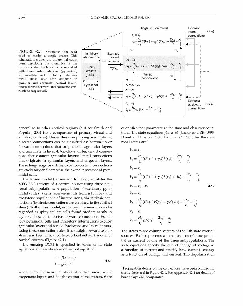
Elsevier UK Chapter: Ch42-P372560 30-9-2006 5:35p.m. Page:564 Trim:7.5in×9.25in
Basal Font:Palatino Margins:Top:40pt Gutter:68pt Font Size:9.5/12 Text Width:42pc Depth:55 Lines
564 42. DYNAMIC CAUSAL MODELS FOR EEG
FIGURE 42.1 Schematic of the DCMused to model a single source. Thisschematic includes the differential equa-tions describing the dynamics of thesource’s states. Each source is modelledwith three subpopulations (pyramidal,spiny-stellate and inhibitory interneu-rons). These have been assigned togranular and agranular cortical layers,which receive forward and backward con-nections respectively.
Extrinsicforward
connections
Inhibitoryinterneurons
Pyramidalcells
Spinystellatecells
FS(x0)
LS(x0)
BS(x0)Extrinsicbackwardconnections
Intrinsicconnections
Extrinsiclateralconnections
Single source model
x7 = x8·
x0 = x5 – x6·
x2 = x5·
x3 = x6·
x8 = ((B + L + γ3I )S(x0)) –· He
τe
2x8τe
x7
τe2
x5 = ((B + L)S(x0) + γ2S(x1)) –· Heτe
2x5τe
x2
τe2
x6 = γ4S(x7) –· Hiτi
2x6τi
x3
τi 2
x1 = x4·
x4 = ((F + L + γ1I )S(x0)+Uu) –· Heτe
2x4τe
x1
τe2
γ4 γ3
γ1 γ2
–
–
–
–
generalize to other cortical regions (but see Smith andPopulin, 2001 for a comparison of primary visual andauditory cortices). Under these simplifying assumptions,directed connections can be classified as: bottom-up orforward connections that originate in agranular layersand terminate in layer 4; top-down or backward connec-tions that connect agranular layers; lateral connectionsthat originate in agranular layers and target all layers.These long-range or extrinsic cortico-cortical connectionsare excitatory and comprise the axonal processes of pyra-midal cells.
The Jansen model (Jansen and Rit, 1995) emulates theMEG-EEG activity of a cortical source using three neu-ronal subpopulations. A population of excitatory pyra-midal (output) cells receives inputs from inhibitory andexcitatory populations of interneurons, via intrinsic con-nections (intrinsic connections are confined to the corticalsheet). Within this model, excitatory interneurons can beregarded as spiny stellate cells found predominantly inlayer 4. These cells receive forward connections. Excita-tory pyramidal cells and inhibitory interneurons occupyagranular layers and receive backward and lateral inputs.Using these connection rules, it is straightforward to con-struct any hierarchical cortico-cortical network model ofcortical sources (Figure 42.1).
The ensuing DCM is specified in terms of its stateequations and an observer or output equation:
ẋ = f�x�u���
h = g�x���42.1
where x are the neuronal states of cortical areas, u areexogenous inputs and h is the output of the system. � are
quantities that parameterize the state and observer equa-tions. The state equations f�x�u��� (Jansen and Rit, 1995;David and Friston, 2003; David et al., 2005) for the neu-ronal states are:1
ẋ7 = x8
ẋ8 = He
�e
��B+L+�3I�S�x0��− 2x8
�e
− x7
�2e
ẋ1 = x4
ẋ4 = He
�e
��F +L+�1I�S�x0�+Uu�− 2x4
�e
− x1
�2e
ẋ0 = x5 −x6
ẋ2 = x5
ẋ5 = He
�e
��B+L�S�x0�+�2S�x1��− 2x5
�e
− x2
�2e
ẋ3 = x6
ẋ6 = Hi
�i
�4S�x7�− 2x6
�i
− x3
�2i
42.2
The states xi are column vectors of the i-th state over allsources. Each represents a mean transmembrane poten-tial or current of one of the three subpopulations. Thestate equations specify the rate of change of voltage asa function of current and specify how currents changeas a function of voltage and current. The depolarization
1 Propagation delays on the connections have been omitted forclarity, here and in Figure 42.1. See Appendix 42.1 for details ofhow delays are incorporated.

Elsevier UK Chapter: Ch42-P372560 30-9-2006 5:35p.m. Page:565 Trim:7.5in×9.25in
Basal Font:Palatino Margins:Top:40pt Gutter:68pt Font Size:9.5/12 Text Width:42pc Depth:55 Lines
THEORY 565
of pyramidal cells x0 = x2 − x3 represents a mixture ofpotentials induced by excitatory and inhibitory (depo-larizing and hyperpolarizing) currents respectively. Thispyramidal potential is the presumed source of observedMEG-EEG signals.
Figure 42.1 depicts the states by assigning each sub-population to a cortical layer. For schematic reasonswe have lumped superficial and deep pyramidal unitstogether, in the infra-granular layer. The matrices F�B�Lencode forward, backward and lateral extrinsic connec-tions respectively. From Eqn. 42.2 and Figure 42.1 itcan be seen that the state equations embody the con-nection rules above. For example, extrinsic connectionsmediating changes in mean excitatory (depolarizing) cur-rent x8, in the supra-granular layer, are restricted tobackward and lateral connections. Interactions, amongthe subpopulations, depend on the constants �1� � � ���4,which control the strength of intrinsic connections andreflect the total number of synapses expressed by eachsubpopulation.
The remaining constants in the state equation pertainto two operators, on which the dynamics rest. The firsttransforms the average density of presynaptic inputs intothe average postsynaptic membrane potential. This trans-formation is equivalent to a convolution with an impulseresponse or kernel:
�t�e =⎧⎨⎩
He
�e
t exp�−t/�e� t ≥ 0
0 t < 042.3
where subscript ‘e’ stands for excitatory and ‘i’ is usedfor inhibitory synapses. H controls the maximum post-synaptic potential and � represents a lumped rate-constant. The second operator S transforms the potentialof each subpopulation into firing rate, which is the inputto other subpopulations. This operator is assumed to bean instantaneous sigmoid non-linearity:
S�x� = 11+exp�−rx�
− 12
42.4
where r = 056 determines its form. Figure 42.2 showsexamples of these synaptic kernels and sigmoid func-tions. Note that the output of the firing rate function canbe negative. This ensures that the neuronal system has astable fixed-point, when all the states are equal to zero.Because the states approximate the underlying popula-tion or density dynamics, the fixed-point corresponds tothe system’s equilibrium or steady state. This means allthe state variables can be interpreted as the deviationfrom steady-state levels. A DCM, at the neuronal level,obtains by coupling sources with extrinsic connections asdescribed above. A typical three-source DCM is shownin Figure 42.3 and is the example used in Chapter 3.
0 2 4 6 80
0.1
0.2
0.3
0.4
tVoltage response to
synaptic input
–10 0 10–0.5
0
0.5
xSynaptic input as afunction of voltage
κ(t )e = t exp(–t /τe) S(x) = 1 – 11 + exp(–rx)
Heτe 2
FIGURE 42.2 Left: form of the synaptic impulse responsefunction, converting synaptic input (discharge rate) into mean trans-membrane potential. Right: the non-linear static transformation oftransmembrane potential into synaptic input. In this figure, the con-stants are set to unity, with the exception of r = 056. See main textfor details.
Spiny stellate
cells
Inhibitoryinterneurons
Pyramidal cells
IntrinsicForward
BackwardLateral
L32
1
32
Input u
F31
FIGURE 42.3 Typical hierarchical network composed of threecortical areas. Extrinsic inputs evoke transient perturbations aroundthe resting state by acting on a subset of sources, usually the lowestin the hierarchy. Interactions among different regions are mediatedthrough excitatory connections encoded by coupling matrices.
Event-related responses
To model event-related responses, the network receivesinputs via input connections U. These connections areexactly the same as forward connections and deliverinputs u to the spiny stellate cells in layer 4. In the presentcontext, inputs u model afferent activity relayed by sub-cortical structures and is modelled with two components:
u�t� = b�t��1��2�+∑�ci cos�2��i−1�t� 42.5

Elsevier UK Chapter: Ch42-P372560 30-9-2006 5:35p.m. Page:566 Trim:7.5in×9.25in
Basal Font:Palatino Margins:Top:40pt Gutter:68pt Font Size:9.5/12 Text Width:42pc Depth:55 Lines
566 42. DYNAMIC CAUSAL MODELS FOR EEG
TABLE 42-1 Prior densities of parameters for connections to the i-th source from thej-th, in the k-th ERP
Fijk = FijGijk Fij = 32 exp��Fij � �F
ij ∼ N�0� 12 �
Bijk = BijGijk Bij = 16 exp��Bij � �B
ij ∼ N�0� 12 �
Extrinsic coupling parameters Lijk = LijGijk Lij = 4 exp��Lij � �L
ij ∼ N�0� 12 �
Gijk = exp��Gijk� �G
ij ∼ N�0� 12 �
Ui = exp��Ui � �U
i ∼ N�0� 12 �
Intrinsic coupling parameters �1 = 128 �2 = 45 �1 �3 = 1
4 �1 �4 = 14 �1
Conduction delays (ms) ii = 2 ij = 16 exp�� ij � �
ij ∼ N�0� 116 �
Synaptic parameters (ms)Ti = 16 T
�i�e = 8 exp��T
i � �Ti ∼ N�0� 1
16 �
Hi = 32 H�i�e = 4 exp��H
i � �Hi ∼ N�0� 1
16 �
Input parameters (s)u�t� = b�t��1��2�+∑�c
i cos �2��i−1�t� �ci ∼ N�0� 1�
�1 = 96 exp���1 � ��
1 ∼ N�0� 116 �
�2 = 1024 exp���2 � ��
2 ∼ N�0� 116 �
The first is a gamma density function b�t��1��2� =��1
2 t�1−1 exp�−�2t�/
���1� with shape and scale constants�1 and �2 (see Table 42-1). This models an event-relatedburst of input that is delayed by �1/�2 s, with respectto stimulus onset and dispersed by subcortical synapsesand axonal conduction. Being a density function, thiscomponent integrates to unity over peristimulus time.The second component is a discrete cosine set modellingsystematic fluctuations in input, as a function of peris-timulus time. In our implementation, peristimulus timeis treated as a state variable, allowing the input to becomputed explicitly during integration.
Critically, the event-related input is exactly the samefor all ERPs. This means the effects of experimental fac-tors are mediated by ERP-specific changes in connec-tion strengths. This models experimental effects in termsof differences in forward, backward or lateral connec-tions that confer a selective sensitivity on each source,in terms of its response to others. The experimental orERP-specific effects are modelled by coupling gains:
Fijk = FijGijk
Bijk = BijGijk 42.6
Lijk = LijGijk
Here, Gijk encodes the k-th ERP-specific gain in couplingto the i-th source from the j-th. By convention, we set thegain of the first ERP to unity, so that subsequent ERP-specific effects are relative to the first.2 The reason we
2 In fact, in our implementation, the coupling gain is a functionof any set of explanatory variables encoded in a design matrix,which can contain indicator variables or parametric variables.For simplicity, we limit this chapter to categorical (ERP-specific)effects.
model experimental effects in terms of gain, as opposedto additive effects, is that by construction, connectionsare always positive. This is assured, provided the gain isalso positive.
The important point here is that we are explaining exper-imental effects, not in terms of differences in neuronalresponses, but in terms of the neuronal architecture orcoupling that generates those responses. This is a funda-mental departure from classical approaches, which char-acterize experimental effects descriptively, at the level ofthe states (e.g. a face-selective difference in ERP amplitudearound 170 ms). DCM estimates these response differen-tials, but only as an intermediate step in the estimation oftheir underlying cause, namely changes in coupling.
Eqn. 42.2 defines the neuronal component of the DCM.These ordinary differential equations can be integrated(see Appendix 42.1) to generate pyramidal depolariza-tions, which enter the observer function to generate thepredicted MEG-EEG signal.
Observation equations
The dendritic signal of the pyramidal subpopulation ofeach source is detected remotely on the scalp surface inMEG-EEG. Critically, the mapping between pyramidalactivity and scalp data is linear:
h = g�x��� = LKx0 42.7
where L is a lead-field matrix (i.e. forward electromag-netic model), which accounts for passive conduction ofthe electromagnetic field (Mosher et al., 1999). If the spa-tial properties (orientation and position) of the source areknown, then the lead-field matrix L is also known. In thiscase, K = diag��K� is a leading diagonal matrix, whichcontrols the contribution �K
i of pyramidal depolarization

Elsevier UK Chapter: Ch42-P372560 30-9-2006 5:35p.m. Page:567 Trim:7.5in×9.25in
Basal Font:Palatino Margins:Top:40pt Gutter:68pt Font Size:9.5/12 Text Width:42pc Depth:55 Lines
THEORY 567
to the i-th source density. If the orientation is not knownthen � becomes a function of free parameters encodingthe location and orientation of the source (see Kiebel et al.,2006 for details). For simplicity we will assume a fixedlocation and orientation for each source but allow theorientation to be parallel or anti-parallel (i.e. �K can bepositive or negative). The rationale for this is that thedirection of current flow induced by pyramidal cell depo-larization depends on the relative density of synapsesproximate and distal to the cell body.
Dimension reduction
For computational reasons, it is sometimes expedientto reduce the dimensionality of the sensor data, whileretaining the maximum amount of information. This isassured by projecting the data onto a subspace definedby its principal eigenvectors or spatial modes �. Theprojection is applied to the data and lead-field:
y ← �y
L ← �L 42.8
� ← ��
In the examples below, the data were projected ontothe first three spatial modes following a singular valuedecomposition of the scalp data, between 0 and 500 ms.Reduction using principal eigenvariates preserves infor-mation in the data; in our examples about 70 per cent.Generally, one uses a small number of modes, notingthat the dimension of the subspace containing predictedresponses cannot exceed the number of sources.
The likelihood model
In summary, our DCM comprises a state equation thatis based on neurobiological heuristics and an observerbased on an electromagnetic forward model. By integrat-ing the state equation and passing the ensuing statesthrough the observer we generate a predicted measure-ment. This corresponds to a generalized convolution ofthe inputs to generate an output h���. This generalizedconvolution furnishes an observation model for the vec-torized data3 y and the associated likelihood:
y = vec�h���+X�X�+�
p�y ����� = N�vec�h���+X�X��diag���⊗V �42.9
Measurement noise � is assumed to be zero mean and inde-pendent over channels, i.e. Cov��� = diag��� ⊗ V , where� is an unknown vector of channel-specific variances.
3 Concatenated column vectors of data from each channel.
V represents the error’s temporal autocorrelation matrix,which we assume is the identity matrix. This is tenablebecause we down-sample the data to about 8 ms. Low-frequency noise or drift components are modelled by X,which is a block diagonal matrix with a low-order dis-crete cosine set for each ERP and channel. The order ofthis set can be determined by Bayesian model selection(see below). In this chapter, we used three componentsfor the first study and four for the second. The first com-ponent of a discrete cosine set is simply a constant.
This model is fitted to data using Bayesian inversion.This involves maximizing the variational free energywith respect to the conditional moments of the freeparameters �. The parameters are constrained by aprior specification of the range they are likely to lie in(Friston, 2003). These constraints, which take the formof a prior density p���, are combined with the likeli-hood p�y�����, to form a posterior density p���y��� ∝p�y�����p��� according to Bayes’ rule. It is this posterioror conditional density we want to approximate. Gaus-sian assumptions about the errors in Eqn. 42.9 enable usto compute the likelihood from the prediction error. Theonly outstanding quantities we require are the priors.
Priors
Under Gaussian assumptions, the prior distribution p��i�of the i-th parameter is defined by its mean and vari-ance. The mean corresponds to the prior expectation. Thevariance reflects the amount of prior information aboutthe parameter. A tight distribution (small variance) cor-responds to precise prior knowledge. Critically, nearlyall the constants in our DCM are positive. To ensurepositivity, we place Gaussian priors on the log of theseconstants. This is equivalent to a log-normal prior on theconstants per se. For example, the forward connections areparameterized as Fij = exp��F
ij�, where p��Fij� = N����2�.
We will use this notion for the other parameters as well.A relatively tight or informative log-normal prior obtainswhen �2 ≈ 1
16 . This allows for a scaling around the priorexpectation of up to a factor of two. Relatively flat priors,allowing for an order of magnitude scaling, correspondto �2 ≈ 1
2 . The ensuing log-normal densities are shownin Figure 42.4 for a prior expectation of unity (i.e. � = 0).
The parameters of the state equation can be dividedinto five subsets: (i) extrinsic connection parameters, whichspecify the coupling strengths among areas; (ii) intrin-sic connection parameters, which reflect our knowledgeabout canonical microcircuitry within an area; (iii) con-duction delays; (iv) synaptic parameters controlling thedynamics within an area; and (v) input parameters, whichcontrol the subcortical delay and dispersion of event-related responses. Table 42-1 shows how the constants
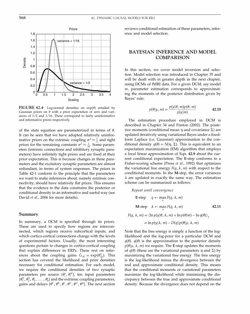
Elsevier UK Chapter: Ch42-P372560 30-9-2006 5:35p.m. Page:568 Trim:7.5in×9.25in
Basal Font:Palatino Margins:Top:40pt Gutter:68pt Font Size:9.5/12 Text Width:42pc Depth:55 Lines
568 42. DYNAMIC CAUSAL MODELS FOR EEG
0 0.5 1 1.5 2 2.5 3 3.5 40
0.2
0.4
0.6
0.8
1
1.2
1.4
1.6
1.8
variance = 1/16
Scaling
Den
sity
Priors
variance = 1/2
FIGURE 42.4 Log-normal densities on exp��� entailed byGaussian priors on � with a prior expectation of zero and vari-ances of 1/2 and 1/16. These correspond to fairly uninformativeand informative priors respectively.
of the state equation are parameterized in terms of �.It can be seen that we have adopted relatively uninfor-mative priors on the extrinsic coupling �2 ≈ 1
2 and tightpriors for the remaining constants �2 ≈ 1
16 . Some param-eters (intrinsic connections and inhibitory synaptic para-meters) have infinitely tight priors and are fixed at theirprior expectation. This is because changes in these para-meters and the excitatory synaptic parameters are almostredundant, in terms of system responses. The priors inTable 42-1 conform to the principle that the parameterswe want to make inferences about, namely extrinsic con-nectivity, should have relatively flat priors. This ensuresthat the evidence in the data constrains the posterior orconditional density in an informative and useful way (seeDavid et al., 2006 for more details).
Summary
In summary, a DCM is specified through its priors.These are used to specify how regions are intercon-nected, which regions receive subcortical inputs, andwhich cortico-cortical connections change with the levelsof experimental factors. Usually, the most interestingquestions pertain to changes in cortico-cortical couplingthat explain differences in ERPs. These rest on infer-ences about the coupling gains Gijk = exp��G
ijk�. Thissection has covered the likelihood and prior densitiesnecessary for conditional estimation. For each model,we require the conditional densities of two synapticparameters per source ���
i � �Hi �, ten input parameters
���1 � ��
2 � �c1� � � � � �c
8� and the extrinsic coupling parameters,gains and delays ��F � �B� �L� �G��U �� �. The next section
reviews conditional estimation of these parameters, infer-ence and model selection.
BAYESIAN INFERENCE AND MODELCOMPARISON
In this section, we cover model inversion and selec-tion. Model selection was introduced in Chapter 35 andwill be dealt with in greater depth in the next chapter,using DCMs of fMRI data. For a given DCM, say modelm, parameter estimation corresponds to approximat-ing the moments of the posterior distribution given byBayes’ rule:
p���y�m� = p�y���m�p���m�
p�y�m�42.10
The estimation procedure employed in DCM isdescribed in Chapter 34 and Friston (2002). The poste-rior moments (conditional mean � and covariance �) areupdated iteratively using variational Bayes under a fixed-form Laplace (i.e. Gaussian) approximation to the con-ditional density q��� = N�����. This is equivalent to anexpectation maximization (EM) algorithm that employsa local linear approximation of Eqn. 42.9 about the cur-rent conditional expectation. The E-step conforms to aFisher-scoring scheme (Press et al., 1992) that optimizesthe variational free energy F�q���m� with respect to theconditional moments. In the M-step, the error variances� are updated in exactly the same way. The estimationscheme can be summarized as follows:
Repeat until convergence
E-step q ← maxq
F�q���m�
M-step � ← max�
F�q���m�
F�q���m� = ln p�y�����m�+ ln p���m�− ln q���q
= ln p�y���m�−D�q��p���y���m�
42.11
Note that the free energy is simply a function of the log-likelihood and the log-prior for a particular DCM andq���. q��� is the approximation to the posterior densityp���y���m� we require. The E-step updates the momentsof q��� (these are the variational parameters � and �) bymaximizing the variational free energy. The free energyis the log-likelihood minus the divergence between thereal and approximate conditional density. This meansthat the conditional moments or variational parametersmaximize the log-likelihood while minimizing the dis-crepancy between the true and approximate conditionaldensity. Because the divergence does not depend on the
Elsevier UK Chapter: Ch42-P372560 30-9-2006 5:35p.m. Page:569 Trim:7.5in×9.25in
Basal Font:Palatino Margins:Top:40pt Gutter:68pt Font Size:9.5/12 Text Width:42pc Depth:55 Lines
EMPIRICAL STUDIES 569
covariance parameters, minimizing the free energy in theM-step is equivalent to finding the maximum likelihoodestimates of the covariance parameters. This scheme isidentical to that employed by DCM for fMRI, the detailsof which can be found in the previous chapter (see alsoFriston, 2002; Friston et al., 2003 and Appendix 2).
Conditional inference
Inference on the parameters of a particular model pro-ceeds using the approximate conditional or posterior den-sity q���. Usually, this involves specifying a parameteror compound of parameters as a contrast cT �. Inferencesabout this contrast are made using its conditional covari-ance cT �c. For example, one can compute the probabilitythat any contrast is greater than zero or some meaningfulthreshold, given the data. This inference is conditioned onthe particular model specified. In other words, given thedata and model, inference is based on the probability thata particular contrast is bigger than a specified threshold.In some situations, one may want to compare differentmodels. This entails Bayesian model comparison.
Model comparison and selection
Different models are compared using their evidence(Penny et al., 2004). The model evidence is:
p�y�m� =∫
p�y���m�p���m�d� 42.12
The evidence can be decomposed into two compo-nents: an accuracy term, which quantifies the data fit; anda complexity term, which penalizes models with a largenumber of parameters. Therefore, the evidence embodiesthe two conflicting requirements of a good model, that itexplains the data and is as simple as possible. In the fol-lowing, we approximate the model evidence for modelm, with the free energy, after convergence. This rests onthe assumption that � has a point mass at its maximumlikelihood estimate (equivalent to its conditional estimateunder flat priors); i.e. ln p�y�m� = ln p�y���m��. Afterconvergence the divergence is minimized and:
ln p�y�m� ≈ F�q���m� 42.13
(see Eqn. 42.11). The most likely model is the one withthe largest log-evidence. This enables Bayesian modelselection. Model comparison rests on the likelihood ratioof the evidence for two models. This ratio is the Bayesfactor Bij . For models i and j:
ln Bij = ln p�y�m = i�− ln p�y�m = j� 42.14
Conventionally, strong evidence in favour of onemodel requires the difference in log-evidence to be about
three or more. We have now covered the specification,estimation and comparison of DCMs. In the next section,we will illustrate their application to real data using twoexamples of how changes in coupling can explain ERPdifferences.
EMPIRICAL STUDIES
In this section, we illustrate the use of DCM by look-ing at changes in connectivity induced in two differentways. In the first experiment, we recorded ERPs duringthe perception of faces and houses. It is well known thatthe N170 is a specific ERP correlate of face perception(Allison et al., 1999). The N170 generators are thought tobe located close to the lateral fusiform gyrus, or fusiformface area (FFA). Furthermore, the perception of houseshas been shown to activate the parahippocampal placearea (PPA) using fMRI (Aguirre et al., 1998; Epstein andKanwisher, 1998; Haxby et al., 2001; Vuilleumier et al.,2001). In this example, differences in coupling define thecategory-selectivity of pathways that are accessed by dif-ferent categories of stimuli. A category-selective increasein coupling implies that the region receiving the con-nection is selectively more sensitive to input elicited bythe stimulus category in question. This can be attributedto a functional specialization of the region receiving theconnection. In the second example, we use an auditoryoddball paradigm, which produces mismatch negativity(MMN) or P300 components in response to rare stimuli,relative to frequent (Linden et al., 1999; Debener et al.,2002). In this paradigm, we attribute changes in couplingto plasticity underlying the perceptual learning of fre-quent or standard stimuli.
In the category-selectivity paradigm, there are nonecessary changes in connection strength; pre-existingdifferences in responsiveness are simply disclosed bypresenting different stimuli. This can be modelled by dif-ferences in forward connections. However, in the oddballparadigm, the effect only emerges once standard stimulihave been learned. This implies some form of perceptualor sensory learning. We have presented a quite detailedanalysis of perceptual learning in the context of empiricalBayes in Chapter 36 (see also Friston, 2003). We con-cluded that the late components of oddball responsescould be construed as a failure to suppress predictionerror, after learning the standard stimuli. Critically, thistheory predicts that learning-related plasticity shouldoccur in backward connections generating the prediction,which are then mirrored in forward connections. In short,we predicted changes in forward and backward connec-tions when comparing ERPs for standard and oddballstimuli.
Elsevier UK Chapter: Ch42-P372560 30-9-2006 5:35p.m. Page:570 Trim:7.5in×9.25in
Basal Font:Palatino Margins:Top:40pt Gutter:68pt Font Size:9.5/12 Text Width:42pc Depth:55 Lines
570 42. DYNAMIC CAUSAL MODELS FOR EEG
In the first example, we are interested in wherecategory-selective differences in responsiveness arise in aforward processing stream. We use inferences based onthe conditional density of forward coupling-gain, whencomparing face and house ERPs, to address this ques-tion. Backward connections are probably important inmediating this selectivity but exhibit no learning-relatedchanges per se. In the second example, our question ismore categorical in nature, namely, are changes in back-ward and lateral connections necessary to explain ERPdifferences between standards and oddballs, relative tochanges in forward connections alone? We illustrate theuse of Bayesian model comparison to answer this ques-tion. (See the figure legends for a description of the dataacquisition, lead-field specification and pre-processing.)
Category-selectivity: effective connectivityin the ventral visual pathway
ERPs elicited by brief presentation of faces and houseswere obtained by averaging trials over three succes-sive 20-minute sessions. Each session comprised thirtyblocks of faces or houses only. Each block containedtwelve stimuli presented for 400 ms every 2.6 s. The stim-uli comprised 18 neutral faces and 18 houses, presentedin greyscale. To maintain attentional set, the subject wasasked to perform a one-back task, i.e. indicate, using abutton press, whether or not the current stimulus wasidentical to the previous.
As reported classically, we observed a stronger N170component during face perception in the posterior tem-poral electrodes. However, we also found other com-ponents, associated with house perception, which weredifficult to interpret on the basis of scalp data. It is gen-erally thought that face perception is mediated by a hier-archical system of bilateral regions (Haxby et al., 2002):a core system of occipito-temporal regions in extrastri-ate visual cortex (inferior occipital gyrus, IOG; lateralfusiform gyrus or face area, FFA; superior temporal sul-cus, STS) that mediates the visual analysis of faces, andan extended system for cognitive functions. This system(intra-parietal sulcus, auditory cortex, amygdala, insula,limbic system) acts in concert with the core system toextract meaning from faces. House perception has beenshown to activate the parahippocampal place area (PPA)(Aguirre et al., 1998; Epstein and Kanwisher, 1998; Haxbyet al., 2001; Vuilleumier et al., 2001). In addition, the ret-rosplenial cortex (RS) and the lateral occipital gyrus aremore activated by houses, compared to faces (Vuilleu-mier et al., 2001). Most of these regions belong to the ven-tral visual pathway. It has been argued that the functionalarchitecture of the ventral visual pathway is not a mosaicof category-specifics modules, but rather embodies a
continuous representation of information about objectattributes (Ishai et al., 1999).
DCM specification
We tested whether differential propagation of neuronalactivity through the ventral pathway is sufficient toexplain the differences in measured ERPs. On the basisof a conventional source localization and previous stud-ies (Allison et al., 1999; Ishai et al., 1999; Haxby et al.,2001, 2002; Vuilleumier et al., 2001), we specified the fol-lowing DCM (Plate 59, see colour plate section): bilat-eral occipital regions close to the calcarine sulcus (V1)received subcortical visual inputs. From V1 onwards, thepathway for house perception was bilateral and con-nected to RS and PPA using forward and backward con-nections. The pathway engaged by face perception wasrestricted to the right hemisphere and comprised con-nections from V1 to IOG, which projects to STS andFFA. In addition, bilateral connections were included,between STS and FFA, as suggested in Haxby et al.(2002). These connections constituted our DCM mediat-ing ERPs to houses and faces. Face- or house-specific ERPcomponents were hypothesized to arise from category-selective, stimulus-bound, activation of forward path-ways. To identify these category-selective streams, weallowed the forward connections, in the right hemi-sphere, to change with category. Our hope was that thesechanges would render PPA more responsive to houses,while the FFA and STS would express face-selectiveresponses.
Conditional inference
The results are shown in Figure 42.5 in terms of predictedcortical responses and coupling parameters. Using thisDCM, we were able to replicate the functional anatomy,disclosed by the above fMRI studies: the response in PPAwas more marked when processing houses versus faces.This was explained, in the model, by an increase in for-ward connectivity in the medial ventral pathway fromRS to PPA. This difference corresponded to a coupling-gain of over fivefold. Conversely, the model exhibiteda much stronger response in FFA and STS during faceperception, as suggested by the Haxby model (Haxbyet al., 2002). This selectivity was due to an increase incoupling from IOG to FFA and from IOG to STS. Theface-selectivity of STS responses was smaller than in theFFA, the latter mediated by an enormous gain of aboutninefold �1/011 = 909� in sensitivity to inputs from IOG.The probability, conditional on the data and model, thatchanges in forward connections to the PPA, STS andFFA were greater than zero, was essentially 100 per centin all cases. The connections from V1 to IOG showedno selectivity. This suggests that category-selectivity

Elsevier UK Chapter: Ch42-P372560 30-9-2006 5:35p.m. Page:571 Trim:7.5in×9.25in
Basal Font:Palatino Margins:Top:40pt Gutter:68pt Font Size:9.5/12 Text Width:42pc Depth:55 Lines
EMPIRICAL STUDIES 571
time (ms)
V1 V1
RS RSIOG
PPAPPASTS
FFA
0 200 400
0
0 200 400–60
–40
–20
–60
–40
–20
–60
–40
–20
0
20
40 mode 1
0 200 400
0
20
40 mode 2
0 200
0
20
40 mode 3
inputFace (predicted)Face (observed)House (predicted)House (observed)
0.11 (100%)
5.56 (100%)0.61 (100%)
0.55 (100%)
FIGURE 42.5 DCM results for the category-selectivity paradigm: Left: predicted (thick) and observed (thin) responses in measurementspace. These are a projection of the scalp or channel data onto the first three spatial modes or eigenvectors of the channel data (faces:grey; houses: black). The predicted responses are based on the conditional expectations of the DCM parameters. The agreement is evident.Right: reconstructed responses for each source and changes in coupling for the DCM modelling category-specific engagement of forwardconnections, in the ventral visual system. As indicated by the predicted responses in PPA and FFA, these changes are sufficient to explainan increase response in PPA when perceiving houses and, conversely, an increase in FFA responses during face perception. The couplingdifferences mediating this category-selectivity are shown alongside connections, which showed category-specific differences (highlighted bysolid lines). Differences are the relative strength of forward connections during house presentation, relative to faces. The per cent conditionalconfidence that this difference is greater than zero is shown in brackets. Only changes with 90 per cent confidence or more are reported andthese connections are highlighted in bold.
The data reported in this and subsequent figures were acquired from the same subject, in the same session, using 128 EEG electrodesand 2048 Hz sampling. Before averaging, data were referenced to mean activity and bandpass filtered between 1 and 20 Hz. Trials showingocular artefacts (∼30 per cent) and 11 bad channels were removed from further analysis. To compute the lead field for each source we used adistributed source reconstruction procedure based on the subject’s anatomical MRI and described in David et al. (2006). Following dimensionreduction to the three principal eigenvariates, the data were down-sampled to 8 ms time bins. These reduced channel data were then used toinvert the DCM.
emerges downstream from IOG, at a fairly high level.Somewhat contrary to expectations (Vuilleumier et al.,2001), the coupling from V1 to RS showed a mild face-selective bias, with an increase of about 80 per cent�1/055 = 182�.
Note how the ERPs of each source are successivelytransformed and delayed from area to area. This reflectsthe intrinsic transformations within each source, thereciprocal exchange of signals between areas and the con-duction delays. These transformations are mediated byintrinsic and extrinsic connections and are the dynamicexpression of category selectivity in this DCM. The con-ditional estimate of the subcortical input is also shownin Figure 42.5. The event-related response input wasexpressed about 96 ms after stimulus onset. The accuracyof the model is evident in the left panel of Figure 42.5,which shows the measured and predicted responses insensor space, after projection onto their three principaleigenvectors.
Auditory oddball: effective connectivityand sensory learning
Auditory stimuli, 1000 or 2000 Hz tones with 5 ms rise andfall times and 80 ms duration, were presented binaurallyfor 15 minutes, every 2 s in a pseudo-random sequence;2000 Hz tones (oddballs) occurred 20 per cent of the time(120 trials) and 1000 Hz tones (standards) 80 per cent ofthe time (480 trials). The subject was instructed to keep amental record of the number of 2000 Hz tones.
Late components, characteristic of rare events, wereseen in most frontal electrodes, centred on 250 ms to350 ms post-stimulus. As reported classically, early com-ponents (i.e. the N100) were almost identical for rareand frequent stimuli. Using a conventional reconstruc-tion algorithm (see figure legend), cortical sources werelocalized symmetrically along the medial part of theupper bank of the Sylvian fissure, in the right mid-dle temporal gyrus, left medial and posterior cingulate,
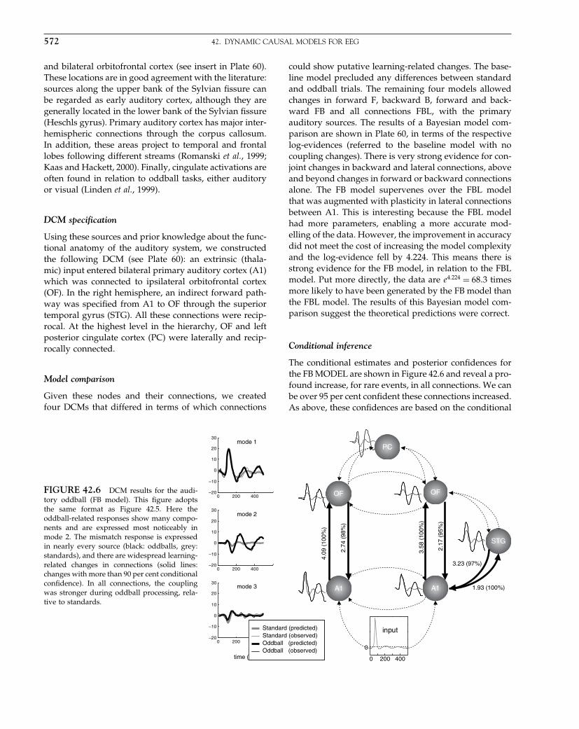
Elsevier UK Chapter: Ch42-P372560 30-9-2006 5:35p.m. Page:572 Trim:7.5in×9.25in
Basal Font:Palatino Margins:Top:40pt Gutter:68pt Font Size:9.5/12 Text Width:42pc Depth:55 Lines
572 42. DYNAMIC CAUSAL MODELS FOR EEG
and bilateral orbitofrontal cortex (see insert in Plate 60).These locations are in good agreement with the literature:sources along the upper bank of the Sylvian fissure canbe regarded as early auditory cortex, although they aregenerally located in the lower bank of the Sylvian fissure(Heschls gyrus). Primary auditory cortex has major inter-hemispheric connections through the corpus callosum.In addition, these areas project to temporal and frontallobes following different streams (Romanski et al., 1999;Kaas and Hackett, 2000). Finally, cingulate activations areoften found in relation to oddball tasks, either auditoryor visual (Linden et al., 1999).
DCM specification
Using these sources and prior knowledge about the func-tional anatomy of the auditory system, we constructedthe following DCM (see Plate 60): an extrinsic (thala-mic) input entered bilateral primary auditory cortex (A1)which was connected to ipsilateral orbitofrontal cortex(OF). In the right hemisphere, an indirect forward path-way was specified from A1 to OF through the superiortemporal gyrus (STG). All these connections were recip-rocal. At the highest level in the hierarchy, OF and leftposterior cingulate cortex (PC) were laterally and recip-rocally connected.
Model comparison
Given these nodes and their connections, we createdfour DCMs that differed in terms of which connections
could show putative learning-related changes. The base-line model precluded any differences between standardand oddball trials. The remaining four models allowedchanges in forward F, backward B, forward and back-ward FB and all connections FBL, with the primaryauditory sources. The results of a Bayesian model com-parison are shown in Plate 60, in terms of the respectivelog-evidences (referred to the baseline model with nocoupling changes). There is very strong evidence for con-joint changes in backward and lateral connections, aboveand beyond changes in forward or backward connectionsalone. The FB model supervenes over the FBL modelthat was augmented with plasticity in lateral connectionsbetween A1. This is interesting because the FBL modelhad more parameters, enabling a more accurate mod-elling of the data. However, the improvement in accuracydid not meet the cost of increasing the model complexityand the log-evidence fell by 4.224. This means there isstrong evidence for the FB model, in relation to the FBLmodel. Put more directly, the data are e4224 = 683 timesmore likely to have been generated by the FB model thanthe FBL model. The results of this Bayesian model com-parison suggest the theoretical predictions were correct.
Conditional inference
The conditional estimates and posterior confidences forthe FB MODEL are shown in Figure 42.6 and reveal a pro-found increase, for rare events, in all connections. We canbe over 95 per cent confident these connections increased.As above, these confidences are based on the conditional
FIGURE 42.6 DCM results for the audi-tory oddball (FB model). This figure adoptsthe same format as Figure 42.5. Here theoddball-related responses show many compo-nents and are expressed most noticeably inmode 2. The mismatch response is expressedin nearly every source (black: oddballs, grey:standards), and there are widespread learning-related changes in connections (solid lines:changes with more than 90 per cent conditionalconfidence). In all connections, the couplingwas stronger during oddball processing, rela-tive to standards.
0 200 400–20
–10
0
10
20
30mode 1
0 200 400–20
–10
0
10
20
30mode 2
0 200–20
–10
0
10
20
30mode 3
time (ms)400
600
standard (predicted)standard (observed)oddball (predicted)oddball (observed)400
Standard (predicted)Standard (observed)Oddball (predicted)Oddball (observed)
0 200 400
0
input
4.09
(10
0%)
3.58
(10
0%)
3.23 (97%)
2.74
(98
%)
2.17
(95
%)
1.93 (100%)A1 A1
OF OF
PC
STG

Elsevier UK Chapter: Ch42-P372560 30-9-2006 5:35p.m. Page:573 Trim:7.5in×9.25in
Basal Font:Palatino Margins:Top:40pt Gutter:68pt Font Size:9.5/12 Text Width:42pc Depth:55 Lines
CONCLUSION 573
–0.5 0 0.5 1 1.5 2 2.50
0.2
0.4
0.6
0.8
1
1.2
1.4
Conditional density of contrast
Contrast
Pro
babi
lity
dens
ity
p (cTη > 0) = 99.9%
FIGURE 42.7 Conditional density of a contrast averaging overall learning-related changes in backward connections. It is evidentthat change in backward connections is unlikely to be zero or lessgiven our data and DCM.
density of the coupling-gains. The conditional density ofa contrast, averaging over all gains in backward connec-tions, is shown in Figure 42.7. We can be 99.9 per centconfident this contrast is greater than zero. The averageis about one, reflecting a gain of about e1 ≈ 27, i.e. morethan a doubling.
These changes produce a rather symmetrical series oflate components, expressed to a greater degree, but withgreater latency, at hierarchically higher levels. In com-parison with the visual paradigm above, the subcorticalinput appeared to arrive earlier, around 64 ms after stim-ulus onset. The remarkable agreement between predictedand observed channel responses is seen in the left panel,again shown as three principal eigenvariates.
In summary, this analysis suggests that a sufficientexplanation for mismatch responses is an increase in for-ward and backward connections with primary auditorycortex. This results in the appearance of exuberantresponses after the N100 in A1 to unexpected stimuli.This could represent a failure to suppress predictionerror, relative to predictable or learned stimuli, whichcan be predicted more efficiently.
CONCLUSION
We have described a Bayesian inference procedure inthe context of DCM for ERPs. DCMs are used in theanalysis of effective connectivity to provide posterioror conditional distributions. These densities can then be
used to assess changes in effective connectivity causedby experimental manipulations. These inferences, how-ever, are contingent on assumptions about the architec-ture of the model, i.e. which regions are connected andwhich connections are modulated by experimental fac-tors. Bayesian model comparison can be used to adjudi-cate among competing models, or hypotheses, as demon-strated above. The approach can be regarded as a neu-robiologically constrained source reconstruction scheme,in which the parameters of the reconstruction have anexplicit neuronal interpretation, or as a characterizationof the causal architecture of the neuronal system gener-ating responses. We have seen that it is possible to testmechanistic hypotheses in a more constrained way thanclassical approaches because the prior assumptions arephysiologically informed.
The DCM in this chapter used a neural-mass modelthat embodies long-range cortico-cortical connections byconsidering forward, backward and lateral connectionsamong remote areas (David et al., 2005). This allows us toembed neural mechanisms generating MEG-EEG signalsthat are located in well-defined regions. This may makethe comparison with fMRI activations easier than alterna-tive models based on continuous cortical fields (Robinsonet al., 2001; Liley et al., 2002). However, it would beinteresting to apply DCM to cortical field models.
Frequently asked questions
In presenting this work to our colleagues, we haveencountered a number of recurrent questions. We usethese questions to frame our discussion of DCM for ERPs.
• How do the results change with small changes in the priors?Conditional inferences are relatively insensitive tochanges in the priors. This is because we use relativelyuninformative priors on the parameters about whichinferences are made. Therefore, confident inferencesabout coupling imply a high conditional precision. Thismeans that most of the conditional precision is basedon the data (because the prior precision is very small).Changing the prior precision will have a limited effecton the conditional density and the ensuing inference.
• What are the effects of wrong network specification (e.g.including an irrelevant source or not including a relevantsource or the wrong specification of connections)?This is difficult to answer because the effects willdepend on the particular data set and model employed.However, there is a principled way in which questionsof this sort can be answered. This uses Bayesian modelcomparison: if the contribution of a particular sourceor connection is in question, one can compute the log-evidence for two models that do and do not containthe source or connection. If it was important, the differ-ences in log-evidence will be significant. Operationally,

Elsevier UK Chapter: Ch42-P372560 30-9-2006 5:35p.m. Page:574 Trim:7.5in×9.25in
Basal Font:Palatino Margins:Top:40pt Gutter:68pt Font Size:9.5/12 Text Width:42pc Depth:55 Lines
574 42. DYNAMIC CAUSAL MODELS FOR EEG
the effects of changing the architecture are reformu-lated in terms of changing the model. Because the datado not change, these effects can be evaluated quanti-tatively in terms of the log-evidence (i.e. likelihood ofthe data given the models in question).
• How sensitive is the model to small changes in the parameters?This is quantified by the curvature of the free energywith respect to parameters. This sensitivity is, in fact,the conditional precision or certainty. If the free energychanges quickly as one leaves the maximum (i.e. con-ditional mode or expectation), then the conditionalprecision is high. Conversely, if the maximum is rela-tively flat, changes in the parameter will have a smallereffect and conditional uncertainty is higher. Condi-tional uncertainly is a measure of the information aboutthe parameter in the data.
• What is the role of source localization in DCM?It has no role. Source localization refers to inversionof an electromagnetic forward model. Because this isonly a part of the DCM, Bayesian inversion of the DCMimplicitly performs the source localization. Having saidthis, in practice, priors on the location or orientation(i.e. spatial parameters) can be derived from classicalsource reconstruction techniques. In this chapter, weused a distributed source reconstruction to furnish spa-tial priors on the DCM. However, these priors do notnecessarily have to come from a classical inverse solu-tion. Our evaluations of DCM, using somatosensoryevoked potentials (whose spatial characteristics are wellknown) suggest that the conditional precision of theorientation is much greater than the location. This meansthat one could prescribe tight priors on the location(from source reconstruction, from fMRI analyses, orfrom the literature) and let DCM estimate the conditionaldensity of the orientation (Kiebel et al., 2006).
• How do you select the sources for the DCM?DCM is an inference framework that allows one toanswer questions about a well-specified model of func-tional anatomy. The sources specify that model. Con-ditional inferences are then conditional on that model.Questions about which is the best model use Bayesianmodel selection as described above. In principle, it ispossible to compare an ensemble of models with allpermutations of sources and simply select the modelthat has the greatest log-evidence. We will illustratethis in a forthcoming multisubject study of the MMNin normal subjects.
• How do you assess the generalizability of a DCM?In relation to a particular data set, the conditionaldensity of the parameters implicitly maximizes gener-alizability. This is because the free energy can be refor-mulated in terms of an accuracy term that is maximizedand a complexity term that is minimized (Penny et al.,2004). Minimizing complexity ensures generalization.
This aspect of variational learning means that we donot have to use ad-hoc measures of generalization (e.g.splitting the data into training and test sets). General-ization is an implicit part of the estimation. In relationto generalization over different data sets, one has toconsider the random effects entailed by different sub-jects or sessions. In this context, generalization andreproducibility are a more empirical issue.
• How can you be sure that a change in connectivity is notdue to a wrong model?There is no such thing as a wrong model. Models canonly be better or worse than other models. We quantifythis in terms of the likelihood of each model (i.e. thelog-evidence) and select the best model. We then usu-ally make conditional inferences about the parameters,conditional on the best model. One could of courseargue that all possible models have not been tested, butat least one has a framework that can accommodateany alternative model.
• What is the basis for the claim that the neural-mass modelsand DCMs are biologically grounded?This is based largely on the use of the Jansen and Ritmodel (1995) as an elemental model for each source.We deliberately chose an established model from theEEG literature for which a degree of predictive andface validity had already been established. This modelhas been evaluated in a range of different contexts andits ability to emulate and predict biological phenomenahas been comprehensively assessed (Jansen and Rit,1995; David et al., 2005 and references therein). The bio-logical plausibility of the extrinsic connections has beenmotivated at length in David and Friston (2003), wherewe show that a network of Jansen and Rit sources canreproduce a variety of EEG phenomena.
• Why did we exclude thalamus from our models?Because it was not necessary to answer the question wewanted to ask. In the models reported in this chapter,the effects of subcortical transformations are embodiedin the parameters of the input function. If one thoughtthat cortico-subcortical interactions were important, itwould be a simple matter to include a thalamic sourcethat was invisible to measurement space (i.e. set thelead field’s priors to zero). One could then use Bayesianmodel comparison to assess whether modelled cortico-thalamic interactions were supported by the data.
• Does DCM deal with neuronal noise?No. In principle, DCM could deal with noise at the levelof neuronal states by replacing the ordinary differ-ential equations with stochastic differential equations.However, this would call for a very different estima-tion scheme in which there was conditional uncertaintyabout the [hidden] neuronal states. Conventionally,these sorts of systems are estimated using a recurrentBayesian update scheme such as Kalman or Particle

Elsevier UK Chapter: Ch42-P372560 30-9-2006 5:35p.m. Page:575 Trim:7.5in×9.25in
Basal Font:Palatino Margins:Top:40pt Gutter:68pt Font Size:9.5/12 Text Width:42pc Depth:55 Lines
REFERENCES 575
filtering. We are working on an alternative (dynamicexpectation maximization), but it will be some timebefore it will be applied to DCM.
• Why are the DCMs for EEG and fMRI not the same?This is an important question, especially if one wantsto use a DCM to explain both fMRI and EEG responsesin the context of multimodal fusion. The DCM forEEG is considerably more complicated than the mod-els used previously for fMRI. In fact, the bilinear formfor the dynamics in fMRI is formally the same as thebilinear approximation to the state equations used inthis chapter. The reason that DCM for EEG rests onmore complicated models is that there is more condi-tional information in electromagnetic data about theparameters. This means that more parameters can beestimated efficiently (i.e. with greater conditional cer-tainty). It would be perfectly possible to replace thebilinear approximation in DCMs for fMRI with the cur-rent neuronal model. However, Bayesian model com-parison would show that the bilinear approximationwas much better because it is not over-parameterizedfor fMRI data. Conversely, model comparison usingboth fMRI and EEG data should select the detailedmodel used here.
• Why try to explain evoked responses solely by a change ineffective connectivity?In DCM, most of the biophysical parameters are rateor connectivity parameters that fall into three groups:(i) extrinsic connections among areas; (ii) intrinsicconnections within an area (i.e. among the threesub-populations); and (iii) within subpopulation (i.e.the rate or time constants governing self-inhibitionor adaptation). We have chosen to explain exper-imental differences in terms of coupling changesbetween areas. This is motivated by theoreticalconsiderations that suggest sensory and perceptuallearning involves experience-dependent changes inextrinsic forward and backward connections. How-ever, the DCM machinery could easily be adapted (by adifferent choice of priors on the parameters) to explaindifferences in terms of changes in intrinsic connections,or even time-constants within a subpopulation. Fur-thermore, using Bayesian model comparison we cancompare models to ask, for example, whether changesin intrinsic or extrinsic connections are the most likelyexplanation for observed responses.
SUMMARY
In this chapter, we have focused on the changes in con-nectivity, between levels of an experimental factor, toexplain differences in the form of ERFs-ERPs. We have
illustrated this through the analysis of real ERPs recordedin two classical paradigms: ERPs recorded during theperception of faces versus houses and the auditory odd-ball paradigm. We were able to differentiate two streamswithin the ventral visual pathway corresponding to faceand house processing, leading to preferential responsesin the fusiform face area and parahippocampal placearea respectively. These results concur with fMRI stud-ies (Haxby et al., 2001;Vuilleumier et al., 2001). We haveshown how different hypotheses about the genesis of theMMN could be tested, such as learning-related changesin forward or backward connections. Our results suggestthat bottom-up processes have a key role, even in latecomponents such as the P300. This finding is particularlyinteresting as top-down processes are usually invoked toaccount for late responses.
APPENDIX
Here we describe the approximate integration of delaydifferential equations of the form:
ẋi�t� = fi�x1�t −�i1�� � � � � xn�t −�in�� 42.A1
for n states x = �x1�t�� � � � � xn�t��T , where state j causeschanges in state i with delay �ij . By taking a Taylor expan-sion about � = 0 we get, to first order:
ẋi = fi�x�−∑j
�ij�fi
/��ij
= fi�x�−∑j
�ijJij ẋj
42.A2
where J = �f/
�x is the system’s Jacobian. 42.A2 can beexpressed in matrix form as:
ẋ = f�x�− �� × J�ẋ 42.A3
where × denotes the Hadamard or element-by-elementproduct. On rearranging 42.A3, we obtain an ordinarydifferential equation that can be integrated in the usualway:
ẋi = D−1f�x�
D = I +� × J42.A4
REFERENCES
Aguirre GK, Zarahn E, D’Esposito M (1998) An area within humanventral cortex sensitive to ‘building’ stimuli: evidence and impli-cations. Neuron 21: 373–83
Elsevier UK Chapter: Ch42-P372560 30-9-2006 5:35p.m. Page:576 Trim:7.5in×9.25in
Basal Font:Palatino Margins:Top:40pt Gutter:68pt Font Size:9.5/12 Text Width:42pc Depth:55 Lines
576 42. DYNAMIC CAUSAL MODELS FOR EEG
Allison T, Puce A, Spencer DD et al. (1999) Electrophysiological stud-ies of human face perception. I: Potentials generated in occipi-totemporal cortex by face and non-face stimuli. Cereb Cortex 9:415–30
Brovelli A, Ding M, Ledberg A et al. (2004) Beta oscillations ina large-scale sensorimotor cortical network: directional influ-ences revealed by Granger causality. Proc Natl Acad Sci USA 101:9849–54
Büchel C, Friston KJ (1997) Modulation of connectivity in visualpathways by attention: cortical interactions evaluated with struc-tural equation modelling and fMRI. Cereb Cortex 7: 768–78
Crick F, Koch C (1998) Constraints on cortical and thalamic projec-tions: the no-strong-loops hypothesis. Nature 391: 245–50
Dau T (2003) The importance of cochlear processing for the forma-tion of auditory brainstem and frequency following responses.J Acoust Soc Am 113: 936–50
David O, Friston KJ (2003) A neural mass model for MEG-EEG:coupling and neuronal dynamics. NeuroImage 20: 1743–55
David O, Garnero L, Cosmelli D et al. (2002) Estimation of neuraldynamics from MEG-EEG cortical current density maps: appli-cation to the reconstruction of large-scale cortical synchrony.IEEE Trans Biomed Eng 49: 975–87
David O, Harrison L, Friston KJ (2005) Modelling event-relatedresponses in the brain. NeuroImage 25: 756–70
David O, Kiebel SJ, Harrison LM et al. (2006) Dynamic causal mod-eling of evoked responses in EEG and MEG. NeuroImage, Feb 8;(Epub ahead of print)
Debener S, Kranczioch C, Herrmann CS et al. (2002) Auditory nov-elty oddball allows reliable distinction of top-down and bottom-up processes of attention. Int J Psychophysiol 46: 77–84
Engel AK, Fries P, Singer W (2001) Dynamic predictions: oscillationsand synchrony in top-down processing. Nat Rev Neurosci 2: 704–16
Epstein R, Kanwisher N (1998) A cortical representation of the localvisual environment. Nature 392: 598–601
Felleman DJ, Van Essen DC (1991) Distributed hierarchical process-ing in the primate cerebral cortex. Cereb Cortex 1: 1–47.
Friston K (2003) Learning and inference in the brain. Neural Netw16: 1325–52
Friston KJ (2002) Bayesian estimation of dynamical systems: anapplication to fMRI. NeuroImage 16: 513–30
Friston KJ, Harrison L, Penny W (2003) Dynamic causal modelling.NeuroImage 19: 1273–302
Harrison L, Penny WD, Friston K (2003) Multivariate autoregressivemodeling of fMRI time series. NeuroImage 19: 1477–91
Haxby JV, Gobbini MI, Furey ML et al. (2001) Distributed and over-lapping representations of faces and objects in ventral temporalcortex. Science 293: 2425–30
Haxby JV, Hoffman EA, Gobbini MI (2002) Human neural systemsfor face recognition and social communication. Biol Psychiatr 51:59–67
Ishai A, Ungerleider LG, Martin A et al. (1999) Distributed repre-sentation of objects in the human ventral visual pathway. ProcNatl Acad Sci USA 96: 9379–84
Jansen BH, Rit VG (1995) Electroencephalogram and visual evokedpotential generation in a mathematical model of coupled corticalcolumns. Biol Cybernet 73: 357–66
Jirsa V (2004) Information processing in brain and behavior dis-played in large-scale scalp topographies such as EEG and MEG.Int J Bifurcation Chaos 14: 679–92
Kaas JH, Hackett TA (2000) Subdivisions of auditory cortex andprocessing streams in primates. Proc Natl Acad Sci USA 97:11793–99
Kiebel SJ, David O, Friston KJ (2006) Dynamic causal modeling ofevoked responses in EEG/MEG with lead-field parameteriza-tion. NeuroImage 30: 1273–84
Liley DT, Cadusch PJ, Dafilis MP (2002) A spatially continu-ous mean field theory of electrocortical activity. Network 13:67–113
Linden DE, Prvulovic D, Formisano E et al. (1999) The functionalneuroanatomy of target detection: an fMRI study of visual andauditory oddball tasks. Cereb Cortex 9: 815–23
Lopes da Silva FH, Hoeks A, Smits H et al. (1974) Model of brainrhythmic activity. The alpha-rhythm of the thalamus. Kybernetik15: 27–37
McIntosh AR, Gonzalez-Lima F (1994) Structural equation mod-elling and its application to network analysis in functional brainimaging. Hum Brain Mapp 2: 2–22
Melcher JR, Kiang NY (1996) Generators of the brainstem auditoryevoked potential in cat. III: Identified cell populations. Hear Res93: 52–71
Mosher JC, Leahy RM, Lewis PS (1999) EEG and MEG: forwardsolutions for inverse methods. IEEE Trans Biomed Eng 46: 245–59
Penny WD, Stephan KE, Mechelli A et al. (2004) Comparing dynamiccausal models. NeuroImage 22: 1157–72
Press WH, Teukolsky SA, Vetterling WT et al. (1992) Numericalrecipes in C. Cambridge University Press, Cambridge, MA
Rennie CJ, Robinson PA, Wright JJ (2002) Unified neurophysicalmodel of EEG spectra and evoked potentials. Biol Cybernet 86:457–71
Riera JJ, Watanabe J, Kazuki I et al. (2004) A state-space model ofthe hemodynamic approach: nonlinear filtering of BOLD signals.NeuroImage 21: 547–67
Robinson PA, Rennie CJ, Rowe DL et al. (2004) Estimation of mul-tiscale neurophysiologic parameters by electroencephalographicmeans. Hum Brain Mapp 23: 53–72
Robinson PA, Rennie CJ, Wright JJ et al. (2001) Prediction of elec-troencephalographic spectra from neurophysiology. Phys Rev EStat Nonlin Soft Matter Phys 63: 021903
Roebroeck A, Formisano E, Goebel R (2005) Mapping directed influ-ence over the brain using Granger causality and fMRI. Neuro-Image 25: 230–42
Romanski LM, Tian B, Fritz J et al. (1999) Dual streams of audi-tory afferents target multiple domains in the primate prefrontalcortex. Nat Neurosci 2: 1131–36
Rosenblum MG, Pikovsky AS, Kurths J et al. (2002) Locking-basedfrequency measurement and synchronization of chaotic oscilla-tors with complex dynamics. Phys Rev Lett 89: 264102
Schnitzler A, Gross J (2005) Normal and pathological oscillatorycommunication in the brain. Nat Rev Neurosci 6: 285–96
Smith PH, Populin LC (2001) Fundamental differences between thethalamocortical recipient layers of the cat auditory and visualcortices. J Comp Neurol 436: 508–19
Stam CJ, Pijn JP, Suffczynski P et al. (1999) Dynamics of the humanalpha rhythm: evidence for non-linearity? Clin Neurophysiol 110:1801–13
Tass PA (2004) Transmission of stimulus-locked responses intwo oscillators with bistable coupling. Biol Cybernet 91:203–11
Vuilleumier P, Armony JL, Driver J et al. (2001) Effects of attentionand emotion on face processing in the human brain: an event-related fMRI study. Neuron 30: 829–41
Wendling F, Bartolomei F, Bellanger JJ et al. (2002) Epileptic fastactivity can be explained by a model of impaired GABAergicdendritic inhibition. Eur J Neurosci 15: 1499–508

Elsevier UK Chapter: Ch43-P372560 30-9-2006 5:36p.m. Page:577 Trim:7.5in×9.25in
Basal Font:Palatino Margins:Top:40pt Gutter:68pt Font Size:9.5/12 Text Width:42pc Depth:55 Lines
C H A P T E R
43
Dynamic Causal Models and Bayesian selectionK. E. Stephan and W. D. Penny
INTRODUCTION
Ever since the description of localizable lesion and exci-tation effects in the nineteenth century, neurosciencehas revolved around the dual themes of functionalspecialization and functional integration. Functional spe-cialization refers to the notion that local neural popu-lations are specialized in certain aspects of informationprocessing, whereas functional integration refers to theinteractions among distinct populations. A variety oftechniques exist for understanding functional specializa-tion of brain regions, which rest on either measuring neu-ronal responses (e.g. neuroimaging, invasive recordings)or observing the consequences of selectively disablingparticular parts of the brain (e.g. anatomical or phar-macological lesions; transcranial magnetic stimulation).Understanding the principles of functional integrationrequires two things: first, simultaneous measurements ofactivity in multiple interacting brain regions and second,a formal model designed to test assumptions about thecausal mechanisms which underlie these interactions (seeChapters 36 and 38 and Friston, 2002).
To specify the structure of a neural system model, oneneeds to specify three things: (i) which areas are ele-ments of the system; (ii) which anatomical connectionsexist; and (iii) which experimentally designed inputsaffect system dynamics, either by directly evoking activ-ity in specific areas (e.g. visual stimuli evoking responsesin primary visual cortex) or by altering the strength ofspecific connections (e.g. changes of synaptic strengthsduring learning), and where these inputs enter the sys-tem. A key issue is how to test competing hypothesesabout the organization of a system. Given experimentalmeasurements of the system of interest, an ideal solu-tion is to formalize each hypothesis in terms of a spe-cific model and use a Bayesian model selection (BMS)procedure that takes into account both model fit and
model complexity (Pitt and Myung, 2002; Penny et al.,2004; see also Chapter 35). In principle, model selectioncan concern any aspect of a system so long as differ-ent models are compared using the same data.1 In thischapter, we focus on how model selection can be used todecide which of several experimentally controlled inputschange particular connection strengths. To illustrate this,we deal with inter-hemispheric integration in the ventralvisual pathway during a letter decision task. After sum-marizing BMS as implemented for dynamic causal mod-elling (DCM) for functional magnetic resonance imaging(fMRI), we present the results from a combined DCMand BMS analysis of a single subject data set (Stephanet al., 2005). Inter-hemispheric integration is a particu-larly instructive example for the usefulness of BMS; thisis because a variety of competing theories about its func-tional principles and mechanisms exist, all of which makefairly precise predictions about what experimental fac-tors should be the primary cause of changes in inter-hemispheric connection strengths and what pattern ofeffective connectivity should be observed.
Bayesian model selection in DCM for fMRI
A generic problem encountered by any kind of mod-elling is the question of model selection: given someobserved data, which of several alternative models is
1 This means that in DCM for fMRI, where the data vector resultsfrom a concatenation of the time series of all areas in the model,only models can be compared that contain the same areas. Inthis case, model selection cannot be used to address whetheror not to include a particular area in the model. In contrast,in DCM for ERPs, the data measured at the sensor level areindependent of how many neuronal sources are assumed in agiven model. Here, model selection could also be used to decidewhich sources should be included.
Statistical Parametric Mapping, by Karl Friston et al. Copyright 2007, Elsevier Ltd. All rights reserved.ISBN–13: 978-0-12-372560-8 ISBN–10: 0-12-372560-7
577
Elsevier UK Chapter: Ch43-P372560 30-9-2006 5:36p.m. Page:578 Trim:7.5in×9.25in
Basal Font:Palatino Margins:Top:40pt Gutter:68pt Font Size:9.5/12 Text Width:42pc Depth:55 Lines
578 43. DYNAMIC CAUSAL MODELS AND BAYESIAN SELECTION
the optimal one? This problem is not trivial because thedecision cannot be made solely by comparing the rela-tive fit of the competing models. One also needs to takeinto account the relative complexity of the models asexpressed, for example, by the number of free param-eters in each model. Model complexity is important toconsider because there is a trade-off between model fitand generalizability (i.e. how well the model explainsdifferent data sets that were all generated from the sameunderlying process). As the number of free parametersis increased, model fit increases monotonically, whereasbeyond a certain point, model generalizability decreases.The reason for this is ‘over-fitting’; an increasingly com-plex model will, at some point, start to fit noise that isspecific to one dataset and thus become less generaliz-able across multiple realizations of the same underlyinggenerative process.2
Therefore, the question: ‘What is the optimal model?’can be reformulated more precisely as: ‘What is the modelthat represents the best balance between fit and complex-ity?’. In a Bayesian context, the latter question can beaddressed by comparing the evidence, p�y�m�, of differ-ent models. According to Bayes’ theorem:
p���y�m� = p�y���m�p���m�
p�y�m�43.1
the model evidence can be considered as a normalizationconstant for the product of the likelihood of the data andthe prior probability of the parameters, therefore:
p�y�m� =∫
p�y���m�p���m�d� 43.2
Here, the numbers of free parameters (as well as thefunctional form) are subsumed by the integration. Unfor-tunately, this integral cannot usually be solved analyti-cally, therefore, an approximation to the model evidenceis needed.
In the context of DCM, one potential solution could beto make use of the Laplace approximation, i.e. to approx-imate the model evidence by a Gaussian that is centredon its mode. As shown by Penny et al. (2004), this yieldsthe following expression for the natural logarithm of themodel evidence: ���y denotes the maximum a posteriori(MAP) estimate, C��y is the posterior covariance of theparameters, C� is the error covariance, �� is the priormean of the parameters, C� is the prior covariance and
2 Generally, in addition to the number of free parameters, thecomplexity of a model also depends on its functional form (Pittand Myung, 2002). This is not an issue for DCM, however,because here competing models usually have the same func-tional form.
h�u����y� is the prediction by the model given the knownsystem inputs u and MAP estimate ���y:
ln p�y�m� = accuracy�m�− complexity�m�
=[−1
2ln �C��−
12
� Ty C−1
� �y
]
−[
12
ln �C��−12
ln �C��y�+12
� T� C−1
� ��
]
�y = y −h�u����y�
�� = ���y −��
43.3
This expression reflects the requirement, as discussedabove, that the optimal model should represent the bestcompromise between model fit (accuracy) and modelcomplexity. The complexity term depends on the priordensity, for example, the prior covariance of the intrinsicconnections. This is problematic in the context of DCMfor fMRI because this prior covariance is defined in amodel-specific fashion to ensure that the probability ofobtaining an unstable system is small (specifically, this isachieved by choosing the prior covariance of the intrinsiccoupling matrix A such that the probability of obtaininga positive Lyapunov exponent of A is p < 0�001; see Fris-ton et al., 2003 for details). Consequently, the comparisonof models with different numbers of connections is con-flated with a comparison of different priors. Alternativeapproximations to the model evidence, which dependless on the priors, are useful for DCMs of this sort.
Suitable approximations, which do not depend on theprior density, are afforded by the Bayesian informationcriterion (BIC) and Akaike information criterion (AIC),respectively. As shown by Penny et al. (2004), for DCMthese approximations are given by:
BIC = accuracy�m�− p�
2ln n
AIC = accuracy�m�−p�
43.4
where p� is the number of parameters and n is the numberof data points (scans). If one compares the complexityterms of BIC and AIC, it is obvious that BIC pays aheavier penalty than AIC as soon as one deals with eightor more scans (which is virtually always the case for fMRIdata):
d�
2ln n > p� ⇒ n > e2 ≈ 7�39 43.5
Therefore, BIC will be biased towards simpler mod-els, whereas AIC will be biased towards more complexmodels. This can lead to disagreement between the twoapproximations about which model should be favoured.We adopt the convention that, for any pairs of models

Elsevier UK Chapter: Ch43-P372560 30-9-2006 5:36p.m. Page:579 Trim:7.5in×9.25in
Basal Font:Palatino Margins:Top:40pt Gutter:68pt Font Size:9.5/12 Text Width:42pc Depth:55 Lines
INTER-HEMISPHERIC INTEGRATION IN THE VENTRAL STREAM 579
mi and mj , a model is selected if, and only if AIC andBIC concur (see below); the decision is then based on theapproximation which gives the smaller Bayes factor (BF):
BFij = p�y�mi�
p�y�mj�43.6
Just as conventions have developed for using p-valuesin frequentist statistics, there are conventions for Bayesfactors. For example, Raftery (1995) suggests interpreta-tion of Bayes factors as providing weak �BF < 3�, positive�3 ≤ BF < 20�, strong �20 ≤ BF < 150� or very strong �BF ≥150� evidence for preferring one model over another.
We conclude this section with a short comment ongroup studies with DCM and BMS. When trying to findthe optimal model for a group of individuals, it is likelythat the optimal model will vary, at least to some degree,across subjects. An overall decision for N subjects canbe made as follows. First, because model comparisonsfrom different individuals are statistically independent,we can compute a group Bayes factor (GBF) by multiplyingall N individual Bayes factors (where k is an index acrosssubjects):
GBFij =∏k
BF kij 43.7
In principle, this is sufficient to select the optimal modelacross a group of subjects. However, the magnitude of thegroup Bayes factor may not always be easily interpretablesince its value depends on N . It can therefore be usefulto compute an average Bayes factor (ABF) which is thegeometric mean of the group Bayes factor:
ABFij = N
√GBFij 43.8
A problem that both GBF and ABF may suffer from isthe presence of outliers.3 For example, imagine you com-pare models mi and mj in a group of 11 subjects where,for 10 subjects, one finds BFij = 10 for a given comparisonof interest and for a single subject one finds BFij = 10−12.In this case, we would obtain GBFij = 10−2 and ABFij ≈0�66. Since these results are driven by a single outlier, itis doubtful whether one should conclude on the basis ofthese values that Y is the better model. A heuristic thatprecludes this sort of thing is the positive evidence ratio(PER), i.e. the number of subjects where there is positive
3 Of course, the problem of outliers is not specific to Bayesianinference with DCMs but is inherent to all group analyses. Inrandom-effects analyses, for example, subjects are assumed toderive from a Gaussian distribution about a typical subject (seeChapter 11, Hierarchical Models). This assumption is clearlyviolated in the presence of outliers.
(or stronger) evidence for model mi divided by the num-ber of subjects with positive (or stronger) evidence formodel mj :
PERij = �k BFkij > 3�
�k BFkji > 3� 43.9
where k = 1� �N and �·� denotes set size.Overall, BMS is a powerful procedure to decide
between competing hypotheses represented by differ-ent DCMs. These hypotheses can concern any part of amodel, e.g. the pattern of intrinsic connections or whichinputs affect the system and where they enter. In thenext section, we present an example that demonstrateshow the combination of DCM and BMS can be appliedto questions of inter-hemispheric integration.
INTER-HEMISPHERIC INTEGRATIONIN THE VENTRAL STREAM
Theories of inter-hemispheric integration
Currently, three major theories of inter-hemispheric inte-gration are entertained (see Stephan et al., 2006a for areview). The oldest is that of information transfer betweenthe hemispheres (e.g. Poffenberger, 1912). In the contextof lateralized tasks with hemisphere-specific inputs (e.g.peripheral visual presentation), this theory predicts thattransfer of sensory information should be asymmetri-cally enhanced from the non-dominant to the dominanthemisphere to ensure efficient processing in the special-ized hemisphere (e.g. Nowicka et al., 1996; Endrass et al.,2002). In terms of effective connectivity, it predicts a task-dependent increase in influence of the non-dominant onthe dominant hemisphere, but only when stimulus infor-mation is initially restricted to the non-dominant hemi-sphere.
A more recent and similarly influential concept hasbeen the notion of inter-hemispheric inhibition (Kinsbourne,1970). It has been argued that the regulatory mechanismsthat ‘coordinate, select, and integrate the processes sub-served by each hemisphere’ will also require a rangeof inter-hemispheric inhibitory mechanisms ‘to achieveunified performance from a bilateral system capableof producing simultaneous and potentially conflictingoutputs’ (Chiarello and Maxfield, 1996). With regard toconnectivity, inter-hemispheric inhibition predicts a task-dependent and symmetric pattern of negative connectionstrengths between hemispheres. It is important to note,however, that this does not necessarily mean that twoareas, which affect each other by task-dependent inter-hemispheric inhibition, show decreased activity during
Elsevier UK Chapter: Ch43-P372560 30-9-2006 5:36p.m. Page:580 Trim:7.5in×9.25in
Basal Font:Palatino Margins:Top:40pt Gutter:68pt Font Size:9.5/12 Text Width:42pc Depth:55 Lines
580 43. DYNAMIC CAUSAL MODELS AND BAYESIAN SELECTION
that task. As can be easily shown in simulations, it is per-fectly possible that task-dependent regional activationscoexist with task-dependent inter-hemispheric inhibitionif other, e.g. intra-hemispheric, influences onto the areasin question are positive.
The third major concept of inter-hemispheric integra-tion concerns hemispheric recruitment or processing modesetting, i.e. whether information processing is restrictedto a single hemisphere or distributed across both hemi-spheres. Several behavioural studies have shown that, ifthe neural resources in the hemisphere receiving a stimu-lus are insufficient for optimal processing, the benefits ofdistributing the processing load across both hemispheresare likely to outweigh the costs of transcallosal infor-mation transfer (see Banich, 1998 for review). Given asufficiently demanding task, this recruitment of an addi-tional hemisphere even occurs during lateralized taskswhen the dominant hemisphere receives the stimulus(Belger and Banich, 1998). This additional recruitment ofthe non-dominant hemisphere requires tight cooperation,i.e. functional coupling, of both hemispheres, regard-less of which hemisphere initially received the stimu-lus. Two components are likely to be expressed in termsof task-dependent changes in effective connectivity: anincrease of the influence from the dominant to the non-dominant hemisphere that reflects the ‘recruitment’ ofthe non-dominant hemisphere, and an increase of con-nection strengths in the opposite direction, induced bythe non-dominant hemisphere ‘returning’ the results ofthe computations delegated to it by the dominant hemi-sphere. Altogether, this cooperation is expected to beexpressed either in terms of a symmetric task-dependentincrease of connection strength between homotopic areasor, if ‘recruitment’ and ‘return’ processes are spatiallysegregated, an asymmetric task-dependent increase ofconnection strength between different areas.
Next, we review an experiment in which inter-hemispheric integration was necessary and could havebeen orchestrated by any of the three mechanismsdescribed above. Using data from a single subject, weprovide an example of how BMS can be used to disam-biguate different theories of inter-hemispheric integra-tion with DCM.
An fMRI study of inter-hemisphericintegration
In a previous fMRI study on the mechanisms underly-ing hemispheric specialization, we investigated whetherlateralization of brain activity depends on the nature ofthe sensory stimuli or on the nature of the cognitive taskperformed (Stephan et al., 2003). For example, microstruc-tural differences between homotopic areas in the left and
right hemisphere have been reported, including visual(Jenner et al., 1999) and language-related (Amunts et al.,1999) areas. Within a given hemisphere, these differ-ences could favour the processing of certain stimuluscharacteristics and disadvantage others and might thussupport stimulus-dependent lateralization in a bottom-up fashion (Sergent, 1982). On the other hand, processingdemands, mediated through cognitive control processes,might determine, in a top-down fashion, which hemi-sphere obtains precedence in a particular task (Levy andTrevarthen, 1976; Fink et al., 1996). To decide betweenthese two possibilities, we used a paradigm in which thestimuli were kept constant throughout the experiment,and subjects were alternately instructed to attend to cer-tain stimulus features and ignore others (Stephan et al.,2003). The stimuli were concrete German nouns (eachfour letters in length) in which either the second or thirdletter was printed in red (the other letters were black). Ina letter decision (LD) task, the subjects had to ignore theposition of the red letter and indicate whether or not theword contained the target letter ‘A’. In a spatial decision(SD) task they were required to ignore the language-related properties of the word and to judge whether thered letter was located left or right of the word centre; 50per cent of the stimuli were presented in the non-fovealpart of the right visual field (RVF) and the other 50 percent in the non-foveal part of the left visual field (LVF).
The results of a conventional fMRI data analysiswere clearly in favour of the top-down hypothesis:despite the use of identical word stimuli in all con-ditions, comparing spatial to letter decisions showedstrongly right-lateralized responses in the parietal cor-tex, whereas comparing letter to visuo-spatial decisionsshowed strongly left-lateralized responses, involvingclassical language areas in the left inferior frontal gyrusand visual areas in the left ventral visual stream, e.g. inthe fusiform gyrus (FG), middle occipital gyrus (MOG)and lingual gyrus (LG) (Plate 61, see colour plate section).Notably, the LG areas also showed a main effect of visualfield, whereas task-by-visual field interactions were notsignificant at the group level due to spatial variability oftheir locations across subjects (see Discussion).
Constructing a basic DCM
Through the conjoint use of lateralized and demandingtasks with peripheral visual representation, we ensuredthat inter-hemispheric integration was a necessary com-ponent of the cognitive processes in this paradigm. Wenow want to demonstrate how to use DCM to inves-tigate which theory of inter-hemispheric integration ismost likely to account for our data. We focus on theventral stream of the visual system which, as shown

Elsevier UK Chapter: Ch43-P372560 30-9-2006 5:36p.m. Page:581 Trim:7.5in×9.25in
Basal Font:Palatino Margins:Top:40pt Gutter:68pt Font Size:9.5/12 Text Width:42pc Depth:55 Lines
INTER-HEMISPHERIC INTEGRATION IN THE VENTRAL STREAM 581
(a)
LGleft
FGleft
FGright
LGright
LVFstim.
BVFstim.
RVFstim.
Inte
r-he
mis
pher
e
Intra-hemisphere
(b)
S+T
S+T
T
TS
S
S×T
S×T
16 models
FIGURE 43.1 (a) Basic model that comprises the left and rightlingual gyrus (LG) and left and right fusiform gyrus (FG). Theareas are reciprocally connected (black arrows). Driving inputs areshown as grey arrows. RVF stimuli directly affect left LG activityand LVF stimuli directly affect right LG activity, regardless of task.Individual stimuli lasted for 150 ms, therefore, these inputs are rep-resented as trains of events (delta-functions). During the instructionperiods, bilateral visual field input was provided for 6 s; this wasmodelled as a boxcar input affecting LG in both hemispheres. (b)Schema showing how the 16 models tested were constructed bycombining four different types of modulatory inputs for inter- andintra-hemispheric connections respectively.
in Plate 61, is preferentially involved in letter decisionsin this experiment. For simplicity, we use a four-areamodel comprising LG and FG in both hemispheres. First,we need to define a model comprising these four areas(Figure 43.1(a)). Starting with the direct (driving) inputsto the system, we model the lateral stimulus presenta-tion and the crossed course of the visual pathways byallowing all RVF stimuli to affect directly left LG activ-ity and all LVF stimuli to directly affect right LG activ-ity, regardless of task. Each stimulus lasted for 150 msonly; therefore these inputs are represented as trains ofshort events (delta functions). The induced activity thenspreads through the system according to the connectionsof the model. For visual areas, a general rule is thatboth intra- and inter-hemispheric connections are recip-rocal and that homotopic regions in both hemispheresare linked by inter-hemispheric connections (Segravesand Rosenquist, 1982; Cavada and Goldman-Rakic, 1989;Kötter and Stephan, 2003).4
Deriving a set of alternative models
Note that up to this point there are few, if any, plau-sible alternatives for how a DCM of inter-hemisphericintegration between LG and FG, respectively, should
4 To be precise, we should point out that in primates left andright area V1 only have extremely sparse callosal connectionswith each other; this is in contrast to other visual areas like V2,which are strongly linked by homotopic callosal connections(Kennedy et al., 1986; Abel et al., 2000).
be constructed. However, the important issue is howexperimental factors affect transcallosal information inthis system during the LD task. This is directly related tothe predictions from the three theories described above.Instead of testing exclusively for these three predictions,we compare a larger, systematically derived set of modelswhich will include those predicted by the three theories.
Given that some areas also showed a main effect ofvisual field, one could assume that inter-hemisphericinteractions between visual areas are primarily deter-mined by the visual field of stimulus presentation, inde-pendent of task demands: for example, whenever astimulus is presented in the LVF and stimulus informa-tion is received initially by the right visual cortex, thisinformation is transmitted transcallosally to the left visualcortex. Vice versa, whenever a stimulus is presented inthe RVF, stimulus information is transmitted transcal-losally from left to right visual cortex. In this scenario,the task performed is assumed to have no influence oncallosal couplings, and task effects could, as shown in aprevious analysis of connectivity, be restricted to mod-ulate functional couplings within hemispheres (Stephanet al., 2003). This model is subsequently referred to as theS-model, for stimulus-dependent.
Alternatively, one might expect that callosal connec-tion strengths depend more on which task is performedthan on which visual field the stimulus is presented in.That is, right → left and/or left → right callosal connec-tions could be altered during the LD task. This type ofmodulation is predicted by two theories described above,the inter-hemispheric inhibition and hemispheric recruit-ment theories; however, they predict opposite directionsof the change in coupling. This model is referred to asthe T-model, for task dependent.
As a third hypothesis, it is conceivable that both visualfield and task exert an influence on callosal connectionstrengths, but independently of each other. This is theS+T-model. As a fourth and final option, one might pos-tulate that task demands modulate callosal connections,but conditional on the visual field, i.e. right → left con-nections are only modulated by LD during LVF stimuluspresentation �LD�LVF� whereas left → right connectionsare only modulated by LD during RVF stimulus presen-tation �LD�RVF�. This is the S ×T-model.
Although less interesting in the present context, thesame questions about the nature of modulatory inputsarise with respect to the intra-hemispheric connections.Therefore, to perform a thorough model comparison,we systematically compared all 16 combinations of howinter- and intra-hemispheric connections are changed inthe four ways (S, T, S + T, S × T� described above (notethat in the models presented here, we only allowedfor modulation of the intra-hemispheric forward con-nections, i.e. from LG → FG; see Figures 43.2, 43.3).
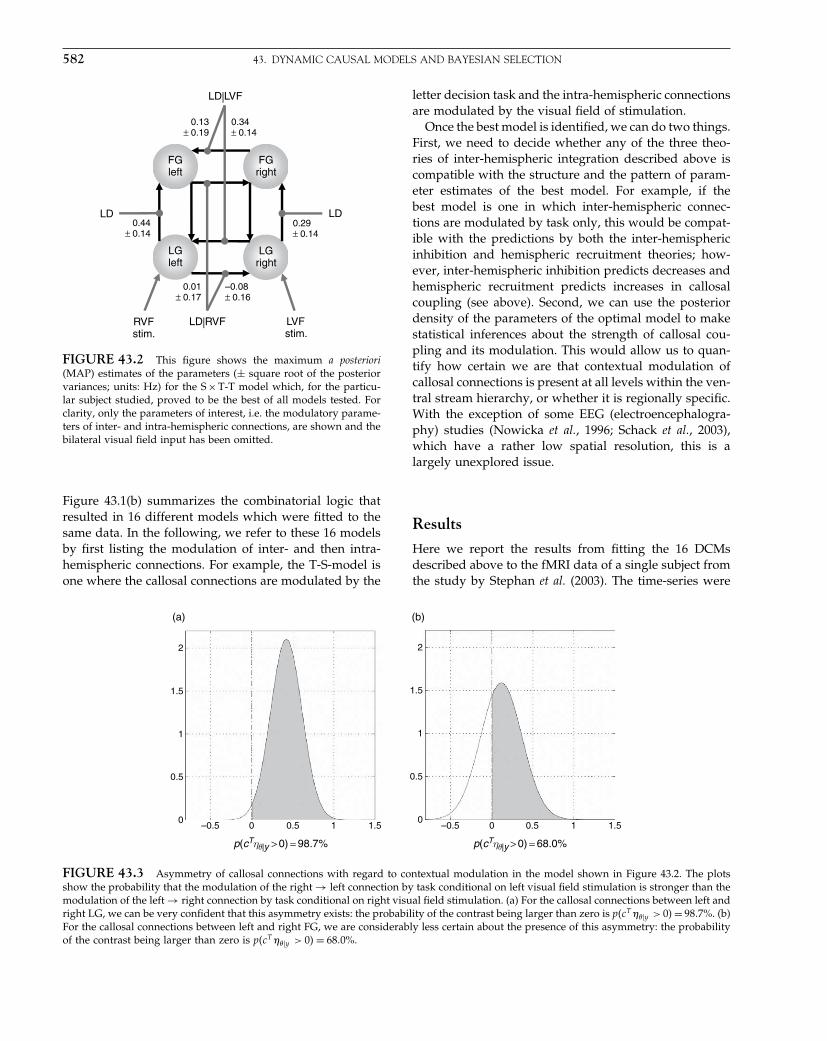
Elsevier UK Chapter: Ch43-P372560 30-9-2006 5:36p.m. Page:582 Trim:7.5in×9.25in
Basal Font:Palatino Margins:Top:40pt Gutter:68pt Font Size:9.5/12 Text Width:42pc Depth:55 Lines
582 43. DYNAMIC CAUSAL MODELS AND BAYESIAN SELECTION
LGright
LGleft
FGleft
FGright
RVFstim.
LVFstim.
LD|RVF
LD|LVF
LDLD0.44
± 0.14
0.01± 0.17
0.29± 0.14
0.13± 0.19
0.34± 0.14
–0.08± 0.16
FIGURE 43.2 This figure shows the maximum a posteriori(MAP) estimates of the parameters (± square root of the posteriorvariances; units: Hz) for the S × T-T model which, for the particu-lar subject studied, proved to be the best of all models tested. Forclarity, only the parameters of interest, i.e. the modulatory parame-ters of inter- and intra-hemispheric connections, are shown and thebilateral visual field input has been omitted.
Figure 43.1(b) summarizes the combinatorial logic thatresulted in 16 different models which were fitted to thesame data. In the following, we refer to these 16 modelsby first listing the modulation of inter- and then intra-hemispheric connections. For example, the T-S-model isone where the callosal connections are modulated by the
letter decision task and the intra-hemispheric connectionsare modulated by the visual field of stimulation.
Once the best model is identified, we can do two things.First, we need to decide whether any of the three theo-ries of inter-hemispheric integration described above iscompatible with the structure and the pattern of param-eter estimates of the best model. For example, if thebest model is one in which inter-hemispheric connec-tions are modulated by task only, this would be compat-ible with the predictions by both the inter-hemisphericinhibition and hemispheric recruitment theories; how-ever, inter-hemispheric inhibition predicts decreases andhemispheric recruitment predicts increases in callosalcoupling (see above). Second, we can use the posteriordensity of the parameters of the optimal model to makestatistical inferences about the strength of callosal cou-pling and its modulation. This would allow us to quan-tify how certain we are that contextual modulation ofcallosal connections is present at all levels within the ven-tral stream hierarchy, or whether it is regionally specific.With the exception of some EEG (electroencephalogra-phy) studies (Nowicka et al., 1996; Schack et al., 2003),which have a rather low spatial resolution, this is alargely unexplored issue.
Results
Here we report the results from fitting the 16 DCMsdescribed above to the fMRI data of a single subject fromthe study by Stephan et al. (2003). The time-series were
(b)(a)
2
1.5
1
0.5
0–0.5 0 0.5 1 1.5
2
1.5
1
0.5
0–0.5 0 0.5 1 1.5
p(cTηθ|y > 0) = 98.7% p(cTηθ|y > 0) = 68.0%
FIGURE 43.3 Asymmetry of callosal connections with regard to contextual modulation in the model shown in Figure 43.2. The plotsshow the probability that the modulation of the right → left connection by task conditional on left visual field stimulation is stronger than themodulation of the left → right connection by task conditional on right visual field stimulation. (a) For the callosal connections between left andright LG, we can be very confident that this asymmetry exists: the probability of the contrast being larger than zero is p�cT ���y > 0� = 98�7%. (b)For the callosal connections between left and right FG, we are considerably less certain about the presence of this asymmetry: the probabilityof the contrast being larger than zero is p�cT ���y > 0� = 68�0%.

Elsevier UK Chapter: Ch43-P372560 30-9-2006 5:36p.m. Page:583 Trim:7.5in×9.25in
Basal Font:Palatino Margins:Top:40pt Gutter:68pt Font Size:9.5/12 Text Width:42pc Depth:55 Lines
DISCUSSION 583
selected based on local maxima of the ‘main effect oftask’ contrast in the SPM (statistical parametric map).However, the regional time-series showed a main effectof task �LD > SD�, a main effect of VF, a simple maineffect (LD > SD separately for LVF and RVF presentation)and task-by-VF interactions (see Discussion).
The BMS procedure indicated that the optimalmodel was the S × T-T-model, i.e. modulation of inter-hemispheric connections by task, conditional on thevisual field of stimulus presentation, and modulation ofintra-hemispheric connection strengths by the task only(Figure 43.2). Table 43-1 shows the Bayes factors for thecomparison of the S ×T-T-model with the other models.The AIC and BIC approximations agreed for all compar-isons. The second-best model was the T-S×T-model (i.e.the ‘flipped’ version of the S × T-T-model). The Bayesfactor of comparing the S × T-T-model with the T-S × T-model was 2.33 which, according to the criteria summa-rized by Penny et al. 2004 (see their Table 1), could beinterpreted as weak evidence in favour of the S × T-T-model. All other comparisons gave Bayes factors largerthan 3, representing positive, strong or very strong evi-dence in favour of the S ×T-T-model (see Table 43-1).
The optimal S×T-T-model has a structure (in terms ofmodulatory inputs) predicted by the information trans-fer hypothesis (see above). It remains to be tested, how-ever, whether the pattern of modulatory parametersalso matches the predictions from that hypothesis, i.e.whether for the left-lateralized LD task the modulation ofright → left connections by LD�LVF is significantly higherthan the modulation of the left → right connections by
TABLE 43-1 Bayes factors (middle column) for thecomparison of the best model with each of the other 15 models
(left column)
S × T-T versus BF Evidence in favour of S × T-T
S +T-S +T 477.31 very strongS +T-S ×T 60.83 strongS +T-T 110.84 strongS +T-S 479.03 very strongS ×T-S +T 3.92 positiveS ×T −S ×T 4.48 positiveS ×T-S 46267.47 very strongT-S +T 19.96 positiveT −S ×T 2.33 weakT −T 3.43 positiveT −S 29.74 strongS-S +T 16.85 positiveS −S ×T 4.81 positiveS-T 5.59 positiveS-VF 1�35E+13 very strong
The right column lists the interpretation of the evidence in favour of the S × T-Tmodel according to the criteria in Raftery (1995); see the summary by Penny et al.(2004).
LD�RVF. Figure 43.2 shows the maximum a posteriori(MAP) estimates ���y of the modulatory parameters (±standard deviation, i.e. the square root of the posteriorvariances) for the S×T-T-model. The modulatory param-eter estimates indeed indicated a strong hemisphericasymmetry: both at the levels of LG and FG, the MAPestimates of the modulation of the right → left connec-tions are much larger than those of the left → rightconnections. But how certain can we be about the pres-ence of this asymmetry? This issue can be addressed bymeans of contrasts cT ���y of the appropriate parameterestimates (cT is a transposed vector of contrast weights).The contrasts comparing modulation of the right → leftconnection by LD�LVF versus modulation of the left →right connection by LD�RVF are shown in Figure 43.3(separately for connections at the level of LG and FG,respectively). These plots show p�cT ���y > 0�, i.e. our cer-tainty about asymmetrical modulation of callosal inter-actions in terms of the probability that these contrastsexceed a value of zero. For the particular subject shownhere, we can be very certain (98.7 per cent) that modu-lation of the right LG → left LG connection by LD�LVFis larger than the modulation of the left LG → right LGconnection by LD�RVF (cf. Figure 43.2). In contrast, weare much less confident (68.0 per cent) that this asymme-try also exists for callosal connections between right andleft FG.
DISCUSSION
In this chapter, we have shown how BMS can helpto decide between different cognitive-neurobiologicalhypotheses, each represented by a specific model.Together with BMS, DCM is a powerful tool to assesswhich experimental manipulations (e.g. stimulus type,induction of cognitive set, learning processes etc.) havea significant impact on the dynamics of the networkunder investigation. By representing experimental fac-tors as external inputs in the model, modelled effects canbe interpreted fairly directly in neurobiological terms:any given DCM specifies precisely where inputs enter andwhether they are driving (i.e. exert their effects throughdirect synaptic responses in the target area) or modula-tory (i.e. exert their effects through changing synapticresponses in the target area to inputs from another area).This distinction, made at the level of neural populations,has a nice correspondence to empirical observations thatsingle neurons can either have driving or modulatoryeffects on other neurons (Sherman and Guillery, 1998).
In our empirical example, we demonstrated that, forthe particular task and subject studied, inter-hemisphericintegration in the ventral visual stream conforms to the

Elsevier UK Chapter: Ch43-P372560 30-9-2006 5:36p.m. Page:584 Trim:7.5in×9.25in
Basal Font:Palatino Margins:Top:40pt Gutter:68pt Font Size:9.5/12 Text Width:42pc Depth:55 Lines
584 43. DYNAMIC CAUSAL MODELS AND BAYESIAN SELECTION
principle of inter-hemispheric information transfer. Thisconclusion rests on two findings: (i) the measured dataare best explained by a model in which inter-hemisphericinteractions depend on task demands, but conditional onthe visual field of stimulus presentation; and (ii) there isa hemispheric asymmetry in context-dependent transcal-losal interactions, with modulation of connections fromthe non-dominant (right) to the dominant (left) hemi-sphere being considerably stronger than modulation ofthe connections in the opposite direction. Importantly,this asymmetry was not equally pronounced for all visualareas studied. It was particularly strong for the callosalconnections between left and right LG: performance ofthe letter decision task specifically enhanced the strengthof the influence of the right on the left LG, but only if thestimulus was presented in the left visual field and thusthe information was initially only available in the righthemisphere. The reversed conditional effect, i.e. modula-tion of left LG → right LG by LD�RVF, was much weaker(and actually slightly negative, see Figure 43.2). Thisresult means that enhancement of callosal connectionswas only necessary if stimulus information was initiallyrepresented in the ‘suboptimal’, i.e. right, hemisphere.
Two short technical comments may be useful for a fullunderstanding of the particular model structure chosenhere. First, one may be concerned about the presenceof correlations between inputs (in the extreme case, thepresence of identical inputs entering the model at multi-ple sites). Concerning model selection, such correlationsare not an issue when using Eqn. 43.3 (which takes intoaccount the posterior covariance of the parameters), butmay be problematic when using approximations such asAIC or BIC (see Eqn. 43.4). This can be easily investi-gated for any given model using synthetic data generatedfrom known parameters and adding observation noise.For the particular model here, we investigated this issueand found that even at high levels of noise: (i) the modelselection reliably chose the correct model; and (ii) theestimates for the contrasts of interests (i.e. comparisonsof modulations of callosal connections) were not biased,i.e. did not deviate significantly from the true values(Stephan et al., unpublished data).
A second question concerns the interpretations of theDCM results in relation to the SPM results. One mayargue that the type of statistical contrast used to decidewhich regions to sample from pre-determines the out-come of the model selection procedure. This is only true,however, for simple models. As an example, let us imag-ine a two-area T-T-model that only consists of left andright LG. In this model, the driving of right LG by LVFand the modulation of the right LG → left LG connectionby the LD task corresponds to modelling a task-by-VFinteraction in left LG. However, it would be misleadingto conclude from this that the full four-area T-T-model
is only appropriate to explain time-series dominatedby task-by-VF interactions. In the full T-T-model withits complex connectivity loops, both main effects andinteractions can be modelled, depending on the relativestrengths of the modulatory inputs and the intrinsic con-nections. For example, as can be demonstrated with sim-ulations, choosing a strongly positive modulation of theintra-hemispheric forward connections by LD, setting thestrength of callosal modulations by LD to low positivevalues and choosing strong intra-hemispheric backwardprojections primarily models a main effect of task in FGand also in LG (because of the back-projections). Over-all, the model parameters need to be fitted to explainoptimally the overall constellation of main effects andinteractions in all areas of the model. This precludesstraightforward predictions about the outcome of modelselection in situations where the model structure is com-plex and where regional time-series are influenced byvarious experimental effects, as in the present data set.
We conclude by emphasizing the importance of modelselection. Model selection is essentially the same ashypothesis testing, in the sense that every hypothesiscan be framed in terms of the difference between twomodels. This makes model selection central to the sci-entific process. Furthermore, model selection can alsoplay an important role in clinical neuroscience, e.g. inpsychiatry where diseases like schizophrenia often com-prise heterogeneous phenotypes. BMS could be used tofind subgroups of patients that differ in terms of DCMsthat optimally explains the measured neurophysiologicaldata. If the neural models are sophisticated enough todistinguish between the effects of different transmitterreceptors, it might also be possible to obtain predictionsfor the optimal pharmacological treatment of individualpatients (see Stephan 2004; Stephan et al., 2006b).
REFERENCES
Abel PL, O’Brien BJ, Olavarria JF (2000) Organization of callosallinkages in visual area V2 of Macaque monkey. J Comp Neurol428: 278–93
Amunts K, Schleicher A, Bürgel U et al. (1999) Broca’s region revis-ited: cytoarchitecture and intersubject variability. J Comp Neurol412: 319–41
Banich MT (1998) The missing link: the role of interhemisphericinteraction in attentional processing. Brain Cogn 36: 128–57
Belger A, Banich MT (1998) Costs and benefits of integrating infor-mation between the cerebral hemispheres: a computational per-spective. Neuropsychology 12: 380–98
CavadaC,Goldman-RakicPS(1989)Posteriorparietalcortexinrhesusmonkey: I. Parcellation of areas based on distinctive limbic andsensory corticocortical connections. J Comp Neurol 287: 393–421
Chiarello C, Maxfield L (1996) Varieties of interhemispheric inhibi-tion, or how to keep a good hemisphere down. Brain Cogn 30:81–108
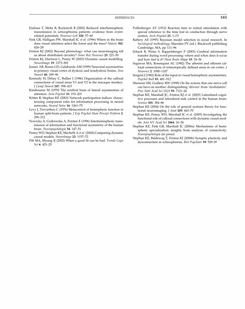
Elsevier UK Chapter: Ch43-P372560 30-9-2006 5:36p.m. Page:585 Trim:7.5in×9.25in
Basal Font:Palatino Margins:Top:40pt Gutter:68pt Font Size:9.5/12 Text Width:42pc Depth:55 Lines
REFERENCES 585
Endrass T, Mohr B, Rockstroh B (2002) Reduced interhemispherictransmission in schizophrenia patients: evidence from event-related potentials. Neurosci Lett 320: 57–60
Fink GR, Halligan PW, Marshall JC et al. (1996) Where in the braindoes visual attention select the forest and the trees? Nature 382:626–28
Friston KJ (2002) Beyond phrenology: what can neuroimaging tellus about distributed circuitry? Annv Rev Neurosci 25: 221–50
Friston KJ, Harrison L, Penny W (2003) Dynamic causal modelling.NeuroImage 19: 1273–302
Jenner AR, Rosen GD, Galaburda AM (1999) Neuronal asymmetriesin primary visual cortex of dyslexic and nondyslexic brains. AnnNeurol 46: 189–96
Kennedy H, Dehay C, Bullier J (1986) Organization of the callosalconnections of visual areas V1 and V2 in the macaque monkey.J Comp Neurol 247: 398–415
Kinsbourne M (1970) The cerebral basis of lateral asymmetries ofattention. Acta Psychol 33: 193–201
Kötter R, Stephan KE (2003) Network participation indices: charac-terizing component roles for information processing in neuralnetworks. Neural Netw 16: 1261–75
Levy J, Trevarthen C (1976) Metacontrol of hemispheric function inhuman split-brain patients. J Exp Psychol Hum Percept Perform 2:299–312
Nowicka A, Grabowska A, Fersten E (1996) Interhemispheric trans-mission of information and functional asymmetry of the humanbrain. Neuropsychologia 34: 147–51
Penny WD, Stephan KE, Mechelli A et al. (2004) Comparing dynamiccausal models. NeuroImage 22: 1157–72
Pitt MA, Myung IJ (2002) When a good fit can be bad. Trends CognSci 6: 421–25
Poffenberger AT (1912) Reaction time to retinal stimulation withspecial reference to the time lost in conduction through nervecentres. Arch Psychol 23: 1–73
Raftery AE (1995) Bayesian model selection in social research. InSociological methodology, Marsden PV (ed.). Blackwell publishingCambridge, MA, pp 111–96
Schack B, Weiss S, Rappelsberger P (2003) Cerebral informationtransfer during word processing: where and when does it occurand how fast is it? Hum Brain Mapp 19: 18–36
Segraves MA, Rosenquist AC (1982) The afferent and efferent cal-losal connections of retinotopically defined areas in cat cortex. JNeurosci 2: 1090–1107
Sergent J (1982) Role of the input in visual hemispheric asymmetries.Psychol Bull 93: 481–512
Sherman SM, Guillery RW (1998) On the actions that one nerve cellcan have on another: distinguishing ‘drivers’ from ‘modulators’.Proc Natl Acad Sci USA 95: 7121–26
Stephan KE, Marshall JC, Friston KJ et al. (2003) Lateralized cogni-tive processes and lateralized task control in the human brain.Science 301: 384–86
Stephan KE (2004) On the role of general systems theory for func-tional neuroimaging. J Anat 205: 443–70
Stephan KE, Penny WD, Marshall JC et al. (2005) Investigating thefunctional role of callosal connections with dynamic causal mod-els. Ann NY Acad Sci 1064: 16–36
Stephan KE, Fink GR, Marshall JC (2006a) Mechanisms of hemi-spheric specialization: insights from analyses of connectivity.Neuropsychologia (in press)
Stephan KE, Baldeweg T, Friston KJ (2006b) Synaptic plasticity anddysconnection in schizophrenia. Biol Psychiatr 59: 929-39

Elsevier UK Chapter: Ch05-P372560 3-10-2006 3:58p.m. Page:63 Trim:7.5in×9.25in
Basal Font:Palatino Margins:Top:40pt Gutter:68pt Font Size:9.5/12 Text Width:42pc Depth:55 Lines
C H A P T E R
5
Non-linear RegistrationJ. Ashburner and K. Friston
INTRODUCTION
This chapter provides an overview of the ideasunderlying non-linear image registration and explainsthe principles behind the spatial normalization in thestatistical parametric mapping (SPM) software. Theprevious chapter described rigid body approaches forregistering brain images of the same subject, whichassume that there are no differences among the shapes ofthe brains. This is often a reasonable assumption to makefor intra-subject registration, but this model is not appro-priate for matching brain images from different subjects.In addition to estimating an unknown pose and position,inter-subject registration approaches also need to modelthe different shapes of the subjects’ heads or brains.
There are also cases when within subject registrationof brain images may need to account for different shapes.This can be because there have been real changes in abrain’s anatomy over time. Such changes can arise asa result of growth, ageing, disease and surgical inter-vention. There can also be shape differences that arepurely due to artefacts in the images. For example, func-tional magnetic resonance imaging (fMRI) data usuallycontain quite large distortions (Jezzard and Clare, 1999),which means that accurate intra-subject alignment withan anatomical image can be problematic. In an fMRIstudy, if a match between anatomical and functionalimages is poor, then this will lead to mis-localizationof brain activity. Interactions between image distortionand the orientation of a subject’s head in the scannercan also cause other problems because purely rigid bodyalignment does not take this into account (Anderssonet al., 2001).
The main application for non-linear image registrationwithin the SPM software is spatial normalization. Thisinvolves warping images from a number of individualsinto roughly the same standard space to allow signalaveraging across subjects. In functional imaging studies,
spatial normalization is useful for determining what hap-pens generically over individuals. A further advantage ofusing spatially normalized images is that activation sitescan be reported according to their Euclidean coordinateswithin a standard space (Fox, 1995). The most commonlyadopted coordinate system within the brain imagingcommunity is that described by Talairach and Tournoux(1988), although new standards are now emerging thatare based on digital atlases (Evans et al., 1993, 1994;Mazziotta et al., 1995).
Another application for non-linear registration is forassisting in image segmentation and for generating indi-vidualized brain atlases (Collins et al., 1995; Tzourio-Mazoyer et al., 2002). If a template image is warped tomatch an individual’s brain image, then other data thatare in alignment with the template can be overlayed onto that image. These additional data can be predefinedlabels or probability maps. The next chapter says moreon this subject.
Sometimes, the actual shape differences among brainsare of interest in their own right. There is now an enor-mous literature on comparing anatomy (Dryden andMardia, 1998; Kendall et al., 1999; Miller, 2004). Most ofthese approaches require some sort of representation ofthe relative shapes of the brains, which can be derivedusing non-linear registration.
Methods of registering images can be broadly dividedinto label based and intensity based. Label based techniquesidentify homologous features (labels) in the source andreference images and find the transformations that bestsuperpose them. The labels can be points, lines or sur-faces. Homologous features are often identified manu-ally, but this process is time-consuming and subjective.Another disadvantage of using points as landmarks isthat there are very few readily identifiable discrete pointsin the brain. Lines and surfaces are more readily identi-fied, and in many instances they can be extracted auto-matically (or at least semiautomatically). Once they are
Statistical Parametric Mapping, by Karl Friston et al. Copyright 2007, Elsevier Ltd. All rights reserved.ISBN–13: 978-0-12-372560-8 ISBN–10: 0-12-372560-7
63

Elsevier UK Chapter: Ch05-P372560 3-10-2006 3:58p.m. Page:64 Trim:7.5in×9.25in
Basal Font:Palatino Margins:Top:40pt Gutter:68pt Font Size:9.5/12 Text Width:42pc Depth:55 Lines
64 5. NON-LINEAR REGISTRATION
identified, the spatial transformation is effected by bring-ing the homologies together. If the labels are points, thenthe required transformations at each of those points isknown. Between the points, the deforming behaviour isnot known, so it is forced to be as ‘smooth’ as possi-ble. There are a number of methods for modelling thissmoothness. The simplest models include fitting splinesthrough the points in order to minimize bending energy(Bookstein, 1989, 1997). More complex forms of interpo-lation, such as viscous fluid models, are often used whenthe labels are surfaces (Davatzikos, 1996; Thompson andToga, 1996).
Intensity (non-label) based approaches identify a spa-tial transformation that optimizes some voxel-similaritymeasure between a source and reference image, whereboth are treated as unlabelled continuous processes. Thematching criterion is often based upon minimizing thesum of squared differences or maximizing the correlationbetween the images. For this criterion to be successful,it requires the reference to appear like a warped ver-sion of the source image. In other words, there must becorrespondence in the grey levels of the different tissuetypes between the source and reference images. In orderto warp together images of different modalities, a fewintensity based methods have been devised that involveoptimizing an information theoretic measure (Studholmeet al., 2000; Thévenaz and Unser, 2000).
Intensity matching methods are usually very suscepti-ble to poor starting estimates, so more recently a numberof hybrid approaches have emerged that combine inten-sity based methods with matching user defined features(typically sulci). Registration methods usually search forthe single most probable realization of all possible trans-formations. Robust optimization methods that almostalways find the global optimum would take an extremelylong time to run with a model that uses millions ofparameters. These methods are simply not feasible forproblems of this scale. However, if sulci and gyri can beeasily labelled from the brain images, then robust meth-ods can be applied in order to match the labelled fea-tures. Robust methods become more practical when theamount of information is reduced to a few key features.The robust match can then be used to bias the registration(Joshi et al., 1995; Davatzikos, 1996; Thompson and Toga,1996), therefore increasing the likelihood of obtaining theglobal optimum.
The next section of this chapter will discuss objectivefunctions, which are a measure of how well images areregistered. Registering images involves estimating somemapping from the domain of one image to the range ofanother, where the measure of ‘goodness’ is the objectivefunction. The mapping is parameterized in some way,and this is the subject of the deformation models section.A procedure for estimating the optimal parameters is
introduced in estimating the mappings, along with somestrategies for improving the internal consistency of theregistration models. Then the spatial normalization in theSPM software is described briefly, before finishing with adiscussion about evaluation strategies for non-linear regis-tration approaches.
OBJECTIVE FUNCTIONS
Image registration procedures use a mathematical modelto explain the data. Such a model will contain a numberof unknown parameters that describe how an image isdeformed. The objective is usually to determine the single‘best’ set of values for these parameters. The measureof ‘goodness’ is known as the objective function. The aimof the registration is usually to find the most probabledeformation, given the data. In such cases, the objectivefunction is a measure of this probability. A key elementof probability theory is Bayes’ theorem, which states:
P���D� = P���D�P�D� = P�D���P��� 5.1
This can be rearranged to give:
P���D� = P�D���P���
P�D�5.2
This posterior probability of the parameters given theimage data �P���D�� is proportional to the probabilityof the image data given the parameters �P�D��� – thelikelihood), times the prior probability of the parameters�P����. The probability of the data �P�D�� is a constant.The objective is to find the most probable parameter val-ues, and not the actual probability density, so this factoris ignored. Bayes’ theorem is illustrated in Plate 4 (seecolour plate section).
The single most probable estimate of the parametersis known as the maximum a posteriori (MAP) estimate.1
There is a monotonic relationship between a value andits logarithm. In practice, the objective function is nor-mally the logarithm of the posterior probability (in whichcase it is maximized) or the negative logarithm (which isminimized). It can therefore be considered as the sum oftwo terms: a likelihood term, and a prior term.
− log P���D� = − log P�D���− log P��� 5.3
1 True Bayesians realize that such a point estimate is slightlyarbitrary as the mode of the probability density may change ifthe parameterization is changed, but it is a commonly acceptedapproach within the image registration field.

Elsevier UK Chapter: Ch05-P372560 3-10-2006 3:58p.m. Page:65 Trim:7.5in×9.25in
Basal Font:Palatino Margins:Top:40pt Gutter:68pt Font Size:9.5/12 Text Width:42pc Depth:55 Lines
OBJECTIVE FUNCTIONS 65
Likelihood term
The likelihood term is a measure of the probability ofobserving an image given some set of model parameters.A simple example would be where an image is mod-elled as a warped version of a template image, but withGaussian random noise added. We denote the intensityof the ith voxel of the image by gi, the parameters by �(a column vector of M elements), and the intensity of theith voxel of the deformed template image by fi���. If thevariance of the Gaussian noise is �2, then the probabilityof observing gi given the parameters is:
P�gi��� = (2��2
)− 12 exp
(− �gi −fi����2
2�2
)5.4
If the Gaussian noise at each voxel is identically andindependently distributed (IID), then the probability ofthe whole image g is obtained from the product of theprobabilities at each of the I voxels.
P�g��� =I∏
i=1
(2��2
)− 12 exp
(− �gi −fi����2
2�2
)5.5
Therefore, the negative log-likelihood is:
− log P�g��� = I
2log
(2��2
)+ I∑i=1
�gi −fi����2
2�25.6
If I and �2 are constant, then maximizing P�g��� can beachieved by minimizing the following sum of squareddifference:
���� = 12�2
I∑i=1
�gi −fi����2 5.7
There is often a slight complication though, and that isthat I may not be constant. It is possible that parts of gcorrespond to a region that falls outside the field of viewof f (i.e. fi��� is not defined at certain voxels). Differ-ent parameter estimates result in different deformationsand, hence, different numbers of voxels without cor-responding regions in the template. For this reason,it is common simply to minimize the mean squareddifference instead. The motivation for this approach isthat it assumes the residuals that should arise from themissing data are drawn from the same distribution asthose that can be computed. Another issue is that theresidual differences are rarely IID in practice, as there areusually correlations among neighbouring voxels. If thisnon-sphericity is not taken into consideration, then themodel will overestimate the likelihood.
The mean-squared difference objective function makesa number of assumptions about the data. If the data donot meet these assumptions then the probabilities may not
accurately reflect the goodness of fit, and the estimateddeformations will be poor. In particular, it assumes thatthe image resembles a warped version of the template.Under some circumstances, it may be better to model spa-tially varying variances, which would effectively weightdifferent regions to a greater or lesser extent. For exam-ple, if matching a template to a brain image containinga lesion, then the mean squared difference around thelesion should contribute little or nothing to the objectivefunction (Brett et al., 2001). This is achieved by assignedlower weights (higher �2) in these regions, so that theyhave much less influence on the final solution.
In addition to modelling non-linear deformations ofthe template, there may also be additional parameterswithin the model that describe intensity variability.2
A very simple example would be the inclusion of anadditional intensity scaling parameter, but the modelscan be much more complicated. There are many possibleobjective functions, each making a different assumptionabout the data and requiring different parameterizationsof the template intensity distribution. These include theinformation theoretic objective functions mentioned inChapter 4, as well as the objective function described inChapter 6. There is no single universally best criterion touse for all data.
Prior term
This term reflects the prior probability of a deforma-tion occurring – effectively biasing the deformations tobe realistic. If one considers a model whereby eachvoxel can move independently in three dimensions, thenthere would be three times as many parameters to esti-mate as there are observations. This would simply not beachievable without regularizing the parameter estimationby modelling a prior probability.
The prior term is generally based on some measureof deformation smoothness. Smoother deformations aredeemed to be more probable – a priori – than defor-mations containing a great deal of detailed information.Usually, the model parameters are such that they can beassumed to be drawn from a multivariate Gaussian distri-bution. If the mean of the distribution of the parameters� (a column vector of length M) is �0 and the covariancematrix describing the distribution is C�, then:
P��� = �2��− M2 �C��− 1
2 exp(
−12
��−�0�T C�
−1 ��−�0�
)
5.8
2 Ideally, the likelihood would be marginalized with respect tothese additional parameters, but this is usually intractable inpractice.
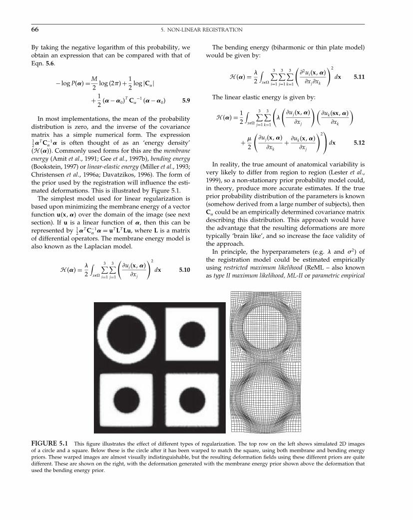
Elsevier UK Chapter: Ch05-P372560 3-10-2006 3:58p.m. Page:66 Trim:7.5in×9.25in
Basal Font:Palatino Margins:Top:40pt Gutter:68pt Font Size:9.5/12 Text Width:42pc Depth:55 Lines
66 5. NON-LINEAR REGISTRATION
By taking the negative logarithm of this probability, weobtain an expression that can be compared with that ofEqn. 5.6.
− log P��� =M
2log �2��+ 1
2log �C��
+ 12
��−�0�T C�
−1 ��−�0� 5.9
In most implementations, the mean of the probabilitydistribution is zero, and the inverse of the covariancematrix has a simple numerical form. The expression12 �T C−1
� � is often thought of as an ‘energy density’�� ����. Commonly used forms for this are the membraneenergy (Amit et al., 1991; Gee et al., 1997b), bending energy(Bookstein, 1997) or linear-elastic energy (Miller et al., 1993;Christensen et al., 1996a; Davatzikos, 1996). The form ofthe prior used by the registration will influence the esti-mated deformations. This is illustrated by Figure 5.1.
The simplest model used for linear regularization isbased upon minimizing the membrane energy of a vectorfunction u�x��� over the domain of the image (see nextsection). If u is a linear function of �, then this can berepresented by 1
2 �T C−1� � = uT LT Lu, where L is a matrix
of differential operators. The membrane energy model isalso known as the Laplacian model.
� ��� =
2
∫x�
3∑i=1
3∑j=1
(�ui�x���
�xj
)2
dx 5.10
The bending energy (biharmonic or thin plate model)would be given by:
� ��� =
2
∫x�
3∑i=1
3∑j=1
3∑k=1
(�2ui�x���
�xj�xk
)2
dx 5.11
The linear elastic energy is given by:
� ��� = 12
∫x�
3∑j=1
3∑k=1
(
(�uj�x���
�xj
)(�uk�sx���
�xk
)
+
2
(�uj�x���
�xk
+ �uk�x���
�xj
)2⎞⎠dx 5.12
In reality, the true amount of anatomical variability isvery likely to differ from region to region (Lester et al.,1999), so a non-stationary prior probability model could,in theory, produce more accurate estimates. If the trueprior probability distribution of the parameters is known(somehow derived from a large number of subjects), thenC� could be an empirically determined covariance matrixdescribing this distribution. This approach would havethe advantage that the resulting deformations are moretypically ‘brain like’, and so increase the face validity ofthe approach.
In principle, the hyperparameters (e.g. and �2) ofthe registration model could be estimated empiricallyusing restricted maximum likelihood (ReML – also knownas type II maximum likelihood, ML-II or parametric empirical
FIGURE 5.1 This figure illustrates the effect of different types of regularization. The top row on the left shows simulated 2D imagesof a circle and a square. Below these is the circle after it has been warped to match the square, using both membrane and bending energypriors. These warped images are almost visually indistinguishable, but the resulting deformation fields using these different priors are quitedifferent. These are shown on the right, with the deformation generated with the membrane energy prior shown above the deformation thatused the bending energy prior.

Elsevier UK Chapter: Ch05-P372560 3-10-2006 3:58p.m. Page:67 Trim:7.5in×9.25in
Basal Font:Palatino Margins:Top:40pt Gutter:68pt Font Size:9.5/12 Text Width:42pc Depth:55 Lines
OBJECTIVE FUNCTIONS 67
Bayes) with Laplace approximation schemes similar to thosementioned in the later chapters. In practice, however,values for these hyperparameters are often imputed ina way that depends upon a subjective belief in what anoptimal trade-off between the likelihood and prior termsshould be.
Deformation models
At its simplest, image registration involves estimating asmooth, continuous mapping between the points in oneimage, and those in another. This mapping allows oneimage to be re-sampled so that it is warped (deformed)to match another (Figures 5.2 and 5.3). There are manyways of modelling such mappings, but these fit into twobroad categories of parameterization (Miller et al., 1997).
• The small deformation framework does not necessarilypreserve topology3 – although if the deformations arerelatively small, then it may still be preserved.
• The large deformation framework generates deforma-tions (diffeomorphisms) that have a number of elegantmathematical properties, such as enforcing the preser-vation of topology.
Both of these approaches require some model of asmooth vector field. Such models will be illustrated with
FIGURE 5.2 This figure illustrates a hypothetical deformationfield that maps between points in one image and those in another.This is a continuous function over the domain of the image.
3 The word ‘topology’ is used in the same sense as in ‘Topolog-ical properties of smooth anatomical maps’ (Christensen et al.,1995). If spatial transformations are not one-to-one and contin-uous, then the topological properties of different structures canchange.
the simpler small deformation framework, before brieflyintroducing the principles that underlie the large defor-mation framework.
Small deformation approaches
First of all, some simple notation is introduced. Each coor-dinate within an image is a vector of three elements. Forexample, the coordinate of the ith voxel could be denotedby xi = [
xi1 xi2 xi3
]. For an image f, the ith voxel may be
indicated by fi or by f�xi�. Similarly, a point in a deforma-tion field can also be denoted as a vector. The ith voxel ofan image deformed this way could be denoted by gi���or g�y�xi����. The images are treated as continuous func-tions of space. Reading off the value at some arbitrarypoint involves interpolating between the original vox-els. For many interpolation methods, the functions areparameterized by linear combinations of basis functions,such as B-spline bases, centred at each original voxel.Similarly, the deformations themselves can be parame-terized by a linear combination of smooth, continuousbasis functions.
y�xi��� =M∑
m=1
�m�m�xi� 5.13
Most models treat the basis functions as scalar fieldsrepresenting deformations in the three orthogonal direc-tions4 (Figure 5.4) such that:
y1�xi��� =M∑
m=1
�m1�m1�xi�
y2�xi��� =M∑
m=1
�m2�m2�xi�
y3�xi��� =M∑
m=1
�m3�m3�xi�
5.14
A potentially enormous number of parameters arerequired to describe the non-linear transformations thatwarp two images together (i.e. the problem can be veryhigh-dimensional). However, much of the spatial vari-ability can be captured using just a few parameters.Sometimes only an affine transformation is used to reg-ister approximately images of different subjects. Thisaccounts for differences in position, orientation and over-all brain dimensions (Figure 5.5), and often provides agood starting point for higher-dimensional registrationmodels. The basis functions for such a transform are
4 Exceptions are some models that use linear elastic regulariza-tion (Christensen et al., 1996a).
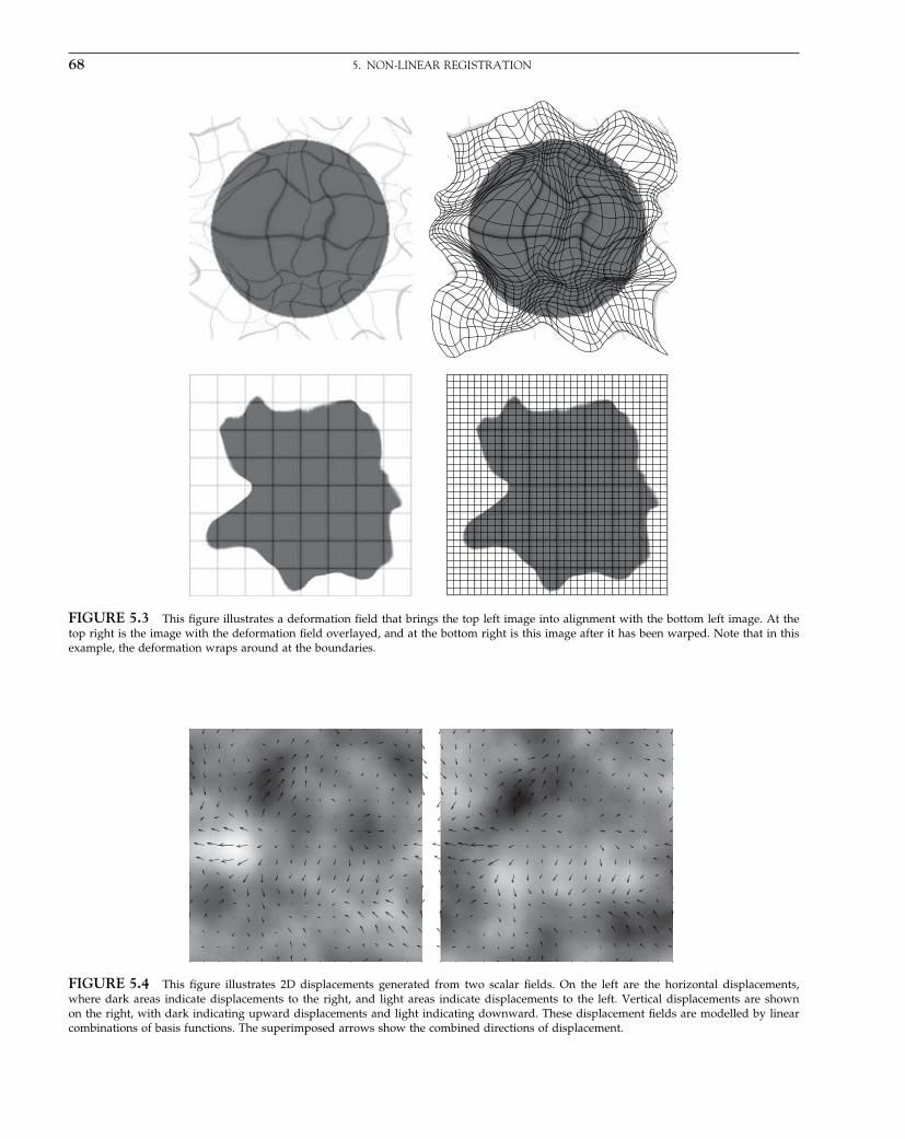
Elsevier UK Chapter: Ch05-P372560 3-10-2006 3:58p.m. Page:68 Trim:7.5in×9.25in
Basal Font:Palatino Margins:Top:40pt Gutter:68pt Font Size:9.5/12 Text Width:42pc Depth:55 Lines
68 5. NON-LINEAR REGISTRATION
FIGURE 5.3 This figure illustrates a deformation field that brings the top left image into alignment with the bottom left image. At thetop right is the image with the deformation field overlayed, and at the bottom right is this image after it has been warped. Note that in thisexample, the deformation wraps around at the boundaries.
FIGURE 5.4 This figure illustrates 2D displacements generated from two scalar fields. On the left are the horizontal displacements,where dark areas indicate displacements to the right, and light areas indicate displacements to the left. Vertical displacements are shownon the right, with dark indicating upward displacements and light indicating downward. These displacement fields are modelled by linearcombinations of basis functions. The superimposed arrows show the combined directions of displacement.

Elsevier UK Chapter: Ch05-P372560 3-10-2006 3:58p.m. Page:69 Trim:7.5in×9.25in
Basal Font:Palatino Margins:Top:40pt Gutter:68pt Font Size:9.5/12 Text Width:42pc Depth:55 Lines
OBJECTIVE FUNCTIONS 69
FIGURE 5.5 Images of six subjects registered using a 12-parameter affine registration (see also Figure 5.9). The affine registration matchesthe positions and sizes of the images.
coordinates themselves, leading to the following param-eterization in 3D:
y1�x��� =�1x1 +�2x2 +�3x3 +�4
y2�x��� =�5x1 +�6x2 +�7x3 +�8
y3�x��� =�9x1 +�10x2 +�11x3 +�12
5.15
Low spatial frequency global variability of head shapecan be accommodated by describing deformations bya linear combination of a few low frequency basisfunctions. One widely used basis function registrationmethod is part of the AIR package (Woods et al., 1998a,b),which uses polynomial basis functions (Figure 5.6) tomodel shape variability. These basis functions are a sim-ple extension to those used for parameterizing affinetransformations. For example, a two-dimensional thirdorder polynomial mapping is:
y1�x��� =�1 +�2x1 +�3x21 +�4x
31
�5x2 +�6x1x2 +�7x21x2
�8x22 +�9x1x
22
�10x32
y2�x��� =�11 +�12x1 +�13x21 +�14x
31
�15x2 +�16x1x2 +�17x21x2
�18x22 +�19x1x
22
�20x32
5.16
FIGURE 5.6 Polynomial basis functions. Note that additionalbasis functions not shown in Eqn. 5.16 are included here.
Other models parameterize a displacement field, whichis added to an identity transform:
y�xi��� = xi +M∑
m=1
�m�m�xi� 5.17
In such parameterizations, the inverse transforma-tion is sometimes approximated by subtracting the
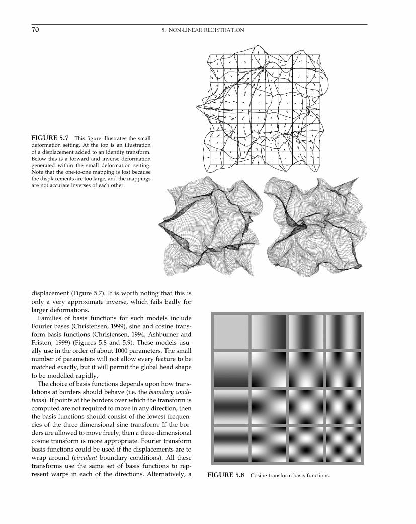
Elsevier UK Chapter: Ch05-P372560 3-10-2006 3:58p.m. Page:70 Trim:7.5in×9.25in
Basal Font:Palatino Margins:Top:40pt Gutter:68pt Font Size:9.5/12 Text Width:42pc Depth:55 Lines
70 5. NON-LINEAR REGISTRATION
FIGURE 5.7 This figure illustrates the smalldeformation setting. At the top is an illustrationof a displacement added to an identity transform.Below this is a forward and inverse deformationgenerated within the small deformation setting.Note that the one-to-one mapping is lost becausethe displacements are too large, and the mappingsare not accurate inverses of each other.
displacement (Figure 5.7). It is worth noting that this isonly a very approximate inverse, which fails badly forlarger deformations.
Families of basis functions for such models includeFourier bases (Christensen, 1999), sine and cosine trans-form basis functions (Christensen, 1994; Ashburner andFriston, 1999) (Figures 5.8 and 5.9). These models usu-ally use in the order of about 1000 parameters. The smallnumber of parameters will not allow every feature to bematched exactly, but it will permit the global head shapeto be modelled rapidly.
The choice of basis functions depends upon how trans-lations at borders should behave (i.e. the boundary condi-tions). If points at the borders over which the transform iscomputed are not required to move in any direction, thenthe basis functions should consist of the lowest frequen-cies of the three-dimensional sine transform. If the bor-ders are allowed to move freely, then a three-dimensionalcosine transform is more appropriate. Fourier transformbasis functions could be used if the displacements are towrap around (circulant boundary conditions). All thesetransforms use the same set of basis functions to rep-resent warps in each of the directions. Alternatively, a FIGURE 5.8 Cosine transform basis functions.

Elsevier UK Chapter: Ch05-P372560 3-10-2006 3:58p.m. Page:71 Trim:7.5in×9.25in
Basal Font:Palatino Margins:Top:40pt Gutter:68pt Font Size:9.5/12 Text Width:42pc Depth:55 Lines
OBJECTIVE FUNCTIONS 71
FIGURE 5.9 Six subjects’ brains registered with both affine and cosine transform basis function registration (see also Figure 5.8), asimplemented by SPM. The basis function registration estimates the global shapes of the brains, but is not able to account for high spatialfrequency warps.
mixture of cosine and sine transform basis functions canbe used to constrain translations at the surfaces of thevolume to be parallel to the surface only (sliding bound-ary conditions). By using a different combination of basisfunction sets, the corners of the volume can be fixed andthe remaining points on the surface can be free to move inall directions (bending boundary conditions) (Christensen,1994). These various boundary conditions are illustratedin Figure 5.10.
Radial basis functions are another family of parame-terizations which are often used in conjunction with anaffine transformation. Each radial basis function is cen-tred at some point, and the amplitude is then a functionof the distance from that point. Thin-plate splines are oneof the most widely used radial basis functions for imagewarping, and are especially suited to manual landmarkmatching (Bookstein, 1989, 1997; Glasbey and Mardia,1998). The landmarks may be known, but interpolationis needed in order to define the mapping between theseknown points. By modelling it with thin-plate splines, themapping function has the smallest bending energy. Otherchoices of basis function reduce other energy measures,and these functions relate to the convolution filters thatare sometimes used for fast image matching (Bro-Nielsenand Gramkow, 1996; Beg et al., 2005).
B-spline bases are also used for parameterizing dis-placements (Studholme et al., 2000; Thévenaz and Unser,2000) (Figure 5.11). They are related to the radial basis
FIGURE 5.10 Different boundary conditions. Above left: fixedboundaries (generated purely from sine transform basis functions).Above right: sliding boundaries (from a mixture of cosine and sinebasis functions). Below left: bending boundaries (from a differentmixture of cosine and sine basis functions). Below right: free bound-ary conditions (purely from cosine basis functions).
functions in that they are centred at discrete points, butthe amplitude is the product of functions of distance inthe three orthogonal directions (i.e. they are separable).The separability and local support of these basis functions

Elsevier UK Chapter: Ch05-P372560 3-10-2006 3:58p.m. Page:72 Trim:7.5in×9.25in
Basal Font:Palatino Margins:Top:40pt Gutter:68pt Font Size:9.5/12 Text Width:42pc Depth:55 Lines
72 5. NON-LINEAR REGISTRATION
FIGURE 5.11 B-spline basis functions.
confers certain advantages in terms of being able rapidlyto generate displacement fields through a convolution-like procedure.
Very detailed displacement fields can be generatedby modelling an individual displacement at each voxel.These may not appear to be basis function approaches,but the assumptions within the registration models oftenassume that the fields are tri-linearly interpolated. This isthe same as a first degree B-spline basis function model.
LARGE DEFORMATION APPROACHES
Approaches that parameterize the deformations them-selves do not necessarily enforce a one-to-one mapping,particularly if the prior is a multivariate Gaussian proba-bility density. Small deformation models that incorporatethis constraint have been devised (Edwards et al., 1998;Ashburner et al., 1999, 2000), but their parameterizationis still essentially within a small deformation setting.
The key element of the large-deformation or diffeomor-phic5 setting is that the deformations are generated bythe composition of a number of small deformations (i.e.warped warps). A composition of two functions is essen-tially taking one function of the other in order to produce
5 A diffeomorphism is a globally one-to-one (bijective) smoothand continuous mapping with derivatives that are invertible(i.e. non-zero Jacobian determinant).
a new function. For two functions, y2 and y1 this wouldbe denoted by:
�y2 �y1��x� = y2�y1�x�� 5.18
For deformations, the composition operation is achievedby re-sampling one deformation field by another. Provid-ing the original deformations are small enough, then theyare likely to be one-to-one. A composition of a pair ofone-to-one mappings will produce a new mapping thatis also one-to-one. Multiple nesting can also be achieved,so that large one-to-one deformations can be obtainedfrom the composition of many very small deformations.
�y3 �y2 �y1��x� = ��y3 �y2��y1��x�
= �y3 � �y2 �y1���x� = y3�y2�y1�x��� 5.19
The early diffeomorphic registration approaches werebased on the greedy ‘viscous fluid’ registration method ofChristensen and Miller (Christensen et al., 1994, 1996b).In these models, finite difference methods are used tosolve the partial differential equations that model oneimage as it ‘flows’ to match the shape of the other.At the time, the advantage of these methods was thatthey were able to account for large displacements whileensuring that the topology of the warped image is pre-served. They also provided a useful foundation fromwhich the later methods arose. Viscous fluid methodsrequire the solutions to large sets of partial differentialequations (see Chapter 19 of Press et al., 1992). The ear-liest implementations were computationally expensivebecause solving the equations used successive over-relaxation. Such relaxation methods are inefficient whenthere are large low frequency components to estimate.Since then, a number of faster ways of solving the differ-ential equations have been devised (Modersitzki, 2003).These include the use of Fourier transforms to convolvewith the impulse response of the linear regularizationoperator (Bro-Nielsen and Gramkow, 1996), or by con-volving with a separable approximation (Thirion, 1995).Another fast way of solving such equations would be touse a multigrid method (Haber and Modersitzki, 2006),which efficiently makes use of relaxation methods overvarious spatial scales.
The greedy algorithm works in several stages. In thefirst stage, a heavily regularized small deformation �y1�would be estimated that brings one image f into slightlybetter correspondence with the other g. A deformed ver-sion of this image would then be created by f1 = f�y1�.Then another small deformation is estimated �y2� bymatching f1 with g, and a second deformed version off created by f2 = f�y2�y1�. This procedure would berepeated, each time generating a warped version of f thatis closer to g. Although the likelihood will be increased

Elsevier UK Chapter: Ch05-P372560 3-10-2006 3:58p.m. Page:73 Trim:7.5in×9.25in
Basal Font:Palatino Margins:Top:40pt Gutter:68pt Font Size:9.5/12 Text Width:42pc Depth:55 Lines
LARGE DEFORMATION APPROACHES 73
FIGURE 5.12 This figure illustrates the largedeformation setting. In this setting, the deforma-tions follow a curved trajectory (just as a rigid-body rotation follows a curved trajectory). Below isan example of a forward and inverse deformation.Unlike those shown in Figure 5.6, these are one-to-one mappings, and the transforms are actuallyinverses of each other.
by such a greedy algorithm, it will not produce thesmoothest possible deformation. Such a warping strategydoes not maximize any clearly defined prior probabilityof the parameters.
More recent algorithms for large deformationregistration do aim to maximize both the log-likelihoodand log-prior. For example, the LDDMM (large defor-mation diffeomorphic metric mapping) algorithm (Beget al., 2005) does not fix the deformation parameters oncethey have been estimated. It continues to update themusing a gradient descent algorithm such that the log-priorterm is properly optimized. Such approaches essentiallyparameterize the model by velocities, and compute thedeformation as the medium warps over unit time (Joshiand Miller, 2000; Miller et al., 2006).
Diffeomorphic warps can also be inverted (Figure 5.12).If each small deformation is generated by adding a smalldisplacement (velocity) to an identity transform, thentheir approximate inverses can be derived by subtract-ing the same displacement. A composition of these small
deformation inverses will then produce the inverse of thelarge deformation.
In principle, a single velocity field could be usedto parameterize the model,6 which would confer cer-tain computational advantages. In Group theory, thevelocities are a Lie algebra, and these are exponentiatedto produce a deformation, which is a Lie group (see e.g.Miller and Younes, 2001; Woods, 2003; Miller et al. 2006;Vaillant et al., 2004). If the velocity field is assumed con-stant throughout, then the exponentiation can be donerecursively in a way that is analogous to exponentiatinga matrix (Moler and Loan, 2003) by recursive squaring.A full deformation can be computed from the square7 ofa half-way deformation, a half-way deformation can be
6 In such a model, the motion is at constant velocity within theLagrangian frame of reference, but variable velocity if viewedwithin the Eulerian frame.7 The use of ‘square’ is in the sense of a composition of a functionby itself.
Elsevier UK Chapter: Ch05-P372560 3-10-2006 3:58p.m. Page:74 Trim:7.5in×9.25in
Basal Font:Palatino Margins:Top:40pt Gutter:68pt Font Size:9.5/12 Text Width:42pc Depth:55 Lines
74 5. NON-LINEAR REGISTRATION
computed by squaring a quarter-way deformation, andso on.
Many researchers are interested in deriving metricsfrom deformations in order to compare the similaritiesof shapes (Miller et al., 1997, Miller, 2004). These met-rics are a measure of the difference between the shapes,and can be thought of as measures of geodesic dis-tance. One example of the use of such distance measureswould be for tackling multivariate classification prob-lems using non-linear kernel methods (such as supportvector machines). In order to be a metric, a measure mustbe non-negative �dist�A�B�� 0�, symmetric �dist�A�B� =dist�B�A�� and satisfy the triangle inequality �dist�A�B�+dist�B�C� � dist�A�C��. The more recent diffeomorphicregistration approaches generate suitable measures ofdifference between shapes, which are derived from theenergy densities of the velocity fields.
ESTIMATING THE MAPPINGS
Most non-linear registration approaches search for amaximum a posteriori (MAP) estimate of the parametersdefining the warps. This corresponds to the mode of theposterior probability density of the model parameters.There are many optimization algorithms that try to findthe mode, but most of them only perform a local search.It is possible to use relatively simple strategies for fit-ting models with few parameters but, as the number ofparameters increases, the time required to estimate themwill increase dramatically. For this reason, it is commonto use optimization algorithms that utilize the derivativesof the objective function with respect to the parameters,as these indicate the best direction in which to search.Some developers use schemes related to gradient descent,whereby the parameters are repeatedly changed by atiny amount in the direction that improves the objectivefunction. This procedure can still be quite slow – partic-ularly when there are dependencies among the parame-ters. Faster algorithms have been devised, which assumethat the probability densities can be approximated bya multivariate Gaussian. Their effectiveness depends onhow good this approximation is.
The Levenberg-Marquardt (LM) algorithm is a verygood general purpose optimization strategy (see Presset al., 1992 for more information). The procedure is a localoptimization, so it needs reasonable initial starting esti-mates. It uses an iterative scheme to update the param-eter estimates in such a way that the objective functionis usually improved each time. Each iteration requiresthe first and second derivatives of the objective function,with respect to the parameters. In the following scheme,I is an identity matrix and � is a scaling factor. The choice
of � is a trade-off between speed of convergence, and sta-bility. A value of zero for � gives the Newton-Raphsonor Gauss-Newton optimization scheme, which may beunstable if the probability density is not well approxi-mated by a Gaussian. Increasing � will slow down theconvergence, but increase the stability of the algorithm.The value of � is usually decreased slightly after iter-ations that decrease (improve) the cost function. If thecost function increases after an iteration, then the previ-ous solution is retained, and � is increased in order toprovide more stability.
��n+1� = ��n� −(
�2� ���
��2
∣∣∣��n�
+ �I)−1
�� ���
��
∣∣∣��n�
5.20
The objective function � ��� is the sum of two terms.Ignoring the constants, these are the negative logarithmof the likelihood ������ and the negative logarithm of theprior probability density �� ����. The prior probability ofthe parameters is generally modelled by a multivariateGaussian density, with mean �0 and covariance C�.
� ��� = 12
��−�0�C�−1��−�0� 5.21
The first and second derivatives of � ��� (see Eqn. 5.9)with respect to the parameters are therefore:
�� ���
��= �����
��+C�
−1��−�0� and
�2� ���
��2= �2�
��2+C�
−1 5.22
If the model is very high-dimensional (more than about4000 parameters), then storing a full matrix of secondderivatives becomes difficult because of memory lim-itations. For this reason, it can be convenient to usesparse representations of the second derivatives, anduse approaches for solving systems of sparse equations(Gilbert et al., 1992). Sparse matrices of second deriva-tives can be obtained by parameterizing the deforma-tions with basis functions that have local support (e.g.B-splines). A faster approach, however, would be to usematrix solvers that are especially designed for the partic-ular class of problem. Full multigrid (FMG) approachesare especially suited to solving such equations, and agood introductory explanation of these methods can befound in Chapter 19 of Press et al. (1992).
Optimization problems for complex non-linear mod-els, such as those used for image registration, can eas-ily get caught in local optima, so there is no guaranteethat the estimate determined by the algorithm is glob-ally optimum. If the starting estimates are sufficientlyclose to the global optimum, then a local optimizationalgorithm is more likely to find the true MAP solution.

Elsevier UK Chapter: Ch05-P372560 3-10-2006 3:58p.m. Page:75 Trim:7.5in×9.25in
Basal Font:Palatino Margins:Top:40pt Gutter:68pt Font Size:9.5/12 Text Width:42pc Depth:55 Lines
SPATIAL NORMALIZATION IN THE SPM SOFTWARE 75
Therefore, the choice of starting parameters can influencethe validity of the final registration result. One methodof increasing the likelihood of achieving a good solutionis gradually to reduce the value of relative to 1/�2
over time.8 This has the effect of making the registrationestimate the more global deformations before estimatingmore detailed warps. Most shape variability is low fre-quency, so an algorithm can get reasonably close to agood solution using a relatively high value for . Thisalso reduces the number of local minima for the earlyiterations. The images could also be smoother for theearlier iterations in order to reduce the amount of con-founding information and the number of local minima.A review of such approaches can be found in Lester andArridge (1999).
Internal consistency
Currently, most registration algorithms use only a singleimage from each subject, which is typically a T1-weightedMR image. Such images only really delineate differenttissue types. Further information that may help the reg-istration could be obtained from other data, such as dif-fusion weighted images (Zhang et al., 2004). This shouldprovide anatomical information more directly related toconnectivity and implicitly function, possibly leading toimproved registration of functionally specialized areas(Behrens et al., 2006). Matching DTI images of a pairof subjects together is likely to give different deforma-tion estimates than would be obtained through match-ing T1-weighted images of the same subjects. The onlyway to achieve an internally consistent match is throughperforming the registrations simultaneously, within thesame model.
Another form of consistency is inverse consistency(Christensen, 1999). For example, suppose a deformationthat matches brain f to brain g is estimated, and alsoa deformation that matches brain g to brain f. If onedeformation field is not the inverse of the other, thensomething has to be wrong. The extreme case of an incon-sistency between a forward and inverse transformation iswhen the one-to-one mapping between the images breaksdown. The best way of ensuring such internal consistencyis through using diffeomorphic matching strategies.
Many registration approaches use the gradients of onlyone of the images to drive the registration, rather thanthe gradients of both. This can be another reason why
8 Regularize heavily to begin with and decrease the amount ofregularization over time. The residuals are much further fromIID in the early iterations, so the likelihood is overestimated.Increasing the regularization partially compensates for this.
inconsistencies may arise between forward and inverseregistration approaches. One way in which the regis-tration can be made more symmetric is iteratively tomatch the images to their warped average. The resultof this procedure would be two deformations that map‘half way’. From the appropriate compositions of these‘half way’ deformations, a pair of deformations can begenerated that map between the original images, and areboth inverses of each other.
Sometimes, instead of simply matching a pair ofimages, the objective is to match the images of multi-ple subjects. This is sometimes done by registering allthe images with a single template image. Such a proce-dure would produce different results depending uponthe choice of template, so this is another area where inter-nal consistency should be considered. One could consideran optimal template being some form of average (Hiraniet al., 2001; Avants and Gee, 2004; Davis et al., 2004; Loren-zen et al., 2004). Registering such a template with a brainimage generally requires smaller (and therefore less errorprone) deformations than would be necessary for regis-tering to an unusually shaped template. Such averagesgenerally lack the detail present in the individual sub-jects. The structures that are more difficult to match aregenerally slightly blurred in the average, whereas thestructures that can be more reliably matched are sharper.Such an average generated from a large population ofsubjects would be ideal for use as a general purpose tem-plate.
SPATIAL NORMALIZATION IN THESPM SOFTWARE
This section describes the steps involved in the algo-rithm that SPM uses to normalize spatially images ofdifferent subjects into roughly the same coordinate sys-tem. The coordinate system is defined by the templateimage (or series of images), which is usually one of theimages released with the software. So far, this chapter hasassumed the template is deformed to match an individ-ual’s brain image. In this section, the individual subjects’images are warped to approximate a template image.This is slightly suboptimal because it assumes the noiseis in the template image rather than the individual image;the original motivation for this strategy was to avoidhaving to invert the estimated deformation fields.
Spatial normalization in SPM is currently implementedin a small deformation setting and warps a smoothedversion of the image to a smooth template. It works byestimating the optimum coefficients for a set of bases,by minimizing the mean squared difference between the

Elsevier UK Chapter: Ch05-P372560 3-10-2006 3:58p.m. Page:76 Trim:7.5in×9.25in
Basal Font:Palatino Margins:Top:40pt Gutter:68pt Font Size:9.5/12 Text Width:42pc Depth:55 Lines
76 5. NON-LINEAR REGISTRATION
template and a warped source image, while simultane-ously minimizing the deviation of the transformationfrom its expected value. The images may be scaled dif-ferently, so an additional parameter �w� is needed toaccommodate this difference. In fact, four intensity scal-ing parameters are used for each template image (alsoto model linear intensity gradients), but they will notbe included in the following description. With a singlescaling parameter, the minimized likelihood function is:
� = 12�2
I∑i=1
�f�y�xi����−wg�xi��2 5.23
A Gauss-Newton approach is used to optimize theparameters. This requires the following first derivatives:
��
��m
= 1�2
I∑i=1
�f�y�xi����
��m
�f�y�xi����−wg�xi�� 5.24
��
�w= 1
�2
I∑i=1
g�xi� �wg�xi�−f�y�xi����� 5.25
and second derivatives:
�2�
��m��n
= 1�2
I∑i=1
(�f�y�xi����
��m
�f�y�xi����
��n
+�2f�y�xi����
��m��n
�f�y�xi����−wg�xi��
)5.26
�2�
�w2= 1
�2
I∑i=1
g�xi�2 5.27
�2�
��m�w=− 1
�2
I∑i=1
�f�y�xi����
��m
g�xi� 5.28
In practice, the following approximate second deriva-tives are used, because they can be computed more easily,and they also make the algorithm more stable:
�2�
��m��n
� 1�2
I∑i=1
�f�y�xi����
��m
�f�y�xi����
��n
5.29
The prior used for non-linear registration is based onthe bending energy of the displacement field. The amountof spatial variability is assumed to be known a priori (i.e. in Eqn. 5.11 is assigned by the user), but the algorithmtries to determine an optimal �2 value for the partic-ular image being registered. SPM is applied to a widevariety of images with different noise properties. Deter-mining an optimal value for �2 may be impractical formost users, so the algorithm uses a heuristic approach toassign a suitable value. The heuristic is based on the meansquared difference between the template and warpedimage, but with a correction based on the number of inde-pendent voxels. This correction is computed at each itera-tion using the smoothness of the residuals. Fully Bayesian
approaches assume that the variance associated with eachvoxel is already known, whereas the approach describedhere is a type of empirical Bayes, which attempts to esti-mate this variance from the residuals. Because the regis-tration is based on smooth images, correlations betweenneighbouring voxels are considered when estimating thevariance. This makes the same approach suitable for thespatial normalization of both high quality MR images,and low resolution noisy PET images.
In practice, it may be meaningless even to attempt anexact match between brains beyond a certain resolution.There is not a one-to-one relationship between the corti-cal structures of one brain and those of another, so anymethod that attempts to match brains exactly must befolding the brain to create sulci and gyri that do not exist.Even if an exact match is possible, because the registra-tion problem is not convex, the solutions obtained byhigh-dimensional warping techniques may not be trulyoptimum. High-dimensional registrations methods areoften very good at registering grey matter with greymatter (for example), but there is no guarantee that theregistered grey matter arises from homologous corticalstructures.
Also, structure and function are not always tightlylinked. Even if structurally equivalent regions can bebrought into exact register, it does not mean that the sameis true for regions that perform the same or similar func-tions. For inter-subject averaging in SPM, an assumptionis made that functionally equivalent regions lie in approx-imately the same parts of the brain. This leads to thecurrent rationale for smoothing images from multisubjectfunctional imaging studies prior to performing statisticalanalyses. Constructive interference of the smeared acti-vation signals then has the effect of producing a signalthat is roughly in an average location. In order to accountfor substantial fine scale warps in a spatial normalization,it is necessary for some voxels to increase their volumesconsiderably, and for others to shrink to an almost neg-ligible size. The contribution of the shrunken regions tothe smoothed images is tiny, and the sensitivity of thetests for detecting activations in these regions may bereduced. This is another argument in favour of spatiallynormalizing on a relatively global scale.
The first step in registering images from different sub-jects involves determining the optimum 12-parameteraffine transformation. Unlike in Chapter 4 – where theimages to be matched together are from the same sub-ject – zooms and shears are needed to register heads ofdifferent shapes and sizes. Prior knowledge of the vari-ability of head sizes and overall proportions is used toincrease the robustness and accuracy of the method (Ash-burner et al., 1997).
The next part is a non-linear registration for correct-ing gross differences in head shapes that cannot be

Elsevier UK Chapter: Ch05-P372560 3-10-2006 3:58p.m. Page:77 Trim:7.5in×9.25in
Basal Font:Palatino Margins:Top:40pt Gutter:68pt Font Size:9.5/12 Text Width:42pc Depth:55 Lines
EVALUATION STRATEGIES 77
accounted for by the affine normalization alone. Thenon-linear warps are modelled by linear combinationsof smooth cosine transform basis functions. For speedand simplicity, a relatively small number of parame-ters (approximately 1000) are used to describe the non-linear components of the registration (Ashburner andFriston, 1999).
Affine registration
Almost all inter-subject registration methods for brainimages begin by determining the optimal affine trans-formation that registers the images together. This stepis normally performed automatically by minimizing (ormaximizing) some mutual function of the images. Theobjective of affine registration is to fit the source image toa template image, using a twelve-parameter affine trans-formation. The images may be scaled quite differently,so an additional intensity scaling parameter is includedin the model.
Without constraints and with poor data, simplemaximum-likelihood parameter optimization can pro-duce some extremely unlikely transformations. For exam-ple, when there are only a few slices in the image, it isnot possible for the algorithms to determine an accuratezoom in the out of plane direction. Any estimate of thisvalue is likely to have very large errors. When a regular-ized approach is not used, it may be better to assign afixed value for this difficult-to-determine parameter, andsimply fit for the remaining ones.
By incorporating prior information into the optimiza-tion procedure, a smooth transition between fixed andfitted parameters can be achieved. When the error for aparticular fitted parameter is known to be large, then thatparameter will be based more upon the prior information.In order to adopt this approach, the prior distribution ofthe parameters has to be specified. This is derived fromthe zooms and shears determined by registering a largenumber of brain images to the template.
Non-linear registration
The non-linear spatial normalization approach of SPMassumes that the image has already been approximatelyregistered with the template according to a twelve-parameter affine registration. This section illustrates howthe parameters describing global shape differences (notaccounted for by affine registration) between an imageand template can be determined. A small-deformationframework is used, and regularization is by the bendingenergy of the displacement field. Further details can befound in Ashburner and Friston (1999).
The deformations are parameterized by a linear com-bination of about 1000 low-frequency three-dimensionalcosine transform bases. The spatial transformation fromx, to y is:
y1�x��� =x1 +u1 = x1 +M∑
m=1
�m1�m�x�
y2�x��� =x2 +u2 = x2 +M∑
m=1
�m2�m�x�
y3�x��� =x3 +u3 = x3 +M∑
m=1
�m3�m�x�
5.30
where �mk is the mth coefficient for dimension k, and�m�x� is the mth basis function at position x. Thebasis functions are separable, and each one is gener-ated by multiplying three one-dimensional basis func-tions together.
�m�x� = �m3�x3��m2
�x2��m1�x1� 5.31
In one dimension, the cosine transform bases are gener-ated by:
�1�i� = 1√I
i = 1��I
�m�i� =√
2I
cos(
��2i−1��m−1�
2I
)i = 1��I�m = 2��M
5.32
EVALUATION STRATEGIES
Validation of warping methods is a complex area. Theappropriateness of an evaluation depends on the partic-ular application that the deformations are to be used for.For example, if the application was spatial normaliza-tion of functional images of different subjects, then themost appropriate evaluation may be based on assessingthe sensitivity of voxel-wise statistical tests (Gee et al.,1997a; Miller et al., 2005). Because the warping proce-dure is based only on structural information, it is blindto the locations of functional activation. If the locationsof activations can be brought into close correspondencein different subjects, then it is safe to say that the spa-tial normalization procedure is working well. The bestmeasure of correspondence depends on how much theimages are smoothed prior to performing the statisticaltests. Different registration methods will perform dif-ferently depending on the amount of smoothing used.For example, the difference in performance of high- ver-sus low-dimensional methods will be less when lots
Elsevier UK Chapter: Ch05-P372560 3-10-2006 3:58p.m. Page:78 Trim:7.5in×9.25in
Basal Font:Palatino Margins:Top:40pt Gutter:68pt Font Size:9.5/12 Text Width:42pc Depth:55 Lines
78 5. NON-LINEAR REGISTRATION
of smoothing is used. Another application may involveidentifying shape differences among populations of sub-jects. In this case, the usefulness of the warping algo-rithm would be assessed by how well the deformationfields can be used to distinguish between the populations(Lao et al., 2004). These approaches can be consideredas forms of cross-validation, because they assess howwell the registration helps to predict additional infor-mation.
Generally, the results of an evaluation are specific onlyto the data used to evaluate the model. MR images varya great deal with different subjects, field strengths, scan-ners, sequences etc, so a model that is good for one setof data may not be appropriate for another. For exam-ple, consider intra-subject brain registration, under theassumption that the brain behaves like a rigid body. Ifthe scanner causes no distortion and computes the pixelsizes and slice thickness of the image volumes exactly,then the best model is a rigid body registration. If thescanner computes the voxel sizes incorrectly, then thebest model may be an affine registration. If there are dis-tortions, then the best registration approach will modeldistortions. Validation should therefore relate to both thedata and the algorithm. The question should be aboutwhether it is appropriate to apply a model to a dataset,given the assumptions made by the model.
An assessment of how well manually defined land-marks in real brains can be colocalized is another usefulvalidation strategy, because it allows the models to becompared with human expertise (Hellier et al., 2001, 2002,2003). The use of simulated images with known underly-ing deformations is not appropriate for proper validationof non-linear registration methods. This is particularlytrue if the deformation model is the same for the simula-tions as it is for the registration, because this only illus-trates whether or not the optimization strategy works.Another commonly used form of ‘evaluation’ involveslooking at the residual difference after registration. Sucha strategy would ignore the possibility of over-fitting,and tends to favour those models with less regulariza-tion.
Within a Bayesian framework, it is possible to comparemodels, and decide which is more appropriate for a givendataset. This involves comparing the posterior probabil-ities for different models, after taking the model com-plexities into consideration. Occam’s razor9 is implicitlyincorporated by penalizing more complicated models.
9 Occam’s razor is the principle that one should not increase,beyond what is necessary, the number of entities required toexplain anything. It is sometimes known as the the principle ofparsimony, and has been historically linked with the philosopher,William of Ockham.
Given a choice of I alternative models, the probability ofmodel �i is given by:
P��i�D� = P�D��i�P��i�∑Ij P�D��j�P��j�
5.33
where the evidence for model �i is obtained bymarginalizing with respect to model parameters ���:
P�D��i� =∫
�P�D����i�P����i�d� 5.34
Unfortunately, the large number of model parame-ters required by non-linear registration would makesuch an exact integration procedure computationallyintractable.10 Note also that this includes a prior proba-bility term for each model, which many may consider assubjective. There are, however, broad criteria for assign-ing such priors, based on an understanding of the modelassumptions, its complexity and on any inconsistenciesit may contain.
In summary: to validate a warping method for aparticular dataset, it must be considered in relation toother available methods. The Bayesian paradigm allowsa model comparison to be made, from which the bestcan be selected. However, this model selection may notgeneralize for all data.
REFERENCES
Amit Y, Grenander U, Piccioni M (1991) Structural image restorationthrough deformable templates. J Am Stat Assoc 86: 376–87
Andersson JLR, Hutton C, Ashburner J et al. (2001) Modeling geo-metric deformations in EPI time series. NeuroImage 13: 903–19
Ashburner J, Andersson J, Friston KJ (1999) High-dimensional non-linear image registration using symmetric priors. NeuroImage9: 619–28
Ashburner J, Andersson J, Friston KJ (2000) Image registration usinga symmetric prior – in three-dimensions. Hum Brain Mapp 9:212–25
Ashburner J, Friston KJ (1999) Nonlinear spatial normalization usingbasis functions. Hum Brain Mapp 7(4): 254–66
Ashburner J, Neelin P, Collins DL et al. (1997) Incorporating priorknowledge into image registration. NeuroImage 6: 344–52
Avants B, Gee JC (2004) Geodesic estimation for large deforma-tion anatomical shape averaging and interpolation. NeuroImage23: S139–S150
Beg MF, Miller MI, Trouvé A et al. (2005) Computing large defor-mation metric mappings via geodesic flows of diffeomorphisms.Int J Comput Vision 61: 139–57
Behrens TEJ, Jenkinson M, Robson MD et al. (2006) A consistent rela-tionship between local white matter architecture and functionalspecialisation in medial frontal cortex. NeuroImage 30: 220–7
10 The use of Laplace approximations in conjunction with ML-IImethods may be possible alternatives though.
Elsevier UK Chapter: Ch05-P372560 3-10-2006 3:58p.m. Page:79 Trim:7.5in×9.25in
Basal Font:Palatino Margins:Top:40pt Gutter:68pt Font Size:9.5/12 Text Width:42pc Depth:55 Lines
REFERENCES 79
Bookstein FL (1989) Principal warps: thin-plate splines and thedecomposition of deformations. IEEE Trans Pattern Anal MachineIntelligence 11: 567–85
Bookstein FL (1997) Landmark methods for forms without land-marks: morphometrics of group differences in outline shape.Med Image Anal 1: 225–43
Brett M, Leff AP, Rorden C et al. (2001) Spatial normalization ofbrain images with focal lesions using cost function masking.NeuroImage 14: 486–500
Bro-Nielsen M, Gramkow C (1996) Fast fluid registration of medi-cal images. In Proc Visualization in Biomedical Computing (VBC),Hhne K-H, Kikinis R, (eds), vol. 1131 of Lecture Notes in ComputerScience. Springer-Verlag, Berlin and Heidelberg, pp 267–76
Christensen GE (1994) Deformable shape models for anatomy.Doctoral thesis, Washington University, Sever Institute ofTechnology
Christensen GE (1999) Consistent linear elastic transformations forimage matching. In Proc Information Processing in Medical Imaging(IPMI), Kuba A, Sámal M, Todd-Pokropek A (eds), vol. 1613of Lecture Notes in Computer Science. Springer-Verlag, Berlin andHeidelberg, pp 224–37
Christensen GE, Rabbitt RD, Miller MI (1994) 3D brain mappingusing using a deformable neuroanatomy. Phys Med Biol 39:609–18
Christensen GE, Rabbitt RD, Miller MI et al. (1995) Topological prop-erties of smooth anatomic maps. In Proc Information Processingin Medical Imaging (IPMI), Bizais Y, Barillot C, Di Paola R (eds).Kluwer Academic Publishers, Dordrecht.
Christensen GE, Kane AA, Marsh JL et al. (1996a) Synthesis of anindividualized cranial atlas with dysmorphic shape. In Proceed-ings of the Workshop on Mathematical Methods in Biomedical ImageAnalysis.
Christensen GE, Rabbitt RD, Miller MI (1996b) Deformable tem-plates using large deformation kinematics. IEEE Trans ImageProcess 5: 1435–47
Collins DL, Evans AC, Holmes C et al. (1995) Automatic 3D segmen-tation of neuro-anatomical structures from MRI. In Proc Informa-tion Processing in Medical Imaging (IPMI), Bizais Y, Barillot C, DiPaola R (eds). Kluwer Academic Publishers, Dordrecht
Davatzikos C (1996) Spatial normalization of 3D images usingdeformable models. J Comput Assist Tomogr 20: 656–65
Davis B, Lorenzen P, Joshi S (2004) Large deformation mini-mum mean squared error template estimation for computationanatomy. In Proc. IEEE International Symposium on BiomedicalImaging (ISBI), IEEE Publishing.
Dryden IL, Mardia KV (1998) Statistical Shape Analysis. John Wileyand Sons, Chichester.
Edwards PJ, Hill DLG, Little JA, Hawkes DJ (1998) Deformationfor image-guided interventions using a three component tissuemodel. Medical Image Analysis 2(4): 355–67
EvansAC,CollinsDL,MillsSR etal. (1993)3Dstatisticalneuroanatom-ical models from 305 MRI volumes. In Proc IEEE-Nuclear ScienceSymposium and Medical Imaging Conference, IEEE Publishing.
Evans AC, Kamber M Collins DL et al. (1994) An MRI-based proba-bilistic atlas of neuroanatomy. In Magnetic Resonance Scanning andEpilepsy, Shorvon S, Fish D, Andermann F et al. vol. 264 of NATOASI Series A, Life Sciences. Plenum Press, New York, pp 263–74
Fox PT (1995) Spatial normalization origins: objectives, applications,and alternatives. Hum Brain Mapp 3: 161–64
Gee JC, Alsop DC, Aguirre GK (1997a) Effect of spatial normaliza-tion on analysis of functional data. In Proc SPIE Medical Imaging1997: Image Processing, Hanson KM(ed.), California
Gee JC, Haynor DR, Le Briquer L et al. (1997b) Advances in elas-tic matching theory and its implementation. In Proc. CVRMed-MRCAS’97, Troccaz J, Grimson E, Mösges R (eds), vol. 1205 of
Lecture Notes in Computer Science. Springer-Verlag, Berlin andHeidelberg
Gilbert JR, Moler C, Schreiber R (1992) Sparse matrices in MAT-LAB: Design and implementation. SIAM J Matrix Anal Applic 13:333–56
Glasbey CA, Mardia KV (1998) A review of image warping methods.J Appl Stat 25: 155–71
Haber E, Modersitzki J (2006) A multilevel method for image regis-tration. SIAM J Sci Comput 27: 1594–607
Hellier P, Ashburner J, Corouge I et al. (2002) Inter subject registra-tion of functional and anatomical data using SPM. In Proc Medi-cal Image Computing and Computer-Assisted Intervention (MICCAI),vol. 2489 of Lecture Notes in Computer Science. Springer-Verlag,Berlin and Heidelberg, pp 590–97
Hellier P, Barillot C, Corouge I et al. (2003) Retrospective evaluationof intersubject brain registration. IEEE Transact Med Imag 22(9):1120–30
Hellier P, Barillot C, Corouge I et al. (2001) Retrospective evalu-ation of inter-subject brain registration. In Proc Medical ImageComputing and Computer-Assisted Intervention (MICCAI), NiessenWJ, Viergever MA (eds), vol. 2208 of Lecture Notes in ComputerScience Springer-Verlag, Berlin and Heidelberg, pp 258–65
Hirani AN, Marsden JE, Arvo J (2001) Averaged template match-ing equations. In Proc Energy Minimization Methods in Com-puter Vision and Pattern Recognition: Third International Workshop,EMMCVPR 2001. LNCS 2134, Figueiredo MAT, Zerubia J, JainAK (eds). Springer-Verlag, Berlin and Heidelberg
Jezzard P, Clare S (1999) Sources of distortion in functional MRIdata. Hum Brain Mapp 8: 80–85
Joshi SC, Miller MI (2000) Landmark matching via large deformationdiffeomorphisms. IEEE Trans Med Imag 9: 1357–70
Joshi SC, Miller MI, Christensen GE et al. (1995) Hierarchical brainmapping via a generalized dirichlet solutions for mapping brainmanifolds. Vision Geometry 2573(1): 278–89
Kendall DG, Barden D, Carne TK et al. (1999) Shape and shape theory.Wiley, Chichester
Lao Z, Shen D, Xue Z et al. (2004) Morphological classification ofbrains via high-dimensional shape transformations and machinelearning methods. NeuroImage 21(1): 46–57
Lester H, Arridge SR (1999) A survey of hierarchical non-linearmedical image registration. Pattern Recognit 32: 129–49
Lester H, Arridge SR, Jansons KM et al. (1999) Non-linear registra-tion with the variable viscosity fluid algorithm. In Proc Infor-mation Processing in Medical Imaging (IPMI), Kuba A, Sámal M,Todd-Pokropek A (eds), vol. 1613 of Lecture Notes in ComputerScience. Springer-Verlag, Berlin and Heidelberg, pp 238–51
Lorenzen P, Davis B, Gerig G et al. (2004) Multi-class posterior atlasformation via unbiased Kullback-Leibler template estimation. InProc Medical Image Computing and Computer-Assisted Intervention(MICCAI), Barillot C, Haynor, DR, Hellier P (eds), vol. 3216 ofLecture Notes in Computer Science. Springer-Verlag, Berlin andHeidelberg, pp 95–102
Mazziotta JC, Toga AW, Evans A et al. (1995) A probabilistic atlasof the human brain: theory and rationale for its development.NeuroImage 2: 89–101
Miller M, Banerjee A, Christensen G et al. (1997) Statistical methodsin computational anatomy. Stat Meth Med Res 6: 267–99
Miller MI (2004) Computational anatomy: shape, growth, andatrophy comparison via diffeomorphisms. NeuroImage 23:S19–S33
Miller MI, Beg MF, Ceritoglu C et al. (2005) Increasing the power offunctional maps of the medial temporal lobe using large defor-mation metric mapping. Proc Nat Acad Sci USA 102: 9685–90
Elsevier UK Chapter: Ch05-P372560 3-10-2006 3:58p.m. Page:80 Trim:7.5in×9.25in
Basal Font:Palatino Margins:Top:40pt Gutter:68pt Font Size:9.5/12 Text Width:42pc Depth:55 Lines
80 5. NON-LINEAR REGISTRATION
Miller MI, Christensen GE, Amit Y et al. (1993) Mathematical text-book of deformable neuroanatomies. Proc Nat Acad Sci USA 90:11944–48
Miller MI, Trouvé A, Younes L (2006) Geodesic shooting for com-putational anatomy. J Math Imag Vision 24: 209–28
Miller MI, Younes L (2001) Group actions, homeomorphisms, andmatching: a general framework. Int J Comput Vision 41(1): 61–84
Modersitzki J (2003) Numerical methods for image registration. OxfordUniversity Press, Oxford
Moler C, Loan CV (2003) Nineteen dubious ways to computethe exponential of a matrix, twenty-five years later. SIAM Rev45(1): 3–49
Press WH, Teukolsky SA, Vetterling WT et al. (1992) NumericalRecipes in C. 2nd edn. Cambridge University Press, Cambridge
Studholme C, Constable RT, Duncan JS (2000) Accurate alignmentof functional EPI data to anatomical MRI using a physics-baseddistortion model. IEEE Trans Med Imag 19(11): 1115–27
Talairach J, Tournoux P (1988) Coplanar stereotaxic atlas of the humanbrain. Thieme Medical, New York
Thévenaz P, Unser M (2000) Optimization of mutual informationfor multiresolution image registration. IEEE Trans Image Process9(12): 2083–99
Thirion JP (1995) Fast non-rigid matching of 3D medical images.Tech. Rep. 2547, Institut National de Recherche en Informatiqueet en Automatique, available from http://www.inria.fr/rrrt/rr 2547.html
Thompson PM, Toga AW (1996) Visualization and mapping ofanatomic abnormalities using a probablistic brain atlas based onrandom fluid transformations. In Proc Visualization in Biomedi-cal Computing (VBC), Hhne K-H, Kikinis R (eds), vol. 1131 ofLecture Notes in Computer Science. Springer-Verlag, Berlin andHeidelberg, pp 383–92
Tzourio-Mazoyer N, Landeau B, Papathanassiou D et al. (2002)Automated anatomical labeling of activations in SPM using amacroscopic anatomical parcellation of the MNI MRI single-subject brain. NeuroImage 15: 273–89
Vaillant M, Miller MI, Younes L et al. (2004) Statistics on diffeo-morphisms via tangent space representations. NeuroImage 23:S161–S169
Woods RP (2003) Characterizing volume and surface deformationsin an atlas framework: theory, applications, and implementation.NeuroImage 18: 769–88
Woods RP, Grafton ST, Holmes CJ et al. (1998a) Automated imageregistration: I. general methods and intrasubject, intramodalityvalidation. J Comput Assist Tomogr 22: 139–52
Woods RP, Grafton ST, Watson JDG et al. (1998b) Automated imageregistration: II. intersubject validation of linear and nonlinearmodels. J Comput Assist Tomogr 22(1): 153–65
Zhang H, Yushkevich PA, Gee JC (2004) Registration of dif-fusion tensor images. In Proc IEEE Computer Society Confer-ence on Computer Vision and Pattern Recognition (CVPR’04),vol. 1, pp I-842–I847

Elsevier UK Chapter: Ch06-P372560 3-10-2006 3:02p.m. Page:81 Trim:7.5in×9.25in
Basal Font:Palatino Margins:Top:40pt Gutter:68pt Font Size:9.5/12 Text Width:42pc Depth:55 Lines
C H A P T E R
6
SegmentationJ. Ashburner and K. Friston
INTRODUCTION
This chapter describes a method of segmenting mag-netic resonance (MR) images into different tissue classes,using a modified Gaussian mixture model. By knowingthe prior spatial probability of each voxel that is greymatter, white matter or cerebrospinal fluid, it is possi-ble to obtain quite robust classifications. A probabilisticframework is presented that enables image registration,tissue classification, and bias correction to be combinedwithin the same generative model. A derivation of a log-likelihood objective function for this unified model isprovided. The model is based on a mixture of Gaussians,and is extended to incorporate a smooth intensity vari-ation and non-linear registration with tissue probabilitymaps. A strategy for optimizing the model parameters isdescribed, along with the requisite partial derivatives ofthe objective function.
Segmentation of brain images usually takes one of twoforms. It can proceed by adopting a tissue classificationapproach, or by registration with a template. The aimof this chapter is to unify these procedures into a singleprobabilistic framework.
• The first approach rests on tissue classification,whereby voxels are assigned to a tissue class accordingto their intensities. In order to make these assignments,the intensity distribution of each tissue class needs tobe characterized, often from voxels chosen to representeach class. Automatic selection of representative voxelscan be achieved by first registering the brain volumeto some standard space, and automatically selectingvoxels that have a high probability of belonging toeach class. A related approach involves modelling theintensity distributions by a mixture of Gaussians, butusing tissue probability maps to weight the classifica-tion according to Bayes’ rule.
• The other approach involves some kind of registration,where a template brain is warped to match the brainvolume to be segmented (Collins et al., 1995). This neednot involve matching volumes: some methods that arebased on matching surfaces (MacDonald et al., 2000;Pitiot et al., 2004) would also fall into this category.These approaches allow regions that are predefined onthe template to be overlaid, allowing different struc-tures to be identified automatically.
A paradigm shift is evident in the field of neuroimag-ing methodology, away from simple sequential process-ing, towards a more integrated generative modellingapproach. The model described in this chapter (which isimplemented in SPM5) is one such example (see also Fis-chl et al., 2004). Both approaches combine tissue classifi-cation, bias correction and non-linear warping within thesame framework. Although the integrated frameworkshave some disadvantages, these should be outweighedby more accurate results. The main disadvantage is thatthe approaches are more complex and therefore moredifficult to implement. In addition, the algorithms areintegrated, making it difficult to mix and match differentprograms within ‘pipeline’ procedures (Zijdenbos et al.,2002; Fissell et al., 2003; Rex et al., 2003). A perceiveddisadvantage of these combined models is that executiontime is longer than it would be for sequentially appliedprocedures. For example, optimizing two separate mod-els with 100 parameters is likely to be faster than opti-mizing a combined single model with 200 parameters.However, the reason a combined model takes longer torun is because it actually completes the optimization.There are usually conditional correlations among param-eters of the different models, which sequential processingdiscounts. The advantage of unified models is that theyare more accurate, making better use of the informationavailable in the data. Scanning time is relatively expen-sive, but computing time is relatively cheap. Complete
Statistical Parametric Mapping, by Karl Friston et al. Copyright 2007, Elsevier Ltd. All rights reserved.ISBN–13: 978-0-12-372560-8 ISBN–10: 0-12-372560-7
81

Elsevier UK Chapter: Ch06-P372560 3-10-2006 3:02p.m. Page:82 Trim:7.5in×9.25in
Basal Font:Palatino Margins:Top:40pt Gutter:68pt Font Size:9.5/12 Text Width:42pc Depth:55 Lines
82 6. SEGMENTATION
models may take longer to run, but they should addvalue to the raw data.
THE OBJECTIVE FUNCTION
In this section, we describe the segmentation model andhow it is used to define an objective function. In the nextsection, we will show how this function is used to esti-mate the parameters of interest. The objective function,minimized by the optimum parameters, is derived froma mixture of Gaussians model. We show how this objec-tive function can be extended to model smooth inten-sity non-uniformity. Tissue probability maps are used toassist the classification, and we describe how the objec-tive function accommodates deformations of these maps,so that they best match the image to segment. The sectionends by explaining how the estimated non-uniformityand deformations are constrained to be spatially smooth.The end-point of these model elaborations is a generativemodel whose inversion segments, spatially normalizesand intensity corrects a given image.
Mixture of Gaussians
A distribution can be modelled by a mixture of K Gaus-sians. This is a standard technique (see e.g. Bishop,1995), which is used widely by many tissue classifica-tion algorithms. For univariate data, the kth Gaussianis modelled by its mean ��k�, variance ��2
k � and mixingproportion (�k, where
∑Kk=1 �k = 1 and �k ≥ 0). Fitting a
mixture of Gaussians (MOG) model involves maximiz-ing the probability of observing the I elements of data y,given the parameterization of the Gaussians. In a simpleMOG, the probability1 of obtaining a datum with inten-sity yi given that it belongs to the kth Gaussian �ci = k�,and that the kth Gaussian is parameterized by �k and�2
k is:
P�yi�ci = k��k��k� = 1
�2��2k �
12
exp(
− �yi −�k�2
2�2k
)6.1
The prior probability of any voxel, irrespective ofits intensity, belonging to the kth Gaussian, given the
1 Strictly speaking, it is a probability density rather than aprobability. The mathematical notation used is P�·� for bothprobabilities and probability densities. Some authors make adistinction by using P�·� for probabilities and p�·� for probabilitydensities.
proportion of voxels that belong to that Gaussian issimply:
P�ci = k��k� = �k 6.2
Using Bayes’ rule, the joint probability of cluster k andintensity yi is:
P�yi� ci = k��k��k��k�
= P�yi�ci = k��k��k�P�ci = k��k� 6.3
By integrating over all k Gaussians, we obtain the prob-ability of yi given the parameters:
P�yi������� =K∑
k=1
P�yi� ci = k��k��k��k� 6.4
The probability of the entire dataset y is derived byassuming that all elements are independent:
P�y������� =∏Ii=1P�yi�������
=∏Ii=1
(∑Kk=1
�k
�2��2k �
12
exp(
− �yi −�k�2
2�2k
))
6.5
This probability is maximized with respect to theunknown parameters (�� � and �), when the follow-ing cost function �� is minimized (because the two aremonotonically related):
=− log P�y�������
=−∑ Ii=1 log
(∑Kk=1
�k
�2��2k �
12
exp(
− �yi −�k�2
2�2k
))6.6
The assumption that voxels are independent is clearlyimplausible, but the priors embody a certain degreeof spatial dependency. This means that the conditionalprobability that a voxel belongs to a tissue class showsspatial dependencies, even though the likelihood inEqn. 6.5 does not.
Intensity non-uniformity
MR images are usually corrupted by a smooth, spatiallyvarying artefact that modulates the intensity of the image(bias). There are a number of sources of this artefact,which are reviewed by Sled et al. (1998). These artefacts,although not usually a problem for visual inspection, canimpede automated processing of the images. Early biascorrection techniques involved homomorphic filtering,but these have generally been superseded. A review of
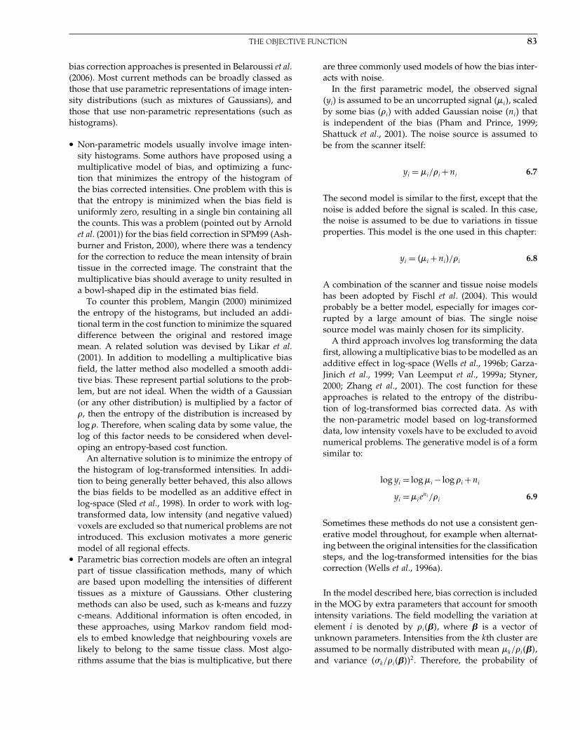
Elsevier UK Chapter: Ch06-P372560 3-10-2006 3:02p.m. Page:83 Trim:7.5in×9.25in
Basal Font:Palatino Margins:Top:40pt Gutter:68pt Font Size:9.5/12 Text Width:42pc Depth:55 Lines
THE OBJECTIVE FUNCTION 83
bias correction approaches is presented in Belaroussi et al.(2006). Most current methods can be broadly classed asthose that use parametric representations of image inten-sity distributions (such as mixtures of Gaussians), andthose that use non-parametric representations (such ashistograms).
• Non-parametric models usually involve image inten-sity histograms. Some authors have proposed using amultiplicative model of bias, and optimizing a func-tion that minimizes the entropy of the histogram ofthe bias corrected intensities. One problem with this isthat the entropy is minimized when the bias field isuniformly zero, resulting in a single bin containing allthe counts. This was a problem (pointed out by Arnoldet al. (2001)) for the bias field correction in SPM99 (Ash-burner and Friston, 2000), where there was a tendencyfor the correction to reduce the mean intensity of braintissue in the corrected image. The constraint that themultiplicative bias should average to unity resulted ina bowl-shaped dip in the estimated bias field.
To counter this problem, Mangin (2000) minimizedthe entropy of the histograms, but included an addi-tional term in the cost function to minimize the squareddifference between the original and restored imagemean. A related solution was devised by Likar et al.(2001). In addition to modelling a multiplicative biasfield, the latter method also modelled a smooth addi-tive bias. These represent partial solutions to the prob-lem, but are not ideal. When the width of a Gaussian(or any other distribution) is multiplied by a factor of, then the entropy of the distribution is increased bylog . Therefore, when scaling data by some value, thelog of this factor needs to be considered when devel-oping an entropy-based cost function.
An alternative solution is to minimize the entropy ofthe histogram of log-transformed intensities. In addi-tion to being generally better behaved, this also allowsthe bias fields to be modelled as an additive effect inlog-space (Sled et al., 1998). In order to work with log-transformed data, low intensity (and negative valued)voxels are excluded so that numerical problems are notintroduced. This exclusion motivates a more genericmodel of all regional effects.
• Parametric bias correction models are often an integralpart of tissue classification methods, many of whichare based upon modelling the intensities of differenttissues as a mixture of Gaussians. Other clusteringmethods can also be used, such as k-means and fuzzyc-means. Additional information is often encoded, inthese approaches, using Markov random field mod-els to embed knowledge that neighbouring voxels arelikely to belong to the same tissue class. Most algo-rithms assume that the bias is multiplicative, but there
are three commonly used models of how the bias inter-acts with noise.
In the first parametric model, the observed signal�yi� is assumed to be an uncorrupted signal ��i�, scaledby some bias �i� with added Gaussian noise �ni� thatis independent of the bias (Pham and Prince, 1999;Shattuck et al., 2001). The noise source is assumed tobe from the scanner itself:
yi = �i/i +ni 6.7
The second model is similar to the first, except that thenoise is added before the signal is scaled. In this case,the noise is assumed to be due to variations in tissueproperties. This model is the one used in this chapter:
yi = ��i +ni�/i 6.8
A combination of the scanner and tissue noise modelshas been adopted by Fischl et al. (2004). This wouldprobably be a better model, especially for images cor-rupted by a large amount of bias. The single noisesource model was mainly chosen for its simplicity.
A third approach involves log transforming the datafirst, allowing a multiplicative bias to be modelled as anadditive effect in log-space (Wells et al., 1996b; Garza-Jinich et al., 1999; Van Leemput et al., 1999a; Styner,2000; Zhang et al., 2001). The cost function for theseapproaches is related to the entropy of the distribu-tion of log-transformed bias corrected data. As withthe non-parametric model based on log-transformeddata, low intensity voxels have to be excluded to avoidnumerical problems. The generative model is of a formsimilar to:
log yi = log �i − log i +ni
yi =�ieni/i 6.9
Sometimes these methods do not use a consistent gen-erative model throughout, for example when alternat-ing between the original intensities for the classificationsteps, and the log-transformed intensities for the biascorrection (Wells et al., 1996a).
In the model described here, bias correction is includedin the MOG by extra parameters that account for smoothintensity variations. The field modelling the variation atelement i is denoted by i���, where � is a vector ofunknown parameters. Intensities from the kth cluster areassumed to be normally distributed with mean �k/i���,and variance ��k/i����2. Therefore, the probability of
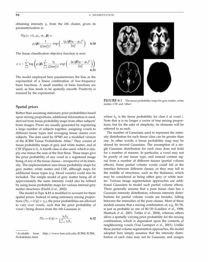
Elsevier UK Chapter: Ch06-P372560 3-10-2006 3:02p.m. Page:84 Trim:7.5in×9.25in
Basal Font:Palatino Margins:Top:40pt Gutter:68pt Font Size:9.5/12 Text Width:42pc Depth:55 Lines
84 6. SEGMENTATION
obtaining intensity yi from the kth cluster, given itsparameterization is:
P�yi�ci =k��k��k��� =
i���1
�2��2k �
12
exp(
− �i���yi −�k�2
2�2k
)6.10
The tissue classification objective function is now:
= −I∑
i=1
log
(i���
K∑k=1
�k
�2��2k �
12
exp(
− �i���yi −�k�2
2�2k
))
6.11
The model employed here parameterizes the bias as theexponential of a linear combination of low-frequencybasis functions. A small number of basis functions areused, as bias tends to be spatially smooth. Positivity isensured by the exponential.
Spatial priors
Rather than assuming stationary prior probabilities basedupon mixing proportions, additional information is used,derived from tissue probability maps from other subjects’brain images. Priors are usually generated by registeringa large number of subjects together, assigning voxels todifferent tissue types and averaging tissue classes oversubjects. The data used by SPM5 are a modified versionof the ICBM Tissue Probabilistic Atlas.2 They consist oftissue probability maps of grey and white matter, and ofCSF (Figure 6.1). A fourth class is also used, which is sim-ply one minus the sum of the first three. These maps givethe prior probability of any voxel in a registered imagebeing of any of the tissue classes – irrespective of its inten-sity. The implementation uses tissue probability maps forgrey matter, white matter and CSF, although maps foradditional tissue types (e.g. blood vessels) could also beincluded. The simple model of grey matter being all ofapproximately the same intensity could also be refinedby using tissue probability maps for various internal greymatter structures (Fischl et al., 2002).
The model in Eqn. 6.11 is modified to account for thesespatial priors. Instead of using stationary mixing propor-tions �P�ci = k��� = �k�, the prior probabilities are allowedto vary over voxels, such that the prior probability ofvoxel i being drawn from the kth Gaussian is:
P�ci = k��� = �kbik∑Kj=1 �jbij
6.12
2 Avaliable from http://www.loni.ucla.edu/ICBM/ICBM_Probabilistic.html
FIGURE 6.1 The tissue probability maps for grey matter, whitematter, CSF and ‘other’.
where bik is the tissue probability for class k at voxel i.Note that � is no longer a vector of true mixing propor-tions, but for the sake of simplicity, its elements will bereferred to as such.
The number of Gaussians used to represent the inten-sity distribution for each tissue class can be greater thanone. In other words, a tissue probability map may beshared by several Gaussians. The assumption of a sin-gle Gaussian distribution for each class does not holdfor a number of reasons. In particular, a voxel may notbe purely of one tissue type, and instead contain sig-nal from a number of different tissues (partial volumeeffects). Some partial volume voxels could fall at theinterface between different classes, or they may fall inthe middle of structures, such as the thalamus, whichmay be considered as being either grey or white mat-ter. Various image segmentation approaches use addi-tional Gaussians to model such partial volume effects.These generally assume that a pure tissue class has aGaussian intensity distribution, whereas intensity distri-butions for partial volume voxels are broader, fallingbetween the intensities of the pure classes. Most of thesemodels assume that a mixing combination of, e.g. 50/50,is just as probable as one of 80/20 (Laidlaw et al., 1998;Shattuck et al., 2001; Tohka et al., 2004), whereas othersallow a spatially varying prior probability for the mixingcombination, which is dependent upon the contents ofneighbouring voxels (Van Leemput et al., 2001). Unlikethese partial volume segmentation approaches, the modeladopted here simply assumes that the intensity distri-bution of each class may not be Gaussian, and assigns
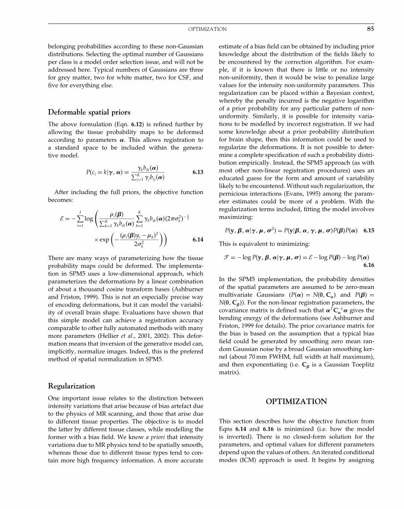
Elsevier UK Chapter: Ch06-P372560 3-10-2006 3:02p.m. Page:85 Trim:7.5in×9.25in
Basal Font:Palatino Margins:Top:40pt Gutter:68pt Font Size:9.5/12 Text Width:42pc Depth:55 Lines
OPTIMIZATION 85
belonging probabilities according to these non-Gaussiandistributions. Selecting the optimal number of Gaussiansper class is a model order selection issue, and will not beaddressed here. Typical numbers of Gaussians are threefor grey matter, two for white matter, two for CSF, andfive for everything else.
Deformable spatial priors
The above formulation (Eqn. 6.12) is refined further byallowing the tissue probability maps to be deformedaccording to parameters �. This allows registration toa standard space to be included within the genera-tive model.
P�ci = k����� = �kbik���∑Kj=1 �jbij���
6.13
After including the full priors, the objective functionbecomes:
� = −I∑
i=1
log
(i���∑K
k=1 �kbik���
K∑k=1
�kbik����2��2k �− 1
2
×exp(
− �i���yi −�k�2
2�2k
))6.14
There are many ways of parameterizing how the tissueprobability maps could be deformed. The implementa-tion in SPM5 uses a low-dimensional approach, whichparameterizes the deformations by a linear combinationof about a thousand cosine transform bases (Ashburnerand Friston, 1999). This is not an especially precise wayof encoding deformations, but it can model the variabil-ity of overall brain shape. Evaluations have shown thatthis simple model can achieve a registration accuracycomparable to other fully automated methods with manymore parameters (Hellier et al., 2001, 2002). This defor-mation means that inversion of the generative model can,implicitly, normalize images. Indeed, this is the preferedmethod of spatial normalization in SPM5.
Regularization
One important issue relates to the distinction betweenintensity variations that arise because of bias artefact dueto the physics of MR scanning, and those that arise dueto different tissue properties. The objective is to modelthe latter by different tissue classes, while modelling theformer with a bias field. We know a priori that intensityvariations due to MR physics tend to be spatially smooth,whereas those due to different tissue types tend to con-tain more high frequency information. A more accurate
estimate of a bias field can be obtained by including priorknowledge about the distribution of the fields likely tobe encountered by the correction algorithm. For exam-ple, if it is known that there is little or no intensitynon-uniformity, then it would be wise to penalize largevalues for the intensity non-uniformity parameters. Thisregularization can be placed within a Bayesian context,whereby the penalty incurred is the negative logarithmof a prior probability for any particular pattern of non-uniformity. Similarly, it is possible for intensity varia-tions to be modelled by incorrect registration. If we hadsome knowledge about a prior probability distributionfor brain shape, then this information could be used toregularize the deformations. It is not possible to deter-mine a complete specification of such a probability distri-bution empirically. Instead, the SPM5 approach (as withmost other non-linear registration procedures) uses aneducated guess for the form and amount of variabilitylikely to be encountered. Without such regularization, thepernicious interactions (Evans, 1995) among the param-eter estimates could be more of a problem. With theregularization terms included, fitting the model involvesmaximizing:
P�y����������2� = P�y�����������P���P��� 6.15
This is equivalent to minimizing:
� = − log P�y����������� = �− log P���− log P���6.16
In the SPM5 implementation, the probability densitiesof the spatial parameters are assumed to be zero-meanmultivariate Gaussians �P��� = N�0� C�� and P��� =N�0� C��). For the non-linear registration parameters, thecovariance matrix is defined such that �T C−1
� � gives thebending energy of the deformations (see Ashburner andFriston, 1999 for details). The prior covariance matrix forthe bias is based on the assumption that a typical biasfield could be generated by smoothing zero mean ran-dom Gaussian noise by a broad Gaussian smoothing ker-nel (about 70 mm FWHM, full width at half maximum),and then exponentiating (i.e. C� is a Gaussian Toeplitzmatrix).
OPTIMIZATION
This section describes how the objective function fromEqns 6.14 and 6.16 is minimized (i.e. how the modelis inverted). There is no closed-form solution for theparameters, and optimal values for different parametersdepend upon the values of others. An iterated conditionalmodes (ICM) approach is used. It begins by assigning

Elsevier UK Chapter: Ch06-P372560 3-10-2006 3:02p.m. Page:86 Trim:7.5in×9.25in
Basal Font:Palatino Margins:Top:40pt Gutter:68pt Font Size:9.5/12 Text Width:42pc Depth:55 Lines
86 6. SEGMENTATION
starting estimates for the parameters, and then iteratinguntil a locally optimal solution is found. Each iterationinvolves alternating between estimating different groupsof parameters, while holding the others fixed at their cur-rent ‘best’ solution (i.e. conditional mode). The mixtureparameters are updated using expectation maximization(EM), while holding the bias and deformations fixed attheir conditional modes. The bias is estimated while hold-ing the mixture parameters and deformation constant.Because intensity non-uniformity is very smooth, it canbe described by a small number of parameters, mak-ing the Levenberg-Marquardt (LM) scheme ideal for thisoptimization. The deformations of the tissue probabilitymaps are re-estimated while fixing the mixture parame-ters and bias field. A low-dimensional parameterizationis used for the spatial deformations, so the LM strategyis also applicable here.
The model is only specified for brain, as there are notissue probability maps for non-brain tissue (scalp etc).Because of this, there is a tendency for the approachto stretch the probability maps so that the backgroundclass contains only air, but no scalp. A workaroundinvolves excluding extra-cranial voxels from the fittingprocedure. This is done by fitting a mixture of two Gaus-sians to the image intensity histogram. In most cases,one Gaussian fits air, and the other fits everything else.A suitable threshold is then determined, based on a50 per cent probability. Fitting only the intra-cranial vox-els also saves time.
Mixture parameters (��� and �)
It is sufficient to minimize with respect to the mix-ture parameters because they do not affect the prior orregularization terms in � (see Eqn. 6.16). For simplic-ity, we summarize the parameters of interest by � =�����������. These are optimized by EM (see e.g.Dempster et al., 1977; Bishop, 1995 or Neal and Hinton,1998), which can be considered as using some distribu-tion, qik, to minimize the following upper bound on �:
≤ EM = −I∑
i=1
log P�yi���
+I∑
i=1
K∑k=1
qik log(
qik
P�ci = k�yi���
)6.17
EM is an iterative approach, and involves alternatingbetween an E-step (which minimizes �EM with respect toqik), and an M-step (which minimizes �EM with respectto �). The second term of Eqn. 6.17 is a Kullback-Leiblerdistance, which is at a minimum of zero when qik = P�ci =k�yi���, and Eqn. 6.17 becomes an equality �� = �EM�.
Because qik does not enter into the first term, the E-stepof iteration n consists of setting:
q�n�ik = P�ci = k�yi���n�� = P�yi� ci = k���n��
P�yi���n��
= pik∑Kj=1 pij
6.18
where
pik = �kbik���∑Kj=1 �jbij���
�2��2k �− 1
2
×exp(
− �i���yi −�k�2
2�2k
)6.19
The M-step uses the recently updated values of q�n�ik in
order to minimize with respect to �. Eqn. 6.17 can bereformulated3 as:
= EM = −I∑
i=1
K∑k=1
qik log P�yi� ci = k���
+I∑
i=1
K∑k=1
qik log qik 6.20
Because the second term is independent of �, the M-stepinvolves assigning new values to the parameters, suchthat the derivatives of the following are zero:
−I∑
i=1
K∑k=1
qik log P�yi� ci = k��� =
I∑i=1
K∑k=1
qik
(log
(K∑
j=1
�jbij���
)− log �k
)
+I∑
i=1
K∑k=1
qik
(12
log��2k �+ 1
2�2�i���yi −�k�
2)
+I∑
i=1
K∑k=1
qik
(12
log�2��− log�i���bik����
)6.21
Differentiating Eqn. 6.21 with respect to �k gives:
�
�k
=
�k
=I∑
i=1
q�n�ik
�2k
��k −i���yi� 6.22
This gives the update formula for �k by solving for � �k
= 0
��n+1�k =
∑Ii=1 q�n�
ik i���yi∑Ii=1 q�n�
ik
6.23
3 Through Bayes’ rule, and because∑K
k=1 qik = 1, we obtain
log P�yi��� = log(
P�yi�ci=k���
P�ci=k�yi���
)=∑K
k=1 qik log(
P�yi�ci=k���
P�ci=k�yi���
).

Elsevier UK Chapter: Ch06-P372560 3-10-2006 3:02p.m. Page:87 Trim:7.5in×9.25in
Basal Font:Palatino Margins:Top:40pt Gutter:68pt Font Size:9.5/12 Text Width:42pc Depth:55 Lines
OPTIMIZATION 87
Similarly, differentiating Eqn. 6.21 with respect to �2k :
�
�2k
= �
�2k
=∑I
i=1 q�n�ik
2�2k
−∑I
i=1 q�n�ik ��k −i���yi�
2
2��2k �2
6.24
This gives the update formula for �2k :
��2k ��n+1� =
∑Ii=1 q�n�
ik ���n+1�k −i���yi�
2
∑Ii=1 q�n�
ik
6.25
Differentiating Eqn. 6.21 with respect to �k:
�
�k
=
�k
=I∑
i=1
bik���∑Kj=1 �jbij���
−∑I
i=1 q�n�ik
�k
6.26
Deriving an exact update scheme for �k is difficult, butthe following ensures convergence:4
��n+1�k =
∑Ii=1 q�n�
ik∑Ii=1
bik���∑Kj=1 �
�n�j bij ���
6.27
Bias (�)
The next step is to update the estimate of the bias field.This involves holding the other parameters fixed, andimproving the estimate of � using an LM optimizationapproach (see Press et al., 1992 for more information).Each iteration requires the first and second derivativesof the objective function, with respect to the parameters.In the following scheme, I is an identity matrix and � isa scaling factor. The choice of � is a trade-off betweenspeed of convergence, and stability. A value of zero for �gives the Newton-Raphson or Gauss-Newton optimiza-tion scheme, which may be unstable. Increasing � willslow down the convergence, but increase the stability ofthe algorithm. The value of � is usually decreased slightlyafter iterations that decrease (improve) the cost function.If the cost function increases after an iteration, then theprevious solution is retained, and � is increased in orderto provide more stability.
��n+1� = ��n� −(
2�
�2
∣∣∣��n�
+�I)−1
F
�
∣∣∣��n�
6.28
The prior probability of the parameters is modelled by amultivariate Gaussian density, with mean �0 and covari-ance C�.
− log P��� = 12
��−�0�C�−1��−�0�+ const 6.29
4 The update scheme was checked empirically, and found toalways reduce �. It does not fully minimize it though, whichmeans that this part of the algorithm is really a generalized EM.
The first and second derivatives of � (see Eqn. 6.16) withrespect to the parameters are therefore:
�
�=
�+C�
−1��−�0� and 2�
�2= 2
�2+C�
−1 6.30
The first and second partial derivatives of are:
�m
= −I∑
i=1
i���
�m
×(
i���−1 +yi
∑Kk=1
qik��k −i���yi�
�2k
)6.31
2
�m�n
=∑Ii=1
i���
�m
i���
�n
(i���−2 +y2
i
∑Kk=1
qik
�2k
)
−∑ Ii=1
2i���
�m �n
×(
i���−1 +yi
∑Kk=1
qik ��k −i���yi�
�2k
)6.32
The bias field is parameterized by the exponential of alinear combination of smooth basis functions:
i��� = exp
(M∑
m=1
�m�im
)�
i���
�m
= �imi����
and 2i���
�m �n
= �im�ini��� 6.33
Therefore, the derivatives used by the optimization are:
�m
=−∑ Ii=1�im
(1+i���yi
∑Kk=1
qik��k −i���yi�
�2k
)
2
�m�n
=∑ Ii=1�im�in
(�i���yi�
2∑
Kk=1
qik
�2k
−i���yi
∑Kk=1
qik ��k −i���yi�
�2k
)6.34
Deformations (�)
The same LM strategy (Eqn. 6.28) is used as for updatingthe bias. Schemes such as LM or Gauss-Newton are usu-ally used only for registering images with a mean squareddifference objective function, although some rare excep-tions exist where LM has been applied to information-theoretic image registration (Thévenaz and Unser, 2000).The strategy requires the first and second derivatives ofthe cost function, with respect to the parameters thatdefine the deformation. In order to simplify deriving the

Elsevier UK Chapter: Ch06-P372560 3-10-2006 3:02p.m. Page:88 Trim:7.5in×9.25in
Basal Font:Palatino Margins:Top:40pt Gutter:68pt Font Size:9.5/12 Text Width:42pc Depth:55 Lines
88 6. SEGMENTATION
derivatives, the likelihood component of the objectivefunction is re-expressed as:
� = −I∑
i=1
log
(K∑
k=1
fiklik
)−
I∑i=1
log i��� 6.35
where
fik = bik���∑Kj=1 �jbij���
6.36
and
lik = �k�2��2k �− 1
2 exp(
− �i���yi −�k�2
2�2k
)6.37
The first derivatives of with respect to � are:
�m
= −I∑
i=1
∑Kk=1
fik
�mlik∑K
k=1 fiklik6.38
The second derivatives are:
2�
�m �n
=I∑
i=1
(∑Kk=1
fik
�mlik
)(∑Kk=1
fik
�nlik
)(∑K
k=1 fiklik)2
−I∑
i=1
∑Kk=1
2fik
�m �nlik∑K
k=1 fiklik6.39
The following is needed in order to compute deriva-tives of with respect to �:
fik
�m
= bik���
�m∑Kj=1 �jbij���
− bik���∑K
j=1 �j bij ���
�m(∑Kj=1 �jbij���
)2 6.40
The second term in Eqn. 6.39 is ignored in the opti-mization (Gauss-Newton approach), but it could be used(Newton-R̀aphson approach). These gradients and cur-vatures enter the update scheme as in Eqn. 6.28.
The chain rule is used to compute derivatives of fik,based on the rate of change of the deformation fieldswith respect to changes of the parameters, and the tissueprobability map gradients sampled at the appropriatepoints. Trilinear interpolation could be used as the tissueprobability maps contain values between zero and one.Care is needed when attempting to sample the imageswith higher degree B-spline interpolation (Thévenaz et al.,2000), as negative values should not occur. B-spline inter-polation (and other generalized interpolation methods)require coefficients to be estimated first. This essentiallyinvolves deconvolving the B-spline bases from the image(Unser et al., 1993a, b). Sampling an interpolated valuein the image is then done by re-convolving the coef-ficients with the B-spline. Without any non-negativity
constraints on the coefficients, there is a possibility ofnegative values occurring in the interpolated probabil-ity map.
One possible solution is to use a maximum-likelihooddeconvolution strategy to estimate some suitable coef-ficients. This is analogous to the iterative method formaximum-likelihood reconstruction of PET (positronemission tomography) images (Shepp and Vardi, 1982),or to the way that mixing proportions are estimatedwithin a mixture of Gaussians model. A second solu-tion is to add a small background value to the probabil-ity maps, and take a logarithm. Standard interpolationmethods could be applied to the log-transformed data,before exponentiating again. Neither of these approachesis really optimal. In practice, 3rd degree B-spline inter-polation is used, but without first deconvolving. Thisintroduces a small, but acceptable, amount of additionalsmoothness to the tissue probability maps.
Example
The segmentation accuracy is illustrated for data gener-ated by the BrainWeb MR simulator (Kwan et al., 1996;Cocosco et al., 1997; Collins et al., 1998). The simulatedimages were all of the same subject, had dimensions of181 × 217 × 181 voxels of 1 × 1 × 1 mm and had 3 percent noise (relative to the brightest tissue in the images).The contrasts of the images simulated T1-weighted, T2-weighted and proton density (PD). The T1-weightedimage was simulated as a spoiled FLASH sequence, witha 30� flip angle, 18 ms repeat time, 10 ms echo time. TheT2 and PD images were simulated by a dual echo spinecho, early echo technique, with 90� flip angle, 3300 msrepeat time and echo times of 35 and 120 ms. Three differ-ent levels of image non-uniformity were used: 0 per centRF (which assumes that there is no intensity variationartefact), 40 per cent RF, and 100 per cent RF (Figure 6.2).Three components were considered: grey matter, whitematter and whole brain (grey and white matter). Becausethe causes of the simulated images were available, itwas possible to compare the segmented images withimages of ‘true’ grey and white matter using the Dicemetric, which is used widely for evaluating segmenta-tion algorithms (e.g. Van Leemput et al., 1999b; Shattucket al., 2001). The probabilities were thresholded at 0.5 inorder to compute the number of misclassifications. If TPrefers to the number of true positives, FP to false posi-tives and FN to false negatives, then the Dice metric isgiven by:
Dice metric = 2×TP2×TP+FP+FN
6.41

Elsevier UK Chapter: Ch06-P372560 3-10-2006 3:02p.m. Page:89 Trim:7.5in×9.25in
Basal Font:Palatino Margins:Top:40pt Gutter:68pt Font Size:9.5/12 Text Width:42pc Depth:55 Lines
OPTIMIZATION 89
FIGURE 6.2 Results from applying themethod to the BrainWeb data. The first columnshows the tissue probability maps for grey andwhite matter. The first row of columns two, threeand four show the 100 per cent RF BrainWeb T1, T2and PD images after they are warped to match thetissue probability maps (by inverting the spatialtransform). Below the warped BrainWeb imagesare the corresponding segmented grey and whitematter.
Our results are shown in Table 6-1. Values range fromzero to one, where higher values indicate better agree-ment.
Discussion
This chapter illustrates a framework whereby tissue clas-sification, bias correction and image registration are inte-grated within the same generative model. The objectivewas to explain how this can be done, rather than focuson the details of a specific implementation. The sameframework could be used for a more sophisticated imple-mentation. When devising a model, it is useful to thinkabout how that model could be used to generate data. Thedistribution of randomly generated data should matchthe distribution of any data the model has to explain.
There are a number of aspects of our model that couldbe improved in order to achieve this goal.
The SPM5 implementation assumes that the brain con-sists of grey and white matter, and is surrounded by athin layer of CSF. The addition of extra tissue probabil-ity maps should improve the model. In particular, greymatter classes for internal structures may allow them tobe segmented more accurately.
It is only a single channel implementation, which cansegment a single image, but is unable to make optimaluse of information from two or more registered images ofthe same subject. Multispectral data may provide moreaccurate results by allowing the model to work withjoint intensity probability distributions. For two regis-tered images of the same subject, one form of objectivefunction would use axis-aligned multivariate Gaussians(with �2
k1 and �2k2 are diagonal elements of a 2×2 covari-
ance matrix).
TABLE 6-1 Dice metrics computed from segmented BrainWeb images
Dice metric
T1 T2 PD
0% 40% 100% 0% 40% 100% 0% 40% 100%
Grey matter 0.932 0.934 0.918 0.883 0.881 0.880 0.872 0.880 0.872White matter 0.961 0.961 0.939 0.916 0.916 0.915 0.923 0.928 0.923Whole brain 0.977 0.978 0.978 0.967 0.966 0.965 0.957 0.959 0.955

Elsevier UK Chapter: Ch06-P372560 3-10-2006 3:02p.m. Page:90 Trim:7.5in×9.25in
Basal Font:Palatino Margins:Top:40pt Gutter:68pt Font Size:9.5/12 Text Width:42pc Depth:55 Lines
90 6. SEGMENTATION
� =−∑ Ii=1 log
(i1���i2���∑K
k=1 �kbik���
)
−∑ Ii=1 log
(∑Kk=1�kbik���
×exp
(− �i1���yi1−�k1�2
2�2k1
)
�2��2k1�
12
exp(− �i2���yi2−�k2�2
2�2k2
)
�2��2k2�
12
⎞⎠ 6.42
Multispectral classification usually requires the images tobe registered together. Another possible extension of theframework could be to include within-subject registration(Xiaohua et al., 2004).
The generative model contains nothing to encode theprobability that neighbouring voxels are more likely tobelong to the same class. The inclusion of such priorsshould make the generative model more realistic. Onesolution could be to include a Markov random field(MRF) (Besag, 1986) in the model. Another strategy formaking the model more realistic may be to have crispertissue probability maps, and more precise warping.
Objective functions, such as the mean squared differ-ence or cross-correlation, can only be used to registerMR images generated using the same sequences, fieldstrengths etc. An advantage that they do have over infor-mation theoretic measures (such as mutual information),is that they are also appropriate for registering to smoothaveraged images. One of the benefits of the approachis that the same averaged tissue probability maps canbe used to normalize spatially (and segment) imagesacquired with a wide range of different contrasts (e.g.T1-weighted, T2-weighted etc). This flexibility could alsobe considered a weakness. If the method is only to beused with images of a particular contrast, then additionalconstraints relating to the approximate intensities of thedifferent tissue types could be included (Fischl et al.,2002). Alternatively, the MR parameters could be esti-mated within the model (Fischl et al., 2004), and the clus-ter means constrained to be more realistic. Rather thanusing fixed intensity distributions for the classes, a betterapproach would invoke some kind of hierarchical mod-elling, whereby prior probability distributions for thecluster parameters are used to inform their estimation.
The hierarchical modelling scheme could be extendedin order to generate tissue probability maps and otherpriors using data from many subjects. This would involvea very large model, whereby many images of differentsubjects are simultaneously processed within the samehierarchical framework. Strategies for creating average(in both shape and intensity) brain atlases are currentlybeing devised (Ashburner et al., 2000; Avants and Gee,2004; Joshi et al., 2004). Such approaches could be refinedin order to produce average shaped tissue probabilitymaps and other data for use as priors.
REFERENCES
Arnold JB, Liow JS, Schaper KA et al. (2001) Qualitative and quan-titative evaluation of six algorithms for correcting intensitynonuniformity effect. NeuroImage 13: 931–43
Ashburner J, Andersson J, Friston KJ (2000) Image registrationusing a symmetric prior – in three-dimensions. Hum Brain Mapp9: 212–25
Ashburner J, Friston KJ (1999) Nonlinear spatial normalization usingbasis functions. Hum Brain Mapp 7: 254–66
Ashburner J, Friston KJ (2000) Voxel-based morphometry – themethods. NeuroImage 11: 805–21
Avants B, Gee JC (2004) Geodesic estimation for large deformationanatomical shape averaging and interpolation. NeuroImage 23:S139–S50
Belaroussi B, Milles J, Carme S et al. (2006) Intensity non-uniformitycorrection in MRI: Existing methods and their validation. MedImage Anal 10: 234–46
Besag J (1986) On the statistical analysis of dirty pictures. J R StatSoc Ser B 48: 259–302
Bishop CM (1995) Neural networks for pattern recognition. OxfordUniversity Press, Oxford
Cocosco CA, Kollokian V, Kwan RK-S et al. (1997) Brainweb: onlineinterface to a 3D MRI simulated brain database. NeuroImage5: S425
Collins DL, Evans AC, Holmes C et al. (1995) Automatic 3D segmen-tation of neuro-anatomical structures from MRI. In Proc Informa-tion Processing in Medical Imaging (IPMI), Bizais Y, Barillot C, DiPaola R (eds). Kluwer Academic Publishers, Dordrecht
Collins DL, Zijdenbos AP, Kollokian V et al. (1998). Design andconstruction of a realistic digital brain phantom. IEEE Trans MedImag 17: 463–68
Dempster AP, Laird NM, Rubin DB (1977) Maximum likelihoodfrom incomplete data via the EM algorithm. J R Stat Soc Series B39: 1–38
Evans AC (1995) Commentary. Hum Brain Mapp 2: 165–89Fischl B, Salat DH, Busa E et al. (2002) Whole brain segmentation:
automated labeling of neuroanatomical structures in the humanbrain. Neuron 33: 341–55
Fischl B, Salat DH, van der Kouwe AJW et al. (2004) Sequence-independent segmentation of magnetic resonance images. Neu-roImage 23: S69–S84
Fissell K, Tseytlin E, Cunningham D, et al. (2003) Fiswidgets: agraphical computing environment for neuroimaging analysis.Neuroinformatics 1: 111–25
Garza-Jinich M, Yanez O, Medina V et al. (1999) Automatic correc-tion of bias field in magnetic resonance images. In Proc Interna-tional Conference on Image Analysis and Processing IEEE ComputerSociety, CA.
Hellier P, Ashburner J, Corouge I et al. (2002) Inter subject registra-tion of functional and anatomical data using SPM. In Proc Medi-cal Image Computing and Computer-Assisted Intervention (MICCAI),vol. 2489 of Lecture Notes in Computer Science. Springer-Verlag,Berlin and Heidelberg
Hellier P, Barillot C, Corouge I et al. (2001) Retrospective evalu-ation of inter-subject brain registration. In Proc Medical ImageComputing and Computer-Assisted Intervention (MICCAI), NiessenWJ, Viergever MA (eds), vol. 2208 of Lecture Notes in ComputerScience. Springer-Verlag, Berlin and Heidelberg, pp 258–65
Joshi S, Davis B, Jomier M et al. (2004) Unbiased diffeomorphicatlas construction for computational anatomy. NeuroImage 23:S151–S60
Elsevier UK Chapter: Ch06-P372560 3-10-2006 3:02p.m. Page:91 Trim:7.5in×9.25in
Basal Font:Palatino Margins:Top:40pt Gutter:68pt Font Size:9.5/12 Text Width:42pc Depth:55 Lines
REFERENCES 91
Kwan RK-S, Evans AC, Pike GB (1996) An extensible MRI simulatorfor post-processing evaluation. In Proc Visualization in BiomedicalComputing, Springer Verlag
Laidlaw DH, Fleischer KW, Barr AH (1998) Partial-volume bayesianclassification of material mixtures in MR volume data usingvoxel histograms. IEEE Trans Med Imag 17: 74–86
Likar B, Viergever MA, Pernuš F (2001) Retrospective correction ofMR intensity inhomogeneity by information minimization. IEEETrans Med Imag 20: 1398–410
MacDonald D, Kabani N, Avis D et al. (2000) Automated 3-D extrac-tion of inner and outer surfaces of cerebral cortex from MRI.NeuroImage 12: 340–56
Mangin J-F (2000) Entropy minimization for automatic correction ofintensity nonuniformity. In Proc IEEE Workshop on MathematicalMethods in Biomedical Image Analysis IEEE Computer Society, CA
Neal RM, Hinton GE (1998) A view of the EM algorithm that justifiesincremental, sparse, and other variants. In Learning in GraphicalModels, Jordan MI (ed.) Kluwer Academic Publishers, Dordrecht,pp 355–68
Pham DL, Prince JL (1999) Adaptive fuzzy segmentation of magneticresonance images. IEEE Trans Med Imag 18: 737–52
Pitiot A, Delingette H, Thompson PM et al. (2004) Expert knowledge-guided segmentation system for brain MRI. NeuroImage 23:S85–S96
Press WH, Teukolsky SA, Vetterling WT et al. (1992) NumericalRecipes in C, 2nd edn. Cambridge University Press, Cambridge
Rex DE, Maa JQ, Toga AW (2003) The LONI pipeline processingenvironment. NeuroImage 19: 1033–48
Shattuck DW, Sandor-Leahy SR, Schaper KA et al. (2001) Mag-netic resonance image tissue classification using a partial volumemodel. NeuroImage 13: 856–76
Shepp LA, Vardi Y (1982) Maximum likelihood reconstruction inpositron emission tomography. IEEE Trans Med Imag 1: 113–22
Sled JG, Zijdenbos AP, Evans AC (1998) A non-parametric methodfor automatic correction of intensity non-uniformity in MRI data.IEEE Trans Med Imag 17: 87–97
Styner M (2000) Parametric estimate of intensity inhomogeneitiesapplied to MRI. IEEE Trans Med Imag 19: 153–65
Thévenaz P, Blu T, Unser M (2000) Interpolation revisited. IEEETrans Med Imag 19: 739–58
Thévenaz P, Unser M (2000) Optimization of mutual informationfor multiresolution image registration. IEEE Trans Image Process9: 2083–99
Tohka J, Zijdenbos A, Evans A (2004) Fast and robust parameterestimation for statistical partial volume models in brain MRI.NeuroImage 23: 84–97
Unser M, Aldroubi A, Eden M (1993a) B-spline signal processing:Part I – theory. IEEE Trans Signal Process 41: 821–33
Unser M, Aldroubi A, Eden M (1993b) B-spline signal processing:Part II – efficient design and applications. IEEE Trans SignalProcess 41: 834–48
Van Leemput K, Maes F, Vandermeulen D et al. (1999a) Automatedmodel-based bias field correction of MR images of the brain.IEEE Trans Med Imag 18: 885–96
Van Leemput K, Maes F, Vandermeulen D et al. (1999b) Automatedmodel-based tissue classification of MR images of the brain. IEEETrans Med Imag 18: 897–908
Van Leemput K, Maes F, Vandermeulen D et al. (2001) A statisti-cal framework for partial volume segmentation. In Proc MedicalImage Computing and Computer-Assisted Intervention (MICCAI),Niessen WJ, Viergever MA (eds) vol. 2208 of Lecture Notes inComputer Science. Springer-Verlag, Berlin and Heidelberg, pp204–12
Wells WM III, Grimson WEL, Kikinis R et al. (1996a) Adaptivesegmentation of MRI data. IEEE Trans Med Imag 15: 429–42
Wells WM III, Viola P, Atsumi H et al. (1996b) Multi-modal volumeregistration by maximisation of mutual information. Med ImageAnal 1: 35–51
Xiaohua C, Brady M, Rueckert D (2004) Simultaneous segmentationand registration for medical image. In Proc Medical Image Com-puting and Computer-Assisted Intervention (MICCAI), Barillot C,Haynor DR, Hellier P (eds) vol. 3216 of Lecture Notes in ComputerScience. Springer-Verlag, Berlin and Heidelberg, pp 663–70
Zhang Y, Brady M, Smith S (2001) Segmentation of brain MRimages through a hidden markov random field model andthe expectation-maximization algorithm. IEEE Trans Med Imag20: 45–57
Zijdenbos AP, Forghani R, Evans AC (2002) Automatic ‘pipeline’analysis of 3-D MRI data for clinical trials: application to multiplesclerosis. IEEE Trans Med Imag 21: 1280–91
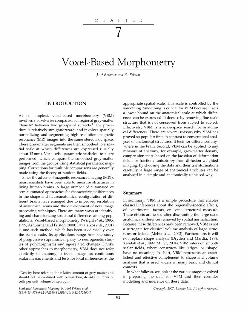
Elsevier UK Chapter: Ch07-P372560 3-10-2006 3:03p.m. Page:92 Trim:7.5in×9.25in
Basal Font:Palatino Margins:Top:40pt Gutter:68pt Font Size:9.5/12 Text Width:42pc Depth:55 Lines
C H A P T E R
7
Voxel-Based MorphometryJ. Ashburner and K. Friston
INTRODUCTION
At its simplest, voxel-based morphometry (VBM)involves a voxel-wise comparison of regional grey-matter‘density’ between two groups of subjects.1 The proce-dure is relatively straightforward, and involves spatiallynormalizing and segmenting high-resolution magneticresonance (MR) images into the same stereotaxic space.These grey-matter segments are then smoothed to a spa-tial scale at which differences are expressed (usuallyabout 12 mm). Voxel-wise parametric statistical tests areperformed, which compare the smoothed grey-matterimages from the groups using statistical parametric map-ping. Corrections for multiple comparisons are generallymade using the theory of random fields.
Since the advent of magnetic resonance imaging (MRI),neuroscientists have been able to measure structures inliving human brains. A large number of automated orsemiautomated approaches for characterizing differencesin the shape and neuroanatomical configuration of dif-ferent brains have emerged due to improved resolutionof anatomical scans and the development of new imageprocessing techniques. There are many ways of identify-ing and characterizing structural differences among pop-ulations. Voxel-based morphometry (Wright et al., 1995,1999; Ashburner and Friston, 2000; Davatzikos et al., 2001)is one such method, which has been used widely overthe past decade. Its applications range from the studyof progressive supranuclear palsy to neurogenetic stud-ies of polymorphisms and age-related changes. Unlikeother approaches to morphometry, VBM does not referexplicitly to anatomy; it treats images as continuousscalar measurements and tests for local differences at the
1 Density here refers to the relative amount of grey matter andshould not be confused with cell-packing density (number ofcells per unit volume of neuropil).
appropriate spatial scale. This scale is controlled by thesmoothing. Smoothing is critical for VBM because it setsa lower bound on the anatomical scale at which differ-ences can be expressed. It does so by removing fine-scalestructure that is not conserved from subject to subject.Effectively, VBM is a scale-space search for anatomi-cal differences. There are several reasons why VBM hasproved so popular: first, in contrast to conventional anal-yses of anatomical structures, it tests for differences any-where in the brain. Second, VBM can be applied to anymeasure of anatomy, for example, grey-matter density,compression maps based on the Jacobian of deformationfields, or fractional anisotropy from diffusion weightedimaging. By choosing the data and their transformationscarefully, a large range of anatomical attributes can beanalysed in a simple and anatomically unbiased way.
Summary
In summary, VBM is a simple procedure that enablesclassical inferences about the regionally-specific effects,of experimental factors, on some structural measure.These effects are tested after discounting the large-scaleanatomical differences removed by spatial normalization.Because these differences have been removed, VBM is nota surrogate for classical volume analysis of large struc-tures or lesions (Mehta et al., 2003). Furthermore, it willnot replace shape analysis (Dryden and Mardia, 1998;Kendall et al., 1999; Miller, 2004); VBM infers on smoothscalar fields, where constructs like ‘edges’ or ‘shape’have no meaning. In short, VBM represents an estab-lished and effective complement to shape and volumeanalyses that is used widely in many basic and clinicalcontexts.
In what follows, we look at the various stages involvedin preparing the data for VBM and then considermodelling and inference on these data.
Statistical Parametric Mapping, by Karl Friston et al. Copyright 2007, Elsevier Ltd. All rights reserved.ISBN–13: 978-0-12-372560-8 ISBN–10: 0-12-372560-7
92

Elsevier UK Chapter: Ch07-P372560 3-10-2006 3:03p.m. Page:93 Trim:7.5in×9.25in
Basal Font:Palatino Margins:Top:40pt Gutter:68pt Font Size:9.5/12 Text Width:42pc Depth:55 Lines
PREPARING THE DATA 93
PREPARING THE DATA
VBM relies on good quality high-resolution MR imagesfrom different subjects, and uses these to identify corre-lations between disease severity and the spatial deploy-ment of different tissue types. Many researchers assumethat voxel-based morphometry can only be implementedwithin the statistical parametric mapping package; this isnot the case. There are many software tools that could beused to perform the requisite sequence of operations. TheMR images are segmented, producing images that reflectthe spatial distribution of a tissue type or attribute (e.g.grey matter). To compare brains of different subjects, allthe grey-matter segments are warped to the same stereo-taxic space. A correction can be applied to the data thataccounts for expansion and contraction during this non-linear spatial normalization. The normalized segmentsare then smoothed. This makes each voxel a measure ofthe proportion of the brain, in a region around the voxelthat is grey matter (i.e. grey-matter density). Statisticalanalysis using the general linear model (GLM) is used toidentify regions that are significantly related to the effectsunder study (Friston et al., 1995). The GLM is a flexibleframework that allows many different tests to be applied.The output is a statistical parametric map (SPM) showingregions where tissue density differs significantly amongthe groups. A voxel-wise SPM comprises the result ofmany statistical tests, so it is necessary to correct for mul-tiple dependent comparisons using the theory of randomfields (Friston et al., 1996; Worsley et al.,1996, 1999).
Segmentation
The images are typically partitioned into different tis-sue classes using one of a number of segmentationtechniques. Usually, VBM involves an analysis of greymatter, but it is possible to work with other tissueclasses or any other scalar measure of anatomy (e.g. frac-tional anisotropy). To segment the images accurately,the image needs to show clear differentiation amongtissue types. Usually, high resolution T1-weighted MRimages are used (Figure 7.1), although multispectralimages may allow more accurate tissue classification.Different segmentation models have different require-ments. For example, many approaches take smooth inten-sity inhomogeneities into account, so they can dealwith some of the artefacts that arise in MR images.Most automated segmentation algorithms assume thatthe intracranial cavity contains only grey matter, whitematter and cerebrospinal fluid (CSF), so they maybe confounded by lesions. However, there are somethat have been especially designed for dealing withsuch pathology (Van Leemput et al., 2001), although
FIGURE 7.1 This figure shows the result of segmenting thegrey matter from a T1-weighted MR image. Note that towardsthe top of the brain, the segmentation is less accurate because thegrey matter is hardly visible in the original image. Similarly, ingrey-matter regions such as thalamus, the intensity is closer tothat of white matter, resulting in incorrect segmentation. Some par-tial volume voxels can be seen around the ventricles. These arisebecause voxels containing signal from both white matter and CSFhave intensities that are close to grey matter.
they generally require multispectral images (e.g. alignedT1- and T2-weighted scans).
Many segmentation approaches use prior spatial infor-mation in the form of tissue probability maps, whichinform the segmentation algorithm about the approxi-mate spatial distribution of the various tissues. In mostcases, the tissue probability maps need to be regis-tered with the image to segment, but the segmentation

Elsevier UK Chapter: Ch07-P372560 3-10-2006 3:03p.m. Page:94 Trim:7.5in×9.25in
Basal Font:Palatino Margins:Top:40pt Gutter:68pt Font Size:9.5/12 Text Width:42pc Depth:55 Lines
94 7. VOXEL-BASED MORPHOMETRY
framework of SPM5 combines this registration with thetissue classification (Ashburner and Friston, 2005).
Spatial normalization
Spatial normalization involves warping all the grey-matter images to the same stereotaxic space, which isachieved by matching to a common template image(Figure 7.2). There are many non-linear registration meth-ods that could be used for this. The unified segmentation-normalization approach (Ashburner and Friston, 2005)in SPM5 is a robust procedure because it accommo-dates conditional dependences among the segmentationand normalization parameters. It is a low-dimensionalmethod, which uses about a thousand parameters todescribe the deformations. Other approaches have manymore degrees of freedom, and may be more accurate.However, just because a method can warp anything toanything else, does not mean that it furnishes the mostlikely registration (high-dimensional procedures gener-ally overfit the data). For example, the evaluations ofHellier et al. (2001, 2002), which compared registrationaccuracy of different approaches, found that the simplespatial normalization of SPM2 was as accurate as othermethods with more degrees of freedom.
The objective of VBM is to localize regions (in stereo-taxic space) where there are significant differences.Accurate spatial normalization and segmentationensures regional differences can be attributable to
FIGURE 7.2 An image (top left) is warped to match a template(top right) to produce a spatially normalized version (top centre).For clarity, the original image was approximately aligned with thetemplate, and the warping only done in two dimensions. The bottomrow shows the difference between the template and image, bothbefore and after the warping.
local effects, rather than systematic, pathology-inducedmis-registration artefacts (Bookstein, 2001). However,registration can never be perfect because there is nocorrespondence between one subject and another at afine spatial scale. For example, many sulci are sharedbetween brains, but this is not the case for all. Generally,the primary sulci, which are formed earliest and tendto be quite deep, are conserved over subjects. Sulci thatdevelop later are much more variable. Therefore, somesulci can be matched objectively, whereas others cannot.VBM accommodates the fact that the scale of anatomicalcorrespondence, and implicitly the scale of differences inanatomy, has a lower bound by smoothing the segments(see below).
Jacobian adjustment
Non-linear spatial normalization changes the volumesof brain regions. This has implications for the inter-pretation of what VBM tests. The objective of VBM isto identify regional differences in the composition ofbrain tissue. To preserve the actual amounts of a tissueclass within each voxel (Goldszal et al., 1998; Davatzikoset al., 2001), a further processing step can be incorpo-rated that multiplies (modulates) the partitioned imagesby the relative voxel volumes before and after warping.These relative volumes are simply the Jacobian determi-nants of the deformation field (Figure 7.3). In the lim-iting case of extremely precise registration (using veryhigh-dimensional registration), all the segments wouldbe identical. The adjustment preserves the differences involume of a particular tissue class (Figure 7.4).
The deformations from spatial normalization mappoints in a template �x1�x2�x3� to equivalent points inindividual source images �y1�y2�y3�. The derivatives ofthe deformation field can be thought of as matrix at eachpoint. These are the Jacobian matrices of the deforma-tions, and are defined by:
J =⎡⎣�y1/�x1 �y1/�x2 �y1/�x3
�y2/�x1 �y2/�x2 �y2/�x3
�y3/�x1 �y3/�x2 �y3/�x3
⎤⎦
The determinant of this matrix encodes the relative vol-umes of deformed and undeformed structures.
Smoothing
The warped grey-matter images are now smoothed byconvolving with an isotropic Gaussian kernel. This makesthe subsequent voxel-by-voxel analysis comparable to aregion of interest approach, because each voxel in the
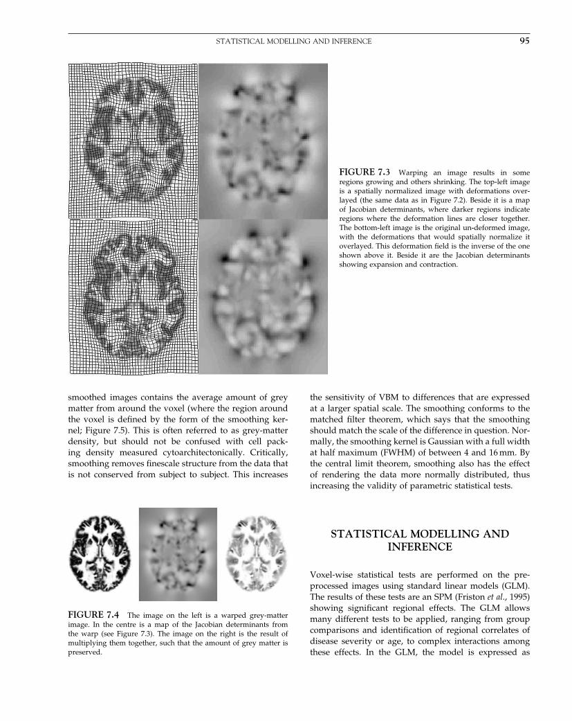
Elsevier UK Chapter: Ch07-P372560 3-10-2006 3:03p.m. Page:95 Trim:7.5in×9.25in
Basal Font:Palatino Margins:Top:40pt Gutter:68pt Font Size:9.5/12 Text Width:42pc Depth:55 Lines
STATISTICAL MODELLING AND INFERENCE 95
FIGURE 7.3 Warping an image results in someregions growing and others shrinking. The top-left imageis a spatially normalized image with deformations over-layed (the same data as in Figure 7.2). Beside it is a mapof Jacobian determinants, where darker regions indicateregions where the deformation lines are closer together.The bottom-left image is the original un-deformed image,with the deformations that would spatially normalize itoverlayed. This deformation field is the inverse of the oneshown above it. Beside it are the Jacobian determinantsshowing expansion and contraction.
smoothed images contains the average amount of greymatter from around the voxel (where the region aroundthe voxel is defined by the form of the smoothing ker-nel; Figure 7.5). This is often referred to as grey-matterdensity, but should not be confused with cell pack-ing density measured cytoarchitectonically. Critically,smoothing removes finescale structure from the data thatis not conserved from subject to subject. This increases
FIGURE 7.4 The image on the left is a warped grey-matterimage. In the centre is a map of the Jacobian determinants fromthe warp (see Figure 7.3). The image on the right is the result ofmultiplying them together, such that the amount of grey matter ispreserved.
the sensitivity of VBM to differences that are expressedat a larger spatial scale. The smoothing conforms to thematched filter theorem, which says that the smoothingshould match the scale of the difference in question. Nor-mally, the smoothing kernel is Gaussian with a full widthat half maximum (FWHM) of between 4 and 16 mm. Bythe central limit theorem, smoothing also has the effectof rendering the data more normally distributed, thusincreasing the validity of parametric statistical tests.
STATISTICAL MODELLING ANDINFERENCE
Voxel-wise statistical tests are performed on the pre-processed images using standard linear models (GLM).The results of these tests are an SPM (Friston et al., 1995)showing significant regional effects. The GLM allowsmany different tests to be applied, ranging from groupcomparisons and identification of regional correlates ofdisease severity or age, to complex interactions amongthese effects. In the GLM, the model is expressed as
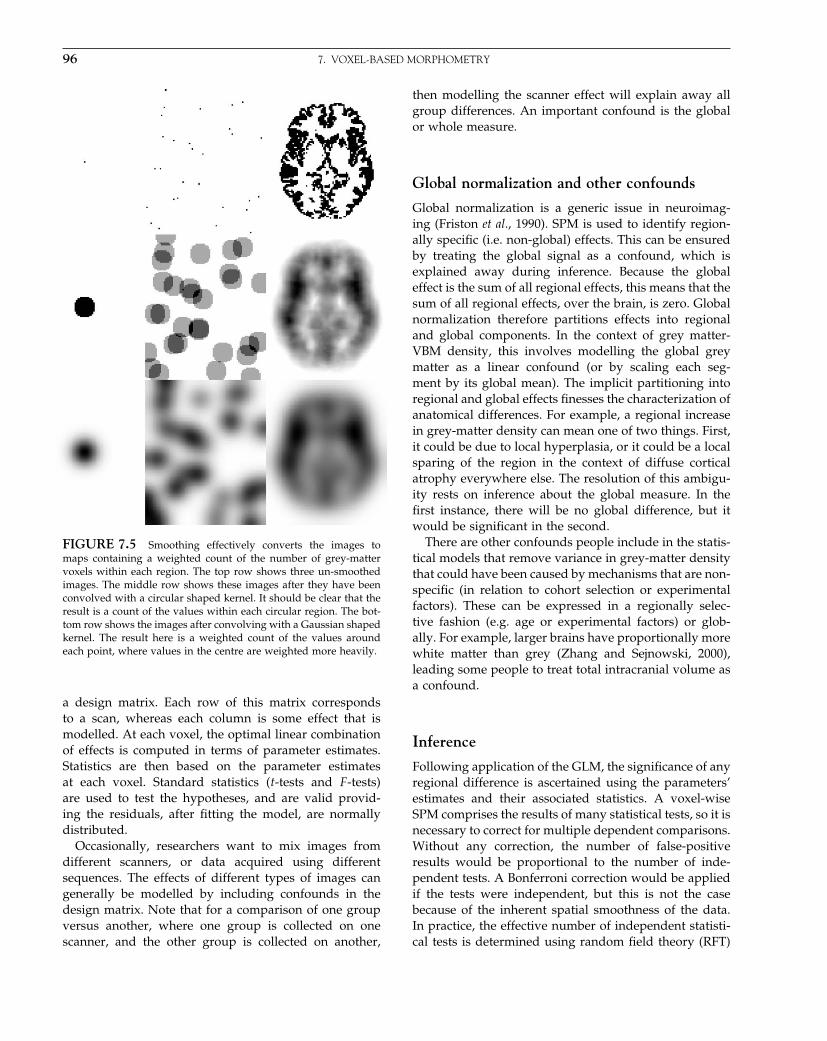
Elsevier UK Chapter: Ch07-P372560 3-10-2006 3:03p.m. Page:96 Trim:7.5in×9.25in
Basal Font:Palatino Margins:Top:40pt Gutter:68pt Font Size:9.5/12 Text Width:42pc Depth:55 Lines
96 7. VOXEL-BASED MORPHOMETRY
FIGURE 7.5 Smoothing effectively converts the images tomaps containing a weighted count of the number of grey-mattervoxels within each region. The top row shows three un-smoothedimages. The middle row shows these images after they have beenconvolved with a circular shaped kernel. It should be clear that theresult is a count of the values within each circular region. The bot-tom row shows the images after convolving with a Gaussian shapedkernel. The result here is a weighted count of the values aroundeach point, where values in the centre are weighted more heavily.
a design matrix. Each row of this matrix correspondsto a scan, whereas each column is some effect that ismodelled. At each voxel, the optimal linear combinationof effects is computed in terms of parameter estimates.Statistics are then based on the parameter estimatesat each voxel. Standard statistics (t-tests and F -tests)are used to test the hypotheses, and are valid provid-ing the residuals, after fitting the model, are normallydistributed.
Occasionally, researchers want to mix images fromdifferent scanners, or data acquired using differentsequences. The effects of different types of images cangenerally be modelled by including confounds in thedesign matrix. Note that for a comparison of one groupversus another, where one group is collected on onescanner, and the other group is collected on another,
then modelling the scanner effect will explain away allgroup differences. An important confound is the globalor whole measure.
Global normalization and other confounds
Global normalization is a generic issue in neuroimag-ing (Friston et al., 1990). SPM is used to identify region-ally specific (i.e. non-global) effects. This can be ensuredby treating the global signal as a confound, which isexplained away during inference. Because the globaleffect is the sum of all regional effects, this means that thesum of all regional effects, over the brain, is zero. Globalnormalization therefore partitions effects into regionaland global components. In the context of grey matter-VBM density, this involves modelling the global greymatter as a linear confound (or by scaling each seg-ment by its global mean). The implicit partitioning intoregional and global effects finesses the characterization ofanatomical differences. For example, a regional increasein grey-matter density can mean one of two things. First,it could be due to local hyperplasia, or it could be a localsparing of the region in the context of diffuse corticalatrophy everywhere else. The resolution of this ambigu-ity rests on inference about the global measure. In thefirst instance, there will be no global difference, but itwould be significant in the second.
There are other confounds people include in the statis-tical models that remove variance in grey-matter densitythat could have been caused by mechanisms that are non-specific (in relation to cohort selection or experimentalfactors). These can be expressed in a regionally selec-tive fashion (e.g. age or experimental factors) or glob-ally. For example, larger brains have proportionally morewhite matter than grey (Zhang and Sejnowski, 2000),leading some people to treat total intracranial volume asa confound.
Inference
Following application of the GLM, the significance of anyregional difference is ascertained using the parameters’estimates and their associated statistics. A voxel-wiseSPM comprises the results of many statistical tests, so it isnecessary to correct for multiple dependent comparisons.Without any correction, the number of false-positiveresults would be proportional to the number of inde-pendent tests. A Bonferroni correction would be appliedif the tests were independent, but this is not the casebecause of the inherent spatial smoothness of the data.In practice, the effective number of independent statisti-cal tests is determined using random field theory (RFT)
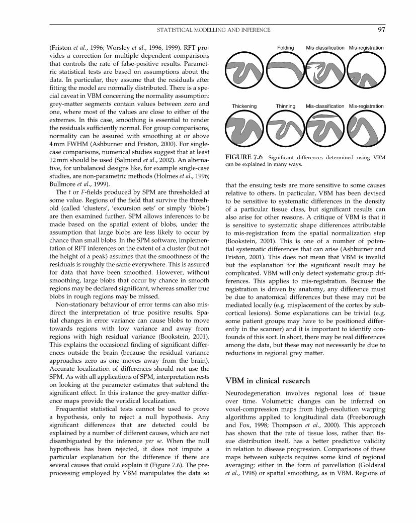
Elsevier UK Chapter: Ch07-P372560 3-10-2006 3:03p.m. Page:97 Trim:7.5in×9.25in
Basal Font:Palatino Margins:Top:40pt Gutter:68pt Font Size:9.5/12 Text Width:42pc Depth:55 Lines
STATISTICAL MODELLING AND INFERENCE 97
(Friston et al., 1996; Worsley et al., 1996, 1999). RFT pro-vides a correction for multiple dependent comparisonsthat controls the rate of false-positive results. Paramet-ric statistical tests are based on assumptions about thedata. In particular, they assume that the residuals afterfitting the model are normally distributed. There is a spe-cial caveat in VBM concerning the normality assumption:grey-matter segments contain values between zero andone, where most of the values are close to either of theextremes. In this case, smoothing is essential to renderthe residuals sufficiently normal. For group comparisons,normality can be assured with smoothing at or above4 mm FWHM (Ashburner and Friston, 2000). For single-case comparisons, numerical studies suggest that at least12 mm should be used (Salmond et al., 2002). An alterna-tive, for unbalanced designs like, for example single-casestudies, are non-parametric methods (Holmes et al., 1996;Bullmore et al., 1999).
The t or F -fields produced by SPM are thresholded atsome value. Regions of the field that survive the thresh-old (called ‘clusters’, ‘excursion sets’ or simply ‘blobs’)are then examined further. SPM allows inferences to bemade based on the spatial extent of blobs, under theassumption that large blobs are less likely to occur bychance than small blobs. In the SPM software, implemen-tation of RFT inferences on the extent of a cluster (but notthe height of a peak) assumes that the smoothness of theresiduals is roughly the same everywhere. This is assuredfor data that have been smoothed. However, withoutsmoothing, large blobs that occur by chance in smoothregions may be declared significant, whereas smaller trueblobs in rough regions may be missed.
Non-stationary behaviour of error terms can also mis-direct the interpretation of true positive results. Spa-tial changes in error variance can cause blobs to movetowards regions with low variance and away fromregions with high residual variance (Bookstein, 2001).This explains the occasional finding of significant differ-ences outside the brain (because the residual varianceapproaches zero as one moves away from the brain).Accurate localization of differences should not use theSPM. As with all applications of SPM, interpretation restson looking at the parameter estimates that subtend thesignificant effect. In this instance the grey-matter differ-ence maps provide the veridical localization.
Frequentist statistical tests cannot be used to provea hypothesis, only to reject a null hypothesis. Anysignificant differences that are detected could beexplained by a number of different causes, which are notdisambiguated by the inference per se. When the nullhypothesis has been rejected, it does not impute aparticular explanation for the difference if there areseveral causes that could explain it (Figure 7.6). The pre-processing employed by VBM manipulates the data so
Thickening Thinning Mis-classification
Folding Mis-classification Mis-registration
Mis-registration
FIGURE 7.6 Significant differences determined using VBMcan be explained in many ways.
that the ensuing tests are more sensitive to some causesrelative to others. In particular, VBM has been devisedto be sensitive to systematic differences in the densityof a particular tissue class, but significant results canalso arise for other reasons. A critique of VBM is that itis sensitive to systematic shape differences attributableto mis-registration from the spatial normalization step(Bookstein, 2001). This is one of a number of poten-tial systematic differences that can arise (Ashburner andFriston, 2001). This does not mean that VBM is invalidbut the explanation for the significant result may becomplicated. VBM will only detect systematic group dif-ferences. This applies to mis-registration. Because theregistration is driven by anatomy, any difference mustbe due to anatomical differences but these may not bemediated locally (e.g. misplacement of the cortex by sub-cortical lesions). Some explanations can be trivial (e.g.some patient groups may have to be positioned differ-ently in the scanner) and it is important to identify con-founds of this sort. In short, there may be real differencesamong the data, but these may not necessarily be due toreductions in regional grey matter.
VBM in clinical research
Neurodegeneration involves regional loss of tissueover time. Volumetric changes can be inferred onvoxel-compression maps from high-resolution warpingalgorithms applied to longitudinal data (Freeboroughand Fox, 1998; Thompson et al., 2000). This approachhas shown that the rate of tissue loss, rather than tis-sue distribution itself, has a better predictive validityin relation to disease progression. Comparisons of thesemaps between subjects requires some kind of regionalaveraging: either in the form of parcellation (Goldszalet al., 1998) or spatial smoothing, as in VBM. Regions of

Elsevier UK Chapter: Ch07-P372560 3-10-2006 3:03p.m. Page:98 Trim:7.5in×9.25in
Basal Font:Palatino Margins:Top:40pt Gutter:68pt Font Size:9.5/12 Text Width:42pc Depth:55 Lines
98 7. VOXEL-BASED MORPHOMETRY
compression and dilation often lie close to each other, sosimple regional averaging approaches may cause differ-ences to cancel (Scahill et al., 2002). The most straight-forward approach involves partitioning the compressionmaps into different tissue classes (cf. the RAVENS mapapproach (Davatzikos et al., 2001)). VBM with simpleintra-subject rigid registration of longitudinal data isa simpler way of achieving similar results (Ashburnerand Friston, 2001). Although it is useful for research,VBM may not be the most sensitive approach for diag-nosing a disease in an individual. For example, VBMmay be able to say that Alzheimer patients have smallerhippocampi than controls, but it is difficult to say forcertain that an individual is in the early stages of thedisease, simply by examining hippocampal volume. Wehave contrasted generative models of regional pathol-ogy and recognition models for diagnosis and classifi-cation. Classification approaches (Davatzikos, 2004; Laoet al., 2004; Davatzikos et al., 2005) are generally notinterested in regionally specific differences, but try tofind the best non-linear function of the data, over theentire brain, which predicts diagnosis. Multivariate ker-nel methods, such as support-vector machines (Vap-nik, 1998), relevance-vector machines (Tipping, 2001) orGaussian process models (Williams and Barber, 1998),are established recognition models that may be useful indiagnosis and endo-phenotyping.
REFERENCES
Ashburner J, Friston KJ (2000) Voxel-based morphometry – themethods. NeuroImage 11: 805–21
Ashburner J, Friston KJ (2001) Why voxel-based morphometryshould be used. NeuroImage 14: 1238–43
Ashburner J, Friston KJ (2005) Unified segmentation. NeuroImage 26:839–51
Bookstein FL (2001) Voxel-based morphometry should not be usedwith imperfectly registered images. NeuroImage 14: 1454–62
Bullmore E, Suckling J, Overmeyer S et al. (1999) Global, voxel,and cluster tests, by theory and permutation, for a differencebetween two groups of structural MR images of the brain. IEEETrans Med Imag 18: 32–42
Davatzikos C (2004) Why voxel-based morphometric analysisshould be used with great caution when characterizing groupdifferences. NeuroImage 23: 17–20
Davatzikos C, Genc A, Xu D et al. (2001) Voxel-based morphom-etry using the RAVENS maps: methods and validation usingsimulated longitudinal atrophy. NeuroImage 14: 1361–69
Davatzikos C, Shen D, Gur RC, et al. (2005) Whole-brain morpho-metric study of schizophrenia revealing a spatially complex setof focal abnormalities. Arch Gen Psychiatr 62: 1218–27
Dryden IL, Mardia KV (1998) Statistical shape analysis. John Wileyand Sons, Chichester
Freeborough PA, Fox NC (1998) Modelling brain deformations inalzheimer disease by fluid registration of serial MR images.J Comput Assist Tomogr 22: 838–43
Friston KJ, Frith CD, Liddle PF et al. (1990) The relationship betweenglobal and local changes in PET scans. J Cereb Blood Flow Metab10: 458–66
Friston KJ, Holmes AP, Poline J-B et al. 1996 Detecting activationsin PET and fMRI: levels of inference and power. NeuroImage4: 223–35
Friston KJ, Holmes AP, Worsley KJ et al. (1995) Statistical parametricmaps in functional imaging: a general linear approach. HumBrain Mapp 2: 189–210
Goldszal AF, Davatzikos C, Pham DL et al. (1998) An image-processing system for qualitative and quantitative volumetricanalysis of brain images. J Comput Assist Tomogr 22: 827–37
Hellier P, Ashburner J, Corouge I et al. (2002) Inter subject registra-tion of functional and anatomical data using SPM. In Proc Medi-cal Image Computing and Computer-Assisted Intervention (MICCAI),vol. 2489 of Lecture Notes in Computer Science. Springer-Verlag,Berlin and Heidelberg, pp 590–87
Hellier P, Barillot C, Corouge I et al. (2001) Retrospective evalu-ation of inter-subject brain registration. In Proc Medical ImageComputing and Computer-Assisted Intervention (MICCAI), NiessenWJ, Viergever MA (eds), vol. 2208 of Lecture Notes in ComputerScience. Springer-Verlag, Berlin and Heidelberg, pp 258–65
Holmes AP, Blair RC, Ford I (1996) Non-parametric analysis ofstatistic images from functional mapping experiments. J CerebBlood Flow Metab 16: 7–22
Kendall DG, Barden D, Carne TK et al. (1999) Shape and shape theory.Wiley, Chichester
Lao Z, Shen D, Xue Z et al. (2004) Morphological classification ofbrains via high-dimensional shape transformations and machinelearning methods. NeuroImage 21: 46–57
Mehta S, Grabowski TJ, Trivedi Y et al. (2003) Evaluation of voxel-based morphometry for focal lesion detection in individuals.NeuroImage 20: 1438–54
Miller MI (2004) Computational anatomy: shape, growth, and atro-phy comparison via diffeomorphisms. NeuroImage 23: S19–S33
Salmond CH, Ashburner J, Vargha-Khadem F et al. (2002) Distri-butional assumptions in voxel-based morphometry. NeuroImage17: 1027–30
Scahill RI, Schott JM, Stevens JM et al. (2002) Mapping the evolutionof regional atrophy in Alzheimer’s disease: unbiased analysis offluid-registered serial MRI. Proc Nat Acad Sci 99: 4703–07
Thompson PM, Giedd JN, Woods RP et al. (2000) Growth patterns inthe developing brain detected by using continuum mechanicaltensor maps. Nature 404: 190–93
Tipping ME (2001) Sparse bayesian learning and the relevance vec-tor machine. J Machine Learning Res 1: 211–44
Van Leemput K, Maes F, Vandermeulen D et al. (2001). Automatedsegmentation of multiple sclerosis lesions by model outlierdetection. IEEE Trans Med Imag 20: 677–88
Vapnik VN (1998) Statistical learning theory. Wiley, New YorkWilliams CKI, Barber D (1998) Bayesian classification with Gaus-
sian processes. IEEE Trans Pattern Recogn Machine Intelligence 20:1342–51
Worsley KJ, Andermann M, Koulis T et al. (1999) Detecting changesin non-isotropic images. Hum Brain Mapp 8: 98–101
Worsley KJ, Marrett S, Neelin P et al. (1996) A unified statisticalapproach for determining significant voxels in images of cerebralactivation. Hum Brain Mapp 4: 58–73
Wright IC, Ellison ZR, Sharma T et al. (1999) Mapping of grey matterchanges in schizophrenia. Schizophren Res 35: 1–14
Wright IC, McGuire PK, Poline J-B et al. (1995) A voxel-basedmethod for the statistical analysis of gray and white matterdensity applied to schizophrenia. NeuroImage 2: 244–52
Zhang K, Sejnowski TJ (2000) A universal scaling law between graymatter and white matter of cerebral cortex. Proc Natl Acad Sci 97.
Elsevier UK Chapter: Ch08-P372560 3-10-2006 3:03p.m. Page:101 Trim:7.5in×9.25in
Basal Font:Palatino Margins:Top:40pt Gutter:68pt Font Size:9.5/12 Text Width:42pc Depth:55 Lines
C H A P T E R
8
The General Linear ModelS.J. Kiebel and A.P. Holmes
INTRODUCTION
In this chapter, we introduce the general linear model. Allclassical analyses of functional data (electroencephalo-graphy/magnetoencephalography (EEG)/(MEG)/fun-ctional magnetic resonance imaging (fMRI)/positronemission tomography (PET)) are based on this model.Analysis comprises three parts: model specification;parameter estimation; and finally inference. Here, wefocus on model specification. This chapter, and indeedthis general linear model section, should be useful intwo ways. First, working through the model equationshelps one to learn about the nature of models and howthey are communicated. Model specification, with anequation, or design matrix (see below), is a crucial stepin the analysis of imaging data. Second, these equationsentail the theory that underpins analysis. Althoughmuch of the modelling in statistical parametric mapping(SPM) is automated, one often encounters situations inwhich it is not obvious how to model data. We hopethat this and the following chapters will help in thesesituations.
We assume that the data have already been prepro-cessed (e.g. reconstructed, normalized, and smoothed).Because SPM is a mass-univariate approach, i.e. the samemodel is used at each voxel, in this and the followingchapters, we will focus on the model for a single voxel.
Model specification is followed by parameter estima-tion and finally, inference using voxel-wise statisticaltests. Here, we treat inferences at a single voxel. Part 4of this book covers inferences over many voxels and themultiple comparison problem this entails.
In the first part of this chapter, we look at the anal-ysis of PET data. In the second part, we extend themodel to accommodate fMRI data. The remaining chap-ters of Part 3 describe, in detail, different aspects ofmodelling in SPM. Chapter 9 focuses on specification ofcontrast weights and Chapter 10 introduces the concept
of non-sphericity, which is important for modelling theerror. Chapter 11 extends the general linear model bycombining multiple models to form hierarchies. Thisapproach is very useful for performing random-effectsanalyses (Chapter 12). Chapter 13 integrates the classicalanalysis of variance, which is a subdomain of the generallinear model, into the SPM framework. Finally, Chap-ters 14, 15 and 16 treat, in detail, specific design issuesfor fMRI and M/EEG data.
THE GENERAL LINEAR MODEL
Before turning to the specifics of PET and fMRI, weconsider the general linear model. This requires somebasic matrix algebra and statistical concepts. These willbe used to develop an understanding of classical hypoth-esis testing. Healy (1986) presents a brief summary ofmatrix methods relevant to statistics. Newcomers to sta-tistical methods are directed towards Mould’s excellenttext Introductory Medical Statistics (1989), while the moremathematically experienced will find Chatfield’s Statis-tics for Technology (1983) useful. Draper and Smith (1981)give a good exposition of matrix methods for the generallinear model, and go on to describe regression analysisin general. The definitive tome for practical statisticalexperimental design is Winer et al. (1991). An excellentbook about experimental design is Yandell (1997). Arather advanced, but very useful, text on linear modelsis Christensen (1996).
The general linear model – introduction
Suppose we conduct an experiment in which we mea-sure a response variable (such as regional cerebral bloodflow (rCBF) at a particular voxel) Yj , where j = 1� � � � � J
Statistical Parametric Mapping, by Karl Friston et al. Copyright 2007, Elsevier Ltd. All rights reserved.ISBN–13: 978-0-12-372560-8 ISBN–10: 0-12-372560-7
101

Elsevier UK Chapter: Ch08-P372560 3-10-2006 3:03p.m. Page:102 Trim:7.5in×9.25in
Basal Font:Palatino Margins:Top:40pt Gutter:68pt Font Size:9.5/12 Text Width:42pc Depth:55 Lines
102 8. THE GENERAL LINEAR MODEL
indexes the observation. Yj is a random variable, conven-tionally denoted by a capital letter.1 Suppose also thatfor each observation we have a set of L�L < J� explanatoryvariables (each measured without error) denoted by xjl,where l = 1� � � � �L indexes the explanatory variables. Theexplanatory variables may be continuous (or sometimesdiscrete) covariates, functions of covariates, or they may bedummy variables indicating the levels of an experimentalfactor.
A general linear model explains the response variableYj in terms of a linear combination of the explanatoryvariables plus an error term:
Yj = xj1�1 +· · ·+xjl�l +· · ·+xjL�L +�j 8.1
Here the �l are (unknown) parameters, corresponding toeach of the L explanatory variables xjl. The errors �j areindependent and identically distributed normal random
variables with zero mean and variance �2, written �j
iid∼� �0��2�.
Examples: dummy variables
Many classical parametric statistical procedures are spe-cial cases of the general linear model. We will illustratethis by going through the equations for two well-knownmodels.
Linear regression
A simple example is linear regression, with one con-tinuous explanatory variable xj for each observationj = 1� � � � � J . The model is usually written as:
Yj = +xj�+�j 8.2
where the unknown parameters are , a constant term in
the model, the regression slope � and �j
iid∼� �0��2�. Thiscan be re-written as a general linear model by using adummy variable, which takes the value xj1 = 1 for all j:
Yj = xj1+xj2�2 +�j 8.3
This has the form of Eqn. 8.1, on replacing �1 with .
Two-sample t-test
Similarly, the two-sample t-test is a special case of a gen-eral linear model: suppose Yj1 and Yj2 are two indepen-dent groups of random variables. The two-sample t-test
1 We talk of random variables, and of observations prior to theirmeasurement, because classical (frequentist) statistics is con-cerned with what could have occurred in an experiment. Oncethe observations have been made, they are known, the residualsare known, and there is no randomness.
assumes Yqj
iid∼ � �q��2�, for q = 1� 2, and assesses thenull hypothesis � 1 = 2. The index j indexes the datapoints in both groups. The standard statistical way ofwriting the model is:
Yqj = q +�qj 8.4
The q subscript on the q indicates that there are two
levels to the group effect, 1 and 2. Here, �qj
iid∼ � �0��2�.This can be rewritten using two dummy variables xqj1
and xqj2 as:
Yqj = xqj11 +xqj22 +�qj 8.5
Which has the form of Eqn. 8.1, after re-indexing for qj.Here the dummy variables indicate group membership,where xqj1 indicates whether observation Yqj is from thefirst group, in which case it has the value 1 when q = 1,
and 0 when q = 2. Similarly, xqj2 ={
0 if q = 11 if q = 2
.
Matrix formulation
In the following, we describe the matrix formulationof the general linear model and derive its least-squaresparameter estimator. We then describe how one can makeinferences based on a contrast of the parameters. Thistheoretical treatment furnishes a set of equations for theanalysis of any data that can be formulated as a generallinear model.
The general linear model can be expressed using matrixnotation. Consider writing out Eqn. 8.1 in full, for eachobservation j, giving a set of simultaneous equations:
Y1 = x11�1 +· · ·+x1l�l +· · ·+x1L�L +�1
��� = ���
Yj = xj1�1 +· · ·+xjl�l +· · ·+xjL�L +�j
��� = ���
YJ = xJ1�1 +· · ·+xJl�l +· · ·+xJL�L +�J
This has an equivalent matrix form:
⎛⎜⎜⎜⎜⎜⎜⎜⎝
Y1���
Yj
���YJ
⎞⎟⎟⎟⎟⎟⎟⎟⎠
=
⎛⎜⎜⎜⎜⎜⎜⎜⎜⎜⎝
x11 · · · x1l · · · x1L
���� � �
���� � �
���
xj1 · · · xjl · · · xjL
���� � �
���� � �
���
xJ1 · · · xJl · · · xJL
⎞⎟⎟⎟⎟⎟⎟⎟⎟⎟⎠
⎛⎜⎜⎜⎜⎜⎜⎝
�1���
�l
����L
⎞⎟⎟⎟⎟⎟⎟⎠
+
⎛⎜⎜⎜⎜⎜⎜⎜⎝
�1����j
����J
⎞⎟⎟⎟⎟⎟⎟⎟⎠

Elsevier UK Chapter: Ch08-P372560 3-10-2006 3:03p.m. Page:103 Trim:7.5in×9.25in
Basal Font:Palatino Margins:Top:40pt Gutter:68pt Font Size:9.5/12 Text Width:42pc Depth:55 Lines
THE GENERAL LINEAR MODEL 103
which can be written in matrix notation as:
Y = X�+� 8.6
where Y is the column vector of observations, � the col-umn vector of error terms, and � the column vector ofparameters; � = ��1� � � � ��l� � � � ��L T . The J × L matrixX, with jlth element xjl is the design matrix. It has onerow per observation, and one column (explanatory vari-able) per model parameter. The important point about thedesign matrix is that it is a near complete description ofour model; the remaining model assumptions are aboutthe distribution of errors. The design matrix encodes andquantifies our knowledge about how the expected signalwas produced.
Parameter estimation
Once an experiment has been completed, we have obser-vations of the random variables Yj , which we denoteby yj . Usually, the simultaneous equations implied bythe general linear model (with � = 0) cannot be solved,because the number of parameters L is typically less thanthe number of observations J . Therefore, some method ofestimating parameters that ‘best fit’ the data is required.This is achieved by the method of ordinary least squares.
Denote a set of parameter estimates by �̃ =��̃1� � � � � �̃L T . These parameters lead to fitted valuesỸ = �Ỹ1� � � � � ỸJ
T = X�̃, giving residual errors e =�e1� � � � � eJ
T = Y − Ỹ = Y −X�̃. The residual sum-of-squaresS = ∑J
j=1 e2j = eT e is the sum of the square differences
between the actual and fitted values, and measures thefit of the model afforded by these parameter estimates.2
The least squares estimates are the parameter estimateswhich minimize the residual sum-of-squares. In full:
S =J∑
j=1
�Yj −xj1�̃1 −· · ·−xjL�̃L�2
This is minimized when:
�S
��̃l
= 2J∑
j=1
�−xjl��Yj −xj1�̃1 −· · ·−xjL�̃L� = 0
This equation is the lth row of XT Y = �XT X��̃. Thus, theleast squares estimates, denoted by �̂, satisfy the normalequations:
XT Y = �XT X��̂ 8.7
2 eT e is the L2 norm of e – geometrically equivalent to the dis-tance between the model and data.
For the general linear model, the least squares estimatesare the maximum likelihood estimates, and are the best lin-ear unbiased estimates.3 That is, of all linear parameterestimates consisting of linear combinations of the data,whose expectation is the true value of the parameters,the least squares estimates have the minimum variance.
If �XT X� is invertible, which it is if, and only if, thedesign matrix X is of full rank, then the least squaresestimates are:
�̂ = (XT X
)−1XT Y 8.8
Overdetermined models
If X has linearly dependent columns, it is rank deficient,i.e. �XT X� is singular and has no inverse. In this case, themodel is overparameterized: there are infinitely manyparameter sets describing the same model. Correspond-ingly, there are infinitely many least squares estimates�̂ satisfying the normal equations. We will illustrate thiswith an example and discuss the solution that is adoptedin SPM.
One way ANOVA example
A simple example of an overdetermined model is theclassic Q group one-way analysis of variance (ANOVA)model. Generally, an ANOVA determines the variabil-ity in the measured response which can be attributed tothe effects of factor levels. The remaining unexplainedvariation is used to assess the significance of the effects(Yandell, 1997, page 4 and pages 202ff). The model for aone-way ANOVA is given by:
Yqj = +�q +�qj 8.9
where Yqj is the jth observation in group q = 1� � � � �Q.Clearly, this model does not specify the parametersuniquely: for any given and �q , the parameters ′ =+d and �′
q = �q −d give an equivalent model for anyconstant d. That is, the model is indeterminate up to thelevel of an additive constant between the constant term and the group effects �q . Similarly, for any set of leastsquares estimates ̂� �̂q . Here, there is one degree of inde-terminacy in the model. This means the design matrix hasrank Q, which is one less than the number of parameters(the number of columns of X). If the data vector Y has
3 Gauss-Markov theorem.
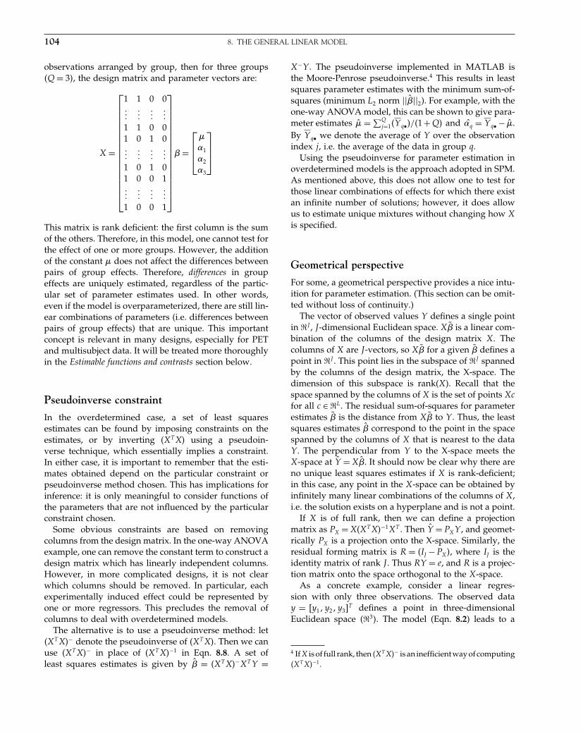
Elsevier UK Chapter: Ch08-P372560 3-10-2006 3:03p.m. Page:104 Trim:7.5in×9.25in
Basal Font:Palatino Margins:Top:40pt Gutter:68pt Font Size:9.5/12 Text Width:42pc Depth:55 Lines
104 8. THE GENERAL LINEAR MODEL
observations arranged by group, then for three groups�Q = 3�, the design matrix and parameter vectors are:
X =
⎡⎢⎢⎢⎢⎢⎢⎢⎢⎢⎢⎢⎢⎢⎢⎢⎢⎣
1 1 0 0���
������
���1 1 0 01 0 1 0���
������
���1 0 1 01 0 0 1���
������
���1 0 0 1
⎤⎥⎥⎥⎥⎥⎥⎥⎥⎥⎥⎥⎥⎥⎥⎥⎥⎦
� =
⎡⎢⎢⎣
�1
�2
�3
⎤⎥⎥⎦
This matrix is rank deficient: the first column is the sumof the others. Therefore, in this model, one cannot test forthe effect of one or more groups. However, the additionof the constant does not affect the differences betweenpairs of group effects. Therefore, differences in groupeffects are uniquely estimated, regardless of the partic-ular set of parameter estimates used. In other words,even if the model is overparameterized, there are still lin-ear combinations of parameters (i.e. differences betweenpairs of group effects) that are unique. This importantconcept is relevant in many designs, especially for PETand multisubject data. It will be treated more thoroughlyin the Estimable functions and contrasts section below.
Pseudoinverse constraint
In the overdetermined case, a set of least squaresestimates can be found by imposing constraints on theestimates, or by inverting �XT X� using a pseudoin-verse technique, which essentially implies a constraint.In either case, it is important to remember that the esti-mates obtained depend on the particular constraint orpseudoinverse method chosen. This has implications forinference: it is only meaningful to consider functions ofthe parameters that are not influenced by the particularconstraint chosen.
Some obvious constraints are based on removingcolumns from the design matrix. In the one-way ANOVAexample, one can remove the constant term to construct adesign matrix which has linearly independent columns.However, in more complicated designs, it is not clearwhich columns should be removed. In particular, eachexperimentally induced effect could be represented byone or more regressors. This precludes the removal ofcolumns to deal with overdetermined models.
The alternative is to use a pseudoinverse method: let�XT X�− denote the pseudoinverse of �XT X�. Then we canuse �XT X�− in place of �XT X�−1 in Eqn. 8.8. A set ofleast squares estimates is given by �̂ = �XT X�−XT Y =
X−Y . The pseudoinverse implemented in MATLAB isthe Moore-Penrose pseudoinverse.4 This results in leastsquares parameter estimates with the minimum sum-of-squares (minimum L2 norm ���̂��2). For example, with theone-way ANOVA model, this can be shown to give para-meter estimates ̂ =∑Q
j=1�Y q•�/�1 +Q� and �̂q = Y q• − ̂.By Y q• we denote the average of Y over the observationindex j, i.e. the average of the data in group q.
Using the pseudoinverse for parameter estimation inoverdetermined models is the approach adopted in SPM.As mentioned above, this does not allow one to test forthose linear combinations of effects for which there existan infinite number of solutions; however, it does allowus to estimate unique mixtures without changing how Xis specified.
Geometrical perspective
For some, a geometrical perspective provides a nice intu-ition for parameter estimation. (This section can be omit-ted without loss of continuity.)
The vector of observed values Y defines a single pointin �J , J -dimensional Euclidean space. X�̃ is a linear com-bination of the columns of the design matrix X. Thecolumns of X are J -vectors, so X�̃ for a given �̃ defines apoint in �J . This point lies in the subspace of �J spannedby the columns of the design matrix, the X-space. Thedimension of this subspace is rank(X). Recall that thespace spanned by the columns of X is the set of points Xcfor all c ∈ �L. The residual sum-of-squares for parameterestimates �̃ is the distance from X�̃ to Y . Thus, the leastsquares estimates �̂ correspond to the point in the spacespanned by the columns of X that is nearest to the dataY . The perpendicular from Y to the X-space meets theX-space at Ŷ = X�̂. It should now be clear why there areno unique least squares estimates if X is rank-deficient;in this case, any point in the X-space can be obtained byinfinitely many linear combinations of the columns of X,i.e. the solution exists on a hyperplane and is not a point.
If X is of full rank, then we can define a projectionmatrix as PX = X�XT X�−1XT . Then Ŷ = PXY , and geomet-rically PX is a projection onto the X-space. Similarly, theresidual forming matrix is R = �IJ −PX�, where IJ is theidentity matrix of rank J . Thus RY = e, and R is a projec-tion matrix onto the space orthogonal to the X-space.
As a concrete example, consider a linear regres-sion with only three observations. The observed datay = �y1�y2�y3
T defines a point in three-dimensionalEuclidean space ��3�. The model (Eqn. 8.2) leads to a
4 IfX is of full rank, then �XT X�− is an inefficient way of computing�XT X�−1.

Elsevier UK Chapter: Ch08-P372560 3-10-2006 3:03p.m. Page:105 Trim:7.5in×9.25in
Basal Font:Palatino Margins:Top:40pt Gutter:68pt Font Size:9.5/12 Text Width:42pc Depth:55 Lines
INFERENCE 105
Y1,Y2,Y3
c = RYY
Y = PXY
X − plane
ˆ
FIGURE 8.1 Geometrical perspective on linear regression. Thethree dimensional data Y lie in a three dimensional space. In thisobservation space, the (two-column) design matrix spans a sub-space. Note that the axes of the design space are not aligned withthe axes of the observation space. The least squares estimate is thepoint in the space spanned by the design matrix that has minimaldistance to the data point.
design matrix X =⎡⎣1 x1
1 x2
1 x3
⎤⎦. Provided the xjs are not
all the same, the columns of X span a two dimensionalsubspace of �3, a plane (Figure 8.1).
INFERENCE
Here, we derive the t- and F -statistics, which are usedto test for a linear combination of effects. We will alsoreturn to the issue of overdetermined models and lookat which linear combinations (contrasts) we can test.
Residual sum of squares
For an independent and identical error, the residualvariance �2 is estimated by the residual sum-of-squaresdivided by the appropriate degrees of freedom: �̂2 =eT eJ−p
∼ �2 �2J−p
J−pwhere p = rank�X�. (See the Appendix (8.2)
for a derivation.)
Linear combinations of the parameterestimates
It is not too difficult to show that the parameter esti-mates are normally distributed: if X is full rank then�̂ ∼ � ����2�XT X�−1�. From this it follows that for a col-umn vector c containing L weights:
cT �̂ ∼ �(cT �� �2cT �XT X�−1c
)8.10
Furthermore, �̂ and �̂2 are independent (Fisher’slaw). Thus, prespecified hypotheses concerning lin-ear compounds of the model parameters cT � can beassessed using:
cT �̂− cT �√�̂2cT �XT X�−1c
∼ tJ−p 8.11
where tJ−p is a Student’s t-distribution with J −p degreesof freedom. For example, the hypothesis � cT � = d canbe assessed by computing
T = cT �̂−d√�̂2cT �XT X�−1c
8.12
and computing a p-value by comparing T with a t-distribution having J −p degrees of freedom. In SPM, allnull hypotheses are of the form cT � = 0. Note that SPMtests based on this t-value are always one-sided.
Example – two-sample t-test
For example, consider the two-sample t-test. The model(Eqn. 8.4) leads to a design matrix X with two columnsof dummy variables indicating group membership andparameter vector � = �1�2
T . Thus, the null hypothesis� 1 = 2 is equivalent to � cT � = 0 with c = �1�−1 T .
The first column of the design matrix contains n1 1s andn2 0s, indexing the measurements from group one, whilethe second column contains n1 0s and n2 1s for group
two. Thus �XT X� =(
n1 00 n2
)� �XT X�−1 =
(1/n1 0
0 1/n2
),
and cT �XT X�−1c = 1/n1 + 1/n2, giving the t-statistic (byEqn. 8.11):
T = ̂1 − ̂2√�̂2�1/n1 +1/n2�
This is the standard formula for the two-sample t-statistic, with a Student’s t-distribution of n1 + n2 − 2degrees of freedom under the null hypothesis.
Estimable functions and contrasts
Recall that if the model is overparameterized (i.e. X isrank deficient), then there are infinitely many parame-ter sets describing the same model. Constraints or theuse of a pseudoinverse isolate one set of parametersfrom infinitely many. Therefore, when examining linearcompounds cT � of the parameters, it is imperative toconsider only compounds that are invariant over thespace of possible parameters. Such linear compounds are
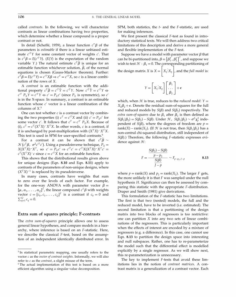
Elsevier UK Chapter: Ch08-P372560 3-10-2006 3:03p.m. Page:106 Trim:7.5in×9.25in
Basal Font:Palatino Margins:Top:40pt Gutter:68pt Font Size:9.5/12 Text Width:42pc Depth:55 Lines
106 8. THE GENERAL LINEAR MODEL
called contrasts. In the following, we will characterizecontrasts as linear combinations having two properties,which determine whether a linear compound is a propercontrast or not.
In detail (Scheffé, 1959), a linear function cT � of theparameters is estimable if there is a linear unbiased esti-mate c′T Y for some constant vector of weights c′. Thatis cT � = E�c′T Y�. �E�Y� is the expectation of the randomvariable Y .) The natural estimate cT �̂ is unique for anestimable function whichever solution, �̂, of the normalequations is chosen (Gauss-Markov theorem). Further:cT � = E�c′T Y� = c′T X� ⇒ cT = c′T X, so c is a linear combi-nation of the rows of X.
A contrast is an estimable function with the addi-tional property cT �̂ = c′T Ŷ = c′T Y . Now c′T Ŷ = c′T Y ⇔c′T PXY = c′T Y ⇔ c′ = PXc′ (since PX is symmetric), so c′
is in the X-space. In summary, a contrast is an estimablefunction whose c′ vector is a linear combination of thecolumns of X.5
One can test whether c is a contrast vector by combin-ing the two properties (i) cT = c′T X and (ii) c′ = PXc′ forsome vector c′. It follows that cT = c′T PXX. Because of(i), cT = cT �XT X�−XT X. In other words, c is a contrast, ifit is unchanged by post-multiplication with �XT X�−XT X.This test is used in SPM for user-specified contrasts.6
For a contrast it can be shown that cT �̂ ∼�(cT �� �2c′T c′). Using a pseudoinverse technique, PX =
X�XT X�−XT , so c′ = PXc′ ⇒ c′T c′ = c′T X�XT X�−XT c′ =cT �XT X�−c since c = c′T X for an estimable function.
This shows that the distributional results given abovefor unique designs (Eqn. 8.10 and Eqn. 8.11) apply tocontrasts of the parameters of non-unique designs, where�XT X�−1 is replaced by its pseudoinverse.
In many cases, contrasts have weights that sumto zero over the levels of each factor. For example,for the one-way ANOVA with parameter vector � =���1� � � � ��Q T , the linear compound cT � with weightsvector c = �c0� c1� � � � � cQ T is a contrast if c0 = 0 and∑Q
q=1 cq = 0.
Extra sum of squares principle; F-contrasts
The extra sum-of-squares principle allows one to assessgeneral linear hypotheses, and compare models in a hier-archy, where inference is based on an F -statistic. Here,we describe the classical F -test, based on the assump-tion of an independent identically distributed error. In
5 In statistical parametric mapping, one usually refers to thevector c as the vector of contrast weights. Informally, we will alsorefer to c as the contrast, a slight misuse of the term.6 The actual implementation of this test is based on a moreefficient algorithm using a singular value decomposition.
SPM, both statistics, the t- and the F -statistic, are usedfor making inferences.
We first present the classical F -test as found in intro-ductory statistical texts. We will then address two criticallimitations of this description and derive a more generaland flexible implementation of the F -test.
Suppose we have a model with parameter vector � thatcan be bi-partitioned into, � = [
�T1 ��T
2
]T , and suppose wewish to test � �1 = 0. The corresponding partitioning of
the design matrix X is X =[
X1
���X2
], and the full model is:
Y =[
X1
���X2
]⎡⎣ �1
� � ��2
⎤⎦+�
which, when � is true, reduces to the reduced model: Y =X2�2 + �. Denote the residual sum-of-squares for the fulland reduced models by S��� and S��2� respectively. Theextra sum-of-squares due to �1 after �2 is then defined asS��1��2� = S��2�− S���. Under �� S��1��2� ∼ �2�2
p inde-pendent of S���, where the degrees of freedom are p =rank�X�− rank�X2�. (If � is not true, then S��1��2� has anon-central chi-squared distribution, still independent ofS���.) Therefore, the following F -statistic expresses evi-dence against � :
F =S��2�−S���
p−p2
S���
J −p
∼ Fp−p2�J−p 8.13
where p = rank�X� and p2 = rank�X2�. The larger F gets,the more unlikely it is that F was sampled under the nullhypothesis H . Significance can then be assessed by com-paring this statistic with the appropriate F -distribution.Draper and Smith (1981) give derivations.
This formulation of the F -statistic has two limitations.The first is that two (nested) models, the full and thereduced model, have to be inverted (i.e. estimated). Thesecond limitation is that a partitioning of the designmatrix into two blocks of regressors is too restrictive:one can partition X into any two sets of linear combi-nations of the regressors. This is particularly importantwhen the effects of interest are encoded by a mixture ofregressors (e.g. a difference). In this case, one cannot useEqn. 8.13 to partition the design space into interestingand null subspaces. Rather, one has to re-parameterizethe model such that the differential effect is modelledexplicitly by a single regressor. As we will show next,this re-parameterization is unnecessary.
The key to implement F -tests that avoid these lim-itations lies in the notion of contrast matrices. A con-trast matrix is a generalization of a contrast vector. Each

Elsevier UK Chapter: Ch08-P372560 3-10-2006 3:03p.m. Page:107 Trim:7.5in×9.25in
Basal Font:Palatino Margins:Top:40pt Gutter:68pt Font Size:9.5/12 Text Width:42pc Depth:55 Lines
INFERENCE 107
column of a contrast matrix consists of one contrastvector. Importantly, the contrast matrix specifies a parti-tioning of the design matrix X.
A contrast matrix c is used to specify a subspace of thedesign matrix, i.e. Xc = Xc. The orthogonal contrast to cis given by c0 = Ip − cc−. Then, let X0 = Xc0 be the designmatrix of the reduced model. We wish to test the effectsXc can explain, after fitting the reduced model X0. Thiscan be achieved using a matrix that projects the data ontothe subspace of Xc, which is orthogonal to X0. We denotethis subspace by Xa.
The projection matrix M due to Xa is derived from theresidual forming matrix of the reduced model X0, whichis given by R0 = IJ −X0X0
−. The projection matrix is thenM = R0 − R, where R is the residual forming matrix ofthe full model, i.e. R = IJ −XX−.
The F -statistic can then be written as:
F = �MY�T MY
�RY�T RY
J −p
p1= Y T MY
Y T RY
J −p
p1∼ Fp1�J−p 8.14
where p1 is the rank of Xa. Since M projects onto a sub-space within X, we can also write:
F = �̂T XT MX�̂
Y T RY
J −p
p1∼ Fp1�J−p 8.15
This equation means that we can compute an F -statisticconveniently for any user-specified contrast without are-parameterization. In SPM, all F -statistics are based onthe full model so that Y T RY is only estimated once andis stored for subsequent use. More about F -contrasts andtheir applications can be found in Chapter 9.
Example – one-way ANOVA
Consider a one-way ANOVA (Eqn. 8.9), where we wishto assess the omnibus null hypothesis that all the groupsare identical: � �1 = �2 = · · · = �Q. Under � the modelreduces to Yqj = +�qj . Since the ANOVA model containsa constant term, , � is equivalent to � �1 = �2 = · · · =�Q = 0. Thus, let �1 = ��1� � � � ��Q�T , and �2 = . Eqn. 8.13then gives an F -statistic which is precisely the standardF -statistic for a one-way ANOVA.
Alternatively, we can apply Eqn. 8.15. The contrastmatrix c is a diagonal Q+ 1-matrix with Q ones on theupper main diagonal and a zero in the Q+1st element onthe main diagonal (Figure 8.2). This contrast matrix testswhether there was an effect due to any group, after takinginto account a constant term across groups. Applicationof Eqn. 8.15 results in the same F-value as in Eqn. 8.13,but without the need to invert two models.
Regressors
Sca
ns
Contrast matrix
FIGURE 8.2 Example of ANOVA design and contrast matrix.Both matrices are displayed as images, where 0s are coded by blackand 1s by white. Left: design matrix, where five groups are modelledby their mean and overall mean. The model is overdetermined byone degree of freedom. Right: F -contrast matrix, which tests for anygroup-specific deviation from the overall mean.
Adjusted and fitted data
Once an inference has been made it is usually necessaryto report the nature of the effect that has been inferred.This can be in terms of the parameter estimates, or in mea-surement space after the estimates are projected throughthe design matrix. In short, one can report significanteffects quantitatively using the parameter estimates orthe responses that these estimates predict. Adjusted dataare a useful way of summarizing effects, after uninter-esting or confounding effects having been removed fromthe raw data Y .
How does one tell SPM which effects are of interest?The partitioning of the design matrix into interesting anduninteresting parts is based upon the same principles asthe F -test developed in the preceding subsection. We canuse an F -contrast for the partitioning, which is equiva-lent to specifying a full and reduced model. Adjusteddata are the residuals of the reduced model, i.e. compo-nents that can be explained by the reduced model havebeen removed from the data. To compute adjusted datawe need to tell SPM which part of the design matrixis of interest (to specify the reduced model). SPM thentreats the part of the design matrix, which is orthogonalto the reduced model, as the effects of interest. This willbe illustrated below by an example. Note that the par-titioning of the design matrix follows the same logic asthe F -test: first, any effect due to the reduced model isremoved and only the remaining effects are taken to beof interest. An important point is that any overlap (cor-relation) between the reduced model and our partitionof interest is explained away by the reduced model. In thecontext of adjusted data, this means that the adjusted
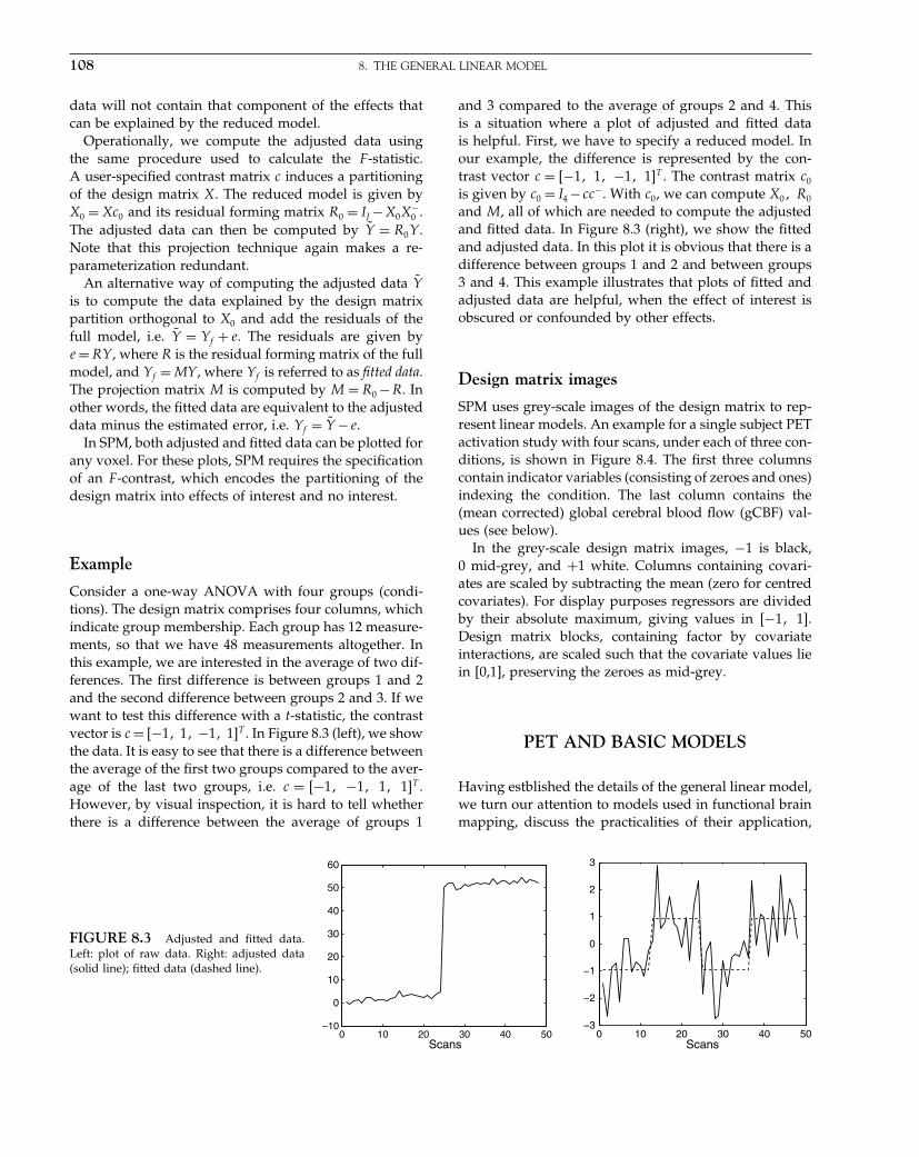
Elsevier UK Chapter: Ch08-P372560 3-10-2006 3:03p.m. Page:108 Trim:7.5in×9.25in
Basal Font:Palatino Margins:Top:40pt Gutter:68pt Font Size:9.5/12 Text Width:42pc Depth:55 Lines
108 8. THE GENERAL LINEAR MODEL
data will not contain that component of the effects thatcan be explained by the reduced model.
Operationally, we compute the adjusted data usingthe same procedure used to calculate the F -statistic.A user-specified contrast matrix c induces a partitioningof the design matrix X. The reduced model is given byX0 = Xc0 and its residual forming matrix R0 = IJ −X0X
−0 .
The adjusted data can then be computed by Ỹ = R0Y .Note that this projection technique again makes a re-parameterization redundant.
An alternative way of computing the adjusted data Ỹis to compute the data explained by the design matrixpartition orthogonal to X0 and add the residuals of thefull model, i.e. Ỹ = Yf + e. The residuals are given bye = RY , where R is the residual forming matrix of the fullmodel, and Yf = MY , where Yf is referred to as fitted data.The projection matrix M is computed by M = R0 −R. Inother words, the fitted data are equivalent to the adjusteddata minus the estimated error, i.e. Yf = Ỹ − e.
In SPM, both adjusted and fitted data can be plotted forany voxel. For these plots, SPM requires the specificationof an F -contrast, which encodes the partitioning of thedesign matrix into effects of interest and no interest.
Example
Consider a one-way ANOVA with four groups (condi-tions). The design matrix comprises four columns, whichindicate group membership. Each group has 12 measure-ments, so that we have 48 measurements altogether. Inthis example, we are interested in the average of two dif-ferences. The first difference is between groups 1 and 2and the second difference between groups 2 and 3. If wewant to test this difference with a t-statistic, the contrastvector is c = �−1� 1� −1� 1 T . In Figure 8.3 (left), we showthe data. It is easy to see that there is a difference betweenthe average of the first two groups compared to the aver-age of the last two groups, i.e. c = �−1� −1� 1� 1 T .However, by visual inspection, it is hard to tell whetherthere is a difference between the average of groups 1
and 3 compared to the average of groups 2 and 4. Thisis a situation where a plot of adjusted and fitted datais helpful. First, we have to specify a reduced model. Inour example, the difference is represented by the con-trast vector c = �−1� 1� −1� 1 T . The contrast matrix c0
is given by c0 = I4 −cc−. With c0, we can compute X0� R0
and M , all of which are needed to compute the adjustedand fitted data. In Figure 8.3 (right), we show the fittedand adjusted data. In this plot it is obvious that there is adifference between groups 1 and 2 and between groups3 and 4. This example illustrates that plots of fitted andadjusted data are helpful, when the effect of interest isobscured or confounded by other effects.
Design matrix images
SPM uses grey-scale images of the design matrix to rep-resent linear models. An example for a single subject PETactivation study with four scans, under each of three con-ditions, is shown in Figure 8.4. The first three columnscontain indicator variables (consisting of zeroes and ones)indexing the condition. The last column contains the(mean corrected) global cerebral blood flow (gCBF) val-ues (see below).
In the grey-scale design matrix images, −1 is black,0 mid-grey, and +1 white. Columns containing covari-ates are scaled by subtracting the mean (zero for centredcovariates). For display purposes regressors are dividedby their absolute maximum, giving values in �−1� 1 .Design matrix blocks, containing factor by covariateinteractions, are scaled such that the covariate values liein [0,1], preserving the zeroes as mid-grey.
PET AND BASIC MODELS
Having estblished the details of the general linear model,we turn our attention to models used in functional brainmapping, discuss the practicalities of their application,
FIGURE 8.3 Adjusted and fitted data.Left: plot of raw data. Right: adjusted data(solid line); fitted data (dashed line).
0 10 20 30 40 50–10
0
10
20
30
40
50
60
Scans0 10 20 30 40 50
−3
−2
−1
0
1
2
3
Scans

Elsevier UK Chapter: Ch08-P372560 3-10-2006 3:03p.m. Page:109 Trim:7.5in×9.25in
Basal Font:Palatino Margins:Top:40pt Gutter:68pt Font Size:9.5/12 Text Width:42pc Depth:55 Lines
PET AND BASIC MODELS 109
2
4
6
8
10
12
α1 α2 α3 ζμ
FIGURE 8.4 Single subject activation experiment, ANCOVAdesign. Illustrations for a three-condition experiment with fourscans in each of three conditions, ANCOVA design. Design matriximage, with columns labelled by their respective parameters. Thescans are ordered by condition.
and introduce some terminology used in SPM. As theapproach is mass-univariate, the same model is used atevery voxel simultaneously, with different parametersand error variances for each voxel. We shall concentrateon PET data, with its mature family of standard sta-tistical experimental designs. Models of fMRI data willbe presented in the next section. Although most PETexperiments employ multiple subjects, many of the keyconcepts are readily demonstrated using a single subjectdesign.
Global normalization
There is an important distinction between regional andglobal effects. Regional effects refer to the response in asingle voxel or a small volume of voxels that is not medi-ated by global effects. Global effects have no regionalspecificity and can be expressed everywhere in thebrain. Usually, global effects are considered as confounds(e.g. arbitrary changes in global signal due to scan-to-scan variations in radioactivity delivered). Althoughtrue global effects are generally unknown, they can beestimated using the whole-brain signal, which entersthe model as a global confound. Typically, modellingglobal effects enhances the sensitivity and accuracy ofthe subsequent inference about experimentally inducedregional effects.
As an example, consider a simple single subject PETexperiment. The subject is scanned repeatedly under bothbaseline (control) and activation (experimental) conditions.
(b)(a)
gCBF
rCB
F
rCB
F
FIGURE 8.5 Single subject PET experiment, illustrative plotsof rCBF at a single voxel: (a) Dot-plots of rCBF; (b) plot of rCBFversus gCBF. Both plots indexed by condition: for baseline, foractive.
Inspection of regional activity (used as a measure ofregional cerebral blood flow (rCBF)), at a single voxel,may not suggest an experimentally induced effect. How-ever, after accounting for global effects (gCBF) differencesbetween the two conditions are disclosed (Figure 8.5).
In statistical parametric mapping, the precise definitionof global activity is user-dependent. The default defini-tion is that global activity is the global average of imageintensities of intracerebral voxels. If Y k
j is the image inten-sity at voxel k = 1� � � � �K of scan j, the estimated globalactivity is gj = Y
•j =∑K
k=1 Y kj /K.
Having estimated the global activity for each scan, adecision must be made about which model of globalactivity should be used. In SPM, there are two alterna-tives. The first is proportional scaling and the second is ananalysis of covariance analysis (ANCOVA).
Proportional scaling
One way to account for global changes is scale each scanby its estimated global activity. This approach is based onthe assumption that the measurement process introducesa (global) scaling of image intensities at each voxel, a gainfactor. Scaling has the advantage of converting the rawdata into a canonical range to give parameter estimates aninterpretable scale. For PET data, the mean global value isusually chosen to be a typical gCBF of 50 ml/min/dl. Thescaling factor is thus 50
ḡ•. We shall assume that the count
rate recorded in the scanner (counts data) has been scaledinto a physiologically meaningful scale. The normalizeddata are Y ′k
j = 50gj
Y kj . The model is then:
Y kj = gj
50�X�k�j +�′k
j 8.16
where �′k ∼ � �0��2k ×diag��gj/50�2��. The diag() operator
transforms a column vector to a diagonal matrix with thevector on its main diagonal and zero elsewhere. This is aweighted regression, i.e. the shape of the error covariance
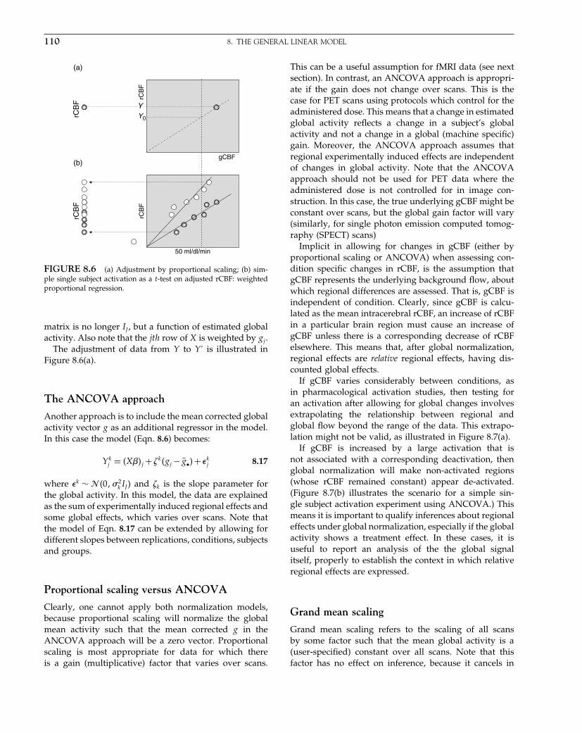
Elsevier UK Chapter: Ch08-P372560 3-10-2006 3:03p.m. Page:110 Trim:7.5in×9.25in
Basal Font:Palatino Margins:Top:40pt Gutter:68pt Font Size:9.5/12 Text Width:42pc Depth:55 Lines
110 8. THE GENERAL LINEAR MODEL
(a)
gCBF
rCB
F
rCB
F
(b)
50 ml/dl/min
rCB
F
rCB
F
YY0
FIGURE 8.6 (a) Adjustment by proportional scaling; (b) sim-ple single subject activation as a t-test on adjusted rCBF: weightedproportional regression.
matrix is no longer IJ , but a function of estimated globalactivity. Also note that the jth row of X is weighted by gj .
The adjustment of data from Y to Y ′ is illustrated inFigure 8.6(a).
The ANCOVA approach
Another approach is to include the mean corrected globalactivity vector g as an additional regressor in the model.In this case the model (Eqn. 8.6) becomes:
Y kj = �X��j + �k�gj − ḡ•�+�k
j 8.17
where �k ∼ � �0��2k IJ � and �k is the slope parameter for
the global activity. In this model, the data are explainedas the sum of experimentally induced regional effects andsome global effects, which varies over scans. Note thatthe model of Eqn. 8.17 can be extended by allowing fordifferent slopes between replications, conditions, subjectsand groups.
Proportional scaling versus ANCOVA
Clearly, one cannot apply both normalization models,because proportional scaling will normalize the globalmean activity such that the mean corrected g in theANCOVA approach will be a zero vector. Proportionalscaling is most appropriate for data for which thereis a gain (multiplicative) factor that varies over scans.
This can be a useful assumption for fMRI data (see nextsection). In contrast, an ANCOVA approach is appropri-ate if the gain does not change over scans. This is thecase for PET scans using protocols which control for theadministered dose. This means that a change in estimatedglobal activity reflects a change in a subject’s globalactivity and not a change in a global (machine specific)gain. Moreover, the ANCOVA approach assumes thatregional experimentally induced effects are independentof changes in global activity. Note that the ANCOVAapproach should not be used for PET data where theadministered dose is not controlled for in image con-struction. In this case, the true underlying gCBF might beconstant over scans, but the global gain factor will vary(similarly, for single photon emission computed tomog-raphy (SPECT) scans)
Implicit in allowing for changes in gCBF (either byproportional scaling or ANCOVA) when assessing con-dition specific changes in rCBF, is the assumption thatgCBF represents the underlying background flow, aboutwhich regional differences are assessed. That is, gCBF isindependent of condition. Clearly, since gCBF is calcu-lated as the mean intracerebral rCBF, an increase of rCBFin a particular brain region must cause an increase ofgCBF unless there is a corresponding decrease of rCBFelsewhere. This means that, after global normalization,regional effects are relative regional effects, having dis-counted global effects.
If gCBF varies considerably between conditions, asin pharmacological activation studies, then testing foran activation after allowing for global changes involvesextrapolating the relationship between regional andglobal flow beyond the range of the data. This extrapo-lation might not be valid, as illustrated in Figure 8.7(a).
If gCBF is increased by a large activation that isnot associated with a corresponding deactivation, thenglobal normalization will make non-activated regions(whose rCBF remained constant) appear de-activated.(Figure 8.7(b) illustrates the scenario for a simple sin-gle subject activation experiment using ANCOVA.) Thismeans it is important to qualify inferences about regionaleffects under global normalization, especially if the globalactivity shows a treatment effect. In these cases, it isuseful to report an analysis of the the global signalitself, properly to establish the context in which relativeregional effects are expressed.
Grand mean scaling
Grand mean scaling refers to the scaling of all scansby some factor such that the mean global activity is a(user-specified) constant over all scans. Note that thisfactor has no effect on inference, because it cancels in

Elsevier UK Chapter: Ch08-P372560 3-10-2006 3:03p.m. Page:111 Trim:7.5in×9.25in
Basal Font:Palatino Margins:Top:40pt Gutter:68pt Font Size:9.5/12 Text Width:42pc Depth:55 Lines
PET AND BASIC MODELS 111
gCBF
rCB
F
g••
(a)
gCBF
(b)
rCB
F
g••
FIGURE 8.7 Single subject data, illustrative (ANCOVA) plotsof rCBF versus gCBF at a single voxel showing potential problemswith global changes. (a) Large change in gCBF between conditions.The apparent activation relies on linear extrapolation of the base-line and active condition regressions (assumed to have the sameslope) beyond the range of the data. The actual relationship betweenregional and global for no activation may be given by the curve, inwhich case there is no activation effect. (b) Large activation inducingincrease in gCBF measured as brain mean rCBF. Filled denotesrest, denotes active condition values if this is an activated voxel,while black denotes active condition values where this voxel isnot activated (in which case an relative deactivation is seen).
the expressions for the t- and F -statistics (Eqns. 8.12and 8.14). However, it does change the scaling and unitsof the data and parameter estimates. The units of bothare rendered adimensional and refer, in a proportionalsense to the grand mean after scaling. This is useful infMRI, where the grand mean of a time-series is set to 100.This means that any activation is expressed as a per centof whole brain mean, over scans.
PET models
In the following, we demonstrate the flexibility of thegeneral linear model using models in the context ofPET experiments. For generality, ANCOVA style mod-els are used, with gCBF as a confounding covariate. Thecorresponding ANCOVA models for data adjusted by
proportional scaling obtain by omitting the global term.Voxel-level models are presented in the usual statisti-cal notation, alongside the SPM description and designmatrix images. The form of contrasts for each design areindicated, and some practical issues of design specifica-tion will be discussed.
Single subject models
Single subject activation design
The simplest experimental paradigm is the single subjectactivation experiment. Suppose there are Q conditions,with Mq scans under condition q. Let Y k
qj denote the rCBFat voxel k in scan j = 1� � � � �Mq under condition q =1� � � � �Q. The model is:
Y kqj = �k
q +k + �k�gqj − ḡ••�+�kqj 8.18
There are Q+ 2 parameters for the model at each voxel:the Q condition effects, the constant term k, and theglobal regression effect, giving a parameter vector �k =��k
1� � � � ��kQ�k� �k�T at each voxel. In this model, repli-
cations of the same condition are modelled with a singleeffect. The model is overparameterized, having only Q+1degrees of freedom, leaving N −Q−1 residual degrees offreedom, where N =∑
Mq is the total number of scans.Contrasts are linear compounds cT �k for which the
weights sum to zero over the condition effects, andgive zero weight to the constant term, i.e.
∑Qq=1 cq = 0
(Figure 8.8). Therefore, linear compounds that test for asimple group effect or for an average effect over groupscannot be contrasts. However, one can test for differencesbetween groups. For example, to test the null hypothesis
2
4
6
8
10
12
α1 α2 α3 ζμ
(b)(a)
gCBF
rCB
F
g••
2μk + α k
3μk + α k
1μk + α k
FIGURE 8.8 Single subject study, ANCOVA design. Illustra-tion of a three-condition experiment with four scans in each ofthree conditions, ANCOVA design. (a) Illustrative plot of rCBF ver-sus gCBF. (b) Design matrix image with columns labelled by theirrespective parameters. The scans are ordered by condition.
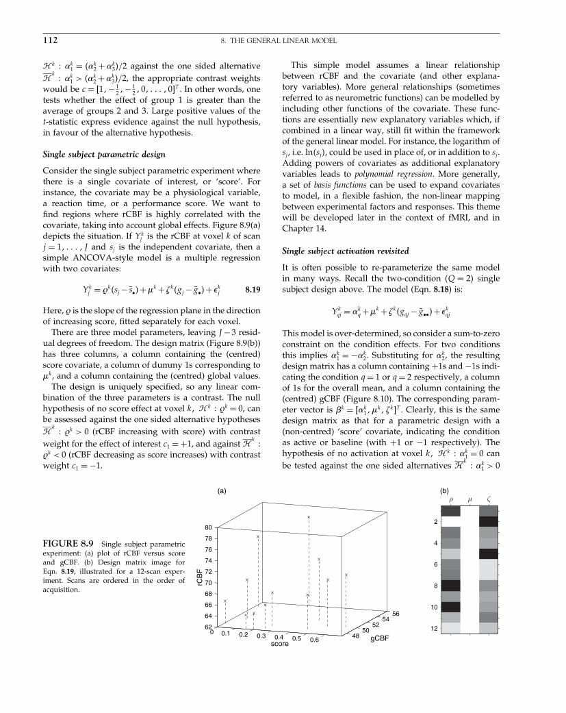
Elsevier UK Chapter: Ch08-P372560 3-10-2006 3:03p.m. Page:112 Trim:7.5in×9.25in
Basal Font:Palatino Margins:Top:40pt Gutter:68pt Font Size:9.5/12 Text Width:42pc Depth:55 Lines
112 8. THE GENERAL LINEAR MODEL
� k �k1 = ��k
2 + �k3�/2 against the one sided alternative
�k
�k1 > ��k
2 + �k3�/2, the appropriate contrast weights
would be c = �1�− 12 �− 1
2 � 0� � � � � 0 T . In other words, onetests whether the effect of group 1 is greater than theaverage of groups 2 and 3. Large positive values of thet-statistic express evidence against the null hypothesis,in favour of the alternative hypothesis.
Single subject parametric design
Consider the single subject parametric experiment wherethere is a single covariate of interest, or ‘score’. Forinstance, the covariate may be a physiological variable,a reaction time, or a performance score. We want tofind regions where rCBF is highly correlated with thecovariate, taking into account global effects. Figure 8.9(a)depicts the situation. If Y k
j is the rCBF at voxel k of scanj = 1� � � � � J and sj is the independent covariate, then asimple ANCOVA-style model is a multiple regressionwith two covariates:
Y kj = �k�sj − s̄•�+k + �k�gj − ḡ•�+�k
j 8.19
Here, � is the slope of the regression plane in the directionof increasing score, fitted separately for each voxel.
There are three model parameters, leaving J −3 resid-ual degrees of freedom. The design matrix (Figure 8.9(b))has three columns, a column containing the (centred)score covariate, a column of dummy 1s corresponding tok, and a column containing the (centred) global values.
The design is uniquely specified, so any linear com-bination of the three parameters is a contrast. The nullhypothesis of no score effect at voxel k� � k �k = 0, canbe assessed against the one sided alternative hypotheses�
k �k > 0 (rCBF increasing with score) with contrast
weight for the effect of interest c1 = +1, and against �k
�k < 0 (rCBF decreasing as score increases) with contrastweight c1 = −1.
This simple model assumes a linear relationshipbetween rCBF and the covariate (and other explana-tory variables). More general relationships (sometimesreferred to as neurometric functions) can be modelled byincluding other functions of the covariate. These func-tions are essentially new explanatory variables which, ifcombined in a linear way, still fit within the frameworkof the general linear model. For instance, the logarithm ofsj , i.e. ln�sj�, could be used in place of, or in addition to sj .Adding powers of covariates as additional explanatoryvariables leads to polynomial regression. More generally,a set of basis functions can be used to expand covariatesto model, in a flexible fashion, the non-linear mappingbetween experimental factors and responses. This themewill be developed later in the context of fMRI, and inChapter 14.
Single subject activation revisited
It is often possible to re-parameterize the same modelin many ways. Recall the two-condition �Q = 2� singlesubject design above. The model (Eqn. 8.18) is:
Y kqj = �k
q +k + �k�gqj − ḡ••�+�kqj
This model is over-determined, so consider a sum-to-zeroconstraint on the condition effects. For two conditionsthis implies �k
1 = −�k2. Substituting for �k
2, the resultingdesign matrix has a column containing +1s and −1s indi-cating the condition q = 1 or q = 2 respectively, a columnof 1s for the overall mean, and a column containing the(centred) gCBF (Figure 8.10). The corresponding param-eter vector is �k = ��k
1�k� �k T . Clearly, this is the samedesign matrix as that for a parametric design with a(non-centred) ‘score’ covariate, indicating the conditionas active or baseline (with +1 or −1 respectively). Thehypothesis of no activation at voxel k� � k �k
1 = 0 canbe tested against the one sided alternatives �
k �k
1 > 0
FIGURE 8.9 Single subject parametricexperiment: (a) plot of rCBF versus scoreand gCBF. (b) Design matrix image forEqn. 8.19, illustrated for a 12-scan exper-iment. Scans are ordered in the order ofacquisition.
4850
5254
56
0 0.1 0.2 0.3 0.4 0.5 0.6
62
64
66
68
70
72
74
76
78
80
gCBFscore
rCB
F
2
4
6
8
10
12
ζμρ(a) (b)

Elsevier UK Chapter: Ch08-P372560 3-10-2006 3:03p.m. Page:113 Trim:7.5in×9.25in
Basal Font:Palatino Margins:Top:40pt Gutter:68pt Font Size:9.5/12 Text Width:42pc Depth:55 Lines
PET AND BASIC MODELS 113
2
4
6
8
10
12
α1 ζμ
FIGURE 8.10 Example design matrix image for single subjectactivation study, with six scans in each of two conditions, formu-lated as a parametric design. The twelve scans are ordered so theyalternate between baseline and activation conditions.
(activation) and �k
�k1 < 0 with contrast weights for the
effects of interest c1 = 1 and c1 = −1 respectively.
Single subject: conditions and covariates
Frequently, there are other confounding covariates inaddition to gCBF that can be added to the model. Forexample, a linear effect of time can be modelled sim-ply by entering the scan number as a covariate. In SPMthese appear in the design matrix as additional columnsadjacent to the global flow column.
Factor by covariate interactions
A more interesting experimental scenario is when a para-metric design is repeated under multiple conditions inthe same subject(s). A specific example would be a PETlanguage experiment in which, during each of twelvescans, lists of words are presented. Two types of wordlist (the two conditions) are presented at each of sixrates (the parametric component). We may be interestedin locating regions where there is a difference in rCBFbetween conditions (accounting for changes in presenta-tion rate), the main effect of condition; locating regionswhere rCBF increases with rate (accounting for condi-tion), the main effect of rate; and assessing evidence
for condition-specific rate effects, an interaction.7 Let Y kqrj
denote the rCBF at voxel k for the j-th measurementunder rate r = 1� � � � �R and condition q = 1� � � � �Q, withsqr the rate covariate (some function of the rates). A suit-able model is:
Y kqrj = �k
q +�kq�sqr − s̄••�+k + �k�gqrj − ḡ•••�+�k
qrj 8.20
Note the q subscript on the parameter �kq , indicating
different slopes for each condition. Ignoring the globalflow for the moment, the model describes two simpleregressions with common error variance (Figure 8.11(a)).SPM describes such factor by covariate interactions as‘factor-specific covariate fits’. The interaction betweencondition and covariate effects is manifest as a dif-ferent regression slope for each condition. There are2Q + 2 parameters for the model at each voxel, �k =��k
1� � � � ��kQ��k
1� � � � ��kQ�k� �k T , with 2Q+ 1 degrees of
freedom. A design matrix for the two condition exam-ple is shown in Figure 8.11(b). The factor by covariateinteraction occupies the third and fourth columns, corre-sponding to the parameters �k
1 and �k2. Here, the covariate
has been split between the columns according to condi-tion and the remaining cells filled with zeroes.
Only the constant term and global slope areconfounds, leaving 2Q effects of interest �k
1 =��k
1� � � � ��kQ��k
1� � � � ��kQ T . As with the activation study
model, contrasts have weights that sum to zero over thecondition effects. For the two-condition word presenta-tion example, contrast weights c1 = �0� 0� 1� 0 T test for acovariate effect in condition one, with large values indi-cating evidence of a positive covariate effect. Weightsc1 = �0� 0� 1
2 � 12 T address the hypothesis that there is no
2
4
6
8
10
12
α1α2ρ1 ρ2 ζμ(a) (b)
rate
rCB
F
••s
kρ2kρ1
kμk +α2
kμk +α1
FIGURE 8.11 Single subject experiment with conditions,covariate, and condition by covariate interaction: (a) illustrative plotof rCBF versus rate. (b) Design matrix image for Eqn. 8.20. Bothare illustrated for the two-condition 12-scan experiment describedin the text. The scans have been ordered by condition.
7 Two experimental factors interact if the level of one affects theexpression of the other.

Elsevier UK Chapter: Ch08-P372560 3-10-2006 3:03p.m. Page:114 Trim:7.5in×9.25in
Basal Font:Palatino Margins:Top:40pt Gutter:68pt Font Size:9.5/12 Text Width:42pc Depth:55 Lines
114 8. THE GENERAL LINEAR MODEL
average covariate effect across conditions, against theone-sided alternative that the average covariate effect ispositive. Weights c1 = �0� 0�−1�+1 T test the null hypoth-esis that there is no condition by covariate interaction,i.e. that the regression slopes are the same.
The contrast weights c1 = �−1�+1� 0� 0 T and c1 =�+1�−1� 0� 0 T are used to assess the hypothesis of nocondition effect against appropriate one-sided alterna-tives. However, inference on main effects is confoundedin the presence of an interaction: in the above model, bothgCBF and the rate covariate were centred, so the condi-tion effects �k
q are the relative heights of the respectiveregression lines (relative to k) at the mean gCBF andmean rate covariate. Clearly, if there is an interaction,then the difference in the condition effects (the separationof the two regression lines) depends on where you lookat them. Were the rate covariate not centred, the com-parison would be at mean gCBF and zero rate, possiblyyielding a different result. More generally, the presenceof an interaction means that the main effects are difficultto interpret. This difficulty is resolved by reporting thesimple effects. In factorial designs, it is usual to test firstfor interactions. If the interactions are significant, onethen proceeds to test for the appropriate simple effects.If it is not, then one reports the main effects.
Multisubject designs
Frequently, experimentally induced changes in rCBF aresmall, and many analyses pool data from different sub-jects to find significant effects. Models of data from manysubjects can either treat the subject effect as a fixed quan-tity (giving fixed-effect models) or treat the subject effectas random (giving random-effect models). In this chapter,we consider fixed-effects models. Random- or mixed-effects models are covered in Chapter 12. In fixed-effectmodels the subject-effect is treated just like a condition-effect and can be regarded as just another factor.
The single-subject designs presented above can beextended to account for subject to subject differences. Thesimplest type of subject effect is an additive effect, oth-erwise referred to as a block effect. This implies that allsubjects respond in the same way, save for an overallshift in rCBF (at each voxel). We extend our notation byadding subscript i for subjects, so Y k
iqj is the rCBF at voxelk of scan j under condition q on subject i = 1� � � � �N .
Multisubject activation (replications)
For instance, the single-subject activation model(Eqn. 8.18) is extended by adding subject effects �k
i givingthe model:
Y kiqj = �k
q +�ki + �k�giqj − ḡ•••�+�k
iqj 8.21
A schematic plot of rCBF versus gCBF for this model isshown in Figure 8.12(a). In SPM terminology, this is a ‘mul-tisubject: replication of conditions’ design. The parame-ter vector at voxel k is �k = ��k
1� � � � ��kQ��k
1� � � � ��kN � �k T .
The design matrix (Figure 8.12(b)) has N columns ofdummy variables corresponding to the subject effects.(Similarly, a multisubject parametric design could bederived from the single-subject case by includingappropriate additive subject effects.)
Again, the model is overparameterized, although thistime we have omitted the explicit constant term from theconfounds, since the subject effects can model an overalllevel. Adding a constant to each of the condition effectsand subtracting it from each of the subject effects givesthe same model. Bearing this in mind, it is clear thatcontrasts must have weights that sum to zero over boththe subject and condition effects.
Condition by replication interactions
The above model assumes that (accounting for globaland subject effects) replications of the same conditiongive the same (expected) response. There are many rea-sons why this assumption may be inappropriate, such
FIGURE 8.12 Multisubject activation experiment,replication of conditions (Eqn. 8.21). Illustrations for afive-subject study, with six replications of each of twoconditions per subject: (a) illustrative plot of rCBF versusgCBF. (b) Design matrix image: the first two columnscorrespond to the condition effects, the next five to thesubject effects, the last to the gCBF regression parameter.The design matrix corresponds to scans ordered by subject,and by condition within subjects.
1
12
24
36
48
60
α1 α2 γ1 γ2 γ3 γ4 γ5 ζ
(b)(a)
gCBF
rCB
F
g••
12αk + γk
11αk + γk
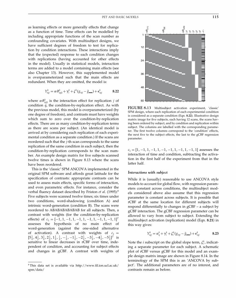
Elsevier UK Chapter: Ch08-P372560 3-10-2006 3:03p.m. Page:115 Trim:7.5in×9.25in
Basal Font:Palatino Margins:Top:40pt Gutter:68pt Font Size:9.5/12 Text Width:42pc Depth:55 Lines
PET AND BASIC MODELS 115
as learning effects or more generally effects that changeas a function of time. Time effects can be modelled byincluding appropriate functions of the scan number asconfounding covariates. With multisubject designs, wehave sufficient degrees of freedom to test for replica-tion by condition interactions. These interactions implythat the (expected) response to each condition changeswith replications (having accounted for other effectsin the model). Usually in statistical models, interactionterms are added to a model containing main effects (seealso Chapter 13). However, this supplemented modelis overparameterized such that the main effects areredundant. When they are omitted, the model is:
Y kiqj = ��k
�qj� +�ki + �k�giqj − ḡ•••�+�k
iqj 8.22
where ��k�qj� is the interaction effect for replication j of
condition q, the condition-by-replication effect. As withthe previous model, this model is overparameterized (byone degree of freedom), and contrasts must have weightswhich sum to zero over the condition-by-replicationeffects. There are as many condition-by-replication termsas there are scans per subject. (An identical model isarrived at by considering each replication of each experi-mental condition as a separate condition.) If the scans arereordered such that the j-th scan corresponds to the samereplication of the same condition in each subject, then thecondition-by-replication corresponds to the scan num-ber. An example design matrix for five subjects scannedtwelve times is shown in Figure 8.13 where the scanshave been reordered.
This is the ‘classic’ SPM ANCOVA implemented in theoriginal SPM software and affords great latitude for thespecification of contrasts: appropriate contrasts can beused to assess main effects, specific forms of interaction,and even parametric effects. For instance, consider theverbal fluency dataset described by Friston et al. (1995):8
Five subjects were scanned twelve times; six times undertwo conditions, word-shadowing (condition A) andintrinsic word-generation (condition B). The scans werereordered to ABABABABABAB for all subjects. Then, acontrast with weights (for the condition-by-replicationeffects) of c1 = �−1� 1�−1� 1�−1� 1�−1� 1�−1� 1�−1� 1 T
assesses the hypothesis of no main effect ofword-generation (against the one-sided alternativeof activation). A contrast with weights of c1 =�5 1
2 � 4 12 � 3 1
2 � 2 12 � 1 1
2 � 12 �− 1
2 �−1 12 �−2 1
2 �−3 12 �−4 1
2 �−5 12 T is
sensitive to linear decreases in rCBF over time, inde-pendent of condition, and accounting for subject effectsand changes in gCBF. A contrast with weights of
8 This data set is available via http://www.fil.ion.ucl.ac.uk/spm/data/
1
12
24
36
48
60
αθ(1
1)
αθ(jq
)
αθ(J
Q)
γ1 γ2 γ3 γ4 γ5 ζ
FIGURE 8.13 Multisubject activation experiment, ‘classic’SPM design, where each replication of each experimental conditionis considered as a separate condition (Eqn. 8.22). Illustrative designmatrix image for five subjects, each having 12 scans, the scans hav-ing been ordered by subject, and by condition and replication withinsubject. The columns are labelled with the corresponding parame-ter. The first twelve columns correspond to the ‘condition’ effects,the next five to the subject effects, the last to the gCBF regressionparameter.
c1 = �1�−1� 1�−1� 1�−1�−1� 1�−1� 1�−1� 1 assesses theinteraction of time and condition, subtracting the activa-tion in the first half of the experiment from that in thelatter half.
Interactions with subject
While it is (usually) reasonable to use ANCOVA stylemodels to account for global flow, with regression param-eters constant across conditions, the multisubject mod-els considered above also assume that this regressionparameter is constant across subjects. It is possible thatrCBF at the same location for different subjects willrespond differentially to changes in gCBF – a subject bygCBF interaction. The gCBF regression parameter can beallowed to vary from subject to subject. Extending themultisubject activation (replication) model (Eqn. 8.21) inthis way gives:
Y kiqj = �k
q +�ki + �k
i �giqj − ḡ•••�+�kiqj 8.23
Note the i subscript on the global slope term, �ki , indicat-
ing a separate parameter for each subject. A schematicplot of rCBF versus gCBF for this model and an exam-ple design matrix image are shown in Figure 8.14. In theterminology of the SPM this is an ‘ANCOVA by sub-ject’. The additional parameters are of no interest, andcontrasts remain as before.

Elsevier UK Chapter: Ch08-P372560 3-10-2006 3:03p.m. Page:116 Trim:7.5in×9.25in
Basal Font:Palatino Margins:Top:40pt Gutter:68pt Font Size:9.5/12 Text Width:42pc Depth:55 Lines
116 8. THE GENERAL LINEAR MODEL
FIGURE 8.14 Multisubject activa-tion experiment, replication of conditions,ANCOVA by subject. Model Eqn. 8.23.Illustrations for a five-subject study, with sixreplications of each of two conditions persubject: (a) illustrative plot of rCBF versusgCBF. (b) Design matrix image: the first twocolumns correspond to the condition effects,the next five to the subject effects, the lastfive to the gCBF regression parameters foreach subject. The design matrix correspondsto scans ordered by subject, and by conditionwithin subjects.
1
12
24
36
48
60
α1 α2 γ1 γ2 γ3 γ4 γ5 ζ1 ζ2 ζ3 ζ4 ζ5
(b)(a)
gCBF
rCB
F
g••
Multistudy designs
The last class of SPM models for PET we considerare the ‘multistudy’ models. In these models, subjectsare grouped into two or more studies. The ‘multistudy’designs fit separate condition effects for each study. Instatistical terms, this is a split plot design. As an exam-ple, consider two multisubject activation studies, the firstwith five subjects scanned twelve times under two condi-tions (as described above), the second with three subjectsscanned six times under three conditions. An exampledesign matrix for a model containing study-specific con-dition effects, subject effects and study-specific globalregression (termed ‘ANCOVA by group’ in SPM) isshown in Figure 8.15. The first two columns of the designmatrix correspond to the condition effects for the first
1
12
24
36
48
60
66
72
78
α 11
α 12
α 21
α 22
α 23
γ 11
γ 12
γ 13
γ 14
γ 15
γ 21
γ 22
γ 23 ζ1 ζ2
FIGURE 8.15 Design matrix image for the example multi-study activation experiment described in the text.
study, the next two to the condition effects for the secondstudy, the next eight to the subject effects, and the lastto the gCBF regression parameter. (The correspondingscans are assumed to be ordered by study, by subjectwithin study, and by condition within subject.)
Contrasts for multistudy designs in SPM have weightsthat, when considered for each of the studies individu-ally, would define a contrast for that study. Thus, con-trasts must have weights which sum to zero over thecondition effects within each study. There are three typesof useful comparison. The first is a comparison of con-dition effects within a study; the contrast weights forthis are padded with zeros for the other studies, e.g.c1 = �1�−1� 0� 0� 0 T for the first study in our example.This has additional power, relative to an analysis of thisstudy in isolation, since observations from the secondstudy make the variance estimates more precise. The sec-ond is an average effect across studies; here, contrastsfor a particular effect are concatenated over studies. Forexample, if the second study has the same conditionsas the first, plus an additional condition, then the con-trast could have weights c1 = �−1� 1�−1� 1� 0 T . Lastly,differences of contrasts across studies can be assessed,such as differences in activation. The contrasts weightsfor the appropriate main effect in each study are con-catenated, with some study-contrasts negated. In ourexample, c1 = �−1� 1� 1�−1� 0 T would be appropriate forlocating regions where the first study activated more thanthe second, or where the second deactivated more thanthe first.
In many instances, it is appropriate to assume that theerror variance between subjects or between studies isthe same (i.e. homoscedasticity). For very different studypopulations or studies using different scanners or pro-tocols, this assumption may not be tenable and the dif-ferent variances should be modelled. We will cover the

Elsevier UK Chapter: Ch08-P372560 3-10-2006 3:03p.m. Page:117 Trim:7.5in×9.25in
Basal Font:Palatino Margins:Top:40pt Gutter:68pt Font Size:9.5/12 Text Width:42pc Depth:55 Lines
PET AND BASIC MODELS 117
specification of this non-sphericity9 in Chapter 10 and,briefly, in the next section on fMRI. These considerationspertain to the assumptions about the covariance compo-nents of the error but do not affect the specification ofthe design matrices considered in this section.
Basic models
In this section, we will discuss some of the models thatare referred to in SPM as basic models. Typically, basicmodels are used for analyses at the second or between-subject level to implement mixed-effects models (seeChapter 12). For example, basic models include the one-sample t-test, the two-sample t-test, the paired t-test anda one-way ANCOVA, which are described below. Forclarity, we shall drop the voxel index superscript k.
One-sample t-test
The one-sample t–test can be used to test the null hypoth-esis that the mean of J scans is zero. This is the simplestmodel available and the design matrix consists of just aconstant regressor. The model is:
Y = x1�1 +� 8.24
where x1 is a vector of ones and � ∼ N�0��2IJ �. The nullhypothesis is � �1 = 0 and the alternative hypothesis is� �1 > 0. The t-value is computed using Eqn. 8.12 as:
T = �̂1√�̂2/J
∼ tJ−1 8.25
where �̂2 = Y T RY/�J −1�, where R is the residual formingmatrix (see above) and Y T RY are the sum of squares ofthe residuals. This could also be expressed as Y T RY =∑J
j=1�Yj − Ŷj�2, where Ŷj = �x1�̂1�j = �̂1.
Two-sample t-test
The two-sample t-test allows one to test the null hypothe-sis that the means of two groups are equal. The resultingdesign matrix consists of three columns: the first twoencode the group membership of each scan and the thirdmodels a common constant across scans of both groups.This model is overdetermined by one degree of free-dom, i.e. the sum of the first two regressors equals thethird regressor. Notice the difference in parameteriza-tion compared to the earlier two-sample t-test example.
9 Non-sphericity refers to the deviation of the error covariancematrix from a diagonal shape or a shape that can be transformedinto a diagonal shape. See also Chapter 10.
Nevertheless, the resulting t-value is the same for a dif-ferential contrast. Let the number of scans in the firstand second groups be J1 and J2, where J = J1 + J2. Thethree regressors consists of ones and zeros, where thefirst regressor consist of J1 ones, followed by J2 zeroes.The second regressor consists of J1 zeroes, followed by J2
ones. The third regressor contains ones only.Let the contrast vector be c = �−1� 1� 0 T , i.e. the alter-
native hypothesis is � �1 < �2. Then:
�XT X� =⎛⎝ J1 0 J1
0 J2 J2
J1 J2 J
⎞⎠ �
This matrix is rank deficient so we use the pseudo-inverse�XT X�− to compute the t-statistic. We sandwich �XT X�−
with the contrast and get cT �XT X�−c = 1/J1 + 1/J2. Thet-statistic is then given by:
T = �̂2 − �̂1√�̂2/�1/J1 +1/J2�
∼ tJ−2 8.26
and �̂2 = Y T RY/�J − 2�. We have assumed here that wehave equal variance in both groups. This assumption maynot be tenable (e.g. when comparing normal subjects withpatients) and we may have to take this non-sphericityinto account (see Chapter 10).
Paired t-test
The model underlying the paired t-test is an extensionof the two-sample t-test model. It assumes that the scanscome in pairs, i.e. one scan of each pair is in the firstgroup and the other is in the second group. The extensionis that the means over pairs are not assumed to be equal,i.e. the mean of each pair is modelled separately. Forinstance, let the number of pairs be Npairs = 5, i.e. thenumber of scans is J = 10. The design matrix consistsof seven regressors. The first two model the deviationfrom the pair-wise mean within group and the last fivemodel the pair-specific means. The model has degrees offreedom one less than the number of regressors.
Let the contrast vector be c = �−1� 1� 0� 0� 0� 0� 0 T , i.e.the alternative hypothesis is � �1 < �2. This leads to:
T = �̂2 − �̂1√�̂2/�1/J1 +1/J2�
∼ tJ−J/2−1 8.27
The difference between this and a two-sample t-test liesin the degrees of freedom J − J/2 − 1. The paired t-testcan be a more appropriate model for a given data set, butmore effects are modelled, i.e. there are fewer degrees offreedom.

Elsevier UK Chapter: Ch08-P372560 3-10-2006 3:03p.m. Page:118 Trim:7.5in×9.25in
Basal Font:Palatino Margins:Top:40pt Gutter:68pt Font Size:9.5/12 Text Width:42pc Depth:55 Lines
118 8. THE GENERAL LINEAR MODEL
One-way ANCOVA
A one-way ANCOVA allows one to model group effects,i.e. the mean of each of Q groups. This model includes theone-sample and two-sample t-tests, i.e. the cases when1 ≤ Q ≤ 2.
Let the number of groups be Q = 3, where there arefive scans within each group, i.e. Jq = 5 for q = 1� � � � �Q.There are a range of different contrasts available. Forinstance, we could test the null hypothesis that the groupmeans are all equal using the F -contrast as describedearlier. We may want to test the null hypothesis thatthe mean of the first two groups is equal to the meanof the third group, i.e. � ��1 + �2�/2 − �3 = 0 and ouralternative hypothesis is � ��1 +�2�/2 < �3. This can betested using a t-statistic, where c = �−1/2�−1/2� 1� 0 T .The resulting t-statistic and its distribution is:
T = ��̂1 + �̂2�/2− �̂3√�̂2/�1/J1 +1/J2 +1/J3�
∼ tJ−Q 8.28
fMRI MODELS
In this section, we describe the analysis of single-sessionfMRI data. Models for fMRI data are slightly more com-plicated than ANCOVA-like models for PET becausefMRI data represent time-series. This means that thedata have serial correlations, and temporal non-sphericitymust be modelled. Furthermore, the data are caused bydynamical processes that call upon a convolution modelfor their modelling.
Historically, SPM was first developed for PET data andthen generalized to handle fMRI data. In this section, wedescribe the extensions this entailed. This section cov-ers linear time-series models for fMRI data, temporal orserial correlations and their estimation, temporal filter-ing, parameter estimation and inference.
A linear time-series model
SPM is a mass-univariate device, i.e. we use the sametemporal model at each voxel. Therefore, we can describethe temporal model for fMRI data by looking at how thedata from a single voxel (a time-series) are modelled. Atime-series comprises sequential measures of fMRI signalintensities over the period of the experiment. Usually,fMRI data are acquired for the whole brain with a sampletime of roughly 2 to 5 s, using an echo-planar imaging(EPI) sequence.
Multisubject data are acquired in sessions, with oneor more sessions for each subject.10 Here, we deal onlywith models for one of these sessions, e.g. a single-subjectanalysis. Multisubject analyses are based on hierarchialmodels and are described in Chapter 12.
Suppose we have a time series of N observationsY1� � � � �Ys� � � � �YN , acquired at one voxel at times ts,where s = 1� � � � �N is the scan number. The approach is tomodel at each voxel the observed time-series as a linearcombination of explanatory functions, plus an error term(where we omit voxel superscripts):
Ys = �1f1�ts�+· · ·+�lf
l�ts�+· · ·+�LfL�ts�+�s 8.29
The L functions f 1���� � � � � f L��� are a suitable set of regres-sors, designed such that linear combinations of them spanthe space of possible fMRI responses for this experiment,up to the level of error. Consider writing out the aboveEqn. 8.29 for all time points ts, to give a set of equations:
Y1 = �1f1�t1�+· · ·+�lf
l�t1�+· · ·+�LfL�t1�+�1
��� = ���
Ys = �1f1�ts�+· · ·+�lf
l�ts�+· · ·+�LfL�ts�+�s
��� = ���
YN = �1f1�tN �+· · ·+�lf
l�tN �+· · ·+�LfL�tN �+�N
which in matrix form is:⎛⎜⎜⎜⎜⎜⎜⎝
Y1���
Ys
���YN
⎞⎟⎟⎟⎟⎟⎟⎠
=
⎛⎜⎜⎜⎜⎜⎜⎝
f 1�t1� � � � f l�t1� � � � f L�t1����
� � ����
� � ����
f 1�ts� � � � f l�ts� � � � f L�ts����
� � ����
� � ����
f 1�tN � � � � f l�tN � � � � f L�tN �
⎞⎟⎟⎟⎟⎟⎟⎠
⎛⎜⎜⎜⎜⎜⎜⎝
�1���
�l
����L
⎞⎟⎟⎟⎟⎟⎟⎠
+
⎛⎜⎜⎜⎜⎜⎜⎝
�1����s
����N
⎞⎟⎟⎟⎟⎟⎟⎠
8.30
or in matrix notation:
Y = X�+� 8.31
Here each column of the design matrix X contains thevalues of one of the continuous regressors evaluated ateach time point ts of fMRI time series. That is, the columnsof the design matrix are the discretized regressors.
The regressors are chosen to span the space of all pos-sible fMRI responses for the experiment in question, suchthat the error vector � is normally distributed with zeromean. As will be discussed later, we assume a seriallycorrelated error process �.
10 The term session will be defined later.

Elsevier UK Chapter: Ch08-P372560 3-10-2006 3:03p.m. Page:119 Trim:7.5in×9.25in
Basal Font:Palatino Margins:Top:40pt Gutter:68pt Font Size:9.5/12 Text Width:42pc Depth:55 Lines
fMRI MODELS 119
Proportional and grand mean scaling
Before we proceed to construction of fMRI regressors,we consider the issue of global normalization. fMRI dataare known to arise from various processes that causeglobally distributed confounding effects (e.g. Anderssonet al., 2001). A simple global confound is scanner gain.This volume-wise gain is a factor that scales the wholeimage and is known to vary slowly during a session.A simple way to remove the effect of gain is to esti-mate the gain for every image and divide all the imageintensities by this estimate. This is known as proportionalscaling.
If one does not use proportional scaling, SPM applies,by default, a session-specific scaling. This type of scalingdivides each volume by a session-specific global estima-tor. This is known in SPM as grand mean scaling. Session-specific grand mean scaling is recommended, because thescaling of fMRI data can vary between sessions and couldmask regional activations.
To estimate the scaling factors, SPM uses a rough esti-mate of the volume-wise intracerebral mean intensity.Note that both kinds of scaling render the mean globalactivity (either of a volume or of a session) 100. The dataand a signal change can then be interpreted convenientlyas a per cent of the global mean.
Constructing fMRI regressors
In the following, we describe how the regressors inEqn. 8.30 are generated and the underlying model ofblood oxygen-level-dependent (BOLD) responses thatthis entails. This process consists of several stages.Although most are hidden from the user, it is helpfulto know about the intermediate processing steps, so thatone can understand the assumptions on which the modelis based. Basically, SPM needs to know two things to con-struct the design matrix. The first is the timing of exper-imental changes and the second is the expected shapeof the BOLD response elicited by these changes. Giventhis information, SPM can then construct the designmatrix.
Experimental timing
Here we describe how a design matrix for one session offunctional data is generated. Let the number of scans in asession be Nscans, where the data be ordered according totheir acquisition. In SPM, a session starts at session-timezero. This time point is when the first slice of the first scanwas acquired. Session-time can be measured in scans orseconds. The duration of a session is the number of scansmultiplied by the volume repetition time (RT), which isthe time spent from the beginning of the acquisition of
one scan to the beginning of the acquisition of the nextscan. We assume that RT stays constant throughout asession. The RT and the number of scans of a given ses-sion define the start and the end of a session. Moreover,because RT stays constant throughout the experiment,one also knows the onset of each scan.
The design of the experiment is described as a seriesof trials or events, where each trial is associated with atrial type. Let N m
trials be the number of trials of trial typem and Ntypes the number of trial types. For each trial j oftrial type m, one needs to specify its onset and duration.Note that we do not need to make a distinction betweenevent-related or blocked designs, so a trial can be eithera short event or an epoch. Let the onset vector of trialtype m be Om so that Om
j is the onset of trial j of trialtype m. For example, the onset of a trial that started atthe beginning of scan four is at session time three (inscans) or at session time 3 · RT (in seconds). Let vectorDm contain the user-specified stimulus durations of eachtrial for trial type m.
Given all the onsets Om and durations Dm, SPM gen-erates an internal representation of the experiment. Thisrepresentation consists of the stimulus function Sm foreach trial type m. All time bins of a session are coveredsuch that the vectors Sm represent a contiguous seriesof time bins. These time bins typically do not cover atime period of length RT, but a fraction of it, to providea well-sampled discrete approximation to the stimulusfunctions Sm, i.e. they are over-sampled with respect tothe data.
The occurrence of a stimulus in a particular time binis represented by an indicator variable of 1 or 0 (but seelater in the Parametric modulation section). In other words,the stimulus function is a long vector of ‘switches’ thatencode the presence or absence of a particular trial type.In this way, stick-functions or boxcar functions of anysort can be represented.
Note that the degree of discretization of the stimulusfunctions is controlled by the user. Time bin size is spec-ified as the number of time bins per RT.11
For example, assume the RT is 3.2 s. Then each time bin,with the default of 16 bins/RT, covers 200 ms. The lengthof the vector Sm is 16Nscans. Note that choosing a smallertime bin size does not necessarily provide a higher tem-poral precision for the resulting regressors in the designmatrix. This is because the BOLD response occupies arather low-frequency band. Therefore, responses to trialsa few hundred milliseconds apart are virtually indistin-guishable.
11 The effective time bin size is accessible in SPM as variablefMRI_T. Its default value is 16.
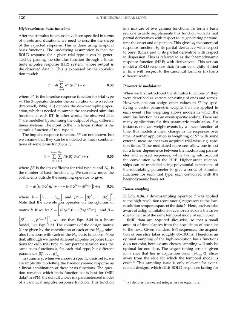
Elsevier UK Chapter: Ch08-P372560 3-10-2006 3:03p.m. Page:120 Trim:7.5in×9.25in
Basal Font:Palatino Margins:Top:40pt Gutter:68pt Font Size:9.5/12 Text Width:42pc Depth:55 Lines
120 8. THE GENERAL LINEAR MODEL
High-resolution basis functions
After the stimulus functions have been specified in termsof onsets and durations, we need to describe the shapeof the expected response. This is done using temporalbasis functions. The underlying assumption is that theBOLD response for a given trial type m can be gener-ated by passing the stimulus function through a linearfinite impulse response (FIR) system, whose output isthe observed data Y . This is expressed by the convolu-tion model:
Y = d�
Ntypes∑m=1
hm ⊗Sm�+� 8.32
where hm is the impulse response function for trial typem. The ⊗ operator denotes the convolution of two vectors(Bracewell, 1986). d�·� denotes the down-sampling oper-ation, which is needed to sample the convolved stimulusfunctions at each RT. In other words, the observed dataY are modelled by summing the output of Ntypes differentlinear systems. The input to the mth linear system is thestimulus function of trial type m.
The impulse response functions hm are not known, butwe assume that they can be modelled as linear combina-tions of some basis functions bi:
Y =Ntypes∑m=1
Nbf∑i=1
d�bi�mi ⊗Sm�+� 8.33
where �mi is the ith coefficient for trial type m and Nbf is
the number of basis functions bi. We can now move thecoefficients outside the sampling operator to give:
Y = d�[�b⊗S1��1 +· · ·+ �b⊗SNtypes ��Ntypes
]�+� 8.34
where b =[b1� � � � � bNbf
]and �m =
[�mT
1 � � � � ��mT
Nbf
]T
.Note that the convolution operates on the columns of
matrix b. If we let X =[
�b⊗S1���� · · · ����b⊗SNtypes �
]and � =
[�1T
� � � � ��NtypesT]T
, we see that Eqn. 8.34 is a linearmodel, like Eqn. 8.31. The columns of the design matrixX are given by the convolution of each of the Ntypes stim-ulus functions with each of the Nbf basis functions. Notethat, although we model different impulse response func-tions for each trial type m, our parametrization uses thesame basis functions bi for each trial type, but differentparameters �m
1 � � � � ��mNbf
.In summary, when we choose a specific basis set bi, we
are implicitly modelling the haemodynamic response asa linear combination of these basis functions. The ques-tion remains: which basis function set is best for fMRIdata? In SPM, the default choice is a parameterized modelof a canonical impulse response function. This function
is a mixture of two gamma functions. To form a basisset, one usually supplements this function with its firstpartial derivatives with respect to its generating parame-ters: the onset and dispersion. This gives: b1 the canonicalresponse function; b2 its partial derivative with respectto onset (time); and b3 its partial derivative with respectto dispersion. This is referred to as the ‘haemodynamicresponse function (HRF) with derivatives’. This set canmodel a BOLD response that: (i) can be slightly shiftedin time with respect to the canonical form; or (ii) has adifferent width.
Parametric modulation
When we first introduced the stimulus functions Sm theywere described as vectors consisting of ones and zeroes.However, one can assign other values to Sm by spec-ifying a vector parametric weights that are applied toeach event. This weighting allows models in which thestimulus function has an event-specific scaling. There aremany applications for this parametric modulation. Forinstance, one can weight events by a linear function oftime; this models a linear change in the responses overtime. Another application is weighting of Sm with someexternal measure that was acquired trial-wise, e.g. reac-tion times. These modulated regressors allow one to testfor a linear dependence between the modulating param-eter and evoked responses, while taking into accountthe convolution with the HRF. Higher-order relation-ships can be modelled using polynomial expansions ofthe modulating parameter to give a series of stimulusfunctions for each trial type, each convolved with thehaemodynamic basis set.
Down-sampling
In Eqn. 8.34, a down-sampling operator d was appliedto the high-resolution (continuous) regressors to the low-resolution temporal space of the data Y . Here, one has to beaware of a slight limitation for event-related data that arisedue to the use of the same temporal model at each voxel.
fMRI data are acquired slice-wise, so that a smallamount of time elapses from the acquisition of one sliceto the next. Given standard EPI sequences, the acquisi-tion of one slice takes roughly 60–100 ms. Therefore, anoptimal sampling of the high-resolution basis functionsdoes not exist, because any chosen sampling will only beoptimal for one slice. The largest timing error is givenfor a slice that lies in acquisition order �Nslices/2 slicesaway from the slice for which the temporal model isexact.12 This sampling issue is only relevant for event-related designs, which elicit BOLD responses lasting for
12 �x denotes the nearest integer less or equal to x.
Elsevier UK Chapter: Ch08-P372560 3-10-2006 3:03p.m. Page:121 Trim:7.5in×9.25in
Basal Font:Palatino Margins:Top:40pt Gutter:68pt Font Size:9.5/12 Text Width:42pc Depth:55 Lines
fMRI MODELS 121
only a few seconds. For blocked designs, timing errorsare small compared to epoch length so that the potentialloss in sensitivity is negligible.
In SPM, there are two ways to solve this slice-timingissue. The first is to choose one time point and tempo-rally realign all the slices to this time. This is called slicetiming correction. However, this interpolation requires arather short RT (<3 s), because the sampling has to bedense, in relation to the width of the BOLD response.The second option is to model latency differences withthe temporal derivative of the HRF. As discussed above,the temporal derivative can model a temporal shift ofthe expected BOLD response. This temporal shift cannot only model onset timing differences due to differentslice times, but also differences due to a different vascu-lar response onset, for example. Note that the temporalderivative can only model small shifts of up to a second(forwards or backwards in time). We generally recom-mend the use of the temporal derivative as part of themodel to capture any potential latency differences.
Additional regressors
It is possible to add regressors to the design matrix with-out going through the convolution process describedabove. An important example is the modelling ofmovement-related effects. Because movement expressesitself in the data directly, and not through any haemody-namic convolution, these are added directly as explana-tory variables in the usual way.
Serial correlations
fMRI data exhibit short-range serial or temporal correla-tions. By this we mean that the error �s at a given scans is correlated with its temporal neighbours. This has tobe modelled, because ignoring correlations leads to aninappropriate estimate of the degrees of freedom. Whenforming a t- or F -statistic, this would cause a biased esti-mate of the standard error leading to invalid tests. Morespecifically, when using ordinary least squares estimates,serial correlations enter through the effective degrees offreedom of the statistic’s null distribution.13 With serialcorrelations the effective degrees of freedom are lowerthan in the case of independence. Ignoring serial correla-tions leads to capricious and invalid tests. To derive cor-rect tests we have to estimate the error covariance matrixby assuming some kind of non-sphericity (Chapter 10).We can then use this estimate in one of two ways.
13 Effective degrees of freedom refer to the degrees of freedom ofan approximation to the underlying null distribution (Worsleyand Friston, 1995).
First, we can use it to form generalized least squaresestimators that correspond to the maximum likelihoodestimates. This is called pre-whitening and involves de-correlating the data (and design matrix) as described inChapters 10 and 22. In this case, the whitened errors areIID and the degrees of freedom revert to their usual value.
The alternative is to proceed with the ordinary leastsquares (OLS) estimates and form statistics in the usualway. One then makes a post-hoc adjustment to thedegrees of freedom (cf. a Greenhouse-Geisser correction)to ensure the inflated estimate of the estimators’ pre-cision is accommodated when comparing the statisticobtained, with its null distribution. Current implemen-tations of SPM use the maximum likelihood approach,which requires no post-hoc correction. However, to retainthe connection with classical statistics in this chapter,we will describe how serial correlations are used withOLS estimates, to give the effective degrees of freedom.In both cases, one needs to estimate the serial correla-tions first.
Note that we are only concerned with serial correla-tions in the error � (Eqn. 8.31). The correlations inducedby the experimental design are modelled by the designmatrix X. Serial correlations in fMRI data are caused byvarious sources including cardiac, respiratory and vaso-motor sources (Mitra et al., 1997).
One model that captures the typical form of serialcorrelations in fMRI data is the autoregressive (order1) plus white noise model �AR�1� + wn� (Purdon andWeisskoff, 1998).14 This model accounts for short-rangecorrelations. We only need to model short-range corre-lations, because we also highpass filter the data. Thehighpass filter removes low frequency components andlong-range correlations. We refer the interested readerto Appendix 8.1 for a mathematical description of theAR�1�+wn model.
Estimation of the error covariance matrix
Assuming that the AR�1�+ wn is an appropriate modelfor the fMRI error covariance matrix, we need to estimatethree hyperparameters (see Appendix 8.1) at each voxel.The hyperparameterized model gives a covariance matrixat each voxel (Eqn. 8.45). In SPM, an additional assump-tion is made to estimate this matrix very efficiently, whichis described in the following.
The error covariance matrix can be partitioned intotwo components. The first component is the correlationmatrix and the second is the variance. The assumptionmade by SPM is that the correlation matrix is the same atall voxels of interest (see Chapter 10 for further details).
14 The AR�1�+wn is also known as the autoregressive moving-average model of order (1,1) (ARMA(1,1)).

Elsevier UK Chapter: Ch08-P372560 3-10-2006 3:03p.m. Page:122 Trim:7.5in×9.25in
Basal Font:Palatino Margins:Top:40pt Gutter:68pt Font Size:9.5/12 Text Width:42pc Depth:55 Lines
122 8. THE GENERAL LINEAR MODEL
The variance is assumed to differ between voxels. In otherwords, SPM assumes that the pattern of serial correla-tions is the same over all interesting voxels, but its ampli-tude is different at each voxel. This assumption seemsto be quite sensible, because the serial correlations overvoxels within tissue types are usually very similar. Theensuing estimate of the serial correlations is extremelyprecise because one can pool information from the subsetof voxels involved in the estimation. This means the cor-relation matrix at each voxel can be treated as a knownand fixed quantity in subsequent inference.
The estimation of the error covariance matrix proceedsas follows. Let us start with the linear model for voxel k:
Y k = X�k +�k 8.35
where Y k is an N ×1 observed time-series vector at voxelk�X is an N ×L design matrix, �k is the parameter vectorand �k is the error at voxel k. The error �k is normallydistributed with � ∼ N�0��k2
V�. The critical difference, inrelation to Eqn. 8.6, is the distribution of the error; wherethe identity matrix I is replaced by the correlation matrixV . Note that V does not depend on the voxel position k,i.e. as mentioned above we assume that the correlationmatrix V is the same for all voxels k = 1� � � � �K. However,the variance �k2 is different for each voxel.
Since we assume that V is the same at each voxel, wecan pool data from all voxels and then estimate V on thispooled data. The pooled data are given by summing thesampled covariance matrix of all interesting voxels k, i.e.VY = 1/K
∑k Y kY kT . Note that the pooled VY is a mixture
of two variance components; the experimentally inducedvariance and the error variance component:
VY =∑k
X�k�kTXT +�k�kT
8.36
The conventional way to estimate the components ofthe error covariance matrix Cov��k� = �k2
V is to userestricted maximum likelihood (ReML) (Harville, 1997;Friston et al., 2002). ReML returns an unbiased estima-tor of the covariance components, while accounting foruncertainty about the parameter estimates. ReML canwork with precision or covariance components; in ourcase we need to estimate a mixture of covariance com-ponents. The concept of covariance components is a verygeneral concept that can be used to model all kinds ofnon-sphericity (see Chapter 10). The model described inAppendix 8.1 (Eqn. 8.44) is non-linear in the hyperpa-rameters, so ReML cannot be used directly. But if we usea linear approximation:
V =∑l
�lQl 8.37
where Ql are N ×N components and the �l are the hyper-parameters, ReML can be applied. We want to specify
Scans
Sca
ns
Scans
FIGURE 8.16 Graphical illustration of the two covariancecomponents, which are used for estimating serial correlations. Left:component Q1 that corresponds to a stationary white variance com-ponent; right: components Q2 that implements the AR�1� part withan autoregression coefficient of 1/e.
Ql such that they form an appropriate model for serialcorrelations in fMRI data. The default model in SPM is touse two components Q1 and Q2. These are Q1 = IN and:
Q2ij={
e−�i−j� i �= j0 i = j
8.38
Figure 8.16 shows the shape of Q1 and Q2.A voxel-wide estimate of V is then derived by re-
scaling V such that V is a correlation matrix.This method of estimating the covariance matrix at
each voxel uses the two voxel-wide (global) hyperparam-eters �1 and �2. A third voxel-wise (local) hyperparame-ter (the variance �2) is estimated at each voxel using theusual estimator in a least squares mass-univariate scheme(Worsley and Friston, 1995):
�2k = Y kTRY k
trace�RV�8.39
where R is the residual forming matrix. This completesthe estimation of the serial correlations at each voxel k.Before we can use these estimates to derive statisticaltests, we will consider the highpass filter and the role itplays in modelling fMRI data.
Temporal filtering
Filtering is motivated by the observation that certain fre-quency bands in the data contain more noise than others.In an ideal world, our experimentally induced effectswould lie in one frequency band and all of the noise inanother. Applying a filter that removes the noise fromthe data would then give us increased sensitivity. How-ever, the data are a mixture of activation and noise thatshare some frequency bands. The experimenter’s task istherefore to make sure that the interesting effects do notlie in a frequency range which is especially exposed tonoise. In fMRI, the low frequencies (say less than halfa cycle per minute, i.e. 1/120 Hz) are known to contain

Elsevier UK Chapter: Ch08-P372560 3-10-2006 3:03p.m. Page:123 Trim:7.5in×9.25in
Basal Font:Palatino Margins:Top:40pt Gutter:68pt Font Size:9.5/12 Text Width:42pc Depth:55 Lines
fMRI MODELS 123
scanner drifts and possibly cardiac/respiratory artefacts.Any activations that lie within this frequency range arevirtually undistinguishable from noise. This is why: (i)fMRI data are highpass filtered to remove noise; and (ii)the experimenter constructs a design that puts the inter-esting effects into frequencies higher than 1/120 Hz. Thisissue is especially important for event-related designsand is described in more detail in Chapter 14. Here, wedescribe how the highpass filter is implemented.
The highpass filter is implemented using a discretecosine transform (DCT) basis set. These are an implicitpart of the design matrix. However, to the user of SPM,they are invisible in the sense that the DCT regressors arenot actually estimated. This is simply to save space. Inpractice, the effects explained by the DCT or drift termsare removed from the data and design matrix using theirresidual forming matrix. This does not affect any of theremaining parameters estimates or any statistics, but iscomputationally more convenient.
Mathematically, for time points t = 1� � � � �N , the dis-crete cosine set functions are fr�t� = √
2/N(cos
(r� t
N
)).
(See Figure 8.17 for an example.) The integer index rranges from 1 (giving half a cosine cycle over the N timepoints), to a user-specified maximum R. Note that SPMasks for a highpass cutoff dcut in seconds. R is then chosenas R = �2NRT/dcut +1 .
To summarize, the regressors in the design matrix Xaccount for all the components in the fMRI time seriesup to the level of residual noise. The highpass filteris effectively a part of the design matrix and removesunwanted low-frequency components. Therefore, long-range correlations are treated as fixed effects. The shortrange correlations are treated as random effects and areestimated using ReML and a linear approximation to theAR�1�+wn model. In the next section, we describe how
–1
0
1
r = 1
–1
0
1
r = 2
–1
0
1
r = 3
–1
0
1
r = 4
–1
0
1
r = 5
–1
0
1
r = 6
–1
0
1
r = 7
t1 tN
FIGURE 8.17 A discrete cosine transform set.
the model parameter estimates are used to form a t- or F -statistic at each voxel, in the context of serial correlations.
Parameter estimates and distributional results
The ordinary least-squares parameter estimates �̂ aregiven by:
�̂ = �XT X�−XT Y = X−Y 8.40
As described above, we estimate the error correlationmatrix V using the ReML method. The error covariancematrix is then given by �̂2V (Eqn. 8.39). The covarianceof the parameter estimates is:
Var��̂� = �2X−VX−T 8.41
A t-statistic can then be formed by dividing a contrast ofthe estimated parameters cT �̂ by its estimated standarddeviation:
T = cT �̂√�̂2cT X−VX−T c
8.42
where �2 is estimated using Eqn. 8.39.The key difference, in relation to the spherical case,
i.e. when the error is IID, is that the correlation matrixV enters the denominator of the t-value. This gives usa more accurate t-statistic. However, because of V , thedenominator of Eqn. 8.42 is not the square root of a�2-distribution. (The denominator would be exactly �2
distributed, when V describes a spherical distribution.)This means that Eqn. 8.42 is not t-distributed and wecannot simply make inferences by comparing with a nulldistribution with trace(RV) degrees of freedom.
Instead, one approximates the denominator with a �2-distribution (Eqn. 8.42). T is then approximated by a t-distribution. The approximation proposed (Worsley andFriston, 1995) is the Satterthwaite approximation (see alsoYandell, 1997), which is based on fitting the first twomoments of the denominator distribution with a �2 dis-tribution. The degrees of freedom of the approximating�2-distribution are called the effective degrees of freedomand are given by:
� = 2E��̂2�2
Var��̂2�= trace�RV�2
trace�RV RV�8.43
See Appendix 8.2 for a derivation of this Satterthwaiteapproximation.
Similarly, the null distribution of an F -statistic in thepresence of serial correlations can be approximated. Inthis case, both the numerator and denominator of theF -value are approximated by a �2-distribution.
Elsevier UK Chapter: Ch08-P372560 3-10-2006 3:03p.m. Page:124 Trim:7.5in×9.25in
Basal Font:Palatino Margins:Top:40pt Gutter:68pt Font Size:9.5/12 Text Width:42pc Depth:55 Lines
124 8. THE GENERAL LINEAR MODEL
Summary
After reconstruction, realignment, spatial normalizationand smoothing, functional imaging data are ready forstatistical analysis. This involves two steps: first, statis-tics indicating evidence against a null hypothesis of noeffect at each voxel are computed to produce a statisticalimage (i.e. an SPM); second, this statistical image must beassessed, while limiting the possibility of false positives.These two steps are referred to as (1) estimation and (2)inference and they are covered separately in this book.
As models are designed with inference in mind itis often difficult to separate the two issues. However,the inference section, Part 4 of this book, is concernedlargely with the multiple comparison problem, i.e. how tomake inferences from large volumes of statistical images.A distinction can be made between such ‘image-level’inference and statistical inference at a single voxel. Thissecond sort of inference has been covered in this chapterand will be dealt with further in the remainder of Part 3.
We have shown how the general linear model, theworkhorse of functional imaging analysis, provides asingle framework for many statistical tests and models,giving great flexibility for experimental design and analy-sis. The use of such models will be further highlighted inthe following chapters, especially Chapters 12, 14, and 16.In the next chapter, we take a closer look at contrastsand how they enable us to interrogate the parameter esti-mates described in this chapter.
APPENDIX 8.1 THE AUTOREGRESSIVEMODEL OF ORDER 1 PLUS WHITE
NOISE
Mathematically, the AR�1�+wn model at voxel k can bewritten in state-space form:
��s� = z�s�+���s�
z�s� = az�s −1�+�z�s� 8.44
where ���s� ∼ N�0���2�� �z�s� ∼ N�0��z
2� and a is theAR�1� coefficient. This model describes the error compo-nent ��s� at time point s and at voxel k as the sum ofan autoregressive component z�s� plus white noise ���s�.We have three hyperparameters15 at each voxel k, thevariances of the two error components �� and �z and the
15 We call these parameters hyperparameters to distinguishthem from the parameter vector �.
autoregressive coefficient a. The resulting error covari-ance matrix is then given by:
E���T � = �z2�IN −A�−1�IN −A�−T +��
2 8.45
where A is a matrix with all elements of the first loweroff-diagonal set to a and zero elsewhere. IN is the identitymatrix of dimension N .
APPENDIX 8.2 THE SATTERTHWAITEAPPROXIMATION
The unbiased estimator for �2 is given by dividingthe sum of the squared residuals by its expectation(Worsley and Friston, 1995). Let e be the residualse = RY , where R is the residual forming matrix. (Notethat many steps in the following equations can bederived using properties of the trace operator; e.g. see theMatrix Reference Manual available under http://www.ee.ic.ac.uk/hp/staff/dmb/matrix/.)
E�eT e� = E�trace�eeT ��
= E�trace�RYY T RT ��
= trace�R�2VRT �
= �2trace�RV�
An unbiased estimator of �2 is given by �̂2 = eT etrace�RV�
. IfV is a diagonal matrix with identical non-zero elements,trace�RV� = trace�R� = J − p, where J is the number ofobservations and p the number of parameters.
In what follows, we derive the Satterthwaite approx-imation to a �2-distribution given a non-spherical errorcovariance matrix.
We approximate the distribution of the squareddenominator of the t-value (Eqn. 8.42) d =�2cT �XT X�−XT VX�XT X�−c �2 with a scaled �2-variate, i.e.,
d ∼ p�ay� 8.46
where p�y� ∼ �2���. We want to estimate the effectivedegrees of freedom �. Note that, for a �2��� distribution,E�y� = � and Var�y� = 2�. The approximation is madeby matching the first two moments of d to the first twomoments of ay:
E�d� = a� 8.47
Var�d� = a22� 8.48
If the correlation matrix V (Eqn. 8.42) is assumed to beknown, it follows that:
� = 2E��̂2�2
Var��̂2�8.49

Elsevier UK Chapter: Ch08-P372560 3-10-2006 3:03p.m. Page:125 Trim:7.5in×9.25in
Basal Font:Palatino Margins:Top:40pt Gutter:68pt Font Size:9.5/12 Text Width:42pc Depth:55 Lines
REFERENCES 125
With E��̂2� = �2 and:
E�eT eeT e� = Var�eT e�+ �E�eT e��2
= 2trace�E�eeT �2�+ trace�E�eeT ��2
= �4�2trace�RV RV�+ trace�RV�2�
we have:
Var��̂2� = E��̂4�−E��̂2�2
= �4�2trace�RV RV�+ trace�RV�2�
trace�RV�2−�4
= 2�4trace�RV RV�
trace�RV�2
Using Eqn. 8.49, we get:
� = trace�RV�2
trace�RV RV�8.50
REFERENCES
Andersson JL, Huttton C, Ashburner J et al. (2001) Modelinggeometric deformations in EPI time series. Neuroimage 13: 903–19
Bracewell R (1986) The Fourier transform and its applications, 2nd edn.McGraw-Hill International Editions, New York
Chatfield C (1983) Statistics for technology. Chapman & Hall,London
Christensen R (1996) Plane answers to complex questions: the theory oflinear models. Springer-Verlag, Berlin
Draper N, Smith H (1981) Applied regression analysis, 2nd edn. JohnWiley & Sons, New York
Friston K, Holmes A, Worsley K et al. (1995) Statistical parametricmaps in functional imaging: a general linear approach. HumBrain Mapp 2: 189–210
Friston KJ, Penny WD, Phillips C et al. (2002) Classical andBayesian inference in neuroimaging: theory. NeuroImage 16:465–83
Harville DA (1977) Maximum likelihood approaches to variancecomponent estimation and to related problems. Am Stat Assoc72: 320–38
Healy M (1986) Matrices for statistics. Oxford University Press,Oxford
Mitra P, Ogawa S, Hu X et al. (1997) The nature of spatiotempo-ral changes in cerebral hemodynamics as manifested in func-tional magnetic resonance imaging. Mag Res Imag Med 37:511–18
Mould R (1989) Introductory medical statistics, 2nd edn. Institute ofPhysics Publishing, London
Purdon P, Weisskoff R (1998) Effect of temporal autocorrela-tion due to physiological noise and stimulus paradigm onvoxel-level false-positive rates in fMRI. Hum Brain Mapp 6:239–49
Scheffé H (1959) The analysis of variance. Wiley, New YorkWiner B, Brown D, Michels K (1991) Statistical principles in experi-
mental design, 3rd edn. McGraw Hill, New YorkWorsley K, Friston K (1995) Analysis of fMRI time-series revisited –
again. Neuroimage 2: 173–81Yandell BS (1997) Practical data analysis for designed experiments.
Chapman & Hall, London
Elsevier UK Chapter: Ch09-P372560 3-10-2006 3:04p.m. Page:126 Trim:7.5in×9.25in
Basal Font:Palatino Margins:Top:40pt Gutter:68pt Font Size:9.5/12 Text Width:42pc Depth:55 Lines
C H A P T E R
9
Contrasts and Classical InferenceJ. Poline, F. Kherif, C. Pallier and W. Penny
INTRODUCTION
The general linear model (GLM) characterizes the rela-tionship between our experimental manipulations andobserved data. It allows us to ask questions like: doesfrontal lobe activity in a memory task depend on age? Isthe activity greater for normal subjects than for patients?While many questions concern only one effect (e.g. age,group), often our questions speak to multiple effects.In 1926, John Russell wrote ‘An experiment is simplya question put to nature � � � Even in the best plannedexperiment the answer can simply be yes or no � � � Thechief requirement is simplicity: only one question shouldbe asked at a time’, but R.A. Fisher’s answer in his 1935Design of experiments was: ‘I am convinced that this viewis wholly mistaken. If we ask Nature a single question,she will often refuse to answer until some other topic hasbeen discussed’. In other words, we model several effectsthat may or may not influence our measures and askseveral questions by comparing the relative importanceof and interactions among those effects. This chapterexplains how one models and tests for effects throughthe use of ‘contrasts’. These enable us to focus on specificquestions that are put to the data.
There is no unique model of an experimentalparadigm. For example, in a functional imaging exper-iment with three conditions ‘A’, ‘B’ and ‘C’, the ‘C’condition (say a ‘baseline’1 or low level condition) canbe modelled explicitly or implicitly. This issue gener-alizes to more complex designs. Contrast specificationand the interpretation of the ensuing results dependon model specification, which, in turn, depends on the
1 There is no absolute baseline condition. In fact, we generallyonly interpret the difference between two conditions, and there-fore an activation pattern in neuroimaging is almost universallyassociated with at least two experimental conditions.
design of the experiment. The most important step is thespecification of the experimental paradigm: if a designis clearly thought through, the questions asked of thedata are generally formulated easily and contrasts arestraightforward to interpret.
In general, it is not very useful simply to show that themeasured signal in a specific brain area is higher underone condition relative to another. Rather, we want toknow whether this difference is statistically significant.We will therefore review the aspects of hypothesis testingthat relate directly to the specification of contrasts.
This chapter is organized as follows. First, we reviewthe theoretical background behind the construction ofcontrasts. In the next section, we describe the rules forconstructing contrasts that specify t-tests. We then dis-cuss F -contrasts and the important issue of correlationsbetween predictors and their impact on the interpretationof t- or F -tests. We conclude with some general remarksand a summary.
CONSTRUCTING MODELS
What should be included in the model?
Put simply, the model should include all factors (con-tinuous or discrete) that might have an impact on themeasurements. Deciding what should or should not beincluded is crucial (for instance, in a functional magneticresonance imaging (fMRI) model, should the subjects’movement estimates be included?). The question ‘shouldthis factor be included in the model?’ can be resolvedwith model selection, but a-priori knowledge is essen-tial to limit the exploration of model space. With limitedinformation about which factors influence the measuredsignal, the model will be larger and more complex.
Statistical Parametric Mapping, by Karl Friston et al. Copyright 2007, Elsevier Ltd. All rights reserved.ISBN–13: 978-0-12-372560-8 ISBN–10: 0-12-372560-7
126

Elsevier UK Chapter: Ch09-P372560 3-10-2006 3:04p.m. Page:127 Trim:7.5in×9.25in
Basal Font:Palatino Margins:Top:40pt Gutter:68pt Font Size:9.5/12 Text Width:42pc Depth:55 Lines
CONSTRUCTING MODELS 127
0 5 10 15 20 25 30 350
1
2
3
4
Time or scans
Reg
ress
or n
umbe
r 1
0 5 10 15 20 25 30 350
0.5
1
Time or scans
Reg
ress
or n
umbe
r 2
0 5 10 15 20 25 30 350
0.5
1
1.5
2
Time or scans
Reg
ress
or n
umbe
r 3
FIGURE 9.1 Model 1: design with simple linearincrease. The regressors, from top to bottom, model (i)the effects of a linear increase in force, (ii) the effect offorce itself and (iii) the baseline response.
To make this point clear, consider an fMRI experimentlooking at motor cortex responses when a subject pressesa device with four different force levels: ‘press’ conditionsare interleaved with ‘rest’ periods. The conditions areordered ‘press force 1’, ‘rest’, ‘press force 2’, ‘rest’, � � � ,‘press force 4’, etc.2
The first issue is how one models the ‘press’ and ‘rest’conditions. One may have very specific prior assump-tions, for example, that the response should be a linearfunction of the force. In this case, we construct a vector (aso-called regressor, covariate, or predictor) that representsthis linear relationship. In the present example, this pre-dictor could comprise 1s for all scans obtained duringthe first (lowest) force level, 2s for all scans acquired dur-ing the second force level, etc. If the ‘rest’ periods arerepresented by zeroes, the model assumes that the dif-ference between rest and the first force level is the sameas the difference between the first and the second forcelevel (or between any two neighbouring force levels).To relax this assumption and construct a more flexiblemodel, the difference between any ‘press’ condition andthe rest period must be modelled explicitly in anotherpredictor that takes value 1 during ‘press’ conditions and0 during ‘rest’.
Our model is then:
yi = x1i �1 +x2
i �2 +�i 9.1
2 This order would not be used in an actual experiment, whereone would normally randomize the different force levels.
for which yi is the ith measurement (scan), x1 representsthe predictor of the linear increase with force, and x2
the difference between ‘press’ (x2i = 1) and ‘rest’ (x2
i = 0).The parameters �1 and �2, which we need to estimate,are the coefficients of the linear functions encoded inour model. The error �i is the difference between themodel prediction and the data yi. If the signal is notzero during the rest condition (and this is always thecase in neuroimaging), this offset has to be modelledby a constant term (i.e. a regressor consisting entirelyof 1s). With this additional regressor, our model iswritten as:
yi = x1i �1 +x2
i �2 +1�3 +�i 9.2
in which �3 represents the absolute offset of the data.Figure 9.1 shows an example for the three regressorsfrom this model3 which, throughout this chapter, we referto as a ‘linear parametric model’ or simply ‘model 1’.Note that this model may or may not provide a goodexplanation for the measured data. It may lack importantpredictors, or the measured response may not be a lin-ear function of force. Two things can be done with thismodel once its parameters have been estimated. One can
3 For models of fMRI data, one needs to take into account thedelay and dispersion of the haemodynamic signal. This is usu-ally done by convolving the regressors with a haemodynamicresponse function (see Chapter 8). Here, we have omitted thisconvolution step to concentrate on the modelling aspect.
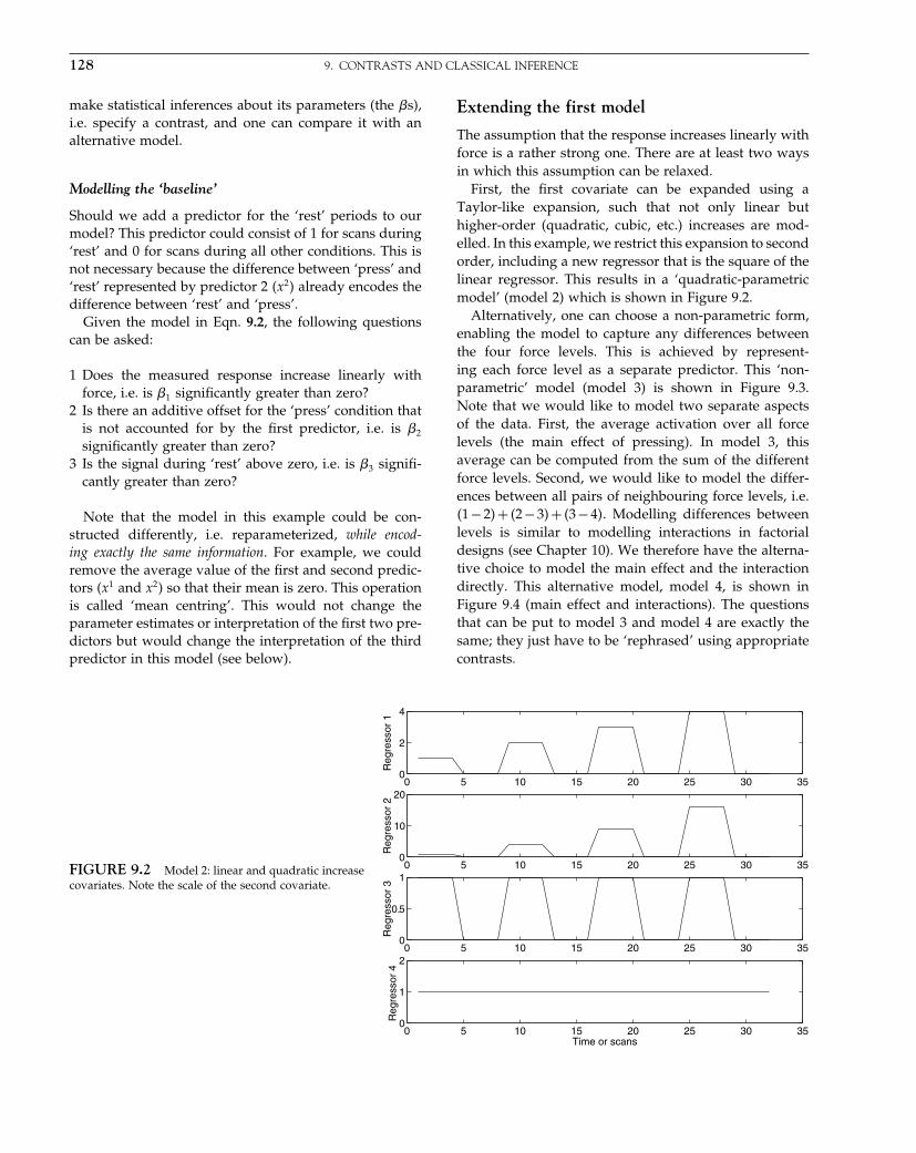
Elsevier UK Chapter: Ch09-P372560 3-10-2006 3:04p.m. Page:128 Trim:7.5in×9.25in
Basal Font:Palatino Margins:Top:40pt Gutter:68pt Font Size:9.5/12 Text Width:42pc Depth:55 Lines
128 9. CONTRASTS AND CLASSICAL INFERENCE
make statistical inferences about its parameters (the �s),i.e. specify a contrast, and one can compare it with analternative model.
Modelling the ‘baseline’
Should we add a predictor for the ‘rest’ periods to ourmodel? This predictor could consist of 1 for scans during‘rest’ and 0 for scans during all other conditions. This isnot necessary because the difference between ‘press’ and‘rest’ represented by predictor 2 �x2� already encodes thedifference between ‘rest’ and ‘press’.
Given the model in Eqn. 9.2, the following questionscan be asked:
1 Does the measured response increase linearly withforce, i.e. is �1 significantly greater than zero?
2 Is there an additive offset for the ‘press’ condition thatis not accounted for by the first predictor, i.e. is �2
significantly greater than zero?3 Is the signal during ‘rest’ above zero, i.e. is �3 signifi-
cantly greater than zero?
Note that the model in this example could be con-structed differently, i.e. reparameterized, while encod-ing exactly the same information. For example, we couldremove the average value of the first and second predic-tors (x1 and x2) so that their mean is zero. This operationis called ‘mean centring’. This would not change theparameter estimates or interpretation of the first two pre-dictors but would change the interpretation of the thirdpredictor in this model (see below).
Extending the first model
The assumption that the response increases linearly withforce is a rather strong one. There are at least two waysin which this assumption can be relaxed.
First, the first covariate can be expanded using aTaylor-like expansion, such that not only linear buthigher-order (quadratic, cubic, etc.) increases are mod-elled. In this example, we restrict this expansion to secondorder, including a new regressor that is the square of thelinear regressor. This results in a ‘quadratic-parametricmodel’ (model 2) which is shown in Figure 9.2.
Alternatively, one can choose a non-parametric form,enabling the model to capture any differences betweenthe four force levels. This is achieved by represent-ing each force level as a separate predictor. This ‘non-parametric’ model (model 3) is shown in Figure 9.3.Note that we would like to model two separate aspectsof the data. First, the average activation over all forcelevels (the main effect of pressing). In model 3, thisaverage can be computed from the sum of the differentforce levels. Second, we would like to model the differ-ences between all pairs of neighbouring force levels, i.e.�1−2�+ �2−3�+ �3−4�. Modelling differences betweenlevels is similar to modelling interactions in factorialdesigns (see Chapter 10). We therefore have the alterna-tive choice to model the main effect and the interactiondirectly. This alternative model, model 4, is shown inFigure 9.4 (main effect and interactions). The questionsthat can be put to model 3 and model 4 are exactly thesame; they just have to be ‘rephrased’ using appropriatecontrasts.
FIGURE 9.2 Model 2: linear and quadratic increasecovariates. Note the scale of the second covariate.
0 5 10 15 20 25 30 350
2
4
0 5 10 15 20 25 30 350
10
20
0 5 10 15 20 25 30 350
0.5
1
0 5 10 15 20 25 30 350
1
2
Time or scans
Reg
ress
or 4
R
egre
ssor
3R
egre
ssor
2R
egre
ssor
1
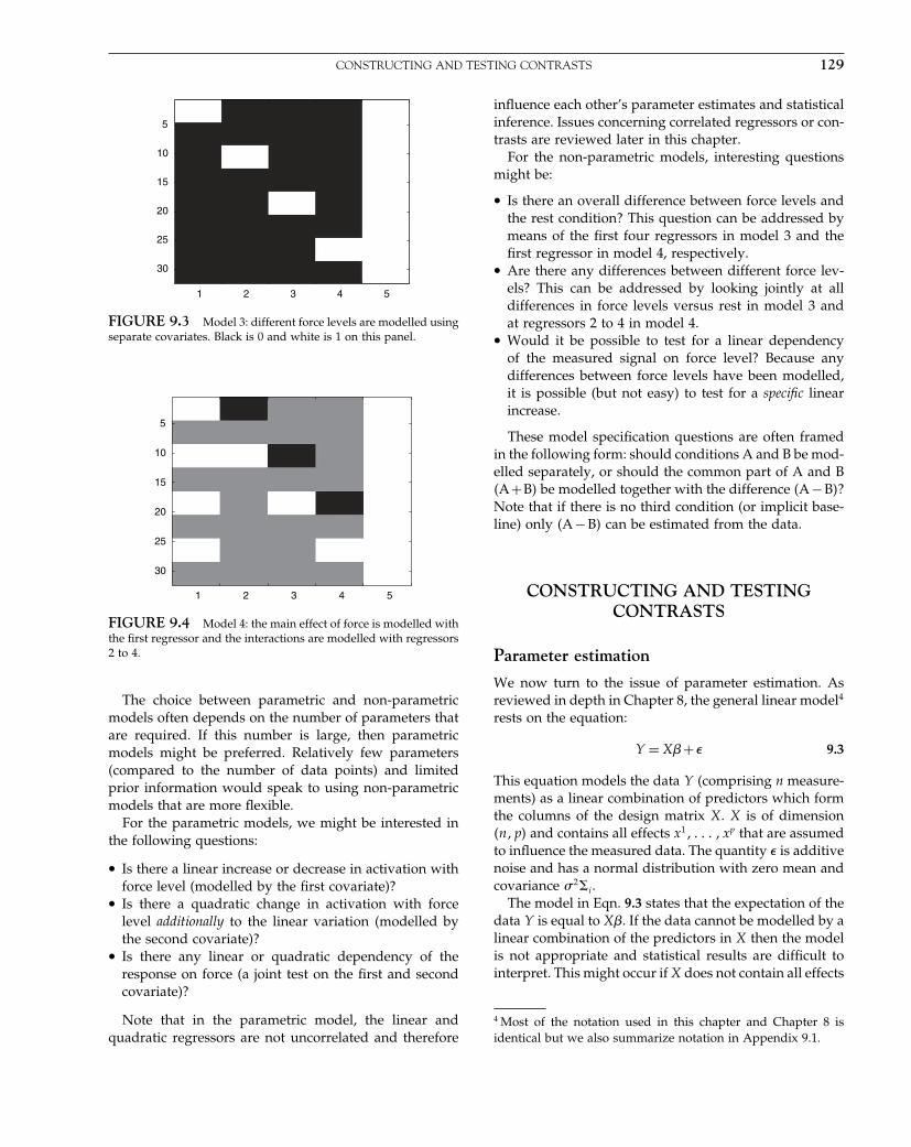
Elsevier UK Chapter: Ch09-P372560 3-10-2006 3:04p.m. Page:129 Trim:7.5in×9.25in
Basal Font:Palatino Margins:Top:40pt Gutter:68pt Font Size:9.5/12 Text Width:42pc Depth:55 Lines
CONSTRUCTING AND TESTING CONTRASTS 129
1 2 3 4 5
5
10
15
20
25
30
FIGURE 9.3 Model 3: different force levels are modelled usingseparate covariates. Black is 0 and white is 1 on this panel.
1 2 3 4 5
5
10
15
20
25
30
FIGURE 9.4 Model 4: the main effect of force is modelled withthe first regressor and the interactions are modelled with regressors2 to 4.
The choice between parametric and non-parametricmodels often depends on the number of parameters thatare required. If this number is large, then parametricmodels might be preferred. Relatively few parameters(compared to the number of data points) and limitedprior information would speak to using non-parametricmodels that are more flexible.
For the parametric models, we might be interested inthe following questions:
• Is there a linear increase or decrease in activation withforce level (modelled by the first covariate)?
• Is there a quadratic change in activation with forcelevel additionally to the linear variation (modelled bythe second covariate)?
• Is there any linear or quadratic dependency of theresponse on force (a joint test on the first and secondcovariate)?
Note that in the parametric model, the linear andquadratic regressors are not uncorrelated and therefore
influence each other’s parameter estimates and statisticalinference. Issues concerning correlated regressors or con-trasts are reviewed later in this chapter.
For the non-parametric models, interesting questionsmight be:
• Is there an overall difference between force levels andthe rest condition? This question can be addressed bymeans of the first four regressors in model 3 and thefirst regressor in model 4, respectively.
• Are there any differences between different force lev-els? This can be addressed by looking jointly at alldifferences in force levels versus rest in model 3 andat regressors 2 to 4 in model 4.
• Would it be possible to test for a linear dependencyof the measured signal on force level? Because anydifferences between force levels have been modelled,it is possible (but not easy) to test for a specific linearincrease.
These model specification questions are often framedin the following form: should conditions A and B be mod-elled separately, or should the common part of A and B�A+B� be modelled together with the difference �A −B�?Note that if there is no third condition (or implicit base-line) only �A −B� can be estimated from the data.
CONSTRUCTING AND TESTINGCONTRASTS
Parameter estimation
We now turn to the issue of parameter estimation. Asreviewed in depth in Chapter 8, the general linear model4
rests on the equation:
Y = X�+� 9.3
This equation models the data Y (comprising n measure-ments) as a linear combination of predictors which formthe columns of the design matrix X. X is of dimension�n�p� and contains all effects x1� � � � � xp that are assumedto influence the measured data. The quantity � is additivenoise and has a normal distribution with zero mean andcovariance �2i.
The model in Eqn. 9.3 states that the expectation of thedata Y is equal to X�. If the data cannot be modelled by alinear combination of the predictors in X then the modelis not appropriate and statistical results are difficult tointerpret. This might occur if X does not contain all effects
4 Most of the notation used in this chapter and Chapter 8 isidentical but we also summarize notation in Appendix 9.1.
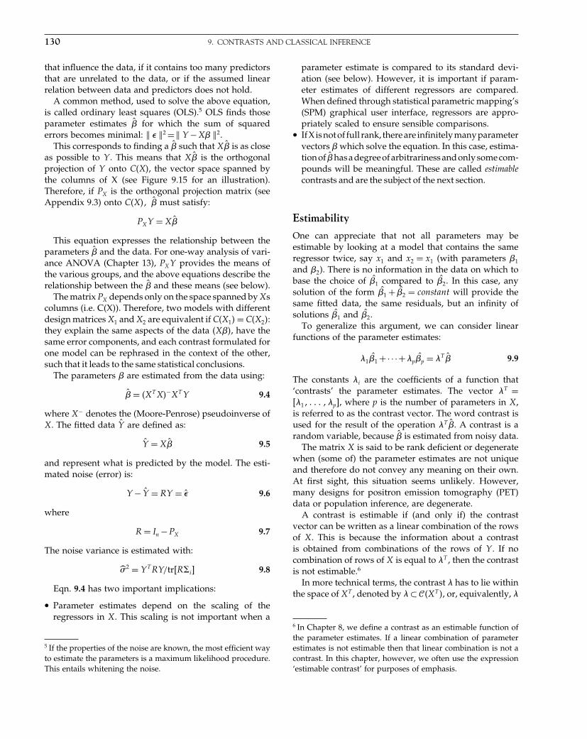
Elsevier UK Chapter: Ch09-P372560 3-10-2006 3:04p.m. Page:130 Trim:7.5in×9.25in
Basal Font:Palatino Margins:Top:40pt Gutter:68pt Font Size:9.5/12 Text Width:42pc Depth:55 Lines
130 9. CONTRASTS AND CLASSICAL INFERENCE
that influence the data, if it contains too many predictorsthat are unrelated to the data, or if the assumed linearrelation between data and predictors does not hold.
A common method, used to solve the above equation,is called ordinary least squares (OLS).5 OLS finds thoseparameter estimates �̂ for which the sum of squarederrors becomes minimal: � � �2 =� Y −X� �2.
This corresponds to finding a �̂ such that X�̂ is as closeas possible to Y . This means that X�̂ is the orthogonalprojection of Y onto C�X�, the vector space spanned bythe columns of X (see Figure 9.15 for an illustration).Therefore, if PX is the orthogonal projection matrix (seeAppendix 9.3) onto C�X�� �̂ must satisfy:
PXY = X�̂
This equation expresses the relationship between theparameters �̂ and the data. For one-way analysis of vari-ance ANOVA (Chapter 13), PXY provides the means ofthe various groups, and the above equations describe therelationship between the �̂ and these means (see below).
The matrix PX depends only on the space spanned by Xscolumns (i.e. C(X)). Therefore, two models with differentdesign matrices X1 and X2 are equivalent if C�X1� = C�X2�:they explain the same aspects of the data �X��, have thesame error components, and each contrast formulated forone model can be rephrased in the context of the other,such that it leads to the same statistical conclusions.
The parameters � are estimated from the data using:
�̂ = �XT X�−XT Y 9.4
where X− denotes the (Moore-Penrose) pseudoinverse ofX. The fitted data Ŷ are defined as:
Ŷ = X�̂ 9.5
and represent what is predicted by the model. The esti-mated noise (error) is:
Y − Ŷ = RY = �̂ 9.6
where
R = In −PX 9.7
The noise variance is estimated with:
�̂2 = Y T RY/trRi� 9.8
Eqn. 9.4 has two important implications:
• Parameter estimates depend on the scaling of theregressors in X. This scaling is not important when a
5 If the properties of the noise are known, the most efficient wayto estimate the parameters is a maximum likelihood procedure.This entails whitening the noise.
parameter estimate is compared to its standard devi-ation (see below). However, it is important if param-eter estimates of different regressors are compared.When defined through statistical parametric mapping’s(SPM) graphical user interface, regressors are appro-priately scaled to ensure sensible comparisons.
• If X is not of full rank, there are infinitely many parametervectors � which solve the equation. In this case, estima-tion of �̂has a degree of arbitrariness and only some com-pounds will be meaningful. These are called estimablecontrasts and are the subject of the next section.
Estimability
One can appreciate that not all parameters may beestimable by looking at a model that contains the sameregressor twice, say x1 and x2 = x1 (with parameters �1
and �2). There is no information in the data on which tobase the choice of �̂1 compared to �̂2. In this case, anysolution of the form �̂1 + �̂2 = constant will provide thesame fitted data, the same residuals, but an infinity ofsolutions �̂1 and �̂2.
To generalize this argument, we can consider linearfunctions of the parameter estimates:
�1�̂1 +· · ·+�p�̂p = �T �̂ 9.9
The constants �i are the coefficients of a function that‘contrasts’ the parameter estimates. The vector �T =�1� � � � ��p�, where p is the number of parameters in X,is referred to as the contrast vector. The word contrast isused for the result of the operation �T �̂. A contrast is arandom variable, because �̂ is estimated from noisy data.
The matrix X is said to be rank deficient or degeneratewhen (some of) the parameter estimates are not uniqueand therefore do not convey any meaning on their own.At first sight, this situation seems unlikely. However,many designs for positron emission tomography (PET)data or population inference, are degenerate.
A contrast is estimable if (and only if) the contrastvector can be written as a linear combination of the rowsof X. This is because the information about a contrastis obtained from combinations of the rows of Y . If nocombination of rows of X is equal to �T , then the contrastis not estimable.6
In more technical terms, the contrast � has to lie withinthe space of XT , denoted by � ⊂ ��XT �, or, equivalently, �
6 In Chapter 8, we define a contrast as an estimable function ofthe parameter estimates. If a linear combination of parameterestimates is not estimable then that linear combination is not acontrast. In this chapter, however, we often use the expression‘estimable contrast’ for purposes of emphasis.

Elsevier UK Chapter: Ch09-P372560 3-10-2006 3:04p.m. Page:131 Trim:7.5in×9.25in
Basal Font:Palatino Margins:Top:40pt Gutter:68pt Font Size:9.5/12 Text Width:42pc Depth:55 Lines
CONSTRUCTING AND TESTING CONTRASTS 131
is unchanged when projected orthogonally onto the rowsof X (i.e. PXT � = � with PXT being the ‘projector’ onto XT ;see Appendix 9.3). The reason for this is as follows: ifthere is redundancy in X, for some linear combinationq, we have Xq = 0. Therefore, Y = X� + Xq + � = X�� +q�+�. So, if we test �T �, we also test �T ��+ q�, hence anestimable contrast � will satisfy �T q = 0. A necessary andsufficient condition for this is that �T = vX.
The SPM interface ensures that any specified contrast isestimable, hence offering protection against contrasts thatwould not make sense in degenerate designs. However,a contrast may be estimable but misinterpreted. In thischapter, we hope to clarify the interpretation of contrasts.
Three design matrices for a two-sample t-test
The (unpaired) two-sample t-test, comparing the meanof two groups, can be implemented in the linear modelframework as follows. Consider an experiment with twogroups of 2 (group 1) and 3 (group 2) subjects. In imagingexperiments, these numbers will be larger (at least 10 orso). We have:
X =
⎡⎢⎢⎢⎢⎣
1 01 00 10 10 1
⎤⎥⎥⎥⎥⎦
then
PXY =
⎡⎢⎢⎢⎢⎣
1/2 1/2 0 0 01/2 1/2 0 0 00 0 1/3 1/3 1/30 0 1/3 1/3 1/30 0 1/3 1/3 1/3
⎤⎥⎥⎥⎥⎦Y = X� =
⎡⎢⎢⎢⎢⎣
ȳ1
ȳ1
ȳ2
ȳ2
ȳ2
⎤⎥⎥⎥⎥⎦
where ȳi is the mean observation in group i. We will nowdescribe two other parameterizations of the same model(such that the matrix PX is identical in all cases) and showhow to specify meaningful contrasts.
Design matrix Parameters Contrasts
(1) X =
⎡⎢⎢⎢⎢⎣
1 01 00 10 10 1
⎤⎥⎥⎥⎥⎦
{�̂1 = ȳ1
�̂2 = ȳ2
�1� 0��̂ = ȳ1
�0� 1��̂ = ȳ2
�1�−1��̂ = ȳ1 − ȳ2
� 5� 5��̂ = mean�ȳ1� ȳ2�
(2) X =
⎡⎢⎢⎢⎢⎣
1 11 10 10 10 1
⎤⎥⎥⎥⎥⎦
{�̂1 + �̂2 = ȳ1
�̂2 = ȳ2
�1� 1��̂ = ȳ1
�0� 1��̂ = ȳ2
�1� 0��̂ = ȳ1 − ȳ2
� 5� 1��̂ = mean�ȳ1� ȳ2�
(3) X =
⎡⎢⎢⎢⎢⎣
1 0 11 0 10 1 10 1 10 1 1
⎤⎥⎥⎥⎥⎦{
�̂1 + �̂3 = ȳ1
�̂2 + �̂3 = ȳ2
�1� 0� 1��̂ = ȳ1
�0� 1� 1��̂ = ȳ2
�1�−1� 0��̂ = ȳ1 − ȳ2
� 5� 5� 1��̂ = mean�ȳ1� ȳ2�
The only intuitive case is the first parameterization. Inthe two other cases, the interpretation of the parameterestimates is not obvious and the contrasts are not intu-itive. In case 3, parameters are not estimable and not allcontrasts are meaningful. Estimable contrasts are orthog-onal to 1 1 −1�, because column 1 plus column 2 equalscolumn 3.
Constructing and testing t-contrasts
If it is clear what the parameter estimates represent, thenspecification of contrasts is simple, especially in the caseof t-contrasts. These contrasts are of the form describedabove, i.e. univariate linear combinations of parameterestimates. We return to our first model, which includesthe four forces and ‘rest’ as regressors. For model 1, wecan ask if there is a linear increase by testing �1 usingthe combination 1�1 +0�2 +0�3 with the contrast vector�T = 1 0 0�. A linear decrease can be tested with �T =−1 0 0�.
To test for the additive offset of the ‘press’ condition,not accounted for by the linear increase, we use �T =0 1 0�. Note here that the linear increase is starting witha value of one for the first force level, and increases to 4for the fourth level (see Figure 9.1).
When testing for the second regressor, we are effectivelyremoving that part of the signal that can be accountedfor by the first regressor. This means that the secondparameter estimate is not the average of the differencebetween the ‘press’ conditions and the rest condition.To obtain the latter difference, we have to constructa re-parameterization of model 1 and replace the firstregressor so that it models only differences of ‘force lev-els’ around an average difference between ‘press’ and‘rest’. This is achieved by orthogonalizing the first regres-sor with respect to the second. This new model, model5, is shown in Figure 9.5. The parameter estimates ofthis new model are [10 30 100] as compared to [10 5100] for model 1. This issue is detailed in Andrade et al.(1999) and an equivalent effect can be seen for F -tests.This emphasizes the principle that one should have inmind not only what is, but also what is not, tested by acontrast.
Another solution (useful in neuroimaging where esti-mating the parameters can be time consuming) is to
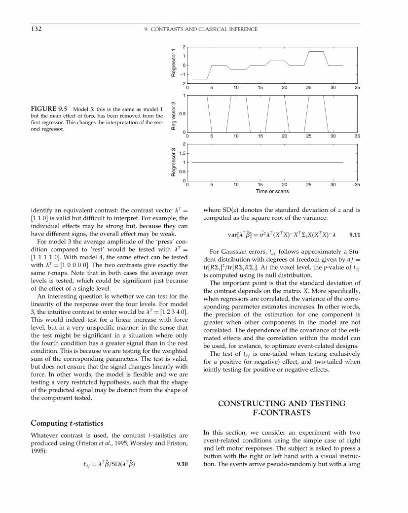
Elsevier UK Chapter: Ch09-P372560 3-10-2006 3:04p.m. Page:132 Trim:7.5in×9.25in
Basal Font:Palatino Margins:Top:40pt Gutter:68pt Font Size:9.5/12 Text Width:42pc Depth:55 Lines
132 9. CONTRASTS AND CLASSICAL INFERENCE
FIGURE 9.5 Model 5: this is the same as model 1but the main effect of force has been removed from thefirst regressor. This changes the interpretation of the sec-ond regressor.
0 5 10 15 20 25 30 35−2
−1
0
1
2
Reg
ress
or 1
0 5 10 15 20 25 30 350
0.5
1
Reg
ress
or 2
0 5 10 15 20 25 30 350
0.5
1
1.5
2
Reg
ress
or 3
Time or scans
identify an equivalent contrast: the contrast vector �T =1 1 0� is valid but difficult to interpret. For example, theindividual effects may be strong but, because they canhave different signs, the overall effect may be weak.
For model 3 the average amplitude of the ‘press’ con-dition compared to ‘rest’ would be tested with �T =1 1 1 1 0�. With model 4, the same effect can be testedwith �T = 1 0 0 0 0�. The two contrasts give exactly thesame t-maps. Note that in both cases the average overlevels is tested, which could be significant just becauseof the effect of a single level.
An interesting question is whether we can test for thelinearity of the response over the four levels. For model3, the intuitive contrast to enter would be �T = 1 2 3 4 0�.This would indeed test for a linear increase with forcelevel, but in a very unspecific manner: in the sense thatthe test might be significant in a situation where onlythe fourth condition has a greater signal than in the restcondition. This is because we are testing for the weightedsum of the corresponding parameters. The test is valid,but does not ensure that the signal changes linearly withforce. In other words, the model is flexible and we aretesting a very restricted hypothesis, such that the shapeof the predicted signal may be distinct from the shape ofthe component tested.
Computing t-statistics
Whatever contrast is used, the contrast t-statistics areproduced using (Friston et al., 1995; Worsley and Friston,1995):
tdf = �T �̂/SD��T �̂� 9.10
where SD�z� denotes the standard deviation of z and iscomputed as the square root of the variance:
var�T �̂� = �̂2�T �XT X�−XT iX�XT X�−� 9.11
For Gaussian errors, tdf follows approximately a Stu-dent distribution with degrees of freedom given by df =trRi�
2/trRiRi�. At the voxel level, the p-value of tdf
is computed using its null distribution.The important point is that the standard deviation of
the contrast depends on the matrix X. More specifically,when regressors are correlated, the variance of the corre-sponding parameter estimates increases. In other words,the precision of the estimation for one component isgreater when other components in the model are notcorrelated. The dependence of the covariance of the esti-mated effects and the correlation within the model canbe used, for instance, to optimize event-related designs.
The test of tdf is one-tailed when testing exclusivelyfor a positive (or negative) effect, and two-tailed whenjointly testing for positive or negative effects.
CONSTRUCTING AND TESTINGF-CONTRASTS
In this section, we consider an experiment with twoevent-related conditions using the simple case of rightand left motor responses. The subject is asked to press abutton with the right or left hand with a visual instruc-tion. The events arrive pseudo-randomly but with a long

Elsevier UK Chapter: Ch09-P372560 3-10-2006 3:04p.m. Page:133 Trim:7.5in×9.25in
Basal Font:Palatino Margins:Top:40pt Gutter:68pt Font Size:9.5/12 Text Width:42pc Depth:55 Lines
CONSTRUCTING AND TESTING F-CONTRASTS 133
0 10 20 30 40Time (secs)
FIGURE 9.6 The left panel shows the design matrix foranalysing two event-related conditions (left or right motorresponses). The shape of the HRF is assumed to be known, up toa scaling factor. The two first regressors have been constructed byconvolution of a series of Dirac functions with the ‘canonical’ HRF(right panel).
inter-stimulus interval. We are interested in brain regionsthat are more activated for right versus left movements.
Our first model assumes that the shape of the haemo-dynamic response function (HRF) can be modelled by a‘canonical HRF’ (see Chapter 14). This model is shownin Figure 9.6. To find brain regions that are moreactive for left versus right motor responses we can use�T = 1 −1 0�. Using Eqn. 9.10 we can compute the t-map shown in Figure 9.7. This shows activation of con-
SPM{T247}
FIGURE 9.7 SPM-t image corresponding to the overall differ-ence between the left and right responses. This map was producedusing the 1 −1 0� contrast weights, using the model shown inFigure 9.6.
tralateral motor cortex plus other typical regions, such asipsilateral cerebellum.
Because there is an implicit baseline, the parameters arealso interpretable individually, and when tested (t-mapsnot shown) they reveal the appropriate visual and motorregions.7 Instead of having the two regressors encod-ing the left and right responses separately, an equiv-alent model could have the first regressor modellingthe response common to right and left and the secondmodelling the difference between them.
The fact that the HRF varies across brain regions andsubjects can be accommodated as follows. A simple exten-sion of the model of Figure 9.6 is presented in Figure 9.8,for which each response is modelled with three basisfunctions. These functions can model small variations inthe delay and dispersion of the HRF, as described inChapter 14. They are mean centred, so the mean parameterwill represent the overall average of the data.
In this new model, how do we test for the effects of,for instance, the right motor response? The most obvi-ous approach is to test for all regressors modelling thisresponse. This does not entail the sum (or average) of theparameter estimates because the sign of those parameterestimates is not interpretable, but rather the (weighted)sum of squares of those parameter estimates. The appro-priate F -contrast is shown in Figure 9.9.
FIGURE 9.8 The same model as in Figure 9.6, but we usethree regressors to model each condition. The first three columnsmodel the first condition (left motor response) while columns 4 to 6model the second condition (right motor response). Each set of threeregressors is the result of the convolution of the stimulus onsetswith the canonical HRF and its derivatives with respect to time anddispersion.
7 Interestingly, there is some ipsilateral activation in the motorcortex such that the ‘left-right’ contrast is slightly less significantin the motor regions than the ‘left’ [1 0 0] contrast.
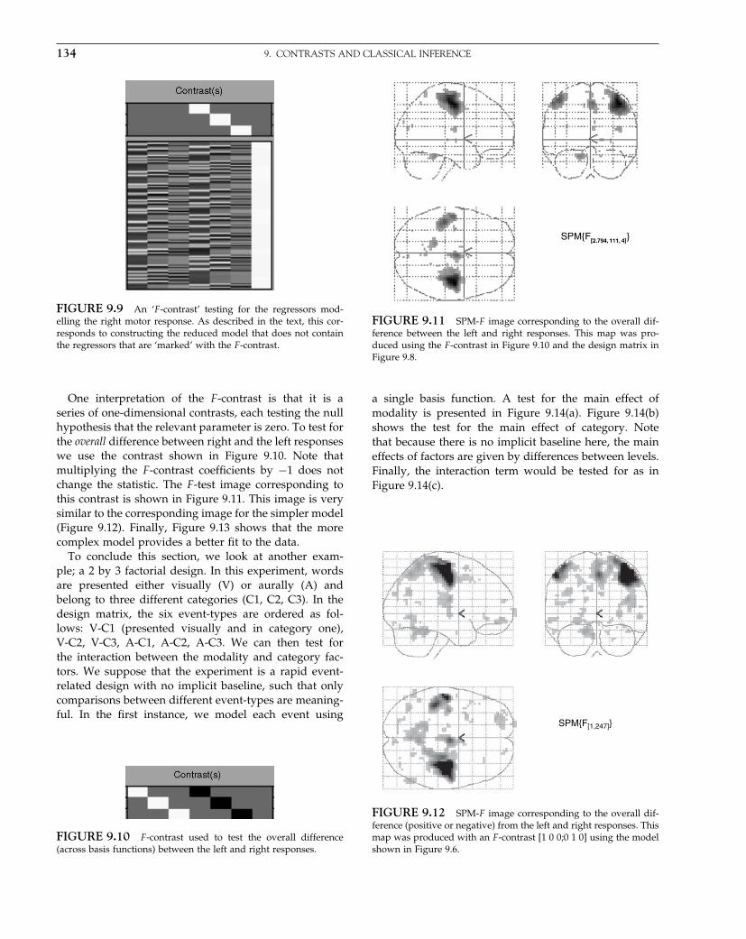
Elsevier UK Chapter: Ch09-P372560 3-10-2006 3:04p.m. Page:134 Trim:7.5in×9.25in
Basal Font:Palatino Margins:Top:40pt Gutter:68pt Font Size:9.5/12 Text Width:42pc Depth:55 Lines
134 9. CONTRASTS AND CLASSICAL INFERENCE
FIGURE 9.9 An ‘F -contrast’ testing for the regressors mod-elling the right motor response. As described in the text, this cor-responds to constructing the reduced model that does not containthe regressors that are ‘marked’ with the F -contrast.
One interpretation of the F -contrast is that it is aseries of one-dimensional contrasts, each testing the nullhypothesis that the relevant parameter is zero. To test forthe overall difference between right and the left responseswe use the contrast shown in Figure 9.10. Note thatmultiplying the F -contrast coefficients by −1 does notchange the statistic. The F -test image corresponding tothis contrast is shown in Figure 9.11. This image is verysimilar to the corresponding image for the simpler model(Figure 9.12). Finally, Figure 9.13 shows that the morecomplex model provides a better fit to the data.
To conclude this section, we look at another exam-ple; a 2 by 3 factorial design. In this experiment, wordsare presented either visually (V) or aurally (A) andbelong to three different categories (C1, C2, C3). In thedesign matrix, the six event-types are ordered as fol-lows: V-C1 (presented visually and in category one),V-C2, V-C3, A-C1, A-C2, A-C3. We can then test forthe interaction between the modality and category fac-tors. We suppose that the experiment is a rapid event-related design with no implicit baseline, such that onlycomparisons between different event-types are meaning-ful. In the first instance, we model each event using
FIGURE 9.10 F -contrast used to test the overall difference(across basis functions) between the left and right responses.
FIGURE 9.11 SPM-F image corresponding to the overall dif-ference between the left and right responses. This map was pro-duced using the F -contrast in Figure 9.10 and the design matrix inFigure 9.8.
a single basis function. A test for the main effect ofmodality is presented in Figure 9.14(a). Figure 9.14(b)shows the test for the main effect of category. Notethat because there is no implicit baseline here, the maineffects of factors are given by differences between levels.Finally, the interaction term would be tested for as inFigure 9.14(c).
SPM{F[1,247]}
FIGURE 9.12 SPM-F image corresponding to the overall dif-ference (positive or negative) from the left and right responses. Thismap was produced with an F -contrast [1 0 0;0 1 0] using the modelshown in Figure 9.6.

Elsevier UK Chapter: Ch09-P372560 3-10-2006 3:04p.m. Page:135 Trim:7.5in×9.25in
Basal Font:Palatino Margins:Top:40pt Gutter:68pt Font Size:9.5/12 Text Width:42pc Depth:55 Lines
CONSTRUCTING AND TESTING F-CONTRASTS 135
Fitted response and adjusted data2.5
2
1.5
1
0.5
0
–0.5
–1.5
Res
pons
e at
[42,
–15
,51]
0 5 10 15
Peri-stimulus time {secs}
20 25 30
–1
Fitted response and adjusted data2.5
2
1.5
1
0.5
0
–0.5
–1.5
Res
pons
e at
[42,
–15
,51]
0 5 10 15Peri-stimulus time {secs}
20 25 30
–1
FIGURE 9.13 Haemodynamic responsesat a single voxel (the maxima of the SPM-F mapin Figure 9.11). The left plot shows the HRF asestimated using the simple model (Figure 9.6)and demonstrates a certain lack of fit. The fitbased on a more flexible model (Figure 9.8) isbetter (right panel).
The number of rows in an interaction contrast (withoutimplicit baseline) is given by:
Nrows =N∏
i=1
�li −1� 9.12
where N is the number of factors and li the number oflevels of factor i.
Interpretation of F-contrasts
There are two equivalent ways of thinking aboutF -contrasts. For example, we can think about theF -contrast in Figure 9.9 as fitting a reduced model thatdoes not contain the ‘right motor response’. This reducedmodel would have a design matrix X0 with zero entries
FIGURE 9.14 F -contrasts testing respectively for (a) the maineffect of modality, (b) the main effect of categories, and (c) theinteraction modality × category.
in place of the ‘right motor response’ regressors of the‘full’ design matrix X. The test then compares the vari-ance of the residuals as compared to that of the full modelX. The F -test simply computes the extra sum of squaresthat can be accounted for by inclusion of the three ‘righthand’ regressors. Following any statistical textbook (e.g.Christensen, 1996) and the work of Friston et al. (1995)and Worsley and Friston (1995), this is expressed by test-ing the following quantity:
Fdf1�df2= �Y T �I −PX0
�Y −Y T �I −PX�Y�/�1
Y T �I −PX�Y/�29.13
with
�1 = tr��R0 −R�i�
�2 = tr�Ri� 9.14
and
df1 = tr��R0 −R�i�R0 −R�i�/tr��R0 −R�i�2 9.15
df2 = tr�RiRi�/tr�Ri�2 9.16
where R0 is the projector onto the residual space of X0
and PX is the orthogonal projector onto X.The second interpretation of the F -test is as a series
of one-dimensional contrasts, each of them testing thenull hypothesis that the respective contrast of parametersis zero.
We now show formally how these two interpretationsare linked. The model in Eqn. 9.3, Y = X�+� is restrictedby the test cT � = 0 where c is now a ‘contrast matrix’.If c yields an estimable function, then we can define amatrix H such that c = HT X. Therefore, HT X� = 0 which,together with Eqn. 9.3, is equivalent to Y ⊂ ��X� andY ⊂ ��H⊥�, the space orthogonal to H . It can be shownthat the reduced model corresponding to this test is X0 =

Elsevier UK Chapter: Ch09-P372560 3-10-2006 3:04p.m. Page:136 Trim:7.5in×9.25in
Basal Font:Palatino Margins:Top:40pt Gutter:68pt Font Size:9.5/12 Text Width:42pc Depth:55 Lines
136 9. CONTRASTS AND CLASSICAL INFERENCE
PX −PH . This is valid if, and only if, the space spannedby X0 is the space defined by ��H�⊥⋂��X�: it is easy toshow that this is indeed the case.
If ��H� ⊂ ��X�, the numerator of Eqn. 9.13 can berewritten as:
Y T �R0 −R�Y = Y T �X0 −R�Y = Y T �PX −X0�Y = Y T �PH�Y9.17
We choose H such that it satisfies the condition abovewith H = �XT �−c, which yields:
Y T �PH�Y = Y T X�XT X�−XT H�HT H�−HT X�XT X�−XT Y
= �̂T c�HT H�−cT �̂ 9.18
This reformulation of the F -test is important for severalreasons. First, it makes the specification and computationof F -tests feasible in the context of large data sets. Speci-fying a reduced model and computing the extra sum ofsquares using Eqn. 9.13 would be computationally toodemanding. Second, it links the t-test and the test of areduced model, and therefore makes it explicit that the‘extra’ variability cannot be explained by the reducedmodel. Third, it makes the test of complex interactionsusing F -tests more intuitive.
The F -contrast that looks at the total contribution ofall the ‘right regressors’ is, however, quite a non-specifictest. One may have a specific hypothesis about the mag-nitude or the delay of the response and would like to testfor this specifically. A reasonable test would be a t-testwith contrast [0 0 0 1 0 0 0 0], testing for a positive valueof the parameter that scales the standard HRF. This isperfectly valid, but it is not a test of the magnitude ofthe response. For instance, if the response has the shapeimplied by the standard model but is delayed signifi-cantly, the test might produce poor results, even if thedelay is taken into account by the temporal derivative(Chapter 14). This may be important when comparingthe magnitude of responses between two conditions: ifthe magnitudes are the same but the delays are differ-ent, across conditions, the test comparing the standardresponse regressors might be misinterpreted: a differencein delays might appear as a difference of magnitude evenif the basis functions are orthogonal to each other.
Note that the simplest F -contrasts are unidimensional,in which case the F -statistic is simply the square of thecorresponding t-statistic. To differentiate between unidi-mensional F -contrasts and t-contrasts in the SPM inter-face, the former are displayed in terms of images and thelatter as bars.
An important point is that, generally, if we are confi-dent about the shape of the expected response, F -tests areoften less sensitive than t-tests. The reason is that, withincreased model complexity, it becomes more likely thata signal of no interest could be captured by the F -contrast.
The F -test implicitly corrects for this (Eqn. 9.13), but thisdecreases sensitivity of the test, as compared to the moreconstrained t-test.
CORRELATION BETWEEN REGRESSORS
Correlationsamongregressorscanmakethe interpretationof tests difficult. Unfortunately, such correlation is oftenimposed by the brain’s dynamics, experimental design orthe method of measurement. The risks of misinterpreta-tion have been extensively discussed in Sen and Srivastava(1990) and Andrade et al., (1999). To summarize, one couldmiss activations when testing for a given contrast if thereis a substantial correlation with the rest of the design. Afrequently encountered example is when the response toa stimulus is highly correlated with a motor response
If one believes that a region’s activity will not be influ-enced by the motor response, then it is advisable to testthis specific region by first removing, from the motorresponse regressor, all that can be explained by the stim-ulus. This can be seen as a ‘dangerous’ procedure becauseif, in fact, the motor response does influence the signalin this region, then an ‘activation’ could be wronglyattributed to a stimulus-induced effect.
Because the issue of what is and what is not testedin a model is so important, we use two complementaryperspectives that might shed light on it. First, from ageometrical perspective, the model is understood as somelow-dimensional space; for purposes of visualization wechoose a two-dimensonal space. The data lie in a greater3D space. The fitted data are an orthogonal projection ofthe data onto the model space (Figure 9.15). If the modelspace is spanned by two predictors C1 and C2, testing forC2 will, in effect, test for the part of C2 that is orthogonalto C1. If the two vectors are very similar (correlated), this
FIGURE 9.15 Geometrical perspective: estimation. The data Yare projected orthogonally onto the space of the design matrix (X)defined by two regressors C1 and C2. The error e is the distancebetween the data and the nearest point within the model space.
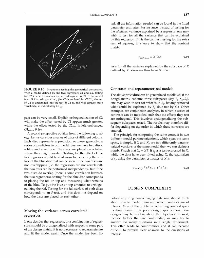
Elsevier UK Chapter: Ch09-P372560 3-10-2006 3:04p.m. Page:137 Trim:7.5in×9.25in
Basal Font:Palatino Margins:Top:40pt Gutter:68pt Font Size:9.5/12 Text Width:42pc Depth:55 Lines
DESIGN COMPLEXITY 137
FIGURE 9.16 Hypothesis testing: the geometrical perspective.With a model defined by the two regressors C1 and C2, testingfor C2 in effect measures its part orthogonal to C1. If the modelis explicitly orthogonalized, (i.e. C2 is replaced by C2orth), the testof C2 is unchanged, but the test of C1 is, and will capture morevariability, as indicated by C1full.
part can be very small. Explicit orthogonalization of C2will make the effect tested by C1 appear much greater,while the effect tested by the C2orth is left unchanged(Figure 9.16).
A second perspective obtains from the following anal-ogy. Let us consider a series of discs of different colours.Each disc represents a predictor, or more generally, aseries of predictors in our model. Say we have two discs,a blue and a red one. The discs are placed on a table,where they might overlap. Testing for the effect of thefirst regressor would be analogous to measuring the sur-face of the blue disc that can be seen. If the two discs arenon-overlapping (i.e. the regressors are not correlated),the two tests can be performed independently. But if thetwo discs do overlap (there is some correlation betweenthe two regressors), testing for the blue disc correspondsto placing the red on top and measuring what remainsof the blue. To put the blue on top amounts to orthogo-nalizing the red. Testing for the full surface of both discscorresponds to an F -test, and this does not depend onhow the discs are placed on each other.
Moving the variance across correlatedregressors
If one decides that regressors, or a combination of regres-sors, should be orthogonalized with respect to some partof the design matrix, it is not necessary to reparameterizeand fit the model again. Once the model has been fit-
ted, all the information needed can be found in the fittedparameter estimates. For instance, instead of testing forthe additional variance explained by a regressor, one maywish to test for all the variance that can be explainedby this regressor. If c is the contrast testing for the extrasum of squares, it is easy to show that the contrastmatrix:
cFull_space = XT Xc 9.19
tests for all the variance explained by the subspace of Xdefined by Xc since we then have H = Xc.
Contrasts and reparameterized models
The above procedure can be generalized as follows: if thedesign matrix contains three subspaces (say S1� S2� S3�,one may wish to test for what is in S1, having removedwhat could be explained by S2 (but not by S3). Otherexamples are conjunction analyses, in which a series ofcontrasts can be modified such that the effects they testare orthogonal. This involves orthogonalizing the sub-sequent subspaces tested. The results may therefore dif-fer depending on the order in which these contrasts areentered.
The principle for computing the same contrast in twodifferent model parameterizations, which span the samespace, is simple. If X and Xp are two differently parame-terized versions of the same model then we can define amatrix T such that Xp = XT . If cp is a test expressed in Xp
while the data have been fitted using X, the equivalentof cp using the parameter estimates of X is
c = cp�TT XT XT�−TT XT X 9.20
DESIGN COMPLEXITY
Before acquiring neuroimaging data one should thinkabout how to model them and which contrasts are ofinterest. Most of the problems concerning contrast spec-ification derive from poor design specification. Poordesigns may be unclear about the objectives pursued,include factors that are confounded, or may try toanswer too many questions in a single experiment.This often leads to compromises and it can becomedifficult to provide clear answers to the questions ofinterest.

Elsevier UK Chapter: Ch09-P372560 3-10-2006 3:04p.m. Page:138 Trim:7.5in×9.25in
Basal Font:Palatino Margins:Top:40pt Gutter:68pt Font Size:9.5/12 Text Width:42pc Depth:55 Lines
138 9. CONTRASTS AND CLASSICAL INFERENCE
This does not preclude the use of a complex paradigm,in the sense that many conditions can and (often shouldbe) included in the design. The process of recruitingsubjects and acquiring data is long and costly, and itis only natural that one would like to answer as manyquestions as possible with the same data. However, thisrequires careful thought about which contrasts will bespecified and whether they actually answer the questionof interest.
SUMMARY
In functional imaging experiments, one is often interestedin many sorts of effects, e.g. the main effect of a factorand the possible interactions between factors. To analyseeach of these effects one could fit several different GLMsand test hypotheses by looking at individual parameterestimates. However, this approach is impractical, becausefunctional imaging data sets are very large. A more expe-dient approach is to fit larger models and test for effectsusing specific contrasts.
In this chapter, we have seen how the specification ofthe design matrix is intimately related to the specificationof contrast weights. For example, it is often the case thatmain effects and interactions can be set up using paramet-ric or non-parametric designs. These different designs lead
to the use of different contrasts. Parametric approaches arefavoured for factorial designs with many levels per factor.Contrasts must be estimable to be interpretable, and wehave described the conditions for estimability.
In fMRI, one can model haemodynamic responsesusing the canonical HRF. This allows one to test for acti-vations using t-contrasts. To account for the variabil-ity in the haemodynamic response, across subjects andbrain regions, one can model the HRF using a canonicalHRF plus its derivatives, with respect to time and disper-sion. Inferences about differences in activation can thenbe made using F -contrasts. We have shown that thereare two equivalent ways of interpreting F -contrasts, oneemploying the extra-sum-of-squares principle to comparethe model and a reduced model, and one specifying aseries of one-dimensional contrasts. Designs with corre-lations between regressors are less efficient and correla-tion can be removed by orthogonalizing one effect withrespect to others. However, this may have a strong impacton the interpretation of subsequent tests. Finally, we haveshown how such orthogonalization can be applied retro-spectively, i.e. without having to refit the models.
In this chapter, we have focused on how to test forspecific treatment effects encoded by the design matrixof the general linear model. However, the general linearmodel also entails assumptions about the random errors.In the next chapter, we examine these assumptions, interms of covariance components and non-sphericity.
APPENDIX 9.1 NOTATION
Y : Data The �n� 1� time series, where n is the number of time points orscans. yi: one of those measures.
c or �: Contrast weights Linear combination of the parameter estimates used to form the(numerator) of the statistics
X: Design matrix or design model the �n�p� matrix of regressors�: Model parameters The true (unobservable) coefficients such that the weighted sum
of the regressors is the expectation of our data (if X is correct)�̂: Parameter estimates The computed estimation of the � using the data Y : �̂ =
�XT X�−XT YC�X�: Vector space spanned by X Given a model X, the vector space spanned by X are all vectors v
that can be written as v = X�PX�X� orM�X�: The orthogonal projector onto X PX = X�XT X�−XT
R: Residual forming matrix Given a model X, the residual forming matrix R = In −XX− trans-forms the data Y into the residuals r = RY .
�2i: scan (time) covariance This �n�n� matrix describes the (noise) covariance between scans
Elsevier UK Chapter: Ch09-P372560 3-10-2006 3:04p.m. Page:139 Trim:7.5in×9.25in
Basal Font:Palatino Margins:Top:40pt Gutter:68pt Font Size:9.5/12 Text Width:42pc Depth:55 Lines
REFERENCES 139
APPENDIX 9.2 SUBSPACES
Let us consider a set of p vectors xi of dimension �n� 1�(with p < n), e.g. regressors in fMRI. The space spannedby this set of vectors is formed from all possible vectors(say u) that can be expressed as a linear combinationof the xi: u = �1x1 + �2x2 + � � � �pxp. If the matrix X isformed with the xi : X = x1x2 � � � xp�, we denote this spaceas ��X�.
Not all the xi may be necessary to form ��X�. Theminimal number needed is called the rank of the matrixX. If only a subset of the xi is selected, they form asmaller matrix X0. The space spanned by X0, ��X0�,is called a subspace of X. A contrast defines twosubspaces of the design matrix X: one that is testedand one of ‘no interest’, corresponding to the reducedmodel.
APPENDIX 9.3 ORTHOGONALPROJECTION
The orthogonal projection of a vector x onto the space ofa matrix A is the vector (e.g a time-series) that is closestin the space C�A�, where distance is measured as thesum of squared errors. The projector onto A, denotedPA, is unique and can be computed with PA = AA−, with
A− denoting the Moore-Penrose pseudoinverse8 of A. Forinstance, the fitted data Ŷ can be computed with
Ŷ = PXY = XX−Y = X�XT X�−XT Y = X�̂ 9.21
Most of the operations needed when working with linearmodels only involve computations in parameter space, asis shown in Eqn. 9.18. For a further gain in computationalexpediency, one can work with an orthonormal basis ofthe space of X, if the design is degenerate. This is howthe SPM code is implemented.
REFERENCES
Andrade A, Paradis A-L, Rouquette S et al. (1999) Ambiguous resultsin functional neuroimaging data analysis due to covariate cor-relation. Neuroimage 10: 83–86
Christensen R (1996) Plane answers to complex questions: the theory oflinear models. Springer, Berlin
Fisher RA (1935) The Design of Experiments. Oliver and Bayd,Edinburgh
Friston KJ, Holmes AP, Worsley KJ et al. (1995) Statistical parametricmaps in functional imaging: a general linear approach. HumBrain Mapp 2: 189–210
Russell EJ (1926) Field experiments: how they are made and whatthey are. Journal of the Ministry of Agriculture 32: 989–1001
Sen A, Srivastava M (1990) Regression analysis – theory, methods, andapplications. Springer-Verlag, Berlin
Worsley KJ, Friston KJ (1995) Analysis of fMRI time-seriesrevisited – again. NeuroImage 2: 73–81
8 Any generalized inverse could be used.
Elsevier UK Chapter: Appendix1-P372560 3-10-2006 4:22p.m. Page:589 Trim:7.5in×9.25in
Basal Font:Palatino Margins:Top:40pt Gutter:68pt Font Size:9.5/12 Text Width:42pc Depth:55 Lines
A P P E N D I X
1
Linear models and inferenceK. Friston
INTRODUCTION
In this appendix, we gather together different perspec-tives on inference with multivariate linear models. Inbrief, we will see that all inference, whether it is based onlikelihood ratios (i.e. classical statistics), canonical vari-ates analysis, linear discriminant analysis, Bayesian anal-ysis or information theory, can be regarded as tests of thesame thing, namely, the statistical dependence betweenone set of variables and another. This is useful to appreci-ate because it means there is no difference between infer-ence using generative models (i.e. functions of causes thatgenerate data) and inference based on recognition models(i.e. functions of data that recognize causes). This equiv-alence rests on the invertability of linear models, whichmeans that recognition or classification models are sim-ply the inverse of generative or forward models. In otherwords, there is no difference between reverse-correlationmethods (e.g. Hansen et al., 2004; Hasson et al., 2004) orbrain-reading (Cox and Savoy, 2003) and conventionalanalyses (e.g. Friston et al., 1996; Worsley et al., 1997;Kherif et al., 2002), provided the models are linear.
In what follows, we look at the problem of establishingstatistical dependencies from an information theory pointof view and then revisit the same issue from a classical,a Bayesian and finally a multivariate perspective.
INFORMATION THEORY ANDDEPENDENCY
The aim of classification is to find some function of datay that can be used to classify or predict their causes x.Conversely, the aim of hypothesis testing is to show thathypothetical causes predict data. For simplicity, we willassume both x and y represent s independent samples
drawn from multivariate distributions. The ability to pre-dict one, given the other, rests on the statistical dependen-cies between x and y that are quantified by their mutualinformation. Irrespective of the form of these dependen-cies, the mutual information is given by the differencebetween both their entropies and the entropy of both:
I�x�y� = H�y�+H�y�−H�x�y�
= H�y�−H�y�x�A1.1
This is the difference between the entropy, or infor-mation, of one minus the information given the other.Under Gaussian assumptions, we have only to considermoments of the densities to second-order (i.e. covari-ances). Their Gaussian form allows us to express thedensities in terms of �y ⊗ Is, the covariance of vec(y) andits conditional covariance �y�x ⊗ Is.
H�y� = �− ln p�y�� = 12
ln ��y ⊗ Is�
H�y �x � = �− ln p�y�x�� = 12
ln ��y�x ⊗ Is�
I�x�y� = s
2�ln ��y�− ln ��y�x��
= s
2ln ��−1
y�x�y�
A1.2
Here and throughout, constant terms have been ignored.The mutual information can be estimated using samplecovariances. From Eqn. A1.1, and using standard resultsfor the determinant of block matrices:
I�x�y� = s
2�ln �yT y�− ln �yT y −yT x�xT x�−1xT y��
H�x� = s
2ln ��x� = s
2ln �xT x�
H�y� = s
2ln ��y� = s
2ln �yT y�
H�x�y� = s
2ln∣∣∣∣[xT x yT xxT y yT y
]∣∣∣∣
A1.3
Statistical Parametric Mapping, by Karl Friston et al. Copyright 2007, Elsevier Ltd. All rights reserved.ISBN–13: 978-0-12-372560-8 ISBN–10: 0-12-372560-7
589

Elsevier UK Chapter: Appendix1-P372560 3-10-2006 4:22p.m. Page:590 Trim:7.5in×9.25in
Basal Font:Palatino Margins:Top:40pt Gutter:68pt Font Size:9.5/12 Text Width:42pc Depth:55 Lines
590 A1. LINEAR MODELS AND INFERENCE
Comparison of Eqn. A1.2 and Eqn. A1.3 shows:
�y = yT y
�y�x = yT y −yT x�xT x�−1xT yA1.4
In fact, we will see below that these are the maximumlikelihood estimates of the covariances. It is sometimesuseful to express the mutual information or predictabil-ity in terms of linearly separable components using thegeneralized eigenvector solution, with a leading diagonalmatrix of eigenvalues �:
�yc = �y�xc�
cT c = I
I�x�y� = s
2ln ��−1
y�x�y�
= s
2ln ���
= s
2ln �1 + s
2ln �2 +· · ·
A1.5
where ci are the generalized eigenvectors, which defineorthogonal mixtures of y that express the greatest mutualinformation with x. This information is simply s
2 ln �i. Wewill see below that ci are canonical vectors. Practicallyspeaking, one could use these vectors to predict x, usingone or more canonical variates vi = yci.
OTHER PERSPECTIVES
Classical inference
In a classical setting, we test a null hypothesis. This callsfor a model comparison, usually of a null model againstan alternate model. We will assume a linear mappingbetween the causes and data:
y = x� +� A1.6
where � is some well-behaved error term. The nullhypothesis is � = 0. Following the Neyman-PearsonLemma, classical statistics uses the maximum likelihoodratio, which, in this context, is:
L = p�y�x� �̂�
p�y�⇒
ln L = ln p�y�x� �̂�− ln p�y�
�̂ = max�
p�y�x��� = �xT x�−1xT y
A1.7
The maximum likelihood value of the parameters isthe usual least squares estimator (this is because we
assumed the errors are IID (independent and identi-cally distributed) and can be derived simply by solving ln p�y�x���/� = 0. The maximum log-likelihoods, underthe null and alternate hypotheses are:
ln p�y� = − s
2ln �R0�−
12
vec�y�T �R−10 ⊗ Is�vec�y�
R0 = maxR0
ln p�y� = yT y
ln p(y�x� �̂
)= − s
2ln �R�− 1
2vec�r�T �R−1 ⊗ Is�vec�r�
r = y −x�̂
R = maxR
ln p�y�x� �̂� = rT r
= yT y −yT x�xT x�−1xT y
A1.8
R0 = �y and R = �y�x are the sum of squares and prod-ucts (SSQP) of the residuals under the null and alter-nate hypotheses respectively. The maximum likelihoodexpression for R0, like the parameters, is obtained easilyby solving ln p�y�/R−1
0 = 0. Similarly for R, substitutingEqn. A1.8 into Eqn. A1.7 shows that the log-likelihoodratio statistic is simply the mutual information:
ln L = s
2�ln �R0�− ln �R�� = s
2�ln ��y�− ln ��y�x�� = I�x�y�
A1.9
In this context, the likelihood ratio is known as Wilk’sLambda = L−1. When the dimensionality of y is one,this statistic is the basis of the F -ratio. When the dimen-sionality of x is also one, the square root of the F -ratio isthe t-statistic. Classical inference uses the null distribu-tion of the log-likelihood ratio to reject the null hypoth-esis that � = 0 to infer that I�x�y� > 0.
A Bayesian perspective
A Bayesian perspective on the predictability issue wouldcall for a comparison of two models, with and withoutx as a predictor. This would proceed using the differ-ences in log-evidence or marginal likelihoods betweenthe alternative and null models:
ln p�y�x�− ln p�y� = − s
2ln �R�+ s
2ln �R0� = I�x�y� A1.10
In the context of linear models, this is simply the mutualinformation.
A multivariate perspective
In linear multivariate models, such as canonical variatesanalysis, canonical correlation analysis, and linear dis-criminant function analysis, one is trying to find a mix-ture of y that affords the best discrimination, in relation

Elsevier UK Chapter: Appendix1-P372560 3-10-2006 4:22p.m. Page:591 Trim:7.5in×9.25in
Basal Font:Palatino Margins:Top:40pt Gutter:68pt Font Size:9.5/12 Text Width:42pc Depth:55 Lines
REFERENCES 591
to x. This proceeds by maximizing the length of a vectorprojected onto the subspace of y, which can be explainedby x, relative to its length in the subspace that cannot.More formally, subject to the constraint cT c = I , we want:
c = maxc
cT Tc
cT Rc
T = �T xT x�
A1.11
where T is referred to as the SSQP due to treatments. Thisis the null space of the residual SSQP. This means the totalSSQP of y decomposes into the orthogonal covariancecomponents:
R0 = T +R A1.12
The canonical vectors c are the principal generalizedeigenvectors:
Tc = Rc�
cT c = I
However, from Eqn. A1.12:
�R0 −R�c = Rc�
R0c−Rc = Rc�
R0c = Rc��+ I� =�yc = �y�xc��+ I�
A1.13
which has exactly the same form as Eqn. A1.5. In otherwords, the canonical vectors are simply the mixturesthat express the greatest mutual information with x; theamount of information is s
2 ln��i +1�, where �i = �i −1 isthe i-th canonical value. From Eqn. A1.5, Eqn. A1.9 andEqn. A1.13 we get:
− ln = I�x�y�
= s
2ln �1 + s
2ln �2 +· · ·
= s
2ln��1 +1�+ s
2ln��2 +1�+· · ·
A1.14
Tests for the dimensionality of the subspace are basedon the canonical values ln��i +1� (see Chapter 37).
SUMMARY
In the context of linear mappings under Gaussianassumptions, the heart of inference lies in the gener-alized eigenvalue solution. This solution finds pairs ofgeneralized eigenvectors that show the greatest statisticaldependence between two sets of multivariate data. Thegeneralized eigenvalues encode the mutual informationbetween the i-th variate and its corresponding vector. Thetotal information is the log-likelihood ratio, or log-Bayesfactor, comparing models with and without a linear map-ping. Special cases of this quantity are Wilk’s Lambda,Hotelling’s T -square, the F -ratio and the t-statistic, uponwhich classical inference is based.
REFERENCES
Cox DD, Savoy RL (2003) Functional magnetic resonance imaging(fMRI) ‘brain reading’: detecting and classifying distributed pat-terns of fMRI activity in human visual cortex. NeuroImage 192:61–70
Friston KJ, Stephan KM, Heather JD et al. (1996) A multivariateanalysis of evoked responses in EEG and MEG data. NeuroImage3: 167–74
Hansen KA, David SV, Gallant JL (2004) Parametric reverse corre-lation reveals spatial linearity of retinotopic human V1 BOLDresponse. NeuroImage 23: 233–41
Hasson U, Nir Y, Levy I et al. (2004) Intersubject synchronization ofcortical activity during natural vision. Science 303: 1634–40
Kherif F, Poline JB, Flandin G et al. (2002) Multivariate model spec-ification for fMRI data. NeuroImage 16: 1068–83
Worsley KJ, Poline JB, Friston KJ et al. (1997) Characterizing theresponse of PET and fMRI data using multivariate linear models.NeuroImage 6: 305–19
Elsevier UK Chapter: Appendix2-P372560 3-10-2006 4:23p.m. Page:592 Trim:7.5in×9.25in
Basal Font:Palatino Margins:Top:40pt Gutter:68pt Font Size:9.5/12 Text Width:42pc Depth:55 Lines
A P P E N D I X
2
Dynamical systemsK. Friston
INTRODUCTION
This appendix reviews models of dynamical systems. Thereview is framed in terms of analyses of functional andeffective connectivity, in which we focus on the natureand form of the models and less on estimation or infer-ence issues. The aim is to relate various models and tomake their underlying assumptions transparent.
As we have seen in the preceding chapters, there area number of models for estimating effective connectiv-ity using neuroimaging time-series. By definition, effec-tive connectivity depends on a causal model, throughwhich it is defined operationally (Friston, 1995). Thisappendix reviews the principal models that could beadopted and how they relate to each other. We considerdynamic causal models (DCM), generalized convolutionmodels (GCM), coherence analyses, structural equationmodels (SEM), state-space models (SSM) and multivari-ate autoregression-moving average (ARMA) models. Inbrief, we will show that they are all special cases of eachother and try to emphasize their points of contact. How-ever, some fundamental distinctions arise that guide theselection of the appropriate models in different situations.We now review these distinctions.
Coupling among inputs, outputsor hidden states?
The first distinction rests upon whether the model isused to explain the coupling between the inputs andoutputs, among different outputs or among the system‘sstates (e.g. neuronal activity in different ensembles). Interms of models, this distinction is between input-outputmodels, e.g. multiple-input-single-output models (MISO)or multiple-input-multiple-output models (MIMO) and
explicit input-state-output models. Usually, the input-output approach is concerned with the non-linear trans-formation of inputs, enacted by a system, to produceits outputs. This is like trying to establish a statisticaldependence of the outputs on the inputs, without anycomment on the mechanisms mediating this dependency.In some instances (e.g. ARMA and coherence analyses),dependences among different outputs are characterized(cf. functional connectivity).
Conversely, the input-state-output approach is gener-ally concerned with characterizing the coupling amonghidden variables that represent the states of the sys-tem. These states are observed vicariously through theoutputs (Figure A2.1). Inferring the coupling amongstates induces the need for a causal model of how statesaffect each other and form outputs (cf. effective con-nectivity). Examples of input-output models include theVolterra formulation and generalized coherence analy-ses in the spectral domain. An example of a model thattries to estimate coupling among hidden states is DCM.In short, input-output models of coupling can proceedwithout reference to the hidden states. Conversely, inter-actions among hidden states require indirect access tothe states through some model of the causal architectureof the system. In the next section, we start by reviewinginput-output models and then turn to input-state-outputmodels.
Deterministic or stochastic inputs?
The second key distinction is when the input is known(e.g. DCM) and when it is not (e.g. ARMA and SEM).This distinction depends on whether the inputs enter asknown and/or deterministic quantities (e.g. experiment-ally designed causes of evoked responses) or whetherwe know (or can assume) something about the statistics
Statistical Parametric Mapping, by Karl Friston et al. Copyright 2007, Elsevier Ltd. All rights reserved.ISBN–13: 978-0-12-372560-8 ISBN–10: 0-12-372560-7
592
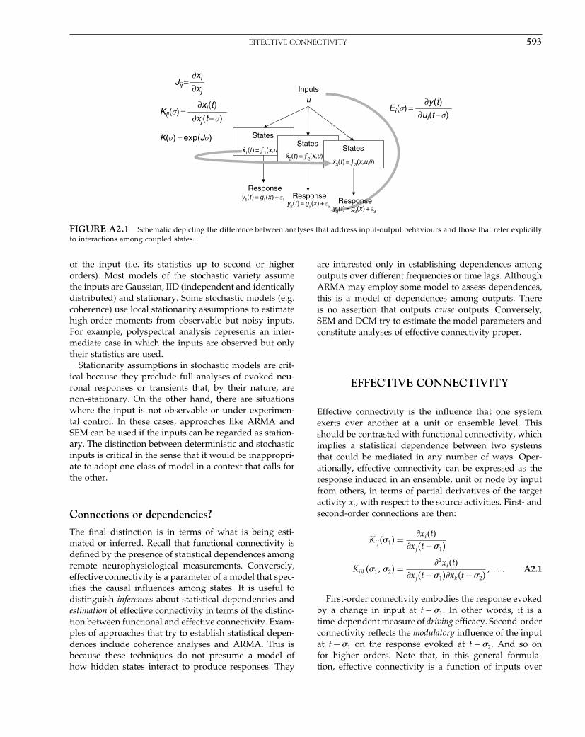
Elsevier UK Chapter: Appendix2-P372560 3-10-2006 4:23p.m. Page:593 Trim:7.5in×9.25in
Basal Font:Palatino Margins:Top:40pt Gutter:68pt Font Size:9.5/12 Text Width:42pc Depth:55 Lines
EFFECTIVE CONNECTIVITY 593
ResponseResponse
Response
States
y1(t ) = g1(x ) + ε1 y2(t ) = g2(x ) + ε2 y3(t ) = g3(x ) + ε3
Inputsu
StatesStates
K(σ) = exp(Jσ)
Kij (σ) =
∂xi (t
)
∂xj (t − σ)
Ei (σ) =
∂y (t
)
∂ui (t − σ)
∂xi
∂xjJij =
x1(t ) = ƒ1(x,u.
.
x2(t ) = ƒ2(x,u).
x3(t ) = ƒ3(x,u,θ).
FIGURE A2.1 Schematic depicting the difference between analyses that address input-output behaviours and those that refer explicitlyto interactions among coupled states.
of the input (i.e. its statistics up to second or higherorders). Most models of the stochastic variety assumethe inputs are Gaussian, IID (independent and identicallydistributed) and stationary. Some stochastic models (e.g.coherence) use local stationarity assumptions to estimatehigh-order moments from observable but noisy inputs.For example, polyspectral analysis represents an inter-mediate case in which the inputs are observed but onlytheir statistics are used.
Stationarity assumptions in stochastic models are crit-ical because they preclude full analyses of evoked neu-ronal responses or transients that, by their nature, arenon-stationary. On the other hand, there are situationswhere the input is not observable or under experimen-tal control. In these cases, approaches like ARMA andSEM can be used if the inputs can be regarded as station-ary. The distinction between deterministic and stochasticinputs is critical in the sense that it would be inappropri-ate to adopt one class of model in a context that calls forthe other.
Connections or dependencies?
The final distinction is in terms of what is being esti-mated or inferred. Recall that functional connectivity isdefined by the presence of statistical dependences amongremote neurophysiological measurements. Conversely,effective connectivity is a parameter of a model that spec-ifies the causal influences among states. It is useful todistinguish inferences about statistical dependencies andestimation of effective connectivity in terms of the distinc-tion between functional and effective connectivity. Exam-ples of approaches that try to establish statistical depen-dences include coherence analyses and ARMA. This isbecause these techniques do not presume a model ofhow hidden states interact to produce responses. They
are interested only in establishing dependences amongoutputs over different frequencies or time lags. AlthoughARMA may employ some model to assess dependences,this is a model of dependences among outputs. Thereis no assertion that outputs cause outputs. Conversely,SEM and DCM try to estimate the model parameters andconstitute analyses of effective connectivity proper.
EFFECTIVE CONNECTIVITY
Effective connectivity is the influence that one systemexerts over another at a unit or ensemble level. Thisshould be contrasted with functional connectivity, whichimplies a statistical dependence between two systemsthat could be mediated in any number of ways. Oper-ationally, effective connectivity can be expressed as theresponse induced in an ensemble, unit or node by inputfrom others, in terms of partial derivatives of the targetactivity xi, with respect to the source activities. First- andsecond-order connections are then:
Kij��1� = �xi�t�
�xj�t −�1�
Kijk��1��2� = �2xi�t�
�xj�t −�1��xk�t −�2�� � � � A2.1
First-order connectivity embodies the response evokedby a change in input at t − �1. In other words, it is atime-dependent measure of driving efficacy. Second-orderconnectivity reflects the modulatory influence of the inputat t − �1 on the response evoked at t − �2. And so onfor higher orders. Note that, in this general formula-tion, effective connectivity is a function of inputs over

Elsevier UK Chapter: Appendix2-P372560 3-10-2006 4:23p.m. Page:594 Trim:7.5in×9.25in
Basal Font:Palatino Margins:Top:40pt Gutter:68pt Font Size:9.5/12 Text Width:42pc Depth:55 Lines
594 A2. DYNAMICAL SYSTEMS
the recent past.1 Furthermore, implicit in Eqn. A2.1 isthe fact that effective connectivity is causal, unless �1
is allowed to be negative. It is useful to introduce thedynamic equivalent, in which the response of the targetis expressed in terms of changes in activity:
Jij = �ẋi
�xj
�Jij
�xk
= �2ẋi
�xj�xk
� � � A2.2
where ẋi = �xi
/�t. In this dynamic form, all influences
are causal and instantaneous. In this appendix, we willcall the K��� effective connections and J coupling. Wewill see later that they are related by K��� = exp�J�� andthat effective connectivity can be formulated in terms ofVolterra kernels. Before considering specific models ofeffective connectivity, we will review briefly their basis(see also Chapter 38).
Dynamical systems
A plausible model of neuronal systems is a non-linear dynamical model that corresponds to an ana-lytic multiple-input-multiple-output (MIMO) system.The state and output equations of a analytic dynamicalsystem are:
ẋ�t� = f�x�u���
y�t� = g�x�+A2.3
Typically the inputs u�t� correspond to designedexperimental effects (e.g. stimulus functions in func-tional magnetic resonance imaging, fMRI), or representstochastic fluctuations or system perturbations. Stochas-tic observation error ∼ N�0�� enters linearly in thismodel. For simplicity, the expressions below deal withsingle-input-single-output (SISO) systems, and will begeneralized later. The measured response y is somenon-linear function of the states of the system x. Thesestate variables are usually unobserved or hidden (e.g.the configuration of all ion channels, the depolarizationof every dendritic compartment etc.). The parametersof the state equation embody effective connectivity,either in terms of mediating the coupling betweeninputs and outputs (MISO models of a single region)or through the coupling among state variables (MIMOmodels of multiple regions). The objective is to estimateand make inferences (usually Bayesian) about theseparameters, given the outputs and possibly the inputs.
1 In contrast, functional connectivity is model-free and simplyreflects the mutual information I�xi� xj�. In this appendix we areconcerned only with models of effective connectivity.
Sometimes this requires one to specify the form of thestate equation. A ubiquitous and useful form is thebilinear approximation; expanding around x0:
ẋ�t� ≈ Ax+uBx+Cu
y = Lx
A = �f
�x� B = �2f
�x�u� C = �f
�u� L = �g
�x
A2.4
For simplicity, we have assumed x0 = 0 and f�0� = g�0� = 0.This bilinear model is sometimes expressed in a morecompact form by augmenting the states with a constant:
Ẋ = �M +uN�X
y = HX
X =[
1x
]M =
[0 0f A
]N =
[0 0C B
]H = [
g L] A2.5
(see Friston, 2002). Here the coupling parameters com-prise the matrices � = A�B�C�L. We will use the bilinearparameterization when dealing with MIMO models andtheir derivatives below. We will first deal with MISOmodels, with and without deterministic inputs.
INPUT-OUTPUT MODELS
Models for deterministic inputs – TheVolterra formulation
In this section, we review the Volterra formulationof dynamical systems. This formulation is importantbecause it allows the input-output behaviour of a sys-tem to be characterized in terms of kernels that can beestimated without knowing the states of the system.
The Fliess fundamental formula (Fliess et al., 1983)describes the causal relationship between the outputs andthe history of the inputs. This relationship conforms toa Volterra series which expresses the output as a gen-eralized convolution of the input, critically without ref-erence to the states. This series is simply a functionalTaylor expansion of the outputs with respect to the inputs(Bendat, 1990). The reason it is a functional expansion isthat the inputs are a function of time:
y�t� = h�u���+
h�u��� =∑i
t∫0
� � �
t∫0
�i��1� � � ���i�u�t −�1�� � � ��
u�t −�i�d�1� � � �� d�i A2.6
�i��1� � � ���i� = �iy�t�
�u�t −�1�� � � �� �u�t −�i�
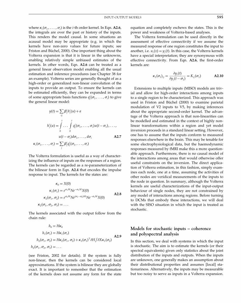
Elsevier UK Chapter: Appendix2-P372560 3-10-2006 4:23p.m. Page:595 Trim:7.5in×9.25in
Basal Font:Palatino Margins:Top:40pt Gutter:68pt Font Size:9.5/12 Text Width:42pc Depth:55 Lines
INPUT-OUTPUT MODELS 595
where �i��1� � � � ��i� is the i-th order kernel. In Eqn. A2.6,the integrals are over the past or history of the inputs.This renders the model causal. In some situations anacausal model may be appropriate (e.g. in which thekernels have non-zero values for future inputs; seeFriston and Büchel, 2000). One important thing about theVolterra expansion is that it is linear in the unknowns,enabling relatively simple unbiased estimates of thekernels. In other words, Eqn. A2.6 can be treated as ageneral linear observation model enabling all the usualestimation and inference procedures (see Chapter 38 foran example). Volterra series are generally thought of as ahigh-order or generalized non-linear convolution of theinputs to provide an output. To ensure the kernels canbe estimated efficiently, they can be expanded in termsof some appropriate basis functions qi
j��1� � � ���i� to givethe general linear model:
y�t� =∑ij
�ijh
ij�u�+
hij�u� =
t∫0
� � �
t∫0
qij��1� � � ���i�u�t −�1�� � � ��
u�t −�i�d�1� � � �� d�i A2.7
�i��1� � � ���i� =∑j
�ijq
ij ��1� � � ���i�
The Volterra formulation is useful as a way of character-izing the influence of inputs on the responses of a region.The kernels can be regarded as a re-parameterization ofthe bilinear form in Eqn. A2.4 that encodes the impulseresponse to input. The kernels for the states are:
�0 = X�0�
�1��1� = e�1MNe−�1MX�0�
�2��1��2� = e�2MNe��1−�2�MNe−�1MX�0�
�2��1��2��3� = � � �
A2.8
The kernels associated with the output follow from thechain rule:
h0 = H�0
h1��1� = H�1��1�
h2��1��2� = H�2��1��2�+�1��1�T �H
/�X�1��2�
h2��1��2��3� = � � �
A2.9
(see Friston, 2002 for details). If the system is fullynon-linear, then the kernels can be considered localapproximations. If the system is bilinear they are globallyexact. It is important to remember that the estimationof the kernels does not assume any form for the state
equation and completely eschews the states. This is thepower and weakness of Volterra-based analyses.
The Volterra formulation can be used directly in theassessment of effective connectivity if we assume themeasured response of one region constitutes the input toanother, i.e. ui�x� = yj�t�. In this case, the Volterra kernelshave a special interpretation; they are synonymous witheffective connectivity. From Eqn. A2.6, the first-orderkernels are:
�1��1�ij = �yi�t�
�yj�t −�1�= Kij��1� A2.10
Extensions to multiple inputs (MISO) models are triv-ial and allow for high-order interactions among inputsto a single region to be characterized. This approach wasused in Friston and Büchel (2000) to examine parietalmodulation of V2 inputs to V5, by making inferencesabout the appropriate second-order kernel. The advan-tage of the Volterra approach is that non-linearities canbe modelled and estimated in the context of highly non-linear transformations within a region and yet modelinversion proceeds in a standard linear setting. However,one has to assume that the inputs conform to measuredresponses elsewhere in the brain. This may be tenable forsome electrophysiological data, but the haemodynamicresponses measured by fMRI make this a more question-able approach. Furthermore, there is no causal model ofthe interactions among areas that would otherwise offeruseful constraints on the inversion. The direct applica-tion of Volterra estimation, in this fashion, simply exam-ines each node, one at a time, assuming the activities ofother nodes are veridical measurements of the inputs tothe node in question. In summary, although the Volterrakernels are useful characterizations of the input-outputbehaviour of single nodes, they are not constrained byany model of interactions among regions. Before turningto DCMs that embody these interactions, we will dealwith the SISO situation in which the input is treated asstochastic.
Models for stochastic inputs – coherenceand polyspectral analysis
In this section, we deal with systems in which the inputis stochastic. The aim is to estimate the kernels (or theirspectral equivalents) given only statistics about the jointdistribution of the inputs and outputs. When the inputsare unknown, one generally makes an assumption abouttheir distributional properties and assumes [local] sta-tionariness. Alternatively, the inputs may be measurablebut too noisy to serve as inputs in a Volterra expansion.

Elsevier UK Chapter: Appendix2-P372560 3-10-2006 4:23p.m. Page:596 Trim:7.5in×9.25in
Basal Font:Palatino Margins:Top:40pt Gutter:68pt Font Size:9.5/12 Text Width:42pc Depth:55 Lines
596 A2. DYNAMICAL SYSTEMS
In this case, they can be used to estimate the inputand output densities in terms of high-order cumulantsor polyspectral density. The n-th order cumulant of theinput is:
cu �1� � � ���n−1� = �u�t�u�t −�1�� � � ��u�t −�n−1�� A2.11
where we have assumed here, and throughout, thatthe expectation E�u�t�� = 0. It can be seen that cumu-lants are a generalization of autocovariance functions.The second-order cumulant is simply the autocovariancefunction of lag and summarizes the stationary second-order behaviour of the input. Cumulants allow one toformulate the Volterra expansion in terms of the second-order statistics of input and outputs. For example:
cyu �a� = �y�t�u�t −�a��
=∑i
t∫0
� � �
t∫0
�i��1� � � ���i� �u�t −�a�u�t −�1� � � �
u�t −�i��d�1 � � � d�i
=∑i
t∫0
� � �
t∫0
�i��1� � � ���i�×
cu �a −�1� � � ��� −�i�d�1� � � d�i A2.12
This equation says that the cross-covariance between theoutput and the input can be decomposed into compo-nents that are formed by convolving the i-th order ker-nel with the input’s i + 1-th cumulant. The importantthing about this is that all cumulants, greater than secondorder, of Gaussian processes are zero. This means that ifwe can assume the input is Gaussian then:
cyu �a� =t∫
0
�i��1�cu �a −�1�d�1 A2.13
In other words, the cross-covariance between the inputand output is simply the autocovariance function of theinputs convolved with the first-order kernel. Althoughit is possible to formulate the covariance between inputsand outputs in terms of cumulants, the more conven-tional formulation is in frequency space using poly-spectra. The n-th polyspectrum is the Fourier transformof the corresponding cumulant:
gu��1� � � ���n−1� =(
12�
)n−1 ∫� � �
∫cu �1� � � ���n−1�e
−j���1� � � ����n−1�d�1� � � �� d�n−1 A2.14
Again, polyspectra are simply a generalization of spec-tral densities. For example, the second polyspectrum is
spectral density and the third polyspectrum is bi-spectraldensity. It can be seen that these relationships are gen-eralizations of the Wiener-Khinchine theorem, relatingthe autocovariance function and spectral density throughthe Fourier transform. Introducing the spectral densityrepresentation:
u�t� =∫
su���e−j�d� A2.15
we can now rewrite the Volterra expansion as:
h�u��� =∑i
�∫−�
� � �
�∫−�
ej��1+� � � � �+�i�t
�1��1� � � ���i�su��1�� � � �� su��i�d�1� � � �� d�i A2.16
where the functions
�1��1� =�∫
0
e−j�1�1�1��1�d�1
�2��1��2� =�∫
0
�∫0
e−j��1�1+�2�2��2��1��2�d�1d�2
� � �
are the Fourier transforms of the kernels. These functionsare called generalized transfer functions and mediate theexpression of frequencies in the output given those in theinput. Critically, the influence of higher order kernels, orequivalently generalized transfer functions means that agiven frequency in the input can induce a different fre-quency in the output. A simple example of this wouldbe squaring a sine wave input to produce an output oftwice the frequency. In the Volterra approach, the ker-nels were identified in the time domain using the inputsand outputs directly. In this section, system identificationmeans estimating their Fourier transforms (i.e. the trans-fer functions) using second and higher order statistics ofthe inputs and outputs. Generalized transfer functionsare usually estimated through estimates of polyspectra.For example, the spectral form for Eqn. A2.13, and itshigh-order counterparts are:
guy�−�1� = �1��1�gu��1�
guuy�−�1�−�2� = 2�2��1��2�gu��1�gu��2�
���
gu � � � y�−�1� � � � �−�n� = n!�n��1� � � � ��n�gu��1�� � � gu��n�
A2.17
Given estimates of the requisite [cross]-polyspectra, theseequalities can be used to provide estimates of the transfer
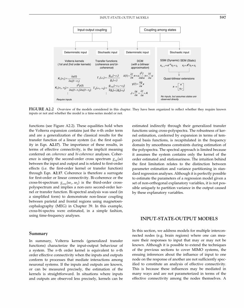
Elsevier UK Chapter: Appendix2-P372560 3-10-2006 4:23p.m. Page:597 Trim:7.5in×9.25in
Basal Font:Palatino Margins:Top:40pt Gutter:68pt Font Size:9.5/12 Text Width:42pc Depth:55 Lines
INPUT-STATE-OUTPUT MODELS 597
SSM (Dynamic)Transfer functions (coherence and bi-
coherence)
Volterra kernels(1st and 2nd order kernels )
DCM(with a bilinearapproximation)
Input-output coupling Coupling among states
Deterministic input Stochastic input Deterministic input Stochastic input
xJ =
xy(t ) =
ux + x + ux (t ) ≈
= A∂x
∂ƒ =
∂x∂
∂x∂g
∂u
∂ƒ∂x∂u
∂2ƒ∂x∂ƒ
xt + 1 = eτAxt + ηt xt = A0xt + ut
Quasi-bilinear extensions
→x
Require inputs No inputs, but assumes states are
observed directly
SEM (Static)
K1 (σ1) =
∂y (t
)
∂ui (t − σ1)
Γ1 (ω1) =
gu y (–ω1)
gu (ω1)
Γ2 (ω1, ω2) =
gυu y (–ω1,–ω2)
2gu(ω1)gu(ω2)K1
(σ1, σ2) = ∂2y
(t
)
∂ui (t − σ1)∂ui
(t − σ2) xi ν
x
... ....
.
FIGURE A2.2 Overview of the models considered in this chapter. They have been organized to reflect whether they require knowninputs or not and whether the model is a time-series model or not.
functions (see Figure A2.2). These equalities hold whenthe Volterra expansion contains just the n-th order termand are a generalization of the classical results for thetransfer function of a linear system (i.e. the first equal-ity in Eqn. A2.17). The importance of these results, interms of effective connectivity, is the implicit meaningconferred on coherence and bi-coherence analyses. Coher-ence is simply the second-order cross spectrum guy���between the input and output and is related to first-ordereffects (i.e. the first-order kernel or transfer function)through Eqn. A2.17. Coherence is therefore a surrogatefor first-order or linear connectivity. Bi-coherence or thecross-bi-spectrum guuy��1��2� is the third-order cross-polyspectrum and implies a non-zero second-order ker-nel or transfer function. Bi-spectral analysis was used (ina simplified form) to demonstrate non-linear couplingbetween parietal and frontal regions using magnetoen-cephalography (MEG) in Chapter 39. In this example,cross-bi-spectra were estimated, in a simple fashion,using time-frequency analyses.
Summary
In summary, Volterra kernels (generalized transferfunctions) characterize the input-output behaviour ofa system. The n-th order kernel is equivalent to n-thorder effective connectivity when the inputs and outputsconform to processes that mediate interactions amongneuronal systems. If the inputs and outputs are known,or can be measured precisely, the estimation of thekernels is straightforward. In situations where inputsand outputs are observed less precisely, kernels can be
estimated indirectly through their generalized transferfunctions using cross-polyspectra. The robustness of ker-nel estimation, conferred by expansion in terms of tem-poral basis functions, is recapitulated in the frequencydomain by smoothness constraints during estimation ofthe polyspectra. The spectral approach is limited becauseit assumes the system contains only the kernel of theorder estimated and stationariness. The intuition behindthe first limitation relates to the distinction betweenparameter estimation and variance partitioning in stan-dard regression analyses. Although it is perfectly possibleto estimate the parameters of a regression model given aset of non-orthogonal explanatory variables, it is not pos-sible uniquely to partition variance in the output causedby these explanatory variables.
INPUT-STATE-OUTPUT MODELS
In this section, we address models for multiple intercon-nected nodes (e.g. brain regions) where one can mea-sure their responses to input that may or may not beknown. Although it is possible to extend the techniquesof the previous sections to cover MIMO systems, theensuing inferences about the influence of input to onenode on the response of another are not sufficiently spec-ified to constitute an analysis of effective connectivity.This is because these influences may be mediated inmany ways and are not parameterized in terms of theeffective connectivity among the nodes themselves. A

Elsevier UK Chapter: Appendix2-P372560 3-10-2006 4:23p.m. Page:598 Trim:7.5in×9.25in
Basal Font:Palatino Margins:Top:40pt Gutter:68pt Font Size:9.5/12 Text Width:42pc Depth:55 Lines
598 A2. DYNAMICAL SYSTEMS
parameterization that encodes this inter-node couplingis therefore required. All the models discussed belowassume some form or model for the interactions amongthe state variables in one or more nodes and attempt toestimate the parameters of this model, sometimes with-out observing the states themselves.
Models for known inputs – dynamiccausal modelling
The most direct and generic approach is to estimate theparameters of Eqn. A2.3 directly and, if necessary, usethem to compute effective connectivity as described inEqn. A2.1 and Eqn. A2.2. Although there are many formsone could adopt for Eqn. A2.3, we will focus on thebilinear approximation, which is possibly the most parsi-monious but useful non-linear approximation available.Furthermore, as shown below, the bilinear approxima-tion re-parameterizes the state equations of the modeldirectly in terms of effective connectivity. Dynamic causalmodelling does not necessarily entail the use of a bilin-ear model. Indeed, DCMs can be specified to any degreeof biological complexity and realism supported by thedata. There are examples in this book where the para-meters of the state equation are already effective connec-tivity or coupling parameters, for example, the extrinsicand intrinsic connections in neural-mass models of event-related potentials (ERPs) (see Chapter 42). However, wefocus on bilinear approximations here because they rep-resent the simplest form to which all DCMs can bereduced. This reduction allows analytic derivation of ker-nels and other computations, like integrating the stateequation, to proceed in an efficient fashion.
Each region may comprise several state variableswhose causal interdependencies are summarized by thebilinear form in Eqn. A2.4. Here the coupling parametersof the state equation are the matrices M and N . For agiven set of inputs or experimental context, the bilinearapproximation to any state equation is:
Ẋ�t� = JX�t�
X�t +�� = eJ�X�t� A2.18
J = M +∑i
Niui
Notice that there are now as many N matrices as thereare inputs. The bilinear form reduces the model to first-order connections that can be modulated by the inputs.
In MIMO models, the coupling is among the states suchthat first-order effective connections are simply:
J = �Ẋ
�X
K = �X�t�
�X�t −��= eJ�
A2.19
Note that these are context-sensitive in the sense that theJacobian J is a function of experimental context or inputsu�t� = u1�t�� � � � �um�t�. A useful way to think about thebilinear matrices is to regard them as the intrinsic orlatent dynamic coupling, in the absence of input, andchanges induced by each input (see Chapter 41 for afuller description):
J�0� = M =[
0 0f�0� A
]
�J
�ui
= Ni =[
0 0Ci Bi
] A2.20
The latent coupling among the states is A. Often, one ismore interested in Bi as embodying changes in this cou-pling induced by different cognitive set, time or drugs.Note that Ci enters as the input-dependent componentof coupling to the constant term. Clearly, it would bepossible to introduce other high-order terms to modelinteractions among the states, but we will restrict our-selves to bilinear models for simplicity.
Dynamic causal modelling has two parts: first, specifi-cation of the state and output equations of an ensembleof region-specific state variables. If necessary, a bilinearapproximation to any state equation reduces the model tofirst-order coupling and bilinear terms that represent themodulation of that coupling by inputs. Second, inversionof the DCM allows one to estimate and make inferencesabout inter-regional connections and the effect of exper-imental manipulations on those connections.
As mentioned above, the state equations do not haveto conform to the bilinear form. This is important becausethe priors may be specified more naturally in terms of theoriginal biophysical parameters of the DCM, as opposedto the bilinear form. A nice example of this is the use oflog-normal priors to enforce positivity constraints on therate constants of ERP models in Chapter 42. Furthermore,the choice of the state variables clearly has to reflect theirrole in mediating the effect of inputs on responses andthe interactions among areas. In the simplest case, thestate variables could be reduced to mean synaptic activityper region, plus any biophysical state variables neededto determine the output (e.g. the states of haemodynamicmodels for fMRI). Implicit in choosing such state vari-ables is the assumption that they model all the dynamicsto the level of detail required. Mean field models and

Elsevier UK Chapter: Appendix2-P372560 3-10-2006 4:23p.m. Page:599 Trim:7.5in×9.25in
Basal Font:Palatino Margins:Top:40pt Gutter:68pt Font Size:9.5/12 Text Width:42pc Depth:55 Lines
INPUT-STATE-OUTPUT MODELS 599
neural-mass models may be useful here in motivating thenumber of state variables and the associated state equa-tions (see Chapter 31). Operationally, issues of parame-terization and number of state variables can be resolvedwith Bayesian model selection and is directed principallyby the nature of the data.
Summary
In summary, DCM is the most general and directapproach to identifying the effective connectivity amongthe states of MIMO systems. The identification of DCMsusually proceeds using Bayesian inversion to estimate theposterior mode or most likely parameters of the modelgiven the data. The state equations can be arbitrarilycomplicated and non-linear, however, there will be anoptimal level of model complexity that is supported bythe data (and identified using Bayesian model selection).The simplest model is probably a bilinear approximationto causal influences among state variables. This servesto minimize the complexity of the model by parame-terizing the model in terms of first-order coupling andits changes with input (the bilinear terms). In the nextsection, we deal with the situations in which the input isunknown. This precludes DCM with deterministic sys-tems, because the likelihood of the responses cannot becomputed unless we know what caused them.
Models for stochastic inputs – SEMand regression models
When the inputs are unknown, and the statistics of theoutputs are considered to second order, one is effectivelyrestricted to linear or first-order models of effective con-nectivity. Although it is possible to deal with discrete-time bilinear models, with white noise inputs, they havethe same covariance structure as ARMA (autoregressivemoving average) models of the same order (Priestley,1988: 66). This means that to distinguish between lin-ear and non-linear models, one would need to studymoments higher than second order (cf. the third-ordercumulants in bi-coherence analyses). Consequently, wewill focus on linear models of effective connectivity,under white stationary inputs. There are two importantclasses of model here: structural equation models andARMA models. Both are finite parameter linear modelsthat are distinguished by their dependency on dynamics.In SEM, the interactions are assumed to be instantaneous,whereas in ARMA the dynamics are retained.
An SEM can be derived from any DCM by assum-ing the inputs vary slowly in relation to neuronal and
haemodynamics. This is appropriate for positron emis-sion tomography (PET) experiments and possibly someepoch-related fMRI designs, but not for event-relateddesigns in ERP or fMRI. Note that this assumption per-tains to the inputs or experimental design, not to thetime constants of the outputs. In principle, it would bepossible to apply DCM to a PET study.
Consider a linear approximation to any DCM wherewe can observe the states precisely and there was onlyone state variable per region:
ẋ = f�x�u�
= Ax+u = �A0 −1�x+u
y = g�x� = x
A2.21
Here, we have discounted observation error but allowstochastic inputs u ∼ N�0�Q�. To make the connection tothe SEM more explicit, we have expanded the connec-tivity matrix into off-diagonal connections and a leadingdiagonal matrix, modelling unit decay A = A0 − 1. Forsimplicity, we have absorbed C into the covariance struc-ture of the inputs Q. As the inputs are changing slowlyrelative to the dynamics, the change in states will be zeroat the point of observation and we obtain the regressionmodel used by SEM:
ẋ = 0 ⇒�1−A0�x = u
x = �1−A0�−1u
A2.22
(see Chapter 38). The more conventional motivation forEqn. A2.22 is to start with an instantaneous regressionequation x = A0x+u that is formally identical to the sec-ond line above. Although this regression model obscuresthe connection with dynamic formulations, it is impor-tant to consider because it is the basis of commonlyemployed methods for estimating effective connectivityin neuroimaging to data. These are simple regressionmodels and SEM.
Simple regression models
x = A0x +u can be treated as a general linear model byfocusing on one region at a time, for example the first, togive (cf. Eqn. 38.11 in Chapter 38):
x1 = �x2� � � �� xn�
⎡⎢⎣
A12���
A1n
⎤⎥⎦+u1 A2.23
The elements of A can then be solved in a least squaressense by minimizing the norm of the unknown stochas-tic inputs u for that region (i.e. minimizing the unex-plained variance of the target region given the states of
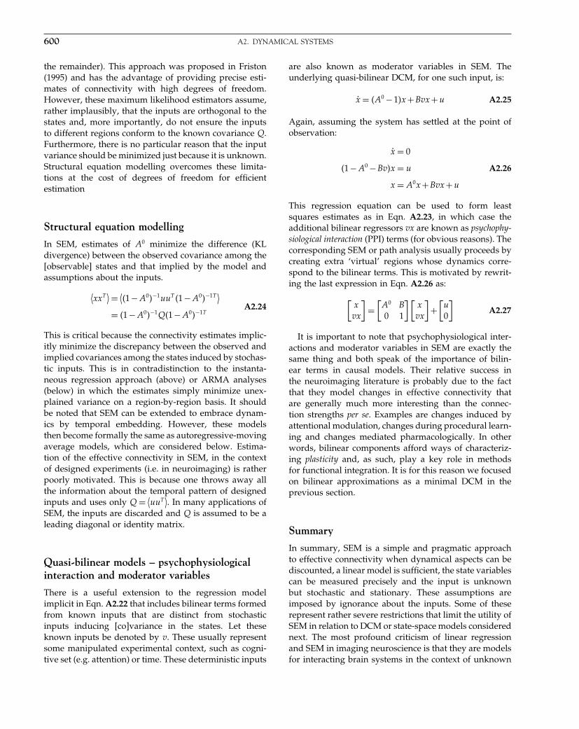
Elsevier UK Chapter: Appendix2-P372560 3-10-2006 4:23p.m. Page:600 Trim:7.5in×9.25in
Basal Font:Palatino Margins:Top:40pt Gutter:68pt Font Size:9.5/12 Text Width:42pc Depth:55 Lines
600 A2. DYNAMICAL SYSTEMS
the remainder). This approach was proposed in Friston(1995) and has the advantage of providing precise esti-mates of connectivity with high degrees of freedom.However, these maximum likelihood estimators assume,rather implausibly, that the inputs are orthogonal to thestates and, more importantly, do not ensure the inputsto different regions conform to the known covariance Q.Furthermore, there is no particular reason that the inputvariance should be minimized just because it is unknown.Structural equation modelling overcomes these limita-tions at the cost of degrees of freedom for efficientestimation
Structural equation modelling
In SEM, estimates of A0 minimize the difference (KLdivergence) between the observed covariance among the[observable] states and that implied by the model andassumptions about the inputs.
⟨xxT
⟩= ⟨�1−A0�−1uuT �1−A0�−1T
⟩= �1−A0�−1Q�1−A0�−1T
A2.24
This is critical because the connectivity estimates implic-itly minimize the discrepancy between the observed andimplied covariances among the states induced by stochas-tic inputs. This is in contradistinction to the instanta-neous regression approach (above) or ARMA analyses(below) in which the estimates simply minimize unex-plained variance on a region-by-region basis. It shouldbe noted that SEM can be extended to embrace dynam-ics by temporal embedding. However, these modelsthen become formally the same as autoregressive-movingaverage models, which are considered below. Estima-tion of the effective connectivity in SEM, in the contextof designed experiments (i.e. in neuroimaging) is ratherpoorly motivated. This is because one throws away allthe information about the temporal pattern of designedinputs and uses only Q = ⟨
uuT⟩. In many applications of
SEM, the inputs are discarded and Q is assumed to be aleading diagonal or identity matrix.
Quasi-bilinear models – psychophysiologicalinteraction and moderator variables
There is a useful extension to the regression modelimplicit in Eqn. A2.22 that includes bilinear terms formedfrom known inputs that are distinct from stochasticinputs inducing [co]variance in the states. Let theseknown inputs be denoted by v. These usually representsome manipulated experimental context, such as cogni-tive set (e.g. attention) or time. These deterministic inputs
are also known as moderator variables in SEM. Theunderlying quasi-bilinear DCM, for one such input, is:
ẋ = �A0 −1�x+Bvx+u A2.25
Again, assuming the system has settled at the point ofobservation:
ẋ = 0
�1−A0 −Bv�x = u
x = A0x+Bvx+u
A2.26
This regression equation can be used to form leastsquares estimates as in Eqn. A2.23, in which case theadditional bilinear regressors vx are known as psychophy-siological interaction (PPI) terms (for obvious reasons). Thecorresponding SEM or path analysis usually proceeds bycreating extra ‘virtual’ regions whose dynamics corre-spond to the bilinear terms. This is motivated by rewrit-ing the last expression in Eqn. A2.26 as:
[xvx
]=[A0 B0 1
][xvx
]+[u0
]A2.27
It is important to note that psychophysiological inter-actions and moderator variables in SEM are exactly thesame thing and both speak of the importance of bilin-ear terms in causal models. Their relative success inthe neuroimaging literature is probably due to the factthat they model changes in effective connectivity thatare generally much more interesting than the connec-tion strengths per se. Examples are changes induced byattentional modulation, changes during procedural learn-ing and changes mediated pharmacologically. In otherwords, bilinear components afford ways of characteriz-ing plasticity and, as such, play a key role in methodsfor functional integration. It is for this reason we focusedon bilinear approximations as a minimal DCM in theprevious section.
Summary
In summary, SEM is a simple and pragmatic approachto effective connectivity when dynamical aspects can bediscounted, a linear model is sufficient, the state variablescan be measured precisely and the input is unknownbut stochastic and stationary. These assumptions areimposed by ignorance about the inputs. Some of theserepresent rather severe restrictions that limit the utility ofSEM in relation to DCM or state-space models considerednext. The most profound criticism of linear regressionand SEM in imaging neuroscience is that they are modelsfor interacting brain systems in the context of unknown

Elsevier UK Chapter: Appendix2-P372560 3-10-2006 4:23p.m. Page:601 Trim:7.5in×9.25in
Basal Font:Palatino Margins:Top:40pt Gutter:68pt Font Size:9.5/12 Text Width:42pc Depth:55 Lines
MULTIVARIATE ARMA MODELS 601
input. The whole point of designed experiments is thatthe inputs are known and under experimental control.This renders the utility of SEM for designed experimentssomewhat questionable.
MULTIVARIATE ARMA MODELS
ARMA (autoregressive-moving average) models can berepresented as state-space (or Markov) models that pro-vide a compact description of any finite parameter linearmodel. From this state-space representation, multivari-ate autoregressive (MAR) models can be derived andestimated using a variety of well-established techniques(see Chapter 40). We will focus on how the state-spacerepresentation of linear models can be derived from thedynamic formulation and the assumptions required inthis derivation. Many treatments of dynamic systemsconsider the dynamic formulation in terms of a state-equation, a continuous state-space model (SSM). Wepreserve the distinction because there is an importantasymmetry in the sense that one can always derive adiscrete SSM from a DCM. However, there is no neces-sary mapping from an SSM to a DCM. This is criticalfor causal inference because only DCMs are causal in thecontrol theory sense (see below).
Assume a linear DCM in which inputs comprise sta-tionary white Weiner processes u ∼ N�0�Q� that areoffered to each region in equal strength (i.e. C = 1). Thisrenders Eqn. A2.3 a linear stochastic differential equation(SDE):
ẋ = Ax+u
y = LxA2.28
The value of x at some future lag comprises a deter-ministic and a stochastic component � that obtains byregarding the effects of the input as an accumulation oflocal linear perturbations:
x�t +�� = e�Ax�t�+�
� =�∫
0
e�Au�t +��d�A2.29
Notice that the stochastic part can be regarded as con-volving the random state-fluctuations with the system’sfirst-order kernel. Using the assumption that the input isuncorrelated, the covariance of the stochastic part is:
W = ⟨��T
⟩=�∫
0
e�AQe�AT
d� A2.30
It can be seen that when the lag is small in relationto the Lyapunov exponents, eig�A� we get e�A ≈ 1 andW ≈ Q�. By incorporating the output transformation andobservation error, we can augment this model to furnisha state-space model with system matrix F = e�A, inputmatrix G = √
W and observation matrix L:
xt = Fxt−1 +Gzt
yt = Lxt +t
A2.31
where z is an innovation representing dynamicallytransformed stochastic input. If we knew L and wereinterested in inferring on the hidden states, we wouldnormally turn to Bayesian filtering (e.g. Kalman filtering)as described in Appendix 5. However, we will assumethat we are more interested in inference about the cou-pling implied by the system matrix. In this case, wecan reformulate the state-space model and treat it as anARMA model.
Critically, every state-space model has an ARMA rep-resentation and vice versa. For example, if L = 1, we caneliminate the hidden states to give:
yt −Fyt−1 = Gzt +t −Ft−1 A2.32
This is simply an ARMA(1,2) model that can be invertedusing the usual procedures (see Chapter 40). The autore-gressive part is on the left and the moving average ofthe innovations is on the right. Critically, Eqn. A2.32formulates the dynamics in terms of, and only of, theresponse variable and random terms. Although it isalways possible to derive an ARMA representation froma DCM (through the state-space representation), thereverse mapping is not necessarily defined. Having saidthis, ARMA models can be useful in establishing the pres-ence of coupling even if the exact form of the coupling isnot specified (cf. Volterra characterizations).
In summary, discrete-time linear models of effectiveconnectivity can be reduced to multivariate AR (or, moregenerally ARMA) models, whose coefficients can be esti-mated given only the states (or outputs) by assuming theinputs are white and Gaussian. They therefore operateunder similar assumptions as SEM but are time-seriesmodels.
A note on causality
There are many schemes for inverting state-space mod-els of the sort in Eqn. A2.31. Inference on the systemmatrix could be considered in the light of functionalconnectivity, however, the regression coefficients are notreally measures of effective connectivity. This is becausethere is no necessary mapping to the parameters of aDCM. In other words, although one can always mapfrom the parameters of a causal model to its state-space
Elsevier UK Chapter: Appendix2-P372560 3-10-2006 4:23p.m. Page:602 Trim:7.5in×9.25in
Basal Font:Palatino Margins:Top:40pt Gutter:68pt Font Size:9.5/12 Text Width:42pc Depth:55 Lines
602 A2. DYNAMICAL SYSTEMS
representation F ← e�A, the inverse mapping does notnecessarily exist (a simple intuition here is that the log ofa negative number is not real).
An interesting aspect of inference on the system matrix(i.e. regression coefficients) is the use of model compari-son to compare the regression of one channel on another.Because these coefficients encode statistical dependenceat different temporal lags, this model comparison is oftenframed in causal terms, by appeal to temporal prece-dence (e.g. Granger causality). However, for many, thisrhetoric represents a category error because the regres-sion coefficients cannot have the attribute ‘causal’. Thisis because causal is an attribute of the state equation thatimplies A = �f
/�x is real. This Jacobian is not defined
in the state-space or ARMA representations because themapping 1
�ln�F � → �f
/�x does not necessarily exist.
It is quite possible to infer Granger causality that isacausal when a cause is observed after its effect. fMRIpresents a good example of an acausal system, becauseof the delay imposed on the expression of neuronaldynamics (which are causal) at the level of haemody-namics (which are not). For example, one region, witha long haemodynamic latency, could cause a neuronalresponse in another that was expressed, haemodynami-cally, before the source. This example demonstrates thatone cannot estimate effective connectivity or couplingusing just the outputs of a system (e.g. observed fMRIresponses).
CONCLUSION
We have reviewed a series of models, all of which can beformulated as special cases of DCMs. Two fundamental
distinctions organize these models. The first is whetherthey model the coupling of inputs to outputs or whetherthey model interactions among hidden states. The sec-ond distinction (see Figure A2.2) is that between mod-els that require the inputs to be known, as in designedexperiments and those where the input is not underexperimental control but can be assumed to be wellbehaved. With only information about the density of theinputs (or the joint density of the inputs and outputs)the models of connectivity that can be used are limited;unless one uses moments greater than second-order, onlylinear models can be estimated.
Many methods for non-linear system identificationand causal modelling have been developed in situationswhere the system input is not under experimental controland, in the case of SEM, for static data. Volterra kernelsand DCMs may be especially useful in neuroimagingbecause we deal explicitly with time-series data gener-ated by designed experiments.
REFERENCES
Bendat JS (1990) Nonlinear system analysis and identification from ran-dom data. John Wiley and Sons, New York
Fliess M, Lamnabhi M, Lamnabhi-Lagarrigue F (1983) An algebraicapproach to nonlinear functional expansions. IEEE Trans CircSys 30: 554–70
Friston KJ (1995) Functional and effective connectivity in neuro-imaging: a synthesis. Hum Brain Mapp 2: 56–78
Friston KJ (2002) Bayesian estimation of dynamical systems: anapplication to fMRI. NeuroImage 16: 465–83
Friston KJ, Büchel C (2000) Attentional modulation of V5 in humans.Proc Natl Acad Sci USA 97: 7591–96
Priestley MB (1988) Non-linear and non-stationary time series analysis.Academic Press, London

Elsevier UK Chapter: Appendix3-P372560 3-10-2006 4:23p.m. Page:603 Trim:7.5in×9.25in
Basal Font:Palatino Margins:Top:40pt Gutter:68pt Font Size:9.5/12 Text Width:42pc Depth:55 Lines
A P P E N D I X
3
Expectation maximizationK. Friston
INTRODUCTION
This appendix describes expectation maximization (EM)for linear models using statistical mechanics (Neal andHinton, 1998). We connect this formulation with classi-cal methods and show the variational free energy is thesame as the objective function maximized in restrictedmaximum likelihood (ReML). In Appendix 4, we showthat EM itself is a special case of variational Bayes(Chapter 24).
The EM algorithm is ubiquitous in the sense that manyestimation procedures can be formulated as such, frommixture models through to factor analysis. Its objectiveis to maximize the likelihood of observed data p�y���,conditional on some hyperparameters, in the presence ofunobserved variables or parameters �. This is equivalentto maximizing the log-likelihood:
ln p�y��� = ln∫
p������d� ≥
F�q��� =∫
q��� ln p���y���d� −∫
q��� ln q���d�
A3.1
where q��� is any density on the model parameters (Nealand Hinton, 1998). Eqn. A3.1 rests on Jensen’s inequalitythat follows from the concavity of the log function, whichrenders the log of an integral greater than the integralof the log. F corresponds to the [negative] free energyin statistical thermodynamics and comprises two terms:the energy and entropy. The EM algorithm alternatesbetween maximizing F and, implicitly, the likelihood ofthe data, with respect to the distribution q��� and thehyperparameters �, holding the other fixed:
E-step� q��� ← maxq
F�q������
M-step� � ← max�
F�q������
This iterative alternation performs a coordinate ascent onF . It is easy to show that the maximum in the E-step
obtains when q��� = p���y���, at which point Eqn. A3.1becomes an equality. The M-step finds the ML estimateof the hyperparameters, i.e. the values of � that maximizep�y��� by integrating ln p���y��� = ln p�y����� + ln p�����over the parameters, using the current estimate of theirconditional distribution. In short, the E-step computessufficient statistics (in our case the conditional mean andcovariance) of the unobserved parameters to enable theM-step to optimize the hyperparameters, in a maximumlikelihood sense. These new hyperparameters re-enterinto the estimation of the conditional density and so onuntil convergence.
The E-step
For linear models, under Gaussian (i.e. parametric)assumptions, the E-step is trivial and corresponds to eval-uating the conditional mean and covariance as describedin Chapter 22:
y = X� +�
y =[y −X�
�
]X =
[XI
]C� =
[∑�iQi 00 C�
]
��y = C��yXTC
−1� y
C��y = �XTC
−1� X�−1
A3.2
where the prior and conditional densities are p��� =N���C�� and q��� = N���y�C��y�. This compact form is aresult of absorbing the priors into the errors by augment-ing the linear system. As described in Chapter 22, the sameaugmentation is used to reduce hierarchal models withempirical priors to their non-hierarchical form. Under locallinearity assumptions, non-linear models can be reducedto a linear form as described in Chapter 34. The result-ing conditional density is used to estimate the hyperpara-meters of the covariance components in the M-step.
Statistical Parametric Mapping, by Karl Friston et al. Copyright 2007, Elsevier Ltd. All rights reserved.ISBN–13: 978-0-12-372560-8 ISBN–10: 0-12-372560-7
603
Elsevier UK Chapter: Appendix3-P372560 3-10-2006 4:23p.m. Page:604 Trim:7.5in×9.25in
Basal Font:Palatino Margins:Top:40pt Gutter:68pt Font Size:9.5/12 Text Width:42pc Depth:55 Lines
604 A3. EXPECTATION MAXIMIZATION
The M-step
Given that we can reduce the problem to estimating theerror covariances of the augmented system in Eqn. A3.2,we only need to estimate the hyperparameters of theerror covariances (which contain the prior covariances).Specifically, we require the hyperparameters that max-imize the first term of the free energy (i.e. the energy)because the entropy does not depend on the hyper-parameters. For linear systems, the free energy is givenby (ignoring constants):
log p���y ��� = −12
ln �C��−12
�y −X��T C−1� �y −X��
∫q��� ln p���y ���d� = −1
2ln �C��−
12
rT C−1� r
− 12
tr�C��yXTC−1
� X�
∫q��� log q��� = −1
2ln �C��y� A3.3
F = 12
ln �C−1� �− 1
2rT C−1
� r
− 12
tr�C��yXTC−1
� X�+ 12
ln �C��y�
where the residuals r = y −X��y . By taking derivativeswith respect to the error covariance we get:
F
C−1�
= 12
C� − 12
rrT − 12
XC��y XT
A3.4
When the hyperparameters maximize the free energy thisgradient is zero and:
C���� = rrT +XC��y XT
A3.5
(cf. Dempster et al., 1981: 350). This means that the ReMLerror covariance estimate has two components: that dueto differences between the data and its conditional pre-diction; and another due to the variation of the param-eters about their conditional mean, i.e. their conditionaluncertainty. This is not a closed form expression forthe unknown covariance because the conditional covari-ance is a function of the hyperparameters. To find theReML hyperparameters, one usually adopts a Fisher scor-ing scheme, using the first and expected second partialderivatives of the free energy:
�� = −E
( 2F
�2ij
)−1 F
�i
F
�i
= tr
( F
C−1�
C−1� QiC
−1�
)
= −12
tr�PQi�+ 12
yT PT QiPy
2F
�2ij
= 12
tr�PQiPQj�−yT PQiPQjPy A3.6
E
( 2F
�2ij
)= −1
2tr�PQiPQj�
P = C−1� −C−1
� XC��yXTC−1
�
Fisher scoring corresponds to augmenting a Gauss-Newton scheme by replacing the second derivative orcurvature with its expectation. The curvature or Hessianis referred to as Fisher’s information matrix1 and encodesthe conditional prediction of the hyperparameters. In thissense, the information matrix has a close connection tothe degrees of freedom in classical statistics. The gradientcan be computed efficiently by capitalizing on any spar-sity structure in the constraints and by bracketing themultiplications appropriately. This scheme is general inthat it accommodates almost any form for the covariancethrough a Taylor expansion of C����.
Once the hyperparameters have been updated theyenter the E-step as a new error covariance estimate togive new conditional moments which, in turn, enter theM-step and so on until convergence. A pseudo-codeillustration of the complete algorithm is presented inFigure 22.4 of Chapter 22. Note that in this implemen-tation one is effectively performing a single Fisher scor-ing iteration for each M-step. One could postpone eachE-step until this search converged, but a single step issufficient to perform a coordinate ascent on F . Techni-cally, this renders the scheme a generalized EM or GEMalgorithm.
It should be noted that the search for the maximumof F does not have to employ Fisher scoring or indeedthe parameterization of C� used above. Other searchprocedures, such as quasi-Newton searches, are com-monly employed (Fahrmeir and Tutz, 1994). Harville(1977) originally considered Newton-Raphson and scor-ing algorithms, and Laird and Ware (1982) recommendseveral versions of EM. One limitation of the linear
1 The derivation of the expression for the information matrixuses standard results from linear algebra and is most easily seenby differentiating the gradient, noting:
P
�j
= −PQjP
and taking the expectation, using
E�tr�PQiPyyT PQj�� = tr�PQiPC�PQj� = tr�PQiPQj�
Elsevier UK Chapter: Appendix3-P372560 3-10-2006 4:23p.m. Page:605 Trim:7.5in×9.25in
Basal Font:Palatino Margins:Top:40pt Gutter:68pt Font Size:9.5/12 Text Width:42pc Depth:55 Lines
REFERENCES 605
hyperparameterization described above is that it does notguarantee that C� is positive definite. This is because thehyperparameters can take negative values with extremedegrees of non-sphericity. The EM algorithm employedby multistat (Worsley et al., 2002) for variance componentestimation in multisubject fMRI studies, uses a slowerbut more stable algorithm that ensures positive definitecovariance estimates.
In Appendix 4, we will revisit this issue and look atlinear hyperparameterizations of the precision. The com-mon aspect of all these algorithms is that they (explicitlyor implicitly) optimize free energy. As shown next, thisis equivalent to restricted maximum likelihood.
RELATIONSHIP TO REML
ReML or restricted maximum likelihood was introduced byPatterson and Thompson in 1971, for estimating variancecomponents in a way that accounts for the loss in degreesof freedom that result from estimating fixed effects(Harville, 1977), i.e. that accounts for conditional uncer-tainty about the parameters. It is commonly employedin standard statistical packages (e.g. SPSS). Under thepresent model assumptions, ReML is formally identicalto EM. One can regard ReML as embedding the E-stepinto the M-step to provide a single log-likelihood objec-
tive function: substituting C��y =(X
TC−1
� X)−1
into theexpression for the free energy gives:
F = −12
ln �C��−12
rT C−1� r − 1
2ln �XT
C−1� X� A3.7
This is the ReML objective function (see Harville,1977: 325). Critically, its derivatives with respect to thehyperparameters are exactly the same as those in the
M-step.2 Operationally, the M-step can be re-formulatedto give a ReML scheme by removing any explicit refer-ence to the conditional covariance using:
P = C−1� −C−1
� X�XTC−1
� X�−1XTC−1
� A3.8
The resulting scheme is formally identical to thatdescribed in Section 5 of Harville (1977). Because onecan eliminate the conditional density, one could think ofReML as estimating the hyperparameters in a subspacethat is restricted in the sense that the estimates are con-ditionally independent of the parameters. See Harville(1977) for a discussion of expressions, comparable to theterms in Eqn. A3.7 that are easier to compute, for particu-lar hyperparameterizations of the variance components.
Having established ReML is a special case of EM, inAppendix 4, we take an even broader perspective andlook at EM as a special case of variational Bayes.
REFERENCES
Dempster AP, Rubin DB, Tsutakawa RK (1981) Estimation in covari-ance component models. J Am Stat Assoc 76: 341–53
Fahrmeir L, Tutz G (1994) Multivariate statistical modelling basedon generalised linear models. Springer-Verlag Inc., New York,pp 355–56
Harville DA (1977) Maximum likelihood approaches to variancecomponent estimation and to related problems. J Am Stat Assoc72: 320–38
Laird NM, Ware JH (1982) Random effects models for longitudinaldata. Biometrics 38: 963–74
Neal RM, Hinton GE (1998) A view of the EM algorithm that justifiesincremental, sparse and other variants. In Learning in graphi-cal models, Jordan MI (ed.). Kluwer Academic Press, Dordrecht,pp 355–68
Worsley KJ, Liao CH, Aston J et al. (2002) A general statistical anal-ysis for fMRI data. NeuroImage 15: 1–15
2 Note
ln �XTC−1
� X� �i
= tr
(�X
TC−1
� X�−1 XTC−1
� X
�i
)
= −tr�C��yXT C−1
� QiC−1� X�

Elsevier UK Chapter: Appendix4-P372560 3-10-2006 4:24p.m. Page:606 Trim:7.5in×9.25in
Basal Font:Palatino Margins:Top:40pt Gutter:68pt Font Size:9.5/12 Text Width:42pc Depth:55 Lines
A P P E N D I X
4
Variational Bayes under the Laplaceapproximation
K. Friston, J. Mattout, N. Trujillo-Barreto, J. Ashburner and W. Penny
INTRODUCTION
This is a rather technical appendix, but usefully connectsmost of the estimation and inference schemes used inprevious chapters, by showing they are all special casesof a single variational approach. This synthesis is under-pinned by reference to the various applications we haveconsidered in detail, so that their motivation and interre-lationships are more evident.
We will derive the variational free energy under theLaplace approximation, with a focus on accounting foradditional model complexity induced by increasing thenumber of model parameters. This is relevant when usingthe free energy as an approximation to the log-evidencein Bayesian model averaging and selection. By settingrestricted maximum likelihood (ReML) in the larger con-text of variational learning and expectation maximiza-tion, we show how the ReML objective function can beadjusted to provide an approximation to the log-evidencefor a particular model. This means ReML can be used formodel selection, specifically to select or compare modelswith difference covariance components. This is useful inthe context of hierarchical models, because it enables aprincipled selection of priors. Deriving the ReML objec-tive function, from basic variational principles, disclosesthe simple relationships among variational Bayes, EMand ReML. Furthermore, we show that EM is formallyidentical to a full variational treatment when the preci-sions are linear in the hyperparameters.
Background
This chapter starts with a very general formulationof inference using approaches developed in statisticalphysics. It ends with a treatment of a specific objective
function used in restricted maximum likelihood (ReML)that renders it equivalent to the free energy in variationallearning. This is important because the variational freeenergy provides a bound on the log-evidence for anymodel, which is exact for linear models. The log-evidenceplays a central role in model selection, comparison andaveraging (see Penny et al., 2004 and Trujillo-Barreto et al.,2004, for examples in neuroimaging).
Although this appendix focuses on the various forms forthe free energy, we use it to link variational Bayes (VB), EMand ReML using the Laplace approximation. This approx-imation assumes a fixed Gaussian form for the conditionaldensity of the parameters of a model and is used implicitlyin ReML and many applications of EM. Bayesian inver-sion using VB is ubiquitous in neuroimaging (e.g. Pennyet al., 2005 and Chapter 24). Its use ranges from spa-tial segmentation and normalization of images duringpre-processing (e.g. Ashburner and Friston, 2005) to theinversion of complicated dynamical causal models offunctional integration in the brain (Friston et al., 2003 andChapter 34). Many of the intervening steps in classicaland Bayesian analysis of neuroimaging data call on ReMLor EM under the Laplace approximation. This appendixprovides an overview of how these schemes are relatedand illustrates their applications with reference to specificalgorithms and routines we have referred to in this book.One interesting issue that emerges from this treatment isthat VB reduces exactly to EM, under the Laplace approx-imation, when the precision of stochastic terms is linearin the hyperparameters. This reveals a close relationshipbetween EM and full variational approaches.
Conditional uncertainty
In previous chapters, we have described the use of ReMLin the Bayesian inversion of electromagnetic models to
Statistical Parametric Mapping, by Karl Friston et al. Copyright 2007, Elsevier Ltd. All rights reserved.ISBN–13: 978-0-12-372560-8 ISBN–10: 0-12-372560-7
606

Elsevier UK Chapter: Appendix4-P372560 3-10-2006 4:24p.m. Page:607 Trim:7.5in×9.25in
Basal Font:Palatino Margins:Top:40pt Gutter:68pt Font Size:9.5/12 Text Width:42pc Depth:55 Lines
VARIATIONAL BAYES 607
localize distributed sources in electroencephalography(EEG) and magnetoencephalography (MEG) (e.g. Phillipset al., 2002; Chapters 29 and 30). ReML provides a princi-pled way of quantifying the relative importance of priorsthat replaces alternative heuristics like L-curve analysis.Furthermore, ReML accommodates multiple priors andprovides more accurate and efficient source reconstruc-tion than its precedents (Phillips et al., 2002). We havealso used ReML to identify the most likely combina-tion of priors using model selection, where each modelcomprises a different set of priors (Mattout et al., 2006).This was based on the fact that the ReML objective func-tion is the free energy used in expectation maximizationand is equivalent to the log-evidence F� = ln p�y���m�,conditioned on �, the unknown covariance componentparameters (i.e. hyperparameters) and the model m. Thecovariance components encoded by � include the priorcovariances of each model of the data y. However, thisfree energy is not a function of the conditional uncer-tainty about � and is therefore insensitive to additionalmodel complexity induced by adding covariance com-ponents (i.e. priors). In what follows we show how F�
can be adjusted to provide the variational free energy,which, in the context of linear models, is exactly the log-evidence ln p�y�m�. This rests on deriving the variationalfree energy for a general variational scheme and treat-ing expectation maximization (EM) as a special case, inwhich one set of parameters assumes a point mass. Wethen treat ReML as the special case of EM, applied tolinear models.
Overview
This appendix is divided into six sections. In the first,we summarize the basic theory of variational Bayesand apply it in the context of the Laplace approxima-tion (see also Chapter 24). The Laplace approximationimposes a fixed Gaussian form on the conditional den-sity, which simplifies the ensuing variational steps. Inthis section, we look at the easy problem of approxi-mating the conditional covariance of model parametersand the more difficult problem of approximating theirconditional expectation or mode using gradient ascent.We consider a dynamic formulation of gradient ascent,which generalizes nicely to cover dynamic models andprovides the basis for a temporal regularization of theascent. In the second section, we apply the theory tonon-linear models with additive noise. We use the VBscheme that emerges as the reference for subsequent sec-tions looking at special cases. The third section considersEM, which can be seen as a special case of VB in whichuncertainty about one set of parameters is ignored. In thefourth section, we look at the special case of linear models
where EM reduces to ReML. The fifth section considersReML and hierarchical models. Hierarchical models areimportant because they underpin parametric empiricalBayes (PEB) and other special cases, like relevance vectormachines. Furthermore, they provide a link with classi-cal covariance component estimation. In the final section,we present some toy examples to show how the ReMLand EM objective functions can be used to evaluate thelog-evidence and facilitate model selection.
VARIATIONAL BAYES
Empirical enquiry in science usually rests upon estimat-ing the parameters of some model of how observed datawere generated and making inferences about the param-eters (or model). Estimation and inference are based onthe posterior density of the parameters (or model), con-ditional on the observations. Variational Bayes is used toevaluate these posterior densities.
The variational approach
Variational Bayes is a generic approach to posterior den-sity (as opposed to posterior mode) analysis that approx-imates the conditional density p���y�m� of some modelparameters �, given a model m and data y. Further-more, it provides the evidence (or marginal likelihood) ofthe model p�y�m� which, under prior assumptions aboutthe model, furnishes the posterior density p�m�y� of themodel itself.
Variational approaches rest on minimizing the Feyn-man variational bound (Feynman, 1972). In variationalBayes, the free energy represents a bound on the log-evidence. Variational methods are well established inthe approximation of densities in statistical physics (e.g.Weissbach et al., 2002) and were introduced by Feynmanwithin the path integral formulation (Titantah et al., 2001).The variational framework was introduced into statisticsthrough ensemble learning, where the ensemble or vari-ational density q��� (i.e. approximating posterior density)is optimized to minimize the free energy. Initially (Hin-ton and von Camp, 1993; MacKay, 1995), the free energywas described in terms of description lengths and cod-ing. Later, established methods like EM were consideredin the light of variational free energy (Neal and Hinton,1998; see also Bishop, 1999). Variational learning can beregarded as subsuming most other learning schemes asspecial cases. This is the theme pursued here, with spe-cial references to fixed-form approximations and classicalmethods like ReML (Harville, 1977).

Elsevier UK Chapter: Appendix4-P372560 3-10-2006 4:24p.m. Page:608 Trim:7.5in×9.25in
Basal Font:Palatino Margins:Top:40pt Gutter:68pt Font Size:9.5/12 Text Width:42pc Depth:55 Lines
608 A4. VARIATIONAL BAYES UNDER THE LAPLACE APPROXIMATION
The derivations in this appendix involve a fair amountof differentiation. To simplify things we will use the nota-tion fx = �f
/�x to denote the partial derivative of the
function f , with respect to the variable x. For time deriva-tives we will also use ẋ = xt.
The log-evidence can be expressed in terms of the freeenergy and a divergence term:
ln p�y�m� = F +D�q����p���y�m��
F = �L����q −�ln q����q
L = ln p�y���
A4.1
Here −�ln q����q is the entropy and �L����q the expectedenergy. Both quantities are expectations under the vari-ational density. Eqn. A4.1 indicates that F is a lower-bound approximation to the log-evidence because thedivergence D�q����p���y�m�� is always positive. In this,note all the energies are the negative of energies consid-ered in statistical physics. The objective is to computeq��� for each model by maximizing F , and then com-pute F itself, for Bayesian inference and model compari-son respectively. Maximizing the free energy minimizesthe divergence, rendering the variational density q��� ≈p���y�m� an approximate posterior, which is exact for lin-ear systems. To make the maximization easier, one usu-ally assumes q��� factorizes over sets of parameters �i:
q��� =∏i
qi A4.2
In statistical physics this is called a mean-field approx-imation. Under this approximation, the FundamentalLemma of variational calculus means that F is maximizedwith respect to qi = q��i� when, and only when:
F i = 0 ⇔ �f i
�qi= f i
qi = 0
f i = F�i
A4.3
F i is the variation of the free energy with respect to qi.From Eqn. A4.1:
f i =∫
qiq\i ln L���d�\i −∫
qiq\i ln q���d�\i
f iqi = I��i�− ln qi − ln Zi
I��i� = �L����q\i
A4.4
where �\i denotes the parameters not in the i-th set. Wehave lumped terms that do not depend on �i into ln Zi,where Zi is a normalization constant (i.e. partition func-tion). We will call I��i� the variational energy, noting itsexpectation under qi is the expected energy. The extremalcondition in Eqn. A4.2 is met when:
ln qi = I��i�− ln Zi ⇔
q��i� = 1Zi
exp�I��i��A4.5
If this analytic form were tractable (e.g. through the useof conjugate priors), it could be used directly. See Bealand Ghahramani (2003) for an excellent treatment ofconjugate-exponential models. However, we will assumea Gaussian fixed-form for the variational density to pro-vide a generic scheme that can be applied to a wide rangeof models.
The Laplace approximation
Under the Laplace approximation, the variational densityassumes a Gaussian form qi = N�i��i� with variationalparameters i and �i, corresponding to the conditionalmode and covariance of the i-th set of parameters. Theadvantage of this is that the conditional covariance can beevaluated very simply. Under the Laplace assumption:
F = L��+ 12
∑i
�U i + ln ��i�+pi ln 2�e�
I��i� = L��i�\i�+ 12
∑j �=i
U j A4.6
Ui = tr��iL�i�i �
pi = dim��i� is the number of parameters in the i-thset. The approximate conditional covariances obtain asan analytic function of the modes by differentiatingEqn. A4.6 and solving for zero:
F�i = 12
L�i�i + 12
�i−1 = 0 ⇒�i = −L��−1
�i�i
A4.7
Note that this solution for the conditional covariancesdoes not depend on the mean-field approximation, butonly on the Laplace approximation. Substitution intoEqn. A4.6 means Ui = pi and:
F = L��+∑i
12
�ln ��i�+pi ln 2�� A4.8
The only remaining quantities required are the varia-tional modes which, from Eqn. A4.5 maximize I��i�. The

Elsevier UK Chapter: Appendix4-P372560 3-10-2006 4:24p.m. Page:609 Trim:7.5in×9.25in
Basal Font:Palatino Margins:Top:40pt Gutter:68pt Font Size:9.5/12 Text Width:42pc Depth:55 Lines
VARIATIONAL BAYES 609
leads to the following compact variational scheme, underthe Laplace approximation:
until convergence
for all i
i = max�i
I��i�
�i = −L��−1�i�i
end
end A4.9
The variational modes
The modes can be found using a gradient ascent basedon:
̇i = �I�i�
��i= I�i��i A4.10
It may seem odd to formulate an ascent in terms of themotion of the mode in time. However, this is useful whengeneralizing to dynamic models (see below). The updatesfor the mode obtain by integrating Eqn. A4.10 to give:
i = �exp�tJ�− I�J−1̇i
J = �̇i
��i= I�i��i�i
A4.11
When t gets large, the matrix exponential disappears,because the curvature is negative definite and we get aconventional Gauss-Newton scheme:
i = −I�i�−1�i�i I�
i��i A4.12
Together with the expression for the conditional covari-ance in Eqn. A4.7, this update furnishes a variationalscheme under the Laplace approximation:
until convergence
for all i
until convergence
I�i��ik= L���i
k+ 1
2
∑j �=i
tr��jL�j�j�ik�
I�i��ik�i
l= L���i
k�il+ 1
2
∑j �=i
tr��jL�j�j�ik�i
l� A4.13
i = −I�i�−1�i�i I�
i��i
end
�i = −L��−1�i�i
end
end
Note that this scheme rests on, and only on, the specifica-tion of the energy function L��� implied by a generativemodel.
Regularizing variational updates
In some instances deviations from the quadratic formassumed for the variational energy I��i� under theLaplace approximation can confound a simple Gauss-Newton ascent. This can happen when the curvature ofthe objective function is badly behaved (e.g. when theobjective function becomes convex, the curvatures canbecome positive and the ascent turns into a descent). Inthese situations, some form of regularization is requiredto ensure a robust ascent. This can be implemented byaugmenting Eqn. A4.10 with a decay term:
̇i = I�i��i −� i A4.14
This effectively pulls the search back towards the expan-sion point provided by the previous iteration andenforces a local exploration. Integration to the fixedpoint gives a classical Levenburg-Marquardt scheme (cf.Eqn. A4.11):
i = −J−1̇i
= ��I − I�i��i�i �−1I�i��i A4.15
J = I�i��i�i −�I
where � is the Levenburg-Marquardt regularization.However, the dynamic formulation affords a sim-pler alternative, namely temporal regularization. Here,instead of constraining the search with a decay term, onecan abbreviate it by terminating the ascent after somesuitable period t = �; from Eqn. A4.11:
i = �exp��J �− I �J−1̇i
= �exp��I�i��i�i �− I�I�i�−1�i�i I�
i��i A4.16
J = I�i��i�i
This has the advantage of using the local gradients andcurvatures while precluding large excursions from theexpansion point. In our implementations � = 1/� is basedon the 2-norm of the curvature � for both regularizationschemes. The 2-norm is the largest singular value and,in the present context, represents an upper bound onrate of convergence of the ascent (cf. a Lyapunov expo-nent).1 Terminating the ascent prematurely is reminiscent
1 Note that the largest singular value is the largest negativeeigenvalue of the curvature and represents the largest rate ofchange of the gradient locally.

Elsevier UK Chapter: Appendix4-P372560 3-10-2006 4:24p.m. Page:610 Trim:7.5in×9.25in
Basal Font:Palatino Margins:Top:40pt Gutter:68pt Font Size:9.5/12 Text Width:42pc Depth:55 Lines
610 A4. VARIATIONAL BAYES UNDER THE LAPLACE APPROXIMATION
Levenburg-Marquardt
Temporal
Gauss-Newton
–10 –8 –6 –4 –2 0 2 4
–5
0
5
10
θ2
θ1
Objective function
(θ2−2)2)F (θ1,θ2) = exp(–128
181
161 (θ1− θ2
)2−2 2
FIGURE A4.1 Examples of Levenburg-Marquardt and tempo-ral regularization. The left panel shows an image of the landscapedefined by the objective function F��1� �2� of two parameters (upperpanel). This landscape was chosen because it is difficult for conven-tional schemes exhibiting curvilinear valleys and convex regions.The right panel shows the ascent trajectories, over 256 iterations(starting at 8, −10), superimposed on a contour plot of the landscape.In these examples, the regularization parameter was the 2-norm ofthe curvature evaluated at each update. Note how the ascent goes offin the wrong direction with no regularization (Gauss-Newton). Theregularization adopted by Levenburg-Marquardt makes its progressslow, in relation to the temporal regularization, so that it fails toattain the maximum after 256 iterations.
of ‘early stopping’ in the training of neural networksin which the number of weights far exceeds the samplesize (e.g. Nelson and Illingworth, 1991). It is interestingto note that ‘early stopping’ is closely related to ridgeregression, which is another perspective on Levenburg-Marquardt regularization.
A comparative example using Levenburg-Marquardtand temporal regularization is provided in Figure A4.1and suggests temporal regularization is better, in thisexample. Either approach can be implemented in the VBscheme by simply regularizing the Gauss-Newton updateif the variational energy I��i� fails to increase after eachiteration. We prefer temporal regularization because it isbased on a simpler heuristic and, more importantly, isstraightforward to implement in dynamic schemes usinghigh-order temporal derivatives.
A note on dynamic models
The second reason we have formulated the ascent as atime-dependent process is that it can be used to invertdynamic models. In this instance, the integration time inEqn. A4.16 is determined by the interval between obser-vations. This is the approach taken in our variationaltreatment of dynamic systems, namely, dynamic expecta-tion maximization or DEM (introduced briefly in Fristonet al., 2005 and implemented in spm DEM.m). DEM pro-
duces conditional densities that are a continuous func-tion of time and avoids many of the limitations of dis-crete schemes based on incremental Bayes (e.g. extendedKalman filtering). In dynamic models the energy is afunction of the parameters and their high-order motion,i.e. I��i� → I��i� �̇i� � � � � t�. This entails the extension ofthe variational density to cover this motion, using gen-eralized coordinates q��i� → q��i� �̇i� � � � � t�. Dynamicschemes are important for the identification of stochasticdynamic casual models. However, the applications con-sidered in this book are restricted to deterministic sys-tems, without random fluctuations in the hidden states,and so we will focus on static models.
Having established the operational equations for VBunder the Laplace approximation, we now look at theirapplication to some specific models.
VARIATIONAL BAYES FORNON-LINEAR MODELS
Consider the non-linear generative model with addi-tive error y = G���+�. Gaussian assumptions about theerrors or innovations p��� = N�0������ furnish a likeli-hood p�y����� = N�G���������. In this example, we canconsider the parameters as falling into two sets � = �����such that q��� = q���q���, where q��� = N������ andq��� = N������. We will also assume Gaussian priorsp��� = N������−1� and p��� = N������−1�. We will referto the two sets as the parameters and hyperparameters.These likelihood and priors define the energy L��� =ln p�y����� + ln p��� + ln p���. Note that Gaussian priorsare not too restrictive because both G��� and ���� arenon-linear functions that can embody a probability inte-gral transform (i.e. can implement a re-parameterizationin terms of non-Gaussian priors).
Given n samples, p parameters and h hyperparameters:
L��� =
− 12
�T �−1�+ 12
ln∣∣�−1
∣∣− n
2ln 2�
− 12
��T ���� + 12
ln∣∣��
∣∣− p
2ln 2�
− 12
��T ���� + 12
ln∣∣��
∣∣− h
2ln 2�
� = G���−y
�� = � −��
�� = � −��
A4.17

Elsevier UK Chapter: Appendix4-P372560 3-10-2006 4:24p.m. Page:611 Trim:7.5in×9.25in
Basal Font:Palatino Margins:Top:40pt Gutter:68pt Font Size:9.5/12 Text Width:42pc Depth:55 Lines
EXPECTATION MAXIMIZATION FOR NON-LINEAR MODELS 611
and
L� = −GT� �−1�−����
L�� = −GT� �−1G� −��
L�i = −12
tr�Pi���T −���−��i•�
�
L��ij = −12
tr�Pij���T −���− 12
tr�Pi�Pj��−��ij A4.18
Pi = ��−1
��i
Pij = �2�−1
��i��j
Note that we have ignored second-order terms thatdepend on G��, under the assumption that the generativemodel is only weakly non-linear. The requisite gradientsand curvatures are:
I����k = L������k + 12
tr���Ak�
I�����kl = L�������kl +12
tr���Bkl�
Akij = −GT
�•kPij�
Bklij = −GT
�•kPijG�•l
I����i = L������i +12
tr���Ci�
I�����ij = L�������ij +12
tr���Dij�
Ci = −GT� PiG�
Dij = −GT� PijG�
A4.19
where G�•k denotes the k-th column of G�. These enter theVB scheme in Eqn. A4.13, giving the two-step scheme:
until convergence
until convergence
��−1 = GT� �−1G� +��
L��� = −GT� �−1�−����
I���k = L���k+ 1
2tr���Ak�
I����kl = −��−1
kl + 12
tr���Bkl�
� = −I��−1�� I���
end
until convergence
��−1
ij = 12
tr�Pij���T −��+Pi�Pj��+��ij
I���i = −12
tr�Pi���T −�+G���GT
� ��−��i•�
�
I����ij = −��−1
ij − 12
tr���GT� PijG��
� = −I��−1�� I���
end
end A4.20
The negative free energy for these models is:
F = −12
�T �−1�+ 12
ln∣∣�−1
∣∣− n
2ln 2�
− 12
��T ���� + 12
ln∣∣��
∣∣+ 12
ln∣∣��
∣∣ A4.21
− 12
��T ���� + 12
ln∣∣��
∣∣+ 12
ln∣∣��
∣∣In principle, these equations cover a large range of
models and will work provided the true posterior is uni-modal (and roughly Gaussian). The latter requirementcan usually be met by a suitable transformation of param-eters. In the next section, we consider a further simplifi-cation of our assumptions about the variational densityand how this leads to expectation maximization.
EXPECTATION MAXIMIZATION FORNON-LINEAR MODELS
There is a key distinction between � and � in the genera-tive model above: the parameters � are hyperparametersin the sense, like the variational parameters, they param-eterize a density. In many instances, their conditionaldensity per se is uninteresting. In variational expectationmaximization, we ignore uncertainty about the hyperpa-rameters and assume q��� is a point mass (i.e. �� = 0). Inthis case, the free energy is effectively conditioned on �and reduces to:
F� = ln p�y���−D�q�����p���y����
=
− 12
�T �−1�+ 12
ln∣∣�−1
∣∣− n
2ln 2�
− 12
��T ���� + 12
ln∣∣��
∣∣+ 12
ln∣∣��
∣∣
A4.22
Here, F� ≤ ln p�y��� becomes a lower bound on the loglikelihood of the hyperparameters. This means the varia-tional step updating the hyperparameters maximizes thelikelihood of the hyperparameters ln p�y��� and becomesan M-step. In this context, Eqn. A4.20 simplifies becausewe can ignore the terms that involve �� and �� to give:
until convergence
until convergence: E-step
��−1 = GT� �−1G� +��
� = −��−1�GT
� �−1�+�����
end
Elsevier UK Chapter: Appendix4-P372560 3-10-2006 4:24p.m. Page:612 Trim:7.5in×9.25in
Basal Font:Palatino Margins:Top:40pt Gutter:68pt Font Size:9.5/12 Text Width:42pc Depth:55 Lines
612 A4. VARIATIONAL BAYES UNDER THE LAPLACE APPROXIMATION
until convergence: M-step
I���i = −12
tr�Pi���T −�+G���GT
� ��
I����ij = −12
tr�Pij���T −�+G���GT
� �+Pi�Pj��
� = −I��−1�� I���
end
end A4.23
Expectation maximization is an iterative parameter re-estimation procedure devised to estimate the parametersand hyperparameters of a model. It was introduced asan iterative method to obtain maximum likelihood esti-mators with incomplete data (Hartley, 1958) and wasgeneralized by Dempster et al. (1977) (see Appendix 3for more details). Strictly speaking, EM refers to schemesin which the conditional density of the E-step is knownexactly, obviating the need for fixed-form assumptions.This is why we used the term variational EM above.
In terms of the VB scheme, the M-step for � = max I���is unchanged because I��� does not depend on ��. Theremaining variational steps (i.e. E-steps) are simplifiedbecause one does not have to average over the condi-tional density q���. This ensuing scheme is that describedin Friston (2002) for non-linear system identification (seeChapter 34) and is implemented in spm_nlsi.m. Althoughthis scheme is applied to time-series, it actually treatsthe underlying model as static, generating finite-lengthdata-sequences. This routine is used to identify haemo-dynamic models in terms of biophysical parameters forregional responses and dynamic causal models (DCMs)of distributed responses in a variety of applications, e.g.functional magnetic resonance imaging (fMRI) (Fristonet al., 2003 and Chapter 41), EEG (David et al., 2005 andChapter 42), MEG (Kiebel et al., 2006), and mean-fieldmodels of neuronal activity (Harrison et al., 2005 andChapter 31).
A formal equivalence
A key point here is that VB and EM are exactly the samewhen Pij = 0. In this instance the matrices A, B and Din Eqn. A4.19 disappear. This means the VB-step for theparameters does not depend on �� and becomes for-mally identical to the E-step. Because the VB-step for thehyperparameters is already the same as the M-step (apartfrom the loss of hyperpriors) the two schemes converge.One can ensure Pij = 0 by adopting a hyperparameter-ization, which renders the precision linear in the hyperpa-rameters, e.g. a linear mixture of precision components Qi
(see below). This resulting variational scheme is used by
the SPM5 version of spm_nlsi.m for non-linear systemidentification.
Hyperparameterizing precisions
One can ensure Pij = 0 by adopting a hyperparameteriza-tion, where the precision is linear in the hyperparameters,e.g. a linear mixture of precision components Qi. Con-sider the more general parameterization of precisions:
�−1 =∑i
f��i�Qi
Pi = f ′��i�Qi
Pij ={
0 i �= j
f ′′��i�Qi i = j
A4.24
where f��i� is any analytic function. The simplest isf��i� = �i ⇒ f ′ = 1 ⇒ f ′′ = 0. In this case VB and EM areformally identical. However, this allows negative contri-butions to the precisions, which can lead to impropercovariances. Using f��i� = exp��i� ⇒ f ′′ = f ′ = f pre-cludes improper covariances. This hyperparameteriza-tion effectively implements a log-normal hyperprior,which imposes scale-invariant positivity constraints onthe precisions. This is formally related to the use of con-jugate [gamma] priors for scale parameters like f��i� (cf.Berger, 1985), when they are non-informative. Both implya flat prior on the log-precision, which means its deriva-tives with respect to ln f��i� = �i vanish (because it hasno maximum). In short, one can either place a gammaprior on f��i� or a normal prior on ln f��i� = �i. Thesehyperpriors are the same when uninformative.
However, there are many models where it is neces-sary to hyperparameterize in terms of linear mixtures ofcovariance components:
� =∑i
f��i�Qi
Pi = −f ′��i��−1Qi�
−1
Pij ={
2Pi�Pj i �= j
2Pi�Pi + f ′′��i�
f ′��i�Pi i = j
A4.25
This is necessary when hierarchical generative mod-els induce multiple covariance components. These areimportant models because they are central to empiricalBayes (see Chapter 22). See Harville (1977) for commentson the usefulness of making the covariances linear in thehyperparameters, i.e. f��i� = �i ⇒ f ′ = 1 ⇒ f ′′ = 0.
An important difference between these two hyperpa-rameterizations is that the linear mixture of precisionsis conditionally convex (Mackay and Takeuchi, 1996),whereas the mixture of covariances is not. This meansthere may be multiple optima for the latter. See Mackay

Elsevier UK Chapter: Appendix4-P372560 3-10-2006 4:24p.m. Page:613 Trim:7.5in×9.25in
Basal Font:Palatino Margins:Top:40pt Gutter:68pt Font Size:9.5/12 Text Width:42pc Depth:55 Lines
RESTRICTED MAXIMUM LIKELIHOOD FOR LINEAR MODELS 613
and Takeuchi (1996) for further covariance hyperparam-eterizations and an analysis of their convexity. Interestedreaders may find the material in Leonard and Hsu (1992)useful further reading.
The second key point that follows from the variationaltreatment is that one can adjust the EM free energy toapproximate the log-evidence, as described next.
Accounting for uncertainty about thehyperparameters
The EM free energy in Eqn. A4.22 discounts uncertaintyabout the hyperparameters because it is conditionedupon them. This is a well-recognized problem, sometimesreferred to as the overconfidence problem, for which anumber of approximate solutions have been suggested(e.g. Kass and Steffey, 1989). Here, we describe a solutionthat appeals to the variational framework within whichEM can be treated.
If we treat EM as an approximate variational scheme,we can adjust the EM free energy to give the variationalfree energy required for model comparison and averag-ing. By comparing Eqn. A4.21 and Eqn. A4.22, we canexpress the variational free energy in terms of F� and anextra term from Eqn. A4.18:
F = F� + 12
ln ������
ij = −L��−1��
A4.26
Intuitively, the extra term encodes the conditional infor-mation (i.e. entropy) about the model‘s covariance com-ponents. The log-evidence will only increase if an extracomponent adds information. Adding redundant compo-nents will have no effect on F . This term can be regardedas additional Occam factor (Mackay and Takeuchi,1996). Adjusting the EM free energy to approximate thelog-evidence is important because of the well-know con-nections between EM for linear models and restrictedmaximum likelihood. This connection suggests that theReML objective function could also be used to evaluatethe log-evidence and therefore be used for model selec-tion. We now consider ReML as a special case of EM.
RESTRICTED MAXIMUM LIKELIHOODFOR LINEAR MODELS
In the case of general linear models G��� = G� with addi-tive Gaussian noise and no priors on the parameters (i.e.�� = 0) the free energy reduces to:
F� = ln p�y���−D�q�����p���y����
= −12
�T �−1�+ 12
ln∣∣�−1
∣∣− n
2ln 2� + 1
2ln∣∣��
∣∣ A4.27
Critically, the dependence on q��� can be eliminated usingthe closed form solutions for the conditional moments:
� = ��GT �−1y
�� = �GT �−1G�−1
to eliminate the divergence term and give:
F� = ln p�y���
= −12
tr��−1RyyT RT �+ 12
ln∣∣�−1
∣∣− n
2ln 2�
− 12
ln∣∣GT �−1G
∣∣� = Ry
R = I −G�GT �−1G�−1GT �−1
A4.28
This free energy is also known as the ReML objectivefunction (Harville, 1977). ReML or restricted maximumlikelihood was introduced by Patterson and Thompson,in 1971, as a technique for estimating variance compo-nents, which accounts for the loss in degrees of freedomthat result from estimating fixed effects (Harville, 1977).The elimination makes the free energy a simple functionof the hyperparameters and, effectively, the EM schemereduces to a single M-step or ReML-step:
until convergence: ReML-step
L���i = −12
tr�PiR�yyT −��RT �
⟨L����ij
⟩= −12
tr�PiR�PjR��
� = −�L�����−1 L���
A4.29
end
Notice that the energy has replaced the variational energybecause they are the same: from Eqn. A4.6 I��� = L���.This is a result of eliminating q��� from the variationaldensity. Furthermore, the curvature has been replacedby its expectation to render the Gauss-Newton descent aFisher-Scoring scheme using:
⟨RyyT RT
⟩= R�RT = R� A4.30
To approximate the log-evidence, we can adjust theReML free energy after convergence as with the EM freeenergy:
F = F� + 12
ln ������
ij = −�L�����−1A4.31
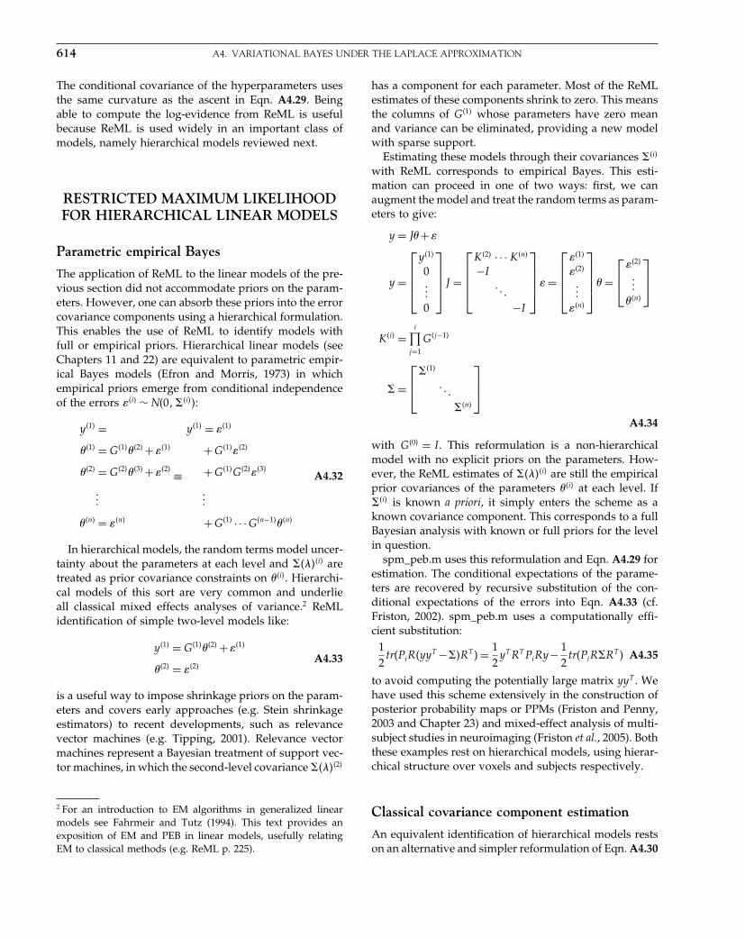
Elsevier UK Chapter: Appendix4-P372560 3-10-2006 4:24p.m. Page:614 Trim:7.5in×9.25in
Basal Font:Palatino Margins:Top:40pt Gutter:68pt Font Size:9.5/12 Text Width:42pc Depth:55 Lines
614 A4. VARIATIONAL BAYES UNDER THE LAPLACE APPROXIMATION
The conditional covariance of the hyperparameters usesthe same curvature as the ascent in Eqn. A4.29. Beingable to compute the log-evidence from ReML is usefulbecause ReML is used widely in an important class ofmodels, namely hierarchical models reviewed next.
RESTRICTED MAXIMUM LIKELIHOODFOR HIERARCHICAL LINEAR MODELS
Parametric empirical Bayes
The application of ReML to the linear models of the pre-vious section did not accommodate priors on the param-eters. However, one can absorb these priors into the errorcovariance components using a hierarchical formulation.This enables the use of ReML to identify models withfull or empirical priors. Hierarchical linear models (seeChapters 11 and 22) are equivalent to parametric empir-ical Bayes models (Efron and Morris, 1973) in whichempirical priors emerge from conditional independenceof the errors ��i� ∼ N�0���i��:
y�1� =��1� = G�1���2� +��1�
��2� = G�2���3� +��2�
���
��n� = ��n�
≡
y�1� = ��1�
+G�1���2�
+G�1�G�2���3�
���
+G�1� · · ·G�n−1���n�
A4.32
In hierarchical models, the random terms model uncer-tainty about the parameters at each level and �����i� aretreated as prior covariance constraints on ��i�. Hierarchi-cal models of this sort are very common and underlieall classical mixed effects analyses of variance.2 ReMLidentification of simple two-level models like:
y�1� = G�1���2� +��1�
��2� = ��2�A4.33
is a useful way to impose shrinkage priors on the param-eters and covers early approaches (e.g. Stein shrinkageestimators) to recent developments, such as relevancevector machines (e.g. Tipping, 2001). Relevance vectormachines represent a Bayesian treatment of support vec-tor machines, in which the second-level covariance �����2�
2 For an introduction to EM algorithms in generalized linearmodels see Fahrmeir and Tutz (1994). This text provides anexposition of EM and PEB in linear models, usefully relatingEM to classical methods (e.g. ReML p. 225).
has a component for each parameter. Most of the ReMLestimates of these components shrink to zero. This meansthe columns of G�1� whose parameters have zero meanand variance can be eliminated, providing a new modelwith sparse support.
Estimating these models through their covariances ��i�
with ReML corresponds to empirical Bayes. This esti-mation can proceed in one of two ways: first, we canaugment the model and treat the random terms as param-eters to give:
y = J� +�
y =
⎡⎢⎢⎢⎣
y�1�
0���0
⎤⎥⎥⎥⎦ J =
⎡⎢⎢⎢⎣
K�2� · · · K�n�
−I� � �
−I
⎤⎥⎥⎥⎦� =
⎡⎢⎢⎢⎣
��1�
��2�
�����n�
⎤⎥⎥⎥⎦� =
⎡⎢⎣
��2�
�����n�
⎤⎥⎦
K�i� =i∏
j=1
G�j−1�
� =⎡⎢⎣
��1�
� � �
��n�
⎤⎥⎦
A4.34
with G�0� = I . This reformulation is a non-hierarchicalmodel with no explicit priors on the parameters. How-ever, the ReML estimates of �����i� are still the empiricalprior covariances of the parameters ��i� at each level. If��i� is known a priori, it simply enters the scheme as aknown covariance component. This corresponds to a fullBayesian analysis with known or full priors for the levelin question.
spm_peb.m uses this reformulation and Eqn. A4.29 forestimation. The conditional expectations of the parame-ters are recovered by recursive substitution of the con-ditional expectations of the errors into Eqn. A4.33 (cf.Friston, 2002). spm_peb.m uses a computationally effi-cient substitution:
12
tr�PiR�yyT −��RT � = 12
yT RT PiRy− 12
tr�PiR�RT � A4.35
to avoid computing the potentially large matrix yyT . Wehave used this scheme extensively in the construction ofposterior probability maps or PPMs (Friston and Penny,2003 and Chapter 23) and mixed-effect analysis of multi-subject studies in neuroimaging (Friston et al., 2005). Boththese examples rest on hierarchical models, using hierar-chical structure over voxels and subjects respectively.
Classical covariance component estimation
An equivalent identification of hierarchical models restson an alternative and simpler reformulation of Eqn. A4.30
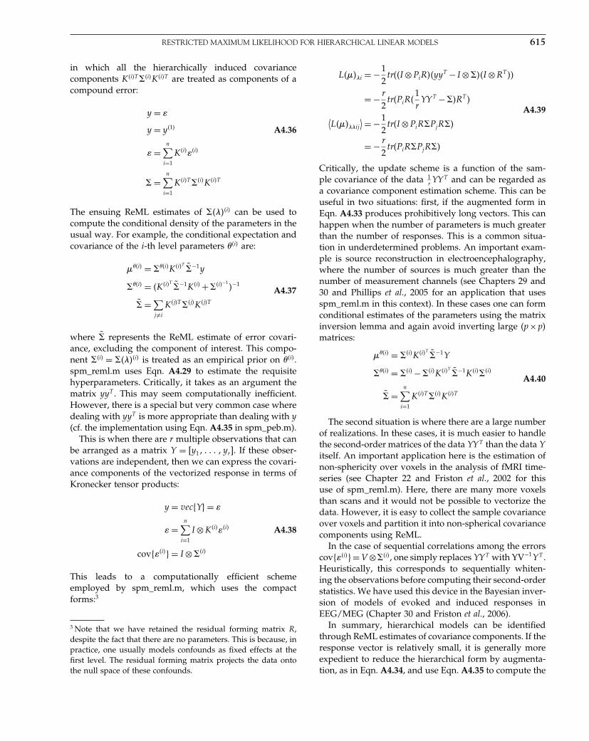
Elsevier UK Chapter: Appendix4-P372560 3-10-2006 4:24p.m. Page:615 Trim:7.5in×9.25in
Basal Font:Palatino Margins:Top:40pt Gutter:68pt Font Size:9.5/12 Text Width:42pc Depth:55 Lines
RESTRICTED MAXIMUM LIKELIHOOD FOR HIERARCHICAL LINEAR MODELS 615
in which all the hierarchically induced covariancecomponents K�i�T ��i�K�i�T are treated as components of acompound error:
y = �
y = y�1� A4.36
� =n∑
i=1
K�i���i�
� =n∑
i=1
K�i�T ��i�K�i�T
The ensuing ReML estimates of �����i� can be used tocompute the conditional density of the parameters in theusual way. For example, the conditional expectation andcovariance of the i-th level parameters ��i� are:
��i� = ���i�K�i�T �̃−1y
���i� = �K�i�T �̃−1K�i� +��i�−1�−1
�̃ =∑j �=i
K�j�T ��j�K�j�T
A4.37
where �̃ represents the ReML estimate of error covari-ance, excluding the component of interest. This compo-nent ��i� = �����i� is treated as an empirical prior on ��i�.spm_reml.m uses Eqn. A4.29 to estimate the requisitehyperparameters. Critically, it takes as an argument thematrix yyT . This may seem computationally inefficient.However, there is a special but very common case wheredealing with yyT is more appropriate than dealing with y(cf. the implementation using Eqn. A4.35 in spm_peb.m).
This is when there are r multiple observations that canbe arranged as a matrix Y = �y1� � � � � yr �. If these obser-vations are independent, then we can express the covari-ance components of the vectorized response in terms ofKronecker tensor products:
y = vec�Y� = �
� =n∑
i=1
I ⊗K�i���i� A4.38
cov���i�� = I ⊗��i�
This leads to a computationally efficient schemeemployed by spm_reml.m, which uses the compactforms:3
3 Note that we have retained the residual forming matrix R,despite the fact that there are no parameters. This is because, inpractice, one usually models confounds as fixed effects at thefirst level. The residual forming matrix projects the data ontothe null space of these confounds.
L���i = −12
tr��I ⊗PiR��yyT − I ⊗���I ⊗RT ��
= − r
2tr�PiR�
1r
YY T −��RT �
⟨L����ij
⟩= −12
tr�I ⊗PiR�PjR��
= − r
2tr�PiR�PjR��
A4.39
Critically, the update scheme is a function of the sam-ple covariance of the data 1
rYY T and can be regarded as
a covariance component estimation scheme. This can beuseful in two situations: first, if the augmented form inEqn. A4.33 produces prohibitively long vectors. This canhappen when the number of parameters is much greaterthan the number of responses. This is a common situa-tion in underdetermined problems. An important exam-ple is source reconstruction in electroencephalography,where the number of sources is much greater than thenumber of measurement channels (see Chapters 29 and30 and Phillips et al., 2005 for an application that usesspm_reml.m in this context). In these cases one can formconditional estimates of the parameters using the matrixinversion lemma and again avoid inverting large �p×p�matrices:
��i� = ��i�K�i�T �̃−1Y
���i� = ��i� −��i�K�i�T �̃−1K�i���i�
�̃ =n∑
i=1
K�i�T ��i�K�i�T
A4.40
The second situation is where there are a large numberof realizations. In these cases, it is much easier to handlethe second-order matrices of the data YY T than the data Yitself. An important application here is the estimation ofnon-sphericity over voxels in the analysis of fMRI time-series (see Chapter 22 and Friston et al., 2002 for thisuse of spm_reml.m). Here, there are many more voxelsthan scans and it would not be possible to vectorize thedata. However, it is easy to collect the sample covarianceover voxels and partition it into non-spherical covariancecomponents using ReML.
In the case of sequential correlations among the errorscov���i�� = V ⊗��i�, one simply replaces YY T with YV−1Y T .Heuristically, this corresponds to sequentially whiten-ing the observations before computing their second-orderstatistics. We have used this device in the Bayesian inver-sion of models of evoked and induced responses inEEG/MEG (Chapter 30 and Friston et al., 2006).
In summary, hierarchical models can be identifiedthrough ReML estimates of covariance components. If theresponse vector is relatively small, it is generally moreexpedient to reduce the hierarchical form by augmenta-tion, as in Eqn. A4.34, and use Eqn. A4.35 to compute the
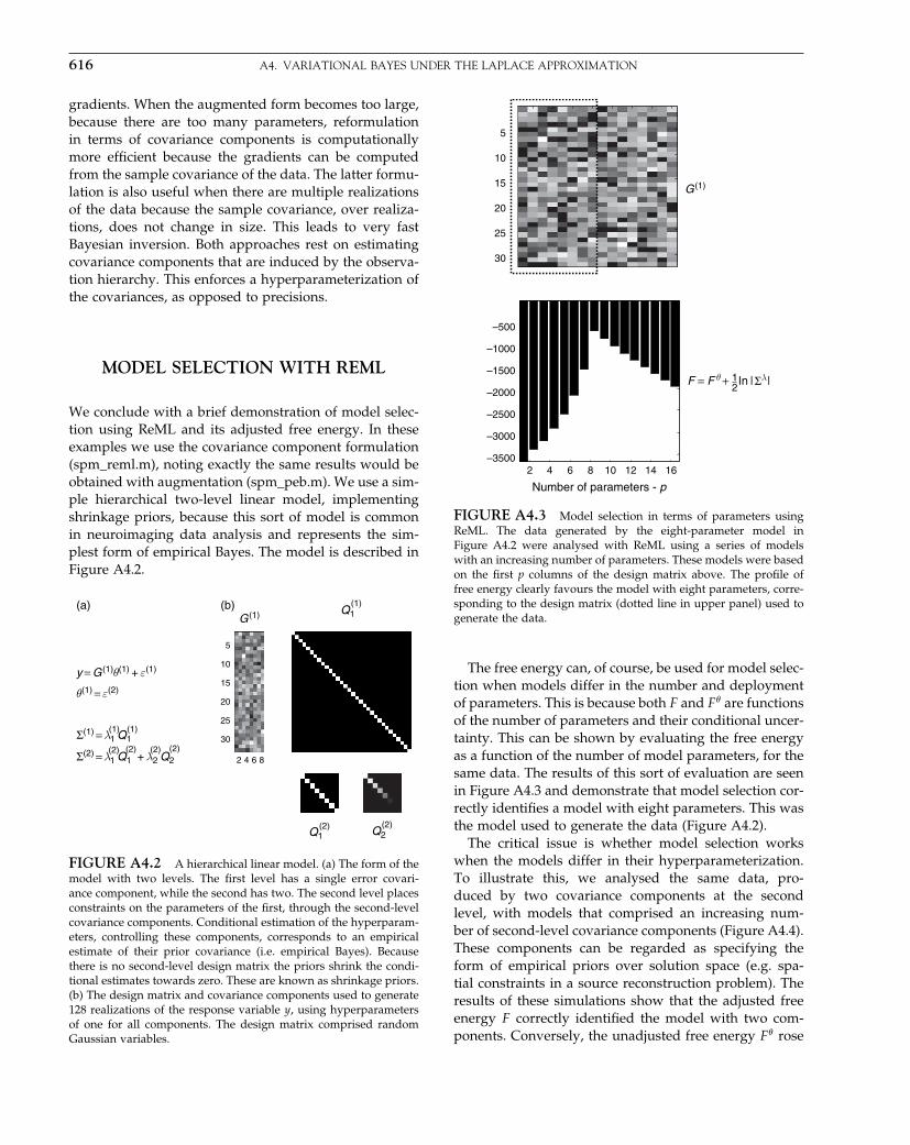
Elsevier UK Chapter: Appendix4-P372560 3-10-2006 4:24p.m. Page:616 Trim:7.5in×9.25in
Basal Font:Palatino Margins:Top:40pt Gutter:68pt Font Size:9.5/12 Text Width:42pc Depth:55 Lines
616 A4. VARIATIONAL BAYES UNDER THE LAPLACE APPROXIMATION
gradients. When the augmented form becomes too large,because there are too many parameters, reformulationin terms of covariance components is computationallymore efficient because the gradients can be computedfrom the sample covariance of the data. The latter formu-lation is also useful when there are multiple realizationsof the data because the sample covariance, over realiza-tions, does not change in size. This leads to very fastBayesian inversion. Both approaches rest on estimatingcovariance components that are induced by the observa-tion hierarchy. This enforces a hyperparameterization ofthe covariances, as opposed to precisions.
MODEL SELECTION WITH REML
We conclude with a brief demonstration of model selec-tion using ReML and its adjusted free energy. In theseexamples we use the covariance component formulation(spm_reml.m), noting exactly the same results would beobtained with augmentation (spm_peb.m). We use a sim-ple hierarchical two-level linear model, implementingshrinkage priors, because this sort of model is commonin neuroimaging data analysis and represents the sim-plest form of empirical Bayes. The model is described inFigure A4.2.
8642
5
10
15
20
25
30
θ(1) = ε (2)
G
(1)(b)(a)
Σ(1) = λ1 Q1
Σ(2) = λ1 Q1 + λ 2 Q2
y = G
(1)θ(1) + ε
(1)
Q2Q1
Q1
(1) (1)
(2)
(2) (2) (2)
(1)
(2) (2)
FIGURE A4.2 A hierarchical linear model. (a) The form of themodel with two levels. The first level has a single error covari-ance component, while the second has two. The second level placesconstraints on the parameters of the first, through the second-levelcovariance components. Conditional estimation of the hyperparam-eters, controlling these components, corresponds to an empiricalestimate of their prior covariance (i.e. empirical Bayes). Becausethere is no second-level design matrix the priors shrink the condi-tional estimates towards zero. These are known as shrinkage priors.(b) The design matrix and covariance components used to generate128 realizations of the response variable y, using hyperparametersof one for all components. The design matrix comprised randomGaussian variables.
5
10
15
20
25
30
2 4 6 8 10 12 14 16–3500
–3000
–2500
–2000
–1500
–1000
–500
G
(1)
Number of parameters - p
||nl21 ΣλF = F
θ +
FIGURE A4.3 Model selection in terms of parameters usingReML. The data generated by the eight-parameter model inFigure A4.2 were analysed with ReML using a series of modelswith an increasing number of parameters. These models were basedon the first p columns of the design matrix above. The profile offree energy clearly favours the model with eight parameters, corre-sponding to the design matrix (dotted line in upper panel) used togenerate the data.
The free energy can, of course, be used for model selec-tion when models differ in the number and deploymentof parameters. This is because both F and F� are functionsof the number of parameters and their conditional uncer-tainty. This can be shown by evaluating the free energyas a function of the number of model parameters, for thesame data. The results of this sort of evaluation are seenin Figure A4.3 and demonstrate that model selection cor-rectly identifies a model with eight parameters. This wasthe model used to generate the data (Figure A4.2).
The critical issue is whether model selection workswhen the models differ in their hyperparameterization.To illustrate this, we analysed the same data, pro-duced by two covariance components at the secondlevel, with models that comprised an increasing num-ber of second-level covariance components (Figure A4.4).These components can be regarded as specifying theform of empirical priors over solution space (e.g. spa-tial constraints in a source reconstruction problem). Theresults of these simulations show that the adjusted freeenergy F correctly identified the model with two com-ponents. Conversely, the unadjusted free energy F� rose

Elsevier UK Chapter: Appendix4-P372560 3-10-2006 4:24p.m. Page:617 Trim:7.5in×9.25in
Basal Font:Palatino Margins:Top:40pt Gutter:68pt Font Size:9.5/12 Text Width:42pc Depth:55 Lines
REFERENCES 617
1 ,,...Q
(2)8Q
(2)
81 G
(1)TQ
(2)G
(1)G
(1)TQ
(2)G
(1) ,,...
FIGURE A4.4 Covariance components used to analyse thedata generated by the model in Figure A4.2. The covariance com-ponents are shown at the second level (upper panels) and after pro-jection onto response space (lower panels) with the eight-parametermodel. Introducing more covariance components creates a seriesmodel with an increasing number of hyperparameters, which weexamined using model selection in Figure A4.5. These covariancecomponents were leading diagonal matrices, whose elements com-prised a mean-adjusted discrete cosine set.
progressively as the number of components and accuracyincreased (Figure A4.5).
The lower panel in Figure A4.5 shows the hyperpa-rameter estimates for two models. With the correctlyselected model, the true values fall within the 90 per centconfidence interval. However, when the model is over-parameterized, with eight second-level components, thisis not the case. Although the general profile of hyperpa-rameters has been captured, this suboptimum model hasclearly overestimated some hyperparameters and under-estimated others.
Conclusion
We have seen that restricted maximum likelihood is aspecial case of expectation maximization and that expec-tation maximization is a special case of variational Bayes.In fact, nearly every routine used in neuroimaging anal-ysis is a special case of variational Bayes, from ordinaryleast squares estimation to dynamic causal modelling.We have focused on adjusting the objective functions
1 2 3 4 5 6 7 8
–690
–685
–680
–675
–670
–665
–660
–690
–685
–680
–675
–670
–665
–660
1 2 3 4 5 6 7 8
F θ
Number of 2nd-levelhyperparameters or components
Hyperparameter estimates
iQ
(2)
(a)
(b)
F
UnadjustedAdjusted
1λ(1) ,...,
1λ(1)
1λ(2)
8λ(2)
1λ(2)
2λ(2)
FIGURE A4.5 Model selection in terms of hyperparametersusing ReML. (a) The free energy was computed using the datagenerated by the model in Figure A4.2 and a series of modelswith an increasing number of hyperparameters. The ensuing freeenergy profiles (adjusted – left; unadjusted – right) are shown asa function of the number of second-level covariance componentsused (from Figure A4.4). The adjusted profile clearly identified thecorrect model with two second-level components. (b) Conditionalestimates (white) and true (black) hyperparameter values with 90per cent confidence intervals for the correct (3-component, left) andredundant (9-component, right) models.
used by EM and ReML to approximate the variationalfree energy under the Laplace approximation. This freeenergy is a lower bound approximation (exact for linearmodels) to the log-evidence, which plays a central rolein model selection and averaging. This means one canuse computationally efficient schemes like ReML for bothmodel selection and Bayesian inversion.
REFERENCES
Ashburner J, Friston KJ (2005) Unified segmentation. NeuroImage 26:839–51
Beal MJ, Ghahramani Z (2003) The variational Bayesian EM algo-rithm for incomplete data: with application to scoring graphicalmodel structures. In Bayesian statistics, Bernardo JM, Bayarri MJ,Berger JO et al. (eds). OUP, Milton Keynes, ch 7
Elsevier UK Chapter: Appendix4-P372560 3-10-2006 4:24p.m. Page:618 Trim:7.5in×9.25in
Basal Font:Palatino Margins:Top:40pt Gutter:68pt Font Size:9.5/12 Text Width:42pc Depth:55 Lines
618 A4. VARIATIONAL BAYES UNDER THE LAPLACE APPROXIMATION
Berger JO (1985) Statistical decision theory and Bayesian analysis, 2ndedn. Springer, Berlin
Bishop C (1999) Latent variable models. In Learning in graphicalmodels, Jordan M (ed.). MIT Press, London
David O, Harrison L, Friston KJ (2005) Modelling event-relatedresponses in the brain. NeuroImage 25: 756–70
Dempster AP, Laird NM, Rubin DB (1977) Maximum likelihoodfrom incomplete data via the EM algorithm. J Roy Stat Soc SeriesB 39: 1–38
Efron B, Morris C (1973) Stein’s estimation rule and its competitors –an empirical Bayes approach. J Am Stat Assoc 68: 117–30
Fahrmeir L, Tutz G (1994) Multivariate statistical modelling basedon generalised linear models. Springer-Verlag Inc., New York,pp 355–56
Feynman RP (1972) Statistical mechanics. Benjamin, Reading, MAFriston KJ (2002) Bayesian estimation of dynamical systems: an
application to fMRI. NeuroImage 16: 513–30Friston K (2005) A theory of cortical responses. Philos Trans R Soc
Lond B Biol Sci 360: 815–36Friston KJ, Penny W, Phillips C et al. (2002) Classical and Bayesian
inference in neuroimaging: theory. NeuroImage 16: 465–83Friston KJ, Penny W. (2003) Posterior probability maps and SPMs.
NeuroImage 19: 1240–49Friston KJ, Harrison L, Penny W (2003) Dynamic causal modelling.
NeuroImage 19: 1273–302Friston KJ, Stephan KE, Lund TE et al. (2005) Mixed-effects and
fMRI studies. NeuroImage 24: 244–52Friston KJ, Henson R, Phillips C et al. (2006) Bayesian estimation of
evoked and induced responses. Hum Brain Mapp in pressHarrison LM, David O, Friston KJ (2005) Stochastic models
of neuronal dynamics. Philos Trans R Soc Lond B Biol Sci360: 1075–91
Hartley H (1958) Maximum likelihood estimation from incompletedata. Biometrics 14: 174–94
Harville DA (1977) Maximum likelihood approaches to variancecomponent estimation and to related problems. J Am Stat Assoc72: 320–38
Hinton GE, von Camp D (1993) Keeping neural networks simple byminimising the description length of weights. In Proc COLT-93pp 5–13
Kass RE, Steffey D (1989) Approximate Bayesian inference in condi-tionally independent hierarchical models (parametric empiricalBayes models). J Am Stat Assoc 407: 717–26
Kiebel SJ, David O, Friston KJ (2006) Dynamic causal modelling ofevoked responses in EEG/MEG with lead field parameteriza-tion. NeuroImage 30: 1273–84
Leonard T, Hsu JSL (1992) Bayesian inference for a covariancematrix. Ann Stat 20: 1669–96
Mackay DJC (1995) Free energy minimisation algorithm for decod-ing and cryptoanalysis. Electron Lett 31: 445–47
Mackay DJC, Takeuchi R (1996) Interpolation models with multi-ple hyperparameters. In Maximum entropy & Bayesian methods,Skilling J, Sibisi S (eds). Kluwer, Dordrecht, pp 249–57
Mattout J, Phillips C, Rugg MD et al. (2006) MEG source localisationunder multiple constraints: an extended Bayesian framework.NeuroImage 30: 753–67
Neal RM, Hinton GE (1998) A view of the EM algorithm that justifiesincremental sparse and other variants. In Learning in graphicalmodels, Jordan MI (ed.). Kulver Academic Press, Dordrecht
Nelson MC, Illingworth WT (1991) A practical guide to neural nets.Addison-Wesley, Reading, MA, pp 165
Penny WD, Stephan KE, Mechelli A et al. (2004) Comparing dynamiccausal models. NeuroImage 22: 1157–72
Penny WD, Trujillo-Barreto NJ, Friston KJ (2005) Bayesian fMRItime series analysis with spatial priors. NeuroImage 24: 350–62
Phillips C, Rugg M, Friston KJ (2002) Systematic regularisation oflinear inverse solutions of the EEG source localisation problem.NeuroImage 17: 287–301
Phillips C, Mattout J, Rugg MD et al. (2005) An empiricalBayesian solution to the source reconstruction problem in EEG.NeuroImage 24: 997–1011
Tipping ME (2001) Sparse Bayesian learning and the relevance vec-tor machine. J Machine Learn Res 1: 211–44
Titantah JT, Pierlioni C, Ciuchi S (2001) Free energy of the FröhlichPolaron in two and three dimensions. Phys Rev Lett 87: 206406
Trujillo-Barreto N, Aubert-Vazquez E, Valdes-Sosa P (2004)Bayesian model averaging. NeuroImage 21: 1300–19
Weissbach F, Pelster A, Hamprecht B (2002) High-order variationalperturbation theory for the free energy. Phys Rev Lett 66: 036129

Elsevier UK Chapter: Appendix5-P372560 3-10-2006 4:25p.m. Page:619 Trim:7.5in×9.25in
Basal Font:Palatino Margins:Top:40pt Gutter:68pt Font Size:9.5/12 Text Width:42pc Depth:55 Lines
A P P E N D I X
5
Kalman filteringK. Friston and W. Penny
INTRODUCTION
Bayesian inversion of state-space models is relatedto Bayesian belief update procedures (i.e. recursiveBayesian filters). The conventional approach to onlineBayesian tracking of states in non-linear or non-Gaussiansystems employs extended Kalman filtering or sequen-tial Monte Carlo methods, such as particle filtering.These implementations of Bayesian filters approximatethe conditional densities of hidden states in a recursiveand computationally expedient fashion, assuming thatthe parameters and hyperparameters of the system areknown. We start with systems (dynamic models) that areformulated in continuous time:
y = g�x�+z
ẋ = f�x�v� A5.1
where the innovations z�t� and causes v�t� are treated asrandom fluctuations. As we will see below this is con-verted into a state-space model in discrete time beforeapplication of the filter. Kalman filters proceed recur-sively in two steps: prediction and update. The predic-tion uses the Chapman-Kolmogorov equation to computethe density of the hidden states x�t� conditioned on theresponse up to, but not including, the current observationy→t−1:
p�xt�y→t−1� =∫
p�xt�xt−1�p�xt−1�y→t−1�dxt−1 A5.2
This conditional density is then treated as a prior for thenext observation and Bayes’ rule is used to compute theconditional density of the states, conditioned upon allobservations y→t. This gives the Bayesian update:
q�xt� = p�xt�y→t� ∝ p�yt�xt�p�xt�y→t−1� A5.3
Critically, the conditional density covers only the hid-den states. This is important because it precludes infer-ence on causes and the ability to de-convolve inputs fromoutputs. This is a key limitation of Bayesian filtering.However, Kalman filtering provides the optimal solutionwhen the assumptions of the underlying model hold andone is not interested in causes or inputs. We now considerin more detail the operation equations for the extendedKalman filter. The extended Kalman filter is a generaliza-tion of the Kalman filter, in which the linear operators ofthe state equations are replaced by the partial derivativesof f�x�v� with respect to the states.
THE EXTENDED KALMAN FILTER
This section provides a pseudo-code specification of theextended Kalman filter based on van der Merwe et al.(2000). To clarify the notation, we will use fx = �f/�x.Eqn. A5.1 can be re-written, using local linearization, asa discrete-time state-space model. This is the formulationtreated in Bayesian filtering procedures:
yt = gxxt +zt
xt = fxxt−1 +wt−1
gx = g�xt�x
fx = exp�f�xt�x�
zt = z�t�
wt−1 =∫
exp�fx��fvv�t −��d� A5.4
For simplicity, we assume �t = 1. The key thing to notehere is that process noise wt−1 is simply a convolution of
Statistical Parametric Mapping, by Karl Friston et al. Copyright 2007, Elsevier Ltd. All rights reserved.ISBN–13: 978-0-12-372560-8 ISBN–10: 0-12-372560-7
619

Elsevier UK Chapter: Appendix5-P372560 3-10-2006 4:25p.m. Page:620 Trim:7.5in×9.25in
Basal Font:Palatino Margins:Top:40pt Gutter:68pt Font Size:9.5/12 Text Width:42pc Depth:55 Lines
620 A5. KALMAN FILTERING
the causes v�t�. This is relevant for Kalman filtering andrelated non-linear Bayesian tracking schemes that assumewt−1 is a well-behaved noise sequence. The covariance ofprocess noise is:
⟨wtw
Tt
⟩= ∫exp�fx��� exp�fx��T d�
≈ � A5.5
= fvRfTv
where R is the covariance of v�t�. We have assumedv�t� has no temporal correlations and that the Lyapunovexponents of fx are large relative to the time-step. Theprediction and update steps are:
for all t
Prediction step
xt = fxxt−1
xt = �+ fx
xt−1fT
x
Update or correction step
K = xt gT
x �+gxxt gT
x �−1
xt ← xt +K�y −g�xt��
xt ← �I −Kgx�
xt
end A5.6
Where is the covariance of observation noise. TheKalman gain matrix K is used to update the predictionof future states and their conditional covariance, giveneach new observation. We actually use xt = xt−1 + �fx − I�f−1
x f�xt−1�. This is a slightly more sophisticated updatethat uses the current state as the expansion point for thelocal linearization. As mentioned in Chapter 37, Kalmanfiltering is also known as variable parameter regression,when the hidden state plays the role of a parameter (seeBüchel and Friston, 1998).
REFERENCES
Büchel C, Friston KJ (1998) Dynamic changes in effective connectiv-ity characterised by variable parameter regression and Kalmanfiltering. Hum Brain Mapp 6: 403–08
van der Merwe R, Doucet A, de Freitas N et al. (2000) The unscentedparticle filter. Technical Report CUED/F-INFENG/TR 380
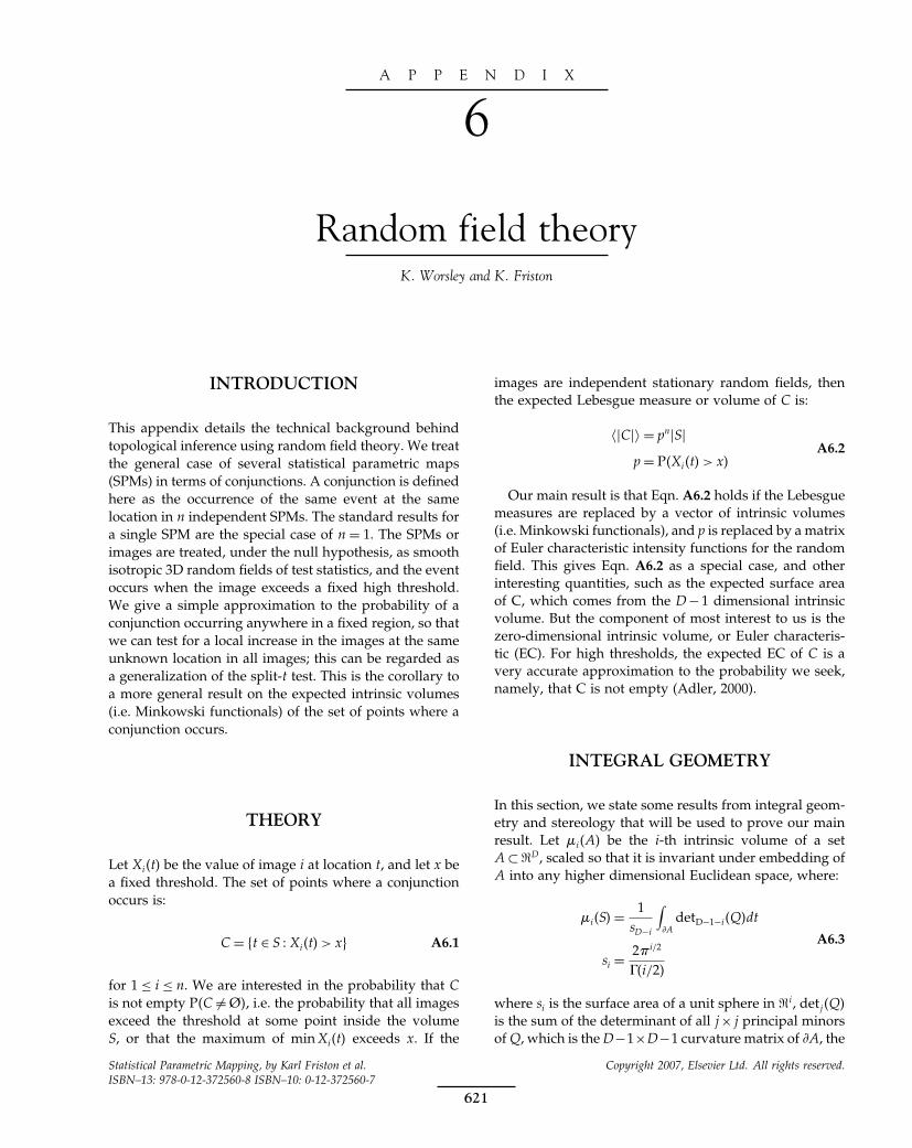
Elsevier UK Chapter: Appendix6-P372560 3-10-2006 4:26p.m. Page:621 Trim:7.5in×9.25in
Basal Font:Palatino Margins:Top:40pt Gutter:68pt Font Size:9.5/12 Text Width:42pc Depth:55 Lines
A P P E N D I X
6
Random field theoryK. Worsley and K. Friston
INTRODUCTION
This appendix details the technical background behindtopological inference using random field theory. We treatthe general case of several statistical parametric maps(SPMs) in terms of conjunctions. A conjunction is definedhere as the occurrence of the same event at the samelocation in n independent SPMs. The standard results fora single SPM are the special case of n = 1. The SPMs orimages are treated, under the null hypothesis, as smoothisotropic 3D random fields of test statistics, and the eventoccurs when the image exceeds a fixed high threshold.We give a simple approximation to the probability of aconjunction occurring anywhere in a fixed region, so thatwe can test for a local increase in the images at the sameunknown location in all images; this can be regarded asa generalization of the split-t test. This is the corollary toa more general result on the expected intrinsic volumes(i.e. Minkowski functionals) of the set of points where aconjunction occurs.
THEORY
Let Xi�t� be the value of image i at location t, and let x bea fixed threshold. The set of points where a conjunctionoccurs is:
C = �t ∈ S � Xi�t� > x� A6.1
for 1 ≤ i ≤ n. We are interested in the probability that Cis not empty P�C �= Ø�, i.e. the probability that all imagesexceed the threshold at some point inside the volumeS, or that the maximum of min Xi�t� exceeds x. If the
images are independent stationary random fields, thenthe expected Lebesgue measure or volume of C is:
��C�� = pn�S�p = P�Xi�t� > x�
A6.2
Our main result is that Eqn. A6.2 holds if the Lebesguemeasures are replaced by a vector of intrinsic volumes(i.e. Minkowski functionals), and p is replaced by a matrixof Euler characteristic intensity functions for the randomfield. This gives Eqn. A6.2 as a special case, and otherinteresting quantities, such as the expected surface areaof C, which comes from the D − 1 dimensional intrinsicvolume. But the component of most interest to us is thezero-dimensional intrinsic volume, or Euler characteris-tic (EC). For high thresholds, the expected EC of C is avery accurate approximation to the probability we seek,namely, that C is not empty (Adler, 2000).
INTEGRAL GEOMETRY
In this section, we state some results from integral geom-etry and stereology that will be used to prove our mainresult. Let �i�A� be the i-th intrinsic volume of a setA ⊂ D, scaled so that it is invariant under embedding ofA into any higher dimensional Euclidean space, where:
�i�S� = 1sD−i
∫�A
detD−1−i�Q�dt
si = 2i/2
�i/2�
A6.3
where si is the surface area of a unit sphere in i, detj�Q�is the sum of the determinant of all j × j principal minorsof Q, which is the D−1×D−1 curvature matrix of �A, the
Statistical Parametric Mapping, by Karl Friston et al. Copyright 2007, Elsevier Ltd. All rights reserved.ISBN–13: 978-0-12-372560-8 ISBN–10: 0-12-372560-7
621

Elsevier UK Chapter: Appendix6-P372560 3-10-2006 4:26p.m. Page:622 Trim:7.5in×9.25in
Basal Font:Palatino Margins:Top:40pt Gutter:68pt Font Size:9.5/12 Text Width:42pc Depth:55 Lines
622 A6. RANDOM FIELD THEORY
boundary of A. Note that �0�A� is the EC by the Gauss-Bonnet theorem, and �D−1�A� is half the surface area ofA. �D�A� = �A� is its volume or Lebesgue measure. Forexample, the intrinsic volumes of a ball of radius r are:
�0�S� = 1 �1�S� = 4r �2�S� = 2r2 �3�S� = �4/3�r3
A6.4
Other examples are provided in Plate 62 (see colour platesections) for some common search volumes. We shall alsouse the result that any functional ��A� that obeys theadditivity rule:
��A∪B� = ��A�+��B�−��A∩B� A6.5
is a linear combination of intrinsic volumes. Let A�B ⊂D, then the Kinematic Fundamental Formula of integralgeometry relates the integrated EC of the intersection ofA and B to their intrinsic volumes.
∫�0�A∩B� = s2 sD
D∑i=0
�i�A��D−i�B�
cDi
cDi = � 1
2 �� D+12 �
� i+12 �� D−i+1
2 �
A6.6
where the integral is over all rotations and translationsof A, keeping B fixed.
RANDOM FIELDS
If Xi�t� is an isotropic random field with excursion setA = �t � X�t� ≥ x� then:
��0�A∩S�� =D∑
i=0
�i�i�S� A6.7
for some constants �i. This follows from the fact that thefunctional ��0�A∩S�� obeys the additivity rule Eqn. A6.5,since �0 does, so it must be a linear combination ofthe intrinsic volumes. The coefficients �i are called Eulercharacteristic (EC) intensities in i, and can be evalu-ated for a variety of random fields (Worsley, 1994; Caoand Worsley, 1999; Adler, 2000; Worsley et al., 2004).Figure A6.1 provides the expressions for some commonstatistics used in SPMs. The EC intensity is a function ofthe image roughness � defined here as cov��X/�t� = �I .
Eqn. A6.7 is fundamental to inference on SPMs becausethe expected EC, �0 = ��0�A∩S�� is an accurate approx-imation to the probability of getting an excursion setby chance (i.e. the adjusted p-value). Its form helpsunderstand how this probability arises: the expected EC
FIGURE A6.1 Euler characteristic intensities for some com-mon statistical fields. These are functions of the field’s roughness �.When roughness is one, these are the Euler characteristic densitiesreferred to in previous chapters.
receives contributions, �i�i�S� from each dimension ofthe search volume. Each contribution is the product of anEC intensity and an intrinsic volume. If we were dealingwith statistically flat images with � = 1, these quantitieswould correspond to EC densities and resolution ele-ments (resel) counts respectively (see Chapter 19). TheEC density represents the expected EC per resel and theresel count represents the resel number at each dimen-sion. We will now generalize this for multiple images.
We can extend Eqn. A6.7 to higher intrinsic volumesby the lemma in Worsley and Friston (2000):
��i�A∩S�� =D∑
j=i
cji�j−i�j�S� A6.8
Elsevier UK Chapter: Appendix6-P372560 3-10-2006 4:26p.m. Page:623 Trim:7.5in×9.25in
Basal Font:Palatino Margins:Top:40pt Gutter:68pt Font Size:9.5/12 Text Width:42pc Depth:55 Lines
REFERENCES 623
Theorem: Let Rk be the upper triangular matrix whose (i,j)elements are �j−ikc
ji if j ≥ i and 0 otherwise; i.e.
Rk =⎡⎢⎣
�0kc11 · · · �0kc
D1
���� � �
���0 · · · �0kc
DD
⎤⎥⎦ and ��S� =
⎡⎢⎣
�0�S����
�D�S�
⎤⎥⎦
where �ik is the EC intensity of Xk�t� in i then:
���C�� = ��0� ��D�T =(
n∏i=1
Ri
)��S� A6.9
Proof: the proof follows by induction on n. FromEqn. A6.8, we see that it is clearly true for n = 1. Let Ak
be the excursion set for Xk�t� so that C = A1 ∩ An ∩S.If the result is true for n = k then by first conditioning onAk+1 and replacing S by Ak+1 ∩S, we get:
���A1 ∩ Ak ∩ �Ak+1 ∩S��� =(
k∏i=1
Ri
)���Ak+1 ∩S��
=(
k∏i=1
Ri
)Rk+1��S� A6.10
by the result for n = 1. This completes the proof.Comparing Eqn. A6.9 with Eqn. A6.2, we see that they
have the same form, where the volumes are replacedby vectors of intrinsic volumes, and the probability isreplaced by the matrix of weighted EC intensities. Thelast element �D = ��C�� is the same as the Lebesgue mea-sure and the first element �0 is the expected EC of the setof conjunctions. This is the approximation to the proba-bility of a conjunction anywhere in S, for high thresholdsx, we require.
EXAMPLE
We shall apply the result in Eqn. A6.9 to some D = 3dimensional functional magnetic resonance imaging(fMRI) data. The purpose of the experiment was to deter-mine those regions of the brain that were consistentlystimulated by all subjects, while viewing a pattern ofradially moving dots. To do this, subjects were presentedwith a pattern of moving dots, followed by a pattern ofstationary dots, and this was repeated 10 times, duringwhich a total of 120 3D fMRI images were obtained atthe rate of one every 3.22 s. For each subject i and atevery point t ∈ 3, a test statistic Xi�t� was calculated
Excursion sets for each image
Front
Back
LeftLGN
RightLGN
Conjunction: intersectionof excursion sets
FIGURE A6.2 Conjunction of six SPM�t� from a visual task(only one slice of the 3D data is shown). The excursion sets of eachare shown in white on a background of brain anatomy (top). Theset of conjunctions C is the intersection of these sets (bottom). Thevisual cortex at the back of the brain appears in C, but the mostinteresting feature is the appearance of the lateral geniculate nuclei(LGN) (arrows).
for comparing the fMRI response between the movingdots and the stationary dots. Under the null hypothe-sis of no difference, Xi�t� was modelled as an isotropicGaussian random field with zero mean, unit varianceand roughness � = 4�68 cm−1. A threshold of x = 1�64,corresponding to an uncorrected level 5 per cent test,was chosen, and the excursion sets for each subject areshown in Figure A6.2 together with their intersection,which forms the set of conjunctions C. The search vol-ume was the whole brain area that was scanned, whichwas an approximate spherical region with a volume of�S� = 1226 cm3. Finally, the approximate probability of aconjunction, calculated from Eqn. A6.9, was 0.0126. Wecan thus conclude, at the 1.26 per cent level, that con-junctions have occurred in the visual cortex, and moreinteresting, the lateral geniculate nuclei (see Figure A6.2).
REFERENCES
Adler RJ (2000) On excursion sets, tube formulae, and maxima ofrandom fields. Ann Appl Probab 10: 1–74
Cao J, Worsley K (1999) The geometry of correlation fields withan application to functional connectivity of the brain. Ann ApplProbab 9: 1021–57
Worsley KJ (1994) Local maxima and the expected Euler character-istic of excursion sets of chi-squared, F and t fields. Adv ApplProbab 26: 13–42
Worsley KJ, Friston KJ (2000) A test for a conjunction. Stat ProbabLett 47: 135–40
Worsley KJ, Taylor JE, Tomaiuolo F et al. (2004) Unified uni-variate and multivariate random field theory. NeuroImage 23:S189–95
Elsevier UK Chapter: Index-P372560 30-9-2006 5:36p.m. Page:625 Trim:7.5in×9.25in
Basal Font:Palatino Margins:Top:40pt Gutter:68pt Font Size:9.5/12 Text Width:42pc Depth:55 Lines
Index
Action potentials, 352, 391, 393, 509latency fluctuation, 435neural mass models, 417
Affine transformation, 12, 50inter-subject registration, 76, 77, 78inverse, 52left-/right-handed coodinate system, 54rigid body transformations, 52, 53, 54small deformation models, 67, 71
Age-related morphometric changes, 92AIR, 59, 67Akaike information criteria, 459, 460, 461, 578Alpha rhythms, 431
blood-oxygenation-level-dependent (BOLD) signalcorrelations, 410
neural mass models, 415, 416, 418Alzheimer’s disease, 55, 98AMOS, 514AMPA (fast excitory) receptors/channels, 394, 399, 402, 403,
474, 528, 530Anaerobic brain hypothesis, 340Analysis of covariance, 5, 17
by group, 116by subject, 115–116one-way, 118removal of movement-related artefacts, 58voxel-wise model, 3
Analysis of variance, 3, 4, 108, 130, 166–177between-subject, 166, 167–168F -contrast, 167–168F -tests, 166mixed designs, 166model evidence, 457multiway, 173–175
partitioned errors, 174–175non-sphericity, 169–170, 172, 175notation, 167one-way, 103–104, 107, 167–170random effects analysis, 162repeated measures (within-subject), 141–142, 166, 168–173,
176–177, 183
partitioned errors, 171, 172, 173pooled errors, 171–173Satterthwaite approximation, 143
two-way, 166, 170–173, 183types, 166
Anatomical models, 4, 32, 33–34, 63Bayesian inversion, 7spatial normalization, 10, 12, 14, 63
Aphasia, 488Associative plasticity, 475, 481Attention, 215, 483, 508, 528
functional selectivity, 451to visual motion, 298–299, 451, 485–486, 512, 514, 515, 516,
520, 537, 542, 556–559dynamic causal model, 40–41, 461–463
Attentional gain, 432, 435Auditory cortex, 345, 486, 553Auditory stimulation, 20, 319, 326
oddball experiments, 487–488, 571–573mismatch negativity, 391
Autoregressive models, 509moving average, 253multivariate see Multivariate autoregressive models
Autoregressive plus white noise model, 121, 123, 124,185, 287
B-splines, 51deformation models
basis functions, 71–72segmentation, 88
event-related potential modelling, 328Balloon model, 182, 339, 341, 342–343, 348, 442
blood-oxygenation-level-dependent (BOLD) response, 187haemodynamic extension see Haemodynamic modelnon-linear evoked responses, 341–343, 347Volterra series expansion, 341, 342, 343, 348
Balloon-Windkessel model see Balloon modeBaseline, 128Basic models, 117–118Basis functions
covariance component decomposition, 151
Elsevier UK Chapter: Index-P372560 30-9-2006 5:36p.m. Page:626 Trim:7.5in×9.25in
Basal Font:Palatino Margins:Top:40pt Gutter:68pt Font Size:9.5/12 Text Width:42pc Depth:55 Lines
626 INDEX
Basis functions (Continued)deformation models
radial, 71small deformation approach, 67, 69, 70–72
functional magnetic resonance imaging, 175linear time-series model, 120
highpass filtering, 184positron emission tomography, 112temporal see Temporal basis functions
Bayes factors, 457–458, 461, 462, 463, 464, 579p-values comparison, 458
Bayes’ theorem, 64Bayesian inference, 34–35, 148, 230, 275, 276–277, 300, 301,
445, 590dynamic causal models, 544, 568–569dynamic models inversion, 441haemodynamic model, 445, 446–447hierarchical models
linear, 280, 286two-level, 149
model averaging, 460model selection, 454multivariate autoregressive models, 536object perception, 479posterior probabilities, 276, 295posterior probability maps, 16, 34, 35, 300priors, 295, 296single-subject responses, 290spatially regularized general linear model, 317spatio-temporal model for electro-encephalography, 328
Bayesian information criteria, 459, 461, 578Bayesian model averaging, 154, 325, 460, 465Bayesian model comparisons, 456Bayesian model selection, 456Bayesian models, 7–8, 16
blood-oxygenation-level-dependent (BOLD) response, 182dynamic models inversion, 441historical aspects, 7–8likelihood, 64model selection/averaging, 454–466multivariate autoregressive models, 536, 538, 539posterior probability, 64
alternative models comparison, 78maps, 16, 34
predictive coding, 479prior probability, 64spatial normalization, 14see also Empirical Bayes; Variational Bayes
Beamformer predictions, 329oscillatory source localization, 388
Belief propagation algorithm, 148, 154–155, 466model averaging, 454, 460model evidence, 456model selection, 454
Bending boundary conditions, 71Bending energy, 66, 76, 77
minimization, 63Benjamini and Hochberg false discovery rate method, 248–249Best linear unbiased estimates, 103
Bias artefact (image intensity non-uniformity)bias field estimates, 85, 86, 87correction, 82–84
image intensity histograms, 83parametric models, 83–84
segmentation optimization, 86, 87Bilinear interpolation, 50Bilinear models, 511–512
approximating functions, 509–510effective connectivity, 508, 509
contextual input-dependent effects, 511, 512, 513coupling, 512psychophysiological interactions, 513, 514static models, 513see also Dynamic causal models
functional integration, 39–40, 41functional magnetic resonance imaging see Dynamic
causal modelsstate equation, 511
Biophysical models, 32, 37–38, 182input-state-output systems, 37–38, 597–599non-linear systems identification, 38
Block study designs, 27, 28, 114, 195–196, 200, 201, 203, 204noise variance, 205
Blood-oxygenation-level-dependent (BOLD) response, 25, 37,178, 313
balloon model see Balloon modelbilinear models, 40canonical haemodynamic response function, 181convolution models, 178dynamic causal models, 545
attentional effects, 556–559conventional analysis comparison, 549–550haemodynamic state equations, 546likelihood model, 546–547neuronal state equations, 545–546noise effects, 552priors, 547–548simulations, 550–552single word processing analysis, 553–556
dynamic model inversion, 441energy dissipation correlations, 407, 408
effect of activation, 408–409, 411event models, 196experimental design, 119, 199
stimulus presentation rate, 38factors influencing blood oxygenation, 340functional magnetic resonance imaging regressors, 119,
120, 121gamma functions, 181glutamate release, 407haemodynamic model, 343–346
balloon component, 343–344, 347experimental results, 347–348regional cerebral blood flow component, 344–346Volterra kernels estimation, 346–347
high-reolutiuon basis functions, 120iterative fitting techniques, 182linear time-invariant models, 179

Elsevier UK Chapter: Index-P372560 30-9-2006 5:36p.m. Page:627 Trim:7.5in×9.25in
Basal Font:Palatino Margins:Top:40pt Gutter:68pt Font Size:9.5/12 Text Width:42pc Depth:55 Lines
INDEX 627
local field potentials relationship, 406neural activity relationship, 339, 340–350
electrophysiological measures, 341linear assumptions, 340, 341magnetic field effects, 340–341modelled time course, 341
non-linear convolution models, 186–187non-linearities, 179, 340, 346
evoked responses, 341–343, 347peak latency differences, 179post-stimulus undershoot, 178, 343, 345, 346, 347, 349, 443,
450–451principle, 340sampling rate, 197saturation, 179, 186–188, 203, 551shape estimation methods, 180–183synaptic activity modelling, 341, 343time series event-related study, 188–191
categorical model, 188–190parametric model, 190–191
timing error/slice timing correction, 120, 121variability, 178–179, 182, 183see also Functional magnetic resonance imaging
Bonferroni correction, 4, 18, 34, 96, 214, 223, 224–226, 238,250, 276
independence of observations, 225–226maximum spatial extent of test statistic, 234maximum test statistic, 232, 233random field thresholds comparison, 228
Boundary conditionselectro-encephalography boundary element
method, 354small deformation models, 70–71
bending, 71circulant, 70sliding, 71
Boundary element method, 353analytical equation, 354–355
analytical solution, 363–364matrix form, 360–361numerical solution, 356–363partial solutions for electrode sites, 362–363partial solutions for scalp, 362
analytical equation approximation, 356centre of gravity method, 356, 357, 359, 361constant potential at vertices method, 356linear potential at vertices method, 356, 357–358,
359–360, 361current source model, 356–357electro-encephalography, 354–355
boundary conditions, 354Green’s theorem, 354limitations of numerical solution, 364–365magneto-encephalography, 355–356solid angles calculation, 358–359
Boxcar designs, 6, 7, 16, 27Brain electrical conductivity, 352, 353Brain response modelling, 32–44Brain shape differences, 63
Brain tumours, 55Brainstem auditory evoked potentials, 562BrainWeb MR simulator, 88–89Broca’s area, 488
Canonical variate analysis, 39, 502, 503–504applications, 505
Cardiac/respiratory biorhythm artefacts, 183, 200, 313highpass filtering, 123
Case studies, 156Categorical experimental designs, 20Category selection, 569–570
event-related potentials, 561visual pathway, 570–571
Causal models, 32see also Dynamic causal models
Causes and brain function, 476–477inference, 477
conditional expectation, 477non-linearities (interactions), 476predictive coding, 478–479recognition from sensory data, 476–477, 478, 479, 500
Cellular plasticity, 475Central limit theorem, application to spatial
smoothing, 13–14, 95Cerebrospinal fluid, image segmentation, 84, 85, 93Chaotic itinerancy, 423, 523Chaotic transience, 423Circulant boundary conditions, 70Closed field configuration, 352Cluster analysis, 39Cluster-level inference, 19, 237–238, 239, 240
power analysis, 243, 244voxel-based morphometry, 97
Cognitive conjunction, 20, 194Cognitive subtraction, 5, 20
confounds, 193context-sensitive functional specialization, 483–484factorial experimental design, 22single-factor subtraction design, 193
Common effect, 174Computational anatomy, 11–14Conditional parameter inference, 454, 455–456
linear models, 455–456non-linear models, 456variance components, 456
Confoundscognitive subtraction, 193data analysis, 15factor by covariate interactions, 113, 114functional magnetic resonance imaging, 25, 119general linear model, 16global effects, 109positron emission tomography, 113
Conjunction analyses, 29Connectionism, 33Connectivity, 32
see also Effective connectivity; Functional connectivity

Elsevier UK Chapter: Index-P372560 30-9-2006 5:36p.m. Page:628 Trim:7.5in×9.25in
Basal Font:Palatino Margins:Top:40pt Gutter:68pt Font Size:9.5/12 Text Width:42pc Depth:55 Lines
628 INDEX
Context-sensitive responses, 5, 471, 472, 476, 483, 508asynchronous neuronal coupling, 522bilinear models, 511, 512, 513cortical connections, 474, 475dynamic causal models, 543
simulations, 550–552dynamic diaschisis, 488factorial experimental designs, 22functional specialization, 483–484general learning algorithm, 480–481non-linear neuronal coupling, 527psychophysiological interactions, 514see also Plasticity
Continuous images, 18–20, 34Contrast matrices, 106–107, 108, 135, 137Contrast vector, 130Contrasts, 126–139, 166
construction, 129–132design compexity, 137–138estimability, 130–131factor by covariate interactions, 114general linear model, 17
inference, 106, 107magneto-/electro-encephalography
event-related responses data, 217–218, 219time-series models, 215
multivariate spatial models, 213multiway within-subject analysis of variance, 177notation, 138positron emission tomography
condition-by-replication interactions, 114–115multistudy designs, 116replication (multisubject activation), 114, 115single subject activation, 111, 112single subject parametric designs, 112
regressor correlations, 136–137reparameterized models, 137spatially regularized general linear model, 317subspaces, 139see also F -contrasts; t-contrasts
Convolution models, 5, 36–37, 38functional magnetic resonance imaging, 6–7, 178–191,
201–203linear time-invariant models, 179non-linear, 186–188
temporal basis functions, 6–7see also Generalized convolution models
Correlation coefficients, 16Cortex
connectivity see Cortico-cortical connections;Thalamo-cortical connections
functional segregation, 33–34, 472hierarchical organization, 22, 421, 473, 480, 481–482,
508, 563empirical Bayes, 479, 482models, 421–423neuronal state equations, 563–565
macrocolumn cytoarchitecture, 416–417microcircuits (minicolumns), 417, 418
neural mass models, 416–421surface mapping, 6
Cortical atrophy, 13Cortical dysplasia, 13Cortical gain control, 408Cortical interneurons, 42, 564Cortico-cortical connections, 416–417, 421–423, 472,
563–564, 568anatomy/physiology, 473–475backward, 473, 474, 475, 477, 480–481, 482, 564driving, 473, 475extrinsic, 473, 565feedback, 482–483forward, 473, 475, 480, 481, 482, 564functional assessment with brain imaging, 483–488intrinsic, 42, 473, 565lateral, 564learning model implementation, 480–482mechanisms of establishment, 475modulatory, 473, 474, 475, 481reciprocal, 473, 480
Cosine transform basis functions, 70, 71, 85inter-subject registration, 77
Covariance components, 140, 277estimation, 143–147, 275, 276, 293, 456
electro-/magneto-encephalography source reconstructionmodels, 369, 379–380, 383
expectation maximization, 277, 279, 282–283,285, 286–290
hierarchical linear models, 279, 280, 281–282, 285model whitening approach, 146non-sphericity estimate pooling (over voxels), 144non-sphericity modelling, 141, 143–144restricted maximum likelihood, 379, 380, 383separable errors, 146–147simulating noise, 145
hierarchical models, 148, 151, 275Covariance matrix, 142, 143, 144, 281, 282
electro-/magneto-encephalography sourcelocalization, 369
Covariates, 127, 128, 129positron emission tomography
factor interactions, 113–114single subject designs, 113
Crossed cerebellar diaschisis, 488
Data analysisprinciples, 10–11spatial transforms, 11–14
Dead time minimization, 200Deformation field, 14Deformation models, 67
evaluation, 77, 78internal consistency, 75inverse consistency, 75large deformation (diffeomorphic) approaches, 72–74morphometry, 14notation, 67

Elsevier UK Chapter: Index-P372560 30-9-2006 5:36p.m. Page:629 Trim:7.5in×9.25in
Basal Font:Palatino Margins:Top:40pt Gutter:68pt Font Size:9.5/12 Text Width:42pc Depth:55 Lines
INDEX 629
segmentationoptimization, 86, 87–88spatial priors, 85
small deformation approach, 67–72basis functions, 67, 69, 70–72boundary conditions, 70–71spatial normalization, 75, 77
Degrees of freedom, 144, 145, 146, 199F -statistic, 143non-sphericity correction, 144, 145, 170
Delta functions, 200event-related functional magnetic resonance imaging, 195
Delusions, 4982-Deoxyglucose uptake, 339–340Design matrix, 34
analysis of varianceone-way between-subject, 167, 168one-way within-subject, 169two-way (repeated measures) within-subject, 172, 173
confounds, 96general linear model see General linear modelhierarchical linear models, 278stochastic versus deterministic study design, 26voxel-based morphometry, 96
Deterministic study design, 26Dice metrics, 88, 89Diffeomorphic (large deformation) registration, 72–74
greedy ’viscous fluid’ method, 72–73internal consistency, 75inverse deformation, 73measures of difference between shapes, 74
Diffeomorphisms, 67Differential effect, 174, 175Diffusion tensor imaging, 54Diffusion weighted images, 75, 92Disconnection syndromes, 33, 472Discrete cosine transformation
functional magnetic resonance imaging low frequency driftsremoval, 314
highpass filtering, 123, 184Discrete local maxima method, 233Distributed source localization models,
electro-/magneto-encephalography, 367, 368, 377–389applications, 383–388
simulated data, 384–386single subject magneto-encephalography data, 386–388
covariance components estimation, 379–380, 383, 388empirical Bayes approach, 369evoked responses, 378functional magnetic resonance imaging-based
priors, 369, 374induced responses, 378linear approaches, 367–375
electro-encephalography simulations, 372–374magneto-encephalography simulations, 370–372
multitrial models, 382–383evoked responses, 382–383induced responses, 383
oscillatory activity, 388
response energy (power) estimation, 381–382restricted maximum likelihood, 369–370, 378–380,
383, 388single trial models, 381–382temporal basis functions, 378, 380–381, 388weighted minimum norms, 367, 368–369, 377, 378
Dummy variables, 102Dynamic causal models, 7, 32, 36–37, 38, 335, 392, 414, 460–463,
598–599attentional modulation (visual motion), 40–41, 461–463Bayes factors, 457, 461, 462, 463, 579Bayesian inference, 544, 568–569Bayesian inversion, 544, 545, 562, 567bilinear approximation, 39–40, 41, 42, 543–544effective connectivity modelling, 541, 542, 545, 562electro-/magneto-encephalography, 561–575
auditory oddball experiment, 571–573dimension reduction, 567empirical studies, 569–573likelihood model, 567observational equations, 566–567priors, 567–568, 573visual pathway category selectivity, 570–571
estimation scheme, 549, 550, 568event-related potentials, 561, 562, 565–566, 568evoked responses, 541–542experimental design, 542–544functional integration, 39–42functional magnetic resonance imaging, 460, 541–560, 575,
577–584attentional effects (construct validity), 556–559Bayesian model selection, 577–579conventional analysis comparison, 549–550inter-hemispheric integration, 580–581, 582–583noise effects, 552priors, 547, 548reproducibility, 555–556simulations (face validity), 550–552single word processing analysis (predictive validity),
553–556haemodynamic state equations, 546inference, 11, 544, 549, 568–569likelihood model, 546–547model evidence, 461–462, 569, 573, 578
computation, 459model selection, 568, 569, 577–579neural mass models, 42–43, 421, 422neuronal state equations, 545–546, 563–565perceptual learning, 487–488principle, 562–563structural equation modelling, 41–42theory, 544–550, 563
Dynamic diaschisis, 488, 489Dynamic mean fields, 399Dynamic models inversion, 441–452
Bayesian inference, 441conditional densities, 441dynamic causal models, 544, 545, 562, 567haemodynamic model, 445–446
Elsevier UK Chapter: Index-P372560 30-9-2006 5:36p.m. Page:630 Trim:7.5in×9.25in
Basal Font:Palatino Margins:Top:40pt Gutter:68pt Font Size:9.5/12 Text Width:42pc Depth:55 Lines
630 INDEX
Dynamic models inversion (Continued)multiple input study, 451single input study, 449–451
Dynamical systemsbrain function, 522identification, 508–509models, 592–602
Echo-planar imagingslice acquisition time, 182, 197
temporal interpolation, 198–199spatially regularized general linear model
event-related responses, 320null data, 318
Effective connectivity, 32, 38–39, 392, 472, 492, 493, 508–521,522–532, 593–594
asynchronous coupling, 522bilinear models, 508, 509, 511, 512, 513, 514brain imaging in assessment, 484–486causal inferences, 476, 483cellular plasticity, 475definitions, 492dynamic causal models, 41, 541, 542, 545, 561–562dynamic models, 516–521ensemble dynamics, 523functional integration, 475–476generalized convolution models, 518–521, 522Kalman filter, 516–517multivariate autoregressive models, 517–518, 534, 537–540neural mass models, 420neuronal transients, 522non-linear coupling, 485–486, 522, 523, 527–528
asynchronous interactions, 528modulatory interactions, 532, 543simulated neuronal populations model, 528–531
psychophysiological interactions, 484, 513–514static models, 512–515
linear, 513structural equation modelling, 514–515
synaptic plasticity, 475synchronous interactions, 522, 523Volterra formulation, 519–520, 521, 522, 525
Efficiency, study design issues, 26–27functional magnetic resonance imaging, 22–23, 193–209
Eigenimage analysis, 493, 494–496, 502, 504functional integration modelling, 39generalized eigenimages, 497–498generalized eigenvector solution, 497, 498limitations, 500
Eigenimages, 492, 493–494canonical variate analysis, 504dimension reduction, 502–503multivariate analysis, 502
Eigenvariates, 494, 495Electro-encephalography
activation effects on spectral profile, 409–410, 411analysis of variance, 166Bayesian inversion of models see Empirical Bayes
computational models, 391–392covariance components, 277data analysis, 10, 11distributed modelling see Distributed source
localization modelsdynamic causal models see Dynamic causal modelsforward models, 352–365
boundary element method approach, 354–355Maxwell’s equations, 352, 353–354
forward problem, 352, 353functional magnetic resonance imaging measures integration
see Functional magnetic resonance imaginghidden Markov models, 311hierarchical models see Hierarchical modelshistorical aspects, 8inverse problem, 352, 353, 367, 377, 407lead field, 352mass-univariate models, 213–124, 216mathematical models, 391, 392multivariate models, 212–213
vectorized forms, 213, 214neuronal models see Neural mass modelsnotation, 212principle, 391source reconstruction see Source reconstructionspatial data, 211, 212–214spatial models, 212–214spatio-temporal model see Spatio-temporal model for
electro-encephalographytemporal models, 212, 214–218three sphere shell model, 363–364, 365time as dimension of response variable, 212, 214, 215time as experimental effect/factor, 212, 214, 215, 216
experimental design issues, 216–217see also Event-related fields; Event-related potentials
Empirical Bayes, 7, 35, 38, 151–154, 275–294cortical hierarchies, 479, 482electro-/magneto-encephalography source reconstruction
models, 326, 367–375, 378–379, 388equal variance model, 152–153hierarchical models, 295, 296, 297, 367, 369
fitting/inference, 148linear models, 278, 280–281, 283, 284–286
hyperparameters estimation, 447, 456learning, 471, 476neuronal implementation in brain, 476, 479–480random effects analysis, 156, 158–161, 163
unbalanced designs, 159–160separable models, 153serial correlations, 6spatial normalization, 76variational Bayes, 456
Ensemble learning see Variational BayesEnsemble (population) dynamics, 391, 523
neuronal interactions, 523see also Population density models
Entropy correlation coefficient, 59Epoch-related study design, 10, 26, 196
trial duration, 197

Elsevier UK Chapter: Index-P372560 30-9-2006 5:36p.m. Page:631 Trim:7.5in×9.25in
Basal Font:Palatino Margins:Top:40pt Gutter:68pt Font Size:9.5/12 Text Width:42pc Depth:55 Lines
INDEX 631
EQS, 514Equal variance model, 152–153Equivalent current dipole methods, 367, 377, 388Error covariance, 277
conditional parameter inference, 456hierarchical models, 148, 279, 280, 281, 282, 285posterior density conditional estimators, 296–297, 298serial correlations, 121–122, 123, 287spatio-temporal data, 214–216
Error variance, 15, 140data analysis, 16estimation methods, 28multistudy/multisubject designs, 116non-sphericity, 140–141pooled versus partitioned errors, 171–173within-subject versus between-subject variability, 28see also Error covariance
Euler characteristic, 18, 226, 227–228, 229, 232, 233, 240Event-related designs, 6, 10, 26, 195, 196
advantages, 196functional magnetic resonance imaging see Functional
magnetic resonance imaginghighpass filtering, 123randomized designs, 195, 196stimulus onset asynchrony, 187–188trial duration, 196–197
Event-related desynchronization, 391, 411, 430, 437neural mass models, 416
Event-related fields, 561neural mass models, 414, 418, 421phase-resetting, 427–428
Event-related potentials, 15, 195, 196, 324, 391, 403, 561dynamic causal models, 561, 562, 565–566, 568
auditory oddball experiment, 571–573empirical studies, 569–573visual pathway category selectivity, 561, 570–571
evoked power, 432–434induced responses, 431–436
driving inputs, 432, 434, 436dynamic effects, 431–432, 433–434, 435, 436–437modulatory effects, 432, 434, 436oscillations modelling, 434–436power, 432–434, 436structural effects, 431–432, 433–434, 435, 436–437
mismatch negativity, 486, 487neural mass models see Neural mass modelsphase-resetting, 427–428
simulations, 428–430spatio-temporal model, 325
damped sinusoid models, 326–327face processing data analysis, 333–334simulated data analysis, 332–333temporal priors, 326wavelet models, 327–328
Event-related responsesfunctional magnetic resonance imaging
temporal basis functions, 7variance component estimation, 290–291
magneto-/electro-encephalography, 211, 218–219
experimental effects, 216hierarchical modelling, 216–217spatio-temporal models, 215temporal effects, 216
spatially regularized general linear model, 319–320null data, 318
see also Event-related fields; Event-related potentialsEvent-related synchronization, 391, 430, 437
neural mass models, 416Evidence framework, 151Evoked responses, 4, 391, 414
dynamic causal models, 541–542functional magnetic resonance imaging/electromagnetic
measures integration, 406–407magneto-/electro-encephalography, 219
distributed source reconstruction model, 378, 382–383, 388neural mass models, 430–431non-linear blood-oxygenation-level-dependent (BOLD)
responses (balloon model), 341–343Exceedance mass, 259Exchangeability, 255, 256Expectation maximization, 283, 284, 305, 603–605
Bayesian inversion models, 367, 446–447, 448covariance components estimation, 275, 277, 279, 282–283,
285, 286–290, 293functional magnetic resonance imaging serial correlations,
286, 287–288dynamic causal models, 422
estimation scheme, 549, 568free energy formulation, 282–283, 478, 486–487general least squares parameter estimates, 289general linear model, 17, 35generalized, 447hyperparameter estimation, 297, 446–447, 456inference/learning modelling, 477–478, 486–487non-linear models, 611–613
dynamic, 446–447, 448restricted maximum likelihood, 379segmentation optimization, 86temporal non-sphericity correction, 215
Expectations, 164–165Experimental design, 20–28, 101, 126
contrast specification, 137–138dynamic causal models, 542–544efficiency, 7, 26–27epoch-related, 26event-related, 26functional magnetic resonance imaging see Functional
magnetic resonance imaginghistorical aspects, 5multiple subjects, 156null events, 205, 208–209principles, 10repeated measures, 141stimulus onset asynchrony, 26–27taxonomy, 193–195
Extra sum of squares, 106, 167Extrastriate cortex, 20
Elsevier UK Chapter: Index-P372560 30-9-2006 5:36p.m. Page:632 Trim:7.5in×9.25in
Basal Font:Palatino Margins:Top:40pt Gutter:68pt Font Size:9.5/12 Text Width:42pc Depth:55 Lines
632 INDEX
F -contrasts, 18, 106, 107, 108, 118, 166,167–168, 174
construction/testing, 132–135effects of interest, 167functional magnetic resonance imaging basis
functions, 175interpretation, 135–136temporal basis functions, 182
F -maps, 15, 20–21F -statistic, 16, 34, 121, 136, 140
correction for non-sphericity, 142, 143degrees of freedom, 143general linear model, 16, 17, 105, 106, 107serial correlations, 122
F -test, 96, 97, 106, 166Face processing, 188–191, 319–320, 333–334, 386–388, 484,
569, 570Factor analysis, 20–21Factorial experimental design, 5, 20–22, 166, 175, 193, 194–195
categorical, 193context-sensitive functional specialization, 483–484interactions, 20–21, 166
F -contrasts construction, 134–135main effects, 20, 166model evidence, 457parametric, 193
single factor, 194psychophysiological interactions, 513–514time series event-related study, 188–191
False discovery exeedance, 247–248False discovery proportion, 247False discovery rate, 230, 235–236, 246–252, 254, 301
adaptiveness, 250–251false discovery exeedance, 247–248false discovery proportion, 247false positives control, 246, 247–248family-wise error rate, 247, 249methods, 248–249multiple testing definitions, 246–248per-comparison error rate, 247, 249rate definition, 247totally null image, 247
False positives (type I error), 34, 141, 223, 238,246, 254
false discovery rate see False discovery ratefamily-wise error see Family-wise error ratefunctional magnetic resonance imaging, 6multiple testing definitions, 246–247permutation tests, 257–258positron emission tomography, 4random field theory, 96–97spatially regularized general linear model, 318topological inference, 237–238
Family-wise error rate, 223–224, 226, 238, 239, 246, 247, 249,252, 254, 258, 261, 276, 301
strong/weak control methods, 247totally null image, 247
Finite difference method, 353, 354Finite element method, 353, 354, 365
Finite impulse response models, 16, 37parameters estimation, 28selective averaging, 180–181temporal basis functions, 180–181, 182, 183
First-order hold (trilinear) interpolation, 50Fisher’s exact test, 259Fisher’s linear discriminant, 504Fixed effect analysis, 7, 11, 28, 29, 35, 156, 158, 279, 285, 296, 297
functional magnetic resonance imaging, 276magneto-/electro-encephalography hierarchical
models, 216, 218positron emission tomography, 114, 161–162
Fliess fundamental formula, 524Focal attention, 416Fokker-Planck equation, 392, 395–396, 403
general formulation, 397solutions, 397–398
numerical, 404time-dependent, 398
vector fields derivation, 396–397Forward models
electro-/magneto-encephalography, 352–365functional magnetic resonance imaging, 339–350
Fourier transforms, 198basis functions, 70
temporal, 180–181, 199event-related response data, 217, 219image re-sampling, 50–51, 52time-series data, 183, 185, 201–202viscous fluid registration methods, 72
Fractional anisotropy, 92, 93Free energy
expectation maximization formulation, 478, 486inference/learning modelling, 478, 486–487model evidence (marginal likelihood) relationship, 303–304negative, 304, 305, 316, 478
Functional connectivity, 32, 33, 34, 38–39, 75, 233, 475–476,492–493, 561–562
definition, 492eigenimage analysis, 39, 493, 494–496
generalized eigenimages, 497–498independent component analysis, 499, 500–501multidimensional scaling, 493, 496–497multivariate analysis of covariance, 502–507
canonical variate analysis, 503–504neural mass models, 420–421non-linear principal component analysis, 499–500, 501partial least squares, 493, 497patterns of correlated activity measurement, 493
Functional integration, 32–33, 471–490, 508, 509, 522, 577bilinear models, 40, 41brain imaging in assessment, 483–488brain lesion studies, 488–489dynamic causal models, 39–43effective connectivity, 475–476eigenimage analysis, 39functional specialization, 472–476modelling, 38–44multivariate autoregressive models, 534
Elsevier UK Chapter: Index-P372560 30-9-2006 5:36p.m. Page:633 Trim:7.5in×9.25in
Basal Font:Palatino Margins:Top:40pt Gutter:68pt Font Size:9.5/12 Text Width:42pc Depth:55 Lines
INDEX 633
neural-mass models, 42–43neuronal codes, 525
Functional magnetic resonance imaginganalysis of variance, 166basis functions, 175convolution models, 6–7, 178–191, 201–203
linear time-invariant models, 179non-linear, 186–188
covariance components, 277data adjustment, 12data analysis, 10, 15, 16
non-parametric, 253spatial transforms, 11–14see also Time series
dynamic causal models see Dynamic causal modelselectro-/magneto-encephalography measures integration,
406–407activation modelling, 408, 410–411dimensional analysis, 407–408effects of activation on BOLD signal, 41, 408–409effects of activation on EEG, 409–410, 411empirical evidence, 410–412membrane potential modelling, 407–408, 410
electro-/magneto-encephalography source localizationpriors, 369, 374
event-related, 7, 15, 16, 188–191, 195–199categorical model, 188–190null events, 208–209number of events, 208number of expeimental conditions, 208parametric model, 190–191signal processing, 15, 16, 200–203statistical perspective, 203–205timing issues, 197–198, 208
evoked responses modelling, 5–6, 36experimental design, 6, 7, 20–28, 119, 193–209
correlations, 205–206dead time minimization, 200efficiency, 201, 202–203, 204, 205–206, 207–208, 209noise, 200non-linearity effects, 207–208number of scans, 199–200optimization, 199–209trials close together in time, 200
false discovery rate, 251–252false positives, 6field inhomogeneity efects, 13forward models, 339–350general linear models, 118–124grand mean scaling, 111historical aspects, 5–7image registration, 49
image distortion effects, 63structural/functional, 58–59, 63
inter-hemispheric integration, 580dynamic causal model, 580–581, 582–583model selection, 583–584
linear time-series model, 118–121down sampling, 120–121
experimental timing, 119grand mean scaling, 119high-resolution basis functions, 120movement-related effects, 121parametric modulation, 120proportional scaling, 119
motion-related artefacts, 11, 12, 57–58, 121multisubject design, 286
permutation tests, 268–270multivariate autoregressive models, 534, 537–538, 539–540non-sphericity considerations, 6, 286
temporal, 118Nyquist ghost artefacts, 58peak-level inference, 243posterior probability maps, 301–302repetition time, 119residual artefacts after realignment, 57–58serial correlations, 6, 121–122
autoregressive plus white noise model, 121, 123error covariance matrix estimation, 121–122, 123ordinary least squares, 121, 123’pre-colouring/pre-whitening’ procedures, 6
slice timing correction, 120spatio-temporal models see Spatially regularized general
linear modelstemporal autocorrelations, 6, 253, 312temporal filtering, 122–123time series see Time seriesvariance components, 7, 286
two-level model estimation, 290–293see also Blood-oxygenation-level-dependent (BOLD) response
Functional specialization, 32, 33, 38, 471–472, 508, 577anatomical models, 33–34context-sensitive, 483
factorial experimental designs, 483–484psychophysiological interactions, 484
cortical segregation, 33–34functional integration, 472–476segregation, 472
cortical forward connections, 473–474dynamic causal modelling, 41
Fuzzy c-means, 83
GABA receptors/channels, 394, 402, 403, 474GABA-ergic neurons, 417, 528Gain modulation, 434–435, 436Gauss-Markov estimators, 23, 24, 185, 279, 280, 281, 285, 287,
289, 294, 314, 448Gauss-Newton methods, 55–56, 74, 76, 87, 88, 446–337, 456
spatial transforms, 12, 13General linear model, 5, 16–18, 34, 35, 36, 38, 101–125, 126, 129,
140, 148, 166, 172, 253, 276, 278adjusted data, 107–108applications, 101autoregressive models, 517contrasts, 17–18, 105–106, 107, 108data analysis, 7design matrix, 17–18, 34, 36, 38, 105, 129, 130, 503

Elsevier UK Chapter: Index-P372560 30-9-2006 5:36p.m. Page:634 Trim:7.5in×9.25in
Basal Font:Palatino Margins:Top:40pt Gutter:68pt Font Size:9.5/12 Text Width:42pc Depth:55 Lines
634 INDEX
General linear model (Continued)constraint terms removal, 104covariates, 16, 34effects of interest, 107factor by covariate interactions, 113formulation, 102–103images, 108linear time-series model, 118, 119, 120multiple study designs, 116multiple subject designs, 115, 161–162one-sample t-test, 117, 162paired t-test, 117partitioning, 105–106, 107response variable effects, 16single subject studies, 111, 112, 113two-sample t-test, 117, 131
dummy variables, 102expectation maximization, 18, 35experimental designs, 193explanatory variables, 102fitted data, 108full model, 106, 107, 108functional magnetic resonance imaging, 118–124,
448, 449linear time-series model, 118–121
hierarchical models, 35inference, 105–108
estimable functions, 106extra sum-of-squares principle, 106residual sum of sqaures, 105
operational equations, 16overdetermined models, 103, 104parameter estimation, 103
geometrical perspective, 104–105linear combinations of estimates, 105pseudoinverse constraint, 104
positron emission tomography see Positron emissiontomography
posterior distribution of parameters, 296posterior mode estimation, 447reduced model, 106, 107–108response variable, 101–102spatially regularized see Spatially regularized general
linear modelsspatio-temporal model for electro-encephalography, 326structural equation modelling (path analysis), 514–515time-series data, 179, 180voxel-based morphometry, 93, 95–96
Generalized convolution models, 509effective connectivity modelling, 518–521
impulse response function (transfer function), 518Volterra formulation, 519–520, 521, 522
Generalized least squares, 288–289Generative models, 11
Bayesian approaches, 7, 8bias (image intensity non-uniformity) correction, 83empirical Bayes, 476image segmentation, 81, 82, 89–90
spatial priors, 85
perception modelling, 477random effects analysis, 151
Gibbs sampling, 309Global activity, 3, 382Global normalization, 3, 6
functional magnetic resonance imaging time series, 24, 119positron emission tomography, 109
analysis of covariance, 110proportional scaling, 109–110
voxel-based morphometry, 96Glutamate receptors, 474, 475Glutaminergic connections/pathways, 422, 528Grand mean scaling, 167
positron emission tomography, 110–111time-series linear model, 119
Granger causality, 535, 562Greedy ’viscous fluid’ registration method, 72–73Greenhouse-Geisser correction, 121, 143, 145, 170, 172, 176, 289Greenhouse-Geisser univariate F -test, 141Green’s theorem, 354Grey matter
electrical activity modelling (small current dipoles), 352image segmentation, 84, 85voxel-based morphometry, 92, 93, 94
confounds, 96, 97smoothing of images, 94–95
Grubb’s exponent, 344, 443, 445
Haemodynamic model (extended balloon model), 343–344,441, 442–445, 546
Bayesian inference procedures, 446–447blood-oxygenation-level-dependent (BOLD) response,
343–346autoregulation, 349, 443, 445deoxyhaemoglobin concentration effects, 344, 347, 348efficacy, 348, 443resting oxygen extraction, 350, 443, 445signal decay, 348–349, 443, 445stiffness parameter, 350transit times, 344, 350, 443, 445validity, 348–350Volterra formulation, 346–347, 444–445
functional magnetic resonance imagingdynamic causal models, 460relation to conventional analysis, 448–449
multiple-input-single-output systems, 442, 443output equation, 443output non-linearity, 443, 444, 445, 448priors, 445–446state equations, 443
Haemodynamic refractoriness, 25, 38, 342, 346, 347, 451Haemodynamic response function, 5–6, 178, 518, 519, 520
biophysical models, 37, 38canonical, 133, 175, 179, 181–182, 183, 184, 199, 290, 448contrasts, 133, 136convolution models, 36, 201–203functional magnetic resonance imaging study design, 23non-linear effects, 38, 180

Elsevier UK Chapter: Index-P372560 30-9-2006 5:36p.m. Page:635 Trim:7.5in×9.25in
Basal Font:Palatino Margins:Top:40pt Gutter:68pt Font Size:9.5/12 Text Width:42pc Depth:55 Lines
INDEX 635
non-linear models using Voletrra series, 25parameterization, 27, 36–37selective averaging, 181study design issues, 27temporal basis functions, 6, 7, 179, 180, 186temporal derivative, 120, 121
Haemodynamic/neuronal response relationship, 4Hallucinations, 262, 498Head structure modelling, 352–353
spherical model, 364, 365anatomically constrained, 365
three sphere shell model, 363–364, 365Head-hat registration approach, 59Heaviside function, 394Hidden Markov models, 276, 305, 311, 508Hierarchical models, 7, 38, 148–155
conjunction analyses, 29cortical networks, 421–423, 479empirical Bayes, 7, 8, 35, 148, 275–294, 295, 296, 297, 367, 369
cortical hierarchies, 479source reconstruction, 378–379
empirical priors, 275, 284, 285inference, 28–29, 35, 148, 154, 218, 275, 277
belief propagation algorithm, 154–155linear models, 278–281
Bayesian perspective, 280–281, 284–285classical perspective, 279–280, 284–285conditional density, 283covariance components estimation, 279, 280, 281–282hyperparameter estimation, 277, 280, 282, 284parameter estimation, 277, 278–279, 280, 282restricted maximum likelihood, 614–616
magneto-/electro-encephalography, 211, 216–219, 378–379design factors, 212hypothesis testing, 218–219notation, 212spatial models, 211, 212–214temporal models, 216–218time frequency analysis, 219time series analysis, 218
model classes (model selection), 454notation, 148parameter estimation, 277posterior probability maps, 277random-effect analysis, 28–29two-level, 149–151
equal variance, 150sensor fusion, 150separable models, 150–151
Highpass filtering, 183–184, 200, 202, 205functional magnetic resonance imaging, 122–123
Hilbert transform, 219Historical aspects, 3–8
Bayesian developments, 7–8electro-encephalography, 8experimental designs, 5functional magnetic resonance imaging, 5–7magneto-encephalography, 8positron emission tomography, 5, 6
spatial normalization, 4statistical parametric mapping, 4–5, 14–15topological inference, 4voxel-wise models, 3, 4
Hodgkin-Huxley model neuron, 391, 393Hotellings T -square test, 503, 504Houses perception, 569, 570Hyperparameter estimation, 140, 141, 456
electro-/magneto-encephalography source localization, 369,370, 374
empirical Bayes, 151–152, 447expectation maximization, 456hierarchical models, 277, 280, 282, 284multivariate spatial models, 213pooled estimates, 185–186time series data, 185–186
Hyperparameters, 150Hypothesis testing
famlily-wise error, 223–224rejection of null hypothesis, 223–224threshold values, 224
ICBM Tissue Probabilistic Atlas, 84Image intensity histograms, 83Image re-sampling, rigid body registration, 50–52
Fourier methods, 50–51, 52generalized interpolation, 51simple interpolation, 50windowed sinc interpolation, 50–51
Independent component analysis, 39, 500–501generative models, 499–500
Individualized brain atlases, 63Induced responses, 382, 414–415, 426
event-related potentials see Event-related potentialsmagneto-/electro-encephalography, 219
distributed source reconstruction model, 378, 383, 388, 389neural mass models, 430–431
oscillatory activity, 434–436trial-to-trial variability, 434–435, 436
neuronal models, 391Inference, 10, 140
Bayesian see Bayesian inferencebelief propagation algorithm, 454causes from sensory data, 477classical, 34, 35, 126–139, 276–277, 279, 295, 301, 590
limitations, 276cluster-level, 237–238, 239, 240, 243conditional parameter, 454, 455–456, 569dynamic causal models, 549general linear model, 105–108
spatially regularized, 317hierarchical models, 28–29, 35, 148, 154, 218, 275, 277,
279–280conjunction analyses, 29fixed-effect analysis, 28, 29random-effect analysis, 28–29
learning comparison, 477, 478linear models, 589–591

Elsevier UK Chapter: Index-P372560 30-9-2006 5:36p.m. Page:636 Trim:7.5in×9.25in
Basal Font:Palatino Margins:Top:40pt Gutter:68pt Font Size:9.5/12 Text Width:42pc Depth:55 Lines
636 INDEX
Inference (Continued)mean field models, 399model, 454, 455–456, 457–458, 463, 568–569multivariate analysis of covariance, 503neuronal implementation in brain, 476–480
expectation maximization, 477, 478, 480nonparametric procedures, 261non-sphericity adjustment, 288–289peak-level, 237–238, 239, 240, 242–243population effects, 29, 156, 164power analysis, 242–243, 244randomization test, 261regional specificity, 239, 244relation to perception, 479set-level, 237–238, 239, 240, 243topological, 10, 18–20, 237–245variational Bayes (ensemble learning), 305–306voxel-based morphometry, 96–97within-subject versus between-subject variability, 28
Information matrix, 205Information theory, 589–590
between-modality registration approaches, 59intensity based registration methods, 64
Input-output models, 594–597Input-state-output models, 37–38, 597–599
hidden states, 37neuronal transients, 524
Integrate-and-fire neurons (spiking model), 392, 393–394Inter-hemispheric integration, 577
alternative models, 581–582functional magnetic resonance imaging, 580theories, 579–580
Inter-scan interval, 199Inter-scan variability, 7, 28, 156, 164, 199Inter-subject registration
affine transformation, 76, 77limitations, 76non-linear registration, 76, 77
Inter-subject variability, 7, 28, 94, 156, 164, 199spatial smoothing of data, 13–14
Interactions, 194, 195difference of differences, 174F -contrasts, 174factorial experimental designs, 22, 166multiway analysis of variance, 174two-way analysis of variance, 170, 172
Intercept, 167Interpolation artefacts, 12, 60, 61Interpolation for image re-sampling
bilinear, 50Fourier methods, 50–51, 52generalized, 51simple, 50trilinear (first-order hold), 50windowed sinc, 50–51
Inverse affine transformations, 52Inverse consistency, 75Inverse problems, 478Isochromatic stimuli, 21
Isoluminant stimuli, 21Item-effects, 197, 206Iterated conditional modes, 85–86
Jansen model, 416, 418, 422, 563, 564, 574
K (slow potassium) ion channels, 394k-means, bias correction, 83Kalman filtering, 447, 483, 619–620
effective connectivity modelling, 516–517Karhunen-Loeve expansion, 494Kendall correlation test, 259Kronecker products, 146, 159, 167, 174, 176, 195, 213, 290, 315,
378, 388, 506, 536Kullback-Liebler divergence, 303, 304, 306, 316, 460, 478, 515
L-curve analysis, 8, 369, 375, 378Landmarks
colocalization assessment, 78functional identification, 4
Langevin equation, 395, 397Laplace approximation, 305, 306, 447, 458–459, 568
Bayesian information criteria, 459model evidence computation, 458–459, 463, 464, 578variational Bayes, 305, 306, 606–610
Laplacian (membrane energy) model, 66Laplacian priors, 324, 325Latency effects, 12, 435
neural mass models, 435, 436Lead field, 352
boundary element method approach see Boundaryelement method
magneto-encephalography, 364Learning, 476–480, 508
empirical Bayes, 471, 476, 479neuronal models, 479–480
general algorithm, 479–480relation to cortical infrastrcture, 480–481
generative models, 477inference comparison, 477, 478maximum likelihood of parameters, 477, 478perceptual, 476, 477
dynamic causal models, 487–488plasticity, 475, 478, 486predictive coding, 479recognition model, 477
Lesion studies, 472functional integration, 488–489
Levenberg-Marquardt algorithm, 74segmentation optimization, 86, 87
Likelihood, 64Linear discriminant analysis, 504Linear dynamical systems, 305, 510Linear models, 101, 127
conditional parameter inference, 455–456convolution, 36, 195, 200dynamic, 510
functional integration modelling, 509

Elsevier UK Chapter: Index-P372560 30-9-2006 5:36p.m. Page:637 Trim:7.5in×9.25in
Basal Font:Palatino Margins:Top:40pt Gutter:68pt Font Size:9.5/12 Text Width:42pc Depth:55 Lines
INDEX 637
effective connectivity, 513empirical Bayes, 277expectation maximization, 277hierarchical see Hierarchical modelsinference, 589–591inversion, 11magneto-/electro-encephalography, with time as factor,
211, 212multivariate, 590–591restricted maximum likelihood, 613–616time-invariant, 10, 16, 17, 23
Linear regression, 102Linear-elastic energy, 66Linearity of response testing (t-contrasts), 132LISREL, 514Local field potentials, 392, 403, 431
blood-oxygenation-level-dependent (BOLD) responserelationship, 341, 406, 410
Localizationism, 33Low resolution tomography (LORETA), 329
constrained (cLORETA), 465, 466priors, 314, 315, 324spatio-temporal deconvolution model for
electro-/magneto-encephalography comparison,331–332
Low-pass filtering, 424
Magnetic resonance imaging, segmentation,81–90
Magneto-encephalographyanalysis of variance, 166Bayesian inversion of models see Empirical Bayesdata analysis, 10, 11distributed modelling see Distributed
source-localization modelsdynamic causal models see Dynamic causal modelsforward models, 352
boundary element method approach, 355–356Maxwell’s equations, 352, 353–354
forward problem, 352, 353functional magnetic resonance imaging measures integration
see Functional magnetic resonance imaginghierarchical models see Hierarchical modelshistorical aspects, 8inverse problem, 352, 353, 367, 377, 407lead field, 352, 364mass-univariate models, 213–124, 216multivariate models, 212–213
vectorized forms, 213, 214neuronal models see Neural mass modelsnotation, 212source reconstruction see Source reconstructionspatial data, 211, 212–214spatial models, 212–214spatio-temporal models, 323–335spherical head model, 364temporal models, 212, 214–218
time as dimension of response variable, 212,214, 215
time as experimental effect/factor, 212, 214, 215, 216experimenetal design effects, 216–217
Main effect, 175, 194, 195analysis of variance
multi-way, 174one-way between-subject, 167, 168two-way, 170, 172
F -contrasts, 174factor by coavariate interaction design, 113, 114factorial experimental designs, 20, 166model evidence, 457
Mann-Whitney test, 259Marginal likelihood, 151–152, 478
see also Model evidenceMarkov chain models, 303, 328, 460Markov random field models, 90, 276
bias correction, 83Mass-univariate models, 3, 4, 15, 301, 313
magneto-/electro-encephalography, 212, 213–214spatial covariances, 214temporal data, 214
Matched filter theorem, 225, 243application to spatial smoothing, 14, 95spatio-temporal models for
magneto-/electro-encephalography, 215MATLAB, 5, 104, 159, 254Matrix methods, 101Maximal statistic distribution, permutation
tests, 258, 259Maximum a posteriori estimates, 64, 305, 306
dynamic causal models, 549electro-/magneto-encephalography source
reconstruction, 379Bayesian inversion models, 367
hierarchical linear models, 280non-linear registration, 74–75
Maximum information transfer, 426Maximum likelihood, 7
functional magnetic resonance imaging filtering, 23–24general linear model, 16, 103hierarchical linear model parameter estimation, 279, 280,
281, 282–283, 284, 285, 286image segmentation optimization, 88multivariate autoregressive models, 536random effects analysis, 156–157relationship to Bayesian estimators, 277serial correlations, 6
error covariance, 121see also Restricted maximum likelihood
Maximum likelihood II, 66–67, 151Maximum test statistic, 232–233
discrete local maxima method, 233maximum spatial extent, 233–234small region searches, 234
Maximum-intensity projection format, 3Maxwell’s equations, 324, 352, 353–354Mean centring, 128

Elsevier UK Chapter: Index-P372560 30-9-2006 5:36p.m. Page:638 Trim:7.5in×9.25in
Basal Font:Palatino Margins:Top:40pt Gutter:68pt Font Size:9.5/12 Text Width:42pc Depth:55 Lines
638 INDEX
Mean field models, 304, 391, 392, 523coupled neuronal populations, 398–399, 523estimation of parameters, 399inference, 399neural mass models, 415, 562neuronal population modelling, 417–418
Mean squared difference, 65rigid body within-modality registration, 55, 56spatial normalization, 75–76
Mean transit time, 344, 350Membrane energy (Laplacian) model, 66Memory, 206, 251, 268, 475Minimum likelihood function, 76Minimum norms, 280, 388Mismatch negativity, 478, 486, 487, 561Mis-registration artefacts, 94, 97Mixed effects analysis, 28, 29, 35, 117, 278, 279, 296Mixture of Gausians image segmentation
bias correction, 83–84objective function, 82
Mixture models, 276Model averaging, 454–455, 460
source localization with anatomicalconstraints, 464–466
Model class, 454Bayesian model averaging, 460model inference, 456
Model construction, 126–127baseline, 128
Model design, 20–28Model evidence
Akaike information criteria, 459, 460, 461, 578Bayes factors, 457–458, 464, 579Bayesian information criteria, 459–460, 461, 578Bayesian model selection, 456computation, 456, 458
Laplace approximation, 458–459, 463, 464dynamic causal models, 461–462, 569, 573, 578free energy relationship, 303–304source reconstruction with multiple
constraints, 463–464Model inference, 454, 455–456
Bayes factors, 457–458dynamic causal models, 568–569source reconstruction, 463
Model selection, 454–466conditional parameter inference, 454, 455–456dynamic causal models, 568, 569, 577–584functional magnetic resonance imaging, 577–579
inter-hemispheric integration, 583–584hierarchical models, 454model averaging, 454, 460model inference, 454, 456–460notation, 455restricted maximum likelihood, 616–617
Monte Carlo simulations, 239, 395permutation tests, 260
Moore-Penrose pseudoinverse, 104Morlet wavelet transform, 217, 219
Morphometric studies, image registration, 55Motion artefacts, 12, 49, 183, 225, 313
data adjustment, 12data realignment, 11, 12
residual artefacts, 57–58preprocessing corrections, 49within-modality image registration, 55
Motor cortex, 345Motor responses
adaptation/plasticity, 5, 22regressor correlations, 136right/left comparison, 132–134
Multidimensional scaling, 39, 493, 496–497Multifactorial experimental design, 5, 20Multiple comparisons problem, 223, 232, 246, 276,
295, 301permutation tests, 159, 253, 254, 257–258
single threshold test, 258, 259suprathreshold cluster tests, 258–259
Multiple linear regression, 16, 20–21Multiple regression analysis see General linear modelMultiple signal classification (MUSIC), 328Multistat, 145Multistudy designs, 34, 35
positron emission tomography, 116–117voxel-wise analysis, 4, 18see also Multiple comparisons problem
Multisubject designs, 156, 164, 199functional magnetic resonance imaging, 286positron emission tomography, 114–116
condition-by-replication interactions, 114–115interactions with subject (ANCOVA by
subject), 115replication of conditions, 114
Multivariate analysis of covariance, 39, 214, 492applications, 505canonical variate analysis, 503–504dimension reduction, 502–503functional connectivity, 502–507multivariate spatial models, 212, 213statistical inference, 503
Multivariate autoregressive models, 311, 542, 562Bayesian estimation, 536, 538, 539Bayesian inference, 536effective connectivity modelling, 517–518, 534, 537–540functional magnetic resonance imaging, 537–538maximum likelihood estimation, 536non-linear, 535theory, 535–536
Multivariate autoregressive-moving averagemodels, 601–602
Multivariate models, 15, 39linear, 504, 506, 590–591source prelocalization, 463spatial
error covariance matrix, 213magneto-/electro-encephalography, 212–213, 214
temporal, 214vectorized, 213, 214
Elsevier UK Chapter: Index-P372560 30-9-2006 5:36p.m. Page:639 Trim:7.5in×9.25in
Basal Font:Palatino Margins:Top:40pt Gutter:68pt Font Size:9.5/12 Text Width:42pc Depth:55 Lines
INDEX 639
Multiway within-subject analysis of variance, 173–175contrasts, 177partitioned errors, 174–175
Mutual information, between-modality registrationapproaches, 59, 60, 61
Nearest neighbour (zero-order hold) resampling, 50Negative free energy, 304, 305, 316, 478Neural mass models, 332, 335, 391, 392, 562, 563–565, 574
continuous neuronal fields, 392conversion operations, 415cortical area (excitatory) coupling, 418–420
functional connectivity modelling, 420–421state equations, 418–420
cortical cytoarchitecture, 416–417electro-/magneto-encephalography, 414–438
signal modelling, 415–416event-related potentials, 42, 43, 44, 392, 414, 416, 418, 421,
423–426, 562–563, 565–566adjusted power, 436bottom-up effects, 424–425induced oscillations modelling, 434–436induced responses, 431–436input effects, 423–424late components, 425–426lateral connections, 426–427phase transition to oscillations, 425, 426phase-resetting, 427–430recurrent loops, 425–426simulations, 428–430top-down effects, 425–426
functional integration, 42–43hierarchical models, 421–423
connections, 421–422state equations, 422–423
induced verus evoked responses, 430–431Jansen model, 416, 418, 422lumped models, 392mean-field approximation, 415, 562neuronal population modelling, 417–418neuronal state equations, 563–565non-linear coupling simulation, 528–531ongoing activity, 430perceptual learning, 42, 43, 44principle, 415
Neurodegeneration, 97–98Neurogenetic studies, 92Neurometric functions, 20, 112Neuron model
deterministic, 393–394, 401energetics, 406–412Fokker-Planck equation, 395–398integrate-and-fire (spiking model), 392, 393–394, 403, 407
temporally augmented, 394inter-spike time, 394, 404mean field models, 398–399membrane potential activations, 408multiple/coupled populations, 398–399
neuronal network applications see Population density modelsnotation, 395simulation parameter values, 397spike-rate adaptation, 394–395stochastic, 401
dynamics, 395–397suprathreshold dynamics, 394synaptic channel dynamics, 394–395, 399transmembrane potential, 407–408, 410
Neuronal activity, 352rate of change of membrane potential, 393regional cerebral blood flow relationship, 339–340
haemodynamic model, 343–346spike activity, relation to BOLD signal, 341
Neuronal codes, 525–527instantaneous rate coding, 526temporal, 526transient, 526
asynchronous, 527synchronous, 526–527
Neuronal ensemble dynamics see Population density modelsNeuronal interaction/coupling, 391, 398–399
context-dependent effects see Context-sensitive responsesdynamic causal models, 541–542, 543neuronal codes, 525–527neuronal transients, 522non-linear coupling, 411–412, 522, 523, 527–528
asynchronous interactions, 528modulatory interactions, 532simulated neural model, 528–531
self-organizing systems, 523see also Effective connectivity
Neuronal transients, 522, 523–525asynchronous, 528input-state-output brain models, 524neuronal codes, 525–526recent history of system inputs, 524synchronous, 528Volterrra series formulation, 524, 525, 526
Newton-Raphson optimization, 74, 87, 88, 515Nitric oxide, 340, 345, 349NMDA receptors/channels, 394, 403, 432, 434, 474, 475, 481NMDA synapses, 528, 530, 532Noise
functional magnetic resonance imaging, 200time series, 22
highpass filtering, 183–184neuronal/non-neuronal sources, 22–23scanner drift, 183
Non-linear modelsautoregressive, 12, 535Bayesian inference, 446–447conditional parameter inference, 456convolution, 186–188
Volterra expansion, 186, 188effective connectivity modelling, 485–486expectation maximization, 611–613functional integration modelling, 476, 509functional magnetic resonance imaging time series, 24–26
Elsevier UK Chapter: Index-P372560 30-9-2006 5:36p.m. Page:640 Trim:7.5in×9.25in
Basal Font:Palatino Margins:Top:40pt Gutter:68pt Font Size:9.5/12 Text Width:42pc Depth:55 Lines
640 INDEX
Non-linear models (Continued)haemodynamic model see Haemodynamic model
(extended balloon model)model evidence computation, 458
Laplace approximation, 458–459posterior mode analysis, 447variational Bayes, 610–611
Non-linear principal component analysis, 499–500, 501applications, 501generative models, 499–500
Non-linear registration, 63–78applications, 63deformation models, 67
diffeomorphic (large deformation), 72–74estimating mappings, 74–75
Levenberg-Marquardt algorithm, 74evaluation strategies, 77–78greedy ’viscous fluid’ method, 72–73inter-subject averaging, 76, 77internal consistency, 75limitations, 76objective functions, 64–67segmentation, 94
Non-linear systems identification, 38Non-parametric procedures, 128, 129, 253–271
parametric procedures comparison, 270Non-sphericity, 15, 17, 117, 140, 166
analysis of variance, 169–170, 172, 175covariance components estimation, 143–144, 286
degrees of freedom, 144, 145pooling estimates over voxels, 144simulating noise, 145
data whitening approach, 141, 146hierarchical models, 150inference adjustment, 288–289iterative estimates, 141, 185–186magneto-/electro-encephalography
spatial models, 212–214temporal data, 214, 218
mass-univariate models, 214measures of departure from sphericity, 142–143post hoc correction, 140–141, 146repeated measures experimental designs, 141, 142statistical parametric mapping approaches, 141time series
hyperparameters estimation, 185–186temporal autocorrelations, 184
2-Norm, 493Null distribution, 223Null events, 205, 208–209Number of scans, 118, 199Nyquist ghost artefacts, 58Nyquist limit, slice-time correction, 199
o-Moms (maximal-order interpolation of minimal support)basis functions, 51
Objective functionsBayes’ theorem, 64
likelihood term, 65prior term, 65–66
empirical Bayesequal variance model, 152separable models, 153
mean-squared difference, 65non-linear registration, 64–67restricted maximum likelihood with Laplace
approximation, 66–67rigid body registration, 55segmentation model, 82–85
Observation equation, 393Occam’s razor (parsimony principle), 78Occam’s window, 455, 460, 465, 466Oddball experimental designs, 196, 569
auditory, 487–488, 571–573mismatch negativity, 391
Omnibus hypothesis, 258Open field configuration, 352Ordinary least squares, 130, 141, 146, 150, 214
general linear model parameter estimation, 103hierarchical linear model estimators, 280serial correlations, 121
distributional results, 123parameter estimates, 123
variational Bayes algorithm, 316Orthogonal projection, 139Oscillatory activity, 388, 414, 415, 492, 562
binding hypothesis, 431, 562blood-oxygenation-level-dependent (BOLD) signal
correlations, 406evoked, 431, 432induced, 415, 431, 432, 434–436local field potentials, 431neural mass models, 392, 415–416, 434–436
cortical area coupling, 420event-related potentials, 425, 426Jansen model, 418
neuronal codes, 526, 527neuronal transients, 524ongoing, 430, 431spectral peaks analysis, 391
Oxygen extraction fraction, 344, 348, 349
Parameter estimation, 129–130, 131, 132hierarchical models, 277, 278–279, 280, 282
Parametric experimental designs, 20–21Parametric maps, 4–5Parametric model construction, 126–127, 128, 129Parametric procedures, 223–230Partial least squares, 493, 497Partial volume effects, 84Partial volume interpolation, 60Partitioned error models, 171, 172, 173, 174–175Path analysis see Structural equation modellingPathological lesions
segmentation models, 93spatial normalization, 13

Elsevier UK Chapter: Index-P372560 30-9-2006 5:36p.m. Page:641 Trim:7.5in×9.25in
Basal Font:Palatino Margins:Top:40pt Gutter:68pt Font Size:9.5/12 Text Width:42pc Depth:55 Lines
INDEX 641
Peak-level inference, 19, 237–238, 239, 240power analysis, 242–243, 244
Perceptual data/perception, 476–477, 479, 508analysis by synthesis, 477generative models, 477
Perceptual inference, 471, 479Perceptual learning, 471, 486–488
dynamic causal models, 487–488neural-mass model, 42, 43, 44plasticity, 475, 478, 569, 571
Permutation tests, 253, 254–261applications, 261–270
multi-subject functional magnetic resonanceimaging, 268–270
multi-subject positron emission tomography, 265–268single-subject positron emission tomography, 262–265
assumptions, 259–260exchangeability, 255, 256generalizability, 261key steps, 261–262Monte Carlo tests, 260multiple testing problem, 257–258
single threshold test, 258suprathreshold cluster tests, 258–259
multistep, 261non-parametric statistics, 259number of relabellings, 260power, 260–261pseudo t-statistics, 260, 261randomization tests, 254–257single voxel activation, 256–257step-down tests, 261test method, 256, 257test size, 260
Phase-synchronization, 427, 428Phrenology, 33Plasticity, 508, 543
associative, 475, 481bilinear models, 509learning-related, 486
perceptual learning, 569, 571task-dependent, 514see also Context-sensitive responses
Polynomial regression, 112Pooled error models, 171–173Population density models, 391–404
applications, 400–403coupling among populations, 401–403single population dynamics, 400–401
deterministic model neuron, 393–394Fokker-Planck equation, 395–398mean field models, 398–399, 417–418multiple/coupled populations, 398–399neuronal populations, 395stochastic effects, 392
Positron emission tomographyactivation scan, 109analysis of variance, 166attenuation correction errors, 57
baseline scan, 109design matrix images, 108false positive rate, 4fixed effects analysis (multisubject designs), 161–162general linear model, 108–117
condition-by-replication interactions, 114–115confounds/covariates, 113, 114factor by covariate interactions, 113–114interactions with subject (ANCOVA by subject), 115multistudy designs, 116–117replication (multisubject activation), 114single subject activation design, 111–112single subject parametric designs, 112
global normalization, 109analysis of covariance, 110proportional scaling, 109–110
grand mean scaling, 110–111historical aspects, 3, 5, 6inter-modality registration methods, 59parametric maps, 4–5peak-level inference, 243permutation tests
multi-subject design, 265–268single-subject design, 262–265
posterior probability maps, 298–301principle, 340random effects analysis (multisubject designs), 161,
162–163residual artefacts after realignment, 57–58spatial correlations (point spread function), 224–225
Posterior probability, 64Posterior probability maps, 16, 34, 35, 295–302
functional magnetic resonance imaging, 301–302hierarchical models, 277positron emission tomography, 298–301posterior density, 295, 296
conditional estimators, 296–298error covariance, 296–297, 298
prior density estimation, 297–298spatially regularized, 313
contrasts, 317general linear model, 317, 318
spatio-temporal models forelectro-/magneto-encephalography, 323
thresholds, 301Postsynaptic potentials, 352, 414
neural mass models, 417, 418, 565Power analysis, inference, 242–243, 244Pre-attentive processing, 486Precision matrices, 455Pre-colouring, 6
temporal autocorrelations, 184Prediction error, 478, 486, 500
neuronal models, 480Predictive coding, 478–479, 483, 486
Bayesian framework, 479Predictors, 127, 128, 129, 130Pre-whitening, 6, 121
temporal autocorrelations, 184–185

Elsevier UK Chapter: Index-P372560 30-9-2006 5:36p.m. Page:642 Trim:7.5in×9.25in
Basal Font:Palatino Margins:Top:40pt Gutter:68pt Font Size:9.5/12 Text Width:42pc Depth:55 Lines
642 INDEX
Principal component analysis, 20, 39, 213, 305, 493event-related potentials modelling, 328non-linear, 499–500, 501
applications, 501generative models, 499–500
singular value decomposition, 39Principal coordinate analysis, 493Prior probability, 64Procedural learning, 475Progressive supranuclear palsy, 92Proportional scaling, 119Pseudo t-statistics, 260, 261Pseudoinverse methods, 104Psychiatric studies, 20Psychomotor poverty, 22Psychopharmacological studies, 5
factorial experimental designs, 22Psychophysiological interactions
bilinear models, 513, 514context-sensitive functional specialization, 484effective connectivity modelling, 513–514factorial experimental designs, 22
Pure insertion assumption, 193–194, 195Pyramidal cells, 42, 417, 418, 421, 424, 564, 565
electro-encephalographic observationalequations, 566–567
Radial basis functions, 71Random effects analysis, 7, 11, 28–29, 38, 156–165, 166, 278,
279, 283, 297empirical Bayes, 156, 158–161, 163
unbalanced designs, 159–160functional magnetic resonance imaging, 163, 277generative model, 151magneto-/electro-encephalography hierarchical
models, 216, 218maximum likelihood, 156–157positron emission tomography, 114, 161–163restricted maximum likelihood, 158separable (hierarchical) models, 150summary statistics approach, 157–158, 160–161, 163, 279
Random field theory, 4, 5, 6, 8, 15, 18–20, 34, 223, 226–230,232–236, 276, 506, 621–623
assumptions, 18bibliography, 230error fields, 19Euler characteristic, 226, 227–228, 229, 232, 233, 240full width at half maximum (FWHM) estimates, 234–235functional imaging data analysis, 228maximum spatial extent of test statistic, 233–234maximum test statistic, 232–233
small region searches, 234non-sphericity, 15small volume correction, 228–229smoothness estimation (spatial correlation), 226, 227
resels, 18, 19, 227, 239spatial covariances correction in mass-univariate
models, 214
thresholds calculation, 227, 228, 238–241Bonferroni thresholds comparison, 228
voxel-based morphometry, 92, 93, 96–97Random variables, 102Randomization tests, 254–257
assumptions, 259exchangeability, 255experimental randomization, 254
condition presentation order, 254inference, 261mechanics, 255–256null hypothesis, 255randomization (permutation) distribution, 255
Randomized designsdisadvantages, 196event-related methods, 195, 196, 205noise variance, 205timing issues, 197–198
RAVENS map approach, 98Realignment, 12
affine transformation, 12subject movement effects, 11temporal, 12time-series images, 55
Receiver operator characteristic (ROC) curve, 242Receptive fields
context-sensitive effects, 471extra-classical effects, 471, 528
Region of interest measurements, 3Regional cerebral blood flow
biophysical models, 37functional magnetic resonance imaging
BOLD signal, 344–346time series, 24
neural activity/metabolic demand relationship, 339–340haemodynamic model, 343–346oxidative metabolism decoupling, 340
positron emission tomography, 109factor by covariate interactions, 113–114multisubject designs, 114–116normalization models, 110single subject activation design, 111, 112–113single subject parametric designs, 112
Regional hypotheses, corrected/uncorrected p values, 229–230Regionally specific effects, 3, 4, 10, 472, 542
anatomical models, 11, 34artefactual changes, 11cognitive conjunctions, 20cognitive subtraction, 20context-sensitive interactions, 483–484data analysis, 15false positive rate, 4mass-univariate approaches, 3, 4, 14, 15topological inference, 19voxel-based morphometry, 95, 96
Registration, 4, 49affine, 78evaluation, 77–78image segmentation, 81
Elsevier UK Chapter: Index-P372560 30-9-2006 5:36p.m. Page:643 Trim:7.5in×9.25in
Basal Font:Palatino Margins:Top:40pt Gutter:68pt Font Size:9.5/12 Text Width:42pc Depth:55 Lines
INDEX 643
intensity based methods, 63, 64inter-modality, 50, 58–61inter-subject, 63intra-modality, 50, 55–58label based methods, 63–64non-linear see Non-linear registrationobjective function, 55reference image, 49rigid body see Rigid body registrationsource image, 49spatial, 11
functional/anatomical data coregistration, 13–14spatial normalization, 4voxel-based morphometry, 94within-subject, 63
Regression models, 599–600Regressors, 127, 128, 129, 130
contrasts construction, 131, 133, 136correlation, 136–137, 205, 206
testing for variance, 137event versus epoch models, 197functional magnetic resonance imaging, 118, 119,
120, 121orthogonalizing, 206–207
Repeated measures analysis of variance, 141–142, 166,176–177, 183
multiway, 173–175one-way, 168–170partitioned errors, 171, 172, 173, 174–175pooled errors, 171–173Satterthwaite approximation, 143two-way, 170–173, 183
Reproducibilitybrain mapping, 6dynamic causal models for functional magnetic resonance
imaging, 555–556Resampling methods, 259
spatial correlations in data, 225Resels, 18, 19, 227, 228Residual sum of sqaures, 103, 105, 106Restricted maximum likelihood, 148, 286–287, 305
Bayesian inversion models, 367, 369–370covariance components estimation, 379, 380, 383distributed electro-/magneto-encephalography source
reconstruction models, 367, 378–380, 383, 388error covariance estimation, 122, 123hyperparameter estimation, 140, 143, 144, 146, 185, 282–283,
285, 288, 296–297, 369–370multivariate spatial models, 213
with Laplace approximation, 66–67linear models, 613–614model selection, 616–617non-sphericity correction, 141, 185–186
temporal variance parameters, 214–215random effects analysis, 158simulating noise, 145temporal basis functions, 183
Retinotopic mapping, 6, 432Ridge regression, 280
Rigid body registration, 49–61, 78between-modality, 58–61
implementation (joint histogram generation), 59–61information theoretic approaches, 59partial volume interpolation, 60
image re-sampling, 50–52Fourier methods, 50–51, 52generalized interpolation, 51simple interpolation, 50windowed sinc interpolation, 50–51
registration step, 50transformations, 50, 52–55
left-/right-handed coodinate system, 54parameterization, 53rotating tensors, 54–55rotations, 52shears, 53translations, 52volumes of differing/anisotropic voxel size, 54zooms, 53
within-modality, 55–58implementation, 56–57mean squared difference, 55, 56objective function, 55optimization, 55–56residual artefacts, 57–58
Sampling rate, 197Satterthwaite approximation, 122, 124–125, 143, 145,
184, 289Scalp fields, 352–353Scanner drift, 183, 200, 313
highpass filtering, 123Scanner gain, 119Schizophrenia, 498Segmentation, 63, 81–90
intensity non-uniformity (bias) correction, 82–84, 85objective function, 82–85
minimization, 85mixture of Gausians, 82
optimization, 85–89bias, 87deformations, 87–88mixture parameters, 86–87
partial volume approaches, 84registration with template, 81regularization of deformations, 85spatial normalization, 94spatial priors, 84–85, 93
deformation, 85tissue classification approach, 81voxel-based morphometry, 92, 93–94
pathological lesions, 93Seizure activity, 416, 418, 426, 563Selective attention, 197Selective averaging, 205Semantic associations, 193, 195
see also Word processing/generation
Elsevier UK Chapter: Index-P372560 30-9-2006 5:36p.m. Page:644 Trim:7.5in×9.25in
Basal Font:Palatino Margins:Top:40pt Gutter:68pt Font Size:9.5/12 Text Width:42pc Depth:55 Lines
644 INDEX
Sensitivity, 140, 242, 246brain mapping, 6functional magnetic resonance imaging time
series, 23inference levels, 19motion correction, 49spatially regularized general linear model, 318statistical parametric mapping, 15topological inference, 237voxel-based morphometry, 95, 97
Sensory data/sensation, 476–477recognition model, 477
Sensory evoked potentials, 40Sensory neuroimgaing, 6Separable models, 150–151
empirical Bayes, 153see also Hierarchical models
Serial correlations, 121–122Set-level inference, 19, 237–238, 239, 240
power analysis, 243, 244Shannon information, 59Shears, inter-subject registration, 76, 77Significance probability mapping, 4, 14Simes method, 248Simple effects, 172, 195Sine transform basis functions, 70, 71Single factor experimental design, 20Singular value decomposition, 39, 493, 495, 527Skull reference X-rays, 4Slice acquisition time, 197
temporal interpolation, 198–199Slice timing correction, 120, 182Sliding boundary conditions, 71Small deformation approaches see Deformation modelsSmall region searches, 234Smoothing, 11, 14
independence of observations, 226label based registration, 64non-sphericity in time-series models, 141spatial correlations, 225, 226temporal autocorrelations, 184threshold power analysis, 243voxel-based morphometry, 92, 93, 94–95
Smoothness estimators, 16Source reconstruction, 8, 11, 211, 323, 324, 334–335, 367, 377,
407, 463anatomical constraints (model averaging), 464–466distributed models see Distributed source localization
models, electro-/magneto-encephalographydynamic causal models, 561, 562, 574electro-encephalography
simulated data, 372–374three sphere shell model, 364
equivalent current dipole methods, 367, 377, 388magneto-encephalography simulated data, 370–372model inversion, 11model selection, 455–456multiple constraints, 463–464variational Bayes, 324
Spatial correlation, 224–225random field theory, 226, 227relation to Bonferroni correction, 225–226
Spatial independent component analysis, 39Spatial modes see EigenimagesSpatial normalization, 4, 11, 12–13, 49, 63, 94, 225
Bayesian inversion of anatomical models, 7between-modality registration, 58evaluation, 77gross anatomical pathology, 13model-based/template technique, 4statistical parametric mapping software, 75–77
scaling parameters, 76voxel-based morphometry, 92, 93, 94
Spatial priorssegmentation, 84–85, 93
deformation, 85spatio-temporal model for electro-encephalography,
324–326, 330Spatial registration, 11, 14
functional/anatomical data coregistration, 13–14Spatial scale, 14Spatial smoothing, 11, 13–14Spatial transforms, 11–14
model inversion, 11realignment, 11, 12
Spatially regularized general linear model, 313–321approximate posteriors, 315–316, 321
autoregression coefficients, 316precisions, 316regression coefficients, 315–316
contrasts, 317false positive rates, 318generative model, 313–318model likelihood, 314notation, 313priors, 314
autoregression coefficients, 315precisions, 315regression coefficients, 314–315
results, 318–320event-related responses, 319–320null data, 318synthetic data, 318–319
spatio-temporal deconvolution, 316–317thresholding, 317variational Bayes, 315, 318, 320
implementation, 316Spatio-temporal model for electro-encephalography, 323–335
approximate posteriors, 328–329regression coefficients, 329–330
Bayesian inference, 328generative model, 324–326implementation, 330–331notation, 324posterior density, 328posterior probability maps, 323precision, 330principal component analysis, 328
Elsevier UK Chapter: Index-P372560 30-9-2006 5:36p.m. Page:645 Trim:7.5in×9.25in
Basal Font:Palatino Margins:Top:40pt Gutter:68pt Font Size:9.5/12 Text Width:42pc Depth:55 Lines
INDEX 645
qualitative results, 331–334comparison with LORETA, 331–332event-related potentials simulation, 332–333face processing data analysis, 333–334
spatial priors, 324–326, 330temporal priors, 323, 326–328, 330
damped sinusoids, 326–327dimensionality, 328wavelets, 327–328
variational Bayes, 324, 328, 333Spatio-temporal models, 11
functional magnetic resonance imaging see Spatiallyregularized general linear model
Spearman correlation test, 259Specificity, 242
brain mapping, 6spatially regularized general linear model, 318
Spherical head model, 364, 365anatomically constrained, 365
Sphericity assumption, 140, 142measures of departure, 142–143violations see Non-sphericity
Spiny stellate neurons, 417, 418, 423, 424, 564, 565Split plot design, 116SPM2, 94SPM5, 84, 85, 89, 94, 316Standard anatomical space, 6, 11State-effects, 197, 206State-space models, 447–448, 508Statistical models, 32, 34–38Statistical non-parametric mapping, 15, 254Statistical parametric mapping, 20, 253
affine registration, 77classical inference, 34degrees of freedom, 143, 145, 146error variances, 5general linear model, 14, 16–18historical aspects, 4–5, 6, 14limitations, 276magneto-/electro-encephalography, 214, 215mass-univariate models, 212, 213–214non-linear registration, 77non-sphericity adjustment, 141, 143–144, 145
model whitening approach, 146positron emission tomography, 4–5principles, 10–30, 34random field theory, 15regionally specific effects, 15sensitivity, 15spatial normalization, 75–77
scaling parameters, 76voxel-based morphometry, 93, 95–96
Stimulus onset asynchrony, 200, 201, 205blood-oxygenation-level-dependent (BOLD)
response, 178, 179event-related designs, 187–188, 197, 204–205, 208haemodynamic response function, 181stochastic designs, 204, 207–208study design issues, 26–27
timing, 200, 208word processing, 25–26
Stochastic processes, 4neuron model, 395–397neuronal codes, 526population density models, 392
Stochastic study design, 26, 28, 201, 203, 204, 207non-stationary, 26null events, 205, 208stationary, 26, 27
Stroke, 13Structural equation modelling, 41–42, 542, 600
effective connectivity, 514–515Sulci, conservation/differences between subjects, 94Sum of squares, 167Summary statistics
error variance estimation, 28partitioned errors for multi-way analysis of variance,
174–175random effects analysis, 157–158, 160–161,
162–163positron emission tomography, 162–163
Synaptic activity, 492balloon model, 341, 343blood flow relationship, 344–345drivers versus modulators, 432effective connectivity, 476efficacy, 476, 512, 524haemodynamic model, 344–345, 348, 350neural mass models, 417, 418
event-related potentials, 424neuron model, 394–395
population density models, 395plasticity, 475
Synchronized activity, 562neuronal codes, 525, 526–527neuronal interactions, 522, 523, 528neuronal transients, 528
System identification, 508–509
t-contrasts, 18, 136, 203construction/testing, 131–132
t-maps, 3, 5, 15, 20t-statistic, 16, 34, 118, 121, 140, 160, 253,
276, 279computation for contrasts construction, 132general linear model, 16, 18, 105, 106positron emission tomography, 112serial correlations, 122
t-test, 16, 96, 97, 223one-sample, 117, 118, 162, 277paired, 117, 166two-sample, 102, 105, 117, 118, 131, 166
Temporal autocorrelations, 141, 142, 143,184–185, 199
functional magnetic resonance imaging, 6, 253pre-colouring, 184pre-whitening, 184–185
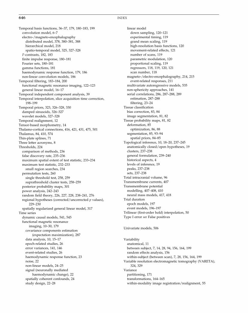
Elsevier UK Chapter: Index-P372560 30-9-2006 5:36p.m. Page:646 Trim:7.5in×9.25in
Basal Font:Palatino Margins:Top:40pt Gutter:68pt Font Size:9.5/12 Text Width:42pc Depth:55 Lines
646 INDEX
Temporal basis functions, 36–37, 179, 180–183, 199convolution model, 6–7electro-/magneto-encephalography
distributed model, 378, 380–381, 388hierarchical model, 218spatio-temporal model, 325, 327–328
F -contrasts, 182, 183finite impulse response, 180–181Fourier sets, 180–181gamma functions, 181haemodynamic response function, 179, 186non-linear convolution models, 186
Temporal filtering, 183–184, 200functional magnetic resonance imaging, 122–123general linear model, 16–17
Temporal independent component analysis, 39Temporal interpolation, slice acquisition time correction,
198–199Temporal priors, 323, 326–328, 330
damped sinusoids, 326–327wavelet models, 327–328
Temporal realignment, 12Tensor-based morphometry, 14Thalamo-cortical connections, 416, 421, 431, 475, 501Thalamus, 84, 410, 574Thin-plate splines, 71Three letter acronyms, 8Thresholds, 224
comparison of methods, 236false discovery rate, 235–236maximum spatial extent of test statistic, 233–234maximum test statistic, 232–233
small region searches, 234permutation tests, 260
single threshold test, 258, 259suprathreshold cluster tests, 258–259
posterior probability maps, 301power analysis, 242–243random field theory, 226, 227, 228, 238–241, 276regional hypotheses (corrected/uncorrected p values),
229–230spatially regularized general linear model, 317
Time seriesdynamic causal models, 541, 545functional magnetic resonance
imaging, 10–30, 179covariance components estimation
(expectation maximization), 287data analysis, 10, 15–17epoch-related studies, 26error variances, 141, 146event-related studies, 26haemodynamic response function, 23noise, 22non-linear models, 24–25signal (neuronally mediated
haemodynamic change), 22spatially coherent confounds, 24study design, 22–28
linear modeldown sampling, 120–121experimental timing, 119grand mean scaling, 119high-resolution basis functions, 120movement-related effects, 121number of scans, 119parametric modulation, 120proportional scaling, 119regressors, 118, 119, 120, 121scan number, 118
magneto-/electro-encephalography, 214, 215event-related responses, 211
multivariate autoregressive models, 535non-sphericity approaches, 141serial correlations, 286, 287–288, 289
estimation, 287–288filtering, 23–24
Tissue classificationbias correction, 83, 84image segmentation, 81, 82
Tissue probability maps, 81, 82deformation, 85
optimization, 86, 88segmentation, 85, 93–94
spatial priors, 84–85Topological inference, 10, 18–20, 237–245
anatomically closed/open hypotheses, 19clusters, 237–238general formulation, 239–240historical aspects, 4levels of inference, 19peaks, 237–238sets, 237–238
Total intracranial volume, 96Transmembrane currents, 407Transmembrane potential
modelling, 407–408, 410neural mass models, 417, 418
Trial durationepoch models, 197event models, 196–197
Trilinear (first-order hold) interpolation, 50Type I error see False positives
Univariate models, 506
Variabilityanatomical, 11between subject, 7, 14, 28, 94, 156, 164, 199random effects analysis, 156within-subject (between scan), 7, 28, 156, 164, 199
Variable resolution electromagnetic tomography (VARETA),324, 329
Variancepartitioning, 171transformations, 164–165within-modality image registration/realignment, 55

Elsevier UK Chapter: Index-P372560 30-9-2006 5:36p.m. Page:647 Trim:7.5in×9.25in
Basal Font:Palatino Margins:Top:40pt Gutter:68pt Font Size:9.5/12 Text Width:42pc Depth:55 Lines
INDEX 647
Variational Bayes, 303–311, 313, 447, 456applications, 306–309
effect size estimation, 309univariate densities, 306–307, 311
factorized approximations, 304–305, 307–308free-form approximations, 305, 309Gibbs sampling, 309Kullback-Liebler divergence, 303, 304, 306, 316Laplace approximation, 305, 306, 606–610model evidence, free energy relationship, 303–304model inference, 305–306, 308–309non-linear models, 610–611notation, 303parameters of component posteriors, 305spatially regularized general linear model, 315, 316, 318, 320spatio-temporal model for
electro-/magneto-encephalography, 324, 328, 333theory, 303–306
Variational free energy, 447Verbal fluency, 115, 161–163, 298, 299, 494–496, 498
see also Word processing/generationViscous fluid registration methods, 72Visual cortex, 341, 343, 345, 406, 410, 421, 432, 437, 472, 473,
475, 478, 481, 524, 527, 542, 563category selection pathway, 570–571inter-hemispheric integration, 579–583modulation by attentional mechanisms, 485–486orientation tuning, 398retinotopic mapping, 6, 432sensory evoked potentials modelling, 40
Visual motion processing/visual attention, 20, 21, 22, 33,40–41, 265, 298–299, 301, 451, 472, 512, 514, 515, 516, 520,537, 556–559
Visual object recognition, 194, 195Visual processing, 476, 477, 501Visual-evoked responses, 23Volterrra series formulation, 7, 25–26, 594–595
effective connectivity modelling, 485–486, 522, 524, 525generalized convolution models, 519–520, 521
input-state-output models, 37, 444–445, 524neuronal transients, 524, 525, 526non-linear convolution models, 186, 207–208non-linear evoked responses (balloon model), 341, 342, 343
haemodynamic model, 346–347, 444–445Voxel-based analysis/models, 3, 4, 10, 11, 14
famlily-wise error, 223–224hierarchical models, 35spatial normalization, 4topological inference, 4, 18–20
Voxel-based morphometry, 14, 92–98, 243clinical applications, 97–98data preparation, 93–95
Jacobian adjustment, 92, 94objectives, 92, 94principles, 92segmentation, 92, 93–94sensitivity, 95, 97smoothing, 92, 93, 94–95
false-positive results, 97spatial normalization, 94statistical modelling, 95–97
confounds, 96, 97global normalization, 96inference, 96–97
Warping templates, 4Wavelet models, 327–328Wavelet transforms, 253
temporal priors for event-related potentialmodelling, 327–328
Weighted minimum normL-curve approach, 369, 375, 378source localization, 388
Bayesian inversion models, 367, 368–369distributed models, 377, 378, 388
Wernicke’s area, 20, 553White matter
electrical conductivity, 352image segmentation, 84, 85segmentation models, 93
Whitening the data (filtering)covariance components estimation, 146functional magnetic resonance imaging time
series, 23–24drifts removal, 24
non-sphericity, 141, 146Wilcoxon test, 259Wilk’s statistic (Wilk’s Lambda), 213, 503, 504, 505Windkessel theory/model, 343, 344, 345, 350, 443
see also Balloon modelWindowed autocorrelation matrix, 381Windowed sinc interpolation, 50–51Within-subject analysis of variance see Repeated measures
analysis of varianceWord processing/generation, 22, 25–26, 186–187, 289, 293, 319,
346, 348, 445, 449–450, 488, 494–496, 498, 505, 550–552,553–556
modality/category factor interactions, 134–135multiple subject data, 163
Zero-order hold (nearest neighbour) resampling, 50Zooms, 76, 77
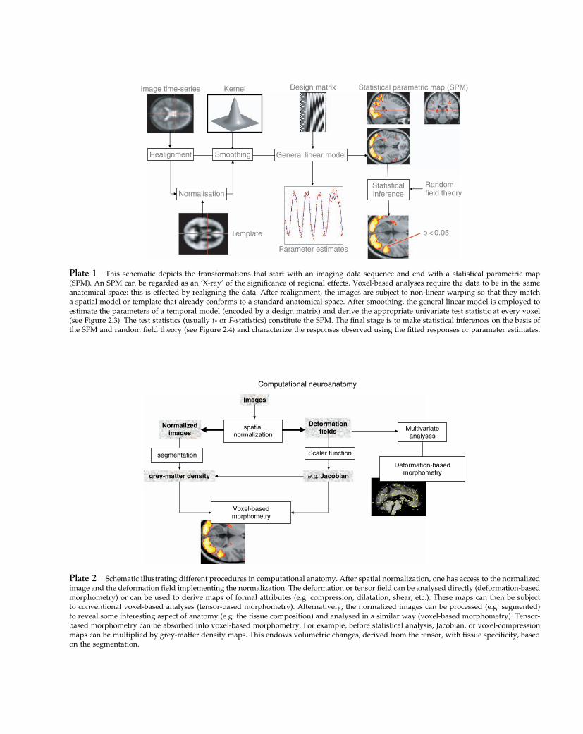
Elsevier UK Chapter: 0Colorplates1 3-10-2006 4:32p.m. Page:1 Trim:7.5in×9.25in
Basal Font:Palatino Margins:Top:40pt Gutter:68pt Font Size:9.5/12 Text Width:42pc Depth:55 Lines
Statistical parametric map (SPM)Image time-series
Parameter estimates
Design matrix
Template
Kernel
Randomfield theory
p < 0.05
Normalisation
Realignment Smoothing General linear model
Statisticalinference
Plate 1 This schematic depicts the transformations that start with an imaging data sequence and end with a statistical parametric map(SPM). An SPM can be regarded as an ‘X-ray’ of the significance of regional effects. Voxel-based analyses require the data to be in the sameanatomical space: this is effected by realigning the data. After realignment, the images are subject to non-linear warping so that they matcha spatial model or template that already conforms to a standard anatomical space. After smoothing, the general linear model is employed toestimate the parameters of a temporal model (encoded by a design matrix) and derive the appropriate univariate test statistic at every voxel(see Figure 2.3). The test statistics (usually t- or F -statistics) constitute the SPM. The final stage is to make statistical inferences on the basis ofthe SPM and random field theory (see Figure 2.4) and characterize the responses observed using the fitted responses or parameter estimates.
Computational neuroanatomy
Multivariateanalyses
Images
segmentation
spatialnormalization
Voxel-basedmorphometry
Deformation-basedmorphometry
Normalizedimages
Deformationfields
Scalar function
grey-matter density e.g. Jacobian
Plate 2 Schematic illustrating different procedures in computational anatomy. After spatial normalization, one has access to the normalizedimage and the deformation field implementing the normalization. The deformation or tensor field can be analysed directly (deformation-basedmorphometry) or can be used to derive maps of formal attributes (e.g. compression, dilatation, shear, etc.). These maps can then be subjectto conventional voxel-based analyses (tensor-based morphometry). Alternatively, the normalized images can be processed (e.g. segmented)to reveal some interesting aspect of anatomy (e.g. the tissue composition) and analysed in a similar way (voxel-based morphometry). Tensor-based morphometry can be absorbed into voxel-based morphometry. For example, before statistical analysis, Jacobian, or voxel-compressionmaps can be multiplied by grey-matter density maps. This endows volumetric changes, derived from the tensor, with tissue specificity, basedon the segmentation.

Elsevier UK Chapter: 0Colorplates1 3-10-2006 4:32p.m. Page:2 Trim:7.5in×9.25in
Basal Font:Palatino Margins:Top:40pt Gutter:68pt Font Size:9.5/12 Text Width:42pc Depth:55 Lines
Temporal basis functions
Single HRF
y (t ) = βT ⊗ u (t ) + εh (t ) = βT (u )
Basis functions
h (t ) = β1T1(t ) + β2T2(t ) + ...
Stimulus function
Ti (u )
T (u )
δ(ti)
Ti ⊗u(t )
Design matrixDesign matrix
SPM{F }
u (t )
FIR modelh (t ) = β1δ (t1) + β2δ (t 2) + ...
y (t ) = ∑ βiu (t – ti) + εi
y (t ) = ∑ βi (Ti ⊗ u(t )) + ε
i
Plate 3 Temporal basis functions offer useful constraints on the form of the estimated response that retain the flexibility of FIR models andthe efficiency of single regressor models. The specification of these constrained FIR models involves setting up stimulus functions u�t� thatmodel expected neuronal changes, e.g. boxcar-functions of epoch-related responses or spike-(delta)-functions at the onset of specific eventsor trials. These stimulus functions are then convolved with a set of basis functions Ti�t� of peristimulus time that, in some linear combination,model the HRF. The ensuing regressors are assembled into the design matrix. The basis functions can be as simple as a single canonical HRF(middle), through to a series of top-hat-functions �i�t� (bottom). The latter case corresponds to an FIR model and the coefficients constituteestimates of the impulse response function at a finite number of discrete sampling times. Selective averaging in event-related fMRI (Buckneret al., 1998) is mathematically equivalent to this limiting case.
LikelihoodPriorPosterior
Parameter Value
Pro
babi
lity
Combining Prior and Likelihood to Obtain the Posterior
Plate 4 This figure illustrates a hypothetical example of Bayes’ theory with a single parameter. By combining the likelihood and priorprobability density, it is possible to obtain a tighter posterior probability density. Note that the area under each of the curves is one.
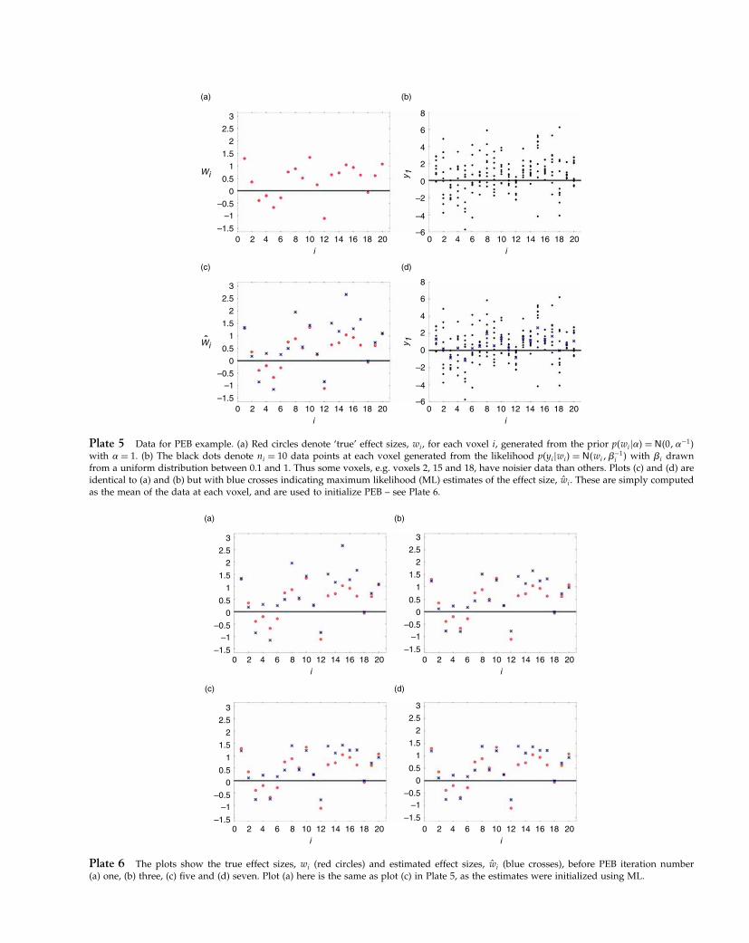
Elsevier UK Chapter: 0Colorplates1 3-10-2006 4:32p.m. Page:3 Trim:7.5in×9.25in
Basal Font:Palatino Margins:Top:40pt Gutter:68pt Font Size:9.5/12 Text Width:42pc Depth:55 Lines
(c)
(b)
Wiˆ y 1y 1
0
2
4
6
8
–2
–4
–6
0 2 4 6 8 10i i
12 14 16 18 20
0 2 4 6 8 10 12 14 1614 16 18 20
(d)
0
2
4
6
8
–2
–4
–60 2 4 6 8 10 12 14 16 18 20
3
2.5
2
1.5
1
0.5
0
–0.5–1
–1.5
(a)
Wi
0 2 4 6 8 10i i
12 18 20
3
2.5
2
1.5
1
0.5
0
–0.5–1
–1.5
Plate 5 Data for PEB example. (a) Red circles denote ‘true’ effect sizes, wi, for each voxel i, generated from the prior p�wi��� = N�0��−1�with � = 1. (b) The black dots denote ni = 10 data points at each voxel generated from the likelihood p�yi�wi� = N�wi��−1
i � with �i drawnfrom a uniform distribution between 0.1 and 1. Thus some voxels, e.g. voxels 2, 15 and 18, have noisier data than others. Plots (c) and (d) areidentical to (a) and (b) but with blue crosses indicating maximum likelihood (ML) estimates of the effect size, ŵi. These are simply computedas the mean of the data at each voxel, and are used to initialize PEB – see Plate 6.
(c)
(b)
0 2 4 6 8 10i i
12 14 16 18 20
0 2 4 6 8 10 12 14 1614 16 18 20
(d)
0 2 4 6 8 10 12 14 16 18 20
3
2.5
2
1.5
1
0.5
0
–0.5–1
–1.5
3
2.5
2
1.5
1
0.5
0
–0.5–1
–1.5
(a)
0 2 4 6 8 10i i
12 18 20
3
2.5
2
1.5
1
0.5
0
–0.5–1
–1.5
3
2.5
2
1.5
1
0.5
0
–0.5–1
–1.5
Plate 6 The plots show the true effect sizes, wi (red circles) and estimated effect sizes, ŵi (blue crosses), before PEB iteration number(a) one, (b) three, (c) five and (d) seven. Plot (a) here is the same as plot (c) in Plate 5, as the estimates were initialized using ML.
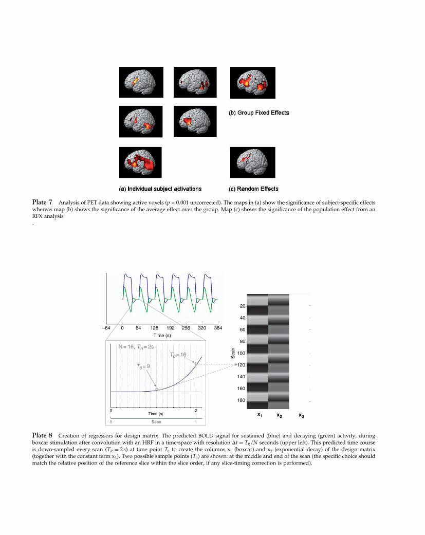
Elsevier UK Chapter: 0Colorplates1 3-10-2006 4:32p.m. Page:4 Trim:7.5in×9.25in
Basal Font:Palatino Margins:Top:40pt Gutter:68pt Font Size:9.5/12 Text Width:42pc Depth:55 Lines
Plate 7 Analysis of PET data showing active voxels (p < 0�001 uncorrected). The maps in (a) show the significance of subject-specific effectswhereas map (b) shows the significance of the average effect over the group. Map (c) shows the significance of the population effect from anRFX analysis.
x2 x3
N = 16, TR = 2s
Scan0 1
o
o
T0 = 16
T0 = 9
x1
Time (s)
–64 0 64 128 192 256 320 384
Sca
n
20
40
60
80
100
120
140
160
180
0 2Time (s)
Plate 8 Creation of regressors for design matrix. The predicted BOLD signal for sustained (blue) and decaying (green) activity, duringboxcar stimulation after convolution with an HRF in a time-space with resolution t = TR/N seconds (upper left). This predicted time courseis down-sampled every scan �TR = 2 s� at time point T0 to create the columns x1 (boxcar) and x2 (exponential decay) of the design matrix(together with the constant term x3�. Two possible sample points �T0� are shown: at the middle and end of the scan (the specific choice shouldmatch the relative position of the reference slice within the slice order, if any slice-timing correction is performed).
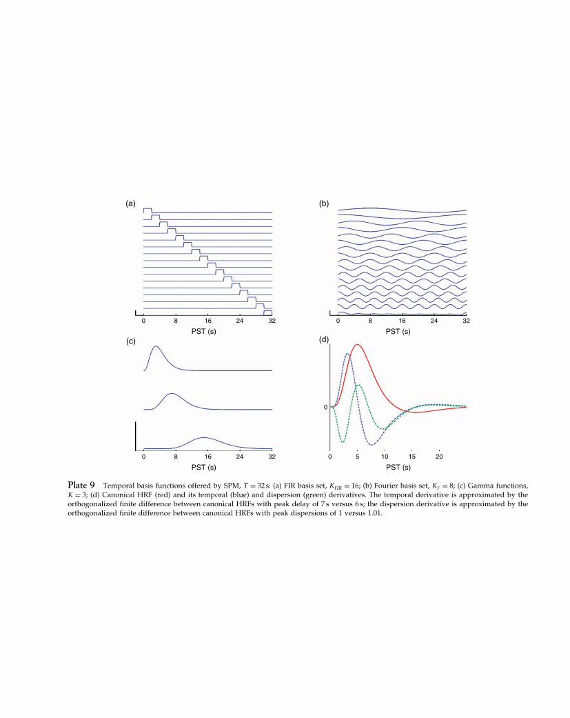
Elsevier UK Chapter: 0Colorplates1 3-10-2006 4:32p.m. Page:5 Trim:7.5in×9.25in
Basal Font:Palatino Margins:Top:40pt Gutter:68pt Font Size:9.5/12 Text Width:42pc Depth:55 Lines
(a)
(c)
80 16
PST (s)
24 32
80 16
PST (s)
24 32 50
0
10
PST (s)
15 20
80 16
PST (s)
24 32
(d)
(b)
Plate 9 Temporal basis functions offered by SPM, T = 32 s: (a) FIR basis set, KFIR = 16; (b) Fourier basis set, KF = 8; (c) Gamma functions,K = 3; (d) Canonical HRF (red) and its temporal (blue) and dispersion (green) derivatives. The temporal derivative is approximated by theorthogonalized finite difference between canonical HRFs with peak delay of 7 s versus 6 s; the dispersion derivative is approximated by theorthogonalized finite difference between canonical HRFs with peak dispersions of 1 versus 1.01.
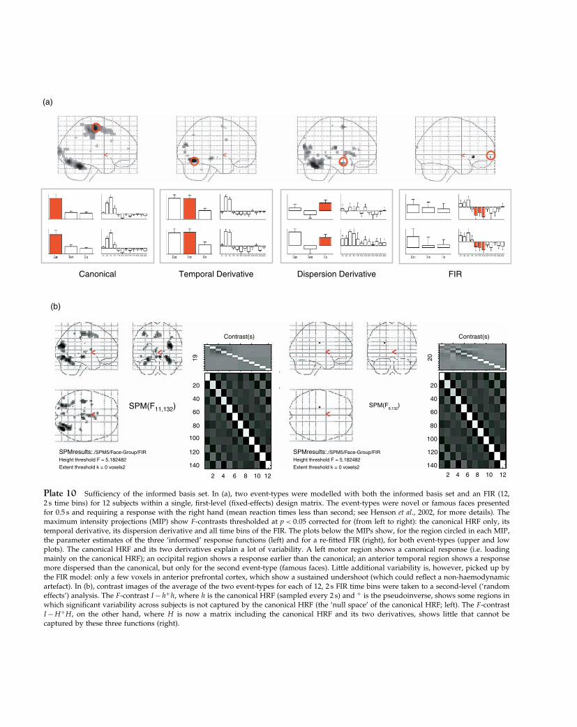
Elsevier UK Chapter: 0Colorplates1 3-10-2006 4:32p.m. Page:6 Trim:7.5in×9.25in
Basal Font:Palatino Margins:Top:40pt Gutter:68pt Font Size:9.5/12 Text Width:42pc Depth:55 Lines
Canonical FIR
(a)
(b)
Temporal Derivative Dispersion Derivative
20
Contrast(s) Contrast(s)
40
60
80
100
120
140
SPMresults:./SPM5/Face-Group/FIR
Height threshold F = 5.182482
Extent threshold k = 0 voxels2
SPMresults:./SPM5/Face-Group/FIR
Height threshold F = 5.182482
Extent threshold k = 0 voxels2
2 4 6 8 10 12
20
SPM(F9,132
)SPM(F11,132)
2019
40
60
80
100
120
140
2 4 6 8 10 12
Plate 10 Sufficiency of the informed basis set. In (a), two event-types were modelled with both the informed basis set and an FIR (12,2 s time bins) for 12 subjects within a single, first-level (fixed-effects) design matrix. The event-types were novel or famous faces presentedfor 0.5 s and requiring a response with the right hand (mean reaction times less than second; see Henson et al., 2002, for more details). Themaximum intensity projections (MIP) show F -contrasts thresholded at p < 0�05 corrected for (from left to right): the canonical HRF only, itstemporal derivative, its dispersion derivative and all time bins of the FIR. The plots below the MIPs show, for the region circled in each MIP,the parameter estimates of the three ‘informed’ response functions (left) and for a re-fitted FIR (right), for both event-types (upper and lowplots). The canonical HRF and its two derivatives explain a lot of variability. A left motor region shows a canonical response (i.e. loadingmainly on the canonical HRF); an occipital region shows a response earlier than the canonical; an anterior temporal region shows a responsemore dispersed than the canonical, but only for the second event-type (famous faces). Little additional variability is, however, picked up bythe FIR model: only a few voxels in anterior prefrontal cortex, which show a sustained undershoot (which could reflect a non-haemodynamicartefact). In (b), contrast images of the average of the two event-types for each of 12, 2 s FIR time bins were taken to a second-level (‘randomeffects’) analysis. The F -contrast I −h+h, where h is the canonical HRF (sampled every 2 s) and + is the pseudoinverse, shows some regions inwhich significant variability across subjects is not captured by the canonical HRF (the ‘null space’ of the canonical HRF; left). The F -contrastI −H+H , on the other hand, where H is now a matrix including the canonical HRF and its two derivatives, shows little that cannot becaptured by these three functions (right).
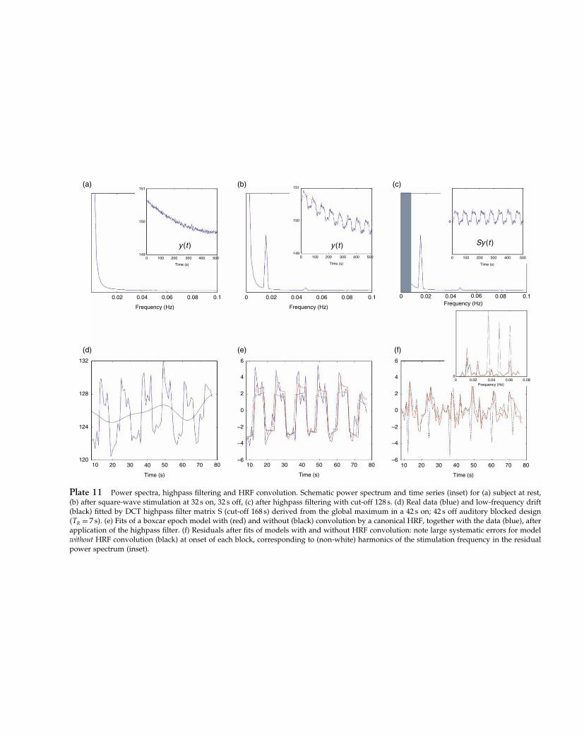
Elsevier UK Chapter: 0Colorplates1 3-10-2006 4:32p.m. Page:7 Trim:7.5in×9.25in
Basal Font:Palatino Margins:Top:40pt Gutter:68pt Font Size:9.5/12 Text Width:42pc Depth:55 Lines
0.02 0.04 0.06
151(a)
y (t ) y (t ) Sy (t )
(b) (c)
(f)(e)(d)
150
1490 100 200 300
Time (s)
400 500
Frequency (Hz)
0.08 0.1
10
132
128
124
12020 30 40
Time (s)
50 60 70 80 10
6
4
2
0
–2
–4
–620 30 40
Time (s)
50 60 70 80 10
6
00 0.02 0.04
Frequency (Hz)0.06 0.08
4
2
0
–2
–4
–620 30 40
Time (s)
50 60 70 80
0 0.02 0.04 0.06
151
150
1490 100 200 300
Time (s)
400 500
Frequency (Hz)
0.08 0.1 0 0.02 0.04 0.06
0
0 100 200 300
Time (s)
400 500
Frequency (Hz)0.08 0.1
Plate 11 Power spectra, highpass filtering and HRF convolution. Schematic power spectrum and time series (inset) for (a) subject at rest,(b) after square-wave stimulation at 32 s on, 32 s off, (c) after highpass filtering with cut-off 128 s. (d) Real data (blue) and low-frequency drift(black) fitted by DCT highpass filter matrix S (cut-off 168 s) derived from the global maximum in a 42 s on; 42 s off auditory blocked design�TR = 7 s�. (e) Fits of a boxcar epoch model with (red) and without (black) convolution by a canonical HRF, together with the data (blue), afterapplication of the highpass filter. (f) Residuals after fits of models with and without HRF convolution: note large systematic errors for modelwithout HRF convolution (black) at onset of each block, corresponding to (non-white) harmonics of the stimulation frequency in the residualpower spectrum (inset).

Elsevier UK Chapter: 0Colorplates1 3-10-2006 4:32p.m. Page:8 Trim:7.5in×9.25in
Basal Font:Palatino Margins:Top:40pt Gutter:68pt Font Size:9.5/12 Text Width:42pc Depth:55 Lines
00
(a) (b)
(c) (d)
0
–100 –50 0 50 100
1
0
0 50–50
1
0.05 0.1 0.15
Frequency (Hz)
Frequency (Hz)
Lag secs
Lag secs
Spectral density before filtering High and Lowpass filter
Spectral density after bandpass filtering Spectral density after highpass filtering
Spe
ctra
l den
sity
Spe
ctra
l den
sity
Aut
ocor
rela
tion
Aut
ocor
rela
tion
0
0 50–50
1
Lag secs
Aut
ocor
rela
tion
0
0 50–50
1
Lag secs
Aut
ocor
rela
tion
0.2 0.250
0 0.05 0.1 0.15
Frequency (Hz)
Spe
ctra
l den
sity
0.2 0.25
00 0.05 0.1 0.15
Frequency (Hz)
Spe
ctra
l den
sity
0.2 0.250
0 0.05 0.1 0.15 0.2 0.25
Plate 12 Models of fMRI temporal autocorrelation. Power spectra and autocorrelation functions for: (a) data (solid black), derived froman AR(16) estimation of the mean, globally-normalized residuals from one slice of an event-related dataset; together with fits of an AR(1)model (dashed blue) and 1/f amplitude model (dashed red); (b) high- (dot-dash) and low- (dotted) pass filters, comprising a bandpass filter(dashed); (c) data and both models after bandpass filtering (note that bandpass filter characteristics in (b) would also provide a reasonableapproximation to residual autocorrelation); (d) data (solid black) and ReML fit of AR(1)+white noise model (dashed blue) after highpassfiltering (also shown is the bandpass filter power spectrum, demonstrating the high-frequency information that would be lost by lowpasssmoothing).

Elsevier UK Chapter: 0Colorplates1 3-10-2006 4:32p.m. Page:9 Trim:7.5in×9.25in
Basal Font:Palatino Margins:Top:40pt Gutter:68pt Font Size:9.5/12 Text Width:42pc Depth:55 Lines
0.7
(a)
(b)
(c)
(d)
0.6
0.5
0.4
0.3
Size of effect at [45, –48, –27]
Size of effect at [45, –63, –15]
Response at [45, –48, –27]
Response at [45, –63, –15]
Effe
ct
SP
M {
F}
Sta
tistic
s: v
olum
e su
mm
ary
(p-v
alue
s co
rrec
ted
for
entir
e vo
lum
e )
voxe
l–le
vel
clus
ter–
leve
lP
unco
rrec
ted
PF
WE
–cor
rP
FD
R–c
orr
F(Z
E)
Pco
rrec
ted
Pun
corr
ecte
dk E 6
1.00
00.
160
7.28
( 3.
30)
0.00
0
x,y,
z {m
m}
45–6
3–1
5
Fitt
ed r
espo
nse
and
adju
sted
dat
a
0.2
0.1 0
–0.1
12
3
3
2.5 2
1.5 1
0.5 0
–0.5 –1
–1.5 –2
0.45 0.4
0.35 0.3
0.25 0.2
0.15 0.1
0.05 0
12
3
2.5 2
1.5 1
0.5 0
02
46
812
1014
1618
20–0
.5
Effe
ct
02
46
810
Per
i-stim
ulus
tim
e {s
ecs}
Per
i-stim
ulus
tim
e {s
ecs}
Fitt
ed r
espo
nse
+/–
sta
ndar
d er
ror
N1
– r
N2
– b
F1
– g
F2
– c
1214
1618
20
45
67
89
1011
12
Pla
te13
Cat
egor
ical
mod
el:r
epet
itio
nef
fect
.(a)
Para
met
eres
tim
ates
(sca
lear
bitr
ary)
from
loca
lmax
imum
inri
ght
fusi
form
�+45
�−4
8�−2
7�,o
rder
edby
cond
itio
n–
N1,
N2,
F1,
F2–
and
wit
hin
each
cond
itio
nby
basi
sfu
ncti
on–
cano
nica
lH
RF,
tem
pora
ld
eriv
ativ
ean
dd
ispe
rsio
nd
eriv
ativ
e.(b
)Fi
tted
even
t-re
late
dre
spon
ses
(sol
id)
and
adju
sted
dat
a(d
ots)
inte
rms
ofpe
rcen
tage
sign
alch
ange
(rel
ativ
eto
gran
dm
ean
over
spac
ean
dti
me)
agai
nst
PST
for
N1
(red
),N
2(b
lue)
,F1
(gre
en)
and
F2(c
yan)
.(c)
SPM
F�
MIP
for
repe
titi
onef
fect
cont
rast
(ins
et),
thre
shol
ded
atp
<0�
001
unco
rrec
ted
,aft
erin
clus
ive
mas
king
wit
hef
fect
sof
inte
rest
(Fig
ure
14.4
)at
p<
0�05
corr
ecte
d.(
d)
Con
tras
tof
para
met
eres
tim
ates
for
repe
titi
onef
fect
(dif
fere
nce
betw
een
first
and
seco
ndpr
esen
tati
ons)
inri
ght
occi
pito
tem
pora
lreg
ion
�+45
�−6
3�−1
5�fo
rca
noni
calH
RF,
tem
pora
lder
ivat
ive
and
dis
pers
ion
der
ivat
ive,
toge
ther
wit
hfi
tted
resp
onse
s(s
olid
)±
one
stan
dar
der
ror
(das
hed
).
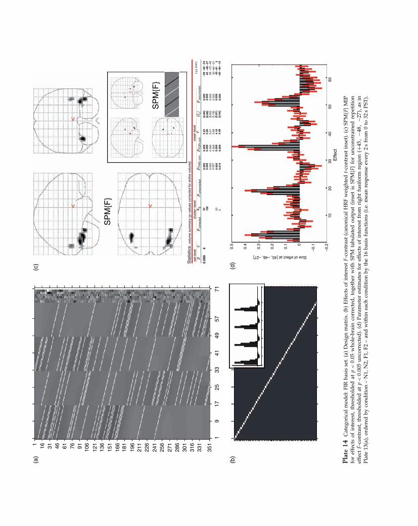
Elsevier UK Chapter: 0Colorplates1 3-10-2006 4:32p.m. Page:10 Trim:7.5in×9.25in
Basal Font:Palatino Margins:Top:40pt Gutter:68pt Font Size:9.5/12 Text Width:42pc Depth:55 Lines
1 16 31 46 61 76 91 106
121
136
151
166
181
196
211
226
241
256
271
286
301
316
331
351
19
1725
3341
4957
71
(a)
(c)
SP
M{F
}
SP
M{F
}
(b)
(d)
0.5
0.4
0.3
0.2
0.1
Size of effect at [45, –48, –27]
0
–0.1
–0.2
1020
30E
ffect
4050
60
p
0.00
0
set-
leve
lcl
uste
r–le
vel
voxe
l–le
vel
corr
ecte
d
Sta
tistic
s: v
olum
e su
mm
ary
(p–v
alue
s co
rrec
ted
for
entir
e vo
lum
e)
4
pun
corr
ecte
d
52 23 3106
0.00
00.
000
0.00
0
0.00
05.
25(6
.84)
(6.6
8)(6
.63)
(5.1
8)(5
.81)
(5.0
4)
5.06
5.01
3.59
4.16
3.48
0.00
00.
000
0.00
00.
000
0.00
0
0.00
0–3
9 45–6
0–4
8–2
739
–72
–40
–21 3
–84
–81
–84
–30
–15
30 45
–24
0.00
00.
000
0.00
00.
000
0.00
00.
000
0.01
4
0.00
7
pun
corr
ecte
dx,
y,z
{mm
}p
FW
E–c
orr
pF
DR
–cor
rp
F(Z
E)
kE
c
Pla
te14
Cat
egor
ical
mod
el:F
IRba
sis
set.
(a)
Des
ign
mat
rix.
(b)
Eff
ects
ofin
tere
stF
-con
tras
t(c
anon
ical
HR
Fw
eigh
ted
t-co
ntra
stin
set)
.(c)
SPM
F�
MIP
for
effe
cts
ofin
tere
st,
thre
shol
ded
atp
<0�
05w
hole
-bra
inco
rrec
ted
,to
geth
erw
ith
SPM
tabu
late
dou
tput
(ins
etis
SPM
F�
for
unco
nstr
aine
dre
peti
tion
effe
ctF
-con
tras
t,th
resh
old
edat
p<
0�00
5un
corr
ecte
d).
(d)
Para
met
eres
tim
ates
for
effe
cts
ofin
tere
stfr
omri
ght
fusi
form
regi
on�+
45�
−48�
−27�
,as
inPl
ate
13(a
),or
der
edby
cond
itio
n–
N1,
N2,
F1,F
2–
and
wit
hin
each
cond
itio
nby
the
16ba
sis
func
tion
s(i
.e.m
ean
resp
onse
ever
y2
sfr
om0
to32
sPS
T).
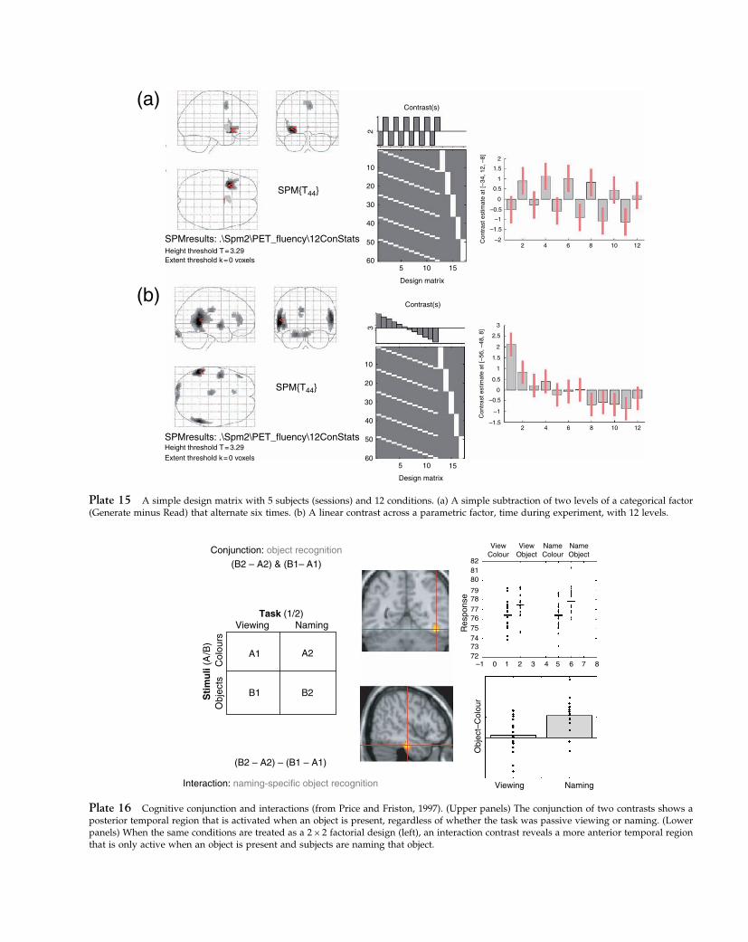
Elsevier UK Chapter: 0Colorplates1 3-10-2006 4:32p.m. Page:11 Trim:7.5in×9.25in
Basal Font:Palatino Margins:Top:40pt Gutter:68pt Font Size:9.5/12 Text Width:42pc Depth:55 Lines
<
<<
(b)
(a)
10
20
30
40
50
60
10
20
30
40
50
605 10
2
Con
tras
t est
imat
e at
[–56
, –48
, 8]
Con
tras
t est
imat
e at
[–34
, 12,
–8]
–1.5
–1
–0.5
0
0.5
1
1.5
2
2.5
3
4 6 8 10 12
2–2
–1
–1.5
–0.5
0
0.5
1
1.5
2
4 6 8 10 12
15
5 10 15
Design matrix
Contrast(s)
Contrast(s)
23
Design matrix
SPMresults: .\Spm2\PET_fluency\12ConStats
SPMresults: .\Spm2\PET_fluency\12ConStats
SPM{T44}
SPM{T44}
Height threshold T = 3.29
Height threshold T = 3.29Extent threshold k = 0 voxels
Extent threshold k = 0 voxels
Plate 15 A simple design matrix with 5 subjects (sessions) and 12 conditions. (a) A simple subtraction of two levels of a categorical factor(Generate minus Read) that alternate six times. (b) A linear contrast across a parametric factor, time during experiment, with 12 levels.
A1 A2
B2B1
Task (1/2)Viewing
Sti
mu
li (A
/B)
Col
ours
Conjunction: object recognition
Interaction: naming-specific object recognition Viewing
Obj
ect–
Col
our
ViewColour
Res
pons
e
ViewObject
NameColour
NameObject
(B2 – A2) – (B1 – A1)
(B2 – A2) & (B1– A1)
Obj
ects
Naming
Naming
72–1
7374757677
7879
808182
0 1 2 3 4 5 6 7 8
Plate 16 Cognitive conjunction and interactions (from Price and Friston, 1997). (Upper panels) The conjunction of two contrasts shows aposterior temporal region that is activated when an object is present, regardless of whether the task was passive viewing or naming. (Lowerpanels) When the same conditions are treated as a 2×2 factorial design (left), an interaction contrast reveals a more anterior temporal regionthat is only active when an object is present and subjects are naming that object.

Elsevier UK Chapter: 0Colorplates1 3-10-2006 4:32p.m. Page:12 Trim:7.5in×9.25in
Basal Font:Palatino Margins:Top:40pt Gutter:68pt Font Size:9.5/12 Text Width:42pc Depth:55 Lines
Design matrix
Parameter
Contrast(s)
6
10
20
30
40
50
5 10 15
Design matrix
SPMresults: .\Spm2\PET_fluency\12ConStatsHeight threshold T = 2.41Extent threshold k = 10 voxels
SPM{T44}
(b)
(a)Sagittal Coronal
VPC VACVPC VAC
0
0
R
R
–104
0
72
032
3362
64 Transverse
60
Word rate
Adj
uste
d ac
tivity
(m
ean
corr
ecte
d)
60 80 10040200
2
Con
tras
t est
imat
e at
[18,
–32
, –12
]
–2
–1.5
–1
–0.5
0
0.5
1
1.5
4 6 8 10 12
63
64
65
66
67
68
2
21 3
4
6
8
10
12
Obs
erva
tion
Plate 17 (a) Non-linear effects of a parametric factor modelled in a single-subject design matrix using a second-order polynomial expansion.(b) A linear time-by-condition interaction contrast in a 2×6 factorial design across 5 subjects.
State-effects Item-effects
50 2
1
0
–1
–2
–3–5 0 5 10 15 20 25 30
2
1
0
–1
–2
–3–5 0 5 10 15 20 25 30
40
30
20
10
0
50
40
30
20
10
0
Par
amet
er e
stim
ates
Par
amet
er e
stim
ates
Motionattention
Colorattention
Motionattention
Colorattention Peristimulus time (s)
V5
V4
Plate 18 State- and item-effects (from Chawla et al., 1999). Attention to colour of radially-moving coloured dots increased both baselineactivity (top left) and evoked responses (top right) – i.e. both offset and gain – in V4 relative to attention to motion. The opposite pattern wasfound in V5 (bottom row).

Elsevier UK Chapter: 0Colorplates1 3-10-2006 4:32p.m. Page:13 Trim:7.5in×9.25in
Basal Font:Palatino Margins:Top:40pt Gutter:68pt Font Size:9.5/12 Text Width:42pc Depth:55 Lines
signal
Log(f)10.10.010.001
white noise
1/f noise
Am
plitu
dePlate 19 Schematic form of 1/f and white noise (dark and light blue respectively) typical of fMRI data, together with experimentally-induced signal at 0.03 Hz (red) and highpass filtering (hatched area).
Random (A–B)
Random (A+B)
Alternating (A–B)Permuted (A–B)
Null Events (A+B)
Null Events (A–B)
(a) (b)
(c)
A–B withnonlinearities
0
1
2Log(
EM
P)
3
4
5
1
2Log(
EM
P)
3
4
5
1
2Log(
EM
P)
3
4
5
5 10 15 20 25 30
SOA/s
0 5 10 15 20 25 30
SOA/s
0 5 10 15 20 25 30SOA/s
0 1 2 3 4 5 6 7 8 9 10
Plate 20 Efficiency for two event-types (from Josephs and Henson, 1999). Efficiency is expressed in terms of ‘estimated measurable power’(EMP) passed by an effective HRF, characterized by a canonical HRF, highpass filter with cut-off period of 60 s and lowpass smoothing by aGaussian 4 s full-width at half maximum (FWHM), as a function of t for main (solid) effect ([1 1] contrast) and differential (dashed) effect([1 −1] contrast). (a) Randomized design. (b) Alternating (black) and permuted (blue) designs. (c) With (green) and without (red) null events.Insert: effect of non-linearity (saturation) on average response as a function of SOA within a 32 s blocked design. Solid line: average responseto a train of stimuli predicted using a second-order Volterra model of haemodynamic responses. The broken line shows the predicted responsein the absence of non-linear or second-order effects (Friston et al., 2000).

Elsevier UK Chapter: 0Colorplates1 3-10-2006 4:32p.m. Page:14 Trim:7.5in×9.25in
Basal Font:Palatino Margins:Top:40pt Gutter:68pt Font Size:9.5/12 Text Width:42pc Depth:55 Lines
Plate 21 For each trial type and subject, the ERR, for each channel, is projected to either three-dimensional brain space (source reconstruc-tion) or interpolated on the scalp surface. This results in either 3-D or 2-D image time-series.
Plate 22 KL-divergence, KL�q��p� for p as defined in Figure 24.2 and q being a Gaussian with mean � and standard deviation . TheKL-divergences of the approximations in Figure 24.2 are (a) 11.73 for the first mode (yellow ball), (b) 0.93 for the second mode (green ball)and (c) 0.71 for the moment-matched solution (red ball).
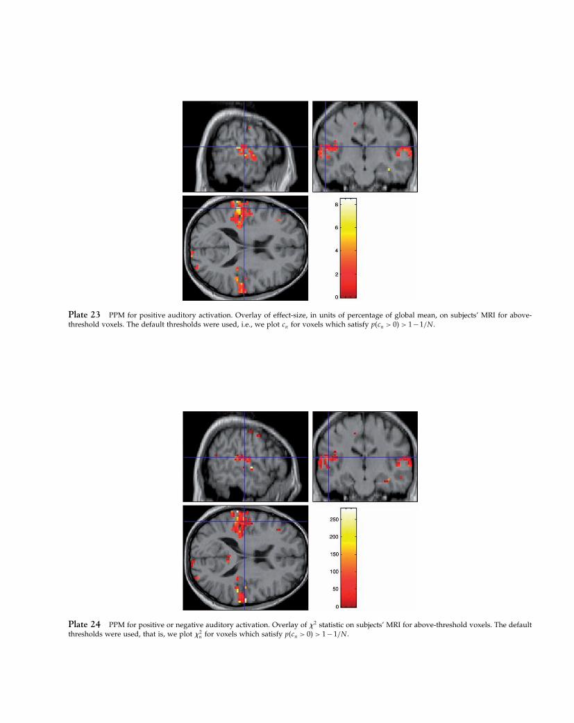
Elsevier UK Chapter: 0Colorplates1 3-10-2006 4:32p.m. Page:15 Trim:7.5in×9.25in
Basal Font:Palatino Margins:Top:40pt Gutter:68pt Font Size:9.5/12 Text Width:42pc Depth:55 Lines
Plate 23 PPM for positive auditory activation. Overlay of effect-size, in units of percentage of global mean, on subjects’ MRI for above-threshold voxels. The default thresholds were used, i.e., we plot cn for voxels which satisfy p�cn > 0� > 1−1/N .
Plate 24 PPM for positive or negative auditory activation. Overlay of �2 statistic on subjects’ MRI for above-threshold voxels. The defaultthresholds were used, that is, we plot �2
n for voxels which satisfy p�cn > 0� > 1−1/N .
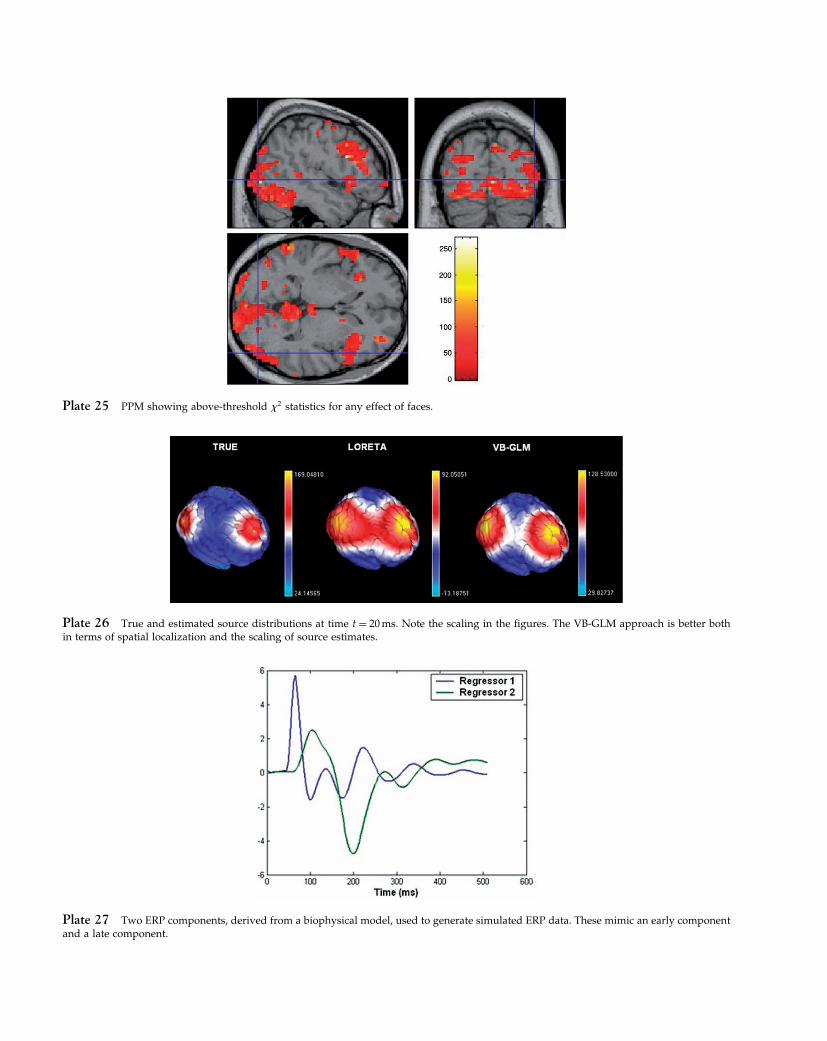
Elsevier UK Chapter: 0Colorplates1 3-10-2006 4:32p.m. Page:16 Trim:7.5in×9.25in
Basal Font:Palatino Margins:Top:40pt Gutter:68pt Font Size:9.5/12 Text Width:42pc Depth:55 Lines
Plate 25 PPM showing above-threshold �2 statistics for any effect of faces.
Plate 26 True and estimated source distributions at time t = 20 ms. Note the scaling in the figures. The VB-GLM approach is better bothin terms of spatial localization and the scaling of source estimates.
Plate 27 Two ERP components, derived from a biophysical model, used to generate simulated ERP data. These mimic an early componentand a late component.

Elsevier UK Chapter: 0Colorplates1 3-10-2006 4:32p.m. Page:17 Trim:7.5in×9.25in
Basal Font:Palatino Margins:Top:40pt Gutter:68pt Font Size:9.5/12 Text Width:42pc Depth:55 Lines
Plate 28 Four components, derived from a biophysical model, used in an over-specified ERP model.
Plate 29 Regression coefficients, wg , from ERP simulation. ‘Coeff 1’ and ‘Coeff 2’ denote the first and second entries in the regressioncoefficient vector wg . True model (left) and estimates from correctly specified model (right).

Elsevier UK Chapter: 0Colorplates1 3-10-2006 4:32p.m. Page:18 Trim:7.5in×9.25in
Basal Font:Palatino Margins:Top:40pt Gutter:68pt Font Size:9.5/12 Text Width:42pc Depth:55 Lines
Plate 30 Estimated regression coefficients, ŵg , from over-specified model. The true coefficients are shown in Plate 29. Note the scalingof coefficients 3 and 4 (the true values are zero). Despite the high temporal correlation between regressors 2 and 3, the coefficients forregressor 3 have been correctly shrunk towards zero. This is a consequence of the spatial prior and the iterative nature of the spatio-temporaldeconvolution (see Figure 26.6).
Plate 31 True regression coefficients for ERP simulation with correlated sources. This simulation used a design matrix comprising theregressors shown in Plate 28, with the first and fourth coefficients set to zero and the second and third set as shown in this figure.

Elsevier UK Chapter: 0Colorplates1 3-10-2006 4:32p.m. Page:19 Trim:7.5in×9.25in
Basal Font:Palatino Margins:Top:40pt Gutter:68pt Font Size:9.5/12 Text Width:42pc Depth:55 Lines
Plate 32 Estimated regression coefficents, ŵg , for ERP simulation with correlated sources. Coefficients 2 and 3 resemble the true values shownin Plate 31, whereas regressors 1 and 4 have been correctly shrunk towards zero by the spatio-temporal deconvolution algorithm.
Plate 33 The figure shows differential EEG topography for faces minus scrambled faces at t = 160 ms poststimulus.
0–15
–10
–5
μV
0
5
10
–10
–5
0
μV 5
10
15
20
B8 A1
50 100 150 200ms
250 300 350 400 0 50 100 150 200ms
250 300 350 400
Plate 34 Sensor time courses for face data at occipito-temporal electrode B8 (left) and vertex A1 (right) for faces (blue) and scrambled faces(red).

Elsevier UK Chapter: 0Colorplates1 3-10-2006 4:32p.m. Page:20 Trim:7.5in×9.25in
Basal Font:Palatino Margins:Top:40pt Gutter:68pt Font Size:9.5/12 Text Width:42pc Depth:55 Lines
8
6
4
2
0
–2
–4
–6
–8
–10
8
6
4
2
0
–2
–4
–6
–80 100 200
ms300 400 0 100 200
ms300 400
Plate 35 First eigen-time-series of downsampled ERP for unfamiliar faces (blue lines in both plots) with wavelet shrinkage approximationsusing Daubechies basis (left) and Battle-Lemarie basis (right).
Plate 36 These images are derived from the source reconstruction of ERPs in response to faces and scrambled faces. The plots showabsolute differences between faces and scrambled faces at t = 160 ms post-stimulus. The maps have been thresholded such that the largestdifference appears in red and 50 per cent of the largest difference appears in blue.
Plate 37 Best fitting sphere on a scalp surface extracted from a subject’s structural MRI.

Elsevier UK Chapter: 0Colorplates1 3-10-2006 4:32p.m. Page:21 Trim:7.5in×9.25in
Basal Font:Palatino Margins:Top:40pt Gutter:68pt Font Size:9.5/12 Text Width:42pc Depth:55 Lines
Plate 38 The left figure shows the original source location, defined by the cortical sheet. The colour scale indicates the radius of the scalpRscalp����� in the direction ����� of the dipole locations �Rsb� ����. The right figure is the transformed source space obtained after applyingEqn. 28.60. The colour scale shows the scaling of the source radii, i.e. Rsphere/Rscalp �����.
Plate 39 Reconstructed sources obtained with ReML using the example shown in Figure 29.2 (SNR = 12): no location priors (top left),with accurate location priors (bottom left), with close inaccurate location priors (top middle), with distant inaccurate location priors (bottommiddle), with both accurate and close inaccurate location priors (top right) and with both accurate and distant inaccurate location priors(bottom right).

Elsevier UK Chapter: 0Colorplates1 3-10-2006 4:32p.m. Page:22 Trim:7.5in×9.25in
Basal Font:Palatino Margins:Top:40pt Gutter:68pt Font Size:9.5/12 Text Width:42pc Depth:55 Lines
(a) M170 on right mid-temporalchannel
–200–250
–200
–150
–100
–50
0
50
0 200 400 600 800
(b) Scalp topography of M170 (c) Ventral view of SPM{t }p < .01 uncorrected
(d) Lateral view of SPM{t }p < .01 uncorrected
Plate 40 Multisubject analysis of face-selective response based on ReML analysis. (a) The mean M170 across participants and (b) its scalptopography. An identity matrix was used for the noise covariance in sensor space. When using only the MSP source prior, subtraction of theabsolute values of the separate source reconstructions for faces versus scrambled faces revealed (c) activation of right fusiform (+51 −39 −15),T(7) = 6.61, (d) right middle temporal gyrus (+63 −69 +3), T(7) = 3.48, and right parahippocampal gyrus (+27 −6 −18), T(7) = 3.32, whenthresholded at p < 0.01 uncorrected. MEG data from a 151-channel CTF Omega system were acquired while 9 participants made symmetryjudgements to faces and scrambled faces. The MEG epochs were baseline-corrected from −100 to 0 ms, averaged over trials (approx. 70 faceand 80 scrambled trials) and low-pass filtered to 20 Hz. A time-window around the peak in the global field power of the difference betweenthe event-related field (ERF) for faces and scrambled faces that corresponded to the M170 was selected for each participant (mean window= 120–200 ms). Segmented cortical meshes of approximately 7200 dipoles oriented normal to the grey matter were created using Anatomist,and single-shell spherical forward models were constructed using Brainstorm. Multivariate source prelocalization (MSP) was used to reducethe number of dipoles to 1500. The localizations on the mesh were converted into 3D images, warped to MNI space using normalizationparameters determined from participants’ MRIs using SPM2, and smoothed with a 20 mm full width half maximum (FWHM) isotropicGaussian kernel. These smoothed, normalized images were used to create an SPM of the t-statistic over participants (final smoothness approx12 × 12 × 12 mm) (c) and (d).
Time-frequency subspace
0 200
Time (ms)
400100 200 300 400
Time (ms)
Right temporal evoked signal(a) (b) (c)
(d)
FacesScrambled
M170
Energy changes (Faces – Scrambled, p < 0.01)
0.10.2 0.30.40.50.6
Time (s)
10
20
30
40
35
45
15
25
0.70.80–0.1
0
1
2
3
–2
–3
–1
Fre
quen
cy (
Hz)
0
0.2
0.4
0.6
0.5
0.7
0.1
0.3
0.8
0.9
1Evokedresponses
Inducedresponses
Faces Scrambled
Front
BackNormalized scalppower topographies
Plate 41 Real data analysis – sensor level: (a) and (b) show the differences, measured on the scalp, between faces and scrambled faces, interms of the event-related field (ERF) from a single sensor (a), and the global energy over sensors (b) using standard time-frequency analysis andstatistical parametric mapping (Kilner et al., 2005). The time-frequency subspace W we tested is shown in (c) by plotting each column as a functionof time. This uses the same representation as the first panel of the previous figure. This subspace tests for responses in the alpha range, around 200ms (see corresponding time-frequency effect in (a)). The corresponding induced and evoked energy distributions over the scalp are shown in (d),for two conditions (faces and scrambled faces).
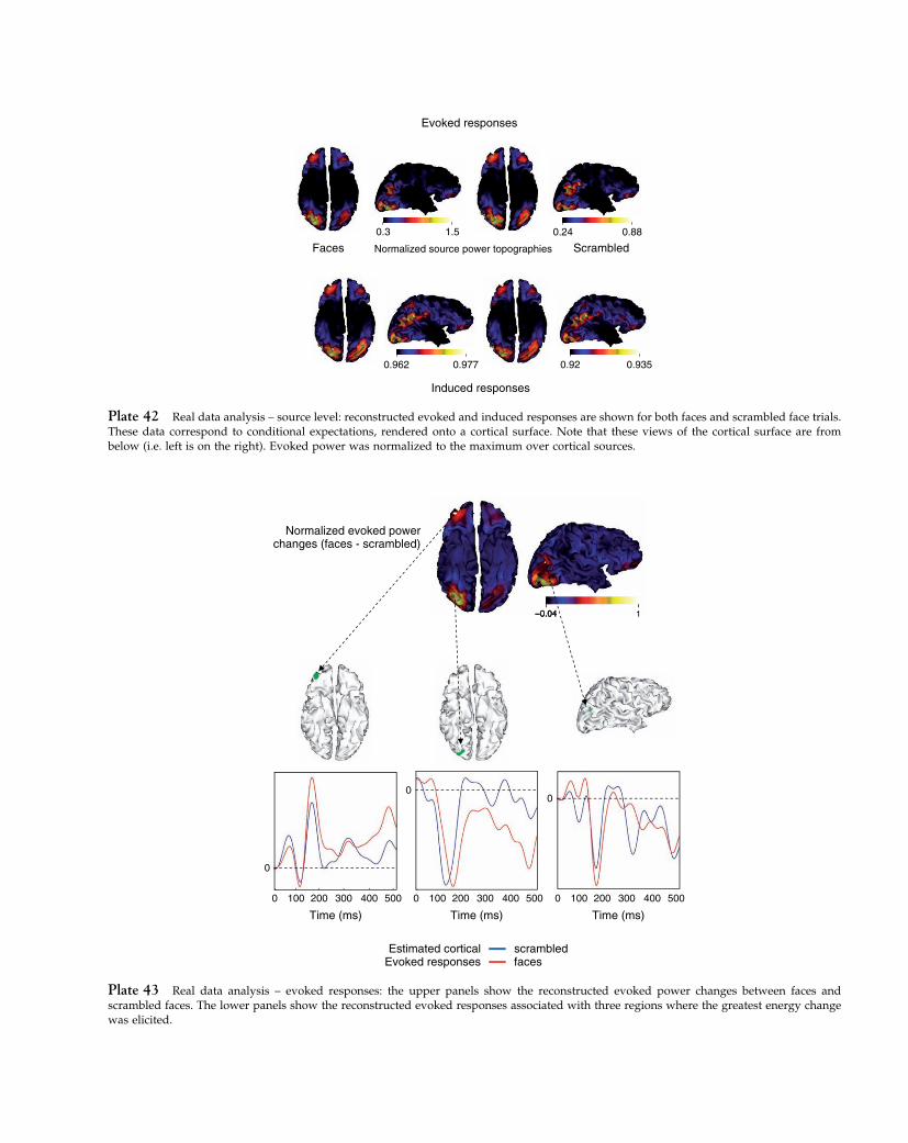
Elsevier UK Chapter: 0Colorplates1 3-10-2006 4:32p.m. Page:23 Trim:7.5in×9.25in
Basal Font:Palatino Margins:Top:40pt Gutter:68pt Font Size:9.5/12 Text Width:42pc Depth:55 Lines
Faces ScrambledNormalized source power topographies
Evoked responses
0.3 1.5 0.24 0.88
Induced responses
0.92 0.9350.962 0.977
Plate 42 Real data analysis – source level: reconstructed evoked and induced responses are shown for both faces and scrambled face trials.These data correspond to conditional expectations, rendered onto a cortical surface. Note that these views of the cortical surface are frombelow (i.e. left is on the right). Evoked power was normalized to the maximum over cortical sources.
Normalized evoked powerchanges (faces - scrambled)
–0.04 1
scrambledfaces
Estimated corticalEvoked responses
Time (ms)
0 100 400200 300 500
0
0 100 400200 300 500
Time (ms)
0
0 100 400200 300 500
Time (ms)
0
Plate 43 Real data analysis – evoked responses: the upper panels show the reconstructed evoked power changes between faces andscrambled faces. The lower panels show the reconstructed evoked responses associated with three regions where the greatest energy changewas elicited.
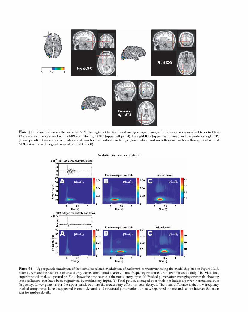
Elsevier UK Chapter: 0Colorplates1 3-10-2006 4:32p.m. Page:24 Trim:7.5in×9.25in
Basal Font:Palatino Margins:Top:40pt Gutter:68pt Font Size:9.5/12 Text Width:42pc Depth:55 Lines
Posteriorright STS
Right IOG
Right OFC0 0.4 1
Plate 44 Visualization on the subjects’ MRI: the regions identified as showing energy changes for faces versus scrambled faces in Plate43 are shown, co-registered with a MRI scan: the right OFC (upper left panel), the right IOG (upper right panel) and the posterior right STS(lower panel). These source estimates are shown both as cortical renderings (from below) and on orthogonal sections through a structuralMRI, using the radiological convention (right is left).
g (ω,t )e g (ω,t )T g (ω,t )i
g (ω,t )e g (ω,t )T g (ω,t )i
Modelling induced oscillations
Plate 45 Upper panel: simulation of fast stimulus-related modulation of backward connectivity, using the model depicted in Figure 33.18.Black curves are the responses of area 1; grey curves correspond to area 2. Time-frequency responses are shown for area 1 only. The white line,superimposed on these spectral profiles, shows the time course of the modulatory input. (a) Evoked power, after averaging over trials, showinglate oscillations that have been augmented by modulatory input. (b) Total power, averaged over trials. (c) Induced power, normalized overfrequency. Lower panel: as for the upper panel, but here the modulatory effect has been delayed. The main difference is that low-frequencyevoked components have disappeared because dynamic and structural perturbations are now separated in time and cannot interact. See maintext for further details.
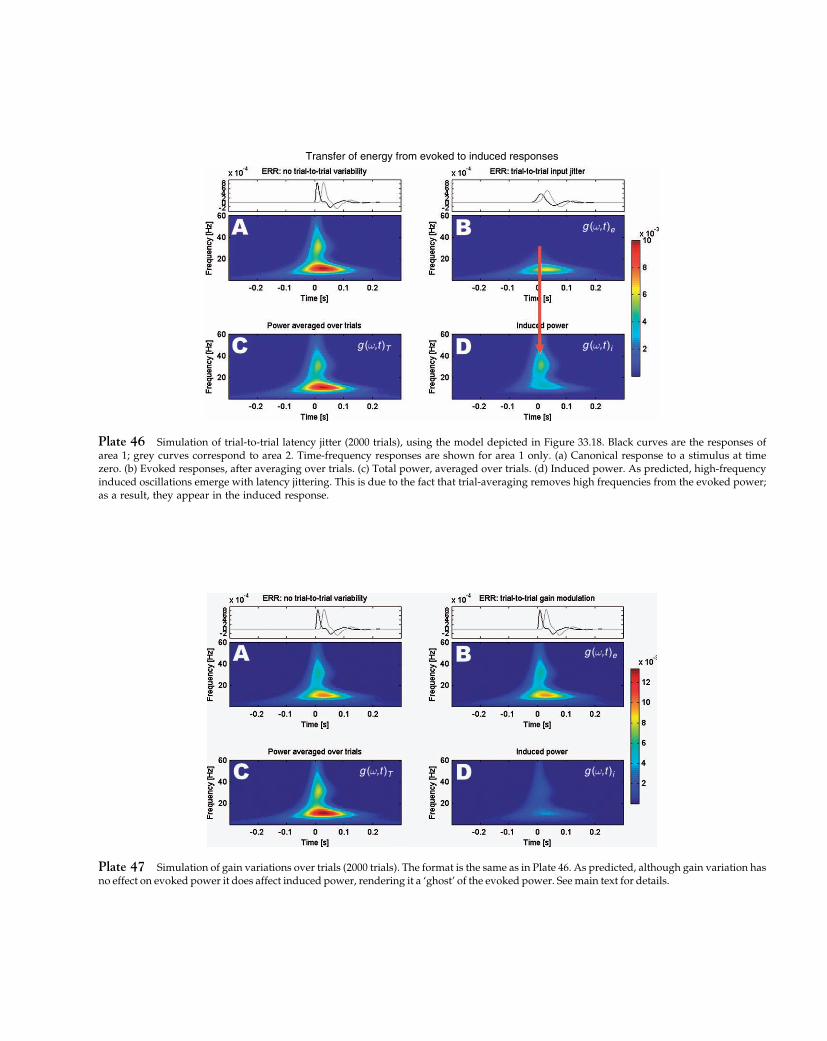
Elsevier UK Chapter: 0Colorplates1 3-10-2006 4:32p.m. Page:25 Trim:7.5in×9.25in
Basal Font:Palatino Margins:Top:40pt Gutter:68pt Font Size:9.5/12 Text Width:42pc Depth:55 Lines
Transfer of energy from evoked to induced responses
g (ω,t )e
g (ω,t )T g (ω,t )i
Plate 46 Simulation of trial-to-trial latency jitter (2000 trials), using the model depicted in Figure 33.18. Black curves are the responses ofarea 1; grey curves correspond to area 2. Time-frequency responses are shown for area 1 only. (a) Canonical response to a stimulus at timezero. (b) Evoked responses, after averaging over trials. (c) Total power, averaged over trials. (d) Induced power. As predicted, high-frequencyinduced oscillations emerge with latency jittering. This is due to the fact that trial-averaging removes high frequencies from the evoked power;as a result, they appear in the induced response.
g (ω,t )e
g (ω,t )T g (ω,t )i
Plate 47 Simulation of gain variations over trials (2000 trials). The format is the same as in Plate 46. As predicted, although gain variation hasno effect on evoked power it does affect induced power, rendering it a ‘ghost’ of the evoked power. See main text for details.

Elsevier UK Chapter: 0Colorplates1 3-10-2006 4:32p.m. Page:26 Trim:7.5in×9.25in
Basal Font:Palatino Margins:Top:40pt Gutter:68pt Font Size:9.5/12 Text Width:42pc Depth:55 Lines
g (ω,t )e
g (ω,t )T g (ω,t )a
Plate 48 Adjusted power (d). The format is the same as in Plate 46. As predicted, the adjusted power is largely immune to the effects oflatency variation, despite the fact that evoked responses still lose their high-frequency components.
(a) (b)
–1 0 1
Plate 49 Inflated cortical representation of (a) two simulated source locations (‘valid’ prior) and (b) ‘invalid’ prior location.
(a) (b)
(c)
–1 0 1
Plate 50 Inflated cortical representation of representative source reconstructions using (a) smoothness prior, (b) smoothness and validpriors and (c) smoothness, valid and invalid priors. The reconstructed values have been normalized between −1 and 1.

Elsevier UK Chapter: 0Colorplates1 3-10-2006 4:32p.m. Page:27 Trim:7.5in×9.25in
Basal Font:Palatino Margins:Top:40pt Gutter:68pt Font Size:9.5/12 Text Width:42pc Depth:55 Lines
Plate 51 3D segmentation of 71 structures of the probabilistic MRI atlas developed at the Montreal Neurological Institute. As shown inthe colour scale, brain areas belonging to different hemispheres were segmented separately.
Plate 52 Different arrays of sensors used in the simulations. EEG-19 represents the 10/20 electrode system; EEG-120 is obtained byextending and refining the 10/20 system; and MEG-151 corresponds to the spatial configuration of MEG sensors in the helmet of the CTFSystem Inc.
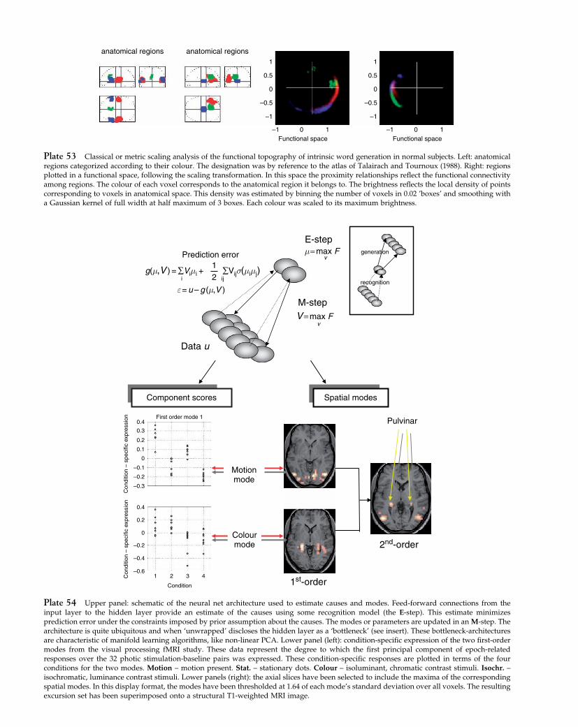
Elsevier UK Chapter: 0Colorplates1 3-10-2006 4:32p.m. Page:28 Trim:7.5in×9.25in
Basal Font:Palatino Margins:Top:40pt Gutter:68pt Font Size:9.5/12 Text Width:42pc Depth:55 Lines
anatomical regions anatomical regions1
0.5
0
–0.5
–1
–1 0Functional space
1
1
0.5
0
–0.5
–1
–1 0Functional space
1
Plate 53 Classical or metric scaling analysis of the functional topography of intrinsic word generation in normal subjects. Left: anatomicalregions categorized according to their colour. The designation was by reference to the atlas of Talairach and Tournoux (1988). Right: regionsplotted in a functional space, following the scaling transformation. In this space the proximity relationships reflect the functional connectivityamong regions. The colour of each voxel corresponds to the anatomical region it belongs to. The brightness reflects the local density of pointscorresponding to voxels in anatomical space. This density was estimated by binning the number of voxels in 0.02 ’boxes’ and smoothing witha Gaussian kernel of full width at half maximum of 3 boxes. Each colour was scaled to its maximum brightness.
v
v
μ = max F
V = max F
E-step
M-step
Prediction error
Data u
recognition
generation
g(μ,V ) = ∑Viμ i +12
∑Vijσ(μ iμ j)ij
ε = u – g (μ,V )
Component scores Spatial modes
2nd-order
1st-order
Motionmode
Colourmode
PulvinarFirst order mode 1
First order mode 2
0.4
0.3
0.2
0.1
0
–0.1
–0.2
–0.3
0.4
0.2
0
–0.6
–0.2
–0.4
1 2 3 4
1 2 3 4
Condition
Con
ditio
n –
spec
ific
expr
essi
onC
ondi
tion
– sp
ecifi
c ex
pres
sion
i
Plate 54 Upper panel: schematic of the neural net architecture used to estimate causes and modes. Feed-forward connections from theinput layer to the hidden layer provide an estimate of the causes using some recognition model (the E-step). This estimate minimizesprediction error under the constraints imposed by prior assumption about the causes. The modes or parameters are updated in an M-step. Thearchitecture is quite ubiquitous and when ‘unwrapped’ discloses the hidden layer as a ‘bottleneck’ (see insert). These bottleneck-architecturesare characteristic of manifold learning algorithms, like non-linear PCA. Lower panel (left): condition-specific expression of the two first-ordermodes from the visual processing fMRI study. These data represent the degree to which the first principal component of epoch-relatedresponses over the 32 photic stimulation-baseline pairs was expressed. These condition-specific responses are plotted in terms of the fourconditions for the two modes. Motion – motion present. Stat. – stationary dots. Colour – isoluminant, chromatic contrast stimuli. Isochr. –isochromatic, luminance contrast stimuli. Lower panels (right): the axial slices have been selected to include the maxima of the correspondingspatial modes. In this display format, the modes have been thresholded at 1.64 of each mode’s standard deviation over all voxels. The resultingexcursion set has been superimposed onto a structural T1-weighted MRI image.
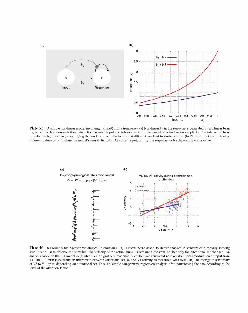
Elsevier UK Chapter: 0Colorplates1 3-10-2006 4:32p.m. Page:29 Trim:7.5in×9.25in
Basal Font:Palatino Margins:Top:40pt Gutter:68pt Font Size:9.5/12 Text Width:42pc Depth:55 Lines
b 1
b 2
yu
Input Response
(a)
Res
pons
e (y
)
Input (u )
b2 = 0.4
b2 = 0.8
u0
2.5
3
2
1.5
1
0.5
00.5 0.55 0.6 0.65 0.7 0.75 0.8 0.85 0.9 0.95 1
(b)
Plate 55 A simple non-linear model involving u (input) and y (response). (a) Non-linearity in the response is generated by a bilinear termuy, which models a non-additive interaction between input and intrinsic activity. The model is noise free for simplicity. The interaction termis scaled by b2, effectively quantifying the model’s sensitivity to input at different levels of intrinsic activity. (b) Plots of input and output atdifferent values of b2 disclose the model’s sensitivity to b2. At a fixed input, u = u0, the response varies depending on its value.
Psychophysiological interaction model
V5 = [V 1 × u ]βPPI + [V1 u]β + ε
(a)
V5 vs. V1 activity during attention andno-attention
V1 activity
V5
activ
ity
3
2
1
0
–1
–1 –0.5 0 0.5 1 1.5 2–2
(b)
Attention
Non-attention
Plate 56 (a) Models for psychophysiological interaction (PPI): subjects were asked to detect changes in velocity of a radially movingstimulus or just to observe the stimulus. The velocity of the actual stimulus remained constant, so that only the attentional set changed. Ananalysis based on the PPI model in (a) identified a significant response in V5 that was consistent with an attentional modulation of input fromV1. The PPI term is basically an interaction between attentional set, u, and V1 activity as measured with fMRI. (b) The change in sensitivityof V5 to V1 input, depending on attentional set. This is a simple comparative regression analysis, after partitioning the data according to thelevel of the attention factor.
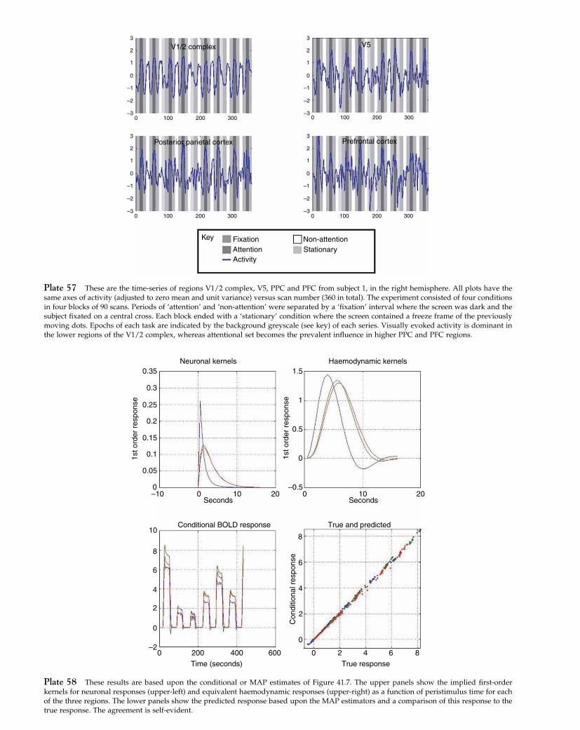
Elsevier UK Chapter: 0Colorplates1 3-10-2006 4:32p.m. Page:30 Trim:7.5in×9.25in
Basal Font:Palatino Margins:Top:40pt Gutter:68pt Font Size:9.5/12 Text Width:42pc Depth:55 Lines
3
2
1
0
–1
–2
–30 100 200
V1/2 complex
Posterior parietal cortex Prefrontal cortex
V5
300
3
2
1
0
–1
–2
–30 100 200 300
3
2
1
0
–1
–2
–30 100 200 300
Key Fixation Non-attentionStationaryAttention
Activity
3
2
1
0
–1
–2
–30 100 200 300
Plate 57 These are the time-series of regions V1/2 complex, V5, PPC and PFC from subject 1, in the right hemisphere. All plots have thesame axes of activity (adjusted to zero mean and unit variance) versus scan number (360 in total). The experiment consisted of four conditionsin four blocks of 90 scans. Periods of ‘attention’ and ‘non-attention’ were separated by a ‘fixation’ interval where the screen was dark and thesubject fixated on a central cross. Each block ended with a ‘stationary’ condition where the screen contained a freeze frame of the previouslymoving dots. Epochs of each task are indicated by the background greyscale (see key) of each series. Visually evoked activity is dominant inthe lower regions of the V1/2 complex, whereas attentional set becomes the prevalent influence in higher PPC and PFC regions.
Seconds
Time (seconds) True response
Seconds
Conditional BOLD response True and predicted
Neuronal kernels0.35
0.3
0.25
0.2
0.15
0.1
0.05
1st o
rder
res
pons
e
0
1.5
1
0.5
0
–0.5
1st o
rder
res
pons
eC
ondi
tiona
l res
pons
e
–10 0 010
10
8
8
66
4 4
22
0
0
0 0 2 4 6 8200 400 600–2
1020 20
Haemodynamic kernels
Plate 58 These results are based upon the conditional or MAP estimates of Figure 41.7. The upper panels show the implied first-orderkernels for neuronal responses (upper-left) and equivalent haemodynamic responses (upper-right) as a function of peristimulus time for eachof the three regions. The lower panels show the predicted response based upon the MAP estimators and a comparison of this response to thetrue response. The agreement is self-evident.
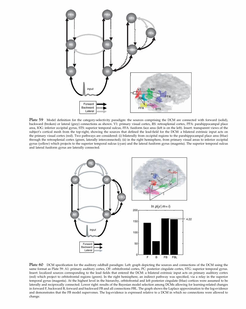
Elsevier UK Chapter: 0Colorplates1 3-10-2006 4:32p.m. Page:31 Trim:7.5in×9.25in
Basal Font:Palatino Margins:Top:40pt Gutter:68pt Font Size:9.5/12 Text Width:42pc Depth:55 Lines
input
ForwardBackward
Lateral
V1 RS
IOG
STSFFA
PPA
PPA PPASTS
FFA
IOG
RS RS
V1 V1
Plate 59 Model definition for the category-selectivity paradigm: the sources comprising the DCM are connected with forward (solid),backward (broken) or lateral (grey) connections as shown. V1: primary visual cortex, RS: retrosplenial cortex, PPA: parahippocampal placearea, IOG: inferior occipital gyrus, STS: superior temporal sulcus, FFA: fusiform face area (left is on the left). Insert: transparent views of thesubject’s cortical mesh from the top-right, showing the sources that defined the lead-field for the DCM: a bilateral extrinsic input acts onthe primary visual cortex (red). Two pathways are considered: (i) bilaterally from occipital regions to the parahippocampal place area (blue)through the retrosplenial cortex (green, laterally interconnected); (ii) in the right hemisphere, from primary visual areas to inferior occipitalgyrus (yellow) which projects to the superior temporal sulcus (cyan) and the lateral fusiform gyrus (magenta). The superior temporal sulcusand lateral fusiform gyrus are laterally connected.
F B FB FBL0
50
100
150
200
input
ForwardBackward
Lateral
4.22
PC
STG
OF
A1
A1
In p(y | m = i )
A1 A1
STG
OFOF
PC
Plate 60 DCM specification for the auditory oddball paradigm: Left: graph depicting the sources and connections of the DCM using thesame format as Plate 59: A1: primary auditory cortex, OF: orbitofrontal cortex, PC: posterior cingulate cortex, STG: superior temporal gyrus.Insert: localized sources corresponding to the lead fields that entered the DCM: a bilateral extrinsic input acts on primary auditory cortex(red) which project to orbitofrontal regions (green). In the right hemisphere, an indirect pathway was specified, via a relay in the superiortemporal gyrus (magenta). At the highest level in the hierarchy, orbitofrontal and left posterior cingulate (blue) cortices were assumed to belaterally and reciprocally connected. Lower right: results of the Bayesian model selection among DCMs allowing for learning-related changesin forward F, backward B, forward and backward FB and all connections FBL. The graph shows the Laplace approximation to the log-evidenceand demonstrates that the FB model supervenes. The log-evidence is expressed relative to a DCM in which no connections were allowed tochange.
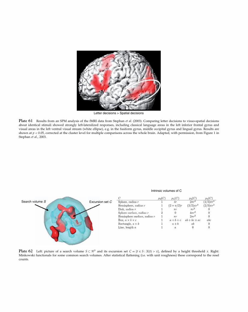
Elsevier UK Chapter: 0Colorplates1 3-10-2006 4:32p.m. Page:32 Trim:7.5in×9.25in
Basal Font:Palatino Margins:Top:40pt Gutter:68pt Font Size:9.5/12 Text Width:42pc Depth:55 Lines
Letter decisions > Spatial decisions
Plate 61 Results from an SPM analysis of the fMRI data from Stephan et al. (2003). Comparing letter decisions to visuo-spatial decisionsabout identical stimuli showed strongly left-lateralized responses, including classical language areas in the left inferior frontal gyrus andvisual areas in the left ventral visual stream (white ellipse), e.g. in the fusiform gyrus, middle occipital gyrus and lingual gyrus. Results areshown at p < 0�05, corrected at the cluster level for multiple comparisons across the whole brain. Adapted, with permission, from Figure 1 inStephan et al., 2003.
Search volume S Excursion set C
Intrinsic volumes of C
Plate 62 Left: picture of a search volume S ⊂ �D and its excursion set C = t ∈ S � X�t� > x�, defined by a height threshold x. Right:Minkowski functionals for some common search volumes. After statistical flattening (i.e. with unit roughness) these correspond to the reselcounts.