ANALYSIS OF CONSUMPTION THEORIES

IN THE ETHIOPIAN ECONOMY

A SENIOR ESSAY SUBMITTED TO THE DEPARTEMENT OF ECONOMICS IN PARTIAL FULLFILLMENT OF THE REQUIREMENTS FOR THE DEGREE OF BACHELOR OF ARTS IN

ECONOMICS

ESSAY ADVISOR:-ATLAW ALEMU (ATO)

ADDIS ABABA UNVERSITY FACULTY OF BUSINESS AND ECONOMICS

DEPARTEMENT OF ECONOMICS

BY-YOSEPH CHALA

i

ACKNOLGEMENTS

HANK GOD!!! AFTER ALL THOSE DAYS, FINALLY, IT COMES TO AN END.

When I am writing this, I feel the ups-and-downs that I have been through for the

past years. But, JESUS is LORD. Those days are now passed only because of HIM. HE

has been the anchor of my life since my birth and I believe HE will be so forever. Oh!

I am living at HIS mercy. GLORY TO GOD!!

When I come to the individuals who were with me during my days at AAU,

definitely family comes first. My father, my sister and my brothers were all with me

and I am glad to thank them, at this time, for every thing they have done for me. You

were all with me for every walk that I walk. Never would I forget that. But, special

thanks should be reserved to my dearest sister, Genet Chala and her husband

Abateneh Mulugeta. I have no word to express the financial contribution and

generosity they have extended to me. Bless You. I am grateful to you. Without your

support, I doubt where I would become at this time. And, it will be totally unfair not

to mention the advice and the contribution that I have been receiving from my

brother, Ephrem Chala. He was an ardent supporter of my higher education from its

conception. I am so indebted to you.

This paper would not come to realization as the form as it is now without a

valuable advice and follow up of my essay adviser, Ato Atlaw Alemu. He is always

open to discussions and ready to supply materials, even at his own expense. I sincerely

appreciate his approach towards his advisees. Thanks a lot.

Next to that friends certainly come. In that case, I am not bold enough to forget

the support from Melaku Taddesse, a grad student at AAU, Mengistu Emo, a senior

alumnus, Ermias Tefera, fellow student at AAU and, of course, Sisay Birru, Loan

Officer at DBE, Nekemte Branch. They were all helping me by providing books,

materials and by extending valuable suggestions in the preparation of this paper.

Besides, I would like to thank all my classmates, particularly Abiot S. of the CBE,

T

ii

Matias A., Sisay K., Mulugeta B., Demssew T. and others who make my stay at AAU

so much enjoyable. I do believe that the memories of those days will last with me.

Yoseph Chala

August, 2008

iii

Table of contents

PAGE

AKNOLGEMENTS----------------------------------------------------------------------i

ABSTRACT----------------------------------------------------------------------------- v

CHPTER ONE

INTODUCTION------------------------------------------------------------------------ 1

1.1 BACKGROUND--------------------------------------------------------------1

1.2 STATEMENT OF THE PROBLEM-------------------------------------------5

1.3 OBJECTIVE OF THE STUDY------------------------------------------------ 5

1.4 SIGNIFICANCE OF THE STUDY-------------------------------------------- 5

1.5 WORKING HYPOTHESIS-------------------------------------------------- 6

1.6 SCOPE AND LIMITATIONS OF THE STUDY-------------------------------6

1.7 ORGANIZATION OF THE STUDY----------------------------------------- 7

CHAPTER TWO

REVIEW OF LITERATURE------------------------------------------------------------ 9

2.1. DEFINITIONS: CONSUMPTION AND CONSUMPTION

EXPENDITUE-------------------------------------------------------- 10

2.2. THEORIES OF CONSUMPTION EXPENDITURE------------------------11

2.2.1. THE CLASSICAL BACKGROUND------------------------------- 11

2.2.2 THE ABSOLUTE INCOME HYPOTHESIS-----------------------12

2.2.3 THE LIFE-CYCLE HYPOTHESIS-------------------------------- 17

2.2.4. THE PERMANENT INCOME HYPOTHESIS--------------------23

2.3. THE ETHIOPIAN CASE--------------------------------------------------34

CHAPTER THREE

DATA, METHODS OF DATA ANALYSIS AND EMPIRICAL ESTIMATION-------39

3.1 SOURCE AND NATURE OF DATA --------------------------------------- 40

3.1.1. AUTOCORELATION----------------------------------------------41

iv

3.1.2. NONSTATIONARITY------------------------------------------------ 42

3.1.3. COINTEGRATION--------------------------------------------------- 43

3.2. MODEL ANALYSIS AND METHODOLOGY--------------------------------44

3.3. EMPIRICAL ESTIMATIONS AND PRESENTATION OF RESULTS------- 46

3.3.1. TESTING FOR UNIT ROOT----------------------------------------- 46

3.3.2. EMPIRICAL ESTIMATION-THE AIH-------------------------------47

- COINTEGRATION TEST-THE AIH------------------------------ 52

- NORMALITY TEST ON THE AIH--------------------------------- 53

3.3.3. EMPIRICAL ESTIMATION-THE PIH------------------------------- 54

- COINTEGRATION TEST-THE PIH------------------------------- 56

3.4. WHY THE PIH HAS FAILED TO EXPLAIN OUR DATA? ------ --------- 57

CHAPTER FOUR

CONCLUSION AND RECOMMENDATIONS------------------------------------------60

4.1. CONCLUSION--------------------------------------------------------------- 60

4.2. POLICY PRESCRIPTIONS-------------------------------------------------- 60

4.2.1. ON UNEMPLOYMENT----------------------------------------------60

4.2.2. ON INFLATION------------------------------------------------------61

BIBILOGRAPHY----------------------------------------------------------------------- 63

ANNEX ONE-REGRESSION OUTPUTS---------------------------------------------- 67

ANNEX TWO- DATA------------------------------------------------------------------71

v

ABSTRACT

In an effort to investigate the dynamic link between consumption and income, this

paper tries to test the validity of the Absolute Income Hypothesis of John Maynard

Keynes and the Permanent Income Hypothesis of Milton Friedman using country

level aggregate time series data. In that case, we found that consumption is not to be a

martingale process i.e., it follows the AIH’s presuppositions. But, that is only in the

short run. In the long run, neither of these theories were able to explain the data at

hand. That is primarily because of the nature of the theory on the AIH’s side and, the

assumptions it rests on and the quality of the data can be mentioned as reasonable

sources of failures for that of the PIH’s. In that essence, the paper concludes by

suggesting some short run policy prescriptions that are in line with Keynes’s

argument.

1

Chapter one

Introduction

1.1 BACKGROUND According to the eighteenth century Scottish classical economist Adam Smith, the

large international variations in income and standards of living over time and across

countries is not primarily because of other factors but due to the transformative effect

of the division of labor. After a century, David Ricardo, another classical economist

from Great Britain, came and accentuated the importance of trade for such differences

in affluence. Still, in the mid-twenty century, an American born neoclassical

economist Robert Solow came up with his highly influential and sophisticated growth

theory that gives emphasis on the importance of technological progress as the source

of such huge differences in income among nations across the globe. This means for

Solow sustained economic growth depends largely on technological advancement and

this innovation determines the country’s steady-state capital stock, a capital stock that

represents the long run equilibrium of the economy. Therefore, if a nation devotes a

large fraction of its income to invest in R&D and in higher educations, the major

sources of technological outlets; it will have a higher level steady-state capital stock,

thereby a higher level of income (Vaish, 1980, Dornbush et al, 1982, Todaro and

Smith, 2003).

In this area, empirical literatures so far produced based on the experiences of

both developed and underdeveloped countries seem to support the validity of Solow’s

argument1 (Barro and Sala-i-Martin, 2004).As the member of the later group,

Ethiopia’s case is not very far from what has been said in the theory. But, this does

not mean that the dire conditions of the country are entirely attributed to the luck of

such investments. Though officials from the government bloc are tireless to persuade

the skeptic public about the current boom the economy has been enjoying for the past

four or five years, both the public and the government know that Ethiopia is one of

1 Actually, Solow was not the first to provide a growth theory for country’s economy but his

theory is “the best known and it is the basic reference point for the literature on growth and

development” (See Todaro and Smith,2003)

2

the poorest country on earth with low level of per capita income ($160, World Bank,

2007), poverty is ubiquitous throughout the nation and the danger of this social unjust

will surely be remained as the major wrestling ground of all stakeholders and the

government at large in the coming years. If we agree on this issue and decide that the

key to reduce the extent of poverty is to register fast and consecutive growth, as the

theory suggests, the major task that should be done is to expand investment in R&D

and in higher education. As various literatures acknowledges, this kind of investment

is essential particularly for the agricultural sector (Mulat Demeke, 2003) and we

know that it depends largely on the amount of the country’s national income that is

saved.

The Ethiopian saving rate, however, was enjoying its good years during the last

days of the imperial regime. In those periods, Gross Domestic Saving (GDS) as a

percent of Gross Domestic Product (GDP) reached 13pc; the highest so far mobilized

(Befekadu Degefe and Berhanu Nega,1999/2000).Since then, as figures show, on

average, it has been fluctuating between 7.2pc in the last days of the military junta

and 4.1pc for the years 1993/94-2004/05, (EEA, Annual Report, 2005/06).This shows

the fact that GDS as the percent of GDP has been very low in Ethiopia both from a

historical perspective and relative to similar economies and it has not been , in it

history, around the usual recommended rates of saving and investment that ranges

from 12pc to 15pc and even as high as 25pc in some cases.

Economists provide a number of explanations for the existence of such kind of

traditionally low saving rate in developing countries and if we consider these

arguments seriously for us, we can easily understand why we are on such trend all

those periods. First of all, the concept of saving is directly related to income and as

mentioned earlier our country is among one of the world’s low income countries. So

such low income forces her to reduce her saving, that is, whatever earned is

consumed. Second, the spread of financial institutions in the country also has a

significant effect on the saving behavior the population. Alas, we all know that we are

unlucky in this respect too. Furthermore, the consumption behavior of the population

clearly determines the fate of the country’s saving rate. In this case, as studies show,

during the imperial era one of the challenges of the development was “to make such

3

transformation as the process involves changes in the traditional consumption

pattern” (Befekadu Degefe and Berhanu Nega: 1999/2000) and in the same report

these academics refer the consumption pattern of the then feudalist society as

“conspicuous consumption”, the famous phrase first used by an early twenty century

American economist and social scientist Veblen to refer the extravagant spending

behavior of Americans of his time( Mitchell,1947).If we also consider the periods of

post revolution , the policies of the Derge regime and its immediate heir are unable to

switch the public from the practice of such large wasteful behaviors. Thus, due to

such and other reasons, we are not enjoying higher saving rate and hence higher

investment and higher growth. As a result, we have become low income earners at

least from the crude arguments of low saving –low investment in R&D and in higher

education in so doing low growth approach.

Nevertheless, in the above discussion we have said so much about saving not

because we are interested in it but it gives a close insight to another important

economic variable what economists call consumption expenditure, the flip side of

saving.

The most important single fact about saving and consumption is that they are two

opposite sides of disposable income, income after tax and any transfers. This shows

that saving means abstaining from present consumption in order to provide for larger

future consumption. In the same way, today’s larger consumption results in low level

of saving and hence lower level of consumption in the future. As a result, every

explanation forwarded in favor of the former implicitly explains the later and vice

versa. Therefore, we would not be mistaken if we assume that the low saving

behavior of the country forwarded earlier is basically due to the fact that the high

consumption behavior of its citizens as the latest report of Ethiopian Economic

Association (EEA) clearly puts:

“this [low saving] is partly due to the subsistence nature of the economy in which total

consumption constitutes a significant share of domestic output” (EEA, 2005/06)

However, data clearly shows that, of this total consumption, private aggregate

consumption usually takes in the lion’s share. For instance, during the years of the

4

military rule, out of the total consumption 92.8pc of the domestic total consumption,

on average, private consumption absorbs 76.2pc; leaving only about 7.2pc for average

GDS.The same is true for the current government, that is, the data collected for the

periods 1993/94 to 2004/05 depicted that out of the 96.1pc of the total consumption,

private consumption again engrosses 78.7pc of the national output to make GDS at its

historically lower level of 4.1pc(EEA, 2005/2006).This and the above facts about

saving and consumption reveal important points about the economy under

investigation. These are we are in the historically low saving trend and

simultaneously we are consuming whatever produced in the economy. Therefore, at

this stage at least we can say something about private consumption expenditure, that

is, it exhausts the largest part of domestic output and it should deserve a close

understanding of how it operates in the economy.

Similarly, according to the Keynesian conventional four sector economy model,

aggregate output is the sum of personal consumption expenditure, total gross

investment, government purchase of goods and services and, of course, net export. Of

these, consumption expenditure is the largest macro variable irrespective of the size

and nature of the economy. In the words of Venieris and Sebold:

“depending on the country in question, expenditures on consumption amount to any where from two-

thirds to four-fifths of net national product.”(Venieris and Sebold, 1977)

Empirical findings in the literature also support the above conclusion.Branson

(2006) shows that 65pc of GNP in the US is absorbed by consumption expenditure.

Similarly, Mankiw (2002) implies that household consumption expenditure makes up

two-thirds of GDP. In the case of Ethiopia, as one can easily guess from the above

discussions, consumption expenditure makes about three-fourth of our total spending

(Oman, 2006).This shows that not only long run growth of the economy but short run

fluctuation of aggregate demand is also highly susceptible to what is going on in the

hands of consumers.

5

1.2 STATEMENT OF THE PROBLEM

As the nature of behavior underlying consumption is extremely important from

the standpoint of economic theory and policy, economists and theoreticians for the

past years have made every effort to examine the consumption behavior of an

economy and to come up with a more credible theory of consumption function. In this

perspective, based on the data on income and aggregate private consumption, many

economists have suggested a number of competing theories. Among these, we here

consider the three most influential and most important works of, Absolute Income

Hypothesis (Keynes, 1936), Life Cycle Hypothesis (Modigliani et al, 1950s) and

Permanent Income Hypothesis (Friedman, 1957).But, the problem is which one is

superior? That is a nearly century old debate for other economies, though we can not

indicate the exact time in our case. Anyway to put it clearly, which of these

outstanding works best reflect the consumption behavior of the Ethiopian economy?

1.3 OBJECTIVE OF THE STUDY

A thorough understanding of the consumption behavior of an economy helps

policy makers, practitioners and the government’s think tanks in general to make a

timely and appropriate policy prescription towards aggregate private spending.

Having this in mind:

- the major objective of this study is to find out the theory that governs the

consumption behavior of the Ethiopian economy and to create a general

understanding of the concept of consumption and its related issues like how it works

in the economy.

1.4 SIGNIFICACE OF THE STUDY

To gauge the effectiveness of alternative economic policies, both economists and

policy makers use the IS-LM model of the economy and from our macroeconomics

background we know that such model is partly based on the country’s Marginal

Prpensity to Consume (MPC) developed on the basis of the consumption behavior of

the economy .As a result, a clear understanding of the impact of any economic policy,

6

whether it is fiscal or monetary , requires a comprehensive understanding of the

concept of MPC which is “an ingredient in determining the response of the economy

to changes in the values of the policy variables” (Venieris and Sebold,

1977).Therefore , the perception of consumption function helps us to determine the

scenario of many public policies.

1.5 WORKING HYPOTHESIS

As said earlier, this paper is neither trying to discover the major determinants of

consumption expenditure in the Ethiopian economy nor aim to model the

consumption behavior of the economy using its own macro variables.Rather, it limits

itself to what has been said in the theories and attempts to test which one of the above

three theories that best represents the consumption behavior of typical Ethiopian

consumers. Consequently, we have the following two theories to work with:

According to Absolute Income Hypothesis:

Consumption is primarily determined by current income.

According to Permanent Income Hypothesis:

Consumption should depend primarily on permanent income.

For this reason, this study hypothesizes that consumption is dependent on permanent

income.

1.6 SCOPE AND LIMITATIONS OF THE STUDY

The scope of this study is not at household level but it is at a national level. This

is only because of the following two reasons. First, there is difficulty of obtaining

household data on consumption and disposable income. But, aggregate data are

readily available from the publication of any one of the government institutions.

Second, if household data are yet to be found, there are still problems of aggregation

and computation due to time and resource constraints. On the contrary, aggregate data

are usually free from these problems.

7

The strength of this study is that it tries simultaneously to discuss the seminal

works of the three giant economists in the fields of consumption. Certainly, this

provides the reader an opportunity to debate over three perspectives at a time.

However, it has the following obvious limitations .The first and most serious

limitation of this study traces with the Life Cycle Hypothesis of Franco Modigliani

and his collaborators. Because as we shall see in the coming discussions, this

hypothesis rests on the assumption that private consumption expenditure at any

period‘t’ is dependent on individuals’ income as well as wealth. Hence, to test the

explanatory power of Modigliani’s theory, one must have time series data on income

and wealth. But, as Modigliani himself acknowledged, generally in the developing

countries aggregate data on wealth is almost nonexistent (Modigliani, 1986) and as

local studies show our country’s case is not different from the above conclusion

(Solomon, 1999, Oman, 2006). In this context, the study becomes unable to analyze

the relationship between income and consumption from the perspective of the Life

Cycle framework. The second serious limitation of this study is that it is subject to the

basic assumptions of the theories. This means when the economists develop their

theories they made some bold assumptions based on the empirical evidences of the

developed world. Unfortunately, some of these assumptions are almost nonexistent in

the context of LDCs like Ethiopia. For instance, as we shall see in the coming

chapters, the latter two theories are based on Irving Fisher’s theory of consumer

behavior which implicitly assumes that there is no borrowing and saving constraints

but as Mankiw puts it “for many such borrowing is impossible”(Mankiw,2002).

The last limitation that should be mentioned here is that the study is limited in the

time span of the available data. So in this case, we will fail to catch the influence of

some missing observations in our analysis.

1.7 ORGANIZATION OF THE STUDY

The paper is organized in the following four major chapters. The first chapter is

an introductory part. The second chapter will provide a detailed analysis of the

consumption theories forwarded in the previous discussions by reviewing a number

of literatures in this respect. Based on that notion, it also formulates the mathematical

8

version of each theory for ease of estimation. The third chapter, the most important

chapter, will have two parts. In the first part, we will briefly discuss the nature and

sources of data and consider some methodological concepts to be used in the study.

The second part will entirely devoted to the process of empirical verification. Chapter

four, the last chapter, will conclude the research findings and recommend some policy

prescriptions

9

Chapter Two

Review of Literatures

In the previous chapter, it was said that aggregate private consumption expenditure or

simply consumption expenditure is the largest component of aggregate demand

irrespective of the nature and type of economy and due to this fact it has become the

major of concern of government policy makers and independent [nonpartisan] researchers

who are interested in policy issues. As a result of this and other factors, macroeconomists

devote much of their precious time to study the behavior of this macro variable in greater

detail and in the literature we can find a number of perspectives on such issue. According

to these literatures economists generally divide determinants of consumption expenditure

into two categories:-objective and subjective determinants (Kurihara, 1957). Objective

determinants include income, the distribution of income, corporate financial policies,

consumers’ liquid assets, the rate of interest and so forth. Contrarily, subjective factors

are security motives, ‘keeping up with the Joneses’, the desire for improvement, financial

prudence et cetera. As a result of this, there are a number of theories or hypotheses in this

field. In this section [generally in this study], however, we only focus on those which are

based on the dynamic relation between consumption and income and we try to

comprehend the essence of the theories forwarded in the introductory part of this paper

with a brief reviews of the classical writings since that helps us to understand the nature

and originality of Keynes’s idea and the subsequent works of those giant economists.

But, before doing that I believe that it is necessary to say some thing about the economic

concepts of consumption and consumption expenditure because economists, chiefly those

interested in the study of household behavior, usually use these concepts in different

contexts. Though it seems we generally have a clear understanding of these

terminologies, as we see in later discussions, one of the serious problems that arise in the

applications of these consumption theories is the luck of clear understanding about such

basic issues. Hence, we should devote some time to deal with those concepts. After that,

we will run into the theoretical debates that attract economists from all around for the

past years.

10

2.1 DEFINITIONS: CONSUMPTION AND CONSUMPTION EXPENDITURE

According to Seldon and Pennance1, consumption is “the process of deriving utility

from a commodity or service. More generally, it describes the business of acquiring

commodities and services in order to obtain satisfaction directly from them; or indicates

the amount of expenditure on them.” Additionally, they argued that consumption dose not

necessary indicate the destruction of the commodity consumed because, for instance,

food is consumed in the same way other objects like movies are also consumed though

the latter action does not include the destruction of the commodity, movie. Thus, in this

concept consumption is not necessarily a tangible process. Similarly, other literatures

argued that consumption should be defined in terms of ‘the use of goods rather than the

expenditure on it in any period’ (Branson, 2006). In general, economists use the word

‘consumption’ to mean the process of acquiring goods and services and the amount of

expenditure on them where the objective is to derive utility. But the problem, in this case,

is that the above definition is not clear about the nature of these commodities to be

consumed. Because we know that in economics consumer goods are generally divided

into two categories: durables and non durables. So, the above definition is no help.

Therefore, we should consider the following explanation. “Consumption expenditures by

household are personal consumption expenditures to national accounts. It includes

expenditures by households on durable consumer goods [automobiles, refrigerators, and

video recorders], nondurable consumer goods [bread, milk, vitamins pencils, shirts,

toothpaste] and consumer expenditure for services [of lawyers, doctors, mechanics,

barbers.]” (McConnell and Brue, 1994 pp.123-124). In this context, households allocate

their income between consumer durables, non durables and services. Though Keynes

agrees with this kind of understanding on consumption expenditure or simply

consumption (Keynes, 1949, pp.61), Modigliani’s Life Cycle Hypothesis (LCH) would

like to take a different perspective as the following definition asserts: “total consumption

consists of current outlays for nondurable goods [bread, milk] and services [net of

changes if any in the stock of nondurable] plus the rental value of stock of service –

yielding consumer durable goods (Ando and Modigliani, 1963). As clearly seen from this

1 Everyman’s Dictionary of Economics,1969, J. M. Dent & Sons Ltd, pp. 88

11

perception, the LCH or Modigliani dose not want to include the expenditure on durable

goods as consumption expenditure by the households while Keynes dose so. But we

know that any ‘careful’ studies on consumption should distinguish between the

investment and consumption activities of consumers or the households by not

incorporating expenditure on consumer durables- investment-in their analysis and the

results of such study are sensitive to the definition they assigned to consumption

expenditure (Houthakker, 1958, Hall, 1978, Flavin, 1981). In other perspective,

Friedman, for his part, assumes that consumption should not incorporate the ‘purchase

price of durables but it should include their use value’ (Houthakker, 1958). Here, such

acquisition of consumer durables is regarded as saving and the use value of the

commodity is measured by ‘depreciation and interest cost rather than expenditure on

them (Branson, 2006). This clearly shows that consumption for Permanent Income

Hypothesis considers only expenditure on nondurable goods, services and the use value

of durables. Understanding these concepts is very helpful for the coming discussions and

when we discuss the central points of the respective theories, the reader should be remind

these different definitions assigned by the respective theories to the variable under study.

Having this in mind, the point to be underscore here is that, in this paper, unless noted

otherwise, though we said that they refer different concepts, the terms consumption and

consumption expenditure are used interchangeably to refer the same thing.

2.2 THEORIES OF CONSUMPTION EXPENDITURE

2.2.1 THE CLASSICAL BACKGROUND

As it is clear largely for economics students, the term “classical economics”, as first

coined by German political philosopher and revolutionary Karl Marx, refers primarily to

Ricardo and his intellectual predecessor, Adam Smith (Dillard, 1979) and similarly John

Maynard Keynes used the term to refer to the disciples of Ricardo, “those, that is so say,

who adopted and perfected the theory of Ricardian economics, including …. John S.

Mill, Alfred Marshall, Edgeworth and Prof. Pigou” (Keynes, 1949)2.As a result of this,

2 In this case, Keynes uses the term ‘classical’ in unusual way because history of economic thought

categorizes F. Y. Edgeworth as the proponent of marginlist school but Keynes considers him as classical

for his own analytical purpose. See Dillard, 1979, pp.14

12

we here use the latter perception of the classical economics, that is, the traditional works

of all the abovementioned thinkers since the time of Ricardo. In so doing, as we clearly

know that during the periods of theses economists, there was hardly any theory or

function that relates consumption and income. This is because of the fact that the

classical theory rests on the assumption of full employment of resources so that out of a

constant full employment of real income the decision of people how much to consume

today and how much to save for the future and vice versa was influenced by changes in

the interest rate (Vaish, 1980).This means that a higher interest rate induced or

encourages the consumers to save more by postponing current consumption while a lower

interest rate discourages saving. Therefore, for the classicists, consumption is a negative

function of interest rate and it is not a function of income for the simple reason that

income is not a variable or income dose not vary in their economy [i.e. it is assumed to be

fixed in a fully employed economy] and this assumption prohibit any possibility of

increase in the equilibrium aggregate income in the short period in the economy. Hence,

we can conclude that for the classical school, consumption is a function of the rate of

interest and the relationship is negative:

Ct = f (i)

where Ct and i represent real consumption expenditure at time‘t’ and the rate of interest

for the same period in the given economy respectively. And the relation between the two

variables is indirect or opposite; that is, as interest rate rises consumption declines and

vice versa.

2.2.2 THE ABSOLUTE INCOME HYPOTHESIS-KEYNES. The 1930’s marked the most important turning point for the economic ideology.

Because the Great Depression (1929-1940) and its aftermaths brought an end to the

traditional economic principles of laissez faire that had been dominating the mind set

almost for two centuries. This means the then conviction was not enough to cope up with

the realities on the ground and as a result of this, many economists, practitioners, policy

makers and pundits were trying to diagnose the economy in order to forward the best

13

prescription. Among these, the point man was Cambridge lecturer John Maynard Keynes

who took the center stage in the wake of the great downturn of the economy of many

industrialized nations of West Europe and US. According to the accounts of many

writers, the Great Depression is still considered as one of the greatest economic

catastrophe of western nations. It saw rapid declines in the production and sale of goods

and a sudden, severe rise in unemployment. For instance, at the worst point in the

depression, more than 15 million Americans-one –quarter of the nation’s workforce-were

unemployed (Blanchard,1997). Given all these factors, the ultimate goal of Keynes

analysis was to discover the factors that determine the volume of employment in any

economy (Keynes, 1949, Dillard, 1979).Thus, as he discussed in his General Theory, the

volume of employment is determined at the equilibrium point of the aggregate supply

function with that of the aggregate demand and the latter relates any given level of

employment to the income which that level of employment is expected to realize. And,

such aggregate demand is further decomposed into- consumption expenditure and

investment expenditure. Consumption expenditure, which is of our interest, becomes his

stepping stone for his analysis of the theory economic fluctuations. Thus, he attempted to

investigate the determinants and the behavior of consumption expenditure when

employment is at a given level and his findings can be summarized as follows.

First, based on the psychological law, experience and facts he said that “men are

disposed, as a rule and on the average, to increase their consumption as their income

increase, but not by as much as the increase in their income.”(Keynes, 1949).This is to

state that the amount of consumption out of income has the same sign as change in

income but smaller in amount. Economists relate this classical guess with the concept of

marginal propensity to consume – a variable that measures additional consumption out of

additional income-and hence, according to Keynes’s intellectual conjecture, marginal

propensity to consume is positive and less than one. Therefore, when a person or an

individual receives an additional birr, he/she spends some of it and saves the rest.

Second, he hypothesized that the ratio of consumption to income decrease as income

rises, i.e. in his own words “a rising income will often be accompanied by increased

saving, and a falling income by decreased saving, on a greater scale at first than

14

subsequently” (Ibid., pp.97). This means the average propensity to consume declines as

income rises and generally the economy will tend to save more and more of its income as

it gets prosperous. From this we can see, it is natural to conclude that as the average

propensity to consume falls, the marginal propensity to consume would do so but only at

a faster rate; hence, marginal propensity to consume is less than average propensity to

consume.

Third and most important of the three, he argued that real consumption is a fairly

stable function of real income i.e. “consumption is obviously much more a function of …

real income than of money-income” (Ibid.). Clearly, this point is a direct attack to the

then governing doctrine of the classical principle that rests its argument based on full

employment and that assumes real consumption is a function of real interest rate. But for

Keynes, who had already ruled out the assumption of full employment, “the short period

influence of the rate of interest on individual spending out of a given income is secondary

and relatively unimportant” (Ibid.).

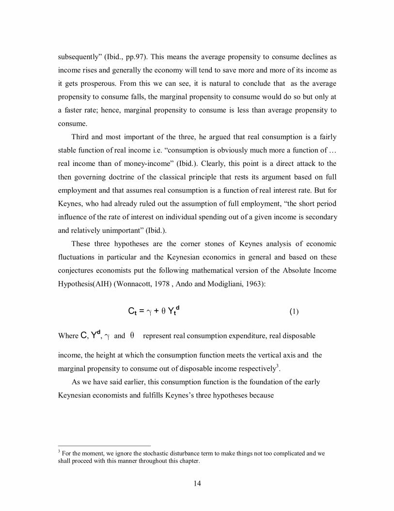
These three hypotheses are the corner stones of Keynes analysis of economic

fluctuations in particular and the Keynesian economics in general and based on these

conjectures economists put the following mathematical version of the Absolute Income

Hypothesis(AIH) (Wonnacott, 1978 , Ando and Modigliani, 1963):

Ct = + Yt

d (1)

Where C, Yd

, and represent real consumption expenditure, real disposable

income, the height at which the consumption function meets the vertical axis and the

marginal propensity to consume out of disposable income respectively3.

As we have said earlier, this consumption function is the foundation of the early

Keynesian economists and fulfills Keynes’s three hypotheses because

3 For the moment, we ignore the stochastic disturbance term to make things not too complicated and we

shall proceed with this manner throughout this chapter.

15

- first Keynes assumed that the marginal propensity to consume ‘c’ obeys that

double restrictions between zero and unity.

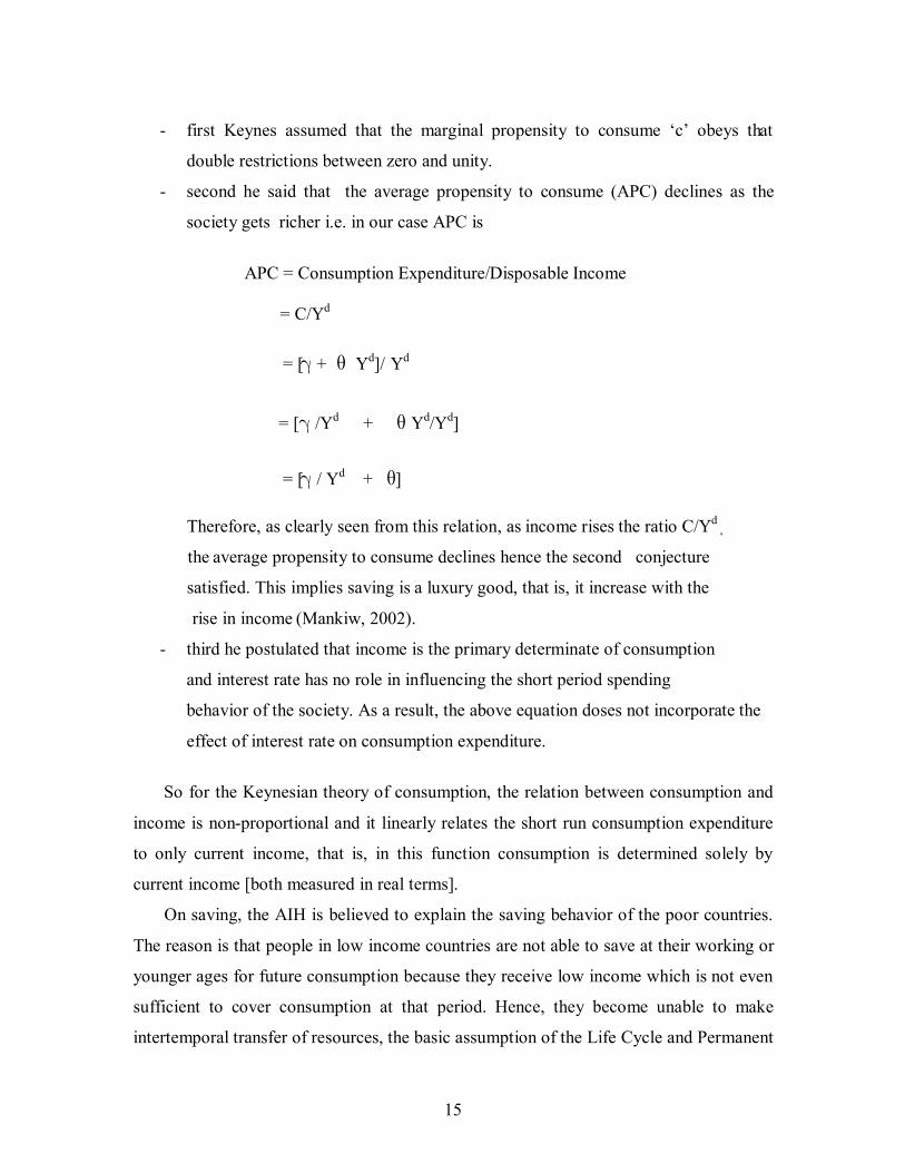
- second he said that the average propensity to consume (APC) declines as the

society gets richer i.e. in our case APC is

APC = Consumption Expenditure/Disposable Income

= C/Yd

= [ + Yd]/ Yd

= [ /Yd

+ Yd/Y

d]

= [ / Yd + ]

Therefore, as clearly seen from this relation, as income rises the ratio C/Yd

,

the average propensity to consume declines hence the second conjecture

satisfied. This implies saving is a luxury good, that is, it increase with the

rise in income (Mankiw, 2002).

- third he postulated that income is the primary determinate of consumption

and interest rate has no role in influencing the short period spending

behavior of the society. As a result, the above equation doses not incorporate the

effect of interest rate on consumption expenditure.

So for the Keynesian theory of consumption, the relation between consumption and

income is non-proportional and it linearly relates the short run consumption expenditure

to only current income, that is, in this function consumption is determined solely by

current income [both measured in real terms].

On saving, the AIH is believed to explain the saving behavior of the poor countries.

The reason is that people in low income countries are not able to save at their working or

younger ages for future consumption because they receive low income which is not even

sufficient to cover consumption at that period. Hence, they become unable to make

intertemporal transfer of resources, the basic assumption of the Life Cycle and Permanent

16

Income theories of consumer’s behavior [We will consider that later on]. So in that

context, consumption is likely to follow only current disposable income (Modigliani and

Cao, 2004). This is exactly what Keynes says.

Hence, after Keynes proposed his consumption function, economists and researchers

soon tried to verify the validity of this function by using both time series and cross-

sectional data and as summarized by Branson, in both cases the results were quite

supporting the theory of John Maynard Keynes or Absolute Income Hypothesis (AIH)

(Branson, 2006). However, according to various literatures, those early empirical success

of the AIH started to loose with the truth on the ground in the mid- 1940s.This is

primarily because of the fact that based on the second conjecture some economists

forecasted that as income rises consumption declines and hence saving rises. So first they

reasoned that there will not be enough aggregate consumption demand to goods and

services and second there will also be no enough investment to absorb such huge

accumulation of saving or capital. Hence, in one way or another, they argued that the

economy will dive into what they called ‘stagnation’. In the literatures, these economists

and their ‘school’ that advocated such kind of conviction is known as ‘stagnationst

school’ (Modigliani, 1986). But, in those days what really happened was contrary to what

the ‘stagnationst’ forecasted based on the AIH (Branson, 2006). This made economists

speculate the validity of Keynes’ arguments. The other most important discovery that

brought stark evidence against the AIH’s basic tenets is that the findings of the 1971

Noble Prize-winning economist Simon Kuznets. In his influential work, Kuznets

collected data on consumption and saving dating back to the 1860s (Mankiw, 2002) and

he found that in the long run there was near proportionality between income and

consumption. This means the value of the intercept “” in equation (1) should be zero

(Dornbush et al, 1982). On top of this, Kuznets argued in the long run there was little

variation in the average propensity to consume or the average propensity to consume was

almost constant for the period under investigation, that is, as income rises, the society did

not decrease its consumption as the theory suggests (Wonnacott, 1978). Thus, these two

results also brought the weaknesses of the AIH to light.

17

Similarly, other economists argued that the above simple consumption function

should by no means be ‘a fundamental law of human nature’ (Gilboy, 1938). In her

paper, Gilboy criticized the simple Keynesian consumption function for not incorporating

the effects of income distribution, working conditions [like farm and non farm families],

and working places [city and village] on its analysis and she clearly provides a detailed

statistical analysis for her argument. In other cases, even these days several economists

used the AIH to forecast the behavior of the consumers in the economy. For instance,

Dornbush, Fisher and Sparks in their 1982 book used the 1926-1940 data for the Canada

economy to test the validity of the AIH. Their finding was satisfactory for those periods

but when they tried to forecast the marginal propensity to consume for the year 1982, it

becomes something devastating, that is, it is far from reality.

Therefore, these phenomena particularly the first two, the ‘stagnation’ doctrine and

the works Kuznets, presented what is known in economics as consumption puzzle among

the then economists and motivated the search for a more sophisticated and dynamic

consumption function that could reconcile such long run – short run discrepancies. This is

the main reason that the contemporary theories of consumption function focus primarily

on this reconciliation effort. Anyway, in doing so, some economists finally arrived at

their own version of consumption function and in the literature we can find a mountain of

debates on this issue but in this study a focus is made only on those works of Modigliani

et al. and Friedman that were proposed in the 1950s when the intellectual debate over

what really determines consumption arrived at its peak point.

2.2.3 THE LIFE-CYCLE HYPOTHESIS-MODIGLIANI-ANDO-BRUMBERG.

In the introductory chapter, it was said that the analysis of the Life-Cycle Hypothesis

(LCH) of consumption expenditure is highly constrained by the nonexistent of time series

data on net worth and that problem is generally acknowledge by a number of economists

including the mastermind, Modigliani. When we consider that case from developing

countries perspectives, as one clearly guesses, the problem becomes very series.

Notwithstanding, in the presence of such problem, Abebe (2005) made an interesting

study that attempts to verify the explanatory power of the LCH in the Ethiopian context.

18

Hence, for that and other theoretical reasons, in this section, we will devote little time for

a brief discussion of the LCH.

As frankly acknowledged by Franco Modigliani, the LCH of consumption and

saving behavior made its departing point on the works of an early twentieth century

American economist Irving Fisher’s theory of Intertemporal Utility Maximization which

argued that rational, utility-maximizing consumers will optimally allocate their resources

to consumption over their life time (Modigliani, 1986).Hence, based on this notion

Franco Modigliani, Albert Ando and Richard Brumberg tried to study the consumer

behavior of the households as well as the economy very carefully(Mankiw,2002). The

main purposes of these three individuals were to explain the determinants of consumption

in the given economy and to solve the long run-short run puzzle that arose when the AIH

came to data. So, contrary to what have been said in the Absolute Income Hypothesis

(AIH) of Keynes, the LCH argued that for a representative consumer who lives for two

periods-present and future -with finite life time at any age‘t’, the consumption decision

depends “not at all on income accruing currently but only on his life resource [the present

value of labour income plus bequests received if any]” (Modigliani, 1986). In other

words, they argued that at any time‘t’, the total consumption of an individual age T will

be proportional to the present value of total resources available to him (Ando and

Modigliani, 1963). Besides this, the LCH observed that an individual consumer has an

income stream that is relatively low at the beginning [at this time the consumer is a net

borrower] and end [here he dissaves] of his life (Branson, 2006). The major reason for

this systematic variation in income throughout the life-cycle of the individual is maturing,

retiring and family size. Hence, saving, for the LCH, is primarily done for the purpose of

financing consumption at the retirement age. To progress further with their theory,

Modigliani and his colleagues made further assumptions. These are income is constant

until retirement, zero thereafter; no interest rate, constant or smooth consumption over

life, no bequest and perfect capital market. These assumptions clearly imply that

“consumption is geared not to current income which is zero during retirement, but rather

to lifetime income” (Dornbush and Fischer, 1994). Following that assumptions, the

Ando-Modigliani version of consumption function for the representative consumer at any

age T, can be written as follows:

19

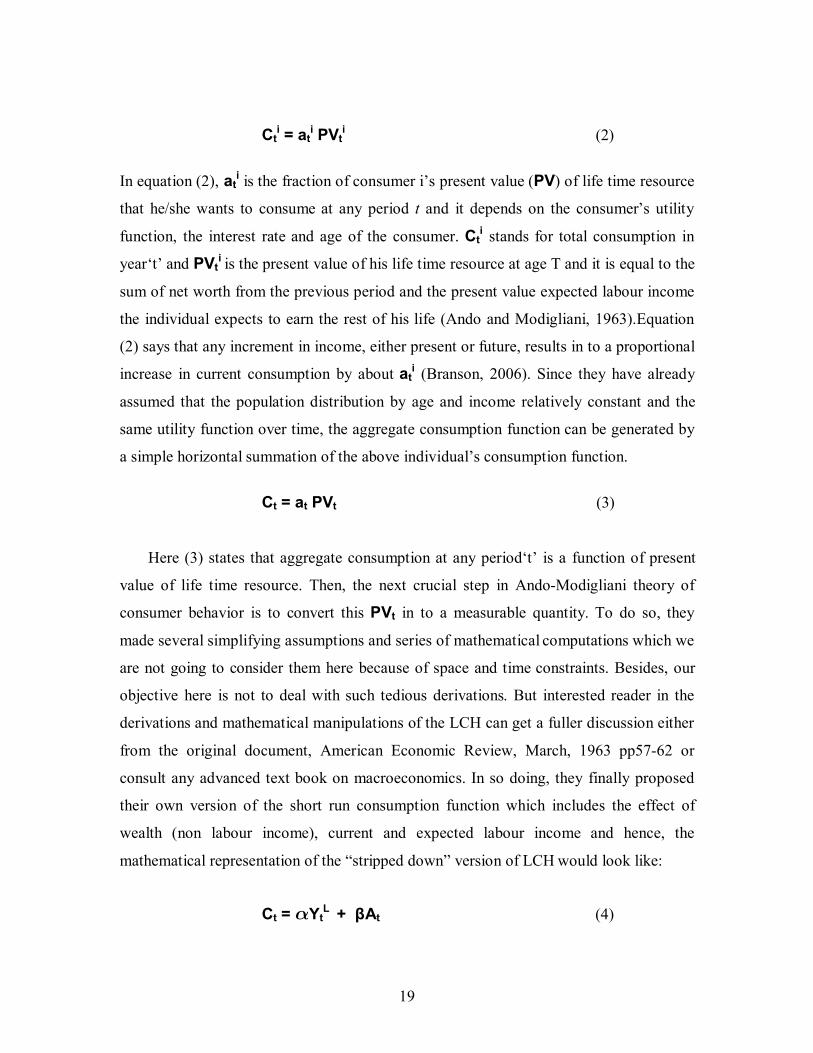
Cti = at

i PVti (2)

In equation (2), ati is the fraction of consumer i’s present value (PV) of life time resource

that he/she wants to consume at any period t and it depends on the consumer’s utility

function, the interest rate and age of the consumer. Cti stands for total consumption in

year‘t’ and PVti is the present value of his life time resource at age T and it is equal to the

sum of net worth from the previous period and the present value expected labour income

the individual expects to earn the rest of his life (Ando and Modigliani, 1963).Equation

(2) says that any increment in income, either present or future, results in to a proportional

increase in current consumption by about ati (Branson, 2006). Since they have already

assumed that the population distribution by age and income relatively constant and the

same utility function over time, the aggregate consumption function can be generated by

a simple horizontal summation of the above individual’s consumption function.

Ct = at PVt (3)

Here (3) states that aggregate consumption at any period‘t’ is a function of present

value of life time resource. Then, the next crucial step in Ando-Modigliani theory of

consumer behavior is to convert this PVt in to a measurable quantity. To do so, they

made several simplifying assumptions and series of mathematical computations which we

are not going to consider them here because of space and time constraints. Besides, our

objective here is not to deal with such tedious derivations. But interested reader in the

derivations and mathematical manipulations of the LCH can get a fuller discussion either

from the original document, American Economic Review, March, 1963 pp57-62 or

consult any advanced text book on macroeconomics. In so doing, they finally proposed

their own version of the short run consumption function which includes the effect of

wealth (non labour income), current and expected labour income and hence, the

mathematical representation of the “stripped down” version of LCH would look like:

Ct = YtL

+ βAt (4)

20

Equation (4) states that aggregate consumption in any given period‘t’ depends on current

labour [non property] income, YtL and assets [non labour income or net worth], At and the

parameters and β measure the marginal propensity to consume out of labour income

and wealth (net) respectively. Beware that in the above equation the parameter

measures the marginal propensity to consume out of both current and expected future

incomes and the latter is, by naïve assumption, the same as current income with ‘possible

scale factor’ (Ando and Modigliani, 1963). Such kind of expectation in economics is

known as naïve expectation (Maddala, 1992). Here, people generally use only current

information of a variable to determine its future values, that is, in our case, they assume

that next period income will be exactly the same as income in the current period and such

assumption gives due emphasis to current income in determining current consumption.

But, as various authors clearly put such kind of assumption has got its own drawbacks

(Wonnacott, 1978) and faced series critics from economists like Robert. E .Hall of

Stanford University. We will see that soon. To return to our discussions, as it is clear

from the above relation in the short run wealth is constant so βAt is the intercept and it is

clearly greater than zero and hence the LCH’ s consumption function looks like its AIH

counterpart. But in the long run, we should assume that there exists economic growth i.e.

income grows and through saving wealth increase. Then, βAt continually shifts up ward

so does the consumption function for each period. In that case, if we join each period

income with its respective new consumption curves and connect the intersection points of

period one’s income with its consumption curve and period two’s income with its

respective consumption curve and so on, we can get the long run consumption function

that passes through these intersection points and hence through the origin. As clearly

stated in the above discussions, these results are exactly the same as what Kuznets found

in his empirical study.

When we come to empirical verifications for the Life-Cycle Hypothesis, we find that

the process is extremely difficult for Modigliani and Brumberg (Modigliani, 1986) and

some kind of indirect even for the US economy, the place where the theory primarily

developed for. This was predominantly because of the lack of aggregate time series data

21

on annual private net worth. But, decades later, the availability of data on net worth

became possible and Ando and Modigliani tested equation (4) for the US economy using

time series data for the period 1929-59 excluding the periods of 1941-1946. And as

Modigliani discussed this in his Nobel Lecture, the result was ‘quite well’ and from those

periods on ward the LCH is considered by the US policy makers , econometric-model

builders and forecasters as the major intellectual contributions that used to analyze and

forecast the behavior of consumers in particular and the economy in general. However,

when we come to other recent efforts of verification, we can see that the realities are still

similar to US’s condition some fifty years ago. For instance, four years ago, by using the

LCH framework, Modigliani and Cao tried to analyze not the consumption but its

flipside, the saving behavior of one of the world’s fastest growing economy, China. In

that case, they encountered the same problem as Modigliani and Brumberg did some fifty

years ago (Modigliani and Cao, 2004). Yet, by using some kind of indirect method, they

tested the theoretical implication of the LCH and they found that the theory has a

remarkable explanatory power. This and similar other incidents indicate that the

empirical verification of the LCH is exceedingly difficult even for developed nations and

the cases of underdeveloped nations are not different. For our country’s case, as we put

earlier, the conditions are worse than other country’s case and any attempt to verify the

applicability of this theory is constrained by the non existent of time series data on net

worth (Solomon, 1999, Oman, 2006). Therefore, for that matter, we are not, here,

privileged to analyze Ethiopia’s case from the perspective of Life-Cycle theory.

Well, as we have seen the Modigliani et al.’s theory of consumer behavior is a

significant departure from the Keynesian approach which assumes consumption in any

period‘t’ is only a function of income earned in that period or current income. And for

LCH individuals always make the best use of the resources at hand to maximize life time

utility other than the simple current utility. For that reason, we see that the LCH relates

consumption to the present value of life resource. But at this time it is necessary to ask

the fate of any windfall gains or transitory deviations from this life time resource. First,

Modigliani argued that such transitory deviations of income are usually responsive to

saving motives rather than consumption (Modigliani, 1986) and hence those parts of

society which are characterized by a large amount of transitory income than their life

22

time income, for instance farmers, save a significant portion of their income than those

with lower transitory income and higher life time income, government employers.

Second, he showed that this saving rate is highly influenced by the long run growth rate

of the economy than the simple per capita income. Consider these arguments for our

country, particularly that of the first. We know that farmers comprise eighty five percent

of the population and as the theory suggests, they are characterized by a huge transitory

income, that is, rural household depend on seasonal agricultural income for their

consumption and this conviction is supported by various empirical findings (Nigussie,

2006). Though they are not detailed and small sample size, his [Nigussie] findings

suggest that such huge transitory income and consumption patters are uncorrelated. This

means consumption (only on food) style is similar or stable throughout the period despite

income fluctuations. Therefore, we can say that if farmers try to smooth consumption in

the face of this erratic income, those periods with high incomes are characterized by high

saving for financing consumption in low income periods. This indicates an important

implication, that is; farmers could also decide the fate of the country’s saving rate if there

is effective policy by the government or other stakeholders to exploit it. We shall fully

discuss this point in the coming chapter.

Other application of the LCH is that it considers the impact population distribution

on aggregate consumption. In this case, though it is subject to debate (Farrell, 1959),

Modigliani and his collaborates argued that saving is primarily done for financing future

consumption, thus the population dominated by many middle age earners is characterized

by high saving ratio. In contrast, if the community is dominated by young folk, like our

country (Befekadu Degefe and Berhanu Nega, 1999/2000 pp.62) and aging population,

the majority of the people are engaged in dissaving, that is, saving rate would be low.

Thus, from this concept, such demographic characteristic might be one of the main

reasons for the existence of low saving trend that we have seen earlier. Clearly, this

finding is contrary to the AIH which simply assumes that the saving rate of the economy

is determined solely by the rate of the growth of the economy. In addition, the theory

under discussion provides a much more powerful estimate of monetary policy than its

competitors (Wonnacott, 1978). This is simply because of the fact that the LCH

incorporates the effect of wealth in its analysis. The above discussions and several other

23

implications of the LC theory point out that the theory being discussed generally provides

a through understanding of the society’s consumption–saving behavior and its analysis of

the variable under investigation is far reaching than the simple theory of Keynes’s ‘rule

of thumb’ or the AIH.

As we have said in the earlier chapter, the application of the LCH is highly limited

by its basic assumptions. In this case, we can raise at least the following points. First,

consider the role of liquidity constraints. Modigliani clearly puts that due to liquidity

constraints consumers failed to maximize their inter-temporal utility and hence their

consumption path become forced to track their current disposable income like the simple

Keynesian consumption model. Hence, such relaxation of the ‘stripped down’ version of

the LCH will result in a different implication of the hypothesis, particularly if the

liquidity constraint is significant. Second, the assumptions about family size, interest rate,

the length of working and retired years, bequests and bequest motives and the case of

myopia etc. pose problems in empirical analysis, though Modigliani argued such

relaxation would not change the validity of the basic hypothesis (1986).

The other point of limitation that should be considered here is that of the assumption

of naïve expectation. The LCH hypothesizes that consumption at any period‘t’ depends

on wealth, current income and expected future income. We know that the latter is the

same as its current value with possible scale factor. Nonetheless, this kind of naïve

expectation brought several controversies in the literature and due to this fact economists

dissatisfied with this concept propounded their own version of expectation known in

literature as rational expectation. Yet, this argument is advanced not only against the

LCH but also to Friedman’s Permanent Income Hypothesis (PIH). So for the sake of

better understanding I believe we should deal with such discussion after a brief review of

the PIH of Milton Friedman.

2.2.4 THE PERMANENT - INCOME HYPOTHESIS-FRIEDMAN In the 1950s, an American economist Milton Friedman tried to study the behavior of

consumers in detail in order to propose the theory that could reconcile the short run –

long run discrepancies of the AIH that arose as a result of the outstanding works of

Kuznets and late in that decade he came up with his own version of consumption

24

expenditure known in literature as Permanent Income Hypothesis (PIH). According to

various literatures, the PIH is considered as one of the most widely studied theory of

consumer behavior (Singh and Drost, 1971). In this work, like Modigliani et al, Friedman

first assumed that households prefer stable consumption path over unstable one

throughout their life, that is, they tend to smooth consumption over time (Sachs and

Larrain B., 1993) and he argued that both measured consumption and income include

‘permanent’ and ‘transitory’ components (Branson, 2006, Vernis and Sebold, 1977). As a

result of this, at any time‘t’, the measured values of consumption(C) and income(Y) for

cross-section and time series aggregate data could be written as:

Ct= Ctp

+ Ctt (5)

Yt = Yt

p + Ytt (6)

In equations (5) and (6)4 both Ct

t and Ytt respectively measure the transitory components

of consumption and income at any period‘t’. Similarly, Cpt and Yp

t respectively represent

the permanent components of both consumption and income in the same period‘t’. The

decomposition of both consumption and income into transitory and permanent is based

on the concept of consumption which Friedman argued that “observed consumption

expenditures do not always reflect real consumption.” (Veranis and Sebold, 1977,

pp377). This means the use of some durable goods such as a refrigerator or VCR is

distributed over life time while there expenditure the consumer incurs has only a one

period effect. This indicates that the consumption of some consumer goods is

characterized by their permanent nature, though the expenditure on them has only

transitory or a one period effect. Equally, consumers do not always follow the same

consumption track or behavior over time, as a result they sometimes are forced to

‘deviate’ from their normal behavior and in this case their consumption, in the Friedman

context, is regarded as transitory (Ibid.).

Thus, the distinction between permanent and transitory income is the existence of

windfall gains or losses made by consumers. That is transitory components are made up

of unforeseen gains or losses to income and they are supposed to cancel out in the long

4 From now on, we will be using the superscript‘t’ to indicate the transitory component of the respective

variable where as the subscript ‘t’ to refer the time period ‘t’.

25

run (Houthakker, 1958). Thus, the PIH considers permanent income as part of current or

measured income that people expects to persist in their future or a kind of average of

present and future income and transitory income is that part they expect to not hold in the

future or any random deviation from the permanent income (Mankiw, 2002, Sachs and

Larrain B.,1993 ). Besides, Friedman argued based on the evaluation of their labour and

non labour income, each consuming unit has an implicit notion of its permanent income.

Relying on this understanding of the permanent and transitory components of income

and consumption, the PIH made three important assumptions known as- permanent

income and transitory income are independent, permanent consumption and transitory

consumption are independent and transitory consumption and transitory income are

independent. This means the co-variances between permanent income and transitory

income, permanent consumption and transitory consumption and transitory consumption

and transitory income are zero (Branson, 2006).

Hence, for Permanent Income model, consumption in the present period or at any

period‘t’ depends, not primarily on the income earned in that period or current income

rather on the expected normal income, or in Friedman’s term, on permanent income

which depends up on the present discounted value of the person’s wealth (Mankiw, 2002,

Wonnacott, 1978) and the fundamental long run relationship between permanent

consumption and permanent income is proportional. Thus,

Ct

p = kYtp (7)

This means aggregate permanent consumption (Ctp) at any time‘t’ is a reasonably

constant fraction of aggregate permanent income (Ytp). Besides, k is the long run

marginal propensity to consume [marginal propensity to consume out of permanent

income] and total consumption of the economy(Ct) at any time‘t’ comprises both

transitory consumption(Ctt) and permanent consumption(kYt

p). Therefore, we can also

put (5) in the following way:

Ct = kYtp + Ct

t (8)

26

By now, it is very clear what (8) says, that is, total observed consumption of the economy

or the individuals at any time‘t’ is the sum of permanent consumption which is a function

of permanent income and its transitory component in the same period. But, we can ignore

the transitory component of equation (8) because it is included in the stochastic

disturbance or error term and as we noted earlier in this chapter, for ease of analysis, we

deal only with deterministic models (Veranis and Sebold, 1977). Hence, equation (8) can

be re-written in the following way:

Ct = kYtp (9)

Thus, we can easily understand from equation (9) what the PIH says. This long-run

relationship shows households consumption at any period‘t’ is a function of their

permanent or the long run expected income, not of their current incomes as the simple

Keynesian ‘rule of thumb’ consumption function considers (Flavin,1981). So, if current

incomes are higher than permanent or average income, they save the difference.

Similarly, if current incomes are lower than that of permanent income, they dissave, that

is, they borrow against future incomes with zero interest rate. Then, the short run

counterpart of equation (9) is:

Ct =k 1- Ypt-1 + kYt (10)

Hence, at any period‘t’, as the short run consumption function shows consumption would

be dependent on the income in that period Yt plus past periods permanent income Ypt-1

which is unobservable variable. So, during the study of consumption behavior of any

economy by using the PIH frame work, defining what permanent income or quantifying

one’s permanent income is one of the toughest jobs any researcher faces (Hall, 1978). In

this context, several literatures suggest different kinds of measuring techniques and there

is no a general consensus in this regard (Bhalla, 1980). As we shortly see, one of the

debatable points of the PIH is the techniques employing in measuring the permanent

income (Singh and Drost 1971, Hall, 1978). Anyway as we have seen earlier, the concept

of permanent income incorporates the idea of expectations, that is, it [permanent income]

is part of people’s income that they expect to realize in the future. Hence, although it

27

exposes Friedman and the PIH to serious critics [we will consider that below], he

assumed that expectation is “adaptive”. This means households readjust or ‘adapt’ their

estimates of the permanent income each period based on their past estimates of actual or

observed incomes and he suggests that the permanent income of the economy or the

household can best be approximated by the weighted sum of current and past values of

observed (current) incomes (Venieris and Sebold, 1977, Branson, 2006) and this

approach is the most conventional one( Bhalla, 1980).Thus, using this concept of

adaptive expectation, Friedman’s permanent income for an infinite horizon at any year‘t’

follows the following pattern:

Yt

p = Yt + (1- ) Yp

t-1 (11)

Alternatively, (11) can be described in the following way

Yt

p = Yt+ (1- ) Yt-1+ (1- ) 2 Yt-2+……+ (1- ) n Yt-n+ … (12)

These two equations are the same in a sense that if we lag (12) by one period, multiply it

by (1- ) and subtract the final result from the original equation, we can easily get (11).

This kind of formulation of the permanent income, despite the controversies it faces

(Singh and Drost, 1971), is very common and it was first used by Friedman himself.

Since then it is extensively used by many researchers (Bhalla, 1980). In equation (11), Yt

is the current or measured income in time period‘t’ and ‘’ is the coefficient of

expectation and it is between zero and one. In this process of approximating permanent

income, Friedman uses a converging geometric series for weighing the consumers past

and current values. And this method is extensively used in empirical researches because

of its ease of manipulation. To appreciate the central point of (11) let us see it in greater

detail. Equation (11) or (12) implies regarding income people use their past experience

to expect or guess what is coming in the future and in this process they are generally

assumed to learn from their mistakes (Gujarati, 2003). In so doing, expectations about

incomes are revised period by period by a fraction of and if this coefficient of

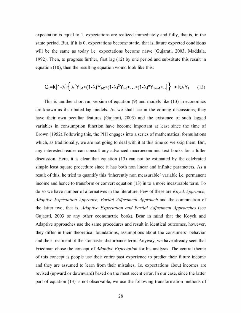
28

expectation is equal to 1, expectations are realized immediately and fully, that is, in the

same period. But, if it is 0, expectations become static, that is, future expected conditions

will be the same as today i.e. expectations become naïve (Gujarati, 2003, Maddala,

1992). Then, to progress further, first lag (12) by one period and substitute this result in

equation (10), then the resulting equation would look like this:

Ct=k1-Yt-1+(1-)Yt-2+(1-)2Yt-3+…+(1-)nYt-n-1+.. + kYt (13)

This is another short-run version of equation (9) and models like (13) in economics

are known as distributed-lag models. As we shall see in the coming discussions, they

have their own peculiar features (Gujarati, 2003) and the existence of such lagged

variables in consumption function have become important at least since the time of

Brown (1952).Following this, the PIH engages into a series of mathematical formulations

which, as traditionally, we are not going to deal with it at this time so we skip them. But,

any interested reader can consult any advanced macroeconomic text books for a fuller

discussion. Here, it is clear that equation (13) can not be estimated by the celebrated

simple least square procedure since it has both non linear and infinite parameters. As a

result of this, he tried to quantify this ‘inherently non measurable’ variable i.e. permanent

income and hence to transform or convert equation (13) in to a more measurable term. To

do so we have number of alternatives in the literature. Few of these are Koyck Approach,

Adaptive Expectation Approach, Partial Adjustment Approach and the combination of

the latter two, that is, Adaptive Expectation and Partial Adjustment Approaches (see

Gujarati, 2003 or any other econometric book). Bear in mind that the Koyck and

Adaptive approaches use the same procedures and result in identical outcomes, however,

they differ in their theoretical foundations, assumptions about the consumers’ behavior

and their treatment of the stochastic disturbance term. Anyway, we have already seen that

Friedman chose the concept of Adaptive Expectation for his analysis. The central theme

of this concept is people use their entire past experience to predict their future income

and they are assumed to learn from their mistakes, i.e. expectations about incomes are

revised (upward or downward) based on the most recent error. In our case, since the latter

part of equation (13) is not observable, we use the following transformation methods of

29

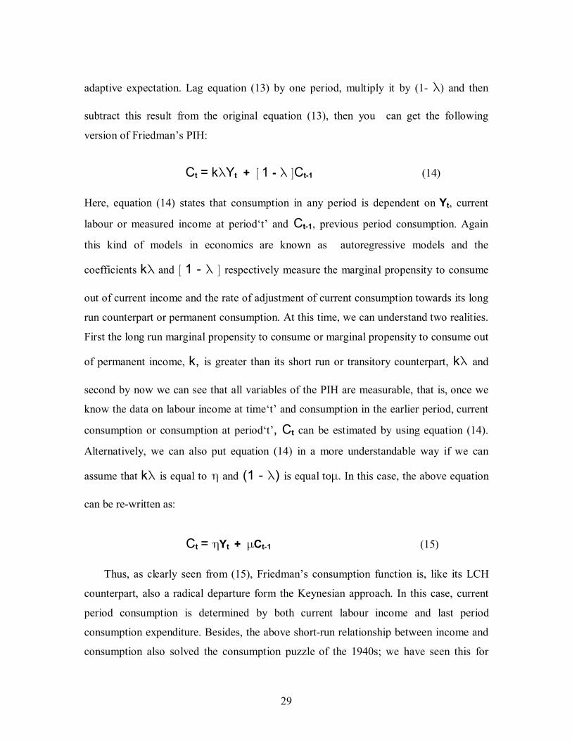
adaptive expectation. Lag equation (13) by one period, multiply it by (1- ) and then

subtract this result from the original equation (13), then you can get the following

version of Friedman’s PIH:

Ct = kYt + 1 - Ct-1 (14)

Here, equation (14) states that consumption in any period is dependent on Yt, current

labour or measured income at period‘t’ and Ct-1, previous period consumption. Again

this kind of models in economics are known as autoregressive models and the

coefficients k and 1 - respectively measure the marginal propensity to consume

out of current income and the rate of adjustment of current consumption towards its long

run counterpart or permanent consumption. At this time, we can understand two realities.

First the long run marginal propensity to consume or marginal propensity to consume out

of permanent income, k, is greater than its short run or transitory counterpart, k and

second by now we can see that all variables of the PIH are measurable, that is, once we

know the data on labour income at time‘t’ and consumption in the earlier period, current

consumption or consumption at period‘t’, Ct can be estimated by using equation (14).

Alternatively, we can also put equation (14) in a more understandable way if we can

assume that k is equal to and (1 - ) is equal to. In this case, the above equation

can be re-written as:

Ct = Yt + Ct-1 (15)

Thus, as clearly seen from (15), Friedman’s consumption function is, like its LCH

counterpart, also a radical departure form the Keynesian approach. In this case, current

period consumption is determined by both current labour income and last period

consumption expenditure. Besides, the above short-run relationship between income and

consumption also solved the consumption puzzle of the 1940s; we have seen this for

30

LCH. For PIH’s part, Friedman assumes that past period consumption acts as a shift

parameter and in the long run, as income rises successively the later part of the above

equation also shifts upward to keep up with the new levels of current incomes. Then, if

we try to connect the intersection points of the new current incomes with the new levels

of lagged values of consumption, we would get the long run consumption function that

passes through the origin. As we have put above, it was this kind of consumption

function that Kuznets had proposed in the mid 1940s. Hence, Milton Friedman, in his

own way, solved one of the problems the Keynesian consumption function.

When we come to the empirical analysis of the PIH, Friedman tested equation (15) or

its counterpart (13) for the US economy for the periods 1905-1951 excluding the war

years. In his groundbreaking book, he put the result as follows k=0.88, = 0.33 and 0.67

for. So, the marginal propensities for the US economy for the specified period can

easily found by multiplying k and , that is equal to, is 0.299 (Wonnacott, 1978) This

means an average US citizen consume only 0.29 cents of labour income from each

additional dollar for the specified period, of course, keeping all other factors unchanged.

This was just what was expected from the theory (Sachs and Larrain B., 1993). Other test

by other individuals show that the permanent income theory generally provides a slightly

better explanation of consumer behavior than a very simple hypothesis based on current

income, though this margin of superiority is “ small and not consistently maintained” (

Friend and Kravis, 1957). Similarly, Singh and Drost (1971) by themselves test the

applicability of the PIH for eleven countries and they conclude that the theory ‘offers a

valid explanation of the consumption behavior of countries with different economic

structures.’ But note that though the theoretical underpinning is the same, they use their

own method of testing techniques that is different form the one we have seen above or

proposed by Friedman.

However, the above success stories of the PIH were forced to face other

contradictory results by different individuals. As reported by Singh and Drost (1971),

economists like Choudhury and Laumans found a significant marginal propensities to

31

consume out of transitory income for different countries. That means consumption

responses to current income ‘beyond the extent attributed to it by the theory’. Such

results are confirmed by economists like Flavin who coined a phrase excess sensitivity to

such property (Flavin, 1981). Hence after, this phrase has become famous in the literature

to refer to such role of current income in the consumption behavior. The other point that

Sing and Frost would like to underscore in their paper is that the existence of some kind

of relationship between transitory and permanent income. Clearly, these two facts

contradict with what the theory assumes. Other literatures criticized the PIH on the bases

of the difficulty of testing it against time series data and so forth. In general, in the

literature, we find a number of critics on the PIH and they usually circle around two

points. The first and the most important of these critics focuses on Friedman’s approach

to the adaptive expectation (Sachs and Larrain B., 1993). We know that in this concept of

adaptive expectation people use their past incomes to forecast their future expected or

permanent income and we have seen that past or lagged consumption are also used to

predict current consumption. From this what we can easily understand is that past or

lagged incomes also help to predict or explain current consumption (Hall, 1978). This

kind of perception, however, is gravely criticized by a number economists. Among these,

Robert Hall of the Stanford University is the forerunner. He argued that ‘intelligent and

forward looking consumers’ use or process not only past experiences about their incomes

but also all the available information, that is, past, current, and future (Hall, 1978). This

kind of expectation in economics is known as rational expectation and in this case rather

than using a simple ‘recursive formula’ consumers are assumed to maximize expected

lifetime utility based on all information available then, that is, they use detailed

conceptual models of the economy to form their expectation (Sachs and Larrain B., 1993,

Hall, 1978). In so doing, based on understanding of the industry of the region they work,

consumers are assumed to develop a numerical model of estimating their income, that is,

they process all the available information each period about current and future incomes

and hence, on the basis of that they determine an appropriate current level of

consumption. In this context, several current studies on consumption prefer to base their

analysis on rational expectation behavior. This rational expectation version of the PIH or

Hall’s Random Walk Hypothesis has several interesting implication regarding the

32

behavior of the consumers in the economy for policy analysis. For instance, it attempts to

explain the effect of news on consumption, that is, it argues that life is full of ‘surprise’

some are predictable while others are not. In this case, he [Hall] considers that only those

unpredictable changes or ‘surprises’ in the life of consumers make them to revise their

consumption. How? Such discussion, however, will take us far a field and it is a bit

complicated so I prefer to skip it. However, a fuller discussion of such concepts can be

found in any advanced macroeconomics text book like Branson (1989) or Romer (2001).

To sum up, Hall’s Hypothesis argued that consumers are rational and use this concept of

rationality to form their expectation; hence, they use all the available information to

decide the optimum level of consumption. In so doing, only that unpredictable

information affects consumption because they always act according to the predictable

news or information. Thus, only past information is not enough to predict current

consumption rather rational expectation behavior should be incorporated in the original

version of the PIH.

The other shortcoming of the PIH is the assumption of no liquidity constraint. We

have seen this case for the LCH. In such context, the approach under discussion argued

that households can borrow and lend as much as they want at zero or the same interest

rate (Houthakker, 1958). That is for Friedman the capital market is assumed to be almost

perfect but “there is not, in practice, a perfect capital market” (Farrell, 1959). Thus,

consumers can not freely borrow against future income and this liquidity constraint

would force them to follow the AIH version of consumption function with a significant

role for current wealth i.e. liquidity constraint is one of the major reasons ‘why

consumption can frequently not adjusted to permanent income’ (Houthakker,1958

Branson, 2006). But, the effect of such constraint is only one sided since it can not limit

the consumers from saving; hence, postponing current consumption for the future would

be optional.

Despite theses failures, the PI theory has several interesting implications for the

economy. Among these, it is useful to identify the effects of income shocks on

consumption. In this case, we have three types of shocks on income-temporary current

shocks, permanent shocks, and anticipated shocks (Sachs and Larrain B., 1993). While

the economy will fully adjust to in the case of permanent shocks, temporary shocks force

33

it to dissave. On the other hand, households tend to raise their saving for anticipated

shocks. In PIH terminologies these outcomes can be restated in the following ways. First

temporary shocks dose not affect permanent income so consumption is not affected that

much. Second, in the face of permanent shocks, consumption falls a lot and saving

affected little. Finally, anticipated shocks cause a decline in permanent income and hence

consumption but saving rises.

Regarding the saving behavior of the economy, though it is arguable( Houthakker,

1958), Friedman assumes that saving is only responsive to the transitory component of

measured income, that is, marginal propensity to consume out of transitory income is

zero (Friend and Kravis, 1957). We have seen that this conclusion came from Friedman’s

third assumption about transitory consumption and transitory income. In this case, a

windfall income will not immediately affect consumption; thereby, it would be saved.

This conclusion is supported by various findings (Bhalla, 1980).The PIH also assumes

that the country’s saving rate tends to be depressed in the face of growing economy. This

is due to the fact that productivity growth means income growth and this growth in

income raises expected or permanent income of the economy relative to current income.

As a result, consumption rises; thereby, saving is forced to decline (Modigliani, 1986).

This conclusion helps to understand why some countries with high per capita income and

highly advanced financial institutions are characterized by unexpected low saving rate

while others which are not enjoying high income or such kind of financial institutions

save a significant portion of their national income. According to this simple argument of

PIH, in the growing economy and hence per capita income, the permanent part of income

becomes higher than that of its transitory counterpart. But we have already said that

saving is very sensitive to transitory income than permanent income. Therefore, in the

face of high growth rates countries which obey the PIH are characterized by low saving.

On the contrary, if low growth rate is always registered in the country, much of the

country’s population can not be certain about its long term expected income so it saves a

significant portion of its current or measured income to finance future consumption. If we

try to relate this suggestion with the current realities of our country, we can appreciate the

following important policy implication. In the introductory part of this study, we

mentioned little about the economic boom or ‘mini boom’ that our country is enjoying

34

right now, the terrible conditions of the country’s saving rate and the importance of

saving to economic growth. So if we analyze such case based on the PIH theory, we can

say that the long run scenario of the country’s saving rate is very worrying. Because as

we said earlier if the current growth persists, a typical Ethiopian consumer’s permanent

component income rises. This causes transitory income to decline; thereby thrift or

saving will be depressed. This point indicates that unless there is some policy

intervention by the respective body of government to do something in this course, we are

on the road to an even depressed saving ratio and hence lower growth trend. We will

fully consider this and similar implications of the theory in the coming chapters.

2.3 THE ETHIOPIAN CASE

From the above discussions it has become very clear that for any economy the

variable consumption expenditure is the largest component of aggregate output and our

country’s case is not far from this conclusion. Due to this nature of private consumption,

there are mountains of debates in the literature and we have already seen that though it is

only in sketchy manner because of space and time constraints. When we come to our

country’s case, however, for the reasons not clearly known, we find only a hand full of

studies on private consumption expenditure (Solomon, 1999) and almost all of these

studies primarily focus either on finding the major determinants of household

consumption expenditure or on the analysis of its flipside- the saving function. But, we

know that our objectives in this study are slightly different from such analyses. For that

reasons in this section, we briefly consider the essence the available few studies primarily

conducted on consumption. I believe that will give us at lest some picture about what has

been done for the past years and the stage of knowledge development regarding the

variable at hand.

For our country, attempts of testing the traditional theories of consumption behavior

are made by a few individuals and according to the materials at hand, the earliest of these

efforts is the one which is made by Asmerom in 1987 (Solomon, 1999). He tried to

assess the consumption behavior of the economy from the outline of the AIH and PIH.

By considering ‘permanent income forecasted from two years moving average process’

he found that consumption to track transitory income rather than that of permanent

35

income. Interestingly, this outcome clearly contradicts with what we have said in our

earlier discussions. However, since the goodness of fit [the R-square] for his model is

very small, we can say that there should be some problems in his specification or data

analysis. Regarding the AIH, he found the result which are not consistent with ‘priori

restrictions implied by the theory’. Another effort to drive a realistic approach of the

consumption function is made by Daniel (Solomon, 1999) though he chiefly interested in

the analysis of the country’s saving trend. Daniel, in his analysis, incorporated the effect

of some important variables like liquidity constraints and uncertainty due to manmade

and natural factors [e.g. war and rainfall variability]. Besides, he tried to show the effect

of foreign savings and taxes on the saving performance of the country. When we

discover the main findings of his study that are relevant to us, we observe that saving is

highly responsive to transitory income. This is exactly the same as what the Life-Cycle-

Permanent Income theory argued. Besides, he used the lag of broad money (M2) as a

proxy to capture the effect of liquidity constraint on consumption, however; his effort

resulted in unexpected outcome i.e., the sign of liquidity constraint becomes positive. The

other important contribution towards the field is of Solomon’s advanced attempt to model

the consumption function for the country using macro variables. In this case, he was

interested in finding the effect of income, inflation, government spending and money

supply, captured by broad money (M2), on consumption expenditure for the periods from

1960-1996. Using the advanced method of the Maximum Likelihood Estimation

procedures and a Vector Autoregressive (VAR) model, he found that private

consumption is responsive to ‘both current disposable income and anticipated permanent

income’ (Solomon, 1999). This implies that both the AIH and PIH framework have some

sort of the explanatory power for our economy.

Though, all these studies provide some picture in understanding the variable under

discussion, one can clearly see that they are a bit outdated. So, we have to look for other

recent studies which provide a better perspective. In that case, we primarily find Oman’s

study (2006). Like his predecessors, Oman’s approach principally focuses on discovering

the determinants of private consumption expenditure using macro variables. In so doing,

in addition to the usual personal disposable income, he incorporated variables like tax

revenue, government expenditure, inflation, rainfall and liquidity constraint captured by,

36

of course , broad money (M2) into his analysis. Then, when we consider the variable of

our interest [real disposable income], he found consumption to track both current

disposable income and [real] permanent income in line with the specifications of AIH

and PIH respectively. Oman’s findings clearly support that of Solomon’s though the

former uses a slightly different methodology for a different sample period.

Generally, we have seen that though they use a little different methodology which is

suitable to their primary objectives, almost all of the above papers concentrate on similar

central ideas of relating consumption with its determinants. In addition to that, they even

employ almost the same economic variable in their analysis and of course, all are dealt

with aggregate level. However, there are also other researches with a slight deviation

from these perspectives. For instance, Zelalem (2005) would like to consider somewhat

different approach in his study. He attempted to analyze, among other things, the effect of

income and household size on consumption expenditure using the year 2000 micro data

for 871 individual households in the capital city. The outcome of this study shows that

consumption is affected by both income, as presupposed by the theories, and household

size. We have marginally seen that the LCH consider the effect of family size into its

analysis. Here, Zelalem utilized such concept in the analysis of household consumption

behavior. When we consider his analysis in detail, we find that the R-square is very low

[0.21] and he attributed that for omitting other important variables from his model. In the

literature, we usually encounter such kind of very low R-square particularly for cross-

sectional data (Gujarati, 2003). Since the data he used in his study is of that kind, such

low R-square should not be considered as a series problem. The shortcoming of

Zelalem’s study that should be mentioned here, however, is that he did not explicitly

indicate the type of income he specified in his model. From our discussion so far, we

know that income is decomposed into past, current and future or the combination of the

tree. We also know that each theory uses its own version of income for its particular

analysis. But, Zelalem did not effectively treat this concept in his paper.

Other important paper that is done at household level and should be mentioned here

is that of EDRI5’s Nigussie’s work on four selected villages in rural Ethiopia. In his part,

5 EDRI-Ethiopian Development Research Institute, a government think tank which is primarily interested

in formulating and analysis of policies.

37

he argued that ‘generally rural households in agrarian communities, where-rain

dependent crop cultivation is the primary source of household income, have income that

vary seasonally’ (Nigussie, 2006). Hence, he tried to verify whether consumption is

responsive to that seasonal income or not. Considering this argument from the Life

Cycle-Permanent Income framework, we understand that he is simply trying to show

whether consumption [primarily on food] is sensitive to that transitory [seasonal]

agricultural income or not. Based on that notion, he conducted a cross-sectional level

study for the total of 247 households in the four rural villages which represent different

agro-ecological zones. Among other important results, the major findings of his study is

that consumption generally does not follow such huge seasonal variation in income i.e.

household consumption expenditure is smooth or similar in the face of such erratic

agricultural income. Again this conclusion clearly shores up the arguments of Modigliani

and Friedman which, as we know, argue consumption is primarily influenced by the

long-run average income of the individual rather than that of short run or transitory gains.

The last, but not the least, study that deserves a fuller discussion here is that of Abebe’s

(2005) powerful and interesting paper on the implication of the Life-Cycle Hypothesis of

Modigliani et.al. In that case, he used a panel data that covers the period 1994-2000 for

1,500 households in both rural and urban areas of the country. Then, he defined his

consumption variable to include households’ expenditures both on food and non food

items but not on ‘durables, rent in urban areas and other expenditures on fixed assets’ and

‘current real value of crops sold by the household were used as proxies for lagged

income’ for rural areas (Abebe, 2005). Besides, he used rainfall as instrument to measure

income shocks in rural areas. To capture the effect of wealth on consumption, he used

proxy variables like total land owned, total value of household assets owned and number

of oxen owned for rural areas and lagged total household income and value of household

assets were used for urban areas. In his analysis, he also tried to asses the effect of

employment status [to capture transitory income shocks], monthly cash saving in iqub, a

widely practiced informal saving association in the Ethiopian tradition [to capture the

possibilities of consumption smoothing] and other important variables on the household’s

decisions on spending its income. Then, he finally found that current consumption is

responsive to ‘lagged variables such as income and wealth and consumption itself’

38

(Abebe, 2005) and he characterized this outcome to precautionary savings, liquidity

constraint, habit persistence etc. Nonetheless, we know that this finding clearly

contradicts what the LCH theory presupposes. Therefore, due to these facts the LCH

could not provide a better understanding of the consumption behavior of the Ethiopian

economy.

To conclude, our discussion, of course this chapter, we have seen the central points

of the theories of consumption behavior that are to be tested in this study. Additionally,

as several countries experiences show these competing theories provide some explanatory

power besides the US and West Europe economies, the economies where these theories

principally developed for. In our case, due to scarcity of researches on this topic, we have

seen only few studies and the major findings of these available papers slightly contradict

with what we have seen in the theories, that is, some studies argued for the existence of

some evidences for theses hypothesis while others provide proofs to refute that argument.

But, be aware that, this paper is not only in a position to report the findings of other

studies but to provide some evidence for or against the explanatory power of these

hypotheses as well. That is the major topic of the next chapter.

39

Chapter Three

DaTa, Methods of data analysis And Empirical Estimation

By reviewing the literatures on the dynamic relation between consumption and income,

chapter two of this study laid down the groundwork for our analysis and, provides

suitable mathematical models of the respective theories for ease of estimation. But, that is

only half of the job to be carried out in this study. The other part, in fact, which would be

the most important part of this study, is to estimate such models using country-level data.

As a result, in this chapter we continue our discussion of the variable under investigation

with the principal objective of estimating the mathematical models provided in chapter

two. Here, we focus only on the models that make use of the available data. Equation (4)

of the Life Cycle Hypothesis is not going to be estimated because of the absence of data

on non-labour income or net worth. In so doing, this chapter is divided into two major

parts. The first part analyzes the nature and sources of data to be used and introduces the

methods to be employed in the analysis process. In this case, we use aggregate time series

data and we know that though its analysis looks very simple, time series data usually

have their own problems and peculiar features. Hence, in the first part of this chapter, we

try to handle this topic. Additionally, a brief discussion of those mathematical models

will be given and we will try to provide the nature of our models, particularly that of

autoregressive [dynamic] model. In all these processes, we will incorporate the

disturbance term to capture the effect of other variables other than income or that of

income shocks on household consumption expenditure. In such context, we deal with

stochastic models rather than those of the deterministic models so far introduced

(Maddala, 1992). The addition of this stochastic variable, nonetheless, poses problems in

estimation. Therefore, such and other topics will be considered in the first part of this

chapter. Then, in the second part, we will be busy of estimating these models by using the

data at hand.

40

3. 1 SOURCE AND NATURE OF DATA

In chapter two, we saw that Keynes’s Absolute Income theory relates current

consumption to current income both measured in real terms and from equation (1) its

stochastic version becomes:

Ct = + Ytd + εt (16)

Ct and Ytd represent consumption expenditure and disposable income at time‘t’

respectively. The new variable, εt, is the error term that captures the effect of all other

variables on consumption other than current income or that of income shocks. Similarly,

from Friedman’s theory of consumption function, we have generated the following

testable form of Permanent Income theory:

Ct = Yt + Ct-1 + vt (17)

In this case also, equation (17) relates current consumption, Ct, with disposable income,

Yt and the lag of current consumption, Ct-1. Here, the error term, vt, serves the same

purpose as that of in equation (16) but it is generated in a slightly different process. We

will consider that later on. The primary objective of this study is to test these two

equations by using the country level aggregate time series data.

Clearly, to estimate these two equations we need data only on consumption

expenditure and disposable income. For that purpose, such data are obtained from

EEA/EEPRI Macroeconomic Database. In that case, we find data on private consumption

expenditure (Ct) and gross or aggregate disposable income (Ytd) for the periods 1953-

1996 E.C.[1960/61-2003/04 G.C]6. However, for that of disposable income (Yt

d) the data

is available only for the periods 1963-1996 E.C. [1970/71-2003/04 G.C.], that is, for the

latter variable we are forced to miss some observations. Additionally, both variables are

6 According to the EEA/EEPRI Database, the figures for the years 1993-1996 E.C [2000/01-2003/04 G.C]

are obtained through some kind of estimation process and they are not actual figures for these two

variables.

41

nominal, i.e., they are measured at current market prices. Thus, as we have seen, our data

are time series in nature and we know that in economics time series data are frequently

plagued by the problems of autocorrelation, nonstationarity and spurious relation. The

presence of such undesirable qualities heavily affects our estimation results and; hence,

leads to misleading conclusions (Gujarati, 2003, Green, 2003).

3.1.1. AUTOCORRELATION

No auto-or serial- correlation between successive disturbance terms is one of the

most important assumptions of the OLS estimation processes. In this case, it argued that

the successive values of the error terms do not follow some kind of ‘systematic pattern’

or there is no intercorrelation among them. However, as we have said earlier, in a number

of economic analyses such relation does not hold and the above assumption is violated.

At this time, we say that the error term in our data is ‘flooded with the problem of serial

correlation or autocorrelation’ (Wooldridge, 2000). The main causes of this serial

correlation are inertia, cobweb phenomena, transformation and manipulation of data, etc

(Gujarat, 2003, Maddala, 1992). The existence of autocorrelation in the series results in

‘linear, unbiased and consistent estimators but they are no longer efficient or do not have

minimum variance’ (Gujarat, 2003). This means the usual t ratios become unreliable for

testing hypothesis; thereby, leading to a wrong or misleading conclusion. Hence, the

problem of autocorrelation has very serious consequences and should carefully be

detected and minimized or avoided if possible.

Although it rests on important assumptions about the existing series, the most famous

detecting instrument for the presence of serial correlation between successive residuals is

that of the Durbin Watson [DW] statistics. From our econometric background, however,

we know that the DW statistic detects only first order serial correlation, i.e. it assumes

that the error term is generated in the process of first order autoregressive method or it is

an AR(1). Besides, it also considers that the model should not contain the lagged values

of the dependent variable as an explanatory variable. For the AIH model, this statistic is

very helpful and can directly be applied to detect the problem. Nonetheless, for that of the

PIH, it [the DW] requires some kind of modification since this model incorporates the

lagged dependent variable as an explanatory variable. In this context, we use the indirect

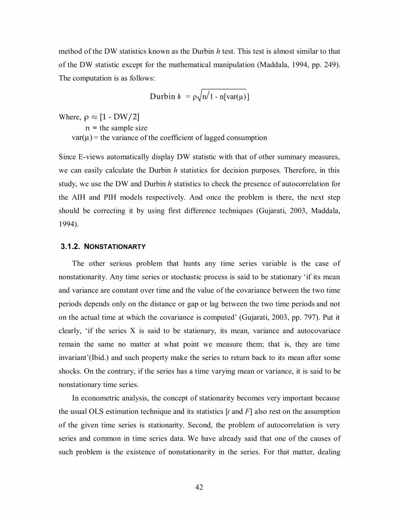
42

method of the DW statistics known as the Durbin h test. This test is almost similar to that

of the DW statistic except for the mathematical manipulation (Maddala, 1994, pp. 249).

The computation is as follows:

Durbin h = ρ n 1 - n[var(µ)]/

Where, ρ [1 - DW/2]

n = the sample size

var( )µ = the variance of the coefficient of lagged consumption

Since E-views automatically display DW statistic with that of other summary measures,

we can easily calculate the Durbin h statistics for decision purposes. Therefore, in this

study, we use the DW and Durbin h statistics to check the presence of autocorrelation for

the AIH and PIH models respectively. And once the problem is there, the next step

should be correcting it by using first difference techniques (Gujarati, 2003, Maddala,

1994).

3.1.2. NONSTATIONARTY The other serious problem that hunts any time series variable is the case of

nonstationarity. Any time series or stochastic process is said to be stationary ‘if its mean

and variance are constant over time and the value of the covariance between the two time

periods depends only on the distance or gap or lag between the two time periods and not

on the actual time at which the covariance is computed’ (Gujarati, 2003, pp. 797). Put it

clearly, ‘if the series X is said to be stationary, its mean, variance and autocovariace

remain the same no matter at what point we measure them; that is, they are time

invariant’(Ibid.) and such property make the series to return back to its mean after some

shocks. On the contrary, if the series has a time varying mean or variance, it is said to be

nonstationary time series.

In econometric analysis, the concept of stationarity becomes very important because

the usual OLS estimation technique and its statistics [t and F] also rest on the assumption

of the given time series is stationarity. Second, the problem of autocorrelation is very

series and common in time series data. We have already said that one of the causes of

such problem is the existence of nonstationarity in the series. For that matter, dealing

43

with the problem of stationarity also helps to provide a solution to that of autocorrelation.

The other importance of stationary time series is that it is used for forecasting purpose. If

the series is not stationary, forecasting process will be difficult. On top of that, a

regression of a nonstationary time series on another nonstationary time series usually

results in spurious or nonsense regression. Therefore, for these and other reasons the

concept of stationarity is very common in time series econometric analysis (Ibid.).

To detect the presence of nonstationarity we can simply use the graphical method

and watch if the series is trending with time or not. If there is trending, we can say that

the given series is nonstationary or has a unit root. Nevertheless, for a formal and

powerful method of testing nonstationarity, we have to conduct the Augmented Dickey-

Fuller (ADF) test by considering the null hypothesis as the existing series has a unit root

(Wooldridge, 2000, Green, 2003). E-views automatically perform this job once we

command it. Hence, once we found that the given series is nonstationary, the next step is

transforming it to stationary time series. To do so, the famous method is taking

successive differences until it becomes stationary. Thus, if the series X is stationary

without any differencing technique, we call it is stationary at level or integrated of order

zero, that is, X~ I (0) However, if it becomes stationary after taking the first-difference,

we call it is an integrated of order one, or X~ I (1). Similarly, if the series becomes

stationary after we difference it twice, it is an integrated of order two or X~I (2) and so

on. In general, if the series X becomes stationary after differencing it d times, we call it is

an integrated of order d or X~I (d). In this case, we know that most macroeconomic time

series becomes stationary after differencing them once (Green, 2003).

3.1.3. COINTEGRATION Earlier, we said that the regression of a nonstationary time series on another

nonstationary time series results into a spurious or nonsense regression. In this case,

although there is no actual relationship between these two variables, the OLS regression

results into a statistically significant t values and large R-squared with high probability

(Wooldridge, 2000), thereby, leading into an incorrect decisions. However, if the linear

combination of these two [or any number of] nonstationary series becomes stationary at

level, i.e., if it is an I (0) process, we can conclude that despite short run differences,

44

these series are cointegrated or they have long run relationships. This concept of

cointegration tries to relate ‘short-run dynamics with that of long-run equilibrium’

(Maddala, 1994). Hence, we should check whether our regression is spurious or not by

conducting a cointegration test.

To execute a cointegration test, again we use the ADF test on the residual (Ibid.) and

once we find that those variables are cointegrated, the next step is to construct an Error

Correction Mechanism (ECM).

3.2. MODEL ANALYSIS AND METHODOLOGY

In this study, we use both a simple liner and an autoregressive models for empirical

analysis. Clearly, the estimation and interpretation processes of the former model are so

straightforward that it will not be considered here. The latter mode, however, has its own

typical features that usually create problems in empirical estimation. Thus, it should

deserver series attention. For these reasons, in this section, we would briefly consider

those features in conjunction with some methodological issues.

The mathematical version of the PIH i.e. equation (17) relates consumption at any

period with that of current income and past period consumption. The addition of lagged

dependent variable as an explanatory variable in our model, nevertheless, poses the

following problems (Gujarati, 2003). First, we know that the OLS assumes that all the

explanatory variables in the model should be fixed in repeated sampling or they are

considered to be nonstochastic. However, in our case, we include, in addition to income,

the lagged value of consumption, stochastic by its nature, on the right hand side of the

equation. Due to his fact, we violate one of the most important assumptions of the

classical linear regression model. Second, to arrive at equation (17) or its deterministic

counterpart [i.e. equation 15]; we made a number of mathematical derivations. In that

process, the error term, vt, lucks some of its desirable properties. This means if we

assume that the error term of equation (9) of the last chapter is ωt then in the processes of

lagging and subtracting vt becomes:

vt = [ωt- (1- ) ωt-1] (18)

45

Thus, the error term in equation (17) depends on that of equation (9) or ωt. For that

reason, if the latter is plugged with the problem of serial correlation, the former would be

so. Hence, we should consider this problem in attacking the problem of serial correlation.

The other problem is the coming of lagged dependent variable as explanatory variable.

Obviously, this violates one of the assumptions of the DW statistic.We have seen this

before. In the process of estimation, we will use the Durbin h statistic to capture the

problem of serial correlation. On top of these, the error term in equation (17) may not

satisfy the OLS assumptions, i.e., the lagged explanatory variable (Ct-1) may be

correlated with that of the error term, vt.

In short, in one way or another, the above arguments suggest not to use the OLS for

models like that of equation (17). Gujarati (2003) argued any direct application of OLS

‘will result into biased and inconsistent estimators’. Green (2003) also acknowledges

models that relate consumption with income usually incorporate the lag of the dependent

variable as a regressor that pose estimation problems. For his part, he concluded that

direct application of OLS to such models would be ‘disastrous’. But, this does not mean

that we are helpless. Wooldridge (2000) takes a different perspective

“Beginners in econometrics are often warned of the danger of serially correlated errors in the

presence of lagged dependent variables. Almost every textbook on econometrics contains

some form of the statement ‘OLS is inconsistent in the presence of lagged dependent variables and serially correlated errors.’ Unfortunately, as a general assertion, this statement

is false” (pp.378)

and later he highlighted that if we have a good reason to incorporate a lagged dependent

variable in our model, we can introduce that and, at the same time, we can use the OLS.

For that matter, we know that the lagged dependent variable in our model is included

because the PIH dictates so. Hence, we will not be mistaken if we estimate equation (17)

by the least square method.

Having said that, to test the validity of the Absolute Income Hypothesis, we will

regress consumption only on current income. If that gives meaningful pictures, the AIH is

accepted, whereas if it does not, the AIH is refuted. Similarly, for the Permanent Income

Hypothesis case, we will run consumption on current income and lagged consumption

46

and if this result is plausible, the PIH is accepted, however, if it does not confirm with

what have said so far, the PIH is rejected.

3.3 EMPERICAL ESTIMATIONS AND PRESENTATION OF RESULTS

Since the usual test statistics of least squares procedure rests on the assumption of the

given time series is stationary, our empirical analysis begins with conducting a unit root

test for our data. Following that, due to its ease of estimation and analysis, theoretical

reasons and chronological order, we first deal with Keynes’s consumption function and

later we will consider Friedman’s case. In this process, most of our subsequent analyses

are based on regression techniques. To carry out this estimation technique successfully,

we will use the software package E-views 3.1 version. Besides, to make concepts very

clear, we also employ graphical analysis whenever necessary.

3.3.1 TESTING FOR UNIT ROOT

The following table summarizes the conditions of stationaryity for the two variables.

NOTE: * &** respectively represent 1% and 5% level of significance for the rejection of

the null hypothesis for the existence of the unit root.

TABLE 1:-RESULTS OF THE ADF TESTS

From the above table, we can clearly understand that, at level, both variables are

nonstationary or they are trending over time. This condition can be clearly understood

from the following graph.

NAME OF VARIABLE

ADF STATISTIC

CONDITIONS OF STATIONARITY

CONSUMPTION (Ct)

-3.373066**

I(1)

DISPOSABLE INCOME (Ytd)

-4.831702*

I(1)

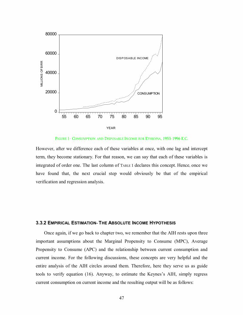
47

0

20000

40000

60000

80000

55 60 65 70 75 80 85 90 95

CONSUMPTION

DISPOSABLE INCOME

YEAR

MIL

LIO

NS

OF

BIR

R

FIGURE 1- CONSUMPTION AND DISPOSABLE INCOME FOR ETHIOPIA, 1953-1996 E.C.

However, after we difference each of these variables at once, with one lag and intercept

term, they become stationary. For that reason, we can say that each of these variables is

integrated of order one. The last column of TABLE 1 declares this concept. Hence, once we

have found that, the next crucial step would obviously be that of the empirical

verification and regression analysis.

3.3.2 EMPIRICAL ESTIMATION- THE ABSOLUTE INCOME HYPOTHESIS

Once again, if we go back to chapter two, we remember that the AIH rests upon three

important assumptions about the Marginal Propensity to Consume (MPC), Average

Propensity to Consume (APC) and the relationship between current consumption and

current income. For the following discussions, these concepts are very helpful and the

entire analysis of the AIH circles around them. Therefore, here they serve us as guide

tools to verify equation (16). Anyway, to estimate the Keynes’s AIH, simply regress

current consumption on current income and the resulting output will be as follows:

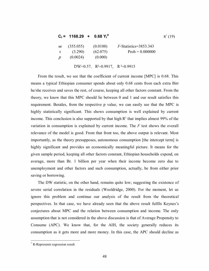
48

Ct = 1168.29 + 0.68 Yt

d R7 (19)

se (355.055) (0.0100) F-Statistics=3853.343

t (3.290) (62.075) Prob = 0.000000

p (0.0024) (0.000)

DW=0.57, R2=0.9917, R-2=0.9915

From the result, we see that the coefficient of current income [MPC] is 0.68. This

means a typical Ethiopian consumer spends about only 0.68 cents from each extra Birr

he/she receives and saves the rest, of course, keeping all other factors constant. From the

theory, we know that this MPC should lie between 0 and 1 and our result satisfies this

requirement. Besides, from the respective p value, we can easily see that the MPC is

highly statistically significant. This shows consumption is well explained by current

income. This conclusion is also supported by that high R2 that implies almost 99% of the

variation in consumption is explained by current income. The F test shows the overall

relevance of the model is good. From that front too, the above output is relevant. Most

importantly, as the theory presupposes, autonomous consumption [the intercept term] is

highly significant and provides an economically meaningful picture. It means for the

given sample period, keeping all other factors constant, Ethiopian households expend, on

average, more than Br. 1 billion per year when their income become zero due to

unemployment and other factors and such consumption, actually, be from either prior

saving or borrowing.

The DW statistic, on the other hand, remains quite low; suggesting the existence of

severe serial correlation in the residuals (Wooldridge, 2000). For the moment, let us

ignore this problem and continue our analysis of the result from the theoretical

perspectives. In that case, we have already seen that the above result fulfils Keynes’s

conjectures about MPC and the relation between consumption and income. The only

assumption that is not considered in the above discussion is that of Average Propensity to

Consume (APC). We know that, for the AIH, the society generally reduces its

consumption as it gets more and more money. In this case, the APC should decline as

7 R-Represents regression result

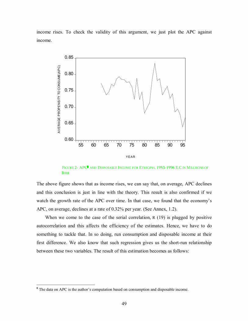
49

income rises. To check the validity of this argument, we just plot the APC against

income.

0.60

0.65

0.70

0.75

0.80

0.85

55 60 65 70 75 80 85 90 95

AV

ER

AG

E P

RO

PE

NS

ITY

TO

CO

NS

UM

E(A

PC

)

YEAR

FIGURE 2- APC8 AND DISPOSABLE INCOME FOR ETHIOPIA, 1953-1996 E.C IN MILLIIONS OF

BIRR

The above figure shows that as income rises, we can say that, on average, APC declines

and this conclusion is just in line with the theory. This result is also confirmed if we

watch the growth rate of the APC over time. In that case, we found that the economy’s

APC, on average, declines at a rate of 0.32% per year. (See Annex, 1.2).

When we come to the case of the serial correlation, R (19) is plugged by positive

autocorrelation and this affects the efficiency of the estimates. Hence, we have to do

something to tackle that. In so doing, run consumption and disposable income at their

first difference. We also know that such regression gives us the short-run relationship

between these two variables. The result of this estimation becomes as follows:

8 The data on APC is the author’s computation based on consumption and disposable income.

50

Ct = 17.768 + 0.65Ytd R (20)

se (219.85) (0.0607) F-Statistics=115.8213

t (0.081) (10.762) Prob = 0.000000

p (0.9361) (0.0000)

DW=2.51, R2=0.7888, R-2=0.7820

NOTE: Now on is used as first difference operator.

From the above result, we can say that the MPC is almost the same and it is still highly

significant. Besides, in the short-run consumption becomes a relatively stable function of

disposable income. That is, in the short-run, individual consumers spend, on average,

only 0.65 cents of each extra Birr and save the rest, 0.35 cents. The former value is a bit

smaller to consider the Ethiopians as ‘myopic’ consumers that waste any windfall gains

and such stable trend of consumption can readily be seen from Figure 3 below. This

result, on the one hand, supports Keynes argument that, in the short-run, consumption is

much more a stable function of real income than that of money income (Dillard, 1979);

on the other hand, it contradicts with what we said in the previous chapters. That means

the literatures so far have already categorized the Ethiopians as extravagant consumers

who spend each extra gains of their income and we have seen that this conclusion rests up

on empirical evidence (Befekadu Degefe and Berhanu Nega, 1999/2000) but our result

does not confirm that. In this paper, however, we are not in a position to investigate why

such discrepancy occurs but we will reconsider this concept in the later discussion. When

we continue our discussion with the above results, in R (20), the constant term is still

meaningful but statistically insignificant with high standard error. Nevertheless, be

reminded that empirical literature in this respect usually does not incorporate the intercept

term in most first difference estimation processes (Gujarati, 2003). Besides, if we re-run

R (20) with out the intercept term, the resulting outcome will be almost identical to that of

the above result (See Annex 1.4). From the DW value, we can see the existence of some

form of serial correlation. But, at this time, it is negative autocorrelation and it is not as

series as the one we saw in earlier results. This shows, in the short-run model, we have

relatively little problem of serial correlation. Be aware that, as we know, autocorrelation

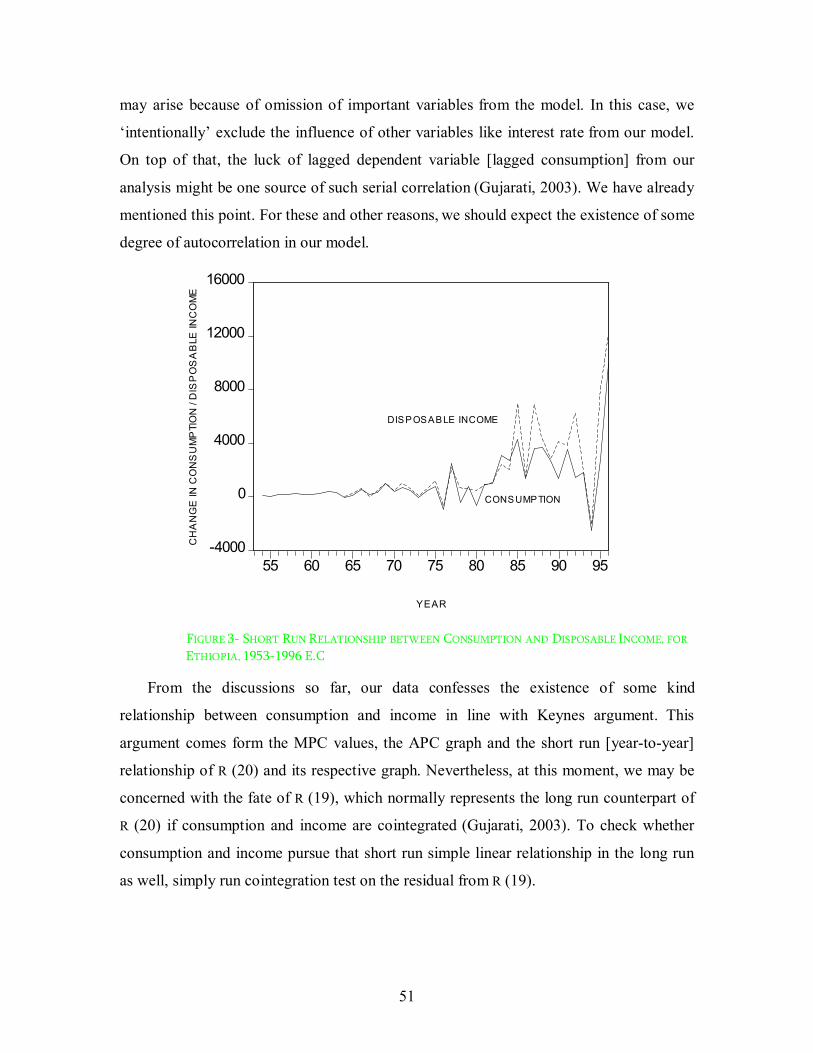
51

may arise because of omission of important variables from the model. In this case, we

‘intentionally’ exclude the influence of other variables like interest rate from our model.

On top of that, the luck of lagged dependent variable [lagged consumption] from our

analysis might be one source of such serial correlation (Gujarati, 2003). We have already

mentioned this point. For these and other reasons, we should expect the existence of some

degree of autocorrelation in our model.

-4000

0

4000

8000

12000

16000

55 60 65 70 75 80 85 90 95

CONSUMPTION

DISPOSABLE INCOME

YEAR

CH

AN

GE

IN C

ON

SU

MP

TIO

N /

DIS

PO

SA

BLE

INC

OM

E

FIGURE 3- SHORT RUN RELATIONSHIP BETWEEN CONSUMPTION AND DISPOSABLE INCOME, FOR

ETHIOPIA, 1953-1996 E.C

From the discussions so far, our data confesses the existence of some kind

relationship between consumption and income in line with Keynes argument. This

argument comes form the MPC values, the APC graph and the short run [year-to-year]

relationship of R (20) and its respective graph. Nevertheless, at this moment, we may be

concerned with the fate of R (19), which normally represents the long run counterpart of

R (20) if consumption and income are cointegrated (Gujarati, 2003). To check whether

consumption and income pursue that short run simple linear relationship in the long run

as well, simply run cointegration test on the residual from R (19).

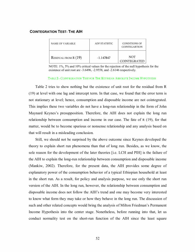
52

COINTEGRATION TEST- THE AIH

NOTE: 1%, 5% and 10% critical values for the rejection of the null hypothesis for the

existence of unit root are -3.6496, -2.9558, and -2.6146 respectively.

TABLE 2:- COINTEGRATION TEST FOR THE KEYNSIAN ABSOLUTE INCOME HYPOTHESIS

Table 2 tries to show nothing but the existence of unit root for the residual from R

(19) at level with one lag and intercept term. In that case, we found that the error term is

not stationary at level; hence, consumption and disposable income are not cointegrated.

This implies these two variables do not have a long-run relationship in the form of John

Maynard Keynes’s presupposition. Therefore, the AIH does not explain the long run

relationship between consumption and income in our case. The fate of R (19), for that

matter, would be to become spurious or nonsense relationship and any analysis based on

that will result in a misleading conclusion.

Still, we should not be surprised by the above outcome since Keynes developed the

theory to explain short run phenomena than that of long run. Besides, as we know, the

sole reason for the development of the later theories [i.e. LCH and PIH] is the failure of

the AIH to explain the long-run relationship between consumption and disposable income

(Mankiw, 2002). Therefore, for the present data, the AIH provides some degree of

explanatory power of the consumption behavior of a typical Ethiopian household at least

in the short run. As a result, for policy and analysis purpose, we use only the short run

version of the AIH. In the long run, however, the relationship between consumption and

disposable income does not follow the AIH’s trend and one may become very interested

to know what form they may take or how they behave in the long run. The discussion of

such and other related concepts would bring the analysis of Milton Friedman’s Permanent

Income Hypothesis into the center stage. Nonetheless, before running into that, let us

conduct normality test on the short-run function of the AIH since the least square

NAME OF VARIABLE

ADF STATISTIC

CONDITIONS OF COINTEGARTION

RESIDUAL FROM R (19)

-1.147847

NOT COINTEGRATED

53

estimate holds the residual to follow some kind of normal distribution (Wooldridge,

2000).

NORMALITY TEST ON THE AIH Normality test [the JB test] for the residual from R (20) shows that the variable is not

distributed in line with the OLS requirement (See Annex, 1.6). This obviously affects the

quality of the parameters, the subsequent inferences and that of the DW statistics. So, for

that reason, we have to do something to make the residual term of R (20) close to normal.

The best prescription is to take the natural logarithm of the variable and run the

regression on that form (Wooldridge, 2000). When we do so, we get the following

results:

lnCt = 0.99 lnYtd R (21)

se (0.077) DW=2.60, R2=0.70, R-2=0.70

t (12.79)

p (0.000)

In R (21), clearly, the slope coefficient measures the short-run elasticity of consumption

expenditure, i.e. the percentage change in consumption because of a one percent rise in

disposable income. Hence, it seems current consumption is very sensitive to current

income i.e. if disposable income rises by one percent, similarly consumption expenditure,

on average, will rise almost by one percent. Of course, that is for the same level of other

factors. But, that is only in the short run. This result also supports Keynes’s argument of

the sensitivity of consumption to current income. When we come to the normality case,

the JB test (Annex, 1.7) shows that in the above short run logarithmic model the error

term is distributed close to that of normal distribution. The DW statistic, however, almost

remains the same. So, at this time, we should reconsider the previous arguments9.

9 We remember that, in the review section, we discuss, among other things, each theory’s arguments on

saving. In this chapter; however, we are unable to consider the empirical validity of such arguments only

because of lack of data on national saving.

54

3.3.3 EMPIRICAL ESTIMATION- THE PERMANENT INCOME HYPOTHESIS From chapter two, we also know that the PIH rests up on the following important

pillars. First, like Keynes, Friedman assumes that MPC is between 0 and 1 but in this

case, we have two MPCs i.e. MPC out of current income and MPC out of long run or

permanent income. For Friedman, the latter should be greater than that of the former.

Second, unlike Keynes, Friedman considers that APC is almost constant over time and

consumption is a function of permanent income than that of current income. Hence, as we

did for the AIH’s cases, these concepts would be very helpful for our subsequent

discussions. Thus, to check the validity of the above arguments, let us run the stochastic

version of the PIH for our data. In that case, the result will be the following:

Ct = 0.45Ytd + 0.402Ct-1 R (22)

se (0.071) (0.1084) F-Statistics= 4120.653

t (6.290) (3.7113) Prob = 0.000000

p (0.000) (0.0008)

DW=0.84, R2=0.9921, R-2=0.9920

As the above result shows, the coefficients of current income and lagged consumption are

highly statistically significant and from the R2 we can say that almost 99% of the

variation in current consumption is explained by that of current income and of last period

consumption behavior. When we consider each coefficient, MCP out of current income

or the short run MPC is 0.45. That means a typical Ethiopian consumer who obeys the

PIH specifications will consume only, on average, 0.45 cents of each extra Birr of current

income. It is a quite low value, particularly when we consider it from the AIH viewpoint,

which was around 0.65. But if the increase or the surge in income continues [real income

grows] the long run MPC will become around 0.75 cents10

. In short, ‘consumers

consumes only 0.45 cents of each extra Birr of current or observed income but when they

10 From chapter two we know that short run MPC is equal to the long run MPC multiplied by that

adjustment parameter i.e. MPC= k = 0.45 and the coefficient of lagged consumption 0.402 is 1- .

Thus, form a simple algebraic manipulation long run MPC [k]becomes 0.75.

55

have time to adjust to a Br.1 change in income, they will increase their consumption

ultimately by about 0.75 cents’ ( Gujarati, 2003). In other words, the short run effect of a

Br.1 increase of income on consumption is only 0.45 cents but in the long run, its effect

almost doubles. These findings clearly support Friedman’s argument about the short run

and long run MPCs and we observe that a long run increase in income results into a

depressed saving. We saw in chapter two that the PIH argues in that way and why that

occurs. Similarly, the adjustment parameter measures the rate of adjustment of current

consumption towards its long run counterpart. In our case, = 0.598; hence, within a

given year, almost 60 % of current consumption is adjusted towards its long run

counterpart. The implication of this concept, however, is beyond the scope of this paper

(Gujarati, 2003)

From these discussions, we can see that the PIH has some kind of explanatory power

of our data. But, if we try to see the APC of our economy from Friedman’s point of view,

we get this result.

1.50

1.55

1.60

1.65

1.70

1.75

1.80

1.85

20000 40000 60000

DISPOSABLE INCOME

AV

ER

AG

E P

RO

PE

NS

ITY

TO

CO

NS

UM

E (

AP

C)

FIGURE 4- APC11 AND DISPOSABLE INCOME FOR ETHIOPIA, 1953-1996 E.C IN MILLIIONS OF

BIRR

11 The data on APC is the author’s computation based on consumption and disposable income and taken as

the ratio of consumption lag and disposable income to that of disposable income.

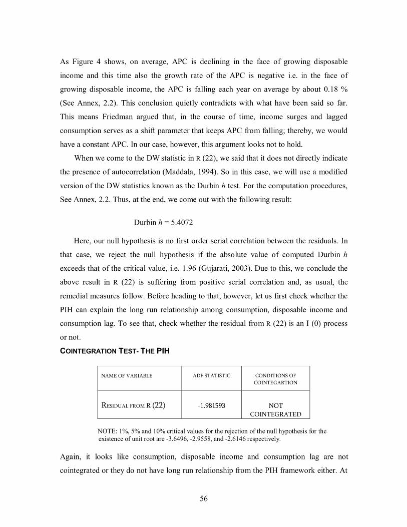
56

As Figure 4 shows, on average, APC is declining in the face of growing disposable

income and this time also the growth rate of the APC is negative i.e. in the face of

growing disposable income, the APC is falling each year on average by about 0.18 %

(See Annex, 2.2). This conclusion quietly contradicts with what have been said so far.

This means Friedman argued that, in the course of time, income surges and lagged

consumption serves as a shift parameter that keeps APC from falling; thereby, we would

have a constant APC. In our case, however, this argument looks not to hold.

When we come to the DW statistic in R (22), we said that it does not directly indicate

the presence of autocorrelation (Maddala, 1994). So in this case, we will use a modified

version of the DW statistics known as the Durbin h test. For the computation procedures,

See Annex, 2.2. Thus, at the end, we come out with the following result:

Durbin h = 5.4072

Here, our null hypothesis is no first order serial correlation between the residuals. In

that case, we reject the null hypothesis if the absolute value of computed Durbin h

exceeds that of the critical value, i.e. 1.96 (Gujarati, 2003). Due to this, we conclude the

above result in R (22) is suffering from positive serial correlation and, as usual, the

remedial measures follow. Before heading to that, however, let us first check whether the

PIH can explain the long run relationship among consumption, disposable income and

consumption lag. To see that, check whether the residual from R (22) is an I (0) process

or not.

COINTEGRATION TEST- THE PIH

NOTE: 1%, 5% and 10% critical values for the rejection of the null hypothesis for the

existence of unit root are -3.6496, -2.9558, and -2.6146 respectively.

Again, it looks like consumption, disposable income and consumption lag are not

cointegrated or they do not have long run relationship from the PIH framework either. At

NAME OF VARIABLE

ADF STATISTIC

CONDITIONS OF COINTEGARTION

RESIDUAL FROM R (22)

-1.981593

NOT COINTEGRATED

57

this time, however, we should be surprised by this outcome, since the PIH is proposed

primarily to explain the long run relationship between these two variables. Unfortunately,

the data at hand does not support the existence of such relationship between current

consumption and long run income. Consequently, the relationship at R (22) becomes

spurious and should not be used for any analysis. When such cases arise, the literatures

frequently suggest to focus on the short run relationship rather than that of the long run as

we did for the AIH’s case. But, at this moment, we cannot do that because we have no

theoretical bases to check the short run implication of a theory that principally developed

to explain the long run relationship. Therefore, at this stage, it is better to list some

possible reasons for the failure of the PIH and wind up this chapter.

3. 4 WHY THE PERMANENT INCOME HYPOTHESIS HAS FAILED TO EXPLAIN OUR DATA? For other economies, this question is almost as old as the theory itself and in the

literature; still there is no consensus among economists and theoreticians on why the PIH

has a remarkable explanatory power in some countries while it fails to do so in others.

Since, we briefly consider those debates in chapter two, in this section; we highlight only

the major points that chiefly related to our case.

A . The Nature and Quality of the Data

We have seen in the previous chapter that households allocate their income

between consumer durable and nondurable goods and services and the respective theory,

be it the AIH or the PIH, formulates its own definition of consumption for its particular

analysis. For Keynes, the term consumption includes every expenditure made by the

households on durable, nondurable and services. His perception was that of total

consumption than expenditure on particular goods. For Friedman, however, consumption

includes expenditure on nondurable goods, services and the use value of durables. From

these, we can see that these two individuals argue for the same thing but in different

ways.

Now come to our case, the data source for this study is EEA/EEPRI Macroeconomic

Data Base and there is no a clear indicator whether the data refers to expenditure on

durables, nondurables or services. However, we would not be mistaken if we assume that

58

CSA considers household’s every expenditure on durable, nondurable and service as

consumption i.e. in line with Keynes’s perception. Because, for it [ the CSA], collecting

expenditure data on nondurable and services and computing the use value of durables are

quite difficult task that claims huge resource, qualified enumerators and advanced

techniques for computation. Thus, this condition clearly affects the quality of our data

and it might be one of the reasons for the failure of the PIH.

B . The Assumptions of The Hypothesis

In this case, we can mention at least the following key points

a) No liquidity constraint- which, as we have seen, force consumers to track

current income than maximizing lifetime utility.

b) Infinite life horizon-this unrealistic assumption ignores the concept of

bequest and the bequest motive which are important sources of saving and

wealth; thereby, future consumption (Modigliani, 1986)

c) The case of ‘excess sensitivity’- we have seen that consumption may be

sensitive to current income ‘beyond the degree attributed to it by the

theory’.

d) The adaptive expectation mechanism-this point is gravely criticized by a

number of economists and based on empirical evidences, they produce

alternative models of expectation to measure long run variables like that of

permanent income. In this case, we can mention, at least, naïve

expectation and rational expectation (Maddala, 1992). In this study, we

estimate the PIH by assuming, Ethiopians obey that of the adaptive

expectation formulation. This is primarily because of the nonexistent of

research on this topic. However, at this time, no one can be sure whether

consumers in this country follow such specification or they use rational or

naïve mechanisms.

Hence, it should be underscored that these bold assumptions might also be the major

causes for the failure of the explanatory power of the PIH for our or data.

59

In this chapter, we tested the explanatory power of the AIH and the PIH and at this

time, we are, at least, confident of saying that John Maynard Keynes’s AIH has a slight

advantage over Milton Friedman’s PIH. However, that is only in the short run. When we

consider the long run case, neither of these theories is able to explain the data at hand. On

the one hand, this conclusion might partly solve the problem that initiates this research;

on the other hand, it brings several controversies. For instance, the AIH assumes

consumption to track current disposable income but we know that income is zero after

retirement. In this case, the AIH argued people consume from autonomous income.

Logically, the source of such income would be saving from working age i.e. prior saving

or borrowing and this accumulated saving clearly results into wealth (Modigliani and

Cao, 2004). Hence, in this context, we can observe that current consumption becomes

sensitive to accumulated wealth. In this case, Modigliani’s argument seems to have an

advantage, while the AIH fails to explain clearly the conditions of consumption after

retirement. This is only one case. The other point is the case of that contradictory result

we saw earlier. This means from the AIH perspective, we can see that Ethiopians cannot

be categorized as ‘myopic’ consumers since consumption is almost stable in the face of

fluctuating income and that of the MPC is relatively low. On the contrary, prior

researches argue that Ethiopians are ‘conspicuous consumers’ who rush to expend each

windfall gain of their income. Clearly, these two arguments do not go together and, in

this paper, we are not going to reconcile such discrepancy because it will take us to the

analysis of wealth, habits, and other factors that affect consumption expenditure other

than that of income (Oman, 2006). Obviously, we do not incorporate these concepts in

this paper only because the scope of the study is limited to that of the analyses of the

theories. But, these two and other related cases require a close attention and I believe they

would be potential sources of future study.

To sum up, our research finds that the AIH is a bit superior than that of the PIH.

From this, we may reasonably ask the following questions. What does this imply for the

country’s economy, what policy prescriptions arise from that and, of course, what the

government and the stakeholders are supposed to do according to the AIH? Well, these

are series of somewhat tough questions but the next chapter may have some answers.

60

Chapter FOUR

CONCLUSION AND Recommendations

4.1 CONCLUSION Here comes the conclusion part. The previous pages were trying to verify the validity

of Keynes’s Absolute Income Hypothesis and Friedman’s Permanent Income Hypothesis

by using country-level time series data. In other words, we were attempting whether

consumption is determined by current or long run expected income and finally we have

found that consumption not to follow a martingale process i.e. its past values were not

useful to predict the current value (Woodridge, 2000) and hence, the PIH were not able to

explain the dynamic relationship between income and consumption in Ethiopia. This

failure, almost, is attributed to the nonexistent of those bold assumptions the theory made

and the lack of data measuring techniques in line with the theory’s assumption. For that

of the AIH, however, it provides a relatively meaningful picture. Be remind that, this is

only in the short run. In the long run, we were not able to analyze the consumption

behavior of the households here. Because both theories lack the ability to explain that in

this period. Hence, our subsequent discussions will primarily focus on that of John

Maynard Keynes’s economic philosophies that are principally related to the variable

under investigation and relevant to us. This is to mean that since our data verify the

existence of some relationship between consumption and income in line with Keynes

presupposition, we use his understanding as a spring board for the respective policy

recommendations. We remember that Keynes used this concept of consumption as a

stepping stone for his analysis of economic fluctuation. Therefore, in the coming

discussions we will try to do the same thing as he did for Britain and West Europe

economies some seventy or so years ago.

4.2. POLICY PRESCRIPTIONS 4.2.1. ON UNEMPLOYMENT- PROGRASSIVE TAXATION

We know that the prime objective of John Maynard Keynes economic philosophy is

to answer the question what determines the volume of employment in the economy

61

(Dillard, 1979) and he found that a high propensity to consume [consumption] is one

source of employment.

Hence, in recession periods, according to Keynes, the major source of unemployment

in any economy is luck of enough spending [aggregate demand] by its economic actors

and to keep this employment at its desired level, such spending, be it by the public, by the

private sector [investment] or by the household [consumption], is necessary. For our case,

a high MPC that indicates a high spending by the household is suitable for employment

in the country plugged with burgeoning numbering of unemployed youth and the

government and its policy think tanks should focus on this point. Here, the MPC [0.65]

serves as a multiplier to these spendings (Mankiw, 2002). In this case, the prescription is

that taxes on income should be progressive. This is to redistribute income from those

with high income and low MPC [Remember that argument on APC] to that of low

income with high MPC. At the end of the day, the society’s APC rises; thereby, more

spending and employment would arise.

4.2.2. ON INFLATION- REGRESSIVE TAXATION In the inflationary periods, on the other hand, the rising price takes ‘wealth away

from some people and hands it over to others in a manner which disregards the maxims

of social equity’ ( Dillard, 1979). Here, to reduce the effect of this rising prices, policies

should focus on curbing ‘effective demand’. This involves decreasing the MPC by

imposing higher tax rates that directly falls on disposable income. In this case, the tax

becomes some kind of regressive. This is because of the fact that MPC is relatively

higher for lower income group than that of higher income groups. Hence, this regressive

taxation system discourages consumption by the mass poor which is characterized by

high MPC, while it encourages the consumption of those with low MPC and high saving

rate.

These arguments make sense for the country suffering from galloping inflation and

high unemployment, like our country’s case, thus; policy makers, think tanks, pundits,

should also consider this argument to attack the inflationary phenomena.

To conclude this chapter, in fact this study, let us underline few points. First, to

repeat the obvious, consumption, in the short run, is found to be responsive to current

62

income than past or expected future income. Due to this fact, the above prescribed tax

policies should focus on this short run relationship between these two variables and

hence, taxes should be transitory, not permanent by their very nature. Second, the above

prescriptions are forwarded in the sense that all other factors like government

expenditure, investment, money supply are assumed to be remaining constant. Of course,

in the short run, these factors usually remain constant. On top of these, we know that the

AIH is primarily developed to explain the consumption behavior of the rich capitalist

societies who can absorb the burdens of both regressive and progressive taxes. In our

case, however, recommending regressive taxation seems not to consider the realities on

the ground and the extent of poverty in the country. But, do get confused that since this

conclusion arises from the findings of the research, we are in a position to recommend the

government and its policy think tanks to follow only that way. Rather, what we are

arguing, here, is that the government policy makers should consider this concept too

when they forward any prescriptions regarding the above problems.

63

BIBILOGRAPHY

1. Abebe Shimeles (2005): “The Dynamics of Consumption in Ethiopia”,

Doctorial Dissertation, Gothenburg University, EEA.

2. Ando, A. AND Modigliani, F., (1963): “The Life Cycle Hypothesis of Saving:

Aggregate Implications and Tests.” American Economic Review,

Vol. 53, No 1, PP. 55-84.

3. Barro, R. J. AND Sala-i-Martin, X., (2004): Economic Growth, Prentice-

Hall of India, New Delhi

4. Befekadu Degefe AND Berhanu Nega, (1999/2000): Annual Report on the

Ethiopian Economy, United Printers, Addis Ababa.

5 Bhalla, S.S., (1980): “The Measurement of Permanent Income and Its

Application to Saving Behavior”, Journal of Political Economy, Vol.

88, No. 4, pp. 722-743.

6. Blanchard, O. J., (1997): Macroeconomics, Prentice Hall, New Jersey

7. Branson, W.H., (1989): Macroeconomics Theory and Policy, Harper &

Row Publishers, New York.

8. Branson, W.H., (2006): Macroeconomics Theory and Policy, AITBS

Publishers, India.

9. Brown, T.M., (1952): “Habit Persistence and Lags In Consumer Behavior”,

Econometrica, Vol. 20, No. 3, pp. 355-371

10. Dillard, D., (1979): The Economics of John Maynard Keynes, Vikas

Publishing, India. 11. Dornbusch, R., Fischer, S. AND Sparks, G.R., (1982): Macroeconomics: First Canadian Edition, McGraw-Hill-Ryerson Limited, Canada.

12. Dornbusch, R. AND Fischer, S., (1994), Macroeconomics, McGraw-Hill Inc,

New York.

13. EEA, (2005/06): Annual Report on the Ethiopian Economy

64

14. Farrell, M.J., (1959): “The New Theories of The Consumption Function”,

Economic Journal, December, pp. 678-695.

15. Flavin M.A., (1981): “The Adjustment of Consumption to Changing

Expectations about Future Income”, Journal of Political Economy,

Vol. 89, No. 5, pp. 974-1009.

16. Friend, I. AND Kravis, I.B., (1957): “Consumption Pattern and Permanent

Income”, American Economic Review, Proceeding, Vol. 47, pp. 536-

554

17. Gilboy, E.W., (1938): “The Propensity to Consume, Summary”, Quarterly

Journal of Economics, November, pp.120-140

18. Greene, W.H., (2003): Econometric Analysis, Prentice Hall, New Jersey

19. Gujarati, D.N., (2003): Basic Econometrics, Tata McGraw-Hill, New Delhi

20. Hall, R.E., (1978): “Stochastic Implications of The Life Cycle-Permanent

Income Hypothesis: Theory and Evidence”, Journal of Political

Economy, Vol. 86, No. 6, pp. 971-987 21. Houthakker, H.S., (1958): “The Permanent Income Hypothesis, A Review

Article”, American Economic Review, Vol. 48, pp.396-406

22. Keynes, J.M., (1949): The General Theory of Employment, Interest &

Money, Macmillan, London.

23. Kurihara, K.K., (1957): Introduction to Keynesian Dynamics, George

Allen & Unwin Ltd, London.

24. Maddala, G.S., (1992): Introduction to Econometrics, Macmillan

Publishing, New York

25. Mankiw, N.G., (2002): Macroeconomics, McGraw Hill Irwin, New York.

65

26. McConnell, C. R., AND Brue, S. L., (1994): Economics: Principles,

Problems, & Policies, McGraw Hill Irwin, New York.

27. Mitchell, C. W., (1947): What Veblen Taught, Selected Writings of

Thorstein Veblen, Sentry Press, New York.

28. Modigliani, F., (1986): “Life Cycle, Individual Thrift and Wealth of Nations.”

American Economic Review, Vol. 76, No. 3, PP. 297-313.

29. Modigliani, F. AND Cao, L. S., (2004): “The Chinese Saving Puzzle and The

Life-Cycle Hypothesis”, Journal of Economic Literature, Vol. XLII

pp. 145-170.

30. Mulat Demeke (2003): “Agricultural Development in Ethiopia: The

Challenges of Overcoming Famine.” in Tesfahun F. & Osman A.,

eds. Challenges and Prospects of Food Security in Ethiopia, Addis

Ababa, Berhan Selam Printing Enterprise.

31. Negussie Tefera (2006): “Consumption and Income Seasonality and Food

Deficiency in Rural Ethiopia”, Paper Presented to the Fourth

Annual Conference of EEA, EEA.

32. Oman Amulu Akway (2006): “An Econometric Analysis of Personal

Consumption Expenditure in Ethiopia”, Unpublished MSc Thesis,

AAU.

33. Romer, D. (2001): Advanced Macroeconomics, McGraw Hill, New York.

34. Sachs, J.D. AND Larrin B, F., (1993): Macroeconomics In the Global

Economy, Prentice Hall, New Jersey.

35. Seldon, A. AND Pennance, F.G., (1969): Everyman’s Dictionary of

Economics, J.M. Dent & Sons Ltd, London.

66

36. Singh, B. AND Drost, H., (1971): “An Alternative Econometric Approach To

The Permanent Income Hypothesis: An International Comparison”,

Review of Economics and Statistics, Vol. LIII, pp.326-334

37. Solomon Tesfay (1999): “Modeling Aggregate Private Consumption Behavior

in Ethiopia”, Unpublished MSc. Thesis, AAU.

38. Todaro, M. P. AND Smith, S. C., (2003): Economic Development, Pearson

Educational Limited, Essex, England.

39. Vaish, M.C., (1980): Macroeconomic Theory, Vikas Publishing House Ltd,

New Delhi.

40. Venieris, Y. P. AND Sebold, F. D., (1977): Macroeconomics: Models and

Policy, John Wiley & Sons, New York.

41. Wonnacott, P., (1978): Macroeconomics, Richard D. Irwin, Inc, Illinois

42. Wooldridge, J.M., (2000): Introductory Econometrics, Thomson South-

Western University Press

43. World Bank, (2007): World Development Indicator

44. Zemalem Tesfaye (2005): “Household Consumption Behavior in A.A: Using

Micro Data”, Senior Essay, AAU

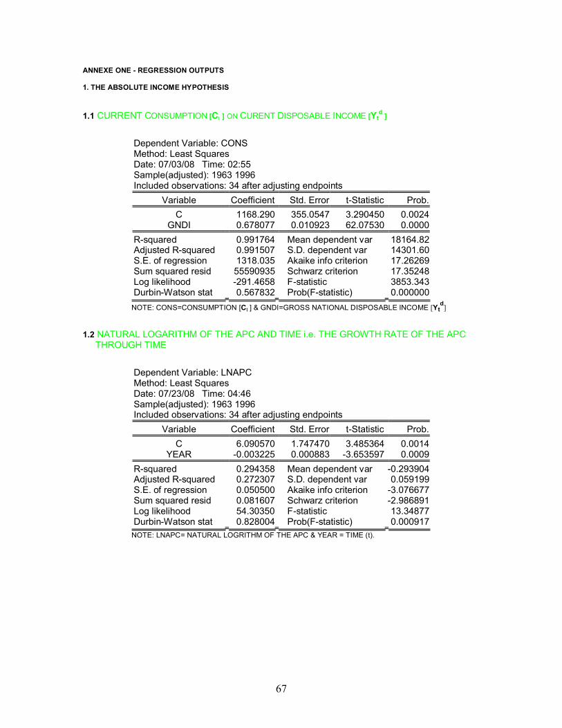
67

ANNEXE ONE - REGRESSION OUTPUTS 1. THE ABSOLUTE INCOME HYPOTHESIS 1.1 CURRENT CONSUMPTION [Ct ] ON CURENT DISPOSABLE INCOME [Yt

d ]

Dependent Variable: CONS Method: Least Squares Date: 07/03/08 Time: 02:55 Sample(adjusted): 1963 1996 Included observations: 34 after adjusting endpoints

Variable Coefficient Std. Error t-Statistic Prob. C 1168.290 355.0547 3.290450 0.0024

GNDI 0.678077 0.010923 62.07530 0.0000 R-squared 0.991764 Mean dependent var 18164.82 Adjusted R-squared 0.991507 S.D. dependent var 14301.60 S.E. of regression 1318.035 Akaike info criterion 17.26269 Sum squared resid 55590935 Schwarz criterion 17.35248 Log likelihood -291.4658 F-statistic 3853.343 Durbin-Watson stat 0.567832 Prob(F-statistic) 0.000000

NOTE: CONS=CONSUMPTION [Ct ] & GNDI=GROSS NATIONAL DISPOSABLE INCOME [Ytd

]

1.2 NATURAL LOGARITHM OF THE APC AND TIME i.e. THE GROWTH RATE OF THE APC THROUGH TIME

Dependent Variable: LNAPC Method: Least Squares Date: 07/23/08 Time: 04:46 Sample(adjusted): 1963 1996 Included observations: 34 after adjusting endpoints

Variable Coefficient Std. Error t-Statistic Prob. C 6.090570 1.747470 3.485364 0.0014

YEAR -0.003225 0.000883 -3.653597 0.0009 R-squared 0.294358 Mean dependent var -0.293904 Adjusted R-squared 0.272307 S.D. dependent var 0.059199 S.E. of regression 0.050500 Akaike info criterion -3.076677 Sum squared resid 0.081607 Schwarz criterion -2.986891 Log likelihood 54.30350 F-statistic 13.34877 Durbin-Watson stat 0.828004 Prob(F-statistic) 0.000917

NOTE: LNAPC= NATURAL LOGRITHM OF THE APC & YEAR = TIME (t).

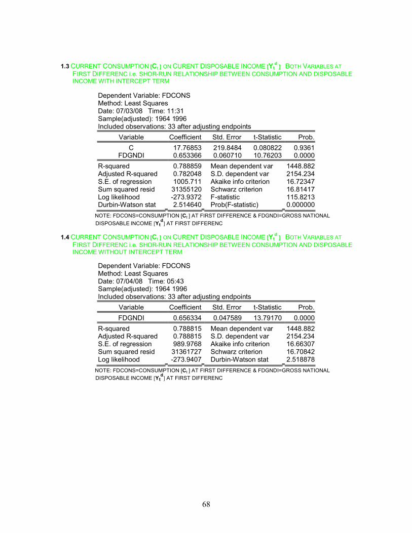
68

1.3 CURRENT CONSUMPTION [Ct ] ON CURENT DISPOSABLE INCOME [Yt

d ] BOTH VARIABLES AT FIRST DIFFERENC i.e. SHOR-RUN RELATIONSHIP BETWEEN CONSUMPTION AND DISPOSABLE INCOME WITH INTERCEPT TERM

Dependent Variable: FDCONS Method: Least Squares Date: 07/03/08 Time: 11:31 Sample(adjusted): 1964 1996 Included observations: 33 after adjusting endpoints

Variable Coefficient Std. Error t-Statistic Prob. C 17.76853 219.8484 0.080822 0.9361

FDGNDI 0.653366 0.060710 10.76203 0.0000 R-squared 0.788859 Mean dependent var 1448.882 Adjusted R-squared 0.782048 S.D. dependent var 2154.234 S.E. of regression 1005.711 Akaike info criterion 16.72347 Sum squared resid 31355120 Schwarz criterion 16.81417 Log likelihood -273.9372 F-statistic 115.8213 Durbin-Watson stat 2.514640 Prob(F-statistic) 0.000000

NOTE: FDCONS=CONSUMPTION [Ct ] AT FIRST DIFFERENCE & FDGNDI=GROSS NATIONAL DISPOSABLE INCOME [Yt

d] AT FIRST DIFFERENC

1.4 CURRENT CONSUMPTION [Ct ] ON CURENT DISPOSABLE INCOME [Yt

d ] BOTH VARIABLES AT FIRST DIFFERENC i.e. SHOR-RUN RELATIONSHIP BETWEEN CONSUMPTION AND DISPOSABLE INCOME WITHOUT INTERCEPT TERM

Dependent Variable: FDCONS Method: Least Squares Date: 07/04/08 Time: 05:43 Sample(adjusted): 1964 1996 Included observations: 33 after adjusting endpoints

Variable Coefficient Std. Error t-Statistic Prob. FDGNDI 0.656334 0.047589 13.79170 0.0000

R-squared 0.788815 Mean dependent var 1448.882 Adjusted R-squared 0.788815 S.D. dependent var 2154.234 S.E. of regression 989.9768 Akaike info criterion 16.66307 Sum squared resid 31361727 Schwarz criterion 16.70842 Log likelihood -273.9407 Durbin-Watson stat 2.518878

NOTE: FDCONS=CONSUMPTION [Ct ] AT FIRST DIFFERENCE & FDGNDI=GROSS NATIONAL DISPOSABLE INCOME [Yt

d] AT FIRST DIFFERENC

69

1.5. NATURAL LOGRATITHM OF CONSUMPTION [Ct ] ON NATURAL LOGARITHM OF DISPOSABLE

INCOME [Ytd ] AT THEIR FIRST DIFFERENC

Dependent Variable: FDLCONS Method: Least Squares Date: 07/07/08 Time: 22:42 Sample(adjusted): 1964 1996 Included observations: 33 after adjusting endpoints

Variable Coefficient Std. Error t-Statistic Prob. FDLGNDI 0.989255 0.077350 12.78934 0.0000

R-squared 0.704144 Mean dependent var 0.075089 Adjusted R-squared 0.704144 S.D. dependent var 0.084825 S.E. of regression 0.046138 Akaike info criterion -3.284508 Sum squared resid 0.068120 Schwarz criterion -3.239160 Log likelihood 55.19439 Durbin-Watson stat 2.605469

NOTE: FDLCONS=NATURAL LOGRATHIM OF CONSUMPTION [Ct ] & FDLGNDI=NATURAL LOGRATHIM GNDI AT FIRT DIFFERENCE 1.6. NORMALITY TEST FOR THE RESIDUL FROM THE SHORT RUN MODEL OF THE AIH-THE JB TEST

0

2

4

6

8

10

12

-3000 -2000 -1000 0 1000 2000

Series: ResidualsSample 1964 1996Observations 33

Mean -3.45E-13Median 78.74249Maximum 2105.521Minimum -2689.450Std. Dev. 989.8725Skewness -0.627252Kurtosis 3.983168

Jarque-Bera 3.493050Probability 0.174379

HO= the residual is normally distributed H1= HO is not true The JB statistic follows the chi-square distribution with 2 degree of freedom

DECESION RULE: Reject HO If the computed p [probability] value of the JB statistic in an application is sufficiently low, which will happen if the value of the statistic is very different from 0. Other wise, do not reject

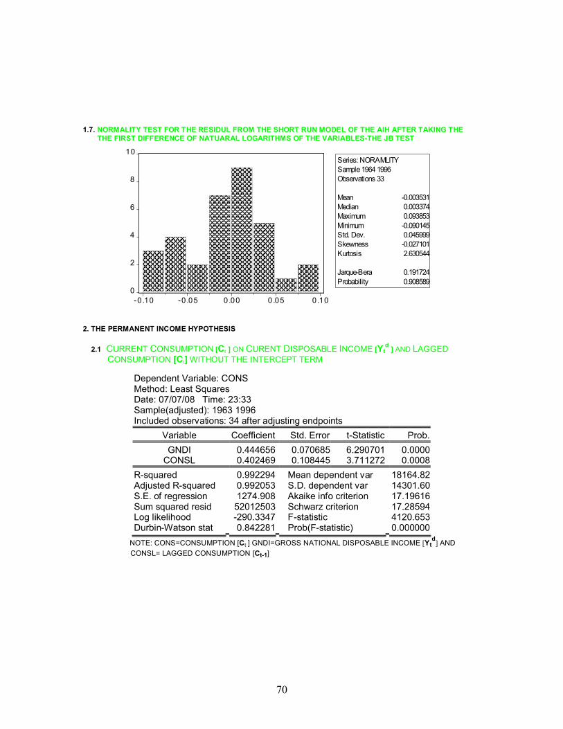
70

1.7. NORMALITY TEST FOR THE RESIDUL FROM THE SHORT RUN MODEL OF THE AIH AFTER TAKING THE THE FIRST DIFFERENCE OF NATUARAL LOGARITHMS OF THE VARIABLES-THE JB TEST

0

2

4

6

8

10

-0.10 -0.05 0.00 0.05 0.10

Series: NORAMLITYSample 1964 1996Observations 33

Mean -0.003531Median 0.003374Maximum 0.093853Minimum -0.090145Std. Dev. 0.045999Skewness -0.027101Kurtosis 2.630544

Jarque-Bera 0.191724Probability 0.908589

2. THE PERMANENT INCOME HYPOTHESIS 2.1 CURRENT CONSUMPTION [Ct ] ON CURENT DISPOSABLE INCOME [Yt

d ] AND LAGGED CONSUMPTION [Ct] WITHOUT THE INTERCEPT TERM

Dependent Variable: CONS Method: Least Squares Date: 07/07/08 Time: 23:33 Sample(adjusted): 1963 1996 Included observations: 34 after adjusting endpoints

Variable Coefficient Std. Error t-Statistic Prob. GNDI 0.444656 0.070685 6.290701 0.0000

CONSL 0.402469 0.108445 3.711272 0.0008 R-squared 0.992294 Mean dependent var 18164.82 Adjusted R-squared 0.992053 S.D. dependent var 14301.60 S.E. of regression 1274.908 Akaike info criterion 17.19616 Sum squared resid 52012503 Schwarz criterion 17.28594 Log likelihood -290.3347 F-statistic 4120.653 Durbin-Watson stat 0.842281 Prob(F-statistic) 0.000000

NOTE: CONS=CONSUMPTION [Ct ] GNDI=GROSS NATIONAL DISPOSABLE INCOME [Ytd

] AND CONSL= LAGGED CONSUMPTION [Ct-1]

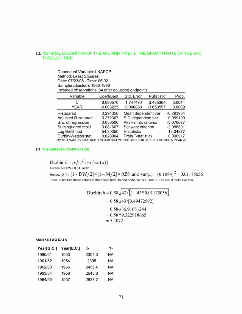
71

2.2. NATURAL LOGARITHM OF THE APC AND TIME i.e. THE GROWTH RATE OF THE APC THROUGH TIME

Dependent Variable: LNAPCP Method: Least Squares Date: 07/23/08 Time: 06:02 Sample(adjusted): 1963 1996 Included observations: 34 after adjusting endpoints

Variable Coefficient Std. Error t-Statistic Prob. C 6.090570 1.747470 3.485364 0.0014

YEAR -0.003225 0.000883 -3.653597 0.0009 R-squared 0.294358 Mean dependent var -0.293904 Adjusted R-squared 0.272307 S.D. dependent var 0.059199 S.E. of regression 0.050500 Akaike info criterion -3.076677 Sum squared resid 0.081607 Schwarz criterion -2.986891 Log likelihood 54.30350 F-statistic 13.34877 Durbin-Watson stat 0.828004 Prob(F-statistic) 0.000917

NOTE: LNAPCP= NATURAL LOGARITHM OF THE APC FOR THE PIH MODEL & YEAR (t)

2.3 THE DURBIN h COMPUTATION

Durbin n 1 n[var( )]/ ρ µh

Givens are DW= 0.84, n=43

Hence, ρ [1 - DW/2] =[1 - .84/2] = 0.58 and var( ) (0.1084) 0.01175056 µ ² Then, substitute these values in the above formula and compute for Durbin h. The result looks like this.

0.58 43 1 43*0.01175056/[ ] Durbin h

0.58 43 /[0.49472592]

0.58 86.91681244

0.58*9.322918665

5.4072

ANNEXE TWO-DATA Year[G.C.] Year[E.C.] Ct Yt 1960/61 1953 2304.3 NA 1961/62 1954 2395 NA 1962/63 1955 2456.4 NA 1963/64 1956 2643.6 NA 1964/65 1957 2827.7 NA

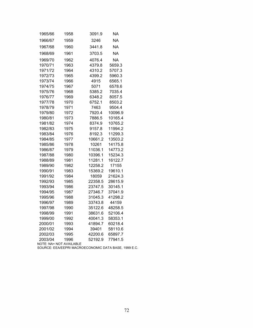
72

1965/66 1958 3091.9 NA 1966/67 1959 3246 NA 1967/68 1960 3441.8 NA 1968/69 1961 3703.5 NA 1969/70 1962 4076.4 NA 1970/71 1963 4379.8 5659.3 1971/72 1964 4310.2 5707.3 1972/73 1965 4399.2 5960.3 1973/74 1966 4915 6565.1 1974/75 1967 5071 6578.6 1975/76 1968 5385.2 7035.4 1976/77 1969 6348.2 8057.5 1977/78 1970 6752.1 8503.2 1978/79 1971 7463 9504.4 1979/80 1972 7920.4 10096.9 1980/81 1973 7886.5 10165.4 1981/82 1974 8374.9 10765.2 1982/83 1975 9157.8 11994.2 1983/84 1976 8192.3 11299.3 1984/85 1977 10661.2 13503.2 1985/86 1978 10261 14175.8 1986/87 1979 11036.1 14773.2 1987/88 1980 10396.1 15234.3 1988/89 1981 11281.1 16122.7 1989/90 1982 12258.2 17155 1990/91 1983 15369.2 19610.1 1991/92 1984 18059 21624.3 1992/93 1985 22358.5 28615.9 1993/94 1986 23747.5 30145.1 1994/95 1987 27346.7 37041.9 1995/96 1988 31045.3 41298.2 1996/97 1989 33743.8 44159 1997/98 1990 35122.6 48258.5 1998/99 1991 38631.6 52106.4 1999/00 1992 40041.3 58353.1 2000/01 1993 41894.7 60218.4 2001/02 1994 39401 58110.6 2002/03 1995 42200.6 65897.7 2003/04 1996 52192.9 77941.5

NOTE: NA= NOT AVAILABLE SOURCE: EEA/EEPRI MACROECONOMIC DATA BASE, 1999 E.C.