The Age-Productivity Gradient: Evidence from a Sample of F1 ...

WWOORRKKIINNGG PPAAPPEERR NNOO.. 222266

The Age-Productivity Gradient:

Evidence from a Sample of F1 Drivers

Fabrizio Castellucci, Mario Padula and Giovanni Pica

May 2009

University of Naples Federico II

University of Salerno

Bocconi University, Milan

CSEF - Centre for Studies in Economics and Finance DEPARTMENT OF ECONOMICS – UNIVERSITY OF NAPLES

80126 NAPLES - ITALY Tel. and fax +39 081 675372 – e-mail: [email protected]

WWOORRKKIINNGG PPAAPPEERR NNOO.. 222266

The Age-Productivity Gradient:

Evidence from a Sample of F1 Drivers

Fabrizio Castellucci *, Mario Padula ** and Giovanni Pica ***

Abstract Aging is a global phenomenon. If older individuals are less productive, an aging working population can lower aggregate productivity, economic growth and fiscal sustainability. Therefore, understanding the age-productivity gradient is key in a aging society. However, estimating the effect of aging on productivity is a daunting task. First, it requires clean measures of productivity. Wages are not such measures to the extent that they reward other workers attributes than their productivity. Second, unobserved heterogeneity at workers, firms and workers/firms level challenges the identification of the age-productivity gradient in cross-sectional data. Longitudinal data attenuate some identification issues, but give rise to the problem of partialling out the effect of aging from the pure effect of time. Third, the study of the age-productivity link requires investigating the role of experience and of seniority. We tackle these issues by focussing on a sample of Gran Prix Formula One drivers and show that the age-productivity link has an inverted U-shape profile, with a peak at around the age of 30-32. JEL Classification: J24,C23, L83. Keywords: Aging, individual effects, firm effects, match effects, Formula One. Acknowledgments: We would like to thank seminar participants at the University Ca’ Foscari of Venice, the University of Milan, and conference participants at the Brucchi-Luchino conference, Bologna, December, 11-12, 2008 and the Third ICEE Conference, Ancona January 30-31, 2009.

* INSEAD ([email protected]) ** University Ca’ Foscari of Venice and CSEF ([email protected]) *** University of Salerno and CSEF ([email protected])

Table of contents

1. Introduction

2. The Formula One Industry

3. Identification

3.1. Drivers effects

3.2. Drivers and teams effects

3.3. Match effects

4. The Age-productivity Gradient

4.1. Results from baseline specifications

4.2. Results from additional specifications

5. Conclusions

References

Appendix

1 Introduction

Aging is a global phenomenon. If older individuals are less productive, an agingworking population can lower aggregate productivity, economic growth and fiscalsustainability. Therefore, understanding the age-productivity gradient is key in aaging society. However, estimating the effect of aging on productivity is a dauntingtask. First, it requires clean measures of productivity. Second, unobserved hetero-geneity at workers, firms and workers/firms level challenges the identification of theage-productivity gradient in cross-sectional data. Longitudinal data attenuate someidentification issues, but gives rise to the problem of partialling out the effect ofaging from the pure effect of time. Third, the study of the age-productivity linkrequires investigating the role of experience and of seniority. Fourth, jobs differ withrespect to the skills they require and different skills may evolve very differently overdifferent working careers.

The literature on micro data has tackled some of these issues, but some remainunresolved. The available evidence seems to indicate that the elderly do suffer adrop in productivity. Medoff and Abraham (1980, 1981), and Waldman and Avolio(1986) use supervisors’ rating to measure productivity and show that older workersare less productive than younger ones. These early studies have been importantattempts to tackle the above mentioned issues, but still suffer from severe short-comings. First, being most of these studies based on cross-sectional data, they areunable to disentangle the effect of age from the effect of tenure, and are unable tocontrol for the fact that workers may self-select into firms according to their pro-ductivity. Second, supervisors may tend to over-reward senior workers for loyaltyand past achievements and therefore supervisors’ rating might be only an imperfectproxy for individual productivity.

These shortcomings are later addressed in the literature. Stephan and Levin(1998) study researchers in the fields of Physics, Geology, Physiology and Biochem-istry. The number of publications and the standard of the journals they appear inare found to be negatively associated with the researchers’ age. Similar evidence isfound in the field of economics where Oster and Hamermesh (1998) conclude thatolder economists publish less than younger ones in leading journals, and that the rateof decline is the same among top researchers as among others.1 The productivityof individuals doing “creative” jobs, such as authors and artists, is measured by thequantity and sometimes the quality of their output. The evidence seems to indicatethat the elderly are less productive. Kanazawa (2003) shows that age-genius curveof scientists bends down around between 20 and 30 years. Similar curves are alsofound for jazz musicians and painters. These papers share a common feature, the useof piece-rate samples, which provide a clean measure of productivity. However, theycannot easily separate the workers’ ability from firm effect and control accordinglyfor workers selection into firms.

To overcome these problems a number of studies use employer-employee matcheddata-set. The evidence based on such data-sets, where individual productivity is

1The same pattern applies to Nobel economists (Dalen, 1999)

2

measured as the workers’ marginal impact on the company’s value-added, finds aninverted U-shaped work performance profile (Andersson et al. (2002), Crepon et al.(2002), Ilmakunnas et al. (2004), Haltiwanger et al. (1999), Hægeland and Klette(1999)).

Individuals in their 30s and 40s have the highest productivity levels. Employeesabove the age of 50 are found to have lower productivity than younger individuals,in spite of their higher wage levels. These papers basically estimate the effect ofaging on productivity by comparing output (or value added) per worker in plants(or firms) with a different age composition of the workforce. A problem with thefact that most studies on age-productivity differences are based on cross-sectionalevidence (with the notable exception of Dostie (2006)) is that reverse causality maybe at work: for example, successful firms generally increase the number of newemployees and this mechanically leads to a younger age structure. Thus, a youngerworkforce could be the effect rather than the cause of firms good performances.

In order to overcome this problem, this paper casts the age-productivity testin its correct setting: within the worker-firm pair. We rely on a unique data-set,that records the race performances for all Gran Prix Formula One (F1) drivers from1991 to 1999. The data provide a clean measure of productivity and have enoughinformation to identify the age-productivity profile after controlling for a host ofworkers and firms characteristics. In particular, we are able to account for tenureand experience – on top of drivers, firms and match effects – and still identify theage-productivity gradient. We find that productivity peaks at the age of 30-32 andthen decreases. Moreover, in accordance with the findings of Abowd et al. (1999),we show that workers effects are more important than firms and match effects indetermining productivity, as they account respectively for 25, 12, and 2 percent ofthe explained variability. Consistently, we find that omitting either firms or matcheffects (or both) in a model with workers effects does not alter the age-productivitygradient.

This paper complements the available results on the age-productivity gradientand provides new insights on the determinants of individual productivity focusingon an admittedly special sample. However, the usefulness of professional sports asa labor market laboratory has long been recognized (Kahn, 2000) and many labor-related questions (e.g. racial discrimination; the relationship between managerialquality and performance) have been tackled using professional sports data (Kahn,1991, 1993, 2006). Of course, it would be unwise to readily generalize our results tothe general population. Yet, the neat identification strategy obtained in this settingmakes our results a useful supplement to those obtained in more standard contextswith – perhaps – less clean identification procedures.

The rest of the paper is organized as follows. Section 2 describes the F1 industryand data. Identification is discussed in Section 3. Section 4 presents the results andSection 5 concludes.

3

2 The Formula One Industry

With its 350 Millions TV viewers per race, F1 racing is considered today the mostpopular sport worldwide. The Auto Club de France held the first Grand Prix racein 1906, but it was not until 1950 that the first World Championship series was held,linking national races in the UK, Monaco, the US, Switzerland, Belgium, France,and Italy. In that year, the form of racing previously called Formula A came tobe known as Formula One and became the pinnacle of automotive technology. Webelieve that there are several grounds on which to focus on F1 to investigate theage-productivity relationship.

First, there are few contexts that provide cleaner measures of performance dif-ferences than that of F1 racing. In F1 racing, there are a limited number of racingteams and a limited number of races; in a given year, all of the teams participatein all the races on the circuit.2 Since all teams are racing on the same racetracksand have cars that must adhere to the same rules, performance differences are easyto measure. Second, although performance is clear after either a race or a racingseason is completed, there is a certain degree of uncertainty on how a team is goingto perform in either the next race or next season. In particular, given the inherentcomplexity of F1 cars and given that cars are usually entirely redesigned betweenseasons, it is uncertain how a new car will stand against competition.

There is a third reason for using F1 racing data, which has to do with theteams seeking constantly to enhance performance by developing their products incollaboration with their suppliers and their drivers. Most of the teams are ownedby the world’s major automobile manufacturers whose motivation is, at least inpart, the exposure to “cutting-edge” technological advances in car design. Unlikeother forms of motor-sport, such as Champ Car or IRL where all competitors race inalmost identical cars built using standard components, F1 racing teams must design,construct and race their own chassis (for this reason F1 teams are officially calledConstructors and a special championship, the World Constructors Championship, isheld every year and awarded to the team that scores the most championship pointsduring a racing season). As F1 teams can, and often do, buy the remaining parts of aracing car from external suppliers, a coordination problem for F1 teams emerges bothin design and racing of the car. Each F1 team seeks to design a car that it regardsas the best compromise of aerodynamic performance, maneuverability, structuralrigidity, and engine power within the rules imposed by the governing body of F1, theFederation Internationale de l’Automobile (FIA). By imposing strict constraints ondimensions, weight, and safety, these rules limit the degrees of freedom in designing acar by taking the interrelations among the various design dimensions to the extreme.For instance, to increase the horsepower of an engine, designers have to consider thatthe increased heat needs to be dissipated by a redesigned cooling system with biggerradiators and, consequently, an increased weight. Given the constraints in size and

2We refer to F1 racing teams as “team” as customarily called in the industry. However, these“teams” are in reality middle-sized firms averaging 164 employees and $34.5 million dollars in assetsin 1997. Besides the racing department in charge of running the cars during the race, these firmshave R&D, Marketing, Production, and Testing departments.

4

weight, other parts of the car need to be redesigned, making sure that the finaloutcome - a racing car - not only produces the desired performance consistently inevery race, but also passes compulsory safety tests.

A fourth reason for focussing on F1 has to do with the role of drivers. Althoughthey are believed to be less important for the final performance than in the past,drivers also play a relevant role in the success of a F1 car. Not only do drivers need toskillfully drive the car during the race itself, but they also need to be involved in thedevelopment of a specific car design. Despite the heavy use of telemetry to obtaindetailed information on a car’s behavior on the track, the driver is still the ultimateprovider of feedback to the car’s engineers and mechanics. Providing feedback ona F1 car is different than providing feedback on any other racing car. Even driversconsidered talented in other racing series need time to acquire this skill. Ultimately,a car’s performance is determined not only by a driver’s sheer talent, but also byher/his ability to provide feedback. For this reason, every time a team wants to hirea new driver, it tries to find somebody who, in the words of one team owner, “isimmediately operational”. That is, the team seeks someone who has proven in thepast s/he can help the team extract the highest performance from the car.

The identification of the age-productivity gradient requires reliable and repeatedmeasures of productivity over time. Moreover, to partial out individual from firmeffects, one has to focus on high turnover industries, where employee change oftenemployers. F1 is the case of an industry where transitions between employers andemployee are frequently observed. This provides a further reason to focus on F1.Abowd et al. (2002) discuss the group-connectedness in employer-employee matchdata and highlight its role in disentangling the firm from the individual effect. Table1 provides an example of the degree of connectedness provided by the F1 data.

Data are drawn from http://www.formula1.com and http://www.4mula1.ro,which provide information on races, drivers and teams. We sample all races thattook place between the 1991 and the 1999 seasons. In each race, performance ismeasured on the basis of the final position of the car. In our time window, pointsare awarded to those cars that finish in the first six places. 10 points are awarded forfirst; 6 points are awarded for second, 4 for third, 3 for fourth, 2 for fifth, 1 for sixth,and 0 for the other placements. Therefore, the sum of points awarded does not growfrom race to race and is fixed to 26. This means that in measuring productivity withthe points awarded to each driver at the end of the race, one does not need to allowfor aggregate effects to capture growth from race to race (or from season to season)in aggregate productivity. This is quite an advantage over measures of productivitybased on wages and value added, since both increase (or decrease) over time becauseof aggregate time effects, not related to aging.3 Beyond the final position of eachcar, we also know the time to complete the race. This an equally valid measure ofcar performance, but contrary to points it is affected by the aggregate effect on cars’speed of technological evolution.

3The problem of identifying time from age effects is common to many settings, such as theevaluation of the age-consumption and saving profile, the age-income profile, and the estimation ofdepreciation of capital goods (or durable goods) from price data.

5

http://www.formula1.com

http://www.4mula1.ro

Each record in our data-set provide car-race level information. Therefore, ourdata-set contains 3,180 observations including all races from 1991 to 1999. Foreach observation, we have the car, the chassis and the engine numbers; the name,nationality, team, the tenure with the team and the year of birth of the driver;the date of the race, the weather conditions in the day of the race, the countrywhere the race is held, and the track length; the nationality, the assets, the numberof employees and the age of the team, the name, nationality and the age of thetechnical director. Overall, we have data on 89 drivers, 22 teams, 8 seasons, and 16races per season. Table 2 collects the drivers’ names, Table 3 the teams names, andTable 4 a sample of the variables available for each race in the 1994 season.

Selected summary statistics are provided in Table 5. The across races mean ofdrivers scores is just above 1, which hides substantial variability between drivers(1.19) and races (1.99). The age of drivers is on average 29.43 and drivers startdriving F1 cars at the age of 25.16. The age of entry in F1 varies across drivers.Esteban Tuero enters at the age of 20, Toshio Suzuki at the age of 38. We observethe entire career of 36 out of 89 drivers, for 30 drivers the career is left truncated,for 17 right truncated and for 6 both left and right truncated. During their careers,drivers change often team: 58 percent of the drivers change team at least once, 36percent twice, 16 percent three times, 4.5 percent four times, and 2.2 five times.Moreover, Andrea De Cesaris, Eric Van De Poele, J. J. Lehto, Jarno Trulli, JohnnyHerbert, Mika Salo change team once in a season, Philippe Alliot twice.

Table 5 also contains information on teams and their technical directors. F1teams count on average 146.8 employees, the average age of technical directors is44.5 and the age of drivers’ entrance in F1 is just below 30. These variables will beused in the estimation exercise, as we clarify in the next section.

3 Identification

To identify the effect of age on drivers performance we provide three alternativemodels. In the baseline model, which we call Model I, we just allow for drivers fixedeffects.4 The estimation of such model would just require panel data on driversperformance and does not exploit any information on teams. To disentangle teamsfrom drivers effect we estimate our Model II, which uses the matched employer-employee structure of the data. Finally, Model III recognizes that drivers mobilitybetween teams might depend on match specific effects. Comparing the three modelsallows to understand the importance of drivers, teams and match effects in theestimation of the age-productivity link.

4An alternative identification strategy is to assume random drivers effects. This approach hasobvious computational advantages over ours in the context of large-scale employer-employee data-sets (see Woodcock (2006) for an application to wage data). However, it requires assuming thatdrivers ability is uncorrelated with all regressors including age. In our setting this assumption isnot likely to hold, as also confirmed by the Hausman test that compares the fixed and the randomeffect models and reveals the presence of systematic differences in the estimated coefficients.

6

3.1 Drivers effects

Productivity, as measured the points at the end of the race, of driver i at time t is:

yit = µ+ θi + α× ageit + εit

where θi is driver i ability and ageit is driver’s i age at time t measured in years.We assume that:

E(yit|ageit) = µ+ θi + α× ageit

It is immediate to verify that α is identified if:

E(yit+1|ageit+1) − E(yit|ageit) = α (1)

which requires that E(εit − εit−1|θi, ageit, ageit−1) = 0. This leads to our first modelfor drivers performance. Model I can be estimated by regressing yit on a set of driversdummies and age. Notice that drivers can sort into teams according to unobservedindividual characteristics. Adding workers fixed effects allows to control for thesorting due to drivers time-invariant characteristics. However, for the estimates ofModel I to be unbiased, one does require that mobility is exogenous, conditional onage and drivers effect.5

Differently, if drivers mobility between teams depends on omitted characteristics(e.g. the quality of the team) that are correlated with age, α cannot be consistentlyestimated in Model I. To understand how this can happen consider the case whereyoung drivers move to higher quality teams while old drivers do the opposite. Theomitted teams characteristics would then be captured by age, possibly generatinga spurious inverse U-shaped relationship between ageing and productivity. Moreformally, E(εit − εit−1|θi, ageit, ageit−1) cannot be equal to zero if the performancevaries systematically between teams and mobility is related to age. To account forthe effect of teams characteristics on drivers performance we turn to our secondmodel.

3.2 Drivers and teams effects

Model II assumes that the drivers performance depends also on team characteristicsthat are fixed over time:

yijt = µ+ θi + ψj(it) + α× ageit + εijt

where j(it) is the team to which driver i belongs at time t. It easy to verify that theteam effect is not identified if no driver changes team from one year to the other.For driver s, who does not change team between years t and t+ 1, the analogue of(1) is:

E(ysjt+1|agest+1) − E(ysjt|agest) = α (2)

5We also estimate a baseline model without drivers effect. The results, not reported for brevity,show that the exogenous mobility assumption, in a model with age effects only, is rejected.

7

while for driver m who changes from team j to team k, it is:

E(ymkt+1|agemt+1) −E(ymjt|agemt) = α+ ψk(mt+1) − ψj(mt) (3)

Equations (2) and (3) identify the team from the age effects. Model II can beestimated by regressing yijt on a set of drivers and team dummies and age. ModelII provides consistent estimates of the age effects, unless drivers mobility betweenteams depends on a match specific team effect. If that is the case, the estimates of αare not consistent and therefore one needs to add match effects to the model.6 Thisleads us to specify and estimate our third model, which accounts for match effects.

3.3 Match effects

Allowing for match specific effects on the top of team and drivers effect poses afundamental identification problem. Since the match effects results from the inter-action of the driver and team effects, the model with match, team and driver effectsis over-parametrized. Suppose for the sake of exposition that α is equal to zero andthat the model is:

yijt = µ+ θi + ψj(it) + φij + εijt (4)

where φij is the match effect. If E(εijt|θi, ψj(it), φij) = 0, the sample analog of theexpected value (4) is:

1Tij

Tij∑

t=1

yijt (5)

where it is assumed that driver i stays with team j for Tij years. If the numberof matches is equal to M , there are M sample moments like (5). With N driversand J teams, identification of driver, team and match effects requires recoveringfrom M sample moments, N + J +M + 1 parameters, which is an impossible task.Identification thus requires additional assumptions. There are many alternativeidentification assumptions. One possibility is to give up on identifying driver fromteam and match effects. Assuming that drivers performance changes with age, themodel can be written as:

yijt = µ+ θi + ψj(it) + φij + α× ageit + εijt (6)

The linearity of the right-hand side of (6) ensures that α can be consistently esti-mated if one can find a sufficient statistic for the sum of driver, team and matcheffects. This leads to the following model:

yit − yij = α(ageit − ageij) + ηit (7)

6Of course, the estimates of α are still consistent if age and match effects are uncorrelated, giventhe drivers and teams effects.

8

where:

yij =1Tij

Tij∑

t=1

yijt (8)

ageij =1Tij

Tij∑

t=1

ageijt (9)

where Tij is the number of years driver i stays with team j.This approach allows to identify the age effect, but is silent about the driver,

the team and the match effect.7 We therefore consider an alternative possibility.Namely, we exploit the richness of our data to model the match effects. In particular,we allow for match effects to depend on drivers age and assume that they are relatedto the distance between the age of the driver and the age of the team, and thatbetween the age of the driver and the age of technical director. Furthermore, weassume that the match effects also depend on whether the team and the driver havethe same nationality, and whether the technical director and the driver have thesame nationality.

Section 4.1 shows results from the three above-described models, extended soas to include a host of time-varying factors that may affect the age-productivityprofile. Section 4.2 presents results from specifications that control for a numberof additional confounding factors that may lie behind our findings. Among otherthings, we will control for the changing quality of the opponents and will be able toseparately identify the effect of age from the effect of tenure and experience.

4 The age-productivity gradient

4.1 Results from baseline specifications

We estimate our three models in turn: model I, featuring drivers effect only, modelII featuring drivers and teams effects, and model III, where we add match effects.For each of them we consider two specifications. A baseline specification with noadditional controls and an extended specification which allows for a list of additionalcovariates including years dummies for 1995-1997, number of entrants in each race,a dummy for rainy weather at the day of the race, the track-length, the number ofrace-laps, a dummy for whether the race takes place at the drivers home.

The results are reported in Table 6 and show that the coefficient on the linearterm of age is positive while the coefficient on the quadratic term is negative in boththe baseline and the extended specification.

Figure 1 displays the age and productivity profile for the three models respec-tively with drivers, drivers and teams, and drivers, teams and match effects forthe baseline specification. The profiles are obtained by projecting the estimatedquadratic polynomial on age. The figure shows that productivity increases with

7We also estimate (7) and get very similar results to those obtained estimating Models I and II.

9

age, until the age of 30 and decreases afterward. The maximum is reached betweenage 30-32. Our estimates also imply that productivity increases by just below halfpoint (0.46) between the age of 20 and 21 in models I and II, and by just above halfpoint (0.52) in model III; and decreases by just below 1/5 of point (0.18) betweenthe age of 34 and 35 in models I and II, and 0.123 in model III.

Overall, our estimates imply that age accounts for as much as 4.5 percent of ex-plained variance of productivity, while drivers effects explain as much as 25 percent,and teams and match effect account respectively for 12 and 2 percent. Results areconsistent with Abowd et al. (1999) who find that firm effects are not as importantas individual effects in explaining individual wage variation in France.

Even though we are able to reject the null that drivers and teams effects areequal to zero, the differences across models and specifications are not sizeable.8 Asmodels with teams and match effects are meant to account for the endogeneity ofmobility decisions, the finding that the age-productivity gradient does not differmuch across models suggest that the endogeneity bias is small. This is a notablefinding in a high-turnover industry such as the F1 industry (see section 2) whichmay suggest that the bias induced by endogenous mobility decisions may be evensmaller in industries characterized by lower rates of job mobility.9

Summing up, this first set of results shows that GP drivers have an age-productivityprofile consistent with that predicted by the theory of human capital. Whether ornot this is an artifact of our data is the concern to which we devote the rest of thissection.

4.2 Results from additional specifications

Interactions between drivers effects and race characteristicsThe list of factors that might lie behind our results is potentially large, even if

our estimates allow for drivers, teams and match effects. At the top of the list,factors that change across drivers and between races (and seasons). For instance,some drivers can be better at racing on wet ground, or on long tracks. Therefore,the change in their performance from race to race might depend on the weatherconditions at the day of the race, or on the tracks characteristics, which mightconfound the effect of age.

We therefore add to our extended specification interaction terms between driverseffects and tracks length, driver effects and number of race-laps, and driver effectand a dummy for rainy weather at the race day. The results are reported in Table7 and are very similar to those reported in Table 6. Productivity increases by 0.45-0.50 between the age 20 and 21 in all models, and decreases by 0.15-0.21 betweenthe age of 34 and 35.

8We do not reject at the standard level the null that the age coefficients are equal across modelsI and II, while we do reject the null that they are equal across models II and III.

9Booth et al. (1999) examine job mobility and job tenure in the UK over the period 1915-90.They find that British men and women held an average of five jobs over the course of their worklives. In our data we observe the entire career for 36 out of 89 drivers. Those drivers change teamalmost once a year during their career.

10

Controlling for all the interactions between drivers effects and race characteristicsin the same regressions does not alter the picture. The results are provided in Table8, and Figure 2 shows the age-productivity profile. Productivity peaks between theage 30 and 32, and has a concave shape in accordance with human capital theory.

Changing rulesChanges in the rules between seasons might also affect differently different drivers.

This is another potential factor that might confound the age effects. For instance,major innovations were introduced in 1994. Refuelling was permitted again withthe use of a standardized refuelling rig, the active/reactive suspension systems wasbanned, and so were the electronic driver aids, such as the traction control, launchcontrol. Moreover, after San Marino accident in 1994, where drivers Roland Ratzen-berger and Ayrton Senna died, restrictions imposed on the front and rear wings, thesize and shape of the rear diffuser, and a wooden “plank” introduced on the under-side of the car to raise the ride height. We therefore add to our specification theinteraction of dummies for years after 1994 with the drivers effects. The results arereported in Table 9 and are again quite similar to those reported in the Tables 6-8.The age-productivity profile is concave and peaks at the age of 30-32, as shown inFigure 3.

Quality of opponentsAnother source of bias that might affect the estimates of the relationship between

aging and productivity may derive from the absence of a proper correction for thequality of the opponents. If, for example, the average quality of opponents decaysover time one may underestimate the effects of aging on productivity. Changes inthe average quality of the opponents may be due either to the changing quality ofincumbent drivers or to compositional changes in the pool of drivers. To address thefirst problem Table 10 presents results controlling for the quality of the opponents,as measured by the cumulative number of points of the rivals since the start of theseason. While the table shows that the quality of opponents does have a negativeinfluence on drivers performances, the coefficients of age and age square are hardlyaffected. Next, to address the potential effect of compositional changes in the poolof drivers due to the fact that low productivity drivers may sort themselves out ofthe profession in younger ages, we control for non-random attrition using propensityscore weights. Predicted probabilities of staying in the sample are obtained runninga probit on a dummy equal to one if the driver is present in the following year (andzero otherwise) on the cumulative number of points in the season and a quadratic inage. The propensity score weights are then computed on the basis of these predictedprobabilities and used in the estimation of the age-productivity gradient. Table 11presents the results that confirm the findings of the previous tables.

Experience and tenureThe shape of the age productivity gradient is likely to depend on drivers experience

and possibly tenure. Drivers’ performance might improve with experience, and also

11

longer driver-team relationship might have a positive effect of performance, allowingthe driver to learn better about his car.

Disentangling the effect of experience and tenure on productivity from that ofage is often hard. Experience and tenure coincide for those worker who do not movebetween jobs, and both change hand-in-hand with age. The high turnover among GPdrivers allows to distinguish experience from tenure. We measure the former withthe age of entry in F1, and the latter with the duration of team-driver relationship foreach driver. However, the age of entry in F1 is fixed for each driver and therefore it isabsorbed into the driver fixed effect. To understand if experience and tenure matterfor the estimated age-productivity profile, we thus exploit the fact that sum of scoresat the end of each race is fixed. This allows adding the normalization equation thatthe sum of driver effect is zero, and therefore estimating models that account for theeffect of experience and tenure on productivity and separate that from the effect ofage and the individual effect. The results for experience are reported in Table 12and those for tenure in Table 13. The Tables reveal that both experience and tenurematter, but leave the overall picture unaffected.

Past performancesAging is not the only and possibly the main driver of performance changes over

time. Productivity changes across races (and seasons) might reflect past perfor-mances. State dependence in the productivity process come from the good perfor-mances in the past having a positive or a negative effect on current performances.The former case might arise when past bad performances make drivers less confidentand then drive less aggressively. The latter, when bad past performances increasethe incentives to drive better in future races. While we cannot identify the precisechannel from which state-dependency in performances arises, we can control for pastperformance. This is done in Table 14, where we add to the set of regressors thescores in the previous race. The results suggest that past has a positive effect oncurrent performance, and that the shape of the age productivity gradient is not verymuch affected.

Non-parametric specificationSo far we have restricted the age effect to enter the productivity equation in

a quadratic fashion. Such assumption is made for convenience. To model moreflexibly the effect of age on productivity, we replace the linear and quadratic ageterms with a set of age dummies. The results are reported in Table 15. The baselinecategory is age between 20 and 22: productivity increases with age until age 32-34 and then starts decreasing. Therefore, allowing for a more flexible specificationmoves the peaks by around 1 year, but leaves the concavity unchanged. Moreover,as one can see from Figure 4, productivity increases relatively little at the beginningof the career, and more from the age of 28 until the peak, and it decreases quitedramatically at the very end of the career.

12

5 Conclusions

Measuring the age-productivity gradient has both positive and normative impli-cations. The shape of the age-productivity profile has implications for aggregateproductivity, economic growth, the sustainability of pension systems and the de-sign of tax systems. Moreover, the optimality of wage schemes based on senioritydepends on the extent to which productivity decreases at old ages.

The empirical evaluation of the age-productivity link is, however, problematic, inthat it requires repeated measures of productivity and possibly employer-employeematch data. Data with such features are seldom available. Good proxies of pro-ductivity are provided by piece-rate samples, such as those on scientist or criminals.However, such data do not allow to disentangle the firm and the individual effects onproductivity. This issue can be addressed by employer-employee match data, which,however, often lack of convincing measures of productivity. Here, we use very specialdata, which share the advantages of both the piece-rate and the employer-employermatch data: data on GP drivers.

GP drivers change often employer in their careers, which makes identification offirm and individual effects possible. Moreover, it is easy to observe their productivity,which we measure as the points awarded to each driver at the end of each race. Thisis an objective measure of productivity and is not affected by aggregate growth,since the sum of points awarded in each race is constant over time.

We find that the age-productivity profile is concave and reaches the maximumbetween the age of 30 and 32. Our result is robust to a number of checks, whichcontrol for the fact that there might be factors changing across races (or seasons)which affect drivers differently. Moreover, we show that the productivity increasesby around 2.6 points between the age of 20 and 30, and decreases by 2.4 pointsbetween the age of 30 and 40. We also show that drivers, teams and match effectmatters, as they account respectively for 25, 12, and 2 percent of the explainedvariance of productivity. However, omitting team and match effects from the drivereffect model does not alter the overall picture on the age-productivity. Since it isvery likely that in a population of GP drivers mobility depends on team and matchcharacteristics, we see this result as indicating that the endogeneity of mobility doesnot affect how productivity evolves with age. While the result pertain to a peculiarpopulation, we might expect the effect of endogenous mobility to be even smaller inthose populations where the role of employer and match specific human capital isless important.

References

Abowd, J.M., F. Kramarz, and D.N. Margolis, “High wage workers and howwage firms,” Econometrica, 1999, 67 (2), 251–333.

, R.H. Creecy, and F. Kramarz, “Computing Person and Firm Effects UsingLinked Longitudinal Employer-Employee Data,” 2002. LEHD Technical Paper

13

2002-06.

Andersson, B., B. Holmlund, and T. Lindh, “Labor Productivity, Age andEducation in Swedish Mining and Manufacturing 1985-96,” 2002. Uppsala, Swe-den.

Booth, Alison L., Marco Francesconi, and Carlos Garcia-Serrano, “JobTenure and Job Mobility in Britain,” Industrial and Labor Relations Review, 1999,53 (1), 43–70.

Crepon, B., N. Deniau, and S. Perez-Duarte, “Wages, Productivity andWorker Characteristics: a French Perspective,” 2002. INSEE.

Dalen, Van Hendrik P., “The Golden Age of Nobel Economists,” AmericanEconomist, 1999, 43, 19–35.

Dostie, B., “Wages, Productivity and Aging,” 2006. IZA DP. 2496.

Hægeland, T. and T.J. Klette, “Do Higher Wages Reflect Higher Productivity?Education, Gender and Experience Premiums in a Matched Plant-Worker DataSet,” in J. L. Haltiwanger, J. R. Spletzer, J. Theeuwes, and K. Troske, eds., TheCreation and Analysis of Employer-Employee Matched Data, Elsevier Science,1999.

Haltiwanger, J.C., J.I. Lane, and J. R. Spletzer, “Productivity DifferencesAcross Employers. The Roles of Employer Size, Age and Human Capital,” Amer-ican Economic Review, May 1999, 89 (2), 94–98. Papers and Proceedings.

Ilmakunnas, P., M. Maliranta, and J. Vainiomaki, “The role of Employerand Employee Characteristics for Plant Productivity,” Journal of ProductivityAnalysis, May 2004, 21 (3), 249–276.

Kahn, Lawrence M, “Discrimination in Professional Sports: A Survey of theLiterature,” Industrial and Labor Relations Review, April 1991, 44 (3), 395–418.

, “Managerial Quality, Team Success, and Individual Player Performance in MajorLeague Baseball,” Industrial and Labor Relations Review, April 1993, 46 (3), 531–547.

, “The Sports Business as a Labor Market Laboratory,” Journal of EconomicPerspectives, Summer 2000, 14 (3), 75–94.

, “Race, Performance, Pay, and Retention Among National Basketball AssociationHead Coaches,” Journal of Sports Economics, 2006, 7 (2), 119–149.

Kanazawa, S., “Why productivity fades with age: the crime-genius connection,”Journal of Research in Personality, 2003, 37, 257–272.

Medoff, J. L. and K. G. Abraham, “Experience, Performance, and Earnings,”Quarterly Journal of Economics, 1980, 95 (4), 703–736.

14

and , “Are Those Paid More Really More Productive? The Case of Experi-ence,” Journal of Human Resources, 1981, 16 (2), 186–216.

Oster, Sharon M. and Daniel S. Hamermesh, “Aging and productivity amongeconomists,” The Review of Economics and Statistics, February 1998, 80 (1),154–156.

Stephan, P.E. and S.G. Levin, “Measures of Scientific Output and the Age-Productivity Relationship,” in Anthony Van Raan, ed., Handbook of QuantitativeStudies of Science and Technology, Elsevier Science, 1998, pp. 31–80.

Waldman, D.A. and B.J. Avolio, “A Meta-Analysis of Age Differences in JobPerformance,” Journal of Applied Psychology, 1986, 71, 33–38.

Woodcock, Simon, “Match Effects,” MPRA Paper 154, University Library ofMunich, Germany September 2006.

15

Figure 1. Age-productivity profile

19

20

21

22

23

20 25 30 35 40

Driver effect Driver and team effectDriver, team and match effect

Note. The figure shows the relation between age and productivity. Age is recorded on the horizontal

axis, and α1 × ageit + α2 × age2it on the vertical axis.

16

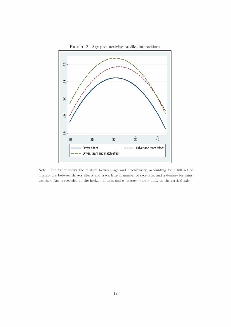
Figure 2. Age-productivity profile, interactions

18

19

20

21

22

20 25 30 35 40


Note. The figure shows the relation between age and productivity, accounting for a full set of

interactions between drivers effects and track length, number of race-laps, and a dummy for rainy

weather. Age is recorded on the horizontal axis, and α1 × ageit + α2 × age2it on the vertical axis.

17

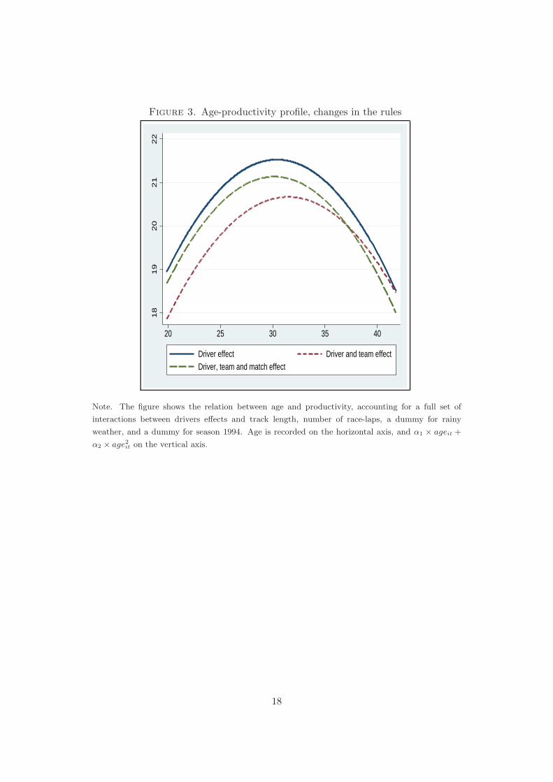
Figure 3. Age-productivity profile, changes in the rules

18

19

20

21

22

20 25 30 35 40



interactions between drivers effects and track length, number of race-laps, a dummy for rainy

weather, and a dummy for season 1994. Age is recorded on the horizontal axis, and α1 × ageit +

α2 × age2it on the vertical axis.

18

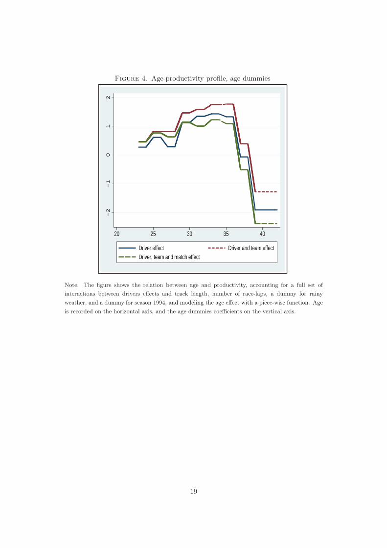
Figure 4. Age-productivity profile, age dummies

−2

−1

01

2

20 25 30 35 40



interactions between drivers effects and track length, number of race-laps, a dummy for rainy

weather, and a dummy for season 1994, and modeling the age effect with a piece-wise function. Age

is recorded on the horizontal axis, and the age dummies coefficients on the vertical axis.

19

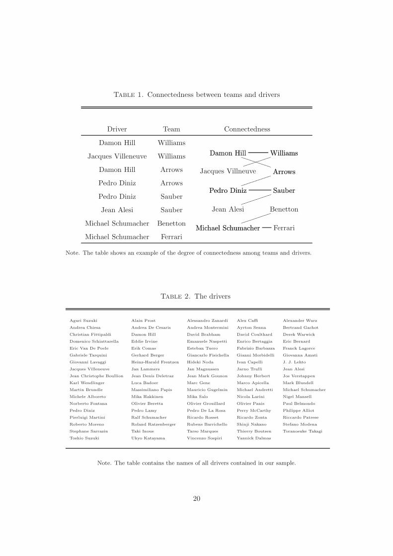
Table 1. Connectedness between teams and drivers

Driver Team Connectedness

Damon Hill WilliamsDamon Hill Williams

Jacques Villneuve

Williams��

Damon Hill

Arrows��

Pedro Diniz

Arrows��Pedro Diniz Sauber

Jean Alesi

Sauber��

Michael Schumacher

Benetton��Michael Schumacher Ferrari

Jacques Villeneuve Williams

Damon Hill Arrows

Pedro Diniz Arrows

Pedro Diniz Sauber

Jean Alesi Sauber

Michael Schumacher Benetton

Michael Schumacher Ferrari

Note. The table shows an example of the degree of connectedness among teams and drivers.

Table 2. The drivers

Aguri Suzuki Alain Prost Alessandro Zanardi Alex Caffi Alexander Wurz

Andrea Chiesa Andrea De Cesaris Andrea Montermini Ayrton Senna Bertrand Gachot

Christian Fittipaldi Damon Hill David Brabham David Coulthard Derek Warwick

Domenico Schiattarella Eddie Irvine Emanuele Naspetti Enrico Bertaggia Eric Bernard

Eric Van De Poele Erik Comas Esteban Tuero Fabrizio Barbazza Franck Lagorce

Gabriele Tarquini Gerhard Berger Giancarlo Fisichella Gianni Morbidelli Giovanna Amati

Giovanni Lavaggi Heinz-Harald Frentzen Hideki Noda Ivan Capelli J. J. Lehto

Jacques Villeneuve Jan Lammers Jan Magnussen Jarno Trulli Jean Alesi

Jean Christophe Boullion Jean Denis Deletraz Jean Mark Gounon Johnny Herbert Jos Verstappen

Karl Wendlinger Luca Badoer Marc Gene Marco Apicella Mark Blundell

Martin Brundle Massimiliano Papis Mauricio Gugelmin Michael Andretti Michael Schumacher

Michele Alboreto Mika Hakkinen Mika Salo Nicola Larini Nigel Mansell

Norberto Fontana Olivier Beretta Olivier Grouillard Olivier Panis Paul Belmondo

Pedro Diniz Pedro Lamy Pedro De La Rosa Perry McCarthy Philippe Alliot

Pierluigi Martini Ralf Schumacher Ricardo Rosset Ricardo Zonta Riccardo Patrese

Roberto Moreno Roland Ratzenberger Rubens Barrichello Shinji Nakano Stefano Modena

Stephane Sarrazin Taki Inoue Tarso Marques Thierry Boutsen Toranosuke Takagi

Toshio Suzuki Ukyo Katayama Vincenzo Sospiri Yannick Dalmas

Note. The table contains the names of all drivers contained in our sample.

20

Table 3. The teams

Arrows BAR/Supertec Benetton Brabham Dallara-Judd

Ferrari Fondmetal-Ford Forti-Ford Jordan Larousse

March-Ilmor Prost Lola Lotus McLaren

Minardi Moda-Judd Pacific-Ilmor Sauber Simtek

Stewart Williams

Note. The table contains the names of all teams contained in our sample.

21

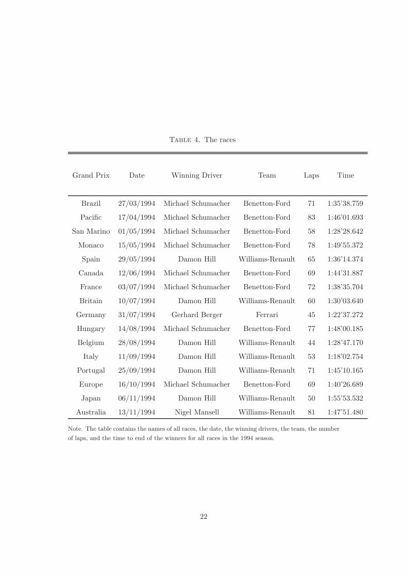
Table 4. The races

Grand Prix Date Winning Driver Team Laps Time

Brazil 27/03/1994 Michael Schumacher Benetton-Ford 71 1:35’38.759

Pacific 17/04/1994 Michael Schumacher Benetton-Ford 83 1:46’01.693

San Marino 01/05/1994 Michael Schumacher Benetton-Ford 58 1:28’28.642

Monaco 15/05/1994 Michael Schumacher Benetton-Ford 78 1:49’55.372

Spain 29/05/1994 Damon Hill Williams-Renault 65 1:36’14.374

Canada 12/06/1994 Michael Schumacher Benetton-Ford 69 1:44’31.887

France 03/07/1994 Michael Schumacher Benetton-Ford 72 1:38’35.704

Britain 10/07/1994 Damon Hill Williams-Renault 60 1:30’03.640

Germany 31/07/1994 Gerhard Berger Ferrari 45 1:22’37.272

Hungary 14/08/1994 Michael Schumacher Benetton-Ford 77 1:48’00.185

Belgium 28/08/1994 Damon Hill Williams-Renault 44 1:28’47.170

Italy 11/09/1994 Damon Hill Williams-Renault 53 1:18’02.754

Portugal 25/09/1994 Damon Hill Williams-Renault 71 1:45’10.165

Europe 16/10/1994 Michael Schumacher Benetton-Ford 69 1:40’26.689

Japan 06/11/1994 Damon Hill Williams-Renault 50 1:55’53.532

Australia 13/11/1994 Nigel Mansell Williams-Renault 81 1:47’51.480

Note. The table contains the names of all races, the date, the winning drivers, the team, the number

of laps, and the time to end of the winners for all races in the 1994 season.

22

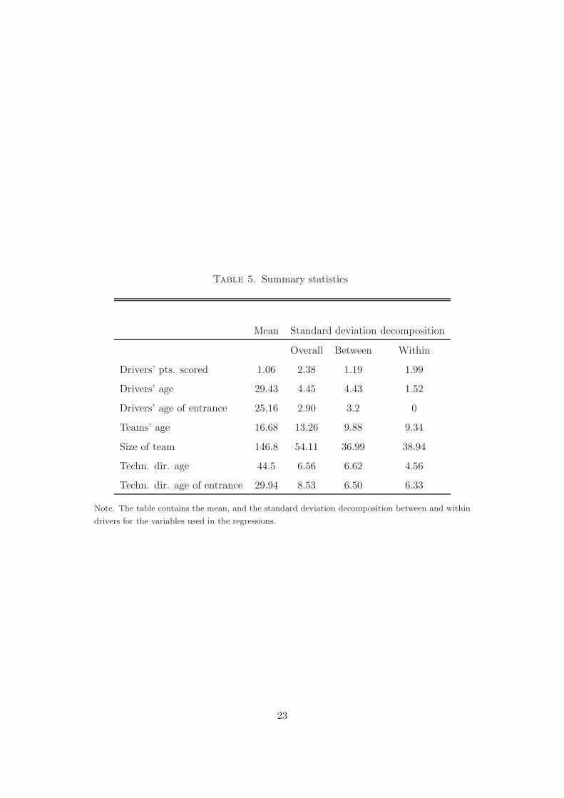
Table 5. Summary statistics

Mean Standard deviation decomposition

Overall Between Within

Drivers’ pts. scored 1.06 2.38 1.19 1.99

Drivers’ age 29.43 4.45 4.43 1.52

Drivers’ age of entrance 25.16 2.90 3.2 0

Teams’ age 16.68 13.26 9.88 9.34

Size of team 146.8 54.11 36.99 38.94

Techn. dir. age 44.5 6.56 6.62 4.56

Techn. dir. age of entrance 29.94 8.53 6.50 6.33

Note. The table contains the mean, and the standard deviation decomposition between and within

drivers for the variables used in the regressions.

23

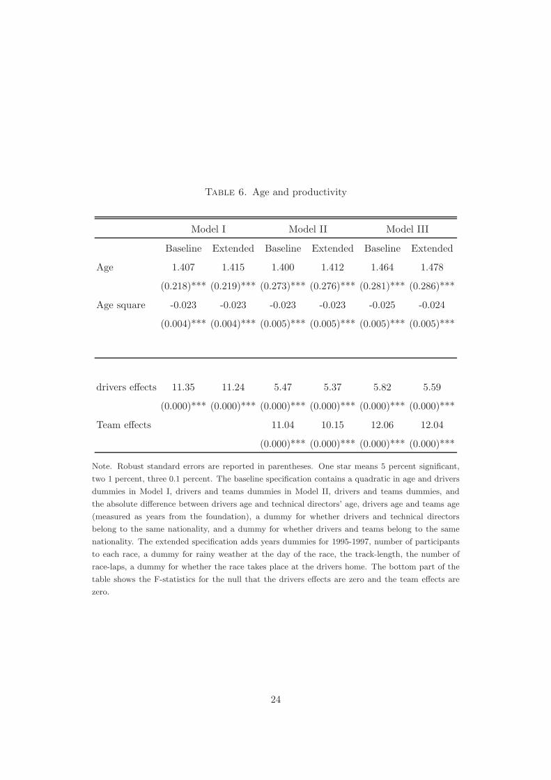
Table 6. Age and productivity

Model I Model II Model III

Baseline Extended Baseline Extended Baseline Extended

Age 1.407 1.415 1.400 1.412 1.464 1.478

(0.218)*** (0.219)*** (0.273)*** (0.276)*** (0.281)*** (0.286)***

Age square -0.023 -0.023 -0.023 -0.023 -0.025 -0.024

(0.004)*** (0.004)*** (0.005)*** (0.005)*** (0.005)*** (0.005)***

drivers effects 11.35 11.24 5.47 5.37 5.82 5.59

(0.000)*** (0.000)*** (0.000)*** (0.000)*** (0.000)*** (0.000)***

Team effects 11.04 10.15 12.06 12.04

(0.000)*** (0.000)*** (0.000)*** (0.000)***

Note. Robust standard errors are reported in parentheses. One star means 5 percent significant,

two 1 percent, three 0.1 percent. The baseline specification contains a quadratic in age and drivers

dummies in Model I, drivers and teams dummies in Model II, drivers and teams dummies, and

the absolute difference between drivers age and technical directors’ age, drivers age and teams age

(measured as years from the foundation), a dummy for whether drivers and technical directors

belong to the same nationality, and a dummy for whether drivers and teams belong to the same

nationality. The extended specification adds years dummies for 1995-1997, number of participants

to each race, a dummy for rainy weather at the day of the race, the track-length, the number of

race-laps, a dummy for whether the race takes place at the drivers home. The bottom part of the

table shows the F-statistics for the null that the drivers effects are zero and the team effects are

zero.

24

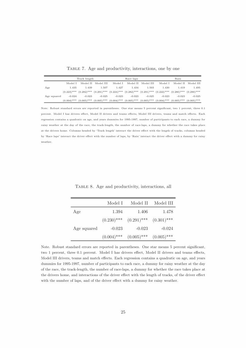
Table 7. Age and productivity, interactions, one by one

Track length Race laps Rain

Model I Model II Model III Model I Model II Model III Model I Model II Model III

Age 1.435 1.439 1.507 1.427 1.434 1.503 1.430 1.419 1.495

(0.223)*** (0.282)*** (0.291)*** (0.224)*** (0.282)*** (0.291)*** (0.222)*** (0.280)*** (0.290)***

Age squared -0.024 -0.023 -0.025 -0.023 -0.023 -0.025 -0.023 -0.023 -0.025

(0.004)*** (0.005)*** (0.005)*** (0.004)*** (0.005)*** (0.005)*** (0.004)*** (0.005)*** (0.005)***

Note. Robust standard errors are reported in parentheses. One star means 5 percent significant, two 1 percent, three 0.1

percent. Model I has drivers effect, Model II drivers and teams effects, Model III drivers, teams and match effects. Each

regression contains a quadratic on age, and years dummies for 1995-1997, number of participants to each race, a dummy for

rainy weather at the day of the race, the track-length, the number of race-laps, a dummy for whether the race takes place

at the drivers home. Columns headed by ‘Track length’ interact the driver effect with the length of tracks, columns headed

by ‘Race laps’ interact the driver effect with the number of laps, by ‘Rain’ interact the driver effect with a dummy for rainy

weather.

Table 8. Age and productivity, interactions, all


Age 1.394 1.406 1.478

(0.230)*** (0.291)*** (0.301)***

Age squared -0.023 -0.023 -0.024

(0.004)*** (0.005)*** (0.005)***


two 1 percent, three 0.1 percent. Model I has drivers effect, Model II drivers and teams effects,

Model III drivers, teams and match effects. Each regression contains a quadratic on age, and years

dummies for 1995-1997, number of participants to each race, a dummy for rainy weather at the day

of the race, the track-length, the number of race-laps, a dummy for whether the race takes place at

the drivers home, and interactions of the driver effect with the length of tracks, of the driver effect

with the number of laps, and of the driver effect with a dummy for rainy weather.

25

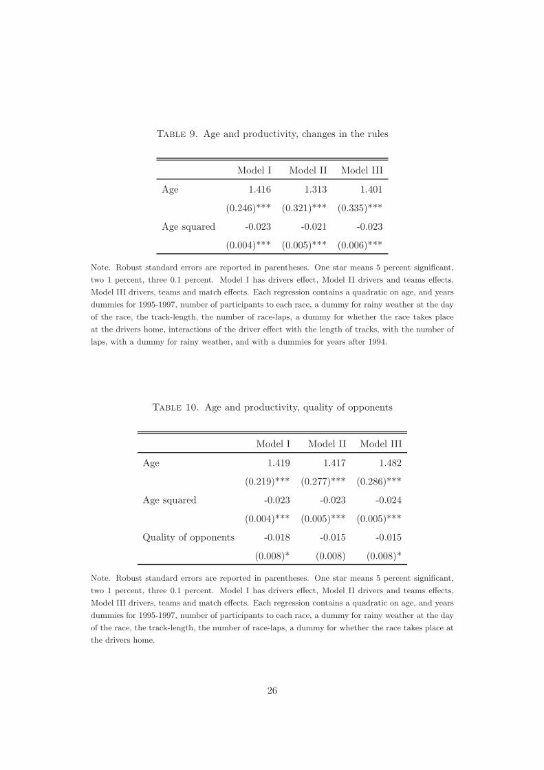
Table 9. Age and productivity, changes in the rules


Age 1.416 1.313 1.401

(0.246)*** (0.321)*** (0.335)***

Age squared -0.023 -0.021 -0.023

(0.004)*** (0.005)*** (0.006)***





of the race, the track-length, the number of race-laps, a dummy for whether the race takes place

at the drivers home, interactions of the driver effect with the length of tracks, with the number of

laps, with a dummy for rainy weather, and with a dummies for years after 1994.

Table 10. Age and productivity, quality of opponents


Age 1.419 1.417 1.482

(0.219)*** (0.277)*** (0.286)***

Age squared -0.023 -0.023 -0.024

(0.004)*** (0.005)*** (0.005)***

Quality of opponents -0.018 -0.015 -0.015

(0.008)* (0.008) (0.008)*





of the race, the track-length, the number of race-laps, a dummy for whether the race takes place at

the drivers home.

26

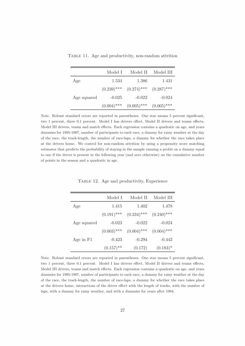
Table 11. Age and productivity, non-random attrition


Age 1.534 1.386 1.431

(0.239)*** (0.274)*** (0.287)***

Age squared -0.025 -0.022 -0.024

(0.004)*** (0.005)*** (0.005)***






at the drivers home. We control for non-random attrition by using a propensity score matching

estimator that predicts the probability of staying in the sample running a probit on a dummy equal

to one if the driver is present in the following year (and zero otherwise) on the cumulative number

of points in the season and a quadratic in age.

Table 12. Age and productivity, Experience


Age 1.415 1.402 1.478

(0.191)*** (0.234)*** (0.240)***

Age squared -0.023 -0.022 -0.024

(0.003)*** (0.004)*** (0.004)***

Age in F1 -0.423 -0.294 -0.442

(0.157)** (0.172) (0.183)*








27

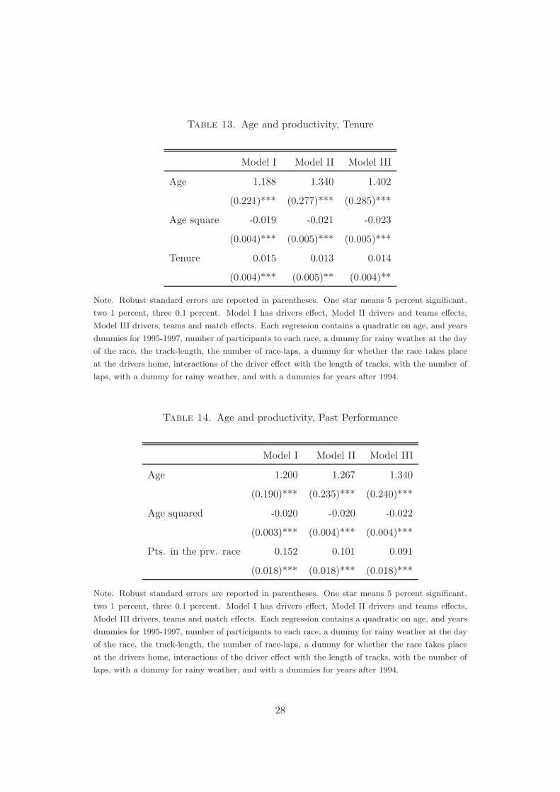
Table 13. Age and productivity, Tenure


Age 1.188 1.340 1.402

(0.221)*** (0.277)*** (0.285)***

Age square -0.019 -0.021 -0.023

(0.004)*** (0.005)*** (0.005)***

Tenure 0.015 0.013 0.014

(0.004)*** (0.005)** (0.004)**








Table 14. Age and productivity, Past Performance


Age 1.200 1.267 1.340

(0.190)*** (0.235)*** (0.240)***

Age squared -0.020 -0.020 -0.022

(0.003)*** (0.004)*** (0.004)***

Pts. in the prv. race 0.152 0.101 0.091

(0.018)*** (0.018)*** (0.018)***








28

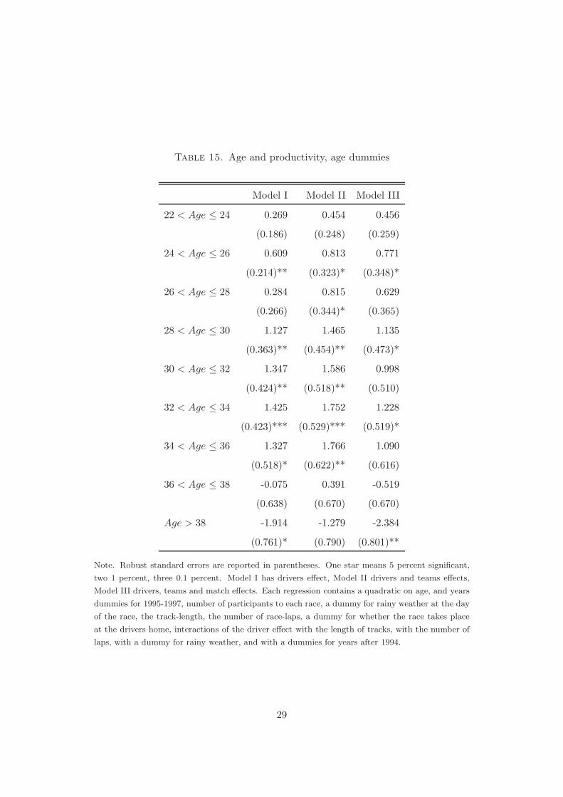
Table 15. Age and productivity, age dummies


22 < Age ≤ 24 0.269 0.454 0.456

(0.186) (0.248) (0.259)

24 < Age ≤ 26 0.609 0.813 0.771

(0.214)** (0.323)* (0.348)*

26 < Age ≤ 28 0.284 0.815 0.629

(0.266) (0.344)* (0.365)

28 < Age ≤ 30 1.127 1.465 1.135

(0.363)** (0.454)** (0.473)*

30 < Age ≤ 32 1.347 1.586 0.998

(0.424)** (0.518)** (0.510)

32 < Age ≤ 34 1.425 1.752 1.228

(0.423)*** (0.529)*** (0.519)*

34 < Age ≤ 36 1.327 1.766 1.090

(0.518)* (0.622)** (0.616)

36 < Age ≤ 38 -0.075 0.391 -0.519

(0.638) (0.670) (0.670)

Age > 38 -1.914 -1.279 -2.384

(0.761)* (0.790) (0.801)**








29

The Age-Productivity Gradient: Evidence from a Sample of F1 ...

Documents

Transcript of The Age-Productivity Gradient: Evidence from a Sample of F1 ...