The 2nd IMAT - Universitas Indonesia
223
The 2 nd IMAT, Nov. 16-17, 2009 Departement of Mechanical Engineering, University of Indonesia 1 The 2 nd IMAT International Meeting on Advances in Thermo-Fluids November 16-17, 2009 Taman Safari, Indonesia Department of Mechanical Engineering University of Indonesia
-
Upload
khangminh22 -
Category
Documents
-
view
3 -
download
0
Transcript of The 2nd IMAT - Universitas Indonesia

The 2nd IMAT, Nov. 16-17, 2009
Departement of Mechanical Engineering, University of Indonesia 1
The 2nd IMATInternational Meeting on Advances in Thermo-Fluids
November 16-17, 2009
Taman Safari, Indonesia
Department of Mechanical Engineering
University of Indonesia

The 2nd IMAT, Nov. 16-17, 2009
Departement of Mechanical Engineering, University of Indonesia 2
TABLE OF CONTENTS
Welcome .. 10
Organizing Committee ... 11
Program Summary . 12
List of Papers .. 14
Cascade Refrigeration System for Low-Temperature Application using CO2+HydrocarbonMixture as Alternative Refrigerant
Nasruddin, Darwin Rio Budi Syaka, M. Idrus Alhamid
Refrigeration and Air-conditioning Laboratory, Department of Mechanical Engineering-Faculty ofEngineering, University of Indonesia, Kampus UI Depok 16424
14
Experimental and Computational Study on Thermal Structure of a SeparatedReattachment Flow under Heated Gas Injection
Harinaldi , Damora Rhakasywi, Sri Haryono
Department of Mechanical Engineering Faculty of Engineering, University of Indonesia, Depok16424
18
Development of Water Mist System for Pool Fire Extinguishment
Yulianto Sulistyo Nugroho, Donny Tigor Hamonangan and Ivan Santoso
Department of Mechanical Engineering University of Indonesia, Kampus UI Depok 16424,INDONESIA
23

The 2nd IMAT, Nov. 16-17, 2009
Departement of Mechanical Engineering, University of Indonesia 3
Preparation of Activated Carbon from Low Rank Coal with CO2 Activation
Awaludin Martin, Bambang Suryawan, Muhammad Idrus Alhamid, Nasruddin
Refrigeration and Air Conditioning Laboratory, Mechanical Engineering Department
Faculty of Engineering, University of Indonesia
29
Experimental Study of Characteristic and Performance of Non-Branded ThermoelectricModule
Zuryati Djafar, Nandy Putra, Raldi A. Koestoer
Heat Transfer Laboratory, Mechanical Engineering Department, University of Indonesia,Kampus Baru UI, Depok, 16424- West Java-Indonesia
35
Development Mathematical Modelling For Design and Analysis Proton ExchangeMembrane Fuel Cell
Hariyotejo Pujowidodoa, Verina Januati Wargadalamb, Ahmad Indra Siswantarac
aCentre for Thermodynamics, Engine and Propulsion System, Agency for Assessment andApplication of Technology, Puspiptek Serpong Tangerang 15314bResearch and Development Centre for The Electricity and Renewable Energy Technology,Ministry of Energy and Mineral Resources Cipulir JakartacFaculty Engineering, University of Indonesia, Depok 16424
40
Experimental Study and Correlation of Two-Phase Flow Evaporation Heat TransferCoefficient of Propane in Intermittent, Stratified Wavy and Annular Flows
Agus S. Pamitrana, Jong-Taek Ohb
aDepartment of Mechanical Engineering, University of Indonesia, Kampus Baru UI, Depok16424, IndonesiabDepartment of Refrigeration and Air-Conditioning Engineering, Chonnam National University,San 96-1, Dunduk-Dong, Yeosu, Chonnam 550-749, Republic of Korea
52

The 2nd IMAT, Nov. 16-17, 2009
Departement of Mechanical Engineering, University of Indonesia 4
Solar-powered Adsorption Desalination cum Cooling: experiments and simulation
Professor Kim Choon Ng, Professor Kim Choon Ng
Mechanical Engineering Dept., Mechanical Engineering Dept., National University of SingaporeNational University of Singapore
60
Glimpses of Solar Energy Research at the Faculty of Mechanical Engineering Universityof Technology Malaysia Skudai, Johor Bharu, Johor
Amer Nordin Darus
Department of Thermofluids, Faculty of Mechanical Engineering, Universiti Teknologi Malaysia
81300 Skudai, Johor Bharu
65
Experimental Study of Confined Biogas Pulse Detonation Combustion
Mazlan A. Wahid, Haffis Ujir, Khalid M. Saqr and Mohsin M. Sies
High-Speed Reacting Flow Laboratory, Faculty of Mechanical Engineering, Universiti TeknologiMalaysia, 81310 Skudai, Johor MALAYSIA
71
Transient Flow Effect due to Geometrical Characteristics of Pressure-Swirl GasolineDirect Injection (GDI) Atomizers
Azhar Abdul Aziz, Mas Fawzi Ali, Zulkarnian Abdul Latiff
Automotive Development Centre (ADC), Faculty of Mechanical Engineering, UniversitiTeknologi Malaysia
78
Swirl Intensity Effect on Premixed Jet Flame
Mohd Heady Jalaluddin, Mohd Ibthisham Ardani, Mazlan A. Wahid
Faculty of Mechanical Engineering, Department of Thermofluid, Universiti Teknologi Malaysia,UTM, Malaysia
85
The 2nd IMAT, Nov. 16-17, 2009
Departement of Mechanical Engineering, University of Indonesia 5
Liquid Fuel Vaporization System
Mazlan Abdul Wahid, Mohsin Mohd Sies, Mohd Khairrul Mohd Suhaimi, Mohd Ayub Sulong
Faculty of Mechanical Engineering, Universiti Teknologi Malaysia, 81310 UTM Skudai, Johor,Malaysia
90
Characteristics of Turbulent Whirling Flow in an Asymmetric Passage
Khalid M. Saqra, Mohsin M. Siesa, Hossam S. Alyb ,Mazlan Abdul Wahida
aHigh-Speed Reacting Flow Laboratory, Faculty of Mechanical Engineering, Universiti TeknologiMalaysia, 81310 Skudai, Johor, MALAYSIAbF Department of Aeronautical Engineering, Faculty of Mechanical Engineering, UniversitiTeknologi Malaysia, 81310 Skudai, Johor, MALAYSIA
97
Thermal Conversion of Biomass using Microwave Irradiation
Farid Nasir Ani, Arshad Adam Salema
Faculty of Mechanical Engineering, Universiti Teknologi Malaysia, 81310 Skudai, Johor Bahru,
Malaysia
.. 102
A Study of Transient flow in a lid-driven square cavity
Nor Azwadi Che Sidik, Muhammad Ammar Nik Mu tasim
Faculty of Mechanical Engineering, Universiti Teknologi Malaysia, UTM Skudai, Johor, Malaysia
.. 110
Efficient Mesh for Driven Square Cavity
Nor Azwadi Che Sidik, Fudhail Abdul Munir
Faculty of Mechanical Engineering, Universiti Teknologi Malaysia, UTM Skudai, Johor, Malaysia
.. 115
Study of Flow Behaviour in Triangular Cavity
Nor Azwadi Che Sidik, Fudhail Abdul Munir
Faculty of Mechanical Engineering, Universiti Teknologi Malaysia, UTM Skudai, Johor, Malaysia
.. 121
The 2nd IMAT, Nov. 16-17, 2009
Departement of Mechanical Engineering, University of Indonesia 6
Design and Fabrication of a 200N Thrust Rocket Motor Based on NH4ClO4 + Al + HTPB asSolid Propellant
Mastura Ab Wahid, Wan Khairuddin Wan Ali
Department of Aeronautics, Faculty of Mechanical Engineering, Universiti Teknologi Malaysia,81310 UTM Skudai, Johor, Malaysia
.. 130
Development of Ammonium Perchlorate + Aluminium Base Solid Propellant
Norazila Othman, Wan Khairuddin Wan Ali
Department of Aeronautics, Faculty of Mechanical Engineering, Universiti Teknologi Malaysia,81310 UTM Skudai, Johor, Malaysia
.. 135
Reduction of Time Consumption For Simulating Lid-Driven Cavity Flow Using LatticeBoltzmann Method (LBM)
H. M. Faizal, C. S. Nor Azwadi
Faculty of Mechanical Engineering, Universiti Teknologi Malaysia, 81310 UTM Skudai, Johor,Malaysia
.. 139
Preliminary Numerical Analysis on Helicopter Main-Rotor-Hub Assembly Wake
Iskandar Shah Ishak, Shuhaimi Mansor, Tholudin Mat Lazim and Muhammad Riza AbdRahman
Department of Aeronautical Engineering, Faculty of Mechanical Engineeing, Universiti TeknologiMalaysia, 81300 Skudai, Johor,Malaysia
.. 144
Virtual Investigation of Free Convection from Concentric Annulus Cylinder by the FiniteDifference Lattice Boltzmann Method
O.Shahrul Azmira, C. S. Nor Azwadib
aFaculty of Mechanical & Manufacturing Engineering, Department of Plant and Automotive,Universiti Tun Hussien Onn Malaysia (UTHM), 86400 Parit Raja, Batu Pahat JohorbFaculty of Mechanical & Manufacturing Engineering, Department of Thermo-Fluid, UniversitiTeknologi Malaysia (UTM), 81310 Skudai, Johor
.. 147
The 2nd IMAT, Nov. 16-17, 2009
Departement of Mechanical Engineering, University of Indonesia 7
Engineering Analysis on the Conceptual Design of Portable Hand Truck for Staircase
Muhamad Hasbullah Padzillaha, Idris Ishakb, Abdul Rahman Musac
aDepartment of Thermo-Fluids, Faculty of Mechanical Engineering, Universiti TeknologiMalaysia, 81310 Skudai, Johor, MalaysiabDepartment of Design, Faculty of Mechanical Engineering, Universiti Teknologi Malaysia,81310 Skudai, Johor, MalaysiacDepartment of Applied-Mechanics, Faculty of Mechanical Engineering, Universiti TeknologiMalaysia, 81310 Skudai, Johor, Malaysia
.. 155
Numerical Analysis of Helicopter Tail Shake Phenomenon: A Preliminary Investigation
Iskandar Shah Ishak, Shuhaimi Mansor, Tholudin Mat Lazim, Muhammad Riza Abd Rahman
Department of Aeronautical Engineering, Faculty of Mechanical Engineering, UniversitiTeknologi Malaysia, 81310 UTM Skudai, Johor, Malaysia
.. 161
Study on Characteristics of Briquettes Contain Different Mixing Ratio of EFB Fibre andMesocarp Fibre
H. M. Faizal , Z. A. Latiff, Mazlan A. Wahid, Darus A. N.
Faculty of Mechanical Engineering, Universiti Teknologi Malaysia, 81310 UTM Skudai
.. 168
The Effect of Underneath Wavy Surface to the Flow Structure Downstream of a BluffBody
Jamaluddin Md Sheriff, Asral, Kahar Osman, Muhamad Hasbullah Padzillah
Faculty of Mechanical Engineering, Universiti Teknologi Malaysia, 81310 UTM Skudai Malaysia
.. 173
Computational Fluid Dynamics Simulation of Stenosis Effect in Upper Human Airways
Zuhairi Sulaiman ,Nasrul Hadi Johari, Kahar Osman
Faculty of Mechanical Engineering, University of Technology Malaysia, 81310 Skudai, Johor,Malaysia
.. 183
The 2nd IMAT, Nov. 16-17, 2009
Departement of Mechanical Engineering, University of Indonesia 8
Study on Characteristics of Briquettes Contain Different Mixing Ratio of EFB Fibre andMesocarp Fibre
H. M. Faizal , Z. A. Latiff, Mazlan A. Wahid, Darus A. N.
Faculty of Mechanical Engineering, Universiti Teknologi Malaysia,81310 UTM Skudai
.. 188
The Flow Modeling of Aneurysm under Physical and Physiological Condition
Ishkrizat Taib1, Kahar Osman2, Mohammed Rafiq Abd Kadir3
1Faculty of Mechanical and Manufacturing Engineering, Universiti Tun Hussein Onn Malaysia,2Faculty of Mechanical Engineering, Universiti Teknologi Malaysia
.. 193
Experimental Evaluation of the Effect of Taper Die on Lubricant Performance
Syahrullail, S., Teh, S.C., Najib, Y.M.
Faculty of Mechanical Engineering, Universiti Teknologi Malaysia, 81310 UTM, Skudai, Johor,Malaysia
.. 198
Unsteady Flow Analysis for Trachea and Main Bronchi for Various Reynolds Number
Mohd Zamani Ngali, Kahar Osman
Faculty of Mechanical Engineering, Universiti Teknologi Malaysia, 81310, Skudai, Johor,Malaysia
.. 202
Thermally-Induced Strain in FCBGA Microelectronics Package Subjected to TransientTemperature Loading
Nazri Bin Kamsah, Nurul Nadiah Bt Mohd Top
Faculty of Mechanical Engineering, Universiti Teknologi Malaysia, 81310 Skudai, Johor,Malaysia
.. 209
A Review – Thermal Load Analysis of Passenger Compartment
Haslinda Mohamed Kamar, Mohd Yusoff Senawi
Department of Thermo-Fluids, Faculty of Mechanical Engineering, Universiti TeknologiMalaysia, 81310 Skudai, Johor Bahru, Malaysia
.. 213

The 2nd IMAT, Nov. 16-17, 2009
Departement of Mechanical Engineering, University of Indonesia 9
Utilization of Waste Cooking Oil as Diesel Fuel and Improvement in Combustion andEmission
Wira Jazair, Mohd Norhisyam
Faculty of Mechanical Engineering, Universiti Teknologi Malaysia, 81310 UTM Skudai, Johor,Malaysia
.. 219

The 2nd IMAT, Nov. 16-17, 2009
Departement of Mechanical Engineering, University of Indonesia 10
WELCOME
It is our pleasure to welcome you, for the Second IMAT 2009, International
Meeting on Advances in Thermo-Fluids, to Taman Safari Bogor, Indonesia. The
Second IMAT 2009 is organized by Department of Mechanical Engineering,
University of Indonesia.
This conference is a follow-up of the First IMAT 2008 organized by Universiti
Teknologi Malaysia. The increased concerns about new technological
innovations and solutions on thermo-fluids recently, the conference will bring the
aims of the First IMAT become stronger. This would bring together academics,
research scientists, and students from Universitas Indonesia (UI), National
University of Singapore (NUS) and Universiti Teknologi Malaysia (UTM) to foster
discussion and exchange ideas, experiences, challenges, solutions, new
methods and techniques, and future research lines in the fields of Fluid
Mechanics, Heat Transfer, Thermodynamics, Advance Fluid Mechanics and
Advance Thermal Engineering. In this light, the Conference covers areas of
research that are prerequisite for advancing thermo-fluids technology to improve
performance.
We wish to provide the most pleasurable time in meeting all participant to talk
and discuss about new researches and applications related to thermal and fluids
engineering, and give an opportunity for the communication and cooperation
between the researchers.
On behalf of the organizing committee, we invite you to our Second IMAT to be
held at Taman Safari Bogor in November 2009.

The 2nd IMAT, Nov. 16-17, 2009
Departement of Mechanical Engineering, University of Indonesia 11
ORGANIZING COMMITTEE
The 2nd IMAT 2009 is organized by Department of Mechanical Engineering,Faculty of Engineering, University of Indonesia.
Kampus UI, Depok 16424, IndonesiaPhone : +62 21 727 0032Fax : +62 21 727 0033Email : [email protected]
Advisory CommitteeProf. Dr. Ir. Bambang Sugiarto, M.Eng (Dean of Engineering Faculty)Dr. Ir. Harinaldi, M.Eng (Head of Mechanical Engineering Department)
Organizing CommitteeChairperson : Agus S. Pamitran, ST, M.Eng., Ph.D.Email : [email protected] : M. Yulianto, MTEmail : [email protected]
Board of ReviewersDr. M. Idrus Alhamid (UI)Dr.-Ing. Nasruddin, M.Eng (UI)Prof. Dr. Azhar Abdul Aziz (UTM)Dr. Mazlan Abdul Wahid (UTM)Prof. Dr. M.N.A. Hawlader (NUS)Prof. Dr. Kim Choon Ng (NUS)Prof. Dr. Ir. Bambang Suryawan, MT (UI)Prof. Dr. Ir. I Made Kartika, Dipl-Ing (UI)Prof. Dr. Ir. Raldi Artono Koestoer (UI)Prof. Dr. Ir. Yanuar MSc. MEng (UI)Prof. Dr. Ir. Budiarso, MSc (UI)Prof. Dr. Ir. Yulianto Sulistyo Nugroho, MSc (UI)Dr.-Ing. Ir. Nandy Putra (UI)

The 2nd IMAT, Nov. 16-17, 2009
Departement of Mechanical Engineering, University of Indonesia 12
PROGRAM SUMMARY
Day 1 : 16 November 2009
08.30 Registration
09.00 Opening ceremony (Prof. Dr. Bambang Sugiarto, Dean of Faculty of
Engineering, Universitas Indonesia)
09.30 Oral Presentation 1
Cascade Refrigeration System for Low-Temperature Application
using CO2/Hydrocarbon Mixture as Alternative Refrigerant.
Dr. Ir. Nasruddin MSc., Universitas Indonesia
09.50 Oral Presentation 2
Glimpses of Solar Energy Research at the Faculty of Mechanical
Engineering
University of Technology Malaysia Skudai, Johor Bharu, Johor
Prof. Amer Nordin Darus MSc., Universiti Teknologi Malaysia
10.10 Oral Presentation 3
Experimental Study of Confined Biogas Pulse Detonation
Combustion
Dr. Mazlan A. Wahid MSc., Universiti Teknologi Malaysia
10.30 Tea Break and Poster Session11.00 Oral Presentation 4
Computational and Experimental Study on Thermal Structure of a
Separated Reattachement Flow Under Heated Gas Injection.
Dr. Ir. Harinaldi MEng., Universitas Indonesia

The 2nd IMAT, Nov. 16-17, 2009
Departement of Mechanical Engineering, University of Indonesia 13
11.20 Oral Presentation 5
Progress in Adsorption Desalination and Cooling
Prof. Dr. K. C. Ng, National University of Singapore
11.40 Oral Presentation 6
The Storage of Methane using Sorption Method.
Loh WS and Kazi, National University of Singapore
12.00 Lunch and Poster Session13.00 Safari Tour and Attractions
18.00 Dinner Buffet20.00 Social Program and Snack
Day 2 : 17 November 2009
07.00 Breakfeast
09.30 Oral Presentation 7
Development of Water Mist System for Pool Fire Extinguishment.
Prof. Dr. Ir. Yulianto S. Nugroho MSc., Universitas Indonesia
09.50 Oral Presentation 8
Transient Flow Effect due to Geometrical Characteristics of
Pressure-Swirl
Gasoline Direct Injection (GDI) Atomizers
Prof. Dr. Azhar Abdul Aziz MEng., Universiti Teknologi Malaysia
10.10 Oral Presentation 9
Desalination Using Solar Energy, Ambient Energy and Waste Heat
Prof. Dr. M N A Hawlader and Zakaria M. A., National University of
Singapore
10.30 Closing Ceremony and Awards.
11.00 Lunch12.00 Visiting Universitas Indonesia
The 2nd IMAT, Nov. 16-17, 2009
Departement of Mechanical Engineering, University of Indonesia 14
Cascade Refrigeration System for Low-TemperatureApplication using CO2+Hydrocarbon Mixture
as Alternative Refrigerant
Nasruddin, Darwin Rio Budi Syaka, M. Idrus Alhamid
Refrigeration and Air-conditioning LaboratoryDepartment of Mechanical Engineering-Faculty of Engineering
University of IndonesiaKampus UI Depok 16424,[email protected]
ABSTRACT
This study was undertaken to obtain experimentaldata of R-744+R-290 mixture as an alternativerefrigerants for the low temperature stage cascaderefrigeration system using the R-13 compressor.Cascade system with compressor R-13 in LS canperform a good result for R-744+R-290 mixture.The performance of the system depends on theR-744+R-290 composition. The increasing massfraction of CO2 in the system will cause thehigher discharge pressure at the LS compressor.This will increase the evaporating temperature.The composition of R-744+R-290 (70g : 30g)could reach temperature around -80oC more stablethan the R-744 pure.
Keywordscascade, refrigerant, mixture, CO2, lowtemperature
1. INTRODUCTION
For more than 50 years, CFCs were considered tobe the “perfect refrigerants” for their goodproperties being stable, non-flammable, lowtoxicity, and inexpensive to produce. Since theMontreal Protocol, the production andconsumption of CFCs and of other ozonedepleting chemicals has been almost phased out inmost industrialized countries.
There are however, only a small number ofalternative refrigerants that can be considered forthe low temperature application range, between -40oC to -70oC. Refrigerants R13 and R503 werepossible refrigerants for this range but their future
use had been capped because of their contributionto the ozone depletion. Possible replacementssuch as R23, R116 and their derivatives, R508Aand R508B have limited value because of theircontribution to the greenhouse effect (Schön,1998).
Kim (2007) and Baolian Niu. (2007) propose anew binary mixture of R744 and R290 as analternative natural refrigerant to R13.Experimental studies for this mixture and R13were performed on a cascade refrigeration systemonly with modification to capillary in low-temperature circuit. COP and refrigerationcapacity of this binary mixture were higher thanthose of R13, at the same time, condensingpressure, evaporating pressure, compression ratio,and discharge temperature were also higher thanthat of R13 when the high- temperature circuit ofcascade refrigeration system was kept invariable.
On the other hand, a mixture of carbondioxidewith ethane (R170) creates near azeotropicmixture, which blends perfectly in the two phaseregion. This mixture creates low temperatureglides compared with that of R744/R290(Nasruddin et al, 2009).
However, R744/R290 (71/29) is considered as apromising alternative refrigerant to R13 when theevaporator temperature is higher than 201 K.Additionally, this zeotropic binary mixture are notperfectly mixed in the new refrigerant, the binarymixture, this refrigerant generate temperatureglide (temperature different between thebeginning and end of phase change process) up to20 K , which will makes a problem in the heat
The 2nd IMAT, Nov. 16-17, 2009
Departement of Mechanical Engineering, University of Indonesia 15
exchangers. This high temperature glide willaffect heat transfer performance in the condenseras well as evaporator.
This study was undertaken to obtain experimentaldata of R744+R290 mixture as a alternativerefrigerants and compared with pure R744 assingle fluid in low-temperature system (LS) andusing R290 as refrigerant in high-temperaturesystem (HS) and equipped with manual expansionvalves.
2. EXPERIMENTAL APPARATUS,PROCEDURE, AND MATERIALS
2.1 Experimental Apparatus
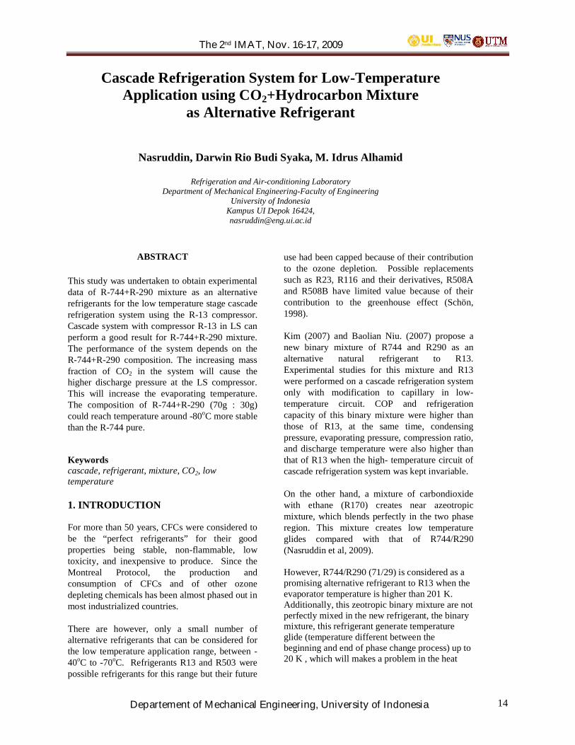
The schematic of experimental apparatus of thecascade system is shown in Fig. 1. It consists oftwo main systems which are low-temperaturesystem (LS) and high-temperature system (HS).In every system has four main components suchas compressor, condenser, expansion device andevaporator Some accessories are also used in thesystem such as oil separator, accumulator, filterdryer. In the cascade system, one heat exchangeris used together in HS and LS. The evaporator ofHS is functioned as the condenser of the LS. Thetype of this heat exchanger is tube-tube with 60cm length and 2.4 in outer diameter.
The compressor for HS is a Tecumseh hermetictype which actually designed for R22 and will beused also for R290 with the capacity 1 hp. The LScompressor is hermetic compressor which has 1hp capacity and designed actually for R13 or R23for low temperature system. The type of theexpansion valve is manual expansion valve fromSporlan with adjustment range 0.17 bar – 6.21bar. The adjustment can be done with a screw atthe top of the valve.
The experimental parameters measured for thisexperiment are also shown in figure 1. Thetemperatures at some points are measured withthermocouples and some pressure gauges arelocated in the system.
(a)
(b)
Figure 1: (a).Schematic of Experimental of Thecascade System (b). p-h Diagram of CascadeSystem
2.2 Experimental Procedure and materials
Before running of the experiment, whole of thesystem must be evacuated by using vacuum pump

The 2nd IMAT, Nov. 16-17, 2009
Departement of Mechanical Engineering, University of Indonesia 16
and run for leak-testing. After assuring there isno leak in the system, refrigerant is charged to theHS and LS. For HS, the system will be chargedwith R290 with the constant composition andcharged refrigerant around 250g. Meanwhile forLS the mass of charged refrigerant mixture of theR290 and R744 are Table 1.
Tabel 1. The composition of charged refrigerantmass of R290/R744
Composition R290 R744
I 0 g 100 g
II 30 g 70 g
4. RESULTS AND DISCUSSION
The experimental results for the first run using100% CO2 in the low-temperature system isshown in Figure 2. It is shown that thetemperature profiles as function of running time.The experiment has run for 6 hours at differentmeasurement locations. The dischargetemperature of the HS-compressor tends toincrease as the highest temperature of the system.The evaporator temperature drops significantlyafter 25 minutes into around -40oC and steady for6 hours. The evaporator of LS can reach around-80oC for the last 3 hours but not stable. It couldbe caused by the solid-ice forming in the LS andalso at the compressor discharge temperature inLS.
Figure 2 : Temperature profile of R-744 in LS 100g and R-290 in HS
The effect of mixing of CO2 with naturalhydrocarbon refrigerant R-290 is shown in Figure3. Generally the temperatures in the system aremore stable than pure CO2 for 4 h running test. Itcould be concluded that the effect of mixing of
CO2 and propane not only can reduce itsflammability but also could stabilize temperaturein the system especially in LS-evaporator.
Figure 3 : Temperature profile of R-744+R-290 inLS (70 g + 30 g) and R-290 in HS
5. CONCLUSION
The cascade system with compressor R-13 in LScan perform a good result for R-290+R-744mixture. Hopefully the performance will be betterif the compressor is designed for R13 or R23 forlow temperature application. The performance ofthe system depends on the R-290+R-744composition. The increasing mass fraction of CO2in the system tend to cause the higher dischargetemperature at the LS compressor. This willincrease the evaporating temperature.
The mixture of R-290+R-744 has someadvantages such as to decrease the flammabilityof refrigerant in compare to pure R-290 and lowerpressure of the discharge pressure in compare topure R-744, and the most important effect toenvironmental protection.
ACKNOWLEDGMENTS
The authors would like to thank University ofIndonesia for supporting this research activity byRUUI.
REFERENCES
[1] Schön P, 1998, New Refrigerants and theEnvironment, The 1998 Business Meeting,UK Controlled Environment Users’ GroupMinutes
The 2nd IMAT, Nov. 16-17, 2009
Departement of Mechanical Engineering, University of Indonesia 17
[1] Kim, J.H., Cho, J.M., Lee, I.H., Lee, J.S., andKim, M.S, 2007, Circulation concentrationof CO2/propane mixtures and the effect oftheir charge on the cooling performance in anair-conditioning system International Journalof Refrigeration Volume 30, pp. 43~49.
[2] Boulian, N, Yufeng, Z. 2006, ExperimentalStudy of the Refrigeration CyclePerformance for R744/R290 Mixtures,International Jurnal Of Refrigeration,30(2007):37-42
[3] Lee, T.S., Liu, C.H. and Chen, T.W., 2006,Thermodynamic analysis of optimalcondensing temperature of cascade-condenser in CO2/NH3 cascade refrigerationsystems International Journal of RefrigerationVolume 29, pp. 1100~1108.
[4] Nasruddin, D. Rahmat, L. Rahadiyan, 2009,”Utilization of CO2/Ethane Mixture as a NewAlternative of Eco-Friendly Refrigerant forLow Temperature Applications”. ICSERA2009, UI Depok, Indonesia.

The 2nd IMAT, Nov. 16-17, 2009
Departement of Mechanical Engineering, University of Indonesia 18
EXPERIMENTAL AND COMPUTATIONAL STUDY ON THERMALSTRUCTURE OF A SEPARATED REATTACHEMENT FLOW UNDER
HEATED GAS INJECTION
Harinaldi , Damora Rhakasywi, Sri Haryono
Department of Mechanical Engineering Faculty of EngineeringUniversity of Indonesia, Depok 16424
Tel : (021) 7270011 ext 51. Fax : (021) 7270077E- mail : [email protected]
ABSTRACTS
Flow channel with sudden expansion produces a separatedflow so that causing a recirculation flow. This investigationis revealing the alteration of the thermal structure within theflow field due to a heated gas penetration. Main focus isplaced on the influence of the ratio of specific momentuminjection (I=0.1 and I=0.5), the injection location of heatedgas (lf= 2H and lf=4H) and the variation of injectiontemperature (Ti=1000C and Ti=3000C) The investigationwas done computationally using finite volume method aswell as experimentally in a closed loop flow channel with abackward-facing step flow configuration. Numericalsolution models turbulence used were k-epsilon standardmodel and RNG k-epsilon. The numerical model was thenvalidated by the experimental results. This model works on2-D and 3-D Reynolds average Navier-Stokes (RANS)equations. From the results of thermal structure obtained, itcan be suggested that increasing the the ratio of specificmomentum injection supports more effective thermal mixingexcept to the narrow region around area injection. Moresignificant results are obtained in the region of shear layerand area downstream of the injection.
Keywords: separated flow, heated gas injection, k-epsilonmodel standard, RNG k-epsilon, numerical model
1. INTRODUCTION
Reattaching separated flow plays a vital importance inmany aspects of engineering equipments, for example inheat exchanger, chemistry reactor and energy system, aswell as in many combustor configurations. Especially inapplication of a combustor this kind of flow field isfrequently used to stabilization flame. In a condition of ahigh speed flow, a reattaching separated flow provides acertain area for flame holding, where the turbulence of flowhighly supports the mixing between fuel and air. In this casethe velocity field speed plays important role in the growth offlammable mixture. Fuel injection into the area ofrecirculation in a reattaching-separated flow such as fromthe bottom wall of a backward facing step is one of methodsthat can be applied. It is then realized that to get an efficientcombustor device needs a comprehensive understanding ofchemistry and mixing process between fuels whichinseminating and air around.
A certain approach to this problem shows that thedifficulties arise because of complex viscous-inviscid
interaction within the flow structure. Many methods suggestempirical estimation of pressure distribution at separatedstream area and some successfulness have been obtained insupersonic flow [1]. Flow patterns after backward facingstep without mass addition have been checked for severalaspects of turbulence transport such as the characteristic ofheat transfer [2]. Along with the development of turbulenceflow theories and the progress in flow diagnostic technologyas well as progress in computational fluid dynamics, theresearch direction moves to the effort to get much moreunderstanding on the mechanism to modify turbulencestructure with excitation external so that the nature oftransport turbulence which support fast transport properties(momentum, heat and mass) can be controlled.
Until about decade of 90th, most research were stilloriented on the fundamental characterization of recirculationflow which formed by various stream geometry in externalflow and also internal flow configuration without existenceof external excitation. The main focus was on theelucidation of various features of fluid dynamics found in arecirculation flow. Entering era of millennium some pioneerresearch on the influence of external excitation was startedsuch as works of Yang and Tsai [3] by using secondary fluidinjection from the bottom wall of a channel flow which havestep contour in the upstream. Their results show the someremarkable alteration of the flow structure which influenceda significant change of heat transfer coefficient in the flowchannel.In a research which focus on the mechanism of convectivemass transfer on mixing process by turbulence in abackward facing step Harinaldi et al. [4] indicated thatmixing process between air stream and injected gas veryintensively occurred within the region from three to fiveheight of step in streamwise direction. The mixing intensityalso influenced by the ratio specific momentum of gasinjection to free air stream. The research also showed thatgas injection can control the level of turbulence in the fieldwith growth resistance mechanism to the coherent structurein the shear layer. Meanwhile, a computational work was
The 2nd IMAT, Nov. 16-17, 2009
Departement of Mechanical Engineering, University of Indonesia 19
reported using Large Eddy Simulation (LES) andstatistical turbulence closures to study unsteadiness effect ofexternal excitation with a slot jet with angle 450 relative tostreamwise direction [5].
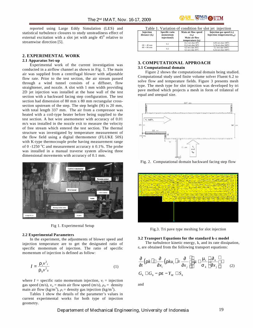
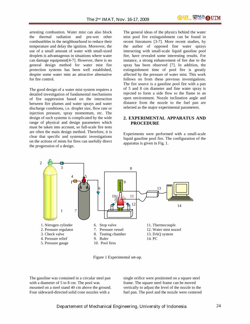
2. EXPERIMENTAL WORK2.1 Apparatus Set-up
Experimental work of the current investigation wasconducted in a airflow channel as shown in Fig. 1. The mainair was supplied from a centrifugal blower with adjustableflow rate. Prior to the test section, the air stream passedthrough a wind tunnel consists of a diffuser, flowstraightener, and nozzle. A slot with 1 mm width providing2D jet injection was installed at the base wall of the testsection with a backward facing step configuration. The testsection had dimension of 80 mm x 80 mm rectangular cross-section upstream of the step. The step height (H) is 20 mm,with total length 337 mm. The air from a compressor washeated with a coil-type heater before being supplied to thetest section. A hot wire anemometer with accuracy of 0.01m/s was installed in the nozzle exit to measure the velocityof free stream which entered the test section. The thermalstructure was investigated by temperature measurement ofthe flow field using a digital thermometer (FLUKE 50S)with K-type thermocouple probe having measurement rangeof 0 -1250 oC and measurement accuracy ± 0.1%. The probewas installed in a manual traverse system allowing threedimensional movements with accuracy of 0.1 mm.
Fig 1. Experimental Setup
2.2 Experimental ParametersIn the experiment, the adjustments of blower speed and
injection temperature are to get the designated ratio ofspecific momentum of injection. The ratio of specificmomentum of injection is defined as follow:
02
0
2
vvI ii
ρρ
= (1)
where I = specific ratio momentum injection, vi = injectiongas speed (m/s), vo = main air flow speed (m/s), 0 = densitymain air flow (kg/m3), i = density gas injection (kg/m3).
Tables 1 show the details of the parameter’s values incurrent experimental works for both type of injectiongeometry.
Table 1. Variation of condition for slot jet injectionInjection
distance (If)Specific ratiomomentuminjection(I)
Main air flow speed(v0)
Main air flowtemperature (t0)
Injection gas speed (vi)Injection temperature(tinj)
0,1 14,1 m/s dan 300C13,2 m/s dan 300C
4,95 m/s dan 1000C5,74 m/s dan 3000C2H = 40 mm
4H = 80 mm0,5 6,5 m/s dan 300C
6,5 m/s dan 300C5,1 m/s dan 1000C
6,32 m/s dan 3000C
3. COMPUTATIONAL APPROACH3.1 Computational domain
Figure 2 shows the computational domain being studied.Computational study used finite volume solver Fluent 6.2 tosolve flow and temperature fields. Figure 3 presents meshtype. The mesh type for slot injection was developed by tripave method which projects a mesh in form of trilateral ofequal and unequal size.
Fig. 2. Computational domain backward facing step flow
Fig.3. Tri pave type meshing for slot injection
3.2 Transport Equations for the standard k- modelThe turbulence kinetic energy, k, and its rate dissipation,
, are obtained from the following transport equations:
( ) ( )
kMbk
j
k
k
t
ji
i
SYGG
xxku
xk
t
+−−+
+
∂∂
+
∂∂
=∂∂
+∂∂
ρε
σµ
µρρ (2)
and

The 2nd IMAT, Nov. 16-17, 2009
Departement of Mechanical Engineering, University of Indonesia 20
( ) ( )
( ) εεεε
ε
ερε
εσµ
µρερε
Sk
CGCGk
C
xxu
xt
bk
j
t
ji
i
+−+
+
∂∂
+
∂∂=
∂∂+
∂∂
2
231
(3)
In these equations, Gk represents the generation ofturbulence kinetic energy due to the mean velocity gradients.Gb is the generation of turbulence kinetic energy due tobuoyancy. YM represents the contribution of the fluctuatingdilatation in compressible turbulence to the overalldissipation rate, C1 , C , and C are constants. k and arethe turbulent Prandtl numbers for k and , respectively. Skand S are user-defined source terms.
3.3 Transport Equations for the RNG k- model
( ) ( )
kMbk
jeff
ji
i
SYGG
xkk
xku
xk
t
+−−+
+
∂∂
∂∂
=∂∂
+∂∂
ρε
µαρρ (4)
and
( ) ( )
( ) εεεε
ε
εε
ρε
µαρερε
SRk
CGCGk
C
xe
xu
xt
bk
jeff
ji
i
+−−+
+
∂∂
∂∂
=∂∂
+∂∂
2
231
(5)
For RNG k- model was also considered to itscharacteristics of:
(i) having additional value at fast dissipation equationwhich can improve accuracy for blocked stream
(ii) Rotation effect of turbulence also considered sothat improve the accuracy for flow rotation.
(iii) providing analytical formula for the number ofPrandtl turbulent, while standard k- model usingconstant value of Prandtl number.
(iv) providing formula for low Reynolds number flow.
4. RESULTSSelected results are presented to describe important
characteristics of thermal structures of the flow field.
4.1 Measurement of Thermal FieldIn order to enable comparing the thermal structure
between some different injection conditions regardless thetemperature magnitude, a normalized temperature [T*] isintroduced and defined as follow:
0
0*TT
TTTinj −
−= (6)
Two-dimensional contour of the normalizedtemperature field for several injection conditions are
presented in Figs. 4(a)-(d). The figures show someremarkable differences of the thermal structure with regardto the heated gas spread due to variations of parameter ofinterest. The spatial density of contour lines suggests thatthe temperature gradient show some different tendency ofheat transfer rate to certain direction. Further analysis ispresented in the discussion section.
(a) lf/H = 2; I = 0.1; Tinj = 100 oC
(b) lf/H = 2; I = 0.1; Tinj = 300 oC
(c) lf/H = 2; I = 0.5; Tinj = 100 oC
(d) lf/H = 4; I = 0.1; Tinj = 300 oC
Fig.4 Contours of Mean Normalized Temperature (T*) forfour different conditions of injection
4.2 Computational Results of Temperature DistributionSome computational results showing the temperaturedistribution of the flow field are presented in Fig. 5 (a) and(b). The computational condition for Fig. 5(a) correspondsto the experimental condition previously shows in Fig. 4(a),meanwhile condition in Fig 5(b) corresponds to condition inFig. 4(d). In general, it can be said that these results show asufficient agreement between the thermal structures
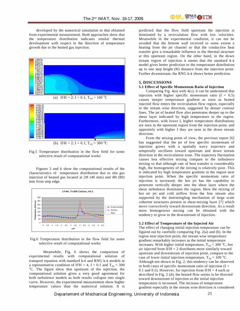
The 2nd IMAT, Nov. 16-17, 2009
Departement of Mechanical Engineering, University of Indonesia 21
developed by the numerical simulation to that obtainedfrom experimental measurement. Both approaches show thatthe temperature distribution indicates similar thermaldevelopment with respect to the direction of temperaturegrowth due to the heated gas injection.
(a) lf/H = 2; I = 0.1; Tinj = 100 oC
(b) lf/H = 2; I = 0.1; Tinj = 300 oC
Fig.5 Temperature distribution in the flow field for someselective result of computational works
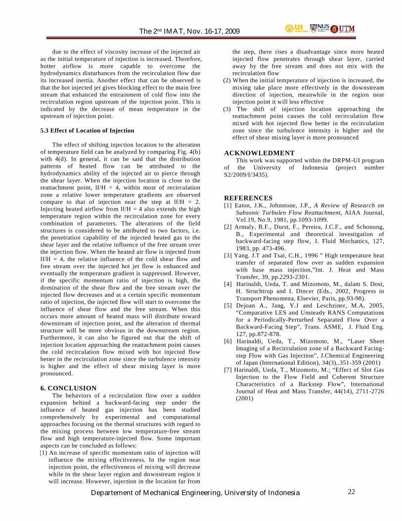
Figures 5 and 6 show the computational results of thecharacteristics of temperature distribution due to slot gasinjection of heated gas located at 2H (40 mm) and 4H (80)mm from step edge.
Lf=4H, Ti=300 Celcius, I=0.1
0
50
100
150
200
250
300
350
0 0.5 1 1.5 2 2.5 3 3.5 4 4.5 5 5.5 6 6.5
x/H
Tem
pera
ture
(Cel
cius
)
ExperimentalEpsilonRNG
Fig.6 Temperature distribution in the flow field for someselective result of computational works
Meanwhile, Fig. 6 shows the comparison ofexperimental results with computational solution oftransport equation with standard k-ε and RNG k-ε models ata representative condition of lf/H = 4, I = 0.1 and T inj = 300oC. The figure show that upstream of the injection, thecomputational solution gives a very good agreement forboth turbulence models as both results collapse into singlecurve. However, the experimental measurement show highertemperature values than the numerical solution. It is
predicted that the flow field upstream the injection isdominated by a recirculation flow with low velocities.Meanwhile in the experimental condition, it can not beavoided that the bottom wall received to some extent aheating from the jet channel so that the conductive heattransfer give a remarkable influence to the thermal structureat this upstream region. On the other hand, in the downstream region of injection it seems that the standard k-εmodel gives better prediction to the temperature distributionup to one step height (H) distance from the injection point.Further downstream, the RNG k-ε shows better prediction.
5. DISCUSSIONS5.1 Effect of Specific Momentum Ratio of Injection
Comparing Fig. 4(a) with 4(c), it can be understood thatinjection with higher specific momentum ratio (I = 0.5)causes steeper temperature gradient as soon as heatedinjected flow enters the recirculation flow region, especiallyin the stream wise direction, suggested by denser contourlines. The jet of heated flow also penetrates deeper up to theshear layer indicated by high temperature in the region.Furthermore, with lower I, higher temperature distributionsare seen in the upstream region from the injection point, andoppositely with higher I they are seen in the down streamdirection.
From the mixing point of view, the previous report [6]has suggested that the jet of low specific momentum ofinjection grows with a spatially wavy trajectory andtemporally oscillates toward upstream and down streamdirection in the recirculation zone. The trajectory fluctuationcauses less effective mixing compare to the turbulencemixing so that although rate of heat transfer is considerablyhigh, the homogeneity of the mixing is relatively poor. Thisis indicated by high temperature gradient in the region nearinjection point. When the specific momentum ratio ofinjection is increased, the hot jet has the capability topenetrate vertically deeper into the shear layer where theshear turbulence dominates the region. Here the mixing ofhot air jet and cold airflow from the free stream alsosupported by the intermingling mechanism of large scalecoherent structures present in shear-mixing layer [7] whichmove convectively toward downstream direction. As a result,more homogenous mixing can be obtained with thetendency to grow to the downstream of injection.
5.2 Effect of Temperature of the Injected AirThe effect of changing initial injection temperature can befigured out by carefully comparing Fig. 2(a) and (b). In theregion near injection point, the stream wise temperaturegradient remarkably increases as the initial temperatureincreases. With higher initial temperature, Tinj = 300 oC, hotair injected from lf/H = 2 distributes more similarly towardupstream and downstream of injection point, compare to thecase of lower initial injection temperature, Tinj = 100 oC.Although not shown in Fig. 2, this tendency can be observedin both cases of specific momentum ratio of injection (I =0.1 and 0.5). However, for injection from lf/H = 4 such asdescribed in Fig. 2 (d), the heated flow seems to be directedtoward downstream of injection as the initial injectiontemperature is increased. The increase of temperaturegradient especially in the stream wise direction is considered
The 2nd IMAT, Nov. 16-17, 2009
Departement of Mechanical Engineering, University of Indonesia 22
due to the effect of viscosity increase of the injected airas the initial temperature of injection is increased. Therefore,hotter airflow is more capable to overcome thehydrodynamics disturbances from the recirculation flow dueits increased inertia. Another effect that can be observed isthat the hot injected jet gives blocking effect to the main freestream that enhanced the entrainment of cold flow into therecirculation region upstream of the injection point. This isindicated by the decrease of mean temperature in theupstream of injection point.
5.3 Effect of Location of Injection
The effect of shifting injection location to the alterationof temperature field can be analyzed by comparing Fig. 4(b)with 4(d). In general, it can be said that the distributionpatterns of heated flow can be attributed to thehydrodynamics ability of the injected air to pierce throughthe shear layer. When the injection location is close to thereattachment point, lf/H = 4, within most of recirculationzone a relative lower temperature gradients are observedcompare to that of injection near the step at lf/H = 2.Injecting heated airflow from lf/H = 4 also extends the hightemperature region within the recirculation zone for everycombination of parameters. The alterations of the fieldstructures is considered to be attributed to two factors, i.e.the penetration capability of the injected heated gas to theshear layer and the relative influence of the free stream overthe injection flow. When the heated air flow is injected fromlf/H = 4, the relative influence of the cold shear flow andfree stream over the injected hot jet flow is enhanced andeventually the temperature gradient is suppressed. However,if the specific momentum ratio of injection is high, thedomination of the shear flow and the free stream over theinjected flow decreases and at a certain specific momentumratio of injection, the injected flow will start to overcome theinfluence of shear flow and the free stream. When thisoccurs more amount of heated mass will distribute towarddownstream of injection point, and the alteration of thermalstructure will be more obvious in the downstream region.Furthermore, it can also be figured out that the shift ofinjection location approaching the reattachment point causesthe cold recirculation flow mixed with hot injected flowbetter in the recirculation zone since the turbulence intensityis higher and the effect of shear mixing layer is morepronounced.
6. CONCLUSIONThe behaviors of a recirculation flow over a sudden
expansion behind a backward-facing step under theinfluence of heated gas injection has been studiedcomprehensively by experimental and computationalapproaches focusing on the thermal structures with regard tothe mixing process between low temperature-free streamflow and high temperature-injected flow. Some importantaspects can be concluded as follows:(1) An increase of specific momentum ratio of injection will
influence the mixing effectiveness. In the region nearinjection point, the effectiveness of mixing will decreasewhile in the shear layer region and downstream region itwill increase. However, injection in the location far from
the step, there rises a disadvantage since more heatedinjected flow penetrates through shear layer, carriedaway by the free stream and does not mix with therecirculation flow
(2) When the initial temperature of injection is increased, themixing take place more effectively in the downstreamdirection of injection, meanwhile in the region nearinjection point it will less effective
(3) The shift of injection location approaching thereattachment point causes the cold recirculation flowmixed with hot injected flow better in the recirculationzone since the turbulence intensity is higher and theeffect of shear mixing layer is more pronounced
ACKNOWLEDMENTThis work was supported within the DRPM-UI program
of the University of Indonesia (project numberS2/2009/I/3435).
REFERENCES[1] Eaton, J.K., Johnstone, J.P., A Review of Research on
Subsonic Turbulen Flow Reattachment, AIAA Journal,Vol.19, No.9, 1981, pp.1093-1099.
[2] Armaly, B.F., Durst, F., Pereira, J.C.F., and Schonung,B., Experimental and theoretical investigation ofbackward-facing step flow, J. Fluid Mechanics, 127,1983, pp. 473-496.
[3] Yang. J.T and Tsai, C.H., 1996 ” High temperature heattransfer of separated flow over as sudden expansionwith base mass injection,”Int. J. Heat and MassTransfer, 39, pp.2293-2301.
[4] Harinaldi, Ueda, T. and Mizomoto, M., dalam S. Dost,H. Struchtrup and I. Dincer (Eds., 2002, Progress inTransport Phenomena, Elsevier, Paris, pp.93-98).
[5] Dejoan A., Jang, Y.J and Leschziner, M.A, 2005,“Comparative LES and Unsteady RANS Computationsfor a Periodically-Perturbed Separated Flow Over aBackward-Facing Step”, Trans. ASME, J. Fluid Eng.127, pp.872-878.
[6] Harinaldi, Ueda, T., Mizomoto, M., “Laser SheetImaging of a Recirculation zone of a Backward Facing-step Flow with Gas Injection”, J.Chemical Engineeringof Japan (International Edition), 34(3),.351-359 (2001)
[7] Harinaldi, Ueda, T., Mizomoto, M.; “Effect of Slot GasInjection to the Flow Field and Coherent StructureCharacteristics of a Backstep Flow”, InternationalJournal of Heat and Mass Transfer, 44(14), 2711-2726(2001)

The 2nd IMAT, Nov. 16-17, 2009
Departement of Mechanical Engineering, University of Indonesia 23
Development of Water Mist System for Pool FireExtinguishment
Yulianto Sulistyo Nugroho, Donny Tigor Hamonangan and Ivan Santoso
Department of Mechanical Engineering University of IndonesiaKampus UI Depok 16424, INDONESIA
Ph. +62 21 7270032, Fax. +62 21 7270033,E-mail: [email protected]
ABSTRACT
A new experimental set-up was designed tostudy experimentally the effect of operatingparameter on the effectiveness of water mistfire suppression. Fine water mist driven bynitrogen through a nozzles system was used tosuppress and extinguish fires from pool ofgasoline at 5 and 8cm diameters. The spraycharacteristics of the mist was characterizedunder a constant pressure of 7 bar and variousnozzle inclination angles of 30o to 60o. Flametemperature and extinction time are used as ameasure of mist effectiveness. In general, theresults show that the inclination angle andheight of the nozzle play key roles inextinguishing performance of water mistsystem. Nevertheless, the flame size can bereduced by setting the mist envelope slightlyabove the pool surface. A flattened flame dueto fire plume buoyancy being overcome bydownward flow of mist was not identified inthe present work.
Keywordswater mist system, pool fire, and nozzleconfiguration.
1. INTRODUCTION
As the leading area of world economic growthfor the last two decades, many Asian countriesenjoy higher rate of economic development.Especially in urban areas of Asia, the spiralingland prices have been responded by theconstruction of tall buildings for multipurposes. In competitive situations, element ofallurement and glamour would come into thefore, playing significant roles in the designconcept of a tall building. With theintroduction of new, synthetic materialsthroughout the tall buildings, the hazards havebecome much more widespread, and the risksto life and property are now much greater [1].
Fire in buildings and industrial facilities causehuman suffering and materials losses. Theeconomic cost from building fires and othercost of fire relevant to fire safety programssuch as incremental building costs and the costof fire services and insurance is estimated toreach up to 1% of the gross domestic product(GDP) of many industrialized nations [2]. Theloss figure from fires in Asia is within acomparable range or higher, since one mustalso count the destructions resulted fromnatural fires. The general public is becomingincreasingly aware of the problems and therisks, and there is now a perceived need to dealwith fire safety in a more organized fashion inwhich engineering solutions are introduced atan early stage, either to prevent the outbreak offire, or to mitigate its effects to an extent thatthe losses are small, and considered"acceptable" in the circumstances. Despite thegreat loss from fire related accidents in urbanareas of Asia, effort to build the capacity ofpersonnel in fire safety areas is limited, andmainly focused in the area of fire fightingtechniques. In recent years, due to progress infire safety technology, economic and socialreasons, many countries are shifting theirbuilding codes from prescriptive-based toperformance-based [1,2]. As consequences,this development requires a great need forbetter fire safety technology for existing andnewly developed buildings and industries.
Deploying an effective fire suppression systemis an important aspect of the fire safety designof a modern building and industrial premises.Drawbacks on the use of excessive amount ofwater in a sprinkler system, and a ban on theuse of ozone depleting Halon 1301 wouldmake research on finding an alternativeprotection system for fire control become anecessity [3].
The 2nd IMAT, Nov. 16-17, 2009
Departement of Mechanical Engineering, University of Indonesia 24
arresting combustion. Water mist can also blockthe thermal radiation and pre-wet othercombustibles in the neighbourhood to reduce theirtemperature and delay the ignition. Moreover, theuse of a small amount of water with small-sizeddroplets is advantageous in situations where watercan damage equipment[4-7]. However, there is nogeneral design method for water mist fireprotection systems has been well established,despite some water mist an attractive alternativefor fire control.
The good design of a water mist system requires adetailed investigation of fundamental mechanismsof fire suppression based on the interactionbetween fire plumes and water sprays and waterdischarge conditions, i.e. droplet size, flow rate orinjection pressure, spray momentum, etc. Thedesign of such systems is complicated by the widerange of physical and design parameters whichmust be taken into account, so full-scale fire testsare often the main design method. Therefore, it isclear that specific and systematic investigationson the actions of mists for fires can usefully directthe progression of a design.
The general ideas of the physics behind the watermist pool fire extinguishment can be found inrecent literatures [3-7]. More recent studies, bythe author of opposed fine water spraysinteracting with small-scale liquid gasoline poolfire, have revealed some interesting results. Forinstance, a strong enhancement of fire due to thespray has been observed [7]. In addition, theextinguishment time of pool fire is greatlyaffected by the pressure of water mist. This workfollows on from these previous investigations.The fire source is a gasoline pool fire with a panof 5 and 8 cm diameter and fine water spray isinjected to form a side flow to the flame in anopen environment. Nozzle inclination angle anddistance from the nozzle to the fuel pan areselected as the major experimental parameters.
2. EXPERIMENTAL APPARATUS ANDPROCEDURE
Experiments were performed with a small-scaleliquid gasoline pool fire. The configuration of theapparatus is given in Fig. 1.
13
10 11
9
8
6
54
2
3
1 714
1. Nitrogen cylinder 6. Stop valve 11. Thermocouple2. Pressure regulator 7. Pressure vessel 12. Water mist nozzel3. Check valve 8. Testing chamber 13. DAQ system4. Pressure relief 9. Ruler 14. PC5. Pressure gauge 10. Pool fires
12
12
Figure 1 Experimental set-up.
The gasoline was contained in a circular steel panwith a diameter of 5 to 8 cm. The pool wasmounted on a steel stand 40 cm above the ground.Four sideward-directed solid cone nozzles with a
single orifice were positioned on a square steelframe. The square steel frame can be movedvertically to adjust the level of the nozzle to thefuel pan. The pool and the nozzle were centered
The 2nd IMAT, Nov. 16-17, 2009
Departement of Mechanical Engineering, University of Indonesia 25
inside a testing chamber with a black colorbackground. Water was pressurized by a highpressure nitrogen gas cylinder, and injectedthrough the nozzle via a stop valve to controlonset of injection. For each test, the pan was filledto 1 cm below the pan lip with fresh fuel. Then,the fire was allowed to burn for at least 20s toensure quasi-steady burning before the waterinjection. The flame height was measured using aruler. Two K type thermocouples were placed atthe centre line of the circular pan at 5 and 10 cmabove the pool surface. In a typical run, importantdata such as flame temperatures, and suppressiontime were recorded via a data logging systemlinked to a computer. The interaction of pool firesand water mist spray were recorded using a digitalvideo camera.
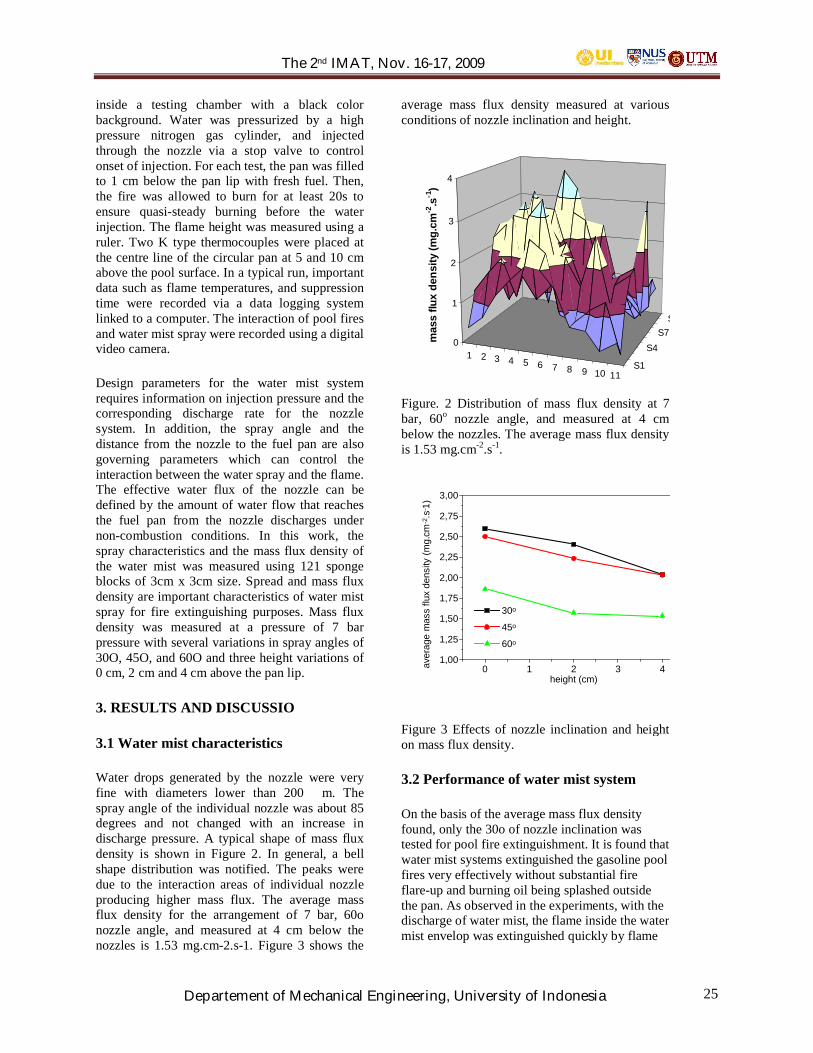
Design parameters for the water mist systemrequires information on injection pressure and thecorresponding discharge rate for the nozzlesystem. In addition, the spray angle and thedistance from the nozzle to the fuel pan are alsogoverning parameters which can control theinteraction between the water spray and the flame.The effective water flux of the nozzle can bedefined by the amount of water flow that reachesthe fuel pan from the nozzle discharges undernon-combustion conditions. In this work, thespray characteristics and the mass flux density ofthe water mist was measured using 121 spongeblocks of 3cm x 3cm size. Spread and mass fluxdensity are important characteristics of water mistspray for fire extinguishing purposes. Mass fluxdensity was measured at a pressure of 7 barpressure with several variations in spray angles of30O, 45O, and 60O and three height variations of0 cm, 2 cm and 4 cm above the pan lip.
3. RESULTS AND DISCUSSIO
3.1 Water mist characteristics
Water drops generated by the nozzle were veryfine with diameters lower than 200 m. Thespray angle of the individual nozzle was about 85degrees and not changed with an increase indischarge pressure. A typical shape of mass fluxdensity is shown in Figure 2. In general, a bellshape distribution was notified. The peaks weredue to the interaction areas of individual nozzleproducing higher mass flux. The average massflux density for the arrangement of 7 bar, 60onozzle angle, and measured at 4 cm below thenozzles is 1.53 mg.cm-2.s-1. Figure 3 shows the
average mass flux density measured at variousconditions of nozzle inclination and height.
1 2 3 4 5 6 7 8 9 10 11S1
S4S7
S10
0
1
2
3
4
mas
s flu
x de
nsity
(mg.
cm-2
.s-1
)
Figure. 2 Distribution of mass flux density at 7bar, 60o nozzle angle, and measured at 4 cmbelow the nozzles. The average mass flux densityis 1.53 mg.cm-2.s-1.
0 1 2 3 41,00
1,25
1,50
1,75
2,00
2,25
2,50
2,75
3,00
30o
45o
60o
aver
age
mas
s flu
x de
nsity
(mg.
cm-2
.s- 1
)
height (cm)
Figure 3 Effects of nozzle inclination and heighton mass flux density.
3.2 Performance of water mist system
On the basis of the average mass flux densityfound, only the 30o of nozzle inclination wastested for pool fire extinguishment. It is found thatwater mist systems extinguished the gasoline poolfires very effectively without substantial fireflare-up and burning oil being splashed outsidethe pan. As observed in the experiments, with thedischarge of water mist, the flame inside the watermist envelop was extinguished quickly by flame

The 2nd IMAT, Nov. 16-17, 2009
Departement of Mechanical Engineering, University of Indonesia 26
quenching and oxygen dilution. Figure 4 showsvariation of temperatures measured above thepool surface at two different locations ofthermocouple with time. Once the water mistdischarge was activated, the temperatures insidethe coverage areas of the mist were quicklydropped as fine water drops cooled the flame.Figure 5 shows the sequences of fireextinguishment. The figure clearly shows there isno flattened flame due to fire plume buoyancybeing overcome by downward flow of mist. Infact the flame size was reduced by covering thefire inside the mist envelope.
The length of a flame is a significant indicator ofthe hazard posed by the flame. Flame lengthdirectly relates to flame heat transfer and thepropensity of the flame to impact surroundingobjects. As a plume of hot gases rises above aflame, the temperature, velocity, and width of theplume changes as the plume mixes with itssurroundings. The size and temperature of theflame are important in estimating the ignition ofadjacent combustibles. This work clearly showsthat the flame geometry is affected by the poolsizes. As a consequence, the period of flamecooling and extinction are longer for larger pooldiameter and nozzle height (Figure 6).
0 20 40 60 80 100
0
100
200
300
400
500
600
700Fi
re e
xtin
guis
hed
Wat
er m
ist d
isch
arge
d
Flam
e ig
nitio
n
h=5 cm h=10 cm
Pressure, p = 7 bar ;Pool fire, D = 8 cmNozzle height, h = 2 cm
Nozzle inclination, 30o
Tem
pera
ture
(oC
)
Time (s)
Figure 4 Variation of temperatures above pool surface with time.
4. CONCLUSIONS
Flame geometry is greatly affected by the poolsizes. Flame cooling is the dominantextinguishing mechanisms of water mist for poolfires. It requires that the employed water mistsystems shall have sufficient spray coverage,water mass flux, and spray momentum. The watermist systems using four sideward-directed solidcone nozzles developed in the current work were
effective in extinguishing pool fire with variousdiameters. The extinguishing performance wasgreatly affected by nozzle inclination and itsheight from the pan lip. In general, the flame sizewas reduced by covering the fire inside the mistenvelope without generating a flattened flame dueto fire plume buoyancy being overcome bydownward flow of mist.
The 2nd IMAT, Nov. 16-17, 2009
Departement of Mechanical Engineering, University of Indonesia 27
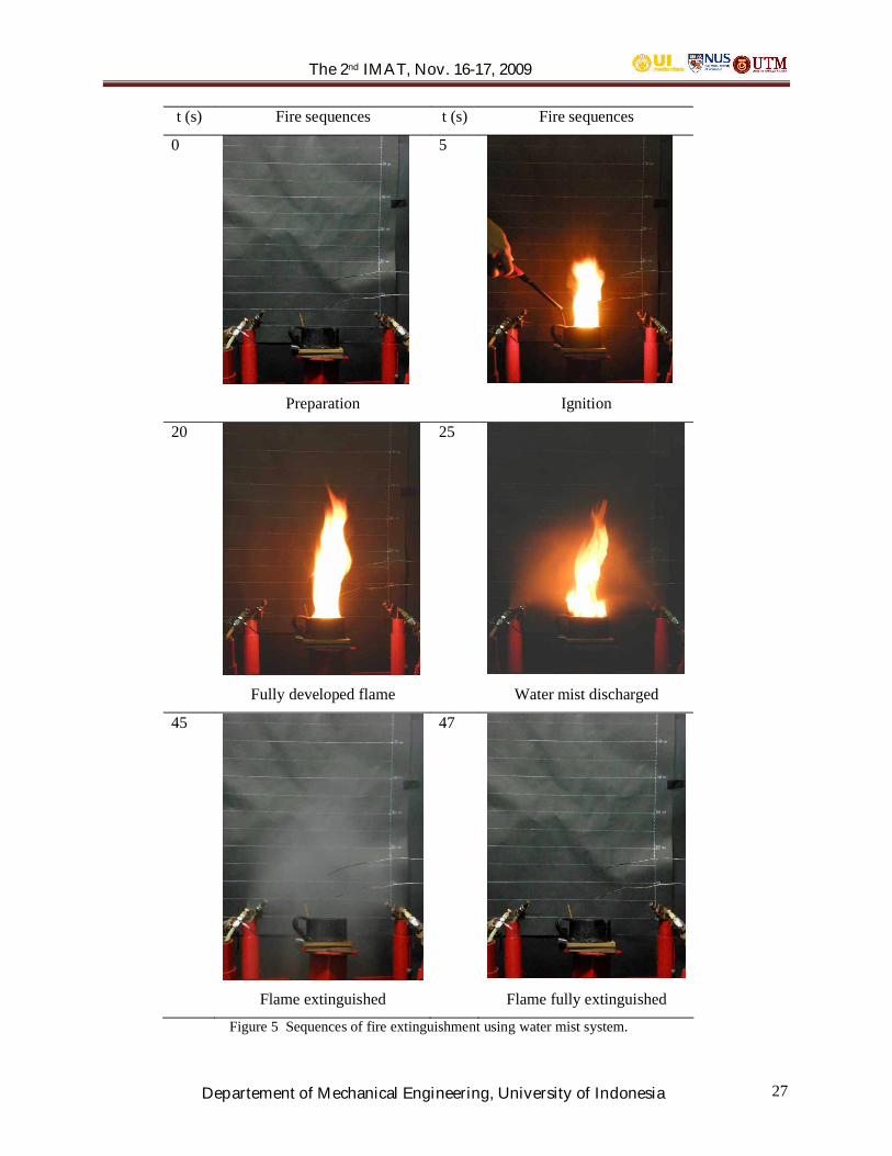
t (s) Fire sequences t (s) Fire sequences
0 5
Preparation Ignition
20 25
Fully developed flame Water mist discharged
45 47
Flame extinguished Flame fully extinguished
Figure 5 Sequences of fire extinguishment using water mist system.

The 2nd IMAT, Nov. 16-17, 2009
Departement of Mechanical Engineering, University of Indonesia 28
0 1 2 3 40
5
10
15
20
25
30
35
Pool diameter 50 mm Pool diameter 80 mm
Nozzle inclination 30o
Extin
guih
men
t tim
e (s
)
Height (cm)
Figure 6 Extinguishment times of pool fires
ACKNOWLEDGEMENT
Dr. Y.S. Nugroho would like to thank thefinancial support from the Directorate forResearch and Public Services University ofIndonesia (DRPM UI) and Directorate General ofHigher Education (DP2M), Ministry of NationalEducation Republic of Indonesia.
REFERENCES
[1] A.M. Hasofer, V.R. Beck, I.D. Bennetts,Risk Analysis in Building Fire SafetyEngineering, Elsevier Butterworth-Heinemann, 2007.
[2] Rasbach, D.J., Ramachandran, G., Kandola,B., Watts, J.M., and Law, M., Evaluation ofFire Safety, Wiley, 2004.
[3] Liu, Z, Carpenter, D., dan Kim, A.K. (2005),Application of Water Mist to ExtinguishLarge Oil Pool Fires for Industrial OilCooker Protection, 8th InternationalSymposium on Fire Safety Science, Beijing,China, pp. 1-12.
[4] Kim, M.B., Jang, Y.J., and Yoon, M.,Extinction Limit of a Pool Fire with a WaterMist, Fire Safety Journal 28 (1997) 295-306.
[5] Mawhinney, J.R and Gerard G. Back III,Water Mist Fire Suppression Systems,Chapter 14 The SFPE Handbook of FireProtection Engineering, 3rd Edition, 2002,pp. 4-311-4-337.
[6] Wighus, R., Aune, P., and Brandt, A.W.,Water Mist versus Sprinklers and Gas FireSuppression Systems –Differences andSimilarities, International Water MistConference, Amsterdam, The Netherlands10 - 12 April 2002.
[7] Nugroho, Y.S., Fajarudin, K., Wahyulianto,D., dan Harinaldi, Pengembangan SistemKabut Air Bertekanan Rendah untukPemadaman Pool Fire, Seminar NasionalTahunan Teknik Mesin SNTTM-VI BandaAceh Nanggroe Darussalam Univ SyiahKuala 20-22 Nop 2007, ISBN 979-97726-8-0.

The 2nd IMAT, Nov. 16-17, 2009
Departement of Mechanical Engineering, University of Indonesia 29
Preparation of Activated Carbon from Low Rank Coal withCO2 activation
Awaludin Martin, Bambang Suryawan, Muhammad Idrus Alhamid, Nasruddin
Refrigeration and Air Conditioning Laboratory, Mechanical Engineering DepartmentFaculty of Engineering-Univeristy of Indonesia
ABSTRACT
The aim of this research is to produce activatedcarbon from Indonesian low rank coal.Activated carbon producing basically involveth following step; raw matrial preparation,carbonization and activation by physical orchemical method and for this research wereuse physical activation methods. Besidecarbonization process (by N2 gas) up totemperature 950oC, in this researchcarbonization with O2 also were use up totemperature 300oC by variation time of processup to 360 minute. Physical activation methodwere use in this research by CO2 as activatingagent up to temperature 950oC by variationtime of process up to 360 minute. Surfacecondition of activated carbon is known byScanning Electron Micrograph (SEM) andiodine number was use to known quality ofactivated carbon. The result of this research isthe maximum of burn off and iodine numberare 71,88% and 589,10 g/kg.
Kyword: coal, activated carbon, burn off,Iodine number
INTRODUCTION
Activated carbon consumption is continuouslybeing increased because they are used inimportant areas such as waste, drinkable watertreatments, atmospheric pollution control,poisonous gas separation, solvent recovery etc(Marsh, Harry and Francisco Rodriguez-Reinoso, 2006). Almost any carbonaceousmaterial can be converted into activated carbonsuch as wood, nut shett, coconut shell, coal atc(Marsh, Harry and Francisco Rodriguez-Reinoso, 2006)
Activated carbon is the most widely usedsorbent, surface area of activated carbon up to4000 m2/g (Yang, Ralph. T, 2003) thusactivated carbon can adsorb an adsorbate inhigh capacity.
Beside surface area, other parameters to knownactivated carbon quality is iodine number.Iodine number is defined as the amount ofiodine (in milligrams) adsorbed by powderedcarbon (per gram) from 0.02 N iodine aqueoussolution (ASTM D4607-94) (Yang, Ralph. T,2003). Iodine number is a simple testing tofind activated carbon quality and iodinenumber has been roughly correlated to thesurface area of pores >10 diameter (Yang,Ralph. T, 2003).
In this research, low rank coal were used asstarting material to producing activated carbon.The modern manufacturing processes toproduce activated carbon basically involve thefollowing steps: raw material preparation, low-temperature carbonization, and physical orchemical activation (Yang, Ralph. T, 2003). Inthis research beside carbinization process (byN2 as innert gas) up to temperature 950oC,oxidation process also done ( by variation ofO2 flowing) up to temperature 300oC withvariation time of process up to 360 minute.Physical activation with CO2 as activatingagent were done up to temperature 950oC withvariation time of process up to 360 minute.
EXPERIMENT SECTION
Coal Characteristics. Low rank coal were useas the starting material and the analysis of coalas shown below:
q Inherent Moisture : 5,59 %q Ash Content : 17,96 %q Volatile Matter : 34,51 %q Fixed Carbon : 41,94 %q Total Sulphur : 1,74 %Certificate of Sampling and Analysis, 2007,PT. Superintending Company of Indonesia(Sucofindo)Experimentation of Prosedure. The as-received coals were crushed and seived to aparticle size of 2-10 mm before being treated.The production of activated carbons by a

The 2nd IMAT, Nov. 16-17, 2009
Departement of Mechanical Engineering, University of Indonesia 30
physical activation technique was completed inan vertical autoclave activation reactor with afurnace. There are three variation process heattreatment to pruduced activated carbon. Theprocessing to produce activated carbons wereas follows:
1. Carbonization; Pyrolysis of fresh coalswere performed in a furnace under astream of High purity of N2 at ± 40cm3/minute as inert gas. The samples wereheated from room temperature tomaximum heat treatment temperatures in600°C for 1 hour. Following thecarbonization process, the char sampleswere gasified, also in the furnace, in astream of CO2 at ± 40 cm3/minute. Thesamples were heated from roomtemperature to maximum heat treatmenttemperatures in 600°C, 700oC, and 750oCfor 1 hour. Scheme of this procedure asshown in figure 1a.
Figure 1a: Scehme of activated carbon;Carbonization and activation
2. Carbonization; Pyrolysis of fresh coalswere performed in a furnace under astream of High purity of N2 at ± 80cm3/minute as inert gas. The samples wereheated from room temperature tomaximum heat treatment temperatures in900 °C for 1 hour. Following thecarbonization process, the char sampleswere gasified, also in the furnace, in astream of CO2 at ± 80 cm3/minute. Thesamples were heated from roomtemperature to maximum heat treatmenttemperatures in 950oC for 3 hour.
3. Carbonization or Oxidation; Pyrolysis offresh coals were performed in a furnaceunder a stream of High purity of O2 atvariation of gas flow. The samples wereheated from room temperature to
maximum heat treatment temperatures in300 °C for 1, 3 and 6 hour. Following thecarbonization process, the char sampleswere gasified, also in the furnace, in astream of CO2 at ±80, 100 and 150cm3/minute. The samples were heatedfrom room temperature to maximum heattreatment temperatures in 950 oC for 1, 3and 6 hour. Scheme of this procedure asshown in figure 1b.
(a)
(b)
Figure 1b: Scehme of activated carbon;Carbonization or OxidationProcess with O2 (a) andActivation Process (b)
After the above process activated carbon werecrushed and seived to a particle size of 10 x 20mesh.
Activated Carbon Characterization.Scanning Electron Micrograph to show surfacecondition were done in Jakarta and Iodinenumber test were done in Bogor

The 2nd IMAT, Nov. 16-17, 2009
Departement of Mechanical Engineering, University of Indonesia 31
RESULT AND DISCUSSION
In this work the result for three processing toproduce activated carbon were compared.
First Procedure
Table 1 describe the effect of temperatureactivation process on amount presentage ofunsure in activated carbon, its impurity unsurestill in activated carbon. First procedure is notresulting the optimum activated carbon yet, themaksimum unsure of carbon in activatedcarbon only 48,53%. The major unsure inactivated carbon is carbon and is present to theextent of 85 to 95%. In addition, activatedcarbons contain other elements such ashydrogen, nitrogen, sulfur and oxigen (BansalR.C. et al., 2005).
Tabel 1. First layer unsure of Activated Carbon
It can be seen in figure 2 that the macroporefrom activated carbon were performed butamost all the surface still covered withimpurity unsure and from table 1 the impurityunsure are oxigen, sulphur and ferro.
(a)
(b)
(c)Figure 2: Activated carbon from first
procedure at 600oC (a), 700oC(b), dan 750oC (c)
Second Procedure
Table 2 describe the effect of activation timeon amount of carbon, longer activation timeresult in higher amount of carbon.
Tabel 2 First layer unsure of Activated Carbonat second Procedure
It can be seen in figure 3, the macropore fromactivated carbon were performed but amost allthe surface still covered with impurity unsureand from table 2 the impurity unsure areoxigen, sulphur and ferro.
Temp.Process
UnsureCarbon
(%)Oxigen
(%)Sulphur
(%)Ferro(%)
600 oC 47,89 29,44 22,67 -700 oC 24,74 8,15 5 62,11750 oC 48,53 4,4 1,73 45,35
Time ofActivation
Process
UnsureCarbon
(%)Oxigen
(%)Sulphur
(%)Ferro(%)
60 minute 75,22 9,33 7,57 7,88180 minute 88,19 7,47 4,34 -

The 2nd IMAT, Nov. 16-17, 2009
Departement of Mechanical Engineering, University of Indonesia 32
(a)
(b)
Figure 3. Activated Carbon; carbonizationat 900oC and activation temperature 950oCwith variation time of process activation1hour (a) and 3 hour (b) (Alhamid. M.I. et al.,2008)
Figure 4 describe the effect of activationtime on burn-off and surface area. It can beseen from figure 4, in general longeractivation time result in higher burn-off andsurface area. This result was consistent withMarsh, Harry et al., 2006, that activationprocess influence of mass flow rate ofactivating agent and activation time.
30
32
34
36
38
40
42
44
46
48
50
60 90 120 150 180
Time of Activation Process (minute)
Bur
n of
f (%
)
0
50
100
150
200
Iodi
ne N
umbe
r (m
g/g)
Burn offAngka Iodine
Figure 4. Weight loss or burn off and IodineNumber during activation processwith heat treatment temperature950oC
Third Procedure
Beside influences of heat rate, mass flowrate of activating agent, activating agent,equipment and activation time, activationprocess also influnce with ratio oxygen andcarbon in raw material (Teng, Hsisheng etal., 1996).
In this procedure, carbinozation with N2 asinnert gas at first and second procedurewere changes with O2 up to temperatur300oC. The aim of this procedure are toincreasing oxygen unsure at the rawmaterial. Activation process were done withCO2 as activating agent up to temperature950oC by variation of CO2 flow and time ofprocess.
Figure 5 describe the effect of stream of O2
and time of process on burn-off. It can beseen from figure 5, in general longercarbonization time and bigger of steram ofO2 resulting in higher burn-off. This result isconsistent with Teng, Hsisheng et al., 1996,that ratio of oxygen and carbon in the coalis ones of factor to improving quality ofactivated carbon product.

The 2nd IMAT, Nov. 16-17, 2009
Departement of Mechanical Engineering, University of Indonesia 33
30
32
34
36
38
40
42
44
46
48
50
0 60 120 180 240 300 360
Time of Process (minute)
Bur
n O
ff (%
)
O2 = 20 ml/mnt
O2 = 50 ml/mnt
O2 = 100 ml/mnt
Figure 5. Weight loss or burn off duringOxidation process with heattreatment temperature 300oC byvariation of O2 flow 20, 50, and 100ml/minute and for 1 houractivation process
Figure 6 describe the effect of time ofprocess activation on burn-off and iodinenumber. It can be seen from figure 6, ingeneral longer activation time resulting inhigher burn-off and iodine number.
Coal were carbonized by 100 ml/minute O2
up to 300oC for 6 hour, Following thecarbonization process, the char sampleswere gasified, also in the furnace, in astream of CO2 at ± 80 cm3/minute up to950oCwith variation time of process are 1, 3,and 6 hour. The
maksimum burn off and iodine number inthis process are 60,44% and 497,9 mg/g.
40
45
50
55
60
65
70
75
50 110 170 230 290 350
Time of Activation Process (minute)
Burn
Off
(%)
0
100
200
300
400
500
600
Iodi
ne N
umbe
r (gr
/kg)
Burn Off
Angka Iodine
Figure 6. Weight loss and Iodine Numberduring activation process with heattreatment temperature 950oC
Figure 7 describe the effect of stream ofCO2 on burn-off and iodine number. It canbe seen from figure 7, in general bigerstream of CO2 resulting in higher burn-offand iodine number.
Coal were carbonized by 100 ml/minute O2
up to 300oC for 6 hour, Following thecarbonization process, the char sampleswere gasified, also in the furnace, in astream of CO2 at ± 80, 100, and 150cm3/minute up to 950oC for 6 hour. Themaksimum burn off and iodine number inthis process are 71,88% and 589,1mg/g.
30
35
40
45
50
55
60
65
70
75
80
50 80 110 140 170 200
Stream of CO2 (ml/menit)
Bur
n O
ff (%
)
0
100
200
300
400
500
600
700
Iodi
ne N
umbe
r (gr
/kg)
Burn OffAngka Iodine
Gambar 7. Weight loss and Iodine Numberduring activation process withheat treatment temperature950oC during activation process
The of result of the third procedure wasconsistent with Marsh, Harry et al., 2006, thatactivated carbon producing influence ofmass flow rate of activating agent,temperature of process and activation time.
CONCLUSION
1. Activated carbon were producedfrom low rank coal with carbonization

The 2nd IMAT, Nov. 16-17, 2009
Departement of Mechanical Engineering, University of Indonesia 34
and activation process with variationof temperature, stream of Nitrogen,Oxygen and carbon dioxide, time ofoxidation and activation process.
2. Producing of activated carbon wasinfluences with mass flow rate ofactivating agent, Heat treatmenttemperature and activation time ofprocess also ratio oxygen and carbonin raw material
3. Weight losses or burn off is similiar withiodine number, increasing weight losswill increasing iodine number thus thesurface area will be larger too
4. The maximum weight loss or burn offand iodine number of activatedcarbon in this research is 71,88% and589,10 g/kg by carbonization (by O2
stream ±100 ml/minute for 6 hour) andactivation process (by CO2 stream±150 ml/minute for 6 hour).
REFFERENCE
[1] Alhamid, M. Idrus d, BambangSuryawan, Nasruddin, Awaludin Martin,Sehat Abdi, Characterization ofActivated Carbon as Adsorbent FromRiau Coal by Physical Activatin Method,The First International Meeting onAdvances in Thermo-fluids, UniversitiTeknologi Malaysia, Malaysia, 26thAugust 2008
[2] Bansal, Roop Chand & MeenakshiGoyal, 2005, Activated CarbonAdsorption, Taylor & Francis Group, USA
[3] Certificate of Sampling and Analysis,2007, PT. Superintending Company ofIndonesia
[4] Marsh, H. & Rodriguez-Reinoso, F. 2006,Activated Carbon, Elsevier Ltd, OxfordUK.
[5] Rouquerol, Jean, François Rouquerol,Kenneth Sing,1998 Absorption ByPowders And Porous Solids, Elsevier
[6] Teng, Hsisheng, Jui-An Ho, Yung-Fu Hsu,and Chien-To Hsieh, 1996, Preparation ofActivated Carbons from BituminousCoals with CO2 Activation. 1. Effects ofOxygen Content in Raw Coals, Ind. Eng.Chem. Res., 35 (11), 4043 -4049,American Chemical Society
[7] Yang, Ralph. T, 2003, Adsorbents:Fundamentals and Applications, Johnwiley and Sons Inc, New Jersey.
The 2nd IMAT, Nov. 16-17, 2009
Departement of Mechanical Engineering, University of Indonesia 35
Experimental Study of Characteristic and Performanceof Non-Branded Thermoelectric Module
Zuryati Djafar, Nandy Putra, Raldi A. KoestoerHeat Transfer Laboratory, Mechanical Engineering Department, University of Indonesia
Kampus Baru UI, Depok, 16424- West Java-IndonesiaPhone: +62-081355026518, Fax: 021-7270033, email: [email protected]
Correspondence: [email protected]
AbstractThermoelectric modules is thermoelement devices that can take advantage to convert heat into electricenergy. As an electrical energy generating system, these elements are not noisy, easy to maintain andrelatively small dimension, light and friendly to the environment because it does not produce pollution. Theaim of this research is to evaluate and to determine characteristic of thermoelectric module as a non-branded (not accompanied by brand and specifications) thermoelectric generator system. The method iscarried out in this research is to drain the fluid (hot water) from a Circulating Thermostatic Bath into awater block; the thermoelectric module is inset between water block and a heatsink-fan. The results showthat a Thermoelectric module on the 4 temperature conditions of the CTB temperature 35 ° C, 40° C, 45 °C and 50 °C can provide a temperature difference of 5.4°C, 7.6°C, 11.7°C and 14.8°C with output powerobtained are 3.07W, 19.02W, 42.8W and 65.13W respectively.
Keywords: characteristic, non branded, thermoelectric module, circulating thermostatic bath, waterblock, output power
I. INTRODUCTION
Thermoelectric generator modules workon the principle of work of Seebeck effect [1], theeffect occurs when there are two differentmaterials connected in a circuit is closed and thesecond connection maintained at differenttemperatures the electrical current will flow in thecircuit, and when one wire decided then connectedwith a galvanometer, it will show the voltagedifference of the two ends. So that the differencein temperature can cause the voltage differencethat produces electromotive force.
Figure 1. Mechanism of Seebeck Efect Principles[2]
Source: Melcor Industries, (www.melcor.com)
Thermoelectric modules are typicallymeasuring 40mm x 40mm or smaller and havemore or less thick, 4 mm. Age of a ThermoelectricModule in accordance with industry standards isapproximately 100000-200000 hours and morethan 20 years when used as a coolant and theamount and the appropriate voltage characteristicsof each module [3].
In the Thermoelectric planning, both forits use as a cooling system and usingThermoelectric generator module, there are 3parameters that must be considered are: Q = heatload to be moved (watts); Tc = temperature ofcold surface of the module (°C);Th = temperature of hot side surface of themodule (°C). Heat Load is the total number ofheat that must be removed by Thermoelectricmodules from the object to be cooled / heat to theenvironment is taken [4].
A Thermoelectric modules can becharacterized by comparing the maximumperformance with a hot junction temperature.Parameters on a mutual interdependence. Electricpower applied to Thermoelectric modules are:
Where: Pin is Electrical power (Watt); V is linevoltage (Volt); I is Current Electricity (Ampere)Currently there are many Thermoelectric moduleson the market. Thermoelectric modules are freely

The 2nd IMAT, Nov. 16-17, 2009
Departement of Mechanical Engineering, University of Indonesia 36
Therefore deemed necessary to conduct thetest specifications so that they can actually knowncapabilities that ca n be produced fromthese Thermoelectric modules. From thecharacteristics, the buyer can know the actualcharacteristics, as desired. Does economicconsiderations or the quality that will be used.
II. RESEARCH METHOD
Accordance with the purpose of the study to beconducted to determine the characteristics of non-branded Thermoelectric modules (modules withoutspecification), then this research made a testinstallation as figure 2 below:
Therefore, in this study was conducted todetermine the characteristics of Thermoelectricmodules are non-branded.
Figure 2. Testing Installation
Mechanism of the Data RetrievalObservations long test 1800 seconds (30
minutes) for each fluid temperature condition in thecirculating Thermostatic Bath (CTB). Variation offluid temperature conditions of the CTB are 35°C,40°C, 45°C and 50°C.
Thermoelectric modules are placedbetween the water block and heatsink-fan, on bothsides of the module (hot side and cold side) eachplaced a type K thermocouple wire, thermocouple isconnected to the gauge ADAMtech special type oftemperature measurement that is connected to thecomputer as a data acquisition. Anotherthermocouple wires placed in the water channel inand out of the water block. Two thermocouple wiresin the fluid in the CTB and to the environment(ambient).
Temperature measurement data on thenumber 6 wire thermocouples were recordeddirectly in the form of a notepad file and can be readvisually on the screen with the help of computersoftware that will be used Advantech. The data readis Thot and Peltier elements Tcold side, fluidTemperatur of Water Block, TemperaturCirculating Thermostatic Bath (CTB), Current andvoltage generated from the second junction ofThermoelectric module through the display readsAVOmeter used. Data of current, voltage andtemperatures then is used to calculate the poweroutput of a given and a large temperature differenceon both sides of Thermoelectric modules.
III. RESULT AND DISCUSSION
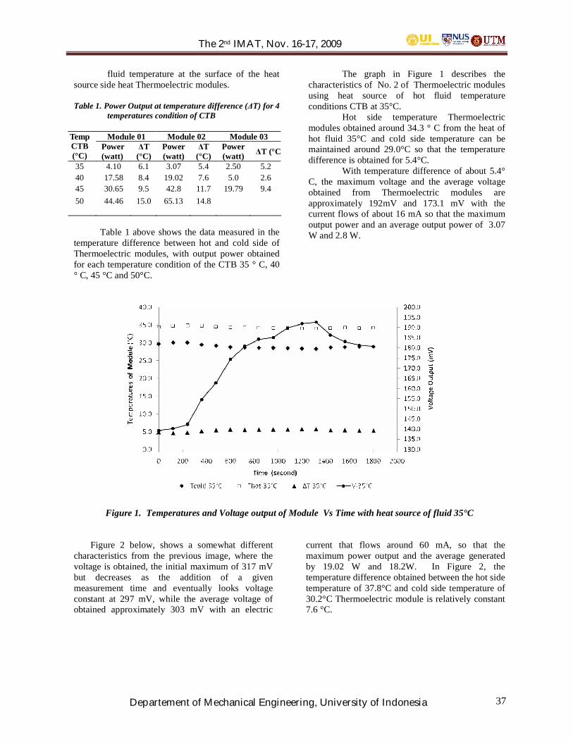
The 2nd IMAT, Nov. 16-17, 2009
Departement of Mechanical Engineering, University of Indonesia 37
fluid temperature at the surface of the heatsource side heat Thermoelectric modules.
Table 1. Power Output at temperature difference ( T) for 4temperatures condition of CTB
Module 01 Module 02 Module 03TempCTB(°C)
Power(watt)
T(°C)
Power(watt)
T(°C)
Power(watt) T (°C)
35 4.10 6.1 3.07 5.4 2.50 5.240 17.58 8.4 19.02 7.6 5.0 2.645 30.65 9.5 42.8 11.7 19.79 9.450 44.46 15.0 65.13 14.8
Table 1 above shows the data measured in thetemperature difference between hot and cold side ofThermoelectric modules, with output power obtainedfor each temperature condition of the CTB 35 ° C, 40° C, 45 °C and 50°C.
The graph in Figure 1 describes thecharacteristics of No. 2 of Thermoelectric modulesusing heat source of hot fluid temperatureconditions CTB at 35°C.
Hot side temperature Thermoelectricmodules obtained around 34.3 ° C from the heat ofhot fluid 35°C and cold side temperature can bemaintained around 29.0°C so that the temperaturedifference is obtained for 5.4°C.
With temperature difference of about 5.4°C, the maximum voltage and the average voltageobtained from Thermoelectric modules areapproximately 192mV and 173.1 mV with thecurrent flows of about 16 mA so that the maximumoutput power and an average output power of 3.07W and 2.8 W.
Figure 1. Temperatures and Voltage output of Module Vs Time with heat source of fluid 35°C
Figure 2 below, shows a somewhat differentcharacteristics from the previous image, where thevoltage is obtained, the initial maximum of 317 mVbut decreases as the addition of a givenmeasurement time and eventually looks voltageconstant at 297 mV, while the average voltage ofobtained approximately 303 mV with an electric
current that flows around 60 mA, so that themaximum power output and the average generatedby 19.02 W and 18.2W. In Figure 2, thetemperature difference obtained between the hot sidetemperature of 37.8°C and cold side temperature of30.2°C Thermoelectric module is relatively constant7.6 °C.
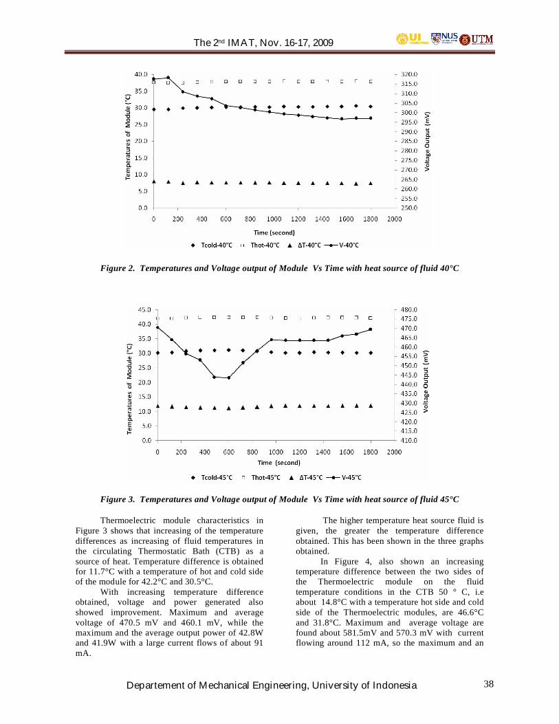
The 2nd IMAT, Nov. 16-17, 2009
Departement of Mechanical Engineering, University of Indonesia 38
Figure 2. Temperatures and Voltage output of Module Vs Time with heat source of fluid 40°C
Figure 3. Temperatures and Voltage output of Module Vs Time with heat source of fluid 45°C
Thermoelectric module characteristics inFigure 3 shows that increasing of the temperaturedifferences as increasing of fluid temperatures inthe circulating Thermostatic Bath (CTB) as asource of heat. Temperature difference is obtainedfor 11.7°C with a temperature of hot and cold sideof the module for 42.2°C and 30.5°C.
With increasing temperature differenceobtained, voltage and power generated alsoshowed improvement. Maximum and averagevoltage of 470.5 mV and 460.1 mV, while themaximum and the average output power of 42.8Wand 41.9W with a large current flows of about 91mA.
The higher temperature heat source fluid isgiven, the greater the temperature differenceobtained. This has been shown in the three graphsobtained.
In Figure 4, also shown an increasingtemperature difference between the two sides ofthe Thermoelectric module on the fluidtemperature conditions in the CTB 50 ° C, i.eabout 14.8°C with a temperature hot side and coldside of the Thermoelectric modules, are 46.6°Cand 31.8°C. Maximum and average voltage arefound about 581.5mV and 570.3 mV with currentflowing around 112 mA, so the maximum and an

The 2nd IMAT, Nov. 16-17, 2009
Departement of Mechanical Engineering, University of Indonesia 39
Figure 4. Temperatures and Voltage output of Module Vs Time with heat source of fluid 50°C
IV. CONCLUSION
The conclusion that can be obtained fromtesting the four temperatur conditions of theCirculating Thermostatic Bath (CTB) 35 ° C, 40 ° C,45 ° C and 50 ° C with an interval of observationduring 1800 seconds (30 minutes) are as follows:• The higher temperature heat source fluid is
provided (hot fluid), the greater the temperaturedifference obtained.
• The optimal temperature difference gives theoutput voltage, current and maximum outputpower.
• Improving the conditions of temperature of CTB5°C, producing a large increase in voltage of100 mV.
• The maximum output power obtained from thefour variations of temperature conditions CTB35 °C, 40 °C, 45 °C and 50°C, are 3.07W,19.02W, 42.8W and 65.13W.
ACKNOWLEDMENT
This work was supported within the DRPM-UIprogram of the University of Indonesia (projectnumber S3/2009/I/3625).
REFERENCES
[1]. www.melcor.com
[2]. Riffat. S.B, Ma .Xiaoli. 2003. Thermoelectrics:a review of Present and Potential Applications.
Applied Thermal Enginering 23 (2003) 913-935. Pergamon-Elsevier Science Ltd
[3]. Nandy Putra, Axel Hidayat, 2006.Pengembangan Alat Uji Kualitas danKarakteristik Elemen Peltier, Seminar NasionalTahunan Teknik Mesin V, UniversitasIndonesia, 21-23 November 2006, ISBN 979-977726-8-0.
[4]. Anonymous. Thermoelectric Handbook.Accessed from www.melcor.com, on October.29. 2006.
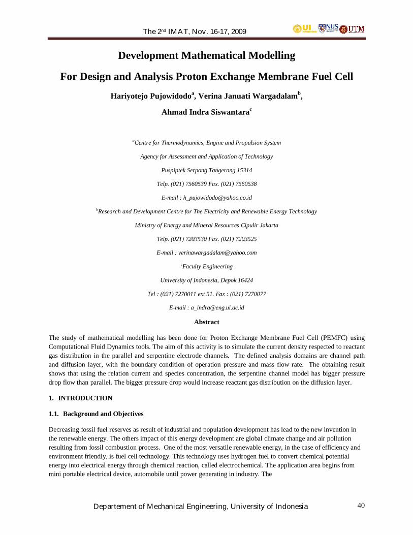
The 2nd IMAT, Nov. 16-17, 2009
Departement of Mechanical Engineering, University of Indonesia 40
Development Mathematical Modelling
For Design and Analysis Proton Exchange Membrane Fuel Cell
Hariyotejo Pujowidodoa, Verina Januati Wargadalamb,
Ahmad Indra Siswantarac
aCentre for Thermodynamics, Engine and Propulsion System
Agency for Assessment and Application of Technology
Puspiptek Serpong Tangerang 15314
Telp. (021) 7560539 Fax. (021) 7560538
E-mail : [email protected]
bResearch and Development Centre for The Electricity and Renewable Energy Technology
Ministry of Energy and Mineral Resources Cipulir Jakarta
Telp. (021) 7203530 Fax. (021) 7203525
E-mail : [email protected]
cFaculty Engineering
University of Indonesia, Depok 16424
Tel : (021) 7270011 ext 51. Fax : (021) 7270077
E-mail : [email protected]
Abstract
The study of mathematical modelling has been done for Proton Exchange Membrane Fuel Cell (PEMFC) usingComputational Fluid Dynamics tools. The aim of this activity is to simulate the current density respected to reactantgas distribution in the parallel and serpentine electrode channels. The defined analysis domains are channel pathand diffusion layer, with the boundary condition of operation pressure and mass flow rate. The obtaining resultshows that using the relation current and species concentration, the serpentine channel model has bigger pressuredrop flow than parallel. The bigger pressure drop would increase reactant gas distribution on the diffusion layer.
1. INTRODUCTION
1.1. Background and Objectives
Decreasing fossil fuel reserves as result of industrial and population development has lead to the new invention inthe renewable energy. The others impact of this energy development are global climate change and air pollutionresulting from fossil combustion process. One of the most versatile renewable energy, in the case of efficiency andenvironment friendly, is fuel cell technology. This technology uses hydrogen fuel to convert chemical potentialenergy into electrical energy through chemical reaction, called electrochemical. The application area begins frommini portable electrical device, automobile until power generating in industry. The

The 2nd IMAT, Nov. 16-17, 2009
Departement of Mechanical Engineering, University of Indonesia 41
compactness and efficiently fuel consumption andenergy conversion makes fuel cell as the future expectationenergy for human life.
Recently fuel cell design and analysisdevelopment has much done through numerical andsimulation model for study the reaction improvement. Thebasic principle of momentum, mass and energy transportbeing used to develop mathematical differential model innumerical solver. From result of modelling could bepredicted pressure distribution, velocity, concentration andalso reactant gas temperature which are useful incomprehending distribution characteristic of gas to electriccurrent performance yielded.
1.2. Literature Review
1.2.1. PEMFC Technology
PEMFC or Proton Exchange Membrane Fuel Cell is adevice of electrochemical energy converter throughoxidation and reduction process at a compact electrolytemembrane. This reaction produces ionization of proton andelectron which is conducted to pass electrolyte membraneand external payload yields water product in cathode sideas a place of the happening of reduction reaction.Concisely the process in PEMFC is shown as follows:
Figure 1. Fuel Cell Reaction Process[10]
Anode :
Cathode :
1.2.2. Reaction Rate
Electrochemical reaction rate determined by activationenergy limit for electron, to transfer from the electrolyte toelectrode or vice versa. This reaction velocity depends onthe yielded electron, named electric current. Current
density is current (electron or ion) per reaction surface areaunit, the value determined by Faraday's law as follows:
(1-1)
Where: nF is transfer charge (electron/mol) and j isreactant flux (mol/s.m2)
In electrochemical reaction, oxidation and reduction occuron the anode and cathode with the following reaction:
Forward reaction (cathode):
(1-2)
Backward reaction (anode):
(1-3)
For equilibrium condition on the electrode, no externalcurrent flow, oxidation and reduction take place on thesame rate:
(1-4)
And reactant species consumption on reaction surface isproportional to concentration according to relation:
Cathode:
(1-5)
Anode:
(1-6)
kb and kf are coefficient of reaction rate
The generated current is difference between forwardcurrent and backward current:
(1-7)
1.2.3. Mathematical Description and PhysicalConservation
Numerical solution for heat transfer, fluid flow and otherrelated process started by arranging Governing Laws forphysical process, which expressed in the form ofmathematical, generally in the equation form of differentialterms. Variable is generalizing by through a modelling

The 2nd IMAT, Nov. 16-17, 2009
Departement of Mechanical Engineering, University of Indonesia 42
analysis of system with decision of quantitativeconservation at one particular volume analysis modelarranges (control volume). In a system physical of comenear by simplification using discretization elements(dividing) and solving equation of continuity by enteringvariable limiting value physical of as limiting valuenumerical calculation.
1.2.4. Control Differential Equation
Decision of conservation utilized in building amathematical modelling for fluid flow system is consisted:
• Fluid mass flow is constant.• Momentum rate of change equal to number of
fluid particle forces (Newton second’s law).• Energy change rate is total heat flow and work in
at fluid particle (First Law of Thermodynamics)
1.2.5. Mass Conservation and Property Change Rate
In obtaining the mathematical differential equation forfluid mass flow, firstly writing down the equilibrium stateof fluid element refers to velocity and cross area as follow:
Mass accumulation in fluid element = mass inflow netto
Figure 2. Fluid mass equilibrium
In vector notation form stated generally:
(1-10)
Which is conservation for compressible fluid element 3dimensional
Physical property change determined by convective terminward/outward (as result of existing flow).
For incompressible flow, the differential equation is:
(1-11)
In analyzing transformation of property in a numericalmodel for conservation of mass and momentum, everyproperty influenced by variables of position (distance) andtime. If property is calculated per mass unit is , hencetotal derivative determined through derivative total todistance and time as follows:
(1-12)
(1-13)
For property change rate per volume stated by :
(1-14)
Hence in the general form of mass conservation becoming :
(1-15)
1.2.6. Momentum Conservation
Newton second’s law states that momentum change rateequal to the resultant of acting forces that is:
Momentum accumulation in the direction of x, y and z are , ,
Figure 3. Force Equilibrium in x direction
By vanishing body force, and entering the momentumsource rate per volume SM, the momentum change ratebecomes :

The 2nd IMAT, Nov. 16-17, 2009
Departement of Mechanical Engineering, University of Indonesia 43
(1-16)
(1-17)
(1-18)
1.2.7. Species Conservation
Within chemical reaction phenomena, the interactionamong reactant species forms reaction product, analysisprocess of numerical system involving species fraction(mass) wherein species conservation governed by amathematical differential equation as follows:
(1-19)
is species mass change rate per volume and
term is species convection flux caused by flowfield , whereas indicates diffusion flux as a resultfrom mass fraction gradient, which expressed in Fick’sLaw :
(1-20)
is coefficient of diffusion, so if substituted becoming
(1-21)
Rl is generation rate of chemistry species per volume unit.
2. Developed Methods
2.1. Modelling
As modelling system in this study, takes formation area ofdiscretization based on 2 dimension model and one part ofpassage channels, either parallel channel and turning one(serpentine). Secondly domain area system divided intoregion of electrode plate gas flow channels and gasdiffusion layer as integration of arrangement of electrolytemembrane (MEA, Membrane Electrolyte Assembly). Forthe definition of process condition, it would be neededinformation such as temperature, pressure for
hydrodynamic simulation; material and reactant propertiesfor mass transport.
Simplified process has been defined in model as follows:
• Steady state and membrane full humidified withideal water and heat management
• Single phase water transport in diffusion layer andgas channel
• Low Reynold number, so flow is laminar• Isothermal and pressure is inversely proportional
to species volume• Reactant governed by Ideal Gas Law
2.2. Implementation
Model simulation for reactant flow distribution in PEMFCwas built with CFD tools software EFD. Computationaldomain generated using CAD model, consisted of channelpaths and diffusion layer. The condition of operation anddimension given in the following table :
Table 1. Data of Simulation Model
Contraint Parameters Boundary Condition/ValueChannel Distribution Paralel dan SerpentineFlow Modes Internal flowSimulation Modes Steady flowFluid Modes Hidrogen and OksigenMomentum DimensionalModes
2 DSpecies Dimensional Modes 1 DH2 inflow (@ 1 A) 0,04 kg/hO2 inflow (@ 1 ampere) 0,02 kg/hStatic Pressure out 108.218 Pa (1 Psig)Electrode Porosity 0,4Diffusion Layer thickness 23 µmElectrolyte membrane Area 50 cm2 (73 mm x 73 mm)Electrode Channel Depth 1 mmH2 mass fraction in and out 1 and 0O2 mass fraction in and out 1 and 0
2.3. Evaluation
In this section would be done the assessment of momentumand mass distribution, accordingly there are three parts ofanalysis such as:
2.3.1. Computational Model
The aim of this step is to know approaching level that usedin solid modelling, process criterion and calculationsolving. Solid modelling was done by using integrated or

The 2nd IMAT, Nov. 16-17, 2009
Departement of Mechanical Engineering, University of Indonesia 44
compatible Computer Aided Design. The importance thingof this stage is the exactly fluid domain bounded byelectrode channel side. The working fluid in this simulationhas the type of internal flow with steady state conditionand using hydrogen and oxygen as reactant and oxidant.Particularly for mass transport, we have to defineparameters such as porosity, permeability, thickness ofdiffusion material and also the relation drop pressure andmass flow. In this model it used the value of pressure asmuch as 200 Pa at the maximum mass flow.
2.3.2. Pressure Drop Calculation
To verify pressure distribution as result of simulationmodel, it is used the Darcy Weisbach correlation tocalculate the pressure drop which depend on the roughnesswall and the change of cross area or solid boundary.
(2-1)
Where :
P = pressure drop (Pa)
l = channel length (m)
d = channel width/depth (m)
v = fluid velocity (m/det)
f = losses factor
For roughness factor , pressure drop calculated by forlaminar flow :
where (2-2)
Meanwhile for the cross area change, solved by theequation form as follow :
(2-3)
In which :
u2 = flow velocity at downstream
Cc = area rasio upstream/downstream
2.3.3. Reactant Consumption
Analytically the species concentration distribution fromsimulation would be verified by theoretical prediction ofreactant consumption rate. Faraday law states current as thefunction of number of electron, reactant consumption rateand Faraday Constant, in the following equation :
(2-4)
i = generated current (A, ampere)
n = number of ionized electron (reduction=4, oxidation=2)
F = Faraday constant = 96485 Coulomb/mol
J = consumption rate of reactant (mol/s)
And for the output parameter of simulation, would beevaluated using ideal gas law to obtain species mol rate, asfollow:
(2-5)
With the explanation of parameters :
P = species preesure (atm)
V = spesies mol rate (mol/s) = J
Runiv = universal gas constant
= 0,0821 litre.atm/mol.K
T = species temperature (oK)
3. Analysis and Result
3.1. Computational Model
Using EFD software could be briefly explained the step ofmodelling consists of:
3.1.1. Solid modelling
It is geometry model that contains domain area of workingfluid. In this model must be defined the solid boundary ofwall also inlet and outlet sides. The area of reaction surfaceof diffusion membrane is 50 cm2.
3.1.2. Boundary Condition
Giving the boundary value at inlet and outlet sides (controlsurface) as the operation criteria. At inlet side defined bythe mass flow condition of each hydrogen and oxygen asreactant and oxidant. Meanwhile at the outlet given bycondition of pressure as written in table 1 before. For masstransport or diffusion, it has to enter the value of propertiessuch as porosity, permeability, thickness and the pressuredrop through membrane.
3.1.3. Meshing
It is the method of generating control element to solvenumerical calculation of mathematical differential from thegoverning laws. For momentum conservation, could be

The 2nd IMAT, Nov. 16-17, 2009
Departement of Mechanical Engineering, University of Indonesia 45
solved meshing on the surface of symmetry plane ofchannel path. Whereas for species conservation, it is usedthe isometric model of domain that covers channel area andmembrane material (catalyst layer).
3.1.4. Mesh Optimation
This is the way of analyze the exactly control element beengenerated to get the better accuracy numerical calculation.
3.1.5. Calculation Goals
It has the aim to assist observing convergence calculationby giving the equation of pressure drop between upstreamand downstream (inlet and outlet).
3.1.6. Solver
This is a numerical calculation phase of differentialequation governing momentum and mass transportphenomena. In this step the evolution of calculatingparameters can be monitored in the graphical form.. Ascalculation goals in this simulation are static pressure andmass fraction from hydrogen gas species and oxygen.
3.1.7. Post Processing
Result of simulation can be observed at part of postprocessor through menu Cut Plot by choosing parameterstatic pressure and mass fraction. This thing to assist inanalyzing reactant gas flow characteristic in PEM Fuel Cellchannels.
3.2. Reactant Distribution Characteristic
In parallel channel the flow characteristics showed by therecirculation caused by the cross flow area changing andbranching. Whereas in serpentine the existing bendedpassages in channel gives more restriction. From result ofmodelling revealed pressure drop is 5400 Pa and in parallelas many as 4200 Pa.
3.3. Drop Pressure Calculation
The pressure loss of flow happened as result of geometryform and cross area dimension difference causing thehappening of energy loss. According to calculation manualby considering loss factor by surface roughness and changeof cross area, there was calculation difference 600 Pa (around 14%) compared to result of simulation. This thingcould be caused by accuracy factor of calculation numberapplied in process of iteration by software. Despitefullyalso calculation approach applied is channel systemanalogue with plumbing system, where the different far
dimension between channel and pipe causes differenceresult of calculation.
3.4. Current Density Calculation
As approach comparison of this PEM Fuel Cell modellingsystem is by applying manual calculation from faraday lawand ideal gas equation. Current density was determined asvalue benchmarking factor. From analysis calculationobtained result of difference 0,02 A to theoreticalcalculation. It means that deviation factor of calculation isvery small.
4. Conclusion
a. Qualitatively flow channels hardly influences flowcharacteristics and also distribution of gas reactant.Flow recirculation at parallel channel resulted from bychange of area and geometry flow, causing distributionof different momentum. Diffusion passes throughporous media with higher level gas concentrationgenerates non-uniformity flow.
b. Difference result of pressure drop calculation withmanual calculation caused by difference value of fluidproperties and definition of computing domain lessoptimal as has been shown in meshing of serpentinechannels. This thing is because of wide comparisonbetween width- length is too far.
c. Reactant gas pressure influences number ofconcentration of gas applied as main variable todetermine level of electric current yielded.
d. Pressure of reactant gas in reaction channelinfluenced by diffusion layer material , that isproperty level of pressure drop at diffusion material.More higher pressure drop at diffusion material henceamounts concentration of gas would increasinglyrising whereas the flow velocity would decrease.
e. Distribution serpentine channels to have pressure dropcharacteristic larger ones compared to parallel , thisthing is as result of level of loss of flow generated bydeformation of geometry channel. But loss as result ofexistence of opponent flow ( recirculation) very low sothat accentual loss especially happened as result ofbend factor.
f. Generally modelling of PEM Fuel Cell by using toolssimulation requires specific data of system materialespecially at diffusion material that is pressure dropinfluence and porosity, a real determines reactant massdiffusion rate .

The 2nd IMAT, Nov. 16-17, 2009
Departement of Mechanical Engineering, University of Indonesia 46
References
1. Armstrong, K.W.(2004). Theses : A Microscopic
Continuum Model of a Proton Exchange Membrane
Fuel Cell Electrode Catalyst Layer. Virginia,
Mechanical Engineering Virginia Polytechnic
Institute and State University.
2. National Energy Technology Laboratory Office of
Fossil Energy U.S. Department of Energy.(2004).
Fuel Cell Handbook , seventh edition, West Virginia.
3. Guilin, H. , Jianren, F.(2006). A Three-Dimensional,
Multicomponent, Two-Phase Model for a Proton
Exchange Membrane Fuel Cell with Straight
Channels, Journal of Energy & Fuels.
4. Hesty, N.W, Wargadalam, V.J.(2007). Model Dua
Dimensi Distribusi Fraksi Air dan Kerapatan Arus
Pada Fuel Cell Berbasis Polimer (PEMFC),
Puslitbangtek Ketenagalistrikan dan Energi Baru
Terbarukan.
5. Liu, H., Zhou, T. (2005). Transport Phenomena
Analysis in Proton Exchange Membrane Fuel Cells,
Journal of Heat Transfer, vol. 127, No. 12, pp. 1363–
1379,
©2005 American Society of Mechanical Engineer.
6. Ma, L. et.al.(2005). Review of the Computational
Fluid Dynamics Modelling of Fuel Cells, Journal of
Fuel Cell Science and Technology, vol.2, No. 4, pp.
246-257.
7. Nguyen, P.T., et.al, Computational Model of PEM
Fuel Cell with Serpentine Gas Flow Channels,
Journal of Power Sources, Desember 2003.
8. Patankar, S. V.(1980), Numerical Heat Transfer and
Fluid Flow, Hemisphere Publishing, USA.
9. Pillay, P. Dr., Professor, Fuel Cells, Concordia Power
Electronics & Energy Research Group (PEER), Dept
of Electrical & Computer Engineering, Concordia
University.
10. Siegel , N.P. (2003). Dissertation : Development and
Validation of a Computational Model for a Proton
Exchange Membrane Fuel Cell , Mechanical
Engineering Virginia Polytechnic Institute and State
University, Virginia.
11. Shimpalee, S. , Greenway, S., Van Zee, J.W.(2006).
The impact of channel path length on PEMFC flow-
field design , Journal of Power Sources.
12. Berning, T., Djilali, N.(2003). Three-dimensional
computational analysis of transport phenomena in a
PEM fuel cell a parametric study , Journal of Power
Sources.
13. Versteeg, H.K, Malalasakera, W..(1995). An
Introduction to Computational Fluid Dynamics The
Finite Volume, Method, Longman Group, England.
14. Wargadalam, V. J., Rochani , S.(2006). Evaluasi
Pengaruh Kandungan Air Pada Reaktan Terhadap
Kinerja Sel Tunam Membran Penukar Proton
(PEMFC), Puslitbangtek Ketenagalistrikan dan
Energi Baru Terbarukan DESDM, Puslitbangtek
Teknologi Mineral dan Batubara, DESDM.
Attachments
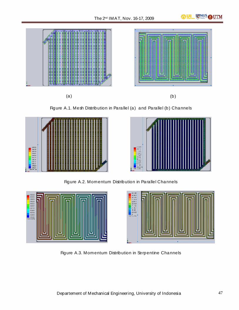
The 2nd IMAT, Nov. 16-17, 2009
Departement of Mechanical Engineering, University of Indonesia 47
(a) (b)
Figure A.1. Mesh Distribution in Parallel (a) and Parallel (b) Channels
Figure A.2. Momentum Distribution in Parallel Channels
Figure A.3. Momentum Distribution in Serpentine Channels
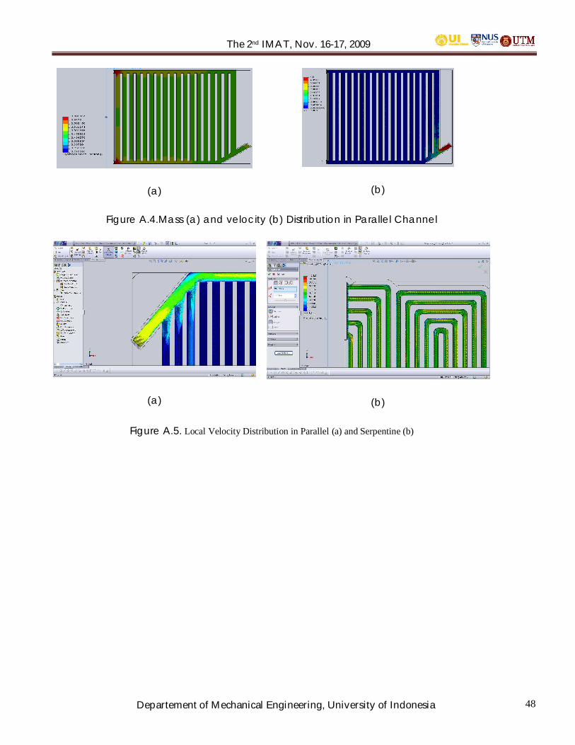
The 2nd IMAT, Nov. 16-17, 2009
Departement of Mechanical Engineering, University of Indonesia 48
(a) (b)
Figure A.4.Mass (a) and velocity (b) Distribution in Parallel Channel
(a) (b)
Figure A.5. Local Velocity Distribution in Parallel (a) and Serpentine (b)
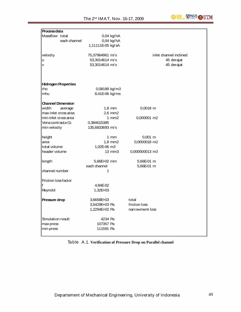
The 2nd IMAT, Nov. 16-17, 2009
Departement of Mechanical Engineering, University of Indonesia 49
Process dataMassflow total 0,04 kg/hA
each channel 0,04 kg/hA1,11111E-05 kg/sA
velocity 75,37964961 m/s inlet channel inclinedu 53,3014614 m/s 45 derajatv 53,3014614 m/s 45 derajat
Hidrogen Propertiesrho 0,08189 kg/m3mhu 8,41E-06 kg/ms
Channel Dimensionwidth average 1,8 mm 0,0018 mmax inlet cross area 2,6 mm2min inlet cross area 1 mm2 0,000001 m2Vena contracta Cc 0,384615385min velocity 135,6833693 m/s
height 1 mm 0,001 marea 1,8 mm2 0,0000018 m2total volume 1,02E-06 m3header volume 13 mm3 0,000000013 m3
length 5,66E+02 mm 5,66E-01 meach channel 5,66E-01 m
channel number 1
Friction loss factorf 4,84E-02Reynold 1,32E+03
Pressure drop 3,6658E+03 total3,5429E+03 Pa friction loss1,2294E+02 Pa narrowment loss
Simulation result 4234 Pamax press 107357 Pamin press 111591 Pa
Table A.1. Verification of Pressure Drop on Parallel channel
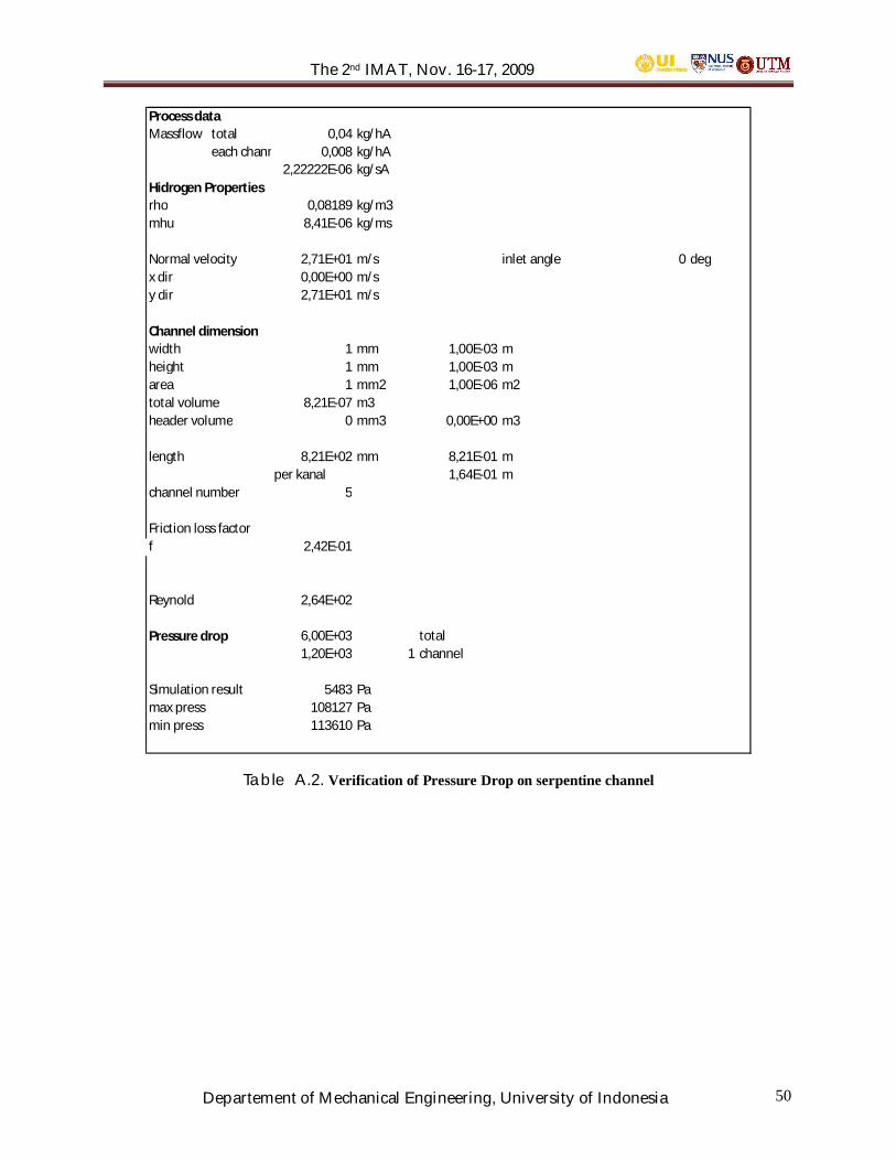
The 2nd IMAT, Nov. 16-17, 2009
Departement of Mechanical Engineering, University of Indonesia 50
Process dataMassflow total 0,04 kg/hA
each channel 0,008 kg/hA2,22222E-06 kg/sA
Hidrogen Propertiesrho 0,08189 kg/m3mhu 8,41E-06 kg/ms
Normal velocity 2,71E+01 m/s inlet angle 0 degx dir 0,00E+00 m/sy dir 2,71E+01 m/s
Channel dimensionwidth 1 mm 1,00E-03 mheight 1 mm 1,00E-03 marea 1 mm2 1,00E-06 m2total volume 8,21E-07 m3header volume 0 mm3 0,00E+00 m3
length 8,21E+02 mm 8,21E-01 mper kanal 1,64E-01 m
channel number 5
Friction loss factorf 2,42E-01
Reynold 2,64E+02
Pressure drop 6,00E+03 total1,20E+03 1 channel
Simulation result 5483 Pamax press 108127 Pamin press 113610 Pa
Table A.2. Verification of Pressure Drop on serpentine channel
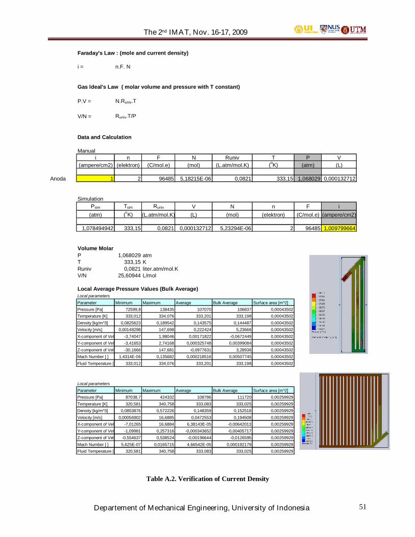
The 2nd IMAT, Nov. 16-17, 2009
Departement of Mechanical Engineering, University of Indonesia 51
Faraday's Law : (mole and current density)
i = n.F. N
Gas Ideal's Law ( molar volume and pressure with T constant)
P.V = N.Runiv.T
V/N = Runiv.T/P
Data and Calculation
Manuali n F N Runiv T P V
(ampere/cm2) (elektron) (C/mol.e) (mol) (L.atm/mol.K) (oK) (atm) (L)
Anoda 1 2 96485 5,18215E-06 0,0821 333,15 1,068029 0,000132712
SimulationPsim Tsim Runiv V N n F i
(atm) (oK) (L.atm/mol.K) (L) (mol) (elektron) (C/mol.e) (ampere/cm2)
1,078494942 333,15 0,0821 0,000132712 5,23294E-06 2 96485 1,009799664
Volume MolarP 1,068029 atmT 333,15 KRuniv 0,0821 liter.atm/mol.KV/N 25,60944 L/mol
Local Average Pressure Values (Bulk Average)Local parametersParameter Minimum Maximum Average Bulk Average Surface area [m^2]Pressure [Pa] 72599,8 138435 107070 106837 0,00043502Temperature [K] 333,012 334,076 333,201 333,198 0,00043502Density [kg/m^3] 0,0825623 0,189542 0,143575 0,144487 0,00043502Velocity [m/s] 0,00148298 147,698 0,222424 5,23666 0,00043502X-component of Velocity [m/s]-3,74047 1,98046 0,00171822 -0,0672449 0,00043502Y-component of Velocity [m/s]-3,41653 2,74168 0,000325748 0,00399084 0,00043502Z-component of Velocity [m/s]-30,1666 147,681 -0,0977631 3,28936 0,00043502Mach Number [ ] 1,4314E-06 0,135682 0,000218516 0,00507745 0,00043502Fluid Temperature [K] 333,012 334,076 333,201 333,198 0,00043502
Local parametersParameter Minimum Maximum Average Bulk Average Surface area [m^2]Pressure [Pa] 87038,7 424332 108786 111720 0,00259929Temperature [K] 320,581 340,758 333,083 333,025 0,00259929Density [kg/m^3] 0,0853876 0,572226 0,148359 0,152518 0,00259929Velocity [m/s] 0,00056902 16,6885 0,0472553 0,194508 0,00259929X-component of Velocity [m/s]-7,01265 16,6884 6,38143E-05 -0,00642013 0,00259929Y-component of Velocity [m/s]-1,09981 0,257316 -0,000343652 -0,00405717 0,00259929Z-component of Velocity [m/s]-0,554637 0,538524 -0,00196644 -0,0126595 0,00259929Mach Number [ ] 5,625E-07 0,0165715 4,66542E-05 0,000192179 0,00259929Fluid Temperature [K] 320,581 340,758 333,083 333,025 0,00259929
Table A.2. Verification of Current Density

The 2nd IMAT, Nov. 16-17, 2009
Departement of Mechanical Engineering, University of Indonesia 52
Experimental Study and Correlation of Two-Phase FlowEvaporation Heat Transfer Coefficient of Propane in
Intermittent, Stratified Wavy and Annular Flows
Agus S. Pamitrana, Jong-Taek Ohb
aDepartment of Mechanical Engineering,University of Indonesia, Kampus Baru UI, Depok 16424, Indonesia
Tel : +62-21-727-0032 ext 233. Fax : +62-21-727-0033E-mail : [email protected]
bDepartment of Refrigeration and Air-Conditioning Engineering,Chonnam National University, San 96-1, Dunduk-Dong, Yeosu, Chonnam 550-749, Republic of Korea
Tel : +82-61-659-6273. Fax : +82-61-659-6279E-mail : [email protected]
ABSTRACT
Two-phase flow heat transfer coefficients forevaporative refrigerants in intermittent, stratifiedwavy and annular flows were evaluated in thisstudy. The experimental data were obtained usingpropane over a heat flux range of 5 to 30 kW m-2,mass flux range of 50 to 600 kg m-2 s-1, saturationtemperature of 0 to 10°C, and quality up to 1.0.The test section was made of stainless steel tubeswith inner diameters of 1.5 mm and 3.0 mm. Theflow pattern of the experimental data wasevaluated with existing flow pattern maps. Theexperimental boiling heat transfer coefficientswere compared with some existing correlationsbased on the flow pattern. A new correlation forflow boiling heat transfer coefficient that is basedon a superposition model for refrigerants in smalltubes is presented.
Keywords: Propane, Flow boiling, Flow pattern,Heat transfer coefficient, Correlation, Horizontalsmall tubes
1. INTRODUCTION
Such awareness has led to a demand forenvironmental friendly evaporation refrigerants insmaller evaporators, which are used in therefrigeration and air conditioning. Propane, aslong term alternative refrigerants, will beimportant in the future for compact heatexchanger applications due to their performanceand their environmental friendliness with zeroOzone Depletion Potential (ODP) and zero GlobalWarming Potential (GWP). Evaporation in smalltubes has great advantages: high heat transfer
coefficient, significant size reduction of compactheat exchangers, and lower required fluid mass.However, heat transfer of two-phase flows insmall tubes cannot be properly predicted usingexisting procedures and correlations because theyare more suitable for large tubes and for generalflow pattern condition. There are relatively fewpublished works on two-phase flow boiling heattransfer of refrigerants in small tubes based onflow pattern. Several studies have dealt with two-phase flow boiling in small tubes, such asreported by Tran et al. (1996), Zhang et al.(2004), Pettersen (2004) and Yun et al. (2005).Wang et al. (1997) and Wojtan et al. (2005) haveproposed flow pattern maps for two-phase flowboiling heat transfer. However, the existingprediction methods of heat transfer coefficientcould not predict well the current experimentaldata for individual flow pattern.
This study was performed to obtain experimentaldata for propane and to evaluate the heat transfercoefficient based on flow pattern during theevaporation in small tubes. The experimentalresults were compared with the predictions fromseveral existing heat transfer coefficientprediction methods. Due to the limitations of thecorrelation for forced convective boiling ofrefrigerants in small tubes, a new correlation ofheat transfer coefficient based on flow pattern forevaporative refrigerant in small tubes wasdeveloped in this study.
2. EXPERIMENTAL FACILITY ANDDATA REDUCTION
The schematic experimental facility is shown in
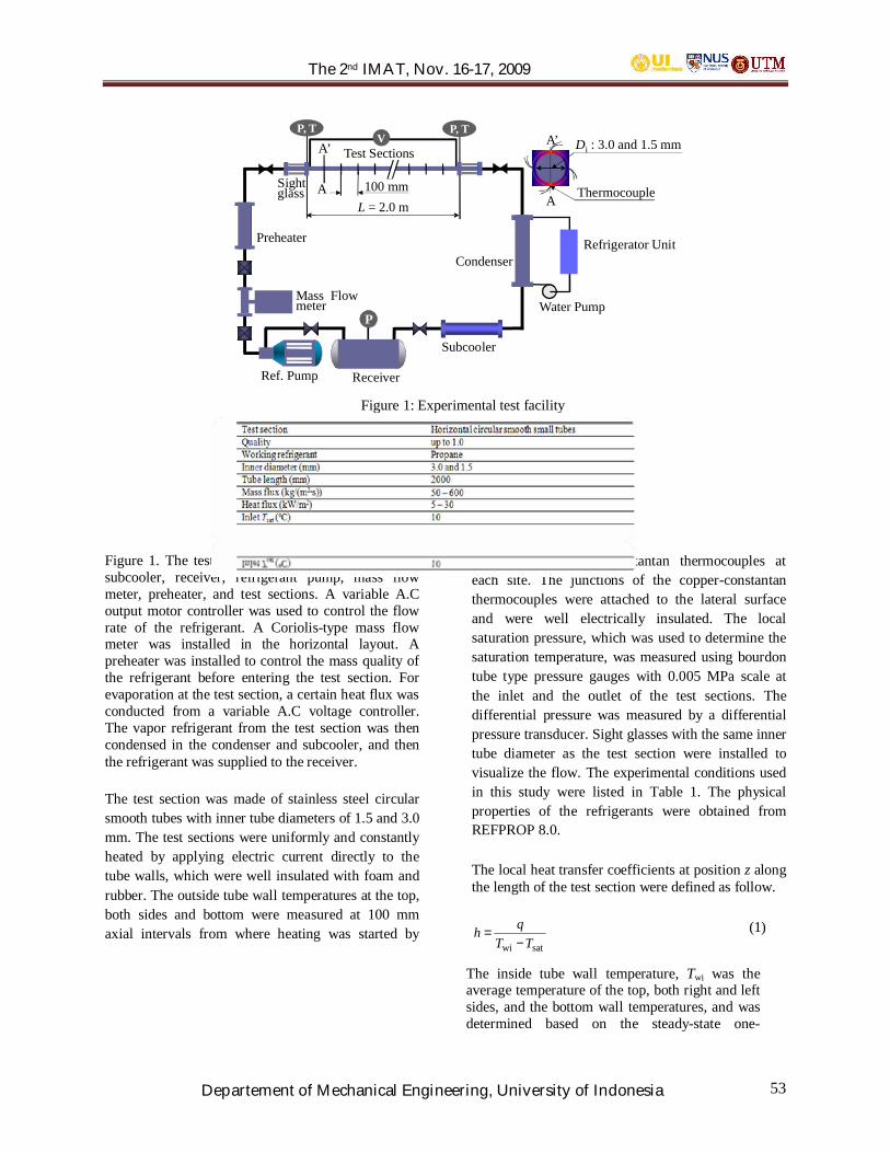
The 2nd IMAT, Nov. 16-17, 2009
Departement of Mechanical Engineering, University of Indonesia 53
Figure 1. The test facility consisted of a condenser,subcooler, receiver, refrigerant pump, mass flowmeter, preheater, and test sections. A variable A.Coutput motor controller was used to control the flowrate of the refrigerant. A Coriolis-type mass flowmeter was installed in the horizontal layout. Apreheater was installed to control the mass quality ofthe refrigerant before entering the test section. Forevaporation at the test section, a certain heat flux wasconducted from a variable A.C voltage controller.The vapor refrigerant from the test section was thencondensed in the condenser and subcooler, and thenthe refrigerant was supplied to the receiver.
The test section was made of stainless steel circularsmooth tubes with inner tube diameters of 1.5 and 3.0mm. The test sections were uniformly and constantlyheated by applying electric current directly to thetube walls, which were well insulated with foam andrubber. The outside tube wall temperatures at the top,both sides and bottom were measured at 100 mmaxial intervals from where heating was started by
using T-type copper-constantan thermocouples ateach site. The junctions of the copper-constantanthermocouples were attached to the lateral surfaceand were well electrically insulated. The localsaturation pressure, which was used to determine thesaturation temperature, was measured using bourdontube type pressure gauges with 0.005 MPa scale atthe inlet and the outlet of the test sections. Thedifferential pressure was measured by a differentialpressure transducer. Sight glasses with the same innertube diameter as the test section were installed tovisualize the flow. The experimental conditions usedin this study were listed in Table 1. The physicalproperties of the refrigerants were obtained fromREFPROP 8.0.
The local heat transfer coefficients at position z alongthe length of the test section were defined as follow.
satwi TTqh−
= (1)
The inside tube wall temperature, Twi was theaverage temperature of the top, both right and leftsides, and the bottom wall temperatures, and wasdetermined based on the steady-state one-
Figure 1: Experimental test facility
Di : 3.0 and 1.5 mm
A
A’
Thermocouple
Subcooler
Receiver
Condenser
Ref. Pump
Preheater
Water Pump
Refrigerator Unit
P
Sightglass
A’
L : 1.0, 1.5, 2.0, 3.0 m
P, TV
A
P, T
Test Sections
Mass Flowmeter
100 mmL = 2.0 m

The 2nd IMAT, Nov. 16-17, 2009
Departement of Mechanical Engineering, University of Indonesia 54
dimensional radial conduction heat transferthrough the wall with internal heat generation.The vapor quality, x, at the measurementlocations, z, were determined based on thethermodynamic properties.
fg
fi
iix
−= (2)
The refrigerant flow at the inlet of the test sectionwas not completely saturated. The subcooledlength was calculated using Eq. (3) to determinethe initial point of saturation.
( )WQiiL
iiiLz fiffif
sc−
=∆−
= (3)
3. FLOW PATTERN
The present experimental results were mapped onWang et al. (1997) and Wojtan et al. (2005) flowpattern maps, which were developed for diabatictwo-phase flows. The Wang et al. (1997) flowpattern map is a modified Baker (1954) map,developed using R-22, R-134a, and R-407Cinside a 6.5 mm horizontal smooth tube. TheWojtan et al. (2005) flow pattern map is amodified Kattan et al. (1998) map, developedusing R-22 and R-410A inside a 13.6 mmhorizontal smooth tube. Kattan et al. (1998) usedfive refrigerants R-134a, R-123, R-402A, R-404A, and R-502 inside 12 mm and 10.92 mm(only for R-134a) tubes, which were heated by hotwater flowing counter-currently to develop theirflow pattern maps on the basis of the Steiner(1993) flow pattern map.
The predicted flow pattern for the selected currentexperimental data by the existing flow patternmaps of Wang et al. (1997) and Wojtan et al.(2005) can be seen in Figures 2 and 3,respectively. The Wang et al. (1997) map showeda better prediction of the flow pattern of thecurrent experimental data for the beginning ofannular flow than the Wojtan et al. (2005) map;however, the Wang et al. (1997) map could notshow the prediction for dry-out condition. Theflow pattern prediction of the current test resultsfor the all test conditions with the Wang et al.(1997) flow pattern map was for the intermittent,stratified wavy, and annular flow. Figures 2 and 3depicts that the stratified wavy flow appeared
earlier for higher mass fluxes and its regime waslonger for the low mass flux condition. Theannular flow appeared earlier for higher massfluxes. The flow pattern prediction of theexperimental results for all the test conditionswith the Wojtan et al. (2005) flow pattern mapwas on intermittent, annular, dry-out, and mistflows. Because the Wojtan et al. (2005) map isdeveloped using a conventional tube, the flowpattern transition of the present experimental datashowed a delay on this map. Overall, Wang et al.(1997) flow pattern map provides a better flowpattern prediction for the current experimentalresults than the Wojtan et al. (2005) flow patternmap. Therefore, the heat transfer coefficient ofthis present study is evaluated based on the Wanget al. (1997) flow pattern map.
4. HEAT TRANSFER COEFFICIENTS
It is well known that the flow boiling heat transferis mainly governed by two importantmechanisms, namely nucleate boiling and forcedconvective heat transfer.
cnbtp hhh += (4)
In two-phase flow boiling heat transfer, thenucleate boiling heat transfer contribution issuppressed by the two-phase flow, especially athigh vapour quality region. At low quality region,the heat transfer coefficient is dominated bynucleate boiling heat transfer contribution, but athigh quality region it is dominated by convectiveheat transfer contribution. This trend can be foundin studies of Pamitran et al. (2007) and Choi et al.(2007). The nucleate boiling heat transfercontribution may be correlated with a nucleateboiling suppression factor, S. Anothercontribution of convective heat transfer may becorrelated with a liquid single phase heat transfer.The F factor is introduced as a convective two-phase multiplier to account for enhancedconvective due to co-current flow of liquid andvapor. A superposition model of heat transfercoefficient may be written as follow,
fnbctp FhShh +=
(5)The heat transfer coefficients of the presentstudy are compared with the results given by four

The 2nd IMAT, Nov. 16-17, 2009
Departement of Mechanical Engineering, University of Indonesia 55
0,1
1
10
100
0,1 1 10 100 1000
100150180
(1-x) ’/x
Gx/
G (kg/m²s)
Str.
Str.WavyAnnular
Intermittent
Propaneq = 15 kW/m²Di = 3.0 mmTsat = 10 C
The current experimental datatransition to annular flow
Figure 2: Present experimental results mapped on Wang et al. (1997) flow pattern map
Figure 3: Present experimental results mapped on Wojtan et al. (2005) flow pattern map
0
50
100
150
200
250
300
350
0 0,2 0,4 0,6 0,8 1
Str.
Intermittent
Propaneq = 15 kW/m²Di = 3.0 mmTsat = 10 °C
Slug + Str.Wavy
SlugAnnular
Str.Wavy
x
Dry-out
Mist
The current experimental data:Intermittent to AnnularAnnular to Dry-out
G(k
g/m
²s)
Table 2: Deviation (%) of the heat transfer coefficient comparison between the present data and the prediction usingexisting correlations
Flow Pattern Previous Correlations
Tran et al.(1996)
Shah(1988)
Jung et al.(1989)
Gungor-Winterton(1987)
Kandlikar(1990)
Intermittent Mean Dev. 14.78 20.70 19.33 34.14 42.85
Average Dev. 9.39 -3.63 7.86 33.66 -42.23
Mean Dev. 14.68 23.22 24.84 29.21 63.65Stratified Wavy
Average Dev. -6.03 7.81 16.64 21.42 -63.65
Annular Mean Dev. 25.01 34.59 36.01 35.42 67.70
Average Dev. -24.53 15.11 34.83 20.51 -67.49

The 2nd IMAT, Nov. 16-17, 2009
Departement of Mechanical Engineering, University of Indonesia 56
correlations for boiling heat transfer coefficient aslisted in Table 2. The Wang et al. (1997) flow patternmap is used to map the present experimental data.The comparison of heat transfer coefficient is basedon flow pattern of intermittent flow, stratified wavyflow and annular flow. For heat transfer coefficient inintermittent flow, stratified wavy flow and annularflow, the best prediction is all given by the Tran et al.(1996). The Tran et al. (1996) correlation wasdeveloped for flow boiling heat transfer in smallchannels. The correlations proposed by Shah (1988)and Jung et al. (1989) also showed good predictionwith the present experimental data. The Shah (1988)correlation was developed using a large data set forconventional tubes. The Jung et al. (1989) correlationwas developed with pure and mixture refrigerants inconventional channels; its F factor contributed a bigcalculation deviation with the current experimentaldata.
The appearance of convective heat transfer forboiling in small tubes occurs later than it does inlarger tubes because of its high boiling nucleation.Chen (1966) introduced a multiplier factor, F=fn(Xtt),to account for the increase in the convectiveturbulence that is due to the presence of the vaporphase. The function should be physically evaluatedagain for flow boiling heat transfer in a small tubethat has a laminar flow condition, which is due to thesmall diameter effect. By considering the flowconditions (laminar or turbulent) in the Reynoldsnumber factor, F, Zhang et al. (2004) introduced arelationship between the factor F and the two-phasefrictional multiplier that is based on the pressuregradient for liquid alone flow, 2
fφ . This relationship
is F=fn( 2fφ ), where 2
fφ is a general form for fourconditions according to Chisholm (1967). For theliquid-vapor flow condition of turbulent-turbulent(tt), laminar-turbulent (vt), turbulent-laminar (tv) andlaminar-laminar (vv), the values of the Chisholmparameter, C, are 20, 12, 10, and 5, respectively.
The F factor in this study is developed as a functionof 2
fφ , F=fn( 2fφ ), where 2
fφ is obtained from Eq. (6).
2
f
g
21
f
g
f
tp2f
11
dddd
dddd
1
dddd
XXC
Fzp
Fzp
Fzp
Fzp
CF
zp
Fzp
++=
−
−
+
−
−
+=
−
−
=φ (6)
The liquid heat transfer is defined by existing liquidheat transfer coefficient correlations by consideringflow conditions of laminar and turbulent. For laminarflow, Ref < 2300, the liquid heat transfer coefficientis obtained from the following correlation:
Dkh f
f 36.4= (7)
For flow with 3000 Ref 104, the liquid heattransfer coefficient is obtained from Gnielinski(1976) correlation, where the friction factor iscalculated from Eqs. (8) and (9).
1Re16 −=f , for Re < 2300 (8)
25.0Re079.0 −=f , for Re > 3000 (9)
For flow with 2300 Ref 3000, the liquid heattransfer coefficient is calculated by interpolation. Forturbulent flow with 104 Ref 5×10⁶, the liquid heattransfer coefficient is obtained from Petukhov andPopov (1963) correlation. Dittus Boelter (1930)correlation is used for turbulent flow with Ref
5×10⁶.
The new factor F, as illustrated in Fig. 4, isdeveloped based on the flow pattern using aregression method. For all flow pattern, the newfactor F is developed as Eq. (10).
( )[ ]1,76.005.0MAX 2.2f += φF , for 2
fφ > 50
( )[ ]1,64.0MAX fφ=F , for 2fφ 50 (10)
where 2fφ is obtained from Eq. (6).
The prediction of the nucleate boiling heat transferfor the present experimental data used Cooper(1984), which is a pool boiling correlation developedbased on an extensive study.

The 2nd IMAT, Nov. 16-17, 2009
Departement of Mechanical Engineering, University of Indonesia 57
Table 3: Coefficients for the Suppression Factor S
Coefficients Intermittent Stratified Wavy Annulara 8.8083 112.2612 0.0026b -0.5846 2.1872 0.1786c 0.2673 1.8048 -0.5981
Table 4: Deviation (%) of the heat transfer coefficient comparison between the present data andthe prediction using the new developed heat transfer coefficient correlations
Deviation Intermittent Stratified Wavy Annular OverallMean 10.78 25.81 13.30 16.63Average -1.57 1.01 -1.36 -0.64
1
10
100
1000
1 10 100 1000
Experimental DataZhang et al. (2004) Factor FNew Factor F
F=MAX(0.64φf, 1)
F=MAX[(0.05φf2.2+0.76), 1]
φf2
h tp/h
lo
Figure 4: Two-phase heat transfer multiplier as a function of φf2
Figure 5: Diagram of the experimental heat transfer coefficient, hexp, vs prediction heat transfer coefficient,hpred, with the new developed heat transfer coefficient correlation
0
1
2
3
4
5
6
7
8
0 1 2 3 4 5 6 7 8
hexp (kW/m2K)
+20%
-20%
MD = 16.63%AD = -0.64%
h exp
(kW
/m2 K
)
The 2nd IMAT, Nov. 16-17, 2009
Departement of Mechanical Engineering, University of Indonesia 58
Chen (1966) defined the nucleate boiling suppressionfactor, S, as a ratio of the mean superheat, Te, to thewall superheat, Tsat. Jung et al. (1989) proposed aconvective boiling heat transfer multiplier factor, N,as a function of quality, heat flux and mass flow rate(represented by employing Xtt and Bo) to representthe strong effect of nucleate boiling in flow boiling asit is compared with that in nucleate pool boiling,hnbc/hnb. The Martinelli parameter, Xtt, is replaced bya two-phase frictional multiplier, 2
fφ , in order toconsider laminar flow in small tubes. By using theexperimental data of this study, the new nucleateboiling suppression factor S based on flow pattern isproposed for each flow patterns of intermittent flow,stratified wavy flow and annular flow as follow.
( ) cb2fa BoS φ= (11)
The coefficients for Eq. (11) are listed inTable 3.
The overall comparison of the experimental heattransfer coefficient, htp, exp, and the predicted heattransfer coefficient, htp, pred, is illustrated in Figure 4and the deviation for each comparison based on
flow pattern is tabulated in Table 4. The newcorrelation agrees closely for the comparison with amean deviation of 16.63% and an average deviationof -0.64%.
5. CONCLUSIONS
Convective boiling heat transfer experiments wereperformed in horizontal small tubes with propane.The current experimental data are mapped on Wanget al. (1997) and Wojtan et al. (2005) flow patternmaps. Wang et al. (1997) predicted the currentexperimental results flow pattern better than Wojtanet al. (2005). In comparison with the flow patternpredicted by Wang et al. (1997) and Wojtan et al.(2005) flow pattern maps, the current experimentaldata shows that annular flow and dry-out occur at alower vapor quality for the evaporation with a higherheat flux, higher mass flux and a lower inner tubediameter. Stratified wavy flow appears earlier forhigher mass flux condition, and the regime is longerfor a lower mass flux condition. A new heat transfercoefficient correlation that is based on flow patternfor boiling refrigerants in small tubes was presentedwith 16.63% mean deviation and -0.64% averagedeviation. Further study on flow boiling heat transfer
based on flow pattern in small tubes is needed forbetter prediction of the heat transfer coefficients.
6. REFERENCES
[1] Baker, O., 1954, “Design of pipe lines forsimultaneous flow of oil and gas”, Oil and GasJ. July, 26.
[2] Chen, J. C., 1966, “A correlation for boilingheat transfer to saturated fluids in convectiveflow”, Industrial and Engineering Chemistry,Process Design and Development 5;322-329.
[3] Chisholm, D., 1967, “A theoretical basis for theLockhart-Martinelli correlation for two-phaseflow”, Int. J. Heat Mass Transfer 10;1767-1778.
[4] Choi, K. I., Pamitran, A. S., Oh, C. Y., Oh, J.T., 2007, “Boiling heat transfer of R-22, R-134a, and CO2 in horizontal smoothminichannels”, Int. J. Refrigeration 30;1336-1346.
[5] Cooper, M. G., 1984, “Heat flow rates insaturated nucleate pool boiling–a wide-rangingexamination using reduced properties”, In:Advances in Heat Transfer. Academic Press16;157-239.
[6] Dittus, F. W. and Boelter, L. M. K., 1930, “Heattransfer in automobile radiators of the tubulartype”, University of California Publication inEngineering 2;443-461.
[7] Gnielinski, V., 1976, “New equations for heatand mass transfer in turbulent pipe and channelflow”, International Chemical Engineering 16:359-368
[8] Gungor, K. E., Winterton, H. S., 1987,“Simplified General Correlation for SaturatedFlow Boiling and Comparisons of Correlationswith Data”, Chem.Eng.Res 65; 148-156.
[9] Jung, D. S., McLinden, M., Radermacher, R.,Didion, D., 1989, “A Study of Flow BoilingHeat Transfer with Refrigerant Mixtures”, Int J.Mass Transfer 32(9);1751-1764.
[10] Kandlikar, S. G., 1990, “A general correlationfor saturated two-phase flow boiling heattransfer inside horizontal and vertical tubes”,Journal of Heat Transfer 112;219-228.
[11] Kattan N., 1996, “Contribution to the heattransfer analysis of substitute refrigerants inevaporator tubes with smooth or enhanced tubesurfaces”, PhD thesis No 1498, Swiss FederalInstitute of Technology, Lausanne, Switzerland.
[12] Kattan, N., Thome, J. R., Favrat, D., 1998,“Flow boiling in horizontal tubes: part 1 –development of a diabatic two-phase flowpattern map”, J. Heat Transfer 120;140-147.
The 2nd IMAT, Nov. 16-17, 2009
Departement of Mechanical Engineering, University of Indonesia 59
[13] Lockhart, R. W. and Martinelli, R. C., 1949,“Proposed correlation of data for isothermaltwo-phase, two-component flow in pipes”,Chem. Eng. Prog. 45;39-48.
[14] Pamitran, A. S., Choi, K. I., Oh, J. T., Oh, H.K., 2007, “Forced convective boiling heattransfer of R0410A in horizontal minichannels”,Int. J. Refrigeration 30;155-165.
[15] Petukhov, B. S. and Popov, V. N., 1963,“Theoretical calculation of heat exchanger inturbulent flow in tubes of an incompressiblefluid with variable physical properties”, HighTemp. 1(1);69-83.
[16] Pettersen, J., 2004, “Flow vaporization of CO2
in microchannels tubes”, Exp. Therm. Fluid Sci.28;111-121.
[17] Shah, M. M., 1988, “Chart correlation forsaturated boiling heat transfer: equations andfurther study”, ASHRAE Trans 2673;185-196.
[18] Steiner, D., 1993, “Heat transfer to boilingsaturated liquids”, VDI-Wärmeatlas (VDI HeatAtlas), Verein Deutcher Ingenieure, ed., VDI-Gessellschaft Verfahrenstechnik undChemieinge- nieurwesen (GCV), Düsseldorf,Germany, (J.W. Fullarton, translator).
[19] Tran, T. N., Wambsganss, M. W., France, D.M., 1996, “Small circular- and rectangular-channel boiling with two refrigerants”, Int. J.Multiphase Flow 22(3);485-498.
[20] Wang, C. C., Chiang, C. S., Lu, D. C., 1997,“Visual observation of two-phase flow patternof R-22, R-134a, and R-407C in a 6.5-mmsmooth tube”, Exp. Therm. Fluid Sci. 15;395-405.
[21] Wojtan, L., Ursenbacher, T., Thome, J. R.,2005, “Investigation of flow boiling inhorizontal tubes: part I – a new diabatic two-phase flow pattern map”, Int. J. Heat MassTransfer 48;2955-2969.
[22] Yun, R., Kim, Y., Kim, M. S., 2005,“Convective boiling heat transfer characteristicsof CO2 in microchannels”, Int. J. Heat. MassTransfer 48;235-242.
[23] Zhang, W., Hibiki, T., Mishima, K., 2004,“Correlation for flow boiling heat transfer inmini-channels”, Int. J. Heat and Mass Transfer47;5749-5763.

The 2nd IMAT, Nov. 16-17, 2009
Departement of Mechanical Engineering, University of Indonesia 60
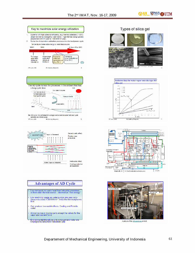
The 2nd IMAT, Nov. 16-17, 2009
Departement of Mechanical Engineering, University of Indonesia 61
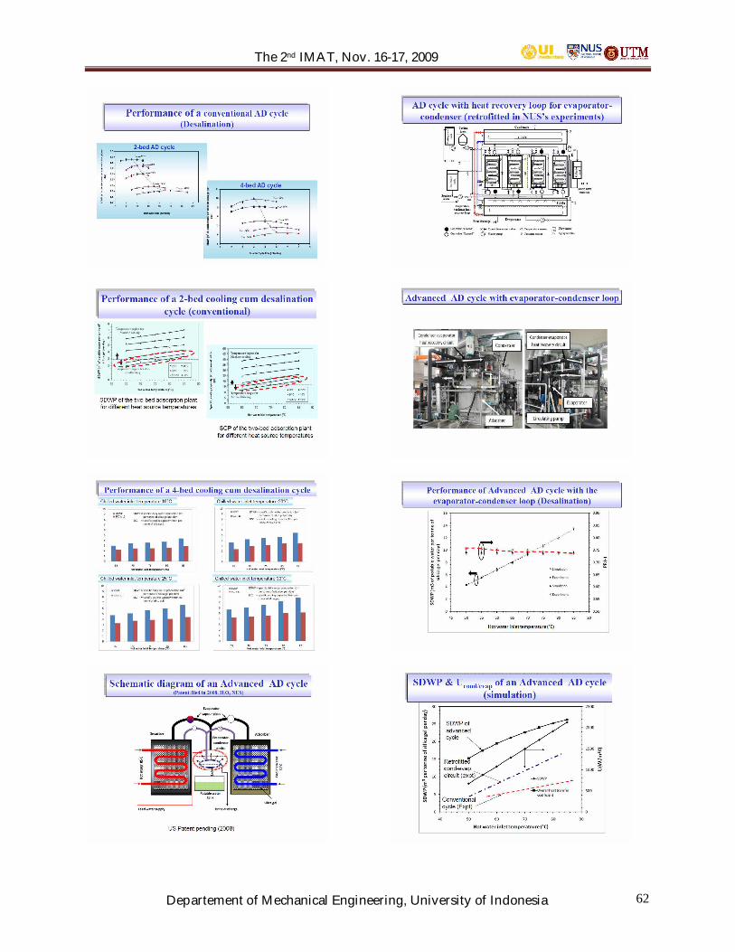
The 2nd IMAT, Nov. 16-17, 2009
Departement of Mechanical Engineering, University of Indonesia 62

The 2nd IMAT, Nov. 16-17, 2009
Departement of Mechanical Engineering, University of Indonesia 63

The 2nd IMAT, Nov. 16-17, 2009
Departement of Mechanical Engineering, University of Indonesia 64
The 2nd IMAT, Nov. 16-17, 2009
Departement of Mechanical Engineering, University of Indonesia 65
Glimpses of Solar Energy Research at the Faculty ofMechanical Engineering University of Technology Malaysia
Skudai, Johor Bharu, Johor
Amer Nordin Darusa
aDepartment of ThermofluidsFaculty of Mechanical Engineering
Universiti Teknologi Malaysia81300 Skudai, Johor BharuE-mail : [email protected]
ABSTRACT
This paper discusses the past and current trend ofsolar energy research s in the Faculty ofMechanical Engineering FKM, at The Universityof Technology Malaysia, UTM. Solar energyresearch at FKM started in the middle of 70’s justafter the world experiences the worst oil crisis inthe world. Earlier attempts begin with modestresearch on low temperature applications of solarenergy. Water heaters, air heaters and solar dryerswere among the first series of research done.Under limited funding and low interest in researchapplications of solar energy only models werebuilt. As time goes by, better equipments werepurchased and more meaningful work was able tobe tried. However, by then oil becomes cheaper.Oil and gas were found in the east coast ofMalaysia. This again offset the interest in solarenergy research. The current research in solarenergy is towards power generation. Direct solarenergy conversion to electrical energy is the maingoal. The extensive application of solar cells isalso seen to be dominating.
1. INTRODUCTION
Since Malaysia is situated in the equatorial regionwith an average radiation of 5,500 KWh persquare meter, it is an ideal location for large scalesolar power installations. Considering thatMalaysia gets on an average 4.5 hours to 8 hoursof free and bountiful sunshine everyday, thepotential for solar power generation is very high.However, the real harnessing of this renewableenergy source is way below its actual potential.
Malaysia has a huge reserve of natural gas andcrude oil which are generally used in powergeneration. Moreover, these fuels are subsidizedto a large extent. Besides, the price of electricity
from the national grid is also relatively cheap.Biomass based power generation is quiteprominent Energy demand in Malaysia
Oil and gas have been the main energy sources inMalaysia. However, with its gas reservesestimated to last for another 33 years and oilreserves another 19 years, the Malaysiangovernment is strengthening the role of renewableenergy (RE) as the fifth cornerstone of energygeneration. Many manufacturing companies inMalaysia are already trying to save energy costs.This creates opportunities to companies offeringenergy management services to determine waysfor saving energy and costs.
Malaysia’s commercial demand for energy isprojected to continue its upward trend, from 1,244Petajoule (PJ) in 2000 to an estimated 2,218 PJ in2010. This consumption growth is mainly drivenby industrialization. As it is common perceptionthat a nation’s economy and use of energy willalways grow hand-in-hand, the Malaysiangovernment, in its 8th Malaysian Plan (2001-2005) has declared RE as the country’s fifth fuelin the energy supply mix to diversify its energysource. Currently, the energy supply mix in thecountry is made up of gas (70 percent), coal (22percent), oil (2 percent) and hydro power (6percent).
2. RENEWABLE ENERGY IN THENINTH MALAYSIAN PLAN
The importance of RE as an enabler of strongeconomic growth is further reinforced in the 9thMalaysian Plan (9MP) (2006-2010), coupled withan emphasis towards Energy Efficiency (EE) bothon production and utilization, while meetingenvironmental objectives. By 2010, RE isexpected to contribute 350MW to total energy
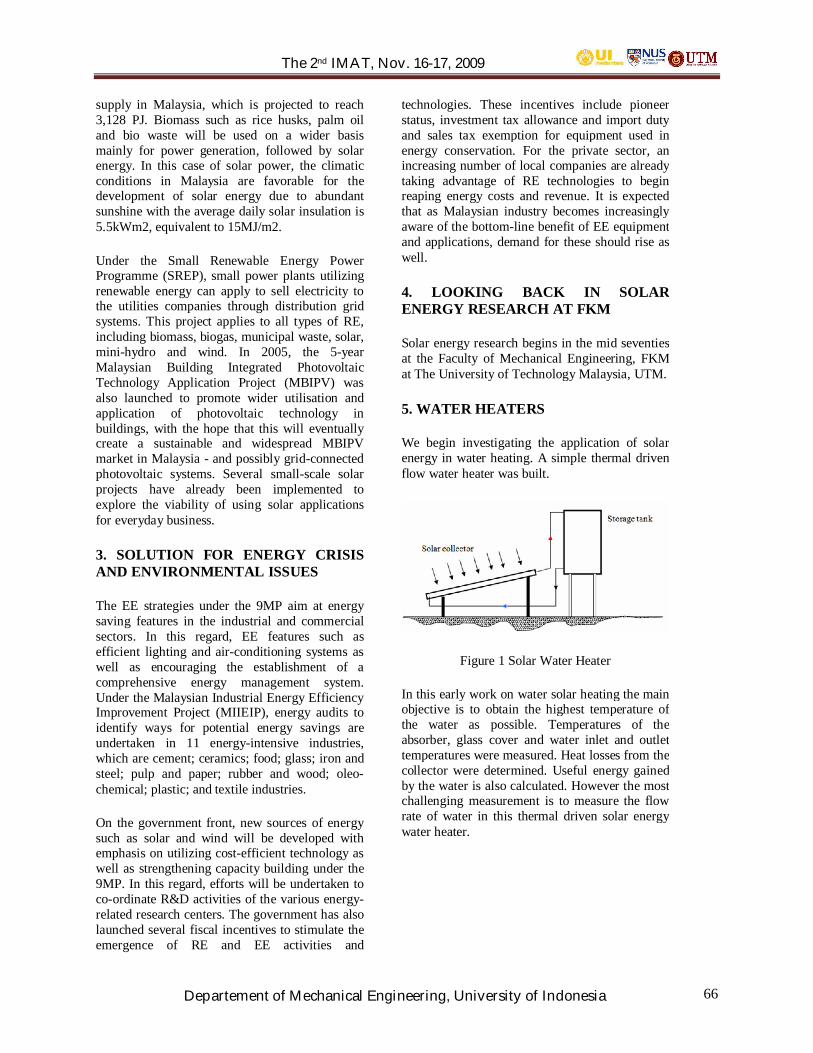
The 2nd IMAT, Nov. 16-17, 2009
Departement of Mechanical Engineering, University of Indonesia 66
supply in Malaysia, which is projected to reach3,128 PJ. Biomass such as rice husks, palm oiland bio waste will be used on a wider basismainly for power generation, followed by solarenergy. In this case of solar power, the climaticconditions in Malaysia are favorable for thedevelopment of solar energy due to abundantsunshine with the average daily solar insulation is5.5kWm2, equivalent to 15MJ/m2.
Under the Small Renewable Energy PowerProgramme (SREP), small power plants utilizingrenewable energy can apply to sell electricity tothe utilities companies through distribution gridsystems. This project applies to all types of RE,including biomass, biogas, municipal waste, solar,mini-hydro and wind. In 2005, the 5-yearMalaysian Building Integrated PhotovoltaicTechnology Application Project (MBIPV) wasalso launched to promote wider utilisation andapplication of photovoltaic technology inbuildings, with the hope that this will eventuallycreate a sustainable and widespread MBIPVmarket in Malaysia - and possibly grid-connectedphotovoltaic systems. Several small-scale solarprojects have already been implemented toexplore the viability of using solar applicationsfor everyday business.
3. SOLUTION FOR ENERGY CRISISAND ENVIRONMENTAL ISSUES
The EE strategies under the 9MP aim at energysaving features in the industrial and commercialsectors. In this regard, EE features such asefficient lighting and air-conditioning systems aswell as encouraging the establishment of acomprehensive energy management system.Under the Malaysian Industrial Energy EfficiencyImprovement Project (MIIEIP), energy audits toidentify ways for potential energy savings areundertaken in 11 energy-intensive industries,which are cement; ceramics; food; glass; iron andsteel; pulp and paper; rubber and wood; oleo-chemical; plastic; and textile industries.
On the government front, new sources of energysuch as solar and wind will be developed withemphasis on utilizing cost-efficient technology aswell as strengthening capacity building under the9MP. In this regard, efforts will be undertaken toco-ordinate R&D activities of the various energy-related research centers. The government has alsolaunched several fiscal incentives to stimulate theemergence of RE and EE activities and
technologies. These incentives include pioneerstatus, investment tax allowance and import dutyand sales tax exemption for equipment used inenergy conservation. For the private sector, anincreasing number of local companies are alreadytaking advantage of RE technologies to beginreaping energy costs and revenue. It is expectedthat as Malaysian industry becomes increasinglyaware of the bottom-line benefit of EE equipmentand applications, demand for these should rise aswell.
4. LOOKING BACK IN SOLARENERGY RESEARCH AT FKM
Solar energy research begins in the mid seventiesat the Faculty of Mechanical Engineering, FKMat The University of Technology Malaysia, UTM.
5. WATER HEATERS
We begin investigating the application of solarenergy in water heating. A simple thermal drivenflow water heater was built.
Figure 1 Solar Water Heater
In this early work on water solar heating the mainobjective is to obtain the highest temperature ofthe water as possible. Temperatures of theabsorber, glass cover and water inlet and outlettemperatures were measured. Heat losses from thecollector were determined. Useful energy gainedby the water is also calculated. However the mostchallenging measurement is to measure the flowrate of water in this thermal driven solar energywater heater.
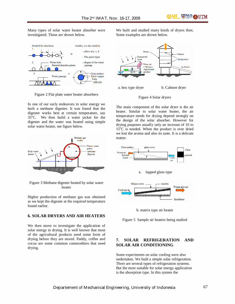
The 2nd IMAT, Nov. 16-17, 2009
Departement of Mechanical Engineering, University of Indonesia 67
Many types of solar water heater absorber wereinvestigated. These are shown below.
Figure 2 Flat plate water heater absorbers
In one of our early endeavors in solar energy webuilt a methane digester. It was found that thedigester works best at certain temperature, say35oC. We then build a water jacket for thedigester and the water was heated using simplesolar water heater, see figure below.
Figure 3 Methane digester heated by solar waterheater
Higher production of methane gas was obtainedas we kept the digester at the required temperaturefound earlier.
6. SOLAR DRYERS AND AIR HEATERS
We then move to investigate the application ofsolar energy in drying. It is well known that mostof the agricultural products need some form ofdrying before they are stored. Paddy, coffee andcocoa are some common commodities that needdrying.
We built and studied many kinds of dryers then.Some examples are shown below.
a. box type dryer b. Cabinet dryer
Figure 4 Solar dryers
The main component of the solar dryer is the airheater. Similar to solar water heater, the airtemperature needs for drying depend strongly onthe design of the solar absorber. However fordrying purposes usually only an increase of 10 to15oC is needed. When the product is over driedwe lost the aroma and also its taste. It is a delicatematter.
a. lapped glass type
b. matrix type air heater
Figure 5 Sample air heaters being studied
7. SOLAR REFRIGERATION ANDSOLAR AIR CONDITIONING
Some experiments on solar cooling were alsoundertaken. We built a simple solar refrigeration.There are several types of refrigeration systems.But the most suitable for solar energy applicationis the absorption type. In this system the

The 2nd IMAT, Nov. 16-17, 2009
Departement of Mechanical Engineering, University of Indonesia 68
compressor in the traditional vapor compressionrefrigerator was replaced with a generator,absorber and rectifier, refer figure below.
a. the system b. the T-s diagram
Figure 6 The vapor absorption solar energyrefrigeration system
The system shown produces ice. We later built amore compact system where the refrigerant filledthe whole system including the solar collector.Thus in this compact system the solar collectoritself acts a generator.
In both systems the valve is actually a capillarytube. We have some problem with this capillarytube. The refrigerant used was ammonia – water.The ammonia-water mixture is very corrosive.We face a great deal of leakage problems. Blackiron was used in the construction of theexperimental rig. Here again we face great deal ofdifficulties in determining the actual refrigerantflow – rate. The cooling load is just the amount ofheat needed to solidify liquid water into ice. Thecompact refrigeration system fails to produce ice,but some coldness was attained.
Natural extension of solar refrigeration cooling isobviously air conditioning. Thus instead ofcooling water to produce ice, the cooling loadnow becomes the cooling of air. See, followingfigure.
Figure 7 Cooling the air directly
Actually solar air conditioning is very attractiveindeed. We are giving a chance to do somesimulation studies in cooling a section of theSultanah Zanariah Library of UTM. In fact, wewere also requested to solar air – condition thewalk – way from the Dewan Sultan Iskandar tothe Sultan Ismail Mosque in the campus.However, analysis and simulation results showthat these projects are not economically viable.The cost of solar cells to run the compressor isvery expensive. Solar absorption system was notproposed as earlier study showed it is also noteconomical too.
8. SOLAR SIMULATOR
As solar energy research depends greatly at themercy of the sun, a solar simulator was built inthe late 80’s. With the help of the ElectricityEngineering Faculty, we build a model solarsimulator.
Figure 8 Solar Simulator
With this simulator, we were able to performsome work indoor. However, we fail to capturethe actual solar environment outdoor. The effectof wind and dust on the solar collector cover offlat plate solar collectors was not able to beappreciated.
In those days, in the 80’s and early 90’s we usedto hold conferences and seminars on solar energyamong the local universities such as theUniversity of Malays, UM, the NationalUniversity, UKM, the University of Science,USM and the University of Agriculture. Most ofour findings were shared and discussed in thisannual seminar on solar energy. Many fruitful andproactive attempts are collectively undertake tofoster the interest on solar energy applications inthe country. However, almost at the same time, oilprices get low and lower. The interest in solarenergy is ebbing.
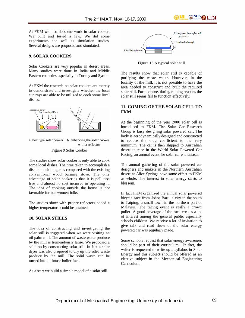
The 2nd IMAT, Nov. 16-17, 2009
Departement of Mechanical Engineering, University of Indonesia 69
with a reflector
At FKM we also do some work in solar cooker.We built and tested a few. We did someexperiments and well as simulation studies.Several designs are proposed and simulated.
9. SOLAR COOKERS
Solar Cookers are very popular in desert areas.Many studies were done in India and MiddleEastern countries especially in Turkey and Syria.
At FKM the research on solar cookers are merelyto demonstrate and investigate whether the localsun rays are able to be utilized to cook some localdishes.
a. box type solar cooker b. enhancing the solar cooker
Figure 9 Solar Cooker
The studies show solar cooker is only able to cooksome local dishes. The time taken to accomplish adish is much longer as compared with the existingconventional wood burning stove. The onlyadvantage of solar cooker is that it is pollutionfree and almost no cost incurred in operating it.The idea of cooking outside the house is notfavorable for our women folks.
The studies show with proper reflectors added ahigher temperature could be attained.
10. SOLAR STILLS
The idea of constructing and investigating thesolar still is triggered when we were visiting anoil palm mill. The amount of waste water produceby the mill is tremendously large. We proposed asolution by constructing solar still. In fact a solardryer was also proposed to dry up the solid wasteproduce by the mill. The solid waste can beturned into in-house boiler fuel.
As a start we build a simple model of a solar still.
Figure 13 A typical solar still
The results show that solar still is capable ofpurifying the waste water. However, in thelocality of the mill, it is not possible to have thearea needed to construct and built the requiredsolar still. Furthermore, during raining seasons thesolar still seems fail to function effectively.
11. COMING OF THE SOLAR CELL TOFKM
At the beginning of the year 2000 solar cell isintroduced to FKM. The Solar Car ResearchGroup is busy designing solar powered car. Thebody is aerodynamically designed and constructedto reduce the drag coefficient to the veryminimum. The car is then shipped to Australiandesert to race in the World Solar Powered CarRacing, an annual event for solar car enthusiasts.
The annual gathering of the solar powered cardesigners and makers in the Northern Australiandesert at Alice Springs have some effect to FKMas whole. The interest in solar energy starts toblossom.
In fact FKM organized the annual solar poweredbicycle race from Johor Baru, a city in the southto Taiping, a small town in the northern part ofMalaysia. The racing event is really a crowdpuller. A good coverage of the race creates a lotof interest among the general public especiallyschools children. We receive a lot of invitation togive talk and road show of the solar energypowered car was regularly made.
Some schools request that solar energy awarenessshould be part of their curriculum. In fact, thewriter is requested to write up a syllabus in SolarEnergy and this subject should be offered as anelective subject in the Mechanical EngineeringCurriculum.

The 2nd IMAT, Nov. 16-17, 2009
Departement of Mechanical Engineering, University of Indonesia 70
Popularity of the solar powered car and bicycleruns short. It lasted for only 3 to 4 years. Themain reason for its failure is lack of funding.Solar powered car and bicycle are not researchoriented. No research was done in solar cell, Theresearch part of the solar cell and battery are takenby the Department of Applied Physics, Faculty ofScience, UTM. We become the user.
12. CONCLUSION
Solar energy research is a never ending activity inFKM. The interest in solar energy is always high.Currently we are engaging our effort in solarpower generation. Organic Rankine Cycle takingsolar energy as the main heat source is reviewed.With the current advancement of computertechnology and efficient commercial engineeringsoftware, more meaningful computer simulationstudies will be attempted.
Solar cooling of buildings is always been ourmain interest in studying solar energy. Bettersystems of solar refrigeration have to beexperimented. New systems will be simulatedusing data taken from the experiments.Thermoelectric refrigeration system is also beingstudied.
Smaller models of solar energy systems will bestudied. With better measuring devices andinstrumentations these smaller models will cutcosts but in same time save space and have ahigher level of portability. Experimental can beperformed anyway, indoor or outdoor.
In order to increase the efficiency or thecoefficient of performance of the solar energysystems, exergy analysis will be performed.
REFERENCES
[1] Lunde, P.J., (1980), Solar Thermal Engineering,John Willy, New York
[2] Kreith, F, and Kreider, J., (1980) SolarEngineering, Hemisphere, New York
[3] Swa, H.A, (1975), Methane Digester, Bachelor ofEngineering Thesis, Faculty of MechanicalEngineering, University of Technology, Malaysia,
[4] Muhammad Shafie Mat Ali, (2004), Solar WaterHeater, An Experimental Study, Bachelor ofEngineering Thesis, Faculty of MechanicalEngineering, University of Technology Malaysia,
[5] Mohamed Mahadir Mohd Shafie, (2005), HeatTransfer Analysis of a Solar Cooker, A SimulationStudy, Bachelor of Engineering Thesis, Faculty of
Mechanical Engineering, University ofTechnology, Malaysia
[6] Mohd Ezani Mahzan, (2005), Design andConstruction of Solar Cloth Dryer, Bachelor ofEngineering Thesis, Faculty of MechanicalEngineering, University of Technology, Malaysia
[7] Rita Azura Roslan, (2005), An Experimental Studyon Solar Still, Bachelor of Engineering Thesis,Faculty of Mechanical Engineering, University ofTechnology, Malaysia
[8] Reza Sharil Mohd Said, (2006), An ExperimentalStudy of a Solar Cooker, Bachelor of EngineeringThesis, Faculty of Mechanical Engineering,University of Technology Malaysia
[9] Mohd Syukri Hashim, (2006), An ExperimentalStudy of Solar Still with Reflector, Bachelor ofEngineering Thesis, Faculty of MechanicalEngineering, University of Technology, Malaysia
[10] Mohd Zaki Akhtar, (2005), Determination of SolarRadiation Distribution of Malaysia, An EmpericalMethod, Bachelor of Engineering Thesis, Facultyof Mechanical Engineering, University ofTechnology, Malaysia
[11] Dalbir Singh s/o Atar Singth, (2006), ParametricStudy of Solar Vapor Compression CoolingSystem, Bachelor of Engineering Thesis, Facultyof Mechanical Engineering, University ofTechnology, Malaysia
[12] Cheng Eng Cong, (2006), Feasibility Study ofSolar Energy Powered of An Organic RankineCycle, Bachelor of Engineering Thesis, Faculty ofMechanical Engineering, University ofTechnology, Malaysia
[13] Sia Toh Ching, (2007), An Exergy Analysis of AFlat Plate Solar Collector, Bachelor ofEngineering Thesis, Faculty of MechanicalEngineering, University of R\Technology,Malaysia
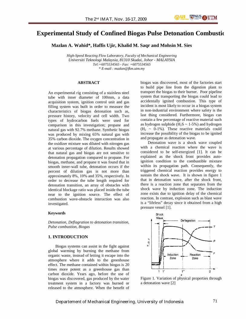
The 2nd IMAT, Nov. 16-17, 2009
Departement of Mechanical Engineering, University of Indonesia 71
Experimental Study of Confined Biogas Pulse Detonation Combustion
Mazlan A. Wahid*, Haffis Ujir, Khalid M. Saqr and Mohsin M. Sies
High-Speed Reacting Flow Laboratory, Faculty of Mechanical EngineeringUniversiti Teknologi Malaysia, 81310 Skudai, Johor - MALAYSIA
Tel:+6075534565 - Fax: +6075534565* E-mail : [email protected]
ABSTRACT
An experimental rig consisting of a stainless steeltube with inner diameter of 100mm, a dataacquisition system, ignition control unit and gasfilling system was built in order to measure thecharacteristics of biogas detonation such as,pressure history, velocity and cell width. Twotypes of hydrocarbon fuels were used forcomparison in this investigation; propane andnatural gas with 92.7% methane. Synthetic biogaswas produced by mixing 65% natural gas with35% carbon dioxide. The oxygen concentration inthe oxidizer mixture was diluted with nitrogen gasat various percentage of dilution. Results showedthat natural gas and biogas are not sensitive todetonation propagation compared to propane. Forbiogas, methane, and propane tt was found that insmooth inner-wall tube, detonation occurs if thepercent of dilution gas is not more thanapproximately 8%, 10% and 35%, respectively. Inorder to decrease the tube length required fordetonation transition, an array of obstacles withidentical blockage ratio was placed inside the tubenear to the ignition source. The effect ofcombustion wave-obstacle interaction was alsoinvestigated.
Keywords
Detonation, Deflagration to detonation transition,Pulse combustion, Biogas
1. INTRODUCTION
Biogas systems can assist in the fight againstglobal warming by burning the methane fromorganic waste, instead of letting it escape into theatmosphere where it adds to the greenhouseeffect. The methane contained within biogas is 20times more potent as a greenhouse gas thancarbon dioxide. Years ago, before the use ofbiogas was discovered, gas produced by the watertreatment system in a factory was burned orreleased to the atmosphere. When the benefit of
biogas was discovered, most of the factories startto build pipe line from the digestion plant totransport the biogas to their burner. Poor pipelinesystem that transporting the biogas could lead toaccidentally ignited combustion. This type ofincident is most likely to occur in a biogas systemin non-industrial environment where safety is thelast thing considered. Furthermore, biogas cancontain a few percentage of reactive material suchas hydrogen sulphide (H2S ~ 1-5%) and hydrogen(H2 ~ 0-1%). These reactive materials couldincrease the possibility of the biogas to be ignitedand propagate as detonation wave.
Detonation wave is a shock wave coupledwith a chemical reaction where the wave isconsidered to be self-energized [1]. It can beexplained as the shock front provides auto-ignition condition to the combustible mixturewithin its propagation path. Consequently, thetriggered chemical reaction provides energy tosustain the shock wave. It is shown in figure 1that in detonation wave, after the shock front,there is a reaction zone that separates from theshock wave by induction zone. The inductionzone exists due to ignition delay of the chemicalreaction. In contrast, explosion such as blast waveis a “lifeless” decay since it obtained from a highpressure vessel [1].
Figure 1. Variation of physical properties througha detonation wave [2]
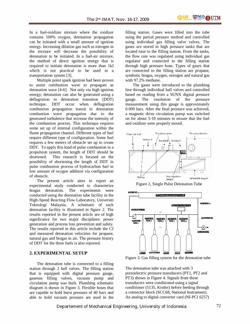
The 2nd IMAT, Nov. 16-17, 2009
Departement of Mechanical Engineering, University of Indonesia 72
In a fuel-oxidizer mixture where the oxidizercontains 100% oxygen, detonation propagationcan be initiated with a small amount of ignitionenergy. Increasing dilution gas such as nitrogen inthe mixture will decrease the possibility ofdetonation to be initiated. In a fuel-air mixture,the method of direct ignition energy that isrequired to initiate detonation is more than 1kJwhich is not practical to be used in atransportation system [3].
Multiple point spark ignition had been provento assist combustion wave to propagate asdetonation wave [4-6]. Not only via high ignitionenergy; detonation can also be generated using adeflagration to detonation transition (DDT)technique. DDT occur when deflagrationcombustion propagation transit to detonationcombustion wave propagation due to thegenerated turbulence that increase the intensity ofthe combustion process. This technique requiressome set up of internal configuration within theflame propagation channel. Different types of fuelrequire different type of configuration. Some fuelrequires a few meters of obstacle set up to createDDT. To apply this kind of pulse combustion in apropulsion system, the length of DDT should beshortened. This research is focused on thepossibility of shortening the length of DDT inpulse combustion process of hydrocarbon fuel inlow amount of oxygen addition via configurationof obstacle.
The present article aims to report anexperimental study conducted to characterizebiogas detonation. The experiments wereconducted using the detonation tube facility in theHigh-Speed Reacting Flow Laboratory, UniversitiTeknologi Malaysia. A schematic of suchdetonation facility is illustrated in figure 2. Theresults reported in the present article are of highsignificance for two major disciplines: powergeneration and process loss prevention and safety.The results reported in this article include the CJand measured detonation velocities for propane,natural gas and biogas in air. The pressure historyof DDT for the three fuels is also reported.
2. EXPERIMENTAL SETUP
The detonation tube is connected to a fillingstation through 2 ball valves. The filling stationthat is equipped with digital pressure gauge,gaseous filling valves, vacuum pump andcirculation pump was built. Plumbing schematicdiagram is shown in Figure 3. Flexible hoses thatare capable to hold burst pressure of 40 bars andable to hold vacuum pressure are used in the
filling station. Gases were filled into the tubeusing the partial pressure method and controlledusing individual gas filling valve valves. Thegases are stored in high pressure tanks that arelocated near to the filling station. From the tanks,the flow rate was regulated using individual gasregulator and connected to the filling stationthrough high pressure hose. Types of gases thatare connected to the filling station are propane,synthetic biogas, oxygen, nitrogen and natural gaswith 97.2% methane.
The gases were introduced to the plumbingline through individual ball valves and controlledbased on reading from a SUNX digital pressuregauge. The resolution of the pressuremeasurement using this gauge is approximately0.009 bars. After the final pressure was achieved,a magnetic drive circulation pump was switchedon for about 5-10 minutes to ensure that the fueland oxidizer were properly mixed.
Figure 2, Single Pulse Detonation Tube
Figure 3. Gas filling system for the detonation tube
The detonation tube was attached with 3piezoelectric pressure transducers (PT1, PT2 andPT3) shown in Figure 4. Signals from thesetransducers were conditioned using a signalconditioner (5135, Kistler) before feeding througha connector block (SCC68, National Instrument).An analog to digital converter card (NI-PCI 6257)
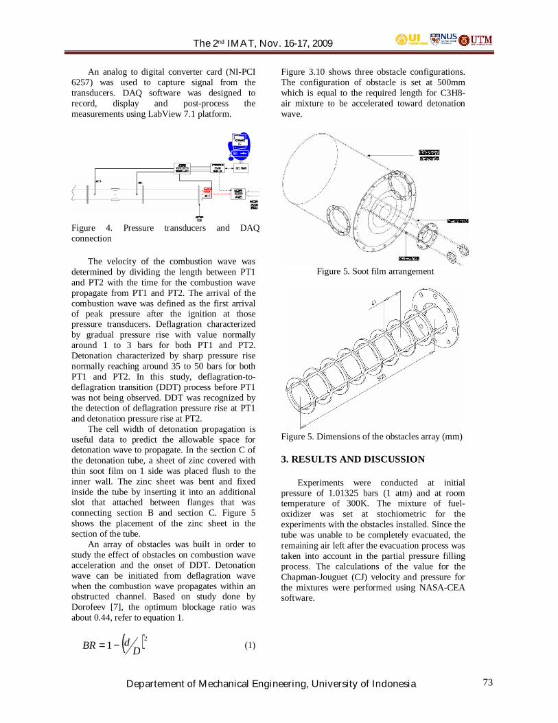
The 2nd IMAT, Nov. 16-17, 2009
Departement of Mechanical Engineering, University of Indonesia 73
An analog to digital converter card (NI-PCI6257) was used to capture signal from thetransducers. DAQ software was designed torecord, display and post-process themeasurements using LabView 7.1 platform.
Figure 4. Pressure transducers and DAQconnection
The velocity of the combustion wave wasdetermined by dividing the length between PT1and PT2 with the time for the combustion wavepropagate from PT1 and PT2. The arrival of thecombustion wave was defined as the first arrivalof peak pressure after the ignition at thosepressure transducers. Deflagration characterizedby gradual pressure rise with value normallyaround 1 to 3 bars for both PT1 and PT2.Detonation characterized by sharp pressure risenormally reaching around 35 to 50 bars for bothPT1 and PT2. In this study, deflagration-to-deflagration transition (DDT) process before PT1was not being observed. DDT was recognized bythe detection of deflagration pressure rise at PT1and detonation pressure rise at PT2.
The cell width of detonation propagation isuseful data to predict the allowable space fordetonation wave to propagate. In the section C ofthe detonation tube, a sheet of zinc covered withthin soot film on 1 side was placed flush to theinner wall. The zinc sheet was bent and fixedinside the tube by inserting it into an additionalslot that attached between flanges that wasconnecting section B and section C. Figure 5shows the placement of the zinc sheet in thesection of the tube.
An array of obstacles was built in order tostudy the effect of obstacles on combustion waveacceleration and the onset of DDT. Detonationwave can be initiated from deflagration wavewhen the combustion wave propagates within anobstructed channel. Based on study done byDorofeev [7], the optimum blockage ratio wasabout 0.44, refer to equation 1.
( )21 D
dBR −= (1)
Figure 3.10 shows three obstacle configurations.The configuration of obstacle is set at 500mmwhich is equal to the required length for C3H8-air mixture to be accelerated toward detonationwave.
Figure 5. Soot film arrangement
Figure 5. Dimensions of the obstacles array (mm)
3. RESULTS AND DISCUSSION
Experiments were conducted at initialpressure of 1.01325 bars (1 atm) and at roomtemperature of 300K. The mixture of fuel-oxidizer was set at stochiometric for theexperiments with the obstacles installed. Since thetube was unable to be completely evacuated, theremaining air left after the evacuation process wastaken into account in the partial pressure fillingprocess. The calculations of the value for theChapman-Jouguet (CJ) velocity and pressure forthe mixtures were performed using NASA-CEAsoftware.
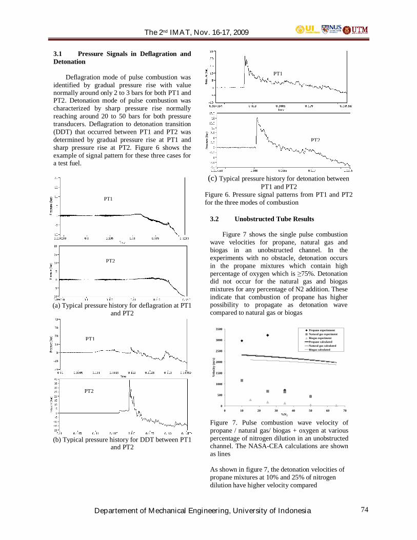
The 2nd IMAT, Nov. 16-17, 2009
Departement of Mechanical Engineering, University of Indonesia 74
3.1 Pressure Signals in Deflagration andDetonation
Deflagration mode of pulse combustion wasidentified by gradual pressure rise with valuenormally around only 2 to 3 bars for both PT1 andPT2. Detonation mode of pulse combustion wascharacterized by sharp pressure rise normallyreaching around 20 to 50 bars for both pressuretransducers. Deflagration to detonation transition(DDT) that occurred between PT1 and PT2 wasdetermined by gradual pressure rise at PT1 andsharp pressure rise at PT2. Figure 6 shows theexample of signal pattern for these three cases fora test fuel.
PT1
PT2
(a) Typical pressure history for deflagration at PT1and PT2
PT1
PT2
(b) Typical pressure history for DDT between PT1and PT2
PT1
PT2
(c) Typical pressure history for detonation betweenPT1 and PT2
Figure 6. Pressure signal patterns from PT1 and PT2for the three modes of combustion
3.2 Unobstructed Tube Results
Figure 7 shows the single pulse combustionwave velocities for propane, natural gas andbiogas in an unobstructed channel. In theexperiments with no obstacle, detonation occursin the propane mixtures which contain highpercentage of oxygen which is 75%. Detonationdid not occur for the natural gas and biogasmixtures for any percentage of N2 addition. Theseindicate that combustion of propane has higherpossibility to propagate as detonation wavecompared to natural gas or biogas
0
500
1000
1500
2000
2500
3000
3500
0 10 20 30 40 50 60 70%N2
Vel
ocity
(m/s
)
Propane experiementNatural gas experimentBiogas experimentPropane calculatedNatural gas calculatedBiogas calculated
Figure 7. Pulse combustion wave velocity ofpropane / natural gas/ biogas + oxygen at variouspercentage of nitrogen dilution in an unobstructedchannel. The NASA-CEA calculations are shownas lines
As shown in figure 7, the detonation velocities ofpropane mixtures at 10% and 25% of nitrogendilution have higher velocity compared
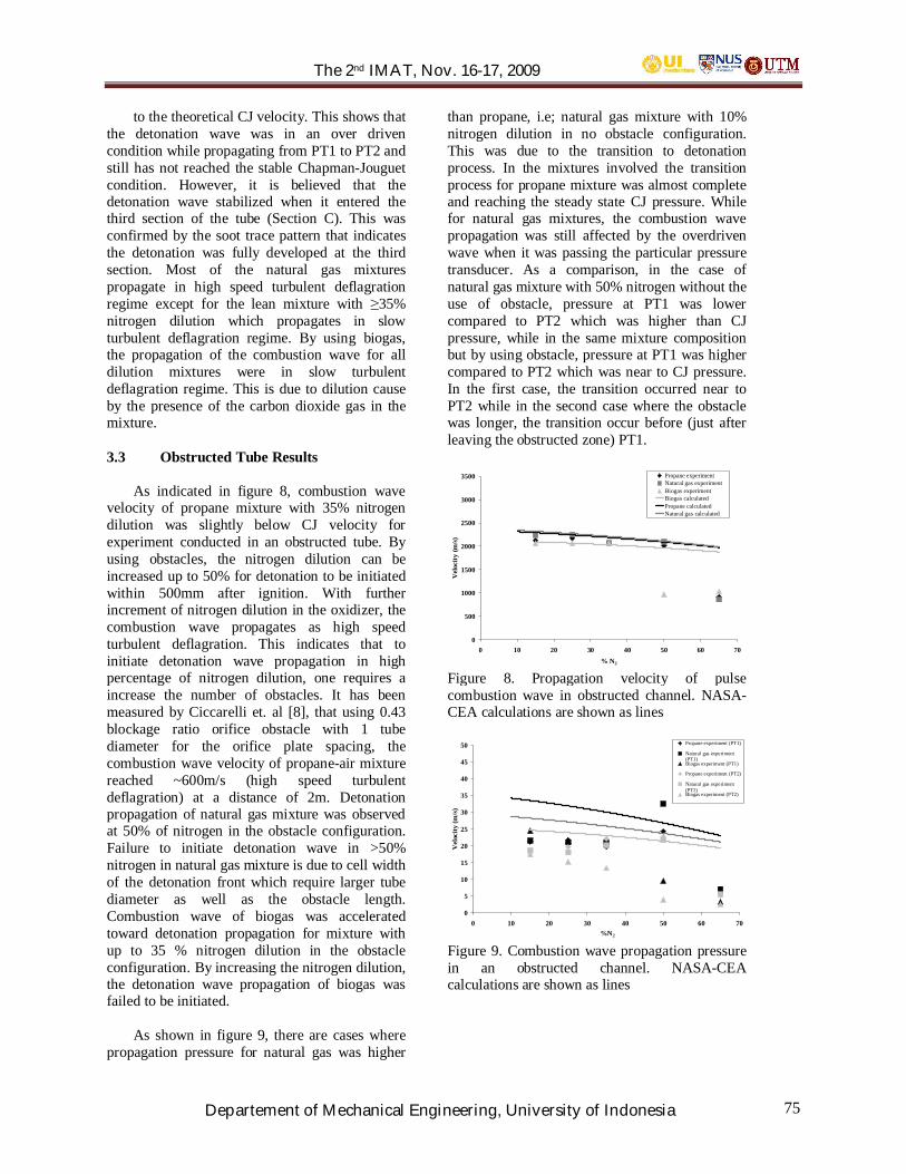
The 2nd IMAT, Nov. 16-17, 2009
Departement of Mechanical Engineering, University of Indonesia 75
to the theoretical CJ velocity. This shows thatthe detonation wave was in an over drivencondition while propagating from PT1 to PT2 andstill has not reached the stable Chapman-Jouguetcondition. However, it is believed that thedetonation wave stabilized when it entered thethird section of the tube (Section C). This wasconfirmed by the soot trace pattern that indicatesthe detonation was fully developed at the thirdsection. Most of the natural gas mixturespropagate in high speed turbulent deflagrationregime except for the lean mixture with 35%nitrogen dilution which propagates in slowturbulent deflagration regime. By using biogas,the propagation of the combustion wave for alldilution mixtures were in slow turbulentdeflagration regime. This is due to dilution causeby the presence of the carbon dioxide gas in themixture.
3.3 Obstructed Tube Results
As indicated in figure 8, combustion wavevelocity of propane mixture with 35% nitrogendilution was slightly below CJ velocity forexperiment conducted in an obstructed tube. Byusing obstacles, the nitrogen dilution can beincreased up to 50% for detonation to be initiatedwithin 500mm after ignition. With furtherincrement of nitrogen dilution in the oxidizer, thecombustion wave propagates as high speedturbulent deflagration. This indicates that toinitiate detonation wave propagation in highpercentage of nitrogen dilution, one requires aincrease the number of obstacles. It has beenmeasured by Ciccarelli et. al [8], that using 0.43blockage ratio orifice obstacle with 1 tubediameter for the orifice plate spacing, thecombustion wave velocity of propane-air mixturereached ~600m/s (high speed turbulentdeflagration) at a distance of 2m. Detonationpropagation of natural gas mixture was observedat 50% of nitrogen in the obstacle configuration.Failure to initiate detonation wave in >50%nitrogen in natural gas mixture is due to cell widthof the detonation front which require larger tubediameter as well as the obstacle length.Combustion wave of biogas was acceleratedtoward detonation propagation for mixture withup to 35 % nitrogen dilution in the obstacleconfiguration. By increasing the nitrogen dilution,the detonation wave propagation of biogas wasfailed to be initiated.
As shown in figure 9, there are cases wherepropagation pressure for natural gas was higher
than propane, i.e; natural gas mixture with 10%nitrogen dilution in no obstacle configuration.This was due to the transition to detonationprocess. In the mixtures involved the transitionprocess for propane mixture was almost completeand reaching the steady state CJ pressure. Whilefor natural gas mixtures, the combustion wavepropagation was still affected by the overdrivenwave when it was passing the particular pressuretransducer. As a comparison, in the case ofnatural gas mixture with 50% nitrogen without theuse of obstacle, pressure at PT1 was lowercompared to PT2 which was higher than CJpressure, while in the same mixture compositionbut by using obstacle, pressure at PT1 was highercompared to PT2 which was near to CJ pressure.In the first case, the transition occurred near toPT2 while in the second case where the obstaclewas longer, the transition occur before (just afterleaving the obstructed zone) PT1.
0
500
1000
1500
2000
2500
3000
3500
0 10 20 30 40 50 60 70% N2
Vel
ocity
(m/s)
Propane experimentNatural gas experimentBiogas experimentBiogas calculatedPropane calculatedNatural gas calculated
Figure 8. Propagation velocity of pulsecombustion wave in obstructed channel. NASA-CEA calculations are shown as lines
0
5
10
15
20
25
30
35
40
45
50
0 10 20 30 40 50 60 70%N2
Vel
ocity
(m/s
)
Propane experiment (PT1)
Natural gas experiment(PT1)Biogas experiment (PT1)
Propane experiment (PT2)
Natural gas experiment(PT2)Biogas experiment (PT2)
Propane calculated
Figure 9. Combustion wave propagation pressurein an obstructed channel. NASA-CEAcalculations are shown as lines
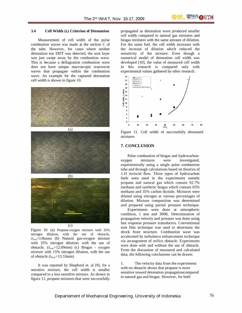
The 2nd IMAT, Nov. 16-17, 2009
Departement of Mechanical Engineering, University of Indonesia 76
3.4 Cell Width ( ) Criterion of Detonation
Measurement of cell width of the pulsecombustion waves was made at the section C ofthe tube. However, for cases where neitherdetonation nor DDT was detected, the soot layerwas just swept away by the combustion wave.This is because a deflagration combustion wavedoes not have unique macroscopic transversewaves that propagate within the combustionwave. An example for the captured detonationcell width is shown in figure 10.
(a)
(b)
(c)Figure 10. (a) Propane-oxygen mixture with 35%nitrogen dilution; with the use of obstacle,
ave=3.86mm) (b) Natural gas-oxygen mixturewith 35% nitrogen dilution; with the use ofobstacle, ( ave=12.09mm) (c) Biogas - oxygenmixture with 15% nitrogen dilution, with the useof obstacle ( ave=13.55mm)
It was reported by Shepherd et. al [9], for asensitive mixture, the cell width is smallercompared to a less sensitive mixture. As shown infigure 11, propane mixtures that were successfully
propagated as detonation wave produced smallercell width compared to natural gas mixtures andbiogas mixtures with the same amount of dilution.For the same fuel, the cell width increases withthe increase of dilution which reduced thesensitivity of the mixture. Even though anumerical model of detonation cell width wasdeveloped [10], the value of measured cell widthin this research is compared only withexperimental values gathered by other research.
0
2
4
6
8
10
12
14
16
18
20
22
24
0 10 20 30 40 50 60 70 80%N2
Cel
l wid
th,
(mm
)
Propane T2Methane T2Propane T1Methane T1Biogas T2Knytautas (1982) Propane
Figure 11. Cell width of successfully detonatedmixtures
7. CONCLUSION
Pulse combustion of biogas and hydrocarbon-oxygen mixtures were investigated,experimentally using a single pulse combustiontube and through calculations based on theories of1-D inviscid flow. Three types of hydrocarbonfuels were used in the experiments namelypropane and natural gas which contain 92.7%methane and synthetic biogas which contain 65%methane and 35% carbon dioxide. Mixtures werediluted using nitrogen at various percentages ofdilution. Mixture composition was determinedand prepared using partial pressure technique. Experiments were done at atmosphericcondition, 1 atm and 300K. Determination ofpropagation velocity and pressure was done usingfast response pressure transducers. Conventionalsoot film technique was used to determine theshock front structure. Combustion wave wasaccelerated by turbulence enhancement techniquevia arrangement of orifice obstacle. Experimentswere done with and without the use of obstacle.From the discussion of measured and calculateddata, the following conclusions can be drawn:
1. The velocity data from the experimentswith no obstacle shows that propane is moresensitive toward detonation propagationcomparedto natural gas and biogas. However, for both

The 2nd IMAT, Nov. 16-17, 2009
Departement of Mechanical Engineering, University of Indonesia 77
hydrocarbon fuels, the probability to the onset ofdetonation is decreased with the increase ofnitrogen dilution. Thus, by preparing injector ofdilution gas such nitrogen at the place where thepossibility of accident is high the gas pipelinecould suppress accidentally ignited combustiblemixture and decrease the possibility of detonationto be initiated.
2. Combustion wave of biogas can beaccelerated toward detonation propagation byusing 500mm length of orifice obstacle with thepercentage of nitrogen up to 35%. By increasingthe length of the obstacle, the onset of detonationcan occur within higher percentage of nitrogendilution. Presence of obstacle in biogas or naturalgas pipeline such as excessive gasket, valve andjunction within short distance could accelerateaccidentally ignited mixture toward detonation.Precaution or any mean of ventilation should beapplied at where the number of obstacle is high inthe gas pipeline.
3. From the cell width data, for same percentageof nitrogen dilution, propane mixture producessmaller cell width structure compared to naturalgas and biogas. Based on dc=13 criterion, thisindicate that detonation wave of propane mixturecan propagate at smaller tube diameter comparedto natural gas mixture.
ACKNOWLEDGMENTThe authors would like to acknowledge thesupport provided by the Malaysian Ministry ofHigher Education (MOHE) under the FRGS grantnumber 78046.
REFERENCES
[1] A.K. Oppenhiem, “Introduction to Gasdynamics ofExplosions”, International Centre For MechanicalSciences, Udine 1970,
[2] K.K.Kuo, Principles of Combustion, 2nd ed, JohnWiley & sons, Inc. 2005
[3] E. Schultz, E. Wintenberger and J. Shepherd.,GALCIT Report: “Investigation of Deflagration-to-Detonation Transition for Application to PulseDetonation Engine Ignition System”, Pasadena
[4] D.C. Bull, J.E. Elsworth, G. Hooper, “ Initiation ofSpherical Detonation in Hydrocarbon/AirMixtures”, Acta Astron, Vol.5, 11; 997-1008, 1978
[5] V.P. Zhukov, A.E. Rakitin, A.Yu. Starikovskii,“Detonation Initiation By High-Voltage PulsedDischarges”, 45th AIAA Aerospace SciencesMeeting and Exhibit, 2007-1029.
[6] I. B. Schild, A. J. Dean,” Influence of SparkEnergy, Spark number and Flow Velocity ON
Detonation Initiation in a Hydrocarbon-fueledPDE”, 41th AIAA Aerospace Sciences Meetingand Exhibit, 2005-4211
[7] S. B. Dorofeev, V. P. Sidorov, M. S. Kusnetsov, I.D. Matsukov, V. I. Alekseev, “Effect of Scale onThe Onset of Detonation”, Shock Wave (2000) 10:137-149
[8] 51. G. Ciccarelli, C.J. Fowler, M. Bardon,“Effect of Obstacle Size and Spacing on TheInitial Stage of Flame Acceleration in a RoughTube”, Shock Wave (2005) 14(3): 161-166
[9] J. E. Shapherd, I. O. Moen, S. B. Murray, P. A.Thibault, “Analysis of the cellular structure ofdetonation”, 21 Symposium (Intl) on Combustion,16, 149-1658, 1986
[10] A. I. Gavrikov, A. A. Efimenko, S. B. Dorofeev, “A Model for Detonation Cell Size Prediction fromChemical Kinetics”, Combustion and Flame120:19-33 (2000)
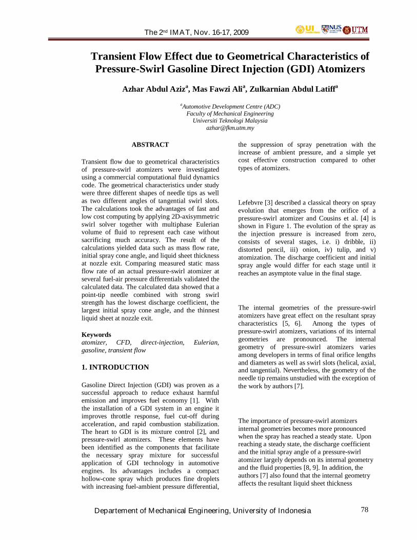
The 2nd IMAT, Nov. 16-17, 2009
Departement of Mechanical Engineering, University of Indonesia 78
Transient Flow Effect due to Geometrical Characteristics ofPressure-Swirl Gasoline Direct Injection (GDI) Atomizers
Azhar Abdul Aziza, Mas Fawzi Alia, Zulkarnian Abdul Latiffa
aAutomotive Development Centre (ADC)Faculty of Mechanical Engineering
Universiti Teknologi [email protected]
ABSTRACT
Transient flow due to geometrical characteristicsof pressure-swirl atomizers were investigatedusing a commercial computational fluid dynamicscode. The geometrical characteristics under studywere three different shapes of needle tips as wellas two different angles of tangential swirl slots.The calculations took the advantages of fast andlow cost computing by applying 2D-axisymmetricswirl solver together with multiphase Eulerianvolume of fluid to represent each case withoutsacrificing much accuracy. The result of thecalculations yielded data such as mass flow rate,initial spray cone angle, and liquid sheet thicknessat nozzle exit. Comparing measured static massflow rate of an actual pressure-swirl atomizer atseveral fuel-air pressure differentials validated thecalculated data. The calculated data showed that apoint-tip needle combined with strong swirlstrength has the lowest discharge coefficient, thelargest initial spray cone angle, and the thinnestliquid sheet at nozzle exit.
Keywordsatomizer, CFD, direct-injection, Eulerian,gasoline, transient flow
1. INTRODUCTION
Gasoline Direct Injection (GDI) was proven as asuccessful approach to reduce exhaust harmfulemission and improves fuel economy [1]. Withthe installation of a GDI system in an engine itimproves throttle response, fuel cut-off duringacceleration, and rapid combustion stabilization.The heart to GDI is its mixture control [2], andpressure-swirl atomizers. These elements havebeen identified as the components that facilitatethe necessary spray mixture for successfulapplication of GDI technology in automotiveengines. Its advantages includes a compacthollow-cone spray which produces fine dropletswith increasing fuel-ambient pressure differential,
the suppression of spray penetration with theincrease of ambient pressure, and a simple yetcost effective construction compared to othertypes of atomizers.
Lefebvre [3] described a classical theory on sprayevolution that emerges from the orifice of apressure-swirl atomizer and Cousins et al. [4] isshown in Figure 1. The evolution of the spray asthe injection pressure is increased from zero,consists of several stages, i.e. i) dribble, ii)distorted pencil, iii) onion, iv) tulip, and v)atomization. The discharge coefficient and initialspray angle would differ for each stage until itreaches an asymptote value in the final stage.
The internal geometries of the pressure-swirlatomizers have great effect on the resultant spraycharacteristics [5, 6]. Among the types ofpressure-swirl atomizers, variations of its internalgeometries are pronounced. The internalgeometry of pressure-swirl atomizers variesamong developers in terms of final orifice lengthsand diameters as well as swirl slots (helical, axial,and tangential). Nevertheless, the geometry of theneedle tip remains unstudied with the exception ofthe work by authors [7].
The importance of pressure-swirl atomizersinternal geometries becomes more pronouncedwhen the spray has reached a steady state. Uponreaching a steady state, the discharge coefficientand the initial spray angle of a pressure-swirlatomizer largely depends on its internal geometryand the fluid properties [8, 9]. In addition, theauthors [7] also found that the internal geometryaffects the resultant liquid sheet thickness
The 2nd IMAT, Nov. 16-17, 2009
Departement of Mechanical Engineering, University of Indonesia 79
downstream of the pressure-swirl atomizers.During transient state, the time for the spray toreach the steady state of atomization is criticalespecially in GDI application where the fuel wasinjected at high frequency [4]. Therefore, aninjector configuration with the least time to reachthe stable stage (v) is highly desirable.
Regions of interest that depicts the most importanttransient flows would be a few millimeters insideand outside the final nozzle orifice. However, itis nearly impossible to perform an experiment tostudy the transient flow within these regions.Thus, a CFD approach to predict the probabletransient flow characteristics is highly helpful inunderstanding the effect of altering severalimportant internal geometries. According toArcoumanis et al. [6], the most suitable approachto represent the actual event is by using volume offluid multiphase model, which consists of mainlytwo phases: (i) liquid fuel, and (ii) air. In thework, just implemented, similar multiphaseapproach was used but the case studies weresimplified into 2D axisymmetric swirlrepresentations.
2. COMPUTATION
The internal nozzle geometry similar to theMitsubishi GDI atomizer was arbitrarily selectedas a base case study. The cross-section of suchatomizer is shown in Figure 2(a). This studycomputes the transient formation of liquid fuelemerging from the geometrically similar pressure-swirl atomizer except for three variations ofneedle valve tips, and two different swirlintensities. The region of particular interest isshown in Figure 2(b), where the swirling motionof the liquid fuel initiated and ended withatomization just downstream the final orifice. Thestudied atomizer can be generally categorized asfollows:
• Atomization approach: high-pressure,swirl, single fluid
• Actuating mechanism: electromagnetic(solenoid)
• Nozzle opening: inwardly• Swirl generator: tangential slots• No. of holes: single• Spray pattern: hollow-cone
The flow inside the pressure-swirl atomizer andits near nozzle vicinity can be simplified into twophases: (i) liquid fuel, and (ii) air. In this study, anEulerian multiphase model was used with n-Heptane representing the liquid fuel. The internalflow was calculated with the followingassumptions:
1. the ambient air is initially quiescent2. the transient effect of the needle lift is
negligible3. needle lift is at maximum and its
distance is constant at 50 micron4. pressure drop from high pressure fuel
line to the injector tangential slot isvirtually negligible
5. the flow is adiabatic and incompressible6. the flow is fully turbulence and the
effects of molecular viscosity arenegligible
7. all fuel entering the needle seat passagefrom all the tangential slots has the samevector relative to the axis of symmetry.
The representation of assumption no. 7 is shownin Figure 3(a). A single swirl inlet angle αparallel to the tangential slot was chosen torepresent the each swirl intensity investigated.The directional vector components are listed as:
• Strong swirl components: axial=0,radial=-0.617, tangential=-0.787
• Weak swirl components: axial=0,radial=-0.899, tangential=-0.438
The above assumption allows the application of2D axisymmetric swirl solver, which greatlyreduces the computing cost. The calculationdomain, which is represented as a 3D volume offluid shown in Figure 2(c), is therefore simplifiedinto a 2D region shown in Figure 3(b). It consistsof only three sections: (i) valve seat passage, (ii)final orifice, and (iii) a few millimetersdownstream the nozzle exit. The 2D rotatingsurfaces for each case were meshed using ascheme size of 0.05 mm. With this scheme size,the resulting number of cells for each case isapproximately 3,000 cells. The minimum andmaximum face areas were approximately 0.2e-03mm2 and 1.0e-03 mm2 respectively. Then, thegrid was a further refined using solution-adaptiverefinement feature. After refinement, the numberof cells for each case increased to 11,000 cellsapproximately. The final minimum and maximumarea of the faces were closing to 0.2e-06 mm2 and
The 2nd IMAT, Nov. 16-17, 2009
Departement of Mechanical Engineering, University of Indonesia 80
1.0e-06 mm2 respectively. The mesh densityvalues were selected after several calculationattempts as a trade-off between accuracy andcomputing cost.
All six configurations are shown in Table 1. Foreach configuration, a computation was done forfuel-ambient pressure differential from 3.0 MPato 10.0 MPa with a step size of 0.5 MPa. Therenormalization group (RNG) k- turbulencemodel was chosen for this study due to severalconsiderations [10]:
1. Extends the k- turbulence model withstrong theoretical basis of determiningconstants without empiricism
2. Computationally more robust thanstandard k- model, plus its ability toreplace wall function with a fine grid
3. Compared with standard k- model, theRNG model is more accurate forseparated flow, stagnation point flow andswirling flow
3. RESULTS AND DISCUSSION
The validation of the calculation was done bymeasuring the static flow rate of a Mitsubishi GDIpressure-swirl atomizer at fuel-ambient pressuredifferential from 3.0 MPa to 10.0 MPa, with astep size of 1.0 MPa. The result of themeasurement and the result from the calculationmade under similar condition are shown on Figure4. It can be seen that all the calculated valuesshowed lower static flow rate compared to theactual measurement. Such difference maybecaused by the fuel flowing through the narrowgap between the needle valve and its guide that isnot considered in these calculations. Although thecalculated mass flow rates are about 6% to 48%lower than the measured value, the overall trend isthe same and the discrepancy is consistentthrough the investigated pressure differentialranges.
The steady state phase contour of the CFDcalculation is shown in Figure 5. It was observedfrom the calculation that the thin liquid sheet hasfully developed and reached its steady state in lessthan 0.16 ms after start of injection (SOI).However, the analysis was arbitrarily done withdata taken at 0.32 ms after SOI. It was found thatwhen it reached a steady state, the resulting initialspray angle remains virtually unchanged for eachcase throughout the ranges of pressure
differentials applied. Such trend showedsimilarity with calculations and measurementsmade by Ren et al. [11] to study the influence ofpressure differential on spray cone angle. Thuswith negligible differences, the spray angle foreach case is considered constant throughout thefuel-air pressure differentials from 3.0 MPa to10.0 MPa.
The effect of each case study on the dischargecoefficient is shown in Figure 6. All the trendsshow much similarity with the Lefevbre [3]classical theory, except between stage (iii) and(iv). For all these cases, the discharge coefficientbetween (iii) and (iv) shows large fluctuation.Nevertheless, the fluctuation is more pronouncewith relatively stronger swirl intensity. As far asneedle shape is concerned, surprisingly theextrude-tip needle showed the minimal time toreach the atomization stable stage (v), while theround-tip needle showed the largest dischargecoefficient fluctuation in stage (iii) and (iv). Tovalidate this result with actual transientmeasurement may not be possible because suchinstantaneous mass flow rate measurement wouldnot be possible even with the latest measuringdevice. Although this result may not be supportedby any experimental work, it still would give agood insight of such phenomena.
Figure 7 shows the liquid film thickness at nozzleexit for each case configuration. The sheetthicknesses were obtained from CFD output dataof volume fraction of liquid fuel, where 50%volume fraction was taken as a borderlinebetween the phases of liquid and gas. Alsoincluded in the Figure is a related empiricalcorrelation found by Suyari and Lefebvre [12].The correlation is given by
25.007.2
∆
=L
LLf P
mdt
ρµ&
(1)
The data of liquid sheet thickness from CFDcalculation showed relatively good agreementwith Suyari-Lefebvre correlation for a pressure-swirl injector static flow of 900 cc/min rated at5.0 MPa. Although Suyari-Lefebvre correlation isfairly simple and failed to describe any effect ofinjector needle shape and swirl intensity, all the

The 2nd IMAT, Nov. 16-17, 2009
Departement of Mechanical Engineering, University of Indonesia 81
liquid sheet thickness relation with fuel-airpressure differential show similar trend.
Next, the theoretical droplet SMDs werecalculated from liquid sheet thicknesses and halfspray cone angles obtained from the CFDcalculations. The result for each caseconfiguration is shown in Figure 8. Thetheoretical droplets SMD were calculated usingWang-Lefebvre SMD correlation [13], which isgiven by:
( )
( ) 75.025.0
25.025.0
2
2
cos39.0
cos52.4SMD
θρσρ
θρ
σµ
fA
L
fA
L
tP
tP
∆
+
∆= (2)
4. CONCLUSIONS
This investigation was about comparing threetypes of needle geometry of pressure-swirlatomizers with two different swirl intensities. Thestudy was done at fuel-air pressure differentialfrom 3.0 to 10.0 MPa with a step size of 0.5 MPa.From the result obtained, several conclusions arederived:
1. The use of 2D axisymmetric swirlmultiphase Eulerian enables rapid andadequate CFD calculation of the internalflow and near nozzle vicinity ofpressure-swirl atomizers.
2. The configuration with low swirlstrength showed more stable fluctuationof discharge coefficient between stages(iii) to (iv).
3. The round-tip needle combination showsthe largest fluctuation of dischargecoefficient. This would suggest that bothpoint-tip and extrude-tip needle have lesstime needed to reach the stable zone (v).Indeed, this would be an excellentadvantage in the application of shortpulse width.
4. Results from the calculations suggestthat relatively high fuel-air pressuredifferential, lower discharge coefficient,stronger swirl intensity, thinner liquidfilm, and larger cone angle producebetter atomization.
5. Needle-tip geometry either alone ormated with swirl strength does affectatomization by means of influencing the
resulting discharge coefficient, liquidfilm thickness and the initial spray coneangle.
6. At fuel-air pressure differential rangingfrom 3.0 to 10.0 MPa, point-tip needlecombined with high swirl intensitygenerally produce lowest dischargecoefficient, thinner liquid film, largerspray cone angle. Thus, it shouldproduces smaller droplet size thanextrude-tip and round-tip needle.
7. Needle tip geometrical shape and swirlgenerator configuration should be aconsiderable factor in designing fuelinjectors especially for GDI application.
ACKNOWLEDGEMENTS
The authors are grateful to the Malaysian Ministryof Science, Technology and Innovation (MOSTI,ref 03-02-06-0000 PR0005/03) for the generousfunding given to this project. The authors are alsograteful to the technicians of the AutomotiveDevelopment Centre (ADC) of UTM in makingthe project a success.
REFERENCES
[1] Zhao, F., Harrington, D. L., and Ming, C. L.“Automotive Gasoline Direct-Injection Engines”.SAE International. 2002
[2] Ohsuga, M., Shiraishi, T., Nogi, T., Nakayama, Y.,and Sukegawa, Y. “Mixture Preparation forDirect-Injection SI Engine”. SAE Paper. 970542
[3] Lefebvre, A. H. “Atomization and Sprays”.Hemisphere Publication. 1989
[4] Cousins, J., Ren, W. M., and Nally, S. “TransientFlows in High Pressure Swirl Injectors”. SAEPaper. 980499
[5] Preussner, C., Doring, C., Fehler, S., andKampmann, S. “GDI: Interaction between MixturePreparation, Combustion System and InjectorPerformance”. SAE Paper. 980498
[6] Arcoumanis, C., Gavaises, M., Argueyrolles, B.,and Gazlin, F. “Modeling of Pressure SwirlAtomizers for GDI Engines”. SAE Paper. 1999-01-5000
[7] Aziz, A. A., and Ali, M. F. “NumericalInvestigation on the Needle-shape of Hollow-ConePressure-Swirl Type Gasoline Direct Injector”.SAE Paper. 2006-01-1002
[8] Doumas, M., and Laster, R. “Liquid-filmProperties for Centrifugal Spray Nozzles”. Chem.Eng. Prog., pp. 518-526, 1953
[9] Dombrowski, N., and Hasson, D. “The FlowCharacteristics of Swirl Centrifugal Spray PressureNozzles with Low Viscosity Liquids”. AICHEJournal, Vol. 15, no 4, p 604. 1969.

The 2nd IMAT, Nov. 16-17, 2009
Departement of Mechanical Engineering, University of Indonesia 82
[10] Yakhot, V., and Orszag, S. A. “RenormalizationGroup Analysis of Turbulence – Basic Theory”, J.Sci Computing, 1: 3-51. 1986
[11] Ren, W. M., Shen, J., and Nally Jr., J. F.“Geometrical Effects Flow Characteristics of aGasoline High Pressure Swirl Injector”. SAEPaper. 971641
[12] Suyari, M., and Lefebvre, A. H. “Film ThicknessMeasurements in a Simplex Swirl Atomizer”.AIAA J. Propul. Power. 2(6):528-533. 1986
[13] Wang, X. F., and Lefebvre, A. H. “Mean DropletSize from Pressure-Swirl Nozzles”. AIAA J.Propul. Power. 3(1):11-18. 1987
LIST OF NOTATIONS
ABBREVIATIONS
CFD Computational Fluid Dynamics
GDI Gasoline Direct Injection
RNG Renormalization Group
SOI Start of Injection
SMD Sauter Mean Diameter
VOF Volume of Fluid
LATIN SYMBOL
A point-tip needle; strong swirl (-)
B extrude-tip needle; strong swirl (-)
C round-tip needle; strong swirl (-)
D point-tip needle; weak swirl (-)
E extrude-tip needle; weak swirl (-)
F round-tip needle; weak swirl (-)
0d final orifice diameter (mm)
k turbulence kinetic energy (m2/s2)
Lm& mass flow rate (g/s)
ft thickness of liquid film at nozzle exit
(µm)
t time (ms)
GREEK SYMBOL
α swirl inlet angle (°)
P∆ pressure differential between liquid fueland ambient (MPa)
ε turbulence dissipation rate (m2/s3)
Lµ liquid fuel viscosity (Ns/m2)
Aρ ambient air density (kg/m3)
Lρ liquid fuel density (kg/m3)
σ surface tension (J/m2)
θ initial half spray cone angle (°)
TABLE
Table 1: Case study configurations
Con
fig.
Needle valve tip Swirl intensityPoint Extrude Round Strong Weak
A BCD EF

The 2nd IMAT, Nov. 16-17, 2009
Departement of Mechanical Engineering, University of Indonesia 83
Figures
Figure 1: (a) Evolution of liquid structure withinjection pressure [3], and (b) Evolution ofdischarge coefficient for a pressure-swirl atomizer[4].
Figure 2: (a) Cross-section of a GDI injector, (b)geometrical region that has great influence on thespray characteristics, (c) volume of fluid of thetangential swirl slots, swirl chamber, and finalorifice.
Figure 3: (a) is representation of fuel inlet vectorentering needle seat passage from angledtangential slots, viewed from nozzle exit (b)boundaries of the 2D rotating region forconfiguration A and D (point tip needle).
Figure 4: Calculated and measured static massflow rate of several atomizer configurations.
Figure 5: Volume fraction of liquid fuel at 0.32ms after start of injection, plotted in grayscale.The color black represent liquid fuel volumefraction 100%. Half spray cone angle ( ) is givenby the direction of densest liquid sheet exiting thenozzle.
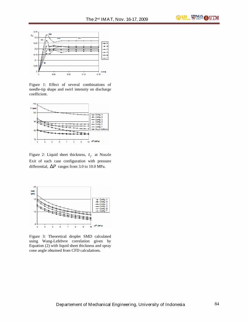
The 2nd IMAT, Nov. 16-17, 2009
Departement of Mechanical Engineering, University of Indonesia 84
Figure 1: Effect of several combinations ofneedle-tip shape and swirl intensity on dischargecoefficient.
Figure 2: Liquid sheet thickness, ft at NozzleExit of each case configuration with pressuredifferential, P∆ ranges from 3.0 to 10.0 MPa.
Figure 3: Theoretical droplet SMD calculatedusing Wang-Lefebvre correlation given byEquation (2) with liquid sheet thickness and spraycone angle obtained from CFD calculations.
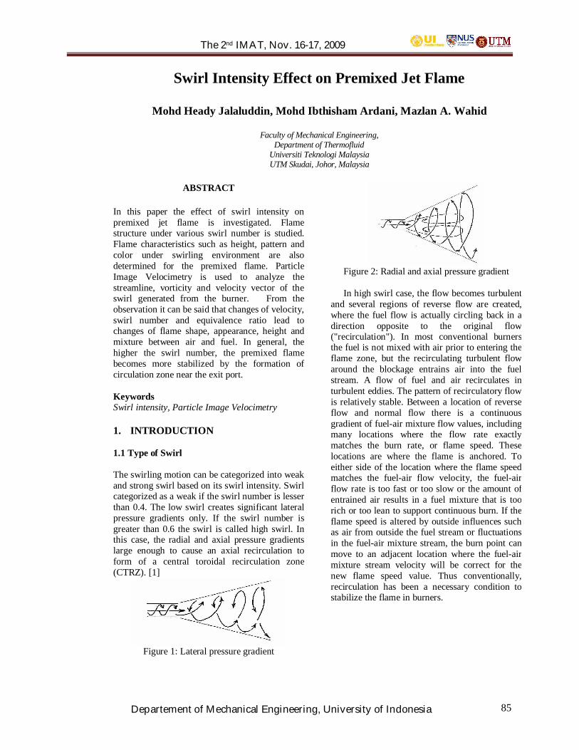
The 2nd IMAT, Nov. 16-17, 2009
Departement of Mechanical Engineering, University of Indonesia 85
Swirl Intensity Effect on Premixed Jet Flame
Mohd Heady Jalaluddin, Mohd Ibthisham Ardani, Mazlan A. Wahid
Faculty of Mechanical Engineering,Department of Thermofluid
Universiti Teknologi MalaysiaUTM Skudai, Johor, Malaysia
ABSTRACT
In this paper the effect of swirl intensity onpremixed jet flame is investigated. Flamestructure under various swirl number is studied.Flame characteristics such as height, pattern andcolor under swirling environment are alsodetermined for the premixed flame. ParticleImage Velocimetry is used to analyze thestreamline, vorticity and velocity vector of theswirl generated from the burner. From theobservation it can be said that changes of velocity,swirl number and equivalence ratio lead tochanges of flame shape, appearance, height andmixture between air and fuel. In general, thehigher the swirl number, the premixed flamebecomes more stabilized by the formation ofcirculation zone near the exit port.
KeywordsSwirl intensity, Particle Image Velocimetry
1. INTRODUCTION
1.1 Type of Swirl
The swirling motion can be categorized into weakand strong swirl based on its swirl intensity. Swirlcategorized as a weak if the swirl number is lesserthan 0.4. The low swirl creates significant lateralpressure gradients only. If the swirl number isgreater than 0.6 the swirl is called high swirl. Inthis case, the radial and axial pressure gradientslarge enough to cause an axial recirculation toform of a central toroidal recirculation zone(CTRZ). [1]
Figure 1: Lateral pressure gradient
Figure 2: Radial and axial pressure gradient
In high swirl case, the flow becomes turbulentand several regions of reverse flow are created,where the fuel flow is actually circling back in adirection opposite to the original flow("recirculation"). In most conventional burnersthe fuel is not mixed with air prior to entering theflame zone, but the recirculating turbulent flowaround the blockage entrains air into the fuelstream. A flow of fuel and air recirculates inturbulent eddies. The pattern of recirculatory flowis relatively stable. Between a location of reverseflow and normal flow there is a continuousgradient of fuel-air mixture flow values, includingmany locations where the flow rate exactlymatches the burn rate, or flame speed. Theselocations are where the flame is anchored. Toeither side of the location where the flame speedmatches the fuel-air flow velocity, the fuel-airflow rate is too fast or too slow or the amount ofentrained air results in a fuel mixture that is toorich or too lean to support continuous burn. If theflame speed is altered by outside influences suchas air from outside the fuel stream or fluctuationsin the fuel-air mixture stream, the burn point canmove to an adjacent location where the fuel-airmixture stream velocity will be correct for thenew flame speed value. Thus conventionally,recirculation has been a necessary condition tostabilize the flame in burners.

The 2nd IMAT, Nov. 16-17, 2009
Departement of Mechanical Engineering, University of Indonesia 86
Figure 3: Sketch of swirling flow field. [2]
1. EXPERIMENTAL SETUP
The experimental setup diagram for Flamevisualization and analysis is shows in Figure 3and experimental setup for Particle ImageVelocimetry (PIV) System and analysis is shownin Figure 5. Swirl can be generated by severalmethods, namely use of vanes, rotating tube andtangential or axial entry. In this experiment, swirlis generated by a burner which was designconsists of cylindrical swirler section attached toconcentric nozzle and settling chamber. Weakswirl is produced by four tangential air injectorsfitted to the rim of the swirler section. Typicalswirl intensities needed for flame stabilization arevery low [3].
Figure 4: The diagram of the experimental setup.
Figure 5: Top schematic view of the burner atswirl section
Figure 6: The example of Schematic PIV Diagram
The laser light source is double pulsed so thattwo images of each seeding particle are recordedby the camera. In this study, Particle ImageVelocimetry (PIV) was used. Images are recordeddirectly with a CCD camera and frame-grabber,and can be studied without the necessary delayand overhead associated with the scanning ofphotograph. The application of PIV allows for asimple realization of the cross-correlationtechnique for pairs of two separate images. Itremoves the ambiguity of the sign of thedisplacement and improves signal dynamics.Setup for experiment PIV system consists ofsystem control, flow imaging, image capture andimage analysis and display.
In this study, the effect of several parameterson the flame shape, color, stability and height isconsidered. The parameters varied duringexperiment were swirl number (S), Equivalenceratio (Ø), Reynolds number (Re), Fuel molefraction (Xfuel), tangential air flow rate, axial airflow rate, fuel flow rate and flame height.
2.1.1 Swirl Number
Swirl number, S, measure the degree of swirlingmotion of the flow. Low swirl phenomena (S
0.4) typically are for which the swirl velocitydoes not cause the flow structure to be drasticallychanged. Flames with low degree of swirl have a

The 2nd IMAT, Nov. 16-17, 2009
Departement of Mechanical Engineering, University of Indonesia 87
limited practical interest mainly due to theinstability problems. At high degree of swirl(S 0.6), radial and axial pressure gradients arelarge enough to cause an axial recirculation in theform of a central toroidal recirculation zone(CTRZ), which is not observed at lower degreesof swirl. Swirl is defined as follows,
BB RGGS θ=
where ;
GB = axial flux of angular momentumG = axial flux of axial momentumR B = burner radius
2.1.2 Equivalence Ratio (Ø)
Mixture equivalence ratios represent thecharacteristic of the mixture. Equivalence ratio iscommonly used to indicate quantitatively whethera fuel and oxidizer mixture is rich, lean, orstoichiometric. For fuel-rich mixtures, Ø > 1, forfuel-lean mixture, Ø < 1, and for a stoichiometricmixture, Ø equals unity. The equivalence ratio isdefined as:
exp
=
FAFA
stoicφ
where the stoichiometric air-fuel ratio is given as;
[ ]fuel
air
stoicfuel
air
stoic MWMWa
mm
FA
176.4
=
=
The stoichiometric air-fuel ratio isdetermined by writing simple atom balances, byassuming that the fuel reacts to form an ideal setof products. For this study, we use a mixture of40%propane and 60% butane fuel, is used. So, fora hydrocarbon fuel, the stoichiometric relation canbe expressed as;
CxHy + a(O2 + 3.76N2) xCO2 + (y/2)H2O +3.76a N2
where ;a = x + y/4
Stoichiometric in the above equation is aterm where complete combustion occurs. For
example, the stoichiometric quantity of oxidizer isjust that amount of oxidizer needed to completelyburn a quantity of fuel. So, the stoichiometric air-fuel ratio is just the right ratio of air and fuel tohave a complete burning process or a completecombustion process.
2.1.3 Fuel Mole Fraction (Xfuel)
Fuel mole fraction is an important and usefulparameter used to characterize the composition ofa mixture, apart from mass fraction. For a multicomponent mixture of gases composed of N1moles of species 1, N2 moles of species 2, and soforth. The mole fraction of species i, Xi is definedas the fraction of the total number of moles in thesystem that are species i. So, mole fraction can bedefined as:
TOTAL
i
i
ii N
NNNN
NX =
+++=
..)( 21
where ;
N = number of mole
It is known that mole fraction is base on volume,so the fuel mole fraction in this study can bedetermined by dividing the fuel volume flowrateover the total volume flowrate of air and fuel.Thus, the fuel mole fraction can be determinedusing this equation;
Total
fuel
airfuel
fuelfuel
Q
Q
QX
•
•
••
•
=+
=)(
where ;
=•
Q Volume flow rate (m3/s)
Fuel mole fraction is a dimensionlessparameter. From the definition, it is known thatthe sum of all the constituent mole fractions of themixture must be unity, or;
1=Σ iiX
In this study, note that the sum of fuel molefraction, Xfuel, and the air mole fraction, Xair, mustbe unity, that is;
1=+ airfuel XX
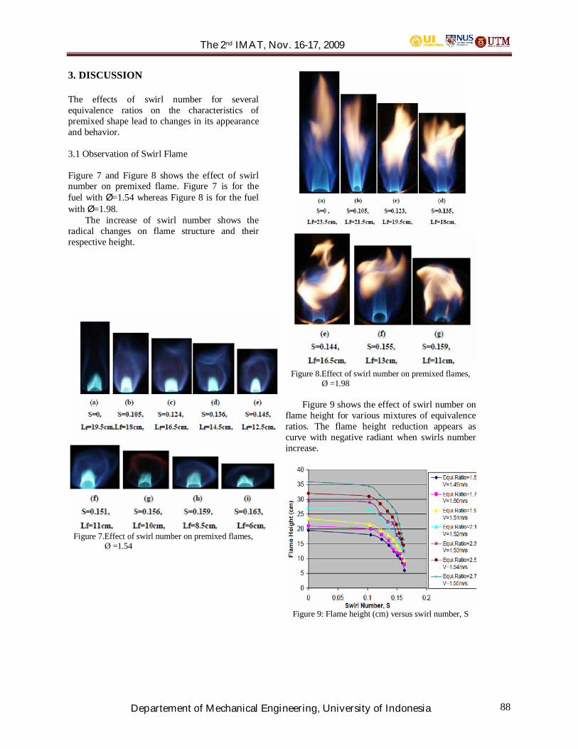
The 2nd IMAT, Nov. 16-17, 2009
Departement of Mechanical Engineering, University of Indonesia 88
3. DISCUSSION
The effects of swirl number for severalequivalence ratios on the characteristics ofpremixed shape lead to changes in its appearanceand behavior.
3.1 Observation of Swirl Flame
Figure 7 and Figure 8 shows the effect of swirlnumber on premixed flame. Figure 7 is for thefuel with Ø=1.54 whereas Figure 8 is for the fuelwith Ø=1.98.
The increase of swirl number shows theradical changes on flame structure and theirrespective height.
Figure 7.Effect of swirl number on premixed flames, Ø =1.54
Figure 8.Effect of swirl number on premixed flames, Ø =1.98
Figure 9 shows the effect of swirl number onflame height for various mixtures of equivalenceratios. The flame height reduction appears ascurve with negative radiant when swirls numberincrease.
Figure 9: Flame height (cm) versus swirl number, S

The 2nd IMAT, Nov. 16-17, 2009
Departement of Mechanical Engineering, University of Indonesia 89
3.2 Particle Image Velocimetry (PIV) Analysis
Figure 10 to 34 shows smoke streamlinepicture for various swirl number, velocity vectormap (Average Filter after masking vector map),vorticity and streamline.
Figure 10 : Smoke streamline picture for variousswirl number
Figure 11 : Velocity Vector Map (Average Filterafter Masking Vector Map)
Figure 12 : Vorticity
Figure 13 : Streamline
From smoke picture of Figure 10 it can beseen that when swirl number, S increases theflame becoming more chaotic, recirculation zoneappear and consequently the flame height will belower. Vorticity is one of the parameter thatshows the tendency for elements of the fluid tospin. The smoke streamline image implies theflow circle’s enforcement or flow swirlingmovement inside the circulation zone. Fromobservation, the vorticity increases if swirlnumber is increases.
5. CONCLUSION
As the conclusion it can be said that swirl helps inmixing and thus enhances combustion, shortensthe flame height and helps to stabilize the flame.From the observation it can be said that changesof velocity, swirl number and equivalence ratiolead to changes of flame shape, appearance,height and mixture between air and fuel. Ingeneral, the higher the swirl number, thepremixed flame becomes more stabilized by theformation of circulation zone near the burner exitport.
ACKNOWLEDGMENT
The authors would like to thank UniversitiTeknologi Malaysia and the Malaysiangovernment for supporting this research activity.
REFERENCES
[1] J. Warnatz, U. Maas, R.W. Dibble,‘Combustion’, Springer-Verlag Berlin,Heidelberg, New York, 3rd Edition; 2000.
[2] A.K. Gupta, M.J. Lewis and M.Daurer “SwirlEffects on Combustion Characteristics ofPremixed Flames”.
[3] R. K Cheng, ‘Velocity and Scalar Charateristicsof Premixed Turbulent Flames Stabilized byWeak Swirl’, Combustion and flame, 1995.

The 2nd IMAT, Nov. 16-17, 2009
Departement of Mechanical Engineering, University of Indonesia 90
Liquid Fuel Vaporization System
Mazlan Abdul Wahid, Mohsin Mohd Sies,Mohd Khairrul Mohd Suhaimi, Mohd Ayub Sulong
Faculty of Mechanical Engineering, Universiti Teknologi Malaysia,81310 UTM Skudai, Johor, Malaysia
ABSTRACT
This research focused in the development ofliquid fuel vaporization system. Thermodynamicparameters considered to transform the fuel fromliquid to gas state, are preheat temperature,vaporization chamber temperature, sprayingpressure and vaporization chamber pressure. Thistransformation requires two important subprocesses which are preheating and atomizing ofthe liquid fuel. In this research, diesel fuel ispreheated at 100°C, 150°C, 200°C, 250°C, 300°C,and 350°C. This temperature has been identifiedto be lower than the auto ignition temperature ofthe diesel fuel at critical pressure. The next stage,which is atomization process, is achieved throughthe injection of liquid fuel at various elevatedpressure, namely at 60, 80 and 100 bar.Atomization process transforms the liquid fuelinto a very fine liquid droplet where the surfacearea of the liquid fuel is significantly increased.SUPERTRAPP calculation is made for n-heptane,n-dodecane and surrogate diesel, as a quantitativebaseline and guidance in developing the liquidfuel vaporization system. From the baselinecalculation, at 1 bar stoichiometric fuel-airmixture is fully vaporize at 276 K, 359 K, and389 K for n-heptane, n-dodecane and surrogatediesel respectively. Fuels at higher molecularweight will vaporized at higher preheattemperature. This has been confirmed by theshadowgraphy technique that is used to observethe vaporization process of diesel qualitatively.
Keywords
Fuel Vaporization,Diesel Fuel, Atomization,Shadowgraphy
1. INTRODUCTION
Liquid Fuel is one of the most practical sources ofenergy that have been used in internal combustion
engine and propulsion system. Liquid fuel hasbeen widely used for land vehicle, aerospace,marine and also stationary combustion equipmentsuch as furnace and boiler. Different type of fuelsnamely gasoline, diesel, kerosene, JP-8 and JP-10are from hydrocarbon base, which are usuallydenoted by the general formula CnHm. Thesehydrocarbon fuels exist in all phases namelysolid, liquid and gas. Every type of liquid fuelsgives difference chemical structure, physical andthermodynamics properties.
Tucker (2005) constructed a flash vaporizationsystem (FVS) for detonation of hydrocarbon fuelsin a pulse detonation engine (PDE). In theresearch four hydrocarbon base fuels which are n-heptane, isooctane, aviation gasoline, and JP-8has been tested. A high pressure fuel flashvaporization system was designed and built toreduce and eliminate the time required toevaporate the fuel droplets. Since these fuels varyin volatility and octane number its present a clearpicture on the benefits of flash vaporization. Fromthe results, the FVS has quickly provided adetonable mixture for all tested fuels withoutcoking or clogging the fuel lines. The mostsignificant achievement of the research was thedetonation of flash vaporized JP-8 and air. Theresults show that the flash vaporized JP-8 used 20percent less fuel to ignite the fuel air mixturetwice as fast (8 ms from 16 ms) when comparedto the unheated JP-8 combustion data. The FVShas been validated as a reliable method to createthe droplet free mixtures required for liquidhydrocarbon fueled PDEs.
The general nature of the processes involved inspray combustion in ideal case for the combustionof a dilute spray is shown in Figure 2.1. Systemcontaining droplet diffusion flames arecharacterized by their yellow nature. [1, 2]
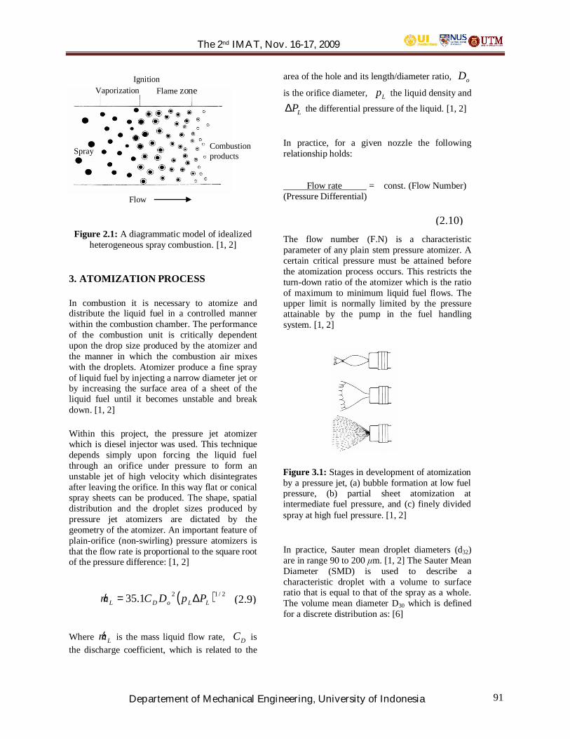
The 2nd IMAT, Nov. 16-17, 2009
Departement of Mechanical Engineering, University of Indonesia 91
Figure 2.1: A diagrammatic model of idealizedheterogeneous spray combustion. [1, 2]
3. ATOMIZATION PROCESS
In combustion it is necessary to atomize anddistribute the liquid fuel in a controlled mannerwithin the combustion chamber. The performanceof the combustion unit is critically dependentupon the drop size produced by the atomizer andthe manner in which the combustion air mixeswith the droplets. Atomizer produce a fine sprayof liquid fuel by injecting a narrow diameter jet orby increasing the surface area of a sheet of theliquid fuel until it becomes unstable and breakdown. [1, 2]
Within this project, the pressure jet atomizerwhich is diesel injector was used. This techniquedepends simply upon forcing the liquid fuelthrough an orifice under pressure to form anunstable jet of high velocity which disintegratesafter leaving the orifice. In this way flat or conicalspray sheets can be produced. The shape, spatialdistribution and the droplet sizes produced bypressure jet atomizers are dictated by thegeometry of the atomizer. An important feature ofplain-orifice (non-swirling) pressure atomizers isthat the flow rate is proportional to the square rootof the pressure difference: [1, 2]
( ) 2/121.35 LLoDL PpDCm ∆=&
Where Lm& is the mass liquid flow rate, DC isthe discharge coefficient, which is related to the
area of the hole and its length/diameter ratio, oDis the orifice diameter, Lp the liquid density and
LP∆ the differential pressure of the liquid. [1, 2]
In practice, for a given nozzle the followingrelationship holds:
Flow rate = const. (Flow Number)(Pressure Differential)
The flow number (F.N) is a characteristicparameter of any plain stem pressure atomizer. Acertain critical pressure must be attained beforethe atomization process occurs. This restricts theturn-down ratio of the atomizer which is the ratioof maximum to minimum liquid fuel flows. Theupper limit is normally limited by the pressureattainable by the pump in the fuel handlingsystem. [1, 2]
In practice, Sauter mean droplet diameters (d32)are in range 90 to 200 m. [1, 2] The Sauter MeanDiameter (SMD) is used to describe acharacteristic droplet with a volume to surfaceratio that is equal to that of the spray as a whole.The volume mean diameter D30 which is definedfor a discrete distribution as: [6]
Flow
Spray
Vaporization Flame zoneIgnition
Combustionproducts
(2.9)
Figure 3.1: Stages in development of atomizationby a pressure jet, (a) bubble formation at low fuelpressure, (b) partial sheet atomization atintermediate fuel pressure, and (c) finely dividedspray at high fuel pressure. [1, 2]
(2.10)

The 2nd IMAT, Nov. 16-17, 2009
Departement of Mechanical Engineering, University of Indonesia 92
3
3
30 ∑∑=
i
ii
NN
Dδ
Where iN is the number of droplets of diameter,
iδ . The volume mean diameter is the averagedroplet volume of the spray. The surface meandiameter is the area or surface of the droplets witha surface area equal to the mean surface area andis given by: [6]
∑∑=
i
ii
NN
D2
30
δ
Where Ni is the number of droplets, and i is theaverage diameter of the size range. The SMD isdefined as the volume to surface mean diameterand is given by: [6]
220
330
32 DDDSMD ==
And is the diameter of an equivalent droplet witha ratio of volume to surface area equal to that ofthe entire spray. [6]
4. EXPERIMENTAL SETUP
The development of the fundamental rig is verycrucial to make sure the experiment can beconducted smoothly. The fundamental rigconsisted of three main subsystems which areliquid fuel vaporization system, fuel handling unitand Shadowgraph setup. Each of the subsystemconsists of several other components. The wholefundamental setup is presented in figure 4.1.
Figure 4.1: The photo of LFVS setup at Highspeed Reacting flow Research Laboratory (HiRef)
The liquid fuel vaporization unit consists of fuelatomizer\injector, vaporization chamber, heatingelement, vacuum pump and nitrogen tank. Themain function of this subsystem is to provide safemedium and confine space for atomizing andvaporizing process to occur. The chamber isfirstly vacuumed by the vacuum pump to send outall the gases within the vaporization chamber, thisis for safety precaution. Secondly, only thenitrogen gas is being charged into thevaporization chamber since nitrogen is not one ofthe combustion agents. Although this method arenot very practical, since the chamber size is verylarge and it is hard to fully vacuum the chamber,but at least the air and oxygen content has beenreduced to the safe point. After that, thepressurized and heated liquid fuel from the fuelhandling unit system will be atomized through thediesel injector\atomizer.
Heating element is very important part for thesuccess of the liquid fuel vaporization system.The fuel is heated just before entering the injectordiesel to increase the internal energy of the fuel.the suitable range of the heater temperature forthis experiment is between 27oC (ambient
(2.11)
(2.12)
(2.13)
Heater
Fuel Pump
Screen
Pump ControlPanel
TemperatureControlPanel
Projector
VaporizationChamber
Injector
5
6
7
8
56 7
8
1
2
3
4
1
2
3
4
The 2nd IMAT, Nov. 16-17, 2009
Departement of Mechanical Engineering, University of Indonesia 93
temperature) to 400oC. The heater is providedwith built in check valve to avoid backward flowof the heated fuel when the fuel pressure increase.The electric heating element is controlled bytemperature control panel. The user needs to inputthe desired temperature into the controller, thethermocouple brought the output data, which isthe actual fuel temperature within the pipe line, ifthe fuel temperature is lower than the desiredtemperature, the heater is switched on but whenthe fuel temperature is above the desiredtemperature, the heater is automatically switchedoff by the multi circuit breaker within the controlpanel.
The diesel injector which acts as an atomizerwithin this system is used to generate smalldroplets during the fuel injection process forpreheated fuel. This single spring diesel injector isused in one of the HINO injection systems. Theinjector is used in spray combustion ofcompression ignition engine for HINOGENERATOR, EH500. This diesel injector isused within the experiment, since the injector canwithstand at relatively high pressure andtemperature. The nozzle type designation for thisdiesel injector is ND-DLLA150S31-33ND97which is manufactured by DENSO Company.
The diesel injector mechanism is fully operatedby mechanical concept. From the high pressurefuel line the liquid fuel is flowed into the injectorfuel inlet. Within the diesel injector, there is smallfuel line connecting the fuel inlet with the valvebody (Figure 3.8). There is a finely machinedneedle valve which uncovers and covers the tinynozzle orifices for the liquid fuel to flow out andavoid the low pressure atomization. The needle isonly opened for the liquid fuel to flow through thenozzle holes when the liquid fuel pressureachieved at certain high pressure. This pressurecan be controlled by the user with adjusting thenozzle retaining\screw which change the pressureof the compression spring within the dieselinjector, since the spring that pushes the pin.
This chamber is designed to provide the confinespace for liquid fuel to completely atomize andvaporize. The chamber is fabricated to withstandwith atmospheric pressure and high elevatedtemperature. Several equipments had beenattached to this liquid fuel vaporization chamber,such as outlet line to the vacuum pump and inletline from the nitrogen tank. This fully transparentglass chamber allowed the light to pass through it,
so the image of atomized and vaporized fuel canbe projected on the white screen.
Another important subsystem of this experimentrig is the fuel handling unit. The fuel handlingunit consists of the fuel filters, fuel pump,solenoid valves, and pump control panel. Thissubsystem will supply and pressurize the liquidfuel before entering the liquid fuel vaporizationsystem.
Fuel pump is one of the components of the fuelhandling unit. This component is used topressurize the liquid fuel before the fuel injectedinto the vaporization chamber through dieselinjector. The TECO fuel pump is generated by the3-phase induction motor which is fabricated byTong Yuan Elec. & Mach. Pvt. Ltd.
All these valves are controlled by the electroniccontrol panel system (figure 3.12). This controlpanel will control the output pressure of thepump. This fuel pump also equipped by oneanalog pressure gauge. The pressure range for thispump is between 0 to 3600 psi which is about 0 to248.211 bar.
4.1 Shadowgraph Setup
A bright point light source is needed to cast asharp shadow on the screen, in this experiment,the Canon LV-S3 projector is used to produce thewhite light beam. The projected image is castedon the white screen and the image produced isrecorded by JVC everio G GZ-MG630 videocamcorder. From the calculation (equation 2.18)the magnification of the shadowgram with respectto the schlieren object is 1.333, since the distancebetween the screen and point light, h, is 2 m andthe distance between the screen and shlieranobject, diesel injector, g, is 0.5 m. This parametersneed to be taken into consideration, since its willaffect the sensitivity or the contrast, geometricblur and diffraction blur of the casted image.

The 2nd IMAT, Nov. 16-17, 2009
Departement of Mechanical Engineering, University of Indonesia 94
Figure 4.2: The schematic diagram for theshadowgraph setup.
5. BASELINE GENERATION
The computed baseline data is important for thedevelopment of the fundamental liquid fuelvaporization system. This chapter will cover allthe procedure for data generation using this code,data calculation and plotting the graphs. Alsomethod for entering the new component into thedatabase and the important technique will beexplained within this chapter. The fuels that willbe studied using SUPERTRAPP are n-heptane, n-dodecane and the new entry data is surrogatediesel.
Figure 5.1: Percentage of fuel in vapor phase forstoichiometric mixture at 1 bar.
At the mixture temperature required toachieve 100% vapor with the n-heptane, only0.45% vapor of n-dodecane and no vapor occurfor the surrogate diesel (Figure 5.1). This showsthe importance of the liquid fuel vaporizationsystem to achieve a vaporized of the surrogatediesel and other heavy fuels.
the fuel vapor should not condense backinto a liquid. If the chamber pressure is increased,the minimum mixture temperature to maintain thefuel in the vapor state would also increase. Theincrease in chamber pressure from 2 to 3 barincreases the minimum mixture temperature by7oC for surrogate diesel (Figure 5.2).
Figure 5.2: Equilibrium liquid vapor state for astoichiometric surrogate diesel and air mixture atvarious chamber pressures.
Figure 5.3: Stoichiometric surrogate diesel airmixture liquid vapor equilibrium in the chamberfor 3 air temperatures at 1 atm. Fuel injectionpressure at 60 bar.
From the generated models, there are nosignificant change in the flash vaporization region(hatched region) and the minimum resultantmixture temperature for the surrogate diesel tovaporize still at 389 K. The are small variances,the fuel temperature needed to vaporize is slightlyincreased for several Kelvin when the fuelinjection pressure increase.

The 2nd IMAT, Nov. 16-17, 2009
Departement of Mechanical Engineering, University of Indonesia 95
6. RESULTS AND DISCUSSION
6.1 Injection Pressure at 60 bar
This section illustrates the sequence of theinjection process of the diesel fuel at 60 bar andheated with heating element at various differenttemperatures. The phase of the diesel achievedjust after the injection process can be determined.The figure 6.6 shows the 60 bar injection processsequences of diesel fuel at 350oC.
6.1.6 60 bar, 350oC
Figure 6.6: 60 bar injection process sequence for350oC.
From figure 6.6, the 60 bar injected fuel is still inthe liquid state. At 350oC (.15 K), the injectedfuel is flash and fully vaporized.
7. CONCLUSIONS
It can be concluded that, this project hassuccessfully fulfilled its objective that is to studyand develop the liquid fuel vaporization systemfor fundamental combustion process. Theunderstanding of the computer database,SUPERTRAPP, and model generation issuccessfully made within this project.
ACKNOWLEDGMENT
Mr. Mohsin B. Mohd Sies, Researcher –Detonation Characteristics of Liquid Biofuels,Vote. 78358. Fundamental Research GrantScheme (FRGS) funded by The Ministry ofHigher Education for RM167,000. October 2008– September 2010.
REFERENCES
[1] Alan Williams. Combustion of Liquid FuelSprays. London: Butterworths, 1990.
[2] Alan Williams, Farid Nasir Hj. Ani.Pembakaran Semburan Bahan Api Cecair.London: Butterworths, 1990.
[3] Yunus A. Cengel, Michael A. Boles. “Fuelsand Combustion.” Thermodynamics anEngineering Approach. New York: McGraw-Hill, 2006.
[4] Yunus A. Cengel, Michael A. Boles. “Gas-Vapor Mixtures and Air Conditioning.”Thermodynamics an Engineering Approach.New York: McGraw-Hill, 2006.
[5] John B. Heywood. “Thermo chemistry ofFuel-Air Mixtures.” Internal CombustionEngine Fundamentals. Singapore: McGraw-Hill International Edition, 1988.
[6] K. Colin Tucker. “A Flash VaporizationSystem for Detonations of HydrocarbonFuels in a Pulse Detonation Engine.” Ohio:Air Force Institute of Technology, 2004.
[7] Kristin L. Panzenhagen. “DetonationBranching in A PDE with LiquidHydrocarbon Fuel.” Ohio: Air Force Instituteof Technology, 2004.
COPYRIGHT
All papers submitted must be original,unpublished work not under consideration forpublication elsewhere. Authors are responsible toobtain all necessary permission for thereproduction of tables, figures and images andmust be appropriately acknowledged. The paper isnot defamatory; and the paper does not infringeany other rights of any third party.
The authors agree that the Technical Committee’sdecision on whether to publish the paper in theConference’s proceedings shall be final. Theauthors should not treat any communication fromthe Technical Committee members who reviewedtheir work as an undertaking to publish the paper.
Prior to final acceptance of the paper, authors arerequired to confirm in writing that they hold allnecessary copyright for their paper and to assignthis copyright to the Conference Organizer.

The 2nd IMAT, Nov. 16-17, 2009
Departement of Mechanical Engineering, University of Indonesia 96
Characteristics of Turbulent Whirling Flow in an AsymmetricPassage
Khalid M. Saqra, Mohsin M. Siesa, Hossam S. Alyb ,Mazlan Abdul Wahida
aHigh-Speed Reacting Flow Laboratory, Faculty of Mechanical Engineering,Universiti Teknologi Malaysia
81310 Skudai, JohorMALAYSIA
Email : [email protected]
bF Department of Aeronautical Engineering, Faculty of Mechanical EngineeringUniversiti Teknologi Malaysia,
81310 Skudai, JohorMALAYSIA
ABSTRACT
We investigate the physics of whirling flow in anasymmetric passage. A 3D RANS CFD modelwas built and solved to predict the steady stateflow field variables in a 500 mm long asymmetriccylindrical passage. Turbulent velocityfluctuations were modeled using the Reynoldsstress turbulence model. The paper presents aninsight to the flow pattern, recirculation zone,velocity profiles and pressure gradients in suchflow configuration. The significance of thepresented qualitative results lies in the potentialapplications of such flow configurations in gas-phase combustors.
1. INTRODUCTION
When any flow has a significant tangentialvelocity component, and the flow terminals arenot coplanar, it is impossible to reduce theproblem to a two dimensional model. In this case,the flow behavior distinguishingly exhibitssignificantly three dimensional gradients of theflow field variables. Grasping these qualities isessential to establish a comprehensiveunderstanding of such complex flowconfiguration for the vast range of applications itinvolves. When the cylindrical flow geometry isaxially asymmetric, the whirling flow exhibitsseparation and reattachment regions around theasymmetry location. This adds double foldcomplexity to the problem in the time-independent solution, let alone transient states.
Whirling and swirling flows are fundamentallydifferent. In the context of polar coordinates, thefirst expresses a flow stream with axial andtangential velocity components. While the latterexpresses a flow stream with solely a tangentialvelocity component. Unlike swirl flows, whirlflows have attracted much less consideration fromthe fluid dynamics research community. Sturovhas studied whirling axisymmetric turbulent flowexperimentally as a case study on turbulent eddies[1]. Five years later, the same problem wasstudied numerically, by reducing it to a twodimensional axisymmetric model [2].
During the 1970s, there has been a growingattention to study flames created in flow fieldswhich have significant tangential velocitycomponents; namely swirling flames. Swirlingflow fields are distinguishingly characterized by acentral recirculation zone (i.e. CRZ). Swirlingflow spreads as it moves downstream, and thecentrifugal force creates a low pressure region inthe centre of the flow. At a certain pointdownstream, this low pressure region causes thevortex to collapse inwards on itself in aphenomenon known as vortex breakdown [3].This vortex breakdown phenomenon is the maincharacteristic of the CRZ. The CRZ provides areversal flow field, in which two main actionstake place. First is the mixing and enthalpyretrieval between combustion products and newfuel and air charges. Second is the matchingbetween reaction times and flow times, which isthe major flame stabilizing mechanism [4]. Theswirling flows and their associated flames havebeen extensively studied during the last fourdecades [5-10].
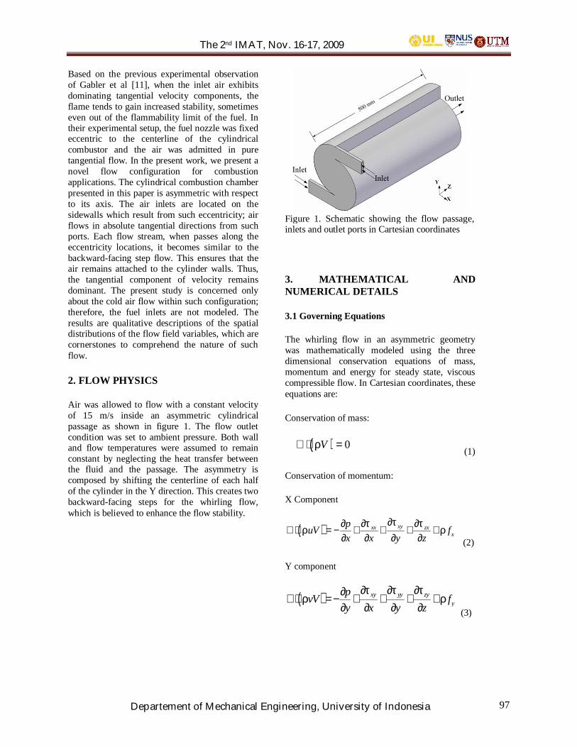
The 2nd IMAT, Nov. 16-17, 2009
Departement of Mechanical Engineering, University of Indonesia 97
Based on the previous experimental observationof Gabler et al [11], when the inlet air exhibitsdominating tangential velocity components, theflame tends to gain increased stability, sometimeseven out of the flammability limit of the fuel. Intheir experimental setup, the fuel nozzle was fixedeccentric to the centerline of the cylindricalcombustor and the air was admitted in puretangential flow. In the present work, we present anovel flow configuration for combustionapplications. The cylindrical combustion chamberpresented in this paper is asymmetric with respectto its axis. The air inlets are located on thesidewalls which result from such eccentricity; airflows in absolute tangential directions from suchports. Each flow stream, when passes along theeccentricity locations, it becomes similar to thebackward-facing step flow. This ensures that theair remains attached to the cylinder walls. Thus,the tangential component of velocity remainsdominant. The present study is concerned onlyabout the cold air flow within such configuration;therefore, the fuel inlets are not modeled. Theresults are qualitative descriptions of the spatialdistributions of the flow field variables, which arecornerstones to comprehend the nature of suchflow.
2. FLOW PHYSICS
Air was allowed to flow with a constant velocityof 15 m/s inside an asymmetric cylindricalpassage as shown in figure 1. The flow outletcondition was set to ambient pressure. Both walland flow temperatures were assumed to remainconstant by neglecting the heat transfer betweenthe fluid and the passage. The asymmetry iscomposed by shifting the centerline of each halfof the cylinder in the Y direction. This creates twobackward-facing steps for the whirling flow,which is believed to enhance the flow stability.
Figure 1. Schematic showing the flow passage,inlets and outlet ports in Cartesian coordinates
3. MATHEMATICAL ANDNUMERICAL DETAILS
3.1 Governing Equations
The whirling flow in an asymmetric geometrywas mathematically modeled using the threedimensional conservation equations of mass,momentum and energy for steady state, viscouscompressible flow. In Cartesian coordinates, theseequations are:
Conservation of mass:
( ) 0Vρ∇ ⋅ =(1)
Conservation of momentum:
X Component
( ) xyxx zxx
puV fx x y z
ττ τρ ρ
∂∂ ∂∂∇⋅ = − + + + +
∂ ∂ ∂ ∂ (2)
Y component
( ) xy yy zyy
pvV fy x y z
τ τ τρ ρ
∂ ∂ ∂∂∇⋅ = − + + + +
∂ ∂ ∂ ∂ (3)
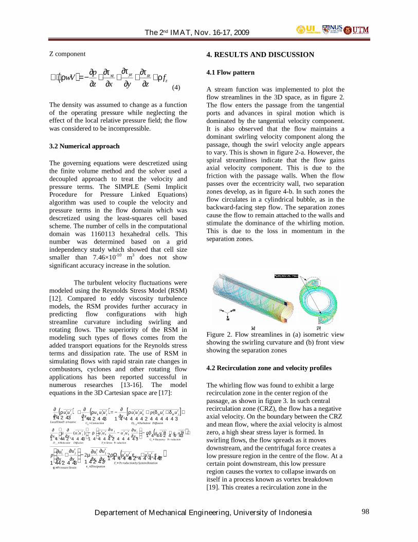
The 2nd IMAT, Nov. 16-17, 2009
Departement of Mechanical Engineering, University of Indonesia 98
Z component
( ) yzxz zzz
pwV fz x y z
ττ τρ ρ
∂∂ ∂∂∇⋅ =− + + + +
∂ ∂ ∂ ∂ (4)
The density was assumed to change as a functionof the operating pressure while neglecting theeffect of the local relative pressure field; the flowwas considered to be incompressible.
3.2 Numerical approach
The governing equations were descretized usingthe finite volume method and the solver used adecoupled approach to treat the velocity andpressure terms. The SIMPLE (Semi ImplicitProcedure for Pressure Linked Equations)algorithm was used to couple the velocity andpressure terms in the flow domain which wasdescretized using the least-squares cell basedscheme. The number of cells in the computationaldomain was 1160113 hexahedral cells. Thisnumber was determined based on a gridindependency study which showed that cell sizesmaller than 7.46×10⁻¹⁰ m3 does not showsignificant accuracy increase in the solution.
The turbulent velocity fluctuations weremodeled using the Reynolds Stress Model (RSM)[12]. Compared to eddy viscosity turbulencemodels, the RSM provides further accuracy inpredicting flow configurations with highstreamline curvature including swirling androtating flows. The superiority of the RSM inmodeling such types of flows comes from theadded transport equations for the Reynolds stressterms and dissipation rate. The use of RSM insimulating flows with rapid strain rate changes incombustors, cyclones and other rotating flowapplications has been reported successful innumerous researches [13-16]. The modelequations in the 3D Cartesian space are [17]:
( ) ( ) [ ]+′+′+′′′−=′′+′′
≡=44444 344444 2144 344 2143421
DiffusionTurbulentD
jikikjkjik
ConvectionC
jikk
erivativeLocalTimeD
ji
ijTij
uupuuux
uuux
uut
,
( δδρ∂∂ρ
∂∂ρ
∂∂
( )+′+′−
′′−′′−
′′
≡≡≡
444 3444 214444 34444 21444 3444 21 roductionBuoyancyG
ijji
oductionStressP
k
ikj
k
jki
DiffusionMolecularD
jikk
ij
ijijL
ugugxuuu
xu
uuuuxx
PrPr,
)( θθρβ∂∂
∂∂
ρ∂∂
µ∂∂
( )44444 344444 21
4342144 344 21 RotationSystembyroductionF
jkmmiikmmjk
nDissipatio
k
j
k
i
Strainessure
i
j
j
i
ij
ijij
uuuuxu
xu
xu
xup
PrPr
22≡
≡≡
′′+′′Ω′′
−
′+
′εερ
∂
∂
∂∂
µ∂
∂
∂∂
εφ
4. RESULTS AND DISCUSSION
4.1 Flow pattern
A stream function was implemented to plot theflow streamlines in the 3D space, as in figure 2.The flow enters the passage from the tangentialports and advances in spiral motion which isdominated by the tangential velocity component.It is also observed that the flow maintains adominant swirling velocity component along thepassage, though the swirl velocity angle appearsto vary. This is shown in figure 2-a. However, thespiral streamlines indicate that the flow gainsaxial velocity component. This is due to thefriction with the passage walls. When the flowpasses over the eccentricity wall, two separationzones develop, as in figure 4-b. In such zones theflow circulates in a cylindrical bubble, as in thebackward-facing step flow. The separation zonescause the flow to remain attached to the walls andstimulate the dominance of the whirling motion.This is due to the loss in momentum in theseparation zones.
Figure 2. Flow streamlines in (a) isometric viewshowing the swirling curvature and (b) front viewshowing the separation zones
4.2 Recirculation zone and velocity profiles
The whirling flow was found to exhibit a largerecirculation zone in the center region of thepassage, as shown in figure 3. In such centralrecirculation zone (CRZ), the flow has a negativeaxial velocity. On the boundary between the CRZand mean flow, where the axial velocity is almostzero, a high shear stress layer is formed. Inswirling flows, the flow spreads as it movesdownstream, and the centrifugal force creates alow pressure region in the centre of the flow. At acertain point downstream, this low pressureregion causes the vortex to collapse inwards onitself in a process known as vortex breakdown[19]. This creates a recirculation zone in the

The 2nd IMAT, Nov. 16-17, 2009
Departement of Mechanical Engineering, University of Indonesia 99
centre of the flow. In swirl stabilized flames, thisbecomes essential to provide sufficient time,temperature and turbulence for a completecombustion of the fuel [20, 21]. However, the roleof the recirculation zone in the whirling flow inhand, when comes to flame stability, might bedifferent. In case of premixed flame, the freshmixture should be introduced tangentially to thewhirl combustor. The products would, then, beconcentrated in the central region of thecombustor. The recirculation zone, in such case,would enhance the mixing between the reactantmixture and the exhaust gases, this in turn mightdecrease the NOx emission and provide completeburning of the mixture. However, the analysis ofreacting flow in such configuration is beyond thescope of the current study.
Figure 3. Central recirculation zone bounded bythe zero axial velocity isosurface
The 2D axial and tangential velocity profiles areshown in figure 4. In figure 4-a, the reversevelocity in the CRZ region is found to have valuesranging from 0.75 to 4.00 m/s. In figure 4-b, theregions where the tangential velocity is in itsmaximum value is very near to the inlet ports.While the minimum tangential velocity,approximately 0.2 m/s, is found in the CRZregion. The location and values of the velocitycomponents sheds some light on the formationmechanism of the CRZ. Such mechanism isbelieved to be analogues to that of the CRZ inswirling flows. The vortex breakdown in the CRZdecelerates the flow velocity and creates volumeof toroidal vortices.
(a)
(b)Figure 4. (a) Contours of axial velocity showing therecirculation zone (b) Contourse of tangentialvelocity. Units in m/s
4.3 Pressure gradients
Pressure gradients in the whirling flowconfiguration are plotted in figure 5 at twolocations parallel to the mean axis of the passage;one at the center and the second near to the wall.The negative pressure gradient at the centralregion of the flow is an indication of the vortexbreakdown phenomenon, which supports the ideathat the recirculation zone for the whirling flowdevelops in a way analogous to that of theswirling flow.
Figure 5. Pressure gradients in two locations ofthe passage
The 2nd IMAT, Nov. 16-17, 2009
Departement of Mechanical Engineering, University of Indonesia 100
5. CONCLUSION
The whirling flow in an asymmetric passage wasnumerically investigated using a steady stateRANS model. The flow was found to exhibitseparation and reattachment downstream theeccentricity step. A recirculation zone,characterized by inverse velocity and negativepressure gradient was found to exist in the centralregion of the flow. The paper sheds the light onthe basic characteristics of whirling flow, which isessential to comprehend for combustionapplications. Further investigation on themechanism of formation for the recirculationzone, mixing characteristics and turbulenceproperties of such flow configuration is necessary.
REFERENCES
[1] G.E. Sturov (1974) Some Problems in Studyand Industrial Application of the Eddy Effect [inRussian], Kuibyshev. Aviats. Inst., Kuibyshev, p.211.
[2] V. V. Tret'yakov and V. I. Yagodkin (1979)Mathematical Analysis of Whirled TurbulentFlow Through a Pipe, Inzhenerno-FizicheskiiZhurnal, V01. 37, No. 2, pp. 254-259
[3] Y. Wang, V. Yang, and R.A. Yetter (2004)Numerical Study on Swirling Flow in anCylindrical Chamber, 42nd AIAA AerospaceSciences Meeting, Reno, Nevada.
[4] Y.A. Eldrainy, K.M. Saqr, H.S. Aly andM.N.M Jaafar CFD Insight of the Flow Dynamicsin a Novel Swirler for Gas Turbine Combustors,International Communications on Heat and MassTransfer [In Press]
[5] J.M. Beer and N.A. Chigier (1972)Combustion Aerodynamics, John Wiley & SonsInc. New York
[6] A.K. Gupta, D.G. Lilly and N. Syred (1984)Swirl Flows, Abacus Press.
[7] X. X. Dang, J. X. Zhao and H. H. Ji,Experimental study of effects of geometricparameters on combustion performance of dual-stage swirler combustor, Hangkong DongliXuebao/Journal of Aerospace Power 22 (2007),no. 10, 1639-1645.
[8] Y. Fu, J. Cai, A. M. Elkady, S. M. Jeng and H.Mongia (2005-a) Fuel and equivalence ratioeffects on spray combustion of a counter-rotatingswirler, 43rd AIAA Aerospace Sciences Meetingand Exhibit - Meeting Papers, pp. 6757-6770
[9] Y. Fu, S. M. Jeng and R. Tacina (2005-b)Characteristics of the swirling flow generated byan axial swirler, Proceedings of the ASME TurboExpo, pp. 517-526.
[10] Y. Fu, J. Cai, S. M. Jeng and H. Mongia(2007) Characteristics of the swirling flowgenerated by a counter-rotating swirler,Collection of Technical Papers - 43rdAIAA/ASME/SAE/ASEE Joint PropulsionConference, pp. 6721-6731.
[11] Gabler, H.C., Yetter, R., and Glassman, I.,Asymmetric Whirl Combustion: A NewApproachfor Non-Premixed Low NOx Gas TurbineCombustor Design, Proceedings ofthe 34thAIAA/ASME/SAE/ASEE Joint PropulsionConference, AIAA Paper 98-3530,Cleveland,OH, July 1998.
[12] M. M. Gibson and B. E. Launder. GroundEffects on Pressure Fluctuations in theAtmospheric Boundary Layer. J. Fluid Mech.,86:491-511, 1978.
[13] Artit Ridluan, Smith Eiamsa-ard, PongjetPromvonge, Numerical simulation of 3Dturbulent isothermal flow in a vortex combustor,International Communications in Heat and MassTransfer, Volume 34, Issue 7, August 2007, Pages860-869
[14] A.F. Najafi, M.H. Saidi, M.S. Sadeghipour,M. Souhar, Numerical analysis of turbulentswirling decay pipe flow, InternationalCommunications in Heat and Mass Transfer,Volume 32, Issue 5, April 2005, Pages 627-638
[15] R. Palm, S. Grundmann, M. Weismuller, S.Saric, S. Jakirlic, C. Tropea, Experimentalcharacterization and modelling of inflowconditions for a gas turbine swirl combustor,Engineering Turbulence Modelling andExperiments 6, Elsevier Science B.V.,Amsterdam, 2005, Pages 835-844

The 2nd IMAT, Nov. 16-17, 2009
Departement of Mechanical Engineering, University of Indonesia 101
[16] M. R. Halder, S. K. Dash, S. K. Som, Anumerical and experimental investigation on thecoefficients of discharge and the spray cone angleof a solid cone swirl nozzle, ExperimentalThermal and Fluid Science, Volume 28, Issue 4,March 2004, Pages 297-305
[17] Launder, B. E., Reece, G. J. and Rodi, W.(1975), Progress in the Development of aReynolds-Stress Turbulent Closure, Journal ofFluid Mechanics, Vol. 68(3), pp. 537-566.
[18] Gibson, M.M., and Launder, B.E, 1978Ground Effects on Pressure Fluctuations in theAtmospheric Boundary Layer. Journal of FluidMechanics, 86 pp:491-511
[19] Y. Wang, V. Yang, R.A. Yetter, Numericalstudy on swirling flow in an cylindrical chamber,42nd AIAA Aerospace Sciences Meeting, Reno,Nevada, 2004.
[20] J.M. Beer, N.A. Chigier, CombustionAerodynamics,Applied Science Publisher,London, 1972.
[21] N. Syred, J.M. Beer, Combustion in swirlingflows: a review, Combustion and Flame 23 (1974)143–201.

The 2nd IMAT, Nov. 16-17, 2009
Departement of Mechanical Engineering, University of Indonesia 102
Thermal Conversion of Biomass using Microwave Irradiation
Farid Nasir Ani a, Arshad Adam Salema
aFaculty of Mechanical Engineering,Universiti Teknologi Malaysia,
81310 Skudai, Johor Bahru,Malaysia.
ABSTRACT
A novel microwave radiation heating techniquewas used to pyrolyse the oil palm biomass (fiberand shell) waste into bio-oil. Thermal treatment ofwhole (as received) oil palm biomass was done ina modified domestic microwave oven usingfluidized bed technology. It was demonstratedthat biomass are poor absorber of microwaves andcannot be pyrolysed or generate vapor on its ownto form bio-oil. Therefore, appropriatemicrowave-absorbing material ie. biomasscarbonaceous char was used to initiate thepyrolysis process thus producing the bio-oil.Effect of this microwave absorber on the yield ofthe bio-oil is presented in the paper. Particularattention on the temperature profile was alsoillustrated during microwave heating of oil palmbiomass. Preliminary physical and chemicalcharacteristics of bio-oil were investigated toconfirm the nature of bio-oil. Image analysis ofchar revealed the quality that can be maintainedduring microwave heating. As the microwavetravels with speed of light, it was found that thevapors were generated as soon as microwave wasON and it stops as microwaves are OFF. Thissignificantly reduces the time and energy forthermal conversion. Further efforts are showingencouraging results, which will demonstrate theadvantage of microwave in terms of saving timeand energy and the quality of products.
KeywordsOil palm biomass; Microwave heating, fluidizedbed, temperature profiles, bio-oil, char
1. INTRODUCTION
Obtaining highly organic chemicals for variousapplications such as fine chemicals, fertilizers,resins and others including biofuels forautomotive is the main aim of thermally treatingthe biomass waste. Fast pyrolysis as one of thethermochemical process converts the biomass intobio-oil (liquid), char (solid) and flue gas in the
temperature range of 400 to 600°C in absence ofoxygen. Fast pyrolysis process not only reducesthe volume of waste significantly, but also allowsrecovery of value-added products. With fastpyrolysis the yield of the liquid i.e. bio-oil or bio-fuels is maximized depending on the processconditions. In our laboratory, the fast pyrolysissystem has been already developed andestablished to obtain bio-oil from variousbiomasses (Ani et al., 2008).
Heating source forms important parameters inobtaining yield and quality of the bio-oil.Traditional methods include conventional heatingmethods i.e. external heating by conduction,convection or radiation (Chen et al., 2008). Thisconventional heating method suffers from certaindrawbacks including heat transfer resistance, heatlosses to surrounding, utilization of portion ofheat supplied to biomass materials, damage toreactor due to electric heating etc. Microwaveenergy has gained interest in recent decades as analternative source of heating technique forpyrolysis of plastic (Pingale and Shukla, 2008;Ludlow-Palafox and Chase, 2001), sewage sludge(Domínguez et al., 2008, Menéndez et al., 2002),biomass (Yu et al., 2007; Huang et al., 2008; Guoet al., 2006; Wan et al., 2009), wood (Miura et al.,2004).
Microwaves are electromagnetic waves withfrequency between 300 MHz to 300 GHz.However, two most common frequencies used are0.915 and 2.45 GHz as per the industrial,scientific and medical (ISM) commission.Previously the microwaves dominated the area offood processing, drying, ceramic curing, and otherheating applications. Now a days, microwaves arebeing explored in various new applicationsbecause of their inherent advantages overconventional or traditional methods. Jones et al.,2002 have stated that microwaves are extremelyefficient in selective heating of materials withoutany loss of heat due to bulk heating nature. Othersinclude higher heating rates, no direct contactbetween the heating source and materials, reduced
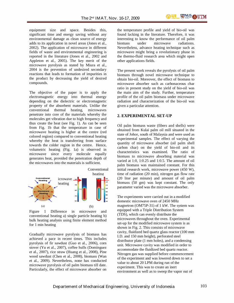
The 2nd IMAT, Nov. 16-17, 2009
Departement of Mechanical Engineering, University of Indonesia 103
equipment size and space. Besides this,significant time and energy saving without anyenvironmental damage as clean source of energyadds to its application in novel areas (Jones et al.,2002). The application of microwave in differentfields of waste and environmental engineering isreported in the literature (Jones et al., 2002 andAppleton et al., 2005). The key merit of themicrowave pyrolysis as stated by Miura et al.,2004 is the prevention of undesired secondaryreactions that leads to formation of impurities inthe product by decreasing the yield of desiredcompounds.
The objective of the paper is to apply theelectromagnetic energy into thermal energydepending on the dielectric or electromagneticproperty of the absorbent materials. Unlike theconventional thermal heating, microwavespenetrate into core of the materials whereby themolecules get vibration due to high frequency andthus create the heat (see Fig. 1). As can be seenfrom Fig. 1b that the temperature in case ofmicrowave heating is higher at the centre (redcolored region) compared to conventional heatingwhereby the heat is transferring from surfacetowards the colder region in the centre. Hence,volumetric heating (Fig. 1a) is observed inmicrowave since every molecule equallygenerates heat, provided the penetration depth ofthe microwaves into the materials is sufficient.
Figure 1 Difference in microwave andconventional heating a) single particle heating b)bulk heating analysis using finite element methodfor 1 min heating
Gradually microwave pyrolysis of biomass hasachieved a pace in recent times. This includespyrolysis of fir sawdust (Guo et al., 2006), cornstover (Yu et al., 2007), coffee hulls (Domínguezet al., 2007), rice straw (Huang et al., 2008), Pinewood sawdust (Chen et al., 2008), biomass (Wanet al., 2009). Nevertheless, none has conductedmicrowave pyrolysis of oil palm biomass till date.Particularly, the effect of microwave absorber on
the temperature profile and yield of bio-oil wasfound lacking in the literature. Therefore, it wasinteresting to know the performance of oil palmbiomass under microwave radiations.Nevertheless, advance heating technique such asmicrowave might bring a revolutionary phase inthe thermo-fluid research area which might openother applications fields.
The present work reveals the pyrolysis of oil palmbiomass through novel microwave technique toobtain bio-oil. Moreover, the effect of biomass tomicrowave absorber such as carbonaceous charratio in present study on the yield of bio-oil wasthe main aim of the study. Further, temperatureprofile of the oil palm biomass under microwaveradiation and characterization of the bio-oil wasgiven a particular attention.
2. EXPERIMENTAL SET-UP
Oil palm biomass waste (fibers and shells) wereobtained from Kulai palm oil mill situated in thestate of Johor, south of Malaysia and were used asexperimental samples. The effect of varying thequantity of microwave absorber (oil palm shellcarbon char) on the yield of bio-oil and itscharacteristics was examined. The ratio ofbiomass to microwave absorbing material wasvaried at 1:0, 1:0.25 and 1:0.5. The amount of oilpalm biomass was maintained constant. For thisinitial research work, microwave power (450 W),time of radiation (20 min), nitrogen gas flow rate(20 liter per minute) and amount of oil palmbiomass (50 gm) was kept constant. The onlyparameter varied was the microwave absorber.
The experiments were carried out in a modifieddomestic microwave oven of 2450 MHzmagnetron (OM75P-31) of 1 kW. The system wasequipped with a Triple Distribution System(TDS), which can evenly distribute themicrowaves throughout the oven. Experimentalset-up for the modified microwave system is asshown in Fig. 2. This consists of microwavecavity, fluidized bed quartz glass reactor (100 mmI.D. and 150 mm height), perforated steeldistributor plate (1 mm holes), and a condensingunit. Microwave cavity was modified in order toaccommodate the fluidized bed quartz reactor.Nitrogen gas was supplied before commencementof the experiment and was lowered down to set avalue to about 20 LPM during run of theexperiment. This was to create an inertenvironment as well as to sweep the vapor out of
Microwaveheating
Conventionalheating
(a) (b)

The 2nd IMAT, Nov. 16-17, 2009
Departement of Mechanical Engineering, University of Indonesia 104
the reactor in order to condense into bio-oil.Temperature of the process was measured usingtwo K-type thermocouples (inside and surface ofbed) connected to Pico data acquisition system,UK and further this was linked to personalcomputer for continuous recording of data.
Conventionally oil palm shell biomass was alsopyrolysed in an electric furnace (Carbolite, UK)by supplying the nitrogen gas. Image analysis ofobtained char was conducted under ZEISSmicroscope image analyzer (Axiotech model),Germany attached with Sony digital color videocamera (SSC DC-338P model). The images ofmicrowave pyrolysed and conventionallyobtained char were compared. The oil palm shellsample size for this comparison was as receivedi.e. large size. The images were captured atdifferent microscope resolution. 5X, 10X, 20X,50X.
Figure 2 Schematic diagram of microwavepyrolysis process: 1. microwave cavity, 2. quartzglass fluidized bed reactor, 3. thermocouples, 4.distributor plate, 5. temperature data acquisitionsystem, 6. personal computer, 7. condensing unit,8. bio-oil collector, 9. rotameter
For each experiment, 50 gm of oil palm biomassand desired amount of microwave absorber weremixed well and charged into the fluidized bedquartz reactor. Microwave reactor system waspurged with nitrogen gas for about 10 min toensure inert environment during pyrolysis.Microwave was switched on to generate theradiation for the set power (450 W) and time (20min). The vapor generated out of the reactor wascondensed using continuous ice water at about 5to 10°C. Bio-oil obtained from microwavepyrolysis of oil palm shell was collected andsealed in glass bottles to avoid any changes in itsproperties for further analysis. Oil remained in the
equipments was also determined via weightdifference of the equipments before and after theexperiments. Thus total bio-oil, and solid charresidue was weighted at the end of theexperiments to investigate the yield. Bio-oil wassubjected to viscosity measurement usingPetrotech equipment available in PetroleumEngineering Department, UTM, and pH valuewas determined using Eurotech pH tutor. FT-IRspectra of bio-oil were performed using ThermoCorporation FT-IR analyser manufactured inMadison, WI, U.S.A. model Nicolet Avatar 370DTGS.
3. RESULTS AND DISCUSSIONS
3.1 Temperature Profile
Figure 3 shows the temperature profiles duringmicrowave pyrolysis of oil palm shell (OPS) andoil palm fiber (OPF) without any microwaveabsorber. It can be observed that absence ofmicrowave absorber i.e. 0 %, results in themaximum bed temperature (T1) to about 100°Cand 80°C for OPS and OPF respectively.Apparently, no pyrolysis or evolution of vaportook place at this stage, though water evaporationwas noticed. This proves those biomasses arepoor absorber of microwaves. The increase intemperature at this stage is due to presence ofmoisture or water inside the biomass. Water isgood microwave absorber (Zhang and Datta,2003) and thus can generate minimal amount ofheat that can evaporate the water within thebiomass. Hence, once the microwave encountersthe biomass, the moisture absorbs the microwavesand creates a dielectric polarization whereby thewater molecules try to align themselves accordingto the radiation, which finally leads to frictionwithin the molecules generating energy in form ofheat. This heat is sensed as increase intemperature. Initially the temperature raisedlinearly but almost came to stable value aftersome time. This is because the water or moisturecomes to super heated point as soon it absorbs themicrowaves, which cause sudden increase intemperature. However, once the water isevaporated from the biomass, there is no material,which can cause the heat since other biomassconstituents do not absorb the microwaves.Therefore, the temperature comes to a stableform.
The addition of microwave absorber particularlythe biomass carbonaceous char not only helped in

The 2nd IMAT, Nov. 16-17, 2009
Departement of Mechanical Engineering, University of Indonesia 105
increase of temperature as shown in Fig. 4 butalso initiated the pyrolysis process by generatingthe vapors. These vapors were trapped viacondensing unit forming bio-oil whose yielddepended on amount of microwave absorber usedas discussed in later section of this paper. It wasobserved that it took few seconds to generate thevapors from oil palm biomass as the microwavewas switched ON. Hence, microwave absorbersplayed a role in absorbing the microwave andtransferring it to heat the biomass materials. Thisassisted to increase the bed temperature, T1 in thepresent study to about 200°C for 1:0.25, 200°Cfor 1:0.5 and 300°C for 1:1 ratio of oil palm shell(OPS) biomass to microwave absorber. Eventhough this temperature is below the reported(Islam and Ani, 2000) temperature to initiate thepyrolysis i.e. around 450 °C, the possible reasonmight be the measurement of temperature inmicrowave cavity. This is because the core orcentre of the biomass particles is at highertemperature compared to surface due topenetration behavior of microwaves into thematerials. Therefore, according to Guo and Lua,2000, the sample internal temperature is ten orhundred degrees higher than that of surface. Thepossibility of interference of metal thermocouplewith microwaves cannot be ignored. Further, thethermocouple was placed at two locations only inthe reactor, measuring that particular reading. Thefact that other location might have reached muchhigher temperature than 400°C due to hot spot asfound in multi-mode domestic microwave ovens.However, in case of oil palm fiber (OPF), thetemperature profile showed much highertemperature averagely 800°C compared to OPS.This could be due to types of biomass used. OPFare much lighter and thin in diameter or thicknesscompared to OPS. Thus, heat is transferreddifferently.
Domínguez et al., 2008, mixed carbon char toachieve high temperature for sewage sludgepyrolysis. They reported that the char obtainedfrom pyrolysis of biomass are good microwavereceptors. Other study (El Harfi et al., 2000) usedcarbon grains of about 0.5 wt % with oil shalesample to pyrolyse under microwave radiation toallow uniform temperature or heating. Menéndezet al., 2002, revealed temperature profile ofmicrowave pyrolysis of sewage sludge with andwithout carbon char obtained during pyrolysis. Amaximum temperature of about 900 °C wasachieved in just 2 min with addition of 5 wt%carbon char with sewage sludge compared to only200°C without any char. Higher temperature
recorded during their study might be also due topresence of high moisture in the sample.
Figure 3 Real time temperature profile of oil palmi) shell, ii) fiber under microwave radiationwithout any microwave absorbers; Microwavepower – 450 W

The 2nd IMAT, Nov. 16-17, 2009
Departement of Mechanical Engineering, University of Indonesia 106
Figure 4 Effect of biomass to microwave absorberratio on real time temperature profile of oil palmshell (OPS) and oil palm fiber (OPF); Microwavepower – 450 W
The sinusoidal nature in the temperature profilesin Figs 3 and 4 shows the discrete working natureof the magnetron from where the microwaves aregenerated. Basically, all domestic microwaveovens works in this type of mode. This means thatthe temperature shoots to higher value when themagnetron is in ON mode and drops to a certainlevel when the magnetron is in OFF mode. Thetemperature profile of OPF during microwavepyrolysis was observed to be more fluctuating andinconsistence compared to OPS. This might bedue to the material interaction with microwaves.Since the materials properties plays an importantrole in microwave treatment rather than themicrowaves itself. Further, the fluidization of thematerials might also contribute in aninconsistence temperature profile. In the presentstudy, the fluidization was not achieved as desiredand microwaves could not penetrate or absorbedhomogenously.
Another interesting investigation as discussedbefore is the volumetric heating nature of thematerials in which the internal section of the bed,was much hotter or at higher temperature thanthat of surface. Fig. 4 shows this profile where the
bed temperature T1 was almost higher than that ofbed surface temperature T2. Obviously in case ofOPF, it was clearer. According to our knowledge,the char formation during pyrolysis also plays animportant role under microwave radiation. Thus,microwave pyrolysis of OPF produced char muchfaster due to its low density and size. Conversely,formation of char in OPS was slower due to largeand hard particles. It is evident that quicker theformation of char from biomass will enhancemore microwaves to be absorbed by newlyformed char and consequently higher temperatureas can be predicted for OPF. This shows that theenergy conversion or absorption within thematerial is also dependent on the penetrationdepth of the microwaves. A comprehensiveunderstanding regarding this was reported byThostenson and Chou, 1999. However, withoutany microwave absorbing material thetemperature profile in Fig. 3 revealed that the bedtemperature T1 was lower in case of OPS oralmost same in case of OPF than the surfacetemperature T2 measured just above the surfaceof the bed. The reason might be the water ormoisture molecules that are vaporizedimmediately when being exposed to microwavesand is deposited on the surrounding walls of thereactor. This water droplets also absorbs themicrowaves and increases the temperature abovethe bed region thus maintaining the surfacetemperature T2 with that of bed temperature T1.
4. EFFECT OF BIOMASS TOMICROWAVE ABSORBER RATIO ONTHE BIO-OIL YIELD
The yield of bio-oil increased with microwaveabsorber till ratio of 1:5 and thereon decreased asshown in Fig. 3. Thus, the maximum bio-oil yieldwas obtained at biomass to microwave absorberratio of 1:0.5. It was assumed that as the amountof microwave absorber is small, biomass couldnot get enough heat to pyrolyse the material.Conversely, higher amount of microwaveabsorber might have lead to localized heating ofchar material alone. Yet the exact reason for thishas to be investigated and understood since theheating characteristics of microwave is very fast.
The only concise study (Guo et al., 2006) hasbeen performed till date to determine theinfluence of microwave absorption media onpyrolysis of fir sawdust. In this study ionic liquid
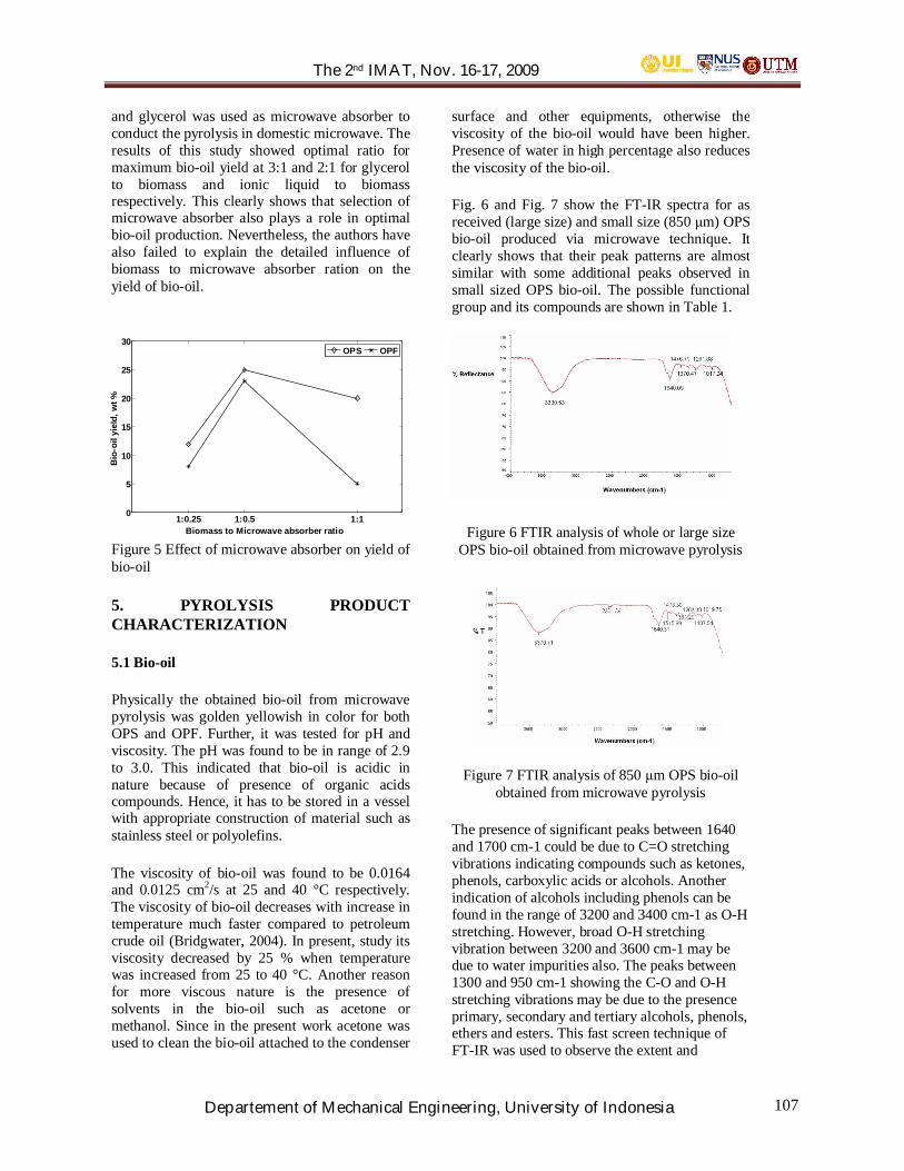
The 2nd IMAT, Nov. 16-17, 2009
Departement of Mechanical Engineering, University of Indonesia 107
and glycerol was used as microwave absorber toconduct the pyrolysis in domestic microwave. Theresults of this study showed optimal ratio formaximum bio-oil yield at 3:1 and 2:1 for glycerolto biomass and ionic liquid to biomassrespectively. This clearly shows that selection ofmicrowave absorber also plays a role in optimalbio-oil production. Nevertheless, the authors havealso failed to explain the detailed influence ofbiomass to microwave absorber ration on theyield of bio-oil.
Figure 5 Effect of microwave absorber on yield ofbio-oil
5. PYROLYSIS PRODUCTCHARACTERIZATION
5.1 Bio-oil
Physically the obtained bio-oil from microwavepyrolysis was golden yellowish in color for bothOPS and OPF. Further, it was tested for pH andviscosity. The pH was found to be in range of 2.9to 3.0. This indicated that bio-oil is acidic innature because of presence of organic acidscompounds. Hence, it has to be stored in a vesselwith appropriate construction of material such asstainless steel or polyolefins.
The viscosity of bio-oil was found to be 0.0164and 0.0125 cm2/s at 25 and 40 °C respectively.The viscosity of bio-oil decreases with increase intemperature much faster compared to petroleumcrude oil (Bridgwater, 2004). In present, study itsviscosity decreased by 25 % when temperaturewas increased from 25 to 40 °C. Another reasonfor more viscous nature is the presence ofsolvents in the bio-oil such as acetone ormethanol. Since in the present work acetone wasused to clean the bio-oil attached to the condenser
surface and other equipments, otherwise theviscosity of the bio-oil would have been higher.Presence of water in high percentage also reducesthe viscosity of the bio-oil.
Fig. 6 and Fig. 7 show the FT-IR spectra for asreceived (large size) and small size (850 m) OPSbio-oil produced via microwave technique. Itclearly shows that their peak patterns are almostsimilar with some additional peaks observed insmall sized OPS bio-oil. The possible functionalgroup and its compounds are shown in Table 1.
Figure 6 FTIR analysis of whole or large sizeOPS bio-oil obtained from microwave pyrolysis
Figure 7 FTIR analysis of 850 m OPS bio-oilobtained from microwave pyrolysis
The presence of significant peaks between 1640and 1700 cm-1 could be due to C=O stretchingvibrations indicating compounds such as ketones,phenols, carboxylic acids or alcohols. Anotherindication of alcohols including phenols can befound in the range of 3200 and 3400 cm-1 as O-Hstretching. However, broad O-H stretchingvibration between 3200 and 3600 cm-1 may bedue to water impurities also. The peaks between1300 and 950 cm-1 showing the C-O and O-Hstretching vibrations may be due to the presenceprimary, secondary and tertiary alcohols, phenols,ethers and esters. This fast screen technique ofFT-IR was used to observe the extent and
1:0.25 1:0.5 1:10
5
10
15
20
25
30
Biomass to Microwave absorber ratio
Bio
-oil
yiel
d, w
t %
OPS OPF
The 2nd IMAT, Nov. 16-17, 2009
Departement of Mechanical Engineering, University of Indonesia 108
presence of hydroxyl group to confirm thephenolic compounds. However, detained analysisthrough GC-MS would demonstrate the actualpresence of chemical entities.
Table 1: FT-IR analysis for functional group inOPS bio-oil
Wavenumbers,cm-1
Functionalgroup
Class ofcompounds
3200 – 3600 O-H Polymeric,waterimpurities
3000 - 2800 C-H Alkanes1780 – 1640 C=O Ketones,
aldehydes,carboxylicacids
1680 – 1580 C=C Alkenes1550 – 1490 -NO Nitrogenous
compounds1475 – 1350 C-H Alkanes950 – 1300 C-O Primary,
secondary andtertiaryalcohols,
phenol, esters,ethers
O-H
900 – 650 O-H Aromatic
6. CONCLUSIONS AND FUTUREWORK
Microwave pyrolysis of oil palm biomass (fiberand shell) for as received was carried out.Pyrolysis under microwave radiation took place atlow temperature. The temperature profiles wereobserved during microwave pyrolysis of OPS andOPF. Microwave absorbers were found toincrease the pyrolysis temperature largely in caseof OPF and to smaller extent in case of OPS. Poorfluidization behavior might have contributed in aninconsistence temperature profiles. However, withthe help of microwave heating the temperaturecould be raised to higher value in few secondsthus considerable saving in time and energy.Microwave absorber not only contributed inincreasing the temperature or initiating thepyrolysis process but also affected the yield ofbio-oil. The physical characterization showedacidic nature of bio-oil with decrease in viscosityagainst temperature. The FT-IR analysis revealed
probable compounds such as ketone, aldehyde,phenols and carboxylic acids with waterimpurities. Further confirmation about thepresence of chemical compounds depends onmore detailed study of microwave pyrolysis bio-oil from oil palm biomass and is currently underprocess which will be published in future articles.Future work is being carried out to develop andinvestigate other potential parameters and processconditions affecting the pyrolysis process ofdifferent biomass in novel microwave system.
ACKNOWLEDGEMENTS
The authors are grateful for E-Science fundingfrom Ministry of Higher Education, Malaysia forfinancial supports. In addition, the authors thankthe staff from Faculty of Mechanical Engineeringand Faculty of Science, Universiti TeknologiMalaysia for their help in obtaining the ImageAnalysis and FT-IR respectively.
REFERENCES
[1] Ani, F. N., Yi L. X., and Salema A. A. ContinuousFast Pyrolysis of Oil Palm Solid Wastes for Bio-Oil Production. In Proceeding of 5th InternationalConference on Combustion, Incineration,Pyrolysis and Emission Control, 16-19 December2008, Chiang Mai, Thailand.
[2] Appleton, T.J., Colder, R.I., Kingman, S.W.,Lowndes, I.S., and Read, A.G. Microwavetechnology for energy-efficient processing ofwaste. Applied Energy, 81 (2005) 85-113.
[3] Bridgwater, A.V. Biomass fast pyrolysis. ThermalScience, 8(2) (2004) 21 – 49.
[4] Chen, M-Q., Wang, J., Zhang, M-X., Chen, M-G.,Zhu, X-F., Min, F-F., Tan, Z-C. Catalytic effectsof eight inorganics additives on pyrolysis of pinewood sawdust by microwave heating. Journal ofAnalytical and Applied Pyrolysis, 82 (2008) 145-150.
[5] Domínguez, A., Fernández, Y., Fidalgo, B., Pis,J.J., and Menéndez, J.A. Bio-syngas productionwith low concentrations of CO2 and CH4 frommicrowave-induced pyrolysis of wet and driedsewage sludge. Chemosphere, 70 (2008) 397-403.
[6] Domínguez, A., Menéndez, J.A., Fernández, Y.,Pis, J.J., Valente Nabais, J.M., Carrott, P.J.M.,Ribeiro Carrott, M.M.L. COnventioanl andmicrowave induced pyrolysis of coffee hulls forthe production of a hydrogen rich fuel gas. Journalof Analytical and Applied Pyrolysis, 79 (2007)128-135.
[7] El harfi, K., Mokhlisse, A., Chanâa, M.B., andOutzourhit, A. Pyrolysis of the Moroccan oilshales under microwave radiation. Fuel, 79 (2000)733-742.
The 2nd IMAT, Nov. 16-17, 2009
Departement of Mechanical Engineering, University of Indonesia 109
[8] Guo, J., and Lua, A.C. Preparation of activatedcarbons from oil-palm-stone chars by microwaveinduced carbon dioxide activation. Carbon, 38(2000) 1985-1993.
[9] Guo, X., Zheng, Y., and Zhou, B. Influence ofabsorption medium on microwave pyrolysis of firsawdust. In Second International Conference onBioinformatics and Biomedical Engineering, May16-18, Shanghai, China.
[10] Huang, Y.F., Kuan, W.H., Lo, S.L., and Lin, C.F.Total recovery of resources and energy from ricestraw using microwave-induced pyrolysis.Bioresource Technology, 99 (2008) 8252-8258.
[11] Islam, M.N., and Ani, F.N. Techno-economic ofrice husk pyrolysis, conversion with catalytictreatment to produce liquid fuel. BioresourceTechnology, 73 (2000) 67-75.
[12] Jones, D.A., Lelyveld, T.P., Mavrofidis, S.D.,Kingman, S.W., and Miles, N.J. Microwaveheating applications in environmental engineering– A review. Resources, Cconversion andRecycling, 34 (2002) 75-90.
[13] Ludlow-Palafox, C., and Chase, H.A. Microwave-Induced pyrolysis of plastic wastes. Industrial andEngineering Chemistry Research, 40 (2001) 4749-4756.
[14] Menéndez, J.A., Inguanzo, M., and Pis, J.J.Microwave-induced pyrolysis of sewage sludge.Water Research, 36 (2002) 3261-3264.
[15] Miura, M., Kaga, H., Sakurai, A., Kakuchi, T.,Takahashi, K. Rapid pyrolysis of wood block bymicrowave heating. Journal of Analytical andApplied Pyrolysis, 71 (2004) 187-199.
[16] Pingale, N.D., and Shukla, S.R. Microwaveassisted ecofriendly recycling of poly (ethyleneterephthalate) bottle waste. European PolymerJournal 44 (2008) 4151-4156.
[17] Popescu, S., Misawa, T., Ohtsu, Y., Fujita, H.,Sanematsu, S. New microwave reactor for paper-based waste neutralization. Resources,Conservation and Recycling, 52 (2008) 671-677.
[18] Thostenson, E.T., and Chou, T.-W. Microwaveprocessing: fundamental and applications.Composites: Part A Applied Science andManufacturing, 30 (1999) 1055-1071.
[19] Wan, Y., Chen, P., Zhang, B., Yang, C., Liu, Y.,Lin, X., and Ruan, R. Microwave-assistedpyrolysis of biomass: Catalyst to improve productselectivity. Journal of Analytical and AppliedPyrolysis, 86 (2009) 161-167.
[20] Yu, F., Deng, S., Chen, P., Liu, Y., Wan, Y.,Olson, A., Kittelson, D., and Ruan, R. Physicaland Chemical properties of bio-oils frommicrowave pyrolysis of corn stover. AppliedBiochemistry and Biotechnology, 136-140 (2007)957-970.
[21] Zhang, H., and Datta, A.K. Microwave powerabsorption in single and multiple item foods.Transaction of Institution of Chemical Engineers,81 (2003) 257-265.
The 2nd IMAT, Nov. 16-17, 2009
Departement of Mechanical Engineering, University of Indonesia 110
A Study of Transient flow in a lid-driven square cavity
Nor Azwadi Che Sidika, Muhammad Ammar Nik Mu tasimb
aFaculty of Mechanical Engineering, Universiti Teknologi MalaysiaUTM Skudai, Johor, Malaysia,
bFaculty of Mechanical Engineering, Universiti Teknologi MalaysiaUTM Skudai, Johor, Malaysia,
ABSTRACT
AbstractIn this paper, lattice Boltzmann scheme is used tosimulate steady incompressible flow inside asquare cavity. Numerical simulations are carriedout for Reynolds number of 100, 400, 1000, 3200and 7500. The governing equation use is thedouble-population lattice Boltzmann formulation.Two-dimensional nine velocity model is used forthe computation of velocity field. The resultsobtained are compared with the results found inthe literature reviews. Present study found thatlattice Boltzmann scheme is able to carry outequivalent results as conventional scheme.
Keywordslid-driven square cavity, lattice Boltzmannscheme, Transient flow
1. INTRODUCTION
Flow in a cavity is an interesting researchproblem and has always been the initial interestamong researchers. Numerous studies have beendone to study the phenomenon of flows insideclosed geometries. The most interesting type ofgeometries is the square cavity. This is due to itssimplicity of its geometry and its boundaryconditions. Many reviews of square cavity using2-D Navier Stokes equations can be studied fromauthors such as Ghia et al. [1], Erturk et al.[2] andAlbensoeder and Kuhlmann [3].
The lattice Boltzmann method has been knownfor many years as one of the alternative tools thatis as competent as Navier Stokes equations. Theadvantage of Lattice Boltzmann Method is that itis much more accurate and easier to apply incomplicated boundary conditions.[4]
Many efforts have been done on rectangularcavity rather than square cavity. Cheng and Hung[5] apply lattice Boltzmann methods to analyzethe 2D vortex structure in a rectangular lid-drivencavity for various Reynolds numbers. Accordingto Shankar and Deshpande [6], there are threeadvantages of studying lid driven cavity flows.The first method is that results are easy tocompare from theory, numerical simulations andexperiments. The second method is that the flowdomain is unaffected by varies Reynoldsnumbers. The third is that the flow reveals theresults that may occur in incompressible flows,complex flows and transition to turbulence.
In this study, we will look at the main objectivewhich is to understand the transient flow in a lid-driven cavity under varies Reynolds numbersusing lattice Boltzmann scheme.
2. LATTICE BOLTZMANN SCHEME
The Lattice Boltzmann Scheme is originallydeveloped from the Lattice Gas Automata. TheLattice Boltzmann Scheme can be derived fromthe continuum Boltzmann Equation [7]. ABoltzmann scheme consists of two steps, astreaming step and a collision step. The statisticaltreatment of a system can be represented in termsof distribution function. Nor Azwadi [8] affirmedthat this distribution function ( ) cxcx ddtf ,, isthe number of particles which positions andvelocities are such that xd and cd at time t .Every particle would move from x to t∆+ cxif there is no collision occurs. Moreover, eachparticle velocity would change from c to
ta∆+c in which a is the acceleration due toexternal forces on a particle at x with a velocityof c .

The 2nd IMAT, Nov. 16-17, 2009
Departement of Mechanical Engineering, University of Indonesia 111
If no collision happens, means that there isconservation of molecules. In other words, thenumber of molecules ( ) cxcx ddtf ,, is equal tothe number of molecules
( ) cxccx ddtttatf ∆+∆+∆+ ,, .
Therefore,
( ) ( ) 0,,,, =−∆+∆+∆+ cxcxcxccx ddtfddtttatf (1)
However, when collision occurs, the arrivingparticles at the points interact with one andanother and by changing the velocity directionthat can be expressed as
( )( ) ( ) dtddfddtf
ddtttatfcxcxcx
cxccxΩ=
−∆+∆+∆+,,
,, (2)
In which ( ) dtddf cxΩ is the lattice Boltzmanncollision operator. The Eq. (2) is dividedby dtdd cx . Next, let dt tends to zero. This would
yield the Boltzmann equation for f as follows;
( )fcfa
xfc
tf
Ω=∂∂
+∂∂
+∂∂
ααα (3)
Where as the ( )fΩ is the expression forcollision operators which controls the speed of
change in f during collision. If the collision is toconserve mass, momentum and energy, it isrequired that;
( ) 01
2
=Ω
∫ cc dfc
(4)
There are two ways that the distribution function( )tf ,,cx can be changed by this collision. The
ways are as follow;
1. When collision takes place, someparticles with initial velocities ofc would have their velocities changeddue to decrease in ( )tf ,,cx .
2. On the other hand, particles that havedifferent velocity at initial will tend tohave velocity of c after the collision dueto the increase in ( )tf ,,cx .
The macroscopic quantities such as fluid density,momentum and energy can be found from thedistribution function by considering theappropriate integral. However, due to thecomplicated nature of the collision integral whereany replacement of collision must satisfy theconservation of mass, momentum and energyexpressed in Eq. (4) is a problem when dealingwith Boltzmann equation. Nor Azwadi [8] statedthat:
collisiontf
xfc
tf
∂∂=
∂∂+
∂∂
αα
Where ;
( )ftf
collision
Ω=∂∂
Equation (6) represents the change in distributionfunction per unit time due to collision. Succi [9]had shown that the particular interest is in thechange in distribution function f in time of
order fτ , the average time between excessive
collisions. The distribution function f can berelated to the equilibrium distribution function
eqf via second order Taylor’s series expansion,that is:
( ) ( ) ( ) ( )2,,,, tOttftftf
collision
eq δδ +∂∂
+≈ cxcx
( ) ( ) ( ) ( )f
eqeq
collision
tftft
tftftf
τδ,,,,,,,, cxcxcxcx −=−=
∂∂
Therefore, the discretized version of the BGKLattice Boltzmann equation can be written asfollow
The 2nd IMAT, Nov. 16-17, 2009
Departement of Mechanical Engineering, University of Indonesia 112
( ) ( )
−∆−=−∆+∆+
f
eqii
iiiffttftttf
τ,, xcx
The other important issues in lattice Boltzmannequations of flow is the Boundary condition.Boundary conditions used is known as the BounceBack scheme [8]. This Boundary condition wasused to obtain the no-slip velocity condition.Meaning when a particle moves to the wall node,the particle distribution scatters back to the nodeit has come from.
1. SPECIFICATION OF THEPROBLEM
For this problem, flow inside a driven squarecavity was investigated numerically. The topboundary moves from left to right with a constantvelocity U. Figure 1 shows the geometry of thedriven square cavity. The other three boundarieswhich is the left, right and the bottom side (wall)are made fixed. The initial assigned value ofdensity, ρ=1.0 is applied to whole field. Next, thevelocities in the interior of the cavities are set tozero. Velocity of U in x direction is applied on topof the boundary while velocity in y direction is setto zero. The bounce back boundary condition isapplied on the three stationary walls. Reynoldsnumber is defined as Re= UL/υ where L is gridlength and υ is the kinematic viscosity.
Figure 2 Geometry of square driven cavity
The grid length is set to be 300 times 300.Size ofthe grid was used to acquire the steady solutionfor the given Reynolds numbers (we need to keepa sufficiently large τ within the stability range).The value of the Reynolds number used for thisproblem are Re=100, 400, 1000, 3200 and 7500.
2. RESULTS AND DISCUSSION
In this section, the numerical results for theproblem obtained from the transient flow forcenter location from driven cavity flow usinglattice Boltzmann equation are discussed.
4.1 Code Validation
In order to study the center location transientflow, it was first applied for driven square cavityflow. Driven cavity flow is a standard benchmarkcase which has been studied by many researchers.For this problem, the velocity, U at the top wallwas maintained at 0.1 lu/s while the velocity atthe other three walls was set to 0 lu/s. On theother hand, the Reynolds numbers were variedfrom 100 to 10000. We now compare theperformance of our code for Stream functions ofRe 400 with the simulations applied by T.H Ji etal [10] at Re 400 in Fig. 3. The fluid motion isgoverned by the well know Navier Stokes withthe fluid properties set as constant. The verticalsidewalls and the bottom wall are made rigid. Thestream flow evolves slowly to the steadystate.[11]The data corresponded was nearly equalto the transient movement trajectory of the centerlocation for the Reynolds Number 400 usingLattice Boltzmann Scheme.
Figure 3 Stream functions in cavity flow at Re400 a) Lattice Boltzmann Scheme b) NavierStokes Equation T.H Ji et al [11]
(9)
U
U = 0V = 0
U = 0V = 0
U = 0 V = 0
a) b)
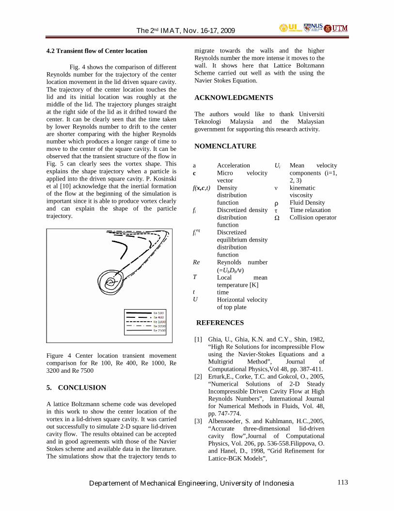
The 2nd IMAT, Nov. 16-17, 2009
Departement of Mechanical Engineering, University of Indonesia 113
4.2 Transient flow of Center location
Fig. 4 shows the comparison of differentReynolds number for the trajectory of the centerlocation movement in the lid driven square cavity.The trajectory of the center location touches thelid and its initial location was roughly at themiddle of the lid. The trajectory plunges straightat the right side of the lid as it drifted toward thecenter. It can be clearly seen that the time takenby lower Reynolds number to drift to the centerare shorter comparing with the higher Reynoldsnumber which produces a longer range of time tomove to the center of the square cavity. It can beobserved that the transient structure of the flow inFig. 5 can clearly sees the vortex shape. Thisexplains the shape trajectory when a particle isapplied into the driven square cavity. P. Kosinskiet al [10] acknowledge that the inertial formationof the flow at the beginning of the simulation isimportant since it is able to produce vortex clearlyand can explain the shape of the particletrajectory.
Figure 4 Center location transient movementcomparison for Re 100, Re 400, Re 1000, Re3200 and Re 7500
5. CONCLUSION
A lattice Boltzmann scheme code was developedin this work to show the center location of thevortex in a lid-driven square cavity. It was carriedout successfully to simulate 2-D square lid-drivencavity flow. The results obtained can be acceptedand in good agreements with those of the NavierStokes scheme and available data in the literature.The simulations show that the trajectory tends to
migrate towards the walls and the higherReynolds number the more intense it moves to thewall. It shows here that Lattice BoltzmannScheme carried out well as with the using theNavier Stokes Equation.
ACKNOWLEDGMENTS
The authors would like to thank UniversitiTeknologi Malaysia and the Malaysiangovernment for supporting this research activity.
NOMENCLATURE
REFERENCES
[1] Ghia, U., Ghia, K.N. and C.Y., Shin, 1982,“High Re Solutions for incompressible Flowusing the Navier-Stokes Equations and aMultigrid Method”, Journal ofComputational Physics,Vol 48, pp. 387-411.
[2] Erturk,E., Corke, T.C. and Gokcol, O., 2005,“Numerical Solutions of 2-D SteadyIncompressible Driven Cavity Flow at HighReynolds Numbers”, International Journalfor Numerical Methods in Fluids, Vol. 48,pp. 747-774.
[3] Albensoeder, S. and Kuhlmann, H.C.,2005,“Accurate three-dimensional lid-drivencavity flow”,Journal of ComputationalPhysics, Vol. 206, pp. 536-558.Filippova, O.and Hanel, D., 1998, “Grid Refinement forLattice-BGK Models”,
ac
f(x,c,t)
fi
fieq
Re
T
tU
AccelerationMicro velocityvectorDensitydistributionfunctionDiscretized densitydistributionfunctionDiscretizedequilibrium densitydistributionfunctionReynolds number(=UbDh/ν)Local meantemperature [K]timeHorizontal velocityof top plate
Ui
ρ
Mean velocitycomponents (i=1,2, 3)kinematicviscosityFluid DensityTime relaxationCollision operator
The 2nd IMAT, Nov. 16-17, 2009
Departement of Mechanical Engineering, University of Indonesia 114
[1] Journal of Computational Physics, Vol. 147,pp. 219-228.
[2] M.cheng, K.C hung, Vortex Structure ofSteady flow in a Rectangular cavity,Computers & Fluids 35 (2006) 1046-1062
[3] P.Shankar, M.Deshpande, Fluid mechanicsin the driven cavity, Annual Review of FluidMechanics 32 (2000) 93-136
[4] S Chen and G.D Doolen, Lattice BoltzmannMethod for fluid flows Annual Review ofFluid Mechanics, 30:229-264, 1998
[5] Nor Azwadi, C.S. and Tanahashi, T., 2006,“Simplified Thermal Lattice Boltzmann inIncompressible Limit”, International Journalof Modern Physics, B 20, pp. 2437-2449.
[6] Succi, S., 2001, The Lattice BoltzmannEquation for fluid dynamics and beyond,Oxford Science Publications, New York.
[7] P.Kosinski, A.kosinska, A.C. Hoffmann,2009 “simulation of solid particles behaviorin a driven cavity flow” An InternationalJournal on the Science and Technology ofWet and Dry Particulate Systems, Vol. 191327-339
[8] Tae Ho Ji, Seo Young Kim, Jae Min Hyun,2007, “Transient mixed convection in anenclosure driven by a sliding lid”, HeqatMass Transfer, 43: 629-638
[9] Nor Azwadi, C.S and Tanahashi, T., 2007,“Three-Dimensional Thermal LatticeBoltzmans Simulation of NaturalConvection in a Cubic Cavity”, InternationalJournal of Modern Physics, B 21, pp.87-96.
[10] Bhatnagar, P. L., Gross, E. P. and Krook,M., 1954, “A Model for Collision Processesin Gasses. 1. Small Amplitude Processes inCharged and Neutral One-ComponentSystem”, Physics Review, Vol. 94, pp. 511–525.
[11] Nor Azwadi C.S and T, Tanahashi, 2008,“Simplified Finite Difference ThermalLattice Boltzmann Method”, InternationalJournal of Modern Physics, B 22, pp. 3865-3876.
[12] Krafczyk, M., Tolke, J., 2009, “Secondorder interpolation of the flow field in thelattice Boltzmann method”, Computers andMathematics with Applications, Vol. 58, pp.898-902.
[13] C.Crowe, M.Sommerfeld, Y.Tsuji,Multiphase Flows with Droplets andParticles, CRC Press LLC, 1998

The 2nd IMAT, Nov. 16-17, 2009
Departement of Mechanical Engineering, University of Indonesia 115
Efficient Mesh for Driven Square Cavity
Nor Azwadi Che Sidik* and Fudhail Abdul Munir**
Faculty of Mechanical Engineering, Universiti Teknologi MalaysiaUTM Skudai, Johor, Malaysia
*[email protected], **[email protected]
ABSTRACT
In this paper, an improved lattice Boltzmann schemeis used to simulate steady incompressible flowinside a square cavity. The newly improved schemeis applied for driven square cavity. Numericalsimulations are carried out for Reynolds numberequal to 5000. The governing equation used is thedouble-population lattice Boltzmann formulation.On the other hand, two-dimensional nine velocitymodel is used for the computation of velocity field.The results obtained are compared with the resultsfound in the literature reviews. Moreover, the timeneeded for the solution to converge is recorded. Thetime obtained is compared with the time required forthe conventional lattice Boltzmann scheme toconverge. Present study found that the computationtime can be reduced without sacrificing the accuracyof the results.
Keywords: driven square cavity, lattice Boltzmannscheme
1. INTRODUCTION
Being a part of Computational Fluid Dynamics(CFD) study, flows inside closed geometries havealways been of focal attention. There have beennumerous studies being carried out on flowbehaviour inside a cavity. The most popular type ofcavity that is studied by vast researchers is flowinside square cavity. This is probably due to itssimplicity of the geometry and application of theboundary conditions. Excellent reviews on drivensquare cavity were written by Ghia et al. [1] ,Erturket al.[2] and Albensoeder and Kuhlmann [3].However, these researchers used the conventionalCFD which is by solving 2-D Navier Stokesequations.
Over the years, there has been a rapid progress indeveloping the lattice Boltzmann method as anefficient alternative to conventional CFD. Anessential advantage of the lattice Boltzmann methodis its ease and accuracy in dealing with complicatedboundary geometries. Apart from that, Filippova and
Hanel[4] stated that in the range of small tomoderate Reynolds numbers, where the flowsolution is not too anisotropic, the lattice-BGKmethod is better compared to the conventionalcomputational fluid dynamics if dealing with flowsin complex geometries as in filters or throughgranular materials.
According to Chew et al.[5], there are threemethods to improve the standard lattice Boltzmannequation (LBE) before it can be applied to complexproblems. The first method is interpolation-supplemented lattice Boltzmann equation (ISLBE)which first proposed by He and Doolen [6]. ISLBEwas first used to simulate flow around a circularcylinder. He and Doolen [6] also mentioned that,there are two obvious advantages of irregular latticegrids over regular grids used in the conventionallattice Boltzmann models. The first advantage is theboundary of the cylinder is described much moreaccurately. The second merit of ISLBE is the meshcan be placed more densely around the cylinder.This will lead to the improvement in term ofnumerical efficiency.
The second method is called the differentialLBE. Differential LBE is based on the solution of apartial differentiationequation. The third method is called grid refinementmethod which was introduced by Filippova andHanel [4]. In this work, we will present animproved lattice Boltzmann scheme to simulateflow inside a driven square cavity. It was foundthat when our model is applied to simulate thedriven cavity flow, a good accuracy of results couldbe obtained.
2. LATTICE BOLTZMANN METHOD
The fundamental idea of Boltzmann work is thata gas is composed of interacting particles that can beexplained by classical mechanics. Since there aremany particles involved, a statistical treatment isneeded and is more suitable. According to Sukopand Thorne [7], the mechanics can be very simpleand it contains streaming in space and billiard-likecollision interactions.

The 2nd IMAT, Nov. 16-17, 2009
Departement of Mechanical Engineering, University of Indonesia 116
The statistical treatment of a system can berepresented in terms of distribution function . It wasstated by Nor Azwadi [8] that this distributionfunction ( ) cxcx ddtf ,, is the number of particleswhich positions and velocities are such that xd and
cd at time t . Each particle would move from x tot∆+ cx if there is no collision occurs. Moreover,
each particle velocity would change from c tota∆+c in which a is the acceleration due to
external forces on a particle at x with a velocity ofc .Furthermore, no collision means that there isconservation of molecules. In other words, thenumber of molecules ( ) cxcx ddtf ,, is equal to thenumber of molecules
( ) cxccx ddtttatf ∆+∆+∆+ ,, . Therefore,
( ) ( ) 0,,,, =−∆+∆+∆+ cxcxcxccx ddtfddtttatf (1)
However, when collision occurs between themolecules the equation that can be represented forthis particular case is that
( ) ( )( ) dtddf
ddtfddtttatfcx
cxcxcxccxΩ=
−∆+∆+∆+ ,,,,(2)
where ( ) dtddf cxΩ is the lattice Boltzmanncollision operator. The equation (2) is dividedby dtdd cx . Next, let dt tends to zero. Thiswould yield the Boltzmann equation for f asfollows;
( )fcfa
xfc
tf
Ω=∂∂
+∂∂
+∂∂
ααα (3)
Solving Boltzmann equation would require anexpression for the collision operator ( )fΩ . If thecollision is to conserve mass, momentum andenergy, it is required that;
( ) 01
2
=Ω
∫ cc dfc
(4)
There are two ways that the distribution function( )tf ,,cx can be changed by this collision. The
ways are as follow;
1. When collision takes place, some particleswith initial velocities of c would havetheir velocities changed due to decreasein ( )tf ,,cx .
2. On the other hand, particles that havedifferent velocity at initial will tend to havevelocity of c after the collision due to theincrease in ( )tf ,,cx .
The macroscopic quantities such as fluid density,momentum and energy can be found from thedistribution function by considering the appropriateintegral. However, due to the complicated nature ofthe collision integral where any replacement ofcollision must satisfy the conservation of mass,momentum and energy expressed in Eq. (4) is aproblem when dealing with Boltzmann equation.Nor Azwadi [8]
collisiontf
xfc
tf
∂∂
=∂∂
+∂∂
αα (5)
Where ;
( )ftf
collision
Ω=∂∂
(6)
Equation (6) represents the change in distributionfunction per unit time due to collision. Succi [9] hadshown that the particular interest is in the change indistribution function f in time of order fτ , theaverage time between excessive collisions. Thedistribution function f can be related to the
equilibrium distribution function eqf via secondorder Taylor’s series expansion, that is:
( ) ( ) ( ) ( )2,,,, tOttftftf
collision
eq δδ +∂∂
+≈ cxcx (7)
( ) ( ) ( ) ( )f
eqeq
collision
tftft
tftftf
τδ,,,,,,,, cxcxcxcx −
=−
=∂∂ (8)
Therefore, the discretised version of the BGKLattice Boltzmann equation can be written as follow
( ) ( )
−∆−=−∆+∆+
f
eqii
iiiffttftttf
τ,, xcx (9)

The 2nd IMAT, Nov. 16-17, 2009
Departement of Mechanical Engineering, University of Indonesia 117
2.1 Improved lattice Boltzmann scheme
The disadvantage of Lattice Boltzmann Method isthat its poor stability condition when dealing withfluid flow with high Reynolds number. Previouswork of stability analysis showed that the relaxationparameter τ=0.5 is the margin of instability. If thevalue of τ is less than 0.5, instability will happens.The equation linking between relaxation parameter τand fluid viscosity is shown below:
τ= 3υ + 0.5 (10)
For viscous fluid, υ>0. Hence, τ>0.5. On the otherhand, the equation for Reynolds number is given as:
Re= UL/υ (11)
where U is the fluid velocity, L is length of thedomain and υ is the kinematic viscosity. From eq.(10) and eq. (11) above, there is inverse relationshipbetween Reynolds number and the viscosity that iswhen Reynolds number is larger, the viscosity issmaller. When viscosity is small, the relaxationparameter will approach to the margin of instabilityvalue that is 0.5. Therefore, to maintain the stabilitycondition at high Reynolds number, the domainlength, L needs to be increased. However, when L isincreased, the mesh size will be increased if uniformmesh is used. This will lead to more time is neededto perform the computation analysis. Hence, forhigh Reynolds numbers, the computationalefficiency will be reduced as more memory isneeded in LBM to store the density distributions.
Therefore, to overcome this problem, in thisproject, the mesh size will not be increased eventhough the length is increased for higher Reynoldsnumber. For this purpose, interpolation method willbe used. On a regular grid in used in conventionallattice Boltzmann model, starting from one grid sitex, the distribution function is advected to aneighbouring grid site during each time step. Thisensure that the distribution function is known at thenext time step. However, for our case, the end pointof the streaming process is no longer a grid node.This means that the distribution function at gridnodes is not known at the next time step. Hence, todetermine the post streaming distribution function atgrid nodes, an interpolation method is used.According to He and Doolen[6], the unknown poststreaming distribution function at the original gridnodes can always be approximately by interpolationusing their neighbouring shifted grid nodes. In thisproblem, the mesh used is shown in Fig. 1. Asshown in the figure, interpolation is required in the
middle of the cavity in x direction.
Fig. 1 Mesh for driven square cavity
1. SPECIFICATION OF THE PROBLEM
For this problem, flow inside a driven squarecavity was investigated numerically. The topboundary moves from left to right with a constantvelocity U. Figure 1 shows the geometry of thedriven square cavity. On the other hand, the otherthree boundaries (wall) are made stationary. Theinitial assigned value of density, ρ=1.0 is applied towhole field. Next, the velocities in the interior of thecavities are set to zero. Velocity of U in x directionis applied on top of the boundary while velocity in ydirection is set to zero. The bounceback boundarycondition is applied on the three stationary walls.Reynolds number is defined as Re= UL/υ where L isgrid length and υ is the kinematic viscosity.
Fig. 2 Geometry of square driven cavity
U

The 2nd IMAT, Nov. 16-17, 2009
Departement of Mechanical Engineering, University of Indonesia 118
The grid length is set to be 400 times 400. Usingthis grid size enables us to obtain steady solution forthe given Reynolds numbers (we need to keep asufficiently large τ within the stability range). Thevalue of the Reynolds number used for this problemis Re=5000.
1. RESULTS AND DISCUSSION
In this section, the numerical results for the problemobtained from the improved lattice Boltzmannscheme are discussed.
4.1 Code Validation
In order to validate the developed code, it was firstapplied for driven square cavity flow. For this typeof flow, the velocity, U at the top wall wasmaintained at 0.1 lu/s while the velocity at the otherthree walls was set to 0 lu/s. On the other hand, theReynolds numbers were varied from 100 to 10000.The graph of velocity profile at mid height wasplotted. The results obtained from Ghia et al. [1]were plotted on the same graph for comparison.Figure 3 (a) to (g) shows the plotted graphs. Goodagreement between lattice Boltzmann method(LBM) and the benchmark solutions has been foundfor every tested case.
(a) Re=100
(b) Re=400
(c) Re=1000
(d) Re=3200
(e) Re=5000
(f) Re=7500
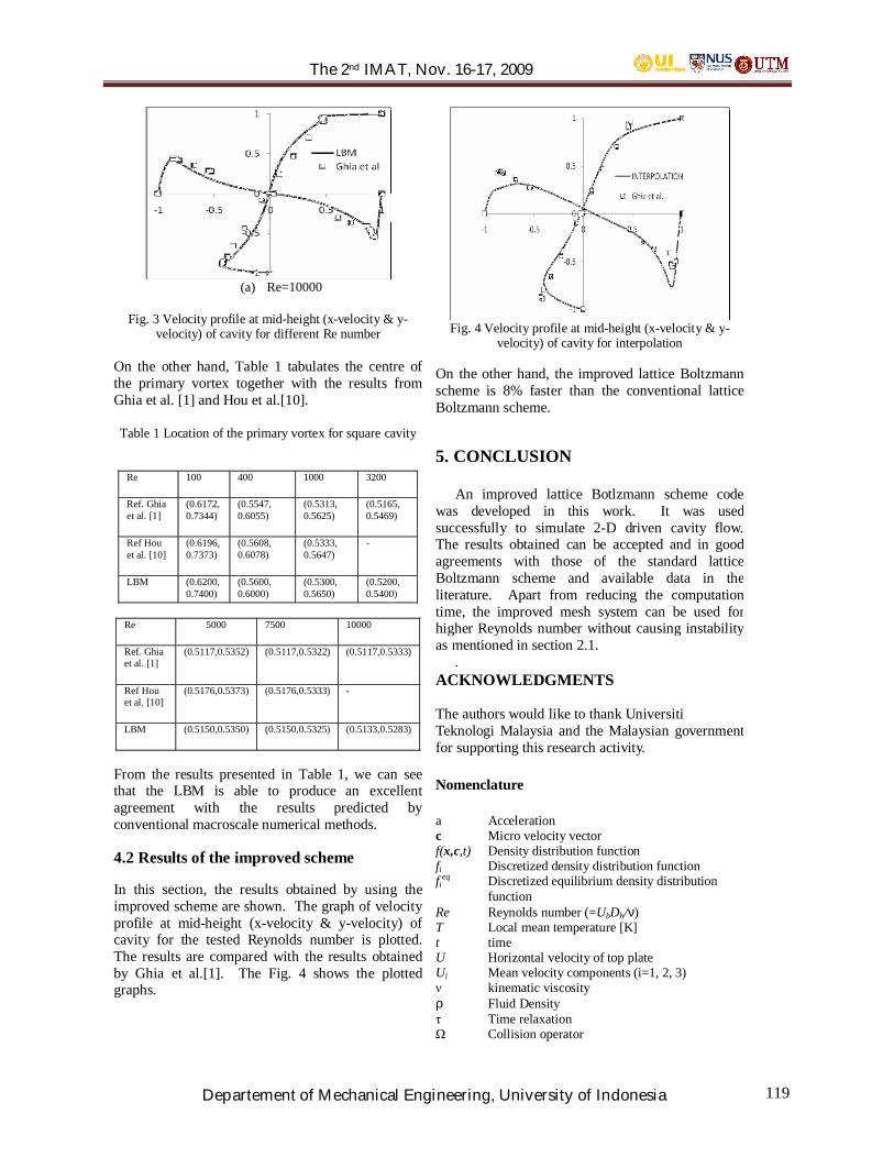
The 2nd IMAT, Nov. 16-17, 2009
Departement of Mechanical Engineering, University of Indonesia 119
(a) Re=10000
Fig. 3 Velocity profile at mid-height (x-velocity & y-velocity) of cavity for different Re number
On the other hand, Table 1 tabulates the centre ofthe primary vortex together with the results fromGhia et al. [1] and Hou et al.[10].
Table 1 Location of the primary vortex for square cavity
Re 100 400 1000 3200
Ref. Ghiaet al. [1]
(0.6172,0.7344)
(0.5547,0.6055)
(0.5313,0.5625)
(0.5165,0.5469)
Ref Houet al. [10]
(0.6196,0.7373)
(0.5608,0.6078)
(0.5333,0.5647)
-
LBM (0.6200,0.7400)
(0.5600,0.6000)
(0.5300,0.5650)
(0.5200,0.5400)
Re 5000 7500 10000
Ref. Ghiaet al. [1]
(0.5117,0.5352) (0.5117,0.5322) (0.5117,0.5333)
Ref Houet al. [10]
(0.5176,0.5373) (0.5176,0.5333) -
LBM (0.5150,0.5350) (0.5150,0.5325) (0.5133,0.5283)
From the results presented in Table 1, we can seethat the LBM is able to produce an excellentagreement with the results predicted byconventional macroscale numerical methods.
4.2 Results of the improved scheme
In this section, the results obtained by using theimproved scheme are shown. The graph of velocityprofile at mid-height (x-velocity & y-velocity) ofcavity for the tested Reynolds number is plotted.The results are compared with the results obtainedby Ghia et al.[1]. The Fig. 4 shows the plottedgraphs.
Fig. 4 Velocity profile at mid-height (x-velocity & y-velocity) of cavity for interpolation
On the other hand, the improved lattice Boltzmannscheme is 8% faster than the conventional latticeBoltzmann scheme.
5. CONCLUSION
An improved lattice Botlzmann scheme codewas developed in this work. It was usedsuccessfully to simulate 2-D driven cavity flow.The results obtained can be accepted and in goodagreements with those of the standard latticeBoltzmann scheme and available data in theliterature. Apart from reducing the computationtime, the improved mesh system can be used forhigher Reynolds number without causing instabilityas mentioned in section 2.1.
.ACKNOWLEDGMENTS
The authors would like to thank UniversitiTeknologi Malaysia and the Malaysian governmentfor supporting this research activity.
Nomenclature
a Accelerationc Micro velocity vectorf(x,c,t) Density distribution functionfi Discretized density distribution functionfieq Discretized equilibrium density distribution
functionRe Reynolds number (=UbDh/ν)T Local mean temperature [K]t timeU Horizontal velocity of top plateUi Mean velocity components (i=1, 2, 3) kinematic viscosity
ρ Fluid Density Time relaxation Collision operator

The 2nd IMAT, Nov. 16-17, 2009
Departement of Mechanical Engineering, University of Indonesia 120
REFERENCES
[1] Ghia, U., Ghia, K.N. and C.Y., Shin, 1982, “High ReSolutions for incompressible Flow using the Navier-Stokes Equations and a Multigrid Method”, Journalof Computational Physics,Vol 48, pp. 387-411.
[2] Erturk,E., Corke, T.C. and Gokcol, O., 2005,“Numerical Solutions of 2-D Steady IncompressibleDriven Cavity Flow at High Reynolds Numbers”,International Journal for Numerical Methods inFluids, Vol. 48, pp. 747-774.
[3] Albensoeder, S. and Kuhlmann, H.C.,2005,“Accurate three-dimensional lid-driven cavityflow”,Journal of Computational Physics, Vol. 206,pp. 536-558.
[4] Filippova, O. and Hanel, D., 1998, “GridRefinement for Lattice-BGK Models”, Journal ofComputational Physics, Vol. 147, pp. 219-228.
[5] Chew, Y.T., Shu, C. and Niu, X.D., 2002, “A NewDifferential Lattice Boltzmann Equation and ItsApplication to Simulate Incompressible Flows onNon-Uniform Grids”, Journal of Statistical Physics,Vol. 107, No ½.
[6] He, H. and Doolen, G., 1997, “Lattice BoltzmannMethod on Curvelinear Coordinates System: Flowaround a circular cylinder”, Journal ofComputational Physics, Vol. 134, pp. 306-315.
[7] Sukop, M.C and Thorne, D.T., 2006, LatticeBoltzmann Modeling : An introduction forgeoscientists and engineers, Springer, New York.
[8] Nor Azwadi, C.S. and Tanahashi, T., 2006,“Simplified Thermal Lattice Boltzmann inIncompressible Limit”, International Journal ofModern Physics, B 20, pp. 2437-2449.
[9] Succi, S., 2001, The Lattice Boltzmann Equation forfluid dynamics and beyond, Oxford SciencePublications, New York.
[10] Hou, S.Q., Zou, Chen, S. and Doolen, G., 1995,“Simulation of Cavity Flow by the lattice BoltzmannMethod”, Journal of Computational Physics, Vol.118, pp. 329-347.
[11] Nor Azwadi, C.S and Tanahashi, T., 2007, “Three-Dimensional Thermal Lattice Boltzmans Simulationof Natural Convection in a Cubic Cavity”,International Journal of Modern Physics, B 21,pp.87-96.
[12] Bhatnagar, P. L., Gross, E. P. and Krook, M., 1954,“A Model for Collision Processes in Gasses. 1.Small Amplitude Processes in Charged and NeutralOne-Component System”, Physics Review, Vol. 94,pp. 511–525.
[13] Nor Azwadi C.S and T, Tanahashi, 2008,“Simplified Finite Difference Thermal LatticeBoltzmann Method”, International Journal ofModern Physics, B 22, pp. 3865-3876.
[14] Krafczyk, M., Tolke, J., 2009, “Second orderinterpolation of the flow field in the latticeBoltzmann method”, Computers and Mathematicswith Applications, Vol. 58, pp. 898-902.
[15] Frish, U., B., Hasslacher and Pomeau, Y., 1986,“Lattice Gas Automata for the Navier-Stokes
Equation”, Physics Review Letter, Vol. 56, pp.1505-1508.
[16] Jin, C. and Xu, K., 2006, “An adaptive grid methodfor two dimensional viscous flow”, Journal ofComputational Physics, Vol. 218, pp. 68-81.
[17] Gladrow, D.W, 2000, Lattice Gas Cellular Automataand Lattice Boltzmann Models, Springer Verlag,New York.
[18] He, X. and L.S., Luo, 1997, “Lattice BoltzmannModel for the Incompressible Navier-StokesEquation”, Journal of Statistical Physics, Vol. 88,pp.927-944.
[19] Luo, L.S. and X., He, 1997, “A Priori Derivation ofthe Lattice Boltzmann Equation”, Physics Review, E56, pp. 6811-6817.
[20] Shu, C., Chew, Y.T., Niu, X.D., Peng, Y., Zheng,H.W., and Liu, N.Y., 2008, “Progress in thedevelopment and application of lattice Boltzmannmethod”, Asian Congress of Fluid Mechanics,Daejeon, Korea.
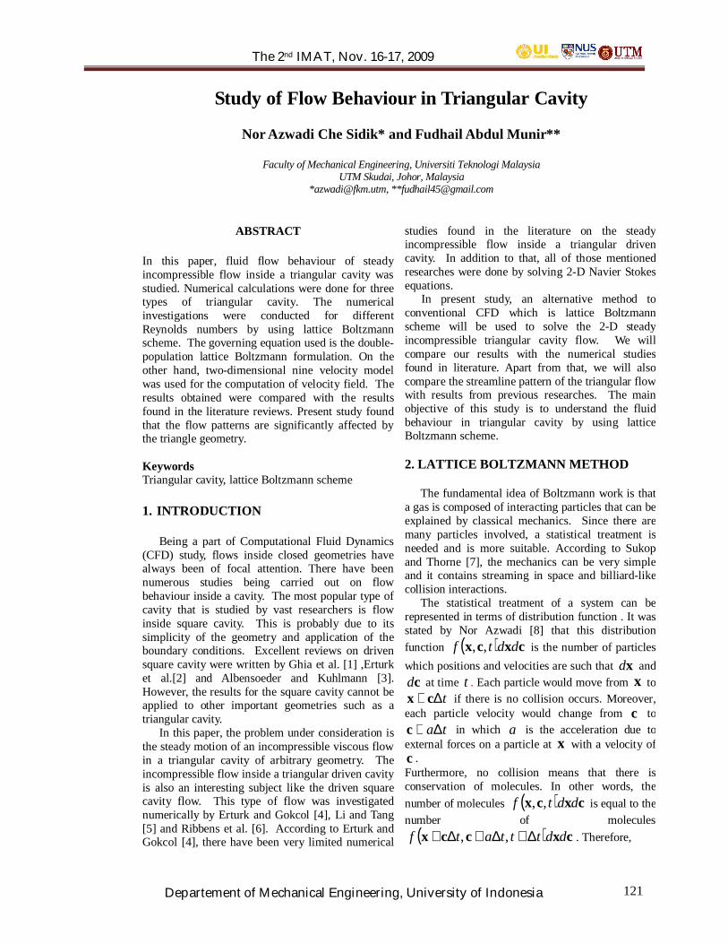
The 2nd IMAT, Nov. 16-17, 2009
Departement of Mechanical Engineering, University of Indonesia 121
Study of Flow Behaviour in Triangular Cavity
Nor Azwadi Che Sidik* and Fudhail Abdul Munir**
Faculty of Mechanical Engineering, Universiti Teknologi MalaysiaUTM Skudai, Johor, Malaysia
*[email protected], **[email protected]
ABSTRACT
In this paper, fluid flow behaviour of steadyincompressible flow inside a triangular cavity wasstudied. Numerical calculations were done for threetypes of triangular cavity. The numericalinvestigations were conducted for differentReynolds numbers by using lattice Boltzmannscheme. The governing equation used is the double-population lattice Boltzmann formulation. On theother hand, two-dimensional nine velocity modelwas used for the computation of velocity field. Theresults obtained were compared with the resultsfound in the literature reviews. Present study foundthat the flow patterns are significantly affected bythe triangle geometry.
KeywordsTriangular cavity, lattice Boltzmann scheme
1. INTRODUCTION
Being a part of Computational Fluid Dynamics(CFD) study, flows inside closed geometries havealways been of focal attention. There have beennumerous studies being carried out on flowbehaviour inside a cavity. The most popular type ofcavity that is studied by vast researchers is flowinside square cavity. This is probably due to itssimplicity of the geometry and application of theboundary conditions. Excellent reviews on drivensquare cavity were written by Ghia et al. [1] ,Erturket al.[2] and Albensoeder and Kuhlmann [3].However, the results for the square cavity cannot beapplied to other important geometries such as atriangular cavity.
In this paper, the problem under consideration isthe steady motion of an incompressible viscous flowin a triangular cavity of arbitrary geometry. Theincompressible flow inside a triangular driven cavityis also an interesting subject like the driven squarecavity flow. This type of flow was investigatednumerically by Erturk and Gokcol [4], Li and Tang[5] and Ribbens et al. [6]. According to Erturk andGokcol [4], there have been very limited numerical
studies found in the literature on the steadyincompressible flow inside a triangular drivencavity. In addition to that, all of those mentionedresearches were done by solving 2-D Navier Stokesequations.
In present study, an alternative method toconventional CFD which is lattice Boltzmannscheme will be used to solve the 2-D steadyincompressible triangular cavity flow. We willcompare our results with the numerical studiesfound in literature. Apart from that, we will alsocompare the streamline pattern of the triangular flowwith results from previous researches. The mainobjective of this study is to understand the fluidbehaviour in triangular cavity by using latticeBoltzmann scheme.
2. LATTICE BOLTZMANN METHOD
The fundamental idea of Boltzmann work is thata gas is composed of interacting particles that can beexplained by classical mechanics. Since there aremany particles involved, a statistical treatment isneeded and is more suitable. According to Sukopand Thorne [7], the mechanics can be very simpleand it contains streaming in space and billiard-likecollision interactions.
The statistical treatment of a system can berepresented in terms of distribution function . It wasstated by Nor Azwadi [8] that this distributionfunction ( ) cxcx ddtf ,, is the number of particleswhich positions and velocities are such that xd and
cd at time t . Each particle would move from x tot∆+ cx if there is no collision occurs. Moreover,
each particle velocity would change from c tota∆+c in which a is the acceleration due to
external forces on a particle at x with a velocity ofc .Furthermore, no collision means that there isconservation of molecules. In other words, thenumber of molecules ( ) cxcx ddtf ,, is equal to thenumber of molecules
( ) cxccx ddtttatf ∆+∆+∆+ ,, . Therefore,

The 2nd IMAT, Nov. 16-17, 2009
Departement of Mechanical Engineering, University of Indonesia 122
( ) ( ) 0,,,, =−∆+∆+∆+ cxcxcxccx ddtfddtttatf (1)
However, when collision occurs between themolecules the equation that can be represented forthis particular case is that
( ) ( )( ) dtddf
ddtfddtttatfcx
cxcxcxccxΩ=
−∆+∆+∆+ ,,,,(2)
where ( ) dtddf cxΩ is the lattice Boltzmanncollision operator. The equation (2) is dividedby dtdd cx . Next, let dt tends to zero. Thiswould yield the Boltzmann equation for f asfollows;
( )fcfa
xfc
tf
Ω=∂∂
+∂∂
+∂∂
ααα (3)
Solving Boltzmann equation would require anexpression for the collision operator ( )fΩ . If thecollision is to conserve mass, momentum andenergy, it is required that;
( ) 01
2
=Ω
∫ cc dfc
(4)
There are two ways that the distribution function( )tf ,,cx can be changed by this collision. The
ways are as follow;1. When collision takes place, some particles
with initial velocities of c would havetheir velocities changed due to decreasein ( )tf ,,cx .
2. On the other hand, particles that havedifferent velocity at initial will tend to havevelocity of c after the collision due to theincrease in ( )tf ,,cx .
The macroscopic quantities such as fluid density,momentum and energy can be found from thedistribution function by considering the appropriateintegral. However, due to the complicated nature ofthe collision integral where any replacement ofcollision must satisfy the conservation of mass,momentum and energy expressed in Eq. (4) is aproblem when dealing with Boltzmann equation.Nor Azwadi [8]
collisiontf
xfc
tf
∂∂
=∂∂
+∂∂
αα (5)
Where ;
( )ftf
collision
Ω=∂∂
(6)
Equation (6) represents the change in distributionfunction per unit time due to collision. Succi [9] hadshown that the particular interest is in the change indistribution function f in time of order fτ , theaverage time between excessive collisions. Thedistribution function f can be related to the
equilibrium distribution function eqf via secondorder Taylor’s series expansion, that is:
( ) ( ) ( ) ( )2,,,, tOttftftf
collision
eq δδ +∂∂
+≈ cxcx (7)
( ) ( ) ( ) ( )f
eqeq
collision
tftft
tftftf
τδ,,,,,,,, cxcxcxcx −
=−
=∂∂ (8)
Therefore, the discretised version of the BGKLattice Boltzmann equation can be written as follow
( ) ( )
−∆−=−∆+∆+
f
eqii
iiiffttftttf
τ,, xcx (9)
3. SPECIFICATION OF THE PROBLEM
In this study, three different types of trianglegeometries were considered. The first type is anisosceles triangle with the 90° being at the top rightcorner. On the other hand, the second type is anisosceles triangle with 90° being at the top leftcorner. The third type is isosceles triangle with 90°at the corner angle. Figure 1 depicts the geometry ofthe three triangles.
(a) 90° at top right corner
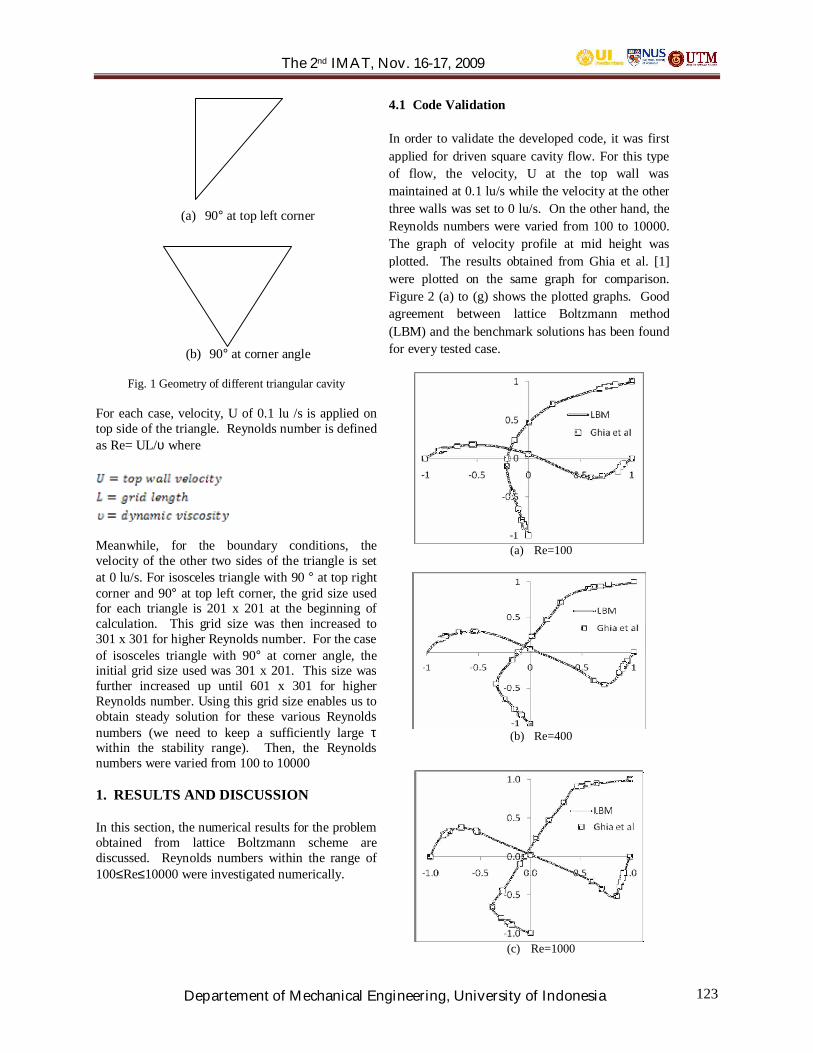
The 2nd IMAT, Nov. 16-17, 2009
Departement of Mechanical Engineering, University of Indonesia 123
(a) 90° at top left corner
(b) 90° at corner angle
Fig. 1 Geometry of different triangular cavity
For each case, velocity, U of 0.1 lu /s is applied ontop side of the triangle. Reynolds number is definedas Re= UL/υ where
Meanwhile, for the boundary conditions, thevelocity of the other two sides of the triangle is setat 0 lu/s. For isosceles triangle with 90 ° at top rightcorner and 90° at top left corner, the grid size usedfor each triangle is 201 x 201 at the beginning ofcalculation. This grid size was then increased to301 x 301 for higher Reynolds number. For the caseof isosceles triangle with 90° at corner angle, theinitial grid size used was 301 x 201. This size wasfurther increased up until 601 x 301 for higherReynolds number. Using this grid size enables us toobtain steady solution for these various Reynoldsnumbers (we need to keep a sufficiently large τwithin the stability range). Then, the Reynoldsnumbers were varied from 100 to 10000
1. RESULTS AND DISCUSSION
In this section, the numerical results for the problemobtained from lattice Boltzmann scheme arediscussed. Reynolds numbers within the range of100≤Re≤10000 were investigated numerically.
4.1 Code Validation
In order to validate the developed code, it was firstapplied for driven square cavity flow. For this typeof flow, the velocity, U at the top wall wasmaintained at 0.1 lu/s while the velocity at the otherthree walls was set to 0 lu/s. On the other hand, theReynolds numbers were varied from 100 to 10000.The graph of velocity profile at mid height wasplotted. The results obtained from Ghia et al. [1]were plotted on the same graph for comparison.Figure 2 (a) to (g) shows the plotted graphs. Goodagreement between lattice Boltzmann method(LBM) and the benchmark solutions has been foundfor every tested case.
(a) Re=100
(b) Re=400
(c) Re=1000

The 2nd IMAT, Nov. 16-17, 2009
Departement of Mechanical Engineering, University of Indonesia 124
(a) Re=3200
(b) Re=5000
(c) Re=7500
(d) Re=10000
Fig. 2 Velocity profile at mid-height (x-velocity & y-velocity) of cavity for different Re number
4.2 Isosceles triangle with 90° at the top rightcorner
Figure 3 (a) to (f) shows the streamline patterns forisosceles triangle with 90° at the top right corner.From the figures shown, there are two significantfeatures revealed by the streamline contours. Thefirst feature is that the number of vortices isincreased when the Reynolds (Re) numbers areincreased. As we can see in Fig. 3 (d), the numberof vortex is increased from previous which are twoto three when the Re number is 1500. On the otherhand, the second significant feature is that the centreof the primary vortex moves downstream to theright as Reynolds number is increased. For instance,Fig. 3 (a) depicts the centre of the primary vortexbeing located at 4/5 of the bottom vertex. However,this centre moves downward to 3/5 of the bottomvertex as the Reynolds number increases.
Apart from the streamline patterns, the locationof the primary vortex was also compared with theresults found in the literature. Table 1 tabulates thecentre of the primary vortex together with the resultsfrom Hou et al. [10].
Table 1 Location of the primary vortex for isoscelestriangle with 90° at the top right corner
Re 100 500 1000LBM (0.7100,0.8300) (0.7100,0.7650) (0.7000,0.7550)Ref[ 10 ] (0.7090,0.8320) (0.7070,0.7676) (0.6992,0.7559)
Re 1500 2000 2500LBM (0.7000,0.7467) (0.7000,0.7467) (0.7000,0.7433)Ref[ 10 ] - - (0.6973,0.7441)
In general, the results in present study are in goodagreement with the results from Hou et al[10].
(a) Re=100
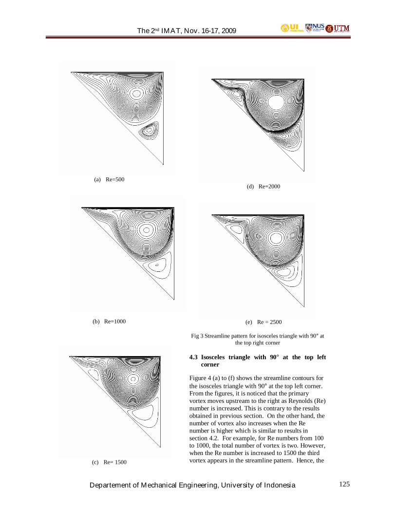
The 2nd IMAT, Nov. 16-17, 2009
Departement of Mechanical Engineering, University of Indonesia 125
(a) Re=500
(b) Re=1000
(c) Re= 1500
(d) Re=2000
(e) Re = 2500
Fig 3 Streamline pattern for isosceles triangle with 90° atthe top right corner
4.3 Isosceles triangle with 90° at the top leftcorner
Figure 4 (a) to (f) shows the streamline contours forthe isosceles triangle with 90° at the top left corner.From the figures, it is noticed that the primaryvortex moves upstream to the right as Reynolds (Re)number is increased. This is contrary to the resultsobtained in previous section. On the other hand, thenumber of vortex also increases when the Renumber is higher which is similar to results insection 4.2. For example, for Re numbers from 100to 1000, the total number of vortex is two. However,when the Re number is increased to 1500 the thirdvortex appears in the streamline pattern. Hence, the
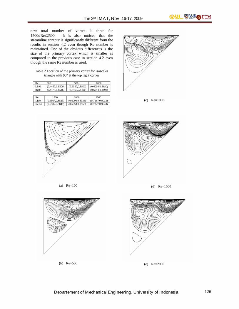
The 2nd IMAT, Nov. 16-17, 2009
Departement of Mechanical Engineering, University of Indonesia 126
new total number of vortex is three for1500≤Re≤2500. It is also noticed that thestreamline contour is significantly different from theresults in section 4.2 even though Re number ismaintained. One of the obvious differences is thesize of the primary vortex which is smaller ascompared to the previous case in section 4.2 eventhough the same Re number is used.
Table 2 Location of the primary vortex for isoscelestriangle with 90° at the top right corner
Re 100 500 1000LBM (0.4450,0.8500) (0.5550,0.8500) (0.6050,0.8650)Ref[4] (0.4473,0.8516) (0.5469,0.8496) (0.6094,0.8691)
Re 1500 2000 2500LBM (0.6567,0.8833) (0.6900,0.8933) (0.7167,0.9033)Ref[4] (0.6582,0.8848) (0.6953,0.8965) (0.7227,0.9043)
(a) Re=100
(b) Re=500
(c) Re=1000
(d) Re=1500
(e) Re=2000
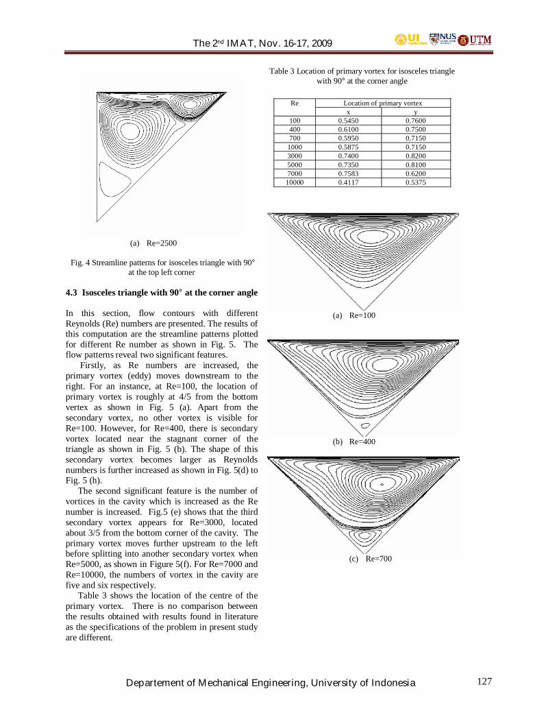
The 2nd IMAT, Nov. 16-17, 2009
Departement of Mechanical Engineering, University of Indonesia 127
(a) Re=2500
Fig. 4 Streamline patterns for isosceles triangle with 90°at the top left corner
4.3 Isosceles triangle with 90° at the corner angle
In this section, flow contours with differentReynolds (Re) numbers are presented. The results ofthis computation are the streamline patterns plottedfor different Re number as shown in Fig. 5. Theflow patterns reveal two significant features.
Firstly, as Re numbers are increased, theprimary vortex (eddy) moves downstream to theright. For an instance, at Re=100, the location ofprimary vortex is roughly at 4/5 from the bottomvertex as shown in Fig. 5 (a). Apart from thesecondary vortex, no other vortex is visible forRe=100. However, for Re=400, there is secondaryvortex located near the stagnant corner of thetriangle as shown in Fig. 5 (b). The shape of thissecondary vortex becomes larger as Reynoldsnumbers is further increased as shown in Fig. 5(d) toFig. 5 (h).
The second significant feature is the number ofvortices in the cavity which is increased as the Renumber is increased. Fig.5 (e) shows that the thirdsecondary vortex appears for Re=3000, locatedabout 3/5 from the bottom corner of the cavity. Theprimary vortex moves further upstream to the leftbefore splitting into another secondary vortex whenRe=5000, as shown in Figure 5(f). For Re=7000 andRe=10000, the numbers of vortex in the cavity arefive and six respectively.
Table 3 shows the location of the centre of theprimary vortex. There is no comparison betweenthe results obtained with results found in literatureas the specifications of the problem in present studyare different.
Table 3 Location of primary vortex for isosceles trianglewith 90° at the corner angle
Re Location of primary vortexx y
100 0.5450 0.7600400 0.6100 0.7500700 0.5950 0.7150
1000 0.5875 0.71503000 0.7400 0.82005000 0.7350 0.81007000 0.7583 0.620010000 0.4117 0.5375
(a) Re=100
(b) Re=400
(c) Re=700

The 2nd IMAT, Nov. 16-17, 2009
Departement of Mechanical Engineering, University of Indonesia 128
(a) Re=1000
(b) Re=3000
(c) Re=5000
(d) Re=7000
(e) Re=10000
5. CONCLUSION
In general, the flow in a triangular cavity issimilar to the flow in a square cavity in terms ofits physical flows Ribben et al [6]. In this paper,Lattice Boltzmann method (LBM) was used toinvestigate the steady fluid in a triangulardriven cavity. The numerical scheme usedproved to be reliable and able to provide steadysolution for various Reynolds numbers. Inaddition to that, the scheme is also moreefficient in terms of time consumption.Although our calculation stopped at Re=10000,the numerical solution could be carried out forhigher Re without any problem.
Apart from that, it is obvious from theresults obtained that the fluid flow behavedsignificantly different as the Reynolds numberincreased. In addition to that, the streamlinepatterns show that the flow structures in atriangular cavity are significantly affected bythe geometry of the triangle.
.ACKNOWLEDGMENTS
The authors would like to thank UniversitiTeknologi Malaysia and the Malaysian governmentfor supporting this research activity.
Nomenclature
acf(x,c,t)fifieq
ReTtU
AccelerationMicro velocity vectorDensity distribution functionDiscretized density distribution functionDiscretized equilibrium density distributionfunctionReynolds number (=UbDh/ν)Local mean temperature [K]timeHorizontal velocity of top plate
The 2nd IMAT, Nov. 16-17, 2009
Departement of Mechanical Engineering, University of Indonesia 129
Ui
ρ
Mean velocity components (i=1, 2, 3)kinematic viscosityFluid DensityTime relaxationCollision operator
REFERENCES
[1] Ghia, U., K.N., Ghia and C.Y., Shin, 1982,“High Re Solutions for incompressible Flowusing the Navier-Stokes Equations and aMultigrid Method”, Journal of ComputationalPhysics,Vol 48, pp. 387-411.
[2] Erturk,E., Corke., and Gokcol, O., 2005,“Numerical Solutions of 2-D SteadyIncompressible Driven Cavity Flow at HighReynolds Numbers”, International Journal forNumerical Methods in Fluids, Vol. 48, pp. 747-774.
[3] Albensoeder, S., and Kuhlmann, H.C.,2005,“Accurate three-dimensional lid-driven cavityflow”,Journal of Computational Physics, Vol.206, pp. 536-558.
[4] Erturk, E., and Gokcol, O., 2007, “Fine gridnumerical solutions of triangular cavity flow”,The European Physical Journal Applied Physics,Vol. 38, pp. 97-105.
[5] Li, M., and Tang, T., 1996, “Steady ViscousFlow in a Triangular Cavity by EfficientNumerical Techniques”. ComputersMathematics Application, Vol. 31, No 10, pp.55-65.
[6] Ribbens, C.J., Watson, L.T., Wang, C.Y.,1992,“Steady Viscous Flow in a Triangular Cavity”,Journal of Computational Physics, Vol. 112.
[7] Sukop, M.C and Thorne, D.T., 2006, LatticeBoltzmann Modeling : An introduction forgeoscientists and engineers, Springer, NewYork.
[8] Nor Azwadi C.S and T, Tanahashi, 2006,“Simplified Thermal Lattice Boltzmann inIncompressible Limit”, International Journal ofModern Physics, B 20, pp.2437-2449.
[9] Succi, S.,2001, The Lattice Boltzmann Equationfor fluid dynamics and beyond, Oxford SciencePublications, New York.
[10] Hou, S., Q., Zou, S., Chen and G., Doolen,1995, “Simulation of Cavity Flow by the latticeBoltzmann Method”, Journal of ComputationalPhysics, Vol. 118, pp. 329-347.
[11] Nor Azwadi C.S and T, Tanahashi, 2007,“Three-Dimensional Thermal Lattice BoltzmansSimulation of Natural Convection in a CubicCavity”, International Journal of ModernPhysics, B 21, pp.87-96.
[12] Bhatnagar, P. L., E. P., Gross, and M., Krook,1954, “A Model for Collision Processes inGasses. 1. Small Amplitude Processes in
Charged and Neutral One-Component System”,Physics Review 94, pp. 511–525.
[13] Nor Azwadi C.S and T, Tanahashi, 2008,“Simplified Finite Difference Thermal LatticeBoltzmann Method”, International Journal ofModern Physics, B 22, pp. 3865-3876.
[14] Dawson, S.P., S., Chen and G., Doolen, 1993,“Lattice Boltzmann Computations for Reaction-Diffusion Equations”, Journal of ChemicalPhysics, Vol. 98, pp. 1514-1523.
[15] Frish, U., B., Hasslacher, and Y., Pomeau, 1986,“Lattice Gas Automata for the Navier-StokesEquation”, Physics Review Letter, Vol. 56, pp.1505-1508.
[16] Gladrow, D.W, 2000, “Lattice Gas CellularAutomata and Lattice Boltzmann Models”,Springer Verlag, New York.
[17] He, X. and L.S., Luo, 1997, “Lattice BoltzmannModel for the Incompressible Navier-StokesEquation”, Journal of Statistical Physics, Vol.88, pp.927-944.
[18] Luo, L.S. and X., He, 1997, “A PrioriDerivation of the Lattice Boltzmann Equation”,Physics Review, E 56, pp. 6811-6817.

The 2nd IMAT, Nov. 16-17, 2009
Departement of Mechanical Engineering, University of Indonesia 130
Design and Fabrication of a 200N Thrust Rocket Motor Basedon NH4ClO4 + Al + HTPB as Solid Propellant
Mastura Ab Wahid*, Wan Khairuddin Wan Ali
Department of Aeronautics, Faculty of Mechanical Engineering,Universiti Teknologi Malaysia, 81310 UTM Skudai, Johor, Malaysia.
ABSTRACT
The development of rocket motor usingpotassium nitrate, carbon and sulphur mixturehas successfully been developed byresearchers and students from UTM andrecently a new combination for solidpropellant is being created. The new solidpropellant will combine a composition ofAmmonium perchlorate, NH4ClO4 withaluminium, Al and Hydroxyl TerminatedPolybutadiene, HTPB as the binder. It is theaim of this research to design and fabricate anew rocket motor that will produce a thrust of200N by using this new solid propellant. Astatic test is done to obtain the thrust producedby the rocket motor and analyses byobservation and also calculation will be done.The experiment for the rocket motor issuccessful but the thrust did not achieve itsrequired thrust.
1. INTRODUCTION
There are many rockets that have beenmanufactured by advanced countries and some ofthem are, the famous Apollo 13, Discovery, AtlasCentaur and many more. All these rockets usedifferent energy source such as chemical, nuclearand solar. As a developing country, Malaysia also islearning to develop its own technology. UniversitiTeknologi Malaysia, UTM, is one of the institutionsthat is trying to develop rockets using solidpropellant. For each composition of propellant thereis an optimum configuration for the design of itsrocket motor. UTM before this had successfullydeveloped rocket motor using potassium nitrate andsucrose (KS) and now a new composition of solidpropellant using Ammonium Perchlorate,(NH4CLO4), Aluminum and HTPB as the binder isbeing developed. It is only natural that a new rocketmotor should be designed and fabricated in order totest this new propellant.
2. METHODOLOGY
In order to calculate the design of a rocketmotor using ammonium perchlorate (AP) +aluminum (AL) + HTPB, few parameters have to beobtained first. They are the specific impulse, theburning rate which is found from the strand burnertest, the composition of the chemicals, the chambertemperature which the burning temperature of thepropellant, the molar mass which is obtained fromthe chemical composition calculation, the totaldensity of the propellant, the molecular mass, thecharacteristic exhaust velocity and also the exhaustcoefficient.
To get this value, software called CHEM isused. This software uses a few basic assumptions tocalculate the parameters stated above. One of itsassumptions is that the vehicle or rocket exitpressure is equal to the ambient pressure to get theoptimum expansion ratio. The chamber pressure isset to be 500psi and the burning time is 3 seconds.The composition of the solid propellant which willbe inputted in CHEM is as shown in table 2.1 andthe result obtained from CHEM is shown in table2.2. By using the value in table 2.2, the designdimension can be calculated by applying the rocketmotor theory. Table 2.3 shows the finalconfiguration of the rocket motor. Table 2.4 showsthe total stress and safety factor for the casing of therocket motor.
Table 2.1: Composition of the propellant
Chemical Composition(%)
AmmoniumPerchlorate 66
Aluminum (Al) 21HTPB 13
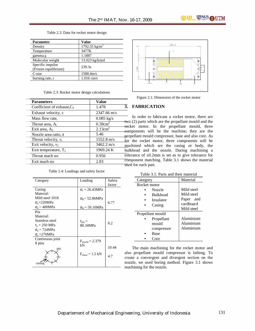
The 2nd IMAT, Nov. 16-17, 2009
Departement of Mechanical Engineering, University of Indonesia 131
Unit in
NozzCaBulkhe Insul
Propell
Table 2.2: Data for rocket motor design
Parameter ValueDensity 1792.55 kg/m3
Temperature 3477Kgamma,γ 1.1887Molecular weight 13.023 kg/kmolSpecific impulse(Frozen equilibrium) 239.3s
C-star 1588.4m/sburning rate, r 1.016 cm/s
Table 2.3: Rocket motor design calculations
Parameters ValueCoefficient of exhaust,CF 1.478Exhaust velocity, c 2347.66 m/sMass flow rate, 0.085 kg/sThroat area, At 0.39cm2
Exit area, A2 2.13cm2
Nozzle area ratio, ε 5.46Throat velocity, vt 1552.8 m/sExit velocity, v2 3462.2 m/sExit temperature, T2 1969.24 KThroat mach no 0.956Exit mach no 2.83
Table 2.4: Loadings and safety factor
Category Loading Safetyfactor
CasingMaterial:Mild steel 1018σy=220MPaσu = 400MPa
σl = 26.43MPa
σθ = 52.86MPa
σR = 59.10MPa6.77
PinMaterial:Stainless steelτy = 250 MPaσu = 724MPaσy =276MPa
τpin =88.34MPa 8.2
Continuous joint8 pins Ftensile = 2.379
kN
Fshear = 1.5 kN
10.44
4.7
Figure 2.1: Dimension of the rocket motor
3. FABRICATION
In order to fabricate a rocket motor, there aretwo (2) parts which are the propellant mould and therocket motor. In the propellant mould, threecomponents will be the machine; they are thepropellant mould compressor, base and also core. Asfor the rocket motor, three components will bemachined which are the casing or body, thebulkhead and the nozzle. During machining atolerance of ±0.2mm is set as to give tolerance forcomponent matching. Table 3.1 shows the materialused for each part.
Table 3.1: Parts and their materialCategory MaterialRocket motor
• Nozzle• Bulkhead• Insulator• Casing
Mild steelMild steelPaper andcardboardMild steel
Propellant mould• Propellant
mouldcompressor
• Base• Core
AluminiumAluminiumAluminium
The main machining for the rocket motor andalso propellant mould compressor is lathing. Tocreate a convergent and divergent section on thenozzle, we used boring method. Figure 3.1 showsmachining for the nozzle.
casing
pin
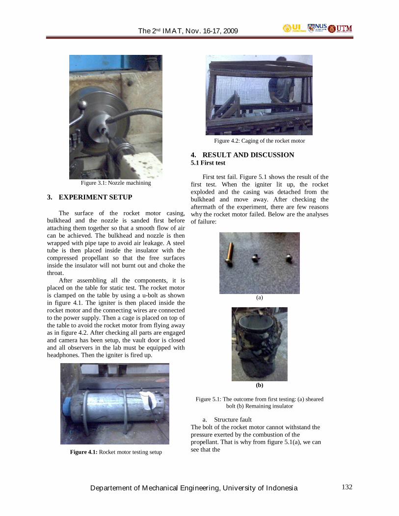
The 2nd IMAT, Nov. 16-17, 2009
Departement of Mechanical Engineering, University of Indonesia 132
Figure 3.1: Nozzle machining
3. EXPERIMENT SETUP
The surface of the rocket motor casing,bulkhead and the nozzle is sanded first beforeattaching them together so that a smooth flow of aircan be achieved. The bulkhead and nozzle is thenwrapped with pipe tape to avoid air leakage. A steeltube is then placed inside the insulator with thecompressed propellant so that the free surfacesinside the insulator will not burnt out and choke thethroat.
After assembling all the components, it isplaced on the table for static test. The rocket motoris clamped on the table by using a u-bolt as shownin figure 4.1. The igniter is then placed inside therocket motor and the connecting wires are connectedto the power supply. Then a cage is placed on top ofthe table to avoid the rocket motor from flying awayas in figure 4.2. After checking all parts are engagedand camera has been setup, the vault door is closedand all observers in the lab must be equipped withheadphones. Then the igniter is fired up.
Figure 4.1: Rocket motor testing setup
Figure 4.2: Caging of the rocket motor
4. RESULT AND DISCUSSION5.1 First test
First test fail. Figure 5.1 shows the result of thefirst test. When the igniter lit up, the rocketexploded and the casing was detached from thebulkhead and move away. After checking theaftermath of the experiment, there are few reasonswhy the rocket motor failed. Below are the analysesof failure:
(a)
(b)
Figure 5.1: The outcome from first testing: (a) shearedbolt (b) Remaining insulator
a. Structure faultThe bolt of the rocket motor cannot withstand thepressure exerted by the combustion of thepropellant. That is why from figure 5.1(a), we cansee that the

The 2nd IMAT, Nov. 16-17, 2009
Departement of Mechanical Engineering, University of Indonesia 133
i. bolt is sheared due to highpressure.
ii. There are air leakages. The casingof the rocket motor is not totally acircular tube therefore there areareas which are air-tight and someare air-leak areas.
b. Chokingi. The insulator is made of paper and
when it is burnt it traps the flow ofthe air at the throat. This causeschoking and as a result the airinside pushed the bulkheadforward but the escaped airpushed the whole casingbackward. Therefore, the highpressure causes the bolt to shear.
ii. Figure 5.1(b) shows the finalcondition of the insulator ofburning complete. The crumbs ofthe paper follow the flame flowand chocked the throat.
c. Propellant temperaturei. Before testing, the propellant must
be cured in an oven. For the firsttest the propellant is used directlyfrom the oven and inserted insidethe rocket motor casing. Thiscauses the initial temperature ofthe propellant to be high andcauses the chamber pressure toincrease too.
For the second test, some changes are made to therocket motor and they are:
a. The throat diameter is enlarged to 16mm toavoid choking.
b. The bolt is changed from steel bolt tostainless steel bolt and the diameter from5mm to 8mm.
c. Type of bolt is change from normal tocountersunk bolt.
3.2 Second Test5.2.1 Observation analysis for the second test
The static test was successful. Figure 5.3 belowshows the rocket motor ignition. As shown fromfigure 5.3, the burning rate obtained from theobservation is 7.6s. As can be seen at time, t=8.00 sthe flames produced are due to the burning ofinsulator paper and not the propellant.Nozzle condition:
As shown in figure 5.4, there is a crust formedon the throat area. This may be also the reason ofchoking for the first test. The initial diameter of
throat is 16mm and after the crust had envelope thenozzle throat, the throat diameter is reduced to11mm. This crust was formed due to excess used ofaluminium. This may result in choking if the nozzlethroat diameter is meant for Mach number 1. Inorder to avoid the blockage, the throat should beenlarged to about 20 – 30 % from the calculateddiameter.
Figure 5.3: Timeline of propellant burning
(a)
(b)
Figure 5.4: Condition inside the nozzle
5.2.2 Numerical Analysis
As mention before the propellant used is less than itsupposed to, therefore the performance for therocket motor can be estimated by back calculations.From the experiment, the value of density of thepropellant and the mass flow rate can be obtained.After obtaining these values, the
t =0s t =0.72s
t =7.6st =2.560s
t =8.00s
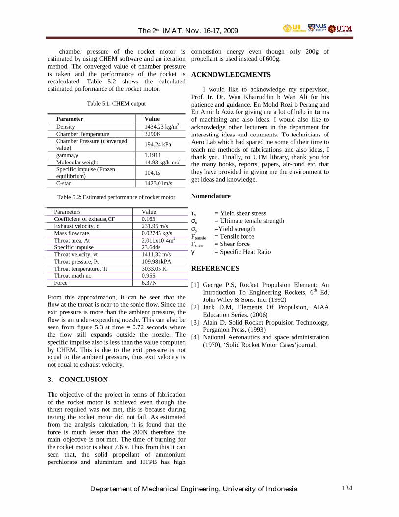
The 2nd IMAT, Nov. 16-17, 2009
Departement of Mechanical Engineering, University of Indonesia 134
chamber pressure of the rocket motor isestimated by using CHEM software and an iterationmethod. The converged value of chamber pressureis taken and the performance of the rocket isrecalculated. Table 5.2 shows the calculatedestimated performance of the rocket motor.
Table 5.1: CHEM output
Parameter ValueDensity 1434.23 kg/m3
Chamber Temperature 3290KChamber Pressure (convergedvalue) 194.24 kPa
gamma,γ 1.1911Molecular weight 14.93 kg/k-molSpecific impulse (Frozenequilibrium) 104.1s
C-star 1423.01m/s
Table 5.2: Estimated performance of rocket motor
Parameters ValueCoefficient of exhaust,CF 0.163Exhaust velocity, c 231.95 m/sMass flow rate, 0.02745 kg/sThroat area, At 2.011x10⁻⁴m2
Specific impulse 23.644sThroat velocity, vt 1411.32 m/sThroat pressure, Pt 109.981kPAThroat temperature, Tt 3033.05 KThroat mach no 0.955Force 6.37N
From this approximation, it can be seen that theflow at the throat is near to the sonic flow. Since theexit pressure is more than the ambient pressure, theflow is an under-expending nozzle. This can also beseen from figure 5.3 at time = 0.72 seconds wherethe flow still expands outside the nozzle. Thespecific impulse also is less than the value computedby CHEM. This is due to the exit pressure is notequal to the ambient pressure, thus exit velocity isnot equal to exhaust velocity.
3. CONCLUSION
The objective of the project in terms of fabricationof the rocket motor is achieved even though thethrust required was not met, this is because duringtesting the rocket motor did not fail. As estimatedfrom the analysis calculation, it is found that theforce is much lesser than the 200N therefore themain objective is not met. The time of burning forthe rocket motor is about 7.6 s. Thus from this it canseen that, the solid propellant of ammoniumperchlorate and aluminium and HTPB has high
combustion energy even though only 200g ofpropellant is used instead of 600g.
ACKNOWLEDGMENTS
I would like to acknowledge my supervisor,Prof. Ir. Dr. Wan Khairuddin b Wan Ali for hispatience and guidance. En Mohd Rozi b Perang andEn Amir b Aziz for giving me a lot of help in termsof machining and also ideas. I would also like toacknowledge other lecturers in the department forinteresting ideas and comments. To technicians ofAero Lab which had spared me some of their time toteach me methods of fabrications and also ideas, Ithank you. Finally, to UTM library, thank you forthe many books, reports, papers, air-cond etc. thatthey have provided in giving me the environment toget ideas and knowledge.
Nomenclature
τy = Yield shear stressσu = Ultimate tensile strengthσy =Yield strengthFtensile = Tensile forceFshear = Shear forceγ = Specific Heat Ratio
REFERENCES
[1] George P.S, Rocket Propulsion Element: AnIntroduction To Engineering Rockets, 6th Ed,John Wiley & Sons. Inc. (1992)
[2] Jack D.M, Elements Of Propulsion, AIAAEducation Series. (2006)
[3] Alain D, Solid Rocket Propulsion Technology,Pergamon Press. (1993)
[4] National Aeronautics and space administration(1970), ‘Solid Rocket Motor Cases’journal.
The 2nd IMAT, Nov. 16-17, 2009
Departement of Mechanical Engineering, University of Indonesia 135
Development of Ammonium Perchlorate + Aluminium BaseSolid Propellant
Norazila Othmana, Wan Khairuddin Wan Alib
Department of Aeronautics, Faculty of Mechanical Engineering, Universiti Teknologi Malaysia,81310 UTM Skudai, Johor, Malaysia
[email protected]@fkm.utm.my
ABSTRACT
Rocket propellant has been identified as acomponent that played an important role in thedevelopment of rockets. The ejected materialin rocket propulsion is due to material calledpropellant. Without propellant, a rocket cannotbe launched. Due to this reason, many havestarted to conduct research on new chemicalcompound of propellant with new technique ifneeded. The objectives of this study are tostudy the thermo-chemistry aspect of thecomposition and to determine the burningcharacteristics parameters. For this reason, thisdissertation presented a detail preparation ofdeveloping a solid propellant usingAmmonium Perchlorate (AP) as an oxidizer,Aluminum (Al) as fuel and HydroxylTerminated Polybutadiene (HTPB) as thebinder. To determine the propellantperformance such as burning rate, testing wasconducted. From testing result the propellantcomposition oxidizer-fuel (76/11) at pressure110 Psi gave the maximum burning rate. Fromtest results the empirical constant, ‘a’ andpressure exponent ‘n’ were calculated for eachdifferent propellant compositions.
KeywordsRockets, solid propellants, AP, Al, HTPB, burningrate, thermo-chemistry, empirical constant, pressureexponent.
1. INTRODUCTION
The design of solid propellant needs to take intoaccount on the composition of the mixture beforeand after the combustion. This is usually dictated bythe total impulse needed. Equation equilibrium is
very important during calculating the heat producedfrom the reaction, temperature in combustionchamber and determining other characteristics of thepropellant, especially when testing the variouscomposition of the compound.
The result from this study will be used todetermine the suitability of the propellant compoundand the method of processing the compound. Fromthe experimental results, the best propellantperformance for any application can be selectedwhich will in turn increase the overall performanceof the rocket. These projects also hope to explorethe various theories involved in rocketry and todiscover the technique and method for preparationand testing of the solid propellant. The difficulty offinding enough information and lacking of adatabase will hopefully be addressed from thisstudy.
2. METHODOLOGY
Theoretical analyses have been conducted on the AP+ Al mixture to obtain the chemical formula,characteristic formula, molecular weight,stoichiometric ratio, specific heat gas ratio, reactionequation, characteristic velocity, effective exhaustvelocity, and thrust force coefficient. Analyses weredone using theoretical calculations and the computerprogram CHEM.Propellants were prepared using the compressionmethod, which was found to be the most suitablemethod to obtain a more compact propellant. Thismethod enables the removal of almost all of thetrapped air inside the propellant grains, leavingonly less than five percent behind. The absence ofair bubbles would produce a low burning-rate andhigh mass propellant as desired [3]. An in-housedesigned and constructed propellant test rig wasused for burning-rate tests at atmospheric pressure.The test rig consists of propellant stand, igniter, andautomatic timer. From the burning-rate tests atatmospheric pressure, burning-rate data wereobtained. In general, propellant performance can be

The 2nd IMAT, Nov. 16-17, 2009
Departement of Mechanical Engineering, University of Indonesia 136
approximated from burning-rate data at differentpressures.
3. THEORITICAL
The products of AP, Al and HTPB reaction wasassumed to consist of ten products. During thereaction the assumptions taken were [1]:
a. The reaction was only between AP, Al andHTPB.
b. CO, H2, Al2O3, N2, HCI, H, H2O, AlCl, Cl,and CO2 were assumed the only product ofthe reaction process. Other componentswere ignored to simplify the calculationanalysis.
The law of conservation of energy states that theenthalpy of the reactants is equal to the enthalpy ofthe products.
[ ] [ ]∑∑ ∆+=∆+oducts
efetsac
ifi hhnhhnPrtanRe
Burning rate test was conducted to determine theperformance of the propellant where it is usuallyexpressed in cm/sec, mm/sec and known as burningrate, r. The commonly accepted formula to calculatethe burning rate is given by [2]:
napr =
4. PROPELLANT FABRICATION
Procedure for the preparation of AmmoniumPerchlorate composite propellant (APCP) compoundincludes the properties and thermo-chemistrycharacteristic of each ingredient which are AP, Aland HTPB.
Figure 1: Propellant fabrication
The propellant was pour into the propellant grainmold and compressed. After a uniform propellantcompound has been produced, it can then beinserted to the propellant casing. The empty casingwhich is the mold for the grain is inserted into acylinder retainer to support the mold when it issubjected to compression forces.The prepared compound was poured into the casingin a small amount at an each time and wascompressed between each pouring using a cylinderrod. When the casing is nearly full, care must betaken to prevent any spillage of the dangerousmaterial. The compression during this stage must bedone slowly and carefully. The compression mouldmethod is chosen to produce the propellant variants
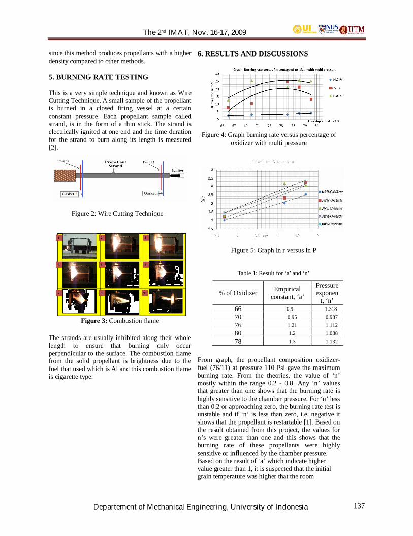
The 2nd IMAT, Nov. 16-17, 2009
Departement of Mechanical Engineering, University of Indonesia 137
since this method produces propellants with a higherdensity compared to other methods.
5. BURNING RATE TESTING
This is a very simple technique and known as WireCutting Technique. A small sample of the propellantis burned in a closed firing vessel at a certainconstant pressure. Each propellant sample calledstrand, is in the form of a thin stick. The strand iselectrically ignited at one end and the time durationfor the strand to burn along its length is measured[2].
Figure 2: Wire Cutting Technique
Figure 3: Combustion flame
The strands are usually inhibited along their wholelength to ensure that burning only occurperpendicular to the surface. The combustion flamefrom the solid propellant is brightness due to thefuel that used which is Al and this combustion flameis cigarette type.
6. RESULTS AND DISCUSSIONS
Figure 4: Graph burning rate versus percentage ofoxidizer with multi pressure
Figure 5: Graph ln r versus ln P
Table 1: Result for ‘a’ and ‘n’
% of Oxidizer Empiricalconstant, ‘a’
Pressureexponen
t, ‘n’66 0.9 1.31870 0.95 0.98776 1.21 1.11280 1.2 1.08878 1.3 1.132
From graph, the propellant composition oxidizer-fuel (76/11) at pressure 110 Psi gave the maximumburning rate. From the theories, the value of ‘n’mostly within the range 0.2 - 0.8. Any ‘n’ valuesthat greater than one shows that the burning rate ishighly sensitive to the chamber pressure. For ‘n’ lessthan 0.2 or approaching zero, the burning rate test isunstable and if ‘n’ is less than zero, i.e. negative itshows that the propellant is restartable [1]. Based onthe result obtained from this project, the values forn’s were greater than one and this shows that theburning rate of these propellants were highlysensitive or influenced by the chamber pressure.Based on the result of ‘a’ which indicate highervalue greater than 1, it is suspected that the initialgrain temperature was higher that the room
The 2nd IMAT, Nov. 16-17, 2009
Departement of Mechanical Engineering, University of Indonesia 138
temperature. It was suggested that in betweentesting the Crawford bomb should be allowed tocool down to room temperature and less than onelower than room temperature.
The burning rate for each propellantcomposition was depended on the pressure appliedduring compression method. Since the pressureapplied could vary during compression method, itwas advisable to produce three set of samples foreach propellant compositions. This will allow threeburning rate testing to be carried out for eachpropellant composition. Averaging can be done onthe basis of three samples which will reduce anyerror [3].
7. CONCLUSIONS
The following conclusions can be drawn based onthe findings of the study:1. The thermochemistry study can be determined
by using the thermochemical data from JANAFTermochemical Table.
2. The parameters that influence the burning rateare chamber pressure, particle size of oxidizer,initial temperature of the propellant, and O/Fratio.
ACKNOWLEDGMENT
Firstly, I would like to express my heartiestappreciation to Prof. Dr. Ir. Wan Khairuddin B.Wan Ali for providing the guidelines beforecompleting this thesis. He is so dedicated for givingme a lot of advices and taught me the methodologyfor the development of solid propellant.
Lastly, thank you to my college under samesupervisor who incessantly shared their informationand perception, especially my closed friendRosmaliza Mat Yaacob and others, such as Mastura,Alif Hafifi, Khairul, Shahrul Ikhwan, Mr. AmirAziz, a master student and Mr. Mohd Rozi Perang, aResearch Officer for sharing their ideas andsuggestions that helped me so much to complete thisthesis.
REFERENCES
[1] Naminosuke Kubota, (2007), Propellants andExplosives, 2nd Edition, Wiley-VCH
[2] Sutton, G.P and Oscar Biblarz, 7th Ed. (2001),Rocket Propulsion Element, John Wiley & Sons,MIT.
[3] Rizalman Mamat (2002), Ciri-ciri PropelanRoket Pepejal Berasaskan Kalium, UniversitiTeknologi Malaysia, Tesis sarjana.

The 2nd IMAT, Nov. 16-17, 2009
Departement of Mechanical Engineering, University of Indonesia 139
Reduction of Time Consumption For Simulating Lid-DrivenCavity Flow Using Lattice Boltzmann Method (LBM)
H. M. Faizala, C. S. Nor Azwadib
aFaculty of Mechanical Engineering,Universiti Teknologi Malaysia,
81310 UTM Skudai, Johor, [email protected]
bFaculty of Mechanical Engineering,Universiti Teknologi Malaysia,
81310 UTM Skudai, Johor, [email protected]
ABSTRACT
2-D driven cavity flow is the widely studiedbenchmark problem by many researchers ofcomputational fluid dynamics field in terms ofaccuracy, numerical efficiency and others. LatticeBoltzmann Method (LBM) is one of thenumerical methods for simulating this type offlow. For solving cavity flow with high ReynoldsNumber, the saving in time consumption is reallyappreciated. Therefore, as the initial study,averaging method for reducing CPU time hasbeen proposed for solving lid driven cavity flowwith low Reynolds Number. The results show thatthe averaging method can save time consumed forsimulation. For instance, in the case of ReynoldsNumber 80, the proposed averaging method cansave about 12% of the original CPU time (withoutaveraging method).
Keywordslid driven cavity, Lattice Boltzmann Method,averaging method
1. INTRODUCTION
The simplicity of the geometry makes the liddriven cavity flow problem is one of the moststudied fluid problems by researchers. In addition,it is easy to code and easy to apply boundaryconditions. Even though the problem lookssimple in many ways, the flow in a cavity retainsall the flow physics with counter rotating vorticesappear at the corners of the cavity.
There are many researchers already made theirresearches on the lid-driven cavity flow with highReynolds Number. For instance, Erturk et. al. ,Erturk & Gokcol, Barragy & Carey , Schreiber &
Keller , Benjamin & Denny , Liao & Zhu , Ghiaet. al. have presented solutions of steady 2-Dincompressible flow in a driven cavity for Re10,000. Among these researchers, Barragy &Carey have also presented solutions forRe=12,500. Moreover, Erturk et. al. and alsoErturk & Gokcol have presented steady solutionsup to Re=20,000 [2].
The above studies are all numerical studies. Thereare very few experimental studies in the literatureon the driven cavity flow. Koseff & Street, Prasad& Koseff have done several experiments on threedimensional driven cavity with various spanwiseaspect ratios (SAR). These experimental studiespresent valuable information about the physics ofthe flow in a driven cavity.
A simulation of incompressible viscous flowwithin a two-dimensional (2D) square cavity byusing Lattice Boltzmann method (LBM) had beendone by Arumuga D. P. et. al with variety ofReynolds numbers [1]. The samples of result fromtheir simulation are shown as below.
Figure 1. Re 1000 Figure 2. Re 3200
Figure 3. Re 5000 Figure 4. Re 7500
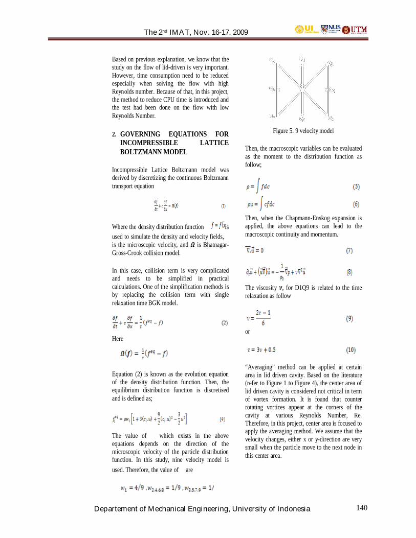
The 2nd IMAT, Nov. 16-17, 2009
Departement of Mechanical Engineering, University of Indonesia 140
Based on previous explanation, we know that thestudy on the flow of lid-driven is very important.However, time consumption need to be reducedespecially when solving the flow with highReynolds number. Because of that, in this project,the method to reduce CPU time is introduced andthe test had been done on the flow with lowReynolds Number.
2. GOVERNING EQUATIONS FORINCOMPRESSIBLE LATTICEBOLTZMANN MODEL
Incompressible Lattice Boltzmann model wasderived by discretizing the continuous Boltzmanntransport equation
Where the density distribution function isused to simulate the density and velocity fields,is the microscopic velocity, and is Bhatnagar-Gross-Crook collision model.
In this case, collision term is very complicatedand needs to be simplified in practicalcalculations. One of the simplification methods isby replacing the collision term with singlerelaxation time BGK model.
Here
Equation (2) is known as the evolution equationof the density distribution function. Then, theequilibrium distribution function is discretisedand is defined as;
The value of which exists in the aboveequations depends on the direction of themicroscopic velocity of the particle distributionfunction. In this study, nine velocity model isused. Therefore, the value of are
Figure 5. 9 velocity model
Then, the macroscopic variables can be evaluatedas the moment to the distribution function asfollow;
Then, when the Chapmann-Enskog expansion isapplied, the above equations can lead to themacroscopic continuity and momentum.
The viscosity , for D1Q9 is related to the timerelaxation as follow
or
“Averaging” method can be applied at certainarea in lid driven cavity. Based on the literature(refer to Figure 1 to Figure 4), the center area oflid driven cavity is considered not critical in termof vortex formation. It is found that counterrotating vortices appear at the corners of thecavity at various Reynolds Number, Re.Therefore, in this project, center area is focused toapply the averaging method. We assume that thevelocity changes, either x or y-direction are verysmall when the particle move to the next node inthis center area.

The 2nd IMAT, Nov. 16-17, 2009
Departement of Mechanical Engineering, University of Indonesia 141
For averaging method, the formula is given as below.
where k is direction, i is coordinate at x-direction andj is coordinate at y-direction.
2. ALGROTIHMS
Figure 8. Simulation Algorithm When “Averaging”Method Included
“Averaging” method is utilized between “collision”and “boundary condition”. The nodes with theaverage value of density distribution function will beused to the next procedure until convergenceconsideration. If converge, the data of these nodes areused as simulation results. If the simulation does notconverge yet, the data of these nodes will be used forthe next iterations.
3. SIMULATION PARAMETER
The configuration of the cavity flow consists of a 2-Dsquare cavity which top plate moves from left to rightdirection with a uniform velocity. Meanwhile, theother walls are fixed. The velocity components
and are in x and y-direction respectively. In
this study, the simulation is done on 32 x 32 latticeunits. Initially, the velocity at all nodes, except thetop plate, is set to zero. The x-velocity of the topplate is U=0.1 and the y-velocity is zero. Uniformfluid density is used, which 1.0 and is imposedinitially. The equilibrium distribution is calculatedusing Equation (4) and is set equal to for all
node at t=0. The distribution function can be foundby a succession of propagation and collisionprocesses. Then, “averaging” method is applied to thecenter area (bounded with four edges point: (9,11),(9,25), (25,11) and (25,25)). By utilizing this method,the CPU time until equilibrium is achieved can bereduced slightly. At the end of each process, thedistribution function is set to equilibrium state. In thissimulation, no slip velocity condition is implementedand bounce-back boundary condition is used on allthe walls. When a fluid particle encounters an objectsuch as wall or other particles, the collision occursand the fluid particle is simple rebounded off theobject in the direction it originated. This phenomenonis called bounce-back boundary condition. Thevelocity components are obtained through thecalculation of particle distribution function. Thissimulation is validated with previous study which hasbeen done by Ghia for Reynolds Number 100.Meanwhile, the reduction of time consumption iscalculated for the case of Reynolds Number 100 and80 by comparing it with the results obtained fromalgorithm without “averaging” method.
Figure 6. Beforemodification
Figure 7. Aftermodification

The 2nd IMAT, Nov. 16-17, 2009
Departement of Mechanical Engineering, University of Indonesia 142
4. RESULTS AND DISCUSSION
5.1 Validation of Results
From the Figure 9 above, the x-velocity obtainedfrom the modified case (using “Averaging” method)shows much agreement with the result by Ghia(1982) except for certain locations (from y/H:0.3 toy/H:0.7) which show slightly different.
Based on Figure 10, the y-velocity obtained frommodified case shows much agreement with the resultfrom Ghia (1982). All the points seems overlap toeach other except at about x/L : 0.2 to x/L : 0.3. Thisshows that “averaging” method is suitable forsimulation especially for low Reynolds Number, Re.However, for simulating the high Re, further study isnecessary in order to ensure that this “averaging”method able to produce accurate result even thoughat disorganized or chaotic flow.
5.2 Reduction of Time Consumption
Figure 11 and Figure 12 show patterns of plot whichare almost same for both cases (original case andmodified case). In addition, the CPU time can besaved until almost 21%.
Based on Figure 14, the plot pattern for both cases(before and after modification) show the similar
shape. Besides that, based on Figure 15, the value ofx-velocity for modified case is also slightly differentif compared with the value for original case. WhenReynolds Number increased becomes higher, thedifference between plots for both cases clearly can beobserved especially for x-velocity. Due to thematters, it is expected the increase in mesh numbermay give more accurate result. As information, thereduction of time consumption for Reynolds Number80 is about 12%.
Figure 9. Result Validation for Ux velocity
Figure 10. Result Validation for Uy velocity
For Re 100
Before [CPUtime] After [CPU time] Improvement[%]
168.1379 133.2841 20.72930018
Figure 11. Result for Ux velocity
Table 13. CPU time for Before and AfterModification
Figure 14. Result for Ux velocity

The 2nd IMAT, Nov. 16-17, 2009
Departement of Mechanical Engineering, University of Indonesia 143
5. CONCLUSION
“Averaging” method has been used to simulate thelid-driven cavity with low Reynolds Number, Re. Itseems very effective in reducing the timeconsumption especially for low Re. When Rebecomes higher, the difference of result appears ifcompared between the modified case and originalcase. It is expected that these differences can bereduced by increasing the mesh used in simulation.
Finally, future works are still needed to ensure thatLattice Boltzmann Method (LBM) can simulate thelid-driven cavity flow with high Reynolds Numberaccurately.
ACKNOWLEDGMENTS
The authors acknowledge the Universiti TeknologiMalaysia for giving cooperation and full of support inthis research activity.
NOMENCLATURE
yxL
H
U
Location in y-axisLocation in x-axisTotal length in x-directionTotal height in y-directionx-velocity of top plate
ReUx
Uy
ρ
Reynolds NumberVelocity in x-directionVelocity in y-directionFluid Density
References
[1] Arumuga, D. P., Anoop K. D.. “IncompressibleViscous Flow Simulation in the Lid-Driven Cavity byLattice Boltzmann Method”, Indian Institute ofTechnology Guwahati.
[2] Ercan Erturk [2008]. “Discussion on DrivenCavity Flow”, Int. Journal for Numerical Methods inFluids (2008)
[3] Albensoeder, S., Kuhlmann, H.C.[2005].“Accurate three-dimensional lid-driven cavity flow”,Journal of Computational Physics 206, 536-–558.
[4] Abouhamza, A., Pierre, R. [2003]. “A NeutralStability Curve for Incompressible Flows in aRectangular Driven Cavity”, Mathematical andComputer Modelling 38, 141-157.
[5] Nor Azwadi Bin Che Sidik [2007]. “TheDevelopment of Simplified Thermal LatticeBoltzmann Models for the Simulation of ThermalFluid Flow Problems”, phD Thesis 2007.
[6] H.M. Faizal, C.S.N. Azwadi [2008]. “InitialStudy on Flow Behaviour Around Four CircularCylinders with Different Reynolds Number by UsingLattice Boltzmann Scheme”, International GraduateConference on Engineering and Science 2008.
For Re 80
Before [CPUtime]
After [CPUtime]
Improvement[%]
119.4188 105.2695 11.84846942
Figure 15. Result for Uy velocity
Table 16. CPU time for Before and After
Modification

The 2nd IMAT, Nov. 16-17, 2009
Departement of Mechanical Engineering, University of Indonesia 144
Preliminary Numerical Analysis onHelicopter Main-Rotor-Hub Assembly Wake
Iskandar Shah Ishak a, Shuhaimi Mansora,Tholudin Mat Lazima and Muhammad Riza Abd Rahmana
aDepartment of Aeronautical EngineeringFaculty of Mechanical Engineeing
Universiti Teknologi Malaysia81300 Skudai, Johor,Malaysia
ABSTRACT
This research aims to improve basic understandingof the viscous unsteady flow observed behind thehelicopter main-rotor-hub-assembly which may leadto helicopter tail shake phenomenon. The numericalstudy was done at a grace of a commercialComputational Fluid Dynamics (CFD) code,FLUENT on a simplified main-rotor-hub assemblyusing stub blades. In this study, the aerodynamicflow field was computed using the Reynolds-Averaged Navier-Stokes (RANS) equations. TheMultiple Reference Frames (MRF) method wasapplied to simulate the main-rotor-hub-assemblyrotation at 1400 rpm with free stream velocity, orforward flight speed of 5, 20 and 30 m/s at zeroangle of attack, respectively. Results depict at higherfree stream velocity more pressure fluctuations,which could translate to bigger aerodynamic forcesexcitation, occurred at the vicinity of helicopter tailplane.
KeywordsUnsteady flow, helicopter tail shake phenomenon,Computational Fluid Dynamic
1. INTRODUCTION
Helicopter tail shake phenomenon is a long draggedissue that adversely affected the overallperformance, occupants’ comfort and handlingqualities of helicopter. It is an interaction of aturbulent wake with the structure part of tail [1]. Thecontributors of the wake, not the least, are main-rotor-hub assembly, pylon, engine intakes andexhausts. In this research, focus will be on main-rotor-hub assembly’s wake as it is believed to be themajor contributor of the problem [2]. This allowsthe simulation to be conducted using blade-stubsconfiguration [3,4,5]. Blade-stubs configuration is acombination of main-rotor-hub assembly withshorter rotor blades.
2. CFD MODELLING DESCRIPTIONS
Reynolds-Averaged Navier-Stokes (RANS)equation models which solve ensemble-averagedNavier-Stokes equations [6] were used for thiscomputational fluid dynamic study. The simulationswere run at a grace of a 64-bit Core 2 Quadcomputer with Multiple Reference Frames (MRF)approach was applied to simulate the main-rotor-hub-assembly rotation at 1400 rpm.
This numerical investigation used an ellipsoidalfuselage based on NASA standard model [7] withthe axes ratio of longitudinal to lateral axes is 4.485.For this research work, the longitudinal axes weretaken as 1120 mm. A simplified main-rotor-hubassembly with short rotor blades were designed andis shown by Fig. 1.
Fig. 1 Model for CFD analysis
3. RESULTS ANALYSIS
All simulation results presented throughout thispaper were run at main–rotor-hub assembly rotationof 1400 rpm with zero angle of attack. Figures 2 and3 show the path lines of turbulent intensity for 20and 30 m/s of free stream velocity, respectively.They depict the maximum value of turbulentintensity (%) becomes higher with the increment offree stream velocity, or forward flight speed. This isreasonable as higher free stream velocity should
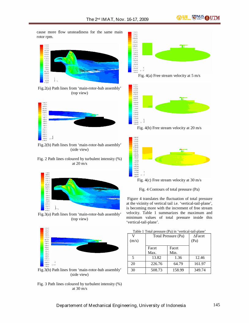
The 2nd IMAT, Nov. 16-17, 2009
Departement of Mechanical Engineering, University of Indonesia 145
cause more flow unsteadiness for the same mainrotor rpm.
Fig.2(a) Path lines from ‘main-rotor-hub assembly’(top view)
Fig.2(b) Path lines from ‘main-rotor-hub assembly’(side view)
Fig. 2 Path lines coloured by turbulent intensity (%)at 20 m/s
Fig.3(a) Path lines from ‘main-rotor-hub assembly’(top view)
Fig.3(b) Path lines from ‘main-rotor-hub assembly’(side view)
Fig. 3 Path lines coloured by turbulent intensity (%)at 30 m/s
Fig. 4(a) Free stream velocity at 5 m/s
Fig. 4(b) Free stream velocity at 20 m/s
Fig. 4(c) Free stream velocity at 30 m/s
Fig. 4 Contours of total pressure (Pa)
Figure 4 translates the fluctuation of total pressureat the vicinity of vertical tail i.e. ‘vertical-tail-plane’,is becoming more with the increment of free streamvelocity. Table 1 summarizes the maximum andminimum values of total pressure inside this‘vertical-tail-plane’.
Table 1 Total pressure (Pa) in ‘vertical-tail-plane’ V(m/s)
Total Pressure (Pa) Facet(Pa)
FacetMax.
FacetMin.
5 13.82 1.36 12.46 20 226.76 64.79 161.97 30 508.73 158.99 349.74
The 2nd IMAT, Nov. 16-17, 2009
Departement of Mechanical Engineering, University of Indonesia 146
Table 1 indicates the range from minimum tomaximum value of total pressure i.e. Facet, islinearly related with free stream velocity. This resulttranslates more aerodynamic forces excitationoccurred with higher forward flight, signalling couldmean more tail shake problem.
3. CONCLUSIONS
This preliminary numerical study has shownsome interesting wake characteristics on helicoptertail shake phenomenon. At a very low free streamvelocity or forward flight speed, the total pressurefluctuation inside the vicinity of tail plane is foundto be significantly small. This could be the lowenergy of free stream is not adequate enough to‘blow’ the highly unsteady wake of main-rotor-hubassembly towards the tail plane. Nevertheless, itdoes not necessarily mean higher forward flightvelocity will always trigger higher pressurefluctuation as the very high energy free streammight somehow ‘soother’ the wake in the vicinity oftail plane. Hence, further investigation is muchrequired to be done to have a more comprehensiveunderstanding of this helicopter tail shakephenomenon.
ACKNOWLEDGMENTS
Authors like to thank Muhammad Khaidhir BinJamil from Universiti Teknologi Malaysia for hisinitial help of this project.
REFERENCES
[1] P.G. de Waad and M. Trouvé, May 1999, “Tail shakevibration, National Aerospace Laboratory (NLR)”,American Helicopter Society Annual Forum.
[2] C. Castellin, 2007, Email Conversation, EurocopterETAGA Aerodynamic Team.
[3] A. Cassier, R. Weneckers and J-M Pouradier, May1994, “Aerodynamic development of the tigerhelicopter”, 50th American Helicopter SocietyForum.
[4] C. Hermans et al., 1997, “The NH90 helicopterdevelopment wind tunnel programme”, EuropeanAerospace Societies Conference, Cambridge UK.
[5] Eurocopter, 2006, “Eurocopter SlidePresentation”, France.
[6] March 2005, “Introductory FLUENT Notes” ,FLUENT V6.2.
[7] P.F. Lorber, T.A. Egofl, 1988, “An UnsteadyHelicopter Rotor-Fuselage Interaction Analysis”,NASA Contractor Report 4178.

The 2nd IMAT, Nov. 16-17, 2009
Departement of Mechanical Engineering, University of Indonesia 147
Virtual Investigation of Free Convection from ConcentricAnnulus Cylinder by the Finite Difference Lattice Boltzmann
Method
O.Shahrul Azmira, C. S. Nor Azwadib
aFaculty of Mechanical & Manufacturing Engineering,Department of Plant and Automotive,
Universiti Tun Hussien Onn Malaysia (UTHM),86400 Parit Raja, Batu Pahat Johor,
bFaculty of Mechanical & Manufacturing Engineering,Department of Thermo-Fluid,
Universiti Teknologi Malaysia (UTM),81310 Skudai, Johor,[email protected]
ABSTRACT
This paper presents numerical study of flowbehavior from a heated concentric annuluscylinder at various Rayleigh number Ra, Prandtlnumber Pr while the aspect ratio is fixed to 5.0 ofthe outer and inner cylinders. The Finite DifferentLattice Boltzmann Method (FDLBM) numericalscheme is proposed to improve the computationalefficiency and numerical stability of theconventional method. The proposed FELBMapplied UTOPIA approach (third order accuracyin space) to study the temperature distribution andthe vortex formation in the annulus cylinder. Thecomparison of the flow pattern and temperaturedistribution for every case via streamline, vorticesand temperature distribution contour withpublished paper in literature were carried out forthe validation purposes. Current investigationconcluded that the UTOPIA FDLBM is anefficient approach for the current problem in handand good agreement with the benchmark solution.
KeywordsUTOPIA, Free convection, finite difference,lattice Boltzmann, concentric cylinder
1. INTRODUCTION
Free convection or known as “natural convection”in an annulus concentric cylinder has beenextensively investigated due to the variety oftechnical applications and practicality such asheat transfer in thermal storage system, electricaltransmission cables (Nor Azwadi and Tanahashi,2007), heat exchanger (Inamuro, Yoshino and
Ogino, 1995), etc. Among the problems related tofree convection, many researchers focused theirinvestigation on the heat transfer and fluid flowbehavior from differentially heated walls in asquare or cubic cavity (Rohde, Kandhai, Derksenand Akker, 2003)(Jami, Mezrhab, Bouzidi andLallemand, 2006). However, the heat transfermechanism and fluid flow behavior in aconcentric annulus cylinder are strongly dependedon the aspect ratio which is defined as a ratio ofthe diameter of the outer to the inner cylinder.The temperature different between the heatedinner cylinder and cold outer cylinder contributesthe density gradient and circulate the fluid in theannulus (Nor Azwadi and Tanahashi, 2007). Thenext important dimensionless parameters are theRayleigh and Prandtl numbers, which affect theheat transfer mechanism, the flow pattern and thestability of the transitions of flow in the system.
The lattice Boltzmann method (LBM), amesoscale numerical method that will be used inpresent study, is an alternative computationalapproach to predict wide range of macroscale heattransfer and fluid flow behaviour (Shan, 1997).Moreover, LBM is consideranbly as a well-knownapproach for the finite difference, finite elementand finite volume techniques for solving theNavier-Stoke equations. LBM has been used fornearly a decade due to its simplicity and easyimplementation. Due to its ability to incorporateparticles interactions at the microscopic level,LBM fits for simulation the behavior of complexflow system (He, Zou, Lou and Dembo 1997),turbulent (Jonas, Chopard, Succi and Toschi,2000), multiphase (McNamara and Alder, 1993),

The 2nd IMAT, Nov. 16-17, 2009
Departement of Mechanical Engineering, University of Indonesia 148
and others (Mezrhab, Jami, Abid, Bouzidi andLallemand, 2006) (Azwadi and Tanahashi, 2006).
In the finite different formulation ofLBM, the governing equations are descretized inthe space and time and solved using third orderaccuracy scheme (UTOPIA). There are manyother discretization methods proposed earlier inthe literature. However, due to the hyperbolicnature of the Boltzmann equation, the UTOPIAscheme is the best choice due to its high accuracyand flexible boundary treatment (Nor Azwadi,2009).
This paper is organized as follows. Section twobriefly describes the formulation of latticeBoltzmann method and the combination ofUTOPIA finite difference lattice Boltzmann(FDLBM) simulation. The specification of theproblem will be discuss in section three while thesection four are discuss the computational resultswill be discussed by comparing with the availableresults in the literature. The final sectionconcludes current study.
2. NUMERICAL METHOD
2.1 Lattice Boltzmann method
The governing equation of two dimensions latticeBoltzmann scheme, discretised in space and time,can be represented as follow
(1)
(2)
where f is the particle distribution function withconstant velocity c at position x and is thecollision integral. Distribution function f and g areused to calculate the velocity and temperaturefields and F is the external force. However, wecan replace the collision integral in Eqs. (1) and(2) with the most well accepted BGK collisionmodel version due to its simplicity and efficiencyof the model (Nor Azwadi and Tanahashi, 2006).The equations that represent this model can bewritten as
(3)
(4)
where feq and geq are the equilibrium distributionfunctions. f and g are the time to achieve theequilibrium condition during the collision processand often called as the time relaxation formomentum and energy respectively. The BGKcollision model describes that 1/ of the non-equilibrium distribution function relaxes to theequilibrium state within time during everycollision process. By substituting Eqs. (3) and (4)into Eqs. (1) and (2), the so-called latticeBoltzmann BGK equation is obtained and can bewritten as follow
(5)
(6)
Eqs. (5) and (6) describe two main processes inthe LBM formulation. The left hand side is thepropagation process refers to the propagation ofthe distribution function to the neighbor nodes inthe direction of its velocity and the right hand sidedescribes the collision process of the particlesdistribution function. The general form of thelattice velocity model is expressed as DnQmwhere D represents the spatial dimension and Q isthe number of connection (lattice velocity) at eachnode (Jonas, Chopard. Succi and Toschi, 2006).
In present study, the D2Q9 and D2Q4 are chosendue to its efficiency and flexibility for boundarytreatment. The microscopic velocity componentsfor this model can be simplified as
(7)
for D2Q9
for D2Q4 (8)
ci in LBM is set up so that in each time step t,every distribution function propagates in adistance of lattice node spacing x. This willensure that the distribution function arrivesexactly at the lattice node after t and collidesimultaneously.

The 2nd IMAT, Nov. 16-17, 2009
Departement of Mechanical Engineering, University of Indonesia 149
The equilibrium distribution function of the D2Q9and D2Q4 models are expressed as follow (NorAzwadi and Tanahashi, 2006)
(9)
(10)
respectively and the value of weights are dependon the microscopic velocity direction
The macroscopic density , velocity uand temperature T are defined from the velocitymoments of distribution function and can becalculated as follow
(10)
(11)
(12)
and the pressure is related to density viawhere in lattice Boltzmann formulation, is
taken as
The macroscopic equation can be obtained via theChapmann-Enskog expension. The details of thederivation can be seen in (Azwadi and Tanahashi,2006) and will not be shown here. By comparingthe obtained macroscopic equations with theNavier-Stoke equation derived from Newton’slaw, the time relaxations can be related to fluidviscosity and thermal diffusivity as follow
(13)
(14)
respectively.
2.2 Finite Difference Lattice BoltzmannMethod
In the finite difference formulation of LBM, thegoverning equations are further decretize in phasespace and time and solve using one of the severalavailable methods in finite difference numerical
scheme. In present study, we choose explicitdiscretisation in time as follow
(15)
The most common finite difference discretisationscheme that normally used by the researchers isthe second order accuracy of upwind scheme.However, in this paper, we applied the third orderaccuracy of upwind scheme (UTOPIA) for spatialdiscretisation in order to generate more accurateresults. The UTOPIA scheme in x- and y-directions are expressed as follow
(16)
(17)
3. SPECIFICATION OF THE PROBLEM
For this problem, flow inside an annulus cylinderwas investigated numerically. Figure 1 shows thegeometry of the heated annulus cylinderenclosure. The boundaries are made stationary forouter cylinder and inner cylinder and no velocityare applied and are set to zero.
Figure 1: Free convection heat transfer inconcentric annulus cylinder
where g is the gravitational acceleration and Tcand Th are the constant temperatures of the outerand inner cylinder respectively. Two non-dimensionless parameters; the Prandtl number Pr,and the Rayleigh number Ra, for heat transfer

The 2nd IMAT, Nov. 16-17, 2009
Departement of Mechanical Engineering, University of Indonesia 150
behaviour of this problem are characterized anddefined as
(18)
(19)
where is the fluid kinematic viscosity, is thethermal diffusivity and L = r0 ri is thecharacteristic length. The values of the Rayleighnumber used for this study are 103, 104 and 105
while the grid length is set to be 101x101,151x151 and 201x201 respectively.
4. RESULTS AND DISCUSSION
In this section, the numerical results for theproblem obtained from the finite different latticeBoltzmann method in predicting the fluid flowand heat transfer problem.
4.1 Validation of Codes
In order to validate the developed codes, we willdemonstrate the capability of finite differentlattice Boltzmann method by consider theproblem of heat transfer from a heated concentricannulus cylinder and the comparison of the resultswill be carried out with the benchmark solutionprovided by Shi, 2006.
In our numerical simulation, the Prandtl numbersare set at 0.716, 0.717, 0.717, 0.718 and 0.718 forRayleigh numbers 2.38 103, 9.50 103,
3.20 104, 6.19 104 and 1.02 105 respectively.
(a) Ra = 2.38 103, Pr = 0.716
(b) Ra = 9.5 103, Pr = 0.717
(c) Ra = 3.20 104, Pr = 0.717
(d) Ra = 6.19 104, Pr = 0.718
(e) Ra = 1.02 105, Pr = 0.718
Figure 2: Plots of isotherms for different Rayleighand Prandtl numbers obtained from the LBM
(a) Ra = 2.38 103, Pr = 0.716
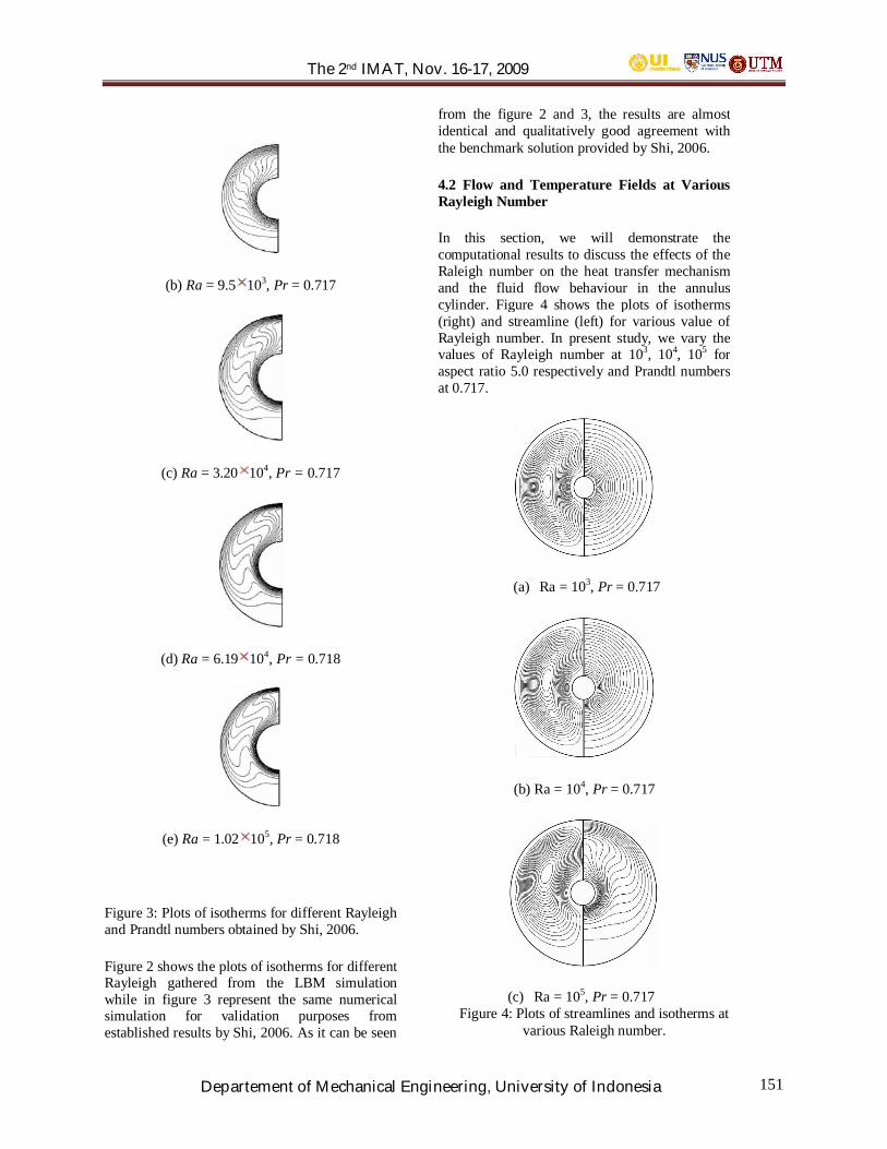
The 2nd IMAT, Nov. 16-17, 2009
Departement of Mechanical Engineering, University of Indonesia 151
(b) Ra = 9.5 103, Pr = 0.717
(c) Ra = 3.20 104, Pr = 0.717
(d) Ra = 6.19 104, Pr = 0.718
(e) Ra = 1.02 105, Pr = 0.718
Figure 3: Plots of isotherms for different Rayleighand Prandtl numbers obtained by Shi, 2006.
Figure 2 shows the plots of isotherms for differentRayleigh gathered from the LBM simulationwhile in figure 3 represent the same numericalsimulation for validation purposes fromestablished results by Shi, 2006. As it can be seen
from the figure 2 and 3, the results are almostidentical and qualitatively good agreement withthe benchmark solution provided by Shi, 2006.
4.2 Flow and Temperature Fields at VariousRayleigh Number
In this section, we will demonstrate thecomputational results to discuss the effects of theRaleigh number on the heat transfer mechanismand the fluid flow behaviour in the annuluscylinder. Figure 4 shows the plots of isotherms(right) and streamline (left) for various value ofRayleigh number. In present study, we vary thevalues of Rayleigh number at 103, 104, 105 foraspect ratio 5.0 respectively and Prandtl numbersat 0.717.
(a) Ra = 103, Pr = 0.717
(b) Ra = 104, Pr = 0.717
(c) Ra = 105, Pr = 0.717Figure 4: Plots of streamlines and isotherms at
various Raleigh number.
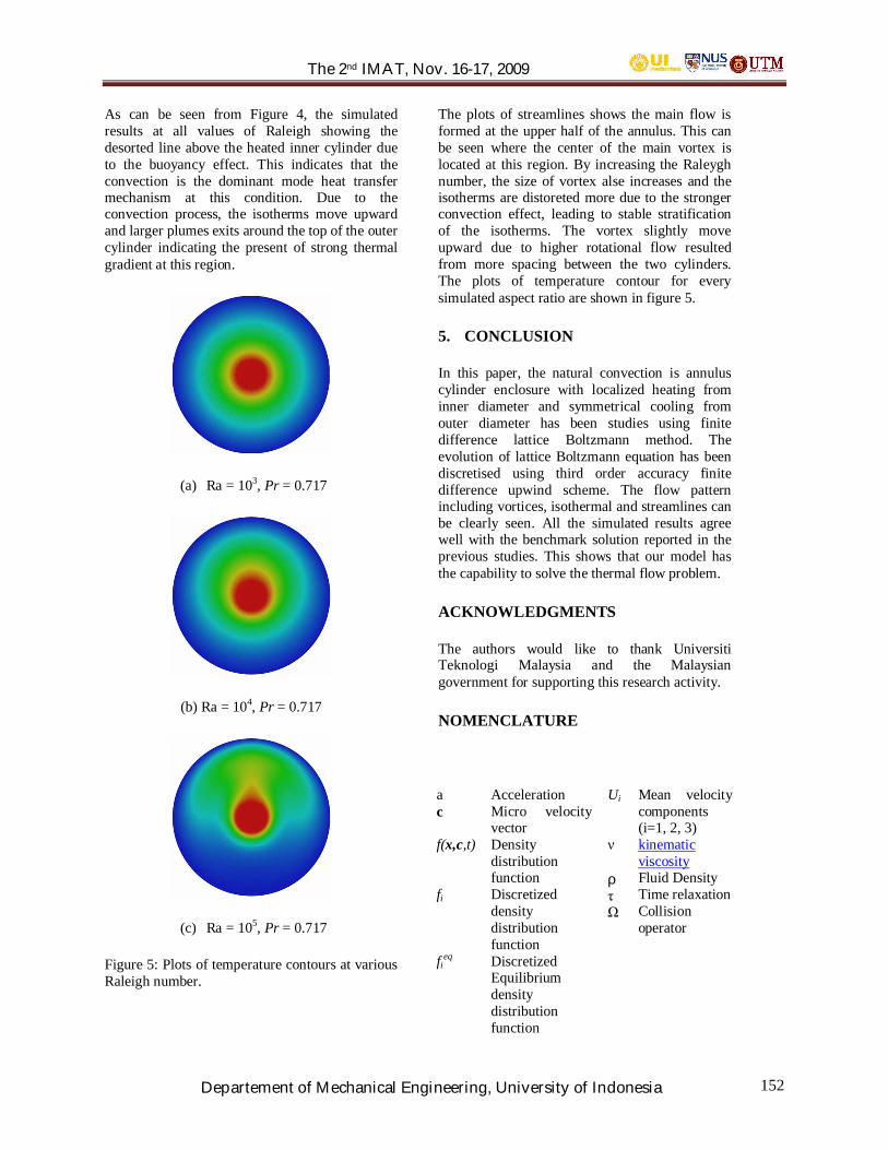
The 2nd IMAT, Nov. 16-17, 2009
Departement of Mechanical Engineering, University of Indonesia 152
As can be seen from Figure 4, the simulatedresults at all values of Raleigh showing thedesorted line above the heated inner cylinder dueto the buoyancy effect. This indicates that theconvection is the dominant mode heat transfermechanism at this condition. Due to theconvection process, the isotherms move upwardand larger plumes exits around the top of the outercylinder indicating the present of strong thermalgradient at this region.
(a) Ra = 103, Pr = 0.717
(b) Ra = 104, Pr = 0.717
(c) Ra = 105, Pr = 0.717
Figure 5: Plots of temperature contours at variousRaleigh number.
The plots of streamlines shows the main flow isformed at the upper half of the annulus. This canbe seen where the center of the main vortex islocated at this region. By increasing the Raleyghnumber, the size of vortex alse increases and theisotherms are distoreted more due to the strongerconvection effect, leading to stable stratificationof the isotherms. The vortex slightly moveupward due to higher rotational flow resultedfrom more spacing between the two cylinders.The plots of temperature contour for everysimulated aspect ratio are shown in figure 5.
5. CONCLUSION
In this paper, the natural convection is annuluscylinder enclosure with localized heating frominner diameter and symmetrical cooling fromouter diameter has been studies using finitedifference lattice Boltzmann method. Theevolution of lattice Boltzmann equation has beendiscretised using third order accuracy finitedifference upwind scheme. The flow patternincluding vortices, isothermal and streamlines canbe clearly seen. All the simulated results agreewell with the benchmark solution reported in theprevious studies. This shows that our model hasthe capability to solve the thermal flow problem.
ACKNOWLEDGMENTS
The authors would like to thank UniversitiTeknologi Malaysia and the Malaysiangovernment for supporting this research activity.
NOMENCLATURE
ac
f(x,c,t)
fi
fieq
AccelerationMicro velocityvectorDensitydistributionfunctionDiscretizeddensitydistributionfunctionDiscretizedEquilibriumdensitydistributionfunction
Ui
ρ
Mean velocitycomponents(i=1, 2, 3)kinematicviscosityFluid DensityTime relaxationCollisionoperator
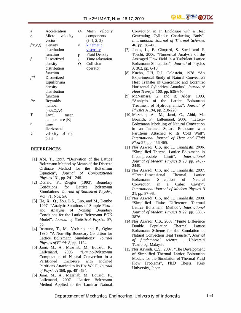
The 2nd IMAT, Nov. 16-17, 2009
Departement of Mechanical Engineering, University of Indonesia 153
ac
f(x,c,t)
fi
fieq
Re
T
t
U
AccelerationMicro velocityvectorDensitydistributionfunctionDiscretizeddensitydistributionfunctionDiscretizedEquilibriumdensitydistributionfunctionReynoldsnumber(=UbDh/ν)Local meantemperature [K]timeHorizontalvelocity of topplate
Ui
ρ
Mean velocitycomponents(i=1, 2, 3)kinematicviscosityFluid DensityTime relaxationCollisionoperator
REFERENCES
[1] Abe, T., 1997. “Derivation of the LatticeBoltzmann Method by Means of the DiscreteOrdinate Method for the BoltzmannEquation”, Journal of ComputationalPhysics 131, pp. 241–246.
[2] Donald, P., Ziegler (1993). BoundaryConditions for Lattice BoltzmannSimulations. Journal of Statistical Physics,Vol. 71, Nos. 5/6
[3] He, X., Q., Zou, L.S., Luo, and M., Dembo1997. “Analytic Solutions of Simple Flowsand Analysis of Nonslip BoundaryConditions for the Lattice Boltzmann BGKModel”, Journal of Statistical Physics 87,pp.
[4] Inamuro, T., M., Yoshino, and F., Ogino1995. “A Non-Slip Boundary Condition forLattice Boltzmann Simulations”, JournalPhysics of Fluids 8, pp. 1124
[5] Jami, M., A., Mezrhab, M., Bouzidi, P.,Lallemand, 2006. “Lattice-BoltzmannComputation of Natural Convection in aPartitioned Enclosure with InclinedPartitions Attached to its Hot Wall”, Journalof Physic A 368, pp. 481-494.
[6] Jami, M., A., Mezrhab, M., Bouzidi, P.,Lallemand, 2007. “Lattice BoltzmannMethod Applied to the Laminar Natural
Convection in an Enclosure with a HeatGenerating Cylinder Conducting Body”,International Journal of Thermal Sciences46, pp. 38–47.
[7] Jonas, L., B. Chopard, S. Succi and F.Toschi, 2006. “Numerical Analysis of theAveraged Flow Field in a Turbulent LatticeBoltzmann Simulation”, Journal of PhysicsA 362, pp. 6-10
[8] Kuehn, T.H, R.J, Goldstein, 1978. “AnExperimental Study of Natural ConvectionHeat Transfer in Concentric and EccentricHorizontal Cylindrical Annulus”, Journal ofHeat Transfer 100, pp. 635-640
[9] McNamara, G. and B. Alder, 1993,“Analysis of the Lattice BoltzmannTreatment of Hydrodynamics”, Journal ofPhysics A 194, pp. 218-228.
[10]Mezrhab, A., M., Jami, C., Abid, M.,Bouzidi, P., Lallemand, 2006. “Lattice-Boltzmann Modeling of Natural Convectionin an Inclined Square Enclosure withPartitions Attached to its Cold Wall”,International Journal of Heat and FluidFlow 27, pp. 456-465.
[11]Nor Azwadi, C.S, and T., Tanahashi, 2006.“Simplified Thermal Lattice Boltzmann inIncompressible Limit”, InternationalJournal of Modern Physics B 20, pp. 2437-2449.
[12]Nor Azwadi, C.S, and T., Tanahashi, 2007.“Three-Dimensional Thermal LatticeBoltzmann Simulation of NaturalConvection in a Cubic Cavity”,International Journal of Modern Physics B21, pp. 87-96.
[13]Nor Azwadi, C.S, and T., Tanahashi, 2008.“Simplified Finite Difference ThermalLattice Boltzmann Method”, InternationalJournal of Modern Physics B 22, pp. 3865-3876.
[14]Nor Azwadi, C.S., 2008. “Finite DifferenceDouble Population Thermal LatticeBoltzmann Scheme for the Simulation ofNatural Convection Heat Transfer”, Journalof fundamental science , UniversitiTeknologi Malaysia
[15]Nor Azwadi, C.S., 2007. “The Developmentof Simplified Thermal Lattice BoltzmannModels for the Simulation of Thermal FluidFlow Problems”, Ph.D Thesis. KeioUniversity, Japan.
The 2nd IMAT, Nov. 16-17, 2009
Departement of Mechanical Engineering, University of Indonesia 154
16 Peng, Y., Y.T, Chew, C., Shu, 2003.“Numerical Simulation of Natural Convectionin a Concentric Annulus between a SquareOuter Cylinder and a Circular Inner Cylinderusing the Taylor Series Expansion and LeastSquare Based Lattice Boltzmann Method”,Journal of physics 67, pp. 026701.1-026701.6
17 Rohde, M., D., Kandhai, J. J., Derksen, andH.E.A., Van Den Akker, 2003. “ImprovedBounce-Back Methods for No-Slip Walls inLattice-Boltzmann Schemes: Theory andSimulations”, Journal of statistical of physics67, pp.066703.1-066703.10
18 Shi, Y., T.S., Zhao, Z.L., Gou 2006. “FiniteDifference Based Lattice Boltzmann Simulationof Natural Convection Heat Transfer in aHorizontal Concentric Annulus”, Journal ofComputer & Fluids A, pp 1-15
19 Sridar, D., N., Balakrishnan, 2003. “An UpwindFinite Difference Scheme for Mesh Lesssolvers”, Journal of Computational Physics189, PP. 1–29.
20 Succi, S., 2006. “The lattice BoltzmannEquation for Fluid Dynamics and Beyond”,Oxford university press, pp 83.
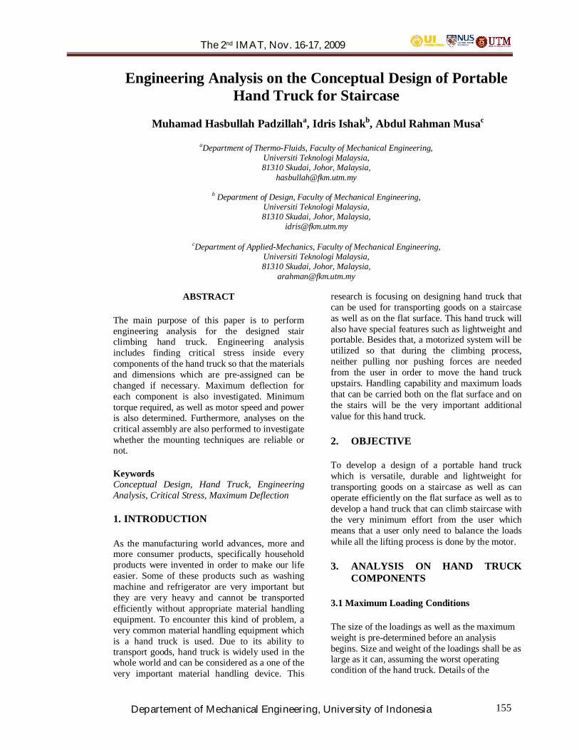
The 2nd IMAT, Nov. 16-17, 2009
Departement of Mechanical Engineering, University of Indonesia 155
Engineering Analysis on the Conceptual Design of PortableHand Truck for Staircase
Muhamad Hasbullah Padzillaha, Idris Ishakb, Abdul Rahman Musac
aDepartment of Thermo-Fluids, Faculty of Mechanical Engineering,Universiti Teknologi Malaysia,81310 Skudai, Johor, Malaysia,
b Department of Design, Faculty of Mechanical Engineering,Universiti Teknologi Malaysia,81310 Skudai, Johor, Malaysia,
cDepartment of Applied-Mechanics, Faculty of Mechanical Engineering,Universiti Teknologi Malaysia,81310 Skudai, Johor, Malaysia,
ABSTRACT
The main purpose of this paper is to performengineering analysis for the designed stairclimbing hand truck. Engineering analysisincludes finding critical stress inside everycomponents of the hand truck so that the materialsand dimensions which are pre-assigned can bechanged if necessary. Maximum deflection foreach component is also investigated. Minimumtorque required, as well as motor speed and poweris also determined. Furthermore, analyses on thecritical assembly are also performed to investigatewhether the mounting techniques are reliable ornot.
KeywordsConceptual Design, Hand Truck, EngineeringAnalysis, Critical Stress, Maximum Deflection
1. INTRODUCTION
As the manufacturing world advances, more andmore consumer products, specifically householdproducts were invented in order to make our lifeeasier. Some of these products such as washingmachine and refrigerator are very important butthey are very heavy and cannot be transportedefficiently without appropriate material handlingequipment. To encounter this kind of problem, avery common material handling equipment whichis a hand truck is used. Due to its ability totransport goods, hand truck is widely used in thewhole world and can be considered as a one of thevery important material handling device. This
research is focusing on designing hand truck thatcan be used for transporting goods on a staircaseas well as on the flat surface. This hand truck willalso have special features such as lightweight andportable. Besides that, a motorized system will beutilized so that during the climbing process,neither pulling nor pushing forces are neededfrom the user in order to move the hand truckupstairs. Handling capability and maximum loadsthat can be carried both on the flat surface and onthe stairs will be the very important additionalvalue for this hand truck.
2. OBJECTIVE
To develop a design of a portable hand truckwhich is versatile, durable and lightweight fortransporting goods on a staircase as well as canoperate efficiently on the flat surface as well as todevelop a hand truck that can climb staircase withthe very minimum effort from the user whichmeans that a user only need to balance the loadswhile all the lifting process is done by the motor.
3. ANALYSIS ON HAND TRUCKCOMPONENTS
3.1 Maximum Loading Conditions
The size of the loadings as well as the maximumweight is pre-determined before an analysisbegins. Size and weight of the loadings shall be aslarge as it can, assuming the worst operatingcondition of the hand truck. Details of the
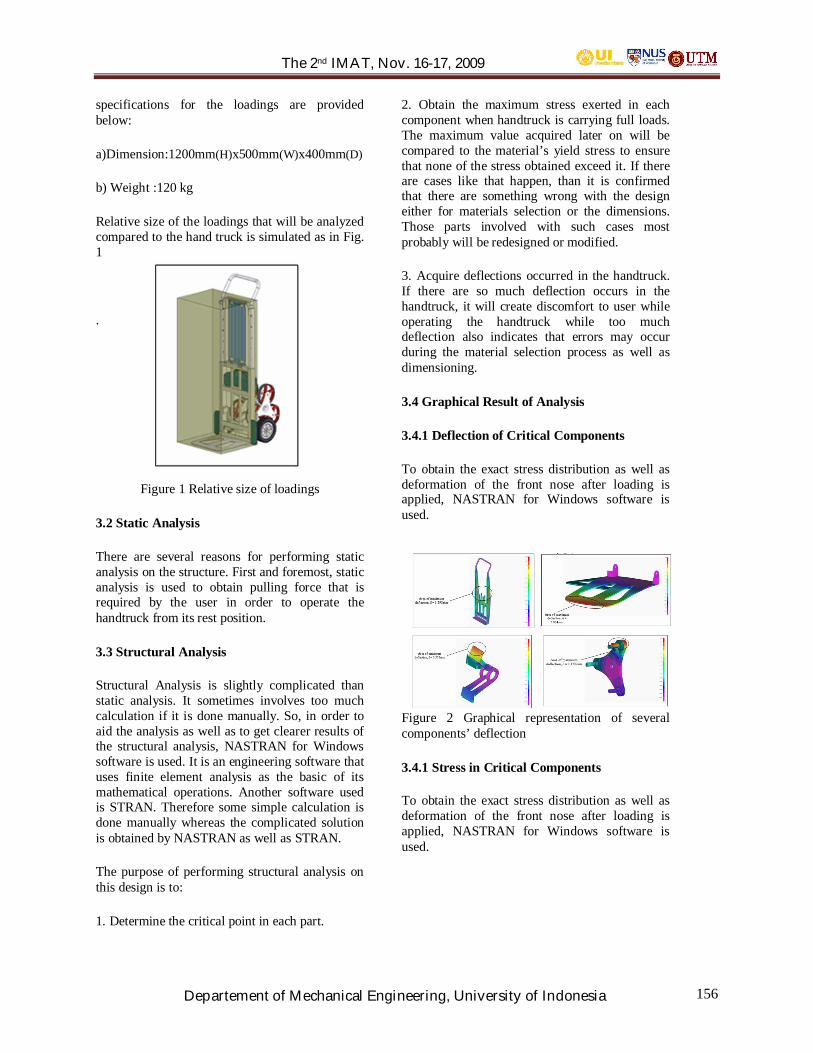
The 2nd IMAT, Nov. 16-17, 2009
Departement of Mechanical Engineering, University of Indonesia 156
specifications for the loadings are providedbelow:
a)Dimension:1200mm(H)x500mm(W)x400mm(D)
b) Weight :120 kg
Relative size of the loadings that will be analyzedcompared to the hand truck is simulated as in Fig.1
.
Figure 1 Relative size of loadings
3.2 Static Analysis
There are several reasons for performing staticanalysis on the structure. First and foremost, staticanalysis is used to obtain pulling force that isrequired by the user in order to operate thehandtruck from its rest position.
3.3 Structural Analysis
Structural Analysis is slightly complicated thanstatic analysis. It sometimes involves too muchcalculation if it is done manually. So, in order toaid the analysis as well as to get clearer results ofthe structural analysis, NASTRAN for Windowssoftware is used. It is an engineering software thatuses finite element analysis as the basic of itsmathematical operations. Another software usedis STRAN. Therefore some simple calculation isdone manually whereas the complicated solutionis obtained by NASTRAN as well as STRAN.
The purpose of performing structural analysis onthis design is to:
1. Determine the critical point in each part.
2. Obtain the maximum stress exerted in eachcomponent when handtruck is carrying full loads.The maximum value acquired later on will becompared to the material’s yield stress to ensurethat none of the stress obtained exceed it. If thereare cases like that happen, than it is confirmedthat there are something wrong with the designeither for materials selection or the dimensions.Those parts involved with such cases mostprobably will be redesigned or modified.
3. Acquire deflections occurred in the handtruck.If there are so much deflection occurs in thehandtruck, it will create discomfort to user whileoperating the handtruck while too muchdeflection also indicates that errors may occurduring the material selection process as well asdimensioning.
3.4 Graphical Result of Analysis
3.4.1 Deflection of Critical Components
To obtain the exact stress distribution as well asdeformation of the front nose after loading isapplied, NASTRAN for Windows software isused.
Figure 2 Graphical representation of severalcomponents’ deflection
3.4.1 Stress in Critical Components
To obtain the exact stress distribution as well asdeformation of the front nose after loading isapplied, NASTRAN for Windows software isused.

The 2nd IMAT, Nov. 16-17, 2009
Departement of Mechanical Engineering, University of Indonesia 157
Figure 3 Graphical representation of severalcomponents’ stress
2. CALCULATION OF MINIMUMTORQUE REQUIRED
Figure 4 Free Body Diagram for findingminimum Torque required
During operation, the only contact between wheeland floor occur at wheel X. Hence, apply momentequilibrium equation at point X to obtain value ofM to balance the equation and that is theminimum value of motor torque required.
∑ = 0xM
NM
M
144.25
0)09.0)(2862()07.0(2.1658)055.0(948
=∴
=++−
Thus, minimum value of motor torque is 25.144≈ 30 Nm
3. ANALYSIS ON CRITICALASSEMBLY
It is very important to perform additional analysison the critical assembly especially for the part thatis using bolts as the medium of assembly. This is
to ensure that the number of bolts used is enoughto sustain shear force as well as axial force duringthe operation of handtruck. All the forcesobtained from previous analysis are than appliedto the bolts.
5.1 Assembly between main frame and motorholder
Figure 5 Free Body Diagram for analyzing criticalassembly
Analysis at point X
Number of bolts, n : 4
Bolt’s Diameter, d : 6 mm
Shear force exerted by bolts, V: 726.9 N
Axial force exerted by bolts, F: 1490 N
Calculating Shear stress exerted by each bolt,
4)006.0)(4(
9.7262π
τ ==nAV
= 6.43 MPa
Calculating Axial stress exerted by each bolt,
4)006.0)(4(
14902π
σ ==nAF
= 13.17 MPa

The 2nd IMAT, Nov. 16-17, 2009
Departement of Mechanical Engineering, University of Indonesia 158
Analysis at point O
Number of bolts, n : 4
Bolt’s Diameter, d : 6 mm
Shear force exerted by bolts, V: 292.9 N
Axial force exerted by bolts, F: 901 N
Calculating Shear stress exerted by each bolt,
4)006.0)(4(
9.2922π
τ ==nAV
= 2.59 MPa
Calculating Axial stress exerted by each bolt,
4)006.0)(4(
9012π
σ ==nAF
= 7.97 MPa
5.2 Assembly between main frame and wheelholder
Figure 5 Free Body Diagram for analyzing criticalassembly
No axial force will be exerted by bolts
Total shear force,
NVV
total
total
11816.58824.1024 22
=∴+=
However, since loading is shared between twowheel holder, shear force for each wheel holder,
21181=V N5.590=
Calculating Shear stress exerted by each bolt,
4)006.0)(2(
5.5902π
τ ==nAV
= 10.44 MPa
5.3 Calculating motor speed and powerrequirement
Estimated Climbing Speed = 48 steps/min
∴ 1 revolution of motor = 3 steps
Motor RPM = 48/3 = 16 RPM
To calculate power requirement of the motor:
srad
N
TPTPower
68.160
)16(260
2
=
==
==
ω
ππω
ωω
WPP
3.503068.1
=×=∴
2. Discussion
In order to obtain the safety factor for the handtruck during maximum loadings of 120kg, a tablethat concludes all the design analysis isconstructed. In the table 1 below, only stressesthat influence the most or the one that havinghighest value are listed in the table.

The 2nd IMAT, Nov. 16-17, 2009
Departement of Mechanical Engineering, University of Indonesia 159
From the table, it can be seen that some of the boxes under safety factor is written ‘too large’. It indicates that valueof safety factor is higher than 60 and that particular structureis definitely safe for any hand truck loadings up to 120 kg.From the table also, it can be seen that value of applicablesafety factor for overall hand truck is 4.31. Allowing 20% ofcalculation tolerance gives safety factor of 3.4.
7. CONCLUSION
Engineering analysis shows that designed hand truck is ableto withstand maximum load of 120 kg with a reasonablesafety factor. The minimum torque calculated also shownthat 30Nm torque is enough to ensure stable movement ofhand truck during climbing.
REFERENCES
[1]Idris Ishak and Richard Lim Boon Keat, Skudai, 2007,Introduction to Basic Sketching and Rendering Techniques,Penerbit UTM.
[2]Khairuddin Hj. Jaffar, Skudai, 1996, Protective Shield forLorry drivers Cabin, Universiti Teknologi Malaysia.
[3]Mohd Hafidz Mohamed Rodzi, Skudai 2004, Drop – on Traffic Bollards (Ikon Trafik Mudah Alih), UniversitiTeknologi Malaysia.
[4]Hamdan Ismail, Skudai, 1990, Rekabentuk Troli Pengangkut Barang Untuk Kegunaan di Tangga dan PelbagaiGuna, Universiti Teknologi Malaysia
[5]Azrul Hazimin Mohamad, Skudai, 1996, Designing a Stairs Handtruck, Universiti Teknologi Malaysia
[6]Callister, W.D, New York, 2007, Materials Science and Engineering : An Introduction, John Wiley & Sons Inc.
[7]Boresi, A.P. and Schimidt, R.D, New York, 2002, Advanced Machanics of Materials, John Wiley & Sons Inc.
[8]Planchard, D.C. and Planchard, M.P., 2005, SolidWorks 2005 Tutorial, Schroff Development Corporation SDCPublications.
[9]Mohamad Kasim Abdul Jalil, Skudai, 2000, Proses dan Kaedah Rekabentuk, Penerbit UTM
Components/
Parts
Materials MaximumBendingStress(MPa)
MaximumAxialStress(MPa)
MaximumShearStress(MPa)
MaximumDeflection(mm)
SafetyFactor
Front Nose(Plate)
AlloySteel 173 - - 2.804 4.31
LowerFrame (Rod)
AluminumAlloy7075-T6
- - 12.12 - 42
WheelHolder(Rod)
AlloySteel - - 1.655 - Too
Large
WheelHolder
AlloySteel 62.17 - - 0.0966 11.98
VerticalFrame
AluminumAlloy7075-T6 36 - - 1.598 15.83
MotorHolder (A)
AlloySteel - -2.76 - 0.216 Too
Large
MotorHolder (B)
AlloySteel - 1.58 - - Too
Large
Main Frame– MotorHolder
SteelGrade 8 - 13.17 6.43 - Too
Large
Main Frame– Wheel
Holder
SteelGrade 8
- 7.97 2.59 - TooLarge
Table 1 Summary of DesignAnalysis

The 2nd IMAT, Nov. 16-17, 2009
Departement of Mechanical Engineering, University of Indonesia 160

The 2nd IMAT, Nov. 16-17, 2009
Departement of Mechanical Engineering, University of Indonesia 161
Numerical Analysis of Helicopter Tail Shake Phenomenon:A Preliminary Investigation
Iskandar Shah Ishak*, Shuhaimi Mansor, Tholudin Mat Lazim,
Muhammad Riza Abd RahmanDepartment of Aeronautical Engineering
Faculty of Mechanical EngineeringUniversiti Teknologi Malaysia
81310 UTM Skudai, Johor, MalaysiaTel: +607-5534664, Fax: +607-5566159
*E-mail: [email protected]
ABSTRACT
The flow field that governs helicopter tail shakephenomenon has often baffled theaerodynamicists and it remains as a long draggedissue that adversely affected the overallperformance, occupants comfort and handlingqualities of helicopter. The objective of thisresearch is to improve basic understanding of theviscous unsteady flow phenomenon observedbehind the main-rotor-hub assembly, as the partis believed to be the major contributor of tailshake phenomenon. Using Computational FluidDynamic (CFD) approach, the FLUENT softwarewas employed and the Multiple Reference Frames(MRF) method was applied to simulate thehelicopter s main-rotor-hub assembly rotation. Inthis study, the aerodynamic flow field wascomputed using the Reynolds-Averaged Navier-Stokes (RANS) equations. As the induced wake,which consequently causing tail to shake differswith the rpm of main-rotor-hub assembly, thispreliminary numerical investigation wasperformed ranging from rpm of 0 to 900, withintervals of 300 rpm. A rotor-hub-fairing wasalso being installed to examine its effect on wakeunsteadiness of this tail shake phenomenon.
KeywordsFlow field, helicopter tail shake, unsteady flow,computational fluid dynamic
1. INTRODUCTION
Tail shake is an issue of major concern forrotorcraft [1] as it is adversely affected the overallperformance and handling qualities of helicopter.Vibrations transmitted from vertical tail to cockpithave also caused discomfort to the occupants [2].It had being reported on the AH-64D Longbow
Apache helicopter, the vibration resulted inincreased cockpit lateral vibration levels, whichincreased crew workload and reduced their abilityto perform precision tasks [3].
This phenomenon is a challenging issue tounderstand with as it involves an interactionbetween aerodynamic flow excitation, whichrelated to flight parameters & structural response,which related to structure characteristics [2]. Agood understanding of this matter is necessary asa typical aspect of tail shake that it has unsteadyrandom character, indicating that the wakeinduced excitation is in also unsteady of nature[2].
Tail shake phenomenon happens partly due to theunsteady flow contributed from the main-rotor-hub assembly that hit the tail part, as shown inFigure 1. Hence, it likely only to happen whenthere is a forward velocity i.e. during hovering orvertical climb/descent, helicopter will notencounter this tail shake problem.
Figure 1: Schematic diagram of tail shake [2]
In this research, focus will be on main-rotor-hubassembly’s wake as it is believed to be the majorcontributor of the problem. This allows the tailshake investigation to be conducted using blade-stubs configuration [4,5,6]. Blade-stubsconfiguration is a combination of main-rotor-hubassembly with short blades.

The 2nd IMAT, Nov. 16-17, 2009
Departement of Mechanical Engineering, University of Indonesia 162
2. CFD MODELLING DESCRIPTION
This numerical study used Reynolds-AveragedNavier-Stokes (RANS) equation models whichsolve ensemble-averaged Navier-Stokes equations[7]. There are several types of RANS-basedmodel and for this simulation, the two-equationmodels of Realizable k- model was employed.The k- model selected is not an issue here as theresearch is keen on the result’s trends, not theresult’s absolute values. The Multiple ReferenceFrames (MRF) approach was applied to simulatethe main-rotor-hub-assembly rotation at variousrpm.
This numerical investigation used an ellipsoidalfuselage based on NASA standard model [8] withthe axes ratio of longitudinal to lateral axes is4.485. This kind of model is selected as it avoidsgeometric complexity and simplifies theinteractions with the wake [8]. For this researchwork, the longitudinal axes were taken as 1120mm. The model is shown in Figure 2.
Figure 2: An ellipsoidal fuselage based on NASAmodel [8]
The model was simulated with a simplified main-rotor-hub assembly attached with short blades i.e.blade-stubs configuration, as shown in Figure 3.This simplified main rotor hub assembly is onlymeant to trigger the unsteady wake due to rotationof main- rotor-hub assembly.
Figure 3: A simplified blade-stubs configuration
Figure 4 depicts the complete model with blade-stubs configuration and an ellipsoidal pylon.
Figure 4: Model for CFD simulation
In Geometry And Mesh Building IntelligentToolkit (GAMBIT), which acts as a pre-processor for CFD analysis, a test section with asize of 2m (width) x 1.5m (height) x 5.8m(length) was virtually created for placing themodel. The size of this test section is similar asthe test section size of Universiti TeknologiMalaysia – Low Speed Tunnel (UTM-LST), asexperimental works also be planned to comparewith this CFD analysis.
In MRF method, two reference frames must becreated with one at the vicinity of the rotatingparts i.e. main-rotor-hub assembly. As there is nospecific rule regarding the size of the frame forrotating parts, this research decided to take thedistance of the frame’s boundary to surface of therotating parts to be 1 aerofoil thickness. Theaerofoil thickness of the main rotor, as depicted inFigure 3, is 10 mm and hence the frame wascreated in such manner as shown in Figure 5.
Ellipsoidal pylon

The 2nd IMAT, Nov. 16-17, 2009
Departement of Mechanical Engineering, University of Indonesia 163
Figure 5 (a): Frame dimensions (side view)
Figure 5(b): Frame for rotating parts (iso view)
Figure 5: Frame for rotating parts
3. RESULTS ANALYSIS
Before running the final simulation, independencegrid analysis had been carried out to verify theresults obtained are free from grid influence. Thisis important to confirm the differences of resultsare due to test configurations, not due to numberof the grid.
All simulation results presented throughout thispaper were run at wind speed, or forward flightvelocity, of 40 m/s.
Figures 6 and 7 show the path lines of turbulentintensity for 0 and 900 rpm of main-rotor-hubassembly, respectively. Viewed from top asshown by Figures 6(a) and 7(a), the path lines areabout symmetrical on both left and right sides for0 rpm, contrary for 900 rpm, the path lines areunsymmetrical indicating there is strong flowinteraction with the rotating main-rotor-hubassembly.
Figure 6(a): Path lines from ‘main-rotor-hubassembly’ (top view)
Figure 6(b): Path lines from ‘main-rotor-hubassembly’ (side view)
Figure 6: Path lines coloured by turbulentintensity (%) at 0 rpm
Figure 7(a): Path lines from ‘main-rotor-hubassembly’ (top view)
Figure 7(b): Path lines from ‘main-rotor-hubassembly’ (side view)
Figure 7: Path lines coloured by turbulentintensity (%) at 900 rpm
Compared to Figure 6(b), turbulent intensity ishigher and wake volume is thicker in Figure 7(b).This shows rotation on main-rotor-hub assemblytriggers a significant unsteady wake which couldcontribute to tail shake problem.
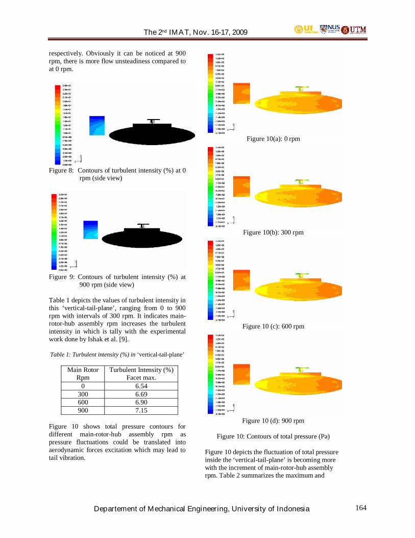
The 2nd IMAT, Nov. 16-17, 2009
Departement of Mechanical Engineering, University of Indonesia 164
respectively. Obviously it can be noticed at 900rpm, there is more flow unsteadiness compared toat 0 rpm.
Figure 8: Contours of turbulent intensity (%) at 0rpm (side view)
Figure 9: Contours of turbulent intensity (%) at900 rpm (side view)
Table 1 depicts the values of turbulent intensity inthis ‘vertical-tail-plane’, ranging from 0 to 900rpm with intervals of 300 rpm. It indicates main-rotor-hub assembly rpm increases the turbulentintensity in which is tally with the experimentalwork done by Ishak et al. [9].
Table 1: Turbulent intensity (%) in ‘vertical-tail-plane’
Figure 10 shows total pressure contours fordifferent main-rotor-hub assembly rpm aspressure fluctuations could be translated intoaerodynamic forces excitation which may lead totail vibration.
Figure 10(a): 0 rpm
Figure 10(b): 300 rpm
Figure 10 (c): 600 rpm
Figure 10 (d): 900 rpm
Figure 10: Contours of total pressure (Pa)
Figure 10 depicts the fluctuation of total pressureinside the ‘vertical-tail-plane’ is becoming morewith the increment of main-rotor-hub assemblyrpm. Table 2 summarizes the maximum and
Main RotorRpm
Turbulent Intensity (%)Facet max.
0 6.54300 6.69600 6.90900 7.15
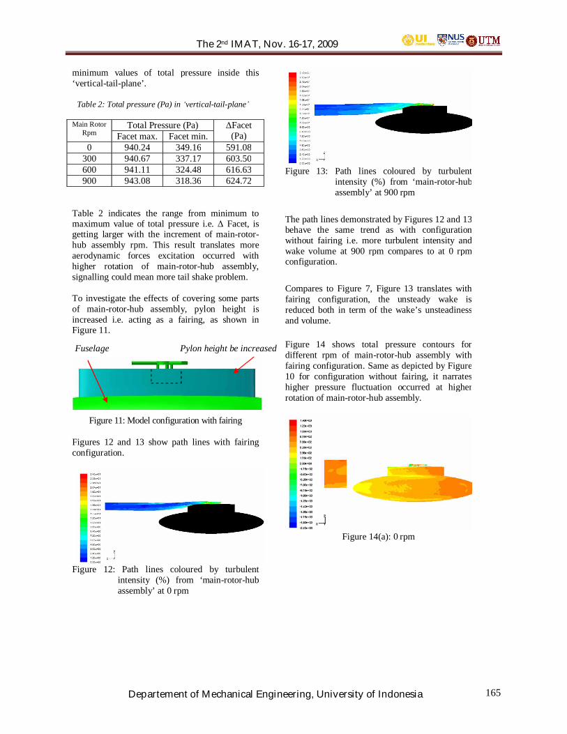
The 2nd IMAT, Nov. 16-17, 2009
Departement of Mechanical Engineering, University of Indonesia 165
minimum values of total pressure inside this‘vertical-tail-plane’.
Table 2: Total pressure (Pa) in vertical-tail-plane
Main RotorRpm
Total Pressure (Pa) Facet(Pa)Facet max. Facet min.
0 940.24 349.16 591.08300 940.67 337.17 603.50600 941.11 324.48 616.63900 943.08 318.36 624.72
Table 2 indicates the range from minimum tomaximum value of total pressure i.e. Facet, isgetting larger with the increment of main-rotor-hub assembly rpm. This result translates moreaerodynamic forces excitation occurred withhigher rotation of main-rotor-hub assembly,signalling could mean more tail shake problem.
To investigate the effects of covering some partsof main-rotor-hub assembly, pylon height isincreased i.e. acting as a fairing, as shown inFigure 11.
Figure 11: Model configuration with fairing
Figures 12 and 13 show path lines with fairingconfiguration.
Figure 12: Path lines coloured by turbulentintensity (%) from ‘main-rotor-hubassembly’ at 0 rpm
Figure 13: Path lines coloured by turbulentintensity (%) from ‘main-rotor-hubassembly’ at 900 rpm
The path lines demonstrated by Figures 12 and 13behave the same trend as with configurationwithout fairing i.e. more turbulent intensity andwake volume at 900 rpm compares to at 0 rpmconfiguration.
Compares to Figure 7, Figure 13 translates withfairing configuration, the unsteady wake isreduced both in term of the wake’s unsteadinessand volume.
Figure 14 shows total pressure contours fordifferent rpm of main-rotor-hub assembly withfairing configuration. Same as depicted by Figure10 for configuration without fairing, it narrateshigher pressure fluctuation occurred at higherrotation of main-rotor-hub assembly.
Figure 14(a): 0 rpm
Fuselage Pylon height be increased
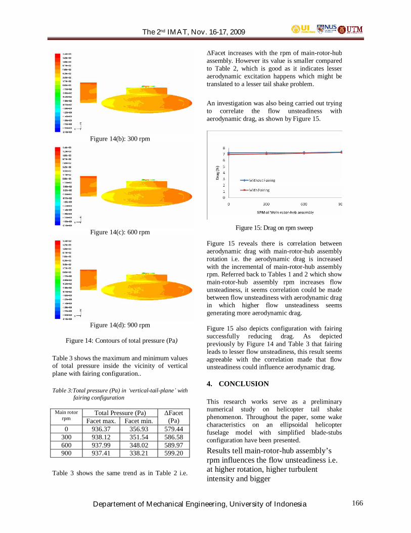
The 2nd IMAT, Nov. 16-17, 2009
Departement of Mechanical Engineering, University of Indonesia 166
Figure 14(b): 300 rpm
Figure 14(c): 600 rpm
Figure 14(d): 900 rpm
Figure 14: Contours of total pressure (Pa)
Table 3 shows the maximum and minimum valuesof total pressure inside the vicinity of verticalplane with fairing configuration..
Table 3:Total pressure (Pa) in vertical-tail-plane withfairing configuration
Main rotorrpm
Total Pressure (Pa) Facet(Pa)Facet max. Facet min.
0 936.37 356.93 579.44300 938.12 351.54 586.58600 937.99 348.02 589.97900 937.41 338.21 599.20
Table 3 shows the same trend as in Table 2 i.e.
Facet increases with the rpm of main-rotor-hubassembly. However its value is smaller comparedto Table 2, which is good as it indicates lesseraerodynamic excitation happens which might betranslated to a lesser tail shake problem.
An investigation was also being carried out tryingto correlate the flow unsteadiness withaerodynamic drag, as shown by Figure 15.
Figure 15: Drag on rpm sweep
Figure 15 reveals there is correlation betweenaerodynamic drag with main-rotor-hub assemblyrotation i.e. the aerodynamic drag is increasedwith the incremental of main-rotor-hub assemblyrpm. Referred back to Tables 1 and 2 which showmain-rotor-hub assembly rpm increases flowunsteadiness, it seems correlation could be madebetween flow unsteadiness with aerodynamic dragin which higher flow unsteadiness seemsgenerating more aerodynamic drag.
Figure 15 also depicts configuration with fairingsuccessfully reducing drag. As depictedpreviously by Figure 14 and Table 3 that fairingleads to lesser flow unsteadiness, this result seemsagreeable with the correlation made that flowunsteadiness could influence aerodynamic drag.
4. CONCLUSION
This research works serve as a preliminarynumerical study on helicopter tail shakephenomenon. Throughout the paper, some wakecharacteristics on an ellipsoidal helicopterfuselage model with simplified blade-stubsconfiguration have been presented.Results tell main-rotor-hub assembly’srpm influences the flow unsteadiness i.e.at higher rotation, higher turbulentintensity and bigger
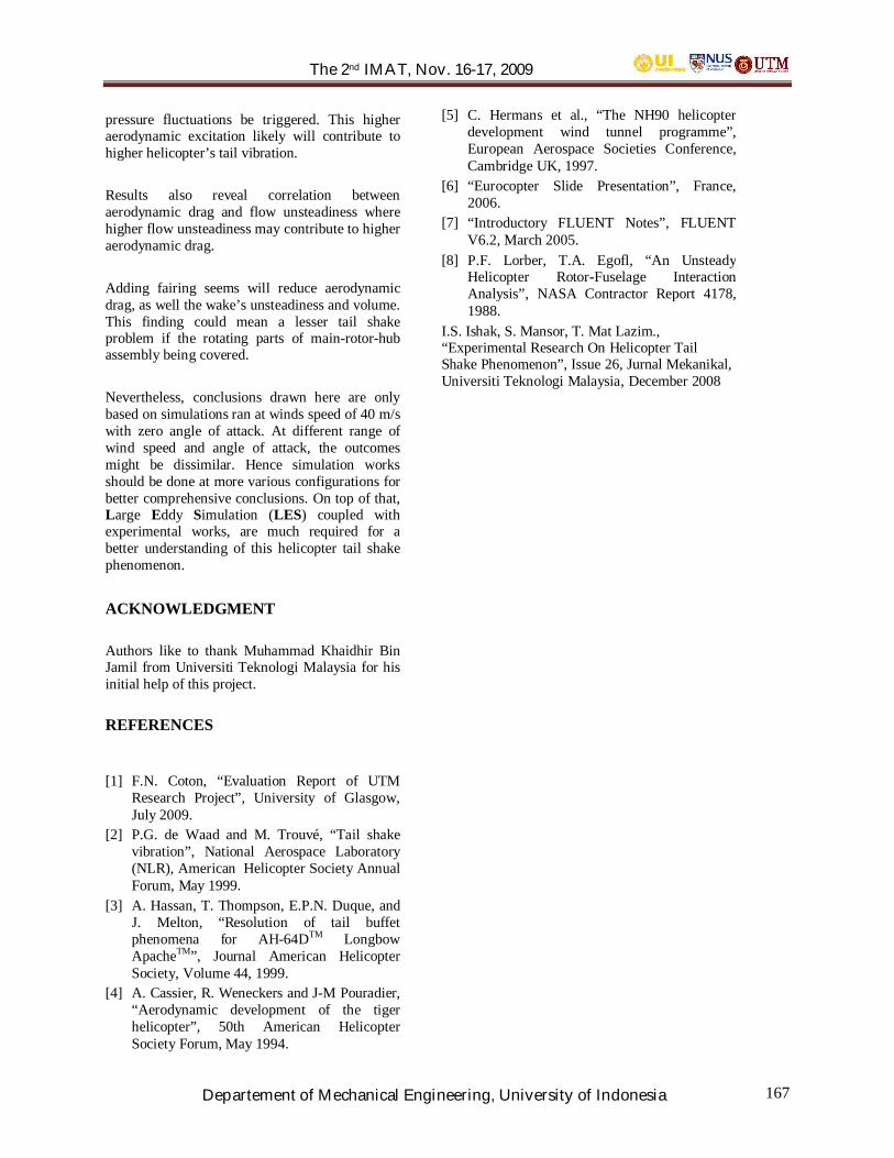
The 2nd IMAT, Nov. 16-17, 2009
Departement of Mechanical Engineering, University of Indonesia 167
pressure fluctuations be triggered. This higheraerodynamic excitation likely will contribute tohigher helicopter’s tail vibration.
Results also reveal correlation betweenaerodynamic drag and flow unsteadiness wherehigher flow unsteadiness may contribute to higheraerodynamic drag.
Adding fairing seems will reduce aerodynamicdrag, as well the wake’s unsteadiness and volume.This finding could mean a lesser tail shakeproblem if the rotating parts of main-rotor-hubassembly being covered.
Nevertheless, conclusions drawn here are onlybased on simulations ran at winds speed of 40 m/swith zero angle of attack. At different range ofwind speed and angle of attack, the outcomesmight be dissimilar. Hence simulation worksshould be done at more various configurations forbetter comprehensive conclusions. On top of that,Large Eddy Simulation (LES) coupled withexperimental works, are much required for abetter understanding of this helicopter tail shakephenomenon.
ACKNOWLEDGMENT
Authors like to thank Muhammad Khaidhir BinJamil from Universiti Teknologi Malaysia for hisinitial help of this project.
REFERENCES
[1] F.N. Coton, “Evaluation Report of UTMResearch Project”, University of Glasgow,July 2009.
[2] P.G. de Waad and M. Trouvé, “Tail shakevibration”, National Aerospace Laboratory(NLR), American Helicopter Society AnnualForum, May 1999.
[3] A. Hassan, T. Thompson, E.P.N. Duque, andJ. Melton, “Resolution of tail buffetphenomena for AH-64DTM LongbowApacheTM”, Journal American HelicopterSociety, Volume 44, 1999.
[4] A. Cassier, R. Weneckers and J-M Pouradier,“Aerodynamic development of the tigerhelicopter”, 50th American HelicopterSociety Forum, May 1994.
[5] C. Hermans et al., “The NH90 helicopterdevelopment wind tunnel programme”,European Aerospace Societies Conference,Cambridge UK, 1997.
[6] “Eurocopter Slide Presentation”, France,2006.
[7] “Introductory FLUENT Notes”, FLUENTV6.2, March 2005.
[8] P.F. Lorber, T.A. Egofl, “An UnsteadyHelicopter Rotor-Fuselage InteractionAnalysis”, NASA Contractor Report 4178,1988.
I.S. Ishak, S. Mansor, T. Mat Lazim.,“Experimental Research On Helicopter TailShake Phenomenon”, Issue 26, Jurnal Mekanikal,Universiti Teknologi Malaysia, December 2008

The 2nd IMAT, Nov. 16-17, 2009
Departement of Mechanical Engineering, University of Indonesia 168
Study on Characteristics of Briquettes Contain DifferentMixing Ratio of EFB Fibre and Mesocarp Fibre
H. M. Faizal , Z. A. Latiff, Mazlan A. Wahid, Darus A. N.
Faculty of Mechanical EngineeringUniversiti Teknologi Malaysia,81310 UTM Skudai
Tel: (+60)7-5534657 E-mail: [email protected]
ABSTRACT
Based on Malaysia Palm Oil Statistics, theproduction of palm biomass residues such asshell, mesocarp fibre and empty fruit bunch(EFB) increased significantly from year to year.These residues especially mesocarp fibre andEFB were dumped in areas adjacent to the palmoil mills. Therefore, briquetting technology isexpected can improve this waste disposal byconverting these residues into solid fuels withhigher energy content per unit volume. In thispaper, the physical characteristics andcombustion properties of briquettes contain newproposed mixture has been investigated. Thismixture composed of mesocarp fibre and EFBfibre in different weight ratios. EFB fibre isobtained after dyring process by superheatedsteam with the pressure ranges from 1.0 to 1.5bar and temperature ranges from 100 to 120oC.Based on several tests done for investigating thecapability of new mixture of palm biomassbriquettes, it was found that the briquette withweight ratio of 60:40 (EFB fibre: mesocarp fibre)satisfies the minimum requirement for commercialbriquette DIN 51731. Besides, this ratio isselected due to the emphasis on the use of largeportion of EFB.
Keywords
Briquetting, briquette, palm biomass, combustionrate, shell, mesocarp fibre, EFB fibre, DIN 51731
1. INTRODUCTION
As reported by Malaysia Palm Oil Board (MPOB,2006), the production of shell, mesocarp fibre andEFB in Malaysia for year 2006 are 5.20x10⁶
tonne/year, 9.66x10⁶ tonne/year, and 17.08x10⁶
tonne/year respectively. Therefore, the utilizationof these residues is very important in order to
prevent waste and dumping areas adjacent to themills.
Conversion of these residues into briquette is oneof the methods to improve the propertiesespecially in term of energy content per unitvolume. As explained by Bhattacharya et al.(1996), densification (briquetting, pelletizing andbaling) is a process that can improve the storageand transportation of biomass fuel.
Chin and Siddiqui (2000) have conducted anexperiment to study the combustion rate onvarious biomass briquettes such as raw husks,sawdust and several others. The compactionpressure was within the range of 1 to 7 MPa. Itwas found that the burning rate increased as thebinder content increased. The binding agents usedin their experiment were molasses and starch.
In year 2002, an experiment that was carried outby Husain et al. (2002) explain the physical andcombustion characteristics of current localbriquettes contain mesocarp fibre and shell in theratio of 60:40. They used starch as binding agent(10% of the weight of residues) with addition ofwater (50% of the weight of residues). Theyfound that the combustion of heap of briquettes inthe stove releases about 0.5kW, air-fuel ratio wasabout 10.2 and ash content was 5.8%. Besides, theaverage compressive strength of about 2.56 MPais considered as a value for good resistance fordisintegration.
Meanwhile, in year 2008, Nasrin et al. (2008)studied the physical and combustioncharacteristics of palm biomass briquettescontaining EFB fibre and palm kernel cake(PKC). The weight ratio for PKC + EFB fibre +sawdust was 30:5:65. In this case, sawdust plays arole as binder. In their study, they found that thestrength of briquettes increased when the sawdustwas added.

The 2nd IMAT, Nov. 16-17, 2009
Departement of Mechanical Engineering, University of Indonesia 169
Thus, in this paper, the physical and combustionproperties of briquettes contain EFB fibre andmesocarp fibre with different mixing ratios werestudied. One ratio then will be selected for furtherstudy in the future to investigate the effect ofcompaction pressure on the combustioncharacteristics of these briquettes such ascombustion rate. The selection of ratio was basedon two aspects. The first aspect is minimumrequirement of commercial briquette DIN 51731in term of gross calorific value and moisturecontent. Meanwhile, the second aspect is theemphasis on the use of EFB.
2. METHOD AND PREPARATION
The palm biomass residues (EFB fibre andmesocarp fibre) have been collected and grindedinto powder.
For making briquette, EFB fibre powder andmesocarp fibre powder are mixed in weight ratioof 20:80, 40:60, 60:40 and 80:20. As bindingagent, starch (20% of weight of residues) andwater (80% of weight of residues). After thesematerials have been mixed homogeneously byusing mixer, it is dried under ambient temperaturefor about 6 hours before pressing process.
For briquetting, constant compaction pressure isused, which was 7 MPa. Figure below shows theexperimental setup for briquetting. The setupconsists of YASUI hydraulic hand press, die set,load cell and data logger.
Figure 1: Experimental Setup for Briquetting
After briquetting, the briquette produced isremoved from the die set and it is dried at roomtemperature for about 1 week to obtain stabilityand rigidity.
The relaxed density of briquettes is obtained bydetermining the volume first using stereometricmethod. This method has been described byRabier et al (2006). Stereometric method is basedon the measurement of the dimensions such asdiameter, length, width and height. Themeasurement is done by using caliper gauge. Byknowing the volume and mass of briquette, therelaxed density is determined by using geometricformulae.
The compressive strength of briquette isinvestigated by using INSTRON machine. Figurebelow shows the sample of briquette undergoesthe compression test.
Figure 2. Briquette Undergoes Compression Test
Meanwhile, the proximate analysis has been donefor raw materials and briquettes produced toinvestigate the moisture content, volatile matter,fixed carbon and ash content. Table 1 belowshows the standard used for this proximateanalysis.
Table 1: Standard Used for Proximate Analysis
Then, the gross calorific value of raw materialsand briquettes is investigated by using bombcalorimeter. This value is very important in orderto compare with minimum requirement forcommercial briquettes stated by DIN 51731.
Properties Standard Used
Moisture Content ASTM D3173
Volatile Matter ASTM D3175
Ash Content ASTM D3174

The 2nd IMAT, Nov. 16-17, 2009
Departement of Mechanical Engineering, University of Indonesia 170
3. RESULTS AND DISCUSSION
3.1 For Raw Materials
The result of proximate analysis for raw materialsis shown in Table 2 below. It is found that themoisture content for all raw materials are stillunder the average of current local practicedbriquette (12.5%) and also satisfies the minimumrequirement of DIN 51731 (<10%).
Table 2. Proximate Analysis for Raw Materials
Meanwhile, the gross calorific value for rawmaterials is shown in Table 3 below. It isexpected that the combination of mesocarp fibreand EFB fibre able to produce the briquette whichsatisfy the minimum requirement of DIN 51731(17500 J/g). Therefore, in the following subsection, the result of different mixing ratio of EFBfibre and mesocarp fibre will be discussed.
Table 3. Gross Calorific Value for Raw Materials
3.2 For Briquettes with Different Mixing Ratio
In this section, the physical characteristics andcombustion properties of briquettes with differentmixing ratio are discussed. The results from thetests are very useful in order to know the effect ofdifferent mixing ratio on durability and potentialof briquette to be commercial briquette.
3.2.1 Physical Characteristics
Figure 3 below shows the sample for briquettewith mixing ratio 80:20 (EFB fibre: mesocarpfibre)
Figure 3. Image of Briquette with Mixing Ratio80:20
The density of briquette is very important inshowing the energy content per unit volume.Thus, high density is necessary in order to reducethe process of uploading the briquette to boilers.
Figure 4. The Relaxed Density of BriquettesContains Different Mixing Ratio.
As shown in Figure 4 above, there is nosignificant difference when mixing ratio ischanged. The range of density is about 988 kg/m3
to 1000 kg/m3. However, when percentage ofmesocarp fibre increased, the relaxed density ofbriquettes also tends to increase. This is mainlydue to the density of mesocarp fibre whichslightly higher that the density of EFB fibre.
Figure 5. Compressive Strength versus Ratio
ITEM EFB shell mesocarp fibreFixed Carbon (%) 15.08315.685 14.889
Moisture Content (%) 7.331 8.528 5.200Volatile Matter (%) 72.96273.208 75.111
Ash Content (%) 4.624 2.579 4.800
Materials Average Calorific Value(kJ/kg)
Shell 19584Fibre frommesocarp
18098
EFB fibre 17465

The 2nd IMAT, Nov. 16-17, 2009
Departement of Mechanical Engineering, University of Indonesia 171
During the compression test, the briquettes werepressed until the crack can be observed. Based onFigure 5, it is found that the values ofcompressive strength are within the range ofabout 2.83 MPa to 2.92 MPa. There is nosignificant difference on the values ofcompressive strength when the weight percentageof EFB fibre increased. All the values obtainedalready exceeded the minimum value for goodresistance to mechanical disintegration ofbriquette, which is about 2.56 MPa. This limit hasbeen stated by Nor Azmmi, M. et al (2006).Besides, Husain, Z. et al (2002) obtained thisvalue through their compression test on briquettecontaining mesocarp fibre and shell in the weightratio of 60:40.
3.2.2 Combustion Properties
The tests for determining gross calorific value andproximate analysis have been done on briquettescontain different mixing ratio of EFB fibre andmesocarp fibre. The weight ratios involved are20:80, 40:60, 60:40 and 80:20.
Gross calorific value for each briquette wasobtained by using Bomb Calorimeter. Figure 6below shows the result of gross calorific value fordifferent weight percentage of EFB fibre inbriquette. As shown in Figure 6 below,
Figure 6. Gross Calorific Value versus WeightPercentage of Fibre
Based on the graph above and the gross calorificvalue of each raw material, it is found that theexistence of mesocarp fibre causes an increase ofgross calorific value for briquettes. However, theaddition of starch with water has degradedslightly the gross calorific value of briquettes. Asreported by Nasrin, A.B. et al (2008), the
minimum gross calorific value for commercialbriquette is 17500 kJ/kg or 17500 J/g. This valueis a minimum requirement stated by DIN 51731.Based on Figure 6 above, it is found that thebriquettes with mixing ratio 60:40, 40:60 and20:80 satisfy this minimum requirement.
Proximate analysis has been done on thebriquettes to investigate the moisture content,volatile matter, fixed carbon and ash content fordifferent mixing ratio of EFB fibre and mesocarpfibre.
Table 4. Proximate Analysis for Briquette withDifferent Mixing Ratio (EFB fibre: Mesocarpfibre)
20:80 40:60 60:40 80:20AshContent
3.742 3.841 3.777 3.401
FixedCarbon
13.354 13.502 13.963 15.478
VolatileMatter
72.175 71.935 71.523 71.000
MoistureContent
10.729 10.723 10.737 10.122
The result of proximate analysis as shown in tableabove shows there is no significant differencebetween each briquette with different mixingratio. All the briquettes contain about 10.1 to10.7% of moisture, 71 to 72% of volatile matter,13.5 to 15% of fixed carbon and 3.4 to 3.8% ofash. Moisture content is one of important aspectsthat must be considered to show the quality ofbriquettes produced. Even though the moisturecontent of briquettes are slightly higher than DIN51731’s minimum requirement (<10.0%), it isconsidered still low if compared with moisturecontent of local practiced palm biomass briquettes(12.5%). This value has been stated by Husain, Z.et al (2002).
4. CONCLUSION
Due to the highest production per year of emptyfruit bunch (EFB) compared to the production ofmesocarp fibre and shell, briquette which containslarge portion of EFB fibre is emphasized in thispaper. The briquette with ratio 60:40 (EFB fibre:mesocarp fibre) is chosen as this type satisfies theminimum requirement of DIN 51731 andcompetitive with local practiced briquette. Due toits fibrous structure, this type of briquette will beused for future study. Due to its fibrous structure,

The 2nd IMAT, Nov. 16-17, 2009
Departement of Mechanical Engineering, University of Indonesia 172
this type of briquette is expected will show goodperformance of combustion characteristicsespecially combustion rate and heat release.
ACKNOWLEDGEMENT
The authors acknowledge the Universiti TeknologiMalaysia for giving cooperation and full of support inthis research activity.
REFERENCES
[1] Bhattacharya S.C., Augustus Leon M. andMizanur Rahman M. (1996). A Study onImproved Biomass Briquetting. RenewableEnergy Technologies in Asia.
[2] Cattaneo, D. (2003). Briquetting-A ForgottenOpportunity. Wood Energy. University ofBrescia.
[3] Chin, O.C., Siddiqui, K. M. (2000).Characteristics of Some Biomass BriquettesPrepared Under Modest Die Pressures. Biomassand Bioenergy. 18, 223-228.
[4] Husain, Z., Zainac, Z., Abdullah, Z. (2002).Briquetting of Palm Fibre and Shell from theProcessing of Palm Nuts to Palm Oil. Biomassand Bioenergy. 22, 505-509. Pergamon.
[5] Nasrin, A.B., Ma, A.N., Choo, Y.M., Mohamad,S., Rohaya, M.H., Azali, A. and Zainal, Z.(2008). Oil Palm Biomass as PotentialSubstitution Raw Materials for CommercialBiomass Briquettes Production. AmericanJournal of Applied Sciences. 5 (3), 179-183.
[6] Nor Azmmi, M., Farid Nasir, A. (2006).Pressurised Pyrolysis of Rice Husk. MasterThesis. UTM Skudai.
[7] Rabier, F., Temmerman, M., Bohm, T.,Hartmann, H., Jensen, P. D., Rathbauer, J.,Carrasco, J., Fernandez, M. (2006). ParticleDensity Determination of Pellets and Briquettes.Biomass and Bioenergy. 30, 954-963.

The 2nd IMAT, Nov. 16-17, 2009
Departement of Mechanical Engineering, University of Indonesia 173
The Effect of Underneath Wavy Surface to the Flow StructureDownstream of a Bluff Body
Jamaluddin Md Sheriffa, Asralb, Kahar Osmana, Muhamad Hasbullah Padzillaha
aFaculty of Mechanical Engineering,Universiti Teknologi Malaysia81310 UTM Skudai MalaysiaE-mail: [email protected]
bFaculty of Mechanical Engineering,Universiti Teknologi Malaysia81310 UTM Skudai MalaysiaE-mail: [email protected]
ABSTRACT
The effect of wind forces on structures such asbuildings and bridges, especially in normaldirection, nearby coastal region is consideredsignificant. The present study investigates theeffect wind passing wave-like structure at theupstream to the flow downstream a bluff body.Particle Image Velocimetry (PIV) technique hasbeen used to measure the vector of the velocity ofthe flow field and to capture the flow pattern invarious wavy floor surfaces conditions withvarious vertical positions of the bluff body. Theeffect of four different Reynolds Numbers (Re)was also investigated. Two dimensionalnumerical solutions for the same test conditionshave been performed by employing k- turbulentmodel. Sinusoidal surfaces were chosen tosimulate the wave conditions for the wavyboundary conditions. The range of Re wasbetween 1480 and 3300 and the wave amplitudeswas in the range of 0.13 to 0.67 of the bluff bodyheight. Comparisons were made against flow overthe flat surface for the same flow conditions. Formost cases studied, both numerical andexperimental results, two vortices were observedto be present in the region in the vicinity close tothe bluff body. Larger size of vortices appears inthe upper area than those in the lower area. Forlow amplitude wave, the flow tends to follow thewave and resulted in large negative axial velocitycomponents zone behind the bluff body. As thewave amplitude increases, the size of thisnegative axial velocity region reduces. For lowamplitude wave, the band-width (range ofmaximum and minimum velocities) of the flowbehind the bluff body, increases as Re increases.However, higher wave amplitude suppresses theflow to the same order of fluctuations. Finally, the
results also show that as the bluff body movesaway from the wavy surface, its effect on the flowdownstream is minimized.
KeywordsPIV, LIF, Wavy Surfaces, Vortex, Bluff Body
1. INTRODUCTIONWind driving forces are considered to be animportant parameter in the design ofinfrastructures such as bridges and buildingslocated nearby coastal region. The direction of thewind loading can possibly come from the landand the sea. The energy of wind exerting on thestructures depend on the flow direction to thecross- area, different direction will give differenteffect to them [9]. The increase of the wind speedcould cause high amplitude of water wave.Consequently, the presence of this water wavewill affect the flow patterns around the structures.Vortices behind the structures are affected by thegeometry of the structures and the presence ofwater wave. These vortices can create high energyand cause vibration that could jeopardize thestructures. Therefore, knowledge of therelationship between water wave and flowbehaviour is important. The study of the effectthree parameters, elevation, aspect ratio, and sideratio, on bluff body and thereby on the local windforces were conducted by Lin et al. [5]. Theseparameters influence the bluff-body flow and thewind loads. Lakehal reported that only the basepressure distribution have seriously affected byturbulence intensity and surface roughness [6].Furthermore, the study in phenomena of windflow on the bridges were also conducted bySchewe and Larsen [12]. The Reynolds numbereffects have been caused by changes of the

The 2nd IMAT, Nov. 16-17, 2009
Departement of Mechanical Engineering, University of Indonesia 174
topological structure of the wake flow. There arelimited resources available on the investigation ofstructures of flow at the coastal or the off-shoreareas which the water wave can influence theprofile of flow.
The objective of this current study is toinvestigate the effect of wavy boundaries uponprofile of flow after a bluff body. Flowbehaviours the downstream region the bluff bodywere studied by measuring the velocity ofperpendicular to the bluff body with the effect ofunderneath of sinusoidal wavy surfaces weremeasured and computed. The experiment wascarried out in a wind tunnel using Particle ImageVelocimetry (PIV) system. Both the magnitudeand direction of the velocity vector at eachparticle location can be inferred, assuming herethat the tracer particles are small enough that theymove with the wind. The numerical studypresented here were conducted with thecommercial Computational Fluid Dynamics(CFD) code FLUENT.
2. EXPERIMENTAL SETUP
Schematic diagram of the experimentalarrangement for this study is shown in Figure 1,showing the location of a bluff body in windtunnel, a camera, and measurement plane. Thebluff body was located at various positionsrelative to wavy surface. Detailed of bluff bodyarrangements are shown in Figure 2. The verticallaser sheet was aligned with the flow directionand was illuminated by the laser beam mountedon top of test section. The CCD camera waspositioned in front of the tunnel and perpendicularto the light sheet. The inlet airflow was seededwith smoke of vaporizing fog oil droplets. Thisproduced seeding particles in the order of 1 m indiameter. PIV driver was used to synchronize thelaser and the CCD operation and data recordedwere saved in the computer.
Computer
CCD Camera
PIV Driver
Laser Source
Air flowTest Section
Bluff BodySinusoidal Wave
Figure 1 Schematic diagram of experimentalsetup and PIV system.
The total length of wind tunnel is 683 cm, and thetest section dimension is 189 x 29 x 45. The frontwall and top wall of the test section werefabricated with 5 mm thick transparent plexiglas.Rear wall was painted black and unmovedsinusoidal wavy surface was placed at the bottomwall. Two blowers of 0.37 HP each were installedto produce the main flow in the tunnel. Theblowers are placed in the lower part of the windtunnel in series. The flow re-circulates in thesystem. Gate valve was attached after the blowerto control the flow rate of the air. The free streamvelocity at inlet were U = 0.8 m/s, 1 m/s, 1.5m/s, and 1.8 m/s were assumed to have a uniformvelocity distribution. The smoke generator wasplaced before the flow into the flow conditioner.
Bluff body with 29 x 1.5 x 3 cm in dimensions isheld between walls of test section. The bluff bodywas always ensured to be parallel with to thewavy surface and perpendicular to the flowdirection. The positions of the bluff body werevaried in sixteen positions. Each set of positionwas tested for three different sinusoidal wavysurfaces of different amplitude. Flat surface wasalso included in the test. To illustrate themovement of wave, positions to the bluff bodywere varied horizontally along a wavy surface.The sketch of the sixteen bluff body positions canbe seen in Figure 2. The position of bluff bodywas also varied vertically aimed to observe theeffect of distance between the bluff body and thewavy surface including the flat surface.
D
13 1
2
3
4
5
6
7
8
9
10
11
12
14
15
16
0.5D
0.5D
0.5D
Y
X
Inlet section
(0,0)
Figure 2 Sketch of the bluff body position (not toscale)
3. NUMERICAL APPROACH
Fluent was used as the numerical tool for thenumerical calculation to simulate the flow. Thefirst step in the simulation was preprocessing,which involved building the bluff body model inGambit. Then finite–volume-based mesh wasapplied and all the required boundary conditionsand flow parameters were imposed. Thenumerical model was then ready to be calculatedand produced the desired results. The final step in

The 2nd IMAT, Nov. 16-17, 2009
Departement of Mechanical Engineering, University of Indonesia 175
analysis was post-processing, which involvesorganization and interpretation of the data andimages.
In this study the simulations were carried out fortwo-dimensional flow and the Reynolds AverageNavier- Stokes Equation (rans) model was used.This choice was made due to the symmetricalbehaviour of the bluff body.
The equation for conservation of mass, orcontinuity equation, can be written as follows:
mii
Suxt
=∂∂
+∂∂ )( ρ
ρρ
(1)
Equation 1 is the general form of the massconservation equation and is valid forincompressible as well as compressible flows.The source Sm is the mass added to the continuousphase from the dispersed second phase (e.g., dueto vaporization of liquid droplets) and any user-defined sources.
The momentum equation has described by
iij
ji
iji
ji Fg
xxpuu
xu
t++
∂
∂+
∂∂
−=∂∂
+∂∂
ρτ
ρρ )()( (2)
where p is the static pressure and igρ and iF aregravitational and external body forces (e.g., forcesthat arise from interaction with the dispersedphase), respectively.
The momentum equation for Reynolds AverageNaviers-Stokes has been written as:
0)( =∂∂
+∂∂
ii
uxt
ρρ
(3)
jiji
ji xx
uux
ut ∂
∂+
∂∂
−=∂
∂+
∂∂ ρ
ρρ )()(.
)(32 ''
jijl
lij
i
j
j
i uuxx
uxu
xu
ρδµ −∂
∂+
∂∂
−∂
∂+
∂∂
(4)
The turbulent kinetic energy, k transport equationfor The RNG ε−k model, given by:
kMbkj
effkj
ii
SYGGxk
xku
xk
t+−−++
∂∂
∂∂
=∂∂
+∂∂
ρεµαρρ )()( (5)
and for dissipation rate,ε written by:
εεεεεεε
ρεε
µαρερε SRk
CGCGk
Cxx
uxt bk
jeff
ji
i+−−++
∂∂
∂∂
=∂∂
+∂∂ 2
231 )()()( (6)
In these equations, Gk represents the generation ofturbulence kinetic energy due to the meanvelocity gradients. Gb is the generation ofturbulence kinetic energy due to buoyancy. YMrepresents the contribution of the fluctuatingdilatation in compressible turbulence to theoverall dissipation rate. The quantities kα and
εα are the inverse effective Prandtl numbers for k
andε , respectively. kS and εS are user-defined
source terms. The model constants ε1C and ε2Chave values derived analytically by the RNGtheory. These values, used by default inFLUENT, are ε1C =1.42, ε2C = 1.68 µC =0.0845.
4. BOUNDARY CONDITIONS
The boundary conditions applied on thissimulation are common to an incompressibleflow. Velocity inlet boundary conditions wereused to define the flow velocity, along with allrelevant scalar properties of the flow, at flowinlets. Present simulation inlet assigned at theright side. Inlet was specified as velocity inlet.Pressure outlet boundary conditions assigned atdomain outlet. Bluff body and wavy surface weretreated as walled, stationary walled and no-slipboundary condition were applied.
5. RESULT AND DISCUSSION
The following section presents the results anddiscussions of flow profile after bluff bodyresulted from the wind flow over wavy surfaces.The experiments were carried out on sixteenpositions, four different Reynolds number, andfour wavy boundary surfaces variations. For bothexperimental and numerical methods, the totalrunning data were 416. The raw velocity vectorfields were recorded for every running (thesample results are shown in Figures 5, 6, and 7).Eight selected positions are analyzed andexhibited in this paper. The data is analyzed basedupon the position and quantity of the vortex orvortices. Analysis is also made for reattachmentlength of the flow. Other parameters are discusseddepending on the nature of the flow. In order to

The 2nd IMAT, Nov. 16-17, 2009
Departement of Mechanical Engineering, University of Indonesia 176
illustrate the expected changes in the structure offlow, the results were presented in horizontal,vertical, and Reynolds number variations. Similardiscussions have also been made by Ahmed andSharma [1], Barlow et. Al [2], and Sohankar [11].The discussions are focused on the flows ofbehind the bluff body.
5.1 Horizontal Variation
Data for horizontal variations are presented forfour various positions. These positions representthe minimum distance between the bluff body andthe wavy surfaces. They were position 4, 8, 12,and 16 as shown in Figure 3
DFlow
Upper area
Lower area
Centerline
481216
13
14
15
9
10
11
1
2
3
5
6
7Middle area
Figure 3 Definition of area of flow behind thebluff body for horizontal variation.
Recirculation zone
Upward flow
Downward flow
Reattachment length
Reattachment length
Free stream
Figure 4 Schematic diagram of flow around thebluff body
The fluid flow passing the bluff body is dividedinto upward and downward flows at upwind faceof the bluff body. This division was also has beenused by Kim et.al [4]. To characterize the flowbehaviour reattachment length will be define asthe distance from the downwind face of the bluffbody to the point where the separated flowreturned to its original datum. In this discussion,the datum is chosen to be at the bottom face or thetop face of the bluff body. This definition will beused throughout in this discussion, as seen inFigure 4. Similar approach was also has been usedby Johansen et.al [3].
Table 1 quantifies the results showing thereattachment length and recirculation zone forexperimental and numerical. The number ofrecirculation zone in the upper area is generallymore than those present in the middle and thelower area.
5.2 Reynolds Number Variation
To simplify the discussion of the data, extremepositions for vertical variations are presented forlocation above the crest of wave and above thetrough, i.e position 1, 4, 9, and 12 as shown inFigure 3. Sample velocity vectors were discussedin detail for a position of bluff body further fromthe wave. The qualitative and quantitative data aresummarized in tabulated form, will be discussedin summary of discussion section. Flowcharacteristics based upon typical observationwere chosen as the basis of discussion.
In this section, four cases with Reynolds numbervarying for the highest position the bluff bodywere analyzed to investigate the influence ofwavy surface on flow behaviour behind the bluffbody. The locations of recirculation zone andreattachment length as function of Reynoldsnumber are obtained by investigating velocitydistribution after the bluff body for experimentaland numerical, as presented in Table 2. Thedefinition of recirculation zone and reattachmentlength will be used throughout in this discussion,as seen in Figure 4.
Comparisons between four ground surfaces datashow that the wavy surfaces with variousamplitudes have significant effect on flowstructure. From this current study can beinvestigated how the size of the recirculation zoneis strongly dependent on the Reynolds number,with a quite evident growth of the recirculationzone size from Reynolds number 1480 to 3300.
Table 2 quantifies velocity vector fieldsdisplaying the reattachment length andrecirculation zone for experimental and numericalresults. The number of recirculation zone in theupper area is more than those present in the lowerarea. In the middle area less number ofrecirculation zone are displayed.
The 2nd IMAT, Nov. 16-17, 2009
Departement of Mechanical Engineering, University of Indonesia 177
5.3 Summary of Discussion
In this section, tabulated data of characteristics ofthe flow for various Reynolds numbers will bediscussed. The characterizations are based on thefollowing definition:
i) Region of negative U-velocitiescomponents behind the bluff body- thisregion is defined as the major activitythat occurred behind the bluff body.Volatile flow in this region can affectthe variation of drag coefficient for thebluff body. Vortex could be present inthis region. Similar characterization hasbeen used by Johansen et.al [3]
ii) Overall bandwidth measured withreferenced to crest positive and negativevelocities-this bandwidth is defined asmeasurement of average fluctuations forU-velocities and V- velocitiescomponents for all flow Reynoldsnumbers for the same wave. Biggerbandwidth shows rigorous change indirection of flow.
iii) Fluctuation of velocities with respect tovariations of each Reynolds number-this fluctuation is defined as the effectof Reynolds number to the flow.
iv) Overall downstream velocitiesapproaching main velocity-thischaracteristic defines the behaviour ofthe flow at further downstream as itmerges into the main stream flow. Highgradient means the flow is approachingthe main stream at a faster rate and lowgradient means otherwise.
5.4 Flat Surface
Moving the bluff body vertically closer to the flatsurface showed region of backflow is in the sameorder of magnitude. High Reynolds numberseemed to produce the smallest region. On theother hand, Johansen et.al [3] showed backflowregion was reduced in size. Also, the overall flowseemed to be reduced in bandwidth. As the bluffbody approached the ground, the flow took longertime to merge with the main flow. Largerfluctuation was observed for low Reynoldsnumber when the body was further away, butreversed phenomena were seen at higherReynolds number.
5.5 Wave-1
These case studies were intended to study theeffect of wavy surface on the flow behaviour.Wave-1 which was a small amplitude wave withslightly sloped surface was observed to changethe flow behaviour. In comparison for fourpositions where the bluff body located above thecrest and the trough of the wave, the size of theregion of negative backward flow increased fiftypercents as compared to that of flat surface.Again, the size of the region of backward flowwas inversely related to Reynolds number, abovethe crest of wave increased Reynolds number theregion becomes smaller for position furthest thewave and larger for position closer to the wave,however for position above the trough is in thecontrary. The bandwidth remained to be in thesame order. High Reynolds number producedhigh fluctuation for body close and further awayfrom the wave as compared to that of lowReynolds number.
5.6 Wave-2
Wave-2, which had amplitude larger than that ofwave-1, was imposed to observe the change offlow behaviour. In comparison of four positionswhere the bluff body was located above the crestand the trough of the wave, the size of the regionof negative backward flow showed decreased halfin size as compared to that of wave-1, eventhough the amplitude of wave-2 was double ofwave-1. When the bluff body was located closestto the wave (position 4 and position 12) the regionof negative velocity showed greater region forposition 12. This is due to the fact that the flowafter the bluff body was affected by the crest ofthe wave that it encountered right after the bluffbody. As the bluff body moved further verticallyupward (position 1 and position 9), the negativeregion of the flow was seemed to be in the sameorder of magnitude but both were lower than thatof position 12 and higher than that of position 4.These results show that the effect of wave isdiminishing but still present and will eventuallyreach size of 1D. For this case, the bandwidthincreased in both locations as it moved furtherupward (position 4 to position 1 and position 12to position 9). Comparing the results of wave-2with that of wave-1, the latter wave showedsmaller bandwidth. This shows that the increasein wave amplitude suppresses the fluctuations offlow for all Reynolds number studied. Forlocation further upward from the wave (position 1

The 2nd IMAT, Nov. 16-17, 2009
Departement of Mechanical Engineering, University of Indonesia 178
and position 9), the amplitude of the wavesshowed no significant effect to the fluctuation ofthe flow.
At position 1, the fluctuation of the flowdecreased as the Reynolds number increased.However, as the bluff body moved closer thewave (position 4), the relationship was otherwise.For position 9, the flow again showed decreasedin fluctuations as the Reynolds numbers increasedbut no significant changes in fluctuation forposition 12 as the Reynolds numbers were varied.
5.7 Wave-3
Further increasing the amplitude of the waveshowed further changes to the flow behaviour.Firstly, the region of negative velocity reduceddrastically to approximately 20 percent of its sizewhen moving from position 1 (highest) to position4 (lowest) when the bluff body is above the crestof the wave. Less drastic reduction was observedwhen bluff body moved from position 9 (highest)to position 12 (lowest) when the bluff body wasplaced above the trough. For the locations of bluffbody above the crest and the trough of the wave,the region of negative velocity seemed toincrease. This shows that, the amplitude of thewave has significant effect on the behaviour ofthe flow right after the bluff body. All results arevalid for all Reynolds numbers studied. Secondly,comparing the bandwidths of all flow conditionsshowed that for the same horizontal position ofthe bluff body, the bandwidth maintained itmagnitude but the magnitude reduced as the bluffbody moved vertically closer to the wave, i.e.approximately 70 percent. Larger fluctuation wasobserved for flow with low Reynolds numberwhen the body was further away, but reversedphenomena were seen at flow with higherReynolds number. However, no significant effectby Reynolds number to the flow fluctuation as thebluff body moved vertically closer to the wave.Finally, this case study shows no particular trendis observed with respect to the flow approachingmain stream velocity. The summary of thequantitative criteria are tabulated in Table 3 andTable 4.
CONCLUSIONS
The results of this study allow the followingconclusions to be drawn:
1. For all cases studied, two vorticesappeared in the region in the vicinityclose to the bluff body. In some casesonly one vortex appeared in this region.
2. Size of vortex in the lower area wasfound to be smaller than that on theupper area.
3. As the bluff body moves horizontallytowards the downhill of the wave, thereattachment length also decreased andvice versa.
4. Non-symmetrical vertical profiles of thevelocities were obtained for flow aroundbluff body with ground effect as opposeto symmetrical flow for flow aroundbluff body without ground effect.
5. Flow with tend to follow wave with lowamplitude and this results wider size ofnegative region. As the amplitudeincreases, the size will reduce.
6. Flow bandwidth was investigated to besuppressed as the amplitude of the waveincreases. The vertical distance of thebluff body only affect the magnitude ofbandwidth.
7. Low amplitude wave was investigated toincrease the fluctuation of the flow as theReynolds number increase. However, forhigher wave amplitude, variation inReynolds number yields the same orderof fluctuation.
REFERENCES
[1] Ahmed, M.R., and Sharma, S.D: AnInvestigation On the Aerodynamics of aSymmetrical Airfoil In Ground Effect,Experimental Thermal and Fluid Science, (2005).29:633–647.
[2] Barlow, Jewel B., Guterres, Rui, andRanzenbach, Robert: Experimental ParametricStudy of Rectangular Bodies With RadiusedEdges in Ground Effect. Journal of WindEngineering and Industrial Aerodynamics,(2001).89:1291–1309.
[3] Johansen, Stein T., Wu, Jiongyang, and Shyy,Wei: Filter Based Unsteady RANS Computation,International Journal of Heat and Fluid Flow,(2004), 25:10-21.
[4] Kim, M.S., Geropp, D.: ExperimentalInvestigation of the Ground Effect on the FlowAround Some Two-Dimensional Bluff Bodies
The 2nd IMAT, Nov. 16-17, 2009
Departement of Mechanical Engineering, University of Indonesia 179
with Moving-Belt Technique, Journal of WindEngineering and Industrial Aerodynamics,(1998), 74-76: 511-519.
[5] Lin, Ning, Letchford, Chris, Tamura, Yukio,Liang, Bo, and Nakamura, Osamu: Characteristicsof Wind Forces Acting on Tall Buildings, Journalof Wind Engineering and IndustrialAerodynamics, (2005), 93:217–242.
[6] Lakehal, D.: Application of the ε−k Modelto Flow Over a Building Placed in DifferentRoughness Sublayers, Journal of WindEngineering and Industrial Aerodynamics,(1998),73: 59-77.
[7] Matsumoto, Jun, and Kawamura, Hiroshi:DNS of Turbulent Ekman Boundary Layer OverPeriodically Wavy Terrain. Department ofmechanical engineering, Science University ofTokyo. Japan, (2001)
[8] Nakayama, A., and Sakio, K.: Simulation ofFlows Over Wavy Rough Boundaries, Center forTurbulence Research Annual Research Briefs,Kobe University, (2002).
[9] Richards, P.J., and Hoxey, R.P.: UnsteadyFlow On the Sides of a 6 m Cube. Journal ofWind Engineering and Industrial Aerodynamics,(2002), 90: 1855–1866.
[10] Rodi, W: Comparison of LES and RANSCalculations of the Flow Around Bluff Bodies.Journal of Wind Engineering and IndustrialAerodynamics, (1997), 69-71: 55-75.
[11] Sohankar, A.: Flow Over a Bluff Body FromModerate to High Reynolds Numbers UsingLarge Eddy Simulation, Computers & Fluids,(2006), 35:1154–1168.
[12] Schewe, Gunter, and Larsen, Allan:Reynolds Number Effects in the Flow Around aBluff bridge Deck Cross Section, Journal of WindEngineeringand Industrial Aerodynamics, (1998),74-76: 829-838.
Table 1 Location of recirculation zone andreattachment length for horizontal variation.
Table 2 Location of recirculation zone andreattachment length at position 1 for various
Reynolds numbers
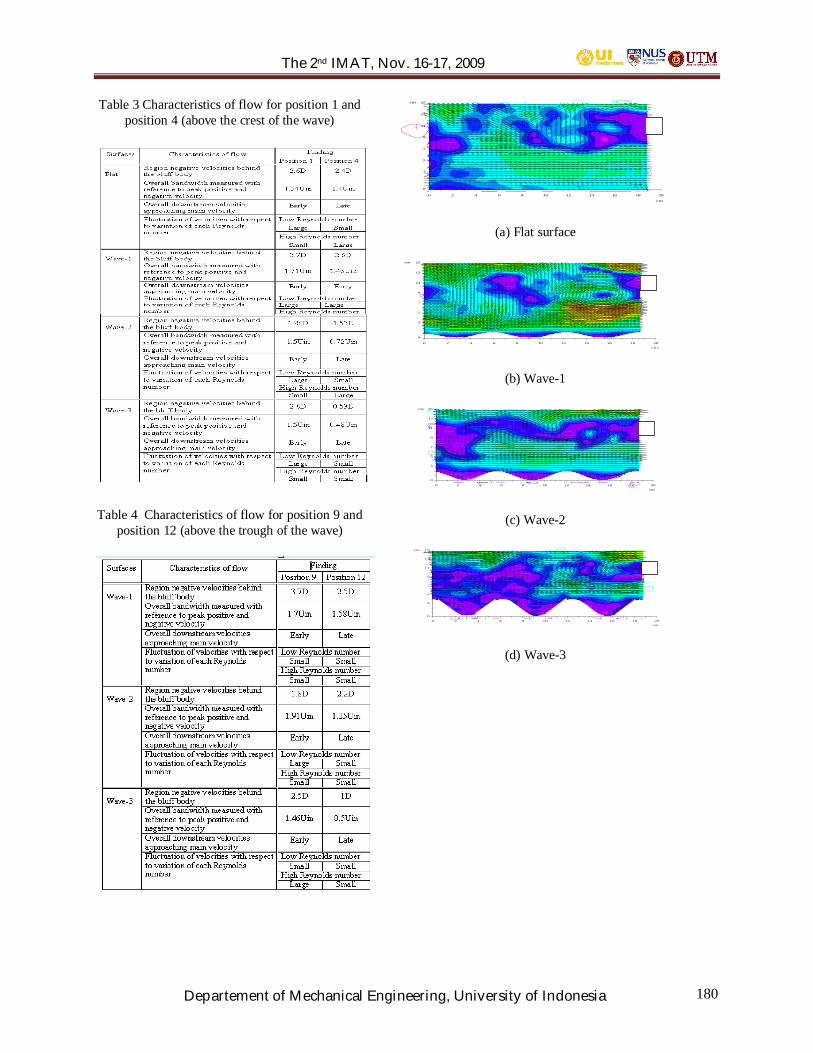
The 2nd IMAT, Nov. 16-17, 2009
Departement of Mechanical Engineering, University of Indonesia 180
Table 3 Characteristics of flow for position 1 andposition 4 (above the crest of the wave)
Table 4 Characteristics of flow for position 9 andposition 12 (above the trough of the wave)
cm
cm
0
3
5
7
9
11
13
15
0 2 4 6 8 10 12 14 16 18 20
(a) Flat surface
cm
cm
0
3
5
7
9
11
13
15
0 2 4 6 8 10 12 14 16 18 20
(b) Wave-1
cm
cm
0
3
5
7
9
11
13
15
0 2 4 6 8 10 12 14 16 18 20
(c) Wave-2
cm
cm
0
3
5
7
9
11
13
15
0 2 4 6 8 10 12 14 16 18 20
(d) Wave-3
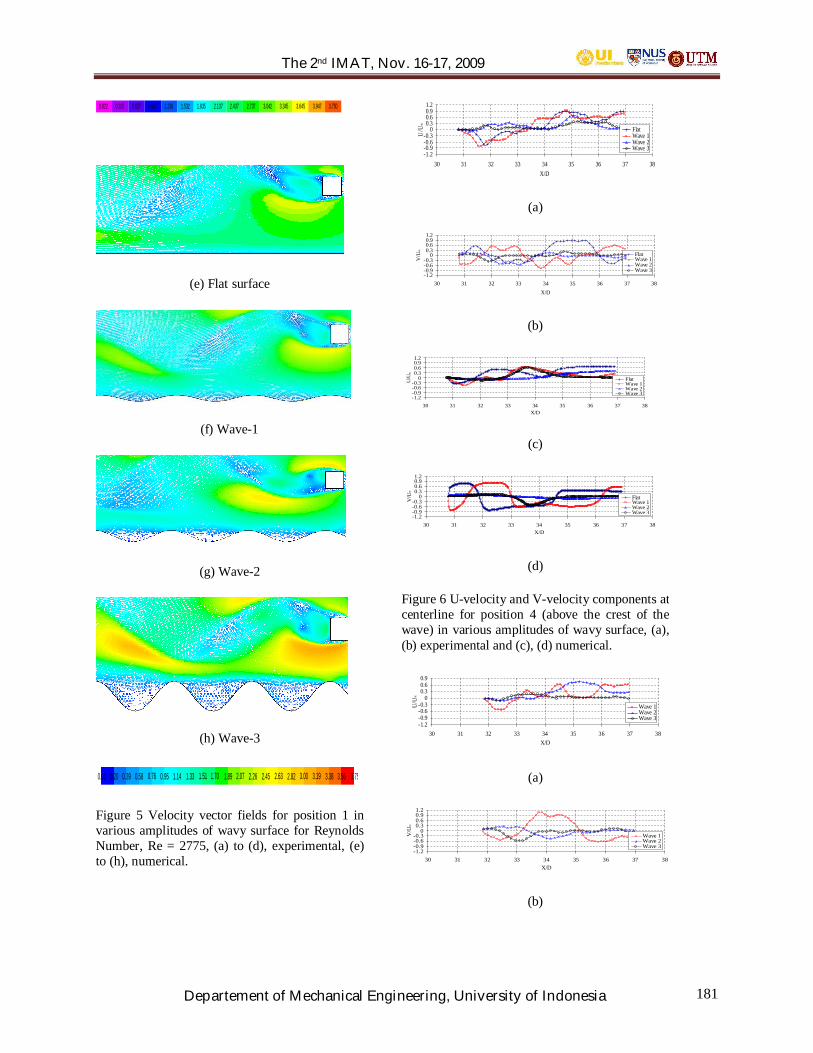
The 2nd IMAT, Nov. 16-17, 2009
Departement of Mechanical Engineering, University of Indonesia 181
0.022 0.325 0.627 0.927 1.230 1.532 1.835 2.137 2.437 2.737 3.042 3.345 3.645 3.947 3.750
(e) Flat surface
(f) Wave-1
(g) Wave-2
(h) Wave-3
3.563.383.193.002.822.632.452.262.071.891.701.511.331.140.950.760.580.390.200.02 3.75
Figure 5 Velocity vector fields for position 1 invarious amplitudes of wavy surface for ReynoldsNumber, Re = 2775, (a) to (d), experimental, (e)to (h), numerical.
-1.2-0.9-0.6-0.3
00.30.60.91.2
30 31 32 33 34 35 36 37 38X/D
U/U Flat
Wave 1Wave 2Wave 3
(a)
-1.2-0.9-0.6-0.3
00.30.60.91.2
30 31 32 33 34 35 36 37 38X/D
V/U Flat
Wave 1Wave 2Wave 3
(b)
-1.2-0.9-0.6-0.3
00.30.60.91.2
30 31 32 33 34 35 36 37 38X/D
U/U Flat
Wave 1Wave 2Wave 3
(c)
-1.2-0.9-0.6-0.3
00.30.60.91.2
30 31 32 33 34 35 36 37 38X/D
V/U Flat
Wave 1Wave 2Wave 3
(d)
Figure 6 U-velocity and V-velocity components atcenterline for position 4 (above the crest of thewave) in various amplitudes of wavy surface, (a),(b) experimental and (c), (d) numerical.
-1.2-0.9-0.6-0.3
00.30.60.9
30 31 32 33 34 35 36 37 38X/D
U/U
Wave 1Wave 2Wave 3
(a)
-1.2-0.9-0.6-0.3
00.30.60.91.2
30 31 32 33 34 35 36 37 38X/D
V/U
Wave 1Wave 2Wave 3
(b)

The 2nd IMAT, Nov. 16-17, 2009
Departement of Mechanical Engineering, University of Indonesia 182
-1.2-0.9-0.6-0.3
00.30.60.91.2
30 31 32 33 34 35 36 37 38X/D
U/U
Wave 1Wave 2Wave 3
(c)
-1.2-0.9-0.6-0.3
00.30.60.91.2
30 31 32 33 34 35 36 37 38X/D
V/U
Wave 1Wave 2Wave 3
(d)
Figure 7 U-velocity and V-velocity components atcenterline for position 12 (above the trough of thewave) in various amplitudes of wavy surface, (a),(b) experimental and (c), (d) numerical.

The 2nd IMAT, Nov. 16-17, 2009
Departement of Mechanical Engineering, University of Indonesia 183
Computational Fluid Dynamics Simulation of Stenosis Effect in UpperHuman Airways
Zuhairi Sulaiman ,Nasrul Hadi Johari, Kahar Osman
aFaculty of Mechanical EngineeringUniversity of Technology Malaysia,
81310 Skudai, Johor, MalaysiaTel : (6019) 911178
E-mail : [email protected]
ABSTRACT
Trachea stenosis; one of chronic obstructionpulmonary disease (COPD), inside the humanlung was studied in this project as it related toflow behavior. First and second generation ofnormal and diseased human airways has beenconstructed and simulated by using numericalmodeling. Stenosis, located at mid section oftrachea has been varied for four sizes of airwaysdiameters; 20, 40, 60 and 80 percent. Laminarflow with Re=1710 with a boundary conditionwere used to visualize a normal human breathing(light exercise). Pressure gradient and air flowvelocity correlations from top of trachea to thebronchi have been studied. The results showedthat stenosis with more than 60 percent diameter,produced significant pressure drop downstreamcompared to smaller diameter at location T2. Theresults also showed drastic increased in flowvelocity along the centerline. In general, intensivetreatment is suggested for stenosis with greaterthan 60 percent diameter.
Keywords
Example:Computational fluid dynamics (CFD), trachealstenosis, airflow
1. INTRODUCTION
Upper human airways geometry is a smalldimension and smaller airways deep down intothe lungs which are inaccessible [1]. Upperhuman airways consist of nose, mouth, pharynx,larynx and trachea. At the edge of trachea, thestructure divides into two branches which calledbronchi and lung up until the alveolar.
Tracheal stenosis is a lung disease caused bytrauma including accidents, chemical exposure,
and intubation. Stenosis is narrowing the tracheaand can obstruct the airflow inside the airways.Symptoms can include, but are not limited to thefollowing: shortness of breathe also known asDyspnea;wheezing or stridor and also asthma [2].This airflow problem inside the airways can beunderstood by using one alternative method:computational fluid dynamics.
Numerous CFD studies exist around the worldswhich address the problem of air flow andparticle deposition in selected segment in humanbody. Natalya et al [3] have simulated the airflowand aerosol deposition in human lungs to see thetrapping particles on the wall and the locations tobe recorded. X.Y Luo et al. [4] used CFD todetermine the turbulent/transitional airflow effectin lung airways and have compared the result withthe laminar and k- model. Besides, Schroter andSudlow [5] who have made the earliestexperimental study of airflow dynamics within ahuman respiratory network concluded that theinspiratory flows were independent on eitherReynolds number or entry velocity profiles.
Besides, there were others CFD studies existwhich address the problem of air flow and particledeposition in selected segments [6-13]. However,most of these studies only focussed on symmetricbifurcation airways, and the effects of obstructiveairways on airflow and particle deposition is veryrare [14]. This study aims to get the correlationsof human airway flow parameters with thetracheal stenosis disease. Pressure distribution andairflow velocity are the significant parameters toanalyze during inhalation for both normal anddiseased trachea.

The 2nd IMAT, Nov. 16-17, 2009
Departement of Mechanical Engineering, University of Indonesia 184
2. METHODOLOGY
In this study, the commercial 3D modelingSoftware, Solidworks® (version 2008) and CFDcode EFD software (Flomerics, version 2008)were used. This software uses the finite volumeanalysis to solve the Navier-Stokes and continuityequations on an arbitrary shaped flow withappropriate boundary conditions. This project isseeking to model only part of whole breathingcycle with steady inspiration, as occurs wheninhaler is used by an asthmatic patient. There isan experiment that showed steady state flow can‘accurately mimic’ conditions during inspirationfor flow rate up to 150 l/min, [15]. His experimentwas agreed by X.Y.Luo et al. [16], in order tosolve flow modeling of upper airways duringheavy breathing, which produces turbulentfeatures.
2.1 The geometric model
The airway model was reconstructedbased on same physiological details as Horfield etal. [17]. However the model only consists of thetrachea, right and left bronchi. Details of themodel dimension are in the Table 1. The top viewtube of the airways labeled as shown by figure 1.In this simple airways model, the real shape oftrachea like C-shape, D-Shape and others are notconsidered.
In figure 2, it shows how the trachea is havingaiding interpreting process of the plotted results.Note that “left” and “right” refer to the anatomicalorientation of human body. Normal asymmetricmodel without disease was built and validated bythe study of Calay et al [1] by comparing bothresults. Later, the Normal Asymmetric Modelreconstructed with the stenosis growth. Themodification of the model configurations are forthe purpose of studying the flow behavior effectby stenosis.
Table 1: Geometric details of the model.
Figure 1.Reconstructure model of normal tracheaand its 1st to 2nd generations. (a) Normal tracheaand main bronchi with the location of stenosis, T2that would be happen. (b) Cross-sectional oftrachea model
Figure 2.Size of stenosis growth by diameterpercentages at T2. Narrowing of diameter sizesis made from 20 percent up to 80 percent.
Segment Diameter(m)
Length(m)
Branchingangle (°)
Trachea 0.016 0.1 0Left 0.012 0.05 73
Right 0.0111 0.022 35
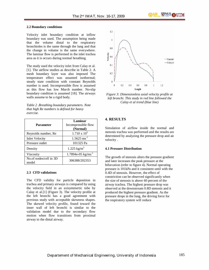
The 2nd IMAT, Nov. 16-17, 2009
Departement of Mechanical Engineering, University of Indonesia 185
2.2 Boundary conditions
Velocity inlet boundary condition at inflowboundary was used. The assumption being madethat the volume distal to the respiratorybronchioles is the same through the lung and thatthe change in volume is the same everywhere.The laminar flow is performed in the inlet tracheaarea as it is occurs during normal breathing.
The study used the velocity inlet from Calay et al.[1]. The airflow studies as describe in Table 2. Amesh boundary layer was also imposed Thetemperature effect was assumed isothermal;steady state condition with constant Reynoldsnumber is used. Incompressible flow is assumedas this flow has low March number. No-slipboundary condition is assumed [18]. The airwayswalls assume to be a rigid body.
Table 2 .Breathing boundary parameters. Notethat high Re numbers is defined for heavyexercise.
ParameterLaminar
Incompressible flow(Normal)
Reynolds number, Re 1.710 x 10³
Inlet Velocity 1.5625 ms-1
Pressure outlet 101325 PaDensity 1.225 kg/m3
Viscosity 1.7894e-05 kg/ms-1
No.of nodes/cell in 3Dmodel 306388/202353
2.3 CFD validations
The CFD validity for particle deposition intrachea and primary airways is compared by usingthe velocity field in an axisymmertic tube byCalay et al.[1] (Figure 3). The velocity profile atthe left bronchi has a good agreement withprevious study with acceptable skewness shapes.The skewed velocity profile, found toward theinner wall of left bronchi is similar to thevalidation model due to the secondary flowmotion when flow transitions from proximalairway to the distal airway.
Figure 3: Dimensionless axial velocity profile atleft bronchi. This study in red line followed the
Calay et al trend (blue line)
4. RESULTS
Simulation of airflow inside the normal andstenosis trachea was performed and the results aredetermined by analyzing the pressure drop and airvelocity .
4.1 Pressure Distribution
The growth of stenosis alters the pressure gradientand later increases the peak pressure at thebifurcation (refer to figure 4). Normal operatingpressure is 101kPa and it consistent until with the0.4D of stenosis. However, the effect ofconstriction can be observed significantly whenthe size of stenosis is above 60 percent of theairway trachea. The highest pressure drop wasobserved at the downstream 0.8D stenosis and itproduced the highest pressure gradient. As thepressure drops in the lung, the driving force forthe respiratory system will reduce

The 2nd IMAT, Nov. 16-17, 2009
Departement of Mechanical Engineering, University of Indonesia 186
Figure 4: Peak pressure correlation of airflowwhen pass through stenosis of different size atlocation T2.
4.2 Velocity profile
Air velocity changed due to the obstruction ofstenosis in the trachea. Figure 7 showed theconstriction of stenosis at T2 location produceddifferent air velocity flow along the airways.
Figure 5: Air velocity at central line along thetrachea. Different graph line determined the airvelocity at different model of trachea, normal andstenosis structure.
With inlet velocity of 1.56 ms-1, it remains stablefor upstream and downstream of T2 locationinside the normal trachea. Stenosis with the size0.8D increased the velocity up to 40 ms-1
compared to only 2 ms-1 for 0.2D when it flow atT2. Although the growing of diameter is 4 times(0.2D to 0.8D), it produce a big different outputflow. At extreme velocity, 40 ms-1 which occurredfrom 0.8D, it significantly increased 20 timesfrom the flow of 0.2D. It seems like when stenosisincreased, it changed the upstream anddownstream at location T2 to become stronger.
7. CONCLUSION
Finally, this CFD method had solved a fluiddynamics problem inside the human lung andproduced the analysis of the effects of obstructedairway narrowing and occlusion on the airstreams.The results showed that stenosis with more than60 percent diameter, produced significantpressure drop downstream compared to smallerdiameter at location T2. The results also showeddrastic increased in flow velocity along thecenterline. In general, intensive treatment issuggested for stenosis with greater than 60percent diameter.
REFERENCES
[1] Calay R.K, Kurujareon J. and Holdo A.E.,“Numerical simulation of respiratory flow patternswithin human lung” Respiratory physiology andneurobiology, 130,201-221]
[2] Hermes C. Grillo, “Surgery of Trachea andBronchi”,Harvard University Gazette, 2004].
[3] Natalya Nowak, Prashant P.Kakade, and AnanthV.Annapragada, “Computional Fluid DynamicsSimulation of Airflow and Aerosol Deposition inHuman Lungs” Annals of BiomedicalEngineering, Vol.31,pp.374-390, 2003.
[4] X.Y.Luo, J.S.Hinton,T.T.Liew and K.K.Tan, “LESmodeling of flow in a simple airwaymodel”Elsevier Medical Engineering & Physics 26, 4003-413, 2004 2]
[5] Schroeter, R.C., & Sudlow,M.F “ Flow patterns inmodels of human bronchial airways”, RepirationPhysiology, 7, 341-355, 1969
[6] Balashazy I, Hofmann W, Mortenen TB,“Inspiratory particle deposition in airwaybifurcation models”, J Aerosol Sciece,1991;22:15-30]

The 2nd IMAT, Nov. 16-17, 2009
Departement of Mechanical Engineering, University of Indonesia 187
[7] Balashazy I, Hofmann W, “Particle deposition inairway bifurcations”, J.Aerosol Science,1993;24:722-45
[8] Hofmann W, Balashazy I, “Particle depositionwithin airway bifurcation”, Staub Renhalt Luft1991;33:178-82
[9] Kim SC, Iglesias JA, “Deposition of inhaledparticles in bifurcating airway models:1.Inspiratory deposition, J Aerosol Med 1989;2:1-14
[10] Kim SC, Fisher DM, Lutz DJ,Gerrity TR,“Particle deposition in bifurcating airway modelswith varying airway geometry, J Aerosol Science1993;25:567-81
[11] Koblinger L, Hofmann W, Monte Carlo,“Modelling of aerosol deposition in human lungs.Part 1: simulation of particle transport instochastic lung structure. J Aerosol Science1990;27:119-38
[12] Lee JW, Goo JH, “Numerical simulation of airflowand inertial deposition of particles in a bifurcatingchannel of square cross section, J Aerosol Med1992;5:131-54
[13] Sclesinger RB, Lippmann M., “Particle depositionin casts of the human upper tracheobroncial tree”.Am Ind Hyg Assoc J 1972;33:237-51
[14] Mark B.M,Jayaraju, S.T. Lacor C., Mey JD,,Noppen M, Vincken, W.Verbanck, “Trachealstenosis” A Flow Dynamics Study, JournalApplied Physiology 2006.
[15] Olson DE,Sudlow MF, Horsfield K, Filey GP,“Convective patterns of flow during inspiration”,Arch Int Med 1973;131:51-7
[16] J.S.Hinton,T.T.Liew and K.K.Tan, “LES modelingof flow in a simple airway model”ElsevierMedical Engineering & Physics 26 , 4003-413,2004 2
[17] Horsfield, K.Dart, G.Olson, D.E Filley, G.F. &Cumming , “Models of the human bronchial tree”,Journal of Applied Physiology,31,207-217
[18] Yang X.L. and Liu Y., “Simulation of effect ofCOPD on respiratory flow,Tsinghua UniversityPress & Springer-Verlag, 2006.
[19] Van Wylen, G.J. and Sonntag, R.E , “Fundamentalof Classical Thermodynamics”, section 5.9, JohnWiley and Sons Inc., New York1965].

The 2nd IMAT, Nov. 16-17, 2009
Departement of Mechanical Engineering, University of Indonesia 188
Study on Characteristics of Briquettes Contain DifferentMixing Ratio of EFB Fibre and Mesocarp Fibre
H. M. Faizal , Z. A. Latiff, Mazlan A. Wahid, Darus A. N.
Faculty of Mechanical EngineeringUniversiti Teknologi Malaysia,81310 UTM Skudai
Tel: (+60)7-5534657 E-mail: [email protected]
ABSTRACT
Based on Malaysia Palm Oil Statistics, theproduction of palm biomass residues such asshell, mesocarp fibre and empty fruit bunch(EFB) increased significantly from year to year.These residues especially mesocarp fibre andEFB were dumped in areas adjacent to the palmoil mills. Therefore, briquetting technology isexpected can improve this waste disposal byconverting these residues into solid fuels withhigher energy content per unit volume. In thispaper, the physical characteristics andcombustion properties of briquettes contain newproposed mixture has been investigated. Thismixture composed of mesocarp fibre and EFBfibre in different weight ratios. EFB fibre isobtained after dyring process by superheatedsteam with the pressure ranges from 1.0 to 1.5bar and temperature ranges from 100 to 120oC.Based on several tests done for investigating thecapability of new mixture of palm biomassbriquettes, it was found that the briquette withweight ratio of 60:40 (EFB fibre: mesocarp fibre)satisfies the minimum requirement for commercialbriquette DIN 51731. Besides, this ratio isselected due to the emphasis on the use of largeportion of EFB.
Keywords
Briquetting, briquette, palm biomass, combustionrate, shell, mesocarp fibre, EFB fibre, DIN 51731
1. INTRODUCTION
As reported by Malaysia Palm Oil Board (MPOB,2006), the production of shell, mesocarp fibre andEFB in Malaysia for year 2006 are 5.20x10⁶
tonne/year, 9.66x10⁶ tonne/year, and 17.08x10⁶
tonne/year respectively. Therefore, the utilizationof these residues is very important in order to
prevent waste and dumping areas adjacent to themills.
Conversion of these residues into briquette is oneof the methods to improve the propertiesespecially in term of energy content per unitvolume. As explained by Bhattacharya et al.(1996), densification (briquetting, pelletizing andbaling) is a process that can improve the storageand transportation of biomass fuel.
Chin and Siddiqui (2000) have conducted anexperiment to study the combustion rate onvarious biomass briquettes such as raw husks,sawdust and several others. The compactionpressure was within the range of 1 to 7 MPa. Itwas found that the burning rate increased as thebinder content increased. The binding agents usedin their experiment were molasses and starch.
In year 2002, an experiment that was carried outby Husain et al. (2002) explain the physical andcombustion characteristics of current localbriquettes contain mesocarp fibre and shell in theratio of 60:40. They used starch as binding agent(10% of the weight of residues) with addition ofwater (50% of the weight of residues). Theyfound that the combustion of heap of briquettes inthe stove releases about 0.5kW, air-fuel ratio wasabout 10.2 and ash content was 5.8%. Besides, theaverage compressive strength of about 2.56 MPais considered as a value for good resistance fordisintegration.
Meanwhile, in year 2008, Nasrin et al. (2008)studied the physical and combustioncharacteristics of palm biomass briquettescontaining EFB fibre and palm kernel cake(PKC). The weight ratio for PKC + EFB fibre +sawdust was 30:5:65. In this case, sawdust plays arole as binder. In their study, they found that thestrength of briquettes increased when the sawdustwas added.
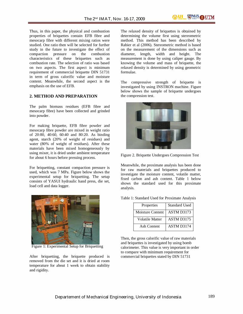
The 2nd IMAT, Nov. 16-17, 2009
Departement of Mechanical Engineering, University of Indonesia 189
Thus, in this paper, the physical and combustionproperties of briquettes contain EFB fibre andmesocarp fibre with different mixing ratios werestudied. One ratio then will be selected for furtherstudy in the future to investigate the effect ofcompaction pressure on the combustioncharacteristics of these briquettes such ascombustion rate. The selection of ratio was basedon two aspects. The first aspect is minimumrequirement of commercial briquette DIN 51731in term of gross calorific value and moisturecontent. Meanwhile, the second aspect is theemphasis on the use of EFB.
2. METHOD AND PREPARATION
The palm biomass residues (EFB fibre andmesocarp fibre) have been collected and grindedinto powder.
For making briquette, EFB fibre powder andmesocarp fibre powder are mixed in weight ratioof 20:80, 40:60, 60:40 and 80:20. As bindingagent, starch (20% of weight of residues) andwater (80% of weight of residues). After thesematerials have been mixed homogeneously byusing mixer, it is dried under ambient temperaturefor about 6 hours before pressing process.
For briquetting, constant compaction pressure isused, which was 7 MPa. Figure below shows theexperimental setup for briquetting. The setupconsists of YASUI hydraulic hand press, die set,load cell and data logger.
Figure 1: Experimental Setup for Briquetting
After briquetting, the briquette produced isremoved from the die set and it is dried at roomtemperature for about 1 week to obtain stabilityand rigidity.
The relaxed density of briquettes is obtained bydetermining the volume first using stereometricmethod. This method has been described byRabier et al (2006). Stereometric method is basedon the measurement of the dimensions such asdiameter, length, width and height. Themeasurement is done by using caliper gauge. Byknowing the volume and mass of briquette, therelaxed density is determined by using geometricformulae.
The compressive strength of briquette isinvestigated by using INSTRON machine. Figurebelow shows the sample of briquette undergoesthe compression test.
Figure 2. Briquette Undergoes Compression Test
Meanwhile, the proximate analysis has been donefor raw materials and briquettes produced toinvestigate the moisture content, volatile matter,fixed carbon and ash content. Table 1 belowshows the standard used for this proximateanalysis.
Table 1: Standard Used for Proximate Analysis
Then, the gross calorific value of raw materialsand briquettes is investigated by using bombcalorimeter. This value is very important in orderto compare with minimum requirement forcommercial briquettes stated by DIN 51731
Properties Standard Used
Moisture Content ASTM D3173
Volatile Matter ASTM D3175
Ash Content ASTM D3174

The 2nd IMAT, Nov. 16-17, 2009
Departement of Mechanical Engineering, University of Indonesia 190
3. RESULTS AND DISCUSSION
3.1 For Raw Materials
The result of proximate analysis for raw materialsis shown in Table 2 below. It is found that themoisture content for all raw materials are stillunder the average of current local practicedbriquette (12.5%) and also satisfies the minimumrequirement of DIN 51731 (<10%).
Table 2. Proximate Analysis for Raw Materials
Meanwhile, the gross calorific value for rawmaterials is shown in Table 3 below. It isexpected that the combination of mesocarp fibreand EFB fibre able to produce the briquette whichsatisfy the minimum requirement of DIN 51731(17500 J/g). Therefore, in the following subsection, the result of different mixing ratio of EFBfibre and mesocarp fibre will be discussed.
Table 3. Gross Calorific Value for Raw Materials
3.2 For Briquettes with Different Mixing Ratio
In this section, the physical characteristics andcombustion properties of briquettes with differentmixing ratio are discussed. The results from thetests are very useful in order to know the effect ofdifferent mixing ratio on durability and potentialof briquette to be commercial briquette.
3.2.1 Physical Characteristics
Figure 3 below shows the sample for briquettewith mixing ratio 80:20 (EFB fibre: mesocarpfibre)
Figure 3. Image of Briquette with Mixing Ratio80:20
The density of briquette is very important inshowing the energy content per unit volume.Thus, high density is necessary in order to reducethe process of uploading the briquette to boilers.
Figure 4. The Relaxed Density of BriquettesContains Different Mixing Ratio.
As shown in Figure 4 above, there is nosignificant difference when mixing ratio ischanged. The range of density is about 988 kg/m3
to 1000 kg/m3. However, when percentage ofmesocarp fibre increased, the relaxed density ofbriquettes also tends to increase. This is mainlydue to the density of mesocarp fibre whichslightly higher that the density of EFB fibre.
Figure 5. Compressive Strength versus Ratio
ITEM EFB shell mesocarp fibreFixed Carbon (%) 15.08315.685 14.889
Moisture Content (%) 7.331 8.528 5.200Volatile Matter (%) 72.96273.208 75.111
Ash Content (%) 4.624 2.579 4.800
Materials Average Calorific Value(kJ/kg)
Shell 19584Fibre frommesocarp
18098
EFB fibre 17465
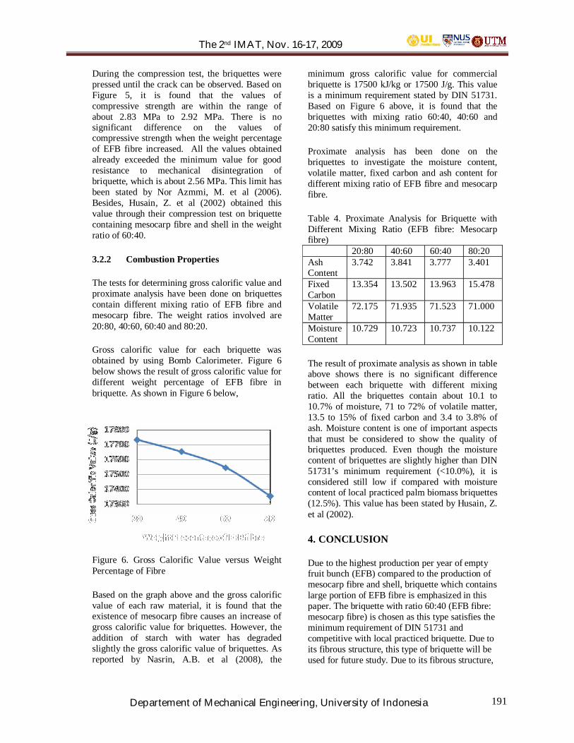
The 2nd IMAT, Nov. 16-17, 2009
Departement of Mechanical Engineering, University of Indonesia 191
During the compression test, the briquettes werepressed until the crack can be observed. Based onFigure 5, it is found that the values ofcompressive strength are within the range ofabout 2.83 MPa to 2.92 MPa. There is nosignificant difference on the values ofcompressive strength when the weight percentageof EFB fibre increased. All the values obtainedalready exceeded the minimum value for goodresistance to mechanical disintegration ofbriquette, which is about 2.56 MPa. This limit hasbeen stated by Nor Azmmi, M. et al (2006).Besides, Husain, Z. et al (2002) obtained thisvalue through their compression test on briquettecontaining mesocarp fibre and shell in the weightratio of 60:40.
3.2.2 Combustion Properties
The tests for determining gross calorific value andproximate analysis have been done on briquettescontain different mixing ratio of EFB fibre andmesocarp fibre. The weight ratios involved are20:80, 40:60, 60:40 and 80:20.
Gross calorific value for each briquette wasobtained by using Bomb Calorimeter. Figure 6below shows the result of gross calorific value fordifferent weight percentage of EFB fibre inbriquette. As shown in Figure 6 below,
Figure 6. Gross Calorific Value versus WeightPercentage of Fibre
Based on the graph above and the gross calorificvalue of each raw material, it is found that theexistence of mesocarp fibre causes an increase ofgross calorific value for briquettes. However, theaddition of starch with water has degradedslightly the gross calorific value of briquettes. Asreported by Nasrin, A.B. et al (2008), the
minimum gross calorific value for commercialbriquette is 17500 kJ/kg or 17500 J/g. This valueis a minimum requirement stated by DIN 51731.Based on Figure 6 above, it is found that thebriquettes with mixing ratio 60:40, 40:60 and20:80 satisfy this minimum requirement.
Proximate analysis has been done on thebriquettes to investigate the moisture content,volatile matter, fixed carbon and ash content fordifferent mixing ratio of EFB fibre and mesocarpfibre.
Table 4. Proximate Analysis for Briquette withDifferent Mixing Ratio (EFB fibre: Mesocarpfibre)
20:80 40:60 60:40 80:20AshContent
3.742 3.841 3.777 3.401
FixedCarbon
13.354 13.502 13.963 15.478
VolatileMatter
72.175 71.935 71.523 71.000
MoistureContent
10.729 10.723 10.737 10.122
The result of proximate analysis as shown in tableabove shows there is no significant differencebetween each briquette with different mixingratio. All the briquettes contain about 10.1 to10.7% of moisture, 71 to 72% of volatile matter,13.5 to 15% of fixed carbon and 3.4 to 3.8% ofash. Moisture content is one of important aspectsthat must be considered to show the quality ofbriquettes produced. Even though the moisturecontent of briquettes are slightly higher than DIN51731’s minimum requirement (<10.0%), it isconsidered still low if compared with moisturecontent of local practiced palm biomass briquettes(12.5%). This value has been stated by Husain, Z.et al (2002).
4. CONCLUSION
Due to the highest production per year of emptyfruit bunch (EFB) compared to the production ofmesocarp fibre and shell, briquette which containslarge portion of EFB fibre is emphasized in thispaper. The briquette with ratio 60:40 (EFB fibre:mesocarp fibre) is chosen as this type satisfies theminimum requirement of DIN 51731 andcompetitive with local practiced briquette. Due toits fibrous structure, this type of briquette will beused for future study. Due to its fibrous structure,

The 2nd IMAT, Nov. 16-17, 2009
Departement of Mechanical Engineering, University of Indonesia 192
this type of briquette is expected will show goodperformance of combustion characteristicsespecially combustion rate and heat release.
ACKNOWLEDGEMENT
The authors acknowledge the Universiti TeknologiMalaysia for giving cooperation and full of support inthis research activity.
REFERENCES
[1] Bhattacharya S.C., Augustus Leon M. andMizanur Rahman M. (1996). A Study onImproved Biomass Briquetting. RenewableEnergy Technologies in Asia.
[2] Cattaneo, D. (2003). Briquetting-A ForgottenOpportunity. Wood Energy. University ofBrescia.
[3] Chin, O.C., Siddiqui, K. M. (2000).Characteristics of Some Biomass BriquettesPrepared Under Modest Die Pressures. Biomassand Bioenergy. 18, 223-228.
[4] Husain, Z., Zainac, Z., Abdullah, Z. (2002).Briquetting of Palm Fibre and Shell from theProcessing of Palm Nuts to Palm Oil. Biomassand Bioenergy. 22, 505-509. Pergamon.
[5] Nasrin, A.B., Ma, A.N., Choo, Y.M., Mohamad,S., Rohaya, M.H., Azali, A. and Zainal, Z.(2008). Oil Palm Biomass as PotentialSubstitution Raw Materials for CommercialBiomass Briquettes Production. AmericanJournal of Applied Sciences. 5 (3), 179-183.
[6] Nor Azmmi, M., Farid Nasir, A. (2006).Pressurised Pyrolysis of Rice Husk. MasterThesis. UTM Skudai.
[7] Rabier, F., Temmerman, M., Bohm, T.,Hartmann, H., Jensen, P. D., Rathbauer, J.,Carrasco, J., Fernandez, M. (2006). ParticleDensity Determination of Pellets and Briquettes.Biomass and Bioenergy. 30, 954-963.

The 2nd IMAT, Nov. 16-17, 2009
Departement of Mechanical Engineering, University of Indonesia 193
The Flow Modeling of Aneurysm under Physical andPhysiological Condition
Ishkrizat Taib1, Kahar Osman2, Mohammed Rafiq Abd Kadir3
1Faculty of Mechanical and Manufacturing EngineeringUniversiti Tun Hussein Onn Malaysia,
Tel : (013) 7270011 ext 51. Fax : (021) 7270077E-mail : [email protected]
2Faculty of Mechanical EngineeringUniversiti Teknologi Malaysia
Tel : (021) 7270011 ext 51. Fax : (021) 7270077E-mail : [email protected]
ABSTRACT
The investigation on the pulsatile flow in ananeurysm can yield unexpected predicament. Thisstudy will analyzed the pulsatile flow usingnumerical modeling for various physical andphysiological conditions at peak and late systoletimes. The results of this study shows the presenceof the vortex is observed at aneurysm region forboth physical and physiological condition. Thepresence of the vortex is proportional to theincrease of flow activity at the aneurysm. The flowactivity is much higher at distal end comparedproximal end region. The different of flow activityshow the different strength of the vortex occurredat the aneurysm bulge. The results also showHBPE peak systole distribute the highest value ofthe pressure among others condition which isexhibits the high risk of the aneurysm fromrupture.
KeywordsAbdominal aortic aneurysm, pulsatile flow,numerical modeling.
1. INTRODUCTION
Aneurysm is focal dilatation of the bloodvessel due the weakening of the main aorta whichprone to be ruptured if not surgically treated. Thephysician determines that the possibility ofrupture in aneurysm is at the largest diameter [1].In clinical practice, AAA is considered thesurgical treatment after the maximal diameter ofaorta exceeds 5-6 cm [2]. The probability of theaneurysm to rupture is high if the diameter of theaneurysm exceed more than 5cm and theaneurysm will be treated using the synthetic graft[1]. R.C. Darling et al reported that the rate of the
aneurysm rupture between 4.1 cm and 7 cm isaround 25% while the rupture of the aneurysmless than 4 cm expansion per year is around 9.5%[3]. Rupture of abdominal aortic aneurysm hashigh morbidity and mortality rates. Many peopledied before entering the operating room. On thatreason, the surgeon has made a difficult decisionbecause of the uncertainty about the risk ruptureof abdominal aortic aneurysm. Duringphysiological pulsatile flow, the largest aneurysmdemonstrates turbulence rather than in smallaneurysm [4]. However, the correlation betweenthe largest of the aneurysm and probability theaneurysm ruptures is still in question mark bymany researchers. The expansion of the aneurysmsegment eventually increase the risk of theaneurysm rupture [5] although, rupture couldoccur in a small aneurysm [1]. The aneurysmrupture is a major complication at the diseasevessel especially in AAA which lead to 90percent of the patients died [6]. Hence, thetechnology will facilitate the medical doctor tomake the early prediction of aneurysm rupture onthe patient and directly make the decision forendovascular repair (EVAR).
Pulsatile flow characteristics in AAA have beenconsidered by many researchers [7,8] in whichthe flow pattern is different from that of steadyflow. The hemodynamic stresses are higher inpulsatile flow rather than in steady flow [8] asillustrated in the pulsatile flow behavior which issignificant to determine the development of theatherosclerosis and thrombus formation in AAAs.Peattie et al [11] has simulated the resting time invivo for fusiform model for the pulsatile flow toanalyze the flow behavior and shear stressdistribution at aneurysm wall. As a result, theflow behavior inside the aneurysm becomesunstable proportional to the increment of thebulge aneurysm size. Egelhoff et al [4] has
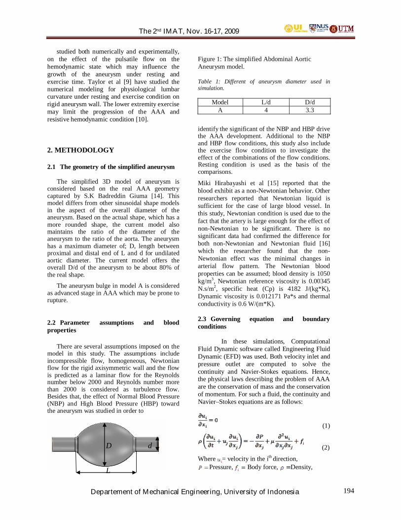
The 2nd IMAT, Nov. 16-17, 2009
Departement of Mechanical Engineering, University of Indonesia 194
studied both numerically and experimentally,on the effect of the pulsatile flow on thehemodynamic state which may influence thegrowth of the aneurysm under resting andexercise time. Taylor et al [9] have studied thenumerical modeling for physiological lumbarcurvature under resting and exercise condition onrigid aneurysm wall. The lower extremity exercisemay limit the progression of the AAA andresistive hemodynamic condition [10].
2. METHODOLOGY
2.1 The geometry of the simplified aneurysm
The simplified 3D model of aneurysm isconsidered based on the real AAA geometrycaptured by S.K Badreddin Giuma [14]. Thismodel differs from other sinusoidal shape modelsin the aspect of the overall diameter of theaneurysm. Based on the actual shape, which has amore rounded shape, the current model alsomaintains the ratio of the diameter of theaneurysm to the ratio of the aorta. The aneurysmhas a maximum diameter of; D, length betweenproximal and distal end of L and d for undilatedaortic diameter. The current model offers theoverall D/d of the aneurysm to be about 80% ofthe real shape.
The aneurysm bulge in model A is consideredas advanced stage in AAA which may be prone torupture.
2.2 Parameter assumptions and bloodproperties
There are several assumptions imposed on themodel in this study. The assumptions includeincompressible flow, homogeneous, Newtonianflow for the rigid axisymmetric wall and the flowis predicted as a laminar flow for the Reynoldsnumber below 2000 and Reynolds number morethan 2000 is considered as turbulence flow.Besides that, the effect of Normal Blood Pressure(NBP) and High Blood Pressure (HBP) towardthe aneurysm was studied in order to
Figure 1: The simplified Abdominal AorticAneurysm model.
Table 1: Different of aneurysm diameter used insimulation.
Model L/d D/dA 4 3.3
identify the significant of the NBP and HBP drivethe AAA development. Additional to the NBPand HBP flow conditions, this study also includethe exercise flow condition to investigate theeffect of the combinations of the flow conditions.Resting condition is used as the basis of thecomparisons.
Miki Hirabayashi et al [15] reported that theblood exhibit as a non-Newtonian behavior. Otherresearchers reported that Newtonian liquid issufficient for the case of large blood vessel. Inthis study, Newtonian condition is used due to thefact that the artery is large enough for the effect ofnon-Newtonian to be significant. There is nosignificant data had confirmed the difference forboth non-Newtonian and Newtonian fluid [16]which the researcher found that the non-Newtonian effect was the minimal changes inarterial flow pattern. The Newtonian bloodproperties can be assumed; blood density is 1050kg/m3, Newtonian reference viscosity is 0.00345N.s/m2, specific heat (Cp) is 4182 J/(kg*K),Dynamic viscosity is 0.012171 Pa*s and thermalconductivity is 0.6 W/(m*K).
2.3 Governing equation and boundaryconditions
In these simulations, ComputationalFluid Dynamic software called Engineering FluidDynamic (EFD) was used. Both velocity inlet andpressure outlet are computed to solve thecontinuity and Navier-Stokes equations. Hence,the physical laws describing the problem of AAAare the conservation of mass and the conservationof momentum. For such a fluid, the continuity andNavier–Stokes equations are as follows:
(1)
(2)
Where = velocity in the ith direction,Pressure, Body force, Density,L
D d

The 2nd IMAT, Nov. 16-17, 2009
Departement of Mechanical Engineering, University of Indonesia 195
Viscosity and Kronecker delta. Theshear stress, at the wall of aneurysm iscalculated based on a function of velocity gradientonly:
(3)
Where u/ y is the velocity gradient along theaneurismal wall taking into considerations thefluid viscosity. Therefore, the simple viscousfluids considered with linear relationship.
The inlet flow is considered fully developedparabolic flow, with zero radial velocity at theinlet, no slip applied at the wall and zero velocitygradient at the outlet. The inlet boundarycondition setting is pulsatile velocity [4] for theresting and exercise condition which whilst theoutlet boundary condition setting is pulsatilepressure [13] for time dependent.
3. RESULTS AND DISCUSSION
The imbalance flow inside the advancedaneurysm yield unexpected problem. Theimbalance flow experiences the presence of thevortex at the aneurysm region. This studydiscusses the effect of pressure distribution at theaneurysm during physical and physiologicalcondition. The high blood pressure in given moreattention since the high possibility of aneurysmrupture is reported in this condition. However,NBP is also taken into consideration ascomparison for those HBP results. Flowsvisualize the presence of vortex for HBPE,HBPR, NBPE and NBPR peak systole at theaneurysm wall as seen in Figure 2. Figure 2shows the flow pattern for the pressuredistribution at the advanced aneurysm wall duringexercise and resting time for HBP and NBP.HBPE peak systole flow is shown the dominatedvortex which fills the entire bulge of theaneurysm wall. The high pressure distributionexerted at the aneurysm wall will weaken the
Figure 2: Flow pattern for the pressure inside theadvanced AAA during the resting time andexercise time waveform for NBP and HBP (a)peak systole exercise time HBP shows thedominated vortex formation inside the aneurysm.(b) peak systole resting time HBP shows the
recirculation flow occur at the proximal end (c)peak systole exercise time NBP shows the vortexformation inside the AAA region (d) peak systoleresting time NBP shows the vortex formation atthe proximal end.
aneurysm wall. The flow during HBPR peaksystole shows the translation and growth of theprimary vortex at distal end of the aneurysm.However, the secondary vortex is seen inproximal end of aneurysm. The vortex strength isobserved more strong in distal end rather than inproximal end. The investigation on the NBPEpeak systole shows the vortex is conquered theentire bulge of the aneurysm when the blood flowtravels from proximal end to distal end. NBPRpeak systole shows the presence of the vortexonly in proximal end which covered roughly onethird from the aneurysm area. As summarized, thepressure distribution is shown to be highest duringHBPE peak systole compared those others results.Similar phenomenon of vortex formation is seenin HBPE and NBPE peak systole.
Moreover, the investigation on the vortexformation is continued for late systole time forboth HBP and NBP during exercise and restingtime which is illustrated in Figure 3. The presenceof the vortex is seen to dominate the whole regionof aneurysm during HBPE late systole as seen inFigure 3(a).
(a)
(b)
(c)
(d)
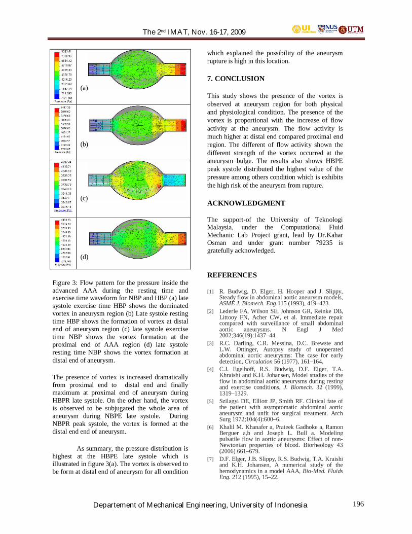
The 2nd IMAT, Nov. 16-17, 2009
Departement of Mechanical Engineering, University of Indonesia 196
(a)
(b)
(c)
(d)
Figure 3: Flow pattern for the pressure inside theadvanced AAA during the resting time andexercise time waveform for NBP and HBP (a) latesystole exercise time HBP shows the dominatedvortex in aneurysm region (b) Late systole restingtime HBP shows the formation of vortex at distalend of aneurysm region (c) late systole exercisetime NBP shows the vortex formation at theproximal end of AAA region (d) late systoleresting time NBP shows the vortex formation atdistal end of aneurysm.
The presence of vortex is increased dramaticallyfrom proximal end to distal end and finallymaximum at proximal end of aneurysm duringHBPR late systole. On the other hand, the vortexis observed to be subjugated the whole area ofaneurysm during NBPE late systole. DuringNBPR peak systole, the vortex is formed at thedistal end end of aneurysm.
As summary, the pressure distribution ishighest at the HBPE late systole which isillustrated in figure 3(a). The vortex is observed tobe form at distal end of aneurysm for all condition
which explained the possibility of the aneurysmrupture is high in this location.
7. CONCLUSION
This study shows the presence of the vortex isobserved at aneurysm region for both physicaland physiological condition. The presence of thevortex is proportional with the increase of flowactivity at the aneurysm. The flow activity ismuch higher at distal end compared proximal endregion. The different of flow activity shown thedifferent strength of the vortex occurred at theaneurysm bulge. The results also shows HBPEpeak systole distributed the highest value of thepressure among others condition which is exhibitsthe high risk of the aneurysm from rupture.
ACKNOWLEDGMENT
The support-of the University of TeknologiMalaysia, under the Computational FluidMechanic Lab Project grant, lead by Dr.KaharOsman and under grant number 79235 isgratefully acknowledged.
REFERENCES
[1] R. Budwig, D. Elger, H. Hooper and J. Slippy,Steady flow in abdominal aortic aneurysm models,ASME J. Biomech. Eng.115 (1993), 419–423.
[2] Lederle FA, Wilson SE, Johnson GR, Reinke DB,Littooy FN, Acher CW, et al. Immediate repaircompared with surveillance of small abdominalaortic aneurysms. N Engl J Med2002;346(19):1437–44.
[3] R.C. Darling, C.R. Messina, D.C. Brewste andL.W. Ottinger, Autopsy study of unoperatedabdominal aortic aneurysms: The case for earlydetection, Circulation 56 (1977), 161–164.
[4] C.J. Egelhoff, R.S. Budwig, D.F. Elger, T.A.Khraishi and K.H. Johansen, Model studies of theflow in abdominal aortic aneurysms during restingand exercise conditions, J. Biomech. 32 (1999),1319–1329.
[5] Szilagyi DE, Elliott JP, Smith RF. Clinical fate ofthe patient with asymptomatic abdominal aorticaneurysm and unfit for surgical treatment. ArchSurg 1972;104(4):600–6.
[6] Khalil M. Khanafer a, Prateek Gadhoke a, RamonBerguer a,b and Joseph L. Bull a. Modelingpulsatile flow in aortic aneurysms: Effect of non-Newtonian properties of blood. Biorheology 43(2006) 661–679.
[7] D.F. Elger, J.B. Slippy, R.S. Budwig, T.A. Kraishiand K.H. Johansen, A numerical study of thehemodynamics in a model AAA, Bio-Med. FluidsEng. 212 (1995), 15–22.

The 2nd IMAT, Nov. 16-17, 2009
Departement of Mechanical Engineering, University of Indonesia 197
[1] E.A. Finol and C.H. Amon, Blood flow inabdominal aortic aneurysms: Pulsatile flowhemodynamics, ASME J. Biomech.Eng. 123(2001), 474–484.
[2] Taylor, T.W., Yamaguchi, T., 1994. Three-dimensional simulation of blood flow in anabdominal aortic aneurysm- steady and unsteadyfow cases. ASME Journal of BiomechnicalEngineering 116, 88-97.
[3] Evangelos Boutsianis, Michele Guala, UfukOlgac, Simon Wildermuth, Klaus Hoyer, YiannisVentikos, Dimos Poulikakos,” CFD and PTVSteady Flow Investigation in an AnatomicallyAccurate Abdominal Aortic Aneurysm”,Journal ofBiomedical Engineering.131(2008),2406-2414.
[4] Peattie, R.A., Schrader, T., Bluth, E.I., Comstock,C.E., 1994. Development of turbulence in steadyflow through models of abdominal aorticaneurysms. Journal of Ultrasound Medicine 13,467-472.
[5] R.A. Peattie, T.J. Riehle and E.I. Bluth, Pulstaileflow in fusiform models of abdominal aorticaneurysms: flow fields,velocity patterns and flow-induced wall stresses, ASME J. Biomech. Eng. 126(2004), 438–446.
[6] Tayfun E. Tezduyar1, Sunil Sathe, MatthewSchwaab and Brian S. Conklin1, “Arterial fluidmechanics modeling with the stabilized space-timefluid-structure interaction technique,”International Journal for Numerical Methods inFluids, vol. 57, (no. 5), pp. 601-629, 2008.
[7] Badreddin Giuma S.K1, Kahar Osman1 andMohamed Rafiq Abdul Kadir1,2, “NumericalModeling of Fusiform Aneurysm with High andNormal Blood Pressure”.
[8] Miki Hirabayashi et al, “A lattice Boltzmann studyof blood flow in stented aneurism”, FutureGeneration Computer Systems, Elsevier B.V, 20(2004) 925–934.
[9] K.M. Khanafer et al.“Modeling pulsatile flow inaortic aneurysms:Effect of non-Newtonianproperties of blood”, IOS Press, Biorheology 43(2006) 661–679.

The 2nd IMAT, Nov. 16-17, 2009
Departement of Mechanical Engineering, University of Indonesia 198
Experimental Evaluation of the Effect of Taper Dieon Lubricant Performance
Syahrullail, S., Teh, S.C., Najib, Y.M.
Faculty of Mechanical Engineering, Universiti Teknologi Malaysia,81310 UTM, Skudai, Johor, Malaysia.
Tel : (60) 7-5534-661 Fax : (60) 7-5566-159E-mail : [email protected]
E-mail : [email protected] : [email protected]
ABSTRACT
In this work, the effects of taper dies on lubricantperformance were investigated. The experimentalworks were done by using cold work plane strainextrusion apparatus. Two types of taper die wereprepared. Paraffinic mineral oil and RBD palmstearin were used as test lubricant. Theevaluations were focused on the forming load(extrusion load), tool and workpiece surfaceroughness. From the results, we found that the dieshape helps to reduce forming load, which couldcontributed in minimizing the energy.
KeywordsExtrusion, paraffinic mineral oil, palm stearin
1. INTRODUCTION
Forming process is designed to exploit thematerial property or plasticity, the ability to flowas solids without deterioration of the properties.In other words, it is a permanent deformation of amaterial under tension, compression, shear or acombination of loads. There are two types ofmechanical work where material undergoesplastic deformation which is cold work and hotwork. Some example of application of hot andcold working is extrusion, forging and rolling. Inthis study, we are focusing the cold work forwardextrusion.
Extrusion is a compression forming process inwhich the work metal is forced to flow through adie opening to produce a desired cross-sectionalshape. The mechanical extrusion of metals andalloys embraces two methods, that is hot and coldextrusion. In hot extrusion, the operation isperformed at a suitable elevated temperature. In
cold extrusion, the billet is placed in the die atroom temperature. The advantages of extrusionincludes, variety of sections possible (hotextrusion), grain structure and strengthenhancement (cold extrusion), close tolerance(cold extrusion), and less or no material wastage.Both methods may be done by the direct andindirect process. Most engineering and structuralmetals may be extruded either hot or cold.
However, in extrusion process, there are otherimportant factors that are influenced the finalproduct, such as the die shape [1], the propertiesof the workpiece, workpiece diameter ratio, andthe frictional condition at the billet and dieinterface. Tools and dies play an important rolesuch as to determine the deformation behavior,the plastic flow [2] and the deformation load. Thefilling of the die cavity of deformed shape inextrusion process is also affected by the die shape.Hence, determining the optimal die angle iscrucial part in die making process [3].
2. MATERIALS AND METHODS
2.1 Experimental apparatusFigure 1 shows the schematic sketch of planestrain extrusion apparatus used in theexperiments. The main components are containerwall and taper die, and workpiece (billet). Thetaper die has two types of die half angle, whichare 30º and 60º. The taper die is made from toolsteel SKD11 and necessary heat treatment weredone before the experiments. The experimentalsurface of taper dies (surface which contact thebillet) were polished with abrasive paper and havesurface roughness Ra less than 0.5 micron. Thelubricant with specified amount was applied onthis surface before the experiments. The other

The 2nd IMAT, Nov. 16-17, 2009
Departement of Mechanical Engineering, University of Indonesia 199
surfaces of experimental apparatus were appliedwith same type of test lubricant.
The material of billet is aluminum alloy AA6061.The billets’ shape was made by the NC wire cutelectric discharge machining device. The surfaceroughness of experimental surface of billet(surface which contact the taper die) is 0.1 micron.
Figure 1 Schematic sketch of cold work planestrain extrusion apparatus and billet.
2.1 Taper die
Figure 2 shows the schematic sketch of two typesof taper used in the experiments. They have 30ºand 60º of die half angle respectively. Testlubricant was applied on this area before theexperiment.
2.2 Test lubricant
The testing lubricant is RBD palm stearin. RBD isan abbreviation for Refined, Bleached andDeodorized. Palm stearin is the solid fractionobtained by fractionation of palm oil aftercrystallization at controlled temperature. In thisexperiments, a standard grade of palm stearinwhich incorporated in Malaysian Standard MS815:1991 was used. The results obtained from theexperiments used RBD palm stearin werecompared with additive free paraffinic mineral oilVG460 (written as paraffin VG460).
2.3 Experimental procedure
The plane strain extrusion apparatus wasassemble and placed on the press machine. Theforming load and displacement data were
recorded by computer. The experiments werecarried out at room temperature. Extrusion wasstopped at piston stroke of 35 mm. The ram speedis constant to 0.85 mm/s. After the experiment,the partially extruded billets were taken out fromthe plane strain extrusion apparatus and thecombined billets were separated for the surfaceroughness measurement and metal flow analysis.
Figure 2 Schematic sketch of taper die with (a)60º and (b) 30º die half angle.
3. RESULTS AND DISCUSSION
3.1 Extrusion load
Figure 3 shows the extrusion load – piston strokecurves. The figure shows that the extrusion loadin the process reached the steady state conditionat the piston stroke 20 mm. From the figure, taperdie 60º has lower extrusion load compared toexperiment which used taper die 30º. Theextrusion load difference is approximately 30 kN.For taper die 60º, there are no obvious differencein extrusion load of RBD palm stearin andparaffinic mineral oil VG460. However, for taperdie 30º, RBD palm stearin shows lower extrusionload compared to paraffinic mineral oil VG460.The extrusion load difference is approximately 7kN.
The increment of die half angle makes thedecrement of the shear friction on the material(billet), and decrease the forming load. For taperdie 30º, the friction due to the shear friction andsliding friction is greater [4]. The conditionbetween the billet and taper die constituted mixedlubrication condition by a thin lubricant layer andadsorption of fatty acids from the palm oil playedrole of maintaining the lubricant layer [5] andgive low extrusion load compared to paraffinic

The 2nd IMAT, Nov. 16-17, 2009
Departement of Mechanical Engineering, University of Indonesia 200
mineral oil. Low friction coefficient of palm oilalso influenced this result [6].
Figure 3 Extrusion load – piston stroke curves.
3.1 Surface finish
The distributions of arithmetic mean surfaceroughness Ra along on the experimental surfaceof billet (sliding plane) were measured. Theexperimental surface of billet is surface of billetwhich contacts the taper die and container. Themeasure direction is perpendicular to theextrusion direction. The average value of thearithmetic mean surface roughness Ra is shown inTable 1. From the figure, the surface roughnessRa for product area of billet which extruded withRBD palm stearin is greater compare to thoseextruded with paraffinic mineral oil VG460 fortaper die 30º. This shows that RBD palm stearin,which is in semi-gel condition (due to its highmelting point), creates thick lubricant layer. Itcondition could reduce the metal-to-metal contactand reduce the extrusion load.
The CCD pictures of billet experimental surfaceat product area for all experimental condition areshown in Figure 4. There are no severe wear werefound.
Table 1 The average value of the arithmeticmean surface roughness of theexperimental surface of billet.
Taper die30º
Taper die60º
RBD palm stearin 0.50 m 0.45 mParaffinic mineral 0.44 m 0.43 m
Taper die 30º Taper die 60º
RBD palm stearin RBD palm stearin
Paraffin VG460 Paraffin VG460
Figure 4 CCD pictures of experimental surface ofbillet at product area (5× magnification)
4. CONCLUSION
The effects of taper die on lubricant performancewere investigated by using cold work plane strainextrusion apparatus. Test lubricant was RBD palmstearin and additive free paraffinic mineral oilVG460. The experimental results show that theincrement of taper die half angle could reduce theforming load; however, this will eliminate theability of RBD palm stearin to reduce the formingload. There are no obvious differences in product(billet) surface quality after the forming process.
ACKNOWLEDGMENT
The author would like to thank Faculty ofMechanical Engineering, Universiti TeknologiMalaysia and IRGS research grant No. 77024 fortheir cooperation on this research.
REFERENCES
[1] S.Y.Lim, F.C.Lin, “Influences of the GeometricalConditions of Die and Workpiece on the BarrelingFormation during Forging-Extrusion Process”,Journal of Material Processing Technology,vol.144, pp.54-58, 2003.

The 2nd IMAT, Nov. 16-17, 2009
Departement of Mechanical Engineering, University of Indonesia 201
[1] J.W.Pilarczyk, J.Markowski, “FEM Analysis ofEffect of Die Angle on Strain and Stress State inProcess of Drawing of Steel for PrestressedConcrete”, Metalurgija, vol.44, no.3, pp.227-330,2005.
[2] S.Z.Qamar, “FEM Study of Extrusion Complexityand Dead Metal Zone”, Archives of MaterialsScience and Engineering, vol.36, no.2, pp.110-117,2009.
[3] J.A.Schey, “Tribology in Metal Forming”, ASME,U.S., 1983.
[4] F.P. Bowden and D. Tabor, “The Friction andLubrication of Solids”, Oxford University Press,U.K., 1986.
[5] B.L. Abdulquadir and M.B. Adeyemi,“Evaluations of Vegetable Oil-based as Lubricantsfor Metal-forming Process”, Industrial Lubricationand Tribology, Emerald, volume 65, no.5, pp. 242-248, 2008.
The 2nd IMAT, Nov. 16-17, 2009
Departement of Mechanical Engineering, University of Indonesia 202
Unsteady Flow Analysis for Trachea and Main Bronchi forVarious Reynolds Number
Mohd Zamani Ngali, Kahar Osman
Faculty of Mechanical Engineering,Universiti Teknologi Malaysia,
81310, Skudai, Johor, Malaysia.E-mail : [email protected], [email protected]
ABSTRACT
The inspiratory flow characteristics in a three-generation lung airway were numericallyinvestigated using a finite difference method forfully two-dimensional laminar Navier Stokesequations. The three-generation simplified airwaygeometry was extracted from previous works.Particular attention was paid to establishingrelations between the increase in inlet flowReynolds number and the overall flowcharacteristics, including flow patterns, vortexdevelopments and pressure distributions. Thestreamline patterns for inlet flow Reynoldsnumber 1000, 2000 and 3000 showed that as theReynolds number increased, the flow becameunsmooth and vortices developed whenever highenough flow velocity encountered stiff changes indirections. The correlations between flow speed,change in directions and vortex developments inthis study suggested that in order to assure themaximum amount of inhaler particles progressdeep in the airways, inhaler aerosol should betaken with deep and slow breaths rather than fastand short breaths.
Keywords
Three-generation lung airway, Navier-Stokesequation, simplified geometry.
1. INTRODUCTION
The respiratory diseases such as asthma,emphysema and bronchitis are connected with theair pollution in the nowadays-urban environmentand the number of these diseases tends toincrease. The therapy of respiratory diseasesmostly uses pharmaceuticals in the form ofaerosol delivered into the lungs. The efficiencyand efficacy of the therapy are also dependent on
the size of the drugs particles, their transport anddeposition in the lungs.
Very little information on the pattern of theparticle deposition or the effectiveness of theaerosol treatment is available and this forms aneffective area of clinical respiratory research.However, knowledge of the airflow mechanismwithin the airway is the first step in theunderstanding of the movement of the particlesand their deposition in the respiratory airflow network. The objective of understanding the airflowcharacteristics can be approached either usingphysical modeling or numerical modeling of therespiratory airflow network.
The airways network has quite smalldimension and the smaller airways deep downinto the lungs are inaccessible. It is difficult tosimulate the highly asymmetric branchingstructure together with curvatures of thebifurcation in physical models. Research on scalemodels shows that it is not easy to retain dynamicsimilarity to the physical model. Therefore, mostexperimental and simulation techniques for thestudy of physical scale models of the airflow inthe lung are limited up to the third generationsonly.
Several studies of respiratory airflow dynamicshave been performed until now. An extensiveliterature search is provided in Kurujareon [1].Schroter and Sudlow [2] made the earliestexperimental study of airflow dynamics within ahuman respiratory network. Their test model wasof a single symmetric bifurcation and flow was atReynolds numbers ranging from 50 to 4500. Theyconcluded that the inspiratory flows wereindependent on either Reynolds number or entryvelocity profiles. Other experimental studies ofthe respiratory airflow dynamics also concludedthat the respiratory flow patterns were

The 2nd IMAT, Nov. 16-17, 2009
Departement of Mechanical Engineering, University of Indonesia 203
likely dependent on the airway geometry(Chang and El Masry, [3]; Isabey and Chang, [4];Pedley, [5]). There also have been a number ofstudies using CFD in both two- and three-dimensional bifurcating tube models. Asignificant difference was found in between theflow patterns predicted by the symmetric and theasymmetric models and also between two- andthree-dimensional models.
The respiratory flow is more dependent onoscillatory time dependent flow and the onset ofturbulence is likely within the central airwayregion. Although there are few studies using arealistic model of the central airway, includingasymmetric bifurcation and multiple generationsof the branching (Gatlin et al., [6]; Wilquem andDegrez, [7]), the results are based on theassumption of the steady flow. The aim of thisstudy is to numerically simulate the timedependent flow phenomenon within a symmetricbifurcation model of the central airway atdifferent breathing conditions.
2. NUMERICAL MODELLING
The simplified airway geometry in this studywas extracted from previous works by T. W. H.Sheu et at. [8] and Y. Liu et al. [9]. The problem,known as the Weibel model of the human centralairway, has been considered by Wilquem andDegrez [7]. The domain, schematically shown inFig. 1, involves a mother branch and a set ofsymmetrically configured lateral and medialbranches. Downstream of the mother branch,there exist two bifurcation points which aresymmetric to the mother branch centerline.
The principal dimensions and the turningangles for this test model are also shown in theschematic diagram. In this study, the full domainwas computed in order to avoid the Coanda effectpresent even in a symmetric configuration.Threeinhalation flow inlet with Reynolds number of1000, 2000 and 3000 were studied. The airwaywall surface was assumed to be in no-slipcondition. The air flow was modeled usingNavier-Stokes with Splitting Method finitedifference solution approach.
Figure 1: The outline of the airways under thepresent investigation, T. W. H. Sheu et at. [8].
The temporal integration of the Navier-Stokes system is achieved using a semi-implicitsplitting method, similar to the method ofKarniadakis et. al [2] and others. Consider theNavier-Stokes expression below
),(1)( vLR
pvNtv
e
vvvvv
+−∇=+∂∂
(1)
where Lv
is the linear viscous term and Nv
is thenon-linear advective term,
.)(,)( 2
vvvNvvL
vvvv
vvv
∇⋅=
∇=
(2)
Integrate the above equation over one time step,∆t,
∫ ∫ ∫∫+ + ++ +∇−=+
∂∂ 1 1 11 ,)(1)(k
k
k
k
k
k
k
k
t
t
t
t
t
te
t
tdtvL
RpdtdtvNdt
tv vvvvv
(3)
where k is the time step.
The first term is easily evaluated withoutapproximation,
.11 kkt
tvvdt
tvk
k
vvv
−=∂∂ +∫
+
(4)
A semi-implicit method treats linear termsimplicitly for stability, and non-linear term is
The 2nd IMAT, Nov. 16-17, 2009
Departement of Mechanical Engineering, University of Indonesia 204
achieved with the second-order Adams-Bashforthmethod,
∫+ ∆
−= −1 )(
21)(
23)( 1k
k
t
t
kk tvNvNdtvN vvvvvv
(5)
The explicit treatment of the nonlinear term
avoids sampling Nv
at the leading time step,which would result in nonlinear algebraicequations, requiring further iteration. The pressureterm is treated by reversing the order ofintegration and differentiation, then introducingtime-averaged pressure,
.11 1 tppdtpdt kt
t
t
t
k
k
k
k
∆∇=
∇=∇ +∫ ∫
+ +
(6)
Implicit treatment of the linear viscous term isachieved with the second-order Crank-Nicholsonmethod,
[ ] .21)(1 212∫
+ ∆∇+∇= +k
k
t
t
kk tvvdtvL vvvv
(7)
The combined difference equation is now,
[ ] tvvR
tp
tvNvNvv
kk
e
k
kkkk
∆∇+∇+∆∇−
=∆
−+−
++
−+
vv
vvvvvv
2121
11
21
)(21)(
23
(7)
The continuity equation is imposed at the leadingtime step,
.01 =⋅∇ +kvv (8)
In splitting method, (7) is integrated numericallyin three for each time step, each stage addressingthe three terms independently. Two intermediate
velocity fields, vv and vv , are introduced in orderto achieve this. The three stages are,
[ ] .2
1,
,)(21)(
23
2121
1
1
tvvR
vv
tpvv
tvNvNvv
kk
e
k
k
kkk
∆∇+∇=−
∆−∇=−
∆
−=−
++
+
−
vvvv
vv
vvvvvv
(9)
In order to process the second step, the average
pressure, p , must be determined. The pressure isnot needed for the first step, and therefore can be
determined after vv .take divergence of (7) and usethe continuity equation to obtain the Poisson’sequation for pressure,
,12
∆
⋅∇=∇ +
tvp kv
(10)
where the nonlinear term is neglected.
All variables require boundary conditions,
including vvv k ,,1 vvv + and p . The boundary
conditions on1+kvv are the natural boundary
conditions, which must be enforced at the finalstage if the splitting method. Boundary conditions
on vv and vv can be chosen to enhance thenumerical aspect of the method. Hence,
0=⋅=⋅ kvkvvvvv
(11)
on all boundaries.
Finally, there are no natural boundary conditionson the pressure since the value of pressure at theboundary depends on the velocity field in theneighborhood of the boundary.
Pressure boundary conditions must beapproximated from the governing equations. Takethe normal component of (7) to get,
tvNvNkvkvkpk kkkkk +∆
−⋅−⋅−⋅=∇⋅ −++ vvvvvvvvvv
111 )(21)(
23
[ ] tvvkR
kk
e
∆∇+∇⋅ + vvv212
21
(12)
Karniadakis [2] has shown that all the right handside terms of above equation can be neglected forlarge Reynolds number, leaving,
.01 =∇⋅ +kpnv (13)
For that reason, Karniadakis [10] recommendshigher order boundary conditions for a better

The 2nd IMAT, Nov. 16-17, 2009
Departement of Mechanical Engineering, University of Indonesia 205
approximation, especially for low Reynoldsnumber flow.
3. RESULTS AND DISCUSSIONS
Streamline patterns throughout the airwaysfor three different inlet Reynolds numbers of1000, 2000 and 3000 will be first discussed in thischapter. Variations of flow intensity, flowdirections, vortex formations throughout theperiod will be scrutinized.
The streamline figure will then furthermagnified on the most critical locations for thevorticity analysis. The analysis will be based onvortex locations, strengths and its effects.
The last section will briefly discuss thepressure drop difference along the airways foreach Reynolds number. Highlight will be takenfor Reynolds number 3000 since many vorticesvariants were found along the airways.
3.1 Streamline Pattern Analysis
Three different Reynolds numbers wereselected for the trachea inlet flow, representingthree dissimilar breathing conditions in physicalmeans. Figure 2 shows the streamline pattern forthe inlet flow Reynolds number of 1000. Thestreamlines were captured for the time equals to0.2, 0.4, 0.6 and 0.8 respectively.
Throughout the observation period, Thestreamline for this particular Reynolds numbershowed very little variations where there werevery minimum change in flow directions in alllocations. Eventhough the forcing function effectfrom the airway inlet were gradually transferreddeeper by the time increment, these changes werenot strong enough to form any vortex on theairway. However, there were still divergenceeffects observed for streamlines close to theairway walls.
Flow development throughout the analyzedairway for inlet flow Reynolds number of 2000can be viewed in Figure 3 below. Unlike theprevious forcing function strength, Reynoldsnumber of 2000 was observed to give significanttransient variation on the streamline pattern.
Figure 2: Streamline pattern for inlet flowReynolds number of 1000.
At the time of 0.2, the flow was seemed to bevery smooth but started to form weak vortices infew locations.
Time = 0.2
Time = 0.4
Time = 0.6
Time = 0.8
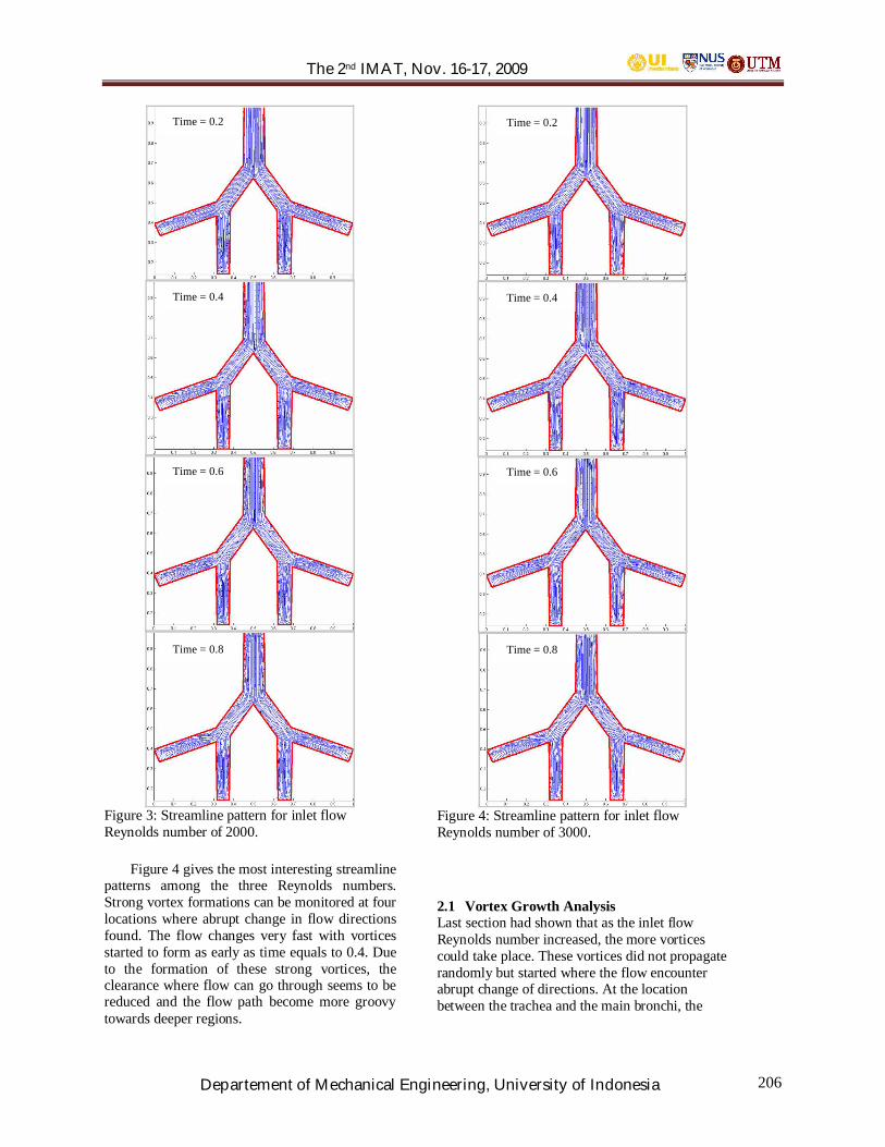
The 2nd IMAT, Nov. 16-17, 2009
Departement of Mechanical Engineering, University of Indonesia 206
Figure 3: Streamline pattern for inlet flowReynolds number of 2000.
Figure 4 gives the most interesting streamlinepatterns among the three Reynolds numbers.Strong vortex formations can be monitored at fourlocations where abrupt change in flow directionsfound. The flow changes very fast with vorticesstarted to form as early as time equals to 0.4. Dueto the formation of these strong vortices, theclearance where flow can go through seems to bereduced and the flow path become more groovytowards deeper regions.
Figure 4: Streamline pattern for inlet flowReynolds number of 3000.
2.1 Vortex Growth AnalysisLast section had shown that as the inlet flowReynolds number increased, the more vorticescould take place. These vortices did not propagaterandomly but started where the flow encounterabrupt change of directions. At the locationbetween the trachea and the main bronchi, the
Time = 0.2
Time = 0.4
Time = 0.6
Time = 0.8
Time = 0.2
Time = 0.4
Time = 0.6
Time = 0.8
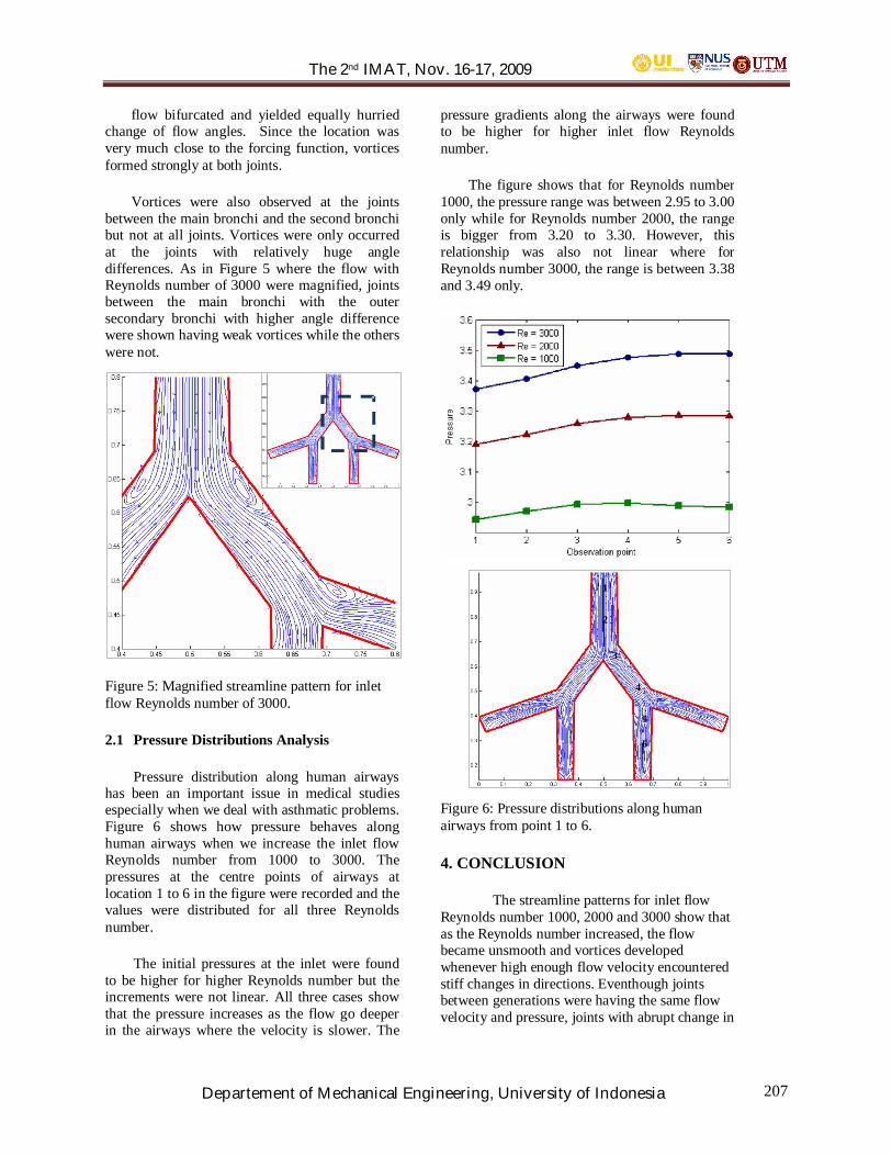
The 2nd IMAT, Nov. 16-17, 2009
Departement of Mechanical Engineering, University of Indonesia 207
flow bifurcated and yielded equally hurriedchange of flow angles. Since the location wasvery much close to the forcing function, vorticesformed strongly at both joints.
Vortices were also observed at the jointsbetween the main bronchi and the second bronchibut not at all joints. Vortices were only occurredat the joints with relatively huge angledifferences. As in Figure 5 where the flow withReynolds number of 3000 were magnified, jointsbetween the main bronchi with the outersecondary bronchi with higher angle differencewere shown having weak vortices while the otherswere not.
Figure 5: Magnified streamline pattern for inletflow Reynolds number of 3000.
2.1 Pressure Distributions Analysis
Pressure distribution along human airwayshas been an important issue in medical studiesespecially when we deal with asthmatic problems.Figure 6 shows how pressure behaves alonghuman airways when we increase the inlet flowReynolds number from 1000 to 3000. Thepressures at the centre points of airways atlocation 1 to 6 in the figure were recorded and thevalues were distributed for all three Reynoldsnumber.
The initial pressures at the inlet were foundto be higher for higher Reynolds number but theincrements were not linear. All three cases showthat the pressure increases as the flow go deeperin the airways where the velocity is slower. The
pressure gradients along the airways were foundto be higher for higher inlet flow Reynoldsnumber.
The figure shows that for Reynolds number1000, the pressure range was between 2.95 to 3.00only while for Reynolds number 2000, the rangeis bigger from 3.20 to 3.30. However, thisrelationship was also not linear where forReynolds number 3000, the range is between 3.38and 3.49 only.
Figure 6: Pressure distributions along humanairways from point 1 to 6.
4. CONCLUSION
The streamline patterns for inlet flowReynolds number 1000, 2000 and 3000 show thatas the Reynolds number increased, the flowbecame unsmooth and vortices developedwhenever high enough flow velocity encounteredstiff changes in directions. Eventhough jointsbetween generations were having the same flowvelocity and pressure, joints with abrupt change in
2
3
4
5
6
1
The 2nd IMAT, Nov. 16-17, 2009
Departement of Mechanical Engineering, University of Indonesia 208
directions showed the development on vortexes. Higher Reynolds number for the inlet flowcould result in more chaotic and unsmooth flowthroughout the airways. Vortex developments andchanges in flow directions are major factors thatcould reduce the amount of drug delivery inasthmatic cases. This study suggests that in orderto assure the maximum amount of inhalerparticles go deep in the airways, patient wheneverthey use the inhaler should take their breathsslowly but deeply rather than fast and shortbreaths.
5. REFERENCES
[1] Kurujareon, J., 2000. Simulations of Airflow in thehuman tracheobronchial network, Ph.D. Thesis,University of Hertfordshire, UK.
[2] Schroter, R.C., Sudlow, M.F., 1969. Flow patternsin model of the human bronchial airways. Respir.Physiol. 7, 341–355.
[3] Chang, H.K., El Masry, O.A., 1982. A modelstudy of flow dynamics in human central airways.Part 1 axial velocity profiles. Respir. Physiol. 49,75–95.
[4] Isabey, D., Chang, H.K., 1982. A model study offlow dynamics in human central airways. Part II:secondary flow velocities. Respir. Physiol. 49, 97–113.
[5] Pedley, T.J., 1977. Pulmonary fluid dynamics.Ann. Rev. Fluid Mech. 9, 229–274.
[6] Gatlin, B., Cuicchi, C., Hammersley, J., Olson,D.E., Reddy, R., Burnside, G., 1995.Computational simulation of steady and oscillatingflow in branching tubes. ASME Bio-Medical.Fluids. Engineering. FED 212, 1–8.
[7] Wilquem, F., Degrez, G., 1997. Numericalmodeling of steady inspiratory airflow throughthree-generation model of the human centralairways. ASME J. Biomech. Engg. 119, 59–65.
[8] T. W. H. Sheu, S. K. Wang and S. F. Tsai, Finiteelement analysis of particle motion in steadyinspiratory airflow, Computer Methods in AppliedMechanics and Engineering, Volume 191, Issues25-26, 12 April 2002, Pages 2681-2698
[9] Y. Liu, R.M.C. Soa, C.H. Zhang, Journal ofBiomechanics 35 (2002) 465–473
[10] G. Karniadakis, M. Israeli, and S. Orszag, 1991,“High-order splitting methods for theincompressible Navier-Stokes equations,” Journalof Computational Physics, 97, pp, 414-443.
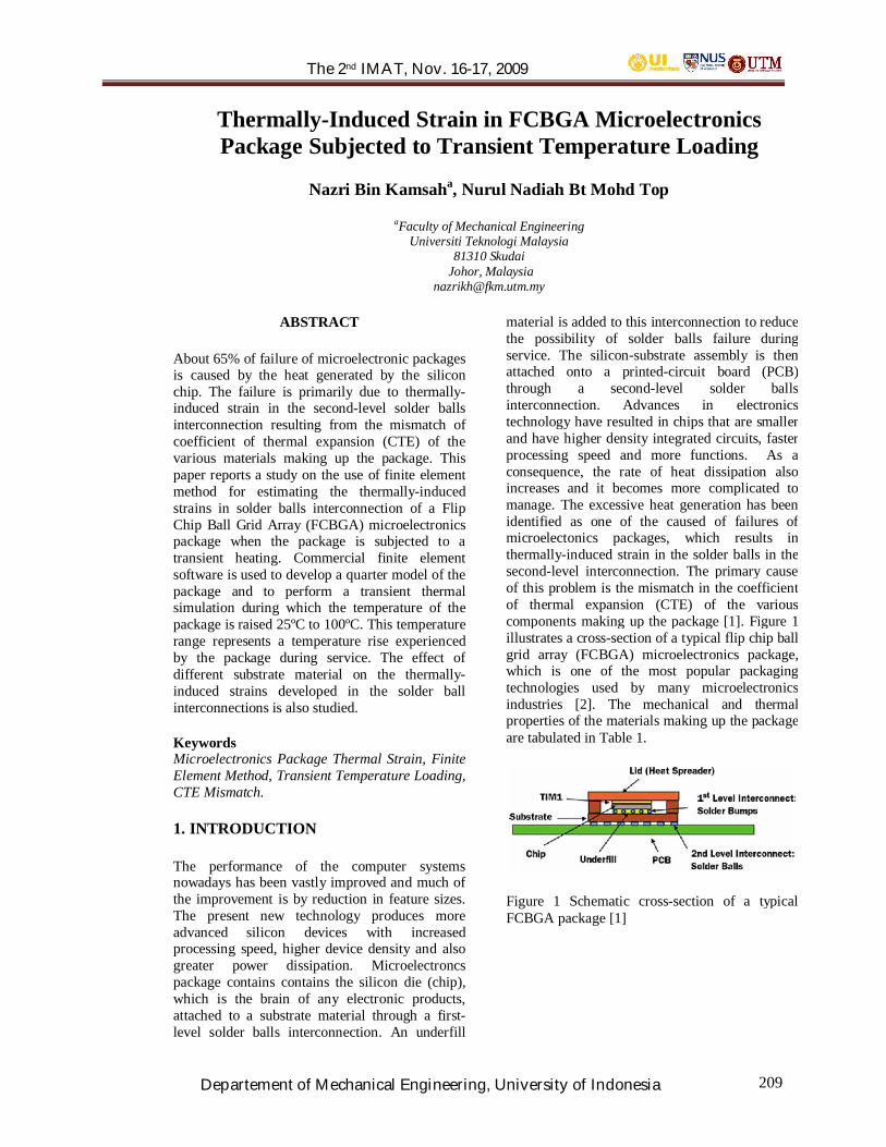
The 2nd IMAT, Nov. 16-17, 2009
Departement of Mechanical Engineering, University of Indonesia 209
Thermally-Induced Strain in FCBGA MicroelectronicsPackage Subjected to Transient Temperature Loading
Nazri Bin Kamsaha, Nurul Nadiah Bt Mohd Top
aFaculty of Mechanical EngineeringUniversiti Teknologi Malaysia
81310 Skudai Johor, Malaysia
ABSTRACT
About 65% of failure of microelectronic packagesis caused by the heat generated by the siliconchip. The failure is primarily due to thermally-induced strain in the second-level solder ballsinterconnection resulting from the mismatch ofcoefficient of thermal expansion (CTE) of thevarious materials making up the package. Thispaper reports a study on the use of finite elementmethod for estimating the thermally-inducedstrains in solder balls interconnection of a FlipChip Ball Grid Array (FCBGA) microelectronicspackage when the package is subjected to atransient heating. Commercial finite elementsoftware is used to develop a quarter model of thepackage and to perform a transient thermalsimulation during which the temperature of thepackage is raised 25ºC to 100ºC. This temperaturerange represents a temperature rise experiencedby the package during service. The effect ofdifferent substrate material on the thermally-induced strains developed in the solder ballinterconnections is also studied.
KeywordsMicroelectronics Package Thermal Strain, FiniteElement Method, Transient Temperature Loading,CTE Mismatch.
1. INTRODUCTION
The performance of the computer systemsnowadays has been vastly improved and much ofthe improvement is by reduction in feature sizes.The present new technology produces moreadvanced silicon devices with increasedprocessing speed, higher device density and alsogreater power dissipation. Microelectroncspackage contains contains the silicon die (chip),which is the brain of any electronic products,attached to a substrate material through a first-level solder balls interconnection. An underfill
material is added to this interconnection to reducethe possibility of solder balls failure duringservice. The silicon-substrate assembly is thenattached onto a printed-circuit board (PCB)through a second-level solder ballsinterconnection. Advances in electronicstechnology have resulted in chips that are smallerand have higher density integrated circuits, fasterprocessing speed and more functions. As aconsequence, the rate of heat dissipation alsoincreases and it becomes more complicated tomanage. The excessive heat generation has beenidentified as one of the caused of failures ofmicroelectonics packages, which results inthermally-induced strain in the solder balls in thesecond-level interconnection. The primary causeof this problem is the mismatch in the coefficientof thermal expansion (CTE) of the variouscomponents making up the package [1]. Figure 1illustrates a cross-section of a typical flip chip ballgrid array (FCBGA) microelectronics package,which is one of the most popular packagingtechnologies used by many microelectronicsindustries [2]. The mechanical and thermalproperties of the materials making up the packageare tabulated in Table 1.
Figure 1 Schematic cross-section of a typicalFCBGA package [1]

The 2nd IMAT, Nov. 16-17, 2009
Departement of Mechanical Engineering, University of Indonesia 210
Table 1 Properties of various material of theFCBGA package [3,4]
Material E (Gpa) CTE(ppm/K)
v
Silicon 131 2.5 0.28Epoxy 14.5 20 0.28CopperPad
69 17 0.34
Solder Ball 26 25 0.36PCB 22 17 0.28
This paper reports on the use of finite elementmethod to estimate the magnitude of thermally-induced strains in the second-level solder ballsinterconnection of the FCBGA package as it issubjected to a temperature rise from 25ºC to100ºC. Commercial finite element software isemployed to develop the simplified model of theFCBA package and to simulate the heatingprocess of the package. Due to the symmetry inthe geometry of the package and the thermalloading, only a quarter section model of thepackage is employed in the analysis. The effect ofdifferent substrate material on the thermally-induced strains in the solder balls interconnectionis also evaluated.
2. FINITE ELEMENTIMPLEMENTATION
Figure 2 shows the finite element (FE) model of aquarter section of the FCBA package. Forsimplicity, the first-level solder ballsinterconnection is assumed to be made up of anunderfill material only. This simplification isacceptable since the solder balls in the first-levelinterconnection are very small and are difficult tomodel. The entire model model is discretizedusing hexahedral elements since they can producemore precise results. The front left and right edgesof the model represent the symmetrical cuttingsurfaces. The thermal and mechanical propertiesare assigned to the respective materials, astabulated in Table 1. All materials are assumed tobehave in a linear elastic manner. Mechanicalcontraints are applied on the left surface such thatthere will be no translation in the 1-direction androtations about the 3-axis. The right surface isconstrained from translation in the 2-direction androtations about the 3-axis. An initial temperatureof 25ºC is prescribed to the entire model. Duringthe transient thermal simulation, the temperatureof the model is then raised from 25ºC to 100ºC in
several time steps. In addition, convection heatloss from the top surface of the silidon chip andthe exposed surfaces of the substrate and theprinted circuit board by prescribing convectiveheat transfer coefficient of 25 W/m2K and theambient air temperature of 25ºC. Also, thesymmetrical cutting surfaces are assumed to beadiabatic. To investigate the effect of substratematerial on the thermally-induced strains, twosubstrate materials are considered in the study.The mechanical and thermal properties of thesematerials are shown in Table 2.
Table 2 Properties of substrate materials [3][4]
Material E (Gpa) CTE(ppm/K)
v
Alumina 275 6.7 0.21Copper 117 17 0.35
Figure 2 FE model of the FCBGA microelectronicpackage
3. RESULTS
Figure 3 shows the deformed shape of thepackage with copper substrate material when itstemperature reaches 100ºC. The contour of totaldisplacement (in m) within the package is shown.It can be observed that the silicon die deforms in aconvex direction because it is stretched in boththe x- and y-direction, by the substrate and thePCB that have much higher CTE. The out-of-plane deformation of the substrate and the PCBunderneath the silicon is also in tandem with thatof the silicon. As a result, the solder ballsinterconnections in this region are in the state ofcompression.

The 2nd IMAT, Nov. 16-17, 2009
Departement of Mechanical Engineering, University of Indonesia 211
Figure 3 Deformation of the package with coppersubstrate at 100°C.
It is also seen that the out-of-plane deformation ofboth the substrate and the PCB continue toincrease further away from the silicon die. Thehighest out-of-plane displacement of the substrateand the PCB is about 1.8x10⁻⁵ m 2x10⁻⁵ m,respectively and these occur at the corner of bothmaterials. Figure 4 shows the deformed shape ofthe package with an alumina substrate at 100ºC.
Figure 4 Deformation of the package withalumina substrate at 100°C.
In this case, the silicon die appears to havedeformed in similar fashion as in the previousmodel but the magnitude of the out-of-planedeformation is much greater than the packagewith copper substrate. This is because the solderballs interconnection which has much higher CTEdictate the out-of-plane deformation. The solderballs interconnection are in the state ofcompression as their expansion is constrained bythe substrate above them. The out-of-planedisplacement at the tip of PCB is about 2.48x10⁻⁵
m, which is almost 25% greater than that in thepackage with copper substrate.
The state of thermally-induced maximumprincipal strain in the second-level solder ballsinterconnection for the package with coppersubstrate is shown in Figure 5. It can be observedform this figure that the highest strain occurs onthe top edge of the solder balls located directlyunderneath the silicon die, along the outer edge ofthe die. The largest strain is about 6.766x10⁻³. The
solder balls located along the left edge of thecopper substrate also appear to be highly strained,on their upper edges that are facing in the x-direction.
Figure 5 Maximum principal strains in solderballs for copper substrate
The state of strain in the second-level solder ballsintrconnection for the package with aluminasubstrate is shown in Figure 6.
Figure 6 State of strains in solder balls foralumina substrate
It can be seen that, in contrast to the package withthe copper substrate, the solder balls locateddirectly underneath the silicon die are lessstrained. Also, almost all the solder ballsexperience somewhat similar level of principalstrain of about 3.68x10⁻³, on their upper faces.The solder balls along the left edge of the aluminasubstrate are also less strained compared to thesame solder balls for copper substrate.
Figure 7(a) shows the most critically strainedsolder ball in the package with copper substrate.This solder ball is loacted at the corner of thesilicon die, underneath the substrate (enclosed in acircle in Figure 5). Clearly, the upper region ofthis solder ball is much higher strained ascompared to the bottom region. Figure 7(b) showsa half-section of the critcal solder ball and itillustrates the state of the maximum principlestrain inside the critical solder ball. It is seen thatthe strain penetrates into the solder ball from boththe upper and bottom surfaces, but the penetration
The 2nd IMAT, Nov. 16-17, 2009
Departement of Mechanical Engineering, University of Indonesia 212
from the top surface goes much deeper into thesolder ball.
(a)
(b)
Figure 7 (a) The most critically strained solderball; (b) The state of inner strain the critical solderball.
CONCLUSION
When an FCBGA electronics package issubjected to a transient temperature rise from25ºC to 100ºC, thermall-induced strains aredeveloped in the solder balls in the second-levelinterconnection. This is due to the CTE mismatchbetween the various materials making up thepackage. The solder balls that are located atunderneath the silicon die, along the edge of thedie experience higher strains at their upper faces.The principal strain in these solder balls arehigher when copper is used as substrate materialcompared to alumina. The solder ball locatedunderneath the corner of the silicon dieexperiences the highest principal strain when thesubstrate material is copper. The principal strainpenetrates into the solder ball from both upperand lower faces of the solder ball but thepenetration is a lot deeper from from the upperface due to the higher strain on the upper face.
REFERENCES
[1] Guatao Wang, Jie-Hua Zhao, Min ding, PaulS. Ho (2002).Thermal Deformation Analysis onFlip-Chip packages using High Resolution MoireInterferometry. Austin: pp 869-875.
[2] Yuko Sawada, Kozo Harada and HirofumiFujioka (2003). Study of Package Warp Behaviorfor High-Performance Flip-Chip BGA.Microelectronics Reliability. Science DirectJournal, 43(3): 465-471.
[3] G.Q. Zhang, W.D van Driel, and X.J. Fan(2006). Mechanics of MicroelectronicsHandbook. Netherlands: 169-263.
[4] S. B. Park, Rahul Joshi, and Bahgat Sammakia(2005). Thermomechanical Behavior of Organicand Ceramic Flip Chip BGA Packages UnderPower Cycling. 21st Semiconductor ThermalMeasurement and Management Symposium.March 15-17. San Jose, CA, USA: IEEE, 214-222.
The 2nd IMAT, Nov. 16-17, 2009
Departement of Mechanical Engineering, University of Indonesia 213
A REVIEW THERMAL LOAD ANALYSIS OF PASSENGERCOMPARTMENT
Haslinda Mohamed Kamara, Mohd Yusoff Senawib
aDepartment of Thermo-FluidsFaculty of Mechanical Engineering,
Universiti Teknologi Malaysia,81310 Skudai, Johor Bahru, Malaysia
Tel : (006) 075534656E-mail : [email protected]
bDepartment of Thermo-FluidsFaculty of Mechanical Engineering,
Universiti Teknologi Malaysia,81310 Skudai, Johor Bahru, Malaysia
Tel : (006) 075534747E-mail : [email protected]
ABSTRACT
The thermal environments in a passengercompartment are created according to theperformance of its air conditioning system.Basically, there are two main aspects that need tobe considered to develop a comprehensive andaccurate passenger compartment thermalsimulation program. The first aspect is loadanalysis in the passenger cabin. Via load analysis,the thermal behavior in the passengercompartment under the influence of the outsideenvironment, over a wide temperature range andunder various air-conditioning (A/C) operatingconditions can be described. The second aspect isthe characteristics of the air-conditionerevaporator coil. In this respect, the transient airtemperature and humidity in the passengercompartment are dependent on the temperatureand humidity of the discharged air. Thedischarged air conditions affect the thermalbehavior inside the passenger cabin. As a result,two selected topics are reviewed in this paper.The pertinent topics are: thermal load analysis inthe passenger compartment, and the linkagebetween the passenger compartment thermal loadmodel and the A/C system.
Keywords
Thermal load simulation, passengercompartment, automotive air conditioning system
1. INTRODUCTION
The required capacity of cooling systems that canmaintain the required conditions in theconditioned passenger compartment can beestimated by carrying thermal load analysis. Thetotal passenger compartment load consists ofexternal and internal loads. The external loadsconsist of heat transfer by conduction through thecabin walls, roof, floor, doors etc, and heattransfer by radiation through glass windows. Theinternal loads consist of sensible and latent heattransfer due to occupants and appliances.
Generally, thermal load calculations involvea systematic procedure by taking into account allthe space energy flows. In practice, a variety ofmethods ranging from simple rules-of-thumb tocomplex Transfer Function Methods are used toarrive at the space loads. Accurate analysis ofspace loads is important in air-conditioning loadcalculations when predicting the peak design dayload for equipment sizing. It is also valuable inobtaining the space envelope temperatures whenperforming thermal comfort studies. Furthermore,the rising demand of energy conservation, moreand more attentions are given on the studies ofthermally non-uniform and dynamicenvironments [1].
2. A REVIEWSeveral thermal load models have appeared in theopen literature. In a study by Ingersoll et al [2],the authors developed a passenger compartmentthermal comfort model to predict human comfort
The 2nd IMAT, Nov. 16-17, 2009
Departement of Mechanical Engineering, University of Indonesia 214
for various environmental conditions, vehicledesign, and Heating, Ventilation, and AirConditioning (HVAC) system operatingconditions. The thermal load model reflects onthe geometrical configuration of the passengercompartment including glazing surfaces; thepertinent physical and thermal properties of theenclosure; the environment conditions; the directand diffuse incident solar radiation through theglass areas; the inlet air parameters as specifiedfrom the HVAC system; and the conduction,convection, mass flow, and radiation heat transfermodes. The model outputs are interior airtemperatures, surface temperatures, air velocitiesand air relative humidity. The passengercompartment and mass flow in the passengercompartment are modeled as lumped parameternetworks. The conduction heat gain through thepassenger compartment was calculated based onsteady-state assumption and the method toconnect the thermal load system and its A/Csystem was not clarified.
Lin et al [3] simulated a steady-state coolingprocess in a simplified GM-10 passengercompartment to evaluate passenger thermalcomfort. Four design parameters were studied,specifically, conditioned air flow rate, A/C outletlocation, body vent location and glass properties.Three dimensional air flow and temperaturedistributions were obtained using CFD approachspecifically, the flow and convection solverVINE3D, which solves a set of partial differentialequations, namely, governing mass, momentumand energy balance. The outputs of the numericalsimulation model are air flow and temperaturedistributions. However, there is no analysis onthe physical link between the A/C systemperformance and the corresponding passengercompartment model, but the effect of A/C outletflow rate was examined by varying the flow ratesat various magnitudes. Stancato and Onusic [4]developed a simulation model to calculate steady-state cooling loads in a cab compartment. Theyincorporate various sources of heat loads into themodel specifically: conduction heat gain throughopaque walls and glasses; solar radiation throughglasses; conduction heat gain through motorcompartment panels; heat gain from people andinfiltration. However, the thermal storage effectsdue to the heat capacity of the interior mass andbody wall were excluded in the analysis. Themodel is a stand-alone model, since the variationsof air temperature inside the cabin are not coupledto the air-conditioner evaporator inlet conditions.
The A/C discharge air temperature wasdetermined experimentally.
Currle et al. [5] investigated the air flowthrough the complete HVAC system together withthe flow field in the passenger compartment usingCFD approach. The HVAC system includes allparts of air handling system such as inlet plenumchamber, fan, filters, air distribution chamber withevaporator, air ducts and vents. The passengercompartment model includes a detaileddescription of the passenger compartmentoccupied by four occupants. However, thecalculation of the temperature field including allrelevant thermal effects such as free convection,conduction and radiation was not performed in thestudy. Currle and Jurgen Maue [6] extended theprevious computational model, by expanding theirstudy to investigate the effects of relevant flowand geometrical parameters on the microclimateand the thermal comfort of the occupants insidethe passenger compartment. The model consistsof three programs which are coupled together.The first program is used to calculate the flow andtemperature distribution inside the passengercompartment using CFD code. The programrepresents the convective heat load inside thepassenger compartment. The second programsimulates the passenger compartment heat load.This program signifies the radiative heat loadinside the cabin. The third program is used tocompute the thermal state and sensation of theoccupants under a given load. However, in thisstudy, they did not investigate the effects of theA/C system performance (specifically at theevaporator inlet air conditions) with regard to thetransient behavior inside the passengercompartment. The inlet conditions at the vents aremanually specified as inlet conditions of thecomputational model. Due to this absence, themodel is developed based on the theoreticalsimulation only without appreciating the realitiesof A/C system as a whole. The study also includethe conduction heat transfer through cabin walls,solar and thermal radiation, into the passengercompartment thermal load model however, themethod is unclear. Furthermore, both studies [5]and [6] are based on steady-state analyses.
Huang [7] built a dynamic computer simulationmodel to calculate temperature and humidityvariations inside a passenger compartment whilesimulating the performance of the A/C system.The vehicle is divided into two linked modulesrepresenting the A/C network and

The 2nd IMAT, Nov. 16-17, 2009
Departement of Mechanical Engineering, University of Indonesia 215
the passenger compartment climate. The A/Cnetwork consists of the evaporator, compressor,condenser, orifice, air handling system, and theconnecting hoses. Pressure drop and thermalcapacity of the evaporator, condenser and theconnecting ducts/hoses are also included in theA/C system model. The passenger compartmentclimate was simulated using lumped capacitancemethod. In this scheme, the temperature andhumidity inside the passenger compartment areassumed spatially uniform at any time during thesimulation. A lumped analysis of the interiormasses such as seats, instrument panel and floorconsole are also incorporated. The transient cabinaverage air temperature, seat average temperatureand cabin average air humidity were modeledusing three non-linear ordinary differentialequations based on mass balance and energybalance. Those equations were solved via afourth-order Runge-Kutta method. A relationshipbetween the A/C system characteristics and thepassenger compartment load model is linked upvia simulation model. The conduction heat gainthrough opaque walls is assumed as one-dimensional transient heat conduction. For acomposite wall analysis, the thermal propertiesand temperature within each individual layer areassumed uniform.
A similar study has been carried out byKhamsi and Petitjean [8]. They developedsimulation software of a car cabin and its A/Csystem. The car cabin thermal simulation wasmodeled based on dynamic and stationaryconditions. This model is meant for computingthe cooling or heating capacities required tocompensate the effect of different heat loadsinside the car cabin and obtaining the requiredcomfort conditions inside the cabin. The outputsof the cabin thermal model are surfacetemperature of various elements, the airtemperature and relative humidity in variouszones and the instantaneous cooling or heatingcapacities required to reach the optimumconditions of comfort in the cabin. However, thetechnique to develop the car cabin thermal loadmodel was not described. The link between thecar cabin model and the A/C model wasestablished via model correlation.
Akihiro Fujita et al [9] developed a numericalsimulation to predict steady-state internal thermalenvironment specifically air velocity and spacetemperature in a passenger cabin. The coupledanalysis of solar radiation, long-wave radiation,
conduction heat gain through the materials andCFD was used in this method. The heatconduction through the materials is based on asteady-state analysis. The effects of ventilationinside the instrument panel and air leaks from thegaps of interior parts were incorporated into themodel but excluded the effect of latent heat andhumidity. Furthermore, no occupants are assumedto be present in the cabin. The study did notportray the effects of A/C load towards itscorresponding cabin model. However, the A/Cdischarge air temperature was determinedexperimentally.
Ali Heydani and Saeed Jani [10] havedeveloped an integrated computer simulationmodel which consists of three mathematicalmodels, specifically, the compression A/Csystem, air handling system and the passengercabin model to predict the transient performanceof an automobile HVAC system. The A/C systemmodel is developed based on a steady-statemathematical model to simulate the performanceof major components of the A/C system. The airhandling simulation model is used to describe theprocess of heating and cooling of fresh or re-circulated air, fan performance along withassociated losses due to movement of air throughthe ducts and the air distribution registers. Thepassenger thermal model is developed using aone-dimensional thermal resistance scheme,which is used to predict the heat load andtemperature distribution inside the passengercompartment. The A/C model and the passengerthermal model are physically linked through theair-conditioner evaporator via a correlationmodel. The thermal model inside the passengercabin is established using a three-dimensionaltransient heat transfer model (which is belongedto lumped system approach). Each sub-region isassumed to be at a uniform temperature under agiven thermal load. The thermal model includesthe effects of conduction, convection, radiation,energy interaction between interior components,energy flow between sub-regions, energyinfiltration into the passenger compartment andheat released due to human loads.
You Ding and Robert Zito [11] developed anumerical model using lumped analysis techniqueto investigate the effects of passengercompartment heat load, discharge paneltemperature and discharge volumetric air flow inrelation to the average air temperature. The studydid not physically couple the passenger cabin

The 2nd IMAT, Nov. 16-17, 2009
Departement of Mechanical Engineering, University of Indonesia 216
model with its A/C performance. Roy et al[12] as well have developed a comparable modelof passenger compartment to calculate surfacetemperatures, air temperature at different levelsand cooling loads. They used a zonal approachmethod to model the cabin thermal. The cabinwas divided into several sets of componentsgeometrically, specifically the external walls(including floor, roof, doors, dashboard, rear shelfand glasses); the internal solid components (seats,and steering wheel) and the internal air. Allmajor elements of heat loads including steady-state conduction through opaque materials;radiation due to temperature difference betweenthe cabin components as well as direct anddiffused solar radiation; convection (natural andforced); and convection and radiation due tooutside environment are incorporated into themodel. The A/C model, particularly its mass flowrate was determined using CFD analysis.
P+Z Engineering [13] have developed aninterface to the two commercial software productswith the aim to directly connecting the numericalcalculation of the refrigerant circuit with atransient cabin simulation. One of the software isused to calculate the transient temperaturebehavior of a cabin. The passenger compartmentmodel is developed using lumped systemapproach.
Rugh [14] on the other hand, has used anintegrated modeling approach composed of CADmodel, computational fluid dynamics (CFD),cabin thermal model and vehicle simulation toolsto assess thermal comfort, fuel economy, andemissions. The CAD is used to define vehicleinterior geometry and to morph a generic vehicleto the appropriate dimensions and generate amesh in preparation for cabin thermal/fluidmodeling using CFD software. The CFDsoftware in conjunction with a solar radiationmodel and vehicle solar load tool is used toprovide solar boundary conditions for the cabinthermal/fluid model. The cabin thermal/fluidmodel predicts the flow field inside the passengercompartment, as well as the surface temperaturesand temperature and humidity of the air. Atransient air-conditioning (A/C) model providesair flow boundary conditions specifically theairflow rates, humidity, and temperatures for theCFD analysis inside the passenger cabin. Acomparable study has also been done by Todd etal [15].
Jonas Jonsson [16] has developed anumerical model using CFD analysis (specificallyFLUENT software) that integrates solar loadwhen computing the 3-D temperature distributionin a passenger compartment. Three cases weresimulated throughout the study: a steady state, atransient soaking and a transient cooling. As wellas Huajun Zhang et al [17] they also usedFLUENT software to simulate the 3-D transienttemperature and air-flow field inside thepassenger compartment with or withoutpassengers. The A/C discharge air temperaturewas determined experimentally. The numericalmodel has been validated using the experimentaldata to investigate the influence of differentfactors on the thermal comfort and the energyconsumption. The test conditions and thenumerical models are described in details. In thefollowing paper, Huajun Zhang et al [18]presented the simulated results. Several findingshave been obtained, among them are, to reducethe cooling load in the passenger compartment isby increasing the inlet air temperature, withoutreducing the volume flow rate of the inlet air andthe thermal comfort in a compartment with givenconditions depends on the number of occupants init.
Farzaneh and Tootoonchi [19] havedeveloped a fuzzy controller to controlautomobile thermal comfort. In their study,Fanger’s predicted mean value (PMV) index isused as controller feedback such as, temperature,relative humidity, air velocity, environmentradiation, activity level and cloths insulation. Toclearly show the effect of control parameters onoccupant thermal comfort a simulation model ofpassenger cabin and the HVAC system has beendeveloped by the authors. This model includesblower, evaporator, heater core as well as theimpact of important thermal loads such as sunradiation, outside air temperature and passengerson climate control of cabin. The thermal loadsgenerated by solar radiation, outside air and cabintemperature difference as well as assumption offour people in cabin have been estimated by usingempirical formula for Peugeot 206 automobile.
3. CONCLUSIONFrom the reviews discussed above, much usefulinformation in the areas of occupant comfort,cabin heat load, heat transfer and A/C systemmodeling are described. Most of the studies usedcomputational fluid dynamics (CFD) technique

The 2nd IMAT, Nov. 16-17, 2009
Departement of Mechanical Engineering, University of Indonesia 217
and numerical simulation to achieve theirobjectives. Generally, CFD solves theconservation equations for mass, momentum, andthermal energy for all nodes of a two- or three-dimensional grid inside or around the object underinvestigation. In theory, the CFD approach isapplicable to any thermo-fluid phenomenon.However, in practice, and in the passengercompartment physics domain in particular, thereare several problematic issues, of which theamount of necessary computing power, the natureof the flow fields, and the assessment of thecomplex occupant-dependent boundary conditionsare the most problematic [20]. This has often ledto CFD applications being restricted to steady-state cases or very short simulation periods. Alumped parameter approach which belongs to thenumerical methods, model the continuousphysical domain of a thermal system as a networkof discrete points, where the unknowns are soughtonly at those points rather than everywhere in thedomain [21, 22 and 23]. Specifically, the nodepoints are centered within the lumps, andtemperatures at the nodes are considered uniformthroughout the lump. Due to that reason, the mostcritical aspect of the lumped parameter approachis to determine the lump size. Although there aremethods for optimizing the lump size of anygiven physical system, they usually involve moreanalytical efforts and computer time than theoriginal problem [2].
In the preceding reviews, there are severalstudies that [7, 8, 10 and 14] have coupled theA/C system analysis with the passengercompartment model. This approach is unique,since it provides a means for an optimized designof passenger compartment climate control systemderived from realistic and accurate behavior of theautomotive A/C system. It also portrays themutual effect between the A/C system and thepassenger compartment. Furthermore, it offers abetter understanding of the synergistic impact ofthe various parameters in the design of the vehiclethat can affect comfort and the possible tradeoffsbetween such parameters.
From the thermal load model point of views,nearly all studies presented above disregard theeffect of thermal storage of the interior mass andneglect interior air humidity analysis. The thermalstorage effect is due to the heat storage of theinterior seats, panels, and vehicle materials. OnlyHuang [7] considered thermal storage effects andvariation of interior air humidity.
ACKNOWLEDEMENTThe authors would like to express theirappreciation to Universiti Teknologi Malaysia forfunding this study.
REFERENCES
[1] Zhang Y. and Zhao R. (2008). RelationshipBetween Thermal Sensation and Comfort in Non-uniform and Dynamic Environments. Building andEnvironment. doi:10.1016/j.buildenv.2008.04.006.
[2] Ingersoll, J. G., Thomas, G. K., Maxwell, L. M.and Niemec, R. J. (1992). Automobile PassengerCompartment Thermal Comfort Model – Part 1:Compartment Cool-Down / Warm-Up Calculation.Society of Automotive Engineers (SAE) TechnicalPaper Series. Paper No. 920265: 232 – 242.
[3] Lin, C. H., Han, T. and Koromilas, C. A. (1992).Effects of HVAC Design Parameters on PassengerThermal Comfort. SAE Transactions. Paper No.920264.
[4] Stancato Fernando, Onusic Helcio (1997). RoadBus Heat Loads Numerical and ExperimentalEvaluation. Society of Automotive Engineers (SAE)Technical Paper Series. Paper No. 971825.
[5] Currle, J., Harper, M., Ross and F., Heid, T.(1997). Evaluation of HVAC System of PassengerCars and Prediction of The Microclimate in ThePassenger Compartment by Application ofNumerical Flow Analysis. Society of AutomotiveEngineers (SAE) Technical Paper Series. PaperNo. 971788.
[6] Currle, J. and Jurgen Maue (2000). NumericalStudy of The Influence of Air Vent Area And AirMass Flux of The Thermal Comfort of CarOccupants. Society of Automotive Engineers (SAE)Technical Paper Series. Paper No. 2000-01-0980.
[7] Huang Chi-Chang Daniel (1998). A DynamicComputer Simulation Model For AutomobilePassenger Compartment Climate Control andEvaluation. Michigan Technological University:Ph.D. Thesis.
[8] Khamsi, Y. and Petitjean, C. (2000). DynamicSimulation of Automotive Passenger CompartmentAnd It’s Air Conditioning System. Society ofAutomotive Engineers (SAE) Technical PaperSeries. Paper No. 2000-01-0982.
[9] Akihiro Fujita, Jun-ichi Kanemaru, HiroshiNakagawa and Yoshiichi Ozeki (2001). NumericalSimulation Method To Predict The ThermalEnvironment Inside A Car Cabin. Society ofAutomotive Engineers of Japan (JSAE). 22: 39 –47.
[10] Ali Heydani and Saeed Jani (2001). Entropy-Minimized Optimization of an Automotive Air-conditioning and HVAC System. Society ofAutomotive Engineers (SAE) Technical PaperSeries. Paper No. 2001-01-0592.
[11] You Ding and Robert Zito (2001). CabinHeat Transfer And Air Conditioning Capacity. Society
The 2nd IMAT, Nov. 16-17, 2009
Departement of Mechanical Engineering, University of Indonesia 218
of Automotive Engineers (SAE) Technical Paper Series.Paper No. 2001-01-0284.
[12] Roy, D. El-Khoury, K. Clodic, D. and Petitjean, C.(2001). Modeling of In-Vehicle Heat TransferUsing Zonal Approach. Society of AutomotiveEngineers (SAE) Technical Paper Series. PaperNo. 2001-01-1333.
[13] P+Z Engineering GmbH (2002). Simulation of anAir Conditioning System and the Vehicle Interior.ATZ Worlwide 2/2002. Volume 104.
[14] Rugh, J. P. and Hendricks, T. J. (2001). Effect ofSolar Reflective Glazing on Ford Explorer ClimateControl, Fuel Economy, and Emissions. Society ofAutomotive Engineers (SAE) Technical PaperSeries. Paper No. 2001-01-3077.
[15] Todd, M. T., Balaji Maniam, Milind Mahajan,Gaurav Anand and Nagendra Jain (2004). e-Thermal: A Vehicle-Level HVAC/PTC SimulationTool. Society of Automotive Engineers (SAE)Technical Paper Series. Paper No. 2004-01-1510.
[16] Jonas Jonsson (2007). Including Solar Load inCFD Analysis of Temperature Distribution in aCar Passenger Compartment. Luleå University ofTechnology, Sweden: Master Thesis.
[17] Huajun Zhang, L. Dai, G. Xu, Y. Li, W. Chen, W-Q. Tao (2009). Studies of Air-flow andTemperature Fields Inside a PassengerCompartment for Improving Thermal Comfort andSaving Energy: Part I Test/Numerical Model andValidation. Applied Thermal Engineering. 29:2022–2027.
[18] Huajun Zhang, L. Dai, G. Xu, Y. Li, W. Chen, W-Q. Tao (2009). Studies of Air-flow andTemperature Fields Inside a PassengerCompartment for Improving Thermal Comfort andSaving Energy: Part II Test/Numerical Model andValidation. Applied Thermal Engineering. 29:2028–2036.
[19] Farzaneh,Y. and Tootoonchi, A. A. (2008).Controlling Automobile Thermal Comfort UsingOptimized Fuzzy Controller. Applied ThermalEngineering. 28 : 1906–1917.
[20] Hensen, J., Bartak, M. and Drkal, F. (2002).Modeling and Simulation of a Double-Skin FacadeSystem. ASHRAE Transactions. 108 (2) : 1251-1259.
[21] Schneider, P. J. (1955). Conduction Heat Transfer.Reading, Massachusetts: Addison-WesleyPublishing Company Advanced Book Program.
[22] Holman, J. P. (1981). Heat Transfer. 5th ed.Auckland: McGraw-Hill International BookCompany.
[23] Shih, T. M. (1984). Numerical Heat Transfer. NewYork : Springer-Verlag.
The 2nd IMAT, Nov. 16-17, 2009
Departement of Mechanical Engineering, University of Indonesia 219
Utilization of Waste Cooking Oil as Diesel Fuel and Improvementin Combustion and Emission
Wira Jazair, Mohd Norhisyam
Faculty of Mechanical Engineering, Universiti Teknologi Malaysia81310 UTM Skudai, Johor, Malaysia
Tel : 6(019) 7326919E-mail : [email protected]
ABSTRACT
Due to high price of Straight Vegetable Oil(SVO) for bio-diesel production, the use of WasteCooking Oil (WCO) will be cost effective.Furthermore, utilization of WCO will refrainwaterways pollution and endanger ecosystem. InMalaysia, more than 50-tone of WCO fromvarious sources was produced everyday. Thisstudy evaluates combustion performance andexhaust emission characteristics of several WCOswith different sources. Modification on fuelproperties has been done to improve thecombustion and exhaust emission of using WCOas diesel fuel. Regular diesel fuel also has beenused for comparison in the test. A 0.6 liter, single-cylinder, air-cooled direct injection diesel enginewas used to perform this experiment. Experimentwas done at variable engine loads at constantspeed.
Keywords
Waste Cooking Oil, Diesel Engine, Emission
1. INTRODUCTION
Energy reserves in the world (Deiterium,Uranium, Coal, Crude oil, Natural gas) only cansupport the user only less than thirty years basedon present consumption. If the consumption rateincreases, the reserve energy might only enoughnot less than twenty years [1]. In addition, highuses of petroleum fuel around the world resultedin increasing the air pollution cause by theburning of the petroleum fuel. On top of that, in2007, crude oil reaches the maximum price over100 dollar US per barrel surpass the price duringOil Crisis around 1980’s [2]. This makes some
alternative diesel fuel particularly bio-dieselbecome popular in a growing number of countriesaround the world. Bio-diesel can be defined asmono alkyl ester of long chain fatty acids derivedfrom renewable lipid sources. Bio-diesel can beproduced from some type of renewable lipidsources such as vegetable oil and animal fat [3].Bio-diesel is uses seriously in developed countrysuch as United State, France, Germany andothers. In Malaysia, bio-diesel becomes morepopular due to the prices and also due to thesecountries vehicle’s regulation and law. As palmoil is a main source of fat in Malaysia, productionof bio-diesel from palm oil will affect the price ofproduct based on fat, such as food and others. Byproducing bio-diesel from palm oil (commercialproduction), there will increase price of crudepalm oil. As alternative, Waste Cooking Oil(WCO) has been chosen to be investigating in thisresearch. Beside the price factor, re-used of WCOcan solve the water pollution that caused byWCO.
2. TEST FUEL
In this research, there are three types of WCOsources used. This three test fuel are named A, Band C. The sources of these fuels are shown inTable 1. These three types of WCO have differentfuel properties due to different cooking style andduration. WCO B and WCO C were used formany times (more than 5 times) and the color ofthe cooking oil changed to become dark brown. Incontrast, for WCO A is only being used two orthree times before it will be drained.
Table 1: Test Fuel SourcesTest Fuel Source Freq. UseWCOME A House Kitchen < 3 timesWCOME B Cafeteria Kitchen > 5 timesWCOME C Indian Muslim Restaurant > 5 times

The 2nd IMAT, Nov. 16-17, 2009
Departement of Mechanical Engineering, University of Indonesia 220
These three test fuels have been transformed intowaste cooking oil methyl ester (WCOME)through transesterification process. This processneeded waste cooking oil (triglyceride) as mainsubstance, methanol as converter of mainsubstance, and with the present of potassiumhydroxide as reaction accelerator (catalyst). Asthe result of this process, two separate layers areproduced after being left about 12 hours. Theupper layer is WCOME or bio-diesel and thebottom layer is glycerin. In order to have cleanbio-diesel, the WCOME layer was rinsed withdistilled hot water (70 – 80 oC). This washingprocess is to make sure remaining methanol orother sustains removed from WCOME.
Table 2 shows the fuel properties of all test fuels.It can be seen that all WCOME has higherkinematic viscosity and density compared withdiesel fuel. Compared with diesel fuel, WCOMEA has 9.1%, WCOME B 13.2% and WCOME C38.6% higher kinematic viscosity. WCOME Chas highest and WCOME A has lowest kinematicviscosity and density among WCOMEs. Thekinematic viscosity and density of WCOMEmight closely relate to the frequent and durationusage of WCOME sources.
3. EXPERIMENTAL SETUPThe test engine is a four-stroke single cylinder
naturally aspirated direct-injection dieselengine (Lister ST1). Base enginespecifications are given in Table 3. Theengine is 94.8mm cylinder diameter and90.0mm stroke. The compression ratio is 16.Standard mechanical injection pump is used.Figure 1 shows the schematic diagram ofexperimental apparatus. Engine performanceand exhaust emissions data are obtainedunder stable operating conditions at enginespeed of 1500rpm. Smoke density ismeasured with a Bosch smoke meter.
4. RESULTS AND DISCUSSION
Table 2 : Fuel PropertiesTest Fuel Kinematic Density
Viscosity (mm2/s) (g/ml)Diesel Fuel 3.918 825WCOME A 4.274 836WCOME B 4.437 844WCOME C 5.431 852
1. Engine
2. Tachometer
3. Dynamometer
4. Fuel tank
5. Three wayvalve
6. Venture meter
7. Surge tank
8. Manometer
9. Thermocouple
10. Smoke meter
11. Thermocoupledisplay unit
12. Dynamometercontrol unit
(a)
Diesel FuelWCOME B
WCOME CWCOME A
Table 3 : Engine SpecificationEngine Type DieselModel Lister ST 1Power Output 10.5 bhpMaximum Speed 3000 rpmCompression Ratio 16Displacement 600 ccBore 94.8 mmStroke 90.0 mm
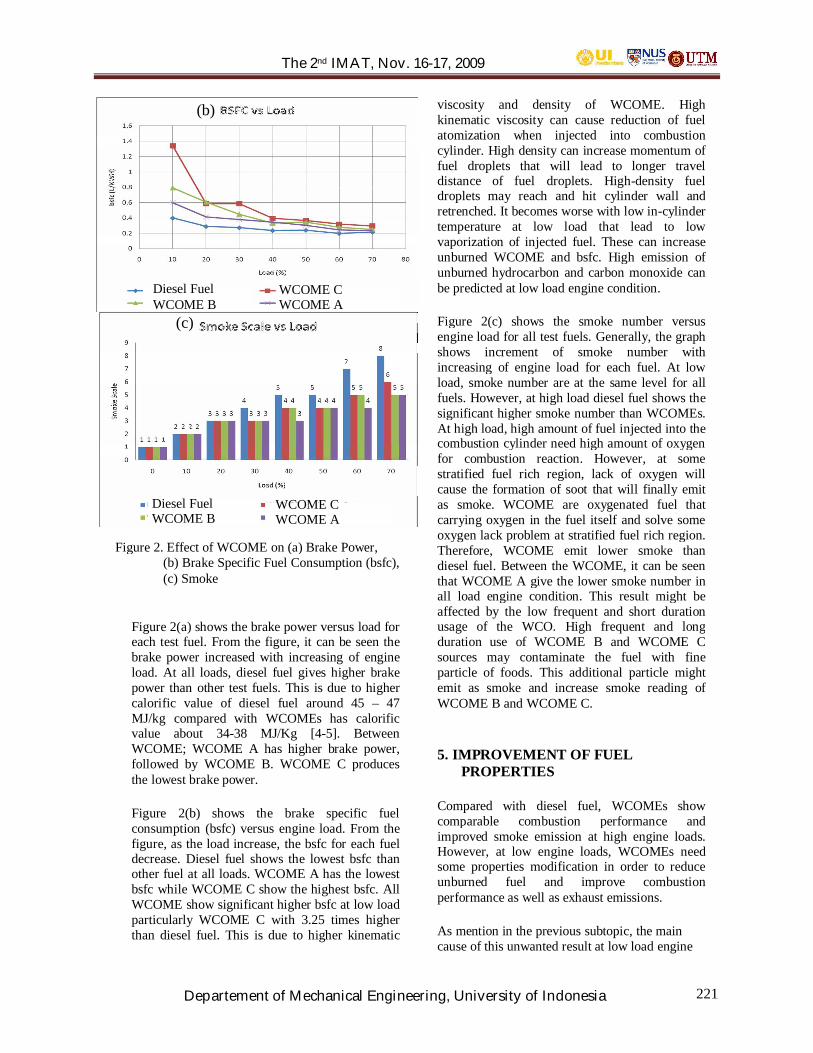
The 2nd IMAT, Nov. 16-17, 2009
Departement of Mechanical Engineering, University of Indonesia 221
Figure 2(a) shows the brake power versus load foreach test fuel. From the figure, it can be seen thebrake power increased with increasing of engineload. At all loads, diesel fuel gives higher brakepower than other test fuels. This is due to highercalorific value of diesel fuel around 45 – 47MJ/kg compared with WCOMEs has calorificvalue about 34-38 MJ/Kg [4-5]. BetweenWCOME; WCOME A has higher brake power,followed by WCOME B. WCOME C producesthe lowest brake power.
Figure 2(b) shows the brake specific fuelconsumption (bsfc) versus engine load. From thefigure, as the load increase, the bsfc for each fueldecrease. Diesel fuel shows the lowest bsfc thanother fuel at all loads. WCOME A has the lowestbsfc while WCOME C show the highest bsfc. AllWCOME show significant higher bsfc at low loadparticularly WCOME C with 3.25 times higherthan diesel fuel. This is due to higher kinematic
viscosity and density of WCOME. Highkinematic viscosity can cause reduction of fuelatomization when injected into combustioncylinder. High density can increase momentum offuel droplets that will lead to longer traveldistance of fuel droplets. High-density fueldroplets may reach and hit cylinder wall andretrenched. It becomes worse with low in-cylindertemperature at low load that lead to lowvaporization of injected fuel. These can increaseunburned WCOME and bsfc. High emission ofunburned hydrocarbon and carbon monoxide canbe predicted at low load engine condition.
Figure 2(c) shows the smoke number versusengine load for all test fuels. Generally, the graphshows increment of smoke number withincreasing of engine load for each fuel. At lowload, smoke number are at the same level for allfuels. However, at high load diesel fuel shows thesignificant higher smoke number than WCOMEs.At high load, high amount of fuel injected into thecombustion cylinder need high amount of oxygenfor combustion reaction. However, at somestratified fuel rich region, lack of oxygen willcause the formation of soot that will finally emitas smoke. WCOME are oxygenated fuel thatcarrying oxygen in the fuel itself and solve someoxygen lack problem at stratified fuel rich region.Therefore, WCOME emit lower smoke thandiesel fuel. Between the WCOME, it can be seenthat WCOME A give the lower smoke number inall load engine condition. This result might beaffected by the low frequent and short durationusage of the WCO. High frequent and longduration use of WCOME B and WCOME Csources may contaminate the fuel with fineparticle of foods. This additional particle mightemit as smoke and increase smoke reading ofWCOME B and WCOME C.
5. IMPROVEMENT OF FUELPROPERTIES
Compared with diesel fuel, WCOMEs showcomparable combustion performance andimproved smoke emission at high engine loads.However, at low engine loads, WCOMEs needsome properties modification in order to reduceunburned fuel and improve combustionperformance as well as exhaust emissions.
As mention in the previous subtopic, the maincause of this unwanted result at low load engine
(b)
Diesel FuelWCOME B
WCOME CWCOME A
(c)
Diesel FuelWCOME B
WCOME CWCOME A
Figure 2. Effect of WCOME on (a) Brake Power,(b) Brake Specific Fuel Consumption (bsfc),(c) Smoke

The 2nd IMAT, Nov. 16-17, 2009
Departement of Mechanical Engineering, University of Indonesia 222
condition is due to high kinematic viscosity anddensity of WCOME. In this study, WCOME Chas been blended with 30% kerosene. Kerosenehas lower kinematic viscosity and density thanWCOME and diesel fuel so that smaller amountof blending percentage will give significantreduction of WCOME’s kinematic viscosity anddensity. 30% blend of kerosene had reducedWCOME C kinematic viscosity by 25% andbecome closer to kinematic viscosity of dieselfuel as shown in Table 4.
Figure 3(a) and 3(b) show bsfc versus load andsmoke versus load respectively. It can be seen infigure 3(b) that Kerosene-WCOME C blendremain same level of smoke emission withWCOME C at high load. In figure 3(a), bsfc ofKerosene-WCOME C is improved by 20% thanWCOME C at low load engine condition. Thisindicates that bsfc of WCOME at low loadsengine condition can be improved by blendingsome amount of kerosene without effecting lowemission obtained at high loads. However, thebsfc improvement by blending 30% kerosene intoWCOME C is not close enough to the bsfcobtained by diesel fuel. This might due to thedensity of Kerosene-WCOME C is still highcompared with diesel fuel. Upon this matter, theauthor will further investigate on affect of furtherreduction of WCOME’s fuel density in order toutilize WCO as diesel fuel.
7. CONCLUSION
1. Diesel fuel produced higher brake power thanWaste Cooking Oil Methyl Ester (WCOME).This is due to higher calorific value of dieselfuel.
2. All WCOMEs have lower smoke emission athigh load compared with diesel fuel. This isbecause WCOMEs are oxygenated fuel thatcan promote combustion at stratified fuel richregion.
3. WCOME has higher bsfc than diesel fuel atlow loads due to higher kinematic viscosityand density of the fuel.
4. Bsfc of WCOME at low loads can beimproved by blending some amount ofkerosene to reduce kinematic viscosity ofWCOME.
5. The affects of further reduction ofWCOME’s density need to be studied.
REFERENCES
[1] Ayse Hilal Demirbas, Imren Demirbas, ImportanceOf Rural Bioenergy For Developing Countries,Energy Conversion And Management, 2007, 48(2007) : 2386 – 2398.
[2] Naruse, S.,“Japan’s Policy toward EnergySecurity”, 2007 JSAE/SAE International Fuels andLubricants Meeting, 2007.
[3] Wang, Shiyi Ou, Pengzhan Liu, Feng XueAnd Shuze Tang, Comparison Of Two DifferentProcesses To Synthesize Biodiesel By Waste CookingOil, Journal of Molecular Catalysis a
Table 4 : Fuel PropertiesTest Fuel Kinematic Density
Viscosity (mm2/s) (g/ml)Diesel Fuel 3.918 825WCOME C 5.431 852WCOME C + 4.067 839.330% Kerosene
Figure 3. Effect of Kerosene-WCOME C on(a) Brake Specific Fuel Consumption (bsfc),(b) Smoke
(b) Smoke Scale vs Load
0123456789
10
0 10 20 30 40 50 60 70
Load (%)
Smok
e Sc
ale
Diesel FuelKerosene-WCOME CWCOME C
(a) BSFC vs Load
0.00
0.20
0.40
0.60
0.80
1.00
1.20
1.40
1.60
0 10 20 30 40 50 60 70 80Load (%)
bsfc
(L/
kWh)
Diesel Fuel
Kerosene-WCOME CWCOME C

The 2nd IMAT, Nov. 16-17, 2009
Departement of Mechanical Engineering, University of Indonesia 223
Chemical,2007, Volume 252, Issues 1-2 : 107 - 112.[4] Hamasaki, K., Kinoshita, E., Tajima, H., Takasaki,
K., Combustion Characteristics of Diesel Engineswith Waste Vegetable Oil Methyl Ester, JSAEJurnal, (01-204) pp.55 20010701.
[5] Wira, J., Harada, T., Kubo, S., Kidoguchi, Y.,Miwa, K., Improvement of Emissions in a DIDiesel Engine Fuelled by Bio-Diesel Fuel andWaste Cooking Oil, SAE 2007-01-2029.