The 2010 Interim Report of the Long-Baseline Neutrino Experiment Collaboration Physics Working...

LBNE-PWG-004

The 2010 Interim Report of the Long-Baseline Neutrino Experiment CollaborationPhysics Working Groups

T. Akiri,19 D. Allspach,20 M. Andrews,20 K. Arisaka,9 E. Arrieta-Diaz,38 M. Artuso,60 X. Bai,57 B. Balantekin,68

B. Baller,20 W. Barletta,42 G. Barr,48 M. Bass,14 B. Becker,45 V. Bellini,12 B. Berger,14 M. Bergevin,6 E. Berman,20

H. Berns,65 A. Bernstein,33 V. Bhatnagar,26 B. Bhuyan,25 R. Bionta,33 M. Bishai,5 A. Blake,11 E. Blaufuss,37

B. Bleakley,58 E. Blucher,13 S. Blusk,60 D. Boehnlein,20 T. Bolton,30 J. Brack,14 R. Breedon,6 C. Bromberg,38

R. Brown,5 N. Buchanan,14 L. Camilleri,16 M. Campbell,20 R. Carr,16 G. Carminati,7 A. Chen,20 H. Chen,5

D. Cherdack,14 C. Chi,16 S. Childress,20 B. Choudhary,24 E. Church,69 D. Cline,9 S. Coleman,15 J. Conrad,42

R. Corey,57 M. DAgostino,2 G. Davies,29 S. Dazeley,33 J. De Jong,48 B. DeMaat,20 C. Escobar,20 D. Demuth,40

M. Diwan,5 Z. Djurcic,2 J. Dolph,5 G. Drake,2 A. Drozhdin,20 H. Duyang,56 S. Dye,21 T. Dykhuis,20 D. Edmunds,38

S. Elliott,35 S. Enomoto,65 J. Felde,6 F. Feyzi,68 B. Fleming,69 J. Fowler,19 W. Fox,27 A. Friedland,35 B. Fujikawa,32

H. Gallagher,63 G. Garilli,12 G. Garvey,35 V. Gehman,35 G. Geronimo,5 R. Gill,5 M. Goodman,2 J. Goon,1

R. Gran,41 V. Guarino,2 E. Guarnaccia,64 R. Guenette,69 P. Gupta,6 A. Habig,41 R. Hackenberg,5 A. Hahn,20

R. Hahn,5 T. Haines,35 S. Hans,5 J. Harton,14 S. Hays,20 E. Hazen,4 Q. He,51 A. Heavey,20 K. Heeger,68

R. Hellauer,37 A. Himmel,19 G. Horton-Smith,30 J. Howell,20 P. Hurh,20 J. Huston,38 J. Hylen,20 J. Insler,36

D. Jaffe,5 C. James,20 C. Johnson,27 M. Johnson,20 R. Johnson,15 W. Johnston,14 J. Johnstone,20 B. Jones,42

H. Jostlein,20 T. Junk,20 S. Junnarkar,5 R. Kadel,32 T. Kafka,63 D. Kaminski,52 G. Karagiorgi,16 A. Karle,68

J. Kaspar,65 T. Katori,42 B. Kayser,20 E. Kearns,4 S. Kettell,5 F. Khanam,14 J. Klein,49 G. Koizumi,20 S. Kopp,62

W. Kropp,7 V. Kudryavtsev,55 A. Kumar,26 J. Kumar,21 T. Kutter,36 T. Lackowski,20 K. Lande,49 C. Lane,18

K. Lang,62 F. Lanni,5 R. Lanza,42 T. Latorre,49 J. Learned,21 D. Lee,35 K. Lee,9 Y. Li,5 S. Linden,4 J. Ling,5

J. Link,64 L. Littenberg,5 L. Loiacono,53 T. Liu,59 J. Losecco,46 W. Louis,35 P. Lucas,20 B. Lundberg,20

T. Lundin,20 D. Makowiecki,5 S. Malys,44 S. Mandal,24 A. Mann,49 A. Mann,63 P. Mantsch,20 W. Marciano,5

C. Mariani,16 J. Maricic,18 A. Marino,15 M. Marshak,39 R. Maruyama,68 J. Mathews,45 S. Matsuno,21 C. Mauger,35

E. McCluskey,20 K. McDonald,51 K. McFarland,53 R. McKeown,10 R. McTaggart,58 R. Mehdiyev,62 Y. Meng,9

B. Mercurio,56 M. Messier,27 W. Metcalf,36 R. Milincic,18 W. Miller,39 G. Mills,35 S. Mishra,56 S. Moed Sher,20

D. Mohapatra,64 N. Mokhov,20 C. Moore,20 J. Morfin,20 W. Morse,5 S. Mufson,27 J. Musser,27 D. Naples,50

J. Napolitano,52 M. Newcomer,49 B. Norris,20 S. Ouedraogo,33 B. Page,38 S. Pakvasa,21 J. Paley,2 V. Paolone,50

V. Papadimitriou,20 Z. Parsa,5 K. Partyka,69 Z. Pavlovic,35 C. Pearson,5 S. Perasso,18 R. Petti,56 R. Plunkett,20

C. Polly,20 S. Pordes,20 R. Potenza,12 A. Prakash,42 O. Prokofiev,20 X. Qian,10 J. Raaf,20 V. Radeka,5

R. Raghavan,64 R. Rameika,20 B. Rebel,20 S. Rescia,5 D. Reitzner,20 M. Richardson,55 K. Riesselman,20

M. Robinson,55 M. Rosen,21 C. Rosenfeld,56 R. Rucinski,20 T. Russo,5 S. Sahijpal,26 S. Salon,52 N. Samios,5

M. Sanchez,29 R. Schmitt,20 D. Schmitz,20 J. Schneps,63 K. Scholberg,19 S. Seibert,49 F. Sergiampietri,9

M. Shaevitz,16 P. Shanahan,20 R. Sharma,5 N. Simos,5 V. Singh,23 G. Sinnis,35 W. Sippach,16 T. Skwarnicki,60

M. Smy,7 H. Sobel,7 M. Soderberg,60 J. Sondericker,5 W. Sondheim,35 J. Spitz,69 N. Spooner,55 M. Stancari,20

I. Stancu,1 J. Stewart,5 P. Stoler,52 J. Stone,4 S. Stone,60 J. Strait,20 T. Straszheim,37 S. Striganov,20 G. Sullivan,37

R. Svoboda,6 B. Szczerbinska,17 A. Szelc,69 R. Talaga,2 H. Tanaka,5 R. Tayloe,27 D. Taylor,32 J. Thomas,34

L. Thompson,55 M. Thomson,11 C. Thorn,5 X. Tian,56 W. Toki,14 N. Tolich,65 M. Tripathi,6 M. Trovato,12

H. Tseung,65 M. Tzanov,36 J. Urheim,27 S. Usman,44 M. Vagins,28 R. Van Berg,49 R. Van de Water,35 G. Varner,21

K. Vaziri,20 G. Velev,20 B. Viren,5 T. Wachala,14 C. Walter,19 H. Wang,9 Z. Wang,5 D. Warner,14 D. Webber,68

A. Weber,48 R. Wendell,19 C. Wendt,68 M. Wetstein,2 H. White,35 S. White,5 L. Whitehead,22 W. Willis,16

R.J. Wilson,14, ∗ L. Winslow,42 J. Ye,59 M. Yeh,5 B. Yu,5 G. Zeller,20 C. Zhang,10 E. Zimmerman,15 and R. Zwaska20

(The Long-Baseline Neutrino Experiment Science Collaboration (LBNE))

A. Beck,19 O. Benhar,54 F. Beroz,19 A. Dighe,61 H. Duan,45 D. Gorbunov,43 P. Huber,64

J. Kneller,47 J. Kopp,20 C. Lunardini,3 W. Melnitchouk,8 A. Moss,19 and M. Shaposhnikov31

(Additional Contributors)1Univ. of Alabama, Tuscaloosa, AL 35487-0324, USA

2Argonne National Laboratory, Argonne, IL 60437, USA3Arizona State University, Tempe, AZ 85287-1504

4Boston Univ., Boston, MA 02215, USA5Brookhaven National Laboratory, Upton, NY 11973-5000, USA

6Univ. of California at Davis, Davis, CA 95616, USA7Univ. of California at Irvine, Irvine, CA 92697-4575, USA

arX

iv:1

110.

6249

v1 [

hep-

ex]

27

Oct

201

1

ii

8Jefferson Lab, Newport News, Virginia 23606, USA9Univ. of California at Los Angeles, Los Angeles, CA 90095-1547, USA

10California Inst. of Tech., Pasadena, CA 91109, USA11Univ. of Cambridge, Madingley Road, Cambridge CB3 0HE, United Kingdom

12Univ. of Catania and INFN, I-95129 Catania, Italy13Univ. of Chicago, Chicago, IL 60637-1434, USA

14Colorado State Univ., Fort Collins, CO 80521, USA15Univ. of Colorado, Boulder, CO 80309 USA16Columbia Univ., New York, NY 10027 USA

17Dakota State University, Brookings, SD 57007, USA18Drexel Univ., Philadelphia, PA 19104, USA

19Duke Univ., Durham, NC 27708, USA20Fermilab, Batavia, IL 60510-500, USA

21Univ. of Hawai’i, Honolulu, HI 96822-2216, USA22Univ. of Houston, Houston, Texas, USA

23Banaras Hindu Univ., Varanasi UP 221005, India24Univ. of Delhi, Delhi 110007, India

25Indian Institute of Technology, North Guwahata, Guwahata 781039, Assam, India26Panjab Univ., Chandigarh 160014, U.T., India

27Indiana Univ., Bloomington, Indiana 47405, USA28Institute for the Physics and Mathematics of the Universe University of Tokyo, Chiba 277-8568, Japan

29Iowa State Univ., Ames, IA 50011, USA30Kansas State Univ., Manhattan, KS 66506, USA

31Ecole Polytechnique Federale de Lausanne, CH-1015 Lausanne, Switzerland32Lawrence Berkeley National Lab., Berkeley, CA 94720-8153, USA33Lawrence Livermore National Lab., Livermore, CA 94551, USA34University College London, London, WIC1E 6BT, England, UK

35Los Alamos National Lab., Los Alamos, NM 87545, USA36Louisiana State Univ., Baton Rouge, LA 70803-4001, USA37Univ. of Maryland, College Park, MD 20742-4111, USA

38Michigan State Univ., East Lansing, MI 48824, USA39Univ. of Minnesota, Minneapolis, MN 55455, USA

40Univ. of Minnesota, Crookston, Crookston, MN 56716-5001, USA41Univ. of Minnesota, Duluth, Dululth, MN 55812, USA

42MIT Massachusetts Inst. of Technology, Cambridge, MA 02139- 4307, USA43Institute for Nuclear Research of the Russian Academy of Sciences, Moscow 117312, Russia

44National Geospatial-Intelligence Agency, Reston, VA 20191, USA45New Mexico State Univ., Albuquerque, NM 87131, USA

46Univ. of Notre Dame, Notre Dame, IN 46556-5670, USA47North Carolina State University, Raleigh, North Carolina 27695, USA

48Univ. of Oxford, Oxford OX1 3RH England, UK49Univ. of Pennsylvania, Philadelphia, PA 19104- 6396, USA

50University of Pittsburgh, Pittsburgh, PA 15260, USA51Princeton University, Princeton, NJ 08544-0708, USA

52Rensselaer Polytechnic Inst., Troy, NY 12180- 3590, USA53Univ. of Rochester, Rochester, NY 14627-0171, USA54“Sapienza” Universita di Roma, I-00185 Roma, Italy55Univ. of Sheffield, Sheffield, S3 7RH, England, UK

56Univ. of South Carolina, Orangeburg, SC 29117, USA57South Dakota School of Mines and Technology, Rapid City, SD 57701, USA

58South Dakota State Univ., Brookings, SD 57007, USA59Southern Methodist Univ., Dallas, TX 75275, USA

60Syracuse Univ., Syracuse, NY 13244-1130, USA61Tata Institute of Fundamental Research, Homi Bhabha Road, Colaba, Mumbai 400005, India

62Univ. of Texas, Austin, Texas 78712, USA63Tuffs Univ., Medford, Massachusetts 02155, USA64Virginia Tech., Blacksburg, VA 24061-0435, USA

65Univ. of Washington, Seattle, WA 98195-1560, USA66Institute for Nuclear Theory, University of Washington, Seattle, WA 98195, USA

67University of Western Ontario, London, Canada68Univ. of Wisconsin, Madison, WI 53706, USA

69Yale Univ., New Haven, CT 06520, USA(Dated: October 31, 2011)

iii

AbstractIn early 2010, the Long-Baseline Neutrino Experiment (LBNE) science collaboration initiated a

study to investigate the physics potential of the experiment with a broad set of different beam,near- and far-detector configurations. Nine initial topics were identified as scientific areas thatmotivate construction of a long-baseline neutrino experiment with a very large far detector. Wesummarize the scientific justification for each topic and the estimated performance for a set of fardetector reference configurations. We report also on a study of optimized beam parameters and thephysics capability of proposed Near Detector configurations. This document was presented to thecollaboration in fall 2010 and updated with minor modifications in early 2011.

PACS numbers: 14.60.Lm, 14.60.Pq, 95.85.Ry, 13.15+g, 13.30.Ce, 11.30.Fs, 14.20.Dh, 26.65.+t, 25.30.Pt,29.40.Ka, 29.40.Gx

∗ Corresponding author: [email protected]

mailto:[email protected]

iv

CONTENTS

I. Introduction 1

II. Far Detector Reference Configurations 1

III. Long-Baseline Physics 3A. Motivation and Scientific Impact 3B. Optimization of the LBNE Beam Design 3

1. Conclusion 5C. νe Appearance 6

1. Current and Planned Experiments θ13 Reach 72. LBNE θ13 Reach 93. Neutrino Mass Hierarchy 134. CP Violation 15

D. νµ Disappearance 17E. θ23 Octant Degeneracy 21F. ντ Appearance 21G. New Physics Searches in LBNE 23H. Next Steps 24I. Conclusions 25

IV. Proton Decay 27A. Motivation and Scientific Impact of Future Measurements 27B. Sensitivity of Reference Configurations 29

1. Proton decay to e+π0 292. Proton decay to νK+ 30

C. Conclusions 32

V. Supernova Burst Physics 34A. Motivation and Scientific Impact of Future Measurements 34B. Sensitivity of Reference Configurations 35

1. Supernova Neutrino Flux Models 352. Event Rates in Water 353. Event Rates in Argon 384. Comparing Oscillation Scenarios 395. Flavor Tagging 41

C. Next Steps 43D. Conclusions 44

VI. Supernova Relic Neutrinos 46A. Motivation and Scientific Impact of Future Measurements 46

1. Motivation for the Measurement 462. Predicting the Relic Flux 473. Current and Future Experimental Status 48

B. Sensitivity of Reference Configurations 49C. Conclusions 56

VII. Atmospheric Neutrinos 57A. Motivation and Scientific Impact 57

1. Confirmatory Role 572. PMNS Matrix Measurements 58

B. Evaluation of Physics Sensitivities 581. Water Cerenkov / Liquid Argon Differences 582. Method and Tools 593. Physics Sensitivities 61

C. Comments on Configuration Options 62

VIII. Ultra-High Energy Neutrinos 64

v

A. Motivation and Scientific Impact of Future Measurements 65B. Sensitivity of Reference Configurations 65C. Next Steps 67D. Conclusions 67

IX. Solar Neutrinos 68A. Motivation and Scientific Impact of Future Measurements 68B. Sensitivity of Reference Configurations 68C. Conclusions 68

X. Geoneutrinos and Reactor Neutrinos 70A. Motivation and Scientific Impact of Future Measurements 70B. Sensitivity of Reference Configurations 70C. Conclusions 71

XI. Short Baseline Physics 72A. Measurements to Support the Far Detector Studies 73

1. In Situ Measurement of Fluxes for the LBL Oscillation Studies 742. Background Measurements for the LBL Oscillation Studies 793. Measurement of Neutrino Induced Background to Proton Decay 80

B. Study of Neutrino Interactions 811. Structure of the Weak Current 812. Strange Content of the Nucleon 843. Search for New Physics 864. Isospin Relations 905. Exclusive and Semi-exclusive Processes in NC and CC 916. Structure of the Nucleon 927. Nuclear Effects 93

C. Requirements for the Near Detector Complex 941. Requirements for the LBL Oscillation Analysis 942. Additional Requirements for the Study of Neutrino Interactions 943. Conclusions 94

XII. Summary 96

Acknowledgments 96

A. Long-Baseline Oscillation Sensitivity Assumptions 971. Inputs for νe Appearance 972. Inputs for νµ Disappearance 1023. Inputs for Resolving θ23 Octant Degeneracy 1034. Inputs for Non-Standard Interactions (NSI) 103

B. Supernova Burst Physics Sensitivity Assumptions 1041. Assumptions for Event Rates in Water 1042. Assumptions for Event Rates in Argon 104

References 105

1

I. INTRODUCTION

This report is the first of an anticipated series of documents from the Long-Baseline Neutrino Experiment (LBNE)Science Collaboration Physics Working Group (PWG) that are intended to assist the collaboration and LBNEProject [1] with establishing the best possible science case. This first document in the series focuses on the rela-tive performance of a set of Far Detector configurations with large water Cerenkov and liquid argon detectors.

Nine initial topics (Table I) were identified as scientific areas that motivate construction of a long-baseline neutrinoexperiment with a very large far detector. In each section of this report we summarize the scientific justification foreach topic, the expected state of knowledge in each area from current and planned experiments, and the estimatedperformance in these areas for each of a set of reference configurations described in Section II. In each section theperformance parameters most relevant to that topic are presented–it must be emphasized that these parameters arein various stages of development and will evolve as the detector groups develop more sophisticated simulations.

Although the primary focus of this report is on the Far Detector configurations, we have included a substantialchapter on the physics requirements for the Near Detector complex. Though the emphasis is on topics that mostimpact the long-baseline mixing parameter measurements, we summarize also some of the broad range of additionalneutrino interaction studies that would be enabled with an enhanced complex and higher neutrino flux than assumedfor the long-baseline studies.

Long-Baseline Physics: Proton decay(a) Mass Hierarchy and CP violation UHE neutrinos(b) Theta13 measurement Atmospheric neutrinos(c) Oscillation parameters precision measurement Solar neutrinos(d) New Phenomena Geo- & Reactor neutrinos

Supernova Burst Neutrinos Supernova Relic Neutrinos

TABLE I. List of topics investigated.

II. FAR DETECTOR REFERENCE CONFIGURATIONS

In order to explore the sensitivity of LBNE in the physics topic areas, a set of “reference” detectors are defined. Areference detector is not a specific detector design, and likely not an optimal one, but rather is a set of performanceparameters based on preliminary designs for LBNE, simulations in some cases and from previous experience (Super-Kamiokande water Cerenkov and ICARUS liquid argon detectors, for example). These parameterized detectors canbe used to study the physics case for various configurations, where a configuration is defined as a set of referencedetectors at specified locations at the near and far sites. The depth requirements for a massive detector at Homestakeare discussed in detail in Ref. [2].

Previous studies have indicated that the expected sensitivity to neutrino oscillation parameter measurements fora 17-kt fiducial mass liquid argon detector is roughly equivalent to a 100-kt water Cerenkov detector. For thepurposes of this comparative study, we have considered the fourteen far detector configurations, listed below, thattotal 300-kt Water Cerenkov Equivalent (WCE) fiducial mass. Although the enumerated configurations are 300-ktWCE, most sections first calculate the performance for 100-kt WCE modules and these results are combined forlarger configurations; this means that the relative performance of many other combinations of lower and higher masscan be deduced relatively straightforwardly. In Section III, Long-Baseline Physics, the focus is on a 200-kt WCEconfiguration to match the LBNE Project reference designs. Table II shows the configuration list in a more compactform that will be referred to throughout the document.

1. Three 100-kt fiducial water Cherenkov detectors at a depth of 4850 feet at DUSEL. Photosensitive area coverageis 15% of total surface area with 10 inch High-QE PMT’s.

1a. Same as 1, but with 30% coverage.

1b. Same as 1a, but with gadolinium loading also.

2. Three 17-kt fiducial liquid argon detectors at a depth of 4850 feet at DUSEL. Assume a scintillation photontrigger is available for proton decay and supernova neutrinos.

2a. Same as 2, but with depth 300 feet and no photon trigger.

2

2b. Same as 2, but with depth 800 feet and no photon trigger.

3. Two 100-kt fiducial water Cherenkov detectors at 4850 foot depth as specified in 1, plus one 17-kt fiducial liquidargon detector at 300 foot depth as specified in 2a.

3a. Same as 3, but with the water Cherenkov modules as in 1a.

3b. Same as 3, but with one water Cherenkov modules as in 1b.

4. Two 100-kt fiducial water Cherenkov detectors at 4850 foot depth as specified in 1, plus one 17-kt fiducial liquidargon detector at 800 foot depth as specified in 2b.

4a. Same as 4, but with the water Cherenkov modules as in 1a.

4b. Same as 4, but with one water Cherenkov modules as in 1b.

5. One 100-kt fiducial gadolinium loaded water Cherenkov detector at 4850 depth as specified in 1b. Two 17-ktliquid argon modules at 300 feet as specified as in 2a.

6. One 100-kt fiducial gadolinium loaded water Cherenkov detector at 4850 depth as specified in 1b. Two 17-ktliquid argon modules at 800 feet as specified as in 2b.

Config.Number

Detector Configuration Description

1 Three 100 kt WC, 15%1a Three 100 kt WC, 30%1b Three 100 kt WC, 30% with Gd2 Three 17 kt LAr, 4850 ft, γ trig2a Three 17 kt LAr, 300 ft, no γ trig2b Three 17 kt, LAr, 800 ft, γ trig3 Two 100 kt WC, 15% + One 17 kt LAr, 300 ft, no γ trig3a Two 100 kt WC, 30% + One 17 kt LAr, 300 ft, no γ trig3b One 100 kt WC, 15% + One 100 kt WC, 30% & Gd + One 17 kt LAr, 300 ft, no γ trig4 Two 100 kt WC, 15% + One 17 kt LAr, 800 ft, γ trig4a Two 100 kt WC, 30% + One 17 kt LAr, 800 ft, γ trig4b One 100 kt WC, 15% + One 100 kt WC, 30% & Gd + One 17 kt LAr, 800 ft, γ trig5 One 100 kt WC, 30% & Gd + Two 17 kt LAr, 300 ft, no γ trig6 One 100 kt WC, 30% & Gd + Two 17 kt LAr, 800 ft, γ trig

TABLE II. Summary of the far detector reference configurations.

3

III. LONG-BASELINE PHYSICS

A. Motivation and Scientific Impact

Long-baseline neutrino oscillation physics is the primary focus for the Long-Baseline Neutrino Experiment (LBNE);the motivation and scientific impact has been well-discussed in numerous documents [3] so it will not be repeatedhere. In each of the following sections, we summarize the motivation for the specific measurement and discuss theprecision expected from current and planned experiments worldwide.

B. Optimization of the LBNE Beam Design

The neutrino beamline is the central component of the Long-Baseline Neutrino Experiment. For several years,beamline designs have been investigated in an effort to optimize the physics reach of the experiment. In this section,we report on the most recent work showing the direct impact of different beam design on the sensitivity to neutrinooscillation parameters.

The LBNE beamline will be a new neutrino beamline that uses the Main Injector (MI) 120 GeV proton accelerator.The longest baseline neutrino oscillation experiment currently in operation is the Main Injector Neutrino OscillationSearch (MINOS) experiment based at Fermilab. It uses the NuMI (Neutrinos at the Main Injector) [4] beamlinefrom the MI. The NuMI beamline has been operational since Jan 21, 2005 and delivered in excess of 1 × 1021

protons-on-target (POT) to the MINOS experiment through 2010 [5]. The GEANT [6] based simulation of the NuMIbeamline has been validated using data from the MINOS experiment. The NuMI simulation software has proven tobe a remarkable success at predicting the measured neutrino charged-current (CC) interaction rates observed in theMINOS near detector with the level of agreement between the data and simulation CC interaction rates within 10%in the region of interest to the MINOS experiment. The current LBNE beamline design is based on the NuMI designand uses the same simulation framework.

(GeV)νE 1 10

PO

T21

CC

evt

s/G

eV/1

00kT

/10

µ ν

0

1000

2000

3000

4000

5000

6000

7000

8000

9000

10000

2 = 2.5e-03 eV 312 m ∆ CC spectrum at 1300km, µ ν

App

eara

nce

Pro

babi

lity

0

0.01

0.02

0.03

0.04

0.05

0.06

0.07

0.08

0.09

0.1

/2π=cp δ = 0.02, 13 θ 2 2sin

=0cp δ = 0.02, 13 θ 2 2sin

/2π=-cp δ = 0.02, 13 θ 2 2sin

= n/acp δ =0, 13 θ 2 2sin

(GeV)νE 1 10

PO

T21

CC

evt

s/G

eV/1

00kT

/10

µ ν

0

1000

2000

3000

4000

5000

6000

7000

8000

9000

10000

2 = -2.5e-03 eV 312 m ∆ CC spectrum at 1300km, µ ν

App

eara

nce

Pro

babi

lity

0

0.01

0.02

0.03

0.04

0.05

0.06

0.07

0.08

0.09

0.1

/2π=cp δ = 0.02, 13 θ 2 2sin

=0cp δ = 0.02, 13 θ 2 2sin

/2π=-cp δ = 0.02, 13 θ 2 2sin

= n/acp δ =0, 13 θ 2 2sin

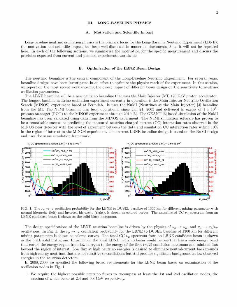
FIG. 1. The νµ → νe oscillation probability for the LBNE to DUSEL baseline of 1300 km for different mixing parameter withnormal hierarchy (left) and inverted hierarchy (right), is shown as colored curves. The unoscillated CC νµ spectrum from anLBNE candidate beam is shown as the solid black histogram.

The design specifications of the LBNE neutrino beamline is driven by the physics of νµ → νµ, and νµ → νe/ντoscillations. In Fig. 1, the νµ → νe oscillation probability for the LBNE to DUSEL baseline of 1300 km for differentmixing parameters is shown as colored curves. The total CC νµ spectrum from an LBNE candidate beam is shownas the black solid histogram. In principle, the ideal LBNE neutrino beam would be one that has a wide energy bandthat covers the energy region from low energies to the energy of the first (π/2) oscillation maximum and minimal fluxbeyond the region of interest. Low flux at high neutrino energies is desired to eliminate neutral-current backgroundsfrom high energy neutrinos that are not sensitive to oscillations but still produce significant background at low observedenergies in the neutrino detectors.

In 2008/2009 we specified the following broad requirements for the LBNE beam based on examination of theoscillation nodes in Fig. 1:

1. We require the highest possible neutrino fluxes to encompass at least the 1st and 2nd oscillation nodes, themaxima of which occur at 2.4 and 0.8 GeV respectively.

4

2. Since neutrino cross sections scale with energy, larger fluxes at lower energies are desirable to achieve the physicssensitivities using effects at the 2nd oscillation node and beyond.

3. To detect νµ → νe events at the far detector, it is critical to minimize the neutral-current contamination atlower energy, therefore it is highly desirable to minimize the flux of neutrinos with energies greater than 5 GeVwhere there is little sensitivity to the oscillation parameters (including the CP phase and the mass hierarchy).

4. The irreducible background to νµ → νe appearance signal comes from beam generated νe events, therefore, ahigh purity νµ beam (lowest possible νe contamination) is required.

We studied the physics performance of several conventional horn focused neutrino beam designs in 2008-2010. Weconsidered different decay pipe geometries and different aluminum horn designs (AGS, NuMI, T2K) and differentbeam tunes (horn/target placement and horn currents). A solid cylindrical water cooled graphite target, two nuclear-interaction-lengths long was chosen as the initial target material and geometry for use with the 700 kW LBNE protonbeam pending the result of radiation damage studies with different target materials. An optimization of the targetmaterial and geometry is underway.

We found that a two horn focusing design using parabolic horns similar to the NuMI horns gave the best performanceof the conventional horn focused beams. We chose the radius of the decay pipe to be 2 m to maximize the yield oflow energy neutrinos in the oscillation region (< 5 GeV). Ideally the length of the decay pipe should be chosen suchthat the pions generating neutrinos in the oscillation energy range to decay will decay. The 1st oscillation maxima at2.5 GeV is generated by 6 GeV pions, for which the decay length is 333 m. The length of the decay pipe was chosento be only 250 m to reduce the excavation volume required. The LBNE decay pipe in the “March 2010” design waschosen to be air cooled to mitigate the risks associated with a water cooled decay pipe - such as NuMI’s. However, theair in the decay pipe absorbs some of the pions in the beam before they decay so for this study we used an evacuatedor helium-filled decay pipe. A technical design for a helium-filled decay pipe is currently being assessed.

The current (2010) best candidate LBNE beam spectrum obtained using a 120 GeV proton beam is shown as thesolid black histogram in Fig. 1. As shown in the figure, the rate of νµ CC events in the region of the 2nd oscillationmaxima (< 1.5 GeV) is much lower than at the 1st oscillation maxima. Currently, we do not have a conventionalhorn focused beamline design that can provide sufficient neutrino flux at the 2nd maxima (< 1.5 GeV) or belowwhere the impact of the CP violating phase is maximal. Therefore for this study, we have focused on optimizing theneutrino flux coverage in the oscillation region of the 1st maximum (1.5–6 GeV).

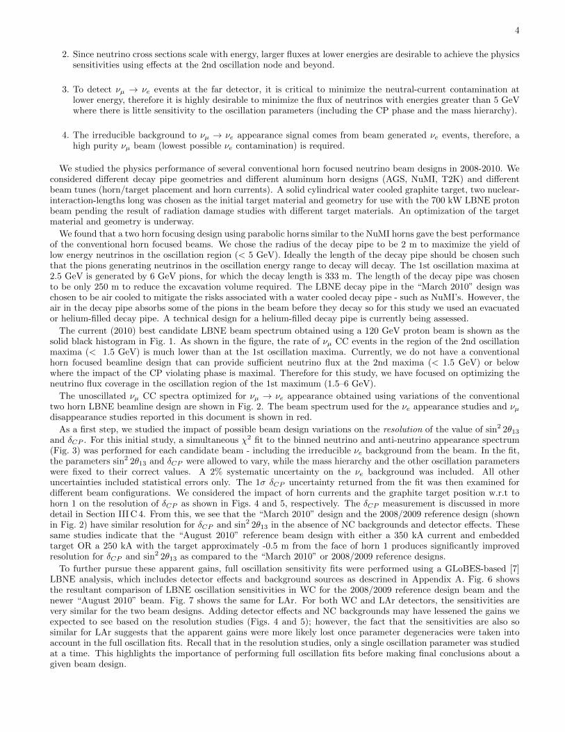
The unoscillated νµ CC spectra optimized for νµ → νe appearance obtained using variations of the conventionaltwo horn LBNE beamline design are shown in Fig. 2. The beam spectrum used for the νe appearance studies and νµdisappearance studies reported in this document is shown in red.

As a first step, we studied the impact of possible beam design variations on the resolution of the value of sin2 2θ13

and δCP . For this initial study, a simultaneous χ2 fit to the binned neutrino and anti-neutrino appearance spectrum(Fig. 3) was performed for each candidate beam - including the irreducible νe background from the beam. In the fit,the parameters sin2 2θ13 and δCP were allowed to vary, while the mass hierarchy and the other oscillation parameterswere fixed to their correct values. A 2% systematic uncertainty on the νe background was included. All otheruncertainties included statistical errors only. The 1σ δCP uncertainty returned from the fit was then examined fordifferent beam configurations. We considered the impact of horn currents and the graphite target position w.r.t tohorn 1 on the resolution of δCP as shown in Figs. 4 and 5, respectively. The δCP measurement is discussed in moredetail in Section III C 4. From this, we see that the “March 2010” design and the 2008/2009 reference design (shownin Fig. 2) have similar resolution for δCP and sin2 2θ13 in the absence of NC backgrounds and detector effects. Thesesame studies indicate that the “August 2010” reference beam design with either a 350 kA current and embeddedtarget OR a 250 kA with the target approximately -0.5 m from the face of horn 1 produces significantly improvedresolution for δCP and sin2 2θ13 as compared to the “March 2010” or 2008/2009 reference designs.

To further pursue these apparent gains, full oscillation sensitivity fits were performed using a GLoBES-based [7]LBNE analysis, which includes detector effects and background sources as descrined in Appendix A. Fig. 6 showsthe resultant comparison of LBNE oscillation sensitivities in WC for the 2008/2009 reference design beam and thenewer “August 2010” beam. Fig. 7 shows the same for LAr. For both WC and LAr detectors, the sensitivities arevery similar for the two beam designs. Adding detector effects and NC backgrounds may have lessened the gains weexpected to see based on the resolution studies (Figs. 4 and 5); however, the fact that the sensitivities are also sosimilar for LAr suggests that the apparent gains were more likely lost once parameter degeneracies were taken intoaccount in the full oscillation fits. Recall that in the resolution studies, only a single oscillation parameter was studiedat a time. This highlights the importance of performing full oscillation fits before making final conclusions about agiven beam design.

5

GeVνE 0 2 4 6 8 10 12 14

PO

T20

CC

eve

nts

/GeV

/kT

/10

µ ν

0

1

2

3

4

5

6

7

8

9

10

2008/2009 LBNE Beam

2008/2009 LBNE Beam

March 2010 Design

Aug 2010 Design with Parabolic Horns

FIG. 2. Various νµ CC spectra obtained using variations of the two horn LBNE design. In black is the 2008/2009 LBNEdesign using an embedded high density carbon target 0.6 cm in radius and 80 cm in length and the two NuMI horns withan evacuated decay pipe 2 m in radius and 280 m in length. In blue is an LBNE design from “March 2010”, which has anembedded graphite target with 0.77 cm radius and 96 cm in length, a modified NuMI horn 1 with a cylindrical front end andNuMI horn 2 operating at 300 kA. The decay pipe in the “March 2010” design is air filled, 2 m in radius and 250 m in length.In red is the “August 2010” LBNE candidate beam design, which has two parabolic NuMI horns operating at 250 kA with thetarget pulled back 30 cm from the face of horn 1.

Neutrino Energy (GeV)1 2 3 4 5 6 7 8

Eve

nts/

0.25

GeV

0

5

10

15

20

25

30

35

40

) = 0.01, 100kT.MW.yr13 θ(22 appearance spectrum, sin e ν

= 0cp δSignal+Bkgd, o = 90 cp δSignal+Bkgd, o = -90 cp δSignal+Bkgd,

e νBeam


Eve

nts/

0.25

GeV

0

5

10

15

20

25

30

35

40

) = 0.01, 100kT.MW.yr13 θ(22 appearance spectrum, sin e ν

= 0cp δSignal+Bkgd, o = 90 cp δSignal+Bkgd, o = -90 cp δSignal+Bkgd,

e νBeam

FIG. 3. The νe appearance spectrum from the 2008/2009 reference beam for an exposure of 100 kT.MW.yr, sin2(2θ13) = 0.01,normal hierarchy (left), and inverted hierarchy (right). No detector effects are included.

1. Conclusion

Despite the fact that the “August 2010” beam design has about a 30% higher flux, it appears to yield similarsensitivity to sin2 2θ13 6= 0, CP violation, and the mass hierarchy as the original 2008/2009 reference beam. Thisholds for both WC and LAr detectors. This suggests that LBNE’s long-baseline oscillation sensitivity may not bevery sensitive to the exact shape of the flux between 3 and 6 GeV.

For the physics studies reported here, we have chosen the “August 2010” beam design with two NuMI parabolichorns ∼6 m apart, 250 kA current and with the target upstream end -30 cm from the upstream face of horn 1 (redspectrum in Fig. 2). [The decay pipe is assumed to be evacuated or helium filled to allow the maximum number of pionsto decay.] The advantage of this beam is that it may be technically easier to build and maintain the target/focusing

6

FIG. 4. The 1σ resolution of δCP as the target position is changed in the 2008/2009 LBNE beam design. Normal hierarchy(left) and inverted hierarchy (right). An exposure of 100 kt.MW.yr is assumed with ν : ν running in the ratio 1:1. No detectoreffects included.

FIG. 5. The 1σ resolution of δCP as the horn current is changed in the 2008/2009 LBNE beam design. Normal hierarchy (left)and inverted hierarchy (right). An exposure of 100 kt.MW.yr is assumed with ν : ν running in the ratio 1:1. No detector effectsincluded.

system.We note that none of the beams studied so far have sufficient flux at the second maxima to impact the measurement

of δCP and sin2 2θ13. Preliminary estimates indicate that we would require at least 5X more flux at the 2nd maximato significantly improve the measurement of δCP and sin2 2θ13 [8].

C. νe Appearance

Motivated by an exciting history of discoveries in neutrino oscillations over the course of the past decade, a majorexperimental effort is underway to probe the last unknown mixing angle, θ13. To date, only an upper limit on θ13

exists (Table III). Information from reactor (Daya Bay, Double CHOOZ, RENO) and accelerator-based (NOvA, T2K)experiments will be able to test whether sin2 2θ13 is non-zero down to the ∼ 0.01 level in the coming years. The nextgeneration of experiments will need to be able to provide:

• a more precise measurement of θ13 (or extension of the limit in the case of non-observation);

• a determination of the neutrino mass hierarchy, assuming non-zero θ13 (i.e. to determine whether the massordering is normal ∆m2

31 > 0 or inverted ∆m231 < 0);

• a measurement of leptonic CP violation (through measurement of the CP violating phase, δCP , assuming non-zero θ13).

7

)13θ(22sin

(d

egre

es)

CP

δ

-150

-100

-50

0

50

100

150

New Beam, normal

Old Beam, normal

New Beam, inverted

Old Beam, inverted

200 kton WCν + 5 yrs ν5 yrs

700 kW

)σ Sensitivity (313θ

-310 -210 -110)13θ(22sin

(d

egre

es)

CP

δ

-150

-100

-50

0

50

100

150

New Beam, normal

Old Beam, normal

New Beam, inverted

Old Beam, inverted


700 kW

)σMass Hierarchy Sensitivity (3

-310 -210 -110

)13θ(22sin

(d

egre

es)

CP

δ

-150

-100

-50

0

50

100

150

New Beam, normal

Old Beam, normal

New Beam, inverted

Old Beam, inverted


700 kW

)σCPV Sensitivity (3

-310 -210 -110

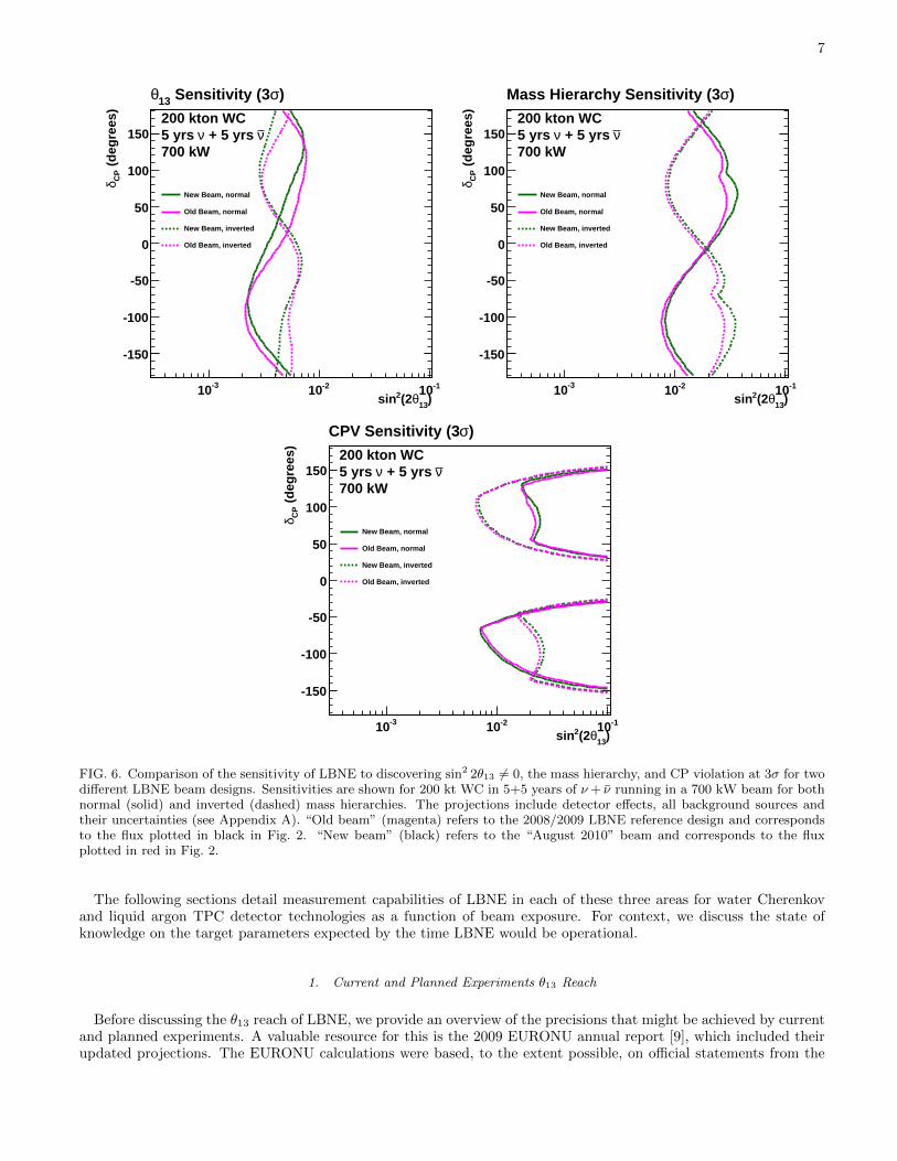
FIG. 6. Comparison of the sensitivity of LBNE to discovering sin2 2θ13 6= 0, the mass hierarchy, and CP violation at 3σ for twodifferent LBNE beam designs. Sensitivities are shown for 200 kt WC in 5+5 years of ν+ ν running in a 700 kW beam for bothnormal (solid) and inverted (dashed) mass hierarchies. The projections include detector effects, all background sources andtheir uncertainties (see Appendix A). “Old beam” (magenta) refers to the 2008/2009 LBNE reference design and correspondsto the flux plotted in black in Fig. 2. “New beam” (black) refers to the “August 2010” beam and corresponds to the fluxplotted in red in Fig. 2.

The following sections detail measurement capabilities of LBNE in each of these three areas for water Cherenkovand liquid argon TPC detector technologies as a function of beam exposure. For context, we discuss the state ofknowledge on the target parameters expected by the time LBNE would be operational.

1. Current and Planned Experiments θ13 Reach

Before discussing the θ13 reach of LBNE, we provide an overview of the precisions that might be achieved by currentand planned experiments. A valuable resource for this is the 2009 EURONU annual report [9], which included theirupdated projections. The EURONU calculations were based, to the extent possible, on official statements from the

8

)13θ(22sin

(d

egre

es)

CP

δ

-150

-100

-50

0

50

100

150

New Beam, normal

Old Beam, normal

New Beam, inverted

Old Beam, inverted

34 kton LArν + 5 yrs ν5 yrs

700 kW

)σ Sensitivity (313θ

-310 -210 -110)13θ(22sin

(d

egre

es)

CP

δ

-150

-100

-50

0

50

100

150

New Beam, normal

Old Beam, normal

New Beam, inverted

Old Beam, inverted


700 kW

)σMass Hierarchy Sensitivity (3

-310 -210 -110

)13θ(22sin

(d

egre

es)

CP

δ

-150

-100

-50

0

50

100

150

New Beam, normal

Old Beam, normal

New Beam, inverted

Old Beam, inverted


700 kW

)σCPV Sensitivity (3

-310 -210 -110

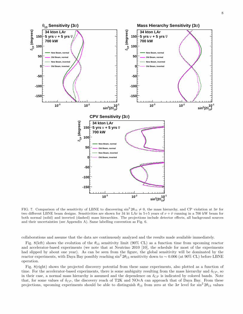
FIG. 7. Comparison of the sensitivity of LBNE to discovering sin2 2θ13 6= 0, the mass hierarchy, and CP violation at 3σ fortwo different LBNE beam designs. Sensitivities are shown for 34 kt LAr in 5+5 years of ν + ν running in a 700 kW beam forboth normal (solid) and inverted (dashed) mass hierarchies. The projections include detector effects, all background sourcesand their uncertainties (see Appendix A). Same labelling convention as Fig. 6.

collaborations and assume that the data are continuously analyzed and the results made available immediately.

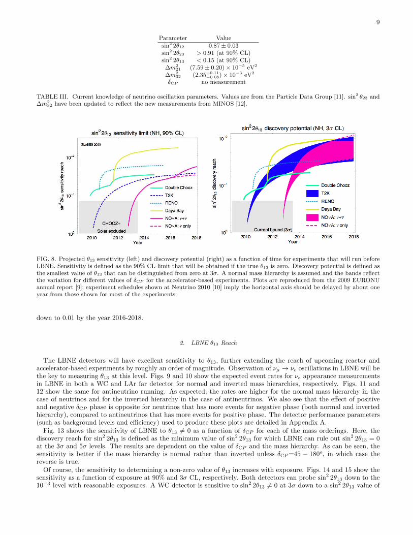
Fig. 8(left) shows the evolution of the θ13 sensitivity limit (90% CL) as a function time from upcoming reactorand accelerator-based experiments (we note that at Neutrino 2010 [10], the schedule for most of the experimentshad slipped by about one year). As can be seen from the figure, the global sensitivity will be dominated by thereactor experiments, with Daya Bay possibly reaching sin2 2θ13 sensitivity down to ∼ 0.006 (at 90% CL) before LBNEoperation.

Fig. 8(right) shows the projected discovery potential from these same experiments, also plotted as a function oftime. For the accelerator-based experiments, there is some ambiguity resulting from the mass hierarchy and δCP , soin their case, a normal mass hierarchy is assumed and the dependence on δCP is indicated by colored bands. Notethat, for some values of δCP , the discovery reach of T2K and NOvA can approach that of Daya Bay. From theseprojections, upcoming experiments should be able to distinguish θ13 from zero at the 3σ level for sin2 2θ13 values

9

Parameter Valuesin2 2θ12 0.87± 0.03sin2 2θ23 > 0.91 (at 90% CL)sin2 2θ13 < 0.15 (at 90% CL)∆m2

21 (7.59± 0.20)× 10−5 eV2

∆m232 (2.35+0.11

−0.08)× 10−3 eV2

δCP no measurement

TABLE III. Current knowledge of neutrino oscillation parameters. Values are from the Particle Data Group [11]. sin2 θ23 and∆m2

32 have been updated to reflect the new measurements from MINOS [12].

FIG. 8. Projected θ13 sensitivity (left) and discovery potential (right) as a function of time for experiments that will run beforeLBNE. Sensitivity is defined as the 90% CL limit that will be obtained if the true θ13 is zero. Discovery potential is defined asthe smallest value of θ13 that can be distinguished from zero at 3σ. A normal mass hierarchy is assumed and the bands reflectthe variation for different values of δCP for the accelerator-based experiments. Plots are reproduced from the 2009 EURONUannual report [9]; experiment schedules shown at Neutrino 2010 [10] imply the horizontal axis should be delayed by about oneyear from those shown for most of the experiments.

down to 0.01 by the year 2016-2018.

2. LBNE θ13 Reach

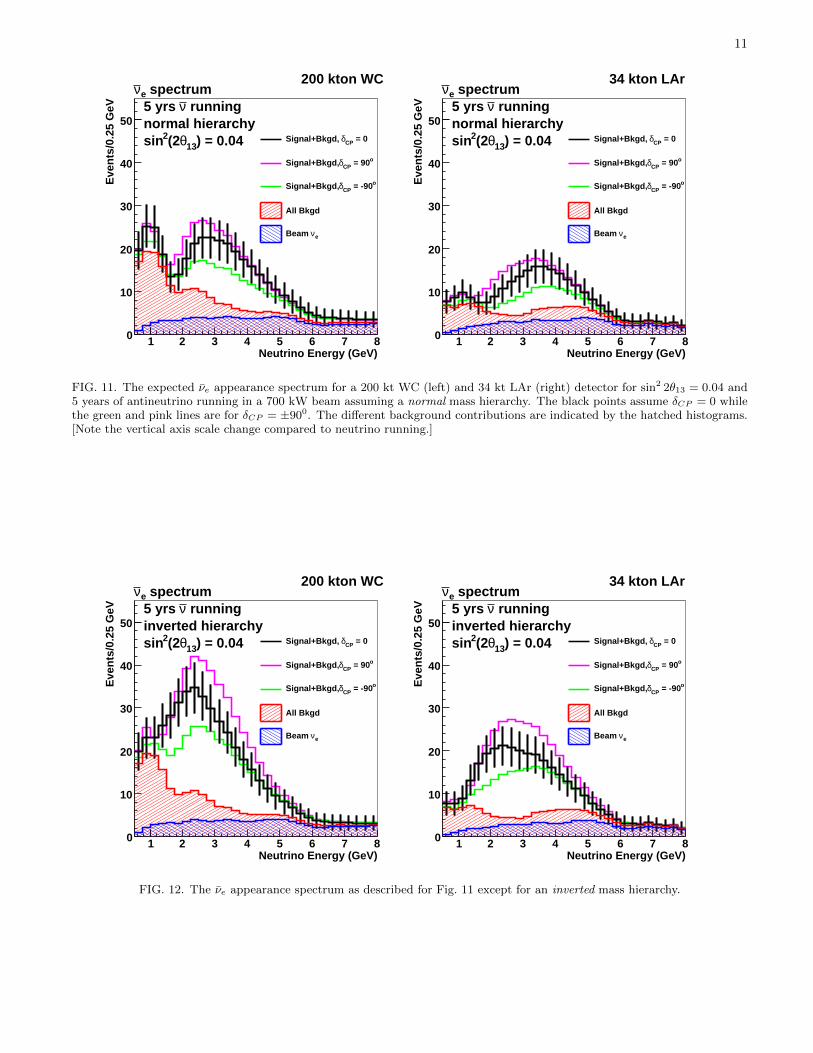
The LBNE detectors will have excellent sensitivity to θ13, further extending the reach of upcoming reactor andaccelerator-based experiments by roughly an order of magnitude. Observation of νµ → νe oscillations in LBNE will bethe key to measuring θ13 at this level. Figs. 9 and 10 show the expected event rates for νe appearance measurementsin LBNE in both a WC and LAr far detector for normal and inverted mass hierarchies, respectively. Figs. 11 and12 show the same for antineutrino running. As expected, the rates are higher for the normal mass hierarchy in thecase of neutrinos and for the inverted hierarchy in the case of antineutrinos. We also see that the effect of positiveand negative δCP phase is opposite for neutrinos that has more events for negative phase (both normal and invertedhierarchy), compared to antineutrinos that has more events for positive phase. The detector performance parameters(such as background levels and efficiency) used to produce these plots are detailed in Appendix A.

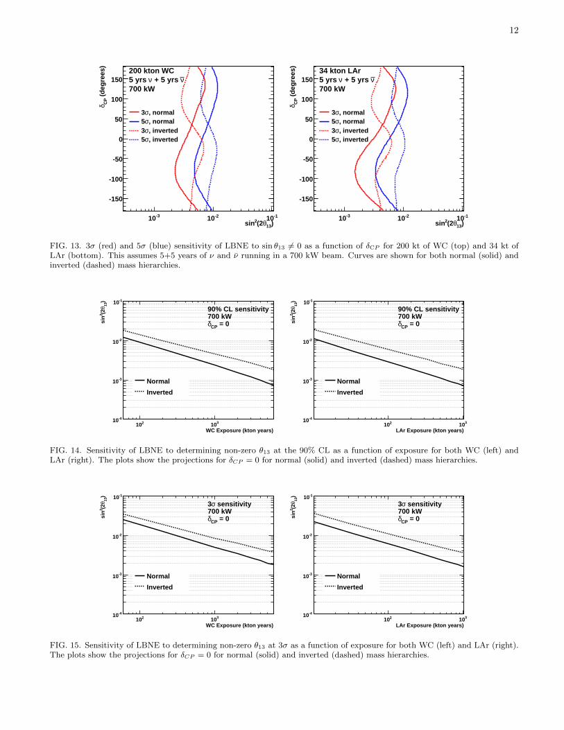
Fig. 13 shows the sensitivity of LBNE to θ13 6= 0 as a function of δCP for each of the mass orderings. Here, thediscovery reach for sin2 2θ13 is defined as the minimum value of sin2 2θ13 for which LBNE can rule out sin2 2θ13 = 0at the 3σ and 5σ levels. The results are dependent on the value of δCP and the mass hierarchy. As can be seen, thesensitivity is better if the mass hierarchy is normal rather than inverted unless δCP=45 − 180o, in which case thereverse is true.

Of course, the sensitivity to determining a non-zero value of θ13 increases with exposure. Figs. 14 and 15 show thesensitivity as a function of exposure at 90% and 3σ CL, respectively. Both detectors can probe sin2 2θ13 down to the10−3 level with reasonable exposures. A WC detector is sensitive to sin2 2θ13 6= 0 at 3σ down to a sin2 2θ13 value of

10


Eve

nts

/0.2

5 G

eV

0

20

40

60

80

100

= 0CPδSignal+Bkgd,

o = 90CPδSignal+Bkgd,

o = -90CPδSignal+Bkgd,

All Bkgd

eνBeam

runningν5 yrs normal hierarchy

) = 0.0413θ(22sin

spectrumeν 200 kton WC


Eve

nts

/0.2

5 G

eV

0

20

40

60

80

100

= 0CPδSignal+Bkgd,



All Bkgd

eνBeam


) = 0.0413θ(22sin

spectrumeν 34 kton LAr

FIG. 9. The expected νe appearance spectrum for a 200 kt WC (left) and 34 kt LAr (right) detector for sin2 2θ13 = 0.04 and5 years of neutrino running in a 700 kW beam assuming a normal mass hierarchy. The black points assume δCP = 0 while thegreen and pink lines are for δCP = ±900. The different background contributions are indicated by the hatched histograms.


Eve

nts

/0.2

5 G

eV

0

20

40

60

80

100

= 0CPδSignal+Bkgd,



All Bkgd

eνBeam

runningν5 yrs inverted hierarchy

) = 0.0413θ(22sin

spectrumeν 200 kton WC


Eve

nts

/0.2

5 G

eV

0

20

40

60

80

100

= 0CPδSignal+Bkgd,



All Bkgd

eνBeam


) = 0.0413θ(22sin

spectrumeν 34 kton LAr

FIG. 10. The νe appearance spectrum as described for Fig. 9 except for an inverted mass hierarchy.

0.008 for 100% of all possible δCP values assuming an exposure of 2000 kt-yrs. The same is true for LAr assumingan exposure of 340 kt-yrs. Hence, LAr appears to have similar θ13 reach as WC with about 1/6 the exposure. [Themain parameter that determines this factor is the ratio of the detector signal efficiencies near the 1st maximum.]

11


Eve

nts

/0.2

5 G

eV

0

10

20

30

40

50

= 0CPδSignal+Bkgd,



All Bkgd

eνBeam


) = 0.0413θ(22sin

spectrumeν200 kton WC


Eve

nts

/0.2

5 G

eV

0

10

20

30

40

50

= 0CPδSignal+Bkgd,



All Bkgd

eνBeam


) = 0.0413θ(22sin

spectrumeν34 kton LAr

FIG. 11. The expected νe appearance spectrum for a 200 kt WC (left) and 34 kt LAr (right) detector for sin2 2θ13 = 0.04 and5 years of antineutrino running in a 700 kW beam assuming a normal mass hierarchy. The black points assume δCP = 0 whilethe green and pink lines are for δCP = ±900. The different background contributions are indicated by the hatched histograms.[Note the vertical axis scale change compared to neutrino running.]


Eve

nts

/0.2

5 G

eV

0

10

20

30

40

50

= 0CPδSignal+Bkgd,



All Bkgd

eνBeam


) = 0.0413θ(22sin

spectrumeν200 kton WC


Eve

nts

/0.2

5 G

eV

0

10

20

30

40

50

= 0CPδSignal+Bkgd,



All Bkgd

eνBeam


) = 0.0413θ(22sin

spectrumeν34 kton LAr

FIG. 12. The νe appearance spectrum as described for Fig. 11 except for an inverted mass hierarchy.

12

)13θ(22sin

(d

egre

es)

CP

δ

-150

-100

-50

0

50

100

150

, normalσ3, normalσ5, invertedσ3, invertedσ5


700 kW

-310 -210 -110)13θ(22sin

(d

egre

es)

CP

δ

-150

-100

-50

0

50

100

150



700 kW

-310 -210 -110

FIG. 13. 3σ (red) and 5σ (blue) sensitivity of LBNE to sin θ13 6= 0 as a function of δCP for 200 kt of WC (top) and 34 kt ofLAr (bottom). This assumes 5+5 years of ν and ν running in a 700 kW beam. Curves are shown for both normal (solid) andinverted (dashed) mass hierarchies.

WC Exposure (kton years)

210 310

)13θ

(22si

n

-410

-310

-210

-110

Normal

Inverted

90% CL sensitivity700 kW

= 0CPδ

LAr Exposure (kton years)

210 310

)13θ

(22si

n

-410

-310

-210

-110

Normal

Inverted

90% CL sensitivity700 kW

= 0CPδ

FIG. 14. Sensitivity of LBNE to determining non-zero θ13 at the 90% CL as a function of exposure for both WC (left) andLAr (right). The plots show the projections for δCP = 0 for normal (solid) and inverted (dashed) mass hierarchies.

WC Exposure (kton years)

210 310

)13θ

(22si

n

-410

-310

-210

-110

Normal

Inverted

sensitivityσ3700 kW

= 0CPδ

LAr Exposure (kton years)

210 310

)13θ

(22si

n

-410

-310

-210

-110

Normal

Inverted

sensitivityσ3700 kW

= 0CPδ

FIG. 15. Sensitivity of LBNE to determining non-zero θ13 at 3σ as a function of exposure for both WC (left) and LAr (right).The plots show the projections for δCP = 0 for normal (solid) and inverted (dashed) mass hierarchies.

13

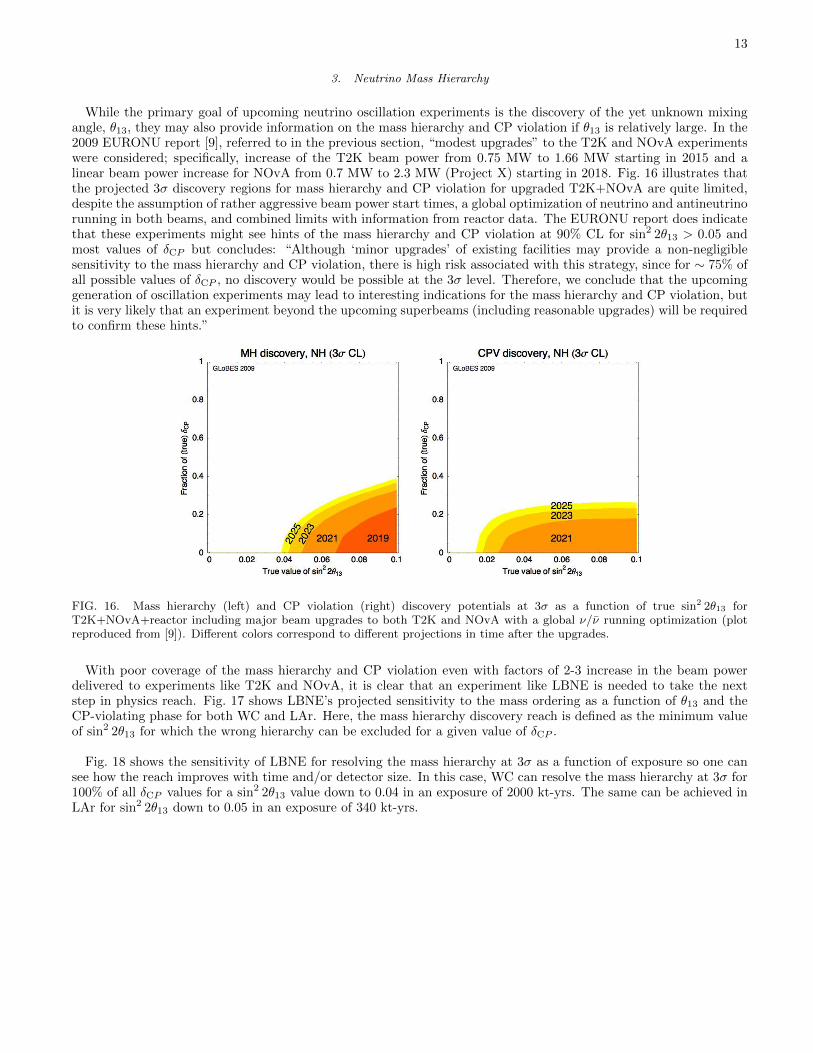
3. Neutrino Mass Hierarchy

While the primary goal of upcoming neutrino oscillation experiments is the discovery of the yet unknown mixingangle, θ13, they may also provide information on the mass hierarchy and CP violation if θ13 is relatively large. In the2009 EURONU report [9], referred to in the previous section, “modest upgrades” to the T2K and NOvA experimentswere considered; specifically, increase of the T2K beam power from 0.75 MW to 1.66 MW starting in 2015 and alinear beam power increase for NOvA from 0.7 MW to 2.3 MW (Project X) starting in 2018. Fig. 16 illustrates thatthe projected 3σ discovery regions for mass hierarchy and CP violation for upgraded T2K+NOvA are quite limited,despite the assumption of rather aggressive beam power start times, a global optimization of neutrino and antineutrinorunning in both beams, and combined limits with information from reactor data. The EURONU report does indicatethat these experiments might see hints of the mass hierarchy and CP violation at 90% CL for sin2 2θ13 > 0.05 andmost values of δCP but concludes: “Although ‘minor upgrades’ of existing facilities may provide a non-negligiblesensitivity to the mass hierarchy and CP violation, there is high risk associated with this strategy, since for ∼ 75% ofall possible values of δCP , no discovery would be possible at the 3σ level. Therefore, we conclude that the upcominggeneration of oscillation experiments may lead to interesting indications for the mass hierarchy and CP violation, butit is very likely that an experiment beyond the upcoming superbeams (including reasonable upgrades) will be requiredto confirm these hints.”

FIG. 16. Mass hierarchy (left) and CP violation (right) discovery potentials at 3σ as a function of true sin2 2θ13 forT2K+NOvA+reactor including major beam upgrades to both T2K and NOvA with a global ν/ν running optimization (plotreproduced from [9]). Different colors correspond to different projections in time after the upgrades.

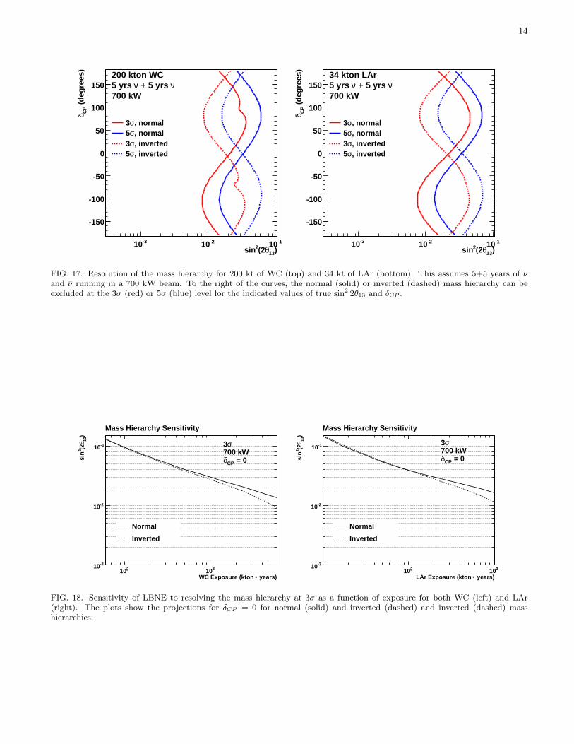
With poor coverage of the mass hierarchy and CP violation even with factors of 2-3 increase in the beam powerdelivered to experiments like T2K and NOvA, it is clear that an experiment like LBNE is needed to take the nextstep in physics reach. Fig. 17 shows LBNE’s projected sensitivity to the mass ordering as a function of θ13 and theCP-violating phase for both WC and LAr. Here, the mass hierarchy discovery reach is defined as the minimum valueof sin2 2θ13 for which the wrong hierarchy can be excluded for a given value of δCP .

Fig. 18 shows the sensitivity of LBNE for resolving the mass hierarchy at 3σ as a function of exposure so one cansee how the reach improves with time and/or detector size. In this case, WC can resolve the mass hierarchy at 3σ for100% of all δCP values for a sin2 2θ13 value down to 0.04 in an exposure of 2000 kt-yrs. The same can be achieved inLAr for sin2 2θ13 down to 0.05 in an exposure of 340 kt-yrs.

14

)13θ(22sin

(d

egre

es)

CP

δ

-150

-100

-50

0

50

100

150



700 kW

-310 -210 -110)13θ(22sin

(d

egre

es)

CP

δ

-150

-100

-50

0

50

100

150



700 kW

-310 -210 -110

FIG. 17. Resolution of the mass hierarchy for 200 kt of WC (top) and 34 kt of LAr (bottom). This assumes 5+5 years of νand ν running in a 700 kW beam. To the right of the curves, the normal (solid) or inverted (dashed) mass hierarchy can beexcluded at the 3σ (red) or 5σ (blue) level for the indicated values of true sin2 2θ13 and δCP .

years)•WC Exposure (kton 210 310

)13θ

(22si

n

-310

-210

-110

Normal

Inverted

σ3700 kW

= 0CPδ

Mass Hierarchy Sensitivity

years)•LAr Exposure (kton 210 310

)13θ

(22si

n

-310

-210

-110

Normal

Inverted

σ3700 kW

= 0CPδ

Mass Hierarchy Sensitivity

FIG. 18. Sensitivity of LBNE to resolving the mass hierarchy at 3σ as a function of exposure for both WC (left) and LAr(right). The plots show the projections for δCP = 0 for normal (solid) and inverted (dashed) and inverted (dashed) masshierarchies.

15

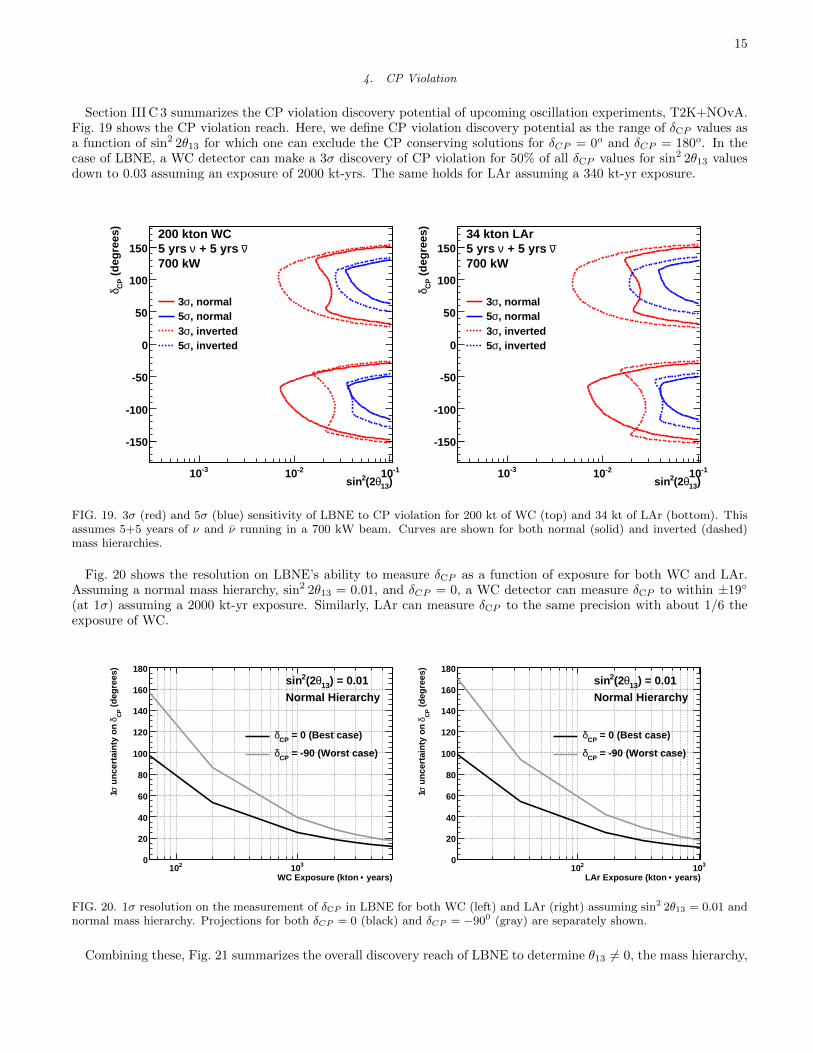
4. CP Violation

Section III C 3 summarizes the CP violation discovery potential of upcoming oscillation experiments, T2K+NOvA.Fig. 19 shows the CP violation reach. Here, we define CP violation discovery potential as the range of δCP values asa function of sin2 2θ13 for which one can exclude the CP conserving solutions for δCP = 0o and δCP = 180o. In thecase of LBNE, a WC detector can make a 3σ discovery of CP violation for 50% of all δCP values for sin2 2θ13 valuesdown to 0.03 assuming an exposure of 2000 kt-yrs. The same holds for LAr assuming a 340 kt-yr exposure.

)13θ(22sin

(d

egre

es)

CP

δ

-150

-100

-50

0

50

100

150



700 kW

-310 -210 -110)13θ(22sin

(d

egre

es)

CP

δ

-150

-100

-50

0

50

100

150



700 kW

-310 -210 -110

FIG. 19. 3σ (red) and 5σ (blue) sensitivity of LBNE to CP violation for 200 kt of WC (top) and 34 kt of LAr (bottom). Thisassumes 5+5 years of ν and ν running in a 700 kW beam. Curves are shown for both normal (solid) and inverted (dashed)mass hierarchies.

Fig. 20 shows the resolution on LBNE’s ability to measure δCP as a function of exposure for both WC and LAr.Assuming a normal mass hierarchy, sin2 2θ13 = 0.01, and δCP = 0, a WC detector can measure δCP to within ±19

(at 1σ) assuming a 2000 kt-yr exposure. Similarly, LAr can measure δCP to the same precision with about 1/6 theexposure of WC.

years)•WC Exposure (kton

210 310

(d

egre

es)

CP

δ u

nce

rtai

nty

on

σ1

0

20

40

60

80

100

120

140

160

180) = 0.0113θ(22sin

Normal Hierarchy

= 0 (Best case)CPδ

= -90 (Worst case)CPδ

years)•LAr Exposure (kton

210 310

(d

egre

es)

CP

δ u

nce

rtai

nty

on

σ1

0

20

40

60

80

100

120

140

160

180) = 0.0113θ(22sin

Normal Hierarchy

= 0 (Best case)CPδ

= -90 (Worst case)CPδ

FIG. 20. 1σ resolution on the measurement of δCP in LBNE for both WC (left) and LAr (right) assuming sin2 2θ13 = 0.01 andnormal mass hierarchy. Projections for both δCP = 0 (black) and δCP = −900 (gray) are separately shown.

Combining these, Fig. 21 summarizes the overall discovery reach of LBNE to determine θ13 6= 0, the mass hierarchy,

16

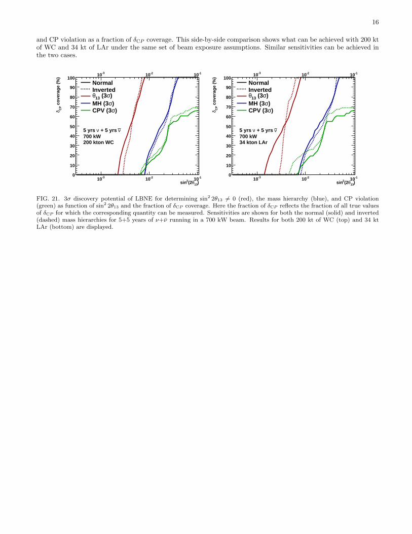
and CP violation as a fraction of δCP coverage. This side-by-side comparison shows what can be achieved with 200 ktof WC and 34 kt of LAr under the same set of beam exposure assumptions. Similar sensitivities can be achieved inthe two cases.

)13θ(22sin

co

vera

ge

(%)

CP

δ

0

10

20

30

40

50

60

70

80

90

100NormalInverted

)σ (313θ)σMH (3)σCPV (3

ν + 5 yrs ν5 yrs 700 kW200 kton WC

-310 -210 -110

-310 -210 -110

)13θ(22sin

co

vera

ge

(%)

CP

δ

0

10

20

30

40

50

60

70

80

90

100NormalInverted

)σ (313θ)σMH (3)σCPV (3

ν + 5 yrs ν5 yrs 700 kW34 kton LAr

-310 -210 -110

-310 -210 -110

FIG. 21. 3σ discovery potential of LBNE for determining sin2 2θ13 6= 0 (red), the mass hierarchy (blue), and CP violation(green) as function of sin2 2θ13 and the fraction of δCP coverage. Here the fraction of δCP reflects the fraction of all true valuesof δCP for which the corresponding quantity can be measured. Sensitivities are shown for both the normal (solid) and inverted(dashed) mass hierarchies for 5+5 years of ν+ν running in a 700 kW beam. Results for both 200 kt of WC (top) and 34 ktLAr (bottom) are displayed.

17

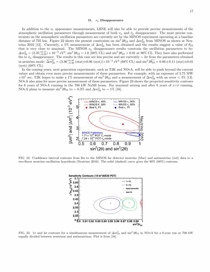
D. νµ Disappearance

In addition to the νe appearance measurements, LBNE will also be able to provide precise measurements of theatmospheric oscillation parameters through measurement of both νµ and νµ disappearance. The most precise con-straints on the atmospheric oscillation parameters are currently set by the MINOS experiment operating at a baselinedistance of 735 km. Figure 22 shows the present constraints on sin2 2θ23 and ∆m2

32 from MINOS as shown at Neu-trino 2010 [12]. Currently, a 5% measurement of ∆m2

32 has been obtained and the results suggest a value of θ23

that is very close to maximal. The MINOS νµ disappearance results constrain the oscillation parameters to be:

∆m232 = (2.35+0.11

−0.08)× 10−3 eV2, sin2 2θ23 = 1.0 (68% CL) and sin2 2θ23 > 0.91 at 90% CL. They have also performedfits to νµ disappearance. The results in this case are less precise and are currently ∼ 2σ from the parameters obtained

in neutrino mode: ∆m232 = (3.36+0.45

−0.40 (stat)±0.06 (syst))×10−3 eV2 (68% CL) and sin2 2θ23 = 0.86±0.11 (stat)±0.01(syst) (68% CL).

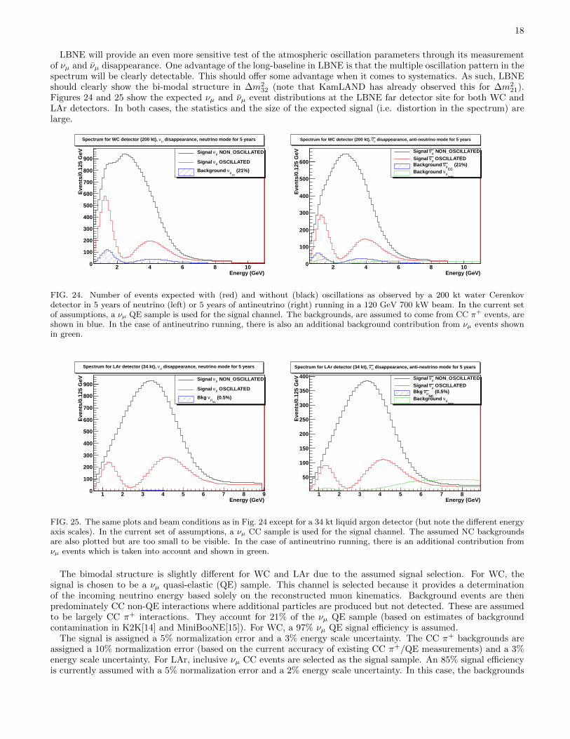
In the coming years, next generation experiments, such as T2K and NOvA, will be able to push beyond the currentvalues and obtain even more precise measurements of these parameters. For example, with an exposure of 3.75 MW×107 sec, T2K hopes to make a 1% measurement of sin2 2θ23 and a measurement of ∆m2

32 with an error < 4% [13].NOvA also aims for more precise measurement of these parameters. Figure 23 shows the projected sensitivity contoursfor 6 years of NOvA running in the 700 kW NuMI beam. For maximal mixing and after 6 years of ν+ν running,NOvA plans to measure sin2 2θ23 to ∼ 0.3% and ∆m2

32 to ∼ 1% [16].

FIG. 22. Confidence interval contours from fits to the MINOS far detector neutrino (blue) and antineutrino (red) data to atwo-flavor neutrino oscillation hypothesis (Neutrino 2010). The solid (dashed) curve gives the 90% (68%) contours.

FIG. 23. 1σ and 2σ contours for a simultaneous measurement of ∆m232 and sin2 2θ23 in NOvA for a 6-year run at 700 kW

equally divided between neutrinos and antineutrinos. Plot is from [16].

18

LBNE will provide an even more sensitive test of the atmospheric oscillation parameters through its measurementof νµ and νµ disappearance. One advantage of the long-baseline in LBNE is that the multiple oscillation pattern in thespectrum will be clearly detectable. This should offer some advantage when it comes to systematics. As such, LBNEshould clearly show the bi-modal structure in ∆m2

32 (note that KamLAND has already observed this for ∆m221).

Figures 24 and 25 show the expected νµ and νµ event distributions at the LBNE far detector site for both WC andLAr detectors. In both cases, the statistics and the size of the expected signal (i.e. distortion in the spectrum) arelarge.

Energy (GeV)2 4 6 8 10

Eve

nts

/0.1

25 G

eV

0

100

200

300

400

500

600

700

800

900 NON_OSCILLATEDµνSignal

OSCILLATEDµνSignal

(21%)CC

µνBackground

disappearance, neutrino mode for 5 yearsµνSpectrum for WC detector (200 kt),

Energy (GeV)2 4 6 8 10

Eve

nts/

0.12

5 G

eV

0

100

200

300

400

500

600

NON_OSCILLATEDµνSignal

OSCILLATEDµνSignal (21%)

CCµνBackground

beam

µνBackground

disappearance, anti-neutrino mode for 5 yearsµνSpectrum for WC detector (200 kt),

FIG. 24. Number of events expected with (red) and without (black) oscillations as observed by a 200 kt water Cerenkovdetector in 5 years of neutrino (left) or 5 years of antineutrino (right) running in a 120 GeV 700 kW beam. In the current setof assumptions, a νµ QE sample is used for the signal channel. The backgrounds, are assumed to come from CC π+ events, areshown in blue. In the case of antineutrino running, there is also an additional background contribution from νµ events shownin green.

Energy (GeV)1 2 3 4 5 6 7 8 9

Eve

nts

/0.1

25 G

eV

0

100

200

300

400

500

600

700

800


OSCILLATEDµνSignal

(0.5%)NC

µνBkg

disappearance, neutrino mode for 5 yearsµνSpectrum for LAr detector (34 kt),

Energy (GeV)1 2 3 4 5 6 7 8

Eve

nts/

0.12

5 G

eV

50

100

150

200

250

300

350


OSCILLATEDµνSignal (0.5%)

NCµνBkg

beam

µνBackground

disappearance, anti-neutrino mode for 5 yearsµνSpectrum for LAr detector (34 kt),

FIG. 25. The same plots and beam conditions as in Fig. 24 except for a 34 kt liquid argon detector (but note the different energyaxis scales). In the current set of assumptions, a νµ CC sample is used for the signal channel. The assumed NC backgroundsare also plotted but are too small to be visible. In the case of antineutrino running, there is an additional contribution fromνµ events which is taken into account and shown in green.

The bimodal structure is slightly different for WC and LAr due to the assumed signal selection. For WC, thesignal is chosen to be a νµ quasi-elastic (QE) sample. This channel is selected because it provides a determinationof the incoming neutrino energy based solely on the reconstructed muon kinematics. Background events are thenpredominately CC non-QE interactions where additional particles are produced but not detected. These are assumedto be largely CC π+ interactions. They account for 21% of the νµ QE sample (based on estimates of backgroundcontamination in K2K[14] and MiniBooNE[15]). For WC, a 97% νµ QE signal efficiency is assumed.

The signal is assigned a 5% normalization error and a 3% energy scale uncertainty. The CC π+ backgrounds areassigned a 10% normalization error (based on the current accuracy of existing CC π+/QE measurements) and a 3%energy scale uncertainty. For LAr, inclusive νµ CC events are selected as the signal sample. An 85% signal efficiencyis currently assumed with a 5% normalization error and a 2% energy scale uncertainty. In this case, the backgrounds

19

are NC events, 0.5% of which are assumed to be misidentified as CC events and assigned a 10% (2%) normalization(energy scale) uncertainty. In the case of antineutrino running, these same assumptions are applied with the additionof an extra level of νµ contamination. The actual parameter assumptions and GLoBES inputs used for the LBNE νµand νµ disappearance projections are provided for both detectors in Appendix A.

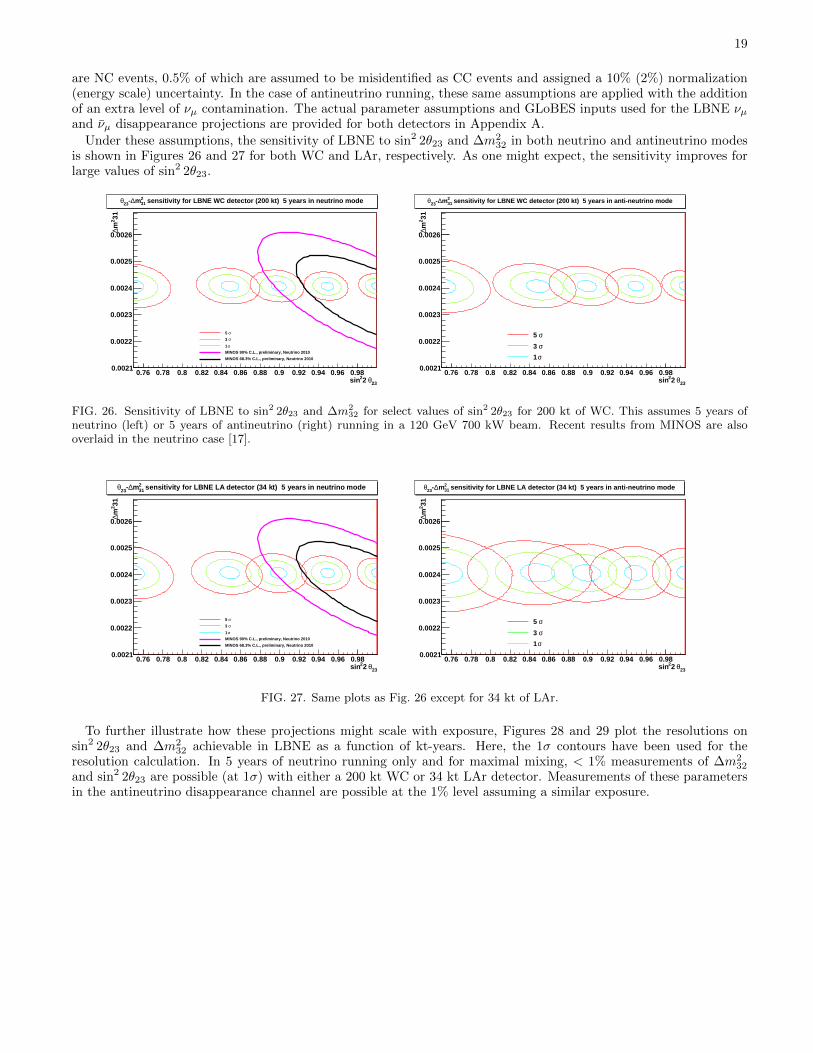
Under these assumptions, the sensitivity of LBNE to sin2 2θ23 and ∆m232 in both neutrino and antineutrino modes

is shown in Figures 26 and 27 for both WC and LAr, respectively. As one might expect, the sensitivity improves forlarge values of sin2 2θ23.

23θ2 2sin0.76 0.78 0.8 0.82 0.84 0.86 0.88 0.9 0.92 0.94 0.96 0.98

312m∆

0.0021

0.0022

0.0023

0.0024

0.0025

0.0026

σ5

σ3

σ1

MINOS 90% C.L., preliminary, Neutrino 2010

MINOS 68.3% C.L., preliminary, Neutrino 2010

sensitivity for LBNE WC detector (200 kt) 5 years in neutrino mode312m∆-23θ

23θ2 2sin0.76 0.78 0.8 0.82 0.84 0.86 0.88 0.9 0.92 0.94 0.96 0.98

312m∆

0.0021

0.0022

0.0023

0.0024

0.0025

0.0026

σ5

σ3

σ1

sensitivity for LBNE WC detector (200 kt) 5 years in anti-neutrino mode312m∆-23θ

FIG. 26. Sensitivity of LBNE to sin2 2θ23 and ∆m232 for select values of sin2 2θ23 for 200 kt of WC. This assumes 5 years of

neutrino (left) or 5 years of antineutrino (right) running in a 120 GeV 700 kW beam. Recent results from MINOS are alsooverlaid in the neutrino case [17].

23θ2 2sin0.76 0.78 0.8 0.82 0.84 0.86 0.88 0.9 0.92 0.94 0.96 0.98

312m∆

0.0021

0.0022

0.0023

0.0024

0.0025

0.0026

σ5

σ3

σ1

MINOS 90% C.L., preliminary, Neutrino 2010

MINOS 68.3% C.L., preliminary, Neutrino 2010

sensitivity for LBNE LA detector (34 kt) 5 years in neutrino mode312m∆-23θ

23θ2 2sin0.76 0.78 0.8 0.82 0.84 0.86 0.88 0.9 0.92 0.94 0.96 0.98

312m∆

0.0021

0.0022

0.0023

0.0024

0.0025

0.0026

σ5

σ3

σ1

sensitivity for LBNE LA detector (34 kt) 5 years in anti-neutrino mode312m∆-23θ

FIG. 27. Same plots as Fig. 26 except for 34 kt of LAr.

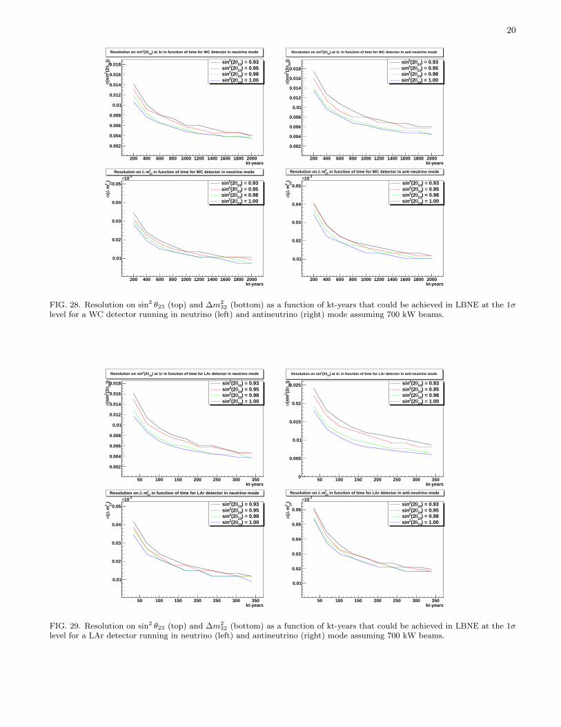
To further illustrate how these projections might scale with exposure, Figures 28 and 29 plot the resolutions onsin2 2θ23 and ∆m2

32 achievable in LBNE as a function of kt-years. Here, the 1σ contours have been used for theresolution calculation. In 5 years of neutrino running only and for maximal mixing, < 1% measurements of ∆m2

32

and sin2 2θ23 are possible (at 1σ) with either a 200 kt WC or 34 kt LAr detector. Measurements of these parametersin the antineutrino disappearance channel are possible at the 1% level assuming a similar exposure.

20

kt-years200 400 600 800 1000 1200 1400 1600 1800 2000

))23θ

(22(s

inσ

0.002

0.004

0.006

0.008

0.01

0.012

0.014

0.016

0.018 ) = 0.9323θ(22sin) = 0.9523θ(22sin) = 0.9823θ(22sin) = 1.0023θ(22sin

in function of time for WC detector in neutrino modeσ) at 123

θ(22Resolution on sin

kt-years200 400 600 800 1000 1200 1400 1600 1800 2000

))23θ

(22(s

inσ

0.002

0.004

0.006

0.008

0.01

0.012

0.014

0.016

0.018) = 0.9323θ(22sin) = 0.9523θ(22sin) = 0.9823θ(22sin) = 1.0023θ(22sin

in function of time for WC detector in anti-neutrino modeσ) at 123θ(22Resolution on sin

kt-years200 400 600 800 1000 1200 1400 1600 1800 2000

)132

m∆(σ

0.01

0.02

0.03

0.04

0.05

-310×) = 0.9323θ(22sin) = 0.9523θ(22sin) = 0.9823θ(22sin) = 1.0023θ(22sin

in function of time for WC detector in neutrino mode132 m∆Resolution on

kt-years200 400 600 800 1000 1200 1400 1600 1800 2000

)132

m∆(σ

0.01

0.02

0.03

0.04

0.05


in function of time for WC detector in anti-neutrino mode132 m∆Resolution on

FIG. 28. Resolution on sin2 θ23 (top) and ∆m232 (bottom) as a function of kt-years that could be achieved in LBNE at the 1σ

level for a WC detector running in neutrino (left) and antineutrino (right) mode assuming 700 kW beams.

kt-years50 100 150 200 250 300 350

))23θ

(22(s

inσ

0.002

0.004

0.006

0.008

0.01

0.012

0.014

0.016


in function of time for LAr detector in neutrino modeσ) at 123θ(22Resolution on sin

kt-years50 100 150 200 250 300 350

))23θ

(22(s

inσ

0

0.005

0.01

0.015

0.02


in function of time for LAr detector in anti-neutrino modeσ) at 123θ(22Resolution on sin

kt-years50 100 150 200 250 300 350

)132

m∆(σ

0.01

0.02

0.03

0.04

0.05


in function of time for LAr detector in neutrino mode132 m∆Resolution on

kt-years50 100 150 200 250 300 350

)132

m∆(σ

0.01

0.02

0.03

0.04

0.05

0.06


in function of time for LAr detector in anti-neutrino mode132 m∆Resolution on

FIG. 29. Resolution on sin2 θ23 (top) and ∆m232 (bottom) as a function of kt-years that could be achieved in LBNE at the 1σ

level for a LAr detector running in neutrino (left) and antineutrino (right) mode assuming 700 kW beams.

21

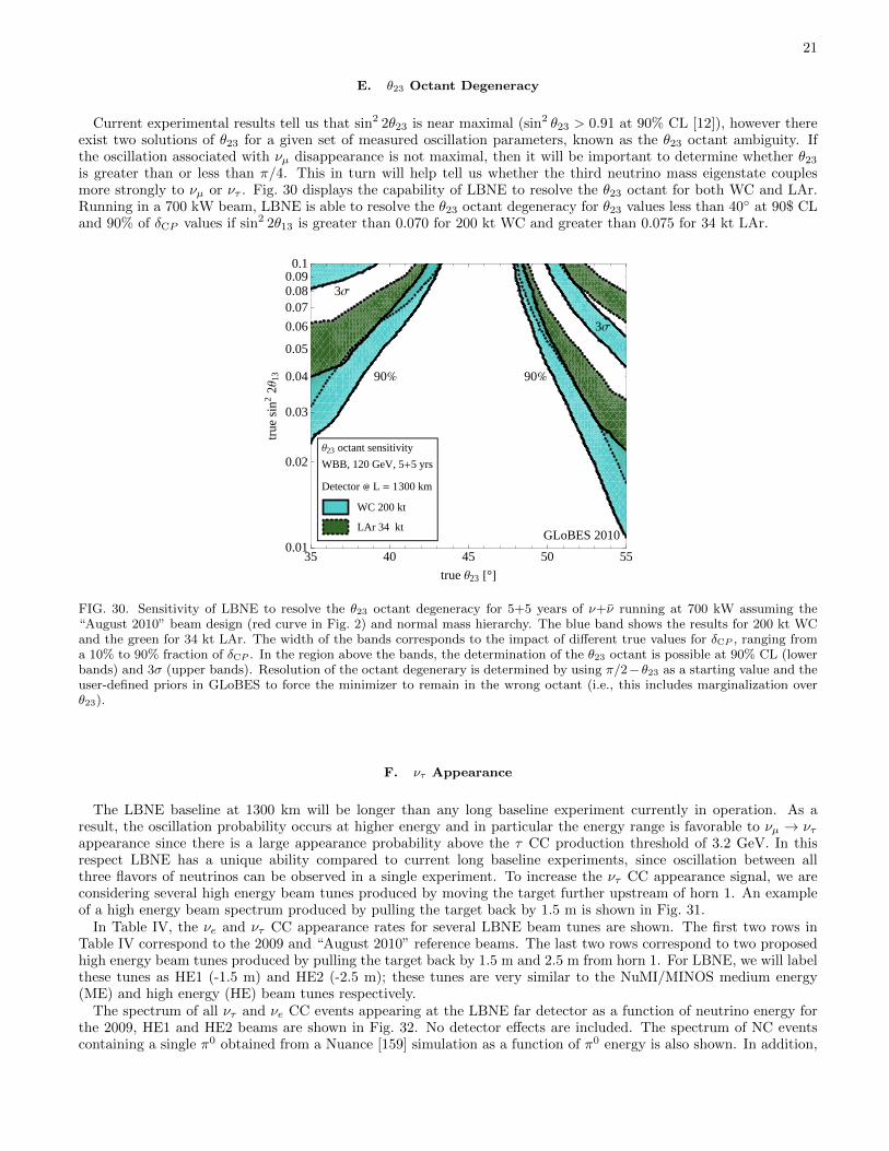
E. θ23 Octant Degeneracy

Current experimental results tell us that sin2 2θ23 is near maximal (sin2 θ23 > 0.91 at 90% CL [12]), however thereexist two solutions of θ23 for a given set of measured oscillation parameters, known as the θ23 octant ambiguity. Ifthe oscillation associated with νµ disappearance is not maximal, then it will be important to determine whether θ23

is greater than or less than π/4. This in turn will help tell us whether the third neutrino mass eigenstate couplesmore strongly to νµ or ντ . Fig. 30 displays the capability of LBNE to resolve the θ23 octant for both WC and LAr.Running in a 700 kW beam, LBNE is able to resolve the θ23 octant degeneracy for θ23 values less than 40 at 90$ CLand 90% of δCP values if sin2 2θ13 is greater than 0.070 for 200 kt WC and greater than 0.075 for 34 kt LAr.

35 40 45 50 550.01

0.02

0.03

0.04

0.05

0.06

0.070.080.090.1

trueΘ23 @°D

true

sin2

2Θ13

GLoBES 2010

Θ23 octant sensitivity

WBB, 120 GeV, 5+5 yrs

Detector L = 1300 km

WC 200 kt

LAr 34 kt

90% 90%

3Σ

3Σ

FIG. 30. Sensitivity of LBNE to resolve the θ23 octant degeneracy for 5+5 years of ν+ν running at 700 kW assuming the“August 2010” beam design (red curve in Fig. 2) and normal mass hierarchy. The blue band shows the results for 200 kt WCand the green for 34 kt LAr. The width of the bands corresponds to the impact of different true values for δCP , ranging froma 10% to 90% fraction of δCP . In the region above the bands, the determination of the θ23 octant is possible at 90% CL (lowerbands) and 3σ (upper bands). Resolution of the octant degenerary is determined by using π/2− θ23 as a starting value and theuser-defined priors in GLoBES to force the minimizer to remain in the wrong octant (i.e., this includes marginalization overθ23).

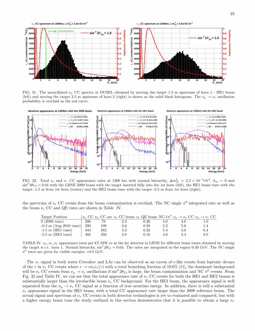
F. ντ Appearance

The LBNE baseline at 1300 km will be longer than any long baseline experiment currently in operation. As aresult, the oscillation probability occurs at higher energy and in particular the energy range is favorable to νµ → ντappearance since there is a large appearance probability above the τ CC production threshold of 3.2 GeV. In thisrespect LBNE has a unique ability compared to current long baseline experiments, since oscillation between allthree flavors of neutrinos can be observed in a single experiment. To increase the ντ CC appearance signal, we areconsidering several high energy beam tunes produced by moving the target further upstream of horn 1. An exampleof a high energy beam spectrum produced by pulling the target back by 1.5 m is shown in Fig. 31.

In Table IV, the νe and ντ CC appearance rates for several LBNE beam tunes are shown. The first two rows inTable IV correspond to the 2009 and “August 2010” reference beams. The last two rows correspond to two proposedhigh energy beam tunes produced by pulling the target back by 1.5 m and 2.5 m from horn 1. For LBNE, we will labelthese tunes as HE1 (-1.5 m) and HE2 (-2.5 m); these tunes are very similar to the NuMI/MINOS medium energy(ME) and high energy (HE) beam tunes respectively.

The spectrum of all ντ and νe CC events appearing at the LBNE far detector as a function of neutrino energy forthe 2009, HE1 and HE2 beams are shown in Fig. 32. No detector effects are included. The spectrum of NC eventscontaining a single π0 obtained from a Nuance [159] simulation as a function of π0 energy is also shown. In addition,

22

(GeV)νE 2 4 6 8 10 12 14 16 18 20

PO

T21

CC

evt

s/G

eV/1

00kT

/10

µ ν

0

1000

2000

3000

4000

5000

6000

7000

8000

9000

10000


App

eara

nce

Pro

babi

lity

0

0.1

0.2

0.3

0.4

0.5

0.6

0.7

0.8

0.9

1

= 1.023 θ 2 2sin productionτ

(GeV)νE 2 4 6 8 10 12 14 16 18 20

PO

T21

CC

evt

s/G

eV/1

00kT

/10

µ ν

0

1000

2000

3000

4000

5000

6000

7000

8000

9000

10000


App

eara

nce

Pro

babi

lity

0

0.1

0.2

0.3

0.4

0.5

0.6

0.7

0.8

0.9

1

= 1.023 θ 2 2sin

FIG. 31. The unoscillated νµ CC spectra at DUSEL obtained by moving the target 1.5 m upstream of horn 1 - HE1 beam(left) and moving the target 2.5 m upstream of horn 2 (right) is shown as the solid black histogram. The νµ → ντ oscillationprobability is overlaid as the red curve.

Energy (GeV)0 2 4 6 8 10 12 14 16 18 20

Eve

nts

(evt

/GeV

/MW

.1E

7s/k

Ton

)

−410

−310

−210

−110

1

10

NC (6.664,1.980)µ ν

CC (beam) (1.117,0.603)e ν

CC (2.027,1.921)e ν −> µ ν

CC (0.517,0.075)τ ν −> µ ν

Neutrino appearance at 1300km with the 2009 beam

Energy (GeV)0 2 4 6 8 10 12 14 16 18 20

Eve

nts

(evt

/GeV

/MW

.1E

7s/k

Ton

)

−410

−310

−210

−110

1

10

NC (7.836,2.731)µ ν

CC (beam) (1.625,0.353)e ν

CC (2.410,1.494)e ν −> µ ν

CC (3.174,0.391)τ ν −> µ ν

Neutrino appearance at 1300km with the HE1 beam

Energy (GeV)0 2 4 6 8 10 12 14 16 18 20

Eve

nts

(evt

/GeV

/MW

.1E

7s/k

Ton

)

−410

−310

−210

−110

1

10

NC (6.507,2.329)µ ν

CC (beam) (1.380,0.217)e ν

CC (1.729,0.892)e ν −> µ ν

CC (3.980,0.225)τ ν −> µ ν

Neutrino appearance at 1300km with the HE2 beam

FIG. 32. Total νe and ντ CC appearance rates at 1300 km with normal hierarchy, ∆m231 = 2.5 × 10−3eV2, δcp = 0 and

sin2 2θ13 = 0.04 with the LBNE 2009 beam with the target inserted fully into the 1st horn (left), the HE1 beam tune with thetarget -1.5 m from 1st horn (center) and the HE2 beam tune with the target -2.5 m from 1st horn (right).

the spectrum of νe CC events from the beam contamination is overlaid. The NC single π0 integrated rate as well asthe beam νe CC and QE rates are shown in Table IV.

Target Position νµ CC νµ CC osc νe CC beam νe QE beam NC-1π0 νµ → νe CC νµ → ντ CC0 (2009 tune) 206 78 2.2 0.26 4.0 4.0 1.0-0.3 m (Aug 2010 tune) 290 108 2.6 0.28 5.2 5.6 1.4-1.5 m (HE1 tune) 444 282 3.2 0.22 5.4 4.8 6.4-2.5 m (HE2 tune) 466 350 2.8 0.16 4.6 3.4 8.0

TABLE IV. νµ, ντ , νe appearance rates per kT.MW.yr at the far detector in LBNE for different beam tunes obtained by movingthe target w.r.t. horn 1. Normal hierarchy, sin2 2θ13 = 0.04. The rates are integrated in the region 0-20 GeV. The NC singleπ0 rates are given for visible energies >0.5 GeV.

The ντ signal in both water Cerenkov and LAr can be observed as an excess of e-like events from leptonic decaysof the τ in ντ CC events where τ → eνeντ (γ) with a total branching fraction of 19.6% [11], the dominant backgroundwill be νe CC events from νµ → νe oscillations if sin2 2θ13 is large, the beam contamination and NC π0 events. FromFig. 32 and Table IV, we can see that the total appearance rate of ντ CC events for both the HE1 and HE2 beams issubstantially larger than the irreducible beam νe CC background. For the HE2 beam, the appearance signal is wellseparated from the νµ → νe CC signal as a function of true neutrino energy. In addition, there is still a substantialνe appearance signal in the HE1 beam, with a total CC appearance rate larger than the 2009 reference beam. Theactual signal and spectrum of ντ CC events in both detector technologies is yet to evaluated and compared, but witha higher energy beam tune the study outlined in this section demonstrates that it is possible to obtain a large ντ

23

appearance signal rate, while also maintaining a significant portion of the νe appearance signal.

G. New Physics Searches in LBNE

In addition to precision measurements of the standard three-flavor neutrino oscillation parameters, LBNE is alsowell-suited for new physics searches in the neutrino sector. For example, the experiment is sensitive to non-standardneutrino interactions and active-sterile neutrino mixing, provided that these effects are not too weak. To illustratethe potential of new physics searches, we will here focus on non-standard interactions (NSI).

Theories beyond the Standard Model can induce Lagrangian operators that couple neutrinos to normal matter innon-standard ways. In the low-energy effective theory relevant to neutrino oscillation experiments, these non-standardinteractions manifest themselves as 4-fermion operators, either of the charged-current (CC) type (e.g. [ναγ

ρ`β ] [qγρq],where `β is a charged lepton) or of the NC type (e.g. [ναγ

ρνβ ] [qq]). Most (but not all) CC NSI are most easily seen in anear detector, while NC NSI can be understood as non-standard matter effects that are visible only in a far detector ata sufficiently long baseline. This is where LBNE has a unique advantage compared to other long-baseline experiments(except atmospheric neutrino experiments, which are, however, limited by systematic effects). Therefore, and becausethere is no near detector definition for LBNE yet, we will here focus on NC NSI. They can be parameterized as newcontributions to the MSW matrix in the neutrino propagation Hamiltonian:

H = U

0∆m2

21/2E∆m2

31/2E

U† + VMSW , (1)

with

VMSW =√

2GFNe

1 + εmee εmeµ εmeτεm∗eµ εmµµ εmµτεm∗eτ εm∗µτ εmττ

. (2)

Here, U is the leptonic mixing matrix, and the ε-parameters give the magnitude of the NSI relative to standard weakinteractions. For new physics scales of few × 100 GeV, we expect |ε| . 0.01. Model-independent bounds on NSI aretypically of order 0.01–1 [18–20]. However, in many concrete models, neutrino NSI are related to non-standard effectsin the charged lepton sector, which are much more strongly constrained [21, 22]. Thus, one could take the point ofview that NSI large enough to be experimentally accessible in the foreseeable future are disfavored by theoreticalarguments. On the other hand, since theoretical prejudices about the properties of neutrinos have been wrong in thepast, once can also adopt the standpoint that our inability to construct a simple model featuring large NSI does notnecessarily mean they cannot exist. Also, NSI provide one explanation [23–25] for the interesting recent observationsby the MINOS [12] and MiniBooNE [26] collaborations that could point to a new source of CP violation, but are notsignificant enough yet to draw any firm conclusions.

To assess the sensitivity of LBNE to NC NSI, we define the NSI discovery reach in the following way: We simulatethe expected event spectra, assuming given “true” values for the NSI parameters, and then attempt a fit assumingno NSI. If the fit is incompatible with the simulated data at a given confidence level, we say that the chosen “true”values of the NSI parameters are within the experimental discovery reach. In Fig. 33, we show the NSI discoveryreach of LBNE for the case where only one of the εmαβ parameters is non-negligible at a time.

We conclude from the figure that LBNE will be able to improve model-independent bounds on NSI in the e–µsector by a factor of two, and in the e–τ sectors by an order of magnitude. Bounds on non-standard effects in theµ–τ sector are already quite strong because of the sensitivity of atmospheric neutrino experiments, but LBNE maybe able to improve also some of the bounds in this sector, and in any case, LBNE bounds will be more robust thanthe ones derived from atmospheric neutrino oscillations. In particular, it has been shown in [27] that atmosphericneutrino bounds can become significantly weaker if the possibility of several NSI being non-zero is taken into account.Since LBNE provides a precise measurement of both the νe appearance and νµ disappearance channels and can beoperated in neutrino and antineutrino mode, we expect it to be more robust with respect to these correlations.

The sensitivity of LBNE to non-unitarity effects in the leptonic mixing matrix (which can be recast into a special caseof non-standard interactions) (see e.g. [21]) is not expected to be competitive with existing limits, which are alreadyof order 10−3. Searches for short-baseline oscillations into sterile neutrinos, on the other hand, would certainly be aworthwhile effort at a near detector. While near detector searches for oscillations between νe and νµ will be limitedby systematic uncertainties in our knowledge of the beam spectrum and flavor composition, oscillations into ντ wouldprovide a very clean signature. However, this would require the construction of a dedicated near detector that is ableto identify ντ . It remains to be seen by how much such a detector could improve existing bounds from the NOMADexperiment [28].

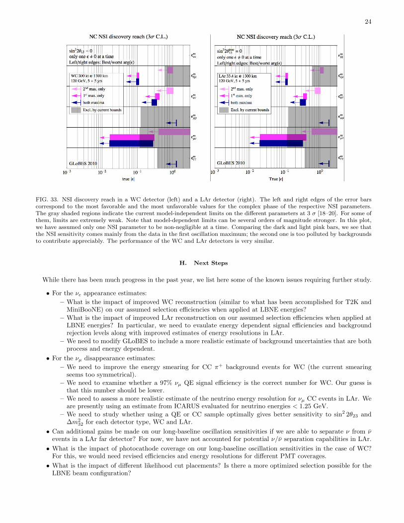
24

FIG. 33. NSI discovery reach in a WC detector (left) and a LAr detector (right). The left and right edges of the error barscorrespond to the most favorable and the most unfavorable values for the complex phase of the respective NSI parameters.The gray shaded regions indicate the current model-independent limits on the different parameters at 3 σ [18–20]. For some ofthem, limits are extremely weak. Note that model-dependent limits can be several orders of magnitude stronger. In this plot,we have assumed only one NSI parameter to be non-negligible at a time. Comparing the dark and light pink bars, we see thatthe NSI sensitivity comes mainly from the data in the first oscillation maximum; the second one is too polluted by backgroundsto contribute appreciably. The performance of the WC and LAr detectors is very similar.

H. Next Steps

While there has been much progress in the past year, we list here some of the known issues requiring further study.

• For the νe appearance estimates:

– What is the impact of improved WC reconstruction (similar to what has been accomplished for T2K andMiniBooNE) on our assumed selection efficiencies when applied at LBNE energies?

– What is the impact of improved LAr reconstruction on our assumed selection efficiencies when applied atLBNE energies? In particular, we need to evaulate energy dependent signal efficiencies and backgroundrejection levels along with improved estimates of energy resolutions in LAr.

– We need to modify GLoBES to include a more realistic estimate of background uncertainties that are bothprocess and energy dependent.

• For the νµ disappearance estimates:

– We need to improve the energy smearing for CC π+ background events for WC (the current smearingseems too symmetrical).

– We need to examine whether a 97% νµ QE signal efficiency is the correct number for WC. Our guess isthat this number should be lower.

– We need to assess a more realistic estimate of the neutrino energy resolution for νµ CC events in LAr. Weare presently using an estimate from ICARUS evaluated for neutrino energies < 1.25 GeV.

– We need to study whether using a QE or CC sample optimally gives better sensitivity to sin2 2θ23 and∆m2

32 for each detector type, WC and LAr.

• Can additional gains be made on our long-baseline oscillation sensitivities if we are able to separate ν from νevents in a LAr far detector? For now, we have not accounted for potential ν/ν separation capabilities in LAr.

• What is the impact of photocathode coverage on our long-baseline oscillation sensitivities in the case of WC?For this, we would need revised efficiencies and energy resolutions for different PMT coverages.

• What is the impact of different likelihood cut placements? Is there a more optimized selection possible for theLBNE beam configuration?

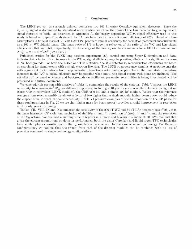
25

I. Conclusions

The LBNE project, as currently defined, comprises two 100 kt water Cerenkov-equivalent detectors. Since theνµ → νe signal is dominated by statistical uncertainties, we chose the mass of the LAr detector to give equivalentsignal statistics in both. As described in Appendix A, the energy dependent WC νe signal efficiency used in thisstudy is based on Super-K analysis and for LAr we have used a constant signal efficiency of 85%. Based on theseassumptions, a fiducial mass of ∼ 17 kt LAr TPC produces similar sensitivity for oscillation parameter measurementsas a 100 kt WC fiducial mass. The mass ratio of 1/6 is largely a reflection of the ratio of the WC and LAr signalefficiencies (15% and 85%, respectively) at the energy of the first νµ oscillation maxima for a 1300 km baseline and

∆m231 = 2.5× 10−3eV2 (∼2.4 GeV).

Published studies for the T2KK long baseline experiment [29], carried out using Super-K simulation and data,indicate that a factor of two increase in the WC νe signal efficiency may be possible, albeit with a significant increasein NC backgrounds. For both the LBNE and T2KK studies, the WC detector νe reconstruction efficiencies are basedon searching for signal events with a single electron like ring. The LBNE νe appearance signal is at neutrino energieswith significant contributions from deep inelastic interactions with multiple particles in the final state. So futureincreases in the WC νe signal efficiency may be possible when multi-ring signal events with pions are included. Thenet effect of increased efficiency and backgrounds on oscillation parameter sensitivities is being investigated will bepresented in a future document.

We conclude this section with a series of tables to summarize the results of the chapter. Table V shows the LBNEsensitivity to non-zero sin2 2θ13 for different exposures, including a 10 year operation of the reference configuration(three ‘100-kt equivalent’ LBNE modules), the CDR ‘200 kt,’ and a single ‘100 kt’ module. We see that the referenceconfigurations reach a sensitivity almost a factor of two higher than a single module; higher beam power would reducethe elapsed time to reach the same sensitivity. Table VI provides examples of the 1σ resolution on the CP phase forthese configurations; in Fig. 20 we see that higher mass (or beam power) provides a rapid improvement in resolutionin the early years of running.

Tables VII, VIII, IX and X summarize the sensitivity of the 200 kT WC and 34 kT LAr detectors to sin2 2θ13 6= 0,the mass hierarchy, CP violation, resolution of sin2 2θ23 (ν and ν), resolution of ∆m2

32 (ν and ν), and the resolutionof the θ23 octant. We assumed a running time of 5 years in ν mode and 5 years in ν mode at 700 kW. We find thatgiven the current assumptions on detector performance, both the water Cerenkov and liquid argon TPC technologieshave similar physics sensitivities to the νµ oscillation parameters. In the case of mixed technology Far Detectorconfigurations, we assume that the results from each of the detector modules can be combined with no loss ofprecision compared to single technology configurations.

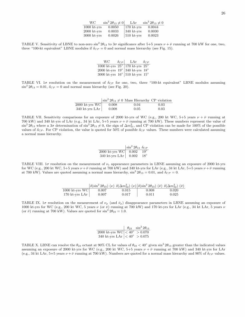
26

WC sin2 2θ13 6= 0 LAr sin2 2θ13 6= 01000 kt-yrs 0.0050 170 kt-yrs 0.00442000 kt-yrs 0.0033 340 kt-yrs 0.00303000 kt-yrs 0.0026 510 kt-yrs 0.0023

TABLE V. Sensitivity of LBNE to non-zero sin2 2θ13 to 3σ significance after 5+5 years ν + ν running at 700 kW for one, two,three “100-kt equivalent” LBNE modules if δCP = 0 and normal mass hierarchy (see Fig. 15).

WC δCP LAr δCP1000 kt-yrs 25 170 kt-yrs 25

2000 kt-yrs 19 340 kt-yrs 18

3000 kt-yrs 16 510 kt-yrs 15

TABLE VI. 1σ resolution on the measurement of δCP for one, two, three “100-kt equivalent” LBNE modules assumingsin2 2θ13 = 0.01, δCP = 0 and normal mass hierarchy (see Fig. 20).

sin2 2θ13 6= 0 Mass Hierarchy CP violation2000 kt-yrs WC 0.008 0.04 0.03340 kt-yrs LAr 0.008 0.05 0.03

TABLE VII. Sensitivity comparisons for an exposure of 2000 kt-yrs of WC (e.g., 200 kt WC, 5+5 years ν + ν running at700 kW) and 340 kt-yrs of LAr (e.g., 34 kt LAr, 5+5 years ν + ν running at 700 kW). These numbers represent the value ofsin2 2θ13 where a 3σ determination of sin2 2θ13 6= 0, the sign of ∆m2

31, and CP violation can be made for 100% of the possiblevalues of δCP . For CP violation, the value is quoted for 50% of possible δCP values. These numbers were calculated assuminga normal mass hierarchy.

sin2 2θ13 δCP2000 kt-yrs WC 0.002 19

340 kt-yrs LAr 0.002 18

TABLE VIII. 1σ resolution on the measurement of νe appearance parameters in LBNE assuming an exposure of 2000 kt-yrsfor WC (e.g., 200 kt WC, 5+5 years ν+ ν running at 700 kW) and 340 kt-yrs for LAr (e.g., 34 kt LAr, 5+5 years ν+ ν runningat 700 kW). Values are quoted assuming a normal mass hierarchy, sin2 2θ13 = 0.01, and δCP = 0.

δ(sin2 2θ23) (ν) δ(∆m232) (ν) δ(sin2 2θ23) (ν) δ(∆m2

32) (ν)1000 kt-yrs WC 0.007 0.015 0.008 0.020170 kt-yrs LAr 0.007 0.017 0.011 0.025

TABLE IX. 1σ resolution on the measurement of νµ (and νµ) disappearance parameters in LBNE assuming an exposure of1000 kt-yrs for WC (e.g., 200 kt WC, 5 years ν (or ν) running at 700 kW) and 170 kt-yrs for LAr (e.g., 34 kt LAr, 5 years ν(or ν) running at 700 kW). Values are quoted for sin2 2θ23 = 1.0.

θ23 sin2 2θ13

2000 kt-yrs WC < 40 > 0.070340 kt-yrs LAr < 40 > 0.075

TABLE X. LBNE can resolve the θ23 octant at 90% CL for values of θ23 < 40 given sin2 2θ13 greater than the indicated valuesassuming an exposure of 2000 kt-yrs for WC (e.g., 200 kt WC, 5+5 years ν + ν running at 700 kW) and 340 kt-yrs for LAr(e.g., 34 kt LAr, 5+5 years ν+ ν running at 700 kW). Numbers are quoted for a normal mass hierarchy and 90% of δCP values.

27

IV. PROTON DECAY

Proton decay, bound neutron decay, and similar processes such as dinucleon decay and neutron-antineutron oscilla-tion test the apparent but unexplained conservation law of baryon number. These decays are already known to be rarebased on decades of prior searches, all of which have been negative. If measurable event rates or even single candidateevents are found, one immediately concludes that they must have proceeded via unknown virtual processes based onphysics beyond the standard model. The impact of demonstrating the existence of a baryon number violating processwould be profound.

The class of theories known as Grand Unified Theories (GUTs) make predictions about baryon number violation andthe life of the proton that may be within reach of the LBNE detectors. Early GUTs were the original motivation forputting kiloton-scale detectors underground. The 22.5 kiloton Super-Kamiokande experiment extended the search forproton decay by more than an order of magnitude. Although there has been no sign of proton decay, the strict limitsfrom these experiments constrain the construction of contemporary GUTs and indeed, a tension between experimentand theory is now commonly discussed. It is very natural to continue the search with 100-kiloton-scale detectors.

A. Motivation and Scientific Impact of Future Measurements

The grand unified theoretical motivation for the study of proton decay has a long and distinguished history [30–32],and has been reviewed many times [33–35]. Contemporary reviews [36–38] discuss the strict limits already set bySuper-Kamiokande and the context of proposed multi-100-kiloton scale experiments such as Hyper-Kamiokande andLBNE. Here are some of the key points related to scientific impact:

• Conservation of baryon number is unexplained, corresponding to no known long-range force.

• Baryon number non-conservation has cosmological consequences, such as a role in inflation and the baryonasymmetry of the universe.

• Proton decay is predicted by a wide range of GUTs.

• Grand unified theories are also often able to accommodate massive neutrinos with characteristics as discoveredover the last decade.

• GUTs incorporate other unexplained features of the standard model such as the relationship of quark and leptonelectric charges.

• The unification scale is suggested experimentally and theoretically by the apparent convergence of the runningcoupling constants of the Standard Model. It is in excess of 1015 GeV.

• The unification scale is not accessible by any accelerator experiment, and can only be probed by virtual processessuch a proton decay.

• GUTs usually predict the relative branching fractions of different nucleon decay modes, requiring of course asizeable sample of proton decay events to test.

• The dominant proton decay mode is often sufficient to roughly identify the likely characteristics of the GUT,such as gauge mediation or the involvement of supersymmetry.

In summary, the observation of even a single unambiguous proton decay event would signal that the ideas of grandunification are correct and would give guidance as to which models most likely describe the universe. One or twoevents would also give guidance to what even larger size detector would be needed to explore the physics in moredetail.

From the body of literature, two decay modes emerge that dominate our experimental design. First, there is thedecay mode of p→ e+π0 that arises from gauge mediation. This is the most famous proton decay mode, often predictedto have the highest branching fraction, and also demonstrably the most straightforward experimental signature for awater Cherenkov detector. The total mass of the proton is converted into the electromagnetic shower energy of thepositron and the two photons from π0 decay, with a net momentum vector near zero.

The second key mode is p→ K+ν. This mode is dominant in most supersymmetric-GUTs, which also often favorseveral other modes involving kaons in the final state. The decay mode with a charged kaon is notable because itpresents the unique opportunity for a liquid argon TPC to detect it with extremely high efficiency. This is because

28

1032

1033

1034

Soudan Frejus Kamiokande IMB

τ/B (years)

Super-K I+II+III

1035

1031

p → e + π0

p → ν K +

p → μ+ K 0

p → e + K 0

n → ν K 0

minimal SU(5) minimal SUSY SU(5)p → e + π0 predictions

flipped SU(5), SO(10), 5D SUSY SU(5)

minimal SUSY SU(5) SUGRA SU(5)

SUSY SU(5) with additional U(1) flavor symmetry

various SUSY SO(10)

SUSY SO(10) with G(224)

p → ν K +

predictions

2 31

2 31

SUSY SO(10) with Unified Higgs

FIG. 34. Proton decay lifetime limits compared to lifetime ranges predicted by Grand Unified Theories. The upper section isfor p→ e+π0, most commonly caused by gauge mediation. The lower section is for SUSY motivated models, which commonlypredict decay modes with kaons in the final state. The marker symbols indicate published limits by experiments, as indicatedby the sequence and colors on top of the figure.

the momentum of the kaon will result in high ionization density which can be compared to the range of the kaon, notto mention the unique final states of K+ decay that should be fully reconstructed.

There are a number of other proton decay channels to consider, but they will not influence the design of a next-generation experiment beyond the above decay modes. There are 27 allowed modes of proton or bound neutroninto anti-lepton plus meson (conserving B − L). The most stringent limits besides p → e+π0 include p → µ+π0

and p → e+η, both of which must have partial lifetimes greater than 4 × 1033 years. Any experiment that will dowell for e+π0 will do well for these decay modes. The decay p → νπ+ or n → νπ0 may have large theoreticallypredicted branching fractions but are experimentally difficult due to sizeable backgrounds from atmospheric neutrinointeractions. The decay p→ µ+K0 is detected relatively efficiently by either water Cherenkov or LAr TPC detectors.There are a number of other possibilities such as modes that conserve B +L, or violate only baryon number, or thatdecay into only leptons. These possibilities are less well-motivated theoretically, as they do not appear as frequently inthe literature. In any case, they can be accommodated with equal ease or difficulty by the large detectors consideredhere.

Fig. 34 shows experimental limits, dominated by recent results from Super-Kamiokande, compared to the rangesof lifetimes predicted by an assortment of GUTs. At this time, the theory literature does not attempt to preciselypredict lifetimes, concentrating instead on suggesting the dominant decay modes and relative branching fractions.The uncertainty in the lifetime predictions come from details of the theory, such as unknown heavy particles massesand coupling constants, as well as poorly known details of matrix elements for quarks within the nucleon.

It is apparent from this figure that a continued search for proton decay is by no means assured of success. In additionto the lifetime ranges shown, there are models that predict essentially no proton decay or lifetimes out of reach of likelyexperiments. With that caveat, an experiment with sensitivity between 1033 and 1035 years is searching in the rightterritory over a wide range of GUTs and even if no proton decay is detected, the stringent lifetime limits will restrictefforts to build such theories. Minimal SU(5) was ruled out by the early work of IMB and Kamiokande; minimalSUSY SU(5) is considered to be ruled out by Super-Kamiokande. In most cases, another order of magnitude in limitwill not rule out specific theories, but will constrain their allowed parameters, perhaps leading to the conclusion thatsome are fine-tuned.

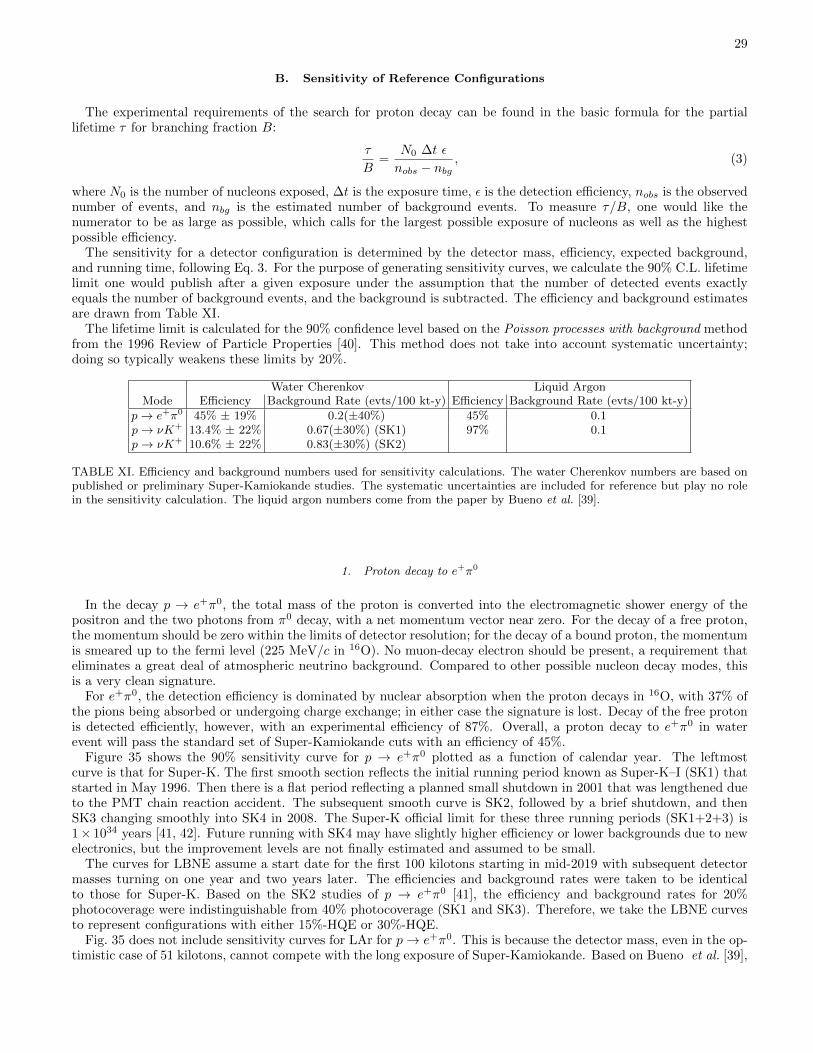
29

B. Sensitivity of Reference Configurations

The experimental requirements of the search for proton decay can be found in the basic formula for the partiallifetime τ for branching fraction B:

τ

B=

N0 ∆t ε

nobs − nbg, (3)

where N0 is the number of nucleons exposed, ∆t is the exposure time, ε is the detection efficiency, nobs is the observednumber of events, and nbg is the estimated number of background events. To measure τ/B, one would like thenumerator to be as large as possible, which calls for the largest possible exposure of nucleons as well as the highestpossible efficiency.

The sensitivity for a detector configuration is determined by the detector mass, efficiency, expected background,and running time, following Eq. 3. For the purpose of generating sensitivity curves, we calculate the 90% C.L. lifetimelimit one would publish after a given exposure under the assumption that the number of detected events exactlyequals the number of background events, and the background is subtracted. The efficiency and background estimatesare drawn from Table XI.

The lifetime limit is calculated for the 90% confidence level based on the Poisson processes with background methodfrom the 1996 Review of Particle Properties [40]. This method does not take into account systematic uncertainty;doing so typically weakens these limits by 20%.

Water Cherenkov Liquid ArgonMode Efficiency Background Rate (evts/100 kt-y) Efficiency Background Rate (evts/100 kt-y)

p→ e+π0 45% ± 19% 0.2(±40%) 45% 0.1p→ νK+ 13.4% ± 22% 0.67(±30%) (SK1) 97% 0.1p→ νK+ 10.6% ± 22% 0.83(±30%) (SK2)

TABLE XI. Efficiency and background numbers used for sensitivity calculations. The water Cherenkov numbers are based onpublished or preliminary Super-Kamiokande studies. The systematic uncertainties are included for reference but play no rolein the sensitivity calculation. The liquid argon numbers come from the paper by Bueno et al. [39].

1. Proton decay to e+π0

In the decay p → e+π0, the total mass of the proton is converted into the electromagnetic shower energy of thepositron and the two photons from π0 decay, with a net momentum vector near zero. For the decay of a free proton,the momentum should be zero within the limits of detector resolution; for the decay of a bound proton, the momentumis smeared up to the fermi level (225 MeV/c in 16O). No muon-decay electron should be present, a requirement thateliminates a great deal of atmospheric neutrino background. Compared to other possible nucleon decay modes, thisis a very clean signature.

For e+π0, the detection efficiency is dominated by nuclear absorption when the proton decays in 16O, with 37% ofthe pions being absorbed or undergoing charge exchange; in either case the signature is lost. Decay of the free protonis detected efficiently, however, with an experimental efficiency of 87%. Overall, a proton decay to e+π0 in waterevent will pass the standard set of Super-Kamiokande cuts with an efficiency of 45%.

Figure 35 shows the 90% sensitivity curve for p → e+π0 plotted as a function of calendar year. The leftmostcurve is that for Super-K. The first smooth section reflects the initial running period known as Super-K–I (SK1) thatstarted in May 1996. Then there is a flat period reflecting a planned small shutdown in 2001 that was lengthened dueto the PMT chain reaction accident. The subsequent smooth curve is SK2, followed by a brief shutdown, and thenSK3 changing smoothly into SK4 in 2008. The Super-K official limit for these three running periods (SK1+2+3) is1× 1034 years [41, 42]. Future running with SK4 may have slightly higher efficiency or lower backgrounds due to newelectronics, but the improvement levels are not finally estimated and assumed to be small.

The curves for LBNE assume a start date for the first 100 kilotons starting in mid-2019 with subsequent detectormasses turning on one year and two years later. The efficiencies and background rates were taken to be identicalto those for Super-K. Based on the SK2 studies of p → e+π0 [41], the efficiency and background rates for 20%photocoverage were indistinguishable from 40% photocoverage (SK1 and SK3). Therefore, we take the LBNE curvesto represent configurations with either 15%-HQE or 30%-HQE.

Fig. 35 does not include sensitivity curves for LAr for p→ e+π0. This is because the detector mass, even in the op-timistic case of 51 kilotons, cannot compete with the long exposure of Super-Kamiokande. Based on Bueno et al. [39],

30

Year

Life

time

Sen

sitiv

ity (

90%

CL)

10 32

10 33

10 34

10 35

1995 2000 2005 2010 2015 2020 2025 2030 2035 2040

Super-K

WC100

WC300

WC200

FIG. 35. Proton decay lifetime limit for p → e+π0 as a function of time for Super-Kamiokande compared to 300 kt of waterCherenkov detector starting in 2019. The water Cherenkov detector is assumed to commission 100 kt each year for the firstthree years; the limits from the partial detector masses of 100 kt or 200 kt is indicated with dashed lines. All limits use thesame detection efficiency of 45% and background rate of 0.2 events/100 kt-years; systematic uncertainties are not included.The limits are at the 90% C.L., calculated for a poisson process including background assuming the detected events equals theexpected background.

an efficiency of 45% with a background rate of 0.1 events per 100 kt-years results in a background subtracted limit atthe 90% CL of 2.6× 1034 years for a 500 kt-year exposure. So a ten year run starting in 2020 of a 51 kt LAr detectordoes not exceed the projected Super-K limit of 3 × 1034 in 2030. Although there is no reason not to search for thismode if such a detector is built, we do not consider e+π0 to be a critical physics topic for a 51 kt or smaller liquidargon detector.

Hybrid configurations can be roughly appreciated from the 100, 200, and 300 kt water Cherenkov curves. Forexample, configurations 5 or 6, 100 kt WC plus 34 kt LAr will lie between the WC100 and WC200 lines in Fig. 35.

After 10 years, a 300 kt water Cherenkov detector would have an expected background of 6 events given ourassumed background rate. This has a significant impact on the 90% C.L. limit we would set, or conversely, the abilityto identify one or two candidate events in such an exposure. It is possible that atmospheric neutrino backgroundscould be reduced in a detector with gadolinium such that it can detect coincident neutron capture. This assumes that(a) proton decay does not eject neutrons from a 16O nucleus and (b) atmospheric neutrino interactions are frequentlyaccompanied by primary or secondary neutrons. If the background rate could be convincingly reduced by a factorof two, from 0.2 events to 0.1 events per 100 kt-years, then a 10-year exposure would set a limit of 1.0 × 1035 yearsinstead of 0.8× 1035 years.

2. Proton decay to νK+

Fig. 36 shows the 90% sensitivity curve for p→ νK+ plotted as a function of calendar year. The leftmost curve isthat for Super-K as described above. The Super-K analysis is described in several publications [43, 44].

The Super-K analysis uses three methods: (i) gamma tag with K+ → µ+ν, (ii) K+ → π+π0, and (iii) a backgroundlimited search for a monoenergetic muon. For the purpose of the Super-K and LBNE water Cherenkov curves, only(i) and (ii) are used, because the the background limited search contributes very little for large exposures. The SK1analysis using methods (i) and (ii) has a relatively high background rate of 0.67 events per 100 kt-year. It is likelythat some re-optimization would benefit large exposures, but for the sake of argument, we assume the final sensitivitywould not change much, as the most likely alteration would be some loss in proton decay signal efficiency in exchange

31

Year

Life

time

Sen

sitiv

ity (

90%

CL)

10 32

10 33

10 34

10 35

1995 2000 2005 2010 2015 2020 2025 2030 2035 2040

Super-K

WC100

WC300

WC200

FIG. 36. Proton decay lifetime limit for p → νK+ as a function of time for Super-Kamiokande compared to 300 kt of waterCherenkov detector starting in 2019. The water Cherenkov detector is assumed to commission 100 kt each year for the firstthree years; the limits from the partial detector masses of 100 kt or 200 kt is indicated with dashed lines. The bold lines usethe efficiency and background numbers for the SK1 analysis; the thin lines use the efficiency and background numbers for theSK2 analysis. The limits are at the 90% C.L., calculated for a poisson process including background assuming the detectedevents equals the expected background.

for lower atmospheric neutrino background. It is also possible that the LBNE detector with smaller PMTs and bettertiming could result in a sharper set of cuts to find the gamma ray tag. In other words, there is some hope that awell-instrumented LBNE water cherenkov detector would perform slightly better than Super-K for p→ νK+, whichis not likely to be true for e+π0. But we have no estimates of this yet, so we conservatively use the SK efficienciesand backgrounds as our benchmark.

As seen in Table XI, the performance of the Super-K analysis is markedly worse for SK2 (20% photocoverage) thanSK1 (40% photocoverage). The efficiency is lower and the background rate is slightly higher. To study this difference,two sets of LBNE water Cherenkov curves are provided in Fig. 36, one set for each case.

Shown on Fig. 37 is the projected sensitivity for a liquid argon TPC of various masses. The efficiency and backgroundrates are taken from Bueno et al. [39]. The high efficiency for p→ νK+ is a classic strong point in favor of liquid argon.Such a proton decay event signature would be highly described by such a detector, with a unique range and ionizationlevel for the charged kaon. The charged kaon will decay at rest to fully reconstructible final states, for example, asubsequent muon with no other particle, indicating K+ → µ+ν (predominant, with 65% branching fraction) shouldhave a muon with momentum reconstructed at 236 MeV/c. Therefore a high efficiency in excess of 90%, with verylow background, is quite plausible.

The most serious background is cosmogenic neutral kaons undergoing charge exchange in the sensitive volume.These could result in the appearance of a charged kaon, mimicking proton decay if the K+ had just the rightmomentum (339 MeV/c). This background process could be effectively studied by measuring the rate of such eventsin momentum sidebands and close to the detector walls. In any case, a fiducial mass reduction is anticipated toeliminate such events, by cutting out candidates near the side walls. In the Bueno et al. paper [39], several differentoverburden and active veto scenarios were considered, with fiducial cuts as much as 6 meters from the wall, resultingin fiducial mass reductions ranging from 66% to 90%. For the sensitivity curves plotted in Fig. 37 we will take ageneric value of 70%. This corresponds to a 2 meter cut from the sidewalls of the planned LBNE detector, reducingthe volume from 14×15×71 meters3 to 14×11×67 meters3. At shallow depths, a key detector element required toallow even this fiducial restriction is some sort of active muon tracking veto that extends wider than the LAr detectoritself. This is used to track nearby cosmic ray muons that could produce neutral kaons or neutrons. Whether sucha veto could be constructed with ease and reasonable cost at either the 300-ft level or 800-ft level is unknown, and

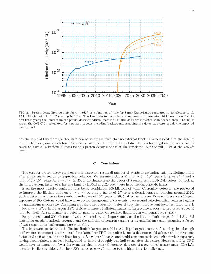
32

Year

Life

time

Sen

sitiv

ity (

90%

CL)

10 32

10 33

10 34

10 35

1995 2000 2005 2010 2015 2020 2025 2030 2035 2040

Super-K

LAr28

LAr14

LAr42

FIG. 37. Proton decay lifetime limit for p→ νK+ as a function of time for Super-Kamiokande compared to 60 kilotons total,42 kt fiducial, of LAr TPC starting in 2019. The LAr detector modules are assumed to commission 20 kt each year for thefirst three years; the limits from the partial detector fiducial masses of 14 and 28 kt are indicated with dashed lines. The limitsare at the 90% C.L., calculated for a poisson process including background assuming the detected events equals the expectedbackground.

not the topic of this report, although it can be safely assumed that no external tracking veto is needed at the 4850-ftlevel. Therefore, one 20-kiloton LAr module, assumed to have a 17 kt fiducial mass for long-baseline neutrinos, istaken to have a 14 kt fiducial mass for this proton decay mode if at shallow depth, but the full 17 kt at the 4850-ftlevel.

C. Conclusions

The case for proton decay rests on either discovering a small number of events or extending existing lifetime limitsafter an extensive search by Super-Kamiokande. We assume a Super-K limit of 3 × 1034 years for p → e+π0 and alimit of 6× 1033 years for p→ e+π0 in 2030. To characterize the power of a search using LBNE detectors, we look atthe improvement factor of a lifetime limit by LBNE in 2020 over these hypothetical Srper-K limits.

Even the most massive configurations being considered, 300 kilotons of water Cherenkov detector, are projectedto improve the lifetime limit on p → e+π0 by only a factor of 2.7 after a decade-long run starting around 2020.Such a detector will cross the symbolic milestone of 1035 years in 2035, after running for 15 years. Because a 10-yearexposure of 300 kilotons would have an expected background of six events, background rejection using neutron taggingvia gadolinium is desirable. Assuming a background reduction factor of two, the improvement factor is raised to 3.4.

For p→ e+π0, a liquid argon TPC of fiducial mass 42 kilotons makes no improvement over the projected Super-Klimit by itself. As supplementary detector mass to water Cherenkov, liquid argon will contribute slightly.

For p → νK+ and 300 kilotons of water Cherenkov, the improvement on the lifetime limit ranges from 1.8 to 3.3depending on photocathode coverage and the addition of neutron tagging using gadolinium (again assuming a factorof two reduction in background rate with Gd).

The improvement factor in the lifetime limit is largest for a 50 kt scale liquid argon detector. Assuming that the highperformance characteristics projected for a large LAr TPC are realized, such a detector could achieve an improvementfactor of 8 to 9 on the lifetime limit for p→ K+ν after 10 years and could continue to do well with further exposure,having accumulated a modest background estimate of roughly one-half event after that time. However, a LAr TPCwould have an impact on fewer decay modes than a water Cherenkov detector of a few times greater mass. The LArdetector is effective chiefly for the SUSY mode of p→ K+ν, due to the high detection efficiency.

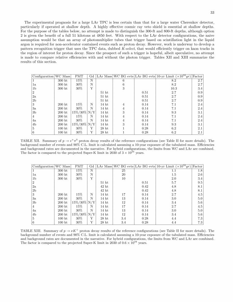
33

The experimental prognosis for a large LAr TPC is less certain than that for a large water Cherenkov detector,particularly if operated at shallow depth. A highly effective cosmic ray veto shield is essential at shallow depths.For the purpose of the tables below, no attempt is made to distinguish the 300-ft and 800-ft depths, although option2 is given the benefit of a full 51 kilotons at 4850 feet. With respect to the LAr detector configurations, the naiveassumption would be that an array of photomultiplier tubes that trigger based on scintillation light in the liquidargon is required for non-accelerator contained events such as proton decay. However, work is underway to develop apattern recognition trigger that uses the TPC data, dubbed K-select, that would efficiently trigger on kaon tracks inthe region of interest for proton decay. Since the prospect of such a trigger is hopeful, albeit speculative, no attemptis made to compare relative efficiencies with and without the photon trigger. Tables XII and XIII summarize theresults of this section.

Configuration WC Mass PMT Gd LAr Mass WC BG evts LAr BG evts 10-yr Limit (×1034yr) Factor1 300 kt 15% N 6 8.2 2.71a 300 kt 30% N 6 8.2 2.71b 300 kt 30% Y 3 10.3 3.42 51 kt 0.51 2.7 0.92a 51 kt 0.51 2.7 0.92b 51 kt 0.51 2.7 0.93 200 kt 15% N 14 kt 4 0.14 7.1 2.43a 200 kt 30% N 14 kt 4 0.14 7.1 2.43b 200 kt 15%/30% N/Y 14 kt 3 0.14 9.3 3.14 200 kt 15% N 14 kt 4 0.14 7.1 2.44a 200 kt 30% N 14 kt 4 0.14 7.1 2.44b 200 kt 15%/30% N/Y 14 kt 3 0.14 9.3 3.15 100 kt 30% Y 28 kt 1 0.28 6.2 2.16 100 kt 30% Y 28 kt 1 0.28 6.2 2.1

TABLE XII. Summary of p → e+π0 proton decay results of the reference configurations (see Table II for more details). Thebackground number of events and 90% C.L. limit is calculated assuming a 10-year exposure of the tabulated mass. Efficienciesand background rates are documented in the narrative. For hybrid configurations, the limits from WC and LAr are combined.The factor is compared to the projected Super-K limit in 2030 of 3× 1034 years.

Configuration WC Mass PMT Gd LAr Mass WC BG evts LAr BG evts 10-yr Limit (×1034yr) Factor1 300 kt 15% N 25 1.1 1.81a 300 kt 30% N 20 1.5 2.61b 300 kt 30% Y 10 2.0 3.42 51 kt 0.51 5.7 9.52a 42 kt 0.42 4.8 8.12b 42 kt 0.42 4.8 8.13 200 kt 15% N 14 kt 17 0.14 2.7 4.53a 200 kt 30% N 14 kt 13 0.14 3.0 5.03b 200 kt 15%/30% N/Y 14 kt 12 0.14 3.4 5.64 200 kt 15% N 14 kt 17 0.14 2.7 4.54a 200 kt 30% N 14 kt 13 0.14 3.0 5.04b 200 kt 15%/30% N/Y 14 kt 12 0.14 3.4 5.65 100 kt 30% Y 28 kt 3.4 0.28 4.4 7.36 100 kt 30% Y 28 kt 3.4 0.28 4.4 7.3

TABLE XIII. Summary of p→ νK+ proton decay results of the reference configurations (see Table II for more details). Thebackground number of events and 90% C.L. limit is calculated assuming a 10-year exposure of the tabulated mass. Efficienciesand background rates are documented in the narrative. For hybrid configurations, the limits from WC and LAr are combined.The factor is compared to the projected Super-K limit in 2030 of 0.6× 1034 years.

34

V. SUPERNOVA BURST PHYSICS


A nearby core collapse supernova will provide a wealth of information via its neutrino signal (see [45, 46] for reviews).The neutrinos are emitted in a burst of a few tens of seconds duration, with about half in the first second. Energiesare in the few tens of MeV range, and luminosity is divided roughly equally between flavors. The baseline model ofcore collapse was confirmed by the observation of 19 neutrino events in two water Cherenkov detectors for SN1987Ain the Large Magellanic Cloud, 55 kpc away [47, 48]. An observed high-statistics core collapse neutrino signal willshed light on a variety of physics and astrophysics topics.

Core collapses are rare events: the expected rate is 2-3 per century in the Milky Way. As for the Homestake andSuper-Kamiokande detectors, the large LBNE detector(s), once constructed, may operate for decades. On this timescale, there is a significant likelihood of a supernova exploding in our galaxy. In a 20-year run of an experiment,the probability of observing a collapse event is about 40%. The detection of the neutrino burst from such an eventwould dramatically expand the science reach of these detectors: from measuring the neutrino mass hierarchy and θ13

mixing angle, to observing the development of the explosion in the core of the star, to probing the equation of state ofmatter at nuclear densities, to constraining physics beyond the Standard Model. Each of these questions representsan important outstanding problem in modern physics, worthy of a separate, dedicated experiment. The possibility totarget them all at once is very attractive, especially since it may come only at incremental cost to the project. Theexpected harvest of physics is rich enough that is essential to prepare to collect as much information as possible whena burst happens.

In contrast to the SN1987A, for which a few dozen neutrinos were observed, the detectors currently on the drawingboard would register thousands or tens of thousands of interactions from the burst. The exact type of interactionsdepends on the detector technology: a water-Cherenkov detector would be primarily sensitive to the electron antineu-trinos, while a liquid argon detector has an excellent sensitivity to electron neutrinos. In each case, the high eventrates imply that it should be possible to measure not only the time-integrated spectra, but also their second-by-secondevolution. This is the key reason behind the impressive physics potential of the planned detectors.

The interest in observationally establishing the supernova explosion mechanism comes from the key role supernovaexplosions play in the history of the universe. In fact, it would not be an exaggeration to say that the ancientsupernovae have in a very large measure shaped our world. For example, modern simulations of galaxy formationcannot reproduce the structure of our galactic disk without taking the supernova feedback into account. Shock wavesfrom ancient supernovae triggered further rounds of star formation. The iron in our blood was once synthesized insidea massive star and ejected in a supernova explosion.

For over half a century, researchers have been grappling to understand the physics of the explosion. The challengeof reconstructing the explosion mechanism from the light curves and the structure of the remnants is akin to recon-structing the cause of a plane crash from a debris field, without a black box. In fact, the supernova neutrinos are justlike a black box: they record the information about the physical processes in the center of the explosion during thefirst several seconds, as it happens.

The explosion mechanism is thought to have three distinct stages: the collapse of the iron core, with the formationof the shock and its breakout through the neutrinosphere; the accretion phase, in which the shock temporarily stalls atthe radius of about 200 km, while the material keeps raining in; and the cooling stage, in which the hot proto-neutronstar loses its energy and trapped lepton number, while the reenergized shock expands to push out the rest of the star.All these stages are predicted to have distinct signatures in the neutrino signal. Thus, it should be possible to directlyobserve, for example, how long the shock is stalled. More exotic features of the collapse may be observable in theneutrino flux as well, such as possible transitions to quark matter or to a black hole. (An observation in conjunctionwith a gravitational wave detection would be especially interesting.)

To correctly interpret the neutrino signal, one needs to take into account neutrino flavor oscillations. Over the lastdecades, the oscillations have been firmly established in solar neutrinos and a variety of terrestrial sources, whichmeans that including them in the supernova case is no longer optional. As it turns out, however, the physics of theoscillations in the supernova environment is much richer than in any of the cases measured to date. Neutrinos travelthrough the changing profile of the explosion, with stochastic density fluctuations behind the expanding shock. Theirflavor states are also coupled due to their coherent scattering off each other: “collective” neutrino effects may bedramatic. The net result is a problem that requires supercomputers, as well as state-of-the-art analytical models, tounderstand.

The effort to understand this complicated evolution has its reward: the oscillation patterns come out very differentlyfor the normal and inverted mass hierarchies. There are also several smoking gun signatures one can look for: forexample, the expanding shock and turbulence leave a unique imprint in the neutrino signal. The supernova signal alsohas a very high sensitivity to values of θ13, down to the levels inaccessible in any laboratory experiment. Additional

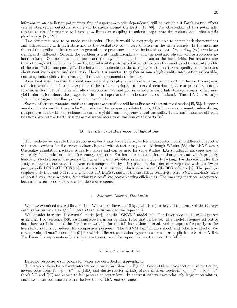
35

information on oscillation parameters, free of supernova model-dependence, will be available if Earth matter effectscan be observed in detectors at different locations around the Earth [49, 50]. The observation of this potentiallycopious source of neutrinos will also allow limits on coupling to axions, large extra dimensions, and other exoticphysics (e.g. [51, 52]).

Two comments need to be made at this point. First, it would be extremely valuable to detect both the neutrinosand antineutrinos with high statistics, as the oscillations occur very different in the two channels. In the neutrinochannel the oscillation features are in general more pronounced, since the initial spectra of νe and νµ (ντ ) are alwayssignificantly different. Second, the problem is truly multidisciplinary and the neutrino physics and astrophysics gohand-in-hand. One needs to model both, and the payout one gets is simultaneous for both fields. For instance, onelearns the sign of the neutrino hierarchy, the value of θ13, the speed at which the shock expands, and the density profileof the star, “all in one package”. The better one understands the astrophysics, the better the quality of informationabout neutrino physics, and vice versa. Hence it is essential to gather as much high-quality information as possible,and to optimize ability to disentangle the flavor components of the flux.

As a final note, because the neutrinos emerge promptly after core collapse, in contrast to the electromagneticradiation which must beat its way out of the stellar envelope, an observed neutrino signal can provide a promptsupernova alert [53, 54]. This will allow astronomers to find the supernova in early light turn-on stages, which mayyield information about the progenitor (in turn important for understanding oscillations). The LBNE detector(s)should be designed to allow prompt alert capability.

Several other experiments sensitive to supernova neutrinos will be online over the next few decades [45, 55]. Howeverone should not consider these to be “competition” for a supernova detection by LBNE: more experiments online duringa supernova burst will only enhance the science yield from a supernova, and the ability to measure fluxes at differentlocations around the Earth will make the whole more than the sum of the parts [49].


The predicted event rate from a supernova burst may be calculated by folding expected neutrino differential spectrawith cross sections for the relevant channels, and with detector response. Although WCsim [56], the LBNE waterCherenkov simulation package, is nearly mature and can be used for some studies, LAr simulation packages are notyet ready for detailed studies of low energy response. Furthermore, neutrino interaction generators which properlyhandle products from interactions with nuclei in the tens-of-MeV range are currently lacking. For this reason, for thisstudy we have chosen to do the event rate computation by using parameterized detector responses with a softwarepackage called SNOwGLoBES [57], written for this purpose, which makes use of GLoBES software [7]. This packageemploys only the front-end rate engine part of GLoBES, and not the oscillation sensitivity part. SNOwGLoBES takesas input fluxes, cross sections, “smearing matrices” and post-smearing efficiencies. The smearing matrices incorporateboth interaction product spectra and detector response.

1. Supernova Neutrino Flux Models

We have examined several flux models. We assume fluxes at 10 kpc, which is just beyond the center of the Galaxy:event rates just scale as 1/D2, where D is the distance to the supernova.

We consider here the “Livermore” model [58], and the “GKVM” model [59]. The Livermore model was digitizedusing Fig. 1 of reference [58], assuming spectra given by Eqn. 10 of that reference. The model is somewhat out ofdate; however it is one of the few fluxes available for the full burst time interval, and it appears frequently in theliterature, so it is considered for comparison purposes. The GKVM flux includes shock and collective effects. Weconsider also “Duan” fluxes [60, 61] for which different oscillation hypotheses have been applied: see Section V B 4.The Duan flux represents only a single late time slice of the supernova burst and not the full flux.

2. Event Rates in Water

Detector response assumptions for water are described in Appendix B.The cross sections for relevant interactions in water are shown in Fig. 39. Some of these cross sections– in particular,

inverse beta decay νe + p→ e+ + n (IBD) and elastic scattering (ES) of neutrinos on electrons νe,x + e− → νe,x + e−

(both NC and CC) are known to few percent or better level. In contrast, others have relatively large uncertainties,and have never been measured in the few tens-of-MeV energy range.

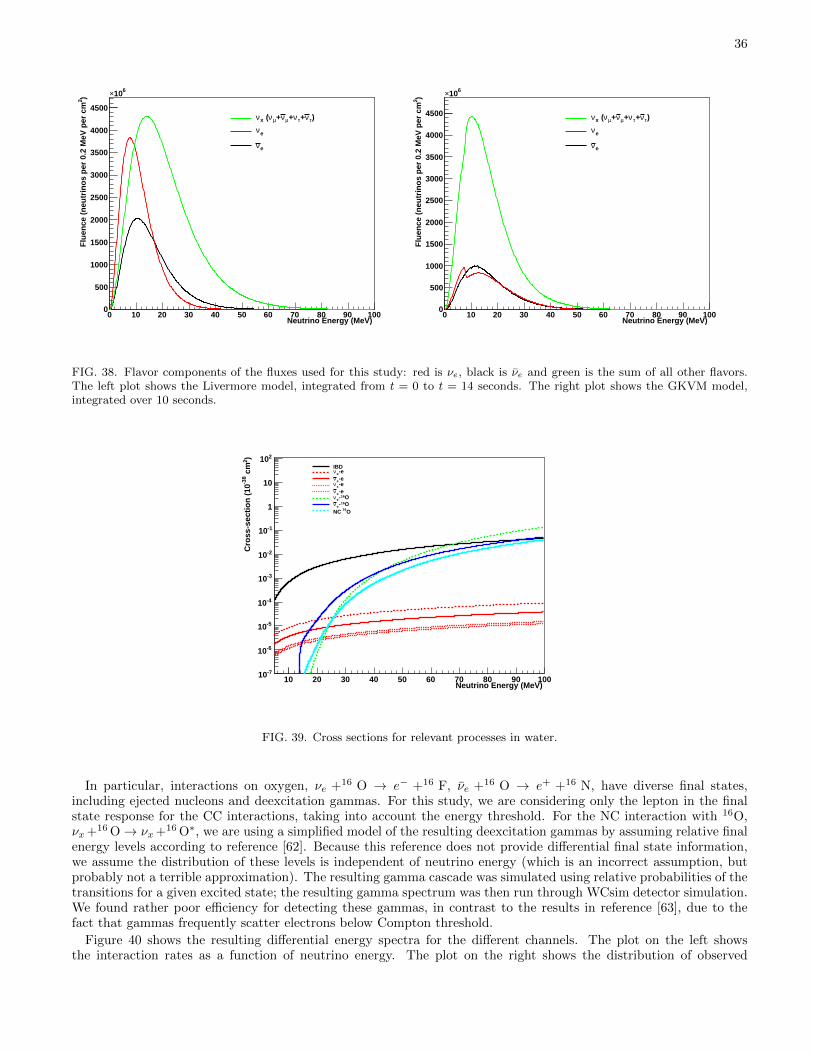
36

Neutrino Energy (MeV) 0 10 20 30 40 50 60 70 80 90 100

)2 F

luen

ce (

neu

trin

os

per

0.2

MeV

per

cm

0

500

1000

1500

2000

2500

3000

3500

4000

4500

610×

)τν+τν+µν+µν (xν

eν

eν

Neutrino Energy (MeV) 0 10 20 30 40 50 60 70 80 90 100

)2 F

luen

ce (

neu

trin

os

per

0.2

MeV

per

cm

0

500

1000

1500

2000

2500

3000

3500

4000

4500

610×

)τν+τν+µν+µν (xν

eν

eν

FIG. 38. Flavor components of the fluxes used for this study: red is νe, black is νe and green is the sum of all other flavors.The left plot shows the Livermore model, integrated from t = 0 to t = 14 seconds. The right plot shows the GKVM model,integrated over 10 seconds.

Neutrino Energy (MeV) 10 20 30 40 50 60 70 80 90 100

)2 c

m-3

8 C

ross

-sec

tion

(10

-710

-610

-510

-410

-310

-210

-110

1

10

210IBD

-eeν-eeν-exν-exν

O16-eνO16-eνO16NC

FIG. 39. Cross sections for relevant processes in water.

In particular, interactions on oxygen, νe +16 O → e− +16 F, νe +16 O → e+ +16 N, have diverse final states,including ejected nucleons and deexcitation gammas. For this study, we are considering only the lepton in the finalstate response for the CC interactions, taking into account the energy threshold. For the NC interaction with 16O,νx+16 O→ νx+16 O∗, we are using a simplified model of the resulting deexcitation gammas by assuming relative finalenergy levels according to reference [62]. Because this reference does not provide differential final state information,we assume the distribution of these levels is independent of neutrino energy (which is an incorrect assumption, butprobably not a terrible approximation). The resulting gamma cascade was simulated using relative probabilities of thetransitions for a given excited state; the resulting gamma spectrum was then run through WCsim detector simulation.We found rather poor efficiency for detecting these gammas, in contrast to the results in reference [63], due to thefact that gammas frequently scatter electrons below Compton threshold.

Figure 40 shows the resulting differential energy spectra for the different channels. The plot on the left showsthe interaction rates as a function of neutrino energy. The plot on the right shows the distribution of observed

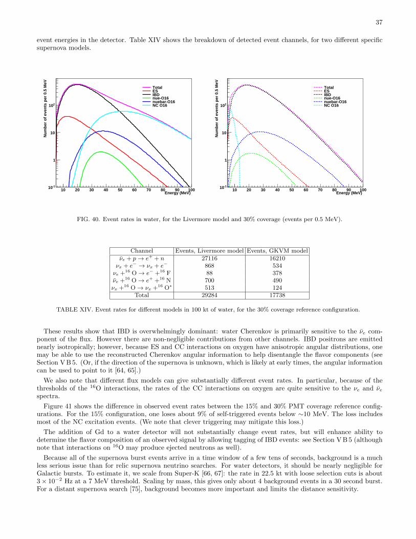
37

event energies in the detector. Table XIV shows the breakdown of detected event channels, for two different specificsupernova models.

Energy (MeV) 10 20 30 40 50 60 70 80 90 100

Num

ber

of e

vent

s pe

r 0.

5 M

eV

-110

1

10

210

TotalESIBDnue-O16nuebar-O16NC O16

Energy (MeV) 10 20 30 40 50 60 70 80 90 100

Num

ber

of e

vent

s pe

r 0.

5 M

eV

-110

1

10

210

TotalESIBDnue-O16nuebar-O16NC O16

FIG. 40. Event rates in water, for the Livermore model and 30% coverage (events per 0.5 MeV).

Channel Events, Livermore model Events, GKVM modelνe + p→ e+ + n 27116 16210νx + e− → νx + e− 868 534νe +16 O→ e− +16 F 88 378νe +16 O→ e+ +16 N 700 490νx +16 O→ νx +16 O∗ 513 124

Total 29284 17738

TABLE XIV. Event rates for different models in 100 kt of water, for the 30% coverage reference configuration.

These results show that IBD is overwhelmingly dominant: water Cherenkov is primarily sensitive to the νe com-ponent of the flux. However there are non-negligible contributions from other channels. IBD positrons are emittednearly isotropically; however, because ES and CC interactions on oxygen have anisotropic angular distributions, onemay be able to use the reconstructed Cherenkov angular information to help disentangle the flavor components (seeSection V B 5. (Or, if the direction of the supernova is unknown, which is likely at early times, the angular informationcan be used to point to it [64, 65].)

We also note that different flux models can give substantially different event rates. In particular, because of thethresholds of the 16O interactions, the rates of the CC interactions on oxygen are quite sensitive to the νe and νespectra.

Figure 41 shows the difference in observed event rates between the 15% and 30% PMT coverage reference config-urations. For the 15% configuration, one loses about 9% of self-triggered events below ∼10 MeV. The loss includesmost of the NC excitation events. (We note that clever triggering may mitigate this loss.)

The addition of Gd to a water detector will not substantially change event rates, but will enhance ability todetermine the flavor composition of an observed signal by allowing tagging of IBD events: see Section V B 5 (althoughnote that interactions on 16O may produce ejected neutrons as well).

Because all of the supernova burst events arrive in a time window of a few tens of seconds, background is a muchless serious issue than for relic supernova neutrino searches. For water detectors, it should be nearly negligible forGalactic bursts. To estimate it, we scale from Super-K [66, 67]: the rate in 22.5 kt with loose selection cuts is about3× 10−2 Hz at a 7 MeV threshold. Scaling by mass, this gives only about 4 background events in a 30 second burst.For a distant supernova search [75], background becomes more important and limits the distance sensitivity.

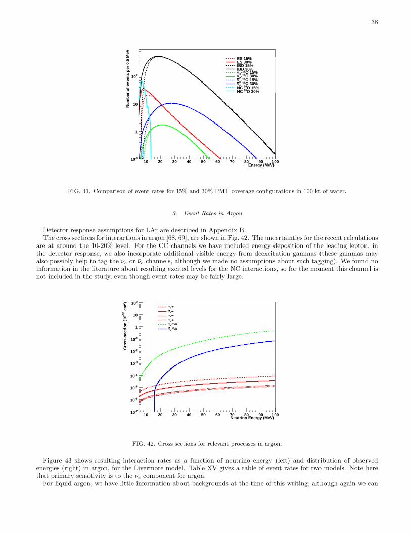
38

Energy (MeV) 10 20 30 40 50 60 70 80 90 100

Num

ber

of e

vent

s pe

r 0.

5 M

eV

-110

1

10

210

ES 15%ES 30%IBD 15%IBD 30%

O 15%16-eνO 30%16-eνO 15%16-eνO 30%16-eνO 15%16NC O 30%16NC

FIG. 41. Comparison of event rates for 15% and 30% PMT coverage configurations in 100 kt of water.

3. Event Rates in Argon

Detector response assumptions for LAr are described in Appendix B.The cross sections for interactions in argon [68, 69], are shown in Fig. 42. The uncertainties for the recent calculations

are at around the 10-20% level. For the CC channels we have included energy deposition of the leading lepton; inthe detector response, we also incorporate additional visible energy from deexcitation gammas (these gammas mayalso possibly help to tag the νe or νe channels, although we made no assumptions about such tagging). We found noinformation in the literature about resulting excited levels for the NC interactions, so for the moment this channel isnot included in the study, even though event rates may be fairly large.

Neutrino Energy (MeV) 10 20 30 40 50 60 70 80 90 100

)2 c

m-3

8 C

ross

-sec

tion

(10

-710

-610

-510

-410

-310

-210

-110

1

10

210-eeν

-eeν-exν

-exνAr40-eνAr40-eν

FIG. 42. Cross sections for relevant processes in argon.

Figure 43 shows resulting interaction rates as a function of neutrino energy (left) and distribution of observedenergies (right) in argon, for the Livermore model. Table XV gives a table of event rates for two models. Note herethat primary sensitivity is to the νe component for argon.

For liquid argon, we have little information about backgrounds at the time of this writing, although again we can

39

Energy (MeV) 10 20 30 40 50 60 70 80 90 100

Num

ber

of e

vent

s pe

r 0.

5 M

eV

5

10

15

20

25

30TotalESnue-Ar40nuebar-Ar40

Energy (MeV) 10 20 30 40 50 60 70 80 90 100

Num

ber

of e

vent

s pe

r 0.

5 M

eV

5

10

15

20

25

30TotalESnue-Ar40nuebar-Ar40

FIG. 43. Event rates in 17 kt of argon (events per 0.5 MeV).

Channel Events, Livermore model Events, GKVM modelνe +40 Ar→ e− +40 K∗ 1154 1424νe +40 Ar→ e+ +40 Cl∗ 97 67νx + e− → νx + e− 148 89

Total 1397 1580

TABLE XV. Event rates for different models in 17 kt of LAr.

assume that they will be less of an issue for burst than for relic supernova neutrinos; furthermore backgrounds willbe well known and can be statistically subtracted from a burst signal. We can assume that cosmic ray muons willbe easily identifiable as long tracks, and Michel electrons can be tagged in association with muons. Backgroundsfor supernova neutrinos in the range from 5-100 MeV will include events from radioactive products associated withmuon spallation (some of which can be substantially delayed with respect to their parent muon). The distributionof spallation products in argon is currently unknown; however, most radioactive decays will deposit less than about10 MeV. At the 300 ft level, the muon rate in one 17 kt module will be about 800 Hz; at 800 ft it is about 200 Hz.Assuming that the fraction of muons producing radioisotopes which decay in the supernova neutrino range of interest(and which cannot be vetoed using space and time correlation information) is less than ∼ 0.01, we can assume thatthis background will not be overwhelming during a nearby supernova burst, even at 300 ft.

4. Comparing Oscillation Scenarios

As described in the introduction to this section, there will likely be significant and observable imprints of oscillationparameters on the observed spectrum of burst supernova neutrino events. For oscillation sensitivity, ability to measureand tag the different flavor components of the spectrum is essential.

Figure 44 compares event rates for normal and inverted hierarchy, for a particular spectrum (a late time slice, notthe full flux) provided by Huaiyu Duan [60]. While information about the hierarchy is clearly present in the waterspectrum, which is mostly νe, the difference between the hierarchies is most dramatic in the observed mostly-νe argonspectrum.

We have attempted a simple quantification of the relative sensitivity of the different single detector configurationsto mass hierarchy. Because fluxes with oscillation signatures are at this time only available representing a fractionof the total flux, we cannot evaluate the full statistical sensitivity. However we have done the following: we havedetermined the minimum statistics for which normal hierarchy is distinguishable from inverted hierarchy, for theDuan multi-angle spectrum [60]. For water Cherenkov (either 15% or 30% coverage), approximately 3500 events arerequired to distinguish the hierarchy at 3σ; 15% and 30% PMT coverage configurations are equally sensitive, becausethe differences occur at relatively high energy. For LAr, about 550 events are required.

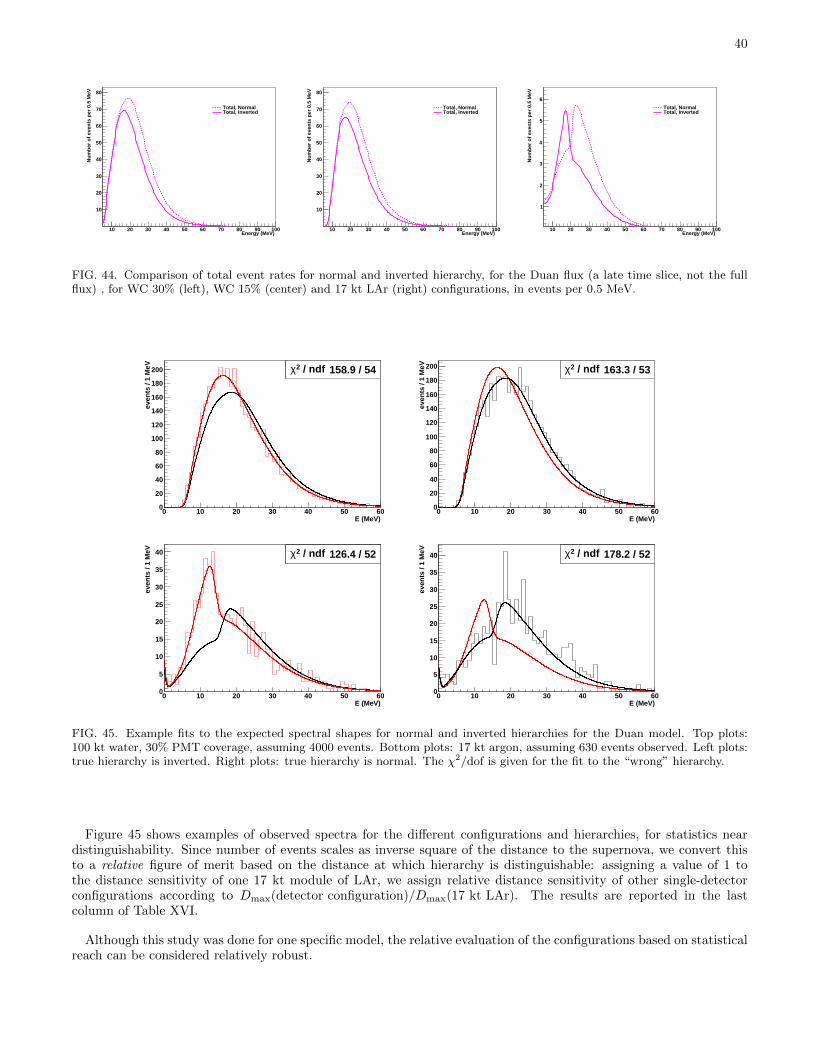
40

Energy (MeV) 10 20 30 40 50 60 70 80 90 100

Nu

mb

er o

f ev

ents

per

0.5

MeV

10

20

30

40

50

60

70

80

Total, NormalTotal, Inverted

Energy (MeV) 10 20 30 40 50 60 70 80 90 100

Nu

mb

er o

f ev

ents

per

0.5

MeV

10

20

30

40

50

60

70

80


Energy (MeV) 10 20 30 40 50 60 70 80 90 100

Nu

mb

er o

f ev

ents

per

0.5

MeV

1

2

3

4

5

6


FIG. 44. Comparison of total event rates for normal and inverted hierarchy, for the Duan flux (a late time slice, not the fullflux) , for WC 30% (left), WC 15% (center) and 17 kt LAr (right) configurations, in events per 0.5 MeV.

/ ndf 2χ 158.9 / 54

E (MeV)0 10 20 30 40 50 60

even

ts /

1 M

eV

0

20

40

60

80

100

120

140

160

180

200 / ndf 2χ 158.9 / 54 / ndf 2χ 163.3 / 53

E (MeV)0 10 20 30 40 50 60

even

ts /

1 M

eV

0

20

40

60

80

100

120

140

160

180

200 / ndf 2χ 163.3 / 53

/ ndf 2χ 126.4 / 52

E (MeV)0 10 20 30 40 50 60

even

ts /

1 M

eV

0

5

10

15

20

25

30

35

40 / ndf 2χ 126.4 / 52 / ndf 2χ 178.2 / 52

E (MeV)0 10 20 30 40 50 60

even

ts /

1 M

eV

0

5

10

15

20

25

30

35

40 / ndf 2χ 178.2 / 52

FIG. 45. Example fits to the expected spectral shapes for normal and inverted hierarchies for the Duan model. Top plots:100 kt water, 30% PMT coverage, assuming 4000 events. Bottom plots: 17 kt argon, assuming 630 events observed. Left plots:true hierarchy is inverted. Right plots: true hierarchy is normal. The χ2/dof is given for the fit to the “wrong” hierarchy.

Figure 45 shows examples of observed spectra for the different configurations and hierarchies, for statistics neardistinguishability. Since number of events scales as inverse square of the distance to the supernova, we convert thisto a relative figure of merit based on the distance at which hierarchy is distinguishable: assigning a value of 1 tothe distance sensitivity of one 17 kt module of LAr, we assign relative distance sensitivity of other single-detectorconfigurations according to Dmax(detector configuration)/Dmax(17 kt LAr). The results are reported in the lastcolumn of Table XVI.

Although this study was done for one specific model, the relative evaluation of the configurations based on statisticalreach can be considered relatively robust.

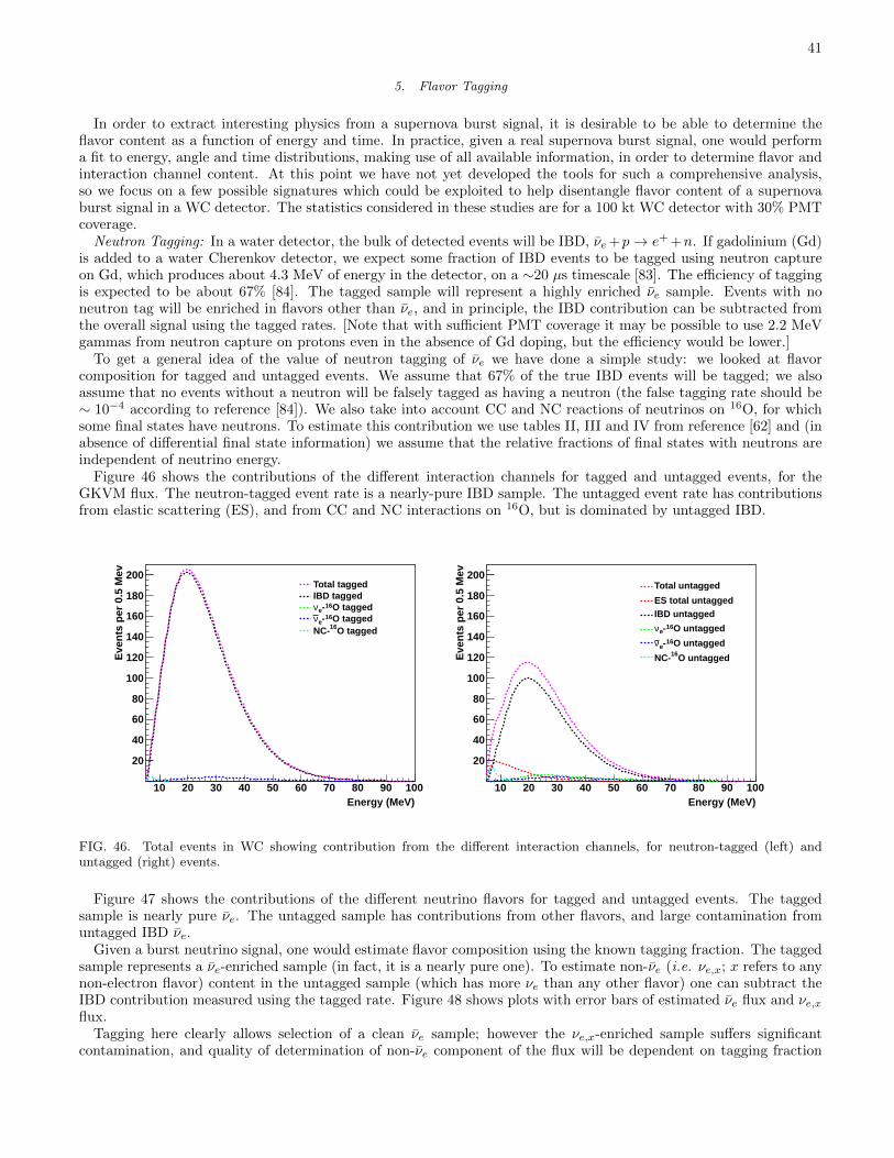
41

5. Flavor Tagging

In order to extract interesting physics from a supernova burst signal, it is desirable to be able to determine theflavor content as a function of energy and time. In practice, given a real supernova burst signal, one would performa fit to energy, angle and time distributions, making use of all available information, in order to determine flavor andinteraction channel content. At this point we have not yet developed the tools for such a comprehensive analysis,so we focus on a few possible signatures which could be exploited to help disentangle flavor content of a supernovaburst signal in a WC detector. The statistics considered in these studies are for a 100 kt WC detector with 30% PMTcoverage.

Neutron Tagging: In a water detector, the bulk of detected events will be IBD, νe+p→ e+ +n. If gadolinium (Gd)is added to a water Cherenkov detector, we expect some fraction of IBD events to be tagged using neutron captureon Gd, which produces about 4.3 MeV of energy in the detector, on a ∼20 µs timescale [83]. The efficiency of taggingis expected to be about 67% [84]. The tagged sample will represent a highly enriched νe sample. Events with noneutron tag will be enriched in flavors other than νe, and in principle, the IBD contribution can be subtracted fromthe overall signal using the tagged rates. [Note that with sufficient PMT coverage it may be possible to use 2.2 MeVgammas from neutron capture on protons even in the absence of Gd doping, but the efficiency would be lower.]

To get a general idea of the value of neutron tagging of νe we have done a simple study: we looked at flavorcomposition for tagged and untagged events. We assume that 67% of the true IBD events will be tagged; we alsoassume that no events without a neutron will be falsely tagged as having a neutron (the false tagging rate should be∼ 10−4 according to reference [84]). We also take into account CC and NC reactions of neutrinos on 16O, for whichsome final states have neutrons. To estimate this contribution we use tables II, III and IV from reference [62] and (inabsence of differential final state information) we assume that the relative fractions of final states with neutrons areindependent of neutrino energy.

Figure 46 shows the contributions of the different interaction channels for tagged and untagged events, for theGKVM flux. The neutron-tagged event rate is a nearly-pure IBD sample. The untagged event rate has contributionsfrom elastic scattering (ES), and from CC and NC interactions on 16O, but is dominated by untagged IBD.

Energy (MeV)10 20 30 40 50 60 70 80 90 100

Eve

nts

per

0.5

Mev

20

40

60

80

100

120

140

160

180

200Total taggedIBD tagged

O tagged16-eνO tagged16-eνO tagged16NC-

Energy (MeV)10 20 30 40 50 60 70 80 90 100

Eve

nts

per

0.5

Mev

20

40

60

80

100

120

140

160

180

200Total untagged

ES total untaggedIBD untagged

O untagged16-eνO untagged16-eνO untagged16NC-

FIG. 46. Total events in WC showing contribution from the different interaction channels, for neutron-tagged (left) anduntagged (right) events.

Figure 47 shows the contributions of the different neutrino flavors for tagged and untagged events. The taggedsample is nearly pure νe. The untagged sample has contributions from other flavors, and large contamination fromuntagged IBD νe.

Given a burst neutrino signal, one would estimate flavor composition using the known tagging fraction. The taggedsample represents a νe-enriched sample (in fact, it is a nearly pure one). To estimate non-νe (i.e. νe,x; x refers to anynon-electron flavor) content in the untagged sample (which has more νe than any other flavor) one can subtract theIBD contribution measured using the tagged rate. Figure 48 shows plots with error bars of estimated νe flux and νe,xflux.

Tagging here clearly allows selection of a clean νe sample; however the νe,x-enriched sample suffers significantcontamination, and quality of determination of non-νe component of the flux will be dependent on tagging fraction

42

Energy (MeV)10 20 30 40 50 60 70 80 90 100

Eve

nts

per

0.5

Mev

20

40

60

80

100

120

140

160

180

200Total tagged

taggedeν taggedxν taggedeν

Energy (MeV)10 20 30 40 50 60 70 80 90 100

Eve

nts

per

0.5

Mev

20

40

60

80

100

120

140

160

180

200Total untagged

untaggedeν untaggedxν untaggedeν

FIG. 47. Total events in WC showing contribution from the different flavors, for neutron-tagged (left) and untagged (right).

Energy (MeV)0 10 20 30 40 50 60 70 80 90 100

Num

ber

of e

vent

s pe

r bi

n

0

0.5

1

1.5

2

2.5

3

310×

-inferredeνWC

Energy (MeV) 0 10 20 30 40 50 60 70 80 90 100

Num

ber

of e

vent

s pe

r bi

n

0

50

100

150

200

250

300

350

-inferrede,xνWC

FIG. 48. Inferred νe (left) and νe,x (right) signals using neutron-tagging information, with uncertainties, for the GKVM flux.

uncertainty (as well as on relative size of that component). The mean number of νe,x events must be greater thanthe uncertainty on the number of untagged νe events for the non-νe component to be measurable. Figure 48 clearlyshows that given our assumptions, it will be possible to determine the size of the νe,x component for the GKVM fluxat 10 kpc. However the untagged sample represents a mix of flavors, and the spectral information for any given flavoris not cleanly measured.

Selection of Elastic Scattering Events: Another potential method for selecting a flavor-enhanced sample in WC isto use the directionality of the neutrino-electron scattering signal: electrons are scattered away from the supernova.(This anisotropy is likely the best method for pointing to the supernova [64, 65].) The ES sample is enriched in νeand νx relative to νe. The relative amounts of the different flavors are sensitive to the neutrino spectrum, and thefractions vary substantially from model to model.

We estimate the quality of a flavor-enriched ES sample by assuming that a fraction εs = 0.66 of ES events willhave cos θ > 0.9, where θ is the reconstructed angle of the scattered event [64]. Such a cut will reduce isotropicbackground by 95%. Figure 49 shows the interaction and flavor compositions of the “ES-enriched” sample selected byan angular cut, for the GKVM model. The non-ES background can be determined by counting events outside of theangular cut window (where we assume for the purpose of determining statistical uncertainty on the ES backgroundsubtraction that non-ES events have isotropic background, although that is not completely true– IBD events have aweak asymmetry, and interactions on 16O have a backwards asymmetry). Figure 50 shows the background-subtracted

43

ES-enriched signal, with statistical error bars, for the GKVM flux.

Energy (MeV)10 20 30 40 50 60 70 80 90 100

Eve

nts

per

0.5

Mev

2

4

6

8

10

12

14

16

18

20

22

24

Total, ES-enriched

IBD, ES-enriched

ES total, ES-enriched

O, ES-enriched16-eνO, ES-enriched16-eν

O, ES-enriched16NC

Energy (MeV)10 20 30 40 50 60 70 80 90 100

Eve

nts

per

0.5

Mev

2

4

6

8

10

12

14

16

18

20

22

24

Total, ES-enriched, ES-enrichedeν, ES-enrichedeν, ES-enrichedxν

FIG. 49. For the GKVM model, interaction (left) and flavor (right) composition of the ES-enriched sample.

Energy (MeV)0 10 20 30 40 50 60 70 80 90 100

Num

ber

of e

vent

s pe

r bi

n

0

50

100

150

200WC Background-subtracted ES

FIG. 50. Background-subtracted ES signal in 5 MeV bins, for the GKVM flux. Error bars are statistical.

Combining Neutron Tagging and Angular Information: It should also be possible to combine angular selection withneutron-tagging to further enhance flavor information in the ES signal. First, because ES events do not have neutrons,the isotropic background in this sample can be reduced by selecting only untagged events.

Second, one can use the tagged sample to determine the νe flux, and then subtract the νe component from the ESsample to determine the νe,x content. Going one step farther: if there were an independent measurement of the νeflux from LAr (or some other detector), one could in principle determine the νx flux, of considerable interest in itself.Figure 51 summarizes the total ES, νe,xES , and νxES scattering rates for the GKVM flux, assuming neutron-taggingand angular selection.

C. Next Steps

We have made preliminary estimates of event rates and simple “anecdotal” evidence of observability of oscillationfeatures for a supernova burst signal, as well as simple studies of information available from flavor tagging. There areseveral improvements and further studies in progress.

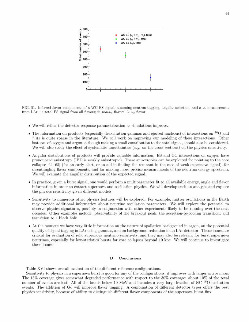
44

1 2 3

Tota

l nu

mb

er o

f ev

ents

0

100

200

300

400

500

600

700

800

), totaleν + eν + xνWC ES (

), totaleν + xνWC ES (

), totalxνWC ES (

FIG. 51. Inferred flavor components of a WC ES signal, assuming neutron-tagging, angular selection, and a νe measurementfrom LAr. 1: total ES signal from all flavors; 2: non-νe flavors; 3: νx flavor.

• We will refine the detector response parametrization as simulations improve.

• The information on products (especially deexcitation gammas and ejected nucleons) of interactions on 16O and40Ar is quite sparse in the literature. We will work on improving our modeling of these interactions. Otherisotopes of oxygen and argon, although making a small contribution to the total signal, should also be considered.We will also study the effect of systematic uncertainties (e.g. on the cross sections) on the physics sensitivity.

• Angular distributions of products will provide valuable information. ES and CC interactions on oxygen havepronounced anisotropy (IBD is weakly anisotropic). These anisotropies can be exploited for pointing to the corecollapse [64, 65] (for an early alert, or to aid in finding the remnant in the case of weak supernova signal), fordisentangling flavor components, and for making more precise measurements of the neutrino energy spectrum.We will evaluate the angular distribution of the expected signal.

• In practice, given a burst signal, one would perform a multiparameter fit to all available energy, angle and flavorinformation in order to extract supernova and oscillation physics. We will develop such an analysis and explorethe physics sensitivity given different models.

• Sensitivity to numerous other physics features will be explored. For example, matter oscillations in the Earthmay provide additional information about neutrino oscillation parameters. We will explore the potential toobserve physics signatures, possibly in conjunction with other experiments likely to be running over the nextdecades. Other examples include: observability of the breakout peak, the accretion-to-cooling transition, andtransition to a black hole.

• At the moment we have very little information on the nature of spallation background in argon, on the potentialquality of signal tagging in LAr using gammas, and on background reduction in an LAr detector. These issues arecritical for evaluation of relic supernova neutrino sensitivity, and they may also be relevant for burst supernovaneutrinos, especially for low-statistics bursts for core collapses beyond 10 kpc. We will continue to investigatethese issues.

D. Conclusions

Table XVI shows overall evaluation of the different reference configurations.Sensitivity to physics in a supernova burst is good for any of the configurations; it improves with larger active mass.

The 15% coverage gives somewhat degraded performance with respect to the 30% coverage: about 10% of the totalnumber of events are lost. All of the loss is below 10 MeV and includes a very large fraction of NC 16O excitationevents. The addition of Gd will improve flavor tagging. A combination of different detector types offers the bestphysics sensitivity, because of ability to distinguish different flavor components of the supernova burst flux.

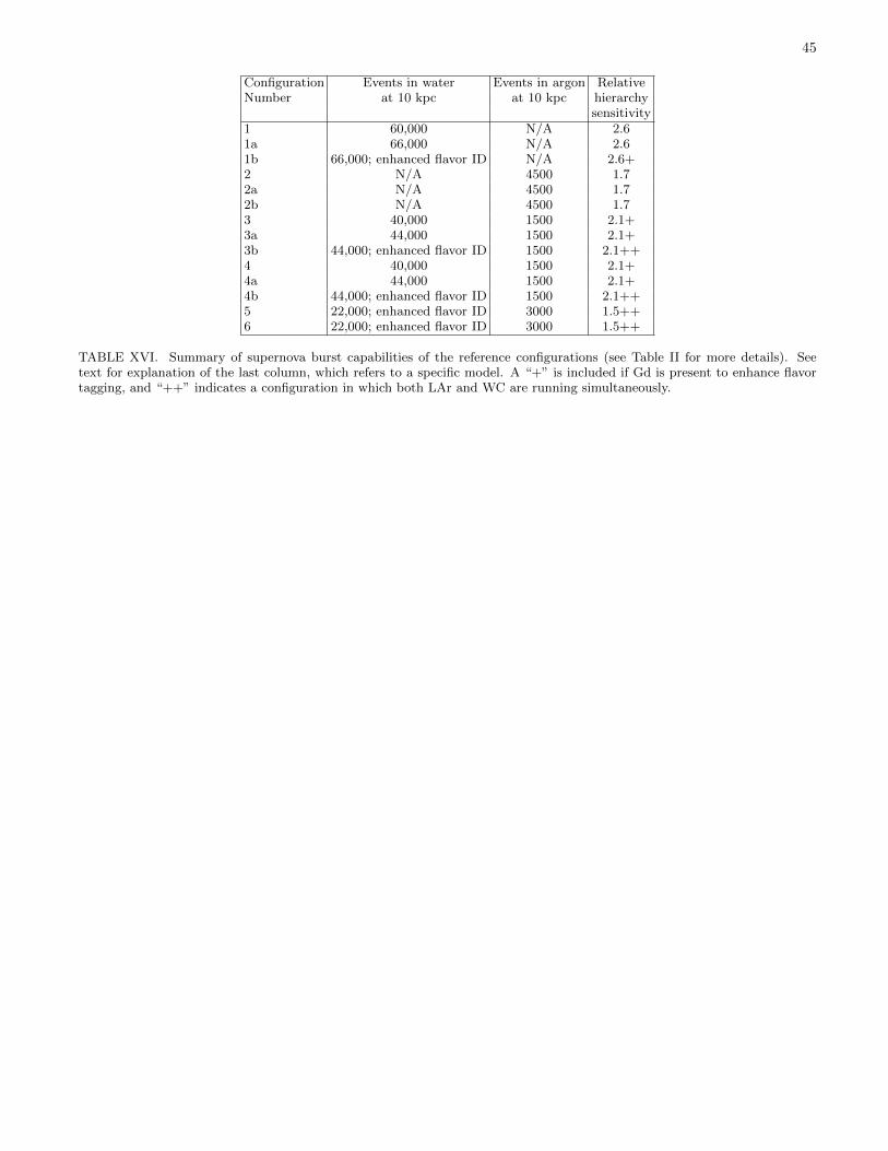
45

Configuration Events in water Events in argon RelativeNumber at 10 kpc at 10 kpc hierarchy

sensitivity1 60,000 N/A 2.61a 66,000 N/A 2.61b 66,000; enhanced flavor ID N/A 2.6+2 N/A 4500 1.72a N/A 4500 1.72b N/A 4500 1.73 40,000 1500 2.1+3a 44,000 1500 2.1+3b 44,000; enhanced flavor ID 1500 2.1++4 40,000 1500 2.1+4a 44,000 1500 2.1+4b 44,000; enhanced flavor ID 1500 2.1++5 22,000; enhanced flavor ID 3000 1.5++6 22,000; enhanced flavor ID 3000 1.5++

TABLE XVI. Summary of supernova burst capabilities of the reference configurations (see Table II for more details). Seetext for explanation of the last column, which refers to a specific model. A “+” is included if Gd is present to enhance flavortagging, and “++” indicates a configuration in which both LAr and WC are running simultaneously.

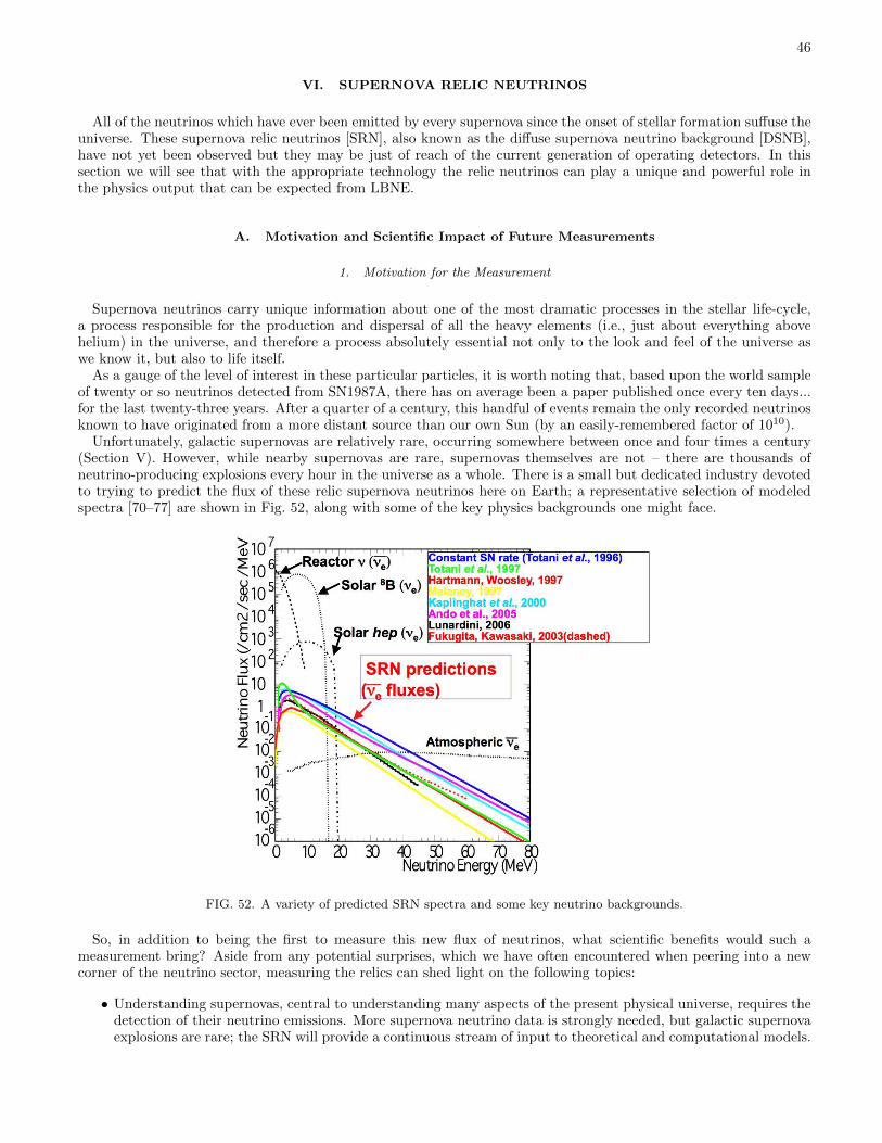
46

VI. SUPERNOVA RELIC NEUTRINOS

All of the neutrinos which have ever been emitted by every supernova since the onset of stellar formation suffuse theuniverse. These supernova relic neutrinos [SRN], also known as the diffuse supernova neutrino background [DSNB],have not yet been observed but they may be just of reach of the current generation of operating detectors. In thissection we will see that with the appropriate technology the relic neutrinos can play a unique and powerful role inthe physics output that can be expected from LBNE.


1. Motivation for the Measurement

Supernova neutrinos carry unique information about one of the most dramatic processes in the stellar life-cycle,a process responsible for the production and dispersal of all the heavy elements (i.e., just about everything abovehelium) in the universe, and therefore a process absolutely essential not only to the look and feel of the universe aswe know it, but also to life itself.

As a gauge of the level of interest in these particular particles, it is worth noting that, based upon the world sampleof twenty or so neutrinos detected from SN1987A, there has on average been a paper published once every ten days...for the last twenty-three years. After a quarter of a century, this handful of events remain the only recorded neutrinosknown to have originated from a more distant source than our own Sun (by an easily-remembered factor of 1010).

Unfortunately, galactic supernovas are relatively rare, occurring somewhere between once and four times a century(Section V). However, while nearby supernovas are rare, supernovas themselves are not – there are thousands ofneutrino-producing explosions every hour in the universe as a whole. There is a small but dedicated industry devotedto trying to predict the flux of these relic supernova neutrinos here on Earth; a representative selection of modeledspectra [70–77] are shown in Fig. 52, along with some of the key physics backgrounds one might face.

FIG. 52. A variety of predicted SRN spectra and some key neutrino backgrounds.

So, in addition to being the first to measure this new flux of neutrinos, what scientific benefits would such ameasurement bring? Aside from any potential surprises, which we have often encountered when peering into a newcorner of the neutrino sector, measuring the relics can shed light on the following topics:

• Understanding supernovas, central to understanding many aspects of the present physical universe, requires thedetection of their neutrino emissions. More supernova neutrino data is strongly needed, but galactic supernovaexplosions are rare; the SRN will provide a continuous stream of input to theoretical and computational models.

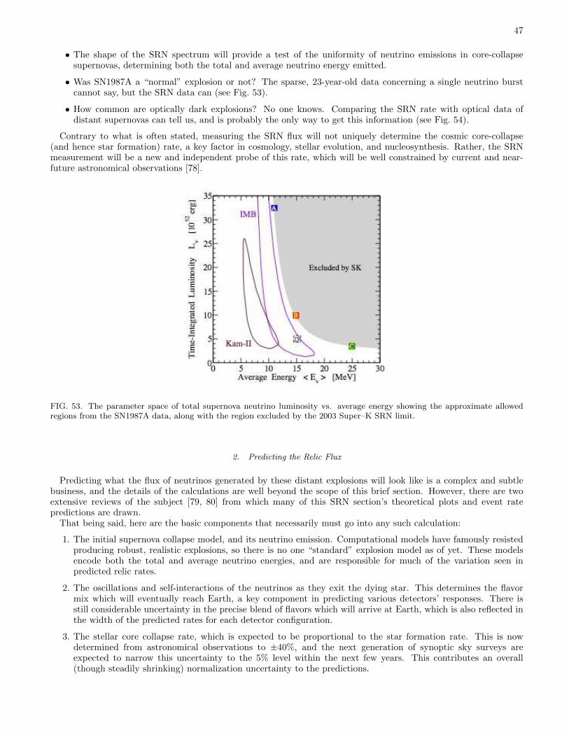
47

• The shape of the SRN spectrum will provide a test of the uniformity of neutrino emissions in core-collapsesupernovas, determining both the total and average neutrino energy emitted.

• Was SN1987A a “normal” explosion or not? The sparse, 23-year-old data concerning a single neutrino burstcannot say, but the SRN data can (see Fig. 53).

• How common are optically dark explosions? No one knows. Comparing the SRN rate with optical data ofdistant supernovas can tell us, and is probably the only way to get this information (see Fig. 54).

Contrary to what is often stated, measuring the SRN flux will not uniquely determine the cosmic core-collapse(and hence star formation) rate, a key factor in cosmology, stellar evolution, and nucleosynthesis. Rather, the SRNmeasurement will be a new and independent probe of this rate, which will be well constrained by current and near-future astronomical observations [78].

FIG. 53. The parameter space of total supernova neutrino luminosity vs. average energy showing the approximate allowedregions from the SN1987A data, along with the region excluded by the 2003 Super–K SRN limit.

2. Predicting the Relic Flux

Predicting what the flux of neutrinos generated by these distant explosions will look like is a complex and subtlebusiness, and the details of the calculations are well beyond the scope of this brief section. However, there are twoextensive reviews of the subject [79, 80] from which many of this SRN section’s theoretical plots and event ratepredictions are drawn.

That being said, here are the basic components that necessarily must go into any such calculation:

1. The initial supernova collapse model, and its neutrino emission. Computational models have famously resistedproducing robust, realistic explosions, so there is no one “standard” explosion model as of yet. These modelsencode both the total and average neutrino energies, and are responsible for much of the variation seen inpredicted relic rates.

2. The oscillations and self-interactions of the neutrinos as they exit the dying star. This determines the flavormix which will eventually reach Earth, a key component in predicting various detectors’ responses. There isstill considerable uncertainty in the precise blend of flavors which will arrive at Earth, which is also reflected inthe width of the predicted rates for each detector configuration.

3. The stellar core collapse rate, which is expected to be proportional to the star formation rate. This is nowdetermined from astronomical observations to ±40%, and the next generation of synoptic sky surveys areexpected to narrow this uncertainty to the 5% level within the next few years. This contributes an overall(though steadily shrinking) normalization uncertainty to the predictions.

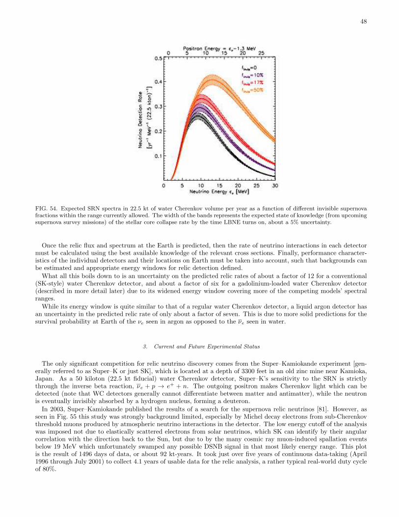
48

FIG. 54. Expected SRN spectra in 22.5 kt of water Cherenkov volume per year as a function of different invisible supernovafractions within the range currently allowed. The width of the bands represents the expected state of knowledge (from upcomingsupernova survey missions) of the stellar core collapse rate by the time LBNE turns on, about a 5% uncertainty.

Once the relic flux and spectrum at the Earth is predicted, then the rate of neutrino interactions in each detectormust be calculated using the best available knowledge of the relevant cross sections. Finally, performance character-istics of the individual detectors and their locations on Earth must be taken into account, such that backgrounds canbe estimated and appropriate energy windows for relic detection defined.

What all this boils down to is an uncertainty on the predicted relic rates of about a factor of 12 for a conventional(SK-style) water Cherenkov detector, and about a factor of six for a gadolinium-loaded water Cherenkov detector(described in more detail later) due to its widened energy window covering more of the competing models’ spectralranges.

While its energy window is quite similar to that of a regular water Cherenkov detector, a liquid argon detector hasan uncertainty in the predicted relic rate of only about a factor of seven. This is due to more solid predictions for thesurvival probability at Earth of the νe seen in argon as opposed to the νe seen in water.

3. Current and Future Experimental Status

The only significant competition for relic neutrino discovery comes from the Super–Kamiokande experiment [gen-erally referred to as Super–K or just SK], which is located at a depth of 3300 feet in an old zinc mine near Kamioka,Japan. As a 50 kiloton (22.5 kt fiducial) water Cherenkov detector, Super–K’s sensitivity to the SRN is strictlythrough the inverse beta reaction, νe + p → e+ + n. The outgoing positron makes Cherenkov light which can bedetected (note that WC detectors generally cannot differentiate between matter and antimatter), while the neutronis eventually invisibly absorbed by a hydrogen nucleus, forming a deuteron.

In 2003, Super–Kamiokande published the results of a search for the supernova relic neutrinos [81]. However, asseen in Fig. 55 this study was strongly background limited, especially by Michel decay electrons from sub-Cherenkovthreshold muons produced by atmospheric neutrino interactions in the detector. The low energy cutoff of the analysiswas imposed not due to elastically scattered electrons from solar neutrinos, which SK can identify by their angularcorrelation with the direction back to the Sun, but due to by the many cosmic ray muon-induced spallation eventsbelow 19 MeV which unfortunately swamped any possible DSNB signal in that most likely energy range. This plotis the result of 1496 days of data, or about 92 kt-years. It took just over five years of continuous data-taking (April1996 through July 2001) to collect 4.1 years of usable data for the relic analysis, a rather typical real-world duty cycleof 80%.

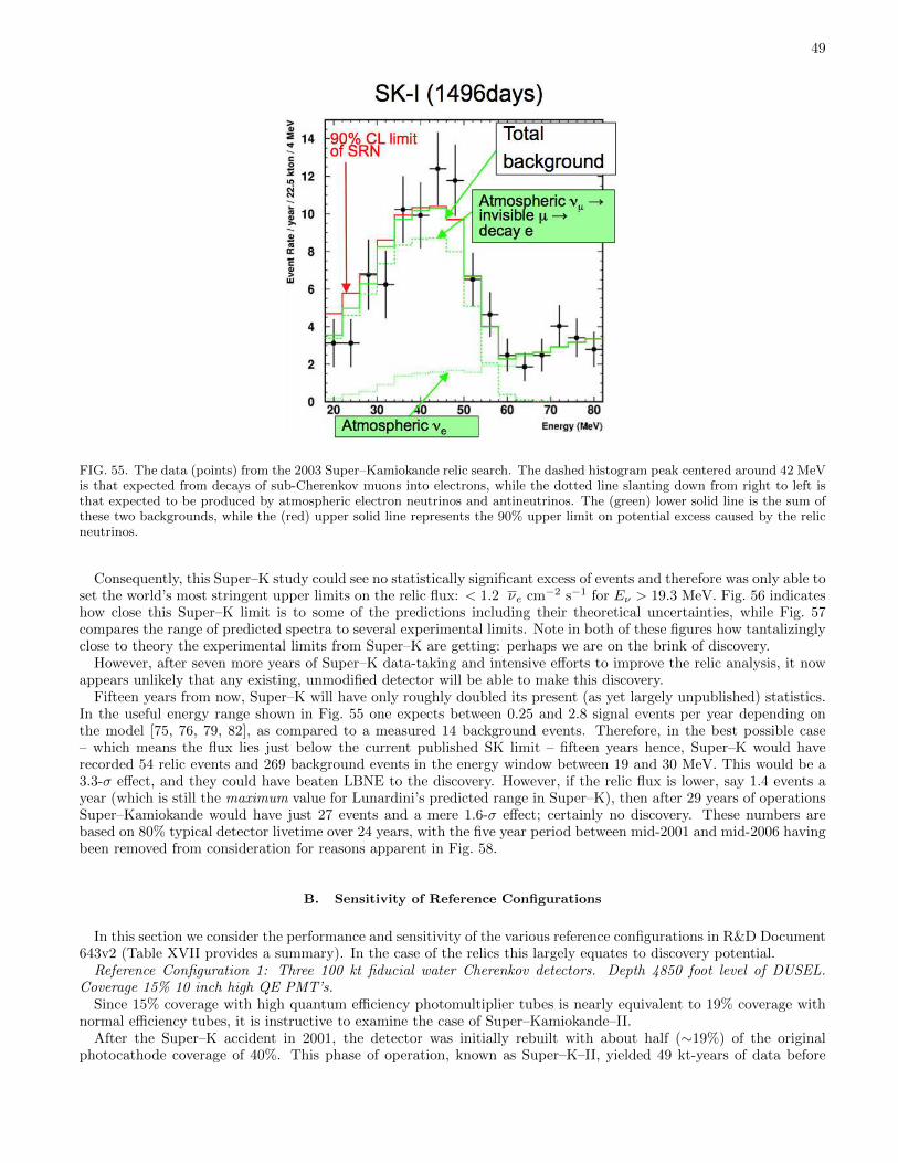
49

FIG. 55. The data (points) from the 2003 Super–Kamiokande relic search. The dashed histogram peak centered around 42 MeVis that expected from decays of sub-Cherenkov muons into electrons, while the dotted line slanting down from right to left isthat expected to be produced by atmospheric electron neutrinos and antineutrinos. The (green) lower solid line is the sum ofthese two backgrounds, while the (red) upper solid line represents the 90% upper limit on potential excess caused by the relicneutrinos.

Consequently, this Super–K study could see no statistically significant excess of events and therefore was only able toset the world’s most stringent upper limits on the relic flux: < 1.2 νe cm−2 s−1 for Eν > 19.3 MeV. Fig. 56 indicateshow close this Super–K limit is to some of the predictions including their theoretical uncertainties, while Fig. 57compares the range of predicted spectra to several experimental limits. Note in both of these figures how tantalizinglyclose to theory the experimental limits from Super–K are getting: perhaps we are on the brink of discovery.

However, after seven more years of Super–K data-taking and intensive efforts to improve the relic analysis, it nowappears unlikely that any existing, unmodified detector will be able to make this discovery.

Fifteen years from now, Super–K will have only roughly doubled its present (as yet largely unpublished) statistics.In the useful energy range shown in Fig. 55 one expects between 0.25 and 2.8 signal events per year depending onthe model [75, 76, 79, 82], as compared to a measured 14 background events. Therefore, in the best possible case– which means the flux lies just below the current published SK limit – fifteen years hence, Super–K would haverecorded 54 relic events and 269 background events in the energy window between 19 and 30 MeV. This would be a3.3-σ effect, and they could have beaten LBNE to the discovery. However, if the relic flux is lower, say 1.4 events ayear (which is still the maximum value for Lunardini’s predicted range in Super–K), then after 29 years of operationsSuper–Kamiokande would have just 27 events and a mere 1.6-σ effect; certainly no discovery. These numbers arebased on 80% typical detector livetime over 24 years, with the five year period between mid-2001 and mid-2006 havingbeen removed from consideration for reasons apparent in Fig. 58.


In this section we consider the performance and sensitivity of the various reference configurations in R&D Document643v2 (Table XVII provides a summary). In the case of the relics this largely equates to discovery potential.

Reference Configuration 1: Three 100 kt fiducial water Cherenkov detectors. Depth 4850 foot level of DUSEL.Coverage 15% 10 inch high QE PMT’s.

Since 15% coverage with high quantum efficiency photomultiplier tubes is nearly equivalent to 19% coverage withnormal efficiency tubes, it is instructive to examine the case of Super–Kamiokande–II.

After the Super–K accident in 2001, the detector was initially rebuilt with about half (∼19%) of the originalphotocathode coverage of 40%. This phase of operation, known as Super–K–II, yielded 49 kt-years of data before

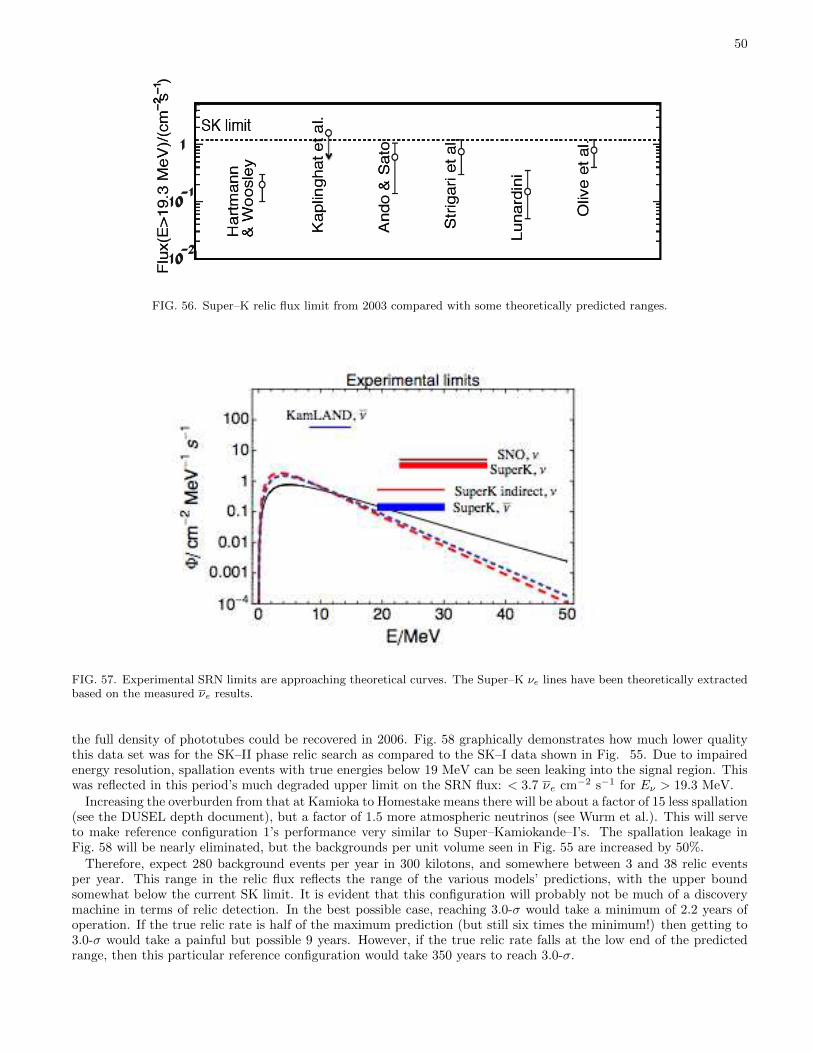
50

FIG. 56. Super–K relic flux limit from 2003 compared with some theoretically predicted ranges.

FIG. 57. Experimental SRN limits are approaching theoretical curves. The Super–K νe lines have been theoretically extractedbased on the measured νe results.

the full density of phototubes could be recovered in 2006. Fig. 58 graphically demonstrates how much lower qualitythis data set was for the SK–II phase relic search as compared to the SK–I data shown in Fig. 55. Due to impairedenergy resolution, spallation events with true energies below 19 MeV can be seen leaking into the signal region. Thiswas reflected in this period’s much degraded upper limit on the SRN flux: < 3.7 νe cm−2 s−1 for Eν > 19.3 MeV.

Increasing the overburden from that at Kamioka to Homestake means there will be about a factor of 15 less spallation(see the DUSEL depth document), but a factor of 1.5 more atmospheric neutrinos (see Wurm et al.). This will serveto make reference configuration 1’s performance very similar to Super–Kamiokande–I’s. The spallation leakage inFig. 58 will be nearly eliminated, but the backgrounds per unit volume seen in Fig. 55 are increased by 50%.

Therefore, expect 280 background events per year in 300 kilotons, and somewhere between 3 and 38 relic eventsper year. This range in the relic flux reflects the range of the various models’ predictions, with the upper boundsomewhat below the current SK limit. It is evident that this configuration will probably not be much of a discoverymachine in terms of relic detection. In the best possible case, reaching 3.0-σ would take a minimum of 2.2 years ofoperation. If the true relic rate is half of the maximum prediction (but still six times the minimum!) then getting to3.0-σ would take a painful but possible 9 years. However, if the true relic rate falls at the low end of the predictedrange, then this particular reference configuration would take 350 years to reach 3.0-σ.

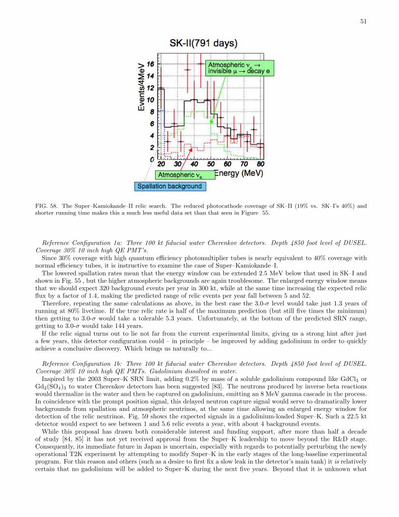
51

FIG. 58. The Super–Kamiokande–II relic search. The reduced photocathode coverage of SK–II (19% vs. SK–I’s 40%) andshorter running time makes this a much less useful data set than that seen in Figure 55.

Reference Configuration 1a: Three 100 kt fiducial water Cherenkov detectors. Depth 4850 foot level of DUSEL.Coverage 30% 10 inch high QE PMT’s.

Since 30% coverage with high quantum efficiency photomultiplier tubes is nearly equivalent to 40% coverage withnormal efficiency tubes, it is instructive to examine the case of Super–Kamiokande–I.

The lowered spallation rates mean that the energy window can be extended 2.5 MeV below that used in SK–I andshown in Fig. 55 , but the higher atmospheric backgrounds are again troublesome. The enlarged energy window meansthat we should expect 320 background events per year in 300 kt, while at the same time increasing the expected relicflux by a factor of 1.4, making the predicted range of relic events per year fall between 5 and 52.

Therefore, repeating the same calculations as above, in the best case the 3.0-σ level would take just 1.3 years ofrunning at 80% livetime. If the true relic rate is half of the maximum prediction (but still five times the minimum)then getting to 3.0-σ would take a tolerable 5.3 years. Unfortunately, at the bottom of the predicted SRN range,getting to 3.0-σ would take 144 years.

If the relic signal turns out to lie not far from the current experimental limits, giving us a strong hint after justa few years, this detector configuration could – in principle – be improved by adding gadolinium in order to quicklyachieve a conclusive discovery. Which brings us naturally to...

Reference Configuration 1b: Three 100 kt fiducial water Cherenkov detectors. Depth 4850 foot level of DUSEL.Coverage 30% 10 inch high QE PMTs. Gadolinium dissolved in water.

Inspired by the 2003 Super–K SRN limit, adding 0.2% by mass of a soluble gadolinium compound like GdCl3 orGd2(SO4)3 to water Cherenkov detectors has been suggested [83]. The neutrons produced by inverse beta reactionswould thermalize in the water and then be captured on gadolinium, emitting an 8 MeV gamma cascade in the process.In coincidence with the prompt position signal, this delayed neutron capture signal would serve to dramatically lowerbackgrounds from spallation and atmospheric neutrinos, at the same time allowing an enlarged energy window fordetection of the relic neutrinos. Fig. 59 shows the expected signals in a gadolinium-loaded Super–K. Such a 22.5 ktdetector would expect to see between 1 and 5.6 relic events a year, with about 4 background events.

While this proposal has drawn both considerable interest and funding support, after more than half a decadeof study [84, 85] it has not yet received approval from the Super–K leadership to move beyond the R&D stage.Consequently, its immediate future in Japan is uncertain, especially with regards to potentially perturbing the newlyoperational T2K experiment by attempting to modify Super–K in the early stages of the long-baseline experimentalprogram. For this reason and others (such as a desire to first fix a slow leak in the detector’s main tank) it is relativelycertain that no gadolinium will be added to Super–K during the next five years. Beyond that it is unknown what

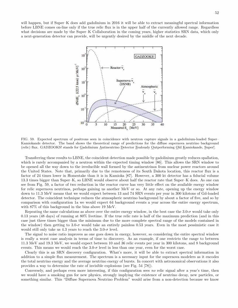
52

will happen, but if Super–K does add gadolinium in 2016 it will be able to extract meaningful spectral informationbefore LBNE comes on-line only if the true relic flux is in the upper half of the currently allowed range. Regardlesswhat decisions are made by the Super–K Collaboration in the coming years, higher statistics SRN data, which onlya next-generation detector can provide, will be urgently desired by the middle of the next decade.

FIG. 59. Expected spectrum of positrons seen in coincidence with neutron capture signals in a gadolinium-loaded Super–Kamiokande detector. The band shows the theoretical range of predictions for the diffuse supernova neutrino background(relic) flux. GADZOOKS! stands for Gadolinium Antineutrino Detector Zealously Outperforming Old Kamiokande, Super!.

Transferring these results to LBNE, the coincident detection made possible by gadolinium greatly reduces spallation,which is rarely accompanied by a neutron within the expected timing window [86]. This allows the SRN window tobe opened all the way down to the irreducible wall formed by the antineutrinos from nuclear power reactors aroundthe United States. Note that, primarily due to the remoteness of its South Dakota location, this reactor flux is afactor of 24 times lower in Homestake than it is in Kamioka [87]. However, a 300 kt detector has a fiducial volume13.3 times bigger than Super–K, so LBNE would observe about half the reactor rate that Super–K does. As one cansee from Fig. 59, a factor of two reduction in the reactor curve has very little effect on the available energy windowfor relic supernova neutrinos, perhaps gaining us another MeV or so. At any rate, opening up the energy windowdown to 11.3 MeV means that we would expect between 13 and 74 SRN events per year in 300 kilotons of Gd-loadeddetector. The coincident technique reduces the atmospheric neutrino background by about a factor of five, and so bycomparison with configuration 1a we would expect 64 background events a year across the entire energy spectrum,with 87% of this background in the bins above 19 MeV.

Repeating the same calculations as above over the entire energy window, in the best case the 3.0-σ would take only0.13 years (48 days) of running at 80% livetime. If the true relic rate is half of the maximum prediction (and in thiscase just three times bigger than the minimum due to the more complete spectral range of the models contained inthe window) then getting to 3.0-σ would take an entirely painless 0.53 years. Even in the most pessimistic case itwould still only take us 4.3 years to reach the 3.0-σ level.

The signal to noise ratio improves as one goes down in energy, however, so considering the entire spectral windowis really a worst case analysis in terms of time to discovery. As an example, if one restricts the range to between11.3 MeV and 19.3 MeV, we would expect between 10 and 36 relic events per year in 300 kilotons, and 8 backgroundevents. This means we would reach the 3.0-σ level in less than one year, even for the worst case.

Clearly this is an SRN discovery configuration. What’s more, it will be able to extract spectral information inaddition to a simple flux measurement. The spectrum is a necessary input for the supernova modelers as it encodesthe total neutrino energy and the average neutrino energy of bursts. In concert with astronomical observations it alsoprovides a way to determine the rate of invisible explosions (see Fig. 54 [78]).

Conversely, and perhaps even more interesting, if this configuration sees no relic signal after a year’s time, thenwe would have a smoking gun for new physics, strongly implying the existence of neutrino decay, new particles, orsomething similar. This “Diffuse Supernova Neutrino Problem” would arise from a non-detection because we know

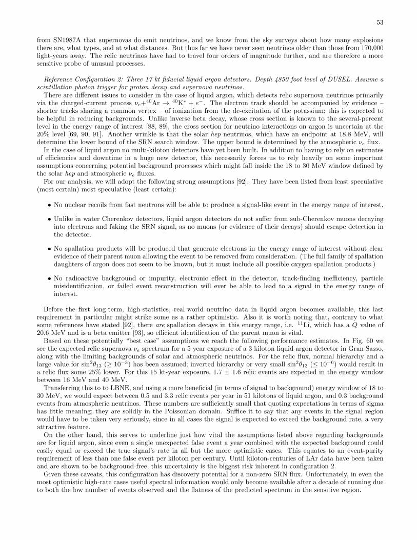
53

from SN1987A that supernovas do emit neutrinos, and we know from the sky surveys about how many explosionsthere are, what types, and at what distances. But thus far we have never seen neutrinos older than those from 170,000light-years away. The relic neutrinos have had to travel four orders of magnitude further, and are therefore a moresensitive probe of unusual processes.

Reference Configuration 2: Three 17 kt fiducial liquid argon detectors. Depth 4850 foot level of DUSEL. Assume ascintillation photon trigger for proton decay and supernova neutrinos.

There are different issues to consider in the case of liquid argon, which detects relic supernova neutrinos primarilyvia the charged-current process νe+

40Ar → 40K∗ + e−. The electron track should be accompanied by evidence –shorter tracks sharing a common vertex – of ionization from the de-excitation of the potassium; this is expected tobe helpful in reducing backgrounds. Unlike inverse beta decay, whose cross section is known to the several-percentlevel in the energy range of interest [88, 89], the cross section for neutrino interactions on argon is uncertain at the20% level [69, 90, 91]. Another wrinkle is that the solar hep neutrinos, which have an endpoint at 18.8 MeV, willdetermine the lower bound of the SRN search window. The upper bound is determined by the atmospheric νe flux.

In the case of liquid argon no multi-kiloton detectors have yet been built. In addition to having to rely on estimatesof efficiencies and downtime in a huge new detector, this necessarily forces us to rely heavily on some importantassumptions concerning potential background processes which might fall inside the 18 to 30 MeV window defined bythe solar hep and atmospheric νe fluxes.

For our analysis, we will adopt the following strong assumptions [92]. They have been listed from least speculative(most certain) most speculative (least certain):

• No nuclear recoils from fast neutrons will be able to produce a signal-like event in the energy range of interest.

• Unlike in water Cherenkov detectors, liquid argon detectors do not suffer from sub-Cherenkov muons decayinginto electrons and faking the SRN signal, as no muons (or evidence of their decays) should escape detection inthe detector.

• No spallation products will be produced that generate electrons in the energy range of interest without clearevidence of their parent muon allowing the event to be removed from consideration. (The full family of spallationdaughters of argon does not seem to be known, but it must include all possible oxygen spallation products.)

• No radioactive background or impurity, electronic effect in the detector, track-finding inefficiency, particlemisidentification, or failed event reconstruction will ever be able to lead to a signal in the energy range ofinterest.

Before the first long-term, high-statistics, real-world neutrino data in liquid argon becomes available, this lastrequirement in particular might strike some as a rather optimistic. Also it is worth noting that, contrary to whatsome references have stated [92], there are spallation decays in this energy range, i.e. 11Li, which has a Q value of20.6 MeV and is a beta emitter [93], so efficient identification of the parent muon is vital.

Based on these potentially “best case” assumptions we reach the following performance estimates. In Fig. 60 wesee the expected relic supernova νe spectrum for a 5 year exposure of a 3 kiloton liquid argon detector in Gran Sasso,along with the limiting backgrounds of solar and atmospheric neutrinos. For the relic flux, normal hierarchy and alarge value for sin2θ13 (≥ 10−3) has been assumed; inverted hierarchy or very small sin2θ13 (≤ 10−6) would result ina relic flux some 25% lower. For this 15 kt-year exposure, 1.7 ± 1.6 relic events are expected in the energy windowbetween 16 MeV and 40 MeV.

Transferring this to to LBNE, and using a more beneficial (in terms of signal to background) energy window of 18 to30 MeV, we would expect between 0.5 and 3.3 relic events per year in 51 kilotons of liquid argon, and 0.3 backgroundevents from atmospheric neutrinos. These numbers are sufficiently small that quoting expectations in terms of sigmahas little meaning; they are solidly in the Poissonian domain. Suffice it to say that any events in the signal regionwould have to be taken very seriously, since in all cases the signal is expected to exceed the background rate, a veryattractive feature.

On the other hand, this serves to underline just how vital the assumptions listed above regarding backgroundsare for liquid argon, since even a single unexpected false event a year combined with the expected background couldeasily equal or exceed the true signal’s rate in all but the more optimistic cases. This equates to an event-purityrequirement of less than one false event per kiloton per century. Until kiloton-centuries of LAr data have been takenand are shown to be background-free, this uncertainty is the biggest risk inherent in configuration 2.

Given these caveats, this configuration has discovery potential for a non-zero SRN flux. Unfortunately, in even themost optimistic high-rate cases useful spectral information would only become available after a decade of running dueto both the low number of events observed and the flatness of the predicted spectrum in the sensitive region.

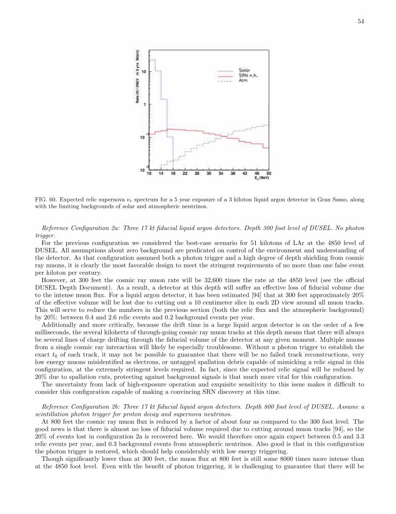
54

FIG. 60. Expected relic supernova νe spectrum for a 5 year exposure of a 3 kiloton liquid argon detector in Gran Sasso, alongwith the limiting backgrounds of solar and atmospheric neutrinos.

Reference Configuration 2a: Three 17 kt fiducial liquid argon detectors. Depth 300 foot level of DUSEL. No photontrigger.

For the previous configuration we considered the best-case scenario for 51 kilotons of LAr at the 4850 level ofDUSEL. All assumptions about zero background are predicated on control of the environment and understanding ofthe detector. As that configuration assumed both a photon trigger and a high degree of depth shielding from cosmicray muons, it is clearly the most favorable design to meet the stringent requirements of no more than one false eventper kiloton per century.

However, at 300 feet the cosmic ray muon rate will be 32,600 times the rate at the 4850 level (see the officialDUSEL Depth Document). As a result, a detector at this depth will suffer an effective loss of fiducial volume dueto the intense muon flux. For a liquid argon detector, it has been estimated [94] that at 300 feet approximately 20%of the effective volume will be lost due to cutting out a 10 centimeter slice in each 2D view around all muon tracks.This will serve to reduce the numbers in the previous section (both the relic flux and the atmospheric background)by 20%: between 0.4 and 2.6 relic events and 0.2 background events per year.

Additionally and more critically, because the drift time in a large liquid argon detector is on the order of a fewmilliseconds, the several kilohertz of through-going cosmic ray muon tracks at this depth means that there will alwaysbe several lines of charge drifting through the fiducial volume of the detector at any given moment. Multiple muonsfrom a single cosmic ray interaction will likely be especially troublesome. Without a photon trigger to establish theexact t0 of each track, it may not be possible to guarantee that there will be no failed track reconstructions, verylow energy muons misidentified as electrons, or untagged spallation debris capable of mimicking a relic signal in thisconfiguration, at the extremely stringent levels required. In fact, since the expected relic signal will be reduced by20% due to spallation cuts, protecting against background signals is that much more vital for this configuration.

The uncertainty from lack of high-exposure operation and exquisite sensitivity to this issue makes it difficult toconsider this configuration capable of making a convincing SRN discovery at this time.

Reference Configuration 2b: Three 17 kt fiducial liquid argon detectors. Depth 800 foot level of DUSEL. Assume ascintillation photon trigger for proton decay and supernova neutrinos.

At 800 feet the cosmic ray muon flux is reduced by a factor of about four as compared to the 300 foot level. Thegood news is that there is almost no loss of fiducial volume required due to cutting around muon tracks [94], so the20% of events lost in configuration 2a is recovered here. We would therefore once again expect between 0.5 and 3.3relic events per year, and 0.3 background events from atmospheric neutrinos. Also good is that in this configurationthe photon trigger is restored, which should help considerably with low energy triggering.

Though significantly lower than at 300 feet, the muon flux at 800 feet is still some 8000 times more intense thanat the 4850 foot level. Even with the benefit of photon triggering, it is challenging to guarantee that there will be

55

no false events at the level of less than one a year arising from failed track reconstructions, very low energy muonsmisidentified as electrons, or spallation debris capable of mimicking a relic signal in this configuration. In termsof cosmic ray-related background rejection (but, sadly, not signal collection), every successful year at 800 feet isequivalent to false-background-free exposure of 408 Mt-years on the 4850 level.

Again here, some high-exposure proof-of-principle data, in this case with a photon trigger, is needed to properlyassess the viability and hence the potential of this configuration for SRN discovery.

Reference Configuration 3: Two 100 kt fiducial water Cherenkov detectors at 4850 feet as specified in configuration1, plus one 17 kt fiducial liquid argon detector at 300 feet with no photon trigger as specified in configuration 2a.

This begins a long series of combinatoric configurations where the various detectors and depths of the the previousconfigurations are mixed and matched. In all cases one or two components are dominant in terms of SRN discoverypotential. The expected rates and known backgrounds will be listed; details can be found in the discussions ofconfigurations 1, 1a, 1b, 2, 2a, and 2b.

By referring to configuration 1, the two 100 kt WC modules of this design would expect to record between 2 and 26relic events a year with 187 background events. By comparison with configuration 2a, a single liquid argon detectorat 300 feet would be expected to see between 0.1 and 0.9 relic events a year, adding little to the configuration even ifdetector-related backgrounds could be well controlled.

WC: SRN signal = 2 – 26 events/year, background = 187 events/yearLAr: SRN signal = 0.1 – 0.9 events/year, atmospheric νe background = 0.1 events/year

Reference Configuration 3a: Two 100 kt fiducial water Cherenkov detectors at 4850 feet as specified in configuration1a, plus one 17 kt fiducial liquid argon detector at 300 feet with no photon trigger as specified in configuration 2a.


Reference Configuration 3b: One 100 kt fiducial water Cherenkov detector at 4850 feet as specified in configuration1, plus one 100 kt fiducial water Cherenkov detector at 4850 feet with gadolinium as specified in configuration 1b, plusone 17 kt fiducial liquid argon detector at 300 feet with no photon trigger as specified in configuration 2a.

WC: SRN signal = 1 – 13 events/year, background = 93 events/yearWC+Gd: SRN signal = 4 – 25 events/year, background = 21 events/yearLAr: SRN signal = 0.1 – 0.9 events/year, atmospheric νe background = 0.1 events/year

Reference Configuration 4: Two 100 kt fiducial water Cherenkov detectors at 4850 feet as specified in configuration1, plus one 17 kt fiducial liquid argon detector at 800 feet with a photon trigger as specified in configuration 2b.


Reference Configuration 4a: Two 100 kt fiducial water Cherenkov detectors at 4850 feet as specified in configuration1a, plus one 17 kt fiducial liquid argon detector at 800 feet with a photon trigger as specified in configuration 2b.


Reference Configuration 4b: One 100 kt fiducial water Cherenkov detector at 4850 feet as specified in configuration1, plus one 100 kt fiducial water Cherenkov detector at 4850 feet with gadolinium as specified in configuration 1b, plusone 17 kt fiducial liquid argon detector at 800 feet with a photon trigger as specified in configuration 2b.

WC: SRN signal = 1 – 13 events/year, background = 93 events/yearWC+Gd: SRN signal = 4 – 25 events/year, background = 21 events/yearLAr: SRN signal = 0.2 – 1.1 events/year, atmospheric νe background = 0.1 events/year

Reference Configuration 5: One 100 kt fiducial water Cherenkov detector at 4850 feet with gadolinium as specifiedin configuration 1b, plus two 17 kt fiducial liquid argon detectors at 300 feet with no photon trigger as specified inconfiguration 2a.

WC+Gd: SRN signal = 4 – 25 events/year, background = 21 events/yearLAr: SRN signal = 0.2 – 1.8 events/year, atmospheric νe background = 0.2 events/year

Reference Configuration 6: One 100 kt fiducial water Cherenkov detector at 4850 feet with gadolinium as specifiedin configuration 1b, plus two 17 kt fiducial liquid argon detectors at 800 feet with photon trigger as specified inconfiguration 2b.

WC+Gd: SRN signal = 4 – 25 events/year, background = 21 events/year

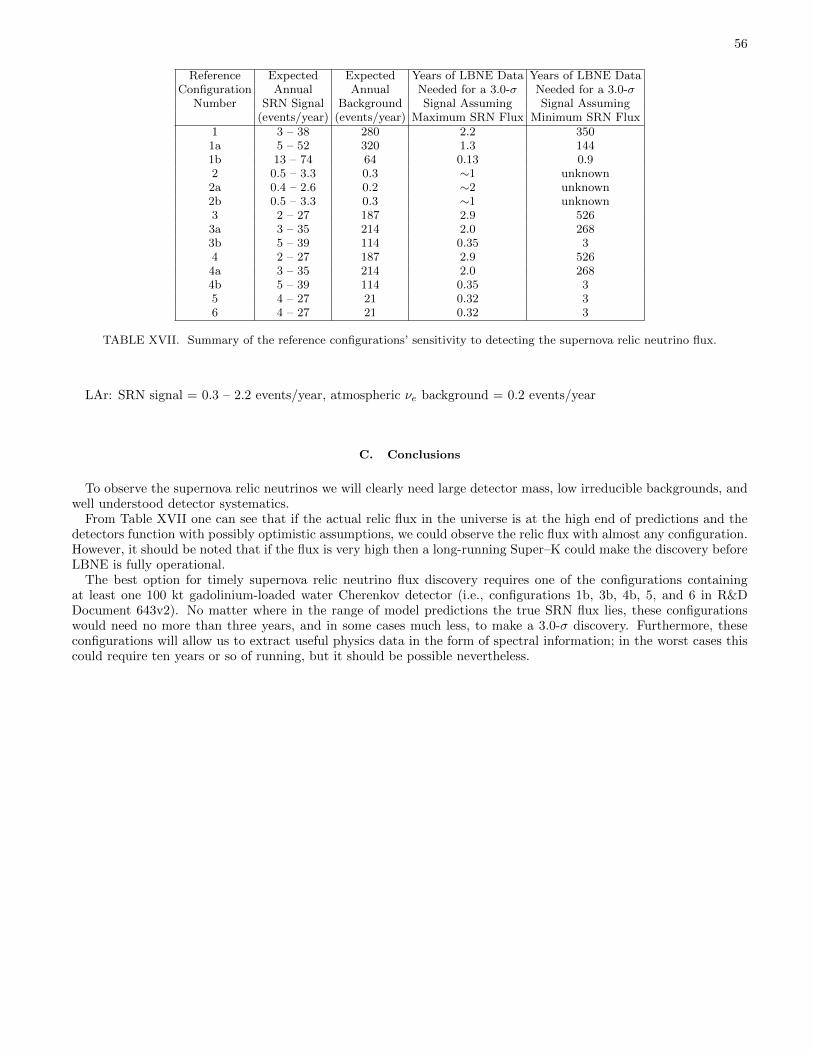
56

Reference Expected Expected Years of LBNE Data Years of LBNE DataConfiguration Annual Annual Needed for a 3.0-σ Needed for a 3.0-σ

Number SRN Signal Background Signal Assuming Signal Assuming(events/year) (events/year) Maximum SRN Flux Minimum SRN Flux

1 3 – 38 280 2.2 3501a 5 – 52 320 1.3 1441b 13 – 74 64 0.13 0.92 0.5 – 3.3 0.3 ∼1 unknown2a 0.4 – 2.6 0.2 ∼2 unknown2b 0.5 – 3.3 0.3 ∼1 unknown3 2 – 27 187 2.9 5263a 3 – 35 214 2.0 2683b 5 – 39 114 0.35 34 2 – 27 187 2.9 5264a 3 – 35 214 2.0 2684b 5 – 39 114 0.35 35 4 – 27 21 0.32 36 4 – 27 21 0.32 3

TABLE XVII. Summary of the reference configurations’ sensitivity to detecting the supernova relic neutrino flux.

LAr: SRN signal = 0.3 – 2.2 events/year, atmospheric νe background = 0.2 events/year

C. Conclusions

To observe the supernova relic neutrinos we will clearly need large detector mass, low irreducible backgrounds, andwell understood detector systematics.

From Table XVII one can see that if the actual relic flux in the universe is at the high end of predictions and thedetectors function with possibly optimistic assumptions, we could observe the relic flux with almost any configuration.However, it should be noted that if the flux is very high then a long-running Super–K could make the discovery beforeLBNE is fully operational.

The best option for timely supernova relic neutrino flux discovery requires one of the configurations containingat least one 100 kt gadolinium-loaded water Cherenkov detector (i.e., configurations 1b, 3b, 4b, 5, and 6 in R&DDocument 643v2). No matter where in the range of model predictions the true SRN flux lies, these configurationswould need no more than three years, and in some cases much less, to make a 3.0-σ discovery. Furthermore, theseconfigurations will allow us to extract useful physics data in the form of spectral information; in the worst cases thiscould require ten years or so of running, but it should be possible nevertheless.

57

VII. ATMOSPHERIC NEUTRINOS

In this section we summarize the potential contributions that atmospheric neutrinos studies could contribute to theoverall LBNE physics program.

A. Motivation and Scientific Impact

Atmospheric neutrinos have played a crucial role in the discovery of neutrino oscillations and the measurement ofneutrino masses and mixing parameters. Atmospheric neutrinos are sensitive, at least in principle, to all of the physicsremaining to be discovered in the PMNS matrix; the flux consists of neutrinos and anti-neutrinos of all flavors, andpasses through significant densities of material, introducing modifications due to matter effects. The size of the earthis nearly optimal for the study of the large neutrino mass splitting, with large oscillation probabilities in the dominantchannel. Three-flavor matter-enhanced atmospheric neutrino mixing is described by a rich phenomenology [95–101] and offers significant opportunities for discovery. In addition to the precision measurements of the dominantoscillation parameters [102, 103], the super-Kamiokande experiment has already carried out studies searching fortau appearance [104], mixing at the solar mass scale [105], three flavor oscillations [106] , as well as more exoticscenarios [107–109]. Magnetized underground detectors have the ability to distinguish neutrinos from anti-neutrinoswith high accuracy, which provides additional strength for resolution of the mass hierarchy and possible measurementof non-zero θ13 [110, 111].

Similar studies can also be carried out with the high-statistics data sample of the LBNE detector, and may providean important complementary measurement of the oscillation parameters as determined using neutrinos from theaccelerator beam.

Atmospheric neutrinos are unique among sources used to study oscillations: the oscillated flux contains neutrinosand antineutrinos of all flavors, matter effects may play a significant role, and the oscillation phenomenology playsout over several decades in energy and path length. These characteristics of the atmospheric flux make it an idealsource for studying a wide range of oscillation and mixing effects.

1. Confirmatory Role

Atmospheric neutrinos have the potential to play a vital role in the context of a comprehensive program to studythe lepton sector because all of the physics that one might hope to examine with beam neutrinos can also be ex-plored (albeit with reduced precision) using atmospheric neutrinos. This includes oscillations at the large ∆m2, tauappearance, νµ → νe mixing in the presence of a non-zero θ13, the CP-violating phase, and the study of the masshierarchy. Because these phenomena play out over a wide range of energy and path lengths, atmospheric neutrinosare very sensitive to alternative explanations or subdominant new physics effects that predict something other thanthe characteristic (L/E) dependence predicted by oscillations in the presence of matter. This power has already beenexploited by the Super-Kamiokande in fits that compare their data binned in terms of energy and zenith angle to ahost of new physics including CPT violation [112, 113], Lorentz invariance violation [114, 115], non-standard inter-actions [116], Mass Varying Neutrinos (MaVaNs) [117], and sterile neutrinos [107–109]. In numerous cases the bestlimits on exotic scenarios come from atmospheric neutrino analyses.

The breadth of physics that one can study with atmospheric neutrinos, the ability to study oscillation phenomenain a complementary way to beam studies, and the sensitivity to small admixtures of ‘new physics’ make atmosphericneutrinos an important part of the overall physics mission of the LBNE experiment. One concrete example is thestudy of ντ appearance in the atmospheric neutrino flux. While a large fraction of the muon neutrinos are thought tooscillate to tau neutrinos, the overall rate of tau interactions is small due to the energy threshold for tau production.Tau events are expected at a rate of around 1 event per kiloton-year in the oscillated atmospheric flux. These eventscan be identified on a statistical basis in water Cerenkov detectors [104], and can be selected in liquid argon detectorsfocussing on hadronic modes and in particular for up-down asymmetries. A recent paper estimates that with a set ofsimple cuts on visible energy, reconstructed zenith angle, and energy of the highest energy pion in events lacking acharged lepton, a 4.3 σ excess over background can be identified in a 100 kt-yr exposure [118]. Confirmation of theappearance of tau neutrinos at the expected level in the atmospheric flux will be an important consistency check onour overall oscillation picture.

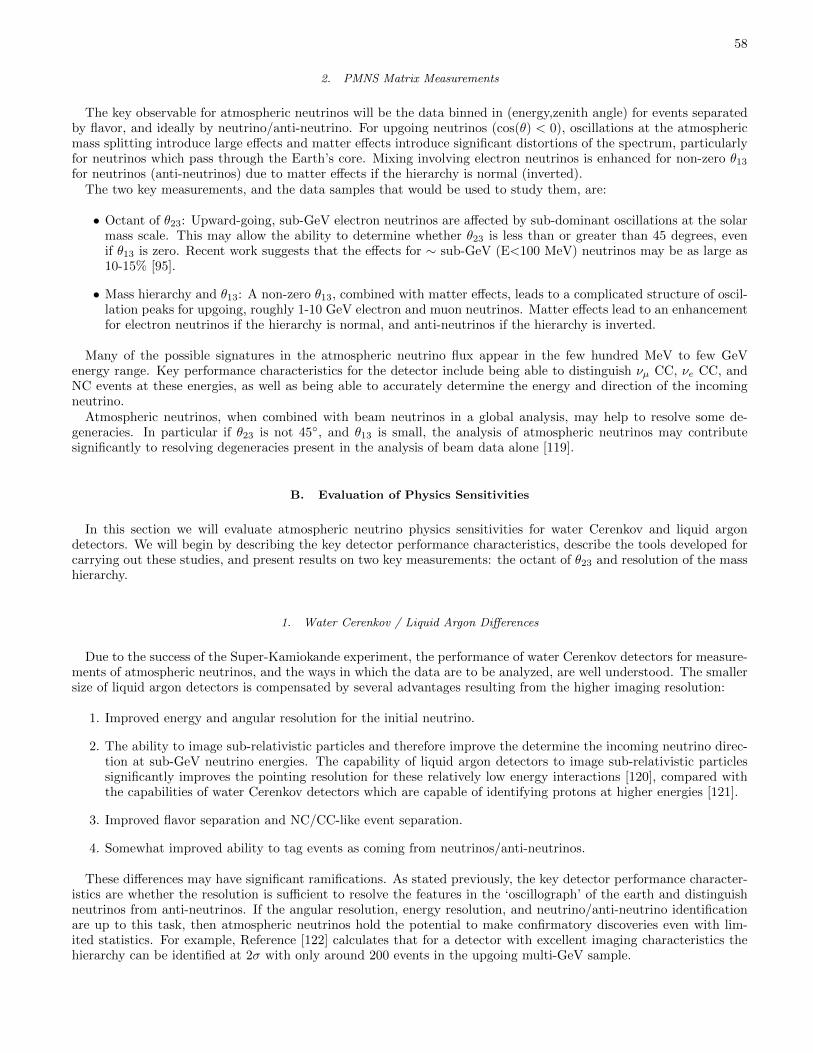
58

2. PMNS Matrix Measurements

The key observable for atmospheric neutrinos will be the data binned in (energy,zenith angle) for events separatedby flavor, and ideally by neutrino/anti-neutrino. For upgoing neutrinos (cos(θ) < 0), oscillations at the atmosphericmass splitting introduce large effects and matter effects introduce significant distortions of the spectrum, particularlyfor neutrinos which pass through the Earth’s core. Mixing involving electron neutrinos is enhanced for non-zero θ13

for neutrinos (anti-neutrinos) due to matter effects if the hierarchy is normal (inverted).The two key measurements, and the data samples that would be used to study them, are:

• Octant of θ23: Upward-going, sub-GeV electron neutrinos are affected by sub-dominant oscillations at the solarmass scale. This may allow the ability to determine whether θ23 is less than or greater than 45 degrees, evenif θ13 is zero. Recent work suggests that the effects for ∼ sub-GeV (E<100 MeV) neutrinos may be as large as10-15% [95].

• Mass hierarchy and θ13: A non-zero θ13, combined with matter effects, leads to a complicated structure of oscil-lation peaks for upgoing, roughly 1-10 GeV electron and muon neutrinos. Matter effects lead to an enhancementfor electron neutrinos if the hierarchy is normal, and anti-neutrinos if the hierarchy is inverted.

Many of the possible signatures in the atmospheric neutrino flux appear in the few hundred MeV to few GeVenergy range. Key performance characteristics for the detector include being able to distinguish νµ CC, νe CC, andNC events at these energies, as well as being able to accurately determine the energy and direction of the incomingneutrino.

Atmospheric neutrinos, when combined with beam neutrinos in a global analysis, may help to resolve some de-generacies. In particular if θ23 is not 45, and θ13 is small, the analysis of atmospheric neutrinos may contributesignificantly to resolving degeneracies present in the analysis of beam data alone [119].

B. Evaluation of Physics Sensitivities

In this section we will evaluate atmospheric neutrino physics sensitivities for water Cerenkov and liquid argondetectors. We will begin by describing the key detector performance characteristics, describe the tools developed forcarrying out these studies, and present results on two key measurements: the octant of θ23 and resolution of the masshierarchy.

1. Water Cerenkov / Liquid Argon Differences

Due to the success of the Super-Kamiokande experiment, the performance of water Cerenkov detectors for measure-ments of atmospheric neutrinos, and the ways in which the data are to be analyzed, are well understood. The smallersize of liquid argon detectors is compensated by several advantages resulting from the higher imaging resolution:

1. Improved energy and angular resolution for the initial neutrino.

2. The ability to image sub-relativistic particles and therefore improve the determine the incoming neutrino direc-tion at sub-GeV neutrino energies. The capability of liquid argon detectors to image sub-relativistic particlessignificantly improves the pointing resolution for these relatively low energy interactions [120], compared withthe capabilities of water Cerenkov detectors which are capable of identifying protons at higher energies [121].

3. Improved flavor separation and NC/CC-like event separation.

4. Somewhat improved ability to tag events as coming from neutrinos/anti-neutrinos.

These differences may have significant ramifications. As stated previously, the key detector performance character-istics are whether the resolution is sufficient to resolve the features in the ‘oscillograph’ of the earth and distinguishneutrinos from anti-neutrinos. If the angular resolution, energy resolution, and neutrino/anti-neutrino identificationare up to this task, then atmospheric neutrinos hold the potential to make confirmatory discoveries even with lim-ited statistics. For example, Reference [122] calculates that for a detector with excellent imaging characteristics thehierarchy can be identified at 2σ with only around 200 events in the upgoing multi-GeV sample.

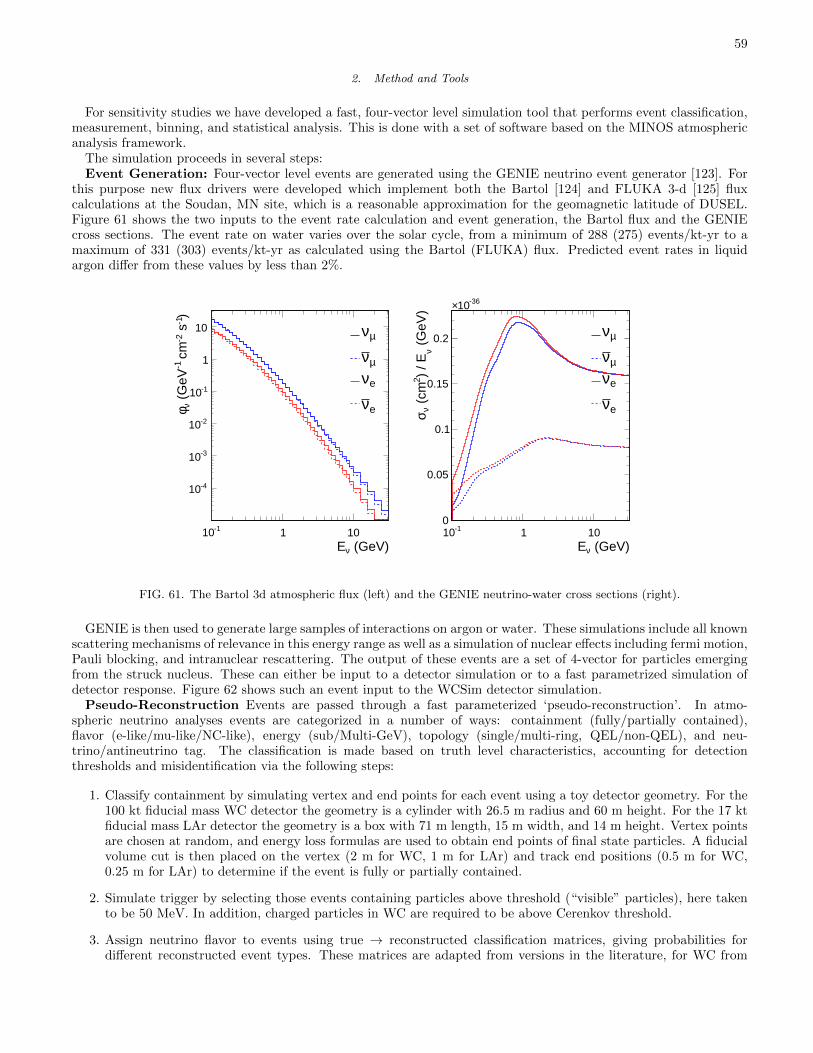
59

2. Method and Tools

For sensitivity studies we have developed a fast, four-vector level simulation tool that performs event classification,measurement, binning, and statistical analysis. This is done with a set of software based on the MINOS atmosphericanalysis framework.

The simulation proceeds in several steps:Event Generation: Four-vector level events are generated using the GENIE neutrino event generator [123]. For

this purpose new flux drivers were developed which implement both the Bartol [124] and FLUKA 3-d [125] fluxcalculations at the Soudan, MN site, which is a reasonable approximation for the geomagnetic latitude of DUSEL.Figure 61 shows the two inputs to the event rate calculation and event generation, the Bartol flux and the GENIEcross sections. The event rate on water varies over the solar cycle, from a minimum of 288 (275) events/kt-yr to amaximum of 331 (303) events/kt-yr as calculated using the Bartol (FLUKA) flux. Predicted event rates in liquidargon differ from these values by less than 2%.

(GeV)ν E

-110 1 10

) -1

s-2

cm

-1 (

GeV

νφ

-410

-310

-210

-110

1

10µν

µνeν

eν

(GeV)νE

-110 1 10

(G

eV)

ν)

/ E2

(cm

νσ

0

0.05

0.1

0.15

0.2

-3610×

µν

µνeν

eν

FIG. 61. The Bartol 3d atmospheric flux (left) and the GENIE neutrino-water cross sections (right).

GENIE is then used to generate large samples of interactions on argon or water. These simulations include all knownscattering mechanisms of relevance in this energy range as well as a simulation of nuclear effects including fermi motion,Pauli blocking, and intranuclear rescattering. The output of these events are a set of 4-vector for particles emergingfrom the struck nucleus. These can either be input to a detector simulation or to a fast parametrized simulation ofdetector response. Figure 62 shows such an event input to the WCSim detector simulation.

Pseudo-Reconstruction Events are passed through a fast parameterized ‘pseudo-reconstruction’. In atmo-spheric neutrino analyses events are categorized in a number of ways: containment (fully/partially contained),flavor (e-like/mu-like/NC-like), energy (sub/Multi-GeV), topology (single/multi-ring, QEL/non-QEL), and neu-trino/antineutrino tag. The classification is made based on truth level characteristics, accounting for detectionthresholds and misidentification via the following steps:

1. Classify containment by simulating vertex and end points for each event using a toy detector geometry. For the100 kt fiducial mass WC detector the geometry is a cylinder with 26.5 m radius and 60 m height. For the 17 ktfiducial mass LAr detector the geometry is a box with 71 m length, 15 m width, and 14 m height. Vertex pointsare chosen at random, and energy loss formulas are used to obtain end points of final state particles. A fiducialvolume cut is then placed on the vertex (2 m for WC, 1 m for LAr) and track end positions (0.5 m for WC,0.25 m for LAr) to determine if the event is fully or partially contained.

2. Simulate trigger by selecting those events containing particles above threshold (“visible” particles), here takento be 50 MeV. In addition, charged particles in WC are required to be above Cerenkov threshold.

3. Assign neutrino flavor to events using true → reconstructed classification matrices, giving probabilities fordifferent reconstructed event types. These matrices are adapted from versions in the literature, for WC from

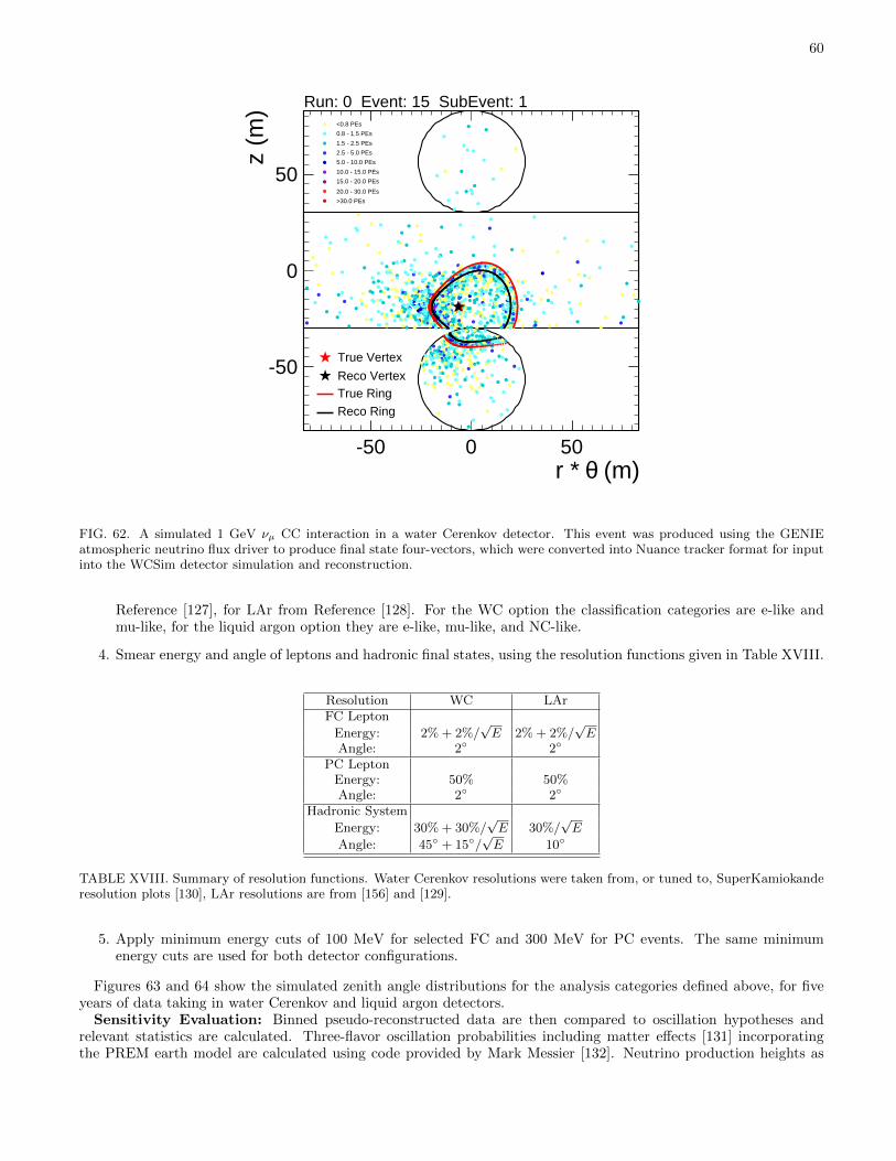
60

(m)θr * -50 0 50

z (m

)

-50

0

50

<0.8 PEs

0.8 - 1.5 PEs

1.5 - 2.5 PEs

2.5 - 5.0 PEs

5.0 - 10.0 PEs

10.0 - 15.0 PEs

15.0 - 20.0 PEs

20.0 - 30.0 PEs

>30.0 PEs

True Vertex

Reco VertexTrue Ring

Reco Ring

Run: 0 Event: 15 SubEvent: 1

FIG. 62. A simulated 1 GeV νµ CC interaction in a water Cerenkov detector. This event was produced using the GENIEatmospheric neutrino flux driver to produce final state four-vectors, which were converted into Nuance tracker format for inputinto the WCSim detector simulation and reconstruction.

Reference [127], for LAr from Reference [128]. For the WC option the classification categories are e-like andmu-like, for the liquid argon option they are e-like, mu-like, and NC-like.

4. Smear energy and angle of leptons and hadronic final states, using the resolution functions given in Table XVIII.

Resolution WC LArFC Lepton

Energy: 2% + 2%/√E 2% + 2%/

√E

Angle: 2 2

PC LeptonEnergy: 50% 50%Angle: 2 2

Hadronic System

Energy: 30% + 30%/√E 30%/

√E

Angle: 45 + 15/√E 10

TABLE XVIII. Summary of resolution functions. Water Cerenkov resolutions were taken from, or tuned to, SuperKamiokanderesolution plots [130], LAr resolutions are from [156] and [129].

5. Apply minimum energy cuts of 100 MeV for selected FC and 300 MeV for PC events. The same minimumenergy cuts are used for both detector configurations.

Figures 63 and 64 show the simulated zenith angle distributions for the analysis categories defined above, for fiveyears of data taking in water Cerenkov and liquid argon detectors.

Sensitivity Evaluation: Binned pseudo-reconstructed data are then compared to oscillation hypotheses andrelevant statistics are calculated. Three-flavor oscillation probabilities including matter effects [131] incorporatingthe PREM earth model are calculated using code provided by Mark Messier [132]. Neutrino production heights as

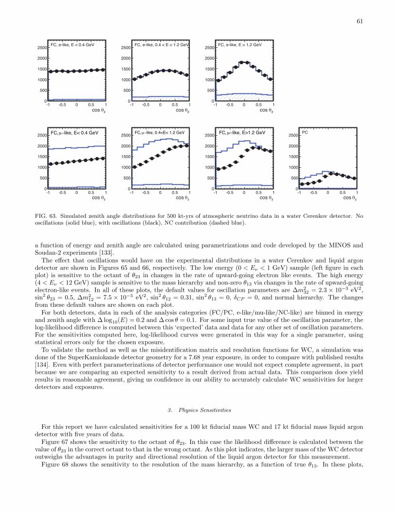
61

zθcos -1 -0.5 0 0.5 1

0

500

1000

1500

2000

2500FC, e-like, E < 0.4 GeV

zθcos -1 -0.5 0 0.5 1

0

500

1000

1500

2000

2500FC, e-like, 0.4 < E < 1.2 GeV

zθcos -1 -0.5 0 0.5 1

0

500

1000

1500

2000

2500FC, e-like, E > 1.2 GeV

zθcos -1 -0.5 0 0.5 1

0

500

1000

1500

2000

2500, E < 0.4 GeVFC,

zθcos -1 -0.5 0 0.5 1

0

500

1000

1500

2000

2500-like, 0.4 < E < 1.2 GeVFC,

zθcos -1 -0.5 0 0.5 1

0

500

1000

1500

2000

2500-like, E > 1.2 GeVFC,

zθcos -1 -0.5 0 0.5 1

0

500

1000

1500

2000

2500PCFC, μ−like, E< 0.4 GeV FC, μ−like, 0.4<E< 1.2 GeV FC, μ−like, E>1.2 GeV

FIG. 63. Simulated zenith angle distributions for 500 kt-yrs of atmospheric neutrino data in a water Cerenkov detector. Nooscillations (solid blue), with oscillations (black), NC contribution (dashed blue).

a function of energy and zenith angle are calculated using parametrizations and code developed by the MINOS andSoudan-2 experiments [133].

The effect that oscillations would have on the experimental distributions in a water Cerenkov and liquid argondetector are shown in Figures 65 and 66, respectively. The low energy (0 < Eν < 1 GeV) sample (left figure in eachplot) is sensitive to the octant of θ23 in changes in the rate of upward-going electron like events. The high energy(4 < Eν < 12 GeV) sample is sensitive to the mass hierarchy and non-zero θ13 via changes in the rate of upward-goingelectron-like events. In all of these plots, the default values for oscillation parameters are ∆m2

32 = 2.3 × 10−3 eV2,sin2 θ23 = 0.5, ∆m2

12 = 7.5 × 10−5 eV2, sin2 θ12 = 0.31, sin2 θ13 = 0, δCP = 0, and normal hierarchy. The changesfrom these default values are shown on each plot.

For both detectors, data in each of the analysis categories (FC/PC, e-like/mu-like/NC-like) are binned in energyand zenith angle with ∆ log10(E) = 0.2 and ∆ cos θ = 0.1. For some input true value of the oscillation parameter, thelog-likelihood difference is computed between this ‘expected’ data and data for any other set of oscillation parameters.For the sensitivities computed here, log-likelihood curves were generated in this way for a single parameter, usingstatistical errors only for the chosen exposure.

To validate the method as well as the misidentification matrix and resolution functions for WC, a simulation wasdone of the SuperKamiokande detector geometry for a 7.68 year exposure, in order to compare with published results[134]. Even with perfect parameterizations of detector performance one would not expect complete agreement, in partbecause we are comparing an expected sensitivity to a result derived from actual data. This comparison does yieldresults in reasonable agreement, giving us confidence in our ability to accurately calculate WC sensitivities for largerdetectors and exposures.

3. Physics Sensitivities

For this report we have calculated sensitivities for a 100 kt fiducial mass WC and 17 kt fiducial mass liquid argondetector with five years of data.

Figure 67 shows the sensitivity to the octant of θ23. In this case the likelihood difference is calculated between thevalue of θ23 in the correct octant to that in the wrong octant. As this plot indicates, the larger mass of the WC detectoroutweighs the advantages in purity and directional resolution of the liquid argon detector for this measurement.

Figure 68 shows the sensitivity to the resolution of the mass hierarchy, as a function of true θ13. In these plots,

62

zθcos -1 -0.5 0 0.5 1

0

100

200

300

400FC, e-like, E < 0.4 GeV

zθcos -1 -0.5 0 0.5 1

0

100

200

300

400FC, e-like, 0.4 < E < 1.2 GeV

zθcos -1 -0.5 0 0.5 1

0

100

200

300

400FC, e-like, E > 1.2 GeV

zθcos -1 -0.5 0 0.5 1

0

100

200

300

400-like, E < 0.4 GeVµFC,

zθcos -1 -0.5 0 0.5 1

0

100

200

300

400-like, 0.4 < E < 1.2 GeVµFC,

zθcos -1 -0.5 0 0.5 1

0

100

200

300

400-like, E > 1.2 GeVµFC,

zθcos -1 -0.5 0 0.5 1

0

100

200

300

400PC

zθcos -1 -0.5 0 0.5 1

0

100

200

300

400NC-like, E < 0.4 GeV

zθcos -1 -0.5 0 0.5 1

0

100

200

300

400NC-like, 0.4 < E < 1.2 GeV

zθcos -1 -0.5 0 0.5 1

0

100

200

300

400NC-like, E > 1.2 GeV

FIG. 64. Simulated zenith angle distributions for 85 kt-yrs of atmospheric neutrino data in a liquid argon detector. Nooscillations (solid blue), with oscillations (black), NC contribution (dashed blue).

normal mass hierarchy corresponds to positive values, inverted hierarchy to negative values. One feature to note is thatboth technologies have a weak sensitivity to the sign of the mass hierarchy even for θ13 = 0, resulting from interferencebetween oscillations at the solar and atmospheric mass scales. For either technology it is easier to resolve a normalmass hierarchy, since resonant matter effects occur for neutrinos rather than anti-neutrinos, with larger interactioncross sections. For the resolution of the mass hierarchy, the larger mass of the WC detector is again the dominantfactor. In future revisions we will explore in more depth the different capabilities of the detector technologies fordistinguishing neutrinos from anti-neutrinos, which may provide an additional compensating factor for liquid argon.

C. Comments on Configuration Options

Configuration options that are designed primarily to improve capabilities for lower energy neutrinos are not expectedto have a significant effect on the study of atmospheric neutrinos. These include having gadolinium in a water Cerenkovdetector, or including a photon trigger for an atmospheric neutrino detector.

The two options for phototube coverage are also expected to have minimal impact on the atmospheric neutrinoanalysis. Since the Super-K data sets included periods where the photodetector coverage was lower (Super-K–II),many studies were done on the differences in detection efficiency and measurement resolution for atmospheric neutrinoswhen comparing the Super-K–I and II detector configurations. These studies [130] indicate that the differences are

63

Zθcos -1 -0.5 0 0.5 1

0

200

400

600

800

1000

1200

1400

1600

FC e-like (0<E<1GeV)No Oscillations

= 0.523θ2sin = 0.423θ2sin = 0.623θ2sin

Zθcos -1 -0.5 0 0.5 1

0

50

100

150

200

250


= 0.013θ2sin = 0.04 (NH)13θ2sin = 0.04 (IH)13θ2sin

FIG. 65. Zenith angle distributions for a low energy (left) and high energy (right) WC e-like data sample. Oscillation parametervalues are given in the text.

Zθcos -1 -0.5 0 0.5 1

0

50

100

150

200


= 0.523θ2sin = 0.423θ2sin = 0.623θ2sin

Zθcos -1 -0.5 0 0.5 1

0

10

20

30


= 0.013θ2sin = 0.04 (NH)13θ2sin = 0.04 (IH)13θ2sin

FIG. 66. Zenith angle distributions for a low energy (left) and high energy (right) liquid argon e-like data sample. Oscillationparameter values are given in the text.

small as far as atmospheric neutrino analyses are concerned, and for the conclusions here we are considering them tobe a relatively small perturbation.

Configuration options that involve placing a liquid argon detector at shallow depths will require more study, but itappears at this time that the analysis and conclusions of [128] which studies cosmogenic backgrounds to proton decayare also directly for atmospheric neutrinos. The veto shield, as proposed, follows the conclusions of this study andshould therefore provide sufficient information to work at the depth of 800 ft with a 17 kt analysis fiducial volume,which is the fiducial volume assumed in the studies mentioned previously, and is the fiducial volume available at4850 ft.

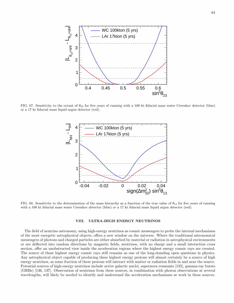
64

23θ2sin0.4 0.45 0.5 0.55 0.6

|/4π>

23θ -

L/4π<

23θ|L

0

1

2

3

4WC 100kton (5 yrs)

LAr 17kton (5 yrs)

FIG. 67. Sensitivity to the octant of θ23 for five years of running with a 100 kt fiducial mass water Cerenkov detector (blue)or a 17 kt fiducial mass liquid argon detector (red).

13θ2) sin232m∆sign(

-0.04 -0.02 0 0.02 0.04

|IH

- L

NH

|L

0

1

2

3

4 WC 100kton (5 yrs)

LAr 17kton (5 yrs)

FIG. 68. Sensitivity to the determination of the mass hierarchy as a function of the true value of θ13 for five years of runningwith a 100 kt fiducial mass water Cerenkov detector (blue) or a 17 kt fiducial mass liquid argon detector (red).

VIII. ULTRA-HIGH ENERGY NEUTRINOS

The field of neutrino astronomy, using high-energy neutrinos as cosmic messengers to probe the internal mechanismsof the most energetic astrophysical objects, offers a new window on the universe. Where the traditional astronomicalmessengers of photons and charged particles are either absorbed by material or radiation in astrophysical environmentsor are deflected into random directions by magnetic fields, neutrinos, with no charge and a small interaction crosssection, offer an unobstructed view inside the acceleration regions where the highest energy cosmic rays are created.The source of these highest energy cosmic rays still remains as one of the long-standing open questions in physics.Any astrophysical object capable of producing these highest energy protons will almost certainly be a source of highenergy neutrinos, as some fraction of these protons will interact with matter or radiation fields in and near the source.Potential sources of high-energy neutrinos include active galactic nuclei, supernova remnants [135], gamma-ray bursts(GRBs) [136, 137]. Observation of neutrinos from these sources, in combination with photon observations at severalwavelengths, will likely be needed to identify and understand the acceleration mechanisms at work in these sources.

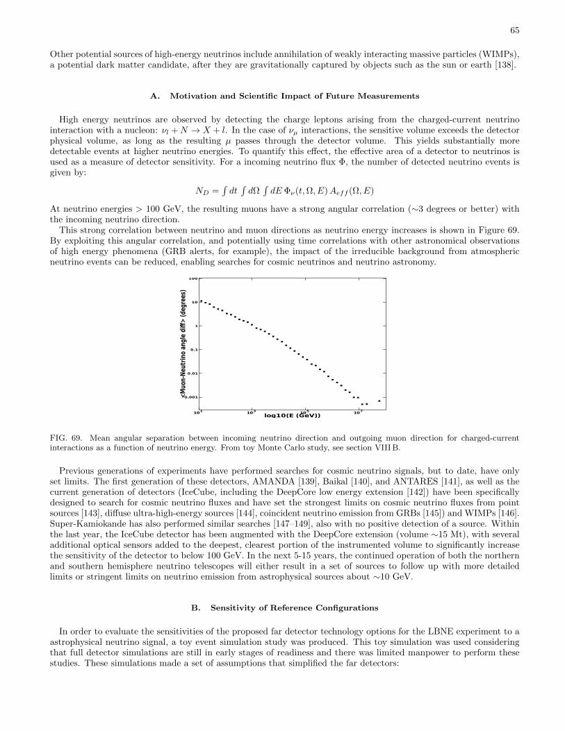
65

Other potential sources of high-energy neutrinos include annihilation of weakly interacting massive particles (WIMPs),a potential dark matter candidate, after they are gravitationally captured by objects such as the sun or earth [138].


High energy neutrinos are observed by detecting the charge leptons arising from the charged-current neutrinointeraction with a nucleon: νl +N → X + l. In the case of νµ interactions, the sensitive volume exceeds the detectorphysical volume, as long as the resulting µ passes through the detector volume. This yields substantially moredetectable events at higher neutrino energies. To quantify this effect, the effective area of a detector to neutrinos isused as a measure of detector sensitivity. For a incoming neutrino flux Φ, the number of detected neutrino events isgiven by:

ND =∫dt∫dΩ∫dE Φν(t,Ω, E)Aeff (Ω, E)

At neutrino energies > 100 GeV, the resulting muons have a strong angular correlation (∼3 degrees or better) withthe incoming neutrino direction.

This strong correlation between neutrino and muon directions as neutrino energy increases is shown in Figure 69.By exploiting this angular correlation, and potentially using time correlations with other astronomical observationsof high energy phenomena (GRB alerts, for example), the impact of the irreducible background from atmosphericneutrino events can be reduced, enabling searches for cosmic neutrinos and neutrino astronomy.

log10(E (GeV))

<M

uon

-Neu

trin

o a

ng

le d

iff>

(d

eg

rees)

101

103

105

107

0.001

0.01

0.1

1

10

100

FIG. 69. Mean angular separation between incoming neutrino direction and outgoing muon direction for charged-currentinteractions as a function of neutrino energy. From toy Monte Carlo study, see section VIII B.

Previous generations of experiments have performed searches for cosmic neutrino signals, but to date, have onlyset limits. The first generation of these detectors, AMANDA [139], Baikal [140], and ANTARES [141], as well as thecurrent generation of detectors (IceCube, including the DeepCore low energy extension [142]) have been specificallydesigned to search for cosmic neutrino fluxes and have set the strongest limits on cosmic neutrino fluxes from pointsources [143], diffuse ultra-high-energy sources [144], coincident neutrino emission from GRBs [145]) and WIMPs [146].Super-Kamiokande has also performed similar searches [147–149], also with no positive detection of a source. Withinthe last year, the IceCube detector has been augmented with the DeepCore extension (volume ∼15 Mt), with severaladditional optical sensors added to the deepest, clearest portion of the instrumented volume to significantly increasethe sensitivity of the detector to below 100 GeV. In the next 5-15 years, the continued operation of both the northernand southern hemisphere neutrino telescopes will either result in a set of sources to follow up with more detailedlimits or stringent limits on neutrino emission from astrophysical sources about ∼10 GeV.


In order to evaluate the sensitivities of the proposed far detector technology options for the LBNE experiment to aastrophysical neutrino signal, a toy event simulation study was produced. This toy simulation was used consideringthat full detector simulations are still in early stages of readiness and there was limited manpower to perform thesestudies. These simulations made a set of assumptions that simplified the far detectors:

66

• The detector fiducial volumes were modeled as spheres with radii producing the same volumes as referenceconfigurations. The detector cross-sectional areas were reproduced to within ∼20%.

• Detectors were assumed to be fully efficient at triggering and reconstructing any muon track within the modeledfiducial volumes for muon energies > 100 MeV.

• Variations in detector technology choices (depth, Gd loading, PMT coverage) are neglected in this study, butdo not greatly impact detection of muons with E > 100 MeV.

• Backgrounds from misreconstructed atmospheric muons and atmospheric neutrinos have not been included.

These should be included in future studies aimed to produce more accurate sensitivities.As part of this simulation, 1 GeV–100 PeV neutrinos were propagated through the earth and weighted based on

interaction probability. Both charged-current and neutral-current interactions are included. Any resulting muonsare propagated until they range out, with special focus on the region surrounding the detector volume. Events thatproduced a muon of sufficient energy within the modeled detectors were counted and used to calculate the detectorneutrino effective areas as a function of energy. The effective areas obtained from this toy simulation are shown inFigure 70 for a 100 kt water cherenkov detector and the 17 kt liquid argon detectors. More details of these simulationsare available in a UHE TG call presentation [150]

This toy simulation tool was also applied to an IceCube-like detector (detector radius of 500 m and muon detectionthreshold of 20 GeV). From this simulation, effective areas and events rates that agree with current sensitivities ofthe IceCube detector were obtained, verifying the approximations made and event rates obtained to an accuracy ofroughly a factor of 2-3.

0 1 2 3 4 5 6 7 8log10(E/Gev)

10-8

10-7

10-6

10-5

10-4

10-3

10-2

10-1

100

101

Aeff

[m^

2]

100 kT WC Effective Area17 kT LAr Effective Area

FIG. 70. 100 kt water cherenkov(WC) and 17 kt Liquid Argon (LAr) effective areas as a function of neutrino energy from thetoy simulation. For comparison, the IceCube effective area at 1 TeV is ∼1 m2.

To evaluate the sensitivity of these detector to predicted astrophysical neutrino fluxes, three test cases whereselected:

1. A generic E−2 point source in the northern hemisphere with a flux roughly equal to the current ANTARESpoint source sensitivity ( dNdEe = 5 × 10−8E−2[GeV −1 cm−2sec−1]) [151]

2. 150 gamma-ray bursts with a neutrino fluence from the Waxman-Bahcall fireball model [136]

3. 100 GeV mass WIMP annihilation at the Galactic Center (GC). This portion of the study is still a work inprogress. Results to be updated soon. [152]

Predicted event rates are produced by convolving the neutrino effective area for each detector with the predictedneutrino flux. The predicted event rates per year are summarized in Table XIX and can be appropriately scaled to thenumber of detectors of each type under consideration. Even with these smaller detector volumes, it should be notedthat the most probably neutrino energy detected is ∼10 TeV, as shown in Fig. 71, the “sweet spot” when convolvinga falling neutrino spectrum with the rise in neutrino effective area.

67

(1) Point source (2)100 WB GRB (3) GC WIMPs100 kt WC 0.7 0.07 TBD17 kt LAr 0.2 0.02 TBD

Toy IceCube 214 18 ∼10s

TABLE XIX. Predicted number of events per year for 3 studied astrophysical sources. Event rates in 1, 2 or 3 of each detectortechnology can be obtained by multiplication of numbers by Ndetector for each type.

0 1 2 3 4 5 6 7 8log10(E/Gev)

0.000

0.005

0.010

0.015

0.020

0.025

0.030

0.035Nu

mbe

r of e

vent

s/G

eVWCLAr

FIG. 71. Energy distribution for detected events from a hypothetical point source with an E−2 spectrum. For both WC andLAr, the mean energy predicted is ∼10 TeV.

C. Next Steps

One item still needs to be completed as part of this study:

• Finish the calculation of expected neutrino rates from the galactic center for 100-GeV WIMPs. This WIMPmass is likely the best chance for an significant impact, given them threshold of the larger neutrino observatories,but rates are still expected to be small.

D. Conclusions

While somewhat simple in nature, this preliminary study of astrophysical neutrino fluxes in the proposed LBNE fardetector technology options indicates that neither 100-300 kt of water cherenkov detector or 17-51 kt of Liquid Argonare optimal detectors for these neutrino signals. Predicted event rates in the proposed detector geometries are notcompetitive with the operating generation of neutrino telescopes. There is a slight advantage for the water-cherenkovoptions in terms of predicted event rates, based on the larger detector cross-sectional area for muon detection, butthis difference is small, and should not be over-emphasized.

This study should not prevent the investigation of astrophysical neutrinos signals in the operating detectors. Pur-suing searches that search for signals at the edge of detector capabilities ensure that background sensitivities (in thiscase, to atmospheric neutrinos) are very well understood and provide an excellent learning opportunities for students.

68

IX. SOLAR NEUTRINOS


Even after the long standing mystery of missing solar neutrinos [153] was explained by data from the Super-Kamiokande and SNO [154] experiments as flavor transformation of solar neutrinos, there are still interesting openquestions in solar neutrino physics. Some of these are astrophysical (like a measurement of the fraction of energyproduction via CNO cycle in the sun, or flux variations due to helio-seismological modes which reach the solar core, orlong-term stability of the solar core temperature). But even particle physics questions remain. Can the MSW modelexplain the amount of flavor transformation as a function of energy, or are non-standard neutrino interactions required?Do solar neutrinos and reactor anti-neutrinos oscillate with the same parameters? Some of these questions will beanswered by experimental data in the immediate future (like SNO+, KamLAND solar phase, further Borexino data,etc.), but high statistics measurements will be necessary to further constrain alternatives to the standard oscillationscenario. Either a large water Cherenkov detector, or a large liquid Argon detector, or a large liquid scintillationdetector offers unique possibilities to study these questions.


Using event selection and reconstruction efficiency similar to Super-Kamiokande, a 300 kt water Cherenkov detectorat DUSEL would collect 470,000 recoil electrons (after selection efficiency) in ten years from 8B solar neutrinos above7 MeV. It could trace the MSW flavor transformation curve with high precision (the uncertainties of 0.5 MeV-wideenergy bins range from 0.3% to 3%) and should be sensitive to the change in flavor transformation due to the earth’smatter density which leads to the so-called day/night effect, the asymmetry ADN = D−N

0.5(D+N) between the event rates

during the day (= D) and night (= N). This asymmetry is expected to be only 1.5 to 2% [155]; it would be measuredby a 300 kt water Cherenkov detector to 0.3% statistical uncertainty thereby constraining ∆m2

solar, which is largewhen measured by solar neutrinos only. This uncertainty is unlikely to improve otherwise, since future low energysolar neutrino measurements cannot constrain it. It is also interesting since a deviation in this parameter betweensolar neutrinos and reactor anti-neutrinos cannot be reconciled by three-flavor mixing effects (like the mixing angle).

Obviously, sparser instrumentation of this 300 kt water Cherenkov detector immediately worsens its sensitivity tosolar neutrinos. Not only will the energy threshold increase, but also the energy resolution and therefore backgroundcontamination worsens. Super-Kamiokande-II demonstrated solar neutrino measurements in a large water Cherenkovdetector with ∼ 3 photo-electrons per MeV with a threshold of 7 MeV. Radioactive background from radon decaysfluctuated above this threshold and contaminated the ∼ 7, 200 solar neutrino events collected. The statistical uncer-tainty of the day/night asymmetry increased to 4.2% from the expected 2.4%. As a conservative estimate, we canexpect the statistical accuracy of the day/night asymmetry measured by a 300 kt water Cherenkov detector to reach0.6% after ten years, if it collects only 3 photo-electrons per MeV. Super-Kamiokande (if it runs continuously untilthen) will have reached ∼ 0.75% at that time.

The solar neutrino physics potential of a 17 kt liquid Argon TPC largely depends on the energy threshold and depth.Since the spallation of the 40Ar (a rather complex nucleus compared to 16O) is likely to produce many long-livedspallation products, only a TPC at the deepest location has a reasonable chance of detecting solar neutrinos. Givena 10 MeV neutrino energy threshold (as reported by the ICARUS collaboration [156]), it could then measure theCC/NC ratio of 8B solar neutrinos with high statistical accuracy and thereby test the MSW flavor transformationcurve with high precision if the detector itself has low radioactivity levels.

The main advantage of a large, clean liquid scintillator detector is its ability to measure low energy solar neutrinosas well. Borexino has demonstrated an energy threshold of 3 MeV for 8B solar neutrinos. Since DUSEL is deepunderground. A large, clean liquid scintillator detector could precisely measure the pep flux (constraining the solarmixing angle to 1%), measure the CNO fluxes and test the MSW flavor transformation curve where it transitionsfrom the vacuum oscillation expectation.

C. Conclusions

Even after several decades of solar 8B neutrino experiments, the LBNE detector at DUSEL has the potential tomake unique precision measurements. For the water Cherenkov option, the full potential is only reached with ahigh density photo-sensor instrumentation yielding at least ∼ 6 photo-electrons per MeV. A large liquid argon TPCwill only impact solar neutrino physics, if the threshold is kept low and the detector is build with state-of-the art

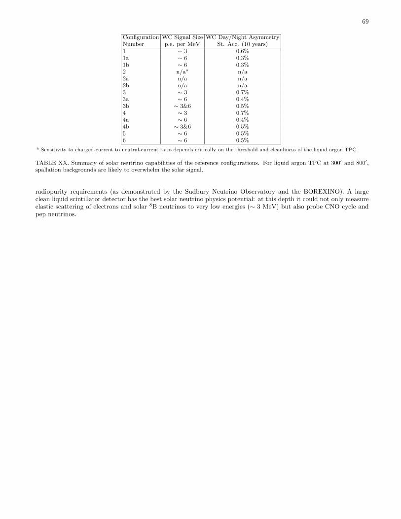
69

Configuration WC Signal Size WC Day/Night AsymmetryNumber p.e. per MeV St. Acc. (10 years)1 ∼ 3 0.6%1a ∼ 6 0.3%1b ∼ 6 0.3%2 n/aa n/a2a n/a n/a2b n/a n/a3 ∼ 3 0.7%3a ∼ 6 0.4%3b ∼ 3&6 0.5%4 ∼ 3 0.7%4a ∼ 6 0.4%4b ∼ 3&6 0.5%5 ∼ 6 0.5%6 ∼ 6 0.5%

a Sensitivity to charged-current to neutral-current ratio depends critically on the threshold and cleanliness of the liquid argon TPC.

TABLE XX. Summary of solar neutrino capabilities of the reference configurations. For liquid argon TPC at 300′ and 800′,spallation backgrounds are likely to overwhelm the solar signal.

radiopurity requirements (as demonstrated by the Sudbury Neutrino Observatory and the BOREXINO). A largeclean liquid scintillator detector has the best solar neutrino physics potential: at this depth it could not only measureelastic scattering of electrons and solar 8B neutrinos to very low energies (∼ 3 MeV) but also probe CNO cycle andpep neutrinos.

70

X. GEONEUTRINOS AND REACTOR NEUTRINOS

Within the earth it is believed that radioactive decays of uranium and thorium are the most significant source ofheat that causes mantle convection, the fundamental geological process that regulates the thermal evolution of theearth and shapes its surface. Until recently, estimates of the total uranium and thorium content of the earth wereinferred from earth formation models. However, it has been known for a long time that the uranium and thoriumdecays produce electron anti-neutrinos, so-called geo-neutrinos, and the detection of these geo-neutrinos near thesurface of the earth can directly inform us of the deep earth uranium and thorium content. The low flux of electronanti-neutrinos from reactors, so called reactor neutrinos, at DUSEL makes it ideal for demonstrating the ability offuture large detectors designed for long range nuclear reactor monitoring.


The geo-neutrino flux observed near the surface of the earth has a contribution from uranium and thorium in thecrust and mantle. For detectors located in continental crust approximately 80% of the signal comes from the crust,with the remainder coming from the mantle. Without the ability to determine the origin of the observed geo-neutrinos,it is not possible to determine the relative contribution from the crust and mantle with a single detector. However,with accurate knowledge of the uranium and thorium content in the crust surrounding DUSEL with approximately200 km, it should be possible to determine the geo-neutrino contribution from the mantle although this requires higherprecision due to the small fraction coming from the mantle.

KamLAND and BOREXINO have currently observed total geo-neutrinos fluxes with sensitivities limited by statis-tics to approximately 30%, this sensitivity will improve only slightly with more time. The SNO+ experiment, which iscurrently under construction, should be able to measure the total geo-neutrino flux to a sensitivity of approximately20%. Because of the low reactor neutrino flux and the large size, a detector at DUSEL would be able to measure thegeo-neutrino flux to approximately 5% (limited by systematic errors) in 1 year. This should also allow for a relativelyaccurate measurement of the mantle geo-neutrino contribution with detailed knowledge of the local uranium andthorium crustal geo-neutrino contribution.

There are two other large geo-neutrino detectors proposed. The LENA detector would be competitive with a largedetector at DUSEL, while the Hanohano detector would be complementary, as it would directly probe the mantle, socombination with a detector on the crust would determine the crustal contribution.

Aside from measuring the total uranium and thorium flux, it is predicted that the ratio of the Th/U abundanceratio in the earth is about 4/1, and measuring deviations from this value could inform us on the processing of thecrustal material. Because this is a ratio, accurate measurement of this requires a larger detector than KamLAND,BOREXINO, or SNO+.

Although the flux of reactor neutrinos at DUSEL is about 24 times smaller than that at KamLAND, with a detectormore than 24 times as large it should be possible to observe more reactor neutrinos. The advantage of DUSEL isthat the nuclear reactors are located further away, resulting in more neutrino oscillation “wiggles” in the energyspectrum. With sufficient energy resolution it might be possible to measure the neutrino mixing parameter ∆m2

12 toapproximately 1%, an improvement upon the 3% accuracy achieved with KamLAND.


In a water Cherenkov detector electron anti-neutrinos can be detected by neutron inverse-beta-decay

νe + p→ n+ e+ (4)

The positrons energy is equal to the antineutrinos energy minus 1.8 MeV. The maximum energy for geo-neutrinos is3.3 MeV, although the peak in the signal is at 2.3 MeV, this results in positrons with a peak energy of 0.5 MeV anda maximum of 1.5 MeV, making it impossible to detect with a water Cherenkov detector even with the addition ofgadolinium and high photocathode coverage. The energy of reactor neutrinos extends up to approximately 9 MeVmaking it possible to detect them with a water Cherenkov detector, however all configurations would have energyresolution below 5%/

√E[MeV], which would wash out the oscillation spectrum, limiting the measurement to a total

flux measurement.In a liquid Ar detector electron anti-neutrinos can be detected by Ar inverse-beta-decay

νe +40 Ar →40 Cl∗ + e+ (5)

71

The threshold for this reaction is approximately 8.5 MeV, which means that it cannot be used to detect either geo-neutrinos or reactor neutrinos. There are also elastic scattering reactions; however, these are sensitive to neutrinos aswell as antineutrinos, so in order to eliminate backgrounds from solar neutrinos we need to be able to reject these bypointing at a level better than one in a thousand. At these low energies this is probably not possible with a liquid Ardetector.

C. Conclusions

The science case for detecting geo-neutrinos is very strong, it is somewhat weaker for detecting reactor neutrinos.However, it is likely not possible that these can be detected with any of the LBNE reference detector configurations,although it may be possible with a large liquid scintillator detector.

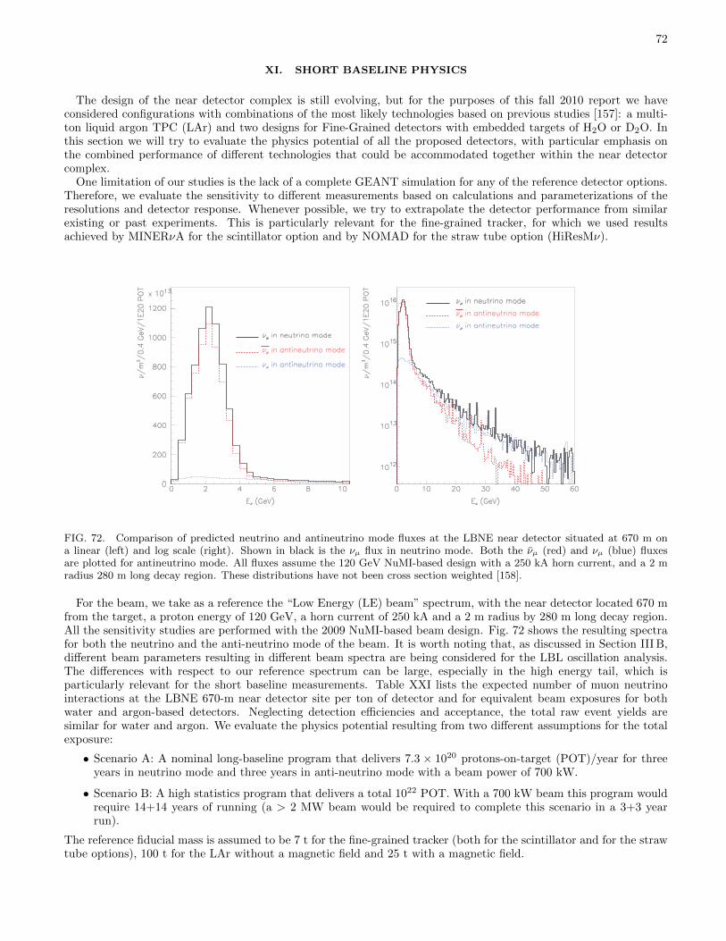
72

XI. SHORT BASELINE PHYSICS

The design of the near detector complex is still evolving, but for the purposes of this fall 2010 report we haveconsidered configurations with combinations of the most likely technologies based on previous studies [157]: a multi-ton liquid argon TPC (LAr) and two designs for Fine-Grained detectors with embedded targets of H2O or D2O. Inthis section we will try to evaluate the physics potential of all the proposed detectors, with particular emphasis onthe combined performance of different technologies that could be accommodated together within the near detectorcomplex.

One limitation of our studies is the lack of a complete GEANT simulation for any of the reference detector options.Therefore, we evaluate the sensitivity to different measurements based on calculations and parameterizations of theresolutions and detector response. Whenever possible, we try to extrapolate the detector performance from similarexisting or past experiments. This is particularly relevant for the fine-grained tracker, for which we used resultsachieved by MINERνA for the scintillator option and by NOMAD for the straw tube option (HiResMν).

FIG. 72. Comparison of predicted neutrino and antineutrino mode fluxes at the LBNE near detector situated at 670 m ona linear (left) and log scale (right). Shown in black is the νµ flux in neutrino mode. Both the νµ (red) and νµ (blue) fluxesare plotted for antineutrino mode. All fluxes assume the 120 GeV NuMI-based design with a 250 kA horn current, and a 2 mradius 280 m long decay region. These distributions have not been cross section weighted [158].

For the beam, we take as a reference the “Low Energy (LE) beam” spectrum, with the near detector located 670 mfrom the target, a proton energy of 120 GeV, a horn current of 250 kA and a 2 m radius by 280 m long decay region.All the sensitivity studies are performed with the 2009 NuMI-based beam design. Fig. 72 shows the resulting spectrafor both the neutrino and the anti-neutrino mode of the beam. It is worth noting that, as discussed in Section III B,different beam parameters resulting in different beam spectra are being considered for the LBL oscillation analysis.The differences with respect to our reference spectrum can be large, especially in the high energy tail, which isparticularly relevant for the short baseline measurements. Table XXI lists the expected number of muon neutrinointeractions at the LBNE 670-m near detector site per ton of detector and for equivalent beam exposures for bothwater and argon-based detectors. Neglecting detection efficiencies and acceptance, the total raw event yields aresimilar for water and argon. We evaluate the physics potential resulting from two different assumptions for the totalexposure:

• Scenario A: A nominal long-baseline program that delivers 7.3 × 1020 protons-on-target (POT)/year for threeyears in neutrino mode and three years in anti-neutrino mode with a beam power of 700 kW.

• Scenario B: A high statistics program that delivers a total 1022 POT. With a 700 kW beam this program wouldrequire 14+14 years of running (a > 2 MW beam would be required to complete this scenario in a 3+3 yearrun).

The reference fiducial mass is assumed to be 7 t for the fine-grained tracker (both for the scintillator and for the strawtube options), 100 t for the LAr without a magnetic field and 25 t with a magnetic field.

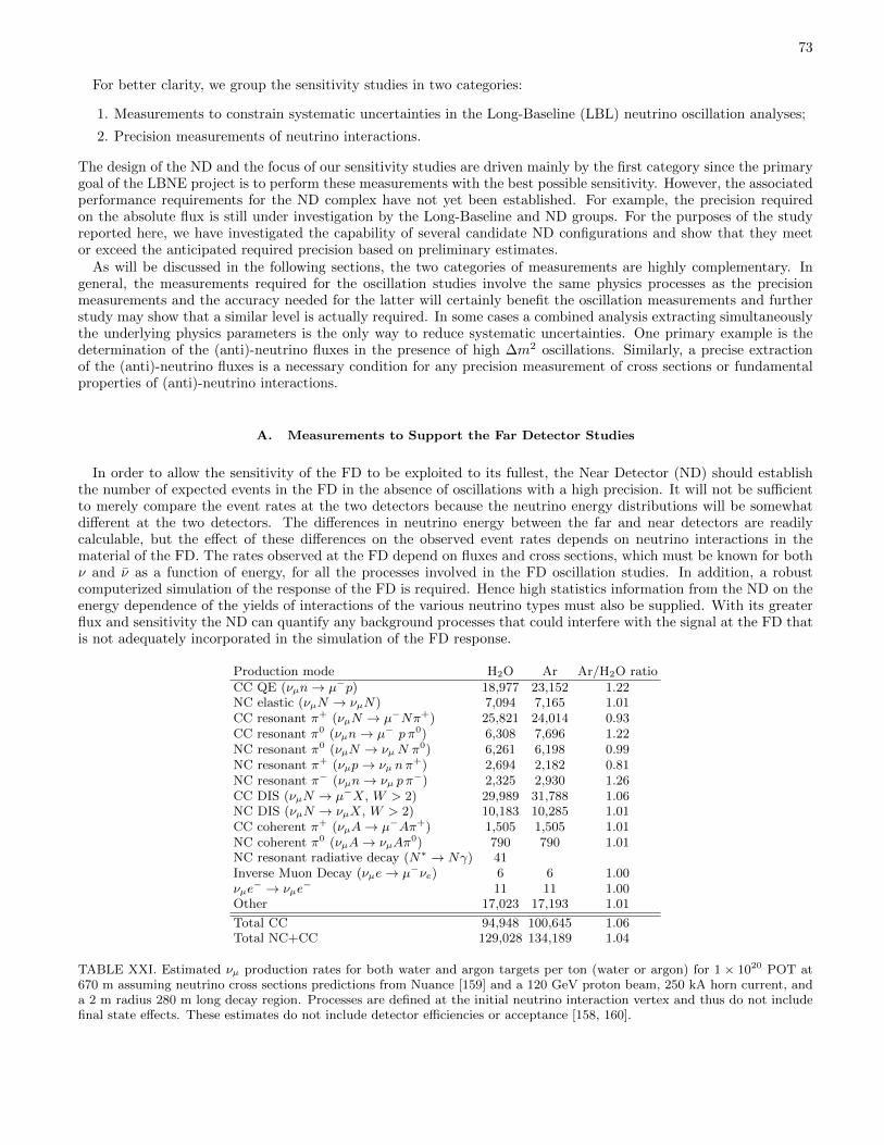
73

For better clarity, we group the sensitivity studies in two categories:

1. Measurements to constrain systematic uncertainties in the Long-Baseline (LBL) neutrino oscillation analyses;

2. Precision measurements of neutrino interactions.

The design of the ND and the focus of our sensitivity studies are driven mainly by the first category since the primarygoal of the LBNE project is to perform these measurements with the best possible sensitivity. However, the associatedperformance requirements for the ND complex have not yet been established. For example, the precision requiredon the absolute flux is still under investigation by the Long-Baseline and ND groups. For the purposes of the studyreported here, we have investigated the capability of several candidate ND configurations and show that they meetor exceed the anticipated required precision based on preliminary estimates.

As will be discussed in the following sections, the two categories of measurements are highly complementary. Ingeneral, the measurements required for the oscillation studies involve the same physics processes as the precisionmeasurements and the accuracy needed for the latter will certainly benefit the oscillation measurements and furtherstudy may show that a similar level is actually required. In some cases a combined analysis extracting simultaneouslythe underlying physics parameters is the only way to reduce systematic uncertainties. One primary example is thedetermination of the (anti)-neutrino fluxes in the presence of high ∆m2 oscillations. Similarly, a precise extractionof the (anti)-neutrino fluxes is a necessary condition for any precision measurement of cross sections or fundamentalproperties of (anti)-neutrino interactions.

A. Measurements to Support the Far Detector Studies

In order to allow the sensitivity of the FD to be exploited to its fullest, the Near Detector (ND) should establishthe number of expected events in the FD in the absence of oscillations with a high precision. It will not be sufficientto merely compare the event rates at the two detectors because the neutrino energy distributions will be somewhatdifferent at the two detectors. The differences in neutrino energy between the far and near detectors are readilycalculable, but the effect of these differences on the observed event rates depends on neutrino interactions in thematerial of the FD. The rates observed at the FD depend on fluxes and cross sections, which must be known for bothν and ν as a function of energy, for all the processes involved in the FD oscillation studies. In addition, a robustcomputerized simulation of the response of the FD is required. Hence high statistics information from the ND on theenergy dependence of the yields of interactions of the various neutrino types must also be supplied. With its greaterflux and sensitivity the ND can quantify any background processes that could interfere with the signal at the FD thatis not adequately incorporated in the simulation of the FD response.

Production mode H2O Ar Ar/H2O ratioCC QE (νµn→ µ−p) 18,977 23,152 1.22NC elastic (νµN → νµN) 7,094 7,165 1.01CC resonant π+ (νµN → µ−Nπ+) 25,821 24,014 0.93CC resonant π0 (νµn→ µ− p π0) 6,308 7,696 1.22NC resonant π0 (νµN → νµN π0) 6,261 6,198 0.99NC resonant π+ (νµp→ νµ nπ

+) 2,694 2,182 0.81NC resonant π− (νµn→ νµ p π

−) 2,325 2,930 1.26CC DIS (νµN → µ−X, W > 2) 29,989 31,788 1.06NC DIS (νµN → νµX, W > 2) 10,183 10,285 1.01CC coherent π+ (νµA→ µ−Aπ+) 1,505 1,505 1.01NC coherent π0 (νµA→ νµAπ

0) 790 790 1.01NC resonant radiative decay (N∗ → Nγ) 41Inverse Muon Decay (νµe→ µ−νe) 6 6 1.00νµe− → νµe

− 11 11 1.00Other 17,023 17,193 1.01

Total CC 94,948 100,645 1.06Total NC+CC 129,028 134,189 1.04

TABLE XXI. Estimated νµ production rates for both water and argon targets per ton (water or argon) for 1 × 1020 POT at670 m assuming neutrino cross sections predictions from Nuance [159] and a 120 GeV proton beam, 250 kA horn current, anda 2 m radius 280 m long decay region. Processes are defined at the initial neutrino interaction vertex and thus do not includefinal state effects. These estimates do not include detector efficiencies or acceptance [158, 160].

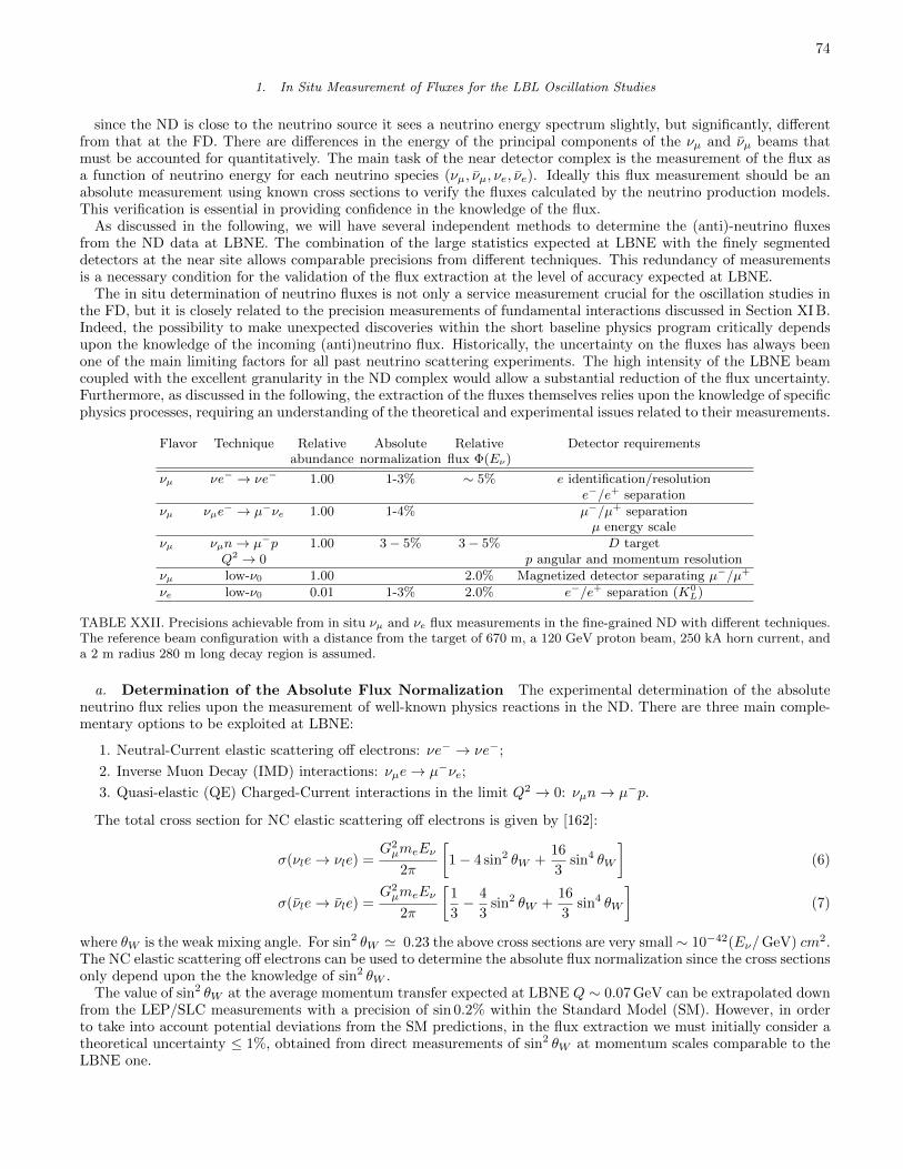
74

1. In Situ Measurement of Fluxes for the LBL Oscillation Studies

since the ND is close to the neutrino source it sees a neutrino energy spectrum slightly, but significantly, differentfrom that at the FD. There are differences in the energy of the principal components of the νµ and νµ beams thatmust be accounted for quantitatively. The main task of the near detector complex is the measurement of the flux asa function of neutrino energy for each neutrino species (νµ, νµ, νe, νe). Ideally this flux measurement should be anabsolute measurement using known cross sections to verify the fluxes calculated by the neutrino production models.This verification is essential in providing confidence in the knowledge of the flux.

As discussed in the following, we will have several independent methods to determine the (anti)-neutrino fluxesfrom the ND data at LBNE. The combination of the large statistics expected at LBNE with the finely segmenteddetectors at the near site allows comparable precisions from different techniques. This redundancy of measurementsis a necessary condition for the validation of the flux extraction at the level of accuracy expected at LBNE.

The in situ determination of neutrino fluxes is not only a service measurement crucial for the oscillation studies inthe FD, but it is closely related to the precision measurements of fundamental interactions discussed in Section XI B.Indeed, the possibility to make unexpected discoveries within the short baseline physics program critically dependsupon the knowledge of the incoming (anti)neutrino flux. Historically, the uncertainty on the fluxes has always beenone of the main limiting factors for all past neutrino scattering experiments. The high intensity of the LBNE beamcoupled with the excellent granularity in the ND complex would allow a substantial reduction of the flux uncertainty.Furthermore, as discussed in the following, the extraction of the fluxes themselves relies upon the knowledge of specificphysics processes, requiring an understanding of the theoretical and experimental issues related to their measurements.

Flavor Technique Relative Absolute Relative Detector requirementsabundance normalization flux Φ(Eν)

νµ νe− → νe− 1.00 1-3% ∼ 5% e identification/resolutione−/e+ separation

νµ νµe− → µ−νe 1.00 1-4% µ−/µ+ separation

µ energy scaleνµ νµn→ µ−p 1.00 3− 5% 3− 5% D target

Q2 → 0 p angular and momentum resolutionνµ low-ν0 1.00 2.0% Magnetized detector separating µ−/µ+

νe low-ν0 0.01 1-3% 2.0% e−/e+ separation (K0L)

TABLE XXII. Precisions achievable from in situ νµ and νe flux measurements in the fine-grained ND with different techniques.The reference beam configuration with a distance from the target of 670 m, a 120 GeV proton beam, 250 kA horn current, anda 2 m radius 280 m long decay region is assumed.

a. Determination of the Absolute Flux Normalization The experimental determination of the absoluteneutrino flux relies upon the measurement of well-known physics reactions in the ND. There are three main comple-mentary options to be exploited at LBNE:

1. Neutral-Current elastic scattering off electrons: νe− → νe−;

2. Inverse Muon Decay (IMD) interactions: νµe→ µ−νe;

3. Quasi-elastic (QE) Charged-Current interactions in the limit Q2 → 0: νµn→ µ−p.

The total cross section for NC elastic scattering off electrons is given by [162]:

σ(νle→ νle) =G2µmeEν

2π

[1− 4 sin2 θW +

16

3sin4 θW

](6)

σ(νle→ νle) =G2µmeEν

2π

[1

3− 4

3sin2 θW +

16

3sin4 θW

](7)

where θW is the weak mixing angle. For sin2 θW ' 0.23 the above cross sections are very small∼ 10−42(Eν/GeV) cm2.The NC elastic scattering off electrons can be used to determine the absolute flux normalization since the cross sectionsonly depend upon the the knowledge of sin2 θW .

The value of sin2 θW at the average momentum transfer expected at LBNE Q ∼ 0.07 GeV can be extrapolated downfrom the LEP/SLC measurements with a precision of sin 0.2% within the Standard Model (SM). However, in orderto take into account potential deviations from the SM predictions, in the flux extraction we must initially consider atheoretical uncertainty ≤ 1%, obtained from direct measurements of sin2 θW at momentum scales comparable to theLBNE one.

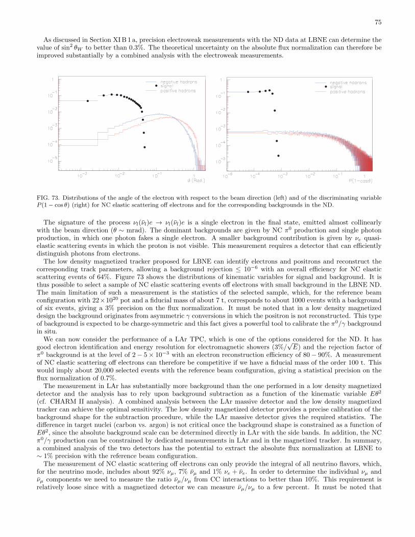
75

As discussed in Section XI B 1 a, precision electroweak measurements with the ND data at LBNE can determine thevalue of sin2 θW to better than 0.3%. The theoretical uncertainty on the absolute flux normalization can therefore beimproved substantially by a combined analysis with the electroweak measurements.

FIG. 73. Distributions of the angle of the electron with respect to the beam direction (left) and of the discriminating variableP (1− cos θ) (right) for NC elastic scattering off electrons and for the corresponding backgrounds in the ND.

The signature of the process νl(νl)e → νl(νl)e is a single electron in the final state, emitted almost collinearlywith the beam direction (θ ∼ mrad). The dominant backgrounds are given by NC π0 production and single photonproduction, in which one photon fakes a single electron. A smaller background contribution is given by νe quasi-elastic scattering events in which the proton is not visible. This measurement requires a detector that can efficientlydistinguish photons from electrons.

The low density magnetized tracker proposed for LBNE can identify electrons and positrons and reconstruct thecorresponding track parameters, allowing a background rejection ≤ 10−6 with an overall efficiency for NC elasticscattering events of 64%. Figure 73 shows the distributions of kinematic variables for signal and background. It isthus possible to select a sample of NC elastic scattering events off electrons with small background in the LBNE ND.The main limitation of such a measurement is the statistics of the selected sample, which, for the reference beamconfiguration with 22×1020 pot and a fiducial mass of about 7 t, corresponds to about 1000 events with a backgroundof six events, giving a 3% precision on the flux normalization. It must be noted that in a low density magnetizeddesign the background originates from asymmetric γ conversions in which the positron is not reconstructed. This typeof background is expected to be charge-symmetric and this fact gives a powerful tool to calibrate the π0/γ backgroundin situ.

We can now consider the performance of a LAr TPC, which is one of the options considered for the ND. It hasgood electron identification and energy resolution for electromagnetic showers (3%/

√E) and the rejection factor of

π0 background is at the level of 2− 5× 10−3 with an electron reconstruction efficiency of 80− 90%. A measurementof NC elastic scattering off electrons can therefore be competitive if we have a fiducial mass of the order 100 t. Thiswould imply about 20,000 selected events with the reference beam configuration, giving a statistical precision on theflux normalization of 0.7%.

The measurement in LAr has substantially more background than the one performed in a low density magnetizeddetector and the analysis has to rely upon background subtraction as a function of the kinematic variable Eθ2

(cf. CHARM II analysis). A combined analysis between the LAr massive detector and the low density magnetizedtracker can achieve the optimal sensitivity. The low density magnetized detector provides a precise calibration of thebackground shape for the subtraction procedure, while the LAr massive detector gives the required statistics. Thedifference in target nuclei (carbon vs. argon) is not critical once the background shape is constrained as a function ofEθ2, since the absolute background scale can be determined directly in LAr with the side bands. In addition, the NCπ0/γ production can be constrained by dedicated measurements in LAr and in the magnetized tracker. In summary,a combined analysis of the two detectors has the potential to extract the absolute flux normalization at LBNE to∼ 1% precision with the reference beam configuration.

The measurement of NC elastic scattering off electrons can only provide the integral of all neutrino flavors, which,for the neutrino mode, includes about 92% νµ, 7% νµ and 1% νe + νe. In order to determine the individual νµ andνµ components we need to measure the ratio νµ/νµ from CC interactions to better than 10%. This requirement isrelatively loose since with a magnetized detector we can measure νµ/νµ to a few percent. It must be noted that

76

the reactions νee → νee and νee → νee result from combined W and Z boson exchange. The corresponding crosssection for νe(νe) is enhanced by a factor of about six (three) with respect to νµ(νµ). The relative νe contributionsto the measured NC elastic scattering sample is therefore increased to about 6% of the total, requiring an additionalmeasurement of the ratio νe/νµ from CC interactions to 10− 15%.

The possibility to achieve the high statistics beam exposure (Scenario B) would have a substantial impact onthe precision achievable with the NC elastic scattering off electrons since this channel is dominated by statisticaluncertainties with the reference beam configuration. The resulting increase in the number of protons on target by afactor of four would allow the collection of about 80,000 events in the LAr detector, providing a statistical precisionof ∼ 0.3%. At this level of precision the theoretical uncertainty on the knowledge of sin2 θW will start to play arole in the determination of the absolute flux normalization and a analysis will require a complementary precisionelectroweak measurement (Section XI B 1 a).

A second process that can be used to crosscheck the absolute flux normalization is the Inverse Muon Decay (IMD):νµe− → µ−νe. However, this reaction is characterized by a very high energy threshold Eν > (m2

µ − m2e)/2me '

10.9 GeV and therefore we expect only about 700 events in the fine-grained tracker with the reference beam config-uration. With a fiducial mass of 100 tons we can collect about 10,000 IMD events in the LAr detector, which wouldprovide an independent flux normalization with a statistical precision of ∼ 1%. The analysis has to rely upon thesubtraction of the large background from νµ CC Quasi-Elastic events with a single reconstructed track in the finalstate and from the corresponding resonance and DIS events. The identification of the charge of the muon is a crucialrequirement for this measurement. This task can be easily accomplished by the downstream magnetized tracker giventhat Eµ ≥ 10.9 GeV. The use of IMD provides a direct measurement of the νµ flux in the high energy tail of thespectrum. A relative determination of the flux as a function of Eν is required to fully constrain the spectrum and toextract the corresponding total integral.

A third independent method to extract both the absolute flux normalization and the relative flux as a function ofEν is through the Quasi-Elastic (QE) CC scattering νµn(p) → µ−p(n). Neglecting terms in (mµ/Mn)2, at Q2 = 0

the QE cross section is independent of neutrino energy for (2EνMn)1/2 > mµ:

dσ

dQ2| Q2 = 0 |=

G2µ cos2 θc

2π

[F 2

1 (0) +G2A(0)

]= 2.08× 10−38 cm2 GeV−2 (8)

which is determined by neutron β decay and has a theoretical uncertainty < 1%. The flux can be extracted experi-mentally by measuring low Q2 QE interactions (0 − 0.05 GeV) and extrapolating the result to the limit of Q2 = 0.This measurement requires a deuterium or hydrogen (for anti-neutrino) target to minimize the smearing due toFermi motion and other nuclear effects. This requirement can only be achieved by using both H2O and D2O targetsembedded into the fine-grained tracker and to extract the events produced in deuterium by statistical subtraction ofthe larger oxygen component. The experimental resolution on the muon and proton momentum and angle is crucial.A low density tracker with ρ ∼ 0.1 g/cm

3would increase the proton range by about one order of magnitude, thus

increasing the proton reconstruction efficiency in the region of Q2 ≤ 0.05 GeV2. The dominant uncertainties arerelated to the extrapolation to Q2 = 0, to the theoretical cross section on deuterium, the experimental resolution,and to the statistical subtraction. Overall, it seems feasible to achieve a precision of 3 − 5% on the fluxes with thecurrent understanding of the theoretical cross sections.

b. Determination of the Relative Flux as a Function of Energy A precise determination of the relativeneutrino flux as a function of energy can be achieved with the low-ν0 method. The dynamics of neutrino-nucleonscattering implies that the number of events in a given energy bin with hadronic energy Ehad < ν0 is proportional tothe neutrino (antineutrino) flux in that energy bin up to corrections O(ν0/Eν) and O(ν0/Eν)2. The method followsfrom the general expression of the ν-nucleon differential cross section:

N (ν < ν0) = CΦ(Eν)ν0

[A+

(ν0

Eν

)B +

(ν0

Eν

)2

C +O(ν0

Eν

)3]

(9)

where the coefficients calA = F2, B = (F2 ± F3)/2, C = (F2 ∓ F3)/6 and Fi =∫ 1

0

∫ ν00Fi(x)dxdν is the integral

of structure function Fi. The number N (ν < ν0) is proportional to the flux up to correction factors of the orderO(ν0/Eν) or smaller, which are not significant for small values of ν0 at energies ≥ ν0. It should be pointed out thatthe coefficients A,B, C are determined for each energy bin and neutrino flavor within the ND data themselves. Sinceour primary interest is the relative flux determination, i.e. neutrino flux in an energy bin relative to another energybin, variations in the coefficients do not affect the relative flux.

The prescription for the relative flux determination is simple: we count the number of ν-CC events below a certainsmall value of hadronic energy (ν0). The observed number of events, up to the correction due to the finite ν0 of the

77

order O(ν0/Eν), in each total visible energy bin is dominated by the corresponding lepton energy, is proportional tothe relative flux. The smaller the factor ν0/Eν , the smaller is the correction. It is apparent from the above discussionthat this method of relative flux determination is not very sensitive to nucleon structure, QCD corrections, and typesof ν-interactions such as scaling or non-scaling. With the excellent granularity and resolution foreseen in the lowdensity magnetized tracker it will be possible to use a value of ν0 ∼ 0.5 GeV or lower, thus allowing flux predictionsdown to Eν ∼ 0.5 GeV. For the scintillator option the value of a usable ν0 is yet to be determined but it is expectedto be higher than that for the low density tracker. Note that the non-prompt backgrounds will be larger with thehigher density detectors, especially for the νµ component at low energy.

In this analysis, the key measurable quantities are the resolution for the low-ν events and the systematic precision ofthe muon-momentum. The νµ(νµ)-CC flux provides a measure of the π+/K+/µ+(π−/K−/µ−) content of the beam.We first obtain the relative νµ(νµ) flux at the ND. We then fit the d2σ/dxF dP

2T of the parent mesons to the νµ flux

with a simple parametrization:

d2σ

dxF dP 2T

= f(xF )g(PT )h(xF , PT ) (10)

The ingredients to this empirical fit to the meson production cross section (EP) are the following:

• Trace parent mesons through a simulation of the beam elements;

• Decay the parent mesons;

• Predict νµ and νµ fluxes by folding experimental acceptance;

• Add external constraints on π/K from hadro-production experiments (MIPP);

• Compare predictions to the measured spectra at the ND and minimize the corresponding χ2.

It must be noted that the simple smoothness requirement on the functional form in Eqn. (10) allows to extend theflux predictions down to Eν ∼ ν0. In order to evaluate the sensitivity which can be achieved at LBNE with the low-ν0

method we performed the flux analysis for the neutrino beam mode (positive focusing) using νµ + νµ CC mock-datafrom the low density magnetized detector and ν0 < 1 GeV. The systematic error analysis included the followingeffects:

• Variation of the functional form in Equation (10);

• Variation of both muon and hadron energy scales;

• Systematic shift of the ν0 values by ±20%;

• Variation of quasi-elastic, resonance and DIS cross sections by ±20%;

• Effect of the beam-transport elements.

The beam-transport uncertainty will require additional studies after completing the design of the beam line since itdepends on the precise beam and on the inert material that the hadrons encounter. Depending upon our knowledge ofp/π/K nuclear collisions, this uncertainty can become dominant for νµ production in the neutrino beam mode at lowenergy. Figure 74 shows the mock-data and the corresponding fitted flux with the ND positioned at 500 m from thetarget. Having constrained the d2σ/dxF dP

2T of the pions/kaons, we can predict the flux at the ND location. Overall

we achieved a precision ≤ 2% on the relative νµ flux with the low-ν0 method in the energy region 1 ≤ Eν ≤ 30 GeV inthe fit with ν0 < 1 GeV. Similar uncertainties are expected for the νµ component (dominant one) in the anti-neutrinobeam mode (negative focusing).

The low-ν0 method was used to study the effect of different locations of the near detector on the flux predictions atthe FD site. The low-ν0 fit described above was repeated assuming a distance of the ND from the target of 1500 m,1000 m, 750 m, and 500 m, respectively. It must be noted that the ratio between the spectra at the FD and NDsites is not flat even at L=1000 m. However, the spectral distortions increase substantially for Eν < 5 GeV as thedistance from the target is reduced. The low-ν0 method can correct for such spectral distortions since it directlyextracts the parent π±/K±/K0

L content from the ND data and extrapolates the fluxes at the FD site by taking intoaccount the beam transport elements and by decaying the mesons. Results show that the FD/ND ratio predicted bythe low-ν0 technique can reproduce the actual FD/ND ratio to better than 2%, regardless of the distance between theND and the target. As a consequence the ND can be located closer to the target without increasing the systematicuncertainties for the LBL oscillation searches.

The relative flux as a function of energy could be also determined from NC elastic scattering off electrons, which isa two body process with the initial electron being at rest. The calculation of the incoming neutrino energy requiresa resolution of few milliradians on the angle of the outgoing electron as well as a good energy resolution. The lowdensity magnetized tracker can in principle fulfill such requirements. However, the limited statistics does not allow a

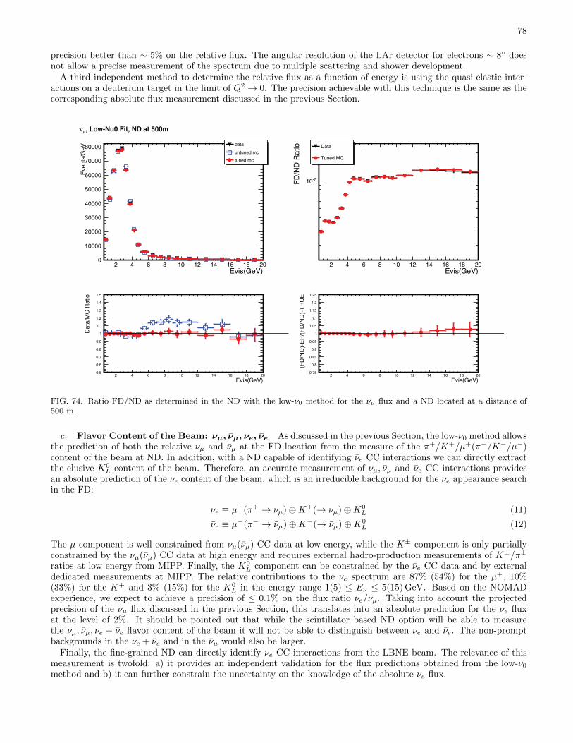
78

precision better than ∼ 5% on the relative flux. The angular resolution of the LAr detector for electrons ∼ 8 doesnot allow a precise measurement of the spectrum due to multiple scattering and shower development.

A third independent method to determine the relative flux as a function of energy is using the quasi-elastic inter-actions on a deuterium target in the limit of Q2 → 0. The precision achievable with this technique is the same as thecorresponding absolute flux measurement discussed in the previous Section.

μν

FIG. 74. Ratio FD/ND as determined in the ND with the low-ν0 method for the νµ flux and a ND located at a distance of500 m.

c. Flavor Content of the Beam: νµ, νµ, νe, νe As discussed in the previous Section, the low-ν0 method allowsthe prediction of both the relative νµ and νµ at the FD location from the measure of the π+/K+/µ+(π−/K−/µ−)content of the beam at ND. In addition, with a ND capable of identifying νe CC interactions we can directly extractthe elusive K0

L content of the beam. Therefore, an accurate measurement of νµ, νµ and νe CC interactions providesan absolute prediction of the νe content of the beam, which is an irreducible background for the νe appearance searchin the FD:

νe ≡ µ+(π+ → νµ)⊕K+(→ νµ)⊕K0L (11)

νe ≡ µ−(π− → νµ)⊕K−(→ νµ)⊕K0L (12)

The µ component is well constrained from νµ(νµ) CC data at low energy, while the K± component is only partiallyconstrained by the νµ(νµ) CC data at high energy and requires external hadro-production measurements of K±/π±

ratios at low energy from MIPP. Finally, the K0L component can be constrained by the νe CC data and by external

dedicated measurements at MIPP. The relative contributions to the νe spectrum are 87% (54%) for the µ+, 10%(33%) for the K+ and 3% (15%) for the K0

L in the energy range 1(5) ≤ Eν ≤ 5(15) GeV. Based on the NOMADexperience, we expect to achieve a precision of ≤ 0.1% on the flux ratio νe/νµ. Taking into account the projectedprecision of the νµ flux discussed in the previous Section, this translates into an absolute prediction for the νe fluxat the level of 2%. It should be pointed out that while the scintillator based ND option will be able to measurethe νµ, νµ, νe + νe flavor content of the beam it will not be able to distinguish between νe and νe. The non-promptbackgrounds in the νe + νe and in the νµ would also be larger.

Finally, the fine-grained ND can directly identify νe CC interactions from the LBNE beam. The relevance of thismeasurement is twofold: a) it provides an independent validation for the flux predictions obtained from the low-ν0

method and b) it can further constrain the uncertainty on the knowledge of the absolute νe flux.

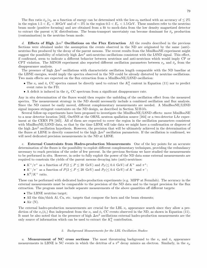
79

The flux ratio νµ/νµ as a function of energy can be determined with the low-ν0 method with an accuracy of ≤ 2%in the region 1.5 < Eν < 30 GeV and of ∼ 3% in the region 0.5 < Eν < 1.5 GeV. These numbers refer to the neutrinobeam mode (positive focusing) and are obtained from a fit to mock-data from the low density magnetized detectorto extract the parent π/K distributions. The beam-transport uncertainty can become dominant for νµ production(contamination) in the neutrino beam mode.

d. Effects of High ∆m2 Oscillations on the Flux Extraction All the results described in the previousSections were obtained under the assumption the events observed in the ND are originated by the same (anti)-neutrino flux produced by the decay of the parent mesons. The recent results from the MiniBooNE experiment mightsuggest the possibility of relatively high ∆m2 anti-neutrino oscillations consistent with the LSND signal. This effect,if confirmed, seem to indicate a different behavior between neutrinos and anti-neutrinos which would imply CP orCPT violation. The MINOS experiment also reported different oscillation parameters between νµ and νµ from thedisappearance analysis.

The presence of high ∆m2 oscillations with characteristic oscillation length comparable with the ND baseline atthe LBNE energies, would imply the spectra observed in the ND could be already distorted by neutrino oscillations.Two main effects are expected on the flux extraction from a MiniBooNE/LSND oscillation:

• The νe and νe CC spectra cannot be directly used to extract the K0L content in Equation (11) nor to predict

event rates in the FD;

• A deficit is induced in the νµ CC spectrum from a significant disappearance rate.

Any in situ determination of the fluxes would then require the unfolding of the oscillation effect from the measuredspectra. The measurement strategy in the ND should necessarily include a combined oscillation and flux analysis.Since the ND cannot be easily moved, different complementary measurements are needed. A MiniBooNE/LSNDsignal imposes stringent constraints on the ND design, as described in Section XI B 3 b.

Several follow-up experiments have been proposed to investigate the MiniBooNE/LSND effects: move MiniBooNEto a near detector location [163], OscSNS at the ORNL neutron spallation source [164] or a two-detector LAr exper-iment at the CERN PS [165]. All of them are expected to cover the region in the oscillation parameters consistentwith MiniBooNE/LSND data, so that by the time LBNE will take data we might have a confirmation or disprove ofthe high ∆m2 oscillation hypothesis. However, the precision that will be ultimately achieved in the determination ofthe fluxes at LBNE is directly connected to the high ∆m2 oscillation parameters. If the oscillation is confirmed, wewill need dedicated precision measurements in the ND at LBNE.

e. External Constraints from Hadro-production Measurements One of the key points for an accuratedetermination of the fluxes is the possibility to exploit different complementary techniques, providing the redundancynecessary to reach precision of the order of few percent. In the previous Sections we have studied the measurementsto be performed in situ. However, in order to fully exploit the power of the ND data some external measurements arerequired to constrain the yields of the parent mesons decaying into (anti)-neutrinos:

• K+/π+ as a function of P (2 ≤ P ≤ 20 GeV) and PT (≤ 0.4 GeV) of K+ and π+;

• K−/π− as a function of P (2 ≤ P ≤ 20 GeV) and PT (≤ 0.4 GeV) of K− and π−;

• K0/K+ ratio.

These can be performed with dedicated hadro-production experiments (e.g. MIPP at Fermilab). The accuracy in theexternal measurements must be comparable to the precision of the ND data and to the target precision for the fluxextraction. The program must include separate measurements of the above quantities off different targets:

• The LBNE neutrino target;

• All the thin/thick Al, Cu, etc. targets that compose the horn and the beam elements;

• Air (N).

The external hadro-production measurements are crucial for the LBL νe appearance search since they allow a pre-diction of the νe(νe) flux independent from the νe and νe CC events observed in the ND, as shown in Equation (11).It must be also noted that in the presence of high ∆m2 oscillations external hadro-production measurements are theonly source of information which can be used to extract the K0

L contribution.

2. Background Measurements for the LBL Oscillation Studies

a. Measurement of NC cross sections The most threatening background to the νe and νe appearancemeasurements in LBNE is NC events in which the detritus of a π0 decay mimics an electron. Similarly, in the νµ

80

and νµ disappearance study the largest background comes from the muonic-decay of a pion/kaon produced in a NCevent. These backgrounds are particularly challenging in the energy region 0.5 ≤ Eν ≤ 3 GeV where an additionalcomplication arises from substantial matter induced neutrino oscillation. It follows that the largest background tothe CC events in the far detector (FD) comes from non-prompt leptons, originating from the hadronic shower in NCand high-yBj CC interactions. As a first step to constrain the error on the non-prompt background to CC eventsin the FD, the fine-grained ND must measure the NC cross sections for different processes and the NC/CC ratio asfunction of the hadron-energy Ehad.

b. Measurement of π0 and γ production in NC and CC The near detector must determine the proportionof NC events as a function of neutrino energy, the yield of secondary π0 in the NC interactions, and the energy andangular distributions of the π0. Similarly, the ND must accurately identify single-photon yields in NC interactionsand, in particular, the radiative decays of resonances where only a single energetic photon is evident. The prevalenceof these decays are much affected by poorly characterized final state interactions and hence will require informationfrom the ND. Recent theoretical work has pointed out that there are NC processes that produce single energeticphotons at a level that could effect LBNE [166, 167]. Thus the ND must provide a detailed characterization of π0 andγ in every class of event: multiplicity, energy, and transverse momentum dependence for a given Ehad in NC and CC.

c. Muonic decays of π± and K± from measurement of charged multiplicities The dominant backgroundto νµ and νµ CC events in the FD will come from the muonic decay of pions and kaons in NC and CC processes.Having determined the NC cross section relative to CC, the ND must determine the charged hadron multiplicity,energy and transverse momentum dependence, and provide an empirical determination of exclusive charged hadronproduction in ν-interaction.

d. Calibration of the neutrino energy scale from reconstructed events The neutrino energy scaledirectly affects the precision of the oscillation scale parameter. The ND measurements should provide an in situcalibration of the Eν scale by measurement of the final state charged lepton and the energy in the hadronic debris.

e. Measurement of exclusive and semi-exclusive processes and their nuclear dependence The NDmust provide differential cross section measurements for various exclusive, semi-exclusive, and inclusive νµ and νµ CCinteractions. Among these, the most important to the FD measurement is the quasi-elastic (QE) interaction. Thechallenge for ND is to reduce and quantify the error due to nuclear effects, arising from initial and final state inter-actions, Fermi motion, Pauli-blocking, etc., in the QE and other CC interactions. To minimize the systematic error,ND should also determine exclusive and inclusive processes involving nucleon resonances. This measurement of back-ground processes from exclusive and semi-exclusive reactions is part of the precision studies outlined in Section XI B 5and Section XI B 7.

3. Measurement of Neutrino Induced Background to Proton Decay

In addition to backgrounds measurements for the long-baseline program, the ND complex can also provide anestimate of the ν induced background to the search for proton (nucleon) decay described in Section IV. Two genericproton decay modes are under study [168]: the π0-mode, e+(µ+) +π0 and the kaon-mode, ν+K+, and e+(µ+) +K0.

The atmospheric neutrino spectrum is different from than that of the LBNE beam. However, an accurate determi-nation of exclusive channels induced by the LBNE neutrino beam at Eν ' 2 GeV will provide empirical constraintsfor the atmospheric-neutrino background to proton decay at the FD, thus reducing the corresponding systematicuncertainty.

π0 Decay Mode The K2K-ND has provided a definitive measurement of e+ + π0 [169]. The ND at LBNEwill have an efficient π0 and e+ identification with purity exceeding 95% and the identification of µ+-mode will bestraightforward. In addition, and importantly, the ND aims to measure the exclusive first-generation mesons such asη, ρ0, etc., besides π0 accompanied by an e+ or a µ+.

Kaon Decay Mode Supersymmetric models favor the proton-to-kaon decay mode. The main focus of the NDmeasurements at LBNE is the exclusive K0 production, i.e. e+/µ+ + K0. There is an existence proof of precisedetermination of K0

S in ν CC and NC interactions [170, 171]. The ND at LBNE will extend the K0 measurement tolower energy. The ν+K+ is a challenge. However, it should be pointed out that if the K0-mode is precisely measuredthen the K+-channel can be accurately predicted.

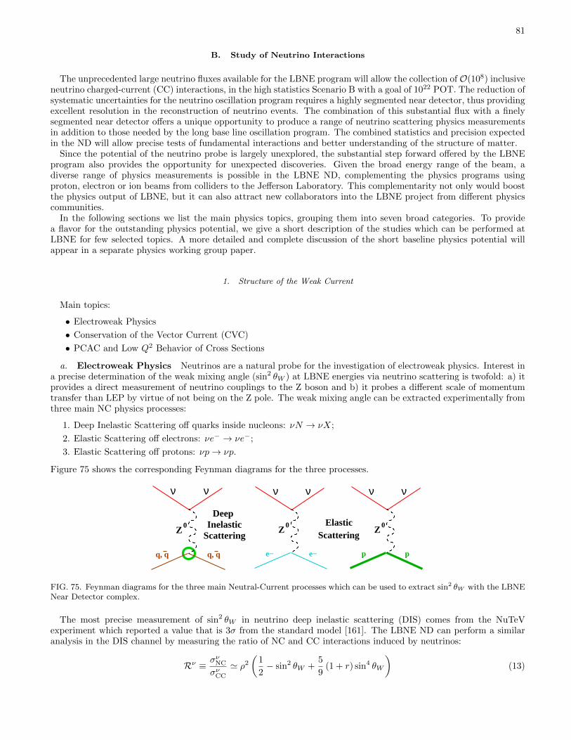
81

B. Study of Neutrino Interactions

The unprecedented large neutrino fluxes available for the LBNE program will allow the collection of O(108) inclusiveneutrino charged-current (CC) interactions, in the high statistics Scenario B with a goal of 1022 POT. The reduction ofsystematic uncertainties for the neutrino oscillation program requires a highly segmented near detector, thus providingexcellent resolution in the reconstruction of neutrino events. The combination of this substantial flux with a finelysegmented near detector offers a unique opportunity to produce a range of neutrino scattering physics measurementsin addition to those needed by the long base line oscillation program. The combined statistics and precision expectedin the ND will allow precise tests of fundamental interactions and better understanding of the structure of matter.

Since the potential of the neutrino probe is largely unexplored, the substantial step forward offered by the LBNEprogram also provides the opportunity for unexpected discoveries. Given the broad energy range of the beam, adiverse range of physics measurements is possible in the LBNE ND, complementing the physics programs usingproton, electron or ion beams from colliders to the Jefferson Laboratory. This complementarity not only would boostthe physics output of LBNE, but it can also attract new collaborators into the LBNE project from different physicscommunities.

In the following sections we list the main physics topics, grouping them into seven broad categories. To providea flavor for the outstanding physics potential, we give a short description of the studies which can be performed atLBNE for few selected topics. A more detailed and complete discussion of the short baseline physics potential willappear in a separate physics working group paper.

1. Structure of the Weak Current

Main topics:

• Electroweak Physics

• Conservation of the Vector Current (CVC)

• PCAC and Low Q2 Behavior of Cross Sections

a. Electroweak Physics Neutrinos are a natural probe for the investigation of electroweak physics. Interest ina precise determination of the weak mixing angle (sin2 θW ) at LBNE energies via neutrino scattering is twofold: a) itprovides a direct measurement of neutrino couplings to the Z boson and b) it probes a different scale of momentumtransfer than LEP by virtue of not being on the Z pole. The weak mixing angle can be extracted experimentally fromthree main NC physics processes:

1. Deep Inelastic Scattering off quarks inside nucleons: νN → νX;

2. Elastic Scattering off electrons: νe− → νe−;

3. Elastic Scattering off protons: νp→ νp.

Figure 75 shows the corresponding Feynman diagrams for the three processes.

ν

Z0

ν

q, qq, q

Deep

ScatteringInelastic

ν

Z0

ν

p p

ν

Z0

ν

e− e−

ElasticScattering

FIG. 75. Feynman diagrams for the three main Neutral-Current processes which can be used to extract sin2 θW with the LBNENear Detector complex.

The most precise measurement of sin2 θW in neutrino deep inelastic scattering (DIS) comes from the NuTeVexperiment which reported a value that is 3σ from the standard model [161]. The LBNE ND can perform a similaranalysis in the DIS channel by measuring the ratio of NC and CC interactions induced by neutrinos:

Rν ≡ σνNC

σνCC

' ρ2

(1

2− sin2 θW +

5

9(1 + r) sin4 θW

)(13)

82

where ρ is the relative coupling strength of the neutral to charged-current interactions (ρ = 1 at tree level in theStandard Model) and r is the ratio of anti-neutrino to neutrino cross section (r ∼ 0.5). The absolute sensitivity of Rνto sin2 θW is 0.7, which implies a measurement of Rν of 1% precision would provide sin2 θW with a precision of 1.4%.Contrary to the NuTeV experiment the anti-neutrino interactions cannot be used for this analysis at LBNE, due tothe large number of νµ DIS interactions in the νµ beam, compared to the νµ DIS interactions. While removing somecancelation of systematics between ν and ν, this fact reduces the statistical uncertainty of the measurement.

The measurement of sin2 θW from DIS interactions can be only performed with the low density magnetized trackersince an accurate reconstruction of the NC event kinematics and of the νe CC interactions are crucial to keep thesystematic uncertainties on the event selection under control. The analysis selects events in the ND after imposing acut on the visible hadronic energy of Ehad > 3 GeV, as in the NOMAD sin2 θW analysis (the CHARM analysis hadEhad > 4 GeV). With the reference 700 kW beam we expect about 3.3 × 106 CC events and 1.1 × 106 NC events,giving a statistical precision of 0.11% on Rν and 0.15% on sin2 θW (Table XXIII).

The use of a low density magnetized tracker can substantially reduce systematic uncertainties with respect to amassive calorimeter. Table XXIII shows a comparison of the different uncertainties on the measured Rν betweenNuTeV and LBNE. The largest experimental systematic uncertainty in NuTeV is related to the subtraction of the νeCC contamination from the NC sample. Since the low density tracker at LBNE can efficiently reconstruct the electrontracks, the νe CC interactions can be identified on an event-by-event basis, reducing the corresponding uncertainty toa negligible level. Similarly, uncertainties related to the location of the interaction vertex, noise, counter efficiency etc.are removed by the higher resolution and by the different analysis selection. The experimental selection at LBNE willbe dominated by two uncertainties: the knowledge of the νµ flux and the kinematic selection of NC interactions. Theformer is relevant due to the larger NC/CC ratio for anti-neutrinos. The total experimental systematic uncertaintyon sin2 θW is expected to be about 0.14%.

δRν/Rν

Source of uncertainty NuTeV LBNE

Data statistics 0.00176 0.00110Monte Carlo statistics 0.00015

Total Statistics 0.00176 0.00110

νe, νe flux (∼ 1.7%) 0.00064 0.00010Energy measurement 0.00038 0.00040Shower length model 0.00054 n.a.

Counter efficiency, noise 0.00036 n.a.Interaction vertex 0.00056 n.a.

νµ flux n.a. 0.00070Kinematic selection n.a. 0.00060

Experimental systematics 0.00112 0.00102

d,s→c, s-sea 0.00227 0.00130Charm sea 0.00013 n.a.r = σν/σν 0.00018 n.a.

Radiative corrections 0.00013 0.00013Non-isoscalar target 0.00010 N.A.

Higher twists 0.00031 0.00070RL (F2, FT , xF3) 0.00115 0.00140

Nuclear correction 0.00020Model systematics 0.00258 0.00206

TOTAL 0.00332 0.00255

TABLE XXIII. Comparison of uncertainties on the Rν measurement between NuTeV and LBNE with the reference beam.The corresponding relative uncertainties on sin2 θW must be multiplied by a factor of 1.4, giving for LBNE a projected overallprecision of 0.36%.

The measurement of Rν will be dominated by model systematic uncertainties on the structure functions of thetarget nucleons. The estimate of these uncertainties for LBNE is based upon the extensive work performed for theNOMAD analysis and includes a NNLO QCD calculation of structure functions (NLO for charm production) [172–174], parton distribution functions (PDFs) extracted from dedicated low-Q global fits, high twist contributions [172],electroweak corrections [175] and nuclear corrections [176–178]. The charm quark production in CC, which has beenthe dominant source of uncertainty in all past determinations of sin2 θW from νN DIS, is reduced to about 2.5% ofthe total νµ CC DIS with Ehad > 3 GeV with the low energy beam spectrum at LBNE. This number translatesinto a systematic uncertainty of 0.13% on Rν (Table XXIII), assuming a knowledge of the charm production cross

83

section to 5%. It is worth noting the recent measurement of charm dimuon production by the NOMAD experimentallowed a reduction of the uncertainty on the strange sea distribution to ∼ 3% and on the charm quark mass mc

to ∼ 60 MeV [179]. The lower neutrino energies available at LBNE reduce the accessible Q2 values with respect toNuTeV, increasing in turn the effect of non-perturbative contributions (High Twists) and RL. The correspondinguncertainties are reduced by the recent studies of low-Q structure functions and by improved modeling with respectto the NuTeV analysis (NNLO vs. LO). The total model systematic uncertainty on sin2 θW is expected to be about0.29% with the reference beam configuration. The corresponding total uncertainty on the value of sin2 θW extractedfrom νN DIS is 0.36% with the 700 kW beam.

Most of the model uncertainties will be constrained by in situ dedicated measurements using the large CC samplesand employing improvements in theory that will have evolved over the course of the experiment. In the low densitytracker we shall collect about 80,000 neutrino induced inclusive charm events with the 700 kW beam. The precisereconstruction of charged tracks will allow to measure exclusive decay modes of charmed hadrons (e.g. D∗+) and tomeasure charm fragmentation and production parameters. The average semileptonic branching ratio Bµ ∼ 5% withthe low energy LBNE beam. The presence a 100-ton LAr TPC in front of the low density tracker will further increasethe potential of the charm analysis, allowing the collection of about 50,000 charm dimuon events with the referencebeam. This sample represent shall be compared with the largest existing sample of 15,400 dimuon events collectedby the NOMAD experiment [179]. Finally, precision measurements of CC structure functions in both the fine-grainedtracker and the LAr detector would further reduce the uncertainties on PDFs and on High Twist contributions.

The precision that can be achieved from νN DIS interactions is limited by both the event rates and by the energyspectrum of the reference 700 kW beam configuration. The high statistics beam exposure of Scenario B (1022 pot)combined with a dedicated run with the high energy beam option would increase the statistics by more than afactor of 20. This major step forward would not only reduce the statistical uncertainty to a negligible level, butwould provide large control samples and precision auxiliary measurements to reduce the systematic uncertainties onstructure functions. The two dominant systematic uncertainties, charm production in CC interactions and low Q2

structure functions, are essentially defined by the available data at present. Overall, the use of a high energy beamwithin the Scenario B can potentially improve the precision achievable on sin2 θW from νN DIS to about 0.2%. Itis worth mentioning the high energy beam is also required for the determination of the fluxes in case high ∆m2

oscillations are present (see Section XI B 3 b).A second independent measurement of sin2 θW can be obtained from NC νµe elastic scattering. This channel has

lower systematic uncertainties since it does not depend upon the knowledge of the structure of nuclei, but has limitedstatistics due to its very low cross section. The value of sin2 θW can be extracted from the ratio of neutrino toanti-neutrino interactions [162]:

Rνe(Q2) ≡ σ(νµe→ νµe)

σ(νµe→ νµe)(Q2) ' 1− 4 sin2 θW + 16 sin4 θW

3− 12 sin2 θW + 16 sin4 θW(14)

in which systematic uncertainties related to the selection and electron identification cancel out. The absolute sensitivityof this ratio to sin2 θW is 1.79, which implies a measurement of Rνe of 1% precision would provide sin2 θW with aprecision of 0.65%.

The event selection was described in details on Section XI A 1 a since the NC elastic scattering off electrons is alsoused for the absolute flux normalization. This analysis can be performed only with the low density magnetized trackerand with a large LAr detector. In the former case the total statistics available is limited to about 1000 (600) ν(ν)events with the minimal exposure of Scenario A and 4500 (2800) ν(ν) events with the Scenario B. These numbers donot allow a competitive determination of sin2 θW by using the magnetized tracker alone. However, if we consider a100 t LAr detector in the ND complex, we expect to collect about 20,000 (12,000) ν(ν) events with Scenario A and80,000 (50,000) ν(ν) events with Scenario B.

As discussed in Section XI A 1 a a combined analysis of both detectors can achieve the optimal sensitivity: the fine-grained tracker is used to reduce systematic uncertainties (measurement of backgrounds and calibration), while the LArND provides the statistics required for a competitive measurement. Overall, the use of the massive LAr detector canprovide a statistical accuracy on sin2 θW of about 0.3% with the high statistics Scenario B. However, the extractionof the weak mixing angle is dominated by the systematic uncertainty on the νµ/νµ flux ratio, which is enteringEquation (14). We evaluated this uncertainty with the low-ν0 method for the flux extraction (see Section XI A 1 c)and we obtained a systematic uncertainty of about 1% on the ratio of the νµ/νµ flux integrals. Therefore, the overall

precision on sin2 θW achievable from NC elastic scattering off electrons is limited to about 0.9% in Scenario A and0.6% in Scenario B. An improvement of this result in Scenario B would require a better understanding of the low-ν(anti)-neutrino cross sections, of the beam transport elements and of the nuclear cross sections.

Together, the DIS and the NC elastic scattering channels involve substantially different scales of momentum transfer,providing a tool to test the running of sin2 θW in a single experiment. To this end, the study of NC elastic scatteringoff protons can provide additional information since it occurs at a momentum scale which is intermediate between

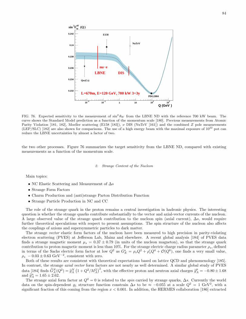
84

Q (GeV )−2

10−1

10 1 102

103

10

0.232

0.234

0.236

0.238

0.24

0.242

Qw(Cs)

NuTeV

E158

PDG2004

(Q ) eff W

θ2sin

DIS

nu−e

LBNE

L=670m, E=120 GeV, 700 kW 3+3y

FIG. 76. Expected sensitivity to the measurement of sin2 θW from the LBNE ND with the reference 700 kW beam. Thecurve shows the Standard Model prediction as a function of the momentum scale [180]. Previous measurements from AtomicParity Violation [181, 182], Moeller scattering (E158 [183]), ν DIS (NuTeV [161]) and the combined Z pole measurements(LEP/SLC) [182] are also shown for comparisons. The use of a high energy beam with the maximal exposure of 1022 pot canreduce the LBNE uncertainties by almost a factor of two.

the two other processes. Figure 76 summarizes the target sensitivity from the LBNE ND, compared with existingmeasurements as a function of the momentum scale.

2. Strange Content of the Nucleon

Main topics:

• NC Elastic Scattering and Measurement of ∆s

• Strange Form Factors

• Charm Production and (anti)strange Parton Distribution Function

• Strange Particle Production in NC and CC

The role of the strange quark in the proton remains a central investigation in hadronic physics. The interestingquestion is whether the strange quarks contribute substantially to the vector and axial-vector currents of the nucleon.A large observed value of the strange quark contribution to the nucleon spin (axial current), ∆s, would requirefurther theoretical speculations with respect to present assumptions. The spin structure of the nucleon also affectsthe couplings of axions and supersymmetric particles to dark matter.

The strange vector elastic form factors of the nucleon have been measured to high precision in parity-violatingelectron scattering (PVES) at Jefferson Lab, Mainz and elsewhere. A recent global analysis [184] of PVES datafinds a strange magnetic moment µs = 0.37 ± 0.79 (in units of the nucleon magneton), so that the strange quarkcontribution to proton magnetic moment is less than 10%. For the strange electric charge radius parameter ρs, definedin terms of the Sachs electric form factor at low Q2 as GsE = ρsQ

2 + ρ′sQ4 + O(Q6), one finds a very small value,

ρs − 0.03± 0.63 GeV−2, consistent with zero.Both of these results are consistent with theoretical expectations based on lattice QCD and phenomenology [185].

In contrast, the strange axial vector form factors are not nearly as well determined. A similar global study of PVES

data [184] finds GNA (Q2) = gNA(1 +Q2/M2

A

)2, with the effective proton and neutron axial charges gpA = −0.80± 1.68

and gnA = 1.65± 2.62.The strange axial form factor at Q2 = 0 is related to the spin carried by strange quarks, ∆s. Currently the world

data on the spin-dependent g1 structure function constrain ∆s to be ≈ −0.055 at a scale Q2 = 1 GeV2, with asignificant fraction of this coming from the region x < 0.001. In addition, the HERMES collaboration [186] extracted

85

the strange quark spin from semi-inclusive DIS data over the range 0.02 ≤ x ≤ 0.6, yielding a negative central value,∆s = 0.037± 0.019± 0.027, although still consistent with the above global average.

A B C

14

[G2

1 (1 + τ)−(F 2

1 − τF 22

)(1− τ) + 4τF1F2

]− 1

4G1 (F1 + F2) 1

16

M2p

Q2

(G2

1 + F 21 + τF 2

2

)TABLE XXIV. Coefficients entering Eqn. 15 for NC elastic scattering and CC QE interactions, with τ = Q2/4Mp.

An independent extraction of ∆s, which does not rely on the difficult measurements of the g1 structure functionat very small x values, can be obtained from (anti)-neutrino NC elastic scattering off proton (see Fig. 75). Thisprocess provides indeed the most direct measurement of ∆s. The differential cross section for NC elastic and CC QEscattering of (anti)-neutrinos from protons can be written as:

dσ

dQ2=G2µ

2π

Q2

E2ν

(A±BW + CW 2

); W = 4Eν/Mp −Q2/M2

p (15)

where the positive (negative) sign is for (anti)-neutrino scattering and the coefficients A,B, and C contain the vectorand axial form factors as listed in Table XXIV.

The axial-vector form factor for NC scattering can be written as the sum of the known axial form factor GA plusa strange form factor GsA:

G1 =

[−GA

2+GsA2

](16)

while the NC vector form factors can be written as:

F1,2 =

[(1

2− sin2 θW

)(F p1,2 − Fn1,2

)− sin2 θW

(F p1,2 + Fn1,2

)− 1

2F s1,2

](17)

where Fp(n)1 is the Dirac form factor of the proton (neutron), F

p(n)2 is the corresponding Pauli form factor, and F s1,2

are the strange vector form factors. These latter are expected to be small from the PVES measurements summarizedabove. In the limit Q2 → 0, the differential cross section is proportional to the square of the axial-vector form factordσ/dQ2 ∝ G2

1 and GsA → ∆s. The value of ∆s can therefore be extracted experimentally by extrapolating the NCdifferential cross section to Q2 = 0.

Previous neutrino scattering experiments have been limited by the statistics and by the systematic uncertaintieson background subtraction. The only information available comes from the analysis of 951 NC νp and 776 NCνp collected by the experiment BNL E734 [187–189]. The LBNE neutrino beam will be sufficiently intense that ameasurement of NC elastic scattering on proton in the fine-grained water ND can provide a definitive statement onthe contribution of the strange sea to either the axial or vector form factor.

Systematic uncertainties can be reduced by measuring the NC/CC ratios for both neutrinos and anti-neutrinos:

Rνp(Q2) ≡ σ(νµp→ νµp)

σ(νµn→ µ−p)(Q2); Rνp(Q2) ≡ σ(νµp→ νµp)

σ(νµp→ µ+n)(Q2) (18)

as a function of Q2. Figure 77 shows the absolute sensitivity of both ratios to ∆s for different values of Q2. Thesensitivity for Q2 ∼ 0.25 GeV2 is about 1.2 for neutrinos and 1.9 for anti-neutrinos, which implies that a measurementof Rνp and Rνp of 1% precision would enable the extraction of ∆s with an uncertainty of 0.8% and 0.5%, respectively.

The design of the fine-grained water ND involves a combination of different nuclear targets. Therefore, most ofthe neutrino scattering is from nucleons embedded in a nucleus, requiring nuclear effects to be taken into account.Fortunately, in the ratio of NC/CC yields, the nuclear corrections are expected to largely cancel out. The ∆s analysisrequires a good proton reconstruction efficiency as well as high resolution on both the proton angle and energy. To thisend, the low density magnetized tracker at LBNE can increase the range of the protons inside the ND, allowing thereconstruction of proton tracks down to Q2 ∼ 0.07 GeV2. This fact will reduce the uncertainties in the extrapolationof the form factors to the limit Q2 → 0.

Table XXV summarizes the expected proton ranges for both the scintillator and the low density (ρ ∼ 0.1 g/cm3)ND options. With the reference 700 kW beam we expect about 2.5(1.5)× 105 νp(νp) events after the selection cutsin the low density tracker, yielding a statistical precision of the order of 0.2%.

We follow the analysis performed by the FINeSSE collaboration [190] and in the SciBooNE experiment for thedetermination of ∆s. In particular, based upon the latter, with the scintillator tracker we expect a purity of about

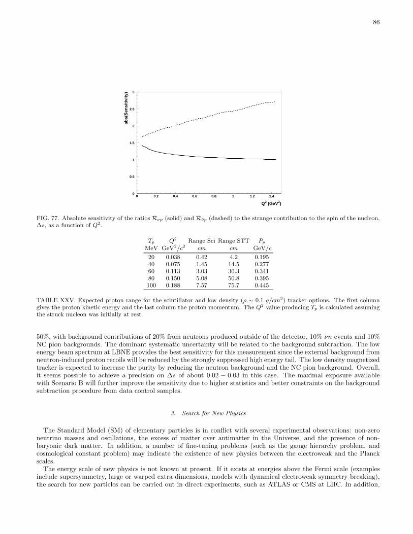
86

0

0.5

1

1.5

2

2.5

3

0 0.2 0.4 0.6 0.8 1 1.2 1.4

Q2 (GeV2)

abs(

Sen

siti

vity

)

FIG. 77. Absolute sensitivity of the ratios Rνp (solid) and Rνp (dashed) to the strange contribution to the spin of the nucleon,∆s, as a function of Q2.

Tp Q2 Range Sci Range STT PpMeV GeV2/c2 cm cm GeV/c

20 0.038 0.42 4.2 0.19540 0.075 1.45 14.5 0.27760 0.113 3.03 30.3 0.34180 0.150 5.08 50.8 0.395100 0.188 7.57 75.7 0.445

TABLE XXV. Expected proton range for the scintillator and low density (ρ ∼ 0.1 g/cm3) tracker options. The first columngives the proton kinetic energy and the last column the proton momentum. The Q2 value producing Tp is calculated assumingthe struck nucleon was initially at rest.

50%, with background contributions of 20% from neutrons produced outside of the detector, 10% νn events and 10%NC pion backgrounds. The dominant systematic uncertainty will be related to the background subtraction. The lowenergy beam spectrum at LBNE provides the best sensitivity for this measurement since the external background fromneutron-induced proton recoils will be reduced by the strongly suppressed high energy tail. The low density magnetizedtracker is expected to increase the purity by reducing the neutron background and the NC pion background. Overall,it seems possible to achieve a precision on ∆s of about 0.02 − 0.03 in this case. The maximal exposure availablewith Scenario B will further improve the sensitivity due to higher statistics and better constraints on the backgroundsubtraction procedure from data control samples.

3. Search for New Physics

The Standard Model (SM) of elementary particles is in conflict with several experimental observations: non-zeroneutrino masses and oscillations, the excess of matter over antimatter in the Universe, and the presence of non-baryonic dark matter. In addition, a number of fine-tuning problems (such as the gauge hierarchy problem, andcosmological constant problem) may indicate the existence of new physics between the electroweak and the Planckscales.

The energy scale of new physics is not known at present. If it exists at energies above the Fermi scale (examplesinclude supersymmetry, large or warped extra dimensions, models with dynamical electroweak symmetry breaking),the search for new particles can be carried out in direct experiments, such as ATLAS or CMS at LHC. In addition,

87

new hypothetical heavy particles inevitably appear as virtual states, leading to different rare processes, absent in theSM. These effects can be found at experiments such as LHCb, charm and beauty factories and are competitive withthe direct searches. If the new physics is associated with existence of new relatively light particles (an example isgiven by the νMSM, see below) then the search for rare processes is superior to high energy experiments. Moreover,it provides a unique possibility for discovery of new physics, not accessible by any of the LHC experiments. We willargue here that the LBNE near detector can be used for these searches.

Main topics:

• Search for νMSM Neutral Leptons

• High ∆m2 Neutrino Oscillations

• Radiative Decay of Sterile Neutrinos

• MiniBooNE Low Energy Anomaly

• Decay of Heavy Weakly Interacting Particles

• νµ → νe Transitions

a. Search for νMSM Neutral Leptons The most economic way to handle in a unified way the problemsof neutrino masses, dark matter and baryon asymmetry of the Universe may be to add to the SM three Majoranasinglet fermions with masses roughly of the order of masses of known quarks and leptons. The appealing feature ofthis theory (called the νMSM for “Neutrino Minimal SM”) is the fact that there every left-handed fermion has aright-handed counter-part, leading thus an equal way of treating of quarks and leptons. The lightest of the three newleptons is expected to have a mass from 1 keV to 50 keV and play the role of the dark matter particle. Two otherneutral fermions are responsible for giving masses to ordinary neutrinos via the see-saw mechanism at the electroweakscale and to creation of the baryon asymmetry of the Universe (for a review see [191]). The masses of these particlesand their coupling to ordinary leptons are constrained by particle physics experiments and cosmology. They should bealmost degenerate, forming thus nearly Dirac fermion (this is coming from the requirement of successful baryogenesis).Different considerations indicate that their mass should be in O(1) GeV region [192].

The νMSM is described by the most general renormalizable Lagrangian containing all the particles of the SM andthree singlet fermions. For the purpose of the present discussion we take away from it the lightest singlet fermion N1

(the “dark matter sterile neutrino”), which is coupled extremely weakly to the ordinary leptons. In addition, we takeN2 and N3 degenerate in mass, M2 = M3 = M . Then the convenient parametrization of the interaction of N ′s withthe leptons of SM is:

Lsinglet =

(κMmatm

v2

) 12[

1√εeiη

L2N2 +√εeiηL3N3

]H −MN2

cN3 + h.c. , (19)

where L2 and L3 are the combinations of Le, Lµ and Lτ

L2 =∑α

xαLα , L3 =∑α

yαLα . (20)

with∑α |xα|2 =

∑α |yα|2 = 1.

In eq.(19) v = 246 GeV is the vacuum expectation value of the Higgs field H, Hi = εifH∗j , matm ' 0.05 eV is

the atmospheric neutrino mass difference, κ = 1 (2) for normal (inverted) hierarchy of neutrino masses. The xα andyα can be expressed through the parameters of the active neutrino mixing matrix (explicit relations can be found in[192]). The parameter ε (by definition, ε < 1) and the CP-breaking phase η cannot be fixed from consideration ofneutrino masses and mixings.

If the mass of N is fixed, smaller ε yields stronger interactions of singlet fermions to the SM leptons. This leads toequilibration of these particles in the early Universe above the electroweak temperatures, and, therefore, to erasing ofthe baryon asymmetry. In other words, the mixing angle U2 between neutral leptons and active neutrinos must besmall, explaining why these new particles has not been seen previously. For small ε,

U2 =κmatm

4Mε. (21)

The region, where baryogenesis is possible in U2 − M plane is shown in Fig. 78. Also shown are the exclusionregions coming from different experiments such as BEBC [194], CHARM [195], and NuTeV [196] and CERN PS191experiment [197, 198] (see also discussion of different experiments in [199]). For the case of normal hierarchy, onlyCERN PS191 have significantly entered into the cosmologically interesting part of the parameter space of the νMSM,situated below the mass of the kaon. If the hierarchy is inverted, there are some constraints even for higher N masses.

88

FIG. 78. Constraints on U2 coming from the baryon asymmetry of the Universe (solid lines), from the see-saw formula (dottedline) and from the big bang nucleosynthesis (dotted line). The regions corresponding to different experimental searches areoutlined by blue dashed lines. Left panel: normal hierarchy; right panel: inverted hierarchy (adopted from Ref. [193]). Pink andred curves indicate the expected sensitivity of the LBNE near detector with the Scenario B exposure of 1022 pot for detectorlengths of 7 m and 30 m, respectively (see text for details).

The lower constraint on U2, coming from baryon asymmetry of the Universe, is somewhat stronger than the “see-saw”constraint.

The most efficient mechanism of sterile neutrino production is through weak decays of heavy mesons and baryons,as can be seen from the left panel of Fig. 79, showing some examples of relevant two- and three-body decays. Heavy

sµ

νµ

D

N2,3

µ

νµ

D

N2,3

π

N 2,3

µ

π

νµ

N2,3

e

µνµ

νe

FIG. 79. Left panel: Feynman diagrams of meson decays producing heavy sterile neutrinos. Right panel: Feynman diagramsof sterile neutrino decays.

mesons can be produced by energetic protons scattering off the target material.In case of the LBNE experiment the relevant heavy mesons are charmed ones. With a typical lifetime (in the

rest frame) of about 10−10 s these mesons mostly decay before further interaction, yielding the sterile neutrino flux.Since these sterile neutrinos are very weakly interacting (see Fig. 78) they can cover quite a large distance beforedecay, significantly exceeding the distance of 670 m from the target to the near LBNE near detector. Neutrino decaysinto SM particles due to mixing with active neutrinos can be searched for in the ND, provided a sufficiently longinstrumented decay region is available. Two examples of the interesting decay modes are presented on the right panelof Fig. 79. More examples can be found in Ref. [200].

We can obtain an estimate of sterile neutrino events to be observed in the LBNE near detector, NLBNEsignal , by

comparing the relevant parameters of the LBNE and CHARM experiments, which are summarized in Table XXVI.

PoT detector distance beam detector charm

length to target energy area production

LBNE 1.0× 1022 7 m 670 m 120 GeV 4× 4 m2 1.0× 10−4

CHARM 2.5× 1018 34 m 480 m 400 GeV 3× 3 m2 4.5× 10−4

TABLE XXVI. Characteristics of LBNE and CHARM experiments.

The number of events linearly grows with the number of proton on target, the number of produced charmed mesons,

89

the detector length (decay region) and the detector area. In particular, this latter condition is valid if the angularspread of the neutrino flux, which is of the order of NmMD/Ebeam, is larger than the angle at which the ND is seenfrom the target. Here Nm is the multiplicity of the produced hadrons, and the above condition is valid for both LBNEand CHARM. The number of events also decreases linearly when the energy increase, since it increases the lifetime,reducing the decay probability within the detector.

Finally, the number of mesons decreases quadratically with the distance between the target and the detector. Theseconsiderations imply a search for νMSM sterile neutrinos can be only competitive with the Scenario B exposure of1022 pot and with a proton energy of 120 GeV.

The analysis can be performed with all detector options, although a low density long decay region reduces back-grounds and allows the detection of both leptonic and hadronic decay modes. Assuming the length of the magnetizedtracker (7 m) as decay region, we can then estimate the ratio between the signal event to be observed in the LBNEND and the ones observed by the CHARM experiment to be about 50.

The CHARM experiment found no sterile neutrino events with zero background and very high (about 65%) efficiency.Since both production and decay rates are proportional to the neutrino mixing angles squared, LBNE will be ableto achieve an improvement by about a factor of seven in the neutrino mixing angle squared U2 with respect to theCHARM experiment. Somewhat smaller numbers can be obtained for kaons by comparing the LBNE and PS191experiments. The expected sensitivity is indicated with red dashed curves in Fig. 78.

The presence of a long LAr detector in front of the fine-grained tracker can enhance the sensitivity to sterileneutrinos by providing an additional, fully instrumented, decay region. In addition, a combined analysis of a massiveLAr detector with the fine-grained magnetized tracker would allow the search for new weakly interacting particlesproduced in NC neutrino interactions within LAr and decaying inside the fiducial volume of the fine-grained tracker.

A better sensitivity to νMSM can be achieved by instrumenting the upstream region of the ND hall (e.g. with theLAr detector and some minimal tracking device upstream). The fiducial volume of the new detector has to be empty(material-free) or fully sensitive in order to suppress background events. The geometry of the ND hall would allow amaximal decay length of about 30 m. The sensitivity of this configuration can be estimated by rescaling the expectedlimits on mixing U2. The expected number of signal events with a total decay length of ∼ 30 m exceeds by about200 times the number of events in CHARM, which implies an improvement by a factor of 15 in sensitivity to U2 withrespect to the CHARM experiment.

It must be noted that if the magnetic moment of the sterile neutrinos is sizeable, the dominant decay channel wouldbe a radiative electromagnetic decay into γν, which has also been proposed as a possible explanation for the observedMiniBooNE low energy excess [201]. This fact, in turn, requires a detector capable of identifying and reconstructingsingle photon events.

b. High ∆m2 Neutrino Oscillations The evidence for neutrino oscillations obtained from atmospheric, long-baseline accelerator, solar, and long-baseline reactor data from different experiments consistently indicates two differentscales with ∆32m

2 ∼ 2.4 × 10−3eV 2 defining the atmospheric oscillations and ∆21m2 ∼ 7.9−5eV 2 defining the solar

oscillations. The only way to accommodate oscillations with relatively high ∆m2 at the eV2 scale is therefore to addone or more sterile neutrinos to the conventional three light neutrinos.

The MiniBooNE experiment reported their anti-neutrino data might be consistent with the LSND νµ → νe oscilla-

tion with ∆m2 ∼ eV 2. Contrary to the anti-neutrino data, the MiniBooNE neutrino data seem to exclude high ∆m2

oscillations, possibly indicating a a different behavior between neutrinos and anti-neutrinos. This difference, whichwould require CP or CPT violation, could also be consistent with the MINOS disappearance analysis.

Models with five (3+2) or six (3+3) neutrinos can potentially explain the MiniBooNE results [202]. In addition tothe cluster of the three neutrino mass states accounting for ”solar” and ”atmospheric” mass splitting two (or three)states at the eV scale are added, with a small admixture of νe and νµ to account for the LSND signal. One distinctprediction from such models is a significant probability for νµ disappearance into sterile neutrinos, of the order of10%, in addition to the small probability for νe appearance.

The Near Detector at LBNE is located at a baseline of 670 m and with the reference “Low Energy (LE)” beamspectrum so it can reach the same value L/Eν ∼ 1 of MiniBooNE and LSND. The large fluxes and the availabilityof fine-grained detectors make the LBNE program well suited to search for oscillations at the eV 2 scale. Due to thepotential differences between neutrinos and anti-neutrinos four possibilities have to be considered in the analysis: νµdisappearance, νµ disappearance, νe appearance and νe appearance. As discussed in Section XI A 1 d, the search forhigh ∆m2 oscillations has to be performed simultaneously with the in situ determination of the fluxes.

To this end, we need to obtain an independent prediction of the νe and νe fluxes starting from the measured νµand νµ CC distributions since the νe and νe CC distributions could be distorted by the appearance signal. Thelow-ν0 method can provide such predictions if external measurements for the K0

L component are available fromhadro-production experiments (Section XI A 1 c).

We will the follow an iterative procedure:

• Extract the fluxes from νµ and νµ CC distributions assuming no oscillations are present;

90

• Comparison with data and determination of oscillation parameters (in any);

• New flux extraction after subtraction of the oscillation effect;

• Iterate until convergence.

The analysis has to be performed separately for neutrinos and anti-neutrinos due to potential CP or CPT violationaccording to MiniBooNE/LSND data.

We measure the ratio of electron to muon CC events:

Reµ(L/E) ≡ # of νeN → e−X

# of νµN → µ−X(L/E); Reµ(L/E) ≡ # of νeN → e+X

# of νµN → µ+X(L/E) (22)

which is then compared with the predictions obtained from the low-ν0 method. Deviations of Reµ or Reµ from theexpectations as a function of L/E would provide evidence for oscillations. It must be noted that this procedure onlyprovides a relative measurement of νe(νe) vs. νµ(νµ). Actually, since the fluxes are extracted from the observedνµ and νµ CC distributions an analysis of the Reµ(Reµ) ratio cannot distinguish between νµ(νµ) disappearance andνe(νe) appearance.

The process of NC elastic scattering off protons (Section XI B 2) can provide the complementary measurementneeded to disentangle the two hypotheses of νµ(νµ) disappearance into sterile neutrinos and νe(νe) appearance. Inorder to cancel systematic uncertainties, we will measure the NC/CC ratio with respect to quasi-elastic scattering:

RNC(L/E) ≡ # of νp→ νp

# of νµn→ µ−p(L/E); RNC(L/E) ≡ # of νp→ νp

# of νµp→ µ+n(L/E) (23)

We can reconstruct the neutrino energy from the proton angle and momentum under the assumption of neglectingthe nuclear smearing (the same for the neutrino CC sample). In the oscillation analysis we are only interested inrelative distortions of the ratio RNC(RNC) as a function of L/E and not in the absolute values of the ratios. ForQ2 > 0.2 GeV2 the relative shape of the total cross sections is not very sensitive to the details of the form factors.To improve the energy resolution we can use events originating from the deuterium inside the D2O target embeddedinto the fine-grained tracker.

An improved oscillation analysis is based on a simultaneous fit to both Reµ(Reµ) and RNC(RNC). The first ratioprovides a measurement of the oscillation parameters while the latter constrains the νe(νe) appearance vs. the νµ(νµ)disappearance. This analysis results in two main requirements for the ND:

• e+/e− separation to provide an unambiguous check of the different behavior between neutrinos and anti-neutrinos suggested by MiniBooNE;

• Accurate reconstruction of proton momentum and angle.

In order to validate the unfolding of the high ∆m2 oscillations from the in situ extraction of the (anti)-neutrinoflux, we would also need to change the beam conditions, since the ND cannot be easily moved. To this end, it will beimportant to have the possibility of a short run with a high energy beam and to change/switch off the beam focusingsystem.

4. Isospin Relations

Main topics:

• Adler Sum Rule

• Tests of Isospin (Charge) Symmetry in Nucleons and Nuclei

The Adler sum rule relates the integrated difference of the anti-neutrino and neutrino F2 to the isospin of the target:

SA(Q2) =

∫ 1

0

dx[F ν2 (x,Q2)− F ν2 (x,Q2)

]/(2x) = 2 Iz, (24)

where the integration is performed over the entire kinematical range of the Bjorken variable x and Iz is the projectionof the target isospin vector on the quantization axis (z axis). For the proton SpA = 1 and for the neutron SnA = −1.

In the quark parton model the Adler sum is the difference between the number of valence u and d quarks of thetarget. The Adler sum rule survives the strong interaction effects because of CVC and provides an exact relationto test the local current commutator algebra of the weak hadronic current. We note in the derivation of the Adler

91

sum rule the effects of non-conservation of the axial current as well as heavy quark production are neglected (see, e.g.[203]).

Experimental tests of the Adler sum rule require the use of a hydrogen target to avoid nuclear corrections to thebound nucleons inside nuclei. The structure functions F ν2 and F ν2 have to be determined from the correspondingdifferential cross sections and must be extrapolated to small x values in order to evaluate the integral (24). The onlytest available is limited by the modest statistics and was performed in bubble chambers by the BEBC collaborationusing about 9,000 ν and 5,000 ν events collected on hydrogen [204].

The LBNE program can provide the first precision test of the Adler sum rule. To this end, the use of the highenergy beam configuration would significantly increase the sensitivity allowing to reach higher Q2 values. Since theuse of a liquid H2 bubble chamber is excluded in the ND hall, the (anti)-neutrino interactions off a hydrogen targetcan only be extracted with a subtraction method from the composite materials of the ND targets. The positionresolution in the location of the primary vertex is crucial with this technique to reduce systematic uncertainties. Forthis reason a precision test of the Adler sum rule can be only performed with the low density magnetized ND.

Two different targets are used resulting in a fiducial hydrogen mass of about 1 ton: the polypropylene (C3H6)nfoils placed in front of the tracking modules and pure carbon foils. The statistical subtraction increases the statisticaluncertainty by a factor of four. With the LBNE fluxes of the minimal exposure (Scenario A) we would collect about1.4(1.0)× 106 inclusive ν(ν) CC events on the hydrogen target. The number of events will increase to 6.4(4.5)× 106

for ν(ν) CC with the Scenario B exposure of 1022 pot. This level of precision will offer the possibility to make newdiscoveries in the quark and hadron structure of the proton.

5. Exclusive and Semi-exclusive Processes in NC and CC

Main topics:

• Quasi-elastic Interactions

• Resonance Production

• Coherent Meson Production

• Diffractive Production

• Deep Inelastic Scattering

At the time of LBNE running it is expected that our knowledge of the (anti)-neutrino cross sections will be muchimproved over present levels. The MINERνA experiment is now running and is expected to collect a total number ofinclusive CC interactions of 9× 106 on a CH target, and 2.7× 106 on both Fe and Pb targets. These raw (excludingefficiencies) rates are assuming a 3-ton fiducial mass, a LE beam run with an accumulated POT of 4.0×1020 and12.0×1020 with the ME NuMI beam configurations in neutrino running mode. The statistical errors on most of therelevant processes will be of the order of 1%.

The goal of the MINERνA experiment is a 7% precision on the relative flux shape and 10% for the absolutenormalization. Therefore, the uncertainties on the cross section measurements will be dominated by the systematicuncertainties associated with the flux determination. This level of precision on the flux is expected to be achievedusing a series of special proton on target runs to probe different pion production kinematic regions and the neutrinodata from these runs will be used to generate the hadron production off the target. The flux shape will be determinedusing the quasi-elastic sample and the absolute normalization using the high energy tail fixed to the CCFR/CHARMcross section measurements.

The analysis of data from the NOMAD experiment will provide complementary measurements of neutrino crosssections at energies which are much higher than the ones in MINERνA. The uncertainties on the neutrino fluxes wereconstrained to 2.5 − 8% in NOMAD by detailed simulations of the beam transport, by external hadron-productionmeasurements (SPY) and by the low-ν0 technique. The reduced flux uncertainties coupled with the good detectorresolution allowed a measurement of the NC coherent π0 cross section to about 14% and a measurement of the neutrinoQE cross section to about 6%. The main limitation of the NOMAD cross section measurements is the limited statisticscollected, especially at low neutrino energies.

Due to the large statistics expected in the ND and the increased precision in the determination of the (anti)-neutrinofluxes described in Section XI A 1, LBNE will overcome the two main limitations of existing and past experiments.Even with the minimal exposure given by Scenario A, it would be possible to measure exclusive cross sections to aprecision comparable to the one of the flux predictions, which will be in the range 1− 3%.

92

6. Structure of the Nucleon

Main topics:

• Measurement of Form Factors and Structure Functions

• QCD Analysis of Parton Distribution Functions

• d/u Parton Distribution Functions at Large x

• GLS Sum Rule and αs• Non-perturbative Contributions and High Twists

• Quark-hadron Duality

• Generalized Parton Distributions

A QCD analysis of the ND data in the framework of global fits to extract parton distribution functions is acrucial step to constrain systematic uncertainties on the electroweak measurements (Section XI B 1 a). In addition,precision measurements of (anti)-neutrino structure functions and differential cross sections would directly affect theLBL oscillation searches, providing an estimate of all background processes which are dependent upon the angulardistribution of the outgoing particles in the FD.

For quantitative studies of inclusive deep-inelastic lepton-nucleon scattering, it is vital to have precise F3 structurefunctions, which can only be measured with neutrino and antineutrino beams, as input into global PDF fits. Becauseit depends on weak axial quark charges, the F3 structure function is unique in its ability to differentiate betweenthe quark and antiquark content of the nucleon. On a proton target, for instance, the neutrino and antineutrino F3

structure functions (at leading order in αs) are given by

xF νp3 (x) = 2x (d(x)− u(x) + s(x) + · · · ) , (25)

xF νp3 (x) = 2x(u(x)− d(x)− s(x) + · · ·

). (26)

In contrast, electromagnetic probes are sensitive only to a sum of quark and antiquark PDFs. Unfortunately, theneutrino scattering cross sections have considerably larger uncertainties than the electromagnetic inclusive crosssections at present. The high statistics of Scenario B offer the promise to reduce the gap between the uncertaintieson the weak and electromagnetic structure functions, and would have a major impact on global PDF analyses.

Recent experiments at JLab have collected high-precision data on the individual F1 and F2 (or FT and FL) structurefunctions at large x from Rosenbluth-separated cross sections. This avoids the need for model-dependent assumptionsabout the ratio R = σL/σT of the longitudinal to transverse cross sections in the extraction of the structure functionsfrom the measured cross sections. Similar quality data on the individual FT and FL structure functions from neutrinoscattering would be available from the ND at LBNE, to maximally complement and facilitate the flavor decompositionof these functions.

In addition to data in the DIS region, there is considerable interest in obtaining data at low Q2 (down to Q2 ∼1 GeV2) and low W (W < 2 GeV), to complement those from JLab. Unpolarized structure functions can be expressedin terms of powers of 1/Q2 (power corrections):

F2,T,3(x,Q2) = F τ=22,T,3(x,Q2) +

Hτ=42,T,3(x)

Q2+Hτ=6

2,T,3(x)

Q4+ ..... (27)

where the first term (τ = 2), expressed in terms of PDFs, represents the Leading Twist (LT) describing the scatteringoff a free quark and is responsible for the scaling of SF via perturbative QCD αs(Q

2) corrections. The Higher Twist(HT) terms (τ = 4, 6) reflect instead the strength of multi-parton correlations (qq and qg). The ND data at LBNEwould allow a good separation of target mass and higher twist corrections, both of which are 1/Q2 suppressed at highQ2, from leading twist contributions [172, 205].

Global PDF fits show that at large values of x (x > 0.5 − 0.6) the d quark distribution (or the d/u ratio) is verypoorly determined. The main reason for this is the absence of free neutron targets. Because of the larger electriccharge on the u quark than on the d, the electromagnetic proton F2 structure function data provide strong constraintson the u quark distribution, but are relatively insensitive to the d quark distribution.

To constrain the d quark distribution a precise knowledge of the corresponding neutron Fn2 structure functions isrequired, which in practice is extracted from inclusive deuterium F2 data. At large values of x the nuclear correctionsin deuterium become large and, more importantly, strongly model dependent, leading to large uncertainties on theresulting d quark distribution.

Several planned experiments at JLab with the energy upgraded 12 GeV beam will measure the d/u ratio up tox ∼ 0.85 using several different method to minimize the nuclear corrections. One method will use semi-inclusive

93

DIS from deuterium with a low-momentum (|p| < 100 MeV) spectator proton detected in the backward center-of-mass hemisphere, to ensure scattering on an almost free neutron (so-called “BONUS” experiment [206]). Preliminaryresults have confirmed the feasibility of this method at the current 6 GeV energies, and a proposal for the extensionat 12 GeV has been approved.

Perhaps the cleanest and most direct method to determine the d/u ratio at large x is from neutrino and antineutrinoDIS on hydrogen. Existing neutrino data on hydrogen have relatively large errors and do not extend beyond x ∼0.5 [207]. A new measurement of neutrino and antineutrino DIS from hydrogen at LBNE with significantly improveduncertainties would therefore make an important discovery about the d/u behavior as x → 1. This measurementis possible with the Scenario B exposure and a statistical subtraction of the hydrogen target from the compositematerials of the fine-grained ND(Section XI B 4). To be competitive with the proposed JLab 12 GeV experiments,the kinematical reach would need to be up to x ∼ 0.85 and with as large a Q2 range as possible to control for highertwist and other sub-leading effects in 1/Q2.

7. Nuclear Effects

Main topics:

• Nuclear Modifications of Form Factors

• Nuclear Modifications of Structure Functions

• Mechanisms for Nuclear Effects in Coherent and Incoherent Regimes

• A Dependence of Exclusive and Semi-exclusive Processes

• Effect of Final State Interactions

• Effect of Short Range Correlations

• Two Body Currents

The study of nuclear effects in (anti)-neutrino interactions off nuclei is directly relevant for the LBL oscillationsearch. The use of water or argon in the FD requires a measurement of nuclear cross sections on the same targets inthe ND. In addition to the different p/n ratio in water and argon, nuclear modifications of cross sections can differfrom 5% to 15% between oxygen and argon, while final state interactions are expected to be about a factor of twolarger in argon [160].

Furthermore, nuclear modifications can introduce a substantial smearing of the kinematic variables reconstructedfrom the observed final state particles. Detailed measurements of the A dependence of different processes are thenrequired in order to understand the absolute energy scale of neutrino events and to reduce the corresponding systematicuncertainties on the oscillation parameters.

In addition to understanding the structure of the free nucleon, an important question in nuclear physics is how thatstructure is modified when the nucleon is inside a nuclear medium. Studies of ratios of structure functions of nucleito those of free nucleons (or in practice the deuteron) reveal nontrivial deviations from unity as a function of x andQ2. These have been explored thoroughly in charged lepton scattering experiments, but little empirical informationexists from neutrino scattering.

Another reason to investigate the medium modifications of neutrino structure functions is that most neutrinoscattering experiments are performed on nuclear targets, from which information on the free nucleon is inferred byperforming a correction for the nuclear effects. In practice this often means applying the same nuclear correction asfor the electromagnetic structure functions, which introduces an inherent model dependence in the result.

In particular, significant differences between photon-induced and weak boson-induced nuclear structure functionsare predicted, especially at low Q2 and low x, which have not been tested. A striking example is offered by the ratioR of the longitudinal to transverse structure functions [177]. While the electromagnetic ratio tends to zero in thephotoproduction limit, Q2 → 0, by current conservation, the ratio for neutrino structure functions is predicted to befinite in this limit. Thus significant discovery potential exists in the study of neutrino scattering from nuclei.

Finally, the extraction of (anti)-neutrino interactions on deuterium from the statistical subtraction of H2O fromD2O, which is required to measure the fluxes (Section XI A 1 a), would allow the first direct measurement of nucleareffects in deuterium at LBNE. This measurement can be achieved since the structure function of free isoscalar nucleonis given by the average of neutrino and anti-neutrino structure functions on hydrogen (F νn2 = F νp2 ). A precisedetermination of nuclear modifications of structure functions in deuterium would play a crucial role in reducingsystematic uncertainties from global PDF fits.

94

C. Requirements for the Near Detector Complex

1. Requirements for the LBL Oscillation Analysis

The detector requirements to support the LBL oscillation analysis are driven by the determination of the fluxes.Three main measurements are needed to obtain accurate predictions of the νµ, νµ, νe, νe content of the beam: a) NCelastic scattering off electrons; b) low-ν0 technique; and c) QE CC scattering off deuterium in the limit Q2 = 0. Themost important background measurement for the νe(νe) appearance search is the determination of the π0/γ contentin NC and high-yBj CC interactions. Similarly, the νµ(νµ) disappearance search requires a precise measurement ofthe yields of π± and K± and of their µ± decays of as a function of energy and angle. In addition, QE, single π andDIS processes and their nuclear dependence must be measured in CC interactions. The above measurements definethe key requirements for the ND complex:

• µ−/µ+ separation for the measurement of the νµ and νµ beam content, the low-ν0 technique and the µ± decaysof π±/K±;

• e−/e+ separation for the measurement of the νe and νe beam content, NC elastic scattering off electrons, andto unfold the fluxes in the presence of high ∆m2 oscillations;

• D2O target embedded in the fine-grained tracker for the νµ flux extraction;

• Possibility to accommodate different nuclear targets to constrain nuclear effects on the predicted event ratesand to study the calibration of the neutrino energy scale;

This list implies that at least part of the near detector complex must be magnetized. The e−/e+ separation and themeasurement of µ± decays of π±/K± are possible only in a magnetized LAr detector or in the low density magnetizedtracker.

The reference exposure of a 3+3 year run with the 700 kW beam seems adequate to achieve a precision of ∼ 1−3%on fluxes and backgrounds, if these detector requirements are satisfied. The reference exposure will also provide therelevant information for the LBL oscillation analysis well before the completion of the nominal LBL data taking (5+5years). An additional requirement would be the possibility to change the beam focusing system and to run with ahigher energy beam spectrum. These options would be crucial to unfolding the fluxes if high ∆m2 oscillations arepresent.

2. Additional Requirements for the Study of Neutrino Interactions

By satisfying the requirements described in the previous Section, there are no significant additional detector re-quirements for the ND complex in order to perform precision studies of fundamental interactions along with satisfyingthe requirements of LB oscillation studies. The only upgrade of the ND complex that might be considered is a modestinstrumentation of the upstream end of the ND hall to increase the decay length for the search for neutral leptonsto ∼ 30 m. Indeed, in most cases the physics processes studied are the same as those used to constrain fluxes andbackgrounds for LB measurements.

From the point of view of the beam design, our sensitivity studies show that the Scenario B high statistics exposurewould be a crucial step to achieve a breakthrough in the precision tests of fundamental interactions and of the structureof matter. For most measurements we considered, the Scenario A reference exposure with the 700 kW beam providesonly limited improvements over existing or future programs, whereas, Scenario B has the potential to bring the LBNEprogram to a level of precision similar to e+e− colliders. To this end, it is also worth noting a run with the highenergy beam option would substantially enhance the physics potential of LBNE.

3. Conclusions

The short baseline measurements are an integral part of the LBL program since the LBL oscillation analysis requiresprecise predictions of fluxes and backgrounds. The precision and resolution achieved by a fine-grained ND complex cantherefore directly affect the design of the FD, especially for the detector options characterized by larger backgroundlevels and lower resolution (e.g. water Cherenkov).

The choice between water Cherenkov and LAr for the technology of the FD has, in turn, some implications inthe design of the ND complex. Since sizeable nuclear modifications are expected on cross sections, the minimal

95

requirement is that the nuclear targets selected for the FD shall also be present in the ND. This condition can beachieved either by using a combination of different detectors at the near site, or by using different dedicated nucleartargets within the same detector technology.

A hybrid FD with water Cherenkov and LAr technologies clearly implies the need for an ND complex with botha LAr TPC and a fine-grained tracker with a water target embedded. Our sensitivity studies showed that, with amagnetized tracker capable of e+/e− separation, such a combination in the ND has an advantage also in terms ofphysics potential over a single detector, regardless of the specific choice of the FD technology. A combined analysiscan provide the absolute normalization of the fluxes to ∼ 1% from NC elastic scattering off electrons in LAr andthe relative fluxes as a function of energy to ≤ 2% from the low-ν0 method in the magnetized tracker. We concludethat the inclusion of an LAr TPC with a magnetized tracker in the ND complex is preferred regardless of the FDconfiguration. The LAr TPC in the ND does not need necessarily to be magnetized when coupled with the trackersince this latter will also serve as a spectrometer for the LAr detector. The crucial parameter for the LAr TPC inlight of a combined performance is a fiducial mass of the order of 100 tons.

With at least one water Cherenkov detector in the far site the most effective solution would be to have a largeLAr TPC without magnetic field with a magnetized tracker. If LAr alone is the choice of the technology for theFD, the possibility of a single magnetized LAr detector might be considered, even if this solution would still have areduced physics potential with respect to a two-detector complex with a LAr TPC and a magnetized tracker. Themagnetic field should be sufficiently high to allow e+/e− separation and the LAr active volume should provide a goodcontainment of the neutrino events. Detailed simulations of (anti)-neutrino interactions in the LAr and a completeflux analysis are required in order to evaluate the figure of merit of a single LAr magnetized detector.

We note that an important issue to be addressed by the LAr detector design is the capability to handle the highevent rates expected at LBNE given the typical drift time of about 600 µs for a 1 m drift length, this issue would bemore prominent if the beam power were increased above the nominal 700 kW.

Table XXVII summarizes the scorecard for the different ND configurations. In addition to the individual detectoroptions, we list the two best configurations from the point of view of a combined analysis including a LAr detectorand a fine-grained tracker. While a magnetized LAr is not needed with the low density magnetized tracker, it wouldbe required to extend the physics potential of the scintillator tracker. The main limitation of the magnetized LArdetector currently considered is the relatively small fiducial volume (∼20 tons), which would not allow a completecontainment of the events so reducing the usable statistics.

Measurement STT Sci+µDet LAr LArB LArB+Sci+µDet LAr+STT

In Situ Flux Measurements for LBL:νe− → νe− Yes No Yes No No Yesνµe− → µ−νe Yes Yes No Yes Yes Yes

νµn→ µ−p at Q2 = 0 Yes Yes No No Yes YesLow-ν0 method Yes Yes No Yes Yes Yesνe and νe CC Yes No No Yes Yes Yes

Background Measurements for LBL:NC cross sections Yes Yes No Yes Yes Yesπ0/γ in NC and CC Yes Yes Yes Yes Yes Yesµ decays of π±,K± Yes No No Yes Yes Yes(Semi)-Exclusive processes Yes Yes Yes Yes Yes Yes

Precision Measurements of Neutrino Interactions:sin2 θW ν N DIS Yes No No No No Yessin2 θW νe Yes No Yes No No Yes∆s Yes Yes Yes Yes Yes YesνMSM neutral leptons Yes Yes Yes Yes Yes YesHigh ∆m2 oscillations Yes No No Yes Yes YesAdler sum rule Yes No No No No YesD/(p+ n) Yes No No No No YesNucleon structure Yes Yes Yes Yes Yes YesNuclear effects Yes Yes Yes Yes Yes Yes

TABLE XXVII. Summary of measurements that can be performed by different ND reference configurations.

96

XII. SUMMARY

In this report we have summarized the interim findings of a 2010 study by the LBNE Science Collaboration PhysicsWorking Group. It provides a snapshot of the projected science capability of various potential LBNE far and neardetector configurations based on a particular set of assumptions, particularly with respect to the far detector perfor-mance parameters. Table XXVIII summarizes some of the assumptions that may significantly affect the conclusionsif they are incorrect. Work to mitigate the uncertainties in the detector and physics models continues and will bereported in future documents.

A. The muon veto for the 800-foot LAr option is >80% effective in conserving fiducial volume in liquid argon.B. Gadolinium-loaded water reduces SRN background by a factor of five.C. For LAr, background during a supernova burst is not significant for any depth, and that an appropriate triggering scheme

will be implemented for high signal efficiency during a burst.D. SK-1(2) detector performance parameters are used for the LBNE WC 30%(15%) pmt coverage studies.E. For LAr, 80% efficiency and <1% background are used for Long-Baseline studies.F. In evaluating impact for proton decay studies, 10 years LBNE running is compared to continued running of SK.G. For WC, current Super-K background rates are assumed for proton decay.H. K select trigger for proton decay mitigates the need for photon trigger in the 300-foot LAr option.

TABLE XXVIII. Summary of some critical performance assumptions on which the section conclusions are based (in no specialorder). The full set of assumptions is detailed in the relevant sections.

ACKNOWLEDGMENTS

We would like to thank the Institute for Nuclear Theory, University of Washington for hosting the LBNE ScienceCollaboration mini-Workshop 9-11 August 2010 [218], during which much of the content of this document was finalized.A preliminary version of this report was made available as an INT publication in spring 2011 [219]. This work wassupported in part by grants from the US Department of Energy and the National Science Foundation.

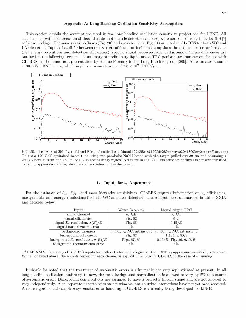
97

Appendix A: Long-Baseline Oscillation Sensitivity Assumptions

This section details the assumptions used in the long-baseline oscillation sensitivity projections for LBNE. Allcalculations (with the exception of those that did not include detector response) were performed using the GLoBES [7]software package. The same neutrino fluxes (Fig. 80) and cross sections (Fig. 81) are used in GLoBES for both WC andLAr detectors. Inputs that differ between the two sets of detectors include assumptions about the detector performance(i.e. energy resolutions and detection efficiencies), specific signal processes, and backgrounds. These differences areoutlined in the following sections. A summary of preliminary liquid argon TPC performance parameters for use withGLoBES can be found in a presentation by Bonnie Fleming to the Long-Baseline group [209]. All estimates assumea 700 kW LBNE beam, which implies a beam delivery of 7.3× 1020 POT/year.

Energy (GeV)0 2 4 6 8 10 12 14 16 18 20

/PoT) at 1300 km

2/GeV/m

νFlux (

-1510

-1410

-1310

-1210

-1110

-1010

flux µν

fluxeν

modeνFluxes in

Energy (GeV)0 2 4 6 8 10 12 14 16 18 20

/PoT

) at

130

0 km

2/G

eV/m

νF

lux

(

-1510

-1410

-1310

-1210

-1110

-1010

-910 flux µν fluxeν

modeνFluxes in

FIG. 80. The “August 2010” ν (left) and ν (right) mode fluxes (dusel120e250(n)i002dr280dz-tgtz30-1300km-0kmoa-flux.txt).This is a 120 GeV optimized beam tune using two parabolic NuMI horns with the target pulled out 30 cm and assuming a250 kA horn current and 280 m long, 2 m radius decay region (red curve in Fig. 2). This same set of fluxes is consistently usedfor all νe appearance and νµ disappearance studies in this document.

1. Inputs for νe Appearance

For the estimate of θ13, δCP , and mass hierarchy sensitivities, GLoBES requires information on νe efficiencies,backgrounds, and energy resolutions for both WC and LAr detectors. These inputs are summarized in Table XXIXand detailed below.

Input Water Cerenkov Liquid Argon TPCsignal channel νe QE νe CC

signal efficiencies Fig. 82 80%signal Eν resolution, σ(E)/E Fig. 85 0.15/E

signal normalization error 1% 1%background channels νµ CC, νµ NC, intrinsic νe νµ CC, νµ NC, intrinsic νe

background efficiencies Fig. 82 1%, 1%, 80%background Eν resolution, σ(E)/E Figs. 87, 86 0.15/E, Fig. 86, 0.15/E

background normalization error 5% 5%

TABLE XXIX. Summary of GLoBES inputs for both detector technologies for the LBNE νe appearance sensitivity estimates.While not listed above, the ν contribution for each channel is explicitly included in GLoBES in the case of ν running.

It should be noted that the treatment of systematic errors is admittedly not very sophisticated at present. In alllong-baseline oscillation studies up to now, the total background normalization is allowed to vary by 5% as a sourceof systematic error. Background contributions are assumed to have a perfectly known shape and are not allowed tovary independently. Also, separate uncertainties on neutrino vs. antineutrino interactions have not yet been assessed.A more rigorous and complete systematic error handling in GLoBES is currently being developed for LBNE.

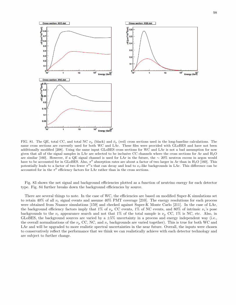
98

FIG. 81. The QE, total CC, and total NC νµ (black) and νµ (red) cross sections used in the long-baseline calculations. Thesame cross sections are currently used for both WC and LAr. These files were provided with GLoBES and have not beenadditionally modified [208]. Using the same input GLoBES cross sections for WC and LAr is not a bad assumption for nowgiven that all of the signal samples in LAr are selected to be inclusive CC channels where the cross sections for Ar and H2Oare similar [160]. However, if a QE signal channel is used for LAr in the future, the ∼ 20% neutron excess in argon wouldhave to be accounted for in GLoBES. Also, π0 absorption rates are about a factor of two larger in Ar than in H2O [160]. Thispotentially leads to a factor of two fewer π0’s that can decay and lead to νe-like backgrounds in LAr. This difference can beaccounted for in the π0 efficiency factors for LAr rather than in the cross sections.

Fig. 83 shows the net signal and background efficiencies plotted as a function of neutrino energy for each detectortype. Fig. 84 further breaks down the background efficiencies by source.

There are several things to note. In the case of WC, the efficiencies are based on modified Super-K simulations setto retain 40% of all νe signal events and assume 40% PMT coverage [210]. The energy resolutions for each processwere obtained from Nuance simulations [159] and checked against Super-K Monte Carlo [211]. In the case of LAr,the background efficiency factors imply that 1% of νµ CC events, 1% of NC events, and 80% of intrinsic νe’s posebackgrounds to the νe appearance search and not that 1% of the total sample is νµ CC, 1% is NC, etc. Also, inGLoBES, the background sources are varied by a ±5% uncertainty in a process and energy independent way (i.e.,the overall normalizations of the νµ CC, NC, and νe backgrounds are varied together). This is true for both WC andLAr and will be upgraded to more realistic spectral uncertainties in the near future. Overall, the inputs were chosento conservatively reflect the performance that we think we can realistically achieve with each detector technology andare subject to further change.

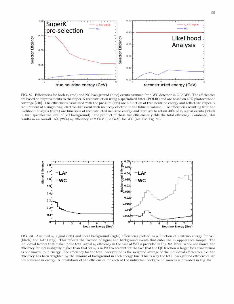
99

FIG. 82. Efficiencies for both νe (red) and NC background (blue) events assumed for a WC detector in GLoBES. The efficienciesare based on improvements to the Super-K reconstruction using a specialized fitter (POLfit) and are based on 40% photocathodecoverage [210]. The efficiencies associated with the pre-cuts (left) are a function of true neutrino energy and reflect the Super-Krequirement of a single-ring, electron-like event with no decay electron in the fiducial volume. The efficiencies resulting from thelikelihood analysis (right) are functions of reconstructed neutrino energy and were set to retain 40% of νe signal events (whichin turn specifies the level of NC background). The product of these two efficiencies yields the total efficiency. Combined, thisresults in an overall 16% (28%) νe efficiency at 2 GeV (0.8 GeV) for WC (see also Fig. 83).


Sig

nal

Eff

icie

ncy

0

0.1

0.2

0.3

0.4

0.5

0.6

0.7

0.8

LAr

WC


Bac

kgro

un

d E

ffic

ien

cy

0

0.005

0.01

0.015

0.02

0.025

0.03

0.035

0.04

0.045

0.05

LAr

WC

FIG. 83. Assumed νe signal (left) and total background (right) efficiencies plotted as a function of neutrino energy for WC(black) and LAr (gray). This reflects the fraction of signal and background events that enter the νe appearance sample. Theindividual factors that make up the total signal νe efficiency in the case of WC is provided in Fig. 82. Note: while not shown, theefficiency for νe’s is slightly higher than that for νe’s in WC to account for the fact that the QE fraction is larger for antineutrinosas one moves up in energy. The efficiency for the total background is the weighted average of the individual efficiencies, i.e. theefficiency has been weighted by the amount of background in each energy bin. This is why the total background efficiencies arenot constant in energy. A breakdown of the efficiencies for each of the individual background sources is provided in Fig. 84.

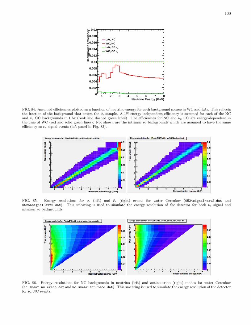
100


Bac

kgro

un

d E

ffic

ien

cy

0

0.002

0.004

0.006

0.008

0.01

0.012

0.014

0.016

0.018

0.02

LAr, NC

WC, NC

µνLAr, CC

µνWC, CC

FIG. 84. Assumed efficiencies plotted as a function of neutrino energy for each background source in WC and LAr. This reflectsthe fraction of the background that enters the νe sample. A 1% energy-independent efficiency is assumed for each of the NCand νµ CC backgrounds in LAr (pink and dashed green lines). The efficiencies for NC and νµ CC are energy-dependent inthe case of WC (red and solid green lines). Not shown are the intrinsic νe backgrounds which are assumed to have the sameefficiency as νe signal events (left panel in Fig. 83).

FIG. 85. Energy resolutions for νe (left) and νe (right) events for water Cerenkov (0524signal-ext2.dat and0525asignal-ext2.dat). This smearing is used to simulate the energy resolution of the detector for both νe signal andintrinsic νe backgrounds.

FIG. 86. Energy resolutions for NC backgrounds in neutrino (left) and antineutrino (right) modes for water Cerenkov(nc-smear-nu-ereco.dat and nc-smear-anu-reco.dat). This smearing is used to simulate the energy resolution of the detectorfor νµ NC events.

101

FIG. 87. Energy resolutions for νµ mis-ID backgrounds in neutrino (left) and antineutrino (right) modes for water Cerenkov(0524dis-ext2.dat and 0524adis.dat). This smearing is used to simulate the energy resolution of the detector for νµ CCevents.

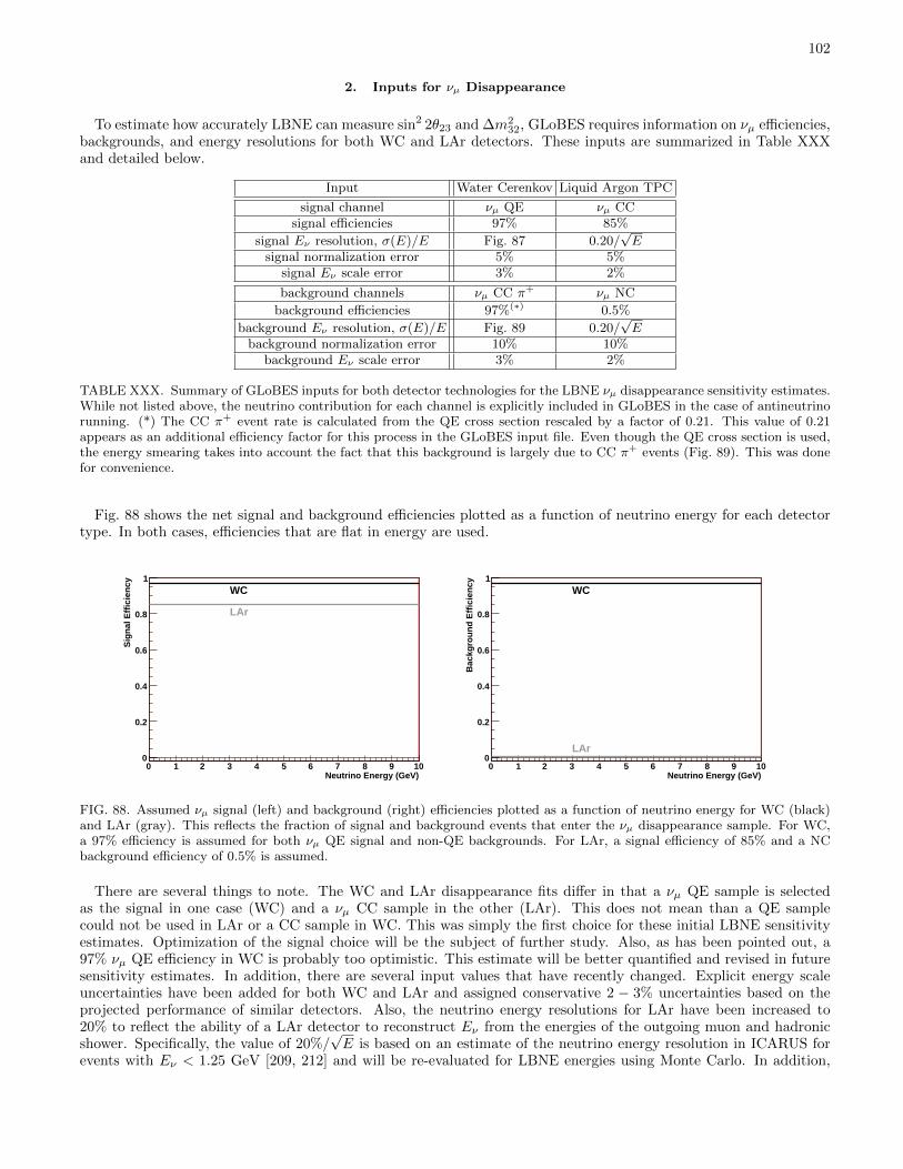
102

2. Inputs for νµ Disappearance

To estimate how accurately LBNE can measure sin2 2θ23 and ∆m232, GLoBES requires information on νµ efficiencies,

backgrounds, and energy resolutions for both WC and LAr detectors. These inputs are summarized in Table XXXand detailed below.

Input Water Cerenkov Liquid Argon TPC

signal channel νµ QE νµ CCsignal efficiencies 97% 85%

signal Eν resolution, σ(E)/E Fig. 87 0.20/√E

signal normalization error 5% 5%signal Eν scale error 3% 2%

background channels νµ CC π+ νµ NC

background efficiencies 97%(∗) 0.5%

background Eν resolution, σ(E)/E Fig. 89 0.20/√E

background normalization error 10% 10%background Eν scale error 3% 2%

TABLE XXX. Summary of GLoBES inputs for both detector technologies for the LBNE νµ disappearance sensitivity estimates.While not listed above, the neutrino contribution for each channel is explicitly included in GLoBES in the case of antineutrinorunning. (*) The CC π+ event rate is calculated from the QE cross section rescaled by a factor of 0.21. This value of 0.21appears as an additional efficiency factor for this process in the GLoBES input file. Even though the QE cross section is used,the energy smearing takes into account the fact that this background is largely due to CC π+ events (Fig. 89). This was donefor convenience.

Fig. 88 shows the net signal and background efficiencies plotted as a function of neutrino energy for each detectortype. In both cases, efficiencies that are flat in energy are used.

Neutrino Energy (GeV)0 1 2 3 4 5 6 7 8 9 10

Sig

nal

Eff

icie

ncy

0

0.2

0.4

0.6

0.8

1WC

LAr

Neutrino Energy (GeV)0 1 2 3 4 5 6 7 8 9 10

Bac

kgro

un

d E

ffic

ien

cy

0

0.2

0.4

0.6

0.8

1WC

LAr

FIG. 88. Assumed νµ signal (left) and background (right) efficiencies plotted as a function of neutrino energy for WC (black)and LAr (gray). This reflects the fraction of signal and background events that enter the νµ disappearance sample. For WC,a 97% efficiency is assumed for both νµ QE signal and non-QE backgrounds. For LAr, a signal efficiency of 85% and a NCbackground efficiency of 0.5% is assumed.

There are several things to note. The WC and LAr disappearance fits differ in that a νµ QE sample is selectedas the signal in one case (WC) and a νµ CC sample in the other (LAr). This does not mean than a QE samplecould not be used in LAr or a CC sample in WC. This was simply the first choice for these initial LBNE sensitivityestimates. Optimization of the signal choice will be the subject of further study. Also, as has been pointed out, a97% νµ QE efficiency in WC is probably too optimistic. This estimate will be better quantified and revised in futuresensitivity estimates. In addition, there are several input values that have recently changed. Explicit energy scaleuncertainties have been added for both WC and LAr and assigned conservative 2 − 3% uncertainties based on theprojected performance of similar detectors. Also, the neutrino energy resolutions for LAr have been increased to20% to reflect the ability of a LAr detector to reconstruct Eν from the energies of the outgoing muon and hadronicshower. Specifically, the value of 20%/

√E is based on an estimate of the neutrino energy resolution in ICARUS for

events with Eν < 1.25 GeV [209, 212] and will be re-evaluated for LBNE energies using Monte Carlo. In addition,

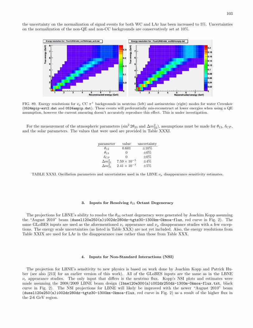
103

the uncertainty on the normalization of signal events for both WC and LAr has been increased to 5%. Uncertaintieson the normalization of the non-QE and non-CC backgrounds are conservatively set at 10%.

FIG. 89. Energy resolutions for νµ CC π+ backgrounds in neutrino (left) and antineutrino (right) modes for water Cerenkov(0524mpip-ext2.dat and 0524ampip.dat). These events will preferentially mis-reconstruct at lower energies when using a QEassumption, however the current smearing doesn’t accurately reproduce this effect. This is under investigation.

For the measurement of the atmospheric parameters (sin2 2θ23 and ∆m232), assumptions must be made for θ13, δCP ,

and the solar parameters. The values that were used are provided in Table XXXI.

parameter value uncertaintyθ12 0.601 ±10%θ13 0 ±0%δCP 0 ±0%

∆m221 7.59× 10−5 ±4%

∆m231 2.41× 10−3 ±5%

TABLE XXXI. Oscillation parameters and uncertainties used in the LBNE νµ disappearance sensitivity estimates.

3. Inputs for Resolving θ23 Octant Degeneracy

The projections for LBNE’s ability to resolve the θ23 octant degeneracy were generated by Joachim Kopp assumingthe “August 2010” beam (dusel120e250(n)i002dr280dz-tgtz30-1300km-0kmoa-flux, red curve in Fig. 2). Thesame GLoBES inputs are used as the aforementioned νe appearance and νµ disappearance studies with a few excep-tions. The energy scale uncertainties (as listed in Table XXX) are not yet included. Also, the energy resolutions fromTable XXIX are used for LAr in the disappearance case rather than those from Table XXX.

4. Inputs for Non-Standard Interactions (NSI)

The projection for LBNE’s sensitivity to new physics is based on work done by Joachim Kopp and Patrick Hu-ber (see also [213] for an earlier version of this work). All of the GLoBES inputs are the same as in the LBNEνe appearance studies. The only input that differs is the neutrino flux. Kopp’s NSI plots and estimates weremade assuming the 2008/2009 LBNE beam design (lbne120e300(n)i002dr250dz-1300m-0kmoa-flux.txt, blackcurve in Fig. 2). The NSI projections for LBNE will likely be improved with the newer “August 2010” beam(dusel120e250(n)i002dr280dz-tgtz30-1300km-0kmoa-flux, red curve in Fig. 2) as a result of the higher flux inthe 2-6 GeV region.

104

Appendix B: Supernova Burst Physics Sensitivity Assumptions

1. Assumptions for Event Rates in Water

We used WCsim [56] to evaluate the detection response in water for the 15% and 30% PMT coverage configurations.At the moment, we do not yet have a perfect match between WCsim output in Super-Kamiokande mode and publishedSK detector parameters in the few to few tens of MeV range [214, 215]– the agreement is at about the 10% level.The resolution used as a function of electron energy is shown in Fig. 90 (left); it was scaled by a factor of 0.66 inorder that WCsim SK-mode output match the resolution in Ref. [214] (in addition to minor simulation mismatch, wedo not have all SK software tools for energy response reconstruction at our disposal for WCsim output, which likelyaccounts for some of the discrepancy).

Trigger efficiency is shown in Fig. 90 (right) for the different configurations; this assumes a trigger requirement of33 hits in 300 ns for the 15% PMT coverage configuration and 39 hits in 300 ns for the 30% configuration. (Notethat we are assuming supernova neutrino events in water are self-triggered; one can imagine a configuration in whichall digitized PMT hits are saved in the event of a high rate, which could improve efficiency.) These efficiencies areslightly worse than SK I [214] and SK II [215] efficiencies.

Electron energy (MeV) 5 10 15 20 25 30

Res

olu

tio

n (

%)

0

20

40

60

80

100

120

140

160

100kt, 15%

100kt, 30%

Electron energy (MeV) 0 5 10 15 20 25 30

Eff

icie

ncy

0

0.2

0.4

0.6

0.8

1

100kt, 15%

100kt, 30%

FIG. 90. Energy resolution (left) and trigger efficiency (right) as a function of electron energy, for 30% and 15% PMT coverages.

2. Assumptions for Event Rates in Argon

For event rate estimates in liquid argon, we assume a detection threshold of 5 MeV. We assume also that suitabletriggering will be provided from photons, charge collection or from some external trigger. The energy resolution usedis from Ref. [216], σ

E = 11%√E

+ 2%.

A summary of preliminary liquid argon TPC performance parameters can be found in a presentation by BonnieFleming to the Long-Baseline group [209].

105

[1] http://lbne.fnal.gov/

[2] A. Bernstein et al., “Report on the Depth Requirements for a Massive Detector at Homestake,” arXiv:0907.4183v2 [hep-ex][3] V. Barger et al., “Report of the US long baseline neutrino experiment study”, Fermilab-0801-AD-E, BNL-77973-2007-IR,

arXiv:0705.4396v1 [hep-ph] (2007); http://nwg.phy.bnl.gov/~diwan/nwg/fnal-bnl/[4] J. Hylen et al., ”Conceptual design for the technical components of the neutrino beam for the main injector (NuMI)”,

FERMILAB-TM-2018 (1997).[5] D. G. Michael et al., “Observation of muon neutrino disappearance with the MINOS detectors in the NuMI neutrino

beam”, hep-ex 0607088, FERMILAB-PUB-06-243, BNL-76806-2006-J A.[6] R. Brun et al., CERN-DD-78-2-REV.[7] http://www.mpi-hd.mpg.de/lin/globes/; arXiv:0407333 [hep-ph] (2004) and arXiv:0701187 [hep-ph] (2007).[8] D. Mohapatra, LBNE docdb #2683.[9] EURONU WP6 2009 yearly report, J. Bernabeu et al., arXiv:1005.3146 [hep-ph].

[10] “XXIV International Conference on Neutrino Physics and Astrophysics,” Athens, Greece, (June, 2010), http://www.

neutrino2010.gr/.[11] K. Nakamura et al. (Particle Data Group), J. Phys. G37, 075021 (2010).[12] P. Vahle, presentation at the XXIV International Conference on Neutrino Physics and Astrophysics (Neutrino 2010) in

Athens, Greece; slides available at http://www.neutrino2010.gr/.[13] T. Kobayashi, Neutrino 2010 presentation on the status of T2K.[14] M.H. Ahn et al. (K2K Collaboration), Phys. Rev. D74, 072003 (2006), arXiv:0606032 [hep-ex].[15] A. A. Aguilar-Arevalo et al. (MiniBooNE Collaboration), Phys. Rev. Lett. 103, 061802 (2009).[16] NOvA technical design report, http://www-nova.fnal.gov/nova_cd2_review/tdr_oct_23/tdr.htm[17] B. Rebel, private communication.[18] S. Davidson, C. Pena-Garay, N. Rius, and A. Santamaria, hep-ph/0302093.[19] M.C. Gonzalez-Garcia, and M. Maltoni, Phys. Rept. 460, 1 (2008), arXiv:0704.1800 [hep-ph].[20] C. Biggio, M. Blennow, and E. Fernandez-Martinez, arXiv:0907.0097 [hep-ph].[21] S. Antusch, J.P. Baumann, and E. Fernandez-Martinez, arXiv:0807.1003 [hep-ph].[22] M.B. Gavela, D. Hernandez, T. Ota, and W. Winter, arXiv:0809.3451 [hep-ph].[23] W.A. Mann, D. Cherdack, W. Musial, and T. Kafka, arXiv:1006.5720 [hep-ph].[24] E. Akhmedov and T. Schwetz, arXiv:1007.4171 [hep-ph].[25] J. Kopp, P. Machado, and S. Parke, to be published soon, the talk by PANM is available from http://www.int.

washington.edu/talks/WorkShops/int_10_2b/People/Machado_P/Machado.pdf.[26] A.A. Aguilar-Arevalo et al., arXiv:1007.1150 [hep-ex].[27] A. Friedland, Alexander and C. Lunardini Phys. Rev. D72, 053009 (2005), arXiv:0506143 [hep-ph].[28] P. Astier et al., Nucl. Phys. B611,[29] Phys.Rev. D81, 093001 (2010).[30] J. C. Pati and A. Salam, Phys. Rev. Lett. 31, 661 (1973).[31] H. Georgi and S. L. Glashow, Phys. Rev. Lett. 32, 438 (1974).[32] S. Dimopoulos, S. Raby and F. Wilczek, Phys. Lett. B 112, 133 (1982).[33] P. Langacker, Phys. Rept. 72, 185 (1981).[34] W. de Boer, Prog. Part. Nucl. Phys. 33, 201 (1994) [arXiv:9402266 [hep-ph]].[35] P. Nath and P. Fileviez Perez, Phys. Rept. 441, 191 (2007) [arXiv:0601023 [hep-ph]].[36] S. Raby et al., arXiv:0810.4551 [hep-ph].[37] G. Senjanovic, AIP Conf. Proc. 1200, 131 (2010) [arXiv:0912.5375 [hep-ph]].[38] T. Li, D. V. Nanopoulos and J. W. Walker, arXiv:1003.2570 [hep-ph].[39] A. Bueno et al., JHEP 0704, 041 (2007) [arXiv:0701101 [hep-ph]].[40] R. M. Barnett et al. [Particle Data Group], Phys. Rev. D 54, 1 (1996).[41] H. Nishino et al. [Super-Kamiokande Collaboration], Phys. Rev. Lett. 102, 141801 (2009) [arXiv:0903.0676 [hep-ex]].[42] http://www-sk.icrr.u-tokyo.ac.jp/whatsnew/new-20091125-e.html

[43] Y. Hayato et al. [Super-Kamiokande Collaboration], Phys. Rev. Lett. 83, 1529 (1999) [arXiv:9904020 [hep-ex]].[44] K. Kobayashi et al. [Super-Kamiokande Collaboration], Phys. Rev. D 72, 052007 (2005) [arXiv:0502026 [hep-ex]].[45] K. Scholberg, arXiv:0701081 [astro-ph].[46] A. Dighe, arXiv:0809.2977 [hep-ph].[47] R. M. Bionta et al., Phys. Rev. Lett. 58, 1494 (1987).[48] K. Hirata et al. [KAMIOKANDE-II Collaboration], Phys. Rev. Lett. 58, 1490 (1987).[49] A. Mirizzi, G. G. Raffelt and P. D. Serpico, JCAP 0605, 012 (2006) [arXiv:0604300 [astro-ph]].[50] S. Choubey, B. Dasgupta, A. Dighe and A. Mirizzi, arXiv:1008.0308 [hep-ph].[51] G. G. Raffelt, arXiv:9707268 [astro-ph].[52] S. Hannestad and G. Raffelt, Phys. Rev. Lett. 87, 051301 (2001) [arXiv:0103201 [hep-ph]].[53] P. Antonioli et al., New J. Phys. 6, 114 (2004) [arXiv:0406214 [astro-ph]].[54] K. Scholberg, Astron. Nachr. 329, 337 (2008) [arXiv:0803.0531 [astro-ph]].[55] K. Scholberg, J. Phys. Conf. Ser. 203, 012079 (2010).

http://lbne.fnal.gov/

http://nwg.phy.bnl.gov/~diwan/nwg/fnal-bnl/

http://www.mpi-hd.mpg.de/lin/globes/

http://www.neutrino2010.gr/



http://www.int.washington.edu/talks/WorkShops/int_10_2b/People/Machado_P/Machado.pdf

http://www.int.washington.edu/talks/WorkShops/int_10_2b/People/Machado_P/Machado.pdf

http://www-sk.icrr.u-tokyo.ac.jp/whatsnew/new-20091125-e.html

106

[56] https://wiki.bnl.gov/dusel/index.php/Simulation/Software

[57] http://www.phy.duke.edu/~schol/snowglobes/

[58] T. Totani, K. Sato, H. E. Dalhed and J. R. Wilson, Astrophys. J. 496, 216 (1998) [arXiv:9710203 [astro-ph]].[59] J. Gava, J. Kneller, C. Volpe and G. C. McLaughlin, Phys. Rev. Lett. 103, 071101 (2009) [arXiv:0902.0317 [hep-ph]].[60] H. Duan and A. Friedland, arXiv:1006.2359 [hep-ph].[61] M. T. Keil, G. G. Raffelt and H. T. Janka, Astrophys. J. 590, 971 (2003) [arXiv:0208035 [astro-ph]].[62] E. Kolbe, K. Langanke and P. Vogel, Phys. Rev. D 66, 013007 (2002).[63] K. Langanke, P. Vogel and E. Kolbe, Phys. Rev. Lett. 76, 2629 (1996) [arXiv:9511032 [nucl-th]].[64] J. F. Beacom and P. Vogel, Phys. Rev. D 60, 033007 (1999) [arXiv:9811350 [astro-ph]].[65] R. Tomas, D. Semikoz, G. G. Raffelt, M. Kachelriess and A. S. Dighe, Phys. Rev. D 68, 093013 (2003) [arXiv:0307050

[hep-ph]].[66] M. Ikeda, http://www-sk.icrr.u-tokyo.ac.jp/sk/pub/m_ikeda_mron.pdf[67] M. Ikeda et al. [Super-Kamiokande Collaboration], Astrophys. J. 669, 519 (2007) [arXiv:0706.2283 [astro-ph]].[68] I. Gil Botella and A. Rubbia, JCAP 0408, 001 (2004) [arXiv:0404151 [hep-ph]].[69] E. Kolbe, K. Langanke, G. Martinez-Pinedo and P. Vogel, J. Phys. G 29, 2569 (2003) [arXiv:0311022 [nucl-th]].[70] T. Totani, K. Sato and Y. Yoshii, Astrophys. J. 460, 303 (1996) [arXiv:9509130 [astro-ph]].[71] K. Sato, T. Totani and Y. Yoshii, Prepared for 4th SFB-375 Ringberg Workshop on Neutrino Astrophysics, Ringberg

Castle, Tegernsee, Germany, 20-24 Oct 1997[72] D. H. Hartmann and S. E. Woosley, Astropart. Phys. 7, 137 (1997).[73] R. A. Malaney, Astropart. Phys. 7, 125 (1997) [arXiv:9612012 [astro-ph]].[74] M. Kaplinghat, G. Steigman and T. P. Walker, Phys. Rev. D 62, 043001 (2000) [arXiv:9912391 [astro-ph]].[75] S. Ando, J. F. Beacom and H. Yuksel, Phys. Rev. Lett. 95, 171101 (2005) [arXiv:0503321 [astro-ph]].[76] C. Lunardini, Phys. Rev. D 75, 073022 (2007) [arXiv:0612701 [astro-ph]].[77] M. Fukugita and M. Kawasaki, Mon. Not. Roy. Astron. Soc. 340, L7 (2003) [arXiv:0204376 [astro-ph]].[78] A. Lien, B. D. Fields and J. F. Beacom, Phys. Rev. D 81, 083001 (2010) [arXiv:1001.3678 [astro-ph.CO]].[79] J. F. Beacom, arXiv:1004.3311 [astro-ph.HE].[80] C. Lunardini, arXiv:1007.3252 [astro-ph.CO].[81] M. Malek et al. [Super-Kamiokande Collaboration], Phys. Rev. Lett. 90, 061101 (2003) [arXiv:0209028 [hep-ex]].[82] L. E. Strigari, M. Kaplinghat, G. Steigman and T. P. Walker, JCAP 0403, 007 (2004) [arXiv:0312346 [astro-ph]].[83] J. F. Beacom and M. R. Vagins, Phys. Rev. Lett. 93, 171101 (2004) [arXiv:0309300 [hep-ph]].[84] H. Watanabe et al. [Super-Kamiokande Collaboration], arXiv:0811.0735 [hep-ex].[85] A. Kibayashi and S. K. Collaboration, arXiv:0909.5528 [astro-ph.IM].[86] Y. Koshio, Ph.D thesis, University of Tokyo (1998)[87] http://www.phys.hawaii.edu/~jgl/post/A~White~Paper~for~Large~Liquid~Scintillation~Detectors~at~DUSEL.

pdf

[88] P. Vogel and J. F. Beacom, Phys. Rev. D 60, 053003 (1999) [arXiv:9903554 [hep-ph]].[89] A. Strumia and F. Vissani, Phys. Lett. B 564, 42 (2003) [arXiv:0302055 [astro-ph]].[90] W. E. Ormand, P. M. Pizzochero, P. F. Bortignon and R. A. Broglia, Phys. Lett. B 345, 343 (1995) [arXiv:9405007

[nucl-th]].[91] M. Sajjad Athar and S. K. Singh, Phys. Lett. B 591, 69 (2004).[92] A. G. Cocco, A. Ereditato, G. Fiorillo, G. Mangano and V. Pettorino, JCAP 0412, 002 (2004) [arXiv:0408031 [hep-ph]].[93] http://nucleardata.nuclear.lu.se/nucleardata/toi/nuclide.asp?iZA=30011

[94] A. Rubbia, J. Phys. Conf. Ser. 171, 012020 (2009) [arXiv:0908.1286 [hep-ph]].[95] O.L.G. Peres et al., Phys. Rev. D79, 113002 (2009).[96] J. Bernabeu et al., Nucl. Phys. B669, 255 (2003).[97] M.C. Gonzalez-Garcia et al., Phys. Rev. D70, 093005 (2004).[98] O.L.G. Peres et al., Phys. Lett. B456, 204 (1999).[99] Akhmedov et al., JHEP 0806 072 (2008).

[100] S.T. Petcov et al., Nucl. Phys. B, 740 (2006).[101] S. Palomares-Ruiz et al., Nucl. Phys. B712, 392 (2005).[102] Y. Ashie et al., Phys. Rev. Lett 93, 101801 (2004).[103] Y. Ashie et al., Phys.Rev. D71, 112005 (2005).[104] K. Abe et al., Phys. Rev. Lett. 97, 171801 (2006).[105] R. Wendell et al., arXiv:1002.3471 [hep-ex] (2010).[106] J. Hosaka et al., Phys. Rev. D74, 032002 (2006).[107] K. Abe et al., Phys. Rev. D77, 052001 (2008).[108] W. Wang, Ph. D Thesis (2007).[109] G. Mitsuka Ph. D Thesis (2009).[110] P. Adamson et al., Phys. Rev. D75, 092003 (2007).[111] D. Indumathi et al., Phys. Rev. D71, 013001 (2005).[112] S. Coleman and S. Glashow, Phys. Lett. B405, 249 (1997).[113] F. Klinkhamer and G. Volovik, Intl. Jour. of Mod. Phys. A20, 2795 (2005).[114] D. Colladay and V. Kostelecky, Phys. Rev. D, 116002 (1998).[115] Y. Grossman et al., Phys. Rev. D72, 125001 (2005).

https://wiki.bnl.gov/dusel/index.php/Simulation/Software

http://www.phy.duke.edu/~schol/snowglobes/

http://www-sk.icrr.u-tokyo.ac.jp/sk/pub/m_ikeda_mron.pdf

http://www.phys.hawaii.edu/~jgl/post/A~White~Paper~for~Large~Liquid~Scintillation~Detectors~at~DUSEL.pdf

http://www.phys.hawaii.edu/~jgl/post/A~White~Paper~for~Large~Liquid~Scintillation~Detectors~at~DUSEL.pdf

http://nucleardata.nuclear.lu.se/nucleardata/toi/nuclide.asp?iZA=30011

107

[116] M. C. Gonzalez-Garcia et al., Nucl. Phys. B573, 3 (2000).[117] D. Kaplan et al., Phys. Rev. Lett. 93, 091801 (2004).[118] J. Conrad et al., arXiv:1008.2984 [hep-ph] (2010).[119] P. Huber et al., arXiv:0501037 [hep-ph] (2005).[120] A. Rubbia, NNN99 Proceedings, arXiv:0001052 [hep-ex] (2001).[121] M. Fechner et al., Phys. Rev. D79, 112010 (2009).[122] S. Petcov and T. Schwetz, arXiv:0511277 [hep-ph] (2005).[123] C. Andreopoulos et al., Nucl. Instrum. Meth. A614, 87 (2010).[124] G. Barr et al., Phys. Rev. D70, 023006 (2004).[125] G. Battistoni et al., Astropart. Phys. 19, 269 (2003).[126] T. Kajita, Talk at NOON2004 (Tokyo), 2004.[127] M. Ishitsuka, Ph. D Thesis (2004).[128] A. Bueno et al., arXiv:0701101 [hep-ph] (2007).[129] R. Gandhi et al., Phys. Rev. D78:073001 (2008).[130] F. Dufour, Ph. D Thesis (2009).[131] V. Barger et al., Phys. Rev. D22, 2718 (1980).[132] M. Messier, private communication (2010).[133] M. Sanchez et al., Phys. Rev. D68, 113004 (2003).[134] C. Ishihara, Ph. D Thesis (2010).[135] J.G. Learned and K. Mannheim, Ann. Rev. Nucl. Part. Sci. 50 679 (2000).[136] Bahcall, J., Waxmann, E., 2001, Physical Review D, 64 023002 (2001).[137] Gueta, et al., Astropart.Phys. 20 429-455 (2004).[138] M. Drees and M. M. Nojiri, Phys. Rev. D 47, 376 (1993).[139] DeYoung, T., et al.et al. (IceCube Collaboration), 2008. J. of Phys. Conf. Ser. 136 022046 (2008).[140] V. Aynutdinov,et al. (BAIKAL Collaboration), Astropart.Phys.25:140-150,2006.[141] The Antares Collaboration Internal Report CPPM-P-1999-02 (1999), arXiv:9907432v1 [astro-ph].[142] IceCube collaboration, in preparation.[143] R. Abbasi, et al., Astrophys.J 701 L47-L51 (2009).[144] M. Ackermann, et al., Astrophys.J 675 1014 (2008).[145] R. Abbasi, et al., Astrophys.J. 710 346-359 (2010).[146] R. Abbasi, et al., Phys. Rev. Lett. 102 201302 (2009), [arXiv:0910.4480].[147] S. Desai, et al., Phys.Rev.D 70 083523 (2004).[148] E. Thrane, et al., Astrophys.J 704 503-512 (2009).[149] M.E.C Swanson, et al., Astrophys.J 652 206-215 (2006).[150] Private collaboration document DUSEL/LBNE R&D Document 994,

http://nwg.phy.bnl.gov/DDRD/cgi-bin/private/ShowDocument?docid=994.[151] E. Presani, et al., Nuclear Physics B Proceedings Supplements 188 270-272 (2009).[152] H. Yuksel, S. Horiuchi, J. Beacom, S. Ando, Phys.Rev.D 76 123506 (2007).[153] B. T. Cleveland et al. Astrophys. J. 496: 505 (1998).[154] S. Fukuda et al., Phys. Rev. Lett. 86, 5651 (2001); Q. R. Ahmad et al., Phys. Rev. Lett. 87), 071301(2001).[155] Phys.Rev. D69, 011104 (2004).[156] A. Guglielmi, talk at XXIV Neutrino Conference (Neutrino 2010), Athens, Greece (June 2010).[157] Internal collaboration document DUSEL/LBNE R&D Document 643-v2, “Reference Near Detector Parameters,” http:

//nwg.phy.bnl.gov/DDRD/html/0006/000643/002/Near%20Detector%20Reference%20Parameters.docx

[158] G.P. Zeller, “Expected Event Rates in the LBNE Near Detectors”, docdb #783, http://nwg.phy.bnl.gov/DDRD/html/0007/000783/001/event-rates.pdf, flux files in http://www.phy.bnl.gov/~bishai/nwg/work/gnumi/prod/

[159] D. Casper, Nucl. Phys. Proc. Suppl. 112, 161 (2002), hep-ph/0208030.[160] R. Petti and G.P. Zeller, “Nuclear Effects in Water vs. Argon”, docdb #740.[161] G.P. Zeller et al., Phys. Rev. Lett. 88, 091802 (2002); erratum-ibid. 90, 239902 (2003)[162] W.J. Marciano and Z. Parsa, J. Phys. G 29 (2003) 2629-2645.[163] I. Stancu et al., arXiv:0910.2698 [hep-ex].[164] The OscSNS Neutrino Experiment http://physics.calumet.purdue.edu/~oscsns/.[165] B. Baibussinov et al., arXiv:0909.0355 [hep-ex].[166] J.A. Harvey, C.T. Hill and R.J. Hill, Phys. Rev. Lett. 99 (2007) 261601; Phys. Rev. D 77 (2008) 085017.[167] J. Jenkins and T. Goldman, Phys. Rev. D 80 (2009) 053005.[168] M.Shiozawa, Talk at NNN09;

http://nnn09.colostate.edu/Talks/Session02/091007-Shiozawa-Nucleon-decay-searches-dist.pdf.[169] S.Mine et al. (K2K Collaboration), Phys. Rev. D 77, 032003 (2008); H. Nishino et al. (Super-Kamiokande Collaboration),

Phys. Rev. Lett. 102, 141801 (2009).[170] P. Astier et al. [NOMAD collaboration], Nucl. Phys. B621/1-2 (2001) 3-34, arXiv:0111057 [hep-ex].[171] D. Naumov et al. [NOMAD collaboration], Nucl.Phys.B 700 (2004) 51-68, arXiv:0409037 [hep-ex].[172] S. Alekhin, S. A. Kulagin, and R. Petti, AIP Conf. Proc. 967, 215 (2007), [arXiv:0710.0124].[173] S. Alekhin, S. Kulagin, and R. Petti, (2008), arXiv:0810.4893 [hep-ph].[174] S. Alekhin, S. Kulagin and R. Petti, Phys. Lett. B 675, 433 (2009).

http://nwg.phy.bnl.gov/DDRD/cgi-bin/private/ShowDocument?docid=994

http://nwg.phy.bnl.gov/DDRD/html/0006/000643/002/Near%20Detector%20Reference%20Parameters.docx

http://nwg.phy.bnl.gov/DDRD/html/0006/000643/002/Near%20Detector%20Reference%20Parameters.docx

http://nwg.phy.bnl.gov/DDRD/html/0007/000783/001/event-rates.pdf

http://nwg.phy.bnl.gov/DDRD/html/0007/000783/001/event-rates.pdf

http://www.phy.bnl.gov/~bishai/nwg/work/gnumi/prod/

http://physics.calumet.purdue.edu/~oscsns/

http://nnn09.colostate.edu/Talks/Session02/091007-Shiozawa-Nucleon-decay-searches-dist.pdf

108

[175] A. B. Arbuzov, D. Y. Bardin and L. V. Kalinovskaya, JHEP 78, 506 (2005); arXiv:0407203 [hep-ph].[176] S. A. Kulagin and R. Petti, Nucl. Phys. A765, 126 (2006).[177] S. A. Kulagin and R. Petti, Phys. Rev. D76, 094023 (2007).[178] S. A. Kulagin and R. Petti, arXiv:1004.3062 [hep-ph].[179] R. Petti and O. Samoylov, Proceedings of DIS10 - Firenze, Italy, 19-23 April 2010.[180] A. Czarnecki and W.J. Marciano, Int. J. Mod. Phy. A15 (2000) 2365[181] S.C. Bennet and C.E. Wieman, Phys. Rev. Lett. 82 (1999) 2484[182] Particle Data Group, W.-M. Yao et al., Journal of Physics, G 33 (2006) 1[183] P.L. Anthony et al [E158 collaboration], Phys.Rev.Lett. 95 (2005) 081601, hep-ex/0504049[184] R. D. Young, J. Roche, R. D. Carlini and A. W. Thomas, Phys. Rev. Lett. 97, 102002 (2006).[185] D. B. Leinweber et al., Phys. Rev. Lett. 94, 212001 (2005).[186] A. Airapetian et al., Phys. Lett. B 666, 446 (2008).[187] L.A. Ahrens et al., Phys. Rev. D 35, 785 (1987)[188] G. Garvey et al., Phys. Rev. C 48, 761 (1993)[189] W.M. Alberico et al., Nucl. Phys. A 651, 277 (1999)[190] L. Bugel et al., arXiv:0402007 [hep-ex].[191] A. Boyarsky, O. Ruchayskiy and M. Shaposhnikov, Ann. Rev. Nucl. Part. Sci. 59 (2009) 191 [arXiv:0901.0011 [hep-ph]][192] M. Shaposhnikov, JHEP 0808 (2008) 008 [arXiv:0804.4542 [hep-ph]].[193] L. Canetti and M. Shaposhnikov, arXiv:1006.0133 [hep-ph].[194] A. M. Cooper-Sarkar et al. [WA66 Collaboration], Phys. Lett. B 160 (1985) 207.[195] F. Bergsma et al. [CHARM Collaboration], Phys. Lett. B 166 (1986) 473.[196] A. Vaitaitis et al. [NuTeV Collaboration], Phys. Rev. Lett. 83 (1999) 4943 [arXiv:9908011 [hep-ex]].[197] G. Bernardi et al., Phys. Lett. B 166 (1986) 479.[198] G. Bernardi et al., Phys. Lett. B 203 (1988) 332.[199] A. Atre, T. Han, S. Pascoli and B. Zhang, JHEP 0905 (2009) 030 [arXiv:0901.3589 [hep-ph]].[200] D. Gorbunov and M. Shaposhnikov, JHEP 0710 (2007) 015 [arXiv:0705.1729 [hep-ph]].[201] M. Soderberg, arXiv:0910.3433 [physics.ins-det][202] M. Maltoni and T. Schwetz, arXiv:0705.0107 [hep-ph][203] B. L. Ioffe, V. A. Khoze and L. N. Lipatov, “Hard Processes. Vol. 1: Phenomenology, Quark Parton Model,” Amsterdam,

Netherlands: North-holland (1984) 340p[204] D. Allasia et al., Z. Physik C 28 (1985) 321-333.[205] A. Accardi, M. E. Christy, C. E. Keppel, P. Monaghan, W. Melnitchouk, J. G. Morfin and J. F. Owens, Phys. Rev. D

81, 034016 (2010).[206] Jefferson Lab experimental proposal PR12-06-13, S. Bultmann, M. E. Christy, H. Fenker, K. A. Griffioen, C. E. Keppel,

S. E. Kuhn, W. Melnitchouk and V. Tsvaskis, spokespersons,http://www.jlab.org/exp$_$prog/proposals/06/PR12-06-113.pdf.

[207] A. Bodek and A. Simon, Z. Phys. C 29, 231 (1985); G. T. Jones et al., Z. Phys. C 44, 379 (1989).[208] M. Messier, UMI-99-23965; E.A. Paschos and J.Y. Yu, Phys. Rev. D65, 033002 (2002).[209] Internal collaboration presentation LBNE R&D document docdb #972, “Efficiencies for LAr20 for GLoBES,” B. Fleming,

Long-Baseline TG meeting (7/26/2010).[210] C. Yanagisawa, C.K. Jung, and P.T. Lee, http://ale.physics.sunysb.edu/uno/publications/numunuePREBWv3.pdf[211] M. Diwan, private communication.[212] B. Fleming, private communication and discussion at INT, August 2010.[213] J. Kopp, LBNE internal document docdb #770.[214] J. Hosaka et al. [Super-Kamiokande Collaboration], Phys. Rev. D 73, 112001 (2006) [arXiv:0508053 [hep-ex]].[215] J. P. Cravens et al. [Super-Kamiokande Collaboration], Phys. Rev. D 78, 032002 (2008) [arXiv:0803.4312 [hep-ex]].[216] S. Amoruso et al. [ICARUS Collaboration], Eur. Phys. J. C 33, 233 (2004) [arXiv:0311040 [hep-ex]].[217] http://arxiv.org/

[218] Institute for Nuclear Theory, University of Washington, summer program INT-10-2b, “Long-Baseline Neutrino Physicsand Astrophysics,” July 26 - August 27, 2010. http://www.int.washington.edu/PROGRAMS/10-2b/

[219] Publication INT-PUB-11-002, Institute for Nuclear Theory, University of Washington.

http://www.jlab.org/exp$_$prog/proposals/06/PR12-06-113.pdf

http://ale.physics.sunysb.edu/uno/publications/numunuePREBWv3.pdf

http://arxiv.org/

http://www.int.washington.edu/PROGRAMS/10-2b/

The 2010 Interim Report of the Long-Baseline Neutrino Experiment Collaboration Physics Working...

Documents

Transcript of The 2010 Interim Report of the Long-Baseline Neutrino Experiment Collaboration Physics Working...