Journal of Econometrics 115 (2003) 53–74www.elsevier.com/locate/econbase

Testing for unit roots in heterogeneous panels�

Kyung So Ima ;∗, M. Hashem Pesaranb, Yongcheol Shinc

aDepartment of Economics, University of Central Florida, P.O. Box 161400,Orlando, FL 32816-1400, USA

bTrinity College, Cambridge CB2 1TQ, UKcSchool of Economics and Management, University of Edinburgh, 50, George Square,

Edinburgh EH8 9JY, UK

Accepted 12 January 2003

Abstract

This paper proposes unit root tests for dynamic heterogeneous panels based on the mean ofindividual unit root statistics. In particular it proposes a standardized t-bar test statistic based onthe (augmented) Dickey–Fuller statistics averaged across the groups. Under a general setting thisstatistic is shown to converge in probability to a standard normal variate sequentially with T (thetime series dimension) → ∞, followed by N (the cross sectional dimension) → ∞. A diagonalconvergence result with T and N → ∞ while N=T → k; k being a 5nite non-negative constant, isalso conjectured. In the special case where errors in individual Dickey–Fuller (DF) regressionsare serially uncorrelated a modi5ed version of the standardized t-bar statistic is shown to bedistributed as standard normal as N → ∞ for a 5xed T , so long as T ¿ 5 in the case of DFregressions with intercepts and T ¿ 6 in the case of DF regressions with intercepts and lineartime trends. An exact 5xed N and T test is also developed using the simple average of the DFstatistics. Monte Carlo results show that if a large enough lag order is selected for the underlyingADF regressions, then the small sample performances of the t-bar test is reasonably satisfactoryand generally better than the test proposed by Levin and Lin (Unpublished manuscript, Universityof California, San Diego, 1993).c© 2003 Elsevier Science B.V. All rights reserved.

JEL classi6cation: C12; C15; C22; C23

Keywords: Heterogeneous dynamic panels; Tests of unit roots; t-bar statistics; Finite sample properties

� This is a substantially revised version of the DAE Working Papers Amalgamated Series No. 9526,University of Cambridge.

∗ Corresponding author.E-mail addresses: kim@bus.ucf.edu (K.S. Im), mhp1@econ.cam.ac.uk (M.H. Pesaran),

y.shin@ed.ac.uk (Y. Shin).

0304-4076/03/$ - see front matter c© 2003 Elsevier Science B.V. All rights reserved.doi:10.1016/S0304-4076(03)00092-7

54 K.S. Im et al. / Journal of Econometrics 115 (2003) 53–74

1. Introduction

Since the seminal work of Balestra and Nerlove (1966), dynamic models have playedan increasingly important role in empirical analysis of panel data in economics. Giventhe small time dimension of most panels, the emphasis has been put on models withhomogeneous dynamics, and until recently little attention has been paid to the analysisof dynamic heterogeneous panels. However, over the past decade a number of impor-tant panel data set covering diEerent industries, regions, or countries over relativelylong time spans have become available, the most prominent example of which is theSummers and Heston (1991) data. The availability of this type of “pseudo” panelsraises the issue of the plausibility of the dynamic homogeneity assumption that un-derlies the traditional analysis of panel data models, and poses the problem of howbest to analyze them. The inconsistency of pooled estimators in dynamic heterogeneouspanel models has been demonstrated by Pesaran and Smith (1995), and Pesaran et al.(1996). The present paper builds on these works and considers the problem of testingfor unit roots in such pseudo panels.Panel based unit root tests have been advanced by Quah (1992, 1994) and Levin and

Lin (1993, LL hereafter). The tests proposed by Quah do not accommodate heterogene-ity across groups such as individual speci5c eEects and diEerent patterns of residualserial correlations. LL’s test is more generally applicable, allows for individual speci5ceEects as well as dynamic heterogeneity across groups, and requires N=T → 0 as bothN (the cross section dimension) and T (the time series dimension) tend to in5nity. 1

Using the likelihood framework, this paper proposes an alternative testing procedurebased on averaging individual unit root test statistics for panels. In particular, wepropose a test based on the average of (augmented) Dickey–Fuller (Dickey and Fuller,1979) statistics computed for each group in the panel, which we refer to as the t-bartest. Like the LL procedure, our proposed test allows for residual serial correlation andheterogeneity of the dynamics and error variances across groups. Under very generalsettings this statistic is shown to converge in probability to a standard normal variatesequentially with T → ∞, followed by N → ∞. A diagonal convergence result with Tand N → ∞ while N=T → k; k being a 5nite non-negative constant, is also conjectured.

In the special case where errors in individual Dickey–Fuller (DF) regressions areserially uncorrelated a modi5ed version of the (standardized) t-bar statistic, denoted byZt̃bar , is shown to be distributed as standard normal as N → ∞ for a 5xed T , so longas T ¿ 5 in the case of DF regressions with intercepts, and T ¿ 6 in the case of DFregressions with intercepts and linear time trends. An exact 5xed N and T test is alsodeveloped using the simple average of the DF statistics. Based on stochastic simulationsit is shown that the standardized t-bar statistic provides an excellent approximation tothe exact test even for relatively small values of N .

1 Since the release of the working paper version of this paper in 1995 a number of other approaches to unitroot testing in heterogeneous panels have also been proposed in the literature. See, for example, Bowman(1999), Choi (2001), Hadri (2000), Maddala and Wu (1999), and Shin and Snell (2000). A review of thisliterature is provided in Baltagi and Kao (2000).

K.S. Im et al. / Journal of Econometrics 115 (2003) 53–74 55

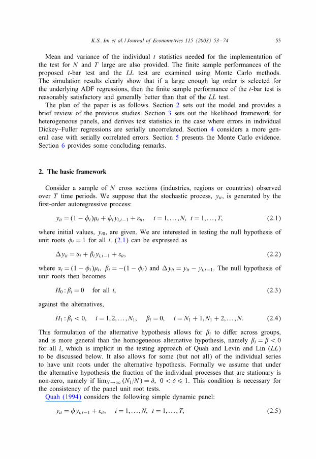
Mean and variance of the individual t statistics needed for the implementation ofthe test for N and T large are also provided. The 5nite sample performances of theproposed t-bar test and the LL test are examined using Monte Carlo methods.The simulation results clearly show that if a large enough lag order is selected forthe underlying ADF regressions, then the 5nite sample performance of the t-bar test isreasonably satisfactory and generally better than that of the LL test.The plan of the paper is as follows. Section 2 sets out the model and provides a

brief review of the previous studies. Section 3 sets out the likelihood framework forheterogeneous panels, and derives test statistics in the case where errors in individualDickey–Fuller regressions are serially uncorrelated. Section 4 considers a more gen-eral case with serially correlated errors. Section 5 presents the Monte Carlo evidence.Section 6 provides some concluding remarks.

2. The basic framework

Consider a sample of N cross sections (industries, regions or countries) observedover T time periods. We suppose that the stochastic process, yit , is generated by the5rst-order autoregressive process:

yit = (1− �i)�i + �iyi; t−1 + �it ; i = 1; : : : ; N; t = 1; : : : ; T; (2.1)

where initial values, yi0, are given. We are interested in testing the null hypothesis ofunit roots �i = 1 for all i. (2.1) can be expressed as

Myit = �i + �iyi; t−1 + �it ; (2.2)

where �i = (1− �i)�i; �i =−(1− �i) and Myit = yit − yi; t−1. The null hypothesis ofunit roots then becomes

H0 : �i = 0 for all i; (2.3)

against the alternatives,

H1 : �i ¡ 0; i = 1; 2; : : : ; N1; �i = 0; i = N1 + 1; N1 + 2; : : : ; N: (2.4)

This formulation of the alternative hypothesis allows for �i to diEer across groups,and is more general than the homogeneous alternative hypothesis, namely �i = �¡ 0for all i, which is implicit in the testing approach of Quah and Levin and Lin (LL)to be discussed below. It also allows for some (but not all) of the individual seriesto have unit roots under the alternative hypothesis. Formally we assume that underthe alternative hypothesis the fraction of the individual processes that are stationary isnon-zero, namely if limN→∞ (N1=N ) = �; 0¡�6 1. This condition is necessary forthe consistency of the panel unit root tests.Quah (1994) considers the following simple dynamic panel:

yit = �yi; t−1 + �it ; i = 1; : : : ; N; t = 1; : : : ; T; (2.5)

56 K.S. Im et al. / Journal of Econometrics 115 (2003) 53–74

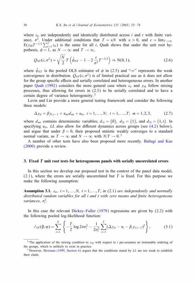
where �it are independently and identically distributed across i and t with 5nite vari-ance, �2. Under additional conditions that T = �N with �¿ 0, and c = limT→∞E(yi0T−1=2∑T

t=1 �it) is the same for all i, Quah shows that under the unit root hy-pothesis, �= 1, as N → ∞ and T → ∞,

QNT (c; �2) =

√N2

T(�̂NT − 1− 2

c�2 T

−3=2)⇒ N(0; 1); (2.6)

where �̂NT is the pooled OLS estimator of � in (2.5) and “⇒” represents the weakconvergence in distribution. QNT (c; �2) is of limited practical use as it does not allowfor the group speci5c eEects and serially correlated and heterogeneous errors. In anotherpaper Quah (1992) considers the more general case where �it and yi0 follow mixingprocesses, thus allowing for errors in (2.5) to be serially correlated and to have acertain degree of variance heterogeneity. 2

Levin and Lin provide a more general testing framework and consider the followingthree models:

Myit = �yi; t−1 + �midmt + uit ; i = 1; : : : ; N ; t = 1; : : : ; T ; m= 1; 2; 3; (2.7)

where dmt contains deterministic variables; d1t = {∅}; d2t = {1}, and d3t = {1; t}. Inspecifying uit ; LL also allow for diEerent dynamics across groups (see (4.2) below),and argue that under � = 0, their proposed statistic weakly converges to a standardnormal variate, as T → ∞ and N → ∞ with N=T → 0. 3

A number of other tests have also been proposed more recently. Baltagi and Kao(2000) provide a review.

3. Fixed T unit root tests for heterogeneous panels with serially uncorrelated errors

In this section we develop our proposed test in the context of the panel data model,(2.1), where the errors are serially uncorrelated but T is 5xed. For this purpose wemake the following assumption:

Assumption 3.1. �it ; i=1; : : : ; N; t=1; : : : ; T , in (2.1) are independently and normallydistributed random variables for all i and t with zero means and 6nite heterogeneousvariances, �2

i .

In this case the relevant Dickey–Fuller (1979) regressions are given by (2.2) withthe following pooled log-likelihood function:

‘NT (�;�) =N∑i=1

{−T2log 2 �2

i −12�2

i

T∑t=1

(Myit − �i − �iyi; t−1)2}

; (3.1)

2 The application of the mixing condition to yi0 with respect to i pre-assumes an immutable ordering ofthe groups, which is unlikely to exist in practice.

3 However, Bowman (1999, Section 6) argues that the conditions stated by LL are too weak to establishtheir claim.

K.S. Im et al. / Journal of Econometrics 115 (2003) 53–74 57

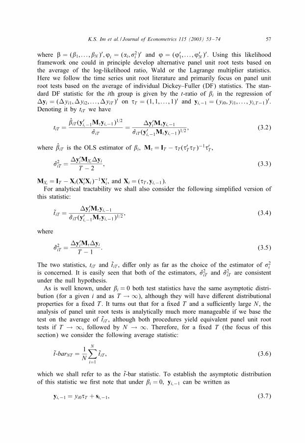
where � = (�1; : : : ; �N )′;�i = (�i; �2i )

′ and � = (�′1; : : : ;�′

N )′. Using this likelihood

framework one could in principle develop alternative panel unit root tests based onthe average of the log-likelihood ratio, Wald or the Lagrange multiplier statistics.Here we follow the time series unit root literature and primarily focus on panel unitroot tests based on the average of individual Dickey–Fuller (DF) statistics. The stan-dard DF statistic for the ith group is given by the t-ratio of �i in the regression ofMyi = (Myi1;Myi2; : : : ;MyiT )′ on �T = (1; 1; : : : ; 1)′ and yi;−1 = (yi0; yi1; : : : ; yi;T−1)′.Denoting it by tiT we have

tiT =�̂iT (y′i;−1M!yi;−1)1=2

�̂iT=

My′iM!yi;−1

�̂iT (y′i;−1M!yi;−1)1=2; (3.2)

where �̂iT is the OLS estimator of �i; M! = IT − �T (�′T �T )−1�′T ,

�̂2iT =

My′iMXiMyiT − 2

; (3.3)

MXi = IT − Xi(X′iXi)−1X′

i , and Xi = (�T ; yi;−1).For analytical tractability we shall also consider the following simpli5ed version of

this statistic:

t̃iT =My′iM!yi;−1

�̃iT (y′i;−1M!yi;−1)1=2; (3.4)

where

�̃2iT =

My′iM!MyiT − 1

: (3.5)

The two statistics, tiT and t̃iT , diEer only as far as the choice of the estimator of �2i

is concerned. It is easily seen that both of the estimators, �̂2iT and �̃2

iT are consistentunder the null hypothesis.As is well known, under �i = 0 both test statistics have the same asymptotic distri-

bution (for a given i and as T → ∞), although they will have diEerent distributionalproperties for a 5xed T . It turns out that for a 5xed T and a suPciently large N , theanalysis of panel unit root tests is analytically much more manageable if we base thetest on the average of t̃iT , although both procedures yield equivalent panel unit roottests if T → ∞, followed by N → ∞. Therefore, for a 5xed T (the focus of thissection) we consider the following average statistic:

t̃-barNT =1N

N∑i=1

t̃iT ; (3.6)

which we shall refer to as the t̃-bar statistic. To establish the asymptotic distributionof this statistic we 5rst note that under �i = 0; yi;−1 can be written as

yi;−1 = yi0�T + si;−1; (3.7)

58 K.S. Im et al. / Journal of Econometrics 115 (2003) 53–74

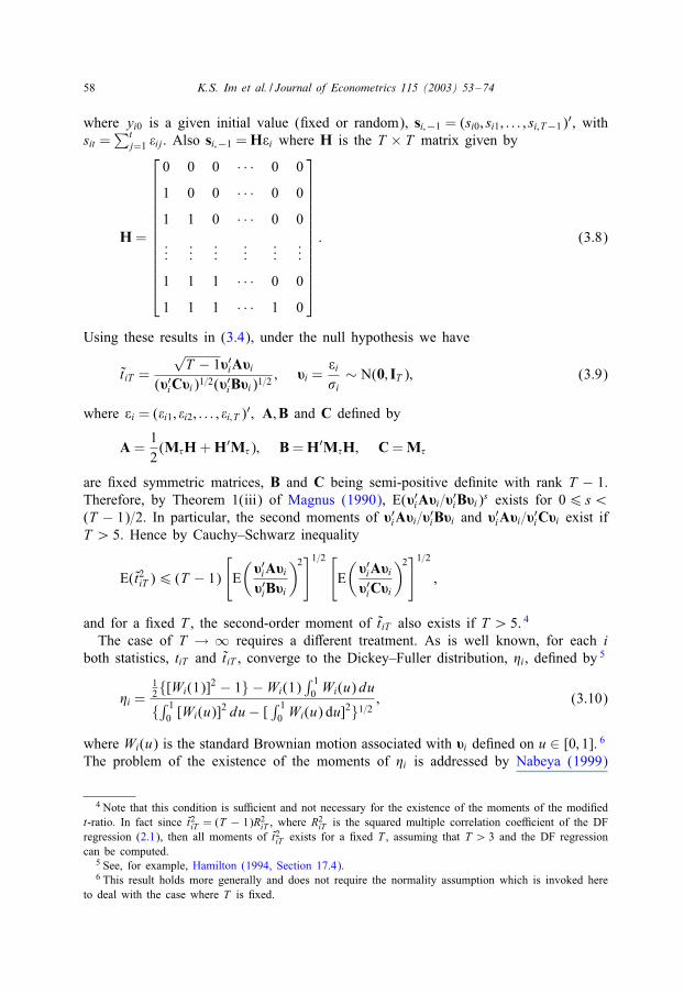
where yi0 is a given initial value (5xed or random), si;−1 = (si0; si1; : : : ; si;T−1)′, withsit =

∑tj=1 �ij. Also si;−1 =H�i where H is the T × T matrix given by

H =

0 0 0 · · · 0 0

1 0 0 · · · 0 0

1 1 0 · · · 0 0

......

......

......

1 1 1 · · · 0 0

1 1 1 · · · 1 0

: (3.8)

Using these results in (3.4), under the null hypothesis we have

t̃ iT =

√T − 1�′iA�i

(�′iC�i)1=2(�′iB�i)1=2; �i =

�i�i

∼ N(0; IT ); (3.9)

where �i = (�i1; �i2; : : : ; �i;T )′; A;B and C de5ned by

A =12(M!H +H′M!); B=H′M!H; C=M!

are 5xed symmetric matrices, B and C being semi-positive de5nite with rank T − 1.Therefore, by Theorem 1(iii) of Magnus (1990), E(�′iA�i=�′iB�i)s exists for 06 s¡(T − 1)=2. In particular, the second moments of �′iA�i=�′iB�i and �′iA�i=�′iC�i exist ifT ¿ 5. Hence by Cauchy–Schwarz inequality

E(t̃2iT )6 (T − 1)

[E(�′iA�i�′iB�i

)2]1=2 [E(�′iA�i�′iC�i

)2]1=2;

and for a 5xed T , the second-order moment of t̃iT also exists if T ¿ 5. 4

The case of T → ∞ requires a diEerent treatment. As is well known, for each iboth statistics, tiT and t̃iT , converge to the Dickey–Fuller distribution, %i, de5ned by 5

%i =12{[Wi(1)]2 − 1} −Wi(1)

∫ 10 Wi(u)du

{∫ 10 [Wi(u)]2 du− [

∫ 10 Wi(u) du]2}1=2

; (3.10)

where Wi(u) is the standard Brownian motion associated with �i de5ned on u ∈ [0; 1]. 6

The problem of the existence of the moments of %i is addressed by Nabeya (1999)

4 Note that this condition is suPcient and not necessary for the existence of the moments of the modi5edt-ratio. In fact since t̃2iT = (T − 1)R2

iT , where R2iT is the squared multiple correlation coePcient of the DF

regression (2.1), then all moments of t̃2iT exists for a 5xed T , assuming that T ¿ 3 and the DF regressioncan be computed.

5 See, for example, Hamilton (1994, Section 17.4).6 This result holds more generally and does not require the normality assumption which is invoked here

to deal with the case where T is 5xed.

K.S. Im et al. / Journal of Econometrics 115 (2003) 53–74 59

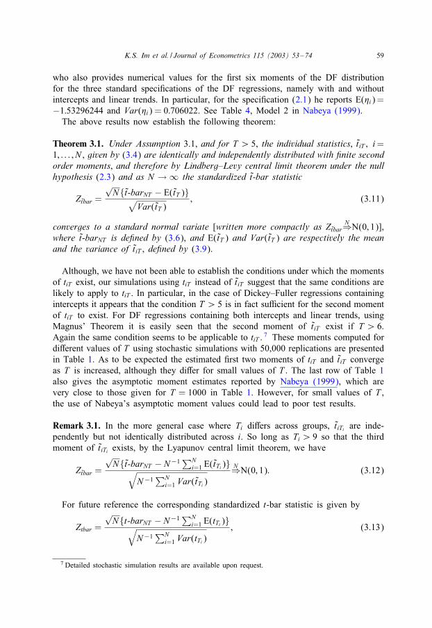
who also provides numerical values for the 5rst six moments of the DF distributionfor the three standard speci5cations of the DF regressions, namely with and withoutintercepts and linear trends. In particular, for the speci5cation (2.1) he reports E(%i)=−1:53296244 and Var(%i) = 0:706022. See Table 4, Model 2 in Nabeya (1999).The above results now establish the following theorem:

Theorem 3.1. Under Assumption 3.1, and for T ¿ 5, the individual statistics, t̃ iT ; i=1; : : : ; N , given by (3.4) are identically and independently distributed with 6nite secondorder moments, and therefore by Lindberg–Levy central limit theorem under the nullhypothesis (2.3) and as N → ∞ the standardized t̃-bar statistic

Zt̃bar =

√N{t̃-barNT − E(t̃T )}√

Var(t̃T ); (3.11)

converges to a standard normal variate [written more compactly as Zt̃barN⇒N(0; 1)],

where t̃-barNT is de6ned by (3.6), and E(t̃T ) and Var(t̃T ) are respectively the meanand the variance of t̃iT , de6ned by (3.9).

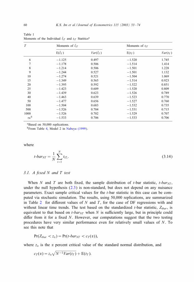
Although, we have not been able to establish the conditions under which the momentsof tiT exist, our simulations using tiT instead of t̃iT suggest that the same conditions arelikely to apply to tiT . In particular, in the case of Dickey–Fuller regressions containingintercepts it appears that the condition T ¿ 5 is in fact suPcient for the second momentof tiT to exist. For DF regressions containing both intercepts and linear trends, usingMagnus’ Theorem it is easily seen that the second moment of t̃ iT exist if T ¿ 6.Again the same condition seems to be applicable to tiT . 7 These moments computed fordiEerent values of T using stochastic simulations with 50,000 replications are presentedin Table 1. As to be expected the estimated 5rst two moments of tiT and t̃iT convergeas T is increased, although they diEer for small values of T . The last row of Table 1also gives the asymptotic moment estimates reported by Nabeya (1999), which arevery close to those given for T = 1000 in Table 1. However, for small values of T ,the use of Nabeya’s asymptotic moment values could lead to poor test results.

Remark 3.1. In the more general case where Ti diEers across groups, t̃ iTi are inde-pendently but not identically distributed across i. So long as Ti ¿ 9 so that the thirdmoment of t̃iTi exists, by the Lyapunov central limit theorem, we have

Zt̃bar =

√N{t̃-barNT − N−1∑N

i=1 E(t̃Ti)}√N−1

∑Ni=1 Var(t̃Ti)

N⇒N(0; 1): (3.12)

For future reference the corresponding standardized t-bar statistic is given by

Ztbar =

√N{t-barNT − N−1∑N

i=1 E(tTi)}√N−1

∑Ni=1 Var(tTi)

; (3.13)

7 Detailed stochastic simulation results are available upon request.

60 K.S. Im et al. / Journal of Econometrics 115 (2003) 53–74

Table 1Moments of the Individual t̃iT and tiT Statiticsa

T Moments of t̃iT Moments of tiT

E(t̃T ) Var(t̃T ) E(tT ) Var(tT )

6 −1:125 0.497 −1:520 1.7457 −1:178 0.506 −1:514 1.4148 −1:214 0.506 −1:501 1.2289 −1:244 0.527 −1:501 1.132

10 −1:274 0.521 −1:504 1.06915 −1:349 0.565 −1:514 0.92320 −1:395 0.592 −1:522 0.85125 −1:423 0.609 −1:520 0.80930 −1:439 0.623 −1:526 0.78940 −1:463 0.639 −1:523 0.77050 −1:477 0.656 −1:527 0.760

100 −1:504 0.683 −1:532 0.735500 −1:526 0.704 −1:531 0.715

1000 −1:526 0.702 −1:529 0.707∞b −1:533 0.706 −1:533 0.706

aBased on 50,000 replications.bFrom Table 4, Model 2 in Nabeya (1999).

where

t-barNT =1N

N∑i=1

tiTi : (3.14)

3.1. A 6xed N and T test

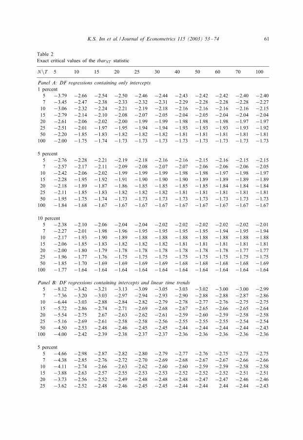
When N and T are both 5xed, the sample distribution of t-bar statistic, t-barNT ,under the null hypothesis (2.3) is non-standard, but does not depend on any nuisanceparameters. Exact sample critical values for the t-bar statistic in this case can be com-puted via stochastic simulation. The results, using 50,000 replications, are summarizedin Table 2 for diEerent values of N and T , for the case of DF regressions with andwithout linear time trends. The test based on the standardized t-bar statistic, Ztbar , isequivalent to that based on t-barNT when N is suPciently large, but in principle coulddiEer from it for a 5xed N . However, our computations suggest that the two testingprocedures have very similar performance even for relatively small values of N . Tosee this note that

Pr(Ztbar ¡ z�) = Pr(t-barNT ¡cT (�));

where z� is the � percent critical value of the standard normal distribution, and

cT (�) = z�√

N−1Var(tT ) + E(tT ):

K.S. Im et al. / Journal of Econometrics 115 (2003) 53–74 61

Table 2Exact critical values of the tbarNT statistic

N\T 5 10 15 20 25 30 40 50 60 70 100

Panel A: DF regressions containing only intercepts1 percent

5 −3:79 −2:66 −2:54 −2:50 −2:46 −2:44 −2:43 −2:42 −2:42 −2:40 −2:407 −3:45 −2:47 −2:38 −2:33 −2:32 −2:31 −2:29 −2:28 −2:28 −2:28 −2:27

10 −3:06 −2:32 −2:24 −2:21 −2:19 −2:18 −2:16 −2:16 −2:16 −2:16 −2:1515 −2:79 −2:14 −2:10 −2:08 −2:07 −2:05 −2:04 −2:05 −2:04 −2:04 −2:0420 −2:61 −2:06 −2:02 −2:00 −1:99 −1:99 −1:98 −1:98 −1:98 −1:97 −1:9725 −2:51 −2:01 −1:97 −1:95 −1:94 −1:94 −1:93 −1:93 −1:93 −1:93 −1:9250 −2:20 −1:85 −1:83 −1:82 −1:82 −1:82 −1:81 −1:81 −1:81 −1:81 −1:81

100 −2:00 −1:75 −1:74 −1:73 −1:73 −1:73 −1:73 −1:73 −1:73 −1:73 −1:73

5 percent5 −2:76 −2:28 −2:21 −2:19 −2:18 −2:16 −2:16 −2:15 −2:16 −2:15 −2:157 −2:57 −2:17 −2:11 −2:09 −2:08 −2:07 −2:07 −2:06 −2:06 −2:06 −2:05

10 −2:42 −2:06 −2:02 −1:99 −1:99 −1:99 −1:98 −1:98 −1:97 −1:98 −1:9715 −2:28 −1:95 −1:92 −1:91 −1:90 −1:90 −1:90 −1:89 −1:89 −1:89 −1:8920 −2:18 −1:89 −1:87 −1:86 −1:85 −1:85 −1:85 −1:85 −1:84 −1:84 −1:8425 −2:11 −1:85 −1:83 −1:82 −1:82 −1:82 −1:81 −1:81 −1:81 −1:81 −1:8150 −1:95 −1:75 −1:74 −1:73 −1:73 −1:73 −1:73 −1:73 −1:73 −1:73 −1:73

100 −1:84 −1:68 −1:67 −1:67 −1:67 −1:67 −1:67 −1:67 −1:67 −1:67 −1:67

10 percent5 −2:38 −2:10 −2:06 −2:04 −2:04 −2:02 −2:02 −2:02 −2:02 −2:02 −2:017 −2:27 −2:01 −1:98 −1:96 −1:95 −1:95 −1:95 −1:95 −1:94 −1:95 −1:94

10 −2:17 −1:93 −1:90 −1:89 −1:88 −1:88 −1:88 −1:88 −1:88 −1:88 −1:8815 −2:06 −1:85 −1:83 −1:82 −1:82 −1:82 −1:81 −1:81 −1:81 −1:81 −1:8120 −2:00 −1:80 −1:79 −1:78 −1:78 −1:78 −1:78 −1:78 −1:78 −1:77 −1:7725 −1:96 −1:77 −1:76 −1:75 −1:75 −1:75 −1:75 −1:75 −1:75 −1:75 −1:7550 −1:85 −1:70 −1:69 −1:69 −1:69 −1:69 −1:68 −1:68 −1:68 −1:68 −1:69

100 −1:77 −1:64 −1:64 −1:64 −1:64 −1:64 −1:64 −1:64 −1:64 −1:64 −1:64

Panel B: DF regressions containing intercepts and linear time trends5 −8:12 −3:42 −3:21 −3:13 −3:09 −3:05 −3:03 −3:02 −3:00 −3:00 −2:997 −7:36 −3:20 −3:03 −2:97 −2:94 −2:93 −2:90 −2:88 −2:88 −2:87 −2:86

10 −6:44 −3:03 −2:88 −2:84 −2:82 −2:79 −2:78 −2:77 −2:76 −2:75 −2:7515 −5:72 −2:86 −2:74 −2:71 −2:69 −2:68 −2:67 −2:65 −2:66 −2:65 −2:6420 −5:54 −2:75 2:67 −2:63 −2:62 −2:61 −2:59 −2:60 −2:59 −2:58 −2:5825 −5:16 −2:69 −2:61 −2:58 −2:58 −2:56 −2:55 −2:55 −2:55 −2:54 −2:5450 −4:50 −2:53 −2:48 −2:46 −2:45 −2:45 −2:44 −2:44 −2:44 −2:44 −2:43

100 −4:00 −2:42 −2:39 −2:38 −2:37 −2:37 −2:36 −2:36 −2:36 −2:36 −2:36

5 percent5 −4:66 −2:98 −2:87 −2:82 −2:80 −2:79 −2:77 −2:76 −2:75 −2:75 −2:757 −4:38 −2:85 −2:76 −2:72 −2:70 −2:69 −2:68 −2:67 −2:67 −2:66 −2:66

10 −4:11 −2:74 −2:66 −2:63 −2:62 −2:60 −2:60 −2:59 −2:59 −2:58 −2:5815 −3:88 −2:63 −2:57 −2:55 −2:53 −2:53 −2:52 −2:52 −2:52 −2:51 −2:5120 −3:73 −2:56 −2:52 −2:49 −2:48 −2:48 −2:48 −2:47 −2:47 −2:46 −2:4625 −3:62 −2:52 −2:48 −2:46 −2:45 −2:45 −2:44 −2:44 2.44 −2:44 −2:43

62 K.S. Im et al. / Journal of Econometrics 115 (2003) 53–74

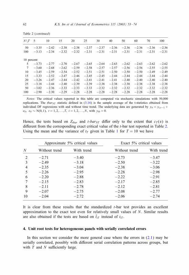
Table 2 (continued)

N\T 5 10 15 20 25 30 40 50 60 70 100

50 −3:35 −2:42 −2:38 −2:38 −2:37 −2:37 −2:36 −2:36 −2:36 −2:36 −2:36100 −3:13 −2:34 −2:32 −2:32 −2:31 −2:31 −2:31 −2:31 −2:31 −2:31 −2:31

10 percent5 −3:73 −2:77 −2:70 −2:67 −2:65 −2:64 −2:63 −2:62 −2:63 −2:62 −2:627 −3:60 −2:68 −2:62 −2:59 −2:58 −2:57 −2:57 −2:56 −2:56 −2:55 −2:55

10 −3:45 −2:59 −2:54 −2:52 −2:51 −2:51 −2:50 −2:50 −2:50 −2:49 −2:4915 −3:33 −2:52 −2:47 −2:46 −2:45 −2:45 −2:44 −2:44 −2:44 −2:44 −2:4420 −3:26 −2:47 −2:44 −2:42 −2:41 −2:41 −2:41 −2:40 −2:40 −2:40 −2:4025 −3:18 −2:44 −2:40 −2:39 −2:39 −2:38 −2:38 −2:38 −2:38 −2:38 −2:3850 −3:02 −2:36 −2:33 −2:33 −2:33 −2:32 −2:32 −2:32 −2:32 −2:32 −2:32

100 −2:90 −2:30 −2:29 −2:28 −2:28 −2:28 −2:28 −2:28 −2:28 −2:28 −2:28

Notes: The critical values reported in this table are computed via stochastic simulations with 50,000replications. The tbarNT statistic de5ned in (3.14) is the sample average of the t-statistics obtained fromindividual DF regressions with and without time trend. The underlying data are generated by yit = yi; t−1 +eit ; eit ∼ N(0; 1); t = 1; 2; : : : ; T; i = 1; 2; : : : ; N , with yi0 = 0.

Hence, the tests based on Ztbar and t-barNT diEer only to the extent that cT (�) isdiEerent from the corresponding exact critical value of the t-bar test reported in Table 2.Using the mean and the variance of tT given in Table 1 for T = 10 we have

Approximate 5% critical values Exact 5% critical values

N Without trend With trend Without trend With trend

2 −2:71 −3:40 −2:73 −3:473 −2:49 −3:18 −2:50 −3:224 −2:35 −3:04 −2:38 −3:065 −2:26 −2:95 −2:28 −2:986 −2:20 −2:88 −2:22 −2:917 −2:15 −2:83 −2:17 −2:858 −2:11 −2:78 −2:12 −2:819 −2:07 −2:75 −2:08 −2:77

10 −2:04 −2:72 −2:06 −2:74

It is clear from these results that the standardized t-bar test provides an excellentapproximation to the exact test even for relatively small values of N . Similar resultsare also obtained if the tests are based on t̃ iT instead of tiT .

4. Unit root tests for heterogeneous panels with serially correlated errors

In this section we consider the more general case where the errors in (2.1) may beserially correlated, possibly with diEerent serial correlation patterns across groups, butwith T and N suPciently large.

K.S. Im et al. / Journal of Econometrics 115 (2003) 53–74 63

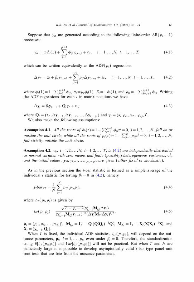
Suppose that yit are generated according to the following 5nite-order AR(pi + 1)processes:

yit = �i�i(1) +pi+1∑j=1

�ijyi; t−j + �it ; i = 1; : : : ; N; t = 1; : : : ; T; (4.1)

which can be written equivalently as the ADF(pi) regressions:

Myit = �i + �iyi; t−1 +pi∑j=1

,ijMyi; t−j + �it ; i = 1; : : : ; N; t = 1; : : : ; T; (4.2)

where �i(1)=1−∑pi+1j=1 �ij; �i=�i�i(1); �i=−�i(1), and ,ij=−∑pi+1

h=j+1 �ih. Writingthe ADF regressions for each i in matrix notations we have

Myi = �iyi;−1 +Qi�i + �i ; (4.3)

where Qi = (�T ;Myi;−1;Myi;−2; : : : ;Myi;−pi) and �i = (�i; ,i1; ,i2; :::; ,ipi)′.

We also make the following assumptions:

Assumption 4.1. All the roots of �i(z)=1−∑pi+1j=1 �ijzj =0; i=1; 2; : : : ; N , fall on or

outside the unit circle, while all the roots of ,i(z)=1−∑pij=1 ,ijzj =0; i=1; 2; : : : ; N ,

fall strictly outside the unit circle.

Assumption 4.2. �it ; i=1; 2; : : : ; N; t=1; 2; : : : ; T , in (4.2) are independently distributedas normal variates with zero means and 6nite (possibly) heterogeneous variances, �2

i ,and the initial values, yi0; yi;−1; : : : ; yi;−pi , are given (either 6xed or stochastic).

As in the previous section the t-bar statistic is formed as a simple average of theindividual t statistic for testing �i = 0 in (4.2), namely

t-barNT =1N

N∑i=1

tiT (pi; �i); (4.4)

where tiT (pi; �i) is given by

tiT (pi; �i) =

√T − pi − 2(y′i;−1MQiMyi)

(y′i;−1MQiyi;−1)1=2(My′iMXiMyi)1=2; (4.5)

�i = (,i1; ,i2; : : : ; ,ipi)′; MQi = IT − Qi(Q′

iQi)−1Q′i ; MXi = IT − Xi(X′

iXi)−1X′i , and

Xi = (yi;−1;Qi).When T is 5xed, the individual ADF statistics, tiT (pi; �i), will depend on the nui-

sance parameters, �i ; i = 1; : : : ; pi, even under �i = 0. Therefore, the standardizationusing E[tiT (pi; �i)] and Var[tiT (pi; �i)] will not be practical. But when T and N aresuPciently large it is possible to develop asymptotically valid t-bar type panel unitroot tests that are free from the nuisance parameters.

64 K.S. Im et al. / Journal of Econometrics 115 (2003) 53–74

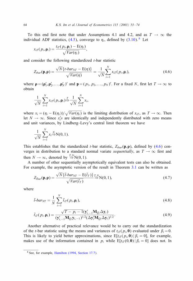
To this end 5rst note that under Assumptions 4.1 and 4.2, and as T → ∞ theindividual ADF statistics, (4.5), converge to %i, de5ned by (3.10). 8 Let

xiT (pi; �i) =tiT (pi; �i)− E(%i)√

Var(%i);

and consider the following standardized t-bar statistic

Ztbar(p; �) =√N{t-barNT − E(%)}√

Var(%)=

1√N

N∑i=1

xiT (pi; �i); (4.6)

where �=(�′1; �′2; : : : ; �′N )′ and p=(p1; p2; : : : ; pN )′. For a 5xed N , 5rst let T → ∞ toobtain

1√N

N∑i=1

xiT (pi; �i)T⇒ 1√

N

N∑i=1

xi;

where xi = (%i − E(%i))=√

Var(%i) is the limiting distribution of xiT , as T → ∞. Thenlet N → ∞. Since x′i s are identically and independently distributed with zero meansand unit variances, by Lindberg–Levy’s central limit theorem we have

1√N

N∑i=1

xiN⇒N(0; 1):

This establishes that the standardized t-bar statistic, Ztbar(p; �), de5ned by (4.6) con-verges in distribution to a standard normal variate sequentially, as T → ∞ 5rst and

then N → ∞, denoted byT; N⇒N(0; 1).

A number of other sequentially asymptotically equivalent tests can also be obtained.For example, the asymptotic version of the result in Theorem 3.1 can be written as

Zt̃bar(p; �) =√N{t̃-barNT − E(t̃T )}√

Var(t̃T )

T; N⇒N(0; 1); (4.7)

where

t̃-barNT =1N

N∑i=1

t̃iT (pi; �i); (4.8)

t̃iT (pi; �i) =√T − pi − 1(y′i;−1MQiMyi)

(y′i;−1MQiyi;−1)1=2(My′iMQiMyi)1=2: (4.9)

Another alternative of practical relevance would be to carry out the standardizationof the t-bar statistic using the means and variances of tiT (pi; 0) evaluated under �i=0.This is likely to yield better approximations, since E[tiT (pi; 0) | �i = 0], for example,makes use of the information contained in pi while E[tiT (0; 0) | �i = 0] does not. In

8 See, for example, Hamilton (1994, Section 17.7).

K.S. Im et al. / Journal of Econometrics 115 (2003) 53–74 65

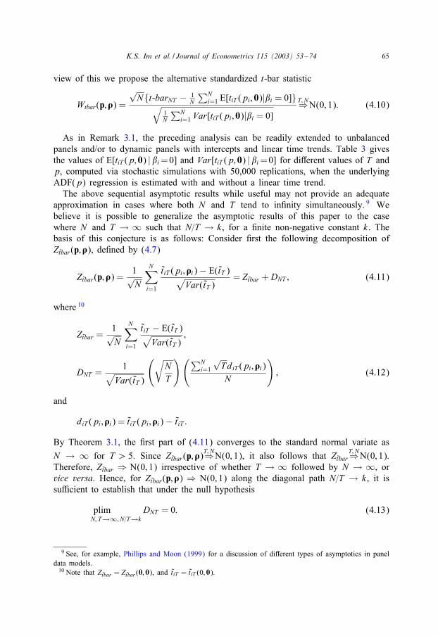
view of this we propose the alternative standardized t-bar statistic

Wtbar(p; �) =√N{t-barNT − 1

N

∑Ni=1 E[tiT (pi; 0)|�i = 0]}√

1N

∑Ni=1 Var[tiT (pi; 0)|�i = 0]

T; N⇒N(0; 1): (4.10)

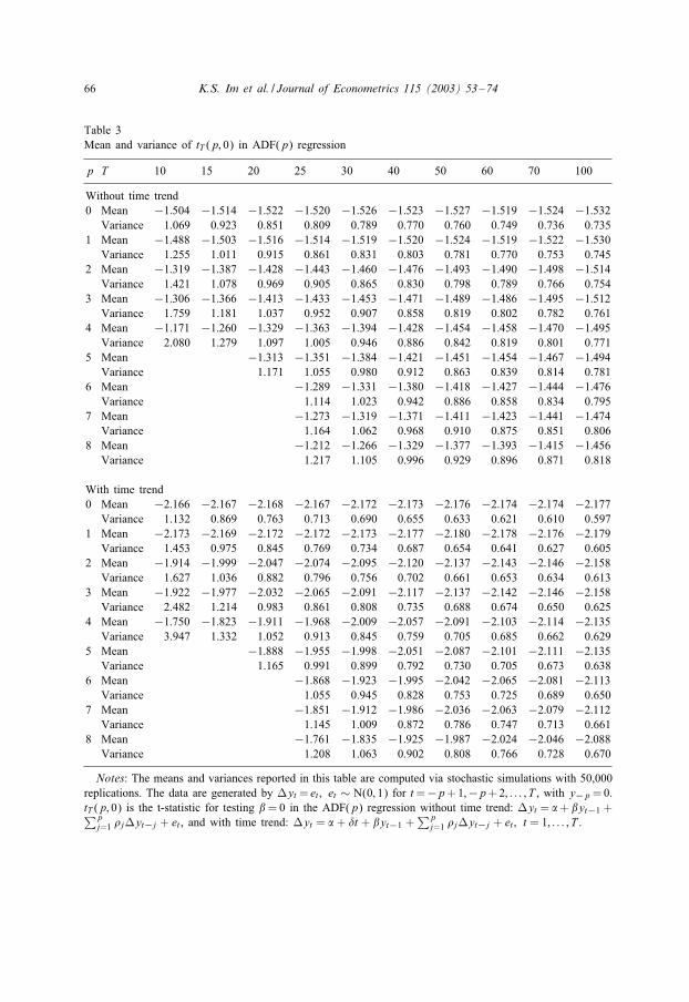
As in Remark 3.1, the preceding analysis can be readily extended to unbalancedpanels and/or to dynamic panels with intercepts and linear time trends. Table 3 givesthe values of E[tiT (p; 0) | �i=0] and Var[tiT (p; 0) | �i=0] for diEerent values of T andp, computed via stochastic simulations with 50,000 replications, when the underlyingADF(p) regression is estimated with and without a linear time trend.The above sequential asymptotic results while useful may not provide an adequate

approximation in cases where both N and T tend to in5nity simultaneously. 9 Webelieve it is possible to generalize the asymptotic results of this paper to the casewhere N and T → ∞ such that N=T → k, for a 5nite non-negative constant k. Thebasis of this conjecture is as follows: Consider 5rst the following decomposition ofZt̃bar(p; �), de5ned by (4.7)

Zt̃bar(p; �) =1√N

N∑i=1

t̃iT (pi; �i)− E(t̃T )√Var(t̃T )

= Zt̃bar + DNT ; (4.11)

where 10

Zt̃bar =1√N

N∑i=1

t̃iT − E(t̃T )√Var(t̃T )

;

DNT =1√

Var(t̃T )

(√NT

)(∑Ni=1

√TdiT (pi; �i)N

); (4.12)

and

diT (pi; �i) = t̃ iT (pi; �i)− t̃iT :

By Theorem 3.1, the 5rst part of (4.11) converges to the standard normal variate as

N → ∞ for T ¿ 5. Since Zt̃bar(p; �)T; N⇒N(0; 1), it also follows that Zt̃bar

T; N⇒N(0; 1).Therefore, Zt̃bar ⇒ N(0; 1) irrespective of whether T → ∞ followed by N → ∞, orvice versa. Hence, for Zt̃bar(p; �) ⇒ N(0; 1) along the diagonal path N=T → k, it issuPcient to establish that under the null hypothesis

plimN; T→∞; N=T→k

DNT = 0: (4.13)

9 See, for example, Phillips and Moon (1999) for a discussion of diEerent types of asymptotics in paneldata models.10 Note that Zt̃bar = Zt̃bar(0; 0), and t̃iT = t̃iT (0; 0).

66 K.S. Im et al. / Journal of Econometrics 115 (2003) 53–74

Table 3Mean and variance of tT (p; 0) in ADF(p) regression

p T 10 15 20 25 30 40 50 60 70 100

Without time trend0 Mean −1:504 −1:514 −1:522 −1:520 −1:526 −1:523 −1:527 −1:519 −1:524 −1:532

Variance 1.069 0.923 0.851 0.809 0.789 0.770 0.760 0.749 0.736 0.7351 Mean −1:488 −1:503 −1:516 −1:514 −1:519 −1:520 −1:524 −1:519 −1:522 −1:530

Variance 1.255 1.011 0.915 0.861 0.831 0.803 0.781 0.770 0.753 0.7452 Mean −1:319 −1:387 −1:428 −1:443 −1:460 −1:476 −1:493 −1:490 −1:498 −1:514

Variance 1.421 1.078 0.969 0.905 0.865 0.830 0.798 0.789 0.766 0.7543 Mean −1:306 −1:366 −1:413 −1:433 −1:453 −1:471 −1:489 −1:486 −1:495 −1:512

Variance 1.759 1.181 1.037 0.952 0.907 0.858 0.819 0.802 0.782 0.7614 Mean −1:171 −1:260 −1:329 −1:363 −1:394 −1:428 −1:454 −1:458 −1:470 −1:495

Variance 2.080 1.279 1.097 1.005 0.946 0.886 0.842 0.819 0.801 0.7715 Mean −1:313 −1:351 −1:384 −1:421 −1:451 −1:454 −1:467 −1:494

Variance 1.171 1.055 0.980 0.912 0.863 0.839 0.814 0.7816 Mean −1:289 −1:331 −1:380 −1:418 −1:427 −1:444 −1:476

Variance 1.114 1.023 0.942 0.886 0.858 0.834 0.7957 Mean −1:273 −1:319 −1:371 −1:411 −1:423 −1:441 −1:474

Variance 1.164 1.062 0.968 0.910 0.875 0.851 0.8068 Mean −1:212 −1:266 −1:329 −1:377 −1:393 −1:415 −1:456

Variance 1.217 1.105 0.996 0.929 0.896 0.871 0.818

With time trend0 Mean −2:166 −2:167 −2:168 −2:167 −2:172 −2:173 −2:176 −2:174 −2:174 −2:177

Variance 1.132 0.869 0.763 0.713 0.690 0.655 0.633 0.621 0.610 0.5971 Mean −2:173 −2:169 −2:172 −2:172 −2:173 −2:177 −2:180 −2:178 −2:176 −2:179

Variance 1.453 0.975 0.845 0.769 0.734 0.687 0.654 0.641 0.627 0.6052 Mean −1:914 −1:999 −2:047 −2:074 −2:095 −2:120 −2:137 −2:143 −2:146 −2:158

Variance 1.627 1.036 0.882 0.796 0.756 0.702 0.661 0.653 0.634 0.6133 Mean −1:922 −1:977 −2:032 −2:065 −2:091 −2:117 −2:137 −2:142 −2:146 −2:158

Variance 2.482 1.214 0.983 0.861 0.808 0.735 0.688 0.674 0.650 0.6254 Mean −1:750 −1:823 −1:911 −1:968 −2:009 −2:057 −2:091 −2:103 −2:114 −2:135

Variance 3.947 1.332 1.052 0.913 0.845 0.759 0.705 0.685 0.662 0.6295 Mean −1:888 −1:955 −1:998 −2:051 −2:087 −2:101 −2:111 −2:135

Variance 1.165 0.991 0.899 0.792 0.730 0.705 0.673 0.6386 Mean −1:868 −1:923 −1:995 −2:042 −2:065 −2:081 −2:113

Variance 1.055 0.945 0.828 0.753 0.725 0.689 0.6507 Mean −1:851 −1:912 −1:986 −2:036 −2:063 −2:079 −2:112

Variance 1.145 1.009 0.872 0.786 0.747 0.713 0.6618 Mean −1:761 −1:835 −1:925 −1:987 −2:024 −2:046 −2:088

Variance 1.208 1.063 0.902 0.808 0.766 0.728 0.670

Notes: The means and variances reported in this table are computed via stochastic simulations with 50,000replications. The data are generated by Myt = et ; et ∼ N(0; 1) for t=−p+1;−p+2; : : : ; T , with y−p =0.tT (p; 0) is the t-statistic for testing �= 0 in the ADF(p) regression without time trend: Myt = �+ �yt−1 +∑p

j=1 ,jMyt−j + et , and with time trend: Myt = � + �t + �yt−1 +∑p

j=1 ,jMyt−j + et ; t = 1; : : : ; T .

K.S. Im et al. / Journal of Econometrics 115 (2003) 53–74 67

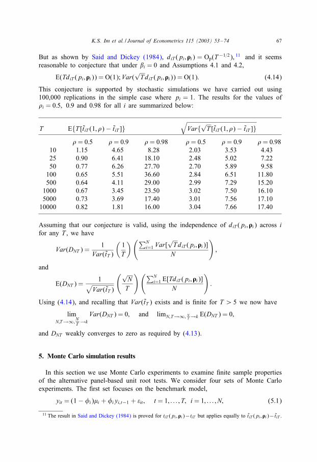
But as shown by Said and Dickey (1984), diT (pi; �i) = Op(T−1=2), 11 and it seemsreasonable to conjecture that under �i = 0 and Assumptions 4.1 and 4.2,

E(TdiT (pi; �i)) = O(1);Var(√TdiT (pi; �i)) = O(1): (4.14)

This conjecture is supported by stochastic simulations we have carried out using100,000 replications in the simple case where pi = 1. The results for the values of,i = 0:5; 0:9 and 0:98 for all i are summarized below:

T E{T [t̃ iT (1; ,)− t̃iT ]}√

Var{√T [t̃iT (1; ,)− t̃iT ]},= 0:5 ,= 0:9 ,= 0:98 ,= 0:5 ,= 0:9 ,= 0:98

10 1.15 4.65 8.28 2.03 3.53 4.4325 0.90 6.41 18.10 2.48 5.02 7.2250 0.77 6.26 27.70 2.70 5.89 9.58100 0.65 5.51 36.60 2.84 6.51 11.80500 0.64 4.11 29.00 2.99 7.29 15.201000 0.67 3.45 23.50 3.02 7.50 16.105000 0.73 3.69 17.40 3.01 7.56 17.1010000 0.82 1.81 16.00 3.04 7.66 17.40

Assuming that our conjecture is valid, using the independence of diT (pi; �i) across ifor any T , we have

Var(DNT ) =1

Var(t̃T )

(1T

)(∑Ni=1 Var[

√TdiT (pi; �i)]N

);

and

E(DNT ) =1√

Var(t̃T )

(√NT

)(∑Ni=1 E[TdiT (pi; �i)]

N

):

Using (4.14), and recalling that Var(t̃T ) exists and is 5nite for T ¿ 5 we now have

limN;T→∞; NT →k

Var(DNT ) = 0; and limN;T→∞; NT →k E(DNT ) = 0;

and DNT weakly converges to zero as required by (4.13).

5. Monte Carlo simulation results

In this section we use Monte Carlo experiments to examine 5nite sample propertiesof the alternative panel-based unit root tests. We consider four sets of Monte Carloexperiments. The 5rst set focuses on the benchmark model,

yit = (1− �i)�i + �iyi; t−1 + �it ; t = 1; : : : ; T; i = 1; : : : ; N; (5.1)

11 The result in Said and Dickey (1984) is proved for tiT (pi; �i)− tiT but applies equally to t̃iT (pi; �i)− t̃iT .

68 K.S. Im et al. / Journal of Econometrics 115 (2003) 53–74

where �it ∼ N(0; �2i ). The second set of experiments allows for the presence of positive

(heterogeneous) AR(1) serial correlations in �it ,

�it = ,i�i; t−1 + eit ; t = 1; : : : ; T; i = 1; : : : ; N; (5.2)

where eit ∼ N(0; �2i ); ,i ∼ U[0:2; 0:4]; U stands for a uniform distribution and ,i’s

are generated independently of eit . The third set of experiments considers the MA(1)error processes,

�it = eit + iei; t−1; t = 1; : : : ; T; i = 1; : : : ; N; (5.3)

where i ∼ U[− 0:4;−0:2], and i’s are generated independently of eit . The fourth setof experiments allows for a linear trend in estimation of the ADF regressions usingthe same data generating process employed in the second set of experiments.In all of the experiments eit (or �it in (5.1)) are generated as iid normal variates with

zero means and heterogeneous variances, �2i . The parameters �i and �2

i are generatedaccording to

�i ∼ N(0; 1); �2i ∼ U[0:5; 1:5]; i = 1; 2; : : : ; N: (5.4)

Under the null �i=1 for all i, while �i=0:9 for all i under the alternative hypothesis. 12

All of the parameter values such as �i; �2i ; ,i or i are generated independently of �it

once, and then 5xed throughout replications. The 5rst set of experiments were carriedout for N =1; 5; 10; 25; 50; 100; T =10; 25; 50; 100. The other experiments were carriedout for N = 10; 25; 50; 100; T = 10; 25; 50; 100, and p = 0; 1; 2; 3; 4. We used 2,000replications to compute empirical size and power of the tests at the 5% nominal level. 13

All experiments are carried out using the following two statistics: the t-bar and theLL tests. The results for the 5rst set of experiments are summarized in Table 4. 14 Asa benchmark, in the 5rst row of this table we give empirical size and power of thestandard DF test. When T = 10, we report only the results for the t-bar tests, becausethe adjustment factors needed to compute the LL statistic are not supplied by Levinand Lin (1993) for T = 10. The t-bar test (i.e. Ztbar de5ned by (3.13) for simple DFregressions) perform well even for small values of T . It has the correct size, and itspower rises monotonically with N and T . In the case of T =10, the power of the t-bartest increases steadily from 0.071 for N = 5 to 0.384 for N = 100. Overall, both tests

12 We also carried out a number of other experiments where we considered heterogeneous alternatives with�i ∼ U[0:85; 0:95]. The results are similar to the ones reported in this section. A complete set of the MonteCarlo results for these experiments are available from the authors on request.13 We have also carried out a number of other experiments including the cases with negatively correlated

AR(1) disturbances or positively correlated MA(1) disturbances in conjunction with the ADF regressionmodels with or without time trend being estimated. Most results are qualitatively similar to what follows.We have further conducted simulation exercises where the ADF order is chosen by information criteria suchas the Akaike Information or the Schwarz Criterion. The tests show a signi5cant degree of size distortions,largely reVecting that in 5nite samples these criteria tend to select a low order for the ADF regressions. Seealso Ng and Perron (1995) for the eEect of the ADF order selection on the 5nite sample performance ofunit root tests in the case of single time series.14 We also carried out a number of experiments allowing for linear trends in the DF regressions and

obtained similar results, although as to be expected the tests tended to have little power for T and N lessthan 25.

K.S. Im et al. / Journal of Econometrics 115 (2003) 53–74 69

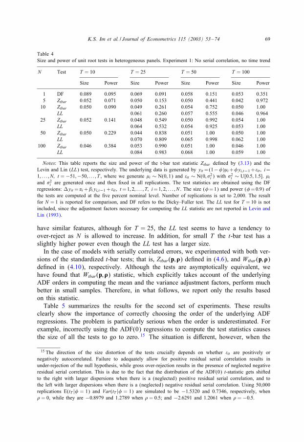
Table 4Size and power of unit root tests in heterogeneous panels. Experiment 1: No serial correlation, no time trend

N Test T = 10 T = 25 T = 50 T = 100

Size Power Size Power Size Power Size Power

1 DF 0.089 0.095 0.069 0.091 0.058 0.151 0.053 0.3515 Ztbar 0.052 0.071 0.050 0.153 0.050 0.441 0.042 0.972

10 Ztbar 0.050 0.090 0.049 0.261 0.054 0.752 0.050 1.00LL 0.061 0.260 0.057 0.555 0.046 0.964

25 Ztbar 0.052 0.141 0.048 0.549 0.050 0.992 0.054 1.00LL 0.064 0.532 0.054 0.925 0.053 1.00

50 Ztbar 0.050 0.229 0.044 0.838 0.051 1.00 0.050 1.00LL 0.070 0.809 0.065 0.998 0.062 1.00

100 Ztbar 0.046 0.384 0.053 0.990 0.051 1.00 0.046 1.00LL 0.084 0.983 0.068 1.00 0.059 1.00

Notes: This table reports the size and power of the t-bar test statistic Ztbar de5ned by (3.13) and theLevin and Lin (LL) test, respectively. The underlying data is generated by yit =(1−�)�i+�yi; t−1 + �it ; i=1; : : : ; N; t =−51;−50; : : : ; T , where we generate �i ∼ N(0; 1) and �it ∼ N(0; �2i ) with �2i ∼ U[0:5; 1:5]. �i

and �2i are generated once and then 5xed in all replications. The test statistics are obtained using the DFregressions: Myit =�i +�iyi; t−1 + �it ; t=1; 2; : : : ; T; i=1; 2; : : : ; N . The size (�=1) and power (�=0:9) ofthe tests are computed at the 5ve percent nominal level. Number of replications is set to 2,000. The resultfor N = 1 is reported for comparison, and DF refers to the Dicky–Fuller test. The LL test for T = 10 is notincluded, since the adjustment factors necessary for computing the LL statistic are not reported in Levin andLin (1993).

have similar features, although for T = 25, the LL test seems to have a tendency toover-reject as N is allowed to increase. In addition, for small T the t-bar test has aslightly higher power even though the LL test has a larger size.In the case of models with serially correlated errors, we experimented with both ver-

sions of the standardized t-bar tests; that is, Ztbar(p; �) de5ned in (4.6), and Wtbar(p; �)de5ned in (4.10), respectively. Although the tests are asymptotically equivalent, wehave found that Wtbar(p; �) statistic, which explicitly takes account of the underlyingADF orders in computing the mean and the variance adjustment factors, perform muchbetter in small samples. Therefore, in what follows, we report only the results basedon this statistic.Table 5 summarizes the results for the second set of experiments. These results

clearly show the importance of correctly choosing the order of the underlying ADFregressions. The problem is particularly serious when the order is underestimated. Forexample, incorrectly using the ADF(0) regressions to compute the test statistics causesthe size of all the tests to go to zero. 15 The situation is diEerent, however, when the

15 The direction of the size distortion of the tests crucially depends on whether �it are positively ornegatively autocorrelated. Failure to adequately allow for positive residual serial correlation results inunder-rejection of the null hypothesis, while gross over-rejection results in the presence of neglected negativeresidual serial correlation. This is due to the fact that the distribution of the ADF(0) t-statistic gets shiftedto the right with larger dispersions when there is a (neglected) positive residual serial correlation, and tothe left with larger dispersions when there is a (neglected) negative residual serial correlation. Using 50,000replications E(tT |� = 1) and Var(tT |� = 1) are simulated to be −1:5320 and 0.7346, respectively, when, = 0, while they are −0:8979 and 1.2789 when , = 0:5; and −2:6291 and 1.2061 when , =−0:5.

70 K.S. Im et al. / Journal of Econometrics 115 (2003) 53–74

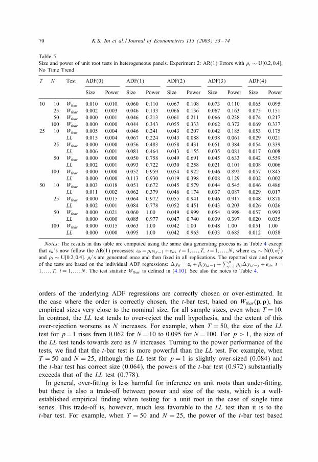
Table 5Size and power of unit root tests in heterogeneous panels. Experiment 2: AR(1) Errors with ,i ∼ U[0:2; 0:4],No Time Trend

T N Test ADF(0) ADF(1) ADF(2) ADF(3) ADF(4)

Size Power Size Power Size Power Size Power Size Power

10 10 Wtbar 0.010 0.010 0.060 0.110 0.067 0.108 0.073 0.110 0.065 0.09525 Wtbar 0.002 0.003 0.046 0.133 0.066 0.136 0.067 0.163 0.075 0.15150 Wtbar 0.000 0.001 0.046 0.213 0.061 0.211 0.066 0.238 0.074 0.217100 Wtbar 0.000 0.000 0.044 0.343 0.055 0.333 0.062 0.372 0.069 0.337

25 10 Wtbar 0.005 0.004 0.046 0.241 0.043 0.207 0.042 0.185 0.053 0.175LL 0.015 0.004 0.067 0.224 0.043 0.088 0.038 0.061 0.029 0.021

25 Wtbar 0.000 0.000 0.056 0.483 0.058 0.431 0.051 0.384 0.054 0.339LL 0.006 0.001 0.081 0.464 0.043 0.155 0.035 0.081 0.017 0.008

50 Wtbar 0.000 0.000 0.050 0.758 0.049 0.691 0.045 0.633 0.042 0.559LL 0.002 0.001 0.093 0.722 0.030 0.258 0.021 0.101 0.008 0.006

100 Wtbar 0.000 0.000 0.052 0.959 0.054 0.922 0.046 0.892 0.057 0.845LL 0.000 0.000 0.113 0.930 0.019 0.398 0.008 0.129 0.002 0.002

50 10 Wtbar 0.003 0.018 0.051 0.672 0.045 0.579 0.044 0.545 0.046 0.486LL 0.011 0.002 0.062 0.379 0.046 0.174 0.037 0.087 0.029 0.017

25 Wtbar 0.000 0.015 0.064 0.972 0.055 0.941 0.046 0.917 0.048 0.878LL 0.002 0.001 0.084 0.778 0.052 0.451 0.043 0.203 0.026 0.026

50 Wtbar 0.000 0.021 0.060 1.00 0.049 0.999 0.054 0.998 0.057 0.993LL 0.000 0.000 0.085 0.977 0.047 0.740 0.039 0.397 0.020 0.035

100 Wtbar 0.000 0.015 0.063 1.00 0.042 1.00 0.048 1.00 0.051 1.00LL 0.000 0.000 0.095 1.00 0.042 0.963 0.033 0.685 0.012 0.058

Notes: The results in this table are computed using the same data generating process as in Table 4 exceptthat �it ’s now follow the AR(1) processes: �it =,i�i; t−1 + eit ; t=1; : : : ; T; i=1; : : : ; N , where eit ∼ N(0; �2i )and ,i ∼ U[0:2; 0:4]. ,i’s are generated once and then 5xed in all replications. The reported size and powerof the tests are based on the individual ADF regressions: Myit = �i + �iyi; t−1 +

∑pj=1 ,ijMyi; t−j + eit ; t =

1; : : : ; T; i = 1; : : : ; N . The test statistic Wtbar is de5ned in (4.10). See also the notes to Table 4.

orders of the underlying ADF regressions are correctly chosen or over-estimated. Inthe case where the order is correctly chosen, the t-bar test, based on Wtbar(p; �), hasempirical sizes very close to the nominal size, for all sample sizes, even when T =10.In contrast, the LL test tends to over-reject the null hypothesis, and the extent of thisover-rejection worsens as N increases. For example, when T = 50, the size of the LLtest for p=1 rises from 0.062 for N =10 to 0.095 for N =100. For p¿ 1, the size ofthe LL test tends towards zero as N increases. Turning to the power performance of thetests, we 5nd that the t-bar test is more powerful than the LL test. For example, whenT = 50 and N = 25, although the LL test for p= 1 is slightly over-sized (0.084) andthe t-bar test has correct size (0.064), the powers of the t-bar test (0.972) substantiallyexceeds that of the LL test (0.778).In general, over-5tting is less harmful for inference on unit roots than under-5tting,

but there is also a trade-oE between power and size of the tests, which is a well-established empirical 5nding when testing for a unit root in the case of single timeseries. This trade-oE is, however, much less favorable to the LL test than it is to thet-bar test. For example, when T = 50 and N = 25, the power of the t-bar test based

K.S. Im et al. / Journal of Econometrics 115 (2003) 53–74 71

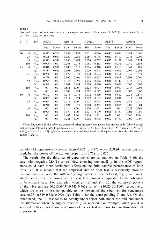
Table 6Size and power of unit root tests in heterogeneous panels. Experiment 3: MA(1) errors with i ∼U[− 0:4;−0:2], no time trend

T N Test ADF(0) ADF(1) ADF(2) ADF(3) ADF(4)

Size Power Size Power Size Power Size Power Size Power

10 10 Wtbar 0.522 0.714 0.099 0.195 0.051 0.086 0.043 0.074 0.043 0.06625 Wtbar 0.696 0.904 0.120 0.281 0.065 0.145 0.043 0.110 0.042 0.09050 Wtbar 0.945 0.998 0.166 0.483 0.070 0.237 0.047 0.151 0.041 0.124100 Wtbar 0.999 1.00 0.265 0.776 0.088 0.415 0.044 0.291 0.040 0.186

25 10 Wtbar 0.810 0.998 0.186 0.618 0.076 0.310 0.050 0.213 0.047 0.188LL 0.787 0.995 0.103 0.391 0.020 0.044 0.013 0.015 0.007 0.002

25 Wtbar 0.926 1.00 0.179 0.853 0.078 0.574 0.048 0.451 0.045 0.379LL 0.899 1.00 0.100 0.601 0.018 0.067 0.009 0.019 0.004 0.001

50 Wtbar 0.999 1.00 0.335 0.995 0.096 0.876 0.048 0.742 0.042 0.645LL 0.999 1.00 0.141 0.894 0.009 0.090 0.004 0.009 0.000 0.000

100 Wtbar 1.00 1.00 0.531 1.00 0.124 0.997 0.058 0.963 0.048 0.908LL 1.00 1.00 0.203 0.994 0.002 0.117 0.001 0.004 0.000 0.000

50 10 Wtbar 0.892 1.00 0.213 0.978 0.072 0.829 0.046 0.682 0.038 0.579LL 0.867 1.00 0.114 0.774 0.029 0.133 0.018 0.031 0.013 0.003

25 Wtbar 0.964 1.00 0.215 1.00 0.073 0.995 0.053 0.973 0.046 0.941LL 0.940 1.00 0.094 0.971 0.018 0.353 0.011 0.086 0.005 0.004

50 Wtbar 1.00 1.00 0.426 1.00 0.120 1.00 0.070 1.00 0.055 0.999LL 0.999 1.00 0.172 1.00 0.021 0.639 0.006 0.129 0.001 0.005

100 Wtbar 1.00 1.00 0.663 1.00 0.150 1.00 0.070 1.00 0.060 1.00LL 1.00 1.00 0.281 1.00 0.008 0.908 0.002 0.199 0.000 0.001

Notes: The results in this table are computed using the same data generation process as in Table 4 exceptthat �it ’s now follow the MA(1) processes, �it = eit + iei; t−1; t=1; : : : ; T; i=1; : : : ; N , where eit ∼ N(0; �2i )and i ∼ U[ − 0:4;−0:2]. i’s are generated once and then 5xed in all replications. See also the notes toTables 4 and 5.

on ADF(1) regressions decreases from 0.972 to 0.878 when ADF(4) regressions areused, but the power of the LL test drops from 0.778 to 0.026!The results for the third set of experiments are summarized in Table 6 for the

case with negative MA(1) errors. Now choosing too small p in the ADF regres-sions could have more detrimental eEects on the 5nite sample performance of bothtests. But, it is notable that the empirical size of t-bar test is reasonably close tothe nominal size, once the suPciently large order of p is selected, e.g. p = 3 or 4.At the same time the power of the t-bar test remains comparable to that obtainedin benchmark case. For example, when p = 3 and T = 25, the empirical powersof the t-bar test are (0:213; 0:451; 0:742; 0:963) for N = (10; 25; 50; 100), respectively,which are more or less comparable to the powers of the t-bar test for benchmarkcase (0:261; 0:549; 0:838; 0:990) (see Table 4 for the corresponding T and N ). On theother hand, the LL test tends to heavily under-reject both under the null and underthe alternative when the higher order of p is selected. For example, when p = 4 isselected, both empirical size and power of the LL test are close to zero throughout allexperiments.

72 K.S. Im et al. / Journal of Econometrics 115 (2003) 53–74

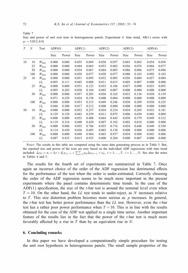
Table 7Size and power of unit root tests in heterogeneous panels. Experiment 4: time trend, AR(1) errors with,i ∼ U[0:2; 0:4]

T N Test ADF(0) ADF(1) ADF(2) ADF(3) ADF(4)

Size Power Size Power Size Power Size Power Size Power

10 10 Wtbar 0.000 0.000 0.055 0.069 0.058 0.057 0.065 0.065 0.054 0.05825 Wtbar 0.000 0.000 0.044 0.065 0.053 0.065 0.056 0.076 0.066 0.07750 Wtbar 0.000 0.000 0.054 0.067 0.064 0.083 0.086 0.096 0.075 0.096100 Wtbar 0.000 0.000 0.058 0.077 0.050 0.077 0.080 0.103 0.092 0.103

25 10 Wtbar 0.000 0.000 0.051 0.093 0.052 0.085 0.056 0.084 0.057 0.084LL 0.095 0.111 0.045 0.088 0.011 0.015 0.005 0.007 0.000 0.000

25 Wtbar 0.000 0.000 0.051 0.123 0.053 0.106 0.057 0.098 0.055 0.093LL 0.095 0.205 0.030 0.104 0.003 0.007 0.000 0.000 0.000 0.000

50 Wtbar 0.000 0.000 0.057 0.203 0.056 0.165 0.053 0.136 0.058 0.139LL 0.071 0.229 0.024 0.158 0.000 0.004 0.000 0.000 0.000 0.000

100 Wtbar 0.000 0.000 0.053 0.315 0.049 0.246 0.038 0.209 0.058 0.225LL 0.046 0.200 0.017 0.212 0.000 0.000 0.000 0.000 0.000 0.000

50 10 Wtbar 0.000 0.000 0.052 0.257 0.054 0.234 0.054 0.205 0.052 0.181LL 0.129 0.129 0.043 0.239 0.011 0.075 0.006 0.030 0.002 0.004

25 Wtbar 0.000 0.000 0.052 0.488 0.064 0.442 0.058 0.379 0.049 0.312LL 0.119 0.316 0.040 0.420 0.007 0.102 0.002 0.018 0.000 0.000

50 Wtbar 0.000 0.000 0.055 0.786 0.055 0.716 0.054 0.648 0.049 0.550LL 0.114 0.430 0.036 0.685 0.003 0.138 0.000 0.008 0.000 0.000

100 Wtbar 0.000 0.000 0.048 0.964 0.063 0.937 0.054 0.888 0.043 0.806LL 0.087 0.435 0.015 0.925 0.000 0.204 0.000 0.007 0.000 0.000

Notes: The results in this table are computed using the same data generating process as in Table 5. But,the reported size and power of the tests are now based on the individual ADF regressions with time trendincluded: Myit = �i + �it + �iyi; t−1 +

∑pj=1 ,ijMyi; t−j + eit ; t = 1; : : : ; T; i = 1; : : : ; N . See also the notes

to Tables 4 and 5.

The results for the fourth set of experiments are summarized in Table 7. Onceagain an incorrect choice of the order of the ADF regression has detrimental eEectsfor the performance of the test when the order is under-estimated. Correctly choosingthe order of the ADF regression seems to be much more important in the presentexperiments where the panel contains deterministic time trends. In the case of theADF(1) speci5cation, the size of the t-bar test is around the nominal level even whenT = 10. On the other hand, the LL test tends to under-reject, as N increases relativeto T . This size distortion problem becomes more serious as p increases. In general,the t-bar test has better power performance than the LL test. However, even the t-bartest has a rather poor power performance when T =10. This is in line with the resultsobtained for the case of the ADF test applied to a single time series. Another importantfeature of the results lies in the fact that the power of the t-bar test is much morefavorably aEected by a rise in T than by an equivalent rise in N .

6. Concluding remarks

In this paper we have developed a computationally simple procedure for testingthe unit root hypothesis in heterogeneous panels. The small sample properties of the

K.S. Im et al. / Journal of Econometrics 115 (2003) 53–74 73

proposed tests are investigated via Monte Carlo methods. It is found that when thereare no serial correlations, the t-bar test performs very well even when T = 10: In thiscase it is possible to substantially augment the power of the unit root tests applied tosingle time series.The situation is more complicated when the disturbances in the dynamic panel are

serially correlated. The t-bar test procedures now require that both N and T should besuPciently large. Furthermore, in the case of serially correlated errors, it is criticallyimportant not to under-estimate the order of the underlying ADF regressions. When weallow for serial correlation and heterogeneity in the underlying data generating process,the simulation results clearly show that if a large enough lag order is selected for theunderlying ADF regressions, then the 5nite sample performances of the t-bar test isreasonably satisfactory and generally better than that of the LL test.Since the working paper version of this paper 5rst appeared in 1995, the t-bar test

has been used extensively in the empirical panel literature and its computations arecoded in econometric software packages such as TSP and Stata. 16 Special care needsto be exercised when interpreting the results of the panel unit root tests. Due to theheterogeneous nature of the alternative hypothesis, H1, as speci5ed by (2.4), rejectionof the null hypothesis does not necessarily imply that the unit root null is rejected forall i, but only that the null hypothesis is rejected for N1 ¡N , members of the groupsuch that as N → ∞; N1=N → �¿ 0. The test result does not provide any guidanceas to the magnitude of �, or the identity of the particular panel members for which thenull hypothesis is rejected.

Acknowledgements

We are grateful to Ron Smith, Stephen Satchell, Michael Binder, James Chu, ChengHsiao, Karim Abadir, Rolf Larsson, Clive Granger, Kevin Lee, Bent Nielson, Jan Mag-nus, JeErey Woodridge, Robert de Jong, Peter Robinson and a number of anonymousreferees for helpful comments. Partial 5nancial support from the ESRC (Grant No.H519255003) and the Isaac Newton Trust of Trinity College, Cambridge is gratefullyacknowledged.

References

Balestra, P., Nerlove, M., 1966. Pooling cross-section and time-series data in the estimation of a dynamiceconomic model: the demand for natural gas. Econometrica 34, 585–612.

Baltagi, B.H., Kao, C., 2000. Nonstationary panels, cointegration in panels and dynamic panels: a survey.Advances in Econometrics 15, 7–51.

Bornhorst, F., Baum, C.F., 2001. IPSHIN: Stata module to perform Im-Pesaran-Shin panel unit root test.Boston College, Department of Economics, Statistical Software Components, No. S419704.

Bowman, D., 1999. EPcient tests for autoregressive unit roots in panel data. Unpublished manuscript, Boardof Governors of the Federal Reserve System, Washington, D.C.

16 The procedure for performing the t-bar test in TSP is provided by Hall and Mairesse (2001), and forStata by Bornhorst and Baum (2001).

74 K.S. Im et al. / Journal of Econometrics 115 (2003) 53–74

Choi, I., 2001. Unit root tests for panel data. Journal of International Money and Banking 20, 249–272.Dickey, D.A., Fuller, W.A., 1979. Distribution of the estimators for autoregressive time series with a unit

root. Journal of the American Statistical Association 74, 427–431.Hadri, K., 2000. Testing for stationarity in heterogeneous panel data. Econometrics Journal 3, 148–161.Hall, B.H., Mairesse, J., 2001. Testing for unit roots in panel data: an exploration using real and simulated

data. Economics Department, UC Berkeley.Hamilton, J.D., 1994. Time Series Analysis. Princeton University Press, Princeton.Levin, A., Lin, C.F., 1993. Unit root tests in panel data: asymptotic and 5nite-sample properties. Unpublished

manuscript, University of California, San Diego.Maddala, G.S., Wu, S., 1999. A comparative study of unit root tests with panel data and a new simple test.

Oxford Bulletin of Economics and Statistics 61, 631–652.Magnus, J., 1990. On certain moments relating to ratios of quadratic forms in normal variables: further

results. Sankhya, 52, Series B, Pt. 1, 1–13.Nabeya, S., 1999. Asymptotic moments of some unit root test statistics in the null case. Econometric Theory

15, 139–149.Ng, S., Perron, P., 1995. Unit root test in ARMA models with data-dependent methods for the selection of

the truncation lag. Journal of American Statistical Association 90, 268–281.Pesaran, M.H., Smith, R., 1995. Estimating long-run relationships from dynamic heterogeneous panels.

Journal of Econometrics 68, 79–113.Pesaran, M.H., Smith, R., Im, K.S., 1996. Dynamic linear models for heterogeneous panels. In: MXatyXas

L, Sevestre P (Ed.), The Econometrics of Panel Data: A Handbook of Theory with Applications, (2ndRevised Edition). Kluwer Academic Publishers, Dordrecht.

Phillips, P.C.B., Moon, R.H., 1999. Linear regression limit theory and non-stationary panel data.Econometrica 67, 1112–1157.

Quah, D., 1992. International patterns of growth: I. Persistence in cross-country disparities. Unpublishedmanuscript, London School of Economics.

Quah, D., 1994. Exploiting cross-section variations for unit root inference in dynamic data. Economics Letters44, 9–19.

Said, S.E., Dickey, D.A., 1984. Testing for unit roots in autoregressive moving average models of unknownorder. Biometrika 71, 599–607.

Shin, Y., Snell, A., 2000. Joint asymptotic results for mean group tests in heterogenous panels: applicationto the KPSS stationarity test. Unpublished manuscript, University of Edinburgh.

Summers, R., Heston, A., 1991. The Penn world table (Mark 5): An expanded set of internationalcomparisons 1950–1988. Quarterly Journal of Economics 106, 327–368.