Testing and simulation of track stiffness on vertical and ...
186
INGENIEURFAKULTÄT BAU GEO UMWELT Lehrstuhl für Verkehrswegebau The influence of track quality to the performance of vehicle-track interaction Duo Liu Vollständiger Abdruck der von der Ingenieurfakultät Bau Geo Umwelt der Technischen Universität München zur Erlangung des akademischen Grades eines Doktor-Ingenieurs genehmigten Dissertation. Vorsitzender: Univ.-Prof. Dr.-Ing. Gebhard Wulfhorst Prüfer der Dissertation: 1. Univ.-Prof. Dr.-Ing. Stephan Freudenstein 2. Univ.-Prof. Dr.-Ing. Ullrich Martin, Universität Stuttgart 3. Univ.-Prof. Dipl.-Ing. Dr. techn. Peter Veit, Technische Universität Graz / Österreich Die Dissertation wurde am 07.04.2015 bei der Technischen Universität München eingereicht und durch die Ingenieurfakultät Bau Geo Umwelt am 12.10.2015 angenommen.
-
Upload
khangminh22 -
Category
Documents
-
view
0 -
download
0
Transcript of Testing and simulation of track stiffness on vertical and ...
INGENIEURFAKULTÄT BAU GEO UMWELT
Lehrstuhl für Verkehrswegebau
The influence of track quality to the performance of vehicle-track interaction
Duo Liu
Vollständiger Abdruck der von der Ingenieurfakultät Bau Geo Umwelt der Technischen Universität
München zur Erlangung des akademischen Grades eines
Doktor-Ingenieurs
genehmigten Dissertation.
Vorsitzender: Univ.-Prof. Dr.-Ing. Gebhard Wulfhorst
Prüfer der Dissertation:
1. Univ.-Prof. Dr.-Ing. Stephan Freudenstein
2. Univ.-Prof. Dr.-Ing. Ullrich Martin, Universität Stuttgart
3. Univ.-Prof. Dipl.-Ing. Dr. techn. Peter Veit,Technische Universität Graz / Österreich
Die Dissertation wurde am 07.04.2015 bei der Technischen Universität München
eingereicht und durch die Ingenieurfakultät Bau Geo Umwelt am 12.10.2015 angenommen.


Table of contents
I
Table of Contents
Terms and definitions .............................................................................................. V
Abstract .................................................................................................................... VI
1. INTRODUCTION ................................................................................................. 1
1.1. Background of the research .............................................................................. 1
1.2. Scope and objectives ......................................................................................... 2
2. STATE OF TECHNOLOGY ................................................................................. 4
2.1. Track geometry (Non-recoverable track settlement) .................................... 4
2.1.1. Track recording wagon (TRW) ......................................................................... 4
2.1.2. Linear-Time-Invariant (LTI) analysis [06] .......................................................... 5
2.1.3. Track irregularity and Power-Spectral-Density function (PSD) [09].............. 6
2.2. Track stiffness (recoverable track deflection under loading) ....................... 7
2.2.1. Load distribution and elastic deflection line (static) ....................................... 7
2.2.2. Characteristics of the stiffness and damping behavior along the track ..... 9
2.3. Modeling approach for analyzing railway track dynamics .......................... 10
2.3.1. Analytic models and calculation of wheel dynamic load ............................ 11
2.3.2. Numerical models ............................................................................................. 12
2.3.3. Finite-Element-Method (FEM) ........................................................................ 13
2.3.4. Multi-Body-Simulation (MBS) .......................................................................... 14
2.3.5. Comparisons and co-simulation ..................................................................... 15
3. PILOT SECTIONS AND DESIGN OF FIELD MEASUREMENT ....................... 18
3.1. Introduction ........................................................................................................ 18
3.2. Selection of pilot sections ................................................................................ 18
3.3. Test program ..................................................................................................... 19
3.3.1. Determination of track geometry (plastic track deformation,
unloaded) 20
3.3.2. Measurement of elastic rail deflection (quasi-static) ................................... 21
3.3.3. Installation of strain gauges ............................................................................ 23
Table of contents
II
3.3.4. Recording the vertical track response under running trains ...................... 24
3.3.5. Measurement of vertical acceleration level .................................................. 25
3.4. Long-term effects .............................................................................................. 27
3.5. Vehicle information ........................................................................................... 27
3.5.1. Vehicle information in sections 1 and 2 (German railway high speed
line) 28
3.5.2. Vehicle information in sections 3 and 4 (Austrian railway high speed
line) 30
4. FIELD MEASUREMENT AND DATA ANALYSIS ............................................. 32
4.1. Track geometry and irregularity (plastic settlement) ................................... 32
4.1.1. Calculation of absolute track geometry ......................................................... 32
4.1.2. Statistical analysis of the measured data ..................................................... 33
4.1.3. Calculation of track quality parameters using Power-Spectral-Density
function (PSD) ................................................................................................... 34
4.2. Rail deflection under static loading (elastic deflection) ............................... 39
4.3. Dynamic rail bending behavior ....................................................................... 41
4.3.1. Automatic peak finding of the measured dynamic strain ........................... 42
4.3.2. Calibration runs with quasi-static loading ..................................................... 43
4.3.3. Rail bending behavior under operational train runs .................................... 45
4.4. Test of track vibration level ............................................................................. 51
4.4.1. Track vibration level under impact load ........................................................ 52
4.4.2. Track vibration level under operational trains .............................................. 53
4.5. Data provision for the numerical simulations ............................................... 55
5. THE NUMERICAL MODELING ......................................................................... 57
5.1. Introduction ........................................................................................................ 57
5.2. Model 1 (FEM) – Calibration of the elastic track model based on field side
Benkelman measurement ................................................................................................. 59
5.2.1. Introduction and modeling approach ............................................................. 59
5.2.2. Model setup and boundary condition ............................................................ 60
5.2.3. The iterative process ........................................................................................ 62
Table of contents
III
5.2.4. Results and conclusions .................................................................................. 66
5.2.5. Automation of the iteration methods (Co-Simulation with ANSYS and
MATLAB) 68
5.3. Model 2 (MBS) – Dynamic simulation of the vehicle track interaction with
pre-defined track excitations ............................................................................................ 70
5.3.1. Background and introduction .......................................................................... 70
5.3.2. Modeling of the vehicle .................................................................................... 70
5.3.3. Inclusion of measured track excitation .......................................................... 72
5.3.4. Modeling results ................................................................................................ 73
5.4. Model 3 (Co-simulation with FEM and MBS) – Calibration of the quasi-
static wheel rail load under modal represented elastic track from FEM ................... 75
5.4.1. Background and introduction .......................................................................... 75
5.4.2. Model condensation and modal analysis ...................................................... 76
5.4.3. Adjustment of the vehicle model with contact markers and model
calculation 79
5.4.4. Simulation results ............................................................................................. 80
5.5. Model 4 (Co-simulation with FEM and MBS) – Calculation of the dynamic
wheel load under elastic track with irregularities (V = 160 km/h) ............................... 81
5.5.1. Background and introduction .......................................................................... 81
5.5.2. Simulation results ............................................................................................. 82
5.6. Conclusion and outcome ................................................................................. 84
6. FEEDBACK BETWEEN VEHICLE AND TRACK UNDER TRACK SIDED
EXCITATIONS ......................................................................................................... 86
6.1. The limitation of the existing method on evaluation of the track
quality and preliminary studies ....................................................................... 86
6.2. The improvement of track quality evaluation method ................................. 88
6.3. Variation of the included influence parameters............................................ 89
6.4. Distribution of dynamic wheel load according to standard track
quality factors (Y = 6) ....................................................................................... 91
6.5. Simulation results under purely track geometry variations (Z = 0) ........... 93
6.6. Simulation results under purely track stiffness variations (Y = 0) ............. 94

Table of contents
IV
6.7. The “hybrid” simulations .................................................................................. 95
6.8. ESD analysis and possibilities of improving existing track measures
with track inspection car in high speed lines ................................................ 99
7. SUMMARY AND CONCLUSIONS .................................................................. 104
7.1. Summary of the workflow .............................................................................. 104
7.2. Conclusions ..................................................................................................... 108
SOURCE OF REFERENCE ................................................................................... 111
List of Figures ....................................................................................................... 115
List of Tables ........................................................................................................ 117
Appendices ........................................................................................................... 119
Annexes and user instructions ........................................................................... 163
Terms and definitions
V
Terms and definitions
Track stiffness – Rigidity of track; track resistance against deformation in response
to traffic loading (here: vertical direction).
Track damping – Viscosity of track, dependent on the loading speed.
Track irregularity – Track geometrical imperfections (variation of track geometry).
Track recording wagon (TRW) – A pushing track measurement wagon operated
under walking speed by human. Sample equipment includes the type CLS from the
company Vogel&Ploetscher.
Track inspection car (TIC) – Powered vehicle for continuous acquisition of the track
geometry under loaded track with different operational speed. Examples of such
vehicles include the OMWE (OberbauMessWagenEinheit) for Germany.
(Fast) Fourier Transformation (FT or FFT) – Frequency representation of a
continuous or discrete signal in time or distance domain (the inverse transformation
from frequency domain back to time or distance domain is called iFT or iFFT).
Power Spectral Density (PSD) – Distribution of the power of a signal by a frequency
per unit frequency.
Energy Spectral Density (ESD) – Distribution of the energy of a signal by a frequency
per unit frequency.
Vertical spread – Maximum difference of elevation of track geometry over the total
evaluated track section in vertical direction with reference to track alignment.

Abstract
VI
Abstract
The term “track quality” defines the conformance quality of the track, or degree to which the
track is built or maintained correctly. Important parameters specifying the general quality level
of the track include the track geometry, track stiffness and damping, which can be evaluated
by dynamic vehicle-track interaction along real tracks. Running railway vehicles excite the track
(with certain track quality level) by exerting repeated dynamic wheel loads on track which will
consequently lead to a decrease of track quality (track deterioration). The research presented
in this dissertation has practically and numerically analyzed the influence of track quality
parameters including track geometry, track stiffness and damping to the performance of
vehicle-track interaction by online data from field measurement at various pilot sections and
the from measurement data verified co-simulation models of Finite-Element-Method (FEM)
and Multi-Body-Simulation (MBS).
Field measurements at preselected pilot sections including ballasted and ballastless tracks
were performed under operational trains with various speed levels. Power Spectral Density
(PSD) analysis was applied for the evaluation and categorization of the measured 3D track
geometry. Classic Benkelman beam method was included for gathering the track stiffness of
individual rail seat. Dynamic measurements with strain gauges and accelerometers along the
track oriented themselves for an illustration of the time dependent dynamic wheel load along
the pilot section (track damping) and their impacts on low frequency track vibration levels in
frequency domain.
Varies numerical simulation models including FEM and MBS are constructed for a systematic
co-simulation including both vehicle and track. A real time illustration of the vehicle and track
interaction is realized for the best view of the counteractive effect from track side parameters
to the vehicle, as well as the other way back.
An innovative track quality evaluation method is introduced with the help of Energy Spectral
Density (ESD) distribution of the simulated dynamic wheel load. Effects of track geometry,
track stiffness and damping to the performance of vehicle track interaction can be now
separately analyzed and evaluated. Determination of the dynamic loading factors for modern
locomotives running on ballastless track can lead to reduced dynamic factors applied for
ballastless track design.

Abstract
VII


Chapter 1: Introduction
1
1. INTRODUCTION
1.1. Background of the research
Train runs excite the track through the wheel - rail contact mechanisms. Under certain
conditions of track, by uneven track settlement or change of stiffness, the load coming
from the train could be significantly higher than the static value. Also, the vehicle itself
contributes to dynamic loads e.g. by wheel flats (not focus of this research). If the static
load of a wheel is F0, then the actual force of this wheel acting on the track (Fdyn) is
calculated as follows:
Fdyn =F0+ Fexc
where Fdyn – dynamic load
F0 – static load
Fexc – excitation load
The excitation load Fexc is a form of time function, which makes the Fdyn to vary in the
time domain. Moreover, from the track side analysis, the excitation load Fexc depends
mostly on the stiffness and the geometrical excitation (track irregularity).
Normally, the most important factors determining the capacity of tracks to handle
excitation loading is track stiffness and damping factors. For optimizing the track
structural design, solutions were developed, such as implementation of high elastic rail
fastening systems, etc.
There is also interaction between the track performance in terms of stiffness and the
track quality in terms of geometry. The appearance of track irregularity along the new
track shows stochastic distributions, which are highly dependent on the initial condition
and the traffic loading. However, when certain track irregularities are spotted, the

Chapter 1: Introduction
2
deterioration of the track quality (conventional, ballasted tracks) according to the traffic
loads is related to the overall track stiffness, which is one of the most determinant
factors from the track side on the level of the excitation load. It is intuitively that higher
track deterioration rate should appear in the location where higher vehicle excitation
load is activated.
In order to get a further view on the quasi-static and the dynamic behavior of the
system, numerical models would be necessary for the simulation of the modification
of the system behavior after years of operation. These numerical procedures focus on
the quasi-static and dynamic performance of the track superstructure, as well as the
track foundation. As the vehicle track interaction is a key element which cannot be
ignored, a complicated train-track interaction model should be generated. Possible
numerical simulation models here include the Finite-Element-Method (FEM) and the
Multi-Body-Simulation (MBS).
1.2. Scope and objectives
In the current economic environment, it is important for railway organizations to be as
competitive as possible. The major task for the railway track engineer often is to
determine the economic effect or allowable limit to increase axle loads and vehicle
speeds on existing tracks. By analyzing the railway track structure using realistic track
simulation models, more informed design decisions can be made. The research
presented in this report aims to the relationship between the track sided stiffness, the
irregularity parameters and the performance of the vehicle track interaction with
modern numerical modeling strategies.
The overall scope of the research presented in this report includes:
Quality of track stiffness;
Stochastic distribution of track irregularities and its representation using Power-
Spectral-Density function (PSD);

Chapter 1: Introduction
3
Identification and verification of railway dynamic analysis models (Finite Element
Method and Multi-Body Simulation);
Analysis and evaluation of the test results;
Conclusions and perspectives.
The overall work plan for the research work includes:
Feasibility study (Literature review and methodologies);
Development of suitable simulation tools based on Multi-Body-Simulation in
combination with Finite Element Models;
The selection and field side measurements on given pilot sections (including
ballasted and ballastless tracks);
Verification of the model with measurement results;
Analysis and conclusions.

Chapter 2 : State of technology
4
2. STATE OF TECHNOLOGY
2.1. Track geometry (Non-recoverable track settlement)
The track geometry level is decisive for the track quality. Track geometrical
imperfections (track irregularity) could cause enormous consequences which leads to
a lower quality of the vehicle track interaction and again counteract on the track quality
degradation. For this research, the wave length defining the overall track irregularity
was set between 0.5 m and 100 m.
The characteristic of the track irregularity normally shows a wide banded spectral
distribution, which makes the rebuild and categorization complicated. Therefore, digital
signal processing techniques are required to provide the best ways of rebuilding the
signal in an identical quality level. Many methodologies were studied and investigated
on the representation of the track irregularity via Fast-Fourier-Transform (FFT) and
Linear-Time-Invariant (LTI) analysis.
2.1.1. Track recording wagon (TRW)
The measurement of the track irregularity is normally included in the track inspection
car (TIC). These measurements are conducted under the travel of the train. Their
recording (especially in vertical direction) of the track irregularity is under the loaded
track condition.
Nonetheless, track recording wagon is found to be better for recording the track
irregularity levels for this study. Those wagons were normally weighted less than 1 t
so their eigen loads can be neglected. By doing so, the measured track irregularity
refers to the unloaded track condition which is identical to the plastic track settlement.
There are various products available in the market which can be easily operated by
human.
Chapter 2 : State of technology
5
2.1.2. Linear-Time-Invariant (LTI) analysis [06]
Due to the fact that the values measured by the TRW are normally indirect and require
further processing, various methods of transferring those measured data into the
realistic track irregularity distribution were developed. The following paragraphs focus
on one of the best analysis methods, the Linear Time Invariant (LTI) analysis.
The LTI system theory can be applied to analyze the response of a linear and time-
invariant system to an arbitrary signal. The basic theory and the applied Fourier
Transformation is found in the literature [07]. Recording of the raw data normally
succeeds through time cursor, but for the distance application of relevant
measurements, the LTI system can also have trajectories in spatial dimensions. The
general work flow of the LTI analysis is shown in Figure 1:
Figure 1 Principle of the LTI system [07]
The raw data for the application of the LTI analysis should fulfill the following two pre-
requisites, the Linearity and the Time invariance. The calculation of the transfer

Chapter 2 : State of technology
6
function relies on the dirac-delta function [08]. After applying the Fourier Transformation
(FT) on the output signal y(t) into Y(jω), the input signal in frequency domain could be
calculated using the Y(jω) and H(jω), as shown above. The calculated X(jω) can be
then converted back to distance signal by applying the Inverse Fourier Transformation
(iFT).
According to the measured raw data from the track recording wagon, it is obvious that
the calculation of absolute track geometry should be only applied in the vertical and
lateral direction (see Chapter 2.1.1 and 2.1.2).
2.1.3. Track irregularity and Power-Spectral-Density function (PSD) [09]
Spectral analysis can be applied on many diverse fields. There are two broad
approaches to spectral analysis, namely the Energy-Spectral-Density of deterministic
signals and Power-Spectral-Density of random signals [09].
The characteristic of the track excitation is that the variation outside the measured
section is uncertain. It is only possible to estimate the statements of the variation. The
method describes how the power of a signal or time series is distributed within
frequency. The convenience is that the power could be here adjusted to the required
target variable, which in this case, is the track excitation. The accuracy of the prediction
of the further track excitations can be increased through the enlargement of the number
of characteristic frequency super-positions.
The PSD function utilizes a pre-defined “Auto-Correlation-Function” (also called
“Transfer function”) and calculates the respective PSD function by Fourier transform of
the transfer function. There are also respective regulations (known as the ORE B176
[10], also called “ERRI”) that define the respective parameters, which were obtained
from a number of measurements carried out by the European railway operators.

Chapter 2 : State of technology
7
2.2. Track stiffness (recoverable track deflection under loading)
The quality of rail transport has a strong relation to the track quality. Wheel load
distribution, within rail track structure, and wheel guidance are characterized by the
overall track design, but particularly by geometrical and elastic properties. The above
mentioned elastic properties usually refer to resilient rail pads, under sleeper pads, sub
ballast mat, etc. [01]. Figure 2 shows a normal railway superstructure together with all
the optional elastic elements (marked in red).
Figure 2 Typical railway superstructure and optional elastic elements
2.2.1. Load distribution and elastic deflection line (static)
Determining the wheel load distribution, within the track superstructure, under given
train loads is always the first step to analyze the overall performance of rail track.
The theory of Winkler and Zimmermann (Winkler, 1867; Zimmermann, 1888) is still
frequently used because it allows a precise calculation of the essential parameters,
which are the rail deflection and the bending moment. It considers the rail as an
infinitely long beam continuously supported by an elastic foundation. This is based on
the assumption that the reaction forces of the foundation are proportional to the
deflection of the beam at every point. This assumption was first introduced by E.
Chapter 2 : State of technology
8
Winkler (WINKLER 1867) and formed the basis of H. Zimmermann’s classical work on
the railroad track in Berlin (ZIMMERMANN 1888) [02]. The actual soil stress distribution
along the load axis based on the half space theory can be also calculated. Sample
deflection lines and stress distribution under typical soft (pad stiffness 40 kN/mm) and
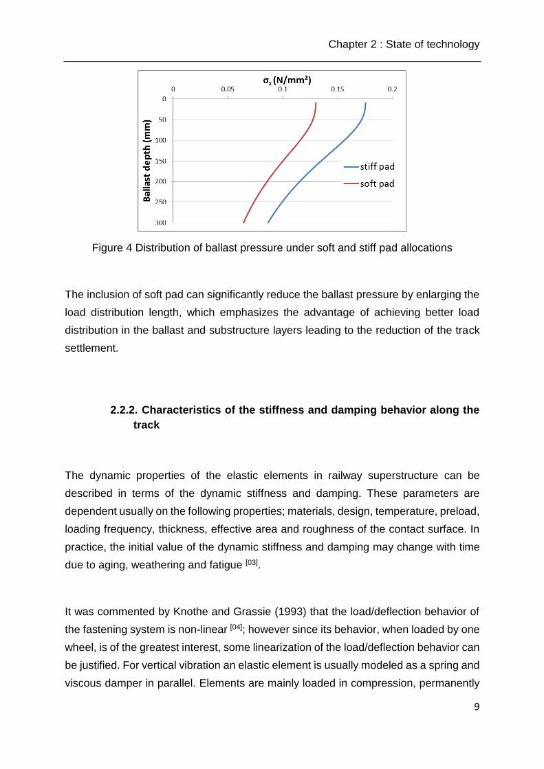
stiff (pad stiffness 500 kN/mm) supports are calculated and shown in Table 1, Figure
3 and Figure 4:
Table 1: Theoretical calculation with Zimmermann therory (Rail type 60E2)
Item Symbol Soft pad Stiff pad
Pad stiffness (kN/mm) c pad 40 500
Ballast stiffness (kN/mm) c ballast 125
System stiffness (kN/mm) c 30.3 100
Static load (kN) Q 100
Contact area B70 (mm²) F 546000
maximum rail deflection (mm) y0 1.17 0.48
Max. rail seat support load (kN) S 35.5 47.9
Ballast surface pressure (N/mm²) p 0.13 0.18
σz at bottom of 30 cm ballast(N/mm²) σz 0.06 0.09
Figure 3 Typical deflection line calculated by Zimmermann Theory
Chapter 2 : State of technology
9
Figure 4 Distribution of ballast pressure under soft and stiff pad allocations
The inclusion of soft pad can significantly reduce the ballast pressure by enlarging the
load distribution length, which emphasizes the advantage of achieving better load
distribution in the ballast and substructure layers leading to the reduction of the track
settlement.
2.2.2. Characteristics of the stiffness and damping behavior along the
track
The dynamic properties of the elastic elements in railway superstructure can be
described in terms of the dynamic stiffness and damping. These parameters are
dependent usually on the following properties; materials, design, temperature, preload,
loading frequency, thickness, effective area and roughness of the contact surface. In
practice, the initial value of the dynamic stiffness and damping may change with time
due to aging, weathering and fatigue [03].
It was commented by Knothe and Grassie (1993) that the load/deflection behavior of
the fastening system is non-linear [04]; however since its behavior, when loaded by one
wheel, is of the greatest interest, some linearization of the load/deflection behavior can
be justified. For vertical vibration an elastic element is usually modeled as a spring and
viscous damper in parallel. Elements are mainly loaded in compression, permanently
Chapter 2 : State of technology
10
by the fastening system, the eigen load and/or repetitively by the traffic. By taking
elastic rail pad as examples, in two dimensional models a pad can be represented by
a pointed support under the rail foot; however for three dimensional models a visco-
elastic layer across the rail foot is often considered (Kumaran, 2003) [05].
The classic methods can provide accurate results, but due to too many idealized
parameter settings, the realistic rail seat deflection and load distribution can never be
simply calculated by applying classic formulas. Firstly, the elastic elements, usually
made from rubber or polymeric compound materials, show normally a nonlinear elastic
behavior under loading. This will make the classic calculation with formulas at higher
deflection rates uncertain. Secondly, the rail seat can have individual elastic behavior
and have a variation of the stiffness even between the neighboring rail seats. This
variation can be caused by different parameters including the initial condition of the
construction and time dependent settlements. Track irregularity with respect to
geometry is affecting the individual performance of rail seats (fastening system) and
therefore the track stiffness quality along the track. Application of the modern numerical
methods for a systematic study of realistic parameter variation is needed.
2.3. Modeling approach for analyzing railway track dynamics
Railway system components can be classified on the basis of their principal properties,
either mass or elastic properties, or both. Together with the geometrical design (layout)
of a track structure, a mechanical design or a model can be described. Such a model
is basically formed by a set of relationships between all components, with inertia
properties. These relationships are influenced by both elastic properties and
dimensions of the components. The set of relationships defines a mechanical model,
suitable for the analysis of the track structural behavior. De Man (2002) comments that
in order to combine properties and dimensions into models, two modeling methods
may be used, the analytical and the numerical modeling [11].

Chapter 2 : State of technology
11
2.3.1. Analytic models and calculation of wheel dynamic load
Analytical models are preferably based on homogenous situations. For instance,
continuous conditions are applied to support a limited number of connections and load
positions. Examples for analytical models are the mathematical solutions of an infinite
beam on an elastic foundation by Zimmermann (1888), Euler, Bernoulli (1736) and
Timoshenko (1926).
It was released by the Deutsche Bundesbahn, in 1993, for the track superstructure
calculation concerning the calculation of dynamic wheel load based on track sided
influencing parameters [12]. The calculation of the maximum possible dynamic wheel
load is realized as follows:
max 𝑄 = 𝑄𝑚𝑒𝑎𝑛 ∗ (1 + 𝑡 ∗ �̅�) = 𝑄𝑚𝑒𝑎𝑛 ∗ (1 + 𝑡 ∗ 𝑛 ∗ 𝜑)
Where Qmean – static load of the wheel
t – Factor, dependent on confidence level (t = 3 for confidence of 99.7 %)
n – Track quality factor
φ – Speed factor
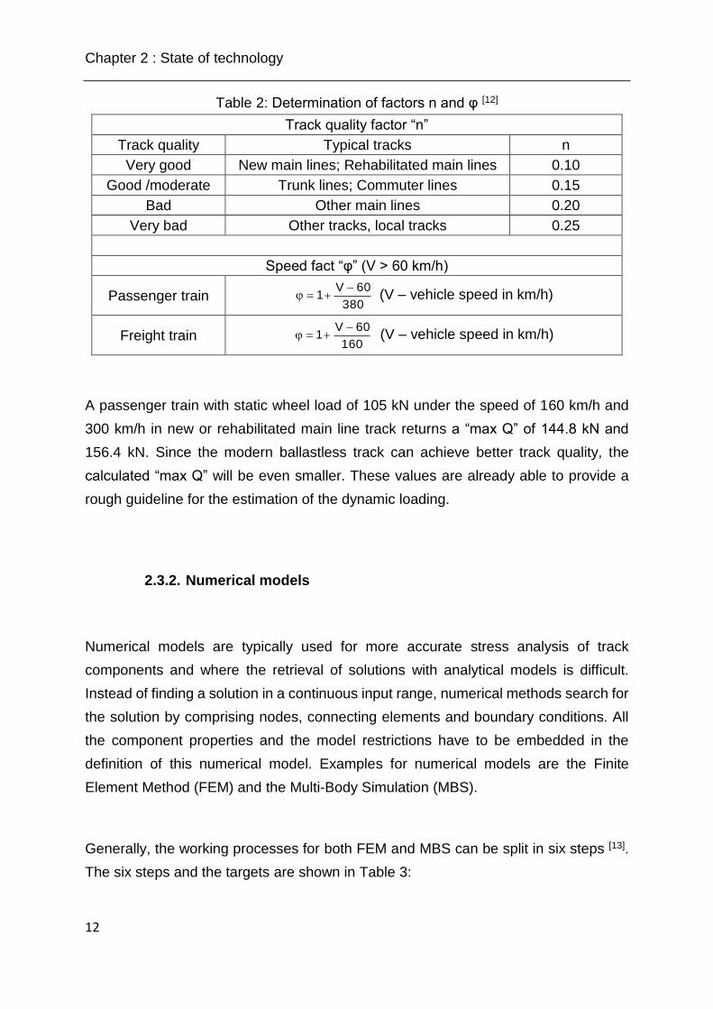
The following Table 2 shows the determination of the factors n and φ with reference to
different operational situations. t = 3 is used for check of rail stresses and thickness
design of slabs/pavements for ballastless track. 0.15% of loads may exceed Qmax
Chapter 2 : State of technology
12
Table 2: Determination of factors n and φ [12]
Track quality factor “n”
Track quality Typical tracks n
Very good New main lines; Rehabilitated main lines 0.10
Good /moderate Trunk lines; Commuter lines 0.15
Bad Other main lines 0.20
Very bad Other tracks, local tracks 0.25
Speed fact “φ” (V > 60 km/h)
Passenger train (V – vehicle speed in km/h)
Freight train (V – vehicle speed in km/h)
A passenger train with static wheel load of 105 kN under the speed of 160 km/h and
300 km/h in new or rehabilitated main line track returns a “max Q” of 144.8 kN and
156.4 kN. Since the modern ballastless track can achieve better track quality, the
calculated “max Q” will be even smaller. These values are already able to provide a
rough guideline for the estimation of the dynamic loading.
2.3.2. Numerical models
Numerical models are typically used for more accurate stress analysis of track
components and where the retrieval of solutions with analytical models is difficult.
Instead of finding a solution in a continuous input range, numerical methods search for
the solution by comprising nodes, connecting elements and boundary conditions. All
the component properties and the model restrictions have to be embedded in the
definition of this numerical model. Examples for numerical models are the Finite
Element Method (FEM) and the Multi-Body Simulation (MBS).
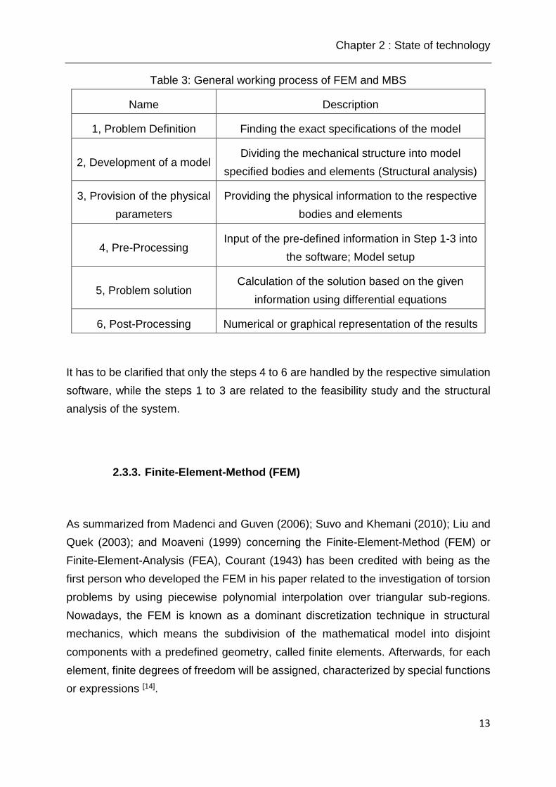
Generally, the working processes for both FEM and MBS can be split in six steps [13].
The six steps and the targets are shown in Table 3:
380
60V1
160
60V1
Chapter 2 : State of technology
13
Table 3: General working process of FEM and MBS
Name Description
1, Problem Definition Finding the exact specifications of the model
2, Development of a model Dividing the mechanical structure into model
specified bodies and elements (Structural analysis)
3, Provision of the physical
parameters
Providing the physical information to the respective
bodies and elements
4, Pre-Processing Input of the pre-defined information in Step 1-3 into
the software; Model setup
5, Problem solution Calculation of the solution based on the given
information using differential equations
6, Post-Processing Numerical or graphical representation of the results
It has to be clarified that only the steps 4 to 6 are handled by the respective simulation
software, while the steps 1 to 3 are related to the feasibility study and the structural
analysis of the system.
2.3.3. Finite-Element-Method (FEM)
As summarized from Madenci and Guven (2006); Suvo and Khemani (2010); Liu and
Quek (2003); and Moaveni (1999) concerning the Finite-Element-Method (FEM) or
Finite-Element-Analysis (FEA), Courant (1943) has been credited with being as the
first person who developed the FEM in his paper related to the investigation of torsion
problems by using piecewise polynomial interpolation over triangular sub-regions.
Nowadays, the FEM is known as a dominant discretization technique in structural
mechanics, which means the subdivision of the mathematical model into disjoint
components with a predefined geometry, called finite elements. Afterwards, for each
element, finite degrees of freedom will be assigned, characterized by special functions
or expressions [14].
Chapter 2 : State of technology
14
The exact work flow which is performed by FEM simulation software is:
Pre-processing: definition of geometry, materials, and element types and
generation of finite-element grids (meshing).
Problem solution: definition of analysis type, boundary conditions and
constraints, application of loads and calculation of solution by intern defined
calculation mechanisms.
Post-processing: Visualization of the analysis results (usually time-
independent).
The FEM software, chosen for this research is named ANSYS. It provides general
solutions to the practical problems for universal purposes. The first version was
released in 1971.
2.3.4. Multi-Body-Simulation (MBS)
Multi-Body Simulation is a newly developed modeling approach in railway engineering
field. Such kinds of simulation software (e.g. SIMPACK) are already widely used in the
design of automobiles or locomotives [15]. On MBS systems, the structural parts or
bodies are often connected using complex joints (complex suspension joints, for
example), with complicated force elements acting between these bodies. Often in such
systems, the bodies themselves can be considered as rigid, as the relative deflection
of the bodies is small in comparison to the rigid body motion. MBS software has
allowed the modelling of these types of dynamic systems, where previously was not
possible. A sample model done at SIMPACK is shown in Figure 5:

Chapter 2 : State of technology
15
Figure 5 Sample SIMPACK Model for railway vehicle [15]
2.3.5. Comparisons and co-simulation
When comparing MBS software to Finite Element (FE) software, the differences
between them become clear. The FE software, which focuses on the elastic body itself,
requires all bodies to be defined as elastic, whereas MBS software, requiring mostly
rigid bodies, focuses more on the complex interaction between them. Table 4 shows a
comparison of the modeling approaches.
Chapter 2 : State of technology
16
Table 4: Comparison of FEM and MBS approach
FEM
Finite-Element-Method
MBS
Multi-Body-Simulation
System
characteristics System with 2D/ 3D Elements System with 3D bodies
Basic elements
Elastic elements
(Material properties, Element
types)
Rigid bodies
(Mass, CoG, Inertia Tensor, etc.)
Formulation of
the system
Elements are connected by
nodes
Connection of bodies with
idealistic joints
Type of analysis Static analysis Kinematic and dynamic analysis
Output results Calculated
Deflections, Strain, Stress
Calculated
Force, Speed, Acceleration
Degrees of
Freedoms
System with many
Degrees of Freedoms
System with limited
Degrees of Freedoms
(Condensation)
Representative
software ANSYS, SoFisTiK … Simpack, Adams…
The FEM gains advantages in the representation of element stiffness, whereas MBS
can easily handle 4D systems with time-dependent dynamic analysis. Considering the
complexity of the vehicle track dynamic system, both approaches have to be utilized
in the most efficient way. The FEM allows the sufficient approximation of the track
flexibility, while the vehicles’ motion, including its complex wheel-rail interface, is
produced within the appropriate MBS system. Therefore, a joint use of both, named
“Co-simulation”, is one of the best solutions [16]. Co-simulation means that both FEM
and MBS programs simulate their respective parts separately on a superior artificial
discretized time-scheme and interchange the conjunctive data at the thus defined
points of time.
The MBS software SIMPACK provides the possibility to preform co-simulation with
FEM software ANSYS by integrating the FEM model into the MBS interface.
Nevertheless, the FEM model should be firstly condensed before such integration. This
condensation is achieved through the modal approach, which calculates a large
number of eigen modes to represent the track stiffness and damping characteristics.
Chapter 2 : State of technology
17
The FEM model should be condensed, since it originally contains too many variables.
The way of condensing the FEM model is to specially define some nodes as so called
“Master nodes”, whereas the other nodes are controversially “Slave nodes”. By doing
so, the master nodes will still hold independent equations, but the results of the slave
nodes will be the linear combination from the results of neighboring master nodes. In
other words, slave nodes will not hold independent variables any longer. By carefully
selection of master nodes, the number of independent variables is significantly reduced
without neglecting the general model characteristics. This calculation is called
“Substructuring analysis”, in ANSYS.
The eigen modes of the FEM system provide the most important information for the
MBS environment, which is how the stiffness and damping of the track should be
represented. The eigen modes of the FEM system are calculated by the so called
“Modal analysis” based on the condensed FEM model. The eigen modes of the elastic
structure represent both its dynamic response and its local deformation, due to the
interfaces loads.

Chapter 3 : Selection of pilot sections and design of field measurement
18
3. PILOT SECTIONS AND DESIGN OF FIELD MEASUREMENT
3.1. Introduction
Field measurements are always the best and most direct way to gather actual
information about the track. Experiences from previous research works about the track
quality evaluations can be utilized. Various field measurements were reviewed in order
to find out the best way of gathering field side data related to this research work.
3.2. Selection of pilot sections
To guarantee comparable situations of the test sections, in order to be able to focus
only on the track quality, the following boundaries for the selection procedure, of the
track sections, have been fixed:
- straight alignment to exclude additional centrifugal forces by the cant deficiency or
centripetal forces due to the cant excess,
- no or moderate longitudinal slope,
- no changes in substructure,
- modern high speed railway lines as the best suitable pilot sections and
- the initial condition of the section should be measured.
A systematic understanding of the vehicle-track interaction relies on both vehicle and
track sided inputs. Since this interaction is generally increased by increasing the speed
level, modern high speed railway lines with different type of superstructure are the best
scenarios for the research work.
An important reason for the variance of the track quality is the initial condition, meaning
how “perfectly” the tracks are built. Modern construction technologies could handle
those construction works without major difficulties, but small variances of the track

Chapter 3 : Selection of pilot sections and design of field measurement
19
sided parameters can never be fully eliminated. Those variances are the key reasons
to provide guidelines for the general deterioration level of the overall track quality.
In total four different measurement sections were selected. General information about
these sections can be seen in Table 5. Clearly, the maximum design speed of 250 or
300 km/h and ballasted or ballastless track system are examined.
Table 5: Selection of measurement sections
Section
number Location between Type of track
Max. design speed
(km/h)
1 Nuremberg and Ingolstadt,
Germany
Ballastless track
Type1 300
2 Nuremberg and Ingolstadt,
Germany
Ballastless track
Type2 300
3 Salzburg and Vienna,
Austria Ballasted track 250
4 Salzburg and Vienna,
Austria
Ballasted track
partially with sub-
ballast-mat
250
The detailed section plan, including the position of all the measurement sensors and
general information about the alignment and the superstructure installations, is found
in appendices 1 to 4.
3.3. Test program
Various activities on the field can be conducted with the focus on different targets.
When talking about the research on vehicle-track interaction and the respective track
quality, the necessary measurement parameters should include the elastic track
deflection, the vertical track geometry and the dynamic track behavior.

Chapter 3 : Selection of pilot sections and design of field measurement
20
3.3.1. Determination of track geometry (plastic track deformation,
unloaded)
The determination of track geometry in the representation of plastic track deformation
was done previously only in the vertical direction. However, for a better understanding
of the influence of the track irregularity to the behavior of the wheel-rail interaction,
there is the necessity to continuously record the track geometry in 3 dimensions.
Track geometry in the representation of plastic track settlement is the direct source
influencing the vehicle-track interactions. By increasing the travel speed, a longer
influence section should be inspected.
The design of modern passenger coach (with air-spring as secondary suspension)
always follows the principle, that an eigen frequency of approximately 1 Hz should be
achieved [17], which means that the calm down time for single impulse could be up to
1 s long (This eigen frequency for locomotives and freight wagons are normally higher
due to the installation of coil springs for secondary suspension). This defines the
minimum wave length which should be included in the calculation of track geometry.
From the previous experiences of the institute, this wave length must have at least 8
repeats in each measurement. Table 6 shows the speed, the respective wave length
and required measurement length.
Table 6: Calculation of the minimum measurement length for geometry
measurement
Speed (km/h) Wave length (m) Minimum Length for geometry measurement (m)
160 44.4 350
250 69.4 550
300 83.3 650
New track recording wagon was introduced and applied in this research work. The
wagon was manufactured by the company Vogel & Plötscher with a type series called
“MessReg CLS” [18]. It can record the respective track parameters continuously along
the line by just pulling the wagon with walking speed. The reader is referred to Figure
6 and Table 7 for the handled parameters, as well as the accuracies.
Chapter 3 : Selection of pilot sections and design of field measurement
21
Table 7: Performance data of movable track recording wagon
(Type CLS from company V&P) [18]
Measured
parameters
Range from
(mm)
Range to
(mm)
Accuracy
(mm)
Gauge 1415 1500 0.005
Versed sine -230 +230 0.005
Gradient -100 +100 0.3
Cant ± 170 0.001°
Distance Continuous 2
Figure 6 Movable track recording wagon (Type CLS from company V&P) [18]
It is essential to mention that the under sleeper gap actually is another phenomenon
of track plastic deformation in vertical direction. These deformations could only be
detected by the loaded track; therefore the gaps are measured by other measurement
methods.
3.3.2. Measurement of elastic rail deflection (quasi-static)
In order to check the uniformity of the vertical load distribution of the track by rail
deflection, it is required to perform static rail deflection measurements at a certain
amount of rail seats (sleepers) within each test section. Rail deflection is influenced by
all the elastic components within the railway sub- and superstructure, as well as by
potential gaps between the sleepers and the ballast. A minimum number of 100 rail
Chapter 3 : Selection of pilot sections and design of field measurement
22
seats (50 continuous on each rail) should be measured at each pilot section for
statistical reasons.
Rail deflection measurements on successive rail seats can be performed using the
track movable, modified Benkelman-beam, which gives the overall rail deflection under
a given quasi-static axle load, as well as the shape of the deflection bowl of one rail
during the approach of the loaded wheel. The quasi-static loading is given by a ballast
bulk wagon with a single axle load. A loco was used to push and pull the wagon with
walking speed within a regular stop to stop distance of about 10 m. In Figure 7 the
design of the Benkelman measurement wagon is shown.
Figure 7 Benkelman beam for the measurement of track elastic deflection
For the analysis purposes, the deflection line should be calculated based on the
measured influence line. The values of the deflection line for each rail seat could not
be directly taken from the measurement data, because the specification for the
deflection line requires stable load (while during the Benkelman measurement, the
load train was moving while the data were measured). Therefore, an interpolation is
carried out, which functions as follows:

Chapter 3 : Selection of pilot sections and design of field measurement
23
The rail seat i, where the deflection line will be drawn, is chosen.
The deflection at the load point (max. deflection) is read from the measurement
i, under the position of s = 0 m
The deflection at x = x0 m (x0 is sleeper spacing) is read from the measurement
i-1, under the position of s = x0 m (which is the exact deflection of x = x0 m when
the load is on the rail seat i)
The deflection at x = 2*x0, 3*x0, 4*x0 etc. can be similarly calculated.
3.3.3. Installation of strain gauges
Strain gauges are installed on the rail and within the length of the sleeper spacing.
Particularly, the strain gauges with length of 6 mm were located at the rail foot middle
point, between the sleepers, and could record the strain changes caused by the wheel
load of the vehicle. The maximum allowable channels for a synchronized
measurement are 64, so when rail foot stress between every two rail seats are
measured, the total length is limited to approximately 20 m, which is too short to
measure dynamic effects. Therefore, the following modifications are made:
Most of the strain gauges should be installed inside the area of the Benkelman
beam measurement;
A difference of installation density should be realized for higher efficiency;
The total number of installed strain gauges should be slightly higher than the
maximum allowable channels to prevent possible failures.
The strain gauges were installed in three different densities named ‘Fine’, ‘Middle’ and
‘Rough’. The allocation of the strain gauges follows the following principles:
1. The dynamic strain / stress caused by the four wheels of one bogie should be
recorded at the same time;

Chapter 3 : Selection of pilot sections and design of field measurement
24
2. The change of the strain / stress in time sequence should be recorded at least
for one cycle with possible fine step size (area ‘fine’);
3. Middle and rough stepped measurement should be located after the ‘fine’ area
for concluding the change of strain / stress during the passage of the train; (area
‘middle’ and ‘rough’)
4. A sufficient length of the measurement section should be provided for gathering
the decay / amplification rate between different cycles.
3.3.4. Recording the vertical track response under running trains
For data recording, the QuantumX is used which measures up to 8 channels at the
same time. Through fire-wire connection, more units can be connected and measured
with synchronized time axis (See Table 8 for hardware information).
Table 8: Data amplifier QuantumX
24 bit A/D conversion for synchronous,
parallel measurements
Sample rate: up to 19.2 kHz/channel,
configurable
Filters: Bessel, Butterworth 0.01 Hz to
3.2 kHz (-1 dB) Electrically isolated inputs
Power supply for active transducers Permissible cable length up to 100 m
This equipment supports a maximum measurement frequency of 19 kHz. Thus a train
running with up 300 km/h, within a distance of 4 mm of the train’s movement one set
of data is recorded. This is required to precisely identify the peak values of the rail foot
Chapter 3 : Selection of pilot sections and design of field measurement
25
strain influence lines. Concerning the evaluation, the strain values were used to
determine the respective rail foot stress, retrieved from the formula σ = ε · E, while the
Young´s modulus E was set equal to 2.1·105 N/mm².
The test should be conducted under normal operational train runs. It must be taken
into account that the measurement data for analysis and evaluation are thus affected
by the respective train speed (fixed according to operational or actual, random
conditions) and train type (axle loads and axle spacing, suspension system), as well
as by load deviations and conditions of the individual axles (potential wheel flats) even
when the train type is identical.
3.3.5. Measurement of vertical acceleration level
Accelerometers are placed on the rail and the sleepers, measuring the vertical
vibration level of the track. The measured raw acceleration level of the track was used
to analyze the track quality and the respective vibration level.
The track side acceleration is often recorded by special made acceleration sensors
(also called accelerometers, see Figure 8). Those sensors utilize the gyroscope theory
to the physically sense in the real-time acceleration level and represent these levels in
a certain type of electric signals.
Figure 8: Typical accelerometers and its internal design

Chapter 3 : Selection of pilot sections and design of field measurement
26
The above Figure 8 shows the internal design of a typical accelerometer. This type of
sensor is also called piezoelectric accelerometer. It records and converts the physical
acceleration into electronic signal. For specific rail and track problems, the included
sensor for data recording is from the company Brüel&Kjaer with upper frequency limit
at 4.5 kHz.
The electric signals of the transducers were transmitted to a signal amplifier by B&K.
An impulse hammer with a head mass of 5.44 kg was also used to extract a standard
impulse load on the rail head in order to calibrate the track vibration behavior.
Allocation of more accelerometers on the rail, the sleepers and in the ballast bed
provides the exact information regarding the elements which are excited the most. In
total, 8 accelerometers are installed in each test section. Their locations are marked
with numbers 1 to 8. A sketch of the sensors allocation and moreover, a picture of the
exact positions of the sensors 3, 4, 7 and 8 and the impulse locations of A and B in the
field, can be found in Figure 9. The locations A and B are the impact points for the
impulse hammer.
Figure 9: Allocation of the measurement sensors
The acceleration of the system under the hammer impulse and the operational train
passages is measured. The amplified signals were sent to a 16 bit PC DAQ-Card of
National Instruments, in a laptop. The digital, raw signals were then analyzed and
evaluated using the software MEDA 2013 from Wölfel.
The accelerometers measure the vibration acceleration level (m/s²) and the impact
hammer measures the impact load (N). The analysis of the measured signals firstly

Chapter 3 : Selection of pilot sections and design of field measurement
27
demands the division of the acceleration channel to the respective load channel in
order to determine the acceleration under the unit loading. This was performed to
eliminate the difference of the hammer excitation load. In the next step, the vibration
speed is determined by integrating the acceleration signal in the time domain. The
calculation of the spectrum distribution relays on the Fast Fourier Transformation
(FFT) of the processed time signal with a band width of Δf = 1.25 Hz and a rectangular
window with 50 % overlap whilst linear average determination of the spectrum
distribution within a time frame of T = 4 s. Finally, the vibration speed spectrum is
illustrated in frequency domain under Terz distribution from 8 Hz to 6.3 kHz
(dependent on the setup of band width in the measurement). The analysis of the data
partially fulfills the requirements written in DIN 45672-2 [19].
It should be noticed that the effect of high speed train runs is more sensible to local
imperfections, and thus the vibration level could be amplified to a higher level even
under very limited track disturbances. These measurements are quite useful to
understand the effect of small track irregularities to the vehicle track interaction. All the
analyses are accomplished in the software program MEDA 2013.
3.4. Long-term effects
The change of track quality in relationship to the operational parameters is always one
of the most determinant factors to specify the general track maintenance strategy. This
especially concerns the newly assembled ballasted tracks due to possible adjustment
effects. Therefore, repeated measurements in sections 3 and 4 were planed within the
time span of approximately 1 year. The change of track sided parameters between
both measurements is particularly interesting for this research topic.
3.5. Vehicle information
Chapter 3 : Selection of pilot sections and design of field measurement
28
Different types of vehicles were measured during the train run tests. As the evaluation
of the measurement data is highly dependent on the design of the vehicles (axle load,
suspension design, etc.), an overview of the measured locomotive and multiple units
were collected and shown in the following sections.
3.5.1. Vehicle information in sections 1 and 2 (German railway high
speed line)
The general information of the locomotive and multiple units can be seen in Table 9 to
Table 11:
Table 9: Inter-City-Express, ICE 1 / ICE 2 (D-DB)
ICE 1 (D-DB BR 401) / ICE 2 (D-DB BR 402)
Type of vehicle EMU
Formation M + 12T + M / M + 6T + L
Max. speed (km/h) 280
Weight (t) 849 / 412
Max. axle load (t) 19.5
Axle formation (locomotive) Bo’Bo’
Axle spacing (locomotive, m) 3.0
*) Pic source: Wikipedia
Chapter 3 : Selection of pilot sections and design of field measurement
29
Table 10: Inter-City-Express, ICE 3 / ICE T (D-DB)
ICE 3 (D-DB BR 403) / ICE T (D-DB BR 411)
Type of vehicle EMU
Formation 4M4T / 4M3T
Max. speed (km/h) 330 / 230
Weight (t) 409 / 368
Max. axle load (t) 17.0 / 15.5
Axle formation (motor car) Bo’Bo’ / (1A)'(A1)’
Axle spacing (m) 2.5
*) Pic source: Wikipedia
Table 11: The express trains IC / RE (D-DB)
Type 101 (D-DB BR 101) / Passenger wagon
Type of vehicle Locomotive / wagon
Formation -
Max. speed (km/h) 220 / 200
Weight (t) 84 / 55-60
Max. axle load (t) 21.7 / 14-15
Axle formation Bo’Bo’
Axle spacing (m) 2.65 / 2.50
*) Pic source: Wikipedia

Chapter 3 : Selection of pilot sections and design of field measurement
30
3.5.2. Vehicle information in sections 3 and 4 (Austrian railway high
speed line)
General information of the locomotive and the multiple units is provided in Table 12 to
Table 14. The Type ICE-T (D-DB BR 411) was already introduced in subsection 3.5.1.
Table 12: Electric Multiple Units KISS (A-ÖBB)
Type KISS, Version Westbahn (A-ÖBB BR 4010)
Type of vehicle EMU
Formation 2M4T
Max. speed (km/h) 200
Weight (t) 310
Max. axle load (t) 17.0
Axle formation (motor car) Bo’Bo’
Axle spacing (m) 2.5
*) Pic source: Wikipedia
Chapter 3 : Selection of pilot sections and design of field measurement
31
Table 13: Electric locomotives (A-ÖBB)
Type 1116 (A-ÖBB BR 1116) / Type 1144 (A-ÖBB BR 1144)
Type of vehicle Locomotive
Formation -
Max. speed (km/h) 230 / 160
Weight (t) 85 / 84
Max. axle load (t) 21.5 / 21.0
Axle formation Bo’Bo’
Axle spacing (m) 3.0
*) Pic source: Wikipedia
Table 14: Passenger wagons (A-ÖBB)
Passenger wagons for IC / RJ
Type of vehicle Wagon
Formation -
Max. speed (km/h) 200 / 250
Weight (t) 55-60
Max. axle load (t) 14-15
Axle formation Bo’Bo’
Axle spacing (m) 2.5
*) Pic source: Wikipedia

Chapter 4 : Field measurement and data analysis
32
4. FIELD MEASUREMENT AND DATA ANALYSIS
This chapter documents the measurements conducted for all the pilot sections. The
sequence of the chapter is according to measurement components. It is manually
defined, that specific strain gauge is located at 0 m and the rail on the left side of the
travel direction, with increasing number of points, is called ‘Left rail’ (refer to
appendices 1 to 4 for detailed position information). This definition is used through all
the following figures and tables in this chapter. Pictures from the measurement
activities can be found in Annexes 1 to 6.
4.1. Track geometry and irregularity (plastic settlement)
4.1.1. Calculation of absolute track geometry
As introduced in chapter 2, an automatic calculation of the absolute track geometry
under the guideline of Linear-Time-Invariant theory (LTI) should be firstly applied for
the measured raw data. This was achieved by the self-developed Matlab program. A
Graphical-User-Interface (GUI) was also created for easier processing and is shown
in Figure 10, the user specification and instructions could be found in User Instruction
manual 1.
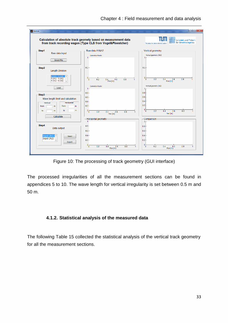
Chapter 4 : Field measurement and data analysis
33
Figure 10: The processing of track geometry (GUI interface)
The processed irregularities of all the measurement sections can be found in
appendices 5 to 10. The wave length for vertical irregularity is set between 0.5 m and
50 m.
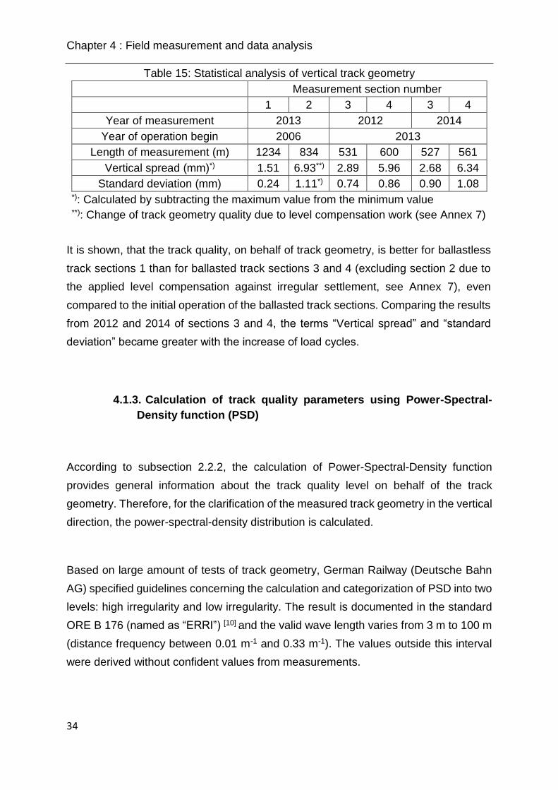
4.1.2. Statistical analysis of the measured data
The following Table 15 collected the statistical analysis of the vertical track geometry
for all the measurement sections.
Chapter 4 : Field measurement and data analysis
34
Table 15: Statistical analysis of vertical track geometry
Measurement section number
1 2 3 4 3 4
Year of measurement 2013 2012 2014
Year of operation begin 2006 2013
Length of measurement (m) 1234 834 531 600 527 561
Vertical spread (mm)*) 1.51 6.93**) 2.89 5.96 2.68 6.34
Standard deviation (mm) 0.24 1.11*) 0.74 0.86 0.90 1.08 *): Calculated by subtracting the maximum value from the minimum value **): Change of track geometry quality due to level compensation work (see Annex 7)
It is shown, that the track quality, on behalf of track geometry, is better for ballastless
track sections 1 than for ballasted track sections 3 and 4 (excluding section 2 due to
the applied level compensation against irregular settlement, see Annex 7), even
compared to the initial operation of the ballasted track sections. Comparing the results
from 2012 and 2014 of sections 3 and 4, the terms “Vertical spread” and “standard
deviation” became greater with the increase of load cycles.
4.1.3. Calculation of track quality parameters using Power-Spectral-
Density function (PSD)
According to subsection 2.2.2, the calculation of Power-Spectral-Density function
provides general information about the track quality level on behalf of the track
geometry. Therefore, for the clarification of the measured track geometry in the vertical
direction, the power-spectral-density distribution is calculated.
Based on large amount of tests of track geometry, German Railway (Deutsche Bahn
AG) specified guidelines concerning the calculation and categorization of PSD into two
levels: high irregularity and low irregularity. The result is documented in the standard
ORE B 176 (named as “ERRI”) [10] and the valid wave length varies from 3 m to 100 m
(distance frequency between 0.01 m-1 and 0.33 m-1). The values outside this interval
were derived without confident values from measurements.
Chapter 4 : Field measurement and data analysis
35
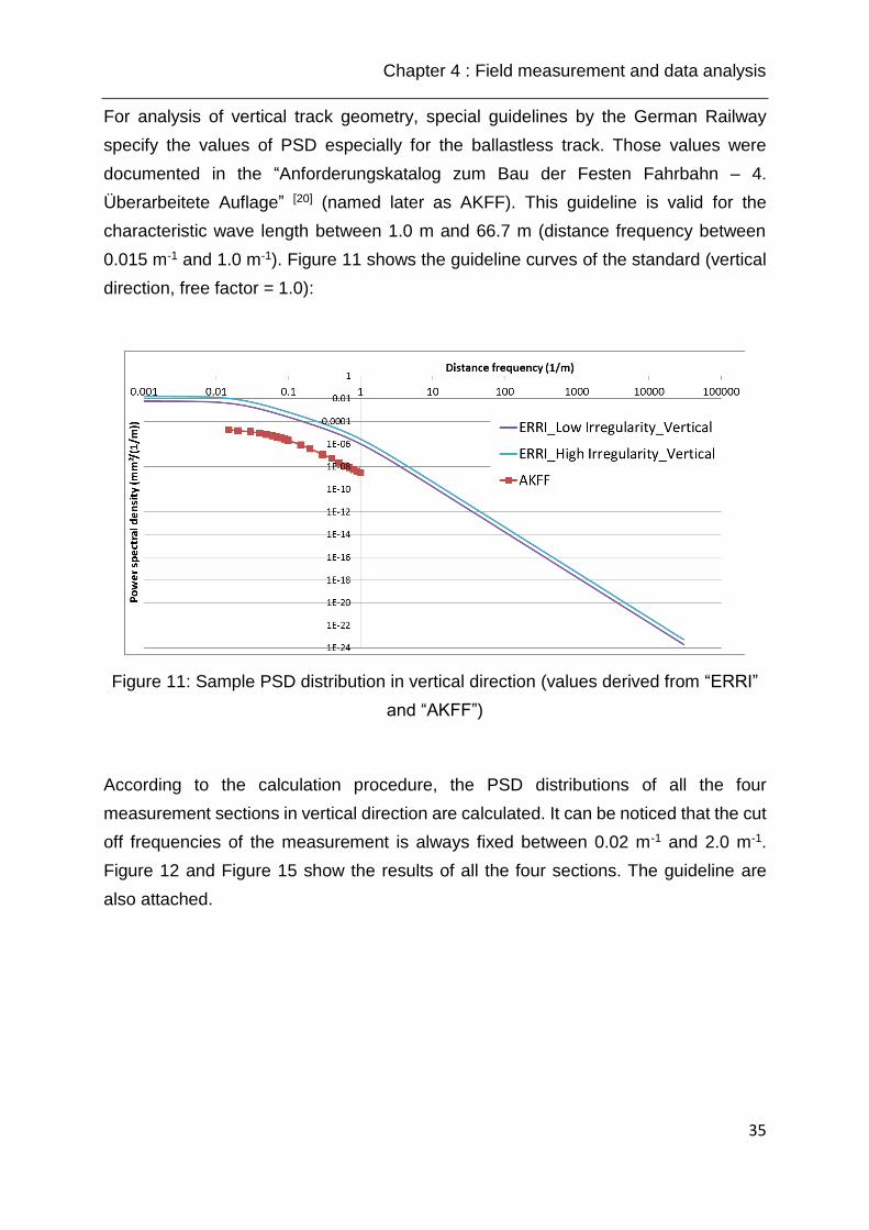
For analysis of vertical track geometry, special guidelines by the German Railway
specify the values of PSD especially for the ballastless track. Those values were
documented in the “Anforderungskatalog zum Bau der Festen Fahrbahn – 4.
Überarbeitete Auflage” [20] (named later as AKFF). This guideline is valid for the
characteristic wave length between 1.0 m and 66.7 m (distance frequency between
0.015 m-1 and 1.0 m-1). Figure 11 shows the guideline curves of the standard (vertical
direction, free factor = 1.0):
Figure 11: Sample PSD distribution in vertical direction (values derived from “ERRI”
and “AKFF”)
According to the calculation procedure, the PSD distributions of all the four
measurement sections in vertical direction are calculated. It can be noticed that the cut
off frequencies of the measurement is always fixed between 0.02 m-1 and 2.0 m-1.
Figure 12 and Figure 15 show the results of all the four sections. The guideline are
also attached.
Chapter 4 : Field measurement and data analysis
36
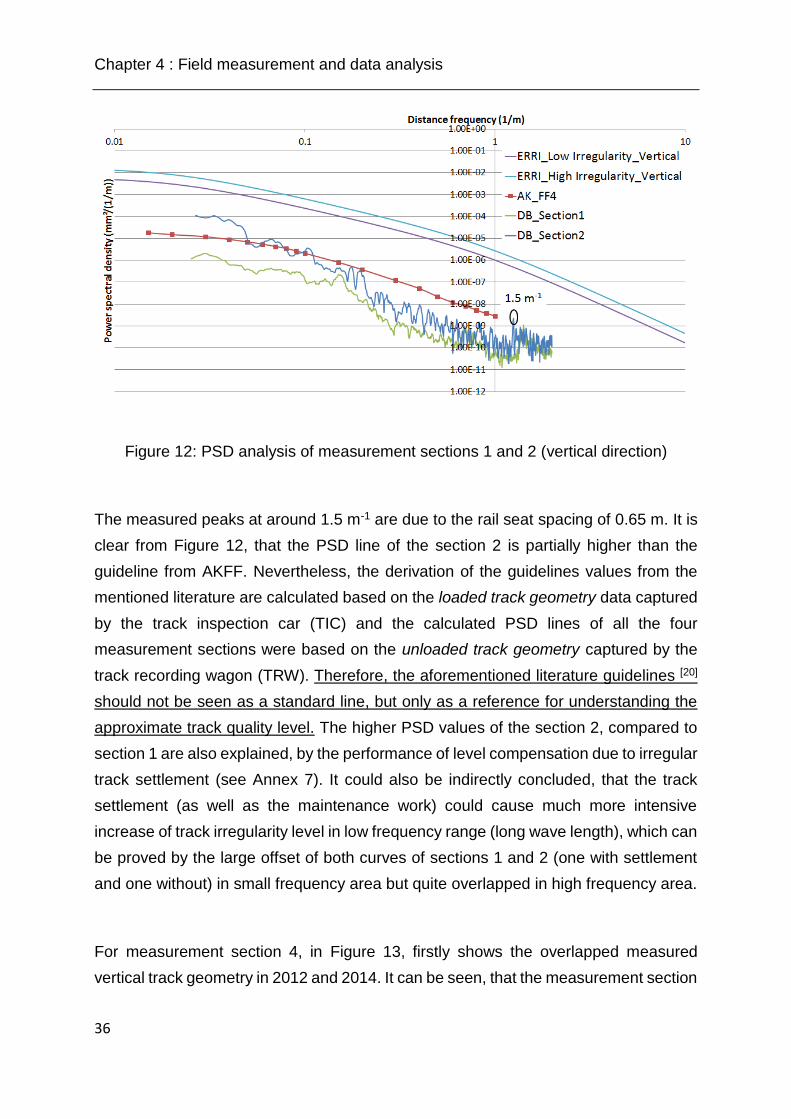
Figure 12: PSD analysis of measurement sections 1 and 2 (vertical direction)
The measured peaks at around 1.5 m-1 are due to the rail seat spacing of 0.65 m. It is
clear from Figure 12, that the PSD line of the section 2 is partially higher than the
guideline from AKFF. Nevertheless, the derivation of the guidelines values from the
mentioned literature are calculated based on the loaded track geometry data captured
by the track inspection car (TIC) and the calculated PSD lines of all the four
measurement sections were based on the unloaded track geometry captured by the
track recording wagon (TRW). Therefore, the aforementioned literature guidelines [20]
should not be seen as a standard line, but only as a reference for understanding the
approximate track quality level. The higher PSD values of the section 2, compared to
section 1 are also explained, by the performance of level compensation due to irregular
track settlement (see Annex 7). It could also be indirectly concluded, that the track
settlement (as well as the maintenance work) could cause much more intensive
increase of track irregularity level in low frequency range (long wave length), which can
be proved by the large offset of both curves of sections 1 and 2 (one with settlement
and one without) in small frequency area but quite overlapped in high frequency area.
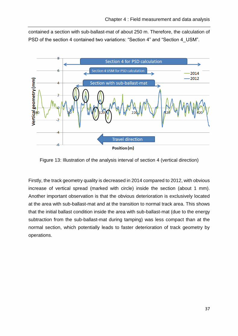
For measurement section 4, in Figure 13, firstly shows the overlapped measured
vertical track geometry in 2012 and 2014. It can be seen, that the measurement section
Chapter 4 : Field measurement and data analysis
37
contained a section with sub-ballast-mat of about 250 m. Therefore, the calculation of
PSD of the section 4 contained two variations: “Section 4” and “Section 4_USM”.
Figure 13: Illustration of the analysis interval of section 4 (vertical direction)
Firstly, the track geometry quality is decreased in 2014 compared to 2012, with obvious
increase of vertical spread (marked with circle) inside the section (about 1 mm).
Another important observation is that the obvious deterioration is exclusively located
at the area with sub-ballast-mat and at the transition to normal track area. This shows
that the initial ballast condition inside the area with sub-ballast-mat (due to the energy
subtraction from the sub-ballast-mat during tamping) was less compact than at the
normal section, which potentially leads to faster deterioration of track geometry by
operations.

Chapter 4 : Field measurement and data analysis
38
Figure 14: PSD analysis of measurement sections 3 and 4 (vertical direction)
Figure 15: PSD analysis of measurement sections 3 and 4 (vertical direction)
Moreover, the overlapped curves of section 4 indicate that both have similar PSD
values expect for the low frequency range, which proves that the track irregularity level
near the transition between the normal section and the section with sub-ballast-mat
have a normal wave length of longer than 10 m.

Chapter 4 : Field measurement and data analysis
39
Two marked distance frequencies of the both curves indicate the wave length of 0.6 m
and 1.2 m, which obviously are identical to 1 and 2 times the sleeper spacing. The
reason for the peak at 0.45 m-1 is analyzed in chapter 6.5 (peak appeared due to
vehicle sided eigen frequency excitation).
For operational and technical reasons, the section 3 in 2012 and 2014 could only hold
an overlapped length of approximately 100 m (the total evaluated length was 500 m)
and therefore there is not direct comparison for the track geometry at this section.
4.2. Rail deflection under static loading (elastic deflection)
The measurement of track elastic deflection was conducted by the Benkelman-beam
method with a ballast wagon of around 20.0 t axle load. The static track behavior of
sections 1 and 2 has been initially measured in November of 2005 by the Technische
Universität München[21]. Additionally, the figures of the overlap of the maximum rail
and slab deflection can be found in appendices 11 to 12, whereas the statistical
analyses of the measurement results are shown in Table 16 to Table 17.
Chapter 4 : Field measurement and data analysis
40
Table 16: Statistical analysis of rail seat deflection at sections 1 and 2 *)
Section 1
(Ballastless track type 1)
Section 2 (Ballastless
track type 2)
Side of the measurement Field side rail Inside rail Field side
rail
Inside rail
Time of measurement 2005 2013 2013 2013 2005
Number of
measurements
49 60 60 50 50
Served wheel load (kN) 90 105 95 105 90
Maximum (mm) 1.46 1.62 1.27 1.69 **) 1.46
Minimum (mm) 1.23 1.18 1.02 1.19 **) 1.22
Mean value (mm) 1.35 1.44 1.15 1.39 **) 1.33
Standard deviation (mm) 0.06 0.07 0.06 0.12 **) 0.06
Coefficient of variation
(%)
4.4 4.9 5.2 8.7 **) 4.4
*): deflected rail shows positive value
**):Change of track stiffness quality due to level compensation work (see Annex 7)
Table 17: Statistical analysis of rail seat deflection at sections 3 and 4 *)
Section 3 Section 4
Sub-ballast-mat without sub-ballast-mat with sub-ballast-mat
Time of measurement 2012
Side of the measurement
Field
side
rail
Insid
e rail
Field
side rail
Insid
e rail
Field side
rail
Inside
rail
Number of
measurements 75 75 43 23 7 7
Served wheel load (kN) 100 85 100 85 100 85
Maximum (mm) 1.25 1.05 1.29 1.10 2.33 2.10
Minimum (mm) 0.86 0.77 0.91 0.89 2.10 1.90
Mean value (mm) 1.05 0.90 1.03 0.99 2.21 2.00
Standard deviation (mm) 0.08 0.07 0.09 0.07 0.08 0.08
Coefficient of variation
(%) 7.8 7.9 8.4 7.2 3.4 3.7
*): deflected rail shows positive value

Chapter 4 : Field measurement and data analysis
41
According to Table 16, the general track quality, specified by the term “coefficient of
variation” (CV), is indicating the advantage of the modern ballastless track in
maintaining the track stiffness index. It is also clear that there are no major differences
between the values measured in 2005 and 2013, for section 1. Due to the applied level
compensation at the section 2 against irregular settlement (see Annex 7), the CV is
increased in 2013 compared to the value in 2005.
According to Table 17, due to the partial installation of sub-ballast-mat at the test
section 4, the data are analyzed separately. In general the rail deflection is determined
by the stiffness of the fastening system, the deflection behavior of the sleepers within
the ballast as well as by the deflection of the ballast, of the base layers at the
superstructure and of the sub-grade. It is concluded that the actual track quality is on
a very good level and the track stiffness varies insignificantly.
Moreover, the introduction of sub-ballast-mat can generally improve the quality of the
dynamic vehicle-track interaction and hence, these sections have limited CV.
Nonetheless, the general idea of evaluating the track quality based on the analysis of
CV might be critical here. The reason being is the different number of measurement
points as well as, the unsmooth transition between the two sections. Therefore, the
quality of vehicle-track interaction should be analyzed through modern numerical
simulation technologies while aiming at a real-time calculation method.
Additionally, the maximum deflection value is influenced not only by the elastic
properties of single rail seat, but also by the rail seats nearby. Therefore, it would be
useful if the deflection line for each rail seat is given. Appendices 13 to 16 show a
typical deflection distribution for each rail seat (sections 3 and 4, each with 9 values,
rail seats 1 – 8 have less values because there are no measurement data for
interpolation). The different colors specify the measurement source of the data. These
data are used as reference values at the FEM model verifications.
4.3. Dynamic rail bending behavior

Chapter 4 : Field measurement and data analysis
42
Various dynamic measurements under quasi-static test runs and operational train runs
were performed at each section.
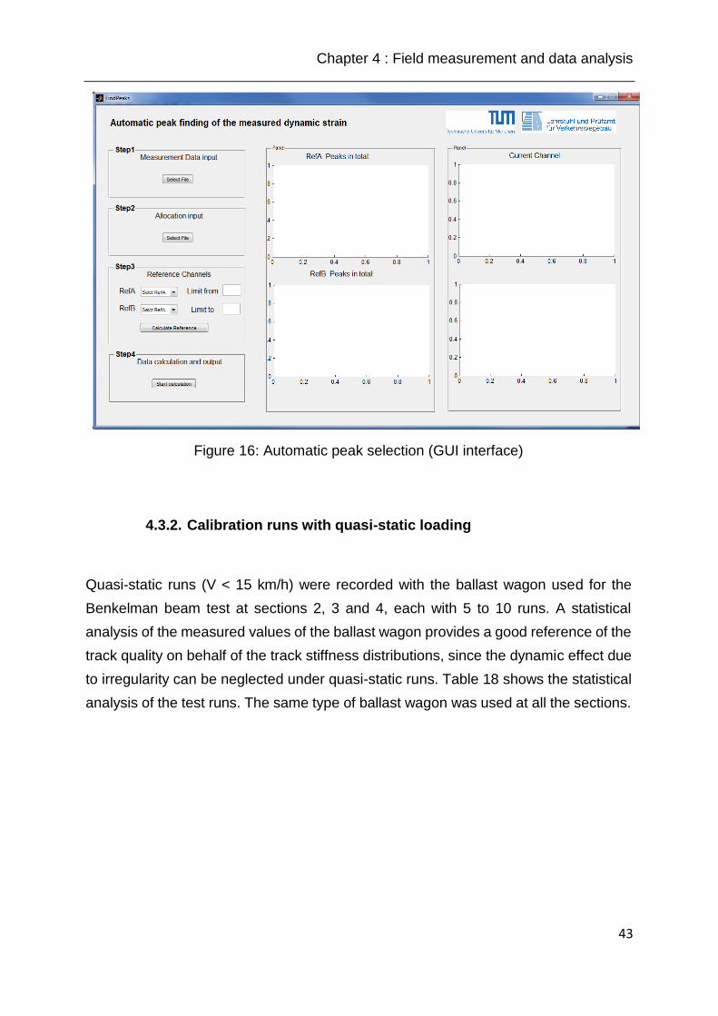
4.3.1. Automatic peak finding of the measured dynamic strain
Due to the huge amount of raw data of each single measurement, the task of retrieving
the strain peaks is time consuming. In order to achieve a higher efficiency of data
processing, a MATLAB program was developed. The program automates the peak
selection even in the case when a certain amount of measurement channels contains
electronic disturbances. A Graphical User Interface (GUI) was also established.
Moreover, the automatic program also overlaps the selected peak values with the raw
data by showing a green dot at the respective location. All the measured raw data
together with the retrieved peaks are illustrated as graphics after each calculation,
which ensures an easy inspection. The GUI interface is shown in Figure 16. Sample
graphical output of raw data sets and the retrieved peaks (green points) can be found
in appendices 17 to 18. User’s specifications and instructions are provided in User
Instruction manual 2.
Chapter 4 : Field measurement and data analysis
43
Figure 16: Automatic peak selection (GUI interface)
4.3.2. Calibration runs with quasi-static loading
Quasi-static runs (V < 15 km/h) were recorded with the ballast wagon used for the
Benkelman beam test at sections 2, 3 and 4, each with 5 to 10 runs. A statistical
analysis of the measured values of the ballast wagon provides a good reference of the
track quality on behalf of the track stiffness distributions, since the dynamic effect due
to irregularity can be neglected under quasi-static runs. Table 18 shows the statistical
analysis of the test runs. The same type of ballast wagon was used at all the sections.
Chapter 4 : Field measurement and data analysis
44
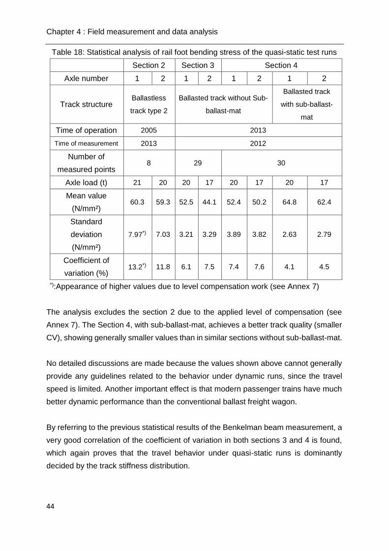
Table 18: Statistical analysis of rail foot bending stress of the quasi-static test runs
Section 2 Section 3 Section 4
Axle number 1 2 1 2 1 2 1 2
Track structure Ballastless
track type 2
Ballasted track without Sub-
ballast-mat
Ballasted track
with sub-ballast-
mat
Time of operation 2005 2013
Time of measurement 2013 2012
Number of
measured points 8 29 30
Axle load (t) 21 20 20 17 20 17 20 17
Mean value
(N/mm²) 60.3 59.3 52.5 44.1 52.4 50.2 64.8 62.4
Standard
deviation
(N/mm²)
7.97*) 7.03 3.21 3.29 3.89 3.82 2.63 2.79
Coefficient of
variation (%) 13.2*) 11.8 6.1 7.5 7.4 7.6 4.1 4.5
*):Appearance of higher values due to level compensation work (see Annex 7)
The analysis excludes the section 2 due to the applied level of compensation (see
Annex 7). The Section 4, with sub-ballast-mat, achieves a better track quality (smaller
CV), showing generally smaller values than in similar sections without sub-ballast-mat.
No detailed discussions are made because the values shown above cannot generally
provide any guidelines related to the behavior under dynamic runs, since the travel
speed is limited. Another important effect is that modern passenger trains have much
better dynamic performance than the conventional ballast freight wagon.
By referring to the previous statistical results of the Benkelman beam measurement, a
very good correlation of the coefficient of variation in both sections 3 and 4 is found,
which again proves that the travel behavior under quasi-static runs is dominantly
decided by the track stiffness distribution.
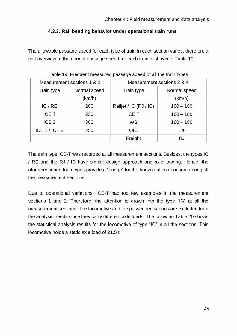
Chapter 4 : Field measurement and data analysis
45
4.3.3. Rail bending behavior under operational train runs
The allowable passage speed for each type of train in each section varies; therefore a
first overview of the normal passage speed for each train is shown in Table 19:
Table 19: Frequent measured passage speed of all the train types
Measurement sections 1 & 2 Measurement sections 3 & 4
Train type Normal speed
(km/h)
Train type Normal speed
(km/h)
IC / RE 200 Railjet / IC (RJ / IC) 160 – 180
ICE T 230 ICE T 160 – 180
ICE 3 300 WB 160 – 180
ICE 1 / ICE 2 250 OIC 120
Freight 80
The train type ICE-T was recorded at all measurement sections. Besides, the types IC
/ RE and the RJ / IC have similar design approach and axle loading. Hence, the
aforementioned train types provide a “bridge” for the horizontal comparison among all
the measurement sections.
Due to operational variations, ICE-T had too few examples in the measurement
sections 1 and 2. Therefore, the attention is drawn into the type “IC” at all the
measurement sections. The locomotive and the passenger wagons are excluded from
the analysis needs since they carry different axle loads. The following Table 20 shows
the statistical analysis results for the locomotive of type “IC” in all the sections. This
locomotive holds a static axle load of 21.5 t.
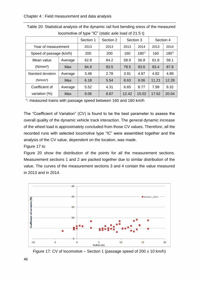
Chapter 4 : Field measurement and data analysis
46
Table 20: Statistical analysis of the dynamic rail foot bending sress of the measured
locomotive of type “IC” (static axle load of 21.5 t)
Section 1 Section 2 Section 3 Section 4
Year of measurement 2013 2013 2013 2014 2013 2014
Speed of passage (km/h) 200 200 160 180*) 160 180*)
Mean value
(N/mm²)
Average 62.8 64.2 58.9 56.8 61.8 58.1
Max 84.9 83.5 78.5 83.6 83.4 87.8
Standard deviation
(N/mm²)
Average 3.48 2.78 3.91 4.87 4.82 4.89
Max 6.18 5.54 8.63 8.06 11.21 12.28
Coefficient of
variation (%)
Average 5.52 4.31 6.65 8.77 7.99 9.32
Max 9.06 8.87 12.42 15.02 17.62 20.04
*): measured trains with passage speed between 160 and 180 km/h
The “Coefficient of Variation” (CV) is found to be the best parameter to assess the
overall quality of the dynamic vehicle track interaction. The general dynamic increase
of the wheel load is approximately concluded from those CV values. Therefore, all the
recorded runs with selected locomotive type “IC” were assembled together and the
analysis of the CV value, dependent on the location, was made.
Figure 17 to
Figure 20 show the distribution of the points for all the measurement sections.
Measurement sections 1 and 2 are packed together due to similar distribution of the
value. The curves of the measurement sections 3 and 4 contain the value measured
in 2013 and in 2014.
Figure 17: CV of locomotive – Section 1 (passage speed of 200 ± 10 km/h)
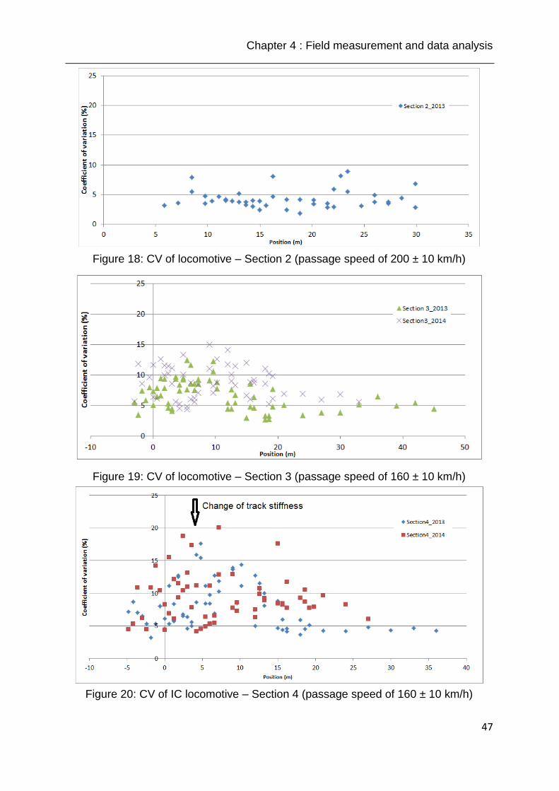
Chapter 4 : Field measurement and data analysis
47
Figure 18: CV of locomotive – Section 2 (passage speed of 200 ± 10 km/h)
Figure 19: CV of locomotive – Section 3 (passage speed of 160 ± 10 km/h)
Figure 20: CV of IC locomotive – Section 4 (passage speed of 160 ± 10 km/h)
Chapter 4 : Field measurement and data analysis
48
The values of sections 3 and 4 are generally higher than for sections 1 and 2 even
when those values were measured under a lower speed level. By refereeing to the
longer operational period of sections 1 and 2, the advantage of ballastless track in
maintaining good track quality is again concluded (even in section 2 with applied level
compensation work against irregular settlement, see Annex 7). The values of sections
1 and 2 are all below 10.0 %. Nevertheless, for section 2, there were only 2 runs (12
data sets) measured, since the section is located in a station with side track.
At sections 3 and 4, there is an area where the CV values are much higher than at
other areas (for section 3 between 0 and 18 m and for section 4 between -5 and 20
m). In order to gain a better understanding on the reasons for this increase, the Table
21 and Figure 21 show the measured elastic deflection only within this area. Hence,
the reason behind the increase of CV values remains within limited length, where
significant change of track geometry occurs, and in other words, higher curvature.
Therefore, those aforementioned areas are already determinant for the overall track
quality indexes.
Table 21: Change of vertical track geometry in sections 3 and 4
Section 3 Section 4
Geometry Height change (mm) 3.0 6.0
Within the length (m) 10 10
Section 3 Section 4
Figure 21: Change of vertical track geometry in sections 3 and 4 (selection)
The other values measured at sections 3 and 4 should be able to provide the guideline
of track quality for modern high speed ballasted tracks. A maximum CV value of 10.0
% is set, showing a relative comfortable and safe track. The values measured in 2014
were slightly higher than those measured in 2013, possibly due to the increase of

Chapter 4 : Field measurement and data analysis
49
speed from 160 to 180 km/h, rather than the change of track quality parameters. This
observation could be also true for the values measured in section 4.
At the location of stiffness change in section 4 (x = 4.2 m), the CV on the measured
dynamic rail foot stress achieves the highest value. By combining the values measured
in section 3, the effect of the increase of the dynamic wheel load at about a generally
extra 5 – 10 %, is expected, due to this stiffness change. Moreover, the change of
travel speed affects the length of the influence area (between 0 and 15 m in 2013 and
between -5 and 20 m in 2014). Therefore, the assumption of a longer influence area
with the increase of passage speed is verified.
The average of the characteristic CV values for the three categories “Passenger
wagon”, “Locomotive” and “Electrical Multiple Units (EMU)”, shown in Table 22,
illustrate the influence of the vehicle to the dynamic vehicle track interaction. Detailed
analysis and graphical documentations can be found in appendices 19 to 21.

Chapter 4 : Field measurement and data analysis
50
Table 22: Average and Max of CV of max rail bending stress for selected train
types
Section 1 Section 2 Section 3 Section 4
Year of
measurement 2013 2013 2014 2013 2014
Coefficient of variation (%)
Type and speed BR 101 (200 km/h) BR 1116 (160 km/h)
Average 5.52 4.31 6.65 8.77 7.99 9.32
Max 9.06 8.87 12.42 15.02 17.62 20.04
Type and speed IC Wagon (200km/h) IC wagon (160 km/h)
Average 13.05 11.60 6.91 8.50 8.35 8.54
Max 15.41 14.76 9.71 11.63 11.00 15.78
Type and speed ICE-T (230 km/h) ICE-T (160 km/h)
Average - 6.47 7.66 8.93 7.65 8.17
Max - 7.64 9.69 12.5 9.82 13.13
Type and speed ICE1/2 Loco (250 km/h)
Average 6.2 7.87 - - - -
Max 8.84 9.35 - - - -
Type and speed ICE1/2 Wagon (250
km/h) Railjet wagon (160 - 180 km/h)
Average 6.44 8.93 8.32 9.35 7.42 9.09
Max 9.72 11.42 11.48 13.35 11.58 13.33
Type and speed ICE 3 (300 km/h)
Average 8.65 9.21 - - - -
Max 11.14 12.56 - - - -
The average and the maximum CV for ICE-T at section 2 is smaller than at sections 3
and 4, again indicating that the track quality at section 2 is better, due to the
implementation of modern ballastless track (even under the applied level
compensation at section 2 against irregular settlement, see Annex 7). This is also the
case for the locomotives in both sections.
The “IC wagon” for all the sections has the same maximum design speed of 200 km/h.
The CV values at sections 1 and 2 are higher than at sections 3 and 4, mostly due to
the difference on passage speed. Although, the maximum values are similar, the
average values are quite different. This shows the reduction of travel quality while
approaching the maximum design speed.
Chapter 4 : Field measurement and data analysis
51
Since the passenger wagons for “Railjet” have design speed of 250 km/h, these values
are compared with the wagons from “ICE 1/2”, which generally hold the same
specifications. Under this base, although the values from both types are similar, the
recorded values at sections 1 and 2 have much higher passage speed, which once
more leads to the same conclusion concerning the track quality between the sections.
The ICE 3 with passage speed of 300 km/h could cause smaller dynamic effects in
comparison to the IC passenger wagon passing with 200 km/h, since the speed of 200
km/h has already achieved the maximum allowable speed for this wagon. It can be
therefore concluded, that the vehicle design is also an important factor influencing the
dynamic vehicle track interaction and there is no evidence that a vehicle running at
higher speed causes higher dynamic loading. This is proven even from the test runs
at same location. This could best indicate that the research of dynamic vehicle track
interaction must rely on real-time virtual and numerical simulation programs.
4.4. Test of track vibration level
Understanding the track vibration behavior under train runs is one of the most
important aspects in the research of dynamic vehicle-track interactions. Those
vibrations are a real-time reflection of the counteractive effect related to the elastic and
damping behavior of the track and vehicle.
Track vibration is the output of all the key parameters which interact during a train
passage. The important parameters are the dynamic wheel load, the track geometry,
the track stiffness and damping, the vehicle design, etc.
In order to separate the influence on the track or on the vehicle, a track-oriented
calibration with impact hammer is performed in advance. By simplifying the impact
load on the track in a form as dirac delta function [8], an intuitive comparison of track
sided parameters is achieved. By retrieving this information related to the track sided
behavior, the vehicle sided influence under dynamic train runs can also be efficiently
analyzed.
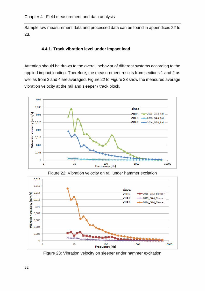
Chapter 4 : Field measurement and data analysis
52
Sample raw measurement data and processed data can be found in appendices 22 to
23.
4.4.1. Track vibration level under impact load
Attention should be drawn to the overall behavior of different systems according to the
applied impact loading. Therefore, the measurement results from sections 1 and 2 as
well as from 3 and 4 are averaged. Figure 22 to Figure 23 show the measured average
vibration velocity at the rail and sleeper / track block.
Figure 22: Vibration velocity on rail under hammer exciation
Figure 23: Vibration velocity on sleeper under hammer excitation
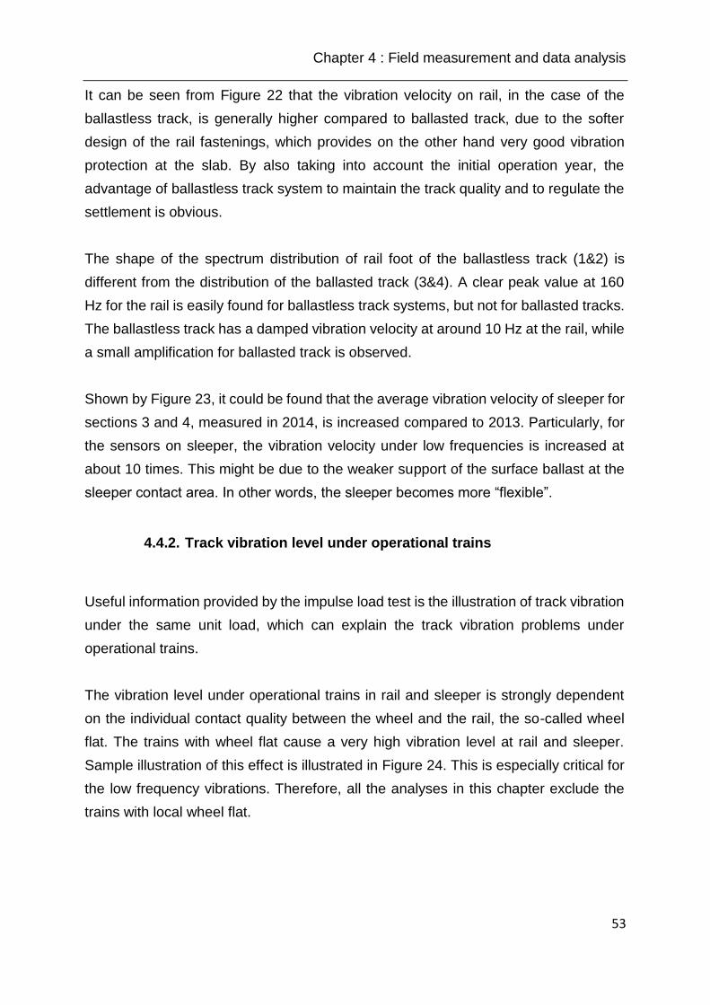
Chapter 4 : Field measurement and data analysis
53
It can be seen from Figure 22 that the vibration velocity on rail, in the case of the
ballastless track, is generally higher compared to ballasted track, due to the softer
design of the rail fastenings, which provides on the other hand very good vibration
protection at the slab. By also taking into account the initial operation year, the
advantage of ballastless track system to maintain the track quality and to regulate the
settlement is obvious.
The shape of the spectrum distribution of rail foot of the ballastless track (1&2) is
different from the distribution of the ballasted track (3&4). A clear peak value at 160
Hz for the rail is easily found for ballastless track systems, but not for ballasted tracks.
The ballastless track has a damped vibration velocity at around 10 Hz at the rail, while
a small amplification for ballasted track is observed.
Shown by Figure 23, it could be found that the average vibration velocity of sleeper for
sections 3 and 4, measured in 2014, is increased compared to 2013. Particularly, for
the sensors on sleeper, the vibration velocity under low frequencies is increased at
about 10 times. This might be due to the weaker support of the surface ballast at the
sleeper contact area. In other words, the sleeper becomes more “flexible”.
4.4.2. Track vibration level under operational trains
Useful information provided by the impulse load test is the illustration of track vibration
under the same unit load, which can explain the track vibration problems under
operational trains.
The vibration level under operational trains in rail and sleeper is strongly dependent
on the individual contact quality between the wheel and the rail, the so-called wheel
flat. The trains with wheel flat cause a very high vibration level at rail and sleeper.
Sample illustration of this effect is illustrated in Figure 24. This is especially critical for
the low frequency vibrations. Therefore, all the analyses in this chapter exclude the
trains with local wheel flat.

Chapter 4 : Field measurement and data analysis
54
Figure 24: Effect of trains with wheel flat (passage speed of approximately 80
km/h)
The major interests for this part lay on the comparative behavior of the track for
sections 3 and 4 measured in 2013 and in 2014. Since similar distribution of vibration
velocity, the train type “InterCity” was selected due to the good amount of measured
samples. Figure 25 shows the analyzed vibration velocity distribution (all included data
sets exclude the wheel flat).
Figure 25: Distribution of vibration velocity – train type IC (V = 160 km/h)
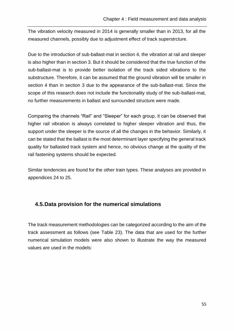
Chapter 4 : Field measurement and data analysis
55
The vibration velocity measured in 2014 is generally smaller than in 2013, for all the
measured channels, possibly due to adjustment effect of track superstrcture.
Due to the introduction of sub-ballast-mat in section 4, the vibration at rail and sleeper
is also higher than in section 3. But it should be considered that the true function of the
sub-ballast-mat is to provide better isolation of the track sided vibrations to the
substructure. Therefore, it can be assumed that the ground vibration will be smaller in
section 4 than in section 3 due to the appearance of the sub-ballast-mat. Since the
scope of this research does not include the functionality study of the sub-ballast-mat,
no further measurements in ballast and surrounded structure were made.
Comparing the channels “Rail” and “Sleeper” for each group, it can be observed that
higher rail vibration is always correlated to higher sleeper vibration and thus, the
support under the sleeper is the source of all the changes in the behavior. Similarly, it
can be stated that the ballast is the most determinant layer specifying the general track
quality for ballasted track system and hence, no obvious change at the quality of the
rail fastening systems should be expected.
Similar tendencies are found for the other train types. These analyses are provided in
appendices 24 to 25.
4.5. Data provision for the numerical simulations
The track measurement methodologies can be categorized according to the aim of the
track assessment as follows (see Table 23). The data that are used for the further
numerical simulation models were also shown to illustrate the way the measured
values are used in the models:
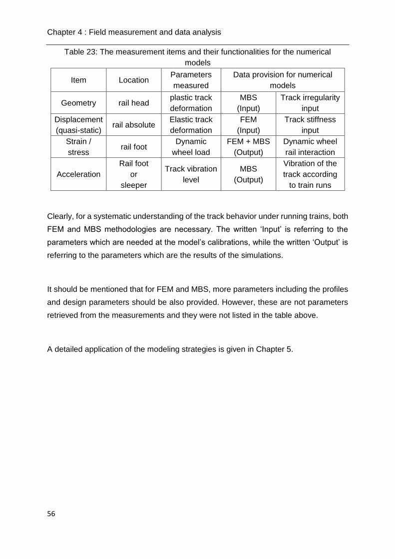
Chapter 4 : Field measurement and data analysis
56
Table 23: The measurement items and their functionalities for the numerical
models
Item Location Parameters
measured
Data provision for numerical
models
Geometry rail head plastic track
deformation
MBS
(Input)
Track irregularity
input
Displacement
(quasi-static) rail absolute
Elastic track
deformation
FEM
(Input)
Track stiffness
input
Strain /
stress rail foot
Dynamic
wheel load
FEM + MBS
(Output)
Dynamic wheel
rail interaction
Acceleration
Rail foot
or
sleeper
Track vibration
level
MBS
(Output)
Vibration of the
track according
to train runs
Clearly, for a systematic understanding of the track behavior under running trains, both
FEM and MBS methodologies are necessary. The written ‘Input’ is referring to the
parameters which are needed at the model’s calibrations, while the written ‘Output’ is
referring to the parameters which are the results of the simulations.
It should be mentioned that for FEM and MBS, more parameters including the profiles
and design parameters should be also provided. However, these are not parameters
retrieved from the measurements and they were not listed in the table above.
A detailed application of the modeling strategies is given in Chapter 5.

Chapter 5 : The numerical modeling
57
5. THE NUMERICAL MODELING
5.1. Introduction
As revealed in Chapter 2, a more detailed understanding of the track behavior
concerning the vehicle-track interaction can be achieved through numerical models.
Various modeling approaches are applied in order to better accomplish the
requirement, including the FEM (Finite-Element-Method) and MBS (Multi-Body-
Simulation).
A numerical model concentrates only on a part of object’s behavior in reality and
simplifies the others. In this chapter, various kinds of models based on the field
measurement are introduced. These models are developed with different objectives.
Imaginary data, as well as experience data, are also used to define parameters of the
models. These models utilize FEM and MBS approaches to solve the problems.
The general structural tree of utilizing measurement data for different modeling
strategies is shown in Figure 26. The colored circles on the top right of each step
symbolize the respective applied technology (refer to section 2.3.5 for software version
information). The step 2.2 (model 1), which refers to the FEM modeling on behalf of
track stiffness, is firstly performed. The step 3.1 (model 2) reads the input of the vehicle
design and measured track irregularity to calculate the dynamic output of the vehicle
track interaction. By condensing the FEM model with substructuring and modal
analysis, the real-time response of elastic track due to passing train loads is able to be
calculated (step 3.2, model 3). The final step – step 4.1 (model 4) – is the result of MBS
calculation, which includes the wheel-rail contact, the track irregularity and track
stiffness (coming from the condensed FEM model).
All the included software programs and their versions can be found in Table 24.
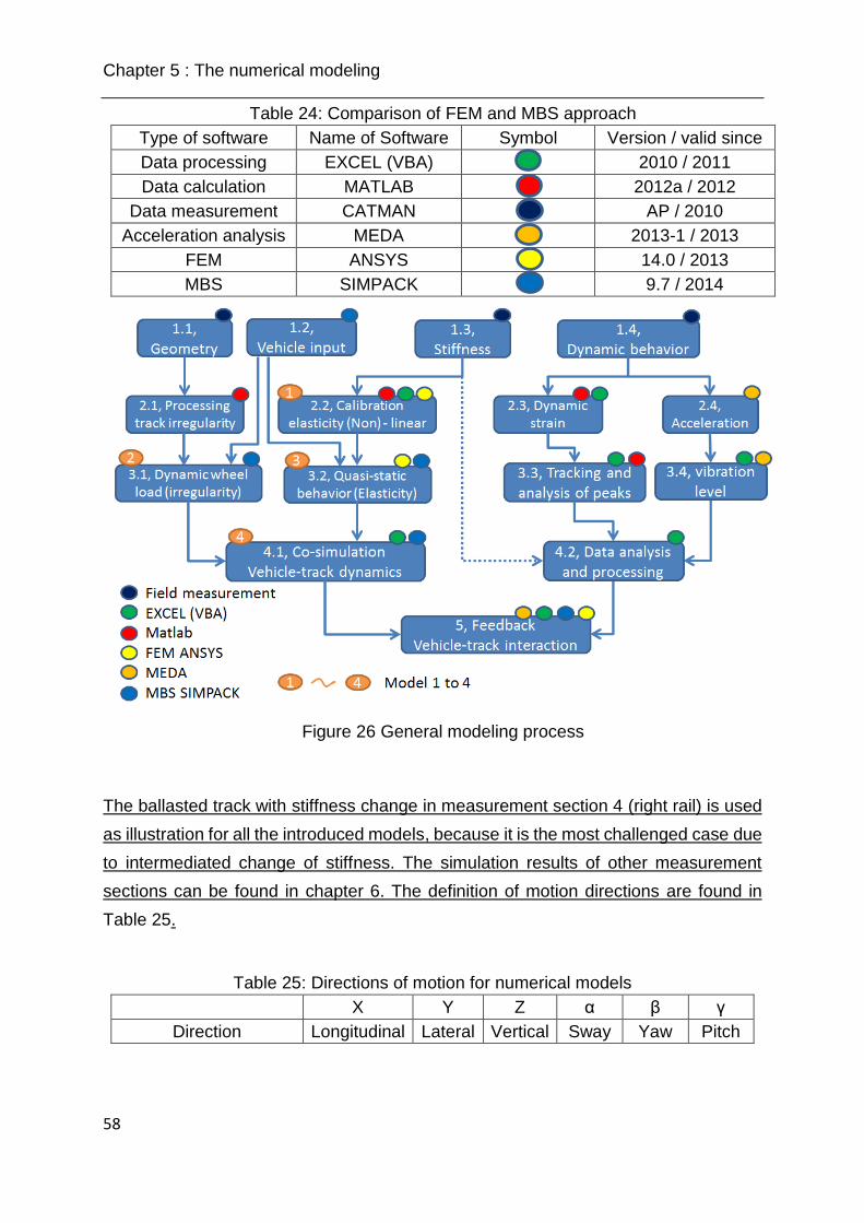
Chapter 5 : The numerical modeling
58
Table 24: Comparison of FEM and MBS approach
Type of software Name of Software Symbol Version / valid since
Data processing EXCEL (VBA) 2010 / 2011
Data calculation MATLAB 2012a / 2012
Data measurement CATMAN AP / 2010
Acceleration analysis MEDA 2013-1 / 2013
FEM ANSYS 14.0 / 2013
MBS SIMPACK 9.7 / 2014
Figure 26 General modeling process
The ballasted track with stiffness change in measurement section 4 (right rail) is used
as illustration for all the introduced models, because it is the most challenged case due
to intermediated change of stiffness. The simulation results of other measurement
sections can be found in chapter 6. The definition of motion directions are found in
Table 25.
Table 25: Directions of motion for numerical models
X Y Z α β γ
Direction Longitudinal Lateral Vertical Sway Yaw Pitch

Chapter 5 : The numerical modeling
59
5.2. Model 1 (FEM) – Calibration of the elastic track model based on field side Benkelman measurement
5.2.1. Introduction and modeling approach
The Finite-Element-Method program ANSYS is included for a deeper understanding of
the measurement results. Simplified rail profile is used with the same physical
parameters with the original profile required for calculation [22]. Table 26 shows the
geometry and the parameters of the simplified model.
Table 26: Parameters of the simplified rail model [22]
hi (mm) bi (mm) Ai (mm2) Zi (mm) Zs (mm)
1 48.3 73.5 3550.05 24.15
83.5 2 114 19 2166 105.3
3 12.8 150 1920 168.7
With Ai – Area of the body i
Zi – Center of gravity of body i
Zs – Center of gravity of the whole system
The whole measurement section of 95 rail seats is built at ANSYS software with 75 rail
seats with variable stiffness and 10 on each side with assumed values for achieving a
reasonable load support at the end rail seats. The mechanism of the FEM model is
shown in Figure 27. The substructure layer is integrated into the ballast layer, since
there is no change in the substructure design along single section. Three elastic layers
naming ‘Pad’ and ‘Ballast + Substructure’ are given with predefined unique values for
each rail seat.
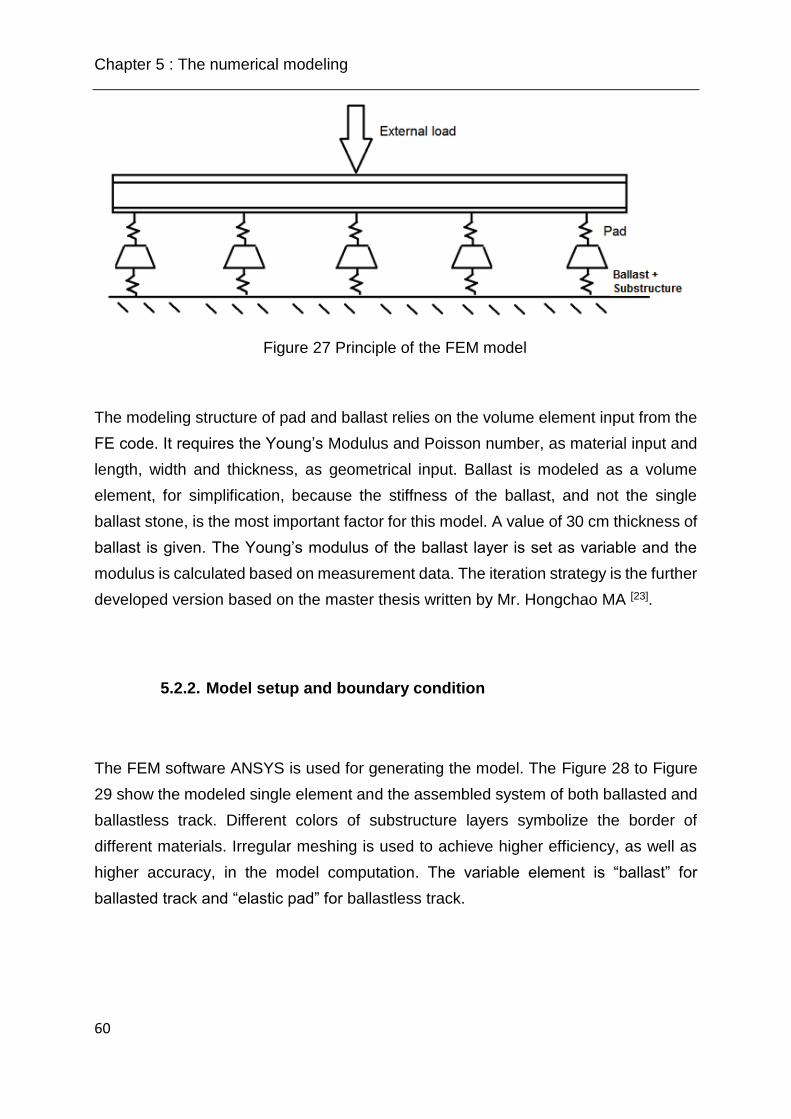
Chapter 5 : The numerical modeling
60
Figure 27 Principle of the FEM model
The modeling structure of pad and ballast relies on the volume element input from the
FE code. It requires the Young’s Modulus and Poisson number, as material input and
length, width and thickness, as geometrical input. Ballast is modeled as a volume
element, for simplification, because the stiffness of the ballast, and not the single
ballast stone, is the most important factor for this model. A value of 30 cm thickness of
ballast is given. The Young’s modulus of the ballast layer is set as variable and the
modulus is calculated based on measurement data. The iteration strategy is the further
developed version based on the master thesis written by Mr. Hongchao MA [23].
5.2.2. Model setup and boundary condition
The FEM software ANSYS is used for generating the model. The Figure 28 to Figure
29 show the modeled single element and the assembled system of both ballasted and
ballastless track. Different colors of substructure layers symbolize the border of
different materials. Irregular meshing is used to achieve higher efficiency, as well as
higher accuracy, in the model computation. The variable element is “ballast” for
ballasted track and “elastic pad” for ballastless track.
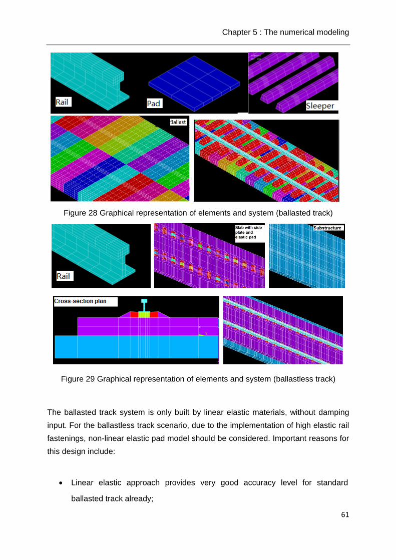
Chapter 5 : The numerical modeling
61
Figure 28 Graphical representation of elements and system (ballasted track)
Figure 29 Graphical representation of elements and system (ballastless track)
The ballasted track system is only built by linear elastic materials, without damping
input. For the ballastless track scenario, due to the implementation of high elastic rail
fastenings, non-linear elastic pad model should be considered. Important reasons for
this design include:
Linear elastic approach provides very good accuracy level for standard
ballasted track already;
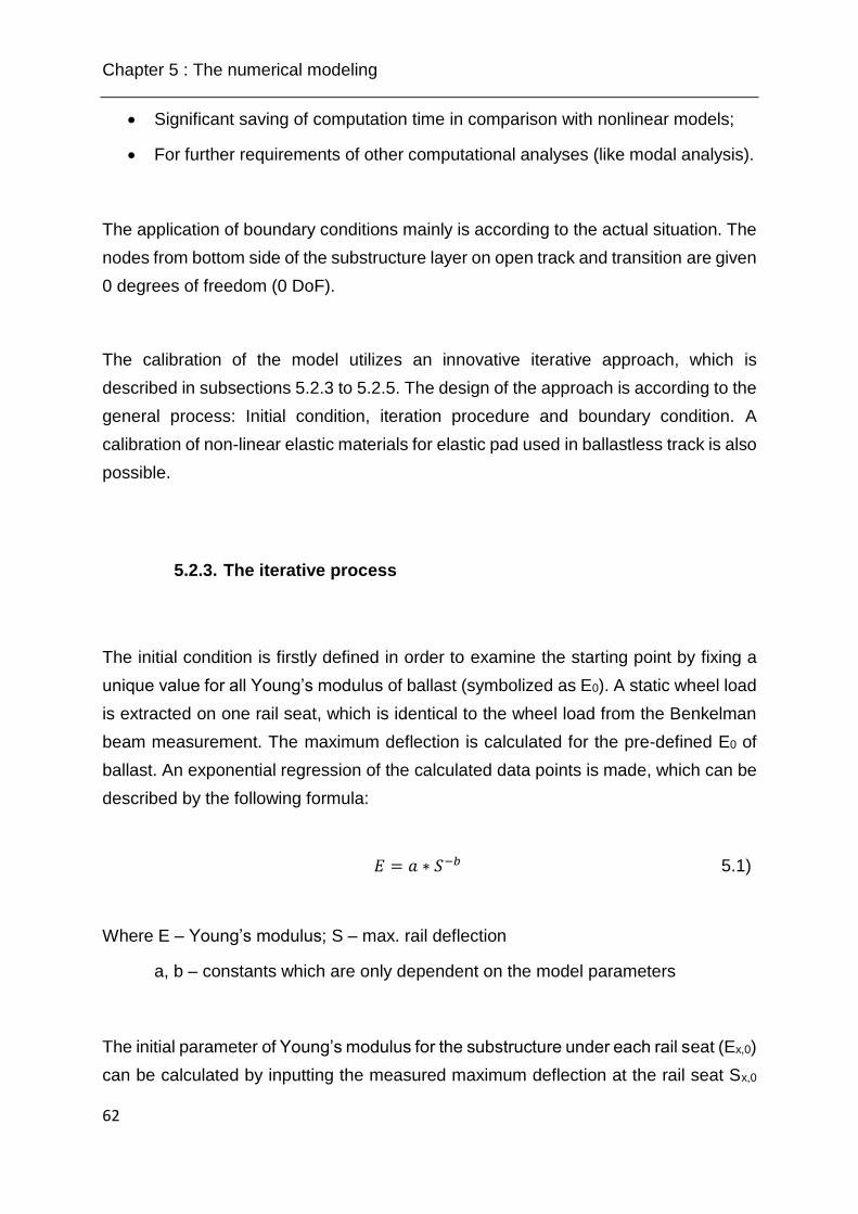
Chapter 5 : The numerical modeling
62
Significant saving of computation time in comparison with nonlinear models;
For further requirements of other computational analyses (like modal analysis).
The application of boundary conditions mainly is according to the actual situation. The
nodes from bottom side of the substructure layer on open track and transition are given
0 degrees of freedom (0 DoF).
The calibration of the model utilizes an innovative iterative approach, which is
described in subsections 5.2.3 to 5.2.5. The design of the approach is according to the
general process: Initial condition, iteration procedure and boundary condition. A
calibration of non-linear elastic materials for elastic pad used in ballastless track is also
possible.
5.2.3. The iterative process
The initial condition is firstly defined in order to examine the starting point by fixing a
unique value for all Young’s modulus of ballast (symbolized as E0). A static wheel load
is extracted on one rail seat, which is identical to the wheel load from the Benkelman
beam measurement. The maximum deflection is calculated for the pre-defined E0 of
ballast. An exponential regression of the calculated data points is made, which can be
described by the following formula:
𝐸 = 𝑎 ∗ 𝑆−𝑏 5.1)
Where E – Young’s modulus; S – max. rail deflection
a, b – constants which are only dependent on the model parameters
The initial parameter of Young’s modulus for the substructure under each rail seat (Ex,0)
can be calculated by inputting the measured maximum deflection at the rail seat Sx,0
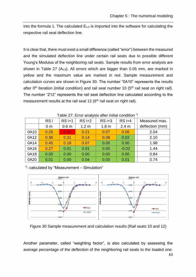
Chapter 5 : The numerical modeling
63
into the formula 1. The calculated Ex,0 is imported into the software for calculating the
respective rail seat deflection line.
It is clear that, there must exist a small difference (called “error”) between the measured
and the simulated deflection line under certain rail seats due to possible different
Young’s Modulus of the neighboring rail seats. Sample results from error analysis are
shown in Table 27 (Ax,0). All errors which are bigger than 0.05 mm, are marked in
yellow and the maximum value are marked in red. Sample measurement and
calculation curves are shown in Figure 30. The number “0A10” represents the results
after 0th iteration (initial condition) and rail seat number 10 (5th rail seat on right rail).
The number “Z12” represents the rail seat deflection line calculated according to the
measurement results at the rail seat 12 (6th rail seat on right rail).
Table 27: Error analysis after initial condition *)
RS i RS i+1 RS i+2 RS i+3 RS i+4 Measured max.
deflection (mm) 0 m 0.6 m 1.2 m 1.8 m 2.4 m
0A10 0.26 0.47 0.21 0.07 0.06 2.04
0A12 0.36 0.31 0.14 0.08 0.02 2.10
0A14 0.45 0.18 0.07 0.00 0.00 1.98
0A16 0.27 0.01 0.01 0.00 -0.02 1.44
0A18 0.00 0.00 0.00 0.00 0.00 0.84
0A20 0.01 0.00 0.04 0.00 0.01 0.74
*): calculated by “Measurement – Simulation”
Figure 30 Sample measurement and calculation results (Rail seats 10 and 12)
Another parameter, called “weighting factor”, is also calculated by assessing the
average percentage of the deflection of the neighboring rail seats to the loaded one.
Chapter 5 : The numerical modeling
64
In other words, the errors at the neighboring rail seats are less decisive than the errors
at the loaded rail seats. This is an important factor for the definition of the new
deflection value for the next iteration. To the factor is given the symbol Fi, where i from
0 to 8 representing the factor of rail seat number i. Table 28 shows the calculated
factors of right rail, in section 4.
Table 28: Illustration of weighting factor
F1 F2 F3 F4 F5 – F8
Weighting factor 1.00 0.73 0.38 0.12 0.00
A recalculation of the Young’s modulus of the ballast is required for all rail seats. This
is recalculated by the so called “iteration procedure”. It utilizes the results from the last
calculation and set them as the pre-conditions for the next calculation round. The
recalculation of the Young’s modulus is based on the results of the error analysis from
the last calculation. The new maximum deflection of the rail seat (Sx,n) is calculated by
the following formula:
[
𝑆1,𝑛
⋮𝑆𝑥,𝑛
] = [
𝑆1,𝑛−1
⋮𝑆𝑥,𝑛−1
] + [
𝐴1,1 ⋯ 𝐴1,𝑖
⋮ ⋱ ⋮𝐴𝑥,1 ⋯ 𝐴𝑥,𝑖
] ∗ [𝐹1
⋮𝐹𝑖
] 5.2)
𝑤𝑖𝑡ℎ 𝐴𝑥,𝑖 𝑟𝑒𝑝𝑟𝑒𝑠𝑒𝑛𝑡𝑖𝑛𝑔 𝑒𝑟𝑟𝑜𝑟 𝑐𝑎𝑙𝑐𝑢𝑙𝑎𝑡𝑒𝑑 𝑎𝑓𝑡𝑒𝑟 𝑖𝑡𝑒𝑟𝑎𝑡𝑖𝑜𝑛 𝑠𝑡𝑒𝑝 𝑛 − 1
Where
Sx,n – Calculated target deflection for rail seat x before iteration i
Ax,j – Error “Measurement – Calculation” at rail seat x (mm)
Fi – weighting factor calculated in the initial condition (See Table 28)
n – Iteration number (n≥1)
i – Rail seat number (i = 0 for the loaded rail seat)
x – Loaded rail seat number
The Sx,n is again used to calculate the Ex,n according to formula 5.1. Then the model is
again calculated for the n+1th iteration.
Chapter 5 : The numerical modeling
65
It is important to define the boundary conditions to end the iteration process. Principally
the iteration should stop when the results from the nth and n-1th iteration returns similar
results (Difference < 0.01 mm). This holds the meaning that, the n+1th iteration will not
make any further change. The boundary condition is concluded in the following
formula:
𝑆𝑥,𝑛 − 𝑆𝑥,𝑛−1 < 0.01 5.3)
𝑤𝑖𝑡ℎ 𝑆𝑥,𝑛 𝑖𝑛𝑐𝑙𝑢𝑑𝑖𝑛𝑔 𝑎𝑙𝑙 𝑡ℎ𝑒 𝑚𝑒𝑎𝑠𝑢𝑟𝑒𝑑 𝑛𝑒𝑖𝑔ℎ𝑏𝑜𝑟𝑖𝑛𝑔 𝑟𝑎𝑖𝑙 𝑠𝑒𝑎𝑡𝑠 𝑖
Following this principle, the result after 6th iteration already fulfills the criterion (see
Table 29):
Table 29: Boundary condition; Diff. Deflection [mm], Iteration 6 – 5 (rounding
applied)
RS i RS i+1 RS i+2 RS i+3 RS i+4 RS i+5 RS i+6 RS i+7 RS i+8
0 m 0.6 m 1.2 m 1.8 m 2.4 m 0 m 0.6 m 1.2 m 1.8 m
Z10 0.00 -0.01 0.00 0.00 0.00 0.00 0.00 0.00 0.00
Z12 0.00 0.00 0.00 0.00 0.00 0.00 0.00 0.00 0.00
Z14 0.01 0.01 0.00 0.00 0.00 0.00 0.00 0.00 0.00
Z16 0.01 0.01 0.01 0.00 0.00 0.00 0.00 0.00 0.00
Z18 0.01 0.01 0.01 0.00 0.00 0.01 0.01 0.01 0.01
Z20 0.00 0.01 0.01 0.00 0.00 0.01 0.01 0.01 0.01
Table 30 shows the number of differences bigger than the limitation (0.01 mm,
rounding applied) after each calculation. It can be concluded that, the iteration
procedure can achieve a very quick convergence without many iteration steps. The
calculation on left rail is also attached:

Chapter 5 : The numerical modeling
66
Table 30: Number of difference over limitation
Between iterations Number of difference bigger than 0.01 mm
Left rail Right rail
1 and 0 335 243
2 and 1 269 131
3 and 2 192 83
4 and 3 103 69
5 and 4 17 12
6 and 5 0 0
Total numbers 450 450
5.2.4. Results and conclusions
It is clear that when this method is applied for the track section, six iteration steps can
already give a converged result. Very good identification can be found between the
measurement and simulation results. Table 31 and Figure 31 show the error analysis
and the final result after the 6th iteration. It can be seen, that the error is significantly
reduced in comparison with the first result, before iteration (shown in Table 27 and
Figure 30).
Table 31: Error analysis after 6th iteration step *)
RS i RS i+1 RS i+2 RS i+3 RS i+4 RS i+5 RS i+6 RS i+7 RS i+8
0 m 0.6 m 1.2 m 1.8 m 2.4 m 0 m 0.6 m 1.2 m 1.8 m
6A10 -0.04 0.17 -0.04 -0.08 0.01 0.03 0.00 0.00 0.00
6A12 -0.01 -0.05 -0.10 -0.01 0.02 0.00 0.01 0.00 0.01
6A14 0.05 -0.11 -0.04 0.00 0.00 -0.01 0.00 0.01 0.00
6A16 0.05 -0.07 0.01 0.00 0.00 0.00 0.01 0.00 0.00
6A18 -0.01 0.01 0.00 0.00 0.00 0.01 0.00 0.00 0.00
6A20 0.00 0.00 -0.01 0.00 0.01 0.00 0.02 0.00 0.00
*): calculated by “Measurement – Simulation”
Chapter 5 : The numerical modeling
67
Figure 31 Measurement and calculation result after 6th iteration (Rail seats 10 and 12)
The advantage of the robust defining of the boundary condition is to provide the
possibility to find the potential measurement errors at certain location. It can be further
seen that the reason for 2nd value at rail seat 10, with a remaining error bigger than 0.1
mm is due to the measurement error at this location. It should be stated that a confident
conclusion of the location of measurement error still requires other measurement
results.
Following conclusions and perspectives can then be stated:
The FEM program can satisfactorily rebuild the test section on behalf of elastic
rail deflections;
An innovative iteration process for calibrating the stiffness under each rail seat
is developed and found to be suitable to solve the task;
The simulation results provide a good evidence that concerning the ‘perfect
overlapped’ curve, no significant measurement errors should exist.
The simulation result can provide evidences to define measurement errors on
site;
The calibrated model can be used for further analysis requirements.
Chapter 5 : The numerical modeling
68
5.2.5. Automation of the iteration methods (Co-Simulation with ANSYS
and MATLAB)
For smoother application and calibration of the FEM model, the iterative process is
translated into the program MATLAB to automatically calibrate the model. This, so
called “co-simulation” approach, replaces all the workflow which was previously
executed by MS EXCEL, and decides intelligently, whether a new iteration step is
required, as well the new input parameters by defining all the regulations by MATLAB
based sentences. In other words, the new MATLAB command is written to control the
simulation works executed by ANSYS. The principle of the structure can be found in
Figure 32. The detailed program, as well as other application scenarios, can be found
the internship report by L. DING [24].
Figure 32: Structure of the co-simulation program
In order to make the program also available for regular users, as well as for easier
processing of similar data sets, a Graphical User Interface (GUI) is also established.
The user only needs to provide with certain input parameters at the developed
MATLAB GUI interface. The calibration of the model is fully automated by the software
even without the user getting contact to the ANSYS interface. All the measured and
calculated curves after each iteration step automatically are output for further
inspection requirements. A list of the required input parameters and comparisons of
the computation time for sample data sets with EXCEL and MATLAB approaches are
shown in Table 32. The GUI interface can be seen in Figure 33. The user specification
and instructions can be found in User Instruction manual 3.

Chapter 5 : The numerical modeling
69
Table 32: Comparison of the calculation time with Excel and Matlab (Model 1)
Data sets *) ME3 EE2 EE3
Standard deviation of measured
data (mm) 0.08 0.20 0.75
Iterations needed 4 6 16
Time needed for EXCEL
processing (min) **) 120/45 180/65 480/165
Time needed for MATLAB (min) **) 120/4 180/6 480/16
Time saving by data processing
(%) > 90 %
*): “ME” for measurement section from this work; “EE” for external data
**): The first value for calculation time with ANSYS; the second value for data
processing for next iteration
Figure 33: Automatic calibration of ANSYS model (GUI interface)
It can be easily seen, that by introducing the automated calculation software, not only
the personal work but also the processing time saved is up to 90 %. This is the time
saving during reading the previous calculated results and calculation of the new input
parameters for the next iteration with ANSYS. Considering that those iterations can
Chapter 5 : The numerical modeling
70
now be performed without personal interference in between, it is extremely useful for
handling large amount of data sets.
5.3. Model 2 (MBS) – Dynamic simulation of the vehicle track interaction with pre-defined track excitations
5.3.1. Background and introduction
The simulation of dynamic vehicle track interaction in a MBS system requires inputs
from both vehicle and track sides. The vehicle relative data are typically the mass and
suspension design, whereas the input from the track side is for this model mainly the
track excitation (irregularity) without track stiffness inputs. In this model, the input
factors from both vehicle and track are illustrated.
5.3.2. Modeling of the vehicle
Despite the fact that the vehicle modelling is not a critical issue for this thesis, a
detailed vehicle modeling with best possible representation of reality is still necessary,
because vehicles, and especially their dynamic performances, are the source of
impact. Therefore, a detailed simulation of the “Mass-spring-damper” behavior of the
vehicle is required. The modern E-locomotive with an axle load of around 21.5 t is
selected, which holds the heaviest axle load, where the most significant dynamic wheel
loading is expected.
The modelling of the locomotive is principally according to the mechanisms described
in Manchester Benchmarks [25] with modifications of detailed values. A detailed list of
modelling parameters can be found in appendix 26 (with adjusted values from master’s
thesis from K. Pandey [26]). The basic topology of the vehicle can be found in Figure
34.
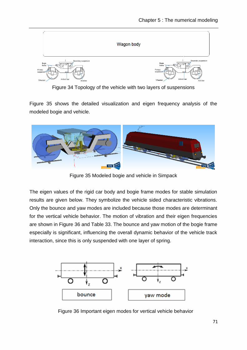
Chapter 5 : The numerical modeling
71
Figure 34 Topology of the vehicle with two layers of suspensions
Figure 35 shows the detailed visualization and eigen frequency analysis of the
modeled bogie and vehicle.
Figure 35 Modeled bogie and vehicle in Simpack
The eigen values of the rigid car body and bogie frame modes for stable simulation
results are given below. They symbolize the vehicle sided characteristic vibrations.
Only the bounce and yaw modes are included because those modes are determinant
for the vertical vehicle behavior. The motion of vibration and their eigen frequencies
are shown in Figure 36 and Table 33. The bounce and yaw motion of the bogie frame
especially is significant, influencing the overall dynamic behavior of the vehicle track
interaction, since this is only suspended with one layer of spring.
Figure 36 Important eigen modes for vertical vehicle behavior

Chapter 5 : The numerical modeling
72
Table 33: The eigen values of selected motion
Rigid body motion Direction of
motion
Natural
frequency (Hz)
Natural
damping (%)
Car body bounce Z 2.36 *) 3.22
Car body yaw β 1.65 2.87
Bogie frame bounce Z 20.38 4.94
Bogie frame yaw β 4.57 2.84
*): The eigen frequency of car body bounce is bigger than 2 Hz due to the coil spring
design of the secondary suspension
The advantage of Simpack is the fully consideration of wheel-rail contact mechanism
including both profiles. Therefore, an exact modeling of rail head profile is required in
the FEM model. A graphical illustration of the contact between wheel and rail is shown
in Figure 37. The blue lines between the wheel and rail profile specify all the possible
contact paths. The classic Kalker contact theory (Method “FASTSIM”) [27] is utilized for
processing of wheel-rail contact force.
Figure 37 Contact between wheel and rail (Profile S1002 and 60E1)
The speed of the vehicle is fixed at 160 km/h, because this is the most frequently
appeared passage speed along the measurement section.
5.3.3. Inclusion of measured track excitation
Noticing that the lateral and longitudinal irregularities can also influence the vehicle
track contact behavior, the measured track geometry (documented in chapter 4.2) is
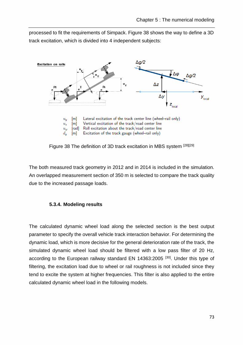
Chapter 5 : The numerical modeling
73
processed to fit the requirements of Simpack. Figure 38 shows the way to define a 3D
track excitation, which is divided into 4 independent subjects:
Figure 38 The definition of 3D track excitation in MBS system [28][29]
The both measured track geometry in 2012 and in 2014 is included in the simulation.
An overlapped measurement section of 350 m is selected to compare the track quality
due to the increased passage loads.
5.3.4. Modeling results
The calculated dynamic wheel load along the selected section is the best output
parameter to specify the overall vehicle track interaction behavior. For determining the
dynamic load, which is more decisive for the general deterioration rate of the track, the
simulated dynamic wheel load should be filtered with a low pass filter of 20 Hz,
according to the European railway standard EN 14363:2005 [30]. Under this type of
filtering, the excitation load due to wheel or rail roughness is not included since they
tend to excite the system at higher frequencies. This filter is also applied to the entire
calculated dynamic wheel load in the following models.
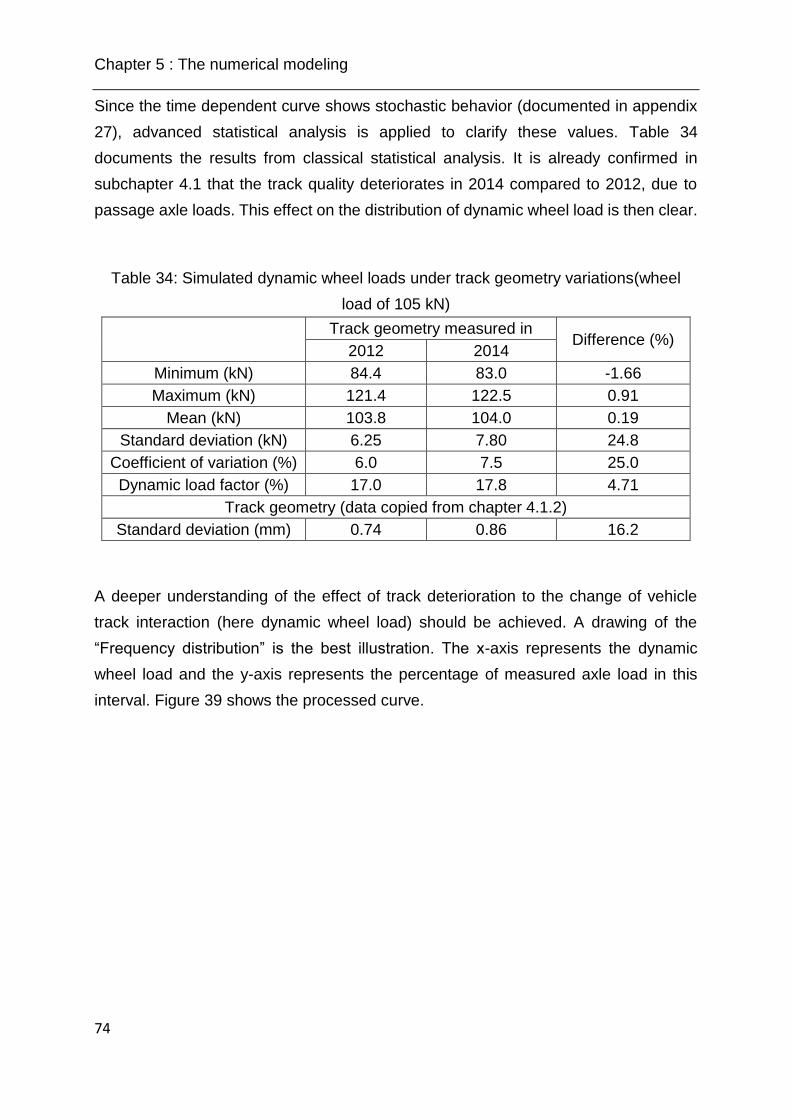
Chapter 5 : The numerical modeling
74
Since the time dependent curve shows stochastic behavior (documented in appendix
27), advanced statistical analysis is applied to clarify these values. Table 34
documents the results from classical statistical analysis. It is already confirmed in
subchapter 4.1 that the track quality deteriorates in 2014 compared to 2012, due to
passage axle loads. This effect on the distribution of dynamic wheel load is then clear.
Table 34: Simulated dynamic wheel loads under track geometry variations(wheel
load of 105 kN)
Track geometry measured in Difference (%)
2012 2014
Minimum (kN) 84.4 83.0 -1.66
Maximum (kN) 121.4 122.5 0.91
Mean (kN) 103.8 104.0 0.19
Standard deviation (kN) 6.25 7.80 24.8
Coefficient of variation (%) 6.0 7.5 25.0
Dynamic load factor (%) 17.0 17.8 4.71
Track geometry (data copied from chapter 4.1.2)
Standard deviation (mm) 0.74 0.86 16.2
A deeper understanding of the effect of track deterioration to the change of vehicle
track interaction (here dynamic wheel load) should be achieved. A drawing of the
“Frequency distribution” is the best illustration. The x-axis represents the dynamic
wheel load and the y-axis represents the percentage of measured axle load in this
interval. Figure 39 shows the processed curve.

Chapter 5 : The numerical modeling
75
Figure 39 The statistical frequency distribution analysis of dynamic load (Section 4)
It can be clearly observed that the deterioration of the track quality leads to a decrease
of appearance in the middle area, close to the static wheel load, and to an increase of
appearance in both surrounding areas. In other words, the level of significance of the
variation of the dynamic load is numerically shown.
5.4. Model 3 (Co-simulation with FEM and MBS) – Calibration of the quasi-static wheel rail load under modal represented elastic track from FEM
5.4.1. Background and introduction
The variation of track stiffness is also an important factor influencing the overall track
dynamics. For sound track without special design specifications, the stiffness of the
track significantly varies in comparison with track irregularity characteristics and this
part was usually neglected.
Chapter 5 : The numerical modeling
76
This cannot be the case for this research, since the track stiffness, which is one of the
both important track sided parameters, influences vehicle track interaction behaviors.
By repeated train load, those variations of track stiffness have counterproductive effect
to the track geometry. In other words, the appearance of track irregularity is normally
the consequence of the “spots” in track stiffness.
Generally, it is suggested to generate track stiffness model in FEM system, since the
materials of the single element can be determined and the simulation of complex
deflection behavior can be ensured. The disadvantage of this approach is the
requirement of complex discretization of the geometry model into small and fine
elements, due to which the model should normally orient itself in time-independent
analysis.
The co-simulation strategy is used to solve the problem. There exists the contact
marker in Simpack, which fully supports the moving contact between rigid and flexible
body [31]. Therefore, the model should be able to utilize information from both FEM and
MBS and to combine them together for the solution. Since MBS is designed to
accomplish time dependent simulations, the FEM model is condensed and utilized as
the prerequisite of the MBS model. This model condensation can be achieved by the
modal analysis approach [32].
5.4.2. Model condensation and modal analysis
The reason for the time-intensive simulation of a FEM model remains at the finite
element meshing of the geometrical model, which creates huge number of
independent formulas. This accuracy is required for the best representation of the
bending behavior of the structure.
A group of generated elements, whose internal behavior is not required to be analyzed
in detail, can be defined as a “Substructure” in FEM model, with pre-defined “Master
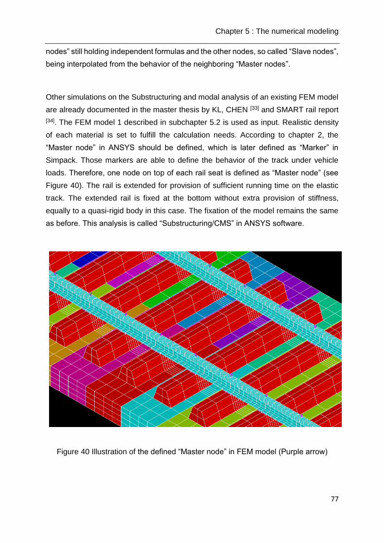
Chapter 5 : The numerical modeling
77
nodes” still holding independent formulas and the other nodes, so called “Slave nodes”,
being interpolated from the behavior of the neighboring “Master nodes”.
Other simulations on the Substructuring and modal analysis of an existing FEM model
are already documented in the master thesis by KL, CHEN [33] and SMART rail report
[34]. The FEM model 1 described in subchapter 5.2 is used as input. Realistic density
of each material is set to fulfill the calculation needs. According to chapter 2, the
“Master node” in ANSYS should be defined, which is later defined as “Marker” in
Simpack. Those markers are able to define the behavior of the track under vehicle
loads. Therefore, one node on top of each rail seat is defined as “Master node” (see
Figure 40). The rail is extended for provision of sufficient running time on the elastic
track. The extended rail is fixed at the bottom without extra provision of stiffness,
equally to a quasi-rigid body in this case. The fixation of the model remains the same
as before. This analysis is called “Substructuring/CMS” in ANSYS software.
Figure 40 Illustration of the defined “Master node” in FEM model (Purple arrow)

Chapter 5 : The numerical modeling
78
The modal analysis of the condensed model is realized in the next step. From all the
selected master nodes, only the eigenmodes in vertical direction are calculated,
because the modes defining tilting and lateral movement are not required to be
included in this research.
The representation of the track stiffness should rely on many different modes due to
different stiffness setting under individual rail seat. Thus, for the best representation,
the number of the included eigenmodes should be the same as the number of “Master
node” itself (in this research about 150 eigen modes). The frequency variation of those
eigenmodes is between 1300 (eigen frequency of mode 1) and 7500 Hz (eigen
frequency of mode 150). This ensures the best representation of stiffness behaviors
for the total measurement section. Figure 41 and Figure 42 show the first two
eigenmodes using counter plots. The graphical and table list of all the included eigen
modes can be found in appendices 28 to 30.
Figure 41 Illustration of eigen mode 1 (f0 = 1298 Hz)
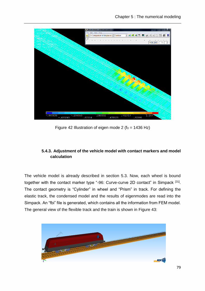
Chapter 5 : The numerical modeling
79
Figure 42 Illustration of eigen mode 2 (f0 = 1436 Hz)
5.4.3. Adjustment of the vehicle model with contact markers and model
calculation
The vehicle model is already described in section 5.3. Now, each wheel is bound
together with the contact marker type “-96: Curve-curve 2D contact” in Simpack [31].
The contact geometry is “Cylinder” in wheel and “Prism” in track. For defining the
elastic track, the condensed model and the results of eigenmodes are read into the
Simpack. An “fbi” file is generated, which contains all the information from FEM model.
The general view of the flexible track and the train is shown in Figure 43:
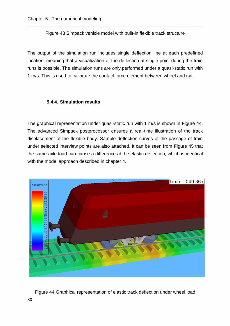
Chapter 5 : The numerical modeling
80
Figure 43 Simpack vehicle model with built-in flexible track structure
The output of the simulation run includes single deflection line at each predefined
location, meaning that a visualization of the deflection at single point during the train
runs is possible. The simulation runs are only performed under a quasi-static run with
1 m/s. This is used to calibrate the contact force element between wheel and rail.
5.4.4. Simulation results
The graphical representation under quasi-static run with 1 m/s is shown in Figure 44.
The advanced Simpack postprocessor ensures a real-time illustration of the track
displacement of the flexible body. Sample deflection curves of the passage of train
under selected interview points are also attached. It can be seen from Figure 45 that
the same axle load can cause a difference at the elastic deflection, which is identical
with the model approach described in chapter 4.
Figure 44 Graphical representation of elastic track deflection under wheel load

Chapter 5 : The numerical modeling
81
Figure 45 Elastic deflection under train passage at certain rail seats
5.5. Model 4 (Co-simulation with FEM and MBS) – Calculation of the dynamic wheel load under elastic track with irregularities (V = 160 km/h)
5.5.1. Background and introduction
After the model calibration, the flexible track input is used for train runs with higher
speed. The track geometry is also read and overlapped with the same location in which
they were measured. In other words, this track is able to represent the real track,
described in chapter 4, on behalf of geometry and stiffness. The track geometry was
measured in 2012 and in 2014. The supposed minor change of track stiffness due to
1 year of operation is not measured in 2014 and the simulation runs for 2014 still use
the track stiffness data from 2012.
An important factor which should be considered is the damping of the track. The
modeling of the track stiffness relies on the modal analysis of the flexible system with
built in modal damping. The damping is categorized as a number in percentage.

Chapter 5 : The numerical modeling
82
The selection of the modal damping should be dependent on the travel speed of the
vehicle, since the modal analysis can only provide a linear damping approach, whereas
the track damping in reality is mostly found to be nonlinear. It is defined under
experience that a modal damping at about 5 % (inclusion of rubber rail pads) is required
for the dynamic run with 160 km/h [35].
5.5.2. Simulation results
The calculated dynamic wheel load along the selected section is the best output
parameter specifying the overall vehicle track interaction behavior, which directly
specifies the content of vehicle track interaction. Since the time dependent curve
shows stochastic behavior, advanced statistical analysis is applied for clarifying the
values. Table 35 documents the results by the conventional statistical analysis. The
major outputs of this section are the appearance of the track stiffness to the overall
performance of vehicle track interaction.
Table 35: Statistical results of the simulated dynamic wheel loads (static wheel load
of 105 kN)
Geometry measured in 2012 Geometry measured in 2014
Only
Geometry
Geometry
+Stiffness
Difference
(%)
Only
Geometry
Geometry
+Stiffness *)
Differenc
e (%)
Minimum (kN) 86.4 88.6 2.5 86.8 87.2 0.5
Maximum(kN) 123.0 118.8 -3.4 125.4 124.6 -0.6
Mean (kN) 103.9 104.0 0.1 103.9 104.0 0.1
Standard
deviation (kN) 7.24 6.19 -14.5 7.60 7.40 -2.6
Coefficient of
variation (%) 7.0 6.0 -14.3 7.3 7.1 -2.7
Dynamic load
factor (%) 18.3 14.3 -21.9 20.7 19.9 -3.9
*): Track stiffness data from measurement in 2012 due to lack of repeated
measurement in 2014

Chapter 5 : The numerical modeling
83
Generally, the inclusion of track stiffness improves the vehicle track interaction
performance. The reason is that the stiffness of the structure can compensate the
effect of irregularity to a certain extend. A dynamic loading factor of approximately 20.0
% can be found under the travel speed at 160 km/h for scenario 2014, which is
principally identical to the measurement results using strain gauges.
Since the track stiffness input for both scenarios remains the same, it is therefore to
conclude, that the improvement of vehicle track interaction due to track stiffness is
dependent on track geometry conditions. The column “Difference” in terms “Standard
deviation, Coefficient of variation and Dynamic loading factor” shows much higher
values for the scenario in 2012 than in 2014, where the track geometry level in 2012 is
still smoother than in 2014. This proves that, the stiffness can compensate the
excitation load better under better track geometry qualities. In other words, the effect
of track stiffness in compensating the excitation from track geometry also decreases
with the decrease of the quality of track. This effect is further investigated in the chapter
6.
The “Frequency distribution” curves in 2012 and in 2014 are attached in Figure 46 and
Figure 47. The legend “Gm” refers to the simulation with only geometry variation and
“GE” referred to the simulation with overlapped geometry and stiffness variations.

Chapter 5 : The numerical modeling
84
Figure 46 The statistical frequency distribution analysis of dynamic load
(measurement in 2012, Section 4)
Figure 47 The statistical frequency distribution analysis of dynamic load
(measurement in 2014, Section 4)
5.6. Conclusion and outcome
In this chapter, the innovative co-simulation is performed and illustrated. The approach
of the co-simulation remains at the combination of ANSYS and Simpack, with Simpack
as master program reading the modal represented elastic model from ANSYS. With
the help of this innovative approach, a dynamic real-time simulation under fully elastic

Chapter 5 : The numerical modeling
85
track was realized. The model 4 described in the section 5.5 can fully integrate both
the track geometry and stiffness, with exact overlapping of the both excitations.
Therefore, this provides the best close to reality information of the interaction between
vehicle and track, as well as their effects on the respective track superstructures.
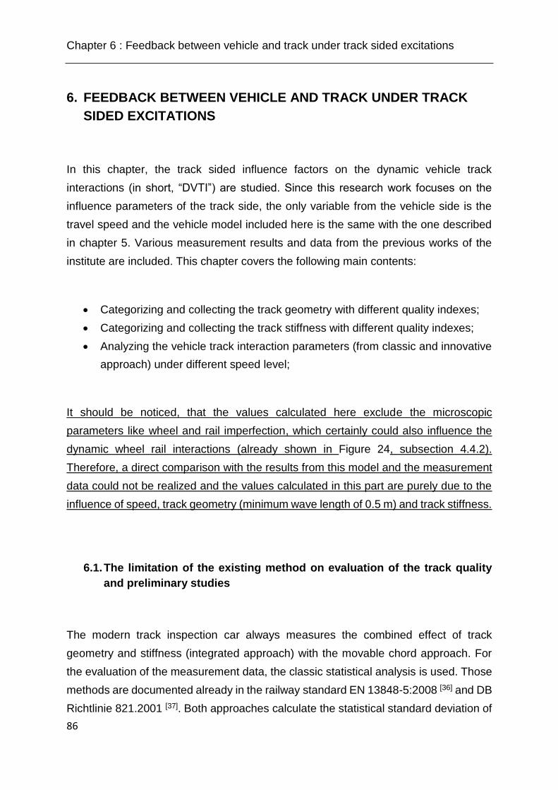
Chapter 6 : Feedback between vehicle and track under track sided excitations
86
6. FEEDBACK BETWEEN VEHICLE AND TRACK UNDER TRACK
SIDED EXCITATIONS
In this chapter, the track sided influence factors on the dynamic vehicle track
interactions (in short, “DVTI”) are studied. Since this research work focuses on the
influence parameters of the track side, the only variable from the vehicle side is the
travel speed and the vehicle model included here is the same with the one described
in chapter 5. Various measurement results and data from the previous works of the
institute are included. This chapter covers the following main contents:
Categorizing and collecting the track geometry with different quality indexes;
Categorizing and collecting the track stiffness with different quality indexes;
Analyzing the vehicle track interaction parameters (from classic and innovative
approach) under different speed level;
It should be noticed, that the values calculated here exclude the microscopic
parameters like wheel and rail imperfection, which certainly could also influence the
dynamic wheel rail interactions (already shown in Figure 24, subsection 4.4.2).
Therefore, a direct comparison with the results from this model and the measurement
data could not be realized and the values calculated in this part are purely due to the
influence of speed, track geometry (minimum wave length of 0.5 m) and track stiffness.
6.1. The limitation of the existing method on evaluation of the track quality
and preliminary studies
The modern track inspection car always measures the combined effect of track
geometry and stiffness (integrated approach) with the movable chord approach. For
the evaluation of the measurement data, the classic statistical analysis is used. Those
methods are documented already in the railway standard EN 13848-5:2008 [36] and DB
Richtlinie 821.2001 [37]. Both approaches calculate the statistical standard deviation of
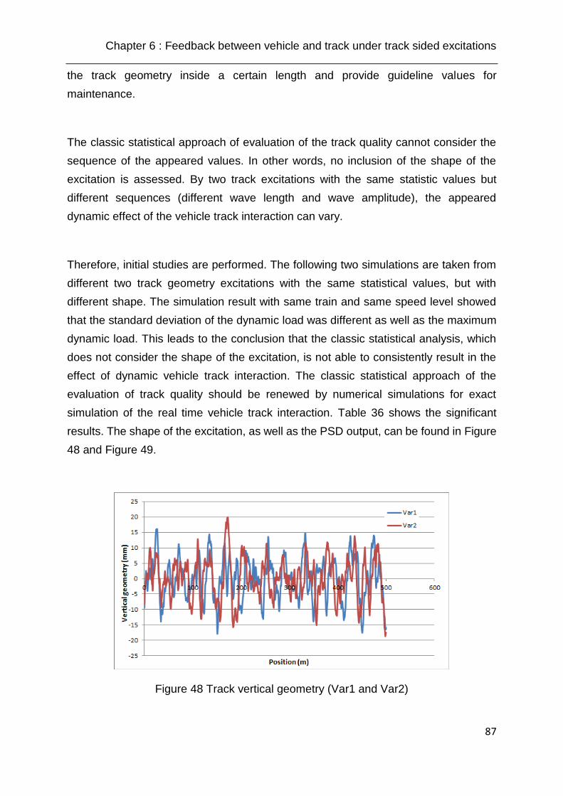
Chapter 6 : Feedback between vehicle and track under track sided excitations
87
the track geometry inside a certain length and provide guideline values for
maintenance.
The classic statistical approach of evaluation of the track quality cannot consider the
sequence of the appeared values. In other words, no inclusion of the shape of the
excitation is assessed. By two track excitations with the same statistic values but
different sequences (different wave length and wave amplitude), the appeared
dynamic effect of the vehicle track interaction can vary.
Therefore, initial studies are performed. The following two simulations are taken from
different two track geometry excitations with the same statistical values, but with
different shape. The simulation result with same train and same speed level showed
that the standard deviation of the dynamic load was different as well as the maximum
dynamic load. This leads to the conclusion that the classic statistical analysis, which
does not consider the shape of the excitation, is not able to consistently result in the
effect of dynamic vehicle track interaction. The classic statistical approach of the
evaluation of track quality should be renewed by numerical simulations for exact
simulation of the real time vehicle track interaction. Table 36 shows the significant
results. The shape of the excitation, as well as the PSD output, can be found in Figure
48 and Figure 49.
Figure 48 Track vertical geometry (Var1 and Var2)
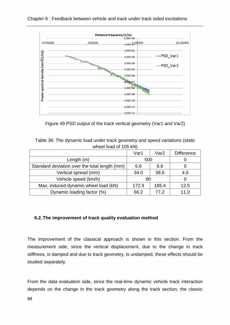
Chapter 6 : Feedback between vehicle and track under track sided excitations
88
Figure 49 PSD output of the track vertical geometry (Var1 and Var2)
Table 36: The dynamic load under track geometry and speed variations (static
wheel load of 105 kN)
Var1 Var2 Difference
Length (m) 500 0
Standard deviation over the total length (mm) 6.6 6.6 0
Vertical spread (mm) 34.0 38.6 4.6
Vehicle speed (km/h) 80 0
Max. induced dynamic wheel load (kN) 172.9 185.4 12.5
Dynamic loading factor (%) 66.2 77.2 11.0
6.2. The improvement of track quality evaluation method
The improvement of the classical approach is shown in this section. From the
measurement side, since the vertical displacement, due to the change in track
stiffness, is damped and due to track geometry, is undamped, these effects should be
studied separately.
From the data evaluation side, since the real-time dynamic vehicle track interaction
depends on the change in the track geometry along the track section, the classic
Chapter 6 : Feedback between vehicle and track under track sided excitations
89
calculation of statistics should be exchanged for the evaluation of the output
parameters by the modern numerical simulations with FEM and MBS.
The wheel dynamic load provides the best surface for the analysis of the DVTI. For
this research, the dynamic wheel load is processed into three terms: “Dynamic loading
factor”, “Energy Spectral Density” and “Statistical frequency distribution”. The term
“Dynamic loading factor” defines the obvious leveling of the DVTI by seeing the
proportion of the maximum dynamic loading to the static one. The other term “Energy
Spectral Density” (ESD) describes the energy of the dynamic load contributing to the
system, by a frequency, per unit frequency [38]. This generally holds the same
calculation method of the “Power Spectral Density” (illustrated in chapter 2) but utilizes
time signal of the dynamic wheel load as input. The processed ESD holds the x and y
unit of Hz and kN²/Hz. This output is distributed in a frequency curve for every
calculated dynamic wheel load. The “Statistical frequency distribution” is the same, as
described in subsection 5.3.4.
All the results from this section are collected from the simulation output of Simpack.
The built-up of the basic models are described in chapter 5.
6.3. Variation of the included influence parameters
As described before, the included parameters, which are studied, are the following
three: the vehicle speed (specified as X), the track geometry (specified as Y) and the
track stiffness (specified as Z). Therefore, for a better categorization, each simulation
is given a three digits “index number” with X, Y and Z which are found as “DVTI_XYZ”.
Table 37 shows the exact numbering of the X, Y and Z and their references.
In order to understand the track quality level, the classic statistical standard deviation
(SR100 for track geometry of DB 821.2001) is calculated as guidelines. But they cannot
provide an accurate quality index concerning the effect of vehicle track interaction, due
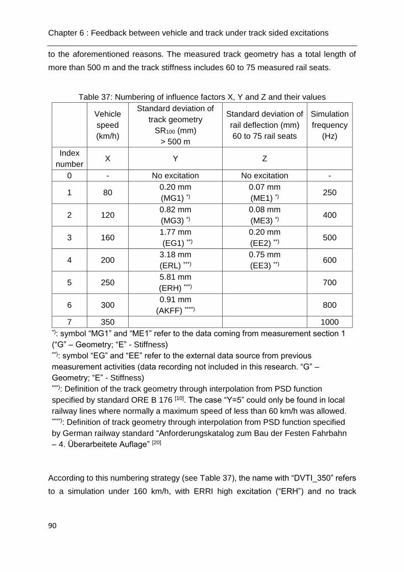
Chapter 6 : Feedback between vehicle and track under track sided excitations
90
to the aforementioned reasons. The measured track geometry has a total length of
more than 500 m and the track stiffness includes 60 to 75 measured rail seats.
Table 37: Numbering of influence factors X, Y and Z and their values
Vehicle
speed
(km/h)
Standard deviation of
track geometry
SR100 (mm)
> 500 m
Standard deviation of
rail deflection (mm)
60 to 75 rail seats
Simulation
frequency
(Hz)
Index
number X Y Z
0 - No excitation No excitation -
1 80 0.20 mm
(MG1) *)
0.07 mm
(ME1) *) 250
2 120 0.82 mm
(MG3) *)
0.08 mm
(ME3) *) 400
3 160 1.77 mm
(EG1) **)
0.20 mm
(EE2) **) 500
4 200 3.18 mm
(ERL) ***)
0.75 mm
(EE3) **) 600
5 250 5.81 mm
(ERH) ***) 700
6 300 0.91 mm
(AKFF) ****) 800
7 350 1000 *): symbol “MG1” and “ME1” refer to the data coming from measurement section 1
(“G” – Geometry; “E” - Stiffness)
**): symbol “EG” and “EE” refer to the external data source from previous
measurement activities (data recording not included in this research. “G” –
Geometry; “E” - Stiffness) ***): Definition of the track geometry through interpolation from PSD function
specified by standard ORE B 176 [10]. The case “Y=5” could only be found in local
railway lines where normally a maximum speed of less than 60 km/h was allowed. ****): Definition of track geometry through interpolation from PSD function specified
by German railway standard “Anforderungskatalog zum Bau der Festen Fahrbahn
– 4. Überarbeitete Auflage” [20]
According to this numbering strategy (see Table 37), the name with “DVTI_350” refers
to a simulation under 160 km/h, with ERRI high excitation (“ERH”) and no track

Chapter 6 : Feedback between vehicle and track under track sided excitations
91
stiffness input; the name with “DVTI_611” refers to a simulation under 300 km/h, with
geometry excitation “MG1” and stiffness input “ME1”.
The travel speed of the vehicle should be also included as a major influence parameter.
A minimum speed level is fixed at 80 km/h, because under this speed level, no
significant dynamic effect should be expected. Moreover, because the ballastless track
with design speed at 300 km/h is included, for purely academic reasons, a maximum
speed of 350 km/h is fixed.
The studied track geometry and track stiffness scenarios have different quality indexes,
in order to research the effect of the dynamic vehicle track interaction under different
tracks. Their data were ranked in sequence, meaning that the scenario with the best
quality always has smaller number in their index. All the studied data refer to tracks in
straight alignment, without specific structures like bridge or tunnels.
With this allocation, there are scenarios like “DVTI_XY0” and “DVTI_X0Z” for the
visualization of the effect of single excitation input. The vertical geometry and
distribution of the maximum rail deflection of the external data are shown in appendices
31 to 32.
6.4. Distribution of dynamic wheel load according to standard track quality
factors (Y = 6)
The German railway standard AKFF defines the limit for the power spectral density
distribution of the vertical track geometry for ballastless tracks. Calculations of dynamic
loading factor dependent on speed levels have been done using track models
according to this track quality limit (PSD track geometry). The calculation is performed
for the train type “Locomotive” (without wheel flats). This distribution can be seen in
Figure 50.
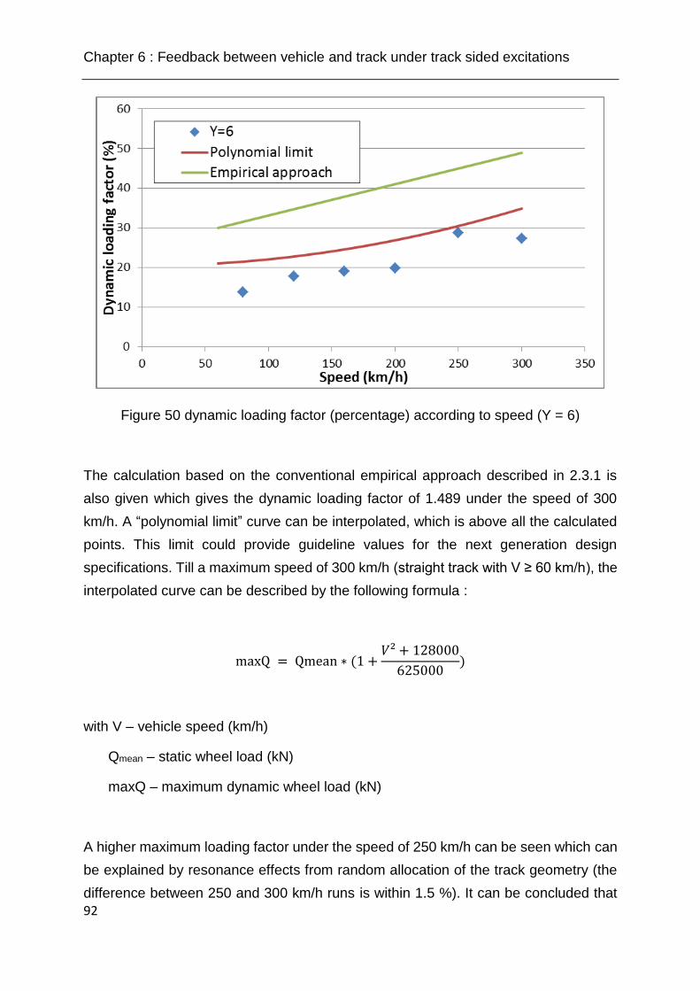
Chapter 6 : Feedback between vehicle and track under track sided excitations
92
Figure 50 dynamic loading factor (percentage) according to speed (Y = 6)
The calculation based on the conventional empirical approach described in 2.3.1 is
also given which gives the dynamic loading factor of 1.489 under the speed of 300
km/h. A “polynomial limit” curve can be interpolated, which is above all the calculated
points. This limit could provide guideline values for the next generation design
specifications. Till a maximum speed of 300 km/h (straight track with V ≥ 60 km/h), the
interpolated curve can be described by the following formula :
maxQ = Qmean ∗ (1 +𝑉² + 128000
625000)
with V – vehicle speed (km/h)
Qmean – static wheel load (kN)
maxQ – maximum dynamic wheel load (kN)
A higher maximum loading factor under the speed of 250 km/h can be seen which can
be explained by resonance effects from random allocation of the track geometry (the
difference between 250 and 300 km/h runs is within 1.5 %). It can be concluded that
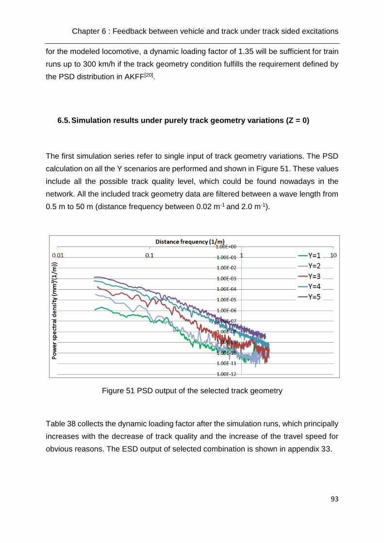
Chapter 6 : Feedback between vehicle and track under track sided excitations
93
for the modeled locomotive, a dynamic loading factor of 1.35 will be sufficient for train
runs up to 300 km/h if the track geometry condition fulfills the requirement defined by
the PSD distribution in AKFF[20].
6.5. Simulation results under purely track geometry variations (Z = 0)
The first simulation series refer to single input of track geometry variations. The PSD
calculation on all the Y scenarios are performed and shown in Figure 51. These values
include all the possible track quality level, which could be found nowadays in the
network. All the included track geometry data are filtered between a wave length from
0.5 m to 50 m (distance frequency between 0.02 m-1 and 2.0 m-1).
Figure 51 PSD output of the selected track geometry
Table 38 collects the dynamic loading factor after the simulation runs, which principally
increases with the decrease of track quality and the increase of the travel speed for
obvious reasons. The ESD output of selected combination is shown in appendix 33.

Chapter 6 : Feedback between vehicle and track under track sided excitations
94
Table 38: The dynamic load under track geometry and speed variations
Track geometry variation (index Y)
Y = 1 Y = 2 Y = 3 Y = 4 Y = 5
Index
X
Speed
(km/h) Dynamic loading factor (%)
1 80 - *) 16.1 17.2 50.8 77.2
2 120 - *) 13.3 21.4 75.5 103.3
3 160 - *) 18.6 19.3 73.8 - **)
4 200 5.0 22.0 26.6 79.6 - **)
5 250 7.5 24.6 31.0 84.5 - **)
6 300 11.4 34.7 48.6 - **) - **)
7 350 43.4 50.7 67.0 - **) - **) *): Simulation not done due to expected insignificant value output **): Simulation not done due to too severe dynamic impacts
6.6. Simulation results under purely track stiffness variations (Y = 0)
The second simulation series concern single input of track stiffness variations. Both
ballasted and ballastless tracks are studied. But because the ballastless track normally
holds obvious non-linear stiffness behavior, which cannot be included in this approach,
the calculated values (in scenario Z = 1) can be slightly different in reality.
Each selected data set contains 60 to 75 single measurements. Table 39 collects the
dynamic loading factor from each simulation result, which principally increases with the
increase of travel speed and reduction of the quality of track stiffness for obvious
reasons. The ESD output of selected combination is shown in appendix 33.
Chapter 6 : Feedback between vehicle and track under track sided excitations
95
Table 39: The dynamic load under track stiffness and speed variations
Track stiffness variation (index Z)
Z = 1 Z = 2 Z = 3 Z = 4
Index
X
Speed
(km/h) Dynamic loading factor (%)
1 80 4.2 4.1 4.1 13.6
2 120 4.1 3.5 3.8 7.0
3 160 4.7 4.0 5.0 13.7
4 200 7.3 5.2 3.6 19.9
5 250 7.4 6.3 6.5 15.3
6 300 8.6 8.7 9.7 16.3
7 350 10.3 10.8 12.6 19.2
6.7. The “hybrid” simulations
In this section, the effect of combining the excitations from Y (geometry) and stiffness
(Z) is studied. This can be realized by the so called “hybrid” simulation with combination
of the factor of X, Y and Z (none with zero indexes).
Due to the free positioning of the overlapped excitations Y and Z, their effect in dynamic
loading can be either amplified or compensated. A virtual simulation program can
combine every X, Y and Z index together, but only a few of those combinations are
close to the real situations. For scientific reasons, the maximum possible speed levels
for each selected Y and Z combination is selected. Table 40 shows the realistic
combination of X, Y and Z and the simulated dynamic loading factor. The maximum
dynamic loading (max Q), based on the analytic method, described in subsection 2.3.1,
is listed in Table 41 for comparison reasons. The reader is referred to Appendices 34
to 36 for the statistical frequency distribution analysis of the dynamic load.

Chapter 6 : Feedback between vehicle and track under track sided excitations
96
Table 40: Realized combination of X, Y and Z and dynamic loading factor
XYZ Max. Speed
limit (km/h)
Dynamic loading factor (%)
Combined Y and Z Z = 0 Y = 0
611 300 11.1 11.4 8.6
522 250 25.2 24.6 6.3
333 160 19.5 19.3 5.0
244 120 74.6 75.5 7.0
154 80 76.7 77.2 13.6
Table 41: Analytical calculation of dynamic loading factor from classic formulas
XYZ Max. Speed limit (km/h) t n φ Dynamic loading
factor (%)
611 300 3.0 0.10 1.632 49.0
522 250 3.0 0.10 1.500 45.0
333 160 3.0 0.15 1.263 56.9
244 120 3.0 0.20 1.158 69.5
154 80 3.0 0.25 1.053 79.0
It is proved that, the dynamic loading factor calculated by Simpack has good identity
under the scenarios “154” and “244” (variation of both results inside 5 %). All the
calculated values by Simpack are smaller than the empirical approach (see section
2.3.1). Under those cases, the track sided parameters are dominant, while the
difference in vehicle design and vehicle performances is not significant for the variation
of the results, due to the limited speed level (v ≤ 120 km/h).
The significant difference of the values of the cases “611”, “522” and “333” can be due
to the improvement of mechanical behavior of the vehicle (technology innovations from
1993 to 2010), which is also determinant for the overall vehicle track interaction. This
contributes to the fact that, the formulas are designed to always stay at the safe side,
which reserves space for the vehicle track interaction behavior under high speed levels
(V > 120 km/h).
The modern high speed lines induce less dynamic effect between vehicle and track
even under higher speed limit, due to improvement of the track geometry condition.
The case “522” represents the high speed ballasted track after about 1 year of
operation; this dynamic loading factor of 25.2 % is the best situation for ballasted track
under this speed level. For a smoother track like the case “611” (dynamic loading factor
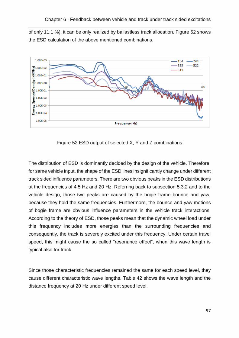
Chapter 6 : Feedback between vehicle and track under track sided excitations
97
of only 11.1 %), it can be only realized by ballastless track allocation. Figure 52 shows
the ESD calculation of the above mentioned combinations.
Figure 52 ESD output of selected X, Y and Z combinations
The distribution of ESD is dominantly decided by the design of the vehicle. Therefore,
for same vehicle input, the shape of the ESD lines insignificantly change under different
track sided influence parameters. There are two obvious peaks in the ESD distributions
at the frequencies of 4.5 Hz and 20 Hz. Referring back to subsection 5.3.2 and to the
vehicle design, those two peaks are caused by the bogie frame bounce and yaw,
because they hold the same frequencies. Furthermore, the bounce and yaw motions
of bogie frame are obvious influence parameters in the vehicle track interactions.
According to the theory of ESD, those peaks mean that the dynamic wheel load under
this frequency includes more energies than the surrounding frequencies and
consequently, the track is severely excited under this frequency. Under certain travel
speed, this might cause the so called “resonance effect”, when this wave length is
typical also for track.
Since those characteristic frequencies remained the same for each speed level, they
cause different characteristic wave lengths. Table 42 shows the wave length and the
distance frequency at 20 Hz under different speed level.
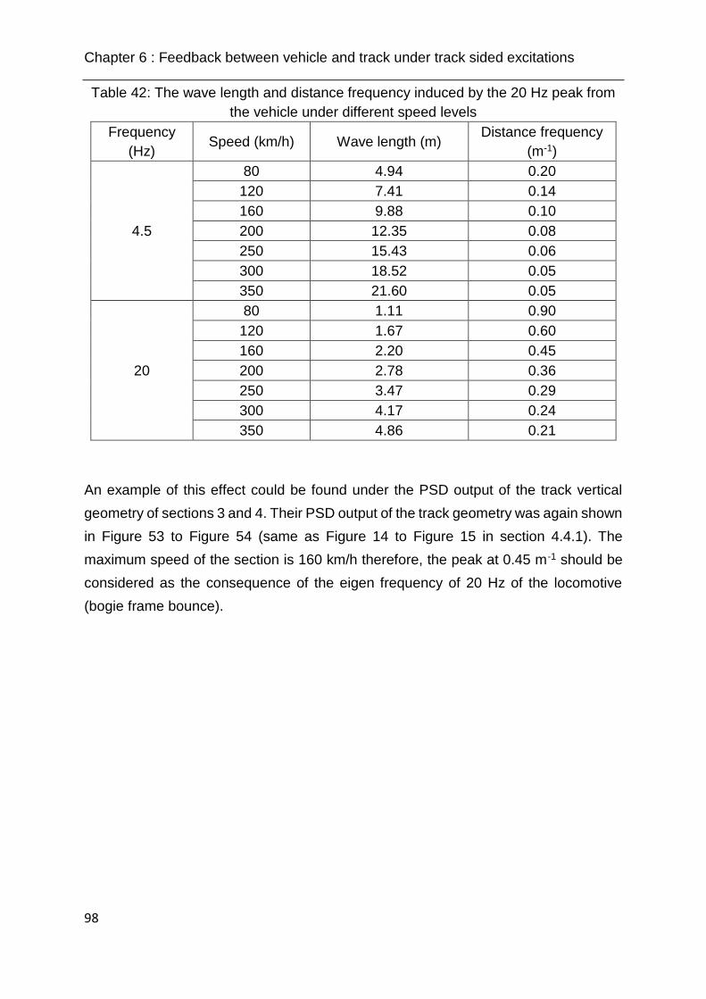
Chapter 6 : Feedback between vehicle and track under track sided excitations
98
Table 42: The wave length and distance frequency induced by the 20 Hz peak from
the vehicle under different speed levels
Frequency
(Hz) Speed (km/h) Wave length (m)
Distance frequency
(m-1)
4.5
80 4.94 0.20
120 7.41 0.14
160 9.88 0.10
200 12.35 0.08
250 15.43 0.06
300 18.52 0.05
350 21.60 0.05
20
80 1.11 0.90
120 1.67 0.60
160 2.20 0.45
200 2.78 0.36
250 3.47 0.29
300 4.17 0.24
350 4.86 0.21
An example of this effect could be found under the PSD output of the track vertical
geometry of sections 3 and 4. Their PSD output of the track geometry was again shown
in Figure 53 to Figure 54 (same as Figure 14 to Figure 15 in section 4.4.1). The
maximum speed of the section is 160 km/h therefore, the peak at 0.45 m-1 should be
considered as the consequence of the eigen frequency of 20 Hz of the locomotive
(bogie frame bounce).
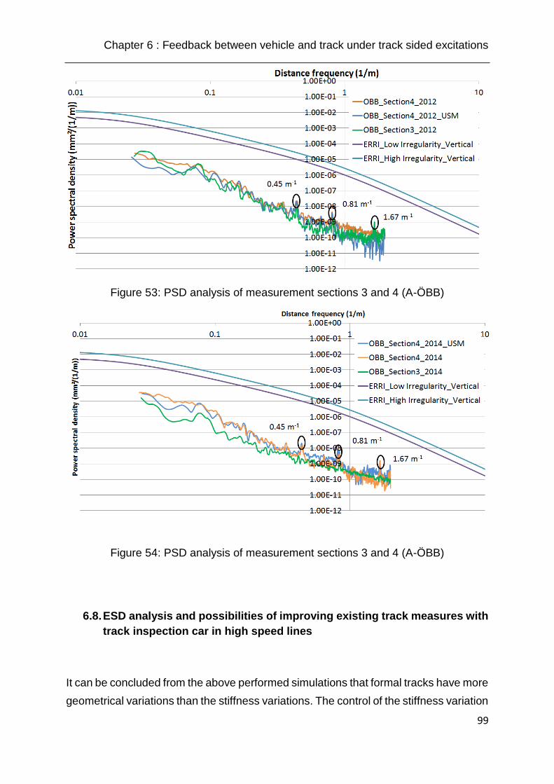
Chapter 6 : Feedback between vehicle and track under track sided excitations
99
Figure 53: PSD analysis of measurement sections 3 and 4 (A-ÖBB)
Figure 54: PSD analysis of measurement sections 3 and 4 (A-ÖBB)
6.8. ESD analysis and possibilities of improving existing track measures with
track inspection car in high speed lines
It can be concluded from the above performed simulations that formal tracks have more
geometrical variations than the stiffness variations. The control of the stiffness variation
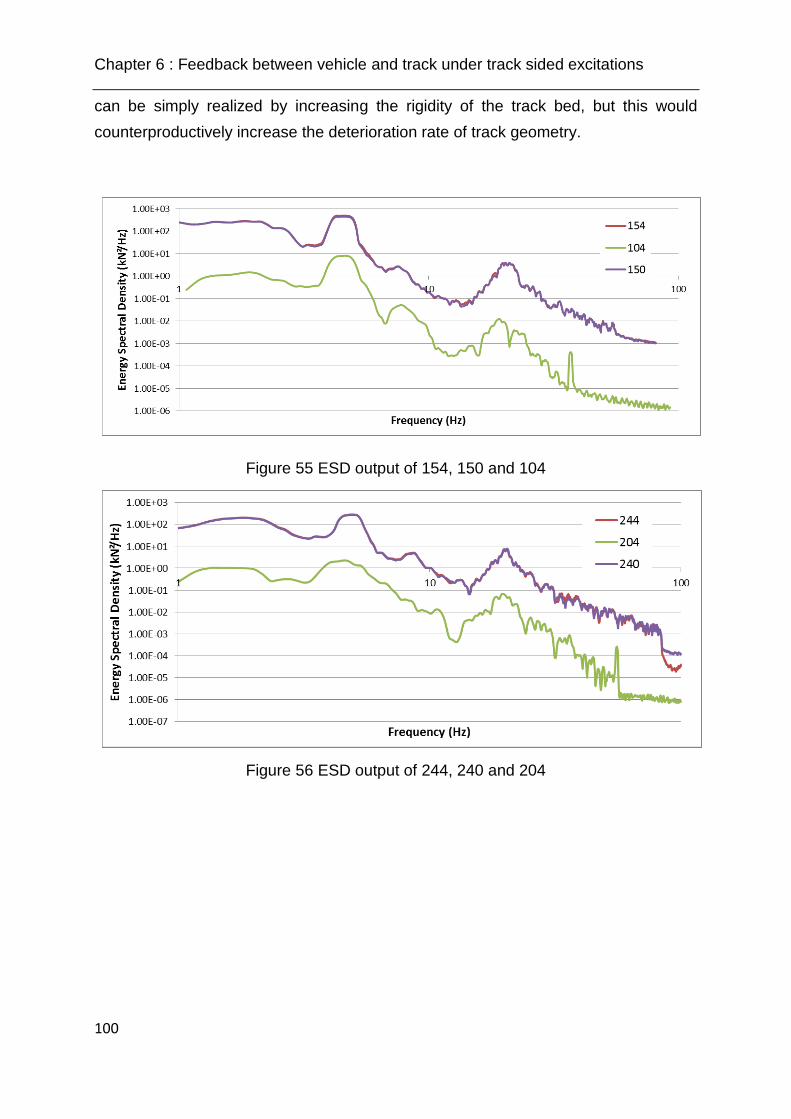
Chapter 6 : Feedback between vehicle and track under track sided excitations
100
can be simply realized by increasing the rigidity of the track bed, but this would
counterproductively increase the deterioration rate of track geometry.
Figure 55 ESD output of 154, 150 and 104
Figure 56 ESD output of 244, 240 and 204
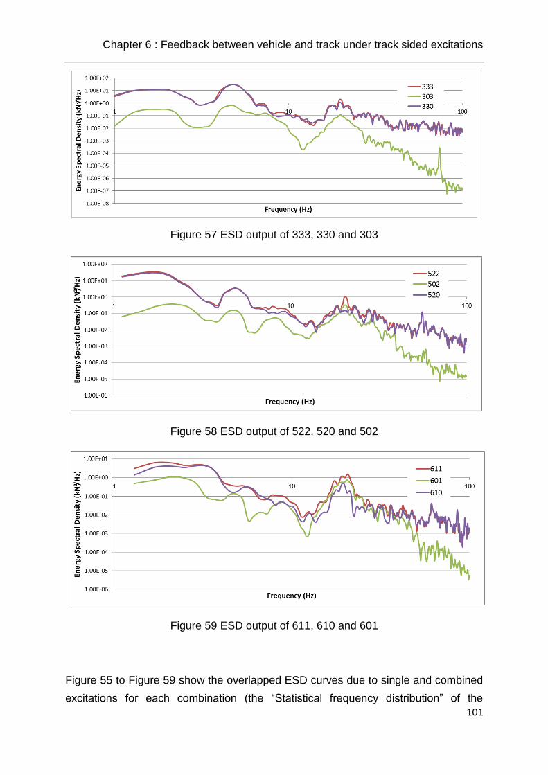
Chapter 6 : Feedback between vehicle and track under track sided excitations
101
Figure 57 ESD output of 333, 330 and 303
Figure 58 ESD output of 522, 520 and 502
Figure 59 ESD output of 611, 610 and 601
Figure 55 to Figure 59 show the overlapped ESD curves due to single and combined
excitations for each combination (the “Statistical frequency distribution” of the

Chapter 6 : Feedback between vehicle and track under track sided excitations
102
scenarios can be found in appendices 34 to 36). The obvious peaks at 4.5 and 20 Hz
are explained in the previous section by the bounce and yaw motion of the bogie frame.
For ballasted track, with maximum design speed at under 160 km/h, the overall
dynamic performance of vehicle track interaction is dominated by the variation caused
by the track geometry (misalignment or settlement problem). This could be proved by
observing the nearly overlapped curves of “154” and “150”, “244” and “240”, “333” and
“330”. Nonetheless, the track stiffness also directly influences in the deterioration rate
of the track geometry quality. Therefore, the general track quality is specified by the
track geometrical condition and the variation of track stiffness can influence the track
quality through an indirect way. Obvious peaks in “104”, “204” and “303” can be
observed, which is identical to the sleeper spacing of the line.
This is not any longer the case while looking at the curve series of “522” and “520” as
well as, “611” and “610”. Noticing that those series refer to the best modern high speed
line (ballasted track or ballastless track) with very well maintained track geometry and
compressively smaller superstructure stiffness than conventional tracks, the ESD
output of the dynamic wheel load due to combined excitation is higher than due to track
geometry excitation under certain frequencies. This frequency level is also larger in the
case of “611” than “522”, because the ballastless track can achieve better track
geometry quality but requires more elasticity in the superstructure. Therefore, for high
speed lines with design speed at 300 km/h or higher, the variation of track stiffness
becomes also the direct influence parameter.
The effect of the excitation to the track stiffness should also be studied by measuring
the change of track elastic deflection separately from the track geometry. The
measurements should include the following items:
Track geometry under unloaded condition;
Track elastic deflection under different speed levels (from quasi-static to max.
operational speed). Continuous vehicle based measurement using Benkelman
beam method (under construction).

Chapter 6 : Feedback between vehicle and track under track sided excitations
103
Both values should be continuously measured on track. Only by gathering the above
mentioned information, it is possible to dedicate the exact source of potential problems
in high speed lines, where direct measures can be applied to every appeared situation.
Chapter 7 : Summary and conclusions
104
7. SUMMARY AND CONCLUSIONS
7.1. Summary of the workflow
As the increase of train speed and axle load is the future trend in railway transportation,
there will be higher requirements in technology in railway engineering field. Such
requirements will focus more on ensuring the overall behavior of the rail system. In
order to better understand the overall behavior of the system and to reduce the
maintenance costs of the track quality (irregularity and stiffness level) in high speed
lines, relative field side observations and computer simulations are applied. Field
measurements provide useful data as an input, whereas the simulation can help to
enlarge the sight of understanding the system’s behavior. The results shown provide
the evidence that such simulation tools are suitable to meet the respective
requirements.
A systematic research work related to the influence of track quality, in terms of stiffness
and geometry, on the performance of vehicle-track interaction and respective track
quality changes, is carried out since January 2012. The research work is supported by
the Karl-Vossloh funding (Project S047/10021/2011) and lasted for 3 years. This report
includes the results from the activities realized in the work plan:
Literature review, as well as collection of data (used as input for preliminary
simulations and preparation of measurement strategies), results and
experiences from previous works (covered in Chapter 2);
Review of existing measures and developments of field measurements for
selected pilot sections (covered in Chapter 3);
Execution of four field measurements at four pilot sections in Germany and
Austria, as well as the analysis and processing of the measurement data
(covered in Chapter 4);
Selection of the suitable numerical simulation algorithms with focus on Finite-
Element-Method (FEM) and Multi-Body-Simulation (MBS) as well as co-
simulations (covered in Chapter 5);

Chapter 7 : Summary and conclusions
105
Innovative solutions for measurement and simulation for retrieving the feedback
of the dynamic interaction between vehicle and track (covered in Chapter 6).
The general procedure of the workflow follows the flip chart shown in Figure 60. The
whole workflow can be divided into four blocks: measurement, data analysis,
simulation and conclusion.
Figure 60 Illustration of the general workflow
Following measurement activities were performed in the pilot sections (Block 1 and
Block 2):
Track geometry (track irregularities): A continuous 3D acquisition of the track
geometry was achieved during the field measurement, including vertical, lateral,
gauge and twist. A sufficient length of the sampling track (> 500 m) was
recorded in order to conclude the necessary parameters for Power-Spectral-

Chapter 7 : Summary and conclusions
106
Density functions, which is necessary for the comparison with the guideline
values derived from various literatures.
Track stiffness (static loading): The Benkelman beam measurement is actually
the best tool to determine the change in track stiffness along the test section. It
records the (quasi-)static rail deflection of selected individual rail seats. The
methodology was applied by the field measurement on more than 400 rail seats
(on both rails), in total. Respective measurement results are shown in Chapter
4.
Calibration measurements using static axle load (quasi-static test runs): Test
runs with limited speed level (V < 15 km/h) were performed in order to determine
the actual axle load of the ballast wagon. These results also provide the
information of the change in the rail foot strain due to the variation of track
stiffness.
Dynamic wheel load: Strain gauges are the most suitable measurement
equipment as they provide accurate measurement data. Problem of
discontinuous installation (at least every sleeper spacing) is solved by smart
arrangement of allocations of strain gauges along the line (through linear
estimation method). In total more than 250 strain gauges were installed in the
measurement sections. The maximum measured speed of train passage is 300
km/h.
Track vibration level: This test was done under two different approaches,
namely the vibration level under singular impulse load and the vibration level
under operational trains. It was found that this method could provide acceptable
guidelines for observation of the track quality deterioration at the early stage.
The overall vibration levels for all the measurement sections were calculated.
A better understanding of the influence of track geometry and track stiffness to the
dynamic vehicle-track interaction can be achieved by applying modern numerical
simulations (Block 3). The selection of the suitable numerical simulation
methodologies relies on the specific target, as well as the experiences from previous
works. Both Finite-Element-Method (FEM) and Multi-Body-Simulation (MBS) models
are reviewed and their advantages as an auxiliary tool for the research work are
summarized. The application of FEM and MBS, as well as the co-simulation between
the both in this research is designed in the following ways:
Chapter 7 : Summary and conclusions
107
FEM: The stiffness of the track was simulated in the FEM models. Multi-elastic
track superstructure models were built which were verified by the field
measurement data. A condensation of the model by Substructural / Modal
analysis was performed, which provides the possibility for time dependent
simulations;
MBS: A full-scaled vehicle model (in this research a locomotive), including
detailed modeling of body and suspensions, was built. The wheel-rail contact
was integrated in the MBS system with realistic wheel and rail head profiles. 3D
track irregularity was included in the generation of the track sided excitation for
the running vehicle, which was either derived from the measurement data or
generated by the pre-given PSD curves;
Co-simulation strategies (Off-line): The condensed FEM model with all the
stiffness information was included into the MBS environment. Special contact
elements were investigated and implemented for transmitting the wheel contact
patch to the track. A full scale simulation of the running vehicle on real track with
both the excitations of track stiffness and track irregularity was realized in the
MBS interface.
Based on the developed technology, a better understanding of the influence
mechanism of the track sided excitations on the behavior of vehicle track interaction
could be achieved (Block 4). Varies inputs of track stiffness and irregularity which had
different quality indexes were collected from previous measurement activities. In
addition, large amount of simulations were performed under the influencing parameters
of vehicle speed, track geometry and track stiffness input. The effect of the geometry
and stiffness to the performance of vehicle track interaction due to the new method
can now be separately analyzed, which previously was not possible.

Chapter 7 : Summary and conclusions
108
7.2. Conclusions
The track sided key parameters of track geometry and track stiffness are determinant
factors for the overall performance of the dynamic vehicle track interaction. A real-time
representation of the dynamic vehicle track interaction under pre-defined vehicle and
track sided parameters is realized by the co-simulation with FEM and MBS. For this
research, the modeled vehicle is a modern electric locomotive with an axle load of 21.5
t.
The individual influencing parameters, like vehicle speed, track geometry and track
stiffness, can be adjusted in the model easily from scenario to scenario. A wide
selection of the values of the three influencing parameters and their simulations were
performed. The selected scenarios are able to cover a wide spectrum of realistic track
qualities from the local lines with strict speed limits to the branch lines with high speed
operations.
One of the major advantages of numerical modeling is the rich output of simulation
results. A direct output of the wheel dynamic load in time sequence is possible which
is normally difficult to measure in a direct way. Dynamic loading factors are calculated
and can be compared with the conventional factors used for coverage of dynamic
effects by increasing the static wheel load e.g. for ballastless track design.
Energy Spectral Density (ESD) functions based on the dynamic wheel load are
calculated. The ESD analyses of the output “dynamic wheel load” can provide the
energy distribution of the vehicle passage under each frequency level. This is the
precise output of the effect of the dynamic wheel load with respect to track quality
deterioration and maintenance strategy (ballasted track). The vehicle and track sided
eigen behavior (shown as peaks in the distribution) shows all the characteristic
frequencies which shall not be overlapped e.g. due to change of passage speed, in
order to avoid resonance effects. For this research, peaks in ESD distribution were
found at 5 Hz and 20 Hz, which are identical to the bounce and yaw modes of the bogie
frame of the modeled locomotive. This vehicle running under 160 km/h can cause due
to the 20 Hz peak a wave length of 2.2 m, which can accelerate the deterioration rate
Chapter 7 : Summary and conclusions
109
of the track geometry quality under this wave length (proved by the PSD distribution of
vertical track geometry for sections 3 and 4).
It is found out from the plotted ESD curves under different scenarios that for design of
ballasted track with stiff superstructure support, the effect of track stiffness to the
overall behavior of the dynamic vehicle track interaction is much less than the effect of
track irregularity. In this case, track measurement by track inspection car (TIC) can use
the integrated measurement approach for specification of maintenance strategies. For
high speed lines, especially with ballastless track, it is preferable to apply separate
measurements for determination of track stiffness and track geometry since their
effects, due to the improved track geometry level and low track stiffeness, become
comparable. These measures shall include the following items:
Track geometry under unloaded condition;
Track elastic deflection under different speed levels (from quasi-static to max.
operational speed due to acquisition of track damping factors).
The second measure may rely on a new continuous vehicle based measurement using
an advanced Benkelman beam method.
Finally it can be concluded from the afarmentionen simulation results, that the
conventional empirical approach for determination of the dynamic loading factor
provides comparative results (less than 5 % of difference) under bad or very bad track
quality and low speed level. E.g. the calculated dynamic loading factor for speed level
120 km/h is 1.70 vs 1.75, for 80 km/h is 1.79 vs 1.77 (conventional empirical approach
vs simulation). However, the conventional approach will be too conservative under
good or moderate track quality with higher speed level. This can be found at 300 km/h
by 1.49 vs 1.11, at 250 km/h by 1.45 vs 1.25 and under 160 km/h by 1.57 and 1.19
(conventional empirical approach vs simulation). This effect is due to the strong
contribution of track quality (if the quality is poor) to the results which overtakes the
major effect coming from the vehicle design. Under good track quality conditions with
improved mechanical design of the vehicle, the dynamic factors will be much smaller
than those from the conventional empirical approach. Consequently, the empirical
Chapter 7 : Summary and conclusions
110
method can always provide a rough estimation of the dynamic loading factor being on
the safe side, but a more precise calculation is possible based on the developed co-
simulation strategy and will give lower dynamic forces in case good track quality is
maintained e.g. for ballastless track design. For modern locomotives without wheel
flats (freight wagons are not considered here), a maximum dynamic loading factor of
1.35 will be sufficient if the track geometry condition fulfills the requirement of AKFF[20]
(defined using PSD distribution of vertical track geoemtry) when the travel speed is
below 300 km/h corresponding to a modified calculation formula for straight track
(speed higher than 60 km/h, compared to the factor 1.49 given by the conventional
empirical approach):
maxQ = Qmean ∗ (1 +𝑉2 + 128000
625000)
Better track quality (with respect to track stiffness and geometry) of ballastless tracks
provided and demonstrated by design and respective construction procedures could
lead to reduced dynamic factors applied for next generation design specifications.
Source of reference
111
SOURCE OF REFERENCE
1. KAEWUNRUEN, S, REMENNIKOV, A.M. (2007), Response and Prediction of
Dynamic Characteristics of Worn Rail Pads Under Static Preloads, University of
Wollongong, Australia
2. ZIMMERMANN, H. (1888), Die Berechnung des Eisenbahnoberbaus, in German,
Verlag von Ernst&Korn (Wihelm Ernst), Berlin, Germany.
3. VAN’T. ZAND. Ir. J. (1994), Assessment of dynamic characteristics of rail pads,
Railway Engineering international edition Number 4
4. KNOTHE, KL, GRASSIE, S.L. (1993), Modelling of railway track and vehicle/track
interaction at high frequencies, Volume 22, Issue 3-4, Vehicle system dynamics.
5. KUMARAN, G., MENON, D. and KRISHNAN, K. (2003), Dynamic Studies of
Railtrack Sleepers in a Track Structure System, Journal of Sound and Vibration.
6. WOLTER, K., (2012), Rekonstruktion der originalen Gleislageabweichungen aus
3-Punkt-Signalen (Wandersehnenmessverfahren) und Beurteilung hinsichtlich
Amplitude, Fehlerwellenlänge sowie Fehlerform. In German. Berlin, Germany,
2012
7. OPPENHEIM, A.V, SCHAFER, R.W. (1999), Zeitdiskrete Signalverarbeitung, 3.
Auflage. In German. Wien, Austria, 1999
8. DIRAC, P. (1958), The Principles of Quantum Mechanics (4th edition, 1958). Page
58. §15 The δ function
9. Intec GmbH (2008), SIMPACK Reference Guide, SIMPACK Release 8.9,
Wessling, Germany
10. ORE B 176: Lastenheft für ein Drehgestell mit verbesserten Eigenschaften bei
Fahrt im Bogen. Utrecht 1991
11. DE MAN, A. P. (2002), DYNATRACK - A survey of dynamic railway track properties
and their quality, PhD, Technical University Delft, DUP Science, Delft University
Press, Netherlands
12. LECHNER B. (2007), Modelling vertical loading, page 13 to 14, Lecture notes for
rail design, Master of Transportation System, Technische Universitaet Muenchen,
Germany

Source of reference
112
13. Intec GmbH (2008), SIMPACK Reference Guide, Page 19, SIMPACK Release 8.9,
Wessling, Germany
14. ALBERS A. , HAEUSSLER P. (2005), Topology optimization of dynamic loaded
parts using multibody simulation and durability analysis, University of Karlsruhe
(TH), Karlsruhe, Germany
15. Intec GmbH (2008), SIMPACK Reference Guide, Page 17, SIMPACK Release 8.9,
Wessling, Germany
16. DIETZ, S., et.al (2001), Interaction of vehicles and flexible tracks by co-simulation
of Multibody vehicle systems and finite element track models, Vehicle system
dynamics
17. WEIDEMANN, C. (2003), Air-springs in Simpack, SIMPACK news, Wessling,
Germany, 2003.
18. Vogel&Plötscher (2010), Production catalog, MessReg CLS.
www.vogelundploetscher.de
19. DIN 45672-2 (1995), Schwingungsmessung in der Umgebung von
Schienenverkehrswegen - Teil 2: Auswerteverfahren (in German), Deutsches
Institut für Normung e.V.
20. DB Netz AG / DB Systemtechnik (2002), Anforderungskatalog zum Bau der Festen
Fahrbahn – 4. Überarbeitete Auflage – Stand 01.08.2002, in German.
21. LEYKAUF, G., LECHNER, B. (2006), research report No. 2253, Chair and institute
of road, railway and airfield construction, TU-Muenchen, Germany.
22. LIU, J. (2007), Tragwirkung der elastische gelagerten Schiene unter exzentrischer
vertikaler und horizontaler Belastung. Lehrstuhl und Prüfamt für Verkehrswegebau
der TU München. Diplomarbeit Nr. 805. In German. Munich, Germany. 2007.
23. MA, HC. (2013), Determination of the dynamic wheel load in vertical direction under
running trains using Finite-Element-Method, Master’s thesis No. 39 (not published),
Chair and institute of road, railway and airfield construction, TU-Muenchen,
Germany.
24. DING, L. (2014), Automatisierung eines Iterationsverfahrens für das FEM-
Programm ANSYS durchgeführt mit MATLAB, Internship report (in German, not
published), Chair and institute of road, railway and airfield construction, TU-
Muenchen, Germany.

Source of reference
113
25. Manchester Metropolitan University (1998), The Manchester Benchmarks for rail
vehicle simulation, Rail Technology unit.
26. PANDEY, K. (2013), Study and numerical simulation of railway vehicle-track
interaction based on vehicle side parameters using SIMPACK, Master’s thesis No.
71 (not published), Chair and institute of road, railway and airfield construction, TU-
Muenchen, Germany.
27. KALKER, J.J. (1982), A Fast Algorithm for the Simplified Theory of Rolling Contact,
Vehicle system dynamics 11 (1982), pp.1-13, Delft University of Technology, Delft,
Netherlands
28. Intec GmbH (2008), SIMPACK Track module, page 10.1-85, SIMPACK release 8.9,
Wessling, Germany.
29. SIMPACK AG (2013), SIMACK Documentation, D22.6.3 Track excitations,
SIMPACK release 9.5, Wessling, Germany
30. DIN EN 14363 (2005), Bahnanwendungen – Fahrtechnische Prüfung für die
fahrtechnische Zulassung von Eisenbahnfahrzeugen – Prüfung des Fahrverhaltens
und stationäre Versuche; Deutsche Fassung EN 14363:2005. In German. Berlin,
Germany, 2005
31. SIMPACK AG (2014), Curve-Curve 2D contact, Page D.15.5.-96, Simpack
documentation release 9.7, Wessling, Germany.
32. Intec GmbH (2008), SIMPACK Track module, page 11.3-107, SIMPACK release
8.9, Wessling, Germany.
33. CHEN, KL. (2014), Dynamische Simulation eines Gleises unter Berücksichtigung
der echtzeitigen Wechselwirkung zwischen Zug und Gleis basierend auf einem
kombinierten Ansatz von FEM und MBS, Master’s thesis No. 68 (in German, not
published), Chair and institute of road, railway and airfield construction, TU-
Muenchen, Germany.
34. FREUDENSTEIN, S., LIU, D., LECHNER, B. (2014), Smart Maintenance and
Analysis of Rail Infrastructure SMART Rail, Final report, work package 3.4 (7th
Framework program), research report No. 3122, Chair and institute of road, railway
and airfield construction, TU-Muenchen, Germany.
35. SIMPACK AG (2011), Flexible Bodies Tutorial I, Page 82, Simpack documentation
release 9.7, Wessling, Germany

Source of reference
114
36. EN 13848-5:2008+A1 (2010), Railway applications – Track – Track geometry
quality – Part 5: Geometric quality levels – Plain line, European Committee for
Standardization.
37. DB Richtlinien 821.2001 (2010), Prüfung der Gleisgeometrie mit
Gleismeesfahrzeugen, in German, Deutsche Bahn.
38. OPPENHEIM, A.V., VERGHESE, G.C. (2010), Signals, systems and inference,
class notes for 6.011: Introduction to communication, control and signal processing,
Massachusetts Institute of Technology

List of figures and tables
115
List of Figures
Figure 1 Principle of the LTI system [07] ............................................................... 5
Figure 2 Typical railway superstructure and optional elastic elements ................ 7
Figure 3 Typical deflection line calculated by Zimmermann Theory .................... 8
Figure 4 Distribution of ballast pressure under soft and stiff pad allocations ....... 9
Figure 5 Sample SIMPACK Model for railway vehicle [15] .................................. 15
Figure 6 Movable track recording wagon (Type CLS from company V&P) [18] ... 21
Figure 7 Benkelman beam for the measurement of track elastic deflection ...... 22
Figure 8: Typical accelerometers and its internal design ................................... 25
Figure 10: Allocation of the measurement sensors ........................................... 26
Figure 11: The processing of track geometry (GUI interface) ............................ 33
Figure 12: Sample PSD distribution in vertical direction (values derived from
“ERRI” and “AKFF”) .................................................................................... 35
Figure 13: PSD analysis of measurement sections 1 and 2 (vertical direction) . 36
Figure 14: Illustration of the analysis interval of section 4 (vertical direction) .... 37
Figure 15: PSD analysis of measurement sections 3 and 4 (vertical direction) . 38
Figure 16: PSD analysis of measurement sections 3 and 4 (vertical direction) . 38
Figure 17: Automatic peak selection (GUI interface) ......................................... 43
Figure 18: CV of locomotive – Section 1 (passage speed of 200 ± 10 km/h) .... 46
Figure 19: CV of locomotive – Section 2 (passage speed of 200 ± 10 km/h) .... 47
Figure 20: CV of locomotive – Section 3 (passage speed of 160 ± 10 km/h) .... 47
Figure 21: CV of IC locomotive – Section 4 (passage speed of 160 ± 10 km/h) 47
Figure 22: Change of vertical track geometry in sections 3 and 4 (selection) .... 48
Figure 23: Vibration velocity on rail under hammer exciation ............................ 52
Figure 24: Vibration velocity on sleeper under hammer excitation .................... 52
Figure 25: Effect of trains with wheel flat (passage speed of approximately 80
km/h) .......................................................................................................... 54
Figure 26: Distribution of vibration velocity – train type IC (V = 160 km/h) ........ 54
Figure 27 General modeling process ................................................................ 58
Figure 28 Principle of the FEM model ............................................................... 60
Figure 29 Graphical representation of elements and system (ballasted track) .. 61
Figure 30 Graphical representation of elements and system (ballastless track) 61
Figure 31 Sample measurement and calculation results (Rail seats 10 and 12) 63
Figure 32 Measurement and calculation result after 6th iteration (Rail seats 10
and 12) ....................................................................................................... 67
Figure 33: Structure of the co-simulation program ............................................ 68
Figure 34: Automatic calibration of ANSYS model (GUI interface) .................... 69
Figure 35 Topology of the vehicle with two layers of suspensions .................... 71
Figure 36 Modeled bogie and vehicle in Simpack ............................................. 71

List of figures and tables
116
Figure 37 Important eigen modes for vertical vehicle behavior ......................... 71
Figure 38 Contact between wheel and rail (Profile S1002 and 60E1) ............... 72
Figure 39 The definition of 3D track excitation in MBS system [28][29] ................. 73
Figure 40 The statistical frequency distribution analysis of dynamic load (Section
4) ................................................................................................................ 75
Figure 41 Illustration of the defined “Master node” in FEM model (Purple arrow)
................................................................................................................... 77
Figure 42 Illustration of eigen mode 1 (f0 = 1298 Hz) ........................................ 78
Figure 43 Illustration of eigen mode 2 (f0 = 1436 Hz) ........................................ 79
Figure 44 Simpack vehicle model with built-in flexible track structure ............... 80
Figure 45 Graphical representation of elastic track deflection under wheel load 80
Figure 46 Elastic deflection under train passage at certain rail seats ................ 81
Figure 47 The statistical frequency distribution analysis of dynamic load
(measurement in 2012, Section 4) ............................................................. 84
Figure 48 The statistical frequency distribution analysis of dynamic load
(measurement in 2014, Section 4) ............................................................. 84
Figure 49 Track vertical geometry (Var1 and Var2) ........................................... 87
Figure 50 PSD output of the track vertical geometry (Var1 and Var2) ............... 88
Figure 51 dynamic loading factor according to speed (track irregularity according
to AKFF) ..................................................................................................... 92
Figure 51 PSD output of the selected track geometry ....................................... 93
Figure 52 ESD output of selected X, Y and Z combinations .............................. 97
Figure 53: PSD analysis of measurement sections 3 and 4 (A-ÖBB) ................ 99
Figure 54: PSD analysis of measurement sections 3 and 4 (A-ÖBB) ................ 99
Figure 55 ESD output of 154, 150 and 104 ..................................................... 100
Figure 56 ESD output of 244, 240 and 204 ..................................................... 100
Figure 57 ESD output of 333, 330 and 303 ..................................................... 101
Figure 58 ESD output of 522, 520 and 502 ..................................................... 101
Figure 59 ESD output of 611, 610 and 601 ..................................................... 101
Figure 60 Illustration of the general workflow .................................................. 105
List of figures and tables
117
List of Tables
Table 1: Theoretical calculation with Zimmermann therory (Rail type 60E2) ....... 8
Table 2: Determination of factors n and φ [12] .................................................... 12
Table 3: General working process of FEM and MBS ......................................... 13
Table 4: Comparison of FEM and MBS approach ............................................. 16
Table 5: Selection of measurement sections ..................................................... 19
Table 6: Calculation of the minimum measurement length for geometry
measurement ............................................................................................. 20
Table 7: Performance data of movable track recording wagon ......................... 21
Table 8: Data amplifier QuantumX .................................................................... 24
Table 9: Inter-City-Express, ICE 1 / ICE 2 (D-DB) ............................................. 28
Table 10: Inter-City-Express, ICE 3 / ICE T (D-DB) ........................................... 29
Table 11: The express trains IC / RE (D-DB) .................................................... 29
Table 12: Electric Multiple Units KISS (A-ÖBB) ................................................. 30
Table 13: Electric locomotives (A-ÖBB) ............................................................ 31
Table 14: Passenger wagons (A-ÖBB).............................................................. 31
Table 15: Statistical analysis of vertical track geometry .................................... 34
Table 16: Statistical analysis of rail seat deflection at sections 1 and 2 *) .......... 40
Table 17: Statistical analysis of rail seat deflection at sections 3 and 4 *) .......... 40
Table 18: Statistical analysis of rail foot bending stress of the quasi-static test
runs ............................................................................................................ 44
Table 19: Frequent measured passage speed of all the train types .................. 45
Table 20: Statistical analysis of the dynamic rail foot bending sress of the
measured locomotive of type “IC” (static axle load of 21.5 t) ...................... 46
Table 20: Change of vertical track geometry in sections 3 and 4 ...................... 48
Table 21: Average and Max of CV of max rail bending stress for selected train
types ........................................................................................................... 50
Table 22: The measurement items and their functionalities for the numerical
models ........................................................................................................ 56
Table 23: Comparison of FEM and MBS approach ........................................... 58
Table 24: Directions of motion for numerical models ......................................... 58
Table 25: Parameters of the simplified rail model [22] ......................................... 59
Table 26: Error analysis after initial condition *) ................................................. 63
Table 27: Illustration of weighting factor ............................................................ 64
Table 28: Boundary condition; Diff. Deflection [mm], Iteration 6 – 5 (rounding
applied) ...................................................................................................... 65
Table 29: Number of difference over limitation .................................................. 66
Table 30: Error analysis after 6th iteration step *) ............................................... 66
Table 31: Comparison of the calculation time with Excel and Matlab (Model 1) 69
Table 32: The eigen values of selected motion ................................................. 72

List of figures and tables
118
Table 33: Simulated dynamic wheel loads under track geometry variations(wheel
load of 105 kN) ........................................................................................... 74
Table 34: Sstatistical results of the simulated dynamic wheel loads (static wheel
load of 105 kN) ........................................................................................... 82
Table 35: The dynamic load under track geometry and speed variations (static
wheel load of 105 kN) ................................................................................. 88
Table 36: Numbering of influence factors X, Y and Z and their values .............. 90
Table 37: The dynamic load under track geometry and speed variations ......... 94
Table 38: The dynamic load under track stiffness and speed variations ........... 95
Table 39: Realized combination of X, Y and Z and dynamic loading factor ....... 96
Table 40: Analytical calculation of dynamic loading factor from classic formulas
................................................................................................................... 96
Table 41: The wave length and distance frequency induced by the 20 Hz peak
from the vehicle under different speed levels ............................................. 98

Appendices
119
Appendices
This document included all the appendices. They were numbered from 1 to 36.

Appendices
120
Appendix 1
Figure: Section plan and installation of test sensors (section 1)
Table: Pilot section 1 in the German railway network (DB)
Item Description
Location between Nuremberg and Ingolstadt
Art of superstructure Ballastless track type 1
Rail fastening Vossloh 300-1
Design speed (km/h) 300
Design axle load (t) 25.0
Alignment horizontal R = ∞
Installed number of strain gauges 64
Measured Benkelman points 120
(60 on each rail)
Measured train runs (high speed) 17
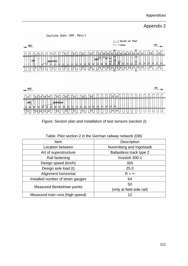
Appendices
121
Appendix 2
Figure: Section plan and installation of test sensors (section 2)
Table: Pilot section 2 in the German railway network (DB)
Item Description
Location between Nuremberg and Ingolstadt
Art of superstructure Ballastless track type 2
Rail fastening Vossloh 300-1
Design speed (km/h) 300
Design axle load (t) 25.0
Alignment horizontal R = ∞
Installed number of strain gauges 64
Measured Benkelman points 50
(only at field side rail)
Measured train runs (high speed) 12
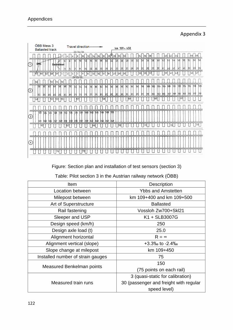
Appendices
122
Appendix 3
Figure: Section plan and installation of test sensors (section 3)
Table: Pilot section 3 in the Austrian railway network (ÖBB)
Item Description
Location between Ybbs and Amstetten
Milepost between km 109+400 and km 109+500
Art of Superstructure Ballasted
Rail fastening Vossloh Zw700+Skl21
Sleeper and USP K1 + SLB3007G
Design speed (km/h) 250
Design axle load (t) 25.0
Alignment horizontal R = ∞
Alignment vertical (slope) +3.3‰ to -2.4‰
Slope change at milepost km 109+450
Installed number of strain gauges 75
Measured Benkelman points 150
(75 points on each rail)
Measured train runs
3 (quasi-static for calibration)
30 (passenger and freight with regular
speed level)
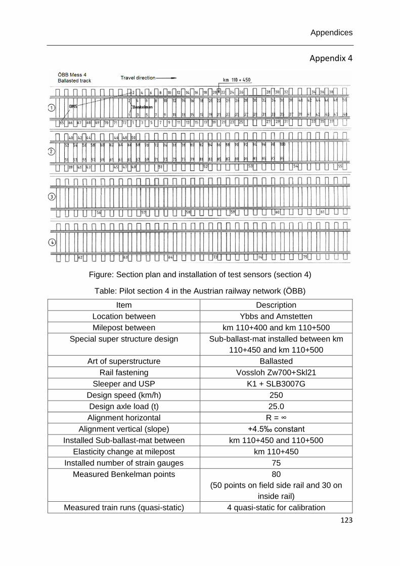
Appendices
123
Appendix 4
Figure: Section plan and installation of test sensors (section 4)
Table: Pilot section 4 in the Austrian railway network (ÖBB)
Item Description
Location between Ybbs and Amstetten
Milepost between km 110+400 and km 110+500
Special super structure design Sub-ballast-mat installed between km
110+450 and km 110+500
Art of superstructure Ballasted
Rail fastening Vossloh Zw700+Skl21
Sleeper and USP K1 + SLB3007G
Design speed (km/h) 250
Design axle load (t) 25.0
Alignment horizontal R = ∞
Alignment vertical (slope) +4.5‰ constant
Installed Sub-ballast-mat between km 110+450 and 110+500
Elasticity change at milepost km 110+450
Installed number of strain gauges 75
Measured Benkelman points
80
(50 points on field side rail and 30 on
inside rail)
Measured train runs (quasi-static) 4 quasi-static for calibration

Appendices
124
Appendix 5
Figure: 3D track geometry (Section 1, 2013)

Appendices
125
Appendix 6
Figure: 3D track geometry (Section 2, 2013)
switch
Appendices
126
Appendix 7
Figure: 3D track geometry (Section 3, 2012)
switch

Appendices
127
Appendix 8
Figure: 3D track geometry (Section 3, 2014)
bridge
Appendices
128
Appendix 9
Figure: 3D track geometry (Section 4, 2012)
bridge
Appendices
129
Appendix 10
Figure: 3D track geometry (Section 4, 2014)
bridge

Appendices
130
Appendix 11
Figure: Measured maximum rail and slab deflection (Section 1, 2005 and 2013)
Figure: Measured maximum rail and slab deflection (Section 2, 2013)
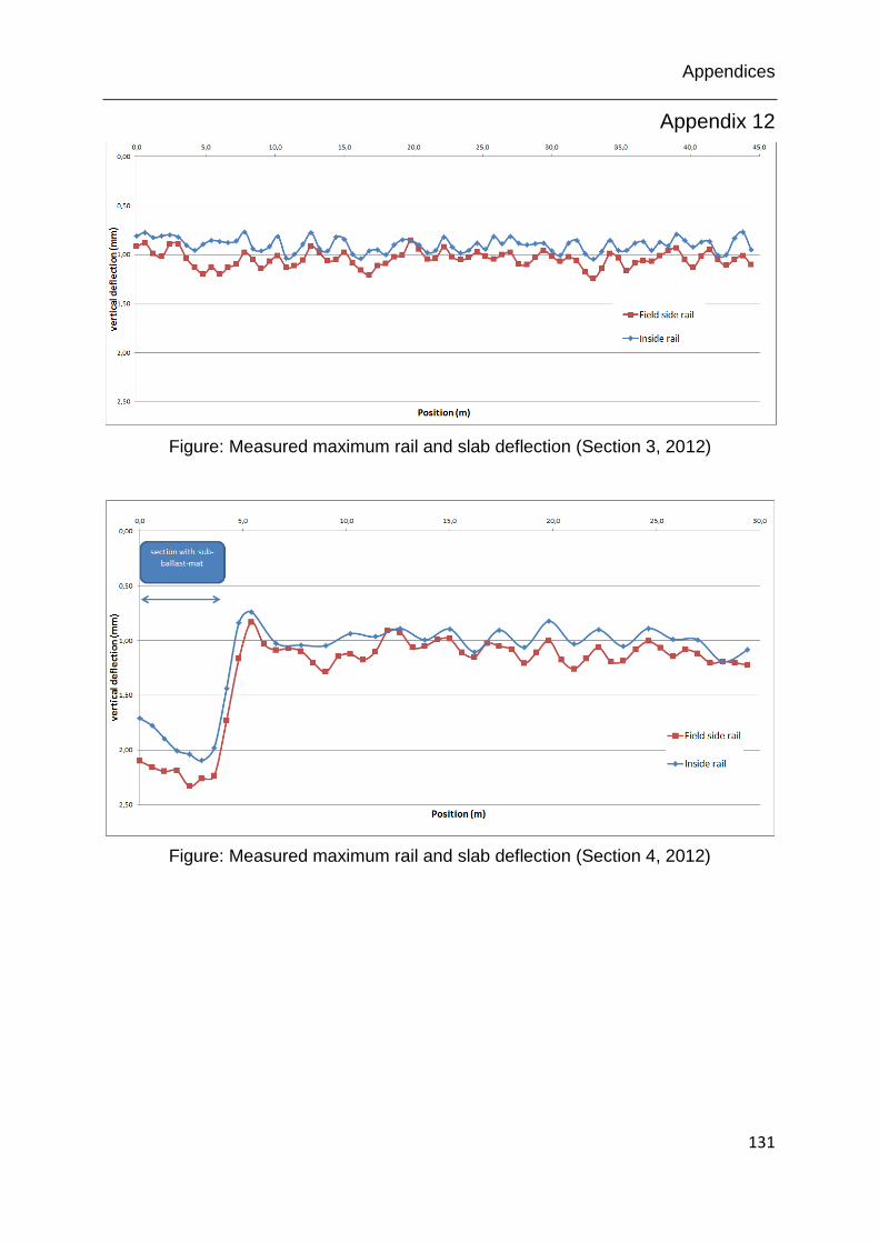
Appendices
131
Appendix 12
Figure: Measured maximum rail and slab deflection (Section 3, 2012)
Figure: Measured maximum rail and slab deflection (Section 4, 2012)

Appendices
132
Appendix 13
Table: Calculated deflection line (Section 3, field side rail)
RS1 RS2 RS3 RS4 RS5 RS6 RS7 RS8 RS9
0 m 0.6 m 1.2 m 1.8 m 2.4 m 3 m 3.6 m 4.2 m 4.8 m
Z1 0.92
Z3 0.89 0.62
Z5 0.99 0.53 0.22
Z7 1.02 0.59 0.21 0.02
Z9 0.90 0.64 0.25 0.03 -0.02
Z11 0.89 0.50 0.19 0.03 -0.01 -0.01
Z13 1.04 0.58 0.10 -0.02 -0.05 0.00 0.00
Z15 1.13 0.72 0.20 -0.05 -0.04 -0.03 0.00 0.01
Z17 1.20 0.72 0.32 0.01 -0.08 -0.01 -0.01 0.00 0.01
Z19 1.13 0.77 0.24 0.07 -0.01 -0.06 -0.01 0.00 0.00
Z21 1.20 0.81 0.30 0.00 -0.02 -0.01 -0.04 0.00 0.00
Z23 1.13 0.86 0.32 0.04 -0.07 -0.03 0.00 -0.03 0.00
Z25 1.10 0.65 0.35 0.04 -0.04 -0.07 -0.02 0.00 -0.03
Z27 0.98 0.70 0.15 0.04 -0.04 -0.05 -0.03 0.00 0.00
Z29 1.05 0.67 0.25 -0.01 -0.08 -0.05 -0.02 -0.02 0.00
Z31 1.14 0.73 0.28 0.02 -0.08 -0.08 -0.03 -0.01 -0.01
Z33 1.07 0.76 0.31 0.06 -0.03 -0.05 -0.03 -0.01 0.00
Z35 1.01 0.59 0.23 0.02 -0.02 0.00 0.01 -0.01 0.00
Z37 1.13 0.73 0.16 0.01 -0.06 -0.04 0.00 0.01 -0.01
Z39 1.12 0.79 0.31 -0.03 -0.05 -0.07 -0.02 0.00 0.01
Z41 1.06 0.75 0.36 0.09 -0.06 -0.04 -0.04 -0.01 -0.01
Z43 0.92 0.59 0.27 0.08 0.00 -0.04 -0.01 0.00 0.00
Z45 0.99 0.57 0.14 -0.01 -0.07 -0.04 -0.02 0.01 0.00
Z47 1.06 0.60 0.18 -0.05 -0.08 -0.07 -0.03 -0.02 0.01
Z49 1.05 0.67 0.22 -0.02 -0.06 -0.07 -0.05 -0.02 -0.01
Z51 0.98 0.67 0.20 0.00 -0.05 -0.03 -0.03 -0.03 0.00
Z53 1.09 0.66 0.21 -0.03 -0.08 -0.05 -0.01 -0.03 0.00
Z55 1.16 0.68 0.27 -0.02 -0.05 -0.06 -0.03 -0.01 0.01
Z57 1.21 0.76 0.27 0.01 -0.06 -0.03 -0.04 -0.01 -0.01
Z59 1.11 0.72 0.26 0.04 0.00 -0.03 0.00 -0.01 -0.01
Z61 1.10 0.82 0.24 0.00 0.00 0.00 -0.01 0.00 0.00
Z63 1.03 0.75 0.34 -0.01 -0.08 0.00 0.00 -0.01 0.00
Z65 1.01 0.67 0.26 0.07 -0.04 -0.07 0.01 0.00 0.00
Z67 0.86 0.63 0.16 0.03 -0.03 -0.01 -0.06 0.01 0.00
Z69 0.95 0.58 0.19 -0.06 -0.03 -0.03 0.00 -0.04 0.01
Z71 1.05 0.56 0.17 0.01 -0.07 -0.01 -0.02 0.01 -0.01
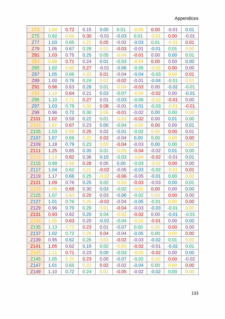
Appendices
133
Z73 1.04 0.72 0.15 0.00 0.01 -0.05 0.00 -0.01 0.01
Z75 0.92 0.64 0.30 -0.01 -0.03 0.01 -0.01 0.00 -0.01
Z77 1.03 0.65 0.21 0.05 -0.02 -0.03 0.01 -0.01 0.01
Z79 1.06 0.67 0.28 0.01 -0.03 -0.01 -0.01 0.01 0.00
Z81 1.03 0.75 0.25 0.05 -0.04 -0.01 0.00 0.00 0.01
Z83 0.98 0.71 0.24 0.01 -0.03 -0.04 0.00 0.00 0.00
Z85 1.02 0.60 0.27 -0.01 -0.06 -0.05 -0.02 0.00 0.00
Z87 1.05 0.66 0.22 0.01 -0.04 -0.04 -0.03 0.00 0.01
Z89 1.00 0.76 0.24 0.02 -0.02 -0.01 -0.04 -0.01 0.01
Z91 0.98 0.63 0.28 0.01 -0.04 -0.03 0.00 -0.02 -0.01
Z93 1.10 0.64 0.21 0.03 -0.07 -0.04 -0.02 0.00 -0.01
Z95 1.10 0.71 0.27 0.01 -0.03 -0.06 -0.02 -0.01 0.00
Z97 1.03 0.78 0.30 0.08 -0.01 -0.01 -0.03 -0.01 -0.01
Z99 0.96 0.72 0.30 0.06 -0.01 -0.02 0.00 0.00 0.00
Z101 1.02 0.59 0.22 0.01 -0.03 -0.02 0.00 0.01 0.00
Z103 1.07 0.67 0.23 0.00 -0.04 -0.02 0.00 0.00 0.01
Z105 1.03 0.69 0.25 0.02 -0.01 -0.02 0.00 0.00 0.01
Z107 1.07 0.69 0.22 0.02 -0.04 0.00 0.00 0.00 0.00
Z109 1.18 0.79 0.23 0.00 -0.04 -0.03 0.00 0.00 0.00
Z111 1.25 0.85 0.35 0.01 -0.05 -0.04 -0.02 0.01 0.00
Z113 1.14 0.82 0.36 0.10 -0.03 -0.04 -0.02 -0.01 0.01
Z115 0.99 0.68 0.28 0.05 0.00 -0.03 -0.02 0.00 0.00
Z117 1.04 0.62 0.21 -0.02 -0.05 -0.03 -0.02 -0.01 0.01
Z119 1.17 0.66 0.25 -0.02 -0.06 -0.05 -0.01 0.00 0.00
Z121 1.09 0.76 0.25 0.02 -0.03 -0.03 -0.03 0.00 0.01
Z123 1.06 0.69 0.30 0.03 -0.02 -0.01 0.00 0.00 0.00
Z125 1.07 0.64 0.20 0.03 -0.06 -0.02 0.00 0.00 0.00
Z127 1.01 0.76 0.20 -0.02 -0.04 -0.05 -0.01 0.00 0.00
Z129 0.96 0.70 0.29 0.01 -0.04 -0.03 -0.03 -0.01 0.00
Z131 0.93 0.62 0.20 0.04 -0.02 -0.02 0.00 -0.01 -0.01
Z133 1.05 0.63 0.20 -0.02 -0.04 -0.02 -0.01 0.00 0.00
Z135 1.13 0.72 0.23 0.01 -0.07 0.00 0.00 0.00 0.00
Z137 1.02 0.72 0.29 0.04 -0.04 -0.05 0.00 0.00 0.00
Z139 0.95 0.62 0.26 0.03 -0.02 -0.03 -0.02 0.01 0.00
Z141 1.05 0.62 0.19 0.02 -0.03 -0.02 -0.01 -0.02 0.01
Z143 1.11 0.71 0.23 0.00 -0.03 -0.03 -0.02 0.00 0.00
Z145 1.05 0.70 0.23 0.00 -0.07 -0.02 -0.02 0.00 -0.02
Z147 1.01 0.65 0.22 0.02 -0.02 -0.04 0.00 0.00 0.00
Z149 1.10 0.72 0.24 0.01 -0.05 -0.02 -0.02 0.00 0.00
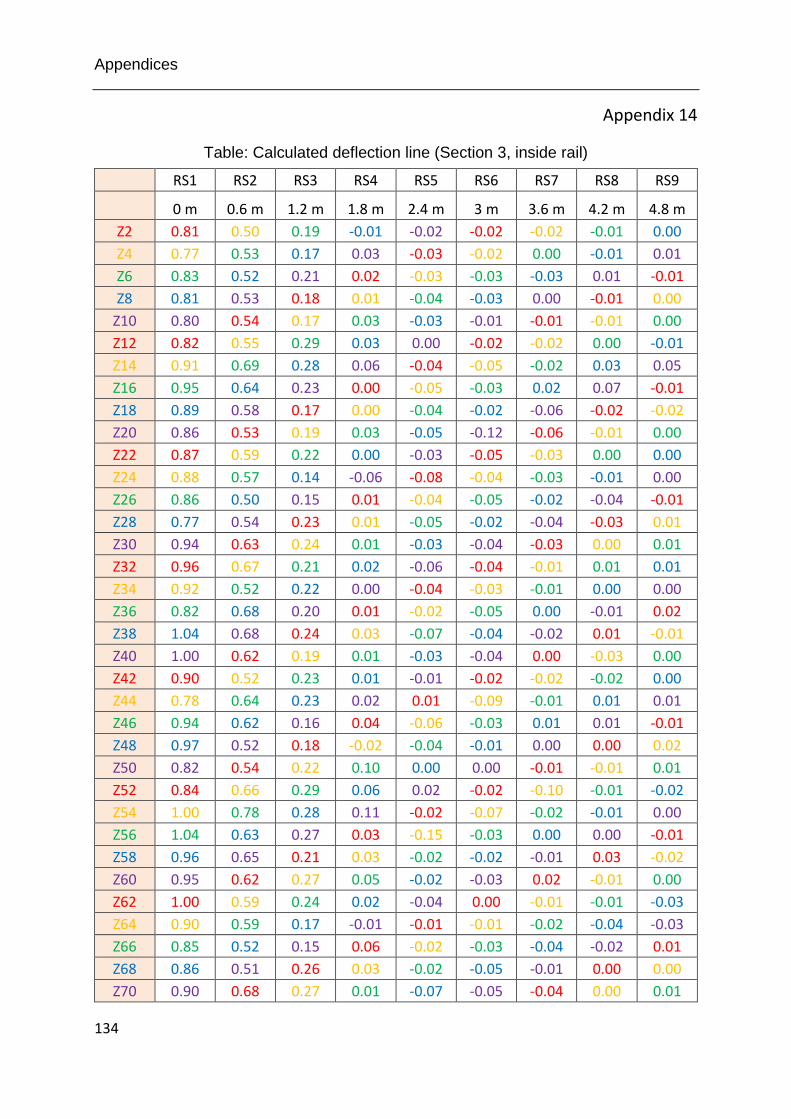
Appendices
134
Appendix 14
Table: Calculated deflection line (Section 3, inside rail)
RS1 RS2 RS3 RS4 RS5 RS6 RS7 RS8 RS9
0 m 0.6 m 1.2 m 1.8 m 2.4 m 3 m 3.6 m 4.2 m 4.8 m
Z2 0.81 0.50 0.19 -0.01 -0.02 -0.02 -0.02 -0.01 0.00
Z4 0.77 0.53 0.17 0.03 -0.03 -0.02 0.00 -0.01 0.01
Z6 0.83 0.52 0.21 0.02 -0.03 -0.03 -0.03 0.01 -0.01
Z8 0.81 0.53 0.18 0.01 -0.04 -0.03 0.00 -0.01 0.00
Z10 0.80 0.54 0.17 0.03 -0.03 -0.01 -0.01 -0.01 0.00
Z12 0.82 0.55 0.29 0.03 0.00 -0.02 -0.02 0.00 -0.01
Z14 0.91 0.69 0.28 0.06 -0.04 -0.05 -0.02 0.03 0.05
Z16 0.95 0.64 0.23 0.00 -0.05 -0.03 0.02 0.07 -0.01
Z18 0.89 0.58 0.17 0.00 -0.04 -0.02 -0.06 -0.02 -0.02
Z20 0.86 0.53 0.19 0.03 -0.05 -0.12 -0.06 -0.01 0.00
Z22 0.87 0.59 0.22 0.00 -0.03 -0.05 -0.03 0.00 0.00
Z24 0.88 0.57 0.14 -0.06 -0.08 -0.04 -0.03 -0.01 0.00
Z26 0.86 0.50 0.15 0.01 -0.04 -0.05 -0.02 -0.04 -0.01
Z28 0.77 0.54 0.23 0.01 -0.05 -0.02 -0.04 -0.03 0.01
Z30 0.94 0.63 0.24 0.01 -0.03 -0.04 -0.03 0.00 0.01
Z32 0.96 0.67 0.21 0.02 -0.06 -0.04 -0.01 0.01 0.01
Z34 0.92 0.52 0.22 0.00 -0.04 -0.03 -0.01 0.00 0.00
Z36 0.82 0.68 0.20 0.01 -0.02 -0.05 0.00 -0.01 0.02
Z38 1.04 0.68 0.24 0.03 -0.07 -0.04 -0.02 0.01 -0.01
Z40 1.00 0.62 0.19 0.01 -0.03 -0.04 0.00 -0.03 0.00
Z42 0.90 0.52 0.23 0.01 -0.01 -0.02 -0.02 -0.02 0.00
Z44 0.78 0.64 0.23 0.02 0.01 -0.09 -0.01 0.01 0.01
Z46 0.94 0.62 0.16 0.04 -0.06 -0.03 0.01 0.01 -0.01
Z48 0.97 0.52 0.18 -0.02 -0.04 -0.01 0.00 0.00 0.02
Z50 0.82 0.54 0.22 0.10 0.00 0.00 -0.01 -0.01 0.01
Z52 0.84 0.66 0.29 0.06 0.02 -0.02 -0.10 -0.01 -0.02
Z54 1.00 0.78 0.28 0.11 -0.02 -0.07 -0.02 -0.01 0.00
Z56 1.04 0.63 0.27 0.03 -0.15 -0.03 0.00 0.00 -0.01
Z58 0.96 0.65 0.21 0.03 -0.02 -0.02 -0.01 0.03 -0.02
Z60 0.95 0.62 0.27 0.05 -0.02 -0.03 0.02 -0.01 0.00
Z62 1.00 0.59 0.24 0.02 -0.04 0.00 -0.01 -0.01 -0.03
Z64 0.90 0.59 0.17 -0.01 -0.01 -0.01 -0.02 -0.04 -0.03
Z66 0.85 0.52 0.15 0.06 -0.02 -0.03 -0.04 -0.02 0.01
Z68 0.86 0.51 0.26 0.03 -0.02 -0.05 -0.01 0.00 0.00
Z70 0.90 0.68 0.27 0.01 -0.07 -0.05 -0.04 0.00 0.01

Appendices
135
Z72 0.98 0.62 0.17 -0.04 -0.09 -0.05 0.00 0.00 -0.04
Z74 0.96 0.51 0.14 -0.05 -0.04 -0.02 -0.01 -0.01 0.01
Z76 0.82 0.53 0.13 0.06 -0.01 -0.01 0.00 0.00 0.00
Z78 0.92 0.59 0.28 0.05 -0.01 0.00 -0.02 -0.01 0.00
Z80 0.98 0.66 0.24 0.05 0.00 -0.04 -0.01 0.00 0.01
Z82 0.96 0.60 0.24 -0.01 -0.03 -0.02 -0.01 0.04 0.03
Z84 0.88 0.63 0.12 0.03 -0.02 -0.01 0.03 0.03 0.02
Z86 0.95 0.52 0.22 0.02 -0.01 0.01 0.00 0.02 0.02
Z88 0.82 0.56 0.20 0.04 -0.04 0.00 0.00 0.01 -0.01
Z90 0.89 0.53 0.19 0.00 0.00 0.00 0.01 0.00 -0.01
Z92 0.81 0.55 0.20 0.05 -0.01 0.00 -0.02 0.01 0.01
Z94 0.89 0.57 0.23 0.05 -0.03 -0.04 -0.01 0.01 0.00
Z96 0.90 0.53 0.25 -0.01 -0.06 -0.02 0.00 0.00 0.01
Z98 0.89 0.60 0.14 -0.04 -0.03 -0.01 -0.02 0.02 0.03
Z100 0.88 0.49 0.23 0.02 -0.01 -0.03 0.03 0.01 0.00
Z102 0.96 0.66 0.22 0.03 -0.04 0.01 -0.02 -0.01 0.04
Z104 1.01 0.61 0.23 0.01 -0.01 -0.05 -0.01 0.03 0.01
Z106 0.88 0.56 0.23 0.05 -0.02 -0.01 0.01 0.01 -0.01
Z108 0.86 0.69 0.30 0.04 -0.02 0.00 0.00 -0.01 -0.01
Z110 0.99 0.75 0.24 0.03 0.00 -0.01 -0.02 -0.01 0.03
Z112 1.05 0.61 0.21 0.06 -0.03 -0.03 -0.03 0.04 0.01
Z114 0.97 0.54 0.29 0.00 -0.04 -0.04 0.03 0.01 0.01
Z116 0.85 0.67 0.25 0.01 -0.04 0.02 0.00 0.00 0.00
Z118 0.96 0.66 0.21 0.00 0.00 -0.03 -0.02 0.00 0.00
Z120 0.96 0.57 0.17 0.02 -0.05 -0.04 -0.01 0.00 0.01
Z122 0.89 0.52 0.18 0.01 -0.03 -0.01 0.00 0.01 0.00
Z124 0.87 0.61 0.20 0.05 -0.01 -0.02 0.01 0.00 0.01
Z126 0.96 0.59 0.30 0.01 -0.04 0.00 0.00 0.00 0.00
Z128 0.88 0.65 0.18 0.00 -0.02 -0.01 0.00 0.00 0.02
Z130 0.91 0.53 0.15 0.00 -0.02 -0.02 -0.01 0.01 0.00
Z132 0.80 0.52 0.20 -0.01 -0.03 -0.01 0.00 0.00 0.00
Z134 0.86 0.62 0.16 0.00 -0.02 -0.04 0.00 0.00 0.00
Z136 0.92 0.55 0.16 -0.01 -0.05 -0.03 0.00 0.01
Z138 0.87 0.52 0.21 0.00 -0.03 0.00 -0.01
Z140 0.87 0.63 0.24 0.04 -0.01 -0.03
Z142 1.01 0.67 0.25 0.00 -0.05
Z144 1.00 0.60 0.12 -0.01
Z146 0.83 0.44 0.14
Z148 0.77 0.56
Z150 0.95
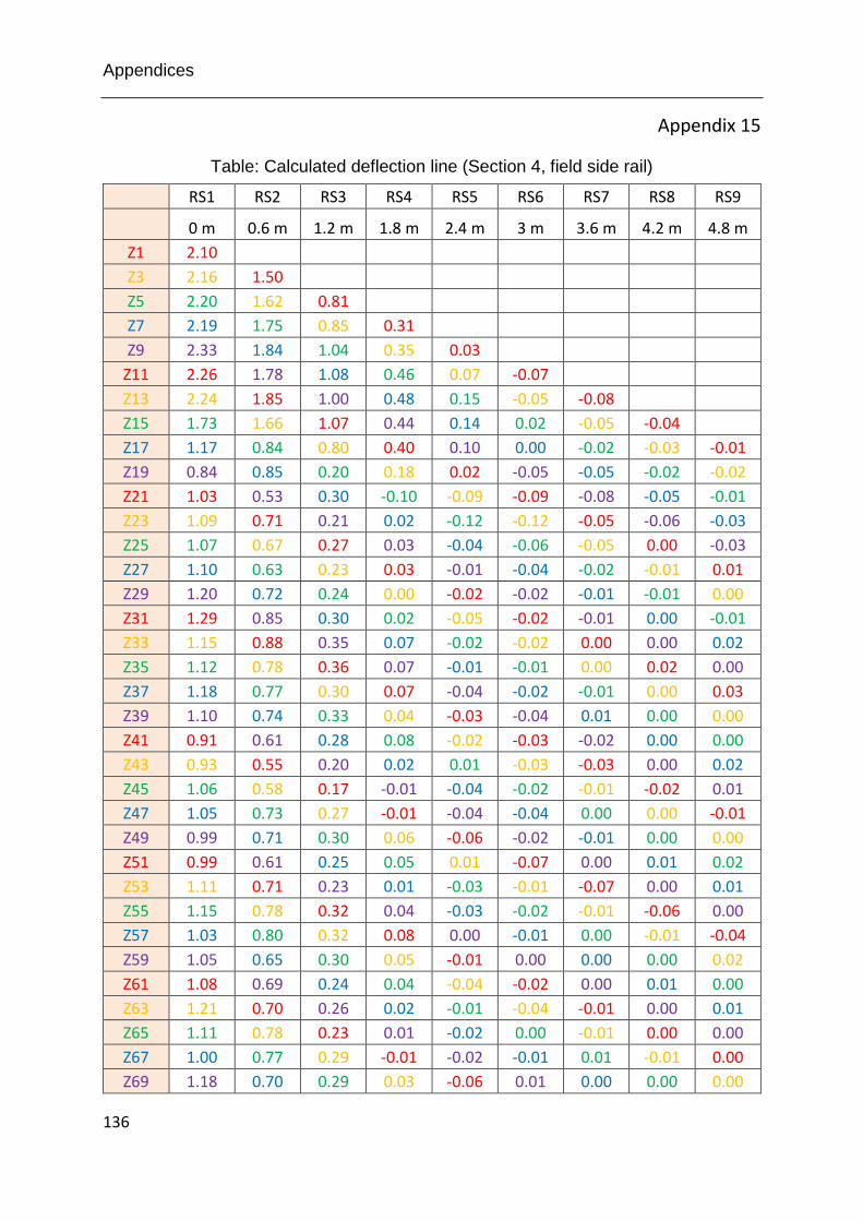
Appendices
136
Appendix 15
Table: Calculated deflection line (Section 4, field side rail)
RS1 RS2 RS3 RS4 RS5 RS6 RS7 RS8 RS9
0 m 0.6 m 1.2 m 1.8 m 2.4 m 3 m 3.6 m 4.2 m 4.8 m
Z1 2.10
Z3 2.16 1.50
Z5 2.20 1.62 0.81
Z7 2.19 1.75 0.85 0.31
Z9 2.33 1.84 1.04 0.35 0.03
Z11 2.26 1.78 1.08 0.46 0.07 -0.07
Z13 2.24 1.85 1.00 0.48 0.15 -0.05 -0.08
Z15 1.73 1.66 1.07 0.44 0.14 0.02 -0.05 -0.04
Z17 1.17 0.84 0.80 0.40 0.10 0.00 -0.02 -0.03 -0.01
Z19 0.84 0.85 0.20 0.18 0.02 -0.05 -0.05 -0.02 -0.02
Z21 1.03 0.53 0.30 -0.10 -0.09 -0.09 -0.08 -0.05 -0.01
Z23 1.09 0.71 0.21 0.02 -0.12 -0.12 -0.05 -0.06 -0.03
Z25 1.07 0.67 0.27 0.03 -0.04 -0.06 -0.05 0.00 -0.03
Z27 1.10 0.63 0.23 0.03 -0.01 -0.04 -0.02 -0.01 0.01
Z29 1.20 0.72 0.24 0.00 -0.02 -0.02 -0.01 -0.01 0.00
Z31 1.29 0.85 0.30 0.02 -0.05 -0.02 -0.01 0.00 -0.01
Z33 1.15 0.88 0.35 0.07 -0.02 -0.02 0.00 0.00 0.02
Z35 1.12 0.78 0.36 0.07 -0.01 -0.01 0.00 0.02 0.00
Z37 1.18 0.77 0.30 0.07 -0.04 -0.02 -0.01 0.00 0.03
Z39 1.10 0.74 0.33 0.04 -0.03 -0.04 0.01 0.00 0.00
Z41 0.91 0.61 0.28 0.08 -0.02 -0.03 -0.02 0.00 0.00
Z43 0.93 0.55 0.20 0.02 0.01 -0.03 -0.03 0.00 0.02
Z45 1.06 0.58 0.17 -0.01 -0.04 -0.02 -0.01 -0.02 0.01
Z47 1.05 0.73 0.27 -0.01 -0.04 -0.04 0.00 0.00 -0.01
Z49 0.99 0.71 0.30 0.06 -0.06 -0.02 -0.01 0.00 0.00
Z51 0.99 0.61 0.25 0.05 0.01 -0.07 0.00 0.01 0.02
Z53 1.11 0.71 0.23 0.01 -0.03 -0.01 -0.07 0.00 0.01
Z55 1.15 0.78 0.32 0.04 -0.03 -0.02 -0.01 -0.06 0.00
Z57 1.03 0.80 0.32 0.08 0.00 -0.01 0.00 -0.01 -0.04
Z59 1.05 0.65 0.30 0.05 -0.01 0.00 0.00 0.00 0.02
Z61 1.08 0.69 0.24 0.04 -0.04 -0.02 0.00 0.01 0.00
Z63 1.21 0.70 0.26 0.02 -0.01 -0.04 -0.01 0.00 0.01
Z65 1.11 0.78 0.23 0.01 -0.02 0.00 -0.01 0.00 0.00
Z67 1.00 0.77 0.29 -0.01 -0.02 -0.01 0.01 -0.01 0.00
Z69 1.18 0.70 0.29 0.03 -0.06 0.01 0.00 0.00 0.00
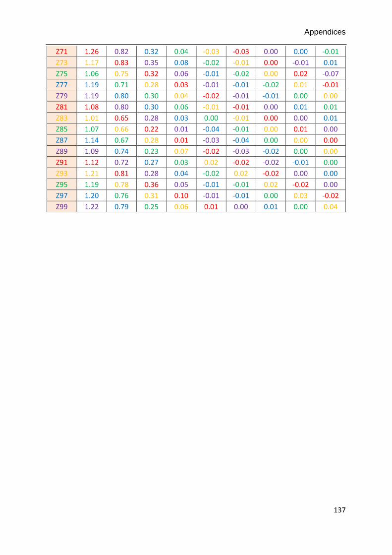
Appendices
137
Z71 1.26 0.82 0.32 0.04 -0.03 -0.03 0.00 0.00 -0.01
Z73 1.17 0.83 0.35 0.08 -0.02 -0.01 0.00 -0.01 0.01
Z75 1.06 0.75 0.32 0.06 -0.01 -0.02 0.00 0.02 -0.07
Z77 1.19 0.71 0.28 0.03 -0.01 -0.01 -0.02 0.01 -0.01
Z79 1.19 0.80 0.30 0.04 -0.02 -0.01 -0.01 0.00 0.00
Z81 1.08 0.80 0.30 0.06 -0.01 -0.01 0.00 0.01 0.01
Z83 1.01 0.65 0.28 0.03 0.00 -0.01 0.00 0.00 0.01
Z85 1.07 0.66 0.22 0.01 -0.04 -0.01 0.00 0.01 0.00
Z87 1.14 0.67 0.28 0.01 -0.03 -0.04 0.00 0.00 0.00
Z89 1.09 0.74 0.23 0.07 -0.02 -0.03 -0.02 0.00 0.00
Z91 1.12 0.72 0.27 0.03 0.02 -0.02 -0.02 -0.01 0.00
Z93 1.21 0.81 0.28 0.04 -0.02 0.02 -0.02 0.00 0.00
Z95 1.19 0.78 0.36 0.05 -0.01 -0.01 0.02 -0.02 0.00
Z97 1.20 0.76 0.31 0.10 -0.01 -0.01 0.00 0.03 -0.02
Z99 1.22 0.79 0.25 0.06 0.01 0.00 0.01 0.00 0.04
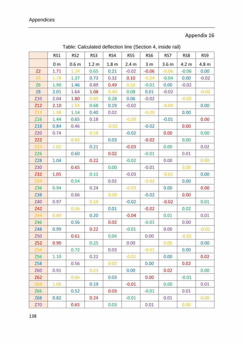
Appendices
138
Appendix 16
Table: Calculated deflection line (Section 4, inside rail)
RS1 RS2 RS3 RS4 RS5 RS6 RS7 RS8 RS9
0 m 0.6 m 1.2 m 1.8 m 2.4 m 3 m 3.6 m 4.2 m 4.8 m
Z2 1.71 1.24 0.65 0.21 -0.02 -0.06 -0.06 -0.06 0.00
Z4 1.78 1.37 0.73 0.32 0.10 -0.04 -0.04 0.00 -0.02
Z6 1.90 1.46 0.89 0.49 0.10 -0.01 0.00 -0.02
Z8 2.01 1.64 1.08 0.40 0.08 0.01 -0.02 -0.02
Z10 2.04 1.80 0.89 0.28 0.06 -0.02 -0.02
Z12 2.10 1.54 0.68 0.19 -0.02 -0.04 0.00
Z14 1.98 1.14 0.40 0.02 -0.09 0.00
Z16 1.44 0.65 0.18 -0.09 -0.01 0.00
Z18 0.84 0.46 -0.02 -0.02 0.00
Z20 0.74 0.18 -0.02 0.00 0.00
Z22 0.65 0.03 -0.02 0.00
Z24 1.02 0.21 -0.03 0.00 0.02
Z26 0.60 0.02 -0.01 0.01
Z28 1.04 0.22 -0.02 0.00 0.00
Z30 0.65 0.00 -0.01 0.00
Z32 1.05 0.12 -0.03 -0.01 0.00
Z34 0.54 0.02 -0.02 0.00
Z36 0.94 0.24 -0.03 0.00 0.00
Z38 0.66 0.00 -0.02 0.00
Z40 0.97 0.19 -0.02 -0.02 0.01
Z42 0.56 0.01 -0.02 0.02
Z44 0.89 0.20 -0.04 0.01 0.01
Z46 0.56 0.02 -0.01 0.00
Z48 0.99 0.22 -0.01 0.00 -0.01
Z50 0.61 0.04 0.00 -0.02
Z52 0.90 0.25 0.00 0.00 0.00
Z54 0.72 0.03 -0.01 0.00
Z56 1.10 0.22 -0.02 0.00 0.02
Z58 0.56 0.02 0.00 0.02
Z60 0.91 0.23 0.00 0.02 0.00
Z62 0.66 0.03 0.00 -0.01
Z64 1.06 0.19 -0.01 0.00 0.01
Z66 0.52 0.03 -0.01 0.01
Z68 0.82 0.24 -0.01 0.01 0.00
Z70 0.65 0.03 0.01 0.00

Appendices
139
Z72 1.03 0.23 0.00 0.00 -0.01
Z74 0.62 0.05 -0.01 -0.01
Z76 0.90 0.31 0.00 -0.01 0.01
Z78 0.75 0.03 -0.02 0.00
Z80 1.05 0.22 -0.02 -0.02 -0.01
Z82 0.58 0.01 -0.03 -0.01
Z84 0.89 0.18 -0.03 -0.01 0.00
Z86 0.58 0.03 -0.02 0.00
Z88 0.99 0.25 -0.04 -0.01
Z90 0.61 0.05 -0.01
Z92 0.99 0.35 -0.01
Z94 0.85 0.04
Z96 1.19 0.29
Z98 0.70
Z100 1.09
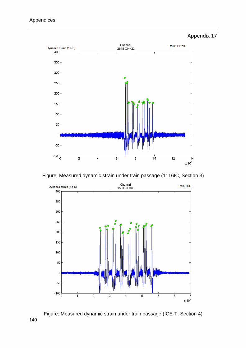
Appendices
140
Appendix 17
Figure: Measured dynamic strain under train passage (1116IC, Section 3)
Figure: Measured dynamic strain under train passage (ICE-T, Section 4)

Appendices
141
Appendix 18
Figure: Measured dynamic strain under train passage (Railjet, Section 3)
Figure: Measured dynamic strain under train passage (Stadler KISS, Section 4)
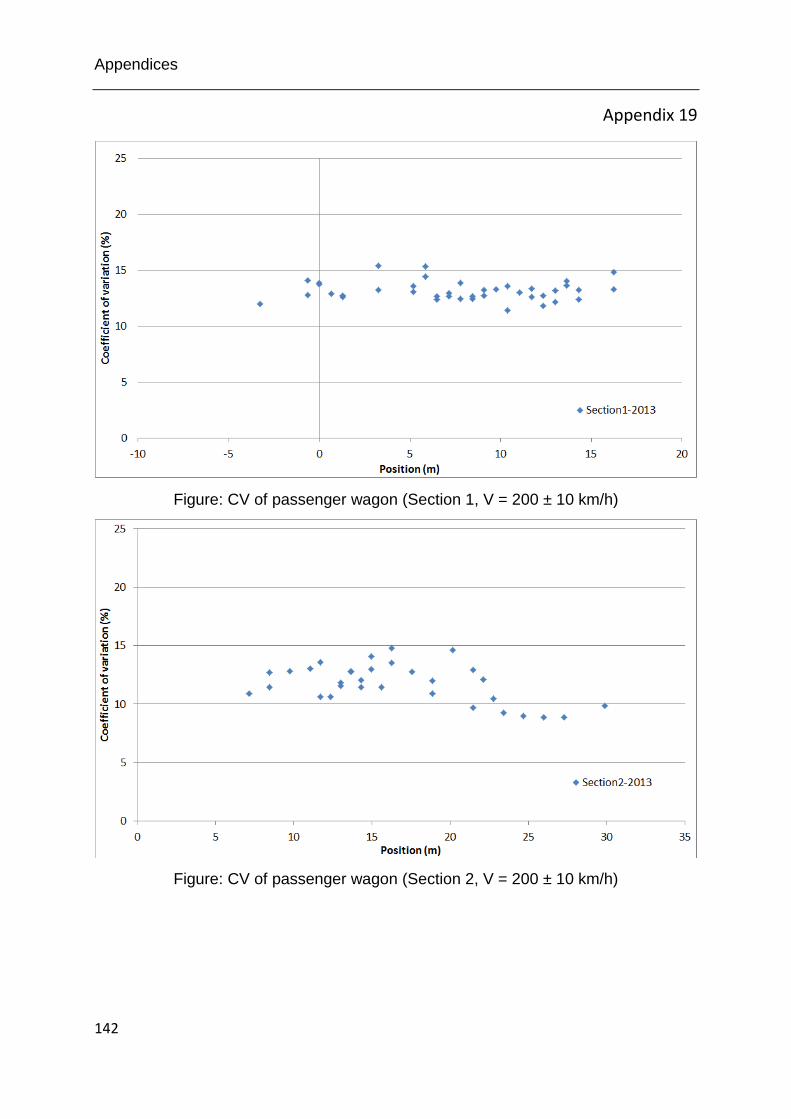
Appendices
142
Appendix 19
Figure: CV of passenger wagon (Section 1, V = 200 ± 10 km/h)
Figure: CV of passenger wagon (Section 2, V = 200 ± 10 km/h)
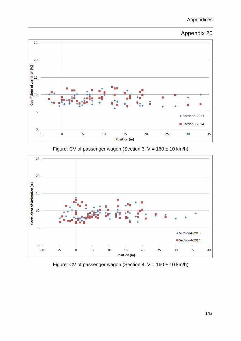
Appendices
143
Appendix 20
Figure: CV of passenger wagon (Section 3, V = 160 ± 10 km/h)
Figure: CV of passenger wagon (Section 4, V = 160 ± 10 km/h)
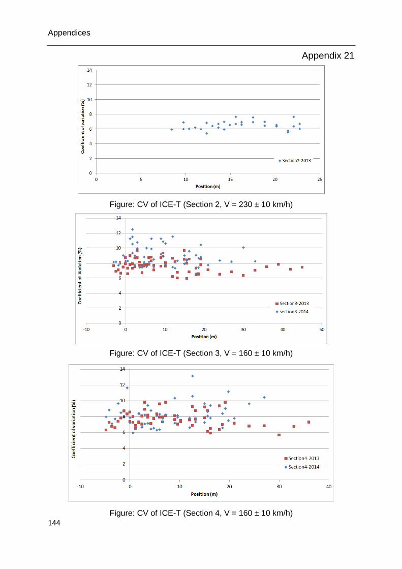
Appendices
144
Appendix 21
Figure: CV of ICE-T (Section 2, V = 230 ± 10 km/h)
Figure: CV of ICE-T (Section 3, V = 160 ± 10 km/h)
Figure: CV of ICE-T (Section 4, V = 160 ± 10 km/h)
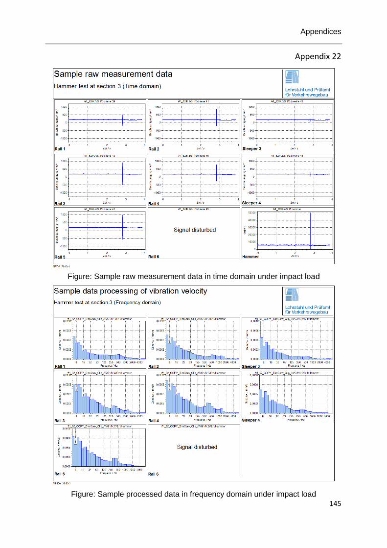
Appendices
145
Appendix 22
Figure: Sample raw measurement data in time domain under impact load
Figure: Sample processed data in frequency domain under impact load
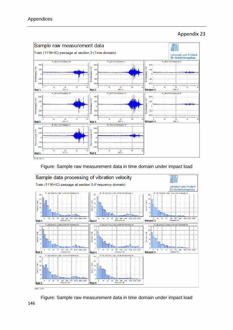
Appendices
146
Appendix 23
Figure: Sample raw measurement data in time domain under impact load
Figure: Sample raw measurement data in time domain under impact load
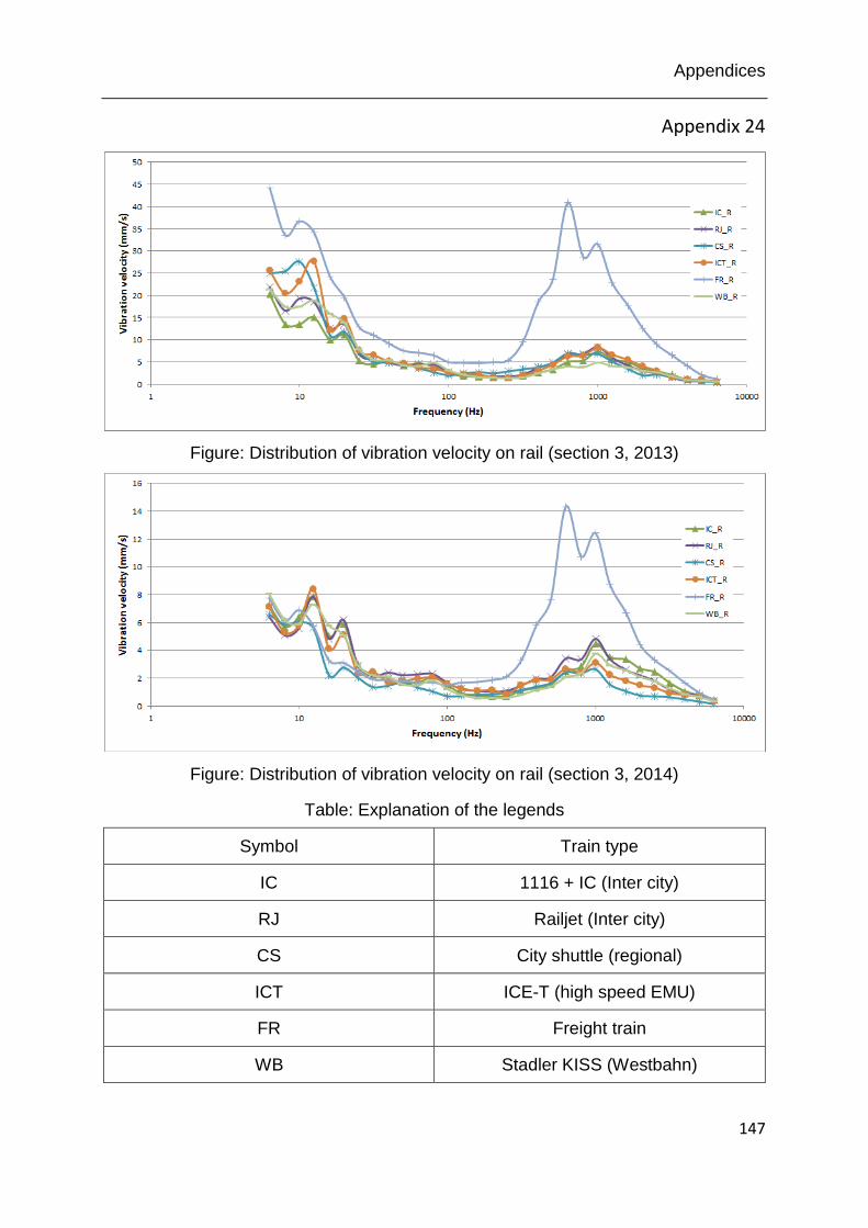
Appendices
147
Appendix 24
Figure: Distribution of vibration velocity on rail (section 3, 2013)
Figure: Distribution of vibration velocity on rail (section 3, 2014)
Table: Explanation of the legends
Symbol Train type
IC 1116 + IC (Inter city)
RJ Railjet (Inter city)
CS City shuttle (regional)
ICT ICE-T (high speed EMU)
FR Freight train
WB Stadler KISS (Westbahn)
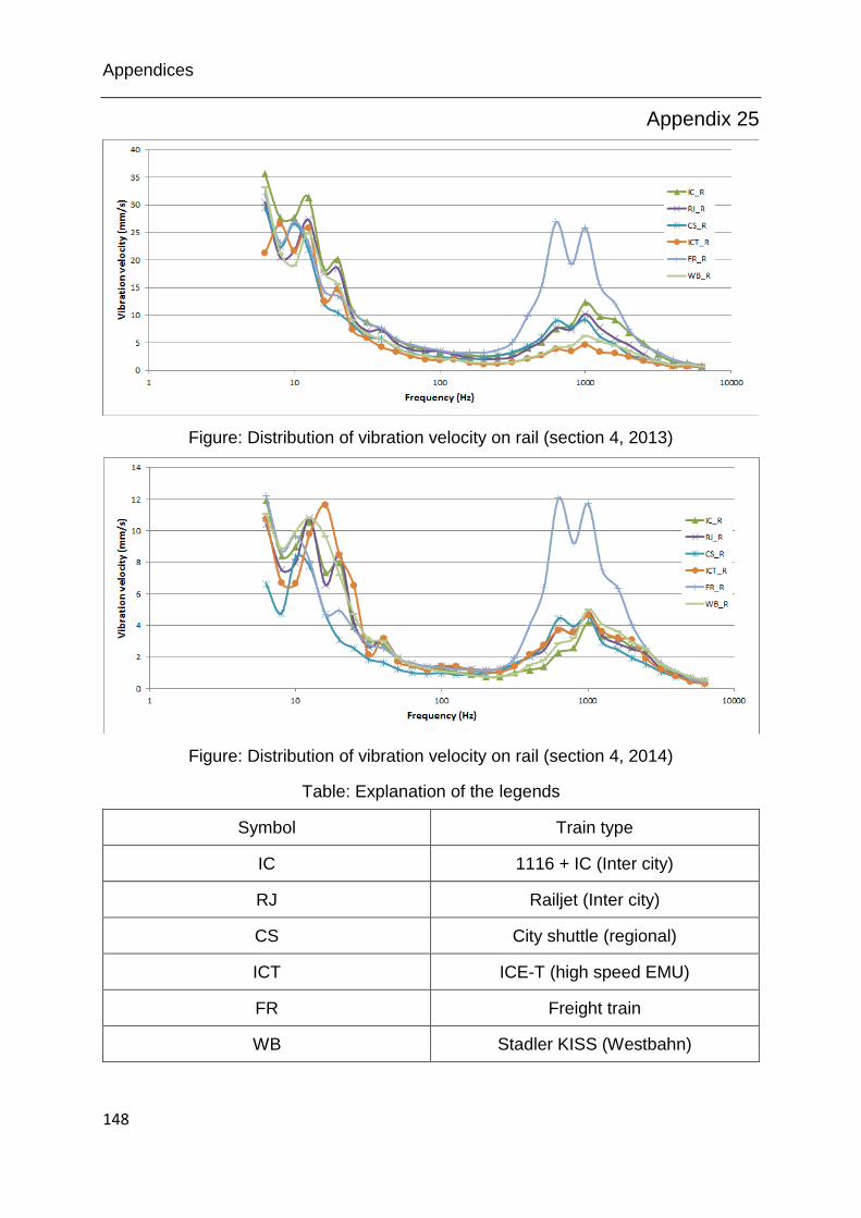
Appendices
148
Appendix 25
Figure: Distribution of vibration velocity on rail (section 4, 2013)
Figure: Distribution of vibration velocity on rail (section 4, 2014)
Table: Explanation of the legends
Symbol Train type
IC 1116 + IC (Inter city)
RJ Railjet (Inter city)
CS City shuttle (regional)
ICT ICE-T (high speed EMU)
FR Freight train
WB Stadler KISS (Westbahn)
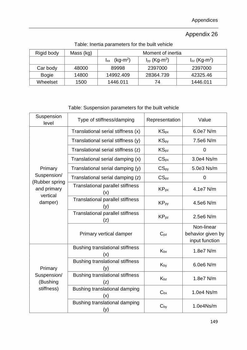
Appendices
149
Appendix 26
Table: Inertia parameters for the built vehicle
Rigid body Mass (kg) Moment of inertia
Ixx (kg-m2) Iyy (Kg-m2) Izz (Kg-m2)
Car body 48000 89998 2397000 2397000
Bogie 14800 14992.409 28364.739 42325.46
Wheelset 1500 1446.011 74 1446.011
Table: Suspension parameters for the built vehicle
Suspension
level Type of stiffness/damping Representation Value
Primary
Suspension/
(Rubber spring
and primary
vertical
damper)
Translational serial stiffness (x) KSpx 6.0e7 N/m
Translational serial stiffness (y) KSpy 7.5e6 N/m
Translational serial stiffness (z) KSpz 0
Translational serial damping (x) CSpx 3.0e4 Ns/m
Translational serial damping (y) CSpy 5.0e3 Ns/m
Translational serial damping (z) CSpz 0
Translational parallel stiffness
(x) KPpx 4.1e7 N/m
Translational parallel stiffness
(y) KPpy 4.5e6 N/m
Translational parallel stiffness
(z) KPpz 2.5e6 N/m
Primary vertical damper Cpz
Non-linear
behavior given by
input function
Primary
Suspension/
(Bushing
stiffness)
Bushing translational stiffness
(x) Kbx 1.8e7 N/m
Bushing translational stiffness
(y) Kby 6.0e6 N/m
Bushing translational stiffness
(z) Kbz 1.8e7 N/m
Bushing translational damping
(x) Cbx 1.0e4 Ns/m
Bushing translational damping
(y) Cby 1.0e4Ns/m

Appendices
150
Bushing translational damping
(z) Cbz 3.0e3 Ns/m
Bushing rotational stiffness (al) Kbal 2.3e3 N/m
Bushing rotational stiffness (be) Kbbe 3.0e3 N/m
Bushing rotational stiffness (ga) Kbga 2.8e3N/m
Bushing rotational damping (al) Cbal 70 Ns/m
Bushing rotational damping (be) Cbbe 50 Ns/m
Bushing rotational damping (ga) Cbga 90 Ns/m
Secondary
suspension
(Secondary
shear spring
and damping
elements)
Longitudinal Shear stiffness Ksx 2.5e5 N/m
Lateral shear stiffness Ksy 2.5e5 N/m
Vertical stiffness Ksz 8.91e6 N/m
Roll bending stiffness Kr 1.05e4 N/m
Pitch bending stiffness Kp 1.05e4 N/m
Torsion stiffness Kt 0
Secondary vertical damper
(mounting stiffness) Km 6.0e6 N/m
Secondary vertical damper
(damping) Csz 4.5e4 Ns/m
Secondary horizontal (or lateral)
damper Csy
Non-linear
behavior given by
input function
Secondary longitudinal or yaw
damping Csx
Non-linear
behavior given by
input function
Anti-roll bar Stiffness K 9.4e5 Nm/rad
Traction rod Stiffness K 5.0e6 N/m
Damping C 2.5e4 Ns/m
Bump Stop Stiffness K
Non-linear
behavior given by
input function
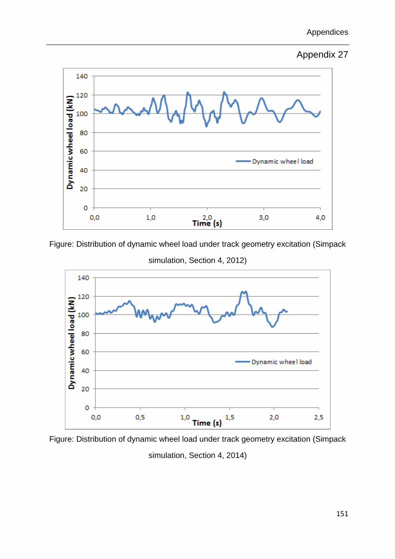
Appendices
151
Appendix 27
Figure: Distribution of dynamic wheel load under track geometry excitation (Simpack
simulation, Section 4, 2012)
Figure: Distribution of dynamic wheel load under track geometry excitation (Simpack
simulation, Section 4, 2014)
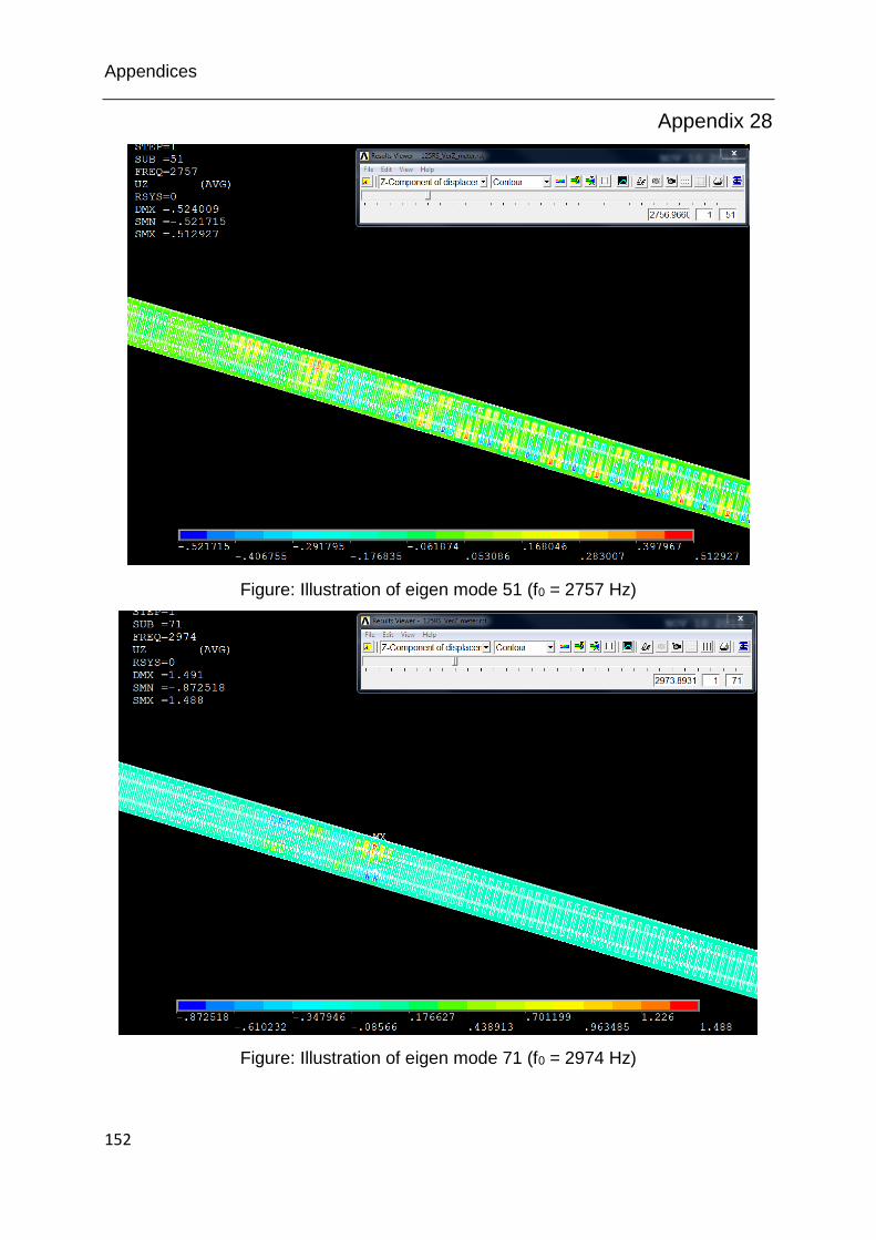
Appendices
152
Appendix 28
Figure: Illustration of eigen mode 51 (f0 = 2757 Hz)
Figure: Illustration of eigen mode 71 (f0 = 2974 Hz)
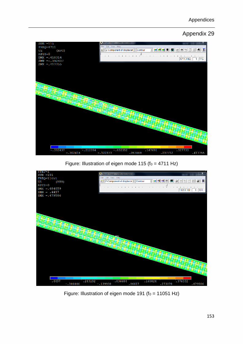
Appendices
153
Appendix 29
Figure: Illustration of eigen mode 115 (f0 = 4711 Hz)
Figure: Illustration of eigen mode 191 (f0 = 11051 Hz)
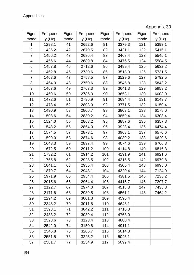
Appendices
154
Appendix 30
Eigen
mode
Frequenc
y (Hz)
Eigen
mode
Frequenc
y (Hz)
Eigen
mode
Frequenc
y (Hz)
Eigen
mode
Frequenc
y (Hz)
1 1298.1 41 2652.6 81 3379.3 121 5393.1
2 1436.2 42 2679.5 82 3421.1 122 5416.1
3 1456.2 43 2686.4 83 3468.4 123 5545.1
4 1456.6 44 2689.8 84 3476.5 124 5584.5
5 1457.8 45 2712.6 85 3499.4 125 5632.2
6 1462.8 46 2730.6 86 3518.0 126 5731.5
7 1463.6 47 2758.5 87 3529.6 127 5792.5
8 1464.3 48 2760.6 88 3545.8 128 5843.2
9 1467.6 49 2767.3 89 3641.3 129 5953.2
10 1469.6 50 2786.3 90 3658.1 130 6003.9
11 1472.6 51 2796.9 91 3694.4 131 6143.7
12 1478.4 52 2803.0 92 3771.5 132 6150.4
13 1490.9 53 2806.7 93 3803.1 133 6178.6
14 1503.6 54 2830.2 94 3859.4 134 6303.4
15 1524.0 55 2863.2 95 3887.6 135 6357.3
16 1543.2 56 2864.0 96 3923.4 136 6474.4
17 1574.5 57 2873.1 97 3968.1 137 6570.6
18 1599.0 58 2874.6 98 4039.2 138 6620.6
19 1643.3 59 2897.4 99 4074.6 139 6766.3
20 1672.5 60 2911.2 100 4114.8 140 6816.3
21 1732.2 61 2914.2 101 4191.9 141 6921.6
22 1765.8 62 2928.5 102 4215.5 142 6979.8
23 1841.1 63 2935.4 103 4306.4 143 6995.0
24 1879.7 64 2948.1 104 4320.4 144 7124.9
25 1971.9 65 2954.4 105 4381.5 145 7235.2
26 2015.6 66 2964.4 106 4415.7 146 7297.7
27 2122.7 67 2974.0 107 4518.3 147 7435.8
28 2171.6 68 2989.5 108 4561.1 148 7464.2
29 2294.2 69 3001.3 109 4596.4
30 2348.2 70 3011.8 110 4648.1
31 2393.1 71 3042.2 111 4715.8
32 2483.2 72 3089.4 112 4763.0
33 2528.6 73 3123.4 113 4880.4
34 2542.0 74 3150.8 114 4911.1
35 2546.8 75 3206.7 115 5014.3
36 2551.5 76 3225.2 116 5045.1
37 2581.7 77 3234.9 117 5099.4

Appendices
155
38 2592.5 78 3263.1 118 5184.0
39 2598.7 79 3308.6 119 5224.7
40 2630.4 80 3322.5 120 5282.9
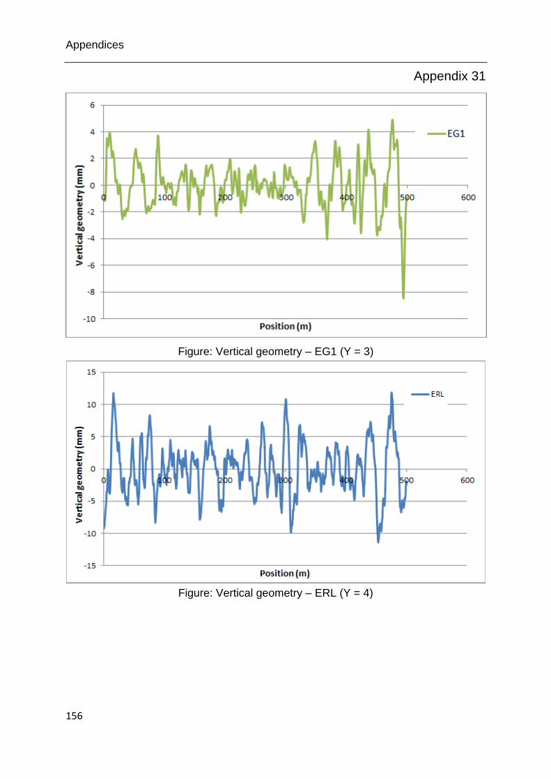
Appendices
156
Appendix 31
Figure: Vertical geometry – EG1 (Y = 3)
Figure: Vertical geometry – ERL (Y = 4)
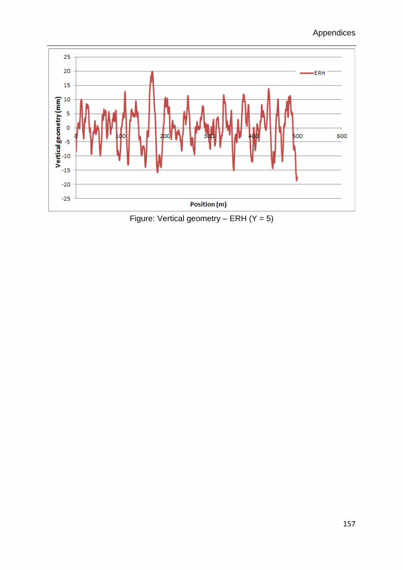
Appendices
157
Figure: Vertical geometry – ERH (Y = 5)
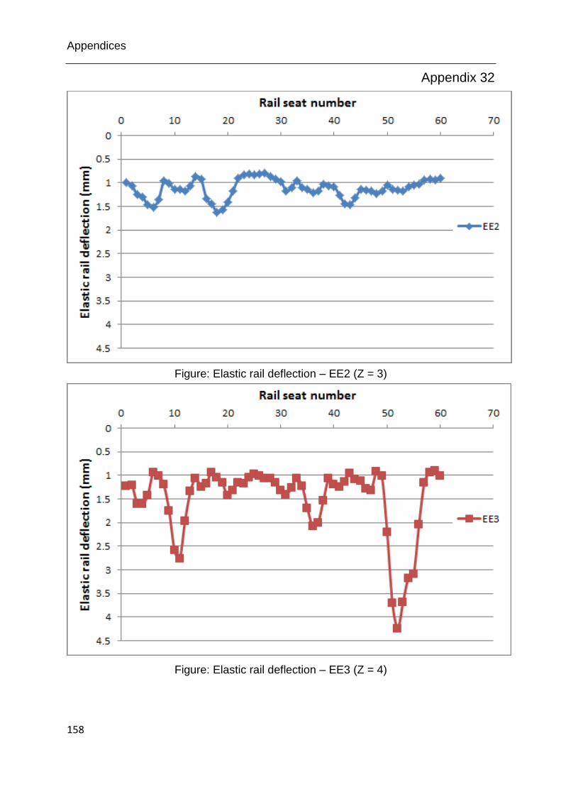
Appendices
158
Appendix 32
Figure: Elastic rail deflection – EE2 (Z = 3)
Figure: Elastic rail deflection – EE3 (Z = 4)

Appendices
159
Appendix 33
Figure: ESD output of selected X and Y combinations (Z = 0)
Figure: ESD output of selected X and Z combinations
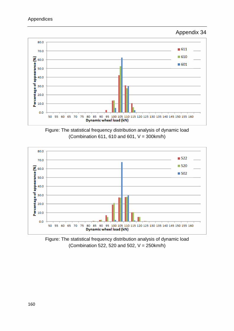
Appendices
160
Appendix 34
Figure: The statistical frequency distribution analysis of dynamic load
(Combination 611, 610 and 601, V = 300km/h)
Figure: The statistical frequency distribution analysis of dynamic load
(Combination 522, 520 and 502, V = 250km/h)
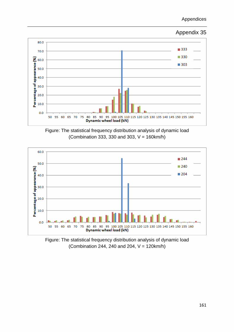
Appendices
161
Appendix 35
Figure: The statistical frequency distribution analysis of dynamic load
(Combination 333, 330 and 303, V = 160km/h)
Figure: The statistical frequency distribution analysis of dynamic load
(Combination 244, 240 and 204, V = 120km/h)

Appendices
162
Appendix 36
Figure: The statistical frequency distribution analysis of dynamic load
(Combination 154, 150 and 104, V = 80km/h)
Annexes and user instructions (UI)
163
Annexes and user instructions
List of annexes and user instructions
Item Page
Annex 1 163
Annex 2 164
Annex 3 165
Annex 4 166
Annex 5 167
Annex 6 168
Annex 7 169
User instruction 1 170
User instruction 2 172
User instruction 3 174

Annexes and user instructions (UI)
164
Annex 1
Pic 1: Overview of measurement section 3 (Ballasted track A-ÖBB)
Pic 2: Overview of measurement section 4 (Ballasted track with/without sub-ballast-
mat A-ÖBB)

Annexes and user instructions (UI)
165
Annex 2
Pic 3: Recording of track geometry by track recording wagon
Pic 4: Ballast wagon for test of Benkelman beam and quasi-static test runs
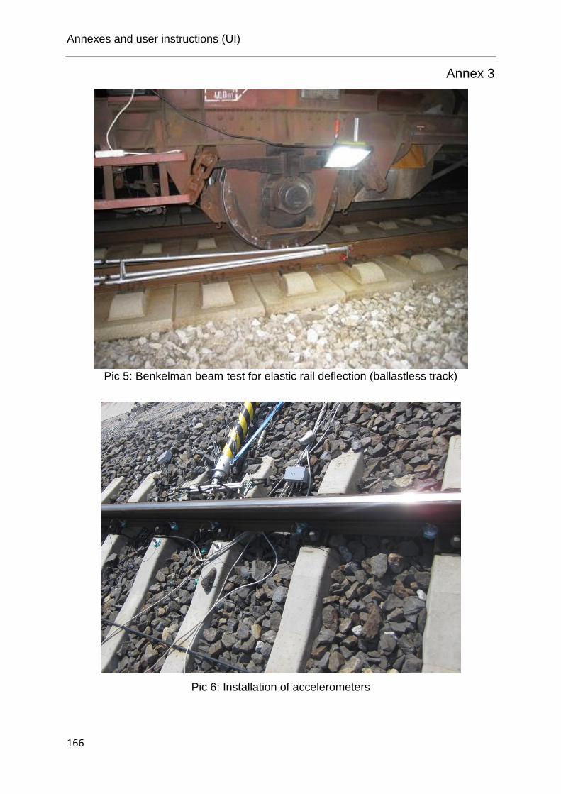
Annexes and user instructions (UI)
166
Annex 3
Pic 5: Benkelman beam test for elastic rail deflection (ballastless track)
Pic 6: Installation of accelerometers
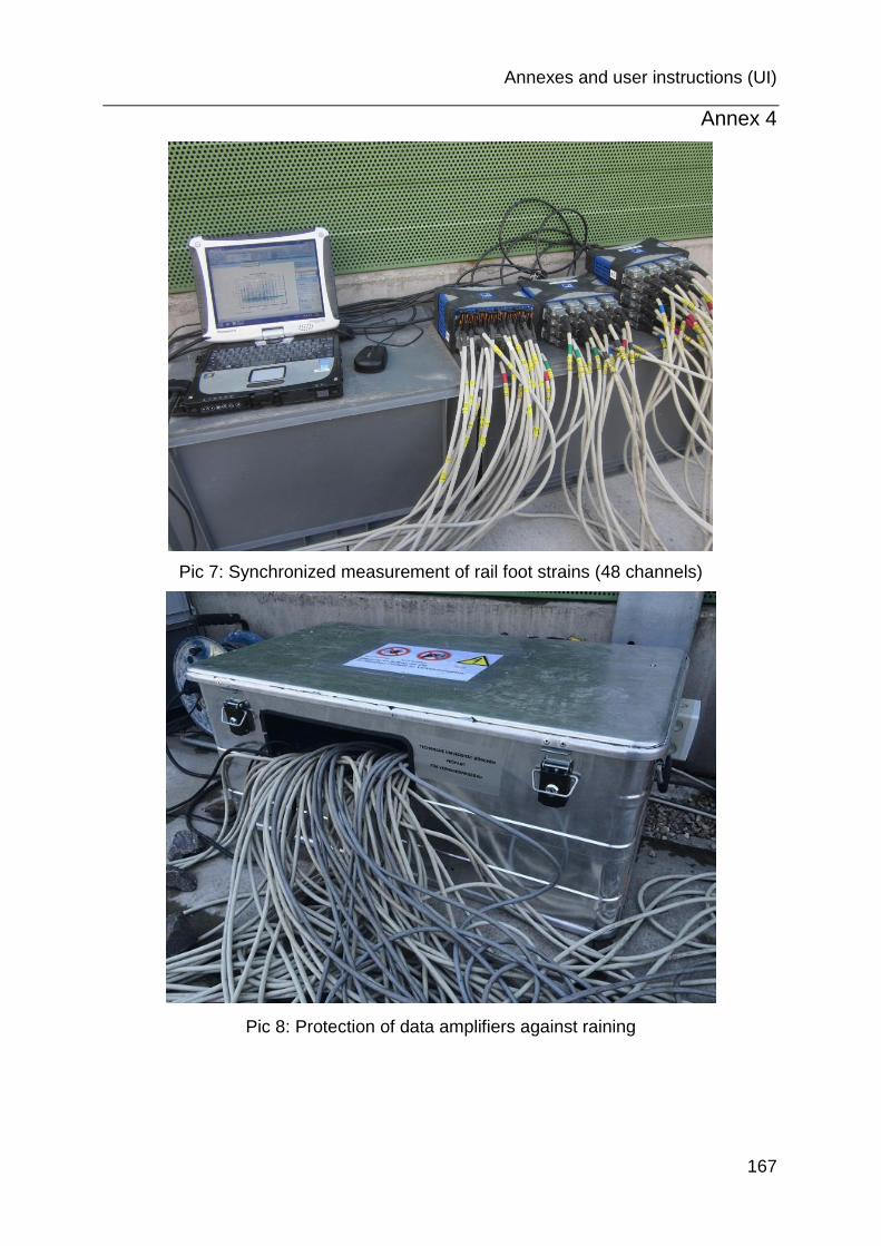
Annexes and user instructions (UI)
167
Annex 4
Pic 7: Synchronized measurement of rail foot strains (48 channels)
Pic 8: Protection of data amplifiers against raining

Annexes and user instructions (UI)
168
Annex 5
Pic 9: Built work station and data amplifiers for vibration measurement
Pic 10: Train passage in section 3 and 4 (Type Railjet)
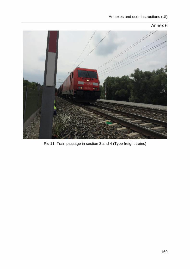
Annexes and user instructions (UI)
169
Annex 6
Pic 11: Train passage in section 3 and 4 (Type freight trains)
Annexes and user instructions (UI)
170
Annex 7
Level compensation in section 2 due to irregular settlement
Due to the fact of local, irregular settlement of the sub-structure (here: earthworks),
level compensation was done at the measurement section 2. The total height of shims
used for vertical rail adjustment varies from about 6 mm up to about 16 mm, which has
major consequences to the track level as well as track deflection in vertical directions.
Consequently the change of track quality is not related to the performance of the slab
track system but to the sub-structure performance. The figure shows the measured
track deflection and geometry.
Figure: Measured maximum rail deflection and vertical track geometry (Section 2)

Annexes and user instructions (UI)
171
User Instruction 1
Calculation of absolute track geometry in vertical and horizontal direction
based on measurement data from track recording wagon (Type CLS
from Vogel&Ploetscher)
Specify working directory of the work; Open Matlab program and GUI window
Step 1, Adjust respect measurement results to required position and load file
Annexes and user instructions (UI)
172
Direction Legend In Column Direction Legend In Column
Position Pos. B Gauge Spurweite D
Vertical A1/A2 G,H Cant Querhöhe E
Horizontal Pfeilhöhe C
Step 2, 3, Parameter selection (Length division, Wave length for vertical and
horizontal) and calculation
Step 4, Result output based on selected vertical channel (A1 or A2)
The result EXCEL sheet should be like the following (Direct importable as track
geometry excitation into Simpack):
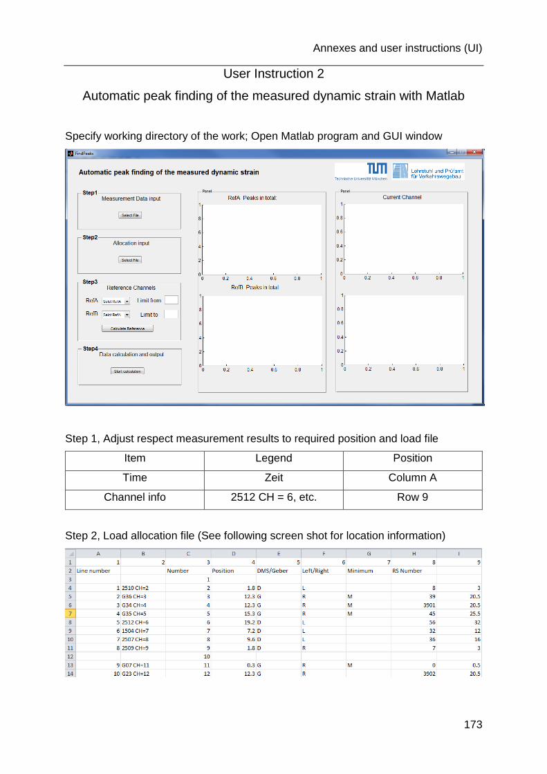
Annexes and user instructions (UI)
173
User Instruction 2
Automatic peak finding of the measured dynamic strain with Matlab
Specify working directory of the work; Open Matlab program and GUI window
Step 1, Adjust respect measurement results to required position and load file
Item Legend Position
Time Zeit Column A
Channel info 2512 CH = 6, etc. Row 9
Step 2, Load allocation file (See following screen shot for location information)
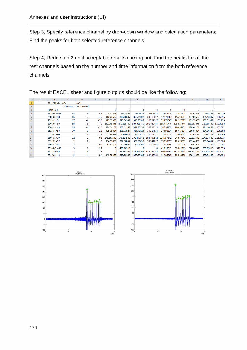
Annexes and user instructions (UI)
174
Step 3, Specify reference channel by drop-down window and calculation parameters;
Find the peaks for both selected reference channels
Step 4, Redo step 3 until acceptable results coming out; Find the peaks for all the
rest channels based on the number and time information from the both reference
channels
The result EXCEL sheet and figure outputs should be like the following:
Annexes and user instructions (UI)
175
User Instruction 3
Automatic calibration of the ANSYS model by Matlab controlled iterations
(Co-simulation with Matlab and ANSYS)
Specify working directory of the work; Open Matlab program and GUI window
Step 1, Specification of basic information for the co-simulation (Directory of ANSYS
program, number of rail seats for calibration, pad elasticity in N/mm²)
Step 2, Adjust respect measurement results to required position and load file (File for
left and right rail being loaded separately)
Item Position
Rail seat number Column A
Max. elastic deflection Column B
Elastic deflection in 0.6, 1.2, 1.8 m, etc. Columns C, D, E, …
Step 3, Provision of calculation parameters (applied wheel load in measurement for
left and right rail)
Step 4, Calculation and data output
The result EXCEL sheet and figure outputs should be like the following:
Annexes and user instructions (UI)
176
1, Output of max. rail deflection after each iteration step
2, Calculated elasticity of the ballast for each rail seat (direct importable into ANSYS
for Substructuring and modal analysis)
3, Overlapped results of the raw data and the calculated results from the last iteration
step