Tensor network ranks - University of Chicago Department of ...

TENSOR NETWORK RANKS

KE YE AND LEK-HENG LIM

Abstract. In problems involving approximation, completion, denoising, dimension reduction, es-timation, interpolation, modeling, order reduction, regression, etc, we argue that the near-universalpractice of assuming that a function, matrix, or tensor (which we will see are all the same object inthis context) has low rank may be ill-justified. There are many natural instances where the objectin question has high rank with respect to the classical notions of rank: matrix rank, tensor rank,multilinear rank — the latter two being the most straightforward generalizations of the former.To remedy this, we show that one may vastly expand these classical notions of ranks: Given anyundirected graph G, there is a notion of G-rank associated with G, which provides us with as manydifferent kinds of ranks as there are undirected graphs. In particular, the popular tensor networkstates in physics (e.g., mps, ttns, peps) may be regarded as functions of a specific G-rank forvarious choices of G. Among other things, we will see that a function, matrix, or tensor may havevery high matrix, tensor, or multilinear rank and yet very low G-rank for some G. In fact thedifference is in the orders of magnitudes and the gaps between G-ranks and these classical ranksare arbitrarily large for some important objects in computer science, mathematics, and physics.Furthermore, we show that there is a G such that almost every tensor has G-rank exponentiallylower than its rank or the dimension of its ambient space.

1. Introduction

A universal problem in science and engineering is to find a function from some given data. Thefunction may be a solution to a PDE with given boundary/initial data or a target function to belearned from a training set of data. In modern applications, one frequently encounters situationswhere the function lives in some state space or hypothesis space of prohibitively high dimension— a consequence of requiring very high accuracy solutions or having very large training sets. Acommon remedy with newfound popularity is to assume that the function has low rank, i.e., maybe expressed as a sum of a small number of separable terms. But such a low-rank assumption oftenhas weak or no justification; rank is chosen only because there is no other standard alternative.Taking a leaf from the enormously successful idea of tensor networks in physics [4, 7, 13, 23, 28,30, 31, 33, 34, 35, 36, 37, 38], we define a notion of G-rank for any undirected graph G. Like tensorrank and multilinear rank, which are extensions of matrix rank to higher order, G-ranks containmatrix rank as a special case.

Our definition of G-ranks shows that every tensor network — tensor trains, matrix productstates, tree tensor network states, star tensor network states, complete graph tensor network states,projected entangled pair states, multiscale entanglement renormalization ansatz, etc — is nothingmore than a set of functions/tensors of some G-rank for some undirected graph G. It becomesstraightforward to explain the effectiveness of tensor networks: They serve as a set of ‘low G-rankfunctions’ that can be used for various purposes (as an ansatz, a regression function, etc). Theflexibility of choosing G based on the underlying problem can provide a substantial computationaladvantage — a function with high rank or high H-rank for a graph H can have much lower G-rankfor another suitably chosen graph G. We will elaborate on these in the rest of this introduction,starting with an informal discussion of tensor networks and G-ranks, followed by an outline of ourmain results.

2010 Mathematics Subject Classification. 15A69, 41A30, 41A46, 41A65, 45L05, 65C60, 81P50, 81Q05.Key words and phrases. Tensor networks, tensor ranks, nonlinear approximations, best k-term approximations,

dimension reduction.

1

2 K. YE AND L.-H. LIM

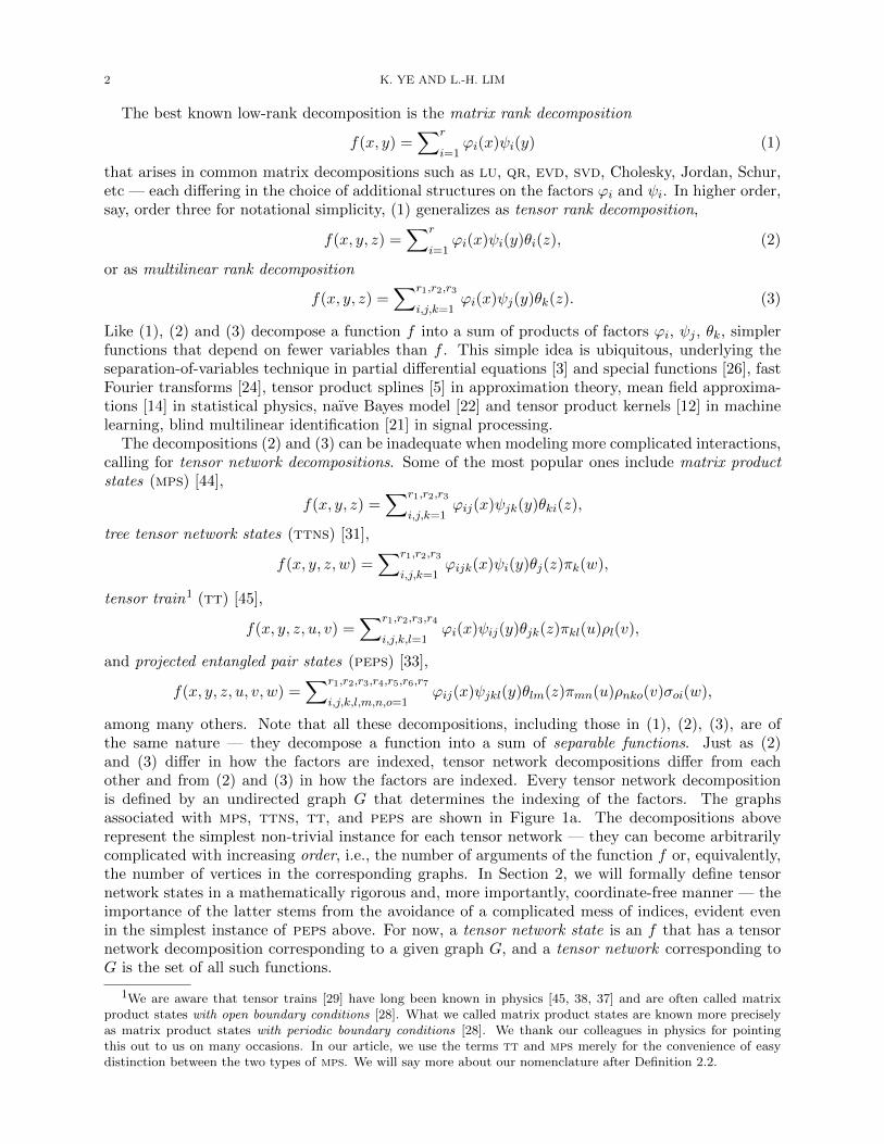
The best known low-rank decomposition is the matrix rank decomposition

f(x, y) =∑r

i=1ϕi(x)ψi(y) (1)

that arises in common matrix decompositions such as lu, qr, evd, svd, Cholesky, Jordan, Schur,etc — each differing in the choice of additional structures on the factors ϕi and ψi. In higher order,say, order three for notational simplicity, (1) generalizes as tensor rank decomposition,

f(x, y, z) =∑r

i=1ϕi(x)ψi(y)θi(z), (2)

or as multilinear rank decomposition

f(x, y, z) =∑r1,r2,r3

i,j,k=1ϕi(x)ψj(y)θk(z). (3)

Like (1), (2) and (3) decompose a function f into a sum of products of factors ϕi, ψj , θk, simplerfunctions that depend on fewer variables than f . This simple idea is ubiquitous, underlying theseparation-of-variables technique in partial differential equations [3] and special functions [26], fastFourier transforms [24], tensor product splines [5] in approximation theory, mean field approxima-tions [14] in statistical physics, naıve Bayes model [22] and tensor product kernels [12] in machinelearning, blind multilinear identification [21] in signal processing.

The decompositions (2) and (3) can be inadequate when modeling more complicated interactions,calling for tensor network decompositions. Some of the most popular ones include matrix productstates (mps) [44],

f(x, y, z) =∑r1,r2,r3

i,j,k=1ϕij(x)ψjk(y)θki(z),

tree tensor network states (ttns) [31],

f(x, y, z, w) =∑r1,r2,r3

i,j,k=1ϕijk(x)ψi(y)θj(z)πk(w),

tensor train1 (tt) [45],

f(x, y, z, u, v) =∑r1,r2,r3,r4

i,j,k,l=1ϕi(x)ψij(y)θjk(z)πkl(u)ρl(v),

and projected entangled pair states (peps) [33],

f(x, y, z, u, v, w) =∑r1,r2,r3,r4,r5,r6,r7

i,j,k,l,m,n,o=1ϕij(x)ψjkl(y)θlm(z)πmn(u)ρnko(v)σoi(w),

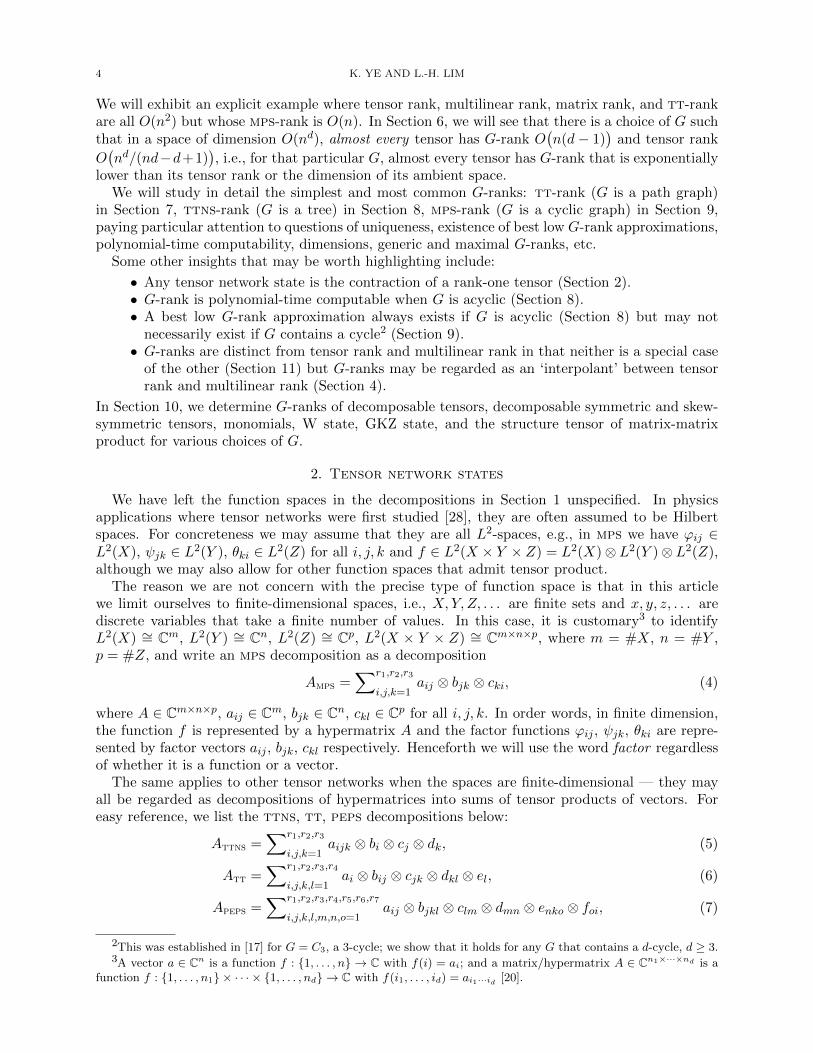
among many others. Note that all these decompositions, including those in (1), (2), (3), are ofthe same nature — they decompose a function into a sum of separable functions. Just as (2)and (3) differ in how the factors are indexed, tensor network decompositions differ from eachother and from (2) and (3) in how the factors are indexed. Every tensor network decompositionis defined by an undirected graph G that determines the indexing of the factors. The graphsassociated with mps, ttns, tt, and peps are shown in Figure 1a. The decompositions aboverepresent the simplest non-trivial instance for each tensor network — they can become arbitrarilycomplicated with increasing order, i.e., the number of arguments of the function f or, equivalently,the number of vertices in the corresponding graphs. In Section 2, we will formally define tensornetwork states in a mathematically rigorous and, more importantly, coordinate-free manner — theimportance of the latter stems from the avoidance of a complicated mess of indices, evident evenin the simplest instance of peps above. For now, a tensor network state is an f that has a tensornetwork decomposition corresponding to a given graph G, and a tensor network corresponding toG is the set of all such functions.

1We are aware that tensor trains [29] have long been known in physics [45, 38, 37] and are often called matrixproduct states with open boundary conditions [28]. What we called matrix product states are known more preciselyas matrix product states with periodic boundary conditions [28]. We thank our colleagues in physics for pointingthis out to us on many occasions. In our article, we use the terms tt and mps merely for the convenience of easydistinction between the two types of mps. We will say more about our nomenclature after Definition 2.2.

TENSOR NETWORK RANKS 3

tt

ϕ

i

ψ

j

θ

k

π

l

ρ

ttns

ψ

i

ϕ θ

j

k

π

mps

ϕ

j

ψkθ

i

peps

ϕ

j

ψ

l

θ

m

π

n

ρ

k

o

σ

i

(a) Graphs associated with common tensor networks.

rank

low G-rank

H: ambient space

solution

low rank

(b) G-rank versus rank.

Figure 1. Every undirected graph G defines a G-rank. Solution that we seek mayhave high rank but low G-rank.

The minimum r in (1) gives us the matrix rank of f ; the minimum r in (2) and the minimum(r1, r2, r3) in (3) give us the tensor rank and multilinear rank of f respectively. Informally, thetensor network rank or G-rank of f may be similarly defined by requiring some form of minimalityfor (r1, . . . , rc) in the other decompositions for mps, tt, ttns, peps (with an appropriate graph Gin each case). Note that this is no longer so straightforward since (i) Nc is not an ordered set whenc > 1; (ii) it is not clear that any function would have such a decomposition for an arbitrary G.

We will show in Section 4 that any d-variate function or d-tensor has a G-rank for any undirectedconnected graph G with d vertices. While this has been defined in special cases, particularly when Gis a path graph (tt-rank [10]) or more generally when G is a tree (hierarchical rank [9, Chapter 11]or tree rank [2]), we show that the notion is well-defined for any undirected connected graph G:Given any d vector spaces V1, . . . ,Vd of arbitrary dimensions, there is a class of tensor networkstates associated with G, as well as a G-rank for any T ∈ V1 ⊗ · · · ⊗ Vd; or equivalently, for anyfunction f ∈ L2(X1×· · ·×Xd); or, for those accustomed to working in terms of coordinates, for anyhypermatrix A ∈ Cn1×···×nd . See Section 2 for a discussion on the relations between these objects(d-tensors, d-variate functions, d-hypermatrices).

Formalizing the notions of tensor networks and G-ranks provides several advantages, the mostimportant of which is that it allows one to develop a rich calculus for working with tensor networks:deleting vertices, removing edges, restricting to subgraphs, taking unions of graphs, restricting tosubspaces, taking intersections of tensor network states, etc. We develop some of these basictechniques and properties in Sections 3 and 6, deferring to [39] the more involved properties thatare not needed for the rest of this article. Among other advantages, the notion of G-rank also shedslight on existing methods in scientific computing: In hindsight, the algorithm in [41] is one thatapproximates a given tensor network state by those of low G-rank.

The results in Section 5 may be viewed as the main impetus for tensor networks (as we pointedout earlier, these are ‘low G-rank tensors’ for various choices of G):

• a tensor may have very high matrix, tensor, or multilinear rank and yet very low G-rank;• a tensor may have very high H-rank and very low G-rank for G 6= H;


We will exhibit an explicit example where tensor rank, multilinear rank, matrix rank, and tt-rankare all O(n2) but whose mps-rank is O(n). In Section 6, we will see that there is a choice of G suchthat in a space of dimension O(nd), almost every tensor has G-rank O

(n(d− 1)

)and tensor rank

O(nd/(nd−d+1)

), i.e., for that particular G, almost every tensor has G-rank that is exponentially

lower than its tensor rank or the dimension of its ambient space.We will study in detail the simplest and most common G-ranks: tt-rank (G is a path graph)

in Section 7, ttns-rank (G is a tree) in Section 8, mps-rank (G is a cyclic graph) in Section 9,paying particular attention to questions of uniqueness, existence of best low G-rank approximations,polynomial-time computability, dimensions, generic and maximal G-ranks, etc.

Some other insights that may be worth highlighting include:

• Any tensor network state is the contraction of a rank-one tensor (Section 2).• G-rank is polynomial-time computable when G is acyclic (Section 8).• A best low G-rank approximation always exists if G is acyclic (Section 8) but may not

necessarily exist if G contains a cycle2 (Section 9).• G-ranks are distinct from tensor rank and multilinear rank in that neither is a special case

of the other (Section 11) but G-ranks may be regarded as an ‘interpolant’ between tensorrank and multilinear rank (Section 4).

In Section 10, we determine G-ranks of decomposable tensors, decomposable symmetric and skew-symmetric tensors, monomials, W state, GKZ state, and the structure tensor of matrix-matrixproduct for various choices of G.

2. Tensor network states

We have left the function spaces in the decompositions in Section 1 unspecified. In physicsapplications where tensor networks were first studied [28], they are often assumed to be Hilbertspaces. For concreteness we may assume that they are all L2-spaces, e.g., in mps we have ϕij ∈L2(X), ψjk ∈ L2(Y ), θki ∈ L2(Z) for all i, j, k and f ∈ L2(X × Y × Z) = L2(X)⊗ L2(Y )⊗ L2(Z),although we may also allow for other function spaces that admit tensor product.

The reason we are not concern with the precise type of function space is that in this articlewe limit ourselves to finite-dimensional spaces, i.e., X,Y, Z, . . . are finite sets and x, y, z, . . . arediscrete variables that take a finite number of values. In this case, it is customary3 to identifyL2(X) ∼= Cm, L2(Y ) ∼= Cn, L2(Z) ∼= Cp, L2(X × Y × Z) ∼= Cm×n×p, where m = #X, n = #Y ,p = #Z, and write an mps decomposition as a decomposition

Amps =∑r1,r2,r3

i,j,k=1aij ⊗ bjk ⊗ cki, (4)

where A ∈ Cm×n×p, aij ∈ Cm, bjk ∈ Cn, ckl ∈ Cp for all i, j, k. In order words, in finite dimension,the function f is represented by a hypermatrix A and the factor functions ϕij , ψjk, θki are repre-sented by factor vectors aij , bjk, ckl respectively. Henceforth we will use the word factor regardlessof whether it is a function or a vector.

The same applies to other tensor networks when the spaces are finite-dimensional — they mayall be regarded as decompositions of hypermatrices into sums of tensor products of vectors. Foreasy reference, we list the ttns, tt, peps decompositions below:

Attns =∑r1,r2,r3

i,j,k=1aijk ⊗ bi ⊗ cj ⊗ dk, (5)

Att =∑r1,r2,r3,r4

i,j,k,l=1ai ⊗ bij ⊗ cjk ⊗ dkl ⊗ el, (6)

Apeps =∑r1,r2,r3,r4,r5,r6,r7

i,j,k,l,m,n,o=1aij ⊗ bjkl ⊗ clm ⊗ dmn ⊗ enko ⊗ foi, (7)

2This was established in [17] for G = C3, a 3-cycle; we show that it holds for any G that contains a d-cycle, d ≥ 3.3A vector a ∈ Cn is a function f : {1, . . . , n} → C with f(i) = ai; and a matrix/hypermatrix A ∈ Cn1×···×nd is a

function f : {1, . . . , n1} × · · · × {1, . . . , nd} → C with f(i1, . . . , id) = ai1···id [20].


Note that Attns, Att, Apeps are hypermatrices of orders 4, 5, 7 respectively. In particular weobserve that the simplest nontrivial instance of peps already involve a tensor of order 7, whichis a reason tensor network decompositions are more difficult than the well-studied decompositionsassociated with tensor rank and multilinear rank, where order-3 tensors already capture most oftheir essence.

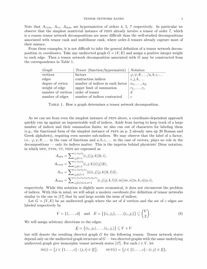
From these examples, it is not difficult to infer the general definition of a tensor network decom-position in coordinates. Take any undirected graph G = (V,E) and assign a positive integer weightto each edge. Then a tensor network decomposition associated with G may be constructed fromthe correspondence in Table 1.

Graph Tensor (function/hypermatrix) Notationvertices factors ϕ,ψ, θ, . . . /a, b, c, . . .edges contraction indices i, j, k, . . .degree of vertex number of indices in each factor n1, . . . , ndweight of edge upper limit of summation r1, . . . , rcnumber of vertices order of tensor dnumber of edges number of indices contracted c

Table 1. How a graph determines a tensor network decomposition.

As we can see from even the simplest instance of peps above, a coordinate-dependent approachquickly run up against an impenetrable wall of indices. Aside from having to keep track of a largenumber of indices and their summation limits, we also run out of characters for labeling them(e.g., the functional form of the simplest instance of peps on p. 2 already uses up 20 Roman andGreek alphabets), requiring even messier sub-indices. We may observe that the label of a factor,i.e., ϕ,ψ, θ, . . . in the case of functions and a, b, c, . . . in the case of vectors, plays no role in thedecompositions — only its indices matter. This is the impetus behind physicists’ Dirac notation,in which mps, ttns, tt, peps are expressed as

Amps =∑r1,r2,r3

i,j,k=1|i, j〉|j, k〉|k, i〉,

Attns =∑r1,r2,r3

i,j,k=1|i, j, k〉|i〉|j〉|k〉,

Att =∑r1,r2,r3,r4

i,j,k,l=1|i〉|i, j〉|j, k〉|k, l〉|l〉,

Apeps =∑r1,r2,r3,r4,r5,r6,r7

i,j,k,l,m,n,o=1|i, j〉|j, k, l〉|l,m〉|m,n〉|n, k, o〉|o, i〉,

respectively. While this notation is slightly more economical, it does not circumvent the problemof indices. With this in mind, we will adopt a modern coordinate-free definition of tensor networkssimilar to the one in [17] that by and large avoids the issue of indices.

Let G = (V,E) be an undirected graph where the set of d vertices and the set of c edges arelabeled respectively by

V = {1, . . . , d} and E ={{i1, j1}, . . . , {ic, jc}

}⊆(V

2

). (8)

We will assign arbitrary directions to the edges:

E ={

(i1, j1), . . . , (ic, jc)}⊆ V × V

but still denote the resulting directed graph G for the following reason: Tensor network statesdepend only on the undirected graph structure ofG— two directed graphs with the same underlyingundirected graph give isomorphic tensor network states [17]. For each i ∈ V , let

in(i) ={j ∈ {1, . . . , c} : (j, i) ∈ E

}, out(i) =

{j ∈ {1, . . . , c} : (i, j) ∈ E},


i.e., the sets of vertices pointing into and out of i respectively. As usual, for a directed edge (i, j),we will call i its head and j its tail.

The recipe for constructing tensor network states is easy to describe informally: Given any graphG = (V,E), assign arbitrary directions to the edges to obtain E; attach a vector space Vi to eachvertex i; attach a covector space E∗j to the head and a vector space Ek to the tail of each directed

edge (j, k); do this for all vertices in V and all directed edges in E; contract along all edges toobtain a tensor in V1 ⊗ · · · ⊗Vd. The set of all tensors obtained this way form the tensor networkstates associated with G. We make this recipe precise in the following.

We will work over C for convenience although the discussions in this article will also apply toR. We will also restrict ourselves mostly to finite-dimensional vector spaces as our study here isundertaken with a view towards computations and in computational applications of tensor networks,infinite-dimensional spaces are invariably approximated by finite-dimensional ones.

Let V1, . . . ,Vd be complex vector spaces with dimVi = ni, i = 1, . . . , d. Let E1, . . . ,Ec becomplex vector spaces with dimEj = rj , j = 1, . . . , c. We denote the dual space of Vi by V∗i (andthat of Ej by E∗j ). For each i ∈ V , consider the tensor product space(⊗

j∈in(i)Ej)⊗ Vi ⊗

(⊗j∈out(i)

E∗j)

(9)

and the contraction map

κG :⊗d

i=1

[(⊗j∈in(i)

Ej)⊗ Vi ⊗

(⊗j∈out(i)

E∗j)]→⊗d

i=1Vi, (10)

defined by contracting factors in Ej with factors in E∗j . Since any directed edge (i, j) must pointout of a vertex i and into a vertex j, each copy of E∗j is paired with one and only one copy of Ej ,i.e., the contraction is well-defined.

Definition 2.1. A tensor in V1 ⊗ · · · ⊗ Vd that can be written as κG(T1 ⊗ · · · ⊗ Td) where

Ti ∈(⊗


(⊗j∈out(i)

E∗j), i = 1, . . . , d,

and κG as in (10), is called a tensor network state associated to the undirected graph G and vectorspaces V1, . . . ,Vd, E1, . . . ,Ec. The set of all such tensor network states is called the tensor networkand denoted

tns(G;E1, . . . ,Ec;V1, . . . ,Vd) :={κG(T1 ⊗ · · · ⊗ Td) ∈ V1 ⊗ · · · ⊗ Vd :

Ti ∈(⊗


(⊗j∈out(i)

E∗j), i = 1, . . . , d

}.

We will always require that E1, . . . ,Ec be finite-dimensional but V1, . . . ,Vd may be of any dimen-sions, finite or infinite. Since a vector space is determined up to isomorphism by its dimension, whenthe vector spaces E1, . . . ,Ec are unimportant (these play the role of contraction indices), we will sim-ply denote the tensor network by tns(G; r1, . . . , rc;V1, . . . ,Vd); or, if the vector spaces V1, . . . ,Vdare also unimportant and finite-dimensional, we will denote it by tns(G; r1, . . . , rc;n1, . . . , nd). Asbefore, ni = dimVi and rj = dimEj .

While we have restricted Definition 2.1 to tensor products of vector spaces V1⊗ · · · ⊗Vd for thepurpose of this article, the definition works with any types of mathematical objects with a notion oftensor product: V1, . . . ,Vd may be modules or algebras, Hilbert or Banach spaces, von Neumannor C∗-algebras, Hilbert C∗-modules, etc. In fact we will need to use Definition 2.1 in the formwhere V1, . . . ,Vd are vector bundles in Section 3.

Since they will be appearing with some frequency, we will introduce abbreviated notations forthe inspace and outspace appearing in (9): For each vertex i = 1, . . . , d, set

Ii :=⊗

j∈in(i)Ej and Oi :=

⊗j∈out(i)

E∗j . (11)


Note that the image of every contraction map κG(T1⊗· · ·⊗Td) gives a decomposition like the oneswe saw in (4)–(7). We call such a decomposition a tensor network decomposition associated with G.A tensor T ∈ V1⊗· · ·⊗Vd is said to be G-decomposable if it can be expressed as T = κG(T1⊗ . . . Td)for some r1, . . . , rc ∈ N; a fundamental result here (see Theorem 4.1) is that:

Given any G and any V1, . . . ,Vd, every tensor in V1 ⊗ · · · ⊗ Vd is G-decomposablewhen r1, . . . , rc are sufficiently large.

The tensor network tns(G; r1, . . . , rc;V1, . . . ,Vd) is simply the set of all G-decomposable tensorsfor a fixed choice of r1, . . . , rc. A second fundamental result (see Definition 4.3 and discussionsthereafter) is that:

Given any G and any T ∈ V1⊗· · ·⊗Vd, there is minimum choice of r1, . . . , rc suchthat T ∈ tns(G; r1, . . . , rc;V1, . . . ,Vd).

The undirected graph G can be extremely general. We impose no restriction on G — self-loops,multiple edges, disconnected graphs, etc — are all permitted. However, we highlight the following:

Self-loops: Suppose a vertex i has a self-loop, i.e., an edge e from i to itself. Let Ee be thevector space attached to e. Then by definition Ee and E∗e must both appear in the inspaceand outspace of i and upon contraction they serve no role in the tensor network state; e.g.,for C1, the single vertex graph with one self-loop, κC1(Ee⊗Vi⊗E∗e) = Vi. Hence self-loopsin G have no effect on the tensor network states defined by G.

Multiple edges: Multiple edges e1, . . . , em with vector spaces E1, . . . ,Em attached have thesame effect as a single edge e with the vector space E1⊗ · · ·⊗Em attached, or equivalently,multiple edges e1, . . . , em with edge weights r1, . . . , rm have the same effect as a single edgewith edge weight r1 · · · rm.

Degree-zero vertices: If G contains a vertex of degree zero, i.e., an isolated vertex notconnected to the rest of the graph, then by Definition 2.1,

tns(G; r1, . . . , rc;n1, . . . , nd) = {0}. (12)

Weight-one edges: If G contains an edge of weight one, i.e., a one-dimensional vector spaceis attached to that edge, then by Definition 2.1, that edge may be dropped. See Proposi-tion 3.5 for details.

In particular, allowing for a multigraph adds nothing to the definition of tensor network states andwe may assume that G is always a simple graph, i.e., no self-loops or multiple edges. Howeverdegree-zero vertices and weight-one edges will be permitted since they are convenient in proofs.

Definition 2.2. Tensor network states associated to specific types of graphs are given specialnames. The most common ones are as follows:

(i) if G is a path graph, then tensor network states associated to G are variously called tensortrains (tt) [29], linear tensor network [32], concatenated tensor network states [13], Heisenbergchains [37, 38], or matrix product states with open boundary conditions;

(ii) if G is a star graph, then they are called star tensor network states (stns) [4];(iii) if G is a tree graph, then they are called tree tensor network states (ttns) [31] or hierarchical

tensors [9, 10, 2];(iv) if G is a cycle graph, then they are called matrix product states (mps) [7, 30] or, more precisely,

matrix product states with periodic boundary conditions;(v) if G is a product of d ≥ 2 path graphs, then they are called d-dimensional projected entangled

pair states (peps) [33, 34];(vi) if G is a complete graph, then they are called complete graph tensor network states (ctns)

[23].

We will use the term tensor trains as its acronym tt reminds us that they are a special case oftree tensor network states ttns. This is a matter of nomenclature convenience. As we can see fromthe references in (i), the notion has been rediscovered many times. The original sources for what


we call tensor trains are [37, 38] where they are called Heisenberg chains. In fact, as we have seen,tensor trains are also special cases of matrix product states. In some sources [28], the tensor trainsin (i) are called “matrix product states with open boundary conditions” and the matrix productstates in (iv) are called “matrix product states with periodic conditions.”

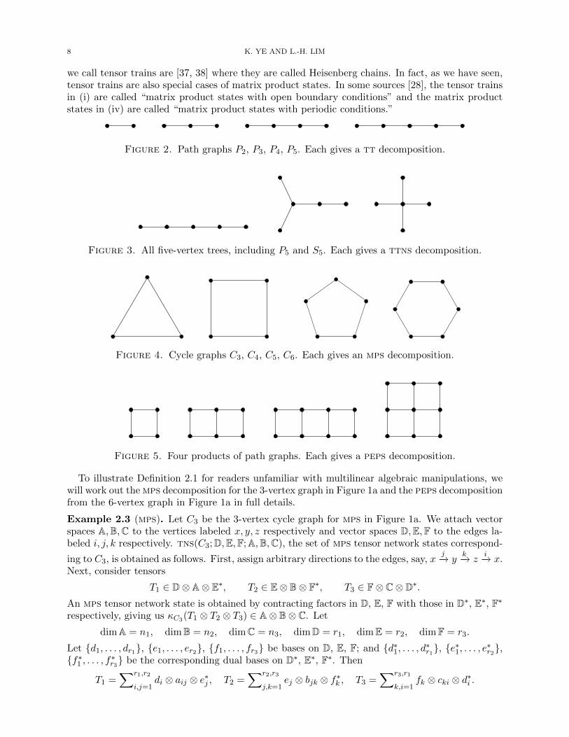
Figure 2. Path graphs P2, P3, P4, P5. Each gives a tt decomposition.

Figure 3. All five-vertex trees, including P5 and S5. Each gives a ttns decomposition.

Figure 4. Cycle graphs C3, C4, C5, C6. Each gives an mps decomposition.

Figure 5. Four products of path graphs. Each gives a peps decomposition.

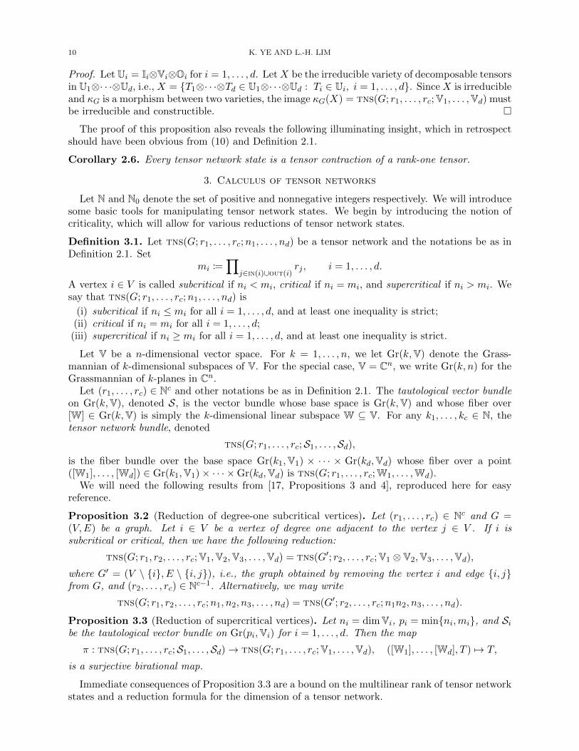
To illustrate Definition 2.1 for readers unfamiliar with multilinear algebraic manipulations, wewill work out the mps decomposition for the 3-vertex graph in Figure 1a and the peps decompositionfrom the 6-vertex graph in Figure 1a in full details.

Example 2.3 (mps). Let C3 be the 3-vertex cycle graph for mps in Figure 1a. We attach vectorspaces A,B,C to the vertices labeled x, y, z respectively and vector spaces D,E,F to the edges la-beled i, j, k respectively. tns(C3;D,E,F;A,B,C), the set of mps tensor network states correspond-

ing to C3, is obtained as follows. First, assign arbitrary directions to the edges, say, xj−→ y

k−→ zi−→ x.

Next, consider tensors

T1 ∈ D⊗ A⊗ E∗, T2 ∈ E⊗ B⊗ F∗, T3 ∈ F⊗ C⊗ D∗.An mps tensor network state is obtained by contracting factors in D, E, F with those in D∗, E∗, F∗respectively, giving us κC3(T1 ⊗ T2 ⊗ T3) ∈ A⊗ B⊗ C. Let

dimA = n1, dimB = n2, dimC = n3, dimD = r1, dimE = r2, dimF = r3.

Let {d1, . . . , dr1}, {e1, . . . , er2}, {f1, . . . , fr3} be bases on D, E, F; and {d∗1, . . . , d∗r1}, {e∗1, . . . , e

∗r2},

{f∗1 , . . . , f∗r3} be the corresponding dual bases on D∗, E∗, F∗. Then

T1 =∑r1,r2

i,j=1di ⊗ aij ⊗ e∗j , T2 =

∑r2,r3

j,k=1ej ⊗ bjk ⊗ f∗k , T3 =

∑r3,r1

k,i=1fk ⊗ cki ⊗ d∗i .


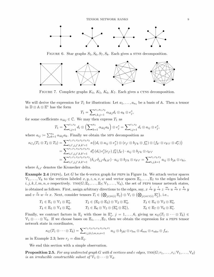
Figure 6. Star graphs S5, S6, S7, S8. Each gives a stns decomposition.

Figure 7. Complete graphs K4, K5, K6, K7. Each gives a ctns decomposition.

We will derive the expression for T1 for illustration: Let a1, . . . , an1 be a basis of A. Then a tensorin D⊗ A⊗ E∗ has the form

T1 =∑r1,n1,r2

i,k,j=1αikjdi ⊗ ak ⊗ e∗j ,

for some coefficients αikj ∈ C. We may then express T1 as

T1 =∑r1,r2

i,j=1di ⊗

(∑n1

k=1αikjak

)⊗ e∗j =

∑r1,r2

i,j=1di ⊗ aij ⊗ e∗j ,

where aij :=∑n1

k=1 αikjak. Finally we obtain the mps decomposition as

κC3(T1 ⊗ T2 ⊗ T3) =∑r1,r1,r2,r2,r3,r3

i,i′,j,j′,k,k′=1κ((di ⊗ aij ⊗ e∗j )⊗ (ej′ ⊗ bj′k ⊗ f∗k )⊗ (fk′ ⊗ ck′i′ ⊗ d∗i′)

)=∑r1,r1,r2,r2,r3,r3

i,i′,j,j′,k,k′=1d∗i′(di) e

∗j (ej′) f

∗k (fk′) · aij ⊗ bj′k ⊗ ck′i′

=∑r1,r1,r2,r2,r3,r3

i,i′,j,j′,k,k′=1(δi,i′δj,j′δk,k′) · aij ⊗ bj′k ⊗ ck′i′ =

∑r1,r2,r3

i,j,k=1aij ⊗ bjk ⊗ cki,

where δi,i′ denotes the Kronecker delta.

Example 2.4 (peps). Let G be the 6-vertex graph for peps in Figure 1a. We attach vector spacesV1, . . . ,V6 to the vertices labeled x, y, z, u, v, w and vector spaces E1, . . . ,E7 to the edges labeledi, j, k, l,m, n, o respectively. tns(G;E1, . . . ,E7;V1, . . . ,V6), the set of peps tensor network states,

is obtained as follows. First, assign arbitrary directions to the edges, say, xj−→ y

l−→ zm−→ u

n−→ vk−→ y

and vo−→ w

i−→ x. Next, consider tensors Ti ∈(⊗

j∈in(i) Ej)⊗ Vi ⊗

(⊗j∈out(i) E∗j

), i.e.,

T1 ∈ E1 ⊗ V1 ⊗ E∗2, T2 ∈ (E2 ⊗ E3)⊗ V2 ⊗ E∗4, T3 ∈ E4 ⊗ V3 ⊗ E∗5,T4 ∈ E5 ⊗ V4 ⊗ E∗6, T5 ∈ E6 ⊗ V5 ⊗ (E∗3 ⊗ E∗7), T6 ∈ E7 ⊗ V6 ⊗ E∗1.

Finally, we contract factors in Ej with those in E∗j , j = 1, . . . , 6, giving us κG(T1 ⊗ · · · ⊗ T6) ∈V1 ⊗ · · · ⊗ V6. If we choose bases on E1, . . . ,E7, then we obtain the expression for a peps tensornetwork state in coordinates,

κG(T1 ⊗ · · · ⊗ T6) =∑r1,r2,r3,r4,r5,r6,r7

i,j,k,l,m,n,o=1aij ⊗ bjkl ⊗ clm ⊗ dmn ⊗ enko ⊗ foi,

as in Example 2.3; here rj = dimEj .

We end this section with a simple observation.

Proposition 2.5. For any undirected graph G with d vertices and c edges, tns(G; r1, . . . , rc;V1, . . . ,Vd)is an irreducible constructible subset of V1 ⊗ · · · ⊗ Vd.


Proof. Let Ui = Ii⊗Vi⊗Oi for i = 1, . . . , d. LetX be the irreducible variety of decomposable tensorsin U1⊗· · ·⊗Ud, i.e., X = {T1⊗· · ·⊗Td ∈ U1⊗· · ·⊗Ud : Ti ∈ Ui, i = 1, . . . , d}. Since X is irreducibleand κG is a morphism between two varieties, the image κG(X) = tns(G; r1, . . . , rc;V1, . . . ,Vd) mustbe irreducible and constructible. �

The proof of this proposition also reveals the following illuminating insight, which in retrospectshould have been obvious from (10) and Definition 2.1.

Corollary 2.6. Every tensor network state is a tensor contraction of a rank-one tensor.

3. Calculus of tensor networks

Let N and N0 denote the set of positive and nonnegative integers respectively. We will introducesome basic tools for manipulating tensor network states. We begin by introducing the notion ofcriticality, which will allow for various reductions of tensor network states.

Definition 3.1. Let tns(G; r1, . . . , rc;n1, . . . , nd) be a tensor network and the notations be as inDefinition 2.1. Set

mi :=∏

j∈in(i)∪out(i)rj , i = 1, . . . , d.

A vertex i ∈ V is called subcritical if ni < mi, critical if ni = mi, and supercritical if ni > mi. Wesay that tns(G; r1, . . . , rc;n1, . . . , nd) is

(i) subcritical if ni ≤ mi for all i = 1, . . . , d, and at least one inequality is strict;(ii) critical if ni = mi for all i = 1, . . . , d;

(iii) supercritical if ni ≥ mi for all i = 1, . . . , d, and at least one inequality is strict.

Let V be a n-dimensional vector space. For k = 1, . . . , n, we let Gr(k,V) denote the Grass-mannian of k-dimensional subspaces of V. For the special case, V = Cn, we write Gr(k, n) for theGrassmannian of k-planes in Cn.

Let (r1, . . . , rc) ∈ Nc and other notations be as in Definition 2.1. The tautological vector bundleon Gr(k,V), denoted S, is the vector bundle whose base space is Gr(k,V) and whose fiber over[W] ∈ Gr(k,V) is simply the k-dimensional linear subspace W ⊆ V. For any k1, . . . , kc ∈ N, thetensor network bundle, denoted

tns(G; r1, . . . , rc;S1, . . . ,Sd),is the fiber bundle over the base space Gr(k1,V1) × · · · × Gr(kd,Vd) whose fiber over a point([W1], . . . , [Wd]) ∈ Gr(k1,V1)× · · · ×Gr(kd,Vd) is tns(G; r1, . . . , rc;W1, . . . ,Wd).

We will need the following results from [17, Propositions 3 and 4], reproduced here for easyreference.

Proposition 3.2 (Reduction of degree-one subcritical vertices). Let (r1, . . . , rc) ∈ Nc and G =(V,E) be a graph. Let i ∈ V be a vertex of degree one adjacent to the vertex j ∈ V . If i issubcritical or critical, then we have the following reduction:

tns(G; r1, r2, . . . , rc;V1,V2,V3, . . . ,Vd) = tns(G′; r2, . . . , rc;V1 ⊗ V2,V3, . . . ,Vd),where G′ = (V \ {i}, E \ {i, j}), i.e., the graph obtained by removing the vertex i and edge {i, j}from G, and (r2, . . . , rc) ∈ Nc−1. Alternatively, we may write

tns(G; r1, r2, . . . , rc;n1, n2, n3, . . . , nd) = tns(G′; r2, . . . , rc;n1n2, n3, . . . , nd).

Proposition 3.3 (Reduction of supercritical vertices). Let ni = dimVi, pi = min{ni,mi}, and Sibe the tautological vector bundle on Gr(pi,Vi) for i = 1, . . . , d. Then the map

π : tns(G; r1, . . . , rc;S1, . . . ,Sd)→ tns(G; r1, . . . , rc;V1, . . . ,Vd), ([W1], . . . , [Wd], T ) 7→ T,

is a surjective birational map.

Immediate consequences of Proposition 3.3 are a bound on the multilinear rank of tensor networkstates and a reduction formula for the dimension of a tensor network.


Corollary 3.4. Let the notations be as above. Then for any (r1, . . . , rc) ∈ Nc, we have

tns(G; r1, . . . , rc;V1, . . . ,Vd) ⊆ Subp1,...,pd(V1, . . . ,Vd)

and

dimtns(G; r1, . . . , rc;n1, . . . , nd) = dimtns(G; r1, . . . , rc; p1, . . . , pd) +∑d

i=1pi(ni − pi).

Note that by Proposition 3.3, all tensor network states can be reduced to one that is eithercritical or subcritical.

The next proposition is useful for describing when we are allowed to remove an edge from thegraph while keeping the tensor network unchanged. The reader may notice a resemblance toProposition 3.2, which is about collapsing two vertices into one and thus results in a reduction inthe total number of vertices, but the goal of Proposition 3.5 is to remove an edge while leaving thetotal number of vertices unchanged.

Proposition 3.5 (Edge removal). Let G = (V,E) be a graph with d vertices and c edges. Let(r1, . . . , rc) ∈ Nc and (n1, . . . , nd) ∈ Nd. Suppose that the edge e ∈ E has weight r1 = 1 andG′ = (V,E \ {e}) is the graph obtained by removing the edge e from G and suppose G′ has noisolated vertices. Then

tns(G; 1, r2, . . . , rd;V1, . . . ,Vd) ' tns(G′; r2, . . . , rd;V1, . . . ,Vd).

Proof. Assume without loss of generality that e = {1, 2}. By definition,

tns(G; 1, r2, . . . , rd;V1, . . . ,Vd) = {κG(T1 ⊗ · · · ⊗ Td) : Ti ∈ Ii ⊗ Vi ⊗Oi, i = 1, . . . , d},tns(G′; r2, . . . , rd;V1, . . . ,Vd) = {κG′(T ′1 ⊗ · · · ⊗ T ′d) : T ′i ∈ I′i ⊗ Vi ⊗O′i, i = 1, . . . , d},

where Ii, I′i are inspaces, Oi, O′i are outspaces, as defined in (11), and κG, κG′ are contraction maps,as defined in (10), associated to G and G′ respectively. Since r1 = 1, E1 ' C and so contributesnothing4 to the factors I1⊗V1⊗O1, I2⊗V2⊗O2, and thus Ii⊗Vi⊗Oi ' I′i⊗Vi⊗O′i for i = 1, 2. Onthe other hand, Ii⊗Vi⊗Oi = I′i⊗Vi⊗O′i for i = 3, . . . , d. Therefore the images of the contractionmap must be isomorphic, as required. �

The assumption that an isolated vertex does not arise in G′ upon removing the edge e is necessarybecause of (12). An immediate consequence of Proposition 3.5 is that tensor trains are a specialcase of matrix product states since

tns(Cd; r1, r2, . . . , rd−1, 1;n1, . . . , nd) = tns(Pd; r1, . . . , rd−1;n1, . . . , nd), (13)

where Cd is the cycle graph with d vertices, the edge with weight 1 is adjacent to the vertex 1 andd, and Pd is the path graph with d vertices.

We end the section with a result about restriction of tensor network states to subspaces of tensors,which will be crucial for an important property of tensor network rank established in Theorem 6.1.

Lemma 3.6 (Restriction lemma). Let G be a graph with d vertices and c edges. Let V1, . . . ,Vd bevector spaces and Wi ⊆ Vi be subspaces, i = 1, . . . , d. Then for any (r1, . . . , rc) ∈ Nc,

tns(G; r1, . . . , rc;V1, . . . ,Vd) ∩W1 ⊗ · · · ⊗Wd = tns(G; r1, . . . , rc;W1, . . . ,Wd). (14)

In particular, we always have

tns(G; r1, . . . , rc;W1, . . . ,Wd) ⊆ tns(G; r1, . . . , rc;V1, . . . ,Vd). (15)

4A one-dimensional vector space is isomorphic to the field of scalars C and C ⊗ E = E for any complex vectorspace E.


Proof. It is obvious that ‘⊇’ holds in (44) and it remains to show ‘⊆’. Let Ej be a vector spaceof dimension rj , j = 1, . . . , c. Orient G arbitrarily and let the inspace Ii and outspace Oi be asdefined in (11) for vertices i = 1, . . . , d. We obtain two commutative diagrams:

∏di=1 Ii ⊗Wi ⊗ Oi

⊗di=1 Ii ⊗Wi ⊗ Oi

⊗di=1 Ii ⊗ Vi ⊗ Oi

tns(G; r1, . . . , rc;W1, . . . ,Wd) W1 ⊗ · · · ⊗Wd V1 ⊗ · · · ⊗ Vd

Ψ′

κ′′

Φ

κ′ κ

ψ′ φ

and ∏di=1 Ii ⊗ Vi ⊗ Oi

⊗di=1 Ii ⊗ Vi ⊗ Oi

tns(G; r1, . . . , rc;V1, . . . ,Vd) V1 ⊗ · · · ⊗ Vd,

Ψ

κ′′′ κ

ψ

where Ψ′ sends (x1, . . . , xd), xi ∈ Ii ⊗Wi ⊗ Oi, i = 1, . . . , d, to x1 ⊗ · · · ⊗ xd and Ψ is definedsimilarly; ψ′, ψ are inclusions of tensor network states into their respective ambient spaces; Φ, φ areinclusions induced by Wi ⊆ Vi, i = 1, . . . , d; κ′ is the restriction of κ := κG; κ′′ the composition ofκ′ and Ψ′; and κ′′′ the composition of κ and Ψ.

For each i = 1, . . . , d, write V+i = Wi and decompose Vi into a direct sum

Vi = V−i ⊕ V+i

for some linear subspace V−i ⊆ Vi. These give us the decomposition∏d

i=1Ii ⊗ Vi ⊗Oi =

∏d

i=1Ii ⊗ (V−i ⊕ V+

i )⊗Oi =∏d

i=1(Ii ⊗ V−i ⊗Oi)⊕ (Ii ⊗ V+

i ⊗Oi).

Now we may write an element T1 ⊗ · · · ⊗ Td ∈ Ψ(∏d

i=1 Ii ⊗ Vi ⊗Oi

)as

T1 ⊗ · · · ⊗ Td = (T−1 + T+1 )⊗ · · · ⊗ (T−d + T+

d ) =∑±T±1 ⊗ · · · ⊗ T

±d ,

where T−i ∈ Ii ⊗ V−i ⊗Oi and T+i ∈ Ii ⊗ V+

i ⊗Oi. Since T±1 ⊗ · · · ⊗ T±d ∈ Ψ

(∏di=1 Ii ⊗ V±i ⊗Oi

),

κ(T1 ⊗ · · · ⊗ Td) ∈∑±κ(

Ψ(∏d

i=1Ii ⊗ V±i ⊗Oi

))=∑±tns(G; r1, . . . , rc;V±1 , . . . ,V

±d ).

Therefore κ(T1 ⊗ · · · ⊗ Td) ∈ V+1 ⊗ · · · ⊗ V+

d implies that Ti ∈ V+i = Wi for all i = 1, . . . , d and

hence κ(T1 ⊗ · · · ⊗ Td) ∈ tns(G; r1, . . . , rc;W1, . . . ,Wd). �

4. G-ranks of tensors

The main goal of this article is to show that there is a natural notion of rank for tensor networkwith respect to any connected graph G. We start by reminding our readers of the classical notionsof tensor rank and multilinear rank, with a small twist — instead of first defining tensor andmultilinear ranks and then defining the respective sets they cut out, i.e., secant quasiprojectivevariety and subspace variety, we will reverse the order of these definitions. This approach willbe consistent with how we define tensor network ranks later. The results in this and subsequentsections require that the vector spaces V1, . . . ,Vd be finite-dimensional.

The Segre variety is the set of all decomposable tensors,

Seg(V1, . . . ,Vd) := {T ∈ V1 ⊗ · · · ⊗ Vd : T = v1 ⊗ · · · ⊗ vd, vi ∈ Vi}.The r-secant quasiprojective variety of the Segre variety is

sr(Seg(V1, . . . ,Vd)

):={T ∈ V1 ⊗ · · · ⊗ Vd : T =

∑r

i=1Ti, Ti ∈ Seg(V1, . . . ,Vd)

},

and its closure is the r-secant variety of the Segre variety,

σr(Seg(V1, . . . ,Vd)

):= sr

(Seg(V1, . . . ,Vd)

).


The (r1, . . . , rd)-subspace variety [15] is the set

Subr1,...,rd(V1, . . . ,Vd) := {T ∈ V1 ⊗ · · · ⊗ Vd : T ∈W1 ⊗ · · · ⊗Wd, Wi ⊆ Vi, dimWi = ri}.The tensor rank or just rank [11] of a tensor T ∈ V1 ⊗ · · · ⊗ Vd is

rank(T ) := min{r ∈ N0 : T ∈ sr

(Seg(V1, . . . ,Vd)

)},

its border rank [15] is

rank(T ) := min{r ∈ N0 : T ∈ σr

(Seg(V1, . . . ,Vd)

)},

and its multilinear rank [11, 6, 15] is

µrank(T ) := min{

(r1, . . . , rd) ∈ Nd0 : T ∈ Subr1,...,rd(V1, . . . ,Vd)}.

Note that rank(T ) = 0 iff µrank(T ) = (0, . . . , 0) iff T = 0 and that rank(T ) = 1 iff µrank(T ) =(1, . . . , 1). Thus

Seg(V1, . . . ,Vd) = {T ∈ V1 ⊗ · · · ⊗ Vd : rank(T ) ≤ 1} = Sub1,...,1(V1, . . . ,Vd),sr(Seg(V1, . . . ,Vd)

)= {T ∈ V1 ⊗ · · · ⊗ Vd : rank(T ) ≤ r},

Subr1,...,rd(V1, . . . ,Vd) = {T ∈ V1 ⊗ · · · ⊗ Vd : µrank(T ) ≤ (r1, . . . , rd)}.When the vector spaces are unimportant or when we choose coordinates and represent tensors

as hypermatrices, we write

Seg(n1, . . . , nd) = {T ∈ Cn1×···×nd : rank(T ) ≤ 1},sr(n1, . . . , nd)

)= {T ∈ Cn1×···×nd : rank(T ) ≤ r},

Subr1,...,rd(n1, . . . , nd) = {T ∈ Cn1×···×nd : µrank(T ) ≤ (r1, . . . , rd)}.The dimension of a subspace variety is given by

dim Subr1,...,rd(n1, . . . , nd) =∑d

i=1ri(ni − ri) +

∏d

j=1rj . (16)

Unlike tensor rank and multilinear rank, the existence of a tensor network rank is not obviousand will be established in the following. A tensor network tns(G; r1, . . . , rc;V1, . . . ,Vd) is definedfor any graph G although it is trivial when G contains an isolated vertex (see (12)). However,tensor network ranks or G-ranks will require the stronger condition that G be connected.

Theorem 4.1 (Every tensor is a tensor network state). Let T ∈ V1 ⊗ · · · ⊗ Vd and let G be aconnected graph with d vertices and c edges. Then there exists (r1, . . . , rc) ∈ Nc such that

T ∈ tns(G; r1, . . . , rc;V1, . . . ,Vd).In fact, we may choose r1 = · · · = rc = rank(T ), the tensor rank of T .

Proof. Let r = rank(T ). Then there exist v(i)1 , . . . , v

(i)r ∈ Vi, i = 1, . . . , d, such that

T =∑r

p=1v(1)p ⊗ · · · ⊗ v(d)

p .

Let us take r1 = · · · = rc = r and for each i = 1, . . . , d, let

Ti =∑r

p=1

(⊗j∈in(i)

e(j)p

)⊗ v(i)

p ⊗(⊗

j∈out(i)e(j)∗p

),

where e(j)1 , . . . , e

(j)r ∈ Ej are a basis with dual basis e

(j)∗1 , . . . , e

(j)∗r ∈ E∗j , i.e., e

(j)∗p (e

(j)q ) = δpq for

p, q = 1, . . . , r and j = 1, . . . , d. In addition, we set e(0)p = e

(d+1)p = 1 ∈ C to be one-dimensional

vectors (i.e., scalars), p = 1, . . . , r. We claim that upon contraction,

κG(T1 ⊗ · · · ⊗ Td) = T.

To see this, observe that for each i = 1, . . . , d, there exists a unique h such that whenever j ∈in(i) ∩ out(h), e

(j)p and e

(j)∗q contract to give δpq; so the summand vanishes except when p = q.


This together with the assumption that G is connected implies that κG(T1 ⊗ · · · ⊗ Td) reduces to

a sum of terms of the form v(1)p ⊗ · · · ⊗ v(d)

p for p = 1, . . . , r, which is of course is just T . �

As an example to illustrate the above proof, let d = 3 and G = P3, the path graph with threevertices. Let e1, . . . , er be a basis of E1 and let e∗1, . . . , e

∗r be the dual basis. Let f1, . . . , fr be a basis

of E2 and let f∗1 , . . . , f∗r be the dual basis. Given a tensor

T =∑r

p=1up ⊗ vp ⊗ wp ∈ V1 ⊗ V2 ⊗ V3,

consider

T1 =∑r

p=1up⊗e∗p ∈ V1⊗E∗1, T2 =

∑r

p=1ep⊗vp⊗f∗p ∈ E1⊗V2⊗E∗2, T3 =

∑r

p=1fp⊗wp ∈ E2⊗V3.

Now observe that a nonzero term in κG(T1 ⊗ T2 ⊗ T3) must come from contracting e∗p with ep andf∗p with fp, showing that T = κG(T1 ⊗ T2 ⊗ T2) ∈ tns(G; r, r;V1,V2,V3).

By Theorem 4.1 and Corollary 3.4, we obtain the following general inclusion relations (indepen-dent of G) between a tensor network and the sets of rank-r tensors and multilinear rank-(r1, . . . , rd)tensors.

Corollary 4.2. Let G be a connected graph with d vertices and c edges. Let V1, . . . ,Vd be vectorspaces of dimensions n1, . . . , nd. Then

sr := {T ∈ V1 ⊗ · · · ⊗ Vd : rank(T ) ≤ r} ⊆ tns(G; r, . . . , r︸︷︷︸c

;V1, . . . ,Vd).

Let (r1, . . . , rc) ∈ Nc and let (p1, . . . , pd) ∈ Nd be given by

pi := min{∏

j∈in(i)∪out(i)rj , ni

}, i = 1, . . . , d.

Then

tns(G; r1, . . . , rc;V1, . . . ,Vd) ⊆ Subp1,...,pd(V1, . . . ,Vd)

In particular, if we let (p1, . . . , pd) ∈ Nd where pi := min{rbi , ni} and bi := # in(i) ∪ out(i), then

sr ⊆ tns(G; r, . . . , r;V1, . . . ,Vd) ⊆ Subp1,...,pd(V1, . . . ,Vd).

Since Nc is a partially ordered set, in fact, a lattice [8], with respect to the usual partial order

(r1, . . . , rc) ≤ (s1, . . . , sc) iff r1 ≤ s1, . . . , rc ≤ sc.

For a non-empty subset S ⊂ L, a partially ordered set, we denote the set of minimal elements ofS by min(S). For example, if S = {(1, 2), (2, 1), (2, 2)} ⊂ N2, then min(S) = {(1, 2), (2, 1)}. ByTheorem 4.1, for any graph G, any vector spaces V1, . . . ,Vd, and any tensor T ∈ V1 ⊗ · · · ⊗ Vd,

{(r1, . . . , rc) ∈ Nc : T ∈ tns(G; r1, . . . , rc;V1, . . . ,Vd)} 6= ∅.

Hence we may define tensor network rank with respect to a given graph G, called G-rank for short,as the set-valued function

rankG : V1 ⊗ · · · ⊗ Vd → 2Nc,

T 7→ min{(r1, . . . , rc) ∈ Nc : T ∈ tns(G; r1, . . . , rc;V1, . . . ,Vd)},

where 2Nc

is the power set of all subsets of Nc. Note that by Theorem 4.1, rankG(T ) will alwaysbe a finite subset of Nc.

Nevertheless, following convention, we prefer to have rankG(T ) be an element as opposed to asubset of Nc. So we will define G-rank to be any minimal element as opposed to the set of allminimal elements.


Definition 4.3 (Tensor network rank and maximal rank). Let G be a graph with d vertices and cedges. We say that (r1, . . . , rc) ∈ Nc is a G-rank of T ∈ V1 ⊗ · · · ⊗ Vd, denoted by

rankG(T ) = (r1, . . . , rc),

if (r1, . . . , rc) is minimal such that T ∈ tns(G; r1, . . . , rc;V1, . . . ,Vd), i.e.,

T ∈ tns(G; r′1, . . . , r′c;V1, . . . ,Vd) and r1 ≥ r′1, . . . , rc ≥ r′c =⇒ r′1 = r1, . . . , r

′c = rc.

A G-rank decomposition of T is its expression as element of tns(G; r1, . . . , rc;V1, . . . ,Vd) whererankG(T ) = (r1, . . . , rc). We say that (m1, . . . ,mc) ∈ Nc is a maximal G-rank of V1 ⊗ · · · ⊗ Vd if(m1, . . . ,mc) is minimal such that every T ∈ V1 ⊗ · · · ⊗ Vd has rank not more than (m1, . . . ,mc).

Definition 4.3 says nothing about the uniqueness of a minimal (r1, . . . , rc) ∈ Nc. We will seelater that for an acyclic graph G, the minimal (r1, . . . , rc) is unique. We will see an extensive listof examples in Section 10 where we compute, for various G’s, the G-ranks of a number of specialtensors: decomposable tensors, monomials (viewed as a symmetric tensor and thus a tensor), thenoncommutative determinant and permanent, the w and ghs states, and the structure tensor ofmatrix-matrix product.

It follows from Definition 4.3 that

tns(G; r1, . . . , rc;V1, . . . ,Vd) = {T ∈ V1 ⊗ · · · ⊗ Vd : rankG(T ) ≤ (r1, . . . , rc)}. (17)

By Corollary 4.2, G-rank may be viewed as an ‘interpolant’ between tensor rank and multilinearrank; although in Section 11, we will see that they are strictly distinct notions — tensor andmultilinear ranks are not special cases of G-ranks for specific choices of G. Since the set in (17) isin general not closed [17], we let

tns(G; r;V1, . . . ,Vd) := tns(G; r;V1, . . . ,Vd)denote its Zariski closure. With this, we obtain G-rank analogues of border rank and generic rank.

Definition 4.4 (Tensor network border rank and generic rank). Let G be a graph with d verticesand c edges. We say that (r1, . . . , rc) ∈ Nc is a border G-rank of T ∈ V1 ⊗ · · · ⊗ Vd, denoted by

rankG(T ) = (r1, . . . , rc),

if (r1, . . . , rc) is minimal such that T ∈ tns(G; r1, . . . , rc;V1, . . . ,Vd). We say that (r1, . . . , rc) ∈ Ncis a generic G-rank of V1 ⊗ · · · ⊗ Vd if (g1, . . . , gc) is minimal such that every T ∈ V1 ⊗ · · · ⊗ Vdhas border rank not more than (g1, . . . , gc).

Observe that by Definitions 4.3 and 4.4, we have

tns(G; r1, . . . , rc;V1, . . . ,Vd) = {T ∈ V1 ⊗ · · · ⊗ Vd : rankG(T ) ≤ (r1, . . . , rc)},tns(G; r1, . . . , rc;V1, . . . ,Vd) = {T ∈ V1 ⊗ · · · ⊗ Vd : rankG(T ) ≤ (r1, . . . , rc)},tns(G; g1, . . . , gc;V1, . . . ,Vd) = V1 ⊗ · · · ⊗ Vd = tns(G;m1, . . . ,mc;V1, . . . ,Vd),

for any (r1, . . . , rc) ∈ Nc and where (m1, . . . ,mc) and (g1, . . . , gc) are respectively a maximaland a generic G-rank of V1 ⊗ · · · ⊗ Vd. Note also our use of the indefinite article — a bor-der/generic/maximal G-rank — since these are not in general unique if G is not acyclic. A morepedantic definition would be in terms of set-valued functions as in the discussion before Defini-tion 4.3.

Following Definition 2.2, when G is a path graph, tree, cycle graph, product of path graphs, ora graph obtained from gluing trees and cycle graphs along edges, then we may also use the termstt-rank, ttns-rank, mps-rank, peps-rank, or ctns-rank to describe the respective G-ranks, andlikewise for their respective generic G-rank and border G-rank. The terms hierarchical rank [9,Chapter 11] and tree rank [2] have also been used for ttns-rank. Discussions of tt-rank, ttns-rank, mps-rank will be deferred to Sections 7, 8, and 9 respectively. We will also compute manyexamples of G-ranks and border G-ranks for important tensors arising from algebraic computationalcomplexity and quatum mechanics in Section 10.


5. Tensor network ranks can be much smaller than matrix, tensor, andmultilinear ranks

Our first result regarding tensor network ranks may be viewed as the main impetus for tensornetworks — we show that a tensor may have arbitrarily high tensor rank or multilinear rank andyet arbitrarily low G-rank for some graph G, in the sense that there is an arbitrarily large gapbetween the two ranks. The same applies to tensor network ranks corresponding to two differentgraphs. For all our comparisons in this section, a single example — the structure tensor for matrix-matrix product — suffices to demonstrate the gaps in various ranks. We will see more examplesin Section 10. In Theorem 6.5, we will exhibit a graph G such that almost every tensor hasexponentially small G-rank compared to its tensor rank or the dimension of its ambient space.

5.1. Comparison with tensor and multilinear ranks. In this and the next subsection, we willcompare different ranks (r1, . . . , rc) ∈ Nc and (s1, . . . , sc′) ∈ Nc′ by a simple comparison of their1-norms r1 + · · · + rc and s1 + · · · + sc′ . In Section 5.3, we will compare the actual dimensions ofthe sets of tensors with these ranks.

Theorem 5.1. For any d ≥ 3, there exists a tensor T ∈ V1⊗· · ·⊗Vd such that for some connectedgraph G with d vertices and c edges,

(i) the tensor rank rank(T ) = r is much larger than the G-rank rankG(T ) = (r1, . . . , rc) in thesense that

r � r1 + · · ·+ rc;

(ii) the multilinear rank µrank(T ) = (s1, . . . , sd) is much larger than the G-rank rankG(T ) =(r1, . . . , rc) in the sense that

s1 + · · ·+ sd � r1 + · · ·+ rc;

(iii) for some graph H with d vertices and c′ edges, the H-rank rankH(T ) = (s1, . . . , sc′) is muchlarger than the G-rank rankG(T ) = (r1, . . . , rc) in the sense that

s1 + · · ·+ sc′ � r1 + · · ·+ rc.

Here “�” indicates a difference in the order of magnitude. In particular, the gap between the rankscan be arbitrarily large.

Proof. We first let d = 3 and later extend our construction to arbitrary d > 3. Set V3 = Cn×n,the n2-dimensional vector space of complex n× n matrices and V1 = V2 = V∗3, its dual space. Let

T = µn ∈ (Cn×n)∗⊗(Cn×n)∗⊗Cn×n ∼= Cn2×n2×n2be the structure tensor of matrix-matrix product

[40], i.e.,

µn =∑n

i,j,k=1E∗ik ⊗ E∗kj ⊗ Eij (18)

where Eij = eieTj ∈ Cn×n, i, j = 1, . . . , n, is the standard basis with dual basis E∗ij : Cn×n → C,

A 7→ aij , i, j = 1, . . . , n. It is well-known that rank(µn) ≥ n2 as it is not possible to multiply twon× n matrices with fewer than n2 multiplications. It is trivial to see that

µrank(µn) = (n2, n2, n2). (19)

Let P3 and C3 be the path graph and cycle graph on three vertices in Figures 2 and 4 respectively.Attach vector spaces V1,V2,V3 to the vertices of both graphs. Then µn ∈ tns(C3;n, n, n;V1,V2,V3)and it is clear that µn /∈ tns(C3; r1, r2, r3;V1,V2,V3) if at least one of r1 ≤ n, r2 ≤ n, r3 ≤ n holdsstrictly. Hence

rankC3(µn) = (n, n, n).

On the other hand, we also have

rankP3(µn) = (n2, n2).


See Theorems 10.10 and 10.9 for more details on computing rankC3(µn) and rankP3(µn). Therequired conclusions follow from

‖rankC3(µn)‖1 = 3n� n2 ≤ rank(µn),

‖rankC3(µn)‖1 = 3n� 3n2 = ‖µrank(µn)‖1,‖rankC3(µn)‖1 = 3n� 2n2 = ‖rankP3(µn)‖1.

To extend the above to d > 3, let 0 6= vi ∈ Vi, i = 4, . . . , d, and set

Td = µn ⊗ v4 ⊗ · · · ⊗ vd ∈ V1 ⊗ · · · ⊗ Vd.

Clearly, its tensor rank and multilinear rank are

rank(Td) = rank(µn) ≥ n2, µrank(Td) = (n2, n2, n2,

d−3︷︸︸︷1, . . . , 1).

Next we compute rankPd(Td) and rankCd

(Td). Relabeling vij1 = Eij and v(k)11 = vk, we get

Td =(∑n

i,j,k=1E∗ik ⊗E∗kj ⊗Eij

)⊗ v4 ⊗ · · · ⊗ vd =

(∑n

i,j,k=1E∗ik ⊗E∗kj ⊗ vij1

)⊗ v(4)

11 ⊗ · · · ⊗ v(d)11 ,

where it follows immediately that

Td ∈ tns(Pd;n2, n2,

d−2︷︸︸︷1, . . . , 1;V1, . . . ,Vd).

Since rankP3(µn) = (n2, n2), by Theorem 10.9,

rankPd(Td) = (n2, n2, 1, . . . , 1︸︷︷︸

d−2

).

Now rewrite Td as

Td =(∑n

i,j,k=1E∗ik ⊗ E∗kj ⊗ Eij

)⊗ v4 ⊗ · · · ⊗ vd

=(∑n

i,j,k,l=1E∗ik ⊗ E∗kj ⊗ vlj

)⊗ v(4)

l1 ⊗ v(5)11 ⊗ · · · ⊗ v

(d−1)11 ⊗ v(d)

1i ,

where

vlj =

{Eij l = i,

0 l 6= i,v

(4)l1 =

{v4 l = i,

0 l 6= i,v

(5)11 = v5, . . . , v

(d−1)11 = vd−1; v

(d)1i = vd, i = 1, . . . , n.

It follows that Td ∈ tns(Cd;n, n, n, n, 1, . . . , 1︸︷︷︸d−4

;V1, . . . ,Vd) and so rankCd(Td) ≤ (n, n, n, n, 1, . . . , 1︸︷︷︸

d−4

).Hence we obtain

‖rankCd(Td)‖1 ≤ 4n+ d− 4� n2 ≤ rank(Td),

‖rankCd(Td)‖1 ≤ 4n+ d− 4� 3n2 + d− 3 = ‖µrank(Td)‖1,

‖rankCd(Td)‖1 ≤ 4n+ d− 4� 2n2 + d− 2 = ‖rankPd

(Td)‖1. �

5.2. Comparison with matrix rank. The matrix rank of a matrix can also be arbitrarily higherthan its G-rank when regarded as a 3-tensor. We will make this precise below.

Every d-tensor may be regarded as a d′-tensor for any d′ ≤ d via flattening [15, 20]. The mostcommon case is when d′ = 2 and in which case the flattening map

[k : V1 ⊗ · · · ⊗ Vd → (V1 ⊗ · · · ⊗ Vk)⊗ (Vk+1 ⊗ · · · ⊗ Vd), k = 2, . . . , d− 1,

takes a d-tensor and sends it to a 2-tensor by ‘forgetting’ the tensor product structures in V1⊗· · ·⊗Vk and Vk+1 ⊗ · · · ⊗Vd. The converse of this operation also holds in the following sense. Supposethe dimensions of the vector spaces V and W factor as

dim(V) = n1 · · ·nk, dim(W) = nk+1 · · ·ndfor integers n1, . . . , nd ∈ N. Then we may impose tensor product structures on V and W so that

V ∼= V1 ⊗ · · · ⊗ Vk, W ∼= Vk+1 ⊗ · · · ⊗ Vd, (20)


where dimVi = ni, i = 1, . . . , d, and where ∼= denotes vector space isomorphism. In which case thesharpening map

]k : V⊗W→ V1 ⊗ · · · ⊗ Vk ⊗ Vk+1 ⊗ · · · ⊗ Vd, k = 2, . . . , d− 1,

takes a 2-tensor and sends it to a d-tensor by imposing the tensor product structures chosen in(20). Note that both [k and ]k are vector space isomorphisms. Applying this to matrices,

Cn1···nk−1×nk···nd ∼= Cn1···nk−1 ⊗ Cnk···nd]k−→ Cn1 ⊗ · · · ⊗ Cnd ∼= Cn1×···×nd ,

and we see that any n1 · · ·nk−1×nk · · ·nd matrix may be regarded as an n1×· · ·×nd hypermatrix.Theorem 5.1 applies to matrices (i.e., d = 2) in the sense of the following corollary.

Corollary 5.2. There exists a matrix in Cmn×p whose matrix rank is arbitrarily larger than itsC3-rank when regarded as a hypermatrix in Cm×n×p.

Proof. Let µn ∈ Cn2×n2×n2be a hypermatrix representing the structure tensor in Theorem 5.1.

Consider any flattening [20] of µn, say, β1(µn) ∈ Cn4×n2. Then by (19), its matrix rank is

rank(β1(µn)

)= n2 � 3n = ‖rankC3(µn)‖1. �

5.3. Comparing number of parameters. One might argue that the comparisons in Theorem 5.1and Corollary 5.2 are not completely fair as, for instance, a rank-r decomposition of T may stillrequire as many parameters as a G-rank-(r1, . . . , rc) decomposition of T , even if r � r1 + · · ·+ rc.We will show that this is not the case: if we measure the complexities of these decompositions bya strict count of parameters, the conclusion that G-rank can be much smaller than matrix, tensor,or multilinear ranks remain unchanged.

Let µn be the structure tensor for matrix-matrix product as in the proof of Theorem 5.1, whichalso shows that

rankC3(µn) = (n, n, n), rankP3(µn) = (n2, n2), µrank(µn) = (n2, n2, n2).

Let r := rank(µn), the exact value of which is open but its current best known lower bound [25] is

r ≥ 3n2 − 2√

2n3/2 − 3n, (21)

which will suffice for our purpose.Geometrically, the number of parameters is the dimension. So the number of parameters

required to decompose µn as a point in tns(C3;n, n, n;V1,V2,V3), tns(P3;n2, n2;V1,V2,V3),Subn2,n2,n2(V1,V2,V3), and σr(Seg(V1,V2,V3)) are given by their respective dimensions:

dimtns(C3;n, n, n;V1,V2,V3) = 3n4 − 3n2, (22)

dimtns(P3;n2, n2;V1,V2,V3) = n6, (23)

dim Subn2,n2,n2(V1,V2,V3) = n6, (24)

dimσr(Seg(V1,V2,V3)) ≥ 9n4 − 6√

2n7/2 − 9n3 − 6n2 + 4√

2n3/2 + 6n− 1. (25)

The dimensions in (22) and (23) follow from [39, Theorem 5.3] and that in (24) follows from (16).The lower bound on the tensor rank in (21) gives us the lower bound on the dimension in (25) by[1, Theorem 5.2].

In conclusion, a C3-rank decomposition of µn requires fewer parameters than its P3-rank decom-position, its multilinear rank decomposition, and its tensor rank decomposition.

6. Properties of tensor network rank

We will establish some fundamental properties of G-rank in this section. We begin by showingthat like tensor rank and multilinear rank, G-ranks are independent of the choice of the ambientspace, i.e., for a fixed G and any vector spaces Wi ⊆ Vi, i = 1, . . . , d, a tensor in W1⊗· · ·⊗Wd hasthe same G-rank whether it is regarded as an element of W1 ⊗ · · · ⊗Wd or of V1 ⊗ · · · ⊗ Vd. The


proof is less obvious and more involved than for tensor rank or multilinear rank, a consequence ofLemma 3.6.

Theorem 6.1 (Inheritance property). Let G be a connected graph with d vertices and c edges. LetWi ⊆ Vi be a linear subspace, i = 1, . . . , d, such that T ∈W1 ⊗ · · · ⊗Wd. Then (r1, . . . , rc) ∈ Nc isa G-rank of T as an element in W1 ⊗ · · · ⊗Wd if and only if it is a G-rank of T as an element inV1 ⊗ · · · ⊗ Vd.

Proof. Let rankG(T ) = (r1, . . . , rc) as an element in W1⊗· · ·⊗Wd and rankG(T ) = (s1, . . . , sc) as anelement in V1⊗ · · · ⊗Vd. Then (s1, . . . , sc) ≤ (r1, . . . , rc). Suppose they are not equal, then si < rifor at least one i ∈ {1, . . . , c}. Since T ∈ tns(G; s1, . . . , sc;V1, . . . ,Vd) and T ∈W1 ⊗ · · · ⊗Wd, wemust have T ∈ tns(G; s1, . . . , sc;W1, . . . ,Wd) by Lemma 3.6, contradicting our assumption thatrankG(T ) = (r1, . . . , rc) as an element in W1 ⊗ · · · ⊗Wd. �

It is well-known that Theorem 6.1 holds true for tensor rank and multilinear rank [6, Proposi-tion 3.1]; so this is yet another way G-ranks resemble the usual notions of ranks. This inheritanceproperty has often been exploited in the calculation of tensor rank and similarly Theorem 6.1 pro-vides a useful simplification in the calculation of G-ranks: Given T ∈ V1 ⊗ · · · ⊗ Vd, we may findlinear subspaces Wi ⊆ Vi, i = 1, . . . , d, such that T ∈W1 ⊗ · · · ⊗Wd and determine the G-rank ofT as a tensor in the smaller space W1 ⊗ · · · ⊗Wd. With this in mind, we introduce the followingterminology.

Definition 6.2. T ∈ V1 ⊗ · · · ⊗ Vd is degenerate if there exist subspaces Wi ⊆ Vi, i = 1, . . . , d,with at least one strict inclusion, such that T ∈W1 ⊗ · · · ⊗Wd. Otherwise T is nondegenerate.

Theorem 6.1 tells us the behavior of G-ranks with respect to subspaces. The next result tells usabout the behavior of G-ranks with respect to subgraphs.

Proposition 6.3 (Subgraph). Let G be a connected graph with d vertices and c edges. Let H be aconnected subgraph of G with d vertices and c′ edges.

(i) Let (s1, . . . , sc′) ∈ Nc′ be a generic H-rank of V1⊗· · ·⊗Vd. Then there exists (r1, . . . , rc) ∈ Ncwith ri ≤ si, i = 1, . . . , c′, such that (r1, . . . , rc) is a generic G-rank of V1 ⊗ · · · ⊗ Vd.

(ii) Let T ∈ V1 ⊗ · · · ⊗ Vd and rankH(T ) = (s1, . . . , sc′). Then there exists (r1, . . . , rc) ∈ Nc withri ≤ si, i = 1, . . . , c′, such that rankG(T ) = (r1, . . . , rc).

Proof. By Proposition 3.5, we have

tns(H; s1, . . . , sc′ ;V1, . . . ,Vd) = tns(G; s1, . . . , sc′ ,

c−c′︷︸︸︷1, . . . , 1;V1, . . . ,Vd). (26)

Since (s1, . . . , sc′) is a generic H-rank of V1 ⊗ · · · ⊗ Vd,

tns(G; s1, . . . , sc′ , 1, . . . , 1;V1, . . . ,Vd) = tns(H; s1, . . . , sc′ ;V1, . . . ,Vd) = V1 ⊗ · · · ⊗ Vd,

implying that V1 ⊗ · · · ⊗ Vd has a generic G-rank with ri ≤ si, i = 1, . . . , c′. The same argumentand (26) show that rankG(T ) = (s1, . . . , sc′ , 1, . . . , 1) ∈ Nc. �

Corollary 6.4. Let T ∈ V1⊗· · ·⊗Vd. Then among all graphs G with d vertices T has the smallestG-rank when G = Kd, the complete graph on d vertices.

Theorem 5.1 tells us that some tensors have much lower G-ranks relative to their tensor rank,multilinear rank, or H-rank for some other graph H. We now prove a striking result that essentiallysays that for some G, almost all tensors have much lower G-ranks relative to the dimension of thetensor space. In fact, the gap is exponential in this case: For a tensor space of dimension O(nd),the G-rank of almost every tensor in it would only be O

(n(d − 1)

); to see the significance, note

that almost all tensors in such a space would have tensor rank O(nd/(nd− d+ 1)

).

Theorem 6.5 (Almost all tensors have exponentially low G-rank). There exists a connected graphG such that ‖rankG(T )‖1 � dim(V1⊗· · ·⊗Vd) for all T in a Zariski dense subset of V1⊗· · ·⊗Vd.


Proof. Let G = Sd, the star graph on d vertices in Figure 6. Let dimVi = ni, i = 1, . . . , d. Withoutloss of generality, we let the center vertex of Sd be vertex 1 and associate V1 to it. Clearly, anyT ∈ V1 ⊗ · · · ⊗ Vd has rankSd

(T ) = (r1, . . . , rd−1) where ri ≤ ni+1, i = 1, . . . , d− 1. Moreover,

{T ∈ V1 ⊗ · · · ⊗ Vd : rankSd(T ) = (n2, . . . , nd)}

is a Zariski open dense subset of V1 ⊗ · · · ⊗ Vd. Now observe that

‖rankSd(T )‖1 = r1 + · · ·+ rd−1 ≤ n2 + · · ·+ nd � n1 · · ·nd = dim(V1 ⊗ · · · ⊗ Vd).

In particular, if ni = n, i = 1, . . . , d, then the exponential gap becomes evident:

‖rankSd(T )‖1 ≤ n(d− 1)� nd = dim(V1 ⊗ · · · ⊗ Vd). �

Proposition 6.6 (Bound for G-ranks). Let G be a connected graph with d vertices and c edges. IfT ∈ V1 ⊗ · · · ⊗ Vd is nondegenerate and rankG(T ) = (r1, . . . , rc) ∈ Nc, then we must have∏

j∈in(i)∪out(i)rj ≥ dimVi, i = 1, . . . , d.

Proof. Suppose there exists some i ∈ {1, . . . , d} such that∏j∈in(i)∪out(i)

rj < dimVi.

By Proposition 3.3, Vi may be replaced by a subspace of dimension∏j∈in(i)∪out(i) rj , showing that

T is degenerate, a contradiction. �

While we have formulated our discussions in a coordinate-free manner, the notion of G-rankapplies to hypermatrices by making a choice of bases so that Vi = Cni , i = 1, . . . , d. In which caseCn1 ⊗ · · · ⊗ Cnd ∼= Cn1×···×nd is the space of n1 × · · · × nd hypermatrices.

Corollary 6.7. Let A ∈ Cn1×···×nd and G be a d-vertex graph.

(i) Let (M1, . . . ,Md) ∈ GLn1(C)× · · · ×GLnd(C). Then

rankG((M1, . . . ,Md) ·A

)= rankG(A). (27)

(ii) Let n′1 ≥ n1, . . . , n′d ≥ nd. Then rankG(A) is the same whether we regard A as an element of

Cn1×···×nd or as an element of Cn′1×···×n′d.

Proof. The operation · denotes multilinear matrix multiplication [20], which is exactly the change-of-basis transformation for d-hypermatrices. (i) follows from the fact that the definition of G-rankis basis-free and (ii) follows from Theorem 6.1. �

7. Tensor trains

Tensor trains and tt-rank (i.e., Pd-rank) are the simplest instances of tensor networks and tensornetwork ranks. They are a special case of both ttns in Section 8 (since Pd is a tree) and mps inSection 9 (see (13)). However, we single them out as tt-rank generalizes matrix rank and may berelated to multilinear rank and tensor rank in certain cases; furthermore, we may determine thedimension of the set of tensor trains and, in some cases, the generic and maximal tt-ranks. Webegin with two examples.

Example 7.1 (Matrix rank). Let G = P2, the path graph on two vertices 1 and 2 (see Figure 2).This yields the simplest tensor network states: tns(P2; r;m,n) is simply the set rank-r matrices,or more precisely,

tns(P2; r;m,n) = {T ∈ Cm×n : rank(T ) ≤ r}, (28)

and so matrix rank is just P2-rank. Moreover, observe that

tns(P2; r;m,n) ∩ tns(P2; s;m,n) = tns(P2; min{r, s};m,n),

a property that we will generalize in Lemma 8.1 to arbitrary G-ranks for acyclic G’s.


Example 7.2 (Multilinear rank). Let G = P3 with vertices 1, 2, 3, which is the next simplest case.Orient P3 by 1→ 2→ 3. Let (r1, r2) ∈ N2 satisfy r1 ≤ m, r1r2 ≤ n, r2 ≤ p. In this case

tns(P3; r1, r2;m,n, p) = {T ∈ Cm×n×p : µrank(T ) ≤ (r1, r1r2, r2)}, (29)

and so

rankP3(T ) = (r1, r2) iff µrank(T ) = (r1, r1r2, r3).

The P3-rank of any T ∈ Cm×n×p is unique, a consequence of Theorem 8.3. But this may be deduceddirectly: Suppose T has two P3-ranks (r1, r2) and (s1, s2). Then T ∈ tns(P3; r1, r2;m,n, p) ∩tns(P3; s1, s2;m,n, p). We claim that there exists (t1, t2) ∈ N2 such that

T ∈ tns(P3; t1, t2;m,n, p) ⊆ tns(P3; r1, r2;m,n, p) ∩ tns(P3; s1, s2;m,n, p)

Without loss of generality, we may assume5 that r1 ≤ s1, r2 ≥ s2, and that r1r2 ≤ s1s2. By (29)and the observation that

Subr1,r1r2,r2(m,n, p) ∩ Subs1,s1s2,s2(m,n, p) = Subr1,r1r2,s2(m,n, p),

the assumption that r2 ≥ s2 allows us to conclude that

Subr1,r1r2,s2(m,n, p) = Subr1,r1s2,s2(m,n, p) = tns(P3; r1, s2;m,n, p)

and therefore we may take (t1, t2) = (r1, s2). So (r1, r2) = rankP3(T ) ≤ (r1, s2) and we must haver2 = s2; similarly (s1, s2) = rankP3(T ) ≤ (r1, s2) and we must have r1 = s1.

Example 7.3 (Rank-one tensors). The set of decomposable tensors of order d, i.e., rank-1 or mul-tilinear rank-(1, . . . , 1) tensors (or the zero tensor), are exactly tensor trains of Pd-rank (1, . . . , 1).

tns(Pd; 1, . . . , 1;n1, . . . , nd) = {T ∈ Cn1×···×nd : rank(T ) ≤ 1}. (30)

The equalities (28), (29), (30) are obvious from definition and may also be deduced from therespective dimensions given in [39, Theorem 4.8].

Theorem 7.4 (Dimension of tensor trains). Let Pd be the path graph with d ≥ 2 vertices and d− 1edges. Let (r1, . . . , rd−1) ∈ Nd−1 be such that tns(Pd; r1, . . . , rd−1;n1, . . . , nd) is supercritical orcritical. Then

dimtns(Pd; r1, . . . , rd−1;n1, . . . , nd) = r2d/2 +

∑d

i=1ri−1ri(ni − ri−1ri)

+∑bd/2c−1

j=1r2j+1(r2

j − 1) + r2d−j−1(r2

d−j − 1), (31)

where r0 = rd := 1 and

rd/2 :=

{rd/2 for d even,

r(d−1)/2r(d+1)/2 for d odd.

If we set ki = mi = ri−1ri, i = 1, . . . , d, in (16), then

dim Subk1,...,kd(V1, . . . ,Vd) =∑d

i=1ri−1ri(ni − ri−1ri) +

∏d−1

j=1r2j ,

and with this, we have the following corollary of (31).

Corollary 7.5. Let Pd be the path graph of d ≥ 2 vertices and d − 1 edges. Let (r1, . . . , rd−1) ∈Nd−1 be such that tns(Pd; r1, . . . , rd−1;V1, . . . ,Vd) is supercritical or critical and mi = ri−1ri,i = 1, . . . , d. Then

tns(Pd; r1, . . . , rd−1;V1, . . . ,Vd) ⊆ Subm1,...,md(V1, . . . ,Vd)

5We cannot have (r1, r2) ≤ (s1, s2) or (s1, s2) ≤ (r1, r2) since both are assumed to be P3-ranks of T . So that leaveseither (i) r1 ≤ s1, r2 ≥ s2 or (ii) r1 ≥ s1, r2 ≤ s2 — we pick (i) if r1r2 ≤ s1s2 and (ii) if s1s2 ≤ r1r2. By symmetrythe subsequent arguments are identical.


is a subvariety of codimension∏d−1

j=1r2j −

(∑bd/2c−1

j=1r2j+1(r2

j − 1) + r2d−j−1(r2

d−j − 1) +m2d/2

).

In particular, we have

tns(P2; r;V1,V2) = σr(Seg(V1,V2)

),

tns(P3; r1, r2;V1,V2,V3) = Subr1,r1r2,r2(V1,V2,V3),

tns(Pd; 1, . . . , 1︸︷︷︸d−1

;V1, . . . ,Vd) = Seg(V1, . . . ,Vd),

where r, r1, r2 ∈ N. For all other d and r, we have a strict inclusion

tns(Pd; r1, . . . , rd−1;V1, . . . ,Vd) ( Subm1,...,md(V1, . . . ,Vd).

We now provide a few examples of generic and maximal tt-ranks, in which G is the path graphP2, P3, or P4 in Figure 2. Again, these represent the simplest instances of more general results fortree tensor networks in Section 8 and are intended to be instructive. In the following let Vi be avector space of dimension ni, i = 1, 2, 3, 4.

Example 7.6 (Generic/maximal tt-rank of Cn1×n2). In this case maximal and generic G-ranksare equivalent since G-rank and border G-rank are equal for acyclic graphs (see Corollary 8.6). By(28), the generic P2-rank of V1 ⊗ V2

∼= Cn1×n2 is min{n1, n2}, i.e., the generic matrix rank.

Example 7.7 (Generic/maximal tt-rank of Cn1×n2×n3). Assume for simplicity that n1n2 ≥ n3,we will show that the generic P3-rank of V1 ⊗ V2 ⊗ V3

∼= Cn1×n2×n3 is (n1, n3). Let (g1, g2) ∈ N2.By Corollary 3.4, if tns(P3; g1, g2;V1,V2,V3) is supercritical at vertices 1 and 3, then

tns(P3; g1, g2;V1,V2,V3) ( V1 ⊗ V2 ⊗ V3.

So we may assume that g1 and g2 are large enough so that tns(P3; g1, g2;V1,V2,V3) is critical orsubcritical at vertex 1 or vertex 3. Thus we must have g1 ≥ n1 or g2 ≥ n3. By Proposition 3.2,

tns(P3;n1, n2;V1,V2,V3) = V1 ⊗ V2 ⊗ V3

and hence the generic P3-rank of V1 ⊗ V2 ⊗ V3 is (n1, n3).

Example 7.8 (Generic/maximal tt-rank of C2×2×2×2). Let n1 = n2 = n3 = n4 = 2. Let(g1, g2, g3) ∈ N3 be the generic P4-rank of V1 ⊗ V2 ⊗ V3 ⊗ V4

∼= C2×2×2×2. By the definition ofP4-rank we must have

(g1, g2, g3) ≤ (2, 4, 2).

Suppose that either g1 = 1 or g3 = 1 — by symmetry, suppose g1 = 1. In this case a 4-tensor intns(P4; 1, g2, g3;V1,V2,V3,V4) has rank at most one when regarded as a matrix in V1⊗ (V2⊗V3⊗V4). However, a generic element in V1 ⊗V2 ⊗V3 ⊗V4 has rank two when regarded as a matrix inV1 ⊗ (V2 ⊗ V3 ⊗ V4), a contradiction. Thus g1 = g3 = 2. Now by Proposition 3.2, if g2 ≤ 3, then

tns(P4; 2, g2, 2;V1,V2,V3,V4) = tns(P2; g2;V1 ⊗ V2,V3 ⊗ V4) ( V1 ⊗ V2 ⊗ V3 ⊗ V4,

since tns(P2; g2; 4, 4) is the set of all 4 × 4 matrices of rank at most three. Hence the genericP4-rank of V1 ⊗ V2 ⊗ V3 ⊗ V4 must be (2, 4, 2).

8. Tree tensor networks

We will now discuss ttns-ranks, i.e., G-ranks where G is a tree (see Figure 3). Since G is assumedto be connected and every connected acyclic graph is a tree, this includes all acyclic G with tensortrains (G = Pd) and star tensor network states (G = Sd) as special cases. A particularly importantresult in this case is that ttns-rank is always unique and is easily computable as matrix ranks ofvarious flattenings of tensors.

We first establish the intersection property that we saw in Examples 7.1 and 7.2 more generally.


Lemma 8.1. Let G be a tree with d vertices and c edges. Let (r1, . . . , rc) and (s1, . . . , sc) ∈ Nc besuch that tns(G; r1, . . . , rc;V1, . . . ,Vd) and tns(G; s1, . . . , sc;V1, . . . ,Vd) are subcritical. Then

tns(G; r1, . . . , rc;V1, . . . ,Vd) ∩ tns(G; s1, . . . , sc;V1, . . . ,Vd) = tns(G; t1, . . . , tc;V1, . . . ,Vd),

where (t1, . . . , tc) ∈ Nc is given by tj = min{rj , sj}, j = 1, . . . , c.

Proof. Without loss of generality, let the vertex 1 be a degree-one vertex (which must exist in atree) and let the edge e1 be adjacent to the vertex 1. It is straightforward to see that

tns(G; t1, . . . , tc;V1, . . . ,Vd) ⊆ tns(G; r1, . . . , rc;V1, . . . ,Vd) ∩ tns(G; s1, . . . , sc;V1, . . . ,Vd).

To prove the opposite inclusion, we proceed by induction on d. The required inclusion holds ford ≤ 3 by our calculations in Examples 7.1 and 7.2. Assume that it holds for d − 1. Now observethat by Proposition 3.2,

tns(G; r1, r2, . . . , rc;V1, . . . ,Vd) = tns(G′; r2, . . . , rc;V1 ⊗ V2,V3, . . . ,Vd),

where G′ is the graph obtained by removing vertex 1 and its only edge e1. Similarly,

tns(G; s1, s2, . . . , sc;V1, . . . ,Vd) = tns(G′; s2, . . . , sc;V1 ⊗ V2,V3, . . . ,Vd).

Therefore,

tns(G; r1, r2, . . . , rc;V1, . . . ,Vd) ∩ tns(G; s1, s2, . . . , sc;V1, . . . ,Vd) =

tns(G′; r2, . . . , rc;V1 ⊗ V2, . . . ,Vd) ∩ tns(G′; s2, . . . , sc;V1 ⊗ V2, . . . ,Vd).

Given T ∈ tns(G′; r2, . . . , rc;V1 ⊗V2, . . . ,Vd)∩ tns(G′; s2, . . . , sc;V1 ⊗V2, . . . ,Vd), there must besome subspace W ⊆ V1 ⊗ V2 such that dimW ≤ min{r2, s2} and thus

T ∈ tns(G′; r2, . . . , rc;W,V3, . . . ,Vd) ∩ tns(G′; s2, . . . , sc;W,V3, . . . ,Vd).

By the induction hypothesis, we have

tns(G′; r2, . . . , rc;W,V3, . . . ,Vd) ∩ tns(G′; s2, . . . , sc;W,V3, . . . ,Vd)= tns(G′; t2, . . . , tc;W,V3, . . . ,Vd).

Since both tns(G; r1, r2, . . . , rc;V1, . . . ,Vd) and tns(G; s1, s2, . . . , sc;V1, . . . ,Vd) are subcritical,tns(G; t1, t2, . . . , tc;V1, . . . ,Vd) is also subcritical. By (15) and Proposition 3.2,

T ∈ tns(G′; t2, . . . , tc;W,V3, . . . ,Vd) ⊆ tns(G′; t2, . . . , tc;V1 ⊗ V2, . . . ,Vd)= tns(G; t1, t2, . . . , tc;V1, . . . ,Vd),

showing that the inclusion also holds for d, completing our induction proof. �

We are now ready to prove a more general version of Lemma 8.1, removing the subcriticalityrequirement. Note that Lemma 8.1 is inevitable since our next proof relies on it.

Theorem 8.2 (Intersection of ttns). Let G be a tree with d vertices and c edges. Let (r1, . . . , rc)and (s1, . . . , sc) ∈ Nc. Then

tns(G; r1, . . . , rc;V1, . . . ,Vd) ∩ tns(G; s1, . . . , sc;V1, . . . ,Vd) = tns(G; t1, . . . , tc;V1, . . . ,Vd),

where (t1, . . . , tc) ∈ Nc is given by tj = min{rj , sj}, j = 1, . . . , c.

Proof. We just need to establish ‘⊆’ as ‘⊇’ is obvious. Let T ∈ tns(G; r1, . . . , rc;V1, . . . ,Vd) ∩tns(G; s1, . . . , sc;V1, . . . ,Vd). Then there exist subspaces W1 ⊆ V1, . . . ,Wc ⊆ Vc such that bothtns(G; r1, . . . , rc;W1, . . . ,Wd) and tns(G; s1, . . . , sc;W1, . . . ,Wd) are subcritical and

T ∈ tns(G; r1, . . . , rc;W1, . . . ,Wd) ∩ tns(G; s1, . . . , sc;W1, . . . ,Wd)

= tns(G; t1, . . . , tc;W1, . . . ,Wd) ⊆ tns(G; t1, . . . , tc;V1, . . . ,Vd),

where the equality follows from Lemma 8.1 and the inclusion from (15). �


Note that subspace varieties also satisfy the intersection property in Theorem 8.2, i.e.,

Subr1,...,rd(V1, . . . ,Vd) ∩ Subs1,...,sd(V1, . . . ,Vd) = Subt1,...,td(V1, . . . ,Vd).However neither Lemma 8.1 nor Theorem 8.2 holds for graphs containing cycles, as we will see inExample 9.7 and Proposition 9.8.

We now establish the uniqueness of G-rank for any acyclic G, i.e., for a given d-tensor T , theG-rank of T is a unique d-tuple in Nd, as opposed to a subset of a few d-tuples in Nd. In particular,the tt-rank and stns-rank of a tensor are both unique.

Theorem 8.3 (Uniqueness of ttns-rank). The G-rank of a tensor T ∈ V1 ⊗ · · · ⊗Vd is unique ifG is a d-vertex tree.

Proof. We may assume that T is nondegenerate; if not, we may replace V1, . . . ,Vd by appropriatesubspaces without affecting the G-rank of T , by Theorem 6.1. Let (r1, . . . , rd) and (s1, . . . , sd) ∈ Ndbe two G-ranks of T . By Proposition 6.6, T lies in the intersection of tns(G; r1, . . . , rd;V1, . . . ,Vd)and tns(G; s1, . . . , sd;V1, . . . ,Vd), and both of them are subcritical since T is nondegnerate. ByLemma 8.1, T lies in tns(G; t1, . . . , td;V1, . . . ,Vd) where ti ≤ ri and ti ≤ si, i = 1, . . . , d. By theminimality in the definition of G-rank, we must have ri = si = ti, i = 1, . . . , d, as required. �

Corollary 8.4 (Uniqueness of generic ttns-rank). Let G be a tree with d vertices. For any vectorspaces V1, . . . ,Vd, there is a unique generic G-rank for V1 ⊗ · · · ⊗ Vd.

As we saw in Examples 7.7 and 7.8, the unique generic P3-rank of Cm×mn×n is (m,n) while theunique generic P4-rank of C2×2×2×2 is (2, 4, 2). There will be many examples in Sections 9 and 10showing that neither Theorem 8.3 nor Corollary 8.4 holds for graphs containing cycles.

The next result is an important one. It guarantees that whenever G is acyclic, G-rank is uppersemicontinuous and thus the kind of illposedness issues in [6] where a tensor may lack a bestlow-rank approximation do not happen.

Theorem 8.5 (ttns are closed). Let G be a tree with d vertices. For any vector spaces V1, . . . ,Vdand any (r1, . . . , rc) ∈ Nc, the set tns(G; r1, . . . , rd;V1, . . . ,Vd) is Zariski closed in V1 ⊗ · · · ⊗ Vd.

Proof. We proceed by induction on d. The statement holds trivially when d = 1 by (12). Supposeit holds for all trees with at most d−1 vertices. Let G be a d-vertex tree. Applying Proposition 3.3to tns(G; r1, . . . , rc;V1, . . . ,Vd), there is a subbundle E of the bundle S1× · · ·×Sd on Gr(k1, n1)×· · · ×Gr(kd, nd) whose fiber over a point ([W1], . . . , [Wd]) is

F := tns(G; r1, . . . , rc;W1, . . . ,Wd),

with the surjective birational map π : E → tns(G; r;V1, . . . ,Vd) induced by the projection map

pr2 :[Gr(k1, n1)× · · · ×Gr(kd, nd)

]×[V1 × · · · × Vd

]→ V1 × · · · × Vd.

pr2 is a closed map since Grassmannian varieties are projective. Thus π is also a closed map. Toshow that tns(G; r1, . . . , rc;V1, . . . ,Vd) is Zariski closed, it suffices to show that E is Zariski closedin[Gr(k1, n1)×· · ·×Gr(kd, nd)

]×[V1×· · ·×Vd

]. As E is a fiber bundle on Gr(k1, n1)×· · ·×Gr(kd, nd)

with fiber F , it in turn suffices to show that F is Zariski closed in V1 ⊗ · · · ⊗ Vd. Since F =tns(G; r1, . . . , rc;W1, . . . ,Wd) is critical, we may apply Proposition 3.2 to F and regard F asthe tensor network of a tree with d − 1 vertices. Therefore F is Zariski closed by the inductionhypothesis. �

Theorems 8.3 and 8.5 together yield the following corollary, which is in general false when G isnot acyclic (see Theorem 9.12).

Corollary 8.6 (Border ttns-rank). For any tree G, border G-rank equals G-rank and is unique.

It is well-known that tensor rank is NP-hard but multilinear rank is polynomial-time computable.We will next see that like multilinear rank, G-rank is polynomial-time computable whenever G isacyclic. We begin with some additional notations. Let G = (V,E) be a connected tree with


d vertices and c edges. Since G is a connected tree, removing any edge {i, j} ∈ E results in adisconnected graph with two components.6 Let V (i) denote the set of vertices in the componentconnected to the vertex i. Then we have a disjoint union V = V (i) t V (j). Now for any vectorspaces V1, . . . ,Vd, we may define a flattening map associated with each edge {i, j} ∈ E,

[ij : V1 ⊗ · · · ⊗ Vd →(⊗

h∈V (i)Vh)⊗(⊗

h∈V (j)Vh). (32)

Note that rank([ij(T )

)is polynomial-time computable as matrix rank for any T ∈ V1 ⊗ · · · ⊗ Vd.

Lemma 8.7. Let V1,V2,E be vector spaces and let κ : (V1 ⊗E)× (E∗ ⊗V2)→ V1 ⊗V2 defined bycontracting factors in E with factors in E∗. For any T1 ∈ V1 ⊗ E and T2 ∈ E∗ ⊗ V2, the rank ofκ((T1, T2)) is at most dimE.

Proof. We denote by r the dimension of E and we take a basis e1, . . . , er of E with dual basise∗1, . . . , e

∗r . By definition, we may write

T1 =∑r

i=1ei ⊗ xi, T2 =

∑r

i=1e∗i ⊗ yi,

for some xi ∈ V1, yi ∈ V2, i = 1, . . . , r. Hence we have

κ((T1, T2)) =∑r

i=1xi ⊗ yi,

and this shows that the rank of κ((T1, T2)) is at most r. �

Theorem 8.8 (ttns-rank is polynomial-time computable). Let G be a tree with d vertices andc edges labeled as in (8), i.e., V = {1, . . . , d} and E =

{{i1, j1}, . . . , {ic, jc}

}. Then for any

T ∈ V1 ⊗ · · · ⊗ Vd, the G-rank of T is given by

rankG(T ) = (r1, . . . , rc), rp = rank([ipjp(T )

), p = 1, . . . , c. (33)

Proof. We will show that for (r1, . . . , rc) as defined in (33), (i) T ∈ tns(G; r1, . . . , rc;V1, . . . ,Vd),i.e., rankG(T ) ≤ (r1, . . . , rc); and (ii) it is minimal in Nc0 such that (i) holds. Together, (i) and (ii)imply that rankG(T ) = (r1, . . . , rc).

Let p be an integer such that 1 ≤ p ≤ c. Since rp = rank([ipjp(T )

), we may write

T =∑rp

i=1Ri ⊗ Si, Ri ∈

⊗h∈V (ip)

Vh, Si ∈⊗

h∈V (jp)Vh, i = 1, . . . , rp.

Let Ep be a vector space of dimension rp attached to the edge {ip, jp}. Let e1, . . . , erp be a basis ofEp and e∗1, . . . , e

∗rp be the corresponding dual basis of E∗p. Then

T = κG

([∑rp

i=1Ri ⊗ ei

]⊗[∑rp

j=1e∗j ⊗ Sj

]).

We let Ri (resp. Sj) take the role of T and repeat the argument. Let {iq, jq} ∈ E be such that iq, jqare both in V (ip). Then V (ip) is the disjoint union V (ip, iq) t V (ip, jq) where V (ip, ∗) denotes thesubset of V (ip) comprising all vertices in the component of vertex ∗ upon removal of {iq, jq} (seeFootnote 6). Since Ri ∈

⊗h∈V (ip) Vh, we may write

Ri =∑r

k=1Pik ⊗Qki, Pik ∈

⊗h∈V (ip,iq)

Vh, Qkj ∈⊗

h∈V (ip,jq)Vh, k = 1, . . . , r, (34)

for some r ∈ N. We claim that we may choose r ≤ rq. Since rq = rank([iqjq(T )

),

dim span{Pik : i = 1, . . . , rp, k = 1, . . . , r} = rq,

and so we may find P1, . . . , Prq such that each Pik is a linear combination of P1, . . . , Prq . Thus foreach i = 1, . . . , rp, Ri can be written as

Ri =∑rq

k=1Pk ⊗Q′ki, Pk ∈

⊗h∈V (ip,iq)

Vh, Q′ki ∈⊗

h∈V (ip,jq)Vh, k = 1, . . . , rq,

6These components are also connected trees and so the subsequent argument may be repeated on each of them.


where each Q′ki is a linear combination of the Qki’s in (34). Then we may write T as

T = κG

([∑rp

i=1

(∑rq

k=1Pk ⊗ fk

)⊗(∑rq

l=1f∗l ⊗Q′li

)⊗ ei

]⊗[∑rp

j=1e∗j ⊗ Sj

])= κG

([∑rq

k=1Pk ⊗ fk

]⊗[∑rp,rq

i,l=1f∗l ⊗Q′li ⊗ ei

]⊗[∑rp

j=1e∗j ⊗ Sj

]),

where f1, . . . , frq is a basis of Eq and f∗1 , . . . , f∗rq is the corresponding dual basis of E∗q .

Repeating the process in the previous paragraph until we exhaust all edges, we obtain T =κG(T1 ⊗ · · · ⊗ Td) for some

Ti ∈(⊗


(⊗k∈out(i)

E∗k), dimEj = rj , i = 1, . . . , d, j = 1, . . . , c.

and thus T ∈ tns(G; r1, . . . , rc;V1, . . . ,Vd), establishing (i).Suppose (s1, . . . , sc) ≤ (r1, . . . , rc) is such that T ∈ tns(G; s1, . . . , sc;V1, . . . ,Vd), i.e., T =

κG(T1 ⊗ · · · ⊗ Td) for some

Ti ∈(⊗

j∈in(i)Fj)⊗ Vi ⊗

(⊗k∈out(i)

F∗k), dimFj = sj , i = 1, . . . , d, j = 1, . . . , c.

However, for each p = 1, . . . , c, we can also write

T = κG

([⊗h∈V (ip)

Th

]⊗[⊗

h∈V (jp)Th

])where [⊗

h∈V (ip)Th

]∈(⊗

h∈V (ip)

(⊗j∈in(h)

Fj ⊗ Vh ⊗⊗

j∈out(h),j 6=pF∗j))⊗ F∗p,[⊗

h∈V (jp)Th

]∈ Fp ⊗

(⊗k∈V (jp)

(⊗j∈in(k),j 6=p

Fj ⊗ Vk ⊗⊗

j∈out(k)F∗j)).

This together with Lemma 8.7 imply that rp = rank([ipjp(T )

)≤ sp and therefore rp = sp, estab-

lishing (ii). �

A weaker form of Theorem 8.8 that establishes the upper bound rankG(T ) ≤ (r1, . . . , rc) in(33) under the assumption that V1, . . . ,Vd are Hilbert spaces appeared in [2, Theorem 3.3]. Animmediate consequence of Theorem 8.8 is the following.

Corollary 8.9 (ttns as an algebraic variety). Let G = (V,E) be a tree with d vertices and c edges.For any (n1, . . . , nd) ∈ Nd and (r1, . . . , rc) ∈ Nc, tns(G; r1, . . . , rc;n1, . . . , nd) is an irreduciblealgebraic variety in Cn1×···×nd with vanishing ideal generated by all (rp+ 1)× (rp+ 1) minors of theflattening map (32) for {ip, jp} ∈ E, taken over all p = 1, . . . , c.

We will see in the next section that when G contains a cycle, G-rank cannot be computed asmatrix ranks of flattening maps and tns(G; r1, . . . , rc;n1, . . . , nd) is not Zariski closed in general.

9. Matrix product states

We will restrict our attention in this section to the case where G = Cd, the cyclic graph ond vertices in Figure 4. This gives us the matrix product states — one of the most widely usedclass of tensor network states. We start by stating the dimensions of mps in the supercritical andsubcritical cases. Theorem 9.1 and Corollary 9.2 appear as [39, Theorem 4.10 and Corollary 4.11].

Theorem 9.1 (Dimension of mps). Let Cd be the cycle graph with d ≥ 3 vertices and d edges. Let(r1, . . . , rd) ∈ Nd be such that tns(Cd; r1, . . . , rd;n1, . . . , nd) is supercritical or critical. Then

dimtns(Cd; r1, . . . , rd;n1, . . . , nd) =∑d

i=1riri+1ni −

∑d

i=1r2i + 1,

where rd+1 := r1.

It follows from the above dimension count that every element in Cm×n×mn is an mps state.


Corollary 9.2. Let C3 be the three-vertex cycle graph and

dimV1 = n1, dimV2 = n2, dimV3 = n1n2.

Thentns(C3;n1, n2, 1;V1,V2,V3) = V1 ⊗ V2 ⊗ V3.

Theorem 9.3 (Generic C3-ranks of mps). Let C3 be the cycle graph on three vertices. If dimVi =ni, i = 1, 2, 3 and n2n3 ≥ n1, n1n3 ≥ n2, then V1 ⊗ V2 ⊗ V3 has generic C3-rank (n1, n2, 1).

Proof. First we have

tns(C3;n1, n2, 1;V1,V2,V3) = tns(P3;n1, n2;V1,V3,V2) = V1 ⊗ V2 ⊗ V3,

where the first equality follows from Proposition 3.5 and the second follows from Proposition 3.2.Next, we claim that there does not exist (r1, r2, 1) ∈ N3 such that

tns(C3; r1, r2, 1;V1,V2,V3) = V1 ⊗ V2 ⊗ V3

and that r1 ≤ n1, r2 ≤ n2 with at least one strict inequality. Take r1 < n1 for example (the othercase may be similarly argued). Again by Proposition 3.5,

dimtns(C3; r1, r2, 1;V1,V2,V3) = dimtns(P3; r1, r2;V1,V3,V2).

By Proposition 3.3,

dimtns(P3; r1, r2;V1,V3,V2) = dim Gr(r1, n1) + dimtns(P2; r2; r1n3, n2)

≤ r1(n1 − r1) + r1n2n3 < n1n2n3

as n2n3 ≥ n1 > r1. Thus

tns(C3; r1, r2, 1;V1,V2,V3) ( V1 ⊗ V2 ⊗ V3.

Hence (n1, n2, 1) is a generic C3-rank of V1 ⊗ V2 ⊗ V3. �

Corollary 9.4. If dimV1 = dimV2 = dimV3 = n, then (n, n, 1), (1, n, n), and (n, 1, n) are all thegeneric C3-ranks of V1 ⊗ V2 ⊗ V3.

Proof. Apply Theorem 9.3 to the case n1 = n2 = n3 = n to see that (n, n, 1) is a generic rank ofV1 ⊗ V2 ⊗ V3. Now we may permute V1,V2 and V3 to obtain the other two generic C3-ranks. �

In case the reader is led to the false belief that the sums of entries of generic C3-ranks are alwaysequal, we give an example to show that this is not the case.

Example 9.5. Let V1,V2,V3 be of dimensions n1, n2, n3 where

n2 6= n3 and ninj ≥ nk whenever {i, j, k} = {1, 2, 3}.By Theorem 9.3, we see that (1, n2, n1) and (n1, 1, n3) are both generic C3-ranks of V1 ⊗ V2 ⊗ V3

but 1 + n2 + n1 6= n1 + 1 + n3.

The following provides a necessary condition for generic Cd-rank of supercritical mps.

Theorem 9.6 (Test for generic Cd-rank). Let (n1, . . . , nd) ∈ Nd and (r1, . . . , rd) ∈ Nd be such thattns(Cd; r1, . . . , rd;n1, . . . , nd) is supercritical, i.e., ni ≥ riri+1, i = 1, . . . , d, where rd+1 := r1. If(r1, . . . , rd) is a generic Cd-rank of V1 ⊗ · · · ⊗ Vd, then there exists j ∈ {1, . . . , d} such that∏

i 6=jni < dnj . (35)

Proof. Fix (r1, . . . , rd) ∈ Nd and consider the function

f(n1, . . . , nd) :=∏d

i=1ni −

∑d

i=1riri+1ni +

∑d

i=1r2i − 1.

We have

f(n1, . . . , nd) ≥∏d

i=1ni −

∑d

i=1n2i +

∑d

i=1r2i − 1 =

∑d

i=1

1

d

∏d

i=1(ni − n2

i ) +∑d

i=1r2i − 1.


If (r1, . . . , rd) is a generic C3-rank, then f(n1, . . . , nd) = 0 by Theorem 9.1. This implies that forsome j = 1, . . . , d, we must have (35). �

The next example shows that intersection of mps are more intricate than that of ttns. Inparticular, Lemma 8.1 does not hold for mps.

Example 9.7 (Intersection of mps). Let U, V, W be two-dimensional vector spaces associatedrespectively to vertices 1, 2, 3 of C3. Let ri ∈ N be the weight of the edge not adjacent to thevertex i ∈ V = {1, 2, 3}.

tns(C3; 2, 1, 2;U,V,W)U

r3 = 2

Vr1 = 2W

r2 = 1

tns(C3; 2, 2, 1;U,V,W)U

r3 = 1

Vr1 = 2W

r2 = 2

By Corollary 9.4, we see that

tns(C3; 2, 1, 2;U,V,W) = tns(C3; 2, 2, 1;U,V,W) = U⊗ V⊗W.

Observe that an element in tns(C3; 2, 1, 2;U,V,W) takes the form

u1 ⊗ v1 ⊗ w1 + u1 ⊗ v2 ⊗ w2 + u2 ⊗ v3 ⊗ w1 + u2 ⊗ v4 ⊗ w2

where u1, u2 ∈ U, v1, v2, v3, v4 ∈ V, w1, w2 ∈W. By symmetry, an element in tns(C3; 2, 2, 1;U,V,W)takes the form

u1 ⊗ v1 ⊗ w1 + u1 ⊗ v2 ⊗ w2 + u2 ⊗ v1 ⊗ w3 + u2 ⊗ v2 ⊗ w4

where u1, u2 ∈ U, v1, v2 ∈ V, w1, w2, w3, w4 ∈ W. However, tns(C3; 1, 1, 2;U,V,W) is a propersubset of U⊗ V⊗W since an element in tns(C3; 1, 1, 2;U,V,W) takes the form

u1 ⊗ v1 ⊗ w + u2 ⊗ v2 ⊗ wwhere u1, u2 ∈ U, v1, v2 ∈ V, w ∈W. Hence

tns(C3; 2, 1, 2;U,V,W) ∩ tns(C3; 2, 2, 1;U,V,W) ) tns(C3; 2, 1, 1;U,V,W)

and thus Lemma 8.1 does not hold for C3.

The main difference between tensor network states associated to trees and those associated tocycle graphs is that one may apply Proposition 3.2 to trees but not to graphs containing cycles. Inparticular, the induction argument used to prove Lemma 8.1 fails for non-acyclic graphs.

Example 9.7 generalizes to the following proposition, i.e., Theorem 8.2 is always false for mps.

Proposition 9.8 (Intersection of mps). Let d ≥ 3 and Cd be the cycle graph with d vertices. Thenthere exists V1, . . . ,Vd and r = (r1, . . . , rd), s = (s1, . . . , sd) ∈ Nd such that

tns(Cd; t;V1, . . . ,Vd) ( tns(Cd; r;V1, . . . ,Vd) ∩ tns(Cd; s;V1, . . . ,Vd), (36)

where t = (t1, . . . , td) ∈ Nd is given by ti = min(ri, si), i = 1, . . . , d.

Proof. Let all Vi’s be two-dimensional. If d is odd, set

r = (2, 1, 2, 1, . . . , 2, 1, 2), s = (2, 2, 1, 2, . . . , 1, 2, 1), t = (2, 1, 1, 1, . . . , 1, 1, 1),

and it is easy to check that (36) holds with strict inclusion. If d ≡ 0 (mod 4), write d = 4m, set

r = (

2m︷︸︸︷1, 2, . . . , 1, 2,

2m︷︸︸︷2, 1, . . . , 2, 1), s = (

2m︷︸︸︷2, 1, . . . , 2, 1,

2m︷︸︸︷1, 2, . . . , 1, 2);

if d ≡ 2 (mod 4), write d = 4m+ 2, set

r = (

2m︷︸︸︷1, 2, . . . , 1, 2, 1, 1,

2m︷︸︸︷2, 1, . . . , 2, 1), s = (

2m︷︸︸︷2, 1, . . . , 2, 1, 2, 2,

2m︷︸︸︷1, 2, . . . , 1, 2).

In both cases, we have t = (1, . . . , 1) and it is easy to verify (36). �


We saw that generic Cd-rank is not unique. The next example shows, nonconstructively, thatthere are tensors with nonunique Cd-ranks. We give explicitly constructed examples in Section 10.

Example 9.9 (mps-rank not unique up to permutation). Let dimV1 = dimV2 = 2 and dimV3 = 3.Consider the mps’s of C3-ranks r = (2, 1, 2), s = (1, 2, 3), and t = (1, 1, 2) respectively:

V3

r1 = 2

V2r2 = 1V1

r3 = 2

V3

s1 = 1

V2s2 = 2V1

s3 = 3

V3

t1 = 1

V2t2 = 1V1

t3 = 2

It is straightforward to see that

tns(C3; 1, 1, 2;V1,V2,V3) ( tns(C3; 2, 1, 2;V1,V2,V3) ∩ tns(C3; 1, 2, 3;V1,V2,V3),

tns(C3; 2, 1, 2;V1,V2,V3) = tns(C3; 1, 2, 3;V1,V2,V3) = V1 ⊗ V2 ⊗ V3.

Thus a generic T ∈ V1⊗V2⊗V3 such that T /∈ tns(C3; 1, 1, 2;V1,V2,V3) has at least two C3-ranks(2, 1, 2) and (1, 2, 3).

As we saw in Theorem 8.5 and Corollary 8.6, for an acyclic G, G-rank is closed, i.e., borderG-rank and G-rank are equivalent. We will see here that this is always false when G is not acyclic.In the following, we show that mps-rank is never closed by constructing a d-tensor whose borderCd-rank is strictly less than Cd-rank for each d ≥ 3, extending [17, Theorem 2].

Let V = Cn×n and let {Eij ∈ Cn×n : i, j = 1, . . . , n} be the standard basis as in the proof ofTheorem 5.1. For each d ≥ 3, define

T :=∑n

i,j,k=1(Eij ⊗ Ejj + Eii ⊗ Eij)⊗ Ejk ⊗Rki ∈ V⊗d, (37)

where for each k, i = 1, . . . , n,

Rki :=∑n

j1,...,jd−4=1Ekj1 ⊗ Ej1j2 ⊗ · · · ⊗ Ejd−5jd−4

⊗ Ejd−4i ∈ V⊗(d−3).

We adopt the convention that Ejk ⊗ Rki = Eji in (37) when d = 3 and Rki = Eki if d = 4. Thefollowing is a straightforward generalization of [17, Theorem 2], with a similar proof.

Theorem 9.10. Let d ≥ 3 and T be defined as above. Then (i) T ∈ tns(Cd;n, . . . , n;V, . . . ,V); (ii)T /∈ tns(Cd;n, . . . , n;V, . . . ,V); (iii) T /∈ Subm1,...,md

(V, . . . ,V) whenever mi ≤ n2, i = 1, . . . , d,with at least one strict inequality.

Corollary 9.11. rankCd(T ) = (n, . . . , n) but rankCd

(T ) 6= (n, . . . , n).

Proof. By Theorem 9.10, we have rankCd(T ) 6= (n, . . . , n) and rankCd

(T ) ≤ (n, . . . , n). It remains

to establish equality in the latter. Suppose not, then rankCd(T ) = (r1, . . . , rd) where ri ≤ n,

i = 1, . . . , d, with at least one strict inequality. Assume without loss of generality that r1 < n.Then r1r2 < n2 and thus

T ∈ Subn2,r1r2,n2,...,n2(V, . . . ,V),

contradicting Theorem 9.10(iii). �

Theorem 9.12 (Nonacyclic G-rank is not closed). Let G = (V,E) be a connected graph with dvertices and c edges that contains a cycle subgraph Cb for some b ≤ d, i.e., there exist b verticesi1, . . . , ib ∈ V such that the b edges (i1, i2), . . . , (ib−1, ib), (ib, i1) ∈ E. Then there exists S ∈ V⊗dsuch that

rankG(S) = (s1, . . . , sc) ≤ (r1, . . . , rc) = rankG(S),

with si < ri for at least one i ∈ {1, . . . , c}.


Proof. Relabeling the vertices if necessary, we may assume that i1 = 1, . . . , ib = b, i.e., the first bvertices of G form the cycle subgraph Cb. Relabeling the edges if necessary, we may also assume thatr1, . . . , rb are the weights associated to (1, 2), . . . , (b, 1), i.e., the edges of Cb. Let r1 = · · · = rb = nand rb+1 = · · · = rc = 1. Let T ∈ V⊗b be as defined in (37) (with b in place of d) and let

S = T ⊗ v⊗(d−b) ∈ Vd where v ∈ V is a nonzero vector. Then

S ∈ tns(G;n, . . . , n︸︷︷︸b

, 1, . . . , 1︸︷︷︸c−b

;n2, . . . , n2).

So rankG(S) ≤ (n, . . . , n, 1, . . . , 1) ∈ Nb×Nc−b = Nc. On the other hand, if (r1, . . . , rb, 1, . . . , 1) ∈ Ncis a border G-rank of S such that ri ≤ n, i = 1, . . . , b, with at least one strict inequality, thenS ∈ Subm1,...,md

(V, . . . ,V) where mi ≤ n2, i = 1, . . . , b, with at least one strict inequality. But this

contradicts Theorem 9.10(iii). Hence rankG(S) = (n, . . . , n, 1, . . . , 1) ∈ Nb × Nc−b = Nc. Lastly, bythe way S is constructed, if (r1, . . . , rb) ∈ Nb is a Cb-rank of T , then (r1, . . . , rb, 1, . . . , 1) ∈ Nc isa G-rank of S. Since by Corollary 9.11, rankCb

(T ) = (r1, . . . , rb) ∈ Nb where n ≤ ri, i = 1, . . . , b,with at least one strict inequality, this completes the proof. �

10. Tensor network ranks of common tensors

We will compute some G-ranks of some well-known tensors from different fields:

Algebra: G-rank of decomposable tensors and monomials, Sn-ranks of decomposable sym-metric and skew-symmetric tensors (Section 10.1);

Physics: Pd-rank and Cd-rank of the d-qubit W and GHZ states (Section 10.2);Computing: P3-rank and C3-rank of the structure tensor for matrix-matrix product (Sec-

tion 10.3).

10.1. Tensors in algebra. The following shows that the term ‘rank-one’ is unambiguous — allrank-one tensors have G-rank one regardless of G, generalizing Example 7.3.

Proposition 10.1. Let G be a connected graph with d vertices and c edges. Let 0 6= v1 ⊗ · · · ⊗vd ∈ V1 ⊗ · · · ⊗ Vd be a rank-one tensor. Then the G-rank of v1 ⊗ · · · ⊗ vd is unique and equals(1, . . . , 1) ∈ Nc.

Proof. As usual, let dimVi = ni, i = 1, . . . , nd. It follows easily from Definition 2.1 that

tns(G; 1, . . . , 1;n1, . . . , nd) = Seg(V1, . . . ,Vd), (38)

and so (1, . . . , 1) is a G-rank of v1⊗ · · · ⊗ vd. Conversely, if (r1, . . . , rc) is a G-rank of v1⊗ · · · ⊗ vd,then (r1, . . . , rc) is minimal in Nc such that v1 ⊗ · · · ⊗ vd ∈ tns(G; r1, . . . , rc;n1, . . . , nd). However,by (38), v1 ⊗ · · · ⊗ vd ∈ tns(G; 1, . . . , 1;n1, . . . , nd), and obviously 1 ≤ ri, i = 1, . . . , c, implyingthat ri = 1, i = 1, . . . , c. �

We next discuss decomposable symmetric tensors and decomposable skew-symmetric tensors. Forthose unfamiliar with these notions, they are defined respectively as

v1 ◦ · · · ◦ vd :=1

d!

∑σ∈Sd

vσ(1) ⊗ · · · ⊗ vσ(d) ∈ Sd(V) ⊆ Vd,

v1 ∧ · · · ∧ vd :=1

d!

∑σ∈Sd

ε(σ)vσ(1) ⊗ · · · ⊗ vσ(d) ∈ Λd(V) ⊆ Vd,

where v1, . . . , vd ∈ V, an n-dimensional vector space, and where ε(σ) denotes the sign of thepermutation σ ∈ Sd.

Theorem 10.2 (stns-rank of decomposable (skew-)symmetric tensors). Let Sn be the star graphwith vertices 1, . . . , n and with 1 as the root vertex. If d = n and v1, . . . , vn ∈ V are linearlyindependent, then v1 ◦ · · · ◦ vn and v1 ∧ · · · ∧ vn both have Sn-rank (n, . . . , n) ∈ Nn.


Proof. Since tns(Sn;n, . . . , n;n, . . . , n) = V⊗n,

v1 ◦ · · · ◦ vn, v1 ∧ · · · ∧ vn ∈ tns(Sn;n, . . . , n;n, . . . , n). (39)

It remains to show that there does not exist (r1, . . . , rn) such that ri ≤ n, i = 1, . . . , n, with atleast one strict inequality, such that v1 ◦ · · · ◦ vn and v1 ∧ · · · ∧ vn ∈ tns(Sn; r1, . . . , rn;n, . . . , n).But this is clear as v1 ◦ · · · ◦ vn and v1 ∧ · · · ∧ vn are nondegenerate tensors in V⊗n. �

It is easy to construct explicit Sn-decompositions of v1 ◦· · ·◦vn and v1∧· · ·∧vn in Theorem 10.2.Let E be n-dimensional with basis e1, . . . , en and dual basis e∗1, . . . , e

∗n. Consider

Σ =1

n!

∑σ∈Sn

vσ(1) ⊗ eσ(2) ⊗ · · · ⊗ eσ(n) ∈ V⊗ E⊗(n−1),

Λ =1

n!

∑σ∈Sn

ε(σ)vσ(1) ⊗ eσ(2) ⊗ · · · ⊗ eσ(n) ∈ V⊗ E⊗(n−1),

and M =∑n

i=1 e∗j ⊗ vj ∈ E∗ ⊗ V. Then

κSn(Σ⊗M⊗(n−1)) = v1 ◦ · · · ◦ vn and κSn(Λ⊗M⊗(n−1)) = v1 ∧ · · · ∧ vn.

A monomial of degree d in n variables x1, . . . , xn may be regarded [15] as a decomposablesymmetric d-tensor over an n-dimensional vector space V:

xp11 · · ·xpnn = v⊗p11 ◦ · · · ◦ v⊗pnn ∈ Sd(V),

where p1, . . . , pn are nonnegative integers such that p1+· · ·+pn = d. If d = n and p1 = · · · = pd = 1,then v1 ◦ · · · ◦ vd = x1 · · ·xd, i.e., a decomposable symmetric tensor is a special case.

Proposition 10.3 (G-rank of monomials). Let G be a connected graph with d vertices and c edges.Let n ≤ d and p1 + · · · + pn = d. Let U be a d-dimensional vector space with basis u1, . . . , ud andV an n-dimensional vector space with basis v1, . . . , vn. If u1 ◦ · · · ◦ ud ∈ tns(G; r1, . . . , rc; d, . . . , d),

then v⊗p11 ◦ · · · ◦ v⊗pnn ∈ tns(G; r1, . . . , rc;n, . . . , n), i.e.,

rankG(v⊗p11 ◦ · · · ◦ v⊗pnn ) ≤ rankG(u1 ◦ · · · ◦ ud). (40)

Proof. Let ϕ : U→ V be the linear map that sends upi+1, . . . , upi+1 to vi+1, i = 0, . . . , n− 1, where

p0 := 0. Let ϕ⊗d : U⊗d → V⊗d be the linear map induced by ϕ. Observe that ϕ⊗d(u1 ◦ · · · ◦ud) = v⊗p11 ◦ · · · ◦ v⊗pnn . Also, ϕ⊗d

(tns(G; r1, . . . , rc; d, . . . , d)

)⊆ tns(G; r1, . . . , rc; d, . . . , d). Hence

v⊗p11 ◦· · ·◦v⊗pnn ∈ tns(G; r1, . . . , rc; d, . . . , d)∩(V⊗p1⊗· · ·⊗V⊗pn) = tns(G; r1, . . . , rc;n, . . . , n). �

The case where number of variables is larger than degree, i.e., n > d, reduces to Proposition 10.3.In this case, a monomial xp11 · · ·x

pnn of degree d will not involve all variables x1, . . . , xn and, as a

tensor, v⊗p11 ◦ · · · ◦ v⊗pnn ∈ Sd(W) where W ⊆ V is an appropriate subspace of dimension ≤ d.

For comparison, the Waring rank7 or symmetric tensor rank of a monomial v⊗p11 ◦ · · · ◦ v⊗pnn

where p1 ≥ p2 ≥ · · · ≥ pn > 0, is∏n−1i=1 (pi + 1), whereas its Waring border rank is

∏ni=2(pi + 1)

[18, 27]; its multilinear rank is easily seen8 to be (n, . . . , n). The monomials include v1 ◦ · · · ◦ vn asa special case. As for v1 ∧ · · · ∧ vn, tensor rank and border rank are still open but its multilinearrank is also easily seen to be (n, . . . , n).

7The Waring rank of a polynomial f of degree d is the smallest r such that f =∑r

i=1 ldi for linear forms l1, . . . , lr.

Its Waring border rank is the smallest r such that f is a limit of a sequence of polynomials of Waring rank r.8The first flattening [1(v⊗p1

1 ◦ · · · ◦ v⊗pnn ), as a linear map, sends vi to vp11 ◦ · · · ◦ v

pi−1i ◦ · · · vpnn , i = 1, . . . , n. It

has full rank n since vp11 ◦ · · · ◦ vpi−1i ◦ · · · vpnn , i = 1, . . . , n, are linearly independent. Ditto for other flattenings.


10.2. Tensors in physics. Let V be two-dimensional and v1, v2 be a basis. For any d ≥ 3, thed-tensors in Vd defined by

Wd :=∑d

i=1v⊗(i−1)1 ⊗ v2 ⊗ v⊗(d−i)

1 and GHZd := v⊗d1 + v⊗d2 ,

are called the d-qubit W state and GHZ state (for Werner and Greenberger–Horne–Zeilinger)respectively.

Observe that Wd = vd−11 ◦v2 is a decomposable symmetric tensor corresponding to the monomial

xd−11 x2. By (39) and Proposition 10.3, we obtain Wd ∈ tns(Sd; d, . . . , d; 2, . . . , 2) but this also

trivially follows from tns(Sd; d, . . . , d; 2, . . . , 2) = tns(Sd; 2, . . . , 2; 2, . . . , 2) = Vd, which shows thatthe inequality can be strict in (40).

We start with the Pd-rank of Wd. Let the vertices of Pd be 1, . . . , d and edges be oriented(1, 2), (2, 3), . . . , (d − 1, d). Let Ei ' E be a two-dimensional vector space associated to (i, i + 1),

i = 1, . . . , d− 1, with basis e1, e2 and dual basis e∗1, e∗2. Note that Wd = κPd

(A⊗ B⊗(d−2) ⊗ C) ∈tns(Pd; 2, . . . , 2; 2, . . . , 2) with A = v1⊗e∗1+v2⊗e∗2 ∈ V⊗E∗, B = e1⊗(v1⊗e∗1+v2⊗e∗2)+e2⊗v1⊗e∗2 ∈V⊗ E∗ ⊗ E, C = v1 ⊗ e2 + v2 ⊗ e1 ∈ V⊗ E. So if rankPd

(Wd) = (r1, . . . , rd−1), then we must haveri = 1 or 2 for i = 1, . . . , d− 1. Let r0 = rd = 1. Suppose ri−1ri = 1 for some i ∈ {1, . . . , d}. Then

Wd ∈ V⊗(i−1) ⊗W⊗ V⊗(d−i) where W ⊆ V is a one-dimensional subspace, which is impossible bythe definition of Wd. Thus we obtain the following.

Lemma 10.4. If rankPd(Wd) = (r1, . . . , rd−1), then ri ∈ {1, 2} and ri−1ri ≥ 2, i = 1, . . . , d, where

r0 = rd = 1.

Theorem 10.5 (tt-rank of W state). Let d ≥ 3. Then rankPd(Wd) = (2, . . . , 2) ∈ Nd−1.

Proof. Suppose not. By Lemma 10.4, there exists i ∈ {2, . . . , d− 2} such that ri = 1, rj = 2 for allj 6= i, and

Wd ∈ tns(Pd;

i−1︷︸︸︷2, . . . , 2, 1,

d−i−1︷︸︸︷2, . . . , 2; 2, . . . , 2).

This implies that Wd = X ⊗ Y for some X ∈ V⊗i and Y ∈ V⊗(d−i), i.e., Wd is a rank-one 2-tensorin V⊗i ⊗ V⊗(d−i), which is impossible by the definition of Wd. �

We next deduce the Cd-ranks of Wd. Let the vertices of Cd be 1, . . . , d and edges be oriented(1, 2), (2, 3), . . . , (d, d+1), with d+1 := 1. Let Ei ' E be a two-dimensional vector space associated

to (i, i+ 1), i = 1, . . . , d, with basis e1, e2 and dual basis e∗1, e∗2. Note that Wd = κCd

(A⊗B⊗(d−2)⊗C) ∈ tns(Cd; 2, . . . , 2; 2, . . . , 2) with A = e1 ⊗ v1 ⊗ e∗1 + e2 ⊗ v2 ⊗ e∗2, B = e1 ⊗ (v1 ⊗ e∗1 + v2 ⊗ e∗2) +e2 ⊗ v1 ⊗ e∗2, C = e2 ⊗ v1 ⊗ (e∗1 + e∗2) + e1 ⊗ v2 ⊗ e∗1, all in E⊗ V⊗ E∗.

Theorem 10.6 (mps-rank of W state). Let d ≥ 3. Then rankCd(Wd) = (r1, . . . , rd) ∈ Nd if and

only if ri = 1 for some i ∈ {1, . . . , d} and all other rj = 2, j 6= i.

Proof. The “if” part follows from Theorem 10.5. Since Wd ∈ tns(Cd; 2, . . . , 2; 2, . . . , 2), if (r1, . . . , rd)is a Cd-rank of Wd with ri ≥ 2 for all i = 1, . . . , d, then ri = 2 for all i = 1, . . . , d. However, we alsohave tns(Cd; r1, . . . , rd; 2, . . . , 2) ⊆ tns(Cd; 2, . . . , 2; 2, . . . , 2) for 1 ≤ r1, . . . , rd ≤ 2. This impliesthat (2, . . . , 2) cannot be a Cd-rank of Wd, showing the “only if” part. �

We now proceed to the GHZ state. GHZ2 = v⊗21 + v⊗2

2 ∈ V ⊗ V is known as the Bell state, arank-two 2 × 2 matrix. For the only connected graph with two vertices, P2, and it is clear thatrankP2(GHZ2) = 2. For d ≥ 3, the arguments for deducing the Pd-rank and Cd-rank of GHZdare very similar to those used for Wd and we will be brief. First observe that GHZd = κPd

(A ⊗B⊗(d−2)⊗C) ∈ tns(Pd; 2, . . . , 2; 2, . . . , 2) with A = v1⊗e∗1 +v2⊗e∗2, B = e1⊗v1⊗e∗1 +e2⊗v2⊗e∗2,C = e1 ⊗ v1 + e2 ⊗ v2, and we may obtain the following analogue of Theorem 10.5.

Theorem 10.7 (tt-rank of GHZ state). Let d ≥ 3. Then rankPd(GHZd) = (2, . . . , 2) ∈ Nd−1.

Likewise, GHZd = κCd(D⊗d) ∈ tns(Cd; 2, . . . , 2; 2, . . . , 2) with D = e1 ⊗ v1 ⊗ e∗1 + e2 ⊗ v2 ⊗ e∗2,

and we obtain the following analogue of Theorem 10.6


Theorem 10.8 (mps-rank of GHZ state). Let d ≥ 3. Then rankCd(GHZd) = (r1, . . . , rd) ∈ Nd if

and only if ri = 1 for some i ∈ {1, . . . , d} and all other rj = 2, j 6= i.

For comparison, note that Wd and GHZd are respectively the monomial xd−1y and the binaryform xd + yd regarded as symmetric tensors. By our discussion at the end of Section 10.1, theWaring rank of Wd is d while that of GHZd is at most 2(d + 1); the border rank and multilinearrank of both states are 2 and (2, . . . , 2) respectively.

10.3. Tensors in computing. Let U = Cm×n, V = Cn×p, and W = Cm×p. Let µm,n,p ∈ U∗ ⊗V∗ ⊗W ∼= Cmn×np×mp be the structure tensor for the product of m × n and n × p rectangularmatrices [40], i.e.,

µm,n,p =∑n

i,j,k=1u∗ik ⊗ v∗kj ⊗ wij (41)

where {uij ∈ U : i = 1, . . . ,m, j = 1, . . . , n}, {vjk ∈ V : j = 1, . . . , n, k = 1, . . . , p}, {wki ∈ W :k = 1, . . . , p, i = 1, . . . , p} are the standard bases of the respective spaces (e.g., uij is the m × nmatrix with one in the (i, j) entry and zeroes everywhere else). The reader might remember thatwe have encountered a special case of this tensor in (18) — that is the structure tensor for productof square matrices, i.e., m = n = p and we wrote µn = µn,n,n.

The structure tensor for matrix-matrix product is widely regarded as the most important tensorin algebraic computational complexity theory; its tensor rank quantifies the optimum complexity formatrix-matrix product and has a current best-known bound of O(n2.3728639) [19]. We will establishthe P3-rank and C3-rank of µm,n,p in the following. For comparison, note that its multilinear rankis (mn, np,mp).

Theorem 10.9 (tt-rank of Strassen tensor). Let m,n, p ≥ 2. Then rankP3(µm,n,p) = (mn,mp).

Proof. Clearly µm,n,p ∈ tns(P3;mn,mp;mn, np,mp) = U∗ ⊗ V∗ ⊗W. As µm,n,p is nondegenerate,µm,n,p /∈ tns(P3; r1, r2;mn, np,mp) if r1 < mn, r2 = mp or if r1 = mn, r2 < mp. �

Theorem 10.10 (mps-rank of Strassen tensor). Let m,n, p ≥ 2. Then (m,n, p), (mn,mp, 1),(mn, 1, np), (1,mp, np) are all C3-ranks of µm,n,p.

Proof. By Proposition 3.5 and Theorem 10.9, we see that (mn,mp, 1), (mn, 1, np), (1,mp, np) areC3-ranks of µm,n,p. It remains to show that (m,n, p) is also a C3-rank of µm,n,p. Let {e1, . . . , em},{f1, . . . , fn}, {g1, . . . , gp} be any bases of vector spaces E, F, G respectively. Then µm,n,p = κC3(A⊗B ⊗ C) ∈ tns(C3;m,n, p;mn, np,mp) with

A =∑m,n

i,j=1ei ⊗ uij ⊗ f∗j ∈ E⊗ U⊗ F∗, B =

∑n,p

j,k=1fj ⊗ vjk ⊗ g∗k ∈ F⊗ V⊗G∗,

C =∑p,m

k,i=1gk ⊗ wki ⊗ e∗i ∈ G⊗W⊗ E∗.

Now let (r1, r2, r3) ≤ (m,n, p) such that µm,n,p ∈ tns(C3; r1, r2, r3;mn, np,mp). If, for example,r1 < m, then r1r2 < mn and thus µm,n,p ∈ tns(C3; r1, r2, r3; r1r2, np,mp) ⊆ Cr1r2 ⊗ Cnp ⊗ Cmp,which is impossible by the definition of µm,n,p. Similarly, we may exclude other cases, concludingthat (r1, r2, r3) = (m,n, p). �

In general, we do not know if there might be other C3-ranks of µm,n,p aside from the four inTheorem 10.10 although for the case m = n = p = 2, we do have

rankC3(µ2,2,2) = {(2, 2, 2), (1, 4, 4), (4, 1, 4), (4, 4, 1)}.To see this, note that if (r1, r2, r3) is a C3-rank of µ2,2,2 with ri ≥ 2, i = 1, 2, 3, then r1 =r2 = r3 = 2 by minimality of C3-ranks; whereas if ri = 1 for some i, say r1 = 1, then µ2,2,2 ∈tns(C3; 1, r2, r3; 2, 2, 2) = tns(P3; r2, r3; 2, 2, 2), and as rankP3(µ2,2,2) = (4, 4), we get r2 = r3 = 4.

One may wonder if proofs of Theorems 10.9 and 10.10 could perhaps give a new algorithm formatrix-matrix product along the lines of Strassen’s famous algorithm. The answer is no: the proofsin fact only rely on the decomposition of µm,n,p given by the standard algorithm for matrix-matrixproduct.


11. Tensor network ranks versus tensor rank and multilinear rank

In Section 4, we saw that G-ranks may be regarded as ‘interpolants’ between tensor rank andmultilinear rank. We will conclude this article by showing that they are nevertheless distinctnotions, i.e., tensor and multilinear ranks cannot be obtained as G-ranks. This is already evidentin 3-tensors and we may limit our discussions to this case. Since d = 3 and there are only twoconnected graphs with three vertices, we have only two choices for G — either C3 or P3.

Proposition 11.1. Let V1,V2, V3 be of dimensions ≥ 4 and let the following sets be in V1⊗V2⊗V3.There exists r ∈ N such that

{T : rank(T ) ≤ r} (42)

is not equal to

{T : rankP3 ≤ (r1, r2)} or {T : rankC3(T ) ≤ (r1, r2, r3)} (43)

for any r1, r2, r3 ∈ N.

Proof. Note that the set on the left of (43) is tns(P3; r1, r2;V1,V2,V3) =: Xr1,r2 , the one on theright is tns(C3; r1, r2, r3;V1,V2,V3) =: Yr1,r2,r3 , and the set in (42) is σ

(Seg(V1,V2,V3)

)=: Σr.

It suffices to take r = 2. Suppose Σ2 = Xr1,r2 for some positive integers r1, r2. Then a genericelement in Xr1,r2 must have rank 2, which implies that r1, r2 ≤ 2. By Example 7.2, we see that

Xr1,r2 = Sub2,4,2(V1,V2,V3),

which implies that a generic T ∈ Xr1,r2 has µrank(T ) = (2, 4, 2); but this gives a contradiction asany T ∈ Σ2 must have µrank(T ) ≤ (2, 2, 2).

Next we show that Σ2 6= Yr1,r2,r3 . We may assume that r1, r2, r3 ≥ 2 or otherwise Yr1,r2,r3becomes Xr1,r2 , Xr1,r3 , or Xr2,r3 by (13). So we have

Y2,2,2 ⊆ Yr1,r2,r3 ,

which implies that the structure tensor µ2 for 2 × 2 matrix-matrix product (cf. (18) and (41)) iscontained in Yr1,r2,r3 . It is well-known [16] that rank(T ) = 7 and thus T 6∈ Σ2 (since that would

mean rank(T ) ≤ 2). Hence Σ2 6= Yr1,r2,r3 . �

Proposition 11.2. Let V be of dimension n ≥ 4 and let the following sets be in V⊗V⊗V. Thereexist s1, s2, s3 ∈ N such that

{T : µrank(T ) ≤ (s1, s2, s3)} (44)

is not equal to

{T : rankP3 ≤ (r1, r2)} or {T : rankC3(T ) ≤ (r1, r2, r3)}for any r1, r2, r3 ∈ N.

Proof. We adopt the shorthands in the proof of Proposition 11.1. In addition, note that the set in(44) is Subs1,s2,s3(V,V,V) =: Zs1,s2,s3 . It suffices to take (s1, s2, s3) = (2, 2, 2). It is obvious thatfor any r1, r2 ∈ N,

Z2,2,2 6= Zr1,r1r2,r2 = Xr1,r2

where the second equality follows from Example 7.2. Next, suppose

Z2,2,2 = Yr1,r2,r3 ,

then a generic T in Yr1,r2,r3 has µrank(T ) = (2, 2, 2). However since T ∈ Yr1,r2,r3 has the form

T =∑r1,r2,r3

i,j,k=1uij ⊗ vjk ⊗ wki,

we have µrank(T ) = (min{r1r2, n},min{r2r3, n},min{r1r3, n}) and therefore

r1r2 = r2r3 = r3r1 = 2,

which cannot hold for any positive integers r1, r2, r3. Hence Z2,2,2 6= Yr1,r2,r3 . �


12. Conclusion

We hope this article provides a convincing explanation as to why G-rank can be a better alter-native to rank under many circumstances, and how it underlies the efficacy of tensor networks incomputational physics and other applications. We also hope that the formalism introduced in thisarticle would help establish a mathematical foundation for tensor networks, the study of which hasthus far relied more on physical intuition, computational heuristics, and numerical experiments;but suffers from a lack of mathematically precise results built upon unambiguous definitions andrigorous proofs.

A word about MERA. A notable omission from this article is the multiscale entanglement renor-malization ansatz or mera, often also regarded as a tensor network state in physics literature. Froma mathematical perspective, mera differs in important ways from other known tensor networks likett, mps, peps, and every other example discussed in our article — these can all be defined purelyusing tensor contractions but mera will require additional operations known as ‘isometries’ and‘disentanglers’ in physics [35, 36, 42, 43]. From a physics perspective, the discussion in [43, Sec-tion III] also highlights a critical difference: while other tensor network states are derived from thephysical geometry, mera is derived from the holographic geometry of the quantum system.

Although our definition of a tensor network state can be readily adapted to allow for moreoperations and thereby also include mera, in this article we restricted ourselves to tensor networkstates that can be constructed out of the three standard operations on tensors — sums, outerproducts, contractions — in multilinear algebra and leave mera to furture work.

Acknowledgments. The authors would like to thank David Gross and Anna Seigal for helpfulpointers. We owe special thanks to Miles Stoudenmire for his careful reading and enlighteningfeedback.

The work in this article is generously supported by AFOSR FA9550-13-1-0133, DARPA D15AP00109,NSF IIS 1546413, DMS 1209136, and DMS 1057064. In addition, LHL’s work is supported by aDARPA Director’s Fellowship and KY’s work is supported by the Hundred Talents Program of theChinese Academy of Science and the Recruitment Program of Global Experts of China.

References

[1] H. Abo, G. Ottaviani, and C. Peterson. “Induction for secant varieties of Segre varieties,” Trans. Amer. Math.Soc., 361 (2009), no. 2, pp. 767–792.

[2] M. Bachmayr, R. Schneider, and A. Uschmajew, “Tensor networks and hierarchical tensors for the solution ofhigh dimensional partial differential equations,” Found. Comput. Math., 16 (2016), no. 6, pp. 1423–1472.

[3] G. Cain and G. H. Meyer, Separation of Variables for Partial Differential Equations, CRC Press, Boca Raton,FL, 2006.

[4] P. Calabrese, M. Mintchev and E. Vicari, “The entanglement entropy of one dimensional systems in continuousand homogeneous space,” J. Stat. Mech. Theor. Exp., 2011, no. 9, 09028, 30 pp.

[5] C. K. Chui, Multivariate Splines, CBMS–NSF Regional Conference Series in Applied Mathematics, 54, SIAM,Philadelphia, PA, 1988.

[6] V. De Silva and L.-H. Lim, “Tensor rank and the ill-posedness of the best low-rank approximation problem,”SIAM J. Matrix Anal. Appl., 30 (2008), no. 3, pp. 1084–1127.

[7] M. Fannes, B. Nachtergaele, and R. F. Werner, “Finitely correlated states on quantum spin chains,” Comm.Math. Phys., 144, (1992), no. 3, pp. 443–490.

[8] G. Gratzer, General Lattice Theory, 2nd Ed, Birkhauser, Basel, 1998.[9] W. Hackbusch, Tensor Spaces and Numerical Tensor Calculus, Springer Series in Computational Mathematics,

42, Springer, Heidelberg, 2012.[10] W. Hackbusch and S. Kuhn, “A new scheme for the tensor representation,” J. Fourier Anal. Appl., 15 (2009),

no. 5, pp. 706–722.[11] F. L. Hitchcock, “The expression of a tensor or a polyadic as a sum of products,” J. Math. Phys., 6 (1927),

no. 1, pp. 164–189.[12] T. Hofmann, B. Scholkopf, and A. J. Smola, “Kernel methods in machine learning,” Ann. Stat., 36 (2008), no. 3,

pp. 1171–1220.


[13] R. Hubener, V. Nebendahl, and W. Dur, “Concatenated tensor network states,” New J. Phys., 12 (2010), 025004,28 pp.

[14] C. Itzykson and J. M. Drouffe, Statistical Field Theory, I & II, Cambridge University Press, Cambridge, England,1989.

[15] J. M. Landsberg, Tensors: Geometry and Applications, Graduate Studies in Mathematics, 128, AMS, Provi-dence, RI, 2012.

[16] J. M. Lansberg, “The border rank of the multiplication of 2 × 2 matrices is seven,” J. Amer. Math. Soc., 19(2006), no. 2, pp. 447–459.

[17] J. M. Landsberg, Y. Qi, and K. Ye, “On the geometry of tensor network states,” Quantum Inf. Comput., 12(2012), no. 3 & 4, pp. 346–354.

[18] J. M. Landsberg and Z. Teitler, “On the ranks and border ranks of symmetric tensors,” Found. Comput. Math.,10 (2010), no. 2, pp. 339—366.

[19] F. Le Gall, “Powers of tensors and fast matrix multiplication,” Proc. Internat. Symp. Symbolic Algebr. Comput.(ISSAC), 39 (2014), pp. 296–303.

[20] L.-H. Lim, “Tensors and hypermatrices,” Art. 15, 30 pp., in L. Hogben (Ed.), Handbook of Linear Algebra, 2ndEd., CRC Press, Boca Raton, FL, 2013.

[21] L.-H. Lim and P. Comon, “Blind multilinear identification,” IEEE Trans. Inform. Theory, 60 (2014), no. 2,pp. 1260–1280.

[22] L.-H. Lim and P. Comon, “Nonnegative approximations of nonnegative tensors,” J. Chemometrics, 23 (2009),no. 7–8, pp. 432–441.

[23] K. H. Marti, B. Bauer, M. Reiher, M. Troyer and F. Verstraete, “Complete-graph tensor network states: a newfermionic wave function ansatz for molecules,” New J. Phys., 12 (2010), 103008, 16 pp.

[24] D. K. Maslen and D. N. Rockmore, “Separation of variables and the computation of Fourier transforms on finitegroups,” J. Amer. Math. Soc., 10 (1997), no. 1, pp. 169–214.

[25] A. Massarenti and E. Raviolo, “The rank of n×n matrix multiplication is at least 3n2− 2√

2n3/2− 3n,” LinearAlgebra Appl., 438 (2013), no. 11, pp. 4500–4509.

[26] W. Miller, Symmetry and Separation of Variables, Encyclopedia of Mathematics and its Applications, 4, Addison-Wesley, Reading, MA, 1977.

[27] L. Oeding, “Border ranks of monomials,” preprint, (2016), arXiv:1608.02530.[28] R. Orus, “A practical introduction to tensor networks: Matrix product states and projected entangled pair

states,” Ann. Physics, 349 (2014), pp. 117–158.[29] I. V. Oseledets, “Tensor-train decomposition,” SIAM J. Sci. Comput., 33 (2011), no. 5, pp. 2295–2317.

[30] S. Ostlund and S. Rommer, “Thermodynamic limit of density matrix renormalization,” Phys. Rev. Lett., 75(1995), no. 19, 3537, 4 pp.

[31] Y. Y. Shi, L. M. Duan, G. Vidal, “Classical simulation of quantum many-body systems with a tree tensornetwork,” Phys. Rev. A, 74 (2006), no. 2, 022320, 4 pp.

[32] C. F. Van Loan, “Tensor network computations in quantum chemistry,” Technical report, (2008), www.cs.

cornell.edu/cv/OtherPdf/ZeuthenCVL.pdf.[33] F. Verstraete and J. I. Cirac, “Renormalization algorithms for quantum-many body systems in two and higher

dimensions,” preprint, (2004), arXiv:cond-mat/0407066.[34] F. Verstraete, M. M. Wolf, D. Perez-Garcia, and J. I. Cirac, “Criticality, the area law, and the computational

power of projected entangled pair states,” Phys. Rev. Lett., 96 (2006), no. 22, 220601, 4 pp.[35] G. Vidal, “Class of quantum many-body states that can be efficiently simulated,” Phys. Rev. Lett., 101 (2008),

no. 11, 110501, 4 pp.[36] G. Vidal, “Entanglement renormalization,” Phys. Rev. Lett., 99 (2007), no. 22, 220405, 4 pp.[37] S. R. White and D. A. Huse, “Numerical renormalization-group study of low-lying eigenstates of the antiferro-

magnetic S = 1 Heisenberg chain,” Phys. Rev. B, 48 (1993), no. 6, pp. 3844–3853.[38] S. R. White, “Density matrix formulation for quantum renormalization groups,” Phy. Rev. Lett., 69 (1992),

no. 19, pp. 2863–2866.[39] K. Ye and L.-H. Lim, “Tensor network calculus,” preprint, (2016).[40] K. Ye and L.-H. Lim, “Fast structured matrix computations: tensor rank and Cohn–Umans method,” Found.

Comput. Math., (2016), to appear.[41] L. Ying, “Tensor network skeletonization,” Multiscale Model. Simul., 15 (2017), no. 4, pp. 1423–1447.[42] Cincio, Lukasz, Jacek Dziarmaga, and Marek M. Rams. ”Multiscale entanglement renormalization ansatz in two

dimensions: quantum Ising model.” Phys. Rev. Lett., 100 (2008) no. 24: 240603.[43] Evenbly, Glen, and Guifre Vidal. ”Tensor network states and geometry.” Journal of Statistical Physics 145.4

(2011): 891-918.[44] Ian Affleck, Tom Kennedy, Elliott H. Lieb, and Hal Tasaki,“Rigorous results on valence-bond ground states in

antiferromagnets”, Phys. Rev. Lett., 59 (1987), Vol. 59, Iss. 7, pp. 799–802.


[45] Anderson, P. W., “New Approach to the Theory of Superexchange Interactions”, Phys. Rev., 115 (1959), Iss. 1,pp. 2–13.

Computational and Applied Mathematics Initiative, Department of Statistics, University of Chicago,Chicago, IL 60637-1514.

Email address: [email protected]

Computational and Applied Mathematics Initiative, Department of Statistics, University of Chicago,Chicago, IL 60637-1514.

Email address: [email protected]

Tensor network ranks - University of Chicago Department of ...

Documents

Transcript of Tensor network ranks - University of Chicago Department of ...