Temporal variations of atmospheric CO2 in dehradun, India during 2009

Air, Soil and Water Research 2013:6 37–45

doi: 10.4137/ASWR.S10590

This article is available from http://www.la-press.com.

© the author(s), publisher and licensee Libertas Academica Ltd.

This is an open access article. Unrestricted non-commercial use is permitted provided the original work is properly cited.

Open AccessFull open access to this and thousands of other papers at

http://www.la-press.com.

Air, Soil and Water Research

O R i g i n A L R e S e A R c h

Air, Soil and Water Research 2013:6 37

Temporal Variations of Atmospheric cO2 in Dehradun, India during 2009

neerja Sharma1, Rabindra K nayak1, Vinay K Dadhwal1, Yogesh Kant2 and Meer M Ali11national Remote Sensing centre, hyderabad. 2indian institute of Remote Sensing, Dehradun.corresponding author email: [email protected]

Abstract: The present study reports the temporal variations of CO2 mixing ratio measured using Vaisala GMP-343 sensor (at 15 m height) in Dehradun (30.1 °N, 77.4 °E) during 2009. Being a valley station, the mixing ratios are controlled by biospheric processes but not by large scale transport phenomenon or local pollution. A distinct diurnal cycle varies from 317.9 ppm in the afternoon to 377.2 ppm in the morning (before sunrise). The minimum early morning (0700–1000 IST) drop and minimum afternoon (1300–1700 IST) trough observed during monsoon months are related to the enhanced vegetation activity due to rain at the site. The maximum night time (2200 IST to next day 0700 IST) build up of CO2 observed during monsoon season is associated with the increase in heterotrophic respiration due to high moisture content in the soil. This is also confirmed by the positive coherence between night time CO2 mixing ratio with soil respiration simulated from Carnagie-Ames-Standford Approach (CASA) model. The strong negative coherence with net ecosystem productivity (simulated from the same model) shows that observations captured the regional changes in emission and uptake of CO2 in atmosphere.

Keywords: carbon dioxide, photosynthesis, soil respiration, ecosystem model

http://dx.doi.org/10.4137/ASWR.S10590

http://www.la-press.com


http://www.la-press.com/air-soil-and-water-research-journal-j99


mailto:[email protected]

Sharma et al

38 Air, Soil and Water Research 2013:6

IntroductionCarbon dioxide (CO2) is the most important green-house gas present in the atmosphere. It accumulates in the atmosphere and plays an important role in con-trolling the planet’s surface temperature. It can be measured using sensors and satellite observations. For example, the Global Atmosphere Watch (GAW) Programme of the World Meteorological Organiza-tion (WMO) focuses on the long term green house gas monitoring network to understand the climate related changes.1 However, the complete understanding of CO2 source and sink requires multiple approaches (with tower measurements, ecosystem analysis, and modeling etc.) due to its complexity of the interac-tions at different time and space scales. Atmospheric CO2 measurement is the best approach to study the CO2 variability on a diurnal and spatial scale.

CO2 mixing ratio has been measured at (a) long term monitoring station, away from anthropogenic activity,2 (b) tall towers where altitudinal variations permit source and sink analysis, (c) near the surface using flux tower, and (d) over urban and complex human affected regions to infer the source and sink pattern and variability. The examples of such studies are listed below. Idso et al3,4 used transects of Phoenix, Arizona, at 2 m to infer the presence of an urban CO2 “dome.” A similar experiment was conducted in Rome based on low level (2 m) measurements.4 The seasonal CO2 mixing ratios were also analyzed in several places including 40 m tower measurements taken in subur-ban Melbourne, Australia.6 Significant diurnal cycles in CO2 surface flux and mixing ratios have been found in Vancouver.7 Mixing ratio measurement from flux tower using eddy covariance method has been carried out in Copenhagen.6,8 Rigby et al9 reported the diurnal and seasonal CO2 mixing ratios measured at 87 m tall tower in central London.

In India, Tiwari et al10 studied atmospheric CO2 observations as a separate tracer of terrestrial, oceanic fluxes and fossil fuel emissions at coastal station Cape Rama. Bhattacharya et al11 infer the relationship of south west monsoon and CO2 mixing ratio for the same station measured from 1993 to 2002. Schuck et al12 identified the summer monsoon signature on high alti-tude CO2 mixing ratio measured by CARBIC aircraft between Germany and India during 2008. Recently, measurement and scaling of CO2 exchanges in wheat using flux-tower was carried out by Patel et al.13

Though in situ observations are important and critical, very few studies have been carried out over India. A continuous measurement provides diurnal pattern which could be decomposed into day time net exchange and night time respiration release. As part of a comprehensive approach to carbon cycle (C-cycle) observations and modeling, National Carbon Project (NCP) of Indian Space Research Organization- Geosphere Biosphere Programme has initiated 3 types of CO2 observations: (i) eddy flux, (ii) continuous atmospheric observations, and (iii) satellite derivation. Continuous measurements of atmospheric CO2 is carried out using Vaisala GMP-343 sensor in Dehradun, Uttrakhand, the first site established during October 2008. The numerous studies which have used this sensor reported reliable results in atmospheric,9,14 subterranean ventilation,15 selection of space plant growth,16 variations within a canopy,17 limnology and oceanographic studies18 and in soil measurements.19

In this paper, we analyzed temporal variations in atmospheric CO2 mixing ratios in Dehradun site dur-ing 2009 and relate them to estimated exchange by biospheric model. However, the impact of long range transport is studied using back trajectory analysis and impact of local pollution by separating mixing ratios during working and non-working days.

site and InstrumentDehradun (30.1 °N, 77.4 °E) is a valley, located in the Shivalik range of the Himalayas at a mean altitude of 700 m. The city has a large area covered under vegeta-tions and trees. The climate of the city varies from hot in summer to severely cold in winter and rain during monsoon season. The Vaisala GMP-343 sensor was installed at the top of a building approximately 15 m from the ground, in the campus of the Indian Institute of Remote Sensing (IIRS). It is mounted sufficiently above and away from the roof top to avoid heating effect of the building on CO2 measurements. Since the building is located on institute premises, which is away from the main traffic, the impact of public vehicular pollution is expected to be negligible.

CO2 observations at 15 minute intervals were taken from the sensor through a data logger. It is a diffusion type instrument where the air diffuses into the measurement chamber through a filter without the requirement of the air to be pumped. It also provides


Temporal variations of atmospheric cO2


an acceptable compromise between size, response time accuracy, and stability. The technical specifica-tions of the sensor and the sensitivity of the instru-ment to temperature, pressure, and relative humidity are given in Table 1.20

Data and MethodologiesDataIn addition to CO2 observations, the following ancil-lary data was also acquired:

a. Meteorological parameters: 3 hourly temperature (°C), pressure (hPa), and relative humidity (RH) data from India Meteorological Department (IMD), Dehradun.

b. Parameters used for running the Carnagie-Ames-Standford Approach (CASA) model: The esti-mates of Net Ecosystem Productivity (NEP) and respiration were computed using the CASA model for which the inputs and their sources are: i. Normalized Vegetation Index (NDVI) data

were based on Moderate Resolution Imaging Spectroradiometer (MODIS) available at 1 km spatial grid over the globe;

ii. Data of climatic parameters are part of past 100 year data base of high resolution (0.5 × 0.5 °) temperature, precipitation and cloudiness pre-pared by Climate Research Unit (CRU) at the University of East Anglia (UEA) (http://www.cru.uea.ac.uk/cru/data/hrg). The CRU cloud fraction data are used to obtain surface solar radiation over the country at monthly time scales by using the methodology described by Mani;21

iii. Extra-terrestrial radiation is obtained from the Surface Radiation Budget (SRB) databases (http://gewex-srb.larc.nasa.gov/);

iv. The land cover map of the country is based on the land cover map of Southeast Asia derived at a 1 km spatial resolution by using multi-date SPOT-VEGETATION data for the global land cover mapping project;22 and

v. The soil attribute map of the country obtained from Food and Agriculture Organization (FAO) of UNESCO’s world soil map.23

MethodologyThe sensor was installed at Dehradun during October 2008 after factory calibration by Vaisala at 25 °C and 1013 hPa. Since Dehradun is located at 700 m, CO2 measurements made at this elevation have to be corrected for the ambient temperature and pressure values. For any Non Dispersive Infra Red sensor these corrections are based on the ideal gas law, therefore we used equation (i) in the present study.20

CO2corrected (ppm) = CO2measured (ppm)*((Tmeasured* Preference)/(Pmeasured*Treference))

(1)

where,

Pmeasured = Measured atmospheric pressure (hPa)

Tmeasured = Measured atmospheric temperature (K)

Preference = Reference barometric pressure (1013 hPa)

Treference = Reference temperature (298 K)

The hourly averages are obtained from corrected values at 15 minute intervals.

A preliminary analysis indicated the diurnal CO2 mixing ratios clearly demarcated (a) early morning decline, (b) afternoon low followed continuing into the evening, and (c) slow increase over night time. Thus, for seasonal behavior analysis CO2, mixing ratio varia-tions from 0700 IST to 1000 IST (period-I), 1200 IST to 1700 IST (period-II) and from 2200 IST to next day 0700 IST (period-III) were analyzed separately.

To understand the influence of carbon exchange on monthly variations, CASA model simulated soil respi-ration and NEP have been analyzed. The influence of vehicular pollution on measurements was examined

Table 1. Vaisala gMP343 key performance statistics and effect of temperature, pressure, relative humidity on sensor performance.

Accuracy At the cO2 calibration points: ±1.5% of reading

Stability ,±2% of reading/yearResponse time 30 sec.noise at 350 ppm ±3 ppmTemperature accuracy (% of reading) (-10 °c to +40 °c)

±0.5

Pressure (900 to 1050 hPa)

±0.5

Relative humidity ±0.006


http://www.cru.uea.ac.uk/cru/data/hrg

http://www.cru.uea.ac.uk/cru/data/hrg

http://gewex-srb.larc.nasa.gov/

Sharma et al


by evaluating the difference of CO2 values on working and non working days. The effect of large scale trans-port is evaluated using back trajectory analysis.24,25

The cAsA ModelThe CASA model26 is a biogeochemical model, which simulates the cycling of carbon between plants, soil, and atmosphere as the exchange of carbon between biogeo-chemical pools. Calculation of monthly terrestrial Net Primary Productivity (NPP) is based on the concept of light-use efficiency modified by temperature and mois-ture stress. Soil carbon cycling and heterotrophic respi-ration (Rh) flux components of the model are based on a compartmental pool structure, with first-order equa-tions to simulate loss of CO2 from decomposing plant residue and surface soil organic matter (SOM). NEP, which is the difference between NPP and Rh, determines the estimation of net carbon exchange between the ter-restrial ecosystems. The model has been implemented by several workers to estimate regional or continental patterns of NPP and the CO2 sink over North America, Eurasia, South America, Africa, and Australia.27–29

Recently, Nayak et al30,31 implemented this model for the Indian terrestrial ecosystem. For this purpose, monthly climatic drivers and NDVI are sampled at 2 min spatial resolution in order to match the model grid size. The soil map provides the data of various compositions of the soil in the upper 30 cm depth (sand, silt, and clay fraction) at a 5 min resolution. Nayak et al31 interpolated this data over the subconti-nent at the model resolution and then a soil attribute map, as per the seven classes defined in the CASA model. The model is forced by time varying climate data bases, NDVI, and stationary maps of soil and vegetation to simulate monthly carbon parameters.

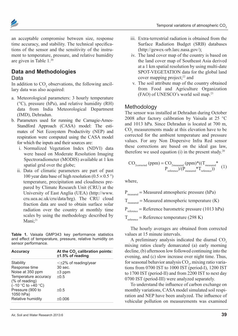
ResultsVariations in the meteorological parametersThe monthly variations of meteorological parameters: (a) relative humidity (%), (b) temperature (°C), and (c) pressure (hPa) in Dehradun during 2009 are shown in Figure 1. Summer at this station is generally from March to June, monsoon months from July to October and winter from November to February. The winter is cold (temperature is less than 20 °C) and humid (RH is above 60%) with high atmospheric pressure (above 930 hPa).

Temperature increases from 16 °C in February to 31 °C in June with low humid conditions (below 50%). From July to October temperature remains above 24 °C with high humid conditions (above 70%) and with low atmospheric pressure. The monthly variations in atmo-spheric pressure shows that the atmospheric boundary layer is dense during winter and rare during summer months, which can strongly contribute to CO2 mixing ratio variations as explained later.

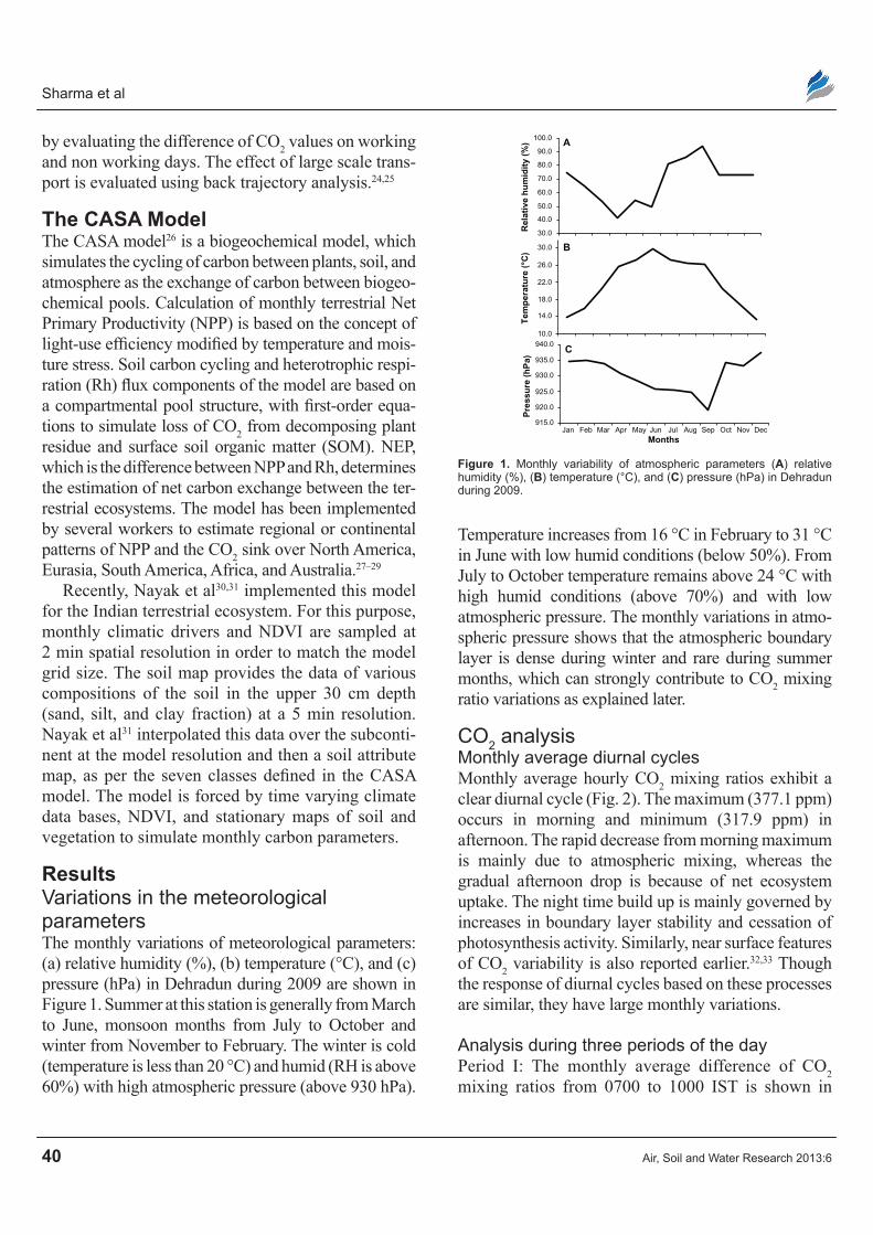
cO2 analysisMonthly average diurnal cyclesMonthly average hourly CO2 mixing ratios exhibit a clear diurnal cycle (Fig. 2). The maximum (377.1 ppm) occurs in morning and minimum (317.9 ppm) in afternoon. The rapid decrease from morning maximum is mainly due to atmospheric mixing, whereas the gradual afternoon drop is because of net ecosystem uptake. The night time build up is mainly governed by increases in boundary layer stability and cessation of photosynthesis activity. Similarly, near surface features of CO2 variability is also reported earlier.32,33 Though the response of diurnal cycles based on these processes are similar, they have large monthly variations.

Analysis during three periods of the dayPeriod I: The monthly average difference of CO2 mixing ratios from 0700 to 1000 IST is shown in

Figure 1. Monthly variability of atmospheric parameters (A) relative humidity (%), (B) temperature (°c), and (c) pressure (hPa) in Dehradun during 2009.

Rel

ativ

e h

um

idit

y (%

)

30.0

50.0

40.0

60.0

70.0

80.0

90.0

100.0

Tem

per

atu

re (

°C)

10.0

14.0

18.0

22.0

26.0

30.0

Pre

ssu

re (

hP

a)

915.0

920.0

925.0

930.0

935.0

940.0

Jan Feb Mar Apr May Jun JulMonths

Aug Sep Oct Nov Dec

A

B

C




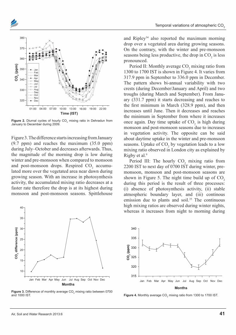
and Ripley34 also reported the maximum morning drop over a vegetated area during growing seasons. On the contrary, with the winter and pre-monsoon seasons being less productive, the drop in CO2 is less pronounced.

Period II: Monthly average CO2 mixing ratio from 1300 to 1700 IST is shown in Figure 4. It varies from 317.9 ppm in September to 336.0 ppm in December. The pattern shows bi-annual variability with two crests (during December/January and April) and two troughs (during March and September). From Janu-ary (331.7 ppm) it starts decreasing and reaches to the first minimum in March (328.9 ppm), and then increases until June. Then it decreases and reaches the minimum in September from where it increases once again. Day time uptake of CO2 is high during monsoon and post-monsoon seasons due to increases in vegetation activity. The opposite can be said about daytime uptake in the winter and pre-monsoon seasons. Uptake of CO2 by vegetation leads to a low mixing ratio observed in London city as explained by Rigby et al.9

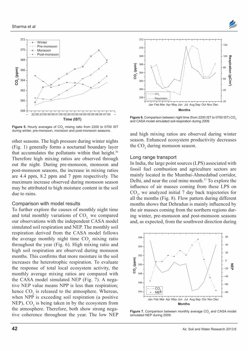
Period III: The hourly CO2 mixing ratio from 2200 IST to next day of 0700 IST during winter, pre- monsoon, monsoon and post-monsoon seasons are shown in Figure 5. The night time build up of CO2 during this period is the result of three processes: (i) absence of photosynthesis activity, (ii) stable atmospheric boundary layer, and (iii) continous emission due to plants and soil.35 The continuous high mixing ratios are observed during winter nights, whereas it increases from night to morning during

01:00 04:00 07:00 10:00 13:00 16:00 19:00 22:00

320

330

340

350

360

370

380

CO

2 (p

pm

)

Time (IST)

Jan Feb Mar Apr May Jun Jul Aug Sep Oct Nov Dec

Figure 2. Diurnal cycles of hourly cO2 mixing ratio in Dehradun from January to December during 2009.


10

15

20

25

30

35

40

CO

2 d

iffe

ren

ce (

pp

m)

Months

Figure 3. Difference of monthly average cO2 mixing ratio between 0700 and 1000 iST.

340

335

330

325

320

315

CO

2 (p

pm

)


Months

Figure 4. Monthly average cO2 mixing ratio from 1300 to 1700 iST.

Figure 3. The difference starts increasing from January (9.7 ppm) and reaches the maximum (35.0 ppm) during July–October and decreases afterwards. Thus, the magnitude of the morning drop is low during winter and pre-monsoon when compared to monsoon and post-monsoon drops. Respired CO2 accumu-lated more over the vegetated area near dawn during growing season. With an increase in photosynthesis activity, the accumulated mixing ratio decreases at a faster rate therefore the drop is at its highest during monsoon and post-monsoon seasons. Spittlehouse


Sharma et al


other seasons. The high pressure during winter nights (Fig. 1) generally forms a nocturnal boundary layer that accumulates the pollutants within that height.36 Therefore high mixing ratios are observed through out the night. During pre-monsoon, monsoon and post-monsoon seasons, the increase in mixing ratios are 4.4 ppm, 8.2 ppm and 7 ppm respectively. The maximum increase observed during monsoon season may be attributed to high moisture content in the soil due to rains.

comparison with model resultsTo further explore the causes of monthly night time and total monthly variations of CO2, we compared our observations with the independent CASA model simulated soil respiration and NEP. The monthly soil respiration derived from the CASA model follows the average monthly night time CO2 mixing ratio throughout the year (Fig. 6). High mixing ratio and high soil respiration are observed during monsoon months. This confirms that more moisture in the soil increases the heterotrophic respiration. To evaluate the response of total local ecosystem activity, the monthly average mixing ratios are compared with the CASA model simulated NEP (Fig. 7). A nega-tive NEP value means NPP is less than respiration; hence CO2 is released to the atmosphere. Whereas, when NPP is exceeding soil respiration (a positive NEP), CO2 is being taken in by the ecosystem from the atmosphere. Therefore, both show strong nega-tive coherence throughout the year. The low NEP

and high mixing ratios are observed during winter season. Enhanced ecosystem productivity decreases the CO2 during monsoon season.

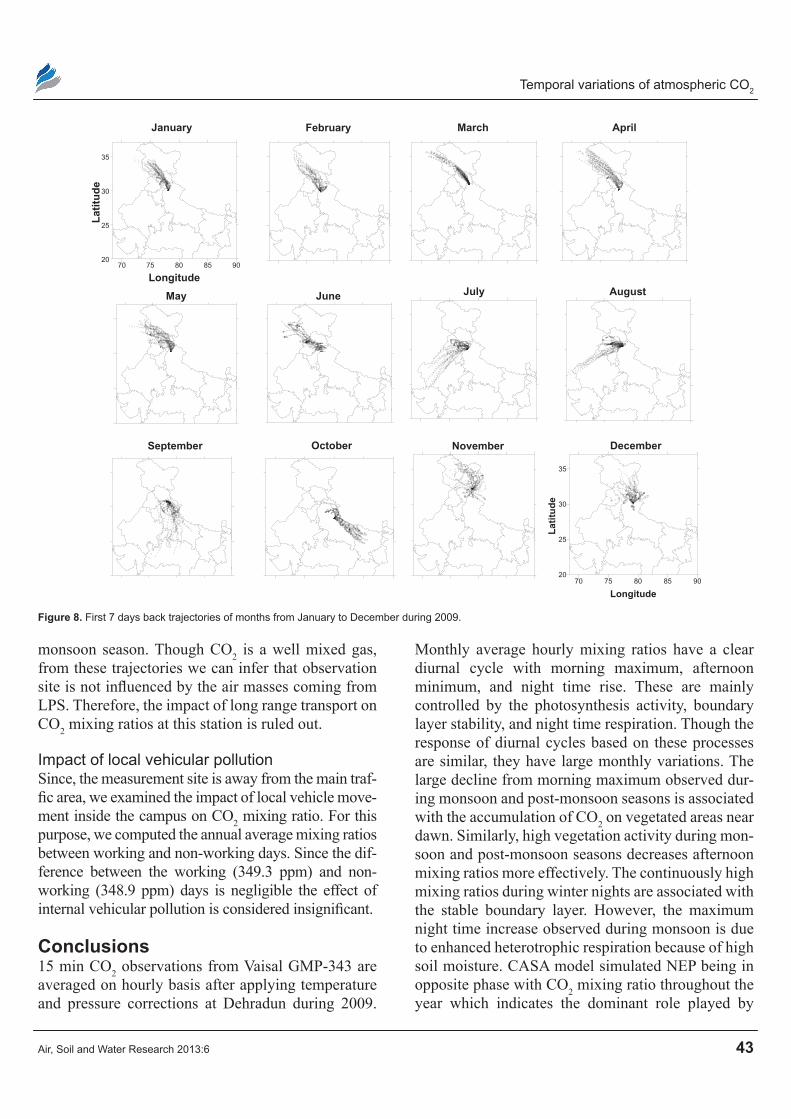
Long range transportIn India, the large point sources (LPS) associated with fossil fuel combustion and agriculture sectors are mainly located in the Mumbai-Ahmedabad corridor, Delhi, and near the coal mine mouth.37 To explore the influence of air masses coming from these LPS on CO2, we analyzed initial 7 day back trajectories for all the months (Fig. 8). Flow pattern during different months shows that Dehradun is mainly influenced by the air masses coming from the northern regions dur-ing winter, pre-monsoon and post-monsoon seasons and, as expected, from the southwest direction during

358

360

362

364

366

368

370

372

CO2

Respiration

Months

CO

2 (p

pm

)

20

40

60

80

100

120

Resp

iration

(gC

/m2)


Figure 6. comparison between night time (from 2200 iST to 0700 iST) cO2 and cASA model simulated soil-respiration during 2009.

344

346

348

350

352

354

356

CO2 NEP

Months

CO

2 (p

pm

)

−80

−60

−40

−20

0

20

40

60

NE

P


Figure 7. comparison between monthly average cO2 and cASA model simulated neP during 2009.

-- 22:00 23:00 00:00 01:00 02:00 03:00 04:00 05:00 06:00 07:00 --358

360

362

364

366

368

370

372

CO

2 (p

pm

)

Time (IST)

Winter Pre-monsoon Monsoon Post-monsoon

Figure 5. hourly averages of cO2 mixing ratio from 2200 to 0700 iST during winter, pre-monsoon, monsoon and post-monsoon seasons.




20

25

30

35

January

Longitude

Lat

itu

de

February April

May June

March

July August

September October November

70 75 80 85 90

70 75 80 85 90

20

25

30

35

December

Longitude

Lat

itu

de

Figure 8. First 7 days back trajectories of months from January to December during 2009.

monsoon season. Though CO2 is a well mixed gas, from these trajectories we can infer that observation site is not influenced by the air masses coming from LPS. Therefore, the impact of long range transport on CO2 mixing ratios at this station is ruled out.

impact of local vehicular pollutionSince, the measurement site is away from the main traf-fic area, we examined the impact of local vehicle move-ment inside the campus on CO2 mixing ratio. For this purpose, we computed the annual average mixing ratios between working and non- working days. Since the dif-ference between the working (349.3 ppm) and non-working (348.9 ppm) days is negligible the effect of internal vehicular pollution is considered insignificant.

conclusions15 min CO2 observations from Vaisal GMP-343 are averaged on hourly basis after applying temperature and pressure corrections at Dehradun during 2009.

Monthly average hourly mixing ratios have a clear diurnal cycle with morning maximum, afternoon minimum, and night time rise. These are mainly controlled by the photosynthesis activity, boundary layer stability, and night time respiration. Though the response of diurnal cycles based on these processes are similar, they have large monthly variations. The large decline from morning maximum observed dur-ing monsoon and post-monsoon seasons is associated with the accumulation of CO2 on vegetated areas near dawn. Similarly, high vegetation activity during mon-soon and post-monsoon seasons decreases afternoon mixing ratios more effectively. The continuously high mixing ratios during winter nights are associated with the stable boundary layer. However, the maximum night time increase observed during monsoon is due to enhanced heterotrophic respiration because of high soil moisture. CASA model simulated NEP being in opposite phase with CO2 mixing ratio throughout the year which indicates the dominant role played by


Sharma et al


the biospheric processes in controlling the carbon exchange. Back trajectory analysis and the amount of mixing ratio between working and non-working days further confirm that the biospheric processes exert a strong control on temporal variations of CO2 mixing ratios at the site.

AcknowledgementsThis research work was carried out as the part of National carbon Project, ISRO-Geosphere and Biosphere Programme. The authors are thankful to the referees for their critical comments and sug-gestions which help to improve the clarity of the manuscript.

Author contributionsConceived and designed the experiments: VKD. Analysed the data: NS, RKN, YK. Wrote the first draft of the manuscript: NS, MMA, VKD. Contributed to the writing of the manuscript: NS, MMA, RKN, VKD. Agree with manuscript results and conclusions: All authors. Jointly developed the structure and arguments for the paper: VKD, NS, MMA. Made critical revisions and approved final version: VKD. All authors reviewed and approved of the final manuscript.

FundingThis project is funded by the National Carbon Project (NCP) of ISRO.

competing InterestsAuthor(s) disclose no potential conflicts of interest.

Disclosures and ethicsAs a requirement of publication author(s) have pro-vided to the publisher signed confirmation of compli-ance with legal and ethical obligations including but not limited to the following: authorship and contribu-torship, conflicts of interest, privacy and confidential-ity and (where applicable) protection of human and animal research subjects. The authors have read and confirmed their agreement with the ICMJE authorship and conflict of interest criteria. The authors have also confirmed that this article is unique and not under consideration or published in any other publication, and that they have permission from rights holders to reproduce any copyrighted material. Any disclosures

are made in this section. The external blind peer reviewers report no conflicts of interest.

References 1. WMO Global Atmosphere Watch (GAW) Strategic Plan: 2008–2011. WMO

TD No. 1384. 2. Keeling CD. The concentration and isotopic abundances of carbon dioxide

in the atmosphere. Tellus. 1960;12(2):200–3. 3. Idso CD, Idso SB, Balling RC. The urban CO2 dome of Phoenix, Arizona.

Phys Geo. 1998;19:95–108. 4. Idso CD, Idso SB, Balling RC. An intensive two-week study of an urban

CO2 dome in Phoenix, Arizona, USA. Atmos Environ. 2001;35:995–1000. 5. Gratani L, Varone L. Daily and seasonal variation of CO2 in the city of Rome

in relationship with the traffic volume. Atmos Environ. 2005;39:2619–24. 6. Coutts A, Beringer M, Tapper J. Characteristics influencing the variability

of urban CO2 fluxes in Melbourne, Australia. Atmos Environ. 2007;41(1): 51–62.

7. Reid KH, Steyn DG. Diurnal variations of boundary-layer carbon dioxide in a coastal city—observations and comparison with model results. Atmos Environ. 1997;31(18):3101–14.

8. Soegaard H, Moller-Jensen L. Towards a spatial CO2 budget of a metro-politan region based on textural image classification and flux measurements. Remote Sens Environ. 2003;87(2–3):283–94.

9. Rigby M, Toumi R, Fisher R, Lowry D, Nisbet EG. First continuous mea-surements of CO2 mixing ratio in central London using a compact diffusion probe. Atmos Environ. 2008;42:8943–53.

10. Tiwari YK, Patra PK, Chevallier F, et al. Carbon dioxide observations at Cape Rama, India for the period 1993–2002 implications for constraining Indian emissions. India Curr Sci. 2011;101:1562–8.

11. Bhattacharya SK, Borole DV, Francey RJ, et al. Trace gases and CO2 isotope records from Cabo de Rama. India Curr Sci. 2009;97:1336–44.

12. Schuck TJ, Brenninkmeijer CAM, Baker AK, Slemr F, von Velthoven PFJ, Zahn A. Greenhouse gas relationships in the Indian summer monsoon plume measured by the CARIBIC passenger aircraft. Atmos Chem Phys. 2010;10:3965–84.

13. Patel, NR, Dadhwal VK, Shah SK. Measurement and Scaling of Carbon Dioxide (CO2) Exchanges in Wheat Using Flux-Tower and Remote Sensing. J Indian Soc Remote Sens. 2011;39(3):383–91.

14. Luijikx IT, Neubert REM, Laan Svan der, Meijer HAJ. Continuous mea-surements of atmospheric oxygen and carbon dioxide on a North sea gas platform. Atmos Meas Tech Discuss. 2009;2:1693–724.

15. Sanchez-Canete EP, Serrano-Ortiz P, Kowalski AS, Oyonarte C, Domingo F. Subterranean CO2 ventilation and its role in the net ecosystem carbon bal-ance of karastic shrubland. Geophys Res Letters. 2011;38: L09802, doi: 10.1029/2011GL047077.

16. Sapunova S, Ivanova T, Kostov P, Naydenov Y, Llieva L, Dandolov L. Monitoring and control of atmospheric gas composition in Space plant growth facilities: selection of CO2 sensors For the svet-3 space greenhouse. Ecol Eng Environ Protec. 2008;1:56–64.

17. Zhen J, Chuan-Kuan W, Xing-Chang W. Spatio-temporal variations of CO2 within the canopy in a temperate deciduous forest, Northeast China. Chinese J Plant Ecol. 2009;35:512–22.

18. Hari P, Pumpanen J, Huotari J, et al. High-frequency measurements of pro-ductivity of planktonic algae using rugged nondispersive infrared carbon dioxide probes. Limnol Oceanogr: Methods. 2008;6:347–54.

19. Vargas R, Baldochhi DD, Allen MF, et al. Looking deeper into the soil: bio-physical controls and seasonal lags of soil CO2 production and efflux. Ecol Appl. 2010;20(6):1569–82.

20. Vaisala. Vaisala CARBOCAP Carbon Dioxide Probe GMP343. Vaisala Oyj, Finland. 2005. http://www.vaisala.com.

21. Mani A. Handbook of Solar Radiation: Data for India. Allied Publishers Private Limited. 1980; New Delhi: 500.

22. Agrawal S, Joshi PK, Shukla Y, Roy PS. SPOT VEGETATION multi tem-poral data for classifying vegetation in south central Asia. Current Science. 2003;84:1440–8.


http://www.vaisala.com



23. Reynolds CA, Jackson TJ, Rawls WJ. Estimated available water content from the FAO soil map of the world, global soil profile databases, pedo-transfer functions. 1999. Boulder, NOAA National Geophysical Data Center.

24. Draxler RR, Rolph GD. HySPLIT (Hybrid Single Particle Lagrangian Inte-grated Trajectory) Model access via NOAA ARL READY website (http://www.arl.noaa.gov/ready/hysplit4.html), NOAA Air Resources Laboratory. Silver Spring, MD. 2003.

25. Rolph GD. Real-time Environmental Applications and Display System (READY) Website (http://www.arl.noaa.gov/ready/hysplit4.html). NOAA Air Resources Laboratory. Silver Spring, MD. 2003.

26. Potter CS, Randerson JT, Field CB. Terrestrial ecosystem production: A process model on global satellite and surface data. Global Biogeochem Cycles. 1993;7(4):811–41.

27. Field CB, Randerson JT, Malmstrom CM. Global net primary production: Combining ecology and remote sensing. Remote Sens Environ. 1995;51(1): 74–88.

28. Thompson MV, Randerson JT, Malstrom CM, Field CB. Change in Net primary production and heterotrophic respiration. How much is neces-sary to sustain the terrestrial carbon sink? Global Biogeochem Cycles. 1996;10(4):711–26.

29. Potter CS, Klooster SA, Myneni RB, Genovese V, Tan PN, Kumar V. Continental scale comparisons of terrestrial carbon sinks estimated from satellite data and ecosystem modeling 1982–1998. Global Planet Change. 2003;39:201–13.

30. Nayak RK, Patel NR, Dadhwal VK. Estimation and analysis of terrestrial net primary productivity over India by remote-sensing-driven terrestrial biosphere model. Environ Monit Assess. 2009;170(1–4):195–213.

31. Nayak RK, Patel NR, Dadhwal VK. Inter-annual variability of Net Primary Productivity over India. Internat J Climat. 2012;DOI: 10.1002/joc.3414.

32. Bakwin PS, Zhao C, Ussler III W, Tans PP, Quesnel E. Measurements of carbon dioxide on a very tall tower. Tellus B. 1995;47(5):535–49.

33. Bakwin PS, Tans PP, White JWC, Andres RJ. Determination the isotopic (13C/12C) discrimination by terrestrial biology from a global net-work of observations. Global Biogeochem Cycles. 1998;12:555–62.

34. Spittlehouse DL, Ripley EA. Carbon dioxide concentrations over a native grassland in Saskatchewan. Tellus. 1997;29:54–65.

35. Yuesi W, Changke W, Xueqing GUO, Guangren LIU, Yao H. Trend, sea-sonal and diurnal variations of atmospheric CO2 in Beijing. Chinese Science Bulletin. 2002;47:24.

36. Stull RB. An Introduction to Boundary Layer Meteorology. Kluwer Acad., Dordrecht, Netherlands. 1988:667.

37. Ghosh D. Large point sources (lps) emissions from India: Regional and sec-toral analysis. Atmos Environ. 2002;36:213–24.


http://www.arl.noaa.gov/ready/hysplit4.html



Temporal variations of atmospheric CO2 in dehradun, India during 2009

Documents

Transcript of Temporal variations of atmospheric CO2 in dehradun, India during 2009