Temporal Patterns of Functional and Dysfunctional Employee Turnover

University of Tennessee, Knoxville University of Tennessee, Knoxville

TRACE: Tennessee Research and Creative TRACE: Tennessee Research and Creative

Exchange Exchange

Doctoral Dissertations Graduate School

12-2011

Temporal Patterns of Functional and Dysfunctional Employee Temporal Patterns of Functional and Dysfunctional Employee

Turnover Turnover

Matthew Scott Fleisher [email protected]

Follow this and additional works at: https://trace.tennessee.edu/utk_graddiss

Part of the Industrial and Organizational Psychology Commons

Recommended Citation Recommended Citation Fleisher, Matthew Scott, "Temporal Patterns of Functional and Dysfunctional Employee Turnover. " PhD diss., University of Tennessee, 2011. https://trace.tennessee.edu/utk_graddiss/1181

This Dissertation is brought to you for free and open access by the Graduate School at TRACE: Tennessee Research and Creative Exchange. It has been accepted for inclusion in Doctoral Dissertations by an authorized administrator of TRACE: Tennessee Research and Creative Exchange. For more information, please contact [email protected].

https://trace.tennessee.edu/

https://trace.tennessee.edu/

https://trace.tennessee.edu/utk_graddiss

https://trace.tennessee.edu/utk-grad

https://trace.tennessee.edu/utk_graddiss?utm_source=trace.tennessee.edu%2Futk_graddiss%2F1181&utm_medium=PDF&utm_campaign=PDFCoverPages

http://network.bepress.com/hgg/discipline/412?utm_source=trace.tennessee.edu%2Futk_graddiss%2F1181&utm_medium=PDF&utm_campaign=PDFCoverPages

mailto:[email protected]

To the Graduate Council:

I am submitting herewith a dissertation written by Matthew Scott Fleisher entitled "Temporal

Patterns of Functional and Dysfunctional Employee Turnover." I have examined the final

electronic copy of this dissertation for form and content and recommend that it be accepted in

partial fulfillment of the requirements for the degree of Doctor of Philosophy, with a major in

Industrial and Organizational Psychology.

David J. Woehr, Major Professor

We have read this dissertation and recommend its acceptance:

T. Russell Crook, William L. Seaver, Don P. Clark

Accepted for the Council:

Carolyn R. Hodges

Vice Provost and Dean of the Graduate School

(Original signatures are on file with official student records.)

Temporal Patterns of Functional and Dysfunctional Employee Turnover

A Dissertation Presented for the Doctor of Philosophy Degree

The University of Tennessee, Knoxville

Matthew Scott Fleisher

December 2011

ii

Copyright © 2011 by Matthew Scott Fleisher

All rights reserved.

iii

Acknowledgements

I would like to thank my wife, Erin, for putting up with the stress, time away during

internships, and general craziness of our lives throughout my graduate training, my

Mother and Father, my brother Danny, and my in-laws for always providing support and

encouragement, my advisor, Dave Woehr for being a great mentor and not giving up on

me when I took an applied job much too soon after defending my proposal, Robert Gibby

and Andy Biga for showing me how hectic, challenging, and fun applied research can be,

and finally, Kim O’Brien and all of the graduate students and faculty at the University of

South Florida who guided me into I-O Psychology and jump-started my career.

iv

Abstract

This study examined temporal patterns in collective employee turnover over a 75 month

interval. Time series models were fit to subgroups of functional and dysfunctional

turnover. Dysfunctional turnover was defined as voluntary separation among high and

average performers and functional turnover was defined as voluntary separation of low

performers. Results provided support for the hypothesis that temporal patterns of

functional and dysfunctional turnover differ. Patterns among high and average performers

were similar, such that employee turnover across several global regions increased during

or near July. In contrast, employee turnover among low performers tended to spike

during or soon after October. Forecast (prediction) accuracy of turnover differed across

groups based on individual performance level. Specifically, turnover among low and

average performers was forecast with greater accuracy than overall aggregated turnover

or turnover among high performers, the latter being the most difficult to forecast. After

time-dependent variation (autocorrelation) was removed from global turnover among

high, average, and low performers, these series were cross-correlated with similarly

cleaned organizational performance outcomes (i.e., net sales, operating income, diluted

net earnings per share). Results from these analyses indicated that organizational

performance had a lagged negative relationship with turnover among high performers.

The dynamic nature of the turnover and performance variables examined underscores the

importance of considering employee turnover as a continuous process. As such,

employee turnover should be proactively managed over time.

v

Table of Contents

Chapter 1 Introduction ........................................................................................................ 1

Chapter 2 Literature Review............................................................................................... 3

Turnover Defined............................................................................................................ 3

Performance as an Antecedent of Turnover.................................................................... 4

Turnover Functionality ................................................................................................... 8

Turnover and Time ....................................................................................................... 18

Chapter 3 The Present Study............................................................................................. 26

Chapter 4 Methods............................................................................................................ 30

Participants and Procedure............................................................................................ 30

Study Variables............................................................................................................. 33

Data Analysis ................................................................................................................ 36

Time Series Models Tested....................................................................................... 36

Model Identification Procedures............................................................................... 40

Preliminary Data Analyses ........................................................................................... 40

Outliers...................................................................................................................... 40

Model Fitting and Cross-Validation ............................................................................. 42

Cross-Correlations among Turnover Rates and with Organizational Performance...... 44

Chapter 5 Results .............................................................................................................. 46

Descriptive Turnover Information ................................................................................ 46

Detecting Seasonality.................................................................................................... 47

Time Series Model Estimation and Cross-Validation .................................................. 48

Research Question 3: Does forecast accuracy differ for functional and dysfunctional

turnover? ....................................................................................................................... 51

Research Question 4: Does forecast accuracy of functional and dysfunctional turnover

differ from that of overall turnover? ............................................................................. 52

Research Question 1: Do functional and dysfunctional turnover demonstrate different

temporal patterns?......................................................................................................... 53

Research Question 2: Does overall level of turnover have a different temporal pattern

than functional or dysfunctional turnover? ................................................................... 56

Supplementary Analyses: Turnover and Organizational Performance......................... 57

Summary of Results...................................................................................................... 58

Chapter 6 Discussion ........................................................................................................ 61

Limitations and Directions for Future Research........................................................... 68

List of References ............................................................................................................. 70

Appendix........................................................................................................................... 82

Bio................................................................................................................................... 148

vi

List of Tables

Table 1. Costs and Benefits of Voluntary Turnover ......................................................... 83

Table 2. Descriptive Statistics of Monthly Turnover Rates.............................................. 84

Table 3. Correlations of Monthly Turnover Rates among High, Average, and Low

Performers................................................................................................................. 85

Table 4. Seasonal Analysis of Variance Results............................................................... 86

Table 5. Final ARIMA Model Parameters........................................................................ 87

Table 6. Summary of Models Forecasting Monthly Turnover ......................................... 88

Table 7. Time Series Regression Results for Global Turnover among Average Performers

................................................................................................................................... 94

Table 8. Time Series Regression Results for Global Turnover among Low Performers . 95

Table 9. Time Series Regression Results for North American Turnover among High

Performers................................................................................................................. 96

Table 10. Time Series Regression Results for North American Turnover among Low

Performers................................................................................................................. 97

Table 11. Time Series Regression Results for AAI Turnover among Low Performers ... 98

Table 12. Time Series Regression Results for Northeast Asian Turnover among Average

Performers................................................................................................................. 99

Table 13. Time Series Regression Results for Career-related Turnover among Average

Performers............................................................................................................... 100

Table 14. Time Series Regression Results for Career-related Turnover among Low

Performers............................................................................................................... 101

Table 15. Cross-correlations of Pre-whitened (Residual) Series for Turnover among High,

Average, and Low Performers ................................................................................ 102

Table 16. Cross-correlations of Pre-whitened (Residual) Series for Turnover among High,

Average, and Low Performers with Organizational Performance.......................... 103

vii

List of Figures

Figure 1. Overall Global Monthly Turnover from Jan 2003 through Mar 2009 ............ 104

Figure 2. Global Monthly Turnover from Jan 2003 through Mar 2009 among High

Performers............................................................................................................... 105

Figure 3. Global Monthly Turnover from Jan 2003 through Mar 2009 among Average

Performers............................................................................................................... 106

Figure 4. Global Monthly Turnover from Jan 2003 through Mar 2009 among Low

Performers............................................................................................................... 107

Figure 5. Monthly Turnover from Jan 2003 through Mar 2009 among High Performers in

North America ........................................................................................................ 108

Figure 6. Monthly Turnover from Jan 2003 through Mar 2009 among Average

Performers in North America.................................................................................. 109

Figure 7. Monthly Turnover from Jan 2003 through Mar 2009 among Low Performers in

North America ........................................................................................................ 110

Figure 8. Monthly Turnover from Jan 2003 through Mar 2009 among High Performers in

all of Asia except China, Korea and Japan and including Australia and India....... 111


Performers in all of Asia except China, Korea and Japan and including Australia and

India ........................................................................................................................ 112

Figure 10. Monthly Turnover from Jan 2003 through Mar 2009 among Low Performers

in all of Asia except China, Korea and Japan and including Australia and India... 113

Figure 11. Monthly Turnover from Jan 2003 through Mar 2009 among High Performers

in Northeast Asia..................................................................................................... 114


Performers in Northeast Asia.................................................................................. 115


in Northeast Asia..................................................................................................... 116


Leaving for Career-related Reasons........................................................................ 117


Performers Leaving for Career-related Reasons..................................................... 118



Figure 17. Average Monthly Global Turnover by Performance Rating and Overall ..... 120

Figure 18. Average Monthly Turnover by Performance Rating in North America........ 121

Figure 19. Average Monthly Turnover by Performance Rating in all of Asia except

China, Korea and Japan and including Australia and India.................................... 122

Figure 20. Average Monthly Turnover by Performance Rating in Northeast Asia........ 123

Figure 21. Average Monthly Turnover by Performance Rating among Employees


viii

Figure 22. Predicted Monthly Turnover from Additive Regression, Robust Regression,

and Decomposition Modeling Plotted against Overall Global Turnover Holdout

Values from April 2008 through March 2009 ........................................................ 125

Figure 23. Predicted Monthly Turnover from HWES Plotted against Overall Global

Turnover Holdout Values from October 2008 through March 2009...................... 126

Figure 24. Predicted Monthly Turnover from Robust Regression and ARIMA Plotted

against Dysfunctional Global Turnover Holdout Values from April 2008 through

March 2009 ............................................................................................................. 127

Figure 25. Predicted Monthly Turnover from ARIMA Plotted against Dysfunctional

Global Turnover Holdout Values from October 2008 through March 2009 .......... 128


against 2-Rated Global Turnover Holdout Values from April 2008 through March

2009......................................................................................................................... 129

Figure 27. Predicted Monthly Turnover from ARIMA Plotted against 2-Rated Global

Turnover Holdout Values from October 2008 through March 2009...................... 130

Figure 28. Predicted Monthly Turnover from HWES Plotted against 3-Rated Global

Turnover Holdout Values from April 2008 through March 2009 .......................... 131

Figure 29. Predicted Monthly Turnover from Additive Regression, Decomposition

Modeling, HWES, and ARIMA Plotted against 3-Rated Global Turnover Holdout

Values from October 2008 through March 2009.................................................... 132

Figure 30. Predicted Monthly Turnover from Additive Regression Plotted against 1-

Rated North American Turnover Holdout Values from April 2008 through March

2009......................................................................................................................... 133

Figure 31. Predicted Monthly Turnover from Additive Regression and Decomposition

Modeling Plotted against 1-Rated North American Turnover Holdout Values from

October 2008 through March 2009......................................................................... 134

Figure 32. Predicted Monthly Turnover from HWES and ARIMA Plotted against 2-Rated

North American Turnover Holdout Values from April 2008 through March 2009 135


against 3-Rated North American Turnover Holdout Values from October 2008

through March 2009................................................................................................ 136


AAI Turnover Holdout Values from October 2008 through March 2009.............. 137


Modeling, and ARIMA Plotted against .................................................................. 138

3-Rated AAI Turnover Holdout Values from April 2008 through March 2009............. 138


Modeling, and ARIMA Plotted against .................................................................. 139

3-Rated AAI Turnover Holdout Values from October 2008 through March 2009 ........ 139


Decomposition Modeling, HWES, and ARIMA Plotted against 2-Rated Northeast

Asian Turnover Holdout Values from October 2008 through March 2009............ 140

Figure 38. Predicted Monthly Turnover from ARIMA Plotted against 3-Rated Northeast

Asian Turnover Holdout Values from April 2008 through March 2009 ................ 141

ix

Figure 39. Predicted Monthly Turnover from ARIMA Plotted against 3-Rated Northeast

Asian Turnover Holdout Values from October 2008 through March 2009............ 142


Career-related Turnover Holdout Values from April 2008 through March 2009 .. 143


Decomposition Modeling, HWES, and ARIMA Plotted against 2-Rated Global

Career-related Holdout Values from April 2008 through March 2009 .................. 144


Career-related Holdout Values from October 2008 through March 2009.............. 145


Global Career-related Holdout Values from April 2008 through March 2009 ...... 146


Modeling, HWES, and ARIMA Plotted against 3-Rated Global Career-related

Holdout Values from October 2008 through March 2009...................................... 147

1

Chapter 1

Introduction

Employee turnover has been studied from a variety of perspectives across several

disciplines, including Organizational Behavior, Industrial-Organizational (I-O)

Psychology, Human Resource Management (HRM), Economics, Sociology, Accounting,

and Industrial Relations (Mobley, 1982). This is not surprising, given the well-

documented negative consequences of excessive employee turnover (Hausknecht, Trevor,

& Howard, 2009; Hinkin & Tracey, 2000; Price, 1989; Morrow & McElroy, 2007;

Simons & Hinkin, 2001; Tracey & Hinkin, 2008).

One method of categorizing turnover is to label it as either functional or

dysfunctional to the organization (Campion, 1991). Functional turnover improves

organizational functioning, whereas dysfunctional turnover is disruptive and costly to

organizations (Dalton, Todor, & Krackhardt, 1982). The present study builds upon

previous research on functional and dysfunctional turnover and literature examining

turnover from a longitudinal perspective. Specifically, the aim of this study is to examine

patterns of functional and dysfunctional turnover within a time series framework.

Previous research has demonstrated that the antecedents of functional and dysfunctional

turnover differ and that turnover antecedents change over time. Based upon these

findings, it is hypothesized that functional and dysfunctional turnover exhibit different

patterns over time. This hypothesis is tested using time series analysis of several years of

monthly turnover data from a large consumer products company. As stated, previous

research supports the present research in two ways: (1) functional and dysfunctional

2

turnover often have different antecedents (e.g., Hart, 1990; Hollenbeck & Williams,

1986; Johnson, Griffeth, & Griffin, 2000; Johnston & Futrell, 1989; Miller, 1987; Park,

Ofori-Dankwa, & Bishop, 1994; Williams, 1999); and (2) the antecedents of turnover at

the individual-level have been shown to change over time (e.g., Dickter, Roznowski, &

Harrison, 1996; Johnston, Griffeth, Burton, & Carson, 1993; Kammeyer-Mueller,

Wanberg, Glomb, & Ahlburg, 2005; Sturman & Trevor, 2001; Youngblood, Mobley, &

Meghno, 1983).

In the following section, relevant turnover literature is reviewed. First, turnover is

defined. Then, performance as an antecedent of turnover is discussed. Next, studies

examining turnover functionality are summarized. Then, the relationship between

turnover and time is discussed, and hypotheses based on previous research are offered.

3

Chapter 2

Literature Review

Turnover Defined

Turnover is defined as “the cessation of membership in an organization by an

individual who received monetary compensation from the organization” (Mobley, 1982;

p. 10). At the individual level, turnover has often been viewed as a dichotomy between

staying with an organization and leaving the organization (Campion, 1991). At the

collective level, turnover can also be viewed as the number or percentage of employees

who leave a group, unit, or organization during a specified time period (Hausknecht &

Trevor, 2011).

The amount of published research on collective turnover has increased in recent

years across several academic disciplines. This interest in a more macro-level perspective

of turnover is understandable given findings of collective turnover predicting

organizational productivity, performance, and customer service (Hausknecht & Trevor,

2011). Although individual-level turnover is very important for explaining why

employees stay with or leave an organization, collective-level turnover is also very

important to organizations for human resources (HR) planning. For example, strategic

HR planning could benefit from an awareness of patterns of different groups of

employees separating at different rates or at different times of the year. Turnover in the

present study is examined at the collective level as the number of employees leaving an

organization each month over several years.

4

Many types of turnover can be found in organizations (Campion, 1991). For

example, turnover can be classified as voluntary or involuntary, avoidable or

unavoidable, and functional or dysfunctional. Voluntary vs. involuntary turnover pertains

to whether or not the termination of employment was initiated by the employee or the

organization, avoidable vs. unavoidable pertains to the feasibility of preventing the

turnover by the organization, and functional vs. dysfunctional refers to turnover that is

desirable (e.g., when poor performers leave; functional) as opposed to turnover that is

undesirable (e.g., when average or strong performers leave; dysfunctional). Dysfunctional

turnover has received attention from HR practitioners and researchers who note the utility

of turnover functionality as opposed to overall frequency (e.g., Beadles, Lowery, Petty, &

Ezell, 2000; Campion, 1991; Hollenbeck & Williams, 1986; Park et al., 1994).

Performance as an Antecedent of Turnover

Individual employee performance has been put forth as an important antecedent

of turnover both theoretically and empirically (Bycio, Hackett, & Alvares, 1990; McEvoy

& Cascio, 1987; Williams & Livingstone, 1994; Zimmerman & Darnold, 2009). Several

meta-analyses have demonstrated a moderate negative relationship between performance

and turnover. McEvoy and Cascio reported a ρ of -.28 between performance and

turnover, suggesting that turnover is lower among good performers. This meta-analytic

finding has been replicated by Bycio et al. (ρ = -.25), Williams and Livingstone (ρ = -

.31), and Zimmerman and Darnold (ρ = -.17). A meta-analysis conducted by Williams

and Livingstone replicated and extended earlier meta-analytic findings. Williams and

Livingstone reported that (1) the negative relationship between performance and turnover

5

is unaffected by unemployment rates and the length of time between measurements of the

two variables (a more recent meta-analysis by Griffeth, Hom, and Gaertner [2000] found

that lag time was a significant moderator of this relationship); (2) this relationship was

stronger in organizations using performance-contingent rewards; and (3) there was

support for a U-shaped relationship between performance and turnover such that in some

cases the relationship between turnover and performance is negative, and in others it is

positive (e.g., when high performers leave an organization to take a better job). Several

primary studies have found a positive relationship between performance and turnover

(Jackofsky, 1984; Jackofsky, Ferris, & Breckenridge, 1986; Johns, 1989; Mossholder,

Bedeian, Norris, Giles, & Feild, 1988; Trevor, Gerhart, & Boudreau, 1997).

In the most recent meta-analysis of the performance–turnover relationship,

Zimmerman and Darnold (2009) added to existing knowledge regarding this relationship

by testing a process model via meta-analytic structural equations modeling (SEM). They

found that the performance–turnover relationship is partially mediated through job

satisfaction and intentions to quit. Specifically, higher job performance leads to increased

job satisfaction, which then leads to lower intention to quit, which finally leads to

reduced voluntary turnover. Job performance also has a direct negative effect on

voluntary turnover. The authors interpret the direct path from performance to turnover

based on Lee and Mitchell’s (1994) unfolding model of turnover. Specifically, employees

may react to shocks in the work environment, such as a low performance evaluation, that

may lead to quitting without initiating job satisfaction or withdrawal cognitions.

6

From a theoretical standpoint, the relationship between performance and turnover

is quite complex. Allen and Griffeth (1999) noted that “…performance may have

simultaneous and sometimes conflicting influences on turnover through both the

perceived ease and the perceived desirability of movement, as well as sometimes leading

directly to turnover” (p. 535). Allen and Griffeth put forth an integrative process model

involving several mediators and moderators of the performance–turnover relationship.

The model posits three mediators of the performance–withdrawal relationship:

desirability of movement (e.g., job satisfaction, organizational commitment, opportunity

to transfer), performance-related shocks (e.g., salient performance feedback, unsolicited

job offers), and ease of movement (e.g., number and quality of alternatives). The

performance–desirability of movement relationship was proposed to be moderated by

reward contingency, such that weaker reward contingency would lead to a stronger

relationship between performance and desirability of movement. Further, the

performance–ease of movement relationship was proposed to be moderated by external

visibility of performance, such that increased external visibility would lead to a stronger

relationship between performance and ease of movement. Finally, desirability of

movement, performance-related shocks, and ease of movement lead to withdrawal

processes (e.g., withdrawal cognitions, job search behavior, and turnover intentions)

which then lead to actual turnover. Most of these propositions were directly or indirectly

supported by previous empirical research. For example, Harrison, Virick, and William

(1996) examined the performance–turnover relationship among 189 sales representatives

from a U.S. telecommunications company under both moderate and maximal reward

7

contingency over time. They found that the performance–turnover relationship was much

stronger under maximally contingent rewards.

More recent primary studies have shed additional light on the performance–

turnover relationship. In a follow-up empirical test of their theoretical model, Allen and

Griffeth (2001) supported many of the proposed mediators and moderators discussed

above. Specifically, with a sample of 130 medical services employees, the authors found

that the performance–turnover relationship was mediated through perceived alternatives

and turnover intentions such that higher job performance led to increased perceived

alternatives, which led to increased turnover intentions and finally, increased actual

turnover. Further, they found that the performance–alternatives relationship was

moderated by visibility such that high visibility of performance was associated with a

moderate, positive relationship between performance and perceived alternatives, with no

relationship between these two variables for those with low visibility of performance.

Additionally, a hypothesized performance–satisfaction relationship was moderated by

contingent rewards such that highly contingent rewards were associated with a moderate,

positive relationship between performance and job satisfaction, with no relationship

between these two variables when rewards were not contingent upon performance.

Jackofsky (1984) proposed that job performance and employee turnover should be

related in a curvilinear manner. Specifically, the relationship should be U-shaped such

that low performers and high performers turnover more often than average performers.

This is due to factors that push low performers away from the organization (either

involuntary turnover or pressure by the organization for these employees to voluntarily

8

exit) and factors that pull high performers to other organizations (e.g., ease of

movement). Jackofsky et al. (1986) found support for this hypothesis among 169 male

accountants and 107 truck drivers.

Trevor et al. (1997) examined relationships among voluntary turnover, job

performance, salary growth, and promotions in a sample of 5,143 exempt employees

across a broad spectrum of job types, divisions, and locations from a single organization

in the petroleum industry. The authors found support for Jackofsky’s (1984) hypothesis

in that turnover was higher among low and high performers than average performers.

However, this relationship was moderated by salary growth and promotions such that low

salary growth and high promotions each produced a more pronounced curvilinear

performance–turnover relationship.

Salamin and Hom (2005) examined curvilinear and moderating effects on the

performance–turnover relationship among 11,098 Swiss bank employees. Using survival

analysis, they found that performance was curvilinearly related to turnover such that low

and high performers were more likely to quit than average performers, and that bonus pay

deterred high performers from quitting more so than pay increases. They also found that

the average number of job levels advanced per promotion increased turnover risk to a

greater extent than did promotion rate. In sum, although performance and turnover are

related, this relationship is not always negative or linear.

Turnover Functionality

Although the negative consequences of turnover have been emphasized more

often, employee turnover can have both positive and negative consequences for

9

individuals and organizations (Dalton, Krackhardt, & Porter, 1981; Dalton & Todor,

1979; 1982; Dalton et al., 1982; Tziner & Birati, 1996). Table 1 in the Appendix lists

many of the known costs and benefits of voluntary employee turnover. Negative financial

and non-financial consequences of turnover are well documented and can be substantial

(Hausknecht et al., 2009; Hinkin & Tracey, 2000; Price, 1989; Morrow & McElroy,

2007; Simons & Hinkin, 2001; Tracey & Hinkin, 2008). However, refinements to utility

analysis have indicated that it is important to consider the functional aspects of employee

turnover when assessing its impact on organizations (Tziner & Birati, 1996; Sturman,

Trevor, Boudreau, & Gerhart, 2003).

As discussed previously, performance and turnover are clearly related. Individual

employee performance acts as an antecedent to turnover and turnover affects

organizational performance. Also, individual performance impacts the organizational

consequences of turnover in another way. Specifically, while turnover among average

and above average performers is detrimental to organizations, turnover among poor

performers can be beneficial. Turnover that is detrimental to organizations is known as

dysfunctional, and turnover that is beneficial is known as functional. Dalton and

colleagues (Dalton et al., 1981; Dalton & Todor, 1979; 1982; Dalton et al., 1982) were

among the first to make this distinction, and found a substantial amount of functional

turnover in organizations. For example, Dalton et al. (1981) found that up to 71% of

voluntary turnover among 1,389 employees from 190 U.S. bank branches was functional.

Specifically, among voluntary turnovers, 71% of these employees were easy to replace

10

and for 42% of these employees their supervisor indicated that they would not rehire the

employee or rated the employee’s performance as low.

Jackofsky (1984) posited that individual job performance, when incorporated with

turnover, would refine the turnover criterion. Jackofsky warned against testing theories

regarding determinants of voluntary turnover with samples containing low performers,

stating, “The turnover among low performing employees may not strongly reflect the

same factors that influence turnover among their higher performing counterparts. The

development of a relevant sample based on performance scores, therefore, allows for a

concomitant development of a ‘clean’ criterion measure against which hypothesized

voluntary turnover factors can be tested” (p. 81).

Numerous studies have documented the prevalence of functional and

dysfunctional turnover in organizations, and several have examined the antecedents of

functional and dysfunctional turnover (e.g., Hart, 1990; Hollenbeck & Williams, 1986;

Johnson, Griffeth, & Griffin, 2000; Johnston & Futrell, 1989; Miller, 1987; Park et al.,

1994; Williams, 1999). For example, Hollenbeck and Williams found that 53% of

turnover among 112 retail salespersons was functional to the organization. They also

reported that turnover functionality was unrelated to work attitudes (i.e., various

dimensions of job satisfaction, motivation to turnover, job involvement, and

organizational commitment). As a group, these work attitudes explained 4% of the

variance in turnover functionality, which was non-significant. Individually, none of the

work attitudes was significantly related to turnover functionality at the conservative cut-

off set by the authors, that is, p < .01. However, at a slightly less conservative but well-

11

accepted cutoff (p < .05) two dimensions of job satisfaction were significantly correlated

with turnover functionality: satisfaction with the work itself (r = .21) and satisfaction

with coworkers (r = .19). Also, the authors demonstrated that the antecedents of turnover

frequency and turnover functionality were dissimilar. The same work attitudes that were

unsuccessful in predicting turnover functionality explained 11% of the variance in

turnover frequency, which was statistically significant. Also, three individual variables

were significant predictors of turnover frequency: satisfaction with pay (r = .32),

motivation to turnover (r = -.29), and organizational commitment (r = .27). The authors

concluded that the antecedents of traditional turnover (frequency) and turnover

functionality likely differ. In discussing their findings, the authors suggested that

variables associated with both turnover frequency and performance are likely to impact

turnover functionality. Thus, antecedents of work motivation, such as contingent reward

structures, goal setting and feedback, and/or training, may be likely antecedents of

functional turnover.

Miller (1987) examined attitudinal differences between functional and

dysfunctional leavers. Miller defined turnover functionality along three dimensions:

quality of the leaver, ease of replacing the leaver, and criticality of the vacated position.

Following the work of Dalton et al. (1981), the quality dimension was a combination of

two items: supervisor-rated employee performance and whether the supervisor would

rehire the employee. In a sample of 2,706 employees who had voluntarily resigned from a

U.S. utility company, Miller found that functional turnover accounted for 23.3% of

leavers on the quality dimension, 43.5% of leavers on the ease of replacement dimension,

12

and 21.7% of leavers on the criticality of position dimension. It was also found that

percentages of functional turnover varied widely across nine occupational groups.

Miller (1987) examined employee attitudes and reasons for leaving as potential

antecedents of functional and dysfunctional turnover. These included attitudes about

upper management, the work itself, merit pay and promotion, the employee’s immediate

supervisor, advancement opportunities and salary, job stress, job security, and overall job

satisfaction. All of these attitude dimensions were assessed in three contexts: reasons for

leaving, pre-turnover attitudes, and post-turnover attitudes. Canonical discriminant

analysis was used to test for differences between the attitudes of functional and

dysfunctional leavers. Negative attitudes regarding the employee’s immediate supervisor

demonstrated the highest discrimination between functional and dysfunctional turnover

for the quality and ease of replacement dimensions. Specifically, high quality employees

(high performers who the supervisor would rehire) and employees who were not easy to

replace demonstrated less negative attitudes toward their former immediate supervisor

than low quality employees and employees who were easy to replace. Low quality and

easy to replace employees were less satisfied with their immediate supervisor than high

quality and difficult to replace employees across three contexts: pre-turnover, at the time

of departure, and post-turnover. Results regarding the criticality of position dimension

were less clear. Combining attitudes into a group, pre-turnover and post-turnover

attitudes respectively explained 26% and 21% of the variance in quality of leavers, 11%

and 5% of the variance in ease of replacement, and 5% and 3% of the variance in

criticality of position. In sum, it was found that: (1) functional turnover exists in non-

13

trivial amounts; (2) percentages of functional turnover differ across occupations; (3)

functional and dysfunctional turnover have different attitudinal antecedents; and (4)

attitudes explain a sizeable amount of the variance in turnover functionality. This last

finding disputes the findings of Hollenbeck and Williams (1986); however, it should be

noted that Miller’s sample was much larger than the 112 retail salespersons surveyed by

Hollenbeck and Williams, and also included participants from multiple occupations.

Johnston and Futrell (1989) also found evidence that that the antecedents of

turnover frequency and turnover functionality are dissimilar. In a sample of 103 sales

personnel of a national consumer goods manufacturer, turnover functionality was related

most strongly to salary (r = .34), while turnover frequency (stay = 1; leave = -1) was

related to propensity to leave (r = -.33), leadership role clarification (r = .24), leadership

consideration (r = .23), role conflict (r = -.22), role ambiguity (r = -.19), and overall job

satisfaction (r = .31). It should be noted that a regression of turnover functionality on the

predictors revealed that both salary and leadership role clarification were related to

functionality, while a discriminant analysis revealed that propensity to leave was the only

significant predictor of turnover frequency. For turnover functionality, results indicated

that higher salary and greater clarification of role expectations by supervisors led to

greater likelihood that high performers would remain with the organization. However, for

turnover frequency, results indicated only that as propensity to leave increased, the

likelihood of an individual leaving the organization also increased.

Phillips, Griffeth, Griffin, Johnston, Hom, and Steel (1989) examined factors

differentiating high and low performing quitters and stayers in a sample of hospital

14

nurses. They found that high performing leavers were most dissatisfied with promotion

and growth opportunities while low performing stayers were most satisfied in general. In

a follow-up study, Griffeth, Phillips, Hom, and Steel (1990) found that low performing

leavers were the least satisfied and that good performing stayers had satisfaction levels

similar to good performing leavers and poor performing stayers (Williams, 1999).

Hart (1990) examined turnover functionality in a sample of 468 U.S. mental

health workers. In accordance with the organization’s philosophy, turnover was defined

as functional among poor and average performers and as dysfunctional among above

average performers. According to this operationalization, 72% of the organization’s

turnover was functional. Further, Hart examined not only the functionality of actual

turnover but also the functionality of turnover intentions (e.g., poor and average

performers with high intentions to quit were labeled as functional and above average

performers with high intentions to quit were considered dysfunctional). Due in part to a

low base rate of actual turnover, discriminant analyses examining differential antecedents

of turnover functionality were not statistically significant. However, discriminant

analyses of turnover intentions were statistically significant and informative. Specifically,

job satisfaction, recognition, pay for performance perceptions, and labor market

perceptions discriminated among groups of high vs. low/average performers with high vs.

low turnover intentions. Thus, partial support was found for the hypothesis that functional

and dysfunctional turnover have different antecedents.

Bailey (1991) examined functional and dysfunctional turnover and store

performance among 4,972 full-time sales employees from 16 stores of a major U.S.

15

department store chain. Also, the effects of age, race, and gender on turnover were

examined. It was found that age, race, and an interaction between age and gender all

significantly influenced turnover functionality. Specifically, turnover was more

functional among minorities, and whereas turnover functionality generally increased with

age among females, it increased with age among males from ages 25 to 64, but sharply

decreased in functionality (became more dysfunctional) among men aged 65 and over.

Further, store-level employee turnover functionality correlated .46 with store sales

growth. These findings indicate that turnover functionality may differ across age groups,

minority vs. majority groups, and gender; and that functional turnover can benefit

organizations.

Park et al. (1994) examined organizational and environmental determinants of

functional and dysfunctional voluntary turnover. The authors collected data at the

organization-level with a survey completed by a personnel director from each of 100

small U.S. manufacturing organizations. Park et al. found that functional turnover was

negatively related to unemployment level and pay, and was positively related to

organizational focus on individual incentive programs. In contrast, dysfunctional turnover

was not significantly related to any of these variables. Dysfunctional turnover was found

to be negatively related to presence of unions, and was positively related to

organizational focus on group incentive programs. In contrast, functional turnover was

not significantly related to any of these variables. The authors offered several potential

explanations for these findings. For instance, the finding that functional turnover

decreases as unemployment level increases (and vice versa) may occur because poorly

16

performing employees are less likely to quit when unemployment levels are high and

more likely to quit when unemployment levels are low due to the availability of

alternative jobs. Additionally, the finding that functional turnover decreases as pay

increases may occur because if pay is high for poor performers relative to other

organizations (as was the operationalization in this study) then they will be less likely to

leave the organization. Further, the finding that functional turnover was positively related

to individual incentive programs likely occurs because poor performers receive lower pay

than average and high performers and thus leave the company. In contrast, the finding

that dysfunctional turnover was positively related to group incentive programs most

likely occurs because average and high performers would likely receive lower pay than

they would with individual incentive programs and thus leave the company for higher

paying jobs.

Williams (1999) examined antecedents of turnover among four groups of U.S.

sales representatives: poor performing leavers, good performing leavers, poor performing

stayers, and good performing stayers. Overall, objective reward contingency (R² = .34),

state unemployment rate (R² = .11), state sales unemployment rate (R² = .08), education

(R² = .09), and tenure (R² = .08) accounted for most of the variance in turnover

functionality. Perceived reward contingency, pay satisfaction, job satisfaction, age, and

gender were unrelated to functionality. More specifically, poor performing leavers

received 100% of their pay from commissions, good performing leavers received 91% of

their pay from commissions, good performing stayers received 77% of their pay from

commissions, and finally, poor performing stayers received 39% of their pay from

17

commissions. With respect to unemployment rates, poor performing leavers quit when

unemployment was high and job opportunities were low. This was explained by the fact

that poor performing leavers, who received 100% commission, earned considerably less

total pay than good performers or poor performers who stayed. This study replicated the

findings of others (e.g., Hollenbeck & Williams, 1986) indicating that job satisfaction,

which is traditionally an acceptable predictor of turnover frequency, is not a very good

predictor of turnover functionality.

Johnson et al. (2000) examined antecedents of turnover functionality among 217

business-to-business sales personnel of a U.S. consumer goods manufacturer. They found

that high-performing leavers had the lowest promotion satisfaction, satisfaction with

supervision, and overall job satisfaction. High-performing stayers had the highest and

low-performing leavers had the lowest level of satisfaction with the work itself. Low-

performing leavers also had the highest and high-performing stayers had the lowest

amount of role ambiguity. Functional and dysfunctional turnover was also differentially

influenced by anxiety about work, intentions to quit, role conflict, and perceived

alternative job opportunities. Thus, unlike previous research, Johnson et al. demonstrated

that traditional antecedents of turnover frequency may also predict turnover functionality.

Shaw and Gupta (2007) examined relationships between pay dispersion and the

quits patterns of good, average, and poor performers among 226 truck drivers. They

found a three-way interaction such that under high pay system communication, pay

dispersion was negatively related to good performer quits when performance-based pay

increases were emphasized, and positively related when they were not. Also, under high

18

pay system communication, pay dispersion was negatively related to average performer

quits when seniority-based pay increases were emphasized, but this relationship was

attenuated when they were not. However, pay dispersion was not consistently related to

quit patterns when pay system communication was low.

Shaw, Dineen, Fang, and Vellella (2009) examined relationships between

employee-organization exchange relationships, HRM practices, and quit rates of good

and poor performers in two studies involving 209 truck drivers (Study 1) and the full-

time employee population of 93 single-unit supermarkets (Study 2). They found that

HRM inducements and investments related negatively to good- and poor-performer quit

rates, whereas expectation-enhancing practices related negatively to good-performer quit

rates and positively to poor-performer quit rates. They also found that expectation-

enhancing practices attenuated the negative relationship between inducements and

investments and good-performer quit rates in Study 1, and exacerbated the negative

relationship with poor-performer quit rates in Study 2.

In sum, several empirical studies have demonstrated differential antecedents of

functional and dysfunctional turnover. Also, to be discussed in the following section,

several studies have demonstrated that the antecedents of turnover change and unfold

over time. The present study builds upon these two general findings by empirically

examining the temporal patterns of functional and dysfunctional turnover.

Turnover and Time

Within the past decade, a growing number of researchers have argued for an

explicit consideration of time in organizational research in general (e.g., George & Jones,

19

2000; Mitchell & James, 2001) and in turnover processes in particular (e.g., Holtom,

Mitchell, Lee, & Eberly, 2008; Kammeyer-Mueller et al., 2005; Steel, 2002; Weller,

Holtom, Matiaske, & Mellewigt 2009). In a large-scale review of turnover and retention

research, Holtom et al. emphatically called for an increased awareness of time in turnover

research, stating “Our review of the turnover research, especially of the past 10 years, has

shown that it is essential to consider time in the turnover process” (p. 258). Further, in a

model depicting turnover research findings from 1995 to 2008, Holtom et al. noted

several areas of study where researchers have integrated temporal elements into turnover

theory. These included work attitudes such as job satisfaction (Trevor, 2001) and

organizational commitment (Bentein, Vandenberg, Vandenberghe, & Stinglhamber,

2005), withdrawal cognitions (Lee & Rwigema, 2005), withdrawal behaviors

(Mossholder, Settoon, & Henagan, 2005), alternative employment opportunities

(Kammeyer-Mueller et al., 2005), and individual performance (Sturman & Trevor, 2001).

One of the most interesting findings from this growing body of research is that the

antecedents of turnover may change over time (Holtom et al., 2008; Lee & Rwigema,

2005, Steel, 2002). Some antecedents may decrease in importance and some may

increase in importance over time for individuals depending on environmental or

psychological factors (e.g., unemployment rates; job satisfaction; organizational

commitment). For instance, Dickter et al. (1996) examined the influence of time on

predictors of voluntary turnover among 1,026 employees from a diverse array of

occupations across the U.S. The authors found that time moderated relationships between

job satisfaction and cognitive ability with turnover, such that the relationships of these

20

two predictors with turnover decreased over time. More specifically, as time progressed,

the strength of the relationship between job satisfaction and turnover became less

negative (moving closer to zero). The same relationship was found for cognitive ability.

In one of the first large-scale, longitudinal examinations of the turnover process,

Youngblood et al. (1983) found different relationships among predictors and turnover

over time in a sample of 1,445 U.S Marine Corps enlistees. For example, behavioral

intentions to quit were found to be lowest and to decline in the time period immediately

prior to turnover. Further, changes in job satisfaction over time, in addition to level, were

related to turnover.

In another relatively early examination of the effects of time on turnover

antecedents, Farkas and Tetrick (1989) found that relationships among job satisfaction,

organizational commitment, and reenlistment intentions among 440 U.S. Navy personnel

changed as tenure increased. The authors posited that commitment and satisfaction may

be either cyclically or reciprocally related over time. Hom and Griffeth (1991) also found

that relationships among antecedents of turnover (e.g., job satisfaction; withdrawal

cognitions and behaviors) changed over time with tenure among 129 nurses.

Johnston et al. (1993) investigated relationships among organizational

commitment, propensity to leave, promotion satisfaction, promotions, and turnover in a

sample of 157 salespersons. Relationships among the variables of interest as well as

salary were found to vary over time. Further, time had a significant main effect on

intrinsic motivation, job involvement, and job satisfaction, which all decreased over time.

21

Somers (1996) applied survival analysis along with traditional Ordinary Least

Squares (OLS) and logistic regression analyses to withdrawal/turnover data from 244

nurses. The results from survival techniques were quite different from those from the

traditional techniques and differed from previous research. Specifically, job satisfaction

predicted turnover while job search behavior did not. One of the key distinctions of

survival analysis that may have contributed to these disparate findings is an explicit

incorporation of time (tenure) into the modeling of employee withdrawal and turnover

processes.

Somers (1999) applied neural network-based statistical analyses to the prediction

of turnover among 577 nurses. Not only did two neural network paradigms (multilayer

perceptron and learning vector quantization) outperform logistic regression in the

prediction of turnover, but uncovered interesting relationships among turnover

antecedents over time. Specifically, relationships between antecedent variables (e.g., job

satisfaction, job withdrawal intentions, affective commitment) demonstrated non-linear

changes over time in the form of floor and ceiling effects which had little effect on

turnover at first and then very large effects on turnover once a threshold was reached.

This study highlights both the dynamic nature of turnover antecedents and the importance

in applying innovative statistical techniques to capture previously unknown relationships

among variables.

Utilizing event history (survival) analyses, Harrison et al. (1996) demonstrated

that time-dependent performance is a better predictor of turnover than time-stationary

performance. Further, performance change over time improved the prediction of turnover

22

by capturing significant incremental variance in turnover risk. Sturman and Trevor (2001)

replicated Harrison et al.’s findings among 1,413 loan originators from a U.S. financial

services organization. The authors also extended Harrison et al.’s findings by

demonstrating that performance trends interacted with current performance in the

prediction of voluntary turnover. More specifically, they found that the negative

relationship between performance trend and voluntary turnover was very strong when

current performance was low but was negligible when current performance was high.

These studies highlight the dynamic nature of an important antecedent of turnover

behavior, that is, employee performance.

Trevor (2001) performed survival analysis on data from 5,506 employees across

hundreds of occupations in the U.S., examining the effects of job satisfaction on

voluntary turnover. Findings indicated that this relationship was moderated by

unemployment rate, education, cognitive ability, and occupation-specific training. More

specifically, when unemployment was low, job satisfaction was more strongly negatively

related to turnover. Also, the negative relationship between job satisfaction and turnover

was stronger when each of three indicators of ‘movement capital’ (i.e., education,

cognitive ability, and occupation-specific training) were high. Further, a negative

relationship between unemployment rate and turnover was stronger when the three

indicators of movement capital were low. Trevor notes that these findings have

implications for dysfunctional turnover of high performers. Specifically, the interaction

between job satisfaction and movement capital indicates that more mobile employees are

more likely to turnover than less mobile employees due to job dissatisfaction. Further,

23

these more mobile employees are likely to be high performers due to higher education,

cognitive ability and occupation-specific training. Thus, the loss of these employees is

likely to be quite dysfunctional to the organization.

Bentein et al. (2005) used latent growth modeling (LGM) to examine

relationships between changes in commitment over time, intentions to quit, and actual

turnover among 330 alumni of a university in Belgium employed across a variety of

occupations. The authors found that a steeper decline over time in an individual’s

affective and normative commitment was associated with a greater rate of increase in

both intentions to quit and actual turnover.

Kammeyer-Mueller et al. (2005) examined time-dependent relationships between

job satisfaction, organizational commitment, critical events, unemployment, perceived

costs of turnover, search for alternative jobs, and turnover behavior among 932 full-time,

exempt employees from 7 U.S. organizations involved in manufacturing, food

distribution, health care, and education. Survival analysis and hierarchical linear

modeling (HLM) revealed that all of the antecedents predicted turnover when examined

over time. Also, critical events predicted turnover directly (not through attitudes) which is

consistent with the unfolding model of voluntary turnover (Lee & Mitchell, 1994).

Further, changes in antecedents over time (e.g., decreases in commitment and increases in

job search behavior) played an important role in predicting turnover.

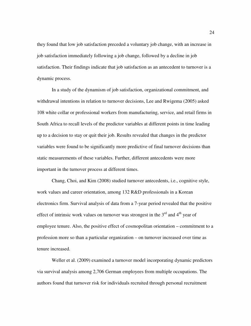
Boswell, Boudreau, & Tichy (2005) examined changes in within-individual job

satisfaction over time in relation to job change (voluntary turnover) among 538 high-level

managers identified through an executive search firm. Using dynamic panel analysis,

24

they found that low job satisfaction preceded a voluntary job change, with an increase in

job satisfaction immediately following a job change, followed by a decline in job

satisfaction. Their findings indicate that job satisfaction as an antecedent to turnover is a

dynamic process.

In a study of the dynamism of job satisfaction, organizational commitment, and

withdrawal intentions in relation to turnover decisions, Lee and Rwigema (2005) asked

108 white collar or professional workers from manufacturing, service, and retail firms in

South Africa to recall levels of the predictor variables at different points in time leading

up to a decision to stay or quit their job. Results revealed that changes in the predictor

variables were found to be significantly more predictive of final turnover decisions than

static measurements of these variables. Further, different antecedents were more

important in the turnover process at different times.

Chang, Choi, and Kim (2008) studied turnover antecedents, i.e., cognitive style,

work values and career orientation, among 132 R&D professionals in a Korean

electronics firm. Survival analysis of data from a 7-year period revealed that the positive

effect of intrinsic work values on turnover was strongest in the 3rd

and 4th

year of

employee tenure. Also, the positive effect of cosmopolitan orientation – commitment to a

profession more so than a particular organization – on turnover increased over time as

tenure increased.

Weller et al. (2009) examined a turnover model incorporating dynamic predictors

via survival analysis among 2,706 German employees from multiple occupations. The

authors found that turnover risk for individuals recruited through personal recruitment

25

sources was lower early in an employee’s tenure than for individuals recruited through

formal sources. Also, this risk peaked significantly later for those recruited through

personal sources. However, this relationship was moderated by tenure such that the

turnover rate differential due to the use of personal recruitment sources diminished as

tenure increased. Finally, the recruitment source effect on turnover risk was partially

mediated by job satisfaction.

In summary, it is clear that turnover is a dynamic process in which antecedents

change over time. Also, several studies have demonstrated that functional and

dysfunctional turnover have different antecedents. Although findings have been mixed,

some studies have also found different antecedents for turnover functionality and

traditional turnover frequency. Based upon these findings, it is hypothesized that

functional and dysfunctional turnover demonstrate different patterns over time from one

another. It is also hypothesized that functional and dysfunctional turnover demonstrate

different patterns over time from overall turnover. These hypotheses are tested by

examining time series patterns of monthly quit rates for good, average, and poor

performers from a large consumer products company over a six year period.

26

Chapter 3

The Present Study

The literature review in the previous chapter reported that substantial functional

and dysfunctional turnover can be found in organizations (e.g., Dalton et al., 1981; Hart,

1990; Hollenbeck & Williams, 1986; Miller, 1987). Also, the antecedents of turnover

frequency and functionality often differ (e.g., Hollenbeck & Williams, 1986; Johnston &

Futrell, 1989; Williams, 1999). Further, the antecedents of functional and dysfunctional

turnover differ (e.g., Hart, 1990; Hollenbeck & Williams, 1986; Johnson et al., 2000;

Johnston & Futrell, 1989; Miller, 1987; Park et al., 1994; Williams, 1999). Additionally,

while the role of time has been examined among antecedents of turnover, turnover as an

outcome has traditionally been operationalized as a dichotomous variable occurring at

one point in time (e.g., Holtom et al., 2008). More specifically, the bulk of turnover

research has focused on the occurrence when individual employees voluntarily transition

from being employed with an organization to no longer being employed with that

organization. Although turnover research has shifted away from stationary antecedents

towards dynamic antecedents, the majority of turnover research has focused on turnover

as a dichotomous, stationary outcome (e.g., stay or leave). One argument of the present

research is that turnover as an outcome variable should be examined as a continuous

process over time.

Several studies have demonstrated that functional and dysfunctional turnover

have different antecedents. To summarize a few examples, unemployment level, pay, and

individual incentive programs have been found to predict functional turnover (Park et al.,

27

1994) and dissatisfaction with promotion and growth opportunities, union presence, and

group incentive programs have been found to predict dysfunctional turnover (Park et al.,

1994; Phillips et al., 1989). Further, although job satisfaction and organizational

commitment are antecedents of both functional and dysfunctional turnover, facets of

these constructs have demonstrated differential relationships with functional and

dysfunctional turnover (Griffeth et al., 1990; Johnson et al., 2000; McNeilly & Russ,

1992; Miller, 1987; Phillips et al., 1989). Further, many of these antecedents of turnover

have been found to be dynamic (e.g., Trevor, 2001; Bentein et al., 2005). Based upon

these findings, it is hypothesized that functional and dysfunctional turnover exhibit

different temporal patterns.

Based on the research summarized in the previous chapter, the present study is

guided by four primary research questions:

1) Do functional turnover and dysfunctional turnover demonstrate different temporal

patterns?

2) Does overall level of turnover have a different temporal pattern than functional or

dysfunctional turnover?

3) Does forecast (prediction) accuracy differ for functional and dysfunctional turnover?

4) Does forecast accuracy of functional and dysfunctional turnover differ from that of

overall turnover?

Traditional turnover research has focused on predicting and explaining employee

turnover in an effort to reduce or eliminate it (Staw, 1980). However, decades of research

has shown us that we are never going to completely eliminate turnover, nor should we

28

(Dalton et al., 1982; Holtom et al. 2008). Instead, organizations should proactively

manage turnover. The better researchers and practitioners can understand and predict

turnover, the better we can manage it. One step in this direction is to understand the

temporal nature of turnover. Although the temporal patterns of turnover antecedents have

been explained through a growing body of research, the temporal pattern of turnover

itself remains largely unexplored. The present study addresses this gap by examining the

temporal nature of functional and dysfunctional turnover at a large consumer products

company. In doing so, the importance of considering employee turnover as a continuous

process to be proactively managed is emphasized.

Dalton and Todor (1979) noted that turnover should be seasonal for at least some

industries and that, in the presence of seasonal variation, turnover frequency at a

particular point in time would not be meaningful. Further, dynamic trends in turnover

antecedents have been found when these variables are examined longitudinally.

Fortunately, there is a well-established method for estimating linear (and nonlinear)

trends and seasonality over time that has a long tradition in the fields of statistics and

economics, that is, time series analysis (Chatfield, 2000). Due to the likelihood of

seasonal variation and temporal trends in employee turnover, time series analysis was

used in the present study to examine temporal patterns of functional and dysfunctional

employee turnover from a multinational consumer products company. Based upon

empirical research mentioned previously, it is hypothesized that functional and

dysfunctional turnover exhibit different temporal patterns and also hypothesized that

these patterns differ from that of overall turnover frequency. In examining these

29

hypotheses, this study extends the findings of previous longitudinal turnover research by

examining seasonality in turnover.

In order to examine the research questions and test the hypotheses, 75 months of

continuous turnover data was obtained from a large consumer products company. Time

series analysis was used to examine the primary research questions. The following

chapter describes the sample data, statistical analyses, and specific methods for testing

hypotheses.

30

Chapter 4

Methods

Participants and Procedure

Just over 6 years (75 months) of turnover data was obtained from a large U.S.-

based multinational consumer products company. Turnover was defined as the number of

employees who left the organization each month from January 2003 through March 2009.

The analysis sample consisted of voluntary turnover only (N = 14,970 employees).

Among these employees 47.6% were female and 52.4% male. Age at time of turnover

was available for 11,772 employees (M = 32.48, SD = 7.18). Employees came from one

of six levels in the organizational hierarchy: Administrative and Technical (A&T; N =

6,962; 46.5%), Management level 1 (N = 3,000; 20.0%), level 2 (N = 3,314; 22.1%),

level 3 (N = 1,395; 9.3%), level 4 (N = 221; 1.5%), and level 5 (N = 77; 0.5%). Finally,

most employees were single (N = 7,178; 47.9%), followed by married (N = 4,840;

32.3%), divorced (N = 179; 1.2%), widowed (N = 61; 0.4%), and separated (N = 33;

0.2%); however, a large percentage of employees were categorized as not being assigned

a marital status (N = 2,679; 17.9%). Although often related to turnover, data regarding

number of children was only available for 2,886 employees (M = 1.70, SD = 0.90).

Finally, employee tenure is very often related to turnover, however, this data was only

available for 2,582 employees (M = 7.25 years, SD = 5.50), most of these in the U.S. Due

to large amounts of missing data among several demographic variables, and because they

were not of concern to the research questions of this study, relationships between

demographics and turnover were not examined.

31

Data were first separated into functional and dysfunctional turnover. In

accordance with organizational policy, functional turnover was defined as turnover

among poor performers (3-rated employees) and dysfunctional turnover was defined as

turnover among average and strong performers (2- and 1-rated employees). According to

the organization, the loss of average and strong performers would be dysfunctional while

the loss of poor performers would be functional to the organization. In the sample under

study in the current research, performance ratings were distributed as follows: 1-rated =

1,455 (9.7%), 2-rated = 11,891 (79.4%), and 3-rated = 1,624 (10.8%).

Due to the possibility of regional differences in turnover, data were also split into

global and regional turnover. Employees were located in one of seven global geographic

regions. These were Western Europe (WE; N = 3,337; 22.3%), North America (NA; N =

2,943; 19.7%), Central & Eastern Europe, Middle East, & Africa (CEEMEA; N = 2,761;

18.4%), Greater China, including mainland China and its markets (GC; N =1,714;

11.4%), Latin America (LA; N = 1,610; 10.8%), all of Asia except China, Korea and

Japan and including Australia and India (AAI; N =1,316; 8.8%), and Northeast Asia,

including Japan and Korea (NEA; N = 1,289; 8.6%).

Additionally, data were split based upon employee-reported reasons for

separation. Employees offered four main reasons for voluntarily leaving the organization.

These were career change (N = 4,974; 33.2%), alternative job opportunity (N = 3,799;

25.4%), family reasons (N = 2,684; 17.9%), and dissatisfaction with the company (N =

1,281; 8.6%); however, for 2,232 (14.9%) employees, although the employee voluntarily

left the organization, they did not disclose their reason for leaving.

32

Data were examined at each of the three different employee performance rating

levels within each geographic region and among each group of employees reporting the

same reason for separation. Due to concerns regarding low base rate of turnover, which

can affect the accuracy of statistical models applied to the data, turnover by rating by

region by separation reason was not examined. In sum, data sets were nested in two

ways: (1) monthly turnover by rating by region, and (2) monthly turnover by rating by

separation reason.

The three different methods of cutting the data (rating, region, reason) resulted in

a total of 37 data sets: global overall (1 data set), global one-, two-, and three-rated (3

data sets), one-, two-, and three-rated for each of the seven regions (21 data sets), and

one-, two-, and three-rated for each of the four separation reasons (12 data sets). Once

these 37 data sets were created, cross-validation (holdout) data was removed from each

data set in the form of a 12-month ‘holdout’ sample and a 6-month ‘holdout’ sample (the

former subsumed the latter). This resulted in a total of 74 “training” data sets (these are

used to create time series models based on features of the data) and 74 holdout data sets

to cross-validate the models fit to the training data. In other words, models were tested on

63 months of data for 37 data sets (with 12 months removed from the total 75 months of

data as a holdout), and on 69 months of data for 37 data sets (with 6 months removed

from the total 75 months of data as a holdout).

33

Study Variables

All of the variables described below with the exception of organizational

performance were obtained from electronic personnel records kept on each employee by

the organization.

Termination Date. The date that each employee left the organization was used to

determine the amount of monthly employee turnover.

Termination Reason. This variable was used to categorize separations as

voluntary, company-initiated, or retirement. Voluntary employee turnover was of primary

interest in the present study. Reasons for voluntary turnover (collected at exit) included

career change (such as change field/career or return to school), family reasons, alternative

job opportunity, or dissatisfaction with the company. Among employees leaving due to

career-related reasons 14% stated that they were returning to school, 28% moved directly

into a new field/career, and 58% noted their career-related reason for separation as

“other”. Company-initiated turnover and turnover due to retirement were excluded from

all analyses.

Performance Rating. The performance ratings utilized by the organization were

supervisor-rated evaluations of subordinate performance. An overall performance rating

was assigned to each employee by their immediate supervisor as part of the

organization’s regular performance evaluation system. This rating process occurs on an

annual basis and is a forced-distribution rating system such that a predetermined

percentage of employees from a work group are assigned to one of three performance

levels: 1 – top rated, 2 – mid rated, or 3 – bottom rated. These percentages are set by the

34

organization in a top-down manner and are based on historical employee performance

data. As stated previously, in the present research, performance ratings were distributed

as: 1-rated, 10%, 2-rated, 79%, and 3-rated, 11%. New employees who have not been

with the organization long enough to receive a formal performance evaluation are

assigned an N (new or not rated); and for some employees performance ratings are

restricted, which are designated R (restricted information). Because the present study

focused on functional and dysfunctional turnover, which is determined by employee

performance, employees in these latter two categories were excluded from all analyses.

The ratings used were each employee’s last performance evaluation rating. The

performance evaluation system leading to the numerical ratings assigned by supervisors

was carefully developed by HR managers, several of them I-O Psychologists, with input

from top management, and has been refined over time. The evaluation process begins

with a goal setting session involving the employee and manager at the beginning of the

year. At the end of the year the employee and manager review these goals and the

manager determines if the goals were satisfactorily met by the subordinate. Further, the

manager rates the employee on several carefully developed dimensions of performance

using behaviorally-anchored rating scales (BARS) provided by global HR and provides

feedback to the subordinate regarding strengths and areas in need of improvement. These

performance ratings, along with a written description of the employee’s successes and

failures regarding their major work assignments throughout the year are utilized by the

manager and upper management in determining the employee’s final performance rating

(1, 2, or 3). Finally, if a work group is too small to reflect the performance distribution

35

imposed by the organization, then work groups are combined until a minimum group size

is obtained. In such situations, managers from each work group and also upper managers

discuss the performance of each employee until all employees are assigned a rating that

meets the distributional requirements of the performance appraisal system. Because the

rating process is annual, all ratings used in the present study were obtained at most one

year prior to the exit date of each employee.

Organizational Performance. Data on several metrics of organizational

effectiveness were pulled from quarterly reports posted on the organization’s website.

Reports were obtained for the same period as turnover data (2003-2009). Metrics

common to all quarters were net sales, operating income, net earnings, and diluted net

earnings per common share. However, net earnings was redundant with operating income

(r = .99), and more redundant with the other outcomes than operating income, so net

earnings was not used in further analyses. A problem with the remaining outcomes was

that they were reported quarterly and the turnover data was reported monthly. Thus, the

quarterly data was expanded into monthly series using the SAS PROC EXPAND routine.

This procedure extrapolates series such as quarterly data into monthly data. This

extrapolated monthly data was examined in conjunction with employee turnover.

Correlations among these outcomes before and after the quarterly data (N = 25) were

expanded into monthly data (N = 75) were net sales—operating income (r = .94 before, r

= .92 after), net sales—diluted net earnings p/share (r = .61 before, r = .59 after), and

operating income—diluted net earnings p/share (r = .70 before, r = .71 after).

36

Data Analysis

Time series analysis was used to examine temporal patterns in turnover. A time

series is a sequence of observations, measured at successive times, spaced at (often

uniform) time intervals. Time series analysis involves fitting statistical models to time

series data, and is a subfield of the more general field of longitudinal data analysis

(Singer & Willett, 2003). Time series models typically require at least ten observations in

time to model a phenomenon, but may often require many more (e.g., 50+) depending

upon the complexity of the model. The time series examined in the present study

consisted of 75 monthly observations. Time series forecasting utilizes statistical models

to forecast future events based on past observations. Such models capitalize on

autoregressive, seasonal, and sometimes cyclical patterns in the data to predict future

values (Chatfield, 2000; Delurgio, 1998).

Time Series Models Tested

Several models were fit to each sample in an effort to determine the best model

for a particular dataset (Delurgio, 1998). The models examined on the present data were:

(1) Additive Time Series Regression, (2a) Holt-Winters Exponential Smoothing (HWES)

with Additive Seasonality, (2b) HWES with Multiplicative Seasonality, (3)

Decomposition Modeling, and (4) Autoregressive-Integrated-Moving-Average (ARIMA)

modeling. All modeling was conducted with NCSS 2007 (Hintze, 2007). Each of these

modeling techniques is now described in more detail.

Additive Time Series Regression. In time series regression the dependent variable

(DV) is the variable you wish to forecast (i.e., turnover), observations are the observed

37

values at each interval (i.e., the number of employees who left the company each month),

and independent variables (IVs) are trend (e.g., Jan. 2003 = 1, Feb. 2003 = 2 …Feb. 2008

= 62) and month (e.g., Jan. = 1, Feb. = 2 …Dec. = 12). Trend is a continuous predictor

and month is a categorical predictor. Because month is categorical, one of the months is

treated as a reference variable against which the means within each other month are

compared. It is recommended that the reference variable chosen have the within-month

mean closest to the grand mean (i.e., the average across all months; January in this

example). The equation for the example model is:

Ŷ = Intercept + β2Feb

+ β3Mar

+ β4Apr

+ β5May

+ β6Jun

+ β7Jul

+ β8Aug

+ β9Sep

+ β10Oct

+ β11Nov

+ β12Dec

+ β13Trend

Each β is a separate regression coefficient and β for the reference variable (Jan.) is not

estimated.

Holt-Winters Exponential Smoothing with Additive Seasonality. Exponential

smoothing assigns exponentially decreasing weights to observations further back in a

time series. Thus, recent observations are given more weight. This smoothing attempts to

account for overall, trend, and seasonal patterns in the data. Whereas time series

regression of monthly data requires 12 parameters to account for trend and seasonality,

HWES only requires 3 parameters to account for trend and seasonality, i.e., alpha (a

leveling factor), gamma (slope), and delta (seasonality). The leveling factor accounts for

error though differencing and a moving average (to be discussed in more detail below),

slope is trend, and seasonality is variation due to month of the year in this case. HWES is

fairly simple and often very accurate. This type of HWES models seasonality additively.

38

Holt-Winters Exponential Smoothing with Multiplicative Seasonality. This

approach is essentially the same approach as above except that seasonality is modeled

multiplicatively rather than additively through the use of logarithms. HWES can also

have an additive or multiplicative trend. However, long horizon forecasts (e.g., 12

months or more) with multiplicative trends tend to over- or under-forecast. Thus, only

HWES with an additive trend is considered here.

Decomposition Modeling. Decomposition modeling is the only approach

discussed here that directly assesses cyclical patterns in the data. Decomposition

modeling decomposes patterns in the data into trend, seasonality, a cyclical pattern, and

error. Cyclical patterns generally span beyond day-to-day, week-to-week, or month-to-

month seasonal patterns and may even span several years in some cases. They are

typically difficult to detect without large data sets (e.g., a decade of monthly data;

possibly more for quarterly data) but can account for important variance in the DV over

time. A thorough examination of decomposition algorithms is beyond the scope of this

manuscript, thus, interested readers should consult Brocklebank and Dickey (2003) and

Delurgio (1998).

Autoregressive-Integrated-Moving-Average (ARIMA) Modeling. ARIMA

modeling, also called the Box-Jenkins approach (Box & Jenkins, 1970; Box, Jenkins, &

Reinsel, 2008), can be much more statistically complex than the approaches listed above

and thus has fewer concrete guidelines and rules of thumb. ARIMA modeling is generally

a black box procedure; that is, estimated parameter values may not be interpretable,

although the algorithms provide forecast values and indices of model fit. Also, model

39

selection requires a number of judgment calls. As an example of possible complexity,

Bianchi, Jarrett, and Hanumara (1998) reported an ARIMA model for predicting calls to

AT&T telemarketing centers with 17 model parameters. ARIMA essentially models three

types of parameters. The first is autoregression (AR). A first-order AR model is

essentially a regression model. The second type of parameter is the amount of

differencing. First-order differencing means that the DV is essentially transformed such

that an observation in time becomes that value minus the preceding value. Second-order

differencing subtracts the value before the preceding value, and so on. Differencing

attempts to control for serial dependencies in the data (e.g., autocorrelations). The third

type of parameter is called a moving average (MA). In ARIMA, the moving average

component models error terms. Furthermore, all three of these types of parameters can

vary in magnitude (e.g., 1, 2, 3…) and also can model non-seasonal and/or seasonal

patterns in the data, thus yielding 6 types of parameters of varying orders: p, d, q, P, D,

and Q. An example is an ARIMA (3,0,2,5,1,4) model. This model is of the following

orders for the non-seasonal components: AR(3), no differencing, and MA(2); and of the

following orders for the seasonal components: AR(5), first differencing, and MA(4). This

model is fairly complex in that it has 15 parameters (3+0+2+5+1+4). Often, ARIMA

models with more than 10 parameters will over-fit the initial data and perform poorly in

cross-validation samples. This problem can be even more serious when the differencing

parameters exceed 1 or 2. No ARIMA model with more than 10 parameters was

examined in the present data (most had 4 to 8 parameters total).

40

Model Identification Procedures

Most of the models described in the present research require seasonality to be

present in the data in order to perform adequately. This requires the application of some

basic model identification procedures. Step 1 involves visually examining scatter plots of

the data. This will often reveal basic trends and may also show seasonality if the pattern

is strong enough. Next, in each full dataset a one-way Analysis of Variance (ANOVA) is

performed with month as a fixed factor. If the F-test is significant, then seasonality is

present. The Kruskal-Wallis test is utilized if the data is not normally distributed. A

significant χ² on this test will also indicate that seasonality is present. Finally, the

autocorrelation and partial autocorrelation functions (ACF and PACF) are examined.

Patterns in plots and values will indicate if the data contains autoregressive patterns,

moving average patterns, or both (Delurgio, 1998).

Preliminary Data Analyses

Outliers

The impact of outliers is an important concern in times series analysis, as with

any type of data analysis. Outliers can severely reduce predictive validity but cannot be

thrown out in time series data. If an outlier is removed, then all data subsequent to the

outlier must also be removed. Also, what one might consider to be an outlier may explain

important variance in the data. Because outliers cannot be thrown out in time series data,

a number of techniques have been developed to deal with them. Some of these methods

are briefly described here. Two methods of outlier detection are the examination of

statistics from multiple regression methods (e.g., Studentized Residual; Cook’s D), and a

41

method developed specifically for time series data by Alwan and Roberts (1988) based

on statistical process control (SPC). Once outliers are detected, they can be (a) cut out of

the data by throwing out all data up to and including that data point (not always the best

option unless the observation occurs very early in the series), (b) integrated into the

model (for some time series techniques such as Dynamic Regression), (c) smoothed, or

(d) down-weighted with Robust Regression procedures. The last two options were

utilized in the present study.

Outliers can be ‘smoothed’ via linear smoothing (e.g., running means) or

nonlinear smoothing procedures (e.g., running medians). In these procedures, the mean or

median of a band of a few data points ordered in time within those months (or days, or

weeks, depending upon the presence and type of seasonality) containing outliers is

calculated and used to replace those few values. Only months (or weeks, depending upon

the time interval under study) with outliers are smoothed and a mean or median of 3-5

data points is typically recommended. Note that cross-validation samples are never

smoothed. If there happens to be an outlier in the cross-validation data then it is typically

recommended that more data be collected until the outlier is no longer in the holdout

sample. Outlier smoothing procedures are very commonly applied in the time series

forecasting literature. In contrast to data smoothing, rather than manipulating the data

directly Robust Regression reduces the impact of outliers by down-weighting the impact

of outliers on regression weights.

In present study, outliers in the “training” samples were detected using methods

described by Alwan and Roberts (1988) and were dealt with using running medians

42

smoothing on bands of three data points (referred to hereafter as RMD3) and also Robust

Regression. For the sake of brevity, outlier analysis results for all 37 data sets are omitted

from this manuscript. What follows is a brief overview of how outliers affected data

analysis and what was done to address this.

The Alwan and Roberts (1988) method detected outliers in 14 of the 37 data sets.

Among these 14 data sets, RMD3 was applied to the data within months for any data set

exhibiting seasonality (how this was detected is described later) and RMD3 was applied

to the data points immediately preceding and following each outlier in the series for all

data sets exhibiting no seasonality. For example, for a series with seasonality, an outlier

occurring in March 2006 would be smoothed using the median of the values for March

2005, March 2006, and March 2007. For a series without seasonality, an outlier occurring

in March 2006 would be smoothed using the median of the values for February 2006,

March 2006, and April 2006.

In addition to smoothing outliers, Robust Regression was applied to all data sets.

Obviously, so outliers were not adjusted twice in the same data set, Robust Regression

was applied only to raw monthly data, including outliers, and not to smoothed data. As a

check that data manipulation (RMD3 smoothing) was not adversely affecting the validity

of the data, holdout R2 values for models fit to the data smoothed with RMD3 were

compared with R2 values for models fit to raw data including outliers.

Model Fitting and Cross-Validation

Time series models were first fit to each data set with cross-validation data

removed. In order to examine model-data fit, several criteria were utilized. These

43

included the assessment of model assumptions (e.g., collinearity), model interpretation

(e.g., magnitude, direction, and significance of coefficients), R² in model-fitting sample,

R² in holdout (cross-validation) sample, an examination of residuals (e.g., normality,

homogeneity of variance, and white noise), prediction intervals, model parameter

parsimony, and finally a scatter plot of forecast values on holdout values. All of these

should be familiar to most readers experienced with non-time series statistics with the

exception of white noise. A time series demonstrates white noise if there is no

autocorrelation among residuals. If the actual observations (raw data) demonstrate white

noise then time series modeling is not feasible (there is no pattern to explain). However,

if applying a model to data with a time-dependent pattern causes there to be a white noise

pattern in the residuals (examined via the Portmanteau Test), this indicates that the

selected model has accounted for all temporal patterns in the data and the only remaining

variation is white noise (Delurgio, 1998).

Holdout (cross-validation) pseudo R2 was calculated for each model using the

formula below.

n

∑ (yi – ŷi)2

i = 1 n

∑ (yi – ymean)2

R2

pseudo = 1 –

i = 1

Pseudo R2 is the sum of the squared residuals divided by the total sum of squares.

Specifically, n is the holdout sample size, y is the actual value of turnover for each

month, ŷ is the predicted (forecast) value of turnover, and ymean is the mean turnover for

the holdout time period. Prediction error was calculated using mean absolute percentage

44

error (MAPE) and root mean squared error (RMSE). MAPE is the sum of the absolute

percentage error divided by n with percentage error being the residual divided by the

observed value multiplied by 100, and RMSE is the square root of the sum of the squared

residuals divided by n - 1. Final diagnostics examining forecast accuracy involved

correlating and plotting the predicted values (forecasts) from the models with the cross-

validation (holdout) data.

Qualitative (e.g., plots of temporal patterns) and quantitative aspects (e.g., best

fitting models for each data set; parameter estimates for trend and seasonality) of time

series models fit to functional and dysfunctional turnover were compared to assess the

primary hypothesis that functional and dysfunctional turnover demonstrate different

temporal patterns. Also, temporal patterns of global functional and dysfunctional turnover

were compared with that of total global turnover. More stringent tests of the differences

between these time series, involving statistical tests of their independence (Haugh, 1976),

are described next.

Cross-Correlations among Turnover Rates and with Organizational Performance

A more stringent test of research question 1 (do functional and dysfunctional

turnover demonstrate different temporal patterns) was conducted using guidelines

outlined by Haugh (1976). Haugh introduced a simple procedure for testing the

independence of time series. The first step in this procedure is to pre-whiten each

univariate series by fitting models which remove autocorrelation from the residuals. The

residuals of these models form white noise series. Each of these white noise series is then

cross-correlated. Significant correlations at various lags represent deviations from

45

independence. Haugh then provided two statistics, SM and SM*, both involving summed

cross-correlations, which can be compared to a chi-square distribution to examine their

statistical significance (testing the null hypothesis of independence). Haugh only

provided approximate guidance regarding the appropriate number of lags to include in

these formulas (e.g., ±N/10), so Haugh’s statistics were calculated in the present study at

all lags around zero up to ±8 (75/10 rounded up). Statistical independence was examined

for global turnover among high, average, and low performers. In all, 54 test statistics

were calculated. This is because there were three comparisons among series (Rate 1–Rate

2, Rate 1–Rate 3, Rate 2–Rate 3), two test statistics (SM and SM*), and each test statistic

was calculated at nine intervals (0 lags to ±8 lags). ARIMA models were fit to the full

data set (N = 75 months) for turnover among high, average, and low performers to obtain

white noise series.

Similar procedures were followed to examine relationships between turnover and

organizational performance. Specifically, the white noise residual series of high, average,

and low performer turnover were cross-correlated with white noise residual series of net

sales, operating income, and diluted net earnings per share. ARIMA models were fit to

the full dataset (N = 75 months) for each of these organizational effectiveness outcomes

to obtain white noise series.

46

Chapter 5

Results

As described in the previous section, several time series models were applied to a

total of 74 data sets (37 cuts of the data with either 6- or 12-month holdout samples

removed). Specifically, all of the following models were tested in all 74 data sets: (1)

Additive Time Series Regression, (2) Robust Regression (discussed in the section

regarding outliers), (3) Holt-Winters Exponential Smoothing (HWES) with Additive

Seasonality, (4) HWES with Multiplicative Seasonality, (5) Decomposition Modeling,

and (6) Autoregressive-Integrated-Moving-Average (ARIMA) modeling. This resulted in

model information (e.g., parameter estimates, variance accounted for by the model,

estimates of model error) and cross-validity information (e.g., holdout R2, forecast error)

for 444 models (6 time series models x 74 data sets). Obviously, results for all of these

models cannot be presented here. Thus, results from a sample of regions (North America,

AAI, and Northeast Asia) and one voluntary separation reason (Career-related turnover)

are reported here. These regions and this separation reason was chosen because, in

general, holdout R2 (cross-validity) values were higher for these data sets. Before these

specific values are discussed, descriptive information for each of the selected data sets is

presented.

Descriptive Turnover Information

Descriptive statistics of monthly turnover for the selected data sets mentioned

above are presented in Table 2. Also, Figures 1 – 16 in the Appendix show the full 75-

month trend of monthly turnover for each. Table 3 presents correlations of monthly

47

turnover rates among high (1-rated), average (2-rated), and low (3-rated) performers. As

discussed previously, the organization regards 1- and 2-rated performance as

dysfunctional and 3-rated performance as functional. Correlations among these variables

confirm this distinction. The average correlation among 1- and 2-rated turnover is .35 and

the average correlation between 1- and 2-rated turnover with 3-rated turnover is .04. The

average correlation among different cuts of 3-rated turnover is .45. This shows that 1- and

2-rated (dysfunctional) turnover are more strongly related to each other than either are

related to 3-rated (functional) turnover. In fact, at the global level, monthly turnover

among 1- and 2-rated employees is correlated at .73. This finding resulted in the creation

of one additional data set, that is, global dysfunctional turnover (monthly turnover among

both 1- and 2-rated employees). However, within specific data cuts correlations among 1-

and 2-rated turnover were lower (ranging from .21 in North America to .64 among

employees leaving for career-related reasons). Thus, 1- and 2-rated turnover were not

combined within regional data cuts or for career-related separation data, i.e., low,

average, and high performers were examined separately.

Detecting Seasonality

To detect the presence of seasonality, first plots of each time series (Figures 1 –

16) were visually examined. Oscillation throughout each series provided a first indication

that seasonality might be present. The next step taken to identify seasonality was to

conduct a one-way ANOVA in each full 75-month dataset with month as a fixed factor.

The results of these ANOVAs are presented in Table 4. F-tests were significant,

indicating that seasonality is present, for turnover among 3-rated employees globally, in

48

North America and AAI, and among employees leaving for career-related reasons. F-tests

were significant for turnover among 2-rated employees in North America and Northeast

Asia, and among employees leaving for career-related reasons. Seasonality was not

detected by this method for any 1-rated employees, or for global overall or dysfunctional

turnover. Kruskal-Wallis tests revealed the same pattern of results1. Plots of average

turnover by month are presented in Figures 17 – 21. These figures reveal that

dysfunctional (1- and 2-rated) turnover tends to peak during the summer months (e.g.,

during or near July)2 while functional (3-rated) turnover tends to peak during the late

fall/early winter months (e.g., October through December). Although there is some

variation across cuts of the data, these general trends provide initial support for the

hypothesis that functional and dysfunctional turnover have different temporal patterns

(research question 1).

Time Series Model Estimation and Cross-Validation

Six types of statistical models were fit to each time series. These were Additive

Time Series Regression, Robust Regression, HWES with Additive and Multiplicative

Seasonality, Decomposition Modeling, and ARIMA modeling. For all of these methods

except ARIMA, the number of model parameters is typically fixed once it is decided to

account for seasonality (and cyclical variation for Decomposition Modeling). The

regression models each have 12 parameters (11 months plus trend), HWES has 3

parameters (a leveling factor, slope, & seasonality), and Decomposition Modeling has 4

1 It should be noted that methods of detecting seasonality using ANOVA are not error free. Thus,

autocorrelation and partial autocorrelation functions were also examined for each series. Plots and values

revealed that seasonality was likely present for some series, but these patterns were not clear. 2 Seasons here pertain to the northern hemisphere.

49

parameters (trend, seasonal, cyclical, & error components). However, the number and

form of parameters modeled with ARIMA can vary widely across data sets, especially if

they exhibit seasonal patterns. Specifically, as discussed in the methods section, ARIMA

models can vary along six dimensions (p, d, q, P, D, and Q). Due to this variability, the

specific ARIMA models fit to the data presented here are shown in Table 5. Notice that

even though ANOVA tests did not indicate that all series contained statistically

significant seasonal variation, all ARIMA models required seasonal parameters to

adequately model the data. This indicates that at least some seasonal variation was

present in all of these data sets. It may be that this seasonal variation is not very strong

for some series or that ANOVA has less power to detect seasonal variation than ARIMA.

Note that ARIMA controls for other patterns in the data in addition to seasonal variation.

Table 6 presents a wealth of information about the time series models fit to the

data. Primarily, it provides several model fit statistics for each time series model, such as

model-fit pseudo R², holdout pseudo R², the squared correlation3 between predicted and

actual forecast values (denoted ŷ—y r2), holdout mean absolute percentage error

(MAPE), and holdout root mean squared error (RMSE). Note that two very important

statistics, model-fit pseudo R² and holdout pseudo R², are provided for models fit to 63

months of data with a 12 month holdout and models fit to 69 months of data with a 6

month holdout4. It may appear that values for only one type of HWES model are

3 If r was negative r

2 was reported as zero.

4 Remember that outliers were detected in several data sets, and that RMD3 smoothing was applied to the

data affected by outliers. Also, as a check that this smoothing did not adversely affect the validity of the

data, holdout pseudo R2 values for models fit to the data smoothed with RMD3 were compared with pseudo

R2 values for models fit to raw data including outliers. It should be noted that 2-rated employees in North

America were the only data presented here in which RMD3 smoothing increased the cross-validity of the

50

provided in Table 6. However, the estimates in this column include both additive and

multiplicative seasonal models. The estimates in the table are for the HWES model with

higher holdout R2 values (additive or multiplicative) for each series. Additionally, for the

regression models reported in Table 6, there is notation indicating if the linear trend was

statistically significant, if seasonality was significant (i.e., parameters for specific moths

were significant), and if both trend and seasonality were significant. An examination of

these regression parameters compliments the ANOVA results to increase our

understanding of seasonality present in each series. Also, unlike ANOVA, time series

regression models both seasonality and linear trend over time simultaneously. White

noise tests of residuals were also examined and used in model building, but are not

presented here.

Overall, the time series models fit the data moderately well in data-fitting samples

but many did not maintain predictive validity in cross-validation samples. For example,

the average variance explained (R2) in training samples reported in Table 6 across all

models was .41 while the average cross-validation R2 across all models was only .08.

Regarding specific time series techniques, in model-fitting samples R2 values were

generally about average for regression and ARIMA models, below average for HWES

and above average for Decomposition Modeling. However, in cross-validation samples

R2 values were on average the lowest for regression models, followed by Decomposition

Models which typically performed poorly in 12-month holdouts and about average

compared to other models in 6-month holdouts. HWES models performed above average

time series models fit to the data. Thus, only results from smoothed data for 2-rated employees in North

America are presented here.

51

compared to other models in 12-month and 6-month holdouts. Finally, ARIMA models

outperformed all other models on average in both 12- and 6-month holdouts (average R2

= .13 and .21, respectively). Despite this, even 21% variance explained is not especially

noteworthy in time series analysis. There was also considerable variation in R2 values

across all samples. For example, holdout R2 values were notably higher for career-related

turnover (as high as .75) than for regional turnover series.

Figures 22 – 44 plot forecast (predicted) monthly turnover rates against actual

holdout turnover rates for those models explaining at least 3% of the variance in a

particular holdout sample (6- or 12-month). Not surprisingly due to the wide variation in

holdout R2 values, several of these figures demonstrate relatively accurate forecast

values, especially with respect to capturing the pattern of a series (e.g., Figures 28, 34,

40, and 41) and many demonstrate relatively inaccurate forecasts. It can be seen from

these figures that in general, ARIMA models outperformed other modeling techniques.

ARIMA models also demonstrated the lowest MAPE and RMSE values on average

(Table 6).

Research Question 3: Does forecast accuracy differ for functional and dysfunctional

turnover?

In training samples, the times series models fit the data best among average

performers (average R2 = .56), then among low performers (average R

2 = .35), and worst

among high performers (average R2 = .26). However, in holdout samples, times series

models fit the data best among low performers (average R2 = .14), then among average

performers (average R2 = .11), and again, worst among high performers (average R

2 =

52

.01). Squared correlations between predicted and actual forecast values, which essentially

capture pattern as opposed to deviation (error), also followed this pattern (average r2 =

.32, .27, and .12 for low, average, and high performer turnover, respectively). Following

the same pattern as the variance accounted for in training samples, holdout MAPE was on

average lowest among average performers (25.92), higher among low performers (42.74),

and highest (indicating poor fit) among high performers (50.11).

Research Question 4: Does forecast accuracy of functional and dysfunctional turnover

differ from that of overall turnover?

Comparisons of forecast accuracy between global overall turnover and global

turnover among high, average, and low performers produced mixed results. Holdout

pseudo R2 values were higher on average when turnover was examined separately by

performance level rather than aggregated. In contrast, MAPE was slightly lower, squared

correlations between predicted and actual forecast values slightly higher, and training

sample pseudo R2 values were higher on average for global overall turnover. However,

the averages of forecast accuracy statistics across models fit to specific performance

levels included turnover among high performers, which were consistently poor. A

comparison of overall global models to models forecasting turnover among just average

and low performers revealed that holdout pseudo R2 values were highest among low

performers (average R2 = .19), squared correlations between predicted and actual forecast

values were also highest among low performers (average r2 = .48), training sample

pseudo R2 values were highest among average performers (average R

2 = .64), and MAPE

was lowest among average performers (average = 22.93). Note that all of these averages

53

are at the global level. Results from regional and career-related turnover models mirror

the results summarized above, and further demonstrate that models fit to turnover among

average and low performers were more accurate in general than models fit to aggregated

overall turnover. However, even overall turnover was modeled more accurately than

turnover among high performers.

Research Question 1: Do functional and dysfunctional turnover demonstrate different

temporal patterns?

In addition to initial evidence provided by ANOVA and plots of average turnover

by month that functional and dysfunctional turnover demonstrate different temporal

patterns, another method of examining differences involved an examination of the

estimated parameters of the time series regression models. Results of these models are

quite easy to interpret, as opposed to ARIMA models which have been described as a

‘black box’ method. Thus, for regression models fit to turnover data among high,

average, and low performers explaining at least 5% of the variance in a particular holdout

sample (6- or 12-month), an additional regression analysis was performed on the full

sample of 75 months of data. This was done so that parameter estimates used for the

explanation of seasonal variation and trend would benefit from maximum statistical

power. Tables 7 – 14 present the results of these time series regressions. As discussed in

the methods section, month is a categorical predictor, so one of the months is treated as a

reference variable against which the means of the other months are compared. Typically,

to provide conservative estimates of seasonal parameters, the reference month chosen for

each model is closest to the grand mean. This was the case for all regression models fit to

54

training data presented in Table 6. However, for the eight regressions presented in Tables

7 – 14, the month demonstrating the highest average turnover in each series was used as

the reference variable specifically to test the significance of the peak of each series

against all other months. This was done because here the primary interest was to see if

peak turnover months differed among high, average, and low performers. Also,

remember that a regression coefficient is not estimated for the reference variable, but the

magnitude of the coefficients of all other months estimate the deviation from the referant.

Three of these regressions involved turnover among average performers (global,

Table 7; Northeast Asian, Table 12; career-related, Table 13). In general, turnover for

these groups was highest during the summer months. Also, controlling for seasonal

variation, there was a significant positive trend in global turnover among average

performers and career-related turnover among average performers, but the trend was not

significant for Northeast Asian turnover among average performers. Only one regression

is shown for turnover among high performers (North American, Table 9). Similar to

turnover among average performers, turnover among high performers in North America

spiked during the summer (July). However, trend was not significant. The remaining four

regressions display turnover among low performers (global, Table 8; North American,

Table 10; AAI, Table 11; career-related, Table 14). In contrast with turnover among

average and high performers, turnover among low performers typically spiked in the late

fall/early winter (e.g., October through December). The trend in turnover among low

performers was significant and positive for three of the four groups, i.e., global, North

American, and AAI, but not for career-related turnover.

55

A more stringent test of research question 1 (do functional and dysfunctional

turnover demonstrate different temporal patterns) was conducted using guidelines

outlined by Haugh (1976) to test the independence of time series among high, average,

and low performer turnover. As mentioned in the methods section, the first step in this

procedure is to pre-whiten each univariate series. To do so, ARIMA models were fit to

the full data set (N = 75 months) for turnover among high, average, and low performers.

These models had to be somewhat “overfit” to the data to obtain white noise in the

residuals. The final white noise series resulted from the following ARIMA models: rate 1

(3,0,3) (0,0,2), rate 2 (1,0,2) (1,0,1), and rate 3 (1,0,3) (0,0,1). These models fit the data

to an acceptable degree, i.e., R2 = 45.08, 64.38, and 50.84, respectively. Unlike previous

model-fitting procedures, the primary concern here was to obtain white noise series.

Thus, although appropriate model-building procedures were followed (e.g., all

parameters significant, high R2, low error statistics), holdout statistics were not calculated

because white noise residuals had to be obtained for the entire series. In short, here the

focus is on explanation, not necessarily prediction, as was the focus with previous time

series models.

Cross-correlations of the white noise (residual) series for turnover among high,

average, and low performers are presented in Table 15. There were no statistically

significant cross-correlations between high performer and low performer turnover or

between average performer and low performer turnover. Further, Haugh’s (1976) test

statistics for the independence of time series (SM and SM*) were not significant for these

comparisons at any lags. These findings provide evidence to support the statistical

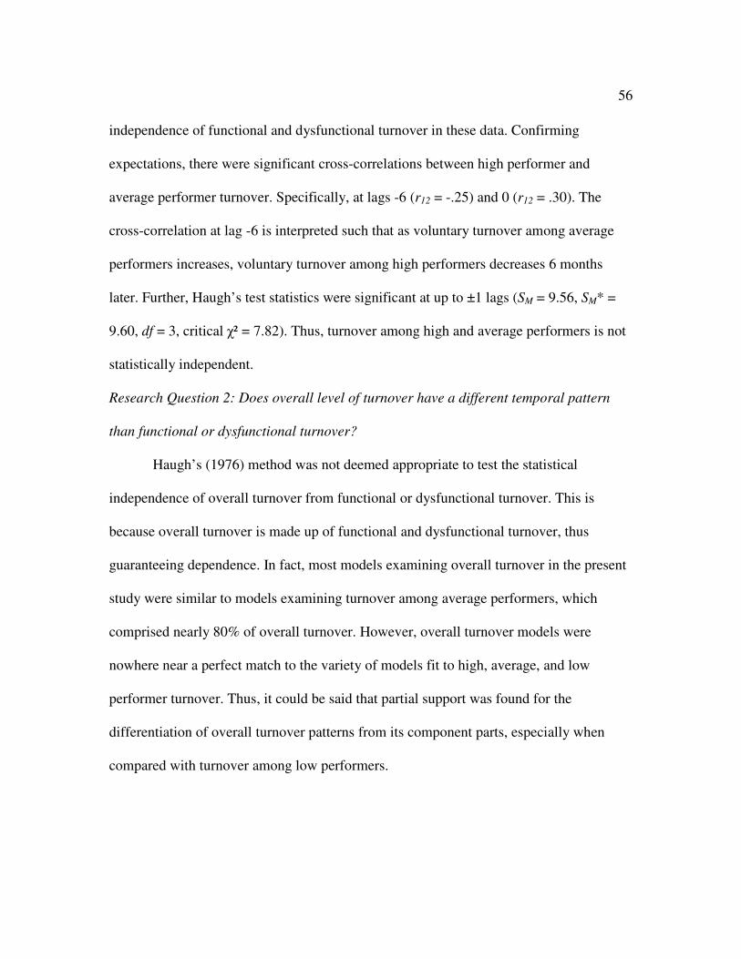
56

independence of functional and dysfunctional turnover in these data. Confirming

expectations, there were significant cross-correlations between high performer and

average performer turnover. Specifically, at lags -6 (r12 = -.25) and 0 (r12 = .30). The

cross-correlation at lag -6 is interpreted such that as voluntary turnover among average

performers increases, voluntary turnover among high performers decreases 6 months

later. Further, Haugh’s test statistics were significant at up to ±1 lags (SM = 9.56, SM* =

9.60, df = 3, critical χ² = 7.82). Thus, turnover among high and average performers is not

statistically independent.

Research Question 2: Does overall level of turnover have a different temporal pattern

than functional or dysfunctional turnover?

Haugh’s (1976) method was not deemed appropriate to test the statistical

independence of overall turnover from functional or dysfunctional turnover. This is

because overall turnover is made up of functional and dysfunctional turnover, thus

guaranteeing dependence. In fact, most models examining overall turnover in the present

study were similar to models examining turnover among average performers, which

comprised nearly 80% of overall turnover. However, overall turnover models were

nowhere near a perfect match to the variety of models fit to high, average, and low

performer turnover. Thus, it could be said that partial support was found for the

differentiation of overall turnover patterns from its component parts, especially when

compared with turnover among low performers.

57

Supplementary Analyses: Turnover and Organizational Performance

Similar procedures as above were followed to examine relationships between

turnover and organizational performance. Specifically, the white noise residual series of

high, average, and low performer turnover discussed above were cross-correlated with

white noise residual series of net sales, operating income, and diluted net earnings per

share. ARIMA models for these series fit the data exceptionally well, i.e., net sales

(3,1,0) (1,1,0) R2 = 99.20, operating income (3,1,0) (1,1,0) R

2 = 98.87, and diluted net

earnings per share (3,1,0) (1,2,0) R2 = 95.70. Table 16 presents cross-correlations of

white noise series for turnover among high, average, and low performers with white noise

series of net sales, operating income, and diluted net earnings per share.

The pattern of significant cross-correlations reveals several interesting findings.

First, as net sales increase, voluntary turnover among high performers decreases one

month later. Additionally, the relationship between operating income and voluntary

turnover among high performers appears to be reciprocal. Specifically, as operating

income increases, voluntary turnover among high performers decreases one month later.

Also, as voluntary turnover among high performers decreases, operating income

increases two months later. As diluted net earnings per share increase, voluntary turnover

among high performers decreases one month later. Strangely, as voluntary turnover

among high performers decreases, diluted net earnings per share decrease seven months

later. However, this finding is less reliable due to the large lag time. Other variables

would have more of an opportunity to influence the outcome over a period of seven

months.

58

As net sales increase, voluntary turnover among average performers decreases

one month later. No significant cross-correlations were found between voluntary turnover

among average performers and operating income. Similar to high performers, as

voluntary turnover among average performers decreases, diluted net earnings per share

decrease seven months later. However, this finding is less reliable due to the large lag

time. No significant cross-correlations were found between voluntary turnover among

low performers and net sales. Also, no significant cross-correlations were found between

voluntary turnover among low performers and operating income. Unexpectedly, as

voluntary turnover among low performers decreases, diluted net earnings per share

increase two months later. However, conversely, as voluntary turnover among low

performers decreases, diluted net earnings per share decrease six months later.

Summary of Results

This study sought to answer four basic research questions: (1) Do functional

turnover and dysfunctional turnover demonstrate different temporal patterns? (2) Does

overall level of turnover have a different temporal pattern than functional or

dysfunctional turnover? (3) Does forecast (prediction) accuracy differ for functional and

dysfunctional turnover? (4) Does forecast accuracy of functional and dysfunctional

turnover differ from that of overall turnover?

In response to research question 1, plots of average turnover by month and results

of ANOVA and time series regression provided evidence that functional turnover and

dysfunctional turnover demonstrate different temporal patterns. Specifically,

dysfunctional turnover tends to peak during the summer months (e.g., during or near

59

July) while functional turnover tends to peak during the late fall/early winter (e.g.,

October through December) for the organization studied here.

A more stringent test of research question 1 was conducted using Haugh’s (1976)

test statistics for the independence of time series. Findings provided evidence to support

the statistical independence of functional and dysfunctional turnover, thus supporting the

primary hypothesis that temporal patterns of functional and dysfunctional turnover differ.

Additionally, empirically validating the practice of the organization of treating turnover

among both average and high performers as dysfunctional, turnover among high and

average performers was statistically dependent.

Unfortunately, research question 2 – comparing the temporal pattern of overall

turnover with patterns of functional and dysfunctional turnover – could not be adequately

tested with the present data due to guaranteed dependence because overall turnover is

made up of functional and dysfunctional turnover.

Regarding research question 3, which involved the forecast accuracy of functional

and dysfunctional turnover, findings provided evidence to support the proposition that

forecast accuracy differs for turnover among employees at different performance levels.

The clearest finding was that forecast accuracy was lowest for predicting turnover among

high performers. This finding is unfortunate as these forecasts would be the most

valuable to the organization.

Results from the examination of research question 4, which compared the forecast

accuracy of functional and dysfunctional turnover with that of overall turnover, were not

clear. Essentially, if forecast accuracy for overall turnover models was compared with

60

average forecast accuracy statistics across models fit to turnover among high, average,

and low performers, several of these statistics favored overall turnover models. However,

poor prediction among models fit to high performer turnover attenuated these averages.

Thus, when forecast accuracy statistics for overall turnover models were compared with

the same statistics for average and low performers, accuracy was higher on average when

turnover was modeled at these two performance levels rather than modeled in aggregate.

In sum, although turnover among high performers could not be modeled very accurately,

models fit to turnover among average and low performers generally fit the data better

than models fit to aggregated overall turnover.

Although not part of the formal research questions, supplementary analyses

examined relationships between turnover and organizational performance (i.e., net sales,

operating income, diluted net earnings per share). Significant cross-correlations revealed

several interesting findings, such as reciprocal relationships between employee turnover

and organizational effectiveness. All significant lagged correlations at less than six lags

revealed negative relationships between turnover and organizational performance, most

of these among high performers. Lagged correlations were also strongest between high

performer turnover and organizational performance.

61

Chapter 6

Discussion

The importance of examining collective turnover has been argued in a recent

large-scale review (Hausknecht & Trevor, 2011). Also, the importance of considering

time in organizational research and in turnover research specifically has been emphasized

(Mitchell & James, 2001; Ployhart & Vandenberg, 2010). Turnover functionality has also

increased our understanding of the turnover process and its antecedents and outcomes

(Park et al., 1994; Williams, 1999). This study examined collective employee turnover

with a specific emphasis on predicting and explaining change over time and describing

differences in turnover among employees at different performance levels.

Broadly, results provided support for dynamic patterns in employee turnover and

differences in these patterns for dysfunctional turnover among high and average

performers and functional turnover among low performers. Thus, the primary hypothesis

that functional and dysfunctional turnover demonstrate different temporal patterns was

supported. The dynamic nature of these data underscores the importance of considering

employee turnover as a continuous process. As such, employee turnover should be

proactively managed over time. For example, results revealed that average and high

performers were more likely to separate from the organization during the summer and

low performers were more likely to separate during the late fall/early winter. Awareness

of these patterns could be integrated into HR planning and strategy formation. For

example, the organization studied here could time interventions aimed at reducing

voluntary turnover to occur just before and/or during the summer in order to have the

62

greatest impact on turnover among high and average performers. Additionally, different

linear trends, controlling for seasonality, were found at different performance levels and

in different regions. Knowledge of which groups of employees are separating at the

highest rates after controlling for other sources of variation would also be very useful

information to organizations.

Remember that all turnover examined in the present study was volunatry, so lay-

offs do not directly account for seasonal differences. One possible seasonal influence on

turnover among average and high performers is that the fiscal year for the company under

study always ended on June 30, so if performance feedback at that time was positive, but

not coupled with a raise or promotion, this may have influenced average and high

performers to leave in July. Additionally, poor performers may have separated later in the

year due to a probationary period that is imposed in between a first-time low performance

evaluation and involuntary separation after continued underperformance. Another

potential explanation for the gap in time between high/average performer turnover and

low performer turnover is that it likely took low performers longer to find alternate

employment than higher performers if the annual performance evaluation triggered job

search behavior. These explanations are consistent with Lee and Mitchell’s (1994)

unfolding model of turnover and the turnover model proposed by Allen and Griffeth

(1999).

Overall, the highest forecast accuracy was found for models of turnover due to

career-related reasons. These models explained up to 28% of the variance in career-

related turnover among high performers, 64% of the variance in career-related turnover

63

among average performers, and 75% of the variance in career-related turnover among

poor performers. Remember that these estimates are from cross-validation samples.

Seasonality was clearly present in these data. Average and high performer separations in

July and August due to career-related reasons may have coincided with school

enrollment, which typically occurs in August. Most employees had a Bachelor’s degree,

so if cognitive ability is related to performance, and considerable research demonstrates

that it is, then average and high performers with higher cognitive ability would be more

likely to enter graduate school.

The fact that seasonality was clearly present for turnover due to career-related

reasons highlights the need to consider this seasonal variation in turnover theory and

research. A sizable amount of time-dependent variance in career-related turnover was

captured with time series models. In fact, the variance explained by time alone was much

greater than that explained by many multivariate predictive models of employee turnover.

Therefore, an important implication of the present research is that time-related variation

in turnover, especially career-related turnover, should be integrated into theoretical

models of turnover and empirical turnover research.

Aside from turnover due to career-related reasons, time series models explained

nearly a third or more of the variance in cross-validation samples of average and low

performers in the three global regions. For example, in North America average performer

R2 = .32 and poor performer R

2 = .41, in Asia except China, Korea and Japan and

including Australia and India average performer R2 = .53 and poor performer R

2 = .41,

and in Northeast Asia, including Japan and Korea average performer R2 = .32 and poor

64

performer R2 = .32. Thus, univariate time series models, which capitalize on systematic

variation over time such as seasonal and cyclical patterns and linear trends, have the

potential to explain a sizable proportion of the variance in employee turnover which has

been unexplored in previous research. Specifically, although previous turnover research

has examined linear change in turnover (simple increases and decreases over time),

seasonality and cyclicality have been ignored.

This study provided evidence that seasonality was present in turnover across a

number of global regions and among employees at different performance levels. This

finding has clear implications for organizational research and practice. Theoretical

models of employee turnover are limited at present in that they do not take into account

seasonal variation in turnover. Further, practitioners do not currently integrate seasonal

variation into statistical models of turnover. The presence of seasonality may play an

important role in the results of a turnover study, but if trends and seasonality are

effectively modeled then they can be parsed out and/or controlled for when assessing the

effectiveness of an intervention, providing less biased estimates of effect size of that

intervention. This supports the importance of well-maintained human capital record-

keeping and tracking by organizations, such as tracking monthly turnover.

Turnover models such as the unfolding model (Lee & Mitchell, 1994) and

constructs such as job embeddedness (Felps et al., 2009) have emerged as important

explanations of employee turnover. Accordingly, interventions have been developed by

practitioners to bolster job attitudes and other factors that pull employees to remain with

an organization, and to mitigate the effects of negative events or ‘push factors’. However,

65

the effectiveness of interventions is sometimes assessed through simple pre/post designs

(e.g., Austin & Harkins, 2008; DeWeese, 2006; Gallagher & Nadarajah 2004; Latona,

1981; Sommer & Merritt, 1994) which do not typically control for the potentiality of

seasonality in the data. These designs measure baseline turnover at time 1, then introduce

an intervention in an effort to decrease turnover, and then measure turnover at time 2

once the effects of the intervention are thought to have been given enough time to take

effect. However, such designs do not take into account the fact that turnover may or may

not change from one time to another for a variety of reasons that are outside of the

influence of the intervention. For example, economic and market conditions may cause

turnover to increase or decrease for many months or even years. Also, there may be

seasonal and/or cyclical variation in turnover such that individuals may be less likely to

quit at certain times of the year (e.g., just before and after the winter holidays when

personal expenses are likely to be high) and more likely to quit at other times of the year

(e.g., during a particular industry’s hiring cycle; during an academic enrollment period).

Such variations in turnover could easily bias the results of a pre/post design. For example,

if there is seasonal variation in turnover then the presumed impact of the intervention

could be either inflated or deflated depending upon the nature of the seasonality and the

particular months in which pre- and post-intervention turnover are assessed.

The present research calls for an integration of time series concepts into turnover

theory and models. The findings presented here clearly indicate that attention should be

given to previously ignored seasonal and/or cyclical variation in employee turnover over

time. Theory and research failing to consider these sources of variation may leave a large

66

proportion of the variance in change in turnover unexplained. In turn, this unexplained

source of variance could influence the results of a turnover study such that findings

indicating a change or a lack of change could be incorrectly attributed to other study

variables such as an organizational intervention. Although not utilized in the present

research, multivariate time series models can be used to control for time-dependent

variance such as seasonality and cyclicality while simultaneously modeling the effects of

an intervention and/or other variables of interest (e.g., employee attitudes, market

conditions, etc.). Future research should therefore combine the strengths and findings of

traditional turnover research with time series concepts by utilizing multivariate time

series modeling techniques. Although some of these techniques can be quite complex, as

demonstrated in the present study they can be as simple as adding month of the year into

a multiple regression equation as a categorical predictor to control for seasonality.

Results also indicated that as voluntary turnover among average performers

increased, voluntary turnover among high performers decreased six months later. One

possible explanation for this is that as the performance gap from the loss of average

performers was felt, pressure was put on high performers to stay. Also, the loss of

average performers could have freed up capital to offer high performers larger bonuses

and pay raises.

Regarding relationships between collective turnover and organizational

performance outcomes, organizational performance had stronger and more pervasive

negative effects on high performer turnover than high performer turnover had on

organizational performance. Organizational performance may have influenced turnover

67

among high performers because they ‘jumped ship’ following a substantial drop in

organizational performance and/or because bonuses and raises were diminished following

low organizational performance. The finding that organizational performance influenced

turnover mirrors previous meta-analytic findings of the relationship between individual

employee performance and turnover (Bycio et al., 1990; McEvoy & Cascio, 1987;

Williams & Livingstone, 1994; Zimmerman & Darnold, 2009), but at a higher level of

analysis. Additionally, similar to the findings reported here, a meta-analysis by Griffeth

et al. (2000) found that lag time was a significant moderator of this relationship. This

study extends previous research by examining the impact of aggregate (company)

performance on collective turnover. Further, turnover and organizational performance

demonstrated univariate autocorrelation. Thus, it was essential to account for this time-

dependent variation in each series before examining relationships between turnover and

performance. This necessary precaution is not typical in published turnover research.

Time series analysis was used in the present study to demonstrate the presence of

non-trivial temporal variation in employee turnover. Future research should consider such

variation in study design and attempt to measure and control for it in analysis. Further,

the finding that functional and dysfunctional turnover exhibit different temporal patterns

underscores the need to disentangle turnover among employees at various performance

levels from overall aggregate turnover. The finding that dysfunctional turnover is

independent from functional turnover suggests that they should not be aggregated into

overall turnover, especially in longitudinal research designs. Doing so would mask

68

important differences in the temporal patterns of turnover among employees at different

performance levels.

Limitations and Directions for Future Research

One of the primary limitations of the present research was that the variance

explained in cross-validation samples was low for many models. A potential explanation

for this is that all of the cross-validation samples occurred after the start of the global

economic crisis, and the majority of the data used to create the models occurred before

the start of the crisis. Market conditions are related to turnover such that sustained poor

conditions typically coincide with increased involuntary turnover and decreased

voluntary turnover. The economic downturn would have been very difficult to predict.

However, if data throughout the economic downturn were integrated with previous data

and used to fit new time series models, it is likely that cyclical variation could be better

modeled which would in turn explain more variance in holdout samples, i.e., forecast

accuracy would improve.

An additional limitation was that no attitudinal antecedents of turnover were

included. Decades of research has demonstrated that attitudes such as job satisfaction and

organizational commitment are important predictors of turnover. However, some research

has provided evidence that these variables are not very good predictors of turnover

functionality (e.g., Johnston & Futrell, 1989). Hollenbeck and Williams (1986) reported

that turnover functionality was unrelated to work attitudes and thus concluded that the

antecedents of turnover frequency and turnover functionality likely differ. The authors

suggested that variables associated with both turnover frequency and performance, such

69

as work motivation, are likely to impact turnover functionality. Maertz and Griffeth

(2004) propose eight motives relating to voluntary turnover. Future research could

examine relationships between these motivational variables and turnover functionality.

Following the findings of this study, future research should also integrate

attitudes/motives into multivariate time series models with turnover functionality.

Also, individuals still remaining with the organization were not included in the

present study. However, survival analysis dictates that everyone has an eventual turnover

date, and stayers in a specific time frame simply have not yet reached their turnover date.

Thus, the present study excluded potential bias due to right-censored data, or data from

individuals for whom the date of turnover is unknown (Dickter et al., 1996).

Popular methods in the organizational sciences such as latent growth modeling

(LGM; Chan, 1998; Meredith & Tisak, 1990) and random coefficient modeling (RCM;

Bliese & Ployhart, 2002) were not used here. LGM was not used in the present research

for two reasons: (1) the variable of interest in the present study (turnover) was observed

(not unobserved, or latent); and (2) within-person change over time could not be

examined with the present data (no variable was observed more than once for the same

individual). RCM was not used for the second reason.

Finally, selecting employees to optimize functional turnover may also lower

employee performance (e.g., antecedents negatively related to employee performance

should be positively related to turnover functionality). Thus, future research should

examine those antecedents of dysfunctional turnover that are not strongly tied to

employee performance.

70

List of References

71

Allen, D. G., & Griffeth, R. W. (1999). Job performance and turnover: A review and

integrative multi-route model. Human Resource Management Review, 9, 525-548.

Allen, D. G., & Griffeth, R. W. (2001). Test of a mediated performance–turnover

relationship highlighting the moderating roles of visibility and reward

contingency. Journal of Applied Psychology, 86, 1014-1021.

Alwan, L. C., & Roberts, H. V. (1988). Time-series modeling for statistical process

control. Journal of Business & Economic Statistics, 6, 87-95.

Austin, M. S., & Harkins, D. A. (2008). Assessing change: Can organizational learning

"work" for schools? Learning Organization, 15, 105-125.

Bailey, E. J. (1991). An assessment of the relationships between measures of employee

turnover, employee demographics, employee performance, and organizational

performance in department stores. Unpublished Dissertation, University of

Alabama.

Beadles, N. A. II, Lowery, C. M., Petty, M. M., & Ezell, H. (2000). An examination of

the relationships between turnover functionality, turnover frequency, and

organizational performance. Journal of Business and Psychology, 15, 331-337.

Bentein, K., Vandenberg, R., Vandenberghe, C., & Stinglhamber, F. (2005). The role of

change in the relationship between commitment and turnover: A latent growth

modeling approach. Journal of Applied Psychology, 90, 468-482.

Bianchi, L., Jarrett, J., & Hanumara, R. C. (1998). Improving forecasting for

telemarketing centers by ARIMA modeling with intervention. International

Journal of Forecasting, 14, 497-504.

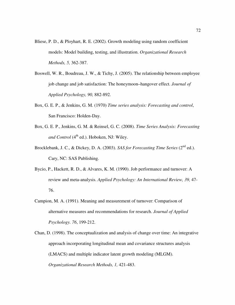
72

Bliese, P. D., & Ployhart, R. E. (2002). Growth modeling using random coefficient

models: Model building, testing, and illustration. Organizational Research

Methods, 5, 362-387.

Boswell, W. R., Boudreau, J. W., & Tichy, J. (2005). The relationship between employee

job change and job satisfaction: The honeymoon–hangover effect. Journal of

Applied Psychology, 90, 882-892.

Box, G. E. P., & Jenkins, G. M. (1970) Time series analysis: Forecasting and control,

San Francisco: Holden-Day.

Box, G. E. P., Jenkins, G. M. & Reinsel, G. C. (2008). Time Series Analysis: Forecasting

and Control (4th

ed.). Hoboken, NJ: Wiley.

Brocklebank, J. C., & Dickey, D. A. (2003). SAS for Forecasting Time Series (2nd

ed.).

Cary, NC: SAS Publishing.

Bycio, P., Hackett, R. D., & Alvares, K. M. (1990). Job performance and turnover: A

review and meta-analysis. Applied Psychology: An International Review, 39, 47-

76.

Campion, M. A. (1991). Meaning and measurement of turnover: Comparison of

alternative measures and recommendations for research. Journal of Applied

Psychology. 76, 199-212.

Chan, D. (1998). The conceptualization and analysis of change over time: An integrative

approach incorporating longitudinal mean and covariance structures analysis

(LMACS) and multiple indicator latent growth modeling (MLGM).

Organizational Research Methods, 1, 421-483.

73

Chang, J. Y., Choi, J. N., & Kim, M. U. (2008). Turnover of highly educated R&D

professionals: The role of pre-entry cognitive style, work values and career

orientation. Journal of Occupational and Organizational Psychology, 81, 299-

317.

Chatfield, C. (2000). Time-Series Forecasting. Boca Raton, FL: Chapman & Hall/CRC.

Dalton, D. R., Krackhardt, D. M., & Porter, L. W. (1981). Functional turnover: An

empirical assessment. Journal of Applied Psychology, 66, 716-721.

Dalton, D. R., & Todor, W. D. (1979). Turnover turned over: An expanded and positive

perspective. Academy of Management Review, 4, 225-235.

Dalton, D. R., & Todor, W. D. (1982). Turnover: A lucrative hard dollar phenomenon.

Academy of Management Review, 7, 212-218.

Dalton, D. R., Todor, W. D., & Krackhardt, D. M., (1982). Turnover overstated: The

functional taxonomy. Academy of Management Review, 7, 117-123.

Delurgio, S. A. (1998). Forecasting Principles and Applications. Hightstown, NJ:

Irwin/McGraw-Hill.

DeWeese, C. (2006). How multiple interventions reduced injuries and costs in one plant.

Work, 26, 251-253.

Dickter, D. N., Roznowski, M. & Harrison, D. A. (1996). Temporal tempering: An event

history analysis of the process of voluntary turnover. Journal of Applied

Psychology, 81, 705-716.

74

Farkas, A. J., & Tetrick, L. E. (1989). A three-wave longitudinal analysis of the causal

ordering of satisfaction and commitment on turnover decisions. Journal of


Felps, W., Mitchell, T. R., Hekman, D. R., Lee, T. W., Holtom, B. C., & Harman, W. S.,

(2009). Turnover contagion: How coworkers’ job embeddedness and job search

behaviors influence quitting. Academy of Management Journal, 52, 545-561.

Fisher, C. D., Schoenfeldt, L. F., & Shaw, J. B. (2006). Human Resource Management

(6th

Ed.). Boston, MA: Houghton-Mifflin Company.

Gallagher, D. R., & Nadarajah, P. (2004). Top management turnover: An analysis of

active Australian investment managers. Australian Journal of Management, 29,

243-274.

George, J. M., & Jones, G. R. (2000). The role of time in theory and theory building.

Journal of Management, 26, 657-684.

Griffeth, R. W., Hom, P. W., & Gaertner, S. (2000). A meta-analysis of antecedents and

correlates of employee turnover: Update, moderator tests, and research

implications for the next millennium. Journal of Management, 26, 463-488.

Griffeth, R. W., Phillips, P. L., Hom, P. W., & Steel, R. P. (1990). Affective and

cognitive variables discriminating between functional and dysfunctional stayers

and leavers: An alternative methodological approach in a health care setting.

Proceedings of the Southern Management Association, 64-66.

75

Harrison, D. A., Virick, M., & William, S. (1996). Working without a net: Time,

performance, and turnover under maximally contingent rewards. Journal of


Hart, D. E. (1990). The effects of perceived reward contingencies, recognition, and

benefits equity on turnover functionality. Unpublished Dissertation, Texas A&M

University.

Haugh, L. D. (1976). Checking independence of two covariance-stationary time-series –

Univariate residual cross-correlation approach. Journal of the American

Statistical Association, 71, 378-385.

Hausknecht, J. P., & Trevor, C. O. (2011). Collective turnover at the group, unit, and

organizational levels: Evidence, issues, and implications. Journal of Management,

37, 352-388.

Hausknecht, J. P., Trevor, C. O., & Howard, M. J. (2009). Unit-level voluntary turnover

rates and customer service quality: Implications of group cohesiveness, newcomer

concentration, and size. Journal of Applied Psychology, 94, 1068-1075.

Hinkin, T. R., & Tracey, J. B. (2000). The cost of turnover: Putting a price on the

learning curve. Cornell Hotel and Restaurant Administration Quarterly, 41, 14-

21.

Hintze, J. (2007). NCSS. Kaysville, UT: NCSS, LLC. www.NCSS.com

Hollenbeck, J. R, & Williams, C. R. (1986). Turnover functionality versus turnover

frequency: A note on work attitudes and organizational effectiveness. Journal of


76

Holtom, B. C., Mitchell, T. R., Lee, T. W., & Eberly, M. B. (2008). Turnover and

retention research: A glance at the past, a closer review of the present, and a

venture into the future. The Academy of Management Annals, 2, 231-274.

Hom, P. W., & Griffeth, R. W. (1991). Structural equations modeling test of a turnover

theory: Cross-sectional and longitudinal analyses. Journal of Applied Psychology,

76, 350-366.

Jackofsky, E. F. (1984). Turnover and job performance: An integrated process model.

The Academy of Management Review, 9, 74-83.

Jackofsky, E. F., Ferris, K. R., & Breckenridge, B. G. (1986). Evidence for a curvilinear

relationship between job performance and turnover. Journal of Management, 12,

105-111.

Johns, G. (1989). Performance and turnover cognitions among managers. Canadian

Journal of the Administrative Sciences, 6, 37-42.

Johnson, J. T., Griffeth, R. W., & Griffin, M. (2000). Factors discriminating functional

and dysfunctional salesforce turnover. Journal of Business & Industrial

Marketing, 15, 399-415.

Johnston, M. W., & Futrell, C. M. (1989). Functional salesforce turnover: An empirical

investigation into the positive effects of turnover. Journal of Business Research,

18, 141-157.

Johnston, M. W., Griffeth, R. W., Burton, S., & Carson, P. P. (1993). An exploratory

investigation in to the relationships between promotion and turnover: A quasi-

experimental longitudinal study. Journal of Management, 19, 33-49.

77

Kammeyer-Mueller, J. D., Wanberg, C. R., Glomb, T. M., & Ahlburg, D. (2005). The

Role of Temporal Shifts in Turnover Processes: It’s About Time. Journal of


Latona, J. C. (1981). Flexitime and the compressed workweek for the small firm: Some

employee reactions. American Journal of Small Business, 5, 23-29.

Lee, G. J., & Rwigema, H. (2005). Mobley revisited: Dynamism in the process of

employee turnover. International Journal of Human Resource Management, 16,

1671-1690.

Lee, T. W., & Mitchell, T. R. (1994). An alternative approach: The unfolding model of

voluntary employee turnover. Academy of Management Review, 19, 51-89.

Maertz, C. P., & Griffeth, R. W. (2004). Eight motivational forces and voluntary

turnover: A theoretical synthesis. Journal of Management, 30, 667-683.

McEvoy, G. M., & Cascio, W. F. (1987). Do good or poor performers leave? A meta-

analysis of the relationship between performance and turnover. Academy of

Management Journal, 30, 744-762.

McNeilly, K. M., & Russ, F. A. (1992). The moderating effect of sales force performance

on relationships involving antecedents of turnover. Journal of Personal Selling &

Sales Management, 12, 9-20.

Meredith, W., & Tisak, J. (1990). Latent curve analysis. Psychometrika, 55, 107-122.

Miller, S. J. (1987). Employee turnover: An investigation of attitudinal differences

between functional and dysfunctional leavers. Unpublished Dissertation,

University of Tennessee, Knoxville.

78

Mitchell, T. R., & James, L. R. (2001). Building better theory: Time and the specification

of when things happen. Academy of Management Review, 26, 530-547.

Mobley, W. H. (1982). Employee turnover: Causes, consequences, and control. Reading,

MA : Addison-Wesley.

Morrow, P., & McElroy, J. (2007). Efficiency as a mediator in turnover–organizational

performance relations. Human Relations, 60, 827-849.

Mossholder, K. W., Bedeian, A. G., Norris, D. R., Giles, W. F.., & Feild, H. S. (1988).

Job performance and turnover decisions: Two field studies. Journal of

Management, 14, 403-414.

Mossholder, K. W., Settoon, R. P., & Henagan, S. C. (2005). A relational perspective on

turnover: Examining structural, attitudinal, and behavioral predictors. Academy of

Management Journal, 48, 607-618.

Park, H. Y., Ofori-Dankwa, J., & Bishop, D. R. (1994). Organizational and

environmental determinants of functional and dysfunctional turnover: Practical

and research implications. Human Relations, 47, 353-366.

Phillips, P. L., Griffeth, R. W., Griffin, M., Johnston, M. W., Hom, P. W., & Steel, R. P.

(1989). Turnover functionality reborn: Personal and work-related factors that

differentiate among high and low performing quitters and stayers. Proceedings of

the Southern Management Association, 130-132.

Ployhart, R. E., & Vandenberg, R. J. (2010). Longitudinal research: The theory, design,

and analysis of change. Journal of Management, 36, 94-120.

79

Price, J. L. (1989). The impact of turnover on the organization. Work and Occupations,

16, 461-473.

Salamin, A., & Hom, P. W. (2005). In search of the elusive U-shaped performance–

turnover relationship: Are high performing Swiss bankers more liable to quit?

Journal of Applied Psychology, 90, 1204-1216.

Shaw, J. D., & Gupta, N. (2007). Pay system characteristics and quit patterns of good,

average, and poor performers. Personnel Psychology, 60, 903-928.

Shaw, J. D., Dineen, B. R., Fang, R., & Vellella, R. F. (2009). Employee-organization

exchange relationships, HRM practices, and quit rates of good and poor

performers. Academy of Management Journal, 52, 1016-1033.

Simons, T., & Hinkin, T. R. (2001). The impact of turnover on hotel profits: A test across

multiple hotels. Cornell Hotel and Restaurant Administration Quarterly 42, 65-

69.

Singer, J. D., & Willett, J. B. (2003). Applied Longitudinal Data Analysis: Modeling

Change and Event Occurrence. New York: Oxford University Press.

Somers, M. J. (1996). Modelling employee withdrawal behaviour over time: A study of

turnover using survival analysis. Journal of Occupational and Organizational


Somers, M. J. (1999). Application of two neural network paradigms to the study of

voluntary employee turnover. Journal of Applied Psychology, 84, 177-185.

80

Sommer, S. M., & Merritt, D. E. (1994). The impact of a TQM intervention on workplace

attitudes in a health-care organization. Journal of Organizational Change

Management, 7, 53-62.

Staw, B. M. (1980). The consequences of turnover. Journal of Occupational Behavior, 1,

253-273.

Steel, R. P. (2002). Turnover theory at the empirical interface: Problems of fit and

function. Academy of Management Review, 27, 346-360.

Sturman, M. C., & Trevor, C. O. (2001). The implications of linking the dynamic

performance and turnover literatures. Journal of Applied Psychology, 86, 684-

696.

Sturman, M. S., Trevor, C. O., Boudreau, J. W., & Gerhart, B. (2003). Is it worth it to

win the talent war? Evaluating the utility of performance-based pay. Personnel


Tracey, J. B., & Hinkin, T. R. (2008). Contextual factors and cost profiles associated with

employee turnover. Cornell Hospitality Quarterly, 49, 12-27.

Trevor, C. O. (2001). Interactions among actual ease-of-movement determinants and job

satisfaction in the prediction of voluntary turnover. Academy of Management

Journal, 44, 621-638.

Trevor, C. O., Gerhart, B., & Boudreau, J. W. (1997). Voluntary turnover and job

performance: Curvilinearity and the moderating influences of salary growth and

promotions. Journal of Applied Psychology, 82, 44-61.

81

Tziner, A., & Birati, A. (1996). Assessing employee turnover costs: A revised approach.

Human Resource Management Review, 6, 113-122.

Weller, I., Holtom, B. C., Matiaske, W., & Mellewigt, T. (2009). Level and time effects

of recruitment sources on early voluntary turnover. Journal of Applied

Psychology, 94, 1146-1162.

West, M., & Harrison, J. (1997) Bayesian Forecasting and Dynamic Models (2nd

Ed.).

New York: Springer-Verlag.

Williams, C. R. (1999). Reward contingency, unemployment, and functional turnover.

Human Resource Management Review, 9, 549-576.

Williams, C. R., & Livingstone, L. P. (1994). Another look at the relationship between

performance and voluntary turnover. Academy of Management Journal, 37, 269-

298.

Youngblood, S. A., Mobley, W. H., & Meghno, B. M. (1983). A longitudinal analysis of

the turnover process. Journal of Applied Psychology, 68, 507-516.

Zimmerman, R. D., & Darnold, T. C. (2009). The impact of job performance on

employee turnover intentions and the voluntary turnover process: A meta-analysis

and path model. Personnel Review, 38, 142-158.

82

Appendix

83

Table 1. Costs and Benefits of Voluntary Turnover

Costs of Turnover Possible Benefits of Turnover

Exit costs

Exit interviews

Farewell parties on work time

Poor performers may choose to leave

and can be replaced with better

employees

Administrative time to process final pay,

close retirement accounts, etc.

Leavers are replaced with more junior

employees who cost less

Replacement costs

Recruitment advertising

Morale improves following departure

of problematic employees

Selection testing, interviewing, reference

checking, medical exams, etc.

Leavers are replaced with people

having more up-to-date technical skill

Hiring bonuses, relocation costs

New employee orientation

Administrative costs to add to payroll, enroll

in benefits, etc.

Vacancies are created to allow for

internal promotions of other

employees, thus increasing their

career satisfaction and motivation

Formal training

Informal mentoring and coaching of new

employees by supervisors and peers

Other costs

Receptiveness to innovation and

change may increase

Voluntary turnover is less painful than

retrenchments

Lost business due to client loyalty to

departing employees

Lost business or poor quality due to short

staffing before replacement, or lower skills

before new hires are up to speed

Expenses of hiring temporaries or paying

overtime while awaiting replacements

Reduced morale of those remaining,

increased stress on those remaining while

short staffed or breaking in replacements

Reduction in company’s reputation as an

employer when staff may choose to leave,

reduced ability to recruit in the labor market

Inability to pursue growth of other business

opportunities due to lack of staff

Loss of training dollars invested in departing

employee

Loss of explicit and tacit organization-

specific knowledge held by departing

employee

Note. Reprinted with permission from Fisher, Schoenfeldt, and Shaw (2006), Table 16.3.

84

Table 2. Descriptive Statistics of Monthly Turnover Rates

Turnover Min Max M SD

Global Overall 112 368 199.60 64.14

1 Rated 6 42 19.40 7.33

2 Rated 84 325 158.55 54.48

3 Rated 5 79 21.65 12.73

North America 7 82 39.24 11.42

1 Rated 0 10 3.64 2.29

2 Rated 6 68 32.03 10.11

3 Rated 0 13 3.57 2.60

AAI 4 33 17.55 6.46

1 Rated 0 6 1.60 1.27

2 Rated 3 27 14.20 5.54

3 Rated 0 7 1.75 1.56

Northeast Asia 2 36 17.19 6.37

1 Rated 0 5 1.67 1.18

2 Rated 0 27 13.04 5.47

3 Rated 0 8 2.48 1.98

Career-related 36 132 66.32 21.34

1 Rated 1 15 5.99 3.01

2 Rated 28 109 52.53 17.96

3 Rated 1 28 7.80 5.06

Note. N = 75 months. AAI is all of Asia except China, Korea and

Japan and including Australia and India.

85

Table 3. Correlations of Monthly Turnover Rates among High, Average, and Low Performers

Turnover 1 2 3 4 5 6 7 8 9 10 11 12 13 14 15

1 Rate 1

2 Rate 2 .73*

3 Rate 3 .15 .23*

4 NA Rate1 .39* .09 -.22

5 NA Rate2 .52* .66

* -.13 .21

6 NA Rate3 .23* .32

* .65

* -.02 .13

7 AAI Rate1 .44* .35

* .27

* .06 .17 .34

*

8 AAI Rate2 .59* .72

* .22 .17 .42

* .30

* .29

*

9 AAI Rate3 -.04 .03 .59* -.10 -.20 .32

* .08 .15

10 NEA Rate1 .28* .28

* -.14 .03 .35

* -.16 -.13 .05 -.21

11 NEA Rate2 .23 .48* .00 -.02 .30

* -.14 -.01 .10 -.10 .26

*

12 NEA Rate3 -.01 .07 .46* -.08 -.08 .05 .12 .05 .32

* -.17 .13

13 Career Rate 1 .74* .60

* .22 .31

* .42

* .36

* .42

* .53

* .03 .05 .08 -.06

14 Career Rate 2 .68* .86

* .17 .16 .67

* .21 .40

* .64

* -.01 .16 .41

* .02 .64

*

15 Career Rate 3 .06 .10 .85* -.17 -.17 .59

* .20 .03 .45

* -.18 .00 .23

* .16 .14

Note. N = 75. * p < .05. Rate 1, 2, and 3 are global monthly turnover for 1-, 2-, and 3-rated employees. NA is North America.

AAI is all of Asia except China, Korea and Japan and including Australia and India. NEA is Northeast Asia. Career is career-

related turnover.

86

Table 4. Seasonal Analysis of Variance Results

Turnover DF Sum of Squares Mean Square F

Global Overall 11 37125.12 3375.01 0.80

Dysfunctional 11 45696.91 4154.264 1.18

1 Rated 11 479.93 43.63 0.79

2 Rated 11 39324.63 3574.97 1.25

3 Rated 11 3347.61 304.33 2.22*

North America

1 Rated 11 63.49 5.77 1.12

2 Rated 11 2890.78 262.80 3.54*

3 Rated 11 151.4181 13.765 2.49*

AAI

1 Rated 11 10.38 0.94 0.54

2 Rated 11 303.71 27.61 0.88

3 Rated 11 54.50 4.95 2.48*

Northeast Asia

1 Rated 11 21.76 1.98 1.54

2 Rated 11 1127.09 102.46 5.93*

3 Rated 11 73.15 6.65 1.94

Career-related

1 Rated 11 117.49 10.68 1.22

2 Rated 11 8155.38 741.40 2.97*

3 Rated 11 608.71 55.34 2.71*

Note. * p < .05.

87

Table 5. Final ARIMA Model Parameters

Turnover Holdout ARIMA (p, d, q, P, D, Q)*

12 month (0,0,0) (5,0,0) Global Overall

6 month (1,0,0) (3,0,0)

12 month (0,0,0) (0,0,5) Dysfunctional

6 month (1,0,0) (0,1,1)

Employee Performance

1 Rated** 2 Rated** 3 Rated***

12 month (0,0,1) (0,1,3) (0,0,0) (5,0,0) (3,0,2) (0,1,1) Global

6 month (0,0,1) (0,1,3) (1,0,0) (1,0,1) (3,0,2) (0,1,1)

12 month (0,0,0) (0,1,3) (0,0,0) (1,1,3) (0,0,0) (2,1,0) North America

6 month (0,0,7) (0,0,0) (0,0,0) (1,1,3) (0,0,0) (2,0,2)

12 month (0,0,0) (4,0,0) (1,0,1) (3,0,0) (0,0,1) (4,1,2) AAI

6 month (0,0,0) (4,0,0) (1,0,1) (3,0,0) (0,0,1) (4,1,2)

12 month (0,0,0) (0,0,9) (0,0,0) (3,1,0) (0,0,0) (3,1,3) Northeast Asia

6 month (0,0,0) (2,1,6) (0,0,0) (0,0,5) (0,0,0) (4,0,3)

12 month (0,0,0) (2,0,1) (0,0,0) (6,1,0) (0,0,0) (2,0,6) Career-related

6 month (0,0,0) (2,0,2) (1,0,0) (4,0,0) (0,0,2) (0,1,5)

Note. * p = non-seasonal autocorrelation (AR), d = non-seasonal differencing,

q = non-seasonal moving average (MA), P = seasonal AR, D = seasonal differencing,

Q = seasonal MA. ** Dysfunctional turnover; *** Functional turnover.

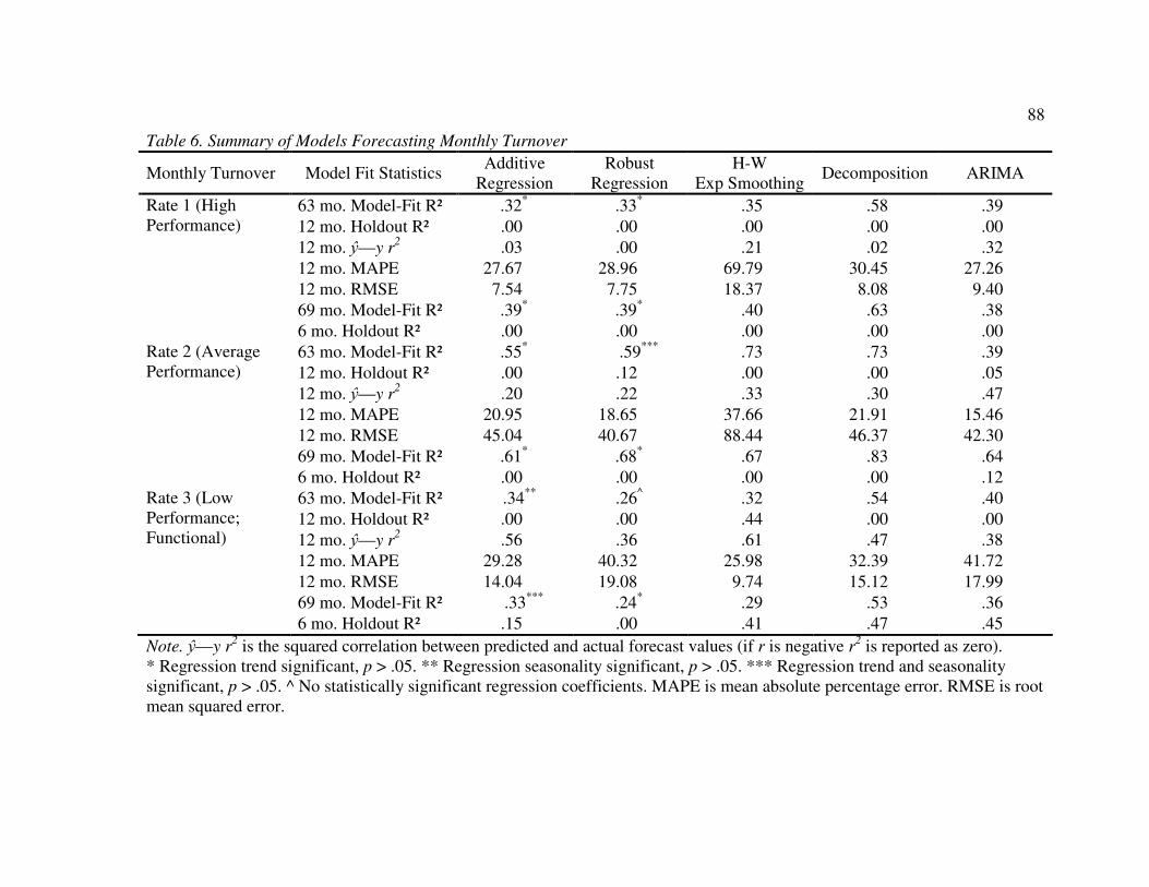
88

Table 6. Summary of Models Forecasting Monthly Turnover

Monthly Turnover Model Fit Statistics Additive

Regression

Robust

Regression

H-W

Exp Smoothing Decomposition ARIMA

63 mo. Model-Fit R² .32* .33

* .35 .58 .39 Rate 1 (High

Performance) 12 mo. Holdout R² .00 .00 .00 .00 .00

12 mo. ŷ—y r2 .03 .00 .21 .02 .32

12 mo. MAPE 27.67 28.96 69.79 30.45 27.26

12 mo. RMSE 7.54 7.75 18.37 8.08 9.40

69 mo. Model-Fit R² .39* .39

* .40 .63 .38

6 mo. Holdout R² .00 .00 .00 .00 .00

63 mo. Model-Fit R² .55* .59

*** .73 .73 .39 Rate 2 (Average

Performance) 12 mo. Holdout R² .00 .12 .00 .00 .05

12 mo. ŷ—y r2 .20 .22 .33 .30 .47

12 mo. MAPE 20.95 18.65 37.66 21.91 15.46

12 mo. RMSE 45.04 40.67 88.44 46.37 42.30

69 mo. Model-Fit R² .61* .68

* .67 .83 .64

6 mo. Holdout R² .00 .00 .00 .00 .12

63 mo. Model-Fit R² .34**

.26^ .32 .54 .40

12 mo. Holdout R² .00 .00 .44 .00 .00

Rate 3 (Low

Performance;

Functional) 12 mo. ŷ—y r2 .56 .36 .61 .47 .38

12 mo. MAPE 29.28 40.32 25.98 32.39 41.72

12 mo. RMSE 14.04 19.08 9.74 15.12 17.99

69 mo. Model-Fit R² .33***

.24* .29 .53 .36

6 mo. Holdout R² .15 .00 .41 .47 .45

Note. ŷ—y r2 is the squared correlation between predicted and actual forecast values (if r is negative r

2 is reported as zero).

* Regression trend significant, p > .05. ** Regression seasonality significant, p > .05. *** Regression trend and seasonality

significant, p > .05. ^ No statistically significant regression coefficients. MAPE is mean absolute percentage error. RMSE is root

mean squared error.

89

Table 6. Continued


Regression

Robust

Regression

H-W


NA Rate 1 63 mo. Model-Fit R² .16^

.18^ .00 .21 .12

12 mo. Holdout R² .03 .00 -- .00 .00

12 mo. ŷ—y r2 .07 .06 -- .03 .02

12 mo. MAPE 57.99 57.62 -- 58.65 69.83

12 mo. RMSE 2.20 2.24 -- 2.28 2.72

69 mo. Model-Fit R² .15^ .18

** .00 .06 .14

6 mo. Holdout R² .05 .00 -- .04 .00

NA Rate 2 RMD3 63 mo. Model-Fit R² .55***

-- .39 .61 .37

12 mo. Holdout R² .00 -- .21 .00 .32

12 mo. ŷ—y r2 .21 -- .24 .23 .33

12 mo. MAPE 50.30 -- 33.58 51.44 29.43

12 mo. RMSE 13.94 -- 11.15 14.64 10.31


-- .28 .58 .33

6 mo. Holdout R² .00 -- .00 .00 .00

NA Rate 3 63 mo. Model-Fit R² .49***

.49***

.32 .53 .32

12 mo. Holdout R² .00 .00 .00 .00 .00

12 mo. ŷ—y r2 .00 .01 .00 .00 .00

12 mo. MAPE 59.23 55.73 62.45 66.54 50.82

12 mo. RMSE 3.44 3.54 3.55 3.75 4.06


.46***

.31 .49 .31

6 mo. Holdout R² .00 .18 .00 .00 .41





mean squared error.

90

Table 6. Continued


Regression

Robust

Regression

H-W


AAI Rate 1 63 mo. Model-Fit R² .20^ .27

^ .00 .25 .14

12 mo. Holdout R² .00 .00 -- .00 .00

12 mo. ŷ—y r2 .00 .00 -- .00 .23

12 mo. MAPE 42.21 37.90 -- 41.05 45.84

12 mo. RMSE 1.32 1.31 -- 1.45 1.00

69 mo. Model-Fit R² .21* .28

* .00 .22 .17

6 mo. Holdout R² .00 .00 -- .00 .00

AAI Rate 2 63 mo. Model-Fit R² .53***

.57***

.49 .65 .50

12 mo. Holdout R² .00 .00 .00 .00 .00

12 mo. ŷ—y r2 .05 .03 .10 .07 .21

12 mo. MAPE 16.33 17.19 26.15 18.75 18.53

12 mo. RMSE 4.59 4.70 6.91 4.88 5.44

69 mo. Model-Fit R² .58* .62

*** .47 .66 .53

6 mo. Holdout R² .00 .00 .53 .00 .33

AAI Rate 3 63 mo. Model-Fit R² .30^ .31

^ .09 .30 .39

12 mo. Holdout R² .06 .00 .00 .21 .34

12 mo. ŷ—y r2 .61 .57 .55 .53 .75

12 mo. MAPE 36.37 40.13 41.35 36.69 50.11

12 mo. RMSE 1.82 2.00 1.89 1.67 1.52


.34***

.10 .31 .34

6 mo. Holdout R² .03 .00 .00 .30 .41





mean squared error.

91

Table 6. Continued


Regression

Robust

Regression

H-W


NEA Rate 1 63 mo. Model-Fit R² .27***

.34***

.04 .32 .41

12 mo. Holdout R² .00 .00 .00 .00 .00

12 mo. ŷ—y r2 .17 .18 .16 .23 .04

12 mo. MAPE 57.36 50.78 60.18 67.59 40.80

12 mo. RMSE 1.48 1.38 1.49 1.68 1.10

69 mo. Model-Fit R² .23^ .26

^ .02 .35 .32

6 mo. Holdout R² .00 .00 .00 .00 .00

NEA Rate 2 63 mo. Model-Fit R² .56***

.65***

.42 .59 .45

12 mo. Holdout R² .00 .00 .00 .00 .00

12 mo. ŷ—y r2 .22 .20 .12 .22 .14

12 mo. MAPE 25.79 26.17 39.45 26.73 28.00

12 mo. RMSE 4.61 4.72 6.33 4.95 5.11


.62**

.37 .56 .41

6 mo. Holdout R² .15 .23 .12 .32 .13

NEA Rate 3 63 mo. Model-Fit R² .27^ .34

** .09 .37 .50

12 mo. Holdout R² .00 .00 .00 .00 .03

12 mo. ŷ—y r2 .12 .13 .07 .06 .27

12 mo. MAPE 42.73 37.83 56.37 43.70 32.63

12 mo. RMSE 2.67 2.50 3.59 2.75 2.42


.35**

.11 .38 .50

6 mo. Holdout R² .00 .00 .00 .00 .32





mean squared error.

92

Table 6. Continued


Regression

Robust

Regression

H-W


Career Rate 1 63 mo. Model-Fit R² .32* .35

* .11 .39 .26

12 mo. Holdout R² .01 .00 .01 .00 .28

12 mo. ŷ—y r2 .06 .00 .44 .07 .44

12 mo. MAPE 68.10 69.56 39.75 67.83 35.47

12 mo. RMSE 3.64 3.85 3.63 3.68 3.09

69 mo. Model-Fit R² .40* .43

*** .07 .48 .39

6 mo. Holdout R² .00 .00 .00 .00 .00

Career Rate 2 63 mo. Model-Fit R² .52***

.58***

.59 .68 .52

12 mo. Holdout R² .30 .30 .30 .41 .64

12 mo. ŷ—y r2 .47 .46 .45 .59 .68

12 mo. MAPE 23.45 23.31 17.75 21.23 13.88

12 mo. RMSE 14.71 14.80 14.76 13.57 10.56


.67***

.50 .76 .60

6 mo. Holdout R² .00 .00 .00 .00 .53

Career Rate 3 63 mo. Model-Fit R² .34**

.39**

.29 .50 .24

12 mo. Holdout R² .00 .00 .17 .00 .39

12 mo. ŷ—y r2 .33 .24 .51 .27 .61

12 mo. MAPE 36.81 48.20 29.79 44.70 26.53

12 mo. RMSE 6.54 7.71 4.75 7.38 4.08


.30**

.18 .46 .53

6 mo. Holdout R² .32 .00 .75 .41 .65





mean squared error.

93

Table 6. Continued


Regression

Robust

Regression

H-W


63 mo. Model-Fit R² .53* .56

* .73 .73 .28 Dysfunctional

(Rates 1 & 2) 12 mo. Holdout R² .00 .08 .00 .00 .15

12 mo. ŷ—y r2 .24 .23 .85 .34 .56

12 mo. MAPE 20.06 18.38 70.73 21.22 15.22

12 mo. RMSE 47.91 45.15 160.61 49.37 43.42

69 mo. Model-Fit R² .61* .66

* .68 .83 .67

6 mo. Holdout R² .00 .00 .00 .00 .14

Global Overall 63 mo. Model-Fit R² .51* .53

* .73 .73 .37

12 mo. Holdout R² .04 .10 .00 .06 .00

12 mo. ŷ—y r2 .14 .15 .82 .26 .54

12 mo. MAPE 15.54 14.95 69.13 14.90 16.22

12 mo. RMSE 44.48 42.92 182.08 43.99 53.50

69 mo. Model-Fit R² .59* .66

* .67 .83 .70

6 mo. Holdout R² .00 .00 .13 .00 .00





mean squared error.

94

Table 7. Time Series Regression Results for Global Turnover among Average Performers

Dependent Variable – Global 2-Rated Turnover

Independent

Variable

Regression

Coefficient Standard Error t p < .05

Intercept 135.07 14.87 9.09 Yes

January -37.12 18.25 -2.03 Yes

February -64.93 18.39 -3.53 Yes

March -47.70 19.10 -2.50 Yes

April -37.96 18.93 -2.01 Yes

May -32.71 18.80 -1.74 No

June 2.48 18.73 0.13 No

July*

August -9.16 19.10 -0.48 No

September -27.07 19.28 -1.40 No

October -58.60 18.70 -3.13 Yes

November -72.60 18.71 -3.88 Yes

December -37.95 18.87 -2.01 Yes

Trend 1.50 0.18 8.52 Yes

Note. * Reference month. N = 75. Method is Huber's Robust Multiple Regression. R2 =

.63, Adjusted R2 = .56, R

2-Press = .24, Root Mean Squared Error = 31.86, Mean Absolute

Percent Error = 17.49.

95

Table 8. Time Series Regression Results for Global Turnover among Low Performers

Dependent Variable – Global 3-Rated Turnover

Independent

Variable

Regression


Intercept 29.51 4.74 6.23 Yes

January -18.31 5.72 -3.20 Yes

February -18.70 5.72 -3.27 Yes

March -20.37 5.72 -3.56 Yes

April -20.03 5.94 -3.37 Yes

May -22.94 5.94 -3.86 Yes

June -16.02 5.94 -2.70 Yes

July -23.26 5.94 -3.92 Yes

August -22.18 5.93 -3.74 Yes

September -21.09 5.93 -3.55 Yes

October*

November -11.91 5.93 -2.01 Yes

December -10.49 5.93 -1.77 No

Trend 0.25 0.06 4.46 Yes

Note. * Reference month. N = 75. Method is Additive Multiple Regression. R2 = .45,

Adjusted R2 = .35, R



96

Table 9. Time Series Regression Results for North American Turnover among High

Performers

Dependent Variable –N. American 1-Rated Turnover

Independent

Variable

Regression



January -2.00 1.27 -1.57 No

February -3.28 1.27 -2.58 Yes

March -2.13 1.27 -1.67 No

April -2.03 1.32 -1.54 No

May -2.18 1.32 -1.66 No

June -3.01 1.32 -2.28 Yes

July*

August -1.49 1.32 -1.13 No

September -3.32 1.32 -2.52 Yes

October -2.47 1.32 -1.88 No

November -2.80 1.32 -2.12 Yes

December -3.46 1.32 -2.62 Yes

Trend -0.01 0.01 -0.69 No





97

Table 10. Time Series Regression Results for North American Turnover among Low

Performers

Dependent Variable –N. American 3-Rated Turnover

Independent

Variable

Regression



January -2.88 1.03 -2.79 Yes

February -3.72 1.03 -3.62 Yes

March -4.30 1.03 -4.19 Yes

April -3.75 1.08 -3.46 Yes

May -2.36 1.07 -2.20 Yes

June -3.54 1.09 -3.25 Yes

July -3.46 1.06 -3.28 Yes

August -3.04 1.08 -2.81 Yes


October*

November -0.32 1.06 -0.30 No

December -3.47 1.06 -3.28 Yes

Trend 0.04 0.01 3.60 Yes





98

Table 11. Time Series Regression Results for AAI Turnover among Low Performers

Dependent Variable –AAI 3-Rated Turnover

Independent

Variable

Regression



January -2.55 0.73 -3.50 Yes

February -1.71 0.73 -2.35 Yes

March -1.88 0.73 -2.58 Yes

April -1.02 0.76 -1.35 No

May -2.05 0.76 -2.71 Yes

June -2.41 0.76 -3.18 Yes

July -2.26 0.76 -2.99 Yes

August -1.45 0.76 -1.92 No


October*

November -0.86 0.76 -1.13 No

December -0.05 0.76 -0.06 No

Trend 0.02 0.01 3.37 Yes





99

Table 12. Time Series Regression Results for Northeast Asian Turnover among Average

Performers

Dependent Variable –NEA 2-Rated Turnover

Independent

Variable

Regression



January -4.95 1.86 -2.66 Yes

February -3.46 1.84 -1.88 No

March -2.27 1.81 -1.25 No

April -4.76 1.98 -2.41 Yes

May -7.81 1.88 -4.15 Yes

June 2.24 1.94 1.16 No

July*

August 3.86 1.98 1.95 No

September -2.63 2.03 -1.30 No

October -8.53 1.91 -4.47 Yes

November -10.07 1.95 -5.17 Yes

December -2.17 1.95 -1.11 No

Trend 0.03 0.02 1.70 No





100

Table 13. Time Series Regression Results for Career-related Turnover among Average

Performers

Dependent Variable –Career-related 2-Rated Turnover

Independent

Variable

Regression



January -26.29 7.43 -3.54 Yes

February -31.37 7.43 -4.22 Yes

March -32.59 7.43 -4.38 Yes

April -24.74 7.72 -3.21 Yes

May -20.77 7.71 -2.69 Yes

June -11.63 7.71 -1.51 No

July*

August -3.87 7.71 -0.50 No

September -18.06 7.71 -2.34 Yes

October -29.26 7.72 -3.79 Yes

November -34.96 7.72 -4.53 Yes

December -24.33 7.72 -3.15 Yes

Trend 0.37 0.07 5.11 Yes





101

Table 14. Time Series Regression Results for Career-related Turnover among Low

Performers

Dependent Variable –Career-related 3-Rated Turnover

Independent

Variable

Regression



January -8.09 2.49 -3.25 Yes

February -8.84 2.49 -3.55 Yes

March -9.87 2.49 -3.96 Yes

April -9.46 2.59 -3.65 Yes

May -10.49 2.59 -4.05 Yes

June -8.36 2.59 -3.23 Yes

July -8.56 2.59 -3.31 Yes

August -8.60 2.59 -3.33 Yes


October*

November -4.87 2.59 -1.88 No

December -4.40 2.59 -1.70 No

Trend 0.03 0.02 1.45 No





102

Table 15. Cross-correlations of Pre-whitened (Residual) Series for Turnover among

High, Average, and Low Performers

Cross-correlation

Lag Rate 1—Rate 2 Rate 1—Rate 3 Rate 2—Rate 3

-8 -.03 .13 .23

-7 .05 .19 -.09

-6 -.25* -.23 .24

-5 .07 -.02 -.22

-4 .04 .08 -.10

-3 .01 .02 -.07

-2 .04 -.01 -.03

-1 .18 -.07 -.04

0 .30* -.06 .00

1 .08 .14 .16

2 .13 -.15 .00

3 .02 .07 .06

4 .00 .15 -.02

5 -.01 -.05 -.06

6 .10 .09 .07

7 -.05 -.09 .12

8 -.15 .14 .06

* p < .05. N = 67-75.

103

Table 16. Cross-correlations of Pre-whitened (Residual) Series for Turnover among High, Average, and Low Performers with

Organizational Performance

Cross-correlation

Rate 1 (High Performance) Rate 2 (Average Performance) Rate 3 (Low Performance)

Lag

Net sales Operating

income

Diluted net

earnings

p/share

Net sales Operating

income

Diluted net

earnings

p/share

Net sales Operating

income

Diluted net

earnings

p/share

-8 -.12 -.13 -.16 .03 .04 -.11 .00 -.01 .10

-7 .09 .10 -.13 -.14 -.15 -.15 .09 .04 -.03

-6 -.05 -.04 .06 .05 .05 .00 -.07 -.16 -.07

-5 -.11 -.20 -.02 -.01 -.06 -.04 .05 .01 -.13

-4 .17 .03 .22 .02 .07 .16 .02 .03 -.03

-3 -.03 -.10 -.11 .04 .02 .06 .06 .04 .11

-2 .14 .09 .06 .09 .04 .12 -.06 -.14 .13

-1 -.27* -.27* -.32* -.24* -.17 -.19 -.15 -.13 .16

0 .00 .08 .00 .22 .21 .10 .13 .09 -.06

1 .08 -.07 -.04 .07 -.05 .02 -.02 -.06 -.16

2 -.18 -.25* -.08 -.06 -.15 -.03 -.02 -.05 -.24*

3 -.12 -.09 -.01 -.08 -.15 -.01 -.07 -.15 -.07

4 .05 .13 .16 -.14 -.07 -.09 .03 .00 .09

5 -.20 -.11 -.18 .09 .11 .15 -.10 -.10 .11

6 -.11 -.03 .00 -.10 -.15 .04 .05 .00 .25*

7 .02 .05 .26* .07 .02 .27* .02 -.01 .10

8 -.02 -.04 .17 .03 -.06 .14 -.09 -.09 -.23

* p < .05. N = 67-75.

104

0

40

80

120

160

200

240

280

320

360

400

0 5 10 15 20 25 30 35 40 45 50 55 60 65 70 75

Monthly Trend

Overa

ll T

urn

over

Figure 1. Overall Global Monthly Turnover from Jan 2003 through Mar 2009

105

0

3

6

9

12

15

18

21

24

27

30

33

36

39

42

45

0 5 10 15 20 25 30 35 40 45 50 55 60 65 70 75

Monthly Trend

1 R

ate

d T

urn

over

Figure 2. Global Monthly Turnover from Jan 2003 through Mar 2009 among High

Performers

106

0

25

50

75

100

125

150

175

200

225

250

275

300

325

350

0 5 10 15 20 25 30 35 40 45 50 55 60 65 70 75

Monthly Trend

2 R

ate

d T

urn

over

Figure 3. Global Monthly Turnover from Jan 2003 through Mar 2009 among Average

Performers

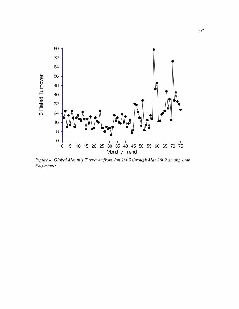
107

0

8

16

24

32

40

48

56

64

72

80

0 5 10 15 20 25 30 35 40 45 50 55 60 65 70 75

Monthly Trend

3 R

ate

d T

urn

over

Figure 4. Global Monthly Turnover from Jan 2003 through Mar 2009 among Low

Performers

108

0

1

2

3

4

5

6

7

8

9

10

11

12

13

14

15

0 5 10 15 20 25 30 35 40 45 50 55 60 65 70 75

Monthly Trend

NA

1 R

ate

d T

urn

over


in North America

109

0

8

16

24

32

40

48

56

64

72

80

0 5 10 15 20 25 30 35 40 45 50 55 60 65 70 75

Monthly Trend

NA

2 R

ate

d T

urn

over


Performers in North America

110

0

1

2

3

4

5

6

7

8

9

10

11

12

13

14

15

0 5 10 15 20 25 30 35 40 45 50 55 60 65 70 75

Monthly Trend

NA

3 R

ate

d T

urn

over

Figure 7. Monthly Turnover from Jan 2003 through Mar 2009 among Low Performers in

North America

111

0

1

2

3

4

5

6

7

8

9

10

11

12

13

14

15

0 5 10 15 20 25 30 35 40 45 50 55 60 65 70 75

Monthly Trend

AA

I 1 R

ate

d T

urn

over


in all of Asia except China, Korea and Japan and including Australia and India

112

0

2

4

6

8

10

12

14

16

18

20

22

24

26

28

30

0 5 10 15 20 25 30 35 40 45 50 55 60 65 70 75

Monthly Trend

AA

I 2 R

ate

d T

urn

over


Performers in all of Asia except China, Korea and Japan and including Australia and

India

113

0

1

2

3

4

5

6

7

8

9

10

11

12

13

14

15

0 5 10 15 20 25 30 35 40 45 50 55 60 65 70 75

Monthly Trend

AA

I 3 R

ate

d T

urn

over


in all of Asia except China, Korea and Japan and including Australia and India

114

0

1

2

3

4

5

6

7

8

9

10

11

12

13

14

15

0 5 10 15 20 25 30 35 40 45 50 55 60 65 70 75

Monthly Trend

NE

A 1

Rate

d T

urn

over


in Northeast Asia

115

0

2

4

6

8

10

12

14

16

18

20

22

24

26

28

30

0 5 10 15 20 25 30 35 40 45 50 55 60 65 70 75

Monthly Trend

NE

A 2

Rate

d T

urn

over


Performers in Northeast Asia

116

0

1

2

3

4

5

6

7

8

9

10

11

12

13

14

15

0 5 10 15 20 25 30 35 40 45 50 55 60 65 70 75

Monthly Trend

NE

A 3

Rate

d T

urn

over


in Northeast Asia

117

0

1

2

3

4

5

6

7

8

9

10

11

12

13

14

15

0 5 10 15 20 25 30 35 40 45 50 55 60 65 70 75

Monthly Trend

Care

er

1 R

ate

d T

urn

over


Leaving for Career-related Reasons

118

0

8

16

24

32

40

48

56

64

72

80

88

96

104

112

120

0 5 10 15 20 25 30 35 40 45 50 55 60 65 70 75

Monthly Trend

Care

er

2 R

ate

d T

urn

over


Performers Leaving for Career-related Reasons

119

0

2

4

6

8

10

12

14

16

18

20

22

24

26

28

30

0 5 10 15 20 25 30 35 40 45 50 55 60 65 70 75

Monthly Trend

Care

er

3 R

ate

d T

urn

over


Leaving for Career-related Reasons

120

0.00

7.00

14.00

21.00

28.00

1 2 3 4 5 6 7 8 9 10 11 12

Means of Rate1

Month

Rate

1

0.00

50.00

100.00

150.00

200.00

1 2 3 4 5 6 7 8 9 10 11 12

Means of Rate2

Month

Rate

2

0.00

10.00

20.00

30.00

40.00

1 2 3 4 5 6 7 8 9 10 11 12

Means of Rate3

Month

Rate

3

0.00

60.00

120.00

180.00

240.00

1 2 3 4 5 6 7 8 9 10 11 12

Means of Overall

Month

Overa

ll

Figure 17. Average Monthly Global Turnover by Performance Rating and Overall

121

0.00

1.50

3.00

4.50

6.00

1 2 3 4 5 6 7 8 9 10 11 12

Means of NArate1

Month

NA

rate

1

0.00

11.25

22.50

33.75

45.00

1 2 3 4 5 6 7 8 9 10 11 12

Means of NArate2

Month

NA

rate

2

0.00

1.75

3.50

5.25

7.00

1 2 3 4 5 6 7 8 9 10 11 12

Means of NArate3

Month

NA

rate

3

Figure 18. Average Monthly Turnover by Performance Rating in North America

122

0.00

0.65

1.30

1.95

2.60

1 2 3 4 5 6 7 8 9 10 11 12

Means of AAIrate1

Month

AA

Irate

1

0.00

4.50

9.00

13.50

18.00

1 2 3 4 5 6 7 8 9 10 11 12

Means of AAIrate2

Month

AA

Irate

2

0.00

0.88

1.75

2.63

3.50

1 2 3 4 5 6 7 8 9 10 11 12

Means of AAIrate3

Month

AA

Irate

3

Figure 19. Average Monthly Turnover by Performance Rating in all of Asia except China, Korea and Japan and including

Australia and India

123

0.00

0.75

1.50

2.25

3.00

1 2 3 4 5 6 7 8 9 10 11 12

Means of NEArate1

Month

NE

Ara

te1

0.00

5.00

10.00

15.00

20.00

1 2 3 4 5 6 7 8 9 10 11 12

Means of NEArate2

Month

NE

Ara

te2

0.00

1.13

2.25

3.38

4.50

1 2 3 4 5 6 7 8 9 10 11 12

Means of NEArate3

Month

NE

Ara

te3

Figure 20. Average Monthly Turnover by Performance Rating in Northeast Asia

124

0.00

2.25

4.50

6.75

9.00

1 2 3 4 5 6 7 8 9 10 11 12

Means of Career_Rate1

Month

Care

er_

Ra

te1

0.00

18.75

37.50

56.25

75.00

1 2 3 4 5 6 7 8 9 10 11 12


Month

Care

er_

Ra

te2

0.00

4.00

8.00

12.00

16.00

1 2 3 4 5 6 7 8 9 10 11 12


Month

Care

er_

Ra

te3

Figure 21. Average Monthly Turnover by Performance Rating among Employees Leaving for Career-related Reasons

125

0

20

40

60

80

100

120

140

160

180

200

220

240

260

280

300

320

64 65 66 67 68 69 70 71 72 73 74 75

Monthly Trend

Turn

over

Variables

Overall_HoldoutOverall_RegresOverall_RobustOverall_Decom

Figure 22. Predicted Monthly Turnover from Additive Regression, Robust Regression, and Decomposition Modeling Plotted

against Overall Global Turnover Holdout Values from April 2008 through March 2009

126

0

20

40

60

80

100

120

140

160

180

200

220

240

260

280

300

320

70 71 72 73 74 75

Monthly Trend

Turn

over

Variables

Overall_HoldoutOverall_HWES

Figure 23. Predicted Monthly Turnover from HWES Plotted against Overall Global Turnover Holdout Values from October

2008 through March 2009

127

0

20

40

60

80

100

120

140

160

180

200

220

240

260

280

300

320

64 65 66 67 68 69 70 71 72 73 74 75

Monthly Trend

Turn

over

Variables

Dysfunct_HoldoutDysfunct_RobustDysfunct_ARIMA

Figure 24. Predicted Monthly Turnover from Robust Regression and ARIMA Plotted against Dysfunctional Global Turnover

Holdout Values from April 2008 through March 2009

128

0

20

40

60

80

100

120

140

160

180

200

220

240

260

280

300

320

70 71 72 73 74 75

Monthly Trend

Turn

over

Variables

Dysfunct_HoldoutDysfunct_ARIMA

Figure 25. Predicted Monthly Turnover from ARIMA Plotted against Dysfunctional Global Turnover Holdout Values from

October 2008 through March 2009

129

0

20

40

60

80

100

120

140

160

180

200

220

240

260

280

300

64 65 66 67 68 69 70 71 72 73 74 75

Monthly Trend

Turn

over

Variables

Rate2_HoldoutRate2_RobustRate2_ARIMA

Figure 26. Predicted Monthly Turnover from Robust Regression and ARIMA Plotted against 2-Rated Global Turnover Holdout

Values from April 2008 through March 2009

130

0

20

40

60

80

100

120

140

160

180

200

220

240

260

280

300

70 71 72 73 74 75

Monthly Trend

Turn

over

Variables

Rate2_HoldoutRate2_ARIMA

Figure 27. Predicted Monthly Turnover from ARIMA Plotted against 2-Rated Global Turnover Holdout Values from October

2008 through March 2009

131

0

5

10

15

20

25

30

35

40

45

50

55

60

65

70

75

64 65 66 67 68 69 70 71 72 73 74 75

Monthly Trend

Turn

over

Variables

Rate3_HoldoutRate3_HWES

Figure 28. Predicted Monthly Turnover from HWES Plotted against 3-Rated Global Turnover Holdout Values from April 2008

through March 2009

132

0

5

10

15

20

25

30

35

40

45

50

55

60

65

70

75

70 71 72 73 74 75

Monthly Trend

Turn

over

Variables

Rate3_HoldoutRate3_RegresRate3_DecomRate3_HWESRate3_ARIMA

Figure 29. Predicted Monthly Turnover from Additive Regression, Decomposition Modeling, HWES, and ARIMA Plotted

against 3-Rated Global Turnover Holdout Values from October 2008 through March 2009

133

0

1

2

3

4

5

6

7

8

64 65 66 67 68 69 70 71 72 73 74 75

Monthly Trend

Turn

over

Variables

NArate1_HoldoutNArate1_Regres

Figure 30. Predicted Monthly Turnover from Additive Regression Plotted against 1-Rated North American Turnover Holdout


134

0

1

2

3

4

5

6

7

8

70 71 72 73 74 75

Monthly Trend

Turn

over

Variables

NArate1_HoldoutNArate1_RegresNArate1_Decom

Figure 31. Predicted Monthly Turnover from Additive Regression and Decomposition Modeling Plotted against 1-Rated North

American Turnover Holdout Values from October 2008 through March 2009

135

0

5

10

15

20

25

30

35

40

45

50

55

64 65 66 67 68 69 70 71 72 73 74 75

Monthly Trend

Turn

over

Variables

NArate2_HoldoutNArate2_HWESNArate2_ARIMA

Figure 32. Predicted Monthly Turnover from HWES and ARIMA Plotted against 2-Rated North American Turnover Holdout


136

0

1

2

3

4

5

6

7

8

9

10

70 71 72 73 74 75

Monthly Trend

Turn

over

Variables

NArate3_HoldoutNArate3_RobustNArate3_ARIMA

Figure 33. Predicted Monthly Turnover from Robust Regression and ARIMA Plotted against 3-Rated North American Turnover

Holdout Values from October 2008 through March 2009

137

0

2

4

6

8

10

12

14

16

18

20

22

24

70 71 72 73 74 75

Monthly Trend

Turn

over

Variables

AAIrate2_HoldoutAAIrate2_HWESAAIrate2_ARIMA

Figure 34. Predicted Monthly Turnover from HWES and ARIMA Plotted against 2-Rated AAI Turnover Holdout Values from


138

0

1

2

3

4

5

6

7

8

64 65 66 67 68 69 70 71 72 73 74 75

Monthly Trend

Turn

over

Variables

AAIrate3_HoldoutAAIrate3_RegresAAIrate3_DecomAAIrate3_ARIMA

Figure 35. Predicted Monthly Turnover from Additive Regression, Decomposition Modeling, and ARIMA Plotted against

3-Rated AAI Turnover Holdout Values from April 2008 through March 2009

139

0

1

2

3

4

5

6

7

8

70 71 72 73 74 75

Monthly Trend

Turn

over

Variables

AAIrate3_HoldoutAAIrate3_RegresAAIrate3_DecomAAIrate3_ARIMA

Figure 36. Predicted Monthly Turnover from Additive Regression, Decomposition Modeling, and ARIMA Plotted against

3-Rated AAI Turnover Holdout Values from October 2008 through March 2009

140

0

2

4

6

8

10

12

14

16

18

20

22

70 71 72 73 74 75

Monthly Trend

Turn

over

Variables

NEArate2_HoldoutNEArate2_RegresNEArate2_RobustNEArate2_DecomNEArate2_HWESNEArate2_ARIMA

Figure 37. Predicted Monthly Turnover from Additive Regression, Robust Regression, Decomposition Modeling, HWES, and

ARIMA Plotted against 2-Rated Northeast Asian Turnover Holdout Values from October 2008 through March 2009

141

0

1

2

3

4

5

6

7

8

64 65 66 67 68 69 70 71 72 73 74 75

Monthly Trend

Turn

over

Variables

NEArate3_HoldoutNEArate3_ARIMA

Figure 38. Predicted Monthly Turnover from ARIMA Plotted against 3-Rated Northeast Asian Turnover Holdout Values from

April 2008 through March 2009

142

0

1

2

3

4

5

6

7

8

70 71 72 73 74 75

Monthly Trend

Turn

over

Variables

NEArate3_HoldoutNEArate3_ARIMA

Figure 39. Predicted Monthly Turnover from ARIMA Plotted against 3-Rated Northeast Asian Turnover Holdout Values from


143

0

1

2

3

4

5

6

7

8

9

10

11

12

13

14

64 65 66 67 68 69 70 71 72 73 74 75

Monthly Trend

Turn

over

Variables

Career1_HoldoutCareer1_ARIMA

Figure 40. Predicted Monthly Turnover from ARIMA Plotted against 1-Rated Global Career-related Turnover Holdout Values

from April 2008 through March 2009

144

0

10

20

30

40

50

60

70

80

90

100

64 65 66 67 68 69 70 71 72 73 74 75

Monthly Trend

Turn

over

Variables

Career2_HoldoutCareer2_RegresCareer2_RobustCareer2_DecompCareer2_HWESCareer2_ARIMA

Figure 41. Predicted Monthly Turnover from Additive Regression, Robust Regression, Decomposition Modeling, HWES, and

ARIMA Plotted against 2-Rated Global Career-related Holdout Values from April 2008 through March 2009

145

0

10

20

30

40

50

60

70

80

90

100

70 71 72 73 74 75

Monthly Trend

Turn

over

Variables

Career2_HoldoutCareer2_ARIMA

Figure 42. Predicted Monthly Turnover from ARIMA Plotted against 2-Rated Global Career-related Holdout Values from


146

0

2

4

6

8

10

12

14

16

18

20

22

24

26

64 65 66 67 68 69 70 71 72 73 74 75

Monthly Trend

Turn

over

Variables

Career3_HoldoutCareer3_HWESCareer3_ARIMA

Figure 43. Predicted Monthly Turnover from HWES and ARIMA Plotted against 3-Rated Global Career-related Holdout Values

from April 2008 through March 2009

147

0

2

4

6

8

10

12

14

16

18

20

22

24

26

70 71 72 73 74 75

Monthly Trend

Turn

over

Variables

Career3_HoldoutCareer3_RegresCareer3_DecomCareer3_HWESCareer3_ARIMA

Figure 44. Predicted Monthly Turnover from Additive Regression, Decomposition Modeling, HWES, and ARIMA Plotted

against 3-Rated Global Career-related Holdout Values from October 2008 through March 2009

148

Bio

Matthew Scott Fleisher was born in Tampa, FL on May 6, 1982. He graduated

from the University of South Florida in 2005 with a B.A. in Psychology. He graduated

from the University of Tennessee in 2011 with a Doctorate in Industrial and

Organizational Psychology and a minor in Statistics. He is currently a Research Scientist

in the Personnel Selection & Development Program at the Human Resources Research

Organization (HumRRO). His applied work has involved test design and validation for

employee selection, survey design and analysis, performance appraisal, job analysis,

leadership assessment, and training program evaluation. In addition to his applied

experience, he has published research in the areas of personality, work ethic, assessment

centers, and graduate training.

Temporal Patterns of Functional and Dysfunctional Employee Turnover

Documents

Transcript of Temporal Patterns of Functional and Dysfunctional Employee Turnover