The diffusion of innovations: A case study in a real-world community of

potential consumers.

The trade-off between social and non-social influences.

by

Erica Salvaj*, Guillermo Armelini**, Mauricio Herrera***

* Facultad de Economía y Negocio - UDD ** ESE Business School – U Andes*** Facultad de Ingeniería - UDD

Presentation PlanIntroduction and context Questions and motivations Datasets and visualizations Data analysis Some math, and predictive model Conclusions and some recomendations

Introduction and context

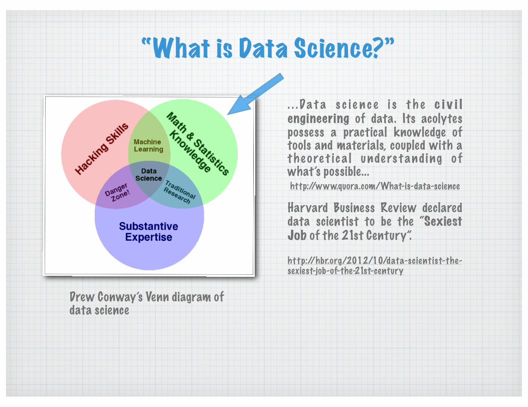
“What is Data Science?”

Drew Conway’s Venn diagram of data science

. . . Da t a s c i e n c e i s t h e c i v i l engineering of data. Its acolytes possess a practical knowledge of tools and materials, coupled with a t h e o re t i c a l unde rs t and i ng o f what’s possible...http://www.quora.com/What-is-data-science

Harvard Business Review declared data scientist to be the “Sexiest Job of the 21st Century”.

ht tp://hbr.org/2012/10/data-scient ist-the-sexiest-job-of-the-21st-century

“What is Data Science?”

. . . Da t a s c i e n c e i s t h e c i v i l engineering of data. Its acolytes possess a practical knowledge of tools and materials, coupled with a t h e o re t i c a l unde rs t and i ng o f what’s possible...http://www.quora.com/What-is-data-science

Harvard Business Review declared data scientist to be the “Sexiest Job of the 21st Century”.

ht tp://hbr.org/2012/10/data-scient ist-the-sexiest-job-of-the-21st-century

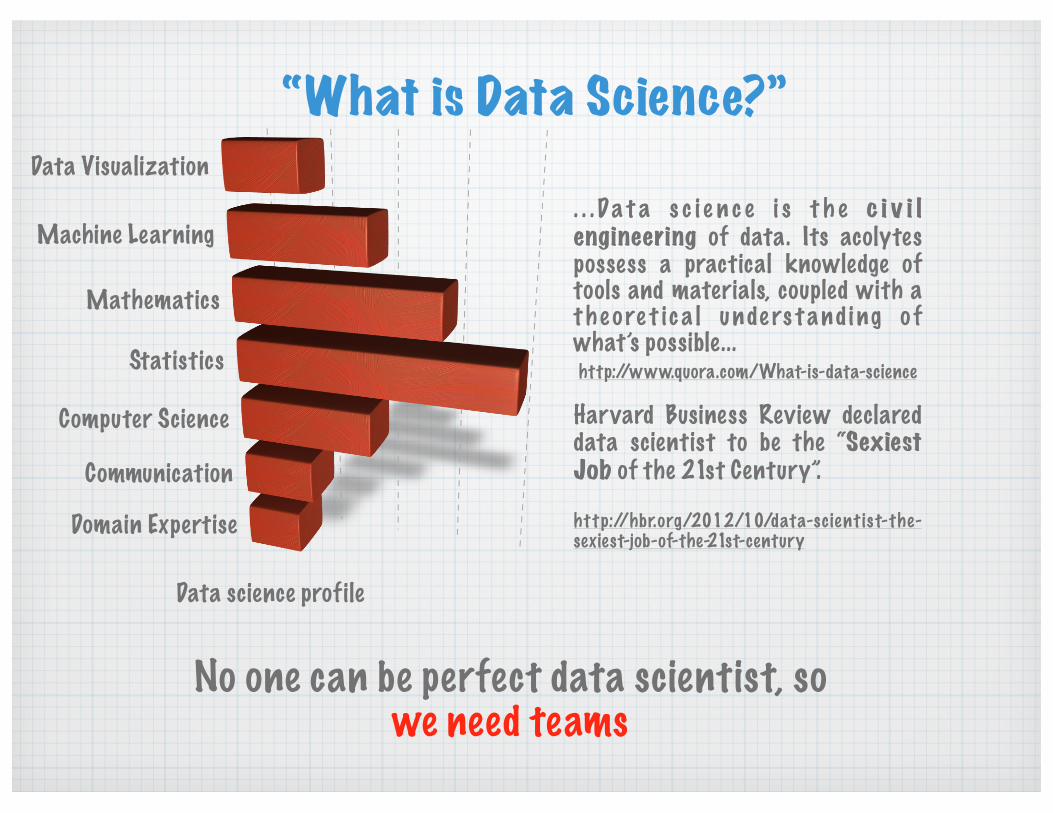
No one can be perfect data scientist, so we need teams

Data science profile

Data Visualization

Machine Learning

Mathematics

Statistics

Computer Science

Communication

Domain Expertise

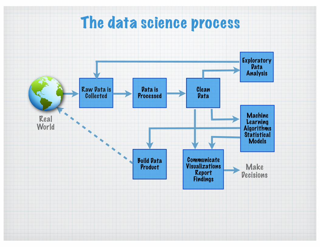
The data science process

Exploratory Data

Analysis

Clean Data

Data is Processed

Raw Data is Collected

Build Data Product

CommunicateVisualizations

Report Findings

Machine Learning

Algorithms Statistical

Models

Make Decisions

RealWorld

Two notices...Columbia University just decided to start an

Institute for Data Sciences and Engineering

with Bloomberg’s help. http://idse.columbia.edu

The Faculty of Engineering of UDD just decided to start an

Center for Sensor Systems and Predictive Analytics

with ?’s help.

Questions and motivations

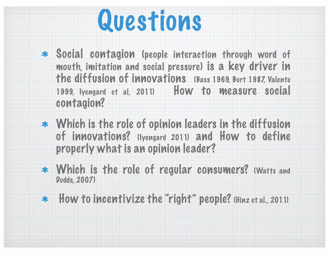
QuestionsSocial contagion (people interaction through word of mouth, imitation and social pressure) is a key driver in the diffusion of innovations (Bass 1969, Burt 1987, Valente 1999, Iyengard et al, 2011) How to measure social contagion? Which is the role of opinion leaders in the diffusion of innovations? (Iyengard 2011) and How to define properly what is an opinion leader?Which is the role of regular consumers? (Watts and Dodds, 2007)

How to incentivize the “right” people? (Hinz et al., 2011)

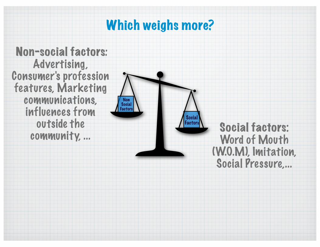
Social factors: Word of Mouth

(W.O.M), Imitation, Social Pressure,...

Social Factors

NonSocial

Factors

Non-social factors: Advertising,

Consumer's profession features, Marketing

communications,influences from

outside the community, ...

Which weighs more?

Datasets and visualizations

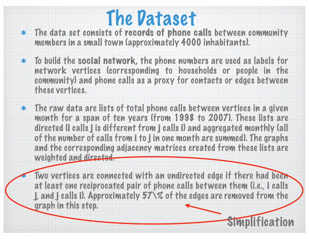
The DatasetThe data set consists of records of phone calls between community members in a small town (approximately 4000 inhabitants).

To build the social network, the phone numbers are used as labels for network vertices (corresponding to households or people in the community) and phone calls as a proxy for contacts or edges between these vertices.

The raw data are lists of total phone calls between vertices in a given month for a span of ten years (from 1998 to 2007). These lists are directed (i calls j is different from j calls i) and aggregated monthly (all of the number of calls from i to j in one month are summed). The graphs and the corresponding adjacency matrices created from these lists are weighted and directed.

Two vertices are connected with an undirected edge if there had been at least one reciprocated pair of phone calls between them (i.e., i calls j, and j calls i). Approximately 57\% of the edges are removed from the graph in this step.

Simplification

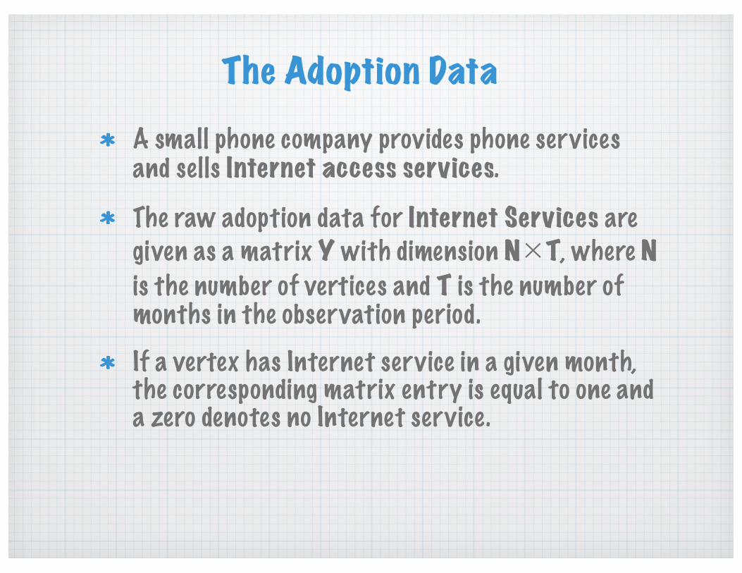
The Adoption DataA small phone company provides phone services and sells Internet access services.

The raw adoption data for Internet Services are given as a matrix Y with dimension N�T, where N is the number of vertices and T is the number of months in the observation period. If a vertex has Internet service in a given month, the corresponding matrix entry is equal to one and a zero denotes no Internet service.

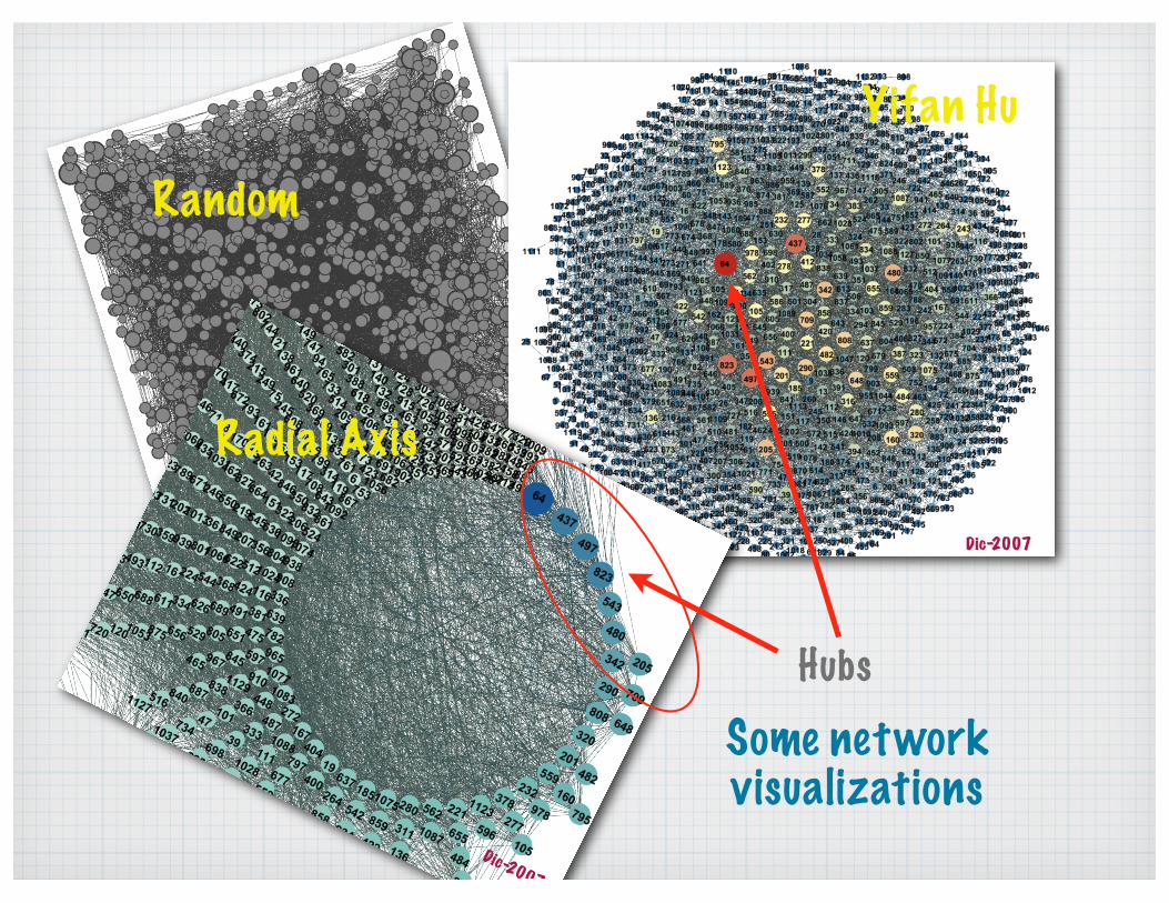
Some networkvisualizations

Hubs

Random

Radial Axis

Yifan Hu

Dic-2007

Dic-2007

Data analysis:The Exploratory Data Analysis (EDA)

The structure of the network over time.The number of edges of a network at a vertex is called the degree of the vertex. The degree d i s t r i b u t i o n o f a network is described by Pk which is the f ract ion of vert ice s having degree k

The figure shows simultaneously the degree distribution functions calculated for several months.

The average probability distribution function (PDF) is shown in black

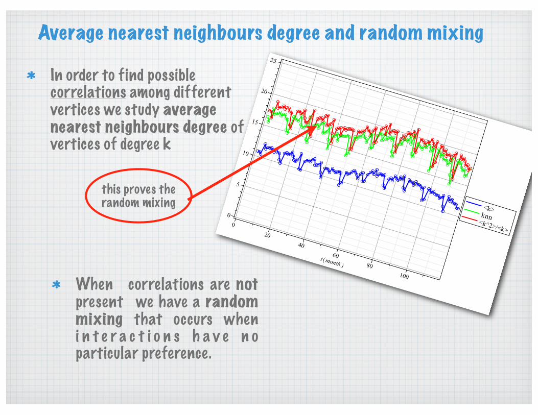
Average nearest neighbours degree and random mixing

In order to find possible correlations among different vertices we study average nearest neighbours degree of vertices of degree k

When correlations are not present we have a random mixing that occurs when i n t e r a c t i o n s h a v e n o particular preference.

this proves the random mixing

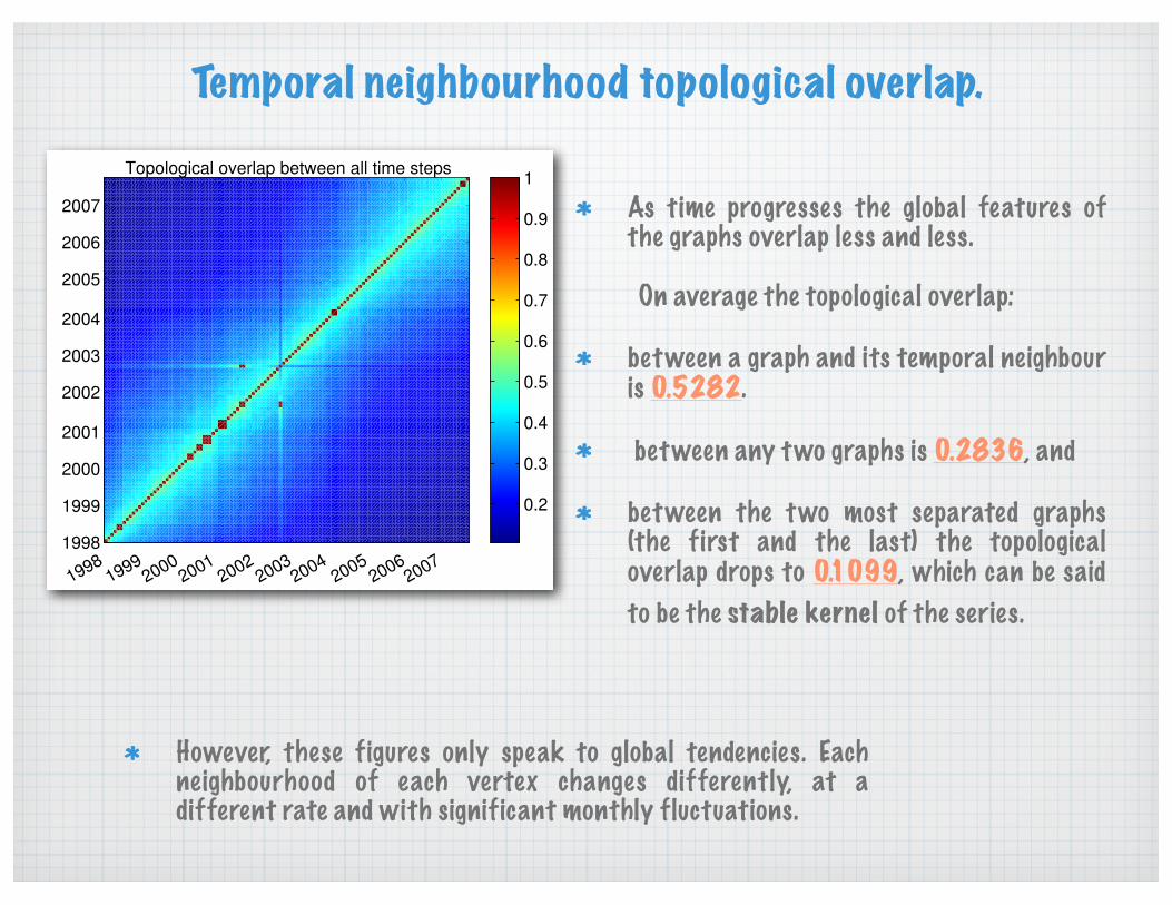
Temporal neighbourhood topological overlap.

As time progresses the global features of the graphs overlap less and less.

between a graph and its temporal neighbour is 0.5282.

between any two graphs is 0.2836, and

between the two most separated graphs (the first and the last) the topological overlap drops to 0.1099, which can be said to be the stable kernel of the series.

1998

1999

2000

2001

2002

2003

2004

2005

2006

2007

Topological overlap between all time steps

19981999

20002001

20022003

20042005

20062007

0.2

0.3

0.4

0.5

0.6

0.7

0.8

0.9

1

However, these figures only speak to global tendencies. Each neighbourhood of each vertex changes differently, at a different rate and with significant monthly fluctuations.

On average the topological overlap:

The strength of a vertex

Strength versus Degree

The strength of a vertex is simply proportional to its degree

The two quantities provide therefore the same information

✓Weight of edge = the number of times per month two vertices call each other.

✓Strength of vertex = sum of all of the weights of the edges conected to the vertex.

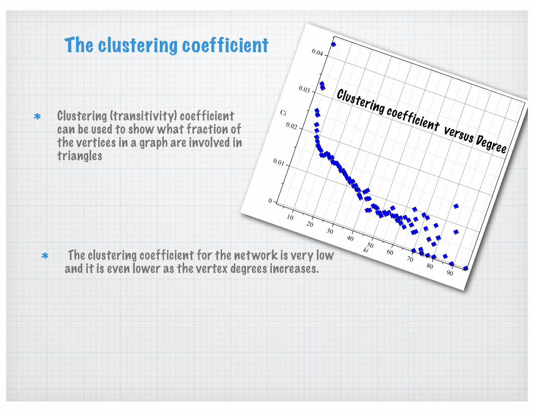
The clustering coefficient

The clustering coefficient for the network is very low and it is even lower as the vertex degrees increases.

Clustering (transitivity) coefficient can be used to show what fraction of the vertices in a graph are involved in triangles

Clustering coefficient versus Degree

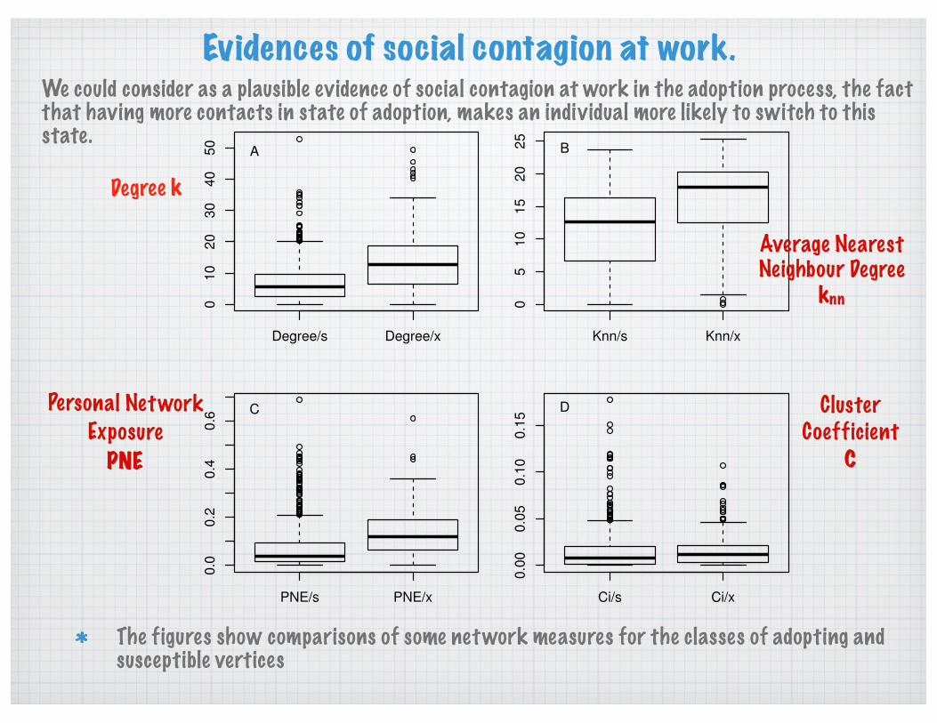
Evidences of social contagion at work.

The figures show comparisons of some network measures for the classes of adopting and susceptible vertices

Degree/s Degree/x

01

02

03

04

05

0

A

Knn/s Knn/x

05

10

15

20

25

B

PNE/s PNE/x

0.0

0.2

0.4

0.6

C

Ci/s Ci/x

0.0

00

.05

0.1

00

.15

D

Degree k

Average Nearest Neighbour Degree

knn

Personal Network Exposure

PNE

Cluster Coefficient

C

We could consider as a plausible evidence of social contagion at work in the adoption process, the fact that having more contacts in state of adoption, makes an individual more likely to switch to this state.

Some preliminary conclusions from EDA.The degree distribution and vertex mean degree in the network remains with little variability as time passes, So, the population have reached a stable network structure

We should take in consideration the local dynamics of vertex rewiring (constant turnover of neighbour vertices)

The degree is one of the most important vertex attributes.

Each vertex of the network, on average, is equally devoted to each of its contacts. The weight associated with each edge is practically independent of the vertices at its ends and about equal to the average weight taken for the entire network. This indicates that in principle there are not preferential or forbidden edges, for receiving the “social contagion”.

The average connectivity of the vertex neighbors exceeds the average connectivity of the vertex itself (proportional mixing). There is not degree correlation.

Low clustering coefficient . The states (susceptible or adopter) of a vertex and those of its neighbours can be treated as independent when these states are updated, this way dynamical correlations can be neglected.

Some math and predictive model

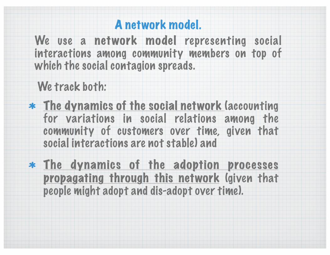
A network model.

The dynamics of the social network (accounting for variations in social relations among the community of customers over time, given that social interactions are not stable) and The dynamics of the adoption processes propagating through this network (given that people might adopt and dis-adopt over time).

We use a network model represent ing social interactions among community members on top of which the social contagion spreads. We track both:

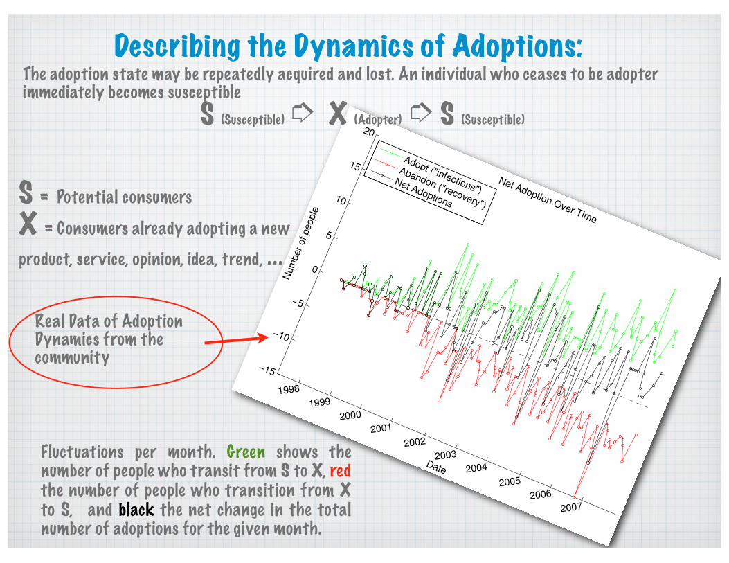
Describing the Dynamics of Adoptions:

S = Potential consumersX = Consumers already adopting a new product, service, opinion, idea, trend, ...

!15

!10

!5

0

5

10

15

20

1998

1999

2000

2001

2002

2003

2004

2005

2006

2007

Date

Net Adoption Over Time

Num

ber

of people

Adopt ("infections")

Abandon ("recovery")

Net Adoptions

S (Susceptible) ➮ X (Adopter) ➮ S (Susceptible)

Real Data of Adoption Dynamics from the community

The adoption state may be repeatedly acquired and lost. An individual who ceases to be adopter immediately becomes susceptible

Fluctuations per month. Green shows the number of people who transit from S to X, red the number of people who transition from X to S, and black the net change in the total number of adoptions for the given month.

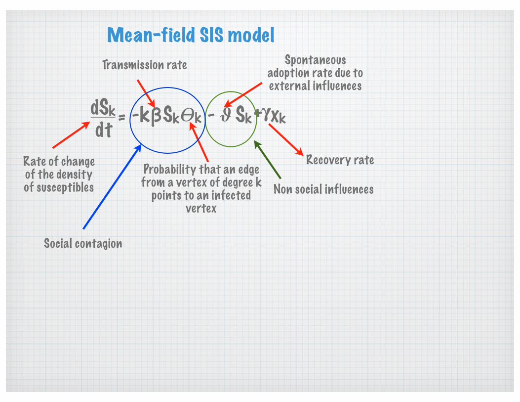
Mean-field SIS model

Sk!kβ Sk"- - xk#+dSkdt =

Rate of change of the density of susceptibles

Probability that an edge from a vertex of degree k

points to an infected vertex

Transmission rate

k

Spontaneous adoption rate due to external influences

Social contagion

Non social influences

Recovery rate

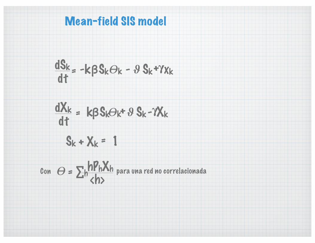
Mean-field SIS model

Sk!kβ Sk"- - xk#+dSkdt = k

Sk!kβ Sk"+ Xk#-dXkdt = k

Sk Xk+ = 1

! hPhXh<h>∑h=Con para una red no correlacionada

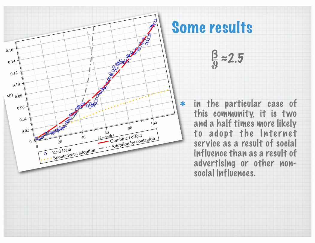
in the particular case of this community, it is two and a half times more likely t o adop t t h e I n te r ne t service as a result of social influence than as a result of advertising or other non-social influences.

Some results

≈2.5β"

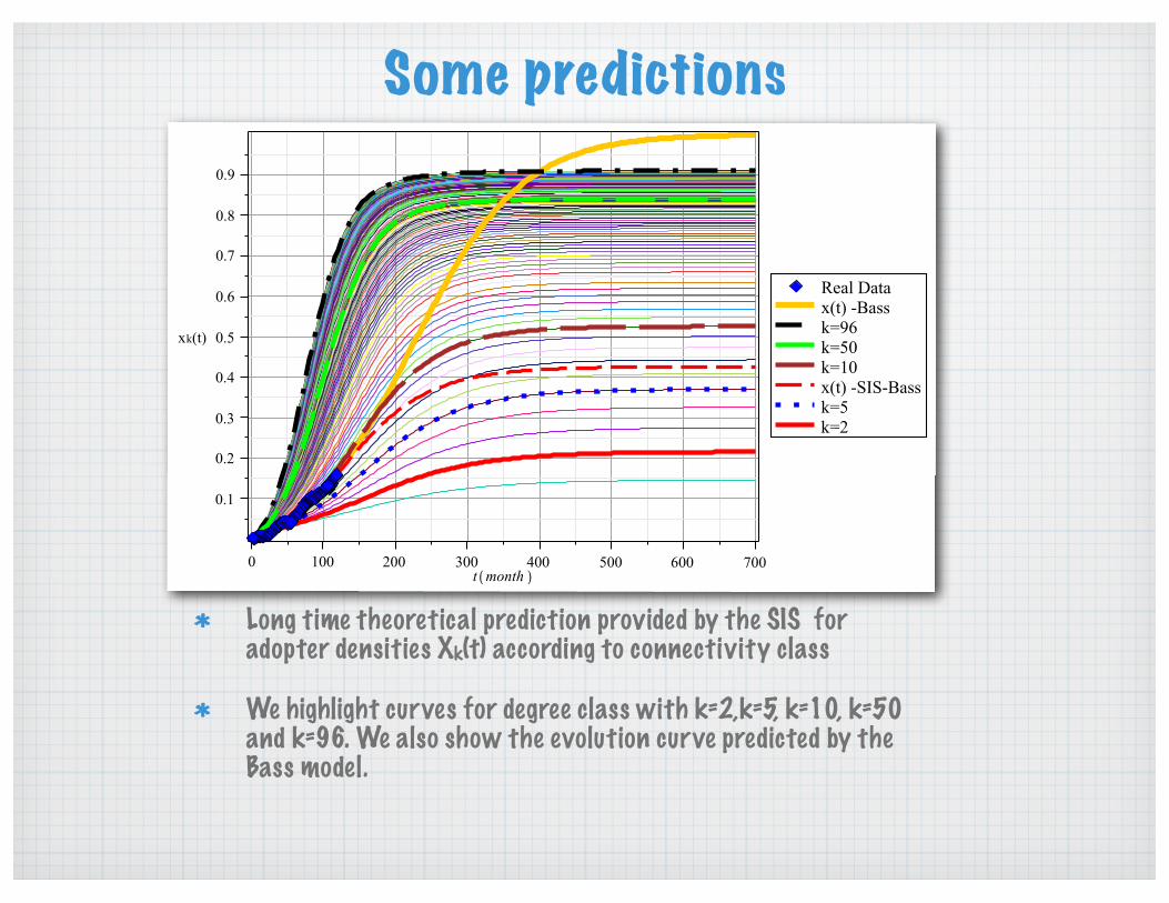
Long time theoretical prediction provided by the SIS for adopter densities Xk(t) according to connectivity class

We highlight curves for degree class with k=2,k=5, k=10, k=50 and k=96. We also show the evolution curve predicted by the Bass model.

Some predictions

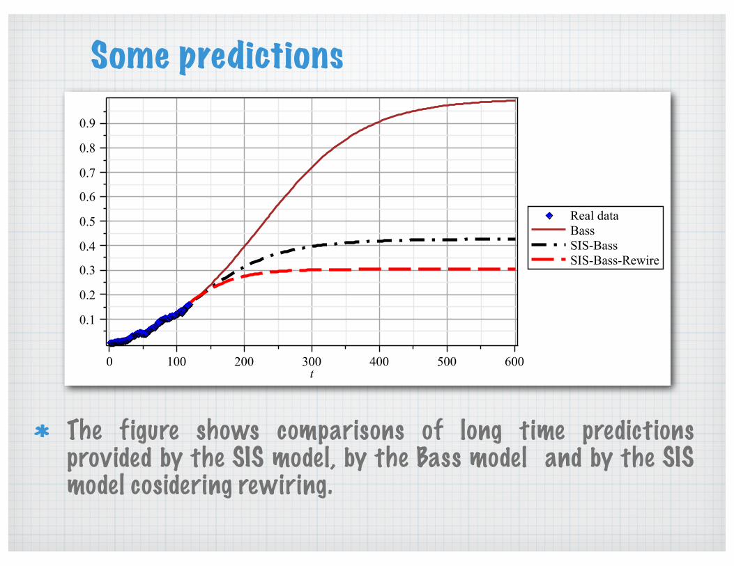
Some predictions

The figure shows comparisons of long time predictions provided by the SIS model, by the Bass model and by the SIS model cosidering rewiring.

ConclusionsWe found evidence that social contagion is at work, and found a way to measure the extent to which it is important.

Social contagion and non-social factors play complementary roles in terms of their impact on the adoption process. Non-social influences are very likely to create spontaneously new adopters whereas the social contagion leads to the growth of already existing adopters. The interplay between these complementary influences gives shape to the dynamics of adoptions.

The contagion spreading is not necessarily enhanced by the dynamics of the network and the prevalence of the contagion could be smaller than in the case of a static network. Thus, the constant turnover of neighbour vertices could produce an effective reduction of the “infectivity”

Given that our findings are based on a real life situation, we point out how relevant is to get a detaliled dataset with complete information of social relations over time to validate any model of diffusion of innovations.

Some Recomendations for working with data

Before you get too involved with the data and start coding you have to visualize data. This entails making plots and building intuition for your particular dataset. EDA helps out a lot, as well as trial and error and iteration.

It’s useful to draw a picture of what you think the underlying process might be with your model. What comes first? What influences what? What causes what? What’s a test of that?

Data is not objective. We build models from the data. A model is an artificial construction where all extraneous detail has been removed or abstracted.

It’s always good to start simply so use simple modelsNatural processes tend to generate measurements whose empirical shape could be approximated by mathematical models with a few parameters that could be estimated from the data.

Muchas Gracias