Tehnički glasnik - TECHNICAL JOURNAL - Sveučilište Sjever
98
-
Upload
khangminh22 -
Category
Documents
-
view
3 -
download
0
Transcript of Tehnički glasnik - TECHNICAL JOURNAL - Sveučilište Sjever


© 2020 Tehnički glasnik / Technical Journal. All rights reserved
ISSN 1846-6168 (Print) ISSN 1848-5588 (Online)
TEHNIČKI GLASNIK - TECHNICAL JOURNAL Scientific-professional journal of University North
Volume 14 Number 1 Varaždin, March 2020 Pages 1–87
Editorial Office:
Sveučilište Sjever – Tehnički glasnik Sveučilišni centar Varaždin
104. brigade 3, 42000 Varaždin, Hrvatska Tel. ++385 42 493 328, Fax.++385 42 493 333
E-mail: [email protected] https://tehnickiglasnik.unin.hr
https://www.unin.hr/djelatnost/izdavastvo/tehnicki-glasnik/ https://hrcak.srce.hr/tehnickiglasnik
Founder and Publisher:
Sveučilište Sjever / University North
Council of Journal: Marin MILKOVIĆ, Chairman; Anica HUNJET, Member; Goran KOZINA, Member; Mario TOMIŠA, Member;
Vlado TROPŠA, Member; Damir VUSIĆ, Member; Milan KLJAJIN, Member; Anatolii KOVROV, Member
Editorial Board: Chairman Damir VUSIĆ (1), Milan KLJAJIN (2)/(1), Marin MILKOVIĆ (1), Krešimir BUNTAK (1), Anica HUNJET (1), Živko KONDIĆ (1), Goran KOZINA (1), Ljudevit KRPAN (1), Krunoslav HAJDEK (1), Marko STOJIĆ (1), Božo SOLDO (1), Mario TOMIŠA (1), Vlado TROPŠA (1), Vinko VIŠNJIĆ (1), Duško PAVLETIĆ (5), Branimir PAVKOVIĆ (5), Mile MATIJEVIĆ (3), Damir MODRIĆ (3), Nikola MRVAC (3), Klaudio PAP (3), Ivana ŽILJAK STANIMIROVIĆ (3), Krešimir GRILEC (6), Biserka RUNJE (6), Predrag ĆOSIĆ (6), Sara HAVRLIŠAN (2), Dražan KOZAK
(2), Roberto LUJIĆ (2), Leon MAGLIĆ (2), Ivan SAMARDŽIĆ (2), Antun STOIĆ (2), Katica ŠIMUNOVIĆ (2), Goran ŠIMUNOVIĆ (2), Ladislav LAZIĆ (7), Ante ČIKIĆ (1)/(2), Darko DUKIĆ (9), Gordana DUKIĆ (10), Srđan MEDIĆ (11), Sanja KALAMBURA (12), Marko DUNĐER (13), Zlata DOLAČEK-ALDUK (4), Dina STOBER (4)
International Editorial Council:
Boris TOVORNIK (14), Milan KUHTA (15), Nenad INJAC (16), Džafer KUDUMOVIĆ (17), Marin PETROVIĆ (18), Salim IBRAHIMEFENDIĆ (19), Zoran LOVREKOVIĆ (20), Igor BUDAK (21), Darko BAJIĆ (22), Tomáš HANÁK (23), Evgenij KLIMENKO (24), Oleg POPOV (24), Ivo ČOLAK (25), Katarina MONKOVÁ (26), Berenika HAUSNEROVÁ (8),
Nenad GUBELJAK (27)
Editor-in-Chief: Milan KLJAJIN
Technical Editor:
Goran KOZINA
Graphics Editor: Snježana IVANČIĆ VALENKO
Linguistic Advisers for English language:
Ivana GRABAR, Iva GRUBJEŠIĆ
IT support: Tomislav HORVAT
Print:
Centar za digitalno nakladništvo, Sveučilište Sjever
All manuscripts published in journal have been reviewed. Manuscripts are not returned.
The journal is free of charge and four issues per year are published
(In March, June, September and December) Circulation: 100 copies
Journal is indexed and abstracted in:
Web of Science Core Collection (Emerging Sources Citation Index - ESCI), EBSCOhost Academic Search Complete, EBSCOhost – One Belt, One Road Reference Source Product, ERIH PLUS, CITEFACTOR – Academic Scientific Journals, Hrčak - Portal znanstvenih časopisa RH
Registration of journal:
The journal "Tehnički glasnik" is listed in the HGK Register on the issuance and distribution of printed editions on the 18th October 2007 under number 825.
Preparation ended: March 2020
Legend:
(1) University North, (2) Mechanical Engineering Faculty in Slavonski Brod, (3) Faculty of Graphic Arts Zagreb, (4) Faculty of Civil Engineering Osijek, (5) Faculty of Engineering Rijeka, (6) Faculty of Mechanical Engineering and Naval Architecture Zagreb, (7) Faculty of Metallurgy Sisak, (8) Tomas Bata University in Zlín, (9) Department of Physics of the University of Josip Juraj Strossmayer in
Osijek, (10) Faculty of Humanities and Social Sciences Osijek, (11) Karlovac University of Applied Sciences, (12) University of Applied Sciences Velika Gorica, (13) Department of Polytechnics - Faculty of Humanities and Social Sciences Rijeka, (14) Faculty of Electrical Engineering and Computer Science - University of Maribor, (15) Faculty of Civil Engineering - University of Maribor, (16) University College of Teacher Education of Christian Churches Vienna/Krems, (17) Mechanical Engineering Faculty Tuzla, (18) Mechanical Engineering Faculty Sarajevo, (19) University of Travnik - Faculty of Technical Studies, (20) Higher Education Technical School of Professional Studies in Novi Sad, (21) University of Novi Sad - Faculty of Technical Sciences, (22) Faculty of Mechanical Engineering -
University of Montenegro, (23) Brno University of Technology, (24) Odessa State Academy of Civil Engineering and Architecture, (25) Faculty of Civil Engineering - University of Mostar, (26) Faculty of Manufacturing Technologies with the seat in Prešov - Technical University in Košice, (27) Faculty of Mechanical Engineering - University of Maribor

CONTENT
TEHNIČKI GLASNIK 14, 1(2020), I-I I
CONTENT I Elmedin Mešić, Adil Muminović, Mirsad Čolić, Marin Petrović, Nedim Pervan Development and Experimental Verification of a Generative CAD/FEM Model of an External Fixation Device 1 İsmail Topcu Investigation of Wear Behavior of Particle Reinforced AL/B4C Composites under Different Sintering Conditions 7 Nina Dmitriyeva, Oleg Popov, Olga Grin Research of Efficiency of the Horizontal Coating Depending on Intensity of Capillary Absorption 15 Lino Kocijel, Igor Poljak, Vedran Mrzljak, Zlatan Car Energy Loss Analysis at the Gland Seals of a Marine Turbo-Generator Steam Turbine 19 Štefanija Klarić, Zlatko Botak, Damien J. Hill, Matthew Harbidge, Rebecca Murray Application of a Cold Spray Based 3D Printing Process in the Production of EDM Electrodes 27 Srđan Medić, Veljko Kondić, Tihomir Mihalić, Vedran Runje Research of the Design Feasibility of a 3-Wheel Electric Vehicle with a Simplified Control System 32 Barış Kavasoğullari, Ertuğrul Cihan, Hasan Demir Energy and Exergy Analysis of LiBr-aq and LiCl-aq Liquid Desiccant Dehumidification System 36 Erhan Arslan, Azim Doğuş Tuncer, Meltem Koşan, Mustafa Aktaş, Ekin Can Dolgun Designing of a New Type Air-Water Cooled Photovoltaic Collector 41 Živko Kondić, Željko Knok, Veljko Kondić, Sanja Brekalo Risk Management in the Higher Education Quality Insurance System 46 Mariia S. Barabash, Bogdan Y. Pisarevskyi, Yaroslav Bashynskyi Taking into Account Material Damping in Seismic Analysis of Structures 55 Maksym Votinov, Olga Smirnova, Maria Liubchenko The Main Directions of the Humanization of Industrial Objects in Urban Environment 60 Behnam Mehdipour, Hamid Hashemolhosseini, Bahram Nadi, Masoud Mirmohamadsadeghi Investigating the Effect of Geocell Changes on Slope Stability in Unsaturated Soil 66 Goran Kos, Neven Ivandić, Krešimir Vidović Tourism as a Factor of Demand in Public Road Passenger Transportation in the Republic of Croatia 76 INSTRUCTIONS FOR AUTHORS III

II TECHNICAL JOURNAL 14, 1(2020), II-II

TEHNIČKI GLASNIK 14, 1(2020), 1-6 1
ISSN 1846-6168 (Print), ISSN 1848-5588 (Online) Original scientific paper https://doi.org/10.31803/tg-20191112161707
Development and Experimental Verification of a Generative CAD/FEM Model of an External Fixation Device
Elmedin Mešić, Adil Muminović, Mirsad Čolić, Marin Petrović, Nedim Pervan
Abstract: This paper presents the development and experimental verification of a generative CAD/FEM model of an external bone fixation device. The generative CAD model is based on the development of a parameterized skeleton algorithm and sub-algorithms for parametric modeling and positioning of components within a fixator assembly using the CATIA CAD/CAM/CAE system. After a structural analysis performed in the same system, the FEM model was used to follow interfragmentary fracture displacements, axial displacements at the loading site, as well as principal and Von Mises stresses at the fixator connecting rod. The experimental analysis verified the results of the CAD/FEM model from an aspect of axial displacement at the load site using a material testing machine (deviation of 3.9 %) and the principal stresses in the middle of the fixator connecting rod using tensometric measurements (deviation of 3.5 %).The developed model allows a reduction of the scope of preclinical experimental investigations, prediction of the behavior of the fixator during the postoperative fracture treatment period and creation of preconditions for subsequent structural optimization of the external fixator. Keywords: external fixation device; generative CAD model; interfragmentary displacements; principal stresses 1 INTRODUCTION
With regard to the organization of models and the application of modern technologies, the design process should be based on the widespread use of computer support in all its stages, i.e. it should be based on the principle of simultaneous design. All this leads to the fact that it is necessary to develop a computer model of products that will meet the requirements defined by a systematic approach to design. In this sense, the basis of a generative CAD model should be a parameterized model with characteristics meeting the requirements of simultaneous design.
Parametric modeling has an advantage over classical modeling enabling a quick and easy acquisition of various design variants, memorization of structural changes and reuse of previously formed models [1]. In engineering analysis, it is often necessary to represent some physical form using unambiguous expressions. These relationships should mathematically describe the geometric shape of an associated 2D or 3D continuous physical shape using scalar parameters. The geometric shape is described by parametric equations and a set of scalar parameters, enabling its visualization, simulation of the interaction of the shape with the environment and geometric transformations. There are many published studies on generative design and parametric modelling [2-7].
The parameterization technique is one of the key points in the process of the automation of an analysis and optimization of design. It should be flexible to allow the description of various complex shapes with a minimum number of geometric constraints. Parameterization adds intelligence to the model, defining the interdependencies between the elements, dimensions and parameters of the model. This allows changes to be made to all model elements connected with the parameters, thereby updating the model transferring it to the new desired configuration. In this way, it is possible to express all dimensions of the fixator as a
function of several sizes or parameters and to couple them with the processes of calculation and later optimization.
The parameterization method used and the algorithms developed should allow for an automatic link between the CAD and FEM models. The developed parameterized model of the external fixator should meet the following requirements: the geometry of the model should as closely as possible map the geometry of the real fixator to enable the FEM analysis and then structural optimization; rapid change of geometry parameters in order to form different fixator configurations; parametric modeling approach based on technical elements with as few design parameters as possible; regularity check of fixator design; analysis of elements loading and stress-strain states using appropriate solver and associativity.
Prior to the fixator parameterization process, the following activities were performed: the fixator configuration complexity check, development of the fixator model design plan, definition of basic independent and dependent parameters, as well as establishment of the most efficient method of the fixator parameterization. 2 DEVELOPMENT OF A GENERATIVE CAD MODEL
With the aim to develop a generative model and to achieve the flexibility of the created fixator model, the so-called Top-Down design method was used. This method involves a working mode with a view from the top over the basic model design, as well as applying associativity and parameterized relations [6]. This approach is actually reflected in the formation of a so-called parameterized skeleton representing the infrastructure of the fixator through which appropriate interactions between design parameters are established (Fig. 1). In this way, the knowledge about design is integrated into the CAD model through the skeleton, which represents the basis of a so-called generative modeling. Therefore, the generative model is not only an extension of the parametric model, but forms a certain

Elmedin Mešić et al.: Development and Experimental Verification of a Generative CAD/FEM Model of an External Fixation Device
2 TECHNICAL JOURNAL 14, 1(2020), 1-6
knowledge base of the design forms represented by the CAD model forms. The knowledge base can also be composed of information obtained “externally” based on experimental and/or structural analysis. The use of a parameterized skeleton of the fixator enables:
- Design based on detailed specifications. All relevant information are stored in the skeleton model. The spatial constraints are completely defined within the skeleton in order to position the components within the fixator assembly.
- Updating the model. The skeleton allows changes to be made to the models of individual components as well as the complete fixator, so that the modifications in the skeleton are reflected to all individual components and subsets of the fixator.
- Model flexibility. The key information stored in the skeleton can be associated with the corresponding fixator components. However, the components can be modified independently of each other and independently of the skeleton, because of not being interconnected. Also, it is possible to remove specific components of the fixator without affecting the others. The skeleton is formed at the very beginning of the
development of a parameterized model based on the analysis of the geometrical characteristics of the components and assembly, as well as their interrelations.
Figure 1 Parametrized skeleton and fixator model
Also, functional requirements and model elements
considered necessary to fulfill its function are included in the analysis. Skeleton basically contains knowledge stored in the form of parameters, relations and basic geometry of design. It is important to define the referent design parameters in the skeleton, i.e. parameters that, through appropriate relations, connect the geometry of the complete structure. After defining the parameters in the skeleton, they are published and used as external parameters when defining the shape and
position of individual components within the fixator assembly. In this way, the parameterized skeleton gives the necessary flexibility to the fixator design in terms of rapid adaptation to the new parameter values [7].
The relations within the skeleton give flexibility of the fixator design in terms of defining the way of changing the shape, position, and orientation of the components in the assembly. Relation arguments contain referent design parameters and geometric elements that position the fixator components with respect to the main coordinate system of the skeleton (Figure 1). Relationships represent the most important part of the generative model and reflect knowledge of the structural, functional and technological properties of the fixator.
The complete fixator design is parameterized with 28 design parameters in order to define the shape of the components, 9 of which are independent parameters. The three referent design parameters of the fixator model are: the outer diameter of the connecting rod ds, the wall thickness of the rod δ and the basic thickness of the plate δpo. Appropriate relations have been established between these three referent parameters and certain parameters of fixator model components comprised by the updating process. In this way, the complete fixator model is updated based on the values of the referent parameters. The referent parameters were selected on the basis of the following ascertainments: their change produces a significant effect on the mass and stability of the fixator; the relations are simply connected with other parameters and allow easy modification of both components and complete fixator; by changing their values, the existing simplicity of the design is retained [10].
In addition to parameters and relations, the skeleton contains the basic geometry of the fixator with all the referent elements for positioning components in space such as points, axes and planes. The position of all the above elements is precisely defined with respect to the main coordinate system of the skeleton using referent parameters for positioning (coordinates of points, distances, lengths, etc.). Subsequently, the local coordinate systems, axes and characteristic points of the fixator components are aligned with the skeleton reference elements (Figure 1). In this way, the complete flexibility of the fixator model is achieved and simultaneous modifications of its components are supported.
After the formation of the fixator skeleton, it is necessary to form parameterized models of its components via the sub-algorithms formed. Fixator components that will change their shape, dimensions or position in the structure during the optimization process need to be parameterized. In this way, parameterization of the model connecting rod of the fixator, clip, clamping ring, clips carrier and clamping plates was performed. In order to design component models, their parameters are first defined in the skeleton and then linked to the fixator components via external parameters.
Developed sub-algorithms are in charge of controlling modifications of parameterized models of the fixator components. These sub-algorithms include: external parameters, relations and commands for shaping models and modifying formed shapes. Sub-algorithms within components retrieve external parameter values from the

Elmedin Mešić et al.: Development and Experimental Verification of a Generative CAD/FEM Model of an External Fixation Device
TEHNIČKI GLASNIK 14, 1(2020), 1-6 3
skeleton. The next step considers relating the design parameters of the components to the external parameters via relations. Finally, modeling of the components is performed using sub-algorithms via shaping commands.
During the formation of the fixator model, it is very important, when associating the relations between components, that all constraints are defined due to proper parameterization. Also, when changing the dimensions of individual components, it is important that complete fixator is properly updated. Testing of the flexibility and correctness of the fixator CAD model also considers its analysis in order to determine possible interference of two or more components of the fixator. When updating a model, overlapping or uncontrolled backlash may occur due to parameter changes. The geometric and meritorious connections of the forms of individual elements allow for an instant adaptation to the changes of the model. Development of generative CAD model is performed in CATIA CAD/CAM/CAE system. 3 STRUCTURAL ANALYSIS
Fixator components are modeled by finite elements of linear (TE4) and parabolic (TE10) tetrahedron type. Both elements belong to the group of 3D isoparametric elements, i.e. solids with six edges, using the same interpolation functions and the same nodes to approximate the geometry and fields of the basic unknowns in the element [8]. There are three degrees of freedom in each node of these finite elements. These are the displacements u, v and w in directions of x, y and z axes of the rectangular coordinate system.
The external fixator is made of special stainless steel for the manufacture of medical devices. For isotropic materials, the constitutive relations or stress-strain relations for a linear elastic material contain only two independent constants: the modulus of elasticity E and the Poisson’s coefficient ν. A special form of anisotropic material is an orthotropic material with three planes of symmetry. It is common for orthotropic material to define material parameters such as modulus of elasticity, Poisson’s coefficient and shear modulus [8]. Bone segment models are made of beech wood with known properties.
The basic loading form of the external fixator is axial pressure. FEM model has been developed to simulate experimental investigation under axial loading, taking into account complete geometry of the fixator and bone model, the connections between the components, the applied load and the constraints applied [9]. During axial loading, bone models relied on spherical joints, while the intensity of axial compression of the proximal bone segment ranged in the interval F = 0 – 600 N with an increase in loading rate of 5 N/s. The FEM model layout of the fixator model before and after maximum axial compression with a representation of the interfacial displacements is given in Fig. 2.
In order to define maximum interfragmental displacement at the fracture site R, displacements of a pair of adjacent points at the end planes of the proximal and distal segments at the fracture site in x, y and z directions were determined [10]. The relative craniocaudal and lateromedial
displacements (x and y directions) and axial displacements (z direction) of the observed points are determined by the following relations:
𝑟𝑟𝐷𝐷(𝑥𝑥) = 𝐷𝐷𝑝𝑝(𝑥𝑥) − 𝐷𝐷𝑑𝑑(𝑥𝑥) 𝑟𝑟𝐷𝐷(𝑦𝑦) = 𝐷𝐷𝑝𝑝(𝑦𝑦) − 𝐷𝐷𝑑𝑑(𝑦𝑦), (1) 𝑟𝑟𝐷𝐷(𝑧𝑧) = 𝐷𝐷𝑝𝑝(𝑧𝑧) − 𝐷𝐷𝑑𝑑(𝑧𝑧) where 𝑟𝑟𝐷𝐷(𝑥𝑥), 𝑟𝑟𝐷𝐷(𝑦𝑦) and 𝑟𝑟𝐷𝐷(𝑧𝑧) are relative displacements of bone model segments at the fracture site in x, y and z directions, 𝐷𝐷𝑝𝑝(𝑥𝑥), 𝐷𝐷𝑝𝑝(𝑦𝑦) and 𝐷𝐷𝑝𝑝(𝑧𝑧) are absolute displacements of bone endpoints of the bone model proximal segment in x, y and z directions, 𝐷𝐷𝑑𝑑(𝑥𝑥), 𝐷𝐷𝑑𝑑(𝑦𝑦) and 𝐷𝐷𝑑𝑑(𝑧𝑧) are absolute displacements of bone endpoints of the bone model distal segment in x, y and z directions.
Figure 2 Non-deformed and deformed structure of the system under a maximum
axial load and interfragmentary movement at the fracture site
The intensity of maximum interfragmental displacement vector at the fracture site R is defined by
𝑅𝑅 = ��𝑟𝑟𝐷𝐷(𝑥𝑥)�2 + �𝑟𝑟𝐷𝐷(𝑦𝑦)�
2 + �𝑟𝑟𝐷𝐷(𝑧𝑧)�2, (2)
Complete mechanical investigations of the fixator
stability, in addition to the analysis of displacements at the fracture site, include the analysis of principal stresses at the characteristic locations of the fixator structure [8, 9]. Here, appropriate stress analysis will only be presented for the case of axial compression as the dominant loading.
During structural FEM and experimental analysis, intensities and directions of principal stresses at two control points in the middle of the fixator connecting rod were monitored and analyzed. The measurement point closer to the bone model segment is labeled as MP-, while the location on the opposite side of the fixator connecting rod is labeled as MP+ (Fig. 3).
The direction of the maximum principal stress 𝜎𝜎1 at MP+ measuring point and the direction of the smallest principal stress 𝜎𝜎3 at MP- measuring point coincide with z axis and the

Elmedin Mešić et al.: Development and Experimental Verification of a Generative CAD/FEM Model of an External Fixation Device
4 TECHNICAL JOURNAL 14, 1(2020), 1-6
axis of symmetry of the connecting rod, respectively. Fig. 3 shows the directions and intensities of the principal stresses at the measuring points (view B). It is observed that at MP+ measuring point the highest principal stress is actually the tensile stress, while at MP- measuring point the lowest principal stress is actually the compression stress. The tensile stresses have a lower intensity than the compression stresses, which is a direct consequence of the eccentric pressure the fixator connecting rod is exposed to. Also, it is noticeable that the dominant principal stresses (𝜎𝜎1 and 𝜎𝜎3) are in a bending plane of the fixator, which does not coincide with the plane of the half-pins [11].
Figure 3 Principal stresses
4 EXPERIMENTAL ANALYSIS
Experimental tests of the fixator were performed at a Material Testing Laboratory at Faculty of Mechanical Engineering of the University of Sarajevo using a tensometric analysis equipment. In real conditions, the fixator is exposed to loading through bone segments. This fact was taken into account so that, during the experimental tests, the fixator loading was performed by means of bone model segments made of beech wood (mechanical properties similar to those of bone) [12].
During the tests, the displacement of the proximal bone segment at the loading site δ was monitored by a displacement transducer, whereas the loading F was controlled by a force transducer (U2A from HBM - Hottinger Baldwin Messtechnik GmbH, Darmstadt, Germany) on a material testing machine (Zwick GmbH & Co., Ulm, Germany, model 143501). Stress analysis by tensometric measurements was performed using a DMC 9012A digital measuring amplifier system with built-in DMV 55 modules to receive signals from type 3/120LY11 electrical resistance strain gauges manufactured by HBM (Fig. 4).
Two Wheatstone quarter bridge circuits with compensatory strain gauges were formed as the connecting rod was exposed to eccentric pressure due to the axial compression at the site of the proximal segment of the bone model [11]. This form of loading is manifested by the
unequal distribution of tension and compression stresses along the longitudinal section of the connecting rod, meaning the neutral line does not coincide with the axis of symmetry of the rod (Fig. 5). Wheatstone quarter bridge circuits consist of an active SG strain gauge and a compensation or inactive SG2 strain gauge of the same type (Fig. 4 and 5). Compensation strain gauges are placed on unloaded plate tied to the fixator connecting rod in immediate vicinity of the active strain gauges. The plate is made of the same material as rod (fixator).
Figure 4 Fixator experimental setup
Applying general Wheatstone bridge equation [13]:
𝑉𝑉𝑜𝑜𝑉𝑉𝑠𝑠
= 𝐾𝐾𝑡𝑡4
(𝜀𝜀1′ − 𝜀𝜀2′ + 𝜀𝜀3′ − 𝜀𝜀4′), (3) to used quarter bridge circuit with compensating strain gauge, measured deformation is obtained based on the following relation: 𝜀𝜀1′ = 4
𝐾𝐾𝑡𝑡
𝑉𝑉𝑜𝑜𝑉𝑉𝑠𝑠
, (4) where 𝑉𝑉𝑜𝑜 and 𝑉𝑉𝑠𝑠 are output voltage and supply voltage of Wheatstone bridge, 𝐾𝐾𝑡𝑡 is a strain gauge coefficient, 𝜀𝜀1′ … 𝜀𝜀4′ are strains measured by the strain gauges.
The active strain gauges were placed on diametrically opposite sides of the connecting rod at the closest and farthest point from the bone model (Fig. 3 and 5). Therefore, their longitudinal axis coincides with the directions of dominant principal strains (𝜀𝜀1 and 𝜀𝜀3) at the measuring points. In this way, it is possible to determine the intensity of the dominant principal stresses at the measurement points [13, 14]. On the other hand, previously derived FEM analysis determined the direction and intensity of the principal stresses and observed that intensities of the other two principal stresses are

Elmedin Mešić et al.: Development and Experimental Verification of a Generative CAD/FEM Model of an External Fixation Device
TEHNIČKI GLASNIK 14, 1(2020), 1-6 5
negligible in relation to the highest principal stress 𝜎𝜎1 on MP+ and the lowest principal stress 𝜎𝜎3 on MP- (Tab. 2). In this case, the flexural strains are much larger than the compression strains (|𝜀𝜀𝑠𝑠| ≫ 𝜀𝜀𝑝𝑝) [15]. The strain distribution in the longitudinal section of the fixator connecting rod is shown schematically in Fig. 5. The principal stresses at the points MP+ and MP− are determined by the following relations: 𝜎𝜎1 = 𝜀𝜀1𝐸𝐸 ; 𝜎𝜎3 = 𝜀𝜀3𝐸𝐸, (5) where E is the modulus of elasticity of the connecting rod material.
Figure 5 Strain gauges arrangement with distribution of strains at fixator
connecting rod Using the Catman software (HBM) for acquisition,
processing, monitoring and analysis of measurement results from a measuring system, by scaling option, the original output strain unit mV/V is transformed to μm/m taking into account strain gauge and bridge factor values.
5 RESULTS AND CONCLUSION
Comparative diagrams of changes in the principal stresses 𝜎𝜎1 and 𝜎𝜎3, as well as a comparative diagram of axial load as a function of displacement at the loading point obtained by experimental testing and FEM method are shown in Fig. 6. A good agreement of the results is observed with maximum deviations of 3.9 % for displacements and 3.5 % for principal stresses.
Tab. 1 shows the values of interfragmentary displacements and displacements at the loading points. It can be observed that the relative axial displacements 𝑟𝑟𝐷𝐷(𝑧𝑧) =4.14 mm are dominant at the fracture points, and that the relative transverse displacements 𝑟𝑟𝐷𝐷(𝑦𝑦) = 0.15 mm and 𝑟𝑟𝐷𝐷(𝑥𝑥) = 0 mm leading to fracture unhealing or poor healing are significantly smaller (Eq. (1)).
Figure 6 Comparative diagram of the principal stresses σ1 on MP+ and σ3 on MP-
(a) and comparative diagram of the axial displacement at the point of load (b)
Table 1 Values of displacements under maximum intensity of load
Met
hods
Displacement of proximal
segment at the fracture gap,
mm
Displacement of distal segment at the fracture gap,
mm
Max. relative displ. at the gap, mm
Displ. at the point
of load, mm
Dp(x) Dp(y) Dp(z) Dd(x) Dd(y) Dd(z) R δ FEA 0.53 4.14 −4.36 0.53 4.29 0.22 4.58 4.18 Exp. - - - - - - - 4.35
Tab. 2 shows the intensities of the principal and Von
Mises stresses generated at the measurement points.
Table 2 Values of displacements under maximum intensity of load
Met
hods
Principal stresses, MPa Von Mises stress, MPa
MP+, SG+ MP−, SG− MP+ MP− σ1 σ2 σ3 σ1 σ2 σ3 σvm σvm
FEA 330 0.2 0.001 −0.003 −0.4 −355 330 355 Exp. 334 - - - - −368 - -
The intensity of the principal stress 𝜎𝜎1 at MP+ measuring
point is significantly higher than the other two principal stresses (𝜎𝜎2 and 𝜎𝜎3). Also, the intensity of the principal stress 𝜎𝜎3 at MP- measuring point is significantly higher than the other two principal stresses (𝜎𝜎1 and 𝜎𝜎2).
The performed research has shown a linear relationship between the load and displacement of bone segments. This is a consequence of the absence of major rotations, displacements and plastic deformations of the fixator components as well as shear within its joints. This also satisfies the basic requirement of fixator stability in terms of preserving the anatomical reduction of bone fragments.

Elmedin Mešić et al.: Development and Experimental Verification of a Generative CAD/FEM Model of an External Fixation Device
6 TECHNICAL JOURNAL 14, 1(2020), 1-6
Using the developed CAD/FEM fixator model, it is possible to control the displacements and stresses generated at any point in the fixator-bone system. The created model can also be used by surgeons in predicting fixator behavior during the postoperative period of bone fracture treatment. Due to extreme flexibility of created CAD model, rapid changes not only of the geometry and position of components and fixator, but also to biomaterials finding their application in external fixation now became possible. In this way, conditions have been created to optimize the fixator design, significantly shortening the time and reducing the costs of the development of medical devices for external bone fixation. Also, the use of such models significantly reduces the volume of preclinical experimental tests on fixators.
Acknowledgements
The authors gratefully acknowledge the support of the Federal Ministry of Education and Science of the Federation of Bosnia and Herzegovina.
6 REFERENCES
[1] Trevlopoulos, K., Feau, C., & Zentner, I. (2019). Parametric models averaging for optimized non-parametric fragility curve estimation based on intensity measure data clustering. Structural Safety, 81. https://doi.org/10.1016/j.strusafe.2019.05.002
[2] Wu, Y., Zhou, Y., Zhou, Z., Tang, J., & Ouyang. H. (2018). An advanced CAD/CAE integration method for the generative design of face gears. Advances in Engineering Software, 126, 90-99. https://doi.org/10.1016/j.advengsoft.2018.09.009
[3] Marinov, M at al. (2019). Generative Design Conversion to Editable and Watertight Boundary Representation. Computer-Aided Design, 115, 194-205. https://doi.org/10.1016/j.cad.2019.05.016
[4] Khan, S. & Awan, M. J. (2018). A generative design technique for exploring shape variations. Advanced Engineering Informatics, 38, 712-724. https://doi.org/10.1016/j.aei.2018.10.005
[5] Jałowiecki, A., Kłusek, P., & Skarka, W. (2017). Skeleton-based Generative Modelling Method in the Context of Increasing Functionality of Virtual Product Assembly. Procedia Manufacturing, 11, 2211-2218. https://doi.org/10.1016/j.promfg.2017.07.368
[6] Amirouche F. (2004). Principles of Computer-Aided Design and Manufacturing. 2nd edition, Prentice Hall, Upper Saddle River, New Jersey.
[7] Mešić, E. (2013). Development of an integrated CAD/KBE system for design/redesign of external bone fixation devices, Doctoral thesis, Mechanical Engineering Faculty Sarajevo.
[8] Zienkiewicz O. C., Taylor R. L., & Zhu J. Z. (2005). The Finite Element Method: Its Basis and Fundamentals. 6th edition, Butterworth-Heinemann, Oxford.
[9] Mešić, E., Avdić, V., Pervan, N., & Repčić, N. (2015). Finite element analysis and experimental testing of stiffness of the Sarafix external fixator. Procedia Engineering, 100, 1598-1607. https://doi.org/10.1016/j.proeng.2015.01.533
[10] Pervan, N., Mešić, E., Čolić, M., & Avdić, V. (2015). Stiffness Analysis of the Sarafix External Fixator based on Stainless Steel and Composite Material. TEM Journal, 4(4), 366-372.
[11] Mešić, E., Avdić, V., & Pervan, N. (2015). Numerical and experimental stress analysis of an external fixation system.
Folia Medica Facultatis Medicinae Universitatis Saraeviensis, 50(1), 74-80.
[12] Radke H., Aron D. N., Applewhite A., & Zhang G. (2006). Biomechanical Analysis of Unilateral External Skeletal Fixators Combined with IM-Pin and without IM-Pin Using Finite-Element Method. Veterinary Surgery, 35(1), 15-23. https://doi.org/10.1111/j.1532-950X.2005.00106.x
[13] Khan, A. S. & Wang, X. (2001). Strain Measurements and Stress Analysis, Prentice-Hall, New Jersey, USA.
[14] Pervan, N., Mešić, E., & Čolić, M. (2017). Stress analysis of external fixator based on stainless steel and composite material. International Journal of Mechanical Engineering & Technology, 8(1), 189-199.
[15] Claes, L., Meyers, N., Schuelke, J., Reitmaier, S., Klose, S., & Ignatius, A. (2018). The mode of interfragmentary movement affects bone formation and revascularization after callus distraction. PloS ONE, 13(8): e0202702. https://doi.org/10.1371/journal.pone.0202702
Authors’ contacts:
Elmedin Mešić Faculty of Mechanical Engineering Sarajevo Vilsonovo šetalište No. 9, 71000 Sarajevo, Bosnia and Herzegovina Tel.: +387 33 729 836 E-mail: [email protected]
Adil Muminović Faculty of Mechanical Engineering Sarajevo Vilsonovo šetalište No. 9, 71000 Sarajevo, Bosnia and Herzegovina Tel.: +387 33 729 832 E-mail: [email protected]
Mirsad Čolić Faculty of Mechanical Engineering Sarajevo Vilsonovo šetalište No. 9, 71000 Sarajevo, Bosnia and Herzegovina Tel.: +387 33 729 843 E-mail: [email protected]
Marin Petrović Faculty of Mechanical Engineering Sarajevo Vilsonovo šetalište No. 9, 71000 Sarajevo, Bosnia and Herzegovina Tel.: +387 33 729 906 E-mail: [email protected]
Nedim Pervan (Corresponding author) Faculty of Mechanical Engineering Sarajevo, Vilsonovo šetalište No. 9, 71000 Sarajevo, Bosnia and Herzegovina Tel.: +387 33 729 841 E-mail: [email protected]

TEHNIČKI GLASNIK 14, 1(2020), 7-14 7
ISSN 1846-6168 (Print), ISSN 1848-5588 (Online) Original scientific paper https://doi.org/10.31803/tg-20200103131032
Investigation of Wear Behavior of Particle Reinforced AL/B4C Composites under Different Sintering Conditions
İsmail Topcu
Abstract: In this study, the effects of different sintering conditions of boron carbide reinforced to aluminum matrix powder on microstructure, density and wear resistance by a mechanical alloying method were researched. Powders produced by mechanical alloying for eight hours at the atrial shaft were compressed with a cold isostatic press die under 350 MPa to obtain cylindrical composite specimens. The raw samples were sintered in high purity argon at 600, 625, 650 °C for 90 minutes. The wear behavior of the Al/B4C metal matrix composite was studied using a pin-on-disk wear tester. Under favorable conditions, it has been observed that reinforced boron carbide wear can be reduced by more than two decades. Various investigations have been made to relate this improved wear performance to reinforcement ratios. Aluminum abrasion test results showed that different types of abrasion occurred and that the abrasion resistance was increased by the change of the bubble rate. In the experimental studies that were carried out, it was observed that wear resistance increased with the proportion of boron carbide reinforced directly by the weight, and especially with a 15% B4C ratio depending on the increased reinforcement ratio. Keywords: B4C; mechanical properties; sintering; wear 1 INTRODUCTION
Powder metallurgy (P/M) is a highly developed production method geared towards obtaining clearly shaped products by mixing alloyed powders prepared beforehand (mechanical alloying). The P/M process is a highly cost-effective and unique part production method in the production of simple or complicated parts in final dimensions. Metal matrix composites (MMC) consist of at least one metal and one reinforcement. In order to reach necessities that cannot be met with single-component materials and expected properties, materials such as fibers, intermetallic particles, compounds, oxides, carbides or nitrides are continuously used [1-4]. Today, MMC composite production has become more available by using various reinforcement particles with the process of liquid-phase sintering. The most important factor behind the development of MMC has become not only good mechanical and physical characteristics but also high-temperature capabilities increased by reinforcements [5, 6]. In addition to the improved mechanical properties, properties such as the thermal expansion coefficient and wear resistance have been substantially increased by ceramic addition [7]. Among the extraordinary physical and mechanical properties of boron carbide is c-BN, which has the second highest hardness value following diamonds. In addition to this property, low density, high melting point and high wear resistance make this material attractive [8].
These elements, reinforced into metal matrix composites, may change the properties of these materials towards a better direction, and in this way, broaden their fields of application. In order for the properties of composites to be changed, carefully checking the size and reinforcement ratios provides various advantages [9, 10]. The need for light and high-strength materials has been known since the invention of the airplane. As the strength and hardness of a material increase, the amount of material that is needed to carry a certain load, its dimensions, and therefore its mass,
decrease. This provides several advantages, such as increased loads and improved fuel efficiency in planes and automobiles [11].
MMC are preferred in specific application areas due to the high modulus of elasticity, strength and better wear resistance than that of conventional alloys. Several studies have investigated the wear resistance of Al MMC strengthened by different reinforcement components (SiC, Al2O3, TiC and B4C), especially under dry sliding conditions [12]. Wear occurs at three stages. These are the initial, mild and severe stages. Wear rate and stages are related to the process temperature; and especially at a critical temperature, the wear mechanism varies based on the mild to severe wear in the MMC. Hard particles increase the transition temperature by approximately 40-50 °C [13].
Wear is a surface phenomenon that occurs by separation and displacement of material. As a result of weight continuing for a certain period of time, change occurs in dimensions. Due to all the mechanical components, the sliding or rolling contact needs to cause an amount of wear. The parts in question are ball-bearings, gears, gaskets, guides, piston rings, splines, brakes and clutches [14]. The wear behaviors of Aluminum matrix composites (AMC) are definitely dependent on the reinforcement particles, particle size and ratio. If the reinforcement particle is well-bonded to the matrix, the wear rate of the composite continuously increases [15-17].
The purpose of this study is to investigate the effects of the 5-15% B4C additions on the wear properties of the Aluminum matrix. Metallographic techniques were used for the characterization process. Wear tests on a disc and by disk were carried out on each sintered specimen with a B4C. Characterization was performed by scanning electron microscopy (SEM) and X-ray. By conducting hardness and density tests, the mechanical properties of these specimens were examined.
İsmail Topcu: Investigation of Wear Behavior of Particle Reinforced AL/B4C Composites under Different Sintering Conditions
8 TECHNICAL JOURNAL 14, 1(2020), 7-14
2 RESEARCH METHODOLOGY 2.1 Materials and Preparation Techniques
This study used 10 µm pure aluminum powder particles
reinforced with B4C particles by 5% and 15% weight (wt.) and composites produced with this reinforcement. The materials that were subjected to the tests were produced with the powder metallurgy (P/M) technique. As the main matrix material, American-origin, atomized pure aluminum (Al) powders with 99.99% purity, 2.699 g/cm3 density and 10 μm nominal size produced by the firm Alfa Aesar, Johnson Matthey GmbH & Co. were utilized, while American-origin boron carbide (B4C) particles with a density of 2.52 g/cm3 and average sizes of 10-30 μm produced by the firm Alfa Aesar, Johnson Matthey GmbH & Co. KG were used as the reinforcement material. 2.2 Characterization
The powder morphologies and microstructures of sintered specimens were examined by using a scanning electron microscope (SEM, JEOL Ltd., JSM5910LV). The determination of the microstructural phases were performed by a Rigaku X-ray diffractometer by using Cu/Kα radiation, 2° beam angle, diffraction angle in the range of 10-85°, increments of 0.02° and counting time of 1 s. An Energy Dispersive Spectrometer (EDS, OXFORD Industries INCAx-sight 7274, (133-eV resolution) was also used for the analysis of the elements present in the microstructure. 2.3 Production of Composites
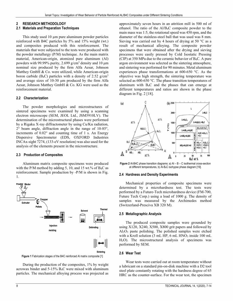
Aluminum matrix composite specimens were produced with the P/M method by adding 5, 10, and 15 wt.% of B4C as reinforcement. Sample production by -P/M is shown in Fig. 1.
Figure 1 Fabrication stages of the B4C reinforced Al matrix composite [1] During the production of the composites, 1% by weight
acrowax binder and 5-15% B4C were mixed with aluminum particles. The mechanical alloying process was projected as
approximately seven hours in an attrition mill in 500 ml of ethanol. The ratio of the Al/B4C composite powder to the main mass was 1:5, the rotational speed was 450 rpm, and the diameter of the stainless-steel ball that was used was 8 mm. Sieving was carried out by 4 hours of drying at 50 °C as a result of mechanical alloying. The composite powder specimens that were obtained after the drying and sieving processes were easily pressed by Cold Isostatic Pressing (CIP) at 350 MPa due to the ceramic behavior of B4C. A pure argon environment was selected as the sintering atmosphere, and sintering was performed for 90 minutes. Metal aluminum experiences phase transformations at 600-650 °C. As the objective was high strength, the sintering temperature was selected as 600-650 °C. The phase transition temperatures of aluminum with B4C and the phases that can emerge at different temperatures and ratios are shown in the phase diagram in Fig. 2 [18].
Figure 2 Al-B4C phase transition diagrams: a) Al – B – C isothermal cross-section
at different temperatures, b) Al-B4C isohypse phase diagram [19].
2.4 Hardness and Density Experiments
Mechanical properties of composite specimens were determined by a microhardness test. The tests were performed by a Future-Tech microhardness device (FM-700, Future Tech Corp.) using a load of 1000 g. The density of samples was measured by the Archimedes method (Switzerland-Presciva XB 320 M). 2.5 Metallographic Analysis
The produced composite samples were grounded by using X120, X240, X500, X800 grit papers and followed by Al2O3 paste polishing. The polished samples were etched with a Kroll solution (3 mL HP, 6 mL HNO3 inside 100 mL H2O). The microstructural analysis of specimens was performed by SEM. 2.6 Wear Test Wear tests were carried out at room temperature without a lubricant on a standard pin-on-disk machine with a D2 tool steel plate constantly rotating with the hardness degree of 65 HRC as the counter-surface. For the wear test, the specimen

İsmail Topcu: Investigation of Wear Behavior of Particle Reinforced AL/B4C Composites under Different Sintering Conditions
TEHNIČKI GLASNIK 14, 1(2020), 7-14 9
pin was selected with the dimensions of ∅10×10 mm, and the wear surface was polished up to a roughness value of 0.159 μm Ra. The test was conducted in four replications to provide repeatability for each specimen. The disk surface was grounded, and a roughness value of 0.830 μm Ra was achieved. For all wear tests, the sliding rate, sliding distance and load were kept constant at 1.04 m/s, 3000 m and 9.8 N, respectively. All wear test specimens were carefully cleaned and dried. The specimens were cleaned with ethanol before and after the test to measure the loss of weight by a sensitivity of ± 0.0001 grams. To achieve good replicability in wear results, at least four tests were carried out in each test condition [20]. Wear surfaces were imaged by using a high-resolution SEM. The Pin On wear test was performed in the apparatus shown in Fig. 3.
Figure 3 The scheme of a pin on a disc wear device
3 RESEARCH DISCUSSION
Images of the aluminum and boron carbide powders taken by the scanning electron microscope are shown in Fig. 4. As seen here, the aluminum powders that were used were not completely spherical, and the average grain size distribution was around 10 µ.
Figure 4 SEM images of the B4C and Al powders a) Al and b) B4Cl
After the process of specimen preparation, the same
magnification rate was used for all composite specimens that were prepared. The SEM images obtained from the flat cross-sections of the Al/B4C composite specimens may be seen in Fig. 5. The images clearly show the homogenous distribution of Al with B4C based on the reinforcement rate especially in the specimens with low reinforcement rates and the phases
aluminum showed with B4C. There were also grey and darker areas in the structure. The grey areas corresponded to the carbide structures that formed, while the darker ones corresponded to the zone where porosity was occasionally intense with increased B4C amounts. The density and hardness values significantly increased by increased the sintering temperature especially in the specimen with a 15% B4C. As seen here, Al3BC were found only in the grey areas. The grey area increased optimally based on the increased ratio of B4C.
Figure 5 Al / B4C composites sintered at 650 °C (a) 5% Al/ B4C reinforced MMC,
(b) 10% Al/ B4C reinforced MMC (c) 15% Al/ B4C reinforced MMC with SEM photographs of different reinforced materials
The purpose of the XRD analysis was to examine the
various phases and reaction products in the Al/B4C composites. As seen in Fig. 6, in the XRD characterization examination on the pure aluminum and B4C powders, the peak belonging to the aluminum powder was seen at 38.70, the secondary peak was seen at 44.80, and similarly, the peaks belonging to the B4C appeared at 28.90 and 38.40, respectively.
Figure 6 XRD pattern of B4C and pure Aluminum powders
The XRD pattern results show the density peaks of Al,
B4C, Al2B and Al3BC (Fig. 7). The AlB2 and Al3BC phases formed at the interface between the main matrix aluminum and the reinforcement B4C. The presence of the AlB2 phase was relatively low [21]. The XRD results showed a more homogenous mixture with the 15% Al/B4C composite in comparison to the other reinforcement rates. The increase in

İsmail Topcu: Investigation of Wear Behavior of Particle Reinforced AL/B4C Composites under Different Sintering Conditions
10 TECHNICAL JOURNAL 14, 1(2020), 7-14
reinforcement increased the peak magnitude of the composite.
As a result of B4C reinforcement, in the XRD characterization analysis of the Al/B4C composite material produced with the highest reinforcement ratio of 15%, aluminum metal powders showed the highest peaks on the (111) and (200) planes, while B4C ceramic powders showed the highest peaks on the (104) and (021) planes. In the XRD analysis of the Al/B4C composite specimen, it was very clearly observed that, as the B4C ratio increased, both peak magnitudes and peak areas noticeably increased for the B4C peaks [22].
Figure 7 XRD pattern of different % content B4C composites in the Al Matrix
As seen in Table1, the highest peak was observed at the
15% reinforcement ratio of Al/B4C.
Table 1 XRD peak areas of Al/B4C composite specimens reinforced at different ratios
Material 2 Theta Angle (38.4°) 2 Theta Angle (28.9°) 5% B4C 2.32 0.58
10 % B4C 2.74 1.03 15% B4C 4.16 1.41
The densities of the produced Al/B4C specimens were
measured. They were found to be in agreement with the literature as they vary in the range of 95% to 97.5%. The main reason for this different ratio was that while B4C has a low density, the B4C rate increased, and porosity was encountered. Equation 1 shows the density calculations.
GLR
C A= .VC
Vρρ
= (1) [23]
In Eq. (1), VL is the volume of the loose powder, VC is
the volume of the compressed powder, ρG is the green density, and ρA is the apparent density.
The lowest density of the Al/B4C composite specimens was calculated in the specimen with a 15% reinforcement as the highest ratio of B4C by weight. Fig. 8 shows the density values of the composites that were produced by different ratios of reinforcements.
Figure 8 Density values of the specimens produced by a 5-15% B4C reinforcement
It was observed that the densities of the produced specimens decreased with the increase in the ratio of reinforcement, but they increased based on sintering temperatures. In the SEM image given in Fig. 9, it is seen that the boron carbide particles were homogenously distributed, and there was no grain enlargement or flocculation.
Figure 9 Al, B4C, Al2BC phase and porosity image of a 15% reinforced Al / B4C
composite sample
Elemental analysis of a 10% B4C reinforced composite sample is shown in Tab. 2.
Table 2 Elemental analysis of a 10% Al/B4C composite specimen Point Material
1. %70.04Al+%18.84B+%11.12C 2. % 100 B4C 3. % 100 Al
The tested specimens were the Al/B4C metal matrix
composite specimens produced by P/M by reinforcing B4C into the Al matrix at different ratios. The expectation from the produced specimens as a result of the experiment was that density would reach the desired level in parallel with the literature (97.5%).The high sintering temperature that was applied and increasing B4C ratio [24].
Hardness test was applied on the composite specimens that were produced and metallographically prepared. In this

İsmail Topcu: Investigation of Wear Behavior of Particle Reinforced AL/B4C Composites under Different Sintering Conditions
TEHNIČKI GLASNIK 14, 1(2020), 7-14 11
test, in order to make sure that the compressive trace covered both the matrix and the reinforcement material, 10 consecutive measurements were made with frequent intervals (150 μ), and the results were obtained by taking the average of the outcomes. The hardness values that were obtained represent the average hardness of the Al/B4C composites. Fig. 10 shows the results of hardness measurements.
Figure 10 The hardness values of the Al/B4C composite specimens produced by
a 5-15% B4C reinforcement The increased ratio of B4C by weight raised the hardness
of the composite. Differences were observed in the measured hardness values of the specimens with different reinforcement ratios. The hardness values of composite materials increased due to the AlB2 and AL3BC phases formed by B4C and aluminum. As opposed to this, low hardness values were occasionally also observed, which may be explained by encountering the pure Al matrix in addition to increased B4C amounts [25].
Some researchers stated that the strength of the material increased with the increased B4C reinforcement ratios. As the reason behind this, they asserted that the carbon content of the structure and hardness values increased linearly. The carburized phase had higher surface tensions in comparison to other specimens and provided an increase in hardness [26]. Based on the assumption in question, the aluminum boride (AlB3) and aluminum-rich boride-carbide (Al3BC) structures that formed on the surface layer that was subjected to wear led to an increase in wear resistance.
Composite specimens that were produced in the same way as the surfaces which were metallographically prepared were subjected to wear tests. Different wear was calculated as both the covered path and loss of weight. The wear rate was calculated by using the following equation.
9mS
N10 .DW
q L F= ×
⋅ ⋅ (2) [27]
In Eq. (2), WS is the wear rate in mm3/Nm, Dm is the mass lost in the test specimens during N revolutions in g, q is the density of the test materials in g/cm3, L is the total sliding distance in m, and FN is the normal force on the pin in N.
The total sliding distance was monitored by an automated recording device. The worn surfaces of all specimens were examined by using SEM. The constant weight of 10 N was used in the wear tests. As shown in Fig. 11, wear tests were carried out at three different sintering temperatures and three different compositions. In the study, an analysis was carried out by considering the loss of weight, wear resistance and wear rates [28].
Figure 11 Wear test results of Aluminum and (5-15% Al/B4C composites; a) Wear rate b) Wear resistance
Since the load that was applied was constant at 10 N, for observing material losses, the ratio of B4C by weight was adjusted to 5, 10 and 15%. As seen in Fig. 11, as the B4C percentage ratio in the alloy increased, the wear rate of the specimens decreased. As the sliding distance increased, wear loss increased, and wear rate decreased. While the wear performance of the pure aluminum and the composite material with a 5% B4C reinforcement was especially poor, with the B4C ratio increased up to 10-15%, it was determined
that the wear loss decreased noticeably. The lowest material loss was observed in the composite containing 15% B4C. Improved wear resistance may be attributed to the presence of the hard Al3BC phase and B4C in the composite. The 15% ratio of B4C by weight increased the observed wear loss. This may be explained by the higher ratio of the Al3BC phase in the composite. In further paths, it was observed that wear resistance decreased probably because of the decreased capacity for the load of the Al matrix to be effectively
İsmail Topcu: Investigation of Wear Behavior of Particle Reinforced AL/B4C Composites under Different Sintering Conditions
12 TECHNICAL JOURNAL 14, 1(2020), 7-14
transferred to the B4C reinforcement. During wear tests, as the Al2B and Al3BC interface phases make fracturing difficult, their load carrying capacities increase. For this reason, the bonding between the reinforcement and the matrix is affected positively, and the wear resistance of the material increases. In addition to this, in general, improved wear resistance in composite specimens was attributed to the synergistic effect of the unique properties of B4Cs and the hard Al3BC interface product [29].
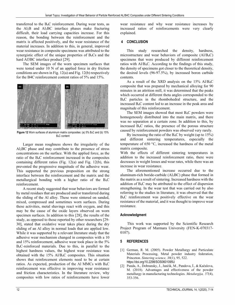
The SEM images of the worn specimen surfaces that were tested under 10 N of an applied force in dry friction conditions are shown in Fig. 12(a) and Fig. 12(b) respectively for the B4C reinforcement content ratios of 5% and 15%.
Figure 12 Worn surfaces of aluminum matrix composites: (a) 5% B4C and (b) 15%
B4C content
Larger mean roughness shows the irregularity of the Al2BC phase and may contribute to the presence of stress concentrations on the surface. With the applied force, as the ratio of the B4C reinforcement increased in the composites containing different ratios (Fig. 12(a) and Fig. 12(b), this prevented the progressive magnitude of the adhesive wear. This supported the previous proposition on the strong interface between the reinforcement and the matrix and the metallurgical bonding with a higher ratio of the B4C reinforcement.
A recent study suggested that wear behaviors are formed by metal residues that are produced and/or transferred during the sliding of the Al alloy. These were sintered on sanded, mixed, compressed and sometimes worn surfaces. During these activities, metal shavings react with oxygen, and this may be the cause of the oxide layers observed on worn specimen surfaces. In addition to this [28], the results of the study, as opposed to those reported by other researchers [29-30], stated that oxidative wear takes place during the dry sliding of an Al alloy in normal loads that are applied low. While it was supported by a relevant literature study that the adhesive wear mechanism changed in composites with a 10 and 15% reinforcement, adhesive wear took place in the 5% B4C-reinforced materials. Due to this, in parallel to the highest hardness values, the highest wear resistance was obtained with the 15% Al/B4C composites. This situation shows that reinforcement elements need to be at certain ratios. As expected, production of the Al MMCs with B4C reinforcement was effective in improving wear resistance and friction characteristics. In the literature review, why composites with low ratios of reinforcements have lower
wear resistance and why wear resistance increases by increased ratios of reinforcements were very clearly explained. 4 CONCLUSION
This study researched the density, hardness, microstructure and wear behaviors of composite (Al/B4C) specimens that were produced by different reinforcement ratios with Al/B4C. According to the findings of this study, the density of specimens got closer to the theoretical density, the desired levels (96-97.5%), by increased boron carbide contents.
As a result of the XRD analysis on the 15% Al/B4C composite that was prepared by mechanical alloying for 90 minutes in an attrition mill, it was determined that the peaks which occurred at different theta angles corresponded to the B4C particles in the rhombohedral structure, and the increased B4C content led to an increase in the peak area and magnitude of this reinforcement.
The SEM images showed that most B4C powders were homogenously distributed into the main matrix, and there was no separation at a certain zone. In addition to this, by increased B4C ratios, the presence of the porous structure caused by reinforcement powders was observed very rarely.
By increasing the ratio of the B4C by weight (up to 15%) and different sintering temperatures, especially the temperature of 650 °C, increased the hardness of the metal matrix composite. With the effects of different sintering temperatures in addition to the increased reinforcement ratio, there were decreases in weight losses and wear rates, while there was an increase in wear resistance.
The aforementioned increase occurred due to the aluminum-rich boride-carbide (Al3BC) phase that formed in the matrix as a result of sintering. Increased hardness with the addition of B4C may be attributed to the effect of dispersion strengthening. In the wear test that was carried out by also referring to the studies in literature, it was observed that the B4C reinforcement was positively effective on the wear resistance of the material, and it was thought to improve wear resistance. Acknowledgment
This work was supported by the Scientific Research Project Program of Marmara University (FEN-K-070317-0107). 5 REFERENCES [1] German, R. M. (2005). Powder Metallurgy and Particulate
Materials Processing, Metal powder industry federation, Princeton. Sintering science, 38(1), 95, 522. https://doi.org/10.2298/SOS0601095U
[2] Panda, A., Dobransky, J., Jančik, M., Pandova, İ., & Kačalova, M. (2018). Advantages and effectiveness of the powder metallurgy in manufacturing technologies. Metalurgija, 57(4), 353-356.

İsmail Topcu: Investigation of Wear Behavior of Particle Reinforced AL/B4C Composites under Different Sintering Conditions
TEHNIČKI GLASNIK 14, 1(2020), 7-14 13
[3] Topcu, I. (2018). Karbon Nanotüp Takviyeli Aluminyum Matriksli AlMg/KNT Kompozitlerinin Mekanik Davranışlarının İncelenmesi, Journal of Graduate School of Natural and Applied Sciences, 4(1), 99-109. https://doi.org/10.28979/comufbed.359796
[4] Thangavel, S., Murugan, M., & Zeelanbasha, N. (2019). Investigation of cutting force in end milling of al/n-tic/mos2 sintered nano composite. Metalurgija, 58(3-4), 251-254.
[5] Akramifard, M. S., Sabbaghian, M., & Esmailzadeh, M. (2014). Microstructure and mechanical properties of Cu/SiC metal matrix composite fabricated via friction stir processing. Materials & Design (1980-2015), 54, 838-844. https://doi.org/10.1016/j.matdes.2013.08.107
[6] Prakash, J. U., Ananth, S., Sivakumar, G., & Moorthy, T. V. (2018). Multi-Objective Optimization of Wear Parameters for Aluminium Matrix Composites (413/B4C) using Grey Relational Analysis. Materials Todays, 5(2), 7207-7216. https://doi.org/10.1016/j.matpr.2017.11.387
[7] Shin, S. E. & Bae, D. H. (2018). Fatigue behavior of Al2024 alloy-matrix nanocomposites reinforced with multi-walled carbon nanotubes. Compos. Part B Eng. 134, 61-68. https://doi.org/10.1016/j.compositesb.2017.09.034
[8] Canakci, A. (2014). Synthesis of novel CuSn10-graphite nanocomposite powders by mechanical alloying. Micro & Nano Letters, 9(2), 109-112. https://doi.org/10.1049/mnl.2013.0715
[9] Manjunatha, B., Niranjan, H. B., & Satyanarayana, K. G. (2018). Effect of amount of boron carbide on wear loss of Al-6061 matrix composite by Taguchi technique and Response surface analysis. Materials Science and Engineering, 376. https://doi.org/10.1088/1757-899X/376/1/012071
[10] Liu, Z. Y., Xu, S. J., Xiao, B. L., Xue, P., Wang, W. G., & Ma, Z. Y. (2012). Effect of ball-milling time on mechanical properties of carbon nanotubes reinforced aluminum matrix composites. Compos. Part Appl. Sci. Manuf. 43, 2161-2168. https://doi.org/10.1016/j.compositesa.2012.07.026
[11] Al-Aqeeli, N., Abdullahi, K., Suryanarayana, C., Laoui, T., & Nouari, S. (2013). Structure of mechanically milled CNT-reinforced Al-alloy nanocomposites. Mater. Manuf. Process. 28, 984-990.
[12] Canakci, A. (2014). Microstructure and Abrasive Wear Behavior of CuSn10-Graphite Composites Produced by Powder Metallurgy. Powder Metallurgy and Metal Ceramics, 53(5-6), 275-287. https://doi.org/10.1007/s11106-014-9614-2
[13] Akbulut, H. & Kara, Y. (2017). Karbon takviyeli karbon nanotüp katkılı epoksi kompozit helisel yayların mekanik davranışları. Journal of the Faculty of Engineering and Architecture of Gazi University, 32. https://doi.org/10.17341/gazimmfd.322166
[14] Fırat, F. K. & Eren, A. (2015). Investigation of FRP Effects on Damaged Arches in Historical Masonry Structures. Journal of the Faculty of Engineering & Architecture of Gazi University, 30. https://doi.org/10.17341/gummfd.46980
[15] Baradeswaran, A., Perumal, N. E., Selvakumar, R., & Franklin, I. R. (2014). Experimental investigation on mechanical behaviour, modelling and optimization of wear parameters of B4C and graphite reinforced aluminium hybrid composites. Materials & Design, 63, 620-632. https://doi.org/10.1016/j.matdes.2014.06.054
[16] Varol, T. & Canakci, A. (2013). Effect of particle size and ratio of B4C reinforcement on properties and morphology of nanocrystalline Al2024-B4C composite powders. Powder Technology, 246, 462-472. https://doi.org/10.1016/j.powtec.2013.05.048
[17] Sathiskumar, N. M., Dinaharan, I., & Vijay, S. J. (2014).
Fabrication and Characterization Of Cu / B4C Surface Dispersion Strengthened Composite Using Friction Stir Processing. Archives of Metallurgy and Materials, 59(1), 83-87. https://doi.org/10.2478/amm-2014-0014
[18] Topcu, İ., Güllüoğlu, A. N., Bilici, M. K, & Gülsoy, H. Ö. (2018). Investigation of wear behavior ofTi-6Al-4V/CNT composites reinforced with carbon nanotubes. Journal of the Faculty of Engineering and Architecture of Gazi University. https://doi.org/10.17341/gazimmfd.460542
[19] Arslan, G. & Kalemtaş, A. (2009). Processing of silicon carbide–boron carbide–aluminium composites, Journal of the European Ceramic Society, 29,473-480. https://doi.org/10.1016/j.jeurceramsoc.2008.06.007
[20] Rashad, M., Pan, F., Yu, Z., Asif, M., Lin, H. & Pan, R. (2015). Investigation on microstructural, mechanical and electrochemical properties of aluminum composites reinforced with graphene nanoplatelets. Prog. Nat. Sci. Mater. Int. 25. 460-470. https://doi.org/10.1016/j.pnsc.2015.09.005
[21] Canute, X. & Majumder, M. C. (2018). Investigation of tribological and mechanical properties of aluminium boron carbide composites using response surface methodology and desirability analysis. Industrial Lubrication and Tribology,70, 301-315. https://doi.org/10.1108/ILT-01-2017-0010
[22] Topcu, I., Gulsoy, H. Ö., Kadıoglu, N., & Gulluoglu, A. N. (2009). Processing and Mechanical properties of B4C Reinforced Al Matrix Composites. Journal of Alloys and Compounds, 482, 516-521. https://doi.org/10.1016/j.jallcom.2009.04.065
[23] Turan, M. E., Sun, Y., Aydin, F., Zengin, H., Turen, Y., & Ahlatci, H. (2018). Effects of carbonaceous reinforcements on microstructure and corrosion properties of magnesium matrix composites. Mater. Chem. Phys. 218, 182-188. https://doi.org/10.1016/j.matchemphys.2018.07.050
[24] Gülsoy, H. Ö., Bilici, M. K., Bozkurt, Y., & Salman, S. (2007). Enhancing the wear properties of iron based powder metallurgy alloys by boron additions. Materials and Design, 28, 2255-2259. https://doi.org/10.1016/j.matdes.2006.05.022
[25] Adegbenjo, A. O., Babatunde, A., & Obadele, B. A. (2018). Densification, hardness and tribological characteristics of MWCNTs reinforced Ti6Al4V compacts consolidated by spark plasma sintering. Journal of Alloys and Compounds, 749, 818-833. https://doi.org/10.1016/j.jallcom.2018.03.373
[26] Saheb, N., Khalil, A., Hakeem, A., Al-Aqeeli, N., Laoui, T., & Qutub, A. (2014). Spark plasma sintering of CNT reinforced Al6061 and Al2124 nanocomposites. Journal of Composite Materials, 18.
[27] Wang, F. C., Zhang, Z. H., Sun, Y. J., Liu, Y., Hu, Z. Y., Wang, H., Korznikov, A. V., Korznikova, E., Liu, Z. F. & Osamu, S. (2015). Rapid and low temperature spark plasma sintering synthesis of novel carbon nanotube reinforced titanium matrix composites. Carbon, 95, 396-407. https://doi.org/10.1016/j.carbon.2015.08.061
[28] Leila, M. & Mohammad, T. V. (2017). Solid Phase Extraction and Determination of Methyldopa in Pharmaceutical Samples Using Molecularly Imprinted Polymer Grafted Carbon Nanotubes. J. Chem. Soc. Pak, 39, 446.
[29] Kumar, L., Alam, S. N., & Sahoo, S. K. (2017). Mechanical properties, wear behavior and crystallographic texture of Al–multiwalled carbon nanotube composites developed by powder metallurgy route. J. Compos. Mater. 51, 1099-1117. https://doi.org/10.1177/0021998316658946
[30] Bastwros, M. M., Esawi, A. M., & Wifi, A. (2013). Friction and wear behavior of Al–CNT composites. Wear, 307, 164-173. https://doi.org/10.1016/j.wear.2013.08.021

İsmail Topcu: Investigation of Wear Behavior of Particle Reinforced AL/B4C Composites under Different Sintering Conditions
14 TECHNICAL JOURNAL 14, 1(2020), 7-14
Authors’ contacts: İsmail Topcu, Assistant Professor, PhD Alanya Aladdin Keykubat University, College of Engineering, Department of Metallurgy and Materials, 07450 Kestel Alanya Antalya, Turkey E-mail: [email protected]

TEHNIČKI GLASNIK 14, 1(2020), 15-18 15
ISSN 1846-6168 (Print), ISSN 1848-5588 (Online) Original scientific paper https://doi.org/10.31803/tg-20181206075710
Research of Efficiency of the Horizontal Coating Depending on Intensity of Capillary Absorption
Nina Dmitriyeva, Oleg Popov, Olga Grin
Abstract: In this article, research of intensity of a capillary suction of horizontal waterproof coatings when using dry polymer plaster mixtures is described. Line charts of dependence of intensity of capillary absorption on the depth of dipping and mortars for waterproofing coatings are made based on test data. The following stage of experiment is modeling of horizontal waterproofing of shell limestone masonry in sandy and clay soils. Samples of stone were laid on waterproofing material. Material was applied according to the plan of experiment, in one, two and three layers on dry and wet surfaces of samples. Thus, during the research, it has been established that the intensity of capillary absorption is affected by porosity of shell limestone, soil conditions and types of waterproof coating. Keywords: capillary absorption; horizontal coating; shell limestone; waterproofing 1 INTRODUCTION
The relevance of research is that in modern world most
people prefer to live in ecological and energy efficient houses. One of such solutions is usage of natural stones in construction of buildings.
Taking into consideration the economic efficiency and resource-saving policy, such natural stone material is shell limestone in Ukraine and Moldova. Economic effect in construction of shell limestone buildings can be seen in up to 20% of reduction of financial costs when compared to using foam concrete blocks and is twice cheaper than brickworks as shell limestone is being mined in Ukraine and Moldova. This important factor contributes to the wide use of this material in building construction.
One of the factors influencing durability of a structure is moisture activity. It is of great relevance for materials with capillary - porous structure, for example, such as shell limestone.
However, the practice with such buildings has shown that the soil moisture has negative influence when it gets into a wall by capillary absorption from soil in case of damage, lack of or improper techniques of a horizontal waterproofing of a building. Violation or failure of waterproofing is one of the main causes of premature wear of structures, increasing of costs on restoring and repairing, and deteriorations of operational properties of the building in general.
Therefore, the research devoted to finding the optimal waterproof coatings for capillary suction control of shell limestone buildings is relevant.
Authors as Komyshev, Eremenok, Izmaylov, Figarov, Orudzhev, Tursunov and Shcherbina deal with issues of studying physical and mechanical properties of limestone shell [1-3].
Works of Alekseev, Afanasyev, Babushkin, Boyko, Bazhenov, Goncharenko, Shilin, Lukinsky, Homenko, Leonovich, Karapuzov, Plough, Meneylyuk and Dmitriyeva are devoted to issues of protection of below-ground parts of buildings and applying waterproofing.
Today, technologies of applying horizontal waterproofing coatings for protection of shell limestone constructions can conditionally be divided into the following groups: rigid; painting; plastering; injection; penetration waterproofing [1, 4]. Each of the listed types of waterproofing has its advantages and shortcomings.
In seismic regions, waterproofing is made of usual 1:2 cement mortar according to Construction Norms and Regulations of PMR 23-02-2009 "Construction in seismic regions" and DBN 1.1-12:2014 "Construction in seismic regions of Ukraine". Application of rolled waterproofing or membranes is not recommended.
Nevertheless, there are problems connected with destructions of integrity of waterproofing protection. These problems are caused by poor quality of waterproof materials; wrong horizontal waterproof coating; violation of temperature conditions when making coatings; emergence of cracks because of differences in temperatures amidst the low-quality waterproof coating; violation of technologies of constructing foundation structures.
In this work, the main emphasis is placed on the research of intensity of a capillary suction of horizontal waterproof coatings when using dry polymeric plaster mixtures.
Grigoriopolsky field shell limestone is stronger than the one from Odessa field and it corresponds to durability brand M35, while the one from Odessa to M15. The structure of materials is given in Fig. 1.
2 RESULTS OF EXPERIMENTS
In the experiment different symbols were accepted – the
name of the shell limestone field: Odessa – A, and Grigoriopolsky – B; the type of horizontal waterproof coating: X1 – a dry mixture of "Gidrozit BS" with addition of 25% of sand, and X2 – cement and sand mortar (1:2) with hydrophobic additive "Sika 1" in the amount of 5%. The thickness rate of sand cement mortar layer varied from 5 mm to 7 mm or 9 mm. The thickness rate of dry mixture "Gidrozit BS" varied from 2 mm to 3 mm or 4 mm. For the comparison,
Nina Dmitriyeva et al.: Research of Efficiency of the Horizontal Coating Depending on Intensity of Capillary Absorption
16 TECHNICAL JOURNAL 14, 1(2020), 15-18
the check samples (CS) have been made of cement and sand mortar (1:2).
Figure 1 Samples, structure: а) Grigoriopolsky pit; b) Ilyinsky field
Waterproof mixture from dry powders was prepared by their gradual addition into water, mixing them constantly, until it became viscous. Then, this mixture was applied with spatula on a surface of a concrete cube. Mixing time and time of technological breaks between the subsequent coats was kept according to instructions of producers [5,6].
Hydrophobized concrete cubes 100 × 100 × 100 mm in size were tested to determine the efficiency of waterproof coatings to capillary absorption. The samples sustained within 30 days after preparation were immersed into the container with water at the bottom of which the metal grid with cells 10 ×10 mm in size was placed so that bottom edge of that would be in contact with water surface. Depth of dipping the samples varied between 5 mm, 10 mm and 15 mm. The determination of an amount of water absorbed by a sample was fixed by weighing in various time terms (1 min, 3 min, 5 min, 10 min, 15 min, 30 min, 1 h, 3 h, 6 h, 24 h) as shown in Fig. 2.
Figure 2 Capillary suction test of samples
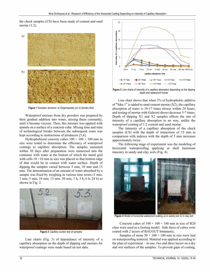
Line charts (Fig. 3) of dependence of intensity of a
capillary absorption on the depth of dipping and mortars for waterproof coatings were made based on test data.
Figure 3 Line charts of intensity of a capillary absorption depending on the dipping
depth and waterproof mortar
Line chart shows that when 5% of hydrophobic additive of "Sika 1" is added to sand cement mortar (X2), the capillary absorption of water is 10-17 times slower within 24 hours, and testing of mortar with Gidrozit shows decrease 3-7 times. Depth of dipping X1 and X2 samples affects the rate of intensity of a capillary absorption in no way, unlike the waterproof coating of 1:2 cement and sand mortar.
The intensity of a capillary absorption of the check samples (CS) with the depth of immersion of 15 mm in comparison with indexes with the depth of 5 mm increases approximately twice.
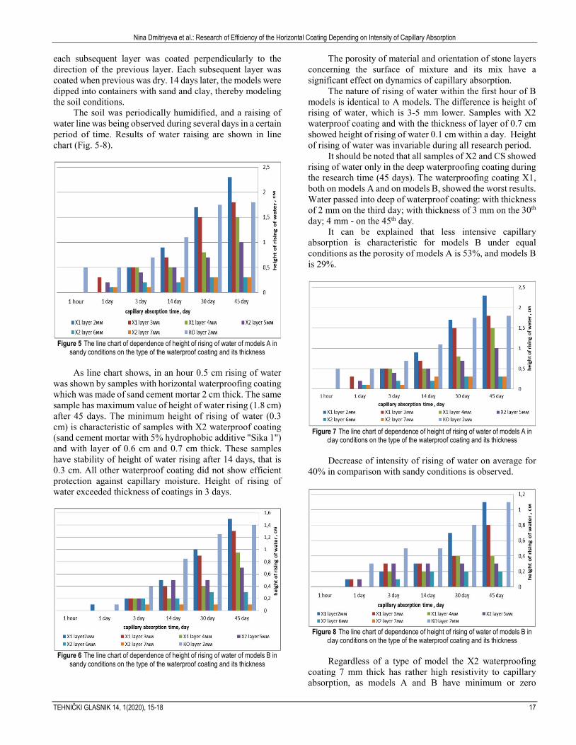
The following stage of experiment was the modeling of horizontal waterproofing applying at shell limestone masonry in sandy and clay soils (Fig. 4).
Figure 4 Model of horizontal waterproof coating: а) in sandy soil; b) in clay soil
Concrete cubes of 100 × 100 × 100 mm in size of B20
class were used as a footing model. Side faces of cubes were coated with 2 layers of BAUGUT bitumastic.
Samples of stone 50 × 100 × 100 mm in size were laid on waterproofing material. Material was applied according to the plan of experiment – in one, two and three layers on a dry and wet surfaces of the samples. To prevent gaps of coating,
a)
b)
Nina Dmitriyeva et al.: Research of Efficiency of the Horizontal Coating Depending on Intensity of Capillary Absorption
TEHNIČKI GLASNIK 14, 1(2020), 15-18 17
each subsequent layer was coated perpendicularly to the direction of the previous layer. Each subsequent layer was coated when previous was dry. 14 days later, the models were dipped into containers with sand and clay, thereby modeling the soil conditions.
The soil was periodically humidified, and a raising of water line was being observed during several days in a certain period of time. Results of water raising are shown in line chart (Fig. 5-8).
Figure 5 The line chart of dependence of height of rising of water of models A in
sandy conditions on the type of the waterproof coating and its thickness As line chart shows, in an hour 0.5 cm rising of water
was shown by samples with horizontal waterproofing coating which was made of sand cement mortar 2 cm thick. The same sample has maximum value of height of water rising (1.8 cm) after 45 days. The minimum height of rising of water (0.3 cm) is characteristic of samples with X2 waterproof coating (sand cement mortar with 5% hydrophobic additive "Sika 1") and with layer of 0.6 cm and 0.7 cm thick. These samples have stability of height of water rising after 14 days, that is 0.3 cm. All other waterproof coating did not show efficient protection against capillary moisture. Height of rising of water exceeded thickness of coatings in 3 days.
Figure 6 The line chart of dependence of height of rising of water of models B in
sandy conditions on the type of the waterproof coating and its thickness
The porosity of material and orientation of stone layers concerning the surface of mixture and its mix have a significant effect on dynamics of capillary absorption.
The nature of rising of water within the first hour of B models is identical to A models. The difference is height of rising of water, which is 3-5 mm lower. Samples with X2 waterproof coating and with the thickness of layer of 0.7 cm showed height of rising of water 0.1 cm within a day. Height of rising of water was invariable during all research period.
It should be noted that all samples of X2 and CS showed rising of water only in the deep waterproofing coating during the research time (45 days). The waterproofing coating X1, both on models A and on models B, showed the worst results. Water passed into deep of waterproof coating: with thickness of 2 mm on the third day; with thickness of 3 mm on the 30th day; 4 mm - on the 45th day.
It can be explained that less intensive capillary absorption is characteristic for models B under equal conditions as the porosity of models A is 53%, and models B is 29%.
Figure 7 The line chart of dependence of height of rising of water of models A in
clay conditions on the type of the waterproof coating and its thickness Decrease of intensity of rising of water on average for
40% in comparison with sandy conditions is observed.
Figure 8 The line chart of dependence of height of rising of water of models B in
clay conditions on the type of the waterproof coating and its thickness Regardless of a type of model the X2 waterproofing
coating 7 mm thick has rather high resistivity to capillary absorption, as models A and B have minimum or zero

Nina Dmitriyeva et al.: Research of Efficiency of the Horizontal Coating Depending on Intensity of Capillary Absorption
18 TECHNICAL JOURNAL 14, 1(2020), 15-18
indexes of height of rising of water. The curve of a depression of a capillary stream from a clay soil into a body of samples (X2, CS and X1 4 mm thick) did not reach a rejection line of the waterproof coating during the research time.
As shown in line chart (Fig. 7-8) failure in the functioning of X1 waterproof coating 2 mm and 3 mm thick happened on the 14th day. 3 CONCLUSIONS
Variating the number of layers of waterproof coating
yielded the following results. During 45 days the sufficient effectiveness of X1 waterproof coating is reached on model A when applying 3 layers 4 mm thick, on model B when applying 3 layers 3 mm and 4 mm thick, both in sandy and clay soil conditions.
Increasing the number of layers of the X2 waterproof coating up to two layers 5 mm and 6 mm thick provides a barrier to a capillary stream during 45 days. At the same time, as it was noted earlier, the same waterproof coating 0.7 cm with one layer also protects.
Thus, the research has established that the intensity of capillary absorption is affected by porosity of shell limestone, soil conditions and types of waterproof coatings.
Decrease in intensity of capillary absorption is promoted by applying the horizontal waterproof coating.
The most efficient waterproof coating accepted both for clay and for sandy conditions, is the cement and sand mortar with 5% hydrophobic additive (from the mass of cement) 7 mm thick. 4 REFERENCES [1] Zarubina L. P. (2011). Gidroizolyatsiya konstruktsiy, zdaniy i
sooruzheniy. St. Petersburg: BHV-St. Petersburg, 28 p. [2] Polyakov, S. V. (1973). Kamennaya kladka iz pil'nykh
izvestnyakov. Polyakov S. V., Izmaylov, Yu. V., Konovodchenko, V. I., Orudzhev, F. M., & Polyakov N. D., Chisinau.
[3] Shcherbina, S. N. (2008). Vliyaniye kapillyarnogo vsasyvaniya vlagi i yego ispareniya na vlagosoderzhaniye sten zdaniy. Shcherbina S. N., Bronik, O. N., Sternik, T. N., & Danchenko, G. A., Vesnik ODABA No. 32, Odessa.
[4] Dmitriyeva, N. V. (2015). Analiz innovatsionnykh metodov vosstanovleniya gidroizolyatsii konstruktsiy iz izvestnyaka-rakushechnika. Dmitriyeva, N. V. & Gostrik, A. O., Vesnik ODABA No. 62 Odessa, 111-116.
[5] https://ukr.sika.com/ru/solutions_products/02/02a024/02a024sa004.html (Accessed in December 2018)
[6] http://gidrozit.com.ua/sukhiesmesi/product/view/1/21.html (Accessed in December 2018)
Authors’ contacts: Nina Dmitriyeva Odessa State Academy of Civil Engineering and Architecture, Ukraine, 65029, Odessa, Didrihsona str. 4 [email protected] Oleg Popov Odessa State Academy of Civil Engineering and Architecture, Ukraine, 65029, Odessa, Didrihsona str. 4 [email protected] Olga Grin GOU "Pridnestrovian State University named after TG Shevchenko", Moldova, 3300, Tiraspol, 25 of October str., 128 [email protected]

TEHNIČKI GLASNIK 14, 1(2020), 19-26 19
ISSN 1846-6168 (Print), ISSN 1848-5588 (Online) Original scientific paper https://doi.org/10.31803/tg-20191031094436
Energy Loss Analysis at the Gland Seals of a Marine Turbo-Generator Steam Turbine
Lino Kocijel, Igor Poljak, Vedran Mrzljak, Zlatan Car
Abstract: The paper presents an analysis of marine Turbo-Generator Steam Turbine (TGST) energy losses at turbine gland seals. The analyzed TGST is one of two identical Turbo-Generator Steam Turbines mounted in the steam propulsion plant of a commercial LNG carrier. Research is based on the TGST measurement data obtained during exploitation at three different loads. The turbine front gland seal is the most important element which defines TGST operating parameters, energy losses and energy efficiencies. The front gland seal should have as many chambers as possible in order to minimize the leaked steam mass flow rate, which will result in a turbine energy losses’ decrease and in an increase in energy efficiency. The steam mass flow rate leakage through the TGST rear gland seal has a low or negligible influence on turbine operating parameters, energy losses and energy efficiencies. The highest turbine energy efficiencies are noted at a high load – on which TGST operation is preferable. Keywords: energy loss; gland seal; marine steam turbine; turbine efficiency 1 INTRODUCTION Today, by taking into account the entire world fleet, the dominant power producers for ship propulsion are marine slow speed two-stroke diesel engines [1]. Several authors have proposed improvement of such engines by using various additives in heavy fuel oil [2], by using alternative fuel mixtures with heavy fuel oil [3, 4] or by using several water injection techniques [5]. Middle speed and fast speed four-stroke diesel engines are also used in marine propulsion plants, usually for the electricity generator drive or for other plant needs [6]. In general usage, marine steam propulsion can rarely be found, but due to the specificity of its operation, steam plants are still dominant in the propulsion of LNG (Liquefied Natural Gas) carriers [7, 8]. Power plants which are nowadays used for LNG carrier propulsion (steam and other plants) are complex systems [9] which usually require power management and a maintenance software [10], as well as multi-objective decision support systems [11]. This paper presents an analysis of marine Turbo-Generator Steam Turbine (TGST) energy losses at gland seals. The analyzed TGST is mounted in the steam propulsion plant of a commercial LNG carrier. Based on measurement results at three TGST loads, various distributions of cumulative steam mass flow rate lost through both gland seals were performed. The influences of an increase in the steam mass flow rate which leaked through front gland seal on TGST developed power, energy power losses and energy efficiencies were investigated. The mechanical efficiency of the investigated steam turbine at all observed loads is also taken into account. Based on the obtained results are presented recommendations for TGST operation. 2 DESCRIPTION OF THE ANALYZED MARINE TGST AND
THE STEAM POWER PLANT IN WHICH IT OPERATES In this paper, a marine TGST which operates in a steam propulsion system of a commercial LNG carrier (main specifications of an LNG carrier are presented in Tab. 1) is
analyzed. The marine TGST is a low-power steam turbine which drives an electricity generator. In an LNG carrier steam propulsion plant, two identical Turbo-Generator Steam Turbines are mounted, and they always operate parallelly because electricity supply should always be secured. TGST is a condensing type, low-power steam turbine which consists of nine Rateau stages [12].
Table 1 Main specifications of an LNG carrier Gross tonnage 100 450 tons Deadweight 84 812 tons Length 288 m Breadth 44 m Main propulsion steam turbine Mitsubishi MS40-2 Steam generators 2 × Mitsubishi MB-4E-KS TGST 2 × Shinko RGA 92-2
Figure 1 Turbo-Generator Steam Turbine (TGST) scheme with marked steam flow
streams
The TGST scheme is presented in Fig. 1. Superheated steam from marine steam generators is delivered directly to all turbines in the marine steam power plant, as well as to both Turbo-Generator Steam Turbines [13] (TGST Inlet, Fig. 1). One small part of the superheated steam delivered to TGST is lost through the front gland seal, while the majority of the delivered steam expanded through nine TGST stages. At the end of steam expansion, one small part of the expanded steam is lost through the rear gland seal, while the rest of the expanded steam exits from TGST to the main marine steam condenser (TGST Outlet, Fig. 1) [14]. Steam gland seals operate in such a manner that they reduce steam

Lino Kocijel et al.: Energy Loss Analysis at the Gland Seals of a Marine Turbo-Generator Steam Turbine
20 TECHNICAL JOURNAL 14, 1(2020), 19-26
pressure, while steam specific enthalpy (energy content) remains almost constant through the seal [15, 16]. The steam mass flow rate lost through both the front and rear gland seals is led to the gland steam condenser. The mechanical energy produced in TGST stages is delivered to an electricity generator. A simplified scheme of the entire marine steam propulsion plant from the commercial LNG carrier is presented in Fig. 2 [17]. The majority of marine steam power plant components are the same as in land-based steam power plants [18, 19], but the operation of a marine steam plant must be much more dynamic. Along with the already mentioned two identical Turbo-Generator Steam Turbines, the marine steam system also consists of two identical steam generators [20] in front of which forced draft fans [21] and air heaters (air is heated with steam) [22] are mounted. The main propulsion turbine is composed of two cylinders (high pressure and low pressure) [23], which drive the main propulsion propeller through a marine gearbox. After expansion in all marine turbines, steam condenses in the main condenser and the obtained condensate is delivered to steam generators through a condensate/feed water heating system [24, 25] by using pumps [26]. Components in marine steam power plant, which are not required in land-based steam power plants, are the evaporator (fresh water generator) and desuperheater (which prepare steam extracted from the main turbine for additional heating purposes) [27].
Figure 2 General scheme of a marine steam propulsion plant from the commercial LNG carrier (SG - Steam Generator; AH - Air Heater; TG - Turbo-Generator; HPC - High Pressure Cylinder (main turbine); LPC - Low Pressure Cylinder (main turbine);
CEP - Condensate Extraction Pump; EVAP - Evaporator; SSC - Sealing Steam Condenser (Gland steam condenser); LPH - Low Pressure Heater; ACP - Auxiliary Condensate Pump; DEA - Deaerator; MFP - Main Feed-water Pump; MFPT - Main
Feed-water Pump Turbine; DES - Desuperheater; HPH - High Pressure Heater) 3 EQUATIONS FOR THE CALCULATION OF ENERGY LOSS
THROUGH GLAND SEALS 3.1 General Energy Analysis Equations The first law of thermodynamics defines the energy analysis of any control volume or system [28, 29]. In a steady state, while disregarding potential and kinetic energy, for a
standard control volume can be defined mass and energy balance equations, according to [30, 31]:
∑=∑ OUTIN mm , (1)
QPhmhm
−=∑ ⋅−⋅∑ OUTOUTININ . (2) The energy power of a fluid stream flow, according to [32], can be calculated as:
hmE ⋅=
en . (3) The type and operation characteristics of a control volume or system define its energy efficiency. Therefore, each control volume or system can have its form of energy efficiency defined. In general, energy efficiency can be defined with the following equation [33, 34]:
inputEnergyoutputEnergy
en =η . (4)
3.2 Analyzed TGST Energy Losses through Gland Seals The mathematical description of energy losses through the TGST front and rear gland seals is based on the conservation of energy. Symbols and markings used in the equations from this section are related to Fig. 1. The energy power input into the analyzed TGST is:
inletinletTGSTIN,en, hmE ⋅= . (5) The cumulative energy power output from TGST is:
PhmE +⋅= outletoutletTGSTOUT,en,
, (6) with a note that the first part of the Eq. (6) represents the energy power output of steam only. The energy power loss through the TGST front gland seal is:
inletFGSFGSPL,en, hmE ⋅= , (7) and the energy power loss through the TGST rear gland seal is:
outletRGSRGSPL,en, hmE ⋅= . (8) From Eq. (7) and Eq. (8), it should be highlighted that the specific enthalpy of steam which passes through the front gland seal is the same as the steam specific enthalpy at the TGST inlet, while the specific enthalpy of steam which passes through the rear gland seal is the same as the steam specific enthalpy at the TGST outlet.

Lino Kocijel et al.: Energy Loss Analysis at the Gland Seals of a Marine Turbo-Generator Steam Turbine
TEHNIČKI GLASNIK 14, 1(2020), 19-26 21
TGST developed power (which is transferred to the electricity generator) is:
( ) ( )outletinletFGSinlet hhmmP −⋅−= , (9) with a note that Eq. (9) does not take into account the mechanical losses in the power transmission from TGST stages to an electricity generator. If mechanical losses are taken into account, then the Eq. (9) should be multiplied with mechanical efficiency at each observed turbine load. Eq. (9) also defines that the developed TGST power is strongly dependable on the steam mass flow rate lost through the front gland seal, while the steam mass flow rate lost through the rear gland seal do not have any influence on the turbine developed power. The cumulative steam mass flow rate lost through both TGST gland seals (front and rear) is:
RGSFGSoutletinletcumulativelost, mmmmm +=−= . (10) Without detail measurements of steam mass flow rates lost through the front and rear gland seals, the cumulative steam mass flow rate lost through both gland seals can be distributed in a various ratios between the front and rear gland seal. This fact is used in the performed analysis – various ratios of cumulative steam mass flow rate lost through both gland seals and its distribution to front and rear gland seal are investigated. The steam mass flow rate lost through the front gland seal (as a share of the cumulative lost steam mass flow rate) is calculated by using the following equation:
(%)frontcumulativelost,FGS zmm ⋅= , (11) while the steam mass flow rate lost through the rear gland seal (as a share of the cumulative lost steam mass flow rate) is calculated as:
(%)rearcumulativelost,RGS zmm ⋅= . (12) (%)frontz in Eq. (11) represents a percentage of the cumulative lost steam mass flow rate through the front gland seal, while (%)rearz in Eq. (12) represents a percentage of the cumulative lost steam mass flow rate through the rear gland seal. Energy power loss through both TGST gland seals (energy power loss of the entire TGST) is:
outletRGSinletFGS
outletoutletinletinlet
TGSTOUT,en,TGSTIN,en,TGSTPL,en,
hmhmPhmhm
EEE
⋅+⋅==−⋅−⋅=
=−=
. (13)
The energy efficiency of the analyzed TGST is:
outletoutletinletinlet
mechanical
TGSTOUT,en,TGSTIN,en,
mechanicalTGSTen,
hmhmP
PEEP
⋅−⋅⋅
=
=+−
⋅=
η
ηη
. (14)
The mechanical efficiency of the analyzed TGST in Eq. (14) is assumed as 96 % at high turbine load, 95 % at middle and 94 % at low turbine load (as can be expected for a low-power marine steam turbine [35, 36]). 4 MEASURED AND CALCULATED STEAM OPERATING
PARAMETERS AT THE TGST INLET AND OUTLET The measured steam operating parameters at the TGST inlet are steam temperature, pressure and mass flow rate, while at the TGST outlet, the measured operating parameters are steam temperature and pressure, Tab. 2.
Table 2 Measured and calculated steam operating parameters at the TGST inlet and outlet
Load
Steam at the TGST inlet
Temperature (°C)
Pressure (MPa)
Mass flow rate (kg/h)
Steam specific enthalpy (kJ/kg)
High Load 451.5 5.99 5966 3306.7 Middle Load 504.5 6.03 4116 3433.5
Low Load 502.5 6.07 3775 3428.3
Load
Steam at the TGST outlet
Temperature (°C)
Pressure (MPa)
Mass flow rate (kg/h)
Steam specific enthalpy (kJ/kg)
High Load 36.83 0.006224 5906.34 2467.3 Middle Load 95.46 0.004224 4074.84 2679.6
Low Load 105.57 0.003974 3737.25 2698.8 Cumulative steam mass flow rate lost
through both gland seals (kg/h) High Load Middle Load Low Load
59.66 41.16 37.75 When the steam mass flow rate lost through turbine gland seals was not taken into consideration, the steam mass flow rate at the turbine inlet is the same as the steam mass flow rate at the turbine outlet. If the steam mass flow rate losses through the turbine gland seals are taken into account, during usual turbine operation, it amounts to about 1 % of the cumulative steam mass flow rate which enters into the turbine (the steam mass flow rate lost through both the front and rear gland seals), regardless of the current turbine load [37]. In the presented analysis, the measurement of steam mass flow rates through the TGST front and rear gland seals or at the TGST outlet were not possible due to the potential problems that the installation of the new measuring equipment could cause. Therefore, it is assumed, as in [37], that the cumulative steam mass flow rate lost through the TGST front and rear gland seals are equal to 1 % of the cumulative steam mass flow rate which enters into the TGST. As a result, the steam mass flow rate at the TGST outlet is calculated as the steam mass flow rate at the TGST inlet

Lino Kocijel et al.: Energy Loss Analysis at the Gland Seals of a Marine Turbo-Generator Steam Turbine
22 TECHNICAL JOURNAL 14, 1(2020), 19-26
reduced by the cumulative steam mass flow rate lost through both gland seals, Tab. 2. Steam specific enthalpies at the TGST inlet and outlet, necessary for the energy analysis, are calculated from the known pressures and temperatures at the turbine inlet and outlet by using the NIST-REFPROP 9.0 software [38]. For obtaining measuring results, the measuring equipment already mounted in the LNG carrier steam propulsion plant is used. The measuring equipment at the TGST inlet and outlet is calibrated and used for the control and regulation of TGST during the LNG carrier operation. The list of used measuring devices is presented in Tab. 3, while detailed specifications of each device can be found on the producers’ websites.
Table 3 The measuring devices used at the TGST inlet and outlet Measured operating
parameter Position Measuring device
Steam temperature TGST inlet Greisinger GTF 601-Pt100 - Immersion probe [39]
Steam pressure TGST inlet Yamatake JTG980A - Pressure Transmitter [40]
Steam mass flow rate TGST inlet Yamatake JTD960A - Differential
Pressure Transmitter [41]
Steam temperature TGST outlet Greisinger GTF 401-Pt100 - Immersion probe [39]
Steam pressure TGST outlet Yamatake JTD910A - Differential Pressure Transmitter [41]
5 THE RESULTS OF ENERGY LOSS ANALYSIS THROUGH
TGST GLAND SEALS WITH DISCUSSION According to the presented equations and steam operating parameters at the TGST inlet and outlet, an analysis of energy losses through the TGST gland seals is performed. Due to the lack of measurement data, several distributions of the cumulative steam mass flow rate lost through both gland seals are observed, as presented in Tab. 4. All presented distributions are observed at each TGST load. According to the Eq. (9), the TGST developed power is highly influenced by two steam mass flow rates – the first one is the steam mass flow rate at the TGST inlet and the second one is the steam mass flow rate lost through the front gland seal. Tab. 4 presents the increase in the steam mass flow rate lost on the TGST front gland seal which resulted with a decrease in turbine developed power due to the decrease in the steam mass flow rate which expands through the turbine. From Tab. 4, two conclusions can be derived. The first one is that the TGST front gland seal should be designed with as many chambers as possible within the seal in order to reduce the leaked steam mass flow rate [42, 43]. The second conclusion is that the increase in the steam mass flow rate which leaked through the front gland seal resulted with a more significant reduction of the TGST developed power as turbine load increases. An increase in the steam mass flow rate which leaked through the front gland seal for 5 % resulted in a decrease in TGST power for 0.38 kW, 0.43 kW and 0.70 kW at low, middle and high turbine load, respectively (values are rounded on two decimal places).
The TGST developed power values presented in Tab. 4 did not take into account turbine mechanical losses. If mechanical losses are taken into account, each value of the turbine developed power should be multiplied with turbine mechanical efficiency (the developed power will be reduced for the mechanical losses), at each observed load. Table 4 Change in the TGST developed power at three observed loads based on
the lost steam mass flow rate distribution on the front and rear gland seals zfront (%) Zrear (%) Developed turbine power (kW)
High Load Middle Load Low Load 30 % 70 % 1386.83 859.41 762.71 35 % 65 % 1386.13 858.98 762.32 40 % 60 % 1385.44 858.55 761.94 45 % 55 % 1384.74 858.12 761.56 50 % 50 % 1384.05 857.69 761.18 55 % 45 % 1383.35 857.26 760.79 60 % 40 % 1382.65 856.83 760.41 65 % 35 % 1381.96 856.40 760.03 70 % 30 % 1381.26 855.97 759.65
At each observed TGST load, the steam energy power input and output (calculated as a product of the steam mass flow rate and steam specific enthalpy) is the same, it did not depend on the distribution of the cumulative steam mass flow rate lost through the gland seals, Fig. 3. The steam energy power inputs and outputs both increase with an increase in the TGST load (from 3594.95 kW to 5479.94 kW for steam energy power inputs and from 2801.65 kW to 4048.05 kW for steam energy power outputs). The difference between the steam energy power input and output, at each observed TGST load, represents the sum of the turbine developed power, mechanical losses and energy power losses through both gland seals.
Figure 3 Steam energy power input and output of TGST at three observed loads
An increase of the steam mass flow rate lost through the TGST front gland seal (an increase in the percentage of the cumulative lost steam mass flow rate at the front gland seal) resulted in a proportional increase in the energy power loss at the front gland seal. According to the Eq. (7), the energy power loss at the TGST front gland seal is most influenced by the steam mass flow rate lost through the seal. As presented in Fig. 4, an increase of the steam mass flow rate lost through the TGST front gland seal resulted in the highest energy power losses’ increase at a high turbine load (from 16.44 kW up to 38.36 kW) and the lowest energy power losses’ increase at a low turbine load (from 10.78 kW up to 25.16 kW). The reason behind such occurrence can be found

Lino Kocijel et al.: Energy Loss Analysis at the Gland Seals of a Marine Turbo-Generator Steam Turbine
TEHNIČKI GLASNIK 14, 1(2020), 19-26 23
in the fact that as turbine load increases, the steam mass flow rate lost through both gland seals simultaneously increases, Tab. 2.
Figure 4 Energy power loss at the front gland seal in relation to the steam mass
flow rate lost at the front gland seal The analyzed distribution of the cumulative steam mass flow rate lost through both TGST gland seals resulted in the fact that an increase of the mass flow rate lost through the front gland seal simultaneously leads to a decrease in the steam mass flow rate lost through the rear gland seal and vice versa. Therefore, the energy power loss at the rear gland seal will decrease proportionally with a decrease in the steam mass flow rate which leaked through the rear gland seal, Fig. 5. From Fig. 5, it is important to notice that a decrease in the energy power loss through the rear gland seal has the highest intensity at a high TGST load (from 28.62 kW up to 12.27 kW) and the lowest intensity at a low TGST load (from 19.81 kW up to 8.49 kW).
Figure 5 Energy power loss at the rear gland seal in relation to the steam mass
flow rate lost at the front gland seal A conclusion which can be derived from Fig. 4 and Fig. 5 is that the values of energy power losses through both TGST gland seals increase with an increase in turbine load. The highest influence on the values of each gland seal energy loss belongs to the leaked steam mass flow rate through the seal. The cumulative energy power loss at both gland seals and its change with an increase in the steam mass flow rate lost through the front gland seal is presented in Fig. 6. As it can be seen in Fig. 6, an increase in the steam mass flow rate leaked through the front gland seal resulted with an increase
in the cumulative energy power loss at both gland seals. An increase in the cumulative energy power loss at both gland seals has a much higher intensity at a high turbine load (from 45.06 kW up to 50.63 kW) in comparison with a middle or low turbine load (from 33.22 kW up to 36.67 kW at a middle and from 30.59 kW up to 33.65 kW at a low turbine load). The presented change of the cumulative energy power loss at both gland seals can be explained in two ways – the first is by using Fig. 4 and Fig. 5, while the second is by using the Eq. (13). An increase in the steam mass flow rate lost through the TGST front gland seal resulted in a simultaneous increase in the energy power loss at the front gland seal, Fig. 4, and with a decrease in the energy power loss at the rear gland seal, Fig. 5. The intensity of the energy power loss increase at the front gland seal is higher than the intensity of the energy power loss decrease at the rear gland seal, which resulted in an increase in the cumulative energy power loss at both gland seals. When using the Eq. (13), an increase in the steam mass flow rate lost through the TGST front gland seal (and simultaneous decrease in the steam mass flow rate lost through the rear gland seal) will result with an increase in the cumulative energy power loss because the steam specific enthalpy at the turbine inlet is much higher than that of the steam specific enthalpy at the turbine outlet, Tab. 2. In standard observations as well as during a conversation with the LNG carrier crew about lost steam mass flow rate through both TGST gland seals, it is concluded that approximately half of the cumulative steam mass flow rate lost through both gland seals is distributed at the front and the other half at the rear gland seal. This analysis shows that in such a distribution ratio situation, the cumulative energy power loss at both TGST gland seals will be equal to 32.12 kW at a low load, 34.95 kW at a middle load and finally 47.84 kW at a high turbine load, Fig. 6.
Figure 6 Cumulative energy power loss at both gland seals in relation to the steam
mass flow rate lost at the front gland seal The energy efficiency of the analyzed TGST is calculated by using the Eq. (14), and the results are presented in Fig. 7 in regards to the steam mass flow rate lost through the front turbine gland seal. The presented results of TGST energy efficiency take into account turbine mechanical losses. An increase in the steam mass flow rate lost through the TGST front gland seal resulted in a decrease in turbine energy efficiency. The decrease in TGST energy efficiency

Lino Kocijel et al.: Energy Loss Analysis at the Gland Seals of a Marine Turbo-Generator Steam Turbine
24 TECHNICAL JOURNAL 14, 1(2020), 19-26
becomes higher and higher as turbine load increases (in the observed range of the mass flow rates lost through the front gland seal, energy efficiency decreases for 0.363 % at a low, for 0.367 % at a middle and for 0.373 % at a high load). Energy losses which define TGST energy efficiency, taken into account in this analysis, are energy losses of the leaked steam throughout both gland seals and mechanical losses. What is not taken into account are the additional energy losses inside the turbine stages (at each stator and rotor of each stage), as well as the energy losses that are caused by the steam expansion process. According to the observed energy losses, the average value of TGST energy efficiency at a low load is 90.19 %, at a middle load 91.28 % and at a high load 92.79 %, Fig. 7.
Figure 7 TGST energy efficiency change in relation to the steam mass flow rate
lost at the front gland seal
Figure 8 Energy power distribution at TGST (the cumulative lost mass flow rate distribution on the front and rear gland seal 50 % - 50 %): (a) High Load; (b) Low
Load Fig. 8 presents TGST energy power distribution at a high
(a) and low (b) turbine load. The presented energy flows are
based on the energy conservation equation which did not include mechanical losses. If the mechanical losses are taken into account, the turbine produced power at each load in Fig. 8 should be multiplied with mechanical efficiency (produced power will be reduced for the mechanical losses) – in that situation, mechanical losses will become an additional energy flow.
The cumulative steam mass flow rate lost through both TGST gland seals in Fig. 8 is divided in two identical parts – half is distributed on the front and half is distributed on the rear gland seal. In such a leaked mass flow rate distribution, the steam energy flow at the front gland seal is higher in comparison to the steam energy flow at the rear gland seal due to the higher steam specific enthalpy at the turbine inlet.
The recommendation for TGST operation which can be derived from the presented analysis is that TGST should operate at a high load as long as possible and the steam mass flow rate leakage through the front gland seal should be minimized. At a high load, TGST energy efficiency will be the highest, while minimization of the steam mass flow rate lost through the front gland seal will reduce TGST energy power losses.
6 CONCLUSIONS The presented paper analyzed energy losses at the gland seals of a marine Turbo-Generator Steam Turbine (TGST). The entire analysis was performed at three different turbine loads in order to examine the energy losses at gland seals in the entire range of the steam turbine operation. The influence of change in the steam mass flow rate which leaked through the front gland seal on the TGST developed power, turbine energy power losses and energy efficiencies is researched. In the analysis, the steam turbine mechanical losses at each observed load were included. The main conclusions can be summarized in the following points: - An increase in the steam mass flow rate which leaked
through the front gland seal resulted in a decrease in the TGST developed power, in an increase in turbine cumulative energy losses and, simultaneously, in a decrease in turbine energy efficiency.
- The front gland seal should be designed with as many chambers as possible within the seal in order to reduce the leaked steam mass flow rate.
- A steam mass flow rate which leaked through the rear gland seal did not influence the TGST developed power, and at the same time, it has a low influence on the change of turbine cumulative energy losses and energy efficiencies.
- TGST load is directly proportional to the turbine developed power, cumulative energy losses and energy efficiencies – all of it increases during an increase in the turbine load.
For the analyzed TGST, it is desirable that it operates at
a high load and has minimal steam mass flow rate leakage through the front gland seal. Such operation will lead to

Lino Kocijel et al.: Energy Loss Analysis at the Gland Seals of a Marine Turbo-Generator Steam Turbine
TEHNIČKI GLASNIK 14, 1(2020), 19-26 25
highest energy efficiency and will decrease cumulative energy losses. Acknowledgments The authors would like to extend their appreciations to the main ship-owner office and the crew of the LNG carrier. This research has been supported by the Croatian Science Foundation under the project IP-2018-01-3739, CEEPUS network CIII-HR-0108, European Regional Development Fund under the grant KK.01.1.1.01.0009 (DATACROSS), the University of Rijeka scientific grant uniri-tehnic-18-275-1447 and the University of Rijeka scientific grant uniri-tehnic-18-18-1146. NOMENCLATURE Abbreviations: LNG Liquefied Natural Gas TGST Turbo-Generator Steam Turbine Latin Symbols: E power of a fluid stream, kW h specific enthalpy, kJ/kg m mass flow rate, kg/s P power, kW Q heat transfer, kW
Greek symbols: η efficiency, -
Subscripts: en energy FGS front gland seal IN inlet (input) OUT outlet (output) PL power loss RGS rear gland seal 7 REFERENCES [1] Raptotasios, S. I., Sakellaridis, N. F., Papagiannakis, R. G., & Hountalas, D. T. (2015). Application of a multi-zone
combustion model to investigate the NOx reduction potential of two-stroke marine diesel engines using EGR. Applied Energy, 157, 814-823.
https://doi.org/10.1016/j.apenergy.2014.12.041 [2] Ryu, Y., Lee, Y., & Nam, J. (2016). Performance and emission
characteristics of additives-enhanced heavy fuel oil in large two-stroke marine diesel engine. Fuel, 182, 850-856. https://doi.org/10.1016/j.fuel.2016.06.029
[3] Sun, X., Liang, X., Shu, G., Wang, Y., Wang, Y., & Yu, H. (2017). Effect of different combustion models and alternative fuels on two-stroke marine diesel engine performance. Applied Thermal Engineering, 115, 597-606. https://doi.org/10.1016/j.applthermaleng.2016.12.093
[4] Sun, X., Liang, X., Shu, G., Lin, J., Wei, H., & Zhou, P. (2018). Development of a surrogate fuel mechanism for application in two-stroke marine diesel engine. Energy, 153, 56-64. https://doi.org/10.1016/j.energy.2018.03.042
[5] Senčić, T., Mrzljak, V., Blecich, P., & Bonefačić, I. (2019). 2D CFD Simulation of Water Injection Strategies in a Large
Marine Engine. Journal of Marine Science and Engineering, 7, 296. https://doi.org/10.3390/jmse7090296
[6] Mrzljak, V., Medica, V., & Bukovac, O. (2017). Quasi-dimensional diesel engine model with direct calculation of cylinder temperature and pressure. Technical Gazette, 24(3), 681-686. https://doi.org/10.17559/TV-20151116115801
[7] Fernández, I. A., Gómez, M. R., Gómez, J. R., & Insua, A. A. B. (2017). Review of propulsion systems on LNG carriers. Renewable and Sustainable Energy Reviews, 67, 1395-1411. https://doi.org/10.1016/j.rser.2016.09.095
[8] Koroglu, T. & Sogut, O. S. (2018). Conventional and Advanced Exergy Analyses of a Marine Steam Power Plant. Energy, 163, 392-403. https://doi.org/10.1016/j.energy.2018.08.119
[9] Ammar, N. R. (2019). Environmental and cost-effectiveness comparison of dual fuel propulsion options for emissions reduction onboard LNG carriers. Shipbuilding, 70(3), 61-77. https://doi.org/10.21278/brod70304
[10] Zhao, F., Yang, W., Tan, W. W., Yu, W., Yang, J., & Chou, S. K. (2016). Power management of vessel propulsion system for thrust efficiency and emissions mitigation. Applied Energy, 161, 124-132. https://doi.org/10.1016/j.apenergy.2015.10.022
[11] Trivyza, N. L., Rentizelas, A., & Theotokatos, G. (2018). A novel multi-objective decision support method for ship energy systems synthesis to enhance sustainability. Energy Conversion and Management, 168, 128-149.
https://doi.org/10.1016/j.enconman.2018.04.020 [12] Final Drawing for Generator Turbine. (2006). Shinko Ind.
Ltd., Hiroshima, Japan, internal ship documentation. [13] Mrzljak, V., Senčić, T., & Žarković, B. (2018). Turbogenerator
Steam Turbine Variation in Developed Power: Analysis of Exergy Efficiency and Exergy Destruction Change. Modelling and Simulation in Engineering, 2018. https://doi.org/10.1155/2018/2945325
[14] Behrendt, C. & Stoyanov, R. (2018). Operational characteristic of selected marine turbounits powered by steam from auxiliary oil-fired boilers. New Trends in Production Engineering, 1(1), 495-501. https://doi.org/10.2478/ntpe-2018-0061
[15] Cangioli, F., Chatterton, S., Pennacchi, P., Nettis, L., & Ciuchicchi, L. (2018). Thermo-elasto bulk-flow model for labyrinth seals in steam turbines. Tribology International, 119, 359-371. https://doi.org/10.1016/j.triboint.2017.11.016
[16] Lorencin, I., Anđelić, N., Mrzljak, V., & Car, Z. (2019). Exergy analysis of marine steam turbine labyrinth (gland) seals. Scientific Journal of Maritime Research, 33(1), 76-83. https://doi.org/10.31217/p.33.1.8
[17] Mrzljak, V. & Poljak, I. (2019). Energy Analysis of Main Propulsion Steam Turbine from Conventional LNG Carrier at Three Different Loads. International Journal of Maritime Science & Technology "Our Sea", 66(1), 10-18.
https://doi.org/10.17818/NM/2019/1.2 [18] Naserbegi, A., Aghaie, M., Minuchehr, A., & Alahyarizadeh,
Gh. (2018). A novel exergy optimization of Bushehr nuclear power plant by gravitational search algorithm (GSA). Energy, 148, 373-385. https://doi.org/10.1016/j.energy.2018.01.119
[19] Elhelw, M., Al Dahma, K. S., & Hamid Attia, A. E. (2019). Utilizing exergy analysis in studying the performance of steam power plant at two different operation mode. Applied Thermal Engineering, 150, 285-293.
https://doi.org/10.1016/j.applthermaleng.2019.01.003 [20] Mrzljak, V., Poljak, I., & Medica-Viola, V. (2017). Dual fuel
consumption and efficiency of marine steam generators for the propulsion of LNG carrier. Applied Thermal Engineering, 119, 331-346. https://doi.org/10.1016/j.applthermaleng.2017.03.078

Lino Kocijel et al.: Energy Loss Analysis at the Gland Seals of a Marine Turbo-Generator Steam Turbine
26 TECHNICAL JOURNAL 14, 1(2020), 19-26
[21] Mrzljak, V., Blecich, P., Anđelić, N., & Lorencin, I. (2019). Energy and Exergy Analyses of Forced Draft Fan for Marine Steam Propulsion System during Load Change. Journal of Marine Science and Engineering, 7, 381.
https://doi.org/10.3390/jmse7110381 [22] Orović, J., Mrzljak, V., & Poljak, I. (2018). Efficiency and
Losses Analysis of Steam Air Heater from Marine Steam Propulsion Plant. Energies, 11(11), 3019.
https://doi.org/10.3390/en11113019 [23] Mrzljak, V., Poljak, I., & Prpić-Oršić, J. (2019). Exergy
analysis of the main propulsion steam turbine from marine propulsion plant. Shipbuilding, 70(1), 59-77.
https://doi.org/10.21278/brod70105 [24] Naserabad, S. N., Mehrpanahi, A., & Ahmadi, G. (2019).
Multi-objective optimization of feed-water heater arrangement options in a steam power plant repowering. Journal of Cleaner Production, 220, 253-270.
https://doi.org/10.1016/j.jclepro.2019.02.125 [25] Zhao, Y., Wang, C., Liu, M., Chong, D., & Yan, J. (2018).
Improving operational flexibility by regulating extraction steam of high-pressure heaters on a 660 MW supercritical coal-fired power plant: A dynamic simulation. Applied Energy, 212, 1295-1309. https://doi.org/10.1016/j.apenergy.2018.01.017
[26] Poljak, I., Orović, J. & Mrzljak, V. (2018). Energy and Exergy Analysis of the Condensate Pump during Internal Leakage from the Marine Steam Propulsion System. Scientific Journal of Maritime Research, 32(2), 268-280. https://doi.org/10.31217/p.32.2.12
[27] Taylor, D. A. (1998). Introduction to Marine Engineering. Elsevier Butterworth-Heinemann.
[28] Mrzljak, V. (2018). Low power steam turbine energy efficiency and losses during the developed power variation. Technical Journal, 12(3), 174-180.
https://doi.org/10.31803/tg-20180201002943 [29] Tan, H., Shan, S., Nie, Y., & Zhao, Q. (2018). A new boil-off
gas re-liquefaction system for LNG carriers based on dual mixed refrigerant cycle. Cryogenics, 92, 84-92.
https://doi.org/10.1016/j.cryogenics.2018.04.009 [30] Ahmadi, G. R. & Toghraie, D. (2016). Energy and exergy
analysis of Montazeri Steam Power Plant in Iran. Renewable and Sustainable Energy Reviews, 56, 454-463.
https://doi.org/10.1016/j.rser.2015.11.074 [31] Noroozian, A., Mohammadi, A., Bidi, M., & Ahmadi, M. H.
(2017). Energy, exergy and economic analyses of a novel system to recover waste heat and water in steam power plants. Energy Conversion and Management, 144, 351-360. https://doi.org/10.1016/j.enconman.2017.04.067
[32] Ali, M. S., Shafique, Q. N., Kumar, D., Kumar, S., & Kumar, S. (2018). Energy and exergy analysis of a 747-MW combined cycle power plant Guddu. International Journal of Ambient Energy, 2018. https://doi.org/10.1080/01430750.2018.1517680
[33] Koroglu, T. & Sogut, O. S. (2017). Advanced exergy analysis of an organic Rankine cycle waste heat recovery system of a marine power plant. Journal of Thermal Engineering, 3(2), 1136-1148. https://doi.org/10.18186/thermal.298614
[34] Ahmadi, G., Toghraie, D., & Ali Akbari, O. (2018). Technical and environmental analysis of repowering the existing CHP system in a petrochemical plant: A case study. Energy, 159, 937-949. https://doi.org/10.1016/j.energy.2018.06.208
[35] Elčić, Z. (1995). Steam turbines. ABB, Karlovac, National and University Library Zagreb.
[36] McGeorge, H. D. (1995). Marine Auxiliary Machinery. 7th edition, Elsevier Science Ltd.
[37] Blažević, S., Mrzljak, V., Anđelić, N., & Car, Z. (2019). Comparison of energy flow stream and isentropic method for
steam turbine energy analysis. Acta Polytechnica, 59(2), 109-125. https://doi.org/10.14311/AP.2019.59.0109
[38] Lemmon, E. W., Huber, M. L., & McLinden, M. O. (2010). NIST reference fluid thermodynamic and transport properties-REFPROP. version 9.0, User’s guide, Colorado.
[39] https://www.greisinger.de (accessed: 28.10.19.) [40] http://www.industriascontrolpro.com (accessed: 29.10.19.) [41] http://www.krtproduct.com (accessed: 23.10.19.) [42] Kostyuk, A. & Frolov, V. (1988). Steam and gas turbines. Mir
Publishers, Moscow. [43] Kanoğlu, M., Çengel, Y. A., & Dincer, I. (2012). Efficiency
Evaluation of Energy Systems. Springer Briefs in Energy, Springer. https://10.1007/978-1-4614-2242-6
Authors’ contacts: Lino Kocijel, PhD Student Faculty of Engineering, University of Rijeka, Vukovarska 58, 51000 Rijeka, Croatia E-mail: [email protected] Igor Poljak, PhD, Assistant Professor Department of Maritime Sciences, University of Zadar, Mihovila Pavlinovića 1, 23000 Zadar, Croatia E-mail: [email protected] Vedran Mrzljak, PhD, Assistant Professor (Corresponding author) Faculty of Engineering, University of Rijeka, Vukovarska 58, 51000 Rijeka, Croatia E-mail: [email protected] Zlatan Car, PhD, Full Professor Faculty of Engineering, University of Rijeka, Vukovarska 58, 51000 Rijeka, Croatia E-mail: [email protected]

TEHNIČKI GLASNIK 14, 1(2020), 27-31 27
ISSN 1846-6168 (Print), ISSN 1848-5588 (Online) Preliminary communication https://doi.org/10.31803/tg-20190719094329
Application of a Cold Spray Based 3D Printing Process in the Production of EDM Electrodes
Štefanija Klarić, Zlatko Botak, Damien J. Hill, Matthew Harbidge, Rebecca Murray
Abstract: Cold spray process principles allow the production of near-net-shape metal parts with a fast layer deposition by using 3D printing techniques via supersonic 3D deposition (SP3D). This innovative additive manufacturing process allows an easy and quick production of copper and aluminium parts with future possibilities to expand materials and alloys. The speed and materials enable the application of this cold spray based 3D printing process for the production of tools. In this paper, Electrical Discharge Machining (EDM) electrodes were fabricated by using SP3D to investigate its application in tool production. Requirements for the materials of electrodes and some existing solutions for the production of EDM electrodes with additive manufacturing methods are described first. The fabrication and experimental results are then presented for 3D printed copper EDM electrodes that were tested by using St 37-2 (DIN 17100) steel as the workpiece. Keywords: additive manufacturing; cold spray; EDM; heat treatment; metal printing 1 INTRODUCTION
Electrical Discharge Machining (EDM) is a process based on the thermoelectric phenomenon and controlled erosion of material due to repetitive short duration sparks generated in the gap separating the tool and workpiece submerged in liquid dielectric [1-3]. The EDM process is compiled of several phases that are performed continuously until the desired workpiece geometry is achieved [2, 3]: • ignition phase, • formation of the plasma channel and vapour bubble, • discharge phase and • ejection phase.
A major advantage of this process is the possibility of
application where machining with more conventional processes would be difficult: workpiece materials with higher hardness (i.e. heat treated steels), micro machining requirements, machining of composites or batch production of parts [1, 4]. Regarding the suitability for EDM processing, Amorim and Weingaertner [3] name electrical conductivity as one of the major properties required from the workpiece. The main parameters of EDM are the type of the EDM machine, workpiece and electrode material, electrode shape and rotation, type of dielectric and method of flushing [3, 5].
Electrical input parameters that must be taken into consideration for EDM are [5, 6]: discharge current (Ip), gap voltage (Vg), pulse ON time (Ton) and pulse OFF time (Toff), polarity, electrode gap, pulse frequency and duty factor.
The effectiveness of the process is measured by the material removal rate, electrode wear, wear ration (ratio of the electrode and material removal rate), surface finish and the difference between the electrode and cavity size (over cut) [5- 9].
Apart from the above mentioned parameters, Amorim and Weingaertner [2, 3] name the workpiece material removal rate, electrode resistance to wear, workpiece surface roughness, tool electrode material machinability and tool electrode material cost as important factors for the electrode material selection.
1.1 EDM Process and Materials for Electrodes
The main considerations for the EDM electrode are the
erosion of the workpiece and transmission of electric current [7, 8]. Therefore, in the selection of electrode material, apart from the above mentioned parameters, electrical and thermal conductivity, the melting point, chemical composition and mechanical properties must be taken into consideration [9-14]. Due to the mentioned requirements, the first obvious choice for an electrode are metallic materials. Typical metals used for EDM electrodes are copper, brass, silver, tungsten, zinc, copper tungsten, silver tungsten, tungsten carbide and tellurium copper [10, 11]. Another very important material in EDM tool production is Graphite (Graphite has lower density and can hence be used for larger electrodes [3], it has a high melting point, but lower mechanical properties than metallic materials [11]). In order to mitigate the fragility of pure graphite, copper graphite electrodes can be used [11].
According to [3], the use of a different electrode material can produce the same results (Copper vs. Graphite). However, the cost difference must be taken into consideration. Copper as an electrode material has some advantages over graphite. Copper is used for applications that require a highly polished surface or coined shape (for engraving), and it is a good choice for a wire EDM [3, 9]. In this paper, EDM electrodes from cold sprayed copper powder were produced by using the additive manufacturing technology SP3D. 1.2 Additive Manufacturing for EDM Electrode Production
Tool production is often connected to the manufacturing of products with (often) complex geometry, limited number of pieces [15] and requirements for specific material properties (i.e. high wear resistance or conductivity). Additive manufacturing introduces some benefits in tool production, such as the decrease of fabrication time or costs, possible elimination or reduction of manufacturing steps and

Štefanija Klarić et al.: Application of Cold Spray Based 3D Printing Process in a Production of EDM Electrodes
28 TECHNICAL JOURNAL 14, 1(2020), 27-31
improvement of tool design/functionality [15, 16]. These benefits allow a valid case to be made to investigate the possibilities of an additive manufacturing application for the production of EDM electrodes.
In the 1990’s, attempts were made to apply stereolithography (STL) models for EDM tool production [17, 18]. Further development of rapid tooling processes resulted in several possible variations of the additive manufacturing of EDM electrodes that could be produced from non-conductive materials (i.e. stereolithography forwarded by metallisation), conductive materials (selective laser sintering (SLS) process) or cast made materials [19-21]. The area of Metal Additive Manufacturing (Metal AM) has been rapidly growing in last five years as it is used for the production of parts in the automotive, aircraft, medical technology industry and in the defence domain [22]. The development of new processes such as SP3D printing (based on the cold spraying of metal) opened the possibility of an investigation of another EDM electrode production method directly from conductive materials (copper). 2 SPEE3D PRINTING OF COPPER
The copper electrodes used in this experiment were 3D printed on a LightSPEE3D printer (SPEE3D, Australia). LightSPEE3D printers utilize a patented Supersonic 3D Deposition (SP3D) process to deposit material into near-net-shape bulk components. The process is derived from the existing cold spray (CS) technology. CS has been and still is used in repair and coating operations around the world, but is primarily limited to 2-dimensional applications. SPEE3D’s technology utilizes its software, TwinSPEE3D, to slice a specified geometry and generate toolpaths by using sophisticated algorithms. The software generates a pre-programed path that a 6 axis robot arm performs over a stationary cold-spray gun to build a part in 3 dimensions.
Unlike the existing 3D printing technologies which require heat to melt material [23-25], SP3D is a kinetic process. Metal particles are accelerated up to Mach 3 [26]. The kinetic energy at this speed causes particles to highly plastically deform when they splat (technical term) onto the surface of the substrate, or part. This creates a high-density
metal part as more material is continuously added. Since the SP3D process is not thermal, it is capable of producing parts significantly faster than other technologies by achieving high deposition rates. A limiting factor on thermal based technologies is the time required to melt and then solidify the material before the next layer is laid down.
Currently, LightSPEE3D is capable of printing aluminium, copper, and various copper and aluminium alloys. Research is being conducted to increase the number of materials that can be printed with useful metallurgical properties for numerous applications using the SP3D technology. Examples of material possibilities include bronzes, stainless steel and titanium, which are all able to be cold sprayed with the existing technologies [27].
The LightSPEE3D printer can produce copper parts at up to 100 g/min [26]. However, for the purpose of EDM tools, the machine deposited material at 20 g/min in order to increase deposition efficiency and dimensional accuracy as a higher production speed was not necessary. The deposition efficiency (DE) at 20 g/min is approximately 90%, with 10% of the powder being removed with a dust extraction system to be recycled. 3 EXPERIMENTAL SETUP 3.1 EDM Electrode Production
EDM electrodes (samples 1 – 9, Tab. 1, Fig. 1) were produced with the following parameters: • Printing parameters: - Carrier gas: air, - Carrier gas stagnation temperature: 400 °C, - Carrier gas stagnation pressure: 30 bar, - Substrate: deoxidized 5052 aluminium at room
temperature - Printing layer thickness: 1.68 mm - Printing time for 4 samples: 90 min • Powder material: AMPS 99.9% Copper, D50 = 30 μm,
D10-D90 = 10 to 45 μm • Electrode geometry is shown in Fig. 1 • Post-printing heat treatment parameters are shown in
Tab.1. After the treatment, electrodes were machined on a lathe to final dimensions.
(a) (b) (c) (d) (e)
Figure 1 Electrodes were produced on the LightSPEE3D printer (a) using a pre-set geometry as displayed on the HMI (b), with dimensions given in mm (c). The as-printed samples (e) were then heat-treated according to Tab. 1, then machined on a lathe to produce the SP3D printed electrode (f).
The printed parts underwent different heat treatment
regimes: 1) no heat treatment, 2) 330 °C, 3 hours, water quench 3) 400 °C 3 hours, water quench (Tab. 1). A control
sample that was produced from the copper bar stock (sample 10, Tab. 1) was included. Heat treatment was performed to reduce the cold working of the material. Oxidation levels and

Štefanija KLarić et al.: Application of Cold Spray Based 3D Printing Process in a Production of EDM Electrodes
TEHNIČKI GLASNIK 14, 1(2020), 27-31 29
conductivity of the 3D printed material are planned to be tested between groups in future research.
Table 1 Post printing heat treatment parameters
Sample no. Heat treatment temperature, °C Heat treatment time / quenching media
1 400 3 hours / water 2 330 3 hours / water 3 Not treated 4 330 3 hours / water 5 Not treated 6 330 3 hours / water 7 400 3 hours / water 8 Not treated 9 400 3 hours / water 10 Produced from copper bar by machining
Machining the as printed components to the required geometry on a lathe was difficult due to the brittle nature of the cold sprayed parts. The material does not deflect, but instead, areas with small cross sections would break in the lathe. The feed rate and depth of the cut were lowered to compensate. A 4-jaw chuck rather than a 3-jaw chuck was needed to adjust for the larger variation in the as printed geometry compared to a typical bar stock.
3.2 EDM Machining
EDM testing was performed on an AG80L Die sinker EDM machine (Sodic Europe Ltd.) in industrial conditions in the Gumiimpex-GRP company in Varaždin, with the following parameters: • Workpiece: St 37-2 steel plate (123 × 70 × 30 mm)
milled and grinded, without thermal processing. Tab. 2shows the mechanical properties and Tab. 3 shows thethermo-physical data from the Iordachescu M et al. study(as cited in [28])
• Dielectric: EDMFLUID 108 MP/S.
Table 2 Mechanical properties of the St 37-2 material (thickness: 16.1 < 40 mm) [29]
Property Value Tensile strength, MPa 360-510 Yield strength, MPa 225
Elongation, % 26 Impact energy KV 20°С, J > 27
Table 3 Thermo-physical data of the St 37-2 material [28] Temperature, ◦C 20 200 400 600 800 1000 1600
Specific heat, J/kg ◦C 465 527 606 761 685 618 840 Density, kg/m3 7850 7770 7700 7630 7590 7510 7100 Conductivity,
W/m ◦C 48.07 43.89 38.04 31.77 25.50 28.01 34.28
Table 4 Chemical composition of the St 37-2 material Element % Element % Element %
Al 0.0265 Mn 1.2726 S 0.0108 C 0.1511 Nb 0.0325 Si 0.2433 Co 0.0318 Ni 0.0468 V 0.0390 Cr 0.0174 P 0.0156 Fe 98.110
Other 0.0026
The chemical composition of the St 37-2 material was measured by using the optical emission spectrometer ARL
3460, which has a database for steel, copper and aluminium. The spectrometer analysis results are shown in Tab. 4.
The used EDM parameters are shown in Tab. 5.
Table 5 EDM parameters Tool electrode Copper Workpiece material St 37-2 steel
Polarity + Peak Current, A 5 Pulse on time, µs 110 Voltage, V 55
Pulse off time, µs 45 Dielectric fluid EDMFLUID 108 MP/S
Surface Roughness, µm 4,1-4,4 Overcut, µm/Side 80
Based on the expected roughness of the treated surface, the machine automatically selected the processing parameters, such as the metal removal rate, pulse ON time, pulse OFF time and electricity power.
4 RESULTS
The obtained test results of the application of the cold spray based printing method, SP3D, for the production of EDM electrodes have shown that material is usable and comparable with the traditionally produced copper electrodes. The test results for all electrodes described in Tab. 1 are shown in Figs. 2-6. Note that no distinct differences are seen at a macro level of the control (sample 10) from the 3D printed samples (Figs. 2-6).
Figure 2 Workpiece after machining
Figure 3 Workpiece surface for the printed and not heat treated EDM electrode (samples 3, 5, 8)
Figure 4 Workpiece surface for the printed and 330 °C heat treated EDM electrode (samples 2, 4, 6)
Figure 5 Workpiece surface for the printed and 400 °C heat treated EDM electrode (samples 1, 7, 9)

Štefanija Klarić et al.: Application of Cold Spray Based 3D Printing Process in a Production of EDM Electrodes
30 TECHNICAL JOURNAL 14, 1(2020), 27-31
The St 37-2 workpiece surface condition after machining with printed electrodes that were not heat treated after printing is shown in Fig. 3. Fig. 4 shows the workpiece surfaces machined with electrodes that were heat treated to 330 °C, and the surfaces machined with electrodes that were heated to 400 °C are shown in Fig. 5.
The surface produced by an electrode that was made by a solid copper bar is shown in Fig. 6.
Figure 6 Workpiece surface for a bar stock produced EDM electrode
(control, sample 10)
The presented results show a possible application of the SP3D printing of metals for the production of EDM electrodes. As this process is cheap and fast in comparison to other metal printing processes [26], it could provide a unique solution in situations where a specific shape of the tool is required.
Research in EDM has produced investigations of processes with electrode cooling in order to reduce electrode wearing [30, 31]. This fact combined with the fact that the SP3D technology can produce solid objects with enclosed channels leads to the possibility that the SP3D printing technology could be a solution for the production of electrodes (and tools in general) with built-in liquid cooling systems. 5 CONCLUSION
The development of a new additive manufacturing process based on cold spray opened a range of possibilities in tool production. In this preliminary research, the SP3D technology was tested for the production of copper EDM electrodes. Three different groups of printed EDM electrodes that varied by heat treatment were compared with a conventionally produced copper electrode (Tab. 1). All electrodes were tested on a mild steel workpiece. Preliminary results have shown that a cold spray based 3D printing technology can be used for EDM with a satisfactory production output.
In the future, research will be conducted in order to increase the efficiency of electrode production and application regarding the following: the influence of heat treatment temperature on conductivity, SP3D produced electrode wear rates and possibly, introduction of the alloying of copper powder in order to improve mechanical properties of electrode materials.
6 REFERENCES
[1] Ranganath, B. J. (2008). Thermal Metal Cutting Processes. New Delhi, India: I. K. International Publishing House Pvt. Ltd
[2] Amorim, F. L. & Weingaertner, W. L. (2004). Die-Sinking Electrical Discharge Machining of a High-Strength Copper-Based Alloy for Injection Molds. J. of the Braz. Soc. of Mech. Sci. & Eng., XXVI(2), 138-144. https://doi.org/10.1590/S1678-58782004000200004
[3] Amorim, F. L. & Weingaertner, W.L. (2007). The Behavior of Graphite and Copper Electrodes on the Finish Die-Sinking Electrical Discharge Machining (EDM) of AISI P20 Tool Steel. J. of the Braz. Soc. of Mech. Sci. & Eng., XXIX(4), 366-371. https://doi.org/10.1590/S1678-58782007000400004
[4] Shabgard, M. R., Gholipoor, A., & Baseri, H. (2016). A review on recent developments in machining methods based on electrical discharge phenomena. Int J Adv Manuf Technol, 87, 2081-2097. https://doi.org/10.1007/s00170-016-8554-z
[5] Jeevamalar, J. & Ramabalan, S. (2015). Die sinking EDM process parameters: a review. Int. J. Mech. Eng. & Rob. Res., 4 (1), 315-326.
[6] Dave, H., Banker, M., Kumar, S., Mathai, V. J., & Vyas, A. (2016). Investigation on the effect of different tool-workpiece combinations on MRR and TWR during EDM process. Journal of Machining and Forming Technologies, 7 (3-4), 171-181.
[7] Sultan, T., Kumar, A., & Gupta, R. D. (2014). Material Removal Rate, Electrode Wear Rate, and Surface Roughness Evaluation in Die Sinking EDM with Hollow Tool through Response Surface Methodology. International Journal of Manufacturing Engineering, 2014. https://doi.org/10.1155/2014/259129
[8] Singh, G., Singh, G., Singh. K., & Singla. A. (2017). Experimental studies on material removal rate, tool wear rate and surface properties of machined surface by powder mixed electric discharge machining. Materials Today: Proceedings 4, 1065-1073.
[9] Ahmad, S. & Lajis, M. A. (2013). Electrical discharge machining (EDM) of Inconel 718 by using copper electrode at higher peak current and pulse duration. IOP Conference Series: Materials Science and Engineering, 50 (1), 012062, https://doi.org/ 10.1088/1757-899X/50/1/012062
[10] Sommer, C. (2001, August). EDM electrodes – a matter of choosing wisely different materials affect machining. Tooling & Production, 53-56.
[11] Kern, R. (2008, July/August). Sinker electrode material selection. EDM Today, Retrieved from http://www.edmtodaymagazine.com/2015/archives/techtips/2008_may_jun_tech_tip/#p=3
[12] Daneshmand, S., Neyestanak, A. A. L., & Monfared, V. (2016). Modelling and investigating the effect of input parameters on surface roughness in electrical discharge machining of CK45. Tehnicki Vjesnik - Technical Gazette, 23(3), 725-730. https://doi.org/10.17559/tv-20141024224809
[13] Ghose, J., Sharma, V., Kumar, N., Krishnamurthy, A., Kumar, S., & Botak, Z. (2011). Taguchi-fuzzy based mapping of EDM-machinability of aluminium foam. Tehnicki Vjesnik - Technical Gazette, 18(4), 595-600.
[14] Bhuyan, R. K., Routara, B. C., & Parida, A. K. (2015). Using entropy weight, OEC and fuzzy logic for optimizing the parameters during EDM of Al-24 % SiC. Advances in Production Engineering & Management, 10(4), 217-227. https://doi.org/10.14743/apem2015.4.204
[15] Cotteleer, M., Neier, M., & Crane, J. (2014, April 07). 3D opportunity in tooling: Additive manufacturing shapes the future. Retrieved from https://www2.deloitte.com

Štefanija KLarić et al.: Application of Cold Spray Based 3D Printing Process in a Production of EDM Electrodes
TEHNIČKI GLASNIK 14, 1(2020), 27-31 31
/insights/us/en/focus/3d-opportunity/additive-manufacturing-3d-opportunity-in-tooling.html
[16] Leal, R., Barreiros, F. M., Alves, L., Romeiro, F., Vasco, J. C., & Santos, M. (2017). Additive manufacturing tooling for the automotive industry. Int J Adv Manuf Technol, 92, 1671-1678. https://doi.org/10.1007/s00170-017-0239-8
[17] Ferreira, J. C., Mateus, A. S., & Aves, A. F. (2006). Rapid tooling aided by reverse engineering to manufacture EDM electrodes. Int J Adv Manuf Technol., 34(11), 1133-1143. https://doi.org/ 10.1007/s00170-006-0690-4
[18] Stucker, B., Bradley, W. L., Norasetthekul, S., & Eubank, P. T. (1995, August). The Production of Electrical Discharge Machining Electrodes Using SLS: Preliminary Results. Paper presented at the Sixth Solid Freeform Fabrication (SFF) Symposium, Austin, Texas, USA. Retrieved from http://sffsymposium.engr.utexas.edu/Manuscripts/1995/1995-33-Stucker.pdf
[19] Kechagias, J., Iakovakis, V., Katsanos, M., & Maropoulos, A. (2008). EDM electrode manufacture using rapid tooling: a review. J Mater Sci, 43(8), 2522-2535. https://doi.org/10.1007/s10853-008-2453-0
[20] Ablyaz, T. R., Shumkov, A. A., & Muratov, K. R. (2017). Studying the Technology of Creating Cortical Electrode Instruments using the Rapid Prototyping Technology. Archives of Foundry Engineering, 14(2), 157-162. https://doi.org/ 10.1515/afe-2017-0068
[21] Amorim, F. L., Lohrengel, A., Müller, N., Schäfer, G., Müller, N., & Czelusniak, T. (2013). Performance of sinking EDM electrodes made by selective laser sintering technique. Int J Adv Manuf Technol., 65, 1423-1428. https://doi.org/10.1007/s00170-012-4267-0
[22] Goldense, B. L. (2018, June 21). Metal AM: Metal Additive Manufacturing Hits Critical Mass. Machine Design. Retrieved from https://www.machinedesign.com/3d-printing/metal-am-metal-additive-manufacturing-hits-critical-mass-pdf-download
[23] Knezovic, N. & Dolsak, B. (2018). In-process non-destructive ultrasonic testing application during wire plus arc additive manufacturing. Advances in Production Engineering & Management, 13(2), 158-168. https://doi.org/10.14743/apem2018.2.281
[24] Bellacicca, A., Santaniello, T., & Milani, P. (2018). Embedding electronics in 3D printed structures by combining fused filament fabrication and supersonic cluster beam deposition. Additive Manufacturing, 24, 60-66. https://doi.org/10.1016/j.addma.2018.09.010
[25] Ameen, W., Al-Ahmari, A., Mohammed, M. K., Abdulhameed, O., Umer, U., & Moiduddin, K. (2018). Design, finite element analysis (FEA), and fabrication of custom titanium alloy cranial implant using electron beam melting additive manufacturing. Advances in Production Engineering & Management, 13 (3), 267-278. https://doi.org/10.14743/apem2018.3.289
[26] Goehrke, S. (2018, May 16). SPEE3D is here to Compete with Casting, 3D Printing Metal at Thrice the Speed of Sound. Retrieved from https://www.spee3d.com/2018/05/16/spee3d-compete-casting-3d-printing-metal-thrice-speed-sound-sarah-goehrke/
[27] Rokni, M. R., Nutt, S. R., Widener, C. A., Champagne, V. K., & Hrabe, R. H. (2017). Review of Relationship Between Particle Deformation, Coating Microstructure, and Properties in High-Pressure Cold Spray. J Therm Spray Tech, 26, 1308-1355. https://doi.org/ 10.1007/s11666-017-0575-0
[28] Kumar, P. & Sinha, A. N. (2018). Studies of temperature distribution for laser welding of dissimilar thin sheets through finite element method. J Braz. Soc. Mech. Sci. Eng. 40, 455. https://doi.org/ 10.1007/s40430-018-1380-5
[29] HRN EN 10025-2:2007: Toplo valjani proizvodi od konstrukcijskih čelika -- 2. dio: Tehnički uvjeti isporuke za nelegirane konstrukcijske čelike (EN 10025-2:2004); Hot rolled products of structural steels - Part 2: Technical delivery conditions for non-alloy structural steels EN 10025-2:2004. (2004). Hrvatski zavod za norme, Zagreb.
[30] Abdulkareem, S., Khan, A. A., & Konneh, M. (2010). Cooling Effect on Electrode and Process Parameters in EDM. Materials and Manufacturing Processes, 25, 462-466. https://doi.org/ 10.1080/15394450902996619
[31] Hui, Z.; Liu, Z.; Cao, Z., & Qiu, M. (2016) Effect of Cryogenic Cooling of Tool Electrode on Machining Titanium Alloy (Ti–6Al–4V) during EDM, Materials and Manufacturing Processes, 31 (4), 475-482. https://doi.org/10.1080/10426914.2015.1037893
Authors’ contacts: Štefanija Klarić, PhD College of Engineering, IT and Environment, Charles Darwin University, Ellengowan Dr, Casuarina 0810, NT, Australia 061889466416, [email protected] Zlatko Botak, PhD University North, Department of Mechanical Engineering, 104. brigade 1, HR-42000 Varaždin, Croatia 042 493 339, [email protected] Damien J. Hill, BEng MRes College of Engineering, IT and Environment, Charles Darwin University, Ellengowan Dr, Casuarina 0810, NT, Australia [email protected] Matthew Harbidge, BEng Advanced Manufacturing Alliance, Charles Darwin University, Ellengowan Dr, Casuarina 0810, NT, Australia [email protected] Rebecca Murray, Dr.-Ing., MSc. Advanced Manufacturing Alliance, Charles Darwin University, Ellengowan Dr, Casuarina 0810, NT, Australia [email protected]

32 TECHNICAL JOURNAL 14, 1(2020), 32-35
ISSN 1846-6168 (Print), ISSN 1848-5588 (Online) Preliminary communication https://doi.org/10.31803/tg-20200124204834
Research of the Design Feasibility of a 3-Wheel Electric Vehicle with a Simplified Control System
Srđan Medić, Veljko Kondić, Tihomir Mihalić, Vedran Runje
Abstract: The need for a simple, customised electric vehicle (EV) has inspired the research of the possibility to build a simple EV tailored for the specific needs of the buyer. This paper is focused on the concept of an EV with no conventional control mechanism. In this paper, a research of user needs, vehicle dynamics, vehicle aerodynamics, type of drive and batteries was carried out. EV aerodynamics characteristics were simulated by using the Computational Fluid Dynamics (CFD) software. The control system was designed in correlations with the maximal safe velocity and the radius of EV turning on a circular path. The stability of the EV, concerning the vehicle turning over and wheels slipping while driving in the curves, was the main concern of this paper. The steering wheel and brake pad were replaced with a control stick. Using the Finite Element Method (FEM) analysis, key parts of the construction were constructed. Keywords: custom made EV; electric vehicle; stability; 3-wheel vehicle; vehicle building; vehicle dynamics 1 INTRODUCTION
For this research, an investor respectively the future user, specified that with the vehicle, he wants to satisfy 80% of his annular needs for transportation. Measurements of user’s daily transportation requirements were taken in the period of one year as shown in Fig. 1.
Figure 1 EV user’s annular transportation requirements
It was deduced that the daily requirement of 60 km
satisfies 83.3 % of user’s requirements. Furthermore, it was specified that the EV should be able to transport two passengers. Taking all that into consideration and having in mind the minimization of the EV’s air drag, friction and mass, the design shown in Fig. 2 was chosen.
Figure 2 EV’s design
2 CFD INVESTIGATION OF EV’s AERODYNAMICS
CHARACTERISTICS
In order to calculate the EV’s drag coefficient Cd, CFD simulations were conducted. The inlet of the rectangular domain was positioned 2L upstream of the EV profile, the
ground is 12L long and is 0.065L from the front wheel axis position, as discussed in [1]. The mesh size was variable, from the smallest elements near the vehicle body to the biggest further away from it, providing y+ between 30 and 90, as discussed in [2]. Turbulence was simulated by two RANS models: the realizable k-ε two-layer model, and SST k-ω model, as described in [2] and [3].
After the verification of the numerical model, using the procedure described in [4], the drag coefficient was determined to be Cd = 0.54 for the chosen EV’s design.
The drag force (Fd) of the EV was calculated from the Eq. (1), and represented in Fig. 3.
2d
d .2
A C vF
ρ ⋅ ⋅ ⋅= (1)
Figure 3 EV’s drag force
3 CHOOSING ADEQUATE ELECTRIC ENGINES
To design the needed drive, the total resistance force to
motion was calculated as explained in [5]. Apart from the aerodynamic drag, the rolling resistance force when traveling in a straight line and the climbing resistance force were calculated in Eq. (2) and presented in Fig. 4.

Srđan Medić et al.: Research of the Design Feasibility of a 3-Wheel Electric Vehicle with Simplified Control System
TEHNIČKI GLASNIK 11, 4(2017), 32-35 33
TR d Ro St .F F F F= + + (2) In wheel electric motors of 3000 W, the nominal power
output of 180 N·m torque was chosen. The chosen motors were manufactured by QS Motor [6].
Figure 4 Total resistance to motion depending on the velocity and road inclination
4 CALCULATING THE REQUIRED BATTERY CAPACITY
Voltage is determined by the chosen motors and it must
be 72 V. The total motion resistance of cruising at 80 km/h on a plain road is FTR = 234.11 N, as shown in Fig. 4. Having wheels with a radius of r = 250 mm dictates the rate per second (RPS) to be 14.15. By using Eq. (3), it was determined that the required power for the described movement is P = 5200.2 W.
2 π.P F r n= ⋅ ⋅ ⋅ ⋅ (3)
Some resistant forces were neglected in order to get real required power, and the power calculated by the Eq. (3) was multiplied by the safety factor of 1.15. This yields that the real required power per motor is Pm = 1993.41 W.
From Fig. 5, which shows the QS motor characteristic, it can be determined that for them to give Pm, the total theoretical current of I = 96 A is needed. When the motors individually give Pm, their efficiency is η = 89.9 %, hence the total current of I = 107 A is actually needed.
Figure 5 QS motor characteristics, [6]
As stated before, EV is then supposed to travel 60 km per day and with an average velocity of 80 km/h, which means that the EV will be used for t = 0.75 h daily. By using the Eq. (4), Q I t= ⋅ (4) it is yielded that the battery capacity needs to be Q = 100 Ah. 5 MANOEUVRABILITY OF THE ELECTRIC VEHICLE
The majority of classic vehicles (e.g. cars) are
manoeuvrable only around the vertical z-axis. This vehicle is manoeuvrable around two axes, the z and x-axis, as shown in Fig. 6.
Figure 6 Manoeuvrability of the EV
The decision to make this EV manoeuvrable around two
axes was derived from the requirements for a greater manoeuvrability and stability of a three wheels EV with a relatively narrow space between front wheels.
5.1 Manoeuvrability around the z-Axis
Turning the x-axis around is accomplished by turning the front wheels left or right. By changing its direction, the vehicle moves along the circle with the radius r. The velocity along that circle is limited because of two reasons: a) wheel slipping due to a bigger centrifugal (Fc) than
friction force (Ft) b) tilting the vehicle due to the high position of the centre
of gravity.
If Fc ≤ Ft,, wheel slipping will not occur. By using the Eq. (5), Fig. 7, which represents the max velocity before the vehicle starts slipping depending on the turn radius, was made.
slip πv g r= ⋅ ⋅ (5)

Srđan Medić et al.: Research of the Design Feasibility of a 3-Wheel Electric Vehicle with Simplified Control System
34 TECHNICAL JOURNAL 14, 1(2020), 32-35
Figure 7 Maximal EV velocity before it starts to slip
5.2 Manoeuvrability around the x-Axis
Centrifugal force acts at the centre of gravity, when multiplied by its distance from the point A Lf (length from A to the horizontal axis from G), creates a centrifugal momentum (Mf) which tends to tilt the vehicle over the front wheel A which is traveling on the inner circle (a wheel traveling on a smaller radius), as it is shown in Fig. 8.
Figure 8 Forces acting on EV when turning
On the other hand, the EV weight multiplied by its
distance from the point A (LG, length from A to the vertical axis from G), creates a weight moment (MG) which tends to keep the vehicle stable with all wheels on the ground.
When Mf ≤ MG, the vehicle is stable without tilting over the front wheel A. Having that in mind and using the Eq. (6), the maximal EV velocity before tilting over when EV is curving was calculated, as shown in Fig. 9.
Gtilt
f
r g Lv
Lµ⋅ ⋅ ⋅
= (6)
Fig. 10 shows that the EV is going to tilt before it starts
to slip. This is unwanted vehicle behaviour. As every driver knows, it is easier to stop the vehicle and
to gain control over the vehicle if slipping occurs before tilting. To lower the effect of vehicle tilting, manoeuvrability around the x-axis is added to this EV design. This manoeuvrability around the x-axis is the ability of EV to lean towards the inner (lower) radius when turning. By this leaning of the EV, LG and Lf are changing their mutual ratios.
Figure 9 Maximal EV velocity before it starts to tilt
Figure 10 Maximal EV velocity before it starts to tilt and slip
Figure 11 Changed LG (LG’) and Lf (Lf’) by EV leaning
By this leaning of the EV, Eq. (6) transforms into Eq. (7).
G Gtilt
f
( sin )cos
r g L Lv'
Lµ α
α⋅ ⋅ ⋅ + ⋅
=⋅
(7)
As shown in Fig. 11, as the leaning angle (α) increases,
so does the maximal EV velocity before tilting. Combining Fig. 7 and Fig. 12 has shown at what lean
angle the slipping of the EV will occur prior to tilting. It was discovered that α ≥ 15° completely satisfies the requirement that the slipping of the EV occurs prior to tilting, as it can be seen in Fig. 13.
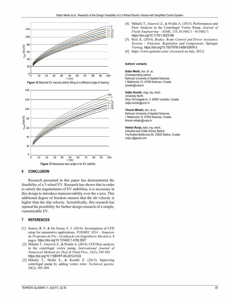
Srđan Medić et al.: Research of the Design Feasibility of a 3-Wheel Electric Vehicle with Simplified Control System
TEHNIČKI GLASNIK 11, 4(2017), 32-35 35
Figure 12 Maximal EV velocity before tilting at a different angle of leaning
Figure 13 Necessary lean angle α for EV stability
6 CONCLUSION
Research presented in this paper has demonstrated the feasibility of a 3-wheel EV. Research has shown that in order to satisfy the requirements of EV stabilities, it is necessary in this design to introduce manoeuvrability over the x-axis. This additional degree of freedom ensures that the tilt velocity is higher than the slip velocity. Scientifically, this research has opened the possibility for further design research of a simple, customizable EV. 7 REFERENCES [1] Soares, R. F. & De Souza, F. J. (2014). Investigation of CFD
setup for automotive applications. POSMEC 2014 – Simpósio do Programa de Pós - Graduação em Engenharia Mecânica, 4 pages. https://doi.org/10.13140/2.1.4150.3527
[2] Mihalić T., Guzović Z., & Predin A. (2014). CFD flow analysis in the centrifugal vortex pump, International Journal of Numerical Methods for Heat & Fluid Flow, 24(3), 545-562. https://doi.org/10.1108/HFF-05-2012-0124
[3] Mihalić T., Medić S., & Kondić Ž. (2013). Improving centrifugal pump by adding vortex rotor. Technical gazette, 20(2), 305-309.
[4] Mihalić T., Guzović Z., & Predin A. (2013). Performances and Flow Analysis in the Centrifugal Vortex Pump. Journal of Fluids Engineering – ASME, 135, 011002-1 - 011002-7. https://doi.org/10.1115/1.4023198
[5] Reif, K. (2014). Brakes, Brake Control and Driver Assistance Systems - Function, Regulation and Components. Springer Vieweg. https://doi.org/10.1007/978-3-658-03978-3
[6] https://www.qsmotor.com/ (Accessed on July, 2012) Authors’ contacts: Srđan Medić, doc. dr. sc. (Corresponding author) Karlovac University of Applied Sciences, I. Meštrovića 10, 47000 Karlovac, Croatia [email protected] Veljko Kondić, mag. ing. mech. University North, Ulica 104 brigade br. 3, 42000 Varaždin, Croatia [email protected] Tihomir Mihalić, doc. dr.sc. Karlovac University of Applied Sciences, I. Meštrovića 10, 47000 Karlovac, Croatia [email protected] Vedran Runje, spec. ing. mech. Industrial and Crafts School Slatina, Trg Ruđera Boškovića 5A, 33520 Slatina, Croatia [email protected]

36 TECHNICAL JOURNAL 14, 1(2020), 36-40
ISSN 1846-6168 (Print), ISSN 1848-5588 (Online) Preliminary communication https://doi.org/10.31803/tg-20180123123455
Energy and Exergy Analysis of LiBr-aq and LiCl-aq Liquid Desiccant Dehumidification System
Barış Kavasoğullari, Ertuğrul Cihan, Hasan Demir
Abstract: In this study, energy and exergy analysis of experimental results obtained from a dehumidification system using LiBr-aq (lithium bromide-water) and LiCl-aq (lithium chloride-water) as desiccant was made. In dehumidifier and regenerator columns polycarbonate sheets, which have not been used before, were used as packing material to increase contact area in purposed liquid desiccant dehumidification system. In the analysis, variation of electrical coefficient of performance and exergy efficiency with airflow rate for different solution mass flow rates were investigated. Because of investigation, maximum values of electrical coefficient of performance and exergy efficiency were calculated approximately as 2.8 and 18%, respectively. Keywords: energy; exergy; liquid desiccant; liquid desiccant dehumidification; polycarbonate packing 1 INTRODUCTION
Nowadays, vapor compression refrigeration systems are extensively used for heating/cooling processes. On the other hand, these types of systems are highly dependent on electrical energy and provide limited humidity control and indoor air quality. For this reason, researchers lead to alternative air conditioning systems.
Liquid desiccant dehumidification systems are good alternatives to the vapor compression systems commonly used in air conditioning processes. The operation of the system is based on the principle that air is brought into contact with a low vapor pressure liquid to remove moisture from the air. In this way, the amount of moisture in the air can be brought to an acceptable level by consuming very small amount of energy.
Although liquid desiccant dehumidification systems have a low coefficient of performance, they are more interesting for general daily usage due to temperature independent humidity control and better indoor air quality [1-4]. In addition, the dilute liquid solution after dehumidification in the system can be regenerated using medium and low-temperature heat sources such as industrial waste heat, solar energy and geothermal energy. The efficiency and the energy saving of the system can be further increased [5-7].
Ahmed et al. [8] carried out exergy analysis of a hybrid air conditioning system operating with liquid desiccant dehumidification system. Xiong et al. [9] also performed exergy analysis of a novel two-phased liquid desiccant dehumidification system and they compared that system with a single-phased dehumidification system. Zhang et al. [10] performed an exergy analysis with the heat and mass transfer analysis of the liquid dehumidification system using LiBr-water solution.
In this study, energy and exergy analysis of a liquid desiccant dehumidification system for two liquid desiccant solutions, which are LiBr and LiCl, was experimentally conducted. The electrical coefficient of performance and exergy efficiency were chosen as performance parameters
and two solutions were compared according to these parameters.
2 SYSTEM DESCRIPTION
In liquid desiccant dehumidification systems, moisture in the air is removed by strong desiccant solutions which are hygroscopic materials. The dehumidification process depends on water vapor pressure difference between liquid desiccant and air. After dehumidification process, diluted solution is regenerated by the regenerator column.
The tested liquid desiccant dehumidification system is shown schematically in Fig. 1. The system consists of dehumidification and regenerator columns, air fans, liquid pumps, heat exchangers and various sensors.
In liquid desiccant dehumidification system, process air enters at point (1) and leaves the dehumidifier at point (3) after its moisture is removed. In the dehumidifier column, strong liquid desiccant solution, which takes some moisture from the air, becomes diluted. Diluted liquid desiccant solution is sent to the regenerator column with the aid of liquid pump at point (8). Before it enters the regenerator column, solution is heated using heating HEx at point (9). Afterwards, the solution is regenerated by passing air through (points 4-6). Regenerated solution is cooled to reduce the surface vapor pressure by cooling HEx (point 12) before it is reused in dehumidifier.
In the tested system, various sensors were placed at specified points to measure temperature, relative humidity, flow rates and pressure difference (Fig. 1). Air flow rates were measured with KIMO-CTV210 (±0.3% sensitivity) sensor, liquid flow rates were measured with GF Signet Capteur 515 sensor (±0.5% sensitivity).
Relative humidity and temperature values of the air at inlet and outlet of dehumidifier and regenerator columns were measured with Vaisala HMT120 (±1.5% RH and ±0.2 °C sensitivity) sensor. Liquid desiccant, hot and cold water temperatures used in HEx's were measured with K type thermocouple (±0.4% °C sensitivity).
In the tested system, novel structured polycarbonate packing materials were used to increase air-solution contact

Barış Kavasoğullari et al.: Energy and Exergy Analysis of LiBr-aq and LiCl-aq Liquid Desiccant Dehumidification System
TEHNIČKI GLASNIK 14, 1(2020), 36-40 37
area and time. Polycarbonate packing materials were formed by cutting large polycarbonate sheets of 2 × 6 m in dimensions of 100 × 300 × 6 mm and channel angles of 30°. Formed polycarbonate sheets and their placement in columns were shown in Fig. 2a and 2b respectively. The
polycarbonate sheets were placed in such a way that the channels would form a zig-zag so that the contact time could be increased, and a smooth flow could be obtained. Average surface area density of the sheets was calculated as 637 m2/m3.
Figure 1 Schematic representation of the system
Figure 2 a) Formed polycarbonate sheets, b) placement of sheets in columns
3 ENERGY AND EXERGY CALCULATIONS
In the study, electrical coefficient of performance and
exergy efficiency were used to investigate performance of the system. Calculations were carried out by EES (Engineering equation solver) software [11].
Electrical coefficient of performance of the system was calculated by Eq. (1):
eve
e
QCOP
W=
(1)
Here, evQ and eW are recovered heat energy and
consumed electrical energy in unit time respectively. evQ was found from the following equation:
a) b)

Barış Kavasoğullari et al.: Energy and Exergy Analysis of LiBr-aq and LiCl-aq Liquid Desiccant Dehumidification System
38 TECHNICAL JOURNAL 14, 1(2020), 36-40
ev a1 2 3 fg( )ΔQ m hω ω= −
(2) In Eq. (2), a1m , ω2 and ω3 represent mass flow rate of
air (kg/s), inlet and outlet absolute humidity of air (kgH2O/kgDryAir) in dehumidifier respectively. Δhfg is the latent heat (kJ/kg) of water. In the purposed system, specific exergy flow (kJ/kg) of any point was calculated by Eq. (3):
[ ]0 0 0( )i i ih h T s sψ = − − (3)
Here, "0" subscript represents the dead state. Exergy
loss of the dehumidifier was found by Eq. (4):
ab a1 2 3 s1 7 8( ) ( )E m mψ ψ ψ ψ= − + −
(4)
In Eq. (4), s1m is mass flow rate (kg/s) of the desiccant solution in dehumidifier column. Exergy losses in the cooling and heating HEx's were calculated by Eq. (5) and (6) respectively:
hexc s1 12 7 cw swi cwo( ) ( )E m mψ ψ ψ ψ= − + −
(5)
hexh s2 10 9 hw hwi hwo( ) ( )E m mψ ψ ψ ψ= − + −
(6)
In Eq. (5), cwm and hwm are the mass flow rate (kg/s) of the cold and hot water respectively. Subscripts "cwi" and "cwo" refer inlet and outlet status of the water in cooling HEx. Similarly, "hwi" and "hwo" represent inlet and outlet status of the water in heating HEx. s2m is mass flow rate (kg/s) of the desiccant solution at heating HEx and regenerator. Exergy loss of the regenerator was found by the following equation:
rej a2 5 6 s2 11 10( ) ( )E m mψ ψ ψ ψ= − + −
(7)
Here, a2m refers the mass flow rate (kg/s) of the air at regenerator. Exergy efficiency of the system was defined by Eq. (8):
ksystem
hw
EnE
=
(8)
In Eq. (8) kE and hwE are gained exergy (kW) by
process air in dehumidifier and consumed exergy (kW) to regenerate the diluted solution in regenerator respectively. These parameters were calculated by following equations:
k a1 3 2( )E m ψ ψ= −
(9)
hwi wthw hw w hwi hwo
hwi( )
T TE m cp T T
T −
= −
(10)
In Eq. (10), Twt and cpw represent dead state temperature
and average specific heat of the water, respectively.
4 RESULTS AND DISCUSSION In the liquid desiccant dehumidification system, energy
and exergy analysis were conducted for 43% wt LiBr-water and LiCl-water solutions separately. Calculations were performed with the aid of EES software according to experimental results. Measured and specified experimental parameters and dead state properties were shown in Tab. 1 [10, 12]. In experimental rig, ARGAL P 06.10 chemical centrifugal pump was used as liquid pump and it operates in between 0-6.3 (kg/s). As it is visible in table, solution mass flow rates were selected as 1.42 and 1.85 (kg/s), which are in operation range of the liquid pump. In the table, T, P, Φ and X values refer to dead state properties of temperature, pressure, relative humidity and concentration, respectively.
Table 1 Experimental parameters and dead state properties
Parameter Measured/specified value Liquid desiccants 43% wt LiBr and LiCl solution Packing height, cm 60 Average air flow rate, m3/h 400, 680, 1000 Average solution mass flow rate, kg/s (dehumidifier) 1.42, 1.85
Cold water inlet/outlet temperature 14/22 °C Hot water inlet/outlet temperature 59.1/50.2 °C Average solution temperature (dehumidifier) 28.7 °C
Average solution temperature (regenerator) 45.8 °C
Dead state properties of water Twt=25 ºC, Pwt=101.3 kPa Dead state properties of air T0=25 ºC, P0=101.3 kPa, Φ0=99% Dead state properties of solution Ts=30 ºC, Xs=0.0001 kg/kg
The distribution of total exergy loss in the system
equipment for LiBr-water solution at 1.42 kg/s desiccant mass flow rate and 400 m3/h air flow rate was shown in Fig. 3. The maximum exergy loss occurred in heating HEx because of high regeneration temperature. In dehumidifier, high surface vapor pressure difference causes high exergy loss.
Figure 3 Distribution of total exergy loss over the equipment
Fig. 4 represents variation of absolute humidity of air in
dehumidifier and regenerator columns for LiBr-water solution at 1.42 kg/s solution mass flow rate and 400 m3/h air flow rate. In the dehumidification process (2-3), air contacts with relatively hot and strong desiccant solution, hence its temperature increases and absolute humidity

Barış Kavasoğullari et al.: Energy and Exergy Analysis of LiBr-aq and LiCl-aq Liquid Desiccant Dehumidification System
TEHNIČKI GLASNIK 14, 1(2020), 36-40 39
decreases. In the regeneration process (5-6), air contacts with hot and diluted solution; therefore, temperature and absolute humidity of air increase.
Figure 4 Variation of absolute humidity of air in dehumidifier and regenerator
columns
Fig. 5 shows the variation of electrical coefficient of performance values for LiBr-water and LiCl-water at 1.42 kg/s solution mass flow rate. During the experiments, mass flow rates of solutions were kept constant at 1.42 kg/s and airflow rates increased from 400 to 1000 m3/h. As it can be seen from the figure, increase in airflow rates will increase the electrical coefficient of performance for both solutions. Since LiCl-water solution has lower surface vapor pressure than LiBr-water, amount of removed moisture ( evQ ) will be higher as well as electrical coefficient of performance. The maximum value of electrical coefficient of performance was obtained as 2.6 at 1000 m3/h airflow rate for LiCl-water solution.
In Fig. 6, variation of electrical coefficient of performance was shown for both solutions at 1.85 kg/s solution mass flow rate. The increase in the liquid desiccant flow rate caused a significant increase in the LiCl solution and insignificant change in the electrical coefficient of performance values in the LiBr solution. The maximum value was obtained with LiCl solution as 2.8 at 1000 m3/h airflow rate.
Figure 5 Variation of electrical coefficient of performance with air flow rate
(�̇�𝑚s1 = 1.42 kg/s)
Figure 6 Variation of electrical coefficient of performance with air flow rate
(�̇�𝑚s1 = 1.85 kg/s)
Figure 7 Variation of exergy efficiency values with air flow rate
(�̇�𝑚s1 = 1.42 kg/s) Fig. 7 shows the variation of exergy efficiency values for LiBr-water and LiCl-water solutions with airflow rates at constant 1.42 kg/s solution mass flow rates. Since exergy efficiency values are highly dependent on amount of removed moisture, LiCl-water solution shows the best performance between two solutions. Airflow rate positively affects the exergy efficiency values for both solutions and the maximum value of about 12% was obtained at 1000 m3/h airflow rate.
Figure 8 Variation of exergy efficiency values with air flow rate
(�̇�𝑚s1 = 1.85 kg/s)
Variation of exergy efficiency values with air flow rate at 1.85 kg/s solution mass flow rates were represented in Fig. 8. Increase in solution mass flow rates enhances the exergy efficiency values for both solutions. As a result of
0,00
0,50
1,00
1,50
2,00
2,50
3,00
400 680 1000
COPe
Air flow rate (m3/h)
LiBr-aq LiCl-aq
0,00
0,50
1,00
1,50
2,00
2,50
3,00
400 680 1000
COPe
Air flow rate (m3/h)
LiBr-aq LiCl-aq
0
2
4
6
8
10
12
14
400 680 1000
Exer
gy e
ffici
ency
, ηsy
stem
Air flow rate (m3/h)
LiBr-aq LiCl-aq
0
5
10
15
20
400 680 1000
Exer
gy e
ffici
ency
, ηsy
stem
Air flow rate (m3/h)
LiBr-aq LiCl-aq

Barış Kavasoğullari et al.: Energy and Exergy Analysis of LiBr-aq and LiCl-aq Liquid Desiccant Dehumidification System
40 TECHNICAL JOURNAL 14, 1(2020), 36-40
calculations, the maximum exergy efficiency value was found at about 18% with LiCl-water solution at 1000 m3/h. 5 CONCLUSION In this study, energy and exergy analysis of a liquid desiccant dehumidification system using LiBr-water and LiCl-water as desiccants was performed using the experimental test results. In the analysis, electrical coefficient of performance and exergy efficiency were chosen as performance parameters and variation of these parameters with air flow rate and solution mass flow rates were investigated. As a result of investigation the following results were obtained: • In experiments conducted with LiBr in the system, the most exergy loss occurred in the heating HEx. By reducing the regeneration temperature, the exergy lost in the heat exchanger can be reduced. However, excess reduction in the regeneration temperature may cause decrease in regeneration performance of the system. • According to the obtained electrical coefficient of performance values and exergy efficiencies, low surface vapor pressure provided by the LiCl solution will provide a great advantage in terms of performance in the system. In the analysis with LiCl solution, the highest electrical coefficient of performance and exergy efficiency values were determined by approximately 2.8 and 18% respectively, while the same parameters were determined to be approximately 1.6 and 5% with LiBr solution. The electrical coefficient of performance values obtained with both solutions show that the system uses the primary energy sources efficiently. Considering the electrical coefficient of performance and exergy efficiencies obtained in the study, the LiCl solution comes to the fore, as mentioned before. However, in selecting the appropriate liquid desiccant to be used in the system, price and availability are important as well as the performance of the system. The LiBr solution offers lower initial investment and operational cost owing to its low price and high availability. For this reason, the use of the LiBr solution would be advantageous in these respects. Acknowledgement
This study was supported by TÜBİTAK with project numbered 114M151. 5 REFERENCES [1] Kavasoğulları, B., Cihan, E., & Demir, H. (2016). Novel
Packing Materials for Open Liquid Desiccant System. Energy Procedia, 91, 785-791. https://doi.org/10.1016/j.egypro.2016.06.244
[2] Ahmed, S., Gandhidasan, P., & Al-Farayedhi, A. (1998). Thermodynamic analysis of liquid desiccants. Solar Energy, 62(1), 11-18. https://doi.org/10.1016/s0038-092x(97)00087-x
[3] Cihan, E., Kavasoğulları, B., & Demir, H. (2017). Enhancement of performance of open liquid desiccant system with surface additive. Renewable Energy, 114, 1101-1112. https://doi.org/10.1016/j.renene.2017.08.002
[4] Yin, Y., Zheng, B., Yang, C., & Zhang, X. (2015). A proposed compressed air drying method using pressurized liquid desiccant and experimental verification. Applied Energy, 141, 80-89. https://doi.org/10.1016/j.apenergy.2014.12.015
[5] Patnaik, S., Lenz, T., & Löf, G. (1988). Experimental Studies with a Solar Open-Cycle Liquid Desiccant Cooling System. Advances in Solar Energy Technology, 1013-1018. https://doi.org/10.1016/b978-0-08-034315-0.50196-8
[6] Factor, H. M. & Grossman, G. (1980). A packed bed dehumidifier/regenerator for solar air conditioning with liquid desiccants. Solar Energy, 24(6), 541-550. https://doi.org/10.1016/0038-092x(80)90353-9
[7] Katejanekarn, T., Chirarattananon, S., & Kumar, S. (2009). An experimental study of a solar-regenerated liquid desiccant ventilation pre-conditioning system. Solar Energy, 83(6), 920-933. https://doi.org/10.1016/j.solener.2008.12.006
[8] Ahmed, C. K., Gandhidasan, P., Zubair, S., & Al-Farayedhi, A. (1998). Exergy analysis of a liquid-desiccant-based, hybrid air-conditioning system. Energy, 23(1), 51-59. https://doi.org/10.1016/s0360-5442(97)00040-6
[9] Xiong, Z., Dai, Y., & Wang, R. (2010). Development of a novel two-stage liquid desiccant dehumidification system assisted by CaCl2 solution using exergy analysis method. Applied Energy, 87(5), 1495-1504. https://doi.org/10.1016/j.apenergy.2009.08.048
[10] Zhang, L., Liu, X., Jiang, J., & Jiang, Y. (2014). Exergy calculation and analysis of a dehumidification system using liquid desiccant. Energy and Buildings, 69, 318-328. https://doi.org/10.1016/j.enbuild.2013.11.025
[11] Klein, S. A., Engineering Equation Solver, F-Chart Software, 2015. Academic Version 9.901.
[12] Xiong, Z. Q., Dai, Y. J., & Wang, R. Z. (2010). Exergy Analysis of Liquid Desiccant Dehumidification System. International Journal of Green Energy, 7(3), 241-262. https://doi.org/10.1080/15435071003795881
Authors’ contacts: Barış KavasoğullarI, Res. Asst. (Corresponding author) Osmaniye Korkut Ata University, Mechanical Engineering Department, Karacaoğlan Yerleşkesi Fakıuşağı Mah. 80000 Merkez/Osmaniye, Turkey Tel: +903288271000, Fax: +903288250097 E-mail: [email protected] Ertuğrul Cihan, Assoc. Prof. Osmaniye Korkut Ata University, Mechanical Engineering Department, Karacaoğlan Yerleşkesi Fakıuşağı Mah. 80000 Merkez/Osmaniye, Turkey Tel: +903288271000, Fax: +903288250097 E-mail: [email protected] Hasan Demir, Assoc. Prof. Osmaniye Korkut Ata University, Chemical Engineering Department, Karacaoğlan Yerleşkesi Fakıuşağı Mah. 80000 Merkez/Osmaniye, Turkey Tel: +903288271000, Fax: +903288250097 E-mail: [email protected]

TEHNIČKI GLASNIK 14, 1(2020), 41-45 41
ISSN 1846-6168 (Print), ISSN 1848-5588 (Online) Preliminary communication https://doi.org/10.31803/tg-20190227095246
Designing of a New Type Air-Water Cooled Photovoltaic Collector
Erhan Arslan, Azim Doğuş Tuncer, Meltem Koşan, Mustafa Aktaş, Ekin Can Dolgun Abstract: The importance of photovoltaic-thermal (PV / T) collector systems in renewable energy technologies is increasing for combined hybrid electrical heat applications. The efficiency of photovoltaic (PV) systems varies between 5-20%. On average, 15% of the solar radiation coming to the PV panel surface is converted to electrical energy and the remainder is lost. In this study, a PV/T collector was designed using two different fluids simultaneously and its efficiency was calculated numerically. PV/T collector systems are specifically designed for agricultural production and their advantages are discussed. In this study, numerical calculations of PV/T collector with a different design have been made. The results were compared with reference to another experimental study. Two different working fluids (air and water) were used in the calculations. The system where air is used as working fluid is called Mode 1 and the system where water is used is called Mode 2. It is aimed to achieve high heat transfer by using water pipes, air ducts and fins placed under PV panels. In this way, it is aimed to produce a more stable hot air and water. In addition, in order to investigate the effect of flow on the yield, different flow rates were calculated. As a result of the theoretical analyses and calculations made in consideration of literature, the total efficiencies of air flow mode (Mode 1) were calculated as 43.2%, 46,2% and 48.7% at 0.0067 kg/s, 0.0072 kg/s and 0.0077 kg/s mass flow rates, respectively. For water flow mode (Mode 2), these values computed as 52.81%, 53.83% and 55.04% at 0.023 kg/s, 0.036 kg/s and 0.054 kg/s mass flow rates, respectively. It was found that PV / T collector efficiency increased with increasing end flow. Designed collector system is preferable in terms of effective use of energy and it can be easily applicable in processes such as hot air-water preparation, drying and greenhouse heating. Keywords: air-water heating; hybrid renewable energy systems; photovoltaic-thermal collector; solar energy 1 INTRODUCTION
Energy demand across the world is increasing day by
day, but only fossil fuel based energy systems are not enough to meet this demand. Therefore, renewable energy technologies are one of the most important areas of research of our time. The utilization of renewable energy sources is also possible with the use of hybrid systems. Solar energy is at the forefront of renewable and sustainable energy research and is used globally for the production of electrical and thermal energy [1-2]. The basis of environmental and economical sustainability depends on the use of renewable energy sources. Hybrid technologies allow to use renewable energy sources and technologies effectively.
Photovoltaic systems can convert only 15-20% of the solar energy and the rest being turned into heat. It is possible to effectively use the heat which cannot transform into electrical energy with photovoltaic-thermal collectors (PV/T). Also, PV/T collector system allows to decrease the temperature of the photovoltaic panel. Thus, efficiency of the photovoltaic (PV) panel would be increased.
Concentrating PV/T (CPV/T) collector collects solar radiation and reflects to a focal spot where the PV panel is located. The benefit of using concentrating PV/T collectors is that the use of reflector material, which is inexpensive compared with PV modules, makes for the use of less PV modules by comparison with flat plate PV/T collectors. By doing so, costly PV modules are switched with economically viable reflector apparatus [3].
Fossil fuels which are primary energy sources are commonly used for heating applications, which is necessary for the food and agricultural production such as drying, pre-heating. The utilization of PV/T technologies in these applications is very important in terms of benefits from the sun. In this manner, energy costs and carbon emissions will be reduced as the usage of fossil fuels declines. The use of PV/T technology eliminates the need for an additional system
for electrical energy. In this way, energy costs can be reduced.
Kalogirou and Tripanagnostopoulos [4] carried out the cost analysis of electricity production from PV/T for domestic hot water supply. As a result, they found that the system could be applied economically. In research conducted by Ceylan et al., [5] the PV module was cooled by water flowing through the spiral pipes connected to the back of the module with temperature control. Designed to keep the temperature of the photovoltaic module at 45 °C, the non-cooled and cooled efficiency of the electrical efficiency of the whole system was tested at 10% and 13%. Ceylan and Gürel [6] experimentally studied the cooling of the PV module in their study. The PV efficiency was calculated as 17% at 45 °C and the exergy efficiency at 55 °C at 21%. In a study performed by Zondag [7], a glazed PV/T, an unglazed PV/T and a conventional PV panel were compared. Mean electrical efficiencies were calculated as 7.6%, 7.2% and 6.6, respectively. Specifications and efficiencies of previous works of PV/T systems are given in Tab. 1.
Solar air collectors are inexpensive and easily applicable systems which produces thermal energy from solar radiation with a small amount of electrical energy consumption. Aktaş et al. [8] performed energy-exergy analysis of a multipass solar air collector. According to the results, average thermal efficiency of the collector reaches up to 72%. In a study conducted by Şevik et al. [9] Double pass solar air collector was used in a drying application of mint and apple samples.
Integration of PV panels and solar collector systems allows to increase both electrical and thermal efficiency values with PV/T technology. In this study, a novel PV/T collector system was designed. Air and water were chosen as the working fluids for Mode 1 and Mode 2, respectively. The collector has been designed to achieve high thermal efficiency and electrical energy. Theoretical analysis of the system performance has been performed. The advantages of the collector, which used air or water as a cooling fluid, have been discussed.

Erhan Arslan et al.: Designing of a New Type Air-Water Cooled Photovoltaic Collector
42 TECHNICAL JOURNAL 14, 1(2020), 41-45
Table 1 Specifications and efficiency values of previous studies of PV/T collectors
Ref. PV/T type Application Efficiency Area, material [10] Flat Plate Hot water supply Electrical: 13.9% 20.44 m2, -
[11] Flat Plate Hot water supply Thermal: 44.5% Electrical: 9% 5.2 m2, polycrystalline
[12] Flat Plate Hot water supply Electrical: 13–13.8% Thermal: 45–54.6% Overall: 58–68.4%
5.1 m2, polycrystalline silicon
[13] Flat Plate Hot water supply Electrical: 9.87% Thermal: 40% 1.64 m2, -
[14] Flat Plate Solar cooling Electrical: 10.6% Thermal: 71% 8.76 m2, -
[15] Flat Plate Hot water supply Exergy: 14.2% Electrical: 13.4-13.5% Overall: 70%
3.18 m2, polycrystalline
[16] Non concentrate PV/T Solar cooling Thermal: 62% Electrical: 13.19% -
[17] CPV/T Space heating + cooling Electrical: 11% Thermal 59% -
[18] CPV/T Hot water supply Electrical: 7.36 -6.85% Thermal: 22.1-7.33% -
[19] CPV/T Solar cooling Electrical: 11% Thermal: 58% 1.8m2, -
[20] CPV/T Solar cooling Thermal: 44% Electrical: 6% 1 m2, monocrystalline
[21] BIPV/T (Building integrated) - Thermal: 48%
Electrical: 10.8% 1.65 m2, polycrystalline
[22] BIPV/T Space heating + hot water supply Thermal: 40% Electrical: 8% 1.42 m2, monocrystalline
[23] BICPV (Building integrated concentrating) - Thermal: 54%
Electrical: 13.9% -
[24, 25] BIPV/T - Thermal: 48% Electrical: 16.4% -
2 ENERGY ANALYSIS
The energy analysis is required to determine the
performance of the designed novel modular PV/T collector. The energy equations of PV/T collector which is simultaneously produced both heat and electrical energy are given below [26]:
in outE E=∑ ∑ (1)
Electrical efficiency of a photovoltaic module is given as follows [27]:
[ ]el ref ref PV ref1 ( )T Tη η β= − − (2)
Here, βref = 0.0045 °C−1 is the temperature coefficient [28]. TPV is the temperature of the PV cells and Tref is the reference temperature which is taken as 25 °C. ηref is the reference PV module efficiency (0.09). TPV has been chosen as 44.70 °C according to the reference case [29].
th,ins a p,a a,o a,i( )Q m C T T= − (3)
th,ins w p,w w,o w,i( )Q m C T T= − (4)
Here am and wm are mass flow rates (kg/s) for air and water, respectively. Cp,a is the spesific heat capacity of air and Cp,w is the specific heat capacity of water (kJ/kgK). Ta,i and
Tw,i are the inlet temperature of the air and water, respectively. Total instantaneous thermal efficiency of the solar collector for air and water working fluids can be calculated with Eq. (5) and Eq. (6), respectively.
a p,a a,o a,ith,ins
c
( )m C T TIA
η−
=∑
(5)
w p,w w,o w,ith,ins
c
( )m C T TIA
η−
=∑
(6)
Here I is the solar radiation value (W/m2) and Ac is the
collector area (m2). Total thermal efficiency of the solar collector for air and water working fluids can be computed as follows [27]:
a p,a a,o a,ith
c
( ) d
d
m C T T t
A I tη
− = ∫∑∫
(7)
w p,w w,o w,ith
c
( ) d
d
m C T T t
A I tη
− = ∫∑∫
(8)
Total PV/T efficiency can be calculated with Eq. (9) and
Eq. (10) for air and water, respectively.

Erhan Arslan et al.: Designing of a New Type Air-Water Cooled Photovoltaic Collector
TEHNIČKI GLASNIK 14, 1(2020), 41-45 43
a p,a a,o a,i elPV/T
c c
( ) d d
d d
m C T T t P t
A I t A I tη
− = +∫ ∫∑∫ ∫
(9)
w p,w w,o w,i elPV/T
c c
( ) d d
d d
m C T T t P t
A I t A I tη
− = +∫ ∫∑∫ ∫
(10)
Pel is electrical power (W). In this study, electrical efficiency was calculated as 0.082 at the constant solar radiation value of 700 W/m2. 3 SYSTEM DESIGN AND MODELS
There are a lot of works about cooling of PV unit.
Generally, air or water cooled PV has been used. When the previous studies are examined, the electrical efficiency in the systems using crystalline solar panels is higher than the systems using thin film panels, while the thermal efficiency is lower. This difference is due to the fact that the crystalline solar panel efficiency is higher than the thin film solar panel efficiency, whereas the thermal efficiency is high in the PV/T panel used in the thin film panel because the heat transfer coefficient value of the thin film solar panels is higher than of the crystalline solar panels. As the glass is used as a cover in the collector, the electrical efficiency decreases while the thermal efficiency increases. The main reason for this situation is that the glass material used on the collector surface does not allow much heat transfer and the increase in the temperature within the system increases every 1 °C above 25 °C by 0.4% and 0.5% in the efficiency of PV cells. Thermal efficiency of the water-cooled PV/T is higher than air-cooled PV/T collectors, while the electrical efficiency is the same. The reason why water-cooled PV/T collector thermal efficiency is high is due to the fact that water is a better heat conductor than air.
Within the framework of the evaluations carried out, the highest efficiency of total PV/T collector is the PV/water+glass characteristics and the lowest efficient PV/T collectors are the polycrystalline PV/air characteristic.
While designing the system, it is aimed to produce thermal energy besides electricity production. As it is known, the hottest area of contact with the fluid in the system is the area under the PV panel. When we approach the whole system step by step, it can be seen that there are several options to increase the heat transfer. Since we cannot make changes in the bottom surface of the PV panel, the ratio of the area contacting / not touching the bottom surface, the total heat transfer area, the thermal conductivity coefficient of the tubes or fins, the velocities of the primary and secondary fluid and turbulence levels.
There are copper pipes in contact with the panel along the PV. The pipes in which the primary fluid circulates are in contact with PV panel. Also, there are copper fins under the PV panel to heat the air. Depending on demand, air or water can be used as working fluid. Also, an electrical insulation material can be applied between the PV panel and the copper pipes for electrical insulation and to provide high thermal conductivity. Schematic view of modular PV/T collector is
given in Fig. 1. PV/T collector can operate in two modes. Air and water are the working fluids for Mode 1 and Mode 2, respectively. Working fluids can be selected and the PV/T collector can produce water or air depending on the demand.
Designed PV module can work efficiently using a proportional integral derivative (PID) controller. When the PV surface temperature, which is measured by the thermocouple, reaches the high value, in other words, PV surface temperature increases, fan or pump adjusts the flow rate by means of the inverter according to the measured temperature value. As the PV panel surface temperature increases, the flow rate of coolant fluid increases proportionally. In theoretical calculations, main water system utilization has been assumed. It has been assumed that there was no recirculation.
In this design, the electrical efficiency characterization is important due to the temperature of the PV module. With this design, the flow rate of coolant in which the PV panel will operate efficiently can be managed.
Figure 1 Schematic view of PV/T collector
The advantages of design of the novel photovoltaic-
thermal (PV/T) collector system: • the increase of PV panel efficiency according to the
conventional one, • obtaining both electrical and heat energy from solar
energy, • increasing efficiency by using air-water at variable flow
rate according to the radiation intensity from the sun, • air or water heating on demand with a single system. 4 RESULTS AND DISCUSSION
PV/T efficiency values depending on mass flow rate of Mode 1 are given in Fig. 2. As can be seen in Fig. 2 and 3, the increase in the mass flow rate value increases the PV/T efficiency.

Erhan Arslan et al.: Designing of a New Type Air-Water Cooled Photovoltaic Collector
44 TECHNICAL JOURNAL 14, 1(2020), 41-45
Theoretical calculations for airflow mode (Mode 1) PV/T have been done at 0.0067 kg/s, 0.0072 kg/s and 0.0077 kg/s mass flow rates. The total efficiency for this mode were calculated as 43.2%, 46.2% and 48.7%, respectively.
PV/T efficiency values depending on the mass flow rate of Mode 2 are given in Fig. 3. PV/T efficiency of water flow mode also increased with the increment of the mass flow rate of water as in air flow mode.
Mass flow rate (kg/s)
0.0066 0.0068 0.0070 0.0072 0.0074 0.0076 0.0078
PV
/T e
ffici
ency
(%)
43
44
45
46
47
48
49
Figure 2 PV/T efficiency values depending on mass flow rate of Mode 1
Mass flow rate (kg/s)
0.020 0.025 0.030 0.035 0.040 0.045 0.050 0.055 0.060
PV
/T e
ffici
ency
(%)
52.5
53.0
53.5
54.0
54.5
55.0
55.5
Figure 3 PV/T efficiency values depending on mass flow rate of Mode 2
5 CONCLUSION
In the last decade, high effective PV/T systems have
become much popular issue within the solar application. In this study, a new type of PV/T system was designed to increase the efficiency of a conventional PV panel. With this novel design, air or water can be used as a cooling fluid. In this way, the efficiency of the PV panel can be increased and the desired hot fluid for the food and agricultural applications can be obtained. Moreover, when solar irradiation is abundant, a large part of the energy load can be met from a renewable source. While the efficiency of a conventional PV panel is average 15-20%, the total efficiency of air flow mode (Mode 1) was calculated as 43.2%, 46,2% and 48.7% at 0.0067 kg/s, 0.0072 kg/s and 0.0077 kg/s mass flow rates,
respectively. For water flow mode (Mode 2), these values were computed as 52.81%, 53.83% and 55.04% at 0.023 kg/s, 0.036 kg/s and 0.054 kg/s mass flow rates, respectively. With this design, the electrical and heat energy are acquired in the most efficient way. In addition, a more stable PV/T system with the heat energy obtained in the same area can be used in many production processes. Especially, this PV/T system design can be used efficiently in drying of food, pre-heating of food and agricultural products processes as well as space heating and domestic hot water production.
6 REFERENCES [1] Khanlari, A., Güler, H. Ö., Tuncer, A.D., Şirin, C., Bilge Y. C.,
Yılmaz, Y., & Güngör, A. (2020). Experimental and numerical study of the effect of integrating plus-shaped perforated baffles to solar air collector in drying application. Renewable Energy, 145, 1677-1692. https://doi.org/10.1016/j.renene.2019.07.076
[2] Khanlari, A., Sözen, A., Şirin, C., Tuncer, A. D. & Gungor, A. (2020). Performance enhancement of a greenhouse dryer: Analysis of a cost-effective alternative solar air heater. Journal of Cleaner Production, 251, 119672. https://doi.org/10.1016/j.jclepro.2019.119672
[3] Hasan, M. A. & Sumathy, K. (2010). Photovoltaic thermal module concepts and their performance analysis: A review. Renewable and Sustainable Energy Reviews, 14, 1845-1859. https://doi.org/10.1016/j.rser.2010.03.011
[4] Kalogirou, S. A. & Tripanagnostopoulos, Y. (2006). Hybrid PV/T solar systems for domestic hot water and electricity production. Energy Conversion and Management, 47, 3368-3382. https://doi.org/10.1016/j.enconman.2006.01.012
[5] Ceylan, İ., Gürel, A.E., Demircan, H., & Aksu B. (2014). Cooling of a photovoltaic module with temperature controlled solar collector. Energy and Buildings, 72, 96-101. https://doi.org/10.1016/j.enbuild.2013.12.058
[6] Ceylan, İ. & Gürel, A. E. (2015). Exergetic Analysis of a New Design Photovoltaic and Thermal (PV/T) System. American Institute of Chemical Engineers Environ Prog, 34, 1249-1253. https://doi.org/10.1002/ep.12108
[7] Zondag, H. A. (2008). Flat-plate PV-Thermal collectors and systems: A review. Renewable and Sustainable Energy Reviews, 12, 891-959. https://doi.org/10.1016/j.rser.2005.12.012
[8] Aktaş, M., Sözen, A., Tuncer, A. D., Arslan, E., Koşan, M., & Çürük, O. (2019). Energy-Exergy Analysis of a Novel Multi-Pass Solar Air Collector with Perforated Fins. International Journal of Renewable Energy Development, 8(1), 47-55. https://doi.org/10.14710/ijred.8.1.47-55
[9] Şevik, S., Aktaş, M., Dolgun, E. C., Arslan, E., & Tuncer, A. D. (2019). Performance analysis of solar and solar-infrared dryer of mint and apple slices using energy-exergy methodology. Solar Energy, 180, 537-549. https://doi.org/10.1016/j.solener.2019.01.049
[10] Bianchini, A., Guzzini, A., Pellegrini, M., & Saccani, C. (2017). Photovoltaic/thermal (PV/T) solar system: Experimental measurements, performance analysis and economic assessment. Renewable Energy, 111, 543-555. https://doi.org/10.1016/j.renene.2017.04.051
[11] Huang, B. J., Lin, T. H., Hung, W. C., & Sun, F. S. (2001). Performance Evaluation of Solar Photovoltaic/Thermal Systems. Solar Energy, 70, 443-448. https://doi.org/10.1016/S0038-092X(00)00153-5
[12] Fudholi, A., Sopian, K., Yazdi, M. H., Ruslan, M. H., Ibrahim, A., & Kazem, H. A. (2014). Performance analysis of

Erhan Arslan et al.: Designing of a New Type Air-Water Cooled Photovoltaic Collector
TEHNIČKI GLASNIK 14, 1(2020), 41-45 45
photovoltaic thermal (PVT) water collectors. Energy Conversion and Management, 78, 641-651. https://doi.org/10.1016/j.enconman.2013.11.017
[13] He, W., Chow, T. T., Ji, J., Lu, J., Pei, G., & Chan, L. (2006). Hybrid photovoltaic and thermal solar-collector designed for natural circulation of water. Applied Energy, 83, 199-210. https://doi.org/10.1016/j.apenergy.2005.02.007
[14] Nasrin, R., Hasanuzzaman, M., & Rahim, N. A., (2017). Effect of high irradiation and cooling on power, energy and performance of a PVT system. Renewable Energy, 116, 552-569. https://doi.org/10.1016/j.renene.2017.10.004
[15] Evola, G. & Marletta, L. (2014). Exergy and thermoeconomic optimization of a water-cooled glazed hybrid photovoltaic/ thermal (PVT) collector. Solar Energy, 107, 12-25. https://doi.org/10.1016/j.solener.2014.05.041
[16] Rosa-Clot, M., Rosa-Clot, P., Tina, G. M., & Ventura, C. (2016). Experimental photovoltaic-thermal Power Plants based on TESPI panel. Solar Energy, 133, 305-314. https://doi.org/10.1016/j.solener.2016.03.024
[17] Xu, Z. & Kleinstreuer, C., (2014). Concentration photovoltaic–thermal energy co-generation system using nanofluids for cooling and heating. Energy Conversion and Management, 87, 504-512. https://doi.org/10.1016/j.enconman.2014.07.047
[18] Tiwari, G. N. & Gaur, A. (2014). Photovoltaic thermal (PVT) systems and its applications. 2nd International Conference on Green Energy and Technology, Dhaka, Bangladesh, 132-138. https://doi.org/10.1109/ICGET.2014.6966678
[19] Coventry, J. S. (2005). Performance of a concentrating photovoltaic/thermal solar collector. Solar Energy, 78, 211-222. https://doi.org/10.1016/j.solener.2004.03.014
[20] Karathanassis, I. K., Papanicolaou, E., Belessiotis, V., & Bergeles, G. C. (2017). Design and experimental evaluation of a parabolic-trough concentrating photovoltaic/thermal (CPVT) system with high efficiency cooling. Renewable Energy, 101, 467-483. https://doi.org/10.1016/j.renene.2016.09.013
[21] Ibrahim, A., Fudholi, A., Sopian, K., Othman, M. Y., & Ruslan, M. H. (2014). Efficiencies and improvement potential of building integrated photovoltaic thermal (BIPVT) system. Energy Conversion and Management, 77, 527-534. https://doi.org/10.1016/j.enconman.2013.10.033
[22] Hazami, M., Mehdaoui, F., Naili, N., Noro, M., & Lazzarin, R., G., A. (2017). Energetic, exergetic and economic analysis of an innovative SolarCombiSystem (SCS) producing thermal and electric energies: Application in residential and tertiary households. Energy Conversion and Management, 140, 36-50. https://doi.org/10.1016/j.enconman.2017.02.040
[23] Connelly, K., Wu, Y., Chen, J., & Lei, Y. (2016). Design and development of a reflective membrane for a novel Building Integrated Concentrating Photovoltaic (BICPV) ‘Smart Window’ system. Applied Energy, 182, 331-339. https://doi.org/10.1016/j.apenergy.2016.07.125
[24] Farshchimonfared, M., Bilbao, J. I., &. Sproul, A. B. (2016). Full optimisation and sensitivity analysis of a photovoltaic–thermal (PV/T) air system linked to a typical residential building. Solar Energy, 136, 15-22. https://doi.org/10.1016/j.solener.2016.06.048
[25] Delisle, V. & Kummert, M., (2016). Cost-benefit analysis of integrating BIPV-T air systems into energy-efficient homes. Solar Energy, 136, 385-400. https://doi.org/10.1016/j.solener.2016.07.005
[26] Sardarabadi, M., Hosseinzadeh, M., Kazemian, A., & Fard M. P. (2017). Experimental investigation of the effects of using metal-oxides/water nanofluids on a photovoltaic thermal system (PVT) from energy and exergy viewpoints. Energy, 138, 682-695. https://doi.org/10.1016/j.energy.2017.07.046
[27] Tiwari, A. & Sodha, M. S. (2006). Performance evaluation of solar PV/T system: An experimental validation. Solar Energy, 80, 751-759. https://doi.org/10.1016/j.solener.2005.07.006
[28] Zondag, H. A., de Vries, D. W., van Helden, W. G. J., van Zolengen, R. J. C., & van Steenhoven, A. A. (2002). The thermal and electrical yield of a PV-thermal collector. Solar Energy, 72, 113-128. https://doi.org/10.1016/S0038-092X(01)00094-9
[29] Jarimi, H., & Abu Bakar, M. N., Othman, M., & Din, M. H. (2016). Bi-fluid photovoltaic/thermal (PV/T) solar collector: Experimental validation of a 2-D theoretical model. Renewable Energy, 85, 1052-1067. https://doi.org/10.1016/j.renene.2015.07.014
Authors’ contacts: Erhan Arslan, MSc Institute of Natural and Applied Science, Gazi University, Teknikokullar, Ankara, Turkey [email protected] Azim Doğuş Tuncer*, MSc, Research Assistant Energy Systems Engineering, Faculty of Engineering-Architecture, Burdur Mehmet Akif Ersoy University, İstiklal Campus, Burdur, Turkey [email protected] Meltem Koşan, MSc, Research Assistant Energy Systems Engineering, Technology Faculty, Gazi University, Teknikokullar, Ankara, Turkey [email protected] Ekin Can Dolgun Institute of Natural and Applied Science, Gazi University, Teknikokullar, Ankara, Turkey [email protected] Mustafa Aktaş, PhD, Professor Energy Systems Engineering, Technology Faculty, Gazi University, Teknikokullar, Ankara, Turkey [email protected]

46 TECHNICAL JOURNAL 14, 1(2020), 46-54
ISSN 1846-6168 (Print), ISSN 1848-5588 (Online) Preliminary communication https://doi.org/10.31803/tg-20200310141424
Risk Management in the Higher Education Quality Insurance System
Živko Kondić, Željko Knok, Veljko Kondić, Sanja Brekalo
Abstract: Due to the factors that affect the results of work on a daily basis, higher education institutions, through their quality assurance systems, or their planning, must assess risks. In doing so, they must take into account all issues of the internal and external context as well as the needs and expectations of all stakeholders in higher education. The paper explains in an appropriate way the concept of risk as well as all the elements that determine it and their classification in the field of higher education. Subsequently, a possible approach to risk management is discussed, with an emphasis on clarifying the principles and the risk management process itself. Finally, the basics of practical application in risk identification, analysis, evaluation and treatment are outlined. Keywords: opportunities; quality assurance; risk; risk management 1 INTRODUCTION
Throughout human history, man has lived and worked in an environment that has always been precarious. Risks have always been a constant companion for man. From prehistoric times people have lived in risky situations. The first risks were related to the inability to procure basic foodstuffs, protection from other species and other necessities for life. Human development has seen many lifestyle changes and the dangers around us. Our activities and lives have become more complex, and so have the risks. Today, we live in environments where exposure to risks is constant, such as traffic risks, food consumption risks, pollution risks, health risks, weather risks, theft risks, risks of various viruses, deadline risks, etc.
In a word, risks are an unavoidable and imminent in everyday life, whether in the private or business sphere. There is no absolute certainty in any business or activity, including in higher education. The only sure thing is that nothing in life and work is safe. There is always an aspect of "certain" uncertainty, risk that is taken or otherwise treated. Risk compromises and challenges goals and achievements, and therefore must be given a certain importance.
Many experts and scholars have discussed risks in an effort to come up with a definition of risk that would be acceptable in all fields of activity. Unfortunately, they have not been unable to fully agree. The reason lies in the fact that the risk is viewed as: "potential loss", "probability of loss", "uncertainty", "dispersion of real from expected results" or as "probability of an outcome that is not expected".
In addition, in all risk definitions, there are two common elements, uncertainty and loss. The significance of uncertainty in risk implies that the outcome of an event is always questionable. If there is a risk, then there are always two possible outcomes. If there is great certainty that the loss will occur, then there is no risk or its magnitude is insignificant. Likewise, if the outcome of an event is certain, there is no risk in that case. Risk is a combination of the likelihood and consequences of an adverse event [1, 2].
When it is said that risk is possible then it is implied that its probability of realization is between 0 and 1. This means that it is neither impossible nor safe to realize. An event can
be unrealizable (probability = 0), certain (probability = 1), or uncertain.
The word risk is derived from the ancient Greek word "rizko" which in translation means a danger to be avoided. Some associate the term risk with the old Italian word "risko". The word risk itself is a little more difficult to understand, and very often, misused. In English, it is mostly used when talking about a chance or a gamble. The meaning of the word risk itself varies in function from the context in which it is used. It has mostly negative connotation. For example, one can rarely hear that there is a risk of winning the lottery, but it can often be heard that there is a risk of failing the exam. According to [3], risk is defined as the effect of uncertainty on targets, where the effect is considered to be deviation from the expected - positive or negative (Fig. 1).
Figure 1 Effect of deviation from expected [4]
It can be simply said that risk represents the possibility
of an event that will have consequences for the achievement of the goals. Unused opportunities or the opportunities for improving a business are also considered a risk. Accordingly, risks are potential adverse events that, for example, in higher education institutions may: compromise the achievement of strategic and operational
goals, programs and projects, systems and activities; impair the quality of study; cause dissatisfaction of stakeholders in the processes; compromise the reputation of the institution and the
confidence of citizens and future students in it; expose the institution to negative financial effects;

Živko Kondić et al.: Risk Management in the Higher Education Quality Insurance System
TEHNIČKI GLASNIK 14, 1(2020), 46-54 47
compromise professionalism and appropriate (ethical) conduct in conducting business;
result in misuse of funds, unauthorized use or misappropriation of property or information;
adversely affect the institution's ability to manage the changed circumstances in a way to minimise or prevent their negative effects on the realization of the study.
As previously mentioned, the risk may be lower or
higher, but it is always present in the processes. As such, it cannot be eliminated, but it can be controlled. This is an undesirable inevitability with which all organizations, including educational ones, coexist. The need for systematic risk management is necessary for survival and further development. If the risk is complex and uncontrollable, it triggers a crisis that erodes the institution at its root. The only way to completely avoid all the risks is not to work at all, which is not possible. Therefore, the risks are sought to be minimized by applying some of the techniques available for risk management. As quality assurance in higher education (QA) has become a daily occurrence at European and Croatian universities and colleges, [2, 5] it is necessary to initiate new support and management processes that address risks and opportunities through its activities. 2 DEFINITION OF BASIC TERMS
To understand the risk, one must also know its internal context, i.e. terms such as threat, vulnerability, consequence, risk criteria and risk owner. 2.1 Threat
Threat is defined as a possible cause of an adverse event that can cause harm to the training processes, to a student, employee or institution as a whole. Damage or negative effects occur as a result of the realization of the threat. 2.2 Vulnerability
Vulnerability is defined as a weakness in a process, in humans, or in resources (assets) that one or more threats can "exploit" and thus cause an incident or damage (loss) to the process, people or the institution as a whole. It is a weakness on the elements of the internal context that is least “resistant” to threats. This weakness is the most visible source of risk in the process or institution. It is important to emphasize that vulnerability is always monitored with threats from the environment or within the system itself. Threats without vulnerability have no effect on risk, that is, if there is no vulnerability in the process (institution), the magnitude of the threat is irrelevant. The reverse is also true. So, if there are no threats in the process (institution), the intensity of its vulnerability is irrelevant. Vulnerability reduction must be a constant concern of all stakeholders in the systems, and especially of employees who perform the highest functions, as it is the most efficient and best way to reduce risk.
2.3 Consequence
The consequence is most often defined as the result of the interaction of threat and vulnerability, that is, the condition when the threat exploited the vulnerability and thus led to the occurrence of damage in the higher education institution (processes, projects, etc.).
This consequence or harm is most often expressed in financial indicators.
The consequences can be both negative and positive. 2.4 Risk Criteria
Risk criteria are reference points that can be determined by internal rules, agreements, norms, rules of practice, contracts or other documents, and represent a measure or an expected goal. Criteria are used to assess the level and significance of the risk to be considered or assumed.
For example, a reference point or criterion may be: minimum value, maximum value, "from – to" reference area, indices, time, financial indicators, etc. 2.5 Risk Owner
Risk Owner is defined as a natural person or legal entity that has assumed the responsibility of risk management and is responsible for and assumes all the consequences of the risk. 3 RISK CLASSIFICATION
There is no universally applicable uniform classification by which risks can be categorized. The approach to risk classification depends largely on the specific nature of each organization's business activity. At the same time, generic risk classification into strategic and operational risk categories is useful. Such a division makes it possible to systematically look at a potentially unlimited number of risks and to more easily determine which level of management will primarily address which risk category. 3.1 Strategic and Operational Risks
Strategic risks are risks associated with the achievement of the medium- and long-term goals and strategic priorities of a higher education institution. These are the risks the consequences of which are addressed to wider interest groups and end users of services (students), stakeholders, etc. Strategic risk management should be an integral part of the key decision-making process at the highest management level within the strategic/mid-term planning, monitoring and evaluation of the implementation process of adopted plans.
Examples of strategic risks at higher education institutions include: a) Risks related to failures in the implementation of public
policies under the jurisdiction of the institution. b) Risks involving the activities of not initiating
development processes and following current trends in the field of education.

Živko Kondić et al.: Risk Management in the Higher Education Quality Insurance System
48 TECHNICAL JOURNAL 14, 1(2020), 46-54
c) Risks related to the institution's ability to ensure long-term financial sustainability.
d) Risks related to changes in the demographic and socio-economic trends of service users and the institution's ability to respond to them.
e) Risks related to fraud, corruption or abuse that undermine citizens' confidence in the institution of public action.
f) Risks associated with technological changes and the institution's ability to respond to and use them in training processes.
g) Risks related to current or potential changes to national or European law in the field of education.
h) Risks related to environmental change, climate change (floods/droughts) and their impacts on the environment and quality of life and functioning of institutions.
i) Service competitiveness and the institution's ability to deliver value to service users.
j) Risks related to failure to meet current and future needs/expectations of service users (students).
Operational risks are risks associated with the
implementation of activities and processes within individual processes in an institution. These are risks that generally relate to the business activity of a higher education institution, within the prescribed deadlines, in accordance with the indicators of the realization of goals, and in accordance with the required quality and applicable laws and procedures. Operational risk management is part of the day-to-day operations and is the responsibility of the executives responsible for the programs, activities and processes, or managers of the organizational components within which these programs, activities and processes are implemented. a) Risks related to the professionalism and ethics of the
employees in performing training activities. b) Risks related to financial misconduct. c) Risks related to violation of regulations, lawsuits,
external judgments (self-analysis, re-accreditation, etc.). d) Risks related to the safety and health of employees and
students. e) Infrastructure risks and risks related to technical aids in
processes. f) Risks related to suppliers and delivery of various goods
and materials. g) Operational risks related to the security of IT systems,
equipment, data, etc.
Although the division of risk into strategic and operational is useful, it should be kept in mind that these two risk categories cannot be viewed in isolation from each other. The interrelation of strategic and operational risks stems from the fact that operational risks can be the cause or effect of strategic risks and vice versa. Causal links and correlations between strategic and operational risks need to be addressed at all stages of risk management.
3.2 Inherent and Residual Risks
On the technical side, two types of risk can be distinguished: inherent and residual risk (Fig. 2).
Inherent risk is the risk or set of risks that an institution faces without considering the established controls in place. This is a type of risk where there are no controls and activities that mitigate the risks. They are caused by the usual circumstances and types of activities being carried out, which may be internal and external.
Figure 2 Inherent and residual risk [3]
Residual risk is the risk or set of risks that remains after
processing (treating) the risk. If this risk is to be accepted then it must be approved by the highest management of the institution. The risk remaining after applying new or expanded controls is residual risk. Neither system is immune to the risks, nor they can be completely eliminated with all controls applied. If the residual risk has not been reduced to an acceptable level, the risk management cycle must be repeated to identify a way to reduce the residual risk to an acceptable level.
Figure 3 Risks by intensity

Živko Kondić et al.: Risk Management in the Higher Education Quality Insurance System
TEHNIČKI GLASNIK 14, 1(2020), 46-54 49
3.3 Division of Risk by Intensity
According to the impact intensity, the risks in higher education institutions can be divided into (Fig. 3): 1) small risks (negligible), 2) medium risks (small), 3) high risks (high) i 4) very high risks (extreme). 3.4 Division of Risk by Relatedness
Risks in higher education institutions can be grouped according to relatedness, such as: risks that may be affected; risks that cannot be affected; risk of failure to comply with legal frameworks; the risk of incorrect recording; the risk of incorrect reporting; visible risks; hidden risks; external stakeholder risks; risks with archiving information; external risks; internal risks; specific; information security risks; personnel risks, etc. 4 RISK MANAGEMENT
Risk management at higher education institutions can be defined as a set of designed and planned activities that are systematically undertaken to minimize the negative impact of risk on training processes and learning outcomes. In other words, it is necessary to find an acceptable combination of cause and effect tolerance that enables actions to reduce adverse events that call into question the normal functioning of the training process.
Risk management is also required by international standards for management systems (quality, environment, security, energy, etc.). In this regard, higher education institutions are required to identify and analyse them in order to take steps to: ensure that the quality assurance system can achieve the
intended results; improve the desired effects; prevent or minimize unintended consequences, and achieve planned improvements.
For example, the standard [6] requires of the institutions to assess risk when designing a quality assurance system, taking in account the external and internal context and the needs and expectations of all stakeholders in the training process. For a more specific application of the requirements of this standard, a more detailed application of the referenced literature is recommended [3, 7, 8].
Managing risks means knowing the conditions and factors that lead to the consequence of which the institutions' leaderships must have some knowledge and various
information and data at their disposal. Therefore, for effective risk management, it is necessary to effectively manage the information on which different decisions are made. The interdependence of quality assurance, risk management and information management is shown in Fig. 4. It is important to note that a basic prerequisite for effective and comprehensive quality assurance management is the need for a sound risk and information management system [9].
Figure 4 Management system interdependency
Risk management at higher education institutions cannot
be considered separately from the strategy and operational education procedures. For the purposes of risk management, an operational procedure should also be defined.
The purpose of the procedure is to describe how the institution intends to implement a systematic approach to risk management and to develop a methodology for risk management processes tailored to the specificities of the particular institution. Risk management is part of the business education system and it is not advisable to look at it separately. It must be an integral part of all operational activities, major projects and defining significant goals in the education and business process. The goal is to recognize the factors and take preventive measures so that the risk does not adversely affect the realization of the defined activities and goals.
Figure 5 Risk management system
For a successful risk management system in higher
education institutions (Fig. 5), it is important to understand and apply the general principles and have an effective risk management process [4]. Its purpose is to increase the likelihood that an institution will realize its goals through the management of threats and adverse situations, and be prepared to seize the opportunities that may arise.

Živko Kondić et al.: Risk Management in the Higher Education Quality Insurance System
50 TECHNICAL JOURNAL 14, 1(2020), 46-54
4.1 Risk Management Principles
The most important principle of risk management in higher education institutions is to prevent events that could cause risk in processes, projects and other activities and thus cause harm. In addition to the above, other principles must be applied, such as: Risk management should be an integral part of the
process map in higher education institutions with defined process features and in synergy with the main, ancillary and management processes [10].
They must be an integral part of the decision-making system at all levels of management, and raise awareness with stakeholders about their importance in the training and business processes.
Risk management is the systematic, structured and timely activities of all the leaders and processes in the institution.
Risk management always adapts to specific situations. Risk management is dynamic, repeatable and sensitive to
change. Risk management explicitly addresses all types of
uncertainty in training processes. Risk management facilitates the continuous
improvement and improvement of the quality of education, processes and the institution as a whole.
It is important to emphasize that all stakeholders should
uphold the principles outlined above, as well as the principles of good practice that they receive during the functioning of the education process.
Figure 6 Risk management process
4.2 Risk Management Process
The process of risk management in higher education institutions [11, 12] can be observed through the following activities (Fig. 6): 1) Risk management planning - the process of defining how
risk management activities will be carried out for a process, project, etc.
2) Risk identification - The process of identifying those risks that may affect an event or project and documenting their features.
3) Qualitative risk analysis - the process of prioritizing risk for further analysis or action by assessing and combining the probabilities of their occurrence and impact.
4) Quantitative risk analysis - the process of numerically analysing the effect of identified risks on the overall objectives of a project or event.
5) Risk Response Planning (treatment) - the process of developing options and actions to improve opportunities and reduce the dangers that threaten the goals of an event or e.g. a project.
6) Risk monitoring and control - the process of implementing risk response plans, monitoring identified risks, monitoring residual risks, identifying new risks and evaluating the effectiveness of the risk process during, e.g. a project.
4.2.1 Risk Management Planning
It is defined as documented information that describes the ways in which an organization will manage risks.
The risk management plan specifies: tools and methods, approaches (scope), responsibilities, roles, resources (amount of funds) that will be used to manage
the risks. 4.2.2 Risk Identification
It is a process that identifies which risks can affect the results, project, goals and documentation of their features. Basically, the answer is: how and what can happen badly or well and when?
The following sources of information and data can be useful for risk identification [13, 14]: Empirical research (regional, national, international,
local, etc.); Opinions of experts and scientists (experts in specific
issues); Results of different analyses of study success; Results of self-analyses carried out; internal and external
judgments in the quality assurance system; Results of accreditation of higher education institutions; Various interviews and surveys of all stakeholders in the
education process; Discussion with focus groups; Strategic business management (SWOT, BSC, etc.); Reports of insurance companies; Results of reviewing the effectiveness of the quality
management system by the highest management of the institution, etc.;
Miscellaneous financial statements; Various professional publications; Reports from the analyses carried out in management
systems (non-conformities, complaints, corrective actions, etc.);
and other information.
During the risk identification it is possible to notice: 1) Known risks (Risks identified very quickly, usually after
initial analysis).

Živko Kondić et al.: Risk Management in the Higher Education Quality Insurance System
TEHNIČKI GLASNIK 14, 1(2020), 46-54 51
2) Predictable risks (Risks that may be encountered - identified based on past experience).
3) Unpredictable risks (Risks that can occur but are very difficult to identify in advance).
4.2.3 Qualitative and Quantitative Risk Analysis
Qualitative risk analysis is the process of prioritising risks for further analysis or action by assessing and combining their likelihood of occurrence and impact.
Quantitative risk analysis is the process of numerically analysing the effects of identified risks on overall project objectives or defined operational objectives. It is conducted over risks that are prioritised in the process of qualitative risk analysis (risks that significantly affect the goals).
Known FMEA analysis [6] and probability theory are most commonly used to perform these analyses [7]. Probability is defined as the possibility of an event occurring in a defined period of time. Each event consists of outcomes. If there are n outcomes then there are 2n events.
Events as occurrences can be [15]: Safe (p = 1.0) Impossible (p = 0,0) Random (p from 0.0 to 1.0).
If the probability of an event is denoted by (p) and if p = 1 then that event is said to be safe. If the probability of an event is equal to p = 0, that event is impossible. A random event is an event that may or may not occur when certain conditions are met. An event that rarely happens is less likely, if it happens more often, is more likely. If it occurs in all cases, it is most likely, so it is said to be an almost certain event [16].
4.2.4 Risk Treatment
In fact, a process aims to reduce the level of risk through multiple steps using different tools. Treatment must be thorough but cost-effective [13]. Once a risk has been identified, analysed and evaluated, it can be accessed in one of the following ways: • try to avoid it or not, • if it cannot be avoided there is a possibility of risk
transfer • if it cannot be avoided there is a possibility of risk
reduction • if it cannot be avoided there is a possibility of risk
acceptance • we consciously take it to take the opportunity. 4.2.5 Risk Control
The risk control process is: implementing risk response plans, monitoring of identified risks, control of residual risks, identifying new risks and assessing the effectiveness of risk-related processes. 5 PRACTICAL APPLICATION
The full functioning of quality assurance systems at higher education institutions is not possible without defining and implementing a process that manages risks and opportunities. This process must be recognised with all its elements of input, processing and output as well as indicators of its success [17].
Table 1 Identification, analysis and assessment of risk
5.1 Stages in the Process of Applying a Risk Management System
The operational risk management system in higher education institutions can be practically implemented through the following steps: 1) Identification of risk issues and their importance;

Živko Kondić et al.: Risk Management in the Higher Education Quality Insurance System
52 TECHNICAL JOURNAL 14, 1(2020), 46-54
2) Orientation on a perceived problem; 3) Decision making by the highest management of the
institution; 4) Appointment of a risk coordinator; 5) Adopting a risk procedure or rulebook; 6) Development of a risk management plan; 7) Identification of risk in processes; 8) Analysis of identified risks; 9) Assessment of inherent and residual risks;
10) Defining treatments for assessed risks, 11) Supervision and control of risk measures.
A similar situation is with regard to risk management during the implementation of different projects at the institution and when defining strategic goals.
Tab. 1 can serve in the procedures of risk identification, analysis and assessment, while Tab. 2 can be successfully used in defining treatment activities for high-intensity risks.
Table 2 Risk treatment
5.2 Methods and tools in Risk Management Processes
Different techniques (tools and methods) need to be known and used in practical risk management procedures. None can capture all the risks that are identified in education processes. Some are only suitable for identification or analysis. Others are for evaluating or defining treatments, and there are some that are appropriate for more than one activity.
Some of the qualitative techniques that are recommended in risk assessment are: What-If Analysis Flowchart/Process mapping Brainstorming (PESTLE, SWOT, etc.) Hazard and Operability Study, HAZOP Failure Mode and Effect Analysis, FMEA Failure Mode, Effect and Criticality Analysis, FMECA Risk Matrix Risk Register Safety Review Relative ranking, etc.
Some of the quantitative techniques that are recommended in risk assessment are: Fault Tree Analysis, FTA Event Tree Analysis, ETA Probabilistic Safety Assessment, PSA Probabilistic Risk Assessment, PRA Risk Matrix Risk Register Rapid Risk Assessment, RRA Reliability Analysis Human Reliability Analysis, HRA Markov Chain Analysis, etc.
5.3 Risk Register
At least one risk register shall be established at the institution level, which shall include information on strategic and operational risks. The risk register shall be updated as necessary and at least annually as part of the regular review by the top management of the quality assurance system to monitor the implementation of the planned risk mitigation measures. When updating the register, information about emerging risks is also entered.
In principle, the risk register shall contain at least the following information: Risk Identification Code Risk category (strategic or operational) Brief description of risk (cause and effect) The level of total risk exposure Area of risk impact Risk management measures (treatment) Persons responsible for implementation of measures and
deadline for implementation. 5.4 Risk Coordinator
The person in charge of the institution is responsible for establishing a risk management system. The heads of its organisational components are responsible for managing the risks that may affect the achievement of the objectives within their competence, that is, related to the functions, activities and processes within their competence.
Practice shows that it is advisable to appoint a strategic risk coordinator and an operational risk coordinator.
The tasks of the strategic risk coordinator are: a) collecting information on strategic risks;

Živko Kondić et al.: Risk Management in the Higher Education Quality Insurance System
TEHNIČKI GLASNIK 14, 1(2020), 46-54 53
b) organizing discussions on the data collected and prioritising the identified strategic risks;
c) recording strategic risks in the risk register and monitoring the management of those risks;
d) updating the information in the risk register based on the collected risk status data.
The tasks of the operational risk coordinator are:
a) collecting information on operational risks related to processes;
b) organizing discussions with the organisation component managers on the data collected and the results of the risk assessments where priority operational risks are identified;
c) entry of operational risks in the risk register and monitoring of operational risk management;
d) updating the information in the risk register based on the collected risk status data.
5.5 Performance Indicators for Risk Management Processes
For monitoring the efficiency and effectiveness of the risk management process, some of its essential key indicators are the following: Risk management should be a regular point in meetings
of bodies, departments, councils and other bodies to allow risk exposure to be considered and the priorities set.
The risk register should be updated regularly after the new situation.
Each identified risk must have its own status in terms of intensity and treatments undertaken.
Each risk must have a responsible person for its monitoring, control, reporting, etc.
6 CONCLUSION
Higher education institutions can have multiple benefits
by implementing risk management systems and processes, such as: increasing the likelihood of achieving the defined goals, encouraging the highest leadership of the institution to
be proactive, making quality decisions based on the analysis and risk
and opportunity assessment, the possibility of preventive acting on the problems that
have not yet occurred, reviewing the experiences of other similar institutions
and initiating adequate activities, raising the awareness of all stakeholders to identify and
adequately treat risks, more efficient use of all available resources, increasing the readiness and reliability of all processes
and projects implemented in the institution, increasing compliance with legal and other relevant
regulations, recognition of other relevant risks,
improving the functioning of the process while improving resilience to problems, etc.
elimination or reduction of losses that may occur in training processes,
improving the health and safety of students and employees and protecting the environment,
etc. 7 REFERENCES [1] ISO/IEC Guide 5:1999. Risk management – Vocabulary. [2] Dolečak-Alduk, Z., Sigmund, V., & Lončar-Vicković, S.
(2008). Osiguranje kvalitete visokog obrazovanja u europskom obrazovnom prostoru. Tehnički vjesnik, 15(1), 39-44. (In Croatian)
[3] ISO IEC 31010:2018 – Upravljanje rizicima – tehnike za procjenu rizika (Risk management — Risk assessment techniques).
[4] Adelsberger, Z. (2010). ISO 31000 i generički pristup upravljanju rizicima. Zbornik radova 10. Hrvatske konferencije o kvaliteti, HDK, Šibenik. (In Croatian)
[5] Kondić, Ž., Maglić, L., Pavletić. D., & Samardžić, I. (2019). Kvaliteta 1, 2, 3. Sveučilište J. J. Strossmayera u Osijeku, Sveučilište Sjever, Sveučilište u Rijeci, Varaždin. (In Croatian)
[6] McDermott, R. E., Mikulak, R. J., & Beauregard, M. R. (1996). The basics of FMEA. Productivity Inc., New York.
[7] ISO/TR 31004:2013; Upravljanje rizicima - smjernice za provedbu ISO 31000 (Risk management - Guidance for the implementation of ISO 31000).
[8] ISO 9001:2015; Sustav upravljanja kvalitetom – Zahtjevi (Quality management systems – Requirements).
[9] Boban, M. (2017). Upravljanje kvalitetom u visokom obrazovanju i analiza rizika. 18th International Symposium on Quality – Kvaliteta kao strategija / Quality as strategy Vodice, 279-289. (In Croatian)
[10] Srića, V. (2011). Mendžment rizika. Velučilište u Šibeniku, Šibeni,. (In Croatian)
[11] Ivković, M. (2009). Osiguranje kvalitete u visokom obrazovanju. Geodetski fakultet Sveučilišta u Zagrebu, Zagreb, p. 21. (In Croatian)
[12] Sprčić, M. (2013). Upravljanje rizicima. Sinergija, Zagreb. (In Croatian)
[13] Jakovičević, D. (2016). Osiguranje i rizici. Sveučilište u Zagrebu, Ekonomski fakultet, Zagreb. (In Croatian)
[14] Andrijanić, I., Gregurek, M., & Merkaš, Z. (2016). Upravljanje poslovnim rizicima. Plejada – Libertas, Zagreb. (In Croatian)
[15] Buhlmann, H. (1970). Matematical Methods in Risk Theory, Springer-Verlag, BHNY.
[16] Lam, R. (2003). Enterprise Risk Manegment From Incentives to Controls, Hoboken, new Jersey, John Wily & Sons.
[17] Lučin, P. (2007). Osiguranje kvalitete u Europskom visokoobrazovnom prostoru, Kvaliteta u visokom obrazovanju. Nacionalna zaklada za znanost, visoko školstvo i tehnologijski razvoj RH, Zagreb, p. 21. (In Croatian)

Živko Kondić et al.: Risk Management in the Higher Education Quality Insurance System
54 TECHNICAL JOURNAL 14, 1(2020), 46-54
Authors' contacts: Živko Kondić, PhD, Prof. University North, Trg dr. Žarka Dolinara 1, 48000 Koprivnica, Croatia E-mail: [email protected] Željko Knok, mr. sc., senior lecturer Polytechnic of Međimurje in Čakovec, Bana Josipa Jelačica 22a, 40000 Čakovec, Croatia E-mail: [email protected] Veljko Kondić, mag. ing. mech. University North, Trg dr. Žarka Dolinara 1, 48000 Koprivnica, Croatia E-mail: [email protected] Sanja Brekalo, PhD Polytechnic of Međimurje in Čakovec, Bana Josipa Jelačica 22a, 40000 Čakovec, Croatia E-mail: [email protected]

TEHNIČKI GLASNIK 14, 1(2020), 55-59 55
ISSN 1846-6168 (Print), ISSN 1848-5588 (Online) Subject review https://doi.org/10.31803/tg-20180523192812
Taking into Account Material Damping in Seismic Analysis of Structures
Mariia S. Barabash, Bogdan Y. Pisarevskyi, Yaroslav Bashynskyi
Abstract: The purpose of this paper is to justify that it is necessary to take into account physical and mechanical properties of soil and different materials of erected structures for damping vibrations in dynamic loads, and to suggest tools for modelling the damping effect (natural or engineering induced) between foundation and soil. A technique is suggested for modelling the behavior of structure in time history analysis taking into account material damping. When solving this problem, the following results were obtained: the physical meaning of material damping was described; Rayleigh damping coefficients were computed through modal damping coefficients. Numerical analysis was carried out for the structure together with soil in earthquake load. Time history analysis was carried out for the problem. Peak values of displacement, speed and acceleration at the roof levels were compared. Analysis results were compared (with and without taking into account material damping). Significant influence of damping on the stress-strain state of the structure has been confirmed. Keywords: computer modelling; dynamic load; LIRA-SAPR; material damping; numerical modelling; structural damping; time history analysis
1 INTRODUCTION
Structural dynamics as a science appeared in the ‘20s of the XX century due to the practical needs of construction, a significant increase in dynamic loads on structures: increased capacity and speed of machines, the speed of moving loads, etc. However, development of structural dynamics in those years lagged significantly behind its theoretical base – the theory of oscillations and building mechanics, and actual information obtained in dynamic tests of structures.
One of the main parameters that determine the behavior of a structure under conditions of harmonic, random, or other dynamic effects is its damping characteristics.
The aim of this work is to study the forced vibrations of steel and concrete structures.
2 DESCRIPTION OF THE STRUCTURAL VIBRATION
PROBLEMS
Differential equation of motion for the structure is presented as [1]: [ ]{ } [ ]{ } [ ]{ } { }( ) ,t+ + =K U C U M U P (1) where: [K] – stiffness matrix of the system; [C] – damping matrix; [M] – mass matrix; { } { } { }, , U U U - unknown vectors of nodal displacements, velocities, accelerations; { }( )tP – vector of external nodal load at time point t.
To solve the system of differential equations of motion, there are two main methods: expansion by mode shapes of natural vibrations and direct (or indirect) integration of the equations of motion. The method of expansion by mode shapes of natural vibrations may be applied only for linear analysis, since the superposition principle is not applied to the nonlinear theory. Direct integration methods such as Runge-Kutta method, Newmark method, Wilson method, method of central differences, etc., may be used to carry out all types of dynamic analysis of structures.
Thus, system of equations of motion solved based on the Newmark method [1-4] in the matrix form is as follows:
[ ] [ ] [ ] [ ]21 1
ΔΔ tt γα= + +A M C K , (2)
{ }
[ ] { } { } { }
[ ] { } { } { }
11
2
( )
1 1 1 1Δ 2Δ
1 1 11 1 ΔΔ 2
ii
i i i
i i i
F t
tt
tt
α αα
γ γ γ
++ = +
+ + + − +
+ + − + −
B
M U U U
C U U U
, (3)
[ ]{ } { }1 1i i+ +=A U B , (4) where [A] – effective stiffness matrix, {B} – effective vector of loads, а α, β, γ – integration factors.
The values of peed and acceleration of nodes in the system are computed by expressions:
{ } { } { }( ) { } { }11
1 1 11 1 ΔΔ 2i ii i i
ttγ γ γ++
= − + − + −
U U U U U , (5)
{ } { } { }( ) { } { }121
1 1 11Δ 2Δ i ii i itt α αα ++
= − − + −
U U U U U , (6)
To obtain complete and reliable description of the stress-
strain state of a structure, it is necessary not only to take into account any and all factors that describe the real object, such as its geometric properties, physical and mechanical properties of material, to take into account initial stress and strain during erection of the structure, but to determine with high accuracy external loads and their character. Typical examples of interaction between load and an object include many modes of dynamic load.
In the active building codes, it is accepted that earthquake acceleration of foundations (and the entire structure) and the base coincide [5]. However, experimental

Mariia S. Barabash et al.: Taking into Account Material Damping in Seismic Analysis of Structures
56 TECHNICAL JOURNAL 14, 1(2020), 55-59
data indicates that the accelerations of foundations may be several times different from the accelerations of the soil base. This can be explained by the fact that not all energy of the earthquake load from the soil is transmitted to the foundation, i.e. part of load is transmitted because of peculiarities of interaction between the foundation and the base. The "loss" (leakage) of part of this energy may occur for a number of reasons:
− the damping effect (natural or engineering simulated) in elements between foundation and soil base (including due to seismic isolation);
− the ‘sliding’ of horizontal seismic wave under the foundation (in case of frictional forces and the specific character of one-way springs between the foundation and the soil base);
− the scatter of stiffness and mass values in the building models (altitude and stylobate parts) [6].
Let us consider the damping effect. If dynamic load is acting on the structure, there is always a damping factor. Damping is provided by structural devices – dampers (vibration dampers). But even if the dampers are not installed, the damping factor is still present and it is caused by material damping. The structure itself has the property of damping vibrations, especially if the structure is rather massive. During severe earthquake, deformations of such structure will go beyond the elasticity limit and the structure will not be destroyed only due to its ability to deform inelastically. Inelastic deformations assume a shape of localized plastic hinges, which causes an increase in compliance and energy absorption. In this case, major part of the earthquake energy is absorbed by the structure through local damage. A soil body under the structure is also a powerful damper.
An accurate description of the damping forces associated with energy dissipation presents significant challenge. These forces may depend on displacements, velocities, stresses, or other factors. Most of the energy dissipation mechanisms in oscillating systems are nonlinear and cannot be reduced to either linear viscous damping or linear hysteresis damping.
Nevertheless, idealized damping models should be considered in analysis since they often give a satisfactory approximation to real behavior of the structure.
If material damping is considered in simulation of behavior of the structure, it allows the user to obtain more adequate picture of the stress-strain state in comparison with the same calculation without damping.
Different materials with different properties contribute differently to vibration damping. The physical meaning of material damping is caused by transferring mechanical energy into thermal energy. It takes place due to microplasticity, rather than viscosity, both in liquids and gases. Viscous damping may be used for any form of excitation. The matrix of viscous damping coefficients [C] in the Rayleigh model [6, 7] is defined as a linear combination of the stiffness matrix of the system [K] and the mass matrix of the system [M] with coefficients α and β presented as: [ ] [ ] [ ]β α= +C K M , (7)
where α and β – Rayleigh damping coefficients. To take into account different materials in the parts of
structure for each element, we specify certain Rayleigh coefficients (Fig. 1), and, thus, compose a combined dissipation matrix. Mass matrix of the structure corresponds to the mass matrix of the whole system, but the stiffness matrix does not: stiffness of the soil spring is not included into this matrix [6].
The values of Rayleigh coefficients (α and β) are not generally known. To determine Rayleigh coefficients, it is necessary to carry out modal analysis of the structure, define empirical damping coefficients for material at the two lowest eigenfrequencies and calculate the coefficients through the modal damping powers:
2 2
, ,i j i j i j
i i j j i i j j
ξ ξ ω ω ξ ξα β
ξ ω ξ ω ξ ω ξ ω= =
+ + (8)
where ωi, ωj – eigen frequencies; ξi, ξi – modal degrees of damping (the ratio of the actual damping to the critical damping for a certain mode shape).
ξ
iω jω ωα
β22
n
n
βωωαξ +=
Figure 1 Dependence of the damping coefficient from the frequency by Rayleigh
3 NUMERIC TEST
Let us take analysis of a building together with soil base
as an example; earthquake loads are considered in 2D formulation (see Fig. 2). The system is designed so that it could redistribute the forces in case individual structural elements are destructed and certain restraints are excluded from the model, i.e. so that local damage does not cause a global collapse. This system is connected to the soil base so that dangerous loads should not be transferred from the base to the foundation of the building (structure), or at least they should be reduced.
To illustrate the effect of damping, the amplitude values of displacements, velocities and accelerations at roof levels are compared. Analysis is carried out in LIRA-SAPR program where time history analysis is performed based on the Newmark method. Dynamic load represents synthesized accelerogram applied at soil (see Fig. 3) [8, 9].

Mariia S. Barabash et al.: Taking into Account Material Damping in Seismic Analysis of Structures
TEHNIČKI GLASNIK 14, 1(2020), 55-59 57
In this example, the width of the building is 10 m and the height is 25 m. The columns are made of reinforced concrete with sizes 350 × 30 cm. The soil consists of a bulk layer and a sand layer.
In LIRA-SAPR program, the matrix of damping coefficients is determined from the stiffness matrix and mass matrix (7) with Rayleigh damping coefficients α and β which are in turn determined from dependence (8).
To do the abovementioned, the system of two equations is composed for the fundamental and the first modes for every soil layer and required coefficients are determined [10]. For the example soils, the values of the Rayleigh damping coefficients are as follows: α = 0.13802, β = 0.000232533 and α = 0.0883596, β = 0.000336736.
Results analyses with and without account of damping are presented. Graphs comparing the results of displacements, velocity and accelerations are shown.
Figure 2 Design model of test problem
Figure 3 Accelerogram
Figure 4 Displacement comparison
Dynamic
XZ

Mariia S. Barabash et al.: Taking into Account Material Damping in Seismic Analysis of Structures
58 TECHNICAL JOURNAL 14, 1(2020), 55-59
Figure 5 Velocity comparison
Figure 6 Acceleration comparison
4 CONCLUSION
Based on the results analyzed and presented in Table 1, we can conclude that damping has significant influence on the stress strain-state of the structure. The methods presented in this paper enable the user to simplify simulation of earthquake loads and ignore imperfections in theory and analysis methods.
New methods of numerical simulation with advanced methods for dynamic analysis, such as account of nonlinear properties of materials [11] and material damping allow the user to conduct numerical experiments properly and develop a number of measures for the earthquake safety of buildings and structures.
5 REFERENCES
[1] Clough, R. & Penzien, J. (1979). Dinamika sooruzheniy (Dynamics of structures). Moscow: Stroyizadt, 320 p. (in Russian).
[2] Gorodetsky, A. S., Pikul, A., & Pysarevskiy, B. (2017). Modelirovanie raboti gruntovih masivov na dinamicheskie vozdeystviya (Modelling of soil behaviour in dynamic load). International Journal for Computational Civil and Structural Engineering, 13(3), 34-41. (in Russian). https://doi.org/10.22337/1524-5845-2017-13-3-34-41
[3] Bate, K. & Wilson, E. (1982). Chislennyie metodyi analiza i metod konechnyih elementov (Numerical methods in finite element analysis). Moscow: Stroyizadt, 448 p. (in Russian).
[4] Nazarov Y. P. (2012). Raschetnyie modeli seysmicheskih vozdeystviy (Calculation models of seismic actions). Moscow: Nauka, 414 p. (in Russian).
[5] Minregion Ukrainy. Budivnitstvo u seysmichnih rayonah Ukryini DBN В.1.1 – 14:2014 (State building standards V.1.1-14:2014. Construction in seismic areas of Ukraine). Kyiv, 2014, 110 p. (in Ukrainian).
[6] Tyapin, A. G. (2012). Dempfirovanie v pryamom i modalnom metodah: effekt iskusstvennogo "urezaniya" koeffitsientov (Damping in direct and modal methods: the effect of artificial "cutting" the coefficients). Seysmostoykoe stroitelstvo. Bezopasnost sooruzheniy – (Seismic resistant construction. Safety of buildings), 1, 29-35. (in Russian).
[7] Birbraer, A. N. (1998). Raschet konstruktsiy na seysmostoykost (Calculation of structures for earthquake resistance). St. Petersburg: Nauka, 255 p. (in Russian)
[8] Barabash, M. S. (2014). Kompyuternoe modelirovanie protsessov zhiznennogo tsikla ob'ektov stroitelstva (Computer modelling of the life cycle processes of construction objects). Kiev: Izd-vo Stal, 301 p. (in Russian).
[9] Barabash, M. S. & Pikul, A. V. (2017). Materialnoe dempphirovanie pri raschete konstruktsiy na dinamicheskie vozdeystviya (Material damping in dynamic analysis of structures). International Journal for Computational Civil and Structural Engineering, 13(3), 13-18. (in Russian). https://doi.org/10.22337/1524-5845-2017-13-3-13-18
[10] Antipov, V. V., Shutova, O. A., & Ofrikhter, V. G. (2016). Chislennoye modelirovaniye dinamicheskogo vozdeystviya ot odinochnogo avtomobilya na uchastok fundamenta zdaniya. Vestnik Permskogo natsional'nogo issledovatel'skogo politekhnicheskogo universiteta. Stroitel'stvo i arkhitektura, 1, 93-102. (in Russian).

Mariia S. Barabash et al.: Taking into Account Material Damping in Seismic Analysis of Structures
TEHNIČKI GLASNIK 14, 1(2020), 55-59 59
[11] Shvab’yuk, V. I. A., Krutii, Y. S. B., & Surianinov, M. (2016) Investigation of the Free Vibrations of Bar Elements with Variable Parameters Using the Direct Integration Method. Strength of Materials, 48(3), 384-393. https://doi.org/10.1007/s11223-016-9776-x
Authors’ contacts:
Maria S. Barabash*, Academician of the Academy of Construction of Ukraine, the director of "LIRA SAPR" Ltd, DSc (Eng.), Doctor of Technical Sciences, Professor, Professor of Department of Computer Technology Building, Institute of Airports, National Aviation University, 1, Kosmonavta Komarova, 03058, Kiev, Ukraine Phone: +38 (095) 286-39-90 E-mail: [email protected], [email protected]; http://www.liraland.com http://orcid.org /0000-0003-2157-521X
Bogdan Y. Pysarevskyi, software engineer "LIRA SAPR" Kiev, 04053, Ukraine, 7a Kiyanovsky side street (pereulok). Phone/fax: +38 (044) 590 58 85, E-mail: [email protected] http://orcid.org/0000-0002-1001-2879
Yaroslav Bashynskyi, postgraduate student, assistant of theDepartment of Computer Technology Building, Institute of Airports, National Aviation University, 1, Kosmonavta Komarova, 03058, Kiev, Ukraine Phone: +38 (050) 480-44- 11 E-mail: [email protected] https://orcid.org/0000-0002- 0875-8647

60 TECHNICAL JOURNAL 14, 1(2020), 60-65
ISSN 1846-6168 (Print), ISSN 1848-5588 (Online) Subject review https://doi.org/10.31803/tg-20190213110424
The Main Directions of the Humanization of Industrial Objects in Urban Environment
Maksym Votinov, Olga Smirnova, Maria Liubchenko Abstract: The tendency to transform the old industrial areas began in 1950-1960 last century in Europe and America. By the end of the twentieth century with the development of the world economy, the time has come when the transformation of industrial infrastructure is becoming a comprehensive phenomenon. Currently, in the economies of developed countries, forms of transformation such as global mergers, takeovers, re-equipment and re-functioning are being intensively implemented. Based on the analysis of positive foreign experience, the main directions of humanization of the urban environment are considered through the transformation of industrial facilities. The transformation of industrial facilities and their territories with a change in functionality becomes the main direction of humanization of the urban environment in the XXI century. Numerous architectural and compositional techniques are allowed to adapt any industrial facility in the dynamic infrastructure of the city. Keywords: humanization; renovation; reorganization; revitalization; urban environment 1 INTRODUCTION
Processes for the transformation of industrial areas have
been arising for a long time. The tendency to transform the old industrial areas began in 1950-1960 in Europe and America, when the old industrial areas within cities with access to highways regained their attractiveness due to lack of free areas in the suburbs, as well as the presence of buildings and infrastructure in the field of point development. By the end of the twentieth century, with the development of the world economy, the time has come when the transformation of industrial infrastructure is becoming a comprehensive phenomenon. Currently, in the economies of developed countries, forms of transformation such as global mergers, takeovers, re-equipment and re-functioning are being intensively implemented.
Production turned out to be neither competitive nor efficient because of socioeconomic problems in the Commonwealth of Independent States. There were also a lot of unexploited industrial facilities and territories have appeared and entailed urban issues that have made the urban anti-humane environment. In these conditions it is necessary to determine the main directions of humanization of the urban environment through the transformation of industrial facilities.
Only certain aesthetic and compositional aspects of industrial facilities forming are considered in research [1, 2, 3].
1.1 Analysis of the Literature Data and the Formulation of
the Problem The latest research analysis of publications has shown
that the issues of improving the industrial objects architectural environment in the city and various aspects of the urban environment formation are considered in the following research papers of authors: 1) The historical development of industrial architectural
objects was considered in the works of Agranovich & Mamleev [4], Vershinin [5] etc.
2) The typological formation of the architectural environment of production objects was researched by Demidov & Khrustalev [6], and Votinov [7]. However, the design methods discussed in these works do not cover many of the humanistic aspects of the modern development of industrial objects.
3) Issues of urban planning of industrial objects, their interaction with residential and other areas of cities were considered in their works: Avdotin et al. [8, 9], Savarenskaya [10], Biryukov [11], and Daun [12].
4) Energy saving and ecologization of the urban environment – scientific works of Sullivan & Krieger [13], Voskresenskiy [14], Côté et al. [15], and Gibson et al. [16].
5) General theoretical studies on the state, current problems, prospects for the development of industrial architecture, including the influence of innovations, were reflected in their works by Vershinin [5], Kim [17], Demidov & Khrustalev [18], Getun [19], and Semenova [20]. Research of the materials on this matter indicates that the
issues of improving the formation of the architecture of production objects is still insufficiently studied. In the ecological crisis, the problem of renovation of industrial areas is transformed into the problem of the discrepancy of the modern urban environment with the ecological and aesthetic requirements of comfort.
Exploring the regulatory documents [21] has shown that their content does not sufficiently reflect the peculiarities of the industrial objects formation with taking into account the growing demands of the population to form functional, environmental and aesthetic comfortable conditions for work and production. Having taken note of this analysis, a holistic methodological approach to the problem of humanization and greening of industrial objects in the urban environment has not appeared, yet. However, a positive experience in solving certain aspects of this problem can be traced in theoretical and design development.

Maksym Votinov et al.: The Main Directions of the Humanization of Industrial Objects in Urban Environment
TEHNIČKI GLASNIK 14, 1(2020), 60-65 61
1.2 Purpose and Objectives of the Research The purpose of the article is to determine the main
directions of humanization of the urban environment through the transformation of industrial facilities.
Objectives of the study: 1) To determine the main approaches of the industrial
environment humanization with full or partial preservation of their functions.
2) To identify the main directions of the urban environment humanization by the elimination of the industrial function.
1.3 Research Methodology and Approaches to Optimizing
and Greening of Industrial Objects in Urban Environment
Analysis of the literature data and regulatory documents of the industrial facilities formation in the urban environment made it possible to determine the main methodology and approaches to the research of this problem.
To formulate the research strategy, positions of the system-ecological and environmental approaches were used. They were the methodological basis for the development of scientifically theoretical principles and directions for the industrial facilities humanization in the urban environment.
The system-ecological approach in the solution of town-planning problems assumes consideration of various objects of town-planning activity as human environment elements. It is aimed at improving the formation of the urban environment and preserving the historical basis, developing and enriching its ecological and aesthetic potential, and an optimal solution to contemporary problems in the environment of life. Such an approach to designing urban environment objects is necessary in connection with anthropogenic pollution of the biosphere, since the consumption of natural resources is becoming more and more dangerous.
The environmental approach is a methodology for researching the working environment as a combination of elements: economic (industrial enterprise and production organization), human (worker and their needs), and public (society’s attitude to production and its employees). The environmental approach used when researching these objects puts forward certain requirements for their formation and the methods are common in professional architectural practice in such concepts as the objective environment (situational structure of the environment and the functional typology of environmental situations). The environmental approach involves the consideration of environment as a result of a person’s mastering their life environment. Accordingly, the activity and behavior of a person are accepted as a determining factor that binds the individual elements of the environment into integrity. The main goal of modern project thinking is the formation principle of the objective and spatial environment as an organic unity of the visual-sensual system and the functional place conditions. The methodology for developing issues of environmental comfort includes: - Analysis of projects and field surveys of domestic and
foreign industrial enterprises and industrial areas located
in urban areas in the creating a comfortable working environment aspect;
- The working premises surveys of industrial enterprises specialized for the work of disabled people [22];
- Systematization of factors affecting the working environment comfort level, taking into account the adverse effects of the working environment on people. The methodology for developing issues of improving the
aesthetic quality of the human labor activity environment in industrial enterprises includes: - Generalization of the scientific research results on the
architectural improvement, artistic level of industrial enterprises and the main industries development;
- The concept of industrial enterprise formation and development considering the possible preferences of workers being in a formed technical environment conditions. It is necessary to take into account the trends of shaping in the world industrial architecture formed under the influence of human environmental engineering, the systematization of technical objects outside the architectural and design activities with negative affecting on the architectural level of industrial enterprises development, the analysis of the patterns of formation, directions for improvement industrial objects.
2 MAIN APPROACHES TO THE HUMANIZATION OF
INDUSTRIAL OBJECTS IN THE URBAN ENVIRONMENT
Industrial construction, performing the city-forming function, actively influences the formation of the cities’ architectural appearance. It has an emotional impact on a person, due to its parameters and specific typological characteristics of architectural forms, introduces additional diversity in the architectural composition of streets and squares. Industrial objects with historical and cultural value undoubtedly have a positive emotional impact on a person.
As a rule, these objects have a high level of architectural and artistic qualities. In most cases, these are buildings with carefully designed facades, precisely calibrated in style and proportions, with an already established, interconnected and high-quality environment, to a person-scale. In this regard, such objects always have a positive visual impact on the person.
Industrial facilities that do not function with their destroyed facades and with abandoned areas in the form of landfills become unsafe and have a negative impact on the psycho-physiological state of a person, especially in large and major cities, where they occupy large areas. The researcher of ecological psychology M. Chernoushek writes about the relevance of the problem of researching the influence of the architectural-spatial environment on a person: "While the physical, chemical and biological influence of the environment on a person is relatively well studied and fixed, the psychological influence of the environment on its creator is man, we know much less. Nevertheless, the psychological impact on the person of the environment created by him is significant, despite the fact that we do not even realize it." In perspective, this aspect

Maksym Votinov et al.: The Main Directions of the Humanization of Industrial Objects in Urban Environment
62 TECHNICAL JOURNAL 14, 1(2020), 60-65
appears to be the key means of humanizing the urban environment [23].
Of great importance for the human perception psychology in the urban environment is the nature of the buildings and structures placement and their large-scale characteristics, color, the preservation level of facades, outdated equipment and technology. This leads to certain contradictions between the man - production - city. Often, such problems are proposed to be solved, eliminating even profitable production. At the same time, the social and economic advantages of the location of industrial facilities in the structure of the city, including direct connection with residential areas, are lost, and the uniqueness of the existing architectural environment is disturbed. Many industrial facilities are an integral part of historic buildings, which are intertwined with the environment. In their own way, they are a naturally formed historical layering environment and continue to exist in a certain abstracted space outside of time.
At the same time, most of the industrial buildings, especially in the central historical part of the city, are monuments of architecture or culture and form the architectural and artistic image of the city. However, since most industrial facilities have not functioned for a long time, under the influence of natural factors, many buildings are dilapidated, and facade decoration elements have been lost. It is also very important to note the compositional and artistic features of industrial buildings. The architectural, artistic, and aesthetic qualities of many industrial buildings are low as a result of unacceptable excessive subordination of architectural issues to technical tasks and limited search for new ways to achieve architectural expressiveness. A natural and actual problem arises: the need to transform the industrial zones of cities into modern conditions and the needs of society. This process does not involve the destruction of an already established organism: it implies a change and transformation of its infrastructure.
There are three main approaches to the transformation of industrial facilities and their territories in order to humanize the urban environment (Fig. 1): 1) With full preservation of the production function; 2) With partial preservation of the production function; 3) With the elimination of the production function.
In order to humanize the industrial infrastructure, it is
necessary to improve the formation of industrial enterprises and their territories while maintaining the production function through reorganization, reconstruction, restoration, adaptation, and modernization.
Reorganization is the transformation of the organizational structure and management structure of the enterprise while maintaining fixed assets and production potential of the facilities. The term "reorganization" has several meanings depending on the scope of application. In this context, it is a kind of radical complex innovation, which is the restructuring of the object’s organizational structure (system, goals, relationships, and norms). The reorganization of industrial buildings and structures makes it possible to effectively control the spatial environment of the city development [24]. One of the approaches to the
reorganization process in the West is based on the elimination of industrial objects and architecture of residential and public buildings opposition.
Reconstruction (lat.) is a radical reorganization, improvement, streamlining of something. Reconstruction in architecture is the restructuring of the city, architectural complex, and buildings, caused by new living conditions [25].
Objects of reconstruction in the field of industrial architecture can be the following: industrial zone of the city, including all industrial areas and individual enterprises; industrial area (node); industrial enterprise; separate functional zones of an industrial enterprise (pre-factory, warehouse, engineering structures, etc.); industrial building; interior production workshop. The named objects correspond to different levels of the spatial industrial production organization.
In modern practice, the reconstruction of industrial facilities uses a number of concepts that reflect either individual aspects of the reconstruction process or specific approaches to carrying out reconstructive measures. These include technical re-equipment - updating and qualitative improvement of the technological equipment characteristics [26].
Technical re-equipment includes a set of measures to improve the technical and economic level of individual technological processes, replace the worn-out equipment of the main production and auxiliary services.
At the same time, not only the replacement of outdated equipment, machine tools, machines and mechanisms often occurs, but also the introduction of new promising technologies. When carrying out activities of architectural and construction industrial facilities reconstruction, it is also expected to replace outdated equipment and introduce new equipment, but, as a rule, to a lesser extent and with preservation of the existing technological process.
Therefore, in the process of reconstruction, various specific weight of the reorganization of the active and passive parts of the basic production assets is applied. The active part of the production assets includes machines and equipment, whereas the passive part includes factory territory with industrial buildings and structures. Reconstruction, first of all, involves the restructuring of existing cost-effective facilities the functioning of which is budget-forming for the city and provides a large number of jobs. In order to humanize the production environment, such facilities should provide for the reconstruction of industrial areas with the ergonomic spaces creation for recreation (short rest) and improvement of environmental and aesthetic environment indicators. Humanization methods of industrial areas should be carried out, first of all, taking into account the analysis of the production impact on the environment and the development of the most effective measures to reduce negative factors (harmful gases into the atmosphere, dust, odors, noise propagation, etc.).
The restoration is used to improve the aesthetic characteristics of the production environment. Basically, the restoration of facades is carried out, if the architecture of

Maksym Votinov et al.: The Main Directions of the Humanization of Industrial Objects in Urban Environment
TEHNIČKI GLASNIK 14, 1(2020), 60-65 63
industrial buildings is of historical value and is an architectural monument.
Adaptation is the reorganization of an industrial facility for its use with a partial change in the functional process.
Regarding to industrial buildings or complexes, measures are proposed with the placement of a technological process related to another industry, as a rule, with less environmental stress on the environment [19].
Figure 1 The main directions of humanization of industrial objects in an urban environment
Complete modernization of the existing manufacture
(refers to high-tech and environmentally ecological production) is reconstruction of buildings and structures, technical re-equipment, landscaping, more efficient use of available space with the introduction of modern technologies. Though this approach, the city does not lose the taxpayer (the company and the place of employment of citizens).
The second method of converting industrial facilities with partial preservation of the production function is most effective. This technique is appropriate in the socio-cultural terms, as it allows saving the production function and at the same time improving the aesthetic characteristics of the
environment by combining the production function of the object and the function of the city. In this case, incomplete re-functionalization allows expanding the social infrastructure of the city and transforming the industrial territory to consider the new requirements.
A part of the industrial area with appropriate architectural and landscape transformations can be used to change the function. This part of the territory can be used for museum, recreational, residential and other functions. Thus, manufacture remains, but the industrial territory receives a new urban development.

Maksym Votinov et al.: The Main Directions of the Humanization of Industrial Objects in Urban Environment
64 TECHNICAL JOURNAL 14, 1(2020), 60-65
The third method of converting industrial facilities with a complete change of production functions is carried out in the process of conservation, revitalization, renovation, environmental rehabilitation, and complete re-functionalization.
Preservation and industrial archaeology are activities that include cultural and historical aspects aimed at the research and preservation of industrial objects that are part of the world material culture. Industrial archaeology is the identification, certification and research of monuments of industrial architecture and technology, the development of proposals for their safety and functioning. In the world practice, monuments of material culture after holding the relevant events function as museum recreational complexes, administrative, exhibition, trade and other objects.
Revitalization is the revival of urban space in which an industrial facility exists. Depending on the urban parameters of the object, this may be the space of the pre-plant zone, the street, the embankment, an industrial facility, a city block with industrial buildings or an industrial area. International practice has shown that it is revitalization that makes it possible to find new, more efficient and cost-effective ways of transforming former industrial facilities. Revitalization requires significantly smaller investments in contrast to renovation (redevelopment) with large-scale changes to the facility and significant investments. The lack of capital works makes it possible to noticeably shorten the period from the start of work on revitalization to the commissioning of a facility with a slightly updated interior and exterior environment. In addition, revitalization allows solving social and cultural problems, landscaping the territory, preserving the monuments of industrial architecture, reducing the load on the environment and improving the image of the city.
Renovation is a set of measures aimed at changing the functional purpose of an industrial facility. Renovation is a collective concept. Renovation is a transformation of an architectural object in which special zones of stability of the architectural space in an urban environment are created on the basis of taking into account psychological, historical, and aesthetic factors. This approach prevents the negative perception by consumers of the space of its significant changes when a separate industrial building, enterprise or district is transformed. Recently, conflict situations have arisen because of the people’s personal attitude towards the architectural space where they live and work. Renovation allows solving the problem of continuity in the urban environment development.
Renovation as a method of humanization is usually used when changing the functional purpose of an industrial object. The industrial object environment often involves adjusting the existing urban planning environment. The renovation process should be understood as measures aimed at removing the production function while preserving the industrial nature of the building and recreating the new function. Inactive or inefficient production facilities, as well as industrial areas that impede the full further development of urban infrastructure, are subject to renovation.
Ecological rehabilitation, most often, involves the use of an industrial site for recreational purposes through the
creation of parks, squares, a system of recreational avenues, etc. In the process of ecological rehabilitation, measures are taken to reclaim industrial areas that have fallen into the contaminated zone by returning the landscape to its original or close-to-original state. This process can be done by recreating the original natural components of the environment (soil, relief, vegetation, and water). In many cases, the professional use of landscape design allows to create a unique landscape environment with high emotional impact on the person.
Full re-functionalization is carried out on dilapidated industrial facilities. In this case, there is a complete demolition of dilapidated industrial facilities and the use of the territory for the new facility construction. 3 CONCLUSIONS
As a result of the research, the following conclusions were formulated: 1) In order to humanize the urban environment, it is
necessary to improve the formation of industrial facilities and their territories while retaining the production function through reorganization, reconstruction, adaptation, and modernization. These activities will create a more comfortable environment for the work processes of human life and improve the ecological and aesthetic indicators of any city.
2) To improve the social and aesthetic characteristics of the urban environment and to humanize it, it is necessary to transform industrial facilities with a partial or complete change of the production function through conservation, revitalization, renovation, environmental rehabilitation, and complete re-functionalization. The transformation of industrial facilities and their
territories with a change in functionality becomes the main direction of the urban environment humanization in the 21st century. Numerous architectural and compositional techniques allow adapting any industrial facility in the dynamic infrastructure of the city.
In further research, it is advisable to consider the main techniques for the formation of alternative objects in non-functioning industrial facilities.
4 REFERENCES [1] Novikov, V. A. & Ivanov, A. V. (1986). Architectural and
aesthetic problems of reconstruction of industrial enterprises. Moscow: Stroiizdat, 168.
[2] Sedova, L. I. (2004). Fundamentals of compositional modeling in an architectural project: studies. allowance. Yekaterinburg: UralGAHA Publishing House, 29.
[3] Chaiko, D. S. (2007). Modern directions of integration of historical production facilities in the urban environment. Moscow: MARHI, 214.
[4] Agranovich, G. M. & Mamleev, O. R. (1996). Reconstruction of industrial enterprises in the historical urban development. News of universities. Building, (1), 100-104.
[5] Vershinin, V. I. (2007). Evolution of industrial architecture. Moscow: Architecture-S, 210.

Maksym Votinov et al.: The Main Directions of the Humanization of Industrial Objects in Urban Environment
TEHNIČKI GLASNIK 14, 1(2020), 60-65 65
[6] Demidov, S.V. & Khrustalev, A. A. (Eds). (1984). Architectural design of industrial enterprises. Moscow: Stroiizdat, 392.
[7] Votinov, M. A. (2013). Prerequisites for the humanization of industrial territories in the largest cities of Ukraine. Kharkiv: KhNUMG im. O. M. Beketova, No. 112, 161-166.
[8] Avdotin, L. N., Lezhava, I. G., & Smolyar, I. M. (2009). Urban planning: Textbook. For universities. St. Petersburg: Tekkniga, 432.
[9] Belousov, V. N. & Kulaga L. N. (Eds). (1981). Basics of the formation of the architectural and artistic appearance of cities. Moscow: Stroiizdat, 192.
[10] Savarenskaya, T. F., Shvidkovsky, D. O., & Petrov, F. A. (2006). History of urban development of art. Moscow: Architecture-S.
[11] Biryukov, L. E. (1978). Basics of planning and improvement of populated areas and industrial areas: studies. Manual for universities. Moscow: High School, 232.
[12] Daun, K. (2012). Humanivity - Innovative Economic Development through Human Growth. Books on Demand, 250.
[13] Sullivan, J. B. & Krieger, G. R. (2001). Krieger Clinical Environmental Health and Toxic Exposures. – Lippincott Williams & Wilkins, 1323.
[14] Voskresenskiy, I. N. (2004). Harmony and ecology: ways of integration. – Landscape architecture. Design, (3), 66-74.
[15] Côté, R., Tansey, J., & Dale, A. (2007). Linking Industry and Ecology: A Question of Design. UBC Press, 288.
[16] Gibson, D. P., Hodgson, J. A., Schroeder, K. L., & Spitzer, D. A. (2010). Navigating Municipal Environmental and Energy Issues: Municipal Law Experts on Meeting New Compliance Standards, Addressing Land Use and Redevelopment Concerns, and Prioritizing Environmental Policies (Inside the Minds). Aspatore Books. 92.
[17] Kim, A. N. N. (1979). Industrial architecture. Moscow: Stroiizdat, 176.
[18] Demidov, S. V. & Khrustalev, A. A. (Eds). (1984). Architectural design of industrial enterprises. Moscow: Stroiizdat, 392.
[19] Getun, G. V. (2009). Fundamentals of the project of promislovy budivel: navch. ambassador. Kiev: Condor, 210.
[20] Semenova, I. V. (2009). Industrial ecology: study guide. Moscow: Academy, 528.
[21] Building Regulations. (1994). II-89-80. Master plans of industrial facilities. Moscow, 44.
[22] Philip, H. (2007).The human impact on biological diversity. How species adapt to urban challenges sheds light on evolution and provides clues about conservation. EMBO Rep. Apr. 8(4): 316-318. https://doi.org/10.1038/sj.embor.7400951
[23] Dyatkov, S. V. & Mikheev, A. P. (2010). The architecture of industrial buildings: a textbook. Moscow: Architecture-S, 552.
[24] Smirnova, O. V. (2014). Loft as an innovative object for the formation of residential buildings. Kharkiv: KhNUMG im. O. M. Beketova, No. 118, 138-141.
[25] Sysoeva, O. (2005). Reconstruction of industrial facilities. Minsk: BNTU, 136
[26] Orange, H. (2016). Reanimating Industrial Spaces: Conducting Memory Work in Post-industrial Societies. Routledge, 254. https://doi.org/10.4324/9781315421179
[27] Hough, M. (2004). Cities and Natural Process: A Basis for Sustainability. Psychology Press, 292. https://doi.org/10.4324/9780203643471
Authors’ contacts:
Maksym Votinov, PhD in Architecture, Associate Professor Department of the Basics of Architectural Design, O. M. Beketov National University of Urban Economy in Kharkiv, 17, Marshal Bazhanov Street, Kharkiv, 61002, Ukraine E-mail: [email protected] Contact tel.: 096-761-89-16
Olga Smirnova, PhD in Architecture, Associate Professor Department of Architecture of Buildings and Structures and Design of Architectural Environment, O. M. Beketov National University of Urban Economy in Kharkiv, 17, Marshal Bazhanov Street, Kharkiv, 61002, Ukraine E-mail: [email protected] Contact tel.: 098-05-99-157
Maria Liubchenko, PhD in Technical Science, Associate Professor Department of the Basics of Architectural Design, O. M. Beketov National University of Urban Economy in Kharkiv, 17, Marshal Bazhanov Street, Kharkiv, 61002, Ukraine E-mail: [email protected] Contact tel.: 098-281-34-42
66 TECHNICAL JOURNAL 14, 1(2020), 66-75
ISSN 1846-6168 (Print), ISSN 1848-5588 (Online) Subject review https://doi.org/10.31803/tg-20190606115822
Investigating the Effect of Geocell Changes on Slope Stability in Unsaturated Soil
Behnam Mehdipour, Hamid Hashemolhosseini, Bahram Nadi, Masoud Mirmohamadsadeghi
Abstract: The purpose of this research is to investigate the performance and efficiency of reinforced slope in the stability of geocell layers in unsaturated soil conditions. Slope reinforced with geocell acts like a beam in the soil due to the geocell having a height (three-dimensional). Due to its flexural properties, it has moment of inertia as well as bending strength, which reduces the displacement and increases the safety factor of the slope. Taking into consideration unsaturated conditions of soil contributes a lot to making results close to reality. One of the well-known models among elastoplastic models for modeling unsaturated soils is Barcelona Basic Model, which has been added to the FLAC2D software by codification. Changes in thickness, length and number of geocell layers are remarkably effective on slope stability. The results show that the geocell's reinforcing efficiency depends on the number of layers and depth of its placement. As the depth of the geocell's first layer increases, the lateral and vertical side elevation of the upper part of the slope increases with respect to the elevation. Load capacity increases with increasing geocell length. By increasing the length of the geocell layer, the joint strength, the mobilized tensile strength, and the bending moment are increased. At u/H = 0.2, an increase in the bending momentum of about 20% occurs with increasing geocell thickness. In u/H = 1, the increase in bending momentum is 10.4%. In addition, by increasing the thickness of the geocell, the Value of moment of the inertia increases and, as a result, the amount of geocell reinforcement bending moment increases. Keywords: Barcelona Basic Model; FLAC2D; geocell; slope; unsaturated soil 1 INTRODUCTION
Different studies have been conducted on reinforced soil slope. The effect of length and distance of reinforcements on the behavior of reinforced soil slope has been widely examined. The obtained results revealed that as the distances between reinforcements increase, the available load in reinforcement layers and consequently wall deformation increase as well. To investigate the failure mechanism of geosynthetic-reinforced soil slope and evaluate the design hypothesis and design methods for such walls, numerical and experimental studies have been carried out showing that the failure surface is different from the propagation of failure region; rather, its location is dependent on geometry, strength, and stiffness of reinforcement elements [1-6]. Employing geocell to reinforce soils has broad applications as an effective and rapid method in civil projects. Geocell-reinforced soil is mainly used to resist static and cyclic loads. In fact, this reinforcement is used to increase the load-bearing capacity of soft soil and decrease settlement and displacements of slopes. Geocell functions as a layer confining soil and prevents the soil from moving outward the loading region. Furthermore, soil swelling is reduced, which leads to some variations in the factor of safety of slope. Geocell increases the bending, tensile and shear strengths of soil and, due to its height, functions as a beam providing moment of inertia and consequently bending strength. Although bending stiffness is low with respect to thickness, it can diminish deformations of layers and cause reduction in the settlement of soil-structure system [7].
Fakher and Jones [8] investigated the effect of bending stiffness of geogrid reinforcement using Flac software. Their results show that although bending stiffness is low with respect to the small thickness of geogrid layer, it can diminish the deformation of geogrid layer and consequently decrease the system settlement [8].
Zhang et al. [9, 10] simulated the performance of geocell reinforcement considering the resistance of contact surface between soil and geocell and assumed the geocell reinforcement as a beam on an elastic bed.
Dash et al. [11] observed through an experimental effort that the geocell layer functioned as a beam with bending behavior. Their results illustrated that as the height of geocell layer increases, the behavior of deep beam becomes dominant in geocell layer. Yang et al. [12] indicated that geocell benefits form a relatively high bending strength where it is necessary to incorporate bending stiffness in modeling geocell layer.
The present study uses beam element in FLAC2D software to incorporate the properties of geocell layer in the simulation of geocell reinforcement.
Construction projects carried out using more advanced technologies are increasingly developing. One of the restrictions on such projects is the inappropriateness of project implementation site as the structure foundation. Recognition of the land appropriateness to construct the foundation requires the knowledge and expertise of engineers and researchers about the soil behavior in different conditions and states. In other words, researchers should be aware of the variation in soil behavior under different circumstances so as to provide a qualitative and quantitative evaluation of the soil behavior in different conditions. However, the principles of classic soil mechanics founded by Carl Tarzaghi are mostly associated with saturated soils [13, 14].
Unsaturated soil is not a specific type of soil but rather a state of soil that can occur for all types of soil based on the filling fluid. Saturation or unsaturation in any region is affected by environmental factors, namely rainfall, evaporation, and rise of groundwater level. In other words, all soils are subjected to either wetting or drying. Therefore, change in the state of pore-water pressure and occurrence of unsaturated conditions are probable for all soils [15].

Behnam Mehdipour et al.: Investigating the Effect of Geocell Changes on Slope Stability in Unsaturated Soil
TEHNIČKI GLASNIK 14, 1(2020), 66-75 67
Full drying conditions of soil, particularly for granular soil, might experience a reduction in the factor of safety by wetting and moisture absorption at the end of construction stages. Moreover, since the shear strength of soil is drastically affected by the degree of soil saturation, it is important to consider correct conditions of saturation or unsaturation of soil once investigating the soil behavior. In fact, although the design is more simplified in geotechnical engineering by not considering unsaturated soil conditions, it increases most of the construction costs [16].
Morgenstern in 1978 [17] proposed a relation to express the shear strength of unsaturated soils where the shear strength was properly separated due to effective stress from the shear strength induced by net stress. In recent years, the effective stress method has been of great interest to many researchers to determine the shear strength of unsaturated soils [18-21].
In 1998, a relation was proposed based on effective stress, cohesion, and internal friction angle of soil to express the shear strength of unsaturated clay [22]. On the other hand, the effective stress of unsaturated soils is in direct proportion to the extent of matric suction within the soil. In this regard, Alonso et al. were among pioneers and their study attracted a great deal of attention such that one can find a large number of basic models in the respective scientific references. [15] This model, as the most known model proposed in the analysis of unsaturated soil, functions on the basis of three major concepts including state surfaces, soil critical state, and empirical tests. This model can be considered as the development of critical state in unsaturated state considering the effect of suction phenomenon [23].
The result of most studies is summarized in the following three parts: A- Fundamentals of stress states and principal variables
employed to create numerous models B- Precise analysis of basic models and investigation of
their strengths and weaknesses C- Progress in the modelling unsaturated soil [14]. 2 THEORY 2.1 Barcelona Basic Model
The present study has used the Barcelona Basic Model that works elastoplastically and is applied to express the stress-strain of unsaturated soils based on stiffening plasticity. This model was first proposed by Alonso in 1990 at Polytechnic University of Catalonia. It is founded on the basis of Cam-Clay Model and capable of expressing many principle facets of the behavior of unsaturated soils, namely silty soils, clayey sands, sandy clay, and clay with low plasticity. It is worth noting that this model has been proposed with the purpose of expressing the behavior of partially saturated soil with low or medium inflation capability. This model is one of the most known proposed models to analyze unsaturated soils which is based on three major principles including state surfaces, soil critical state, and empirical tests. This model can be considered as the development of critical state in unsaturated state considering the effect of suction phenomenon. The Barcelona Basic
Model has two independent stress variables in the form of net stress and soil suction. [10]
ij ij ij ijuσ σ= − ∂ (1)
a wS u u= − (2) Where ijσ stands for net stress tensor, σij denotes total stress tensor, ∂ij
is Kronecker delta, S is soil suction, ua stands for pore-air pressure, uij, uw is pore-water pressure. The relations of Barcelona Basic Model are written based on four variables including net mean stress P, deviatoric stress q, nest suction S, and specific volume v.
1 2 3
3P
σ σ σ+ += (3)
2 2 21 2 2 3 1 3
1 ( ) ( ) ( )2
q σ σ σ σ σ σ= − + − + − (4)
Where σ1, σ2, σ3 are the principal stresses of soil. If the soil is isotopically loaded at constant suction until the net mean stress across the normal consolidation line (NCL), the specific volume is obtained by the following relation.
c( ) ( )ln Pv N s sP
λ= − (5)
Here λ(s) is the stiffness parameter along the normal consolidation line at constant suction S, and Pc stands for the reference pressure in v = N(s). If unloading and reloading occur at constant suction, then the soil behavior is assumed as elastic. A constant suction is considered for all surfaces in the Barcelona Basic Model. The stiffness parameter on the normal consolidation line is defined at a constant suction as follows:
[ ]( ) (0) (1 )exp( )s r s rλ λ β= − + (6)
r is a parameter defining the maximum soil stiffness and β controls the soil stiffness increase rate induced by suction. Similar to the actions due to the applied net stress, suction also yields elastic and plastic strains. Once the soil reaches the already-experienced maximum suction, the irrecoverable strain is initiated [23].
In the Barcelona Basic Model, partial volumetric strain dεv
depends on the variations of net mean stress, given as the
following relation.
1 2 3d d d dvε ε ε ε= + + (7)
2 2 21 2 2 3 1 3
2d (d d ) (d d ) (d d )3qε ε ε ε ε ε ε= − + − + − (8)
The partial strain induced by net mean and deviatoric
stresses are divided into two components, namely elastic

Behnam Mehdipour et al.: Investigating the Effect of Geocell Changes on Slope Stability in Unsaturated Soil
68 TECHNICAL JOURNAL 14, 1(2020), 66-75
strain dεe
and plastic strain dεp. On the other hand, the partial
volumetric strain, due to the suction decrease by wetting or the suction increase by drying, is found to be purely elastic.
e p e pp sd (d d ) (d d )ε ε ε ε ε= + + + (9)
This model consists of a suction decrease yield curve
showing that the effect of suction change on the soil state to reach the yield point is as important as the effect of variation in the net mean stress. The volumetric elastic strain is generated by the net mean stress in the elastic region.
p dd vpk pv p
ε =
(10)
When the net mean stress meets the pre-consolidation stress p0 at the constant suction S, the soil is still in the normal consolidation state and the total volumetric strain is obtained by Eq. (11).
p 0
0
d( )d vpps
v pλε = (11)
Therefore, the plastic volumetric strain is defined by the
subtraction of the elastic volumetric strain from the total volumetric strain.
p (0) dd vpk p
v pλε
∗
∗−
= (12)
Similarly, elastic, plastic, and total volumetric strains
dependent on suction variations are given by relations (13), (14), and (15), respectively.
p
atm
dd svk
k sv s p
ε =+
(13)
0
0 atm
d( )d vsss
v s pλε =
+ (14)
p 0
0 atm
d( )d vsss ks
v s pλε −
=+
(15)
Thus, once the yield state occurs, the increment of pre-
consolidation pressure and yield suction can be presented using stiffening rules, given by the following relations.
p0
0
dd
(0) vpp v
kpε
λ
∗
∗=
− (16)
p0
0 atm
d( ) vp
s
s v ds p s k
ελ
=+ −
(17)
Here ks is the stiffness parameter for suction change in the elastic region. In the states of total stress, deviatoric stress q
defines the effect of shear stress. The Barcelona Basic Model suggests that the shear strength increases by suction. It is a general attribute of partially saturated soils which is obtained by adding apparent cohesion ps.
sp ks= (18) Here k defines the cohesion increase by suction increase. The critical state line at each constant suction (s) is horizontal in saturation conditions (Fig. 1).
Figure 1 Failure surface in space (s, p, q) [23]
The respective equation for the critical state line is as
follows:
2 20( )( )sf q M p p p p= − + − (19)
Where, M is the slope of critical state line. The non-associated flow rule is applied to accurately estimate the correct value of k0.
p
p 20
d 2d (2 )
s
vp s
qM p p p
ε αε
=+ −
(20)
Here α is the parameter of non-associated flow rule relation (20). The strain caused by changing deviatoric stress is obtained by relation (21).
p 1d d3q qG
ε = (21)

Behnam Mehdipour et al.: Investigating the Effect of Geocell Changes on Slope Stability in Unsaturated Soil
TEHNIČKI GLASNIK 14, 1(2020), 66-75 69
FISH is employed to codify the Barcelona Basic Model in FALC2D. The codification method of Barcelona Basic Model is very identical to the modified Cam-Clay Model. 2.2 Water-Soil Characteristic Curve
Numerous functions have been proposed so far to describe a water-soil characteristic curve. The present study has benefited from the model proposed by Van Genuchten. This model is defined by relation (22).
1
1 ( )r
mns r
θ θθ θ αψ
−=
− +
(22)
Here α, m, and n are fitting parameters. ψ stands for soil
suction and θs, θr are residual water content and saturated water content, respectively. The slope of curve is affected by m at higher values of suction. m and n are correlated according to relation (23).
11mn
= − (23)
Replacing relation (23) in relation (22), the general
relation for the function of water-soil characteristic curve is obtained. Regarding this relation, a certain amount of suction is reached for any specific degree of soil saturation [24, 25].
11
1
1 ( )
r
s r n n
θ θθ θ
αψ −
−=
− +
(24)
Values for relation (24) are represented in Tab. 1. They
are based on SWCC curve with the regression R2= 0.942 (Fig. 2).
Table 1 Parameters of the relation for water-soil curve θs
θr
α (m−1)
0.48 0.1 0.3
Figure 2 Water-soil characteristic curve
2.3 Geocell
Due to the three-dimensional structure, the geocell results in side enclosure of the particles of soil inside the cells. Also, geocell reinforcement causes the vertical enclosure of the soil within the geocells in two ways. Firstly, through the friction between the soil-cellular materials formed by the walls of the cell. Secondly, the geocell reinforcement acts like a soil enclosure layer that prevents soil movement outside of the loading zone [26]. The decorative effect of the geocell layer is also enhanced by the force of tensile strength in the geocell’s reinforcement due to resistance to vertical loads (Fig. 3).
Figure 3 Soil Enclosure Characteristic by Geocell [27]
Contact resistances due to interactions between the
geocell and the soil of the two sides of the geocell layer increase the lateral enclosure and reduce lateral strain. As a result, the modulus of elasticity of the geocell-soil system increases. (Fig. 4).
Figure 4 The effect of lateral resistance of the geocell reinforcement [28]
Figure 5 a) Failure mechanism of geocell reinforcement, b) forces acted on the
geocell [29] Geocell reinforcement has tensile and shear force in the
interface of soil and geocell. Furthermore, due to having thickness and elasticity modulus, it offers moment of inertia and consequently bending moment. As it can be observed in (Fig. 5). T, M, and Q are tensile force, bending moment, and shear force of geocell, respectively. q(y) is applied to the upper part of geocell layer while p(y) induced by the bed

Behnam Mehdipour et al.: Investigating the Effect of Geocell Changes on Slope Stability in Unsaturated Soil
70 TECHNICAL JOURNAL 14, 1(2020), 66-75
reaction is acted in the lower part of geocell layer. h is the thickness of geocell reinforcement and T(x) is the strength of the soil-geocell interface.
Normal and shear forces causing the response of adjoining elements are calculated using the following equations at t + ∆t [30].
( Δ )t tn n n nF K u A Aσ+ = + (25) ( Δ ) ( ) ( 0 5Δ )Δt t t t . t
si si s si siF F K u A Aσ+ += + + (26) Where, ( )t t
nF +∆ is the normal force at t + ∆t, ( )t tsiF +∆ is the
shear force at t + ∆t, un stands for the absolute penetration of the adjoining element node perpendicular to the targeted surface, ( 0.5 )t t
siu + ∆∆ is relative shear displacement, σn is normal stress, Kn and Ks are normal and shear stiffness, respectively, A is the specified area allocated to each node, and σsi is the extra shear stress due to the stress generated in the adjoining element. The values of normal and shear stiffness are calculated using the following relation [27].
min
4310 max
Δn s
k Gk k
z
+ = = ×
(27)
Here k is bulk modulus and G is soil shear modulus. Δzmin is the width of the smallest adjoining zone in the normal direction. [31] 3 NUMERICAL MODEL
The Barcelona Basic Model is a soil behavioral model used to investigate the reinforced slope. This model is added to the finite difference Flac software through codification. In FISH code written based on the triaxial test for validation of the Barcelona Basic Model, the generation algorithms of p, q, v, ε, S (suction) have been predicted. Soil properties are given in Tab.1.
Table 1 Model parameters [23] Parameter Value Description
G 3.3 MPa Shear modulus M 0.82 Slope of critical state line λ 0.14 Slope of modified isotropic line К 0.015 Slope of elastic inflation line
β 16.4 MPa−1 The parameter that controls the soil stiffness increase using suction.
r 0.26 Constant value associated with the maximum soil stiffness
k 1.24 Cohesion increase by suction increase ks 0.01 Elastic stiffness parameter for suction change ν 1.915 Poisson’s ratio Pc 0.043 MPa Reference pressure
The conditions of numerical modeling are summarized
in four main steps, namely generation of model geometry and reinforced slope, setting boundary conditions and respective stresses, running the program to approach initial equilibrium,
and finally investigation of the factor of safety and deformation of reinforced slope and bending variations of geocell in the unsaturated state of soil. The concerned slope has a width of 50 m and a height of 30 m. The sensitivity analysis and modeling have been conducted to select the optimum limit such that any further increase in the limit yields no change in results and merely increases the computational time. Due to the symmetry, only half of the slope has been modeled. The symmetry line is positioned on the right side of the model. To analyze the model more precisely as to determine the factor of safety (FOS) and deformation of the reinforced soil slope, a finer mesh is applied. Moreover, the mesh size becomes larger once moving away from the slope so as to reduce the computational time. The lower boundary of the model has been fixed against any movement and displacement in all directions while the vertical boundary in solely constrained in the horizontal direction (Fig. 6). The investigated parameters to address the effect of geocell reinforcement on the factor of safety and failure surface are as follows: (u) depth of the first geocell layer measured from the slope top level, (N) number of geocell layers, (h) height of geocell layer, and (L) length of geocell layer. To simplify the obtained results, the dimensionless form of all available parameters have been expressed with respect to the slope height (e.g. u/H or L/H).
The secant modulus of geocell (M) has been set to 150 (kN/m) at a strain of 2.5%. Furthermore, the tensile strength and thickness of geocell has been considered to be 60 (kN/m) and 0.5 m, 0.1 m respectively. The Modulus of elasticity has been 50 MPa. The investigated non-reinforced clay slope has a factor of safety of 1.13 and a displacement of 15.6 cm in dry soil. The foundation soil of slope is saturated but the soil of embankment is unsaturated. All of the models are used at the suction of 10 kPa and moisture of 25%, according to SWCC (Turning point).
Figure 6 The view of the reinforced slope with geocell studied in the research
3.1 Validation
The Barcelona Basic Model has been applied to Flac software by making the following assumptions. 1- Net mean stress is equal to total mean stress, which is a practical assumption. 2- Soil suction is a variable affecting both soil strength and stiffness.

Behnam Mehdipour et al.: Investigating the Effect of Geocell Changes on Slope Stability in Unsaturated Soil
TEHNIČKI GLASNIK 14, 1(2020), 66-75 71
Figure 7 Validation of the generated model in Flac software using the Barcelona
Basic Model (suction of 90 kPa)
A single element with axisymmetric conditions is considered for the simulation to model triaxial tests on the soil of the reference model. Boundary conditions of the single element have been taken into account. In practice, the single element exhibits one quarter of the triaxial sample being tested, which has been fixed in two other directions. According to Fig. 7, the curve obtained in the study conducted by Alonso is negligibly different from the curve obtained from the results of Flac software where the error is less than 5%. The validation results suggest that the proposed model has an acceptable capability of explaining the behavior of unsaturated soil. 4 EFFECT OF NUMBER OF GEOCELL LAYERS ON THE
STABILITY OF REINFORCED SLOPE
As shown in Fig. 8, an increase in the number of reinforcement layers enhances the factor of safety. Such a behavior can be attributed to the extension of adjoining zone and higher frictional resistance at the soil-geocell interface. Therefore, higher horizontal shear stress occurs in the soil behind the failure surface. In these conditions, bending stiffness and shear strength of reinforcements are also enhanced, thus avoiding horizontal displacements of soil.
Figure 8 Variations in the improvement factor of safety slope against the number of
geocell layers
Improvement rate of the factor of safety based on the number of layers mainly depends on the depth of the first geocell reinforcement layer. This can be addressed as the
ability of the first reinforcement layer to avoid the propagation of sliding surface which can consequently affect the overall slope stability. The performance of other geocell layers is largely associated with the improvement of lateral deformation of slope. Geocell length is 22 m and its thickness 0.5 m. In u/H=0.6 by increasing the number of layers, FOS increases up to 13.8%. (Fig. 8).
Figure 9 Displacement variations against the number of geocell layers
As it can be observed in Fig. 9, an increase in u/H from
0.2 to 0.6 causes a reduction in slope displacement by 22.6%. Therefore, the results reveal that the first geocell layer functions as a wide slap and yields the redistribution of load in a broader surface and reduction in the stress intensity. The first geocell layer dramatically transfers the force to the lower parts and consequently leads to force transfer to other geocell layers along with the enhancement of the stability performance.
Figure 10 Variation in the axial force of geocell layer versus the number of geocell
layers
Based on Fig. 10, as the number of geocell layers increases, the axial force of geocell layer is noticeably reduced. In fact, receiving the main portion of forces in the first geocell layer, the moment of inertia is largely delivered to the first geocell layer and it is consequently diminished in other layers (Fig. 11).

Behnam Mehdipour et al.: Investigating the Effect of Geocell Changes on Slope Stability in Unsaturated Soil
72 TECHNICAL JOURNAL 14, 1(2020), 66-75
Figure 11 Variations of the bending moment in geocell layer against the number of
geocell layers 5 EFFECT OF LENGTH OF GEOCELL LAYERS ON THE
STABILITY OF REINFORCED SOIL
Fig. 12 shows the variations of the improvement factor of slope affected by the length of reinforcement layer. The obtained results demonstrate that as the reinforcement layer increases in length, the factor of safety is enhanced as well. This is attributed to the increase in restraining, interface, tensile, and bending strengths by increasing the length of geocell layer. u/H = 0.2 and thickness of geocell is considered to be 0.5 m.
Figure 12 Variations of slope improvement factor affected by the length of
reinforcement layer
Figure 13 Variation of slope displacement affected by the length of reinforcement
layer As indicated in Fig. 13, the displacement of slope is
reduced by lengthening the geocell layer. Increasing L/H
ratio from 0.6 to 2.6 in the geocell layer, the displacement is reduced by 7.32%. Furthermore, the displacement is declined by 13.81% in three geocell layers. At L/H = 1.8, as the number of layers increases from 1 to 3, the displacement is reduced by 15.2%.
Increasing L/H from 0.6 to 2.6 in one geocell layer, the axial force is reduced in geocell by 7%. Moreover, it is reduced by 14.44% in other three layers of geocell. At L/H = 2.6, increasing the number of layers from 1 to 3, the axial force is declined by 5.18%. The effect of length on three layers of geocell is more tangible than on one layer of geocell (Fig. 14).
Figure 14 Variation of axial force of geocell layer affected by the length of
reinforcement layer
According to the investigation of bending moment, it is declined approximately by 7% and 11.4% in one and three geocell layers, respectively. At L/H=2.6, the bending moment is reduced by 20% by increasing the number of geocell layers (Fig. 15).
Figure 15 Variation of the bending moment in geocell layer affected by the length
of reinforcement layer 6 INVESTIGATION OF CHANGES IN THE THICKNESS OF
THE GEOCELL LAYER ON STABILITY OF REINFORCED SLOPE
As expected, the coefficient reliability increases (FOS)
with increasing elevation of the geocell layer (Fig. 16). Maximum slope velocity and also shear strain occur at
the level of the slopes located above the geocell, and in the shear height below the geocell layer, resistance to the lateral movement of the soil increases. In u/H = 0.6, the maximum effect of the thickness of the geocell layer on coefficient reliability is about 8%. The investigations are carried out under conditions of a geocell layer of 18 meters in length.

Behnam Mehdipour et al.: Investigating the Effect of Geocell Changes on Slope Stability in Unsaturated Soil
TEHNIČKI GLASNIK 14, 1(2020), 66-75 73
Figure 16 The factor of safety slope affected by the thickness change of the
geocell layer
By increasing the height of the geocell layer, the moment of inertia increases and, consequently, the bending moment of geocell reinforcement increases as well. In this condition, the behavior of geocell layer is identical to a deep beam, reducing the reinforcement deformation and consequently declining the lateral deformation of slope. On the other hand, the reinforcement efficiency is dramatically dropped by decreasing the height of geocell layer.
Figure 17 The displacement of the slope affected by the thickness change of the
geocell layer According to Fig. 17, the highest displacement rate
occurs in the ratio u/H = 1. In this case, most displacements occur in the geocell sublayer and the geocell layer does not have any effect on controlling the forces due to the weight of the soil. On the other hand, if the geocell layer in this case has a very deep depth of surface (u/H = 1) the amount of lateral displacement in the upper part of the slope increases and all displacement occurs in the upper part of the slope. This reduces the shear coefficient reliability, and in this case it also behaves as a not reinforced slope. In u/H = 0.2, the increase in thickness reduces the displacement of 10%, which has the least effect on the increase compared to the rest of the ratios. By reducing the height of the geocell's surface, the reinforcement efficiency decreases in the redistribution of the load at a wider and deeper level and the three-dimensional array of geocell, such as plate reinforcements, is shown (Fig. 17). By increasing the thickness of the geocell, the amount of moment inertia increases and as a result, the amount of bending moment reinforcing geocell increases. In this case, the behavior of the geocell layer is like a deep beam, which
reduces the reinforcing shift and, as a result, reduces the lateral shift of the slope. On the other hand, by decreasing the height of the geocell layer, the amount of reinforcing output extremely decreases. The maximum increase in force at u/H = 0.6 is about 13% and the least effect on u/H = 0.8 is about 8% (Fig. 18).
Figure 18 Variation of axial force of geocell affected by the thickness of
reinforcement layer
The beam element, due to its height and modulus of elasticity, can create an inertia momentum and cause a bending moment to resist a change in shape. It seems that in this case, the geocell layer of the beam simulated can act like a wide slab and cause a redistribution of load and load transfer at a larger and deeper level of the soil. The depth of placement of the first layer of geocell has a great role in increasing the shear coefficient reliability and reducing the lateral deformations of the slope. The results show that by reducing the thickness of the geocell reinforcement, the created moment of inertia decreases and, as a result, the bending moment of reinforcing decreases (Fig. 19). At u/H = 0.2, an increase in the bending momentum of about 20% occurred with increasing geocell thickness. In u/H = 1, the increase in bending momentum is 10.4%.
Figure 19 Variations of the bending moment in geocell layer affected by the suction
change 7 CONCLUSION
The results show that the effective depth of the geocell layer is in the mid-sectional heights of the slope, and the increase in the number of geocell layers has a greater effect

Behnam Mehdipour et al.: Investigating the Effect of Geocell Changes on Slope Stability in Unsaturated Soil
74 TECHNICAL JOURNAL 14, 1(2020), 66-75
on the stability of the slope rather than the increase in geocell length. By locating the first layer of the geocell in an effective area, the development of the defect plates decreases and leads them to a greater depth. In this regard, other geocell reinforcers behave like a slab that transmits vertical pressures from the highest layer into the deeper depth of the soil. In fact, the first layer causes the relation between geocell layers to transfer strain. If the length of the geocell is very small relative to the sliding surface, the flexural moment of the geocell layer is negated. The reason for this is due to the very small amount of moment formed by the tensile force of the geocell layer.
Increasing L/H from 0.6 to 2.6 in one geocell layer, the axial force is reduced in geocell by 7%. Moreover, it is reduced by 14.44% in other three layers of geocell. At L/H = 2.6, increasing the number of layers from 1 to 3, the axial force is declined by 5.18%. The effect of length on three layers of geocell is more tangible than on one layer of geocell.
The effective length of the reinforcing layer is equal to the length of the geocell, which is located inside the slip surface, and in this area a great deal of tensile, shear and flexural force is mobilized in the geocell. On the other hand, the length of the reinforcing layer should be somewhat higher than the length of the slip surface, in order to prevent the development of possible slip surfaces, and also provide an appropriate length to counteract the pulling out of the reinforcing layer against the forces involved. The improvement in the coefficient of reliability based on the number of geocell layers depends largely on the depth of the first reinforcing layer. The reason for this is the ability of the first layer of reinforcing to prevent the spread of the slip surface, which can affect the stability of the entire slope. The performance of other layers of geocell can be greatly correlated with improvement of lateral displacement of the slope. The results show that by increasing the geocell reinforcing moment, the created inertia of moment decreases, and results in a decrease in the reinforcing flexural moment. In this case, the behavior of the reinforcing geocell approaches to the reinforcing plate and its efficiency decreases.
8 REFERENCES [1] Hegde, A. M. & Sitharam, T. G. (2015). Three-dimensional
numerical analysis of geocell-reinforced soft clay beds by considering the actual geometry of geocell pockets. Canadian Geotechnical Journal, 52(9): 1396-1407. https://doi.org/10.1139/cgj-2014-0387
[2] Skinner, G. D. & Roweb, R. K. (2005). Design and behaviour of a geosynthetic reinforced retaining wall and bridge abutment on a yielding foundation. Geotextiles and Geomembranes, 23(3), 234-260. https://doi.org/10.1016/j.geotexmem.2004.10.001
[3] Leshchinsky, B. (2012). Effects of Geocell Confinement on Strength and Deformation Behavior of Gravel. Journal of Geotechnical and Geoenvironmental Engineering, 139(2), 340-352. https://doi.org/10.1061/(ASCE)GT.1943-5606.0000757
[4] Zornberg, J. G. et al. (2003). Strain Distribution within Geosynthetic-Reinforced Slopes. Journal of Geotechnical and Geoenvironmental Engineering, 129(1), 32-45.
https://doi.org/10.1061/(ASCE)1090-0241(2003)129:1(32) [5] Lazhar, B., Hacene, B., & Jarir, Y. (2011). Internal Stability
Analysis of Reinforced Earth Retaining Walls. Geotech Geol Eng, 29, 443-452. https://doi.org/10.1007/s10706-011-9390-4
[6] Chen, R. H. & Chiu, Y. M. (2008). Model Tests of Geocell Retaining Structures. Geotextiles and Geomembranes, 26(1), 56-70. https://doi.org/10.1016/j.geotexmem.2007.03.001
[7] Chen, R. H., Huang, Y. W., & Huang, F. C. (2013). Confinement Effect of Geocells on Sand Samples Under Triaxial Compression. Geotextiles and Geomembranes, 37(1), 35-44. https://doi.org/10.1016/j.geotexmem.2013.01.004
[8] Fakher, A. & Jones, C. J. F. P. (2001). When the bending stiffness of geosynthetic reinforcement is important. Geosynthetics International, 8(5), 445-460. https://doi.org/10.1680/gein.8.0202
[9] Zhang, L., Zhao, M. H., Zou, X. W., & Zhao, H. (2009). Deformation analysis of geocell reinforcement using winkler model. Comput Geotech, 36(6), 977-983. https://doi.org/10.1016/j.compgeo.2009.03.005
[10] Zhang, L., Zhao, M. H., Zou X. W., & Zhao, H. (2010). Analysis of geocell reinforced mattress with consideration of horizontal vertical coupling. Comput Geotech, 37(6), 748-756. https://doi.org/10.1016/j.compgeo.2010.06.001
[11] Dash, S. K., Rajagopal, K., & Krishnaswamy, N. R. (2007). Behaviour of geocell reinforced sand beds under strip loading. Canadian Geotechnical Journal, 44(7), 905-916. https://doi.org/10.1139/t07-035
[12] Yang, X. M., Han, J., Parsons, R. L., & Leshchinsky, D. (2010). Three dimensional numerical modeling of single geocell-reinforced sand. Front. Archit. Civ. Eng. China, 4(2), 233-240. https://doi.org/10.1007/s11709-010-0020-7
[13] Roy, K., Hawlader, B., Kenny, S., & Moorec, I. (2015). Finite element modeling of lateral pipeline–soil interactions in dense sand. Canadian Geotechnical Journal, 53(3), 490-504. https://doi.org/10.1139/cgj-2015-0171
[14] Sheng, D. (2011). Review of fundamental principles in modelling unsaturated soil behavior. Computers and Geotechnics, 38(6), 757-776. https://doi.org/10.1016/j.compgeo.2011.05.002
[15] Sheng, D. (2011). Constitutive Modelling of Un saturated Soils: Discussion of Fundamental Principles. Unsaturated soils, 1, 91-112.
[16] Uchaipichat, A. (2011). Effective stress parameter of unsaturated granular soils. International Conference on Mechanical, Automobile and Robotics Engineering, (ICMAR 2011). http://psrcentre.org/images/extraimages/ 31.%201011182.pdf
[17] Fredlund, D. G., Morgenstern, N. R., & Widger, A. (1978). Shear strength of unsaturated soils. Canadian Geotechnical Journal, 15(3), 313-321. https://doi.org/10.1139/t78-029
[18] Yang, K. H., Thuo, J. N., Chen, J.-W., & Liu, C. N. (2018). Failure investigation of a geosynthetic-reinforcedsoil slope subjected to rainfall. Geosynthetics International, 26(1), 1-62. https://doi.org/0.1680/jgein.18.00035
[19] Oberg, A. L. & Sallfors, G. A. (1996). Rational approach to the determination of the shear strength parameters of unsaturated soils. Proc. 1st Intl Conf. Unsaturated Soils, Paris, 151-158. http://worldcat.org/isbn/9054105836
[20] Bolzon, G., Schrefer, A., & Zienkiewicz, O. C. (1996). Elastoplastic soil constitutive laws generalizedto partially saturated states. Geochnique, 46(2), 279-289. https://doi/10.1680/ geot.1996.46.2.279
[21] Wu, L. Z., Huang, R. Q., Xu, Q., Zhang, L. M., & Li, H. L. (2015). Analysis of physical testing of rainfall-induced soil slope failures. Environ Earth Sci, 73(12), 8519-8531.

Behnam Mehdipour et al.: Investigating the Effect of Geocell Changes on Slope Stability in Unsaturated Soil
TEHNIČKI GLASNIK 14, 1(2020), 66-75 75
https://doi.org/10.1007/s12665-014-4009-8 [22] Khalili, N. & Khabbaz, M. H. (1998). A unique relationship
for χ for the determination of the shear strength of unsaturated soils. Geotechnique, 48(5), 681-687. https://doi.org/10.1680/geot.1998.48.5.681
[23] Alonso, E. E., Gens, A., & Josa, A. (1990). A constitutive model for partially saturated soils. Geotechnique, 40(3), 405-430. https://doi.org/10.1680/geot.1990.40.3.405
[24] Sreedeep, S. & Singh, D. N. (2006). Nonlinear curve-fitting procedures for developing soil-water characteristic curves. Geotech Test J., 29(5), 409-418. https://doi.org/10.1520/GTJ14104
[25] Van Genuchten, M. Y. (1980). A closed form equation for predicting the hydraulic conductivity of unsaturated soils. Soil Sci Soc Am J, 44, 892-898. https://doi.org/10.2136/sssaj1980 .03615995004400050002x
[26] Cheng, Y. M., Lansivaara, T., & Wie, W. B. (2007). Two-dimensional slope stability analysis by limit equilibrium and strength reduction methods. Computers and Geotechnics, 34, 137-150. https://doi.org/10.1016/j.compgeo.2006.10.01
[27] Zhou, H. & Wen, X. (2008). Model studies on geogrid e or geocell-reinforced sand cushion on soft soil. Geotextiles and Geomembranes, 26(3), 231-238. https://doi.org/10.1016/j.geotexmem.2007.10.002
[28] Pokharel, S. K., Han, J., Leshchinsky, D., Parsons, R. L., & Halahmi, I. (2010). Investigation of factors influencing behavior of single geocell-reinforced bases under static loading. Geotextiles and Geomembranes, 28, 570-578. https://doi.org/10.1016/j.geotexmem.2010.06.002
[29] Mehdipour, I., Ghazavi, M., & Moayed, R. Z. (2013). Numerical study on stability analysis of geocell reinforced slopes by considering the bending effect. Geotext. Geomembr, 37, 23-34. https://doi.org/10.1016/j.geotexmem.2013.01.001
[30] Zhao, M. H., Zhang, L., Zou, X. J., & Zhao, H. (2009). Research progress in two direction composite foundation formed by geocell reinforced mattress and gravel piles. Chinese Journal of Highway and Transport, 29(1), 1-10. http://zgglxb.chd.edu.cn/EN/Y2009/V22/I1/1
[31] Madhavi Latha, G., Rajagopal, K., & Krishnaswamy, N. R. (2006). Experimental and theoretical investigations on geocell supported embankments. International Journal of Geomechanics, ASCE, 6, 30-35. https://doi.org/10.1061/(ASCE)1532-3641(2006)6:1(30)
Authors’ contacts: Behnam Mehdipour, PhD (Corresponding author) Department of Civil Engineering, Najafabad Branch, Islamic Azad University, Najafabad, Iran [email protected]
Hamid Hashemolhosseini, PhD, Professor Department of Civil Engineering, Isfahan University of Technology, Isfahan, Iran [email protected] Bahram Nadi, PhD, Assistant Professor (Corresponding author) Department of Civil Engineering, Najafabad Branch, Islamic Azad University, Najafabad, Iran [email protected] Masoud Mirmohamadsadeghi, PhD, Associated Professor of Civil Engineering
Department of Water and Natural Environment, Isfahan Higher Education and Research Institute (IHEARI), Ministry of Energy, Isfahan, I. R. Iran [email protected]

76 TECHNICAL JOURNAL 14, 1(2020), 76-87
ISSN 1846-6168 (Print), ISSN 1848-5588 (Online) Subject review https://doi.org/10.31803/tg-20191210120738
Tourism as a Factor of Demand in Public Road Passenger Transportation in the Republic of Croatia
Goran Kos, Neven Ivandić, Krešimir Vidović
Abstract: The paper presents the results of research in tourism as one of the most important factors in the public passenger transport demand. The research has been carried out for the requirements of creating a Tourism Satellite Account (TSA) for the Republic of Croatia for 2016. Traffic and tourism, as strategic economic activities of the Republic of Croatia, have the characteristics of complex and dynamic systems, mutually conditioned by the guidelines of the demand and supply chain of tourist product values. Therefore, the paper is oriented towards the analysis of the significance of tourism for public road passenger transport in the Republic of Croatia. During 2016, road intercity passenger transport carried 50.4 million passengers, out of which 98 percent in domestic and 2 percent in international transport. Passenger road transportation is marked by mild seasonal oscillations, with the summer period marked by the lowest level of demand, and the period from January to March by the largest number of passengers. The provision of public road transportation services in 2016 realised a revenue of 1.8 billion kuna for 433 business subjects registered in this activity. The trends indicate an increase in the number of travelled kilometres by buses with passengers. Keywords: public bus transport; tourism; tourism satellite account; tourism transport demand 1 INTRODUCTION
Tourism is one of the most significant factors of demand in the public road passenger transportation. In order to determine the share of public road passenger transportation that participates in generating the revenues, the paper presents the results of studies carried out for the requirements of the Tourism Satellite Account (TSA) of the Republic of Croatia for 2016. The Tourism Satellite Account provides an insight into the macro-economic aggregates that describe the volume and the economic impact of tourism based on observing the expenditures of visitors according to their origin and the integration of the expenditures of visitors with the tables of supply and use of national accounts.
The aim of the paper is to analyse the volume and characteristics of tourism demand in public road passenger transportation in the Republic of Croatia in order to comprehend the significance of tourism for this economic activity, but also to determine the key physical and monetary features of the total demand and the demand of visitors.
The first Section contains introductory observations. The second Section provides an overview of key literature that connects the research in the domain of tourism and public road passenger transportation. The key papers published over the last thirty years have been analysed. The third Section provides insight into the methodology of using the Tourism Satellite Account as a means of measuring the significance of tourism for the public road passenger transportation. The Tourism Satellite Account is a methodology founded by the United Nations World Tourism Organisation (UNWTO), which uses the concepts, classifications, definitions, tables and aggregates to measure the economic effects of tourism on a national economy at an annual basis. The fourth Section contains the analysis and key characteristics of public road passenger transportation and tourism in Croatia, whereas the fifth Section presents the results of studying the characteristics of passengers and tourists in Croatia. The
sixth Section contains the concluding observations and proposals for future research. 2 LITERATURE REVIEW The studies that connect tourism and transportation started in the mid-1980s [1, 2]. Such studies usually referred to the transportation of tourists by air, rail and water transport (sea and river transportation of tourists). The studies related to the road transport of tourists were mostly reduced to the study of tourists travelling by passenger cars, i.e. individual road transportation means. There are few studies carried out that indicate the use of public road passenger transportation of tourists in tourism destinations, i.e. tourism attractive areas.
More recent studies, i.e. the ones dating to the beginning of this century, began with the authors Van Middelkoop et al. who collected data about the selection of tourism destinations in order to define the rules for developing trip models. The data were collected and analysed in the Netherlands in 1998 [3].
The studies that followed and were carried out by the author Awaritefe considered mainly the motives of tourists in the selection of tourism destinations. Studies were also carried out in Third World countries [4]. The attractiveness of the destination, high-quality services, facilities, a favourable location and accessibility of destinations are the most important factors in the selection of a tourism destination. Public transportation also proved to be an important factor in the selection of the destination, i.e. tourists were more motivated to visit a destination that provided a better public transportation connection.
In the paper [5], the authors Jurčević et al. studied the relation between tourism and the transportation industry in the Republic of Croatia, whose share of tourism amounts to almost one fifth of the GDP. The most important thing from the transportation aspect is certainly the infrastructure of all transport branches, but primarily of road transport.

Goran Kos et al.: Tourism as a Factor of Demand in Public Road Passenger Transportation in the Republic of Croatia
TEHNIČKI GLASNIK 14, 1(2020), 76-87 77
At the same time, there are problems in the destinations that attract an excessive number of tourists, i.e. areas where the limits of the carrying capacity of tourists are exceeded. The authors Aguilo et al. [6] studied different strategies in the tourism policy intended to reduce the number of tourists who use private transportation by motor vehicles and represent the need for a greater usage of public, group or charter transportation in the destinations. Taking the Balearic Islands as the case study, discrete models of selection were used to evaluate various methods of modelling the function of transportation demand for the lease of cars and public buses, and in this way they identify the corrective potential of the proposed policy.
For the needs of modelling traffic during the tourist season, there is an increasing need for new traffic models that would be implemented during and outside the tourist season. Paper [7] by Novačko et al. presents a model for the evaluation of data for the need of a classical four-stage model of transportation demand by passenger cars in small towns and a suitable model for tourism destinations. The procedure consists of creating an initial origin-destination travel matrix from the data on the traffic count and the definition of an average rate of generating the travelling of households and tourists.
The authors Ševrović et al. [8] studied the public transport of passengers and the model of the distribution of transportation costs in the public urban and suburban transport. The paper gives an overview of the level of subsidising the public transportation of passengers in European cities and cities in the Republic of Croatia. Based on the example of passenger transportation in the Dubrovnik-Neretva County, the region in the south part of Mediterranean Croatia, a general proposal of the model of expenditure distribution has been presented, and an example of cost distribution per units of local self-government has been given. The research was carried out in a distinctly tourist region with a high seasonality feature in the number of tourists during the year.
The relation of tourism demand in public passenger transportation is also in the focus of the International Association of Public Transport (UITP). Their studies show that public transportation contributes to the global attractiveness of the city – destination [9]. This plays an important role in the development of urban tourism, since public transportation is often the main transportation means for visitors – either for travelling to work, getting to know the city, arriving to visit the cultural sights. The studies of the US association of public carriers have shown that cities which offer bus and rail transport to airports are more attractive for business passengers, international conferences and meetings, thus realizing the benefits to the local economy. In the association, they state that public transportation generates a wide spectrum of economic benefits for cities. Public transportation in cities allows savings and creates value for individuals, companies and the public authority, especially through higher tax revenues. Public transportation also helps in influencing private investments in the city centres. Overall, an investment into public transportation generates value which exceeds the initial investment by three to four times.
When public transportation systems are integrated into the strategies of economic development – urban development and housing policies, education and employment strategies, as well as the tourism sector –cities can truly evolve.
The service of transportation in tourism depends on the physical availability of the destination, movement within the destination and the transport itself [10]; as it is stated in the research by the authors Kovačić et al. In today’s world, transportation is not just an attraction of a desired destination. The authors state that travelling by a certain vehicle can be a tourist attraction if the transportation means has been designed to evoke a sense of joy and excitement. The authors analyse transport modes that are an attraction and provide an overview of certain modes of transportation. It is also stated that the foreign tourists arriving to Croatia mostly arrive by cars and other road vehicles (91 percent), whereas other modes of transportation are less represented (air transport – eight percent, shipping – one percent, rail transport represented only marginally) [11].
In the paper [12], authors Purba et al. conclude that the quality of service is the key indicator of the system, since many elements that represent the quality of service are in the transport system. The goal of the mentioned research has been to define the main aspects of the quality of service of the transit system in a tourist-educational city and a business city.
The authors Hall et al. [13] carried out a research on the use of public transportation by the tourists (their choice, problems, desires and habits) and how to direct the tourists to more sustainable methods of travelling than that of individual transport. The authors focused on marketing and its role in the promotion of travelling. Different factors that affect travelling include habits, such as gender, age, socio-economic status, culture and language. The authors recommend more information on the availability of material in English, signs and maps that are easy to understand. One of the main conclusions drawn by the authors is that “customers want a transportation system that satisfies their needs.” In another paper by the same authors [14], they claim that “poor public transport may be detrimental to the tourism experience, but top public transport will not necessarily improve it.”
The authors Babić et al. [15] analyse the quality of services provided by bus terminals and conclude that good functioning of the terminal is the key factor for the tourism promotion of single tourism regions, starting from the assumption that guests form their first impression when arriving to the bus terminal. The research referred to the satisfaction evaluation of the customers in terms of the quality of certain services of the main bus terminal of the city of Rijeka in Croatia. By analysing the collected surveys, it has been determined that the level of dissatisfaction was the highest in relation to the layout of the waiting room, functionality of platforms and the quality of the facilities and services, which confirms the need for infrastructure modernisation.
Authors Castillo-Manzanoa et al. [16] have stated that tourism plays an important role in the economic growth, particularly in middle- and high-income countries, with a

Goran Kos et al.: Tourism as a Factor of Demand in Public Road Passenger Transportation in the Republic of Croatia
78 TECHNICAL JOURNAL 14, 1(2020), 76-87
strong correlation to the transport sector. They determined that the provision of adequate transport means is a key requirement for the development of any tourism destination, especially for air transport and high-speed rail. The analysis covers 28 EU countries for the period from 1996 to 2014.
Extensive research in the area of using public transport for the transport of tourists was carried out by Gronau [17]. The ever-growing transport demand by tourists in holiday destinations and an increase of CO2 emissions motivates a new trend among the German destinations – promotion of green transport for the tourists. A key innovation is the guest ticket concept, which offers tourists with the option of free public transport, for buses and trains, within the defined destination areas during their stay. Research shows that tourist companies and local politicians do not see the need for sustainable transportation, nor the need for behavioural change among tourists. Larger travel agencies were more inclined to support guest tickets. A project which brings together 25 local tourist boards in six Alpine countries to support and promote soft mobility has been described. Most municipalities are in Austria and Italy.
Authors Gross et al. [18] studied the guidelines that affect the selection of the tourist transportation choice, i.e. a contribution to sustainable tourist accommodation. The analysis shows that the most important socio-demographic guidelines of using public transport are age, household size, household net income, availability of cars and current professional activity.
Authors Le-Klähn et al. [19] considered how the models of tourist movements and transport modes are important topics in tourism research. However, little is known about how tourists in urban destinations make decisions on which areas to visit and how to use transportation to the place of attraction. Research results show that the choice of tourists in terms of the transport mode and the visited areas is closely connected and should therefore be jointly considered. Public transport in urban destinations is likely to be used by well-informed visitors, who are also aware of the cost of transport.
The travel partner and motivation also affect the choice of the method of operation. The decision about travelling outside the city is influenced by the country of residence of the visitor, length of stay, number of previous trips, perception of ease of travel, and local attractions. The research confirmed that public transport is a dominant method of transportation for the tourists who visit smaller areas (i.e. stay in the city), while other modes of transport are used for out-of-town travel. They also studied the influence of introducing special tourist tickets for people who travel in a group of maximum five people, an attractive marketing strategy that should be adopted by other cities. Since the price is an important factor in the selection of the operation mode, tourists are offered discounts and promotions are organised.
The mode of transport and the spatial scope of the visits are interconnected. Therefore, in order to ensure sustainable mobility with the support to the dispersion of tourists, provision of efficient and well-connected systems of public transport is of utmost importance for the cities. This is particularly important for the improvement of destination attraction since transportation is part of the tourist experience
and satisfaction with the destination. Tourists are more motivated to visit destinations with good public transport and vice versa, whereas destinations with poor public transport are less attractive to tourists. 3 TOURISM SATELLITE ACCOUNT AS A MEANS OF
MEASURING THE IMPORTANCE OF TOURISM FOR PUBLIC ROAD PASSENGER TRANSPORTATION
The specific characteristics of tourism originate from the
fact that tourism determines the position of a customer, and not the kinds of produced assets or services, the type of used or spent inputs, the use of production inputs or production method. As a phenomenon related to the travelling of people, from the aspect of demand, tourism includes activities of visitors and their roles in the purchase of goods and services, whereas from the aspect of supply, tourism needs to be understood as a set of production activities which are mainly oriented to the demand generated by visitors, i.e. as an amalgam of industries such as transport, accommodation, serving of food and drinks, recreation and entertainment, as well as travel agencies [20].
Such understanding of tourism has also resulted in the establishment of the methodological frames for the Tourism Satellite Account as a system which, by representing a link between tourist statistics (International Recommendations on Tourism Statistics - IRTS 2008) [21] and standard tables of national accounts (Fig. 1), enables the measurement of the economic influence of the direct contact of visitors and suppliers/producers of the products and services required by visitors; in other words, the direct influence of tourism on the economy.
Figure 1 Graphical representation of the supply and use tables balance Source: authors on the basis Statistical Division, Unated Nations (2018)
Representing a step forward in quantifying and
harmonizing the direct effects of tourism based on a clearly understandable, equivalent, and internationally binding accountancy system, the Tourism Satellite Account represents a system of concepts, classifications, definitions, tables (Fig. 2) and aggregates connected from the functional perspective with the standard tables of the System of National Accounts. During 2008, the second version of the conceptual frame established in 2000 and titled 2008 Tourism Satellite Account: Recommended Methodological Framework (TSA: RMF 2008) [22] was launched in order to “ensure better internal consistency of tourism statistics with the rest of the statistical system of the country and to ensure better international comparability of data.” [20]. Following concepts and definitions are key for compilation of the Tourism Satellite Account (according to TSA: RMF 2008 and IRTS 2008 [21, 22]):

Goran Kos et al.: Tourism as a Factor of Demand in Public Road Passenger Transportation in the Republic of Croatia
TEHNIČKI GLASNIK 14, 1(2020), 76-87 79
• tourism – includes the activities of persons who travel and stay in places outside their usual environment, not longer than one year in continuation, for holidays, business and other reasons, if the activities in this case are not being paid from the very place of visit (payments that cover the remuneration). The basic forms of tourism are: - domestic tourism – activities of persons with
permanent residence in the given area, who travel within this area, as well as outside their usual environment;
- incoming tourism – activities of persons who have no permanent residence in the given area, and who travel through the area that is outside their usual environment, and
- outgoing tourism – activities of persons with permanent residence in the given area, who travel and stay in places outside that area.
According to the country of origin, the categories of tourism are:
- interior tourism – domestic tourism and incoming tourism,
- national tourism – domestic tourism and incoming tourism, and
- international tourism – arrival tourism and outgoing tourism.
• visitor – as a narrower concept than a passenger, a visitor is any person who travels to a place different from their usual environment for a period shorter than 12 months, whose main travelling purpose is not the performance of an activity funded by the visited place. The visitors can be: - tourists – visitors who stay for at least one night in a
commercial or non-commercial accommodation in the visited place / country, and
- one-day visitors – visitors who do not spend a night in a commercial or non-commercial accommodation in the visited place / country.
• usual environment – represents a complex concept which differs from country to country reflecting a different density of the population, cultural habits, availability of transport, vicinity of national and administrative borders. Regardless of these differences, the concept of the usual environment can be related to the following criteria: - frequency of travelling (except for visits to holiday
houses that always represent tourism travelling),
- duration of travelling, - crossing of administrative and national borders, and - distance from the place of usual residence (it is
recommended that the distance from the place of residence is used as an additional criterion, with the frequency and duration of travel and the crossing of administrative borders).
An important feature of tourism characteristic activities is that they must serve directly the visitors, which means that these are the activities in which there are direct contacts between product / service providers and customers. This requirement does not represent a limitation since in the catering activities, the producer and the salesperson are usually the same subject, whereas in the case of a product, there is usually one or several intermediaries between the goods producer and the end-customer.
Table 1 Tourist characteristic products for the consumption and tourism characteristic activities (tourism activities). Source: TSA: RMF 2008 [20]
Products Tourism activities 1. accommodation services for visitors 1. accommodation for visitors
2. services of food and drinks catering
2. activity of serving food and drinks
3. inter-city rail passenger services 3. rail passenger transport 4. road passenger transport services 4. road passenger transport
5. water passenger transport services 5. water passenger transport
6. air passenger transport services 6. air passenger transport 7. renting of equipment for passenger transportation
7. renting of equipment for passenger transport
8. services of travel agencies and other booking services
8. travel agencies and other activities of providing booking services
9. cultural services 9. culture 10. sport and recreation services 10. sport and recreation
11. products characteristic for tourism in a specific country
11. retail with products characteristic for tourism in a specific country
12. services characteristic for tourism in a specific country
12. other activities characteristic for tourism in a specific country
Tourist activity represents a set of statistical units/plants
that for their main activity (activity that generates the highest added value) have the activity characteristic for tourism (Tab. 1).
Figure 2 Graphical representation of tourism satellite account core tables Source: authors on the basis of 2018 RMF: RMF

Goran Kos et al.: Tourism as a Factor of Demand in Public Road Passenger Transportation in the Republic of Croatia
80 TECHNICAL JOURNAL 14, 1(2020), 76-87
The term statistical unit/plant can be described as a company, or its part, that participates in one, or prevailingly one, type of economic activity from one location or one geographic area, for which the data are available. Since business subjects can also have a secondary activity, tourist activities can also produce products that are not products characteristic for tourism.
The determination of tourist activities in TSA: RMF 2008 has been adapted to the ISIC classification (International Standard Industrial Classification of All Economic Activities, ISIC, Rev. 4), with separation of the so-called tourism activities characteristic for tourism and activities that are characteristic for tourism of a certain country.
Access to the assessment of the volume of road passenger transport services in the tourism satellite account [22, 23] is related to the treatment of the key modes of the used transport (rail, road, air and sea) and the status of tourists (domestic, outgoing, incoming).
The definition of a visitor does not include only the individual passengers who travel for personal reasons, but also the passengers who travel for business. The consumption by business passengers can be wholly or partly paid by the employer (covering of accommodation costs, etc.) which in the frame of the European System of National and Regional accounts [24], understands that these expenditures are observed as the intermediary consumption of the production unit regardless of the method in which these services are purchased. However, as part of tourism statistics, these expenditures are regarded as tourism consumption since they are directly connected with the activities of the visitors on their trip.
Such approach limits the possibility of comparing tourism consumption with the aggregate final consumption of the households since tourism consumption does not have to be part of the final consumption.
The classification of products related to passenger transport has been defined in the frame of the International Recommendations for Tourism Statistics 2008 [21]. This document, namely, contains the identification of products (products characteristic for tourism, related products and other products for consumption) and tourism industries in compliance with the internationally adopted classification of products and production activities (Central Product Classification – CPC, Ver. 2 and International Standard Industrial Classification of All Economic Activities – ISIC, Rev. 4).
The group of products characteristics for tourism also includes the products of passenger transport, these being the services of rail, road, water and air passenger transport. The relevant tourism activities related to passenger transportation are rail, road, water and air passenger transport.
The defined characteristic products of passenger transport understand the determining of the following segments of tourists and visitors: incoming tourists, incoming one-day visitors, domestic tourists, domestic one-day visitors, outgoing tourists in the segment of travelling within Croatia and outgoing one-day visitors in the segment of travelling within Croatia.
For each of the segments and the transportation characteristics of tourism products in compliance with the methodological frame of the tourism satellite account, the amount of tourism expenditures is estimated as the most significant segment of tourism consumption that includes not only what the visitors have paid from their own budget, but also the expenditures of the company / country related to the costs of business trips. Tourism expenditures do not include social transfers in goods, with the exception of refunding the expenditures that are initially realised by the visitor (e.g. healthcare services), as well as the expenditures related to the ownership of holiday houses.
The services of road passenger transport belong to the group of services characteristics for tourism. The estimation of the amount of tourism expenditures for the services of road passenger transport in the tourism satellite account (TSA: RMF 2008 and IRTS 2008 [21, 22]) is related to the status of tourists and visitors regarding the country of origin and the destination of travelling (domestic, outgoing, incoming) and the classification of products in compliance with IRTS 2008, i.e. the internationally adopted classification of products (Central Product Classification, CPC, Ver. 2.1) and production activities (International Standard Industrial Classification of All Economic Activities, ISIC, Rev. 4).
The group of road passenger transport services according to IRTS 2008 includes taxi services in urban and inter-city traffic, services of a rented car with a driver, services of urban ad suburban special bus transport (charter, excursions and other periodical services of bus transport), services of passenger transport using human or animal driving (e.g. rickshas and similar transport means), inter-city special bus transport (charter, excursions and other unscheduled bus services), other services such as transport by funiculars, cable cars, lifts, transport by buses and similar transport means for sightseeing (excluding rail), services of inter-city scheduled bus transport and services of inter-city special bus transport (charter, excursions and other periodical bus services).
The surface passenger transport services in compliance with the Classification of Products per Activities of the Republic of Croatia 2015 – KPD 2015 (OG 157/2014) include services of inter-city scheduled road transport of passengers, services of inter-city road passenger transport by special lines, other road passenger transport services by special lines, services of passenger transport by funiculars, cable cars and lifts, services of renting buses with drivers, services of road passenger transport for sightseeing and services of local special or charter bus transport. 4 ROAD PASSENGER TRANSPORTATION ROAD
PASSENGER TRANSPORT AND TOURISM IN CROATIA
Traffic and tourism, as strategic economic activities of the Republic of Croatia, feature the characteristics of complex and dynamic systems [25], mutually conditioned by the guidelines of the supply and demand of the chain of values of tourism products.
Transport enables a circular flow of visitors from the place of residence to the destination and back, but it also ensures tourist mobility in the destination of stay. In some

Goran Kos et al.: Tourism as a Factor of Demand in Public Road Passenger Transportation in the Republic of Croatia
TEHNIČKI GLASNIK 14, 1(2020), 76-87 81
cases, transport also becomes a tourism attraction and a motive to undertake travelling [26, 28].
Public road transport encompasses the road transport of passengers or cargo which is under the same conditions available to all users of transport services and which is performed for commercial purposes in order to realize profit by carriers [30], and there is distinction between the national transport of passengers and international transport of
passengers. National transport includes the transport of passengers from the place of entry to the place of exit within the borders of the Republic of Croatia, whereas international transport includes the transport of passengers between the place of entry into the Republic of Croatia and the place of exit abroad and vice versa, and the transport performed between two places abroad.
Table 2 Capacities of public passenger transport service providers in the period from 2010 to 2017 (Source: Central Bureau of Statistics of the Republic of Croatia)
2010 2011 2012 2013 2014 2015 2016 2017 Coaches / Buses – total 2,049 2,065 2,114 2,118 2,277 2,512 2,501 2,594
Seats 97,113 93,841 95,250 98,135 103,692 114,390 113,852 119,213 Average number of seats 47.4 45.4 45.1 46.3 45.5 45.5 45.5 46.0
Number of passenger places (seating and standing) 110,002 105,651 106,103 109,128 115,625 129,221 128,217 135,869
Figure 3 Capacities of public transport service providers in the period from 2010 to 2017 (Source: processed by the authors based on the data of the Central Bureau of
Statistics)
Table 3 Travelled kilometres and carried passengers in road passenger transport in the period from 2010 to 2017 (Source: Central Bureau of Statistics of the Republic of Croatia)
2010 2011 2012 2013 2014 2015 2016 2017 Travelled km of buses, in millions 145.0 145.5 144.7 155.9 157.4 161.4 175.8 191.3
Travelled km of buses with passengers, in millions 138.3 137.6 136.9 147.0 150.1 153.1 166.2 183.1 Carried passengers, in millions 56.4 52.6 52.3 54.3 54.0 52.1 50.4 49.6
National transport 53.9 50.5 49.9 52.1 52.4 51.2 49.2 47.9 International transport 2.5 2.1 2.3 2.2 1.6 0.9 1.2 1.7
Passenger km, in millions 3,284 3,145 3,249 3,507 3,648 3,377 3,802 4,150 National transport 2,748 2,645 2,730 3,002 3,163 2,999 3,326 3,624
International transport 536 500 519 505 485 378 476 526
Regarding the character of the available data of official statistics and other available administrative sources, as well as the characteristics of the studies carried out as part of the TSA project, the focus of the analysis of road passenger
transport is related to the services of the inter-city scheduled road passenger transport.
The economic subjects that provided services of road passenger transport in 2017 disposed with 2,594 buses of the total capacity of 135,869 seating and standing passenger

Goran Kos et al.: Tourism as a Factor of Demand in Public Road Passenger Transportation in the Republic of Croatia
82 TECHNICAL JOURNAL 14, 1(2020), 76-87
places, i.e. 119,213 seats (data of the Central Bureau of Statistics, Republic of Croatia). The tabular presentation of
capacities in the period from 2010 to 2017 is given in Tab. 2, and the graphic presentation is given in Fig. 3.
Table 4 Trends in the number of travelled kilometres and carried passengers in road transport in the period from 2010 to 2017 (Source: Central Bureau of Statistics of the
Republic of Croatia) 2011 2012 2013 2014 2015 2016 2017 Change rates, percentages (%)
Travelled km of buses 0.34 −0.55 7.74 0.96 2.54 8.92 8.82 Travelled km of buses with passengers −0.51 −0.51 7.38 2.11 2.00 8.56 10.17
Carried passengers −6.74 −0.57 3.82 −0.55 −3.52 −3.26 −1.59 National transport −6.31 −1.19 4.41 0.58 −2.29 −3.91 −2.64
International transport −16.00 9.52 −4.35 −27.27 −43.75 33.33 41.67 Passenger km −4.23 3.31 7.94 4.02 −7.43 12.59 9.15
National transport −3.75 3.21 9.96 5.36 −5.18 10.90 8.96 International transport −6.72 3.80 −2.70 −3.96 −22.06 25.93 10.50
Figure 4 Change rates in the number of travelled kilometres and carried passengers in the road transport of passengers in the period from 2010 to 2017
During 2017, there were 49.6 million passengers carried
in road passenger transport, out of which 96.6 percent in national and 3.4 in international transport. The trends indicate an increase in the number of travelled kilometres by buses with passengers.
The number of carried passengers in national transport is in a decrease and the number of carried passengers in international transport is increasing. Trends for the period from 2010 to 2017 in a numerical form are presented in Tables 3 and 4, whereas in a graphical form, they are presented in Fig. 4.
According to the Register of Annual Financial Reports managed by FINA (Croatian Financial Agency in charge of payment operations) in 2016, 433 registered business subjects in the activity Other passenger land transport n.e.c., which includes the urban and suburban surface transport of passengers, taxi service and other surface transport of passengers (excluding rail transport of passengers) realized a sales revenue (outside the group) in the amount of 1.8 billion kuna (82 percent of business revenues), i.e. a pre-tax profit in the amount of 97.6 million kuna. The average business revenue per business subject amounted to 5.1 million kuna (Tab. 5).
Table 5 Revenues and expenditures of the activity Other passenger land transport n.e.c. (NKD 2007 4939), in kn. Source: FINA (Croatian Financial Agency)
433 business subjects 2015 2016 Business revenues 2,057,596,568 2,207,150,614 Sales revenues (outside the group) 1,697,000,487 1,818,743,533 Other business revenues 360,596,081 388,407,081 Total revenues 2,077,510,762 2,227,713,445 Total expenditures 2,029,805,438 2,130,041,765 Pre-tax profit 47,705,324 97,671,680
5 STUDY OF THE CHARACTERISTICS OF PASSENGERS
AND TOURISTS IN CROATIA
This chapter presents a methodotological framework for exploring the problem of road passenger transport. Moreover, it also presents the results of the research, based on the available databases, and the authors research. 5.1 Methodological Frame of Research
Regarding the nature of the available data of official statistics and other available administrative sources, as well as the features of the research carried out as part of this project, the focus of the analysis of road passenger transport

Goran Kos et al.: Tourism as a Factor of Demand in Public Road Passenger Transportation in the Republic of Croatia
TEHNIČKI GLASNIK 14, 1(2020), 76-87 83
is related to the services of the inter-city scheduled road transport of passengers. During the research, the following available sources of data have been used (Fig. 5): - data of the Central Bureau of Statistics (Državni zavod za
statistiku - DZS) about the number of carried passengers in the national and international road transport in 2016;
- data of the Financial Agency (Financijska agencija - FINA) about the realized revenue of the company providers registered for inter-city transport in 2016;
- in-depth interview/survey of the representatives of service providers of inter-city road passenger transport, including also the collection of data about the physical and financial aspects of business in 2016;
- survey of passengers in inter-city bus transport, and - the available data on aggregate expenditures for transport
costs (number of visitors and average expenses) paid to Croatian transport service providers from the research Consumption of Foreign Passengers in Croatia and the Domestic Passengers Abroad from 2016, Tourist Activity of the Population of the Republic of Croatia 2016, TOMAS Summer 2017 [24]. The survey of passengers in inter-city bus transport was
carried out in cooperation with a specialized agency for data gathering, and the research included 333 respondents, passengers in bus transport older than 18 years of age and 140 bus lines. The survey was carried out at seven bus stations during the period from July to November 2017 in order to ensure time- and location-diverse samples of passengers. There were 85 passengers surveyed at the bus station in Zagreb, 69 passengers in Split, 54 passengers in Osijek, 51 passengers in Rijeka, 33 passengers in Dubrovnik, 21 passengers in Varaždin, and 20 passengers in Poreč. During July and August, 147 interviews were carried out, and from September to November, 186 interviews were carried out. The method of collecting data was the computer-assisted personal interview (CAPI) method, and the instrument of gathering data was a structured questionnaire in the Croatian, English, and German languages. The computer-logic control of the input data in a questionnaire which includes the control of the allowed values of every question and the logic control between the questions in the questionnaire was performed in the SAS® System (Statistical Analitical Software) program package, and the data were analysed according to the main segments: domestic passengers on a one-day trip (n=97), domestic passengers on multiple-day trip (n=115), foreign passengers on a one-day trip (n=16) and foreign passengers on multiple-day trip (n=105).
Since the available sources on the amount and structure of tourism expenditures of domestic and foreign tourists and one-day visitors do not enable an estimate of the amount of tourism expenditures for the services of road passenger transport, the estimate has been done on the basis of a combination of indicators from the statistical and administrative sources on the side of supply, and the specific ad-hoc studies carried out on a sample of inter-city road transportation service providers, i.e. sample of passengers on these lines.
Figure 5 Model of algorithm for exploring the road transport demand of tourists
5.2 Research Results
In road inter-city passenger transport during 2016, there were 50.4 million of passengers carried. The number of carried passengers marks mild seasonal oscillations, with the summer period (July - September) marking the lowest level of demand, and the period from January to March marking the highest number of passengers. By providing road transport services in 2016, there were 1.8 billion kuna of revenues realized (business revenues – revenues from the sales outside the group) according to the data from the Register of Annual Financial Reports managed by FINA for 433 business subjects registered in the activity of Other Surface Transport of Passengers. It should be noted that the legal entities according to the data from the Central Bureau of Statistics carried 96.4 percent of the total number of passengers, and physical entities 3.6 percent. In national transport, passengers in road transport on average travel 67.6 km, around 50 percent more than the distance of 40 – 50 km that can be considered a usual environment as a criterion for non-tourism travelling.
The realisation of in-depth interviews with the representatives of road transport service providers did not result in a satisfactory level of data quality that would provide insight into the structure of the gross values of production per segments of passengers and visitors. There were namely only three out of the planned twenty service providers who agreed to participate in the research. However, an overview of key findings has been given for further work on the estimate of the value of expenditures made by tourists and one-day visitors for the services of passenger road transportation: - business revenue mainly, i.e. in whole realised through
road transport services; - share of travelling longer than 50 km (trips that can be
considered as travelling outside the usual environment) oscillate extremely among the carriers, in the range from 5% to 0% of the total number of passengers, i.e. 30-95% of revenues;
- structure of the ticket price distribution: 20% tax, 10% station services, 10% other fees, 60% transport services provided by the carrier;

Goran Kos et al.: Tourism as a Factor of Demand in Public Road Passenger Transportation in the Republic of Croatia
84 TECHNICAL JOURNAL 14, 1(2020), 76-87
- tickets are sold through the following channels: station 60%, 20% in the buses, 20% on the Internet,
- prices of tickets are season-wise adapted depending on the demand;
- key intermediary costs and other costs of the carrier: fuel, tolls, incomes, depreciation, service, taxes, and
- as key problems, the following are recognized: possibility of getting a preferential status related to the costs of fuel purchase (reduced excise tax) and added-value tax, duration of line concessions. An additional insight into the characteristics of
passengers is given by the carried out survey of passengers on bus lines with an adaptation to weights related to the seasons (period July – September and the rest of the year) and locations (counties of intensive and less intensive tourist traffic), resulting in the passengers from Croatia accounting for 84 percent of all passengers in road transportation, while foreign passengers account for 16 percent. The group in which from the total number of passengers, the non-tourist segment has been isolated (passengers who travel on scheduled lines for business and similar reasons and shorter
trips), the citizens of Croatia account for 79 percent, and the passengers from abroad for 21 percent of the total number of visitors (according to their presence, the passengers from Bosnia and Herzegovina, Germany, Austria and France are the dominant ones). During the survey, domestic visitors realised 91 percent of travelling to destinations in Croatia (domestic travels), and 9 percent with destinations abroad (outgoing travels). In terms of travels to a destination in Croatia (domestic travels), 35 percent of the trips were one-day, and 65 percent were multiple-day travels. All surveyed domestic passengers on outgoing travels planned multiple-day travels.
Considering the yearly average increase in road passenger transport prices in 2017 by 0.2% [25] and the average expenditures for the transport per passenger of €11.1 in 2017 (passengers on one-day trips spend on average €7.6, and on multiple-day trips €13.1), the total expenditures of domestic visitors for road transport services in the year 2016 in Croatia were estimated to be in the amount of €296.1 million, and of foreign visitors in the amount of €100.5 million.
Table 6 Structure of bus passengers regarding the origin and duration of travelling and the estimate of tourism expenditures in 2016. (Source: processed by the authors based on the research results from the document Report 2: Report on the carried out ad hoc studies realized as part of the project Tourism Satellite Account of the Republic of Croatia
for 2016: The development of the statistical base and estimate of the national tourism consumption, Section 3) Total Domestic passengers Foreign passengers Total Domestic Foreign Total One-day Multiple-day Total One-day Multiple-day Structure of passengers in % 100 84 16 100 41 59 100 12 88 Structure of visitors in % 100 79 21 100 65 35 100 12 88 Number of passengers in mil. 50.4 42.5 8.0 42.5 17.3 25.2 8.0 1.0 7.0 Passengers on tourism trips in mil. 37.2 29.2 8.0 29.2 10.3 18.9 8.0 1.0 7.0 Tourism expenditures of domestic and incoming visitors in mil. € 396.6 296.1 100.5 296.1 78.6 217.5 100.5 7.3 93.1
Tourist expenditures of outgoing visitors in mil. € 34.4 0.0 34.4
Figure 6 Structure of bus passengers according to the origin and duration of travelling, in percentages, year 2016

Goran Kos et al.: Tourism as a Factor of Demand in Public Road Passenger Transportation in the Republic of Croatia
TEHNIČKI GLASNIK 14, 1(2020), 76-87 85
Figure 6 Structure of bus passengers according to the origin and duration of travelling, in percentages, year 2016 (continuataion)
6 CONCLUSIONS
The goal of the paper was to conduct an analysis of the volume and characteristics of tourism demand in public road passenger transportation in the Republic of Croatia, in order to determine the importance of tourism for this economic activity and to define the crucial physical and monetary characteristics of the overall demand of visitors. The paper presents the results of the research in tourism as one of the major factors of demand in public passenger transportation. Research was carried out for the needs of creating a Tourism Satellite Account for the Republic of Croatia for 2016. The Tourism Satellite Account provides insight into the macro-economic aggregates that describe the volume and economic influence of tourism by considering the expenditures of visitors. Traffic and tourism, as strategic economic activities of the Republic of Croatia, feature the characteristics of complex and dynamic systems, mutually conditioned by the guidelines of the supply and demand of the value chain of tourism products.
The past research by other authors related to the transportation of tourists by road were mainly reduced to the studies of the travelling of tourists by passenger cars, i.e. individual road transport means. Moreover, few studies which indicate the use of the public road passenger transport of tourists in tourism destinations, i.e. tourism attractive
areas, have been made. Therefore, this is the first more detailed research of the usage of public road transport by domestic and foreign tourists and visitors.
The methodology of research consisted of the analysis of the available data of the Central Bureau of Statistics about the Number of Carried Passengers in the National and International Road Transport in 2016, the analysis of the data of the Financial Agency about the realised revenue of the providers of companies registered for inter-city transport in 2016, of in-depth interviews and surveying of the representatives of the providers of services of inter-city road passenger transport, the gathering of data about the physical and financial aspects of operation in 2016, the survey of passengers in inter-city bus transport and the analysis of the available data on aggregate expenditures of the transport costs paid to the Croatian transport service providers from the research periodically carried out by the scientists and experts from the Institute for Tourism from Zagreb.
One should also mention the problems in studies, and those are the high prices for the services of surveying in order to obtain a sufficient sample which provides representative results and the non-cooperation of bus carriers to share business information about passenger transport.
The carried out studies have undoubtedly indicated the importance of the tourism demand of the road inter-city passenger transport in Croatia. Although the average length

Goran Kos et al.: Tourism as a Factor of Demand in Public Road Passenger Transportation in the Republic of Croatia
86 TECHNICAL JOURNAL 14, 1(2020), 76-87
of travel is 67.6 km, around 50 percent more than the distance of 40 – 50 km, which can be considered the usual environment as a criterion for non-tourism travelling, the carried out survey of passengers has shown that during the surveying period, domestic visitors realized 91 percent of travelling to destinations in Croatia (domestic trips), and 9 percent to destinations abroad (outgoing travelling). In terms of travelling to destinations in Croatia (domestic travelling), 35 percent of travelling was a one-day trip, and 65 percent were multiple-day trips. All surveyed domestic passengers in outgoing travelling have planned a multiple-day trip.
It should be emphasised that the gathered data on the expenditures of passengers and visitors for road passenger transport services are only indicative of turism flows in public bus transportation and the carried out research should be considered as a pilot research which has indicated the problems of gathering data on the side of demand in road passenger transport. In this sense, future studies of road passenger transport need to be of a greater extent by volume and the structure should be adapted to the characteristics of the population. They should also ensure a more active participation of passenger transport service providers in order to enable the connection of data by supply and demand. Equally, future studies that should be carried out in order to obtain a complete picture about the usage of public transportation of tourists should focus on research in the transportation of passengers by air, water (sea and river) and rail transport. Acknowledgment
The paper was written on the basis of research titled Tourism Satellite Account of the Republic of Croatia for 2016: Development of the statistical base and estimation of domestic tourism expenditure, Institute of Tourism, 2017, carried out for the needs of the Croatian Ministry of Tourism. 7 REFERENCES [1] Pearce, P. L. & Promnitz, J. (1984). Research for tourist
Highways. Australian Road Research, 14(3), 156-160. [2] Colon, I. (1985). The role of tourism in alcohol-related
highway fatalities. Substance Use and Misuse, 20(4), 577-582. https://doi.org/10.3109/10826088509044936 [3] Van Middelkoop, M., Borgers, A. W. J., & Timmermans, H. J.
P. (2003). Modelling tourist destination choice using a decision table induction algorithm. Environment and Planning, 35(9), 1669 -1687. https://doi.org/10.1068/a35182
[4] Awaritefe , O. (2004). Motivation and Other Considerations in Tourist Destination Choice: A Case Study of Nigeria. Tourism Geographies, 6(3), 303-330. https://doi.org/10.1080/1461668042000249638
[5] Jurčević, M., Madunić, P., & Tolušić, I. (2006). Relations Between Transport and Tourism - Croatia’s Possibilities. PROMET, 18(5), 369-378. Available from: https://traffic.fpz.hr/index.php/PROMTT/article/view/708
[6] Aguiló, E., Palmer, T., & Rosselló, J. (2012). Road transport for tourism: evaluating policy measures from consumer profiles. Road Transport for Tourism: Evaluating Policy
Measures from Consumer Profiles. Tourism Economics, 18(2), 281-293. https://doi.org/10.5367/te.2012.0120
[7] Novačko, L., Šimunović, Lj., & Krasić, D. (2014). Estimation of Origin-Destination Trip Matrices for Small Cities. Promet, 26(5), 419-428. https://doi.org/10.7307/ptt.v26i5.1501
[8] Ševrović, M., Brčić, D., & Kos, G. (2015). Transportation Costs and Subsidy Distribution Model for Urban and Suburban Public Passenger Transport. Promet, 27(1), 23-33. https://doi.org/10.7307/ptt.v27i1.1486
[9] Flausch, A. (2015). How public transport supports business and tourism in cities. Secretary general, International association of public transport (UITP).
[10] Kovačić, M. & Milošević, T. (2016). Interdependence of Transport and Tourism. Pomorski zbornik, 52(1), 99-111. https://doi.org/10.18048/2016.52.06
[11] Glavni plan i strategija razvoja turizma Republike Hrvatske, Institut za turizam, Zagreb, 2011.
[12] Purba, A., Nakamura, F., Herianto, D., Wayan, D. I., Jafri, M., & Niken, C. (2017). Transit system service quality in a tourism-education city and a business city. International Journal of Technology, 8(6), 1159-1167.
https://doi.org/10.14716/ijtech.v8i6.768 [13] Hall, C. M., Le-Klähn, D.-T., & Ram, Y. (2017). Tourism,
Public Transport and Sustainable Mobility. Channel View Publications, Bristol/Blue Ridge Summit, p. 231.
[14] Hall, C. M., Le-Klähn, D.-T., & Ram, Y. (2017). Tourism, public transport and sustainable mobility. Transport reviews. ChannelViewPublications, p. 248.
[15] Babic, T., Golob, M., & Babic, S. (2018). The results of a study of a bus terminal for the purpose of tourism promotion. 7th International scientific symposium economy of Eastern Croatia - vision and growth, Proceedings Paper, Osijek, 691-699.
[16] Castillo-Manzanoa, J. I., Castro-Nuñoa, M., López-Valpuestaa, L., Pedregal-Tercerob, D., J., & Garrido-Michóc, J. H. (2018). High Speed Rail: Fast tracking tourism in the EU? Annals of Tourism Research, 71, 64-66. https://doi.org/10.1016/j.annals.2018.02.005
[17] Gronau, W. (2017). Encouraging behavioural change towards sustainable tourism: a German approach to free public transport for tourists, Journal of Sustainable Tourism, 25(2), 265-275. https://doi.org/10.1080/09669582.2016.1198357
[18] Gross, S. & Bente, G. (2018). Sustainable mode of transport choices at the destination – public transport at German destinations. Tourism Review, 73(3), 401-420. https://doi.org/10.1108/TR-11-2017-0177
[19] Le-Klähn, D., Roosen, J., Gerike, R. C., & Hall, C. M. (2015). Factors affecting tourists' public transport use and areas visited at destinations. Tourism Geographies, 17(5), 738-757. https://doi.org/10.1080/14616688.2015.1084527
[20] Ahlert, G. (2007). Methodological aspects of preparing the German TSA, empirical findings and initial reactions. Tourism Economics, 13(2), 275-287.
https://doi.org/10.5367/000000007780823195 [21] International Recommendations for Tourism Statistics 2008,
(IRTS 2008) [22] Tourism Satellite Account: Recommended Methodological
Framework 2008 (TSA: RMF 2008) [23] Satelitski račun turizma RH za 2016. godinu: Razvoj statističke
osnove i procjena unutarnje turističke potrošnje. Institut za turizam, Zagreb, 2017.
[24] Eurostat. European system of accounts, (ESA 2010), Luxembourg: Publications Office of the European Union, 2013.

Goran Kos et al.: Tourism as a Factor of Demand in Public Road Passenger Transportation in the Republic of Croatia
TEHNIČKI GLASNIK 14, 1(2020), 76-87 87
[25] Consumer Price Indices, december 2017. Croatian Burrau of Statistics, Zagreb, Januar 2018.
[26] Istraživanje javnog prijevoza putnika u cestovnom, željezničkom, zračnom i pomorskom prijevozu republike hrvatske za potrebe izrade satelitskog računa turizma (TSA), Fakultet prometnih znanosti, Zagreb, studeni 2017.
[27] Horak, S. (2006). Tranzitni turizam. Knjiga Hrvatski turizam - bijelo, plavo, zeleno. Institut za turizam, Zagreb.
[28] TOMAS Ljeto 2017. Institut za turizam, 2018., Zagreb [29] Horak S. Turizam i promet. Zagrebačka škola za menadžment,
knjiga-edicija ZSM, Zagreb, 2007. [30] Šolman, Š. (2010). Uloga cestovnog prometa u turizmu
Hrvatske. Acta Turistica Nova, 4(2), 121-250. [31] Statistical Division United Nation: Handbook of Supply, Use
and Input-Output Tables with Extensions and Applications, Studies in Methods, Series F, No. 74, Rev. 1, 2018.
Authors’ contacts: Goran Kos, PhD (Corresponding author) Institute for Tourism Vrhovec 5, HR-10.000 Zagreb, Croatia E-mail: [email protected] Neven Ivandić, PhD Institute for Tourism Vrhovec 5, HR-10.000 Zagreb, Croatia E-mail: [email protected] Krešimir Vidović, PhD Ericsson Nikola Tesla d.d. Krapinska 45, HR-10.000 Zagreb, Croatia E-mail: [email protected]

88 TECHNICAL JOURNAL 14, 1(2020), 88-88
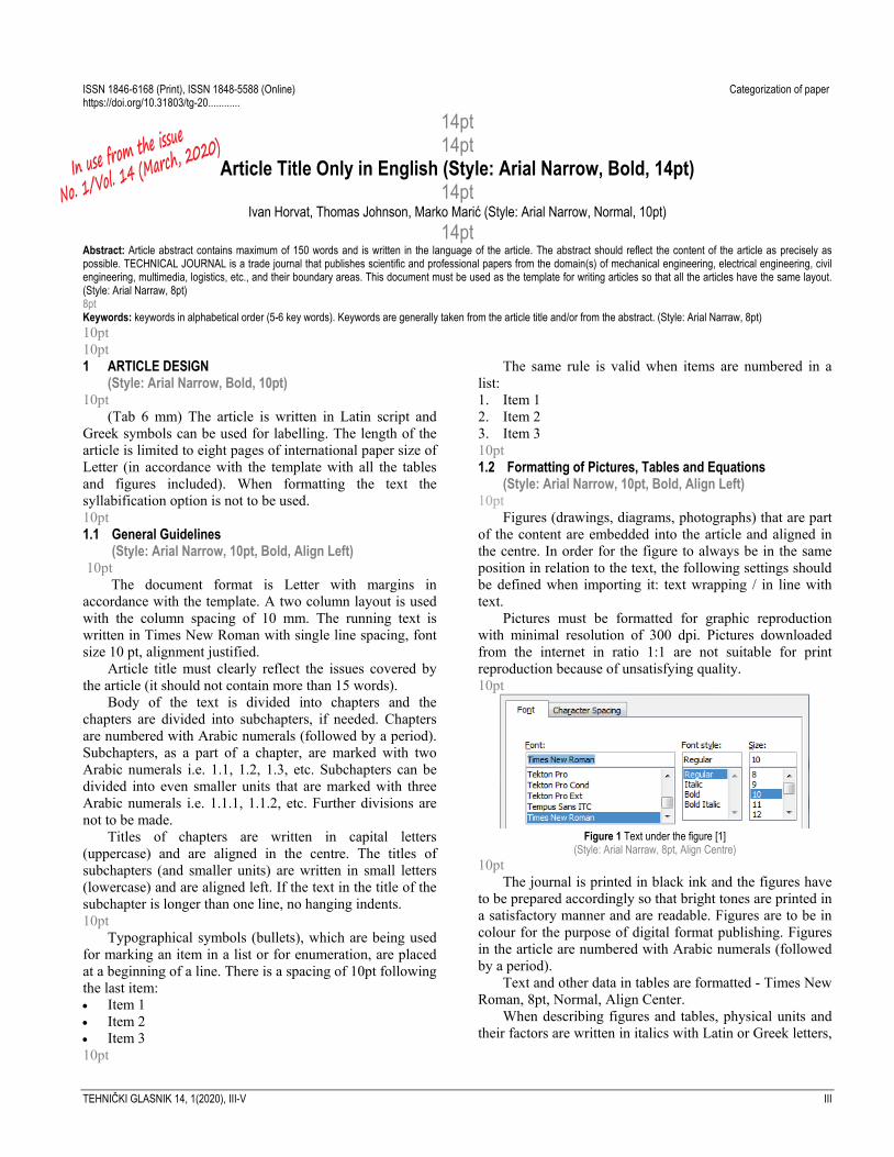
TEHNIČKI GLASNIK 14, 1(2020), III-V III
ISSN 1846-6168 (Print), ISSN 1848-5588 (Online) Categorization of paper https://doi.org/10.31803/tg-20............
14pt 14pt
Article Title Only in English (Style: Arial Narrow, Bold, 14pt) 14pt
Ivan Horvat, Thomas Johnson, Marko Marić (Style: Arial Narrow, Normal, 10pt) 14pt
Abstract: Article abstract contains maximum of 150 words and is written in the language of the article. The abstract should reflect the content of the article as precisely as possible. TECHNICAL JOURNAL is a trade journal that publishes scientific and professional papers from the domain(s) of mechanical engineering, electrical engineering, civil engineering, multimedia, logistics, etc., and their boundary areas. This document must be used as the template for writing articles so that all the articles have the same layout. (Style: Arial Narraw, 8pt) 8pt Keywords: keywords in alphabetical order (5-6 key words). Keywords are generally taken from the article title and/or from the abstract. (Style: Arial Narraw, 8pt) 10pt 10pt 1 ARTICLE DESIGN
(Style: Arial Narrow, Bold, 10pt) 10pt
(Tab 6 mm) The article is written in Latin script and Greek symbols can be used for labelling. The length of the article is limited to eight pages of international paper size of Letter (in accordance with the template with all the tables and figures included). When formatting the text the syllabification option is not to be used. 10pt 1.1 General Guidelines
(Style: Arial Narrow, 10pt, Bold, Align Left) 10pt
The document format is Letter with margins in accordance with the template. A two column layout is used with the column spacing of 10 mm. The running text is written in Times New Roman with single line spacing, font size 10 pt, alignment justified.
Article title must clearly reflect the issues covered by the article (it should not contain more than 15 words).
Body of the text is divided into chapters and the chapters are divided into subchapters, if needed. Chapters are numbered with Arabic numerals (followed by a period). Subchapters, as a part of a chapter, are marked with two Arabic numerals i.e. 1.1, 1.2, 1.3, etc. Subchapters can be divided into even smaller units that are marked with three Arabic numerals i.e. 1.1.1, 1.1.2, etc. Further divisions are not to be made.
Titles of chapters are written in capital letters (uppercase) and are aligned in the centre. The titles of subchapters (and smaller units) are written in small letters (lowercase) and are aligned left. If the text in the title of the subchapter is longer than one line, no hanging indents. 10pt
Typographical symbols (bullets), which are being used for marking an item in a list or for enumeration, are placed at a beginning of a line. There is a spacing of 10pt following the last item: • Item 1• Item 2• Item 310pt
The same rule is valid when items are numbered in a list: 1. Item 12. Item 23. Item 310pt 1.2 Formatting of Pictures, Tables and Equations
(Style: Arial Narrow, 10pt, Bold, Align Left) 10pt
Figures (drawings, diagrams, photographs) that are part of the content are embedded into the article and aligned in the centre. In order for the figure to always be in the same position in relation to the text, the following settings should be defined when importing it: text wrapping / in line with text.
Pictures must be formatted for graphic reproduction with minimal resolution of 300 dpi. Pictures downloaded from the internet in ratio 1:1 are not suitable for print reproduction because of unsatisfying quality. 10pt
Figure 1 Text under the figure [1] (Style: Arial Narraw, 8pt, Align Centre)
10pt The journal is printed in black ink and the figures have
to be prepared accordingly so that bright tones are printed in a satisfactory manner and are readable. Figures are to be in colour for the purpose of digital format publishing. Figures in the article are numbered with Arabic numerals (followed by a period).
Text and other data in tables are formatted - Times New Roman, 8pt, Normal, Align Center.
When describing figures and tables, physical units and their factors are written in italics with Latin or Greek letters,
In use from the iss
ue
No. 1/Vol. 14 (March, 2020)

Ivan Horvat at al.: Article Title Only in English
IV TECHNICAL JOURNAL 14, 1(2020), III-V
while the measuring values and numbers are written upright. 10pt
Table 1 Table title aligned centre (Style: Arial Narraw, 8pt, Align Centre)
1 2 3 4 5 6 ABC ab ab ab ab ab ab DEF cd cd cd cd cd cd GHI ef ef ef ef ef ef
10 pt Equations in the text are numbered with Arabic
numerals inside the round brackets on the right side of the text. Inside the text they are referred to with equation number inside the round brackets i.e. ".... from Eq. (5) follows ...." (Create equations with MathType Equation Editor - some examples are given below). 10pt
[ ]0avg 0
0
1( , ) ( ), ( ) d ,t t
tF t t F q p
tτ τ τ
+= ∫ (1)
-cos cos 2cos cos ,2 2
α β α βα β ++ = ⋅ (2)
T T T( ) .=AB B A (3) 10pt
Variables that are used in equations and also in the text or tables of the article are formatted as italics in the same font size as the text. 10pt
Figure 2 The texts under figures
(Style: Arial Narraw, 8pt, Align Centre) 10pt
Figure 3 The texts under figures
(Style: Arial Narraw, 8pt, Align Centre)
Figures and tables that are a part of the article have to be mentioned inside the text and thus connected to the content i.e. „ … as shown in Fig. 1…“ or „data from Tab. 1…“ and similar. 10pt 2 PRELIMINARY ANNOTATION 10pt
Article that is offered for publication cannot be published beforehand, be it in the same or similar form, and it cannot be offered at the same time to a different journal. Author or authors are solely responsible for the content of the article and the authenticity of information and statements written in the article.
Articles that are accepted for publishing are classified into four categories: original scientific papers, preliminary communications, subject reviews and professional papers.
Original scientific papers are articles that according to the reviewer and the editorial board contain original theoretical or practical results of research. These articles need to be written in such a way that based on the information given, the experiment can be repeated and the results described can be achieved together with the author’s observations, theoretical statements or measurements.
Preliminary communication contains one or more pieces of new scientific information, but without details that allow recollection as in original scientific papers. Preliminary communication can give results of an experimental research, results of a shorter research or research in progress that is deemed useful for publishing.
Subject review contains a complete depiction of conditions and tendencies of a specific domain of theory, technology or application. Articles in this category have an overview character with a critical review and evaluation. Cited literature must be complete enough to allow a good insight and comprehension of the depicted domain.
Professional paper can contain a description of an original solution to a device, assembly or instrument, depiction of important practical solutions, and similar. The article need not be related to the original research, but it should contains a contribution to an application of known scientific results and their adaptation to practical needs, so it presents a contribution to spreading knowledge, etc.
Outside the mentioned categorization, the Editorial board of the journal will publish articles of interesting content in a special column. These articles provide descriptions of practical implementation and solutions from the area of production, experiences from device application, and similar. 10pt 3 WRITING AN ARTICLE 10pt
Article is written in the English language and the terminology and the measurement system should be adjusted to legal regulations, standards (ISO 80 000 series) and the SI international system of units. The article should be written in third person.
Introduction contains the depiction of the problem and an account of important results that come from the articles that are listed in the cited literature.

Ivan Horvat et al.: Article Title Only in English
TEHNIČKI GLASNIK 14, 1(2020), III-V V
Main section of the article can be divided into several parts or chapters. Mathematical statements that obstruct the reading of the article should be avoided. Mathematical statements that cannot be avoided can be written as one or more addendums, when needed. It is recommended to use an example when an experiment procedure, the use of the work in a concrete situation or an algorithm of the suggested method must be illustrated. In general, an analysis should be experimentally confirmed.
Conclusion is a part of the article where the results are being given and efficiency of the procedure used is emphasized. Possible procedure and domain constraints where the obtained results can be applied should be emphasized. 10pt 4 RECAPITULATION ANNOTATION 10pt
In order for the articles to be formatted in the same manner as in this template, this document is recommended for use when writing the article. Finished articles written in MS Word for Windows and formatted according to this template must be submitted using our The Paper Submission Tool (PST) (https://tehnickiglasnik.unin.hr/ authors.php) or eventually sent to the Editorial board of the Technical Journal to the following e-mail address: [email protected]
The editorial board reserves the right to minor redaction corrections of the article within the framework of prepress procedures. Articles that in any way do not follow these authors' instructions will be returned to the author by the editorial board. Should any questions arise, the editorial board contacts only the first author and accepts only the reflections given by the first author. 10pt 5 REFERENCES (According to APA) 10pt
The literature is cited in the order it is used in the article. Individual references from the listed literature inside the text are addressed with the corresponding number inside square brackets i.e. "… in [7] is shown …". If the literature references are web links, the hyperlink is to be removed as shown with the reference number 8. Also, the hyperlinks from the e-mail addresses of the authors are to be removed. In the literature list, each unit is marked with a number and listed according to the following examples (omit the subtitles over the references – they are here only to show possible types of references): 9pt [1] See http://www.bibme.org/citation-guide/apa/ [2] See http://sites.umuc.edu/library/libhow/apa_examples.cfm [3] (Style: Times New Roman, 9pt, according to APA) [4] Amidzic, O., Riehle, H. J., & Elbert, T. (2006). Toward a
psychophysiology of expertise: Focal magnetic gamma bursts as a signature of memory chunks and the aptitude of chess players. Journal of Psychophysiology, 20(4), 253-258. https://doi.org/10.1027/0269-8803.20.4.253
[5] Reitzes, D. C. & Mutran, E. J. (2004). The transition to retirement: Stages and factors that influence retirement adjustment. International Journal of Aging and Human Development, 59(1), 63-84. Retrieved from
http://www.baywood.com/journals/PreviewJournals.asp?Id=0091-4150
[6] Jans, N. (1993). The last light breaking: Life among Alaska's Inupiat Eskimos. Anchorage, AK: Alaska Northwest Books.
[7] Miller, J. & Smith, T. (Eds.). (1996). Cape Cod stories: Tales from Cape Cod, Nantucket, and Martha's Vineyard. San Francisco, CA: Chronicle Books.
[8] Chaffe-Stengel, P. & Stengel, D. (2012). Working with sample data: Exploration and inference. https://doi.org/10.4128/9781606492147
[9] Freitas, N. (2015, January 6). People around the world are voluntarily submitting to China’s Great Firewall. Why? Retrieved from http://www.slate.com/blogs/future_tense/ 2015/01/06/tencent_s_wechat_worldwide_internet_users_are_voluntarily_submitting_to.html (Style: Times New Roman, 9pt, according to APA)
10pt 10pt Authors’ contacts: 8pt Full Name, title Institution, company Address Tel./Fax, e-mail 8pt Full Name, title Institution, company Address Tel./Fax, e-mail Note: Gray text should be removed in the final version of the article because it is for guidance only.

VI TECHNICAL JOURNAL 14, 1(2020), VI-VII

TEHNIČKI GLASNIK 14, 1(2020), VI-VII VII


![Истраживања ваљевске Грачанице 2011. године. Glasnik istorijskog arhiva [45]](https://static.fdokumen.com/doc/165x107/632378633c19cb2bd1068738/istrazhivaa-vaevske-grachanitse-2011-godine-glasnik.jpg)