
technical report documentation page - Caltrans - CA.gov
624
STATE OF CALIFORNIA • DEPARTMENT OF TRANSPORTATION TECHNICAL REPORT DOCUMENTATION PAGE TR0003 (REV 10/98) 1. REPORT NUMBER CA15-1535 2. GOVERNMENT ASSOCIATION NUMBER 3. RECIPIENT'S CATALOG NUMBER 4. TITLE AND SUBTITLE First Responder Support Systems Testbed (FiRST): Cross Cutting Cooperative Systems for Emergency Management 5. REPORT DATE August 2014 6. PERFORMING ORGANIZATION CODE N/A 7. AUTHOR Dr. Richard Church, Dr. John Shynk, Dr. Micah Brachman, Carlos Baez 8. PERFORMING ORGANIZATION REPORT NO. N/A 9. PERFORMING ORGANIZATION NAME AND ADDRESS University of California, UC Santa Barbara Office of Research 10. WORK UNIT NUMBER N/A 3227 Cheadle Hall, 3rd Floor Santa Barbara CA 93106-2050 11. CONTRACT OR GRANT NUMBER TA-65A0257 A03 12. SPONSORING AGENCY AND ADDRESS California Department of Transportation (Caltrans) Division of Research, Innovation and System Information, MS-83 1227 O Street Sacramento, CA 95814 13. TYPE OF REPORT AND PERIOD COVERED Final Report November 2007-November 2013 14. SPONSORING AGENCY CODE N/A 15. SUPPLEMENTARY NOTES 16. ABSTRACT This project was defined in terms of four main Tracks. Each Track addressed a specific research component of emergency operations. Track I involved the development of a prototype, mobile, virtual emergency operations center. Track II was concerned with testing and developing modeling approaches for emergency evacuation. Track III addressed a number of needs for interoperable communication facing intelligent transportation systems (ITS) and public safety (PS), and track IV was concerned with potential applications of wireless sensor networks (WSN). Here we emphasized the development of WSN that can be used to improve work zone safety. A demonstration of the Virtual Emergency Operations Center which was developed as a part of this project were highlighted by the Department of Homeland Security. It was demonstrated that for some large scale emergencies that contra-flow operations may be valuable in substantially reducing clearing times, however, manpower and equipment needed to support such an operation may not be available on a timely basis. A survey of evacuation participants subject to a mandatory evacuation indicated that nearly 10% of the population did not leave and that the choice of an exit location could alter clearing times. Both micro-scale traffic simulation and multi-commodity flow-optimization were tested in modeling evacuation. The feasibility of interoperable communications between ITS and PS has been investigated. We reported on best field practices for deploying wireless broadband, specifically for the Dedicated Short Range Communications (DSRC), and multihop ITS/PS networks. To reduce Caltrans’ worker injuries and fatalities in work zones, we investigated the use WSN and cooperative algorithms for sub-meter localization. Our simulation shows promising results for using the emerging Internet of Things (IOT) for work zone safety in both urban and rural environments. 17. KEY WORDS Cooperative systems, emergency management, transportation modeling, traffic simulation, evacuation, communication system protocols, interoperable communications, dedicated short range communications, DSRC, Internet of Things (IoT) 18. DISTRIBUTION STATEMENT No Restriction. This document is available to the public through the National Technical Information Service, Springfield, VA 22161 19. SECURITY CLASSIFICATION (of this report) Unclassified 20. NUMBER OF PAGES 624 21. COST OF REPORT CHARGED 1 Reproduction of completed page authorized. ADA Notice For individuals with sensory disabilities, this document is available in alternate formats. For information call (916) 654-6410 or TDD (916) 654-3880 or write Records and Forms Management, 1120 N Street, MS-89, Sacramento, CA 95814.
-
Upload
khangminh22 -
Category
Documents
-
view
0 -
download
0
Transcript of technical report documentation page - Caltrans - CA.gov

STATE OF CALIFORNIA • DEPARTMENT OF TRANSPORTATION TECHNICAL REPORT DOCUMENTATION PAGE TR0003 (REV 10/98)
1. REPORT NUMBER
CA15-1535
2. GOVERNMENT ASSOCIATION NUMBER 3. RECIPIENT'S CATALOG NUMBER
4. TITLE AND SUBTITLE
First Responder Support Systems Testbed (FiRST): Cross Cutting Cooperative Systems for Emergency Management
5. REPORT DATE
August 2014 6. PERFORMING ORGANIZATION CODE
N/A 7. AUTHOR
Dr. Richard Church, Dr. John Shynk, Dr. Micah Brachman, Carlos Baez
8. PERFORMING ORGANIZATION REPORT NO.
N/A 9. PERFORMING ORGANIZATION NAME AND ADDRESS
University of California, UC Santa Barbara Office of Research
10. WORK UNIT NUMBER
N/A 3227 Cheadle Hall, 3rd Floor Santa Barbara CA 93106-2050
11. CONTRACT OR GRANT NUMBER
TA-65A0257 A03 12. SPONSORING AGENCY AND ADDRESS
California Department of Transportation (Caltrans) Division of Research, Innovation and System Information, MS-83 1227 O Street Sacramento, CA 95814
13. TYPE OF REPORT AND PERIOD COVERED
Final Report November 2007-November 2013
14. SPONSORING AGENCY CODE
N/A 15. SUPPLEMENTARY NOTES
16. ABSTRACT
This project was defined in terms of four main Tracks. Each Track addressed a specific research component of emergency operations. Track I involved the development of a prototype, mobile, virtual emergency operations center. Track II was concerned with testing and developing modeling approaches for emergency evacuation. Track III addressed a number of needs for interoperable communication facing intelligent transportation systems (ITS) and public safety (PS), and track IV was concerned with potential applications of wireless sensor networks (WSN). Here we emphasized the development of WSN that can be used to improve work zone safety. A demonstration of the Virtual Emergency Operations Center which was developed as a part of this project were highlighted by the Department of Homeland Security. It was demonstrated that for some large scale emergencies that contra-flow operations may be valuable in substantially reducing clearing times, however, manpower and equipment needed to support such an operation may not be available on a timely basis. A survey of evacuation participants subject to a mandatory evacuation indicated that nearly 10% of the population did not leave and that the choice of an exit location could alter clearing times. Both micro-scale traffic simulation and multi-commodity flow-optimization were tested in modeling evacuation. The feasibility of interoperable communications between ITS and PS has been investigated. We reported on best field practices for deploying wireless broadband, specifically for the Dedicated Short Range Communications (DSRC), and multihop ITS/PS networks. To reduce Caltrans’ worker injuries and fatalities in work zones, we investigated the use WSN and cooperative algorithms for sub-meter localization. Our simulation shows promising results for using the emerging Internet of Things (IOT) for work zone safety in both urban and rural environments.
17. KEY WORDS
Cooperative systems, emergency management, transportation modeling, traffic simulation, evacuation, communication system protocols, interoperable communications, dedicated short range communications, DSRC, Internet of Things (IoT)
18. DISTRIBUTION STATEMENT
No Restriction. This document is available to the public through the National Technical Information Service, Springfield, VA 22161
19. SECURITY CLASSIFICATION (of this report)
Unclassified
20. NUMBER OF PAGES
624
21. COST OF REPORT CHARGED
1 Reproduction of completed page authorized.
ADA Notice For individuals with sensory disabilities, this document is available in alternate formats. For information call (916) 654-6410 or TDD (916) 654-3880 or write Records and Forms Management, 1120 N Street, MS-89, Sacramento, CA 95814.

DISCLAIMER STATEMENT
This document is disseminated in the interest of information exchange. The contents of this report reflect the views of the authors who are responsible for the facts and accuracy of the data presented herein. The contents do not necessarily reflect the official views or policies of the State of California or the Federal Highway Administration. This publication does not constitute a standard, specification or regulation. This report does not constitute an endorsement by the Department of any product described herein.
For individuals with sensory disabilities, this document is available in alternate formats. For information, call (916) 654-8899, TTY 711, or write to California Department of Transportation, Division of Research, Innovation and System Information, MS-83, P.O. Box 942873, Sacramento, CA 94273-0001.
2

First Responder Support Systems Testbed (FiRST) Contract # 65A0257
Cross-Cutting Cooperative Systems Final Report
3
The First Responders Systems Testbed (FiRST) is comprised of a number of interrelated tasks, all with a focus of addressing the needs of the State of California and Caltrans. This project was conceived as an attempt to address a number of critical issues that Caltrans and other public agencies will face in the event of disasters and disruptive events. California needs the capability of responding quickly and efficiently to any disaster, and its road, communication, and data systems networks will play key roles in any response. Caltrans will play a significant role in operating and managing the highway infrastructure during any crisis, whether it be flooding in the central valley, a large earthquake in an urban center such as Los Angeles or San Francisco, a Tsunami that will take out segments of Highway 101 on the North coast of California or the Ports of LA or Long Beach, or even a major industrial crisis like that of a failure at Diablo Canyon Power Plant.
A set cross-cutting cooperative systems is required to respond to any major emergency, the different tracks developed under the FiRST contract addressed the integration of such systems. It investigated the significant capability required to manage assets, communicate and share information across jurisdiction and geographical boundaries, and the ability to access up-to-date information and model possible
consequences of action. This is not a simple task and often complacency can set in when the return period for such events can be long. For example, the 1994 Northridge 6.7 earthquake caused considerable damage, even though it is considered to be a mild earthquake compared to a 7.5 or greater trembler. For Caltrans to promote safety, aid in emergency response, secure roadways, and enhance maintenance, there are a number of key elements
Principal Investigator: Dr. Richard Church
Co-Principal Investigator: Dr. John Shynk
University of California Santa Barbara
Contract Manager: Ramez Gerges, Ph.D., P.E.

First Responder Support Systems Testbed (FiRST) Contract # 65A0257
Cross-Cutting Cooperative Systems Final Report
4
that should be addressed. This includes the development of a virtual operations center. In major disasters, there are no guarantees that operations centers will remain intact or be capable of operating. In several recent past events, like that in Santa Barbara County, the county’s emergency operation center was at risk to a major wildfire and had to be closed, making coordinated operations more difficult to control. In response the county built a new state of the art facility that contains on-line records for all county operations, is configured to serve as a fully functional command and control center, backup generators and fuel storage to support the center in times of power disruptions, as well as many other features. But, such brick and mortar facilities cannot be fully relied upon and it is important to develop the capabilities to operate a virtual emergency operations center from anywhere. It is also important to develop communications systems that can cross agencies, handle voice, video, and data, so that managers can easily communicate, coordinate, and operate their response effectively and efficiently. It is also important to be able to develop and test approaches for operating a transportation system in a crisis, supporting both supply and evacuation needs. The citizens of the State rely on Caltrans to ensure safe highway operations on a daily basis, but even more so in a time of crisis. The FiRST project was designed to address a number of these needs by developing state-of-the art prototypes and models for possible use in future Caltrans operations.
This project was defined in terms of four main tracks or Tasks. Each Track addressed a specific component of emergency operations. Track I involved the development of a prototype emergency operations center. Track II was concerned with testing and developing a modeling approach for emergency evacuation. Track III addressed a number of needs for interoperable communication and their integration to support those cooperative systems, and track IV was concerned with investigating the use of wireless sensor and communication network. Here we emphasized the development of wireless sensor networks that can be used to improve work zone safety.
This report covers developments of those cross-cutting cooperative systems investigated in all four tracks. Altogether, this project has accomplished several significant milestones. These include:
The development of a prototype virtual emergency operations center (VEOC). The VEOC prototype implemented the Unified Incident Command and Decision Support (UICDS) architecture originally developed by the Department of Homeland Security (DHS). This effort was demonstrated during the Golden Guardian statewide exercise in 2012 and 2013, and was recognized by DHS as the first successful implementation of the UICDS architecture in California. In addition, this VEOC was designed to integrate and use the Caltrans PeMS data, as well access to the Caltrans Earth.
Developed a simulation of a large are evacuation associated with San Luis Obispo. This simulation utilized PTV VISSIM micro-scale traffic simulation system. Two approaches were developed, one based upon dynamic trip assignment, and the other based upon fixed trip assignment. Both approaches were test on a mock contra-flow operations plan as well as a baseline operations scenario. The mock contra-flow plan was shown to provide substantial

First Responder Support Systems Testbed (FiRST) Contract # 65A0257
Cross-Cutting Cooperative Systems Final Report
5
promise in clearing a large region like San Luis Obispo. This result is important in that this may form the basis for better levels of service in an emergency for Caltrans assets.
Surveyed participants in a wildfire evacuation and demonstrated that the number of people deciding to evacuate and their timing could be estimated by a Rayleigh Probability Model. Our survey indicated that approximately 10% of the homes had at least one occupant who stayed behind, even when the neighborhood was engulfed in flames. This fact alone suggests that emergency managers will have to address a relatively large population who stayed behind.
Developed a new prototype multi-commodity flow optimization model that can be used as a potentially fast tool to estimate clearing times and bottlenecks at a meso-scale. This model could mimic actual routes chosen when tested against actual evacuation data.
Developed an emergency equipment and personnel allocation model that can be used to allocate resources during a major contra-flow event with the objective of placing a contra-flow plan in action as quickly as possible. This model was not fully tested or developed as appropriate data was not supplied by Caltrans.
Integrated the on-going national standards development activities to achieve interoperable communications between agencies using the intelligent transportation systems (ITS), and the public safety (PS) frequency bands. It developed and documented best field practices for the deployment of wireless broadband for Caltrans and other first responders.
Investigated multihop networks as an alternative approach for integrating both ITS & PS networks to enhance wireless services required by first responders.
Developed and demonstrated the use of broadband channel emulation technology as a robust tool for broadband wireless protocol testing and validation in various deployment environment
Developed a prototype for Hastily Deployed intranet Network (HDiN) nodes. The HiDN prototype provides different communications technologies to connect to the Internet, and provides a local intranet to connect cooperating first responders. When connectivity to the Intranet is restored, it synchronizes itself; it is designed to work when other systems won’t. The HiDN nodes could be engineered to support the VEOC functionality including the integration of PeMS, hosting a local copy of Caltrans` Earth, as well as broadcasting video streams from selected sources. It is envisioned that the current suitcase size prototype could provide critical support of Caltrans and other first responders without relying on the availability of the Internet or the cloud.
Developed innovative solutions to reduce Caltrans’ worker injuries and fatalities in work zones using networked wireless sensors. These sensors can be deployed along work sites to monitor the safety of work zones. It can be deployed on traffic cones and its cost would be relatively low to fully deploy. Potentially, this technology could also extended to the emerging connected vehicles environment.
Overall this project was a significant success, providing cutting edge modeling, technology enhancement and prototype development that can be used by future generations of Caltrans employees. Reports on each of the project tracks follows in order.

6
First Responder Support Systems Testbed (FiRST) Cross Cutting Cooperative Systems for Emergency Management
Table of Contents
1 EXECUTIVE SUMMARY..................................................................................................................................................... 3
2 TRACK I – Virtual Emergency Operation Center (VEOC) ................................................................................... 6
2.1 VEOC High-Level Architecture ......................................................................................................................... 11
2.2 High-Level Systems Requirements ............................................................................................................... 23
2.3 The Golden Guardian Demonstration .......................................................................................................... 37
3 TRACK II – Cross Cutting Modeling & Simulation..........................................................................................,. ...... 51
3.1 Simulating An Evacuation Event. ..................................................................................................................... 54
3.2 Summary of Dynamic Traffic Assignment in VISSIM ............................................................................... 85
3.3 Cognitively Engineered Evacuation Routes ................................................................................................................ 164
3.3 Modeling the Evacuation Decision ................................................................................................................ 218
3.4 Planning for a Disaster. ..................................................................................................................................... 325
4 TRACK III – Interoperable Communications......................................................................................., ................... 432
4.1 Best Practices For Wireless Broadband Deployment. .......................................................................... 433
4.2 Multihop Networks: An Alternative Wireless Broadband Communications ................................ 467
4.3 Broadband Wireless Channel Emulation ................................................................................................... 487
4.4 Interoperable Emergency Communications: The HiDN Platform ..................................................... 513
4 TRACK IV – FiRST Baseline Enhancement & Maintenance...........,. .................................................................. 549
5.1 Wireless Sensor Networks for Cooperative Work Zone Safety. ........................................................ 552
5.2 Simulink and Hardware in the Loop ........................................................................................................... 581
5.3 Matlab Code ......................................................................................................................................................... 589

7
Principal Investigator: Dr. Richard Church University of California Santa Barbara
Contract Manager: Ramez Gerges, Ph.D., P.E.
First Responder Support Systems Testbed (FiRST) Contract # 65A0257
Cross-Cutting Cooperative Systems
TRACK I – Virtual Emergency Operation Center (VEOC)
Final Report
Virtual Emergency Operation Center (VEOC): This research was requested by Caltrans to support statewide multi-agency disaster response operations and management, as well as for day-to-day incident management at the Districts. The task was to investigate a robust architecture and to develop a standard-based prototype implementation for a VEOC. The selected VEOC architecture was to be scalable across functional, jurisdictional, and geographical boundaries.
This effort developed a set of requirements and demonstrated a prototype implementation that is based on the Unified Incident Command and Decision Support (UICDS) architecture originally developed by the Department of Homeland Security (DHS). Additionally, it developed for the first time a special software adapter to integrate the Caltrans’ PeMS data into the VEOC implementation. This effort was demonstrated during the Golden Guardian statewide exercise in 2012 and 2013, and was recognized by DHS as the first successful implementation of the UICDS architecture in California.

8
Virtual Emergency Operations Center Architecture, Prototype, and Demonstration
February 3, 2014

FiRST Testbed VEOC Final Report: Architecture and Prototype
9
1 VEOC Executive Summary This report presents an operational scenario and a high level architecture developed for the Virtual Emergency Operation Center (VEOC). A subset of the VEOC architecture has been implemented using the Unified Incident Command and Decision Support (UICDS). A high-level comparison between VEOC and WebEOC is described.
The operational scenario developed is intended to demonstrate how the VEOC is able to support incident management across functional, jurisdictional, and geographical boundaries. The scenario shows how VEOC enables incident management organizations from various jurisdictions and performing different incident response functions to interwork transparently as single integrated virtual incident management organization.
The VEOC architecture is designed to support incident management applications from different vendors that perform different incident management functions to inter-work across different jurisdictions and geographical locations. The architecture of VEOC enables it to scale up to support large incidents and provides an efficient mechanism for communications and information distribution.
A prototype implementation of a scaled-down VEOC architecture is developed using the UICDS. The prototype receives information from PeMS and LCS, and analyzes the data in real time for traffic incidents. When a traffic incident is detected, a UICDS incident is created that triggers off other incident response actions. A Viewer application is also developed for viewing incident information and data from PeMS and LCS.

FiRST Testbed VEOC Final Report: Architecture and Prototype
10
2 Project Description 2.1 Objectives and Scope The main objectives of this project are threefold: to identify major high-level requirements for a virtual emergency operations center (VEOC), to implement a simplified prototype based on the Unified Incident Command and Decision Support (UICDS) framework to study the feasibility of essential requirements, and to investigate and compare selected essential enabling technologies.
2.2 Introduction The project demonstrated the critical impact of the status of the transportation network during few state-wide exercises, namely the Golden Guardian in handling earthquake scenario.
• Architecture and Prototype This section describes the high-level VEOC architecture, and a prototype based on UICDS.
• VEOC High-Level Systems Requirements This section presents the high-level systems requirements and testing for future implementation efforts.

FiRST Testbed VEOC Final Report: Architecture and Prototype
11
3 VEOC High-Level Architecture The architecture of VEOC is designed to support incident management across jurisdictional, functional, and geographical boundaries, ranging from small local incidents to large-scale incidents. The VEOC architecture is organized as a network of systems. Each system connects a group of incident management applications within the same jurisdiction or geographical area. Different incident management applications connected to a system may provide different incident management functions. In addition, different sensors may also be connected to a system to provide data for monitoring and managing incidents. The systems are interconnected to form a federation to enable communications and information exchange throughout the entire federation.
Scalability
The network-of-systems architecture enables VEOC to scale up to support management of large incidents. As the scale of incident response increases to include more jurisdictions or geographical areas, the number of systems in the federation that are involved in the incident management also increases. Similarly, as more incident response functions are needed, the number of incident management applications that are involved in the incident response also increases.
Information and Communication Model
The VEOC architecture provides an efficient information dissemination and communication model. Each system in the federation supports information exchange between incident management applications using the publish-subscribe model. It enables information relevant to the incident response to be published and accessible by incident management applications connected to the system. Each incident management application subscribes and receives only information that is relevant or of interest.
The VEOC architecture also supports information exchange between systems in the federation. Information is forwarded from one system to the others based on pre-arranged mutual agreements. When forwarded information is received by a system, it delivers the information to the local management applications according to their subscription preferences. This approach not only supports information dissemination across the federation, but also minimizes the amount of information that is exchanged between systems, as it eliminates pair-wise information exchange between incident management applications connected to different systems.
UICDS Implementation
The VEOC architecture can be implemented using UICDS. The UICDS architecture (Figure 1) consists of a network of ‘cores’, with each core connecting multiple clients. Each VEOC system in a federation can be implemented by a UICDS core. VEOC inter-system communication is provided by UICDS inter-core communication.

FiRST Testbed VEOC Final Report: Architecture and Prototype
12
Figure 1: UICDS High Level Architecture
The high-level architecture of VEOC is as shown in Figure. It supports the operation scenario described in Section 4 that involves incident management across a number of jurisdictions, geographical areas, and functional organizations. There are four jurisdictions shown in Figure, namely Caltrans, county, state, and federal jurisdictions. Each jurisdiction is supported by a UICDS core. Each UICDS core has a number of incident management applications connected to it. For example, at the state level, the state police and state Office of Emergency Management (OEM) are connected to the State UICDS Core. Similarly, the County UICDS Core and Federal UICDS Core have, respectively, county level and federal level incident management applications connected to them.

FiRST Testbed VEOC Final Report: Architecture and Prototype
13
PeMS
LCS
CHP
State PD
UICDS Admin Console
State Jurisdiction
State UICDS Core
Data
PeMS Adapter
LCS Adapter
CHP Adapter
TMC
FD HAZMAT
UICDS Admin Console
COP Caltrans UICDS Core XMPP County UICDS Core County Jurisdiction
Data EMS Local PD
Airport Control Tower
Probe Data
Video
FAA Airline
UICDS Admin
Console
Federal
UICDS Web Services Sensor Data
Caltrans Jurisdiction
Federal UICDS Core Jurisdiction
Client specific protocol XMPP FBI EPA Airport
Management
Figure 2: VEOC High Level Architecture
State OEM
Probe Data Adapter
Video Adapter
UICDS Admin Console
Adapters
In Figure, the Caltrans UICDS Core has a number of traffic applications connected to it via adapters, including PeMS, CHP, LCS, probe data, and roadside video. These applications collect various important traffic incident information and traffic data that are needed in monitoring and managing incident responses. In UICDS, these data sources are considered as data sensors. The functionalities of the adapters that connect these data sensors to the UICDS core include:
• Data and operations adaptation
The adapters connect to the UICDS core and data sensors using APIs and data formats specified by the UICDS and data sensors respectively. Inside the adapters, mapping of data and operations is performed between the two data formats and APIs.
• Sensor data retrieval In the UICDS architecture, sensor data is delivered using an out-of-band approach
whereby incident management applications are notified of sensor data availability by the UICDS core. The incident management applications then proceed to retrieve sensor data directly from the sensors. The adapters provide such an interface for the retrieval of sensor data.

FiRST Testbed VEOC Final Report: Architecture and Prototype
14
• Incident detection and creation In addition to receiving data continuously from the sensors, the adapters may also analyze the data in real time to detect various traffic incidents or events, such as accidents or congestions. Upon detecting such traffic incidents or events, the adapters register the incidents in UICDS by creating a UICDS incident in the UICDS core. Notifications are then sent by the UICDS core to incident management applications to inform them of the incidents.
Common Operating Picture
In the VEOC architecture, a Common Operating Picture (COP) application is connected to the Caltrans UICDS Core. The role of the COP application is to continuously collect information from various sources and create a common operating picture that provides important information needed for monitoring and managing incidents. Examples of such information include information about traffic incidents, such as the type, location, time and description of incidents, and traffic data related to incidents.
Administration Console
The UICDS Administration Console provides the capabilities for managing UICDS cores, such as managing information sharing agreements and resource profiles.
Standards
UICDS adopts a number of standards related to incident management. The Emergency Data Exchange Language – Distribution Element (EDXL-DE) is used to encapsulate messages to and from the UICDS core. EDXL-DE facilitates routing of properly formatted XML emergency messages to recipients. The Emergency Data Exchange Language – Resource Messaging (EDXL-RM) is used to provide a set of standard formats for emergency response messages. The Common Alerting Protocol (CAP) is used to provide the format for exchanging emergency alerts. Access to the UICDS core is via web services as defined in the UICDS Web Service Definition Language (WSDL). The Extensible Messaging and Presence Protocol (XMPP) is used for messaging between UICDS cores.

FiRST Testbed VEOC Final Report: Architecture and Prototype
15
4 Operation Scenario In this section, we describe an operational scenario to show how a UICDS-based VEOC can integrate emerging capabilities with traditional emergency management functions to achieve integrated cross-organizational emergency management.
Scenario – Concept of Operation
The following describes details of the scenario, and the operation flows:
Creation of an incident in a UICDS core causes notifications to be sent to incident management systems or applications that are connected to the core. This enables incident management systems to be informed of the incident and to initiate incident response procedures. Incident notifications are also sent to other UICDS cores that are involved in the incident management and that have pre-arranged agreements to share incident information.
a) Incident notifications are sent by the County UICDS Core to local incident management organizations, namely the local Police Department (PD), Fire Department (FD), EMS, and HAZMAT.
A UICDS core often connects incident management organizations that are in the same jurisdiction. When an incident is created in the core, incident notifications are automatically sent to these organizations, enabling them to respond to the incident immediately.
b) Inter-core incident notifications are also sent by the County UICDS Core to Caltrans, State, and Federal UICDS Cores.
In addition, incident notifications are also forwarded to other UICDS cores that have pre- arranged agreements for information sharing. These other UICDS cores then deliver the notifications to their local incident management systems. This approach allows the system to scale up and minimize traffic between cores.
c) Upon receiving the incident notification, the Caltrans UICDS Core delivers the notification to local incident management systems, namely the Traffic Management Center (TMC) and the Common Operating Picture (COP) application, to inform them of the incident and enable them to initiate appropriate response actions. The Caltrans UICDS Core forwards the incident notification to the local TMC.
d) The TMC detects a traffic incident on the interstate highway from real-time analysis of PeMS data. The TMC is continuously receiving data from PeMS, and CHP, as well as live roadside videos. It analyzes the data in real time to detect any traffic incident and anomaly.
e) The TMC verifies the incident has occurred by cross-correlating the PeMS data with CHP data and other resources such as live videos. This significantly increases the
FiRST Testbed VEOC Final Report: Architecture and Prototype
16
accuracy and timeliness of incident detection. It enables the TMC to verify that the incident has occurred, and to provide further information on the incident, such as location, time, and nature of the incident. After verifying the incident, the TMC creates (registers) an incident in the Caltrans UICDS Core. This enables other incident management organizations to initiate their response actions.
f) The TMC creates Sensor Observation Information (SOI) Work Products (WP) in the Caltrans UICDS Core for CHP data, PeMS data, video, and LCS data.
To ensure the involved incident management organizations stay informed and have access to latest sensor data from Caltrans, the TMC creates SOI WPs in the UICDS core for sensor data that is related to the incident. This enables incident management applications to obtain sensor data needed to support their response action plans.
g) The TMC associates SOI WPs with the specific incident in the Caltrans UICDS Core.
This creates in the UICDS system an association between the incident and sensor data that is related to the incident. In this way, incident management applications will stay informed as they will be notified when sensor data related to the incident is available.
h) The Caltrans UICDS Core sends incident and WP notifications to the field incident response team to inform it of the incident and available sensor data.
i) The Caltrans UICDS Core also forwards incident and WP notifications to the County, State, and Federal UICDS Core.
Through interconnection and information sharing agreements, the County, State, and Federal UICDS Cores receive notifications of the incident and available sensor data. These notifications are then delivered to incident management organizations in the county, state, and federal jurisdictions, thereby enabling these organizations to immediately initiate their incident response actions.
j) Upon receiving incident and WP notifications, the field incident response team through the COP application requests and retrieves CHP data, PeMS data, and LCD data.
The COP application, using information in the notifications, retrieve data from sensors to create a common operating picture that contains important information needed for monitoring and managing the response to the incident, including the type, location, time, and description of the incident, and traffic data related to the incident.
k) When the County UICDS Core receives incident and WP notifications from the Caltrans UICDS Core, it delivers the notifications to incident management organizations in its jurisdiction, including the local PD, FD, EMS, and HAZMAT.

FiRST Testbed VEOC Final Report: Architecture and Prototype
17
Probe Vehicles CHP PeMS
Video Sensors TMC LCS COP County
UICDS Core State UICDS
Core Federal
UICDS Core
nt / WP N
/ WP Noti 1. Inciden
Probe DaOI WPs fo
y)
eMS, Video & ane Crash o
on Highwa
ta, CHP, P
ications (Pl
B4
B1. Notifi B2. PeM S Data
B10. Associate WPs to Incident
Caltrans UICDS Core
A4. Incident Notification (Plane Disappearing from Radar)
ed
. UICDS Operation
Non-UICDS Operation
r LCS Data
t f n Highway)
B12. Incide B13. Request / Receive Probe Data, CHP Data, PeMS
Data, Video & LCD Data
Figure 3: VEOC Operation Flow at Caltrans UICDS Core Level
way)
ash on High
s (Plane Cr
otification
B1
B9. Create S
B6. Vide
ified
ane Crash
CHP Data
cident Ver
cident (Pl
ident Detect e Data
o
B3. Inc
B5. Prob
B7. In
B8. Create In
ncident cations
The notifications inform county-level incident management organizations of the specific incident and provide them with access to sensor data related to the incident. This enables county-level incident management organizations to immediately respond to the incident.
l) In case of a wide area emergency that goes beyond a single county, the State UICDS Core may then receive the emergency notification from the County UICDS Core, it delivers the notification to the state law enforcement (CHP) and the state Office of Emergency Management (e.g. CalEMA) to enable them to initiate state-level response.
m) Upon receiving incident and WP notifications from the Caltrans UICDS Core about the wide area emergency, the State UICDS Core sends the notifications to the CHP and CalEMA. These notifications from the Caltrans UICDS Core contain more precise and detailed information on the incident.

FiRST Testbed VEOC Final Report: Architecture and Prototype
18
UICDS Web Services Client specific protocol Sensor Data XMPP
Figure 4: Architecture of Phase I Prototype
PeMS Historical PeMS LCS
PeMS Adapter
Viewer 1
LCS Adapter
Viewer 2
UICDS Core 1 UICDS Core 2
UICDS Admin Console
UICDS Admin Console
5 Prototyping The prototyping work involves implementing a scaled-down version of the VEOC architecture using UICDS. Figure 4 shows the architecture of the prototype. The prototype involves two UICDS cores. The UICDS Core 1 connects to the PeMS system, and Historical PeMS system at FIRST Testbed that contains historical PeMS data. The UICDS Core 2 connects to the LCS system. Each UICDS core also connects to a Viewer application that provides viewing of incident and traffic data, and a UICDS Administration Console.
5.1 Components The components included in this prototype are the PeMS Adapter, LCS Adapter, and Viewer application. The UICDS Administration Console is provided by UICDS.
PeMS Adapter
The PeMS Adapter is a bridge that connects the PeMS system to the UICDS Core 1. It supports automatic data retrieval and processing from PeMS through an FTP interface. It also provides additional data analysis and incident identification capabilities. Upon identifying an incident, the PeMS Adapter will create a UICDS incident and publish this incident in the UICDS Core 1. The PeMS Adapter also provides an interface for the Viewer application to access the PeMS data.
The PeMS Adapter also connects to the Historical PeMS system at the FIRST Testbed. When PeMS is not available, the PeMS Adapter is able to retrieve historical data from the Historical PeMS system.

FiRST Testbed VEOC Final Report: Architecture and Prototype
19
LCS Adapter
Similar to the PeMS Adapter, the LCS Adapter is a bridge that connects the LCS system to the UICDS Core 2. It supports automatic data retrieval and processing from LCS via an HTTP interface. It also provides additional data analysis and incident identification capabilities. Upon identifying an incident, the LCS Adapter will create a UICDS incident and publish this incident in the UICDS Core 2.
Figure 5: UICDS Administration Console Viewer Application
The Viewer application is a web-based application that retrieves data from the PeMS Adapter and LCS Adapter to create a common operation picture of an incident. It provides VEOC users with a single portal for viewing data from PeMS and LCS, as well as viewing of UICDS incidents. In this phase, users could view the following data using the Viewer application:
• Loop data from PeMS • Lane closure incident data from LCS • Incident data from the UICDS core
UICDS Administration Console
This is the administration system for managing the UICDS core. Figure shows a snapshot of the system. The administration functions available include:
• Managing agreements with other UICDS cores, such as creating, rescinding and modifying agreements. A mutual agreement needs to be established for UICDS cores to share information with one another.

FiRST Testbed VEOC Final Report: Architecture and Prototype
20
• Managing resource profiles, such as creating, deleting and updating resource profiles • Viewing of incidents, work products, etc.
5.2 UICDS Services The PeMS Adapter, LCS Adapter, and Viewer application interact with the UICDS core using web services provided by the UICDS core. These UICDS services include Resource Instance Service, Resource Management Service, Work Product Service, Sensor Service, Incident Management Service, and Notification Service. The services accessed by each of the prototype components are described below.
PeMS Adapter
Using the Resource Instance Service, the PeMS Adapter registers itself with the UICDS core as a resource instance. It uses the Sensor Service to create a Sensor Observation Information (SOI) work product. The SOI work product contains information that is needed by other applications to retrieve the PeMS data directly from the PeMs Adapter. The PeMS Adapter also uses the Incident Management Service to create and publish UICDS incidents in the UICDS core.
PeMS Adapter also publishes the raw data retrieved from PeMS system to a web-based user interface.
LCS Adapter
The LCS Adapter uses the Resource Instance Service to register itself with the UICDS core as a resource instance. It also uses the Sensor Service to create a SOI work product that contains the information needed for other applications to retrieve LCS data from the LCS Adapter. In addition, the LCS Adapter uses the Incident Management Service to create and publish UICDS incidents in the UICDS core.
LCS Adapter also publishes the raw data retrieved from PeMS system to a web-based user interface.
Viewer Application The Viewer application uses the Resource Instance Service to register itself with the UICDS core as a resource instance. It is notified through the Notification Service when incidents or work products that it subscribes to are created or updated.
Viewer Application publishes the received incident notification messages and associated information to a web-based user interface.
5.3 Operation Flow The operation flow of the Phase I prototype is as shown in Figure 6. In this operational scenario, both the PeMS Adapter and LCS Adapter retrieve data from PeMS and LCS respectively, and analyze the data in real-time for traffic incidents. The PeMS Adapter detects a traffic incident

FiRST Testbed VEOC Final Report: Architecture and Prototype
21
and creates (or registers) an incident in the UICDS Core 1. The Viewer 1 application is notified of the incident. The incident information is also sent to UICDS Core 2, and then onto the Viewer 2 application. Both Viewer applications then retrieve data from the PeMs Adapter and present it to users for viewing.
The LCS Adapter detected another incident and creates an incident in UICDS Core 2. The Viewer 2 application is notified of the incident. This incident is also sent to UICDS Core 1. As a result, the Viewer 1 application is also notified of the incident. The Viewer applications then proceed to retrieve data from LCS present it to users.
Figure 6: Operation Flow of Phase I Prototype
UICDS Admin
Console UICDS Core 1
PeMS Adapter PeMS
Historical Viewer PeMS 1
Viewer LCS LCS UICDS 2 Adapter Core 2
UICDS Admin
Console
A1. Create Profiles B1. Create Profiles
A2. Register B2. Register
A4. Incident Detected
A5. Create
ent Detected
SOI WP
ncident
te WPs to Incident
s tions
UICDS Operation
Non-UICDS Operation
ve LCS Data uest / Recei B11. Req
a
eMS Dat
st / Receive P
B12. Reque
e PeMS Data est / Receiv A11. Requ
S Data
eceive LC
WP Notifica
S Incident /
B10. PeM
quest / R
A12. Re
s
Notification
cident / WP
A10. LCS In
P Notification
ncident / W
B9. LCS I
ns P Notificatio cident / W A9. PeMS In
A8. Incident
tifications A7. Associat
B7. Associa A6. Create I
B6. Create I
cident
cations
SOI WP
ncident
e WPs to In
/ WP Notifi
nt / WP No
A3. Histor
ata
B4. Incid
B5. Create
B3. LCS D B8. Incide
ata
Data
ical PeMS D
A3. PeMS
Details of the operation flow at UICDS Core 1 are as follows:
A1. UICDS Administration Console creates profiles in the UICDS Core 1 for the PeMS Adapter and Viewer 1 application.
A2. Upon starting up, the PeMS Adapter and Viewer 1 application register with UICDS Core 1.
A3. The PeMS Adapter receives data in real time from PeMS. In the event that the PeMS system is not available, the PeMS Adapter will retrieve data from the Historical PeMS system which contains historical PeMS data. (non-UICDS operation).
A4. In analyzing PeMS data, the PeMS Adapter detects a traffic incident. A5. The PeMS Adapter creates a Sensor Observation Information (SOI) Work Product
(WP) for PeMS data.

FiRST Testbed VEOC Final Report: Architecture and Prototype
22
A6. The PeMS Adapter creates an incident in UICDS Core 1. A7. The PeMS Adapter associates the SOI WP with the incident.
A8. The UICDS Core 1 sends Incident and WP notifications to the Viewer 1 application. A9. The UICDS Core 1 also sends Incident and WP notifications to the UICDS Core 2.
A10. The UICDS Core 1 receives (LCS) incident and WP notifications from UICDS Core 2, and sends them to the Viewer 1 application.
A11. The Viewer 1 application retrieves PeMS data from the PeMS Adapter and presents the data to the user (non-UICDS operation).
A12. The Viewer 1 application retrieves LCS data from the LCS Adapter and presents the data to the user (non-UICDS operation).
Details of the operation flow at UICDS Core 2 are as follows:
B1. UICDS Administration Console creates profiles in the UICDS Core 2 for the LCS Adapter and Viewer 2 application.
B2. Upon starting up, the LCS Adapter and Viewer 2 application register with UICDS Core 2.
B3. The LCS Adapter receives data in real time from LCS. (non-UICDS operation). B4. In analyzing LCS data, the LCS Adapter detects a traffic incident.
B5. The LCS Adapter creates an SOI WP for LCS data. B6. The LCS Adapter creates an incident in UICDS Core 2. B7. The LCS Adapter associates the SOI WP with the incident. B8. The UICDS Core 2 sends Incident and WP notifications to the Viewer 2 application. B9. The UICDS Core 2 also sends Incident and WP notifications to the UICDS Core 1. B10. The UICDS Core 2 receives (PeMS) incident and WP notifications from UICDS Core
1, and sends them to the Viewer 2 application. B11. The Viewer 2 application retrieves LCS data from the LCS Adapter and presents the
data to the user (non-UICDS operation). B12. The Viewer 2 application retrieves PeMS data from the PeMS Adapter and presents
the data to the user (non-UICDS operation).

FiRST Testbed VEOC Final Report: Architecture and Prototype
23
5.4 High-Level Systems Requirements The high-level systems requirements of VEOC are described in this section.
Generic Functionalities
VEOC-SR 1. VEOC shall provide a Common Operating Picture (COP) of incidents to system users and shall keep the COP up to date throughout the incident management process.
VEOC-SR 2. The COP shall support user access through standard Web browsers on desktop computers, laptop computers and mobile devices.
VEOC-SR 3. The user interface of the COP, including presentation, data type and content, shall be customizable to fit the different user requirements and user device capabilities.
VEOC-SR 4. The COP shall support user-configurable monitoring on authorized and interested types of incidents.
VEOC-SR 5. The COP shall support incident monitoring with user-configurable threshold values and methods of notification.
VEOC-SR 6. The COP shall support multiple options to deliver notifications, including SMS and email at minimum.
VEOC-SR 7. The COP shall support dashboard-like user interface and provide access to information of system resource and incidents based on user account authorization and configuration.
VEOC-SR 8. VEOC shall support critical communications, such as real-time chatting, status update, streaming video, streaming audio/voice, between incident management agencies, personnel, applications and other entities.
System Management
VEOC-SR 9. VEOC shall provide system management functionalities that include, at a minimum, system configuration, user account management, access control system and data back-up, system resource allocation.
Interconnection
VEOC-SR 10. The VEOC shall be able to interconnect multiple incident management applications and entities across all levels of jurisdictions, including local, state and federal. Examples of incident management entities include traffic management centers, incident management centers, traffic management centers, police, fire departments, hazmat, and emergency medical services.
VEOC-SR 11. The VEOC shall be able to interconnect geographically distributed incident management applications and entities.
FiRST Testbed VEOC Final Report: Architecture and Prototype
24
Information management and dissemination
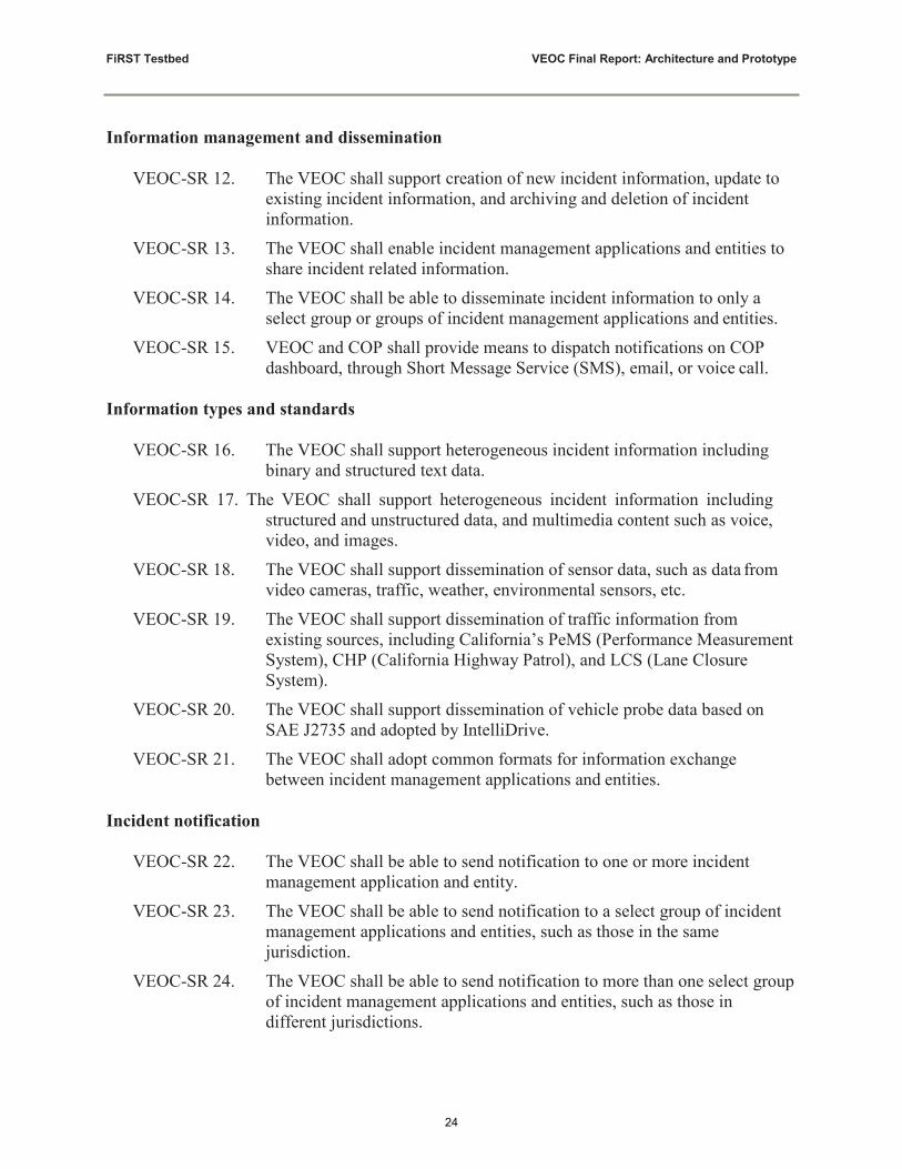
VEOC-SR 12. The VEOC shall support creation of new incident information, update to existing incident information, and archiving and deletion of incident information.
VEOC-SR 13. The VEOC shall enable incident management applications and entities to share incident related information.
VEOC-SR 14. The VEOC shall be able to disseminate incident information to only a select group or groups of incident management applications and entities.
VEOC-SR 15. VEOC and COP shall provide means to dispatch notifications on COP dashboard, through Short Message Service (SMS), email, or voice call.
Information types and standards
VEOC-SR 16. The VEOC shall support heterogeneous incident information including binary and structured text data.
VEOC-SR 17. The VEOC shall support heterogeneous incident information including structured and unstructured data, and multimedia content such as voice, video, and images.
VEOC-SR 18. The VEOC shall support dissemination of sensor data, such as data from video cameras, traffic, weather, environmental sensors, etc.
VEOC-SR 19. The VEOC shall support dissemination of traffic information from existing sources, including California’s PeMS (Performance Measurement System), CHP (California Highway Patrol), and LCS (Lane Closure System).
VEOC-SR 20. The VEOC shall support dissemination of vehicle probe data based on SAE J2735 and adopted by IntelliDrive.
VEOC-SR 21. The VEOC shall adopt common formats for information exchange between incident management applications and entities.
Incident notification
VEOC-SR 22. The VEOC shall be able to send notification to one or more incident management application and entity.
VEOC-SR 23. The VEOC shall be able to send notification to a select group of incident management applications and entities, such as those in the same jurisdiction.
VEOC-SR 24. The VEOC shall be able to send notification to more than one select group of incident management applications and entities, such as those in different jurisdictions.

FiRST Testbed VEOC Final Report: Architecture and Prototype
25
Network
VEOC-SR 25. The VEOC shall adopt the Internet Protocol (IP) as the network layer protocol.
VEOC-SR 26. The VEOC shall be able to operate in both IPv4 and IPv6 networks VEOC-SR 27. Communication within the VEOC shall be fully functional over both
wireline and wireless networks.
VEOC-SR 28. Communication between the VEOC and connected incident management applications and entities shall be fully functional over both wireline and wireless networks.
VEOC-SR 29. The VEOC shall support communication with incident management applications running on fixed devices (such as desktop computers), portable devices (such as laptop computers), and mobile devices (such as mobile phones).
Availability, scalability, and performance
VEOC-SR 30. The VEOC shall be scalable to interconnect incident management applications and entities from local to national level.
VEOC-SR 31. The VEOC shall be able to recover to its prior operating state from partial or complete system failures.
VEOC-SR 32. The VEOC shall have the ability to backup and restore critical system data.
VEOC-SR 33. The COP shall maintain up-to-date incident information, whereby the latency in updating information shall not be greater than 1 minute.
Security and privacy
VEOC-SR 34. Incident management applications and entities that connect to the VEOC shall be authenticated before access is permitted.
VEOC-SR 35. Incident management applications and entities that connect to the VEOC shall be permitted to only access incident information that it has authorization for.
VEOC-SR 36. The VEOC shall refuse unauthenticated Incident management applications and entities to connect to the VEOC.
VEOC-SR 37. Personal identifiable information, if any, disseminated through the VEOC is strictly accessible only to authorized incident management applications and entities and on a need-to-know basis.
VEOC-SR 38. The VEOC shall be able to control the type of information shared by different groups of incident management applications and entities, such as those in different jurisdictions.

FiRST Testbed VEOC Final Report: Architecture and Prototype
26
VEOC-SR 39. The VOEC shall provide means for authorized personnel to obtain
information stored by the VEOC. VEOC-SR 40. The VEOC shall monitor, detect, report, log, and respond to security
incidents. VEOC-SR 41. The VEOC shall be able to remove access to the VEOC by any incident
management application or entity. VEOC-SR 42. The VEOC shall be able to reinstate access to the VEOC by any incident
management application or entity. VEOC-SR 43. Information exchanged between the VEOC and incident management
applications and entities shall be protected from tampering and unauthorized access.
VEOC-SR 44. The VEOC shall provide a means to authenticate messages originating from connected incident management applications and entities.
VEOC-SR 45. Information exchanged within the VEOC shall be protected from tampering and unauthorized access.
VEOC-SR 46. The VEOC shall be able to authenticate messages originating from connected management applications and entities.
VEOC-SR 47. The VEOC shall be protected against physical intrusion. VEOC-SR 48. The VEOC shall provide physical access control for VEOC system
elements. VEOC-SR 49. The VEOC shall implement management, operational, and technical
security measures to protect assets, elements, and information within the VEOC.
VEOC-SR 50. The VEOC shall provide a means for encrypting and decrypting data. VEOC-SR 51. The VEOC shall provide mechanisms for creating, updating, and revoking
security credentials. VEOC-SR 52. The VEOC shall be protected against Denial of Service (DoS) attacks. VEOC-SR 53. The VEOC shall have at least industry-standard security measures for
protection against cyber security threat such as software virus, malware, intrusions, and denial of service attacks.

FiRST Testbed VEOC Final Report: Architecture and Prototype
27
5.5 Requirements Mapping A subset of the VEOC high-level system requirements has been implemented in this prototype. Details of requirements mapping are shown in Table 1.
Table 1: Requirements Mapping for Phase I Prototype
Requirement Phase I Prototype Implementation
VEOC-SR 1. Implemented
VEOC-SR 2. Partially implemented. User access is currently provided through desktop and laptop.
VEOC-SR 3. Not implemented VEOC-SR 4. Not implemented
VEOC-SR 5. Not implemented VEOC-SR 6. Not implemented
VEOC-SR 7. Not implemented VEOC-SR 8. Not implemented
VEOC-SR 9. Not implemented VEOC-SR 10. Implemented
VEOC-SR 11. Implemented VEOC-SR 12. Implemented
VEOC-SR 13. Implemented VEOC-SR 14. Implemented
VEOC-SR 15. Not implemented
VEOC-SR 16. Partially implemented. Structured text data is currently supported.
VEOC-SR 17. Not implemented VEOC-SR 18. Not implemented
VEOC-SR 19. Partially implemented. Traffic information from PeMS and LCS are currently supported.
VEOC-SR 20. Not implemented VEOC-SR 21. Implemented
VEOC-SR 22. Implemented VEOC-SR 23. Implemented

FiRST Testbed VEOC Final Report: Architecture and Prototype
28
VEOC-SR 24. Implemented VEOC-SR 25. Implemented
VEOC-SR 26. Partially implemented. IPv4 is currently supported.
VEOC-SR 27. Partially implemented. Wireline network is currently supported.
VEOC-SR 28. Partially implemented. Wireline network is currently supported.
VEOC-SR 29. Partially implemented. Fixed and portable devices are currently supported.
VEOC-SR 30. Not implemented VEOC-SR 31. Not implemented VEOC-SR 32. Not implemented
VEOC-SR 33. Implemented VEOC-SR 34. Implemented
VEOC-SR 35. Not implemented VEOC-SR 36. Implemented
VEOC-SR 37. Not implemented VEOC-SR 38. Implemented
VEOC-SR 39. Implemented VEOC-SR 40. Not implemented
VEOC-SR 41. Not implemented VEOC-SR 42. Not implemented
VEOC-SR 43. Not implemented VEOC-SR 44. Not implemented
VEOC-SR 45. Not implemented VEOC-SR 46. Not implemented
VEOC-SR 47. Implemented VEOC-SR 48. Implemented
VEOC-SR 49. Not implemented VEOC-SR 50. Not implemented
VEOC-SR 51. Not implemented

FiRST Testbed VEOC Final Report: Architecture and Prototype
29
VEOC-SR 52. Not implemented VEOC-SR 53. Not implemented
5.6 Test Scenarios The following test scenarios have been defined for the VEOC prototype.
Test Scenario ID P-001
Purpose
Verify that users can access the COP application through a web browser on a desktop and laptop.
Requirements Number VEOC-SR1, VEOC-SR 2 (partial)
Test Step Action Results
1 Open a browser on a desktop computer and type in the URL of the Viewer 1 application Browser displays latest incident information
2 Open a browser on a laptop computer and type in the URL of the Viewer 1 application Browser displays latest incident information
Test Scenario ID P-002
Purpose
Verify that VEOC is able to interconnect multiple incident management applications and entities
Requirements Number VEOC-SR 10, VEOC-SR 11
Test Step Action Results
1
Start UICDS Core 1 and UICDS Core 2
Confirm UICDS Core 1 and UICDS Core 2 are running using the UICDS Administration Console
2 Start Viewer 2 application Viewer 2 application started 3 Start PeMS Adapter PeMS Adapter started
4 Open a browser on a desktop computer and connect to Viewer 2 application
Browser displays incident information or PeMS data as they become available
Test Scenario ID P-003
Purpose
Verify that VEOC is able to support creation, update, archival and deletion of incident information

FiRST Testbed VEOC Final Report: Architecture and Prototype
30
Requirements Number VEOC-SR 12
Test Step Action Results
1 Start Viewer 1 application, then PeMS Adapter
Viewer 1 application and PeMS Adapter started
2 Open a browser on a desktop computer and connect to Viewer 1 application Browser displays new incident when it occurs
3 Using UICDS Administration Console, close the incident Message confirm incident is closed
4 Using UICDS Administration Console, archive the closed incident Message confirm incident is archived
5 Using UICDS Administration Console, delete the archived incident Message confirm incident is deleted
Test Scenario ID P-004
Purpose
Verify that VEOC is able to share incident information with a select group of incident management applications and entities
Requirements Number VEOC-SR 13, VEOC-SR 14
Test Step Action Results
1
Create agreement to share incident information between UICDS Core 1 and UICDS Core 2
Agreement created
2 Open a browser on a desktop computer and connect to Viewer 1 application Browser displays LCS incident information
3 Using UICDS Administration Console, disable the sharing agreement
Browser will not display LCS incident information
Test Scenario ID P-005
Purpose Verify that VEOC is able to support structured text incident information
Requirements Number VEOC-SR 16 (partial)
Test Step Action Results
1 Using UICDS Administration Console, select a work product
XML representation of the work product is displayed
Test Scenario ID P-006

FiRST Testbed VEOC Final Report: Architecture and Prototype
31
Purpose
Requirements Number Test Step Action Results
Verify that VEOC is able to disseminate information from PeMS and LCS
VEOC-SR 19 (partial)
1 Open a browser on a desktop computer and connect to Viewer 1 application Browser connected to Viewer 1 application
2 Select PeMS tab, then a district Browser displays PeMS data 3 Select LCS tab, then a district Browser displays LCS data
Test Scenario ID
Purpose
Requirements Number
Test Step Action Results
P-007
Verify that VEOC support common formats for incident information exchange between incident management applications and entities
VEOC-SR 21
1 PeMS Adapter and LCS Adapter create incident information in XML format PeMS and LCS incident information created
2 Using UICDS Console, display PeMS and LCS incident information
PeMS and LCS incident information displayed in XML format
Test Scenario ID
Purpose
Requirements Number
Test Step Action Results
P-008
Verify that VEOC is able to send notifications to incident management applications and entities in the same or different jurisdictions
VEOC-SR 22, VEOC-SR 23, VEOC-SR 24
1 Open a browser on a desktop computer and
connect to Viewer 1 application
Browser displays PeMS incident information after Viewer 1 application receives PeMS notification
2
Create agreement to share incident information between UICDS Core 1 and UICDS Core 2
Browser displays PeMS and LCS incident information after Viewer 1 application receives PeMS and LCS notifications
Test Scenario ID P-009
Purpose Verify that VEOC operates over a wireline IPv4 network and communicates with incident management applications running on desktop and laptop

FiRST Testbed VEOC Final Report: Architecture and Prototype
32
computers
Requirements Number
VEOC-SR 25, VEOC-SR 26 (partial), VEOC-SR 27 (partial), VEOC-SR 28 (partial), VEOC-SR 29 (partial)
Test Step Action Results
1
Connect a laptop computer to the computer running UICDS Core 2 using a wireline IPv4 network
Laptop computer and computer running UICDS Core 2 connected by a wireline IPv4 network
2 Start LCS Adapter and Viewer 2 application on the laptop computer LCS Adapter and Viewer 2 application started
3 Open a browser on a third desktop computer and connect to Viewer 2 application
Browser displays LCS incident information when it occurs
Test Scenario ID P-010
Purpose
Verify that the COP application maintains up-to-date information whereby the latency in updating information is not greater than 1 minute
Requirements Number VEOC-SR 33
Test Step Action Results
1
Open a browser on a desktop computer and connect to Viewer 1 application
Browser displays PeMS incident information when it occurs. PeMS incident timestamp is not older than 1 minute from the Viewer last update timestamp
Test Scenario ID P-011
Purpose
Verify that VEOC only allows access by authenticated incident management applications and denies access by unauthenticated incident management applications
Requirements Number VEOC-SR 34, VEOC-SR 36
Test Step Action Results
1
Configure Viewer 1 application with valid credential for accessing UICDS Core 1, then restart Viewer 1 application
Viewer 1 application restarted with valid credential
2 Open a browser on a desktop computer and connect to Viewer 1 application
Browser displays PeMS and LCS incident information when they occur
3
Configure Viewer 1 application with invalid credential for accessing UICDS Core 1, then restart Viewer 1 application
Viewer 1 application restarted with invalid credential
4 Open a browser on a desktop computer and Browser unable to display PeMS or LCS

FiRST Testbed VEOC Final Report: Architecture and Prototype
33
connect to Viewer 1 application incident information
Test Scenario ID P-012
Purpose
Verify that VEOC is able to control the type of information shared by different groups of incident management applications
Requirements Number VEOC-SR 38
Test Step Action Results
1
Using UICDS Administration Console, add ‘incident’ to the list of interests in Viewer resource profile, then restart Viewer 1 application
Viewer 1 application restarted with resource profile that includes ‘incident’ in the interests list
2 Open a browser on a desktop computer and connect to Viewer 1 application
Browser displays PeMS incident information when it occurs
3
Using UICDS Administration Console, remove ‘incident’ from the list of interests in Viewer resource profile, then restart Viewer 1 application
Viewer 1 application restarted with resource profile that does not have ‘incident’ in the interests list
4 Open a browser on a desktop computer and connect to Viewer 1 application
Browser unable to display PeMS incident information
Test Scenario ID P-013
Purpose
Verify that VEOC permits authorized personnel to access information stored by VEOC
Requirements Number VEOC-SR 39
Test Step Action Results
1 Login as administrator to the UICDS console, using an incorrect password Login is denied
2 Login as administrator to the UICDS console, using the correct password Access is granted
3 Select an incident Information of the incident is shown in XML
Test Scenario ID P-014
Purpose
Verify that VEOC is protected from physical intrusion and by physical access control
Requirements Number VEOC-SR 47, VEOC-SR 48

FiRST Testbed VEOC Final Report: Architecture and Prototype
34
Test Step Action Results
1 Check that VEOC can only be physically
accessed through designated entrances
VEOC can only be physically accessed through a designated door to the secured room housing the VEOC
2 Check that a physical access credential is required at designated entrances
A security batch is required at the designated door to enter the secured room
5.7 Installation This section describes the prerequisites and procedures for installing the VEOC prototype.
5.7.1 Prerequisite Install JRE 6. Installation procedure is available at:
http://www.oracle.com/technetwork/java/javase/index-137561.html
Alternatively, user may install JDK 6. Installation procedure is available at:
http://www.oracle.com/technetwork/java/javase/index-137561.html
5.7.2 Install UICDS core UICS installation procedures are described in:
UICDS System Installation Plan UICDS-PLN-SIP-R02C02 September 27, 2010 SAIC
5.7.3 Install Tomcat Tomcat installation procedure is available at: http://tomcat.apache.org/
Please note that this Tomcat installation is in addition to the Tomcat used by UICDS core. The path to this Tomcat installation is referred to as [TOMCAT_INSTALLATION] in the installation procedures below.
5.7.4 Install PeMS Adapter A. An instance of Tomcat is required to support PeMS Adapter. Both software should
collocate on the same computer B. Unzip the provided pems.zip to get one war file, PemsData.war, and one directory,
“PeMS”. C. Move the PemsData.war to the [TOMCAT_INSTALLATION]\webapps\

FiRST Testbed VEOC Final Report: Architecture and Prototype
35
D. Go to the unzipped directory and find the configuration file, config.prop.
E. Update the following parameters according to the PeMS access credential and local configuration
a. PemsFtpServer => fully qualified domain name of PeMS FTP site b. PemsFtpUser => User name to access PeMS system c. PemsFtpPwd => Password to access PeMS system d. PemsOutputPath => [TOMCAT_INSTALLATION]\webapps\PemsData\web\
5.7.5 Install LCS Adapter A. An instance of Tomcat is required to support LCS Adapter. Both software should
collocate on the same computer. B. Unzip the provided lcs.zip to get one war file, LcsData.war, and one directory, “LCS”. C. Move the LcsData.war to the [TOMCAT_INSTALLATION]\webapps\ D. Go to the unzipped directory and find the configuration file, config.prop. E. Update “PemsOutputPath” => [TOMCAT_INSTALLATION]\webapps\LcsData\web\
5.7.6 Install Viewer Application A. An instance of Tomcat is required to support Viewer application. Both software should
collocate on the same computer B. Unzip the provided viewer.zip to get one war file, ViewerData.war, and one directory,
“Viewer”. C. Move the ViewerData.war to the [TOMCAT_INSTALLATION]\webapps\ D. Go to the unzipped directory and find the configuration file, config.prop. E. Update the following parameters:
a. Update CoreHostName according to the fully qualified domain name of the associated UICDS core.
b. Update ViewerOutpoutPath => [TOMCAT_INSTALLATION]\webapps\ViewerData\web\
5.8 System Startup This section will outline the procedures to startup the VEOC systems. Depending on the system configuration, some procedures may be repeated on multiple computers. For instance, if Viewer application, PeMS/LCS adapter and the associated UICDS Core are installed on separate computers, Java runtime environment and Tomcat will be needed on each of the computer. Tomcat instance on each individual computer will need to be activated separately. Please refer to aforementioned installation procedures for the prerequisite.

FiRST Testbed VEOC Final Report: Architecture and Prototype
36
5.8.1 Start UICDS The procedures for starting UICDS are described in:
UICDS System Installation Plan UICDS-PLN-SIP-R02C02 September 27, 2010 SAIC
5.8.2 Start Tomcat This procedure is repeated on all computers running Tomcat. Please note that this Tomcat instance is different the Tomcat instance used by UICDS, if any of the PemS Adapter, LCS Adapter or Viewer application is collocated with the UICDS Core.
• Verify that Tomcat is not running • Go to [TOMCAT_INSTALLATION]/bin then execute “startup.bat”. (Windows
environment) • Verify that Tomcat is running • If a war file of Viewer application, PeMS Adapter or LCS Adapter is deployed in this
Tomcat, you can verify if the data viewing feature is running properly by visiting different URLs. o For Viewer application: http://[HOST_NAME]/ViewerData/
o For PeMS data: http://[HOST_NAME]/PemsData/ o For LCS data: http://[HOST_NAME]/LcsData/
5.8.3 Start PeMS Adapter • Go to [PEMS_ADAPTER_INSTALLATION]/
Execute the following command to start a PeMS Adapter o java -jar target\PemsAdapter. jar -l=pems.log -c=config.prop -r=P
•
5.8.4 Start LCS Adapter • Go to [LCS_ADAPTER_INSTALLATION]/ • Execute the following command to start a LCS Adapter
• java -jar target\LcsAdapter. jar -l=lcs.log -c=config.prop –r=L
5.8.5 Start Viewer Application • Go to [VIEWER_APPLICATION_INSTALLATION]/ • Execute the following command to start a Viewer application
• java -jar target\viewer. jar -l=cop.log -c=config.prop –r=V

FiRST Testbed VEOC Final Report: Architecture and Prototype
37
6 The Golden Guardian Demonstration The Caltrans-FiRST Testbed participated in the California Earthquake Clearinghouse (CEC) shakeout technology demonstrations and exercise on October 2012. The purpose of the exercise was to demonstrate multi-agency cooperation during an earthquake including two-way interoperable data exchange of many types created using various applications between different participating organizations. The California office of emergency services (OES) has now added UICDS compliance to its requirement.
Caltrans, pioneered the integration of data about the status of the transportation network with emergency management functionalities in a standard based implementation developed under the virtual emergency operation center (VEOC) track of the FiRST Testbed research efforts.
The exercise participants were the Cal EMA (OES), Caltrans FiRST Testbed, US Geological Survey (USGS), Earthquake Engineering Research Institute, NASA, San Diego County and the California Geological Survey. The exercise was coordinated by SAIC representing the Department of Homeland Security (DHS).
The Caltrans' FiRST Testbed at UCSB has been the first operating UICDS core in California capable of core-to-core communication with the DHS infrastructure. The FiRST-VEOC core, demonstrated the capability of processing the Caltrans PeMS data and simulate traffic conditions and highway closures at the identified hazard areas defined for the exercise anywhere in California.

FiRST Testbed VEOC Final Report: Architecture and Prototype
38
7 Related Systems This section presents a high-level comparison between VEOC and WebEOC.
WebEOC is an incident management system from ESi Acquisition, Inc. that enables users to view and post information through a number of status boards. Its functionalities include monitoring and updating events status, tracking and managing tasks and resources, report generation, mapping, messaging, and other utilities. WebEOC servers may communicate with one another through ESiWebFUSION which acts as a communication hub. WebEOC also supports CAP for alerts.
VEOC enables different incident management systems from different vendors and incident management organizations to interoperate, share incident information, and monitor and manage incidents in a distributed and collaborative manner. Its functionalities include creating and updating incidents, incident command organization structures, and incident action plans; tracking and managing tasks and resources; mapping; and disseminating sensor data and incident information.
A major difference between VEOC and WebEOC is that VEOC acts as a middleware to enable incident management applications from various vendors, and those that perform different incident response functions, to interwork transparently as single integrated virtual incident management organization. WebEOC has various incident response functions all built into the system and allows communications only amongst WebEOC servers. Further, VEOC adopts a number of open standards related to incident management in implementing the functionalities and services it provides. These include:
• NIEM for incident management, incident command, incident action plan and tasking services
• EDXL-RM for resource management • OGC SOS for sensor service • OGC WMS and WFS for mapping service • IEPD for LEITSC • CAP for alerting service
It is to be noted that in a wide area emergency such as earthquakes in California, Internet may be out for days or even a week, and this will render cloud based applications (e.g. WebEOC ) unavailable. A solution has been investigated and partially implemented under Track III, where a portable platform implementing the Hastily Deployed interanet Network (HDiN) will provide local wireless intranet services in the ITS and Public Safety bands, provide local mapping (e.g. Caltrans Earth), as well supporting the UICDS based VEOC. When The Intranet is restored the HDiN will use the UICDS core to automatically synchronize with other incident management platforms such as WebEOC.

FiRST Testbed VEOC Final Report: Architecture and Prototype
39
8 Glossary
API Application Programming Interface CAP Common Alerting Protocol CFR Crash and Fire Rescue CHP California Highway Patrol COP Common Operating Picture DDS Data Distribution Service EXDL-DE Emergency Data Exchange Language – Distribution Element EXDL-RM Emergency Data Exchange Language – Resource Messaging EMS Emergency Medical Service EPA Environment Protection Agency FAA Federal Aviation Administration FBI Federal Bureau of Investigation FD Fire department HAZMAT Hazardous Materials IEPD Information Exchange Package Documentation LEITSC Law Enforcement Information Technology Standards Council LCS Lane Closure System NIEM National Information Exchange Model OEM Office of Emergency Management OGC Open Geospatial Consortium OMG Object Management Group PD Police Department PeMS Performance Measurement System SOI Sensor Observation Information SOS Sensor Observation Service TMC Traffic Management Center UICDS Unified Incident Command and Decision Support VEOC Virtual Emergency Operation Center WFS Web Feature Service WMS Web Map Service WP Work Product WSDL Web Service Definition Language XMPP Extensible Messaging and Presence Protocol

UICDS Implementation at the Caltrans-FiRST Testbed
Ramez Gerges, Ph.D., P.E.
Caltrans – DRISI FiRST Testbed
40

Unified Incident Command & Decision Support
41

FiRST Testbed R&D Efforts
42
Caltrans Strategic Goal: Provide the safest transportation system in the nation for users and workers Strategic Objective: To look ahead and evaluate standard based solutions to address Caltrans' mobility and safety challenges Partners: Caltrans – Division of Research Innovation & System Information (DRISI) Caltrans - Office of Emergency Management (OEM) Caltrans - Maintenance Office of Radio Communications (ORC) UCSB - FiRST Testbed (FiRST.transcal.ucsb.edu)

FiRST Testbed R&D Efforts
43
Caltrans’ Challenge: • A statewide standard-based Common Operational Data (UICDS) • A statewide web-based Common Operational Picture (COP) • Local continuity of operation with or without Internet access • Fail-safe operation and synchronization to cloud-based WebEOC FiRST Testbed Solution: Hastily Deployed Network (HDN) platform that address • Emergency Management
• Virtual Emergency Operation Center (VEOC) • Emergency Communications
• Interoperable Data-Centric Public Safety & ITS Broadband • Satellite SMS Communicator (anywhere, anytime)

44
Emergency Management Virtual Emergency Operation Center (VEOC)
A standard-based state-wide UICDS compliant implementation: • Support Common Operational Data • Support Common Operational Picture (COP) • Capture incident information without Internet Connectivity • Provide real-time access to Caltrans local & regional resources • Integrate data from PeMS & LCS (Caltrans) & CHP • Support the Common Alerting Protocol (CAP) • Replace the D4-Bay Area Incident Response System (BAIRS)* • Replace the D7-Major Events Response Tracking (MERTS)* • Replace the Responder developed for D3* • Support day-to-day (e.g. urban and rural work zones) • Embedded HDN-UICDS core for wide-area emergencies (e.g.
earthquakes, tsunami, etc.) * Phase II: Pending Funding Approval

45
PeMS Historical PeMS
LCS
CHP
Phase I PeMS Adapter
LCS Adapter
CHP Adapter
Local
PD
EMS
HDN Admin Console
WebEOC
Data
FiRST UICDS Core
XMPP
HDN-UICDS Core
Phase II
UICDS Admin Console
VEOC
NTRIP Adapter
Probe Data Adapter
Video Adapter
CAP
CAP over XMPP
NTRIP
Phase II
Probe Data
Video
HDN 6
VEOC–HDN-UICDS

46
Hastily Deployed Network (HDN) Platform Interoperable Data-Centric Emergency Communications
• Broadband-over-Power (BoP) HDN_ITS Station • 3G/4G wireless router • Satellite SMS Communicator & GPS • ITS Radio (5.9 GHz) • Public Safety Radio (4.9 GHz). • Point-Point & Mesh topologies • WSN Gateway (6LoWPAN) • Embedded UICDS Core • Embedded Google Earth Enterprise
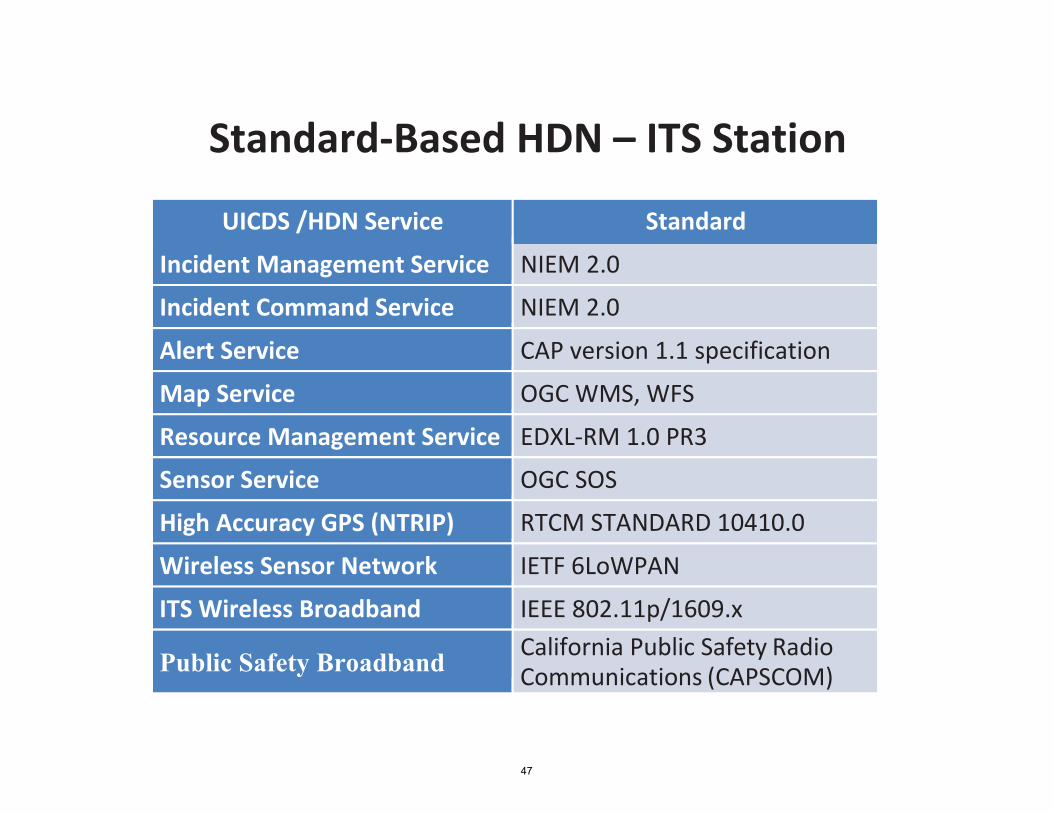
47
Standard-Based HDN – ITS Station
UICDS /HDN Service Standard
Incident Management Service NIEM 2.0
Incident Command Service NIEM 2.0
Alert Service CAP version 1.1 specification
Map Service OGC WMS, WFS
Resource Management Service EDXL-RM 1.0 PR3
Sensor Service OGC SOS
High Accuracy GPS (NTRIP) RTCM STANDARD 10410.0
Wireless Sensor Network IETF 6LoWPAN
ITS Wireless Broadband IEEE 802.11p/1609.x
Public Safety Broadband California Public Safety Radio Communications (CAPSCOM)

Shake, Out 2013 P,art:ners espon e
• I,';•_ .
(Mpi8 J -W.oductJon t thl!I Cll!' se...nd Ml:.sO,J: 2013 hi', Ame kl
llmptr 2 • of fl K Thrall: cfE,; cke Throogh lhi!
ch pl r 3 • AI.OOA f'Ur'6 in ktW
Cliaple,l' 1 - ESIU w,h D!t.! U.oogt, l.!JCDS
9 C:hlll)l:e.t :5 • Pubk Health D&II Th,oiql IJICM Ch p t:et & · illA5A .li'I. S '
h<1f,ter 1 • Na:d Mm 5 (Nits)
l O • l111l:S Fi,Jkl p Dr!llliing TIYt1uohULCDSh1
Dl I • l:·VE"Clct:R MIKI R NI; rrorn /i'1,5A JP\. ,d TlwQJ9h U!COS
CMfiltt 16 • l t:.Med L EW11i.Jt,t1m1 lad (l nlET)
Shcr;,d TIY IJICDS
t J9 • Vrll!ill USA IIYl!'-111',' (OMetbill'I rv:ISl\lrn) toUIC
Ch p 20 • \'W ry Lili''- M OGC M.:>,p airtc-xt stM!l.scl Cl'IUICOS ActniiC«- Chapter Z1 • '11.t..recy L Aw-' ffJ Googje-arth TI-,rwghurms OGC Cont Wod\l'ro<b;t Chapter 22 • \'l.ba('/ Lint;> In Oor;('. Map (onte,;t W kProdud
Wl)W 23 - ,>2 L.15 Mrtf Il"IClltl!tt at)d l\bW "lwed
pl Z4 • ilZ Plwl'll' !iliar!!d I'lliioagk, E.vlh
27 - E.w'tl'ot 1al:.U ' "!il,ineeti "'11 lwe.lltd'I In
2 • NICS l'alc,\,,-l.l) eilll® . Rf.Plllr r z · GCO! l'Wlc I i: J<Jr mo E\lafltS Roc e:IGH:
CJI p'fer 30 •C$f'O!fi11GQ,,r H1ffjce of ;c1'1CY s:etviCM:{C ) AlcGIS Cll'IIM-
--OOIJltt :n - semtll. E)a(UaMEv lut.tion Pr(9'affl (l-151:EP)
Chllple 32- CGn'rnel)lp knil Rosh ti, CM!r, C611ornl!I E111lhilil < 48
R

49
US Department of Homeland Security, Washington, DC 20528
Homeland Security
July 19 , 2013
Ms Coco Briseno Cheif
Division of Research Innovation and System InformationCalifornia Department of Transportation (Caltrans)1227 O St. 5th FloorSacramento, CA 95814
Dear Ms Briseno:
The Department of Homeland Security, Directorate of Science and Technology, is pleased that the California Department of Transportation (Caltrans) FiRST Testbed at the University of California Santa Barbara has been participating in the implementation of the Unified Incident Command and Decision Support (UICDS) information sharing middleware.
In September 2011, the California Emergency Management Agency made UICDS compliance a requirement of its procurement for the Response Information Management System (RIMS). The FiRST Testbed was one of the early adopters of the UICDS architecture as part of their virtual emergency operation center (VEOC) project. We appreciate the fact that Caltrans developed and deployed the UICDS-PeMS adapter to provide real-time status of the transportation network, and enable incidents simulation anywhere on the California highways. DHS values Caltrans continuing research in extending the UICDS architecture, its resiliency and ability to detect, alert, and share common operational data about other hazards.
The Caltrans' FiRST Test Bed has been an integral part of the growth of the UICDS implementation and we value their installation of one of the first UICDS cores in California, becoming a leader across the nation among departments of transportation.
The collaboration between DHS, Caltrans' FiRST Testbed and the California Earthquake Clearinghouse partnership - representing its five constituent founders: California Geological Survey, United States Geological Survey, Earthquake Engineering Research, Institute, California rEmergency Management Agency, and the California Seismic Safety Commission - has resulted in impressive improvements in technology applications to earthquake hazards.

50
DH wiJl continue supporting expanded UICDS participation in 2014 and we hope that the FiRST Testbed will continue their fine work to benefit the citizen f Calif mia in an emergency.
Sincerely.
Lawrence E. Skelly Program Manager Deprutment of Homeland Security Science and Technology Directorat
CC: Dr. R. Church Associate Dean Division of Mathematical. Life and Physical Sciences UCSB-FiRST Testbed 1832 Ellison Hall Santa Barbara CA 93106-4060

51
First Responder Support Systems & Technologies (FiRST) Testbed
Principal Investigator: Dr. Richard Church Dr. Micah Brachman
Carlos Baez University of California Santa Barbara
Contract Manager: Ramez Gerges, Ph.D., P.E.
Contract # 65A0257 Cross-Cutting Cooperative Systems
TRACK II – Cross Cutting Modeling & Simulation
Final Report

52
First Responder Support Systems & Technologies (FiRST) Testbed
TRACK II – Cross Cutting Modeling & Simulation
Models are one of the most effective forms of testing transportation system plans. Such plans could involve the
conversion of a highway lane to a high occupancy/toll (HOT) lane or the operational settings of a series of
signals. The focus of this task was centered on the development and testing of models to support evacuation
planning. This research was requested by Caltrans to support statewide disaster response operations and
management and was directed at the problem of evacuation. Several major concerns have been raised with
Caltrans personnel, including the potential risk from a nuclear power plant disaster at Diablo Canyon, a tsunami
impacting a coastal area such as the northern coast of California, the Ports of LA and Long Beach, and Marina
Del Rey, a major wildfire, flood, or earthquake. All of these events may trigger a massive evacuation along
corridors that may have been compromised by the event. We began this task with a literature review focused on
the issue of disaster response, mitigation, and capabilities. This literature review is given in the enclosed report
called “Planning for a disaster: a review of the literature with a focus on transportation related issues.” This
literature review gives several examples of how California’s capabilities in responding to a crisis could be easily
thwarted. For example, it is documented that many hospitals have limited supplied of drugs and food, existing
on regular, daily shipments for resupply. Without an intact transport system, it is clear that regular care as well
as emergency care would come to a halt. As another part of this work, we developed a prototype evacuation
simulation model for a large scale evacuation involving the Diablo Nuclear Power Plant. The nuclear plant
triggered evacuation was modeled using a state of the art micro-simulation model called PTV VISSIM. The
simulation results demonstrated that a mock plan based upon contra-flow operations could significantly reduce
the time it would take to evacuate San Luis Obispo as compared to a baseline scenario. This is reported in
enclosed document titled “Simulating an evacuation event: a test case involving the Diablo Canyon Power
Plant.” Several elements were raised in the development of this evacuation model, including when will people
make the fateful decision to leave and what route will they take. To better understand the decision to leave an
area being hit with a disaster as well as estimate when individuals might leave, we surveyed people who were
given mandatory evacuation ordered during the Jesusita fire in Santa Barbara. Our results indicated that up to
10% of the people did not evacuate even when they were under a mandatory evacuation order to do so. We
found that a Rayleigh Probability model could be used to estimate the frequency of when people begin their
exodus. This work is reported in “Modeling the evacuation decision.” We also wanted to better understand the

53
First Responder Support Systems & Technologies (FiRST) Testbed
TRACK II – Cross Cutting Modeling & Simulation
decision affecting the pathway chosen when someone leaves. Our survey suggested that a number of people
were somewhat sophisticated in the route choice, taking routes not part of their daily routines, but likely to be
ones which avoided traffic jams and thus aiding in them getting out quickly. This survey and work is reported in
“Cognitively Engineered Evacuation Routes.” As a part of this we show that a multi-commodity flow
optimization model can be used to model multiple exit choice, congestion behavior in terms of route avoidance,
and route choice without the need to use a micro-scale traffic simulation model, which can be nearly cost
prohibitive to perform in most areas. One of the tasks that was envisioned as a part of this work was the
evacuation of an area triggered by a Tsunami. Initially, this was selected by District 7 to be the Marina Del Rey
area that is comprised of Venice and the Marina communities. The evacuation flood risk maps show that this
area could be inundated by a large tsunami. At risk I a relative large population, a peninsula comprised of
homes and apartment complexes and even a school where many must travel north on only one of three roads
before heading inland for safety. The second area of interest was the Ports of LA and Long Beach. Either one is
of great interest and of potential significance to California. This final work element was not finished as the
support funds for this project were cut as a cost saving measure by Caltrans. Additionally, the Division of
Research, Innovation, and System Information requested that we make no contact to nay Caltrans Districts for
information or support, even though this work was originally suggested by District 7 staff. Although, we respect
the leadership of DRISI and their decisions this last task element could not be completed without closer ties
with District 7.
Following this introduction, the Track II final report includes the following sections in reverse chronological order:
1) Simulating an evacuation event: A test case involving the Diablo Canyon Power Plant
2) Summary of Dynamic Traffic Assignment in VISSIM
3) Cognitively Engineered Evacuation Routes
4) Modeling the Evacuation Decision
5) Modeling for Emergency Preparedness Literature Review

54
Simulating an evacuation event:
A test case involving the Diablo Canyon Power Plant

55
Simulating an evacuation event: A test case involving the Diablo Canyon Power
Plant
Micah L. Brachman Richard L. Church
Carlos A. Baez
FiRST Project GeoTrans Laboratory
Department of Geography University of California, Santa Barbara
January 31, 2014
This report has been developed as a part of the First Responders System Testbed (FiRST) project at the University of California, Santa Barbara. The FiRST project investigates the integration of transportation and communication modeling and simulation to improve understanding and techniques of emergency preparedness and response. Please cite this report as: Brachman, ML, RL Church, and CA Baez (2013) “Simulating an evacuation event: a test case involving the Diablo Canyon Power Plant” (Report #01-2014-01), GeoTrans Laboratory, UCSB, Santa Barbara CA.
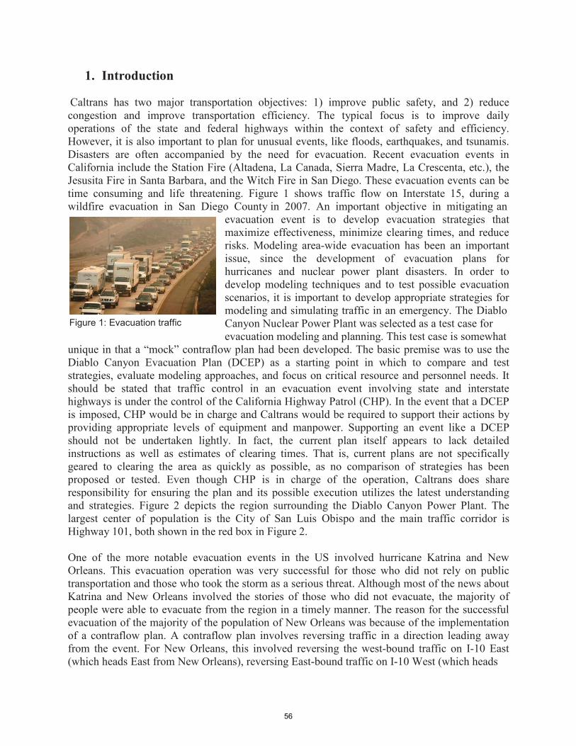
56
1. Introduction
Caltrans has two major transportation objectives: 1) improve public safety, and 2) reduce congestion and improve transportation efficiency. The typical focus is to improve daily operations of the state and federal highways within the context of safety and efficiency. However, it is also important to plan for unusual events, like floods, earthquakes, and tsunamis. Disasters are often accompanied by the need for evacuation. Recent evacuation events in California include the Station Fire (Altadena, La Canada, Sierra Madre, La Crescenta, etc.), the Jesusita Fire in Santa Barbara, and the Witch Fire in San Diego. These evacuation events can be time consuming and life threatening. Figure 1 shows traffic flow on Interstate 15, during a wildfire evacuation in San Diego County in 2007. An important objective in mitigating an
evacuation event is to develop evacuation strategies that maximize effectiveness, minimize clearing times, and reduce risks. Modeling area-wide evacuation has been an important issue, since the development of evacuation plans for hurricanes and nuclear power plant disasters. In order to develop modeling techniques and to test possible evacuation scenarios, it is important to develop appropriate strategies for modeling and simulating traffic in an emergency. The Diablo
Figure 1: Evacuation traffic Canyon Nuclear Power Plant was selected as a test case for evacuation modeling and planning. This test case is somewhat
unique in that a “mock” contraflow plan had been developed. The basic premise was to use the Diablo Canyon Evacuation Plan (DCEP) as a starting point in which to compare and test strategies, evaluate modeling approaches, and focus on critical resource and personnel needs. It should be stated that traffic control in an evacuation event involving state and interstate highways is under the control of the California Highway Patrol (CHP). In the event that a DCEP is imposed, CHP would be in charge and Caltrans would be required to support their actions by providing appropriate levels of equipment and manpower. Supporting an event like a DCEP should not be undertaken lightly. In fact, the current plan itself appears to lack detailed instructions as well as estimates of clearing times. That is, current plans are not specifically geared to clearing the area as quickly as possible, as no comparison of strategies has been proposed or tested. Even though CHP is in charge of the operation, Caltrans does share responsibility for ensuring the plan and its possible execution utilizes the latest understanding and strategies. Figure 2 depicts the region surrounding the Diablo Canyon Power Plant. The largest center of population is the City of San Luis Obispo and the main traffic corridor is Highway 101, both shown in the red box in Figure 2.
One of the more notable evacuation events in the US involved hurricane Katrina and New Orleans. This evacuation operation was very successful for those who did not rely on public transportation and those who took the storm as a serious threat. Although most of the news about Katrina and New Orleans involved the stories of those who did not evacuate, the majority of people were able to evacuate from the region in a timely manner. The reason for the successful evacuation of the majority of the population of New Orleans was because of the implementation of a contraflow plan. A contraflow plan involves reversing traffic in a direction leading away from the event. For New Orleans, this involved reversing the west-bound traffic on I-10 East (which heads East from New Orleans), reversing East-bound traffic on I-10 West (which heads
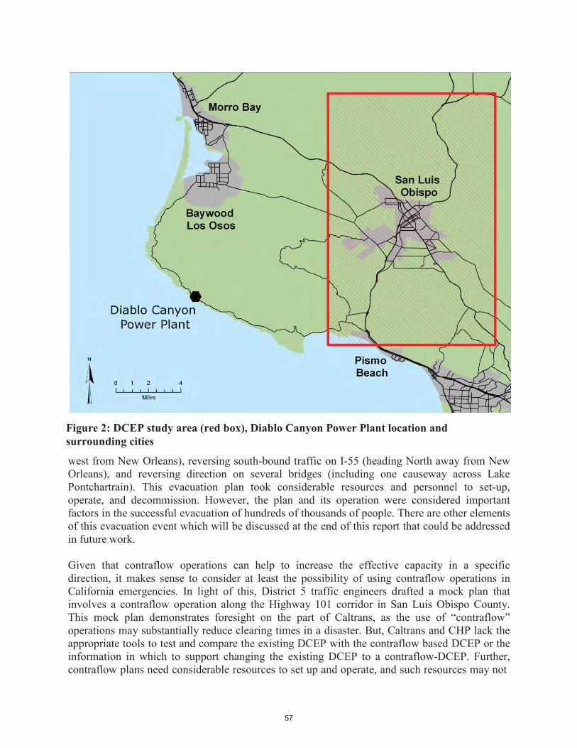
57
Figure 2: DCEP study area (red box), Diablo Canyon Power Plant location and surrounding cities
west from New Orleans), reversing south-bound traffic on I-55 (heading North away from New Orleans), and reversing direction on several bridges (including one causeway across Lake Pontchartrain). This evacuation plan took considerable resources and personnel to set-up, operate, and decommission. However, the plan and its operation were considered important factors in the successful evacuation of hundreds of thousands of people. There are other elements of this evacuation event which will be discussed at the end of this report that could be addressed in future work.
Given that contraflow operations can help to increase the effective capacity in a specific direction, it makes sense to consider at least the possibility of using contraflow operations in California emergencies. In light of this, District 5 traffic engineers drafted a mock plan that involves a contraflow operation along the Highway 101 corridor in San Luis Obispo County. This mock plan demonstrates foresight on the part of Caltrans, as the use of “contraflow” operations may substantially reduce clearing times in a disaster. But, Caltrans and CHP lack the appropriate tools to test and compare the existing DCEP with the contraflow based DCEP or the information in which to support changing the existing DCEP to a contraflow-DCEP. Further, contraflow plans need considerable resources to set up and operate, and such resources may not
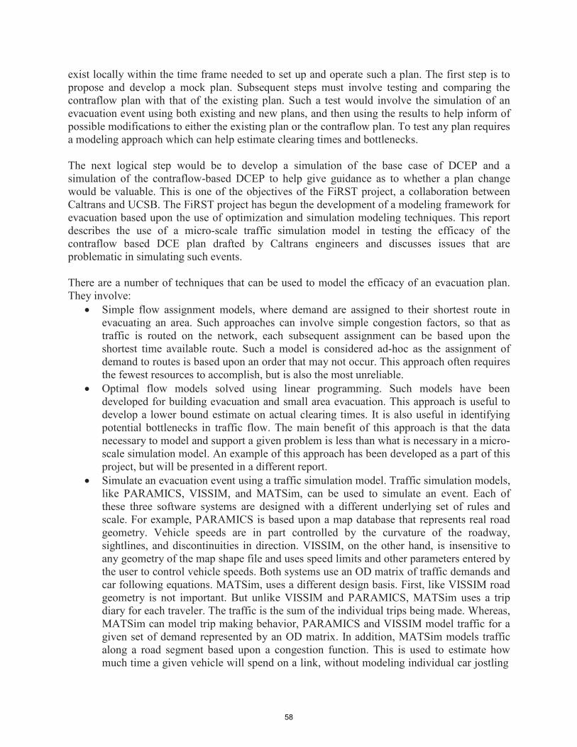
58
exist locally within the time frame needed to set up and operate such a plan. The first step is to propose and develop a mock plan. Subsequent steps must involve testing and comparing the contraflow plan with that of the existing plan. Such a test would involve the simulation of an evacuation event using both existing and new plans, and then using the results to help inform of possible modifications to either the existing plan or the contraflow plan. To test any plan requires a modeling approach which can help estimate clearing times and bottlenecks.
The next logical step would be to develop a simulation of the base case of DCEP and a simulation of the contraflow-based DCEP to help give guidance as to whether a plan change would be valuable. This is one of the objectives of the FiRST project, a collaboration between Caltrans and UCSB. The FiRST project has begun the development of a modeling framework for evacuation based upon the use of optimization and simulation modeling techniques. This report describes the use of a micro-scale traffic simulation model in testing the efficacy of the contraflow based DCE plan drafted by Caltrans engineers and discusses issues that are problematic in simulating such events.
There are a number of techniques that can be used to model the efficacy of an evacuation plan. They involve:
• Simple flow assignment models, where demand are assigned to their shortest route in evacuating an area. Such approaches can involve simple congestion factors, so that as traffic is routed on the network, each subsequent assignment can be based upon the shortest time available route. Such a model is considered ad-hoc as the assignment of demand to routes is based upon an order that may not occur. This approach often requires the fewest resources to accomplish, but is also the most unreliable.
• Optimal flow models solved using linear programming. Such models have been developed for building evacuation and small area evacuation. This approach is useful to develop a lower bound estimate on actual clearing times. It is also useful in identifying potential bottlenecks in traffic flow. The main benefit of this approach is that the data necessary to model and support a given problem is less than what is necessary in a micro- scale simulation model. An example of this approach has been developed as a part of this project, but will be presented in a different report.
• Simulate an evacuation event using a traffic simulation model. Traffic simulation models, like PARAMICS, VISSIM, and MATSim, can be used to simulate an event. Each of these three software systems are designed with a different underlying set of rules and scale. For example, PARAMICS is based upon a map database that represents real road geometry. Vehicle speeds are in part controlled by the curvature of the roadway, sightlines, and discontinuities in direction. VISSIM, on the other hand, is insensitive to any geometry of the map shape file and uses speed limits and other parameters entered by the user to control vehicle speeds. Both systems use an OD matrix of traffic demands and car following equations. MATSim, uses a different design basis. First, like VISSIM road geometry is not important. But unlike VISSIM and PARAMICS, MATSim uses a trip diary for each traveler. The traffic is the sum of the individual trips being made. Whereas, MATSim can model trip making behavior, PARAMICS and VISSIM model traffic for a given set of demand represented by an OD matrix. In addition, MATSim models traffic along a road segment based upon a congestion function. This is used to estimate how much time a given vehicle will spend on a link, without modeling individual car jostling

59
along the link. Consequently, MATSim can model events much faster than the other two systems.
Thus, there are pros and cons for each of these systems, where one may be ideal for one task and another may be better for another. In this paper, we report on the use of VISSIM.
2. Data base development
In simulating an event, it is important to capture all elements that will significantly impact the functions being modeled or estimated. As a starting data base, we acquired NAVTEQ map tiles from PTV Corporation that covered the San Luis Obispo and Santa Barbara Counties. The main feature being modeled is the performance of Highway 101, using either the contraflow plan or Highway 101 without controls (there is a general split of traffic heading north and traffic heading south, and these splits are based upon the general evacuation plan). We developed a second form of the NAVTEQ network data by modifying it to match road closures, lane reversals, and route modifications as specified in the “mock” contraflow plan. The NAVTEQ data base contains center line information for road ways, lane data, and other attribute data, including the designation of a street being one-way and turn restrictions. Speed limits are not often given. It is important that all speed limits and assumed travel speeds be specified as well in the network. It is also important to capture multi-lane layouts accurately, turn lanes, and other elements. This data preparation can take a considerable amount of time to set up. In fact, setting up a data base for micro-scale traffic simulation is a time consuming and detailed task. For, VISSIM, it is absolutely necessary to have an accurate depiction of the network with respect to the attributes but not necessarily with respect to the road geometry.
As exact road geometry is not necessary for the simulation per se, one can be somewhat frugal in the time spent in generating an exact geometry as long as the attributes (like speed limits) are accurate. An example of this can be seen in Figure 3. Figure 3 depicts a short portion of Highway 101 and surrounding roads. You will note that the road segments are depicted as straight line segments drawn in blue. Logical connections are colored with magenta. Logical connections depict ramps and turn restrictions. This helps to aid in the use of the database in terms of navigation, supporting the common directions of “turn left” here and “take off ramp on right.” Note that the road network data (in blue) does not always have a connected set of lines (i.e. streets). The magenta lines represent turn and route restrictions, and without some of these restrictions, the network may not be completely connected. It should also be noted here that the network does not contain many shape points. Shape points are used in line representation to depict curves in roads. But, shape points are added features that expand the size of the data base. If one wants to use a database for navigation purposes, exact geometry with significant positional accuracy is not necessary. Consequently, a database can be reduced in size by keeping the use of shape points to a minimum, while still retaining enough data in which to provide navigational capabilities. Also note in Figure 3, that the lanes of the segment of Highway 101 in the figure are not depicted. The short portion of Highway 101 is depicted as two parallel lines, one representing the South-bound lanes and the other representing the North-bound lanes. Thus, the position and number of lanes are not depicted on the map (the number of lanes, however, is

60
included as an attribute). This is another element that may or not be resolved in the development of a traffic simulation model.
Figure 3: An example of road data layout from NAVTEQ where Highway 101 traverses from the center bottom to the top right corner of the image. The alignment of 101 is depicted with two parallel lines, depicting the South-bound and North-bound lanes. Each roadway is depicted with a line associated with a given direction of travel.
To understand this from a graphical perspective, roughly the same section of the map in Figure 3 has been resized and projected using an aerial photo as the background in Figure 4. Each roadway segment in Figures 3 and 4 is depicted with a line associated with a given direction of travel. For example, there is a somewhat vertical line segment at the bottom right corner of Figure 3 which abruptly turns left. This segment is depicted with one line segment, indicating that there is only one direction of travel. This same roadway can be found toward the center of Figure 4, where it can be seen that this line represents an off ramp for Highway 101. Note that this captures a given travel function, but does not accurately depict the roadway as it does not coincide with the image. In fact, this is not an unusual occurrence. In Figure 4, it can be seen that many of the road segments do not coincide with the image. Although the section of Highway 101 is represented by parallel lines with a reasonable level of accuracy, the major road crossing Highway 101 at the interchange is depicted with dual lines that coincide with only one direction of the separated roadway. Also observe that the intersection at the top center of the image in Figure 4 captures connectivity, but represents the roads connected to the intersection with less than what most would be considered reasonable from a graphical perspective. There are methods to automatically generate road curvatures from navigational databases, e.g. S2P, but such techniques cannot be relied upon to eliminate all issues in road representation.
One of the reasons why road depiction is discussed here is that micro-scale simulations greatest asset is the ability to depict vehicle movement along roadways in a realistic image. Such “moving pictures” of traffic help to visualize a given traffic event. The more an image departs
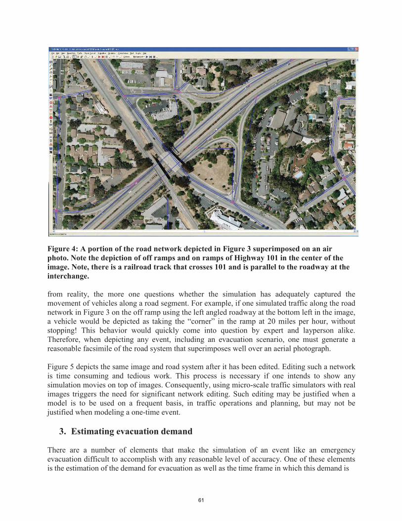
61
Figure 4: A portion of the road network depicted in Figure 3 superimposed on an air photo. Note the depiction of off ramps and on ramps of Highway 101 in the center of the image. Note, there is a railroad track that crosses 101 and is parallel to the roadway at the interchange.
from reality, the more one questions whether the simulation has adequately captured the movement of vehicles along a road segment. For example, if one simulated traffic along the road network in Figure 3 on the off ramp using the left angled roadway at the bottom left in the image, a vehicle would be depicted as taking the “corner” in the ramp at 20 miles per hour, without stopping! This behavior would quickly come into question by expert and layperson alike. Therefore, when depicting any event, including an evacuation scenario, one must generate a reasonable facsimile of the road system that superimposes well over an aerial photograph.
Figure 5 depicts the same image and road system after it has been edited. Editing such a network is time consuming and tedious work. This process is necessary if one intends to show any simulation movies on top of images. Consequently, using micro-scale traffic simulators with real images triggers the need for significant network editing. Such editing may be justified when a model is to be used on a frequent basis, in traffic operations and planning, but may not be justified when modeling a one-time event.
3. Estimating evacuation demand
There are a number of elements that make the simulation of an event like an emergency evacuation difficult to accomplish with any reasonable level of accuracy. One of these elements is the estimation of the demand for evacuation as well as the time frame in which this demand is

62
Figure 5: A portion of the road network depicted in Figure 3 superimposed on an air photo after network editing. This editing is required when movies of an event are made superimposed on an air photo image. In addition, some editing is necessary to eliminate unrealistic, abrupt changes in direction on a road segment like an off ramp.
exerted. What makes this a complicated exercise is the lack of information concerning whether an individual will attempt to first return to the area to pick someone up, like an elderly person or a “latchkey” child. Also complicating the estimate is not knowing daytime and night time populations of neighborhoods. Often one assumes that an average number of vehicles will depart per household in each neighborhood. Although this may be somewhat realistic, based upon average vehicle ownership in a neighborhood, such an estimate must be made given the lack of specific information about individual behavior during an event. For the exercise reported here, we estimated demand for evacuation to be one vehicle per household. The total number of households was identified for each census block. Each block was represented by a centroid and the total demand for that census block was assigned to the centroid point. The nearest road segment to the centroid point based upon Euclidean distance was identified. These locations became inputs for traffic during the event.
It is important to note that the evacuation scenarios modeled here do not make any assumptions with respect to school children. For example, in a daytime emergency it would be expected that many parents would want to retrieve their children by going to their schools and picking them up. In the Diablo Canyon Evacuation Plan children are to be bused to special pick up points, e.g. a school in Santa Maria in the event of a mandatory evacuation. If parents do not understand all of the elements of such a plan, there may be a reverse flow in traffic that is generated by parents making needless trips and needless confusion.

63
Another major element that needs to be estimated is the distribution of departures from a neighborhood. For example, is there an immediate onslaught of traffic generated by people attempting to flee in a panic, or is there a more organized and deliberate demand in evacuating over a longer time period? For the estimates here, we assumed that demand for evacuation was exerted randomly over a two hour period. Data exists for evacuation demand and its distribution for events such as hurricanes. In an event such as a hurricane, inhabitants often have a warning which may be hours if not days ahead of the possible disaster. But, for an event such as a nuclear power plant disaster, the distribution of demand over time is unpredictable. For example, in the recent case in Japan, the tsunami caused significant damage to all infrastructure including a nuclear power plant. In some cases, evacuations were not immediate, but took days and even weeks to accomplish. Whatever the case, it is clear that inhabitants need clear concise information and guidance. It should be noted that shorter evacuation time periods for the DCEP results in grid lock.
4. Simulation results for a non-contraflow evacuation plan
We used VISSIM from PTV Corporation to model traffic flow on the network. To generate information about traffic flow, we placed VISSIM data collectors on each entrance ramp in the contraflow section of Route 101. Additional data collector sets were defined:
Data Collector set 1: this totals flow per time period leaving the network, having travelled either south or north on U.S. Highway 101 to a designated point outside of the evacuation zone.
Data Collector set 2: this totals North-bound flow per unit time period on U.S. Highway 101, having reached Atascadero and a designated point outside of the evacuation zone.
Data Collector set 3: this totals South-bound flow per unit time period on U.S. Highway 101, having reached Avila Beach and a designated point outside of the evacuation zone.
Data Collector set 4: this totals North-bound flow per unit time period on U.S. Highway 101, having reached the Highway 58 junction north of Cuesta Grade.
Data Collector set 5: this totals North-bound flow per unit time period on U.S. Highway 101, just north of the last 101 entrance ramp at Monterey Street.
Data Collector set 6: this totals vehicles per unit time period having entering U.S. Highway 101, North-bound or South-bound
In addition to vehicle flow data, these collectors also captured vehicle speeds [mph] (maximum, minimum and average) and queue delay times [seconds] (maximum, minimum, and average). We also collected data on system wide information like latent demand, average speed and delays. The position of the non-ramp data collector points are given in Figure 6. Figure 6 depicts the evacuation region, major roads, and the population density of the region that is outlined in Figure 2. One can easily observe from Figure 2 that the majority of the population in the area being

64
Figure 6. Location of special data collectors on Highway 101 and general region surrounding San Luis Obispo.
modeled resides in or near San Luis Obispo. Although there are communities north of Diablo Canyon Nuclear power plant that are along the coast (e.g. Morro Bay and Los Osos), these communities are supposed to evacuate by heading north along State Route 1 and Northeast along State Route 46 thereby circumventing the use of Highway 101. We assumed that this would be
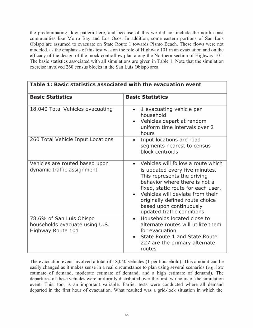
65
the predominating flow pattern here, and because of this we did not include the north coast communities like Morro Bay and Los Osos. In addition, some eastern portions of San Luis Obispo are assumed to evacuate on State Route 1 towards Pismo Beach. These flows were not modeled, as the emphasis of this test was on the role of Highway 101 in an evacuation and on the efficacy of the design of the mock contraflow plan along the Northern section of Highway 101. The basic statistics associated with all simulations are given in Table 1. Note that the simulation exercise involved 260 census blocks in the San Luis Obispo area.
Table 1: Basic statistics associated with the evacuation event
Basic Statistics Basic Statistics
18,040 Total Vehicles evacuating • 1 evacuating vehicle per household
• Vehicles depart at random uniform time intervals over 2 hours
260 Total Vehicle Input Locations • Input locations are road segments nearest to census block centroids
Vehicles are routed based upon • Vehicles will follow a route which dynamic traffic assignment is updated every five minutes.
This represents the driving behavior where there is not a fixed, static route for each user.
• Vehicles will deviate from their originally defined route choice based upon continuously updated traffic conditions.
78.6% of San Luis Obispo households evacuate using U.S. Highway Route 101
• Households located close to alternate routes will utilize them for evacuation
• State Route 1 and State Route 227 are the primary alternate routes
The evacuation event involved a total of 18,040 vehicles (1 per household). This amount can be easily changed as it makes sense in a real circumstance to plan using several scenarios (e.g. low estimate of demand, moderate estimate of demand, and a high estimate of demand). The departures of these vehicles were uniformly distributed over the first two hours of the simulation event. This, too, is an important variable. Earlier tests were conducted where all demand departed in the first hour of evacuation. What resulted was a grid-lock situation in which the

66
software could not reach a set of stable routes or pathways, where many vehicles traveled in circles, as capacity was limited in their movements towards on-ramps. Part of this outcome was the result of erratic routes generated when vehicles had almost no option as to where they could head. When pathways were fixed for each neighborhood in travelling towards their “assigned” highway ramp, this type of problem did not occur, however, significant traffic congestion was experienced throughout the entire area of San Luis Obispo. Examples of this are given in the appendix.
The main results generated for the base case of no contraflow options are given in Table 2. As described above, this simulation involved the use of a calibrated dynamic traffic assignment model. The results represent tabulations made at the 3-hour time mark, after the evacuation event started. At the 3-hour mark, 13,292 vehicles of the 18,040 were still in the process of evacuating.
Table 2: Simulation results for the base case (no contraflow sections) Data type 1 2 3 4 5 6 7 measurement 13292 4159 4923 7.2 23865. 903.87 566
1 Number of vehicles in the network, All Vehicle Types 2 Number of vehicles that have left the network, All Vehicle Type 3 Average delay time per vehicle [s], All Vehicle Types 4 Average speed [mph], All Vehicle Types 5 Total delay time [h], All Vehicle Types 6 Latent delay time [h], All Vehicle Types 7 Latent demand, All Vehicle Types
Furthermore, 4,159 vehicles had successfully reached one of the evacuation exits (Atascadero or Pismo Beach). Average vehicle speed during the evacuation was 7.2 miles per hour, and the average delay per vehicle was 4,923 seconds or approximately 45% of the 3 hour period. As vehicle departures were spread out over the first two hours, an average delay of close to an hour and a half suggests that most vehicles spend the majority of their trip in some form of delay, caused by congestion. Note that at the end of the three hour period, 566 vehicles had not yet been able to depart. Overall, the statistics for the base case evacuation indicate a near grid-lock situation with significant delays such that a majority could not reach an exit of the evacuation region within three hours.
Figure 7 depicts the network at the 2 hour time mark. Each arc on the network is coded in a color that represents the average vehicle speed 2 hours after the evacuation event starts. Note many sections of Highway 101 have traffic speeds that range from 6-12 miles per hour, and that the majority of the road network within the City of San Luis Obispo experienced vehicle speeds that averaged less than 6 miles per hour. Given that the majority of the network within the city close to Highway 101 experienced such slow vehicle speeds, one can classify this condition as near grid-lock. When assessing the results of this simulation, one must keep in mind that this is a highly optimistic result for the base case. First, this does not consider any existing traffic on the network when the call for evacuation occurs. Second, this does not account for any trip chaining that may exist in a true evacuation, where a vehicle may leave a home, proceed to another

67
Figure 7. Map depicting congestion on network at the 2 hour time mark in simulating a non-contraflow scenario. Note those areas colored in pink represent traffic speeds of less than 6 miles per hour.
13

68
location to pick someone up, and then proceed to an entrance route on the highway to evacuate. Third, demand for those without cars, people with disabilities, the elderly, and those hospitalized have not been considered. Thus, the results underestimate the demand for those who cannot evacuate without assistance. Finally, the students who are housed on campus at Cal-Poly San Luis Obispo have not been included. Adding these other demands would add significantly to the critical nature of the event and further degrade the traffic flow.
Another way in which we can depict an evacuation is in terms of the number of vehicles that have successfully reached an outlet (or exit) of the evacuation area per given time interval. Figure 8 depicts for the base case the number of vehicles that have left the evacuation area for each half hour time interval (given in seconds). For example, in the first time interval (0-1800 seconds), only a negligible number of vehicles have reached an exit (Atascadero or Pismo Beach).
Figure 8. The number of vehicles successfully exiting the evacuation area by time intervals in seconds. Note flow totals per interval are quite low. Part of this is associated with very low average speeds on Highway 101 and near grid lock conditions in areas close to Highway 101 in the City of San Luis Obispo.
5. Simulation results for a contraflow based evacuation plan
The mock contraflow plan was based upon reversing traffic flow on South-bound Highway 101 at San Luis Bay Drive to North-bound flow. San Luis Bay Drive is south of the City of San Luis Obispo. Thus, all lanes of Highway 101 through San Luis Obispo are used to handle North- bound traffic. The end of the contraflow section is at Santa Barbara Road at the southern boundary of the City of Atascadero. The plan involves blocking specific on-ramps and off ramps to aid in directing flow for both South-bound and North-bound lanes. Other ramps are reversed
Base Case Vehicle Totals 1200
1000
800
600
400 Number of Vehicles exiting system
200
0

69
in direction of use so that vehicles can enter and travel northward on what was originally designed for South-bound use. Additionally, traffic crossing most overpasses is to be blocked, forcing traffic that reaches the highway to enter the highway. In preliminary simulations, it was found that because of a mismatch between demand generated to the east of Highway 101 and to the west of Highway 101, traffic circulated in an unusual manner that was not realistic. This situation also made it difficult to calibrate a model using dynamic traffic assignment. Accordingly, this one element was not modeled as a part of the contraflow plan. The Appendix depicts a fixed route plan which is amenable to such route closures within the simulation. The results for the contraflow plan are compared to the non-contraflow plan in Table 3. First, it should be observed that the contraflow plan resulted in average traffic speeds during evacuation of 20.3 miles per hour, whereas in the base case speeds averaged 7.2 miles per hour. From this fact alone, one can assume that evacuation is substantially aided with the use of a contraflow option. Of the 18,040 vehicles departing San Luis Obispo and evacuating using Highway 101, only 4,248 vehicles are still on the network at the end of the three hour time mark. This is substantially lower than the amount of traffic moving on the network at the end of the three hour time period for the base case (that is, 13,292)! This also means that a majority of the demand (12,855) had successfully evacuated and left an exit point at the end of the simulation period, whereas in the base case less than a third of this number had reached an exit in the same amount of time. Overall, one can observe, that in every category, the contraflow plan appears to outperform what would be achieved without contraflow operations. One telling statistic is that the average delay per vehicle for the contraflow plan is 31% of the average delay found for the base case.
Table 3: Simulation results comparing contraflow with no contraflow sections Data type 1 2 3 4 5 6 7 Non Contraflow
13,292 4,159 4,923 7.2 23,865. 903.87 566
Contraflow 4,248 12,855 1,528 20.3 7,262 202.71 0
1 Number of vehicles in the network, All Vehicle Types 2 Number of vehicles that have left the network, All Vehicle Type 3 Average delay time per vehicle [s], All Vehicle Types 4 Average speed [mph], All Vehicle Types 5 Total delay time [h], All Vehicle Types 6 Latent delay time [h], All Vehicle Types 7 Latent demand, All Vehicle Types
Figure 9 shows the number of vehicles that have successfully left the area during different time segments of the simulation. For instance, in the time interval of 3600 to 5400 seconds (1hour- 1 ½ hours) approximately 2,900 vehicles were successful in leaving the evacuation area. Note that after the first hour the system reaches a plateau in traffic exiting the system and continues through the third hour. There appears to be a substantial gain in the numbers of vehicles successfully evacuating in each time period for the contraflow case as compared to the base case, except for the first half hour in which few vehicles exited the system in either case. The same caveats hold true for the contraflow case as for the base case, that is, with respect to the issues of

70
ignoring existing base-flow of traffic on streets and highways, people without cars, people with a disability that prevents them from driving, people hospitalized or in convalescent care facilities, and the student body at Cal-Poly San Luis Obispo.
Figure 9. The number of vehicles successfully exiting the evacuation area by time intervals in seconds for the mock contraflow plan.
Figure 10 displays the network at the 2 hour time mark for the contraflow case. Each arc on the network is coded in a color that represents the average vehicle speed 2 hours after the evacuation event starts. Some of the sections of Highway 101 have traffic speeds that range from 6-12 miles per hour, and there are a number of areas within the City of San Luis Obispo that experience vehicle speeds that average less than 6 miles per hour. If one compares Figure 10 with that of Figure 7, one will see that the contraflow case appears to result in fewer areas of the City and fewer sections of Highway 101 experiencing extremely slow speeds in contrast to the base case.
In a general comparison between the base case and the contraflow case, it is clear that a majority of the residents of San Luis Obispo are able to evacuate within three hours under contraflow, but are not with base case operations. It is important to note that the results for each case might dramatically change given a different departure histogram. For example, spreading demand over a larger time frame may result in better traffic flows in comparison to restricting all departures to be made within the first two hours. Further, if such a model were to be used in fine-tuning an evacuation plan, then a number of different scenarios would need to be run in order to both fine tune a plan as well as identify major bottlenecks that might need traffic control. It is also important to note that there may be specific road issues that are part of a local knowledge base (local transportation engineers and traffic control officers) that need to be included in the traffic simulation. This “local” knowledge cannot be easily recreated and consequently, it is important that local experts be involved in such planning.
Contraflow Vehicle Totals 3500
3000
2500
2000
1500
1000
500
0
Number of vehicles exiting system
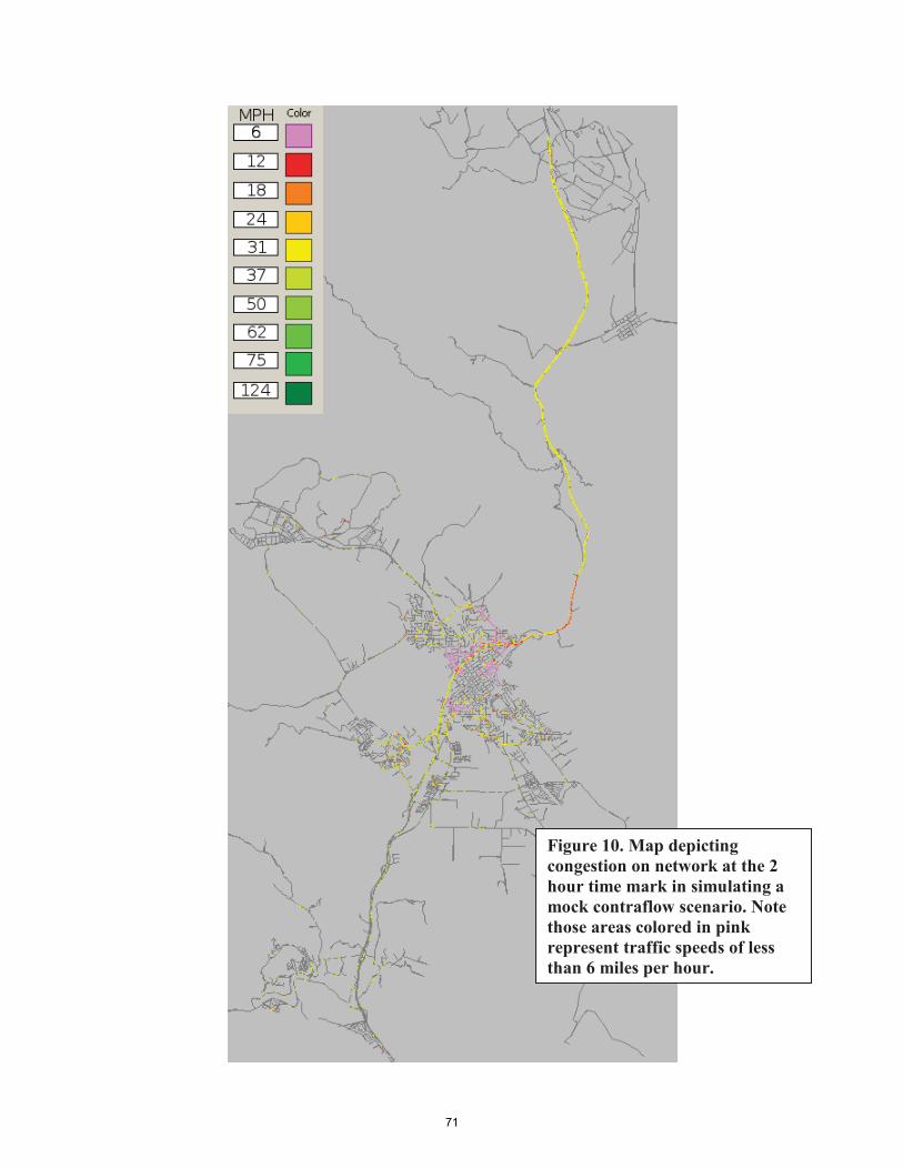
71
Figure 10. Map depicting congestion on network at the 2 hour time mark in simulating a mock contraflow scenario. Note those areas colored in pink represent traffic speeds of less than 6 miles per hour.

72
6. Discussion of results
Charts and screenshots both indicate significant queues building over time on many sections of the transportation network for the base case. Areas within the City of San Luis Obispo have the longest queues and slowest vehicle speeds which is to be expected given the high population density and corresponding travel demand (traffic inputs). The base case (no contraflow) queuing and congestion may be the primary reason that only 1/3 of the vehicles on the network make it to 'safer' areas away from the Diablo Canyon power plant in the time frame that was modeled. In contrast, the contraflow example yields demonstrably better results, where the majority of vehicles make it to an exit point of the evacuation area and where the average vehicle speed is nearly three times faster. Overall, the “mock” contraflow plan appears to be very promising. Although this is only a “mock” evacuation plan, there are appealing features to this plan in that the capacity to handle traffic heading away from San Luis Obispo has been significantly enhanced. However, there are elements in the mock plan that deserves further scrutiny. They are:
• Alternate routes should be fully utilized for evacuation, most notably State Route 1 (Northwest area of network) and State Route 227 (East area of network). This may mean that more traffic should be diverted from San Luis Obispo and Highway 101, or vice versa. Such an analysis would need to be based upon the DCEP plan and a micro-scale traffic model.
• The mock contraflow plan does not allow vehicles to utilize Highway 101 over- or underpasses, whereas the simulation model results reported here do allow that traffic to occur. This helps to relieve some disparities in travel demand between those neighborhoods on the east of Highway 101 and those on the west of Highway 101. Selected crossing locations can help to balance traffic demand entering Highway 101, fully utilizing the contraflow section and the regular flow section of the highway.
• The simulation model does not consider the possibility of trip chaining, where an individual may start at their place of work, return to their home, pick up someone and proceed to evacuate. This is a more realistic situation in an emergency, and such behavior cannot be captured in this modeling approach.
• The mock evacuation plan is far from complete. One can consider this as an exercise in thinking forward to a possible emergency. Such plans can be complicated and the requirements to fully support such a plan have not been fully analyzed within the context of setting up a contraflow segment. Operating a contraflow plan in Louisiana during hurricane Katrina took a considerable amount of state resources and time to set up. In the case of Katrina, state troopers and parish police had a considerable amount of advanced warning and time to set up the road system for contraflow operations. In a nuclear plant disaster, there may be little warning and the personnel needed to setup a contraflow system may take time to amass.

73
7. Limitations
The simulation presented here is a best-case type simulation. Traffic is likely to be worse as there are a number of assumptions that have been made. First, the simulation results are based upon 1 vehicle departing per household. This is likely to be a lower bound on the average number of vehicles being used in evacuation. Second, we have assumed that departures times are random with the first two hours of the event. Random uniform departures from traffic input points over the 2 hour window may not reflect trip departure timing during a real evacuation. This assumption does not necessarily match what might be expected in actual behavior, as little data has been collected for such events and a complete understanding has yet to be developed. Although, demands for major evacuation events like hurricanes are better understood, these often happen over larger time frames, and such events do not necessarily represent the urgency that might be present for a wildfire, tsunami, or nuclear disaster. Third, special demands like hospitals, nursing homes, the homeless, those who don’t own cars, and those living at Cal-Poly San Luis Obispo have not be included. The bottom line is that a contraflow plan for this area appears to be beneficial, aiding in substantial increases in average travel speeds and in larger numbers of vehicles leaving considerably earlier than what happens in the base case (do nothing).
8. Suggested Future work
The objective of this project was to capture the essence of a mock contraflow plan involving an emergency at the Diablo Canyon Power Plant. Although many of the main problem elements were captured to the point that a simulation model could be applied, there are a number of remaining issues that should be considered in any future improvements to the VISSIM model addressing. They include:
1) Current traffic inputs should be overlaid on aerial imagery and the placement be assessed. It may be possible to move these inputs to correspond better with the actual locations of housing within each census block.
2) Highway 101 entrance ramp daily traffic counts supplied in the appendix of the Caltrans plan could be used to calibrate traffic flow. These counts could essentially serve as a scaling factor to help determine how heavily each entrance ramp will be used.
3) Network geometry should be corrected using aerial imagery. Only selected intersections at Highway 101 were corrected. This may not materially change the results of the model as the attributes of the links dictate use in a simulation but improve its use in visualization.
4) Traffic signal timing should be implemented, and reduced speed areas and conflict zones defined for the entire network. Also, fine tuning of merging behavior is necessary. Both tasks can be very time consuming. Collecting signal settings for the city and integrating them would help to close many of the remaining gaps in the model developed here.

74
5) Plume spread model(s) could be integrated with the traffic simulation model to assess radioactive material exposure risk during the evacuation.
Beyond the work involved with the simulation effort using VISSIM, there are several problems that should receive attention. The first of these is the development of a model that helps estimate the time it will take to amass resources and set up a contraflow plan in an emergency. In fact, Caltrans should develop supply models which estimate how much time it would take to reach any part of their system with a prescribed set of equipment and trained personnel. A second problem of major importance is the development of models which can estimate the demand for evacuation on the part of those not using personal vehicles and those requiring assistance (e.g. those who need public transit). Further work should also involve modeling when evacuation demand is exerted during an emergency. Finally, more accurate methods should be developed for determining the location of individuals by time of day. The simulation here is based upon the assumption that everyone starts at their home and evacuates. This is clearly a poor assumption during daytime hours, when many people are at school or work. Models like SimAgent may be employed for this purpose.

75
Appendix: Simulation for a contraflow evacuation plan using fixed routes
Evacuation modeling can be accomplished using linear flow models. This type of modeling technique has been used in building egress models as well as wide area evacuation, including emergency evacuation planning zones around nuclear power plants. Perhaps one of the most widely accepted approaches is one based upon paths. As an example, one form of that has been used to generate an estimate of evacuation effectiveness is the following:
1) Generate for each leaving vehicle a departure time. 2) For the vehicle that has not yet left and has the earliest departure time, identify the
shortest path to leave based upon an estimate of congestion generated by those who have already left and chosen a route. Assign this vehicle to that path which is the shortest according to current trip assignments.
3) Have all vehicles left? If yes, stop and tally the times vehicles reached an exit to the evacuation region. If not, then return to step 2.
This approach can be used to give a rough approximate of the effectiveness of an evacuation plan. An alternate form of this is to define fixed routes for sets of individuals in leaving an area. For example, in the San Luis Obispo area there were 260 different individual neighborhoods that are used for sources of vehicles leaving the area. For each of these 260 neighborhoods (or census blocks) we can define a route that those vehicles will take to leave the area. We assume here that people will not make dynamic route changing decisions, but use what looks to be logically the route of first choice. This type of option is supported in the PTV VISSIM software as well. In order to perform a simulation using this option, it was necessary to code a fixed route for each of the neighborhoods. The simulation is then used to model congestion associated with the fixed route plan. This approach is just as efficacious as the path based model described above. In fact, in many ways it can be considered to be better than that approach as it more accurately depicts individual route congestion. In this appendix, we present the results of a simulation based upon fixed routing for each census block.
The assumptions used in the example presented here are the same as those presented in Table 1, with the exception that each of the 260 neighborhoods have a defined route for exiting the area and that all demand is set up to leave in the first hour of the simulation. Whereas, the dynamic traffic assignment results presented in the main section of this report are specified for evacuation demand spread out over two hours, we assumed for the fixed route analysis a more intense, shorter duration of evacuation demand.
At the end of the first hour of simulation, 2,005 vehicles (11.2%) have passed Cuesta Grade. This represents flow that has passed safely over the grade heading to Atascadero. At this same time 6,226 vehicles (34.9%) have passed the last entrance ramps on Monterey Street in San Luis Obispo. This means that in the first hour, approximately a third of the traffic demand has reached a point where they have merged onto Highway 101 and are traveling north from San Luis Obispo.
The evacuation event can be analyzed from the perspective of each onramp and sections of Highway 101. Rather than show details of each highway element, data in this appendix is

76
summarized for all ramps, those on the freeway north of Cuesta Grade and those on the highway north of the Monterey Street onramps. Figure 11 presents a chart which gives the distribution of vehicles reaching the northern most collector point over the time of the simulation. This depicts the number of vehicles having reached north of Cuesta Grade per minute. Note that the time lag in traffic reaching this collector point is approximately 22 minutes. After 22 minutes the traffic reaching this point begins to increase until it averages a flow of approximately 60 vehicles a minute. To serve approximately all 18,000 vehicles would take up to 4 hours. Figure 12 gives this same distribution for those cars passing just north of the Monterey Street exit at the northern boundary of the City of San Luis Obispo). This figure shows that the number of vehicles having merged onto Highway 101 and begin their trip to Atascadero starts with almost no lag in time from the beginning of the evacuation event. The traffic volume per minute quickly ramps up to an average that is between 100 and 110 vehicles per minute. Much of this volume is predicated on the number and capacity of entrance ramps as well as the time in which it takes to merge into the traffic lanes on Highway 101.
Figure 11: Total vehicles per minute passing data collector on Route 101 at end of contraflow section
Total Vehicles per Minute - North of Cuesta Grade
200
180
160
140
120
100
80
60
40
20
0 1 11 21 31 41 51
Time after evacuation begins [min]
Num
ber o
f Veh
icle
s
Figure 13 depicts the number of vehicles merging onto Highway 101 per minute over all entrance ramps. This shows that the number of vehicles entering the system quickly ramps up to 180 vehicles per minute, but as congestion starts on Highway 101, the entrance flow begins to decline. After the first fifteen minutes the traffic entering onto Highway 101 declines to an equilibrium rate of approximately 110-115 vehicles per minute.
As the traffic begins to increase, average vehicle speeds on Highway 101 begin to decrease. This phenomena can be understood by calculating the maximum delay that is experienced by any one

77
vehicle entering the system. Figure 14 depicts the maximum queue delay faced by those vehicles reaching the end of the contraflow section. Note here that queue delays for cars reaching this point reach 1500 seconds at the end of the hour. This means that of the cars reaching this point, the maximum queue delay experienced was approximately 25 minutes.
Figure 12: Total Vehicles per minute passing data collector on Route 101 after the last entrance ramp at San Luis Obispo heading north.
Total Vehicles per Minute - North of Monterey Street onramps
200
180
160
140
120
100
80
60
40
20
0 1 11 21 31 41 51
Time after evacuation begins [min]
Num
ber o
f Veh
icle
s
Figure 15 depicts a similar trend for the maximum queue delay faced by vehicles having passed the Monterey Street onramp, except that the maximum delays begin to ramp up from zero almost immediately after the start of the evacuation event. Here the maximum delay experienced by any one vehicle reaching this location at the end of the first hour is 50 minutes. That is, almost all of the travel experienced by that vehicle in that hour was queue delay! This means that there is considerable delay experienced by drivers in reaching Highway 101.
To understand where congestion occurs during the evacuation event and the fixed route scenario, maps were produced for three times: 20 minutes, 40 minutes, and 60 minutes. The images produced by VISSIM show the average speed [mph] of each vehicle on the network after 20 minutes, 40 minutes, and 60 minutes of simulation time. Highest speeds are indicated by green colors and lowest speeds by purple, with yellow at the midpoint. Figure 13 depicts the status of the system after 20 minutes. Note that the average speeds on Highway 101 are principally colored yellow, indicating that the speeds averaged 21-30 miles per hour. There are some locations on Highway 101 which experienced larger delays and are colored brown to red. In the City of San Luis Obispo, delays on a number of arterials are colored magenta or red. This means

78
that speeds on these streets ranged from 0 to 6 mph (magenta) and 6-12 mph (red). Thus, the traffic in the city is congested even after the first 20 minutes over many of the major streets.
Figure 13: Total Vehicles per minute passing data collectors on all Highway 101 entrance ramps.
Vehicles entering any Highway 101 entrance ramp
200
180
160
140
120
100
80
60
40
20
0 1 11 21 31 41 51
Time after evacuation begins [min]
Num
ber o
f Veh
icle
s

79
Figure 14: Maximum queue delay time on Route 101 at the end of the contraflow section
Max Queue Delay Time - North of Cuesta Grade 3500 3000
2500
2000
1500
1000
500
0
1 11 21 31 41 51 Time after evacuation begins [min]
Max
imum
Que
ue D
elay
for a
ny V
ehic
le [s
ec]
Figure 15: Maximum queue delay time on Highway 101 after last entrance ramps
Max Queue Delay Time - North of last entrance ramp on Moterey Street
3500 3000 2500 2000 1500 1000
500
0 1 11 21 31 41 51
Time after evacuation begins [min]
Max
imum
Que
ue D
elay
for a
ny V
ehic
le [s
ec]

80
Figure 16: Maximum queue delay time on all Highway 101 entrance ramps
Max Queue Delay Time - All vehicles having entered Highway 101
3500 3000 2500 2000 1500 1000
500
0 1 11 21 31 41 51
Time after evacuation begins [min]
Max
imum
Que
ue D
elay
for a
ny V
ehic
le [s
ec]

81
Figure 17: Vehicle speeds 20 minutes after evacuation begins
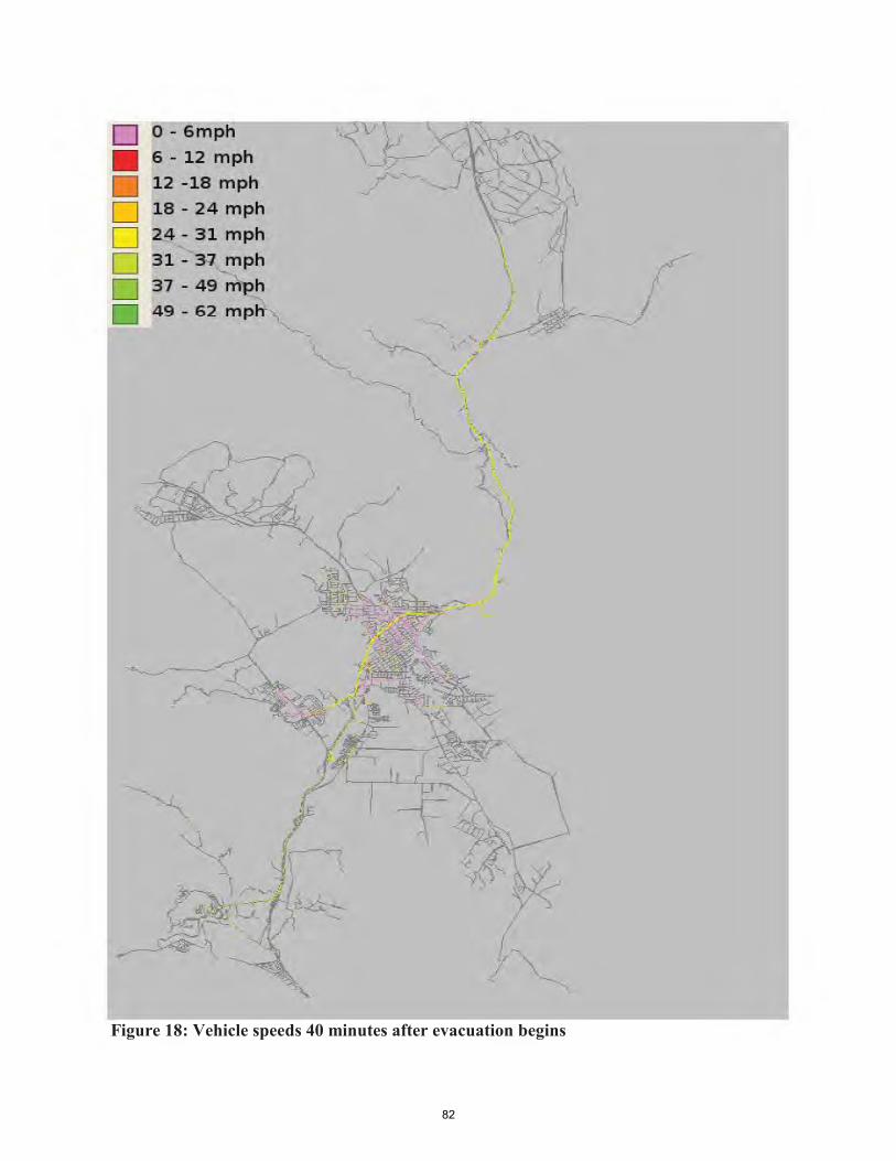
82
Figure 18: Vehicle speeds 40 minutes after evacuation begins

83
Figure 19: Vehicle Speeds 60 minutes after evacuation begins.

84
Figure 18 gives the view of traffic congestion at the 40 minute time period. Here it can be seen that the traffic speeds on Highway 101 have not materially changed, but congestion in the City has increased, where many street segments that were coded as red at the 20 minute mark are now colored in magenta at the 40 minute mark, indicating that traffic has been further slowed down. Note that some street segments colored in yellow at the 20 minute mark are now colored in magenta at the 40 minute mark. Also note that congestion has spread to outlying streets in the city. This pattern of congestion extends even further when moving from the 40 minute mark to the hour mark (Figure 19). It should not be a surprise that the constraints on fast evacuation are associated with the capacity of the highways to carry that traffic as well as the ramp capacities in accommodating inflow traffic. One must note that such patterns of congestion would have advanced faster with higher levels of congestion within the city without a contraflow setup.
It is important to note that this appendix presents results for a fixed route plan for all residents. This mimics the type of modeling that has been done in the past with fixed routes (without dynamic traffic assignment). The results here differ from the contraflow plan generated for dynamic travel assignment in one principal way: travel demand is spread out over one hour and not two hours. In either case (dynamic or fixed), a complete evacuation can be accomplished in approximately four hours. This estimate, of course, ignores possible delay effects of trip chaining, ignores populations needing assistance, does not include the impact of Cal-Poly San Luis Obispo, and ignores current traffic levels on streets and highways. What is important is that there appears to be a very real benefit to designing a contraflow plan, assuming local resources are ready and available to support such a plan.

85
First Responder Support Systems & Technologies (FiRST) Testbed
TRACK II – Cross Cutting Modeling & Simulation Summary of Dynamic Traffic Assignment in VISSIM
Summary of Dynamic Traffic Assignment in VISSIM
Carlos A. Baez
FiRST Project Geotrans Laboratory
University of California, Santa Barbara June 29, 2014
This report has been developed as a part of the First Responders System Testbed (FiRST) project at the University of California, Santa Barbara. The FiRST project investigates the integration of transportation and communication modeling and simulation to improve understanding and techniques of emergency preparedness and response. Please cite this report as: Baez, CA (2014) “Summary of Dynamic Traffic Assignment in VISSIM” Geotrans Laboratory, UCSB, Santa Barbara CA.
86
First Responder Support Systems & Technologies (FiRST) Testbed
TRACK II – Cross Cutting Modeling & Simulation Summary of Dynamic Traffic Assignment in VISSIM
Table of Contents 1.0 Introduction 1.1 Summary Scope 1.2 Sources
2.0 Foundations of Transportation Networks in VISSIM 2.1 Network Agents 2.2 The Transportation Network 2.2.1 Links and Connectors 2.2.2 Nodes 2.2.3 Markers 2.2.4 Routes 2.3 Network Agents and the Transportation Graph 2.4 Compiling Transportation Network Graphs 2.4.1 Parking Lot Zones and Network Compilation 2.4.2 Vehicle Input Markers and Network Compilation
3.0 Transportation System Modeling with Traffic Assignment 3.1 Supply Models 3.1.1 Network Information 3.1.2 Network Capabilities 3.1.3 Spatial Dimensions of Supply Models 3.1.4 Temporal Dimensions of Supply Models 3.2 Demand Models 3.2.1 The Spatial Dimensions of Demand Models 3.2.2 The Temporal Dimensions of Demand Models 3.2.3 Route Choice 3.2.4 Demand Modeling Data and its Collection 3.3 Traffic Assignment 3.3.1 Equilibrium in Traffic Assignment

87
First Responder Support Systems & Technologies (FiRST) Testbed
TRACK II – Cross Cutting Modeling & Simulation Summary of Dynamic Traffic Assignment in VISSIM
3.3.2 The Process of Traffic Assignment 3.3.3 Non-Equilibrium Dynamic Traffic Assignment
4.0 Transportation Model Validity, Calibration, and Validation 4.1 Model Verification 4.1.1 Errors from the Data Collection and Management Process 4.1.2 Model Coding Errors 4.1.3 Model Errors Resulting from Software 4.1.4 Model Review with Simulation 4.2 Model Calibration 4.2.1 Defining the Scope of Calibration 4.2.2 The Calibration Strategy 4.3 Model Validation
5.0 Traffic Assignment Modeling in VISSIM 5.1 Supply Models 5.2 Demand Models 5.3 Traffic Assignment in VISSIM 5.3.1 Static Traffic Assignment in VISSIM 5.3.2 Dynamic Traffic Assignment in VISSIM 5.4 The Evaluating Dynamic Traffic Assignment Models in VISSIM
6.0 Setting up Traffic Assignment in VISSIM

88
First Responder Support Systems & Technologies (FiRST) Testbed
TRACK II – Cross Cutting Modeling & Simulation Summary of Dynamic Traffic Assignment in VISSIM
1. Introduction
In this summary, we will cover the use of Dynamic Traffic Assignment (DTA) in
transportation systems modeling with VISSIM1. Roughly speaking, DTA is the modeling of
the interaction between a transportation network and its users (network agents) with
special consideration to how these interactions evolve through time. This is in contrast to
the Static Traffic Assignment (STA) modeling approach which does not take into account the
temporal aspects of transportation network-network agent interactions in that either the
nature or impact of these interactions is limited or more simply, time is omitted from the
model altogether. The difference between the dynamic and static approaches will be
highlighted throughout this report and presented in the context of modeling evacuations in
the VISSIM environment.
1.1 Scope
The scope of this summary will be that of a general introduction as to how DTA operates in
VISSIM and a general guide in how to implement DTA in VISSIM. No prior knowledge will be
assumed about DTA; however, some prior knowledge about using VISSIM is required. The
goal here is to allow a beginning VISSIM user with a limited background in transportation
modeling to: develop an intermediate understating of how DTA works in VISSIM, know how
to implement DTA in a modeling project, and how to interpret the output of the DTA model.
1 VISSIM is a transportation modeling software product created by the PTV Group.

89
First Responder Support Systems & Technologies (FiRST) Testbed
TRACK II – Cross Cutting Modeling & Simulation Summary of Dynamic Traffic Assignment in VISSIM
The understanding of the DTA process and its output will be the main emphasis of the main
text while the implementation of DTA in VISSIM will be left to the appendix of this report.
1.2 Sources
Our main sources of information include the 2011 PTV VISION VISSIM 5.30-05 user manual2
and the author’s experiences working with the Mission Canyon and Diablo Canyon
evacuation models in VISSIM. Thus, the bulk of the material can be presumed to have
originated from the PTV manual unless otherwise noted in the text.
2. Foundations of Transportation Networks in VISSIM
Transportation system modeling in VISSIM takes place using a micro-scale simulation
approach whereby discrete network agents (such as individual vehicles, bikes, buses,
people, etc.) interact with each other on a transportation network, which consists of a set
of locations and the set of connections between them (such as roads, bus lanes, bike lanes,
etc.). The micro-scale simulation aspect of this modeling entails that the interaction
between network agents is modeled at a fine resolution in terms of: 1) time, 2) the individual
behaviors and attributes of the network agents (agent heterogeneity),3 and 3) the
context/state/environment of the transportation network as it relates to the network
agents. We now explore these concepts in further detail.
2.1 Network Agents
At the core of transportation system models in VISSIM are network agents. Fundamentally,
the network agents are realizations of abstract entities whereby the realizations are the
2 5.30 represents a compromise for the VISSIM 5.xx versions and, unless noted, the concepts and procedures described in this summary should be compatible with and 5.xx version after 5.20. 3 In contrast, coarser approaches (such as macro or meso scale modeling) do not consider individual interactions but rather consider the aggregate behavior groups of homogeneous network agents, usually with analytical functions.

90
First Responder Support Systems & Technologies (FiRST) Testbed
TRACK II – Cross Cutting Modeling & Simulation Summary of Dynamic Traffic Assignment in VISSIM
actual individual objects that move within the modeled transportation network during the
simulation. The abstract entity on the other hand, simply refers to the vehicle type, which
specifies the range that the attributes of a realization can take. In VISSIM, the default vehicle
types are (other types exist)4 cars and heavy goods vehicles (HGVs). As such, a simulation
using the default vehicle types for generating network agent realizations will populate the
transportation model simulation with realizations of cars and HGVs in accordance with
parameters set by the modeler regarding the total number realizations needed and the
specified proportions of each vehicle type. In VISSIM, one does not declare the population
size of each vehicle type individually, but rather declares the number of desired realizations
for the simulation and uses a vehicle composition, which is a collection of vehicle types, to
specify the proportions of vehicle types. Furthermore, one is not limited to using the default
vehicle composition of one standard car and one standard HGV vehicle type as vehicle
compositions are neither restricted to only two vehicle types or to only standard cars and
HGVs. In fact, additional vehicle composition classes can be generated whereby each vehicle
composition can possess more, fewer, or different entity classes. Furthermore, multiple
instances of a particular vehicle type are also allowed in a vehicle composition, although
typically each multiple of a vehicle type possess different value ranges or distributions for
single or multiple entity attributes, which are defined as the set of characteristics that are
pre-specified (often by default or by the modeler) and immutable for all network agents.
In other words, all realizations of network agents are assigned a specific value for every
entity attribute it possess5 and the specific value assigned to each network agent (and for
each of its attributes) is based upon the specifications of its vehicle type. Although these
specifications are pre-defined for all entity attributes in terms of the allowable value
ranges and how the allowable entity attribute values are distributed, the range and
4 For example, busses, trams, bicycles, and pedestrians can be modeled in VISSIM. 5 All vehicle types possess the same set of entity attributes.

91
First Responder Support Systems & Technologies (FiRST) Testbed
TRACK II – Cross Cutting Modeling & Simulation Summary of Dynamic Traffic Assignment in VISSIM
distribution of values can be readily modified by the modeler.
It should be noted that the specific entity attribute values assigned to all network agent
realizations, regardless of entity class, are always independent of the actions or
characteristics of any other network agents and of other transportation network
components with which the network agent might interact.6 The entity attributes include:
the desired speed of the vehicle,7 vehicle length (an attribute not modifiable by the
modeler), the weight of the vehicle, max and desired acceleration, vehicle width, vehicle
occupancy, and the power of the vehicle. In all, the ability to create multiple vehicle types
allows for different geographic areas or time periods to have varying populations of
vehicles and occupancy. Beyond entity attributes, another fundamental aspect of network
agents are their behaviors which we define as the rules guiding how network agents react
with other network agents, to certain events or components of the transportation
network or components located on it. Similar to entity attributes, many parameters of
driver behavior can be modified, although, unlike entity attributes, rather than having to
specify them for every entity class, driver behavior affects all entity classes in a similar
way. How these behaviors are imparted to network agents is discussed in Section 2.2.1.
Examples of some driver behaviors include the look-ahead distance, lack of attention,
looking back, lane changing, and inter-driver co-operation. By and large the
implementation of these behaviors are pre-defined by VISSIM although a variety of
implementation options are offered and, in some cases, they can be modified by the
modeler in terms of the behavior’s extent or its propensity to occur. As to how the
behaviors and attribute ranges and distributions are determined for each class is beyond
the scope of this report. VISSIM provides default attributes and behaviors to the standard
6 This is in contrast to the ‘state’ of an entity, which describes characteristics of entities that are subject to change. 7 This is the speed that a vehicle of this type would travel as if it was unencumbered by traffic or the nature of the road it was traveling along.

92
First Responder Support Systems & Technologies (FiRST) Testbed
TRACK II – Cross Cutting Modeling & Simulation Summary of Dynamic Traffic Assignment in VISSIM
vehicle types, but again, whether these values are appropriate is up to the modeler to
decide. It suffices to say however, that the model parameters are typically selected in
order to either reflect the attributes and behaviors of the network agents from a
transportation system being modeled, or parameters can be selected to produce scenarios
of interest. Whatever the justification for the specific parameter assignments, however,
the importance of this task should not be underestimated as these parameters essentially
guide every network agent’s decisions during the simulation and thus play a large role in
determining the nature and outcomes of interactions between agents. This is readily
apparent considering that a network agent’s attributes will largely guide how they will
move through the transportation network subject to their behaviors when such agents
encounter other agents. Typically these interactions are non-linear and thus there is a
possibility that the aggregate behavior can be sufficiently non-linear (or even chaotic8) in
nature such that our general understanding of the model is diminished. As a consequence,
our ability to make predictions is diminished given the uncertainty surrounding how
attributes and behaviors affect aggregate behavior. This is not meant to imply that every
model will be problematic, but rather a strong recommendation to carefully assign
attributes and behaviors to network agents despite the availability of default behaviors
and attributes when conducting micro-simulations in VISSIM. This comment is especially
important with systems that are large and complex or when fine measures about the
network agent travel behavior are desired.9
8 Chaos entails 3 behavioral characteristics of a system, however for DTA modeling typically include only two specific characteristics of chaos, and whether they are exhibited in the model, are of interest. These characteristics include: a sensitivity to initial conditions and instances where very different initial conditions produce the same outcome. A common example in transportation modeling is a minor event such as merging into a lane resulting in a huge traffic jam. 9 If there is not sufficient information to guide the assignment of behaviors and attributes, performing extensive validation and verification procedures is advisable. Visual examination of the experiments and sensitivity analyses of parameters are commonly used in cases where information is scarce.
93
First Responder Support Systems & Technologies (FiRST) Testbed
TRACK II – Cross Cutting Modeling & Simulation Summary of Dynamic Traffic Assignment in VISSIM
2.2 The Transportation Network
In dynamic traffic assignment, the transportation network is first and foremost the domain
where interactions between network agents occur and thus the network must be defined
accordingly. To model transportation networks, VISSIM uses a graph approach. The main
components of a graph are vertices and edges, whereby the vertices represent a particular
location of interest on the transportation network (such as the end of a street, beginning of
an intersection, transition point between a street and road, etc.) The edges represent a
connection (such as roads, bike paths, or bus lanes) between vertices. Thus, when creating
an abstraction of our transportation network graph (TNG) in VISSIM, links are created to
explicitly represent the edges as well as vertices. Additionally, VISSIM allows for the creation
of logical connectors, which are used to connect links and are often used in modeling an
intersection or turn restrictions along a route. It is only on these three components that
network agents can be located, travel through, or interact with other network agents given
that all network agents are constrained to the transportation network until they “exit” the
transportation network.10 There are special elements, called nodes, that will be discussed
below which allow, for example, one to define a controls for an area. Nodes are objects that
are distinct from the network vertices. This could be a point of confusion that arises with
people who are familiar with network models, as the terms vertices and nodes are often
used interchangeably. In VISSIM, nodes are NOT to be confused with vertices. Vertices are
points of connection for edges or simply endpoints of edges. Nodes may not necessarily
represent network features, but serve a wider function.
Another important aspect of the transportation network is that VISSIM’s simulation
approach allows for the TNG’s links and connectors to dynamically influence network agent
10 Exiting the network usually occurs in one of two ways: network agents can “drive off” the network if the last link on their route is not connected to any other link, or they disappear from the network. The latter usually this occurs due extreme congestion not permitting a network agent to enter a new link or general transportation network after a substantial amount of time.
94
First Responder Support Systems & Technologies (FiRST) Testbed
TRACK II – Cross Cutting Modeling & Simulation Summary of Dynamic Traffic Assignment in VISSIM
decisions or actions as they move through the network. All of these objects can be assigned
attributes and behaviors that can affect the actions of network agents that interact directly
or indirectly with any of them. The non-link and connector network objects of interest in
this report includes nodes, markers, and routes given their role in Static Traffic Assignment
(STA) and Dynamic Traffic Assignment (DTA). The first object of interest, a node, is simply a
component that has a defined boundary, which can be as small as an area including a
subsection of a link or connector or as large as a collection of links and connectors. Its
functions include inducing temporary changes in certain behaviors of network agents as
they travel through such a node, with the node type determining the behavior to target.
Markers are objects located at specific points in a network and can influence network agents
at a distance or as they approach the object. They can also be used to specify source points
for vehicle instantiation. Finally, routes are objects that can be overlaid on links and
connectors and perform the function of routing network agent’s from a set origin to a set
destination via fixed (i.e. fixed or static) routes. A final note on network objects is that
beyond simply influencing network agent behaviors or actions, many components also serve
functions related to the way VISSIM operates in general. For instance, certain nodes help
determine the ultimate topology of the graph that VISSIM will use for the simulation. Both
markers and nodes are used to introduce and remove vehicles from the TNG. More details
will follow in their respective sections.
2.2.1 Links and Connectors
The first way in which links and connectors influence network agents is that they can possess
many attributes that directly affect the movement or travel decisions of network agents.
The most obvious one is the physical capacity of the link or connector, which is a function
of the number of lanes that they have and their length. In VISSIM, links and connectors have
no immediate maximum length restrictions however, with respect to lanes, connectors are

95
First Responder Support Systems & Technologies (FiRST) Testbed
TRACK II – Cross Cutting Modeling & Simulation Summary of Dynamic Traffic Assignment in VISSIM
limited to a single lane,11 whereas links can be created with up to 20 independent lanes.
Further, link and connector attributes include: cost, gradient, lane closure status, lane
change permissibility, and lane-width, all of which affect the actions of network agents as
they travel through the links and connects, or, in a more indirect way, by influencing the
decision making of network agents as they plan their trips. As with the entity attributes,
default link and connector attributes are provided by VISSIM but many can be modified by
the analyst. Lastly, links and connectors can influence network agents through their
behavior type, an attribute that modifies the driver behavior of each vehicle agent as they
make contact with the link or connector by traveling on it. These modifications to the driver
behavior remain with the network agent as long as they remain on the same link or
connection. If a subsequent link or connection is reached but shares the same behavior type
as the previous link or connection, then the driver behavior will remain the same.
Otherwise, the network agent will adjust its behavior to that of the new link or connection
it has entered.
2.2.2 Nodes
To reiterate, nodes are non-point behavior changing objects or indicators located
throughout the TNG. Even though links and edges are similar with respect to the graph,
nodes are not analogues of vertices of a TNG. Whereas vertices are created when an edge
is specified, nodes are created at specific locations in the transportation network. Nodes are
used to coordinate special types of interactions between agents, directly manage the
actions of agents, and/or temporarily modify the behaviors of individual network agents
within the influence area of the node. Often Nodes indicate critical decision-making
points/areas of the transportation network. Lastly, Nodes can be used to help VISSIM
manage the topology of the TNG in an efficient manner. In the remainder of the report we
11 Connectors join links by associating lanes of two links rather than just associating the links themselves. Also, a single link lane can connect be to multiple link lanes on both the ‘incoming’ and ‘outgoing’ end.

96
First Responder Support Systems & Technologies (FiRST) Testbed
TRACK II – Cross Cutting Modeling & Simulation Summary of Dynamic Traffic Assignment in VISSIM
will refer to a specific Node object by capitalizing ‘Node’ 12. The rationale for this is that
there are a multitude of objects in VISSIM that are conceptually viewed as nodes but are
not named or recognized as nodes by VISSIM13 thus impeding a clear, concise discussion
about the structure of transportation networks in VISSIM.14 Issues of semantics aside, the
three types of nodes that exist in VISSIM are zonal, indicator, and decision point nodes. This
includes objects such as parking lot zones, yielding zones, conflict zones, and reduced speed
areas. We will concentrate our discussion here to parking lot zones and the use of nodes in
STA and DTA in VISSIM.
Parking lots zones15 (PLZs) are used to specify the origin, or a location on a TNG where
network agents can enter the network and often, to also specify the destination or network
exit point for network agents. The idea behind this is that during simulation runs, VISSIM
will search for paths that can be used by the network agent to get from its designated origin
to its designated destination, a process more extensively discussed in Section 3.4.2. In
VISSIM, Nodes are essentially indicator nodal objects that are used to manage the topology
of the complete TNG. The first way in which it accomplishes this is by assisting VISSIM in
determining the topological relationships between non-link/non-connector network
objects on the TNG. Its second and largest role, particularly when working with massive
TNGs, is that nodes can help reduce the complexity of the complete TNG by transforming it
into a more topologically simple abstract graph. This will be discussed in section 2.4.1. The
size of such Nodes can be as small as that needed to cover a simple fork in a road, which
would include a segment of one link’s end and those of the two other links, or, their size can
12 The specific object ‘Node’ will always be capitalized while the conceptual class node will never be capitalized beyond the location of this footnote. 13 This is because VISSIM organizes and names its objects mainly by their designated function. Thus, many conceptually similar objects end up being scattered throughout the many program menus. 14 The segregation of conceptually similar objects arguably leads to many redundant descriptions, explanations or references. 15 The parking lot zones are used for modeling parking lots, but in VISSIM they also serve the function of designating origins and destinations for network agents.

97
First Responder Support Systems & Technologies (FiRST) Testbed
TRACK II – Cross Cutting Modeling & Simulation Summary of Dynamic Traffic Assignment in VISSIM
as large as would be needed to encompass a massive cloverleaf freeway interchange
structure, which usually are modeled with a large number of links and connectors.
Regardless of the “apparent” size of a Node, they viewed as a “vertex” within the TNG16
when VISSIM complies the TNG for a given simulation.
2.2.3 Markers
The marker of interest is predominantly17 that of the vehicle input marker (VIM) whose role
is that of designating a location on a link in the TNG from which vehicles can enter. The
parameters of this type of marker include a set of time intervals whose number and length
are defined by the modeler.18 Furthermore, each time interval is loaded with information
about the volume of network agents that will leave within a particular time interval and the
vehicle composition of the vehicle types that will leave that node. Purposely excluded as a
VIM attribute, however, are parameters with information about the destination of the
vehicles emanating from the VIMs. As previously stated, this is a function that can be
handled with PLZ nodes.
2.2.4 Routes
Routes function by forcibly routing network agents, of selected vehicle types, through an
entire fixed (or static) route upon entering the route, but only if the network agent’s point
of entry was the route’s origin. Furthermore, similar to Nodes, on certain junctions of the
TNG, routing decisions maybe placed whereby network agents can diverge to different
connected static routes according to proportions set by the modeler.19 Also, the vehicle
types that are allowed on the routes can be restricted, including places where network
16 One exception to this is that nodes can either be aggregated into a single polygon node or maintained as a collection of link segment nodes. Although both nodes have the same function, the latter approach allows for more control over the model by allowing certain nodes to be ignored for information collecting purposes or as a decision point in DTA. Furthermore, it is possible to convert between these two types if needed. 17 Other types of markers include things such as stop signs and desired speed decision markers 18 Note multiple vehicle input nodes can be placed and share the same time intervals 19 The vehicle type proportions can be set to vary with time.

98
First Responder Support Systems & Technologies (FiRST) Testbed
TRACK II – Cross Cutting Modeling & Simulation Summary of Dynamic Traffic Assignment in VISSIM
agents can diverge to different paths.
2.3 Network Agents and the Transportation Network Graph
In the previous sub-sections, much of the relationships between network agents and TNGs
have been discussed. To summarize, a TNG can directly and indirectly influence network
agents via the attributes of links and connectors. Furthermore, since TNGs are the only
place where vehicles are allowed to be located we can expect network agent-to-network
agent interactions to occur here as well, with the outcome of these interactions being
dependent on the behavior, state, and attributes of the interacting network agents as well
as those of the relevant TNG links and connectors. Lastly, additional objects can be located
on the TNG (such as nodes, markers and routes) that can further extend the influence of the
TNG in a variety of ways, including how vehicles are controlled in routing. Discussion on the
issue of routing and guidance on selecting between the VIM and PLZ approaches is
presented in Section 3.4. Nevertheless, we can begin to introduce some of the issues
surrounding the PLZ and VIM paradigms by looking further into how TNGs are processed by
VISSSIM.
2.4 Compiling Transportation Network Graphs
Before the micro-simulations phase of the model begins, VISSIM must first compile the TNG,
as well as any associated network components, into an abstract TNG, which is a secondary
TNG that VISSIM uses during the simulation phase for a variety of purposes.20 Exactly how
the abstract TNG is compiled and eventually used, however, is largely dependent on
whether a VIM or PLZ modeling approach was selected. To explain how they differ with
respect to the compilation process, and the implications of these differences, we begin the
discussion with the PLZ approach, as the compilation of the TNG is extremely critical for its
implementation.
20 It should be noted despite the creation of an abstract TNG, all direct Network Agent-Network Agent or Network Agent-Network interactions occur strictly on the original TNG.
99
First Responder Support Systems & Technologies (FiRST) Testbed
TRACK II – Cross Cutting Modeling & Simulation Summary of Dynamic Traffic Assignment in VISSIM
2.4.1 Parking Lot Zones and Network Compilation
When using PLZs there are two general issues that must be addressed due to the very nature
of PLZs. First, although PLZs have explicitly defined origins and destinations for every
instantiated vehicle, there are no routes that are provided beforehand by VISSIM in order
to guide vehicles from their origin to their destination. As a result, VISSIM must somehow
provide these vehicles with some mechanism to find routes (if they exist at all!) in a process
that can be computationally challenging. Second, even if the set of routes between an origin
and destination are known, the attractiveness of routes (or general cost - in the unattractive
sense) relative to others must be established. This is further complicated when costs beyond
distance are considered, such as travel time or tolls or when certain vehicle classes are
subject to different restrictions.
Routes and Parking Lot Zones
Consider a sufficiently large and/or complex network with a non-trivial number of PLZs. In
this case, routing can be an extremely daunting task as the set of all possible paths between
an origin and destination, or even just the subset including only reasonable paths, might be
incredible in size and thus making the route search process computationally infeasible
considering an incredible amount of computational power would be required to find and
search through an enormous set of possible routes, and not to mention, the amount of
memory that would be required to store these route sets would be extremely large. This is
further complicated by the fact that since not all vehicles leave at the same time or from
the same place, a naïve approach to routing becomes more impossible as the number of
modeled vehicles increases. In order to reduce the severity of these computational issues,
during compilation, the PLZ approach attempts to reduce the complexity of the route issues
by forming a less complex, and thus more computationally manageable, abstract TNG via
vertex and link reductions. The goal here is for the abstract graph to retain only the
information from the original TNG that is needed in order to efficiently find and store

100
First Responder Support Systems & Technologies (FiRST) Testbed
TRACK II – Cross Cutting Modeling & Simulation Summary of Dynamic Traffic Assignment in VISSIM
routes.21To reduce the vertex set size for the abstract TNG, rather than having vertices
where every link begins and ends (following the VISSIM’s graph approach), vertices are
limited to locations where critical routing decisions occur and around certain network
components, which can potentially obstruct routes (such as PLZs). As hinted to in Section
2.2.2, this process involves the use of Nodes, which are created on critical decision points,
such as over intersections, or they simply surround the network component – such as is the
case with PLZs.
As for the link reduction procedure, it largely follows the vertex reduction as VISSIM will
merely combine a series of sequential links segments, from the TNG, that connect two
Nodes in order to create a new link, known as an edge, for the abstract graph. Thus, when
searching for routes or storing them, only the edge information will be analyzed or
recorded. Therefore, after this graph reduction procedure, the resultant abstract graph
should contain far fewer vertices and links than the original TNG which in turn should result
in a set of paths that is also smaller. This, in turns, reduces the computational burden.
Route Attractiveness
Within VISSIM, the issue of keeping track of route attractiveness is largely addressed by the
use of the abstract TNG. In addition to simplifying the TNG by generalizing it to a set of
routes through the use of edges, the abstract TNG maintains information about the
generalized costs/ attractiveness of these edges. Thus, as the simulation unfolds, the edge
information is continually computed and updated so as to reflect the most current state of
the various parts of the network, which in turn will assist vehicles in navigating efficiently
through the network.22
2.4.2 Vehicle Input Markers and Network Compilation
21 The exact way in which these routes are found are discussed in Section 4. 22 The process of agents (vehicles) choosing between routes and the manner in which edge cost are calculated is presented in more detail in Section 3 and 4.
101
First Responder Support Systems & Technologies (FiRST) Testbed
TRACK II – Cross Cutting Modeling & Simulation Summary of Dynamic Traffic Assignment in VISSIM
In contrast to the PLZ modeling approach, VIM (Vehicle Input Marker) is the least
complicated in terms of compiling the TNG. With the VIM approach, VISSIM will depend
mostly on the topology of the original TNG23 rather than an abstract TNG during the
simulation phase. This is mainly due to not having any destination explicitly specified. This
eliminates the need for VISSIM to find an explicit route set, and their associated general
costs, for any vehicles starting from a VIM. In fact, in this paradigm VISSIM will simply release
vehicles onto the TNG and then leave it to other network objects (such as paths) to guide
vehicles, but only if such network objects happen to interact with the VIM instantiated
vehicles. In fact, in the absence of any interaction with a network object capable of routing
vehicles will aimlessly travel through the network until it somehow exits the network, or
disappears from the network due either severe congestion or it reaching a dead-end.
3. Transportation System Modeling with Traffic Assignment24
Formally, a transportation system model consists of the three parts: a supply component, a
demand component, and a component concerning how these two components interact
with each other - the component of traffic assignment. The first component, supply, consists
of the structure of the transportation network to be modeled and how such a network
responds to congestion generated by the vehicles.25 The demand component on the other
hand, is concerned with the task of modeling vehicular trips, which includes the trip origin,
destination, and departure times. Also, part of the demand component involves
determining the general routing preferences of drivers within the model. As such, the traffic
assignment component then consists of primarily of how vehicles will select their routes
from an origin to a destination given the preferences and decisions made by the agents
23 Assuming no origin and destination PLZs are used in the model. 24 This section is based heavily on the book Transportation Systems Analysis: Models and Applications (2009) by Ennio Cascetta and the FHA’s Traffic Analysis Toolbox Volume XIV (2012). 25 Some authors refer to this as the level of service attributes.

102
First Responder Support Systems & Technologies (FiRST) Testbed
TRACK II – Cross Cutting Modeling & Simulation Summary of Dynamic Traffic Assignment in VISSIM
(vehicle drivers). It is important to note that the nature of each component of the model is
in some way largely driven by the intended scope of an associated transportation project.
In turn, the transportation project’s scope is often the outcome of negotiations between a
variety of stakeholders, which may have different goals or visions for the project – often
because of some vested interests related to the project. Without knowing the scope of a
project beforehand, it is rather difficult to generate a set of general guidelines. For instance,
the level of effort that should be devoted to defining certain aspects of components is one
aspect that can widely vary from project to project. Some projects might call for an extreme
amount of detail and accuracy of a certain aspect of one component, while other projects
might see the very same aspect as an unimportant. Therefore, the discussion of each
component in this report will try to focus on outlining the general characteristics of each
component rather than attempting to describe a plethora of special circumstances about
them. For this section, the goal is for this guide to serve more as a starting point rather than
a solution manual.
3.1 Supply Models
In relation to the other two components, the supply model can be thought of as a
foundation for the other two components in the transportation systems model. While the
relationship with the traffic assignment component is trivial, the modeling focus begins with
recognizing the organization of the supply model as it will serve as an input for the demand
model, both for functional reasons and in order to determine how the demand model can
be structured. Unless a transportation network is planned and built from scratch, it is
difficult to make sense of the nature of the demand component of the model. This is not to
say that every other aspect of the supply model should be specified before addressing any
issues of demand, such as determining the relationship between link capacity/type and
travel times, but nonetheless, without first understanding the organization of the
transportation network, understanding any of the other model’s components, let alone

103
First Responder Support Systems & Technologies (FiRST) Testbed
TRACK II – Cross Cutting Modeling & Simulation Summary of Dynamic Traffic Assignment in VISSIM
determining what they should look like, is an arduous if not impossible task. Finally, it should
be noted that the modeling of supply can be conducted with one of two approaches, that
is, from a prescriptive approach or through a descriptive approach.
3.1.1 Network Information
The core components of a supply model are the network topology and geometry and thus,
acquiring or constructing a representation of the network is the first order of business. The
network is generally based on information from one of three sources: a GIS database, data
from existing models, or from aerial or ground level photography. In the first two cases, a
network representation can be obtained from a variety of sources ranging from public
institutions ranging from Federal institutions to more local ones, such as city or regional
planning departments, often for little or no cost. Alternatively, academic institutions and
commercial entities can also provide either GIS databases or model data but often at a
price. In either case, the advantages of pre-existing data sources are such that much less
effort is often needed to produce a supply model, although the quality of the data can be
a serious issue if the data is outdated, incomplete, or is flawed in that key networks
connections are absent or that the data is simply inaccurate.
The photography option allows the modeler to directly digitize a transportation network
to the modeler’s specifications. Even though the topology may be easily digitized from an
aerial photograph, it is still necessary to acquire a large amount of ancillary data, including
speed limits, sight lines, turn restrictions, etc. Much of this can be collected manually,
increasing the level of effort required, or be acquired from a third-party source. Another
key component of the transportation network involves the control data, which includes
information about traffic signal information, stop sign locations, and ramp meters.
Compared to the other required pieces of information, control data can be extremely
difficult to obtain due to the fact that such information is often held only by the
jurisdictions or agency managing the signal. Even if the agency grants access to control

104
First Responder Support Systems & Technologies (FiRST) Testbed
TRACK II – Cross Cutting Modeling & Simulation Summary of Dynamic Traffic Assignment in VISSIM
data, the quality or type of the information delivered might pose problems. Some
databases might be easy to access, but they can also be difficult to use or simply absent or
outdated thereby limiting their utility.26
3.1.2 Network Capabilities
Many of the types of network objects and their characteristics were previously discussed in
Section 2 and section 3.1.1. Most capabilities of the transportation network are described
by the characteristics of network links, traffic controls, and the pricing mechanism used to
charge for use of certain components of the transportation network. As for link
characteristics, the most important attribute is the capacity, which is closely associated with
its speed limit as well as the number of lanes involved. Other factors include whether link
lanes have any use restrictions, such as with HOV lanes or when trucks are restricted to use
the right-most lanes. These characteristics are particularly crucial to encode in the network.
Although they may have little influence on traffic at free-flow, when a significant amount of
congestion occurs their role is greatly increased with respect to helping maintain the fidelity
of the model.
Traffic controls, too, are important, especially for critical components of the network.
Missing or incorrectly specified signal controls for instance can undoubtedly affect the
behavior in unintended ways. If a key set of signal controls or a sufficient number of signal
controls are missing from the network or when they are incorrectly specified, the
transportation network’s behavior may not be consistent with the existing transportation
flow. In this case, any decisions concerning network development may be misguided. The
final key component of supply models involves pricing. The appropriate pricing scheme
needs to be implemented as it will principally manage the key parameter of this component
26 This issue is often addressed with the use of local knowledge or with software solutions provided in transportation system modeling software.
105
First Responder Support Systems & Technologies (FiRST) Testbed
TRACK II – Cross Cutting Modeling & Simulation Summary of Dynamic Traffic Assignment in VISSIM
of the supply model – the cost of using the corresponding network link(s).27 The different
price schemes include: fixed pricing whereby cost remains constant; time-based pricing
which adjusts the cost according to time of day; and dynamic pricing, a system in which the
cost of using a link depends on the demand for using it with higher demand translating to
higher costs (and vice-versa).
3.1.3 Spatial Dimensions of Supply Models
The spatial dimensions of the supply system are defined by the geographical area involved
and the scale at which every identified feature is represented. The spatial domain of a model
and spatial scale of the features modeled within the domain are critical in that they largely
determine the overall structure of the transportation system model. Overall, the scope or
requirements of the project control the definition of the domain and necessary scale in
order to create a model with a suitable level of fidelity.
Spatial Domain
The task of delimiting the spatial domain of a transportation network, which we refer to as
the primary study area,28 includes many considerations of not only the features of interest
but also those which interact with them either directly or indirectly. In the transportation
modeling context this includes identifying the locations and characteristics of relevant
transportation network routes and of relevant geographic areas which may contain
facilities, locations, or services that directly or indirectly affect the transportation network
of interest, or vice versa. With respect to transportation routes, routes located outside the
primary study area that are significant alternatives to any routes inside the primary study
area, and vice-versa, should be included. Without including such alternative routes, a
significant choice is being excluded for the purposes of routing thereby increasing the
possibility of incorrectly assigning volumes or routes to vehicles. Furthermore, in sufficiently
27 Note that these parameters can be modified for demand model related reasons, which are discussed later in Sub-section 3.2. 28 We use this term out of pure convenience.

106
First Responder Support Systems & Technologies (FiRST) Testbed
TRACK II – Cross Cutting Modeling & Simulation Summary of Dynamic Traffic Assignment in VISSIM
complex transportation networks, the magnitude of the distortions and/or their
characteristics might not be readily obvious thereby casting doubts on the scope and validity
of the model. Similarly, places where queues or congestion can potentially spill out of the
model’s spatial domain should be included. Moreover, in models that do not prioritize the
generation of unbiased routing behavior, it is important to consider a domain that captures
all relevant components, which might control overall performance. Likewise, interfering
with queuing behavior by poorly defining the spatial domain can result in distorted volume
measurements, which in turn can result in biased transportation network performance
measurements or biased route choices. As for determining which geographic areas to
include or exclude from the primary study area, areas that serve as either barriers (whether
natural or administrative) or as significant traffic sources or sinks should be seriously
considered when determining the spatial domain of a project. Significant omissions can
result in measurement biases and thereby complicate the interpretation or applicability of
model results. From a more practical standpoint, knowledge of these factors are also
important as data often also dictates a project’s feasibility and the scope of the results
produced by its models.
Spatial Scale
For micro-scale transportation models, the spatial scale is a key focal point and involves the
fine details within the model. This involves a combination of capturing detailed
transportation network geometry and topology, capturing interactions between highly
granular model elements and capturing the interaction between these two facets by adding
spatial context to the model. The motivation for such a high level of model granularity is
that it provides the ability to capture a variety of potentially significant interactions. For
example, a detailed topological representation of an intersection can reveal a high level of
queuing in a single turning lane in what would otherwise be a moderately congested link at
107
First Responder Support Systems & Technologies (FiRST) Testbed
TRACK II – Cross Cutting Modeling & Simulation Summary of Dynamic Traffic Assignment in VISSIM
a larger scale.29 Likewise, a model of a highway in a city might attempt to include complex
and subtle behaviors such as acceleration behavior and aggressive or hesitant lane-changing
behavior in an attempt to capture the effects or outcomes of these behaviors, which can be
equally - if not more - complex than the behaviors themselves. There is a great interest in
capturing the resulting vehicle behaviors and interactions in and around traffic “conflict
zones” such as on and off ramps. Here the heavily congested environment and the
significance of the location (with respect to role in the transportation network) allows for
the actions of one or a few vehicles to have potentially large effects on operations.30
The availability of the appropriate data can pose a significant challenge to modeling efforts.
When considering the extensive costs of collecting data itself (let alone highly detailed data)
and the technological/methodological limitations of data collection efforts, the scarcity of
high-resolution data should be of no surprise. Without having data at the appropriate
resolution or the ability to compute a model at a high resolution, problems of model bias
arise.
3.1.4 Temporal Dimensions of Supply Models
The essential question in resolving the temporal dimension is whether the structure and
characteristics of a transportation network are static or dynamic through time. Examples of
varying transportation network characteristics through time include having a network link
with varying speed limits or toll charges that depend on the time of day or the level of
congestion. Another example is a network link capacity that can change when restricting
access to certain lanes depending on vehicle type and/or the time of day. These types of
29 To further elaborate on this example, a right turn lane on to a popular avenue might be congested while the rest of the lanes, incapable of making a right turn, are rather free. In a coarser model with no lanes, the model representation would assume all lanes could turn right, or at least, more vehicles would be able to turn right than is actually possible. 30 The example of a single vehicle causing an entire traffic jam might be hyperbolic for this discussion, but undoubtedly, single vehicles can have a significant impact on traffic flow as when a driver has to break in order to accommodate aggressive driving which in turn affects other vehicles or vehicle-vehicle interactions and so forth.

108
First Responder Support Systems & Technologies (FiRST) Testbed
TRACK II – Cross Cutting Modeling & Simulation Summary of Dynamic Traffic Assignment in VISSIM
changes are commonly the result of operational policies, as is the case with lane
management, or it can be legal in nature as with “Cruising Laws” which can result in the
shutting down of entire streets or boulevards. In contrast to the previous examples, the
temporal nature of the transportation network’s structure often defined over longer time
periods with the addition of new links to the transportation network or the removal or
reconfiguration of existing links. The length of the analysis dictates the nature of the
network characteristics with shorter analysis periods being more static than longer term
analysis. That is, models with short analysis periods (< 6 Hrs.) tend to be focused on the
modeling of homogeneous periods such as either off-peak or high-peak periods. In contrast,
models with longer temporal domain (> 6 Hrs.) often vary network characteristics in
recognition that different times of days require different management strategies and
policies. Lastly, in terms of modeling structural changes to the transportation network,
scenario-based approaches are used whereby a set of either short or long-term analyses are
conducted and compared in order to understand the nature of the current transportation
network and the effect of structural changes.
3.2 Demand
Transportation demand models have two main components, one addressing the willingness
of individuals to make trips between different locations and the other, concerning how trip-
makers establish their route preferences. Moreover, these components include the
motivation for trips, trip frequency, the time at which these trips occur, the destination of
these trips, the mode by which the trip will take place, and the route that will be taken to
the destination. In all, demand models attempt to connect information about vehicle trips
(including their origin and destinations, and departure times) and route preferences with
that of the characteristics of trip makers and the transportation network. Although much
information is available about the characteristics of trip-makers, data about travel demand
is problematic as it is difficult to obtain and also, the nature of available trip-maker and

109
First Responder Support Systems & Technologies (FiRST) Testbed
TRACK II – Cross Cutting Modeling & Simulation Summary of Dynamic Traffic Assignment in VISSIM
travel demand data complicates modeling efforts. First, in terms of data availability, direct
collection of disaggregate travel data is desirable; however, such efforts are limited by high
costs, issues of time,31 and technical and methodological constraints. Furthermore, when
trip-maker characteristic data and travel demand data is available it is usually in an
aggregate form thereby making it difficult to establish any relationships between the
characteristics of trip-makers and travel. Nonetheless, many methods and models have
been developed to cope with these challenges. These alternatives, however, also possess
their own set of requirements and limitations, which must be compatible with the goals of
the modeler, the data that is available, and the nature of what is being modeled.
3.2.1 The Spatial Dimensions of Demand Models
Defining the spatial dimensions of a demand model requires that both the spatial extent of
the model be defined and that a spatial scale be determined. Here we take the spatial
extent of the model to be the as previously defined for the supply model while the spatial
scale refers to both the size of features that will be included in the demand model and to
the extent to which the location of included features is generalized.
Spatial Domain
The definition of the spatial domain of the demand model is similar to that of the supply
model. To reiterate, the study area must: include routes that interact with the primary study
area (as well as significant alternatives), acknowledge significant physical and/or
administrative barriers, and consider the locations of any facility, area, or service that might
significantly interact with the primary study area in a direct or indirect manner. As a result,
the spatial domain of the demand model should be equal in size to the supply model as the
supply model has already taken into consideration the elements of the demand model. If
31 Large and detailed data sets are often produced; however, there is a significantly large time period between when the data was collected and when the data is in a condition to be used in models. This delay precludes the data’s use in projects that require relatively recent data (such as real time modeling projects), or in projects that are modeling a constantly changing environment or one that has sufficiently changes since the data collection.

110
First Responder Support Systems & Technologies (FiRST) Testbed
TRACK II – Cross Cutting Modeling & Simulation Summary of Dynamic Traffic Assignment in VISSIM
they do not match however, two possible outcomes include the modeling of features that
are not relevant to the model or the exclusion of significant features in the supply or
demand model.
Spatial Scale
In defining the spatial scale of the demand model, the process is more complex as it is largely
dependent on the spatial scale of the features in the supply model. We note that it is often
the case that it is not possible to collect data at the desired scale. This typically implies that
the demand data is not sufficiently detailed in terms of location as a result of data
aggregation. It is possible to proceed with the modeling effort in this case; however, the
model is likely to produced biased results and with much uncertainty surrounding the
nature of the bias. This uncertainty can be reduced via external measurements, such as with
the use of traffic counts, but without changing the demand data, the bias cannot be
mitigated.
In the case that finer demand model elements are desired, the demand data must be
disaggregated via some defined process with a general aim of reducing the amount of
locational generalization and also, to have the new disaggregate demand features to be
more reflective of the demand they represent. As previously discussed, this process is also
potentially problematic in terms of bias and uncertainty. However, this issue can also be
lessened in this case with the use of external measurements. One such example is the use
of land-use or parcel data, which can used to estimate how vehicle trip origins are
distributed in a more detailed way. Another case about scale and demand data to consider
is when demand data requires aggregation.32 This process, as with data disaggregation, can
increase the amount bias and uncertainty in the demand data. Furthermore, the amount of
uncertainty surrounding the bias can be reduced in a similar fashion with the use of external
data sources. Unlike the disaggregation process however, bias cannot be reduced as it is
32 This is often the case due to issues of privacy or the lack of computational resources.

111
First Responder Support Systems & Technologies (FiRST) Testbed
TRACK II – Cross Cutting Modeling & Simulation Summary of Dynamic Traffic Assignment in VISSIM
inherent to the aggregation process although it can be managed to a large extent. The
essence of bias minimization is to establish a high degree of homogeneity of demand within
the new aggregated features in terms of the aggregated demand collectively possessing
very similar locations, land uses, and accessibility to the transportation system, services, or
facilities. None-the-less, the effectiveness of this technique is limited by the ultimate
resolution of the demand data. This is particularly evident when considering the relationship
between the supply model and the demand model whereby coarse demand data can
produce heavily distorted traffic patterns because of the generalization of the locational
aspect of demand data.
3.2.2 The Temporal Dimensions of Demand Models
Defining the temporal dimensions of a demand model requires specifying the set of time
periods we are interested in for the study of a transportation system (whether directly or
indirectly) and the relationship between these periods. More precisely this includes
declaring the specific periods of time that allow us to understand the system being studied
(the model period) and also, the set of all model periods relevant to the understanding of a
transportation system (the analysis period) and their relationship to each other. We note
that the analysis period can contain multiple model periods within it and that these periods
do not necessarily have to occur sequentially. Generally, the size of the analysis period is a
function of the motivation for studying the transportation system and the nature of what is
being studied. In other words, the study might require data about a short period or it might
require data that covers an extended amount of time. For instance, an assessment the
economic impact of the project over its lifetime might require an analysis period decades
long whereas a performance assessment of a new on-ramp during rush hour might only
require an analysis period of a few hours. Furthermore, the nature of the project itself can
also determine the length of the analysis period. For example, if a new on-ramp’s impact

112
First Responder Support Systems & Technologies (FiRST) Testbed
TRACK II – Cross Cutting Modeling & Simulation Summary of Dynamic Traffic Assignment in VISSIM
over time were to be studied but it happened that it was to be opened in increments over
an extended amount of time, the length of the analysis period in this case would likely be
considerably larger. As for the general criteria for determining the time-frame of the model
period, the observed (or assumed) level of the variability in the transportation system’s
behavior and characteristics are of particular interest. This typically includes variations in
the system’s parameters, the nature of supply, demand, and how they interact, and the
variables exogenous to the system. In all, if these behaviors or characteristics are observed
or assumed to be stable, we consider the system to be stationary. Conversely, if only some
behaviors or facets are observed or assumed to be stable, the system is considered to be
dynamic. If a system is found to be stationary, it can be taken as a sign of the existence of
an equilibrium of supply and demand within the system (in the broadest sense). In turn, this
implies that a short model period can be used to generate results about a transportation
system that are equally valid to those produced by a longer model period as the measured
characteristic of the system and the time at which they are measured are independent of
each other. Furthermore, it also implies that the results from a short model period can also
be extended or extrapolated to any sized period including the entire analysis period.
Alternatively, if a system is found to be dynamic, the system is assumed to have a partial
system equilibrium. Here some of the elements of supply and demand remain in equilibrium
while other elements change as the result of endogenous or exogenous factors.33
3.2.3 Route Choice
The role of route choice models in the demand model is to establish how routes are selected
by trip-makers. In all, this component is concerned with the process by which route
preferences are established rather than the actual routes that are used. Moreover,
33An example of the difference between full and partial equilibrium is a comparison of peak-hour traffic models with and without peak spreading. In both cases, the same number of cars is present during the model period, and supply and demand are in equilibrium. The key difference then is the dynamic nature of demand in terms of departure times.

113
First Responder Support Systems & Technologies (FiRST) Testbed
TRACK II – Cross Cutting Modeling & Simulation Summary of Dynamic Traffic Assignment in VISSIM
depending on the objectives of the modeler and the trip data that is available, the decision-
making model in this component can consist of simple or naïve route-selection mechanisms
or they can comprise a collection of sophisticated processes that model complex decision-
making behaviors. Regardless of the complexity of the route choice model that is selected
or the parameters that are used, the models consist of two basic components: route
preferences that are established by a set of route attributes and characteristics and the
information that is available to trip-makers regarding the network and its state. A variety of
modeling dimensions can be defined for each of these components including: the inclusion
of stochastic or dynamic model elements, the frequency of events and the order in which
they occur, and the mechanisms by which the model is implemented. In terms of selecting
a route choice model, their utility is, again, largely dependent on the nature of what is being
modeled, the objectives of the modeler, and the limitation imposed by the lack of
computational resources or data. As such, we limit the discussion of route choice models to
that of a brief discussion of several key model facets: probabilistic decision-making, the
nature of information about the transportation network, and trip planning and re-routing
behavior. The first of these facets considers whether decisions are to be stochastic or
deterministic in nature. In general, the stochastic approach is preferred as it more
representative of decision-making that occurs in the real world and because it provides a
more flexible modeling framework. More specifically, with respect to the latter point, in a
stochastic framework, alternative choices can be more easily accommodated into the
decision-making process, in both a practical terms and conceptually, in comparison to their
implementation in deterministic frameworks. A drawback about stochastic approaches is
that they can require substantial computational resources. The second model facet
concerns determining the data that informs routing decisions and the nature of such data.
For route choice modeling, the most relevant and important pieces of knowledge are that
of the structure of the transportation network and that of the state of the network. The

114
First Responder Support Systems & Technologies (FiRST) Testbed
TRACK II – Cross Cutting Modeling & Simulation Summary of Dynamic Traffic Assignment in VISSIM
extent of knowledge of these features must be specified for all trip-makers. Furthermore,
the nature of this knowledge must also be indicated particularly with respect to whether it
can be updated and its availability. In general, the principal factor for determining the extent
and nature of knowledge about a transportation network is the ability of trip-makers to
learn about a transposition system or to possess historical knowledge about its structure
and operations. The third issue, trip-planning and re-routing behavior, mostly addresses a
combination of issues presented in the first two facets, however, it also adds an element of
time. This has significant implications for the other two facets. For example, consider the
addition of en-route route planning to a route choice model with stochastic decision-
making. Without en-route planning, a stochastic route decision model will have trip-makers
use different routes according to some probability distribution that is based on the relative
attractiveness of the various route choices. With en-route planning, however, the stochastic
nature of the route choice model is practically eliminated if the route adjustments are
always adhered to. Also, if an efficient route has been found and learned, what would be
the purpose of route planning technology? To conclude, the key components of route
choice establishes a preference for routes, and the extent and nature of the knowledge of
trip-makers with respect to the transportation system. Furthermore, it is possible to
implement a variety of behaviors into a route choice model, however, the impact of the
additions are often closely tied to other aspects of the model. Consequently, the
development of general rules/guidelines for building or evaluating route choice models
without knowledge where they will be applied is extremely difficult.
3.2.4 Demand Modeling Data and its Collection
Traditionally, trip data was collected through the use of massive survey studies where
participants were asked for information about their trips. This data usually contained
information about trip origin, destination, and trip-type and was used to create origin and
destination (OD) matrices at the scale of transportation analysis zones (TAZs). Such surveys

115
First Responder Support Systems & Technologies (FiRST) Testbed
TRACK II – Cross Cutting Modeling & Simulation Summary of Dynamic Traffic Assignment in VISSIM
however were plagued by their high cost, were difficult to implement, and if data was
collected, its uses and scope were very limited. In light of these limitations, other methods
were developed in an attempt to measure or estimate OD matrices. One general approach
involved the collection of traffic data whereby various traffic-measuring instruments were
placed throughout a transportation network. Then upon the collection of sufficient traffic
data (in terms of both volume and locational coverage), the collected data was directly used
to produce “synthetic” OD matrices using a set of techniques known as Origin and
Destination Matrix Estimation (ODME) Techniques. A second approach is the development
of OD matrices via the use regional travel demand models. Here, coarse OD matrices are
extracted from the travel demand model34 and are then disaggregated with the use of traffic
data. Finally, regardless of the approach that is taken, after the initial OD matrices are
created they require calibration of some form to ensure that the OD matrices (or their more
refined derivatives) can be relied upon for use in transportation models. The details of this
process are covered in Section 4.2, however, we note here that this process often requires
the collection of additional data. Depending on the calibration approach that is taken the
data collection efforts might include: OD matrices generated by other models, traffic
datasets not used in the OD matrix generation process (including those generated by
different studies or with different technologies), or the collection of new traffic data. In
terms of new data collection, we note that attempting a traffic-data collection effort similar
to the initial one is an option, however, other alternatives exist and might often be more
appropriate. In contrast to trip data, data for route choice models was both easy and difficult
to collect. Data about the attractiveness of routes can be derived from the attributes and
characteristics of their links. This data would then be assessed in a cumulative manner and
then compared to the assessment of a different route.35 As a result, the data requirements
34 The coarseness of the OD data is the result of the scale of regional demand models. 35 For instance, some methods calculate a weighted sum of a route’s travel time and the costs associated with traveling and compare them to one or more route alternatives in a standardized way (so as be able to

116
First Responder Support Systems & Technologies (FiRST) Testbed
TRACK II – Cross Cutting Modeling & Simulation Summary of Dynamic Traffic Assignment in VISSIM
for basic route choice models (those that only consider travel time and travel cost) are easy
to meet. Enhancing these models is also possible through the use of econometric techniques
and discrete choice models in order to establish the relative importance of each link
attribute and property, as well as other factors. This requires additional data and might not
be easily procured. The most difficult aspect of route choice model building involves
collecting data about the knowledge of trip-makers concerning the structure and
operational performance of a transportation network as well as the use of route planning
technologies. Without survey data about the trip-makers in the study area, either existing
datasets can serve as a proxy to generate an estimate or assumptions can be made about
the use of route planning technology.
3.3 Traffic Assignment
The traffic assignment stage of the transportation system model is where we model the
interaction between the components of supply and demand. More specifically, this involves
the actual routing of vehicles on the network - a process that is subject to the trip demand
(the trip origin, destination, and departure time), the structure of the network, and to the
routing preferences and choices of the trip-makers. Traffic assignment models estimate the
present state of a transportation system or some component of it (such as the levels of
travel demand and its spatial nature), or attempt to measure the potential impact of
changes in land-use or in transportation system. Underlying traffic assignment is the
concept of an assignment equilibrium, which for now can be simply thought of as a stable
pattern of vehicle routing, in the transportation system as a whole, which emerges after
routing choices from trip-makers become gradually more consistent. The theoretical
significance of assignment in equilibrium is that these patterns develop as the result of all
trip-makers finding their best and stable route choices. This then allows modelers to
establish the relative attractiveness between paths). The path that had the lowest total weighted sum is considered the most attractive.

117
First Responder Support Systems & Technologies (FiRST) Testbed
TRACK II – Cross Cutting Modeling & Simulation Summary of Dynamic Traffic Assignment in VISSIM
measure the impacts of changes to the supply or demand by simply comparing the
difference between systems when they are at their respective equilibrium.
3.3.1 Equilibrium in Traffic Assignment
Although the concept of equilibrium provides a solid theoretical foundation for
transportation system analyses, there are various types of equilibrium that can occur given
the nature of what is being modeled and the nature of the model itself. The implications of
this is that a lack of knowledge about the relationships between what is being modeled, of
how the model was constructed, or the modeling methods can result in the
misinterpretation of a model outcome or simply result in the generation of a meaningless
outcome.
User-Equilibrium and System-Equilibrium
The first important concept about equilibrium is to recognize the difference between user-
equilibrium and system-equilibrium. The latter is based on the premise that maximizing the
performance of a transportation system is the ultimate goal and as such, routing policies
must be followed by trip-makers to achieve system equilibrium. Since compliance is
expected from trip-makers, a regular pattern of vehicle routing occurs from which no one
deviates, thereby forming a condition of equilibrium.
To understand the significance of this, consider that the underlying premise of user-
equilibrium is that users are allowed to change their routing decisions so that route
selection maximizes their own interests/utility. Consequently, this implies that in a user-
equilibrium, a stable pattern will only develop once every trip-maker has made a routing
decision such that no single trip-maker has an incentive to change their route choice. In
other words, in user-equilibrium any unilateral36 switch to another route by any trip-maker
can only result in the trip-maker being at best no worse off. System-equilibrium requires
the development of a routing policy, a very challenging task, in which the cooperation of
36 It is assumed here that coordination and cooperation (even between two trip-makers) is not possible.

118
First Responder Support Systems & Technologies (FiRST) Testbed
TRACK II – Cross Cutting Modeling & Simulation Summary of Dynamic Traffic Assignment in VISSIM
trip-makers is required. This is unlikely due to incompatible incentives (trip-maker might
be better off by deviating from the routing policy), and because of this it is not a model
framework that is present in most transportation systems. Thus, we shall focus on user-
equilibrium throughout the rest of the report with the exception of one particular model.
Static and Dynamic User-Equilibrium
The simplest version of user-equilibrium is formalized in Wardrop’s User-Equilibrium
principle37 which states that given a connected transportation network and a set of trips
that correspond to the transportation network,38 for all trips that have the same origin and
destination, the generalized cost associated with their route choice will all be equal. Also,
that cost will also be the lowest possible cost and no user will be able to unilaterally switch
their route choice so as to lower their trip cost.
We note that in Wardrop’s User-Equilibrium principle there is no mention of time despite
the fact that this principle can be extended into transportation networks with a temporal
dimension. In effect, the issue of time in relation to Wardrop’s User-Equilibrium principle
results in the emergence of two conceptually distinct modeling approaches, Static User
Equilibrium (SUE) and Dynamic User Equilibrium (DUE), with the latter approach
incorporating time in Wardrop’s principle and the former approach excluding it.
As previously mentioned, DUE incorporates time into Wardrop’s principle through the
addition of a temporal dimension to the transportation network.39 This is achieved by
appending temporal information to the transportation network by creating additional sets
of nodes that represent the original nodes through time. This allows the possibility of trip-
makers occupying the same location without co-locating by simply being there at different
37 Wardrop, John Glen, and J. I. Whitehead. "Correspondence. Some theoretical aspects of road traffic research." ICE Proceedings: Engineering Divisions. Vol. 1. No. 5. Thomas Telford, 1952. 38 Meaning that trips have a one defined origin node, one defined destination node, and that both of these nodes are located on the transportation network. 39 So long as the temporal network is logically connected (e.g. no time travel, etc.) Wardrop’s principle also holds as we can simply solve an isomorphic atemporal graph.

119
First Responder Support Systems & Technologies (FiRST) Testbed
TRACK II – Cross Cutting Modeling & Simulation Summary of Dynamic Traffic Assignment in VISSIM
times. As for links, the atemporal spatial links between nodes are removed and replaced
with forward directed spatio-temporal links that preserve the spatial connection but only
after crossing some time-period. This type of networks is commonly referred to as
diachronic networks.
As for the Wardrop’s principle through time, we only need to amend the principle to state
that the experienced travel time would be the same for all trips that depart from the same
location at the same time and that have the same destination. In other words, the trips leave
from the same place at the same time and they arrive at the same destination at the same
time.
Static and Dynamic Traffic Assignment
Although the SUE and DUE assumptions describe a condition of equilibrium regarding the
route choices of the trip-makers and the associated costs of certain trips, they do not
completely characterize, respectively, static traffic assignment (STA) and dynamic traffic
assignment (DTA). In particular, they fail to either highlight or provide context about the
some key aspects about the nature of traffic assignment in both models. Concerning static
traffic assignment, one significant aspect about it is that ultimately the assignment of traffic
occurs as if all trips happened simultaneously and instantaneously. The implication of this
set up is that travel demand is inelastic thereby precluding changes to arrival or departure
times. Furthermore, in terms of solving a STA problem with SUE, uncongested and
congested networks can prove to be problematic. On one hand, if the network is
uncongested in such a way that volume has no impact on link costs or travel times, an all-
or-nothing assignment would be appropriate as it would assign all vehicles with the same
origin and destination to the same (and shortest) route. On the other hand, using the SUE
approach for STA with congested networks can also prove to be challenging as traffic
assignments are sensitive to the levels of demand. This is problematic as increases in
congestion result in the path costs or travel times determined by the SUE being less

120
First Responder Support Systems & Technologies (FiRST) Testbed
TRACK II – Cross Cutting Modeling & Simulation Summary of Dynamic Traffic Assignment in VISSIM
reflective of the actual experienced travel time of the trip. Lastly, this issue is further
complicated as STA generally does not generate unique solutions in terms of path flows40
which creates uncertainty as to how vehicles are routed. With dynamic traffic assignment
with DUE, there are two key properties that are integral to its approach: the treatment of
travel time and the implications of DUE for determining route choice. In DTA with DUE, trip-
makers are allowed to postpone their departure without incurring any penalties (costs or
time) as result of an emphasis on the experienced travel time rather than the amount of
time. Thus, the travel times/costs generated by DTA and DUE are likely to closely
approximate the “true costs” of the trip. As to how DTA with DUE is able to operate is
through the use of consistent reevaluations of path costs which are in part calculated by
anticipating the actions of trip-makers and the use of historical data about the
transportation system as a whole. This leads to improved predictions about the
transportation system’s performance however not without the use of significant
computational power.
3.3.2 The Process of Traffic Assignment
Independent of the traffic assignment approach that is adopted, traffic assignment
consists of three general phases – route search, assignment of trips to paths, and trip
loading. In the route search phase, there is a search for the shortest path between all
origins and destinations pairs of interest. This search process is repeated every time the
network traffic data is updated. Subsequently, the second phase attempts to assign traffic
to paths with the objective of establishing an equilibrium. Many methods have been
developed to establish equilibrium in a variety of situations. In DTA, these methods
include the Frank-Wolfe Algorithm, method of successive average (MSA), and gradient
projection. The final phase, trip loading, is tasked with evaluating the traffic assignment
40 SUE however does produce unique solutions for link flow values if the link cost functions are strictly monotonic.

121
First Responder Support Systems & Technologies (FiRST) Testbed
TRACK II – Cross Cutting Modeling & Simulation Summary of Dynamic Traffic Assignment in VISSIM
from the previous phase and determining if the assignment has converged to equilibrium,
or whether further iterations of traffic assignment are required.
To measure convergence in DTA, the relative gap measure is commonly used. This
measure functions by comparing the current path assignments to ideal path assignments,
which consists of the shortest possible route that the trip could have taken. Then, if the
cumulative difference between the assignments is below a certain pre-specified tolerance,
the traffic assignment is assumed to have converged and no further iterations of traffic
assignment are conducted. Alternatives to the relative gap method include other
measures that are indicative of stability in the transportation network but not necessarily
convergence to some equilibrium. Accordingly, these alternative approaches are necessary
for the analysis of transportation systems experiencing certain conditions or exhibiting
erratic behaviors. Examples of these conditions and behaviors include heavy congestion
(including gridlock) and highly unstable travel times.
3.3.3 Non-Equilibrium Dynamic Traffic Assignment
The approaches to traffic assignment discussed above were all founded on some principle
of equilibrium, however, there are many situations where traffic equilibrium would not be
appropriate. Two prominent examples of this are models of unexpected events that require
trip-makers to react to such events with limited guidance as to what to expect and also,
models in which trip-makers have to make route choices solely based on their experience
or on navigation devices. In the first situation, equilibrium cannot be established as there is
inherently no information available that would enable trip-makers to anticipate future
traffic patterns and behavior. Instead, the trip-maker is left to rely on limited and potentially
useless information, such as historical traffic patterns, or is left to react constantly to
developments in transportation system. As for the second situation, equilibrium is implicitly
not desired by the model (at least in an immediate sense) as it is designed to study situations
where the development of equilibrium is either gradual, limited, or prevented. More
122
First Responder Support Systems & Technologies (FiRST) Testbed
TRACK II – Cross Cutting Modeling & Simulation Summary of Dynamic Traffic Assignment in VISSIM
concisely, the conceptual underpinnings of non-equilibrium DTA are that route choice is
dynamic, in the sense that routing decisions are re-evaluated by a trip-maker at some phase
of his or her trip, and that the information that is provided for the route (re)evaluation
cannot be used to anticipate the future state of the network.
Developing Non-Equilibrium Dynamic Traffic Assignment Models
The development of a non-equilibrium DTA model begins with the identification and
characterization of the event to which trip-makers will react.41 This process includes
specifying the location of the event, the time at which it will transpire, and how it will occur.
The latter aspect includes determining the nature of the stimuli that will trigger the event,
as well as, how the supply model might change. For example, an event can result in the
closing or the shutdown of a lane (as with a car accident) or an entire highway. Alternatively,
heavy automobile traffic on a freeway might prompt a designated lane to be repurposed for
general use. Subsequently, the next tasks include outlining how the various aspects of the
demand model will be affected by the event, including the nature of the traffic knowledge
and information travelers will possess or have access to, and then determining how the
impacts will be handled within the model. For this phase, it is difficult to establish what
specific issues will require attention and what the mitigation plan, if required, should look
like. None-the-less, insofar as general guidelines go, they include identifying any pre-existing
or new modeling conflicts, such as those related to event induced changes to the model,
and also, implementing solutions that are reasonable and consistent with both the nature
of the event and with a larger plan about how any and all changes will be handled,
particularly those affecting the demand model. For example, an event might result in an
origin and a destination becoming disconnected thereby creating an unsolvable traffic
41 In the case that there is no explicit event that occurs (such as in models that have trip makers gradually learning the nature of a transportation system), the event of interest is simply the introduction of the subjects to the transportation system.

123
First Responder Support Systems & Technologies (FiRST) Testbed
TRACK II – Cross Cutting Modeling & Simulation Summary of Dynamic Traffic Assignment in VISSIM
assignment problem unless the destination is moved to a location that is accessible to the
origin. If so, the location should then be, again, consistent or compatible with the nature of
the event and the reaction to this change. For instance, consider a model of an evacuation
related to a sudden and severe natural disaster. In the case that a citizen was driving home
but could no longer reach it due to highway damage resulting from the disaster, that
citizen’s new destination should follow the evacuation plan rather than a different home
(the logic being that the trip’s motivation should remain unchanged) unless there is a strong
reason to believe that the citizen will not follow the established plan. Non-equilibrium DTA
models can begin with any type of traffic assignment approach or with the lack of one.
Furthermore, each assignment approach can have some type of equilibrium conditions
associated with it. In contrast, the traffic assignment procedures of non-equilibrium models
lack any type of equilibrium conditions and furthermore, these assignment procedures are
mostly all the same or at most, closely related. This is because most non-equilibrium DTA
models use a one-shot assignment or a derivative. Fundamental to one-shot assignment is
that information about the shortest paths in the network is continually being updated but
that the updates are only “assigned” to travelers that enter the network at the time that
the update was created. As a result, only newly generated vehicles possess the more recent
traffic/shortest path information. Furthermore, the information assigned is derived from
information about state of the transportation network exclusively from the very instant that
the new traveler enters the network. The paths derived from this process are known as the
instantaneous shortest paths. The reasoning behind this type of approach is that before
departing, travelers would receive a final update about the state of the transportation
network and use that to choose a route. Likewise, if the traveler was already on some path
and some event occurred that required re-routing, the traveler would use the knowledge of
the state of the transportation network just prior to the event to make route decisions. In
light of recent advances in technology as well as the prevalence of many advanced
124
First Responder Support Systems & Technologies (FiRST) Testbed
TRACK II – Cross Cutting Modeling & Simulation Summary of Dynamic Traffic Assignment in VISSIM
navigation instruments (such as smart phones and in-car navigation systems), the
assumptions of a “one-shot” assignment have been questioned. Consequently, some
refinements have been developed in order to relax the “static” nature of route
“assignment”42 by allowing travelers to update their knowledge about the transportation
network’s “current” shortest paths at decision nodes located throughout the transportation
network. Furthermore, such decision nodes should be located at points in the network
where at least two distinct feasible paths emanate from that point and lead to a destination.
Thus, this node would be a point a where the traveler could refresh his or her knowledge
about the state of the transportation network and then have the option to adjust their route
choice. These two facets form the basis of “dynamic” “assignment” although the procedure
as a whole is referred to as “Dynamic Assignment (with Feedback) in a One-Shot
Simulation.”
4.0 Transportation Model Validity, Calibration, and Validation43
The focus of this section is to give an overview of issues and methods related to detecting
and correcting errors in our models (model verification), ensuring that the models we
created are able to legitimately and accurate represent the system being modeled (model
calibration), and lastly, testing the reliability and robustness of the model (model
validation). Although many of the issues and methods could be presented in a more
inclusive manner with respect to other transportation system modeling approaches, this
section will concentrate on Dynamic Traffic Assignment and Micro-scale Simulation.
Nonetheless, many of the principles discussed here will have applicability beyond these
two modeling approaches.
42 The terms are quoted here as they are widely used transportation terms that, unfortunately, are homonyms of other common transportation terms. 43 This section is based heavily on and the FHA’s Traffic Analysis Toolbox Volume XIV (2012) and Traffic Analysis Volume III (2004).

125
First Responder Support Systems & Technologies (FiRST) Testbed
TRACK II – Cross Cutting Modeling & Simulation Summary of Dynamic Traffic Assignment in VISSIM
4.1 Model Verification
The ultimate goal of model verification is to minimize the number of errors related to setting
up and running a transportation model. Furthermore, this process is the first step in
determining the quality of the model and of the results that it generates. If a model is beset
with numerous or significant errors, there is little reason to trust or rely on the outputs that
are generated, particularly if the nature of these errors are unknown. In modeling traffic
assignment, there are multiple points where error can be introduced. These errors can be
categorized into three main classes, which are based on when the error occurred in the
modeling process. The three classes include errors that occurred during the data collection
or preparation stage, errors related to the coding of the model, and errors that result from
bugs present in software used to run the transportation model.
4.1.1 Errors from the Data Collection and Management Process
The first point where mistakes can enter into the modeling process is when data is being
collected or managed. Common errors here include recording incorrect measurement
values, which includes forgetting to record them, conducting improper data conversions (in
both a mathematical and computational sense), and lastly, mismanaging data in terms of
properly maintaining and documenting its collection, editing, and storage.
At this phase, the most effective way to address these issues is to have well-developed plans
about data collection procedures and how to handle any collected data. Then, it simply
becomes a matter of carefully executing these plans and being vigilant about any
irregularities than might arise.
4.1.2 Model Coding Errors
At this point, we presume that the data the modeler receives is correct and that any errors
are due solely to mistakes in the coding of the model. As a result, the verification of model
coding only requires that erroneously entered parameters/measurements or incorrectly
constructed model elements be rectified. The following discussion shall cover some

126
First Responder Support Systems & Technologies (FiRST) Testbed
TRACK II – Cross Cutting Modeling & Simulation Summary of Dynamic Traffic Assignment in VISSIM
significant mistakes that commonly occur or that can be significant enough to cause
concern.
Errors in Supply Models
The coding errors that occur in supply models are generally related to the connectivity of
the network or the result of assigning incorrect properties to links. To begin, the most
common types of connectivity errors include the omission of an existing connection, the
addition of a connection that does not exist, and that of incorrectly setting the directionality
of an arc. The effect of the first two is rather evident, however, that of directionality errors
depend on the nature of the mistake and the software that is being used. One outcome is
that there is simply not a connection where one is supposed to exist and another is that an
irregular and non-existent connection is established. Connectivity errors, can (and do) occur
in any part of a network, however, extra scrutiny should be placed in areas of the network
that have complex or uncommon geometry and also, areas of the network that experience
high volumes of traffic. Examples of the former include intersections and transition zones
where the number of lanes increase or decrease. It is often easy to overlook connections in
and out of highways, such as off and on ramps and connections with major arterial roads.
The assignment of correct properties to links is often a difficult task given that links often
contain numerous properties, and because the number of links in a model can be very large.
As such, the complete assessment of all links in even a moderately sized network can be
extremely time consuming or resource intensive for a modeler. Thus, to use time and other
resources in an efficient manner, a modeler could place a greater emphasis on verifying the
more critical properties of links and limit the verification efforts to the links that are most
significant to the operation of a transportation network.
For modeling dynamic traffic assignment, the most important link properties are those that
are strongly connected to the travel times/costs in traveling along a link as these can affect
which route will be chosen as the shortest path when making a trip assignment. Thus, the
127
First Responder Support Systems & Technologies (FiRST) Testbed
TRACK II – Cross Cutting Modeling & Simulation Summary of Dynamic Traffic Assignment in VISSIM
link properties that should be inspected thoroughly are that of its speed limit, its use
restrictions and the vehicle classes affected by such restrictions, the number of lanes it has,
and lastly, the presence of any traffic control devices (such as stop signs and traffic lights)
on it and the properties of such devices. Finally, areas that experience a high volume of
traffic, major intersections, and areas where congestion can have a significant impact on
traffic flow should be prioritized for scrutiny.
Errors in Demand Models
The verification of demand models is comprised of two main tasks: 1) verifying the OD
matrix; and 2) verifying the characteristics and behavior of vehicles. Common errors
associated with specifying an OD matrix include loading the wrong OD matrix and entering
the wrong locations for the origin or destination. The former is typically a problem when
multiple time-periods are being tested and the wrong matrix is sometimes loaded by pure
chance. Likewise, the latter is generally the result of a random error.
In both of these cases, these errors can be identified with a careful review, however, when
working with large OD matrices this can be a cumbersome task. Thus, if time or resource
budgets are limited, the verification of origin (and destinations) with a high number of
outgoing (incoming) vehicles should be prioritized focused on origins and destinations with
greater traffic. As with the OD matrix, vehicle attributes and behavior data should also be
reviewed via a close inspection. This is likely to require considerable effort as OD each OD
pair needs to be verified in relation to the amount and types of vehicles that would make
such a trip. Finally, if the OD matrix is large, verification efforts would likely have to be
limited to those origins and destinations associated with high traffic volumes (or
passengers), areas sensitive to traffic volume, 44 and areas with a significant number of
44 The scrutiny of areas sensitive to traffic congestion should include those origin and destination areas associated with trips that contribute to the congestion. The problem here is that the identity of these additional ODs that should be investigated might not be immediately obvious without information about traffic assignment.

128
First Responder Support Systems & Technologies (FiRST) Testbed
TRACK II – Cross Cutting Modeling & Simulation Summary of Dynamic Traffic Assignment in VISSIM
special vehicles (such as large trucks or high occupancy vehicles).
4.1.3 Model Errors Resulting from Software
Modeling software oftentimes includes bugs that might produce errors in the model results.
The nature of these bugs can range from the improper implementation of algorithms to
those that result in the model terminating early because of a programming bug. For the
bugs related to the operation of the software (as opposed to the operation of the model),
not much action can be taken besides contacting the software firm to receive assistance or
in the case of an open source program, attempting to find the bug and fix it. With bugs that
affect the model however, many steps can be taken to identify bugs. The first is to find the
software’s page concerning known issues about the software. This step allows the modeler
to avoid these problems and often, to learn about workarounds. The next step then, is for
the modeler to test the software. One possibility is to run simple test cases on the software
and observe whether any undesirable behaviors or incorrect results are observed or
generated. These tests can be tailored to test issues that commonly arise when modeling
traffic or to test issues known to plague the modeling software, as well as other rival
programs. Again, depending on the nature of the bug, there might be a workaround or if
not, the firm or programmers associated with the software will have to fix the issue.
4.1.4 Model Review with Simulation
This phase of the model verification involves the use of visual inspection of various types of
model runs (simulations) in order to identity errors that might have eluded detection in the
earlier phases. The visual and animated components of this process are particularly valuable
as they allow us to identify many issues that would not be readily recognizable by
extrapolating from model outputs. Furthermore, they allow for a more broad verification of
many of the model’s components by visually scanning the model simulation.
It should also be pointed out that this phase is a critical part of the verification of the model
as it is the last review before the calibration phase begins. If mistakes manage to avoid

129
First Responder Support Systems & Technologies (FiRST) Testbed
TRACK II – Cross Cutting Modeling & Simulation Summary of Dynamic Traffic Assignment in VISSIM
detection here, they might be detected only after a substantial amount of time-consuming
calibration, and possibly, after validation work has been completed. Such circumstances
would require the re-calibration of the model to take place thus causing the modeling
project to incur significant delays.
Model Review Tests
Two general types of tests exist for evaluating simulation models: single-run testing and
iterative-run stress testing. The data inputs for these tests include the transportation model
data. It is encouraged to use additional datasets (either real or synthetic) in order to reduce
the chance that any error remains undetected. As for the difference between these two
approaches, it is rather minimal as they employ similar methods, however, because of how
the tests are ordered and structured, they will ultimately allow different analyses to be
performed.
Single-run tests consist of running a series of iterations of the DTA model. This begins by
using only a small fraction of the traffic from the DTA model with subsequent iterations
using ever-larger proportions of vehicles. A key exception in this procedure is when a
network coding error is found. Under such a condition, the coding error would first be
corrected. Then, the process would start all over again, beginning with a small fraction of
traffic to be assigned. In all, this process is repeated until the traffic levels reach the same
level as that of the transportation model. In other words, the single-run test ends when an
iteration of the model simulation has handled all demand and is completed error free. The
design of the single-run test is set up in such a way that the more simple and obvious coding
errors are caught in the early iterations. Because early iterations only use a fraction of the
traffic from the full model, finding these errors early on saves a substantial amount of time.
Furthermore, because of the number of iterations involved in this process, by the time that
demand levels approach full demand, most (if not all) links and potential paths should have
already been used in some iteration. Thus, if no errors are identified by the last iteration, it

130
First Responder Support Systems & Technologies (FiRST) Testbed
TRACK II – Cross Cutting Modeling & Simulation Summary of Dynamic Traffic Assignment in VISSIM
is almost a certainty that all obvious network-coding errors have been eliminated. With
respect to the less obvious issues, the single-run test emphasizes carefully observing the
loading and full clearing of the transportation network, and watching for traffic flow that is
unusual in nature. During the network-loading phase, the main behavior or condition to
search for is where queuing or excessive congestion forms. It is not that these situations are
inherently an error, but they are of interest because their formation at this stage of the
model is often an indicator of a coding error related to the capacity of a transportation
network or to the level of demand assigned to the area in terms of volume or the rate at
which vehicles enter the network. While the latter can be easily rectified by correcting
demand parameter values, the lack of capacity is very problematic as its impact often
includes significant delay in vehicles entering the network. Moreover, some modeling
software simply prevents the entry of a vehicle into the network if its entry into the network
is sufficiently delayed. Just as attention during the network-loading phase is focused on
observing proper vehicle entry onto the transportation network, during the network-
clearing phase, attention is focused on observing whether there is proper exiting of vehicles
from the network. This is typically indicated by vehicles that remain within the network for
an unreasonably long time and by vehicles avoiding routes that seem reasonably superior
to the actual route choice. Often, unusual routing behaviors in the network-clearing phase
are indicative of connectivity errors that reduce access such as a missing link error or the
misconfiguring of a link such that it is render inaccessible or unattractive to the point that
the link is not used. Also, vehicle behavior in route choices should be collected so as to
determine the location of the network coding errors. The final component of single-run
testing is to monitoring the network for unusual traffic flow. Situations consistently
exhibiting congestion for unnecessarily long periods are of interest here and in particular
are those that only begin clearing at a relatively late point in the simulation. Such situations
are indicative of a connectivity error.

131
First Responder Support Systems & Technologies (FiRST) Testbed
TRACK II – Cross Cutting Modeling & Simulation Summary of Dynamic Traffic Assignment in VISSIM
In comparison to single-run testing, iterative-run stress testing can be thought of a test of
longer-term behavior. The basis of the model is to monitor a network for unusual behavior
all the way through the development of an equilibrium condition. At this point, the model
simulations do not stop but rather continue while looking for any unusual traffic behavior.
Essentially, the objective of the iterative-run stress test is to assess whether unusual
behaviors are short-term artifacts of the ongoing assignment process or a more long-term
event resulting from a coding error. Thus, while conducting an iterative-run stress test it is
important to be observing when the transportation model converges into equilibrium and
to observe whether any unusual congestion remains despite the equilibrium conditions.
Only when equilibrium is confirmed and unusual congestion remains significant can events
be concluded to be the result of a coding error.
4.2 Model Calibration
The process of model calibration can be defined as a process that seeks to determine the
set of model parameters which best allow the corresponding transportation model to
reproduce the observed behavior of a transportation system of interest. Furthermore, the
selected model parameters should also be able to replicate other instances of the
transportation system’s observed behavior in a statistically significant manner. In the
context of a DTA, model calibration is very similar to that of other transportation models in
that the calibration process considers links flow measures, including speed and volume, and
the amount of queuing that occurs, as well as its intensity. However, because of the nature
of DTA, additional measures related to trips are also considered. These measures include a
trip’s departure time and the route choice. Furthermore, the calibration of DTA models
requires a more extensive consideration of spatial scale. As with any transportation model,
a DTA model requires the modeling of an area of interest (the primary area). However, as
previously discussed in Section 3, DTA models also require that areas outside of the primary

132
First Responder Support Systems & Technologies (FiRST) Testbed
TRACK II – Cross Cutting Modeling & Simulation Summary of Dynamic Traffic Assignment in VISSIM
area of interest (secondary areas) also be modeled if the interaction with the primary area
and any secondary areas is significant. The implication for the calibration process is that
data concerning the secondary area is not as detailed in comparison to that of the primary
area. As such, the calibration efforts will be required to consider the nature between these
two areas in light of this type of situation. This, however, is not meant to imply that the
secondary area should always be further developed to compensate for the lack of fidelity or
that the secondary area should also be calibrated. Rather the calibration effort only requires
that the interaction be reflective of the interaction that is observed.
4.2.1 Defining the Scope of Calibration
The definition of calibration listed above emphasized two general goals for the
transportation mode: 1) the model be able to reproduce the observed behavior of a
transportation model as best as possible; and 2) the model should be robust enough to
reproduce observations of the transportation system for periods following the observations
used in the calibration process and also of the periods preceding such observations. Such
goals however, are rather vague without an accompanying framework. In the discussion
below, we offer a rough framework for determining the scope of the calibration process.
This framework has two main components: 1) determining the objectives of calibration
process, and 2) identifying and selecting the performance measures by which the
transportation model’s performance will be evaluated.
Calibration Process Objectives
The process of establishing the scope of a calibration procedure begins by first defining the
objectives of the project and using these principles to develop a set of validation objectives
for the calibration process. In all, the structure of calibration framework is geared to
ensuring that the objectives of the calibration process all directly support the objectives of
the project and that there are procedures developed to verify the calibration process itself.
Furthermore, the calibration process objectives are evaluated in terms of whether they are
133
First Responder Support Systems & Technologies (FiRST) Testbed
TRACK II – Cross Cutting Modeling & Simulation Summary of Dynamic Traffic Assignment in VISSIM
compatible with the objectives of the project stakeholders. This process might require that
the calibration objectives be revised if objections are raised by stakeholders against certain
aspects of these plans. Nonetheless, once these calibration objectives are approved, then
the more specific aspects of the calibration process can be determined. This task would
include specifying the performance measures to be used, the spatial and temporal
dimensions of the calibration procedure, and the methods by which performance
measurements would be evaluated.
Identifying and Selecting Performance Measures
The first step toward determining what performance measures will be used in the
calibration process is to determine whether a performance measures can be measured in
the field and whether the modeling software being used can produce them as part of the
model output. Simply put, the performance measure must be both collectable and a part of
the model output in order for it to be a part of the calibration process. Without field
measurements of the performance measure, the model output’s measurements cannot be
evaluated. Formally, if a candidate measure satisfies the requirements and is compatible
with the project and stakeholder objectives, the measure is adopted. Once plausible
performance measures are identified, the final step is to determine how the performance
measures that were collected are to be compared to the results produced by the model’s
output. In selecting the method to perform this task, it is important to keep in mind that an
exact agreement between the model and the field observations is highly unlikely, if not
impossible, due to the stochastic nature of models (including DTA) and the natural variability
of the data that is collected from the field. As such, the degree of variability in field data is
first determined and then statistical tools are employed in order to establish amount of
error or variability that would be tolerated in the transportation model.
4.2.2 The Calibration Strategy
The primary task of the calibration process is make adjustments to a model which so that it

134
First Responder Support Systems & Technologies (FiRST) Testbed
TRACK II – Cross Cutting Modeling & Simulation Summary of Dynamic Traffic Assignment in VISSIM
is better able to reproduce the observed behavior of the transportation system. Once the
calibration processes’ objectives, priorities and evaluation criteria are decided, the rules and
a general guide to this task are established, then the calibration process to begin. However,
because of the complex nature of DTA and transportation models in general, many issues
often persist that require further guidance in order to address them effectively. The goal of
this section is then to provide one possible framework for calibrating DTA models. To begin
this discussion, we being by recalling that DTA is a complex model that requires an extensive
amount of information, a large part of which consists of the characteristics or parameters
of many of the features in the model. Consequently, the sheer number of parameters would
greatly hinder any effort to calibrate every parameter and furthermore, the complex
relationships between parameters, as is usually the case in DTA, would make any such
attempt effectively impossible (with the exception of small or trivial cases). In spite of these
circumstances however, DTA can still contribute to the understanding of a transportation
system. Through the careful selection of model parameters to focus on and the
development of a coherent and systematic calibration process, the challenges facing
calibration can be greatly reduced.
Selecting Parameters to Calibrate
One starting point for evaluating model parameters for the calibration process is to
eliminate from consideration those parameters that are known to be set correctly with a
high degree of confidence. This approach allows for a greater amount of attention to be
allocated to parameters in which there is less certainty about them being set correctly. In
addition, it should be noted that this policy could be adopted in a flexible manner in that
not every parameter of a certain class needs to be excluded. For instance, features located
in a critical point in the transportation network can have all their parameters examined but
the same feature located in an isolated area can forgo having some of its parameters being
reviewed.

135
First Responder Support Systems & Technologies (FiRST) Testbed
TRACK II – Cross Cutting Modeling & Simulation Summary of Dynamic Traffic Assignment in VISSIM
Another point to consider is the nature of DTA in that it is very sensitive to parameters
dealing with traffic flow (link capacity and traffic speed) and route choices.45 Thus, one
potential strategy would be to prioritize the analysis and adjustment of parameters that
most likely to affect or interact with these two parameters. Furthermore, this could also be
extended to prioritizing facilities that can have a large impact on traffic flow or route
choices. A potential downside to this approach however, is that overly emphasizing traffic
flow can reduce the robustness of a model by ignoring other factors that are also important
in DTA. For instance, travel times are a main determining factor in route choice in DTA and
thus should often be checked in conjunction with traffic flow. Thus, when applying the
method listed above, it is important to recall that in DTA, congestion is only important in
terms of how it affects travel times and route decision. Finally, it should be noted that before
correcting parameters related to route choice, all adjustments to link capacity should be
performed first given that path-choice is largely dependent on traffic speed.
Calibrating Traffic Flow Parameters
As mentioned above, traffic flow is vital to the DTA and the calibration process for system
performance. In addition, route choice is very closely tied with traffic flow. However,
calibration is a complex process that requires an understanding how these parameters are
collected and how to manipulate them directly within the context of DTA. To begin, the
collection of traffic flow information for calibrating DTA models should be large enough to
capture the extent of the data’s variability, including periods of congestion and free-flow.46
Furthermore, the data collection efforts should be focused on collecting information at key
points and should be consistent with the type of location or facility at which the
measurements are made. For instance, the measurement of capacity at a signalized
45 Given their importance, these two parameters are discussed in more detail below. 46 In a technical and practical sense, a link can have the same amount of flow despite there being different levels of congestion. This again is related to the principle that in DTA process congestion is only important by itself but rather in how it affects travel times and route choices.

136
First Responder Support Systems & Technologies (FiRST) Testbed
TRACK II – Cross Cutting Modeling & Simulation Summary of Dynamic Traffic Assignment in VISSIM
intersection must be based upon vehicle movement through the intersection as well as
information about the signal parameters. In contrast, non-signalized intersections and
facilities (such as highways and rural areas) simply require identifying where queues form
and measurements of the rate at which the queue dissipates at specific times of the day.
With respect to determining the maximum possible flow rate of a location or facility within
a model, the process is based on manipulating input demand traveling through a link in
order to measure the maximum possible flow rate of that link. The process simply requires
the development of a queue by temporarily increasing the input demand of areas that are
upstream for the location of interest. The necessary queue length will depend on whether
the location is signalized or not. The process of calibration of capacity then requires that the
modeled maximum possible flow rates and that the congestion in a model run are in
agreement with field observations. Two types of complications however, can arise in a
model run related to the presence or absence of bottlenecks that result from a
misconfigured capacity parameter. In the first case, the model run does not show a
bottleneck occurring where one should occur. To fix this, the input demands of the model
are further increased until the bottleneck occurs and at which point the capacity calibration
resumes. These increases must be removed before any route calibration occurs. Conversely,
when bottlenecks occur when they have not been observed in the field, the local capacity
has to be increased. It is important that no false bottlenecks remain after the capacity
calibration process.
Finally, to measure the overall fit the model with respect to capacity a variety of statistical
methods can be employed. One such approach is the use of goodness-of-fit tests that
compare simulated and observed modeled speed estimates. Alternatively, one can use the
mean squared error of the difference between the maximum achievable flow rates
estimated through the model and the capacity measurements observed in the field as a
measure of goodness.

137
First Responder Support Systems & Technologies (FiRST) Testbed
TRACK II – Cross Cutting Modeling & Simulation Summary of Dynamic Traffic Assignment in VISSIM
Calibrating Route Choice
The calibration of route choice is largely driven by the assumptions made about how drivers
make routing decisions in general and about how they assess specific routes. The first facet
includes the decision paradigm used by drivers for route decision making. An example would
be utility maximization that only takes into account travel time and cost. Further
considerations include whether some type of equilibrium is required (such as start or
dynamic user equilibrium), the nature of information about traffic conditions accessible to
drivers, and how any traffic information will be used by drivers for path choice decisions.
Examples of different approaches to information include access to real-time information
when making the decision and along the route or only allow route planning to occur before
the trip. The approaches that are selected should produce global route choice behaviors
that correspond to those observed in the field. As for the assessment of routes by drivers,
the calibration is both global and local in nature. On the global scale, the considerations
include setting the parameters for utility or generalized cost functions that result in cost or
travel times that match those measured in the field. For the more local scale, the route
selection from the model can be compared to that of actual route choices observed in the
field. This is a particularly important step if local knowledge plays a large role in the route
decision-making process. In addition to visual inspections, goodness-of-fit test or mean
squared error test of model generated and observed link volumes can be used to evaluate
the model calibration.
Calibrating Origin and Destination Matrices
Before discussing the process of calibrating OD matrices, the nature of such matrices must
be established. Up to this point, references to origin and demand matrices have mostly
referred to static OD matrices, which include ODT matrices. Dynamic OD matrices have been
discussed (albeit not directly) within the context of some traffic assignment approaches.

138
First Responder Support Systems & Technologies (FiRST) Testbed
TRACK II – Cross Cutting Modeling & Simulation Summary of Dynamic Traffic Assignment in VISSIM
The fundamental distinction between static and dynamic OD matrices lies in the fact that
dynamic OD matrices are not fixed whereas in the static case they are fixed. For the dynamic
case, trips are allowed to vary in terms of their departure times.
Dynamic OD matrices are important as they are required for models implementing a
dynamic user equilibrium approach. The implementation of such matrices is complicated,
however, no general procedures have yet been developed that can be used with a wide
range of matrices in terms of size and congestion behaviors. Consequently, many of these
matrices are calibrated using procedures developed for static matrices but in an iterative
process that moves the trip departure times forward or backward until the DTA model
convergences. The nature of these algorithms and other aspects of the convergence process
are beyond this paper. With this said, we now turn our focus to the calibration of static OD
matrices.
The calibration of static OD matrices begins with the estimation of these matrices. In this
process, the objective is to produce an OD matrix from data that produces traffic patterns
similar to those that are observed. Potential data sources for this process include raw traffic
data or other OD matrices. Subsequently, the OD matrix is implemented into an assignment
procedure and the results are compared to traffic measurements collected from the field.
Then, adjustments are made accordingly to the OD matrix and the process is repeated until
a good fit is developed. Although this process can be conducted manually, many methods
typically automate this procedure. The process is commonly referred to as origin and
demand matrix estimation.
System-wide Performance Calibration
The final step of the calibration process is to ensure that the system as a whole behaves
according to the recorded observations of the transportation system. In the discussion
above, many parameters were discussed in relation to calibration; nonetheless, many other
parameters might need calibration for which guidelines could be developed. The issue with
139
First Responder Support Systems & Technologies (FiRST) Testbed
TRACK II – Cross Cutting Modeling & Simulation Summary of Dynamic Traffic Assignment in VISSIM
developing general guidelines, however, is that they can vary drastically depending on the
nature of the parameter. Instead of describing many specific situations, we shall discuss a
situation that is more general in nature: the use of performance measures to calibrate
system-wide performance. Performance measures are the criteria by which to evaluate the
model, in addition to standard measures such as traffic flows and route choice.
The calibration objectives should be selected in accordance with the project and
stakeholder objectives. The importance of the calibration objective is that it specifies what
deviations are acceptable when comparing the model generated performance measures
and the observed field measurements. Depending on the nature of the performance
measure, the process of attempting to meet these tolerances might affect the calibration
efforts of other measures – most importantly those of traffic flow and route choice.
4.3 Model Validation
The final aspect of the model evaluation process is to determine the robustness of the
model itself. Often, despite efforts and every intention to maintain a wide model scope, the
assumptions adopted in the model, the inclusion/exclusion of certain parameters, or the
nature of the calibration efforts might restrict any applications of the model beyond the
situation it was designed to address. In any case, before a judgment of robustness can be
made, the model must be tested with a scope defined. Tests of robustness simply need a
second comparable and compatible dataset that was not used to calibrate the original
model. Then, depending on the results of the new model outcome, the test can support the
robustness of the model or not.
We note that the scope can also be limited to the exact situation for which the original
model was developed. In such case, validation can be seen as an extension of the verification
and calibration process in that it can provide additional feedback for improving the
parameters used in the model. By using a second dataset, it is possible that a situation
develops within the model that highlights a previously unknown error, or it can also suggest

140
First Responder Support Systems & Technologies (FiRST) Testbed
TRACK II – Cross Cutting Modeling & Simulation Summary of Dynamic Traffic Assignment in VISSIM
parameters that result in a better fit. A serious obstacle for these efforts however, is that
additional high-quality datasets are not very common given the difficulty of collecting data.
In contrast, high-quality historical datasets are often available and barring issues of
incompatibility, they can be a part of the model’s validation process. Moreover, if a model
is able to replicate the behaviors of the present and the past, they are highly desirable. If a
model can consistently replicate past system’s behavior, then this is indicative of a model’s
ability to predict.
5. Traffic Assignment Modeling in VISSIM
In this section, we consider the development of both static and dynamic traffic assignment
models in VISSIM. For purposes of brevity, it is presumed that the previous sections have
been read, however, some concepts and definitions will be revisited in order to place them
in the context of traffic assignment.
5.1 Supply Models
In Section 2.2, we discussed the construction and nature of the transportation network in
VISSIM. To reiterate, both the transportation network and how it responds to congestion is
largely exogenous to our transportation system model. However, pseudo-endogenous
modeling of the supply network can be implemented in VISSIM by using an iterative
modeling approach. Here, the outcome of a simulation run would be used to make changes
in the subsequent iteration. Similarly, many modeling elements (such as Nodes and
markers) that affect the TNG can be adjusted in an iterative matter.
For DTA modeling, VISSIM’s approach to supply modeling allows for the construction of a
very detailed transportation model, and consequently, calibration efforts must be very
targeted and specific. However, both of these tasks can be very burdensome as some link
parameters cannot be adjusted directly as they are defined in terms of driving behaviors or
vehicle characteristic as outlined in Section 2.2. Therefore, to induce specific changes to a
link, driving or vehicle parameters must constantly be adjusted until the desired behaviors

141
First Responder Support Systems & Technologies (FiRST) Testbed
TRACK II – Cross Cutting Modeling & Simulation Summary of Dynamic Traffic Assignment in VISSIM
are produced in the model. In addition, because driving behaviors or vehicle characteristics
are defined for classes, changes to specific links require the definition of a new driving
behavior or vehicle class, which is potentially very time consuming to accomplish if many
links require specific changes. Conversely, system-wide changes to links are trivial as any
changes to driving behavior or vehicle classes automatically apply to all relevant links.
5.2 Demand Models
The core components of demand are the origin and destination (OD) information and the
route choice mechanism. The first includes the trip departure information for all trips taken
while the latter determines how route preferences are determined and how routes
selections are made. In VISSIM, the selection of the traffic assignment modeling approach
is dependent on how each core demand component in represented within VISSIM.
Additionally, the modeling approach selection for the OD information largely drives the
selection of the route choice modeling approach. As such, both modeling approaches are
selected simultaneously.
OD information can be inputted into VISSIM by the user through one of two previously
discussed ways – one using VIMs and the other with PLZs. The fundamental difference
between these two approaches is that with the VIM approach, only origins are explicitly
defined whereas with the PLZ approach, both the origin and destination are explicitly
defined. The information about origins and destinations is exogenous47 in VISSIM and any
adjustments to this component performed manually.
Similar to OD information, route choice criteria is also largely exogenous and its
parameters must be defined by the modeler. In turn, the adopted OD modeling approach
determines the type of parameter that is required. With the VIM approach, vehicle routes
are predetermined and thus no route preference parameters are defined. Some
47 Technically, dynamic traffic assignment can have the demand component of the model determine departure time endogenously, but in VISSIM, departure time is exogenous (although stochastic in nature).
142
First Responder Support Systems & Technologies (FiRST) Testbed
TRACK II – Cross Cutting Modeling & Simulation Summary of Dynamic Traffic Assignment in VISSIM
parameters are required to be defined however, if stochastic routes are implemented with
VIMs. These parameters define the proportion of vehicles that will adopt a route if they
enter the route as described in Section 2.2.4. In contrast, the PLZ approach requires the
definition of a general cost function to evaluate the desirability of a route. Three
parameter values are required in this function to specify the relative weight of travel time,
travel distance, and financial costs within the general cost of a route. Also, if a route has
any financial costs associated with traveling over one of its links, these parameter values
must be specified as well. As for how route choices are established with PLZs, VISSIM uses
a stochastic utility based approach based on the Kirchhoff distribution formula. In this
calculation, the lower the general cost of a route, the higher the probability of that route
being chosen, all else being equal. This formula includes an exogenous parameter, µ,
where µ >0, which determines how sensitive the function is to differences in utility. Values
of µ approaching 0 imply that the relative differences in utility between routes are
increasingly irrelevant. Conversely, larger µ values imply that any relative differences in
utility between routes increasingly matter.
5.3 Traffic Assignment
In VISSIM, the most basic type of traffic assignment possible is static routing. Here,
information about every vehicle’s origin, destination, and route choice is known and is
directly implemented in VISSIM. The nature of a static routing model is that vehicles are not
allowed to respond to changes in the state of the network, including levels of congestion,
during a simulation or any other simulation thereafter. Vehicles are simply to follow the
routes they were assigned. This is not to say that static routes can never factor in congestion
or other network state criteria into determining route assignments. It is only that with a
static routing approach such considerations must be made outside of the model. For
example, empirical route choice data from commuters is likely to reflect route decisions that

143
First Responder Support Systems & Technologies (FiRST) Testbed
TRACK II – Cross Cutting Modeling & Simulation Summary of Dynamic Traffic Assignment in VISSIM
consider congestion due to commuters being familiar with an area’s congestion pattern. In
any case, static routing models inform us about how trips will unfold in terms of travel times
and where congestion developed in the network, but they cannot explain how or why
without more information or a model. While this limited scope is fine for many applications,
other uses require more explanatory power. For the modeling of traffic, traffic assignment
models provided that capability.
5.3.1 Static Traffic Assignment in VISSIM
Static traffic assignment (STA) as previously defined (Section 3.3.1) is not readily feasible in
VISSIM due to the incompatibility between the assumptions of STA’s of instant and
simultaneous path selection and VISSIM’s simulation based modeling approach. STA could
be implemented in VISSIM but it would require determining the route choices outside of
VISSIM. Solving STA requires the calculation of the instantaneous shortest paths and a
mechanism to establish route assignments that collectively possess a static user equilibrium
property but neither of these are features are accessible in VISSIM. One plausible alternative
to STA is using a static routing model with routes determined by a shortest path calculation,
a model known as all-or-nothing traffic assignment. This approach would lack SUE however,
and although reaching SUE could be attempted with an iterative assignment method, the
tedious nature of this process negates STA’s biggest advantage – its simplicity.
5.3.2 Dynamic Traffic Assignment in VISSIM
In contrast to static traffic assignment, dynamic traffic assignment (DTA) allows for the
consideration of time in trip departures. As a result, DTA represents relaxing STA’s
assumptions that all vehicles leave at the same time and are comprised of fixed route
choices, thereby providing a more flexible modeling framework. For example, by relaxing
both assumptions, DTA allows for traffic assignment approaches with immediate feedback
in which vehicles are constantly aware the congestion in the network and update their route
144
First Responder Support Systems & Technologies (FiRST) Testbed
TRACK II – Cross Cutting Modeling & Simulation Summary of Dynamic Traffic Assignment in VISSIM
choice accordingly (a route guidance model). Such a model is used to model a transportation
system where vehicles are equipped with devices that have access to real time information
about congestion. Other possibilities include DTA models with a deterministic user-
equilibrium, which is essentially the same as dynamic user equilibrium only that departure
times are fixed, and non-equilibrium models that, as explained in Section 3.3, are used to
model situations where sudden events occur which require drivers to react by rerouting .
In VISSIM, all three models listed above can be built, calibrated, and validated.
From a practical perspective, DTA also has its advantages. For one, VISSIM includes an
automated DTA procedure that spares the modeler from manually coding route information
– a significant issue in complex and/or large networks. Moreover, the assignment process
can have the route assignments move towards converging and with minimal effort from the
modeler. All that is required is that the modeler enters a few parameters regarding
convergence. Such capabilities come at a heavy price however. Assuming non-trivial route
choice criteria and non-trivial transportation networks, modeling with dynamic traffic
assignment is computationally difficult due to the dynamic nature of the interaction
between the supply and demand components of the transportation system. For instance, in
the route selection process, a set of path choices from an origin to a destination must be
created and evaluated in order to select a route. Given a sufficiently large network, the path
set for an origin and destination can be enormous. Furthermore, the path creation process
is complicated by the fact that the state/properties of the paths (i.e. cost, congestion) is a
function of the path choices of other network agents or vehicles and how these paths
interact through time thus introducing an even greater amount of complexity into this
approach. Ultimately, as previously discussed in Section 3, the modeler must assess the
tradeoffs between simplicity and complexity and decide whether DTA is appropriate or
necessary to model the transportation system at hand.

145
First Responder Support Systems & Technologies (FiRST) Testbed
TRACK II – Cross Cutting Modeling & Simulation Summary of Dynamic Traffic Assignment in VISSIM
5.4 The Evaluating Dynamic Traffic Assignment Models in VISSIM
For the tasks of verifying and calibrating models, VISSIM provides a platform and an array
of tools that facilitates finding common errors. One of its most significant aids is simply being
able to visualize the transportation network, particularly during the simulation phase. It is
possible to catch many errors here simply by scanning the network and looking for unusual
behaviors. Furthermore, VISSIM provides a couple of visualization tools and viewing modes
that accelerate the verification and calibration process. The Route Visualization tool for
instance, allows one to visualize the assigned paths between an origin and destination pair,
as well as the path’s detours and non-converging paths. This feature facilitates the search
for connectivity issues or links with faulty parameter values as the tool highlights missing
paths and obviously incorrect path volume and cost information.
In terms of information reporting data, VISSIM is able to provide an extensive amount of
information about system, path, or vehicle measures. It is able to report information, such
as traffic counts or average speeds, from specific points as well as over intervals of various
lengths (e.g paths and links). Additionally, VISSIM provides information in both an
aggregate and disaggregate form thereby allowing the analysis of the transportation
network at different scales.
All output data can be generated in a text format or in a database format. The information
remains mostly accessible although the size of the dataset can make analyses more
difficult without data analysis tools. For a variety of measurements, VISSIM provides a tool
(Analyzer Reports) that collects and presents model measurements in a simple and
organized document. One downside to VISSIM is that it lacks the capability to visualize the
collected data as a map overlay even though this capability exists while the simulation is
running. In all, VISSIM provides most, if not all, the tools needed to conduct the non-
software related verification and calibration recommendations laid out in Section 4.1 and
4.2 without any issues or special considerations. Furthermore, its data collection tools

146
First Responder Support Systems & Technologies (FiRST) Testbed
TRACK II – Cross Cutting Modeling & Simulation Summary of Dynamic Traffic Assignment in VISSIM
allow for a wide variety of analyses to be performed with littler effort. Finally, the
provided visualization tools are limited in some respects and yet, the included visualization
tools in conjunction with VISSIM’s simulation approach are beyond adequate for detecting
errors and calibrating DTA models.
6. Setting up Traffic Assignment in VISSIM
The directions in the guide below are written to provide an overview of the set-up for a
static routing model, as well as, a dynamic traffic assignment model. This guide attempts to
touch on all general principles and sacrifices detail for brevity. The reasoning behind this
decision was that including additional material would almost amount to re-writing the
manual. As noted in the introduction, the instructions are for VISSIM version 5.30 and
although they might be compatible with subsequent versions of VISSIM, significant changes
in VISSIM’s platform might require that these instructions be altered.
A. Introduction
For the following sections, we presume that the transportation network graph is
complete, in terms of having all links and connectors are located, connected, and loaded
onto VISSIM. We also assume that all relevant type of vehicles classes for this model have
already been constructed in VISSIM. For information on the coding the network please see
Section 6.3.1-2 in the VISSIM manual and Section 6.4.1 for information about vehicle
classes.
B. Static Routing
I. The first step here is to place vehicle input markers at the all origin locations for
vehicles.
1. This is accomplished by first visiting and clicking the Vehicle Inputs button
located in the button toolbar [the button looks like a car stacked on a truck] in
order to enable the editing of vehicle input data. One is now in Vehicle Inputs
editing mode.

147
First Responder Support Systems & Technologies (FiRST) Testbed
TRACK II – Cross Cutting Modeling & Simulation Summary of Dynamic Traffic Assignment in VISSIM
2. Visit the link where vehicles will enter the network during the simulation
process.
3. Right-click a particular point on the targeted link, where vehicles will actually
enter, to locate the vehicle input marker. We recommend locating this point as
close as possible on the beginning of the link (that is the side opposite from
where vehicles would leave the link when they travel on it).
4. Repeat steps ii to iii until all locations where vehicles may originate from have a
vehicle input marker.
II. Next, the volume of departing vehicles and when they depart must be set for all
vehicle input markers.
1. Confirm that one is still in Vehicle Inputs editing mode (see section A.a.i if
unsure about this).
2. To see the temporal and volume data of all vehicle input markers right click any
point out the VISSIM network. This is the Vehicle Inputs box
a. Double clicking a link that contains vehicle input markers will display the
temporal and volume data of only the links located on that link.
3. The time intervals for which vehicles are to leave from are to be created.
a. First locate the Time subsection on the far right side of the Vehicle Inputs
box.
• This subsection contains the sets of intervals for which vehicle
volume and vehicle composition information can be entered for all
vehicle input markers.
• The top number on the list represents the beginning of the first interval
and the subsequent number below marks the end of the interval.
148
First Responder Support Systems & Technologies (FiRST) Testbed
TRACK II – Cross Cutting Modeling & Simulation Summary of Dynamic Traffic Assignment in VISSIM
b. To add a time interval, right-click inside the Time subsection and select ‘New’ from the context menu that appears after the right-click. A new line
should appear at the end of the list of the Time subsection.
c. Enter a value in this new line in order to create a new interval break value. • If the new interval break values is greater than all values in the Time
subsection, a new interval beginning at the former highest value in this
section will be created and reflected on the subsection to the left of
the Time subsection. • Otherwise, if the new interval break value (M) is between two existing
interval break values (L and H where L<M<H), two new intervals will be
created. • One of the new intervals is characterized by L as its lower
bound and M as its upper bound while the other new interval
has the lower bound M and an upper bound H. • Note: new values cannot be equal to any of the values already existing
in the time subsection
d. Editing of time values can be accomplished by selecting the time value to
change with the mouse, typing in a new time to this line, and pressing
enter. • The possible values for new edited value are restricted to a range equal
to the interval break values that were immediately lesser than and
greater than the interval break value that was modified.
e. To delete intervals select the start time of the interval to be deleted, press
delete, and confirm this decision with the prompt asking for confirmation. • Multiple intervals can be deleted by holding CRTL and selecting
multiple interval values before pressing delete.

149
First Responder Support Systems & Technologies (FiRST) Testbed
TRACK II – Cross Cutting Modeling & Simulation Summary of Dynamic Traffic Assignment in VISSIM
4. Once the time intervals are developed, the volume and type of vehicles leaving
the vehicle input markers must be defined. The vehicle type of the vehicles
entering the network must be defined in order for volume to be defined.
a. To edit volume information select find the row corresponding to the vehicle
input marker of interest by finding the link number of the link that the
marker is located on.
• Note: if there are multiple input vehicle markers on the same link,
there will be multiple rows for each link granted that they all have at
least 1 time interval where vehicle composition differs from all other
input vehicle markers on that link.
• Vehicle markers with similar vehicular composition
throughout all intervals will be condensed into a single
b. Find a time interval column that is to be modified belonging to the target
row selected in the previous step.
• Click on the upper box of row within this time interval column and enter
desired volume information is entered.
c. While remaining on the same time interval column, click on box below the
volume information. This produces a menu where the vehicle composition
of the vehicles leaving is determined.
d. Repeat steps 2-3 for all relevant time intervals columns for current row.
e. Repeat this process for all rows present in the Vehicle Inputs box.
III. Next, we create routes and routing decision procedures.
1. This begins with the creation of a route
a. First we must enter Routes mode which is done by clicking on the Routes
button [resembles a blue snaking line] in the button toolbar.
b. Click on the link or connector where the beginning of the route will be.

150
First Responder Support Systems & Technologies (FiRST) Testbed
TRACK II – Cross Cutting Modeling & Simulation Summary of Dynamic Traffic Assignment in VISSIM
c. Right-click on a point on the targeted link or connector where the new
route is actually to begin. This should create a red bar (also known as a
routing decision point) on the selected point and a Create routing decision
box should appear.
• A type of route will be need to be selected at this point. The two types
of interest are Static and Partial Routes. Understanding their function
requires more information about the route design process and thus,
they will be discussed in Step XXX of this subsection.
• To edit the location of the routing decision point left-click the link where
this point is located, left-click on the routing decision point, left-click on
the destination link, and left-click on the desired location
d. Select a destination link or connector for where the route will end.
e. Right-click on a point on this new targeted link or connector where the new
route is to end – a green bar should appear (a route destination point). If a
connection exists between the selected route decision and destination points, a
highlighted consecutive sequence of links representing a possible connection
will appear48.
• If no consecutive sequence of links or connectors exists, no links will be
highlighted.
• Note: A vehicle is committed to the route belonging to the first route
decision point that it encounters until it reaches a route destination
point that corresponds to this route decision point. Thus if another route
decision point49 is encountered before reaching the correct route
destination point, the second route decision point will be ignored.
48 Routes are defined as a fixed consecutive sequence of links and connectors which contain a routing decision point and at least one destination point that is accessible from the origin point of the route. 49 The exception here is partial routing points – a point discussed in Section 8 of this subsection.

151
First Responder Support Systems & Technologies (FiRST) Testbed
TRACK II – Cross Cutting Modeling & Simulation Summary of Dynamic Traffic Assignment in VISSIM
However, once a matching route decision point-destination point is
completed the vehicle can now commit to a new route.
• [Optional] Editing a route emanating from a route destination point
• Right-clicks outside the network and bring up the Routes window.
• Double click on the routing decision belonging to the target route to
highlight the target route.
• Single right click an intermediate point on the highlighted route.
• Move the intermediate point to some position in a new link and
allow VISSIM to recalculate the link sequence. Note: Intermediate
points can be repositioned by dragging them to a new position
• Accept the changes with a single left click outside the highlighted
route.
f. [Optional] Multiple routing destinations points can be created for a routing
decision point by selecting another link after establishing the first route
destination point and again right-clicking somewhere in this link to place an
additional route destination point.
• Same rules apply regarding connection feasibility.
• To manage vehicles when there are multiple destinations, once all
destinations have been created, we bring up the Routes window.
• Now select the tab at the top corresponding to the type of route
we selected (Static or Partial)
• Then we find the routing decision point of interest and click on it.
This should update the boxes under the Decision box.
• Define the proportion of vehicles that are to be headed to each
possible route destination point associated with the routing

152
First Responder Support Systems & Technologies (FiRST) Testbed
TRACK II – Cross Cutting Modeling & Simulation Summary of Dynamic Traffic Assignment in VISSIM
decision point of interest by filling the box in the time interval
column that corresponds to the every route destination point. • [Optional] If these proportions are to vary through time, it is
possible to add additional time intervals to allow the distribution
of route destinations to vary through time. • Repeat for all routing decisions in both the Static and Partial tabs.
g. Repeat Steps 2-6 as needed. However, if a new routing decision point is
to be defined, double click on the network before proceeding Steps 2-6.
h. Note: The difference between a Static route and a Partial route is
essentially that while Static routes ultimately control the origin and
destination of vehicles, Partial routes are allowed to reroute any
vehicles, that encounters the partial route’s decision point, over a set of
routes regardless of the route the vehicle might be committed to or the
vehicle’s destination so long as the detour allows the vehicle access to
its original route. This is as once the vehicles exit at the Partial route’s
destination point, the vehicles then continue to their original route.
i. Routing decision points and destination points can be deleted from the
Routes window by simply selecting wither of the points and pressing
delete.
IV. Simulation
Our model is complete and ready for simulation. To commence the simulation,
press the ‘Continuous’ option in the ‘Simulation’ menu.
V. Post-simulation analysis
A variety of analyses can be performed using VISSIM. Here we present an
abridged list of useful evaluations and its general type. For reasons of brevity,
no instructions on their set-up will be included. See Section 11 of the VISSIM

153
First Responder Support Systems & Technologies (FiRST) Testbed
TRACK II – Cross Cutting Modeling & Simulation Summary of Dynamic Traffic Assignment in VISSIM
manual for more details about setting-up each analysis.
a. Travel Times – Travel time over an interval defined by two
locations
b. Delay Times - Congestion over an interval defined by two or more
locations
c. Data Collector – Aggregate vehicle data at a point
d. Queue Counter and Vehicle Stops – Aggregate congestion at a
point
e. Vehicle Record – Individual vehicle data over a time interval
f. Link Evaluation – Aggregated vehicle data over a link
g. Node Evaluation – Aggregated vehicle data over an interval
starting at a node
h. Network Performance Evaluation – Aggregated vehicle data over
time interval
i. Vehicle input – Individual vehicle data over time interval
C. Dynamic Traffic Assignment
I. The first step in setting up a Dynamic Traffic Assignment Model is to develop
the Origin-Destination (OD) matrices and then enter them into VISSIM.
1. The OD matrices used by VISSIM are stored in a “matrix file format”
with the extension (.FMA). Thus an OD file would be named [file
name].FMA.
2. Comments in the .FMA files begin with a “*”
3. Information required in the file is:
a. The time interval for which the OD matrix will be used (hh.mm).
This time interval is defined in absolute time. In other words,

154
First Responder Support Systems & Technologies (FiRST) Testbed
TRACK II – Cross Cutting Modeling & Simulation Summary of Dynamic Traffic Assignment in VISSIM
although 0:00 can represent any time of the day, it represents
the beginning of the simulation (unless the absolute start time is
changed).
b. A scaling factor that can be used to scale the matrix globally
c. The number of locations that are origins or destinations (zones)
d. An index for all zones present in the OD matrix
e. A matrix describing for each zone the destination volume of
vehicles that will depart within the time interval defined for the
OD matrix.
f. Example file:
* time interval (hh.mm)
0.00 1.50
* scaling factor
1.0
*number of zones
4
*zones
1 2 3 4
*trips between zones
0 1 5 6
7 0 2 3
2 1 0 9
9 3 6 0
An example reading from file above is: Between 0:00 and 1:50,
seven vehicles will depart from zone 2 for zone 1.
155
First Responder Support Systems & Technologies (FiRST) Testbed
TRACK II – Cross Cutting Modeling & Simulation Summary of Dynamic Traffic Assignment in VISSIM
g. Note: Multiple OD matrices can be developed for a model and
the time intervals than they are relevant for can overlap.
4. Once the OD matrix files are done they must be imported into VISSIM
a. Select the TRAFFIC menu in the VISSIM task bar. Here DYNAMIC
TRAFFIC ASSIGNEMENT will be an option in the drop down menu
and should be selected.
b. Upon the appearance of the Dynamic Assignment window,
check the matrices option.
c. Select New to load a directory menu and locate your matrix file
in your system. The file should now appear in the Matrices box.
• Matrix files can be deleted by simply selecting the target
file in the Matrices box and press the Delete button.
d. Ensure that the Traffic composition is the correct one. If not click
the target matrix file and press edit to modify the Traffic
composition.
• Note: Desired speed attributes for the traffic created by
the matrix will not adopt the values corresponding to the
Traffic composition specified here but rather by the
properties of the corresponding to the actual node/zone
(the Parking Zone in this case) which vehicles emanate
from.
II. After the OD matrix files are loaded, the transportation network graph has to
be amended with parking lot zones (PLZs) and Nodes. PLZs will serve as origin
and destination points for vehicles and Nodes are required for the of the
abstract transportation graph.
1. Identify location for PLZ

156
First Responder Support Systems & Technologies (FiRST) Testbed
TRACK II – Cross Cutting Modeling & Simulation Summary of Dynamic Traffic Assignment in VISSIM
a. PLZ will be located on a link edge
b. Routes cannot be established through PLZs
• Try establishing Nodes on border of network.
• If they must be located in the interior of the network,
construct a link that is connected to the network and
place PLZ on this link
2. Create Node
a. Enter Nodes mode
b. Create Node on the link the PLZ will be located and next to the
specific location for PLZ
• Right click in Nodes mode just above the link on which
the Node and PLZ will be created and drag mouse to
second point just below link.
• Double right click on a third point located on the same
edge next to where the PLZ will located
• Ensure Node Evaluation and Dyn. Assignment boxes are
checked
c. Create second node next to PLZ opposite to the first Node.
Remain on the same edge.
3. Creating PLZs
a. Enter Parking Lot mode (blue icon with a P).
b. Select a link with a left click.
c. Create PLZ by right clicking on a link at the desired location and
dragging the mouse
d. Only one PLZ can be located between two Nodes.

157
First Responder Support Systems & Technologies (FiRST) Testbed
TRACK II – Cross Cutting Modeling & Simulation Summary of Dynamic Traffic Assignment in VISSIM
4. Set up PLZ
a. Note the No. and Name parameters. These are the nominal
identifiers of the PLZ, not an origin and destination zone
identifier.
b. Select Zone connector or Abstract parking lot for Type.
• Zone connectors allow vehicles to exit the network
without slowing down whereas Abstract parking lots
require that vehicles make a complete stop before they
exit the network.
c. The number in the Zone box within the Dyn, Assignment section
corresponds to the zone number from origin and destination
matrix.
5. Check Nodes and Edges for errors
a. Enter Nodes mode
b. Select Edit menu and click on Check Node/Edges option
c. If error box appears, correct error.
III. The next step in constructing a DTA model is to specify the temporal
parameters of the simulation. They will control how long the simulation will last
and how often the network is to be evaluated.
1. Set up Simulation Period
a. Select the Simulation menu
b. Select the Parameters option
c. Adjust simulation time parameters
• Period – length of simulation
• Start time – the nominal start time of the simulation

158
First Responder Support Systems & Technologies (FiRST) Testbed
TRACK II – Cross Cutting Modeling & Simulation Summary of Dynamic Traffic Assignment in VISSIM
• Simulation resolution – Time step(s) per simulation
second
• Simulation speed – Simulated seconds per second
d. Click OK
2. Set up an Evaluation Interval
a. Select the Traffic menu
b. Next to Evaluation interval select a time interval (the units are in
simulation seconds)
• This interval value should depend on the output
measurement detail that is required
• Should be no more than half the size of the Simulation
Period’s length
c. Click OK
IV. Before we can begin our calibration phase, we need to specify the way in which
routes are searched and the way route costs are evaluated.
1. Set-Up Route Costs
a. Cost Coefficients for Travel Time, Distance, and Link Cost
determine the general cost of a path. Each vehicle class is
assigned a unique set of parameters.
• Select the Base Data menu
• Select the Vehicle Types option
• Select the vehicle class of interest
• Press the Edit option
• Move to the Special tab
• Under Dynamic Assignment select Cost Coefficients
• Enter the desired cost coefficients
159
First Responder Support Systems & Technologies (FiRST) Testbed
TRACK II – Cross Cutting Modeling & Simulation Summary of Dynamic Traffic Assignment in VISSIM
• Repeat for all relevant vehicle classes
b. Link costs have to be set on a link-by-link basis. Charges are set
per km traveled on the link and they have up to 2 fixed
surcharges.
• Enter Links and Connectors mode
• Double click on link of interest
• Click on the Other tab
• Select the Cost button
• Set parameters accordingly
• Repeat for all relevant links
2. Set-up Route Search
a. Route Guidance is a feature that allows a vehicle to reconsider
their route decision at a fixed interval.
• Select Traffic menu
• Select the Dynamic Assignment option
• Select the Route Guidance button at the bottom left
side of the box
• Keep new route to destination parking lot option
• Set Offset and Route guidance interval to desired
interval
• Select the second Route Guidance if needed
V. The initial calibration effort consists of developing a collection of paths to be
evaluated by vehicles. VISSIM requires that they be found by vehicles and as
such, we will adjust the model’s path related parameters to encourage path
search for now. Also, we need to store these costs so that we have path cost
information to go along with the paths.

160
First Responder Support Systems & Technologies (FiRST) Testbed
TRACK II – Cross Cutting Modeling & Simulation Summary of Dynamic Traffic Assignment in VISSIM
1. Path Search
a. Select Traffic menu
b. Select the Dynamic Assignment option
c. Store Costs
• Check Store cost option is on
• Select Exponential smoothing or MSA approach and
enter the desired parameter
• Exponential smoothing and MSA are two
methods that use previous cost information to
generate new path cost estimates
d. Store Paths (and volumes)
• Ensure Store paths option is on
• Alter Kirchhoff exponent is required
e. Search new Paths
• Ensure Search new paths is checked
• Select the Dynamic Assignment option
• Press Extend button next to Search new paths • Reject paths with total higher costs higher by than the
total cost of best path is off • Search for paths for O-D pairs with zero volume is off • Stochastic edge penalization for alternative paths search
is on
f. Correction of overlapping paths is on
g. Avoid long detours is off
2. We are almost ready to run. The following settings are going to allow
the network to load slowly. If the network is fully loaded, the path

161
First Responder Support Systems & Technologies (FiRST) Testbed
TRACK II – Cross Cutting Modeling & Simulation Summary of Dynamic Traffic Assignment in VISSIM
search process becomes more difficult. Thus we start with a small
amount of vehicle and gradually increase the volume until we reach full
demand
a. Scale Volume and run model
• Select Traffic menu
• Select the Dynamic Assignment option
• Scale Total Volume to is set to desired level
• Press OK
• Go to
• Select Simulation menu
• Select the Multirun option
• Enter desired Number of runs and Dynamic Assignment
Volume Increment parameter
• Press Start
VI. Once this set of model runs is completed, we begin the main calibration
process. At this point, we expect to have all the route information that we need
and thus can stop searching for new routes. Furthermore, we need to define
the convergence criteria will use in the model and the data outputs we want.
1. Turn off route search options
a. Undo all steps from step C.iv.4
b. Undo all steps from C.v.1
• The exceptions here are: C.v.1.f and C.v.1.e.v; they stay
the same
2. Set Convergence Criteria
a. Select Traffic menu
b. Select the Dynamic Assignment option

162
First Responder Support Systems & Technologies (FiRST) Testbed
TRACK II – Cross Cutting Modeling & Simulation Summary of Dynamic Traffic Assignment in VISSIM
c. Click the Convergence button
d. Select desired convergence criteria and parameter
3. Scale Volume
a. Select Traffic menu
b. Select the Dynamic Assignment option
c. Scale Total Volume to is set to 100%
4. Evaluations
a. Select the Evaluation menu
b. Select Files option
c. Select relevant measurements
• Consider those listed in B.v.1
• Paths Evaluation – Aggregate vehicle data over a path
• Convergence Evaluation – Aggregate vehicle data
(required if looking to have model converge to an
equilibrium)
5. Run Model
a. Select Simulation menu
b. Select the Multirun option
c. Enter desired Number of runs
d. Set Dynamic Assignment Volume Increment parameter to 0
e. Press Start
VII. If convergence is being sought, the multirun will stop at the iteration that
reaches equilibrium. A message box will appear and ask the user if they wish to
continue. Otherwise, the model will continue running until all iterations are
complete. The convergence statistics in this case can be inspected by opening
the Convergence Evaluation file.

163
First Responder Support Systems & Technologies (FiRST) Testbed
TRACK II – Cross Cutting Modeling & Simulation Summary of Dynamic Traffic Assignment in VISSIM
VIII. In terms of calibration, the model can be further evaluated to verify whether
traffic patterns match or whether set performance criteria were met. The
general procedures to follow are discussed in Section 4. As for the analysis of
model data, this process will depend greatly on the nature and scope of the
project. Such discussion is beyond the scope of this guide.

164
First Responder Support Systems & Technologies (FiRST) Testbed
TRACK II – Cross Cutting Modeling & Simulation Cognitively Engineered Evacuation Routes
Cognitively Engineered Evacuation Routes
Micah Brachman
Introduction
After deciding to evacuate, the next choice an evacuee must make is which route to take.
The presumed goal of each evacuee is to select a route that moves quickly and safely out of
harm’s way. The cognitive processes that enable an evacuee to meet this goal are complex
and may differ for each individual. Yet in order to determine the best routes out of a
hazardous area for an entire neighborhood, we must consider the route choices that all
individuals make. One approach that a transportation engineer may take for determining
the best evacuation routes out of a neighborhood is to formulate a mathematical model.
Such models can represent the physical characteristics of a road network with great
accuracy, but may use assumptions about evacuee route choice behavior that lead to
inaccurate representations of traffic flow on a system of evacuation routes. One such
assumption is that evacuees will choose the shortest distance route from their route origin
to the nearest exit out of their neighborhood.
A network flow model that explicitly accounts for evacuee cognition may represent a
system of evacuation routes during an event with greater accuracy than a model based

165
First Responder Support Systems & Technologies (FiRST) Testbed
TRACK II – Cross Cutting Modeling & Simulation Cognitively Engineered Evacuation Routes
solely on behavioral assumptions. In this paper, we first use empirical evacuation routes
from a survey of wildfire evacuees to test common assumptions about evacuee route choice
behavior and to determine which wayfinding strategies evacuees actually used. Next, we
formulate a Cognitively Engineered Evacuation Routes (CEER) model, which can measure
how the cognitive processes of wayfinding and environmental perception might impact
traffic flow on a system of evacuation routes. By allowing the parameters of this model to
vary stochastically, we can determine the locations of potential traffic flow bottlenecks
while accounting for the uncertainties associated with individual route choice behavior. In
the process of building and solving this model, we address the following research questions:
1) Do evacuees take the shortest distance route to the nearest exit?
2) What characteristics of the environment influence evacuee route choice?
3) Can a model that accounts for evacuee cognition represent a system of
evacuation routes with greater accuracy?
4) How does behavioral uncertainty impact this system of evacuation routes?
This research paper represents a hybrid approach for modeling traffic flow during an
evacuation. We borrow heavily from the conceptual and methodological frameworks of
hazards, transportation engineering, and cognitive science. This approach allows for
flexibility in both the questions we ask and how we answer them, with Geographic
Information Science and spatial analysis providing the basic foundation. We hope that the

166
First Responder Support Systems & Technologies (FiRST) Testbed
TRACK II – Cross Cutting Modeling & Simulation Cognitively Engineered Evacuation Routes
results of this research can inform the design of future evacuation routing models, and assist
emergency managers in the development of evacuation plans and implementation of traffic
management techniques.

167
First Responder Support Systems & Technologies (FiRST) Testbed
TRACK II – Cross Cutting Modeling & Simulation Cognitively Engineered Evacuation Routes
Literature Review
1. Hazard Perception and Behavior
Within the discipline of Geography, the subfield of Hazards provides a basis for
understanding human interactions with the environment. One goal of the hazards approach
is to better understand the variability in perception of hazards to help determine the best
response (Kasperson and Dow 1993). The environment is both a source of hazards as well
as a resource (White 1945), thus perception of a hazard and its potential impact may be
central to understanding human behavior under risk and uncertainty (White et al. 1958).
The hazards approach often rejects models of decision-making based on strict economic
rationality, but rather takes a behavioral approach in which perception and awareness
dictate the boundaries on a range of choices (White 1961). This does not necessarily imply
that people behave irrationally when faced with a hazard, but rather that the ability of people
to understand the world around them and choose from appropriate courses of action is
dynamic and uncertain (Simon 1957). While modern communication and geospatial
technologies have given people access to extensive information about hazards that may
help them make decisions (Iwan et al. 1999), psychology under conditions of risk and
uncertainty still plays a critical role in determining the course of action they will take
(Stone 2006, Coleman et al. 2011).

168
First Responder Support Systems & Technologies (FiRST) Testbed
TRACK II – Cross Cutting Modeling & Simulation Cognitively Engineered Evacuation Routes
2. Wayfinding
Wayfinding is the process of determining and following a route between an origin and
destination (Golledge 1999). Determining and following a route may be influenced by how
people perceive the environment around them (Golledge et al. 1995), thus they may use
one or more wayfinding strategies to simplify the route planning process (Hirtle and Garling
1992). Laboratory and field research have suggested some general wayfinding strategies,
including shortest distance, least time, and movement in the direction of the destination
(Golledge et al. 1995), as well as choosing straighter routes rather than routes with many
turns (Bailenson et al. 1998, Bailenson et al. 2000). These wayfinding strategies may allow
people to find good routes when they lack the knowledge or capacity to find the best route
possible. A study of wayfinding behavior for people trying to solve the classical traveling
salesman problem found that their heuristic solutions were very close to mathematically
produced optimal solutions (MacGregor and Ormerod 1996). One unique characteristic of
emergency evacuations is the additional stress that evacuees may be under. Stress can
interact with variables in the physical environment to influence cognition, but the specific
role of stress in the wayfinding process is unclear (Evans et al 1984). Experiencing a certain
amount of stress during an evacuation may actually allow individuals to process
environmental information more effectively, but excessive stress may lead to distortions in
information processing that can hinder route choice (Ozel 2001). Mathematical models of
different wayfinding strategies can be used to study emergency evacuations (Lovas 1998),

169
First Responder Support Systems & Technologies (FiRST) Testbed
TRACK II – Cross Cutting Modeling & Simulation Cognitively Engineered Evacuation Routes
and can be formulated to account for the impact of environmental variables such as limited
visibility due to the smoke produced during a fire (Jeon et al 2011). Other models have been
used to measure how cognition may impact route planning (Rahman and Mahmood 2008)
and have shown how environmental conditions may lead to more complex exit and route
choice behavior when compared with a shortest distance strategy (Veeraswamy et al. 2009).
There have been few studies that measure the impact of environmental variability on
evacuation wayfinding in human subjects. One such study found that the presence of smoke
and limited exit sign visibility have a significant impact on the routes chosen by people
evacuating from a building fire, and concluded that empirical data plays an important role
in developing explanations of evacuation wayfinding behavior (Kobes et al. 2010).
3. Network Flow Modeling
Determining the routes evacuees choose is one of the fundamental problems in evacuation
planning (Yuan and Wang 2007), and network flow models are frequently used to estimate
the amount of traffic flow on a system of evacuation routes. These models are often built
on Wardrop's (1952) principles of route choice, thus use the assumptions that all evacuees
will take the shortest available route (Hobeika et al. 1994, Yamada 1996) and that evacuees
will always choose a less congested route if the shortest path route becomes too congested
(Chalmet et al. 1982, Hobeika and Kim 1998, Langford 2010). Network flow models
utilizing these basic assumptions are commonly used to generate “best case” evacuation
routes and clearing times; thus, they are suited more for planning purposes than for the

170
First Responder Support Systems & Technologies (FiRST) Testbed
TRACK II – Cross Cutting Modeling & Simulation Cognitively Engineered Evacuation Routes
study of specific evacuation behaviors.
Researchers have addressed behavioral uncertainty by considering multiple objectives
such as minimizing both the length of an evacuation route and the risk associated with using
it (Alcada-Almeida et al. 2009), and tried to minimize evacuation time while accounting
for the needs of priority evacuees whose limited mobility make them more socially
vulnerable (Hamacher and Tufekci 1987). Other models have been used to examine the
impact of egress points on network clearance time (Kalafatas and Peeta 2009), determined
how to optimize traffic flow during staged evacuation (Liu et al.
2006b), and assessed the impacts of different behavioral response curves (Ozbay and Yazici
2006). Researchers have also attempted to account for the non-linear processes inherent in
an emergency evacuation by allowing arc capacities to vary (Choi et al. 1988), developed
algorithms to improve model solution time for large networks (Lu et al. 2005, Mitchell and
Radwan 2006, Tan et al. 2009), and assess the impact of data uncertainty by testing models
on random networks (Miller-Hooks and Sorrel 2008). One promising advance in network
flow modeling is an explicit accounting for how physical hazard characteristics, such as the
depth of floodwaters, may influence evacuation behavior (Liu et al. 2006a). Very few
network flow models seek to address the uncertain nature of route choice during an
emergency evacuation. This uncertainty has been attributed to both the inherent behavioral
characteristics of evacuees (Fahy 1995) and to the geophysical characteristics of the hazard
and road network (Yuan et al. 2006).

171
First Responder Support Systems & Technologies (FiRST) Testbed
TRACK II – Cross Cutting Modeling & Simulation Cognitively Engineered Evacuation Routes
4. Cognitive Engineering
Cognitive engineering uses the principles of cognitive psychology and related disciplines
to inform the design of person-machine systems (Norman 1986). Also known as cognitive
systems engineering (Hollnagel and Woods 1983) and cognitive ergonomics (Jorgensen
1990), this set of principles has principally been applied to the design of interfaces for
computers (Gerhardt-Powals 1996) and other electronic devices. Recently, it has been
argued that cognitive engineering principles should be applied to the design of geospatial
decision support tools as well:
"Useful and usable solutions to people’s geospatial problems
can only be found by considering people’s cognition, abilities,
and strategies brought to the problem-solving process."
(Raubal 2009, p. 2).
One of our research goals is to use the CEER model to produce solutions to the problem of
evacuating a neighborhood quickly and safely that are useful for both academic researchers
as well as the fire, police, and emergency management professionals responsible for
evacuation traffic management. The conceptual model shown in Figure 1 clarifies what we
hope to gain by using the principles of cognitive engineering to design a system of

172
First Responder Support Systems & Technologies (FiRST) Testbed
TRACK II – Cross Cutting Modeling & Simulation Cognitively Engineered Evacuation Routes
evacuation routes. Most current approaches to modeling a system of evacuation routes
consider either the route choice behavior of individual evacuees (i.e. user goals) or
the physical characteristics of the road network and the hazard being evacuated from (i.e.
physical system). The CEER model bridges the gap between these two approaches by
considering the wayfinding strategies that evacuees may use to execute a safe evacuation in
conjunction with the network flow models that academic researchers may use to evaluate
the potential effectiveness of an emergency evacuation plan. By using the principles of
cognitive engineering to design our CEER model, we hope to produce solutions to the
problem of representing a system of emergency evacuation routes that accounts for the goals
of both evacuees and those responsible for planning and managing the evacuation process.
Figure 1: Theoretical basis for the cognitively engineered evacuation routes approach, adapted from (Norman 1986).

173
First Responder Support Systems & Technologies (FiRST) Testbed
TRACK II – Cross Cutting Modeling & Simulation Cognitively Engineered Evacuation Routes
B. Data
1. Jesusita Fire Evacuation Routes
Our evacuation route dataset was collected using an online survey of people in Santa
Barbara, CA who were affected by the 2009 Jesusita wildfire. Respondents were presented
with an interactive map interface and asked to click each road segment that they traveled
on when evacuating from the fire (Survey Question QPATH). This map interface was
followed by a text box in which evacuees were asked to write a turn-by- turn description
of their evacuation route (Q23)10. In order to develop a consistent dataset of evacuation
routes, we established a set of rules to determine the validity of the evacuation routes
provided by respondents. Our starting dataset of 141 routes includes every survey response
where the respondent clicked at least one segment on the interactive map. We used two
additional survey questions to help determine route validity. The first was an interactive
map interface where we asked respondents to click on the road segment on which they live
(QWHERE). The second was a text box where respondents were asked to enter the name
of the street on which they live (QSTREET).
Route validity was determined by three basic rules: a) the route must have a valid origin
node, b) all nodes in a route must be connected by a series of single links thus forming a
completely connected path, and c) the route must have a valid destination node. Route origin

174
First Responder Support Systems & Technologies (FiRST) Testbed
TRACK II – Cross Cutting Modeling & Simulation Cognitively Engineered Evacuation Routes
was determined by applying the following four specific rules to our initial set of 141 routes:
1) If QPATH contains QWHERE, QWHERE is the route origin
2) If QPATH contains QSTREET, QSTREET is the route origin
3) If QWHERE is the first street named in Q23 or connects directly to the
first street named in Q23, QWHERE is the origin
4) If QSTREET is the first street named in Q23 or connects directly to the
first street named in Q23, the segment of QSTREET that connects directly
to the second street named in Q23 is the route origin
These rules effectively limit selection of evacuation routes to respondents who evacuated
from their current place of residence. One important group of respondents that is excluded
using these selection criteria is evacuees who moved to a new place of residence after the
fire, a group that includes evacuees whose homes were damaged or destroyed. To account
for these people, we introduced one additional rule to establish a valid route origin:
5) If the first street named in Q23 is in QPATH, the first street named in Q23
is the route origin
The next set of rules was used to connect routes that had segments missing. Many
respondents reported some difficulty zooming in and out with the interactive map interface,
thus did not click very small street segments. These segments are needed to
have a fully connected route; thus, we added these segments to the route if they meet
the following criteria:

175
First Responder Support Systems & Technologies (FiRST) Testbed
TRACK II – Cross Cutting Modeling & Simulation Cognitively Engineered Evacuation Routes
6) The sum of QPATH segment distances is greater than or equal to 80% of
the sum of all segment distances needed to fully connect the route
7) Each gap in QPATH can be filled by adding no more than two segments
We generated 61 fully connected routes using these criteria. Many of the remaining
unconnected routes had gaps that exceeded the 80% distance and two link criteria, thus we
used the turn-by-turn route description provided by respondents in Q23 to connect these
routes using the following rules:
8) If the first or second street mentioned in Q23 directly connects to the route
origin, the link of that street that directly connects to the origin is added to
the route
9) If the next street mentioned in Q23 directly connects to the street added in
the previous step, the first link of this street and any intermediate links
needed to connect these two streets are added to the route
The previous step is repeated until either the streets mentioned in Q23 do not directly
connect or a terminal node of our study area network is reached. Forty-seven routes were
modified using these rules. A final set of rules were used to remove street segments that

176
First Responder Support Systems & Technologies (FiRST) Testbed
TRACK II – Cross Cutting Modeling & Simulation Cognitively Engineered Evacuation Routes
were accidentally clicked by respondents.
10) If an arc is not connected to any other arcs in the evacuation route, it is
removed.
11) If a route contains branching arcs, these arcs were removed unless they
were explicitly named by the respondent in Q23.
After applying this set of rules to our original survey responses we identified ninety-
seven evacuation routes.
2. GIS Data
We collected several GIS data layers in order to assess environmental and physical road
network characteristics present during the Jesusita Fire evacuation. Several fire perimeter
polygons representing the location of the Jesusita Fire at different points in time were
obtained through the County of Santa Barbara online GIS data catalog. These polygons
were generated while the Jesusita Fire was burning by personnel from the California
Department of Fire and Forestry Protection. To determine elevations in our study area,
we acquired the United States Geological Survey 7.5-minute Digital Elevation Model
(DEM) covering Santa Barbara. This DEM was produced as part of the National Mapping
Program, and has 30 by 30 meter grid cells. We also obtained a shapefile showing private
roads in our study area from the Santa Barbara County Department of Planning and

177
First Responder Support Systems & Technologies (FiRST) Testbed
TRACK II – Cross Cutting Modeling & Simulation Cognitively Engineered Evacuation Routes
Development, and a road shapefile with street names, address ranges, and
speed limits from the Santa Barbara County GIS office. Finally, in order to estimate the
population of our study area we obtained a cadastral shapefile from the Santa Barbara
County assessor's office.
C. Methods
1. Route Comparison
The first research question we address is whether Jesusita fire evacuees took the shortest
distance route to their nearest exit. We used Dijkstra's algorithm to calculate the shortest
distance route from each evacuee's origin node to each of three different potential network
exits. The network exits we selected represent the intersections of major roads in our study
area (Figure 2), and were the three most heavily used exits based on our Jesusita fire survey
data. We selected the shortest of these three routes for comparison to our empirical Jesusita
Fire evacuation routes. Twenty-eight (29%) evacuees took the shortest distance route to
their nearest exit, while sixty-two evacuees (64%) took evacuation routes that were longer
than the shortest distance route to their closest exit.
The remaining seven evacuees (7%) selected network exits at a minor side street, thus
traveled shorter distances than if they had selected one of our three designated network

178
First Responder Support Systems & Technologies (FiRST) Testbed
TRACK II – Cross Cutting Modeling & Simulation Cognitively Engineered Evacuation Routes
Figure 2: Jesusita Fire study area road network

179
First Responder Support Systems & Technologies (FiRST) Testbed
TRACK II – Cross Cutting Modeling & Simulation Cognitively Engineered Evacuation Routes
exits. Of the sixty-two evacuees who took routes that were longer than the shortest distance
route to their nearest exit, sixteen (26%) choose the nearest exit but took a longer route to
get there while forty-six (74%) choose an exit that was not the nearest to them.
From this analysis we can conclude that a majority of Jesusita Fire evacuees did not take
the shortest distance route to their nearest exit, and that the primary reason for this was that
evacuees selected an exit other than the closest exit to their starting location.
Why might evacuees choose a more distant exit? One factor that may have contributed
to the choice of a more distant exit is traffic congestion. Although we do not have direct
empirical measurements of traffic congestion at the time of the evacuation, we did ask
evacuees about their perception of traffic congestion with the following survey question:
How would you describe the traffic conditions you experienced
while you were evacuating?
a. Gridlock
b. Heavily congested
c. Moderately congested
d. Lightly congested
e. Free flowing
f. Don't recall Our analysis of responses to this question shows little evidence that evacuee perception of
congestion contributed to selection of a more distant exit. Overall, 69% of evacuees
characterized traffic conditions as 'Free flowing' or 'Lightly congested' while only 15%
characterized traffic conditions as 'Heavily congested' or 'Gridlock'. Of our evacuees who 129

180
First Responder Support Systems & Technologies (FiRST) Testbed
TRACK II – Cross Cutting Modeling & Simulation Cognitively Engineered Evacuation Routes
did not choose their closest exit, 74% characterized traffic as 'Free flowing' or 'Lightly
congested' and 9% as 'Heavily congested' or 'Gridlock'. Evacuees who choose their closest
exit selected 'Free flowing' or 'Lightly congested' 68% of the time and the later two
categories 18%. Of course the implicit assumption in this analysis is that evacuees would
select a different exit node while evacuating if they experienced heavy traffic congestion.
In our survey we asked evacuees if they changed their route while evacuating, and found
that 84% did not.
Another factor that may have contributed to evacuees choosing a more distant exit is
elevation. Our study area is in the foothills of Santa Barbara and there is a wide elevation
range, with a high point of 309 meters above sea level and a low point of 70 meters. We
hypothesize that evacuees selected exits that are at a lower elevation than their closest exit.
One possible reason for selecting a lower elevation exit is that these exits connect to the
major arterial streets of Santa Barbara, thus providing evacuees more routing options to
their final destination. Another possible reason is that like many wildfires, the Jesusita Fire
started at a higher elevation then spread downhill towards more densely populated areas.
Evacuees may have perceived lower elevation exits to be safer because they seemed further
from the fire. To test this hypothesis, we assigned each exit node the elevation value of the
DEM grid cell within it falls. We find that on average, evacuees select exits that are 4.2
meters lower than the nearest exit. Although this difference is small, a one sample t-test
reveals that it is statistically significant (p- value < 0.001), thus we can conclude that
Jesusita fire evacuees selected exits at lower elevation than their closest exit.
130

181
First Responder Support Systems & Technologies (FiRST) Testbed
TRACK II – Cross Cutting Modeling & Simulation Cognitively Engineered Evacuation Routes
The last hypothesis we tested is that evacuees selected exits that were further away from
the fire than their closest exit. We used shapefile polygons showing the location of the
Jesusita fire to calculate the distance from the fire to each survey respondent's exit node
at the time of their evacuation. On average, evacuees chose exits that are 30 meters further
from the fire than their closest exit. A one-tailed t-test indicates that this difference is not
statistically significant (p-value > 0.1). One reason that this difference may be statistically
insignificant is that evacuees choose exits based on their relative distance from the fire
rather than their absolute distance. We determined relative fire distance values by
calculating how much further away each exit is than the exit closest to the fire at that time
period. Comparison of these relative values reveals that on average evacuees prefer exit
nodes that are 42% further away from the fire than the exit closest to the fire. These data
do not follow a normal distribution, thus we performed a Wilcoxon signed rank test, and
determined that this difference is not statistically significant (p-value = 0.11). Based on
these tests we can reject the hypothesis that evacuees will select exits that are further away
from the fire than their closest exit.
The selection of an exit is a critical step in determining the route an evacuee will take. We
can see from the analysis presented above that during the Jesusita Fire, the elevation of
exits may have been an influential factor in the route selection process. We can visualize
the impact of exit selection on evacuation routes by comparing two maps. The first map
(Figure 3) shows all routes used by Jesusita Fire evacuees aggregated to each street
segment in our study area.
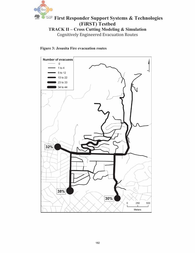
182
First Responder Support Systems & Technologies (FiRST) Testbed
TRACK II – Cross Cutting Modeling & Simulation Cognitively Engineered Evacuation Routes
Figure 3: Jesusita Fire evacuation routes

183
First Responder Support Systems & Technologies (FiRST) Testbed
TRACK II – Cross Cutting Modeling & Simulation Cognitively Engineered Evacuation Routes
This map indicates a relatively even distribution of evacuees to destination nodes, as well
as an even distribution of evacuees on the roads leading into these nodes. The second map
(Figure 4) shows the shortest distance routes to each evacuee's nearest exit, again
aggregated to the street segment level. We see that the distribution of evacuees to exit
nodes is not balanced, but rather favors the exits at Foothill Rd and Alamar Rd (39% of
total evacuees) and Los Olivos (47%) over the exit at State St and Alamar Rd (13%).
The distribution of evacuees on the roads leading into these nodes is not balanced either.
Perhaps most striking when comparing these two maps is the differences in traffic flow
on many streets throughout the road network. Thus, it is important to investigate not only
the exit node selection process for Jesusita fire evacuees, but the street segment selection
process as well.
We have established that a majority of Jesusita fire evacuees did not choose their closest
exit. Therefore, it makes little sense to investigate the street selection process using the
shortest distance routes to their nearest exit. We used Dijkstra’s algorithm to calculate each
evacuee's shortest distance route to their chosen exit. Separating out the exit node selection
process may allow for a less biased measurement of factors that influence the selection of
street segments along an evacuation route. Of the ninety-seven evacuation routes obtained
from our survey respondents, forty (41.2%) are not the shortest possible in travelling from
their origin node to their chosen exit node. The greatest distance difference between an
evacuation route and a shortest distance route is 1072 meters, and the average distance
difference between an evacuation route and the shortest distance route is approximately

184
First Responder Support Systems & Technologies (FiRST) Testbed
TRACK II – Cross Cutting Modeling & Simulation Cognitively Engineered Evacuation Routes
158 meters.
Figure 4: This map shows the shortest distance routes to each evacuee’s nearest exit.

185
First Responder Support Systems & Technologies (FiRST) Testbed
TRACK II – Cross Cutting Modeling & Simulation Cognitively Engineered Evacuation Routes
Figure 5: Jesusita Fire evacuation routes and shortest distance routes. The grey bars show the length of shortest distance routes, and the black bars show the additional distance traveled by evacuees who did not take the shortest distance route to their chosen destination.
A plot showing the distance of each evacuation route and its corresponding shortest
distance route (Figure 5) reveals that a majority of distance differences fall below this
average, with a few outliers where this difference is significantly greater. From these data
we may infer that most survey respondents who did not choose a shortest distance
evacuation route did choose a route with a slight distance difference. It is important to
note that multiple shortest paths may exist between an origin and destination, thus it is
possible that evacuees chose a route that utilized completely different links and nodes than
the single shortest path route we calculated with Dijkstra’s algorithm. While it would be
possible to assess evacuee link and node choice and determine if alternate shortest paths
were used during the evacuation that is beyond the scope of this analysis.

186
First Responder Support Systems & Technologies (FiRST) Testbed
TRACK II – Cross Cutting Modeling & Simulation Cognitively Engineered Evacuation Routes
Why do evacuees choose a route that is longer than the shortest distance between their
origin and chosen exit? One of the most intuitive answers to this question is that evacuees
prefer routes that may get them to their destination more quickly than the shortest distance
route. While a majority of the streets in our study area have a posted speed limit of 25
miles per hour, several of the major arterials have speed limits of 35 mph. We
hypothesized that evacuees chose routes that have a higher posted speed limit than the
shortest distance route. To test this hypothesis, we obtained speed limit data for every
street segment in our study area using both GIS data and field observations. We then
calculated the average speed limit for each evacuation route and compared it to the average
speed limit for each corresponding shortest distance route. On average evacuees select
routes with a speed limit that was 0.4mph greater than the shortest distance route. This
difference may seem small, but a one-sample t-test reveals that it is statistically significant
(p-value <0.01). We can accept the hypothesis that Jesusita fire evacuees chose routes
with a higher posted speed limit than the shortest distance route.
Another factor that may influence evacuee route selection is the direction of travel.
Evacuees may favor street segments that lead them directly away from the fire rather than
street segments that are moving perpendicular or towards the fire. We tested this hypothesis
by calculating the azimuth of each street segment in our study area. An azimuth of
0°represents a street segment that points due north while an azimuth of 180° is due south,
while azimuths of 270° and 90° are due west and due east, respectively. A map of the
earliest recorded Jesusita fire perimeter (Figure 6) shows that fire was north
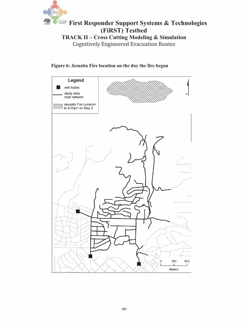
187
First Responder Support Systems & Technologies (FiRST) Testbed
TRACK II – Cross Cutting Modeling & Simulation Cognitively Engineered Evacuation Routes
Figure 6: Jesusita Fire location on the day the fire began

188
First Responder Support Systems & Technologies (FiRST) Testbed
TRACK II – Cross Cutting Modeling & Simulation Cognitively Engineered Evacuation Routes
(0°) to northeast (45°) of our study area. It follows that evacuees might choose routes that
utilize street segments heading due south (180°) to southwest (225°) to move directly away
from the fire. The average azimuth of routes chosen by our evacuees is 210.5°, while the
average azimuth of the shortest distance routes is 211.3°. A t-test reveals that the difference
between these azimuths is not statistically significant (p-value > 0.1) thus we cannot
conclude that the direction of street segments influenced the route selection of Jesusita Fire
evacuees.
One unique feature of our study area road network is that there are both public and private
roads. Public roads are owned and maintained by the City or County of Santa Barbara and
are freely accessible to anyone. Private roads are owned and maintained by private
landowners, and may feature physical barriers to entry such as locked gates or perceptual
barriers to entry such as 'private road' or 'no trespassing' signs. Some of these private roads
provide the only connection between homes or subdivisions and the public road network,
thus evacuees had no choice but to drive on them. Other private roads pass through private
party but connect two or more parts of the public road network. Private roads of this later
type can theoretically be driven on by anyone, provided that there are no physical barriers
to entry or egress. Yet, many people might be unaware that these private roads actually
connect two public sections of the road network, or might be dissuaded from driving on
them by warning signs or other perceptual barriers.
We believe that utilization of connecting private roads may influence whether an evacuee

189
First Responder Support Systems & Technologies (FiRST) Testbed
TRACK II – Cross Cutting Modeling & Simulation Cognitively Engineered Evacuation Routes
takes the shortest distance route between their origin and exit. Two such roads in our study
area are Glendessary Lane and Mission Park Drive. Glendessary Lane connects to Mission
Canyon Road, a major arterial route through our study area. Multiple signs are posted at the
entrance to Glendessary Lane indicating that it is a private road and a dead end, but there
are no physical barriers. While it is indeed a private road, Glendessary Lane actually
connects to Mission Park Drive, another private road which in turn is connected to a public
street, Puesta Del Sol Road. Three Jesusita Fire evacuees chose to drive on Glendessary
Lane and Mission Park Drive, and two of these three evacuees chose the shortest distance
route from their origin to exit. Perhaps more striking is that four evacuees who did not take
their shortest distance route could have if they had chosen to drive on these two private
roads. These four evacuees could have traveled a total of 371 meters less if they had used
Glendessary Lane and Mission Park Drive. While the sample size for private road
utilization is too small to test for statistical significance, we believe that it is important to
consider the impact of private road utilization issue when modeling evacuation traffic flow.
2. Network flow
In the previous section, we uncovered several wayfinding strategies that evacuees may
have used during the Jesusita Fire. It is clear that while distance remains the primary factor
when choosing an evacuation route, the elevation of road network exits, speed limits on
street segments, and utilization of private roads all may play a role. Our previous analysis
was focused on understanding the evacuation route choice process for an individual or

190
First Responder Support Systems & Technologies (FiRST) Testbed
TRACK II – Cross Cutting Modeling & Simulation Cognitively Engineered Evacuation Routes
ij
ij ij
ij
household. These results help us develop the Cognitively Engineered Evacuation Routes
model (CEER), which can be used to predict evacuation traffic flow at the aggregate level.
While many aggregate approaches consider only distance or travel time, our approach is
unique in that we account for the individual wayfinding strategies used by Jesusita Fire
evacuees:
i,j index of network nodes A set of directed arcs connecting i,j dij distance from i to j
µij traffic flow capacity from i to j
8 total evacuee traffic flow K set of wayfinding strategies
k cij cost of traveling from i to j for evacuees using strategy k L set of arc congestion levels
c l cost of traveling from i to j at congestion level l
′Α l breakpoints in the interval[0, µ ]
bi net evacuee traffic flow at node i
Decision Variables:
x k traffic flow from i to j for evacuees using strategy k
fijl traffic flow from i to j at congestion level l

191
First Responder Support Systems & Technologies (FiRST) Testbed
TRACK II – Cross Cutting Modeling & Simulation Cognitively Engineered Evacuation Routes
ij
The objective of this model (1) is to minimize the total cost for evacuees traveling along
the road network, plus the total traffic congestion cost. The conservation of flow constraint
(2) ensures that all traffic flow on the network leaves the origin nodes, passes through any
intermediate nodes, and arrives at one of the destination nodes. Our next two constraints
(3,4) insure that a congestion cost is imposed when flow on an arc exceeds a specific
percentage of that arc’s total capacity. No negative traffic flow is allowed, nor can traffic
flow exceed the total capacity of a given arc (5).
This formulation is similar to many linear cost multicommodity network flow models
commonly used in operations research (Kennington 1978). Along this vein, the
'commodities' are the set of wayfinding strategies K in our model, and the cost of traveling
along an arc, c k , varies depending upon which wayfinding strategy is used. The addition
of a congestion cost to the travel cost allows us to model how traffic congestion may
cause evacuees to change their wayfinding strategy. This piecewise- linear (Wagner 1975)
approach to modeling costs accounts for the decreasing returns (Glover et al. 1992)
associated with choosing an evacuation route as congestion becomes heavier. To our
knowledge, there are no emergency evacuation modeling approaches that combine
multicommodity network flow and piecewise-linear costs. The CEER model represents a
novel approach to modeling traffic flow during an emergency evacuation.

192
First Responder Support Systems & Technologies (FiRST) Testbed
TRACK II – Cross Cutting Modeling & Simulation Cognitively Engineered Evacuation Routes
While results from our survey indicated that most evacuees did not change their route while
evacuating, most survey respondents also reported that they experienced little traffic
congestion. Most people in Mission Canyon had at least 24 hours to evacuate before the
Jesusita Fire directly impacted their neighborhood, thus evacuation departures
were generally spread out, reducing traffic congestion. Future wildfires could force people
to evacuate in a much shorter time period; thus, it is important to account for the congestion
that may occur.
We tested the applicability of the CEER model by applying it to the study area of our
Jesusita fire survey. The goal of this model is to predict evacuee traffic flow at the aggregate
level. The first step is to determine the total amount of evacuee traffic flow in our study
area and the origin locations. We used the cadastral shapefile and results of from our
Jesusita fire survey to calculate these data. First, we selected all tax parcels from the
cadastral shapefile that have their centroid within the boundaries of our study area. We
then used the property classification field to determine the amount of flow from each
parcel. Parcels classified as single-family residences, condos or rancho estates were
assigned one unit of flow, and residential income parcels with 2-4 units were assigned three
units of flow.
This preliminary calculation assumes that one vehicle (ie. one flow unit) evacuates from
each housing unit in our study area. Our Jesusita Fire survey results indicate that many

193
First Responder Support Systems & Technologies (FiRST) Testbed
TRACK II – Cross Cutting Modeling & Simulation Cognitively Engineered Evacuation Routes
households utilized more than one vehicle when evacuating. Our evacuee flow calculation
should be adjusted to reflect this. We asked survey respondents how many people
evacuated from their household. Replies to this question indicated that an average of 1.8
vehicles departed from each household, with a minimum of one vehicle and a maximum
of six. The simplest way to account for these additional vehicles would be to multiply this
average by the amount of flow from each parcel. Alternatively, we could randomly
multiply each unit of flow by a value drawn from the empirical distribution of the number
of vehicles used by survey respondents. This method allows us to avoid the conceptually
difficult assumption that 1.8 vehicles evacuate from each household. Rather, between one
and six vehicles depart from each household, with a mean of 1.8.
Finally, we assigned the vehicular flow from each parcel centroid to the closest (Euclidian
distance) node on our road network. After this nearest node assignment we have a total
flow ( 8 ) of 2638 vehicles evacuating from our study area. For nodes that are neither an
evacuation route origin or destination the total flow is set to zero, forcing any traffic flow
which enters these nodes to leave them. Each of our three destination nodes can handle
the entire flow on our network, allowing the evacuation routes to resolve endogenously.
By using this method of determining evacuee traffic demand we assume that all housing
units are occupied, that all residents are home at the time of the evacuation, and that all
residents will obey a mandatory evacuation order. We used this approach because it is

194
First Responder Support Systems & Technologies (FiRST) Testbed
TRACK II – Cross Cutting Modeling & Simulation Cognitively Engineered Evacuation Routes
unlikely to underestimate the total evacuee traffic flow from a residential neighborhood.
Emergency evacuations are by nature wrought with uncertainty, thus it is critical to have
a traffic flow estimation method that can be applied quickly and that will generate an upper
bound on the amount of traffic flow to expect.
We used the comparison of Jesusita Fire evacuation routes to shortest distance routes to
inform the design of our wayfinding strategies K. While distance remains the most
important factor in determining an evacuation route, speed limits and knowledge of private
roads may influence the decision of which roads to take. We developed the following
general evacuation wayfinding strategies:
k1 = shortest distance k2 = shortest travel time according to posted speed limits k3 = shortest distance with limited private road use k4 = shortest travel time with limited private road use
We calculated a different arc cost cij
k for each wayfinding strategy:

195
First Responder Support Systems & Technologies (FiRST) Testbed
TRACK II – Cross Cutting Modeling & Simulation Cognitively Engineered Evacuation Routes
The cost of using an arc for evacuees using wayfinding strategy k1 is simply the distance
of that arc. For strategy k2 , the arc cost is an adjusted distance which reflects the potential
decrease in traveling time when driving on arcs with a 35mph speed limit rather than arcs
with a 25mph speed limit. We assigned two different arc costs for evacuees
using heuristic k3 : if the arc is on a public road, the cost is the same as distance, while if
the arc represents a private road, the cost is a very large number M. Because the objective
of our model is to minimize the total cost, assigning a very high cost to private road arcs
will effectively prevent flow on them except for evacuees who must use a
private road to leave their origin node. The arc cost for wayfinding strategy k4 is identical
to k3 except that our cost for public roads is adjusted to account for speed limits as in k2 .

196
First Responder Support Systems & Technologies (FiRST) Testbed
TRACK II – Cross Cutting Modeling & Simulation Cognitively Engineered Evacuation Routes
gfinal part of this formula ( ij
C ) is the green time ratio, which we use to account for the ij
0
w g
The next model parameters we set are the capacity for flow on each arc ( µij ). These
capacities are calculated using the following formula, which is based on the Highway
Capacity Manual:
The basic saturation flow rate for an arc ( S ) is 1800 passenger cars per hour. This ij
value is adjusted based on the number of lanes on an arc ( nlanesij ), and adjustment
factors based on the width of the lane ( f ) and the uphill or downhill grade ( f ). The ij ij

197
First Responder Support Systems & Technologies (FiRST) Testbed
TRACK II – Cross Cutting Modeling & Simulation Cognitively Engineered Evacuation Routes
reduction in arc capacity at controlled intersections. For arcs that end at an uncontrolled
intersection the value of this ratio is 1, and for arcs that end at a stop sign it is 1/2. There is
only one actual traffic signal in our study area, and we determined this ratio observing this
signal from 4pm to 5pm on a weekday afternoon and timing the cycle time ( Cij ) and
duration of the green period ( gij ).
We choose a set of arc congestion levels L that reflects the traffic conditions a driver may
experience during an evacuation:
l1 = free flowing l2 = moderate congestion l3 = heavy congestion
The impact of these different levels of congestion is modeled by setting different traffic
congestion costs:
l1 cij = 0 l2 cij = dij
l3 cij = dij + dij

198
First Responder Support Systems & Technologies (FiRST) Testbed
TRACK II – Cross Cutting Modeling & Simulation Cognitively Engineered Evacuation Routes
ij
ij
We also set our capacity breakpoints ( ′Α l ), which determine the amount of traffic flow
on an arc at which the congestion cost will increase. These breakpoints may vary for
individual evacuees based on their driving style and knowledge of the road network. We
set each of these three values at for the initial instance of our CEER model, then
allowed them to vary stochastically for later solutions to reflect the uncertainty associated
with the differences between individual evacuees. This method of modeling congestion is
linear, and therefore it may not capture traffic dynamics such as queuing or lane changing
behavior. We believe this simpler representation of congestion is a good approximation
of a highly complex phenomenon, and has the benefits producing a fast model solution
time while accounting for behavioral uncertainty.
D. Results
We solved the CEER model using LPSolve on a Dell Precision T3500 with 12GB of RAM
and a quad-core 2.4 Ghz processor. The initial instance of our CEER model was solved to
optimality in 57.09 seconds. For this solution, average distance traveled by an evacuee
was approximately 1,328 meters and the total distance that all evacuees traveled along
private roads was 7,928 meters. After solving the initial instance of our model, we
allowed the capacity breakpoints ( ′Α l ) to vary stochastically to reflect the uncertainty
associated with how evacuees will react to traffic congestion. We randomly sample three

199
First Responder Support Systems & Technologies (FiRST) Testbed
TRACK II – Cross Cutting Modeling & Simulation Cognitively Engineered Evacuation Routes
values from a uniform distribution of capacity breakpoints, with a minimum value of 0.01
and a maximum value of 0.98 . Together these breakpoints must sum to the total
capacity of each arc ( ). We solve 1,000 instances of the CEER model, each with a
different set of capacity breakpoints. The average distance traveled by an evacuee for all
1,000 stochastic instances of the model is 1,318 meters, and the average total distance that
all evacuees traveled along private roads was 8,211 meters. Next we examine two specific
stochastic model instances: the minimum total distance and the maximum total distance
traveled. These solutions are of special interest as they can be thought of as the 'best-case'
and 'worst-case' scenarios. For the minimum total distance solution, the average distance
traveled by an evacuee was approximately 1,295 meters and the total distance that all
evacuees traveled along private roads was 8,612 meters. These values for the maximum
total distance solution were 1,380 and 7,928, respectively. The final stochastic model
instance we generated is the maximum distance traveled on private roads. The total
distance traveled on private roads is 13,736 meters and the average distance traveled by
an evacuee is 1,352 meters. The complete parameters for these results are shown in Figure
7 below. We also created traffic flow maps based on these results (Figure 8), which allow
for a more intuitive visual assessment.
In the earlier comparison of Jesusita Fire evacuation routes to the shortest distance routes,
we found that evacuees choose exits at a lower elevation than their nearest exit. The potential
influence of destination node elevation is not explicitly accounted for in the first version of

200
First Responder Support Systems & Technologies (FiRST) Testbed
TRACK II – Cross Cutting Modeling & Simulation Cognitively Engineered Evacuation Routes
our CEER model, thus we develop a second version that accounts for elevation by limiting
the flow capacity of our destination nodes. In the previous section, we observed that the total
amount of evacuation traffic flowing to each of our three network exits was more balanced
(32%, 38%, 30%) than the amount of flow to each exit for the

201
First Responder Support Systems & Technologies (FiRST) Testbed
TRACK II – Cross Cutting Modeling & Simulation Cognitively Engineered Evacuation Routes
Figure 7: CEER model parameters and results
Model instance ′Αij
1
′Αij
1
′Αij
1
Average distance
traveled by an evacuee (m)
Total private road distance (m)
Initial solution .33 .33 .33 1,328 7,928
Maximum
distance .34
.04
.62
1,380
7,928
Minimum
distance .79
.07
.14
1,295
8,612
Maximum private road distance
.24
.05 .71 1,352 13,736
shortest distance to nearest exit routes (39%, 13%, 47%). We used this information to set
the amount of flow into our three network destination nodes:

202
First Responder Support Systems & Technologies (FiRST) Testbed
TRACK II – Cross Cutting Modeling & Simulation Cognitively Engineered Evacuation Routes
Figure 8: Maps showing results of the CEER model. (1) is the initial model instance, (2) is the maximum total distance, (3) is the minimum total distance, (4) is the maximum total distance on private roads. Thicker lines indicate more traffic flow, percentages indicate amount of total flow into each destination node.

203
First Responder Support Systems & Technologies (FiRST) Testbed
TRACK II – Cross Cutting Modeling & Simulation Cognitively Engineered Evacuation Routes
The first term represents an equal allocation of the total traffic flow 8 to each of our
three destination nodes, then the second term represents an adjustment of this flow
demand based on how much the elevation of a given destination node elevi differs from
the mean elevation of all destination nodes ( eleviΕD ). By applying this equation to our
study area data we allocated 31%, 39%, and 30% of the total traffic flow to our three
network exits, respectively. These values are very similar to the values we observed in
the survey results. While limiting the flow capacity of destination nodes may impose
unnecessary constraints on the results of our model for our specific study area, we believe
that the above methodology may be important for calibrating the CEER model if applied
to other road networks. As with the previous version of the CEER model, we solved an
initial instance of the capacitated destination version of the model and then solved 1000
model instances with stochastic variation of the capacity breakpoints. The results of these
model instances are shown in Figure 9.

204
First Responder Support Systems & Technologies (FiRST) Testbed
TRACK II – Cross Cutting Modeling & Simulation Cognitively Engineered Evacuation Routes
Figure 9: Capacitated destination CEER model parameters and results
Model instance ′Αij 1 ′Αij
1 ′Αij
1
Average distance traveled by an
evacuee (m)
Total private road distance (m)
Initial solution .33 .33 .33 1,342 7,928
Maximum distance .34 .04 .62 1,352 7,928
Minimum distance .79 .07 .14 1,321 7,928
Maximum private road distance
.24 .05 .71 1,344 8,940

205
First Responder Support Systems & Technologies (FiRST) Testbed
TRACK II – Cross Cutting Modeling & Simulation Cognitively Engineered Evacuation Routes
These results and the associated maps have considerably less solution variability than our
the first formulation of our model, which allowed destination nodes to have unlimited
capacity. We believe that it is important to produce a wide range of model solutions given
the dynamic and uncertain nature of emergency evacuations, and therefore do not consider
the capacitated destination version of the CEER model for the remainder of this report.
E. Discussion
In discussing the implications of our research, it is useful to refer back to the research
questions posed at the beginning of this report:
Do evacuees take the shortest distance route to the nearest exit?
It is clear from our assessment of Jesusita fire evacuation routes that a majority of survey
respondents did not take the shortest distance route to the nearest exit. When we compared
the actual evacuation routes to the shortest distance route to each evacuee's chosen exit, the
assumption of shortest path routes is reasonably accurate. Based on this finding,
understanding how evacuees choose an exit becomes a critical factor for modeling
evacuation routes for a given study area.
What characteristics of the environment influence evacuee route choice?
The answer to this question can be split into two parts. Elevation is the characteristic of the
environment that influenced the choice of an exit for the Jesusita fire evacuees. We believe
that traffic congestion and distance from the fire may have influenced the choice

206
First Responder Support Systems & Technologies (FiRST) Testbed
TRACK II – Cross Cutting Modeling & Simulation Cognitively Engineered Evacuation Routes
of an exit as well, but there was insufficient statistical evidence to show that these other
factors were significant. Speed limits are a characteristic of the environment that
influenced the choice of roads for Jesusita fire evacuees, and knowledge of private road
'shortcuts' may be an important factor as well. Direction of travel, road gradient and width,
and intersection control type are all factors that should be further analyzed in future studies.
Can a model that accounts for environmental perception represent a system of
evacuation routes with greater accuracy?
To answer this question is it useful to refer back to Figure 3, which shows the actual Jesusita
fire evacuation routes taken by our survey respondents. Comparison of this map to the
fourth map produced by our CEER model (Figure 8, bottom right) shows that the modeled
traffic flow pattern is similar to the actual flow pattern. When compared to the traffic flow
pattern produced when one assumes that all evacuees will take the shortest path route to
their nearest exit (Figure 4), we can see that our CEER model, which accounts for
environmental perception, is more accurate. These results are specific to our study area and
the Jesusita fire, thus additional research is needed to better define the role of environmental
perception in evacuation route modeling.
How does behavioral uncertainty impact this system of evacuation routes?
We can see from Figure 8 that a system of evacuation routes can have very different traffic
flow patterns depending on the wayfinding strategies and response to congestion
of evacuees. Much of the behavioral uncertainty during emergency evacuations is due to

207
First Responder Support Systems & Technologies (FiRST) Testbed
TRACK II – Cross Cutting Modeling & Simulation Cognitively Engineered Evacuation Routes
their infrequent occurrence and difficulties in collecting data. Often the default modeling
approach is to assume that people will behave the same way during an evacuation as they
do during normal vehicular travel. Other evacuation modeling approaches may assume that
people will panic and behave irrationally. We believe the truth lays somewhere in between
these two extremes, but this cannot be confirmed without additional empirical data on
emergency evacuations.
These answers to our initial research questions are valuable for future studies, but additional
analysis is needed to help evacuation planners and emergency managers make use of our
CEER model results. To address this need, we produce a new set of maps (Figure 28)
showing the ratio of traffic flow volume to capacity (v/c) for each arc on our network:
These maps can be used to identify 'hotspots' on the road network, where a high volume of
evacuation traffic flow may lead to long queues and bottlenecks. Displaying the results of
our CEER model in this manner is useful because certain areas of the network are likely to
become congested regardless of the wayfinding strategy and response to congestion of
evacuees. A composite map (Figure 11) showing the average volume to capacity
ratio across all four of the maps in Figure 10 clearly identifies these 'hotspot' areas.
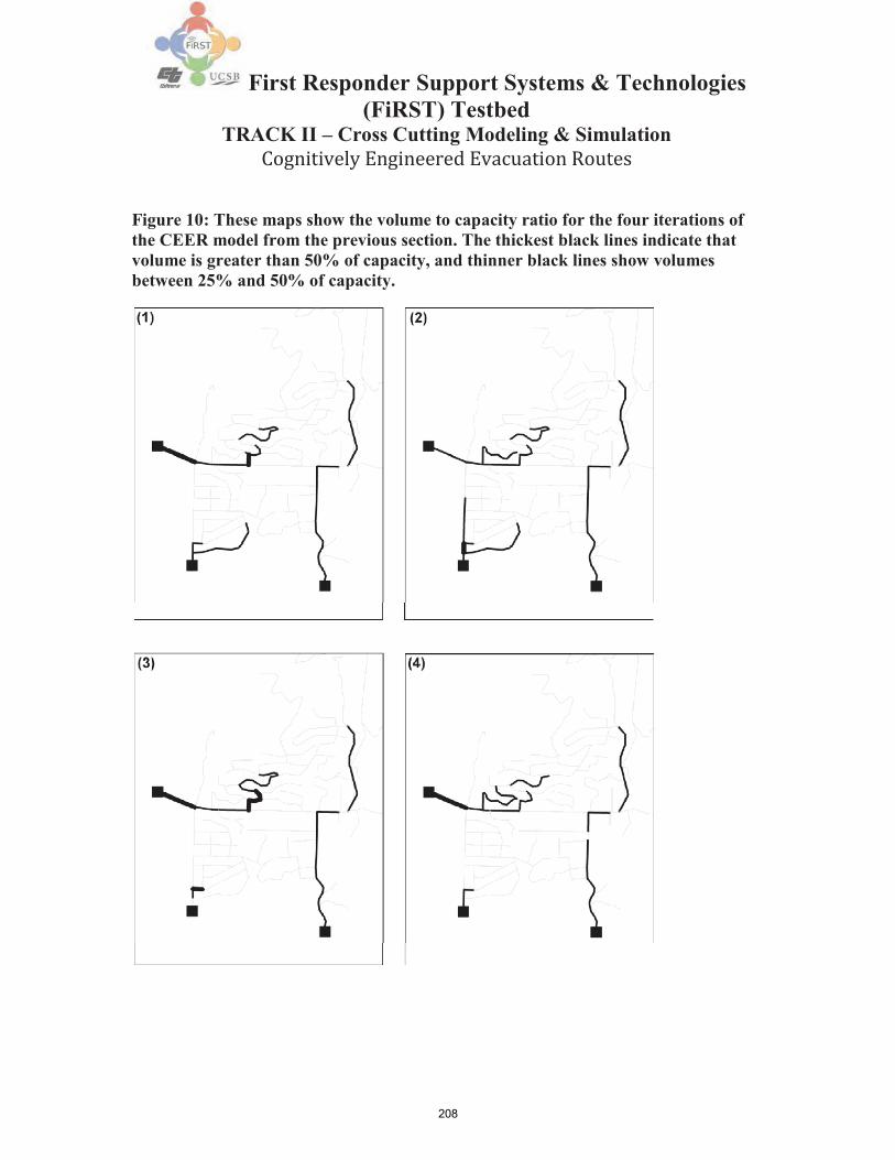
208
First Responder Support Systems & Technologies (FiRST) Testbed
TRACK II – Cross Cutting Modeling & Simulation Cognitively Engineered Evacuation Routes
Figure 10: These maps show the volume to capacity ratio for the four iterations of the CEER model from the previous section. The thickest black lines indicate that volume is greater than 50% of capacity, and thinner black lines show volumes between 25% and 50% of capacity.

209
First Responder Support Systems & Technologies (FiRST) Testbed
TRACK II – Cross Cutting Modeling & Simulation Cognitively Engineered Evacuation Routes
Figure 11: Composite volume to capacity ratio for CEER model results. The thickest black lines indicate that volume is greater than 50% of capacity, and thinner black lines show volumes between 25% and 50% of capacity.
The potential for bottlenecks on Cheltenham Road, Tye Road and upper Mission Canyon
Road are of particular concern as these roads are located in steep, heavily vegetated terrain
in which a wildfire can spread quickly. The westbound section of Foothill Road is of
concern as well, although evacuees have the option of turning left onto Alamar Road to

210
First Responder Support Systems & Technologies (FiRST) Testbed
TRACK II – Cross Cutting Modeling & Simulation Cognitively Engineered Evacuation Routes
reduce congestion on these links. Downstream congestion on Alamar Road and lower

211
First Responder Support Systems & Technologies (FiRST) Testbed
TRACK II – Cross Cutting Modeling & Simulation Cognitively Engineered Evacuation Routes
Mission Canyon Road are of lesser concern because a wildfire is less likely to spread
quickly into these areas.
Although a model that incorporates wayfinding can represent a system of evacuation routes
with greater accuracy than a model based on simpler behavioral assumptions, it is still
difficult to fully account for the unique behaviors of individual evacuees. The CEER model
is intended to represent aggregate traffic flow in our study area, thus by design cannot fully
represent individual choices and decision-making. In addition, some routes taken by
Jesusita fire evacuees simply defy what any researcher might reasonably expect. Figure 12
shows two examples of such routes.
Figure 12: Unexpected routes taken by Jesusita fire evacuees. Black lines show the actual evacuation route and thick grey lines show the shortest distance route. The circle is the route origin node, the black square is the route destination node.

212
First Responder Support Systems & Technologies (FiRST) Testbed
TRACK II – Cross Cutting Modeling & Simulation Cognitively Engineered Evacuation Routes
In the first map, the evacuee chose a route that was 747 meters longer than the shortest
distance route between the same origin and destination. Even more surprising is that this
evacuee drove uphill and in the direction of the Jesusita fire, which had spread into the
northern most sections of our study area at this evacuee's time of departure. One possible
explanation is that this evacuee wanted to get a closer look at the fire before leaving the
area. In the second map, the evacuee chose a route that was 1,072 meters longer than the
shortest distance route. One possible explanation for this choice is that the evacuee wanted
to avoid Tunnel Road, which intersects Mission Canyon Road , one of our identified traffic
congestion 'hotspots’. These routes represent complex evacuation behavior that would be
difficult to account for in any generalized, aggregate traffic model. Future research
directions include developing models that can better reflect individual evacuee choice, as
well as collecting the additional evacuation data that is needed to make generalized claims
about evacuation behavior. Further exploration into evacuation psychology is also needed,
perhaps by incorporating more open-ended questions in future surveys or conducting
follow-up interviews with survey respondents. The survey comments left by the two
evacuees whose routes are mapped above exemplify the complexity of evacuation process:
Comment 1:
" I first received information regarding the fire from high school friends
that lost their home in the tea fire. He heard about the fire over his cb
band and called me to get out. We saw smoke right behind our homes and
got out as it was windy and hot and it seemed likely to spread as the fire

213
First Responder Support Systems & Technologies (FiRST) Testbed
TRACK II – Cross Cutting Modeling & Simulation Cognitively Engineered Evacuation Routes
personnel have no access to water drop equipment in Santa Barbara any
longer. Sometimes neighbor helping neighbor is the most effective early
warning system. I alerted my 85 year old neighbor who was sleeping and
had not heard the warnings yet. Being a good neighbor and clearing your
brush and being aware of each other is important when you live in a high
risk area. I grew up in this home and this was my lifetime 5th evacuation
and the one that came the closest to taking my home with it."
Comment 2:
" 1. When the winds blow look to the hills.
2. Keep looking.
3. Install a 1 1/2" fire hose line. "

214
First Responder Support Systems & Technologies (FiRST) Testbed
TRACK II – Cross Cutting Modeling & Simulation Cognitively Engineered Evacuation Routes
References
1. L. Alcada-Almeida, L. Tralhao, L. Santos and J. Countinho-Rodrigues, "A Multiobjective Approach to Locate Emergency Shelters and Identify Evacuation Routes in Urban Areas", Geographical Analysis, vol. 41, pp. 9-27 (2009).
2. J. N. Bailenson, M. S. Shum and D. H. Uttal, "Road climbing: Principles governing asymmetric route choices on maps", Journal of Environmental Psychology, vol. 18, pp. 251- 264 (1998).
3. J. N. Bailenson, M. S. Shum and D. H. Uttal, "The initial segment strategy: A heuristic for route selection", Memory & Cognition, vol. 28, pp. 306-318 (2000).
4. L. G. Chalmet, R. L. Francis and P. B. Saunders, "Network models for building evacuation", Management Science, vol. 28, pp. 86-105 (1982).
5. T. Charnkol and Y. Tanaboriboon, "Evacuee behaviors and factors affecting the tsunami trip generation model: A case study in Phang-nga, Thailand", Journal of Advanced Transportation, vol. 40, pp. 313-330 (2006).
6. W. Choi, H. W. Hamacher and S. Tufekci, "Modeling of building evacuation problems by network flows with side constraints", European Journal of Operational Research, vol. 35, pp. 98-110 (1988).
7. G. W. Evans, M. A. Skorpanich, T. Garling, K. J. Bryant and B. Bresolin, "The effects of pathway configuration, landmarks and stress on environmental cognition", Journal of environmental psychology, vol. 4, pp. 323-335 (1984).
8. R. F. Fahy, "EXIT89 - An Evacuation Model for High-Rise Buildings - Recent Enhancements and Example Applications", International Conference of Fire Research and Engineering, Orlando, FL (1995).
9. J. Gerhardt-Powals, "Cognitive engineering principles for enhancing human- computer performance", International Journal of Human-Computer Interaction, vol. 8, pp. 189-211 (1996).
10. R. Golledge, A. Frank and W. Kuhn, "Path selection and route preference in human navigation: A progress report. Spatial Information Theory A Theoretical Basis for GIS", vol. 988, pp. 207-222 (1995).
215
First Responder Support Systems & Technologies (FiRST) Testbed
TRACK II – Cross Cutting Modeling & Simulation Cognitively Engineered Evacuation Routes
11. R. G. Golledge, "Human Wayfinding and Cognitive Maps", Wayfinding Behavior: Cognitive Mapping and other Spatial Processes, vol. pp. (1999).
12. H. W. Hamacher and S. Tufekci, "On the Use of Lexicographic Min Cost Flows in Evacuation Modeling", Naval Research Logistics, vol. 34, pp. 487-503 (1987).
13. S. C. Hirtle and T. Gärling, "Heuristic rules for sequential spatial decisions", Geoforum, vol. 23, pp. 227-238 (1992).
14. A. G. Hobeika and C. Kim, "Comparison of traffic assignments in evacuation modeling", IEEE Transactions on Engineering Management, vol. 45, pp. 192-198 (1998).
15. A. G. Hobeika, S. Kim and R. E. Beckwith, "A Decision-Support System for Developing Evacuation Plans around Nuclear-Power Stations", Interfaces, vol. 24, pp. 22-35 (1994).
16. E. Hollnagel and D. D. Woods, "Cognitive systems engineering: New wine in new bottles", International Journal of Man-Machine Studies, vol. 18, pp. 583-600 (1983).
17. W. D. Iwan, L. S. Cluff, J. F. Kimpel, H. Kunreuther, S. H. Masaki-Schatz, J. M. Nigg, R. S. Roth, H. Ryland, E. Stanley and F. H. Thomas, "Natural hazards and policy- Mitigation emerges as major strategy for reducing losses caused by natural disasters", Science, vol. 284, pp. 1943-1947 (1999).
18. G.-Y. Jeon, J.-Y. Kim, W.-H. Hong and G. Augenbroe, "Evacuation performance of individuals in different visibility conditions", Building and Environment, vol. 46, pp. 1094- 1103 (2011).
19. A. H. Jorgensen, "Thinking-aloud in user interface design: a method promoting cognitive ergonomics", Ergonomics, vol. 33, pp. 501-507 (1990).
20. G. Kalafatas and S. Peeta, "Planning for Evacuation: Insights from an Efficient Network Design Model", Journal of Infrastructure Systems, vol. 15, pp. 21 (2009).
21. M. Kobes, I. Helsloot, B. de Vries, J. G. Post, N. Oberijé and K. Groenewegen, "Way finding during fire evacuation; an analysis of unannounced fire drills in a hotel at night", Building and Environment, vol. 45, pp. 537-548 (2010).
22. W. P. Langford, "A Space-Time Flow Optimization Model for Neighborhood Evacuation", Master's Thesis, Department of Operations Research, Naval Postgraduate
216
First Responder Support Systems & Technologies (FiRST) Testbed
TRACK II – Cross Cutting Modeling & Simulation Cognitively Engineered Evacuation Routes
School, Monterey, CA (2010).
23. Y. Liu, M. Hatayama and N. Okada, "Development of an Adaptive Evacuation Route Algorithm under Flood Disaster", Annuals of Disaster Prevention Research Institute, Kyoto University, vol. pp. 189-195 (2006).
24. Y. Liu, X. Lai and G. L. Chang, "Cell-Based Network Optimization Model for Staged Evacuation Planning Under Emergencies", Transportation Research Record, vol. 1964, pp. 127-135 (2006).
25. G. G. Lovas, "Models of wayfinding in emergency evacuations", European Journal of Operational Research, vol. 105, pp. 371-389 (1998).
26. Q. Lu, B. George and S. Shekhar, "Capacity Constrained Routing Algorithms for Evacuation Planning: A Summary of Results", Advances in Spatial and Temporal Databases, vol. pp. 291-307 (2005).
27. J. N. MacGregor and T. Ormerod, "Human performance on the traveling salesman problem", Attention, Perception, & Psychophysics, vol. 58, pp. 527-539 (1996).
28. E. Miller-Hooks and G. Sorrel, "The Maximal Dynamic Expected Flows Problem for Emergency Evacuation Planning", 87th Annual Meeting of the Transportation Research Board, Washington, D.C. (2008).
29. S. W. Mitchell and E. Radwan, "Heuristic Priority Ranking of Emergency Evacuation Staging to Reduce Clearance Time", Transportation Research Record, vol. 1964, pp. 219- 228 (2006).
30. D. A. Norman, "Cognitive Engineering", User Centered System Design; New Perspectives on Human-Computer Interaction, vol. pp. 31-61 (1986).
31. F. Ozel, "Time pressure and stress as a factor during emergency egress", Safety Science, vol. 38, pp. 95-107 (2001).
32. A. Pel, M. Bliemer and S. Hoogendoorn, "A review on travel behaviour modeling in dynamic traffic simulation models for evacuations", Transportation, vol. 39, pp. 97- 123 (2012).
33. A. Rahman and A. K. Mahmood, "Simulating human cognitive behaviors in pre- evacuation planning", 3rd International Symposium on Information Technology, Kuala Lumpur, Malaysia (2008).

217
First Responder Support Systems & Technologies (FiRST) Testbed
TRACK II – Cross Cutting Modeling & Simulation Cognitively Engineered Evacuation Routes
34. M. Raubal, "Cognitive Engineering for Geographic Information Science", Geography Compass, vol. 3, pp. 1087-1104 (2009).
35. H. A. Simon, Models of man; social and rational, Wiley, Oxford, England, (1957)
36. R. Stone, "Facing a tsunami with no place to run", Science, vol. 314, pp. 408-409 (2006).
37. Q. Tan, G. H. Huang, C. Wu, Y. Cai and X. Yan, "Development of an inexact fuzzy robust programming model for integrated evacuation management under uncertainty", Journal of Urban Planning and Development, vol. 135, pp. 39 (2009).
38. A. Veeraswamy, P. J. Lawrence and E. R. Galea, "Implementation of Cognitive Mapping, Spatial Representation and Wayfinding Behaviours of People Within Evacuation Modeling Tools", (2009).
39. G. F. White, "Human Adjustment to Floods", Department of Geography Research Papers, No. 29, (1945).
40. G. F. White, "The Choice of Use in Resources Management", Natural Resources Journal, vol. 1, pp. 23-40 (1961).
41. G. F. White, W. C. Calef, J. W. Hudson, H. M. Mayer, J. R. Shaeffer and D. J. Volk, "Changes in Urban Occupance of Flood Plains in the United States", Department of Geography Research Papers, No. 57, vol. pp. (1958).
42. T. Yamada, "A network flow approach to a city emergency evacuation planning", International Journal of Systems Science, vol. 27, pp. 931-936 (1996).
43. F. Yuan, L. D. Han, S. M. Chin and H. Hwang, "Proposed Framework for Simultaneous Optimization of Evacuation Traffic Destination and Route Assignment", Transportation Research Record, vol. 1964, pp. 50-58 (2006).
44. Y. Yuan and D. Wang, "Multi-Objective Path Selection Model and Algorithm for Emergency Evacuation", International Conference on Automation and Logistics, Jinan, China (2007).

218
First Responder Support Systems & Technologies (FiRST) Testbed
TRACK II – Cross Cutting Modeling & Simulation Modeling the Evacuation Decision
Modeling the Evacuation Decision
Micah Brachman
1.0 Introduction
Emergency evacuations are essential for protecting people from hazardous events such as
wildfires, tsunamis, hurricanes, industrial accidents, and terrorist actions. One way to assess
the effectiveness of an evacuation plan is through mathematical models that represent the road
topology, population characteristics, and hazard conditions of a specific geographic area.
Current emergency evacuation models are often based upon assumptions about spatial behavior
that may poorly represent human actions during an actual evacuation. In this paper we address
the issue of when and whether a resident may decide to evacuate. Most evacuation modeling is
based upon assumptions as to when people will decide to evacuate. The assumptions as to when
people will flee have a great impact on the outcome in modeling an evacuation event.
The stay-or-go decision of people living in a mandatory evacuation area is of critical importance
to emergency managers. One of the objectives of this part of the research was to develop a
better understanding of spatial behavior during an emergency evacuation. Collectively, such
behavior may either cause gridlock or may be manageable.
219
First Responder Support Systems & Technologies (FiRST) Testbed
TRACK II – Cross Cutting Modeling & Simulation Modeling the Evacuation Decision
2.0 Research Design, Data and Methods
On the afternoon May 5th, 2009 a wildfire began in the foothills above Santa Barbara,
California. Named the Jesusita Fire after a popular hiking trail in the area of ignition, this fire
burned nearly 9,000 acres, destroyed 80 homes, and caused 30 firefighter injuries. An
estimated 30,500 people were ordered to evacuate due to the danger posed by this fire, and
29,000 people were warned that they might be ordered to evacuate on short notice. The
analysis of the Jesusita Fire evacuation presented in this paper is the outcome of a natural
experiment. We rely on observations of variables related to the natural environment, the
population at risk, and the wildfire itself in several neighborhoods in Santa Barbara that were
impacted by the Jesusita Fire.
Emergency evacuations are infrequent, dynamic processes, and thus it is extremely difficult
to control specific variables or be certain that variables are independent. Although this natural
experiment does not have the inherent reliability of a controlled study, we attempted to
collect data in a way that allows for the contribution from all variables to be measured. Given
the paucity of empirical data from emergency evacuations, we believe that both our analysis
and the data collected to perform it represent an important addition to the body of scientific
knowledge related to this complex process.
2.1 Jesusita Fire Survey
We developed an online survey instrument to assess household behavior during the Jesusita

220
First Responder Support Systems & Technologies (FiRST) Testbed
TRACK II – Cross Cutting Modeling & Simulation Modeling the Evacuation Decision
fire for an approximately two square mile study area covering the Mission Canyon and Oak
Park neighborhoods in Santa Barbara (Figure 1). There were a total of 57 items that can be
split out into four general categories: risk perception, information flow, travel behavior, and
demographics.
Most risk perception items used a Likert scale, while questions covering information flow and
demographics were generally closed-ended with an open-ended ‘other’ response. Travel
behavior was measured through simple yes/no questions and other closed-ended questions such
as a novel map interface that allows respondents to trace the evacuation route they took. Many
critical questions are asked twice using both open-ended and closed-ended formats, allowing
for cross-checking validation of answers as well as the possibility of obtaining responses we
did not anticipate. The two methods used to recruit survey participants were door hangers placed
on the front doorknob or fence and an email list provided by the Mission Canyon Association.
We distributed approximately 2,000 door hangers covering 857 houses, 324 condos, and 40
apartment buildings between November 19th and November 24th, 2010. Six hundred current
and former residents of Mission Canyon were recruited via email on November 23rd. These
potential respondents voluntarily provided an email address to the Mission Canyon Association,
but do not necessarily still reside in the neighborhood. The internet-only English language
instrument effectively limited participation to Anglophones with Internet access and basic
computer skills. There were 264 total responses to the survey.
221
First Responder Support Systems & Technologies (FiRST) Testbed
TRACK II – Cross Cutting Modeling & Simulation Modeling the Evacuation Decision
2.2 Secondary data
We collected several GIS data layers that allowed us to assess environmental and physical road
network characteristics during the Jesusita Fire evacuation. Several fire perimeter polygons
representing the location of the Jesusita Fire at different points in time between May 5 and May
7, 2009 were obtained through the County of Santa Barbara online GIS data catalog. These
polygons were generated while the Jesusita Fire was burning by mapping personnel from the
California Department of Fire and Forestry Protection. To determine elevations in our study area,
we acquired the United States Geological Survey 7.5-minute Digital Elevation Model (DEM)
covering Santa Barbara. This DEM was produced as part of the National Mapping Program, and
has 30 by 30 meter grid cells. We also obtained a shapefile showing private roads in our study
area from the Santa Barbara County Department of Planning and Development, and a street layer
from the Santa Barbara County GIS Office with numerous data fields including street names,
address ranges, and speed limits. In order to estimate the population of our study area we obtained
a cadastral dataset from the Santa Barbara County assessor's office. We also downloaded data
from three weather stations located near our study area. Access to this historic weather station data
was provided by the weather underground website (http://www.wunderground.com).

222
First Responder Support Systems & Technologies (FiRST) Testbed
TRACK II – Cross Cutting Modeling & Simulation Modeling the Evacuation Decision
Figure 1: Red roads show the Jesusita Fire survey study area.
.

223
First Responder Support Systems & Technologies (FiRST) Testbed
TRACK II – Cross Cutting Modeling & Simulation Modeling the Evacuation Decision
2.3 Methods
The methods used for this research are statistical analysis and hypothesis testing based upon
survival analysis. Primary data and secondary data are used extensively in the application
each of these methods. In this paper our focus is on the evacuation decision: Will people
choose to evacuate from a wildfire, and if so, when will they depart? We use survival
analysis to measure the impact of risk perception, distance from the fire, and environmental
conditions on this decision. The results of our survival analysis inform the design of a
generalized Rayleigh probability model, which can predict the departure timing of
evacuees.
3.0 Modeling the Evacuation Decision
The critical decision faced by an individual when confronted by a fast-moving wildfire in
the woodland-urban interface is composed of two interrelated but distinct questions: Will
I evacuate? If I decide to evacuate, when shall I go? We believe that many of the same
factors affect the answer to each of these questions, thus we use the term evacuation
decision to encompass both. Despite being an area of active research across diverse
disciplines such as psychology, sociology, geography, and engineering, much remains to
be learned about the evacuation decision. The infrequency of evacuations as well as the
variability of affected populations and the hazard itself makes generalization of research

224
First Responder Support Systems & Technologies (FiRST) Testbed
TRACK II – Cross Cutting Modeling & Simulation Modeling the Evacuation Decision
findings especially difficult. Our contribution to the body of knowledge on the evacuation
decision presented in this paper should thus be considered in the proper context. We study
the evacuation decision for a single wildfire event for several neighborhoods in Santa
Barbara, CA that are within or near the wildland-urban interface. Despite the specificity of
this research project, we hope that our findings will contribute to a better understanding of
the factors that affect the evacuation decision for wildfires and other hazards as well.
The basic question we address with this research is: What factors influence the wildfire
evacuation decision? We believe that numerous factors influence this decision, many of
which are difficult or impossible to observe or measure. It is thus important to narrow this
basic research question into specific hypotheses that can be tested using factors we are
able to measure. The four research hypotheses we test are:
1) People who receive a mandatory evacuation order are more likely to evacuate,
and will evacuate earlier than people who do not
2) People who believe the fire posed a high risk are more likely to evacuate, and
will evacuate earlier than those who believe the fire posed a lesser risk
3) People who are close to the fire are more likely to evacuate, and will evacuate
earlier that people who are further away
4) Environmental factors such as high temperature and high wind speed increase
the likelihood of evacuation at the time of their occurrence.

225
First Responder Support Systems & Technologies (FiRST) Testbed
TRACK II – Cross Cutting Modeling & Simulation Modeling the Evacuation Decision
The factors considered in these hypotheses are interrelated and may be codependent. For
example, it is unlikely that someone would receive an evacuation order unless they were
within a certain distance from the fire. We attempt to control for this potential
covariance in our analysis to the greatest extent possible, and thus treat these factors as
independent variables with an implicit understanding of the limitations of this approach.
This paper is structured as follows: First, we review the literature related to both the
evacuation decision and the methods we shall use to address it. Next, we present both the
primary and secondary datasets used in our analysis. We then describe the use of survival
analysis to determine the significance of various factors in the wildfire evacuation decision,
and develop a generalized modeling framework for predicting when evacuees will depart.
We conclude by discussing the implications of our results, the limitations of this study, and
possible directions for future research.
3.1 Literature Review
Statistical Models of the Evacuation Decision
Statistical models are often used to test research hypothesis related to the evacuation
decision and identify new factors that may be significant. A properly specified statistical
model needs an underlying conceptual framework, such as representing specific evacuation
behaviors as a binary ‘yes/no’ decisions. The most useful output of such models is often an
assessment of which variables correlate with the evacuation decision and/or an estimate of

226
First Responder Support Systems & Technologies (FiRST) Testbed
TRACK II – Cross Cutting Modeling & Simulation Modeling the Evacuation Decision
when people will depart which can be used to represent travel demand in traffic engineering
models. The discrete choice model is frequently used to represent such decision making,
and can be used to address problems such as choosing an exit from a building during a fire
(Ren-Yong and Hai-Jun 2010) or estimating the probability that a household will evacuate
during specific time periods before a hurricane makes landfall (Fu and Wilmot 2004). A
model of evacuation decision making during a hazardous materials spill in Nanticoke, PA
found the timing and content of warning messages that evacuees received were significant
factors in their departure timing (Sorensen 1991). Another model of the evacuation decision
involving the 2004 Indian Ocean tsunami showed that distance to nearest seashore,
education level, and local knowledge were significantly related to household evacuation
timing (Charnkol and Tanaboriboon 2006). Research focused on the Three Mile Island
nuclear power plant accident found distance from the plant and the actions of friends and
neighborhoods to be significant factors in the decision to evacuate or not (Zeigler et al. 1981,
Cutter and Barners 1982). A study of people affected by Hurricanes Hugo and Andrew
found prior evacuation experience and perception of high risk to be important variables in
the decision to evacuate or stay home (Riad et al. 1999). Researchers studying wildfires in
parts of Australia found distance from the fire and the number of vehicles owned to be
significant household-level predictors of the decision to evacuate (Alsnih et al. 2005), and
receipt of voluntary and mandatory evacuation orders has also been positively correlated
with the decision to evacuate from a wildfire in the woodland-urban interface (Mozumder et
al. 2008).

227
First Responder Support Systems & Technologies (FiRST) Testbed
TRACK II – Cross Cutting Modeling & Simulation Modeling the Evacuation Decision
Survival Analysis
One alternative to discrete choice models is survival analysis. This statistical method for
studying the occurrence and timing of events is well suited to analysis of longitudinal data
with censoring and time-dependent covariates, which can be difficult to handle using
traditional statistical techniques (Allison 1995). The method has been adapted to analyze
time series data in numerous fields, including epidemiology (Hagan et al. 2004),
engineering (Christian et al. 1994), economics (Burton et al. 2003), and political science
(Berry and Berry 1990). Survival analysis has been used in the general field of
transportation, but seldom in studies of emergency evacuations to date. Hensher and
Mannering (1994) applied survival analysis to several transportation problems such as how
long commuters delay trip departures to avoid traffic congestion and how long travelers
may wait before trying a new mode of transportation. Other researchers have used survival
analysis to compare the duration of trips for the purposes of shopping, personal business,
or free time between men and women (Niemeier and Morita 1996). The scheduling of
different travel activities has been addressed through survival analysis as well, accounting
for both the duration of the work-to-home commute (Bhat 1996) and the amount of time
spent at home (Mannering et al. 1994). One potential output of such analyses is a time-
dependent simulation that can forecast travel activities independently of the data used in
the initial survival models (Auld et al. 2011). Survival analysis is well suited to evacuation
decision data, which is often right-censored (people evacuate before the end of the study

228
First Responder Support Systems & Technologies (FiRST) Testbed
TRACK II – Cross Cutting Modeling & Simulation Modeling the Evacuation Decision
period) and can have time-dependent factors such as an individual's distance from the
hazard. Despite this fit, the only published survival analysis of the evacuation decision that
we found during a thorough literature search (Fu and Wilmot 2006) uses a Cox Regression
model (Cox 1972) and a piecewise exponential survival model to estimate dynamic travel
demand during a hurricane evacuation, accounting for factors such as receipt of an
evacuation order and distance from the storm. To our knowledge there is no published
survival analysis of wildfire evacuation data, although there is an interesting application of
survival analysis to assess the relationship between the age of wildfire fuels and the
probabilities of wildfire occurrence (Moritz et al. 2004).
Rayleigh Probability Distribution
Survival analysis and other statistical modeling techniques are very useful for assessing
the significance of specific variables on the decisions made by individuals. These methods
can also be used to forecast the behavior of individual based on the values of these
variables. One drawback to the use of these models for forecasting is that they produce
estimates of the decision outcome for each individual that are specific to the event or
process being studied. This makes generalization of these forecasts difficult, especially
for events such as emergency evacuations, which vary significantly depending on the
characteristics of both the hazard and the population at risk. The Rayleigh probability
distribution has been used to model wind velocity (Corotis et al. 1978), predict ocean
waves (Ochi 1978), and has been applied to numerous other natural processes.

229
First Responder Support Systems & Technologies (FiRST) Testbed
TRACK II – Cross Cutting Modeling & Simulation Modeling the Evacuation Decision
Transportation applications using this distribution include modeling how airline traffic is
effected by weather and other uncertainties (Jinwhan et al. 2012) and improving vehicle
fuel efficiency using adaptive cruise control systems (Khayyam et al. 2011). Tweedie et
al. (1986) used the Rayleigh probability distribution to model evacuee departure times for
a nuclear power plant evacuation. Many evacuation researchers have since adopted this
approach to model evacuation travel demand for other hazards such as hurricanes
(Duanmu et al. 2011) and tsunamis (Mas et al. 2012). It is important to select evacuation
travel demand models that can accurately replicate traffic conditions during actual
evacuations in an area of study (Yazici and Ozbay 2008). One advantage of using a pre-
specified probability distribution to model travel demand rather than an event- specific
statistical model is it may be possible to move towards a generalized forecasting model of
evacuation travel demand.

230
First Responder Support Systems & Technologies (FiRST) Testbed
TRACK II – Cross Cutting Modeling & Simulation Modeling the Evacuation Decision
3.2 Data used in the evacuation decision
Our primary data is from a survey of Santa Barbara residents we conducted following the
May 2009 Jesusita wildfire. The complete survey can be found in the appendix section of
this r e p o r t . The secondary data we utilize include GIS data layers downloaded from the
Santa Barbara County GIS website (http://www.countyofsb.org/gis/) and weather data
downloaded from three weather stations near our study area.
Primary Data
Several survey questions were used to establish that respondents were in Santa Barbara and
living in our study area during the Jesusita fire. The survey question below was asked of
all respondents who met the previous criteria:
Question 7. Did you evacuate during the Jesusita Fire?
(Yes, No, Don’t Recall)
Only respondents that responded yes or no were considered for further analysis. These
data were transformed into a binary variable (evac), with 1 = Yes and 0 = No. We asked
all respondents who indicated that they evacuated during the Jesusita Fire to provide the
time and date of their evacuation. The interface we used to collect these data allowed
respondents to select a one-hour time period from midnight on May 5th until 11pm on May
11th. The official start time of the Jesusita Fire was 1pm on May 5 and nearly all mandatory
evacuation orders were lifted by 10am on May 10. All of our survey response fall into this

231
First Responder Support Systems & Technologies (FiRST) Testbed
TRACK II – Cross Cutting Modeling & Simulation Modeling the Evacuation Decision
time period, with the exception of 10 respondents who gave an evacuation time that was
before the fire started. We assumed that these respondents may have made an error
when indicating their time period of evacuation, thus we excluded them from our analysis.
The last evacuation time given by a survey respondent was 3pm on Saturday May 9th, thus
we have 99 total one-hour time intervals between when the fire started and when the last
respondent evacuated. Each respondent who answered yes to the evacuation question is
thus assigned a value from 1 to 99 indicating the 1-hour time period in which they
evacuated.
Many factors may influence the decision to evacuate. For the purpose of hypothesis testing
it is convenient to split these factors into several general categories. Notification is one
category of factors that may influence the decision to evacuate, and includes variables such
as whether an individual was told to evacuate and how they received information about the
evacuation and the hazard. Variables that measure distance from the hazard form another
important category, as well as variables that assess the risk perception of affected people.
We use data from our survey to develop variables in each of these categories. The complete
survey can be found in the appendix section of this paper.
We also asked additional questions related to demographics, housing tenure, and previous
evacuation experience. Demographics questions include sex and age, housing tenure
questions asked how long respondents had lived in Santa Barbara and whether they rented

232
First Responder Support Systems & Technologies (FiRST) Testbed
TRACK II – Cross Cutting Modeling & Simulation Modeling the Evacuation Decision
or owned, and our evacuation experience question asked whether respondents had ever
evacuated from a fire or other hazard prior to the Jesusita Fire. These factors are not
included in our research hypotheses as it is difficult to predict how they will influence the
decision to evacuate if at all. We include these variables to test for any emergent,
unexpected relationships that could be further assessed in future research.
Secondary Data
The GIS data layers we downloaded include basic study area features such as road topology,
tax parcels, and census block groups as well as fire-specific variables such as polygon layers
that show the extent of the Jesusita Fire and the boundaries of mandatory evacuation zones
at several time periods. We also downloaded data for several weather and environmental
variables from three weather stations located near our study area. By matching these
secondary data to the locations given by survey respondents, we can generate several
additional notification and distance variables.
4.0 Methods
4.1 Geolocation of Survey Respondents
Survey respondents must first be assigned a location before GIS variables can be calculated.
Based on advice received from the UCSB Human Subjects Institutional Review Board, it
was determined that the greatest location precision we could ask respondents was the city
block they lived on. We believe that it is more intuitive for people to identify their location
by street name than block number, thus we used ArcGIS to split each street in our study

233
First Responder Support Systems & Technologies (FiRST) Testbed
TRACK II – Cross Cutting Modeling & Simulation Modeling the Evacuation Decision
area into segments that correspond to the length of a block In our survey we asked
respondents to indicate their location by clicking the street segment they lived on using an
interactive GoogleMaps interface, and also asked that they type in the name of the street
they lived on in a text box. We began with an initial set of 234 survey responses, which
includes all respondents who indicated that theyeither did or did not evacuate during the
Jesusita Fire and typed in the name of the street on which they live. Of these 234
respondents, 151 clicked on a street segment using the GoogleMaps interface. Many
respondents indicated difficulties using the GoogleMaps interface in the comments section
of our survey, which may explain the discrepancy between the number of responses to the
text-based and map-based location questions.
The first method we used to geolocate respondents was to simply match the street name
they entered in the text box to the street name of the segment they clicked on the map.
We corrected text box entries to account for misspellings, abbreviations (e.g. Dr/Drive),
and commonly used alternate street names (e.g. Highway 192/Foothill Road) and were
able to assign 134 respondents to street segments using this method. Six respondents
who did not click a street segment on the map provided an exact address (house number
and street) in the text box. The location of these respondents was generalized to the
street segment level. We removed nine responses from our original dataset that could
not be matched to any street segment in the study area. These respondents did not click
a street on the map, and either entered a street name in the text box that was not in our
234
First Responder Support Systems & Technologies (FiRST) Testbed
TRACK II – Cross Cutting Modeling & Simulation Modeling the Evacuation Decision
study area or provided only a numeric house number but no street. In this initial round of
geolocations we matched 140 out of the 225 valid survey r e s p o n s e s to a street
segment in our study area.
The remaining 85 survey respondents entered a street from our study area in the text box
but did not click a street segment on the map. It is important to assign these respondents
spatiotemporal variables thus we develop a method to geolocate them that accounts for the
lack of geographic precision inherent in their survey response. For each of these
respondents we matched the street name they entered to a random street segment of the
same name in our study area. This method certainly introduces a degree of uncertainty
regarding the accuracy of assignment of our spatiotemporal variables, but we believe this
uncertainty is mediated by several factors. Many streets in our study area are less than four
blocks in length, thus a randomly assigned location that is three blocks away from the
respondent’s true location still provides an acceptable approximate location within our
study area. Uncertainty is inherent to most spatiotemporal data, and the fire perimeter and
evacuation zone polygons that we use to generate variables for our survey respondents are
not an exception. We believe that the uncertainty associated with this pseudo-random
geolocation method is mitigated by maintaining an acceptable standard of location
precision, and should not ultimately bias our results due to the uncertainty inherent in all
geographic data.
To generate our GIS variables we first calculated the midpoint of each street segment

235
First Responder Support Systems & Technologies (FiRST) Testbed
TRACK II – Cross Cutting Modeling & Simulation Modeling the Evacuation Decision
assigned to a survey respondent. These street segment midpoints are used to represent the
place of residence of each survey respondent. We downloaded polygon layers showing the
boundaries of mandatory evacuation zones at 22 specific points in time, thus we can
determine if the place of residence of each respondent was located in a mandatory
evacuation zone. We use these data to generate a binary variable (mangis).
For evacuees who were in a mandatory zone at or before their time of evacuation are
assigned mangis = 1, for those who were not mangis = 0. For non-evacuees mangis = 1 if
their house was in a mandatory evacuation zone at any time period from t = 1 to t =99, and
0 if not. The second GIS variable we calculate is the distance from the fire for each
respondent from t =1 to the time of their evacuation (fdist). Respondents who did not
evacuate have a distance from the fire from t =1 to t =99. We first downloaded polygon
layers showing the boundaries of the Jesusita fire at 10 specific points in time. We then
calculate the cartesian distance from each street segment midpoint to nearest point on each
fire perimeter polygon at these 10 points in time. To generate hourly distance measurements
for each respondent, we interpolated between observed fire time periods (
fdist') using the formula below:
fdist t +1 fdist't +
fdist't+n − fdist't
n

236
First Responder Support Systems & Technologies (FiRST) Testbed
TRACK II – Cross Cutting Modeling & Simulation Modeling the Evacuation Decision
This linear interpolation gives a rough, inexact measure given the non-linear nature of
fire spread, but we believe this method is preferable to assuming a static fire location
over time.
We also used the survey respondent locations to assign weather variables. We calculated
the Euclidian distance from each street segment midpoint to each of the three weather
stations, and assigned each midpoint to its closest weather station. Two of these weather
stations are located on the western boundary of our study area near the intersection of
Foothill Road and Alamar Avenue, and the other is located further south, approximately
300 meters away from the eastern boundary. These data are unique compared to our
other in that we have non-interpolated measurements for each survey respondent at each
time period leading up to their evacuation (or from T=1 to T= 99 for non-evacuees).
Observations were recorded at approximately 10 minute intervals for two if the weather
stations and at 5 minute intervals for the third, so the data needed aggregation to match
the 1-hour evacuation intervals from our survey. For four of our weather variables, air
temperature (temp), wind direction (winddir), wind speed (windspd), and humity (hum)
we simply took the average of all observations at each weather station within each one
hour time period. For our fifth weather variable, maximum wind speed (windgust) we
took the maximum value observed at each weather station during each time period.
Our final set of location-based variables are used to indicate the unique geographic areas
in which survey respondents were located (Figure 2). Our first geographic area (zone1)

237
First Responder Support Systems & Technologies (FiRST) Testbed
TRACK II – Cross Cutting Modeling & Simulation Modeling the Evacuation Decision
encompasses the part of our study area north of Foothill Road (i.e. Highway 192). This
area is the location of Mission Canyon and is unique for its steep, mountainous terrain and
the limited egress options out of the neighborhood during evacuations. The second area
(zone2) between Foothill Road and Mission Creek is significantly flatter and has many
more egress point. Our third geography zone (zone3) is south of Mission Creek and covers
an area that is generally considered safe from all but the most extreme wildfires. These
variables are simply coded as one or zero depending on the location of the respondent.
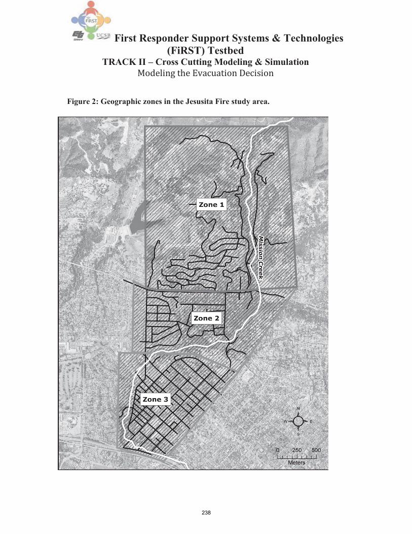
238
First Responder Support Systems & Technologies (FiRST) Testbed
TRACK II – Cross Cutting Modeling & Simulation Modeling the Evacuation Decision
Figure 2: Geographic zones in the Jesusita Fire study area.
239
First Responder Support Systems & Technologies (FiRST) Testbed
TRACK II – Cross Cutting Modeling & Simulation Modeling the Evacuation Decision
4.2 Survivor Function Comparison
Survival analysis is a way to model the time it takes for events to occur. One of the most
prevalent uses of this methodology is to examine time until death for recipients of different
medical treatments, hence the term ‘survival’. The event we are concerned with is
evacuation from a wildfire, thus ‘survival’ in this analysis should be thought of as ‘time to
evacuation.’ Everyone who evacuated from the wildfire is considered to be a ‘survivor’,
which makes sense intuitively as evacuation is a typical response when people are faced
with exposure to a natural hazard that may result in injury or death.
The first step in our survival analysis of the Jesusita Fire evacuation is to generate a
survivor function. Let T represent the time to evacuation, a random variable with a
cumulative distribution function P(t) = Pr(T :: t) and a probability density function p(t) =
dP(t)/dt. The survivor function S(t) is the probability that a survey respondent evacuated
after time t, where t can be any time period from the start of the fire until all mandatory
evacuation orders were lifted. This is simply the complement of the distribution function
1 – P(t). Survey responses for people who did not evacuate are considered to be right
censored since observation of these respondents is terminated at t =99. All evacuations
occurred at or before t =99, and all non-evacuees are censored at t =99, thus our survival
data set can be described as single right censored. We used the Kaplan-Meier method to
estimate the survival function for our data. For each observed event time t =1,2,3...99 we

240
First Responder Support Systems & Technologies (FiRST) Testbed
TRACK II – Cross Cutting Modeling & Simulation Modeling the Evacuation Decision
simply divide the number of evacuees by the total number of responses (208). For our
non-evacuees the Kaplan-Meier estimate is undefined.

241
First Responder Support Systems & Technologies (FiRST) Testbed
TRACK II – Cross Cutting Modeling & Simulation Modeling the Evacuation Decision
We believe it is more intuitive to think of an evacuation survival function in terms of the
percentage of people who have evacuated over time, thus we simply subtract each Kaplan-
Meier estimate from one and multiply by 100 to calculate this percentage at each time
period. The survival curve produced by the Jesusita Fire evacuation survivor function is
shown in Figure 3 below.
Figure 3: Jesusita Fire Evacuation Survival Curve
There are several distinct time periods at which a majority of the evacuations occurred.
They are May 5th from the start of the fire at 1pm until 9pm, May 6th from noon until
6pm, and May 7th from 1pm until 5pm. At the end of our study period at 3pm on the 9th
of May, 30 (or 14.4%) of a total 208 survey respondents had not evacuated. The presence

242
First Responder Support Systems & Technologies (FiRST) Testbed
TRACK II – Cross Cutting Modeling & Simulation Modeling the Evacuation Decision
i
of these distinct evacuation clusters is not surprising as a majority of wildfire events in
Southern California are driven by Santa Ana winds which generally begin in the afternoon
and continue until twilight. This environmental factor is closely linked to the speed at
which the fire spreads, and is taken into account by emergency managers when deciding
to issue an evacuation warning or mandatory evacuation order. Many Southern California
residents living in the wildland-urban interface understand that Santa Ana winds
contribute to rapid spread of wildfires thus may have a heightened sense of danger when
these conditions exist. Examination of the Jesusita fire evacuation survivor function can
provide preliminary clues as to which factors may influence the timing of the decision to
evacuate.
One method for preliminary testing of our research hypotheses is to determine whether
there is a statistical difference in the time to evacuation (i.e. survival times) for different
groups of evacuees. We can formulate the hypothesis test as follows:
H0 : h1 t)= h2 t)= ... = hn t for all t HA : hi t0 ) hj t0 for all least one pair i, j and time t0
Let:
ti = times when people evacuated dik = the number of evacuations from group k at time ti
Yik = the number of people in group k that had not yet evacuated at time ti These
d = Αn j 1 dij
Yi = j 1 Yij Α n

243
First Responder Support Systems & Technologies (FiRST) Testbed
TRACK II – Cross Cutting Modeling & Simulation Modeling the Evacuation Decision
Α
We compute the vector Z, where the kth element is
D d Z = d − Y i k ik ik
i 1 Yi
and also compute the covariance matrix Α and the test statistic X 2 = Z 'Α −1 Z .
Under the null hypothesis, X2 followsa 2 distributionwith ndegreesof freedom,
thus if X 2 2 we reject H . 1−α,df n 0
The first groups we compare are those who reported receiving a mandatory evacuation
order and those who did not. We find significant support (p-value < 0.001) that there is a
difference in evacuation times for these two groups. We can plot survival curves for each
of these groups, which allow us to visually assess how these evacuation times differ. As
seen in Figure 4 the survival curves for these two groups are similar for the first few hours
of the evacuation but then diverge at approximately 5pm on May 5th. This initial similarity
can be attributed in part to people evacuating soon after seeing flames and smoke in the
foothills, before they actually received an official evacuation order. The similarity may
also be explained by the phone tree system set up in Mission Canyon where residents warn
each other of a wildfire outbreak, but which may not be considered a “mandatory
evacuation order” per se. The later divergence of the survival functions for these two
groups lends support to the hypothesis that people who receive a mandatory evacuation
order evacuated earlier than those who did not.
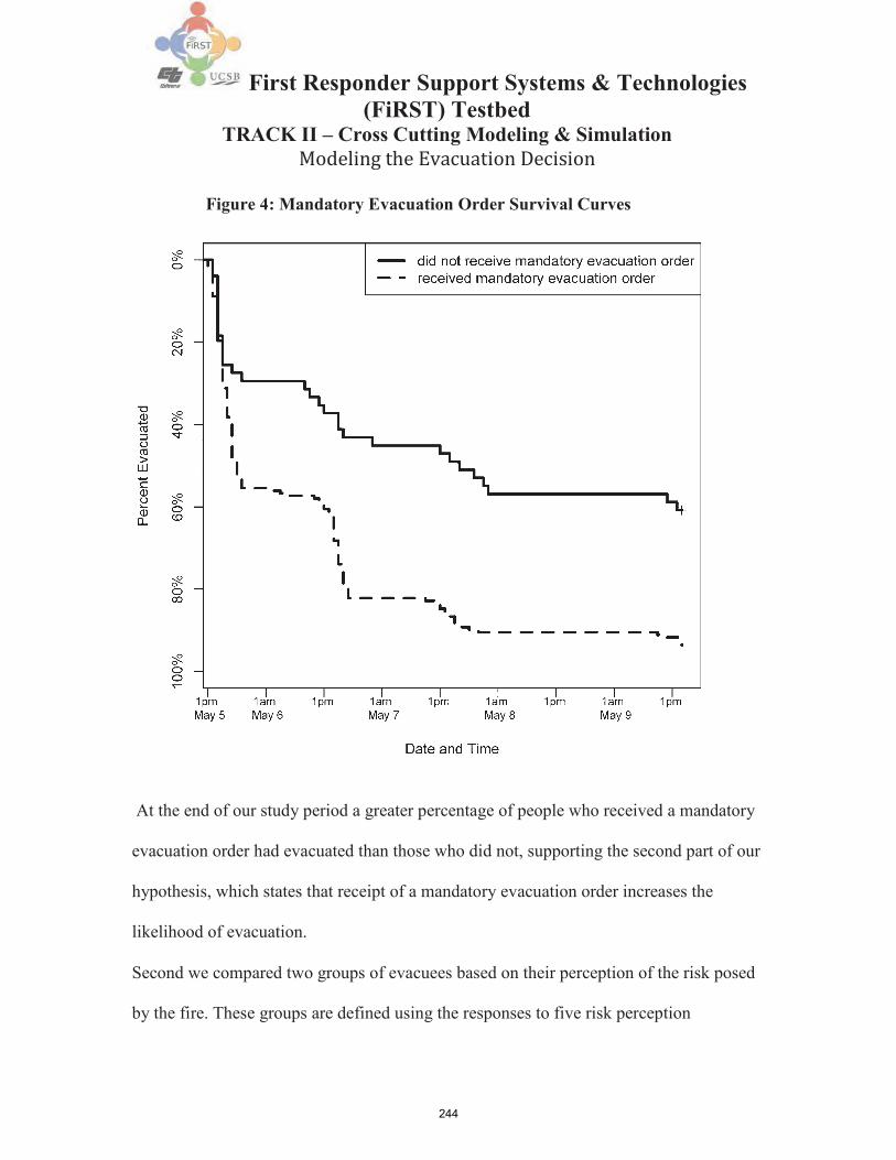
244
First Responder Support Systems & Technologies (FiRST) Testbed
TRACK II – Cross Cutting Modeling & Simulation Modeling the Evacuation Decision
Figure 4: Mandatory Evacuation Order Survival Curves
At the end of our study period a greater percentage of people who received a mandatory
evacuation order had evacuated than those who did not, supporting the second part of our
hypothesis, which states that receipt of a mandatory evacuation order increases the
likelihood of evacuation.
Second we compared two groups of evacuees based on their perception of the risk posed
by the fire. These groups are defined using the responses to five risk perception

245
First Responder Support Systems & Technologies (FiRST) Testbed
TRACK II – Cross Cutting Modeling & Simulation Modeling the Evacuation Decision
questions. We first calculated the mean response value to the five questions for each
evacuee. Respondents with mean values that fall above our neutral risk score of zero
generally agreed that the Jesusita Fire posed a high risk, thus were assigned to the high-
risk group. Respondents with mean values that fall below our neutral risk score were
assigned to the low risk group. Again we found significant support (p-value < 0.01) that
there is a difference in evacuation times for these two groups. The survival curves for
these two groups (Figure 5) show divergence throughout the entire evacuation time
period, with a higher percentage of respondents who perceived that the Jesusita Fire
posed a high risk deciding to evacuate. This comparison supports the hypothesis that
people who perceived a high risk evacuated earlier and were more likely to evacuate.
The last groups of survey respondents we compared are those who reported being one-
quarter mile or closer to the Jesusita Fire and those who reported being further away than
one-quarter mile. These groups are split at one-quarter mile because that was the median
answer to this question among all survey respondents. There is significant support (p-
value < 0.001) for a difference in evacuation times for these two groups.
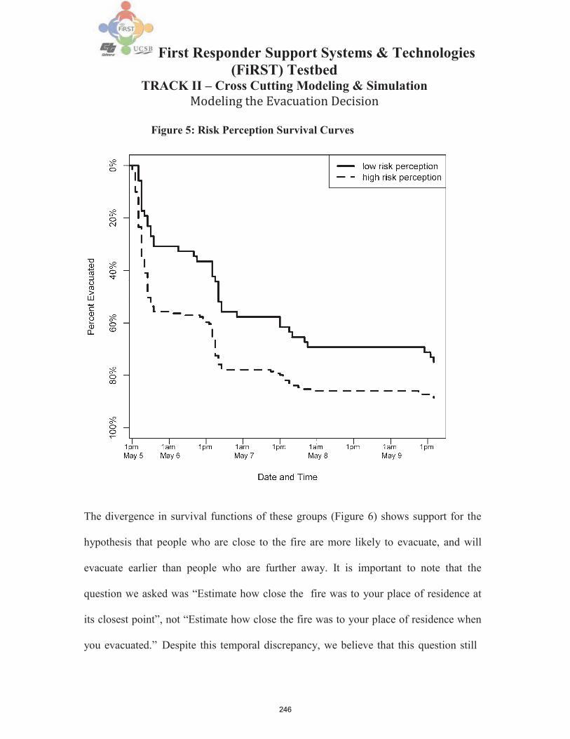
246
First Responder Support Systems & Technologies (FiRST) Testbed
TRACK II – Cross Cutting Modeling & Simulation Modeling the Evacuation Decision
Figure 5: Risk Perception Survival Curves
The divergence in survival functions of these groups (Figure 6) shows support for the
hypothesis that people who are close to the fire are more likely to evacuate, and will
evacuate earlier than people who are further away. It is important to note that the
question we asked was “Estimate how close the fire was to your place of residence at
its closest point”, not “Estimate how close the fire was to your place of residence when
you evacuated.” Despite this temporal discrepancy, we believe that this question still

247
First Responder Support Systems & Technologies (FiRST) Testbed
TRACK II – Cross Cutting Modeling & Simulation Modeling the Evacuation Decision
may capture the effect that distance from the fire had on the decision to evacuate. While
it is likely that the fire had not yet reached its closest point to a given respondent’s
residence at the time that they evacuated, it is also likely that they perceived that the fire
would get close based on wind direction, smoke, ash, and other environmental clues. Fire
distance can be thought of as a more indirect, proxy measure that may interact with
perception of danger or other variables to influence the decision to evacuate.
Figure 6: Fire Distance Survival Curves

248
First Responder Support Systems & Technologies (FiRST) Testbed
TRACK II – Cross Cutting Modeling & Simulation Modeling the Evacuation Decision
4.3 Environmental Time Series
We used a graphical method for preliminary testing of the influence of environmental cues
such as air temperature and wind speed on the evacuation decision. Unlike the variables
we tested by comparing survival curves, we can measure the change in these environmental
factors at very short time intervals. This temporal variation and the fact that most evacuees
likely experienced similar environmental conditions at a given time makes it difficult to
define different groups based on these factors. We developed a simple plot (Figure 7)
showing the number of evacuations during each time 1-hour time period along with the
average air temperature and maximum wind speed at the time period. This plot shows
similar diurnal cycles for all three measurements. Temperature, maximum wind speed,
and the number of evacuations reach their lowest value at night, and reach their peaks in
the early to mid-afternoon. This pattern should come as no surprise to one who is familiar
with the Southern California wildfire season and the Santa Ana winds that usually preclude
it. This plot provides visual support for the hypothesis that environmental factors such as
high temperature and high wind speed increase the likelihood of evacuation at the time of
their occurrence.

249
First Responder Support Systems & Technologies (FiRST) Testbed
TRACK II – Cross Cutting Modeling & Simulation Modeling the Evacuation Decision
Figure 7: The number of evacuations in each time period plotted with wind and temperature data

250
First Responder Support Systems & Technologies (FiRST) Testbed
TRACK II – Cross Cutting Modeling & Simulation Modeling the Evacuation Decision
4.4 Cox Regression Models
To further assess the influence of these variables on the decision to evacuate we developed
two Cox Regression Models. The Cox Regression is one of the most widely used survival
analysis modeling techniques, and the most commonly used Cox regression is the
proportional hazards model, which uses a hazards function to represent the distribution of
survival times. The hazards function h(t), which for our purposes can be thought of as the
instantaneous risk of evacuation at time t conditional on not having yet evacuated, is
defined as follows:
Pr[ t T t + t)| T t] h(t) = lim
t 0 t f (t) S(t)
One unique feature of the Cox Proportional Hazards model is that it does not require
choice of a particular probability distribution to represent survival times. We can leave
the baseline hazards function α t) = log h0 t) unspecified, allowing us to assess which
factors influence the decision to evacuate even if the actual evacuation survival
distribution is unknown. We do know the survival time distribution for the Jesusita Fire
evacuation, but this distribution appears to be non-parametric and thus would be difficult
to fit using the commonly used Gompertz or Weibull distribution. While the baseline
hazard can take any form, the covariates enter the model linearly thus the model is
c onsidered semi-parametric. The general form of the Cox Proportional Hazards model
=
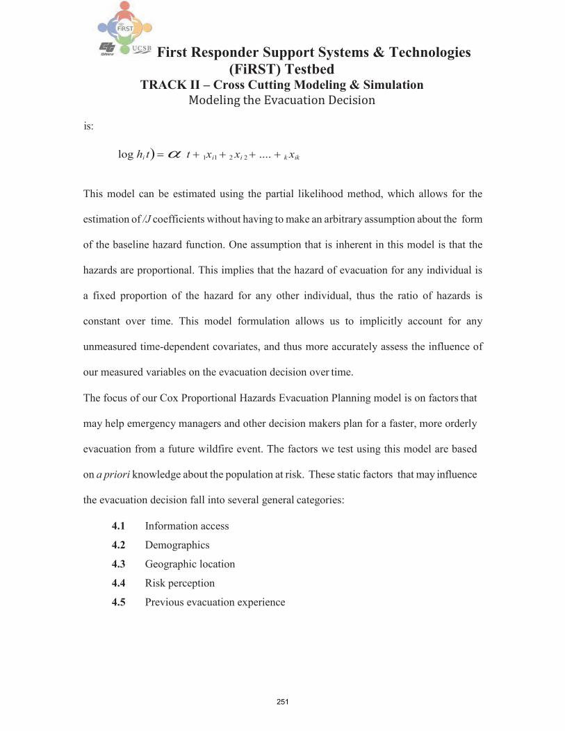
251
First Responder Support Systems & Technologies (FiRST) Testbed
TRACK II – Cross Cutting Modeling & Simulation Modeling the Evacuation Decision
is: log hi t) = α t + 1xi1 + 2 xi 2 + .... + k xik
This model can be estimated using the partial likelihood method, which allows for the
estimation of /J coefficients without having to make an arbitrary assumption about the form
of the baseline hazard function. One assumption that is inherent in this model is that the
hazards are proportional. This implies that the hazard of evacuation for any individual is
a fixed proportion of the hazard for any other individual, thus the ratio of hazards is
constant over time. This model formulation allows us to implicitly account for any
unmeasured time-dependent covariates, and thus more accurately assess the influence of
our measured variables on the evacuation decision over time.
The focus of our Cox Proportional Hazards Evacuation Planning model is on factors that
may help emergency managers and other decision makers plan for a faster, more orderly
evacuation from a future wildfire event. The factors we test using this model are based
on a priori knowledge about the population at risk. These static factors that may influence
the evacuation decision fall into several general categories:
4.1 Information access
4.2 Demographics
4.3 Geographic location
4.4 Risk perception
4.5 Previous evacuation experience

252
First Responder Support Systems & Technologies (FiRST) Testbed
TRACK II – Cross Cutting Modeling & Simulation Modeling the Evacuation Decision
Of course these factors are not truly static is the sense that many of them can change for
an individual over time. Rather they are static in the sense that emergency managers can
have knowledge of these factors well before a wildfire occurs, and they are unlikely to
change at the same time scale as the wildfire itself. In generating the data for our model
we simply have one row for each survey respondent that answered each survey question
under consideration (n = 200). We first formulated this model using 22 variables from our
primary and secondary data sets that fit into the categories defined above. We then
finalized the planning model using backward elimination, by which we start with all
candidate variables and delete any that are not statistically significant at a p-value < 0.1.
The variables included in the final planning model are shown in the formulation below.
log hi t) = α t + 1mandi + 2 personali + 3neighborsi + 4 residencei +
5 prevevaci + 6tsbi + 7 zone3i
All variables are significant at p-value < 0.05 (Figure 8). Receipt of a mandatory
evacuation order (mand) is positively correlated with the decision to evacuate, as is
perception that the fire posed a high risk to a respondent’s personal safety (personal) or
place of residence (residence). Previous evacuation from a wildfire or other event
(prevevac) is also positively correlated with the decision to evacuate. This relationship
may be explained in part by the large number of long-term residents of Mission Canyon
who responded to our survey, which is the part of our study area most frequently threatened
by wildfires. One geographic zone indicator variable (zone3) is negatively correlated with
the decision to evacuate, which makes sense given that this zone was the furthest from the
fire and was only partially under a mandatory evacuation order.

253
First Responder Support Systems & Technologies (FiRST) Testbed
TRACK II – Cross Cutting Modeling & Simulation Modeling the Evacuation Decision
Figure 8: Planning Model Results
Perception that the fire posed a high risk to neighbors (neighbors) is negatively correlated
with the decision to evacuate. This finding may be counterintuitive for researchers who
believe that the people around them heavily influence an individual’s decision making.
There are many possible explanations for this counterintuitive finding. One is that an
individual decides whether to evacuate or not well in advance of the occurrence of a
wildfire, thus is not influenced by any effect the fire may be having on people nearby.
Another more nuanced explanation lies in the fuzzy definition of ‘neighbor’, which can
be interpreted as ‘the people next door’, ‘the people down the street’, or the ‘people who
live in the same neighborhood as me’. Given the irregularity with which fire my affect
individual homes and/or property in a neighborhood, it is possible that while survey
respondents recognized that other people in the neighborhood were at high risk,
personally they felt safe. The number of years the respondent has lived in Santa Barbara

254
First Responder Support Systems & Technologies (FiRST) Testbed
TRACK II – Cross Cutting Modeling & Simulation Modeling the Evacuation Decision
Α
(tsb) is also negatively correlated with the decision to evacuate.
This finding can also be interpreted in a number of ways, but may lend support to the
notion that people make up their minds whether to evacuate or not well in advance of the
actual event. Long term residents of our study area may have experienced wildfires
before, and thus created defensible space or purchased personal firefighting equipment
such as hoses and sprinklers in preparation to ‘stay and defend’ their home.
As mentioned earlier, the central assumption of the Cox Proportional Hazards model is
that the hazard for any individual is a fixed proportion of the hazard for any other
individual. Checking for violations of this assumption is important for assessing how
well the fitted model describes our data. One way to check for violations of
proportionality is to calculate the Schoenfeld residuals for each covariate and plot them
against time. The Schoenfeld residual is the covariate value for each individual that
evacuated minus its expected value. The expected value at ti is an average of the
covariate weighted by the likelihood of failure for each individual in the risk set at ti :
jΕR (ti )
Sresidual = xik xjk pj
− i 1

255
First Responder Support Systems & Technologies (FiRST) Testbed
TRACK II – Cross Cutting Modeling & Simulation Modeling the Evacuation Decision
The plot for each covariate should show residuals to be randomly distributed throughout
time, and the line fitted to these residuals should be horizontal. The plots in Figure 9
show clustering of residuals around the earlier time intervals of our study period, which
is not surprising given that most of our observed evacuations occurred then. In the plot
of residuals for our mandatory evacuation order variable (mand) the fitted line deviates
from horizontal and we see additional clustering of residual values beyond the early
time intervals. We thus consider the hazard for this variable to be non- proportional. In
the second set of plots (Figure 10), variable prevevac and variable zone3 both show
departures from the horizontal fitted line and clustering of residuals that indicate non-
proportionality. Although the slope of the fitted line for variable tsb varies considerably,
its overall trend is approximately horizontal and the residuals are well scattered.
One way to account for non-proportional hazards is to include interactions between the
offending covariates and time in the Cox regression model.

256
First Responder Support Systems & Technologies (FiRST) Testbed
TRACK II – Cross Cutting Modeling & Simulation Modeling the Evacuation Decision
Figure 9: Schoenfeld Residuals (1)
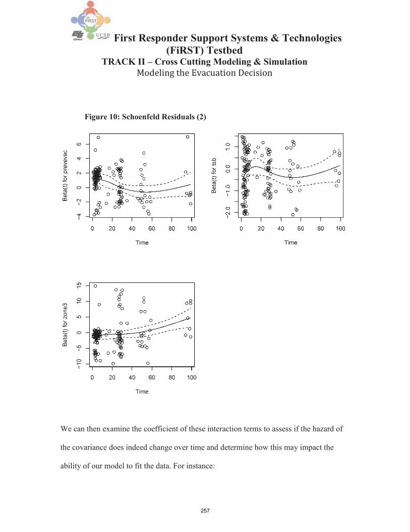
257
First Responder Support Systems & Technologies (FiRST) Testbed
TRACK II – Cross Cutting Modeling & Simulation Modeling the Evacuation Decision
Figure 10: Schoenfeld Residuals (2)
We can then examine the coefficient of these interaction terms to assess if the hazard of
the covariance does indeed change over time and determine how this may impact the
ability of our model to fit the data. For instance:

258
First Responder Support Systems & Technologies (FiRST) Testbed
TRACK II – Cross Cutting Modeling & Simulation Modeling the Evacuation Decision
log hi t)= α t + ( 1 + 2t)mandi + 3 personali + 4 neighborsi + 5residencei + ( 6 + 7t) prevevaci + 8tsbi +( 9 + 10t)zone3i
The interaction variables (for mand, prevevac, and zone3, respectively) are all highly
significant (p-value < 0.01) and each has a negative coefficient indicating a
declining effect over time. The signs for the coefficients of the original mand and prevevac
variables are positive, thus one way this trend could be interpreted is that people who
decided not to evacuate stuck with this decision despite receipt of a mandatory evacuation
order or a previous evacuation experience. The original coefficient sign for zone3 is
negative, thus the corresponding interaction term may reflect the increased number of
people evacuating from zone 3 as the fire moved closer and threatened this part of our
study area. Although these three variables appear to violate the assumption of proportional
hazards, the reason for these violations makes sense in the context of the process we are
trying to model. The coefficient estimates for original non-interacted terms can be
considered to represent the average effect over the entire study period, thus we maintain
the original formulation of our planning model.
A secondary assumption made in the Cox Proportional Hazards Model is that the
parametric part of the model is linear in form. We can test for nonlinearity by plotting
the Martingale residuals against each non-dichotomous covariate. The solid line that we
fit to these data should exhibit little or no deviation from the horizontal dashed line if the
parametric part of the model is indeed linear. We can see in Figure 11 that this is the case,

259
First Responder Support Systems & Technologies (FiRST) Testbed
TRACK II – Cross Cutting Modeling & Simulation Modeling the Evacuation Decision
thus we can be confident that the functional form of our planning model is linear and thus
correctly specified.
Of course the most intuitive test of model fit is how well the model generated survival
curve matches our empirical data. As seen in Figure 12, the evacuation time distribution
produced by our planning model fitted values appears to approximate our empirical
evacuation time distribution well. The planning model overestimates the number of
evacuees during the evening of May 6th, which may be attributed to the fact that a small
but significant number of survey respondents decided to remain in their homes beyond
this point in time despite receiving a mandatory evacuation order and being well aware
of the high risk posed by the fire to their personal safety and their property. Despite this
divergence the empirical data is very close to being within the 95% confidence interval
of our modeled data for this section of the curve, thus the planning model can be
considered to be a good representation of our Jesusita Fire evacuation time series.

260
First Responder Support Systems & Technologies (FiRST) Testbed
TRACK II – Cross Cutting Modeling & Simulation Modeling the Evacuation Decision
Figure 11: Planning Model Martingale Residuals

261
First Responder Support Systems & Technologies (FiRST) Testbed
TRACK II – Cross Cutting Modeling & Simulation Modeling the Evacuation Decision
Figure 12: Planning Model Survival Curve
The second Cox model we developed is focused on evacuation operations. Evacuation
operations refers to actions taken by emergency managers, police officers, and other
personnel who are responsible for managing the logistics of an emergency evacuation after
the onset of a hazardous event. We use this model to assess dynamic, time-dependent
factors that may influence the evacuation decision with the goal of helping emergency

262
First Responder Support Systems & Technologies (FiRST) Testbed
TRACK II – Cross Cutting Modeling & Simulation Modeling the Evacuation Decision
managers respond to changing conditions on the ground after the start of a wildfire. Unlike
our planning model these factors are difficult or impossible to measure before a wildfire
starts, and can change at rates similar to those at which the fire changes. These dynamic
factors include:
4.6 Distance from fire
4.7 Location in mandatory or voluntary evacuation zone
4.8 Wildfire impact on homes and property
4.9 Weather
This model incorporates time-dependent variables, so it requires a different data structure
than our planning model. We have one row for each survey respondent at each 1-hour
period of time from the start of the fire until they evacuated. Respondents who did not
evacuate have 99 rows, the number of hours covering the entire study period. This model
is first formulated using 19 variables from our survey and GIS data that fit into the
categories defined above. The general form of this model is very similar to the Cox
Proportional Hazards model, with slight adjustments needed to account for both time
dependent and non-time dependent variables:
log hi t) = α t + 1xi1 + 2 xi 2 t + .... + k xik
We finalized this operations model using backward elimination and deleted any variables
that are not statistically significant at a p-value < 0.1. The final form of the operations
model is shown below:
log hi t) = α t + 1tempi (t) + 2 windspdi (t) + 3d1i + 4 d 2i + 5 zone2i

263
First Responder Support Systems & Technologies (FiRST) Testbed
TRACK II – Cross Cutting Modeling & Simulation Modeling the Evacuation Decision
Each of the variables in our operations model is significant at p-value < 0.01 and is
positively correlated with the decision to evacuate (Figure 13). This positive correlation
makes intuitive sense for environmental factors such as air temperature (temp) and wind
speed (windspd) which are often indicative of increased wildfire severity and faster fire
spread. The positive correlation of a geographic zone indicator variable (zone2) also
makes sense given that this zone was the next closest to the fire after Mission Canyon (i.e.
zone1) and was under a mandatory evacuation order. The destruction of a respondent's
home (d1) by the Jesusita fire is also positively correlated with the decision to evacuate,
as is damage to a respondent's home (d2). While these variables are static and thus we
cannot know exactly when their place of residence was impacted, we believe this variable
may serve as a proxy measure of the overall impact of the fire on the built environment.
Figure 13: Operations Model Results

264
First Responder Support Systems & Technologies (FiRST) Testbed
TRACK II – Cross Cutting Modeling & Simulation Modeling the Evacuation Decision
Despite the similarity in form of the operations model to the planning model, the
operations model is not a proportional hazards model. The time-dependent covariates in
the operations model will change at different rates for different individuals, thus the ratios
of their hazards cannot remain constant. We can ignore the test for proportional hazards
and proceed directly to the test for non-linearity to assess the fit of the model. In the plot
of Martingale residuals against our two non-dichotomous covariates temp and windspd,
(Figure 14) the solid line that we fit to the data shows no deviation from the horizontal
dashed line. We can therefore be confident that the functional form of our operations
model is linear and correctly specified.

265
First Responder Support Systems & Technologies (FiRST) Testbed
TRACK II – Cross Cutting Modeling & Simulation Modeling the Evacuation Decision
Figure 14: Operations Model Martingale Residuals

266
First Responder Support Systems & Technologies (FiRST) Testbed
TRACK II – Cross Cutting Modeling & Simulation Modeling the Evacuation Decision
The final and most important check for the fit of our operations model was to plot the
modeled survival curve against our empirical evacuation data. As seen in Figure 15, our
operations model significantly under predicts the number of evacuees for most of our study
time period. A great majority of our empirical survival curve falls outside the 95%
confidence intervals for our modeled data. This means that our operations model can be
considered to be a poor fit for our empirical evacuation data.
Figure 15: Operations Model Survival Curve

267
First Responder Support Systems & Technologies (FiRST) Testbed
TRACK II – Cross Cutting Modeling & Simulation Modeling the Evacuation Decision
One possible reason for this poor fit is the large number of records in our dataset at where
evacuation does not occur. The data structure required for this type of model has one row
for each time period t from the start of the fire until the time at which an evacuee departed.
Survey respondents who did not evacuate have 99 rows. Of the 6,504 total observations
at which evacuation is possible there are only 178 at which an evacuation actually occurs
(evac = 1). Thus even though some of the factors may in fact correlate with the evacuation
decision over time, there may simply be too few non-zero response variables to establish
a good model fit. One possible method for dealing with this issue would be to exclude
the time periods from the dataset where no one evacuates, or to introduce time-lagged
variables into the model formulation. This is beyond the scope of our current analysis but
could prove useful for future modeling efforts.
Despite the poor fit of our operations model we believe that the covariates considered do
play some role in the decision to evacuate. Two ordinary least squares regressions of the
form yi = 0 + 1x1 + i
confirm the likelihood of this relationship. In our first regression model the number of
evacuations per hour is the dependent variable and the average air temperature average is
the independent variable. We find that air temperature accounted for 16% of the variance
in the number of evacuations per hour (R2 = 0.16) and is highly significant (p-value <

268
First Responder Support Systems & Technologies (FiRST) Testbed
TRACK II – Cross Cutting Modeling & Simulation Modeling the Evacuation Decision
0.001). The second regression also has evacuations per hour as the dependent variable,
with average wind speed at each hour as the independent variable. Average wind speed
accounted for 46% of the variance in the number of evacuations per hour (R2 = 0.46, p value
< 0.001). The relationship, if any, between the decision to evacuate and our two 'fire
impact' variables d1 and d2 is less clear. Not surprisingly, every respondent whose house
was damaged or destroyed by the fire decided to evacuate. Due to the design of the survey
questions we cannot know the time at which these respondent's homes were damaged or
destroyed for comparison to the time at which they evacuated. Given the results of our
survival curve comparison we believe these variables may be important, but should be
measured differently for future modeling efforts.
4.5 Rayleigh Probability Model
We used the results of our survival analysis to inform the design of our Rayleigh
Probability Model. While survival analysis is useful for assessing the influence specific
variables may have on the evacuation decision, we prefer to use a model based on the
Rayleigh Probability Distribution to actually forecast evacuation travel demand because it
may be easier to generalize for additional wildfire evacuation datasets. In our earlier
comparison of survival curves we determined that receipt of a mandatory evacuation order,
perception of the risk posed by the fire, and distance from the fire at its closest point are
variables that influence the evacuation decision. Our Cox proportional hazards planning
model confirms the significance of these variables, but also indicates that having previous
evacuation experience and the amount of time one has lived in Santa Barbara may be

269
First Responder Support Systems & Technologies (FiRST) Testbed
TRACK II – Cross Cutting Modeling & Simulation Modeling the Evacuation Decision
influential as well. Although the overall fit of our operations model to the empirical data
is poor, our post-analysis reveals that the environmental factors of wind speed and air
temperature are positively correlated with the number of evacuations in a one-hour time
period. These factors are considered in the formulation of our Rayleigh Probability Model
for evacuation travel demand. Let,
π3,if the fire has burned homes f1 = 2, if the fire poses a significant threat to homes
1, if the fire poses a minimal threat to homes
π3, if wind speed and air temperature are extreme
f2 = 12, if wind speed and air temperature are above average 1, if wind speed and air temperature are at or below average
π3,if all residents have been ordered to evacuate f3 = 2, if some residents have been ordered to evacuate
1,no evacuation order issused ( f + f + f )
fbar 1 2 3
3
Rayleigh Probability Model:
Pevac = exp − T ^ fbar / 50

270
First Responder Support Systems & Technologies (FiRST) Testbed
TRACK II – Cross Cutting Modeling & Simulation Modeling the Evacuation Decision
The three factors that influence the probability of evacuation Pevac are analogous to the
significant variables from our survival analysis. The first factor f1 is intended to capture the
effect of distance from the fire on the evacuation decision. We believe that quantifying
distance using the impact on homes as a proxy for an actual distance measurement may be
more intuitive for the emergency managers and traffic engineers that may use our model. In
addition, accurate distance measurements can be difficult to obtain in lieu of the smoke
generated by a wildfires and the steep, mountainous terrain on which they often occur.
Similarly, our second factor f2 allows for an estimation-based measurement
for environmental factors which can vary locally but whose overall effect is usually quite
obvious. The third factor f3 refers to the number of residents of a wildfire-prone neighborhood
or subdivision who have been notified that an emergency evacuation order is in effect. In our
formulation T is a vector of sixteen elements that are simply the whole numbers 1,2,3... 16.
These numbers represent the sixteen half-hour time steps that occur in an 8-hr time period,
the length of time of a typical shift for police officers and other personnel often responsible
for managing traffic during an emergency evacuation. It is important to note that the
significant factors from our survival analysis related to the perception of danger, previous
evacuation experience, and the length of residency in Santa Barbara are not included in our
Rayleigh Probability Model. These variables are difficult to measure without the use of a
comprehensive survey and may vary significantly for different portions of a neighborhood.
We believe they should be left out of the model in the interest of generalizability.

271
First Responder Support Systems & Technologies (FiRST) Testbed
TRACK II – Cross Cutting Modeling & Simulation Modeling the Evacuation Decision
5.0 Results
We tested the applicability of the Rayleigh Probability Model for evacuation travel demand
using both our primary and secondary datasets related to the Jesusita Fire. This model can
only represent travel demand during a single eight hour time period. Using our survey data
we calculated the number of evacuations per hour from the start of the fire (May 5th at
1pm) until 9pm on May 5th. The empirical evacuation time distribution that we used to
test model fit is shown in Figure 16.
Figure 16: 8hr Empirical Evacuation Time Distribution

272
First Responder Support Systems & Technologies (FiRST) Testbed
TRACK II – Cross Cutting Modeling & Simulation Modeling the Evacuation Decision
We determine the appropriate value for f2 by comparing weather conditions for our eight
hour study period to both the conditions over the five day time period of the Jesusita Fire
evacuation and the normal conditions experienced during early May in our study area. The
mean wind speed for our eight-hour time period was approximately 3mph, while the value
for our entire five-day time period was approximately 2.3mph. The corresponding values
for air temperature are 77.0° F and 76.0° F, respectively. These values are similar, but

273
First Responder Support Systems & Technologies (FiRST) Testbed
TRACK II – Cross Cutting Modeling & Simulation Modeling the Evacuation Decision
when compared to the values for average weather conditions in our study area in early
May1 (61.3° F, 1.7mph), we see a considerable difference. Based on these differences we
determined that wind speed and air temperatures were above average but fell well short of
the extremes for the five day Jesusita Fire evacuation time period (101.2°F, 10.4mph).
This lead us to assign f2 = 2.
One way to determine the appropriate value of f3 is to calculate the percentage of
evacuees from our eight-hour time period who reported receiving a mandatory evacuation
order. Of our one hundred evacuees from this time period, eighty-five reported receiving
mandatory evacuation order (85%). In addition, all evacuees located in geographic zone
one (n=83) were under a mandatory evacuation order by 5:45pm on May 5th, while
e vacuees from zone two (n =17) were not officially ordered to evacuate until May 6th2.
The appropriate value for f3 is 2, indicating that some residents have been ordered to
evacuate.
1 We downloaded the seven-day averages from May 5th - May 12th for 2007 through 2012 from the same weather stations used to download data for our weather variables. These values are simply the mean of the seven-day average for all years.
2 The timing of these mandatory evacuation orders was obtained from the official
press releases from the Santa Barbara County Emergency Operations Center.
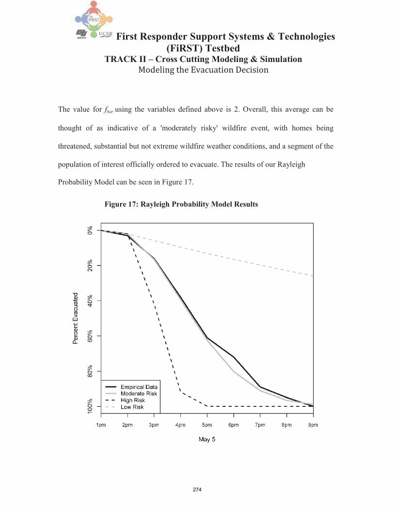
274
First Responder Support Systems & Technologies (FiRST) Testbed
TRACK II – Cross Cutting Modeling & Simulation Modeling the Evacuation Decision
The value for fbar using the variables defined above is 2. Overall, this average can be
thought of as indicative of a 'moderately risky' wildfire event, with homes being
threatened, substantial but not extreme wildfire weather conditions, and a segment of the
population of interest officially ordered to evacuate. The results of our Rayleigh
Probability Model can be seen in Figure 17.
Figure 17: Rayleigh Probability Model Results

275
First Responder Support Systems & Technologies (FiRST) Testbed
TRACK II – Cross Cutting Modeling & Simulation Modeling the Evacuation Decision
The evacuation probability curve generated for our 'moderate risk' wildfire event is an
excellent match for our empirical data. We generated two additional curves with our
model that correspond to a 'high risk' wildfire event ( fbar = 3) and a 'low risk' wildfire
event ( fbar = 1). It should be noted that these additional curves are purely hypothetical
and have not been compared to any empirical evacuation distributions.
6.0 Discussion The evacuation decision encompasses two critical questions: will people evacuate, and if
they choose to evacuate, when will they depart? The success of an emergency evacuation
is heavily dependent on having accurate answers to these questions. Survival analysis can
be used to model the both of these evacuation decision questions simultaneously, but has
been used infrequently in the fields of hazards and emergency management. We believe
that survival analysis is an intuitive and powerful method for modeling the evacuation
decision and should be used more often by researchers.
The findings of our survival analysis suggest that receipt of an evacuation order, distance
from the fire, and risk perception are important factors for people faced with the evacuation
decision. While impact of these factors has been well documented in past emergency
evacuation research, comparing the survival curves for different groups of people allows
for simple visualizations of how each factor effects the evacuation decision over time. The
Cox Regression framework allows us to determine the relative influence of multiple
276
First Responder Support Systems & Technologies (FiRST) Testbed
TRACK II – Cross Cutting Modeling & Simulation Modeling the Evacuation Decision
factors while implicitly controlling for any unmeasured variables. Measuring every
variable is nearly impossible for events as complex as an emergency evacuation, thus the
Cox Regression is particularly useful.
One drawback to survival analysis as well as many other statistical modeling techniques is
that they require large, detailed datasets that can be difficult to obtain. A Rayleigh
Probability Model utilizing simple, easily estimated data can be used to forecast the rate of
evacuations over an 8-hour time window. The Rayleigh function is very similar to the S-
curve function, which is widely used to forecast evacuation departure timing for hurricanes
and other hazards. To our knowledge, no research has shown that the S-curve or Rayleigh
function can be used to forecast evacuation departure timing for a wildfire. Models of this
type may be preferable to event and place-specific statistical analysis because they are
more easily applied and tested for other emergency evacuation datasets.
One of the major limitations of the current formulation of our Rayleigh Probability Model
is that it does not account for people who did not evacuate. One could infer that non-
evacuees are of little interest when trying to manage the logistics of an emergency
evacuation. Yet because California firefighters must protect people who choose to stay in
homes that are threatened by a wildfire, there is both an in-flow and out- flow of traffic
during an evacuation that must be managed. Understanding who is likely not to evacuate
and why a critical question left is largely untouched by our research.
277
First Responder Support Systems & Technologies (FiRST) Testbed
TRACK II – Cross Cutting Modeling & Simulation Modeling the Evacuation Decision
Besides the aforementioned study of non-evacuees, there are several other directions for
future research. The Rayleigh Probability Model should be tested on additional emergency
evacuation datasets to determine if it is indeed suitable as the basis of a general framework
for forecasting evacuation travel demand. Currently there is a paucity of empirical data on
emergency evacuations, thus additional survey research should be undertaken to develop
new datasets. Finally, new methods of collecting data on emergency evacuations should
be employed. Approximately two-thirds of our survey respondents reported using a cell
phone immediately before or during their evacuation, thus the increasingly advanced
capabilities of mobile technologies could be harnessed to generate data that builds a better
understanding of the evacuation process.

278
First Responder Support Systems & Technologies (FiRST) Testbed
TRACK II – Cross Cutting Modeling & Simulation Modeling the Evacuation Decision
Relevant References
1. P. D. Allison, Survival analysis using SAS: A practical guide, SAS Institute Inc, Cary, NC, (1995)
2. R. Alsnih, J. Rose and P. Stopher, "Understanding household evacuation decisions using a stated choice survey–case study of bush fires", 84th Annual Meeting of the Transportation Research Board, Washington, DC (2005).
3. J. Auld, T. Rashidi, M. Javanmardi and A. Mohammadian, "Dynamic Activity Generation Model Using Competing Hazard Formulation", Transportation Research Record: Journal of the Transportation Research Board, vol. 2254, pp. 28-35 (2011).
4. J. N. Bailenson, M. S. Shum and D. H. Uttal, "Road climbing: Principles governing asymmetric route choices on maps", Journal of Environmental Psychology, vol. 18, pp. 251-264 (1998).
5. J. N. Bailenson, M. S. Shum and D. H. Uttal, "The initial segment strategy: A heuristic for route selection", Memory & Cognition, vol. 28, pp. 306-318 (2000).
6. F. S. Berry and W. D. Berry, "State Lottery Adoptions as Policy Innovations: An Event History Analysis", The American Political Science Review, vol. 84, pp. 395-415 (1990).
7. C. R. Bhat, "A generalized multiple durations proportional hazard model with an application to activity behavior during the evening work-to-home commute", Transportation Research Part B: Methodological, vol. 30, pp. 465-480 (1996).
8. T. Brandstetter, L. A. Garrow, M. P. Hunter and D. F. Southworth, "Modeling Altruistic and Aggressive Driver Behavior in a No-Notice Evacuation", 87th Annual Meeting of the Transportation Research Board, Washington, D.C. (2008).
9. I. Burton, R. W. Kates and G. F. White, The environment as hazard, The Guilford Press, New York, (1993)
10. M. Burton, D. Rigby and T. Young, "Modelling the adoption of organic horticultural technology in the UK using Duration Analysis", Australian Journal of Agricultural and
279
First Responder Support Systems & Technologies (FiRST) Testbed
TRACK II – Cross Cutting Modeling & Simulation Modeling the Evacuation Decision
Resource Economics, vol. 47, pp. 29-54 (2003).
11. L. G. Chalmet, R. L. Francis and P. B. Saunders, "Network models for building evacuation", Management Science, vol. 28, pp. 86-105 (1982).
12. T. Charnkol and Y. Tanaboriboon, "Evacuee behaviors and factors affecting the tsunami trip generation model: A case study in Phang-nga, Thailand", Journal of Advanced Transportation, vol. 40, pp. 313-330 (2006).
13. M. Chen, "Traffic Signal Timing for Urban Evacuation", Master's Thesis, Department of Civil Engineering, University of Maryland, College Park (2005).
14. X. Chen, J. W. Meaker and F. B. Zhan, "Agent-Based Modeling and Analysis of Hurricane Evacuation Procedures for the Florida Keys", Natural Hazards, vol. 38, pp. 321-338 (2006).
15. X. Chen and F. B. Zhan, "Agent-based modelling and simulation of urban evacuation: relative effectiveness of simultaneous and staged evacuation strategies", Journal of the Operational Research Society, vol. 59, pp. 25-33 (2006).
16. S. I. Chien and V. V. Korikanthimath, "Analysis and Modeling of simultaneous and staged emergency evacuations", Journal of Transportation Engineering-Asce, vol. 133, pp. 190-197 (2007).
17. Y. C. Chiu, J. Villalobos, B. Gautam and H. Zheng, "Modeling and Solving Optimal Evacuation Destination-Route-Flow-Staging Problem for No-Notice Extreme Events", 85th Annual Meeting of the Transportation Research Board, Washington, DC (2006).
18. Y. C. Chiu and H. Zheng, "Real-time mobilization decisions for multi-priority emergency response resources and evacuation groups: Model formulation and solution", Transportation Research Part E-Logistics and Transportation Review, vol. 43, pp. 710- 736 (2007).
19. Y. C. Chiu, H. Zheng, J. Villalobos and B. Gautam, "Modeling no-notice mass evacuation using a dynamic traffic flow optimization model", IIE Transactions, vol. 39, pp. 83-94 (2007).
20. W. Choi, H. W. Hamacher and S. Tufekci, "Modeling of building evacuation problems by network flows with side constraints", European Journal of Operational Research, vol. 35, pp. 98-110 (1988).
280
First Responder Support Systems & Technologies (FiRST) Testbed
TRACK II – Cross Cutting Modeling & Simulation Modeling the Evacuation Decision
21. J. T. Christian, C. C. Ladd and G. B. Baecher, "Reliability applied to slope stability analysis", Journal Name: Journal of Geotechnical Engineering; (United States); Journal Volume: 120:12, vol. pp. Medium: X; Size: Pages: 2180-2207 (1994).
22. R. L. Church and T. J. Cova, "Mapping evacuation risk on transportation networks using a spatial optimization model", Transportation Research Part C-Emerging Technologies, vol. 8, pp. 321-336 (2000).
23. R. L. Church and R. M. Sexton, "Modeling small area evacuation: Can existing transportation infrastructure impede public safety?" Vehicle Intelligence & Transportation Analysis Laboratory, University of California, Santa Barbara (2002).
24. C. N. Coleman, S. L. Simon, M. A. Noska, J. L. Telfer and T. Bowman, "Disaster preparation: lessons from Japan", Science, vol. 332, pp. 1379 (2011).
25. C. E. Colten, "Basin Street Blues: drainage and environmental equity in New Orleans, 1890-1930", Journal of Historical Geography, vol. 28, pp. 237-257 (2002).
26. R. B. Corotis, A. B. Sigl and J. Klein, "Probability models of wind velocity magnitude and persistence", Solar Energy, vol. 20, pp. 483-493 (1978).
27. T. J. Cova, "Public Safety in the Urban--Wildland Interface: Should Fire-Prone Communities Have a Maximum Occupancy?" Natural Hazards Review, vol. 6, pp. 99- 108 (2005).
28. T. J. Cova, "Simulating Evacuation Shadows", Association of American Geographers Annual Meeting, Boston, MA (2008).
29. T. J. Cova and R. L. Church, "Modelling community evacuation vulnerability using GIS", International Journal of Geographical Information Science, vol. 11, pp. 763-784 (1997).
30. T. J. Cova, F. A. Drews, L. K. Siebeneck and A. Musters, "Protective Actions in Wildfires: Evacuate or Shelter-in-Place?" Natural Hazards Review, vol. 10, pp. 151 (2009).
31. T. J. Cova and J. P. Johnson, "Microsimulation of neighborhood evacuations in the urban-wildland interface", Environment and Planning A, vol. 34, pp. 2211-2229 (2002).
32. T. J. Cova and J. P. Johnson, "A network flow model for lane-based evacuation
281
First Responder Support Systems & Technologies (FiRST) Testbed
TRACK II – Cross Cutting Modeling & Simulation Modeling the Evacuation Decision
routing", Transportation Research Part a-Policy and Practice, vol. 37, pp. 579-604 (2003).
33. D. R. Cox, "Regression Models and Life-Tables", Journal of the Royal Statistical Society. Series B (Methodological), vol. 34, pp. 187-220 (1972).
34. CSSC, "The Tsunami Threat to California: Findings and Recommendations on Tsunami Hazards and Risks", Seismic Safety Commission, State of California (2005).
35. S. Cutter and K. Barnes, "Evacuation behavior and Three Mile Island", Disasters, vol. 6, pp. 116-124 (1982).
36. S. L. Cutter, "Vulnerability to environmental hazards", Progress in Human Geography, vol. 20, pp. 529 (1996).
37. S. L. Cutter, American Hazardscapes: The Regionalization of Hazards and Disasters, Joseph Henry Press, Washington, DC, (2001)
38. S. L. Cutter and C. T. Emrich, "Moral hazard, social catastrophe: The changing face of vulnerability along the hurricane coasts", Annals of the American Academy of Political and Social Science, vol. 604, pp. 102-112 (2006).
39. N. Dash and H. Gladwin, "Evacuation Decision Making and Behavioral Responses: Individual and Household", Natural Hazards Review, vol. 8, pp. 69-77 (2007).
40. F. N. de Silva and R. W. Eglese, "Integrating simulation modelling and GIS: spatial decision support systems for evacuation planning", Journal of the Operational Research Society, vol. 51, pp. 423-430 (2000).
41. J. Duanmu, M. Chowdhury and K. Taaffe, "A simulation modeling framework for community-wide evacuation planning", Journal of Transportation Security, vol. 4, pp. 1- 18 (2011).
42. G. W. Evans, M. A. Skorpanich, T. Garling, K. J. Bryant and B. Bresolin, "The effects of pathway configuration, landmarks and stress on environmental cognition", Journal of environmental psychology, vol. 4, pp. 323-335 (1984).
43. R. F. Fahy, "EXIT89 - An Evacuation Model for High-Rise Buildings - Recent Enhancements and Example Applications", International Conference of Fire Research and Engineering, Orlando, FL (1995).

282
First Responder Support Systems & Technologies (FiRST) Testbed
TRACK II – Cross Cutting Modeling & Simulation Modeling the Evacuation Decision
44. FEMA, "Hazard Mitigation Report for the East Bay Fire in the Oakland-Berkeley Hills", FEMA-919-DR-CA (1991).
45. FEMA, "Reuniting the Families of Katrina and Rita", Louisiana Family Assistance Center, Louisina Department of Health and Hospitals (2006).
46. H. Fu and C. Wilmot, "Survival Analysis-Based Dynamic Travel Demand Models for Hurricane Evacuation", Transportation Research Record: Journal of the Transportation Research Board, vol. 1964, pp. 211-218 (2006).
47. H. Fu and C. G. Wilmot, "Sequential logit dynamic travel demand model for hurricane evacuation", Transportation Research Record: Journal of the Transportation Research Board, vol. 1882, pp. 19-26 (2004).
48. J. Gerhardt-Powals, "Cognitive engineering principles for enhancing human- computer performance", International Journal of Human-Computer Interaction, vol. 8, pp. 189-211 (1996).
49. F. Glover, D. Klingman and N. V. Phillips, Network Models in Optimization and their Applications in Practice, John Wiley & Sons, Inc, New York, (1992)
50. R. Golledge, A. Frank and W. Kuhn, "Path selection and route preference in human navigation: A progress report. Spatial Information Theory A Theoretical Basis for GIS", vol. 988, pp. 207-222 (1995).
51. R. G. Golledge, "Human Wayfinding and Cognitive Maps", Wayfinding Behavior: Cognitive Mapping and other Spatial Processes, vol. pp. (1999).
52. D. Gomes, J. Otis L. Graham, E. H. Marshall and A. J. Schmidt, Sifting through the Ashes: Lessons Learned from the Painted Cave Fire, Regents of the University of California, Santa Barbara, (1993)
53. H. Hagan, H. Thiede and D. C. Des Jarlais, "Hepatitis C Virus Infection Among Injection Drug Users: Survival Analysis of Time to Seroconversion", Epidemiology, vol. 15, pp. 543-549 (2004).
54. H. W. Hamacher and S. Tufekci, "On the Use of Lexicographic Min Cost Flows in Evacuation Modeling", Naval Research Logistics, vol. 34, pp. 487-503 (1987).
55. S. H. Hamdar and H. S. Mahmassani, "From Existing Accident-Free Car-Following Models to Colliding Vehicles: Exploration and Assessment", 87th Annual Meeting of the
283
First Responder Support Systems & Technologies (FiRST) Testbed
TRACK II – Cross Cutting Modeling & Simulation Modeling the Evacuation Decision
Transportation Research Board, Washington, D.C. (2008).
56. C. E. Haque, "Risk assessment, emergency preparedness and response to hazards: The case of the 1997 Red River Valley flood, Canada", Natural Hazards, vol. 21, pp. 225-245 (2000).
57. D. Helbing, I. J. Farkas, P. Molnar and T. Vicsek, "Simulation of pedestrian crowds in normal and evacuation situations", Pedestrian and Evacuation Dynamics, vol. pp. 21– 58 (2002).
58. D. A. Hensher and F. L. Mannering, "Hazard-based duration models and their application to transport analysis", Transport Reviews, vol. 14, pp. 63-82 (1994).
59. S. C. Hirtle and T. Gärling, "Heuristic rules for sequential spatial decisions", Geoforum, vol. 23, pp. 227-238 (1992).
60. A. G. Hobeika and C. Kim, "Comparison of traffic assignments in evacuation modeling", IEEE Transactions on Engineering Management, vol. 45, pp. 192-198 (1998).
61. A. G. Hobeika, S. Kim and R. E. Beckwith, "A Decision-Support System for Developing Evacuation Plans around Nuclear-Power Stations", Interfaces, vol. 24, pp. 22-35 (1994).
62. E. Hollnagel and D. D. Woods, "Cognitive systems engineering: New wine in new bottles", International Journal of Man-Machine Studies, vol. 18, pp. 583-600 (1983).
63. H. Hu, H. Wei, X. Liu and X. Yang, "Car-following model featured with factors reflecting emergency evacuation situation", Journal of Southeast University (English Edition), vol. 24, pp. 216-221 (2008).
64. W. D. Iwan, L. S. Cluff, J. F. Kimpel, H. Kunreuther, S. H. Masaki-Schatz, J. M. Nigg, R. S. Roth, H. Ryland, E. Stanley and F. H. Thomas, "Natural hazards and policy- Mitigation emerges as major strategy for reducing losses caused by natural disasters", Science, vol. 284, pp. 1943-1947 (1999).
65. G.-Y. Jeon, J.-Y. Kim, W.-H. Hong and G. Augenbroe, "Evacuation performance of individuals in different visibility conditions", Building and Environment, vol. 46, pp. 1094-1103 (2011).
66. K. Jinwhan, M. Tandale and P. K. Menon, "Modeling Air-Traffic Service Time

284
First Responder Support Systems & Technologies (FiRST) Testbed
TRACK II – Cross Cutting Modeling & Simulation Modeling the Evacuation Decision
Uncertainties for Queuing Network Analysis", Aerospace and Electronic Systems, IEEE Transactions on, vol. 48, pp. 525-541 (2012).
67. A. H. Jorgensen, "Thinking-aloud in user interface design: a method promoting cognitive ergonomics", Ergonomics, vol. 33, pp. 501-507 (1990).
68. G. Kalafatas and S. Peeta, "Planning for Evacuation: Insights from an Efficient Network Design Model", Journal of Infrastructure Systems, vol. 15, pp. 21 (2009).
69. R. E. Kasperson and K. Dow, "Hazard Perception and Geography", Behavior and Environment: Psychological and Geographic Approaches, vol. pp. 193-222 (1993).
70. J. L. Kennington, "A Survey of Linear Cost Multicommodity Network Flows", Operations Research, vol. 26, pp. 209-236 (1978).
71. N. Ketchella, S. Cole, D. Marriott, P. J. Stephens, I. R. Brearley, J. Fraserb, J. Dohenyb and J. Smartb, "The EGRESS Code for human movement and behaviour in emergency evacuations", Engineering for Crowd Safety: Proceedings of the International Conference on Engineering for Crowd Safety, London, Uk, 17-18 March, 1993, vol. pp. (1993).
72. H. Khayyam, S. Nahavandi and S. Davis, "Adaptive cruise control look-ahead system for energy management of vehicles", Expert Systems with Applications, vol. 39, pp. 3874-3885 (2011).
73. S. H. Kim, S. Shekhar and M. Min, "Contraflow transportation network reconfiguration for evacuation route planning", Ieee Transactions on Knowledge and Data Engineering, vol. 20, pp. 1115-1129 (2008).
74. R. D. Knabb, J. R. Rhome and D. P. Brown, "Tropical Cyclone Report: Hurricane Katrina", National Hurricane Center (2006).
75. M. Kobes, I. Helsloot, B. de Vries, J. G. Post, N. Oberijé and K. Groenewegen, "Way finding during fire evacuation; an analysis of unannounced fire drills in a hotel at night", Building and Environment, vol. 45, pp. 537-548 (2010).
76. E. Kwon and S. Pitt, "Evaluation of emergency evacuation strategies for downtown event traffic using a dynamic network model", Transportation Research Record: Journal of the Transportation Research Board, vol. 1922, pp. 149-155 (2005).

285
First Responder Support Systems & Technologies (FiRST) Testbed
TRACK II – Cross Cutting Modeling & Simulation Modeling the Evacuation Decision
77. W. P. Langford, "A Space-Time Flow Optimization Model for Neighborhood Evacuation", Master's Thesis, Department of Operations Research, Naval Postgraduate School, Monterey, CA (2010).
78. E. Larson, "Waiting For Hurricane X", Time Magazine, vol. 152, pp. 62-66 (1998).
79. M. K. Lindell and R. W. Perry, Communicating environmental risk in multiethnic communities, Sage Publications, Thousand Oaks, (2004)
80. M. K. Lindell and C. S. Prater, "Critical behavioral assumptions in evacuation time estimate analysis for private vehicles: Examples from hurricane research and planning", Journal of Urban Planning and Development-Asce, vol. 133, pp. 18-29 (2007).
81. Y. Liu, M. Hatayama and N. Okada, "Development of an Adaptive Evacuation Route Algorithm under Flood Disaster", Annuals of Disaster Prevention Research Institute, Kyoto University, vol. pp. 189-195 (2006).
82. Y. Liu, X. Lai and G. L. Chang, "Cell-Based Network Optimization Model for Staged Evacuation Planning Under Emergencies", Transportation Research Record, vol. 1964, pp. 127-135 (2006).
83. S. M. Lo, Z. Fang, P. Lin and G. S. Zhi, "An evacuation model: the SGEM package", Fire Safety Journal, vol. 39, pp. 169-190 (2004).
84. G. G. Lovas, "Models of wayfinding in emergency evacuations", European Journal of Operational Research, vol. 105, pp. 371-389 (1998).
85. Q. Lu, B. George and S. Shekhar, "Capacity Constrained Routing Algorithms for Evacuation Planning: A Summary of Results", Advances in Spatial and Temporal Databases, vol. pp. 291-307 (2005).
86. J. N. MacGregor and T. Ormerod, "Human performance on the traveling salesman problem", Attention, Perception, & Psychophysics, vol. 58, pp. 527-539 (1996).
87. F. Mannering, E. Murakami and S.-G. Kim, "Temporal stability of travelers' activity choice and home-stay duration: Some empirical evidence", Transportation, vol. 21, pp. 371-392 (1994).
88. E. Mas, F. Imamura and S. Koshimura, "Agent based simulation of the 2011 Great East Japan Earthquake Tsunami evacuation. An integrated model of tsunami inundation and evacuation", 9th International Conference on Urban Earthquake Engineering,

286
First Responder Support Systems & Technologies (FiRST) Testbed
TRACK II – Cross Cutting Modeling & Simulation Modeling the Evacuation Decision
Tokyo, Japan (2012).
89. E. Miller-Hooks and G. Sorrel, "The Maximal Dynamic Expected Flows Problem for Emergency Evacuation Planning", 87th Annual Meeting of the Transportation Research Board, Washington, D.C. (2008).
90. S. W. Mitchell and E. Radwan, "Heuristic Priority Ranking of Emergency Evacuation Staging to Reduce Clearance Time", Transportation Research Record, vol. 1964, pp. 219-228 (2006).
91. M. A. Moritz, J. E. Keeley, E. A. Johnson and A. A. Schaffner, "Testing a basic assumption of shrubland fire management: how important is fuel age?" Frontiers in Ecology and the Environment, vol. 2, pp. 67-72 (2004).
]
92. P. Mozumder, N. Raheem, J. Talberth and R. P. Berrens, "Investigating intended evacuation from wildfires in the wildland-urban interface: Application of a bivariate probit model", Forest Policy and Economics, vol. 10, pp. 415-423 (2008).
93. D. A. Niemeier and J. G. Morita, "Duration of trip-making activities by men and women", Transportation, vol. 23, pp. 353-371 (1996).
94. D. A. Norman, "Cognitive Engineering", User Centered System Design; New Perspectives on Human-Computer Interaction, vol. pp. 31-61 (1986).
95. M. K. Ochi, "Generalization of Rayleigh probability distribution and its application", Journal of Ship Research, vol. 22, (1978).
96. K. Ozbay and M. A. Yazici, "Analysis of network-wide impacts of behavioral response curves for evacuation conditions", 2006 IEEE Intelligent Transportation Systems Conference, Toronto, Canada (2006).
97. F. Ozel, "Time pressure and stress as a factor during emergency egress", Safety Science, vol. 38, pp. 95-107 (2001).
98. A. Pel, M. Bliemer and S. Hoogendoorn, "A review on travel behaviour modeling in dynamic traffic simulation models for evacuations", Transportation, vol. 39, pp. 97- 123 (2012).
99. A. J. Pel and M. C. J. Bliemer, "Evacuation Plan Evaluation: Assessment of Mandatory and Voluntary Vehicular Evacuation Schemes by means of an Analytical Dynamic Traffic Model", 87th Annual Meeting of the Transportation Research Board,

287
First Responder Support Systems & Technologies (FiRST) Testbed
TRACK II – Cross Cutting Modeling & Simulation Modeling the Evacuation Decision
Washington, D.C. (2008).
100. C. Penry-Davey and P. Chinn, "Hurricane Katrina: The storm that drowned a city", NOVA, Corporation for Public Broadcasting DVD, 56 minutes (2005).
101. M. Pidd, F. N. deSilva and R. W. Eglese, "A simulation model for emergency evacuation", European Journal of Operational Research, vol. 90, pp. 413-419 (1996).
102. A. Rahman and A. K. Mahmood, "Simulating human cognitive behaviors in pre- evacuation planning", 3rd International Symposium on Information Technology, Kuala Lumpur, Malaysia (2008).
103. M. Raubal, "Cognitive Engineering for Geographic Information Science", Geography Compass, vol. 3, pp. 1087-1104 (2009).
104. G. Ren-Yong and H. Hai-Jun, "Logit-based exit choice model of evacuation in rooms with internal obstacles and multiple exits", Chinese Physics B, vol. 19, pp. 30-51 (2010).
105. J. K. Riad, F. H. Norris and R. B. Ruback, "Predicting Evacuation in Two Major Disasters: Risk Perception, Social Influence, and Access to Resources", Journal of Applied Social Psychology, vol. 29, pp. 918-934 (1999).
106. M. Saadatseresht, A. Mansourian and M. Taleai, "Evacuation planning using multiobjective evolutionary optimization approach", European Journal of Operational Research, vol. In Press, Corrected Proof, pp. (2008).
107. G. Santos and B. E. Aguirre, "A Critical Review of Emergency Evacuation Simulation Models", Proceeding of Conference Building Occupant Movement During Fire Emergencies, Gaithersburg, Maryland (2004).
108. H. Sbayti and H. S. Mahmassani, "Optimal Scheduling of Evacuation Operations", Transportation Research Record, vol. 1964, pp. 238-246 (2006).
109. A. Schadschneider, W. Klingsch, H. Klüpfel, T. Kretz, C. Rogsch and A. Seyfried, "Evacuation dynamics: Empirical results, Modeling and Applications", Encyclopedia of Complexity and System Science, vol. pp. 3142-3176 (2008).
110. H. A. Simon, Models of man; social and rational, Wiley, Oxford, England, (1957)
111. K. Smith, Environmental Hazards: Assessing Risk and Reducing Disaster,
288
First Responder Support Systems & Technologies (FiRST) Testbed
TRACK II – Cross Cutting Modeling & Simulation Modeling the Evacuation Decision
Routledge, New York, (2004)
112. M. Smith, "The Storm", Frontline, Public Broadcast Service DVD, 60 min, (2005).
113. J. H. Sorensen, "When shall we leave? Factors affecting the timing of evacuation departures", International Journal of Mass Emergencies and Disasters, vol. 9, pp. 153- 165 (1991).
114. R. Stone, "Facing a tsunami with no place to run", Science, vol. 314, pp. 408-409 (2006).
115. Q. Tan, G. H. Huang, C. Wu, Y. Cai and X. Yan, "Development of an inexact fuzzy robust programming model for integrated evacuation management under uncertainty", Journal of Urban Planning and Development, vol. 135, pp. 39 (2009).
116. G. Theodoulou and B. Wolshon, "Alternative methods to increase the effectiveness of freeway contraflow evacuation", Transportation Research Record, vol. 1865, pp. 48- 56 (2004).
117. S. W. Tweedie, J. R. Rowland, S. J. Walsh, R. P. Rhoten and P. I. Hagle, "A methodology for estimating emergency evacuation times", The Social Science Journal, vol. 23, pp. 189-204 (1986).
118. UNDRO, "Mitigating natural disasters: phenomena, effects and options. A manual for policy and planner", vol. pp. (1991).
119. E. Urbina and B. Wolshon, "National review of hurricane evacuation plans and policies: a comparison and contrast of state practices", Transportation Research Part a- Policy and Practice, vol. 37, pp. 257-275 (2003).
120. A. Veeraswamy, P. J. Lawrence and E. R. Galea, "Implementation of Cognitive Mapping, Spatial Representation and Wayfinding Behaviours of People Within Evacuation Modeling Tools", (2009).
121. H. M. Wagner, Principles of Operations Research, Prentice-Hall, Inc, Englewood Cliffs, (1975)
122. J. Wardrop, "Some theoretical aspects of road traffic research", Proceedings of the Institution of Civil Engineers, Part II, vol. 1, pp. 352-362 (1952).
123. W. L. Waugh and R. J. Hy, Handbook of Emergency Management: Programs and

289
First Responder Support Systems & Technologies (FiRST) Testbed
TRACK II – Cross Cutting Modeling & Simulation Modeling the Evacuation Decision
Policies Dealing with Major Hazards and Disasters, Greenwood Press, New York, (1990)
124. G. F. White, "Human Adjustment to Floods", Department of Geography Research Papers, No. 29, (1945).
125. G. F. White, "The Choice of Use in Resources Management", Natural Resources Journal, vol. 1, pp. 23-40 (1961).
126. G. F. White, W. C. Calef, J. W. Hudson, H. M. Mayer, J. R. Shaeffer and D. J. Volk, "Changes in Urban Occupance of Flood Plains in the United States", Department of Geography Research Papers, No. 57, vol. pp. (1958).
127. B. M. Williams, A. P. Tagliaferri, S. S. Meinhold, J. E. Hummer and N. M. Rouphail, "Simulation and Analysis of Freeway Lane Reversal for Coastal Hurricane Evacuation", Journal of Urban Planning and Development, vol. 133, pp. 61-72 (2007).
128. B. Wolshon, ""One-Way-Out":Contraflow Freeway Operation for Hurricane Evacuation", Natural Hazards Review, vol. 2, pp. 105-112 (2001).
129. B. Wolshon, "Empirical Characterization of Mass Evacuation Traffic Flow", 87th Annual Meeting of the Transportation Research Board, Washington, D.C. (2008).
130. B. Wolshon, A. Catarella-Michel and L. Lambert, "Louisiana highway evacuation plan for Hurricane Katrina: Proactive management of a regional evacuation", Journal of Transportation Engineering-Asce, vol. 132, pp. 1-10 (2006).
131. B. Wolshon and E. Marchive, "Emergency Planning in the Urban-Wildland Interface: Subdivision-Level Analysis of Wildfire Evacuations", Journal of Urban Planning and Development, vol. 133, pp. 73-81 (2007).
132. C. Xie, D.-Y. Lin and S. Travis Waller, "A dynamic evacuation network optimization problem with lane reversal and crossing elimination strategies", Transportation Research Part E: Logistics and Transportation Review, vol. 46, pp. 295- 316 (2010).
133. T. Yamada, "A network flow approach to a city emergency evacuation planning", International Journal of Systems Science, vol. 27, pp. 931-936 (1996).
134. M. A. Yazici and K. Ozbay, "Evacuation Modeling in the United States: Does the Demand Model Choice Matter?" Transport Reviews, vol. 28, pp. 757-779 (2008).

290
First Responder Support Systems & Technologies (FiRST) Testbed
TRACK II – Cross Cutting Modeling & Simulation Modeling the Evacuation Decision
135. F. Yuan, L. D. Han, S. M. Chin and H. Hwang, "Proposed Framework for Simultaneous Optimization of Evacuation Traffic Destination and Route Assignment", Transportation Research Record, vol. 1964, pp. 50-58 (2006).
136. Y. Yuan and D. Wang, "Multi-Objective Path Selection Model and Algorithm for Emergency Evacuation", International Conference on Automation and Logistics, Jinan, China (2007).
137. D. J. Zeigler, S. D. Brunn and J. H. Johnson, Jr., "Evacuation from a Nuclear Technological Disaster", Geographical Review, vol. 71, pp. 1-16 (1981).

291
First Responder Support Systems & Technologies (FiRST) Testbed
TRACK II – Cross Cutting Modeling & Simulation Modeling the Evacuation Decision
Appendix
The complete Jesusita Fire survey as seen by online respondents can be seen below.

292
First Responder Support Systems & Technologies (FiRST) Testbed
TRACK II – Cross Cutting Modeling & Simulation Modeling the Evacuation Decision

293
First Responder Support Systems & Technologies (FiRST) Testbed
TRACK II – Cross Cutting Modeling & Simulation Modeling the Evacuation Decision

294
First Responder Support Systems & Technologies (FiRST) Testbed
TRACK II – Cross Cutting Modeling & Simulation Modeling the Evacuation Decision

295
First Responder Support Systems & Technologies (FiRST) Testbed
TRACK II – Cross Cutting Modeling & Simulation Modeling the Evacuation Decision

296
First Responder Support Systems & Technologies (FiRST) Testbed
TRACK II – Cross Cutting Modeling & Simulation Modeling the Evacuation Decision

297
First Responder Support Systems & Technologies (FiRST) Testbed
TRACK II – Cross Cutting Modeling & Simulation Modeling the Evacuation Decision

298
First Responder Support Systems & Technologies (FiRST) Testbed
TRACK II – Cross Cutting Modeling & Simulation Modeling the Evacuation Decision

299
First Responder Support Systems & Technologies (FiRST) Testbed
TRACK II – Cross Cutting Modeling & Simulation Modeling the Evacuation Decision

300
First Responder Support Systems & Technologies (FiRST) Testbed
TRACK II – Cross Cutting Modeling & Simulation Modeling the Evacuation Decision

301
First Responder Support Systems & Technologies (FiRST) Testbed
TRACK II – Cross Cutting Modeling & Simulation Modeling the Evacuation Decision
P

302
First Responder Support Systems & Technologies (FiRST) Testbed
TRACK II – Cross Cutting Modeling & Simulation Modeling the Evacuation Decision

303
First Responder Support Systems & Technologies (FiRST) Testbed
TRACK II – Cross Cutting Modeling & Simulation Modeling the Evacuation Decision

304
First Responder Support Systems & Technologies (FiRST) Testbed
TRACK II – Cross Cutting Modeling & Simulation Modeling the Evacuation Decision

305
First Responder Support Systems & Technologies (FiRST) Testbed
TRACK II – Cross Cutting Modeling & Simulation Modeling the Evacuation Decision

306
First Responder Support Systems & Technologies (FiRST) Testbed
TRACK II – Cross Cutting Modeling & Simulation Modeling the Evacuation Decision
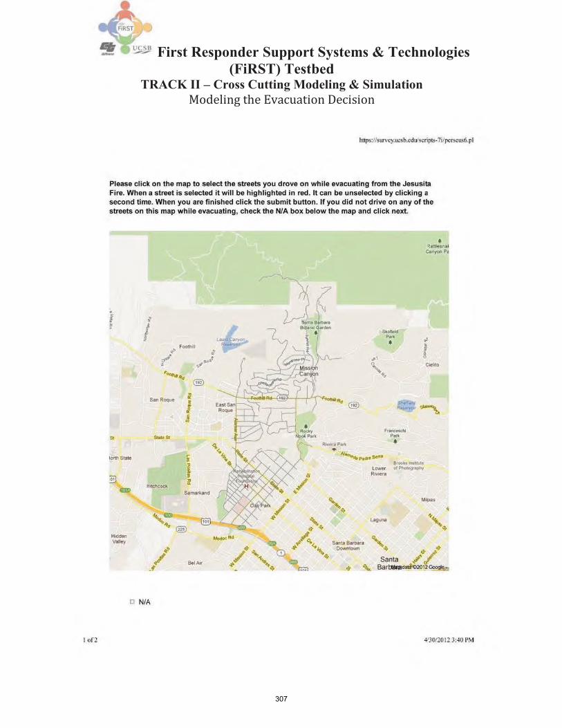
307
First Responder Support Systems & Technologies (FiRST) Testbed
TRACK II – Cross Cutting Modeling & Simulation Modeling the Evacuation Decision

308
First Responder Support Systems & Technologies (FiRST) Testbed
TRACK II – Cross Cutting Modeling & Simulation Modeling the Evacuation Decision

309
First Responder Support Systems & Technologies (FiRST) Testbed
TRACK II – Cross Cutting Modeling & Simulation Modeling the Evacuation Decision

310
First Responder Support Systems & Technologies (FiRST) Testbed
TRACK II – Cross Cutting Modeling & Simulation Modeling the Evacuation Decision

311
First Responder Support Systems & Technologies (FiRST) Testbed
TRACK II – Cross Cutting Modeling & Simulation Modeling the Evacuation Decision

312
First Responder Support Systems & Technologies (FiRST) Testbed
TRACK II – Cross Cutting Modeling & Simulation Modeling the Evacuation Decision

313
First Responder Support Systems & Technologies (FiRST) Testbed
TRACK II – Cross Cutting Modeling & Simulation Modeling the Evacuation Decision

314
First Responder Support Systems & Technologies (FiRST) Testbed
TRACK II – Cross Cutting Modeling & Simulation Modeling the Evacuation Decision

315
First Responder Support Systems & Technologies (FiRST) Testbed
TRACK II – Cross Cutting Modeling & Simulation Modeling the Evacuation Decision

316
First Responder Support Systems & Technologies (FiRST) Testbed
TRACK II – Cross Cutting Modeling & Simulation Modeling the Evacuation Decision

317
First Responder Support Systems & Technologies (FiRST) Testbed
TRACK II – Cross Cutting Modeling & Simulation Modeling the Evacuation Decision

318
First Responder Support Systems & Technologies (FiRST) Testbed
TRACK II – Cross Cutting Modeling & Simulation Modeling the Evacuation Decision

319
First Responder Support Systems & Technologies (FiRST) Testbed
TRACK II – Cross Cutting Modeling & Simulation Modeling the Evacuation Decision

320
First Responder Support Systems & Technologies (FiRST) Testbed
TRACK II – Cross Cutting Modeling & Simulation Modeling the Evacuation Decision

321
First Responder Support Systems & Technologies (FiRST) Testbed
TRACK II – Cross Cutting Modeling & Simulation Modeling the Evacuation Decision

322
First Responder Support Systems & Technologies (FiRST) Testbed
TRACK II – Cross Cutting Modeling & Simulation Modeling the Evacuation Decision

323
First Responder Support Systems & Technologies (FiRST) Testbed
TRACK II – Cross Cutting Modeling & Simulation Modeling the Evacuation Decision

324
First Responder Support Systems & Technologies (FiRST) Testbed
TRACK II – Cross Cutting Modeling & Simulation Modeling the Evacuation Decision

325
Planning for a disaster: A review of the literature with a focus
on transportation related issues
Micah L Brachman Richard L Church
Department of Geography 1832 Ellison Hall UC Santa Barbara
Santa Barbara, CA 93106 -4060

326
Planning for a disaster: a review of the literature with a focus on
transportation related issues
Micah L Brachman
Richard L Church
GeoTrans Laboratory Department of Geography
University of California, Santa Barbara Santa Barbara, CA 93106-4060
August 19, 2009

327
This report has been developed as a part of the First Responders System Testbed (FiRST) project at the University of California, Santa Barbara. The FiRST project investigates the integration of transportation and communication modeling and simulation to improve understanding and techniques of emergency preparedness and response. Please cite this report as: Brachman, ML and RL Church (2009) “Planning for disaster: a review of the literature with a focus on transportation related issues” (FiRST report), Geotrans Laboratory, UCSB, Santa Barbara CA

328
Report Outline
Preface
1. Introduction 2. Defining Terms 3. Evacuation 4. Disaster preparedness 5. Warning system location 6. Emergency shelter location 7. Emergency response 8. Prepositioning and storing emergency
resources 9. Infrastructure fragility 10. Findings 11. Conclusion 12. References
Acknowledgements
We wish to acknowledge helpful comments from Dr. Ramez Gerges and others in the Caltrans Department of Research and Innovation (DRI). We would like to acknowledge support from DRI (contract # 65A0257) under the direction of Mr. Larry Orcutt. Any and all statements made or implied in this report are those of the authors and should not be construed as opinions or policy of Caltrans.

329
Preface
The spectrum of possible emergency events ranges from natural events like floods, pandemics
and earthquakes to human activity-based disasters like terrorism, train accidents, and nuclear
power plant failures. Because disasters do not happen very often, most people become
complacent about risks, such as floods and earthquakes. But when one does happen, like
hurricane Katrina hitting New Orleans, it is easy to tell when a system response is inadequate.
The value of advanced planning and modeling can help to reduce the likelihood of inadequate
response to an emergency. It is the responsibility of public agencies to be prepared to deal with
such disasters.
Although this report for the most part does not focus on specific types of disasters it is important
to understand that there are major risks to the population of California across a wide spectrum of
specific types of events. Some events could be particularly disastrous. For example, a study
concluded that a terrorist strike on a chlorine tank car along a major railroad route in the
Washington, D.C. area could produce a toxic cloud 4 miles by 41 miles and kill and injure up to
100,000 people (Jay Boris, Naval Research Lab). The risk in a number of cities in California is
equally great. Even accidents involving bulk shipments of chlorine are dangerous. In 2005 a train
accident near Graniteville, S.C. involving a chlorine tank car killed 8 and hospitalized 240
people due to a toxic cloud. Although the probability of such an event has been lowered as some
cities have switched to using bleach and other more stable forms of chlorine or other methods of
disinfection for water and sewage treatment, this risk is a major issue in the United States.
Another example of risk is flooding in California’s Central Valley. The system of levees in the
Central Valley is considered old and inadequate. In a recent report to the California Department
of Water Resources (Independent Review Panel Report (2007)), it is stated that the “the outlook
for the future under business-as-usual is grim.” The reasons for this prognosis are based upon the
current state of the levee system, a better understanding of possible seismic events, the prospect
of large and more frequent storms based upon climate change, and the growth of communities
and infrastructure within the flood plain. The fact is that major roads and highways may be cut
off by floodwaters, reducing the capabilities of emergency response for large areas of the Central
Valley.

330
Even frequent and well planned for events such as wildfires can present transportation
challenges. The May 5, 2009 Jesusita Fire constituted a grave threat to the city of Santa Barbara,
necessitating the evacuation of nearly 30,000 residents. By most accounts, the threat posed by
this hazard was handled well: firefighting resources were allocated efficiently, citizen
evacuations went smoothly, and loss of property and life was minimized. Yet during the Jesusita
Fire, mandatory evacuation zone boundaries were drawn to specifically exclude nursing homes,
hospitals, and other facilities with large evacuation assistance needs. While people remained in
these facilities, most major arterial routes in Santa Barbara were extremely congested due to
evacuation traffic. Had the winds shifted and these facilities been threatened, could emergency
response personnel have moved in and successfully evacuated these vulnerable populations?
Federal agencies such as the Department of Homeland Security (DHS), the Federal Emergency
Management Agency (FEMA), and State agencies such as California’s Office of Emergency
Services have a primary goal to ensure safety, plan to respond in the event of a disaster as well as
promote plans and regulations that will decrease risk, increase safety, and reduce possible
damages. In a recent report (State of California: Emergency Plan (Draft, Nov. 2008)) all state
agencies, including Caltrans are assigned functions associated with responding to an emergency.
Agencies such as Caltrans must be prepared for their roles in disaster/incident response. To do
this requires a great deal of advanced planning and analysis, for the risks of not planning and
responding too late with too little are great and the benefits of making the appropriate response in
a timely manner are considerable.
The goal in planning for major emergencies is to plan for the extraordinary. It is important to
develop advanced plans whenever possible as well as support research into model development
and data collection that can support real time event tracking and mitigation. It is also important
to make the best use of limited resources by maximizing the benefits provided to an area
undergoing a disaster, whether that be in providing supplies, inspecting damaged infrastructure,
or guiding people in an evacuation. The best response to an emergency is based upon advanced
planning and research, frequent emergency drills, and maintaining appropriate levels of
resources that may be needed in an emergency. This report presents a review of the literature

331
associated with techniques that have been developed to support disaster planning, response,
management and mitigation as well as discuss how some of these techniques can be used
specifically for transportation analysis and planning.
Preface Notes: Data or material in preface references the following reports or papers
The data on chlorine based toxic cloud deaths was calculated by Dr. Jay Boris of the Naval Research Laboratory in Washington, D.C. He testified that a worst-case scenario for that city could result in up to a hundred thousand fatalities. An independent Homeland Security Council report on possible scenarios estimated that a ruptured chlorine gas tank car could kill as many as 17,500 people and injure an additional 10,000.
Independent Review Panel Report (2007) “A California Challenge – Flooding in the Central Valley,” Department of Water Resources, State of California, Oct 15, 2007.
State of California Emergency Plan, Office of Emergency Services, Nov. 20, 2008. (Draft)

332
1. Introduction
Mitigating the impacts of a disaster, like a wildfire, flood or earthquake, rests on doing a number
of things right. One can think of all of the elements in disaster planning and operations as links in
a chain, in which any link can prove to be crucial and compromise the other elements. To
mitigate the impacts of a potential disaster requires considerable forethought, training, and
resources. Recent events like 9-11, Hurricane Katrina, and the Oakland Hills fire have
demonstrated that many problems can arise requiring quick decisions, crucial information, and
plans that can be successfully implemented. In this report, our objective is to review the
scientific literature on emergency disaster preparedness, ranging from advanced planning and
resource allocation to real-time operations during a disaster. The major objective of this review is
to focus on specific tools and modeling approaches that an agency, such as Caltrans, should
consider developing or using in emergency management operations.
It is important to recognize that many governmental agencies, like the California Emergency
Management Agency (CalEMA), and private organizations like the American Red Cross already
play a significant role in disaster planning and mitigation. For example, in California each county
is required to set up contingency plans for a wide variety of possible disasters. It is also
fundamentally clear that in many circumstances, current systems respond with the necessary
capabilities in a timely fashion and gain high marks in subsequent public review. Further,
planning drills and mock emergencies also help to focus on critical issues of communication,
coordination, and training. Also, modeling tools are being developed which may make it easier
to make critical decisions in terms of which roads to close and how to best help an area evacuate.
Past success in dealing with emergencies should not make anyone complacent, as there is still
room for improvement in both planning and operations response. For example, there still exist
problems of communication between agencies based upon equipment protocols, and the
capability to transmit timely event data often doesn’t exist. To highlight this issue, one only
needs to look at a recent article in the Santa Barbara Sound that focused on the lack of timely
information available to the public associated with the July, 2008 Gap wildfire. Fire maps that
were posted on public kiosks were often several days out of date. Traffic information about road

333
closures was often misleading, leading to more congestion than necessary. Perhaps the most
egregious issue raised in the article is that the City of Santa Barbara cable TV channel posted
road closure and other fire information about the 2007 Zaca Fire but not the Gap fire of 2008
while the Gap fire was in progress! As a further example of the possible lack of preparation on
the part of emergency services in California, it was found in a recent audit by the City of Los
Angeles Controller that the city lacks an overall strategic plan to respond to an emergency such
as “an earthquake, fire or other calamity” (LA Times; July 15, 2008). The internal audit
identified that 16 of the city’s emergency preparedness plans have not been updated for at least
three years, and that one of the fire department plans had not been updated since 1992.
Preparedness should begin with a list of needs to be addressed in the event of an emergency. For
each need, specific methods should be outlined in terms of how this need is to be met during the
emergency. Do resources exist to meet the emergency demand and how much time will it take in
order to respond? What techniques will be available to monitor the event and determine exactly
where such resources should be allocated? When the demand for a resource outstrips supply, is
there an approved priority defined approach to allocate this scarce resource optimally? Managers
of state and county agencies need to ensure that their departments have developed contingency
plans so that after an emergency has happened, the agencies are noted for their effective
response.
Key factors in any emergency include understanding which infrastructure elements are still
functional to support emergency response and possible evacuation, the ability to communicate to
those involved as to the actions they need to take, the capability to collect and share real time
data about the event among agencies, the capability to respond with support teams and resources,
and the restoration of immobilized services as quickly as possible. For a transportation agency or
public works department, this entails having enough personnel trained and available to inspect
infrastructure, support special communication and transportation needs, and develop and
implement an evacuation or emergency response plan.
The major focus of this report is on modeling techniques than can aid in emergency management
operations. When there exist a multitude of issues and competing needs for resources, models

334
can be a significant aid to decision makers before, during, and after an emergency. The basic
premise is that many problems are difficult to address without good models and appropriate data.
Using such tools and data may help smooth operations and avert tragedy.
This report has been developed as a part of the First Responders System Testbed (FiRST) project
at the University of California, Santa Barbara. The FiRST project investigates the integration of
transportation and communication modeling and simulation to improve understanding of
emergency preparedness and response. The report is organized as follows: We begin by defining
key terminology commonly used in the academic literature on emergency management. The next
section is a detailed examination of emergency evacuation modeling at multiple scales, with
special focus on contraflow lane reversal. Disaster preparedness in California is then examined
via analysis of state and county emergency plans, followed by several model formulations that
may help planners locate emergency warning systems and shelters optimally. Next we cover
emergency response, with a specific focus on models that help allocate personnel and resources
where they are needed most. One technique that can greatly aid emergency responders is the pre-
positioning of resources in preparation for a disaster, thus we cover this topic in detail as well.
We examine the issue of infrastructure fragility, and then conclude with a series of
recommendations.
2. Defining terms
This section is devoted to defining the terminology that is used within the field of disaster
management. Throughout this section we use issues associated with Hurricane Katrina to
underscore specific points. We begin with the term disaster. In the most general sense, a
disaster occurs when a natural or human-caused event exceeds the capabilities of our respond to
it, resulting in an adverse outcome. One of the better definitions of disaster found in the
academic literature is “an event, concentrated in time and space, in which a community
experiences severe danger and disruption of its essential functions, accompanied by widespread
human, material or environmental losses, which often exceed the ability of the community to
cope without external assistance (Smith 2004).” It is further possible to subdivide disasters into
natural and human, with the former referring to a physical earth process beyond human control

335
and the later referring to an event caused directly by human actions. This distinction is not
absolute, as exemplified by the extensive flooding of New Orleans by Hurricane Katrina that
resulted from a natural storm surge overtopping man-made levees.
Underlying any disaster is a hazard, which is any natural or technological threat to people or
things they value (Cutter 2001). In the case of Katrina, the major hazard was the hurricane itself
with storm surge, high winds, and inadequate levee systems as sub-hazards. Risk is nearly
universally defined as the product of the probability of a hazard occurring and the vulnerability
of the people affected by this hazard (Mitigating natural disasters: phenomena, effects and
options. A manual for policy and planner, 1991). For example, the people of New Orleans faced
a high risk of being adversely affected by Katrina due to the increasing probabilities that it would
hit the city (Hurricane Katrina Probabilities Report Number 15 & Hurricane Katrina Probabilities
Report Number 21, National Hurricane Center) and the dual vulnerabilities of living in a
floodplain and not having the means or desire to evacuate to higher ground.
Vulnerability is defined as the potential for loss, with physical vulnerability
encompassing the interactions between nature and society and social vulnerability composed
of the demographic and economic characteristics of different population groups. Put simply,
physical vulnerability is the likelihood of exposure to a given hazard while social vulnerability is
the likelihood of adverse outcomes (Cutter 1996). These two types of vulnerability are not
mutually exclusive and depend heavily on the underlying geography of a place. For example, the
physical geography of the New Orleans city site lies at the root of vulnerability, which is a city
occupying a very low area that relies on a levee system and pumps for protection.
There are several important geographic parameters for any hazard that help determine physical
vulnerability. These can also be thought of as “environmental parameters for human response”
(Burton, Kates et al. 1993), as they also largely determine how people may respond when faced
with a hazard and thus are a component of social vulnerability as well. Magnitude can be
generalized as a measurement of the energy released by a given hazard. For example, Katrina
had sustained winds of 110 knots when it first made landfall on the gulf coast, thus was classified

336
as a Category 3 hurricane according to the Saffir-Simpson Hurricane Scale (Knabb 2006). Other
familiar measures of magnitude include the Richter scale for earthquakes, the Fujita scale for
tornados, and could include the surge height of a tsunami or speed of movement of a wildfire
front. Frequency is how often an event of this magnitude occurs. Katrina was a Category 5
storm shortly before landfall, and the frequency of the formation of a Category 5 hurricane
forming in the Atlantic basin is on average once every three years (Atlantic Tracks File, 1851-
2007, National Hurricane Center). Over 80 tsunamis have hit the California coast since 1850,
thus the frequency of such an event is approximately once every 2 years (The Tsunami Threat to
California, CA Seismic Safety Commission). Duration is how long the event persists. As an
example, Katrina produced hurricane force winds in New Orleans for less than 24 hours, but the
subsequent floodwaters inundated the city for weeks afterward. The Gap Fire in the Santa Ynez
Mountains near Santa Barbara began on July 1, 2008 and was declared fully contained on July
28th (InciWeb, Gap Wildland Fire). Areal extent is space covered by event, which ranges from
relatively small such as the 9,443 acres burned by the Gap Fire to very large in the case of
Katrina, with hurricane force winds at one point extending 90 nautical miles from the storm’s
center. (Knabb 2006) Speed of onset is length of time between initial event appearance and
its peak. Katrina was classified as a tropical storm five days before reached its peak category 5
strength, thus giving this event a much slower speed of onset than a tsunami (a few hours at
most) or an earthquake (instantaneous). Spatial dispersion is the pattern of distribution over
the space in which the event can occur. Hurricane wind speed and earthquake intensity decrease
with distance from the event center, while a wildfire front may jump large areas or change
direction in an unpredictable fashion. Temporal spacing is the sequence of events. A simple
timeline for the events in New Orleans surrounding Katrina could be storm surge, levee
breaches, flooding, while a timeline for an earthquake could be ground shaking, building
collapse, structure fire, aftershock. Time periods are also an important component of temporal
spacing, particularly when planning evacuations or search and rescue operations.
Understanding the unique history of social vulnerability in New Orleans is essential to
forming a complete picture of the Katrina disaster. Land value in the city is greatest on the
highest ground, not surprising given the geographic advantage of being the last to flood and the

337
first to dry out. African-Americans have always inhabited the lowest laying land, with Jim Crow
laws and redlining practices perpetuating slavery’s legacy of racial segregation (Colten 2002).
When floods strike, the poorest citizens suffer most, perpetuating the cycle of poverty and
vulnerability. The geographic variation in social vulnerability requires different mitigation,
response, and recovery actions – the one-size-fits-all approach is ineffective (Cutter, Emrich et
al. 2006). Living in the most flood prone areas is only one component of the social vulnerability
of New Orleans’ marginalized populations. With poverty comes limited access to resources,
with the inability to secure private transportation playing a significant role in the Katrina tragedy.
Mistrust of authority grows out of inequality, leading to a significant communication gaps
between government and impoverished citizens. One method that allows emergency
management officials to focus disaster mitigation efforts is to identify ‘hotspots’ of vulnerability.
For example, Rashed and Weeks (2003) use a Geographic Information System (GIS) to identify
census tracts in Los Angeles County that are vulnerable under historic earthquake scenarios. In
each scenario, vulnerability is calculated as a function of both the physical geography and
socioeconomic population characteristics of affected places. This spatial multicriteria analysis is
combined with fuzzy logic to produce a methodology that takes into account the inherent
uncertainty in measuring vulnerability, providing a more robust analysis of susceptibility to
earthquakes in Los Angeles.
The four stages of emergency management commonly used in the United States are
mitigation, preparedness, response, and recovery (Waugh and Hy 1990). Mitigation actions
reduce the long-term risk of vulnerable populations, including but not limited to zoning
decisions, building and safety codes, insurance, and hazard mapping. In assessing the extensive
building damage caused by Katrina, the FEMA Mitigation Assessment Team concluded that the
lack of a building code not only contributed to residential damage but also to essential facilities
including hurricane evacuation shelters, police and fire stations, hospitals, and Emergency
Operations Centers (FEMA 2006). Inhabitants of areas along the wildland/urban interface are
generally advised to create defensible space on their property to prevent a wildfire from
spreading from natural fuels to man-made structures. Preparedness activities build
operational capability for disaster response and include emergency operations planning,
personnel training, and emergency warning systems and communication networks. One of the

338
few positive outcomes of Hurricane Katrina was the successful development and execution of a
contraflow evacuation plan which involved switching the direction of travel of one the I-10
freeway segments to accommodate heavy traffic flow in one direction. This procedure is
examined in detail in a later section of this report, but it is important to note that during the
Katrina evacuation nearly all persons with access to private transportation were able to escape
the city well before hurricane landfall and in less time than anticipated by planners (Wolshon,
Catarella-Michel et al. 2006). Prepositioning of emergency supplies and locating emergency
warning systems are two preparedness activities of particular relevance in California, both of
which are further discussed in greater detail. Actions taken in the immediate time periods
before, during, or after a disaster fall under response, encompassing warnings, evacuations,
sheltering, and search and rescue. Preparedness largely determines response capabilities, which
were severely limited during Katrina by the inadequate allocation of vehicles and emergency
shelters. New Orleans city buses picked up residents and transported them to the Superdome,
which was only stocked with enough provisions to feed 15,000 people for 3 days. 30,000
evacuees crowded into the Superdome, which lost electrical power and was completely
surrounded by water. 500 school buses that could have been utilized to evacuate vulnerable
residents were flooded and immobilized, and the national guard barracks and the high water
rescue vehicles they contained were flooded as well, forcing guardsmen to concentrate on saving
themselves (Smith 2005). A mutual aid agreement allows emergency responders in California to
solicit assistance from other agencies, whose help is often critical to appropriate response to
large hazards (Akella 2008). Recovery activities are focused on restoring vital systems that
expedite the return to normal life, such as setting up temporary housing, clearing debris, and
rebuilding or repairing damaged infrastructure. The Army Corps of Engineers unit based in New
Orleans was concerned about the levees, yet had no external monitoring equipment for them and
had to rely on media reports to find out if they were functioning. Since roads and canals were
inaccessible, the Army Corps had to rely on helicopters for the levee repairs necessary to hold
the water at bay. It took over a month for the combination of levee repair and pumping to finally
dry out the city (Penry-Davey and Chinn 2005). A study of recovery from the 1994 Northridge
earthquake found that socially vulnerable populations such as the poor, elderly, and ethnic
minorities often rely heavily on non-governmental organizations (NGOs) to met disaster relief

339
needs (Bolin 1998). The four stages of emergency response are distinct but clearly interrelated,
as the following conceptual model from Lindell and Perry (2004) shows.
The final key term that we will define in this section is interoperability. Soon after Katrina
made landfall, electricity, land lines, cellular networks, and local media outlets failed, leaving
emergency officials completely unaware of the extent of damage and the massive flooding that
had begun in the city’s ninth ward. This massive infrastructure failure contributed to the inability
of public safety responders to communicate, but the use of different communication technologies
operating on separate frequencies by the multitude of agencies responsible for emergency
response looms much larger. Communications interoperability allows personnel from various
emergency management agencies to talk seamlessly over one radio and data system across a
wide geographic area such as a metropolitan region or state. While achieving interoperability
has been a long-standing goal of law enforcement, fire and rescue agencies, funding, governance,
and cooperation remain major obstacles to implementation (Mountjoy 2005).
340
3. Evacuation
Modeling the complex spatial interactions between people and their environment that occur
during an evacuation is an important step in developing a successful emergency plan. Despite
recent advances in technological capabilities and modeling techniques, coordinating the
movement of large numbers of frightened people through a confined space in a short amount of
time presents a daunting challenge for researchers. This problem is inherently geographic in
nature: spatial and temporal scales are what define the complexity of the evacuation process and
dictate the appropriate modeling technique. Spatial scale is important in accounting for the
location and characteristics of populations that must evacuate, the layout of the transportation
network, and the area affected by a hazard when formulating an evacuation plan. Temporal scale
is crucial as well, as event speed of onset largely dictates the start and end times of an
evacuation. This scale-based approach has its roots in two classic problems, a large-scale
evacuation due to a nuclear power plant accident and the small-scale evacuation of a building.
Building evacuation is of great importance even in transportation as techniques developed first
for building evacuation now form the basis for most evacuation models in transportation.
Disastrous fires such as the 1977 Beverly Hills Supper Club (Southgate, Kentucky), which killed
165 people forced building engineers and fire departments to determine appropriate safe routes
from buildings, establish maximum occupancy standards for rooms and change materials to
retard the spread of fire. Although the scale of a building is different from a neighborhood or
town many of the same issues underlying safe evacuation are present.
Before discussing the nuclear accident and building evacuation problems, it is important to
define what is meant by a model. In the simplest construct, a model is a simplified version of a
real world process, system, phenomenon, or entity. For our purposes this model must include
one or more mathematical equations, thus allowing for a solution through enumeration, an
algorithm or a heuristic technique. Often models are solved many times with varying input
parameters, thus producing a host of solutions to give researchers a better idea of how certain
inputs can affect model results. Introducing an element of randomness in a model can produce a

341
stochastic simulation, which accounts for uncertainty within the underlying process. When
geography is explicitly accounted for in such a model it generally will fall into the classification
of spatial optimization or spatial statistics.
Back to the question at hand: how best to model evacuations due to a nuclear power plant
accident or building fire? Since these problems are fundamentally different in scale, the best
approaches for modeling them are different as well. To get the most accurate representation of
how people may behave when leaving a building, each person should be individually represented
in the model. This technique is known as agent-based modeling or microsimulation, and is best
suited to problems of limited size due to the computational complexity of representing individual
people and their interactions. Microsimulation can also refer to the modeling of individual
vehicles on a transportation network, but the essential small-scale characteristic of such an
approach remains. At the other end of the spectrum is the large-scale evacuation required in the
event of an accident at a nuclear power plant. Here the goal is to move thousands of people
away from the accident site as quickly as possible, thus the inherent size of the problem makes
microsimulation less feasible. Macro-scale models group population into larger units, which can
then be moved through the transportation network under different starting conditions producing a
generalized evacuation plan. The benefit of such an approach is that it can simplify the complex
interactions of large groups and thus be solved quickly, which is essential to real-time modeling
for decision support. One downside is that the further away one moves from the reality of
individuals as independent actors, the greater the likelihood of individuals or groups of people
being unaccounted for in the model. Between these two approaches is the meso-scale model,
which is neither microscopic nor macroscopic but rather borrows elements from each. A meso-
scale model will not represent people individually but may aggregate them into relatively small
population units, unlike the macro-scale model, which seeks the largest feasible unit. The spatial
extent of meso-modeling can be at the neighborhood or community level, or the entire area
affected, e.g. hazardous material cloud or a plume of radioactive material.
Choosing the appropriate modeling scale to use is an important question that extends beyond the
narrow scope of evacuations. One way to aid in making the choice of scale is to group potential
hazard responses into a typology of disaster management decisions (Wallace 1985). Using this

342
framework, a micro-scale model is considered best suited to an operational decision such as a
neighborhood evacuation occurring at a small spatial and temporal scale. A strategic disaster
management decision is made at a large temporal and spatial scale, thus a disaster preparedness
tactic such as resource pre-positioning is best modeled at the macro-scale. Tactical operations
incorporate both operational and strategic decision making processes, while meso-scale models
are often used for location-routing problems at a medium temporal scale such as providing EMS
coverage. Now that these different modeling scales have been defined, we will examine how
researchers have used them to model evacuations in response to hazards.
Quantitative modeling is an important compliment to the various qualitative studies of
emergency evacuation. The partial meltdown at the Three-Mile Island Nuclear facility in 1979
spurred survey-based research on the geography of evacuee behavior, examining route
preferences and travel distance (Zeigler, Brunn et al. 1981) and the spatial distribution of social
vulnerability (Cutter and Barnes 1982). Many evacuation modeling approaches are based on the
groundbreaking research of Dial (1971), who developed a method to account for the fact that
drivers will often choose routes that are not the shortest distance to their destinations. This
approach better reflects the dynamic and unpredictable flow of traffic during an evacuation.
Other researchers have built on this framework and introduced an element of random route
assignment that represents driver behavioral decisions under conditions of distance and network
topology uncertainty (Daganzo and Sheffi 1977). Estimation of network clearance time emerges
as the central focus of evacuation modeling, thus most of the current research has its roots in a
modeling approach that can calculate clearance times given variability in network characteristics,
intersection control and design, and evacuation strategies. One of the first examples of this is
NETVACI, which uses the mathematical relationships between flow, speed, density, queuing,
and other traffic measures to estimate clearance time on a node/arc network representation
(Sheffi et al. 1982). Applications of this model to simulate evacuations around several nuclear
facilities demonstrated that it could efficiently handle relatively large networks, an important
consideration even with the development of faster and more capable computers.
An early example of a decision support system designed to craft an evacuation plan is the
Transportation Evacuation Decision Support System (TEDSS), which allows planners to

343
estimate network clearance times for various evacuation scenarios for nuclear power plants
(Hobeika, et al. 1994). Another important component of an evacuation plan is where to house
evacuees. Yamada (1996) solved two network transportation problems, a shortest path problem
and minimum cost network flow problem, with the goal of allocating residents to places of
refuge during a simulated evacuation in Yokosuka City, Japan. Results show that the classical
shortest path (Dijkstra 1959) solution results in a more uniform evacuation plan and shortest
average distance, while the minimum cost solution will split evacuee flows forcing some
residents to go to a place of refuge that is not their closest. One interesting theoretical outcome
of this research occurs when evacuees are instructed to go to a location further away than the
nearest shelter: the greater the disparity between shortest path and maximum network flow
solutions, the greater the potential problem of non-compliance by evacuated populations,
resulting in an event which will take longer to clear and where a few shelters are likely to be
overwhelmed.
Many early models of building evacuation use a network flow formulation similar to those
discussed above. Chalmet and Francis (1982) present some of the first research to address
problems such as bottlenecks that may occur during the emergency evacuation of buildings.
They present a simple model that can efficiently allocate evacuees to exits, thus helping prevent
bottlenecks from occurring. For a given building, let:
k total number of people to be evacuated n total number of exit routes j index of exit routes x j people using exit route j t j (x j ) time for x j people to clear exit route j
We can then allocate people to exit routes to minimize the time that it takes the last person to get
out of the building using the following formulation:

344
Minimize Z max t j x j : j 1,...,n
subject to :
1) Λ x j k j
2) x1,..., xn 0
This model seeks to minimize the maximum amount of time it takes a given group of people to
evacuate using a given exit, while ensuring that the entire building is evacuated. The two major
assumptions of this model are that each evacuee has access to every exit route, and that the time
to clear an exit route relies only on the number of people using it. Comparison of the estimated
clearing time of an eleven story building generated by a related but more complex model to
empirical measurement of an actual evacuation showed that the model was overly optimistic,
largely due to the inability to account for queuing and inefficient evacuee movement through
stairwells. This model weakness is due to a linear equation structure that assumes all flows
along arcs between origin and destination nodes are constant. This is the very feature that is
faced when evacuating an area, where the speed of traffic decreases as the density or number of
vehicles per lane mile increase.
A way to account for this weakness is to introduce nonlinear side constraints to the model which
allow dynamic evacuee movement to be accounted for (Choi et al. 1988). Models of this type
can often be solved expeditiously for small scale building evacuations, but otherwise offer little
advantage when compared with agent-based microsimulation. EXIT89 is an early example of a
high-rise building microsimulation model which allows stochastic variation in individual
evacuee behavior, queuing, and evacuation speed to be represented, thus producing a result more
closely in line with actual emergency conditions (Fahy 1995). The ability to model individuals
can be incorporated into a Geographic Information System (GIS) to create valuable tools for
emergency planners.
Most evacuation based decision support systems are base upon a model integrated with a
Geographical Information System (GIS). These computer programs use the topology and feature
attribute capabilities of GIS in conjunction with location decisions and simulation runs produced

345
by models to assist in the decision processes of emergency planners. One of the first systems
designed specifically for emergency evacuations is CEMPS, the Configurable Emergency
Management and Planning System (Pidd et al. 1996 and de Silva and Eglese 2000). In this
system, the GIS is used first to map the terrain and identify the population to be evacuated.
These data are stored in a database, which is accessed by a discrete microsimulation model that
is used to assess various routing schemes for moving the evacuated population to designated safe
areas. The major limitations of most of this earlier work are due to the inability of the
microsimulation model to account for dynamic route selection due to congestion, traffic effects
such as ‘scrunching’, and the behavior of emergency vehicles. Many of these issues have been
addressed by subsequent microsimulation research, greatly improving realistic representation of
traffic conditions during evacuations.
One novel approach of representing traffic dynamics is to adopt methods commonly used in
physics (Helbing 2001). Using models analogous to micro-scale (particle-base), meso-scale (gas-
kenetic), and macro-scale (fluid-dynamic) approaches, physicists have concluded that it is
possible to simulate complex traffic interactions and develop natural laws that explain driver
behaviors under a multitude of traffic conditions. Of particular interest is a model that
incorporates both macro-scale and micro-scale approaches that is well suited to the traffic jams
and bottlenecks that may occur during an evacuation.
Rapid housing development and population growth in fire prone areas is of particular concern to
California evacuation planners. Most evacuations at the wildand-urban interface occur at the
neighborhood level, thus are well scaled to commercial microsimulation software. (Cova and
Johnson 2002) developed a modeling approach that incorporates a custom evacuation scenario
generator, GIS, and an off-the-shelf microsimulation package to estimate the time it would take
each household to evacuate under a multitude of conditions. Using individual household
evacuation times allows planners to assess the spatial variability of vulnerability to a hazard and
provides a much greater level of detail compared to traditional evacuation measures such as
network clearing time. This enables plans that are tailored to the specific needs of a community
and thus have a greater probability of successful execution.

346
Timing of evacuations is another important problem that must be addressed by emergency
managers, especially when a large population must be relocated on short notice. Inefficient
scheduling can lead to traffic gridlock, impeding the evacuation procedure and increasing
evacuee risk of being affected by a hazard. Issues of temporal scale were examined in a
microsimulation of a large-scale evacuation of San Marcos, Texas, where researchers found that
staged evacuations are more efficient than an all-at-once evacuation for densely populated areas
with a grid street network (Chen and Zhan 2006). Recent research in modeling of the process of
passenger loading and unloading of planes identified that the fastest method of loading and
unloading occurred when people are staged, but also separated (e.g. every third row). Thus, it
may be possible to show in simulation that staging with separation may aid in evacuation as well.
Many evacuation modeling approaches rely on the delimitation of an emergency planning zone
(EPZ). Cova and Church (1997) point out that defining an EPZ in advance is problematic for fast
moving hazards where the population that will need to evacuate is unknown in advance.
Because of this they developed a critical cluster model (CCM) to identify neighborhoods that
may face transportation difficulties if forced to evacuate. As previously noted, most evacuation
modeling addresses either macro-scale events like a hurricane or micro-scale events such as a
building fire. The Cova and Church model is among the first to address neighborhood, or meso-
scale, evacuation vulnerabilities. The first step in finding a vulnerable neighborhood, or critical
cluster, is develop a network representing flow capacities along with attaching estimates of the
population needing to evacuate at each node of the network. The next step is to apply the CCM
to find clusters of contiguous nodes that have the highest average population per exit lane. This
problem is closely related to the graph partitioning problem, and can be defined using the
following notation:

347
ΛΛ
N set of all nodes N1 contiguous partition of nodes containing i * N2 nodes connected to N1
i index of nodes j index of nodes connected to i ai weight of node i (population) cij cost of arc ij (lanes) s maximum size (in nodes) of N1
i* index of root node Ε N1
Ι1, if node i is in Nx 1
i λ0, otherwise Ι1, if node i is in N N
y 1 and node j is in
2
ij λ0, otherwise
Using this notation, we can formulate the model as:
Λai xi
Maximize Z = i cij yij
i j
subject to : 1) xi − x j yij ′ϖi, j and ′ϖj,i Ε N
2) Λ xi s i
3) xi* 1 4) xi, yij Ε {0,1} ′ϖi, j Ε N
This model maximizes the total population relative to the capacity of the exit lanes, defined as
those links connecting selected cluster nodes and nodes directly outside the cluster. The CC
model was applied to data of the Santa Barbara area and each node was assigned an evacuation
vulnerability value (associated with the worst case cluster in which that node was a member)
resulting in an evacuation vulnerability map of Santa Barbara. The results of this application

348
clearly showed that evacuation difficulty varied from area to area. Transportation planners
already recognized some of the more vulnerable areas, but other areas that were identified were a
surprise to many.
Church and Sexton (2002) use a different methodology to research evacuation vulnerability at
the micro-scale. The Mission Canyon neighborhood in Santa Barbara was previously identified
as a critical cluster due to a sizeable population base reliant on a limited number of routes for
evacuation. This neighborhood also lies in the urban-wildland interface and is especially
vulnerable to wildfires propelled by sundowner winds moving down canyon with great speed.
Previous work had estimated evacuation time for such areas by comparing the total vehicle
demand to the number of lanes leaving the neighborhood. This research tests the assumptions of
this macro-scale approach by modeling different evacuation scenarios using micro-scale traffic
simulation. Running multiple simulations allowing the number of vehicles, number of exit
routes, road capacity, and level of traffic control to vary, Church and Sexton found that major
evacuation problems might occur without a significant coordinated traffic control effort and
extensive resident education. Several interesting problems arise from this microsimulation,
including the inability of the software to model vehicles that back out of driveways. During
times of high fire risk, emergency officials recommend that people back into the driveway (so
they are facing the street) to speed up evacuations, but this recommendation is rarely followed.
Another interesting problem is that drivers are given dynamic feedback during the
microsimulation, thus mimicking the effect of a special radio channel broadcasting real time
information on crowding along specific evacuation routes. This assumption speeds up the
simulated evacuations, but may not reflect the actions of drivers (turning on the radio) or local
broadcast or information gathering capabilities. Overall, they find that while macro-scale
evaluation provides similar evacuation time estimates as microsimulation, neither approach can
fully account for driver behavior or the behavior of what might happen during an accident or
blocked exit (e.g. people abandoning their vehicles on the street causing a relatively permanent
roadblock).

349
One assumption that is frequently made in evacuation modeling is that drivers will behave
rationally. Among these assumed behaviors are that evacuees will understand the instructions
given them by officials coordinating the evacuation, follow these instructions exactly and obey
all posted speed limits and traffic laws. While it is often necessary to make assumptions in order
to limit the size and complexity of models, the fear and panic that often occurs when people are
threatened should not be overlooked as it may severely affect their decision making. Pel and
Bliemer (2008) help account for this uncertainty by introducing a model that explicitly
incorporates driver behavior when assessing both voluntary and mandatory evacuation plans.
Their three-stage model includes travel demand, travel choice, and network loading components,
with the travel choice module capable of modeling the behavioral responses of the evacuees
towards evacuation instructions such that they can be followed fully, followed in part, or rejected
completely. Models such as these represent an important advance for researchers who seek to
produce the most accurate representation of an evacuation situation possible.
Another problem faced by emergency managers is compliance with a mandatory evacuation
order. Dow and Cutter (2002) report that only 65% of South Carolinians ordered to evacuate in
response to Hurricane Floyd actually did so, thus greatly compounding the problem of keeping
people safe from the storm. A related problem is ‘shadow evacuation’, which occurs when
people decide to evacuate despite not receiving any official instructions to do so. This may
contribute to traffic delays and emergency resource shortages, impeding the safety of those who
are directly threatened by the hazard. Research based in Long Island, NY concluded that
evacuation planning areas should be expanded in response to the high likelihood of shadow
evacuation in the event of a nuclear accident (Johnson 1985). While this approach may help
traffic planners design better evacuation models, it does not address the underlying causes of a
shadow evacuation. Environmental cues, such as high winds and smoke during a wildfire, can
prompt people to evacuate even if they are not directly threatened. A more troubling cause of
shadow evacuations is mistrust of information or the authorities who provide it (Lindell and
Perry 2004), a problem that may be addressed by providing the most accurate hazard information
as quickly as possible to people in an effected area. Although shadow evacuations have been
modeled using microsimulation (Cova 2008), further research on this problem through
mathematical modeling techniques may be of great benefit to evacuation planners.

350
The successful evacuation of New Orleans prior to the arrival of Katrina was made possible
through the use of contraflow. Contraflow involves reversing the direction of traffic for a set of
lanes along a route, so the capacity of a route to handle traffic in a desired direction is enhanced.
The success of using contraflow is highlighted in the following statement by Kathleen Blanco
(Former Governor of Louisiana):
“Before Katrina came, I developed a new evacuation plan that includes contra-
flow, where both sides of the interstates are used for outbound traffic. I am proud
that we rapidly moved over 1.2 million people - some 92% of the population - to
safety without gridlock or undue delay prior to Katrina.”
Contraflow lane reversal is a valuable option in emergency evacuations by increasing the
outbound traffic capacity of a given road or freeway. The first large scale implementation of
contraflow occurred in Georgia and South Carolina for Hurricane Floyd evacuations in 1999, and
a majority of hurricane threatened states have now adopted contraflow plans (Urbina and
Wolshon 2003). As the quote above illustrates, contraflow can be very effective in efficiently
moving a substantial proportion of the population in areas threatened by large-scale disasters.
Yet the tragic aftermath of Hurricane Katrina shows that it is not a ‘magic bullet’ solution for
evacuation planning, especially in places like New Orleans with large populations without access
to private transportation. While the vast majority of contraflow evacuation plans are hurricane-
specific, many characteristics could be generalized and implemented for other large-scale
disasters.
The state of Florida revised its contraflow evacuation plan in response to the busy 2004
hurricane season. With 4 major hurricanes prompting the evacuation of nearly 10 million
people, the Florida Division of Emergency Management and the Florida Department of
Transportation determined that an improved contraflow plan was necessary given the probability
of its implementation for future hurricane evacuations. Some essential components of the
updated plan are daylight only contraflow implementation, pre-positioning of traffic coordination

351
and emergency response vehicles along the contraflow route, and clear delineations of agency
roles and means of communication. Specific routing recommendations include assigning the
same number of lanes for contraflow exit points as the contraflow route itself has and keeping
highway shoulders open for disabled vehicles and emergency responder use. (Contraflow Plan
for the Florida Intrastate Highway System, 2005)
Empirical assessment of contraflow evacuation plans utilized during hurricane events shows
substantial improvements in vehicle capacity yet also clearly illustrates drawbacks. During the
2000 Hurricane Floyd evacuation, the South Carolina Department of Transportation (SCDOT)
measured a 67% increase in the number of vehicles evacuated per hour with four outbound
freeway traffic lanes when compared to the standard two inbound, two outbound configuration.
Safety, accessibility and cost emerge as the most pressing problems during a contraflow
operation. Freeways are generally not designed to handle opposing flow, thus confusing signage,
inadequate collision barriers and limited exit ramp accessibility can lead to accidents and
breakdowns that may further traffic delays. Contraflow plans can reduce or eliminate inbound
traffic, limiting the ability of emergency service personnel to assist those left behind. Manpower
requirements can be substantial, with more than 70 personnel needed for an 18 interchange
contraflow plan in North Carolina (Wolshon 2001). These empirical results provide a basis for
modeling and simulation-based research, which can address the challenges of contraflow
evacuations in a controlled setting.
Microsimulation of contraflow for hurricane evacuation of New Orleans showed how suboptimal
entry point design and location could limit the number of evacuees able to leave the city
(Theodoulou and Wolshon 2004). A North Carolina coastal evacuation simulation showed
extensive queue formation at contraflow termination points, highlighting the need for further
research on optimal access points and interchange functionality (Williams, et al. 2007) Another
challenge in modeling contraflow is the increased size of network flow problems that must
account for each individual lane rather than representing roads as a single arc. Tuydes and
Ziliaskopoulos (2006) use a tabu search heuristic to address the computational complexity of
modeling a contraflow evacuation on a large urban network. Although most research has been
directed towards hurricane evacuation, contraflow can be incorporated into traffic management
352
models for other large-scale disasters. Research comparing different evacuation strategies for
downtown Minneapolis, Minnesota also shows that access to a contraflow corridor is a critical
determinant of overall effectiveness. By increasing capacity of key entrance ramps, evacuation
time was substantially reduced for an evacuation simulation that included more than 50,000
spectators at a major sports venue. (Kwon and Pitt 2005)
Lane-based traffic routing can improve traffic flow during an evacuation by eliminating
congestion at critical intersections. When Los Alamos, New Mexico was evacuated in response
to the 2000 Cerro Grande wildfire, a lane-based routing plan helped 11,000 residents escape this
isolated mountain community using the one available exit in under 4 hours (Mynard, et al. 2003)
The essence of a lane-based plan is that it restricts lane changes and directs traffic to make turns
at intersections in order to avoid cross traffic. Cova and Johnson (2003) use a lane-based
routing model to simulate traffic during an evacuation of downtown Salt Lake City, generating a
40% improvement in network clearing time when compared to no routing plan.
A new and promising approach to contraflow modeling is taken by (Meng, Ling et al. 2008).
The optimal contraflow lane configuration problem (OCLCP) and the optimal contraflow lane-
scheduling problem (OCLSP) are addressed by combining the linear programming and
microsimulation methods. First, the linear program is used to determine a feasible lane-reversal
plan that minimizes total travel time in the central business district of Singapore. This plan
becomes an input to a microsimulation model developed with PARAMICS software that mimics
the response of drivers to these lane reversals. This methodology allows researchers to
systematically evaluate each contraflow plan by providing instant data on traffic flow rates and
queuing via the microsimulation software.
Although contraflow under emergency evacuation conditions is not implemented as part of their
routing plan, it could be incorporated under a similar modeling framework. This unification of
traffic routing methods has the potential to further improve network clearing times for mass
evacuations, especially if used to address the access point and queuing problems of contraflow
operations. There remains a central question that has not been answered by any of the above

353
models: What evacuation routes will drivers actually choose? Route choice behavior is largely
based on the assumptions of rational driver behavior under perfect information, both of which
are questionable in emergency evacuation situations given a large-scale disaster. Chiu and
Mirchandani (2008) propose a dynamic feedback information routing system, in which
evacuation routes are updated according to the current traffic conditions. Such a system could be
implemented using existing traffic monitoring and mass communication technologies, and can
significantly improve evacuation effectiveness through real-time management.
Spatial and temporal scales are crucial geographic factors in determining the evacuation
modeling approach best suited to a given hazard. Individual (micro), aggregate (macro), and
intermediate (meso) spatial scale models all have specific strengths and weaknesses which
should be carefully considered based on both the capabilities of researchers and the needs of
agencies. Timing is critical: a contraflow evacuation plan requiring 5 hours of lead time for
placement of signage and personnel is of little use in the face of a levee that breaks without
warning. With careful consideration of these factors, modeling can prove invaluable to the
formulation of a successful evacuation strategy. The contraflow operations in New Orleans prior
to Hurricane Katrina and lane-based routing of evacuees from the Los Alamos, New Mexico
Cerro Grande Wildfire provide two examples that demonstrate the benefits in modeling
evacuations.
4. Disaster Preparedness
Counties and state organizations are tasked with the development of disaster plans, involving a
coordination of agencies and nongovernmental organizations. Such planning documents often
list possible emergencies (from chemical spills to flooding), areas of vulnerability (from high fire
risk areas to nuclear power plant evacuation zones), and plans for addressing such emergencies.
Typically, counties plan drills that are used to train and test for the ability to respond to an
emergency. They often are based upon an emergency scenario, bringing a wide variety of
emergency personnel in handling a mock disaster drill. These drills are used to identify
weaknesses in plans, strengthen ties of communication and promote a focus on coordination and
team building.

354
The role of Caltrans as defined in a November 20, 2008 draft of the State of California
Emergency Plan presents several logistical issues of particular interest to researchers affiliated
with the First Responders System Testbed project. The first Caltrans responsibility of interest is
the classification of state property suitable for use as temporary emergency housing. Selecting
suitable sites can be thought of as a function of accessibility via the existing transportation
network, proximity to populations in need of temporary shelter, and cost effectiveness in the
transportation and support services necessary to meet the needs of affected people. Another
Caltrans role is the support of fire-fighting efforts though traffic control via lane-closures or
special OES requests such as movement of emergency supplies. Closure of a lane for emergency-
only use or allocation of HOV lanes may provide the extra traffic capacity necessary for fire
personnel to respond quickly to a dangerous wildfire, and likewise enable the efficient and timely
transport of emergency supplies to places of need. Caltrans responsibilities for dealing with
hazardous materials and radiological substances also present opportunities for research.
Restoring contaminated highways and other state transportation facilities is essential to
maintaining efficient and safe traffic flow. Traffic routing with differing network capacities
under emergency conditions and allocation of assets before an emergency event occurs emerge
as pervasive themes that can be addressed through various modeling techniques to improve
Caltrans disaster preparedness.
Responsibility for emergency management in California counties falls under the auspices of each
county office of emergency services (OES). A brief survey of county OES websites shows wide
discrepancies in the quality, quantity, organization, and accessibility of various types of
emergency information that is provided to the public. For example, the San Luis Obispo County
Office of Emergency Services website (http://www.slocounty.ca.gov/OES/) is well organized,
with a direct link to the general county emergency operations plan, dam and levee failure
evacuation plans and maps of potential inundation areas, and Diablo Canyon Nuclear Power
Plant emergency planning information including potential evacuation routes. In contrast,
emergency management information for Alameda County, site of the disastrous Oakland Hills
wildfire of 1991, is scattered throughout various county agency websites including county sheriff
and county emergency medical services. While these websites contain specifically targeted
information, including how day care centers should prepare for an earthquake and special
considerations for evacuating medically fragile persons, the lack of a single disaster information

355
clearinghouse appears to be a glaring deficiency. Also missing from any of these web resources
is a map showing evacuation routes. This omission may be due to scale discrepancies between
the size of the county itself and the areas that may be evacuated or the variable nature of the
routes that may be implemented depending on the geographic characteristics of a specific
disaster. Whatever the cause of the omission, a simple map directing people to their optimal
evacuation route could be extremely valuable to overall preparedness. Added to this is the fact
that the web site is probably updated occasionally, rather than being designed to give up to date
information during a disaster. This is not a particular criticism of the Alameda county web site
but a general criticism of most web sites.
Unfortunately, there still are noticeable problems in coordination for large area disasters. Despite
performing mock drills at an airport or some other type of disaster, there has been too little focus
on the sum of all emergency capabilities in responding to a major disaster. This issue was
recently discussed by Haji and Lewis (2006) in their study of disaster preparedness of hospitals
in Los Angeles County. It should be first noted that a hospital by itself is not designed or
operated to handle a large-scale emergency. Hospitals normally operate within given bounds of
patient flow and emergency demand. Government programs such as Medicare and private
insurance companies reimburse hospitals based upon realistic estimates of costs. Beds not
occupied by patients add to a hospitals cost of operations, but do not add to revenue. Insurance
companies reimburse for patient care and not for maintaining unused facilities. Since hospitals
do plan for fluctuating levels in patient care, this means that bed occupancy is not always at
100%. But just how large should a hospital be, or regionally, how large should the combined
capacity of hospitals be in order to handle an emergency event? Given that hospitals by
themselves are encouraged to operate at a size which matches average demand plus some surge
capacity, it would not be surprising to see that many hospitals are at capacity a certain percentage
of the time. When that happens they have little flexibility in handling a large surge based upon an
emergency. The economics of hospital operations today has probably pushed the operating
envelop toward being at 100% capacity a minimum percentage of the time. One can argue that if
a hospital never reaches 100% bed occupancy, then it is too large and is not as efficient as it
needs to be in the current operating and reimbursement environment. What this means is that
hospitals are not rewarded in maintaining surge capacity for the unlikely event of an emergency.

356
Haji and Lewis surveyed a sample of hospitals in Los Angeles County in order to assess
emergency preparedness. Their survey involved 45 hospitals (each interviewed by telephone as
well as being the object of a personal visit). This sample represented more than 50% of the
existing hospitals in LA County. Their findings are not surprising in light of the economics of
hospital reimbursement discussed above. First, only 29% of the hospitals in the survey had a
surge capacity that exceeded 20 beds. It was stated that all hospitals maintained an emergency
medical supply of at least 3 days, but they did not state that this supply included all elements,
including food and water (for both patients and staff). Less than half of the hospitals maintained
more than 10 isolation rooms. Fewer than half of the hospitals maintained stockpiles of chemical
antidotes and antibiotics. Finally, 60% of the hospitals diverted patients to other hospitals more
than 20% of the time. Altogether, this means that 20% of the time a majority of the hospitals
lacks the capacity to handle emergency patients. Although it is possible to immediately cancel
elective procedures, it is necessary to identify average patient volumes involving elective
procedures in order to estimate the level of emergency capacity. Also, since many procedures are
now handled in outpatient surgery centers, it may be that the total surge capacity of the hospital
system in LA is woefully lacking, especially in terms of beds in satisfying demand in an
emergency. But this issue of preparedness could be surveyed across a number of organizations
and services. In a recent issue of the LA times (Jan 25, 2009), it was noted that over the last
decade the number of pediatric hospital beds in California had declined by 19%, even when the
child population has increased. This has resulted in hospitals moving very sick children from
their hospitals in order to make way for even sicker children due to the lack of free beds. The
lack of capacity to handle anything out of the norm has been lost.
The fact is that hospitals operate as an independent unit in a larger system. The lack of a system
wide perspective may mean that emergency capabilities are less than desired. This same issue
may be true for a wide variety of critical needs, ranging from bridge inspectors to fuel storage for
emergency vehicles. For example, do the highway patrol and Caltrans maintain resources to
supply their workers in the event of an emergency, e.g. water, fuel, and food? Are methods in
place to track personnel during an emergency? Is there capability to set up a field unit to support
an effort oriented at maintaining quarantine or supporting an evacuation? Should agencies such

357
as Caltrans train people to assist organizations like the Red Cross and local search and rescue
groups in an emergency?
It should be noted that the list of local emergency capabilities can often be expanded
significantly by mutual aid agreements, which is a common strategy for fighting large wildfires.
Through mutual aid agreements, many cities and counties from across a region may donate
needed equipment and crews for a lengthy time to fight a large uncontrolled wildfire. But what is
less understood is the capability of handling a large demand locally when it would take too long
to respond with mutual aid or when an emergency exists that stretches the ability of an agency to
cope with an emergency when no mutual aid agreement exists, or when the time taken in seeking
and getting outside aid has exacerbated the initial problem. For example, if the lack of hospital
beds and associated care is in short supply, patients may need to be transported long distances to
other hospitals or it may be that temporary tent hospitals should be erected. But what is the
length of time needed to address this need and can it be accomplished in a timely manner?
Regardless of which action is taken, contingency plans for such an outcome need to be made, if
an event is to be handled effectively.
Given the many overlapping responsibilities of Caltrans in the event of an emergency,
coordination and cooperation with state, county, and local agencies and officials is essential to a
successful and efficient response. While divergent planning and capabilities among agencies can
make this task seem overwhelming, research such as the Los Angeles County hospital survey can
help identify strengths and vulnerabilities within a wide variety of systems and infrastructure
critical to emergency management. Regional planning via mutual aid agreements and other
predetermined coordination can greatly improve the ability of statewide agencies respond to
disasters that often transcend jurisdictional bounds, ultimately protecting critical infrastructure
and personal property and saving lives. For example, developing a real time equipment inventory
and tracking system for Caltrans may help in responding to large scale events that requires a
response involving a larger than average amount of equipment. This type of problem should be
modeled within the context of analyzing the time it would take to respond to a place in the state
with a level of response that equals or exceeds some pre-specified response.

358
5. Warning System Location
For some emergencies, timing is so important that it is obvious that a warning system needs to be
implemented. The classical approach for doing this is to use a set of warning sirens. For
example, many cities and counties in the Midwest have warning sirens, so that people can be
alerted to an impending tornado. A warning siren is designed to be loud enough to disrupt
virtually everyone within its vicinity, alerting them to take some type of evasive action. More
recent systems include the reverse 911 systems, where phones within a target area are called with
a prerecorded message for some type of issue like “evacuate immediately, wildfire approaching”
Reverse 911 systems are now in vogue as they can be easily targeted to a specific area and can
be used with a specific message. The coverage of a reverse 911 systems is based upon homes
that have landline telephones as well as those people who have registered their cell phones with
system operators. During the recent Tea fire in Santa Barbara County, some people stated that
either they didn’t get a 911 call or the call was very late in terms of the value of the warning.
Thus, warning sirens have a continued role in emergency warning. Siren systems are used
extensively throughout California1 to warn people of hazards such as a tsunami, dam failure,
nuclear accident, or campus emergency. FEMA guidelines dictate that a state or local emergency
operations plan should explicitly include the location and geographic reach of warning sirens
(FEMA September 1996). One of the fundamental questions when designing an emergency siren
warning system is where to locate them so that the configuration of sirens meets the population
coverage requirements of an emergency plan.
One of first research papers to deal specifically with emergency siren location is a case study of a
tornado that hit Kalamazoo, Michigan in 1980 (Hodler 1982). While tornados are rare enough in
California that it is not essential to design siren systems to warn against them, several important
transferable findings emerge from this research. The first and most relevant is that geography
1 There are a number of examples in California involving the use of warning sirens. For example, Crescent City uses a warning siren to alert people to a tsunami risk. San Luis Obispo County operates a system of 131 sirens to warn of an accident at Diablo Canyon Nuclear power plant. Ventura County operates a system of 11 sirens to warn of a dam failure at Casitas Reservoir. Cities such as Coronado and Alameda maintain siren systems for emergencies like wildfire, flood, chemical spills etc. and universities like UC Berkeley and UC Riverside maintain campus warning systems. Even industries operate warning sirens. For example, Union Pacific has a warning siren system associated with their operations near Roseville, CA.

359
λ
j
j
λ
matters: Due to the downwind location and scarcity of sirens, more than two-thirds of residents
surveyed in the area of town struck first by the tornado reported not hearing them at all. Another
interesting finding is that seventeen percent of all survey respondents did not know the meaning
of the sirens, despite the fact that they were tested once a month. These results indicate that
optimizing the location of sirens is essential to effective warning, as is communication with
populations they are intended to protect.
Another important factor in developing an emergency siren warning system is cost. Budget
limitations often dictate the type and amount of equipment that is available, thus affecting the
spatial extent of siren coverage that planners may work with. Set covering location models can
be used to determine where to locate a predetermined number of sirens such that they cover the
most population, thus implicitly accounting for cost restrictions. Models of this type allow
planners to assess the tradeoffs inherent in using different technologies, siting scenarios, and
policy options and can be redeployed to account for changes in population distributions and in
the transportation network (Current and O'Kelly 1992). The Current and O’Kelly model can be
defined using the following notation:
i an index used to refer to a small area of population, like a neighborhood
j an index used to refer to a site for possible siren placement
Oi {j | an omnidirectional siren placed at j can be heard at area i }
Ri {j | a rotating siren placed at j can be heard at area i } O the cost of locating an omnidirectional siren at site j
R the cost of locating a rotational siren at site j
R Ι1, if site j is selected for a rotating siren j 0, if not
X O Ι1, if site j is selected for an omnidirectional siren j 0, if not
Using the above notation, we can define the siren placement model of Current and O’Kelly as
follows:
c
c
X

360
j
j
j j j j Minimize Z ΛcO X O + Λc R X R
subject to :
jΕO jΕR
1) Λ X O + Λ X R 1 for each area i j j
jΕOi jΕRi
2) X O Ε {0,1} for each j Ε O
3) X R Ε {0,1} for each j Ε R
The above model is a form of the well-known Location Set Covering Problem that was originally
defined by Toregas et al. (1971). Essentially, this model selects both the types and locations of
the sirens so that the cost of the siren system is minimized while ensuring that all areas are
“covered” or are within the warning zone of at least one siren. The objective function minimizes
the total costs of the selected sirens. The first constraint establishes that each small area has at
least one siren site selected that is within the siren warning zone. There is one such constraint for
each area. This is a relative small and compact integer-linear optimization model. It can be
applied to relative large regions involving thousands of sites and small areas. General purpose
software packages exist which can be used to solve this problem over a range of options or
scenarios. Overall, this type model can be used to design a warning system for a region or for a
corridor like a highway or coastline.
Another modeling approach for locating emergency sirens is the p-center location problem,
whose objective is to minimize the greatest distance of all population units from their nearest
warning siren. This problem can be conceptualized as having the smallest possible warning
radius around all sirens, given a set number of sirens and people to be served (Suzuki and
Drezner 1996). Integrating models such as these into GIS can provide a robust platform for
planners seeking to locate warning sirens optimally. Accurate measurement of siren coverage is
largely a function how well population is represented, thus current research is focused on
comparing points, regions, and polygons as population representation units. In a study locating
emergency warning sirens in Dublin, Ohio, researchers found that the optimal solution for each
representation used the same number of sirens, with region and polygons best suited to situations
where complete population coverage is necessary (Murray, O’Kelly, and Church 2008).

361
The massive toll of the December 26, 2004 Indian Ocean tsunamis served as a chilling reminder
of the danger posed by these hazards. In response to that event, the California Seismic Safety
Commission published a report citing the great danger posed to the state by tsunamis and finding
that public education, warning systems, and evacuation plans were lacking (CSSC 2005). Sirens
are a critical component of a tsunami warning system since they can warn both permanent
residents and the transient populations that crowd California’s beaches during the tourist season.
One important consideration is that warning systems must be designed to withstand the effects of
the hazard: a siren will be completely ineffective if toppled by the earthquake that triggers a
tsunami (Darienzo, et al. 2005). Likewise, even the most robust siren system depends on public
knowledge. If people do not understand the meaning of a siren or are not aware of an appropriate
evacuation route, the warning will fail to protect them. It is possible to incorporate warning
systems, risk perception, and human response into risk management models that simulate
hazards. Research on managing risk associated with volcanic eruptions in New Zealand, along
with other associated projects, has led to the development of a five-step approach for effective
early warning systems (adapted from Leonard, et al. 2008):
1) Develop event detection and public notification infrastructure
2) Plan organizational responsibilities, evacuation routes, and communication channels
3) Organize communications between government agencies, local emergency managers,
scientists, media and the public
4) Educate emergency staff and populations at risk
5) Perform simulations and exercises
The above steps should be viewed as a continuous feedback loop with any one step informing the
others at any stage of warning system development. Methodologies such as these that emphasize
human considerations can be used in conjunction with geographic location models to design
early warning systems that can better protect the public from disasters.
Warning sirens, reverse 911, and other methods of alerting the public of an impending hazard
remain valuable resources for many emergency management agencies. Yet it is important to
consider changing communication technologies, personal transportation choices, and hazard
vulnerabilities when choosing the appropriate warning system. Increasing intraday travel and

362
frequent variation on the traditional home to work (or school) travel path require the ability of a
system to warn people of hazards based on personal proximity rather than assuming their
location at a given point in time. While emergency sirens traditionally fill this role, decreased
testing and gaps in public knowledge and awareness often render these systems less effective
than would be otherwise. Dependence on land line-based reverse 9-1-1 calls presents obvious
pitfalls in an era of ubiquitous cell phone use, and non-compliance with voluntary cell phone
registration for these calls may leave a large segment of the population uncovered. One
promising new warning technique is an automated system that sends out warning tones and
messages to all cell phones within range of cell phone towers in areas likely to be affected by a
given hazard. Such a system has been proposed for the State of California by Lt. Governor John
Garamendi (it is also called for national implementation in the WARN act. (Christian Science
Monitor; May 15, 2007)) Used in conjunction with an automated radio and television-based
system, this hazard warning infrastructure could be used to direct threat-specific instructions to a
vast majority of threatened people. Dynamic generation of area-specific evacuation routes send
via text message is one example the myriad of research projects made possible by this
technological advance. Perhaps the ideal system is a combination of warning sirens, reverse 9-1-
1 phone and emergency radio broadcasts. In the recent Tea fire (2008) in Santa Barbara,
residents of mission canyon complained that the warning given by reverse 9-1-1 was too late or
didn’t happen and asked why a siren system had not been considered.
Siren systems have been set up in California for a number of purposes. It is important to
recognize that as a community grows it may also outgrow the region covered by the system and
render the system less than effective. Thus it is important to monitor the coverage of such
systems to ensure that they meet the original goals of warning all residents. Identifying specific
areas of hazard vulnerability in the state such as tsunami prone coastal highways can help locate
warning sirens optimally.
6. Emergency Shelter Location
Locating emergency shelters to meet the needs of people impacted by a disaster is a very
important step in the preparedness phase of emergency management. The Louisiana Superdome

363
and New Orleans Civic Center served as emergency shelters for people displaced by Hurricane
Katrina, but inadequate stores of food, water, and medical supplies and the unexpected extent of
flooding, among other factors, turned these shelters into the site of disaster itself. Although the
academic literature is relatively sparse when addressing emergency shelter location, there is both
theoretical and technical research that can help us locate shelters so that future humanitarian
disasters may be avoided.
In determining how to locate emergency shelters it is important to first understand a few
theoretical concepts so that the problem can be appropriately addressed. Earlier in this report we
define social vulnerability, a concept that can readily be applied to the shelter location problem.
Bolin’s (1991) analysis of sheltering in the wake of earthquakes in several California
communities found that temporary shelters were used disproportionately by low income citizens
who were more likely to live in older more easily damaged buildings and largely lacked the
financial resources to move. While this finding may seem intuitive, it is important that shelters
are located where they are needed most. Many Hispanic residents of a neighborhood affected by
the 1987 Whittier Narrow earthquake camped in city parks and yards as opposed to returning to
damaged but structurally sound buildings due to fear and a lack of Spanish-speaking building
inspectors. The Red Cross developed multi-lingual outreach programs to address these cultural
and language barriers, thus helping to ensure all residents were aware of the best sheltering
options.
Physical vulnerability also is an important factor to consider when locating shelters. After the
aforementioned Whittier Narrow earthquake, a Red Cross emergency shelter had to be evacuated
due to severe aftershocks. The powerful 1989 Loma Prieta earthquake left nearly 8000 people
homeless in Santa Cruz County thus an emergency shelter had to remain open for 66 days, nearly
3 times longer than emergency managers had planned as necessary for shelter operations. While
the location of physical vulnerabilities is more difficult to predict than social vulnerabilities, it is
essential that emergency shelter location plans take into account a multitude of potential
scenarios with varying physical site impacts.
In a review of emergency sheltering and temporary housing in the aftermath of hurricane
Katrina, Nigg (2006) concludes that advanced planning for large-scale multi-hazard disasters
across agency and political jurisdictions is essential to meet the needs of evacuated populations.

364
In California, mutual aid agreements can help meet the needs of people requiring evacuation
assistance or medical care, but sheltering location is often left to individual city or county
departments. Cross-jurisdictional and interagency cooperation and communication in
determining the best sheltering options might be aided by geospatial analysis and modeling
techniques.
Agencies such as Caltrans may want to use a decision support system for disaster management
(DSS-DM) for flexible and robust prediction of earthquake damage and losses. One such system
allows emergency management planners to test specific earthquake intensity scenarios to
generate estimates of injuries sustained and infrastructure impairment and destruction to
determine the need for emergency shelters (Aleskerov 2005) What is missing from this particular
system is a determination of the optimal location of these shelters, and especially important
question given the widespread damage to buildings and the transportation network that can occur
in a large earthquake.
Kar (2008) used GIS to perform a site suitability analysis on existing and potential emergency
evacuation shelters in Florida, thus determining a discrete set of the best shelter locations.
Findings show that 48% of existing shelters and 57% of potential shelters are located in flood
prone areas, are too close to chemical storage facilities, or are located in other physically
unsuitable sites. A methodology was developed using a weighted linear combination of
qualitative and quantitative factors to determine if a site is suitable for an emergency shelter in
the event of a hurricane storm surge in several Florida counties. Proximity to existing evacuation
routes, health care facilities, hazardous materials and flood zones are among the factors that are
measured and weighted using GIS overlays. One limitation of this study is that the physical
characteristics of the shelters themselves are not incorporated into the site assessment
methodology. Building material, size, and accessibility all could be included for a more robust
suitability analysis.
Other modeling approaches can incorporate site suitability as well as decision making by both
emergency managers and evacuees under various scenarios to determine the best locations for
emergency shelters. Kongsomsaksakul (2005) proposes a location-allocation model for placing
shelters when planning for populations evacuated during a flood event. In this bi-level linear
programming problem a planning authority determines the number and locations of shelters with

365
the objective of minimizing total evacuation time on a given transportation network while a
group of evacuees simultaneously decides which shelter to go to by which route given shelter
location and capacity. This model is tested through a simulated flood scenario in Logan, Utah
where a dam collapses with 21% out of a population base of approximately 5000 people live in
the flood inundation zone. Bi-level programming problems can be somewhat difficult to solve to
optimality, so a genetic algorithm was employed to solve the problem. This heuristic was used to
search for the best set of shelter locations. Perhaps the most important finding to emerge from
this research is the trade off between shelter capacity and the number of shelters selected.
Higher shelter capacity means fewer are needed to meet the demand of evacuees, thus total
evacuation time is lower. The major limitation of this modeling approach is the lack of ability to
account for irrational route choice or other complex evacuee behavior. This can be overcome by
adding a finer modeling scale to the larger problem such as a traffic microsimulation or cell
transmission model.
Another interesting modeling technique for locating emergency shelters is proposed by Yazici
and Ozbay (2007). Their cell transmission model takes into account disruptions to vital links in
the transportation network that may result from an event such as a hurricane or earthquake and
adjusts the locations and capacities of emergency shelters accordingly. Based on the results of
simulated evacuation scenarios for Cape May, New Jersey, they find that using a deterministic
approach that assumes a specific traffic capacity at vital nodes on the transportation network can
leave emergency shelters incapable of providing enough food, water, and medicine to evacuees.
This finding is eerily reminiscent of what happened at the Louisiana Superdome during
Hurricane Katrina, where unexpected floodwaters cut off essential supply routes resulting in
massive shortages of necessary supplies. The solution proposed by these researchers is to
calculate the probabilities of disruption for important transportation links, then incorporate these
into a stochastic simulation within the model to determine shelter locations and capabilities
under the uncertainties inherent in an evacuation. This approach is similar to an approach used to
preposition supplies that is discussed in a later section of this report that covers prepositioning
and storage of emergency resources.

366
Schools and other public facilities are often enlisted to serve as emergency shelters due to easy
accessibility, sturdy construction, and the layout and floor space necessary to accommodate the
needs of large numbers of people. Usually such considerations such as centralized location
given the population distribution and multiple access routes via the existing transportation
network are taken into account when determining where to place schools, but vulnerability to
hazards is often largely overlooked. Doerner (2008) presents a model that can assist in the
decision of where to place a school or other public facility taking into account the flood
inundation risk from a tsunami, a hazard that threatens many areas of coastal California. This
multi-objective model first determines the shortest distance from each population center to the
nearest school within the bounds of a maximum acceptable distance, then takes into account the
risk of a tsunami, and finally seeks to minimize the costs associated with locating the facilities.
This type of multi-objective model is useful to decision makers in that it can take into account
many factors that help ultimately determine where a school or other public facility is located.
Also, this type of model can be easily reconfigured to account for the risk of other disasters such
as wildfires, earthquakes, or chemical spills.
Although few shelter location models have been developed to support evacuation events, perhaps
the one that is most appropriate in making advanced decisions for shelter location is the recently
developed model of Alcada-Almeida et al. (2009). This model is based upon designing a system
to serve a specific region. Each area or neighborhood of the region is identified as a customer or
demand. Potential sites for shelters are identified and routes between demand areas and shelters
are identified. Each route between a demand area and a shelter site is analyzed within the context
of travel time, risk in terms of the route being compromised by the hazard, a risk factor
associated with a shelter being overcome by the event, and the times to move injured patients
from shelters to the regional hospital. The model optimizes the location of a given number of
shelters by minimizing the sum of weighted distances that people would need to travel to their
closest shelter, the sum of the demand weighted risks of the assigned evacuation routes being
compromised by the event, the sum of the demand weighted risks that individual shelters may be
compromised by the events, and the sum of demand weighted distances that injured victims may
be transported from shelters to the regional hospitals.

367
i index used to a demand area or neighborhood where S is the number of areas.
λ
j
λ
j the set of nodes i
c an index referring the cth candidate path
d c
ij the distance of the cth candidate path between i and j
r c
ij the risk associated with the cth candidate path between i and j.
p the number of shelters being located
E the number of potential sites which can be selected for a shelter
S the number of demand areas
y Ι1, if site j is selected for a shelter i 0, otherwise
rj the risk associated with shelter site j being compromised.
t j the transit time from shelter site j to the regional hospital
ai the demand population at area i
max j
the maximum number of evacuees a shelter at j can handle
k min the minimum number of evacuees that is needed to justify opening a shelter at j
c Ι1, if demand at i ij 0, otherwise
is served by a shelter at j accesses by candidate path c
k
x

368
Given the above notation we can structure the following integer-linear programming model,
ij
which contains four separate objectives:
Min ΛΛΛa d c xc i ij ij
i j c
Min ΛΛΛa r c xc i ij ij
i j j
Min ΛΛΛa r xc i i ij
i j c
Min ΛΛΛa t xc i j ij
i j c
Subject to:
1) Λ Λ xc 1 for each i 1,2,..., S j c
2) Λ Λ a xc k max y
for each j 1,2,..., E i ij j j
i c
3) Λ Λ a xc k min y for each j 1,2,..., E
i c
4) Λ y j j
i ij j j
p
5) y j Ε {0,1} for each j 1,2,..., E
6) xij Ε {0,1} for each i 1,2,..., S and j 1,2,..., E
The above contains four objectives: minimize the total distance involved in evacuating all people
to shelters, minimize the demand weighted risk of paths chosen, minimize the demand weighted
risk of a located shelter not being operable, and minimize the demand weighted distances to the
hospital for possible transit of injured people. The first objective ensures that each demand area
must assign to a shelter using some route or path alternative. The second constraint ensures that
people are assigned to only those locations selected for a shelter and that the total number of
people assigned to a shelter does not exceed the capacity of that shelter. The third constraint
maintains that at least a threshold level of demand is met at all selected shelter locations. The

369
fourth constraint specifies that exactly p sites are selected for shelters, and the remaining
conditions represent the binary integer requirements on the decision variables. This model was
applied to the city of Coimbra, Portugal for the purposes of locating shelters to serve the area in
the event of a wildfire. Although this model does have some elements that could be enhanced or
improved, it is representative of the style of model that would be ideal for planning shelters and
storage locations for disaster recovery. It would be desirable to develop this style of model in
conjunction with a GIS in order to support advanced planning as well as guide event operations
(e.g. decide which shelters to open during an emergency).
7. Emergency Response
As can be surmised from the topics in the previous sections, there are elements of emergency
response and incident management that have been studied intensively. Emergency response is
one of those areas. This is especially true in what is called pre-hospital care, or emergency
medical services (EMS). At issue is the capability of responding to an emergency within a
desired period of time or standard. Quick response is a feature of most public safety services, like
police, fire, & EMS. Even though quick response is needed for transportation safety, such
services are often provided by local police departments, county sheriffs, the California Highway
Patrol, and local fire departments. Caltrans often responds in a role that supports the actions of
the CHP, etc. in installing changeable message signs, closing streets with barriers, and inspecting
damage. The traditional focus on modeling emergency response has been on fire and EMS, as
those services are oriented towards emergencies, rather than a mix of routine business (e.g.
patrolling a highway stretch and stopping unsafe vehicles) and emergency response (e.g.
responding to an accident or hazardous material spill).
Emergency response services require significant levels of personnel and vehicles. For example
cities like Toronto have nearly 120 ambulances operating around the clock. The City of Los
Angeles maintains 106 fire stations and has more than 3,900 personnel and serves an area of
approximately 471 square miles. This means that on the average one station serves an area of
approximately 4.4 square miles or an area with a service radius of approximately 1.2 to 1.5
miles. The Fire Department budget in Los Angeles totaled $814 million for the fiscal year 2008-

370
ij i i
2009. Because the costs of providing such services tends to be high, it is important to be as
efficient as possible in providing and allocating them. This has led to a relatively rich literature
on modeling the allocation of emergency services. The first attempt to optimize fire services and
emergency services in general was proposed by Toregas et al. (1971). Their approach was based
upon a rather simple assumption, that is, the cost of providing fire services was a function of the
number of stations that were located. Since labor is the highest single cost element of providing
fire service and since most stations are allocated a standard number of crew members, then total
costs is roughly a function of the number of stations that are located to serve a given area. Given
this basic, but powerful assumption, they defined the problem of allocating fire services as:
Minimize the number of stations needed to geographically cover all demand areas
and locate them so that each area has a station within a maximum pre-specified
response distance or time.
They called this problem the Location Set Covering Problem (LSCP). To solve this problem they
proposed the following set of notation:
i index of fire demand zones or blocks
j index of potential station locations or response positions
dij distance or travel time to fire demand zone i from potential station site j
Si the maximum allowable distance or travel time in serving a demand zone from a station
N {j | d S } the set of sites that can serve demand zone i within the maximum time or
distance of response
Ι1, if a station is located at site j
j λ0, if not
The LSCP problem can then be formulated as the following optimization problem:
X

371
Minimize Z Λ X j j
subject to :
1) Λ X j 1 for each demand zone i jΕNi
2) X j Ε{0,1} for each site j
This model is an integer-linear programming problem, which can be solved by special purpose
algorithms and general-purpose optimization software. When this model was first proposed,
there was limited computer software and computational power to solve a model such as this. But,
with the advancement of personal computers and modeling software packages, models like the
one presented above can be applied to problems involving thousands of demand zones and sites,
providing the capability for easy application. Toregas worked with Public Technology, Inc. for
many years and helped to apply this model to more than 100 large cities (by the mid 1980’s) in
the US for the purposes of locating or relocating fire stations into efficient service patterns. It is
important to recognize that many types of applications of this model are possible, from the
location of fire stations to the location of road equipment, highway patrol offices, and emergency
shelters.
Given a standard of service, e.g. fire service within a mile and a half, it may take more stations to
cover an entire region than exists in a budget to provide such services. This is especially true if a
region contains both rural and urban areas. This has led to two different coping strategies: 1)
define a rural level of service (e.g. respond in 30 minutes) and an urban level of maximal service
(e.g. respond within 10 minutes), and 2) relax the assumption that everyone must be served
within the stated maximal time or distance standard. Actually, both strategies are used. First,
resources are usually not available to offer the same level of service to those that live in rural
areas as compared to those who live in denser communities. Thus, it is common to establish
different standards for rural and urban services. Second, many communities are not able to offer
services to everyone within a maximum time or distance standard. For example, for many
ambulance operations it is often stated as a goal to provide service within X minutes 90% of the
time. To structure a model that captures this type of objective we can define the following
emergency resource allocation problem:

372
Minimize the needed number of stations or vehicles to provide service coverage
within S minutes (or distance) for α percentage of the total population and locate
them in such a manner as to accomplish this goal.
This problem statement is a form of the maximal covering location problem of Church and
ReVelle (1974). To structure this in a formal mathematical statement, consider the following
notation:
ai a measure of demand (e.g. population) at zone i
Y Ι1, if demand at i is covered within Si minutes (or distance) i
λ0, if not
Using the above notation along with the notation introduced earlier in this section, we can define
the following optimization model:
Minimize Z Λ X j j
subject to :
1) Λ X j Yi for each demand i jΕNi
2) ΛaiYi α Λai i i
3) X j Ε{0,1} for each site j 4) Yi Ε{0,1} for each demand i
This model contains two major types of constraints. The first constraint establishes whether a
given demand zone is covered by a station. If a station is selection from among the set of sites,
Ni , then the sum on the left hand side of condition (1) is 1 or greater, which allows the variable
Yi to equal one in value, thus accounting for the fact that demand zone i is covered. If no
facilities are located within the set, Ni , then the sum of selected facilities equals zero, forcing
Yi 0 . Thus, constraints of type 1 are used to define if coverage has been provided to a given
demand zone. The second constraint states that the total coverage provided across all zones has
to equal or exceed α fraction of the total demand population. The other constraints are used to

373
represent the restrictions on the decision variables, as they must be binary in value. The objective
of this model is set to minimize the sum of the vehicle/stations/units that are being located
subject to the constraints that establish that a high level of coverage must be provided.
This model is a form of the well-known maximal covering location problem, where the objective
is to provide coverage to at least α % of the total demand population while minimizing the
resources needed to accomplish this level of coverage. There are a number of variations of this
model that are based upon issues that are important in special types of applications. For example,
one variant optimizes the resources needed for several types of responding vehicles (e.g. pumper
and ladder trucks) where different service distances are set for each type of equipment. The idea
is that the above model is quite flexible and can be modified to fit a given problem setting. It is
has been applied in a number of resource settings, especially emergency response. For example,
it would make sense to apply this type of model to assess the costs of providing certain types of
response for incidents along major highway sections, or for inspection teams to survey a road
system after an earthquake. A related model has been used to locate salt and sand storage piles
for winter snow removal, in order to optimize the efficiency of snow and ice removal.
During the 1970’s the U.S. Government funded studies that were called Research Applied to
National Needs (RANN). These projects involved services such as solid waste management, fire
protection, police, and EMS. One of the centers for this work was the Rand Corporation
partnership with New York City. The New York City–Rand Fire Department study attempted to
integrate new computer planning models into fire services in order to make system delivery more
efficient. One of the most famous models developed in New York City was the square root law
of emergency response time. Essentially, Kolesar and Walker identified a relationship between
response time and distance, which was both intuitive and appeared to fit response time data
collected from the fire department. This model has been used to identify response patterns in a
number of cities. The square root law estimated response time as a function of distance by
segmenting the response into two different distance zones, a nearby distance zone with a
nonlinear response time function and a further zone with a linear response time function. This
two-part function was fitted to the response time means over a large number of small time
intervals. For the data used, the R-square value was unusually high in value, indicating that most
of the variance found in the travel time data was explained by the square root model. This model

374
made it a relative simple task to estimate travel times by using distances, and this allowed either
distance standards or response time standards to be applied. The task of estimating response
times has been expanded with recent studies that have used large data sets representing 100’s of
thousands of emergency responses.
There are a number of problems associated with the allocation of resources for emergencies. For
example, one problem is to locate shelters so that people can be served away from a disaster site
(see the previous section). This can be done with a model such as the maximal covering location
problem or the location set covering problem. For example, let’s say that a major emergency has
impacted an area or region. Then it is necessary to decide which shelter locations to open and
operate. From a list of shelter options, a model can then be used to optimize the selection. In
Florida, there are a number of options as to which shelters may be open. Along with deciding
which shelters to operate it is also necessary to decide how such shelters are going to be provided
provisions. For some shelter locations, provisions are already stored for such an event. For other
locations, it will be necessary to truck them in from other locations. Even this storage provision
location problem can be thought of in terms of a covering model. That is, one can use one of the
above models to identify the set of storage provision sites such that any potential shelter site can
be provided adequate provisions within a set number of hours. This is an important problem, as it
is necessary to store provisions for a possible emergency. This type of provisioning problem
must be solved in advance and must be operational long before any emergency support can rely
on such a system.
One of the major issues in emergency response is that when a vehicle is being used or is
inoperable, it is unavailable to serve. For example, in ambulance services, vehicle crews can be
busy as much as 40% of the time on the average. This means that the closest vehicle may be busy
and something further away would need to respond. Thus, it is important to take possible vehicle
availability into account while allocating emergency vehicles in a region. The problem is that
vehicle availability is a function of where other vehicles are placed. For example, if an area of
relative high demand has only one allocated vehicle and is often busy 50% of the time, then
response times to a given call would be delayed on the average 50% of the time, as the closest
vehicle is already busy and something much further away must respond. While if that same area
has several allocated vehicles, the workload of each unit can be reduced, and the percentage of

375
time that a call cannot be served by several local units is reduced. There are several ways in
which this type of problem has been addressed. For example, let’s assume for the sake of
analysis that most emergency calls take an hour to serve2. Given this assumption we can then
estimate average vehicle business, bs , in the following manner:
Λ fi
bs i
24 p
where:
fi the average frequency of calls per day in demand zone i
p the number of service vehicles in operation
Given a level of business of the average vehicle, it is then possible to calculate the probability of
whether a response can be made to a given call within the maximal response time standard. If we
assume that each vehicle’s busyness is independent of other vehicles, then the probability that k k
independent vehicles are busy is: bs . If k vehicles are positioned within a maximal coverage
distance or time of a demand zone, then the probability that it can be served by one of the k
vehicles without delay is:
qk 1 − bs
Thus, we can calculate the probability of being served without delay for any number of allocated
vehicles, k. This means that if k vehicles are located within a coverage time of demand i , then
demand i is covered qk fraction of the time. To integrate this into the above covering model we
need the following variable:
Y Ι 1, demand i is covered by exactly k vehicles or units i,k
λ0, if not
2 This is an assumption that is often taken in the allocation of ambulances. The 1 hour service time is an inherent assumption of the system status management system of Jack Stout.
k

376
We can now formulate an expected coverage model in the same form as the previous model as:
Minimize Z Λ X j j
subject to :
1) Λ X j kYi for each demand i jΕNi
2) ΛYi,k 1 for each demand i k
3) ΛΛ aiqkYi,k α Λai i k i
4) X j Ε{0,1} for each site j 5) Yi,k Ε{0,1} for each demand i and each level k
This model minimizes the resources needed and allocates them so that coverage is provided α
fraction of the time. The main feature is that it accounts for the fact that vehicles are not always
available as they may be serving another demand. This formulation is an expanded version of the
previous model and can be thought of as a variant of the maximal expected coverage location
model of Daskin (1983). The first constraint in this model is used to define the number of
units/vehicles that have been located which are within the coverage time of a given zone. It
allows a given variable, Yi k to equal one in value if k units have been located in the vicinity of
demand i. The second constraint ensures that coverage for a given demand can be accounted for
at only one service level, k. Altogether, the objective forces coverage to be accounted for at
exactly the highest provided level. Constraint 3 specifies that at least a certain fraction of all
demand must be covered by vehicles that are available (and therefore not busy). Overall, this
model can help to allocate emergency response vehicles to provide high levels of service
coverage while accounting for the fact that some of the time each vehicle is busy and not
available to handle a simultaneous call.
The maximum expected coverage model is based upon an assumption that is not always met.
That is, vehicle busyness is not always equal across a system. This might be the case for a dense
but small city, but on the average, there can be differences between the busyness of individual
emergency units. This is an issue that has been modeled by a number of researchers during the
past decade. To address this there have been two principal approaches: the use of a queuing

377
model like the hypercube model of Larson or the use of local busyness estimates developed by
q 1 − (b )
ReVelle and Hogan (1989). The ReVelle and Hogan approach begins with an estimate of the
demand for emergency response within a neighborhood or coverage area of zone i . This can be
expressed as follows:
ri Λ fh hΕNi
Where ri is the local demand among the zones that are within the coverage standard of zone i .
Suppose that there are k vehicles or responding units within the neighborhood of i . Then the
demand within the local region can be spread among the k units. This means that the local
busyness estimate when there are k vehicles allocated locally can be calculated as:
b ri
i,k 24k
Given this local busyness estimate, we can then calculate the fraction of the time that an
emergency call in the neighborhood of i can be handled by one of the k local units as:
k i,k i,k
This estimate allows us to refine the above emergency response model so that it is more accurate
within the context of busyness estimates. This can be expressed as follows:
Minimize Z Λ X j j
subject to :
1) Λ X j kYi for each demand i jΕNi
2) ΛYi,k 1 for each demand i k
3) ΛΛ aiqi,kYi,k α Λai i k i
4) X j Ε{0,1} for each site j 5) Yi,k Ε{0,1} for each demand i and each level k

378
The major difference between this model and the previous model statement is that the busyness
estimates that are used in constraints of type 3 are based upon the local busyness estimates rather
than global busyness estimates. The description of the objective function as well as the
constraints is exactly the same as what was given for the previous model. There are two issues
that should be stated here. The local busyness estimates are based upon an assumption that the
calls handled from the local region to other areas minus the calls of the local region handled by
other areas nets out to be zero. The second assumption is that the vehicles or units within the
local region are assumed to be independent. Neither one of these assumptions holds, but this
approach is an approximation which yields a tractable model for a problem that is quite difficult
to solve analytically. The form of the model given above is a variant of the Local Reliability
based Maximal Expected Coverage model developed by Sorensen and Church (2007). The
Sorensen and Church model has been tested for a number of problem data sets and has been
found to be relatively accurate at estimating expected coverage globally as a sum of local
expected coverage estimates, as well to as generate solutions that tend to outperform the original
MALP model of ReVelle and Hogan (1989).
Research on modeling emergency/incident response has been concentrated on the provision of
fire and EMS services. The difference between these two application areas boils down to the
level of individual unit busyness. In fire service provision, most crews are not busy very often
handling fire calls, and therefore are usually available to handle a call when received. For EMS
response, individual responding units can be quite busy as described above, and being busy
impacts potential service for the next emergency call. Good reference papers for this area of
modeling can be found in Swersey (1994) and Sorensen and Church (2007).
Few have applied such models to allocating incident management resources for traffic
management. In the state of Washington, a study demonstrated that responding very quickly to
simple issues like stalled vehicles and stranded motorists could translate to better traffic flow,
less congestion, and fuel savings. Providing this kind of incident management can be
accomplished by two approaches, roving/patrolling response vehicles along a corridor and
posting response vehicles at dispatch points. The second approach has been modeled by Zografos
et al. (2002). Their problem involved allocating incident response vehicles (e.g. tow trucks)
resources at dispatch locations in order to handle stranded cars, accidents, etc. along major

379
roadways. They developed an incident response logistics decision support system and tested
several models, including the maximal covering location model, the location set covering model,
and the p-median model. They developed a special form of the p-median location model that
appeared to perform the best for the type of problem being solved. This is a unique paper in that
it appears to be the only paper in the literature devoted to optimizing resource allocation for
roadway incident response. Unfortunately, the main issue that was overlooked in their model is
that of vehicle busyness. Overall, it makes sense to fine tune the type of models described in this
section and apply them for roadway incident response. This is an important area for continued
research development and application for roadway incident response.
8. Prepositioning and Storage of Emergency Resources
One of the issues that has gained attention is the need to make a quick response with emergency
resources (e.g. water, food, and medical supplies) in the event of a major disaster. For example,
during hurricane Katrina, people stranded in New Orleans did not have adequate supplies of food
and water. It is also necessary to have a plan for shelters, should evacuation be necessary as well
as respond with necessary medical and emergency personnel. Prepositioning can be defined as
the storage of critical resources at specific locations in order to ensure that an area or region can
be served during or after a disaster with timely delivery of those needed resources.
Recent disasters (like that of the 2004 tsunami in Indonesia which resulted in the deaths of nearly
130,000 people, hurricane Katrina in 2005 which killed more than 1800 people, the cyclone in
Myanmar which killed 22,000 people, and the 2008 Chinese earthquake in Sichuan killed nearly
70,000 people) have focused attention on the ability to respond with to an emergency with
needed supplies. One of the first references associated with considering the option of supply
prepositioning involved an air force operations plan associated with the Berlin blockade after
World War II. Since that time, few if any papers have modeled the problem of prepositioning
supplies in order to mitigate the effects of an emergency. Our literature search identified only
three papers that optimized inventory or located storage facilities for emergency operations.
Granted, agencies like the American Red Cross store materials so that they can respond quickly
with supplies to support evacuees and house evacuees, but with the exception of these three

380
papers, no one has modeled supply positions for emergency response using logistics models. The
three exceptions are the works of Akkihal (2006), Rawls and Turnquist (2006, and Yushimito
and Ukkusuri (2008). These three research papers address this problem using different but
related constructs. Akkihal (2006) appears to be the first to model the problem of prepositioning
for emergencies. Specifically, he addressed the problem of storing emergency supplies for
humanitarian relief.
The United Nations operates a global relief supply depot in southern Europe (Brindisi, Italy),
which is known as the UN Humanitarian Response Depot. This depot maintains an inventory of
virtually everything, from shelters and tools to food and drugs to help in the emergency relief
following a disaster. Akkihal stated that the time to respond was critical and that the UN’s
current location could respond within 24 to 48 hours to virtually anywhere in the world using
aircraft. Akkihal addressed only the time to load and fly, and not the time to seek approval and
other stages in the process of providing relief. He argued for the fact that, such a response was
possibly too long for some regions of the world. Thus, he proposed a model to locate additional
storage around the world. He reasoned that the objective should be to minimize the time to reach
expected events weighted by the population at risk. He developed an approach to estimate
population at risk for a number of regions throughout the world. His model can be explained by
the use of the following notation:
i index used to refer to a demand area
j index used to refer to a potential depot site
dij the distance between demand region i and depot site j , measured as the great circle
arc distance between the two locations
Hi the mean annual homelessness as a result of natural hazards
Ι1, if a depot is located at site j j
λ0, otherwise
wij
Ι1, if demand region i λ0, otherwise
is to be served by a depot at j
p the number of depots to be located
y

381
Akkihal argued that it would be best to “minimize the delivery lead-time to those people who
would need it.” Thus he suggested that depots should be located in such a manner as to minimize
the average distance from warehouses to people who were likely to require humanitarian aid. He
calculated for each region an estimate of the annual average of homelessness that resulted from
natural disasters. He used these estimates as a proxy for the demand that such a system would be
called upon to respond with aid. With this he set up the following depot storage location model:
Minimize Z ΛΛ Hidij wij i j
Subject to:
1) Λ wij j
1 for each region i
2) wij y j
for each region i and each depot site j
3)
Λ y j j
p
4) y j Ε {0,1} for each depot site j
5) wij Ε {0,1} for each region i and depot site j
The above model minimizes the total average air distance in serving global disaster-caused
homelessness. It assumes that the closest depot will serve each region. This model specifies that
p facilities are to be located in the third constraint. Demand regions are forced to assign to one
depot site in the first constraint. The second constraint limits regional assignments to only those
sites that have been selected to house a storage depot. The objective forces regional assignments
to their closest open depot.
Even though this model is specially defined for the location of emergency relief storage depots, it
is an exact form of a classic location model called the p-median problem. The p-median model
was originally defined by Hakimi (1964,1965). The integer programming model given above is a

382
model that was first formulated by ReVelle and Swain (1970) for the location of public facilities.
When applied for locating a global system of relief storage depots, Akkihal found that the best
location for one depot was in south central Asia and not Italy. The best two depot positions
would be in south central Asia and Shanghai. The best three-depot configuration is associated
with adding a depot in South America. It is surprising that Africa was not was not selected for a
site until a configuration of four or more depots were specified. Thus, optimal solutions to
problems that may seem particularly simple may differ from that of general intuition. This
underscores the value of using models to aid in analysis and decision-making. In fact, a site in
Europe (like that of the existing site) does not prove to be valuable until nine depots are located.
This means that the current depot location is not sited at a location that can provide as quick a
relief as it might be possible for many parts of the world.
At first it should be a bit surprising to discuss a global relief supply storage problem, when
focused on issues of emergency response for a state like California. Yet the same model can be
applied at a state rather than a global scale. It may be important to establish major storage depots
with adequate supplies for a major emergency along with a transport structure to supply the
needs of an emergency in any region of the state. Thus, the logistics model developed by Akkihal
could be redefined for a statewide system.
To be prepared for an emergency, it is important to have a plan for the distribution of emergency
supplies. Supplies could entail fuel for transport, food, medical supplies, water, and other needed
materials. To develop a plan, it is important to identify the region of interest, e.g. the State of
Florida. Then it is necessary to identify the towns and population centers of interest within the
region as well as specify the current road network. From this, we need to identify the demand for
resources of interest should a disaster strike a city or town. To do this, we can develop a set of
planning scenarios, and for each scenario we need to estimate the amount of resource demand for
each city. For example, say a city is impacted only in scenarios 1, 4, and 9. This means that
emergency supplies are needed for this city only under those specific scenarios. The overall plan
should involve the prepositioning/storage of supplies among the towns or cities. To store
supplies at a given location requires the location of an emergency storage facility. The major
goal would be to minimize the cost of meeting emergency resource requirements for each city or

383
town over all scenarios, by locating emergency storage facilities, prepositioning a certain amount
of each resource at each supply site, and identifying the least cost logistics plan in distributing
supplies for each disaster scenario.
It is also necessary to realize that certain transportation links may not be available during a given
scenario, or that the capacity of a given link is reduced due to the event. For example, let us
assume that in scenario 5, the main highway to town A may be closed due to flooding. This
means that alternate routes may be necessary for transporting emergency supplies to town A
during that scenario, or that the emergency supply needs to be prepositioned at that town. It is
also possible that a scenario may involve the loss of a given storage facility. This means that in
some cases a given supply depot may not be available to supply its own population or nearby
towns. It is also possible that a supply or route may be partially compromised during an
event/scenario that results in either a reduced transport capacity or the loss of some of the
prepositioned supply/resource.
To formally define this problem within the context of a logistics planning model, consider the
following notation.
i, j indices used to refer to given nodes or cities
N the set of nodes i
s an index referring to a given emergency scenario
S the set of scenarios s
Ps the probability that a given scenario will occur
k an index referring to a given resource type
K the set of resource types k
l an index used to refer to a given facility capacity level

384
λ
i
ij
ij
i
ij
i
il i s ij ij
ji i i ij i
L the set of possible capacity levels l
A {(i, j) | node i and node j are connected by a road }
Ι1, if supply capacity level l is located at node i il 0, otherwise
r k the amount of resource k that is allocated to node i
qk is the unit cost of resource k
us the capacity of arc (i, j) during scenario s
cks the cost of shipping a unit of resource k during scenario s along arc (i, j)
vks the level of demand for commodity/resource k during scenario s at node i
xks the amount of resource of type k shipped through link (i, j) in scenario s
α s the fraction of allocated supply at node i that is available during scenario s
Fil the cost to locate a facility of capacity level l at node i
Given the above notation we can structure the following integer-linear programming model:
Min Z ΛΛ F y + ΛΛ qk r k + Λ Λ Λ P cks xks iΕN lΕL kΕK iΕI sΕS (i, j )ΕA kΕK
Subject to:
1) Λ xks + α S r k
Λ xks + vks
for each i Ε N , k Ε K and s Ε S ( j ,i )ΕA (i, j )ΕA
2) Λ xks us for each (i, j) Ε A and s Ε S ij ij
kΕK
il
y
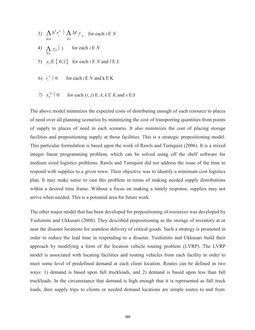
385
i
ij
3) Λbk r k Λ M y i l il
kΕK lΕL
for each i Ε N
4) Λ yil 1 lΕL
for each i Ε N
5) yil Ε {0,1} for each i Ε N and l Ε L
6) r k 0 for each i Ε N and k Ε K
7) x ks 0 for each (i, j) Ε A, k Ε K and s Ε S
The above model minimizes the expected costs of distributing enough of each resource to places
of need over all planning scenarios by minimizing the cost of transporting quantities from points
of supply to places of need in each scenario. It also minimizes the cost of placing storage
facilities and prepositioning supply at those facilities. This is a strategic prepositioning model.
This particular formulation is based upon the work of Rawls and Turnquist (2006). It is a mixed
integer linear programming problem, which can be solved using off the shelf software for
medium sized logistics problems. Rawls and Turnquist did not address the issue of the time to
respond with supplies to a given town. Their objective was to identify a minimum cost logistics
plan. It may make sense to cast this problem in terms of making needed supply distributions
within a desired time frame. Without a focus on making a timely response, supplies may not
arrive when needed. This is a potential area for future work.
The other major model that has been developed for prepositioning of resources was developed by
Yushimito and Ukkusari (2008). They described prepositioning as the storage of inventory at or
near the disaster locations for seamless delivery of critical goods. Such a strategy is promoted in
order to reduce the lead time in responding to a disaster. Yushimito and Ukkusari build their
approach by modifying a form of the location vehicle routing problem (LVRP). The LVRP
model is associated with locating facilities and routing vehicles from each facility in order to
meet some level of predefined demand at each client location. Routes can be defined in two
ways: 1) demand is based upon full truckloads, and 2) demand is based upon less than full
truckloads. In the circumstance that demand is high enough that it is represented as full truck
loads, then supply trips to clients or needed demand locations are simple routes to and from

386
client locations and the supply facilities. If demand is less than a full truck load, then deliveries
can be made as a set of routes, where each route supplies several clients at once and is
represented as a set of stops. There are several approaches that can be used to formulate the
LVRP, however, the simplest is a model that is based upon a set of predefined route alternatives
(LVRP_PR), where routes are selected simultaneously with the selection of facility locations.
This version of the LVRP is conceptually simpler than one in which route are determined
simultaneously with site selection, because predefining a series of possible route alternatives
eliminates the need to embed multiple travelling salesman sub-problems for each selected
facility. The LVRP_PR can be formulated using the following notation:
I the set f client locations
J the set of candidate locations
i, j indices use to index client and candidate locations respectively
k a index of routes for a given candidate facility
f j the fixed cost of establishing a prepositioned storage facility at location j
Pj the set of feasible routes for candidate facility j
c jk the cost of route k associated with candidate facility j
aijk
x j
Ι1, if route k associated with facility j serves client location i λ0, if not
Ι1, if candidate j is selected for a facility λ0, otherwise
y jk
Ι1, if route k associated with facility j is selected λ0, otherwise

387
The LVRP_PR model can be defined as the problem of selecting sites for distribution/storage
facilities while simultaneously selecting routes associated with selected storage facilities to
supply clients in a manner that minimizes total prepositioning and routing/delivery costs:
Minimize Z Λ f j x j + Λ Λ ckj xkj j j kΕPj
Subject to:
1) ΛΛaijk y jk 1 for each client i j k
2) y jk x j for each j and k Ε Pj
3) x j Ε {0,1} for each j
4) y jk Ε {0,1} for each j and k Ε Pj
The objective involves minimizing costs of site selection/development and the costs of
distribution to all clients. The first constraint of this model involves the selection of a delivery
routes so that each client is served by a route. The second constraint maintains that the selection
of a specific route based at a facility site j cannot be selected unless site j has been chosen as a
location for supply prepositioning. This is an integer-linear programming model, which can be
solved by a variety of techniques employing a column generation approach associated with the
vehicle routes.
Yushimito and Ukkusuri modified the above type of problem for the prepositioning problem for
emergency supply. At issue in prepositioning is the fact that a system may be compromised in its
ability to supply a set of possible clients. Otherwise, the problem of prepositioning can be
approached in exactly the same manner as supply location and vehicle routing in classic logistics
problems. In such a case, the formulation above can be used without modification. But, in a
disaster certain road links may no longer be available as they may be flooded or ruined. This
would render certain routes from being usable. Also, a supply depot may also be unusable as it

388
could be damaged or destroyed in the disaster. To address these types of possibilities, Yushimito
and Ukkusuri assumed that each road link could be assigned a probability of failure. They also
assumed that such failure events were independent. They defined the probability of a link
between i and k failing as pik . This means that the probability of a link (i, k ) being usable is:
(1 − pik )
Suppose that a path between i and j is comprised of two arcs, one from i to k and the other
from k to j . Then the probability of a path being usable from i and j can be calculated as:
(1 − pik )(1 − p jk )
This was defined as the reliability of the associated path. Such a calculation can be done when
the probabilities of edge failure are known a priori and are independent across all edges. For
every predefined route in the VRP_PR, we can calculate the reliability of the route. This can be
designated as R jk . The second assumption made by Yushimito and Ukkusuri is that there are
known failure probabilities for each possible facility site, q j . Thus, the probability that a supply
facility is available is (1 − q j ) . Using these two elements together, Yushimito and Ukkusari
defined a probabilistic version of the LVRP_PR for prepositioning supply as follows:
Maximize Z ΛΛ R jk y jk (1 − q j ) j kΕPj
Subject to:
1) ΛΛaijk y jk 1 for each client i j k
2) y jk x j for each j and k Ε Pj
3) Λ f j x j B
j

389
4) x j Ε {0,1} for each j
5) y jk Ε {0,1} for each j and k Ε Pj
This prepositioning involves locating a set of supply facilities that costs no more than an
available budget, B . The objective involves maximizing the sum of service reliabilities, where
each reliability value is the product of route reliability and facility reliability. In essence, this
model maximizes an un-weighted reliability value of serving all demand. Yushimito and
Ukkusuri argue that the above model can be solved by identifying the most reliable path to a
given client from a storage site. They show that maximizing the reliability in serving every
demand can be achieved when the most reliable path is used to reach a given client. Thus, it is
necessary to find the most reliable path between a given storage site and all clients. They show
that the problem of finding the most reliable path between a facility and a client can be solved as
a form of the well-known shortest path algorithm between an origin and a destination. Thus, the
set of route alternatives for a given facility would be comprised of the most reliable routes
between a given site and each demand. When they overlap and are within capacity they can then
be combined. Thus, it is not necessary to use a column generation scheme in solving the
maximum reliability prepositioning problem. Unfortunately, the above model may strike a poor
balance between reliably serving small clients as compared to large clients. That is, it would not
make much sense to increase the reliability of a very small client demand at the expense of
reducing the reliability of a very large client demand. Thus, it would make sense to modify the
above model objective to:
Maximize Z ΛΛ d jk R jk y jk (1 − q j ) j kΕPj
Where d jk equals the number of clients served by route alternative k from facility site j . This
objective could be used in place of the objective suggested by Yushimito and Ukkusuri without
changing the difficulty of solving the overall model.
Prepositioning of emergency resources is an important way to mitigate the effects of a hazard
and prevent it from becoming a full-fledged disaster. If a hazard spirals out of control and

390
becomes a disaster despite our best efforts, having resources prepositioned at critical locations
can greatly improve the effectiveness of the response effort. Despite the obvious benefits of
prepositioning, this strategy has been the focus of very little research within the emergency
management academic community. The p-median problem can be solved to optimize the
location of global relief supply depots as well as supply depot location problem at the national,
state, or local scale and thus provides a solid mathematical foundation for addressing this
question. A strategic prepositioning model takes into account the cost of transport, storage, and
prepositioning of emergency supplies providing valuable information to decision makers given
limited budgets and resources. The location vehicle routing problem can be solved to locate
supply storage facilities and route delivery vehicles while taking into account the potential for
disruptions along the transportation network, and therefore is an effective way to account for the
uncertainty associated with the scale, intensity, and duration of many hazards. All of the
modeling approaches described above can greatly assist in decision making and planning under a
multitude of disaster scenarios, and can be modified to answer the specific questions an agency
such as Caltrans must ask to determine the best actions to take.
9. Infrastructure Fragility
Although emergency planning often addresses issues like that of backup power, there does not
appear to be a part of the modeling literature that is devoted to public vulnerability due to the
lack of backup power. For example, water supply districts often locate backup generators so that
water pressure can be maintained during times of power outages. In addition, sewer districts
often maintain backup generators for pumps at critical lift stations, in order to ensure the system
works during power outages. Similarly, telephone companies have maintained backup power for
landlines by keeping banks of batteries at switching facilities. Cell towers often do not have long-
term back-up supplies, so that some services are not guaranteed to operate. Maintaining
communication systems during emergencies is an emerging problem as more households are
increasingly relying on cell phones as their only form of communication. This trend may also be
exacerbated by the use of cable-internet connections, which are also vulnerable to power outages
and do not usually have backup power systems. Consequently, it is important to address the
fragility of infrastructure in emergency planning.

391
There is, however, a growing interest in identifying vulnerabilities, especially with respect to
infrastructure. In terms of transportation, there are a number of vulnerability issues should
something fail or be intentionally taken out. For example, when a trestle fire destroyed a Union
Pacific railroad link in downtown Sacramento, CA in March of 2007, most trains had to be
rerouted about 125 miles in order to get to their destination. That is, the loss of a structure
approximately 300 feet long resulted in rail cars being detoured nearly 125 miles. The sudden
loss of infrastructure can result in a significant impact, either limiting transportation or requiring
detours that are quite long. In a recent study, Peterson and Church (2008) modeled all freight
flows destined for or originating from the State of Washington. This principally involved the
Class 1 railroads serving Washington, namely BNSF (Burlington Northern Santa Fe) and UP
(Union Pacific). Peterson and Church proposed a methodology for determining the impact of
losing a railroad bridge in terms of the needed rerouting of freight. For the State of Washington,
there are approximately 999 origin-destination route pairs involving the Washington as either an
origin or a destination in the Bureau of Transportation Statistics rail freight database. About a
third of these routes typically cross the BNSF bridge at Sandpoint, Idaho. If this bridge is lost
due to some type of accident or terrorist event, all traffic that would have used this bridge will
need to be rerouted. Without considering issues of track capacity, rerouted distances averaged
350 miles more than what would occur with the bridge. That is, the loss of a rail bridge in
Sandpoint, Idaho could have a significant impact on freight associated with the State of
Washington. Peterson and Church (2008) also suggest how capacity data could be used to model
routes after a possible bridge interdiction. They suggested that since some routes are already
operating close to capacity, it may be that detours could be even longer than what had been
estimated or that the capacity to handle such traffic along other routes does not exist and some
freight might need to be curtailed.
The Legislature of the State of Pennsylvania has considered requiring their Department of
Transportation to establish a contingency plan to reroute rail traffic due to a loss of railroad
infrastructure such as a bridge, tunnel, or yard. Approximately 30% of the nation’s freight uses
rail. This statistic is likely to increase with increasing fuel costs as rail is 4 times more fuel
efficient than truck. In terms of moving towards more sustainable activities (like that suggested
in California’s AB32), it is clear that rail will play a larger role in freight transport, especially for

392
distances that exceed 800 miles. Since the Ports of Long Beach and Los Angeles combined
handle approximately 40% of all containers imported into or exported out of the U.S., it plays a
major role in global transport flows. Most container traffic heading into California through any
California port will be placed on rail if the trip exceeds 1000 miles. This means that rail
infrastructure within California as well as bridges and tunnels outside California could have a
detrimental impact on the ability to handle freight if they should be compromised. It is important
to develop an understanding of the major vulnerabilities in advance of a disaster as well as to
develop the best possible contingency plans for coping with such disruptions.
Infrastructure could be compromised by either a natural disaster or an intentional terrorist strike.
For example, a heavy storm in December 2007 resulted in the closure of a 20-mile section of
Interstate 5 near Chehalis, Washington for nearly a week. This would be considered “a piece of
cake” event as compared to the events that are possible should the levee system in the Central
Valley of California be compromised by a major storm or earthquake. It is imperative to
understand the risks and locations of such events and develop appropriate plans to handle such a
disaster. The road system in Central California could be compromised to the extent that traffic
for many communities could be entirely cut off, something that California has not experienced to
any great extent. The fact is that priorities for upgrading levees should be set not just in terms of
protecting property and safety, but also within the context of protecting supply routes and
evacuation routes for an area. This also means that Caltrans and other State agencies need to
coordinate with water resource agencies, flood and levee operations districts so that emergency
plans are coordinated with the state of such systems as levees, reservoir operations, etc.
The issue of intentional harm is not one to be taken lightly. The disruptions caused by the
terrorist acts of 9/11 are quite small to what could possible occur or what natural disasters might
do in harming infrastructure. There is a growing literature associated with identifying
infrastructure that is especially vulnerable or critical. If an element is critical but not very
vulnerable within the context of a natural disaster, then the only way in which that element might
be compromised is due to an intentional strike. Some of the research literature is directed at
identifying those elements that are particular important in system operation (facilities, networks,
& protocols). For example, Church et al. (2004) presented two models that can be used in supply

393
logistics systems that are aimed at identifying the critical points of supply and the impacts of a
worst-case interdiction. Their presentation also gives a relatively complete list of research papers
associated with military interdiction of supply routes. Gubesic et al. (2008) discuss a number of
approaches that can be used to assess critical elements of a network system. The basis for much
of this work has been to analyze the range of possible outcomes, from worst-case to expected
case damages, should a system be compromised by the loss of certain components, e.g. a bridge
or a road.
The basic idea is that transport, communication systems, electrical transmission, and pipeline
networks should be analyzed in order to identify the range of possible outcomes in terms of the
loss of system operability as well as identify strategies in which to lessen those risks and
potential damages. For example, a highway may have one bridge that is especially vulnerable to
an earthquake or to flooding which might undermine the foundation. Whatever the risk is, it may
be that this one component is especially at risk. What if the entire route is useless if that element
is damaged? Then, it may be important to ensure that this one component is strengthened or
protected so that the risk of losing an important route is substantially reduced. The overall
strategy would be to identify the elements that if protected or reengineered could keep lifeline
support systems in operation, e.g. water transportation, food, supplies, and communications.
Each system needs to be analyzed within this perspective. The transportation system is a critical
element in securing many of the lifeline systems (food, medications, personnel) in the event of
an emergency so the transport infrastructure should be given a high priority for analysis as well
as strengthening. The problem of re-engineering or fortifying a system component in order to
minimize losses in the event of a disaster has been addressed only recently (see Church and
Scaparra (2007) as an example).
Designing a transportation system so that it can provide lifeline services, like food and
emergency services as well as support evacuation when needed was recently proposed by
Viswanath and Peeta (2003). Suppose that there exists a region with an existing road network.
The network represents roads or highways that connect towns or cities. The major cities
represent the origins and destinations of specific services or commodities. The idea is that routes
of commodities or services between all major towns should be supported if at all possible.

394
ij
xk
Although a route between a given origin/destination pair should be efficient, the route cannot
traverse along a given road unless that road has been seismically upgraded to withstand a major
earthquake. Viswanath and Peeta optimized road improvements subject to a budget constraint so
that as many OD pairs are supported by a seismically safe route. The objectives were to
maximize the population that were covered by these major routes and hence served by a specific
commodity type as well as optimize the efficiency (distance) of each of the routes. Consider the
following notation:
i, j, m indices used to represent towns and cities
A {(i, j) | a road connects towns or cities i and j } Em {(i, j) | area m is accessible to road link (i, j)} k index of commodity or type of service
O(k ) the origin node i for commodity route k
D(k ) the destination node i for commodity route k
ck the unit cost of routing commodity or service along link (i, j) Ε A
fij the cost of seismically upgrading road (i, j) Ε A
The Viswanath and Peeta model contains the following three decision variables:
Ι1, if there is a unit of flow of commodity k on link (i, j) ij
λ0, otherwise
y Ι1, if link (i, j) is used in a commodity flow path ij
λ0, otherwise
Ι1, if demand m is accessible from a link on a flow path m
λ0, otherwise
The formal multi-objective optimization model can then be stated as follows:
Maximize Λam Zm m
Minimize Λ Λ(ck xk + ck xk )
Subject to:
ij ij k (i, j )ΕA
ji ji
z

395
λ
ij
ji
ij
ij
ij
ij
1) xk − Ι 0, if i O(k ) xk λ− 1, if i Dk) ′ϖi, k Λ ij Λ ji
(i, j )ΕA ( j ,i )ΕA λ 0, otherwise
2) Z Λ Λ (xk + xk ) for each area m m ij ji
k (i, j )ΕEm
3) xk y for all k and (i, j) Ε E
4) xk yij for all k and all (i, j) Ε E
5) Λ fij yij B (i, j )ΕE
6) Λ xk 1 for all i and k (i, j )ΕA
7) Λ xk 1 for all k and j D(k ) (i, j )ΕA
8) Λ xk | Q | −1 for all k (i, j )ΕA where i, jΕQ
9) xk Ε {0,1} and xk Ε {0,1} for all k and (i, j) Ε E ij ji
10) yij Ε {0,1} for all k and (i, j) Ε E
10) z m Ε {0,1} for all m
The above model can be used to identify which routes should be made safe so that services can
be transported to as many communities as possible and so that feasible evacuation routes exist
after an earthquake. The basic idea is to design the best “safe-routes” system within budget
limitations and serve as many communities as possible as well as make the hardened routes as
efficient as possible. Although it may be the object to upgrade all bridges over time, such a
model can be used to prioritize the upgrading process. Further, all bridges may be upgraded to
some standard that is deemed acceptable, however, it may be valuable to then use the above style
of model to consider which bridges or road links to upgrade to an even stricter standard, so that
should a particularly powerful earthquake hit, there still represents a backbone of roads that can
survive and be used in an emergency.
It should be pointed out that the model just described was cast within the context of providing
routes that would survive an earthquake. But there are other dangers that might be of great

396
importance to consider within this context. One is potential flooding. A recent TRB report
discussed possible impacts of climate change on transportation infrastructure. The greatest such
impact is the possible flooding of low coastal areas due to storm surges and seal level rise. The
TRB report suggests that virtually all transportation planning adopt a new perspective of dealing
with possible climate change impacts. To do this requires a two step process: 1) identify possible
infrastructure risks due to climate change, and 2) mitigate possible risks by planning in light of
such risks. The model given above is an example of modeling to provide transportation services
given an earthquake, but it could be modified to handle issues like that of extreme weather
events, coastal flooding, etc.
Natural disasters such as earthquakes and flooding and human-caused disasters such as a terrorist
attack both pose substantial risks to the transportation network. Mitigating the potential impact
of these events requires careful identification of critical elements of transportation infrastructure
so that steps can be taken to protect them from the multitude of hazards they face. Infrastructure
can fail without warning, as demonstrated by the complete collapse of the I-35W freeway bridge
in Minneapolis in 2007. Modeling techniques can be used to assess infrastructure fragilities on
railways, freeways, levee systems, and any number of other important transportation features to
help agencies take necessary steps to mitigate the impact of a worst-case disaster scenario.
10. Findings
This report has covered a number of elements associated with planning, mitigating, and
managing events involving a disaster. To adequately serve a region with appropriate
transportation, shelter, and life supporting resources it is important to anticipate, plan, train, and
maintain an adequate mix of resources and personnel to respond appropriately. Thus far this
report has focused on the role of modeling in disaster management, including modeling possible
evacuations, prepositioning emergency supplies, designating shelter locations, modeling
infrastructure fragility, designing systems so that they operate during disasters, designing plans
for response, and designing interoperable communication systems. Yet even the most well
thought out models and system designs may suffer from flaws that can only be rectified through
careful design and real world validation. The first step in this process is to identify some of the

397
major shortfalls in current practice involving agencies responsible for emergency disaster
response. To this end, the literature review above was complemented by a series of interviews
conducted with emergency management personnel from several agencies in California.
The subjects of these interviews included Caltrans personnel, geospatial information specialists,
and emergency management professionals from the campus to the county level. Interviews
followed a semi-structured format, which allowed us to expand upon interesting topics while
keeping focused on the subjects most relevant to the problem at hand. Santa Barbara County has
faced four major wildfires in the past three years, thus these events comprised one major focus,
along with earthquakes, chemical and nuclear accidents or attacks, tsunamis and other threats
specific to the central coast region. Interviews were often followed by impromptu tours of the
subject's workplace, including facilities like a Caltrans Traffic Management Center (TMC), an
Emergency Operations Center (EOC), several Geographic Information System (GIS) hardware
and software installations, and an emergency shelter utilized during the 2009 Jesusita Fire. In the
interest of candid and informational discussion, we choose to maintain the confidentiality of our
interview subjects3. The following findings are informed by both our literature review as well as
the series of interviews we conducted:
1) It is important to identify areas within the State of California that face a significant
disaster risk and also face a significant risk in evacuating safely. This type of analysis
would require modeling evacuation vulnerability and mapping event risk, and should be
coordinated with data from OES, water resources agencies, MPO’s and other relevant
organizations to provide a comprehensive risk map. One such area that was previously
modeled (see section 3) is the Mission Canyon neighborhood in Santa Barbara. Due in
part to this research, Mission Canyon residents were particularly well organized and
actually evacuated before the official order came through during the May 2009 Jesusita
fire. Also during this event, an evacuation contingency plan that was developed during
the Zaca Fire was used to split most of the Santa Barbara area (Goleta, Santa Barbara,
Montecito) into zones that could be evacuated in 1.5 hours or less. These zones were used
to conduct a staged evacuation by identifying mandatory evacuation areas and evacuation
3 A complete list of interview subjects can be found in the references section of this report.

398
warning areas based on the latest fire and weather conditions assessed by fire officials
and CHP. It would be useful for emergency management purposes to have the entire
county broken into these 1.5-hour zones using population densities, road network
characteristics, and hazard probabilities. This method is not infallible however, as the
Jesusita fire was only 40 minutes from Montecito at one point but the threatened area was
not under mandatory evacuation. Wildfires remain a threat, as Montecito, Carpentaria,
and some areas west of State Highway 154 still have intact chaparral of considerable age
and vulnerability in the event of a wildfire. Flooding is now a major concern for the city
and county given the extensive fire damage in many watersheds and the El Nino
prediction for winter 2009-2010. Maps showing the areas of greatest concern could be
helpful for planning purposes, and evacuation procedures for flood-prone areas should be
determined well in advance of an event. Earthquakes and the tsunamis they may cause
remain a major concern, and the uncertainty of the timing and spatial extent of such
events presents a unique challenge in identifying and protecting areas at risk. Another
area of concern to central coast emergency managers and Caltrans traffic engineers is the
Diablo Canyon Nuclear Power Plant and the surrounding communities of Pismo Beach
and San Luis Obispo. A contraflow evacuation plan has been developed for this area but
might be improved through modeling and simulation. This topic is further discussed in
the third recommendation of this section.
2) For areas that face specific risks designate emergency evacuation routes and ensure
such routes will be as safe as possible based upon infrastructure design and
condition. The 2007 Zaca fire was a significant event but progressed at a speed, which
allowed for extensive evacuation contingency planning. Evacuation routes were
designated using major arteries as the primary routes out of fire-prone canyon
communities, with planned work-arounds should these primary routes be inaccessible.
Since the fire never reached highly populated areas, most of these evacuation plans were
not executed. Evacuation operations are legally a law enforcement function, with
Caltrans assisting with road closures, traffic direction, and signage. Collaboration and
data sharing between these two agencies could improve route designation and traffic
flow, in particular information on current road construction projects and closures. Other

399
data used for evacuation routing includes cadastral parcels, Verizon point-of-presence
(POP) locations, as well as the locations of nursing homes, day care centers, and schools
to determine where assistance to vulnerable populations may be required. These data
should be shared amongst agencies as well. Several issues that arise frequently during
evacuation that may impede safety are that people will follow habitual routes rather than
the routes they are directed to use and often think they can outrun hazards such as
wildfires.
3) Test and refine evacuation simulation models across multiple scales covering options
such as contraflow, and develop the capability of analyzing evacuation flows on-the-
fly using transportation, census, cadastral and employment datasets in a
Geographic Information System (GIS). Caltrans personnel designed the Diablo
Canyon Nuclear Power Plant contraflow evacuation plan in December 2007. There seems
to be considerable doubt within the agency as to whether the plan could be successfully
implemented due to the considerable CHP and Caltrans manpower required to control
traffic. Currently there is not a contraflow plan for the City of Santa Barbara, as the
current staged evacuation method seems to work adequately given the relatively slow
spread of recent wildfire events. The major challenge in designing a Santa Barbara
contraflow plan is finding and allocating the manpower required to control the numerous
101 Freeway on/off ramps. Cities that have successfully implemented contraflow such as
New Orleans have more spacing between freeway access points thus reducing the
manpower required. There are two trends that have emerged in recent events requiring
evacuations: The first is encouraging voluntary early evacuation so that emergency
personnel have more time and resources to focus on vulnerable populations if/when the
mandatory evacuation order is made. The second is rethinking the necessity of ordering a
mandatory evacuation, with a greater focus on teaching people how to create defensible
space and to ‘stay-and-defend’ during wildfires. One important task is to develop
methods to estimate and model evacuation needs of special needs, like the elderly and
youth using public assets like transit buses. Santa Barbara Metropolitan Transit District
(MTD) bus drivers are required to pull over and immediately report any hazardous
situation (wildfires, floods, traffic accidents, etc) thus might provide a novel source of

400
geoinformation as well as accessible transportation for vulnerable populations during a
disaster. Especially vulnerable populations include transients, tourists, and recent
immigrants with limited English comprehension. Integration of real-time traffic flow data
from Caltrans into a GIS would be of great use to emergency managers during both the
planning and operational phases of emergency evacuations. Major issues include the
large percentage of the workforce that commutes to Santa Barbara from other parts of the
county, thus leading to major differences in on and off peak traffic flow.
4) Model shelter locations and supplies for ease of access, size, and capabilities in
supporting an emergency. According to emergency management personnel, sheltering
operations in response to the Jesusita fire went well. Wednesday, May 6, 2009 and
Thursday, May 7 were the days when the fire posed the biggest threat to the community,
and thus the number of evacuees needing shelter was greatest during these days as well.
Overall, the number of evacuees needing shelter was much less than the 20% of the
evacuated population that the Red Cross generally assumes. The ability to provide
adequate sheltering during this event was largely due to the short time of the mandatory
evacuation order. The longer an event and the subsequent evacuations persist, the more
difficult it becomes to provide shelter to evacuees. Although the Jesusita Fire emergency
shelter on the UCSB campus was well staffed and stocked with supplies, it is notable that
this was the third facility that had been used to house this shelter. The initial location
proved too small to accommodate the influx of evacuees, and the subsequent shelter
location was closed when threatened by the fire itself. This lack of suitable shelter
locations and on-the-fly relocation may become significant impedance to evacuee safety
during future events, especially those that strike without advanced warning such as
earthquakes or terrorist attacks.
5) Develop resource requirement models so that the need for resources to support
special needs like bridge inspections is understood, and plans for infrastructure
inspection after a disaster can be quickly carried out. One of the biggest concerns for
Caltrans in the event of a major earthquake is ensuring the structural integrity of bridges
and freeway on and off ramps. The large scale and chaotic nature of an earthquake makes
401
it especially important to quickly assess freeway damage to provide access to rescue
teams and evacuees. Significant damage to freeway infrastructure occurred in the San
Francisco Bay Area during the 1989 Loma Prieta earthquake and more recently in the
Los Angeles Basin during the 1994 Northridge earthquake. There is a general concern
within the emergency management community that the central coast region is 'overdue'
for a major earthquake and may be unprepared to handle the immediate infrastructure
inspections necessary to facilitate rescue operations and ensure safety along major
transportation corridors.
6) Model emergency supply storage and placement in order to estimate what will be
needed statewide to respond adequately in a timely fashion, with a focus on locating
equipment in hot spot regions of the state. CMS boards are essential in notifying the
public of the road closures and designated evacuation routes when hazardous conditions
exist. The primary role of Caltrans during emergency events is to respond by closing
roads and controlling the placement of and messages on CMS boards. Once the lead
command (Fire Department or CHP) determines that a road closure is necessary, a
Caltrans maintenance crew places barricades, which are then usually staffed by CHP or
local police. These signs are often left in places where they are likely to be put to use:
one example is State Highway 192, a major transportation corridor and evacuation route
for the foothill neighborhoods of Santa Barbara. There are many factors that should be
taken into account when modeling placement of CMS signs, including visibility and the
extended traffic queuing that may occur during evacuations.
7) Develop models that route rapid response vehicles to incidents in areas with
significant congestion in order to maximize the value provided by such a service.
One type of event that agencies such as Caltrans may not be prepared for during
emergency operations is a secondary event that forces a road closure at a critical link
along the transportation network. An example of such an event is the trailer fire that
occurred next to the 101 Freeway during the Jesusita Fire evacuation that forced a
temporary closure of the freeway, causing massive traffic gridlock. Fortunately, motorists
stuck on the 101 and surrounding side streets were not directly threatened by the wildfire
402
itself, but the impact of such secondary events on evacuation safety should be modeled to
improve agency preparation and response time.
8) Analyze, test, and deploy communication systems that can provide geographic
information over a wide area to mobile units of different agencies. The flow of
geographic information between agencies and personnel during emergency operations is
often disjointed. During the Jesusita Fire, CalFire mappers uploaded fire perimeter GIS
layers based on information from personnel in the field to a State OES FTP site, which
was then accessed by mappers at the County EOC to create maps. These county mappers
were then responsible for creating operational maps incorporating utility, population, and
road closure data for use by emergency officials, as well as electronic and hard copy
maps for the general public. There were issues in maintaining sufficient mapping
personnel to keep up with map requests, as well as making sure that the latest and most
accurate geoinformation was used. City GIS personnel were unable to access the map
layers they needed and there was considerable redundancy in the maps that were
produced, resulting in a large degree of uncertainty regarding the latest and most accurate
geoinformation. During the 2008 Tea Fire, the demand for updated fire maps far
outpaced the city’s ability to produce them. Part of the problem was that there was no
data connection between city GIS server and Emergency Operations Center (EOC)
server. This lack of accurate geoinformation led to severe consequences: Several police
officers were burned by this fire because they were stationed too close to the active front.
Better coordination between the city and county is needed, and a mobile device-based or
Internet system that provides consistent reliable information could greatly assist
emergency managers in decision-making. The City of Anaheim has an Enterprise Virtual
Operations Center that integrates, synthesizes, and distributes real time data (GIS,
responder locations, communications) via the Internet for decision support. A tool that
incorporates real time traffic information and the latest event maps would be very useful
in developing and altering evacuation routes, especially if it could be used in conjunction
with the radios already used by emergency personnel. The ability to instantly locate
personnel and share information (pictures, text, etc) within defined user groups could also
be helpful, provided the system was reliable and easy to use.

403
9) Establish a mechanism to use participatory/voluntary data provided by people with
cell phones, allowing them to send video and images along with descriptive text to a
central clearing house, thereby allowing people to provide data on an event as it
unfolds. Organized volunteer data gathering by people in the area of harm may aid in
their rescue and evacuation by providing valuable information. Since a 911 call center
may be overwhelmed by calls during an emergency, many calls providing information
cannot be handled. If an individual can send a text message with GPS coordinates (e.g.
from an iPhone) or an image, this data could be streamed directly to support personnel in
a mobile command center allowing for better information about an event. There is
considerable debate concerning the role of citizens in developing and accessing
emergency management information. Any disaster information provided by citizens
should be crosschecked for reliability, although sometimes the best disaster information
comes from the media or from outside of official sources. The Santa Barbara county GIS
department used a Google Map to display official evacuation zone and fire perimeter
information during the Jesusita fire, but it was difficult to ensure accuracy and maintain
this map with other more pressing duties such as providing maps to officials and decision
makers. A group of graduate students created a competing Google Map of evacuation
zones and fire perimeters relying on data from numerous sources, which one emergency
manager found to be more accurate and useful than the official county map. It is very
important to strike a balance between volunteered geographic information (VGI) and
official sources of geographic information during emergencies so that the public stays
informed but people are not overwhelmed and confused by conflicting information.
10) Develop formal emergency communication links and systems so that emergency
managers can quickly and effectively convey the most accurate and up-to-date
information to the public. Currently there are a multitude of systems used to alert
people living in the Santa Barbara area of potentially hazardous situations. As of
February 2009 more than 28,000 users had signed up for the UCSB campus alert system
with 9,345 wireless devices registered to receive automatic text message alerts. The Santa
Barbara City Reverse 911 system uses Verizon phone connection data and GIS to

404
determine the size of polygons representing the areas to be notified. Goleta uses a
different notification system that had several notable mishaps during the 2008 Gap fire,
including instructing residents of the seaside community of Isla Vista to evacuate. The
best way to convey spatial information during an emergency and exactly what
information should be provided remain open-ended questions. For example, the danger in
making evacuation routes public is that evacuees may blindly follow them and ignore
instructions that route them around hazards such as spot fires that occur far in front of the
main flame front. Traditional sources such as television and radio remain important
communication outlets for emergency information, but are losing ground to the Internet
and mobile devices. The county is considering developing an ESRI ArcIMS site to help
disseminate spatial information quickly and coherently over the Internet, including
evacuation zones and road closures. Another option is to develop a mobile disaster
decision support system (MDDSS) which allows people to access emergency information
from official sources as well as volunteered information from other users within their
disaster support network (DSN). Such as system could also show the locations of all
members of the DSN, and provide a routing service that takes into account road closures
and hazard location, all on a mobile device such as an iPhone or Blackberry.
11) Model the fragility of infrastructure and its potential impact on public safety.
During the Jesusita Fire, the Santa Barbara county emergency operations center (EOC)
had to be relocated to the UCSB campus when the fire threatened its downtown location.
Computers and other equipment were moved because there is insufficient funding for two
fully operational EOCs, and there was an approximately one hour delay after the move
before the phone lines were connected, leaving a dangerous communication gap while the
new EOC was set up. Obviously, a non-operational emergency operations center poses a
major hazard to the public when a fast-moving wildfire is threatening property and lives.
One possible solution to such infrastructure vulnerabilities is development of portable
self-contained emergency management units such as the trailer used by CalFire for GIS
services. Models should be developed to locate new facilities in such as way that
minimizes risk from events such as wildfires, and ensures designs that can withstand the
shaking of an earthquake and the strong winds produced by storms.

405
11. Conclusion
A devastating event such as Hurricane Katrina often leads both the public and the government
agencies charged with serving them to rethink disaster preparedness, mitigation, response, and
recovery and to ask the omnipresent question, “What would I do if the unthinkable happens?”
The power of this tragedy to spurn such questions is one reason why it is mentioned frequently
throughout this report. It is important to review the lessons learned from Hurricane Katrina and
other recent disasters when developing a research agenda for the hazards that affect California.
One of the few things that went right during Hurricane Katrina was the successful
implementation of a contraflow evacuation plan. As detailed in the evacuation section of this
report, everyone with access to private transportation who chose to evacuate the city was able to
do so and in less time than anticipated by planners. This success would not have been possible
without extensive research performed at academic institutions such as the Louisiana State
University Hurricane Center. A variety of modeling techniques were employed to determine the
best strategy, leading to “the most effective highway-based evacuation in the history of the Gulf
Coast and, perhaps, in the history of the entire United States.” (Wolshon, 2006, p.1) Of course
few would argue that the overall emergency management of Hurricane Katrina was a success.
The destruction and subsequent abandonment of large portions of the city and the death of nearly
one thousand city residents exemplifies the severe deficiencies that occurred in all four stages of
emergency management. Some might argue that the overwhelming and unexpected magnitude
of the storm lead to inevitable outcomes, but most hazards researchers agree that more could
have been done to accommodate the needs of vulnerable people who were disproportionately
affected by this event. It makes sense to expand the notation of the an “area at risk” to an “area at
risk with the potential for disproportionate impacts on specific demographic sectors.” The
majority of current emergency evacuation research is centered on people who own and drive
vehicles, not those who are old, infirm, young, poor, or those with disabilities such as the blind.
Emergency operations needs to be based upon good demographic data so that everyone can be
considered covered within the plan.

406
The City of New Orleans was devastated by Hurricane Katrina, a natural event whose effects
were amplified by human decisions made over multiple time and spatial scales. Most disasters fit
this description: they are a function of the both the geographic characteristics of the hazard itself
and the vulnerabilities and actions of the people whom it affects. Although government and
citizens alike were aware of the destructive potential a direct hit from a strong hurricane posed to
New Orleans, they were woefully underprepared for this ‘worst case’ scenario. Many cities in
California face similar dire threats, whether from flooding, earthquakes, wildfires, tsunamis,
chemical spills, nuclear accidents, or the actions of a terrorist group or rouge state. Much like
New Orleans, the cities and the agencies responsible for protecting them are for the most part
unprepared for the potential impacts of a major hazard.
The Jesusita Fire nearly became a major disaster for the City of Santa Barbara. The original Red
Cross shelter was moved when it was threatened by the fire, thus reducing the number of
possible shelter sites increasing the risk of not being able to meet the needs of vulnerable
populations. Likewise, the EOC was moved when threatened by the fire, a contingency action
that was actually discussed during the Gap Fire, yet still resulted in ‘downtime’ making active
management difficult. Despite doubling the size of the sheriffs’ department via mutual aid an
event such as the 101 Freeway trailer fire would have pushed manpower requirements and
planning abilities to the limit had it persisted. Models should be designed that account for such
unexpected events to increase the odds of successful emergency management and reduce the
probability of destruction of property and loss of human life. We conclude this report with what
is perhaps our most important recommendation: We must assume that the ‘worst case’ disaster
scenario will occur and prepare our citizens and government agencies accordingly.
407
11. References
Personal Interview Subjects
Richard Abrams, County of Santa Barbara Zacharias Hunt, County of Santa Barbara Yolanda McGlinchey, City of Santa Barbara Frank Quon, Caltrans District 7 Rick Sachse, Global Traffic Technologies Fred Samuel, University of California, Santa Barbara Shayne Sandeman, Caltrans District 5 Shashi Shehkar, University of Minnesota, Twin Cities David Ybarra, Caltrans District 5
Literature
Mitigating natural disasters: phenomena, effects and options. A manual for policy and planner. (1991). New York: United Nations Disaster Relief Organization.
State and Local Guide 101:Guide for All-Hazard Emergency Operations Planning. (1996):
FEMA.
Hurricane Pam Exercise Concludes. (2004). No. R6-04-093: FEMA.
Contraflow Plan for the Florida Intrastate Highway System. (2005) Tallahassee, FL: Florida Department of Transportation, Traffic Engineering and Operations Office.
The Tsunami Threat to California: Findings and Recommendations on Tsunami Hazards and
Risks. (2005). No. CSSC 05-03: Seismic Saftey Commission, State of California.
Hurricane Katrina in the Gulf Coast, Mitigation Assessment Team Report: Building Performance Observations, Recommendations, and Technical Guidance. (2006). No. 549: FEMA.
Reuniting the Families of Katrina and Rita. (2006): Louisiana Family Assistance Center,
Louisiana Department of Health and Hospitals.
A Year of Healing: The American Red Cross Response to Hurricanes Katrina, Rita, and Wilma. (2006): American Red Cross.

408
A California Challenge - Flooding in the Central Valley. (2007): Department of Water Resources, State of California.
Gap Wildland Fire. (2008). Retrieved. from http://165.221.39.44/incident/1384/.
Hazard Mitigation Assistance Program Guidance: Pre-Disaster Mitigation, Flood Mitigation
Assistance, Repetitive Flood Claims, Severe Repetitive Loss. (2008): FEMA.
State of California Emergency Plan - November 20, 2008 Draft. (2008): Governors Office of Emergency Services, State of California.
Abdallah, S., Heinzen, R., & Burnham, G. (2007). Immediate and long-term assistance following
the bombing of the US Embassies in Kenya and Tanzania. Disasters, 31(4), 417-434.
Aboelata, M., Bowles, D., & Chen, A. (2004). Transportation Model for Evacuation in Estimating Dam Failure Life Loss. Paper presented at the Proceedings of the Australian Committee on Large Dams Conference, Melbourne, Victoria, Australia.
Abusch-Magder, D., Bosch, P., Klein, T. E., Polakos, P. A., Samuel, L. G., & Viswanathan, H.
(2007). 911-NOW: A network on wheels for emergency response and disaster recovery operations. Bell Labs Technical Journal, 11(4), 113-133.
Afshar, A. M., & Haghani, A. (2008). A Heuristic Framework for Optimizing Hurricane
Evacuation Operations. Paper presented at the 87th Annual Meeting of the Transportation Research Board, Washington, D.C.
Akella, M. (2008). First Responders and Crisis Map Symbols: Making Communication Clearer.
Paper presented at the AutoCarto 2008 Conference, Sheperdstown, WV.
Akkihal, A. R. (2006). Inventory Pre-positioning for Humanitarian Operations. Massachusetts Institute of Technology.
Alcada-Almeida, L., Tralhao, L., Santos, L., & Countinho-Rodrigues, J. (2009). A
Multiobjective Approach to Locate Emergency Shelters and Identify Evacuation Routes in Urban Areas. Geographical Analysis, 41(1), 9-27.
Aleskerov, F., Iseri, A., Aysegül, S., Akin, T. H. L., & Altay, G. (2005). A cluster-based decision
support system for estimating earthquake damage and casualties. Disasters, 29(3), 255- 276.
Alsnih, R., Rose, J., & Stopher, P. (2005). Understanding household evacuation decisions using
a stated choice survey–case study of bush fires. Paper presented at the 84th Annual Meeting of the Transportation Research Board, Washington, DC.
Altay, N., & Green, W. G. (2006). OR/MS research in disaster operations management.
European Journal of Operational Research, 175(1), 475-493.
409
Arnoldy, B. (2007, May 15). Disaster alert? Check your cellphone. Christian Science Monitor, p. 2.
Asaeda, G. (2002). The day that the START triage system came to a STOP: Observations from
the World Trade Center disaster. Academic Emergency Medicine, 9(3), 255-256.
Ashley, S. T., & Ashley, W. S. (2008). Flood fatalities in the United States. Journal of Applied Meteorology and Climatology, 47(3), 805-818.
Aymond, P. I. (2005). Emergency Data Exchange Language (EDXL) Implementer's Guide:
Working Draft: OASIS Emergency Management TC.
Baker, D., & Refsgaard, K. (2007). Institutional development and scale matching in disaster response management. Ecological Economics, 63(2-3), 331-343.
Baker, M. S. (2007). Creating order from chaos: Part I: Triage, initial care, and tactical
considerations in mass casualty and disaster response. Military Medicine, 172(3), 232- 236.
Ballard, A. J. (2007). Traffic operations for hurricane evacuation. Transportation Research
Record, 195-204.
Barbarosoglu, G., & Arda, Y. (2004). A two-stage stochastic programming framework for transportation planning in disaster response. Journal of the Operational Research Society, 55(1), 43-53.
Barbarosoglu, G., Ozdamar, L., & Cevik, A. (2002). An interactive approach for hierarchical
analysis of helicopter logistics in disaster relief operations. European Journal of Operational Research, 140(1), 118-133.
Bastien, M. C., Dumas, M., Laporte, J., & Parmentier, N. (1985). Evacuation Risks: A Tentative
Approach for Quantification. Risk Analysis, 5(1), 53-61.
Batta, R., & Mannur, N. R. (1990). Covering-Location Models for Emergency Situations That Require Multiple Response Units. Management Science, 36(1), 16-23.
Beamon, B. M., & Kotleba, S. A. (2006). Inventory management support systems for emergency
humanitarian relief operations in South Sudan. The International Journal of Logistics Management, 17(2), 187-212.
Beamon, B. M., & Kotleba, S. A. (2006). Inventory modelling for complex emergencies in
humanitarian relief operations. International Journal of Logistics Research and Applications, 9(1), 1-18.

410
Beard, C. C. (2004). Prioritization of emergency network traffic using ticket servers: A performance analysis. Simulation-Transactions of the Society for Modeling and Simulation International, 80(6), 289-299.
Bijker, W. E. (2007). American and Dutch coastal engineering: Differences in risk conception
and differences in technological culture. Social Studies of Science, 37(1), 143-151.
Blue, V. J., & Adler, J. L. (1998). Emergent Fundamental Pedestrian Flows from Cellular Automata Microsimulation. Transportation Research Record, 1644(1), 29-36.
Bolin, R., & Stanford, L. (1991). Shelter, Housing and Recovery: A Comparison of U.S.
Disasters. Disasters, 15(1), 24-34.
Bolin, R., & Stanford, L. (1998). The Northridge Earthquake: Community-based Approaches to Unmet Recovery Needs. Disasters, 22(1), 21-38.
Bonnett, C. J., Peery, B. N., Cantrill, S. V., Pons, P. T., Haukoos, J. S., McVaney, K. E., et al. (2007). Surge capacity: a proposed conceptual framework. American Journal of Emergency Medicine, 25(3), 297-306.
Bostian, C. W., Midkiff, S. F., Kurgan, W. M., Carstensen, L. W., Sweeney, D. G., & Gallagher,
T. (2002). Broadband communications for disaster response. Space Communications, 18(3-4), 167-177.
Branas, C. C., & Revelle, C. S. (2001). An iterative switching heuristic to locate hospitals and
helicopters. Socio-Economic Planning Sciences, 35(1), 11-30.
Brandstetter, T., Garrow, L. A., Hunter, M. P., & Southworth, D. F. (2008). Modeling Altruistic and Aggressive Driver Behavior in a No-Notice Evacuation. Paper presented at the 87th Annual Meeting of the Transportation Research Board, Washington, D.C.
Braun, B., & McCarthy, J. (2005). Hurricane Katrina and abandoned being. Environment and
Planning D-Society & Space, 23(6), 802-809.
Brown, D. E., Robinson, C. D., & Virginia Univ, C. (2005). Development of Metrics to Evaluate Effectiveness of Emergency Response Operations: Defense Technical Information Center.
Brown, G. G., & Vassiliou, A. L. (1993). Optimizing Disaster Relief - Real-Time Operational
and Tactical Decision Support. Naval Research Logistics, 40(1), 1-23.
Buck, D. A., Trainor, J. E., & Aguirre, B. E. (2006). A critical evaluation of the incident command system and NIMS. Journal of Homeland Security and Emergency Management, 3(3).
411
Burby, R. J. (2006). Hurricane Katrina and the paradoxes of government disaster policy: Bringing about wise governmental decisions for hazardous areas. Annals of the American Academy of Political and Social Science, 604, 171-191.
Burton, I., Kates, R. W., & White, G. F. (1993). The environment as hazard (2nd ed.). New
York: The Guilford Press.
Butts, C. T., Petrescu-Prahova, M., & Cross, B. R. (2007). Responder communication networks in the World Trade Center disaster: Implications for modeling of communication within emergency settings. Journal of Mathematical Sociology, 31(2), 121-147.
Canton, L. G. (2006). San Francisco 1906 and 2006: An emergency management perspective.
Earthquake Spectra, 22, S159-S182.
Chakraborty, J., Tobin, G. A., & Montz, B. E. (2005). Population Evacuation: Assessing Spatial Variability in Geophysical Risk and Social Vulnerability to Natural Hazards. Natural Hazards Review, 6(1), 23-33.
Chalmet, L. G., Francis, R. L., & Saunders, P. B. (1982). Network models for building evacuation. Management Science, 28(1), 86-105.
Champion, H. R., Mabee, M. S., & Meredith, J. W. (2006). The state of US trauma systems:
public perceptions versus reality - Implications for US response to terrorism and mass casualty events. Journal of the American College of Surgeons, 203(6), 951-961.
Chan, T. C., Killeen, J., Griswold, W., & Lenert, L. (2004). Information technology and
emergency medical care during disasters. Academic Emergency Medicine, 11(11), 1229- 1236.
Chang, M. S., Tseng, Y. L., & Chen, J. W. (2007). A scenario planning approach for the flood
emergency logistics preparation problem under uncertainty. Transportation Research Part E-Logistics and Transportation Review, 43(6), 737-754.
Charnkol, T., & Tanaboriboon, Y. (2006). Evacuee behaviors and factors affecting the tsunami
trip generation model: A case study in Phang-nga, Thailand. Journal of Advanced Transportation, 40(3), 313-330.
Chen, L. C., Liu, Y. C., & Chan, K. C. (2006). Integrated Community-Based Disaster
Management Program in Taiwan: A case study of Shang-An Village. Natural Hazards, 37(1-2), 209-223.
Chen, X., Meaker, J. W., & Zhan, F. B. (2006). Agent-Based Modeling and Analysis of
Hurricane Evacuation Procedures for the Florida Keys. Natural Hazards, 38(3), 321-338.
Chen, X., & Zhan, F. B. (2006). Agent-based modelling and simulation of urban evacuation: relative effectiveness of simultaneous and staged evacuation strategies. Journal of the Operational Research Society, 59(1), 25-33.

412
Chien, S. I., & Korikanthimath, V. V. (2007). Analysis and Modeling of simultaneous and staged emergency evacuations. Journal of Transportation Engineering-Asce, 133(3), 190-197.
Chiu, Y. C., & Mirchandani, P. B. (2008). Online behavior-robust feedback information routing
strategy for mass evacuation. Ieee Transactions on Intelligent Transportation Systems, 9(2), 264-274.
Chiu, Y. C., Villalobos, J., Gautam, B., & Zheng, H. (2006). Modeling and Solving Optimal
Evacuation Destination-Route-Flow-Staging Problem for No-Notice Extreme Events. Paper presented at the 85th Annual Meeting of the Transportation Research Board, Washington, DC.
Chiu, Y. C., & Zheng, H. (2007). Real-time mobilization decisions for multi-priority emergency
response resources and evacuation groups: Model formulation and solution. Transportation Research Part E-Logistics and Transportation Review, 43(6), 710-736.
Chiu, Y. C., Zheng, H., Villalobos, J., & Gautam, B. (2007). Modeling no-notice mass evacuation using a dynamic traffic flow optimization model. IIE Transactions, 39(1), 83- 94.
Choa, F., Milam, R. T., & Stanek, D. (2003). CORSIM, PARAMICS, and VISSIM: What the
Manuals Never Told You. Paper presented at the 9th TRB Conference on the Application of Transportation Planning Methods, Baton Rouge, Louisiana.
Choi, W., Hamacher, H. W., & Tufekci, S. (1988). Modeling of building evacuation problems by
network flows with side constraints. European Journal of Operational Research, 35(1), 98-110.
Church, R., & ReVelle, C. (1974). The maximal covering location problem. Papers in regional
science, 32(1), 101-118.
Church, R. L., & Cova, T. J. (2000). Mapping evacuation risk on transportation networks using a spatial optimization model. Transportation Research Part C-Emerging Technologies, 8(1-6), 321-336.
Church, R. L., & Scaparra, M. P. (2007). Protecting critical assets: The r-interdiction median
problem with fortification. Geographical Analysis, 39(2), 129-146.
Church, R. L., Scaparra, M. P., & Middleton, R. S. (2004). Identifying Critical Infrastructure: The Median and Covering Facility Interdiction Problems. Annals of the Association of American Geographers, 94(3), 491-502.
Church, R. L., & Sexton, R. M. (2002). Modeling small area evacuation: Can existing
transportation infrastructure impede public safety? : Vehicle Intelligence & Transportation Analysis Laboratory, University of California, Santa Barbara.

413
Clark, A. M. (2006). On developing disaster resilient communications infrastructure. Marine Technology Society Journal, 40(4), 27-34.
Colten, C. E. (2002). Basin Street Blues: drainage and environmental equity in New Orleans,
1890-1930. Journal of Historical Geography, 28(2), 237-257.
Colten, C. E. (2005). An Unnatural Metropolis: Wresting New Orleans from Nature: Louisiana State University Press.
Comfort, L. K., Ko, K., & Zagorecki, A. (2003). Modeling fragility in rapidly evolving disaster
response systems. Institute of Governmental Studies, UC Berkeley. Paper 2003-2.
Cova, T. J. (2005). Public Safety in the Urban–Wildland Interface: Should Fire-Prone Communities Have a Maximum Occupancy? Natural Hazards Review, 6, 99.
Cova, T. J. (2008). Simulating Evacuation Shadows. Paper presented at the Association of
American Geographers Annual Meeting, Boston, MA.
Cova, T. J., & Church, R. L. (1997). Modelling community evacuation vulnerability using GIS. International Journal of Geographical Information Science, 11(8), 763-784.
Cova, T. J., & Johnson, J. P. (2002). Microsimulation of neighborhood evacuations in the urban-
wildland interface. Environment and Planning A, 34(12), 2211-2229.
Cova, T. J., & Johnson, J. P. (2003). A network flow model for lane-based evacuation routing. Transportation Research Part a-Policy and Practice, 37(7), 579-604.
Crowther, K. G., Haimes, Y. Y., & Taub, G. (2007). Systemic Valuation of Strategic
Preparedness Through Application of the Inoperability Input-Output Model with Lessons Learned from Hurricane Katrina. Risk Analysis, 27(5), 1345-1364.
Current, J., & O'Kelly, M. (1992). Locating Emergency Warning Sirens. Decision Sciences,
23(1), 221-234.
Cutter, S., & Barnes, K. (1982). Evacuation behavior and Three Mile Island. Disasters, 6(2), 116-124.
Cutter, S. L. (1996). Vulnerability to environmental hazards. Progress in Human Geography,
20(4), 529.
Cutter, S. L. (2001). American Hazardscapes: The Regionalization of Hazards and Disasters. Washington, DC: Joseph Henry Press.
Cutter, S. L., Boruff, B. J., & Shirley, W. L. (2003). Social Vulnerability to Environmental
Hazards. Social Science Quarterly, 84(2), 242-261.
414
Cutter, S. L., & Emrich, C. T. (2006). Moral hazard, social catastrophe: The changing face of vulnerability along the hurricane coasts. Annals of the American Academy of Political and Social Science, 604, 102-112.
Cutter, S. L., Emrich, C. T., Mitchell, J. T., Boruff, B. J., Gall, M., Schmidtlein, M. C., et al.
(2006). The Long Road Home: Race, Class, and Recovery from Hurricane Katrina. Environment: Science and Policy for Sustainable Development, 48(2), 8-20.
Cutter, S. L., & Gall, M. (2007). Hurricane Katrina: A Failure of Planning or a Planned Failure?
Felgentreff, Carsten und Glade, Thomas (Hg.)(2007): Naturrisiken und Sozialkatastrophen. Berlin. Heidelberg: Spektrum.(In Druck).
Daganzo, C. F. (1994). The cell transmission model: a dynamic representation of highway traffic
consistent with the hydrodynamic theory. Transportation research Part B: Methodological, 28(4), 269-287.
Daganzo, C. F. (1995). The Cell Transmission Model: Network Traffic. Transportation Research Part B: Methodological, 29(2), 79-93.
Daganzo, C. F., & Sheffi, Y. (1977). On stochastic models of traffic assignment. Transportation
Science, 11(3), 253-274.
D'Amore, A. R., & Hardin, C. K. (2005). Air force expeditionary medical support unit at the Houston floods: Use of a military model in civilian disaster response. Military Medicine, 170(2), 103-108.
Darienzo, M., Aya, A., Crawford, G. L., Gibbs, D., Whitmore, P. M., Wilde, T., et al. (2005).
Local Tsunami Warning in the Pacific Coastal United States. Natural Hazards, 35(1), 111-119.
Daskin, M. S. (1983). A Maximum Expected Covering Location Model: Formulation, Properties
and Heuristic Solution. Transportation Science, 17(1), 48.
Davis, M. V., MacDonald, P. D. M., Cline, J. S., & Baker, E. L. (2007). Evaluation of public health response to hurricanes finds North Carolina better prepared for public health emergencies. Public Health Reports, 122(1), 17-26.
de Silva, F. N., & Eglese, R. W. (2000). Integrating simulation modelling and GIS: spatial
decision support systems for evacuation planning. Journal of the Operational Research Society, 51(4), 423-430.
DeKay, M. L., & McClelland, G. H. (1993). Predicting Loss of Life in Cases of Dam Failure and
Flash Flood. Risk Analysis, 13(2), 193-205.
Dekle, J., Lavieri, M. S., Martin, E., Emir-Farinas, H., & Francis, R. L. (2005). A Florida County Locates Disaster Recovery Centers. Interfaces, 35(2), 133-139.

415
der Heide, E. A. (2006). The importance of evidence-based disaster planning. Annals of Emergency Medicine, 47(1), 34-49.
Dial, R. B. (1971). A probabilistic multipath traffic assignment model which obviates path
enumeration. Transportation Research, 5(2), 83-111.
Dijkstra, E. W. (1959). A note on two problems in connexion with graphs. Numerische Mathematik, 1(1), 269-271.
Dixit, V. V., Ramasamy, S., & Radwan, E. (2008). Assessment of I-4 Contraflow Plans:
Microscopic vs. Mesoscopic Simulation. Paper presented at the 87th Annual Meeting of the Transportation Research Board, Washington, D.C.
Doerner, K. F., Gutjahr, W. J., & Nolz, P. C. (2008). Multi-criteria location planning for public
facilities in tsunami-prone coastal areas. OR Spectrum, 1-28. Dombroski, M., Fischhoff, B., & Fischbeck, P. (2006). Predicting Emergency Evacuation and
Sheltering Behavior: A Structured Analytical Approach. Risk Analysis, 26(6), 1675-1688.
Dombroski, M., Fischhoff, B., & Fischbeck, P. (2006). Predicting emergency evacuation and sheltering behavior: A structured analytical approach. Risk Analysis, 26(6), 1675-1688.
Dosa, D. M., Grossman, N., Wetle, T., & Mor, V. (2007). To evacuate or not to evacuate. lessons
learned from Louisiana nursing home administrators following Hurricanes Katrina and Rita. Journal of the American Medical Directors Association, 8(3), 142-149.
Dow, K., & Cutter, S. L. (2002). Emerging Hurricane Evacuation Issues: Hurricane Floyd and
South Carolina. Natural Hazards Review, 3(1), 12-18.
Dreier, P. (2006). Katrina and power in America. Urban Affairs Review, 41(4), 528-549.
Dudin, A., & Nishimura, S. (1999). A BMAP/SM/1 queueing system with markovian arrival input of disasters. Journal of Applied Probability, 36(3), 868-881.
Dudin, A., & Semenova, O. (2004). A stable algorithm for stationary distribution calculation for
a BMAP/SM/1 queueing system with Markovian arrival input of disasters. Journal of Applied Probability, 41(2), 547-556.
El-Anwar, O. (2008). Multi-Objective Optimization of Temporary Housing for the 1994
Northridge Earthquake. Journal of Earthquake Engineering, 12, 81-91.
Elliott, J. R., & Pais, J. (2006). Race, class, and Hurricane Katrina: Social differences in human responses to disaster. Social Science Research, 35(2), 295-321.
Eom, S. B., Lee, S. M., Kim, E. B., & Somarajan, C. (1998). A survey of decision support
system applications (1988-1994). Journal of the Operational Research Society, 49(2), 109-120.

416
Erharuyi, N., & Fairbairn, D. (2003). Mobile geographic information handling technologies to support disaster management. Geography, 88, 312-318.
Erkut, E., & Verter, V. (1995). A Framework for Hazardous Materials Transport Risk
Assessment. Risk Analysis, 15(5), 589-601.
Fahy, R. F. (1995, September 10-15). EXIT89 - An Evacuation Model for High-Rise Buildings - Recent Enhancements and Example Applications. Paper presented at the International Conference of Fire Research and Engineering, Orlando, FL.
Feinberg, W. E., & Johnson, N. R. (1995). Firescap: A computer simulation model of reaction to
a fire alarm. Journal of Mathematical Sociology, 20(2-3), 247-269.
Fiedrich, F., Gehbauer, F., & Rickers, U. (2000). Optimized resource allocation for emergency response after earthquake disasters. Safety Science, 35(1-3), 41-57.
FitzGerald, D. J., Sztajnkrycer, M. D., & Crocco, T. J. (2003). Chemical weapon functional
exercise - Cincinnati: Observations and lessons learned from a "typical medium-sized" city's response to simulated terrorism utilizing weapons of mass destruction. Public Health Reports, 118(3), 205-214.
Fothergill, A., & Peek, L. A. (2004). Poverty and disasters in the United States: A review of
recent sociological findings. Natural Hazards, 32(1), 89-110.
Franco, C., Toner, E., Waldhorn, R., Maldin, B., O'Toole, T., & Inglesby, T. V. (2006). Systemic collapse: Medical care in the aftermath of Hurricane Katrina. Biosecurity and Bioterrorism-Biodefense Strategy Practice and Science, 4(2), 135-146.
Gaddis, E. B., Miles, B., Morse, S., & Lewis, D. (2007). Full-cost accounting of coastal disasters
in the United States: Implications for planning and preparedness. Ecological Economics, 63(2-3), 307-318.
Garb, J. L., Cromley, R. G., & Wait, R. B. (2007). Estimating populations at risk for disaster
preparedness and response. Journal of Homeland Security and Emergency Management, 4(1).
Garrick, B. J. (2002). Perspectives on the Use of Risk Assessment to Address Terrorism. Risk
Analysis, 22(3), 421-423.
Georgiadou, P. S., Papazoglou, I. A., Kiranoudis, C. T., & Markatos, N. C. (2007). Modeling emergency evacuation for major hazard industrial sites. Reliability Engineering & System Safety, 92(10), 1388-1402.
Gheorghe, A. V., & Vamanu, D. (1995). Pilot decision support system for nuclear power
emergency management. Safety Science, 20(1), 13-26.

417
Gomes, D., Otis L. Graham, J., Marshall, E. H., & Schmidt, A. J. (1993). Sifting through the Ashes: Lessons Learned from the Painted Cave Fire. Santa Barbara: Regents of the University of California.
Goodchild, M. F. (2006). GIS and disasters: Planning for catastrophe. Computers, Environment
and Urban Systems, 30(3), 227-229.
Gregory, W. J., & Midgley, G. (2000). Planning for disaster: developing a multi-agency counselling service. Journal of the Operational Research Society, 51(3), 278-290.
Grubesic, T. H., Matisziw, T. C., Murray, A. T., & Snediker, D. (2008). Comparative approaches
for assessing network vulnerability. International Regional Science Review, 31(1), 88. Gunes, A. E., & Kovel, J. P. (2000). Using GIS in emergency management operations. Journal
of Urban Planning and Development-Asce, 126(3), 136-149.
Haghani, A., & Oh, S. C. (1996). Formulation and solution of a multi-commodity, multi-modal network flow model for disaster relief operations. Transportation Research Part a-Policy and Practice, 30(3), 231-250.
Haimes, Y. Y. (2006). On the Definition of Vulnerabilities in Measuring Risks to Infrastructures.
Risk Analysis, 26(2), 293-296.
Haimes, Y. Y., & Longstaff, T. (2002). The Role of Risk Analysis in the Protection of Critical Infrastructures Against Terrorism. Risk Analysis, 22(3), 439-444.
Hakimi, S. L. (1964). Optimum locations of switching centers and the absolute centers and
medians of a graph. Operations Research, 12(3), 450-459.
Hakimi, S. L. (1965). Optimum distribution of switching centers in a communication network and some related graph theoretic problems. Operations Research, 13(3), 462-475.
Hamacher, H. W., & Tufekci, S. (1987). On the Use of Lexicographic Min Cost Flows in
Evacuation Modeling. Naval Research Logistics, 34(4), 487-503.
Hamalainen, R. P., Lindstedt, M. R. K., & Sinkko, K. (2000). Multiattribute risk analysis in nuclear emergency management. Risk Analysis, 20(4), 455-467.
Hamdar, S. H., & Mahmassani, H. S. (2008). From Existing Accident-Free Car-Following
Models to Colliding Vehicles: Exploration and Assessment. Paper presented at the 87th Annual Meeting of the Transportation Research Board, Washington, D.C.
Hankin, B. D., & Wright, R. A. (1958). Passenger Flow in Subways. Operational Research
Quarterly, 9(2), 81-88.

418
Haque, C. E. (2000). Risk assessment, emergency preparedness and response to hazards: The case of the 1997 Red River Valley flood, Canada. Natural Hazards, 21(2-3), 225-245.
Harrald, J. R. (2006). Agility and discipline: Critical success factors for disaster response. Annals
of the American Academy of Political and Social Science, 604(1), 256-272.
Helbing, D. (2001). Traffic and related self-driven many-particle systems. Reviews of Modern Physics, 73(4), 1067.
Helbing, D., Farkas, I. J., Molnar, P., & Vicsek, T. (2002). Simulation of pedestrian crowds in
normal and evacuation situations. Pedestrian and Evacuation Dynamics, 21–58.
Henderson, L. J. (2004). Emergency and Disaster: Pervasive Risk and Public Bureaucracy in Developing Nations. Public Organization Review, 4(2), 103-119.
Hernandez, J. Z., & Serrano, J. M. (2001). Knowledge-based models for emergency management systems. Expert Systems with Applications, 20(2), 173-186.
Hobeika, A. G., Kim, S., & Beckwith, R. E. (1994). A Decision-Support System for Developing
Evacuation Plans around Nuclear-Power Stations. Interfaces, 24(5), 22-35.
Hodler, T. W. (1982). Residents' preparedness and response to the Kalamazoo Tornado. Disasters, 6(1), 44-49.
Horner, M. W., & Downs, J. A. (2008). An Analysis of the Effects of Socio- economic Status on
Hurricane Disaster Relief Plans. Paper presented at the 87th Annual Meeting of the Transportation Research Board, Washington, D.C.
Iannella, R., Robinson, K., & Rinta-Koski, O. (2007). Towards a Framework for Crisis
Information Management Systems (CIMS). Paper presented at the 14th Annual TIEMS Conference, Trogir, Croatia.
Ishigami, T., Kobayashi, K., Umemoto, M., & Matsunaga, T. (2004). A simplified simulation
method for selecting the most effective off-site protective action. Reliability Engineering & System Safety, 86(1), 61-74.
Jaeger, P. T., Shneiderman, B., Kenneth, R. F., Preece, J., Qu, Y., & Wu, P. F. (2007).
Community response grids: E-government, social networks, and effective emergency management. Telecommunications Policy, 31(10-11), 592-604.
Jain, S., & McLean, C. (2003). A framework for modeling and simulation for emergency
response. Paper presented at the 2003 Winter Simulation Conference.
Jederberg, W. W. (2005). Issues with the integration of technical information in planning for and responding to nontraditional disasters. Journal of Toxicology and Environmental Health- Part a-Current Issues, 68(11-12), 877-888.

419
Jia, H., Ordonez, F., & Dessouky, M. (2007). A modeling framework for facility location of medical services for large-scale emergencies. IIE Transactions, 39(1), 41 - 55.
Johnson, J. H., Jr. (1985). A Model of Evacuation--Decision Making in a Nuclear Reactor
Emergency. Geographical Review, 75(4), 405-418.
Kaiser, R., Spiegel, P. B., Henderson, A. K., & Gerber, M. L. (2003). The application of geographic information systems and global positioning systems in humanitarian emergencies: Lessons learned, programme implications and future research. Disasters, 27(2), 127-140.
Kaji, A. H., & Lewis, R. J. (2006). Hospital Disaster Preparedness in Los Angeles County.
Academic Emergency Medicine, 13(11), 1198-1203.
Kamel, N. M. O., & Loukaitou-Sideris, A. (2004). Residential assistance and recovery following the Northridge earthquake. Urban Studies, 41(3), 533-562.
Kano, M., Ramirez, M., Ybarra, W. J., & Bourque, L. B. (2007). Are schools prepared for emergencies? A baseline assessment of emergency preparedness at school sites in three Los Angeles County school districts. Education and Urban Society, 39(3), 399-422.
Kar, B., & Hodgson, M. E. (2008). A GIS-Based Model to Determine Site Suitability of
Emergency Evacuation Shelters. Transactions in GIS, 12(2), 227-248.
Kates, R. W., Colten, C. E., Laska, S., & Leatherman, S. P. (2006). Reconstruction of New Orleans after Hurricane Katrina: A research perspective. Proceedings of the National Academy of Sciences, 103(40), 14653-14660.
Kendra, J. M., & Wachtendorf, T. (2003). Elements of resilience after the World Trade Center
disaster: Reconstituting New York City's Emergency Operations Centre. Disasters, 27(1), 37-53.
Ketchella, N., Cole, S., Marriott, D., Stephens, P. J., Brearley, I. R., Fraserb, J., et al. (1993). The
EGRESS Code for human movement and behaviour in emergency evacuations. Engineering for Crowd Safety: Proceedings of the International Conference on Engineering for Crowd Safety, London, Uk, 17-18 March, 1993.
Kienberger, S., & Steinbruch, F. (2005). P-GIS and disaster risk management: Assessing
vulnerability with P-GIS methods – Experiences from Búzi, Mozambique. Paper presented at the Mapping for Change, Int. Conference on Participatory Spatial Information Management and Communication, PGIS ’05, Nairobi, Kenya.
Kim, S. H., Shekhar, S., & Min, M. (2008). Contraflow transportation network reconfiguration
for evacuation route planning. Ieee Transactions on Knowledge and Data Engineering, 20(8), 1115-1129.
420
Kirkpatrick, J. S., Howard, J. M., & Reed, D. A. (2002). Assessing homeland chemical hazards outside the military gates: industrial hazard threat assessments for department of defense installations. Science of the Total Environment, 288(1-2), 111-117.
Knabb, R. D., Rhome, J. R., & Brown, D. P. (2006). Tropical Cyclone Report: Hurricane
Katrina: National Hurricane Center.
Kongsomsaksakul, S., Yang, C., & Chen, A. (2005). Shelter location-allocation model for flood evacuation planning. Journal of the Eastern Asia Society for Transportation Studies, 6, 4237-4252.
Kost, G. J., Tran, N. K., Tuntideelert, M., Kulrattanamaneeporn, S., & Peungposop, N. (2006).
Katrina, the Tsunami, and Point-of-Care Testing: Optimizing Rapid Response Diagnosis in Disasters. American Journal of Clinical Pathology, 126(4), 513-520.
Kourniotis, S. P., Kiranoudis, C. T., & Markatos, N. C. (2001). A systemic approach to effective
chemical emergency management. Safety Science, 38(1), 49-61. Kovel, J. P. (2000). Modeling disaster response planning. Journal of Urban Planning and
Development-Asce, 126(1), 26-38.
Kunreuther, H. (2006). Disaster Mitigation and Insurance: Learning from Katrina. The ANNALS of the American Academy of Political and Social Science, 604(1), 208-227.
Kwon, E., & Pitt, S. (2005). Evaluation of emergency evacuation strategies for downtown event
traffic using a dynamic network model. Transportation Research Record: Journal of the Transportation Research Board, 1922(1), 149-155.
Laben, C. (2002). Integration of remote sensing data and geographic information system
technology for emergency managers and their applications at the Pacific Disaster Center. Optical Engineering, 41(9), 2129-2136.
Laefer, D. F., Koss, A., & Pradhan, A. (2006). The need for baseline data characteristics for GIS-
based disaster management systems. Journal of Urban Planning and Development-Asce, 132(3), 115-119.
Lam, C., Lin, M. R., Tsai, S. H., Choy, C. S., & Chiu, W. T. (2007). Comparison of the
expectations of residents and rescue providers of community emergency medical response after mudslide disasters. Disasters, 31(4), 405-416.
Landry, C. E., Bin, O., Hindsley, P., Whitehead, J. C., & Wilson, K. (2007). Going Home:
Evacuation-Migration Decisions of Hurricane Katrina Survivors. Southern Economic Journal, 74(2), 326-343.
Laska, S. (2004). What if Hurrican Ivan Had Not Missed New Orleans? Natural Hazards
Observer, 29(2), 5-6.

421
Laska, S., & Morrow, B. H. (2006). Social Vulnerabilities and Hurricane Katrina: An Unnatural Disaster in New Orleans. Marine Technology Society Journal, 40(4), 16-26.
Lee, I., & Torpelund-Bruin, C. (2008). Multiplicatively-weighted order-k Minkowski-metric
Voronoi models for disaster decision support systems. Paper presented at the IEEE International Conference on Intelligence and Security Informatics, Taipei, Taiwan.
Lee, J. Y. (2007). A three-dimensional navigable data model to support emergency response in
microspatial built-environments. Annals of the Association of American Geographers, 97(3), 512-529.
Lempert, R. J., & Collins, M. T. (2007). Managing the Risk of Uncertain Threshold Responses:
Comparison of Robust, Optimum, and Precautionary Approaches. Risk Analysis, 27(4), 1009-1026.
Leonard, G. S., Johnston, D. M., Paton, D., Christianson, A., Becker, J., & Keys, H. (2008).
Developing effective warning systems: Ongoing research at Ruapehu volcano, New Zealand. Journal of Volcanology and Geothermal Research, 172(3-4), 199-215.
Leonard, H. B., & Howitt, A. M. (2006). Katrina as prelude: Preparing for and responding to
Katrina-class disturbances in the United States - Testimony to US Senate Committee, March 8, 2006. Journal of Homeland Security and Emergency Management, 3(2).
Leung, M. F., Santos, J. R., & Haimes, Y. Y. (2003). Risk Modeling, Assessment, and
Management of Lahar Flow Threat. Risk Analysis, 23(6), 1323-1335.
Levy, J. K., Hartmann, J., Li, K. W., An, Y., & Asgary, A. (2007). Multi-Criteria Decision Support Systems for Flood Hazard Mitigation and Emergency Response in Urban Watersheds. Journal of the American Water Resources Association, 43(2), 346-358.
Lim, E., & Wolshon, B. (2005). Modeling and Performance Assessment of Contraflow
Evacuation Termination Points. Transportation Research Record, 1922(-1), 118-128.
Lin, Z., Zhao, X., Ismail, K. M., & Carley, K. M. (2006). Organizational Design and Restructuring in Response to Crises: Lessons from Computational Modeling and Real- World Cases. Organization Science, 17(5), 598.
Lindell, M. K., & Perry, R. W. (2004). Communicating environmental risk in multiethnic
communities. Thousand Oaks: Sage Publications.
Lindell, M. K., & Prater, C. S. (2007). Critical behavioral assumptions in evacuation time estimate analysis for private vehicles: Examples from hurricane research and planning. Journal of Urban Planning and Development-Asce, 133(1), 18-29.
422
Liu, H. X., Ban, J. X., Ma, W. T., & Mirchandan, P. B. (2007). Model reference adaptive control framework for real-time traffic management under emergency evacuation. Journal of Urban Planning and Development-Asce, 133(1), 43-50.
Liu, R. H., Van Vliet, D., & Watling, D. (2006). Microsimulation models incorporating both
demand and supply dynamics. Transportation Research Part a-Policy and Practice, 40(2), 125-150.
Liu, Y. (2007). An Integrated Optimal Control System for Emergency Evacuation: University of
Maryland, College Park.
Liu, Y., Chang, G.-L., Liu, Y., & Lai, X. (2008). A Corridor-Based Emergency Evacuation System for Washington D.C.: System Development and Case Study. Paper presented at the 87th Annual Meeting of the Transportation Research Board, Washington, D.C.
Liu, Y., Hatayama, M., & Okada, N. (2006). Development of an Adaptive Evacuation Route
Algorithm under Flood Disaster. Annuals of Disaster Prevention Research Institute, Kyoto University(49), 189-195.
Liu, Y., Lai, X., & Chang, G. L. (2006). Cell-Based Network Optimization Model for Staged
Evacuation Planning Under Emergencies. Transportation Research Record, 1964(1), 127-135.
Lively, D., Elhamshary, O., & Tournay, W. (2006). Advanced Traveler Information Systems: An
Overview of California’s System Application and Its Performance as Part of Emergency Response Planning Paper presented at the 85th Annual Meeting of the Transportation Research Board, Washington, DC.
Lo, S. M., Fang, Z., Lin, P., & Zhi, G. S. (2004). An evacuation model: the SGEM package. Fire
Safety Journal, 39(3), 169-190.
Lucus, V. (2006). Analysis of the baseline assessments conducted in 35 US State/Territory Emergency Management Programs: Emergency Management Accreditation Program (EMAP) 2003-2004. Journal of Homeland Security and Emergency Management, 3(2).
Malaikrisanachalee, S., & Adams, T. M. (2005). Lane-based network for flow analysis and
inventory management of transportation networks. In Information Systems and Technology (pp. 101-110).
Malone, B. L. (2004). Wireless search and rescue: Concepts for improved capabilities. Bell Labs
Technical Journal, 9(2), 37-49.
Mansourian, A., Rajabifard, A., Zoej, M. J. V., & Williamson, I. (2006). Using SDI and web- based system to facilitate disaster management. Computers & Geosciences, 32(3), 303- 315.
423
Martin, I. M., Bender, H., & Raish, C. (2007). What Motivates Individuals to Protect Themselves from Risks: The Case of Wildland Fires. Risk Analysis, 27(4), 887-900.
Martinez, K., Hart, J. K., & Ong, R. (2004). Sensor network applications. Computer, 37(8), 50-
56.
Mattox, K. L. (2006). Hurricanes Katrina and Rita: role of individuals and collaborative networks in mobilizing/coordinating societal and professional resources for major disasters. Critical Care, 10(1).
McGill, W. L., Ayyub, B. M., & Kaminskiy, M. (2007). Risk Analysis for Critical Asset
Protection. Risk Analysis, 27(5), 1265-1281.
Mendonca, D. (2007). Decision support for improvisation in response to extreme events: Learning from the response to the 2001 World Trade Center attack. Decision Support Systems, 43(3), 952-967.
Mendonca, D., Jeffereson, T., & Harrald, J. (2007). Collaborative adhocracies and mix-and-
match technologies in emergency management - Using the emergent interoperability approach to address unanticipated contingencies during emergency response. Communications of the Acm, 50(3), 45-49.
Mendonca, D., Rush, R., & Wallace, W. A. (2000). Timely knowledge elicitation from
geographically separate, mobile experts during emergency response. Safety Science, 35(1-3), 193-208.
Meng, Q., Ling, H., & Cheu, R. L. (2008). Microscopic traffic simulation model-based
optimization approach for the contraflow lane configuration problem. Journal of Transportation Engineering-Asce, 134, 41-49.
Mileti, D. S., & Sorensen, J. H. (1990). Communication of emergency public warnings: A social
science perspective and state-of-the-art assessment: ORNL-6609, Oak Ridge National Lab., TN (USA).
Miller-Hooks, E., & Sorrel, G. (2008). The Maximal Dynamic Expected Flows Problem for
Emergency Evacuation Planning. Paper presented at the 87th Annual Meeting of the Transportation Research Board, Washington, D.C.
Mitchell, S. W., & Radwan, E. (2006). Heuristic Priority Ranking of Emergency Evacuation
Staging to Reduce Clearance Time. Transportation Research Record, 1964(-1), 219-228.
Montz, B. E., & Gruntfest, E. (2002). Flash flood mitigation: recommendations for research and applications. Global Environmental Change B: Environmental Hazards, 4(1), 15-22.
Mountjoy, J. J. (2005). Broken Connections. Washington, DC: Council of State Governments.

424
Murray, A. T., Matisziw, T. C., & Grubesic, T. H. (2007). Critical network infrastructure analysis: interdiction and system flow. Journal of Geographical Systems, 9(2), 103-117.
Murray, A. T., O’Kelly, M. E., & Church, R. L. (2008). Regional service coverage modeling.
Computers and Operations Research, 35(2), 339-355.
Mustafa, D. (2005). The terrible geographicalness of terrorism: Reflections of a hazards geographer. Antipode, 37(1), 72-92.
Mynard, C. R., Keating, G. N., Rich, P. M., & Bleakly, D. R. (2003). Geographic Information
System (GIS) Emergency Support for the May 2000 Cerro Grande Wildfire (No. LA- 14007-MS). Los Alamos: LANL.
Myung, Y. S., & Kim, H. (2004). A cutting plane algorithm for computing k-edge survivability of a network. European Journal of Operational Research, 156(3), 579-589.
Nelson, B. D., Dierberg, K., Scepanovic, M., Mitrovic, M., Vuksanovic, M., Milic, L., et al.
(2005). Integrating quantitative and qualitative methodologies for the assessment of health care systems: Emergency medicine in post-conflict Serbia. BMC Health Services Research, 5(14).
Nieburg, P., Waldman, R. J., & Krumm, D. M. (2005). Hurricane Katrina - Evacuated
populations - Lessons from foreign refugee crisis. New England Journal of Medicine, 353(15), 1547-1549.
Nigg, J. M., Barnshaw, J., & Torres, M. R. (2006). Hurricane Katrina and the flooding of New
Orleans: Emergent issues in sheltering and temporary housing. Annals of the American Academy of Political and Social Science, 604, 113-128.
Oh, S. C., & Haghani, A. (1997). Testing and evaluation of a multi-commodity multi-modal
network flow model for disaster relief management. Journal of Advanced Transportation, 31(3), 249-282.
Okasaki, N. W. (2003). Improving transportation response and security following a disaster. Ite
Journal-Institute of Transportation Engineers, 73(8), 30-32.
Ozdamar, L., Ekinci, E., & Kucukyazici, B. (2004). Emergency logistics planning in natural disasters. Annals of Operations Research, 129(1-4), 217-245.
Papamichail, K. N., & French, S. (1999). Generating feasible strategies in nuclear emergencies -
a constraint satisfaction problem. Journal of the Operational Research Society, 50(6), 617-626.
Pel, A. J., & Bliemer, M. C. J. (2008). Evacuation Plan Evaluation: Assessment of Mandatory
and Voluntary Vehicular Evacuation Schemes by means of an Analytical Dynamic Traffic Model. Paper presented at the 87th Annual Meeting of the Transportation Research Board, Washington, D.C.
425
Pelling, M. (2002). Assessing urban vulnerability and social adaptation to risk - Evidence from Santo Domingo. International Development Planning Review, 24(1), 59-76.
Penry-Davey, C., & Chinn, P. (Writer) (2005). Hurricane Katrina: The storm that drowned a city
[DVD]. In C. Penry-Davey & P. Chinn (Producer), NOVA. United States: Corporation for Public Broadcasting.
Perry, R. W., & Lindell, M. K. (2003). Preparedness for emergency response: Guidelines for the
emergency planning process. Disasters, 27(4), 336-350.
Peterson, M. (2002). The Limits of Catastrophe Aversion. Risk Analysis, 22(3), 527-538. Peterson, S. K., & Church, R. L. (2008). A Framework for Modeling Rail Transport
Vulnerability. Growth and Change, 39(4), 617-641.
Pidd, M., deSilva, F. N., & Eglese, R. W. (1996). A simulation model for emergency evacuation. European Journal of Operational Research, 90(3), 413-419.
Piegorsch, W. W., Cutter, S. L., & Hardisty, F. (2007). Benchmark Analysis for Quantifying
Urban Vulnerability to Terrorist Incidents. Risk Analysis, 27(6), 1411-1425.
Pierce, J. R., Pittard, A. E. I., West, T. A., & Richardson, J. M. (2007). Medical response to hurricanes Katrina and Rita: Local public health preparedness in action. Journal of Public Health Management and Practice, 13(5), 441-446.
Poulter, B., & Halpin, P. N. (2008). Raster modelling of coastal flooding from sea-level rise.
International Journal of Geographical Information Science, 22(2), 167.
Prater, C., Peacock, W. G., Arlikatti, S., & Grover, H. (2006). Social capacity in Nagapattinam, Tamil Nadu after the December 2004 Great Sumatra earthquake and tsunami. Earthquake Spectra, 22, S715-S729.
Predtechenskii, V. M., & Milinskii, A. I. (1978). Planning for Foot Traffic Flow in Buildings.
New Delhi: Amerind.
Rashed, T., & Weeks, J. (2003). Assessing vulnerability to earthquake hazards through spatial multicriteria analysis of urban areas. International Journal of Geographical Information Science, 17(6), 547-576.
Rawls, C. G., & Turnquist, M. A. (2006). Pre-positioning of Emergency Supplies for Disaster
Response. Paper presented at the IEEE International Symposium on Technology and Society, Queens, NY.
Reer, B. (1994). A Probabilistic Method for Analyzing the Reliability Effect of Time and
Organizational Factors. European Journal of Operational Research, 75(3), 521-539.

426
Reshetin, V. P., & Regens, J. L. (2003). Simulation modeling of anthrax spore dispersion in a bioterrorism incident. Risk Analysis, 23(6), 1135-1145.
ReVelle, C., & Hogan, K. (1989). The maximum availability location problem. Transportation
Science, 23(3), 192-200.
ReVelle, C. S., & Swain, R. (1970). Central facilities location. Geographical Analysis, 2(1), 30- 42.
Rich, R. C., & Conn, W. D. (1995). Using Automated Emergency Notification Systems to
Inform the Public: A Field Experiment. Risk Analysis, 15(1), 23-28. Rodriguez, H., Trainor, J., & Quarantelli, E. L. (2006). Rising to the challenges of a catastrophe:
The emergent and prosocial behavior following Hurricane Katrina. Annals of the American Academy of Political and Social Science, 604, 82-101.
Rosoff, H., & Winterfeldt, D. v. (2007). A Risk and Economic Analysis of Dirty Bomb Attacks
on the Ports of Los Angeles and Long Beach. Risk Analysis, 27(3), 533-546.
Saadatseresht, M., Mansourian, A., & Taleai, M. (2008). Evacuation planning using multiobjective evolutionary optimization approach. European Journal of Operational Research, In Press, Corrected Proof.
Saccomanno, F., & Haastrup, P. (2002). Influence of Safety Measures on the Risks of
Transporting Dangerous Goods Through Road Tunnels. Risk Analysis, 22(6), 1059-1069.
Saha, A. K., Arora, M. K., Gupta, R. P., Virdi, M. L., & Csaplovics, E. (2005). GIS-based route planning in landslide-prone areas. International Journal of Geographical Information Science, 19(10), 1149-1175.
Sarker, B. R., Mann, L., Triantaphyllou, E., & Mahankali, S. (1996). Power restoration in
emergency situations. Computers & Industrial Engineering, 31(1-2), 367-370.
Sbayti, H., & Mahmassani, H. S. (2006). Optimal Scheduling of Evacuation Operations. Transportation Research Record, 1964(1), 238-246.
Schneider, S. K. (2005). Administrative breakdowns in the governmental response to Hurricane
Katrina. Public Administration Review, 65(5), 515-516.
Seed, R. B., Bea, R. G., Abdelmalak, R. I., Athanasopoulos-Zekkos, A., Boutwell, G. P., Briaud, J. L., et al. (2008). New Orleans and Hurricane Katrina. I: Introduction, Overview, and the East Flank. Journal of Geotechnical and Geoenvironmental Engineering, 134(5), 701-717.
Shapira, S. C., & Cole, L. A. (2006). Terror medicine: Birth of a discipline. Journal of Homeland
Security and Emergency Management, 3(2).

427
Sheffi, Y., Mahmassani, H., & Powell, W. B. (1982). A Transportation Network Evacuation Model. Transportation Research Part a-Policy and Practice, 16(3), 209-218.
Sheu, J. B. (2007). An emergency logistics distribution approach for quick response to urgent
relief demand in disasters. Transportation Research Part E-Logistics and Transportation Review, 43(6), 687-709.
Shim, K. C., Fontane, D. G., & Labadie, J. W. (2002). Spatial decision support system for
integrated river basin flood control. Journal of Water Resources Planning and Management-Asce, 128(3), 190-201.
Simard, A. J., & Eenigenburg, J. E. (1990). An Executive Information System to Support Wildfire Disaster Declarations. Interfaces, 20(6), 53-66.
Sims, B. (2007). 'The day after the hurricane' - Infrastructure, order, and the New Orleans police
department's response to Hurricane Katrina. Social Studies of Science, 37(1), 111-118.
Singh, M. P., Mohan, M., Panwar, T. S., & Chopra, H. V. K. (1991). Estimation of Vulnerable Zones Due to Accidental Release of Toxic Materials Resulting in Dense Gas Clouds. Risk Analysis, 11(3), 425-440.
Smith, K. (2004). Environmental Hazards: Assessing Risk and Reducing Disaster (4th Edition
ed.). New York: Routledge.
Smith, M. (Writer) (2005). The Storm [DVD]. In D. Fanning (Producer), Frontline. United States: Public Broadcast Service.
Snyder, L., & Daskin, M. (2006). Stochastic p-robust location problems. IIE Transactions,
38(11), 971-985.
Sobel, R. S., & Leeson, P. T. (2006). Government's response to hurricane katrina: A public choice analysis. Public Choice, 127(1-2), 55-73.
Sohn, M. D., & Lorenzetti, D. M. (2007). Siting Bio-Samplers in Buildings. Risk Analysis, 27(4),
877-886.
Sorensen, J. H., & Church, R. L. (2009). Intergrating Expected Coverage and Local Reliability for EMS Location Problems. Socio-Economic Planning Sciences, to appear.
Southworth, F. (2008). Multi-Criteria Sensor Placement for Emergency Response. Applied
Spatial Analysis and Policy, 1(1), 37-58.
Spence, P. R., Lachlan, K. A., & Griffin, D. R. (2007). Crisis communication, race, and natural disasters. Journal of Black Studies, 37(4), 539-554.
Srinivasan, K. (2002). Transportation Network Vulnerability Assessment: A Quantitative
Framework. Southeastern Transportation Center Security Papers, 60-79.

428
Starr, C. (1969). Social Benefit versus Technological Risk. Science, 165(3899), 1232-1238.
Sundstrom, S. C., Blood, C. G., & Matheny, S. A. (1996). The optimal placement of casualty evacuation assets: a linear programming model. Paper presented at the IEEE Winter Simulation Conference.
Suzuki, A., & Drezner, Z. (1996). The p-center location problem in an area. Location Science,
4(2), 69-82.
Swartz, S. M., & Johnson, A. W. (2004). A multimethod approach to the combat air forces mix and deployment problem. Mathematical and Computer Modelling, 39(6-8), 773-797.
Swersey, A. J. (1994). The deployment of police, fire, and emergency medical units. Handbooks in operations research and management science, 6, 151–190.
Syrett, J. I., Benitez, J. G., Livingston, W. H., & Davis, E. A. (2007). Will emergency health care
providers respond to mass casualty incidents? Prehospital Emergency Care, 11(1), 49-54.
Takahashi, S. (1998). Social geography and disaster vulnerability in Tokyo. Applied Geography, 18(1), 17-24.
Takeda, J., Tamura, K., & Tatsuki, S. (2003). Life recovery of 1995 Kobe earthquake survivors
in Nishinomiya City: A total-quality-management-based assessment of disadvantaged populations. Natural Hazards, 29(3), 565-583.
Theobald, D. M., & Romme, W. H. (2007). Expansion of the US wildland-urban interface.
Landscape and Urban Planning, 83(4), 340-354.
Theodoulou, G., & Wolshon, B. (2004). Alternative methods to increase the effectiveness of freeway contraflow evacuation. Transportation Research Record, 1865(1), 48-56.
Tobin, G. A., & Montz, B. E. (1997). Natural Hazards: Explanation and Integration. New York:
The Guilford Press.
Toregas, C., Swain, R., ReVelle, C., & Bergman, L. (1971). The location of emergency service facilities. Operations Research, 16(6), 1363-1373.
Townsend, F. F. (2006). The Federal Response to Hurricane Katrina: Lessons Learned.
Washington, DC: Department of Homeland Security.
Travis, J. (2005). Hurricane Katrina - Scientists' fears come true as hurricane floods New Orleans. Science, 309(5741), 1656-1659.
Tufekci, S. (1995). An integrated emergency management decision support system for hurricane
emergencies. Safety Science, 20(1), 39-48.
429
Tuydes, H., & Ziliaskopoulos, A. (2006). Tabu-based heuristic approach for optimization of network evacuation contraflow. Transportation Research Record: Journal of the Transportation Research Board, 1964(1), 157-168.
Uitto, J. I. (1998). The geography of disaster vulnerability in megacities - A theoretical
framework. Applied Geography, 18(1), 7-16.
Urbina, E., & Wolshon, B. (2003). National review of hurricane evacuation plans and policies: a comparison and contrast of state practices. Transportation Research Part a-Policy and Practice, 37(3), 257-275.
Velez, E. G. (2006). Adaptation of VISSIM, A Dynamic Simulation Model, to the Traffic Behavior at Intersections in Mayaguez, Puerto Rico. University of Puerto Rico, Mayaguez.
Viswanath, K., & Peeta, S. (2003). Multi-commodity maximal covering network design problem
for planning critical routes for earthquake response. Transporation Research Record, 1857, 1-10.
Walker, W. E., Chaiken, J. M., & Ignall, E. J. (1979). Fire department deployment analysis: a
public policy analysis case study. New York: North Holland.
Wallace, W. A., & De Balogh, F. (1985). Decision Support Systems for Disaster Management. Public Administration Review, 45(Special Issue), 134-147.
Wang, X. Y., Qu, J. Y., Shi, Z. Q., & Ling, Y. S. (2003). GIS-based prediction and assessment
system of off-site accident consequence for Guangdong nuclear power plant. Radiation Protection Dosimetry, 106(3), 257-262.
Waugh, W. L., & Hy, R. J. (1990). Handbook of Emergency Management: Programs and
Policies Dealing with Major Hazards and Disasters. New York: Greenwood Press.
Wearne, S. H. (2007). Managing recovery after widespread damage. Proceedings of the Institution of Civil Engineers-Municipal Engineer, 160(4), 209-212.
Wei, H., Zeng, Q.-A., Hu, H., Wang, X., & Kukreti, A. R. (2008). Integrated Urban Evacuation
Planning Framework for Responding to Man-Made Disasters over Surface Transportation Network. Paper presented at the 87th Annual Meeting of the Transportation Research Board, Washington, D.C.
Wei, Y. M., Xu, W. X., Fan, Y., & Tasi, H. T. (2002). Artificial neural network based predictive
method for flood disaster. Computers & Industrial Engineering, 42(2-4), 383-390.
Williams, B. M., Tagliaferri, A. P., Meinhold, S. S., Hummer, J. E., & Rouphail, N. M. (2007). Simulation and Analysis of Freeway Lane Reversal for Coastal Hurricane Evacuation. Journal of Urban Planning and Development, 133, 61-72.

430
Wise, C. R. (2006). Organizing for homeland security after Katrina: Is adaptive management what's missing? Public Administration Review, 66(3), 302-318.
Wisner, B. (1998). Marginality and vulnerability - Why the homeless of Tokyo don't 'count' in
disaster preparations. Applied Geography, 18(1), 25-33.
Wisner, B., Blaikie, P., Cannon, T., & Davis, I. (2004). At Risk: Natural hazards, people's vulnerability and disasters (2nd ed.). London: Routledge.
Wolshon, B. (2001). "One-Way-Out":Contraflow Freeway Operation for Hurricane Evacuation.
Natural Hazards Review, 2(3), 105-112.
Wolshon, B. (2007). Emergency transportation preparedness, management, and response in urban planning and development. Journal of Urban Planning and Development-Asce, 133(1), 1-2.
Wolshon, B. (2008). Empirical Characterization of Mass Evacuation Traffic Flow. Paper
presented at the 87th Annual Meeting of the Transportation Research Board, Washington, D.C.
Wolshon, B., Catarella-Michel, A., & Lambert, L. (2006). Louisiana highway evacuation plan
for Hurricane Katrina: Proactive management of a regional evacuation. Journal of Transportation Engineering-Asce, 132(1), 1-10.
Wolshon, B., & Marchive, E. (2007). Emergency Planning in the Urban-Wildland Interface:
Subdivision-Level Analysis of Wildfire Evacuations. Journal of Urban Planning and Development, 133(1), 73-81.
Xue, D., & Dong, Z. (2000). An intelligent contraflow control method for real-time optimal
traffic scheduling using artificial neural network, fuzzy pattern recognition, and optimization. Ieee Transactions on Control Systems Technology, 8(1), 183-191.
Yamada, T. (1996). A network flow approach to a city emergency evacuation planning.
International Journal of Systems Science, 27(10), 931-936.
Yan, S. Y., & Shih, Y. L. (2007). A time-space network model for work team scheduling after a major disaster. Journal of the Chinese Institute of Engineers, 30(1), 63-75.
Yazici, M. A., & Ozbay, K. (2007). Impact of probabilistic road capacity constraints on the
spatial distribution of hurricane evacuation shelter capacities. Transportation Research Record(2022), 55-62.
Yi, W., & Ozdamar, L. (2007). A dynamic logistics coordination model for evacuation and
support in disaster response activities. European Journal of Operational Research, 179(3), 1177-1193.

431
Yu, L., Li, X., & Zhuo, W. (2005). GA-Based Calibration of VISSIM for Intercontinental Airport of Houston (IAH) Network Using GPS Data. Paper presented at the 84th Transportation Research Board Annual Meeting, Washington, DC.
Yuan, F., Han, L. D., Chin, S. M., & Hwang, H. (2006). Proposed Framework for Simultaneous
Optimization of Evacuation Traffic Destination and Route Assignment. Transportation Research Record, 1964(1), 50-58.
Yuan, Y., & Wang, D. (2007, August 18 - 21, 2007). Multi-Objective Path Selection Model and Algorithm for Emergency Evacuation. Paper presented at the International Conference on Automation and Logistics, Jinan, China.
Yushimito, W. F., & Ukkusuri, S. V. (2008). A Location-Routing Approach for the
Humanitarian Pre-Positioning Problem. Paper presented at the 87th Annual Meeting of the Transportation Research Board, Washington, D.C.
Zeigler, D. J., Brunn, S. D., & Johnson, J. H., Jr. (1981). Evacuation from a Nuclear
Technological Disaster. Geographical Review, 71(1), 1-16.
Zhan, F. B., & Chen, X. (2008). Agent-Based Modeling and Evacuation Planning. Geospatial Technologies and Homeland Security: Research Frontiers and Future Challenges.
Zlatanova, S., van Oosterom, P., & Verbree, E. (2006). Geo-information support in management
of urban disasters. Open House International, 31(1), 62-69.
Zografos, K. G., & Androutsopoulos, K. N. (2005). A Decision Support System for Hazardous Materials Transportation and Emergency Response Management. Paper presented at the 84th Annual Meeting of the Transportation Research Board, Washington, DC.
Zografos, K. G., Androutsopoulos, K. N., & Vasilakis, G. M. (2002). A real-time decision
support system for roadway network incident response logistics. Transportation Research Part C, 10(1), 1-18.
Zografos, K. G., Douligeris, C., & Tsoumpas, P. (1998). An integrated framework for managing
emergency-response logistics: The case of the electric utility companies. Ieee Transactions on Engineering Management, 45(2), 115-126.
Zou, N., Yeh, S. T., Chang, G. L., Marquess, A., & Zezeski, M. (2005). Simulation-Based
Emergency Evacuation System for Ocean City, Maryland, During Hurricanes. Transportation Research Record, 1922(-1), 138-148.

432
First Responder Support Systems Testbed (FiRST) Contract # 65A0257
Cross-Cutting Cooperative Systems
Principal Investigator: Dr. Richard Church University of California Santa Barbara
Contract Manager: Ramez Gerges, Ph.D., P.E.
TRACK III – Interoperable Communications
Final Report
Interoperable Communications: Interoperability between first response agencies had been enacted in California. Nationally, the FCC has addressed the radio spectrum shortage and made available a vast frequency spectrum for the ITS Dedicated Short Range Communications(DSRC) and public safety (PS) use at the 5.9 GHz and the 4.9 GHz bands, respectively. This report documents the research efforts at the FiRST Testbed that complemented the national standards development activities (IEEE 802.11p, IEEE 1609, and SAE J2735). Additionally, it investigated the feasibility of interoperable communications that may be applicable to both the ITS & PS bands. The report include the following chapters:
• Chapter 1: Best Field Practices For Wireless Broadband Deployment • Chapter 2: Multihop Networks: An Alternative Wireless Broadband Communications for ITS & PS • Chapter 3: Broadband Channel Emulation: A Protocol Testing & Validation Tool for DSRC & Public
Safety Wireless Environment

433
First Responder Support Systems Testbed (FiRST) Contract # 65A0257
Cross-Cutting Cooperative Systems
TRACK III – Interoperable Communications
Final Report
Best Field Practices For Wireless Broadband Deployment
Principal Investigator: Dr. Richard Church University of California Santa Barbara
Contract Manager: Ramez Gerges, Ph.D., P.E.

434
FiRST Testbed UCSB -65A0257
Best Practices For Wireless Broadband Deployment 4/22/2014
Table of Contents 1 Introduction ..............................................................................................................................................436 2 Backhaul Analysis Results .......................................................................................................................437
2.1 Approach & Assumptions ..................................................................................................... 2.1.1 Requirements................................................................................................................... 2.1.1 Analysis Methodology ....................................................................................................
2.1 Results ....................................................................................................................................439 2.1.1 Profile Results ................................................................................................................. 444
3 Specifications & Acceptance Template ...................................................................................................446 3.1 Introduction ......................................................................................................................... 3.2 Definitions........................................................................................................................... 3.3 Radio Specifications............................................................................................................
3.3.1 Wireless Access............................................................................................................. 3.3.2 Wireless Backhaul ...........................................................................................................447
3.4 Wireless Generic Implementation .........................................................................................448 3.4.1 Generic Implementation................................................................................................
3.5 Video Surveillance Overlay Design ..................................................................................... 451 3.5.1 System Requirements.................................................................................................... 3.5.2 Camera Requirements .....................................................................................................452 3.5.3 Encoder Requirements ....................................................................................................453 3.5.4 Local Storage Requirements .......................................................................................... 454 3.5.5 Enclosure Requirements................................................................................................ 3.5.6 Central Monitoring & Control Requirements ................................................................455
3.6 Training & Documentation Requirements Language .............................................. 456 3.7 Maintenance & Support Requirements Language ................................................... 457
4 Location for Pilot Installation ................................................................................................................459 4.1.1 Limitations of the Gaviota Site ..................................................................................... 4.1.2 UCSB - HWY 217 Pilot Site.........................................................................................
4.2 Best practice Installation Procedure ........................................................................ 461 4.2.1 Site Survey / Pre-Installation Activities ........................................................................ 4.2.2 Installation.....................................................................................................................
4.3 Best practice System Testing & Commissioning ..................................................... 462 4.4 Best practice Acceptance Test Procedure ................................................................463

435
FiRST Testbed UCSB -65A0257
Best Practices For Wireless Broadband Deployment 4/22/2009
1 Introduction The FiRST Testbed provides this report as an example of current best practices for wireless broadband deployment. This effort started in support of Caltrans' needs to investigate the feasibility of installing wireless broadband services at the Safety Roadside Rest Areas (SRRA) statewide.
The goal of this effort has been to develop and validate specifications, acceptance test, and pilot installation of wireless broadband at the FiRST Testbed (UCSB -East Gate). The task investigated both commercially available Wi-Fi services and specially designed infr astructure. An earlier ve rsion of this re port was delivered to Caltrans in 2008 to support the SRRA Engineering Integrati on Work Group (Chair: Ferdinand Milanes - Maintenance). Based on our work Caltrans developed and issued the SRRA request for proposal (RFI # 010208). The research team also participated in evaluation the technical merits of the RFI responses and provided input to the PATH resear chers. Service related issues and business m odels (e.g. build and operate) have been out of Task 3-3 scope and were addressed and reported under a separate contract with PATH (TO6100).
This report addresses the technical issues associated with wireless broadband in general. Chapter 2 (Backhaul Analysis Results) and Chapter (Specification & Accep tance Template) provides m ore details th an what was developed for the Caltran s' SRRA RFI. Chapter 4 (Pilot Installation) discuss the p ilot installation and the observed best practices to be used for deploying W i-Fi traveler info rmation services at more than 80 SRRA's statewide. Appendices A and B reflect Caltran s input from the SRRA Engineering & Integration Work Group input.

436
FiRST Testbed UCSB -65A0257
SRRA Broadband Report 4/22/2009
2 Backhaul Analysis Results A backhaul analysis was conducted to investigate the feasibility of servicing the 87 statewide SRRA’s by using the state- owned microwave towers. The locations for both the towers and the SRRA have been provided by Caltrans-Office of Radio Engineers and District 6 respectively. The study has been performed to identify if the RF path and link budget lend them to a point-to-point or point-to-multipoint solution.
2.1 Approach & Assumptions
2.1.1 Requirements The backhaul analysis used data provided by Caltrans for the rest area sites and microwave towers. We have assumed a tower height of 45 ft. and a height at the rest-stop locations of 20 ft. We have utilized available GIS databases for terrain and images. The terrain layer utilized is modeled as terrain samples at every 30m or 1 ArcSec and the layer for the state of California is illustrated in Figures 1 and 2 below. The image layer utilized as background for plots and screen captures is derived from 1:3,000,000 scale maps.
2.1.1 Analysis Methodology
We first needed to identify backhaul tower candidates for each SRRA, and then perform a PTP analysis for each of the candidates for the specific SRRA, reviewing LOS from a terrain perspective. To qualify the links, we analyzed typical LOS distances for WiFi-based PTP/PMP solutions with a 20MHz bandwidth channel operating at 4.9GHz. The following table provides the radio performance levels for a typical WiFi (802.11a) based radio with its respective modulation and coding schemes utilized on the analysis.

437
FiRST Testbed UCSB -65A0257
SRRA Broadband Report 4/22/2009
Figure 1 802.11a WiFi Performance Parameters

438
FiRST Testbed SRRA Broadband Report UCSB -65A0257 4/22/2009
2.1.1.1 Antenna Specifications The antenna pattern (Figure 4) was considered for both the SRRA and Microwave Tower locations in order to optimize the available data rate for each potential link.
2.1.1.1Propagation Model In order to analyze link feasibility, we have utilized the LOS propagation model using free space path loss attenuation through every single path analyzed. The formula of free space path loss propagation model is described below as a reference:
Figure 2 Free Space Propagation Model
Figure 3 Antenna Pattern (21dBi patch panel)
Figures 6 and 7 illustrate the terminal and environment configurations of the modeled microwave tower, and assuming an environment fading margin of 8.3dB.
2.1 Results After importing the SRRA locations, we obtained a network topology as illustrated in Figures 8 and 9.
In cooperation with advanced analysis tools provided as a service by Wi4Net, we were able to complete analysis of all sites. Find below multiple figures to illustrate the SRRA’s connected to potential Microwave Towers throughout the state of California in 5 zoom areas:

439
FiRST Testbed UCSB -65A0257
SRRA Broadband Report 4/22/2009
Figure 4 SRRA Topology
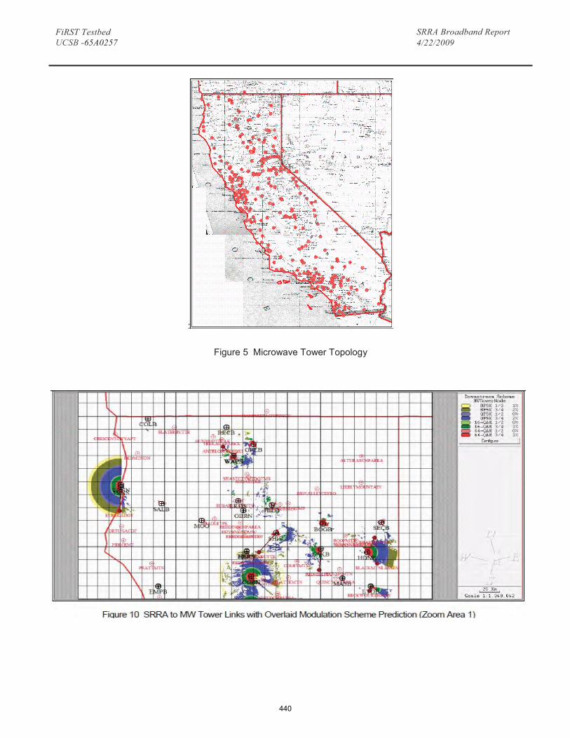
440
FiRST Testbed UCSB -65A0257
SRRA Broadband Report 4/22/2009
:
Figure 5 Microwave Tower Topology
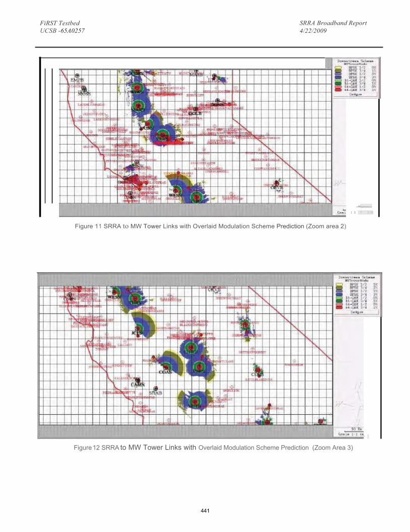
441
FiRST Testbed UCSB -65A0257
SRRA Broadband Report 4/22/2009
Figure 12 SRRA to MW Tower Links with Overlaid Modulation Scheme Prediction (Zoom Area 3)
J '
Figure 11 SRRA to MW Tower Links with Overlaid Modulation Scheme Prediction (Zoom area 2)
ir,,- -
1 l ? 2:?0
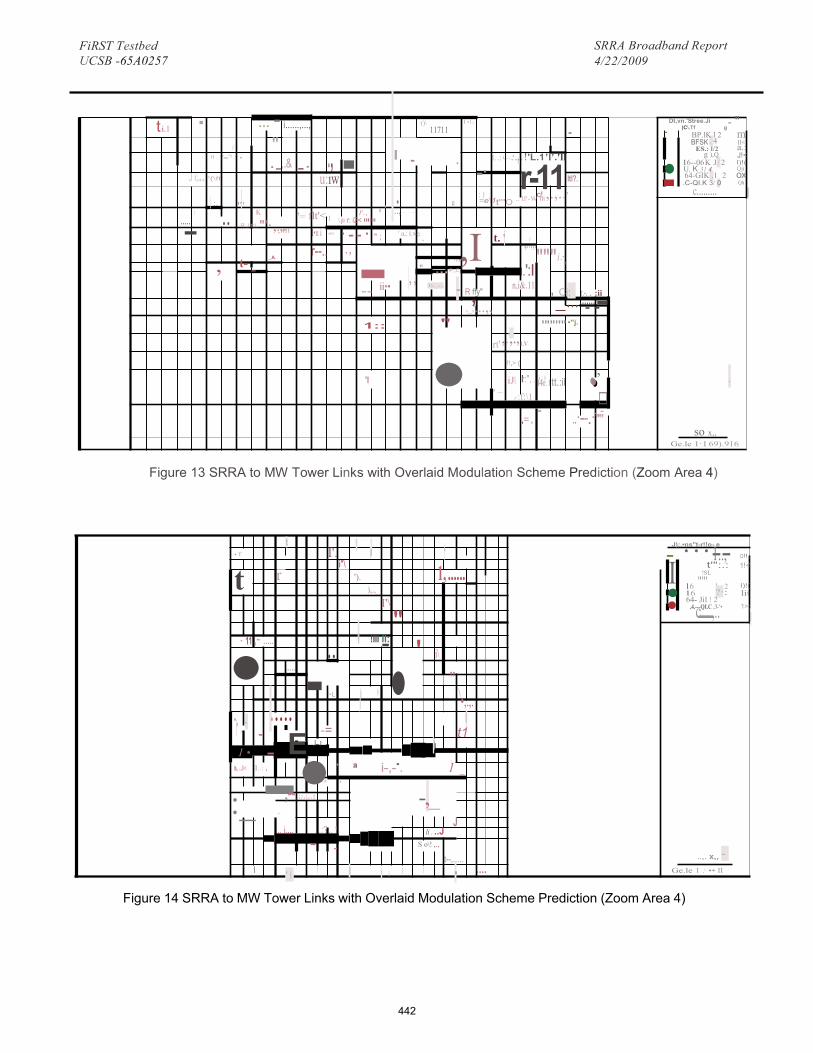
442
FiRST Testbed UCSB -65A0257
SRRA Broadband Report 4/22/2009
l
Figure 14 SRRA to MW Tower Links with Overlaid Modulation Scheme Prediction (Zoom Area 4)
' I - ···-1..-,J);,•ns"t-r!!o- e
• I t'":.: 1!< °'': !SL
16 ""' 2
• 16 ?·: 64- Jil ! 2
• I)!( lit 1>:
I
. ..... ' ,
- - • - .. '• L
I !Iii -II: "
,4.---QI.C .3-'• c........................................................................................,..
-= • ' \•,.,.
l t1
,I
- I
•
:_ . ,--
. a i-,-•. 1I _
-,_ .. i,,,.. .:? .. !
J S o\! ,.,
' I I ' • .... I I I I I t--,.....
-- li . ..J
,;;,i,.z
.. ,fl
1..: , h, ..l<
1 • l E-
- I
I I "
..... i\
,- ..... · 11
..,. x,, - Ge.le 1 : •• ll
I'\ ),.,_
1, ...... '). r t i"\
' I'.• T
I t
Figure 13 SRRA to MW Tower Links with Overlaid Modulation Scheme Prediction (Zoom Area 4)
t i.1 · H ,_.,(:
-
... - i......,...," ·-,.& -· - · ()\ l •1.: Dt,vn.'Stree.Ji
11711 - - )C\.Tf g
., - . -·l. .: i,,. , :...!'L.1 'l'.'ll
r-11
BP.lK l 2
- - "
mBFSK , 4 ll<
•ES.: l/2
g ),Q 16--06 K J / 2
a.: J!< I)!(
U, K 31 4 Qj( ,1 i;,,., '{\ft u:iw ltl?. 64-GIK ,1 2 ox
Ql(
· :. ,., • : ) c! ,.,..,
.C-QI.K 3/ 0
..-...c......... I
1 .. u =e\1t""O .. ll'-W Ill
' K
R',J ttJ, "'· ,.,. '= flt'< I r., ' ' ..,f .. . . ....
, m ,,, \ jlr r: i2< '"'" · - - ·
, t- -_A.
l•n i
r--.. - " ; ., ' a,: l.>c .
. .,,.,I t. '
-- ii•• ,, " ... P,:,C
J)._-.,
-' ,, - R ffy"
,..r.,,,
.':I n,i&.11
""" i ··,,
,_,...,, - 1::
'I • "
rt' ,.',., LV
!!,> (
... '""''" •"j.
, Ci; ....... r.-, - - , :ii
iJl Ir:", . i.:) ,_
T' :f:\1 •••□, .
,= ,
l4r.1tt.:il
- ..·--.· "", -
so x,, Ge.le 1·1 69).916
443
FiRST Testbed SRRA Broadband Report UCSB -65A0257 4/22/2009
2.1.1 Profile Results As an example, we have included examples of potential successful links (Figures 15 and 16), as well as links that were rejected (Figures 17 and 18).
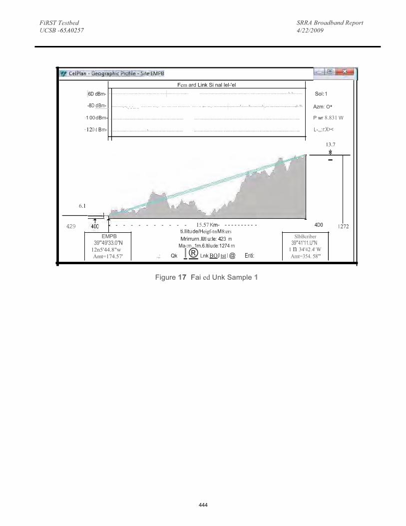
444
FiRST Testbed UCSB -65A0257
SRRA Broadband Report 4/22/2009
Figure 17 Fai ed Unk Sample 1
· Sol: 1
.
· 1 00 dBm- . · 12D d Bm- .
Azm: o• P wr 8.831 W
L -.,,: r:X><
13.7
*
6.1
429 - - - - - - - - - - - 15.57 Km- - - - - - - - - - - 4D0 1272
EMPB 39"'49'33.0''N
12n5'44.8"w Amt=174.57'
ti.llitu de/Heigf-t n M 8:ers Mrirrurn.llJtl u:le: 423 m SlbBcriber
.,; Qk I ® Lnk BOJ tst l @ M a-:m ..1rn.6.ltilu de: 1 274 rn
Enti: 1 n 34'42 .4' W Amt=354. 58"'
39"'41'11.U"N
··································································· ························································································· ····· ········ ··········-··-.,·..·... .. ···· ··· ···-· ··· ··· ··· ········· ···· ·· •··· ···-· ····················································· -·····························•············
.................................................................. .................................................................................................. .................................... ............................... ..................................................................................................
Fcm ard Link Si nal lel-'el -6D dBrn-
-8D d Bm-

445
FiRST Testbed UCSB -65A0257
SRRA Broadband Report 4/22/2012
3 Specifications & Acceptance Template
3.1 Introduction The FiRST Testbed research ream has developed a template of specifications, installation guidelines, performance measures, and acceptance test that can be used for a generic SRRA site. In collaboration with the ORC, Caltrans will apply and secure statewide licenses for both the 4.9 GHz and 5.9 GHz bands. Initially, we will use the equipment procured under the DHS-ITEP and that were transferred to the FiRST Testbed. These are Wi4Net radios (FR2003) that can be used for WiFi Access (2.4 GHz), as well as the 4.9/5.9 GHz bands. Based on District 6 observations at the SRRA, It is safe to assume an average of 20 simultaneous users at any given time, with mixed data rates. Support for Video Surveillance Overlay specifications at the SRRA assumes using the 4.9 GHz.
Basically, we assume availability of some form of backhaul at each SRRA, with wireless backhaul as the main option. Alternatives to Wireless Backhaul are considered outside of the scope of this project. In general, throughout this chapter, reference is made to “Wireless Backhaul” as means of backhaul to each SRRA.
3.2 Definitions Annex A and Annex B include a list of acronyms and units referenced in this document.
3.3 Radio Specifications Vendor shall provide for Wireless Access at each SRRA utilizing the 2.4 GHz band (WiFi based) for wireless access by SRRA visitors, with optional overlay (in addition to 2.4 GHz) of 4.9 GHz and/or 5.9 GHz access (WiFi based) for government purposes. Where feasible, Vendor will provide for Wireless Backhaul from the statewide (microwave) network to the SRRA. Caltrans will provide optimum Microwave tower location for establishing the backhaul connection, with signal interface point (Ethernet). Where such Wireless Backhaul is not available, Caltrans will provide an alternative form of backhaul. Where applicable, Vendor will provide for a short haul wireless link that connects the Northbound / Southbound SRRA’s or Westbound / Eastbound SRRA’s, so that one of SRRA’s leverages the backhaul of the other.
3.3.1 Wireless Access Vendor shall meet the following specifications:
a) Transceiver type: Broadband, Time Division Duplex, ODFM, Non Line Of Site capable
b) Transceiver frequency (standard): 2400-2483.5 MHz
c) Transceiver frequency (optional): Public Safety 4940-4990 MHz; ITS 5850-5925 MHz
d) Channel Bandwidth: 5, 10, 20 MHz
e) Antenna type: Omni-directional, 6dBi gain or more, diversity (two antenna) implementation
f) Power Output (from radio): +20dBm minimum, adjustable
g) Receiver sensitivity: Exceeding values in table below

446
FiRST Testbed UCSB -65A0257
SRRA Broadband Report 4/22/2012
h) Data protocol: WiFi-based, 802.11 a/g -based
i) Security: AES, WPA, WPA2, TKIP
j) QoS: IEEE 802.1p / 802.1q, WME
k) Remote Management: SNMP, TelNet
l) Digital connection type: RJ45
m) Environmental: Designed and rated for full weather exposure
n) Mounting provisions: Brackets and band clamps for attachment to pole (round aluminum, octagonal concrete, round wood, and round steel)
3.3.2 Wireless Backhaul Vendor shall meet the following specifications:
a) Transceiver type: Broadband, Time Division Duplex, ODFM, Non Line Of Site capable
b) Transceiver frequency (standard): Public Safety 4940-4990 MHz
c) Channel Bandwidth: 5, 10, 20 MHz
d) Antenna type: Directional, 21dBi gain or more
e) Power Output (from radio): +20dbm minimum, adjustable
f) Receiver sensitivity: Exceeding values in table below

447
FiRST Testbed UCSB -65A0257
SRRA Broadband Report 4/22/2009
g) Data protocol: WiFi-based, Pre-WiMAX-based or WiMAX-based (Vendor shall specify recommendation)
h) Security: AES
i) QoS: IEEE 802.1p / 802.1q (Vendor shall specify other QoS features)
j) Remote Management: SNMP, TelNet
k) Digital connection type: RJ45
l) Environmental: Designed and rated for full weather exposure
m) Mounting provisions: Brackets and band clamps for attachment to pole (round aluminum, octagonal concrete, round wood, and round steel)
3.4 Wireless Generic Implementation
3.4.1 Generic Implementation As described in Section 3.3, the basic concept assumes a form of backhaul to each of SRRA, with wireless backhaul as the main option. Alternatives to Wireless Backhaul are considered outside of the scope of this project. In general, reference is made in this document to “Wireless Backhaul” as means of backhaul to each SRRA. It is assumed that a “Long haul Wireless Backhaul” will connect either the Northbound/Westbound SRRA or the Southbound/Eastbound SRRA to the State Backhaul network. It is assumed that the SRRA with backhaul connection (whether to the State Backhaul Network or an alternative form of backhaul) will connect to the other SRRA (if applicable) through a “Short haul Wireless Backhaul”. The following diagram depicts this concept in more detail. Wireless Access would be provided in 2.4 GHz as a standard, with the option to also provide Wireless Access in the 4.9 GHz band and/or 5.9 GHz band. The radio specifications in the previous section are written accordingly.
For the wireless backhaul connections, the licensed 4.9GHz band is assumed. Caltrans will comply with the rules governing the use of this band, and its applicability to the SRRA application. Alternatively, unlicensed spectrum (in the 5.x GHz bands) could be considered, and should yield similar results (assuming the unlicensed spectrum to have open channels available) in terms of the analysis presented in Chapter 2.

448
FiRST Testbed UCSB -65A0257
SRRA Broadband Report 4/22/2012
With regards to the number of simultaneous users, and throughput that may be expected, we are providing the following diagrams, assuming various possible average frame sizes. The average frame size will depend on the application (and particular mix of application at a given time), where, for example, a VoIP application would have a small average frame size, and a FTP application a large frame size. The following graphs assume a frame size of 1024 bytes, 512 bytes and 128 bytes, respectively.

449
FiRST Testbed UCSB -65A0257
SRRA Broadband Report 4/22/2009
Figure 20 Throughput Versus Number of Users ( 512 byte packet size)
50 40 30
Air Data Rate(Mbit /s)
20 10
8.00
6.00 C)
4.00 0
w 2.00
0.00 0
I- ..
- 30@512 50@512
'S 10.00 -¼-
C. Cl 2 0
.Q 12.00 - - 10@512 20@512
!! 14.00 .t::
----..-1@512 16.00 - 2@512
5@512
Effec ti ve Optim um Throughput (MbiUs) for different number of sources
and packet size
Figure 21 Throughput Versus Number of Users (128 byte packet size)
Air Data Rate(Mbit/s)
50 40 20 ----- ----- ----
30 0 .00 ------ ----- 0 10
ti .w:!
- - - - - - - - -:-:.=- -=- ---! -=-- ""'""'=- - &_ 4 .oo - 30@1281--- - - - - - -
g, 3 .00 -+- 50@128 0 I- C)
- 1 0 @1 28 1---- - - - - - - - - - - ============== ; === =1 --¼- 20@128
-+- 1@128 2@128
6.00 5@128
Effective Optimum Throughput (Mbit/s) for differ ent number of source s
and pac,ket size

450
FiRST Testbed UCSB -65A0257
SRRA Broadband Report 4/22/2012
It should be realized that the graphs depict simultaneous sessions. Typically, many more users are in fact connected to the same AP at the same time, but the actual number of users actually sending or receiving data is much smaller than the number of people connected. This is because of the nature of typical applications of the users, such as e-mail and web- browsing. The graphs reference the number of users actually sending and receiving information.
There are 8 modulation levels identified for each of the lines in each graph in accordance with the IEEE 802.11-2007 standard specifications. For a 20 MHz channel, under ideal conditions, an “Air Data Rate” of 54 Mbps applies, but under reduced link conditions, this will drop to one of seven lower modulation levels, as depicted in the graphs. Based on the above graphs, and assuming an average package size of 512 bytes (Figure 20), and an average modulation level 4, the throughput with 5 users is about 5 Mbps. This means that each user on average experiences a throughput of 1 Mbps. However, the actual number of connected people may be well over 20, since typically only few of the connected users are actually transmitting or receiving data at the same time. Therefore, based on this example, the user experience of 20 connected users can be expected to result in a 1 Mbps connection rate. The above example assumes that the backhaul will be able to support the aggregate 5 Mbps capacity, or possibly more than this if traffic from a Northbound/Westbound and Southbound/Eastbound SRRA is combined over the backhaul.
3.5 Video Surveillance Overlay Design Caltrans is planning to implement a video surveillance overlay implementation at the SRRA sites. It is assumed that the central monitoring & control location shall be accommodated with server and viewing station, with a scalable, software Digital Video Management Solution (DVMS). At selected SRRA locations, a PTZ camera shall be added, in combination with a weatherized equipment enclosure to accommodate encoder (if not using an IP camera), power supply and local storage capability. Local access shall be possible through the 4.9 GHz band, and remote access and viewing shall be provided for utilizing the SRRA backhaul connection.
The PTZ camera shall either be co-located with the Wireless Access radio (using wired Ethernet connection), or, in case a different location at the SRRA would provide for a better camera position, the camera shall be equipped with a 4.9 GHz wireless connection to connect to the backhaul point at the SRRA.
3.5.1 System Requirements Vendor shall propose a video overlay option with the following system requirements:
a) At SRRA, the following equipment shall be offered:
i. PTZ Camera
ii. Encoder (if PTZ camera is analog)
iii. Local Storage
iv. Optional Wireless Connection (if camera and Wireless Access physical location at SRRA are different, based on optimum camera location, from field of view perspective)
v. Outdoor Equipment Enclosure
b) At central monitoring & control location, the following equipment shall be offered:
i. Server
ii. Storage capability
iii. Viewing Station with monitors
iv. DVMS
The following diagrams provide a schematic of the video overlay system implementation.

451
FiRST Testbed UCSB -65A0257
SRRA Broadband Report 4/22/2012
3.5.2 Camera Requirements Caltrans should select a preference with regards to optical zoom for the cameras. The standard industry options for professional level PTZ cameras are 23X, 26X or 35X. The higher this number, the more expensive the camera (but better quality video is achieved at further distances). We assumed 35X in this document for reference purposes only.

452
FiRST Testbed UCSB -65A0257
SRRA Broadband Report 4/22/2012
Vendor as a minimum shall meet the following specifications:
a) Camera Type: Analog video camera, with PTZ capability and IP interface (IP Camera).
b) Pan Range: 360 degree continuous rotation range.
c) PTZ format: Pelco and Competitive Control Protocol or similar.
d) Format: NTSC color, with Black & White capability (auto switching)
e) Lighting Level: At ½ second shutter speed, 0.1 LUX (color), 0.02 LUX (Black & White)
f) Shutter Speed: ½ -1/30,000 second, automatic
g) Resolution: Up to 4CIF (user definable)
h) Lens zoom range: 35X optical (with an additional 12X of digital zoom)
i) White Balance and Gain Control: Automatic, with manual override/disable
j) Optical Zoom Speed: 3.0 seconds minimum
k) Window blanking: User defined rectangular shapes, 8 minimum, to mask camera view
l) Camera dome housing and mount requirements:
i. Environmental Requirements: -300C to +600C, full operation
ii. Environmental rating: NEMA 4X
iii. Mounting means: Arm attached to a pole, holds camera assembly approximately 2 feet from the pole.
iv. Pole attachment requirements: Arm shall attach to round aluminum, octagonal concrete, round wood, and round steel utility poles. Mount shall not require holes to be drilled into utility poles. Also include building mounting solution, where needed.
v. Maximum wind surface area: 1 square foot.
vi. Housing heater: Thermostatically controlled, designed to maintain full camera operation down to –300C
3.5.3 Encoder Requirements Vendor shall meet the following specifications:
a) Basic purpose: Conversion of analog video signal from cameras to IP format
b) Input Signal: Standard 1.0 volt Peak to Peak, 75 ohms, NTSC format
c) Control Input Signal: RS232/422/485 Serial format
d) Output Signal: IP format, 10/100 Base T auto sensing
e) Digital Video Streams: 2 each, MPEG-4 standard
f) Frame Rate: Individual selectable, up to 30 per second (adjustable), 700 horizontal, 480 vertical

453
FiRST Testbed UCSB -65A0257
SRRA Broadband Report 4/22/2012
g) Output connection type: RJ45
3.5.4 Local Storage Requirements The following table reflects the needed capacity for 4CIF resolution and based on average motion. A 250GB of local storage capacity yields about 17 days of storage at 15 FPS. Typical field numbers may result in 17-30 days of actual storage capacity (based on our experience).
Vendor shall meet the following specifications:
a) Video Storage Capacity: 250 GB minimum
b) System must be fully compatible and integrated with central DVMS system
c) System shall allow local access for configuration of all system parameters (frame rates, resolution, PTZ patterns, motion detection, etc.)
d) Local Storage system shall allow for the system to work independently, with all features available at the Central
Monitor Station, even if no backhaul connection to the Central Monitor Station is available.
3.5.5 Enclosure Requirements Battery back-up function shall be considered for each individual site. A sample requirement is referenced in the video overlay portion of the requirements, but could be requested also for the Wireless Backhaul and Wireless Access radios. Furthermore, equipment housing type should be based on Caltrans requirement. Stainless steel is suggested for reference purposes only.
Vendor shall meet the following specifications:
a) Equipment housing: All pole mounted equipment, with the exception of the camera and its associated camera
housing, shall be contained within an equipment housing
b) Housing type: stainless steel, hinged door, boltable, NEMA 3R minimum
c) Housing Size: 12” wide x 16” high x 7” deep, maximum
d) Housing Mounting: brackets and band clamps for attachment to pole (round aluminum, octagonal concrete, round wood, and round steel)
e) Penetrations: All entry into this housing shall be weather rated
f) Required Input power: 120 Volts AC.
g) Power source attachment: Provide a weathertight power connection.

454
FiRST Testbed UCSB -65A0257
SRRA Broadband Report 4/22/2012
h)
Transient protection: Provide suitable means to protect all pole-mounted equipment from electrical disturbances and transients originating from electrical power source.
i) Brownout/ Blackout protection: Provide means to keep all pole mounted equipment full function during a power source outage of up to 15 minutes.
j) Fusing: Overcurrent protection of all pole mounted equipment. Install internal to equipment housing. Provide external pilot light (red, visible from ground level) that indicates overcurrent protection is open.
3.5.6 Central Monitoring & Control Requirements Caltrans shall specify monitoring requirements for individual SRRA, as a starting point, two (2) 19 inch screen are suggested. With regards to central storage, the required capacity depends on the number of cameras and storage policy. The resolution and frame rate of the video to the central location will depend on the backhaul capacity. It is recommended to request a scalable Direct Attached Storage (DAS) solution as a cost-effective starting point. This solution is recommended to be expandable at least to 6TB of raw capacity. The following table allows for calculation of required storage, based on the actual architecture.
Vendor shall meet the following specifications:
a) Vendor solution must include software that can control the pan, tilt and zoom (PTZ) capabilities of all cameras that
are part of the system.
b) Vendor solution must include color analog cameras that have the capability of monochrome night vision that is automatically activated by built in sensors that detect light level or by use of motion detection.
c) Vendor solution must include software that has built in security functionality to control user account access and an
audit trail for all files accessed.
d) Must have three (2) 19” widescreen LCD displays with software that allows user definable views from one to 16 cameras per screen.
e) Central Monitoring Station must be able to control 50 cameras minimum.
f) All digital video signals from the cameras must be able to be recorded.
g) Central Monitoring Station must be equipped with Direct Attached Storage (DAS) solution, incorporated with the
server machine, with the capability to expand to 6TB of raw capacity.
h) Video output can be used on analog and or DVI standard monitors.
i) Software must provide a logical map of cameras and associated equipment locations.
j) Software must have the capability to rename the cameras on the logical map.
455
FiRST Testbed UCSB -65A0257
SRRA Broadband Report 4/22/2012
k) Preset PTZ locations must be selectable on the system software Central Monitoring Station.
l) Software must support an unlimited number of user accounts.
m) Vendor solution must include software that has built in security functionality to control user account access and an audit trail for all files accessed.
n) Vendor solution must include a database (e.g. Microsoft SQL) that stores activity logs and audit trail information.
o) System must offer definable levels of system access and control including, but not limited to, specific cameras for
specific users.
p) Any network PC must be able to be used as an additional monitoring station and control the camera used.
q) Video (live or archived) can be made available for viewing over the WAN/network.
r) Security and authorizations are required.
s) Logging of all such activity is required.
t) System must use MPEG-4 or h.264 video compression.
u) Vendor solution must have the ability to detect motion and activate camera recording upon detection of motion with a pre-event buffer.
v) Must have browser based access control and management of cameras.
w) Joystick required for manual selectable remote control of the cameras at the Central Monitoring Station.
x) System must have the capability of accepting other video feeds (i.e., DOT cameras, IP based).
y) System must offer search and playback capabilities for each camera in the forward or reverse direction, frame by
frame, and from beginning to end.
z) Reviewed images can be zoomed in or out and be printed to a local or network printer.
aa) Still images must be exportable as a JPEG, TIFF or other acceptable equivalent file type.
bb) Must have/provide capability/equipment to transfer archived video onto removable digital media (CD/DVD) in a secured format to maintain integrity of the video and maintain chain-of-custody evidence requirements.
cc) Videos transferred onto removable digital media (CD/DVD) must be able to be played back on any Windows
based PC.
dd) Provide all software and hardware to remotely monitor and control the cameras.
ee) Provide all necessary equipment for one complete workstation capable of viewing and controlling video images and camera operations.
3.6 Training & Documentation Requirements Language Vendor shall provide Training according to the following minimal requirements:
a) Vendor shall prepare, administer and conduct on-site training program designed for 10 designated personnel to
fully and efficiently operate and maintain the installed system. Training will be of sufficient scope and depth to

456
FiRST Testbed UCSB -65A0257
SRRA Broadband Report 4/22/2012
ensure all designated personnel who complete the program shall be fully qualified, certified and capable of operating the system and subsystems as installed, including system configuration. All training shall be completed at least seven (7) days prior to scheduled start of the system.
b) Vendor shall provide a copy of all training aids and operational manuals to Caltrans
c) Vendor shall provide name and contact information of the person(s) or organization(s) that will assist the Caltrans with any technical questions for a minimum of six (6) months starting from the date of acceptance.
d) Description of complete training program including:
i. Duration of the training.
ii. What are requirements for training facility (to be provided by Caltrans)
iii. Any optional training that is not included in the price of the proposal, but available for additional fees that is to be provided.
e) The Training Program is expected to address at a minimum:
i. Basic radio installation procedure
ii. Radio configuration procedure (local and remote)
iii. Basics of radio planning (as relevant to deployment) and overview of implemented radio channel plan
iv. How to manage system
v. How to operate the hardware and software to control camera capabilities such as zooming, panning, focusing, etc.
vi. How to record and retrieve data, as well as storage and backup procedures
vii. How to conduct a search and retrieval process of pre-recorded video from the server according to time stamps and any other identifier that may be used
The Vendor shall provide Caltrans the following minimum documentation:
a) Operations manual and specifications of all installed hardware and software
b) Overall network diagram and IP addressing scheme
c) Site generic wiring / connection diagrams for radio sites and camera sites
d) Radio plan and FCC licensing information for all wireless radios and links
3.7 Maintenance & Support Requirements Language Vendor must provide complete details on provided maintenance & support services addressing the following minimum issues and requirements:
a) Period of maintenance coverage shall be 1 year from the date of acceptance
b) Phone support and procedure. Vendor must indicate whether this service is offered 24/7 or otherwise.
c) Describe response procedure for:
i. First-time response to service calls
ii. Escalation calls

457
FiRST Testbed UCSB -65A0257
SRRA Broadband Report 4/22/2012
d) Equipment replacement procedures and policy for maintaining spares locally. Maintenance shall provide for replacement of any failed equipment with related services.
e) Emergency response service with a guaranteed response time, location of dispatch by responding party and process to be followed for the following events:
i. Backhaul radio outage
ii. Access radio outage
iii. Network control and monitoring center outage
iv. Camera outage
f) Maintenance coverage for routine services on a periodic basis, including cleaning (for cameras), filter replacements, and other applicable required routine maintenance. Vendor shall detail what the routine maintenance services comprise of and how many times per year they will be performed.
g) Maintenance plan shall include software and firmware patches, upgrades, and related implementation services.
h) Suggest optional maintenance service plans and reasons for recommendation. Vendor shall include option for extended maintenance for period of 5 years from the date of acceptance.

458
FiRST Testbed UCSB -65A0257
SRRA Broadband Report 4/22/2012
4 Location for Pilot Installation
4.1.1 Limitations of the Gaviota Site Originally we surveyed the Gaviota site as a pilot for the SRRA installation. The Gaviota site includes both a Northbound and Southbound SRRA. Based on our site survey, we determ ined that a Short haul backhaul between the two sites would be feasible. Al so, a small building is available to m ount equipment and connect to power. The lim itation of the site is that a Long haul Wireless Backhaul to the State Backhaul Network, according to our st udy in Chapter 2 of this report, is not possible. An alternative form of backhaul would need to be considered to be able to utilize this SRRA for a test implementation. Also, an additional wireless repeater may be used here to achieve a backhaul connection.
4.1.2 UCSB - HWY 217 Pilot Site Based on the above limitations, we chose to use the UCSB-East Gate (EG) located at HWY 217 as an alternative test site to v alidate the SRRA technical require ment and other future testing required for the FiRST Testbed Interoperable Communi cation task. This location provides an acceptable view from the camera, easy access for the UCSB backbone fiber optic network, and will allow th e research team easy access to the test facility in a safe manner.

459
FiRST Testbed UCSB -65A0257
SRRA Broadband Report 4/22/2012

460
FiRST Testbed UCSB -65A0257
SRRA Broadband Report 4/22/2012
The EG pilot implementation would allow verifying all specifications with an actual implementation, and with actual measurements. The FiRST Testbed will validate the above template of specifications, installation guidelines, performance measures, and acceptance test. We intend to use hardware from various vendors for a generic Wi-Fi (802.11a/g) and wireless broadband at 4.9 and 5.9 GHz spectrum (Wi4 Net), as well as DSRC standard compliant devices (Denso, Siemens, ARADA, etc.)
The pilot will validate the video overlay requirem ents as addressed in the above s ection. We chose to install the PTZ camera collocated with the W ireless Access radio, and connected through the f iber optic backbone provided by UCSB at the EG cabinet. Alterna tively, the camera could be placed away from the Wireless Access radio, with a wireless link. The FiRST Testbed will have access to the West Gate camera controlled intersection, and will tap in to the video feed and provide a se lf-enclosed solution that includes also local storage with video stored at this unit at 15 or 30 FPS (and 4CIF resolution). Remote viewing and control at variable rates to test video quality at different compre ssion methods and wireless bandwidths. The variable frame rate will be available on a conti nued basis, or just on de mand. Any stored video will only be used for the FiRST Testbed and other resear ch needs and in accordance with the UC rules and regulations.
4.2 Best practice Installation Procedure
4.2.1 Site Survey / Pre-Installation Activities a) Identify geographic locations for each system component (e.g. radio, enclosure, cam era, etc.) and
make note of geographic references such as GPS la titude/longitude coordinates street intersection with corner identification, pole numbers from city plates, etc.
b) Check LOS/non-LOS scenarios between radios , and assess LOS conditions for access po int locations and camera locations. Report / justify recommendation of location of each component.
c) If feasible, perform link throughput test with test radios until the minimum necessary throughput is obtained between nodes on each link. Take note of the equipm ent used such as antenna m odel numbers, cables lengths/losses and antenna height.
d) Take pictures of the system component locations. Identify mount locations, and Caltrans interface points (signal and power). Determine applicable cable length.
e) Verify unlicensed channel utilization at each location, for applicable bands.
f) Generate an RF channel plan for all radio components.
g) Generate summarized report describing the information above for each system component location in the network.
4.2.2 Installation h) Create a plan establishing dates for installation of each system component and site.

461
FiRST Testbed UCSB -65A0257
SRRA Broadband Report 4/22/2012
i) Provide pre-configured radios wi th adjusted cabling to field crew , in accordance with project schedule.
j) Notify the Caltran s project m anager that the in stallation will sta rt 2 days prior to the f irst visit, identifying the names of the field crew personne l involved and the description (m ake/model/color) and license plates of any vehicles that will be used throughout the installation process.
k) Before the work at a given site, co nfirm readiness of interface points (signal and p ower) with the Caltrans.
l) At the first site visit to install the system components, verify readiness of Caltrans interface points (signal and power). Also, confirm any differences in cable lengths, compared to prepared cablin g and cable length as measured during the site survey. Confirm mount brackets and mount location.
m Install Long haul W ireless Backhaul link and antennas. Pow er the components and verify that all devices are powered up. Connect a la ptop to the Ethernet connector at the subscriber location and telnet to the radio controller that serves as an AP. Verify the conn ection. Verify that signal levels and modulation schemes achieved are accep ted. Throughput tests can be run to ensure pro per individual link performance. Verify antenna pointing to be optimized.
n) Install Short haul W ireless Backhaul link and antennas. Pow er the components and verify that all devices are powered up. Connect a la ptop to the Ethernet connector at the subscriber location and telnet to the radio controller that serves as an AP. Verify the conn ection. Verify that signal levels and modulation schemes achieved are accep ted. Throughput tests can be run to ensure pro per individual link performance. Verify antenna pointing to be optimized.
o) Install Wireless Access AP and antennas. Pow er the components and verify that all devices are powered up. Utilize a W iFi enabled laptop to ve rify connection. Verify that signal lev els and modulation schemes achieved are accepted, nearby th e AP. Throughput tests can be run to ensure proper individual link performance.
p) If applicable, install cam era overlay components. If wireless conne ction to the backhaul point is required, wireless link needs to be verified (following instruction as in item f) above). Local Storage device shall be programm ed to adjust camera automatically (create pattern), prog ram encoder and set archiving settings.
4.3 Best practice System Testing & Commissioning a) Report on m easured signal level, modulation sc heme and throughput for applicable wireless
backhaul connections.
b) Perform drive-test / walk-test to assess coverage in the accessible areas of the site. The coverage map should justify th e selected location for th e Wireless Access radio(s). Report with coverage map indicating measured modulation scheme.
c) If applicable, report on local settings of video system such as reso lution/frame-rate for ea ch stream, areas of interest program med into the pattern, and record ing settings). Commission each

462
FiRST Testbed UCSB -65A0257
SRRA Broadband Report 4/22/2012
camera at the central monitor statio n, assuming a sufficient bandwidth backhaul connection is in place.
d) Report to Caltrans about site completion, and provide summary report.
4.4 Best practice Acceptance Test Procedure Acceptance test will have the following basic template format.

463
FiRST Testbed UCSB -65A0257
SRRA Broadband Report 4/22/2009
Appendix A – Caltrans SRRA Steering Committee (SC) Questions & Assumptions

Appendix B – Caltrans SRRA Workgroup Input
464
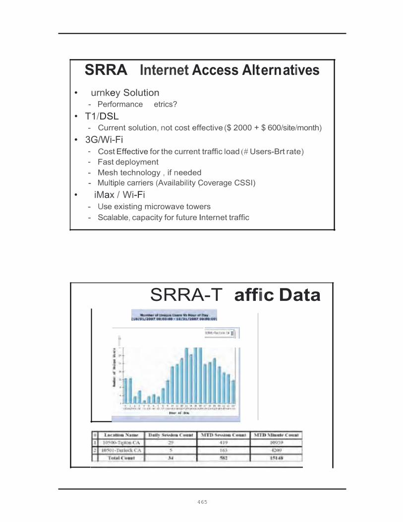
465
• iMax / Wi-Fi - Use existing microwave towers - Scalable, capacity for future Internet traffic
1 Multiple carriers (Availability Coverage CSSI)
Cost Effective for the current traffic load (# Users-Brt rate) Fast deployment Mesh technology , if needed
- - - -
- Current solution, not cost effective ($ 2000 + $ 600/site/month) 3G/Wi-Fi
etrics?
•
- Performance T1/DSL •
SRRA Internet Access Alt ern atives • urnkey Solution
SRRA-T affic Data
"

466
moth ly cos t /Site (- $1 00 :about 15 % of the cost of T1 ) RA ' s ) th e DGS delegauon · or a 1I SR 550□ t site (b elow
R o u g h O r d e r o f M a g n i t u d e ( R O M ) c o s t s
14 simultaneous user (pending test)No video downloading Most Cost effeo1ive Scalable ( for the near term traffic) Shortest installation time Best unlimited rate State contracting issue (CSSI) Coverage (RFI}
• • • • • • • •
• •
SRRA- Cost E, ffective lntern 1e t Acoess Current SRRA 'Traffic .. Number of users rs about 5'0/day • Tripton has more Wi-Fi traffic than Turlock (5times)• 8 users/hr (Peak hours 12- 4 PM and 6 -8 PM)
Using 3G cellular Router {pending validation & verification)
S RA-E GWG _ Ge g,es, P.E.
1 1f1 51,Dl'
Ute Sa'<i11 R>e Olfi% Si!Uabc.la: ,r,v. ,'!l r.e i'l!!S&
- E' ended re, 11! All!l1lr11eo• E!V/i.fi Brifo e.''rmi srC"3r r 5.>.=i::un ·, s.. , in
1,/[d eo i:::a lllll!res. Ba l rr ;!Ind= @b--------
3G-2-WiFi • Identifled altemative products:
• Multi earner sorution (AT&T, Verizon. Sprint, T obile}• Multip le V e n dors• Different pack.i:_gi n _g, power , etc
· Testing soon

467
First Responder Support Systems Testbed (FiRST) Contract # 65A0257
Cross-Cutting Cooperative Systems
TRACK III – Interoperable Communications
Final Report
Multihop Networks: An Alternative Wireless Broadband Communications
Link Quality Metrics and Measurements in Public Safety & ITS Communications
Principal Investigator: Dr. Richard Church University of California Santa Barbara
Contract Manager: Ramez Gerges, Ph.D., P.E.

468
1 Abstract ............................................................................................................................... 469
2 Introduction .......................................................................................................................... 469
3 802.11 Wireless Link Challenges ......................................................................................... 469
4 Link Quality Metrics .............................................................................................................. 472
5 Measurements Techniques for Link Quality ......................................................................... 476
5.1 Active Measurements for Link Quality ........................................................................... 476
Passive Measurements for Link Quality ................................................................................... 478
5.2 Hybrid Measurements for Link Quality .......................................................................... 479
6 Applications of link qualities ................................................................................................. 479
6.1 Opportunistic Routing for Multihop Networks ................................................................ 479
6.2 Link Adaptation for Wireless Links ................................................................................ 480
7 Bibliography ......................................................................................................................... 482

469
1 Abstract Wireless networks are very different from wired networks. The nature of the medium
strongly impacts the performance of network’s protocols. Also, wireless networks offer greater control and flexibility as several network parameters such as topology, coverage and link rate can be controlled. New protocols have been developed which take advantage of distinctive wireless channel characteristics such as diversity and topology control. This report summarizes the developed metrics to capture and evaluate wireless link quality, proposed measurements techniques to acquire these metrics, and then some of the network systems to exploit link quality metrics.
2 Introduction In recent times there has been a great proliferation of wireless devices, and growing
popularity of 802.11 based wireless networks. These networks come in the form of enterprise networks, wireless hotspots, and more recently wireless mesh networks. The common underlying requirement of each of these networks is to provide good performance either improved throughput or satisfying QoS constraints. However the nature of the wireless medium, and 802.11 MAC protocol make it much harder to provide these guarantees when compared to a wired network. A wireless link experiences diversity, i.e., highly varying loss rate and bandwidth. Hence, maximizing throughput, guaranteeing fairness or QoS pose several challenges. This is further accentuated by artifacts of the 802.11 MAC such as the well known hidden node problem. Also, protocols developed for wired networks do not account for the characteristics of the wireless channel and this reduces their usability over wireless networks.
Wireless channels experience several distinctive characteristics. Being a broadcast medium,
interference has a huge impact on protocols, both from within the network and from external sources. In addition, RF propagation characteristics cause great diversity in the channel. It has been shown that it is very hard to abstract wireless channels with a simple model. The rest of this report is defined as follow: Section 3 gives an overview of the wireless channel’s characteristics and challenges; Section 4 summarizes the developed metrics for wireless link qualities in literature, Section 5 lists the proposed measurements schemes to capture and monitor link quality metrics, then the paper ends with Section 6 in which examples of network systems that exploit link quality metrics are provided.
3 802.11 Wireless Link Challenges Compared to wired link, wireless communication suffers from high transmission errors and
its performance changes frequently and dramatically, highly depending on the channel quality, which usually exhibits great variability. The sources of variation include user mobility, environmental changes and interference. The rapidly varying channel condition results in changing packet error rate (PER), therefore making network bandwidth a highly dynamic resource. Due to the dynamic variability, the wireless link quality needs to be measured and provided to wireless applications and protocols, in order for wireless networks to most effectively utilize and manage resources. Many performance improvement mechanisms depend on this information. For example, in order to perform load-balancing or power-control in WLANs, the link quality between access points and clients must be measured (1), (2).

470
Moreover, routing protocols seek effective routes, which consist of high-quality point-to-point links, in multi-hop deployments; therefore the goodness of the component links along a path needs to be periodically evaluated (3), (4). Similarly, link quality affects the performance of wireless sensor networks, including network lifetime, network throughput, resource usage and reliability (5), (6), (7), (8).
As indicated, among the main factors affecting link quality are RF Propagation
characteristics. The mechanisms involved in RF propagation are diverse, but can be attributed to reflection, diffraction and scattering. The resultant signal experiences two kinds of effects, large scale path loss and small scale fading.
Large scale path loss: The average received power for a signal drops off with distance, and this is referred to as large scale path loss. There are many models which predict received power/signal strength. Some examples are Free Space (Pr.a.Pt / d2) and Two Ray Ground (Pr.a.Pt / d4) where Pr is the received power, Pt is the transmitted power, and d is the distance between transmitter and receiver. Both theoretical and measurement based models indicate that the average signal strength decreases logarithmically with distance. Large scale path loss determines the coverage of a transmitter, thus its interference region. Actual coverage of the transmitter depends on the obstacles present, interference and other factors. Small scale fading: Signals transmitted from a radio arrive at the receiver at slightly different times due to different paths followed, this phenomenon is called multipath. These waves combine at the receiver antenna and cause the resulting signal to vary widely in amplitude and phase. This causes rapid fluctuation in signal quality over small periods of time or distance and is called small-scale fading. These effects are further amplified when the obstacles are moving objects. This causes fluctuations in channel bit error rate, causing fluctuations in packet loss (9), (10).
Both these factors affect the strength of the received signal at the receiver. The packet is
received by the card if the received signal strength is greater than a threshold. Received signal strength, and noise floor can be used to indicate the goodness of the link and the average signal strength can be used to compute the transmitter receiver distance. Researchers have used signal strength stability to detect and ignore bad links in routing protocols (11), (12). Signal strength has also been used for indoor positioning of a wireless device in some coordinate space (13), (14), (15), which can then be used in geographic routing protocols (16), (17).
The network’s dynamic nature, combined with adverse signal-propagation effects, raises
issues that are difficult to address. In order to study the sensitivity of wireless link quality to adverse signal-propagation effects, authors in (18) ran extensive series of outdoor experiments to assess 802.11 link qualities, examining twelve factors that potentially influence it. All the conducted experiments used standard, off-the-shelf two hardware nodes that periodically sent messages to each other directly over the medium access control layer with a 2-Mbit-per-second transmission rate and maximum transmission power. For each received packet, authors recorded the link quality and used it to assess possible influencing factors. Signal strength of the received packets used as a measurement of link quality in these experiments. Signal strength responds quickly to changes in link quality, and current 802.11 cards use a large scale to describe it.

471
Experiments conducted by authors in (18) identified the following factors were highly influential:
User orientation: In most wireless applications, users carry portable devices such as PDAs or notebooks. Because such nodes are rarely completely still and their antennas are often not strictly omni-directional, experiments assessed the influence on link quality of a node’s orientation for all three axes in space. Results indicated that link quality is affected only slightly, and the resulting minor link quality fluctuations can be ignored. However, a node’s orientation is typically changed when the users holding the node changes the orientation of his or her own body. Thus, this user’s body shadows the link if the body blocks the line of sight between the two communicating nodes. Experiments consisted of placing two nodes at a fixed distance facing each other, while a person holding the node turned around. When the turning user faced away from the other node (around 180 degrees), the user’s body reduced the signal strength to such an extent that packets were lost. In further experiments, we found that the user’s shadowing reduced the transmission range from 250 meters in open space to approximately 150 meters. Because people often change their orientation, such frequent and significant link quality fluctuations are likely to occur. Dynamic object shadowing: In urban environments, dynamic objects such as people and cars are common. Obviously, these objects can shadow links and influence link quality. However, the significance of such shadowing varies. It is still possible, for example, to listen to a radio even if people are gathered around it, reducing the received signal. Experiments conducted to observe the affect of people and cars on link quality depends on their distance from the nearest node. Results showed that a single car between two nodes that are 100 meters apart is sufficient to cause packet loss if the car is 1 meter away from either node. Even at 5 meters, the car continues to exert considerable influence. Similar results were found for people, although their effect is weaker. Placing a single person in front of a node reduced signal strength severely (corresponding to shadowing by a user’s own body), and the influence was still considerable at a distance of 1 meter. Because cars and people appear frequently in urban environments — especially in groups — severe link quality fluctuations are likely. 802.11 card models: By definition, 802.11 wireless cards comply with the same specification; thus, if their transmission power is equal, we would expect the same behavior. However, cards from different makers can perform differently. In this experiment, authors recorded the received signal strength at different distances with either two 802.11 Brand A cards or two Brand B cards. The range, signal-strength decay, and packet-loss threshold differed in the experiments with the two types of cards. This is most likely caused by differences in radio frequency design and signal processing algorithms. Node height: In the conducted experiments, node height also significantly influenced link quality. If one node was below belt height, link quality degraded independently of the other node’s height. Thus, the performance of nodes placed at ground level is particularly poor and designers should avoid such placements in sensor networks. In military and disaster-recovery applications, frequent node height changes can occur and thus cause strong link quality fluctuations. For most applications, however, node placement is less significant as people typically carry nodes at a sufficient height.

472
Additional Issues: Authors assessed other candidate factors as well, but found them to have little or no influence on link quality. For example, the type of ground surface (such as sand or grass) had only a slight influence. Moreover, small-scale node movements (as when nodes are carried by a person, for example) had no affect on link quality. Large- scale movement at different speeds (evaluated up to 50 kilometers per hour) was also irrelevant for link quality (the Doppler shift is relevant only at much higher speeds). They also found no influence from communication patterns including message length, payload pattern (random content versus 0/1 alternating bits), and communication load (such as a low versus high number of transmitted messages per unit time). However, a high communication load can cause collisions and thus packet loss due to the hidden terminal problem because nodes incorrectly sense that the busy communication channel is idle. This is particularly noticeable in areas where many nodes are located close together.
4 Link Quality Metrics As we seen, link quality should be considered in developed protocols and schemes for
optimum network performance. Several parameters and properties of the network are used to measure and control link quality. We can categorize these parameters to:
Controllable Parameters: These comprise of tunable parameters such as transmit power, carrier sense threshold, link rate, and operating channel. These parameters affect topology of the network, including loss rate, connectivity, interference etc, and play a key role in link quality and corresponding protocol performance. Observable properties: These comprise of properties such as signal strength, bit error rate, and transmission time. These properties allow us to infer the current channel conditions and link quality and to make more informed decisions regarding which parameters to control.
The wireless link quality needs to be measured and provided to wireless applications and
protocols, in order for wireless networks to most effectively utilize and manage resources. In this section we summarize major link quality metrics proposed in literatures. Authors in (19) indicates that major studies for link quality typically employ one of the following four metrics in order to capture point-to-point link qualities. Each of these metrics provides an average estimation of the link quality over a period of time.
Received Signal Strength Indication (RSSI): is a dimensionless quantity, which represents the signal strength observed at the receiver’s antenna during packet reception. RSSI values vary from 0 to Rmax; the maximum value depends on the chipset of the wireless card. For example, wireless cards with the Atheros chipset report Rmax = 60, Cisco cards have Rmax = 100, while in Intel cards the RSSI provides the actual received power in the negative dBm scale (for example, RSSI = -55 for the Intel cards implies a received power equal to -55 dBm). Note that the specifications of each card provide a formula for translating the RSSI values to power (dBm). Signal to Interference plus Noise Ratio (SINR): represents the extent to which the power of the received signal exceeds the sum of noise plus interference at the receiver. Various models have been developed to map the SINR to the Bit Error Rate (BER) or the Packet Error Rate (PER) in presence of white noise or fading. Recent studies have
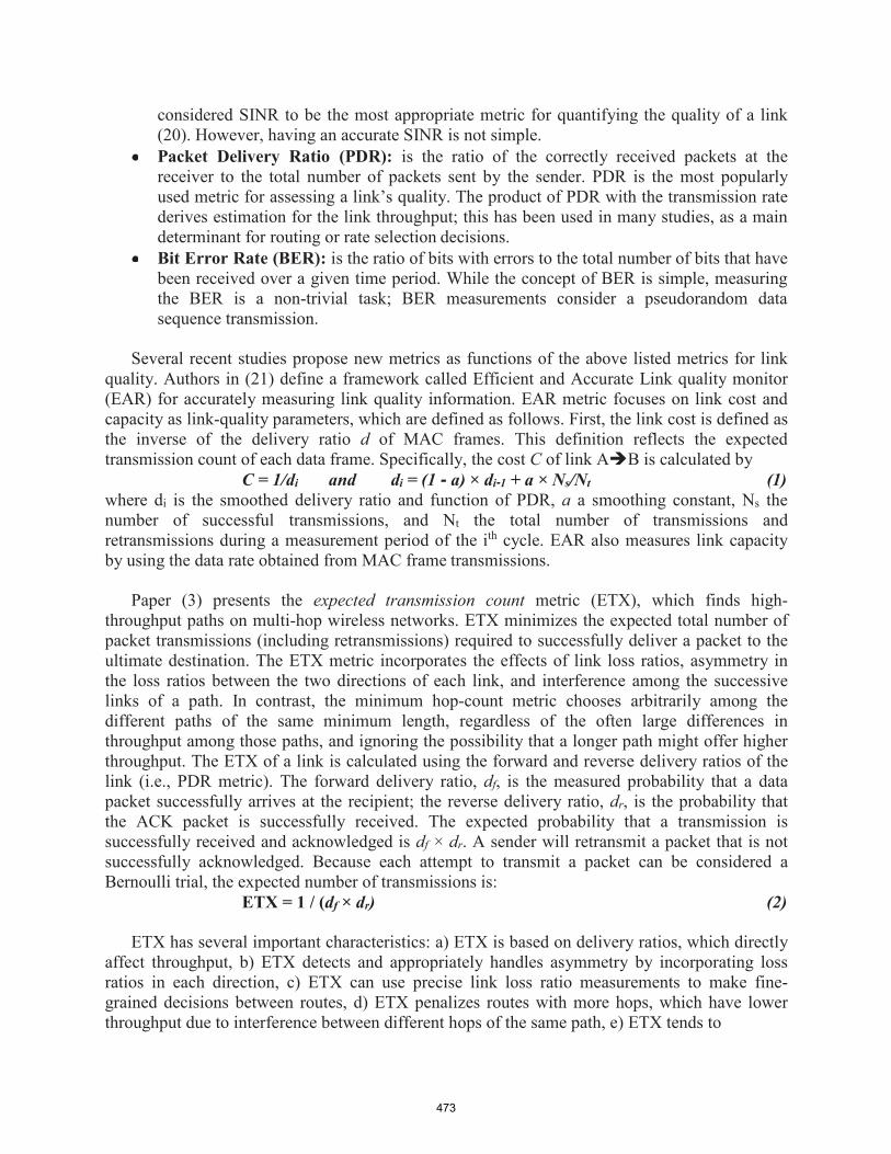
473
considered SINR to be the most appropriate metric for quantifying the quality of a link (20). However, having an accurate SINR is not simple. Packet Delivery Ratio (PDR): is the ratio of the correctly received packets at the receiver to the total number of packets sent by the sender. PDR is the most popularly used metric for assessing a link’s quality. The product of PDR with the transmission rate derives estimation for the link throughput; this has been used in many studies, as a main determinant for routing or rate selection decisions. Bit Error Rate (BER): is the ratio of bits with errors to the total number of bits that have been received over a given time period. While the concept of BER is simple, measuring the BER is a non-trivial task; BER measurements consider a pseudorandom data sequence transmission.
Several recent studies propose new metrics as functions of the above listed metrics for link quality. Authors in (21) define a framework called Efficient and Accurate Link quality monitor (EAR) for accurately measuring link quality information. EAR metric focuses on link cost and capacity as link-quality parameters, which are defined as follows. First, the link cost is defined as the inverse of the delivery ratio d of MAC frames. This definition reflects the expected transmission count of each data frame. Specifically, the cost C of link AB is calculated by
C = 1/di and di = (1 - a) × di-1 + a × Ns/Nt (1) where di is the smoothed delivery ratio and function of PDR, a a smoothing constant, Ns the number of successful transmissions, and Nt the total number of transmissions and retransmissions during a measurement period of the ith cycle. EAR also measures link capacity by using the data rate obtained from MAC frame transmissions.
Paper (3) presents the expected transmission count metric (ETX), which finds high-
throughput paths on multi-hop wireless networks. ETX minimizes the expected total number of packet transmissions (including retransmissions) required to successfully deliver a packet to the ultimate destination. The ETX metric incorporates the effects of link loss ratios, asymmetry in the loss ratios between the two directions of each link, and interference among the successive links of a path. In contrast, the minimum hop-count metric chooses arbitrarily among the different paths of the same minimum length, regardless of the often large differences in throughput among those paths, and ignoring the possibility that a longer path might offer higher throughput. The ETX of a link is calculated using the forward and reverse delivery ratios of the link (i.e., PDR metric). The forward delivery ratio, df, is the measured probability that a data packet successfully arrives at the recipient; the reverse delivery ratio, dr, is the probability that the ACK packet is successfully received. The expected probability that a transmission is successfully received and acknowledged is df × dr. A sender will retransmit a packet that is not successfully acknowledged. Because each attempt to transmit a packet can be considered a Bernoulli trial, the expected number of transmissions is:
ETX = 1 / (df × dr) (2)
ETX has several important characteristics: a) ETX is based on delivery ratios, which directly affect throughput, b) ETX detects and appropriately handles asymmetry by incorporating loss ratios in each direction, c) ETX can use precise link loss ratio measurements to make fine- grained decisions between routes, d) ETX penalizes routes with more hops, which have lower throughput due to interference between different hops of the same path, e) ETX tends to

474
minimize spectmm use, which should maximize overall system capacity.. In addition, ETX may decrease the energy consumed per packet, as each transmission or retransmission may increase a node' s energy consumption.
An extension to ETX metric is proposed in (22) that assigns weights to individual links based
on the Expected Transmission Time (ETT) of a packet over the link. The ETT is a function of the loss rnte and the bandwidth of the link. Authors defined the ETT of a link as a "bandwidth- adjusted ETX." In other words, link quality starts with the ETX (number of expected transmissions) and then gets multiplied by the link bandwidth to obtain the time spent in transmitting the packet. We can fonnalize this as follows. Let S denote the size of the packet (for example, 1024 bytes) and B the bandwidth (rnw data rate) of the link. Then:
ETI = ETX *SIB (3) Note that this definition of ETT does not incorporate backoff time spent waiting for the radio channel; it only reflects the time spent actually using the channel.
Authors in (23) develop a modified version of ETX, called mETX, to model long-teim link
quality and short-te1m link dynamics. mETX corrects ETX shortcoming that it doesn't cope well with short-term channel variations because it uses the mean foss ratios in making routing decisions. In addition a new routing metric caUed effective numbeJ of transmissions (ENT) is defined. Both the mETX and the ENT capture the time-varying characteristics of a wireless chailllel in a form that could be directly translated into network and application layer quality constraints. These metrics project both the mean and the variance of certain parameters of the physical layer onto the space of netwmking parameters using tools from large deviations theory and effective bandwidths.
Another link quality metric assessment method for mesh networks is defined in (24) and
named QUEST (QUality ESTimation). QUEST is based on a delivery ratio vs. SNR (Signal to Noise Ratio) mapping table called profile that can be managed offiine. QUEST estimates the quality of a target link as the delivery ratio by perfonning profile lookup for any incoming messages including broadcast hello, beacon, data packets, etc. Therefore, no designated protocol to achieve the delivery ratio infmmation, with the form of (delivery ratio, taTget neighbor, transmission rate)-tuple, is required in QUEST. The Figure 1: QUEST Algorithm QUEST algorithm is defined in Figure 1.
The link inefficiency (I) is proposed as link cost metric in (25). Authors model a link i to have a ce1iain Packet Success Probability PSPlt) at time t, such that every transmission is successful with probability PSP;(t) independently of the others, then the mean number of trnnsmissions is 1/PSPi(t) . Since the ene1·gy used foJ each re-transmission is assumed to be similar, the energy to transmit the packet successfully is prop01iional to I = 1/PSP;(t). While the perfectly efficient link
Al, oritl101 1 QUE I: RX NR-.=: N 2: dri {= D li ery 3: if fr. m re ive 4: d pr file I 5: end if

475
is I=1, this metric grows as a link gets worse, i.e., the inefficiency increases corresponding to a larger amount of energy spent on that link due to retransmissions.
Extending the work in (25), authors in (26) focus on two classes of estimators, Packet
Counting (PC) and SNR-based. PC estimators measure the packet success probability (PSP) directly by calculating the ratio of the number of successful packet transmissions to the total number of transmissions. The advantages of PC-based estimators are that they are simple, intuitive, and require little or no a priori information. Their disadvantages are the accuracy, timeliness, and overhead of the measurements. The precision of PC-based estimates depends on the number of transmissions of the packets of interest. On the other hand, a large number of transmissions incur latency in the estimate, which can make it obsolete in time-varying conditions. Furthermore, since packet success rate, in general, depends on the size of the packet and the data rate (i.e., the modulation-coding scheme) at which packets are transmitted, PC- based estimates are specific to the bit rates and packet sizes of the counted packets.
SNR-based link quality estimators in (26) make use of SNR measurements obtained from the
physical layer of the communications stack. They rely on the assumption that there is a strong correlation between the measured SNR and the current PSP of a link. The advantages of SNR- based estimators are that they potentially require fewer measurements, are more timely, and are more accurate than PC-based estimators in time-varying conditions. Their primary disadvantage is that they require prior information on the mapping between the SNR and PSP, which is environment and radio dependent. Authors in (26) surveyed the accuracy of SNR-based metric in previous literatures. A thorough study of an outdoor in (10) for static IEEE 802.11b network concluded that the SNR reported by the physical layer is not predictive of link reliability. However, the study also demonstrated that the multipath delays experienced outdoors far exceeded the delays tolerated by the radios that were used, generating significant inter-symbol interference. A subsequent indoor study in (27) of a static 802.11 network operating at the 2 Mbps data rate showed a strong correlation between measured SNR and PSP, and one that follows the theoretical relationship quite closely, provided external interference is limited. In (28), the authors showed an SNR-based estimator to converge more rapidly than a PC-based estimator on a link experiencing a sudden change in transmission power. This estimator maps Kalman-filtered SNR measurements to PSP using an empirical model. In other related work, (29) describes a hybrid approach using both SNR and packet counting to classify links as “good” or “bad”. However, authors of (26) mitigate the bias of using SNR measurements from only successfully received transmissions. The results suggest that SNR-based schemes have the potential to provide better and more efficient estimates of link reliability than PC-based schemes, especially as the time variability (or Doppler spread) of the channel increases.
Papers (30), (31) present ongoing work on short-term link estimation (STLE) that takes fine- grained link dynamics - in the order of milliseconds - into account and increases the prediction quality for successful packet transmissions, especially, for highly dynamic links. STLE integrates into routing protocols by adapting neighbor tables to accurately reflect the current situation of a dynamic link. Overall, short-term link estimation has three key contributions: (1) to predict the probability of successful packet transmission of any link type by taking short-term dynamics into account, (2) to suggest links of low to intermediate quality for routing when they have become temporarily reliable, and (3) to integrate easily with today’s long-term link estimators and routing protocols.

476
5 Measurements Techniques for Link Quality Metrics There is an increasing amount of research effort on measuring wireless link quality. Accurate
link-quality measurement is essential to solve the problem associated with varying link-quality, as one can see from the following use-cases.
Selection of the best relay node: Accurate link-quality information can reduce the recovery cost of lost frames caused by link quality fluctuations. Supporting Quality-of-Service (QoS): Wireless link-quality information enables applications and network protocols to effectively meet users' QoS requirements. For example, applications, such as VoIP and IPTV, can dynamically adjust their service level that can be sustained by varying link-quality in the network. On the other hand, link- quality-aware routing protocols can accurately locate a path that satisfies the QoS (e.g., throughput and delay) requirements based on the link-quality information. Network failure diagnosis: Link-quality statistics can be used to diagnose and isolate faulty nodes/links (or faulty areas), facilitating network management. This is very useful in case of wireless sensor networks in monitoring and covering scenarios since it is required to have a clear picture of local link conditions for network troubleshooting. Identifying high-quality channels: Link-quality information helps network to identify high-quality channels. Due to the use of shared wireless media, link-quality differs from one channel to another, and hence, determining the best-quality channel is of great importance to channel assignment algorithms.
It is important to remember that measurement techniques have their failings and the accuracy of the result depends on the methodology used. Measurement techniques have to address several challenges. Among those challenges:
Accuracy and efficiency. A measurement technique must yield accurate results at as low a cost as possible. Link-asymmetry-awareness. Measurement schemes must be able to identify and exploit wireless link asymmetry that results from interference, obstacles, or weather conditions. For example, if there is interference in the vicinity of node A, then signals from a remote node B to A might be disrupted, whereas signals from node A are normally strong enough to overcome the interference. While B might reach A via node C that has high-quality links to both A and B, node A can use the direct link to B, thus saving network resources. Flexibility and feasibility. Measurement techniques must be flexible enough to cope with time-varying link-quality.
Measurement techniques could be classified to three main categorizes: Active measurements
Passive measurements, and hybrid measurements that combine between active and passive measurements. In the following subsection we summarize the research efforts within these categories.
5.1 Active Measurements for Link Quality In this category, nodes usually probe link quality by injecting certain probe packets on the
corresponding link and observe the objective metrics. Two popular assessment methods to obtain link quality: broadcast probings and unicast probings. Broadcast probings (4), (3), (22) are further categorized to broadcastFR (broadcast with Fixed Rate) and broadcastMR (broadcast

477
with Multiple Rates). broadcastFR measures the delivery ratio using a fixed, lowest transmission rate. Therefore, it does not need to send a probe packet, which is typically a hello message, to all one-hop neighbors with different transmission rates. However, considering the multiple transmission rates feature in the current 802.11 devices for data communications, relying on only the lowest transmission rate for the link quality measurement is undesirable. broadcastMR, an improved form of broadcastFR, performs periodic hello message broadcast at different transmission rates. Although it incurs a small overhead (e.g., 1 packet per second), broadcasting does not always generate the same quality measurements as actual data transmissions due to different PHY settings (e.g., modulation). Thus, broadcast probing provides inaccurate link- quality measurements. Moreover, its use of an identical type of probing in both directions of a link generates bi-directional results, thus un-/under-exploiting link asymmetry.
On the other hand, unicast method (22)[19] scores high on accuracy as it utilizes all the
available transmission rates for the delivery ratio measurement and uses the same data rate for probing a link as that for actual data transmissions over the link. However, frequent probing of link to each neighbor incurs a significant overhead. As the number of neighbors increases, probe packets might throttle the entire channel capacity and degrade the performance of the network due to its per-neighbor/-rate probing.
Expected transmission count (ETX) (3) and Expected transmission time (ETT) (22) use
broadcast packets to probe the links. For the ETX metric, a node A for example, sends out a broadcast packet every time period. All of A's neighbors keep track of the packets received in the last T periods, and compute the delivery ratio of the link from A to themselves as ratio (Nr=T), where Nr is the number of packets received in T. Broadcast packets sent are of some standard packet size, and are sent out at the lowest rate and hence do not account for differences in packet sizes and link rates on each of the unicast links. In addition, broadcast packets are not acknowledged; hence link directionality information is not recorded.
On the other hand, to accurately measure link bandwidth in ETT (22) they propose a packet
pair technique. In the packet pair technique, node A for example, sends a pair of packets back to back to a neighbor B, first one small (137 bytes) and second one bigger (1137 bytes). The first packet serves as a marker to measure the beginning of the second packet. The time difference between the receipts of the two packets is used as the transmission time of the second packet, and is used to measure the link bandwidth. Minimum value of last 10 consecutive cycles is used as an estimate. When the link is using auto-rate mechanism, this measurement granularity becomes very coarse. A finer granularity measurement is also not possible since the technique involves actively sending packets and incurs a lot of network overhead.
SNR-based estimation, proposed in (26), mitigates the bias of using SNR measurements from
only successfully received transmissions. It does so by employing measurement of broadcast probes transmitted at a lower (and, hence, more reliable) data rate than that of the data packets of interest. The scheme optimizes the parameters of each estimator, and compares their performance over a range of channel variability speeds.

478
5.2 Passive Measurements for Link Quality Passive monitoring is the most efficient and accurate since it uses actual data traffic.
However, it may incur overhead in case of probing idle links. For example, QUEST (24) uses passive monitor scheme to estimates the delivery ratio by performing profile lookup for any received management, control or data packet. Ideally, it should have zero time duration overhead. However, in a wireless mesh network, a node needs to disseminate the link quality estimate for all links with other nodes in its transmission range, in order to assist the routing protocols in route establishment decisions. Accordingly, QUEST has the same overhead as broadcast probing, but it provides the link quality estimate for all transmission rates as compared with the broadcast probing, which provides the link estimate for only the lowest rate.
Another passive monitor scheme is proposed in (32) to monitor and measure the Packet Error Rate (PER) over a link. There scheme depends on that whenever a node transmits a data frame to neighbor n, the MAC-layer reports whether the transmission was successful or not. Using an indicator variable F where F=1 when a frame exchange failed, and F=0 otherwise. Then, the proposed scheme infers the PER of wireless link to neighbor n as follows:
PERn (1-a)×PERn + a×F (4) where a denotes the weight parameter. Authors suggested to use a=0.1 while the default PER value is set to 0. To track the link quality change even when no packets are forwarded to n, authors suggests using an aging scheme and periodically reducing PERs of unused links. When this reduction makes the estimated PER become lower than the actual one, packets may be forwarded to n, but the estimated PER will increase after transmission failures. The magnitude and frequency of reduction should balance such overhead and prompt adjustment. Paper suggests to multiply PERs of unused links by 0.9 every 30 seconds.
The short-term link estimator (STLE) (30), (31) does not send probe packets to test for link
availability, it bases on packet overhearing. Hence, a node overhears packets sent by neighboring nodes and collects statistics on the current reachability. When a node considers the incoming direction of an unreliable link temporarily stable and concludes that it offers a routing improvement, it sends a message to the link neighbor to inform it about short-term link availability. The neighboring node may then consider routing subsequent packets over the newly available link. If the node is selected as next hop, link-layer acknowledgments continuously provide information about link availability.
The pattern of link quality and behavior of several link quality estimators for sensor networks
are studied in (6), (33). These works explore the temporal correlation in the link quality to each individual neighbor sensor node based on a sequence of packets that a sensor node hears/overhears from the monitored sensor node over time. In this study, link quality is defined as: packets received in t / max (packets expected to be received in t, packets received in t), where t is a time window. Thus, for an estimator to measure the link quality, a minimum rate for message exchange between neighbor sensor nodes is required. Authors suggested a message exchange every 30 seconds.
Authors in (34) propose a novel approach, based on a weighted regression algorithm, to
allow each sensor node to capture the spatial correlation in the quality of its links. The intuition

479
behind spatial correlation is that sensor nodes geographically close to each other may have correlated link quality. Authors show that the spatial correlation in link quality of neighbor sensor nodes can be captured to estimate the link quality with substantially less transmission cost than the link quality estimators based on temporal correlation. The history information of link quality for one node may be used for estimating not only its own link quality but also that of other neighbor sensor nodes geographically close. By categorizing the links into classes in accordance with their quality ranges and then employing a separate regression model for each class, the link quality at a given geographical point can be very accurately estimated.
A recent study (35) defines the design of an online learning link adaptation system through
the formation of databases that hold channel information and the associated performance for each physical layer parameter set. Although machine learning has been applied to link adaptation (36), an online learning framework is not yet available. Online learning, which is accomplished here through real-time database updating, allows link adaptation to adjust to changing mitigating factors. Using a machine learning classification procedure based on k-nearest neighbor we harness database information to predict the best parameter set for a given wireless channel realization without explicit knowledge of the wireless channel input/output model.
5.3 Hybrid Measurements for Link Quality In this category, measurement schemes combine between active and passive measurements.
As an example, Efficient and Accurate Link quality monitor (EAR) frame work proposed in (21) gathers link information using three methods - (a) Passive, (b) Cooperative, and (c)Active. The Passive method is employed when the node is currently sending data on the link, and EAR records statistics based on outgoing packets. If a link, say A-B, is not currently active, but A-C link is active and B can overhear C, A informs B that it is going into a cooperative mode. In this mode B records number of packets received on the A-C link and are on the same rate as previously reported on A-B. This is reported to A and taken as the Ns parameter. A can then derive link cost since it knows the total number of transmissions and retransmissions on the A-C link (Nt). In the Active mode, node A sends unicast probe packets every probe period to node B on its last recorded rate. To reduce network overhead, this probing period is exponentially increased if the link is either stable or idle. By exploiting data traffic in the network as probe packets, and dynamically and adaptively selecting the most effective of the three schemes, EAR not only reduces the probing overhead, but also decreases the measurement variations, thanks to the large number of “natural” probe (i.e., real traffic) packets.
6 Examples of Network Systems Exploiting Link Quality Metrics As discussed in Section 3, there are several network applications that benefit and exploit
monitoring and measuring link quality. In this section, we describe two set of applications: 1) Opportunistic Routing, and 2) Link Adaptation.
6.1 Opportunistic Routing for Multihop Networks Opportunistic routing is routing protocol that consists of high-quality point-to-point links in
multi-hop deployments. Therefore, the goodness of the wireless links along a path needs to be periodically evaluated for seek effective routes.

480
There are two main classes of opportunistic transmission policies for wireless ad hoc networks. The first is to exploit time diversity of individual links by adapting the transmit rate to the time-varying channel condition (37), (38). In (38), authors proposed the Opportunistic Auto Rate (OAR) scheme, in which a flow transmits with higher data rate and more back-to-back packets when its channel condition is better. Exploiting multi-user diversity is another class of opportunistic transmission, which jointly leverages the time and spatial heterogeneity of channels to adjust rates. In wireless networks, a node may have packets destined to several neighboring nodes. Selecting instantaneously an “on-peak” receiver with the best channel improves the channel utilization efficiency(39), (40), (41), (42). For example, Opportunistic packet Scheduling and Auto Rate (OSAR) scheme (40) and Medium Access Diversity (MAD) scheme (41) are proposed to exploit multiuser diversity, in which a sender multicasts a channel probing message (e.g. Group RTS in MAD) before the data transmissions. Each receiver replies the current channel condition and then the sender schedules the rate adapted transmission to the receiver with the best channel quality.
Another multi-user diversity opportunistic routing scheme that exploits ETX metric is
proposed in (22). In such scheme, each node maintains an exponentially weighted moving average of ETX samples. The default path is the shortest path between the source and destination in terms of ETX. Node i selects the forwarding nodes that satisfy the following conditions: 1) The forwarding node’s ETX to the destination is lower than i’s ETX to the destination, 2) The forwarding node’s ETX to i is within a threshold. The first constraint ensures that the packet makes progress. The second constraint ensures that i hears the forwarding node’s transmissions with a high probability to avoid duplicate retransmissions.
ExOR (43), (44) is a seminal multi-user diversity opportunistic routing protocol. In ExOR,
senders broadcast a batch of packets (10-100 packets per batch). Each packet contains a list of nodes that can potentially forward it. In order to maximize the progress of each transmission, the forwarding nodes relay data packets in the order of their proximity measured by the ETX metric to the destination. To minimize redundant transmissions, ExOR uses a batch map, which records the list of packets each node has received; every forwarding node only forwards data that has not been acknowledged by the nodes closer to the destination. ExOR imposes strict timing constraints among the forwarders to facilitate coordination in the relay process. Only one forwarder can be active at a time, and spatial reuse of the wireless spectrum is reduced. Furthermore, ExOR’s forwarding paths can easily diverge, i.e., nodes on the different forwarding paths may not hear from each other and cause duplicate forwarding. These difficulties make it unclear how well ExOR supports multiple simultaneous flows.
MORE (45) applies network coding to opportunistic routing in a clever way. Since random
coding can effectively generate linearly independent coded packets with a high probability, the forwarding nodes in MORE do not need to coordinate which packets are forwarded by which nodes. However, MORE selects forwarding nodes in a similar way as ExOR and does not prevent diverging paths, which can lead to waste of resource usage. Furthermore, it does not rate- limit the initial transmission of packet batches, and may cause degradation in aggregate network performance and fairness.

481
ROMER (46), another opportunistic routing protocol, tries to forward the packets simultaneously along multiple paths. It incorporates a credit based scheme to limit the number of transmissions that a packet is allowed before reaching the destination. Even with the credit based scheme, there is still significant overhead since a packet is allowed to be forwarded by multiple nodes at each hop. Also, setting the credit is non-trivial and static credit has difficulties in coping with different topologies. As a result, ROMER only supports a single flow.
In addition to opportunistic routing protocols for mesh networks, researchers have also
designed opportunistic routing protocols for ad-hoc and sensor networks. For example, (47) and (48) both dynamically select forwarding nodes based on recent link quality. However, in both protocols, only one forwarding node is selected before transmissions, and they cannot take advantage of transmissions reaching nodes other than the previously selected forwarder. (49) balances the energy consumption rates of different nodes in a sensor network by opportunistically incorporating forwarders’ energy consumption.
6.2 Link Adaptation for Wireless Links Rate adaptation is a critical component to ensure optimal system performance in these
dynamic mobile environments. The IEEE 802.11 protocol specifications allow multiple transmission rates at the physical layer (PHY), which use different modulation and coding schemes. For example, the 802.11p PHY offers eight different bitrates, ranging from 3 to 27 Mbps, from which transmitters can choose. Higher data rates allow high quality links to transmit more data, but have a higher loss probability on low quality links. On the other hand, a low data rate is more resilient to low quality links, but fails to achieve a high throughput in a high quality link. Rate Adaptation is the problem of selecting the best transmission rate based on the real-time link quality, so as to obtain maximum throughput at all times.
Several rate adaptation schemes have been proposed in the literature. Receiver Based
AutoRate (RBAR) (50) is a signal-to-noise ratio (SNR) based scheme that uses feedback from the receiver to select the sender’s optimal rate. In this scheme, the sender sends an RTS frame before every packet, and receiver measures the SNR of the link and compares it with SNR thresholds from an a priori calculated wireless channel model, calculates the optimal rate, and sends it back to the sender as part of the CTS frame. SNR-Guided Rate Adaptation (SGRA) (51) performs a measurement study of SNR as a prediction tool for channel quality.
SampleRate (52) is a throughput-based scheme that aims to minimize the mean packet
transmission time. It chooses the bit-rate that it predicts will provide the most throughput based on estimates of the expected per-packet transmission time for each bit-rate. SampleRate uses the idea of active probing, in which it periodically sends packets at bit-rates other than the current one to estimate when another bit-rate will provide better performance.
On the other hand, Robust Rate Adaptation Algorithm (RRAA) (53) uses passive
measurements to calculate packet loss by using an estimation window and measures it against empirical low and high packet loss thresholds for different bitrates, in order to choose the correct bitrate. RRAA’s approach is to minimize the delay due to the estimation window by using a short-term loss ratio and making the estimation window’s size adaptive.

482
Recently, a Context-Aware Rate Selection (CARS) (54) algorithm that makes use of context information (e.g. vehicle speed and distance from neighbor) is proposed for link adaptation in high speed environments such as vehicular networks. The core idea of CARS is to make use of context information from the application layer, in addition to the frame transmission statistics received from the lower layers. Figure 2 shows the overall system architecture of the CARS scheme. The context information used in CARS broadly consists of information about the environment that is available to the node and which has an effect on the packet delivery probability. Such information could include the position, speed and acceleration of the vehicle, the distance from the neighboring vehicle, and environment factors such as location, time of day, weather, and type of road and traffic density. Authors in (54) chose the two most significant of these parameters; distance from the receiver and the vehicle’s speed for the current implementation of CARS. Vehicles in CARS are assumed to use periodic broadcast probes to gain information about their position and speed as well as the position and speed of their neighbors.
The key idea of the CARS algorithm is to estimate the
Figure 2: CARS System Architecture
link quality packet error rate (PER) metric using both context information as well as past history. The CARS rate selection algorithm estimates the packet error by means of a weighted decision function involving two functions, EC and EH. The function EC, through learned empirical model, estimates the packet error rate using the context information (ctx), transmission rate and packet length as input parameters. The function EH uses an exponentially weighted moving average (EWMA) of past frame transmission statistics for each bitrate, similar to schemes such as SampleRate. Hence the PER is computed as follow:
PER = a×EC(ctx, rate, len) + (1-a)×EH(rate, len) (5) where a determines whether to give preference to the context information or to the EWMA. a is assigned based on the vehicle speed. When speed is zero, there is no opportunity for doing any prediction of link quality using context information, so EWMA is given preference. On the other hand, when vehicle speed is high, context information is given preference.

483
7 Bibliography 1. MDG: Measurement-Driven Guidelines for 802.11 WLAN Design. I. Broustis, K. Papagiannaki, S. V. Krishnamurthy, M. Faloutsos, and V. Mhatre. 2007. ACM Mobicom.
2. Measurement-Based Self Organization of Interfering 802.11 Wireless Access Networks. B. Kauffmann, F. Baccelli, A. Chainteau, V. Mhatre, K. Papagiannaki, and C. Diot. 2007. IEEE INFOCOM.
3. A High-Throughput Path Metric for Multi-Hop Wireless Routing. D. S.J. De Couto, D. Aguayo, J. Bicket, and R. Morris. San Diego, California, USA : s.n., 2003. ACM MOBICOM.
4. ExOR: Opportunistic Multi-Hop Routing for Wireless Networks. Morris, S. Biswas and R. 2005. ACM SIGCOMM.
5. Energy efficient forwarding strategies for geographic routing in lossy wireless sensor networks. K. Seada, M. Zuniga, A. Helmy, and B. Krishnamachari. Baltimore, MD, USA : s.n., 2004. ACM SenSys. pp. 108–121.
6. Taming the underlying challenges of reliable multihop routing in sensor networks. A. Woo, T. Tong, and D. Culler. Los Angeles, CA : s.n., 2003. ACM SenSys.
7. Understanding packet delivery performance in dense wireless sensor networks. Govindan, J. Zhao and R. Los Angeles, CA : s.n., 2003. ACM SenSys. pp. 1–13.
8. Impact of radio irregularity on wireless sensor networks. G. Zhou, T. He, S. Krishnamurthy, and J. A. Stankovic. Boston, MA : s.n., 2004. ACM MobiSys. pp. 125–138.
9. Rappaport, T.S. Wireless Communications: Principles and Practice. Piscataway, NJ : IEEE, 1996.
10. Link-level Measurements from an 802.11b Mesh Network. D. Aguayo, J. Bicket, S. Biswas, G. Judd, R. Morris. 2004. ACM SIGCOMM.
11. Signal Stability-based Adaptive Routing for Ad Hoc Mobile Networks. R. Dube, C. Rais, K. Wang, S. Tripathi. 1997. IEEE Personal Communication.
12. EUDA: Detecting and Avoiding Unidirectional Links in Ad Hoc Networks. J. Lee, Y. Ko, S. Lee. 2004, ACM Mobile Computing and Communications Review.
13. The Cricket Location-Support System. N. Priyantha, A. Chakraborthy, H. Balakrishnan. 2000. 6th ACM Mobicom.
14. Signal Strength based indoor geolocation. Y. Chen, H. Kobayashi. 2002. IEEE International Conference on Communications.
15. Ad hoc positioning system (APS) using AOA. D. Niculescu, Badri Nath. 2003. IEEE Infocom.

484
16. GPSR: greedy perimeter stateless routing for wireless networks. B. Karp, H. T. Kung. 2000. 6th ACM Mobicom.
17. GLIDER: Gradient Landmark-Based Distributed Routing for Sensor Networks". Q. Fang, J. Gao, L. J. Guibas, V. de Silva, L. Zhang. 2005. IEEE INFOCOM .
18. Gregor Gaertner, Vinny Cahill. Understanding Link Quality in 802.11 Mobile Ad Hoc Networks. IEEE INTERNET COMPUTING. February 2004.
19. Assessing Link Quality in IEEE 802.11 Wireless Networks: Which is the Right Metric? Angelos Vlavianos, Lap Kong Law, Ioannis Broustis, Srikanth V. Krishnamurthy, Michalis Faloutsos. 2008. PIMRC.
20. Measurement -Based Models of Delivery and Interference in Static Wireless Networks. C. Reis, R. Mahajan, M. Rodrig, D. Wetherall, and J. Zahorjan. 2006. ACM SIGCOMM.
21. On Accurate Measurement of Link Quality in Multihop Wireless Mesh Networks. Shin, Kyu- Han Kim and Kang G. Los Angeles, California, USA : s.n., 2006. ACM MobiCom.
22. Routing in Multi-Radio, Multi-Hop Wireless Mesh Networks. R. Draves, J. Padhye, and B. Zill. Philadelphia, PA, USA : s.n., 2004. ACM MobiCom.
23. Quality-aware routing metrics for time-varying wireless mesh networks. Balakrishnan, C. E. Koksal and H. 11, November 2006., IEEE Journal on Selected Areas in Communications, Vol. 24, pp. 1984–1994.
24. Reliable, Low Overhead Link Quality Estimation for 802.11 Wireless Mesh Networks. Lochan Verma, Seongkwan Kim, Sunghyun Choi, Sung-Ju Lee. 2008. WiMesh .
25. Measurement and Characterization of Link Quality Metrics in Energy Constrained Wireless Sensor Networks. Dhananjay La, Arati Manjeshwar, Falk Herrmann, Elif Uysal-Biyikoglu, Abtin Keshavarzian. 2003. IEEE GLOBECOM.
26. Measuring Indoor Mobile Wireless Link Quality. Souryal, Andreas Wapf and Michael R. 2009. IEEE ICC.
27. Link assessment in an indoor 802.11 network. M. R. Souryal, L. Klein-Berndt, L. E. Miller, and N. Moayeri. 2006. IEEE WCNC.
28. A Kalman filter based link quality estimation scheme for wireless sensor networks. M. Senel, K. Chintalapudi, D. Lal, A. Keshavarzian, and E. J. Coyle. 2007. IEEE GLOBECOM.
29. Improving wireless link delivery ratio classification with packet SNR. Y. Ma, Y. Yu, G.-H. Lu, and Z.-L. Zhang. 2005. IEEE Int. Conference on Electro Information Technology.
30. Challenges in Short-term Wireless Link Quality Estimation. Muhammad Hamad Alizai, Olaf Landsiedel, Alexander Becher. Berlin, Germany : s.n., 2008. 7th GI/ITG Fachgespraech Wireless Sensor Networks (FGSN'08).

485
31. Towards Short-Term Wireless Link Quality Estimation. Alexander Becher, Olaf Landsiedel, Georg Kunz, Klaus Wehrle. Charlottesville, Virginia, USA : s.n., 2008. HotEmNets’08.
32. Efficient geographic routing in multihop wireless networks. S. Lee, B. Bhattacharjee, and S. Banerjee. Urbana-Champaign, IL : s.n., 2005. ACM MobiHoc.
33. Culler, A. Woo and D. Evaluation of efficient link reliability estimators for low-power wireless networks. U.C. Berkeley. 2003. Technical Report UCB//CSE-03-1270.
34. Exploring Spatial Correlation for Link Quality Estimation in Wireless Sensor Networks. Lee, Yingqi Xu Wang-Chien. 2006. IEEE Percom.
35. An Online Learning Framework for Link Adaptation in Wireless Networks. Robert C. Daniels and Robert W. Heath, Jr. San Diego, CA : s.n., 2009. Information Theory and Applications Workshop.
36. A supervised learning approach to adaptation in practical MIMO-OFDM wireless systems. R. C. Daniels, C. M. Caramanis, and R. W. Heath, Jr. 2008. IEEE GlobCom.
37. A rate-adaptive MAC protocol for multi-hop wireless networks. G. Holland, N. Vaidya, and P. Bahl. 2001. ACM MobiCom.
38. Opportunistic media access for multirate ad hoc networks. B. Sadeghi, V. Kanodia, A. Sabharwal, and E. Knightly. 2002. ACM MobiCom.
39. Opportunistic beamforming using dumb antennas. P. Viswanath, D. Tse, and R. Laroia. 6, 20002, IEEE Trans. on Inform. Theory, Vol. 48, pp. 1277–1294.
40. Opportunistic media access control and rate adaptation for wireless ad hoc networks. J. Wang, H. Zhai, Y. Fang, and M. C. Yuang. 2004. IEEE ICC.
41. Exploiting medium access diversity in rate adaptive wireless LANs. Z. Ji, Y. Yang, J. Zhou, M. Takai, and R. Bagrodia. 2004. ACM MobiCom.
42. Contention-based prioritized opportunistic medium access control in wireless LANs. M. Zhao, H. Zhu, W. Shao, V. O. K. Li and Y. Yang. 2006. IEEE ICC.
43. Opportunistic routing in multi-hop wireless networks. Morris, S. Biswas and R. Cambridge, MA : s.n., 2003. The Second Workshop on Hot Topics in Networks (HotNets-II).
44. ExOR: Opprotunistic multi-hop routing for wireless networks. Morris, S. Biswas and R. Philadelphia, PA : s.n., 2005. ACM SigComm.
45. Trading structure for randomness in wireless opportunistic routing. S. Chachulski, M. Jennings, S. Katti, and D. Katabi. 2007. ACM SigComm.
46. ROMER: resilient opportunistic mesh routing for wireless mesh networks. Y. Yuan, H. Yuan, S. H. Wong, S. Lu, and W. Arbaugh. 2005. IEEE WiMESH.

486
47. MAC-layer anycasting in wireless ad hoc networks. Vaidya, R. Choudhury and N. 2003. Hot Topics in Networks (HotNets).
48. Opportunistic routing in dynamic ad hoc networks: The oprah protocol. Westphal, C. 2006. IEEE MASS.
49. Processed data collection using opportunistic routing in location aware wireless sensor networks. C. Chen, D. Aksoy, and T. Demir. 2006. International Conference on Mobile Data Management.
50. A rate-adaptive MAC protocol for multihop wireless networks. G. Holland, N. Vaidya, and V. Bahl. 2001. ACM MobiCom.
51. A practical snr-guided rate adaptation. J. Zhang, K. Tan, J. Zhao, H. Wu, and Y. Zhang. 2008. IEEE Infocom.
52. Bicket, J. C. Bit-rate selection in wireless networks. MIT. 2005. Masters Thesis.
53. Robust rate adaptation for 802.11 wireless networks. S. H. Wong, H. Yang, S. Lu, and V. Bhargavan. 2006. ACM MobiCom.
54. CARS: Context-Aware Rate Selection for Vehicular Networks. Pravin Shankar, Tamer Nadeem, Justinian Rosca, and Liviu Iftode. 2008. IEEE ICNP.

487
Broadband WirelessChannel Emulation A Protocol Testing & Validation Tool for DSRC & Public Safety
Wireless Environment
This document explains how to setup and run the Electrobit (Annite) Propsim F8 Channel Emulator
http://www.elektrobit.com/download/1944/datasheet_eb_propsim_f8/pdf
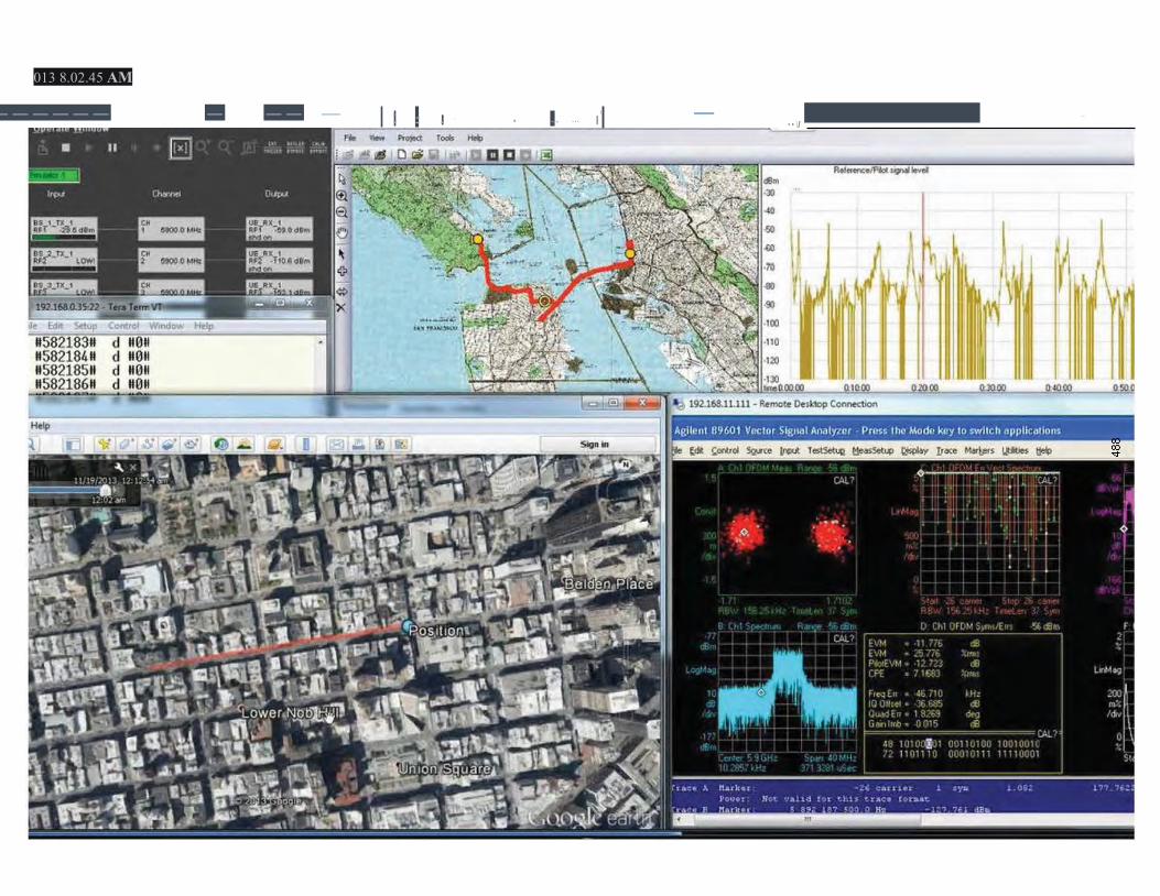
013 8.02.45 AM
------ - -- - . ' - ; ' . .,., ... ' ' -- • • \I
---

p_ll -18 - 2013 9.44.51 AM
! a
File Edit xtup C<>ntrol Wrndow t¾elp
.:' .-.
ij4 ff d U01f • J t1&.9 H d 118 H
ij OH d 110 11 1151 1f cl IIBM #5211 d 11011 1153K d B0N !
- 1 r
'l !'ll
--:··. ,--;.
:: •) "J G:ogle q.r>rl P01"l 's r ,
•!magb !:.' 2 ..., ':'o--,;i -,11 !·,t:s.
)n1:i,x,,- ( ---- .:, :-:-.';:,::_. - - - - - - - - - - - - - - - _r- -- - --- - - ------

490
System Setup
The Elektrobit Propsim F8 has multiple N-connector rf inputs, GPIB, DVI, USB and Ethernet. The power switch is in the upper left corner.
Ensure the 120V power cable is connected to the unit, connect a monitor, keyboard and mouse to the EB F8 Propsim unit (“the F8”)
Power on the F8 and wait until the main screen appears, this takes up to 5 minutes. Connect the Arada RSU unit to its power over Ethernet PoE and connect the network to the PoE. Connect the antenna output directly into the P1 port on the EB IFU box. Connect P3 into the Agilent EXA. (Warning: use an attenuator at the input of the IFU as needed to prevent possible overload)

491
The PC computer runs a remote session of the 89601B
Note: Connections are on Port 1 and Port 3 of the IFU

492
Above: at the startup screen click on Running View then Open
Above: clicking on open brings up a file open dialog. Note this file used 5/2/2013 where the others have a time stamp in 2012. Click on TestPacific.smu and open it.

493
Above: opening the TestPacific.smu file shows this in “Running View”. Note there is no signal
Open an existing project file to playback the San Diego Simulation Step 1 Open existing file in WES

494
Above: this is the menu to open to begin a simulation, the WES Tool
Step 2 Load Project
Above: click on the menu items shown, load project
Step 3: Look for *.wpj

495
Above: locate the applicable file
Step 4 wait a few seconds, this display appears:

496
Step 5 goto Project -> play back in emulator
Step 6 wait and this screen opens:
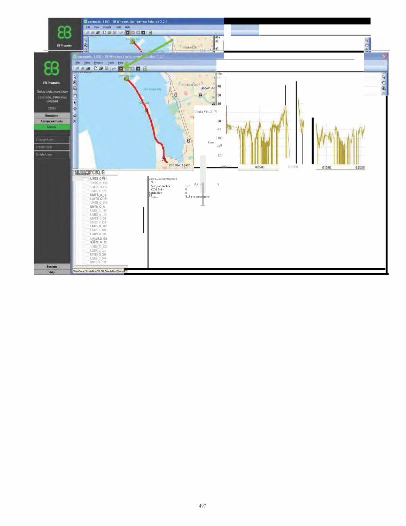
497
1lrnC1t1
uM1s_o_,,s
<llm <lO
Chui.a V1st,3 - 70
,9:)
· 100 Cost ,,,o
I MUIUIClfl'ClfQJB - - UMTS_O_◄61
UMIS_0_110 UMTS_O_l'l3 UMIS_0_:!2'5 UMTS_o_,s UMTS O 16' UMIS_0_116 UMTS_O_A UMIS_0_.!59 UMIS_o_,16 UMTS_0_68 UMTS_0_158 UMIS_0_<6' UMIS_0_108 UMIS_0_60
.._. UM'i°S.J.eetCIIPfoptfllC'I N- . $c,-codo OlN-
a8,u_nd,r_.edicn
•76 0 0
P,1 l ·l
· 120
... -000.00 0.1000
Unadet/.eciOH
uMrs_o_m UMJSJl.'63
UMIS_O_Zl2 UMIS_o_i,;,i UMTS_!l_284 UMIS_0_199 UMTS_0_:111
- -

498
Measurement on the Agilent EXA Ensure that the Agilent machine is powered on (The button is located at the front at the lower left side.. Wait until the self-test is finished. This takes approximately three minutes.
Open a remote Desktop connection. The IP address for the Agilent is 192.168.111.11. The user name is ‘Instrument’ and the password is ‘measure4u’.
Above: The initial screen of the Agilent EXA Signal Analyzer. Click on the 89601 VSA.
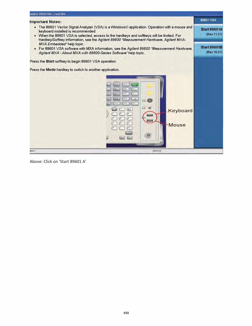
499
Above: Click on ‘Start 89601 A’

500
Above: The main screen of the VSA. Open a setup file by clicking on file recall setup.

501
Above: Select the appropriate set up file and click open. Use the June demo file.
Make sure that the Input is coming from the hardware for real-time measurement. Use recording to play
back a recording.

502
Above: Note the pattern gets distorted as the emulator plays back

503
Setup of the Arada for the radio source Our Arada system has an IP set to 192.168.0.40 . To make use of this local IP, set the Host PC computer such that it has an IP on this 192.168.0 network. Open a control panel windowNetwork and InternetNetwork and sharing Centern the network settingsChange Adapter settingsright click on Local Area connectionProperties In TCP/IP v4 advanced settings add an IP address (if one is not already assigned) using the same last number as the main static IP.

504
For example if the PC’s address is 128.111.122.140 then add an IP of 192.168.0.140 . Now the Arada can be accessed without having to change the main IP of the PC. See Appendix: Network Settings for a detailed description.
Connect to the Arada using Tera Term with an SSH connection. In the Start menu, click on Tera Term. Enter the connection information as follows:

505
The Arada can be set to begin transmission at powerup by running a
change the setting so at the command line:
script. In this case we want to
Above: this is the initial screen from Tera Term. Enter the address, CHANGE the Service to SSH. TCP port will change to 22 when you click SSH.
a. Type the IP address of the Arada being used b. Click the Telnet radio button and click OK (user= root, pwd=password) c. If the Arada radio does not log in then repower the unit by disconnecting and
reconnecting the 12V power cable.
The root directory should be active. Stop the running transmit processes by entering the CLI menu and sending the command ‘apphalt’. This stops the default transmission so we can send specific data:
a. type ‘cli’ (a different prompt should appear) b. type ‘apphalt’ c. type exit
Now the Arada radio should be ready to be set to a specific channel, power and xmit type.

506
d. getwbsstxrxencdec -s 180 -t BSM -o norx -a1 -r6 -j 3
Note: Arada Locomate user manual page 3-16:
We modified the command line to add the data rate and output power level. We omit ‘–e sign’ and simply transmit the BSM on channel 180 at the rate of 6 Mbps, command of 3dBm has an effective output of about 1dBm
Above: expected output of entering the command. There are errors encountered in the text but there should be packets counting quickly.
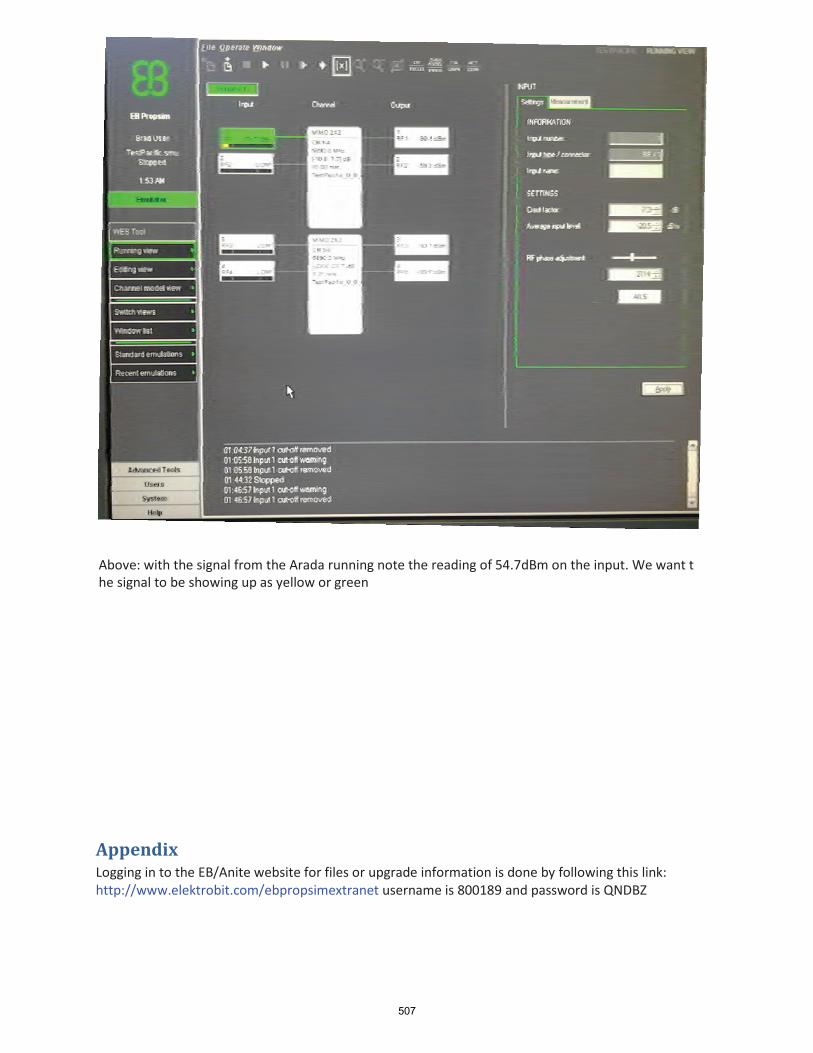
507
Above: with the signal from the Arada running note the reading of 54.7dBm on the input. We want t he signal to be showing up as yellow or green
Appendix Logging in to the EB/Anite website for files or upgrade information is done by following this link: http://www.elektrobit.com/ebpropsimextranet username is 800189 and password is QNDBZ

508
':J'
I h tp5 /t propsu:nE?Ctranetari 1 te,com
- -
Anite
- • -
""'
For""""1nlomleaon oo Prop,;,rr® chonriet "'™ranon sokluons pleass "'10 acqu,reo tt11s product one on ll>e 28th ol January, 2013 P1ease see Amte',s webs.le for moro details WWH arnte: com
Usarnitffle eoo,n
-I U>OIN
fwtdffll 'hliliMIII !tlli:':#ilOP'.ttPOA:t
Latest information on Propsim products N-r..wiur••• opl{Ofl• ,;and ll■■■lln • c.on 11il,u.r■110'l ...,.11:ii ll • In PniPt.lm Fe 1•a10 cn■,inel em l>l1otor
- "' "''ll O'WTrfl.ll l■! l'ICl ll!'• t. •■if l <I L,11'. t ■"111,1l,ill!O r'I - Vlr W l O-,,....'l • lll:lhtg ,t,111,m ,:,1"1 - 'Wfl::Q; - N.Wffi(J•CltitiH' i:i•:t1111n• .,,.,, ,:,,.,,,,• • e ci,1,11tle1n
Latest news
Search from the Knowledge Base W■fll lD I.now how llJ c.r• ■te C h an ne l .,hJd ....... ,.
WCndeM111 now to make • Tea.! S'11tuo'? 11'1'11i,. • ciin Gnti Cl.,.,,,..,.lJP • n'Cl,r rJ""(I<:"';,
P1••"• • t: fo,t 1;a•1,c,y,, :,ll!'lo.l._..,V -IJ _. ... ,.,. IMelii• Jlant,
Need personal support?
2U1;2",, 1 1:i EB P r e s <s Rel•••• •ESPR0 1¥1F32RADIO C.MANNl:L 1..t.M.11.ATOIII: OICLl!C T l'JD PilNALliJT ,oA>TMG O $T ll'IT ST <lQ1"1 Ct
File management
j,{11:.-1111:f)
110 . .. . . .. 1•••• - I. Ql,)11' ((!O} T()
0 VV. 171 RAO•O ¢M#.N1'18L MOblH• .I} ll'OH •V1'V MQOltl:.ANDW1A L $ (: QM '■l l,JN l (: A.'l'IQN 3
I •n12,1 flle P'P' EIP z L Ppjg9,d flle P'P' tfTTP: ■
EB P re• • Rel H ,S ill . EEi ... l O OTA TEST SVSTEP,l lt,IP LE ME NT ED BUCCESSFUL.LV AT NEC CAStO ""40 El■LE C:O""'JrlU C,,,,TIONS
.A:nite
1 ----
- -
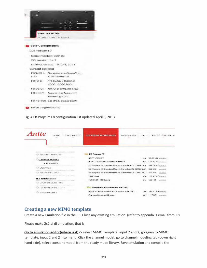
509
Fig. 4 EB Propsim F8 configuration list updated April 8, 2013
Creating a new MiMO template Create a new Emulation file in the EB. Close any existing emulation. (refer to appendix 1 email from JP)
Please make 2x2 bi di emulation, that is
Go to emulation editor(where is it) -> select MiMO Template, input 2 and 2, go again to MIMO template, input 2 and 2 into menu. Click the channel model, go to channel modeling tab (down right hand side), select constant model from the ready made library. Save emulation and compile the

510
emulation by pressing the 4 squares in the main menu. Go to running view, open the emulation You just did and run it
In this case the file was named PacificTest when the WES tool is run. Describe the connection to the filename for the shapefile this is the one used by the test pacific program emulation that was sent to us. When the WES tool is run this runs, behold:
Installing the WES update: If this file(s) is not already present in the Propsim F8, download it here. In the Software Downloads section under Product updates, goto Propsim F8. The file we want is WES 3.6.0 Release Full Propism Installer. To download, use Internet Explorer Browser as download issues have been reported with non- ie browsers. Once setup file is downloaded transfer the file to the EB. The set up file is stored in My Documents. Open the setup file and follow the installation instructions. Two different installers will appear as shown below.

511

512
Fig. 5 Download the file TestDrives and extract. TestDrives contains these folders
Initial load of SD Simulation test software into EB Extract the file in the PC instead of in the EB. Load this folder onto a USB Memory (such as a flash memory stick), then upload to the EB unit. Insert the flash stick into the EB’s spare USB port, then using the file manager, copy the file onto the EB’s local hard drive. When the WES program is run it will ask for this file.

First Responder Support Systems Testbed (FiRST)
Dr. Rick Churh1, PI Dr. Ramez L. Gerges2, Contract Manager
Brad Rogers1 , Field Engineer
1. Department of Geography University of California, Santa Barbara, CA 93106-9560
2. Office of Communication Systems Research California Department of Transportation, FiRST Testbed
1
513

514
Integration of Cellular (e.g. LTE) and DSRC for ITS/PS Applications
Spectrum allocation and Interoperability were once the main obstacles for both ITS (Intelligent Transportation Systems) and Public Safety radio services. Licensed Frequency spectrum has been available for both ITS (75 MHz at 5.9 GHz), and PS (50 MHz at 4.9 GHz) for the almost 15 years. However, we still don’t have the seamless service continuity when users move between different network services. Interoperability has been the focus of current federal initiatives (e.g. first net) to address the PS intra- agency communication. Similarly, in the commercial “connected vehicles” environment, DSRC standards have been developed for vehicle-to-vehicle active safety applications.

515
The intent of this brief study is to explore the feasibility of integrating heterogeneous wideband networks (e.g. DSRC and PS), and cellular wide area services (e.g. LTE) to address the current gap of agency-to-citizens communications. The emerging machine-to- machine and the Internet-of-Things will drive the future evolution of seamless services for everyone.
Operational & Technical Challenges in Public Safety Domain

516
PS organizations must operate in a difficult environment and in various operational scenarios, which are characterized by a number of significant challenges:
• Interoperability. Interoperability barriers among the communication systems of various PS organizations are still present at the local and national level.
• Broadband Connectivity: Table 1 provides examples of current and future PS applications that are driving the need for broadband connectivity to transmit images or video. The wireless communication technologies currently deployed (e.g. APCO25) provide only limited data capacity (e.g., 28.8Kbits). Using the DSRC/WAVE in the 4.9 GHz in addition to the ITS 5.9 GHz band is a challenging task. Both the frequency spectrum allocation and the hardware/software technologies are available to support the desired applications. However, the deployment of these new technologies may be inhibited the limited budget of the involved jurisdictions. Current federal initiatives such as the FirstNet at 700 MHz may be a more practical approach as they provided the required fund and the implementation standards (LTE).
• Challenging operational environment: PS infrastructures may be destroyed or degraded as a consequence of the crisis. For example an earthquake, flooding or tsunami can destroy the physical network infrastructure or disrupt the supply chain used in humanitarian logistics. Even if the PS infrastructure is not destroyed, it can be overloaded by the increase of traffic due to panic calls as in the 9/11 event.
• Equipment lifecycle: Evolving technologies and standards may cause the existing wireless equipment to become obsolete. Due to the different market sizes (200:1 ratio), the equipment lifecycle in the PS domain is usually less dynamic than the commercial domain.
It is hoped that the FirstNet initiative will address these PS challenges.
Public Safety Spectrum & Architecture
In 2002, the FCC allocated the 4.9 GHz (4940-4990 MHz) band for public safety use, adopting service rules in 2003 to encourage agencies to benefit from high-speed applications like real-time video, data downloads, and short-range wireless networking at emergency incidents. Those rules allowed utilities and other commercial entities to use the spectrum to provide public safety services if they were authorized by traditional public safety licensees. In 2009, the FCC modified

517
the 4.9 GHz band regulations to enhance broadband use of the channels by first responders, including making it easier for them to use fixed point-to-point links to share time-sensitive data and streaming video during emergencies. Because the FCC believes the development of the 4.9 GHz band has not met its potential, the Commission released an R&O in June 2012, to reevaluate existing policies and to consider new approaches to spur robust and efficient use in this band. The R&O corrects minor errors; including reinstating an exemption of 4.9 GHz band applications from certified frequency coordination requirements; and correcting and clarifying the 4.9 GHz band plan.
In July 2007, the Federal Communications Commission (FCC) designated the lower half of the 700 MHz Public Safety Band (763-768/793-798 MHz) for broadband communications. This spectrum had been cleared by the Digital Television and Public Safety Act of 2005. In early 2009, Congress directed the FCC to develop a National Broadband Plan, including recommendations for a dedicated public safety broadband network. Later in 2009, public safety chose Long Term Evolution (LTE) as the primary technology for the broadband network. In 2012, the FirstNet was mandated by the Congress.
FirstNet The Middle Class Tax Relief and Job Creation Act of 2012 created the First Responder Network Authority (FirstNet) as an independent authority within NTIA. The Act directs FirstNet to establish a single nationwide, interoperable public safety broadband network. The FirstNet Board is responsible for making strategic decisions regarding FirstNet’s operations. FirstNet is expected to enable police, firefighters, emergency medical technicians, and other first responders to effectively communicate with one another during emergencies and to use new technology to improve response time, keep communities safe, and save lives.
700 MHz Spectrum after Public Law 112-96

518
Issues that it still to be addressed are:
• Whether to establish formal coordination requirements in the 4.9 GHz band • Whether the 700 MHz Regional Planning Committees (RPCs) could administer a
database registration process • Whether expanding eligibility to critical infrastructure entities and commercial users
would promote more effective and efficient use of the band • Whether eligibility for commercial users should be on a secondary basis subject to a
shutdown feature to allow public safety priority access • Whether the First Responder Network Authority (FirstNet) is or should be eligible for a
4.9 GHz band license • Technical approaches to increase spectrum efficiency, usage, and throughput in the 4.9
GHz band LTE – Long Term Revolution
The First complete LTE specifications 2008 became available in 2008. LTE is specified at the following layers:
Physical Layer:
• Can support portable speeds over 100 MPH • MIMO (Multiple Input Multiple Output) technology • Bandwidth up to 20 MHz • High order modulation (64QAM)
Media Access:
• DL: OFDM • UP: SC-FDMA
Network Architecture: • All IP end-to-end • Flatter architecture
The table below reflects the LTE potential data rates for different frequency bandwidths.

519
Additionally LTE technologies promise the following:
• An end-to-end all-IP significantly higher capacity • Peak date rate up to 300 Mbps • Round-trip delay <10ms • Call setup latency < 300ms • QOS Support • Deployable in existing 3G frequency bands already auctioned or allocated (FirstNet)
spectra.
LTE Network Architecture
Integration of Cellular (e.g. LTE) and DSRC for ITS/PS Applications
WAVE/DSRC at 4.9/5.9 GHz
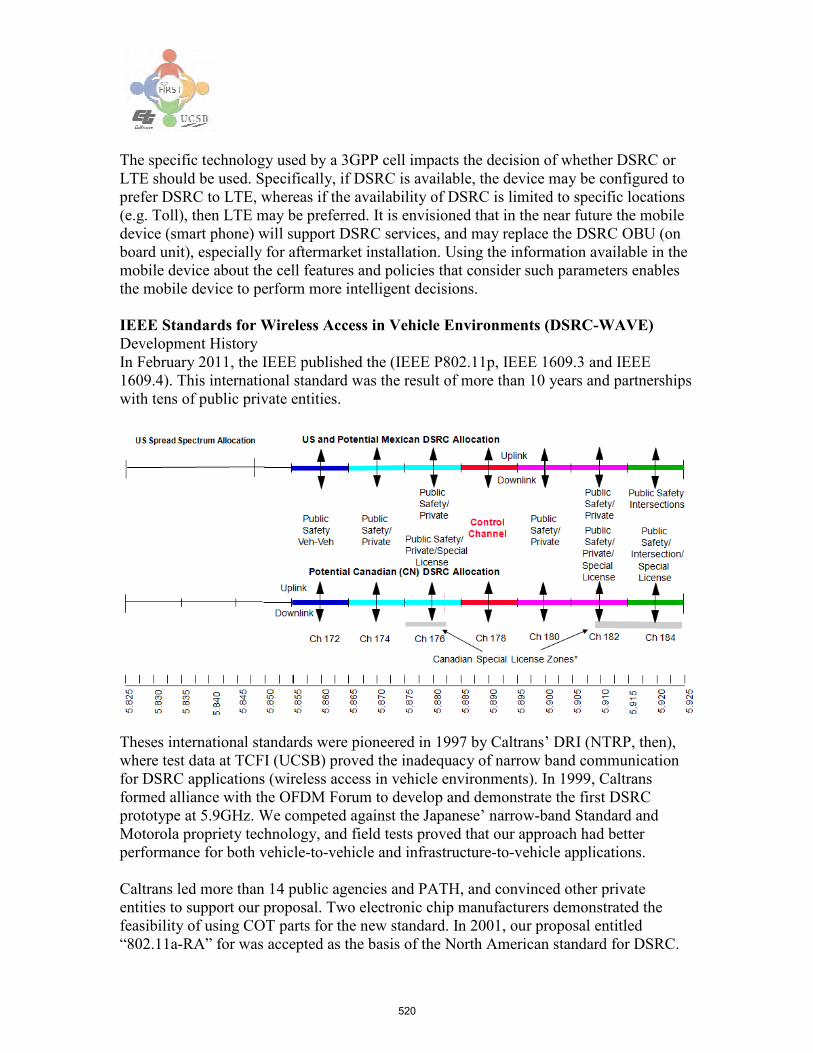
520
The specific technology used by a 3GPP cell impacts the decision of whether DSRC or LTE should be used. Specifically, if DSRC is available, the device may be configured to prefer DSRC to LTE, whereas if the availability of DSRC is limited to specific locations (e.g. Toll), then LTE may be preferred. It is envisioned that in the near future the mobile device (smart phone) will support DSRC services, and may replace the DSRC OBU (on board unit), especially for aftermarket installation. Using the information available in the mobile device about the cell features and policies that consider such parameters enables the mobile device to perform more intelligent decisions.
IEEE Standards for Wireless Access in Vehicle Environments (DSRC-WAVE) Development History In February 2011, the IEEE published the (IEEE P802.11p, IEEE 1609.3 and IEEE 1609.4). This international standard was the result of more than 10 years and partnerships with tens of public private entities.
Theses international standards were pioneered in 1997 by Caltrans’ DRI (NTRP, then), where test data at TCFI (UCSB) proved the inadequacy of narrow band communication for DSRC applications (wireless access in vehicle environments). In 1999, Caltrans formed alliance with the OFDM Forum to develop and demonstrate the first DSRC prototype at 5.9GHz. We competed against the Japanese’ narrow-band Standard and Motorola propriety technology, and field tests proved that our approach had better performance for both vehicle-to-vehicle and infrastructure-to-vehicle applications.
Caltrans led more than 14 public agencies and PATH, and convinced other private entities to support our proposal. Two electronic chip manufacturers demonstrated the feasibility of using COT parts for the new standard. In 2001, our proposal entitled “802.11a-RA” for was accepted as the basis of the North American standard for DSRC.
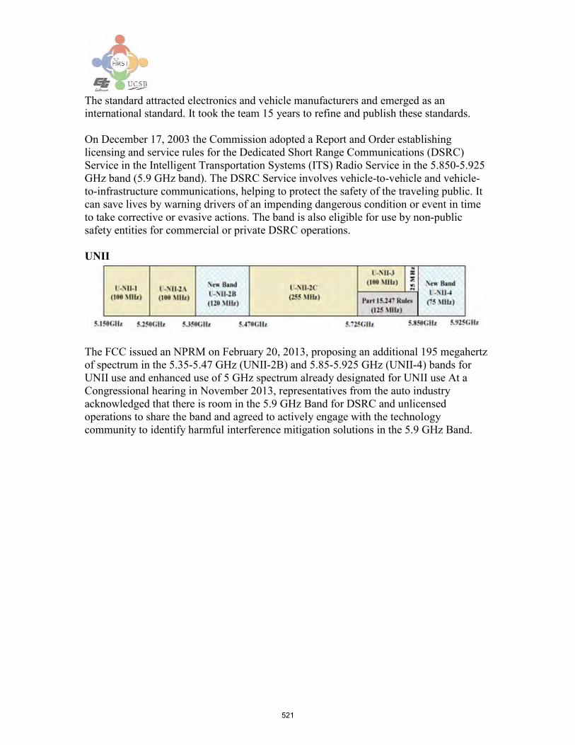
521
The standard attracted electronics and vehicle manufacturers and emerged as an international standard. It took the team 15 years to refine and publish these standards.
On December 17, 2003 the Commission adopted a Report and Order establishing licensing and service rules for the Dedicated Short Range Communications (DSRC) Service in the Intelligent Transportation Systems (ITS) Radio Service in the 5.850-5.925 GHz band (5.9 GHz band). The DSRC Service involves vehicle-to-vehicle and vehicle- to-infrastructure communications, helping to protect the safety of the traveling public. It can save lives by warning drivers of an impending dangerous condition or event in time to take corrective or evasive actions. The band is also eligible for use by non-public safety entities for commercial or private DSRC operations.
UNII
The FCC issued an NPRM on February 20, 2013, proposing an additional 195 megahertz of spectrum in the 5.35-5.47 GHz (UNII-2B) and 5.85-5.925 GHz (UNII-4) bands for UNII use and enhanced use of 5 GHz spectrum already designated for UNII use At a Congressional hearing in November 2013, representatives from the auto industry acknowledged that there is room in the 5.9 GHz Band for DSRC and unlicensed operations to share the band and agreed to actively engage with the technology community to identify harmful interference mitigation solutions in the 5.9 GHz Band.

DEMO2: Interoperable Emergency Communications
• Interoperable Emergency Communications – Wireless Channel Emulation
• Tx Signals (BPSK, QPSK, 16QAM, 64QAM) • Rx Signals (BPSK, QPSK, 16QAM, 64QAM) through the GG
channel • Repeat for QPSK at 5 MHz, same GG channel segment
– How to set the EB for a specific Run? – Antenna Patterns
• How to set the RFX Antenna ?
3/10/2014
522

523
HiDN Station Basic Configuration

524
Portable 3G/4G
Wireless N Router
Portable GPS
Tracker
IPV6 Border Router
HiDN
Tablet 2 Radio Antennas

525
HiDN Block Diagram

526
Device Names
• 3G Portable router: TP-LINK TL-MR3020 • 4.9-5.9 GHz radios • Two RF Antennas • Tablet or laptop • Portable GPS Device: SPOT Connect
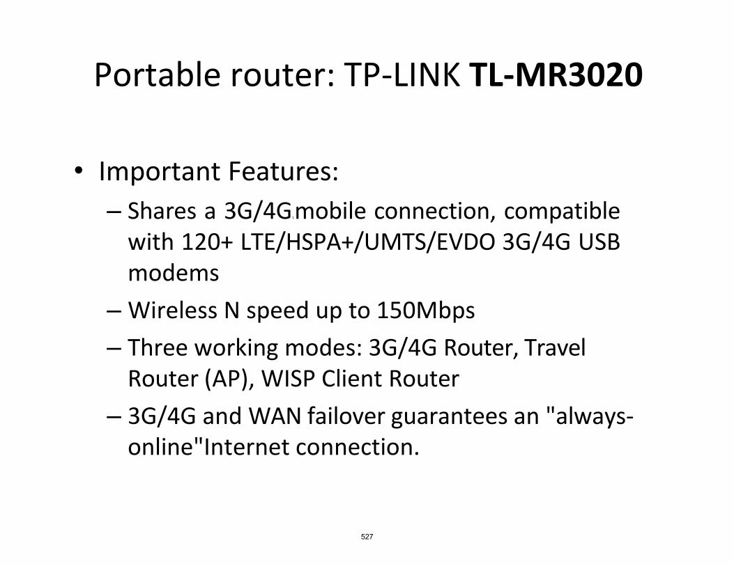
527
Portable router: TP-LINK TL-MR3020
• Important Features: – Shares a 3G/4G1 mobile connection, compatible
with 120+ LTE/HSPA+/UMTS/EVDO 3G/4G USB modems
– Wireless N speed up to 150Mbps – Three working modes: 3G/4G Router, Travel
Router (AP), WISP Client Router – 3G/4G and WAN failover guarantees an "always-
online"Internet connection.

528
The General Working

529
TP LINK - MODES
(A) 3G/4G Router Mode: Operation - with a 3G/4G modem/card, it joins a
3G/4G network as well as act as a wireless central hub to broadcast its SSID. Using this other devices can join Internet.

530
(B) WISP Mode: • Operation - The Router will act as a wireless
card to connect with WISP as well as a wireless central hub to broadcast its SSID for user wireless LAN clients, and the other wireless devices can connect to the Router for Internet connection.

531
(C) AP Mode Operation - In AP mode, the Router will act as a
wireless access point supporting four further modes, Access Point mode, Repeater mode, Bridge with AP mode and Client mode. These are shown n the table in the next slide.

532
Access Point (AP) Mode
Router will act as a wireless central hub for user’s wireless LAN clients, giving a wireless extension for user’s current wired network.
Repeater Mode the Router can extend the coverage of another wireless Access Point or Router.
Bridge with AP Mode
Router can wirelessly connect two remote LANs together.
Client Mode the Router will act as a wireless card to connect with wireless network.

533
TP Link: Few Facts
• Default IP Address: 192.168.0.254 • Default Subnet: 255.255.255.0 • SSID: TP-LINK_POCKET_3020_xxxxxx.
(xxxxxx is the last six characters of the router’s MAC address.)
• Credentials: User name and Password - admin

534
Installing TP-Link (A) In 3G/4G Mode: A.1 PC Configuration 1. For Windows7 machines, follow the path, Start
→ Settings → Control Panel → View network status and tasks → Manage network connection. Right click Wireless Network Connection, and select Properties.
2. Select Internet Protocol Version 4 (TCP/IPv4). 3. Select “Obtain an IP address automatically” and
“Obtain DNS server address automatically”. Click OK to finish the settings.

535
n
A.2 Connect to Network 1. Select the ico at the bottom right corner
of your machine. 2. Refresh the Network list and wait for TP Link
device to appear. 3. If you get ‘Connected’ Message after clicking
‘Connect’, you are now on the wireless network.

536
A.3 Router Configuration 1. Open your Web Browser and type
http://192.168.0.254 2. In the login window which appears, enter the
default user name and password. 3. You should see following screen

537
4. Refer 3G/4G section on the status tab. It must say ‘Identifies’ for 3G/4G USB Modem and ‘100%’ for the Signal strength.
5. Go to Quick setup tab and click Next. 6. Choose Internet Access type and click Next 7. Select your ISP (Verizon in this case) . 8. You can change Network name and password(by
using WPA). Current password is mentioned on the next slide.

538
TP-LINK
• TP Link is the SSID of the already configured Wireless Network. I have configured it in 3G/4G Mode.
• Its WPA Password is FiRST.

539
Agilent N9010 VSA How to setup for these measurements
• In the Agilent click on File, Recall, Recall Setup
Select the file eb demo nov.set and click on Open. This loads all of the Agilent settings automatically for this set of measurements.
3/10/2014

540
Set Trigger and Level for the Agilent • Setting for direct connection from the Arada at 1dBm. When the signal
comes from the EB it will be -50dB:m, adjust these 2 values as needed
Arada at 1dBm: Ch 1 Spectrum: 2dBm Ch 1 Trigger: 2mV
EB at -50dBm: Ch 1 Spectrum: -50dBm Ch 1 Trigger: 780uV
NOTE: Clicking on the value, the mouse wheel will adjust the setting

541
TX Signals, BPSK
•

542
Direct TX output BPSK
The Arada is programmed to Service channel 180, type BSM, rate of 3MBps and 1dBm The OFDM measurement will detect the change from 64QAM to BPSK and 2 dots will appear instead of the 8 x 8 pattern.
3/10/2014
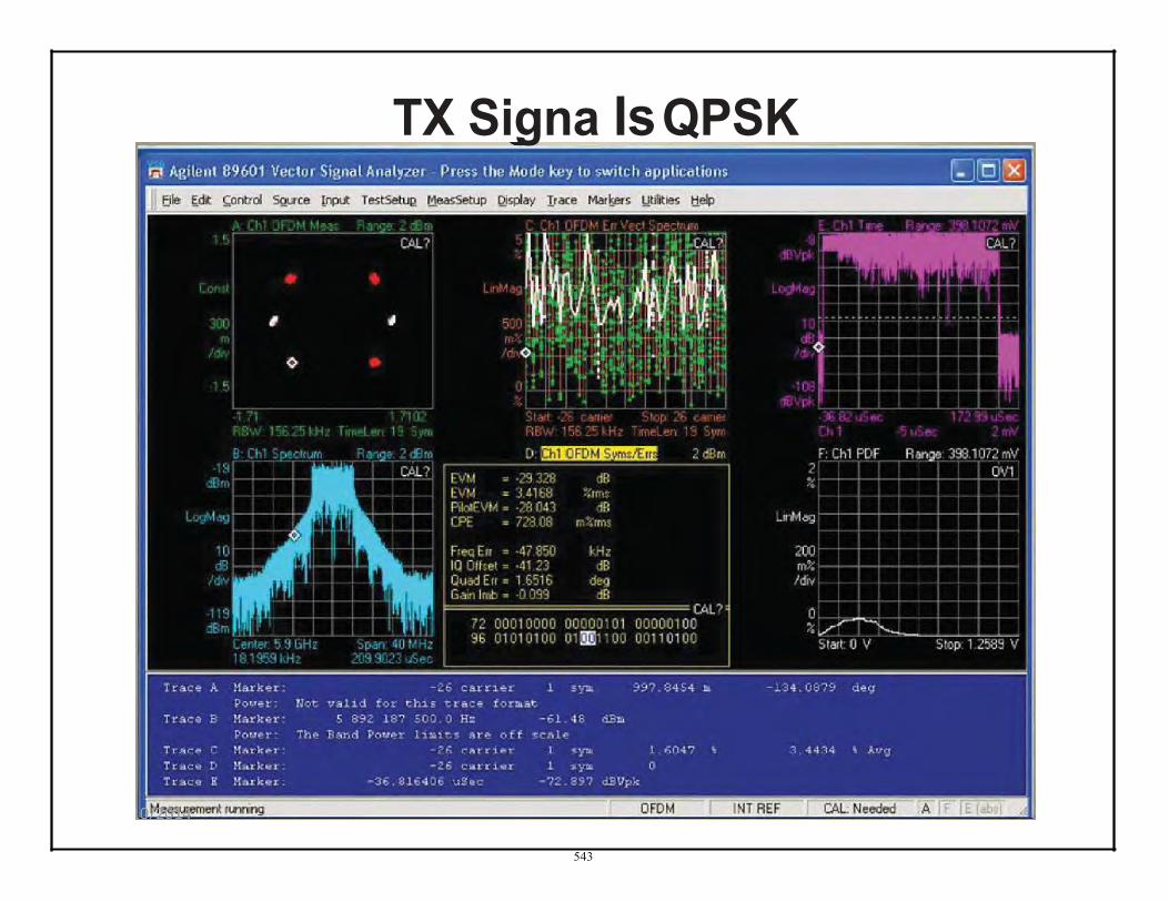
543
TX Signa Is QPSK

544
Direct TX output QPSK The Arada is programmed to Service channel 180, type BSM, rate of 6MBps and 1dBm The OFDM measurement will detect the change from BPSK to QPSK and 4 dots will appear with 2 index markers instead of the 2.
3/10/2014

545
◊ r
•-·- ,. ,
j
%
·,:
TX Signals 16QAM
11 I•
[)(Q]LE)
r ,-- (.AL?
:'I . .. ,,, f .. • I
wa 1 ,' --1 ---- C L?
'! : r • '' . -'
· 1 I • "' t .. .. ...
.' ••-•.•••••I••••.••••••••·••• l I••• - •• ' . • . . ' j . I I
cl I • : : : : : '. l :" I · ,,
I . r , ; : "
,r: ,11 .. , ,I 1·, :•1,, 1
r;( :: r ,r..: 1 i· .... r 1r ·.,.;., 1 ·-· ''.,,"1
-, r
-- -
j -~-
1 ! ,1 _ P'="• •r-.ir,· r-, ,·,c1 - - ,:f rn CAL' .
[iJ CJil OFDM SYJMIErr 2 dBrn F: Ch1 PDF Ran o 398 1072 rnV EVM • ·31 38'5 dB
2 EVM • 2 6':/f;l ; ; 1 ms
m!: ,ms
[-'1 ••::r . ':I LH: I :." _'.,;...' _1 ,.1::
:,v,r• •HI, ,.. : 11'· .:1 i ; ;°'1 •I ;
G-:iin lmb ,. ·0.0-4 8 dB = = = = = = = = = = = = = = CAL?
48 1 0000 94 1C135C4 9 AOBC4EDO 72 ·1 &(1D558 2012 461F Al 8BEC.6'5
0 f
Sl r t O V $lc,p l 2589 V
T eir;:e ..W&,, H.a1:l.1eL; -16 CSJ:'?'l. t' fMWj .L. :33,S,Z, l3S.8l:I0:3 tie,;,
P(ll.l«l.": Hot: valid for i::ti.1.i ;:.rr,,;;; t on,,:a.,t Trac:.;, B H1n·li;;,r-: s 8 2 187 5( 1 1) . O H:.:: - i 2 . 595' -cl.Bi..
Pcl1.J'!!r: Ih B = . d P6<i'!!'-" 1 1 1»1 ,:. ;: oi f.:!:cr..l!! Tr c C Hark r: Tr!=lce [' H.arksr:
- ,26 ca.rriscr -?6 c a !t i !"
-36.83.5938 uSec
=')[JM -!. 2607 3 . 6 92 \ A'.l'J 1 ?.
-7-t.l.58 d.9Vpk
DFID
I
Pilotf \/M CPE
· 2 9 28:: 52& 02
dB 1D fiR• F re-q Err ; -,17 6 71 l·.Hz 2 00· I Q Olr-;et :a .3 3 676 dB mo/. Otiad E 11 ,. 1 6562 deg /drv

546
Direct TX output 16QAM The Arada is programmed to Service channel 180, type BSM, rate of 18 MBps and 1dBm. The OFDM measurement will detect the change from QPSK to 16QAM and 16 plus 2 dots will appear instead of the 6.
3/10/2014

547
TX Signals 64QAM

548
Direct TX output 64QAM The Arada is programmed to Service channel 180, type BSM, rate of 24 MBps and 1dBm. The OFDM measurement will detect the change from 16QAM to 64QAM and 64 plus 2 dots will appear instead of the 16.
3/10/2014

First Responder Support Systems Testbed (FiRST)
Contract # 65A0257 Cross-Cutting Cooperative Systems
TRACK IV – FiRST Baseline Enhancement and Maintenance
Wireless Sensor Networks for Cooperative Work Zone Safety
Final Report
Wireless Sensor Networks for Cooperative Work Zone Safety: Safety at work zones remains a serious concern for Caltrans. This research was in response to the loss of Caltrans workers on Highway 96 and other work zone fatalities. As we move into the “connected vehicles” environment, new challenges and opportunities are emerging. A cooperative system approach that integrates sensors and wireless communications and employ new localization algorithms will offer a new design for safer work zones in urban and rural areas.
This project provides the basis of innovative solutions to reduce Caltrans’ worker injuries and fatalities in work zones. Localization methods are critical to cooperative algorithms for sub-meter localization, we describe their use for two scenarios. The first scenario involves smart cones that are located along the work zone area, to directly detect dangerous events and alert Caltrans’ workers in work zones. In the second scenario, the nodes are vehicles traveling at high speeds on highways. It is assumed that vehicles can communicate with other vehicles and the infrastructure within the emerging “connected vehicles” environment. We address this class of localization algorithms that are able to fuse the data coming from neighboring vehicles and refine their own position estimates within a specific lane, and without the need for a dense fixed nodes along the roadside. In addition to the theoretical treatment, this report includes
549
Principal Investigator: Dr. Richard Church Co-Principal Investigator: Dr. John Shynk
University of California Santa Barbara
Contract Manager: Ramez Gerges, Ph.D., P.E.

"""""
'·
-
,45 1-,- "I ,.,-11"'' P>,rJ.,,g I 2
1 2 u JO " r30 I IS . 75 o.i,
.S..d.tir>JP
_f;l,e,_,.,,,,.,, R,,,,,,{,,,,Jll>-,,da Ho., If'
-lt,,.t/P"'"-s
Show.Lost I□---:@ Unr,.,ewed Even!,
--{S/\SOOO l' \ 5 Sodtmi F,s. to Rmda Hoat .. "" Emn._
Start T_imf? i: ve ut. N a.ttt e C.a.n1il!1"a N aan10(s) Car.didi!n t:u Priority
:µ,e J;m.OJ 14 ;10 50,005 East Ga W!.l I 00 l!1ll!l§: Tue J on tl/ 14 J0 · 5,0 005 E ,t G,1,· 100
Tut Jan 0V1 4,10:49.09 IDil. 1\10
_
FiRST Baseline Enhancement & Maintenance
550

551
552
Cooperative High-Accuracy Localization Algorithms for Low- and High-Mobility
Nodes A Final Report Submitted to
Division of Research, Innovation, and System Information California Department of Transportation
Sacramento, CA 95814 from
Department of Electrical and Computer Engineering University of California
Santa Barbara, CA 93106-9560
I. EXECUTIVE SUMMARY
As the transportation infrastructure ages, there is an increasing need for the maintenance and rehabilitation of the road network, which means there will be more work zones. Safety at work zones remains a serious concern for Caltrans, and research is lacking in addressing methods to directly detect dangerous events and alert Caltrans’ workers in work zones. As we move into the “connected vehicles” environment, new challenges and opportunities are emerging. Workers’ safety is not limited to urbanized areas; the recent loss of Caltrans workers on Highway 96 due to a landslide is a reminder of this class of hazards. A cooperative system approach that integrates sensors and wireless communications and employ new localization algorithms will offer a new design for safer work zones in urban and rural areas. There has been a surge of interest in using wireless technologies for both transportation and public safety. Recently, the FCC issued a new notice of proposed rule-making (NPRM 13-49) for wireless broadband spectrum. The US Department of Transportation is starting a new DSRC initiative focused on vehicle-to-infrastructure communication, and the US Department of Commerce is moving forward with the FirstNet wireless broadband initiative for public safety. Those challenges and opportunities require a trained workforce. The virtual wireless lab, and the modeling and testing infrastructure at the First Responder Support Systems Testbed (FiRST) has been leveraged to address these new opportunities.

553
II. INTRODUCTION
This project provides innovative solutions to reduce Caltrans’ worker injuries and fatalities in work zones. The proposed architecture integrates wireless sensor networks (WSN) for reliable in- cident detection and alerting of workers via a heterogeneous wireless communications networks. In addition to the WSN, both DSRC (5.9 GHz) and public safety radios (PS-4.9 GHz) can be used to communicate with the emerging “connected vehicles” environment and CHP/EMS vehicles. The architecture employs the FirstNet (700 MHz-D Block) for wide-area public safety communications. A critical element for detecting hazards and alerting Caltrans workers is the use of high-accuracy localization algorithms. Two different localization subsystems were investigated to improve the safety of highway workers, as well as the driving public as they approach work-zone lanes in both urban and rural settings.
The first subsystem consists of a wireless sensor network of smart cones which includes a cen- tralized master node, and are used in work zones to control traffic flow and protect construction and maintenance workers. The second subsystem performs localization of vehicles at normal highway speeds using cooperative techniques only between “connected vehicles” that form an ad hoc network, and without any fixed road-side nodes. Different sensors can be used for different hazard conditions and work environments. One sensor class detects car intrusion on urban work zones. The other class of sensors can be used to monitor and detect when hill-slopes are primed for sliding and provide early indications of rapid, catastrophic movement. Both sensor classes employ the same WSN platform and cooperative systems architecture, and Caltrans workers would receive real time alerts using Personal Safety Networked Sensors (PSNS).
Caltrans funded the development of the FiRST Testbed into a unique research facility ready to offer solutions for the above mission critical areas according to the published DRISI wireless research roadmap. The return on investment (ROI) in the FiRST Testbed materialized in realizing answers and deployable solutions to the above mission critical areas. Short term ROI is realized in deploying the PSNS and to save the lives of Caltrans workers. A long-term ROI will be achieved from developing an excellent workforce and maintaining a Caltrans competitive research advantage at the national level. This project leverages the simulation, lab, and field infrastructure at the FiRST Testbed to provide deployable solutions in order to save Caltrans workers’ lives, improve safety, and increase mobility of the transportation network.
III. OVERVIEW OF LOCALIZATION APPROACHES
There has been much research in wireless communications over the last several years directed toward localization techniques that improve upon conventional methods based on the Global Posi- tioning System (GPS). Most of these techniques involve some form of cooperation or collaboration among nodes, where they exchange position estimates with their neighbors in order to improve these

554
estimates. Since GPS signals provide a location accuracy of only 7 m for 97% of the time, other more sophisticated methods and signal processing techniques are needed to bring localization into the sub-meter range. Differential GPS (DGPS) and Network Real-Time Kinematic (NRTK) positioning can improve upon the location accuracy of GPS [1], but they mainly compensate only for ionospheric and tropospheric distortions. They do not correct for multipath distortion, which can be a significant channel impairment, especially in urban environments and for high-mobility nodes [2].
When there is significant multipath propagation, the received signal is a mixture of line-of-sight (LOS) and non-LOS (NLOS) waveforms which are necessarily delayed [3], [4]. As a result, the composite received signal has distortion and its power can vary over time, resulting in fading and even loss of signal for extended periods. Moreover, the additive noise of NLOS signals is no longer Gaussian; it is sometimes modeled as the sum of Gaussian and exponential random processes, resulting in an exponentially modified Gaussian distribution. This is important because adaptive algorithms such as the Kalman filter (KF) require a Gaussian noise model for accurate estimation. As a result, other techniques are required such as particle filtering (PF) [5].
In this report, we describe cooperative algorithms for sub-meter localization of nodes for two highway scenarios. The first scenario involves smart cones that are located along the highway where there is maintenance or construction work. The cones can communicate with each other, and there is a central node called a smart drum that collects the data from all smart cones, which can be fused and relayed to personnel within the cone zone. From this information, it is possible to construct a virtual map of the work area, which is updated when a cone is moved or accidentally displaced by a worker. The main purpose of this cone arrangement is to alert personnel of a potential problem if there is a sudden change to the virtual map caused by vehicles moving into closed lanes and hitting one or more of the smart cones.
In the second scenario, the nodes are vehicles traveling at high speeds on highways, which often tend to move in clusters so that neighbors can be designated within some radius extending from the center of a cluster. It is assumed that most of the vehicles are capable of estimating their own positions, and that information can be regularly broadcast to their neighbors [6]. The localization algorithms are able to fuse all the data coming from their neighbors, in order to refine their position estimates, and without the need for fixed nodes along the roadside. From these position estimates, it should be possible to detect when vehicles change lanes, even when the highway has significant curvature.
IV. REVIEW OF PREVIOUS WORK
A. Signal Propagation Models (References [10] and [11])
Reference [10], “Experimental Characterization of DSRC Signal Strength Drops,” describes a model for predicting null points for Dedicated Short-Range Communications (DSRC) on the basis of two-

555
wave ground reflections. Null points due to destructive interference were estimated within a range of ±7 m, demonstrating a high accuracy of prediction and an improvement over existing analytical models and experimental data found in the literature. The model for the received power LOS distance depends on the transmitted power, the receive antenna gain, the wavelength, and a system loss factor. The NLOS path is more complicated, as it depends on the relative permittivity and the reflection coefficients for vertical and horizontal polarizations. The test equipment and parameters were as follows: (i) wireless safety unit (WSU) with integrated 802.11p-based wireless access in vehicular environments (WAVE) radio chip, (ii) omni-directional DSRC antenna, (iii) GPS receiver and antenna, (iv) wireless short messages (WSMs) sent with a 100 ms period, (v) 16 dBm transmit power, and (vi) 6 Mbps data rate. The following quantities were measured: vehicle position, speed, acceleration, heading, time stamp, and the receive signal strength indication (RSSI) obtained from the WSU. In an example experiment, the model derived a null point at 82.2 m, whereas experimentally it was observed at 78 m (outgoing) and 90 m (incoming). A packet success ratio (PSR) higher than 70% was found within distances less than 310 m. High errors in the model before the null point are probably due to multiple reflections from the vehicle itself. The results of paper [10] can be exploited to implement accurate signal propagation models for algorithm development and computer simulations.
Reference [11], “Use of RSSI and Time-of-Flight Wireless Signal Characteristics for Location Tracking,” attempted to determine the correlation between the error from time-of-flight (TOF) mea- surements and the error from RSSI methods. Any relationship between the two was expected to help associate probabilities in distance estimation for use in particle filtering (PF), but they discovered no such relationship. A particle filter was implemented to obtain upper and lower bounds for various simulated scenarios. Noise samples in the input and measurement were varied, and the maximum noise level from which it can recover and the number of particles were studied. It was found that the number of particles had no bearing on how long the algorithm took to stabilize. However, the final error after stabilization decreased with an increase in the number of particles. The following were observed: (i) RSSI showed a sharp decline for small distance variations and then was roughly linear. (ii) A high variation was found in the distance errors for RSSI, with spikes probably due to Rayleigh fading effects. (iii) The TOF computation overestimated the distance, and the magnitude of error did not vary as much as the error itself. The results in paper [11] are useful for our signal models in order to incorporate RSSI and TOF in the position estimation algorithms.
B. Vehicle Localization (References [7], [8], [9], [4], [1], and [5])
Reference [7], “Peer-to-Peer Cooperative Positioning, Part I: GNSS-Aided Acquisition,” describes sharing Global Navigation Satellite System (GNSS) aiding quantities like Doppler, satellite carrier- to-noise (C/N) ratio, and secondary code delay to facilitate improved and faster localization. The approach is similar to assisted GNSS but does not require additional infrastructure, and can be useful

556
in environments with adversely affected availability. This unstructured peer-to-peer (P2P) approach is also highly scalable and robust in heterogeneous time-varying networks, without a control or data fusion center or P2P ranging. Vehicles are assumed to be equipped with P2P networking capabilities and GPS. In a centralized cooperative approach, data are collected from all receivers, and then enhanced data are returned to all receivers. Mean acquisition time (MAT) simulations were conducted, for light indoor and open sky conditions, and pedestrian and vehicular mobility. The results show that the performance of the P2P approach is equivalent to assisted GNSS, but offers the advantages mentioned above. In order to combine the information coming from different peers, the following methods of weighting were proposed: (i) uniform weights, (ii) weights related to the aiding quality, (iii) weights related to the distance, and (iv) a closest peer approach.
Reference [8], “Peer-to-Peer Cooperative Positioning, Part II: GNSS- Hybrid Devices with GNSS and Terrestrial Ranging Capability,” is a continuation of the previous paper that develops a hybrid system capable of fusing GNSS positioning and a local ranging system to obtain the best localization information. Again, it is assumed that every node (vehicle or pedestrian) has the capability of GNSS localization and has a short-distance ranging system. It is suggested that fully decentralized versions of these algorithms can be developed with each node having capabilities of fusing data on its own. The different information sources are merged using estimation algorithms such as the KF, PF, or a least-squares (LS) estimator. Using previous knowledge of the transmitted power, environmental variables, and received signal strength, the distance is estimated by inverting a path loss model, though it turns out that the accuracy achieved using this method is generally not acceptable. The intra-node TOF distance is estimated by taking into account the speed of light and measuring the time difference between the transmitted and received signal. Several estimation algorithms were considered: (i) LS, which is simple to implement, (ii) extended KF (EKF), due to the nonlinear model, (iii) unscented KF (UKF), which can perform better than the EKF, (iv) PF, which was initialized by a simple KF, and (v) sum-product algorithm over a wireless network (SPAWN), of which a hybrid version is proposed in the paper. Particle filtering provided the best performance, and the system had the following advantages: (i) dramatic improvement in localization in areas without GPS, (ii) no data fusion is required, and (iii) nodes with a priori positioning are not needed. Papers [7] and [8] are mostly tutorial in nature, but they include several approaches which were for our two mobility scenarios, such as PF and signal information such as RSSI and TOF.
Reference [9], “Performance Assessment of Cooperative Positioning Techniques,” presents an overview of the performance of cooperative positioning (CP) algorithms. Novel CP schemes for various communication architectures were investigated via a performance analysis for centralized and distributed approaches. In the centralized approach, ten users could interact and exchange information
moving over an area of 100×100 m2 according to a random walk mobility model. WiFi hotspots were placed in such a way that two of them could be accessed on average, and P2P interaction between

557
6
users was realized by a short-range communication system. In the distributed approach, intricate ranging and distributed positioning procedures were based on two CP protocol transactions and time-of-arrival (TOA) estimation in low data-rate impulse-radio ultra-wideband (IR-UWB) networks. These CP approaches are expected to adequately cover emerging short-range applications requiring P2P communications, through mesh networking and precise indoor location. It was shown that the proposed CP schemes can significantly improve the accuracy of positioning information in different scenarios. Specifically, the availability in a WiFi scenario can be increased by centralized CP techniques. Our work also involves collaborative wireless communications between nodes (vehicles and smart cones), as well as fixed locations such as roadside nodes.
Reference [4], “Improvements in Terrain-Based Road Vehicle Localization by Initializing an Un- scented Kalman Filter Using Particle Filters,” develops an algorithm to initialize a UKF using a PF for applications with initial non-Gaussian probability density functions (pdfs). The method was applied to estimating the position of a vehicle along a one-mile test track and a 7 km span of a highway using terrain-based localization where the pitch response of the vehicle was compared to a pre-measured pitch map for the road. Data were collected using DGPS, and the UKF operated until a desired threshold of performance was achieved. The UKF vehicle positioning algorithm was shown to be capable of localizing a vehicles longitudinal position with sub-meter accuracy and with a significant reduction in computations compared to PF. We also used PF for position estimation, but instead can be initialized by an EKF or UKF, not vice versa as in this paper. For the high-mobility scenario, we believe that PF will yield better performance than a UKF, though with a greater complexity that depends on the number of particles needed. Other papers suggest that PF offers more accurate results than any of the KF-based approaches.
Reference [1], “Hybrid Cooperative Positioning Based on Distributed Belief Propagation,” proposes a novel cooperative positioning algorithm that fuses information from satellites and terrestrial wireless systems, and is suitable for GPS-challenged scenarios. The proposed message-passing algorithm is SPAWN mentioned above in Reference [8]. The mathematical formulation is as follows: (i) Mobility is modeled as a Markov process, which is independent of that in other nodes. (ii) The measurement likelihood depends only on the current state and can be split into two factors, since range and pseudo- range measurements are independent. (iii) Pseudo-range measurement noise samples are independent across nodes but with known variances. (iv) Range measurement noise samples are also independent, but with symmetric link variances that are known by node pairs. The resulting SPAWN algorithm combines terrestrial ranging from neighboring peers and pseudo-ranging from visible satellites, and provides an estimate of a posteriori distributions of a nodes position. Simulation results show the superior performance of SPAWN compared to competing algorithms, such as LS and the KFs Our work also improve GPS localization performance using cooperative techniques among vehicles. A Markov model can be used to give probabilistic estimates of vehicle lane positions.

558
Reference [5], “Distributed High Accuracy Peer-to-Peer Localization in Mobile Multipath Environ- ments,” focuses on multipath interference which is prevalent in cities and urban canyon environments, and is a challenge for high-accuracy localization of fast-moving vehicles. Multipath tends to dominate the received signal, which is no longer Gaussian in nature. This paper proposes a P2P architecture where nodes collaborate with each other to refine their position estimates. It assumes that each vehicle is equipped with a sensor capable of receiving TOAs from surrounding vehicles and anchor nodes. Each measurement is modeled as an LOS signal with Gaussian noise or an NLOS signal with Gaussian plus exponential noise. Each vehicle is assumed to be equipped with an accelerometer and a magnetometer. A graphical model was implemented where each vehicle and anchor is treated as a node, and hidden nodes and vehicle positions are estimated using a PF. At every time instant, each vehicle receives estimated locations from its neighbors and its own location using a particle filter. Simulations demonstrate that the PF accurately estimates vehicle locations in high NLOS environments, and there is an improvement in localization performance if more anchor nodes are added to the model.
C. Lane Position (References [2] and [3])
Reference [2], “Co-operative Lane Level Positioning Using Markov Localization,” proposes using inter-vehicle cooperative communication systems to improve road traffic efficiency and safety in multipath environments, without the need for complicated processing algorithms or high-accuracy sensors. It is assumed that most vehicles are equipped with GPS receivers, and they can communicate with each other by sending information regarding position via an ad hoc network. Using the available position data, a Markov chain model is used to find the lane positions of the vehicles and determine when lane changes occur. Each vehicle has a conditional probability for each of the possible lanes, and these are adapted over time using sequential prediction and correction steps. In simulations conducted to validate the algorithm, GPS data were collected from each vehicle, and the performance was improved using a PF fused with a Butterworth filter to remove noise. The results show that this simple localization method works well compared to other methods which use more complex processing techniques or expensive sensors.
Reference [3], “Real-Time Experiment in Markov-Based Lane Position Estimation Using Wireless Ad-Hoc Network,” is a continuation of the previous paper that focuses on the low-pass Butterworth filter and PF for GPS noise rejection. The vehicle localization software included the following threads: (i) Server thread for sending GPS data to other vehicles. (ii) Client thread for receiving GPS data from other vehicles. (iii) GPS thread for reading GPS measurements from sensors. (iv) Filters for rejecting receiver measurement noise. (v) A localization algorithm for lane position estimation using the Markov model. The GPS data were processed by the particle and Butterworth filters to reject noise and reduce errors due to ionospheric effects, a lack of visible satellites, and multipath. The

559
PF compensates for the delay introduced by the Butterworth filter used to remove high frequencies. Simulations show that the Markov localization algorithm with filtering works well even without prior knowledge of the initial lane positions, and by using low-cost GPS receivers instead of more expensive sensors. A similar Markov model can be incorporated in our receiver algorithms in order to estimate vehicle lane positions.
V. COOPERATIVE LOCALIZATION USING SMART CONES
A. Introduction
In this section, we describe a high-accuracy localization algorithm that improves the safety of roadway workers. The proposed system consists of a wireless sensor network (WSN) of smart cones that includes a centralized master node and several sensor nodes. The master cone maps the topology of all sensor cones placed along the periphery of a work zone, with the goal of providing decimeter location accuracy. The low-mobility smart cone network can detect vehicles that intrude on a work zone, alert construction workers of impending danger, and notify high-mobility vehicles approaching the work zone. The master cone creates a work zone topology by estimating angles and distances relative to the sensor cones using radio interferometric measurements (RIM) and received signal strength indication (RSSI) measurements. Computer simulations characterize the performance that can be achieved for realistic environment conditions.
The recent increase in worker fatalities and injuries in roadway construction and maintenance zones across California is a serious concern for the California Department of Transportation (Caltrans). In order to offer an improved level of safety as well as mobility services in work zones, we describe a high-accuracy localization algorithm in this paper. Currently a work zone is protected from vehicle intrusion by warning approaching vehicles using traffic signs placed well ahead of the construction area. Cones are placed close to the impacted lane(s) in order to reduce the driving space within the construction zone. However, at high speeds there have been cases where drivers miss these warnings and intrude on the work zone by hitting the cones. There are other indirect ways of alerting drivers, for example by broadcasting information on a changeable message sign (CMS). Most of the research addressing work-zone safety is vehicle-centric [15], [16], [17], requiring that vehicles give more space to workers, and the algorithms do not directly alert workers to give them time to avoid injuries. The approach in this paper is work-zone-centric with a focus on worker safety, and is achieved by alerting them to dangerous situations.
We describe a cooperative algorithm for sub-meter localization of nodes in a WSN [13] that involves smart cones located along the roadway where there is maintenance or construction work. A master cone collects data from all surrounding sensor cones and communicates it to personnel through a work zone station. From this information, it is possible to construct a virtual map of the work area that is continuously updated. If there are any changes to this map, for example caused by an intruding

560
changeable end of work zone message sign
sensor cones: type II
master cone
sensor cones: type I
work space
buffer space
termination area
activity area
transition area
advance warning area
about 1000 m
roadway traffic warning signs
Fig. 1. Work zone and smart cone placement.
vehicle or when a cone is accidentally displaced by a worker, alert signals are transmitted. We use a radio interferometric technique (RIM) for determining bearings from the master node to
several sensor nodes at unknown positions in the network. By grouping various network nodes for RIM, a virtual antenna array is formed from which phase differences between two received signals can be used to estimate their angle of arrival (AOA) [18]. To obtain distances between the master and sensor cones, we use RSSI measurements [11]. In computer simulations, path loss models for various scenarios are based on measurement results carried out within WINNER [19]. Together, these distances and AOAs allow the network topology to be created from which vehicle intrusions can be detected.
B. Work Zone Layout and Smart Cones
A typical work zone layout is depicted in Figure 1, which consists of an advance warning area, transition area, activity area, and termination area [20]. This temporary traffic control zone includes the entire section of roadway between the first advance warning sign and the last traffic control device, where traffic returns to normal flow and conditions. In the advance warning area, drivers are informed about the construction zone, and in the transition area, traffic flow is channelized to a new

561
path. The activity area is where construction takes place, and it consists of two distinct sub-areas: the buffer space and work space. The termination area allows vehicles to return to normal conditions, and there may be a CMS at the end of the work zone.
There are three types of smart cones in the network: one master cone, several type I sensor cones, and several type II sensor cones. The master cone is located within the buffer space of the activity area where there are no workers, type I sensor cones are located in the transition area, and type II sensor cones are located all along the activity area up to the termination area. The master cone has three important functions: (i) accurately estimate its own position, (ii) estimate the spatial configuration of all sensor cones in the work zone, and (iii) create a topology of sensor cones in order to detect any sudden changes and to receive interrupts due to vehicle intrusions. The three types of cones are equipped as follows. Master Cone:
• ZigBee×R with 3 tags, one for each axis denoted by {Mx, My, Mz} [18] as shown in Figure 2. This is used to estimate the phase differences and signal strengths of the transmitted signals from the sensor cones.
• Inertial measurement unit (IMU) with accelerometer and optional gyroscope and magnetometer. This is used to obtain the orientation of the master cone with respect to the horizontal plane.
• Global Positioning System (GPS) with NTRIP (networked transport of RTCM via internet protocol) and DGPS (differential GPS) support, which allows the master cone to estimate its position with sub-meter accuracy. (RTCM is the Radio Technical Commission for Maritime Services.) The accuracy of standard GPS is only about 10 meters (m), but this can be improved by using phase correction with NTRIP data and offset correction using DGPS data.
Sensor Cone Type I:
• ZigBee×R with one tag denoted by R. This is used to provide the measured phase and signal strength of signals transmitted to the master cone.
• IMU accelerometer with optional gyroscope and magnetometer, which can generate an interrupt. This is used for motion detection when there is an unexpected collision due to vehicle intrusion. The interrupt notifies the master cone to generate an alert.
Sensor Cone Type II:
• ZigBee×R only, with one tag denoted by R. This cone is similar to type I, but without an IMU for cost effectiveness.
C. Radio Interferometric Measurements (RIM)
In order to determine the AOAs of the transmitted radio frequency (RF) signals between the various cones, several measurements are collected. From RIM, the goal is to estimate the time differences of arrival (TDOAs) between the individual tags {Mx, My, Mz } that form a virtual antenna array. These

562
z
Mz
three axes
x Mx My y
R
dMz R
master cone sensor cone
Fig. 2. Cone structures and antenna orientations.
hyperbola
master one center
01
Mx R
sensor cone
R
Mz R
Mx Mz
Mx My
2
My
0
Fig. 3. Angles and distances based on a hyperbola. The three tags of the master cone are equally spaced: dMxMy = dMxMz = dMy Mz 6 d. The distance between the center of the master cone and sensor cone R is denoted by dRSSI because it is estimated using RSSI.
angles along with the distance measurements provided by RSSI allow the network to detect changes in the cone topology. The measurements are obtained using the following sequence of events (see Figure 3 for the three angles):
• Mz and Mx transmit, My and R receive, θ1 is estimated. • Mz and My transmit, Mx and R receive, θ2 is estimated. • β is estimated by averaging θ1 and θ2.
These are repeated as part of the localization algorithm described in a subsequent section.

563
x
x z
1
For the latter case, the transmitter from a tag of one cone sweeps between 2.4 and 2.483 GHz, and the receiver of another tag (either on the master cone or a sensor cone) measures the phase of the incoming frequencies. The transmitter and receiver roles are then reversed and the phase is measured again.
From distance measurements, we have for the first phase difference with RF or beat frequency wavelength λ [18]:
Rearranging this expression gives
from which the desired angle is
Δφ1 = (2π/λ)(dMx R − dMz R). (2)
dMxR − dMz R = Δφ1λ/2π, (3)
d2 − (dM R − dM R)2 θ1 = tan−1 x z
(dM R − dM R)2 , (4)
where d is the distance between any two tags on the master cone (see the caption of Figure 3). Although θ1 has been written in terms of distances between the cones, we find they are not needed because the measurement Δφ1 is available and d is fixed and known. Substituting (3) yields
−1 4π2d2 − Δφ2λ2 θ1 = tan 1
Δφ2λ2 . (5)
D. Time Difference of Arrival (TDOA)
TDOA defines a hyperbolic relationship between the transmitter and a receiver as shown in Figure 3 [18]. Various distances are defined; for example, the distance between Mx and R is dM R, and the distance between the center of the master cone and R is dRSSI. These distances and the angles between Mx, Mz, and R define a hyperbola that intersects R, with an asymptote that passes through the midpoint of the line between Mx and R. Observe in the figure that Mx and Mz are located at the foci of the hyperbola. We are interested in angles θ1 and θ2, as determined by the line from R to the midpoint between Mx and Mz, and likewise to the midpoint between My and Mz. From these results, the AOA β between the master cone and a sensor cone is estimated as the average of θ1 and θ2.
The phase differences between tags on the master cone and a sensor cone are defined as follows:
Δφ1 6 φR − φMx , Δφ2 6 φR − φMy , (1)
where φR is the receiver phase at the sensor node, and likewise for the other phases. Two methods for estimating these are as follows:
• Beat frequency between two high-frequency carriers. • Using ZigBee×R sensor nodes at 2.4 GHz with special firmware.

564
2
2
y z
Likewise for the other phase: dMy R − dMz R = Δφ2λ/2π, (6)
which gives a similar expression for θ2:
−1 d2 − (dM R − dM R)2 θ2 = tan y z
(dM R − dM R)2
= tan −1 4π2d2 − Δφ2λ2
Δφ2λ2 . (7)
Combining these results yields the estimated AOA:
β = (θ1 + θ2)/2. (8)
E. Received Signal Strength Indication (RSSI)
The local received signal power relative to the transmit power is a function of the distance between two cones. From RSSI measurements [11], it is possible to estimate the distances between the master and sensor cones. The RF propagation loss in outdoor environments for line-of-sight (LOS) transmission is modeled as
LLOS(dRSSI) = Lo1 + 10n1 log10(dRSSI)+ X1, dRSSI < db (9)
Lo2 + 10n2 log10(dRSSI)+ X2, dRSSI > db,
where n1 = 2.34, n2 = 3.73, and db = 6.2 is the break-point distance. The standard deviations for the additive log-normal noise terms {X1, X2} are 1 = 0.6 and 2 = 0.42. These parameters were
derived from ground plain measurements [21]. {Lo1, Lo2} are generated from the following equations [12]:
Lo1 = 41 + 20 log10(f /5), (10)
Lo2 = 41 + 20 log10(f /5) − 17.3 log10(db), (11)
where f is the carrier frequency. The distance between the center of the master cone and R is then obtained by solving for dRSSI:
10[(LLOS −Lo1)/10n1 ], dRSSI < db dRSSI = (12)
10[(LLOS −Lo2)/10n2 ], dRSSI > db.
When there is multipath propagation, the following non-LOS (NLOS) expression should be used [12]:
LNLOS = LLOS(dA)+ 20 − 12.5n3 + 10n3 log10(dB), (13)
where n3 = max(2.8 − 0.0024dA, 1.84), and {dA, dB} are the transmitter and receiver distances, respectively, to the closest obstruction causing the multipath. The distance dRSSI is again obtained

565
RSSI Between Master and Sensor Cones 10
0
-10
-20
-30
-40
-50
-60
-70
-80
-90
-100 0 10 20 30 40 50
Distance (m): d for LOS, d = d for NLOS RSSI A B
RSS
I (dB
)
NLOS LOS
Fig. 4. RSSI versus distance for LOS and NLOS.
by (12), but with LNLOS in place of LLOS. Since (12) is used for both kinds of signals, because in practice we cannot distinguish between LOS and NLOS measurements, the accuracy of dRSSI will be degraded with an increase in the percentage of NLOS measurements.
F. Localization Algorithm
The localization algorithm for each of the sensor cones consists of the following steps performed nominally every second, where we have included the time argument t on the estimated quantities:
• For every cone, estimate their positions using current RSSI and AOA measurements. Based on the estimated distance dRSSI(t) and angle β(t), the x and y coordinates are computed using the usual trigonometric formulas:
x(t) = dRSSI(t) cos(β(t)), y(t) = dRSSI(t) sin(β(t)). (14)
• Compare the current cone topology with the most recent topology at the previous time instant t − 1 by computing the following differences. Difference in angle estimates:
Δβ(t) = |β(t) − β(t − 1)|. (15)
Difference in x-y coordinates:
Δx(t) = |x(t) − x(t − 1)|, Δy(t) = |y(t) − y(t − 1)|. (16)
– If any of these differences exceeds a specified threshold, an alarm is triggered, indicating a possible vehicle intrusion.
– If there is an interrupt from any of the type I sensor cones, the construction workers are alerted.
• Repeat this sequence of steps for all cones.

566
Angle versus Phase 90
80
70
60
50
40
30
20
10
0 0 0.05 0.1 0.15 0.2 0.25 0.3 0.35 0.4
Phase ⊗φ (degrees)
Angle versus Phase 90
80
70
60
50
40
30
20
10
0 0 0.05 0.1 0.15 0.2 0.25 0.3 0.35 0.4
Phase ⊗φ (degrees)
Fig. 5. Angle θ versus phase Δφ for dRSSI = 50 m. (a) σφ = 0.05. (b) σφ = 0.01.
Angl
e θ (d
egre
es)
Angl
e θ (d
egre
es)
G. Computer Simulations
Figure 4 shows example simulations for the LOS and NLOS expressions in (9) and (13). These plots were generated by subtracting LLOS and LNLOS from a transmitted power of 30 dB. The transmission frequency is f = 5.9 GHz, and dA = dB for the NLOS measurements. Observe that the RSSI measurements for LOS are generally stronger than those for NLOS for a given distance. This means that the estimated distance dRSSI for NLOS measurements will be greater than the actual distance between the master cone and a sensor cone.
Examples of the estimated angle θ from (5) (or (7)) are shown in Figure 5. We have assumed dRSSI = 50 m, and added zero-mean Gaussian noise with variance φ to Δφ. The topology simulation in Figure 6 assumes a transmitted power of 30 dB, transmission frequency f = 5.9 GHz, and distance d = 0.1 m between Mx, My, and Mz. The master cone is located at coordinates (0, 0), and the sensor cone at (10, 5), corresponding to a distance of 11.18 m. The standard deviation of the Gaussian phase noise is φ = 0.01. Figure 6 shows position estimates of the sensor cone for 100 sets of LOS measurements, demonstrating sub-meter accuracy.

567
Cone Position Estimates using RSSI and Phase Measurements 7
6
5
4
3
2
1
0 0 2 4 6 8 10 12
Position x (m)
Fig. 6. Topology of master cone and sensor cone. The master cone is located at the origin (0, 0) and the sensor cone at (10, 5).
Posi
tion
y (m
)
Sensor Cone Estimates Actual Positions
H. BeagleBoard-xM Hardware
The BeagleBoard-xM will be placed on the master cone and is used for data collection. A properly configured BeagleBoard-xM allows the user to run standalone Simulink models, which are capable of collecting live input data. This will be helpful in the work zone because the master cone receives updated information on location status from sensors placed on each of the two secondary smart cones in order conclude whether or not any of the smart cones has been displaced. In order to improve performance, cameras with virtual line detection capacity can be used near a work zone. Two cameras create two virtual lines, which in turn are used to calculate the speed and direction of a vehicle when it is close to a work zone. A combination of this approach and the smart cones would make the alert system more accurate and would lead to a safer work zone. A Users’ Manual is included as an attachment to this report that describes how to implement a fully functioning BeagleBoard on which standalone Simuling models can be run.
I. Summary
In this section, we have proposed a wireless sensor network consisting of smart cones in a roadway work zone that is designed to improve the safety of maintenance and construction workers. A master cone uses angle of arrival (TDOA) and distance (RSSI) measurements to create a topology of several sensor cones along the roadway, from which it is possible to detect intruding vehicles. A work zone station can alert workers about displaced cones and inform them of dangerous situations. This approach can be extended to continuously track workers who are wearing sensor tags. We also initiated development of a hardware module for a real-time implementation. The model can be extended to support the emerging “connected vehicles” environment to achieve sub-meter localization (within a

568
Fig. 7. BeagleBoard connectors and accessories.
lane) of high-mobility vehicles [5], [22]. The work zone station should also be able to alert distant vehicles of upcoming work zone activity and of any incidents.
Finally, we summarize some features of the low-mobility localization.
• Current work zone configurations can be used to develop accurate lane closure models and to implement optimal smart cone layouts.
• Each smart cone will be equipped with an IMU to detect motion and a radio based on wireless access in vehicular environments (WAVE) [13] to communicate position changes to the smart drum, and without a GPS capability. The cooperative algorithms developed for the smart drum will collate all the incoming data in order to construct a virtual map of the work zone. These data include signal strength (RSSI) and time-of-flight (TOF) [10], [11].
• Adaptive beamforming algorithms can provide improved position estimation and a direction-of- arrival (DOA) capability. Time-division multiplexing (TDM) of the smart cone signals is used to assess localization performance when the number of drum antennas is limited.
• Computer simulations of a work zone combined with the high-mobility vehicle models mentioned below are used to evaluate how they operate together. These can be used to refine both sets of

569
models and both sets of position estimation algorithms.
0 1 0 Δt 0 0 0 0 0 0
⎢ 0 0 0 0 0 0 0 1 0 0 ⎢ ⎢⎣ ⎢⎦
⎢ ⎢
VI. COOPERATIVE LOCALIZATION AMONG VEHICLES
A. State-Space Mobility Model
In this section, we describe a discrete-time state-space representation that is used to model the mobility of several vehicles. It is a recursive model where positions and velocities in the future depend on previous positions and velocities, as well as vehicle accelerations, and there can be random fluctuations which are modeled by additive noise. This type of state-space model is widely used in engineering to represent the dynamic behavior of parameters of interest, which can be exploited by adaptive algorithms to estimate those parameters.
Assume for simplicity that there are only two vehicles; the extension to any number of independent vehicles is straightforward. The state vector at time instant k is
x(k) 6 [p1x(k), p1y (k), v1x(k), v1y (k), p2x(k), p2y (k), v2x(k), v2y (k), offsetx(k), offsety(k)]T , (17)
where {pnx(k), pny(k)} and {vnx(k), vny (k)} are the {x, y} positions and velocities, respectively, of the nth vehicle, and {offsetx(k), offsety(k)} are the {x, y} GPS offsets affecting both vehicles. The goal is to accurately estimate these positions, velocities, and offsets over time using a combination of GPS and receive signal strength indication (RSSI) measurements, as well as accelerations provided by inertial measurement units (IMUs) located in the vehicles. The state vector at the next time instant is generated according to the following recursive state model:
x(k + 1) = A(k)x(k)+ D(k)u(k)+ B(k)w(k), (18)
where A(k) is a state-transition matrix that describes how x(k) maps to x(k + 1): ⎡
1 0 Δt 0 0 0 0 0 0 0
⎢
0 0 1 0 0 0 0 0 0 0
⎢
⎢
0 0 0 1 0 0 0 0 0 0 ⎢
0 0 0
A(k) = ⎢
0 0 0
⎢
0 1 0 Δt 0 0 1 0
0 0 0
Δt 0 0
⎢ . (19)
⎢ ⎢ 0 0 0 0 0 0 1 0 0 0 ⎢
0 0 0 0 0 0 0 0 1 0 0 0 0 0 0 0 0 0 0 1
The input vector u(k) contains the vehicle accelerations in the {x, y} directions:
u(k) 6 [a1x(k), a1y (k), a2x(k), a2y (k)]T , (20)

570
which are propagated to x(k + 1) via the following matrix:
T ⎡ 0 0 1 0 0 0 0 0 0 0
D(k) = Δt ⎢ 0 0 0 1 0 0 0 0 0 0 . (21) ⎢ ⎢ ⎣ 0 0 0 0 0 0 1 0 0 0 ⎦
0 0 0 0 0 0 0 1 0 0
Each element of x(k) is assumed to have independent additive noise, and so B(k) = I is the identity matrix and the noise components are defined as follows:
w(k) 6 [wp1x(k), wp1y (k), wv1x(k), wv1y (k), wp2x(k), wp2y (k),
wv2x(k), wv2y (k), woffsetx(k), woffsety(k)]T . (22)
The fixed increment Δt is the duration of time from k to k + 1, and so A(k) = A and D(k) = D are constant matrices, independent of time. Thus, the state equation in (18) simplifies to
x(k + 1) = Ax(k)+ Du(k)+ w(k). (23)
Ignoring the additive noise, we describe specifically how the positions and velocities change with time according to the model. The first element of x(k + 1) has the update
p1x(k + 1) = p1x(k)+ Δtv1x(k), (24)
i.e., the new position is the previous position plus the distance traveled, which is the velocity v1x(k) multiplied by the time interval Δt. This change in position is handled easily by the state-space model, where we see the first row in A(k) of (19) contains 1 and Δt at the appropriate locations to give (24). The third element of x(k) has the update
v1x(k + 1) = v1x(k)+ Δta1x(k), (25)
i.e., the new velocity is the previous velocity plus any change, which is the acceleration a1x(k) multiplied by the time interval Δt. The rows in A(k) for the velocities contain only 1, and the Δt appears in (21) because it needs to multiply the acceleration contained in u(k). Similar equations hold in the y direction, and all these results are similar for the second vehicle (and any other vehicle in the general model). The GPS offsets are assumed to be constant in this model; they are included in x(k) so that they can be estimated by the KF and EKF algorithms described in the next section.
The previous model is a representation of the motion of the vehicles, and (i) it is used to simulate their behavior in MATLAB and (ii) its parameters {A, D}, as well as the noise covariance, are embedded in the KF/EKF equations that estimate x(k) at each time instant. There are two types of measurements for the positions of the vehicles: GPS and RSSI. The RSSI measurements are available more frequently, perhaps 50 samples/s, whereas the GPS measurements are less frequent, on the order of 1 sample/s. They also have different measurement models, which we discuss now.

571
The GPS measurement model has the following form:
yGPS(k + 1) = FGPS(k + 1)x(k + 1)+ v(k + 1), (26)
where for two vehicles there are four measurements:
yGPS(k + 1) 6 [y1(k + 1), y2(k + 1), y3(k + 1), y4(k + 1)]T . (27)
The following measurement matrix indicates how the elements of x(k + 1) are combined to generate y(k + 1):
⎡ 1 0 0 0 0 0 0 0 1 0
(k + 1) = ⎢ 0 1 0 0 0 0 0 0 0 1 ,F ⎢ (28) GPS ⎢ ⎢ ⎣ 0 0 0 0 1 0 0 0 1 0 ⎦
0 0 0 0 0 1 0 0 0 1
which we see is independent of time: FGPS(k + 1) = FGPS, Ignoring the additive noise vector v(k), the first element of y(k + 1) is
y1(k + 1) = p1x(k + 1)+ offsetx(k + 1), (29)
i.e., it is the position of the first vehicle in the x-direction plus the GPS offset (which affects both vehicles equally). The other elements of yGPS(k + 1) are generated in the same way, and so the measurement vector provides information only about the vehicle positions and not their velocities. The equations for the state-space model and the GPS measurement model are linear. If we assume that the noise vectors w(k) and v(k) are zero-mean Gaussian with covariance matrices Cww(k) and Cvv(k), then a standard KF can be used to estimate x(k), as discussed in the next section.
The measurement model based on RSSI is nonlinear as follows:
yRSSI(k + 1) = f(x(k + 1)) + v(k + 1), (30)
where f (·) represents the nonlinearity, and v(k + 1) is additive Gaussian noise with zero mean and covariance Cvv(k) (similar to that for the GPS measurements, but with a different covariance Cvv(k)). For RSSI measurements, the nonlinearity is typically modeled as [12]
22.7 log10 ( d12 ( k + 1)) + 41+ 20 log 10 (5 .9 × 109/5 9
f(x(k ×+ 1)) = 10 ) , (31)
22.7 log10(d21(k + 1)) + 41+ 20 log10(5.9 × 10⁹/5 × 109)
and so yRSSI(k + 1) has only two elements (for two vehicles): they are the distances between the vehicles in each direction computed from elements of x(k + 1) as follows:
d12(k + 1) = [x1(k + 1) − x (k 1)]2 5 + + [x2(k + 1) − x6(k + 1)]2 = f1(x(k + 1)), (32)
d21(k + 1) = [x5(k + 1) − x1(k + 1)]2 + [x (k + 1) − x (k + 1)]2 6 2 = f2(x(k + 1)). (33)
The subscripts on x(k + 1) in this equation (i.e., {1, 2, 5, 6}) correspond to the vehicle position elements of x(k + 1), and so the nonlinear expression is just the geometric distance equation between

572
two points. Even though theoretically f1(x(k + 1)) = f2(x(k + 1)) because we would expect d12(k + 1) = d21(k + 1), they lead to different components in the EKF equations, and they are corrupted by different noise elements in v(k + 1).
B. KF and EKF State Estimation
In order to incorporate both types of measurements which are collected at different rates, we use a combination of KF and EKF algorithms. Since RSSI measurements are available more frequently, they determine the time interval Δt, and an EKF is used to update the state vector every time instant. When a GPS measurement becomes available, it is used to adjust the state estimate right after the most recent RSSI measurement, and then the new state estimate is used for the next RSSI measurement.
There are two types of state estimates with the following notation:
predicted: x(k + 1|k), filtered: x(k + 1|k + 1). (34)
The first argument is the time instant of the state estimate, and the second argument is the time instant of the most recent measurement vector, either one time step earlier (predicted) or the current time instant (filtered) due to a new measurement (GPS or RSSI). The predicted state estimate uses the state-space model to propagate the previous filtered state estimate from x(k|k) to x(k + 1|k) at the next time instant, in order to maintain an accurate estimate in between measurements. When the measurement at time instant k +1 is received, the algorithm incorporates that information to generate the new filtered state estimate x(k + 1|k + 1). The initial filtered state estimate is the mean of the
state: x(0|0) = μx(0), which are the anticipated average values of the initial positions, velocities, and GPS offsets.
The prediction stage regardless of the type of previous measurement (GPS or RSSI) is as follows:
x(k + 1|k) = Ax(k|k) + Du(k), (35)
where x(k|k) is the most recent filtered state estimate based on measurements up to time instant k, {A, D} were the previously defined matrices for the state-space model, and u(k) contains the accelerations that are available from the IMUs. The KF and EKF algorithms require an estimate of the covariance matrix for the state estimation error, which is defined by
x(k + 1|k) 6 x(k + 1) − x(k + 1|k). (36)
Although x(k + 1) is not available (since we seek an estimate of the state vector), it is possible to recursively compute the covariance matrix Cxx(k + 1|k) 6 E[x(k + 1|k)x(k + 1|k)] as follows:
Cxx(k + 1|k) = ACxx(k|k)AT + Cww(k). (37)
The initial value of the state covariance of the state: Cxx(0|0) = Cxx(0), which are the initial variances of the positions, velocities, and GPS offsets.

573
For the filtered stage, we consider GPS measurements first because they are linear and so the standard KF is used. The Kalman gain is computed as follows:
G TGPS(k + 1) = Cxx(k + 1|k)F G xPS(FGPSCx (k + 1|k)FT 1vv −GPS + C ) , (38)
where Cxx(k + 1|k) is given above, and the measurement matrix FGPS is defined in (28). The mea- surement error (also called the “innovations”) is the difference between the actual GPS measurements and those estimated by the measurement model:
yGPS(k + 1|k) = yGPS(k + 1) − FGPSx(k + 1|k), (39)
where yGPS(k + 1) is defined in (27), and yGPS(k + 1|k) 6 FGPSx(k + 1|k) contains the estimated GPS measurements. The measurement error is used to generate the filtered state estimate:
x(k + 1|k + 1) = x(k + 1|k) + GGPS(k + 1)yGPS(k + 1|k). (40)
The update for the filtered covariance matrix, which is needed for (37) at the next iteration, is obtained from the predicted covariance matrix as follows:
Cxx(k + 1|k + 1) = [I − GGPS(k + 1)FGPS]Cxx(k + 1|k). (41)
These alternating predicted and filtered estimates are generated as new measurements are collected. For the RSSI measurements, it is necessary to linearize f (·), after which it is possible to use
the standard equations above. However, because of the linearization, the resulting EKF is only an approximation, and so its accuracy may vary depending on the quality of the linear approximation. The particle filtering (PF) approach mentioned in the introduction can be used to provide improved state estimates. The corresponding measurement matrix is (recall that yRSSI(k + 1) has only two elements for two vehicles)
T ⎡ (22.7/d )(∂d12/∂x1) (2 . /∂x 12 2 7/d21)(∂d21 1)
⎢ (22.7/d12)(∂d12/∂x2) (22.7/d21)(∂d21/∂x2) ⎢ 0 0 ⎢ 0 0 ⎢
⎢ ⎢ ⎢
FRSSI (k + 1) = , (42) 12 (1222 .7/6d )(∂d /∂x21 ) (2212 .7/d⎢ 6 )(∂d
/∂x ) (22.⎢7/d 12)(∂d12/∂x5) (22.7/d21)(∂d21/∂x5) ⎢ ⎢ 0 0 ⎢
0 0 ⎢ 0 0 ⎢
⎣ ⎦ 0 0
where the derivatives are obtained as follows: ∂d12 x1 − x5 ∂d12 x2 − x6 ∂d12 −(x1 − x5) ∂d12 −(x2 − x6)
= , = , = , = (43) ∂x1 d12 ∂x2 d12 ∂x5 d12 ∂x6 d12
∂d −(x − ∂d x xx ) ∂d −(x − x ) ∂d x − x 21 6 − 2 21 = 5 1 , 21 = 6 2 , 21 = 5 1 , = . (44) ∂x1 d21 ∂x2 d21 ∂x5 d21 ∂x6 d21

574
Actual Position KF Only
EKF Only EKF & KF
Posi
tion
(m)
car1, scenario2 car2, scenario2 14 8
7
12
6
10 5
8 4
3 6
2
4
1
2 0 20 40 60 80 100
0
0 20 40 60 80 100 time(s) time(s)
Fig. 8. Example computer simulations of car positions based on GPS and RSSI measurements.
Actual Position KF Only EKF Only EKF & KF
Posi
tion
(m)
y y
Although we have dropped the argument k +1 on the partial derivatives for notational convenience, the measurement matrix FRSSI(k + 1) actually depends on time (unlike FGPS which is fixed):
T ⎡ x1(k + 1) − x5(k + 1) −[x5(k + 1) − x
1(k + 1)]
⎢ x2(k + 1) − x6(k + 1) −[x6(k + 1) − x2(k + 1)] ⎢ 0 0 ⎢ 0 0 ⎢
⎢ ⎢ FRSSI x (k + 1) x (k + 1) (k + 1) = (22.7/d212 ⎢ 5 −
− 1[x (k + 1) − x (k + 1)] x6(k + 1) x2(k + 1) .
(k + 1)) 1 5⎢⎢
⎢ [x (k + 1) x (k + 1)]2
− −
−
⎢ 0 0 ⎢ ⎢ 0 0 ⎢
0 0 ⎣ ⎦
0 0 (45)
When an RSSI measurement is obtained, FRSSI(k + 1) and FRSSI(k + 1) are used in place of FGPS and FGPS(k + 1) in the KF equations above, and the innovations sequence in (39) is replaced by
yRSSI(k + 1|k) = yRSSI(k + 1) − f (x(k + 1|k)), (46)
which is based on (30) and f (·). Since the EKF Kalman gain for RSSI measurements is derived from FRSSI(k + 1), we designate it by GRSSI(k + 1).
Example computer simulations of the KF and EKF algorithms are presented in Figure 8, where we observe that the combined KF and EKF algorithms provide the best performance. Even better performance is obtained using particle filters, and a Markov chain model can be used to estimate lane changes.

575
C. Particle Filter
Particle filters are sequential Monte Carlo methods based on point mass (“particle”) representations of probability density functions (pdfs) that can be applied to a state-space model [23]. Similar to the KF and EKF, two models are required in order to analyze and make inferences about a dynamic system: a model describing the evolution of the state vector with time (the system model), and a model relating the noisy measurements to the state (the measurement model). We assume that these models are available in a probabilistic form; in particular, new measurements are represented in the Bayesian form consisting of two stages: prediction and measurement update. The prediction stage uses the system model to predict the state pdf from one measurement time to the next. Since the state is usually subject to unknown disturbances (modeled as random noise), prediction generally translates and spreads the state pdf. The measurement update operation uses the latest measurements to modify the prediction pdf. This is achieved using Bayes theorem, which is an algorithm for updating knowledge about the state given additional information from new data.
Based on the previously described state-space model, the particle filter algorithm has several steps for each iteration defined by new observations. Let xi(k) be the ith particle of statex(k) at time instant k. Assume there are Ns such particles, and these are weighted by wi(k). The particle filter update can be represented symbolically as follows:
i i Ns i i Ns
{x (k),w (k)}i=1 = PF {x (k − 1),w (k − 1)}i=1, y(k) , (47)
where y(k) is the observation at the kth time instant. In order to update the state estimate, we sample xi(k) from the pdf p(x(k)|xi(k − 1), y(k)). For most models, this evaluation is not analytically
possible. Therefore, a local linearization technique is applied where instead of p(x(k)|xi(k−1), y(k)), we use
q(x(k)|xi(k − 1), y(k)) = p(x(k)|xi(k − 1)). (48)
The weights are updated as follows: i i p(y(k)|xi(k))p(xi(k)|xi(k − 1)) w (k) ∝ w (k − 1)
Substituting (48), this expression simplifies to q(xi(k)|xi(k − 1), y(k))
. (49)
wi(k) ∝ wi(k − 1)p(y(k)|xi(k)). (50)
These weights are then normalized:
wi(k) = wi(k)
. Ns wi(k) i=1
(51)
Although the algorithm above should ideally work, in practice a resampling technique is required in order to overcome a degeneracy problem. This problem occurs because after a few iterations, we often find that all but one particle have a negligible weight. It has been shown in [24] that the

576
Actual Trajectory GPS output Estimated Trajectory
Posi
tion
in Y
dire
ctio
n
Car1 Car2 20 14
12
15 10
8
10 6
4
5 2
0
0 -2
-4
-5 -6
0 500 1000 1500 2000 2500 3000 3500 4000 4500
0 500 1000 1500 2000 2500 3000 3500 4000 4500 Position in X direction Position in X direction
Fig. 9. Example computer simulations of car positions based on GPS measurements using a particle filter (PF).
Actual Trajectory GPS output Estimated Trajectory
Posi
tion
in Y
dire
ctio
n
i=1
i=1
variance of these so-called ”importance weights” can only increase over time, and thus it is impossible to avoid degeneracy without resampling. A suitable measure of degeneracy of the PF algorithm is the following estimate of effective sample size:
Neff = 1
Ns (wi(k))2 . (52)
Whenever a significant degeneracy is observed (i.e., when Neff falls below some threshold NT ), we would apply the symbolic resampling algorithm:
i i Ns i i Ns
{x (k),w (k − 1)}i=1 = RESAMPLE {x (k − 1),w (k − 1)}i=1 . (53)
The basic idea of resampling is to eliminate particles that have small weights and to concentrate on particles with large weights. The resampling step involves generating a new set {xi∗(k)}Ns by resampling (with replacement) Ns times from an approximate discrete representation of p(x(k)|y(1 : k)) given by
Ns
p(x(k)|y(1 : k)) ≈ i=1
wi(k)δ(x(k) − xi(k)), (54)
so that Pr(xi∗(k) = xi(k)) = wi(k), where δ(m) is the Kronecker delta function. The resulting sample is in fact an independent and identically distributed sample from a discrete density, and so the weights are reset to have a uniform distribution: wi(k) = 1/Ns.
For the following example, the state-space model in (18) and measurement model in (26) are used. The pdfs for the PF are Gaussian as follows:
p(x(k)|x(k − 1)) = N (Ax(k − 1) + Du(k − 1), Cww), (55)
p(y(k)|x(k)) = N (FGPSx(k), Cvv), (56)
where Cww and Cuu are the noise covariance matrices perviously defined. Assume there are only two vehicles, where each vehicle changes lanes. GPS data was generated at a rate of 50 Hz (Δt = 1/50 in

577
ij
ij
2π 2
1 R 1 2N ×2N
1 1 I
A), there were Ns = 100 particles, and the resampling threshold was NT = 1/2Ns. Figure 9 shows the actual trajectories for the two cars, as well as the GPS observations around those trajectories, which we see have relatively large errors (on the order of 3 meters). The PF estimator accurately tracks the motions of both vehicles, even during lane changes.
D. Cramer-Rao Lower Bound
In this section, we provide an expression for the Cramer Rao lower bound (CRLB) [4] for the vehicle scenario with anchors and probe vehicles that have enhanced GPS. Let the positions of N vehicles with low-accuracy GPS be denoted by the vector u1, whose components are complex- valued and specify the horizontal and vertical coordinates. The positions of the fixed anchors and probe vehicles are denoted by the vector u2, which has M complex components. These two vectors are collected together into the following composite vector:
z = u1
u2
N +M
(57)
The distance between two components of z is computed as
zi − zj = eT z (58)
where element i of eij is 1 and element j is −1. Suppose for some neighborhood of vehicles and anchors that there are L such distance measurements. All location differences can be written as
s = Ez ∈ CL×1 (59)
where E ∈ RL×(N +M ) has L rows eT corresponding to all the measurements. Observe that this vector can be written as the sum of u1 and u2 as follows:
s = E1u1 + E2u2, (60)
where we have partitioned E = [E1 E2] with E1 ∈ RL×N and E2 ∈ RL×M . The actual distances are given by d = |s|, where this notation takes the absolute value of each element of s. Let the kth distance estimate be dk = dk +nk, where nk is zero-mean Gaussian with variance 2. The covariance matrix is
E (d − |s|)T (d − |s|) |u = 2I, (61)
and so the joint Gaussian pdf for the estimates is L 1
f (d|u) = √ exp(−(dk − |sk|))2/2 2). (62) k=1
It is shown in [4] that the Fisher information matrix is
F = 1
ET D2 E1 ET DRDI E1 ∈ R , (63) 2 ET DRDI E1 ET D2E1
∈ C

578
which contains the following real-valued diagonal matrices: ⎡ ⎡
s1/|s1| 0 ··· 0 s1/|s1| 0 ··· 0 . . . .
0 . . . 0 . (64) DR = Re ⎢ . . . ⎢ , DI = Im ⎢ . . . ⎢
. . 0 ⎣ . . 0 ⎦ ⎣ ⎦ 0 ··· 0 sL/|sL| 0 ··· 0 sL/|sL|
Observe that F has rank 2N corresponding to the horizontal and vertical location estimates for the N vehicles with low-accuracy GPS. The CRLB is obtained by inverting F.
Consider an example with N = 6 vehicles with low-accuracy GPS, and M = 3: one anchor and two probe vehicles. The actual coordinates on a simple rectangular grid are u1 = [1 + j, 2 + j, 3+ j2, 1+ j3, 3+ j4, 2+ j5]T and u2 = [4 + j, 2+ j3, 1+ j5]T . We assume that the six low-accuracy vehicles communicate with each other in both directions, which means 30 measurements. Also, these vehicles receive information (one direction) from the anchor and probe vehicles, corresponding to 18 more measurements for a total of L = 48 distance measurements. The CRLB for each of the 6
vehicles is obtained from the diagonal elements of F−1, which in this example are
CRLB = [0.4410, 0.4426, 0.3299, 0.2577, 0.3278, 0.5531, 0.2440, 0.1763,
0.2480, 0.2373, 0.1801, 0.1460]T , (65)
where 2 = 1 has been used. Observe that these variance values are less than the distances between vehicles.
E. Summary
The First Responder Support Systems Testbed (FiRST) has developed innovative solutions to improve transportation safety using ITS cooperative systems. This report addresses the following Caltrans goals.
• Safety: Provides a safer work-zone, with deployable solutions that can save the lives of many Caltrans workers for both urban and rural settings.
• Service: Maintains Caltrans competitive advantage at the national level by providing a unique and cost-effective ITS proving grounds. It also provides specialized training to improve Caltrans workforce professional capacity.
Finally, we summarize features of the high-mobility localization approaches.
• Models have been developed for vehicle mobility that includes clusters of cars traveling on several lanes in both directions. A car-following model can be be included where the behavior of one group of vehicles (speed, acceleration, and so on) is controlled by a lead group [14]. The model can incorporate construction zones with smart cones where the number of lanes is reduced, and include a smart drum that communicates with on-coming lead vehicles.

579
• Each vehicle is assumed to be equipped with standard GPS, a WAVE radio, an IMU, and RSSI. GPS provides initial rough position estimates that are improved by a combination of the following measurements [8]: (i) received signals from vehicles in a neighborhood, (ii) received signal strength (RSSI), (iii) speed and orientation information from the IMU. Particle filtering (PF) initialized by a Kalman filter (KF) can be used to fuse the data and generate improved position estimates, which are in turn transmitted to vehicles in the neighborhood.
• Markov chains can be developed for estimating the probabilities that vehicles are in particular lanes. They would include a prediction step that propagates these probabilities in between measurements, and a correction step that incorporates the KF/EKF/PF results to refine lane estimates. Road curvature could be included in order to evaluate the lane estimation algorithms.
VII. REFERENCES
1) M. A. Caceres, F. Penna, H. Wymeersch, and R. Garello, “Hybrid cooperative positioning based on distributed belief propagation,” IEEE Journal on Selected Areas in Communications, vol. 29, pp. 1948– 1958, Dec. 2011.
2) T.-S. Dao, Y. K. Leung, C. M. Clark, and J. P. Huissoon, “Co-operative lane-level positioning using Markov localization,” in Proc. IEEE Intelligent Transportation Systems Conf., Toronto, Canada, Sep. 2006.
3) T.-S. Dao, C. M. Clark, and J. P. Huissoon, “Realtime experiments in Markov-based lane position estima- tion using wireless ad-hoc network,” in Proc. IEEE Intelligent Vehicles Symp., Eindhoven, Netherlands, 2008.
4) A. J. Dean, J. W. Langelaan, and S. N. Brennan, “Improvements in terrain-based, road vehicle localization by initializing an unscented Kalman filter using particle filters,” in Proc. American Control Conf., Baltimore, MD, pp. 700–707, June/July 2010.
5) V. N. Ekambaram and K. Ramchandran, “Distributed high accuracy peer-to-peer localization in mobile multipath environments,” in Proc. IEEE Global Telecommunications Conf., Miami, FL, pp. 1–5, Dec. 2010.
6) V. N. Ekambaram, K. Ramchandran, and R. Sengupta, “Collaborative high accuracy localization in mobile multipath environments,” Nov. 2012.
7) R. Garello, L. Lo Presti, G. Corazza, J. Samson, and G. W. Hein, “Peer-to-peer cooperative positioning, Part I: GNSS-aided acquisition,” InsideGNSS, pp. 55–63, Mar./Apr. 2012.
8) R. Garello, J. Samson, M. A. Spirito, and H. Wymeersch, and G. W. Hein, “Peer-to-peer cooperative positioning, Part II: Hybrid devices with GNSS & terrestrial ranging capability,” InsideGNSS, pp. 56–64, July/Aug. 2012.
9) C. Mensing, S. Sandi, J. J. Nielsen, B. Denis, M. Maman, J. Rodriguez, S. Hadzic, J. Bastos, Z. He, Y. Ma, S. Zazo, V. Savic, I. Arambasic, M. Laaraiedh, and B. Uguen, “Performance assessment of cooperative positioning techniques,” 2010.
10) R. Miucic, Z. Popovic, and S. M. Mahmud, “Experimental characterization of DSRC signal strength drops,” in Proc. IEEE Int. Conf. on Intelligent Transportation Systems, pp. 1–5, Oct. 2009.

580
11) J. J. Davies, F. Kamangar, G. Zaruba, M. Huber, and V. Athitsos, “Use of RSSI and time-of-flight wireless signal characteristics for location tracking,” in Proc. Int. Conf. on Pervasive Technologies Related to Assistive Environments, Crete, Greece, May 2011.
12) J. Gozalvez, S. Miguel, and R. Bauza, “Impact of the radio channel modelling on the performance of VANET communication protocols,” Telecommunication Systems, vol. 50, no. 3, pp. 149–167, July 2012.
13) R. L. Gerges, “ITS radio service standards and wireless access in vehicular environments (ITS-WAVE) at 5.9 GHz,” Encyclopedia of RF and Microwave Engineering, K. Chang, Ed., Wiley, Hoboken, NJ, vol. 3, pp. 2241–2256, 2005.
14) J. J. Olstam and A. Tapani, “Comparison of car-following models,” Swedish National Road and Transport Research Institute, 2004.
15) S. Biswas, R. Tatchikou, and F. Dion, “Vehicle-to-vehicle wireless communication protocols for enhancing highway traffic safety,” IEEE Communications Mag., vol. 44, no. 1 pp. 74–82, Jan. 2006.
16) B. Hu and H. Gharavi, “A joint vehicle-vehicle/vehicle-roadside communication protocol for highway traffic safety,” International Journal of Vehicular Technology, vol. 2011, Jan. 2011.
17) Y. Qiao and F. Qiao, “Person-to-infrastructure (P2I) wireless communications for work zone safety enhancement,” in Proc. IEEE International Conf. on Intelligent Transportation Systems, Anchorage, AK, pp. 680–684, Sep. 2012.
18) I. Amundson, J. Sallai, X. Koutsoukos, and A. Ledeczi, “Radio interferometric angle of arrival estimation,” in Proc. European Conf. on Wireless Sensor Networks, Coimbra, Portugal, pp. 1–16, Feb. 2010.
19) P. Kyo sti, et al., WINNER II Channel Models, IST-4-027756 WINNER II D1.1.2 V1.2, Feb. 2008. 20) California Manual on Uniform Traffic Control Devices (MUTD), California Department of Transportation
(Caltrans), Jan. 2012. 21) A. Mart ınez-Sala, et al., “An accurate radio channel model for wireless sensor networks simulation,”
Journal of Communications and Networks, vol. 7, no. 4, pp. 401–407, Dec. 2005. 22) T.-S. Dao, K. Y. K. Leung, C. M. Clark, and J. P. Huissoon, “Markov-based lane-positioning using
intervehicle communication,” IEEE Trans. on Intelligent Transportation Systems, vol. 8, no. 4, pp. 1524– 9050, Dec. 2007.
23) M. S. Arulampalam, S. Maskell, N. Gordon, and T. Clapp, “A tutorial on particle filters for online nonlinear/non-Gaussian Bayesian tracking,” IEEE Trans. Signal Processing, vol. 50, pp. 174–188, Feb. 2002.
24) A. Doucet, S. Godsill, and C. Andrieu, “On sequential Monte Carlo methods for Bayesian filtering,” Statistics and Computing, vol. 10, pp. 197–208, July 2000.

581
BEAGLEBOARD-XM CONFIGURATION FOR COMPATIBILITY WITH SIMULINK MODELS, A DETAILED MANUAL
I. INTRODUCTION
The BeagleBoard-xM is an open hardware embedded device that can be used for many engineering systems thanks to its Texas Instruments’ 1 GHz ARM Cortex-A8 processor, and to support package called BeagleBoard Package from Simulink to run standalone simulink application models. This package is only supported on Windows. This manual details the configuration requirements and steps that need to be followed in order to be able to have a fully functioning BeagleBoard-xM on which standalone Simulink models can be run. We describe a simple model showing how to configure and run a Simulink model on the BeagleBoardxM.
This report documents the basic steps required to be familiar with this embedded system in order to experiment with more complex Simulink models that are required for the cooperative localization methods described in the above report. The adaptive algorithms such as the Kalman filter (KF) and other techniques such as particle filter (PF) are required to process the vehicles data to achieve the required highway lane localization. The follwing cod Matlab code fuses GPS, signal strength (RSSI), and vehicles parameters to achieve sub-meter localization in both line-of-sight (LOS) and multipath (NLOS) environment.
II. SYSTEMS ACCESSORIES AND REQUIREMENTS
• A Windows 32-bit or 64-bit computer. The computer should be equipped with a COM port or a USB port. A laptop computer is easier to use—and it is suggested that you use one—because of connectivity reasons. This is because as shown later in the process, the computer needs to be connected to the BeagleBoard using an Ethernet cable. Also, internet availability on the host computer is necessary. This is easily possible if the host computer is connected to the internet wirelessly.
• USB to serial port cable (in the case of a computer with just a serial port). Or a serial cable (for a computer with a COM port). It is important to check the cable connectivity and compatibility, otherwise connectivity may not be possible. A new cable (with available driver software on a CD or online) is always suggested in any case (if funds are available). A Gigaware USB to serial cable from Radio Shack is suggested.
• Micro SD memory card of 4 GB or more capacity. A micro SD card adapter (which usually comes with the memory card itself) is also required for needed connectivity to the computer.
• Ethernet cable (of an average length). • Beagleboard-xM. The only way to know if it is a fully functional one without suffering
through so much troubleshooting is to use a new board (if funds are available). • A +5 V/2.5 A power cable. A D-Link made cable is suggested.

582
III. BEAGLEBOARD SUPPORT PACKAGE, BEAGLEBOARD-XM CONFIGURATION, AND SIMULINK
I. SUPPORT PACKAGE INSTALLATION:
• Open MATLAB. • In the MATLAB command window, type targetupdater and press enter. • In the set up support package window that pops up, choose the BeagleBoard option and
click next. • In the select a board window that appears, choose BeagleBoard-xM for the board
version. • Connect the host computer to the BeagleBoard-xM using the USB to serial cable (USB
end on the host computer and the serial port end on the BeagleBoard-xM). If your computer has COM port, you can use the serial cable in this step. Either connectivity method works well.
• Connect the host computer to the BeagleBoard-xM using the Ethernet cable (one end on the host computer and another end on the board).
• Connect a 5 V/2.5 A power cable (from board to power to power socket). • If you have them, connect headphones/speakers to the BeagleBoard (this is an optional
step although it may be helpful in the end). • Click next. • In the get firmware window, choose download frominternet then click on download. • Insert a 4 GB micro SD card or larger into the host computer. Note that this card should
be formatted in the exFAT mode and with the quick format option disabled. (If prompted to format it, in case it has not already been formatted, you can still do it at this step but remove it and insert it back into the computer for connectivity purposes.)
• On the select a drive page, click refresh, and then click next. • On the write firmware page, click on write. • On the select serial port page, select the serial port to which the BeagleBoard is
connected then click next. The proper port number on a specific computer usually shows up as the default choice.
• Remove the micro SD memory card from the host computer and insert it into the BeagleBoard-xM.
• Press the reset button on the BeagleBoard-xM. (It is an easily recognizable white button on the board closer to the corner.) Then click next.
• In this step, you need to set up IP configurations. The easy way to do this is to minimize the configure board window. Then activate the Internet Connection Sharing (ICS): i) Go to Windows start menu, click Start, click Control Panel, type adapter in the
control panel search box, and click on View network connections. ii) Right click on the connection that you want to share. (Note that sharing the
wireless network is the easiest way.) And then click on properties.

583
iii) Click on the sharing tab, and then select allow other network users to connect through this computer’s internet connection box. If prompted to choose a private network, chose the LAN connection. This will allow automatic IP assignment to your computer’s Ethernet port (the one where the Ethernet cable is connected). Then click OK.
• On the configure board window, give the board a name if you do not like the automatically generated one. Then choose automatically get IP address. (This is the best option in assigning IP unless you are using your own home network with readily available IP address to assign automatically.)
• On the confirm board configuration page, an automatically assigned IP address, a user name, and a password are displayed. Please write them down since they are required for future log in.
• You may now disconnect the USB to serial cable since it is no longer needed. • Since the password is assigned automatically (not static), it may change in the future. To
know the new IP address in the future, you may press and release the USER button to listen to the board hardware speak its IP. (This where your headphones/speakers help.)
• On the support package complete window, select the show support package examples box, if you want to see different examples. Then click finish.
• Keep your board connected to the computer.
II. RUNNING SIMULINK MODEL ON BEAGLEBOARD-XM
Depending upon the needed application, the user may run a more complex Simulink standalone model on the BeagleBoad-xM. The example below is a simple sine model that takes the user through how to configure communication between the BeagleBoard-xM and Simulink, tune parameters of the algorithm that is running on the board through Simulink, and use Simulink to monitor results of the algorithm being run on the board. The results can be displayed on a Scope or a Display. It should also be noted that, depending upon the application at hand, some other accessories may be required (say when doing audio processing, image processing, or data collection, for example).
A. CREATE A SIMULINK MODEL
• In MATLAB, click on home, new, and then choose Simulink Model. • In the MATLAB command window, enter simulink. • In the Simulink Library browser, click on simulink, and then on sources. • Drag a Sine Wave block and drop it in the new model window. To change parameters,
double click on the sine wave and set the parameters as shown below.

584
• Click on Simulink, then click on math operations, and then drag and drop a Slider Gain into the model window
• Connect the output of the Sine Wave to the input of the Slider Gain. • Click on Simulink, then click on Sinks, and then drag drop a Scope and connect the output
of the Slider Gain to the input of the Scope. • Save the Simulink model. The basic model designed above is displayed below.

585
B. CONFIGURATION AND RUNNING THE MODEL ON THE BEAGLEBOARD-XM
With your board still connected to the computer:
• In the Simulink model window create above, set the stop time to inf. This means infinite period; once the simulation starts running, it stops only when you pause or stop it.
• In the Simulink model, choose tools, then choose run on target hardware, and then choose prepare to run.
• In the pop up window, in the drop down menu, choose BeagleBoard as target hardware. After that, all the parameters and settings on that page will be automatically populated (TCP/IP port number, host name shown as IP address, user name, password, and build/directory). To check if the displayed IP address matches the BeagleBoard one, with your speakers or headphones on, press and release the BeagleBoard user button (the easily identifiable white button next to the reset button) to hear it read out loud by the board.
• Leave the TCP/IP port number to the default value (that is 17725). This port is used for communication between Simulink and the board.
• Press OK. • In the simulink model, set the simulation mode to external as shown in the image below.
Then click Run.

586
• Now that when the model is running on the BeagleBoard, a command window like then one below will appear. Note that, since technically speaking, BeagleBoardxM is only compatible with Ubuntu/Linux (and not compatible with Windows), this method of running Simulink models externally allows us to use the BeagleBoard externally using a Windows computer. It should also be noted that this is the easiest way to run a Simulink model on the BeagleBoard-xM since running it directly through linux is not that ubiquitous yet (if it has been done at all).
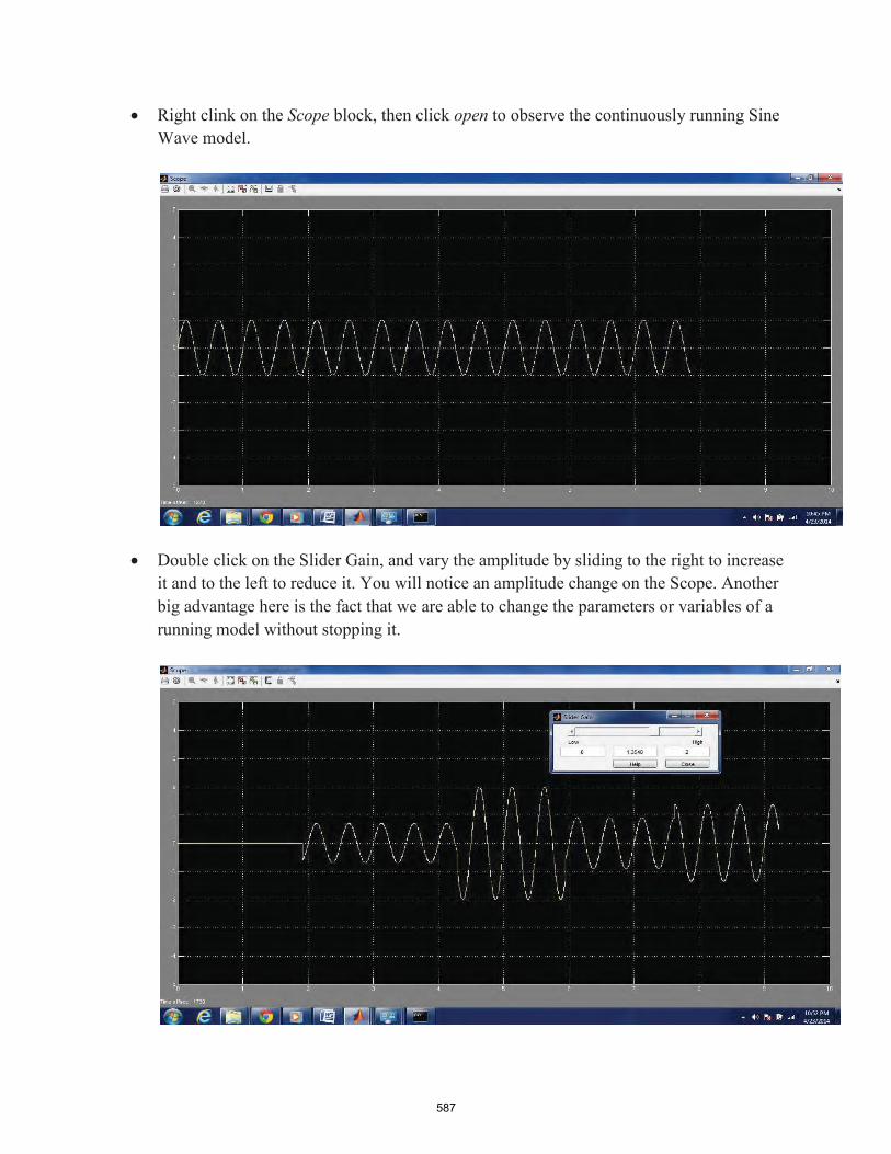
587
• Right clink on the Scope block, then click open to observe the continuously running Sine Wave model.
• Double click on the Slider Gain, and vary the amplitude by sliding to the right to increase
it and to the left to reduce it. You will notice an amplitude change on the Scope. Another big advantage here is the fact that we are able to change the parameters or variables of a running model without stopping it.

588
• In the Simulink model, press the Stop button. The command window that appeared above should now display a new message showing that the simulation has been stopped.
• Save the model. Close everything. You may now disconnect the board.
III. CONCLUSION
That concludes our intended process of showing how a Simulink model can be run on a BeagleBoard and the advantages of doing so. It obvious that, thanks to MathWorks, the BeagleBoard can be configured and different Simulink models can be created and run on it for different engineering applications, even with the ability to change model parameters and variables without stopping or pausing the running model at hand.

589
∗
∗ −
− ∗
\ \ \
1
MATLAB Code
cl ear , cl o se a l l ;
dA1M = 0 . 1 ; %i n m r a nge = 50; %i n m
lamda = 2 r a nge ; r e s = 0.001;
e rro rT a b le ( 1 ) = 0 . 1 ; e rro rT a b le ( 2 ) = 0 . 0 5 ; e rro rT a b le ( 3 ) = 0 . 0 1 ; e rro rT a b le ( 4 ) = 0 . 0 ;
fo r i = 1 : 4
e r r o r = e rro rT a b le ( i ) ; %e r r o r = 0 . 1 ; %i n degr ees
count = 0 ; f o r phase = 0 : r e s : dA1M / lamda 360 re s
count = c ount + 1 ; %phaseMeasured = p i / 180 ∗ phase ; phaseMeasured = p i / 180 ∗ normrnd ( phase , e r r o r ) ; dA1MR = phaseMeasured / ( 2 ∗ pi ) ∗ lamda ;
b e t a ( count , i ) = a bs ( a t a n ( ( s q r t ( ( dA1M/ 2 ) 2 (dA1MR / 2 ) ˆ 2 ) ) / ( dA1MR / 2 ) ) 180 / p i ) pha se Va l ( count , i ) = pha s e ;
end end
f ig u re p lo t ( phase Val ( : , 2 ) , b e t a ( : , 2) , ’ k ’ , ’ Line Width ’ , 1 . 5 ) ; t i t l e ( ’ Angle v e r s u s Phase ’ , ’ Font Siz e ’ , 1 6 ) ; xl abe l ( ’ Phase De l ta phi ( d e g re e s ) ’ , ’ Font Siz e ’ , 1 6 ) yl abe l ( ’ Angle t h e t a ( degr ees ) ’ , ’ Font Siz e ’ , 1 6 ) s e t ( gca , ’ Font Siz e ’ , 1 5 , ’ Line Width ’ , 1 . 5 ) gr i d
f ig u re p lo t ( phase Val ( : , 3 ) , b e t a ( : , 3) , ’ k ’ , ’ Line Width ’ , 1 . 5 ) ; t i t l e ( ’ Angle v e r s u s Phase ’ , ’ Font Siz e ’ , 1 6 ) ;

590
\ \ \
∗ − ∗ ∗
∗ − ∗ −
∗ − ∗ ∗
∗ ∗
xl abe l ( ’ Phase De l ta phi ( d e g re e s ) ’ , ’ Font Siz e ’ , 1 6 ) yl abe l ( ’ Angle t h e t a ( degr ees ) ’ , ’ Font Siz e ’ , 1 6 ) s e t ( gca , ’ Font Siz e ’ , 1 5 , ’ Line Width ’ , 1 . 5 ) gr i d
cl ear , cl o se a l l
c l e a r v a r s LOS = 1 ;
Pt = 30;% i n dB f = 5.9;% i n Ghz ha = 0 . 5 ; hb = 0 . 5 ; lamda = 3 ∗ 10ˆ 8/ ( f ∗ 10ˆ 9) ;
%Old Model % Rbp = 4 ( ha 1) (hb 1)/ lamda ; % n1 = 2.27; % n2 = 4 ; % L01 = 41+20 log10 ( f / 5 ) ; % L02 = 41+20 log10 ( f / 5) 17.3 log10 ( Rbp ) ; % s igma 1 = 1 ; % s igma 2 = 1 ;
%New Model Rbp = 6 . 2 ; n1 = 2 . 34 ; n2 = 3 . 73 ; L01 = 41+20 log10 ( f / 5 ) ; L02 = 41+20 log10 ( f / 5) 17.3 log10 ( Rbp ) ; sigma1 = 0 . 6 ; sigma 2 = 0.42;
fo r LOS = 0 : 1
count = 0 ; f o r d = 1: 0.25: 50
count = c ount + 1 ; if LOS
if d<Rbp los s = L01 + 10 n1 log10 ( d ) ; shadow = l ognr nd (0 , sigma 1 ) ;
else

591
l o s s = L02 + 10 n2 l∗og 10 ∗ ( d ) ; shadow = l ognr nd (0 , sigma 2 ) ; end
else if d<Rbp
los s = L01 + 10 n1 l∗og 10 ∗ ( d ) ; shadow = l ognr nd (0 , sigma 1 ) ;
else l o s s = L02 + 10 n2 l∗og 10 ∗ ( d ) ; shadow = l ognr nd (0 , sigma 1 ) ;
end temp = 2 . 8 − 0.0024 ∗d; n j = max ( [ temp ,1 .8 4] ); l o s s = l oss +20 −12.5∗ nj +10∗ nj ∗ log10 ( d ) ;
end RSSIMeasured ( count , LOS+ 1 ) = Pt−loss − shadow ; end
end
f ig u re p l o t ( [ 1 : 0 . 2 5 : 5 0 ] , RSSIMeasured ( : , 1 ) , ’ k ’ , ’ Line Width ’ , 2 ) ; xl abe l ( ’ D i s t a n c e (m) : d { RSSI } fo r LOS , d A = d B f or NLOS’ , ’ Font Siz e ’ , 16) yl abe l ( ’ RSSI ( dB ) ’ , ’ Font Siz e ’ , 1 6 ) t i t l e ( ’ RSSI Between Ma s t e r and Se nsor Cones ’ , ’ Font Siz e ’ , 1 6 ) a x is ([0 50 − 100 1 0 ] ) s e t ( gca , ’ Font Siz e ’ , 1 5 , ’ Line Width ’ ,1.5) gr i d hold on p l o t ( [ 1 : 0 . 2 5 : 5 0 ] , RSSIMeasured ( : , 2 ) , ’ k −− ’ , ’ Line Width ’ , 2 ) ; h = l e gend ( ’ NLOS’ , ’ LOS ’ , 1 ) ;
cl ear , cl o se a l l ;
dA1M = 0 . 1 ; %i n m r a nge = 50; %i n m
%Assuming m a s t e r node i s a t 0 , 0 and M and A1 a t +c ,0 , − c , 0 posCone . x = 1 0 ; posCone . y = 5 ;
lamdaRange = 2∗ r a nge ;
b e t a R e f = a t a n ( posCone . x / posCone . y ) 180/∗ pi ; dRef = s q r t ( posCone . x 2 + posCone . y ˆ 2 ) ;

592
∗ − ∗ ∗
∗ − ∗ −
∗ − ∗ ∗
∗ ∗
∗ ∗
dA1MR = dA1M∗ cos ( b e ta R e f ∗ p i /1 80) ; phase = dA1MR∗ 360/ lamda Range ;
e r r or = 0.01; c l e a r posMeasured
f = 5 . 9 ; %i n Ghz Pt = 30; %i n dB
%Old Model % Rbp = 4 ( ha 1) (hb 1)/ lamda ; % n1 = 2.27; % n2 = 4 ; % L01 = 41+20 log10 ( f / 5 ) ; % L02 = 41+20 log10 ( f / 5) 17.3 log10 ( Rbp ) ; % s igma 1 = 1 ; % s igma 2 = 1 ;
%New Model Rbp = 6 . 2 ; n1 = 2 . 34 ; n2 = 3 . 73 ; L01 = 41+20 log10 ( f / 5 ) ; L02 = 41+20 log10 ( f / 5) 17.3 log10 ( Rbp ) ; sigma1 = 0 . 6 ; sigma 2 = 0.42;
f o r i =1: 100
phase Measured = normrnd ( phase , e r r o r ) ; dA1MR = phase Measured / ( 360) ∗ lamdaRange ;
be taMeasured = abs ( a t a n ( ( s q r t ( ( dA1M/2 )ˆ2 − (dA1MR / 2 ) ˆ 2 ) ) / ( dA1MR / 2 ) ) ∗ 180 / p i ) ;
d = d Ref ; LOS = 1 ; if LOS
if d<Rbp los s = L01 + 10 n1 log10 ( d ) ; shadow = l ognr nd (0 , sigma 1 ) ;
else
end
l o s s = L02 + 10 n2 log10 ( d ) ; shadow = l ognr nd (0 , sigma 2 ) ;

593
∗ ∗
∗ ∗
− ∗
− − ∗
∗
el se if d<Rbp
los s = L01 + 10 n1 log10 ( d ) ; shadow = l ognr nd (0 , sigma 1 ) ;
else
end
l o s s = L02 + 10 n2 log10 ( d ) ; shadow = l ognr nd (0 , sigma 1 ) ;
end
temp = 2 . 8 0.0024 d; n j = max ( [ temp ,1 .84 ] ); l o s s = l oss +20 −12.5∗ nj +10∗ nj ∗ log10 ( d ) ;
RSSI = Pt−lo s s − shadow ;
dMeasured = 1 0 ˆ ( ( Pt RSSI L01 ) / ( 1 0 n1 ) ) ; i f dMeasured>Rbp
end
dMeasured = 1 0 ˆ ( ( Pt−RSSI−L02 ) / ( 1 0 ∗ n2 ) ) ;
end
posMeasured ( i , 2 ) = d Measured∗ cos ( beta Measured ∗ pi / 1 8 0 ) ; posMeasured ( i , 1 ) = d Measured∗ s i n ( beta Measured ∗ pi / 1 8 0 ) ;
f ig u re s c a t t e r ( posMeasured ( : , 1 ) , posMeasured ( : , 2 ) , ’ k ’ , ’ Line Width ’ , 1 ) t i t l e ( ’ Cone P o s i t i o n E s t i m a t e s u s i n g RSSI and Phase Measurements ’ , ’ Font Siz e ’ , 1 6 ) xl abe l ( ’ P o s i t i o n x (m) ’ , ’ Font Siz e ’ , 16 ) ; yl abe l ( ’ P o s i t i o n y (m) ’ , ’ Font Siz e ’ , 16 ) ; s e t ( gca , ’ Font Siz e ’ , 1 5 , ’ Line Width ’ , 1 . 5 ) ; a x is ([0 12 0 7 ]) gr i d hold on s c a t t e r ( posCone . x , posCone . y , ’ k ’ , ’ ’ , ’ Line Width ’ , 1 ) hold on s c a t t e r ( 0.05 ,0.05 , ’ k ’ , ’ ∗ ’ , ’ Line Width ’ , 1 )
l e gend ( ’ Se nsor Cone E s t i m a t e s ’ , ’ A ct ual P o s i t i o n s ’ , 2 )

594
% Lane and car g r id % Modified t o i n c l u d e very n o i s y % measurements of t h e GPS o f f s e t s
cl ear , cl o se a l l ;
% S t a ndar d l a ne width i s 12 f e e t = 3 . 6 6 m e t e r s % Assume 4 l a n e s with e dge s 0 , 3.66 , 7.32 , 10.98 , and 14 . 64 m % and with c e n t e r s 1 . 8 3 , 5 . 4 9 , 9 . 1 5 , and 12.81 m width = 3 . 6 6 ; l a n e 1 = 1 . 83 ; l a n e 2 = 5 . 49 ; l a n e 3 = 9 . 15 ; l a n e 4 = 12.81;
% P ar am et er s alphaLOSNLOS = 0 . 1; % P r o b a b i l i ty f o r Markov c h a i n w Sigma = 0 .0 00 01 ; % P r o cess n o i s e s t a n d a rd d e v i a t i o n GPS Sigma = 0 .2 5 ; % GPS measurement n o i s e s t a n d a r d devi a t i o n RSSI Sigma = 0 . 25 ; % RSSI measurement n o i s e s t a n d a r d d e v i a t i on RSSI2D Sigma = 5 ; % 2DRSSI measurement n o i s e s t a n d a r d d e v i a t i o n TOF Sigma = 0 . 2 5 ; % TOF n o i s e s t a n d a r d d e v i a t ion w x Sigma = w Sigma ; % S t a n d a r d devi a t i on of p r o c e s s n o i s e w( k ) w y Sigma = w Sigma ; % i n x− and y−di re ct io ns
NumOfCars = 3 ; % Number of c a r s Num Offsets = 2 ; % Number of o f f s e t s , x− and y−d i r ect i ons
% Sample r a t e i s 50 Hz Ts = 1 / 50; % Sample p er i o d i s 0 . 0 2 s Tsim = 100; % S i m u l a t i o n t ime i n s e c onds Nsamp = Tsim / Ts ; % Number of d i s c r e t e −time sa mple s i n s i mu la t io n
% Random o f f s e t s o f f s e t X = normrnd ( 0 , 2 ) % Random o f f s e t Y = normrnd ( 0 , 2 ) o f f s e t X = 4 % O v e r r i d e with s p e c if ic v a l u e s o ffs e t Y = 4
% S ta t e vec t or def i ned : [ p x1 ; p y1 ; p dot x1 ; p dot y 1 ; . . . o f fs e t X ; o ffs e t Y ] % 30 m/ s = 67.1 mph % I n i t i a l v a l u e s x 0 1 = [ 1 0 ; la n e 1 ; 30; 0 ; 30; la n e 2 ; 30; 0 ; 50; la n e 3 ; 30; 0 ; o f f s e t X ; o f f s e t Y ] ;

595
−
−
−
− −
−
−
− −
% I n i t i a l i z e a c c e l e r a t i o n s of a l l c a r s i n t h e x d i r ec t i o n t o z e r o p ddot x = zer os ( Nsamp , NumOfCars ) ;
% O ver r i de x d i re c t i o n a c c e l e ra t i o ns p ddot x ( 6/ Ts : 8/ Ts , 1) = 4 ; p ddot x ( 9 / Ts : 10 / Ts , 1 ) = 4; p ddot x ( 20/ Ts :2 1 / Ts , 2 ) = 4 ; p ddot x ( 28/ Ts :3 0 / Ts , 2 ) = 4; p ddot x ( 65/ Ts :6 7 / Ts , 3 ) = 4; p ddot x ( 75/ Ts :7 7 / Ts , 3 ) = 4 ;
% I n i t i a l p o s i t i o n s of a l l c a r s i n t h e x di r ec t io n p x = zer os ( Nsamp , NumOfCars ) ; p x ( 1 , 1 ) = x 0 1 ( 1 ) ; p x ( 1 , 2 ) = x 0 1 ( 5 ) ; p x ( 1 , 3 ) = x 0 1 ( 9 ) ;
% I n i t i a l p o s i t i o n s of a l l c a r s i n t h e y di r ec t io n p y = z e r o s ( Nsamp+ 2 , NumOfCars ) ; % Need k+2 because of d e r i v a t i v e s below p y( 1 , 1 ) = x 0 1 ( 2 ) ; p y( 1 , 2 ) = x 0 1 ( 6 ) ; p y( 1 , 3 ) = x 0 1 ( 10) ;
% D escr i b e car l ane c ha nge s a l o n g y−di r e c t i o n ( m e t e r s )
% S pec i f y s t a r t t ime of l ane c ha nge s ( i n s ) and si g n (+ move l e f t / r i g h t ) % Car 1: 10( +) , 40( ) % Car 2: 30( +) , 7 0 ( + ) % Car 3 : 50( +) % Need a loop f o r each c a r change
f or i = 2: 10/ Ts
p y( i , 1 ) = p y( i − 1 , 1 ) ; p y( i , 2 ) = p y( i − 1 , 2 ) ; p y( i , 3 ) = p y( i − 1 , 3 ) ;
end
change = 5 ; % Seconds t o change l a n e s f o r i = 10/ Ts + 1 : ( 10 + change ) / Ts
p y( i , 1 ) = p y( i − 1 , 1 ) + width ∗Ts / change ; p y( i , 2 ) = p y( i − 1 , 2 ) ; p y( i , 3 ) = p y( i − 1 , 3 ) ;
end
f o r i = ( 10 + change ) / Ts + 1 : 3 0 / Ts

596
p y( i , 1 ) = p y( i − 1 , 1 ) ; p y( i , 2 ) = p y( i − 1 , 2 ) ;
p y( i , 3 ) = p y( i − 1 , 3 ) ; end
change = 6 ; % Seconds t o change l a n e s f o r i = 30/ Ts + 1 : ( 30 + change ) / Ts
p y( i , 1 ) = p y( i − 1 , 1 ) ; p y( i , 2 ) = p y( i − 1 , 2 ) + width ∗Ts / change ; p y( i , 3 ) = p y( i − 1 , 3 ) ;
end
f o r i = ( 30 + change ) / Ts + 1 : 4 0 / Ts p y( i , 1 ) = p y( i − 1 , 1 ) ; p y( i , 2 ) = p y( i − 1 , 2 ) ; p y( i , 3 ) = p y( i − 1 , 3 ) ;
end
change = 4 ; % Seconds t o change l a n e s f o r i = 40/ Ts + 1 : ( 40 + change ) / Ts
p y( i , 1 ) = p y( i − 1 ,1 ) − width ∗Ts / change ; p y( i , 2 ) = p y( i − 1 , 2 ) ; p y( i , 3 ) = p y( i − 1 , 3 ) ;
end
f o r i = ( 40 + change ) / Ts + 1 : 5 0 / Ts p y( i , 1 ) = p y( i − 1 , 1 ) ; p y( i , 2 ) = p y( i − 1 , 2 ) ; p y( i , 3 ) = p y( i − 1 , 3 ) ;
end
change = 5 ; % Seconds t o change l a n e s f o r i = 50/ Ts + 1 : ( 50 + change ) / Ts
p y( i , 1 ) = p y( i − 1 , 1 ) ; p y( i , 2 ) = p y( i − 1 , 2 ) ;
p y( i , 3 ) = p y( i − 1 , 3 ) + width ∗Ts / change ; end
f o r i = ( 50 + change ) / Ts + 1 : 7 0 / Ts p y( i , 1 ) = p y( i − 1 , 1 ) ;
p y( i , 2 ) = p y( i − 1 , 2 ) ; p y( i , 3 ) = p y( i − 1 , 3 ) ;
end
change = 7 ; % Seconds t o change l a n e s

f o r i = 7 0 / Ts + 1 : ( 70 + change ) / Ts p y( i , 1 ) = p y( i − 1 , 1 ) ;
p y( i , 2 ) = p y( i − 1 , 2 ) + width ∗Ts / change ; p y( i , 3 ) = p y( i − 1 , 3 ) ;
end
f o r i = ( 70 + change ) / Ts +1: 100/ Ts+2 p y( i , 1 ) = p y( i − 1 , 1 ) ; p y( i , 2 ) = p y( i − 1 , 2 ) ; p y( i , 3 ) = p y( i − 1 , 3 ) ;
end
% Compute a c c e l e r a t i o n s i n y di− r ec t i o n p dot y = d i f f ( p y ) . / Ts ; p ddot y = d i f f ( p dot y ) . / Ts ;
% C ons t r uct i nput vec t or f o r s t a t e − s p a c e model % ba se d on acc ele rat ion s u = zer os ( Nsamp , 2 Nu∗ mOfCars ) ; fo r i = 1 : NumOfCars
u( : , 2 ∗ i −1) = p ddot x ( : , i ) ; u( : , 2 ∗ i ) = p ddot y ( : , i ) ;
end
% M at r i ces fo r s t a t e −space model
% A mat r i x fo r updat i n g s t a t e s A = eye ( 4 N∗u mOfCars+ NumOffsets ) ; tempA = [ 1 0 Ts 0 ;
0 1 0 Ts ; 0 0 1 0 ; 0 0 0 1 ] ;
fo r i = 1 : NumOfCars A( 4 ∗ i −3:4∗ i , 4 ∗ i −3:4∗ i ) = tempA ; % R e p e a t s temp a l o n g di a go na l
end
% D m a t r i x f o r i n c or p o r a t i n g ac ce l e r a t i o ns D = zer os ( 4 Nu∗m OfCars+ NumOffsets , 2 NumO∗f Cars ) ; tempD = Ts . [ Ts / 2 0 ;∗
0 Ts / 2 ; 1 0 ; 0 1 ] ;
fo r i = 1 : NumOfCars D( 4 ∗ i −3:4∗ i , 2 ∗ i −1:2∗ i ) = tempD ; % R e p e a t s p at t e r n f o r a cce l e r a t i o ns
end
597

598
% F m a t r i x f o r GPS : e x t r a c t s p o s i t i ons with o f f s e t s FGPS = z e r o s ( 2 N∗ umOfCars+ NumOffsets , 4 Num∗O fCars+ NumOffsets ) ; tempF = eye ( 2 ) ; fo r i = 1 : NumOfCars
FGPS( 2 ∗ i −1:2∗ i , 4 ∗ i −3:4∗ i −2) = tempF ; % R e p e a t s p at t e r n f o r pos i t i o n s FGPS( 2 ∗ i −1:2∗ i , end −1: end ) = tempF ; % Add o f f s e t s
end FGPS ( 7 , 1 3 ) = 1 ; % Measure o f f s e t s FGPS ( 8 , 1 4 ) = 1 ;
% Q ma t r ix f o r p r o c e s s n o i s e Q = eye ( 4 N∗u mOfCars+ NumOffsets ) ; tempQ = [ ( Ts ˆ 2 / 2 w∗ x Sigma )ˆ2 0 ( Ts ˆ2 /2 w x S∗i gma ) ( Ts w x∗ S igma∗ ) 0 ;
0 ( Ts ˆ 2 / 2 w∗ y Sigma )ˆ2 0 ( Ts ˆ2 /2 ∗ w y Sigma ) ( ∗ Ts ∗w y Sigma ) ; ( Ts ∗ w x Sigma ) ( ∗ Ts ˆ 2 / 2 w∗ x Sigma ) 0 ( Ts ∗ w x Sigma )ˆ2 0; 0 ( Ts ∗w y Sigma ) ( ∗T s ˆ 2 / 2 w∗ y Sigma ) 0 ( Ts w∗ y Sigma ) ˆ 2 ] ;
fo r i = 1 : NumOfCars Q( 4 ∗ i −3:4∗ i , 4 ∗ i −3:4∗ i ) = tempQ ;
end Q = w Sigma ˆ 2 . ∗ eye ( 4 ∗Nu mOfCars+ Num Offsets ) ; % O v e r r i d e pr evi ous form %Q( end − 1, end − 1) = 0 ; % Zero var i ance f o r GPS p o s i t i o n o f f s e t s %Q( end , end ) = 0 ;
% G ener at e a c t u a l c a r t r a j e c t o r i e s from s t a t e − s p a c e model x = zer os ( Nsamp , 4 Nu∗ mOfCars+ NumOffsets ) ; w = normrnd ( 0 , w Sigma , Nsamp , 4 Nu∗ mOfCars+ NumOffsets ) ; % P r o c e s s n o i s e w( : , 4 ∗ Nu mOfCars+ NumOffsets − 1) = 0 ; % No noi se f or o f f s e t s w( : , 4 N∗ umOfCars+ NumOffsets ) = 0 ; x ( 1 , : ) = x 0 1 ; % I n i t i a l s t a t e v ect or
f o r i n s t a n t = 2 : Nsamp
x( i n st a n t , : ) = A∗x ( instant − 1 , : ) ’ + D∗u ( instant , : ) ’ + w( in stant , : ) ’ ; end
% G ener at e GPS s i g n a l s f o r i n s t a n t = 1 : Nsamp
v = normrnd ( 0 , GPS Sigma , 2 Num∗O fCars+ NumOffsets , 1 ) ; v ( 7 , 1 ) = normrnd ( 0 , 5 ) ; % Large n o i s e f o r o f f s e t measurements v ( 8 , 1 ) = normrnd ( 0 , 5 ) ;
y GPS ( i n s t a n t , : ) = FGPS∗x ( in s t a n t , : ) ’ + v ; % F i n c o rp or a te s o f f s e t s end
% S i m u l a t e LOS / NLOS zvar = GenLOSNLOS( Nsamp , NumOfCars , alphaLOSNLOS ) ;

599
∗
∗
∗
∗ ∗
−
∗
− −
% G ener at e RSSI s i g n a l s f o r i n s t a n t = 1 : Nsamp
v = normrnd ( 0 , RSSI Sigma , 2 NumOfCars , 1 ) ; zv = z v a r ( : , : , i n s t a n t ) ; RSSI = GenRSSI ([ x ( instan t , 1 ) x ( in stant , 5 ) x ( instant , 9 ) ] , . . .
[ x ( i ns t a nt , 2 ) x ( i n s t a n t , 6 ) x ( i n s t a n t , 1 0 ) ] , NumOfCars , zv ) ; y RSSI ( i ns t a nt , : ) = [ RSSI ( 1 , 2 ); RSSI ( 2 , 1 ); RSSI (1 , 3 ); RSSI (3 , 1 ); RSSI (2 , 3 ); RSSI (3 ,
end
% G ener at e TOF S i g n a l %v t = zer os ( 2 nchoosek ( NumOfCars , 2 ) , 1 ) ; % Check i f n o i s e s houl d be i n c l u d e d %f o r in st an t = 1 : Nsamp
%v t = normrnd ( 0 , TOF Sigma , 2 nchoosek ( NumOfCars , 2 ) , 1 ) ; %[TOF] = GenTOF( [ x (1 ) x (5 ) x ( 9 ) ] , [ x ( 2 ) x ( 6 ) x ( 1 0 ) ] , NumOfCars ) ; %y TOF ( i n s t a n t , : ) = [ TOF ( 1 , 2 ) ; TOF ( 2 , 1 ) ; TOF ( 1 , 3 ) ; TOF ( 3 , 1 ) ; TOF ( 2 , 3 ) ; TOF ( 3 , 2 ) ] +
%e nd
% G ener at e 2D RSSI s i g n a l s f o r i n s t a n t = 1 : Nsamp
v = normrnd ( 0 , RSSI2D Sigma , 2 2 NumOfCars , 1 ) ; zv = z v a r ( : , : , i n s t a n t ) ; Dxy = Gen2DRSSI ( [ x ( i n s t a n t , 1 ) x ( i n s t a n t , 5 ) x ( i n s t a n t , 9 ) ] , . . .
[ x ( i ns t a nt , 2 ) x ( i n s t a n t , 6 ) x ( i n s t a n t , 1 0 ) ] , NumOfCars ) ; y Dxy( i ns t a n t , : ) = [ Dxy( 1 , 2 , 1 ) ; Dxy( 1 , 2 , 2 ) ; Dxy( 2 , 1 , 1 ) ; Dxy( 2 ,1 , 2 ) ; Dxy( 1 , 3 , 1 ) ; Dxy
end
%RunGPSonly4 %RunRSSIonly
%RunGPS RSSI RunGPS 2DRSSI
% KF and EKF ( GPS and RSSI ) % u = s t a t e s p a c e i nput vec t or % x k = c u r r e nt s t a t e es t i m at e v e c t o r % c l o c k = time i n s t a n t T s % Q = p r o cess c ovar i ance m a t r i x % REKF = measurement c o v a r i a n c e m a t r i x % P k = c u r r e nt i n n o v a t i ons c o v a r i a n c e m a t r i x % A = s t a t e s p a c e t r an s i t i o n m a t r i x % D = s t a t e s p a c e i nput m a t r i x % F = measurement m a t r i x

600
∗ ∗ ∗
−
∗
− −
% y = GPS measurement v e c t o r % yRSSI = RSSI measurement v e c t o r
f unc t i o n [ x hat , P ] = KF EKF ( u , x k , c loc k , Q, R , REKF, P k , A, D, F , y , yRSSI )
% PREDICTION STAGE ( f o r KF and EKF ) : x hat = A∗ x k + D∗u ’ ; P = A∗P k∗A’ + Q;
% I f GPS i s a v a i l a b l e , go t o KF f i l t e r i n g s t a g e i f mod( clock , 1 ) = = 0 % Update r a t e f o r KF
% FILTERING STAGE: K = P∗F’ / ( F∗P∗F’ + R ) ; % Kalman g a i n y hat = F∗ x hat ; x hat = x hat + K∗(y ’ − y hat ) ; P = ( eye ( l engt h (A) ) − K∗F) ∗ P;
else
i f 1
end end
FRSSI = GenF ( x hat ) ; KRSSI = P FRSSI ’ / ( FRSSI P FRSSI ’ + REKF ) ; % EKF g a i n [ RSSI hat ] = GenyForRSSI ( [ x hat ( 1 ) x hat ( 5 ) x hat ( 9 ) ] , [ x hat ( 2 ) x hat ( 6 ) x hat y hat RSSI = [ RSSI hat ( 1 , 2 ) ; RSSI hat ( 2 , 1 ) ; RSSI hat ( 1 , 3 ) ; RSSI hat ( 3 , 1 ) ; RSSI hat (
x hat ( 1 3 ) ; x h a t ( 1 4 ) ] ; % I n c l u d e es t im a t e s of o f f s e t s yRSSI = [ yRSSI , y (7 ) , y ( 8 ) ] ; % I ncl ude measured o f f s e t s x hat = x h a t + KRSSI ∗( yRSSI ’ − y hat RSSI ) ; P = ( eye ( l engt h (A) ) − KRSSI∗FRSSI ) ∗ P;
% KF and EKF ( GPS and RSSI ) % u = s t a t e s p a c e i nput vec t or % x k = c u r r e nt s t a t e es t i m at e v e c t o r % c l o c k = time i n s t a n t T s % Q = p r o cess c ovar i ance m a t r i x % REKF = measurement c o v a r i a n c e m a t r i x % P k = c u r r e nt i n n o v a t i ons c o v a r i a n c e m a t r i x % A = s t a t e s p a c e t r an s i t i o n m a t r i x % D = s t a t e s p a c e i nput m a t r i x % F = measurement m a t r i x % y = GPS measurement v e c t o r % yRSSI = RSSI measurement v e c t o r

601
f unc t i o n [ x hat , P ] = KF KF ( u , x k , c loc k , Q, R, RKF, P k , A, D, F , y , y Dxy )
% PREDICTION STAGE ( f o r KF and EKF ) : x hat = A∗ x k + D∗u ’ ; P = A∗P k∗A’ + Q;
% I f GPS i s a v a i l a b l e , go t o KF f i l t e r i n g s t a g e i f mod( clock , 1 ) = = 0 % Update r a t e f o r KF
% FILTERING STAGE: K = P∗F’ / ( F∗P∗F’ + R ) ; % Kalman g a i n y hat = F∗ x hat ; x hat = x hat + K∗(y ’ − y hat ) ; P = ( eye ( l engt h (A) ) − K∗F) ∗ P;
e l s e
i f 1 F2DRSSI = z e r o s ( 1 4 , 1 4 ) ;
F2DRSSI ( 1 , 1 ) = 1 ; F2DRSSI ( 5 , 1 ) = −1; %c a r 121 F2DRSSI ( 2 , 2 ) = 1 ; F2DRSSI ( 6 , 2 ) = −1; %c a r 122 F2DRSSI ( 1 , 3 ) = −1; F2DRSSI ( 5 , 3 ) = 1 ; %c a r 211
F2DRSSI ( 2 , 4 ) = −1; F2DRSSI ( 6 , 4 ) = 1 ; %c a r 212 F2DRSSI ( 1 , 5 ) = 1 ; F2DRSSI ( 9 , 5 ) = −1; %c a r 131 F2DRSSI ( 2 , 6 ) = 1 ; F2DRSSI ( 1 0 , 6 ) = −1; %c a r 132 F2DRSSI ( 1 , 7 ) = −1; F2DRSSI ( 9 , 7 ) = 1 ; %c a r 311
F2DRSSI ( 2 , 8 ) = −1; F2DRSSI ( 1 0 , 8 ) = 1 ; %c a r 312
F2DRSSI ( 5 , 9 ) = 1 ; F2DRSSI ( 9 , 9 ) = − 1; %c a r 231 F2DRSSI ( 6 , 1 0 ) = 1 ; F2DRSSI ( 1 0 , 1 0 ) = − 1; %c a r 232 F2DRSSI( 5 , 11 )= − 1 ; F2DRSSI ( 9 , 1 1 ) = 1 ; %c a r 321 F2DRSSI( 6 , 12 )= − 1 ; F2DRSSI ( 1 0 , 1 2 ) = 1 ; %c a r 322 F2DRSSI ( 1 3 , 1 3 ) = 1 ; F2DRSSI ( 1 4 , 1 4 ) = 1 ; %O f f s e t s F2DRSSI = F2DRSSI ’ ;
K2DRSSI = P F2∗D RSSI ’ / ( F2DRSSI P F2∗D ∗R SSI ’ + RKF ) ; % EKF g a i n y hat2 DRSSI = F2DRSSI ∗ x h a t ; % I ncl ude e s t im at e s of o f f s e t s y2DRSSI = [ y Dxy , y ( 7 ) , y ( 8 ) ] ; % I n c l u d e measured o f f s e t s x hat = x h a t + K2DRSSI∗( y2DRSSI ’ − y hat2 DRSSI ) ; P = ( eye ( l engt h (A) ) − K2DRSSI∗F2DRSSI) ∗ P;
end end
%%%%%%%%%%%%%%%%%%%%%%%%%%%%%%%%%%%%%%%%%%%%%%%%%%%%%%%%%%%%%%%%%%%%%%%%

602
% KALMAN FILTER AND EKF ( GPS and RSSI s i g n a l s )
% R ma trix f o r KF R KF = eye ( 2 ∗ NumOfCars+ NumOffsets ) . ∗ GPS Sigma ˆ 2 ; R KF ( 7 , 7 ) = 5 ; R K
F ( 8 , 8 ) = 5 ; %R KF = eye ( 2 ∗ NumOfCars ) . ∗ 100 ; % O v e r r i d e p r e v i o u s
% R EKF m a t r i x f o r EKF R EKF = eye ( 2 Nu∗ mOfCars+ NumOffsets ) R∗ SSI Sigma ˆ 2 ; R EKF ( 7 , 7 ) = 5 ; R EKF ( 8 , 8 ) = 5 ;
% R EKF m a t r i x f o r 2D RSSI R 2DKF = eye ( 4 N∗u mOfCars+ NumOffsets ) R∗ SSI2D Sigma ˆ 2 ; R 2DKF ( 1 3 , 1 3 ) = 5 ; R 2DKF ( 1 4 , 1 4 ) = 5 ;
% I n i t i a l c ond i t i ons % A c t u a l s t a r t i n g c ond i t i ons : %x k = x 0 1; % E v e ry th in g zer o : %x k = zer os ( 1 4 , 1 ) ; % E ver y t h i n g zero , except c o r r e c t o f f s e t s %x k = [ zer os (1 2 , 1 ) ; o f f s et X ; of f s et Y ] ; % C or r ect v e l o c i t i e s only : x k = [ y GPS ( 1 , 1 ) ; y GPS ( 1 , 2 ) ; 30; 0 ; y GPS (1 , 3 ) ; y GPS ( 1 , 4 ) ; 30; 0 ; y GPS ( 1 , 5 ) ; y % C or r ect v e l o c i t i e s and o f f s e t s : %x k = [ y GPS (1 , 1 ); y GPS ( 1 , 2 ) ; 30; 0 ; y GPS (1 , 3 ); y GPS ( 1 , 4 ) ; 30; 0 ; y GPS (1 , 5 ); y % C or r ect v e l o c i t i e s and l anes ( y p−o s i t i ons ) : %x k = [ y GPS ( 1 , 1 ) ; l a n e 1 ; 30; 0 ; y GPS ( 1 , 3 ) ; l a n e 2 ; 30; 0 ; y GPS ( 1 , 5 ) ; l ane3 ; 3 0 ;
P k = 100. eye (∗ 4 N umO∗ fCars+ NumOffsets ) ; %P k = Q;
% Use KF / GPS f o r time i n s t a n t 1 % PREDICTION STAGE : x hat = A∗ x k + D∗u( 1 , : ) ’ ; P = A∗P k∗A’ + Q;
% FILTERING STAGE: K = P∗FGPS ’ / ( FGPS∗P∗FGPS ’ + R KF ) ; % Kalman g a i n y h a t = FGPS∗ x hat ;

603
− ∗ ∗ ∗ −
∗
− −
−
−
x k = x hat + K (y GPS ( 1 , : ) ’ y hat ) ; P k = ( eye ( l engt h (A) ) K FGPS) P; Output ( 1 , : ) = x k ’ ;
% KF / EKF loop f o r i n s t a n t = 2 : Nsamp % St a r t a t t ime i n s t a n t 2
cl ock = i n s t a n t Ts ; % 1 Hz r a t e f o r GPS [x hat , P hat ] = KF KF( u ( i nstant , : ) , x k , c loc k , Q, R KF,R 2DKF , P k , A, D , . . .
FGPS , y GPS ( i n s t a n t , : ) , y Dxy ( i n s t a n t , : ) ) ; x k = x hat ; % Save f o r next i t e r a t i o n P k = P hat ; Output ( i ns t a nt , : ) = x h a t ; % Save f o r p l ot t i ng
end
%%%%%%%%%%%%%%%%%%%%%%%%%%%%%%%%%%%%%%%%%%%%%%%%%%%%%%%%%%%%%%%%%%%%%%%%%%%%%%%%%% % P l o t t r a j e c t o r i es f i gu r e ; hold a l l ; % A c t u a l p o s i t i ons p lo t ( x ( : , 1 ) , x ( : , 2) , ’ Line Width ’ , 2 ) ; p lo t ( x ( : , 5 ) , x ( : , 6) , ’ Line Width ’ , 2 ) ; plot ( x ( : , 9 ) , x ( : , 10) , ’ Line Width ’ , 2 ) ; gr i d ; s e t ( gca , ’ Font Siz e ’ , 1 5 , ’ Line Width ’ , 1 . 5 ) xl abe l ( ’ P o s i t i o n i n x d i re c t i on (m) ’ , ’ Font Siz e ’ , 16 ); yl abe l ( ’ P o s i t i o n i n y d i re c t i on (m) ’ , ’ Font Siz e ’ , 16 ); t i t l e ( ’ Car T r a j e c t o r i e s ’ , ’ Font Siz e ’ , 1 6 ) ;
f i g u r e ; hold a l l ; % A c t u a l ve lo c i t i e s i n y d i r ec t i on p l o t ( x ( : , 4 ) , ’ Line Width ’ , 2 ) ; p l o t ( x ( : , 8 ) , ’ Line Width ’ , 2 ) ; plot ( x (: ,12) , ’ Line Width ’ , 2 ) ; gr i d ; s e t ( gca , ’ Font Siz e ’ , 1 5 , ’ Line Width ’ , 1 . 5 ) x l a b e l ( ’ Time ( samples ) ’ , ’ Font Size ’ , 1 6 ) ; y l a b e l ( ’ Ve lo c i ty i n y−d i r e c t i o n (m/ s ) ’ , ’ Font Size ’ , 1 6 ) ; t i t l e ( ’ Car V e l o c i t i e s i n y−Dire c t io n ’ , ’ Font Siz e ’ , 1 6 ) ;
f i g u r e ; hold a l l ; % A c t u a l ve lo c i t i e s i n x d i r ec t ion p l o t ( x ( : , 3 ) , ’ Line Width ’ , 2 ) ; p l o t ( x ( : , 7 ) , ’ Line Width ’ , 2 ) ; plot ( x (: ,11) , ’ Line Width ’ , 2 ) ; gr i d ; s e t ( gca , ’ Font Siz e ’ , 1 5 , ’ Line Width ’ , 1 . 5 ) x l a b e l ( ’ Time ( samples ) ’ , ’ Font Size ’ , 1 6 ) ; y l a b e l ( ’ Ve lo c i ty i n x−d i r e c t i o n (m/ s ) ’ , ’ Font Size ’ , 1 6 ) ; t i t l e ( ’ Car V e l o c i t i e s i n x−Dire c t io n ’ , ’ Font Siz e ’ , 1 6 ) ;

604
− −
− −
−
−
f i gu r e ; hold a l l ; % GPS p o s i t i o n s p lo t (y GPS ( : , 1 ) , y GPS ( : , 2 ) , ’ LineWidth ’ , 2 ) ; p lo t (y GPS ( : , 3 ) , y GPS ( : , 4 ) , ’ LineWidth ’ , 2 ) ; plot (y GPS ( : , 5 ) , y GPS ( : , 6 ) , ’ LineWidth ’ , 2 ) ; gr i d ; s e t ( gca , ’ Font Siz e ’ , 1 5 , ’ Line Width ’ ,1.5) xl abe l ( ’ GPS P o s i t i o n i n x d i r ec t ion (m) ’ , ’ Font Siz e ’ , 16) ; yl abe l ( ’ GPS P o s i t i o n i n y d i r ec t ion (m) ’ , ’ Font Siz e ’ , 16) ; t i t l e ( ’ GPS Measurements ’ , ’ Font Siz e ’ , 1 6 ) ;
f ig u re ; hold a l l ; % KF Po s i t i on s p l o t ( Output ( : , 1 ) , Output ( : , 2 ) , ’ Line Width ’ , 2 ) ; p l o t ( Output ( : , 5 ) , Output ( : , 6 ) , ’ Line Width ’ , 2 ) ; p l o t ( Output ( : , 9 ) , Output ( : , 1 0 ) , ’ Line Width ’ , 2 ) ; gr i d ; s e t ( gca , ’ Font Siz e ’ , 1 5 , ’ Line Width ’ , 1 . 5 ) x l a b e l ( ’ KF F i l t e r E s t i m a t e i n x d i re c t i on (m) ’ , ’ Font Siz e ’ , 16 ); y l a b e l ( ’ KF F i l t e r E s t i m a t e i n y d i re c t i on (m) ’ , ’ Font Siz e ’ , 16 ); t i t l e ( ’ KF P o s i t i o n E s t i m a t e s Based on GPS ’ , ’ Font Siz e ’ , 1 6 ) ;
f ig u re ; hold a l l ; % KF Ve lo c i t i e s i n x di r ec t io n p l o t ( Output ( : , 3 ) , ’ Line Width ’ , 2 ) ; p l o t ( Output ( : , 7 ) , ’ Line Width ’ , 2 ) ; plot ( Output (: ,11) , ’ Line Width ’ , 2 ) ; gr i d ; s e t ( gca , ’ Font Siz e ’ , 1 5 , ’ Line Width ’ , 1 . 5 ) x l a b e l ( ’ Time ( samples ) ’ , ’ Font Size ’ , 1 6 ) ; yl abe l ( ’ KF ve lo c i ty i n x−dir ec t i o n (m) ’ , ’ Font Siz e ’ , 16) ; t i t l e ( ’ KF V e l o c i t i e s i n x−Dire c t io n ’ , ’ Font Siz e ’ , 1 6 ) ;
f ig u re ; hold a l l ; % KF Ve lo c i t i e s i n y di r ec t io n p l o t ( Output ( : , 4 ) , ’ Line Width ’ , 2 ) ; p l o t ( Output ( : , 8 ) , ’ Line Width ’ , 2 ) ; plot ( Output (: ,12) , ’ Line Width ’ , 2 ) ; gr i d ; s e t ( gca , ’ Font Siz e ’ , 1 5 , ’ Line Width ’ , 1 . 5 ) x l a b e l ( ’ Time ( samples ) ’ , ’ Font Size ’ , 1 6 ) ; yl abe l ( ’ KF ve lo c i ty i n y−dir ec t i o n (m) ’ , ’ Font Siz e ’ , 16) ; t i t l e ( ’ KF V e l o c i t i e s i n y−Dire c t io n ’ , ’ Font Siz e ’ , 1 6 ) ;
f ig u re ; hold a l l ; % O f f s e t e s t i m at es p lo t ( Output (: , 13 ) , ’ Line Width ’ , 2 ) ; plot ( Output (: ,14) , ’ Line Width ’ , 2 ) ; gr i d ;

605
∗ ∗
∗ ∗
−
∗ ∗
s e t ( gca , ’ Font Siz e ’ , 1 5 , ’ Line Width ’ , 1 . 5 ) x l a b e l ( ’ Time ( samples ) ’ , ’ Font Size ’ , 1 6 ) ; yl abe l ( ’ Of f s et s (m) ’ , ’ Font Siz e ’ , 1 6 ) ; t i t l e ( ’ O f f s e t E s t i m a t e s ’ , ’ Font Siz e ’ , 1 6 ) ;
%%%%%%%%%%%%%%%%%%%%%%%%%%%%%%%%%%%%%%%%%%%%%%%%%%%%%%%%%%%%%%%%%%%%%%%%%%%%%%%%%% % KALMAN FILTER AND EKF ( GPS and RSSI s i g n a l s )
% R ma t r ix f o r KF R KF = eye ( 2 NumOfCars+ NumOffsets ) . GPS Sigma ˆ 2 ; R KF ( 7 , 7 ) = 5 ; R KF ( 8 , 8 ) = 5 ;
%R KF = eye ( 2 ∗ NumOfCars ) . ∗ 100 ; % O v e r r i d e p r e v i o u s
% R EKF m a t r i x f o r EKF R EKF = eye ( 2 NumOfCars+ NumOffsets ) RSSI Sigma ˆ 2 ; R KF ( 7 , 7 ) = 5 ; R KF ( 8 , 8 ) = 5 ;
% I n i t i a l c ond i t i ons % A c t u a l s t a r t i n g c ond i t i ons : %x k = x 0 1; % E v e ry th in g zer o : %x k = zer os ( 1 4 , 1 ) ; % E ver y t h i n g zero , except c o r r e c t o f f s e t s %x k = [ zer os (1 2 , 1 ) ; o f f s et X ; of f s et Y ] ; % C or r ect v e l o c i t i e s only : x k = [ y GPS ( 1 , 1 ) ; y GPS ( 1 , 2 ) ; 30; 0 ; y GPS (1 , 3 ) ; y GPS ( 1 , 4 ) ; 30; 0 ; y GPS ( 1 , 5 ) ; y % C or r ect v e l o c i t i e s and o f f s e t s : %x k = [ y GPS (1 , 1 ); y GPS ( 1 , 2 ) ; 30; 0 ; y GPS (1 , 3 ); y GPS ( 1 , 4 ) ; 30; 0 ; y GPS (1 , 5 ); y % C or r ect v e l o c i t i e s and l anes ( y p o s i t i ons ) : %x k = [ y GPS ( 1 , 1 ) ; l a n e 1 ; 30; 0 ; y GPS ( 1 , 3 ) ; l a n e 2 ; 30; 0 ; y GPS ( 1 , 5 ) ; l ane3 ; 3 0 ;
P k = 100. eye ( 4 NumOfCars+ NumOffsets ) ; %P k = Q;
% Use KF / GPS f o r time i n s t a n t 1 % PREDICTION STAGE : x hat = A∗ x k + D∗u( 1 , : ) ’ ; P = A∗P k∗A’ + Q;
% FILTERING STAGE: K = P∗FGPS ’ / ( FGPS∗P∗FGPS ’ + R KF ) ; % Kalman g a i n y h a t = FGPS∗ x hat ;

606
− ∗ ∗ ∗ −
∗
− −
−
−
x k = x hat + K (y GPS ( 1 , : ) ’ y hat ) ; P k = ( eye ( l engt h (A) ) K FGPS) P; Output ( 1 , : ) = x k ’ ;
% KF / EKF loop f o r i n s t a n t = 2 : Nsamp % St a r t a t t ime i n s t a n t 2
cl ock = i n s t a n t Ts ; % 1 Hz r a t e f o r GPS [x hat , P hat ] = KF EKF( u ( instant , : ) , x k , c loc k , Q, R KF , R EKF , P k , A, D , . . .
FGPS , y GPS ( i n s t a n t , : ) , y RSSI ( i n s t a n t , : ) ) ; x k = x hat ; % Save f o r next i t e r a t i o n P k = P hat ; Output ( i ns t a nt , : ) = x h a t ; % Save f o r p l ot t i ng
end
%%%%%%%%%%%%%%%%%%%%%%%%%%%%%%%%%%%%%%%%%%%%%%%%%%%%%%%%%%%%%%%%%%%%%%%%%%%%%%%%%% % P l o t t r a j e c t o r i es f i gu r e ; hold a l l ; % A c t u a l p o s i t i ons p lo t ( x ( : , 1 ) , x ( : , 2) , ’ Line Width ’ , 2 ) ; p lo t ( x ( : , 5 ) , x ( : , 6) , ’ Line Width ’ , 2 ) ; plot ( x ( : , 9 ) , x ( : , 10) , ’ Line Width ’ , 2 ) ; gr i d ; s e t ( gca , ’ Font Siz e ’ , 1 5 , ’ Line Width ’ , 1 . 5 ) xl abe l ( ’ P o s i t i o n i n x d i re c t i on (m) ’ , ’ Font Siz e ’ , 16 ); yl abe l ( ’ P o s i t i o n i n y d i re c t i on (m) ’ , ’ Font Siz e ’ , 16 ); t i t l e ( ’ Car T r a j e c t o r i e s ’ , ’ Font Siz e ’ , 1 6 ) ;
f i g u r e ; hold a l l ; % A c t u a l ve lo c i t i e s i n y d i r ec t i on p l o t ( x ( : , 4 ) , ’ Line Width ’ , 2 ) ; p l o t ( x ( : , 8 ) , ’ Line Width ’ , 2 ) ; plot ( x (: ,12) , ’ Line Width ’ , 2 ) ; gr i d ; s e t ( gca , ’ Font Siz e ’ , 1 5 , ’ Line Width ’ , 1 . 5 ) x l a b e l ( ’ Time ( samples ) ’ , ’ Font Size ’ , 1 6 ) ; y l a b e l ( ’ Ve lo c i ty i n y−d i r e c t i o n (m/ s ) ’ , ’ Font Size ’ , 1 6 ) ; t i t l e ( ’ Car V e l o c i t i e s i n y−Dire c t io n ’ , ’ Font Siz e ’ , 1 6 ) ;
f i g u r e ; hold a l l ; % A c t u a l ve lo c i t i e s i n x d i r ec t ion p l o t ( x ( : , 3 ) , ’ Line Width ’ , 2 ) ; p l o t ( x ( : , 7 ) , ’ Line Width ’ , 2 ) ; plot ( x (: ,11) , ’ Line Width ’ , 2 ) ; gr i d ; s e t ( gca , ’ Font Siz e ’ , 1 5 , ’ Line Width ’ , 1 . 5 ) x l a b e l ( ’ Time ( samples ) ’ , ’ Font Size ’ , 1 6 ) ; y l a b e l ( ’ Ve lo c i ty i n x−d i r e c t i o n (m/ s ) ’ , ’ Font Size ’ , 1 6 ) ; t i t l e ( ’ Car V e l o c i t i e s i n x−Dire c t io n ’ , ’ Font Siz e ’ , 1 6 ) ;

607
− −
−
−
f i gu r e ; hold a l l ; % GPS p o s i t i o n s p lo t (y GPS ( : , 1 ) , y GPS ( : , 2 ) , ’ LineWidth ’ , 2 ) ; p lo t (y GPS ( : , 3 ) , y GPS ( : , 4 ) , ’ LineWidth ’ , 2 ) ; plot (y GPS ( : , 5 ) , y GPS ( : , 6 ) , ’ LineWidth ’ , 2 ) ; gr i d ; s e t ( gca , ’ Font Siz e ’ , 1 5 , ’ Line Width ’ ,1.5) xl abe l ( ’ GPS P o s i t i o n i n x d i r ec t ion (m) ’ , ’ Font Siz e ’ , 16) ; yl abe l ( ’ GPS P o s i t i o n i n y d i r ec t ion (m) ’ , ’ Font Siz e ’ , 16) ; t i t l e ( ’ GPS Measurements ’ , ’ Font Siz e ’ , 1 6 ) ;
f ig u re ; hold a l l ; % KF Po s i t i on s p l o t ( Output ( : , 1 ) , Output ( : , 2 ) , ’ Line Width ’ , 2 ) ; p l o t ( Output ( : , 5 ) , Output ( : , 6 ) , ’ Line Width ’ , 2 ) ; p l o t ( Output ( : , 9 ) , Output ( : , 1 0 ) , ’ Line Width ’ , 2 ) ; gr i d ; s e t ( gca , ’ Font Siz e ’ , 1 5 , ’ Line Width ’ , 1 . 5 ) x l a b e l ( ’ KF F i l t e r E s t i m a t e i n x d i re c t i on (m) ’ , ’ Font Siz e ’ , 16 ); y l a b e l ( ’ KF F i l t e r E s t i m a t e i n y −
− d i re c t i on (m) ’ , ’ Font Siz e ’ , 16 );
t i t l e ( ’ KF P o s i t i o n E s t i m a t e s Based on GPS ’ , ’ Font Siz e ’ , 1 6 ) ;
f ig u re ; hold a l l ; % KF Ve lo c i t i e s i n x di r ec t io n p l o t ( Output ( : , 3 ) , ’ Line Width ’ , 2 ) ; p l o t ( Output ( : , 7 ) , ’ Line Width ’ , 2 ) ; plot ( Output (: ,11) , ’ Line Width ’ , 2 ) ; gr i d ; s e t ( gca , ’ Font Siz e ’ , 1 5 , ’ Line Width ’ , 1 . 5 ) x l a b e l ( ’ Time ( samples ) ’ , ’ Font Size ’ , 1 6 ) ; yl abe l ( ’ KF ve lo c i ty i n x−dir ec t i o n (m) ’ , ’ Font Siz e ’ , 16) ; t i t l e ( ’ KF V e l o c i t i e s i n x−Dire c t io n ’ , ’ Font Siz e ’ , 1 6 ) ;
f ig u re ; hold a l l ; % KF Ve lo c i t i e s i n y di r ec t io n p l o t ( Output ( : , 4 ) , ’ Line Width ’ , 2 ) ; p l o t ( Output ( : , 8 ) , ’ Line Width ’ , 2 ) ; plot ( Output (: ,12) , ’ Line Width ’ , 2 ) ; gr i d ; s e t ( gca , ’ Font Siz e ’ , 1 5 , ’ Line Width ’ , 1 . 5 ) x l a b e l ( ’ Time ( samples ) ’ , ’ Font Size ’ , 1 6 ) ; yl abe l ( ’ KF ve lo c i ty i n y−dir ec t i o n (m) ’ , ’ Font Siz e ’ , 16) ; t i t l e ( ’ KF V e l o c i t i e s i n y−Dire c t io n ’ , ’ Font Siz e ’ , 1 6 ) ;
f ig u re ; hold a l l ; % O f f s e t e s t i m at es p lo t ( Output (: , 13 ) , ’ Line Width ’ , 2 ) ; plot ( Output (: ,14) , ’ Line Width ’ , 2 ) ; gr i d ;

608
∗ ∗
s e t ( gca , ’ Font Siz e ’ , 1 5 , ’ Line Width ’ , 1 . 5 ) x l a b e l ( ’ Time ( samples ) ’ , ’ Font Size ’ , 1 6 ) ; yl abe l ( ’ Of f s et s (m) ’ , ’ Font Siz e ’ , 1 6 ) ; t i t l e ( ’ O f f s e t E s t i m a t e s ’ , ’ Font Siz e ’ , 1 6 ) ;
% G e n e r a t e measurement e s t i m a t e s f o r RSSI s i g n a l s between a l l c a r s % x = c a r x p o s i t i o n s % y = c a r y p o s i t i o n s % N = number of c a r s
f unc t i o n RSSI hat = GenyForRSSI ( x , y )
f = 5. 9; % i n Ghz N = l e ngt h ( x ) ;
fo r i = 1 :N
posCar i . x = x ( i ) ; posCar i . y = y ( i ) ; fo r j = 1 :N
posCar j . x = x ( j ) ; posCar j . y = y ( j ) ;
i f d i j ˜= 0
d i j = s q r t (( p o s C a r i . x−posCar j . x ) 2 + ( posCar i . y−posCar j . y ) 2
RSSI hat ( i , j ) = 22.7 log10 ( d i j )+ 41+20.0 log10 ( f / 5 ) ; else
end
end
RSSI hat ( i , j ) = −1;
end
end
% Compute l o s s due t o shadowing % d = d i s t a n c e
f u n c t i o n shadow = GenShadowing ( d )
nu = 4 ; % 4 t o 12 dB m = e ps ; % a ve ry s m a l l number c l o s e t o 0 %D = d + 10; %d s = D/ l o g ( 2 ) ; %a ut oCor r = nu ˆ2 ∗ exp(− abs ( d ) / ds ) ;

609
s i g = s q r t ( l o g ( nu / ( mˆ2+1 )) ); %mu = l o g (mˆ 2 / ( s q r t ( nu+ mˆ2) ) ) ; shadow = l ognr nd ( 0 . 0 1 , s i g ) ;
% O v e r r i d e above shadow = 0 ;
end
% G ener at e RSSI s i g n a l s between a l l c a r s % x = c a r x p o s i t i o n s % y = c a r y p o s i t i o n s % N = number of c a r s % z = LOSNLOS m a t r i x
f u n c t i o n RSSI = GenRSSI ( x , y , N, z )
fo r i = 1 :N posCar i . x = x ( i ) ; posCar i . y = y ( i ) ; fo r j = 1 :N
posCar j . x = x ( j ) ; posCar j . y = y ( j ) ;
i f d i j ˜= 0
d i j = s q r t (( p o s C a r i . x−posCar j . x ) 2 + ( posCar i . y−posCar j . y ) 2
i f z == 0 RSSI ( i , j ) = GenPathLoss ( 1 , d i j , 0 , 0 ) + GenShadowing ( d i j ) ; %
else
else
end
RSSI ( i , j ) = GenPathLoss ( 0 , d i j , d i j , d i j ) + GenShadowing ( d i j )
end
end
RSSI ( i , j ) = −1;
end
end
% Determine p a th l o s s % d = d i s t a n c e % LOS = l i n e of s i g h t % dA =

610
∗ ∗
∗ ∗
− ∗
% dB =
f u n c t i o n l o s s = GenPathLoss ( LOS , d , dA , dB )
f = 5 . 9 ; % f r e quency i n Ghz ha = 5 ; hb = 5 ; lambda = 3 ∗ 10ˆ 8/ ( f ∗ 10ˆ 9) ; Rbp = 4 ∗( ha − 1) ∗(hb − 1)/ lambda ;
if LOS if d < Rbp
l o s s = 22.7 log10 ( d )+ 41+20.0 log10 ( f / 5 ) ; el se
else
end
l o s s = 40.0 ∗ log10 ( d )+ 41 − 17.3∗ log10 ( Rbp )+ 20 ∗ log10 ( f / 5 ) ;
i f dA < Rbp l o s s = 22.7 log10 ( d )+ 41+20.0 log10 ( f / 5 ) ;
el se
end l o s s = 40.0 ∗ log10 ( d )+ 41 − 17.3∗ log10 ( Rbp )+ 20 ∗ log10 ( f / 5 ) ;
end
temp = 2 . 8 0.0024 dA ; n j = max ( [ temp ,1 .8 4] ) ; lo s s = l o s s +20 −12.5∗ nj +10∗ nj ∗ log10 ( dB ) ;
% O v e r r i d e above l o s s = 22.7 ∗ log10 ( d )+ 41+20.0 ∗ log10 ( f / 5 ) ;
end
% G ener at e LOS / NLOS Markov v a r i a b l e s f o r a l l c a r s % a t each time i n s t a n t
% T = number of sa mple s % N = number of c a r s % a l pha = Markov par a met er with r a n g e [0 , 1 ]
f u n c t i o n z v a r = GenLOSNLOS( T , N, a l p h a )
f o r i = 1 :N % i n i t i a l fo r j = 1 :N
markov = ra nd ;

611
−
−
i f markov <= a l pha zvar ( i , j , 1 ) = 1 ;
end
end
else
end
zvar ( i , j , 1 ) = 0 ;
fo r k = 2 : T f o r i = 1 :N % f o r a l l time
fo r j = 1 :N markov = ra nd ; i f zvar ( i , j , k 1) == 0
i f markov <= a l pha / 2 zvar ( i , j , k ) = 1 ;
else
else
end
zvar ( i , j , k ) = 0 ;
i f markov <= (1 al pha ) / 2 ; zvar ( i , j , k ) = 0 ;
end
end
end
end
end
else
end
zvar ( i , j , k ) = 1 ;
% G ener at es F m at r i x f o r EKF
f unc t i on F = GenF( x )
% D is ta n c e s d12 = s q r t ( ( x(1) − x ( 5 ) ) ˆ 2 + ( x(2) − x (6 ) ) ˆ 2 ) ; d21 = s q r t ( ( x(5) − x ( 1 ) ) ˆ 2 + ( x(6) − x (2 ) ) ˆ 2 ) ; d13 = s q r t ( ( x(1) − x ( 9 ) ) ˆ 2 + ( x(2) − x (1 0 ) ) ˆ2 ) ; d31 = s q r t ( ( x(9) − x ( 1 ) ) ˆ 2 + ( x(10) − x ( 2 ) ) ˆ 2 ) ; d23 = s q r t ( ( x(5) − x ( 9 ) ) ˆ 2 + ( x(6) − x (1 0 ) ) ˆ2 ) ; d32 = s q r t ( ( x(9) − x ( 5 ) ) ˆ 2 + ( x(10) − x ( 6 ) ) ˆ 2 ) ;
% F el em ent s F11 = 2 2 . 7 / d12 ∗ abs ( x(1) − x ( 5 ) ) / d12 ;

612
F12 = 22 .7 / d12 ∗ abs ( x(2) − x ( 6 ) ) / d12 ; F15 = 22.7 / d12 ∗ −abs ( x(1) − x ( 5))/ d12 ; F16 = 22.7 / d12 ∗ −abs ( x(2) − x ( 6))/ d12 ;
F21 = 22.7 / d21 ∗ −abs ( x(5) − x ( 1))/ d21 ; F22 = 22.7 / d21 ∗ −abs ( x(6) − x ( 2))/ d21 ; F25 = 22 .7 / d21 ∗ abs ( x(5) − x ( 1 ) ) / d21 ; F26 = 22 .7 / d21 ∗ abs ( x(6) − x ( 2 ) ) / d21 ;
F31 = 22 .7 / d13 ∗ abs ( x(1) − x ( 9 ) ) / d13 ; F32 = 22 .7 / d13 ∗ abs ( x(2) − x ( 1 0 ) ) / d13 ; F39 = 22 .7 / d13 ∗ −abs ( x(1) − x ( 9 ) ) / d13 ; F310 = 22 .7 / d13 ∗ −abs ( x(2) − x ( 1 0 ) ) / d13 ;
F41 = 22.7/ d31 ∗ −abs ( x(9) − x ( 1))/ d31 ; F42 = 22.7/ d31 ∗ −a bs ( x (10) − x ( 2))/ d31 ; F49 = 2 2 . 7 / d31 ∗ abs ( x(9) − x ( 1 ) ) / d31 ; F410 = 22 .7 / d31 ∗ a bs ( x(10) − x (2 ) ) / d31 ;
F55 = 22 .7 / d23 ∗ abs ( x(5) − x ( 9 ) ) / d23 ; F56 = 22 .7 / d23 ∗ abs ( x(6) − x ( 1 0 ) ) / d23 ; F59 = 22 .7 / d23 ∗ −abs ( x(5) − x ( 9 ) ) / d23 ; F510 = 22 .7 / d23 ∗ −abs ( x(6) − x ( 1 0 ) ) / d23 ;
F65 = 22.7/ d32 ∗ −abs ( x(9) − x ( 5))/ d32 ; F66 = 22.7/ d32 ∗ −a bs ( x (10) − x ( 6))/ d32 ; F69 = 22.7/ d32 ∗ abs ( x(9) − x ( 5))/ d32 ; F610 = 22.7/ d32 ∗ a bs ( x(10) − x (6 ))/ d32 ;
F = [ F11 F12 0 0 F15 F16 0 0 0 0 0 0 0 0 ; F21 F22 0 0 F25 F26 0 0 0 0 0 0 0 0 ;
F3 1 F3 2 0 0 0 0 0 0 F39 F310 0 0 0 0 ; F4 1 F4 2 0 0 0 0 0 0 F49 F410 0 0 0 0 ; 0 0 0 0 F55 F56 0 0 F59 F510 0 0 0 0 ; 0 0 0 0 F65 F66 0 0 F69 F610 0 0 0 0 ; 0 0 0 0 0 0 0 0 0 0 0 0 1 0 ;
0 0 0 0 0 0 0 0 0 0 0 0 0 1 ] ; % I n c l u d e s o f f s e t s end
% G ener at e RSSI s i g n a l s between a l l c a r s % x = c a r x p o s i t i o n s % y = c a r y p o s i t i o n s % N = number of c a r s

613
− −
− −
% z = LOSNLOS m a t r i x
f unc t i o n Dxy = Gen2DRSSI(x , y , N)
fo r i = 1 :N posCar i . x = x ( i ) ; posCar i . y = y ( i ) ; fo r j = 1 :N
posCar j . x = x ( j ) ; posCar j . y = y ( j ) ; d i j = s q rt (( p o s C a r i . x posCar j . x ) 2 + ( posCar i . y p o s C a r j . y ) ˆ 2 ) ; i f d i j ˜= 0
%shadow = GenShadowing ( d i j ) ; shadow = 0 ; Dxy( i , j , 1 ) = posCar i . x p o s C a r j . x + shadow / 2 ; Dxy( i , j , 2 ) = posCar i . y p o s C a r j . y + shadow / 2 ;
else
end
end
end
end
Dxy ( i , j , 1 ) = 0 ; Dxy ( i , j , 2 ) = 0 ;

614
∗
∗ ∗ ∗
∗ ∗
%% Programed by Adam M o r t azavi % U n i v e r s i t y of C a l i f o r n i a S a n t a Ba rba ra , May 25 , 2014
%% c l e a r memory , s cr een , and c l o s e a l l f i g u r e s cl ear , c l c , cl o se a l l ;
%% Pa ra me te rs Ts = 1/ 50; % A ma t r ix A = eye ( 2 4+2) ; temp = [ 1 0 Ts 0 ;
0 1 0 Ts ; 0 0 1 0 ; 0 0 0 1 ; ] ;
fo r i = 1 : 2
end A( 4 ∗ i −3:4∗ i , 4 ∗ i −3:4∗ i ) = temp ;
% D ma trix D= zer os ( 2 4+2 ,2 2) ; temp = Ts [0 0 ;
0 0 ; 1 0 ; 0 1 ; ] ;
fo r i = 1 : 2 D( 4 ∗ i −3:4∗ i , 2 ∗ i −1:2∗ i ) = temp ;
% F ma trix F = zer os ( 2 2 , 2 4+2) ; temp = [ 1 0 ;
0 1 ; ] ; fo r i = 1 : 2
F( 2 ∗ i −1:2∗ i , 4 ∗ i −3:4∗ i −2) = temp ; F( 2 ∗ i −1:2∗ i , end −1: end ) = temp ;
end
%%
%Sigma of w(k ) i n X and Y d ir ec t i o n w uX Sigma = . 0 1 ; w uY Sigma = . 0 1 ;
%Sigma of v(k ) i n X and Y dir ec tio n
end

615
∗ ∗
∗ ∗ ∗ ∗ ∗ ∗ ∗ ∗
∗ ∗ ∗ ∗ ∗ ∗ ∗ ∗
∗
− −
∗
GPS Xmeas Sigma = 2 ; %GPS s t a n d a r d d e v i a t i on GPS Ymeas Sigma = 2 ; %GPS s t a n d a r d d e v i a t i on
%%%%%%%%%%%%%%%%%%%%%%%%%%%%%%%%%%%%%%%%%%%%%%%%%%%%%%%%%%%%%%%%%%%%%%%%%% %% I n iti aliz e Q m a t r i x : used by KF , EKF and EKF&KF % I n i t i a l i z e R KF ma trix , R EKF m a t r i x %%%%%%%%%%%%%%%%%%%%%%%%%%%%%%%%%%%%%%%%%%%%%%%%%%%%%%%%%%%%%%%%%%%%%%%%%% %P ro c e s s e r r o r f o r Q ma t r ix u x Sigma = w uX Sigma 15; u y Sigma = w uY Sigma 15; % S e t up Q m a t r i x Q = eye ( 2 4+2) ; temp = [ ( Ts ˆ 2 / 2 u x Sigma )ˆ2 0 Ts ˆ2 / 2 u x Sigma Ts u x Sigma 0 ;
0 ( Ts ˆ 2 / 2 u y Sigma )ˆ2 0 Ts ˆ2 / 2 u y Sigma Ts u y Sigma ; Ts u x Sigma Ts ˆ 2 / 2 u x Sigma 0 ( Ts u x Sigma )ˆ2 0; 0 Ts u y Sigma Ts ˆ 2 / 2 u y Sigma 0 ( Ts u y Sigma ) ˆ 2 ; ] ;
fo r i = 1 : 2
end Q( 4 ∗ i −3:4∗ i , 4 ∗ i −3:4∗ i ) = temp ;
Q( end 1, end 1) = . 0 5 ˆ 2 ; Q( end , end ) = . 0 5 ˆ 2 ;
%% %B
Bw = zer os ( 1 0 , 1 ) ; Bw(1 )= Ts ˆ 2 / 2 ; Bw(2 )= Ts ; Bw(3 )= Ts ˆ 2 / 2 ; Bw(4 )= Ts ; Bw(5 )= Ts ˆ 2 / 2 ; Bw(6 )= Ts ; Bw(7 )= Ts ˆ 2 / 2 ; Bw(8 )= Ts ;
%% GPS Xmeas Sigma = 2 ; GPS Ymeas Sigma = 2 ; %Measurement e r r o r f o r measurement ma t r ix , R KF GPS x Sigma = GPS Xmeas Sigma ; GPS y Sigma = GPS Ymeas Sigma ; % S e t up R KF ma t r ix R = eye ( 2 2) ; fo r i = 1 : 2
R( i ∗2 −1, i ∗2 −1) = ( GPS x Sigma ∗ 1 ) ˆ2 ; R( i ∗ 2, i ∗ 2) = ( GPS y Sigma ∗ 1 )ˆ2 ;

616
end a= ac celerati on ( ) ; %% Pr ocess e q u a t io n x [ k ] = s y s ( k , x [ k − 1 ] , u [ k ] ) ; nx = 1 0 ; % number of s t a t e s s y s = @( k , xkm1 , uk ) A ∗ xkm1 + D a∗( k , 2 : end) ’ + Bw. uk;∗% + 25 xkm1 ∗/ ( 1 + xkm1 ˆ 2 ) + 8 c ∗
% ( re t u rn s column v e c t o r )
%% O b s e r v a t i o n e q u a t i o n y [k ] = obs ( k , x [k ] , v [k ] ) ; ny = 4 ; % number of o bse r va t i ons obs = @( k , xk , vk ) F ∗ xk + vk ; % ( re t u rn s column v e c t o r )
%% PDF of p r o c e s s n o i s e and n o i s e ge ne r a t o r f unc t i o n nu = 1 0 ; % s iz e of t h e vec t or of pr oces s sigma u = s q r t (Q ) ; p sys n o i s e = @( u ) mvnpdf ( u , z e r o s ( 1 , nu ) ’ , sigma u ) ; gen sys n o i s e = @( u ) normrnd ( 0 , d i a g ( sigma u ) , 1 0 , 1 ) ; % sample from p sys n
%% PDF of obser vat i o n n o i s e and n o i s e gener a t o r f unct i o n
nv = 4 ; % size of t h e v e c t o r of o b s e r va t
sigma v = ) ;
s q r t ( R
p obs n o i s e = @( v ) mvnpdf ( v , z e r o s ( 1 , nv ) ’ , sigma v ) ; gen obs n o i s e = @( v ) normrnd ( 0 , d i a g ( sigma v ) , 4 , 1 ) ; % sample from p obs n o
%% In i t i a l PDF % p x0 = @( x ) normpdf ( x , 0 , s q r t ( 1 0 ) ) ; % i n i t i a l pdf % I n i t i a l C ondi t i ons fo r P a r t i c l e F i l t e r o ffs e t X = normrnd ( 0 , 2 ) ; o ffs e t Y = normrnd ( 0 , 2 ) ; x 0 PF1 = [ 7 0 ; 2 . 5 ; 4 0 ; 0 ; . . . c a r 1 : p x p y p dot x p dot y
20; 7 . 5 ; 40; 0 ; . . . o ffs e t X ; o f fs e t Y ; ] ; %o ffs e t X and o f fs e t Y
gen x0 = x 0 PF1 ;%@( x) normrnd ( 0 , s qr t ( 1 0 ) ) ; % sample from p x0 ( r e t
%% T r ans i t i on p ri o r PDF p ( x [ k ] | x[ k − 1]) % ( under t h e s u p o s i t i o n of a d d i t i v e p r o c e s s n o i s e ) % p xk given xkm 1 = @( k , xk , xkm1 ) p sys noi se ( xk − s y s ( k , xkm1 , 0 ) ) ;
%% Obser vat i on l i k e l i h o o d PDF p ( y [ k ] | x[k ] ) % ( under t h e s u p o s i t i o n of a d d i t i v e p r o c e s s n o i s e ) p yk given xk = @( k , yk , xk ) p obs noi se ( yk − obs ( k , xk , 0 ) ) ;
%% Number of t ime s t e p s T = 100/ Ts ;
%% S e p a r a t e memory s p a c e

617
x = zer os ( nx , T ) ; y = zer os ( ny , T ) ; u = zer os ( nu , T ) ; v = zer os ( nv , T ) ;
%% Simu la te s y s t e m i n i t =@( v ) normrnd ( gen x0 , 2 one∗s ( 10 ,1) ,10 ,1) ; % xh0 = i n i t ( ) ; % i n i t i a l s t a t e u( : , 1 ) = 0 ; % i n i t i a l p r o c e s s n o i s e v( : , 1 ) = g e n obs n o i s e ( ) ; % i n i t i a l o bs e r va t i o n n o i s e x( : , 1 ) = x 0 PF1 ; y( : , 1 ) = obs ( 1 , x 0 PF1 , v (: ,1)); fo r k = 2 : T
% h e r e we a r e b a s i c a l l y sa mpl ing from p xk given xkm 1 and from p yk given xk u( : , k ) = g e n sys n o i s e ( ) ; % si m ul at e p r o cess noi se v( : , k ) = g e n obs n o i s e ( ) ; % s i m u l a t e o bs e r va t i o n n o i s e x( : , k ) = s y s ( k , x ( : , k − 1 ) , u ( : , k ) ) ; % s i mu la te s t a t e y ( : , k ) = obs (k , x ( : , k ) , v ( : , k ) ) ; % s i m u l a t e o b s e r va t i o n
end
%% S e p a r a t e memory xh = zer os ( nx , T ) ; xh ( : , 1 ) = xh0 ; yh = zer os ( ny , T ) ; yh ( : , 1 ) = obs ( 1 , xh0 , 0 ) ;
pf . k = 1 ; % i n i t i a l i t e r a t i o n number pf . Ns = 100; % number of p a r t i c l e s pf . w = zer os ( pf . Ns , T ) ; % w e i g h t s pf . p a r t i c l e s = z e r o s ( nx , pf . Ns , T ) ; % p a r t i c l es pf . gen x0 = gen x 0 ; % f unc t i o n f o r sampling from i n i t i a l pdf pf . p yk given xk = p yk given xk ; % f unc t i o n of t h e o b s e r va t i o n l ik e l i h o o d pf . g e n sys noi se = g en sys n o i s e ; % f unc t i o n f o r gen e r a t i n g s yste m n o i s e %pf . p
x0 = p
x0 ; % i n i t i a l p r i or PDF p (x [ 0 ] ) %pf . p xk given xkm1 = p xk given xkm 1 ; % t r a n s i t i o n p r i o r PDF p ( x [ k ] | x[ k − 1])
%% E s t i m a t e s t a t e fo r k = 2 : T
% f pr i n t f ( ’ I t e r a t i on = %d/%d n’\ , k , T ) ; % s t a t e e s t ima t io n pf . k = k ; %[xh ( : , k ) , pf ] = p a r t i c l e f i l t e r ( sys , y ( : , k ) , pf , ’ mu l t in o m ia l re s a mp l in g ’ ) ; [ xh ( : , k ) , pf ] = p a r t i c l e f i l t e r ( sys , y ( : , k ) , pf , ’ sys t emat i c re s a mp l in g ’ ) ;
% f i l t e r ed o b s e r v a t i o n yh ( : , k ) = obs (k , xh ( : , k ) , 0 );
end
% %% Make p lo ts of t h e evo l ut i o n of t h e d e n s i t y

618
−
−
% f i g u r e % hold on ; % x i = 1 : T ; % y i = 25: 0.25: 25; % [ xx , yy ] = meshgrid ( xi , y i ) ; % den = zer os ( s iz e ( xx ) ) ; % xhmode = z e r o s ( s i z e ( xh ) ) ; % % f o r i = x i % % f o r each time s t e p pe rform a k e r n e l d e n s i t y e s t i m a t i o n % den ( : , i ) = k s d e n s i t y ( pf . p a r t i c l e s ( 1 , : , i ) , yi , ’ k e r n e l ’ , ’ e pa ne c hnikov ’ ) ; % [ ˜ , i d x ] = max ( den ( : , i ) ) ; % % % est i m at e t h e mode of t h e d ens i t y % xhmode ( i ) = y i ( i d x ) ; % p lo t3 ( re pma t ( xi ( i ) , le n g t h ( yi ) , 1 ) , yi ’ , den ( : , i ) ) ; % end % view ( 3 ) ; % box on ; % t i t l e ( ’ E vol ut i on of t he s t a t e dens i t y ’ , ’ Font Siz e ’ , 1 4 ) % % f i g u r e % mesh ( xx , yy , den ) ; % t i t l e ( ’ E vol ut i on of t he s t a t e dens i t y ’ , ’ Font Siz e ’ , 1 4 )
%% p l o t of t h e s t a t e vs e s t i m a t e d s t a t e by t h e p a r t i c l e f i l t e r vs p a r t i c l e p a t h s y1= downsample ( y ( 1 , : ) , 1 0 ) ; y2= downsample ( y ( 2 , : ) , 1 0 ) ; y3= downsample ( y ( 3 , : ) , 1 0 ) ; y4= downsample ( y ( 4 , : ) , 1 0 ) ; f ig u re hold on ; % h1 = plot ( 1 :T, s q u e e z e ( pf . p a r t i c l e s ) , ’ y ’ ) ; plot ( x ( 1 , : ) , x ( 2 , : ) ) ; p lo t ( y1 , y2 , ’ cyan ’ ) p lo t ( xh ( 1 , : ) , xh ( 2 , : ) , ’ r ’ ) ; l e gend ( ’ A ct ual T r a j e c t o r y ’ , ’ GPS out put ’ , ’ E s t im a t e d T r a j e c t o r y ’ ) xl abe l ( ’ P o s i t i o n i n X di r e c t i on ’ ) yl abe l ( ’ P o s i t i o n i n Y di r e c t i on ’ ) t i t l e ( ’ Car1 ’ ) gr i d on
f ig u re hold on plot ( x ( 5 , : ) , x ( 6 , : ) ) ;

619
−
−
− −
−
p l o t ( y3 , y4 , ’ cyan ’ ) p lo t ( xh ( 5 , : ) , xh ( 6 , : ) , ’ r ’ ) ; l e gend ( ’ A ct ual T r a j e c t o r y ’ , ’ GPS out put ’ , ’ E s t im a t e d T r a j e c t o r y ’ ) xl abe l ( ’ P o s i t i o n i n X di r e c t i on ’ ) yl abe l ( ’ P o s i t i o n i n Y di r e c t i on ’ ) t i t l e ( ’ Car2 ’ ) gr i d on
%% p l o t of t h e o b s e r v a t i o n vs f i l t e r e d o b s e r v a t i o n by t h e p a r t i c l e f i l t e r
r e t u rn ;
f u n c t i o n u = acc eleratio n ()
Ts = 1 / 5 0 ; %Sampling t ime of 50Hz , 0 .02 s t = 500; %s i m u l a t i o n t ime 100 s k = t / Ts ; % number of t ime s t e p s time = ( 0 : Ts : t Ts ) ’ ; % in i t i a l i z e t ime v e c t o r NumOfCar = 2 ; alphaLOSNLOS = 0 . 1 ; % seed = 2 0 ; % se e d = r a n d i ( 100) ; % seed = 6 6 ; % seed = 8 1 ; seed = 3 5 ;
%% %GENERATE A ccel er at i o n %%%%%%%%%%%%%%%%%%%%%%%%%%%%%%%%%%%%%%%%%%%%%%%%%%%%%%%%%%%%%%%%%%%%%%%%%%
p ddot x = z e r o s ( k , 1 ) ; % i n i t i a l i z e c a r 1 a c c e l e r a t i on v e c t o r x d i re c t i o n p ddot x 2 = z e r o s ( k , 1 ) ; % i n i t i a l i z e c a r 2 a c c e l e r a t i o n v e c t o r x di r ec t io n p y = zer os ( k + 2 , 1 ) ; p y2 = zer os ( k + 2 , 1 ) ;
%P o s i t i o n i n y di rec t i o n d u r i n g f i r s t 10 s f or i = 1: 10/ Ts
p y( i ) = 2 . 5 ; p y2 ( i ) = 7. 5;
end
%From 6 s t o 8 s c a r 1 a c c e l e r a te t h e n de ce l e r a t e t o g e t in f ro nt of c a r 2

620
− ∗ ∗
% p ddot x ( 6 / Ts : 8 / Ts ) = 4 ; p ddot x ( 9/ Ts :10/ Ts ) = −4;
%From 10 s t o 16 s , change l a n e s h e r e : f o r i = 1 0 / Ts : 1 6 / Ts
p y( i ) = p y( i −1)+45∗ Ts∗ p i / 180; %c a r 1 change t o l a n e 2 p y2 ( i ) = p y2 ( i −1)−45∗Ts∗ p i / 180; %c a r 2 change t o l a n e 1
end
%From 16 s t o 30 s , st ay i n new l anes f o r i = 1 6 / Ts : 3 0 / Ts
p y ( i ) = 7 . 5 ; %c a r 1 s ta y i n l ane2 p y2 ( i ) = 2. 5; %c a r 2 s t a y i n l a n e 1
end
%From 30 s t o 36 s , change l a n e s h e r e : f o r i = 3 0 / Ts : 3 6 / Ts
p y( i ) = p y( i 1)+45 Ts p i / 180; %c a r 1 change t o l a n e 3 p y2 ( i ) = 2. 5; %c a r 2 don ’ t change l a ne , s t a y i n l a n e 1
end
%From 36 s t o end s ta y i n new la n e s f o r i = 36/ Ts : k+2
p y ( i ) = 12 .5 ; %c a r 1 s t a y i n l a n e 3 p y2 ( i ) = 2. 5; %c a r 2 s t a y i n l a n e 1
end
p dot y = d i f f ( p y ) . / Ts ; p ddot y = d i f f ( p dot y ) . / Ts ; p dot y2 = d i f f ( p y2 ) . / Ts ; p ddot y2 = d i f f ( p dot y2 ) . / Ts ; u = [ time p ddot x p ddot y p ddot x2 p ddot y2 ] ;
end
f u n c t i o n [ xhk , pf ] = p a r t i c l e f i l t e r ( sys , yk , pf , r e s a m p l in g st r a t e gy ) %% G e n e r i c p a r t i c l e f i l t e r % % Note : when r e s a m p l i n g i s pe r forme d on each s t e p t h i s a l g o r i t h m i s c a l l e d % t h e B o o t s t r a p p a r t i c l e f i l t e r % % Usage : % [ xhk , pf ] = p a r t i c l e f i l t e r ( sys , yk , pf , r e sa mp i ng st r a t e gy ) % % I nput s :

621
|
∗ ∗ ∗
−
% s ys = f u n c t i o n handl e t o p r o c e s s e q u a t i o n % yk = o b se r va t i o n v e c t o r a t t ime k ( column v e c t o r ) % pf = s t r u c t u r e with t h e f o l l o w i n g f i el ds % . k = i t e ra t i o n number % . Ns = number of p a r t i c l e s % . w = wei ght s ( Ns T) % . p a r t i c l es = p a r t i c l es ( nx Ns T) % . gen x 0 = f u n c t i o n h a n d l e of a pr ocedur e t h a t s a mple s from t he i n i t i % . p yk given xk = f unc t i o n h a n d l e of t h e o b s e r va t i o n l ik e l i h o o d PDF p ( y [ k ] % . g e n sys noi se = f u n c t i o n h a n d l e of a pr ocedur e t h a t g e n e r a t e s s ys t e m n o i s e % r e s a mp l i ng s t r a t e g y = re s a m p l in g s t r a t e g y . Set i t e i t h e r to % ’ mu l t in o m ia l r e sam p l i n g ’ or ’ s y s te ma t ic re s a mp l in g ’ % % O ut put s : % xhk = e s t i m a t e d s t a t e % pf = t h e same s t r u c t u r e a s i n t h e i nput b u t updat e d a t i t e r a t i o n k % % R ef er ence : % [ 1 ] Arulampalam e t . al . ( 2 00 2) . A t u t o r i a l on p a r t i c l e f i l t e r s f o r % o n l in e n o n l i n e a r / non−g a u s s i a n b a y e s i a n t r a c k i n g . IEEE Tr a n s a c t i ons on % S i gna l P r o ce s s i ng . 50 ( 2 ) . p 174−−188
%% Programmed by : % Diego Andres A l v a r e z Marin ( diegotorquemada@gmail . com ) % U n i v e r s i d a d N a c i o n a l de Colombia a t Ma n i z a l e s , F e b r u a r y 29 , 2012
%% Modified by : % Adam M or t azavi % U n i v e r s i t y of C a l i f o r n i a S a n t a Ba rba ra , May 25 , 2014 % This code i s modi f i ed to work f o r more t han one s t a t e .
%% k = pf . k ; i f k == 1
e r r o r ( ’ er r o r : k must be an i n t e ge r g r e a t er or e q u a l t h a n 2 ’ ) ; end
%% I n i t i a l i z e v a r i a b l e s Ns = pf . Ns ; % number of p a r t i c l e s nx = s i z e ( pf . p a r t i c l e s , 1 ) ; % number of s t a t e s
wkm1 = pf . w ( : , k 1 ); % wei ght s of l a s t i t e r a t i o n i f k == 2
fo r i = 1 : Ns % s i mu la te i n i t i a l p a r t i c l e s pf . p a r t i c l es ( : , i , 1 ) = pf . gen x 0 ( ) ; % a t t ime k=1

622
−
∗
∗ ∗
end wkm1 = re pma t ( 1 / Ns , Ns , 1 ) ; % a l l p a r t i c l e s have t h e same we ight
end
%% % The i m por t a nce s a mpl ing f u n c t i o n : % PRIOR : ( t h i s method i s s e n s i t i ve t o o u t l i e r s ) THIS IS THE ONE USED HERE % q xk given xkm1 yk = pf . p xk given xkm1 ;
% OPTIMAL : % q xk given xkm1 yk = q xk given xkm1 ˆ i yk ; % Note t h i s PDF can be appr oxi mat ed by MCMC methods : t hey a re e x p e n s iv e but % t h e y may be u se f ul when non− i t e r a t i v e schemes f a i l
%% S e p a r a t e memory xkm1 = pf . p a r t i c l e s ( : , : , k 1 ); % e x t r a c t p a r t i c l e s from l a s t i t e r a t i on ; xk = zer os ( s i z e ( xkm1 ) ) ; % = zer os ( nx , Ns ) ; wk = zer os ( s i z e ( wkm1 ) ) ; % = zer os ( Ns , 1 ) ;
%% Algori thm 3 of Ref [ 1 ] fo r i = 1 : Ns
% xk ( : , i ) = s a m p l e vect or fro m q xk given xkm1 yk gi ven xkm1 ( : , i ) and yk % Using t h e PRIOR PDF : pf . p xk given xkm1 : eq 62 , Ref 1 . xk ( : , i ) = s y s ( k , xkm1 ( : , i ) , pf . g e n sys n o i s e ( ) ) ;
% E quat i o n 48 , Ref 1 . % wk ( i ) = wkm1 ( i ) p yk given xk ( yk , xk ( : , i ) ) p xk given xkm 1 ( xk ( : , i ) , xkm1 ( : , % w e i g h t s ( when usi ng t he PRIOR pdf ) : eq 63 , Ref 1 wk( i ) = wkm1 ( i ) ∗ pf . p yk given xk ( k , yk , xk ( : , i ) ) ;
% w e i g h t s ( when usi ng t he OPTIMAL pdf ) : eq 53 , Ref 1 % wk ( i ) = wkm1 ( i ) p yk given xkm 1 ( yk , xkm1 ( : , i ) ) ; % we do n o t know t h i s PDF
end ;
%% Norma liz e we ight v e c t o r wk = wk . / sum ( wk ) ;
%% Cal c ul at e e f f e c t i v e sample s i ze : eq 48 , Ref 1 Neff = 1 / sum ( wk . ˆ 2 ) ;
%% Resampling % remove t h i s c o n d i t io n and sample on each i t e r a t i o n : % [ xk , wk] = r esampl e ( xk , wk , r e s a m p l i n g st r a t e gy ) ;

623
∗
end
∗
−
−
% i f you want t o implement t h e b o o t s t rap p a r t i c l e f i l t e r re s a mp le per cen t a j e = 0 . 50 ; Nt = r e s a mp l e p e rc e n ta je Ns ; i f Neff < Nt
d i s p ( ’ Resampling . . . ’ ) [ xk , wk] = r e s a m p l e ( xk , wk , r e s a m p l i n g st r a t e gy ) ;
% {xk , wk} is an a p p r o x i m a t e di s cr e te re p r e s e n t a t i o n of p ( x k | y { 1: k })
%% Compute es t i m at ed s t a t e xhk = z e r o s ( nx , 1 ) ; fo r i = 1 : Ns ;
xhk = xhk + wk ( i ) xk ( : , i ) ; end
%% S t o r e new w e i g h t s and p a r t i c l e s pf . w( : , k ) = wk ; pf . p art i cles (: ,: , k ) = xk ; ret u
rn ; % bye , bye ! ! !
%% Resampling f u n c t i o n f unc t i on [ xk , wk, i d x ] = r e s a m p l e ( xk , wk, r e s a mp l i ng st r a t e gy )
Ns = l e n g t h ( wk ) ; % Ns = number of p a r t i c l e s
% wk = wk . / sum ( wk ) ; % n o r m a l i z e we ight v e c t o r ( a l r e a d y done )
s w itc h r e s a m p l i n g st r a t e gy case ’ mu l t in o m ia l re s a mp l in g ’
wi th r e pl acemen t = t r u e ; id x = ra n d s a m p le ( 1 : Ns , Ns , w ith r e pl acement , wk ) ;
% THIS IS EQUIVALENT TO: e dge s = min ( [ 0 cumsum ( wk) ’] , 1 ) ; % p ro t ec t a g a i ns t a c c u m u l a t e d round of f edges ( end ) = 1 ; % g e t t h e upper edge e x a c t % t h i s works l i k e t h e i n v e r s e of t h e e m p i r i c a l d i s t r i b u t i o n and r e t u r n s % t h e i n t e r v a l where t h e sample i s t o be found [ , i d x ] = h i s t c ( s o r t ( ra nd ( Ns , 1 )) , e dge s ) ;
%} c a s e ’ sys t emat i c re s a mp l in g ’
% t h i s i s p e rfo rm in g l a t i n hyperc ube sampling on wk e dge s = min ( [ 0 cumsum ( wk ) ’ ] , 1 ) ; % p r o t e c t a g a i n s t accum u l a t ed round of f edges ( end ) = 1 ; % g e t t h e upper edge e x a c t u1 = ra nd / Ns ;
{

624
% t h i s works l i k e t h e i n v e r s e of t h e e m p i r i c a l d is t r i b u t i o n and r e t u r n s % t h e i n t e r v a l where t h e sample i s t o be found [ , i d x ] = h i s t c ( u1 : 1 / Ns : 1 , edges ) ;
% c a s e ’ r e gul ar i zed p f ’ TO BE IMPLEMENTED % c a s e ’ st ra t i f ie d s a m p l i n g ’ TO BE IMPLEMENTED % case ’ r e s i d u a l s a m p l i n g ’ TO BE IMPLEMENTED ot her w i se
e r r o r ( ’ Resampling s t r a t e g y n o t implemented ’ ) end ;
xk = xk ( : , i d x ) ; % ex tr a c t new p a r t i c le s wk = re pma t ( 1 / Ns , 1 , Ns ) ; % now a l l p a r t i c l e s have t h e same we ight
re t u rn ; % bye , bye ! ! !