Final Report

FHWA/IN/JTRP-2005/5

Technical Issues Related to the Use of Fly Ash and Slag During Late-Fall (Low Temperature) Construction Season

By

Anand Krishnan Jinesh K. Mehta

Graduate Research Assistants

Jan Olek Professor of Civil Engineering

Principal Investigator

and

W. J. Weiss Professor of Civil Engineering

Co-Principal Investigator

School of Civil Engineering Purdue University

Joint Transportation Research Program Project Number: C-36-19I

File Number: 5-5-9 SPR-2475

Prepared in Cooperation with the Indiana Department of Transportation and the

U. S. Department of Transportation Federal Highway Administration

The contents of this report reflect the views of the authors, who are responsible for the facts and the accuracy of the data presented herein. The contents do not necessarily reflect the official views and policies pf the Indiana Department of Transportation or Federal Highway Administration at the time of publication. The report does not constitute a standard, specification or regulation.

Purdue University

West Lafayette, IN 47907 June 2006

TECHNICAL REPORT STANDARD TITLE PAGE 1. Report No.

2. Government Accession No.

3. Recipient's Catalog No.

FHWA/IN/JTRP-2005/5

4. Title and Subtitle Technical Issues Related to the Use of Fly Ash and Slag During Late-Fall (Low Temperature) Construction Season

5. Report Date June 2006

6. Performing Organization Code

7. Author(s) Anand Krishnan, Jinesh K. Mehta, Jan Olek, W. J. Weiss

8. Performing Organization Report No. FHWA/IN/JTRP-2005/5

9. Performing Organization Name and Address Joint Transportation Research Program 1284 Civil Engineering Building Purdue University West Lafayette, IN 47907-1284

10. Work Unit No.

11. Contract or Grant No.

SPR-2475 12. Sponsoring Agency Name and Address Indiana Department of Transportation State Office Building 100 North Senate Avenue Indianapolis, IN 46204

13. Type of Report and Period Covered

Final Report

14. Sponsoring Agency Code

15. Supplementary Notes Prepared in cooperation with the Indiana Department of Transportation and Federal Highway Administration. 16. Abstract

The potential for scaling of concrete pavement containing fly ash is one of the durability concerns which imposes restrictions on the use of fly ash in paving applications in Indiana during the period of low temperatures (e.g., the late fall construction season). These restrictions increase the cost of paving projects, and occasionally, results in seasonal cement shortages. The objective of this study was to develop a better understanding of the scaling mechanism through a series of laboratory tests that focused on the role of material properties and length and temperature of curing in controlling scaling. Additionally, an attempt was made to simulate field conditions in the laboratory and to relate these results with performance of concrete pavement.

Concrete mixtures were prepared with two different slumps using material combinations that had previously shown high susceptibility to scaling. These mixtures were used to study the influence of the length of moist curing and drying periods on scaling of fly ash concrete, exposed to normal and low early-age temperatures. The scaling studies were supplemented with microstructural and chloride ion penetration tests to assist in the interpretation of these results. To study the influence of temperature of curing, fresh properties and scaling were measured for low temperature cast and cured specimens. To understand the behavior of actual pavement constructed in late fall, large size insulated specimens were prepared at low temperature in the laboratory, for scaling and other relevant studies. In relating laboratory scaling results to field performance, wide differences have been observed indicating severity of laboratory scaling test (ASTM C672). Extensive literature review and telephone survey was conducted to collect information regarding field scaling performance of pavements with supplementary cementitious materials. Based on above information and further laboratory studies, five main parameters are suggested to resolve the apparent discrepancies between laboratory results and field observations. Simultaneously, a risk analysis approach was used to determine the probability of scaling in Indiana. It was determined that probability of initiation of scaling for a typical pavement is only 0.5%. It was further concluded that, for replacement levels 20-25%, fly ash can be used to produce scaling-resistant concrete during late fall paving season for climatic conditions similar to that encountered in Indiana. 17. Key Words fly ash, slag, scaling resistance, maturity, low temperature paving, freezing and thawing resistance, strength development, late-fall construction

18. Distribution Statement No restrictions. This document is available to the public through the National Technical Information Service, Springfield, VA 22161

19. Security Classif. (of this report)

Unclassified

20. Security Classif. (of this page)

Unclassified

21. No. of Pages

358

22. Price

Form DOT F 1700.7 (8-69)

31-1 6/06 JTRP-2005/5 INDOT Division of Research West Lafayette, IN 47906

INDOT Research

TECHNICAL Summary Technology Transfer and Project Implementation Information

TRB Subject Code: 32-1 Concrete Admixtures June 2006 Publication No.: FHWA/IN/JTRP-2005/5, SPR-2475 Final Report Technical Issues Related to the Use of Fly Ash and Slag

During the Late-Fall (Low Temperature) Construction Season

Introduction Current INDOT specifications (Section

501.03) permit the use of fly ash and slag in concrete pavement only between April 1 and October 15 of the same calendar year. This limitation is intended to address concerns regarding the potential for inadequate durability performance of concrete containing such materials when the concrete is placed in the late fall construction season. The objective of this research was to evaluate whether concrete pavements containing fly ash (FA) or ground, granulated blast furnace slag (GGBFS) can be constructed under conditions typical of those expected in the late fall in Indiana to provide adequate durability to freeze-thaw and salt scaling resistance.

The project is broadly divided in to two phases. Phase I contains the results of preliminary studies on materials and concrete properties influencing scaling. In the Phase II, a more focused study on scaling of concrete containing supplementary cementitious materials (SCM) was performed. The whole project was divided in to six tasks. The first task focused on compilation of published data on the topics of freeze-thaw and scaling resistance, air-void analysis in hardened concrete, and maturity and strength development of

concretes containing fly ash and slag. The second task focused on characterization of cements, fly ashes and slags from INDOT’s list of approved materials for selection of representative materials and formulating a logical method to be used in the subsequent experiments. Preliminary tests on various mortar and concrete mixture combinations were performed in Task 3. After initial tests on paste and mortar specimens, binder compositions were selected to prepare concrete mixtures.

Based on these three primary tasks, the need for a more focused study on scaling behavior of concrete was identified. In Phase II, the entire study was conducted on the worst performing cement and fly ash combination identified in Phase I. The fourth and fifth tasks covered the study of factors influencing the scaling resistance of concrete. In addition, a microstructure and chloride ion penetration study was performed to assist in the interpretation of results. Finally, in task six, the discrepancy between laboratory results and field observations was addressed and summary of results from the entire study was prepared.

Findings Models can be developed for strength

prediction of cement mortars and Strength Activity Index (SAI) predictions for fly ashes using the supplier’s data on chemical composition and physical properties of the materials. These models can be successfully used to forecast the expected changes in strength (for cements) and SAI (for fly ashes) as a result of changes in properties of the material.

Mathematical models can be developed to express maturity parameters like ultimate strength and rate of reaction of mortar mixtu

The maturity method could be used to effectively predict the age required to attain a given strength level for mortar mixtures cured under any temperature history. Concrete containing fly ash or slag can be exposed to freeze and thaw cycles at relatively early ages without significant reduction in durability factor provided that it reaches compressive strength of at least 3500 psi and has low amounts of freezable water in addition to

31-1 6/06 JTRP-2005/5 INDOT Division of Research West Lafayette, IN 47906

minimum air contents of 6% and air-void spacing less than 0.008”.

Since all concrete mixtures tested were supposed to represent slowest hydrating systems

under low temperature conditions, it is believed that mixtures prepared with similar fly ashes or slag, but using other cements, would also pass the freeze-thaw durability test.

Implementation Based on the study on scaling in concrete

containing fly ash, it can be recommended that the use of supplementary materials with current replacement levels and current INDOT temperature guidelines can be extended throughout the year for climatic conditions of Indiana for pavement construction. The reasons for this conclusion are evident in the entire study and have also been briefly listed below.

Experimental results showed that adequate F-T resistance can be obtained when concrete has a compressive strength of at least 3500 psi and has low amounts of freezable water in addition to minimum air contents of 6% and air-void spacing less than 0.008 inch.

In regard to scaling, the ASTM C 672 was found to be too severe and does not represent the climatic conditions observed in Indiana. Risk analysis indicated that the overall probability of scaling to initiate in any typical pavement in Indiana is very low.

The scaling resistance of concrete in actual pavement is most likely to be better than that of the corresponding laboratory specimens. This can be attributed to low slump, better finishing with slip-form paver, and most-favorable temperature profile developed during freezing due to a higher thickness of pavement compared to laboratory specimens.

Out of the total of seven different combinations of cementitious materials studied

in this research, only one combination showed a scaled mass higher than the specified limit when studied as per ASTM C672. Moreover, when the tests were repeated using second shipment of the “worst” performing materials from the same source, even the laboratory specimens did not develop any scaling. This indicates that the probability of getting the worst performing combination of materials is very low.

The worst performing combination of materials that showed severe scaling damage in the laboratory did not show any scaling when attempt was made to simulate the actual field conditions in the laboratory.

Survey information showed that out of 12 states having similar or more severe climatic conditions than Indiana, nine states allow the use of fly ash or slag throughout the entire year. None of these states reported having any major scaling resulting from the use of these materials during the late fall construction season.

Based on the results of this research study, it is recommended that INDOT should revise their standard specifications to allow slag and fly ash in concrete pavements to be placed after October 15th, providing that the contractor understands the risk involved when the target strength for adequate F-T resistance (3500 psi) is not achieved.

Contacts

For more information: Prof. Jan Olek Principal Investigator School of Civil Engineering Purdue University West Lafayette, IN 47907-2051 Phone: (765) 494-5015 Fax: (765) 496-1364 E-mail: olek@ecn.purdue.edu

Indiana Department of Transportation Division of Research 1205 Montgomery Street P.O. Box 2279 West Lafayette, IN 47906 Phone: (765) 463-1521 Fax: (765) 497-1665 Purdue University Joint Transportation Research Program School of Civil Engineering West Lafayette, IN 47907-1284 Phone: (765) 494-9310 Fax: (765) 496-7996 E:mail: jtrp@ecn.purdue.edu http://www.purdue.edu/jtrp

i

TABLE OF CONTENTS Abstract ................................................................................................................................ i List of Figures ................................................................................................................... vii List of Tables .................................................................................................................... xii Chapter1: Introduction .........................................................................................................1

1.1. Background............................................................................................................1 1.2. Problem Statement.................................................................................................3 1.3. Research Objective and Scope of Project ..............................................................4 1.4. Organization of Report ..........................................................................................7

Chapter 2: Literature review ...............................................................................................8

2.1. Introduction............................................................................................................8 2.2. Studies of F-T and Deicer Salt Scaling of Concrete Containing SCM..................8 2.3. Current Understanding of the Influence of Various Materials on Scaling ..........11

2.3.1. Cementitious Materials Types and Contents ...............................................11 2.3.2. Coarse and Fine Aggregates ........................................................................13

2.4. Concrete Properties, Preparation, and Characteristics Influencing Scaling Behavior ...............................................................................................................14

2.4.1. Air Void Content, Spacing Factor, and Carbon Content of Fly Ash ...........15 2.4.2. Slump and Bleeding of Concrete .................................................................16 2.4.3. Placing and Finishing of Concrete...............................................................17 2.4.4. Degree of Hydration ....................................................................................18 2.4.5. Early and Later Age Strength of Concrete...................................................19 2.4.6. Porosity, Pore Size Distribution, and Sorptivity of Concrete ......................20

2.5. Environmental and Other Parameters Influencing Durability of Concrete under Cold Weather Conditions.....................................................................................23

2.5.1. Curing Type and Temperature .....................................................................23 2.5.2. Rate of Freezing and Minimum Temperature..............................................26 2.5.3. De-icing Salt Solutions; Types and Concentration......................................27

2.6. Summary of Proposed Mechanisms of Scaling of Concrete ...............................29 2.6.1. Hydraulic Pressure Mechanism ...................................................................30 2.6.2. Osmotic Pressure Mechanism......................................................................31 2.6.3. Combined Hydraulic and Osmotic Pressure Mechanism ............................32 2.6.4. Crystal Growth Mechanism .........................................................................33 2.6.5. Thermal Shock, Thermal Incompatibility or Thermal Mismatch................34 2.6.6. A Case-Specific Approach Based on Summary of Various Mechanisms ...35

2.7. Maturity Method..................................................................................................39

ii

Chapter 3: Selection of Cements and Supplementary Cementing Materials................... 41

3.1. Introduction......................................................................................................... 41 3.2. Development of Mathematical Model for Strength Prediction of Cement Mortars

............................................................................................................................. 43 3.3. Development of Mathematical Model for Strength Activity Index (SAI)

Prediction for Fly Ashes ..................................................................................... 46 3.4. Sensitivity Analysis ............................................................................................ 49

3.4.1. Sensitivity Analysis for Strength of Cements............................................. 49 3.4.2. Summary of Sensitivity Analysis for Cements........................................... 52 3.4.3. Sensitivity Analysis for Class C Fly Ash.................................................... 53 3.4.4. Summary of Sensitivity Analysis for Class C Fly Ash............................... 55

3.5. Identification of Cements for Further Study....................................................... 55 3.6.Selection of Class C Fly Ashes............................................................................ 59 3.7. Selection of Class F fly Ashes ............................................................................ 62 3.8. Selection of Slags ............................................................................................... 63 3.9. Summary of Materials Selected.......................................................................... 63

Chapter 4: Development of Procedures for Identifying Material Combinations that may

Exhibit Low Rate of Strength Gain............................................................................ 65 4.1. Introduction..........................................................................................................65 4.2. Experimental Procedures .....................................................................................66

4.2.1. Preparation of Mortar Test Specimens ........................................................66 4.2.2. Curing and Test Procedures for Maturity and Compressive Strength Tests67 4.2.3. Preparation of Paste Specimens ...................................................................70

4.3. Maturity Method..................................................................................................71 4.3.1. Introduction..................................................................................................71 4.3.2. Equivalent Age Concept ..............................................................................72 4.3.3. Hyperbolic Strength Maturity Relationship.................................................73 4.3.4. Determination of Ultimate Strength.............................................................75 4.3.5. Determination of Rate Constants .................................................................76 4.3.6. Determination of Activation Energy............................................................77

4.4. Approach for Development Strength Models and Binder Selection ...................78 4.4.1. Summary of Values of Ultimate Strength, Rate of Reaction and Energy

Constant...........................................................................................................78 4.4.2. Development of Mathematical Model for Strength Prediction in Mortars..80 4.4.3. Comparison of Actual Strength Results with Results Predicted from the

Model ..............................................................................................................83 4.4.4. Non-Evaporable Water Content Determination...........................................86 4.4.5. Summary of Results from Non-Evaporable Water Content tests ................88 4.4.6. Late Fall Temperatures in the State of Indiana............................................89 4.4.7. Identification of Slow Strength Gaining Mortar Mixtures ..........................93 4.4.8. Selection of Concrete Mixture Composition Based on Material Tests and

Trends from Time-temperature Contour Plots ................................................99 4.5. Summary............................................................................................................101

iii

Chapter 5: Evaluation of Properties of Concrete Mixtures.............................................103

5.1. Introduction........................................................................................................103 5.2. Experimental Procedures ...................................................................................104

5.2.1. Preparation of Concrete .............................................................................104 5.2.2. Curing and Test Procedures for Compressive, and Flexural Strength of

Specimens .....................................................................................................105 5.2.3. Curing and Testing of Specimens Subjected to Freeze-Thaw Cycling .....106 5.2.4. Curing and Testing of Specimens for Salt Scaling Tests...........................107 5.2.5. Test Procedure for Determining Sorptivity................................................108 5.2.6. Test Procedure for Air void Analysis on Hardened Concrete Sections.....109 5.2.7. Test Procedure for Determination of Resonant Frequency of Concrete....110

5.3.Results and Data Analysis ..................................................................................111 5.3.1. Compressive Strength Tests.......................................................................111 5.3.2. Flexural Strength Tests ..............................................................................112 5.3.3. Comparison of Rate Constants for Concrete Mixtures with Companion

Mortar Mixtures ............................................................................................115 5.3.4. Freeze-Thaw Durability and Air Void Analysis........................................116 5.3.5. Sorptivity Tests and Weight Loss on Drying.............................................119 5.3.7. Resonant Frequency Development Over Time..........................................125 5.3.9. Observations from Scaling Tests ...............................................................130

5.4. Summary............................................................................................................138 Chapter 6: Summary and Conclusions for Phase I of the Research Objectives and Scope

of Work for Extended Study (Phase II) on Scaling Behavior of Concrete Containing SCM ..........................................................................................................................141 6.1. Introduction........................................................................................................141 6.2. Summary for Phase I .........................................................................................142

6.2.1. Summary of Analysis and Selection of Cementitious Systems .................142 6.2.2. Summary of Tests Procedures and Results of Mortar Tests ......................143 6.2.3. Summary of Analysis of Concrete Test Results ........................................145

6.3. Conclusions for Phase I .....................................................................................147 6.4. Research Objectives and Scope of Work for Phase II .......................................148

Chapter 7: Constituent Materials and Their Influence on Scaling Resistance of Concrete ....................................................................................................................153

7.1. Introduction........................................................................................................153 7.2. Constituent Materials.........................................................................................153 7.3. Study of Influence of Individual Constituent Materials on Scaling Performance .......................................................................................................156

7.3.1. Influence of Chemical Admixtures and Fly Ash on Near-Surface Region Density of Hydrated Paste.............................................................................156

7.3.2. Role of Deleterious Aggregates .................................................................161 7.3.3. Influence of Variability of Cementitious Materials on Scaling Behavior .164

7.4. Summary............................................................................................................173

iv

Chapter 8: Influence of Length and Type of Curing on Salt Penetration and Scaling ...174

8.1. Introduction........................................................................................................174 8.2. Specimen Preparation and Experimental Procedures ........................................177

8.2.1. Influence of the Length of Moist-Curing and Drying on Scaling..............178 8.2.2. Microstructural Study ................................................................................181 8.2.3. Study of Chloride Ion Penetration .............................................................189

8.3. Results and Data Analysis .................................................................................190 8.3.1. Rate of Scaling and Probable Governing Parameters ................................191 8.3.2. Influence of the Moist-Curing and Drying Periods on Scaling of Low

Slump Mixtures.............................................................................................192 8.3.3. Influence of Moist-Curing and Drying on Scaling for High Slump Mixtures ........................................................................................................195 8.3.4. Scaling Rate of Specimens Conditioned for More Than 28 Days .............197 8.3.5. Porosity of Specimens Exposed to Different Curing Regimes..................199 8.3.6. Study of Chloride Ion Penetration .............................................................202 8.3.7. Differential Salt Concentration Study........................................................205

8.4. Summary............................................................................................................207 Chapter 9: Influence of Low Temperature Curing on Fresh Properties and Scaling of

Concrete ....................................................................................................................208 9.1. Introduction........................................................................................................208 9.2. Preparation of Specimens and Experimental Procedure....................................210

9.2.1. General Parameters and Procedures for Low Temperature Study.............210 9.2.2. Setting time Measurement at Low Temperature........................................212 9.2.3. Bleeding of Concrete and Effect of Evaporation Rate at Low Temperature ..........................................................................................213 9.2.4. Scaling of 75-mm Deep Specimens Cured at Low Temperature ..............214 9.2.5. Scaling of Concrete With Different Early Age Evaporation (Drying Periods)

.......................................................................................................................215 9.2.6. Scaling and Other Relevant Studies for 300-mm Deep Specimens...........216 9.2.7. Porosity Determination in Field and Laboratory Specimens.....................221

9.3. Observations and Results...................................................................................222 9.3.1. Setting Time Measurement at Low Temperature ......................................222 9.3.2. Bleeding of Concrete and Effect of Evaporation at Low Temperature .....224 9.3.3. Scaling of Normal Size Specimens Cured at Low Temperature ...............227 9.3.4. Scaling of Concrete With Different Early Age Drying Periods ................229 9.3.5. Low Temperature Curing of Large Size Specimens..................................230 9.3.6. Porosity Determination in Field and Laboratory Specimens.....................241

9.4. Summary............................................................................................................244 Chapter 10: Discrepancies Between Laboratory Results and Field Observations Relating

to Scaling of Concrete Containing SCM...................................................................245 10.1. Introduction......................................................................................................245

v

10.2. Literature Review Expressing Discrepancy Between Laboratory and Field Performance for Scaling of Concrete Containing SCM.....................................246

10.3. Survey of Field Performance of Concrete Containing SCM in Different States Relating to Issues of Scaling..............................................................................248

10.4. Parameters Responsible for Discrepancy Related to Fresh Concrete..............257 10.4.1. Influence of Early Age Evaporation on Scaling and Surface Porosity....258 10.4.2. Finishing Operation- Hand Finishing Versus Machine Finishing ...........264

10.5. Parameters Responsible for Discrepancy Related to Hardened Concrete .......267 10.5.1. Influence of Size of the Specimen on Minimum Surface Temperature,

Rate of Freezing and Scaling ........................................................................267 10.5.2. Study of the Cumulative F-T Cycles and Intermediate Drying ...............274 10.5.3. Current Practices for the Use of De-icing Salts .......................................280

10.6. Determination of Probability of Scaling in the Field.......................................281 10.6.1. Determination of Detrimental Event that Could Cause Scaling in Concrete

Pavement .......................................................................................................281 10.6.2. Monte Carlo Simulation and Risk Analysis for Scaling Probability

Determination................................................................................................285 10.7. Summary..........................................................................................................289

Chapter 11: Summary, Conclusions and Recommendations..........................................291

11.1. Introduction......................................................................................................291 11.2. Summary and Conclusions from Experimental Studies ..................................291

11.2.1. Materials Selection and its Influence on Scaling Performance ...............291 11.2.2. Studies of Different Conditioning Periods and Slumps...........................292 11.2.3. Influence of Low Temperature Curing on Early Age Properties and

Scaling...........................................................................................................292 11.2.4. Discrepancy Between Laboratory Scaling Results and Field Observations..................................................................................................293 11.2.5. Summary and Conclusion Derived from Linking Together all the

Parameters Studied........................................................................................294 11.3. Overall Conclusions from the Research Project ..............................................296

11.3.1. Guidelines for Materials, Mixing and Slump of Concrete.......................298 11.3.2. Guidelines for Placement, Finishing and Curing.....................................299 11.3.3. Temperature Guidelines...........................................................................300

References........................................................................................................................302 Appendix A.......................................................................................................................A1 Appendix B .......................................................................................................................B1 Appendix C .......................................................................................................................C1

vi

LIST OF FIGURES Figure 1.1: Flowchart of activities in various tasks ............................................................6 Figure 2.1: Relationship between air content and spacing factor (Saucier et al., 1991)...16 Figure 2.2: Relation of scaled mass to MIP porosity of 50 and 75 MPa strength concrete .......................................................................................................................22 Figure 3.1: Actual versus predicted compressive strength ...............................................45 Figure 3.2: Actual versus predicted SAI for Class C fly ash ............................................48 Figure 3.3: Actual versus predicted SAI for Class F fly ash ............................................49 Figure 3.4: Strength change as a function of fineness ......................................................50 Figure 3.5: Strength change as a function of C3S ............................................................51 Figure 3.6: Strength change as a function of alkali ..........................................................51 Figure 3.7: Strength change as a function of C2S .............................................................52 Figure 3.8: Strength change as a function of C3A ............................................................52 Figure 3.9: SAI sensitivity by varying lime content of fly ash.........................................54 Figure 3.10: SAI sensitivity by varying alkali content of fly ash .....................................54 Figure 3.11: SAI sensitivity by varying fineness (% retained on 45μm sieve) of fly ash 55 Figure 3.12: C3S content comparison for screened cements............................................58 Figure 3.13: Alkali content comparison for screened cements.........................................58 Figure 3.14: Fineness comparison for screened cements..................................................59 Figure 3.15: Lime content comparison for Class C fly ashes ...........................................61 Figure 4.1: Data logger for temperature determination ....................................................68 Figure 4.2: Typical time-temperature plot for mortars cured at 23ºC ..............................68 Figure 4.3: Strength versus equivalent age plot at different temperatures for mixture M12 ...........................................................................................................................73 Figure 4.4: Relative strength gain versus equivalent age plot for mixture M12 (@ 23ºC) .. ...........................................................................................................................73 Figure 4.5: Determination of ultimate strength, S∞ (mixture M 21).................................75 Figure 4.6: Determination of rate constants, kt mixture M 21).........................................76 Figure 4.7: Determination of activation energy/gas constant, Q (mixture M 21).............77 Figure 4.8: Actual versus predicted ultimate strength ......................................................81 Figure 4.10: Actual versus predicted strength at 23°C .....................................................83 Figure 4.13: Non-evaporable water content for pastes cured at 23°C ..............................86 Figure 4.14: Non-evaporable water content for pastes cured at 10°C ..............................86 Figure 4.15: Non-evaporable water content for pastes cured at 1°C ................................87 Figure 4.16: Minimum and maximum temperatures in Indiana (Years 1997 through 1999)

...........................................................................................................................89 Figure 4.17: Pavement temperature at varying depths in the month of October ..............91 Figure 4.18: Temperature gain due to hydration at ¼ inch depth from pavement surface ..........................................................................................................................91

vii

Figure 4.19: Simulated values of time and temperature required by all mortar mixtures to reach strength level of 3500 psi ..................................................................................93

Figure 4.20: Simulated values of time and temperature required by all control mixtures to reach strength level of 3500 psi ..............................................................................94

Figure 4.21: Simulated values of time and temperature required by all mixtures containing Rockport fly ash to reach strength level of 3500 psi.................................94

Figure 4.22: Simulated values of time and temperature required by all mixtures containing Clifty Creek fly ash to reach strength level of 3500 psi............................96

Figure 4.23: Simulated values of time and temperature required by all mixtures containing Miami Fort fly ash to reach strength level of 3500 psi .............................96

Figure 4.24: Simulated values of time and temperature required by all mixtures containing Will County fly ash to reach strength level of 3500 psi............................97

Figure 4.25: Simulated values of time and temperature required by all mixtures containing slag to reach strength level of 3500 psi .....................................................98

Figure 5.1: Schematic of scaling specimen.....................................................................107 Figure 5.2: Schematic of sorptivity tests.........................................................................109 Figure 5.3: Variation in compressive strength with age .................................................112 Figure 5.4: Comparison of rate constants for concrete and mortar mixtures..................115 Figure 5.5: Durability factors after different curing periods...........................................117 Figure 5.6: Temperature cycles of a specimen in the freeze-thaw chamber...................118 Figure 5.7: Weight gain during sorptivity for samples conditioned for 14 days ............120 Figure 5.8: Weight gain during sorptivity for samples conditioned for 28 days ............121 Figure 5.9: Determination of sorptivity for specimen conditioned for 28 days (C02) ...123 Figure 5.10: Percent weight loss on drying with age (% of original weight) .................124 Figure 5.11: Resonant frequency development with time ..............................................125 Figure 5.12: Average scaled weight for different concrete mixtures after different

conditioning periods after 50 cycles .........................................................................127 Figure 5.13: Comparison of scaled weight per unit surface area for different concrete

mixtures after different conditioning periods............................................................129 Figure 5.14: Average scaled weight for different concrete mixtures and curing conditions

coated with curing compound after 50 cycles...........................................................130 Figure 5.15: Amount of scaling at 5-cycle intervals.......................................................131 Figure 5.16: SEM image of surface layer of C02 specimen (I) ......................................133 Figure 5.17: SEM image of bulk (away from the surface) region of C02 specimen (I).133 Figure 5.18: SEM image of surface layer of C02 specimen (II).....................................134 Figure 5.19: SEM image of bulk (away from the surface) region of C02 specimen (II)134 Figure 5.20: SEM image of surface layer of C02 specimen before and after segmentation .........................................................................................................................135 Figure 5.21: SEM image of bulk (away from the surface) region of C02 specimen before

and after segmentation ..............................................................................................135 Figure 5.22: SEM image of surface layer of C01 specimen before and after segmentation .........................................................................................................................136 Figure 5.23: Correlation between amount of scaling and slump ....................................137 Figure 6.1: Outline of the objectives and relevant actions for the scaling study ............150 Figure 7.1: Particle size distribution for the cement and fly ash ....................................155

viii

Figure 7.2: Influence of WRA and AE on separation into two layers with different density; (a) measured densities of top and bottom portions for paste with WRA and AEA, and (b) Photos of paste separation ..................................................................160

Figure 7.3: (a) Change in volume of separated surface, and ratio of density of the separated regions with change in w/cm for pastes containing 20% fly ash, and (b) Change in volume of separated surface and ratio of density of the separated regions with change in w/cm for pastes containing cement only ..........................................160

Figure 7.4: X-ray diffraction pattern of weathered shale particles .................................163 Figure 7.5: Scaling of concrete surface around deleterious sand particles .....................164 Figure 7.6: Scaled surfaces after 50 F-T cycles, (a) btch-00 (worst performing)

combination of cement and fly ash, and (b) btch-03 (better performing) combination of cement and fly ash ................................................................................................166

Figure 7.7: X-ray diffraction of btch-03 fly ash .............................................................170 Figure 7.8: Scaled mass of concrete containing different cement-fly ash combinations

plotted against their (a) (C2S-C3S) values, (b) (C2S + SAI7) values, and (c) (C2S-C3S + SAI7)..............................................................................................................172

Figure 8.1: Typical temperature profile inside the freeze-thaw room ............................180 Figure 8.2: Schematic diagram of specimen selection and orientation for SEM study..182 Figure 8.3: Arrangement of SEM images taken at different depths ...............................184 Figure 8.4: Images taken at 500X magnification from the surface (left) and bulk (right)

regions of the concrete, respectively.........................................................................185 Figure 8.5: Images acquired for 1-3-a sample at 500X from top towards center ...........186 Figure 8.6: (a) Steps in image analysis and (b) calculation of percentage of porosity ...188 Figure 8.7: Cumulative scaled mass after 10 cycles normalized with respect to total

scaled mass................................................................................................................192 Figure 8.8: Influence of wet curing and drying on scaling of low slump mixture; (a) total

scaled mass (after 50 F-T cycles) for different conditioning periods, (b) cumulative scaled mass for specimens exposed to 5 different lengths of moist-curing and 1 day of drying, and (c) cumulative scaled mass for specimens exposed to 5 different lengths of moist-curing and 7 days of drying............................................................194

Figure 8.9: Influence of wet curing and drying on scaling of low slump mixture; (a) total scaled mass (after 50 F-T cycles) for different conditioning periods, and (b) cumulative scaled mass for 1 day moist-curing and all the different drying periods

............................................................................................................................... 197 Figure 8.10: Scaled mass for specimens with conditioning periods longer than 28 days .........................................................................................................................198 Figure 8.11: Normalized porosity for 1 day moist-cured and 3 days dried sample........200 Figure 8.12: Influence of moist-curing periods on microstructure and porosity of

concrete; (a) micrographs (500X) of the surface and bulk regions of the samples and (b) changes in porosity with time..............................................................................201

Figure 8.13: Influence of drying period on microstructure and porosity of concrete; (a) micrographs (500X) of surface and bulk regions of the samples and (b) changes in porosity with time. ....................................................................................................202

Figure 8.14: Depth of salt penetration for different conditioning periods......................203 Figure 8.15: Relation of salt penetration depth with scaling for highly scaled specimens

ix

.........................................................................................................................204 Figure 9.1: Outline of low temperature curing study......................................................209 Figure 9.2: Picture showing covered (right) and uncovered segment (left) of scaling

specimen....................................................................................................................216 Figure 9.3: Process of preparation of large size specimen..............................................218 Figure 9.4: Results of calculations for prediction of flexural strength for control mixture ......................................................................................................................220 Figure 9.5: Data for setting time of concrete containing fly ash at 23ºC and 1ºC..........223 Figure 9.6: Surface of 6”x 12” cylinders at various intervals after finishing .................225 Figure 9.7: Loss of water versus time with constant wind effect of 9 mph for fly ash and

control specimens......................................................................................................226 Figure 9.8: Scaling results for concrete cured at different temperatures ........................228 Figure 9.9: Time of prevention of evaporation after finishing versus scaled mass ........229 Figure 9.10: Time temperature profile for all the specimens immediately after casting

until they were moved to F-T room ..........................................................................232 Figure 9.11: Surfaces of the fly ash 1 specimen after 50 F-T cycles ..............................233 Figure 9.12: Time temperature profile for F-T room and respective temperature profile

obtained using thermocouples placed at different locations .....................................235 Figure 9.13: Time temperature profile in PCC pavement in Indiana .............................237 Figure 9.14: Time-temperature profile in PCC pavement in Quebec, Canada...............238 Figure 9.15: Effect of wind in the rate of heat transfer in the large slab ........................240 Figure 9.16: Representative images for different concrete cured at low temperature ....242 Figure 9.17: Ratio of surface to bulk porosity for different concrete .............................243 Figure 10.1: Results from field observation of scaling of concrete containing fly ash

(Thomas, 1997) .........................................................................................................247 Figure 10.2: (a) Lansing bridge constructed in 1977 with 20% class F fly ash and (b) U.S. Highway 52 constructed in 1992 with 33% fly ash (Thomas, 2000) ..........248 Figure 10.3: States selected for scaling problem survey.................................................249 Figure 10.4: Total mass scaled for samples exposed to different wind velocities..........260 Figure 10.5: (a) Scaled mass for different wind speeds and (b) scaled mass for different

total water loss...........................................................................................................261 Figure 10.6: Porosity gradient for evaporation specimens, normalized against minimum

value ..........................................................................................................................262 Figure 10.7: Segmentation of images at lower threshold ...............................................263 Figure 10.8: Modified porosity gradients for high and no evaporation specimens ........264 Figure 10.9: Parking slab with differential scaling performance (Thomas, 2000) .........266 Figure 10.10: Partitioned mold for size effect study.......................................................268 Figure 10.11: Final mold before mixing, with 1” thick base of aggregates....................270 Figure 10.12: F-T cycle temperatures (room and 2 mm below surface of all six

specimens).................................................................................................................271 Figure 10.13: Thermal massing effect of large size specimens ......................................272 Figure 10.14: Total hours of wetting event at each time with sub-zero temperature .....276 Figure 10.15: Results of evaporation and intermittent drying study ..............................279 Figure 10.16: Snapshot of the program prepared for data analysis for event determination.............................................................................................................284

x

Figure 10.17: Summary of simulation results, with % of probability for all months .....287 Figure 10.18: Simulation results showing probability for scaling for flat works ...........288 Figure 11.1: Relative importance of all parameters studied ...........................................294

xi

LIST OF TABLES Table 2.1: General information about prevalent salt** ....................................................29 Table 2.2: Summary showing applicability to each mechanism to specific type of

concrete .......................................................................................................................36 Table 2.3: Critical summary of various mechanisms using “A case specific approach” .38 Table 3.1: Summary of cement data .................................................................................42 Table 3.2: Constant values at different ages .....................................................................44 Table 3.3: Summary of Class C fly ash data.....................................................................46 Table 3.4: Summary of Class F fly ash data .....................................................................46 Table 3.5: Constants for Class C SAI ................................................................................47 Table 3.6: Constants for Class F SAI ...............................................................................48 Table 3.7: Selection of cements ........................................................................................57 Table 3.8: Selection of Class C fly ashes..........................................................................60 Table 3.9: Selection of Class F fly ashes ..........................................................................62 Table 3.10: Properties of slag ...........................................................................................63 Table 3.11: Summary of materials selected......................................................................63 Table 4.1: List of binder combinations .............................................................................67 Table 4.2: Summary of Su, kr and Q values ......................................................................78 Table 4.3: Average minimum temperatures......................................................................89 Table 4.4: Summary of selected mixtures for tests on concrete .....................................102 Table 5.1: Compressive strength data at different ages (Moist room curing at 21ºC)....111 Table 5.2: Flexural strength results for 6” x 6” x 21” beams .........................................113 Table 5.3: Flexural strength results for 3” x 3” x 15” beams at various ages.................113 Table 5.4: Comparison of flexure strength results at 7 days...........................................114 Table 5.5: Data after 300 cycles of freeze-thaw for 3-day moist cured specimens ........117 Table 5.6: Data after 300 cycles of freeze-thaw for 14-day moist cured specimens ......117 Table 5.7: Results from air void analysis........................................................................119 Table 5.8: Summary of sorptivity values........................................................................122 Table 5.9: Compilation of information for various mixtures..........................................138 Table 7.1: Mixture Proportions and fresh concrete properties .......................................154 Table 7.2: List of paste samples prepared to study influence of fly ash and admixture.157 Table 7.3: Properties of deleterious particles present in sand.........................................163 Table 7.4: Comparison of various component and properties old and new cements .....167 Table 7.5: Comparison of various components and properties of old and new fly ashes .........................................................................................................................170 Table 8.1: Testing matrix -- curing regimes ...................................................................176 Table 8.2: List of SEM specimens obtained from 25-mm slump concrete ....................182 Table 8.3: Details of total and analyzed specimens........................................................190 Table 8.6: Summary of study of effect of salt concentration front on scaling................206 Table 9.1: Summary of various test specimens and experimental procedures ...............213 Table 9.2: Details 300 mm deep specimens prepared for lower temperature study .......221

xii

Table 9.3: Results for initial and final setting time.........................................................223 Table 10.1: Summary of information on scaling obtained from 12 states surrounding

Indiana.......................................................................................................................250 Table 10.2: Mass of specimens before and after evaporation.........................................259 Table 10.3: Summary of specimens and results of size effect study ..............................270 Table 10.4: Data for freezing and wetting event for a typical year ................................275 Table 10.5: Determination of number of events for different locations .........................284 Table 10.6: Probability distribution assigned to each factor under study.......................286 Table 10.7: Simulation settings for Monte Carlo simulation..........................................286

1

CHAPTER1: INTRODUCTION

1.1. Background

Supplementary cementitious materials such as fly ash and slag are commonly

incorporated in concrete pavements, bridges, residential and commercial buildings. Use

of these materials can result in considerable cost savings as well as provide potential

improvements to durability, strength and permeability of concrete. These materials are

used either as inclusions or replacements by weight of cement. When used as inclusions,

fly ash or slag is interground with the cement clinker during the cement manufacturing

process to obtain blended cements. Up to 50% fly ash or slag has been used in the

preparation of blended cements. When used as replacements, some part of the cement by

weight used in the concrete mixture is replaced with either fly ash or slag. Typically, the

level of replacement ranges from 15 to 35% of the total cementitious material, but can be

as high as 70% in mass concrete construction like dams.

Slag is a by-product of the iron industry. Chemically, slag is a mixture of lime,

silica, alumina and magnesia. When granulated blast furnace slag is ground to an

appropriate fineness, it can be used either as a separate binder which is capable of

reacting hydraulically with water or as a component added to Portland cement (either by

inter-grinding or by blending) to produce slag cement. In the latter case, the calcium

hydroxide and alkalis released by hydrating Portland cement act as activators that

accelerate the hydration of slag. Fly ash is a by-product of the coal combustion process.

2

The reactivity of fly ash used in concrete is classified (according to ASTM C618) as

either Class F or Class C. This classification is based in the cumulative content of silicon

dioxide (SiO2), aluminum oxide (Al2O3) and iron oxide (Fe2O3). The sum of these oxides

has to be a minimum of 50% for Class C fly ash and a minimum of 70% for Class F fly

ash. Class C fly ashes generally contain more than 10% of lime (CaO) and are known to

be more reactive than low calcium (ASTM Class F) fly ashes in which the lime content is

typically lower than 10% (Mehta, 1989). The degree of reactivity of fly ash is also

influenced by its glass content, carbon content, particle size and shape distribution. Class

C fly ash is normally produced from lignite or sub-bituminous coal, whereas Class F fly

ash is normally produced from burning anthracite or bituminous coal.

As a result of fly ash variability, the properties of the concrete mixtures

incorporating these materials can also vary. The use of fly ash and slag typically

improves the workability of the concrete mixture, but it can make it more cohesive.

Although the addition of these mineral admixtures often leads to a retardation of early

age strength of concrete, strengths higher than that of plain concrete are typically

observed at later ages. This improvement in strength can be attributed to the pozzolanic

reaction described by equation 1.2. Typical cements react with water to form calcium

silicate hydrate (C-S-H) and calcium hydroxide (CH) as shown in equation 1.1. The

pozzolans take part in a secondary reaction (equation 1.2) with the calcium hydroxide

produced by the hydration of cement to form additional calcium silicate hydrate, as

shown in equation 1.2.

CHHSCHSCn +−−→+ (1.1)

HSCHCHPozzolans −−→++ (1.2)

3

The increase in the amounts of C-S-H gel due to pozzolanic reaction is known to

be beneficial to the strength. Also, the use of supplementary materials in concrete leads

to pore refinement, thereby making the concrete less penetrable. This reduction in

permeability has been the main motivation for using these materials in applications where

increased durability is required.

There have been concerns about the slow strength development of concrete

mixtures containing fly ash or slag when the ambient temperatures are low. These

concerns arise mainly due to the fact that the ability of fly ash and slag to undergo

reaction described by equation 1.2, depends on the availability of CH (calcium

hydroxide) in the system. This coupled with the fact that lower temperatures

significantly slow the rate of the pozzolanic reaction can make the concrete made with fly

ash and slag susceptible to durability problems when exposed to freeze-thaw conditions.

1.2. Problem Statement

Current INDOT specifications (Section 501.03) permit the use of fly ash and slag

in concrete pavement only between April 1 and October 15 of the same calendar year.

This limitation is intended to address concerns regarding the potential for inadequate

durability performance of concrete containing such materials when the concrete is placed

during the late fall construction season. Due to slow strength gain, the concrete

containing these materials may be susceptible to freezing and thawing cycles and scaling

in the presence of deicing salts. There are also misgivings regarding the compatibility of

many high carbon fly ashes with the air-entraining agents. Moreover, for scaling

resistance, discrepancies are observed between laboratory results and field observations,

4

which need to be substantiated by in-depth studies. Therefore understanding scaling

mechanism and parameters, which can influence scaling performance, is essential.

1.3. Research Objective and Scope of Project

The objective of this research was to evaluate whether concrete pavements

prepared with fly ash or GGBFS can be constructed under conditions typical of those

expected in the late fall in Indiana to provide adequate durability to freeze-thaw and salt

scaling resistance. This research also aims at providing valuable information for

developing a rationally based approach for the use of supplementary materials in concrete

pavements constructed during the late fall construction season. The scope of this project

is diverse in that it requires an understanding of the mechanisms of concrete to freeze-

thaw and scaling resistance, the role of the air-void system and other factors that can

affect durability such as strength, water ingress and presence of internal water gradient.

Also, properties such as setting time and bleeding need to be studied specifically at low

temperature as they can influence the quality of surfaces exposed to deicing chemicals.

Prediction models are needed to characterize low strength development in certain binary

mixture combinations under temperatures typically expected during late fall construction

season.

The project is broadly divided in to two phases. In the first phase, primary studies

were conducted and the main problems were identified. In the second phase, a more

focused study on scaling of concrete containing SCM was performed. The entire project

was divided into six tasks. The first task focused on compilation of data published in

various journals on the topics of freeze-thaw and scaling resistance, air-void analysis in

5

hardened concrete, and maturity and strength development of concretes containing fly ash

and slag. Topics related to degree of hydration and micro structural changes in hydrated

paste were also analyzed as were the issues dealing with curing and exposure and their

influence on F-T and scaling resistance of concrete. The second task focused on

characterizing cements, fly ashes and slags from INDOT’s list of approved materials,

and formulating a logical method for the selection of representative materials to be used

in the subsequent experiments. Preliminary tests on various mortar and concrete mixture

combinations were performed in Task 3. These included strength evaluation, maturity

tests on mortars and non-evaporable water content determination on pastes. Mixture

combinations were selected after this phase for further tests on concrete in this task. It

involved tests on the durability of concrete subjected to various curing conditions such as

fog-curing and air-drying under controlled temperature and relative humidity. Based on

these three primary tasks, conclusions were formulated and need for more focused study

on scaling behavior of concrete have been identified. The fourth and fifth tasks were

preformed to determine parameters influencing scaling resistance and the role of low

temperature curing. The detailed objectives and scope of this study are discussed in

Chapter 6. Finally, in task six, the discrepancy between laboratory results and field

observations was addressed and conclusions based on entire study were prepared. Figure

1.1 shows the flowchart of activities involved in both phases of this research.

6

Figure 1.1: Flowchart of activities in various tasks

Overview of the Entire Research Program

Task 1 – Literature Review and Database Development

• Literature review on use of SCM in concrete and durability performance

• Summary of influence of concrete properties, preparation and exposure conditions on F-T and scaling resistance

• Summary of mechanisms for scaling

Task 2 - Preliminary Material Characterization and Mixture Development

• Elemental analysis on cement, fly ash, slag and their combinations

• Maturity, degree of hydration and compressive strength tests for each mixture

• Screening of mixtures from the above tests

Task 3 - Correlation of Material Characteristics and Maturity with Durability

• Maturity tests • Compressive strength tests (1, 7, 28

days) • Flexure tests (1, 7, 28 days) • Freeze thaw tests to determine

durability factors using the resonant frequency method at 300 cycles

• Preliminary salt scaling resistance tests by visual rating, scaled weight

Task 4 – Study of parameters to improve scaling resistance of concrete

• Influence of low temperature curing on setting time and bleeding

• Influence of low temperature curing on scaling of regular and large size specimens

• Study of surface porosity of laboratory and field specimens

Task 5- Influence of low temperature curing on early age properties and scaling

• Influence of materials variability on scaling

• Influence of moist curing and drying periods on scaling and determination of optimum moist curing and drying periods

• Influence of slump and salt conc.

Task 6 – Determination of reasons for discrepancy between laboratory results and field observations with conclusions and recommendations

• Substantiating and understanding the discrepancy with literature review and telephonic survey

• Study of parameters which could create the discrepancy in the scaling results

• Risk analysis for scaling probability • Conclusions and recommendations

Phase-I: Primary studies and identification of main problem

Phase-II: Extended studies concerning scaling of concrete

7

1.4. Organization of Report

This report contains two phases; the first phase is divided into six chapters, while

the second part which is extended work on scaling, is divided into five chapters. Chapter

1 provides background information about the research and presents objectives and scope

of this research. A detailed literature review is presented in Chapter 2. Chapter 3

describes how all the approved material sources namely, cement, fly ash and slag are

used in the preliminary characterization and screening of materials for further tests.

Preliminary screening of mortar mixture combinations is discussed in Chapter 4. The

screening process involved analysis of strength-maturity relationships for all mixture

combinations tested, non-evaporable water content determination on pastes and

mathematical models developed for strength prediction at varying temperatures and ages.

Chapter 5 includes results and analysis of test data for tests like durability of concrete to

freeze-thaw and scaling resistance. This chapter also includes results and analysis of

mechanical tests including compressive strength, flexural strength, maturity data and

results of air void analysis on hardened concrete. Chapter 6 presents conclusions derived

from experimental and analytical work and also elaborate on the need for focused study

on the scaling performance of concrete containing SCM. The objective and scope of

extended work on scaling is also mentioned in this chapter. The descriptions for five

more chapters following Chapter 6, which are part of Phase II of this report, are outlined

in Chapter 6.

8

CHAPTER 2: LITERATURE REVIEW

2.1. Introduction

Concrete containing supplementary cementitious materials (SCM), such as fly ash

and slag has numerous advantages over plain cement concrete in terms of durability and

cost effectiveness. However, there are a few issues related to the use of SCM in concrete,

that must be addressed for its use in late fall paving applications. These issues include a

slower rate of strength gain, delayed setting time with a longer bleeding period, and

reduced effectiveness of the air-entraining agent due to the presence of carbon in fly ash.

All of the above could influence durability issues like freeze-thaw (F-T) and the scaling

performance of concrete. This literature review will focus on various case studies

performed regarding F-T and scaling performance of concrete containing cementitious

materials, with special concentration being on scaling of concrete containing fly ash.

Moreover, to understand the role of a particular parameter, the findings regarding

individual parameters are also discussed. Finally, a literature review of the effects of

various proposed mechanisms on scaling is provided, based on which a “case-specific

approach” is suggested for this scaling study.

2.2. Studies of F-T and Deicer Salt Scaling of Concrete Containing SCM

This section reviews the investigations conducted on the scaling studies by

various researchers mainly in laboratory and sometimes in the actual field.

9

Various binary and ternary blends were tested in a study at Virginia Department

of Transportation (VDOT) and all combinations showed satisfactory durability factors

after 300 cycles of freezing and thawing and only one binary blend (having 60% slag)

showed mass loss in excess of 7% (Lane and Ozyildirim, 1999). In yet another study,

Langan et al. (1990) observed poor scaling resistance in concrete with 50% fly ash in his

laboratory study. All four fly ash paving mixtures tested in this study showed visual

ratings of 5 (worst rating) for scaling resistance after five or ten cycles of freeze-thaw. It

was observed that the addition of a superplasticizer resulted in an increase in the spacing

factor, which corresponds to reduced durability factors.

Marchand et al. (1992) found that only blended silica fume cement with fly ash or

slag concrete, cured with a membrane-forming curing compound, displayed a mass of

scaled-off particles below 1.5 kg/m2 (0.31 psf). None of the water-cured specimens

exhibited satisfactory scaling resistance. Addition of fly ash or slag resulted in poorer

resistance to scaling compared to the blended silica fume cement.

Bilodeau et al. (1991) found that increasing the water to cementitious materials

(w/cm) ratio resulted in an increased amount of scaling. They observed a lot of

variability in the results from scaling tests on fly ash concretes and showed that concrete

incorporating up to 30% fly ash performed satisfactorily under the scaling test with some

minor exceptions. Also, increased replacement levels of cement with fly ash resulted in

an increase in the amount of scaling. Concrete with a higher w/cm was more susceptible

to problems related to deicer salt scaling and internal micro-cracking due to the freeze

and thaw cycles (Bilodeau et al., 1991). For most of the mixtures tested, good scaling

10

resistance (less than 0.8 kg/m2 or 0.16 psf recommended by the Ministry of

Transportation of Ontario, Toronto) was observed only after three days of moist curing.

Whiting (1989) performed a study for the Portland Cement Association on the

strength and durability of residential concretes containing fly ash. She reported that all of

the concrete mixtures containing fly ash showed a greater rate of early age scaling than

the companion concretes mixtures prepared without fly ash. In some instances, relatively

good resistance to deicer scaling was obtained when the total cementitious materials

content was fairly high, the fly ash chosen exhibited a relatively low demand for an air-

entraining admixture and the replacement level was limited to 25%.

Naik et al. (1995) found that two properly cured air-entrained concrete mixtures,

one containing 40% Class F fly ash and the other containing 50% Class C fly ash, had

excellent resistance to freezing and thawing. The 40% Class F fly ash concrete showed

moderate scaling, but the 50% class C fly ash concrete showed severe scaling after 50

cycles of freezing and thawing. A long-term performance study of high volume fly ash

concrete (Naik et al., 2003) reported that except for surface scaling of all the concrete

containing high volume fly ash, the long-term performance of concrete was improved by

addition of high volume fly ash (HVFA). In another study, Bouzoubaâ (2002) showed

that HVFA-blended cement concrete that contain fly ash in excess of 50% replacement,

exhibited improvements in all properties except scaling resistance, when compared to the

concrete in which the fly ash and cement were added separately at the mixer

The primary details about scaling resistance of concrete seem to show poor

scaling performance of concrete containing supplementary materials. However, there

was a significant difference observed in various findings and in their reasoning about the

11

scaling. Therefore, it is essential to take a comprehensive look at these findings to arrive

at a meaningful correlation and a holistic view. Thus, regarding the durability of concrete

under cold weather condition, the various parameters were divided into three main

classifications, which were described in subsequent sections.

2.3. Current Understanding of the Influence of Various Materials on Scaling

Scaling resistance of the concrete is one of the tests, which has a very high degree of

variation (20 - 25%; Marchand, 1996) associated with the results, a major portion of

which can be attributed to variability of the constituent materials and the composition of

the concrete. Hence, a brief summary of the literature current addressing the influence of

constituent materials on scaling was necessary.

2.3.1. Cementitious Materials Types and Contents

The type and composition of cementitious materials in the mixtures seem to have

a significant influence on the durability performance of concrete. It is believed that finer

cements can improve concrete durability due to the reduction in the average size of the

capillary pores. There have also been reports of the detrimental influence of high

alkali/high C3A cements on the scaling resistance of concrete (Marchand et al., 2000).

Marchand also mentioned that the use of finer cement could improve the F-T durability

of concrete. Similar to other recent studies, Jackson (1958) reported that the scaling of

concrete increased with the C3A and alkali contents and mentioned that long-term

exposure to low-sodium chloride solutions was found to significantly reduce the salt

scaling resistance of air-entrained concretes made with high C3A cements. Girodet et al.

12

(1997) studied the influence of cement on F-T resistance and reported that for plain

cement mortars the best behavior was obtained for a low Blaine-specific surface area, a

low C3A content, and a high C2S content. This shows that criterion for good F-T

durability and scaling performance might be contradictory as the former requires low

Blaine specific surface area while later is improved with high Blaine surface area.

Therefore, care should be taken in evaluating the performance of concrete for a particular

durability issue.

To study the influence of that fly ash on scaling, Marchand et al. (1997)

investigated the scaling of sawed surfaces of concrete containing fly ash. He observed

that the negative effect of fly ash on scaling resistance is not solely related to the surface

microstructure of concrete. The use of fly ash appeared to have an intrinsic effect on the

deterioration mechanisms. He also experimentally disproved the argument, that due to

the slower hydration of the fly ash, at early ages reduction in effective cementitious

materials would cause increase in effective w/cm and would decrease the durability of

concrete. For this purpose he compared fly ash concrete with high w/c plain cement

concrete in regard to scaling performance. Barrow et al. (1989) found that neither the

strength nor the water to cementitious materials ratio is a governing factor in determining

the scaling resistance of concrete containing fly ash for typical quality concrete

construction. They observed that for a given curing temperature, the best scaling

resistance was exhibited by concrete that did not contain any fly ash. Klieger and Gebler

(1987) showed that in general air–entrained concretes with or without fly ash exhibited

good resistance to freezing and thawing when moist-cured at 23°C (73ºF), but the Class F

fly ash showed lower resistance when it was compared to concrete made with Class C fly

13

ash cured at low temperatures. No such observation was reported for scaling results.

Rodway (1998) tested five different fly ashes covering a wide range of lime contents,

which were used as 25% replacement in concrete mixtures. It was found that regardless

of the lime content of the fly ash, a satisfactory air void size and spacing values could be

obtained to produce durable fly ash concrete. Also, studies have shown that lower

replacement levels of cement with fly ash or slag, in the range of 20-35%, are optimal for

satisfactory durability to frost conditions (Nasser and Lai, 1993). There also have been

recommendations that a minimum cementitious material of 335 kg/m3 (564 lb/yd3) and a

maximum water to cementitious material ratio of 0.45 should be adopted for satisfactory

performance of concrete when it is subjected to deicer salts (Kosmatka et al., 2002).

2.3.2. Coarse and Fine Aggregates

It has been observed that similar concrete mixtures using different types of coarse

aggregates exhibit difference in resistance to F-T or scaling. Thermal incompatibility or

freezing of the moisture within the aggregates were considered major parameters that

influences the scaling results. In addition, in the laboratory and the field it was observed

that scaling often involves a fracture plane at the interface between the coarse aggregate

and the surface mortar. Sometimes deleterious chert or shale type aggregates showed

poor interface and increased the overall scaling damage by weakening the aggregate paste

bond in the surface region.

Klieger (2003) reported that the optimum concrete air requirement for frost

resistance increased as the maximum size of aggregate decreased. For the air-dried

concretes at a particular maximum size of aggregate, the cement content appeared to have

14

little effect on the optimum concrete air content. Jansen (2000) showed that the salt

scaling resistance of concrete specimens using a vitrified coarse aggregate was poor due

to the reduced bond of the aggregates with the paste. This poor bond not only allowed

the top layer of mortar to spall very quickly, but subsequent damage continued at an

accelerated rate even after the coarse aggregates were completely exposed. In the late

1940s, extensive studies of coarse aggregate (Indiana Limestone) as a component of

concrete was conducted by several researchers. The pavement distress observed in

Indiana due to blowups and frost action were attributed to coarse aggregates (Slate,

1949). It was reported that the coarse aggregates with poor performances had higher

values of porosity, absorption, and vacuum saturation and lower values of bulk density.

No cases of scaling were reported due to such coarse aggregates.

2.4. Concrete Properties, Preparation, and Characteristics Influencing Scaling Behavior

There are several critical factors associated with the properties of concrete that

influence the durability of concrete that under cold weather conditions. Some of the very

important early age properties, i.e., air void content and spacing factor, slump, finishing

etc., are primarily discussed here. Other important properties like degree of hydration,

early and later age strength and porosity, which would determine the amount of freezable

water and the degree of resistance provided by the concrete, are also discussed in this

section.

15

2.4.1. Air Void Content, Spacing Factor, and Carbon Content of Fly Ash

Research has shown that proper air void spacing is the most critical factor

determining the resistance of concrete to freezing and thawing (Marchand et al., 1996,

Pigeon et al., 1987 and 1996). When the air voids were close together, the surrounding

cement paste does not expand when it is frozen, thereby preventing crack formation and

scaling. ASTM C 457 (1998) specifies a maximum air-void spacing of 0.008 inch

(200 μm) for concrete exposed to freezing and thawing cycles. It has been shown that the

carbon content in fly ash reduces the effectiveness of the air-entraining agent. Sturrup et

al. (1983) found that doubling the carbon content required doubling the air-entraining

admixture to entrain about 6.5 ± 1% air. They mentioned in their findings that as long as

the required air contents were obtained, the carbon content in the fly ash did not

adversely affect the performance of fly ash concrete during freezing and thawing.

Klieger and Gebler (1987) observed that the organic matter content in fly ash was the

most significant factor affecting the retention of air voids in fresh concrete. The total

carbon content and the loss on ignition of the fly ash showed less correlation with the

retention of air content in fresh concrete than did the organic matter content. Class C fly

ash was found to retain a greater amount of entrained air than the Class F fly ash.

Apart from the spacing factor of 200 μm (0.008 in.), which is most commonly

used for specifying durability, field concrete having air content values in the range of 5-

8% are also thought of as being durable. Though this is generally true, it may not always

be the case. It is normally assumed that concrete containing air content of about 6% will

have a spacing factor of about 200 μm. Figure 2.1 shows that concrete having an air

content of 6% can have spacing factors ranging from 100 μm to 400 μm (Saucier et al.,

16

1991). Conversely, a spacing factor of 200 μm can be obtained with concrete with an air

content as low as 4% and as high as 9%. Hence, when producing concretes that will be

exposed to cold weather conditions, it is always safer to specify the critical spacing factor

value instead of completely relying on the air content values as is done in field

construction.

Figure 2.1: Relationship between air content and spacing factor (Saucier et al., 1991)

2.4.2. Slump and Bleeding of Concrete

A few studies have observed the influence of slump on the scaling performance of

concrete. Fagerlund (1986) reported that normal strength concretes with very high

slumps tend to have reduced scaling resistance. In such concretes, it was observed that

bleeding increases permeability in the surface region and could leave bleed channels

below the aggregates and weaken the bonds between the aggregate and the paste. Very

high slump could result in the air void system being destabilized in certain cases

(Marchand, 1994).

17

Microstructural investigations have shown a higher porosity at the surface (0 - 10

mm) as opposed to the bulk of the concrete (Marchand et al., 2000). Higher slump of

concrete may result in higher bleed water at the top surface, rendering the surface

susceptible to damage due to deicer salts. Test results indicate that the higher porosity of

the surface layer tends to reduce the deicer salt scaling resistance of wood-troweled

laboratory samples during the first cycles of freeze thaw. Swenson (1969) suggested

some requirements for concrete to be durable to the effects of freezing and thawing and

salt scaling. For example, for severe exposures, the water to cement ratio should not

exceed 0.45 and slump should not exceed 88 mm (3.5”).

2.4.3. Placing and Finishing of Concrete

The placing and finishing of concrete plays an important role in determining the

air void characteristics and surface formation and thereby influence the F-T and scaling

resistance. Improper placing or over-compaction could lead to a reduction in the total air

content, which could then lead to F-T damage in concrete. Over-finishing could destroy

the air void structure in the surface region or create a formation of high w/c paste in the

surface region that could cause excessive scaling.

Klieger et al. (1955) showed that the scaling resistance of air-entrained plain

concretes was not influenced by surface exposure, temperature, or time of final finishing,

despite changes in bleeding of all concretes. For concrete containing slag, Luther et al.

(1994) reported the effects of various finishing on scaling. No clear difference was seen

between using a wooden tool and a magnesium tool for final finishing. The use of an

edging tool was linked to an increase in scaling.

18

Issa et al. (1994) in one of their case studies for a scaling investigation of concrete

driveways reported that scaling of the concrete was mainly governed by the surface

finish. They suggested that floating tends to bring the cement and water to the surface.

Therefore, floating too early or too long brings an excess of fines to the surface, which

damages and weakens the bond between the surface and the concrete below by the

formation of a paste with w/c. This paste may not have been condensed enough because

of the presence of high water content, which led to concrete scaling and flaking of the

surface.

Molded surfaces as opposed to troweled surfaces could show significantly

different performance in the case of scaling. There is not enough literature available on

this aspect, but it can be assumed that molded surfaces would be more prone to scaling

damage in comparison to trowel finished surfaces (Marchand, 1994). Swenson (1969)

also mentioned that finishing is critical as excessive laitance is vulnerable to frost action,

especially in the presence of de-icing salts.

2.4.4. Degree of Hydration

The degree of hydration is an important parameter in determining the amount of

internal water present in a paste mixture, which can be useful in predicting the

performance of similar concrete mixtures under freezing conditions. In a binary system

containing cement and fly ash, quantifying the fly ash reaction products as well as the

cement hydration products becomes essential. Selective dissolution procedures have

been adopted to determine the degree of fly ash reaction. Lam et al. (2000) found that in

HVFA pastes containing 45% and 55% fly ash, more than 80% of the fly ash remained

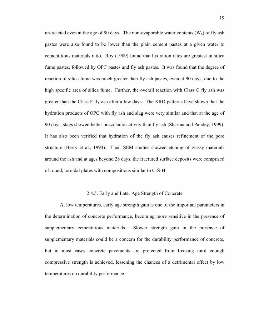
19

un-reacted even at the age of 90 days. The non-evaporable water contents (Wn) of fly ash

pastes were also found to be lower than the plain cement pastes at a given water to

cementitious materials ratio. Roy (1989) found that hydration rates are greatest in silica

fume pastes, followed by OPC pastes and fly ash pastes. It was found that the degree of

reaction of silica fume was much greater than fly ash pastes, even at 90 days, due to the

high specific area of silica fume. Further, the overall reaction with Class C fly ash was

greater than the Class F fly ash after a few days. The XRD patterns have shown that the

hydration products of OPC with fly ash and slag were very similar and that at the age of

90 days, slags showed better pozzolanic activity than fly ash (Sharma and Pandey, 1999).

It has also been verified that hydration of the fly ash causes refinement of the pore

structure (Berry et al., 1994). Their SEM studies showed etching of glassy materials

around the ash and at ages beyond 28 days, the fractured surface deposits were comprised

of round, toroidal plates with compositions similar to C-S-H.

2.4.5. Early and Later Age Strength of Concrete

At low temperatures, early age strength gain is one of the important parameters in

the determination of concrete performance, becoming more sensitive in the presence of

supplementary cementitious materials. Slower strength gain in the presence of

supplementary materials could be a concern for the durability performance of concrete,

but in most cases concrete pavements are protected from freezing until enough

compressive strength is achieved, lessening the chances of a detrimental effect by low

temperatures on durability performance.

20

Studies by Gebler and Klieger (1986) indicated that higher compressive strength

is essential in improving the scaling resistance of concrete. Average compressive

strengths of 24.1 MPa (3500 psi), 30.8 MPa (4460 psi) and 33.8 MPa (4910 psi) were

reported for three concrete mixtures (cured at 4.4ºC or 40ºF); the first containing Class F

fly ash, the second Class C fly ash and the third plain cement respectively. They reported

that as the compressive strength increased, the deicer scaling resistance generally

improved. The cementitious material contents were 306.7 kg/m3 (517 lb/yd3) and 281

kg/m3 (474 lb/yd3) in the fly ash mixtures and plain cement mixture, respectively.

Swenson (1969) recommended that air-entrained concrete should have strengths in the

range of 24.1 - 31 MPa (3500 - 4500 psi) for better scale resistance in case of severe

exposures.

Bilodeau et al. (1994) studied the mechanical and durability properties of concrete

with eight different fly ashes and two different cements from various sources in the

United States. It was reported that with an increase in compressive strength, the chloride

ion permeability reduced drastically; but no relationship was observed between scaling

and compressive strength. The final visual evaluation of test slabs subjected to the

deicing salt scaling test showed that all of the high-volume fly ash concretes had equally

poor performances in the test.

2.4.6. Porosity, Pore Size Distribution, and Sorptivity of Concrete

The resistance of concrete to the ingress of harmful salts or to that of water

depends upon the permeability of the system. In other words, a denser microstructure of

concrete not only ensures less ingress of harmful salts, but also reduces water absorption,

21

which is important with respect to improving the durability of concrete to freezing and

thawing cycles. Additionally, the filling of air voids with water was experimentally

proven the most probable cause of high scaling in virgin concretes (Jacobsen et al.,

1997). In an unsaturated system, water flows within a porous media under the action of a

capillary force, which in turn depends on the pore structure of the material. Thus, the

capillary force is the strongest when the material is completely dry and it reduces with

saturation. In concrete, water absorption could be influenced by the porosity of the

aggregate, the porosity of the cement gel matrix, the packing geometry of the constituent

particles, e.g., sand, coarse aggregate, and in some cases, could be due to the inclusion of

air-entraining admixtures (Hall and Yau, 1987).

The porous distribution seems to have a significant influence on the scaling

resistance of concrete. For similar strength concrete mixtures, finer and more refined

pores might be more detrimental to scaling because of higher stresses generated by a

longer freezing time and a higher degree of saturation (Lindmark, 1999). It is difficult to

determine the exact pore size distribution of concrete, however, a weak trend was

observed as shown in Figure 2.2 between the MIP values and scaled mass for high-

strength concrete (50 and 75 MPa) studied by Baroghel-Bouny et al. (1995).

22

Figure 2.2: Relation of scaled mass to MIP porosity of 50 and 75 MPa strength concrete

The sorptivity test, which involves the theory of capillary suction, can be used to

determine the cumulative absorption, as well as the rate of ingress, of water into the

concrete. Hence, it is useful in studying the quality of concrete surfaces subjected to wet

and dry cycling (Gopalan, 1996; Hall, 1989; Hall and Yau, 1987; Martys and Ferraris,

1997). Gopalan (1996) found that when adequate curing was provided, a 37% reduction

in sorptivity was observed in a mix containing 40% fly ash. This study also reported that

under fog-cured conditions, the sorptivity of fly ash concrete was lower than OPC

concrete; but under dry-curing, the sorptivity of the fly ash concrete was higher than the

OPC concrete. McCarter (1993) tested the top, bottom and cut surfaces for their

sorptivity test and found the top surface to have the highest sorptivity values, followed by

the bottom and cut surfaces.

R2 = 0.3312

0

0.5

1

1.5

2

2.5

4 6 8 10 12 14 16

MIP POROSITY(%)

SCA

LED

MA

SS (K

G/M2 )

23

2.5. Environmental and Other Parameters Influencing Durability of Concrete under Cold

Weather Conditions

Other than concrete properties, durability performance is largely dependent on

conditioning of the specimens and type of exposure conditions. There have been several

studies addressing curing, but there is a very little consistency observed in the results, a

summary of which follows. Moreover, the effects of the rate of freezing, minimum air

temperature, and salt concentration are also briefly described.

2.5.1. Curing Type and Temperature

Curing plays an important role in reducing the permeability of concrete. This is

particularly true for concrete containing supplementary materials, as the dependence on

curing increases with increased replacement levels of cement. It was found that the

compressive strength of concrete with 50% fly ash was more adversely affected by

inadequate curing (Thomas and Mathews, 1994). Ballim (1993) suggested that

increasing the duration of moist curing was a more effective way of extending the

durability of concrete than increasing the cement content.

On the other hand, Nasser and Lai (1993) reported that increasing the curing

period did not increase the frost resistance. Incorporating 35 to 50% fly ash in concrete

was detrimental to frost resistance even though the specimens were cured for 80 days.

However, these authors found that a 20% fly ash content in concrete resulted in

satisfactory performance (durability factor greater than 60%), and 35% fly ash resulted in

doubtful to satisfactory performance (durability factor between 40% and 60%). Also

they determined from SEM micrographs that a decrease in the freezing and thawing

24

resistance may be due to slow displacement of microcrystalline Ca(OH)2 and fibrous

ettringite hydrates from the dense C-S-H zones to the air voids during freeze-thaw

cycling.

Bilodeau et al. (1991) found that the mass of scaling residue reduces significantly

when membrane-curing was adopted instead of moist-curing. Extended moist-curing and

drying periods did not affect significantly the performance ash concretes in the scaling

tests, at least within the periods investigated. In the laboratory (Bilodeau, 1991) and in

the field (Marchand, 1992) it has been observed that concrete cured with membrane-

forming curing compounds have better resistance as compared to similar water-cured

concretes. The use of curing compound was observed to result in scaling resistance as

good as that of concrete moist-cured for 14 days, but the results seemed to vary with the

type of curing compound used (Langlois et al., 1989). They also found accelerated heat-

curing of specimens had a very detrimental influence on the scaling resistance.

Stark et al. (2002) reported results of their scaling study for different concrete

specimens placed for about 35 years or more in the PCA outdoor facility. This study of

the effects of the season of construction clearly indicated that all the concrete specimens

containing plain cement as the binder constructed in late fall, under different curing

regimes, were more prone to scaling than specimens constructed in the summer.

Additionally, it was shown that among all the curing treatments, the specimens cured

under air showed minimal scaling, which indicated that concrete constructed without fly

ash was also susceptible to scaling when constructed in late fall. To evaluate different

admixtures, they found that the performance of the control mix and the mix containing

30% fly ash by weight of cement as a supplement, both showed moderate scaling

25

resistance. Further, these specimens proved to be more scaling resistant then the concrete

constructed in late fall with plain cement. However, in this study, fly ash was added as a

supplement, which increased the cementitious materials content significantly and

consequently the improved scaling resistance.

Isaac et al. (1994) reported that, irrespective of curing conditions, concrete

containing 50% slag showed poor resistance to scaling, while concrete containing 25%

slag behaved in a similar manner as the reference concrete. It was also observed that for

different types of slag 22 and for 25% and 35% percentage replacement of fly ash, there

was no specific relationship developed between the curing temperature and the amount of

scaling for different curing temperatures of 10ºC (50ºF), 23ºC (73ºF) and 38ºC (100oF)

(Hadchiti et al., 1988).

Klieger (1957), based on his study for the Highway Research Board, developed

guidelines for “Curing Requirements for Scale Resistance of Concrete”. He specified

that for plain air-entrained and non-air-entrained concrete, an increase in curing increased

the scaling resistance of concrete. Plain concrete cured at low temperatures was more

prone to scaling than that cured at room temperature. In further studies on the influence

of aggregates (Klieger, 2003), it was observed that concretes moist-cured continuously

required more entrained air for adequate resistance to freezing and thawing than air-dried

concretes. Gunter and Hilsdorf (1987) showed that prolonged curing of Portland cement

concretes in water might reduce the durability of air-entrained concrete. Concrete

containing slag could be more prone to scaling at later age than at an early age because of

the effect of carbonation (Gunter, 1987).

26

In summary, it can be said that in most cases plain concrete, when cast and cured

at low temperatures, proved more prone to scaling compared to normal temperature cured

plain concrete, while no such particular trend was observed for concrete containing fly

ash or slag. The use of a curing compound seems to be the most effective means of

reducing scaling and no general relationship between the duration of moist-curing and

scaling resistance could be developed.

2.5.2. Rate of Freezing and Minimum Temperature

It has been observed that the rate of freezing has very dissimilar influences

resulting in internal damage due to freeze-thaw and scaling damage in the presence of a

de-icing salt solution. For freeze-thaw durability, it is believed that the higher the rate of

freezing, the lower the spacing factor for similar resistance should be. For concrete

prepared with a w/c ratio between 0.5 and 0.6, Powers (1949) proposed a critical spacing

factor value of 250 μm for a freezing rate of 11°C/h. Different concrete mixtures having

a constant w/c ratio of 0.5 but having variable spacing factors were subjected to F-T

cycles (Pigeon et al., 1985). The critical spacing factors for various freezing rates were

evaluated from length change measurements done at the completion of 300 cycles. It was

found that the critical spacing factor reduced significantly when the freezing rate was

increased from 2 to 6°C/h. Malhotra (1982) reported that concretes with spacing factor

values in the range of 250 to 300 μm can resist 300 cycles of freezing and thawing in

water when the freezing rate is 8°C/h. These results indicated that though the test results

obtained from ASTM C 666 procedure B (freezing in air, thawing in water) were

identical to test results from procedure A (freezing and thawing in water), concretes

27

frozen in water exhibited surface scaling after 300 cycles whereas those frozen in air did

not.

In case of scaling, it has been observed that increasing the freezing rate, decreases

the scaling or, that there is no significant influence of rate of freezing on scaling damage.

This is mainly because rapid cooling allows less time for moisture uptake during cooling

thereby, reducing the development of scaling. Studer (1993) found no influence of either

duration of the frost cycle or freezing rate on scaling. He varied the rate in the very

narrow interval (-2.0oC/h to -3.4oC/h) and therefore should have very limited effect on

overall results. He found that minimum temperature has much larger influence on scaling

results than duration of cycle and hence, severity of temperature cycle can be well

characterized by minimum temperature reached in the salt solution. Jacobsen (1995)

studied effect of three different cooling rates 2.8, 4.9 and 12oC/h on scaling for non air-

entrained and air entrained concrete. He observed that reducing the cooling rate with the

same minimum temperature in comparison to extending the time at minimum

temperature with faster cooling rate showed higher weight loss due to scaling. Lindmark

(1998) reported that if the rest of the frost cycle is unchanged than scaling decreases as

cooling rate increases. However, he mentioned that scaling may be repeated several

times during the cooling phase, so the final result cannot be quantitatively predicted.

2.5.3. De-icing Salt Solutions; Types and Concentration

The use of de-icing salt has definitely been shown, in both the laboratory and the

field, to increase the severity and extent of concrete scaling. In the initial studies of

Verbeck and Klieger (1957), the effect of the concept of pessimum solution was shown.

28

They studied the effects of four dissimilar de-icing agents (CaCl2, NaCl, urea, and ethyl

alcohol) on the scaling resistance of concrete at various concentration levels. They

observed greater amounts of surface scaling at relatively low intermediate concentrations

(2 - 4% by weight) and that the severity concentration curves associated with the four

agents were similar. Between 2 - 4% NaCl concentrations appeared to be the most

detrimental solution for scaling of concrete. Similar observations were made by Grieb et

al. (1962); out of five agents he studied, calcium chloride appeared to be more effective

and less harmful to the concrete, while the severity of the damage from sodium chloride

and urea were found to be essentially the same. To develop a better understanding of the

application of salt in the field, a summary of the various salt mixtures being applied in the

field in Indiana, along with its application rate, and advantages-disadvantages are in

Table 2.1. Note that these salts are being used as deicing or anti-icing agents, alone and

in various combinations.

Based on the above summary of numerous studies it seems that different

researchers have found different parameters to be important in the determination of total

scaling. Based on their observations, several mechanisms have been suggested for the

scaling of concrete. None of these mechanisms are widely accepted but summarizing

then will be helpful in addressing the ensuing issues.

29

Table 2.1: General information about prevalent salt**

Chemical Name, Formula, (Eutectic Temperature, E. T.)

Advantages Disadvantages Application Rates for lane miles

Costs

Sodium Chloride, NaCl

E. T. = -21.1oC (-6oF)

Low initial cost, effective above 20oF, melts snow and penetrates ice

Corrosive, slow below 20oF, must dissolve before ice melting begins.

30-50 gallons/lm, 30% (deicing -250 lbs/lm every 3 hour)

Liquid salt cost 4-6¢ per gallon,$25 - $45 per ton.

Calcium Chloride, CaCl2

E. T. = -51.1oC (-60oF)

Effective at lower temperatures than NaCl, attracts moisture from air which hastens its dissolving and melting, releases heat when it dissolves.

More costly, requires extra handling effort, very corrosive, tends to keep pavement wet.

30 to 50 gallons per lane mile (32%) for anti-icing.

$150-300 (flake) - $250-400/ton (pellets) - 30-65¢ per gallon liquid

Magnesium Chloride, MgCl2

E. T. = -33.33oC (-28oF)

Effective at lower temperatures than salt (used for less than 0oF), attracts moisture from air which hastens its dissolving and melting.

More costly than salt, corrosive, may increase concrete scaling and spalling, tends to keep pavement wet.

30 to 50 gallons per lane mile for anti-icing

50 - 70¢ per gallon of 30% solution, $300 per ton dry flake.

**This information was compiled at the University of Wisconsin-Madison. The information was collected from numerous TRB, State DOT, and Canadian provincial reports; manufacturers product literature; trade journals; and industry sources.

2.6. Summary of Proposed Mechanisms of Scaling of Concrete

Based on various experimental and field results, several mechanisms have been

suggested by different researchers to explain scaling behavior. A few of the relevant

mechanisms are discussed here briefly, and will be discussed further in explaining the

30

results in successive chapters. Since this is not the main focus of this study, brief

overview is given with the details available in the cited references.

2.6.1. Hydraulic Pressure Mechanism

This mechanism suggested by Powers (1945) is widely accepted for F-T damage

in concrete, which is based on the fact that the freezing of water causes approximately

9% expansion. The destruction of concrete by freeze-thaw is a result of the pressure

generated when freezing water expands in the pores and displaces unfrozen water. The

mechanism for scaling damage as explained by powers is summarized below.

The capillary voids in the surface-layer of concrete are saturated to a certain depth

due to the water collecting on the surface. The surface water freezes first, effectively

sealing the surface. Freezing then progresses inwardly from the surface, displacing the

unfrozen water towards the interior. During thawing the ice in the less saturated interior

capillary voids will tend to melt at a lower temperature. This causes melting to occur

outwardly from the interior. However, due to the presence of salt in the surface solution,

the surface ice might melt prior to the surface capillary ice. In such cases, an external

source of moisture would be available and some of this water would be absorbed into the

concrete. Thus, the overall degree of saturation and the depth of saturation would be

increased by repetitions of the freeze-thaw cycle. This process would continue until

some critical depth of saturation is attained, which would result in hydraulic pressures

great enough to cause surface disintegration.

The governing parameters for this mechanism, is flow distance (spacing factor),

degree of saturation, and rate of freezing. This mechanism does not address the

31

deleterious effect of pessimum salt solution. Powers developed a mathematical

formulation for determining the spacing factor but recent research has created doubt on

the validity of this formulation (Lindmark, 1997).

2.6.2. Osmotic Pressure Mechanism

This mechanism was proposed later by Powers and Helmuth (1953) to address

other observations relating to deicing salts. The osmotic pressure mechanisms are

dependent on the fact that capillary voids and gel pores might be filled with a solution of

water and deicing agents or to a small extent, alkali ions. Prior to freezing, the capillary

voids contain an aqueous solution of deicing agents and are in equilibrium with each

other. Freezing of the capillary solution, results in a mixture of relatively pure ice and a

solution of higher salt concentration. It can be assumed that the gel pores surrounding

this capillary cannot freeze because of their very small size. Thus, the solution in the

capillary voids and gel pores cannot be in equilibrium at this point. When cooling

proceeds, the unfrozen water in the smaller pores will gain more free energy than the ice

already formed, which will create a potential difference, in turn creating moisture that

moves out from the small pores into the large ones, where it will freeze onto the existing

ice body.

Several improvements were later suggested to this mechanism. Most recently

modified form of this mechanism was suggested by Lindmark (1997). He explained this

phenomenon by the main premise being the osmotic ice body growth in porous systems.

In a concrete specimen, osmotic ice body growth is significantly facilitated, as compared

to the situation in the interior of a moisture-isolated specimen, when the pore liquid is

32

connected to the reservoir of liquid in which the liquid pressure remains atmospheric. It

is the central role of salt in the outer solution to provide such a reservoir of liquid at

temperatures below the freezing point of the pore solution. He also pointed out the

limitation that no numerical solution was obtainable because of the high degree of

uncertainty associated with the pore size distribution.

2.6.3. Combined Hydraulic and Osmotic Pressure Mechanism

Currently, the following mechanism is widely accepted by various researchers for

scaling of concrete. Powers (1965) proposed that most scaling issues could be explained

by the combined effect of osmotic and hydraulic pressure. The osmotic pressure would

be due to the presence of salts; and since this would draw more moisture into pores where

ice and salt existed together, the subsequent increased ice formation in these pores would

cause increased hydraulic pressure when water is expelled from these pores. Powers also

states that deicing salts will spread much faster in the capillary pores than in the gel pores

and that the salt concentration gradient thereby formed between the gel pores and the

capillary pores would promote this mechanism.

Marchand and Pleau (2000) further explained that the total pressure induced in the

system is the sum of the pressures generated by both phenomena and is influenced by the

amount of salts dissolved in the pore solution. The higher the salt solution; the lower the

amount of freezable water at a given temperature; thus, the hydraulic pressure decreases

with an increase in the salt concentration. On the other hand, the osmotic pressure

increases with an increase in the salt concentration. The combination of these two

33

phenomena yields a moderate salt concentration (2 - 4%), which causes maximum

scaling.

2.6.4. Crystal Growth Mechanism

Hansen (1954) was the first to suggest the crystal growth mechanism, involving

formation and growth of salt crystals, to explain severe scaling of concrete subjected to

deicing agents. The process resulting in the formation of and growth of these crystals,

which in turn results in surface disintegration, was visualized by Hansen as follows:

The application of the salt for the purpose of ice removal results in a salt solution

covering the surface of the slab. Salt molecules from this solution tend to migrate into

the concrete by either diffusion or absorption. If the surface of the concrete is then sealed

by a layer of ice, separation of the salt from the solution is an expansion reaction; and

since the solution cannot escape through the surface, the formation of crystals will

displace the salt solution into pores that are not already filled. By this process, repeated

cycles of freezing could cause the liquid in the concrete to become an aqueous solution of

de-icing salts. Cooling or evaporation can cause crystallization of salt in the pores of the

concrete. This action results in a condition in which the film of the solution surrounding

the capillary crystal is not in equilibrium with the solution in the surrounding pores.

Consequently, salt molecules diffuse into the capillaries and allow the crystal to continue

to grow. After the pore is completely filled with a salt crystal, continued growth will

cause the crystal to be extruded or will cause the development of pressure, which can

result in scaling.

34

This is considered the most likely mechanism for observed scaling behavior in the

field because of the initial application of a high salt solution and the drying of the

pavement between freezing cycles. However, this will not explain the results of

laboratory scaling tests because there is no drying between consecutive cycles for

crystallization to occur.

2.6.5. Thermal Shock, Thermal Incompatibility or Thermal Mismatch

Hartmann (1957) reported that damage was caused by the rapid consumption of

melting heat, which results in the rapid cooling of the upper layer of the concrete when

deicer is applied. This sharp change in temperature produces stresses in the already

frozen surface layer of mortar. Thus, he considered thermal shock as the mechanism of

scaling in field performance.

Another similar mechanism illustrates that concrete deterioration due to the

freeze-thaw cycles may be attributed to the difference in the thermal incompatibility of

aggregates and cement paste. Parsons and Johnson (1944) concluded that if the thermal

expansion of an aggregate differs considerably from that of the paste, a potential

incompatibility exists that might result in excessive internal stresses if concrete is

subjected to large temperature changes.

Recently, Valenza II and Scherer (2004), with the help of a novel experiment

suggested thermal mismatch as the most important mechanism. Their experimental

results demonstrated the occurrence of a thermal expansion mismatch (or bi-material)

mechanism explains for all of the observed salt scaling phenomenology. According to

the authors, scaling occurs when the stress in the freezing layer rises above the tensile

35

strength of the brine-containing ice, resulting in cracking. With the help of a visco-elastic

analysis of the stresses in the brine/ice layer, it was shown that pure ice would not crack,

but a layer containing more than 1% NaCl would. The damage from the cracking of the

ice is exacerbated by the weakening of the cement paste from exposure to concentrated

brine. However, not being able to account for the effect of air voids in the concrete is the

major limitation of this mechanism. Hence, it can be said that this mechanism might be

considered responsible when non-air entrained concrete is studied.

2.6.6. A Case-Specific Approach Based on Summary of Various Mechanisms

Based on the extensive literature review, it can be assumed that scaling is not a

single point process; different magnitudes of forces can be generated at different

temperatures, depending on the degree of saturation and the salt concentration in the

surface region. Based on the degree of resistance, a particular mechanism might govern

the scaling behavior in a given case. The exact mechanism of scaling is still considered

unknown because none of the mechanisms proposed to date explain all the different

laboratory and field observations. However, from a holistic look at the extensive

literature review and experimental results, it becomes evident that the type of concrete

and other boundary conditions are not similar in all of the previous studies. Moreover,

some correlation was observed for similar types of concrete or boundary conditions, in

the scaling behavior and for suggested mechanisms. Based on such observations, Table

2.2 was prepared, which provides the maximum applicability of each mechanism to a

specific type of concrete based on the results and reasoning provided in various studies.

36

Thus, it can be said that although the damage is the same, the reason for the damage can

change based on the type of concrete and the boundary conditions.

Table 2.2: Summary showing applicability to each mechanism to specific type of concrete

No. Governing mechanism Most applicable type of concrete

1 Hydraulic pressure mechanism Plain concrete or concrete with

higher porosity, carbonated concrete containing slag

2 Osmotic pressure mechanism Air entrained concrete with fly ash, refined pore structure

3 Combined hydraulic and osmotic pressure mechanism Air entrained plain concrete

4 Crystal growth mechanism Actual pavements exposed to drying while freezing

5 Thermal shock or thermal incompatibility

Actual pavements, application of sudden deicing solution

6 Bi-material or thermal mismatch Non-air-entrained plain concrete

“A case-specific mechanism of scaling” approach is suggested here to simplify

the problem and to understand the influencing parameters. Based on the understanding

developed from the detailed analysis of the results of various studies, Table 2.3 proposes

such an approach for different types of concrete. Also, scaling is not a single-point

process so for each scaling problem, there might be several mechanisms acting at the

same time, one of which would be the governing mechanism and would influence the

results significantly. Therefore, Table 2.3 provides probable governing mechanisms in

the order of its importance, along with the major influencing parameters. Here it should

be noted that for simplicity and better comparison, the exposure conditions and the

strength of the concrete are assumed constant for all types of concrete. For this ideal

condition, an approximated comparison for the types of stresses and the degree of

37

resistance are shown thereby, as well as the potential for damage. It should be noted that

this is just an approximate representation of extensive literature review and laboratory

study. This approach should be refined further to give more precise and exact solution to

individual problems.

Overall, based on all the literature, scaling could be considered as a function of

the tensile strength, the salt concentration in the surface, the minimum concrete

temperature, the air void structure and the degree of saturation of the concrete, the traffic

movements, and many more parameters. Moreover, the surface composition, pore

structure and degree of drying can influence results by changing the penetrability of salt

in the concrete. Thus, it seems that scaling is the combined effect of many parameters,

which make the process complex to model. Therefore, the above mentioned case-specific

approach could help in reducing the complexity of the problem by pointing out important

parameters for a particular type of concrete and providing the proper focus on the

governing parameters. For the problem at hand, the focus will be scaling of air-entrained

concrete containing fly ash in the field and laboratory. Moreover, the role of the

suggested influencing parameters is verified using a few laboratory results.

38

Table 2.3: Critical summary of various mechanisms using “A case specific approach”

Type of concrete

Dominating mechanism and reasoning

Degree of resistance and generated stresses

Influencing parameters

Non-air entrained, plain cement concrete

Bi-material mechanism, thermal mismatch, coherent layer and ice cracking

Low degree of resistance, lower stresses are generated due to this mechanism

Minimum temperature, DOH (Degree of Hydration), porosity and strength, surface salt concentration

Air entrained plain cement concrete

Balance of hydraulic and osmotic pressure and subsequent increase in degree of saturation

High degree of resistance and moderate stresses generated due to mechanism

Degree of saturation, minimum temperature, DOH, porosity and strength, surface salt concentration

Air entrained concrete containing fly ash

Governed more by higher osmotic pressure generated due to refined pore structure and critical degree of saturation

High degree of resistance and high stresses generated due to this mechanism, because of presence of small pores and progressive filling

Pore size distribution, inner salt concentration, length of wetting, degree of saturation, minimum temperature, DOH, porosity and strength, surface salt concentration

Air entrained concrete containing slag

Effect of carbonation, hydraulic pressure due to increased porosity, degree of saturation

Moderate degree of resistance because of increase in porosity due to carbonation and moderate stresses due to mechanism

Extent of carbonation, degree of saturation, minimum temperature, DOH, porosity and strength, surface salt concentration

Air entrained plain cement concrete in the field

More osmotic effect due to lower rate of freezing, effect of traffic movement, thermal shock or crystal growth mechanism

High degree of resistance when cured at normal temperature, moderate resistance when cured at low temperature due to chances of higher porosity and degree of saturation in surface region, moderate stresses

Curing temperature, vehicular movement, size and rate of cooling, bleeding-evaporation and surface porosity, degree of saturation, minimum temperature, DOH, and strength, surface salt concentration

Air entrained concrete containing fly ash in the field

More osmotic effect due to lower rate of freezing, effect of traffic movement, thermal shock or crystal growth mechanism

High degree of resistance, irrespective of curing temperature, moderate stresses because of shorter actual length of wetting, while freezing

Vehicular movement, bleeding-evaporation and surface porosity, size and rate of cooling, length of wetting, pore size distribution, degree of saturation, min. temp., DOH, surface salt concentration

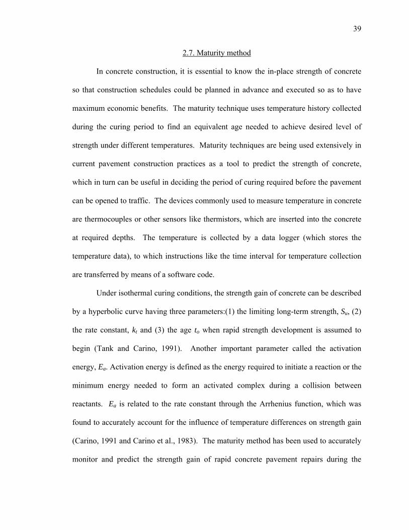
39

2.7. Maturity method

In concrete construction, it is essential to know the in-place strength of concrete

so that construction schedules could be planned in advance and executed so as to have

maximum economic benefits. The maturity technique uses temperature history collected

during the curing period to find an equivalent age needed to achieve desired level of

strength under different temperatures. Maturity techniques are being used extensively in

current pavement construction practices as a tool to predict the strength of concrete,

which in turn can be useful in deciding the period of curing required before the pavement

can be opened to traffic. The devices commonly used to measure temperature in concrete

are thermocouples or other sensors like thermistors, which are inserted into the concrete

at required depths. The temperature is collected by a data logger (which stores the

temperature data), to which instructions like the time interval for temperature collection

are transferred by means of a software code.

Under isothermal curing conditions, the strength gain of concrete can be described

by a hyperbolic curve having three parameters:(1) the limiting long-term strength, Su, (2)

the rate constant, kt and (3) the age to when rapid strength development is assumed to

begin (Tank and Carino, 1991). Another important parameter called the activation

energy, Ea. Activation energy is defined as the energy required to initiate a reaction or the

minimum energy needed to form an activated complex during a collision between

reactants. Ea is related to the rate constant through the Arrhenius function, which was

found to accurately account for the influence of temperature differences on strength gain

(Carino, 1991 and Carino et al., 1983). The maturity method has been used to accurately

monitor and predict the strength gain of rapid concrete pavement repairs during the

40

curing period (Okamoto and Whiting, 1994). The prediction using the maturity method,

however, seemed to underestimate strengths at early ages. Pinto and Hover (1990) found

that the initial and final set times could be predicted for any mixture provided the

activation energy is obtained. Early age curing temperatures have been found to

influence the ultimate strength of concrete. McIntosh (1956) reported that for equal

maturities, specimens exposed to low early age temperatures were weaker at early

maturities but stronger at later maturities. Many other researchers also reported this

“cross-over” effect where lower early age curing temperatures resulted in higher ultimate

strengths.

41

CHAPTER 3: SELECTION OF CEMENTS AND SUPPLEMENTARY CEMENTING MATERIALS

3.1. Introduction

In order to understand the complexities involved with various chemical reactions

in concrete containing cement and mineral admixtures like fly ash and slag, it was

decided to gather data on various cements, fly ashes and slag and study the influence of

various chemical components in each of these materials on factors like rate of strength

gain and strength activity index which would be essential in cold weather conditions.

The material selection was conducted in conjunction with the INDOT sponsored project

on the use of supplementary materials in the late fall construction season. A listing of all

INDOT approved sources of cement, fly ash and slag was collected. Mill certificates

were obtained from 28 sources of cement, nine sources of Class C fly ash, four sources of

Class F fly ash and one source of slag. The mill certificates for cements contained data

like chemical compositions of C3S, C2S, C3A, fineness (m2/kg), alkali content and

strength data for tests performed at different ages. For fly ashes chemical compositions

of lime, SiO2, Al2O3, Fe2O3, alkali content and strength activity index values at different

ages were provided. For the slag, values of sulfide, alkali content and strength activity

index were provided. The data obtained were either in the form of yearly averages or

monthly averages for a period of 12 months. All the mill certificates were then used to

prepare a comprehensive database of different parameters from various sources of

42

Table 3.1: Summary of cement data

Blaine Compressive strength, psi (MPa)Fineness(m2/kg) 1 day 3day 7 day 28 day

Type IC01 Blue circle 54 17 0.81 408.0 10 3924 (27) 4793 (33) 5835 (40)C02 Lonestar, IN 60.01 13.54 0.54 360.8 8.22 2272 (16 ) 3439 (24) 4390 (30) 5790 (40)C03 Lonestar, IL 52.5 17.2 0.9 332.3 10.3 1794 (12) 3441 (24) 4328 (30) 5438 (37)C04 Holnam, MI 54.83 17.08 0.74 400.8 9.33 3400 (23) 4472 (31)C05 Holnam, MO 58.89 15.09 0.47 375.5 8.65 3356 (23) 4832 (33)C06 Siam cement 63.79 23.32 0.43 355.5 8.76 4009 (28) 5077 (35) 6529 (45)C07 Southdown (Pitts) 51 0.61 384.0 8 1995 (14) 3225 (22) 4365 (30)C08 Lonestar, MO 51.72 21.47 0.49 366.0 6.47 1841 (13) 3135 (22) 4172 (29) 6060 (42)C09 Essroc, Logansport 62.45 0.25 383.9 8.58 1521 (10) 3293 (23) 5421 (37) 6916 (48)C10 Essroc, Essexville 56.58 0.95 382.0 7.7 2681 (18) 3198 (22) 4646 (32) 5734 (40)C11 Lafarge, Paulding 62.45 0.45 358.5 7.9 1624 (11) 3235 (22) 4313 (30) 5864 (40)C12 Southdown, Fairborn 51.83 0.59 395.1 6.14 2011 (14) 3454 (24) 4216 (29) 5346 (37)C13 Southdown, MI 56.15 14.23 0.94 396.1 6.54 3648 (25) 4375 (30) 5412 (37)C14 Lafarge, Bath 59.06 0.65 373.1 6.59 3912 (27) 4744 (33) 6044 (42)C15 Lafarge, Alpena 63.76 0.54 363.8 8 2074 (14) 3900 (27) 4658 (32) 5950 (41)

Type I/IIC16 Lehigh portland 49.31 25.85 0.49 373.4 6.46 2414 (17) 3765 (26) 4688 (32)C17 Southdown (KY) 51.63 22.59 0.65 386.4 6.33 2997 (21) 3957 (27) 5600 (39)C18 Heracles, Greece 62.8 11.4 0.52 379.4 6 3652 (25) 4328 (30)C19 Essroc, Speed 56.09 0.52 374.6 6.91 1853 (13) 4119 (28) 6168 (43)C20 Lafarge, Joppa 60 0.46 380.2 7.33 2017 (14) 3728 (26) 4843 (33) 6103 (42)C21 River Cement, MO 58.26 15.44 0.54 360.7 6.53 2087 (14) 3476 (24) 4685 (32) 6243 (43)

Type IIIC22 Lehigh portland 53.15 25.15 0.49 610.2 4.93 4365 (30) 5768 (40) 6979 (48)C23 Lonestar, IN 59 11.75 0.6 552.1 9 4138 (29) 5199 (36) 6030 (42)C24 Lonestar, IL 53.0 16.6 0.9 562.1 10.4 4348 (30) 5395 (37) 6108 (42)C25 Holnam, MI 53.81 16.94 0.72 525.3 9.15 2620 (18) 4470 (31) 5203 (36)C26 Essroc, Logansport 61 0.31 622.0 8.3 2854 (20) 5212 (36) 6679 (46)C27 Essroc, Speed 54.63 0.51 593.1 6.74 3170 (22) 4700 (32) 5799 (40)C28 Southdown, MI 57.33 14 0.96 633.3 6.67 4550 (31) 5207 (36) 5993 (41)

C3A (%)Alkali (Na2O

equiv.)Cement ID Company C3S(%) C2S (%)

43

cement, fly ash and slag. The database was prepared in such a way that it would provide

an easy reference of chemical compositions, fineness and results of mechanical properties

for all materials under consideration. Models were developed for strength prediction in

cements and strength activity index (SAI) prediction in fly ashes. Sensitivity analyses

were performed to evaluate the influence of various chemical components, fineness on

the strength and SAI of cements and fly ashes respectively. Subsequent divisions in this

chapter discuss models for strength, strength activity index prediction and the scientific

approach involved in screening cements, fly ashes and slag for subsequent tests.

3.2. Development of Mathematical Model for Strength Prediction of Cement Mortars

A detailed listing of the cement information shown in Table 3.1 used in the

development of mathematical models was prepared. In order to select a manageable

number of cements for the subsequent tasks of the project, which involved tests on

mortars and concrete, steps were taken so as to screen few cements. The approach

adopted for screening the materials was such that all mixtures prepared with the screened

materials would cover a wide range of possible mixture combinations in the state of

Indiana. It was decided to perform some analysis, which would indicate the sensitivity of

strength of cements to variation of each chemical component under consideration and

fineness at varying ages. As it is known that each of C3S, C2S, C3A, fineness (m2/kg),

and alkali content has a significant influence on the strength development and

subsequently the ultimate strength of concrete, the compressive strength was initially

expressed as a linear function of each of the above components. An initial expression

shown in equation 3.1 was adopted for describing compressive strength.

44

A)E(CD(Alkali)S)C(CS)B(C)A(Fineness f 323c ++++= (3.1)

The square of the difference of the error between the strength values obtained

from the above-predicted equation and actual strength data obtained from the mill

certificates was minimized towards zero in order to obtain the values of the coefficients

i.e., Assume initial values of A, B, C, D, E ⇒ ∑ (fc predicted – fc actual)2 0 ⇒ obtain

constants

The values of coefficients obtained at ages of 1, 3, 7 and 28 days after performing

iterations are shown in Table 3.2.

Table 3.2: Constant values at different ages

Since, it was desired to obtain a single expression for describing the compressive

strength of concrete taking all chemical components of cement and period of curing, a

relation for describing the constants of each parameter in equation 3.1 as a function of

time was developed. The expressions for predicting the values of constants as a function

of time are given below:

A = 0.4794*ln (t) + 6.646 (3.2)

B = 18.845*ln (t) - 8.2275 (3.3)

C = -0.0204*(t)2 + 0.4485*t + 15.95 (3.4)

D = -745.93*ln (t) + 1061.3 (3.5)

Age (days) Fineness C3S C2S Alkali C3A1 6.69 -10.01 16.94 1383.80 -98.293 7.19 13.34 16.20 -58.96 -2.867 7.44 31.34 18.45 -680.73 31.99

28 8.32 52.59 12.49 -1155.45 53.15

Constants

45

E = 44.128*ln (t) - 74.351 (3.6)

On substituting the constants given by equations 3.2 through 3.6 in equation 3.1, the

expression for compressive strength of concrete as a function of parameters like C3S,

C2S, C3A, fineness (m2/kg), alkali content and period of curing is given by:

cf = (0.4794*ln (t) + 6.646)*Fineness + (18.845*ln (t) - 8.2275)*C3S +

(-0.0204*(t)2 + 0.4485*t +15.95)* C2S + (-745.93*ln (t) + 1061.3)*Alkali +

(44.128*ln (t)-74.351)*C3A (3.7)

The above equation (3.7) gave very good strength predictions when compared

with the actual strength data obtained from the mill certificates. A plot of actual strength

values versus strength predicted from equation (3.7) is shown in Figure 3.1. The plot had

an R2 = 0.93.

Figure 3.1: Actual versus predicted compressive strength

0

1000

2000

3000

4000

5000

6000

7000

8000

0 2000 4000 6000 8000

Predicted Strength (psi)

Act

ual S

tren

gth

(psi

)

1 day3 day7 day28 day

R2 = 0.93

46

3.3. Development of Mathematical Model for Strength Activity Index (SAI) Prediction

for Fly Ashes

A detailed compilation of information on Class C fly ashes is shown in the Table

3.3 and a compilation of information on Class F fly ashes is also shown in Table 3.4.

Similar to a model developed for compressive strength for cements, a model was

developed for predicting the strength activity indexes (SAI) for fly ashes. An expression

of the form shown in equation 3.8 was used for predicting the strength activity index for

Class C fly ash.

Table 3.3: Summary of Class C fly ash data

Table 3.4: Summary of Class F fly ash data

Station Fly ash ID CaO (%) Alkali

(%)

Fineness (% retained 45 μm sieve)

Carbon (%) SAI7 SAI28

Miami Fort FA10 2.08 0.68 26.34 2.38 80.21 85.83Petersburg FA11 2.57 0.48 24.96 1.67 79.64 84.07Owensbury, FA12 5.46 0.93 14.48 1.63 87.78Coronado FA13 3.85 0.90 22.30 0.44 87.10 91.90

Station Fly ash ID CaO (%) Alkali

(%)

Fineness (% retained 45 μm sieve)

Carbon (%) SAI7 SAI28

Mitchell FA01 24.22 1.19 10.67 0.46 94.83 99.43Schahfer FA02 25.22 1.20 10.76 0.26 94.02 99.89Clifty creek FA03 18.78 1.09 13.78 2.19 96.98 102.15Joliet FA04 24.49 1.85 13.19 0.25 96.28Rockport FA05 18.57 0.70 21.88 0.68 85.50Will County FA06 25.80 1.65 11.52 0.35 96.85Joppa FA07 25.29 1.40 17.15 0.36 93.34 98.45St.Louis FA08 24.96 1.40 13.78 0.34 88.79 99.15Chouteau,U1 FA09 25.74 1.28 14.18 0.16 91.97

47

SAI = A*(Lime)0.33 + B*(Alkali)0.33 + C*(Fineness)0.33 (3.8)

The values of constants obtained on minimizing the squared difference of the

values between actual and predicted SAI are shown in Table 3.5 below.

Table 3.5: Constants for Class C SAI

The values of the constants when plotted with respect to age were obtained as:

A = (0.4277*t + 21.226) (3.9)B

= (0.8133*t + 24.494) (3.10)C = (-0.0579*t -

3.7435) (3.11)

Hence equation (3.8) takes the form

SAI = (0.4277*t + 21.226)*(Lime)0.33 + (0.8133*t + 24.494)*(Alkali)0.33 +

(-0.0579*t - 3.7435)*(Fineness)0.33 (3.12)

The above equation gave reasonable predictions when compared with the actual

SAI values, which can be observed from the Figure 3.2. The coefficient of correlation

was obtained as 0.87.

ConstantsAge (days) Lime Alkali Fineness

7 24.22 18.80 -4.1528 33.20 1.72 -5.37

48

Figure 3.2: Actual versus predicted SAI for Class C fly ash

Similar to the Class C fly ashes, a relation of the form shown below in equation

3.13 was used to predict SAI for Class F fly ashes.

SAI = A*(Lime) + B*(Alkali) + C*(Fineness) (3.13)

The values of the constants obtained on minimizing the squared difference of the values

of actual and predicted SAI are shown in Table 3.6:

Table 3.6: Constants for Class F SAI

The values of constants when plotted as a function of age was obtained as

A = (0.0509*t + 6.5998) (3.14)

B = (0.1206*t + 7.1127) (3.15)

C = (-0.0052*t + 2.4463) (3.16)

Age (days) Lime Alkali Fineness7 6.96 7.96 2.41

28 8.03 10.49 2.30

Constants

8486889092949698

100102104

80 85 90 95 100 105 110Predicted SAI

Act

ual S

AI

7 day

28 day

R2 =0.87

49

Equation (3.13) then takes the following form:

SAI = (0.0509*t + 6.5998)*Lime + (0.1206*t + 7.1127)*Alkali +

(-0.0052*t + 2.4463)*Fineness (3.17)

The above predicted equation gave a very good relation when compared with the actual

SAI values. A plot showing the comparison is shown in Figure 3.3.

Figure 3.3: Actual versus predicted SAI for Class F fly ash

3.4. Sensitivity Analysis

3.4.1. Sensitivity Analysis for Strength of Cements

After developing a mathematical model given by equation (3.7), which can

predict the compressive strength of mortars made with any cement in the range of values

of chemical constituents and fineness obtained from mill certificates as well as cements

having a chemical composition different from the original matrix, the next step was to

determine the significance of each of the parameters involved in equation (3.7). This was

required in order to select a manageable number of cements from the INDOT approved

78

80

82

84

86

88

90

92

94

78 80 82 84 86 88 90 92 94Predicted SAI

Act

ual S

AI

7 day28 day

R2 =1

50

list for performing preliminary tests on mortars. In order to select the cements, a strength

sensitivity analysis was carried out, where the average values of each parameter involved

namely, C3S, C2S, C3A, fineness (m2/kg), and alkali content were computed for all

cements shown in the table. In order to determine the sensitivity of strength to changes in

fineness at any given age, the value for fineness was varied from 300 to 500 m2/kg

keeping all other parameters, namely, C3S, C2S, C3A and alkali content constant at their

average values.

Similarly, the strength sensitivity analysis was performed for all other parameters

by varying one parameter over a certain range of values while keeping all others constant

at the average values. The plots of sensitivity of strength to changes in fineness, C3S,

C2S, alklali and C3A content are shown in Figures 3.4 through 3.8, respectively. C3S

content was varied from 50% to 60%, C2S content was varied from 15% to 25%, alkali

content was varied from 0.5 to 1.5% and C3A content was varied from 5 to 10%.

Figure 3.4: Strength change as a function of fineness

1000

2000

3000

4000

5000

6000

7000

8000

0 5 10 15 20 25 30Time (days)

Com

pres

sive

str

engt

h

Fineness=300sq.m/kgFineness =400sq.m/kgFineness=500sq.m/kg

51

Figure 3.5: Strength change as a function of C3S

Figure 3.6: Strength change as a function of alkali

2000

3000

4000

5000

6000

7000

8000

0 5 10 15 20 25 30Time (days)

Com

pres

sive

str

engt

h

C3S=50%

C3S=60%

0

1000

2000

3000

4000

5000

6000

7000

8000

0 5 10 15 20 25 30Time (days)

Com

pres

sive

str

engt

h

Alkali=0.5%Alkali=1.0%Alkali=1.5%

52

Figure 3.7: Strength change as a function of C2S

Figure 3.8: Strength change as a function of C3A

3.4.2. Summary of Sensitivity Analysis for Cements

From the plot for strength sensitivity to fineness (Figure 3.4), it is seen that

fineness plays an important role in the strength development of concrete at all ages with a

0

1000

2000

3000

4000

5000

6000

7000

8000

0 10 20 30 40Time (days)

Com

pres

sive

str

engt

h

C3A=5%C3A=10%

0

1000

2000

3000

4000

5000

6000

7000

8000

0 10 20 30 40Time (days)

Com

pres

sive

str

engt

h

C2S=15%

C2S=25%

53

higher fineness value of the cement showing higher strengths at all ages. Higher C3S

content (Figure 3.5) seems to affect the strength more at later ages. An increase in the

alkali content of cement increases the strength at early ages but reduces the strengths after

ages of 7 days (Figure 3.6). Increase in the C2S content (Figure 3.7) does not appear to

have any affect on the strength development of concrete. Increase in C3A content seems

to increase the strength marginally at ages beyond 28 days (Figure 3.8).

3.4.3. Sensitivity Analysis for Class C Fly Ash

Similar to the sensitivity analysis done for cements, a similar approach was

adopted for Class C fly ashes where the SAI sensitivity to variation of each parameter

namely fineness, lime and alkali was determined. The average values for each of the

above parameters were computed and the SAI sensitivity for each parameter was

determined by varying the parameter under consideration while keeping the other

parameters at their average values. Equation (3.12) was used for varying the values of

various parameters under consideration and to observe the subsequent effect on the SAI

values. Figure 3.9 shows the effect of varying the lime content of fly ash on the SAI

when it is varied from 15 to 20 to 25%. As observed from the plot, higher value of lime

content results in higher SAI at all ages. In contrast, when the fineness (percent retained

on 45 μm sieve) of fly ash is increased from 10 to 17 to 25%, the SAI of fly ash decreases

at all ages (Figure 3.11). However, when the alkali content of fly ash is increased from

0.5 to 1 to 1.5%, the SAI shows increased values at early ages, converging at an age of

about 28 days (Figure 3.10).

54

Figure 3.9: SAI sensitivity by varying lime content of fly ash

Figure 3.10: SAI sensitivity by varying alkali content of fly ash

80

85

90

95

100

105

0 5 10 15 20 25 30

Time (days)

SAI

Lime=15%Lime=20%Lime=25%

84

86

88

90

92

94

96

98

100

0 5 10 15 20 25 30Time (days)

SAI

Alkali =0.5%Alkali=1%Alkali=1.5%

55

Figure 3.11: SAI sensitivity by varying fineness (% retained on 45 μm sieve) of fly ash

3.4.4. Summary of Sensitivity Analysis for Class C Fly Ash

From the above plots, it is observed that an increase in the lime content of fly ash

from 15 to 20 to 25% increases the SAI of the fly ash, the increase being more significant

at ages beyond 28 days (Figure 3.9). An increase in the fineness (% retained on 45 μm

sieve) of the fly ash from 10 to 17 to 25% decreases the SAI of fly ash at all ages

uniformly. The increase in the alkali content however, seems to have a different effect on

the SAI of fly ash. When the alkali content of fly ash is increased from 0.5 to 1 to 1.5%,

the SAI shows significant increase at early ages; however, the difference in the values of

SAI at the 3 alkali contents used for the analysis converges at an age of about 28 days.

3.5. Identification of Cements for Further Study

Since, a manageable number of cements was required for further tests, selection

of cements was carried out using the information obtained from strength sensitivity

88

90

92

94

96

98

100

102

0 5 10 15 20 25 30Time (Days)

SAI

Fineness=10%Fineness=17%Fineness=25%

56

analyses. Among all the type I cements, the average values of all sensitive parameters

like C3S, C2S, C3A, fineness and alkali content were computed. Lonestar cement (C02)

was observed to have all the values close to the average values computed. Since it was

also the most commonly used laboratory cement at Purdue University, it was chosen as

the baseline cement. Cements, which would contribute towards early age strength

development, would require the presence of high amounts of alkali or higher fineness as

observed from the sensitivity analysis for cements. Essroc cement (C10) had all values

close the average except for the alkali content, which was a high value of 0.95%.

Therefore, this cement was selected. Lonestar, Type III cement was chosen as the

cement with a very high fineness value of 552.10 m2/kg but all other chemical component

values being close to the average. In order to look at the worst-case scenario towards

strength development, Lehigh cement having a relatively low C3S value was chosen.

This cement had other values close to the average, but a high C2S content of 25.85%.

Table 3.7 shows a detailed listing of all cements and the values of different strength

sensitive parameters like C3S, C2S, C3A, fineness and alkali content.

The cements selected are shown in Table 3.7 by the symbol (*). Figures 3.12

through 3.14, respectively, show the comparison of selected cements C10, C16 and C23

with respect to the C3S, alkali and fineness contents of baseline cement (C02).

57

Table 3.7: Selection of cements

Compressive strength( psi)

1 day 3day 7 day 28 dayType IBlue circle C01 54.00 17.00 0.81 408.0 10.00 3924 4793 5835Lonestar, IN (*) C02 60.01 13.54 0.54 360.8 8.22 2272 3439 4390 5790 BASELINELonestar, IL C03 52.51 17.15 0.92 332.3 10.30 1794 3442 4328 5438Holnam, MI C04 54.83 17.08 0.74 400.8 9.33 3400 4472Holnam, MO C05 58.89 15.09 0.47 375.5 8.65 3356 4832Siam cement C06 63.79 23.32 0.43 355.5 8.77 4009 5077 6529Southdown (Pitts) C07 51.00 0.61 384.0 8.00 1995 3225 4365Lonestar, MO C08 51.72 21.47 0.49 366.0 6.47 1841 3135 4172 6060Essroc, Logansport C09 62.45 0.25 383.9 8.58 1521 3293 5421 6916Essroc, Essexville (*) C10 56.58 0.95 382.0 7.70 2681 3198 4646 5734 High AlkaliLafarge, Paulding C11 62.45 0.45 358.5 7.91 1625 3235 4313 5864Southdown, Fairborn C12 51.83 0.58 395.1 6.14 2011 3454 4216 5346Southdown, MI C13 56.15 14.23 0.94 396.1 6.54 3648 4375 5412Lafarge, Bath C14 59.06 0.65 373.1 6.59 3912 4744 6044Lafarge, Alpena C15 63.77 0.54 363.8 8.00 2074 3900 4658 5950Type I/IILehigh portland (*) C16 49.31 25.85 0.49 373.4 6.46 2414 3765 4688 Low C3SSouthdown (KY) C17 51.63 22.59 0.65 386.4 6.33 2997 3957 5600Heracles, Greece C18 62.80 11.40 0.52 379.4 6.00 3652 4328Essroc, Speed C19 56.09 0.52 374.6 6.91 1853 4119 6168Lafarge, Joppa C20 60.00 0.46 380.2 7.33 2017 3728 4843 6103River Cement, MO C21 58.26 15.44 0.54 360.7 6.53 2087 3476 4685 6243

AVG Type I& I/II 57.01 17.85 0.59 375.7 7.66 2084 3557 4622 5962Type IIILehigh portland C22 53.15 25.15 0.49 610.2 4.94 4365 5768 6979Lonestar, IN (*) C23 59.00 11.75 0.61 552.1 9.00 4138 5199 6030 High FinenessLonestar, IL C24 52.99 16.59 0.91 562.1 10.40 4348 5395 6108Holnam, MI C25 53.81 16.94 0.72 525.3 9.15 2620 4470 5203Essroc, Logansport C26 61.00 0.31 622.0 8.30 2854 5212 6679Essroc, Speed C27 54.63 0.51 593.1 6.74 3170 4700 5799Southdown, MI C28 57.33 14.00 0.96 633.3 6.67 4550 5207 5993

Company C3A (%) CommentsBlaine

Fineness (m2/kg)

Alkali Na2O equiv.

C3S(%) C2S (%)Cement ID

58

Figure 3.12: C3S content comparison for screened cements

Figure 3.13: Alkali content comparison for screened cements

00.10.20.30.40.50.60.70.80.9

1

Alk

ali (

Na 2

O e

quiv

alen

t)

C02 C10 C16 C23

C02C10C16C23

45

50

55

60

% C

3SC02 C10 C16 C23

C02C10C16C23

59

Figure 3.14: Fineness comparison for screened cements

3.6. Selection of Class C Fly Ashes

A compilation showing the average values of parameters like lime, fineness,

alkali and carbon content along with the SAI values at 7 and 28 days for all the Class C

fly ashes is shown in the Table 3.8 below. It is a known fact that the addition of fly ash

contributes towards the later age strength development because of the pozzolanic

reaction, which is responsible for the formation of additional C-S-H gel at later ages.

300

350

400

450

500

550

600

Fine

ness

(m2 /k

g)C02 C10 C16 C23

C02C10C16C23

60

Table 3.8: Selection of Class C fly ashes

(#) - Average of fly ashes excluding FA03 and FA05

(*) – Denotes selected fly ashes

Also, higher amount of lime results in a higher calcium to silica ratio as a result of

which the fly ash becomes more self-cementing. Hence, the amount of lime was used an

important parameter in the screening of Class C fly ashes. Also, from the plots for

sensitivity analysis of fly ashes, it was observed that higher alkali content leads to higher

SAI values at early ages. However, the presence of large amounts of carbon reduces the

effectiveness air-entraining admixture in concrete mixtures. The Class C fly ashes shown

in the Table 3.8 could be distinctly classified in two groups with one group consisting of

FA03 and FA05, which have relatively low lime contents of about 18%. The other group

of fly ashes has lime content in the range of about 25%. The average values shown in the

Table 3.8 were calculated for fly ashes from the high lime (above 25%) category. A plot

showing the variation in lime contents for all the Class C fly ashes is shown in Figure

3.15.

Station Fly ash ID CaO (%) Alkali (%)

Fineness (% retained 45 μm

sieve)

Carbon (%) SAI7 SAI28

Rockport (*) FA05 18.57 0.70 21.88 0.68 85.50Clifty Creek (*) FA03 18.78 1.09 13.78 2.19 96.98 102.15

Mitchell FA01 24.22 1.19 10.67 0.46 94.83 99.43Joliet FA04 24.49 1.85 13.19 0.25 96.28

St.Louis FA08 24.96 1.40 13.78 0.34 88.79 99.15Schahfer FA02 25.22 1.20 10.76 0.26 94.02 99.89

Joppa FA07 25.29 1.40 17.15 0.36 93.34 98.45Chouteau,U1 FA09 25.74 1.28 14.18 0.16 91.97

Will County (*) FA06 25.80 1.65 11.52 0.35 96.85AVG (#) 25.10 1.42 13.03 0.31 93.73 99.23

61

Figure 3.15: Lime content comparison for Class C fly ashes

From the sensitivity analysis plots, it was observed that increasing the lime

content from 15 to 25% increases the SAI by 12.81% at 7 days and 17.23% 28 days.

Hence higher lime content is important for early and late SAI. Increasing the alkali

content from 0.5 to 1.5% increases the SAI by 7.4% at 7 days and 0.61% at 28 days.

Hence higher alkali content is important for early SAI. Fineness was observed to be

relatively unimportant for SAI. Both the fly ashes, FA03 and FA05, which represents

low lime contents, were chosen for further tests to be done with mortars. Another feature

of the fly ash FA03 was its high carbon content, which has a potential to reduce the

effectiveness of the air-entraining admixtures. The above two fly ashes were chosen so

as to represent the worst-case scenario, as low lime contents would not be beneficial

towards later age strength development. The third Class C fly ash that was chosen was

15

18

21

24

27

Lim

e co

nten

t (%

)

FA05 FA03 FA01 FA04 FA08 FA02 FA07 FA09 FA06

Fly Ash ID

FA05FA03FA01FA04FA08FA02FA07FA09FA06

62

FA08 as it displayed values of fineness, lime, alkali and carbon similar to the average of

all the fly ashes in the 25% lime content category.

3.7. Selection of Class F Fly Ashes

Table 3.9 shows a summary of lime, alkali, fineness, carbon contents and SAI

values at 7 and 28 days for all Class F fly ashes considered in this project.

Table 3.9: Selection of Class F fly ashes

(*) – Denotes selected fly ash

Evaluation of data in Table 3.9 reveals that fly ash FA10 has the lowest lime

content and relatively low SAI index at both 7 and 28 days, which is detrimental for both

early and later age strength development. In addition, it also has the highest carbon

content, which would reduce the effectiveness of the air-entraining admixtures. The

selection of this fly ash thus represented a worst-case scenario with respect to strength

development and durability.

Station Fly ash ID CaO (%) Alkali (%)

Fineness (% retained 45 μm sieve)

Carbon (%) SAI7 SAI28

Miami Fort (*) FA10 2.08 0.68 26.34 2.38 80.21 85.83Petersburg FA11 2.57 0.48 24.96 1.67 79.64 84.07Owensbury FA12 5.46 0.93 14.48 1.63 87.78Coronado FA13 3.85 0.90 22.30 0.44 87.10 91.90

63

3.8. Selection of Slags

Since only one source of slag was listed in the INDOT approved list, it was

decided to use this slag from Holnam Inc., for the preliminary screening tests on mortars.

Some properties of this slag (Grade 100) are shown in Table 3.10.

Table 3.10: Properties of slag

3.9. Summary of Materials Selected

Table 3.11 shows a summary of all cements and supplementary cementitious

materials selected for preliminary testing on mortars.

Table 3.11: Summary of materials selected

Cement Fly ash Slag No. Name/Type Location Name/Type Name/Type Location Name/Type

1. Lonestar (Type I)

Greencastle, IN

Mineral Solutions (Class C)

Rockport, IN (Rockport Station)

Holnam Inc. Chicago

2. Lonestar (Type III)

Greencastle, IN

Mineral Solutions (Class C)

Romeoville, IL (Will County Station)

3. Lehigh (Type I/II) Mitchell, IN

ISG Resources Inc., (Class C)

Madison, IN (Clifty Creek Station)

4. Essroc (Type I)

Essexville, MI

ISG Resources Inc., (Class F)

Northbend, OH (Miami Fort Station)

Fineness (m2/kg)

Alkali as Na2O (%)

SAI (7 day)

SAI (28 day)

530.5 0.785 85.2 119.6

64

CHAPTER 4: DEVELOPMENT OF PROCEDURES FOR IDENTIFYING MATERIAL COMBINATIONS THAT MAY EXHIBIT LOW RATE OF STRENGTH GAIN

4.1. Introduction

The objective of this chapter is to identify combinations of cement, fly ash and

slag, which have the potential for slow strength gain. This is especially critical for the

low temperature conditions that may be encountered during the late fall construction

season in Indiana. A screening program was implemented to identify mixtures that

exhibit slow strength gain. This program consisted of compressive strength tests on

mortar cubes, maturity testing of mortar specimens at different ages, and non-evaporable

water content determination of companion pastes. Strength-maturity relationships were

developed for twenty-four mixture combinations, enabling the strength to be predicted at

any age under any temperature history. This allows for identification of potentially slow

strength developing material combinations for further tests in concrete. Non-evaporable

water content tests on pastes helped in verifying the trends observed from actual test

results as well as results obtained from mathematical, maturity based models.

This chapter provides background information on the maturity method, equivalent

age, and the concept of relative strength gain. The analysis performed in this chapter is

used to define three properties, rate of reaction (kt), activation energy (Ea), and the

ultimate strength (Su). These material properties were used to formulate mathematical

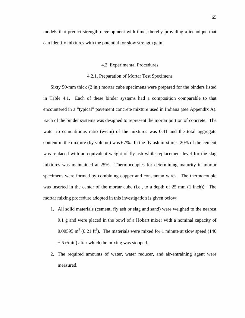
65

models that predict strength development with time, thereby providing a technique that

can identify mixtures with the potential for slow strength gain.

4.2. Experimental Procedures

4.2.1. Preparation of Mortar Test Specimens

Sixty 50-mm thick (2 in.) mortar cube specimens were prepared for the binders listed

in Table 4.1. Each of these binder systems had a composition comparable to that

encountered in a “typical” pavement concrete mixture used in Indiana (see Appendix A).

Each of the binder systems was designed to represent the mortar portion of concrete. The

water to cementitious ratio (w/cm) of the mixtures was 0.41 and the total aggregate

content in the mixture (by volume) was 67%. In the fly ash mixtures, 20% of the cement

was replaced with an equivalent weight of fly ash while replacement level for the slag

mixtures was maintained at 25%. Thermocouples for determining maturity in mortar

specimens were formed by combining copper and constantan wires. The thermocouple

was inserted in the center of the mortar cube (i.e., to a depth of 25 mm (1 inch)). The

mortar mixing procedure adopted in this investigation is given below:

1. All solid materials (cement, fly ash or slag and sand) were weighed to the nearest

0.1 g and were placed in the bowl of a Hobart mixer with a nominal capacity of

0.00595 m3 (0.21 ft3). The materials were mixed for 1 minute at slow speed (140

± 5 r/min) after which the mixing was stopped.

2. The required amounts of water, water reducer, and air-entraining agent were

measured.

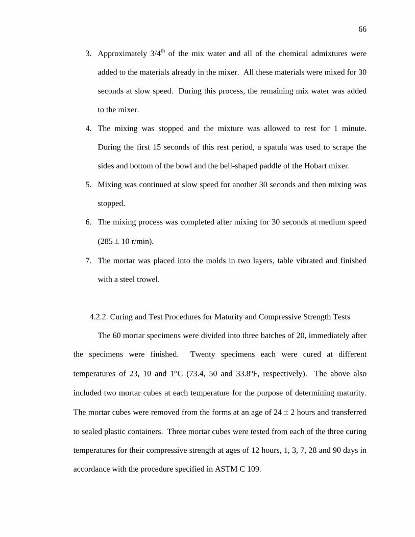
66

3. Approximately 3/4th of the mix water and all of the chemical admixtures were

added to the materials already in the mixer. All these materials were mixed for 30

seconds at slow speed. During this process, the remaining mix water was added

to the mixer.

4. The mixing was stopped and the mixture was allowed to rest for 1 minute.

During the first 15 seconds of this rest period, a spatula was used to scrape the

sides and bottom of the bowl and the bell-shaped paddle of the Hobart mixer.

5. Mixing was continued at slow speed for another 30 seconds and then mixing was

stopped.

6. The mixing process was completed after mixing for 30 seconds at medium speed

(285 ± 10 r/min).

7. The mortar was placed into the molds in two layers, table vibrated and finished

with a steel trowel.

4.2.2. Curing and Test Procedures for Maturity and Compressive Strength Tests

The 60 mortar specimens were divided into three batches of 20, immediately after

the specimens were finished. Twenty specimens each were cured at different

temperatures of 23, 10 and 1°C (73.4, 50 and 33.8ºF, respectively). The above also

included two mortar cubes at each temperature for the purpose of determining maturity.

The mortar cubes were removed from the forms at an age of 24 ± 2 hours and transferred

to sealed plastic containers. Three mortar cubes were tested from each of the three curing

temperatures for their compressive strength at ages of 12 hours, 1, 3, 7, 28 and 90 days in

accordance with the procedure specified in ASTM C 109.

67

Table 4.1: List of binder combinations

The temperature history of each mortar mixture was determined using the average

of two cubes. The temperature data was collected using a data logger that collected data

at 30-second intervals and recorded the average temperatures at 10-minute intervals. The

device for determination of temperature history of mortar specimens is shown in Figure

4.1. Typical time versus temperature plots are shown in Figure 4.2 for plain and

accelerator containing mortar mixtures cured at 23°C (73.4ºF). These plots show an

increase in temperature with time during the first eleven hours, which can be attributed to

the heat of hydration. After this period, the temperature stabilizes at a level close to the

curing temperature. The figure also shows the influence of an accelerating admixture on

1 M01 Lonestar cement + Rockport fly ash2 M02 Lonestar cement + Clifty Creek fly ash 3 M03 Lonestar cement + Miami Fort fly ash4 M04 Lonestar cement + Will County fly ash5 M05 Lehigh cement + Rockport fly ash6 M06 Lehigh cement + Clifty Creek fly ash7 M07 Lehigh cement + Miami Fort fly ash8 M08 Lehigh cement + Will County fly ash9 M09 Essroc cement + Rockport fly ash

10 M10 Essroc cement + Clifty Creek fly ash11 M11 Essroc cement + Miami Fort fly ash12 M12 Essroc cement + Will County 13 M17 Lonestar III cement + Rockport fly ash14 M18 Lonestar III cement + Clifty Creek fly ash15 M19 Lonestar III cement + Miami Fort fly ash16 M20 Lonestar III cement + Will County fly ash17 M13 Lonestar cement (Control mix)18 M14 Lehigh cement (Control mix)19 M15 Essroc cement (Control mix)20 M16 Lonestar III cement (Control mix)21 M21 Lonestar cement + Holnam Slag22 M22 Lehigh cement + Holnam Slag23 M23 Essroc cement + Holnam Slag24 M24 Lonestar III cement + Holnam Slag

Mix No. Mix ID Binder Combination

68

the temperature development. It could be observed that the mixture with accelerator

developed a higher peak temperature (27.5ºC or 81.5ºF) than the mixture without

accelerator (25.5°C or 77.9ºF).

Figure 4.1: Data logger for temperature determination

Figure 4.2: Typical time-temperature plot for mortars cured at 23°C

23.5

24

24.5

25

25.5

26

26.5

27

27.5

28

0 10 20 30 40 50Time (hours)

Tem

pera

ture

(o C)

M14M14+accelerator

69

Tests were conducted using a universal testing machine to determine compressive

strength at ages of 12 hours, 1, 3, 7, 28 and 90 days. The loading rate for this test was

maintained at 300 lb/s. The average of three failure loads was used in computing the

compressive strength at any age. The strength values for all mortar mixtures are reported

in Appendix B.

4.2.3. Preparation of Paste Specimens

Twenty-four binder systems (Table 4.1) were used to prepare pastes with water to

cementitious ratio (w/cm) of 0.41. Paste specimens were prepared excluding the

aggregates, using similar proportions adopted in making mortars. Again the replacement

level of cement for mixtures containing fly ash and slag were 20% and 25%, respectively.

The procedure given below was adopted for preparing the paste mixtures:

1. The solid materials (cement, fly ash, or slag) were initially dry mixed for 30

seconds at slow speed (140 ± 5 r/min) using a Hobart mixer with a nominal

capacity of 0.0014 m3 (0.05 ft3), so as to homogenize the mixture. The mixing

was stopped.

2. Measured quantities of air-entraining admixture and water reducer were then

added to this homogenized mixture containing cementitious materials.

3. Approximately 3/4th of the measured amount of water was added to the mixture

and mixing was conducted at slow speed for 30 seconds. During this period, the

remaining water was slowly added to the mixer.

4. Mixing was stopped for 1-minute interval. During this rest period, a spatula was

used to scrape the paddle as well as the sides and bottom of the mixing bowl.

70

5. Mixing was continued for 30 seconds at slow speed and then stopped.

6. The mixing operation was finished after mixing at medium speed (285 ± 10

r/min) for a period of 30 seconds.

7. The paste mixture was placed in the molds in a single layer and table vibrated.

4.3. Maturity Method

4.3.1. Introduction

As discussed in section 2.4, the maturity method provides a tool for predicting the

in-place strength of concrete. The maturity method had been used for predicting the

strength gain of concrete for rapid pavement repairs (Okamoto and Whiting, 1994).

Since the maturity method is useful for scheduling various construction activities, the

cost of any construction project can be optimized.

Strength maturity relationships were developed for the twenty-four mortar

mixtures tested for this project. Three maturity parameters were determined from

experiments: the ultimate strength (Su), the rate of reaction (kr), and the energy of

activation (Ea). Determination of these parameters is discussed in Sections 4.3.4, 4.3.5

and 4.3.6. Mathematical models were developed for the prediction of Su and kr. The

models were developed so as to account for the composition and fineness of cement and

supplementary materials. Subsequently, these models were used in the relative strength

gain expression for the purposes of strength prediction of various mortar mixtures at any

given age subjected to any temperature history. Strength development plots are

developed for all the mortar mixture combination at several curing temperatures to

indicate the potential for slow strength gain.

71

4.3.2. Equivalent Age Concept

There have been reports by many researchers regarding difficulties in the

prediction of strength using maturity concepts for concrete cured at different

temperatures (Carino, 1991). Early work by Nurse-Saul showed problems especially at

low maturity values. To overcome these problems, it was suggested that the Arrhenius

function be used to account for the effects of initial curing temperature on the early rate

of hydration of cement. Freiesleben et al. (Carino, 1991) suggested an expression for

equivalent age (equation 4.1) based on the Arrhenius expression:

tet TrTaQ

e Δ=⎟⎠⎞

⎜⎝⎛

+−

+−

15.2731

15.2731

(4.1)

where te = equivalent age

Δt = time interval

Ta = absolute temperature, °C

Tr = reference temperature, °C

Q = activation energy / universal gas constant (Ea/R) where R = 8.314 J/ (mol K)

The reference temperature for experiments performed for this project was 23°C

(73ºF). Equation 4.1 accurately accounts for the variations in temperature on strength

development in mortars at the temperatures under consideration.

72

4.3.3. Hyperbolic Strength Maturity Relationship

Although a particular mixture combination would be expected to have a unique

strength–maturity relationship, it has been reported that a unique relationship does not

exist for mixtures cured at different temperatures (Carino, 1991). This is verified by

Figure 4.3, which shows the results of mortar tests performed using binder M12. This

problem is overcome by using a relative strength gain expression suggested by Carino

(Carino, 1991). When the relative strength gain (given by equation 4.2) is plotted as a

function of equivalent age, the data points for mortar specimens (prepared using binder

M12) cured at different temperatures fall on a single curve (Figure 4.4).

)(1)(

ot

ot

u ttkttk

SS

−+−

= (4.2)

where S = the strength at any given age,

Su = the ultimate strength,

kt = rate constant at a given temperature

to = offset time or the time at which strength gain is assumed to begin

t = specimen age

The relative strength gain function can be related to the equivalent age by

introducing an age conversion factor α = r

t

kk

where kr is the rate of reaction, which is

the initial slope of the curve shown in Figure 4.4.

73

Figure 4.3: Strength versus equivalent age plot at different temperatures for mixture M12

Figure 4.4: Relative strength gain versus equivalent age plot for mixture M12 (@ 23°C)

0

1000

2000

3000

4000

5000

6000

7000

8000

0 20 40 60 80 100 120Equivalent age (days)

Com

pres

sive

stre

ngth

(psi

)

T 23

T 10

T 1

0.00

0.20

0.40

0.60

0.80

1.00

1.20

0.1 1 10 100Equivalent age (days)

Rela

tive

stre

ngth

gai

n (S

/Su)

Predicted strength ratio

Actual strength ratio

74

Substituting the age conversion factorα in equation 4.2, the relative strength gain

function can be expressed in terms of equivalent age as shown in equation 4.3.

)(1)(

or

or

u ttkttk

SS

−+−

=α

α (4.3)

Also, the product α t = te (equivalent age), and α to = t1 (constant) hence equation 4.3

can be written as

)(1)(

1

1

ttkttk

SS

er

er

−+−

=∞

(4.4)

4.3.4. Determination of Ultimate Strength

Ultimate strength (Su) is one of the important maturity parameters. Ultimate

strength was determined using the last 3 testing ages (7, 28, 90 days). Ultimate strength

was determined by plotting the inverse of strength versus the inverse of age for all

mixtures. Figure 4.5 shows determination of ultimate strength for mixture M21. The

inverse of the intercept of the plot at each temperature gives the ultimate strength for that

temperature. It was observed for some of the mortar mixtures that lower curing

temperatures result in higher ultimate strength values. This has also been reported in the

literature (Carino, 1991).

75

Figure 4.5: Determination of ultimate strength, S∞ (mixture M 21)

4.3.5. Determination of Rate Constants

The second maturity parameter of interest is the rate constant, kt, which describes

the rate of reaction for a particular mixture at any given curing temperature. The rate

constant was computed along the lines of the procedure specified by ASTM C1074. For

each curing temperature, A was computed for the earliest four ages in accordance with

equation 4.5.

A)( SS

S

u −= (4.4)

The values of A were plotted versus age for each curing temperature (Figure 4.6).

The rate constants (kt) were obtained from the slopes of the best-fit straight lines for each

curing temperatures. Since the equivalent age for this research was obtained with respect

to a temperature of 23°C (73.4ºF), the rate of reaction, kr in this case is the rate constant

y = 0.00109280x + 0.00015986R2 = 0.998

y = 0.00055627x + 0.00012991R2 = 0.994

y = 0.00026569x + 0.00013483R2 = 0.997

0.E+00

1.E-04

2.E-04

3.E-04

4.E-04

5.E-04

6.E-04

0.00 0.05 0.10 0.15 0.20 0.25 0.30 0.35

1/Age (1/Time)

1/st

reng

th (1

/psi

)

23 C

10 C

1C

76

value, kt at 23°C. While plotting the relative strength gain versus equivalent age plot

(Figure 4.4), the concept of the age conversion factor was introduced, where α is the ratio

of rate constant at a particular temperature to the rate constant at which equivalent age is

computed, which is 23°C in this case. Hence, the ratio α for a temperature 23°C would

be 1.

y = 0.097x + 0.147R2 = 0.996

y = 0.496x + 0.010R2 = 0.997

y = 0.221x - 0.047R2 = 0.987

0.00

0.50

1.00

1.50

2.00

2.50

3.00

3.50

4.00

0 5 10 15 20 25 30

Age (days)

S/(S

u-S)

23 C10 C1 C

Figure 4.6: Determination of rate constants, kt (mixture M 21)

4.3.6. Determination of Activation Energy

The third maturity parameter to be determined is the activation energy, Ea. The

activation energy is necessary in computation of equivalent age for mortars cured at

different temperatures. The value of the activation energy (Ea) divided by the universal

gas constant (R) is a constant Q. In order to compute Q, the natural logarithms of the rate

constant (kt) values are plotted versus the inverse of temperature (in Kelvin), as shown in

77

Figure 4.7. The negative of the slope of this plot is the ratio of activation energy to the

gas constant, Q.

Figure 4.7: Determination of activation energy/gas constant, Q (mixture M 21)

4.4. Approach for Development Strength Models and Binder Selection

4.4.1. Summary of Values of Ultimate Strength, Rate of Reaction and Energy Constant

Table 4.2 summarizes the parameters used in the strength – maturity relationship

(equation 4.4) for mortars. The values of Q ranged from about 3500 to 6200.

Researchers have commonly used a Q value of 5000 for strength prediction. The rate of

reaction values ranged from 0.353 to 0.943, higher values indicating a higher rate of

reaction. The ultimate strengths ranged from about 5300 psi (36.5 MPa) to about 8500

psi (58.6 MPa). Typically, mixtures prepared with supplementary materials showed

higher ultimate strengths compared to mixtures prepared with similar control cements,

confirming the beneficial effect of the pozzolanic reaction on the ultimate strength. The

values of kr, Su obtained from actual experiments were then used to develop mathematical

y = -5655.75x + 18.33R2 = 0.99

-2.500

-2.000

-1.500

-1.000

-0.500

0.0003.3E-03 3.5E-03 3.7E-03

1/Temperature (1/Kelvin)

Ln(K

t)

78

models for predicting kr and Su. These models and actual values of Q were used in the

strength-maturity hyperbolic relationship given by equation 4.4 to predict strength of any

mortar mixture at any given age and subjected to any temperature history.

Table 4.2: Summary of Su, kr and Q values

Mix ID Binder CombinationSu (@ 23 o C)

kr (@ 23 o C)

Q

M01 Lonestar cement + Rockport fly ash 6337 0.426 5314M02 Lonestar cement + Clifty Creek fly ash 7407 0.543 4606M03 Lonestar cement + Miami Fort fly ash 5991 0.353 3674M04 Lonestar cement + Will County fly ash 6112 0.430 4453M05 Lehigh cement + Rockport fly ash 5660 0.406 6271M06 Lehigh cement + Clifty Creek fly ash 6916 0.716 4726M07 Lehigh cement + Miami Fort fly ash 6276 0.511 4747M08 Lehigh cement + Will County fly ash 6860 0.366 5543M09 Essroc cement + Rockport fly ash 5305 0.493 4560M10 Essroc cement + Clifty Creek fly ash 6910 0.470 5615M11 Essroc cement + Miami Fort fly ash 5851 0.444 4021M12 Essroc cement + Will County 6454 0.519 3971M17 Lonestar III cement + Rockport fly ash 7515 0.801 5156M18 Lonestar III cement + Clifty Creek fly ash 8525 0.719 3922M19 Lonestar III cement + Miami Fort fly ash 6833 0.817 5043M20 Lonestar III cement + Will County fly ash 7053 0.790 3513M13 Lonestar cement (Control mix) 6405 0.784 4913M14 Lehigh cement (Control mix) 7412 0.854 4993M15 Essroc cement (Control mix) 6630 0.846 5277M16 Lonestar III cement (Control mix) 7878 0.943 5277M21 Lonestar cement + Holnam Slag 7417 0.496 5656M22 Lehigh cement + Holnam Slag 7549 0.567 5944M23 Essroc cement + Holnam Slag 7065 0.425 5675M24 Lonestar III cement + Holnam Slag 8122 0.772 4021

79

4.4.2. Development of Mathematical Model for Strength Prediction in Mortars

As it was earlier observed from the sensitivity analyses performed on the data

from mill certificates, the strength development is mainly sensitive to the fineness, alkali

content and C3S content (section 3.4.1). It is also known that C2S content in cement

contributes primarily to the later age strength development in concrete. Higher fineness,

C3S and alkali content of the cement are also known to be responsible for a higher initial

rate of reaction. The sensitivity analyses of fly ash showed that the strength activity

index is dependent on the lime, fineness, and alkali content. There have been reports of

problems of reduction in the air content in concrete mixtures prepared with fly ashes

containing high amount of carbon. Since only one slag was tested, the chemical

components of the slag were not taken into consideration in the development of

mathematical models. Therefore, based on the factors mentioned above, the ultimate

strength and rate of reaction for the mortars was initially expressed in a form given by

equations 4.5 and 4.6 below:

Su = Wc * (C1 * Fc+ C2 * C3S + C3 * C2S + C4 * Ac)+ Wfa * (C5 * Ffa + C6 * Lime

+ C7 * Afa+ C8 * Carbon)+ Ws* C9 (4.5)

kr = Wc * (D1 * Fc + D2 * C3S + D3 * C2S + D4 * Ac)+ Wfa * (D5 * Ffa + D6 *

Lime + D7 * Afa + D8 * Carbon)+ Ws * D9 (4.6)

where Cn and Dn are constants to be determined by regression analysis. Wc = wt% of

cement, Wfa = wt % of fly ash, Ws = wt% of slag, Fc = Fineness of cement, Ffa = Fineness

of fly ash, Ac = Alkali of cement, Afa = Alkali of fly ash

80

In this project, the data analysis was performed using the data analysis feature of

Microsoft Excel® software. The actual values of ultimate strength or rate of reaction

determined from experiments were selected as the dependent variable (Y-axis input

range) and the properties obtained from mill certificates including fineness, C3S, C2S and

alkali for cements and fineness, lime, alkali and carbon contents for fly ashes were

selected as independent variables (X-axis input range). After the values of the constants

were determined, the significance of each independent variable was assessed. A

statistical approach was adopted where a confidence level of 95% was specified and the

corresponding p-values (significance) were determined. Using this approach enabled one

or more variables to be eliminated from the equations 4.5 and 4.6.

For ultimate strength, a significance level of 0.05 was specified. The variables

(used in equation 4.5) producing a p-value ≤ 0.05 were retained in the model and those

producing values greater than 0.05 were eliminated. Further iteration or regression

analysis was carried out until a point when all parameters in the modified equation for

ultimate strength were statistically significant (i.e., p ≤ 0.05). The alkali content of

cement and the alkali content of fly ash were found to be statistically insignificant for

predicting the ultimate strength. The final equation for predicting ultimate strength for

the mortar mixture combinations tested was of the form given in equation 4.7.

Su = Wc*(8.27 * Fc + 46.18 * C3S + 61.68 * C2S)+Wfa*(-186.10 * Ffa + 236.80 *

Lime + 3130.60 * Carbon) + 878.31 * Slag (4.7)

A similar procedure was adopted for eliminating insignificant parameters from the

rate of reaction expression given by equation 4.6. Regression analysis was continued to a

point until a reasonable value of coefficient of correlation was obtained between the

81

actual rate of reaction values and the predicted values. The significance level for all

parameters after repetitive regression analysis was p ≤ 0.27. The C3S and alkali content

of cement and the lime content of fly ash were parameters that were determined to be

statistically insignificant. The final equation for predicting the rate of reaction for the

mortar mixture combinations tested was of the form given below:

kr = (0.00189 * Fc + 0.004207 * C2S)+ (-0.03444 * Ffa - 0.2594 * Afa + 0.1515 *

Carbon) - 0.02716 * Slag (4.8)

The values predicted for the ultimate strength and rate of reaction using equations

4.7 and 4.8 are in very good agreement with the actual values obtained from experiments

as shown in Figures 4.8 and 4.9.

Figure 4.8: Actual versus predicted ultimate strength

y = 1.01x - 93.21R2 = 0.83

5000

5500

6000

6500

7000

7500

8000

8500

9000

5000 5500 6000 6500 7000 7500 8000 8500 9000Predicted Ultimate Strength (psi)

Act

ual U

ltim

ate

Stre

ngth

(psi

)

82

Figure 4.9: Actual versus predicted rate of reaction

4.4.3. Comparison of Actual Strength Results with Results Predicted from the Model

As observed from the plots shown in Figures 4.8 and 4.9, the values predicted by

the mathematical models for ultimate strength and rate of reaction were in excellent

agreement with the actual values obtained. These models (equations 4.7 and 4.8) were

then used in equation 4.4 for strength prediction at the temperatures of 23, 10 and 1°C

(73.4, 50 and 33.8ºF), at which the actual strength tests on mortars were carried out.

Actual values of Q given in table 4.2 were used in predicting strength because of

difficulties in developing a mathematical model. The equivalent age term (te) in equation

4.4 was computed using the Arrhenius function given by equation 4.1. The following

plots (Figures 4.10 through 4.12) show the comparison between actual and predicted

strength results at the three temperatures at ages of 3, 7 and 28 days. The coefficient of

correlation for the plot at a temperature of 23ºC was 0.98.

y = 0.998x + 0.001R2 = 0.83

0.000

0.200

0.400

0.600

0.800

1.000

1.200

0.000 0.200 0.400 0.600 0.800 1.000 1.200Pedicted Kr

Act

ual k

r

83

Figure 4.10: Actual versus predicted strength at 23°C

Figure 4.11: Actual versus predicted strength at 10°C

0

1000

2000

3000

4000

5000

6000

7000

8000

9000

0 1000 2000 3000 4000 5000 6000 7000 8000 9000

Predicted strength (psi)

Act

ual S

tren

gth

(psi

)

3 day7 day28 day

R2=0.90

0

1000

2000

3000

4000

5000

6000

7000

8000

9000

0 1000 2000 3000 4000 5000 6000 7000 8000 9000Predicted strength (psi)

Act

ual S

tren

gth(

psi)

3 day7 day28 day

R2=0.98

84

Figure 4.12: Actual versus predicted strength at 1°C

The plot shown in Figure 4.10 indicates that predicted strength and actual strength

values match most accurately. This is due to the fact that the ultimate strength and rate of

reaction values were predicted using actual data results obtained at a temperature of

23°C. McIntosh (36) and several others reported the crossover effect (Section 2.4). They

found that lower initial curing temperatures result in lower degree of hydration at early

ages but results in higher degrees of hydration at later ages primarily due to the better

dispersion of hydration products. Consequently, lower initial curing temperatures result

in higher ultimate strengths. Hence, theoretically the ultimate strength values that were

computed at 23°C and used for development of the mathematical model might result in

conservative estimates for the other two temperatures of 10 and 1°C. This is also verified

0

1000

2000

3000

4000

5000

6000

7000

8000

9000

0 1000 2000 3000 4000 5000 6000 7000 8000 9000

Predicted strength (psi)

Act

ual S

tren

gth

(psi

)

3 day7 day28 day

R2=0.92

85

from Figure 4.10 in which the data points are closely spaced, but in Figures 4.11 and 4.12

the data points have a wider distribution.

4.4.4. Non-evaporable Water Content Determination

As discussed in section 4.2.3, twenty-four paste mixtures were prepared for

determination of non–evaporable water content (Wn). The paste samples were powdered

by using a pestle and bowl. Water contained in pastes containing cement, mineral

admixtures like fly ash, ground granulated blast furnace slag can be divided into two:

evaporable water and chemically bound or non-evaporable water. The evaporable water

content was determined by oven drying the paste sample to 105°C (221ºF). The

chemically bound water was determined by heating the sample in a furnace set to a

temperature of 1050°C (1922ºF). The non-evaporable water content, Wn for pastes was

calculated as the ratio of the difference between the weight on ignition at 1050°C and the

weight after oven drying at 105°C to the weight of the sample on ignition at 1050°C.

Wn = (W1050 -W105)*100 / W1050 (4.9)

where W105 = weight of sample after oven drying at 105°C

W1050 = weight of sample after ignition at 1050°C

For paste samples containing cement, fly ash and slag, necessary corrections due

to the loss on ignition of cement, fly ash and slag were made based on the weight ratios

of the individual components present in the mortar sample. Following plots show the

comparison of non-evaporable water contents for paste mixtures containing fly ash or

86

slag. Fig 4.13, 4.14 and 4.15, respectively, show the non-evaporable water contents for

pastes cured at temperatures of 23, 10 and 1°C (73.4, 50, 33.8ºF, respectively).

Figure 4.13: Non-evaporable water content for pastes cured at 23°C

Figure 4.14: Non-evaporable water content for pastes cured at 10°C

5

7

9

11

13

15

17

M01

M02

M03

M04

M05

M06

M07

M08

M09

M10

M11

M12

M21

M22

M23

Mix ID

Wn

(%)

1 day

3 day

7 day

2

4

6

8

10

12

14

16

M01

M02

M03

M04

M05

M06

M07

M08

M09

M10

M11

M12

M21

M22

M23

Mix ID

Wn

(%)

1 day3 day7 day

87

Figure 4.15: Non-evaporable water content for pastes cured at 1°C

4.4.5. Summary of Results from Non–Evaporable Water Content tests

For all the mixtures evaluated, it is evident from Figures 4.13 through 4.15 that

lower curing temperatures result in lower amounts of non-evaporable water especially at

ages up to 3 days. Mixtures M01, M02, M03 and M04 were all prepared with Lonestar

cement (Type I) but with fly ashes from the Rockport, Clifty Creek, Miami Fort and Will

County plants respectively. At the three ages tested, Rockport ash showed the lowest Wn

value at 1 day, but the Miami Fort ash showed lowest Wn values at 3 and 7 days. A

similar trend was observed at the other two curing temperatures of 10 and1°C (50ºC and

33ºC, respectively). For mixtures M05, M06, M07 and M08 prepared with Lehigh

cement, a similar trend was observed in which Rockport ash showed the lowest Wn

values at 1 day but the Miami Fort ash showed lowest values at 3 and 7 days at all three

temperatures. For mixtures M09, M10, M11, M12 prepared with Essroc cement, a

similar trend as observed with the other two cements was found for all fly ashes tested at

4

6

8

10

12

14

16

M01

M02

M03

M04

M05

M06

M07

M08

M09

M10

M11

M12

M21

M22

M23

Mix ID

Wn

(%)

1 day3 day7 day

88

temperatures of 23 and 10°C. However, at 1°C and 1day age, the combination with

Clifty Creek ash showed the lowest Wn value. So, in general it is observed that Rockport

ash shows the lowest Wn value at 1 day, but the Miami Fort shows the lowest Wn value at

3 and 7 days for all curing temperatures.

For mixtures prepared with slag, no definite trend was observed. At 1-day age,

mixture with Lonestar (Type I) cement showed the lowest Wn value at 23°C, but showed

the highest Wn values at 10º and 1°C, respectively. At this age, mixture made with

Essroc cement showed the lowest Wn values at 10 and 1°C.

4.4.6. Late Fall Temperatures in the State of Indiana

As this project deals with temperatures typical in the late fall construction season,

the temperature history of both the atmosphere (air temperature) and freshly constructed

concrete pavements during the fall season was studied. Figure 4.16 shows the air

temperature in the months of October to April for years 1997, 1998 and 1999.

89

Figure 4.16: Minimum and maximum temperatures in Indiana (years 1997 through 1999)

Table 4.3: Average minimum temperatures

Table 4.3 shows the average minimum temperatures for the three years 1997,

1998 and 1999. During the period studied, the lowest average minimum air temperature

of -14.99°C (5ºF) occurred in the month of January. The second lowest average

minimum air temperature of -9.84°C (14.3ºF) was observed in the month of December.

The average minimum temperatures in the months of October and April, which mark the

beginning and end, respectively, of the period during which use of supplementary

materials is not permitted are 1.48º (34.7ºF) and 2.10°C (35.8ºF), respectively. Figure

4.17 shows the temperature history of a freshly constructed concrete pavement at various

depths from the pavement surface. The data for this plot was obtained from another

Average minimum temperatures, deg C (1997 to 1999)Oct Nov Dec Jan Feb Mar Apr1.48 -3.52 -9.84 -14.99 -5.07 -7.05 2.10

-30

-20

-10

0

10

20

30

40

O N D J F M A O N D J F M A O N D J F M A

Month

Tem

pera

ture

(o C

)

Min Air TempMax Air Temp

90

project on performance related specifications. The plot shows the temperature history of

the atmosphere as well as that of a pavement at depths of ¼ in. (0.635 cm), 1.5 in. (3.81

cm) and 7 in. (17.8 cm) from the surface. As expected, the heat generated due to

hydration during the initial period increases with an increase in pavement depth.

Figure 4.18 shows the difference between the air and concrete temperatures at a

depth of ¼ in. from the surface. It can be seen that there is an increase in internal

temperature due to the hydration of cement. This increase is visible for about 2 days,

after which period the difference between the internal temperature and the ambient

temperature is minimal. As with any chemical reaction, this higher temperature is likely

to accelerate the hydration and strength gain. The shaded portions in Figure 4.18 show

the maturity index, i.e., the product of temperature versus time gained due to hydration at

a pavement depth of ¼ in. from the pavement surface. From the above plot, it was

observed that at a pavement depth of ¼ inch, a maturity of 7.3°C-days is gained during

the initial 1.8 days after placement of concrete due to the heat liberated during hydration.

Higher maturities would be gained at greater pavement depths.

91

Figure 4.17: Pavement temperature at varying depths in the month of October

Figure 4.18: Temperature gain due to hydration at ¼ inch depth from pavement surface

0

5

10

15

20

25

30

35

0.0 0.5 1.0 1.5 2.0 2.5 3.0 3.5 4.0

Time (days)

Tem

pera

ture

(o C)

Air Temp1/4 in1-1/2 in7 in

-4

-2

0

2

4

6

8

10

0.0 0.5 1.0 1.5 2.0 2.5 3.0 3.5 4.0

Time (days)

Diff

eren

ce o

f 1/4

in a

nd a

ir te

mpe

ratu

re (o C

)

Difference

92

4.4.7. Identification of Slow Strength Gaining Mortar Mixtures

The purpose of this section was to identify binder combinations that when used in

mortars would result in slow strength gain, especially under low temperature conditions.

Using the mathematical models developed in section 4.4.2 that allowed prediction of the

rate of reaction, kt and ultimate strength, S∞ in the hyperbolic strength gain equation (4.4),

the prediction of strength (S) at any age cured under any temperature for any given

mixture could be made. Therefore, the time required to attain a given strength level for

any binder composition subjected to a particular curing temperature could be determined.

A strength level of 3500 psi (24.1 MPa) was specified for concrete to be durable when

exposed to cycles of freezing and thawing. Using this strength level, contour plots were

developed that show variation in age required by all the twenty-four mixtures to reach a

strength of 3500 psi at 4 curing temperatures of 25, 15, 5 and 0°C (77, 59, 41 and 32ºF).

The contour plots for all mortar mixtures are shown in Figure 4.19.

Figure 4.20 shows the age required by all control mortar mixtures (plain) to reach

3500 psi. The example of how the plot can be used is also shown in Figure 4.20. One

should enter the temperature axis (for example, 15°C) and proceed horizontally to

intercept one of the curves and then move down to the X-axis where the time required

could be obtained. Figure 4.20 shows that Lonestar ((Type I), M13) and Essroc cements

(M15) are the slowest to attain strength of 3500 psi (24.1 MPa) at all temperatures. As

expected, M16 containing Lonestar (Type III) cement was the fastest to reach this

strength level at all temperatures.

93

Figure 4.19: Simulated values of time and temperature required by all mortar mixtures to reach strength level of 3500 psi

Figure 4.21 shows the age required by all mixtures containing Rockport fly ash to

develop strength of 3500 psi. It is observed from this figure that the combination M01

with Lonestar cement (Type I) is the slowest to develop strength of 3500 psi at all

temperatures above 5°C (41ºF). However, below 5°C, the combination M05 with Lehigh

cement seems to be slightly slower. Combination M17 containing Lonestar (Type III)

cement was the fastest strength gaining at all temperatures.

0

5

10

15

20

25

30

0 2 4 6 8 10 12 14 16 18 20

Time (days)

Tem

pera

ture

(o C

)M01M02M03M04M05M06M07M08M09M10M11M12M13M14M15M16M17M18M19M20M21M22M23M24

94

Figure 4.20: Simulated values of time and temperature required by all control mixtures

to reach strength level of 3500 psi

Figure 4.21: Simulated values of time and temperature required by all mixtures

containing Rockport fly ash to reach strength level of 3500 psi

0

5

10

15

20

25

30

0 5 10 15 20

Time (days)

Tem

pera

ture

( o C)

M13

M14

M15

M16

0

5

10

15

20

25

30

0 5 10 15 20

Time (days)

Tem

pera

ture

( o C)

M01

M05

M09

M17

95

Figure 4.22 shows the variation in age required by all mixtures containing Clifty

Creek fly ash to develop a compressive strength of 3500 psi (24.1 MPa) at different

temperatures. It is observed that the combination with Essroc cement (M10) is the

slowest to develop strength of 3500 psi at all temperatures up to 15°C (59ºF). Above this

temperature, mixtures prepared with Essroc cement (M10), Lehigh cement (M06) and

Lonestar (Type I) cement (M02) showed similar trends. Again, mixture containing

Lonestar (Type III) cement (M18) was the fastest at all temperatures.

Figure 4.23 shows the variation in age required to develop a compressive strength

of 3500 psi at different temperatures by all mixtures containing Miami Fort fly ash. The

mixture combination M03 containing Lonestar (Type I) cement was the slowest to reach

3500 psi at temperatures above 5°C. Below this temperature, combination M07

containing Lehigh cement was the slowest. Combination M19 containing Lonestar (Type

III) cement was the fastest strength developing at all temperatures.

Figure 4.24 shows the variation in age required by all mixtures containing Will

County fly ash to develop a compressive strength of 3500 psi at different temperatures. It

is observed that below the temperature of 5°C, combination M08 containing Lehigh

cement is the slowest strength developing. However, above this temperature,

combination M04 containing Lonestar (Type I) cement is the slowest. Again, the

combination M20 containing Lonestar (Type III) cement was the fastest.

96

Figure 4.22: Simulated values of time and temperature required by all mixtures containing Clifty Creek fly ash to reach strength level of 3500 psi

Figure 4.23: Simulated values of time and temperature required by all mixtures

containing Miami Fort fly ash to reach strength level of 3500 psi

0

5

10

15

20

25

30

0 5 10 15 20Time (days)

Tem

pera

ture

( o C) M02

M06

M10

M18

0

5

10

15

20

25

30

0 5 10 15 20

Time (days)

Tem

pera

ture

( o C)

M03

M07

M11

M19

97

Figure 4.24: Simulated values of time and temperature required by all mixtures

containing Will County fly ash to reach strength level of 3500 psi

Figure 4.25 shows the variation in age required by all mixtures containing slag to

reach strength of 3500 psi when cured at different temperatures. It is observed that

mixtures prepared with Essroc and Lehigh cement (M22 and M23) show identical trends

at all temperatures. However, mixture M21 prepared with Lonestar (Type I) cement

seemed to be the slowest strength developing mixture. Again, the combination M24

containing Lonestar (Type III) cement was the fastest strength developing at all

temperatures.

0

5

10

15

20

25

30

0 5 10 15 20

Time (days)

Tem

pera

ture

( o C) M04

M08M12M20

98

Figure 4.25: Simulated values of time and temperature required by all mixtures

containing slag to reach strength level of 3500 psi

4.4.8. Selection of Concrete Mixture Composition Based on Material Tests and Trends

from Time-temperature Contour Plots

From the data compilation for all Class C fly ashes in Table 3.8, Rockport fly ash

had the lowest strength activity index value at 7 days. When all 4 fly ashes selected for

tests on mortars, including Miami Fort (Class F) ash were considered, the Miami Fort fly

ash showed the lowest 7-day SAI value (Table 3.8 and Table 3.9). The relative

differences in SAI values of the four fly ashes used in mortar mixtures reflected in the

strength predictions made using the mathematical models. According to these models,

mixtures containing Rockport fly ash and Miami Fort fly ash were among the slowest to

develop strength of 3500 psi especially at low temperatures. Also pastes containing

Rockport and Miami Fort fly ashes had the lowest non-evaporable water content values,

0

5

10

15

20

25

30

0 5 10 15 20

Time (days)

Tem

pera

ture

( o C)

M21M22M23M24

99

especially at low temperatures (Section 4.4.4 and 4.4.5). From the fly ash data

compilation, it was observed that Clifty Creek (Class C) and Miami Fort (Class F) fly ash

had the highest carbon contents (Table 3.8 and Table 3.9). The selection of candidate

binder combinations for subsequent tests on concrete was carried out based on factors

like potential for slow strength gain at low temperatures (observed from time-temperature

contour plots), SAI values of the fly ashes used for mortar tests and high carbon contents

in fly ash that could reduce the effectiveness of air-entraining agents.

Table 4.4 shows the binder systems selected for subsequent tests on concrete.

Mixture M13 containing Lonestar (Type I) cement was chosen as the control (plain)

mixture because this cement was found to be the slowest reacting at all temperatures

considered. Among all mixtures containing Rockport fly ash, combinations with

Lonestar (Type I) cement and Lehigh cement (M01 and M05) were found to be the

slowest reacting below temperatures of 15°C (59ºF). Hence these two mixtures were

selected for further tests on concrete.

A mixture with high carbon Class C fly ash (Clifty Creek) that was slow reacting

at temperatures below 15°C (59ºF) was the one prepared with Essroc cement (M10).

Mixture combination M07 containing Lehigh cement and Miami fort fly ash (high carbon

Class F) was the slowest reacting below temperatures of 5°C. Thus mixtures M10 and

M07 were selected on the basis of slow strength gain at low temperatures and due to high

contents of carbon in the fly ashes contained in them. For mixtures prepared with slag,

Lonestar cement (Type I) was observed from the contour plot to be the slowest reacting

especially at low temperatures.

100

A compilation of all mixtures screened, based on the worst-case scenario is shown

in Table 4.4. One control (plain) mixture, two mixtures with the slowest reacting Class C

fly ash (Rockport), one mixture with the high carbon Class C fly ash (Clifty Creek), one

mixture with the high carbon Class F fly ash (Miami Fort), and one mixture with slag

were selected.

4.5. Summary

1. Maturity determination and strength tests were performed on twenty-four mortar

mixtures at various ages.

2. Strength-maturity relationships were developed for all mixtures at different

temperatures tested. Parameters like ultimate strength, rate constant and activation

energy were determined.

3. These parameters were utilized to develop mathematical models to predict the

ultimate strength and rate of reaction in terms of chemical components and fineness

of cement and fly ash used.

4. Using the models and the maturity based hyperbolic relative strength gain equation,

contour plots were developed that allow determination of age required by all mixtures

to attain a strength level of 3500 psi (24.1 MPa) at various temperatures.

5. Non-evaporable water content tests on paste mixtures were carried out to verify the

test results from strength, maturity tests.

6. Six different mixtures (with binder systems highlighted in Table 4.4), having the

potential for slow strength gain under low temperature conditions were identified.

101

These binders were then used to produce concrete specimens that were tested for

durability related problems.

Table 4.4: Summary of selected mixtures for tests on concrete

1 Lonestar Lehigh Essroc Lonestar (III) Rockport Clifty Creek Miami Fort Will Co. Slag Control2 Lonestar Lehigh Essroc Lonestar (III) Rockport Clifty Creek Miami Fort Will Co. Slag Slow reacting ash3 Lonestar Lehigh Essroc Lonestar (III) Rockport Clifty Creek Miami Fort Will Co. Slag Slow reacting ash4 Lonestar Lehigh Essroc Lonestar (III) Rockport Clifty Creek Miami Fort Will Co. Slag Slow slag mix5 Lonestar Lehigh Essroc Lonestar (III) Rockport Clifty Creek Miami Fort Will Co. Slag Slow high carbon C ash6 Lonestar Lehigh Essroc Lonestar (III) Rockport Clifty Creek Miami Fort Will Co. Slag Slow high carbon F ash

Mixture Cements Fly Ash/Slag Comments

102

103

CHAPTER 5: EVALUATION OF PROPERTIES OF CONCRETE MIXTURES

5.1. Introduction

The objective of this chapter is to describe the performance of concrete mixtures

exposed to low temperatures at early ages. Concrete mixtures used in this study were

selected based on results from mortar tests discussed in the previous chapter. A total of

six mixtures were selected. These six mixtures were identified to have the potential for

slow strength development, especially under low temperature conditions. The logic

behind selecting the slowest reacting mixtures was that if the slowest reacting mixture

with a particular cement and fly ash passes the durability tests, then all other mixtures

made with a similar fly ash but different cements should be durable. Freeze-thaw and salt

scaling tests were performed. Flexural strength and compressive strength tests were also

carried out to ascertain whether the concrete mixtures satisfied strength requirements

prescribed by INDOT specifications. Other tests discussed in this chapter are sorptivity,

which deals with the rate of ingress of water in a particular mixture and the cumulative

absorption over time. Results from tests to determine the weight loss on drying over time

and the resonant frequency gained due to hydration of different mixtures are also

discussed. Test results to determine the air void spacing in concrete exposed to cycles of

freezing and thawing are also presented. An attempt was made relate the freeze-thaw and

scaling resistance to factors like strength, air-void spacing, rate of water ingress, moisture

loss on drying, and slump.

104

5.2. Experimental Procedures

5.2.1. Preparation of Concrete

Concrete mixtures were prepared with water to binder ratio of 0.44 and 70% (by

volume) of aggregates. Mixture proportions are shown in Appendix A. The replacement

level by weight of cement with fly ash for fly ash mixtures was 20% and with slag for the

slag mixture was 30%. All solid materials were weighed to the nearest 0.1 kg (3.5 oz.).

Following is the procedure adopted for mixing of concrete.

1. Sand and coarse aggregates were mixed with approximately 1/3rd of the mixing

water for one minute and the mixture was allowed to rest for a few minutes for the

purpose of moisture absorption.

2. Cement and fly ash or slag was then added to the mixture of sand and coarse

aggregates and mixed in order to homogenize the materials.

3. The following materials were added to the mixing pan while the mixer was in

operation: (a) Measured amount of air-entraining admixture (previously diluted

with 200 ml or 6.8 fl. oz. of water), (b) another 1/3rd of the mix water, (c) water

reducer (previously diluted with 500 ml or 16.9 fl. oz. of water), and (d) the

remaining 1/3rd of water. After the process of addition of the above materials was

complete, mixing was continued for additional two minutes.

4. The mixer was stopped and the concrete mixture was allowed to rest for a period

of three minutes. During the first 30 seconds of this rest period, material sticking

to the sides of the mixing pan was scraped.

5. The mixing was resumed for additional two minutes.

105

5.2.2. Curing and Test Procedures for Compressive, and Flexural Strength of Specimens

The compressive strength was determined on 4” x 8” (10 cm x 20 cm) cylinders.

Compressive strength cylinders were prepared for testing at ages of 3, 7 and 28 days.

The cylinders were de-molded after a period of 24 ± 2 hours and transferred to a fog

room (100% RH) where they were stored at a temperature of 21°C (69.8ºF) until test

time. The strength testing was performed using a 600-kip testing machine (2667 kN) and

a loading rate of about 30,000 lb/min (133 kN/min). Average of the results of three

specimens tested in compression was used in the computation of compressive strength at

each age.

Flexural strength tests were performed on beam specimens of dimension 15” x 3”

x 3” (38 cm x 7.5 cm x 7.5 cm). Flexural strength specimens were prepared for testing at

ages of 12 h, 1, 2, 3, 7, 14 and 28 days. All specimens except the ones to be tested at 12

hours were de-molded after a period of 24 ± 2 hours and transferred to a fog room (100%

RH) maintaining a temperature of 21°C. Average failure load from two specimens tested

in third-point loading were used to calculate the flexural strength at any age. The flexural

strength values until the first four test ages were used in computation of rate constant

values for all mixtures. Another set of beam specimens of dimension 21” x 6” x 6” (53

cm x 15 cm x 15 cm) were prepared for flexural strength determination at 7 days. This

was done to determine whether the concrete specimens satisfied the INDOT flexural

strength requirement (for opening to traffic) of 550 psi (3.8 MPa) when tested at an age

of 7 days. The strength testing was performed using a 60-kip (267-kN) Universal Testing

Machine and the loading rate for all beams tested was maintained 1800 lb/min

(8 kN/min).

106

5.2.3. Curing and Testing of Specimens Subjected to Freeze-Thaw Cycling

The freeze thaw testing was performed in accordance with ASTM C666,

procedure A which involves freezing and thawing the test specimens in water. Each

freeze thaw cycle consisted of lowering the temperature of the specimens from 4.4°C to

-17.8°C (40ºF to 0.04ºF) and raising it from -17.8°C to 4.4°C in a total time of about 4

hours. Four concrete prisms of dimension 16” x 4” x 3” (40.5 cm x 10 cm x 7.5 cm)

were prepared for each of the six pre-selected concrete mixtures for the purpose of freeze

thaw testing. Two prisms (specimen No. 3 and 4) were moist cured for a period of 14

days (ASTM C666 standard procedure) and two prisms (specimen No. 1 and 2) were

moist cured just for 3 days before commencement of tests in order to simulate the worst-

case scenario where concrete may be exposed to freezing conditions within few days

after casting.

It can be observed from the contour plots in Figure 4.19 that most of the mortar

mixtures cured at a temperature of 23°C (73.4°F) develop strength of 3500 psi (24.1

MPa) within 3 to 5 days after placing. Also, a maturity gain of 7.3°C-days due to the

heat of hydration is observed close to the pavement surface (Figure 4.18) and higher

maturity gains can be expected at greater pavement depths. Taking the above into

account, wet curing period of 3 days was selected for freeze thaw specimens. The

concrete prisms were subjected to a total of 300 cycles of freezing and thawing. The

weight loss and resonant frequency of the specimens was tested after every 36 cycles

(maximum) of freezing and thawing. A specimen is considered to pass the freeze thaw

test if the durability factor at the end of 300 cycles is higher than 60%.

107

3% NaCl solution

Concrete

Styrofoam

10 inch 7.5 inch

3 inch

5.2.4. Curing and Testing of Specimens for Salt Scaling Tests

The tests for determining the resistance to salt scaling were performed using a

procedure similar to that described in ASTM C672. Instead of using visual rating as the

criterion for evaluating the scaling resistance, the weight loss of the scaled particles was

used. Four scaling slabs of dimensions 15” x 10” x 3” (38 cm x 25 cm x7.5 cm) were

cast for each of the six concrete mixtures. Each specimen was cut along the width into

half so as to obtain two specimens of dimension 7.5” x 10” x 3” (19 cm x 25 cm x 7.5

cm) as shown in Figure 5.1. Thus, a total of eight specimens were obtained.

Figure 5.1: Schematic of scaling specimen

The effect of a curing compound (W.R. Meadows Inc., Sealtight 1610, White,

Wax, Water-Based Concrete Curing Compound) on the resistance of concrete to deicer

salts was also studied. Two specimens each, with and without curing compound were

subjected to scaling tests after a moist curing period of 14 days followed by air-drying at

20 ± 1°C (68 ± 2°F) for 14 days (standard procedure). Also two specimens each, with

and without curing compound were subjected to scaling tests after a moist curing period

108

of 3 days followed by air drying at 20 ± 1°C for 3 days (see Appendix C). These set of

specimens were expected to simulate the worst case of scenario of actual pavement

concrete in the field. All specimens were subjected to 50 cycles of freezing and thawing

in an automatic temperature control room. Each cycle consisted of lowering the room

temperature to -18°C (0.4ºF) for a period of 16 to 18 hours and increasing it to 23°C

(73.4°F) for a period of 6 hours. All specimens were subjected to a 3% NaCl solution.

An enclosure consisting of Styrofoam® was glued to the top of the specimens to contain

the salt solution. After every 5 cycles of freezing and thawing, the surface of each

specimen was flushed off with tap water and the scaled particles were collected and

weighed. The experimental set up for a scaling specimen is shown in Figure 5.1.

5.2.5. Test Procedure for Determining Sorptivity

The method of capillary sorption was adopted for determining the rate of

absorption as well as the cumulative amount of water absorbed by different concrete

specimens. The sorptivity test was conducted on 2-in. hick discs cut from the middle

portion of 4” x 8” inch cylinders. The specimens were coated with epoxy on the curved

surface so as to allow water ingress into concrete only from the bottom flat surface. The

specimens were immersed in a plastic container containing water and supported in such a

way that about 0.4” (1 cm) of the lower part of the specimens was in water. The

experimental set up is shown in the Figure 5.2.

109

Figure 5.2: Schematic of sorptivity tests

The sorptivity was determined on specimens exposed to two different

conditioning procedures. Two specimens from each concrete mixture were moist cured

for a period of 3 days followed by air drying at 50% RH at 20 ± 1°C (68 ± 2°F) for 11

days. Two more specimens were moist cured for 3 days followed by air-drying at 50%

RH at 20 ± 1°C for 25 days. Two specimens were tested for their sorptivity for each

conditioning procedure.

It is known that less saturated systems have more water ingress due to sorption.

The purpose of having two conditioning periods was to investigate the water sorptivity in

relatively saturated systems and in dry systems. By evaluating the sorptivity in all

concrete mixtures conditioned for different periods, the potential for damage in concrete

cured for different periods due to freeze-thaw cycles could be assessed.

5.2.6. Test Procedure for Air void Analysis on Hardened Concrete Sections

The tests for determination of air void content as well as the spacing between air

voids was performed in accordance with ASTM C457. Rectangular specimens of

dimensions 7” x 3” (17.5 cm x 7.5 cm) that were 1-in. thick (25-cm) were cut from

concrete prisms of dimension 16” x 4” x 3” (40.5 cm x 10 cm x 7.5 cm) which were

2” concrete specimen Water

Supports for specimen

110

prepared in the same batch as the specimens for freeze thaw testing. The sections were

cut in a direction perpendicular to the finished surface. In order to clearly distinguish

between various components of concrete like paste, air void, fine aggregate and coarse

aggregate, polishing of the cut section was carried out. In order to remove coarse

irregularities on the specimen surface, polishing was first carried out using No.100 silicon

carbide abrasive. The specimen surface was then polished with finer abrasives like

No.220, No. 320, No. 600, No.800 and finally No.1000 until polished surface was able to

reflect light when viewed at a low incident angle. When the abrasive was changed during

the polishing process, the specimen was cleaned gently and thoroughly to remove any

traces of the previous polishing abrasive. After polishing with different abrasives, hot

water was run down on the polished surface to remove any traces of abrasives sticking on

the surface. The polished surface was viewed under the microscope to check the quality

of polishing. Microscopic determination of various components of the polished concrete

surface was carried out at a magnification of 90x.

5.2.7. Test Procedure for Determination of Resonant Frequency of Concrete

The resonant frequency of concrete was determined as per ASTM E 1876-01.

Using this values and geometric parameters dynamic young’s modulus was determined.

One specimen of dimension 3” x 4” x 16” (7.5 cm x 10 cm x 40.5 cm) was prepared for

each mixture for the purpose of monitoring the resonant frequency development in the

flexural mode. The first frequency was determined 24 after casting and this value was

used as the original or initial frequency. The specimens were moist cured at a

111

temperature of 20 ± 1°C (68 ± 3°F). The resonant frequency was determined at several

ages for all mixtures.

5.3.Results and Data Analysis

5.3.1. Compressive Strength Tests

As mentioned in section 5.2.2, compressive strength tests were carried out at 3, 7

and 28 days on the 4” x 8” (10 cm x 20 cm) cylinders. The average compressive strength

values were obtained from three cylinders. The test results obtained at different ages are

shown in Table 5.1. Plots showing the variation in strength of the six concrete mixtures

with time are shown in Figure 5.3. It is evident from the plots that mixture C03 (Lonestar

+ slag) has the highest strength values beyond the 3-day age and up to 28-day age. As

expected, the control mixture C01 (Lonestar) shows the highest strength value at the age

of 3 days. Also, after 28 days of curing, all mixtures containing fly ash or slag exhibit

higher strength values than the control mixture, implying that the secondary pozzolanic

reaction increases the strength at later ages. For mixtures C02, C03, C06, the beneficial

effect on strength due to the pozzolanic reaction takes place as early as 7 days, but for

mixtures C04 and C05, the improvement in strength is observed only at about 13 and 21

days, respectively.

Table 5.1: Compressive strength data at different ages (Moist room curing at 21°C)

3 days 7 days 28 daysC01 Lonestar control 4288 (29.6) 4999 (34.5) 5881 (40.5)C02 Lonestar + Rockport 4093 (28.2) 5357 (36.9) 7023 (48.4)C03 Lonestar + slag 4147 (28.6) 5742 (39.5) 7893 (54.4)C04 Lehigh + Rockport 3558 (24.5) 4660 (32.1) 6608 (45.6)C05 Lehigh + Miami Fort 3450 (23.8) 4396 (30.3) 6159 (42.5)C06 Essroc + Clifty Creek 4033 (27.8) 4979 (34.3) 6812 (47.0)

Compressive strength, psi (MPa)Mix ID Cementing Material

112

Figure 5.3: Variation in compressive strength with age

It is also to be noted that mixtures C04 and C05 contained Lehigh cement, which

had the lowest C3S content and highest C2S content. Also, mixture C05 that was

prepared with Miami Fort fly ash shows the lowest SAI value at 28 days compared to the

other two fly ashes (Rockport and Clifty Creek) used for concrete preparation.

5.3.2. Flexural Strength Tests

As discussed in section 5.2.3, flexural strength tests were performed on beams of

two different dimensions. The 7-day testing on 6” x 6” x 21” beams was performed to

verify whether the six concrete mixtures under consideration satisfied the INDOT

flexural strength requirement (for opening to traffic) of 550 psi (3.8 MPa).

3000

4000

5000

6000

7000

8000

0 5 10 15 20 25 30Age (days)

Com

pres

sive

str

engt

h (p

si)

C01C02C03C04C05C06

113

Table 5.2: Flexural strength results for 6” x 6” x 21” beams

Table 5.2 shows the flexural strength results obtained from an average of two

beams of dimension 6” x 6” x 21” (15 cm x 15 cm x 53 cm) tested at 7 days. The

flexural strength of the beams tested in third point bending was computed as follows:

2.*

'db

LloadfailureAveragef f = (5.1)

where ='ff modulus of rupture, =L span length, =b width of specimen and =d depth

of specimen. The span was 18 inches (45.5 cm). Mixture C03 had the highest flexural

strength at 7 days among all concrete mixtures tested. A similar trend was observed with

the compressive strength data. Also, all the six mixtures satisfied the INDOT

requirement (for opening to traffic) of 550 psi (3.8 MPa) flexural strength when tested at

an age of 7 days.

Table 5.3: Flexural strength results for 3” x 3” x 15” beams at various ages

Age ff' (psi) Age ff' (psi) Age ff' (psi) Age ff' (psi) Age ff' (psi) Age ff' (psi)0.5 490 0.5 437 0.5 337 0.5 276 0.5 387 0.5 319

1.00 675 1.02 607 1 537 1.04 541 1.00 535 1.00 6832.00 809 2.08 668 2 744 2.01 625 2.00 719 2.00 8083.00 833 3.00 779 3 925 3.00 783 3.00 733 3.00 9347.00 983 7.00 975 7 1137 7.00 865 7.00 864 7.00 103314.00 1001 14.00 1038 14 1249 14.00 959 14.00 912 14.00 100728.00 1073 28.00 978 28 1118 28.00 1004 28.00 933 28.00 1086

Mix C05 Mix C06Mix C01 Mix C02 Mix C03 Mix C04

Beam 1 Beam 2C01 Lonestar control 9400 (41.8) 9731 (43.3) 9566 (42.6) 797 (5.5)C02 Lonestar + Rockport 8809 (39.2) 8437 (37.5) 8623 (38.6) 719 (5.0)C03 Lonestar + slag 10660 (47.4) 9749 (43.4) 10205 (45.4) 850 (5.9)C04 Lehigh + Rockport 8062 (35.9) 7944 (35.3) 8003 (35.6) 667 (4.6)C05 Lehigh + Miami Fort 8236 (36.6) 7770 (34.6) 8004 (35.6) 667 (4.6)C06 Essroc + Clifty Creek 8383 (37.3) 8991 (40.0) 8687 (38.7) 724 (5.0)

Average failure load, lb (N)

Flexural strength, psi (MPa)Mix ID Mixture combination Failure load, lb (N)

114

Table 5.3 shows the flexural strength results obtained by testing 3” x 3” x 15” (7.5

cm x 7.5 cm x 38 cm) beams at various ages. The tests on 3” x 3” x 15” beams were

performed in order to determine the effect of specimen size on flexural strength at 7-day

age and also to obtain the rate constants for each concrete mixture. The span length for

these beams was 13 inches (33 cm), i.e., the supports were placed at 1 inch (25 cm) from

either end of the beam. The results for these beams followed the same general trend as

the larger beams tested. Mixture C03 showed the highest strength values at 7-day age.

The lowest values were shown by mixtures C04 and C05 and this trend was also

observed with the larger beams tested.

Table 5.4: Comparison of flexure strength results at 7 days

Table 5.4 provides a comparison of strength results obtained by testing beams of

dimension 6” x 6” x 21” (15 cm x 15 cm x 53 cm) and 3”x 3” x 15” (7.5 cm x 7.5 cm x

38 cm) at 7 days. Except mixture C06, all other mixtures showed an increase in strength

of about 23 to 30% when the tests were performed on the smaller (3”x 3” x 15”) beams.

Mixture C06 showed a very high increase of 43% when strength testing was performed

on 3”x 3” x 15” beams as opposed to 6” x 6” x 21” beams.

Ratio6" x 6" x 21" 3" x 3" x 15"

C01 Lonestar control 797 983 1.23C02 Lonestar + Rockport 719 975 1.36C03 Lonestar + slag 850 1043 1.23C04 Lehigh + Rockport 667 865 1.3C05 Lehigh + Miami Fort 667 864 1.3C06 Essroc + Clifty Creek 724 1033 1.43

Mix ID Cementing Material Size

115

5.3.3. Comparison of Rate Constants for Concrete Mixtures with Companion Mortar

Mixtures

This section provides the analysis and comparison of the rate constants for

concrete mixtures and corresponding mortar mixtures. The rate constant for concrete was

computed using the flexural strength results of up to 3 days (first 4 data points from Table

5.3). The procedure for determining rate constants is discussed in section 4.3.5. Figure

5.4 shows the comparison of rate constants obtained for concrete mixtures and those

obtained for companion mortar mixtures at 23°C (73.4°F).

Figure 5.4: Comparison of rate constants for concrete and mortar mixtures

From this Figure, it is observed that the rate constant values for mortar and

concrete prepared with similar binders are different. However, similar rate constant

trends are obtained for all concrete mixtures except mixture C06, when compared to the

trends from companion mortar mixtures. Also, there may be differences in the rate

0

0.2

0.4

0.6

0.8

1

1.2

1.4

1.6

1.8

C01 C02 C03 C04 C05 C06

Mixture

Rat

e co

nsta

nt, k

t

Mortars ktConcrete kt

116

constant trends due to different testing mechanisms, i.e., compression for mortars and

flexure for concrete. In general, the rate constant trends obtained from concrete mixtures

justified the selection of the six binders for tests on concrete based on mortar tests.

5.3.4. Freeze-Thaw Durability and Air Void Analysis

As mentioned in section 5.2.3, all concrete mixtures were evaluated for their

freeze-thaw resistance after being exposed to two different curing procedures. The

durability factors were computed in accordance with the procedure specified in ASTM

C666. Since the measured weight losses were very small (below 2%), they were not

considered in determining the durability factor. The % weight loss and durability factors

at the end of 300 cycles for specimens cured for 3 and 14 days are shown in Tables 5.5

and 5.6, respectively. Also, Figure 5.5 shows the comparison of average durability

factors evaluated for all mixtures for specimens moist cured for different periods. The

durability factors for freeze thaw resistance, irrespective of the length of curing for all

mixtures was higher than 83%, indicating a good performance. It was observed from

experiments that for the same type of binder, specimens cured for 3 days had higher

resonant frequencies at the end of 300 cycles compared to those cured for 14 days. This

is most likely because mixtures, especially containing supplementary cementitious

materials did not hydrate fully when cured for only 3 days and hydration process

probably continued with age during the thawing phase of each cycle.

117

Table 5.5: Data after 300 cycles of freeze-thaw for 3-day moist cured specimens

Table 5.6: Data after 300 cycles of freeze-thaw for 14-day moist cured specimens

80

85

90

95

100

105

C01 C02 C03 C04 C05 C06

Mixture ID

Ave

rage

Dur

abili

ty F

acto

r

3 day cure14 day cure

Figure 5.5: Durability factors after different curing periods

In order to account for the maturity gain of the specimens exposed to freeze-thaw

cycles at early ages of curing, the maturity gain during every cycle, assuming a datum

temperature of –10°C (14°F) was determined. It is observed from Figure 5.6 that a

Parameter Specimen C01 C02 C03 C04 C05 C06Weight Loss (%) 1 0.195 -0.067 0.896 0.182 1.165 0.157 Weight Loss (%) 2 0.365 0.083 1.704 0.496 0.465 -0.155 Durability Factor 1 99.02 94.41 83.56 93.34 99.89 90.91 Durability Factor 2 98.04 94.94 82.40 91.87 100.34 94.52

Avg Durability Factor 1 & 2 98.53 94.68 82.98 92.60 100.11 92.71

Parameter Specimen C01 C02 C03 C04 C05 C06 Weight Loss (%) 3 0.182 -0.004 0.434 0.173 0.100 -0.046 Weight Loss (%) 4 -0.071 -0.037 0.070 0.061 0.070 0.016 Durability Factor 3 98.73 99.89 94.39 98.71 98.13 98.92 Durability Factor 4 98.64 99.89 95.42 99.02 98.78 99.14

Avg Durability Factor 3 & 4 98.69 99.89 94.91 98.87 98.45 99.03

118

maturity of approximately 18°C-hrs (shown by the shaded region) is gained during every

cycle. Thus, a maturity of approximately 5400°C-h (9752ºF-h) or about 225°C-days

(225ºF-days) would be gained at the end of 300 cycles. This corresponds to an additional

age of about 13 days when companion prisms are cured continuously at 21°C (69.8°F).

So, the original frequencies used for computation of the durability factors for specimens

moist cured for 3 days was based on a value obtained at 16 days of curing at 21°C (i.e., 3

+ 13 days). The results of resonant frequencies obtained for prisms continuously moist

cured for 21°C were discussed in section 5.3.7.

-25

-20

-15

-10

-5

0

5

0 5 10 15 20 25 30

Time (hrs)

Tem

pera

ture

(o C)

Figure 5.6: Temperature cycles of a specimen in the freeze-thaw chamber

Air void analysis was performed in accordance with the procedure specified in

ASTM C457. The detailed procedure is explained in section 5.2.6. A magnification of

90x was used for all the specimens tested. One specimen was tested for determination of

air void content and the spacing factor for each mixture. The sections were cut in the

119

direction perpendicular to which the specimens were finished. As mentioned earlier,

sections of 7-inch length and 3-inch height were used. This facilitated counting of at

least 1300 points as required by the standard. Results of microscopic air-void

determination performed in accordance with ASTM C457 shown in Table 5.7 indicate

that most mixtures had air content over 6% with air-void spacing values less than 0.008”

(0.203 mm). This verified the common belief that concretes having an air content of over

6% and an air-void spacing less than 0.008” would be durable when subjected to the

effects of freeze-thaw cycles. All mixtures had air contents in excess of 5.7%. All

mixtures except C06 had air void spacing factor less than 0.008 inch. Mixture C06 was

marginally over the ASTM C457 prescribed spacing factor for concrete to be durable.

Table 5.7: Results from air void analysis

C01 Lonestar control 6.4 0.0059 (0.150)C02 Lonestar + Rockport 7.1 0.0073 (0.185)C03 Lonestar + slag 5.9 0.0078 (0.198)C04 Lehigh + Rockport 6.1 0.0064 (0.162)C05 Lehigh + Miami Fort 7.1 0.0075 (0.191)C06 Essroc + Clifty Creek 5.7 0.0089 (0.226)

Mix ID Mixture combination % Air content

Spacing factor, in. (mm)

5.3.5. Sorptivity Tests and Weight Loss on Drying

As mentioned in section 5.2.4, two conditioning procedures were adopted for each

of the six concrete mixtures for the purpose of determining sorptivity as well as the

cumulative absorption of water over a period of time. Figure 5.7 shows the results

obtained from sorptivity tests on different concrete mixtures that were moist cured for 3

days followed by air drying at 50% RH at 20 ± 1°C (68 ± 2ºF) for 11 days. Figure 5.7

120

shows the cumulative weight gain due to capillary sorption plotted as a function of the

square root of time in hours. It is clear from this figure that mixtures C01, C03 and C06

have the lowest cumulative sorption values after about 36 hours of immersion in water.

Figure 5.7: Weight gain during sorptivity for samples conditioned for 14 days

An important observation from the graph is that after a total of 14 days of

conditioning, mixture C03 (Lonestar cement + slag) shows similar sorption trend as the

control mixture C01. Higher sorption values might indicate higher susceptibility to

damage due to freezing and thawing cycles. Also, higher sorption values indicate the

higher permeability of the system, which in turn corresponds to lower strength. The

capillary sorption tests were also performed on another set of specimens that were cured

for a longer period of time. These set of specimens were moist cured for 3 days followed

0

1

2

3

4

5

6

7

8

9

0.00 1.00 2.00 3.00 4.00 5.00 6.00 7.00 8.00

Square root of time (hrs0.5)

Wei

ght g

ain

due

to c

apill

ary

sorp

tion

(g)

C01C02C03C04C05C06

121

by air-drying at 50% RH at 20 ± 1°C (68 ± 2ºF) for 25 days. The results of these tests are

shown in Figure 5.8.

Figure 5.8: Weight gain during sorptivity for samples conditioned for 28 days

It is known that drier systems have more ingress of water due to capillary sorption

compared to relatively saturated systems. Compared to the previous method of

conditioning (14 days), all mixtures that were conditioned for a total of 28 days (3day

moist cure and 25 day air dry) showed higher cumulative sorption values. The trends in

Figure 5.8 are similar to that in Figure 5.7 with C01, C03 and C06 showing the lowest

cumulative sorption values after 36 hours of immersion in water. Mixture C05 shows a

significant increase in the amount of water gained after 28 days of conditioning compared

to 14-day conditioning period, which suggests an increased permeability of the system.

0

2

4

6

8

10

12

14

16

18

0.00 1.00 2.00 3.00 4.00 5.00 6.00 7.00

Square root of time (hrs0.5)

Wei

ght g

ain

due

to c

apill

ary

sorp

tion

(g)

C01C02C03C04C05C06

122

The rate of capillary sorption also known as the sorptivity was also determined. The

cumulative water gained per unit area, i (g/mm2) can be expressed as:

5.0tSi = (5.2)

where S = sorptivity in mm/minute0.5

and 5.0t = square root of time in minutes

The sorption values for the linear portions of the plots shown in Figures 5.7 and

5.8 were plotted as a function of the square root of time. Data up to about 625 minutes

was typically linear and hence all points up to this point were used in computing

sorptivity. A typical plot showing computation of sorptivity is shown in Figure 5.9.

Table 5.8 shows the sorptivity values obtained for all the six mixtures tested for

specimens conditioned for different periods mentioned earlier.

Table 5.8: Summary of sorptivity values

From this table, it is clear that for a particular mixture, the sorptivity increases

with an increase in the duration of curing. Mixture C02 showed the highest sorptivity

after 14 days of conditioning followed by mixtures C05 and C04. After 28 days of

Mixture ID Combination 14 day age 28 day ageC01 Lonestar control 0.0149 0.0230C02 Lonestar + Rockport 0.0219 0.0356C03 Lonestar + slag 0.0167 0.0285C04 Lehigh + Rockport 0.0203 0.0347C05 Lehigh + Miami Fort 0.0217 0.0455C06 Essroc + Clifty Creek 0.0176 0.0282

Sorptivity, S (mm/min0.5)

123

conditioning, C05, C02 and C04 showed the highest sorptivity values respectively. In

general, mixtures C01, C03 and C06 had the lowest sorptivity values.

Figure 5.9: Determination of sorptivity for specimen conditioned for 28 days (C02)

Weight loss on drying tests was performed on specimens of dimension 3x3x11

inches. This test was carried out in order to determine the rate at which the six concrete

mixtures hydrate over time when subjected to air drying. The specimens were de-molded

from the forms after 24 hours of casting and weighed. This weight was used as the base

(or initial) weight. The specimens were then transferred to a drying room maintained at a

temperature of 20 ± 1°C (68 ± 2ºF) and relative humidity of 50%. Two specimens were

used for each mixture and an average value of weight loss determined at several ages was

used for further analysis. Figure 5.10 shows the average percent weight loss, which was

computed as a percentage of the original weight determined 24 hours after casting.

y = 3.563E-02x + 1.676E-01

0

0.2

0.4

0.6

0.8

1

1.2

0 5 10 15 20 25

Square root of time - min0.5

Incr

ease

in m

ass

per

unit

area

(g

/mm

2 )

124

Figure 5.10: Percent weight loss on drying with age (% of original weight)

It is evident from the figure that mixtures C04 and C05 have the highest weight

loss percentages over the test period (over 50 days). This is an indication that these two

mixtures show slow hydration over the period evaluated. This is believed to be primarily

because of Lehigh cement with which they are prepared, having C2S content of about

25%. It is also well known that C2S in cement is responsible for later age strength

development. For most of the mixtures, the % weight loss curves are steep up to about

20 days, after which they become relatively flat. Mixture C03 had a high initial weight

loss, which may be due to the higher replacement level of cementitious material used.

After 28 days of drying, mixtures C01, C06, C03 and C02 had the lowest drying

percentages, respectively. At the same age, mixtures C04 and C05 had the highest drying

percentages, which in turn would correspond to slower hydration and thus slow strength

0.75

1.00

1.25

1.50

1.75

2.00

2.25

2.50

2.75

0 10 20 30 40 50 60

Time (days)

Ave

rage

wei

ght l

oss

% (%

of

orig

inal

wei

ght a

fter 2

4 hr

cu

re)

C01C02C03C04C05C06

125

development. This fact was confirmed by the results of compressive and flexural

strength tests discussed in earlier sections.

5.3.7. Resonant Frequency Development Over Time

Figure 5.11 shows the resonant frequency development as a function of the curing

time. It is observed from the above plot that mixture C06 had the highest resonant

frequency (kHz) at 1 day age. Mixtures C04 and C05 showed the lowest frequencies at

this age, which was in agreement with the fact that these mixtures were prepared with

Lehigh cement, having a relatively low C3S content. Mixtures C06, C03 and C02

showed similar or higher resonant frequencies compared to the control mixture C01 at

about 1 day age while mixture C04 exceeds the frequency of C01 at about 10 days.

Figure 5.11: Resonant frequency development with time

1.5

1.6

1.7

1.8

1.9

2

0 4 8 12 16 20 24 28Age (days)

Freq

uenc

y (K

Hz)

C01C02C03C04C05C06

126

Mixture C05 prepared with a Class F fly ash never exceeds the frequency of the control

mixture C01 and shows the lowest frequencies even after 28 days of moist curing.

5.3.8. Effect of Conditioning Period on the Salt Scaling Resistance

As discussed earlier, the scaling specimens conditioned for two different periods

were subjected to cycles of freezing and thawing with 3% NaCl solution on the surface

for the purpose of deicing. The resistance to freeze thaw action in the presence of deicer

salt solution was estimated based on the weight of scaled particles. It was mentioned in

section 2.2 that concrete specimens having weight loss greater than 0.8 kg/m2 after 50

cycles of freezing and thawing in the presence of salt solution is not considered to be

scaling resistant. This value has been proposed by the Ministry of Transportation of

Ontario (MTO) and is commonly used by researchers for evaluating the scaling resistance

of concrete. ASTM C672 recommends visual rating as a criterion for evaluating the

scaling resistance of concrete. However, since the method of visual rating is highly

operator subjective, the scaling resistance of concrete for this research was determined on

the basis of total weight of scaled particles at the end of 50 cycles of freezing and

thawing.

Figure 5.12 shows the average weight of scaled particles of two specimens tested

for each mixture. The figure shows the comparison when the specimens are conditioned

for a total of 6 days (3 day moist cure followed by 3 day dry cure at 20 ± 1°C (68 ± 2ºF)

and 50% RH) and a total of 28 days (14 day moist cure followed by 14 day dry cure at 20

± 1°C and 50% RH).

127

Figure 5.12: Average scaled weight for different concrete mixtures after different

conditioning periods after 50 cycles

From this figure, it is clear that after a total of 6 days of conditioning, mixture

C02 had the maximum weight loss due to scaling, followed by mixtures C03 and C06

after 50 cycles. Mixture C02 had an average scaled weight of 108.73 g (3.83 oz) while

mixtures C03 and C06 had average scaled weights of 58.23 g (2.05 oz.) and 39.48 g

(1.39 oz), respectively. Increasing the total conditioning period from 6 days to 28 days

seemed to have a beneficial effect on the scaling resistance of mixtures C02, C03 and

C06. The average scaled weights for C02, C03 and C06 after 28 days of conditioning

were 46 g (1.62 oz), 11.73 g (0.41 oz) and 7.34 g (0.26 oz), respectively.

The average scaled weight per unit surface area was also computed for the

purpose of comparison with the value of 0.8 kg/m2, recommended by the MTO. Figure

0

20

40

60

80

100

120

C01 C02 C03 C04 C05 C06

Mixture ID

Ave

rage

sca

led

wei

ght (

g)

6 day age28 day age

128

5.13 provides a comparison of the different concrete mixtures with respect to the total

average scaled weight per unit surface area and also distinctly shows mixtures that do not

satisfy the maximum scaled weight of 0.8 kg/m2. After a total conditioning period of 6

days, mixtures C02, C03 and C06 failed the scaling resistance test. C02, C03 and C06

had scaled unit weights of 2.878, 1.601 and 1.085 kg/m2, respectively. However, after a

total conditioning period of 28 days, only mixture C02 with a scaling of 1.265 kg/m2

failed the test. Pictures of scaled surfaces of specimens cured for both conditioning

periods can be found in Appendix C.

Scaling resistance tests were also performed on specimens that were coated with a

layer of curing compound. The purpose of this test was to determine whether or not the

curing compound would have any beneficial effect on the weight loss of concrete

specimens exposed to the salt solution. Figure 5.14 shows the average scaled weight per

unit area for different mixtures coated with the curing compound. It is evident from

Figure 5.14 that the layer of curing compound causes a significant reduction in the

amount of surface scaled concrete. Except mixture C04 cured for 6 days, all other

mixture combinations tested after 6 day and 28 days of conditioning showed weight loss

less than 5 g (0.17 oz). All the mixtures had scaled weights much below the maximum

prescribed value of 0.8 kg/m2. Also, from visual observation of the surface, it was found

that the layer of curing compound peels off from the surface gradually. It could be

concluded that during the initial cycles, the curing compound acts a protective shield for

the surface concrete layer thereby reducing the amount of scaling. Even though some of

the curing compound peels off gradually, it cures the surface layer of concrete and makes

it reasonably resistant to the freeze thaw action in the presence of deicing salts. The

129

pictures of scaled surfaces of the specimens coated with curing compound after both

conditioning periods are shown in Appendix C.

Figure 5.13: Comparison of scaled weight per unit surface area for different concrete

mixtures after different conditioning periods

0.0

0.5

1.0

1.5

2.0

2.5

3.0

3.5

C01 C02 C03 C04 C05 C06Mixture ID

Scal

ed w

eigh

t/sur

face

are

a (k

g/m

2 )6 day age28 dayage

MTO Limit (0.8 kg/m2)

130

Figure 5.14: Average scaled weight for different concrete mixtures and curing conditions

coated with curing compound after 50 cycles

5.3.9. Observations from Scaling Tests

There are several critical factors that may influence the amount of scaling in

concrete. Researchers have earlier pointed out the importance of a stable air void system

with a maximum air void spacing of 0.008 inches for concrete to be resistant to the

effects of freezing and thawing (Marchand et al., 1996, Pigeon et al., 1987, Pigeon et al.,

1996). The amount of freezable water in the system, amount of bleed water, sufficient

strength of concrete and proper construction practices are some other factors governing

the scaling resistance. Higher the bleeding, greater would be the porosity of the surface

layer. Consequently, the ingress of salt solution into the surface layer would be greater,

rendering it potentially weak against the freeze-thaw action.

0.0

0.5

1.0

1.5

2.0

2.5

3.0

3.5

C01 C02 C03 C04 C05 C06Mixture ID

Scal

ed w

eigh

t/sur

face

are

a (k

g/m

2 )

6 day age28 day age

131

It was observed from experiments that most of the scaling occurs during the first

10 to 15 cycles. After the top layer scales off, there is very minimal scaling till the

completion of the test, i.e., until the completion of 50 cycles. Figure 5.15 shows the

average scaled weight of two specimens (conditioned for 6 days) tested at every 5-cycle

intervals. It is observed that a bulk of the scaling occurs up to about 15 cycles.

Figure 5.15: Amount of scaling at 5-cycle intervals

This Figure implies that the top few millimeters of the finished surface is the most

susceptible to scaling in the presence of deicer salts. The resistance of the top layer of

any concrete would depend upon factors like porosity and water absorption. Higher

strength would also improve the scaling resistance of concrete. This is explained by the

fact that increasing the curing period for the specimen’s results in reduced scaling.

Figures 5.16 and 5.17 show images obtained using a scanning electron

microscope (SEM) for the surface layer of C02 and the bulk portion of C02. It can be

0

10

20

30

40

50

60

70

80

90

0 10 20 30 40 50

Number of cycles

Ave

rage

sca

led

wei

ght (

g

C01C02C03C04C05C06

132

seen from Figures 5.16 and 5.17 that the surface layer of C02 has a much higher porosity

compared to the bulk of C02. As a result of the increased porosity at the surface layer,

the salt solution can penetrate easily into the concrete thereby resulting in damage after

repeated after freeze-thaw cycles. Some additional images to confirm the difference in

porosities at the surface layer and a region away from the surface are shown in Figures

5.18 and 5.19.

The difference in porosities at the surface layer and bulk region of concrete

becomes more evident after segmentation of the porous regions, which is shown in Figure

5.20 and 5.21. The qualitative evaluation of these figures show that the surface layer of

C02 after segmentation has more porosity (shown by dark regions) compared to the bulk

region of C02 after segmentation. Also, on comparing Figures 5.20 and 5.22, it is found

that C01 has a lower porosity at the surface layer compared to C02. Consequently, the

amount of scaling in mixture C01 would be lower compared to C02 and this is reflected

in the scaled weight per unit area plot shown in Figure 5.13.

133

Figure 5.16: SEM image of surface layer of C02 specimen (I)

Figure 5.17: SEM image of bulk (away from the surface) region of C02 specimen (I)

134

Figure 5.18: SEM image of surface layer of C02 specimen (II)

Figure 5.19: SEM image of bulk (away from the surface) region of C02 specimen (II)

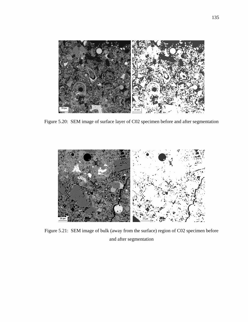
135

Figure 5.20: SEM image of surface layer of C02 specimen before and after segmentation

Figure 5.21: SEM image of bulk (away from the surface) region of C02 specimen before

and after segmentation

136

Figure 5.22: SEM image of surface layer of C01 specimen before and after segmentation

Table 5.9 compiles all possible causes that could influence the scaling of concrete.

It is anticipated that higher sorptivity values would result in increased problems with

regards to scaling. Mixtures C04 and C05 had similar sorptivity values after 14 days of

conditioning as compared to C02, but did not scale as much as C02 after 6 days of

conditioning. C05 had the highest sorptivity after 28 days of conditioning, but was

among the most resistant to scaling. Hence, a definite trend could not be established

between the amount of scaling and the water ingress into the concrete mixture. No

particular trend was observed when the weight loss on drying data was compared with

scaling. Also, higher strengths did not necessarily show improved resistance to scaling of

concrete mixtures. However, some correlation existed between the slump and amount of

scaling for a particular concrete mixture.

Figure 5.23 shows the amount of scaled weight plotted against the slump for all

concrete mixtures tested. It is observed from this figure that higher slumps may have

137

caused higher scaling in the concrete mixtures tested. Higher slumps might result in

higher amount of bleed water during the process of vibration, thereby resulting in

increased porosity of the top few millimeters in concrete. This is verified from Figures

5.20 and 5.22, which show the SEM images of the surface layers of mixture C02 (scaled

excessively) and mixture C01 (little scaling). Further investigations need to be carried

out in order to validate this trend.

Figure 5.23: Correlation between amount of scaling and slump

0.0

0.5

1.0

1.5

2.0

2.5

3.0

3.5

0.0 0.5 1.0 1.5 2.0

Slump (in)

Scal

ed w

eigh

t (kg

/m2 )

6 day age28 day age

138

Table 5.9: Compilation of information for various mixtures

Conversion: 1 g = 0.035 oz; 1” = 2.5 cm; 1 psi = 6.9 kPa

Lone

star

cont

rol

Lone

star

+

Rock

port

Lone

star

+

sla

g

Lehi

gh+

Ro

ckpo

rtLe

high

+

M

iami

Fort

Essr

oc+

Clifty

Cr

eek

Test Remarks C01 C02 C03 C04 C05 C06Compressive strength (psi)-4x8 7 day 4999.20 5357.26 5742.36 4659.85 4395.69 4978.91Compressive strength (psi)-4x8 28 day 5881.21 7022.99 7893.46 6607.65 6159.29 6812.14Flexural Strength (psi)-6x6x21 7 day 797.13 718.58 850.38 666.92 666.92 723.92

Sorptivity (mm/min0.5)

3 + 11day cure 0.0149 0.0219 0.0167 0.0203 0.0217 0.0176

Sorptivity (mm/min0.5)

3+25 day cure 0.0230 0.0356 0.0285 0.0347 0.0455 0.0282

Weight loss on drying (% of original) 6 day 1.08 1.45 1.6 1.55 1.65 1.28

Weight loss on drying (% of original) 28 day 1.73 2.18 2.1 2.41 2.44 1.86Resonant frequency (KHz) 6 day 1.785 1.795 1.795 1.745 1.735 1.82Resonant frequency (KHz) 28 day 1.849 1.866 1.904 1.87 1.818 1.912Scaled weight-50 cycles (g)

3 + 3 day age 2.64 108.73 58.23 22.43 13.48 39.63

Scaling (50 cycles) (kg/m2)

3 + 3 day age 0.073 2.989 1.601 0.617 0.370 1.089

Scaled weight-50 cycles (g)

14 + 14 day age 2.12 46.00 11.73 7.09 10.85 7.34

Scaling (50 cycles) (kg/m2)

14 + 14 day age 0.058 1.265 0.323 0.195 0.298 0.202

Average slump (inch) 0.9 1.9 1.8 1.4 1.1 0.9

139

5.4. Summary

1. All concrete mixtures prepared with supplementary materials had 28-day compressive

strength in excess of 6000 psi. All mixtures except the ones prepared with Lehigh

cement exceeded the strength of the control mixture after 7 days of curing.

2. All mixtures satisfied the INDOT flexural strength requirement (for opening to

traffic) of 550 psi when tested at an age 7 days.

3. Most of the mixtures satisfied the maximum air-void spacing factor requirement of

0.008” (0.203 mm). Mixture C06 had a spacing factor of 0.0089” (0.226 mm).

4. Freeze thaw testing for all concrete mixtures was performed after two different

periods of curing. All mixtures moist cured for 3 days and 14 days satisfied the

minimum durability factor requirement of 60%.

5. Salt scaling resistance was evaluated by determining the scaled weight per unit

surface area. Two conditioning procedures were investigated. One set of specimens

was moist cured for 3 days followed by 3 days of air-drying. Mixtures C02, C03 and

C06 failed the test as they had scaled particles in excess of 0.8 kg/m2. Another set of

specimens was moist cured for 14 days followed by 14 days of air-drying. Only

mixture C02 had scaled particles in excess of 0.8 kg/m2 in this case.

6. Application of curing compound reduced the amount of scaling significantly for

specimens conditioned for different periods.

7. Slump appears to correlate with the amount of scaling. Higher slump corresponded to

higher scaling. Higher slump might result in higher amount of bleed water at the

surface layer resulting in higher porosity at the surface compared to the bulk region of

140

the concrete specimen. This was verified by obtaining images using a SEM. Further

investigations are required in order to explain these findings.

141

CHAPTER 6: SUMMARY AND CONCLUSIONS FOR PHASE I OF THE RESEARCH AND OBJECTIVES AND SCOPE OF WORK FOR EXTENDED STUDY

(PHASE II) ON SCALING BEHAVIOR OF CONCRETE CONTAINING SCM

6.1. Introduction

The focus of this project was to investigate whether concrete mixtures prepared

with fly ash or slag can have adequate durability and strength when exposed to low

temperatures at early ages. Essentially, in this phase of research, studies were conducted

in three parts, each of which has been described in detail in Chapters 3, 4 and 5. Chapter

3 described how chemical composition and physical characteristics of cements and fly

ashes used in this research were analyzed in an attempt to identify parameters that may

lead to low rate of strength development. Chapter 4 described the results and analysis of

strength and maturity tests on mortars and non-evaporable water content on pastes.

Mathematical models to predict material combinations that may result in slow strength

development especially under low temperature conditions were developed. Mixtures

selected during this part were used for full-scale tests on concrete as discussed in Chapter

5, which provided background for extended work on critical issue of scaling.

This chapter presents conclusions reached during each of the three parts of Phase

I and provides need for further study. Based on these preliminary results, objectives of

further study (Phase II) along with scope of work are also given in this chapter.

142

6.2. Summary for Phase I

6.2.1. Summary of Analysis and Selection of Cementitious Systems

In Chapter 3, a mathematical model was developed to predict strength for Type I,

Type I/II, and Type III cements at various curing ages using information like C3S, C2S,

C3A, fineness, alkali content, and strength provided by the cement producer on the mill

certificate. Sensitivity analysis was performed to determine the influence of composition

and fineness on strength. As one may expect, higher fineness was found to correlate with

an increase in strength at all ages. Increasing the C3S content had a beneficial effect on

strength at later ages. Varying the C2S and C3A content did not seem to affect the

strength development process significantly. Again as expected, increasing the alkali

content had a beneficial effect on early age strength but a detrimental effect on the later

age strength.

Four cements were selected for further tests on mortars based on the results from

sensitivity analysis. One cement exhibited values of chemical components and fineness

close to average of all the Type I and Type I/II cements. This cement (Lone Star, Type I)

was selected to represent the baseline case. Three more cements were chosen, one with

high alkali content (Essroc, Type I), one with a high fineness (Lone Star, Type III) and

one with a low C3S content (Lehigh, Type I/II). Similar to the analysis performed for

cements, a mathematical model was also developed to characterize fly ashes using their

strength activity index (SAI). The sensitivity analysis performed for all the fly ashes

showed that increasing the lime content increases the SAI at all ages. The SAI also

increased with alkali content at early ages, but converged at an age of about 28 days.

143

Increasing the fineness (% retained on 45 μm sieve) of fly ash seemed to reduce the SAI

at all ages.

Based on this analysis, four fly ashes were chosen for further study. Baseline fly

ash (Will County Station) was chosen as the one that exhibited values of all of the

sensitive parameters close to the average of all Class C fly ashes. Two other fly ashes

(Rockport Station and Clifty Creek Station) that showed distinctly less lime content

compared to other fly ashes in the Class C category were also chosen to represent the

worst-case scenario with respect to their contribution to strength development. A Class F

fly ash (Miami Fort Station) having the lowest lime content and the highest carbon

content was also chosen. Since only one slag was approved by INDOT, this slag was

also selected for further tests.

These above selections were made to facilitate testing that represents numerous

mixtures having a wide range of chemical constituents, which could represent the

possible mixture combinations made using materials on the current approved list in the

state of Indiana.

6.2.2. Summary of Tests Procedures and Results of Mortar Tests

After individual materials were selected based on statistical analysis, mortar cubes

were prepared using twenty-four mixture combinations. The cubes were stored at various

temperatures and tested at various ages to enable strength-maturity relationships to be

developed for the twenty-four mortar mixture combinations so that parameters like

ultimate strength, rate of reaction and activation energy could be determined.

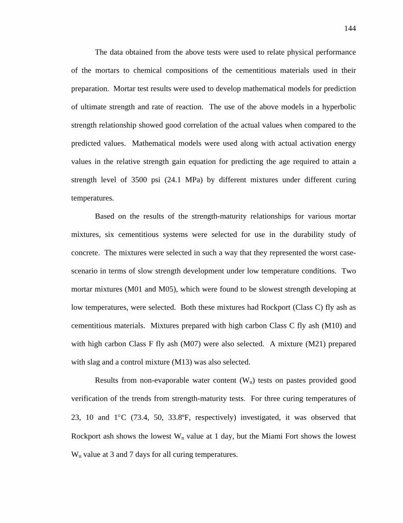
144

The data obtained from the above tests were used to relate physical performance

of the mortars to chemical compositions of the cementitious materials used in their

preparation. Mortar test results were used to develop mathematical models for prediction

of ultimate strength and rate of reaction. The use of the above models in a hyperbolic

strength relationship showed good correlation of the actual values when compared to the

predicted values. Mathematical models were used along with actual activation energy

values in the relative strength gain equation for predicting the age required to attain a

strength level of 3500 psi (24.1 MPa) by different mixtures under different curing

temperatures.

Based on the results of the strength-maturity relationships for various mortar

mixtures, six cementitious systems were selected for use in the durability study of

concrete. The mixtures were selected in such a way that they represented the worst case-

scenario in terms of slow strength development under low temperature conditions. Two

mortar mixtures (M01 and M05), which were found to be slowest strength developing at

low temperatures, were selected. Both these mixtures had Rockport (Class C) fly ash as

cementitious materials. Mixtures prepared with high carbon Class C fly ash (M10) and

with high carbon Class F fly ash (M07) were also selected. A mixture (M21) prepared

with slag and a control mixture (M13) was also selected.

Results from non-evaporable water content (Wn) tests on pastes provided good

verification of the trends from strength-maturity tests. For three curing temperatures of

23, 10 and 1°C (73.4, 50, 33.8ºF, respectively) investigated, it was observed that

Rockport ash shows the lowest Wn value at 1 day, but the Miami Fort shows the lowest

Wn value at 3 and 7 days for all curing temperatures.

145

6.2.3. Summary of Analysis of Concrete Test Results

All concrete mixtures containing supplementary materials had a 28-day

compressive strength greater than 6000 psi (41.4 MPa). Most of the mixtures containing

supplementary materials exceeded the compressive strength of the control mixture at 7

days. All six mixtures had flexural strengths in excess of 550 psi (3.8 MPa) at 7 days,

which is the value adopted by INDOT for opening of pavement to traffic.

Sorptivity tests were carried out for mixtures cured for different periods. In

general, for specimens cured for both 14 and 28 days, it was observed that weaker

mixtures have higher sorptivity and cumulative sorption values. This may be due to

higher permeability in weaker systems resulting from an undeveloped microstructure.

Weight loss on drying test results showed that stronger mixtures had lower weight loss on

drying. This confirms the fact the weaker mixtures have more internal water available

for hydration.

All concrete mixtures (irrespective of the curing period, i.e., 3 or 14 days)

prepared with supplementary materials passed the ASTM C 666 test for freeze-thaw

resistance with satisfactory durability factors (generally greater than 83%). In general,

the freeze-thaw resistance seems to be correlated to the strength, i.e. stronger concretes

seem to be more resistant to the effects of cyclic temperatures.

Scaling resistance tests were performed on specimens conditioned for two different

periods. After a total of 6 days conditioning, mixtures C02, C03 and C06 had over 0.8

kg/m2 of scaled particles. After a total of 28 days conditioning, only mixture C02 had

over 0.8 kg/m2 of scaled particles. Most mixtures had spacing factors smaller than

0.008” (0.203 mm) and strength values more than specified. An attempt was made to

146

correlate scaling with factors like strength, sorptivity, weight loss on drying and the

resonant frequency development with time. Developing a correlation to quantify the

process of scaling in terms of the above factors was very difficult because of highly

complicated nature of problem. Therefore some of the general trends are summarized

below along with needs of further research in this area:

• In general, it was found that scaling resistance was improved by increasing the total

duration of curing. But here only two curing durations were studied, so to develop

proper relation of moist curing and drying on scaling and to determine optimum

conditioning period for the best scaling resistance, more extensive study with variety

of conditioning period is required.

• Out of six combinations studied, only one combination (C02-Lonestar cement +

Rockport fly ash) showed poor scaling resistance for both curing periods. Therefore,

further study with this combination should represent the worst case scenario and

should help in providing more complete guidelines.

• Application of curing compound seems to significantly improve the scaling resistance

of all specimens, irrespective of the conditioning period, probably due to presence of

highly impermeable layer formed on the surface.

• For different mixtures tested, higher slump was found to correlate with an increase in

the amount of scaling. It is not clear, however, whether increasing the duration of

curing for high slump (up to about 2.5”) concrete would necessarily improve the

scaling resistance. As a result, the exact relationship between conditioning periods

for scaling of high slump mixtures should be determined. More research is needed on

the effect of type and length of curing on scaling of high slump concrete.

147

• As the issue is related to low temperature curing, influence of low temperature curing

on scaling performance also needs to be studied.

• Based on the literature data and the collected field information, it was noted that the

results from laboratory tests on scaling resistance may not necessarily depict a true

picture of the field performance; hence better understanding of the differences

between field and laboratory exposure conditions and how these differences affect

scaling is essential for development of practical construction guidelines.

6.3. Conclusions for Phase I

Based on the analysis of all test results generated in the course of this investigation, the

following conclusions are drawn:

1. Models can be developed for strength prediction of cement mortars and SAI

prediction of fly ashes using the supplier’s data on chemical composition and

physical properties of the material. These models can be successfully used to

forecast the expected changes in strength (for cements) and SAI (for fly ashes) as a

result of changes in properties of the material.

2. Mathematical models can be developed to express maturity parameters like ultimate

strength and rate of reaction of mortar mixture in terms of percent weight of the

materials contained in them, chemical composition and physical characteristics of

the materials.

3. The maturity method could be used effectively to predict the age required to attain a

given strength level for mortar mixtures cured under any temperature history.

148

4. Concrete containing fly ash or slag can be exposed to freeze and thaw cycles at

relatively early ages without significant reduction in durability factor provided that

it reaches compressive strength of at least 3500 psi (24.1 MPa) and has low

amounts of freezable water in addition to minimum air contents of 6% and air-void

spacing less than 0.008”.

5. Since all concrete mixtures tested were supposed to represent slowest hydrating

systems under low temperature conditions, it is believed that mixtures prepared

with similar fly ashes or slag, but using other cements would also pass the freeze-

thaw durability test.

6. Specific conclusions regarding scaling performance of concrete and overall

guidelines are presented at the end of Phase II of this project report.

6.4. Research Objectives and Scope of Work for Phase II

The conclusions of phase I of this research helped in formulating background for

extended research on the issue of scaling. Therefore, the focus of Phase II of the research

is the salt-scaling resistance of concrete containing SCM, both in the laboratory and

under field conditions typically experienced in Indiana with particular attention given to

pavements constructed during a season of low temperatures. To address these problems,

based on background study in Phase I, three research goals were formulated as outlined

in Figure 6.1. Brief listing of the tasks associated with each goal along with the

description of types of specimens and other relevant details are also provided in Figure

6.1.

149

The first goal of this extended study is to develop basic understanding of scaling

phenomenon and determine the parameters that significantly influence scaling results. To

simulate the worst-case scenario, the entire study of Phase II was conducted on the worst

performing cementitious materials combination identified in Phase I (mixture C02, Lone

Star cement + Rockport fly ash). This approach helped in conducting more focused

study, results of which can be applicable to wide range of materials with high degree of

confidence. Specimens prepared with these materials were fabricated at two different

slumps and were subjected to wide range of curing conditions that are described in detail

in section 8.2 (Table 8.1). In addition, a microstructure and chloride ion penetration

study was performed to assist in the interpretation of results.

The second goal of the study was to evaluate the influence of low-temperature

casting and curing on fresh concrete properties and scaling performance of fly ash

concrete. First, various fresh concrete properties like setting time, bleeding, etc. were

determined at two low temperatures (1oC and 10oC). The scaling performance was

evaluated for laboratory size, 250 mm x 190 mm x 75 mm (10” x 7.5” x 3”), regular

specimens as well as large-size, 3000 mm x 1000 mm x 1000 mm (118” x 39” x 39”)

insulated specimens that were assumed to simulate thermal conditions that can be

encountered in the actual pavement. Temperature profiles for actual pavements located

in the low temperature regions were also collected and evaluated, to determine how well

the large size specimens simulate the temperature distribution in the pavement.

Microstructural study was performed on some field and laboratory specimens to compare

concrete bulk and surface porosities.

150

Figure 6.1: Outline of the objectives and relevant actions for the scaling study

Evaluation of influence of material parameters on scaling

Lit. review and observations

ASTM C 672 and 8.2.1

Tasks to attain goals Source/Relevant studies

SCALING OF CONCRETE CONTAINING FLY ASH

Study of deleterious sand and variation in cementitious materials

60 slabs -250 x 190 x 75 mm size, 25 and 63 mm slump (T-8.1)

Brief details of specimens or study

Goa

l 1

Stud

y of

role

of

influ

enci

ng p

aram

eter

s

Effects of size and thermal mass

Early age evaporation study

Climatic studies & Risk analysis for scaling probability

Evaluation of influence of curing durations on scaling

Microstructural study 25 x 25 x 25 mm specimens viewed under SEM (T-8.2) Porosity gradient using SEM

Chloride ion penetration study 100 x 200 mm cylinders, with curing regimes as above (T-8.1 ) Cl- detection using AgNO3

Goa

l 3

Dis

crep

ancy

in la

b &

fiel

d ob

serv

atio

ns

Goa

l 2

Low

tem

p. c

urin

g an

d re

late

d is

sues

Effects of low temp. curing on setting time and bleeding

ASTM C 403 & ASTM C 232 at 1oC temperature

ASTM C 672 and section 9.2.4 to 9.2.6

12” deep cylinders for bleeding and microstructure study, few field cores for to compare the porosity with field concrete (T-9.1)

Regular size specimens cast and cured at 1 and 10oC. Large size slabs (900 x 300 x 300 mm), cast and curd at 1oC (T-9.2)

Effects of low temp. on scaling for regular and large size specimens

Study of pavement temp. profiles Actual pavement temperature profile for Indiana & Quebec LTTP database

Scaling and microstructure

Scaling and temp. study

3 slabs 250 x 190 x 75mm, exposed to diff. evaporation (T-10.2)

6 slabs-55 to 245 mm depth in lab (T-10.3), 2 slabs outside (T-10.4)

250 x 190 x 75 mm size slabs- exposed to intermittent drying Scaling as per 10.5.2.2

Determination of detrimental event from 30 years of data, and risk analysis for probability of occurring one such event

NIST model, C++ Program and @Risk 4.5TM software

Intermittent drying study

151

An extensive literature review revealed that, unlike what is observed in the

laboratory, scaling of concrete containing fly ash is rare in the field. Various researchers

have discussed the severity of test ASTM C 672 (Thomas, 1997 and Naik, 1995) but no

firm conclusions are presented on the causes of this discrepancy between laboratory and

field scaling. Therefore, the third objective of this study was to explore potential causes

of discrepancy and to suggest the ways to resolve this paradox. To accomplish this goal,

detailed information regarding field scaling performance of concrete was collected with

the help of extensive literature review and telephone survey. This information when

combined with and additional laboratory results, lead to suggestion of some parameters

that may be responsible for observed discrepancy in field and laboratory scaling

performance of concrete. In addition, based on these parameters and a detailed study of

climatic data collected over 30 years period, the probability of scaling for a typical

concrete mixture containing fly ash in Indiana was obtained using the risk analysis

approach.

6.5. Organization of the Report for Phase II

This part of the report is divided into five chapters, which are presented in

continuation of six chapters of phase I. Chapter 7 provides detailed discussion of the

influence of the material parameters on scaling based on laboratory observations. The

influence of various conditioning periods on scaling and chloride ion penetration is

discussed in Chapter 8. This chapter also includes microstructural analysis near-surface

region of concrete. Chapter 9 presents the results and analysis for fresh properties and

scaling behavior of concrete cast and cured at low temperatures for two different sizes of

152

specimens. The temperature profiles observed for concrete in the field obtained from the

Long Term Pavement Performance (LTPP) database are also shown. Chapter 10 contains

a literature review and a compilation of a survey on field scaling performance conducted

in 12 mid-western and north-eastern states, including Indiana. Various suggestions are

also presented regarding the discrepancy between the laboratory scaling results and the

field observations. In addition, based on climatic data and risk analysis, Chapter 6

provides the probability for scaling of a typical concrete pavement for the most extreme

climatic conditions of Indiana. Chapter 11 presents summary, guidelines and conclusions

for phase II addressing scaling performance of concrete containing SCM.

153

CHAPTER 7: CONSTITUENT MATERIALS AND THEIR INFLUENCE ON SCALING RESISTANCE OF CONCRETE

7.1. Introduction

The early and later age performance of concrete is highly dependent on the

properties of constituent materials so an understanding of these materials is also essential

for better interpretation of the results. Hence, this chapter addresses the issues related to

constituent materials specifically in regard to scaling. The focus of the detailed study is

to determine the potential of problems for concrete containing fly ash during late fall

constructions. Therefore, the properties of the worst performing materials (Lone Star

cement and Rockport fly ash), selected based on results from section 5.3, is described in

this chapter. The effects of other parameters influencing performance of selected

materials are studied in consecutive chapters. Additionally, the individual role of each

constituent material in regard to scaling and the effects of variability in materials are

discussed, with some important observations.

7.2. Constituent Materials

The results presented in section 5.3.8 of this report, showed that the combination

of certain cementitious materials (Lone Star cement + Rockport fly ash) exhibited the

slowest strength gain and maximum scaling (in terms of mass lost). For that reason, this

combination of materials was used in the current study. The typical mixture proportions

154

used are shown in Table 7.1. Specimens containing plain cement (control mix) were

made with Lone star type I cement for better comparison of results.

Table 7.1: Mixture Proportions and fresh concrete properties

Materials 25 mm (1” )Slump 63 mm (2.5”) Slump Cement 244.4 kg/m3 (412 lb/yd3) 244.4 kg/ m3 (412 lb/yd3)

Fly Ash 61.1 kg/m3 (103 lb/yd3) 61.1 kg/ m3 (103 lb/yd3) Water 134.1 kg/m3 (226 lb/yd3) 134.1 kg/ m3 (226 lb/yd3)

Fine Aggregate (SSD) 881.0 kg/m3 (1485 lb/yd3) 881.0 kg/ m3 (1485 lb/yd3) Coarse Aggregate (SSD) 987.8 kg/ m3 (1665 lb/yd3) 987.8 kg/ m3 (1665 lb/yd3) Water Reducer (WRA) 450 ml (15.2 oz) 1250 ml (42.3 oz)

Air Entraining Agent (AE) 79 ml (2.7 oz) 134 ml (4.5 oz) Measured Slump 25 +/- 5 mm (1”+/-0.2”) 63 +/- 7 mm(2.5” +/-0.3”)

Measured Fresh Air (%) 6.5 +/- 0.3 6.5 +/- 0.4

A water-to-cementitious materials ratio (w/cm) of 0.44 was selected, as this is

close to the maximum w/cm that INDOT permits for paving. Approximately 70% of the

total concrete volume was composed of sound aggregates. Fly ash was used to replace

20% of the cement by weight, which gave the Portland cement/fly ash ratio of 4.0. Type-

I Lone Star cement used in study had a Blaine fineness of 360 m2/kg and consisted of

60% C3S, 13.5% C2S, 8.2% C3A, and 0.54% alkali (Na2O equivalent). The class C

(Rockport) fly ash used had a CaO content of 18.5%, an alkali content of 0.7% and a

carbon content of 0.68%.

The mixture contained a Vinsol-based air entraining admixture (Daravair 1400) to

create and stabilize air bubbles to meet the target air content of 6.5%. A mid-range

water-reducing agent (WRA), WRDA-82, was used to increase workability. This WRA

is an aqueous solution of modified lignosulfonates with a hydration catalyst. Although

155

most of the mixtures in this study had a slump of 25 mm (1”), some mixtures were

produced with the slumps of 63 mm (2.5”). The w/cm in the 63 mm slump mixtures was

the same as that used in the 25 mm slump mixtures and the increase in slump was

achieved by varying the content of WRA. The objective behind increasing the slump

using the WRA content only was to study the effect of slump on scaling independent of

strength of the concrete.

Figure 7.1 shows the particle size distribution of the cementitious materials as

determined using a particle analyzer laser. It can be seen that the mean cement particle is

approximately 22 microns while the fly ash demonstrates a well distributed range of

particle sizes with a concentration of particles at slightly less than 1 micron and a

concentration at approximately 18 microns.

Figure 7.1: Particle size distribution for the cement and fly ash

0 1 10 100 1000Particle Diameter (Microns)

0.0

2.0

4.0

6.0

8.0

Freq

uenc

y (%

)

CementFly Ash

156

7.3. Study of Influence of Individual Constituent Materials on Scaling Performance

It is evident from the literature review that the influence of various material

parameters on scaling performance was not studied extensively. In particular, none of the

literature sources available examined the influence that chemical and mineral admixtures

might have on the density of the near-surface region; hence, an indirect study was

performed to quantify the effect of admixtures on surface density. In addition, the effects

of deleterious fine aggregate particles on scaling performance are also examined in the

following sections.

7.3.1. Influence of Chemical Admixtures and Fly Ash on Near-Surface Region Density of

Hydrated Paste

As mentioned in the previous section, mixtures with two different slumps were

used to study the scaling performance, the change of slump being the results of change in

the WRA content. Many other researchers have reported that scaling increases with an

increase in the slump of the concrete (section 5.3.9 of this report, and Whiting, 1989).

Therefore, it was important to identify whether the reduction in scaling resistance is

related to an increased bleeding and reduction in density of near surface region (thinning)

of the specimen or if there might be higher amount of admixture and fly ash in the

surface region because of lower density. Additionally, buoyancy might allow more air

bubbles to escape from the region of reduced density thus making it less frost resistant.

157

7.3.1.1. Experimental Procedures

In an attempt to quantify the effects that chemical and mineral admixtures might

have on the near-surface density, three set of experiments (studies) were performed.

Three series of paste samples were prepared in each of the three studies. The paste

composition is listed below in Table 7.2, illustration of which follows.

Table 7.2: List of paste samples prepared to study influence of fly ash and admixture

Study 1(w/cm-1.0, fly ash and admixture type

varied)

Study 2 (20% fly ash, w/cm and admixture type

varied)

Study 3 (0% fly ash, w/cm and admixture

type varied)

sam

ple

Notation Fly ash (%)

CA Notation W/CM CA Notation W/CM CA

1 FA0W 0 W FC1.0W 1 W C1.0W 1 W 2 FA10W 10 W FC0.8W 0.8 W C0.8W 0.8 W 3 FA20W 20 W FC0.6W 0.6 W C0.6W 0.6 W 4 FA30W 30 W FC0.4W 0.4 W C0.4W 0.4 W Se

ries 1

5 FA40W 40 W 1 FA0A 0 A FC1.0A 1 A C1.0A 1 A 2 FA10A 10 A FC0.8A 0.8 A C0.8A 0.8 A 3 FA20A 20 A FC0.6A 0.6 A C0.6A 0.6 A 4 FA30A 30 A FC0.4A 0.4 A C0.4A 0.4 A Se

ries 2

5 FA40A 40 A 1 FA0B 0 B FC1.0B 1 B C1.0B 1 B 2 FA10B 10 B FC0.8B 0.8 B C0.8B 0.8 B 3 FA20B 20 B FC0.6B 0.6 B C0.6B 0.6 B 4 FA30B 30 B FC0.4B 0.4 B C0.4B 0.4 B Se

ries 3

5 FA40B 40 B W- Water reducer, A- Air entraining agent, B-both (Water reducer +Air entraining agent), CA- Chemical Admixture

In the study 1, liquid pastes (w/cm = 1) were prepared with different levels of

supplementary cementitious materials. As mentioned earlier, three series of samples

158

were prepared in this study. Each series had five samples, in which 0%, 10%, 20%, 30%,

or 40% of the cement was replaced with fly ash. Mixture proportions for the 25 mm

slump mixture (Table 7.1) were used for proportioning the amount of WRA (0.22% by

weight of cement) and AE (0.03% by weight of cement). The samples used in the first

and second series contained only water reducing agent (WRA), and air entraining agent

(AE) respectively, while samples in third series contained both WRA and AE. For each

sample, all the materials including water were combined in a bottle and shaken for one

minute before being allowed to settle. The paste was then poured into a clear plastic cup

and allowed to set and hydrate for 48 hours, without any disturbance. In the cases, where

distinct top and bottom layers were observed, they were carefully separated. Volume and

mass of these sections were determined to calculate the densities.

In the study 2, pastes were made with a 20% constant cement replacement with

fly ash. In this study, three series were prepared, with four samples in each series. Each

sample consisted of 500 grams (1.1 lb) of cementitious materials, and the water was

varied to achieve water to cementitious materials ratios of 1.0, 0.8, 0.6, and 0.4. Similar

to previous section, first series contained only WRA, second series contained only AE

and third series contained both. Thus, total of 12 paste samples were prepared for this

case.

To quantify the effect of fly ash, in the study 3 another 12 samples were prepared

in three different series. The third study was identical to second study, except no fly ash

was added in this study. For study 2 and 3, paste samples were prepared similar to study

1. Results of all the three studies are described below.

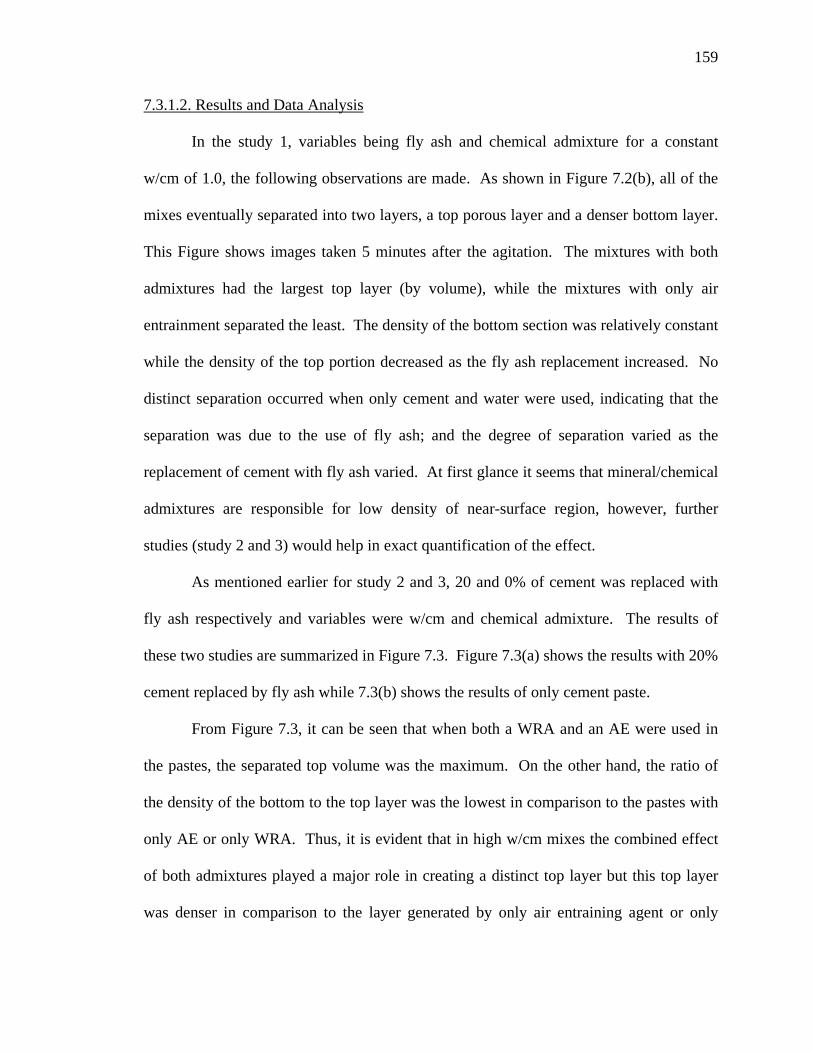
159

7.3.1.2. Results and Data Analysis

In the study 1, variables being fly ash and chemical admixture for a constant

w/cm of 1.0, the following observations are made. As shown in Figure 7.2(b), all of the

mixes eventually separated into two layers, a top porous layer and a denser bottom layer.

This Figure shows images taken 5 minutes after the agitation. The mixtures with both

admixtures had the largest top layer (by volume), while the mixtures with only air

entrainment separated the least. The density of the bottom section was relatively constant

while the density of the top portion decreased as the fly ash replacement increased. No

distinct separation occurred when only cement and water were used, indicating that the

separation was due to the use of fly ash; and the degree of separation varied as the

replacement of cement with fly ash varied. At first glance it seems that mineral/chemical

admixtures are responsible for low density of near-surface region, however, further

studies (study 2 and 3) would help in exact quantification of the effect.

As mentioned earlier for study 2 and 3, 20 and 0% of cement was replaced with

fly ash respectively and variables were w/cm and chemical admixture. The results of

these two studies are summarized in Figure 7.3. Figure 7.3(a) shows the results with 20%

cement replaced by fly ash while 7.3(b) shows the results of only cement paste.

From Figure 7.3, it can be seen that when both a WRA and an AE were used in

the pastes, the separated top volume was the maximum. On the other hand, the ratio of

the density of the bottom to the top layer was the lowest in comparison to the pastes with

only AE or only WRA. Thus, it is evident that in high w/cm mixes the combined effect

of both admixtures played a major role in creating a distinct top layer but this top layer

was denser in comparison to the layer generated by only air entraining agent or only

160

water reducer. Therefore, the tendency of a combined effect of both admixtures could be

considered such that it would provide restraint against the generation of a very high

localized w/cm ratio in the very top surface.

Figure 7.2: Influence of WRA and AE on separation into two layers with different density; (a) measured densities of top and bottom portions for paste with WRA and AEA,

and (b) Photos of paste separation

0.4 0.6 0.8 1W/C of different slurries

1

2

3

4

5

6

Rat

io o

f Den

sity

of B

otto

m to

top

regi

on

0

0.1

0.2

0.3

0.4

Volu

me

of to

p re

gion

(CC

)

Change in Volume and Density with w/c(Solid line- Density, Dotted line- Volume)

BothAEWRABothAEWRA

0.4 0.6 0.8 1

W/C of different slurries

1

2

3

4

5

6

Rat

io o

f Den

sity

of B

otto

m to

top

regi

on

0

0.1

0.2

0.3

0.4

Volu

me

of to

p re

gion

(CC

)

Change in Volume and Density with w/c(Solid line- Density, Dotted line- Volume)

BothAEWRABothAEWRA

Figure 7.3: (a) Change in volume of separated surface, and ratio of density of the

separated regions with change in w/cm for pastes containing 20% fly ash, and (b) Change in volume of separated surface and ratio of density of the separated regions with change

in w/cm for pastes containing cement only

(b) (a)

WRA Only

AEA Only

WRA +AEA

0% 10% 20% 30% 40%0 10 20 30 40

Percent Fly Ash Replacement (%)

0.0

0.3

0.6

0.9

1.2

1.5

Top MaterialBottom Material

Cement, Fly Ash, WRA, and AEA

Percentage replacement of fly ash Percentage replacement of fly ash

Den

sity

(g/c

c)

w/cm of different pastes w/cm of different pastes

161

Comparing Figures 7.3(a) and (b) pastes with w/cm of 0.8 and higher, it was

observed that the density of the near-surface region was lower for most pastes containing

fly ash than the pastes with only cement. For a very high w/cm therefore, the presence of

a higher amount of fly ash on the surface is possible, leading to layer separation and

possible weakening of the surface region. However, an almost nil separation effect was

observed for a w/cm of 0.6 and less. Real-life concrete mixes that contain coarse

aggregate and are typically prepared at w/cm lower than 0.5 and would show a higher

degree of restraint would be present towards settlement. Therefore, the presence of

higher a percentage of fly ash in the surface region would not be a concern for concrete

pavements containing fly ash, where the w/cm is in the range of 0.4 to 0.5.

7.3.2. Role of Deleterious Aggregates

7.3.2.1. Introduction and Observation

Based on the literature review, it is evident that deleterious or porous coarse

aggregates can increase scaling significantly (Klieger, 2003 and Jansen, 2000) but no

such observations are available for fine aggregates. In this section an observation is

reported about the influence of deleterious fine aggregate particles on scaling

performance. As far as freeze-thaw resistance is concerned, fine aggregates do not have

negative influence, and even the presence of a small amount of deleterious fine aggregate

does not create any major damage to the concrete. In the case of scaling, however,

different results are possible.

During scaling study, difference in scaled mass was observed for a few specimens

that were prepared using new fine aggregate. This aggregate confirmed the INDOT

162

specifications and had deleterious (non-durable) materials under the specified limit (4%

of total fine aggregates). In this case in both the fly ash and the control specimens,

similar scaling behavior was observed after the first five to seven F-T cycles; scaling was

initiated by the fracture of small dark grey particles on the specimens’ surface. These

dark grey or black particles were collected and evaluated under a scanning electron

microscope and in an X-ray diffractometer. In addition, using optical microscope and

specific gravity determinations were also conducted for such particles present in the fine

aggregates.

7.3.2.2. Results and Data Analysis

Figure 7.4 shows the results of the X-ray diffraction analysis, which indicate that

significant amount of clay minerals (illite and kaolinite) were present in these particles.

Also the EDX of the Scanning Electron Microscope (SEM) showed presence of alumina,

silica, iron and oxygen in significant amounts. The above information and further

petrography analysis under optical microscope to analyze the texture and grain size,

revealed that these deleterious particles were weathered shale particles, which can be

present in natural river sand. A few other properties for these particles were determined

and are reported in the Table 7.3.

163

2-Theta

Figure 7.4: X-ray diffraction pattern of weathered shale particles

Table 7.3: Properties of deleterious particles present in sand

Property Technique/tools used Observations

Size and shape and texture

Vernier caliper and Petrographical microscope, (ASTM C 295)

Dark grey to black color, rounded or flaky, 2 - 4 mm x 3.5 - 4.5 mm size, plate-like structure, weathered surface.

Percentage of particles

Random sampling as per ASTM D75

Average 2.5% of total weight of aggregates.

Composition of particles

Energy Dispersive X-ray (EDX) analysis using SEM

Composed of mainly alumina, silica, iron and oxygen, presence of calcium and magnesium also observed.

Mineralogical analysis X-ray diffraction

Mainly clay minerals, such as illite, kaolinite, etc., also quartz and calcite observed.

Specific gravity ASTM C 128 2.28, low in comparison to average specific gravity of sand 2.64.

Though small in overall quantity, the weathered shale particles were lighter than

other sand grains and so a greater number of these particles were visible on the surface of

the specimen. Since the freeze-thaw durability of such particles is very poor, they

Qua

rtz

Kao

linite

Illite

164

fractured and caused de-lamination (scaling) of the surrounding mortar. Figure 7.5 shows

the scaling caused by the presence of these particles in the surface region after 5 F-T

cycles.

Figure 7.5: Scaling of concrete surface around deleterious sand particles

In summary, aggregate could play an important role in reducing the scaling

resistance of sound concrete. As the above results confirmed the deleterious role of the

fine aggregate in scaling, the source of fine aggregate was changed for further study.

7.3.3. Influence of Variability of Cementitious Materials on Scaling Behavior

7.3.3.1. Introduction

Based on the primary study that included various cements and fly ashes (section

5.3.8), it can be said that small changes in the chemical composition of cements can have

a significant influence on scaling performance. This is evident in Figure 5.13 which

shows that the scaled mass varied from 0.3 kg/m2 to 3.0 kg/m2, depending on

combination of materials used. It should be noted that in that particular study the mixture

165

proportions for all of concretes were the same except for the composition of cementitious

materials.

In this study a similar variation in scaling performance was observed when the

shipment of cement and fly ash were received from the same source (as used in the initial

part of study), 3 years after an initial acquisition. The concrete cast from the originally

acquired cement and fly ash, scaled on an average 2.5 kg/m2, while the concrete prepared

with new cement and fly ash scaled only 0.2 kg/m2. A comparison of the scaled surfaces

of the concrete containing the old (btch-00) and the new (btch-03) cement and fly ash is

shown below in Figure 7.6. The properties of the old and new cements and fly ashes

were compared and the probable reasons for improvement in the observed scaling results

are proposed. The changes in chemical composition of both cement and fly ash are

discussed in sections 7.3.3.2 and 7.3.3.3, respectively. It is strongly emphasized that to

determine scaling performance, the combined influence of the cement and fly ash

components should be considered.

166

(a) (b)

Figure 7.6: Scaled surfaces after 50 F-T cycles, (a) btch-00 (worst performing) combination of cement and fly ash, and (b) btch-03 (better performing) combination of

cement and fly ash

7.3.3.2. Cement

The chemical composition of old and new cement (as reported on mill

certificates) is given in Table 7.4. There is a considerable (approximately 55%) increase

in C2S content and a corresponding 13% decrease in C3S observed. Theoretically, the

cement with higher C3S should give higher early strength and should, therefore, show

better scaling resistance. However, as shown in Figure 7.6 exactly opposite results were

observed. Similarly, although btch-2003 cement has higher content of alkalis and C3A, it

showed better scaling resistance, which is contradictory to what have been proposed in

some other studies (Marchand et al., 2000 and Jackson, 1958). It is therefore essential to

accurately interpret the results to address all of the above discrepancies.

167

Table 7.4: Comparison of various component and properties old and new cements

Comp. strength, psi (MPa) Lone Star cement

(Indiana) C3S C2S C3A

Alkali as

Na2O eq.

Fineness 1 day 3 day 7 day

Shipment -1 btch-00: Aug 2000 60.01 13.54 8.22 0.54 360.8 2272

(15.7) 3439 (23.7)

4390 (30.3)

Shipment -2 btch-03: Sept 2003 52 21 10 0.696 362.0 2150

(14.8) 3400 (23.4)

4390 (30.3)

First, the reason for such a wide variation in C3S and C2S content for cements

coming from the same source was explored. After the discussion with technical support

personnel of Lone Star cement. It was found that when the btch-00 cement was obtained,

the plant had been importing clinker from Thailand, as changes were being made in the

plant. The clinker for btch-03 cement was produced in the local plant, using the local

materials. Since, the sources of materials for this btch-00 and btch-03 cements were

totally different, that lead to a wide differences in their chemical composition.

It is well known that C2S produces only about half of the CH that is produced by

the C3S (Neville, 1996). As a result, the extent of pozzolanic reactions in the system with

lower C3S content (btch-03 concrete), therefore will be lower in comparison to btch-00

concrete.

The scaling results strongly support the hypothesis that refinement in pore

structure is the major cause of increased scaling damage for laboratory concrete

containing fly ash, as already noted in the case-specific literature summary of scaling.

Pore refinement due to secondary reaction is widely known to be the most beneficial

effect of fly ash in concrete. However, in the case of scaling that pore refinement may be

detrimental under certain conditions. Specifically, it is hypothesized that pore refinement

168

might increase the degree of saturation during consecutive F-T cycles because smaller

pores, which might not dry out during non-freezing part of the cycle. To further

investigate this hypothesis, the reactivity of fly ash in a given cementitious system was

evaluated and is discussed in section 7.3.3.3. Also, the values for alkali content of

cement are considered very normal for typical Type-I cement in this study, so the

observation by other researchers that high alkali/high C3A cement have poorer scaling

resistance might not be applicable for this case.

7.3.3.3. Fly Ash

The available components and properties of both original and new suite of fly

ashes are reported in Table 7.5. It can be seen from the data that the lime content, carbon

content, and fineness (% retained on 45 µm sieve) of both fly ashes are almost identical.

However, a significant increase (15%) in the 7 days Strength Activity Index (SAI7) for

btch-03 fly ash was observed. The SAI 7 of 98% is very close to the strength of plain

cement (100%), which indicates high reactivity of new fly ash (btch-03). Further

analysis of the fly ash was done, therefore, to determine the exact reasons for increase in

SAI7 value.

Table 7.5: Comparison of various components and properties of old and new fly ashes

Rockport fly ash Lime (%)

Alkali (%)

Fineness (% retained on 45 µm sieve)

Max. % frequency

Carbon (%) SAI7

Batch- Aug 2000 18.57 0.70 21.88 18 µm 0.68 85.50 Batch- Aug 2003 18.48 1.0 20.1 10 µm 0.46 98

SAI7- Strength activity index at 7 days as per ASTM C 311

169

Though the percentage retained on the 45µm sieve for both fly ashes was similar,

the particle size distribution for these fly ashes showed considerable difference. The

maximum frequency of new (btch-03) fly ash particles was observed at 10 µm versus 18

µm for the old (btch-00) fly ash, which means that a higher amount of finer particles was

present in the case of btch-03 fly ash, which could increase the reactivity of fly ash at the

early ages.

An increased number of finer particles and a small increase in the alkali content

are probably not the only parameters that could increase the SAI of fly ash significantly.

It should be remembered that SAI is the property of combined cement and fly ash system.

The SAI values obtained for btch-03 fly ash, were obtained with btch-03 Lone Star type I

cement. As described earlier, this cement had a comparatively low C3S and a high C2S

content. In this combination of cement and fly ash, the self cementing properties of fly

ash could play an important role in early strength development.

To develop better insight into the mineralogical characteristic of btch-03 fly ash,

an X-ray diffraction analysis was performed and the results are shown in Figure 7.7. As

commonly observed in reactive class C fly ashes a significant amount of gypsum and

ettringite was observed in this fly ash. The presence of these components, along with

high alkali content, could lead to significant reactivity of fly ash at early ages.

170

2-Theta

Figure 7.7: X-ray diffraction of btch-03 fly ash 7.3.3.4. Data Analysis and Proposed Hypothesis

Upon close observation of the cement and fly ash composition, it seems that a

lower overall pozzolanic activity might help in improving scaling performance. To

verify this hypothesis with the available results, components affecting pozzolanic activity

were examined separately as mentioned below. The first component considered was the

C2S content of cement. A higher C2S reduces the overall amount of CH in the system

and thus the overall pozzolanic activity. The second important component that can be

considered here is C3S of cement. A higher C3S could increase the amount of CH

significantly and thereby help promote pozzolanic activity. Thus, the lower the C3S in

the cement, the lower should be the overall pozzolanic reaction. Thus, the SAI7 of fly

ash is also one of the parameters that is related to pozzolanic activity in the system.

Generally, it is believed that a minimal amount of pozzolanic activity will take place

during the first seven days of hydration (Mehta, 1996). Hence, a higher value of SAI7

may be attributed primarily to the reaction of fly ash itself with water. Therefore, the

Ettri

ngite

Quartz

Gyp

sum

171

expected overall pozzolanic activity should decrease with an increase in SAI7 value

because there will be less unhydrated fly ash available in the cement-fly ash system when

cement hydration generated CH becomes available.

Assuming that the above reasoning is correct the sum of C2S-C3S + SAI7 should

yield a factor, increase in which should yield a decrease in pozzolanic activity. Based on

the earlier proposed hypothesis, the reduction in pozzolanic activity should lead to

reduction in scaling. Figures 7.8(a), (b) and (c) shows (C2S-C3S), (C2S + SAI7) and

(C2S-C3S + SAI7) values plotted against scaling results obtained from all different

cement-fly ash combinations studied in this and in earlier Chapter 5. Moreover, Figure

7.8 shows scaling results plotted against (C2S-C3S + SAI7) value for all the different

combinations. The plotted parameters show good correlation indicating that the decrease

in pozzolanic activity also reduces scaling damage.

Some of the field observations reported for High Volume Fly Ash (HVFA)

concrete (Thomas, 2000) indicate that at later ages scaling is usually observed in the

concrete with class F fly ash. This suggests that the pozzolanic activity can be one of the

parameters that controls scaling damage of field concrete. It should be noted that

hypothesis presented in this section is based on the limited volume of data; further

research is required to confirm the proposed reasoning.

172

R2 = 0.6483

0

1

2

3

4

-50 -40 -30 -20

C2S- C3S of cement

Scal

ed m

ass

(kg/

m2 )

R2 = 0.7355

0

1

2

3

4

95 105 115 125

C2S of cement+ SAI7 of fly ash

Sca

led

mas

s (k

g/m

2 )

R2 = 0.8166

00.5

11.5

22.5

33.5

35 45 55 65 75

C2S- C3S of cement+ SAI7 of fly ash

Scal

ed m

ass

(kg/

m2 )

(c)

Figure 7.8: Scaled mass of concrete containing different cement-fly ash combinations plotted against their (a) (C2S-C3S) values, (b) (C2S + SAI7) values, and (c) (C2S-C3S +

SAI7) In summary, it is evident that the scaling behavior of concrete depends on the

cement-fly ash interaction and how these materials influence formation of microstructure

and the pore size distribution. To develop an understanding of mechanism of the scaling

of fly ash concrete, it is therefore important to characterize the effect of minor changes in

cementitious materials and relate these changes to scaling performance while keeping all

the other parameters constant. This issue has not been addressed by researchers thus far.

Therefore, a detailed systematic study is required to confirm actual importance of the

above components in scaling results and to develop a more precise relationship between

(a) (b)

173

the cementitious materials components and the scaling performance of concrete. With

limited availability of time and resources for this particular project, these issues could not

be addressed in this research.

7.4. Summary

This chapter discussed studies and observations addressing the influence of

various material properties on scaling performance of concrete. Role of admixtures was

evaluated with the help three different studies. An observation regarding influence of

deleterious fine aggregates on scaling is reported. It can be summarized that knowledge

of material parameters is vital for better interpretation of results. Additionally scaling of

concrete containing fly ash is highly dependent on the type of pore size distribution, and

therefore the variability in cementitious materials could change scaling performance

significantly. Pore refinement due to pozzolanic activity seems to be a major parameter

influencing scaling results, but further study is required to confirm this hypothesis and to

provide better guidelines for materials selection.

153

CHAPTER 7: CONSTITUENT MATERIALS AND THEIR INFLUENCE ON SCALING RESISTANCE OF CONCRETE

7.1. Introduction

The early and later age performance of concrete is highly dependent on the

properties of constituent materials so an understanding of these materials is also essential

for better interpretation of the results. Hence, this chapter addresses the issues related to

constituent materials specifically in regard to scaling. The focus of the detailed study is

to determine the potential of problems for concrete containing fly ash during late fall

constructions. Therefore, the properties of the worst performing materials (Lone Star

cement and Rockport fly ash), selected based on results from section 5.3, is described in

this chapter. The effects of other parameters influencing performance of selected

materials are studied in consecutive chapters. Additionally, the individual role of each

constituent material in regard to scaling and the effects of variability in materials are

discussed, with some important observations.

7.2. Constituent Materials

The results presented in section 5.3.8 of this report, showed that the combination

of certain cementitious materials (Lone Star cement + Rockport fly ash) exhibited the

slowest strength gain and maximum scaling (in terms of mass lost). For that reason, this

combination of materials was used in the current study. The typical mixture proportions

154

used are shown in Table 7.1. Specimens containing plain cement (control mix) were

made with Lone star type I cement for better comparison of results.

Table 7.1: Mixture Proportions and fresh concrete properties

Materials 25 mm (1” )Slump 63 mm (2.5”) Slump Cement 244.4 kg/m3 (412 lb/yd3) 244.4 kg/ m3 (412 lb/yd3)

Fly Ash 61.1 kg/m3 (103 lb/yd3) 61.1 kg/ m3 (103 lb/yd3) Water 134.1 kg/m3 (226 lb/yd3) 134.1 kg/ m3 (226 lb/yd3)

Fine Aggregate (SSD) 881.0 kg/m3 (1485 lb/yd3) 881.0 kg/ m3 (1485 lb/yd3) Coarse Aggregate (SSD) 987.8 kg/ m3 (1665 lb/yd3) 987.8 kg/ m3 (1665 lb/yd3) Water Reducer (WRA) 450 ml (15.2 oz) 1250 ml (42.3 oz)

Air Entraining Agent (AE) 79 ml (2.7 oz) 134 ml (4.5 oz) Measured Slump 25 +/- 5 mm (1”+/-0.2”) 63 +/- 7 mm(2.5” +/-0.3”)

Measured Fresh Air (%) 6.5 +/- 0.3 6.5 +/- 0.4

A water-to-cementitious materials ratio (w/cm) of 0.44 was selected, as this is

close to the maximum w/cm that INDOT permits for paving. Approximately 70% of the

total concrete volume was composed of sound aggregates. Fly ash was used to replace

20% of the cement by weight, which gave the Portland cement/fly ash ratio of 4.0. Type-

I Lone Star cement used in study had a Blaine fineness of 360 m2/kg and consisted of

60% C3S, 13.5% C2S, 8.2% C3A, and 0.54% alkali (Na2O equivalent). The class C

(Rockport) fly ash used had a CaO content of 18.5%, an alkali content of 0.7% and a

carbon content of 0.68%.

The mixture contained a Vinsol-based air entraining admixture (Daravair 1400) to

create and stabilize air bubbles to meet the target air content of 6.5%. A mid-range

water-reducing agent (WRA), WRDA-82, was used to increase workability. This WRA

is an aqueous solution of modified lignosulfonates with a hydration catalyst. Although

155

most of the mixtures in this study had a slump of 25 mm (1”), some mixtures were

produced with the slumps of 63 mm (2.5”). The w/cm in the 63 mm slump mixtures was

the same as that used in the 25 mm slump mixtures and the increase in slump was

achieved by varying the content of WRA. The objective behind increasing the slump

using the WRA content only was to study the effect of slump on scaling independent of

strength of the concrete.

Figure 7.1 shows the particle size distribution of the cementitious materials as

determined using a particle analyzer laser. It can be seen that the mean cement particle is

approximately 22 microns while the fly ash demonstrates a well distributed range of

particle sizes with a concentration of particles at slightly less than 1 micron and a

concentration at approximately 18 microns.

Figure 7.1: Particle size distribution for the cement and fly ash

0 1 10 100 1000Particle Diameter (Microns)

0.0

2.0

4.0

6.0

8.0

Freq

uenc

y (%

)

CementFly Ash

156

7.3. Study of Influence of Individual Constituent Materials on Scaling Performance

It is evident from the literature review that the influence of various material

parameters on scaling performance was not studied extensively. In particular, none of the

literature sources available examined the influence that chemical and mineral admixtures

might have on the density of the near-surface region; hence, an indirect study was

performed to quantify the effect of admixtures on surface density. In addition, the effects

of deleterious fine aggregate particles on scaling performance are also examined in the

following sections.

7.3.1. Influence of Chemical Admixtures and Fly Ash on Near-Surface Region Density of

Hydrated Paste

As mentioned in the previous section, mixtures with two different slumps were

used to study the scaling performance, the change of slump being the results of change in

the WRA content. Many other researchers have reported that scaling increases with an

increase in the slump of the concrete (section 5.3.9 of this report, and Whiting, 1989).

Therefore, it was important to identify whether the reduction in scaling resistance is

related to an increased bleeding and reduction in density of near surface region (thinning)

of the specimen or if there might be higher amount of admixture and fly ash in the

surface region because of lower density. Additionally, buoyancy might allow more air

bubbles to escape from the region of reduced density thus making it less frost resistant.

157

7.3.1.1. Experimental Procedures

In an attempt to quantify the effects that chemical and mineral admixtures might

have on the near-surface density, three set of experiments (studies) were performed.

Three series of paste samples were prepared in each of the three studies. The paste

composition is listed below in Table 7.2, illustration of which follows.

Table 7.2: List of paste samples prepared to study influence of fly ash and admixture

Study 1(w/cm-1.0, fly ash and admixture type

varied)

Study 2 (20% fly ash, w/cm and admixture type

varied)

Study 3 (0% fly ash, w/cm and admixture

type varied)

sam

ple

Notation Fly ash (%)

CA Notation W/CM CA Notation W/CM CA

1 FA0W 0 W FC1.0W 1 W C1.0W 1 W 2 FA10W 10 W FC0.8W 0.8 W C0.8W 0.8 W 3 FA20W 20 W FC0.6W 0.6 W C0.6W 0.6 W 4 FA30W 30 W FC0.4W 0.4 W C0.4W 0.4 W Se

ries 1

5 FA40W 40 W 1 FA0A 0 A FC1.0A 1 A C1.0A 1 A 2 FA10A 10 A FC0.8A 0.8 A C0.8A 0.8 A 3 FA20A 20 A FC0.6A 0.6 A C0.6A 0.6 A 4 FA30A 30 A FC0.4A 0.4 A C0.4A 0.4 A Se

ries 2

5 FA40A 40 A 1 FA0B 0 B FC1.0B 1 B C1.0B 1 B 2 FA10B 10 B FC0.8B 0.8 B C0.8B 0.8 B 3 FA20B 20 B FC0.6B 0.6 B C0.6B 0.6 B 4 FA30B 30 B FC0.4B 0.4 B C0.4B 0.4 B Se

ries 3

5 FA40B 40 B W- Water reducer, A- Air entraining agent, B-both (Water reducer +Air entraining agent), CA- Chemical Admixture

In the study 1, liquid pastes (w/cm = 1) were prepared with different levels of

supplementary cementitious materials. As mentioned earlier, three series of samples

158

were prepared in this study. Each series had five samples, in which 0%, 10%, 20%, 30%,

or 40% of the cement was replaced with fly ash. Mixture proportions for the 25 mm

slump mixture (Table 7.1) were used for proportioning the amount of WRA (0.22% by

weight of cement) and AE (0.03% by weight of cement). The samples used in the first

and second series contained only water reducing agent (WRA), and air entraining agent

(AE) respectively, while samples in third series contained both WRA and AE. For each

sample, all the materials including water were combined in a bottle and shaken for one

minute before being allowed to settle. The paste was then poured into a clear plastic cup

and allowed to set and hydrate for 48 hours, without any disturbance. In the cases, where

distinct top and bottom layers were observed, they were carefully separated. Volume and

mass of these sections were determined to calculate the densities.

In the study 2, pastes were made with a 20% constant cement replacement with

fly ash. In this study, three series were prepared, with four samples in each series. Each

sample consisted of 500 grams (1.1 lb) of cementitious materials, and the water was

varied to achieve water to cementitious materials ratios of 1.0, 0.8, 0.6, and 0.4. Similar

to previous section, first series contained only WRA, second series contained only AE

and third series contained both. Thus, total of 12 paste samples were prepared for this

case.

To quantify the effect of fly ash, in the study 3 another 12 samples were prepared

in three different series. The third study was identical to second study, except no fly ash

was added in this study. For study 2 and 3, paste samples were prepared similar to study

1. Results of all the three studies are described below.

159

7.3.1.2. Results and Data Analysis

In the study 1, variables being fly ash and chemical admixture for a constant

w/cm of 1.0, the following observations are made. As shown in Figure 7.2(b), all of the

mixes eventually separated into two layers, a top porous layer and a denser bottom layer.

This Figure shows images taken 5 minutes after the agitation. The mixtures with both

admixtures had the largest top layer (by volume), while the mixtures with only air

entrainment separated the least. The density of the bottom section was relatively constant

while the density of the top portion decreased as the fly ash replacement increased. No

distinct separation occurred when only cement and water were used, indicating that the

separation was due to the use of fly ash; and the degree of separation varied as the

replacement of cement with fly ash varied. At first glance it seems that mineral/chemical

admixtures are responsible for low density of near-surface region, however, further

studies (study 2 and 3) would help in exact quantification of the effect.

As mentioned earlier for study 2 and 3, 20 and 0% of cement was replaced with

fly ash respectively and variables were w/cm and chemical admixture. The results of

these two studies are summarized in Figure 7.3. Figure 7.3(a) shows the results with 20%

cement replaced by fly ash while 7.3(b) shows the results of only cement paste.

From Figure 7.3, it can be seen that when both a WRA and an AE were used in

the pastes, the separated top volume was the maximum. On the other hand, the ratio of

the density of the bottom to the top layer was the lowest in comparison to the pastes with

only AE or only WRA. Thus, it is evident that in high w/cm mixes the combined effect

of both admixtures played a major role in creating a distinct top layer but this top layer

was denser in comparison to the layer generated by only air entraining agent or only

160

water reducer. Therefore, the tendency of a combined effect of both admixtures could be

considered such that it would provide restraint against the generation of a very high

localized w/cm ratio in the very top surface.

Figure 7.2: Influence of WRA and AE on separation into two layers with different density; (a) measured densities of top and bottom portions for paste with WRA and AEA,

and (b) Photos of paste separation

0.4 0.6 0.8 1W/C of different slurries

1

2

3

4

5

6

Rat

io o

f Den

sity

of B

otto

m to

top

regi

on

0

0.1

0.2

0.3

0.4

Volu

me

of to

p re

gion

(CC

)

Change in Volume and Density with w/c(Solid line- Density, Dotted line- Volume)

BothAEWRABothAEWRA

0.4 0.6 0.8 1

W/C of different slurries

1

2

3

4

5

6

Rat

io o

f Den

sity

of B

otto

m to

top

regi

on

0

0.1

0.2

0.3

0.4

Volu

me

of to

p re

gion

(CC

)

Change in Volume and Density with w/c(Solid line- Density, Dotted line- Volume)

BothAEWRABothAEWRA

Figure 7.3: (a) Change in volume of separated surface, and ratio of density of the

separated regions with change in w/cm for pastes containing 20% fly ash, and (b) Change in volume of separated surface and ratio of density of the separated regions with change

in w/cm for pastes containing cement only

(b) (a)

WRA Only

AEA Only

WRA +AEA

0% 10% 20% 30% 40%0 10 20 30 40

Percent Fly Ash Replacement (%)

0.0

0.3

0.6

0.9

1.2

1.5

Top MaterialBottom Material

Cement, Fly Ash, WRA, and AEA

Percentage replacement of fly ash Percentage replacement of fly ash

Den

sity

(g/c

c)

w/cm of different pastes w/cm of different pastes

161

Comparing Figures 7.3(a) and (b) pastes with w/cm of 0.8 and higher, it was

observed that the density of the near-surface region was lower for most pastes containing

fly ash than the pastes with only cement. For a very high w/cm therefore, the presence of

a higher amount of fly ash on the surface is possible, leading to layer separation and

possible weakening of the surface region. However, an almost nil separation effect was

observed for a w/cm of 0.6 and less. Real-life concrete mixes that contain coarse

aggregate and are typically prepared at w/cm lower than 0.5 and would show a higher

degree of restraint would be present towards settlement. Therefore, the presence of

higher a percentage of fly ash in the surface region would not be a concern for concrete

pavements containing fly ash, where the w/cm is in the range of 0.4 to 0.5.

7.3.2. Role of Deleterious Aggregates

7.3.2.1. Introduction and Observation

Based on the literature review, it is evident that deleterious or porous coarse

aggregates can increase scaling significantly (Klieger, 2003 and Jansen, 2000) but no

such observations are available for fine aggregates. In this section an observation is

reported about the influence of deleterious fine aggregate particles on scaling

performance. As far as freeze-thaw resistance is concerned, fine aggregates do not have

negative influence, and even the presence of a small amount of deleterious fine aggregate

does not create any major damage to the concrete. In the case of scaling, however,

different results are possible.

During scaling study, difference in scaled mass was observed for a few specimens

that were prepared using new fine aggregate. This aggregate confirmed the INDOT

162

specifications and had deleterious (non-durable) materials under the specified limit (4%

of total fine aggregates). In this case in both the fly ash and the control specimens,

similar scaling behavior was observed after the first five to seven F-T cycles; scaling was

initiated by the fracture of small dark grey particles on the specimens’ surface. These

dark grey or black particles were collected and evaluated under a scanning electron

microscope and in an X-ray diffractometer. In addition, using optical microscope and

specific gravity determinations were also conducted for such particles present in the fine

aggregates.

7.3.2.2. Results and Data Analysis

Figure 7.4 shows the results of the X-ray diffraction analysis, which indicate that

significant amount of clay minerals (illite and kaolinite) were present in these particles.

Also the EDX of the Scanning Electron Microscope (SEM) showed presence of alumina,

silica, iron and oxygen in significant amounts. The above information and further

petrography analysis under optical microscope to analyze the texture and grain size,

revealed that these deleterious particles were weathered shale particles, which can be

present in natural river sand. A few other properties for these particles were determined

and are reported in the Table 7.3.

163

2-Theta

Figure 7.4: X-ray diffraction pattern of weathered shale particles

Table 7.3: Properties of deleterious particles present in sand

Property Technique/tools used Observations

Size and shape and texture

Vernier caliper and Petrographical microscope, (ASTM C 295)

Dark grey to black color, rounded or flaky, 2 - 4 mm x 3.5 - 4.5 mm size, plate-like structure, weathered surface.

Percentage of particles

Random sampling as per ASTM D75

Average 2.5% of total weight of aggregates.

Composition of particles

Energy Dispersive X-ray (EDX) analysis using SEM

Composed of mainly alumina, silica, iron and oxygen, presence of calcium and magnesium also observed.

Mineralogical analysis X-ray diffraction

Mainly clay minerals, such as illite, kaolinite, etc., also quartz and calcite observed.

Specific gravity ASTM C 128 2.28, low in comparison to average specific gravity of sand 2.64.

Though small in overall quantity, the weathered shale particles were lighter than

other sand grains and so a greater number of these particles were visible on the surface of

the specimen. Since the freeze-thaw durability of such particles is very poor, they

Qua

rtz

Kao

linite

Illite

164

fractured and caused de-lamination (scaling) of the surrounding mortar. Figure 7.5 shows

the scaling caused by the presence of these particles in the surface region after 5 F-T

cycles.

Figure 7.5: Scaling of concrete surface around deleterious sand particles

In summary, aggregate could play an important role in reducing the scaling

resistance of sound concrete. As the above results confirmed the deleterious role of the

fine aggregate in scaling, the source of fine aggregate was changed for further study.

7.3.3. Influence of Variability of Cementitious Materials on Scaling Behavior

7.3.3.1. Introduction

Based on the primary study that included various cements and fly ashes (section

5.3.8), it can be said that small changes in the chemical composition of cements can have

a significant influence on scaling performance. This is evident in Figure 5.13 which

shows that the scaled mass varied from 0.3 kg/m2 to 3.0 kg/m2, depending on

combination of materials used. It should be noted that in that particular study the mixture

165

proportions for all of concretes were the same except for the composition of cementitious

materials.

In this study a similar variation in scaling performance was observed when the

shipment of cement and fly ash were received from the same source (as used in the initial

part of study), 3 years after an initial acquisition. The concrete cast from the originally

acquired cement and fly ash, scaled on an average 2.5 kg/m2, while the concrete prepared

with new cement and fly ash scaled only 0.2 kg/m2. A comparison of the scaled surfaces

of the concrete containing the old (btch-00) and the new (btch-03) cement and fly ash is

shown below in Figure 7.6. The properties of the old and new cements and fly ashes

were compared and the probable reasons for improvement in the observed scaling results

are proposed. The changes in chemical composition of both cement and fly ash are

discussed in sections 7.3.3.2 and 7.3.3.3, respectively. It is strongly emphasized that to

determine scaling performance, the combined influence of the cement and fly ash

components should be considered.

166

(a) (b)

Figure 7.6: Scaled surfaces after 50 F-T cycles, (a) btch-00 (worst performing) combination of cement and fly ash, and (b) btch-03 (better performing) combination of

cement and fly ash

7.3.3.2. Cement

The chemical composition of old and new cement (as reported on mill

certificates) is given in Table 7.4. There is a considerable (approximately 55%) increase

in C2S content and a corresponding 13% decrease in C3S observed. Theoretically, the

cement with higher C3S should give higher early strength and should, therefore, show

better scaling resistance. However, as shown in Figure 7.6 exactly opposite results were

observed. Similarly, although btch-2003 cement has higher content of alkalis and C3A, it

showed better scaling resistance, which is contradictory to what have been proposed in

some other studies (Marchand et al., 2000 and Jackson, 1958). It is therefore essential to

accurately interpret the results to address all of the above discrepancies.

167

Table 7.4: Comparison of various component and properties old and new cements

Comp. strength, psi (MPa) Lone Star cement

(Indiana) C3S C2S C3A

Alkali as

Na2O eq.

Fineness 1 day 3 day 7 day

Shipment -1 btch-00: Aug 2000 60.01 13.54 8.22 0.54 360.8 2272

(15.7) 3439 (23.7)

4390 (30.3)

Shipment -2 btch-03: Sept 2003 52 21 10 0.696 362.0 2150

(14.8) 3400 (23.4)

4390 (30.3)

First, the reason for such a wide variation in C3S and C2S content for cements

coming from the same source was explored. After the discussion with technical support

personnel of Lone Star cement. It was found that when the btch-00 cement was obtained,

the plant had been importing clinker from Thailand, as changes were being made in the

plant. The clinker for btch-03 cement was produced in the local plant, using the local

materials. Since, the sources of materials for this btch-00 and btch-03 cements were

totally different, that lead to a wide differences in their chemical composition.

It is well known that C2S produces only about half of the CH that is produced by

the C3S (Neville, 1996). As a result, the extent of pozzolanic reactions in the system with

lower C3S content (btch-03 concrete), therefore will be lower in comparison to btch-00

concrete.

The scaling results strongly support the hypothesis that refinement in pore

structure is the major cause of increased scaling damage for laboratory concrete

containing fly ash, as already noted in the case-specific literature summary of scaling.

Pore refinement due to secondary reaction is widely known to be the most beneficial

effect of fly ash in concrete. However, in the case of scaling that pore refinement may be

detrimental under certain conditions. Specifically, it is hypothesized that pore refinement

168

might increase the degree of saturation during consecutive F-T cycles because smaller

pores, which might not dry out during non-freezing part of the cycle. To further

investigate this hypothesis, the reactivity of fly ash in a given cementitious system was

evaluated and is discussed in section 7.3.3.3. Also, the values for alkali content of

cement are considered very normal for typical Type-I cement in this study, so the

observation by other researchers that high alkali/high C3A cement have poorer scaling

resistance might not be applicable for this case.

7.3.3.3. Fly Ash

The available components and properties of both original and new suite of fly

ashes are reported in Table 7.5. It can be seen from the data that the lime content, carbon

content, and fineness (% retained on 45 µm sieve) of both fly ashes are almost identical.

However, a significant increase (15%) in the 7 days Strength Activity Index (SAI7) for

btch-03 fly ash was observed. The SAI 7 of 98% is very close to the strength of plain

cement (100%), which indicates high reactivity of new fly ash (btch-03). Further

analysis of the fly ash was done, therefore, to determine the exact reasons for increase in

SAI7 value.

Table 7.5: Comparison of various components and properties of old and new fly ashes

Rockport fly ash Lime (%)

Alkali (%)

Fineness (% retained on 45 µm sieve)

Max. % frequency

Carbon (%) SAI7

Batch- Aug 2000 18.57 0.70 21.88 18 µm 0.68 85.50 Batch- Aug 2003 18.48 1.0 20.1 10 µm 0.46 98

SAI7- Strength activity index at 7 days as per ASTM C 311

169

Though the percentage retained on the 45µm sieve for both fly ashes was similar,

the particle size distribution for these fly ashes showed considerable difference. The

maximum frequency of new (btch-03) fly ash particles was observed at 10 µm versus 18

µm for the old (btch-00) fly ash, which means that a higher amount of finer particles was

present in the case of btch-03 fly ash, which could increase the reactivity of fly ash at the

early ages.

An increased number of finer particles and a small increase in the alkali content

are probably not the only parameters that could increase the SAI of fly ash significantly.

It should be remembered that SAI is the property of combined cement and fly ash system.

The SAI values obtained for btch-03 fly ash, were obtained with btch-03 Lone Star type I

cement. As described earlier, this cement had a comparatively low C3S and a high C2S

content. In this combination of cement and fly ash, the self cementing properties of fly

ash could play an important role in early strength development.

To develop better insight into the mineralogical characteristic of btch-03 fly ash,

an X-ray diffraction analysis was performed and the results are shown in Figure 7.7. As

commonly observed in reactive class C fly ashes a significant amount of gypsum and

ettringite was observed in this fly ash. The presence of these components, along with

high alkali content, could lead to significant reactivity of fly ash at early ages.

170

2-Theta

Figure 7.7: X-ray diffraction of btch-03 fly ash 7.3.3.4. Data Analysis and Proposed Hypothesis

Upon close observation of the cement and fly ash composition, it seems that a

lower overall pozzolanic activity might help in improving scaling performance. To

verify this hypothesis with the available results, components affecting pozzolanic activity

were examined separately as mentioned below. The first component considered was the

C2S content of cement. A higher C2S reduces the overall amount of CH in the system

and thus the overall pozzolanic activity. The second important component that can be

considered here is C3S of cement. A higher C3S could increase the amount of CH

significantly and thereby help promote pozzolanic activity. Thus, the lower the C3S in

the cement, the lower should be the overall pozzolanic reaction. Thus, the SAI7 of fly

ash is also one of the parameters that is related to pozzolanic activity in the system.

Generally, it is believed that a minimal amount of pozzolanic activity will take place

during the first seven days of hydration (Mehta, 1996). Hence, a higher value of SAI7

may be attributed primarily to the reaction of fly ash itself with water. Therefore, the

Ettri

ngite

Quartz

Gyp

sum

171

expected overall pozzolanic activity should decrease with an increase in SAI7 value

because there will be less unhydrated fly ash available in the cement-fly ash system when

cement hydration generated CH becomes available.

Assuming that the above reasoning is correct the sum of C2S-C3S + SAI7 should

yield a factor, increase in which should yield a decrease in pozzolanic activity. Based on

the earlier proposed hypothesis, the reduction in pozzolanic activity should lead to

reduction in scaling. Figures 7.8(a), (b) and (c) shows (C2S-C3S), (C2S + SAI7) and

(C2S-C3S + SAI7) values plotted against scaling results obtained from all different

cement-fly ash combinations studied in this and in earlier Chapter 5. Moreover, Figure

7.8 shows scaling results plotted against (C2S-C3S + SAI7) value for all the different

combinations. The plotted parameters show good correlation indicating that the decrease

in pozzolanic activity also reduces scaling damage.

Some of the field observations reported for High Volume Fly Ash (HVFA)

concrete (Thomas, 2000) indicate that at later ages scaling is usually observed in the

concrete with class F fly ash. This suggests that the pozzolanic activity can be one of the

parameters that controls scaling damage of field concrete. It should be noted that

hypothesis presented in this section is based on the limited volume of data; further

research is required to confirm the proposed reasoning.

172

R2 = 0.6483

0

1

2

3

4

-50 -40 -30 -20

C2S- C3S of cement

Scal

ed m

ass

(kg/

m2 )

R2 = 0.7355

0

1

2

3

4

95 105 115 125

C2S of cement+ SAI7 of fly ash

Sca

led

mas

s (k

g/m

2 )

R2 = 0.8166

00.5

11.5

22.5

33.5

35 45 55 65 75

C2S- C3S of cement+ SAI7 of fly ash

Scal

ed m

ass

(kg/

m2 )

(c)

Figure 7.8: Scaled mass of concrete containing different cement-fly ash combinations plotted against their (a) (C2S-C3S) values, (b) (C2S + SAI7) values, and (c) (C2S-C3S +

SAI7) In summary, it is evident that the scaling behavior of concrete depends on the

cement-fly ash interaction and how these materials influence formation of microstructure

and the pore size distribution. To develop an understanding of mechanism of the scaling

of fly ash concrete, it is therefore important to characterize the effect of minor changes in

cementitious materials and relate these changes to scaling performance while keeping all

the other parameters constant. This issue has not been addressed by researchers thus far.

Therefore, a detailed systematic study is required to confirm actual importance of the

above components in scaling results and to develop a more precise relationship between

(a) (b)

173

the cementitious materials components and the scaling performance of concrete. With

limited availability of time and resources for this particular project, these issues could not

be addressed in this research.

7.4. Summary

This chapter discussed studies and observations addressing the influence of

various material properties on scaling performance of concrete. Role of admixtures was

evaluated with the help three different studies. An observation regarding influence of

deleterious fine aggregates on scaling is reported. It can be summarized that knowledge

of material parameters is vital for better interpretation of results. Additionally scaling of

concrete containing fly ash is highly dependent on the type of pore size distribution, and

therefore the variability in cementitious materials could change scaling performance

significantly. Pore refinement due to pozzolanic activity seems to be a major parameter

influencing scaling results, but further study is required to confirm this hypothesis and to

provide better guidelines for materials selection.

174

CHAPTER 8: INFLUENCE OF LENGTH AND TYPE OF CURING ON SALT PENETRATION AND SCALING

8.1. Introduction

It is well known that for portland cement to properly hydrate, moisture loss must

be prevented. This is typically achieved by proper curing conditions. Since pozzolanic

reactions are generally slower than the standard portland cement reactions, proper curing

conditions are especially important for concrete containing supplementary materials. As

mentioned earlier (section 2.5.1), researchers have reported contradictory results

regarding the influence of the length of the moist-curing and drying periods on scaling

performance of the fly ash concrete. To develop a better understanding of how sensitive

scaling resistance is to the moist-curing and drying periods and to the age of fly ash

concrete, a series of moist-curing and drying regimes (Table 8.1) were investigated using

25 mm (1”) and 63 mm (2.5”) slump mixtures (Table 7.1). Thus, the effects of various

combinations of three variables; length of the moist-curing period, length of the drying

period and the slump on scaling performance was evaluated.

One of the questions that exist in testing concrete is whether the properties of

concrete near the surface represent the properties of bulk concrete. Several researchers

have suggested that surface concrete is defined as the portion of the concrete that is

influenced by curing. Jacobsen et al. (1997) reported that scaling is most influenced by

“both the air void characteristics and the pore structure of the surface layer”. When

175

evaluating scaling potential, it is important to study the structure of concrete in the

surface layer because that layer will be most vulnerable to scaling when concrete is

constructed during a period of falling temperatures.

Scanning electron microscopy (SEM) evaluation was performed to investigate the

structure of near-surface layers of the laboratory concrete. This study was performed to

verify the existence of a thin porous region at the surface of the concrete at the early ages,

which, if present, may initiate the scaling process or reduce the forces required to cause

scaling. To quantify the variation in porosity between the bulk and surface regions of the

concrete, porosity gradients (normalized porosity at various depths) were developed for

various ages from the surface towards the core of the concrete for different specimens.

Salt concentration in the surface region is one of the important parameters in

determining total scaling damage at early and later ages (Lindmark, 1997). The rate of

salt penetration depends on the pore structure and the degree of saturation of the concrete.

During early ages, the combined effect of hydration of cement and the secondary reaction

of fly ash changes the pore structure significantly. In addition, the effect of different

drying periods changes the relative humidity (degree of saturation) inside the concrete

and makes it difficult to predict the chloride penetration. Therefore, to quantify the salt

penetration ingress and to obtain correlation with scaling, 4” x 8” (100 mm x 200 mm)

cylindrical specimens were prepared and analyzed for salt penetration depth. Additional

tests were also performed (using variable salt concentrations) to quantify the effect of the

salt concentration on scaling behavior of concrete. Moreover, the microstructure and salt

penetration study helped in understanding the scaling results from different conditioning

periods.

176

Table 8.1: Testing matrix -- curing regimes

25 mm (1”) nominal slump mixtures

Number Specimen ID

Length of moisture curing (98% RH, 23oC) after 1 day

sealed curing

Dry curing (50% RH,

21oC)

Fresh concrete

air content (%)

Measured slump, in.

(mm)

1 1-1-a 1 day 2 1-2-a 2 days 3 1-3-a 3 days 4 1-7-a 7 days 5 1-14-a 14 days 6 1-28-a 28 days

6.2 0.8 (20.3)

7 3-1-a 2 days 1 day 8 3-2-a 2 days 2 days 9 3-3-a 2 days 3 days 10 3-7-a 2 days 7 days 11 3-14-a 2 days 14 days 12 3-28-a 2 days 28 days

6.5 0.9 (22.9)

13* 5-1-a 4 days 1 day 14* 5-2-a 4 days 2 days 15* 5-3-a 4 days 3 days 16* 5-7-a 4 days 7 days 17* 5-14-a 4 days 14 days 18* 5-28-a 4 days 28 days

6.2 0.9 (22.9)

19 7-1-a 6 days 1 day 20 7-2-a 6 days 2 days 21 7-3-a 6 days 3 days 22 7-7-a 6 days 7 days 23 7-14-a 6 days 14 days 24 7-28-a 6 days 28 days

6.8 1.0 (25.4)

25 14-1-a 13 days 1 day 26 14-2-a 13 days 2 days 27 14-3-a 13 days 3 days 28 14-7-a 13 days 7 days 29 14-14-a 13 days 14 days 30 14-28-a 13 days 28 days

6.4 0.9 (22.9)

31 28-1-a 27 days 1 day 32 28-2-a 27 days 2 days 33 28-3-a 27 days 3 days 34 28-7-a 27 days 7 days 35 28-14-a 27 days 14 days 36 28-28-a 27 days 28 days

6.6 0.9 (22.9)

* Results not analyzed due to problem with finishing

177

Table 8.1 continued

63 mm (2.5”) nominal slump mixture

Number Specimen ID

Length of moisture curing (98% RH, 23oC) after 1 day

sealed curing

Dry curing (50% RH,

21oC)

Fresh concrete

air content (%)

Measured slump, in.

(mm)

1 1-1-b 1 day 2 1-2-b 2 days 3 1-3-b 3 days 4 1-7-b 7 days 5 1-14-b 14 days 6 1-28-b 28 days

6.3 2.2 (55.9)

7 3-1-b 2 days 1 day 8 3-2-b 2 days 2 days 9 3-3-b 2 days 3 days 10 3-7-b 2 days 7 days 11 3-14-b 2 days 14 days 12 3-28-b 2 days 28 days

6.5 2.5 (63.5)

13 5-1-b 4 days 1 day 14 5-2-b 4 days 2 days 15 5-3-b 4 days 3 days 16 5-7-b 4 days 7 days 17 5-14-b 4 days 14 days 18 5-28-b 4 days 28 days

6.4 2.1 (53.3)

19 7-1-b 6 days 1 day 20 7-2-b 6 days 2 days 21 7-3-b 6 days 3 days 22 7-7-b 6 days 7 days 23 7-14-b 6 days 14 days 24 7-28-b 6 days 28 days

6.8 2.6 (66.0)

Note: The actual slump of the test specimens varied slightly from the nominal values reported in the Table, but the nominal (target) slump values are used in this report to distinguish between low and high slump mixes.

8.2. Specimen Preparation and Experimental Procedures

The mixture proportions for the concrete used in the scaling study were described

in the previous chapter (Table 7.1). Prior to mixing, the weight of all the constituent

178

materials was determined within 0.1% accuracy. All mixtures were prepared in a

counter-current pan mixer with an effective capacity of 1.8 ft3 (0.051 m3). The size of the

individual batches for most of the studies was 1.5 ft3 (0.042 m3). The following mixing

sequence was followed in the preparation of all mixtures. First, sand and coarse

aggregates were mixed with approximately one third of the mixing water for one minute

and the mixture was allowed to rest for three minutes for the purpose of moisture

absorption. Then, the mixer was started again and cement and fly ash were added,

followed by the addition of another one third of the mixing water. This was followed by

addition of an air entraining admixture (previously diluted in 200 ml water) and the water

reducer (previously diluted in 500 ml water). Finally, the remaining water was added to

the mixture. After all the materials were added, the mixing continued for an additional

two minutes. The mixer was then stopped for three minutes, after which the mixing was

resumed for additional two minutes. Once the mixing was completed, fresh properties

(slump and air content) were assessed, and slab scaling specimens and cylinders for

chloride ion penetration were prepared. Specimens for microstructure study were

obtained from either cylindrical or slab specimens. Further details regarding

experimental procedures are described in consecutive sections.

8.2.1. Influence of the Length of Moist-Curing and Drying on Scaling

The slab specimens for scaling test were prepared by placing concrete in 75 mm x

380 mm x 250 mm (3” x 15” x 10”) forms. The concrete was rodded and then vibrated

for 15 - 20 seconds. The excess concrete was screeded off the surface of the specimens

which stayed uncovered for 30 minutes. The specimens were then finished using the

179

steel trowel. Great care was taken to avoid over-finishing of the surface. After the

finishing operation was completed, the specimens were covered with plastic lids to seal

them; however, the lids did not touch the surface. The slabs were stored under plastic

sheets (covering the entire specimen, including the lids), until the time at which they were

demolded (24 ± 2 hours after casting). Care was taken to avoid any kind of evaporation

from the specimens during the first 24 hours, and this curing procedure is considered to

represent sealed curing.

After demolding, each slab was cut into halves using a diamond saw to create two

75 mm x 190 mm x 250 mm (3” x 7.5” x 10”) test specimens. In some cases, the scaling

specimens were shorter (165 mm instead of 190 mm) as a 25-mm wide strip was

removed from one end for microscopic observations described in section 8.2.2. Once cut,

each specimen was either moist-cured in a fog room (>98% RH, 23oC/73.4ºF) for two,

six, thirteen or twenty seven days (the period of moist-curing excluded the first 24 hours

when specimens were in the molds) or taken to the controlled humidity room (50% RH,

21ºC/69.8ºF) for drying. At specified times, the most-cured specimens were also

removed from the fog room and allowed to dry cure in a temperature and relative

humidity controlled room (50% RH, 21oC). Table 8.1 provides a complete list of the

specimens prepared, along with the details of curing. Suffixes “a” and “b” used in this

Table refer to specimen with a slump of 25 mm (1”) and 63 mm (2.5”), respectively. For

example, specimen 3-7-a was stored for the first 24 hours in a sealed mold. After

demolding, it was moist-cured at 98% RH for an additional two days, and dried in a 50%

RH environment for seven days. At the end of the drying period, the sides of the

specimens were covered with epoxy and outfitted with a solution reservoir, which was

180

created by attaching either a rubber membrane or StyrofoamTM sheets around the top

perimeter of each slab. The interfaces between the membranes/Styrofoam and the sides

of the specimens were carefully sealed with silicone caulk to prevent leakage of the

solution. The caulk was permitted to cure for at least six hours and then the specimens

were moved to an automatically-controlled, variable temperature chamber (F-T room)

where 50 cycles of freezing and thawing were applied to a specimen ponded with a 3%

solution of sodium chloride on the surface.

The typical daily temperature profile inside the F-T room is shown in Figure 8.1.

Each daily temperature cycle consisted of the room’s temperature being maintained at

-16oC (3.2ºF) for a period of five hours before the temperature was raised at a rate of

6.3oC/hr to 22oC (71.6ºF). That temperature was then maintained for a period of five

hours. At the end of five hours the room was cooled at a rate of 7.5oC/hr until it reached

approximately -8oC and then cooled at a slower rate of 1.55oC/hr until it reached -16oC.

Figure 8.1: Typical temperature profile inside the freeze-thaw room

-18

-14

-10

-6

-2

2

6

10

14

18

22

0 2 4 6 8 10 12 14 16 18 20 22 24

Time(hours)

Tem

pera

ture

(C)

181

The adopted scaling test procedure differs from the ASTM C 672 standard in the

following three aspects. First, ASTM recommends visual rating as a criterion for

evaluating the scaling resistance of concrete. However, since the method of visual rating

is highly operator-subjective, monitoring of the weight of the scaled materials was

adopted in this research. The top surface of a specimen was gently flushed with water

after every five cycles and the scaled particles were collected, dried, and weighed. This

procedure was repeated for up to 50 F-T cycles. In addition to providing an unbiased

measure of the extent of scaling, the weight measurements also provided information on

the rate of damage development. Second, ASTM refers to the use of calcium chloride as

the de-icing salt, but based on findings from previous studies (Verbeck and Klieger, 1956

and Setzer, 1997), it was clear that sodium chloride at 3% concentration was the most

detrimental salt for concrete scaling. Therefore, in order to represent the worst-case

scenario with respect to scaling, a solution of NaCl was used in this study. In addition,

ASTM specifies analysis of two specimens for each condition but due to the large volume

of specimens involved and the limited resources available, only one specimen was

evaluated for each test condition.

8.2.2. Microstructural Study

This section discusses the application of the scanning electron microscope (SEM)

for the quantification of differences in the porosities of surface and bulk portions of the

1-in. (25-mm) slump scaling specimens. The specimens for SEM studies measured 25

mm x 25 mm x 25 mm (1” x 1” x 1”) and were cut from the central portion of the scaling

slabs, as described in section 8.2.1 and shown in Figure 8.2. For selected curing regimes,

182

separate cylinders were cast and exposed to same curing conditions as the scaling slabs.

These cylinders were then used to obtain the 25 mm x 25 mm x 25 mm samples for

microscopic studies. Table 8.2 shows the total number of specimens prepared for

microscopic study.

Figure 8.2: Schematic diagram of specimen selection and orientation for SEM study

Table 8.2: List of SEM specimens obtained from 25-mm slump concrete

No Sample name Moist-curing period (days)

Drying period (days)

Analysis (no. of images and magnifications used)

1 1-1-a 0 1 90 (500x) 2 1-3-a 0 3 90 (500x) 3 7-1-a 6 1 90 (500x) 4 3-1-a 2 1 30 (500x) 5 3-3-a 2 3 30 (500x) 6 3-7-a 2 7 30 (500x) 7 3-14-a 2 14 30 (500x) 8 3-28-a 2 28 30 (500x) 9 7-3-a 6 3 30 (500x)

Central section (25 mm x 75 mm x 250 mm)

25 mm x 25 mm x 25 mm specimen cut from the top

Surface studied under microscope

183

Once obtained, the 25 mm x 25 mm x 25 mm (1” x 1” x 1”) specimens were

submerged in acetone for at least three days to stop the hydration. They were then dried

for about 10 hours in an oven set to 105oC (221ºF) to remove any evaporable water

present in the samples. The dried samples were then placed in small cylindrical molds

and impregnated with an ultra-low viscosity epoxy. A vacuum was applied to the molds

for at least three hours to facilitate extrusion of the air and penetration of the epoxy. The

specimens were then kept at atmospheric pressure for six more hours. They were then

placed in a 70oC (158ºF) oven for 8 to 10 hours to allow the epoxy to harden. After that

they were cooled down in the air and demolded. After demolding, a diamond-blade saw,

cooled by propylene glycol, was used to remove excess epoxy layer and to expose a fresh

concrete surface for microscopic evaluation. The specimens were polished on a lapping

wheel using successive finer grades (45, 30 and 15 μm) of diamond grit. Final polishing

was done on polishing wheels with diamond paste of successively finer sizes of 3 μm, 1

μm and 0.25 μm. A very thin palladium coating was then applied to the polished samples

using sputter coater. The specimens were evaluated in a scanning electron microscope

operated in backscatter mode, to study the surface characteristics.

8.2.2.1. Image Acquisition

As shown in Figure 8.3, the images were taken from the top 10 - 12 mm of the 25

mm x 25 mm specimen at 500x (a few times at 100x magnification) using scanning

electron microscope. It was observed that 500x magnification (size of the frame 0.17 mm

x 0.17 mm) was giving better resolution of air voids and capillary porosity, hence most of

the study was performed at this magnification. To account for the localized variation in

184

concrete microstructure, the entire surface of the SEM specimen was examined first using

500x magnification to identify unusual clustering of specific features (aggregate, cement

grain, pores, etc.) that could potentially bias the results of image analysis. Representative

images (9 - 10 images) were then taken, without including any extreme features,

throughout the whole length at each depth. A series of 40 - 50 consecutive images was

taken in the top one millimeter of the sample. The next set of about 10 images was taken

at the depth of 2 mm and an additional set of 10 images was taken at the depth of 10 - 12

mm from the top.

Figure 8.3: Arrangement of SEM images taken at different depths

In the backscatter mode, the porosity appears as black areas whereas; the white

bright angular scattered features are the unhydrated cement grains (maximum specific

gravity). Various sand grains are visible with different grayscale tones depending on the

specific chemical composition. Few cement grains are surrounded by the hydration

product (C-S-H), visible as off-white colored areas. The fly ash particles are distinctly

visible at early ages because of their circular shape and off-white color. Moreover, quite

a few cenospheres (completely empty) and plerospheres (packed with numerous small

Concrete specimen 25 mm x 25 mm section

Bulk of the specimen (10 - 12 mm from top)

Top mm 0 -1 -2 :: :: :: -10 :: :: -25

185

spheres) are visible among fly ash particles. Figure 8.4 shows two sample images

obtained for specimen 1-3-a. It is very apparent that the microstructure of the bulk

concrete looks much denser than that of the surface layer.

Figure 8.4: Images taken at 500x magnification from the surface (left) and bulk (right) regions of the concrete, respectively

For the purpose of porosity determination, the location of the area from which the

images were acquired was carefully selected to avoid unusually high concentration of

aggregates. Some of the representative images acquired are shown in the Figure 8.5.

Clearly evident from these images is a great degree of heterogeneity of the

microstructure. Even with extreme care exercised while obtaining the images, porosity

varied significantly, depending on the local microstructure of the specimen. Therefore,

rather than plotting individual porosity, normalized porosity with respect to bulk was

used for entire analysis. Since the real purpose of this experiment was to examine the

differences in porosity between top and bulk zones of these specimens, this approach

should be satisfactory.

20µ

20µ

186

Figure 8.5: Images acquired for 1-3-a sample at 500x from top towards center

0.18 to 0.34 mm

0.35 to 0.51 mm

0.0 to 0.17 mm

10 - 12 mm from top (bulk)

187

8.2.2.2. Image Analysis and Determination of Porosity

Image Pro Plus™ software was used to clean and analyze acquired images. First,

images were segmented into a black (pore) and white (solid) image to differentiate the

porous regions. Pixels of different grayscale were analyzed and, using a certain threshold

value, the black portions (porosity) was separated from all other components. Then the

properties such as area and percentage area of the pores were obtained by counting the

separated features after filtering. The percentage of area was obtained using the built-in

feature called “per area”, which represented percentage of porosity in each image at

particular threshold. After a number of trials with different thresholding, it was

concluded that when normalized against the minimum value (bulk region), the variation

in normalized porosity at different thresholds was insignificant when the images were

acquired with the same settings (e.g., same brightness, contrast, and focus).

Figure 8.6 shows the whole process of image segmentation and quantification.

By taking 9 - 10 images at each depth, the average value of the porosity at each depth

was obtained and then normalized value was plotted against the depth of the specimen.

After this process was completed, the effects of moist-curing and drying on surface

porosity was quantified using these normalized porosity values of specimens with

different conditioning periods.

188

(a)

(b)

Figure 8.6: (a) Steps in image analysis and (b) calculation of percentage of porosity

Image cleaned using different filters

Threshold applied to separate the features of

interest

Image enhanced using contrast and brightness

features

189

8.2.3. Study of Chloride Ion Penetration

As mentioned earlier in section 8.1, to obtain the salt penetration depth that can be

correlated to the scaling of the specimens, a series of 4” x 8” (100 mm x 200 mm)

cylinders was prepared with the same 25 mm (1”) slump mixture proportions as shown in

Table 7.1. To minimize the variability of the results, the specimen preparation, including

finishing, was identical to that used in scaling specimens. The cylinders were covered

with plastic lids until the time at which they were demolded (24 ± 2 hours after casting).

The same conditioning period was used as shown in Table 8.1 for 25 mm slump

specimens. The notation used was also similar to that used in Table 8.1, but no suffixes

were used as only single slump specimens were prepared. At the end of the drying period

a reservoir was created on the surface of each cylinder by covering its sides with a water-

proof epoxy and attaching duct tape around the top perimeter. A 3% NaCl solution (200

ml) was ponded on the top surface of each specimen for 24 ± 1 hours while they were

kept at room temperature. After the solution was removed, each cylinder was split in

accordance with specification ASTM C496. After splitting, the specimens were sprayed

with a solution of AgNO3 (Collepardi, et al., 1972) and the depth of chloride penetration

was measured with a micrometer by taking an average of 7 readings across the face of the

specimen to the nearest 0.01 mm. The readings were taken at least 10 mm away from

edge and readings were not taken from the points where penetration was obstructed by

the presence of coarse aggregates.

To study the effect of high a chloride concentration on scaling, a total of three

large slabs (250 mm x 390 mm x 75 mm) were cast similar to other scaling specimens.

These slabs were exposed to 3 days of moist-curing and 3 days of drying. At the end of

190

that curing regime, the slabs were cut in halves and used to prepare six scaling slabs.

After installing a solution confining dam on the surface, each set of two slabs was

exposed to 10%, 6% and 3% solution of sodium chloride respectively and kept inside F-T

chamber for two weeks. After 15 F-T cycles, four slabs that were exposed to 10% and

6% solution were removed out of the chamber. The solution was removed and

thoroughly. Following that, 3% solution was placed on their surfaces and they continued

to be exposed to an additional 35 F-T cycles with other set of scaling slabs.

8.3. Results and Data Analysis

The following sections describe the scaling response of the concrete containing

fly ash when exposed to different conditioning periods. Table 8.3 provides summary of

total number of specimens produced and number of specimens that were analyzed. The

set of specimens having 1” (25 mm) slump and moist-cured for five days (see Table 8.1,

1” slump, specimens 13 - 18) are excluded from detailed analysis because of difficulties

with finishing. The results of microstructure study are also analyzed in view of the

observed scaling. The results of chloride ion penetration study and its correlation to

scaling are also presented in this section.

Table 8.3: Details of total and analyzed specimens

Slump Total conditioning periods for all the specimens (36 + 24 = 60 slabs)

Specimen data is analyzed for following conditioning periods (30 + 24 = 54 slabs)

25 mm (1”)

1, 3, 5, 7, 14 and 28 days of moist-curing and 1, 2, 3, 7, 14 and 28 days

of drying. Total 6 x 6 = 36 slabs

1, 3, 7, 14 and 28 days of moist-curing and 1, 2, 3, 7, 14 and 28 days of drying.

Total 5 x 6 = 30 slabs 63

mm (2.5”)

1, 3, 5, and 7 days of moist-curing and 1, 2, 3, 7, 14 and 28 days of drying.

Total 4 x 6 = 24 slabs

1, 3, 5 and 7 days of moist-curing and 1, 2, 3, 7, 14 and 28 days of drying.

Total 4 x 6 = 24 slabs

191

8.3.1. Rate of Scaling and Probable Governing Parameters

As mentioned in the Table 8.3 not all the results are used for detailed analysis.

However, one observation can be made from all the specimens very noticeably. From all

the 60 slabs, where substantial scaling occurred (i.e., the specimens with a total scaled

mass of greater than 0.8 kg/m2), 52 - 94% of the scaled mass was measured during the

first 10 F-T cycles. It was also observed that if a specimen did not develop any major

scaling problems during the first 10 F-T cycles it would generally remain lightly scaled

even if exposed to the total of 100 cycles.

Figure 8.7 illustrates rate of scaling for highly scaled specimens. It shows scaled

mass at 10 cycles normalized against the total scaled mass of each specimen. For easy

understanding of reader, the zone of scaling pattern is shown with a dark band covering

all the specimens. It can be seen that rate of scaling is very high for first 10 cycles, and

reduces significantly after that. Moreover, it was noted that most of the highly scaled

specimens (lines light in color) belonged to mixture with 63 mm (2.5”) slump. This

observation confirms the findings presented earlier in this report (section 5.3.9), that

higher slump could lead to increased scaling by increasing the porosity of top region due

to increase in bleeding. However, it was also observed that many 63 mm slump

specimens showed low scaling. This supports the notion that other parameters, in

addition to weak microstructure and high surface porosity, control scaling behavior of

concrete containing fly ash. It is hypothesized that one such parameter could be salt

penetration profile in the surface region of the specimen. Thus, in the subsequent

sections further explanation is provided as to the influence of both the above factors on

scaling results.

192

Figure 8.7: Cumulative scaled mass after 10 cycles normalized with respect to total scaled mass

8.3.2. Influence of the Moist-Curing and Drying Periods on Scaling of Low Slump

Mixtures

The influence of the length and type of conditioning period that the scaling

specimens were subjected to before being exposed F-T cycles on the observed amount of

scaling (as measured by the total scaled off mass) is summarized in Figure 8.8.

Specifically Figure 8.8(a) shows total scaled mass for all five series of wet curing after 50

cycles of freezing and thawing as a function of total length of conditioning period (wet +

dry). Each point (total scaled mass) shown in Figure 8.8(a) represents scaled mass for

each specimen subjected to a specific conditioning (wet and dry periods), details of which

can be found in Table 8.1. Figures 8.8(b) and (c) show cumulative scaled mass with

0

0.2

0.4

0.6

0.8

1

1.2

0 5 10 15 20 25 30 35 40 45 50

Number of cycles

Scal

ed m

ass

(Kg/

m2)

at 1

0 an

d 50

cyc

les,

N

orm

aliz

ed a

gain

st to

tal m

ass

52%

94%

193

increase in number of F-T cycles, for all wet cured specimens that were subjected to 1

day and 7 days of drying, respectively, at the end of the wet curing period.

Figure 8.8(a) shows that 7 days of moist-curing is the most beneficial with respect

to reducing scaling, irrespective of the length of the drying period. However, for each of

the moist-curing periods the subsequent drying of 1 to 3 days resulted in lowest scaling.

At the same time scaling increased dramatically for all the wet cured specimens that were

subsequently dried for 7 days. This behavior is illustrated in detail in Figure 8.8(c),

which shows that the mass lost by all five sets of wet cured specimen was noticeably

higher than for cases where these specimens were dried for 7 days as opposed to 1 day

(Figure 8.8(b)).

The overall scaling for even longer drying periods (14 and 28 days) remained

very similar to that observed at 7 days (Figure 8.8(a)). The only exception was observed

for point representing specimen subjected to 14 days of wet curing and 14 days of drying.

Since this is the only point that does not follow what otherwise appears to be a consistent

pattern observed for all other specimen, it is assumed that it represents an experimental

error rather than real phenomenon.

194

(a)

Figure 8.8: Influence of wet curing and drying on scaling of low slump mixture; (a) total scaled mass (after 50 F-T cycles) for different conditioning periods, (b) cumulative scaled

mass for specimens exposed to 5 different lengths of moist-curing and 1 day of drying, and (c) cumulative scaled mass for specimens exposed to 5 different lengths of moist-

curing and 7 days of drying

(b) (c)

0.0 0.2 0.4 0.6 0.8 1.0 1.2 1.4 1.6 1.8 2.0

0 10 20 30 40 50 60

Tota

l sca

led

mas

s (k

g/m

2 )

1 day 3 days 7 days 14 days28 days

Moist curing period

Total length of conditioning period (wet + dry) prior to F-T exposure (days)

7 days dried

0

0.2

0.4

0.6

0.8

1

1.2

1.4

1.6

1.8

2

0 10 20 30 40 50

No. of cycles

1 day3 day7 days14 days28 days

Moist Curing Period

Number of F-T cycles

Drying period: 7 days 1 day dried

0

0.2

0.4

0.6

0.8

1

1.2

1.4

1.6

1.8

2

0 10 20 30 40 50

No. of cycles

Scal

ed m

ass

(Kg/

m2 )

1 day3 days7 days14 days28 days

Moist Curing Period

Number of F-T cycles

Drying period: 1 day

195

8.3.3. Influence of Moist-Curing and Drying on Scaling for High Slump Mixtures

For the 63 mm (2.5”) slump specimens, the trends were minimally different from

those observed for low slump mixtures. This might be attributed to the fact that the

surface microstructure and the pore size distribution were most likely different for

specimens with higher slump. Although water-cementitious ratio of the higher slump

mixtures was essentially the same as that of the lower slump mixtures (the increase in

slump was achieved by the use of water-reducing admixtures), there is a possibility that

higher slump mixtures may have more bleeding channels near the surface and thus higher

chloride intake.

Figure 8.9 shows the effects of moist-curing and drying on the 63 mm slump

specimens. Similar to Figure 8.8(a), Figure 8.9(a) shows scaled mass after 50 cycles

against the total length of the conditioning period prior to exposure to F-T cycles. It is

apparent that after 3 days of moist-curing, the effect of moist-curing does not seem to

help in improving scaling resistance of concrete. This is a different behavior than that

observed in 1” (25 mm) slump specimens where 7 days of moist-curing appeared to be

most beneficial. Also, it should be noted that, although for 3 days moist-curing the scaled

mass is minimum, it is still higher than the scaled mass for 3 day moist-cured specimens

of 25 mm slump mixtures. This indicates that at early age, the effect of hydraulic

pressure, which is dependent on total amount of freezable water in the surface region,

dominates the scaling results. Thus, it can be said that optimum moist-curing and drying

period with respect to scaling resistance could be the function of mixture proportion and

slump of the concrete.

196

Figure 8.9(b) showed that for one day moist-cured specimens, effect of drying

became insignificant after three days of drying, however 28 days dried specimen showed

exceptionally low scaling. Figure 8.9(a) show scaled mass after 50 cycles against the

total length of the conditioning period prior to exposure to F-T cycles. It is apparent that

after 3 days of moist-curing the effect of moist-curing does not seem to help in improving

the scaling resistance of concrete. This is a different behavior from that observed in 1-in.

(25-mm) slump specimens, where 7 days of moist-curing appeared to be most beneficial.

Also, it should be noted that although for 3 days of moist-curing the scaled mass is at

minimum, it is still higher than the scaled mass for 3 days moist cured specimens of 1-in.

slump mixtures. This indicates that at early age the effect of hydraulic pressure, which is

dependent on total amount of freezable water in the surface region, dominates the scaling

results. Thus, it can be said that the optimum moist-curing and drying period with

respect to scaling resistance could be the function of mixture proportions and slump of

the concrete.

Moreover, in Figure 8.9(a) it can be noticed that the peaks are shifting for total

scaled mass (marked with circles), with increase in moist-curing period. The longer the

specimen was moist-cured, the longer it took to create drying front for maximum scaling

damage. Thus, it can be seen that the scaling is maximum for specimens exposed to 1

and 3 days of moist-curing after 7 days of drying whereas, for specimens moist-cured for

5 to 7 days, it is maximum after 14 and 28 days of drying, respectively. For specimens

(both, low and high slump) conditioned for longer period of time, little difference in

scaled mass and rate of scaling was observed. These results are described in the next

section.

197

1 days moist cured

0

0.5

1

1.5

2

2.5

3

3.5

0 10 20 30 40 50

No. of cycles

Scal

ed m

ass

(Kg/

m2 )

1 day 2 days

3 days 7 days

14 days 28 days

Drying Period

(b)

Figure 8.9: Influence of wet curing and drying on scaling of low slump mixture; (a) total scaled mass (after 50 F-T cycles) for different conditioning periods, and (b) cumulative

scaled mass for 1 day moist-curing and all the different drying periods

8.3.4. Scaling Rate of Specimens Conditioned for More Than 28 Days

Figure 8.10 shows scaled mass for specimens conditioned for more than 28 days.

Unlike what was observed in specimens conditioned for shorter periods of time, in these

specimens lower amount of scaling was observed during the first five F-T cycles than

(a)

0.0 0.5

1.0 1.5

2.0 2.5

3.0 3.5

0 5 10 15 20 25 30 35 40 Total age of the specimen(days)

1 day 3 days 5 days 7 days

Moist curing period

Tota

l sca

led

mas

s (k

g/m

2 )

Total length of conditioning period (wet + dry) prior to F-T exposure (days)

198

during the next cycles. Thus, it becomes evident that for longer conditioned specimens

the onset of scaling is delayed. However, upon further exposure the rate of scaling is

significantly increased. This indicates that with improvement in surface strength, higher

salt concentration (osmotic pressure) generated at particular plane governs the scaling

behavior. This has been confirmed by the fact that that average size (area and thickness)

of the scaled particles increased with the increase in conditioning time. Since the longer

conditioning times result in overall improvement of the strength of the surface regions of

the specimens, the scaled particles are more resistant to breaking into small pieces and

tend to peel off in bigger chunks. Based on results presented here and in the preceding

section, it can be hypothesized that scaling mechanism might change depending on age

and degree of curing of given specimen.

To further investigate this hypothesis, results of microstructural and chloride ion

penetration studies are presented in consecutive sections.

0

0.4

0.8

1.2

1.6

2

0 5 10 15 20 25 30 35 40 45 50No. of cycles

Scal

ed m

ass

(Kg/

m2 )

14 moist-14 dried28 moist- 28 dried28 moist-3 dried5 moist-28 dried

Figure 8.10: Scaled mass for specimens with conditioning periods longer than 28 days

199

8.3.5. Porosity of Specimens Exposed to Different Curing Regimes

As described in section 8.2.2.2, the changes in porosity with depth from the

surface were determined for specimens exposed to different curing regimes. As an

example, Figure 8.11 shows the results of normalized porosity obtained from specimen

1-3-a. As mentioned earlier, the normalized value of porosity yields an unbiased

indication of change in porosity from the surface to bulk regions of the particular

specimen. It can be seen that the porosity of the top 2 mm of the specimen is much

higher than that of the bulk of the concrete. Especially high values of porosity are

observed in the top 0.7 mm of the concrete. It appears that for the laboratory specimens

(see box in the top portion of Figure 8.11) that have been exposed to freezing and

thawing cycles at early ages, higher porosity and lower tensile strength of concrete might

be considered as an important parameter contributing to scaling damage. It should be

remembered, however, that this data is for 4 days old concrete and that the surface

porosity will reduce with further hydration. Individual effects of moist-curing and drying

on surface and bulk porosity are described in subsequent sections.

200

Figure 8.11: Normalized porosity for 1 day moist-cured and 3 days dried sample

8.3.5.1. Influence of Moist-Curing Period on Porosity

Figure 8.12 illustrates the changes in the microstructure and porosity of the

specimens with an increase in the moist-curing period. Shown in Figure 8.12(a) are

typical examples of scanning electron micrographs obtained from the vicinity of sample

surface and the bulk regions of the 1-in. slump concrete after three different moist-curing

periods. It can be seen that as the time of the moist-curing increases, the microstructure

densifies. Figure 8.12(b) provides a comparison between the relative porosity and its

changes over time at the surface of the concrete. At one day the surface of the specimen

is nearly 12 times more porous than the bulk concrete at 7 days. While hydration reduces

this porosity, the porosity at the surface remains approximately 3 times greater than the

bulk concrete at 7 days. This is consistent with the influence of the moist-curing period

on scaling described in section 8.3.2, in which a significant reduction in scaling was

1.792.21 3.40 3.90 1.59

1.55

1.00 -10 -9 -8 -7 -6 -5 -4 -3 -2 -1 0

0 1 2 3 4 5Porosity (normalized against minimum value)

Dep

th o

f the

spe

cim

en (m

m)

Porosity much higher in the top 0.75 mm of the specimen.

201

observed for moist-curing period of 1 to 7 days. It can be seen that after 7 days of moist-

curing there is no significant reduction in the surface porosity observed, which suggests

that for a 25-mm slump specimen, the optimum moist-curing period is 7 days, after which

no significant effect of moist-curing on the surface microstructure is evident .

(a) (b)

Figure 8.12: Influence of moist-curing periods on microstructure and porosity of concrete; (a) micrographs (500X) of the surface and bulk regions of the samples and (b)

changes in porosity with time.

8.3.5.2. Influence of Drying Period and Porosity

To verify the influence of the drying period on the change of surface porosity, the

specimens with a 3 day moist-curing period and different drying periods (listed in Table

8.2) are viewed under SEM using 500x magnification. The porosity was determined for

each specimen and average porosity near the surface (top 2 mm) and in the bulk (10 - 12

mm from top) of the specimen was computed. Typical images are shown in Figure

8.13(a), and the ratio of surface region porosity to the bulk porosity at 7 days is plotted in

the Figure 8.13(b). During early days (1 - 2 days) of drying, when influence of drying

was not significant even at the top surface, a significant decrease in porosity in the

50u

1 Day Moist - Surface 3 Day Moist - Surface 7 Day Moist -Surface

1 Day Moist Heart 3 Day Moist Heart 7 Day Moist Heart

0 2 4 6 8Moist Curing Time (Days)

0

4

8

12

16

Rat

io o

f Por

osity

to

7-D

ay H

eart

Por

osity

1 day moist bulk 3 day moist bulk 7 day moist bulk

Rat

io o

f sur

face

por

osity

to 7

-da

y bu

lk p

oros

ity

202

surface (in comparison to bulk concrete) was observed. As the drying period was

increased, the decrease in the surface porosity with respect to bulk became insignificant.

At longer drying periods, it can even be seen that the surface porosity increases slightly,

which could probably be attributed to the hypothesis that longer drying coarsens the

microstructure. However, that effect can be considered as very minor in comparison to

the accuracy of the microstructural analysis of porosity.

Figure 8.13: Influence of drying period on microstructure and porosity of concrete; (a)

micrographs (500X) of surface and bulk regions of the samples and (b) changes in porosity with time.

8.3.6. Study of Chloride Ion Penetration

To obtain information on how moist-curing and drying time influences the depth

of salt penetration, 100 mm x 200 mm (4” x 8”) cylinders were prepared using the 25 mm

slump mixture (Table 7.1) as mentioned in section 8.2.3. A total of 36 specimens were

investigated in this study.

203

Figure 8.14 shows the depth of the salt penetration for different moist-curing and

drying periods. Each line represents the total number of days of drying while the

different points on the lines represent different moist-curing periods (1, 2, 3, 7, 14 and 28

days). The salt penetration depth is plotted against the total age of the specimen so that

the effect of hydration can be accounted for along with the length of moist-curing and

drying periods. As a general trend it can be said that, at any age as the drying time

increases (different solid lines in Figure 8.14), the salt penetration depth increases. At the

same time for any particular drying period, an increase in the duration of moist-curing

(individual symbols) the salt penetration depth decreases. It is evident that with

continued hydration, the pore structure becomes more refined and reduces the salt

penetration depth significantly. In general, the effect of moist-curing reduces salt

penetration significantly, especially for shorter drying periods.

Figure 8.14: Depth of salt penetration for different conditioning periods

0.0

1.0

2.0

3.0

4.0

5.0

6.0

7.0

8.0

0 10 20 30 40 50 60

Total Number of Days

Salt

pene

trat

ion

dept

h (m

m)

1 day

28 days

14 days

7days

3 days 2 days

Drying period

28 days moist-cured and 28 days dried specimen

28 days moist-cured and 1 day dried specimen

204

The effect of the drying on salt penetration is distinctly evident for very long

conditioning periods. For 28-day moist cured specimen, the salt penetration depth is

almost 4 times higher for the 28-day dried specimen than for the 1-day dried specimen

(marked with dots).

The salt penetration inside the specimen can be considered as a combined

function of moist-curing and drying with an ongoing hydration effect, which is the reason

why the data is so scattered in the case of the salt penetration depth with respect to total

curing time. To further explore the relationship between the extent of scaling and the

depth of chloride penetration, Figure 8.15 is plotted for the specimens that had total

scaled mass more than 0.8 kg/m2. The Figure shows very weak trend that with increase

in salt penetration depth of scaling decreases.

Figure 8.15: Relation of salt penetration depth with scaling for highly scaled specimens

0.8

1.0

1.2

1.4

1.6

1.8

2.0

0.0 1.0 2.0 3.0 4.0 5.0 6.0 7.0 8.0Salt penetration depth (mm)

Tota

l Sca

led

Mas

s(kg

/m2 )

205

To further address the issue of this variability, a small study with different

percentage of salt was conducted to capture the effect of salt penetration during freezing

and thawing, the results of which are described below.

8.3.7. Differential Salt Concentration Study

The specimen preparation and experimental procedure for this study are described

at the end of section 8.2.3. When the slabs were exposed to the first 15 F-T cycles with

different surface concentrations, scaling was observed only in the specimen with 3%

surface concentration. Surface solutions of 6% and 10% did not freeze for these

specimens for the minimum room temperature of -16oC (3.2ºF) and therefore, no scaling

was observed for these slabs. However, when these specimens were once again exposed

to a 3% salt solution a distinct behavior was observed after 5 more cycles. It was

observed that, for these specimens a relatively thick layer of concrete came off the

surface. The scaled mass, for specimens previously exposed to high concentration

solution, was composed of flakes of concrete with 1 to 1.5 mm thickness in comparison

to usual scaled mass of 0.2 - 1.0 mm thick. This indicates that the plane of higher

chloride concentration moves further down with increase in surface concentration and

thereby creates more scaling in the specimen, which is reflected in the larger sizes of

scaled mass. Typical observation about scaled mass for all the three sets is reported

below in Table 8.6.

206

Table 8.6: Summary of study of effect of salt concentration front on scaling

Specimens with different initial exposure Characteristics 3%

concentration 6% concentration

10% concentration

Freezing of surface at minimum temp.

Solid ice formation on the surface

Very weak ice formation

No formation of ice, most liquid phase

Initial scaled mass after 15 cycles 0.9 kg/m2 None None

Scaled mass after 20 cycles 1.05kg/m2 0.6 kg/m2 0.75 kg/m2

Characteristics of scaled mass between 15 - 20 cycles

Small flakes of 0.2 to 1 cm2 area and 0.2 - 1.0 mm thickness

Medium flakes of 0.5 to 3 cm2 area and 0.5 - 2.0 mm thickness

Large flakes of 0.5 to 5.8 cm2 area and 0.6 - 3.0 mm thickness

Image showing scaled mass in each case

These results clearly explain detrimental effect of high chloride concentration in

the surface region. This implies that plane of high stress concentration is governed by

osmotic pressure generated due to high salt concentration during freezing. Therefore it

can be summarized that for early ages, low degree of stresses generated by hydraulic

pressure can easily create scaling but for longer conditioned and stronger matrix, high

degree of stresses generated by osmotic pressure are required to create substantial scaling

in the specimens.

207

8.4. Summary

This chapter addressed the influence of conditioning periods and slump on the

scaling results. Based on a study of a wide range of conditioning periods for the typical

pavement mixture studied (25 mm slump), it can be said that 7 days of moist-curing and

1 - 3 days of drying are the optimum period that ensure the best scaling performance,

while four 63 mm specimens 3 days of moist-curing proved the most beneficial. A

microstructural study confirmed early age surface of laboratory concrete is highly porous

and leads to substantial scaling during the first few cycles of freezing and thawing. The

direct salt penetration measurements did not lead to any conclusive results; however

study with high concentration solution confirmed that the effect of chloride ion

concentration profile in the surface region is more important for specimens conditioned

for longer periods. In general, it can be said that the scaling results at early age are

governed by hydraulic pressure while osmotic pressure governs the overall process at

later ages.

208

CHAPTER 9: INFLUENCE OF LOW TEMPERATURE CURING ON FRESH PROPERTIES AND SCALING OF CONCRETE

9.1. Introduction

The previous chapter showed that fly ash concrete can be more susceptible to

scaling than plain concrete, cast at 23oC (73.4ºF) and tested as per ASTM C672, after

exposure to different conditioning periods (up to 56 days). The focus of this research was

to determine whether concrete pavements constructed using fly ash and placed in

environmental conditions similar to those experienced during the late fall or early spring

in Indiana, would show increased susceptibility to scaling. Specifically, more data was

needed on how lower temperatures encountered during the late fall or early spring

construction season influence fresh properties such as slump, setting time and bleeding of

fly ash concrete, and how changes in these properties can influence changes in these

properties can influence scaling. These issues are addressed in this chapter.

Fresh properties (setting time and bleeding) were first evaluated for concrete

mixed at low temperature. Two types of slabs (250 mm x 190 mm x 75 mm and 900 mm

x 300 mm x 300 mm) were prepared at low temperatures for the scaling study. Figure

9.1 outlines the various specimens studied and the tests performed for the low

temperature cured concrete.

209

Figure 9.1: Outline of low temperature curing study

The setting time of plain and fly ash concrete was measured at 1oC (33.8ºF).

Additionally, bleeding tests were also performed at 1oC. To obtain more information

about the rate of bleeding, the rate of evaporation was measured at constant wind speed.

To determine the effect of casting/curing temperature on scaling, a scaling test was

performed using standard 75-mm deep (250 mm x 190 mm x 75 mm) specimens that

were cast and cured at both 1oC and 10oC (33.8ºF and 50ºF). To establish the appropriate

time for applying the curing compound the effect of early age evaporation was evaluated

using scaling specimens.

Tests performed for concrete cured at low temperature

250 mm x 190 mm x 75 mm specimens

300 mm x 300 mm x 900 mm specimens

Setting time test (as per ASTM C

403 at 1oC)

Setting time and bleeding tests - indirect measures

0

Scaling tests (Specimens cast and cured at 1 & 10oC)

Scaling tests (specimens cast and cured at 1oC) Effect of early age drying

on scaling (0.5, 2, 4 and 15 hours of drying at

1oC)

Bleeding and Rate of evaporation (9

mph wind speed at 1oC temperature)

Temp. profile inside specimen and limitations/LTPP data

Microstructure study for field core and lab

samples

Scaling and other associated studies

Influence on early age properties &

microstructure

210

For the low temperature study, the specimen size and degree of hydration can

influence the performance of the concrete. Therefore, to simulate a large thermal mass of

actual pavement, 300-mm deep (900 mm x 300 mm x 300 mm) specimens were prepared

for scaling and other relevant studies. Moreover, the temperature profiles were

developed for actual pavements using the Long Term Pavement Performance (LTPP)

database and the limitations of laboratory testing for large size scaling specimens are

discussed. Concrete microstructure was studied for field and laboratory specimens cured

at low temperature as well.

9.2. Preparation of Specimens and Experimental Procedure

The focus of this study was to address issues associated with concrete pavements

that are constructed at low temperatures. Therefore, selection of the various parameters

required careful consideration of the practical aspects of the low temperature construction

season to simulate the worst case scenario. To avoid repetition of the same information

in various sections of the report, section 9.2.1 outlines the selection of the various

parameters and procedures specific to all low temperature studies.

9.2.1. General Parameters and Procedures for Low Temperature Study

The average minimum temperature that was measured between 1971 and 2000 in

the month of November in West Lafayette area was 1oC (Indiana Climate Page).

Moreover, INDOT specification (Section 502.11) stipulates that “PCCP shall not be

placed on frozen sub-grade or sub-base. PCCP shall be placed when the ambient

temperature is 2ºC (35ºF) and above, unless the procedures outlined in the QCP for lower

211

temperatures are followed. PCCP operations shall be discontinued when the ambient

temperature is descending and is 4ºC (40ºF) or below.” As a result, 1oC can be

considered the minimum expected temperature during pavement construction in the late

fall or early spring.

Based on this information, 1oC was selected as the mixing and curing temperature

for most of the studies. Consequently, the constituent materials were weighed and stored

in a constant temperature chamber (1 ± 1oC and 35 ± 5% RH) for 48 hours before mixing.

Final moisture correction was performed using a sample that was taken from the cold

room before mixing. To minimize the time of exposure to higher temperatures, the

materials were taken to the laboratory only during mixing and after mixing they were

once again returned to the cold room for finishing and curing.

The mixture proportions for this study were similar to the proportions given in

Table 7.1, except for the amount of water reducer. This was the same worst performing

combination of materials (Lone Star cement + Rockport fly ash) that was evaluated in

section 5.3.8 of this report. It was observed that for mixtures prepared at 1oC, the

quantity of water reducer was reduced to half (i.e., 225 ml/yd3) of the original quantity

given in Table 3.1. For one of the study at 10oC the water reducer was reduced to 75%

(i.e., 337.5 ml/yd3) of its original quantity to achieve the same 1 inch slump. The mixing

sequence and procedures were identical to the procedures described in section 8.2.1.

The specimens were stored in the cold room until the minimum flexural strength

requirement was achieved. A master curve was developed for this mixture using flexural

strength and maturity data obtained earlier (Table 8.3). It was assumed that there was no

significant variation in the composition and properties of materials. Using software

212

developed for maturity calculation (Barde, 2004, and Graveen, Barde and Weiss, 2003),

with time-temperature data, the strength of the specimens were back calculated.

According to INDOT (Specification Section 501.23) the minimum flexural

strength requirement for pavements for opening to traffic, is 550 psi (3.8 MPa). That

requirement effectively stipulates that no pavement can be exposed to de-icing salts until

it achieves 550 psi flexural strength. Therefore, the specimens were stored in the cold

room until they achieved maturity equivalent to a flexural strength of 550 psi. To

simulate the worst possible case, it was decided to expose these slabs to a scaling test as

soon as maturity equivalent to a flexural strength of 550 psi was achieved.

Table 9.1 provides the specific details of the tests performed along with the

number and type of specimens prepared. A description of the tests can be found in the

experimental procedure for the individual tests in the following sections.

9.2.2. Setting time Measurement at Low Temperature

To quantify the influence of fly ash on the setting time of concrete at low

temperatures, the setting time was measured at 1oC for concrete with and without fly ash,

as per ASTM C403. Immediately after mixing, the concrete was taken into the cold room

and the coarse aggregates were removed by sieving the concrete using standard 4.75 mm

(no. 4) sieve. Due to the lower ambient temperature, the penetration readings were taken

at 2 hour intervals until the penetration resistance exceeded 4000 psi (27.6 MPa).

Additionally, the setting time of the concrete containing fly ash was also measured at

23oC as per ASTM C403. The interval between consecutive readings was maintained as

1 hour during that study.

213

Table 9.1: Summary of various test specimens and experimental procedures

Test Name

Number and type of specimens

Temperature (cast & cured)

Specimen details

Procedure/ Comments

Setting time

2 - specimens with and without fly ash; 1 - speciemen with fly

ash

Performed at 1oC; Performed

at 23oC

Concrete sieved

from 4.75 mm sieve

ASTM C 403 with reading interval of 2

hours due to low temperature

Bleeding 2- Specimens with and without fly ash

for each slump

All the tests performed at

1oC

Concrete with 25, 50

and 100 mm slump

Test performed in accordance to ASTM

C 232

Scaling of 75 mm

deep specimen

2 - slabs with and without fly ash; 2 -

slabs with and without fly ash

Cast and cured at 1oC; Cast and cured at

10oC

250 mm x 190 mm x

75 mm slabs

ASTM C 672 Specimen preparation

and experimental procedure identical to

previous studies Scaling (early age

drying)

2- slabs with fly ash each having 0.5, 2, 4 and 15 hours of early

age drying

Cast and cured at 1oC

250 mm x 190 mm x

75 mm slabs

Similar procedures as above study except

for the early age drying

Scaling of 300

mm specimen

3 slabs; 2 with fly ash and 1 without fly ash

Cast and cured at 1oC ambient

temperature

300 mm x 300 mm x 900 mm

slabs

Role of various surface treatments

and salt applications also studied

Micro-structure

study

2 - lab specimens with and without fly

ash; 2 - field specimens with and

without fly ash

Lab concrete-cured at 10oC, field concrete-cured at min.

12oC

6” x 12” cylinders 2.5” x 15”

cores

SEM specimens were prepared after 7 days

of curing

1” = 25 mm approximately

9.2.3. Bleeding of Concrete and Effect of Evaporation Rate at Low Temperature

At lower temperatures, the presence of fly ash can lead to slower setting and the

resulting longer bleeding time of concrete can be an issue. Therefore, a bleeding test was

performed as per ASTM C232 for low temperature (1oC) cured concrete with different

slump mixtures, with and without fly ash. A greater depth of concrete can have a higher

bleeding; therefore, 6” x 12” (150 mm x 300 mm) cylinders were prepared for a bleeding

test, to better represent the field conditions. Three specimens were prepared for the

214

concrete, with and without fly ash, having slumps of 1”, 2” and 4” each. The slump was

increased by increasing the water reducer only (constant w/cm of 0.44). Additionally,

after finishing photographs of specimens at different intervals were taken for better visual

comparison.

Additional 6” x 12” specimens with a 2-inch slump were prepared for an early age

evaporation study. The mass of these specimens was monitored continuously.

Specimens were exposed to a constant wind speed of 9 mph (14.5 kph) immediately after

finishing. Wind speed of 9 mph was selected because it falls in the range of the average

wind speed for most regions of Indiana. The mass loss with time for specimens with and

without fly ash was then compared.

9.2.4. Scaling of 75-mm Deep Specimens Cured at Low Temperature

To study the effect of the mixing and curing temperatures on scaling, 250 mm x

190 mm x 75 mm (10” x 7.5” x 3”) specimens were prepared and cured at 1 and 10oC.

The specimen preparation was very much similar to that used for regular scaling

specimens described in section 8.2, except for the curing temperature. A set of two

scaling specimens was prepared for both temperatures. One specimen in each set was

equipped with thermocouples that were placed at 2 mm, 4 mm, 20 mm and 30 mm from

the top surface to monitor the temperature of the specimens. The time-temperature data

of the thermocouples placed at the center (30 mm from top) of the specimen were used to

determine the maturity values. The specimens were stored at cold temperatures (35 ± 5%

RH), until they achieved a flexural strength equivalent to 550 psi. Immediately after that

215

they were moved to F-T chamber and exposed to 50 cycles of freezing and thawing with

salt solution on the surface.

9.2.5. Scaling of Concrete With Different Early Age Evaporation (Drying Periods)

At low temperatures, due to the delayed setting time and a longer bleeding period,

early prevention of moisture loss caused by application of a curing compound might pose

a threat of accumulation of more bleed water on the surface. Therefore, it is important to

know the influence of this surface layer on the scaling results. It is difficult to study this

influence by directly applying a curing compound on the surface because, as observed in

section 5.3.8 of this study, application of curing compound reduces scaling substantially

by creating a barrier to salt penetration. Hence, by covering the surface with plastic lids

for different durations, the influence of time of prevention of evaporation (early age

drying) on scaling was studied.

Total of eight scaling specimens were prepared and cured at a low temperature

(1oC). The specimen preparation was identical to those described in the previous section.

Each set of 2 specimens was covered with plastic lids for 30 minutes, 2 hours, 4 hours,

and 15 hours after final finishing of the specimens. Thirty minutes was selected as the

earliest time because as per the INDOT specification (Section 504.04) the curing

compound should be applied within 30 minutes of final finishing or as soon as the surface

water disappears. Moreover, 15 hours was selected as the maximum duration because the

initial setting time of the concrete containing fly ash at low temperature (1oC) was

observed to be in the same range. Figure 9.2 shows one of the parts of the slab covered

after 30 minutes, while the second part was not yet covered with the lid. These

216

specimens also were cured at low temperature until they achieved flexural strength of 550

psi, then they were moved to F-T room for scaling study.

Figure 9.2: Picture showing covered (right) and uncovered segment (left) of scaling specimen

9.2.6. Scaling and Other Relevant Studies for 300-mm Deep Specimens

The smaller size of the laboratory specimens resulted in setting times, bleeding,

and scaling that might not represent the actual condition of the pavement. In an attempt

to generate similar behavior similar to that which may be experienced in the actual

pavement, large size (300-mm deep) specimens also were prepared and tested.

9.2.6.1. Selection of Test Parameters

The present pavement thickness in Indiana varies from 225 mm to 375 mm (9” to

15”), so 300-mm (12”) thick specimen was selected for this study. The length and width

of the specimen were kept constant at 900 mm x 300 mm. The forms were insulated on

all sides with 50-mm thick StyrofoamTM sheets, to represent a segment of real pavement

plastic

217

having considerably large dimensions and a single direction of heat flow. Additionally, a

one-inch thick layer of coarse aggregates (cooled at 1oC) was placed at the bottom of the

mold to simulate the actual subgrade conditions. Total of two wooden forms were built

and equipped with wheels attached to the base for ease of transport. Additionally, a

wooden stick was installed in the center of the base for attachment of thermocouples to

be placed at various depths in the specimen.

The original surface area of the slab (900 mm x 300 mm or 419 in2) was larger

than the minimum requirement in ASTM C672 (75 in2) for a scaling study. Therefore, it

was decided to divide the slab surface into three segments. This allowed for three

different surface finish/preparations to be studied for scaling resistance simultaneously

using a single specimen. The three parts were each 300 mm x 300 mm (12” x 12”) to

obtain the following surface conditions; trowel-finished without curing compound

(representing the worst case scenario), trowel-finished with curing compound, and tinned

with curing compound (identical to field condition).

9.2.6.2. Specimen Preparation

The mixing procedure was identical to the procedure described in section 8.2.

Using one batch of concrete (1.8 ft3, 0.05 m3), half of the mold was filled in the vicinity

of the concrete mixer. The mold was then wheeled out to the cold room. A second batch

of concrete was then prepared and immediately after mixing, the concrete pan was taken

into the cold room to complete the process of casting. A needle vibrator was used for the

vibration, at an angle of 20o such that it penetrated the whole layer. The surfaces were

screeded and final trowel finishing was performed after one hour. The fresh properties of

218

the concrete then were measured and it was confirmed that desired slump and air content

were obtained. The Figure 9.3 shows the specimen preparation for the large size

specimen.

Figure 9.3: Process of preparation of large size specimen

Thermocouples were attached to a wooden stick in order to closely monitor the

temperature at various depths and to obtain a useful temperature profile. Four

thermocouples were placed close to the surface (2, 4, 6, and 8 mm from the top), two at

the center of the specimen (150 mm from top) and two at the bottom (290 mm from top).

Care was taken while placing and finishing the concrete to see that the locations of the

thermocouples was not changed.

Large slabs of 12” x 12” x 36”

internal dimension,

insulated from all sides

All materials were kept inside cold room at 1oC, for two days before

mixing

Concrete was placed and

finished inside cold room at 1oC

Thermocouples placed at the center and at

various depths (2, 4, 6, 8,150

and 290 mm from top)

219

After finishing the entire slab with a normal trowel finish, 1/3rd of the surface was

tinned using standard hand tining tool. Then another third of the trowel finished slab was

covered with plastic lid, as soon as the surface moisture disappeared. The areas not

covered with the plastic lid were then covered with the liquid curing compound. To

simulate the worst case, application rate of 4.0 m2/l was maintained, which is less than

minimum specified rate of the INDOT specification (3.7 m2/l).

To determine maturity, continuous temperature monitoring was conducted.

Before exposing these slabs to the F-T cycles, it was essential to create a leak-proof dike

on the surface. Therefore, 18 - 24 hours of exposure at 23oC (73.4ºF) was incorporated in

the maturity calculations for curing the epoxy and the sealant used to prepare dike on the

concrete surface. Based on these calculations, at the appropriate time the specimen was

taken out of the cold room and kept at room temperature. Waterproof epoxy was applied

on all edges, where the reservoir dike was supposed to be placed. A reservoir made with

StyrofoamTM sheets was placed on this surface, and a silicon caulk was used to bond the

surface and seal all the interfaces. Based on the time-temperature data, as soon as the

specimens achieved a maturity equivalent to flexural strength of 550 psi (3.8 MPa), they

were moved to the F-T room. Figure 5.4 below shows the results of the calculations for

prediction of the flexural strength with a typical temperature profile for the control

specimen.

220

Figure 9.4: Results of calculations for prediction of flexural strength for control mixture

Three 300 mm deep slabs were prepared, including two specimens containing fly

ash and one control specimen. The details of prepared specimens can be found in Table

9.2. Control specimen (control) and one of the fly ash specimens (fly ash 2) were tested

with the usual procedure of applying salt solution to the surface before exposing

specimens to F-T cycles. To verify whether the time of application of the de-icing salt

can make any difference in scaling, 3% salt was applied to the surface of the second slab

containing fly ash (fly ash 1) after first exposing its surface to a known quantity of frozen

water. Thus, adding salt solution to the surface before the first freezing cycle, one

221

specimen was treated with the salt after the first freezing of water on the surface, which

helped to simulate field application of de-icing salt.

Table 9.2: Details of 300-mm deep specimens prepared for lower temperature study

Specimen size Mix type, Source, (ID) Application of salt Condition

simulated 300 mm x 300 mm x 900 mm (1’ x 1’ x 3’)

Fly ash - 1” slump, 7.0% air (fly ash1)

Salt applied after first freezing

Effect of de-icing salt application

300 mm x 300 mm x 900 mm (1’ x 1’ x 3’)

Fly ash - 1” slump, 6.5% air (fly ash2)

Salt solution kept on surface before first freezing

Effect of anti-icing with low salt concentration

300 mm x 300 mm x 900 mm (1’ x 1’ x 3’)

Control - 1” slump, 6.5% air (control)

Salt solution kept on surface before first freezing

Effect of anti-icing with low salt concentration

9.2.7. Porosity Determination in Field and Laboratory Specimens

To study the influence of low temperature curing on surface porosity, a

microstructure study was performed for some of the laboratory and field specimens cured

at low temperature. The laboratory specimens were obtained from the surface of the 6” x

12” (150 mm x 300 mm) cylinders having a 1” slump, prepared for the bleeding study.

For comparative purposes, a microstructure study was also performed on specimens of

obtained from a few cores, removed from the actual pavement section that were placed

on October 15 - 16, 2003 (E & B Paving, Rochester, Indiana). October 15 is the last date

on which fly ash can be used for pavement construction in Indiana. The pavement was

cored within 7 days after placement and a 1”-thick disc was cut from the surface of the

core and stored in the acetone for at least 3 days to stop further hydration. The 1” x 1” x

1” sample was then cut from the disc and embedded in the epoxy following the procedure

222

described in section 8.2.2. After polishing, SEM images were acquired (at 100x

magnification) throughout the surface and bulk of the concrete. After processing of the

images, the ratio of the average porosity of the surface to that of bulk was obtained for

each specimen.

9.3. Observations and Results

This section will report the observations and results of various low temperature

curing studies. Along with this, further data and observations from literature are

presented to substantiate the results obtained in this study and to explore potential

limitations of the 900-mm deep specimen study used.

9.3.1. Setting Time Measurement at Low Temperature

As mentioned in the previous section, the setting time of the concrete with and

without fly ash was measured at low temperature (1oC) using the standard ASTM C403

procedure. Additionally, the setting time of the concrete containing fly ash was measured

at 23oC. The results for the setting times determination are plotted in Figure 9.5.

According to ASTM C403, initial and final setting time of concrete is defined as time

when pressure required for 1” penetration reaches to 500 and 4000 psi (3.4 MPa and 27.6

MPa), respectively. The results presented in Figure 9.5 were used to tabulate the initial

and final setting times reported in Table 9.3 for fly ash concrete. For comparison, this

Table also includes the values of setting times for plain concrete that were obtained in

another set of experiments.

223

Figure 9.5: Data for setting time of concrete containing fly ash at 23oC and 1oC

Table 9.3: Results for initial and final setting time

Properties Fly ash concrete at 1oC (hours)

Plain concrete at 1oC (hours)

Fly ash concrete at 23oC (hours)

Initial setting time 15.6 10 4.5 Final setting time 21.8 14.5 7.5

These results indicate that for concrete exposed to low temperatures, the addition

of fly ash increases the initial and final setting times by almost 50% when compared to

plain concrete. Moreover, the setting times of fly ash concrete cast at 1oC are almost

three times that of similar concrete prepared at 23oC.

It should be noted that the actual setting times for field concrete setting times

might be considerably lower, even at low ambient temperatures, because of higher heat of

hydration generated in the large pavement sections. This issue is important for late

season construction, as excessively long setting times could influence the amount and

y = 5E-08x4.1066

R2 = 0.9929y = 2E-16x6.1909

R2 = 0.9853

100

1000

10000

100 1000 10000

Elapsed time (min)

Pene

trat

ion

Resi

stan

ce(p

si)

Measured at 23oC

Measured at 1oC

224

rate of bleeding of the concrete. The results of the study of bleeding at low temperatures

for normal and fly ash concretes are discussed below.

9.3.2. Bleeding of Concrete and Effect of Evaporation at Low Temperature

The 6” x 12” specimens were prepared with 1”, 2” and 4” slump in order to

measure the amount of bleed water at low temperatures. However, it was found that no

measurable quantity of bleeding water could be collected from either the fly ash mix or

the control mix, even with the 4” slump specimens. This can be attributed to the fact that

all mixtures used constant w/cm of 0.44 and the increase in slump was achieved by

addition of water reducer. In the absence of a quantifiable water accumulation,

photographs taken at regular intervals, were used to show the difference in the apparent

surface moisture bleeding of the fly ash and the control specimen. Sample photographs

taken for 2-in. slump specimen (representing concrete that can be realistically placed

using slip-forming technique) are shown in Figure 9.6.

Figure 9.6 shows that for specimens with similar slump, the surface of samples

containing fly ash has a wetter appearance than the surface of control specimens. Thus,

the effect of delayed setting and an increased period of bleeding are distinctly visible in

the concrete containing fly ash. However, there is no sizeable accumulation of water on

the surface and thus, it was difficult to measure the quantity of bleeding water for such

specimens as per standard ASTM procedure.

To quantify the bleeding indirectly, the rate of evaporation was measured for fly

ash and control specimens of 2” slump exposed to a constant wind speed of 9 mph (14.5

kmph). Mass losses were measured at regular intervals and plotted as a total water loss in

225

Figure 9.7. It can be seen that the total water loss for the control specimen was higher

than for the fly ash specimen.

Figure 9.6: Surface of 6”x 12” cylinders at various intervals after finishing

Fly

ash

spec

imen

s C

ontro

l spe

cim

ens

4 hours 10 hours

4 hours 6 hours

226

Figure 9.7: Loss of water versus time with constant wind effect of 9 mph for fly ash and

control specimens

From this data and the photos of specimens, it can be inferred that the rate of

evaporation, and thereby the rate of bleeding, of the control specimen was significantly

higher than the fly ash specimen during the first few hour after placement. As the control

specimen approached its initial setting time, the rate of evaporation reduced significantly.

However, for the fly ash specimen, a constant rate of evaporation was observed for a

longer period. However, the total weight loss in the specimens after one day was very

similar for both specimens. This indicates that in the case of the fly ash concrete, due to

the delayed setting time, the bleeding time also increases. It has been previously reported

(Fox, 2004) that the spherical shape and smaller size of the fly ash particles will slow

down the rate of bleeding and thereby the rate of evaporation in the fly ash concrete. In

0

1

2

3

4

5

6

7

8

0 100 200 300 400 500 600 700 800 900

Time (minute)

Wat

er lo

ss (k

g/m

2 )Control specimen

Fly ash specimen

227

summary, despite their “wetter” appearance, the overall bleeding of the fly ash concretes

were not considerably different from that of plain concrete.

9.3.3. Scaling of Normal Size Specimens Cured at Low Temperature

This section describes the scaling results of a set of two specimens, cast and cured

at 1oC and 10oC, respectively. Additionally, these results were compared to the

corresponding specimen cured at 23oC previously described in Chapter 4 (3 day moist

cured and 1 day dried). Thus, the scaling results for concrete with and without fly ash

cured at three different temperatures and exposed to the F-T cycles after acquiring

flexural strength of 550 psi are described herein.

For better comparison of the results for concrete with and without fly ash, Figure

9.8 shows the difference in the scaling results for specimens cured at different

temperatures. To get better resolution of this trend, the scaled mass was obtained by

deducting the minimum values for that particular mixture from all individual results. For

fly ash concrete, a decrease in the curing temperature appeared to cause a decrease in

scaling, while for the control specimen scaling increased when there was a decrease in

the curing temperature. However, one should keep in mind that there is an intrinsic

variability associated with scaling test results and the very weak trend observed may be

an artefact.

228

Figure 9.8: Scaling results for concrete cured at different temperatures

These results are consistent with the PCA outdoor study scaling results reported

by Stark et al. (2002). On the other hand, Hadchiti et al. (1988), who studied concrete

containing different types of fly ash at different curing temperatures, could not find any

particular correlation between the curing temperature and scaling. In present study and in

the case of Stark et al. (2002), only one cement and fly ash combination was studied, so

the trend could be different when different cement and fly ash combinations are studied.

Finally, as described earlier 75-mm (3.5-in.) deep specimen might not represent actual

field conditions at low temperatures and so a similar study using 900-mm (35-in.) deep

specimens was performed, the results of which are described in the section 9.3.5. For this

particular case, considering all of the above results, the following reasoning could be

hypothesized for the observed behavior.

0

0.1

0.2

0.3

0.4

0.5

0 5 10 15 20 25

Temperature (0C)

Diff

eren

ce in

sca

led

mas

s

w.r.

t. m

inim

um v

alue

(kg/

m2 )

Fly ash 1

Fly ash 2

Control 1Control 2

Avg. of control specimens

Avg. of fly ash specimens

229

9.3.4. Scaling of Concrete With Different Early Age Drying Periods

Since concrete containing fly ash has longer setting times and bleeding periods,

there is greater chance that water cab accumulate on the surface when evaporation is

prevented through the application of a curing compound. To study this, the influence of

the time of membrane application on prevention of moisture loss after (0.5, 2, 4, and 15

hours after final finishing) on scaling of specimens was studied. Figure 9.9 shows the

results of this study. In this case, the difference in the scaled mass for these specimens is

shown with respect to the minimum scaled mass value for better resolution of the effect.

Figure 9.9: Time of prevention of evaporation after finishing versus scaled mass

As expected, with an increase in the time of membrane application (prevention of

moisture loss), the scaling decreased. It was visually observed that in specimens that

have been covered with curing membrane at 0.5 or 2 hours after finishing, surface started

crumbling and flaking off within the first 2 - 3 cycles of freeze and thaw. The damaged

surface layer was extremely thin and concrete appeared to be dusty. Thus, the treatment

0

0.05

0.1

0.15

0.2

0 3 6 9 12 15 18

Time (Hours)

Scal

ed m

ass

(kg/

m2 )

Diff

eren

ec in

sca

led

mas

w.r.

t m

inim

um v

alue

mas

s (k

g/m

2 )

230

that reduces surface evaporation at low temperatures seems to have an effect of forming a

very thin highly porous surface layer. The total scaled mass for this layer does not seem

to be more than 0.15 kg/m2. Thus, it can be inferred that even though early application of

a curing compound during the low temperature season might pose some potential

problems, but the magnitude of scaling is not very significant. Moreover, actual

pavements contain tines, which will increase the rate of evaporation.

Based on this study it was revealed that a weak surface layer caused by the

accumulation of bleeding water had a little influence on the scaling results when there

was no external evaporation barrier applied to the concrete. Hence, to improve the

scaling performance of a particular concrete, specifically at low temperatures, it appears

that it is not advisable to apply a curing compound until the surface water film (sheen) is

completely is gone.

9.3.5. Low Temperature Curing of Large Size Specimens

This section describes results of scaling performance of concrete with and without

fly ash for 900 mm x 300 mm x 300 mm deep specimens. To see how well these

specimens simulate pavement temperatures in the field, they were compared with data

from the LTPP database.

9.3.5.1. Setting Time, Bleeding and Flexural Strength of Large Size Specimens

Table 9.2 described details of three 300 mm deep specimens that were evaluated

in this study. To determine setting time and maturity of these specimens, their

temperatures were monitored using the thermocouples. Figure 9.10 shows the time

231

temperature profile before moving them into the F-T chamber. Unlike in the case of

small specimens, it can be seen that although fresh concrete was exposed to an ambient

temperature of 1oC, even the surface of the specimens experienced temperature in the

range of 8 - 10ºC due to the effect of heat of hydration. The scratch hardness test was

used to determine approximate setting time of concrete inside large molds. The

approximate setting time of the fly ash mix was estimated as 8 hours and 40 minutes,

while for the control mix it was estimated 5 hours 20 minutes. From the data and visual

observations, for large size specimens, due to an overall higher temperature inside the

specimen, the setting time was noted to be almost half the setting time of the small size

specimen (for both the fly ash and the control) in the same ambient temperature. Thus,

the size effect significantly influences the results, specifically at low temperature.

The bleeding of concrete in the large size specimens was not as distinctly visible

as in the case of the smaller size specimen. Due to the quicker setting of concrete, there

was an overall lower bleeding time fore these specimens. However, even in this case the

surface of the fly ash concrete was found to be wetter for a little longer period of time

than the control specimen. Therefore, it can be said that for actual pavement, because a

quicker initial setting time is possible, bleeding would not be as important an issue as in

the case of the small size specimens.

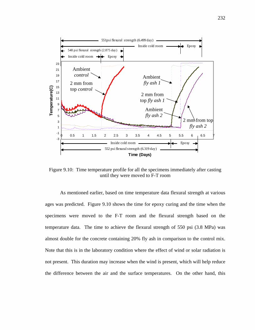
232

Figure 9.10: Time temperature profile for all the specimens immediately after casting

until they were moved to F-T room

As mentioned earlier, based on time temperature data flexural strength at various

ages was predicted. Figure 9.10 shows the time for epoxy curing and the time when the

specimens were moved to the F-T room and the flexural strength based on the

temperature data. The time to achieve the flexural strength of 550 psi (3.8 MPa) was

almost double for the concrete containing 20% fly ash in comparison to the control mix.

Note that this is in the laboratory condition where the effect of wind or solar radiation is

not present. This duration may increase when the wind is present, which will help reduce

the difference between the air and the surface temperatures. On the other hand, this

-3

-1

1

3

5

7

9

11

13

15

17

19

21

23

0 0.5 1 1.5 2 2.5 3 3.5 4 4.5 5 5.5 6 6.5 7

Time (Days)

Tem

pera

ture

(C)

Amb_fly ash1

top_fly ash1

Amb_control

top_control

Amb_fly ash2

top_fly ash2

548 psi flexural strength (2.875 day)

552 psi flexural strength (6.319 day)

551psi flexural strength (6.499 day)Inside cold room

Inside cold room Epoxy

Epoxy

EpoxyInside cold room

Ambient control

2 mm from top control

Ambient fly ash 1

2 mm from top fly ash 1

Ambient fly ash 2

2 mm from top fly ash 2

233

duration might decrease in the presence of solar radiation, due to the fact that daytime

pavement temperatures can rise much higher than the air temperature (Rawhouser, 1945).

9.3.5.2. Scaling Results for Large Size Specimens

After the desired flexural strength was attained, one of the specimens (fly ash 1)

was kept inside the F-T room. To simulate an actual de-icing treatment, a known

quantity of water was first frozen on its surface. Following this, enough salt was added to

form 3% solution which was then ponded for a continuous 50 F-T cycles. No scaling

was observed in this case at the end of 50 cycles on any of the three surfaces. Figure 9.11

shows all three surfaces of this specimen after 50 cycles, indicating no scaling.

Figure 9.11: Surfaces of the fly ash 1 specimen after 50 F-T cycles

234

Although the exact reason for the absence of scaling is difficult to establish, it can

perhaps be attributed to the less permeable microstructure (result of slower setting),

specific method of salt solution application, the temperature effect in larger specimens, or

the combined effect of all. Therefore, in the second phase two more specimens (fly ash 2

and control) were prepared (see Table 9.2). In this case, the salt was applied on the bare

surface (without prior freezing of pure water) and then the specimens were exposed to 50

cycles of freezing and thawing. Similar to fly ash 1 specimen, none of these two

specimens showed any signs of scaling. These specimens were equipped with

thermocouples to monitor their temperature. Details of the temperature data collected are

discussed in the next section.

9.3.5.3. Study of Temperature Variation with Freeze-Thaw Cycles Inside the Specimens

Figure 9.12 shows the temperature profile inside different specimens along with

the temperature of the F-T room. Thermocouples were placed inside the specimens and

also in the surface salt solution. The temperature profiles obtained from the different

locations are shown in this Figure.

It was observed that although the temperature of the room dropped to -15oC (5ºF),

the temperature inside the 300-mm deep specimen did not fall below -5oC, even at

location of 2 mm below the surface. In fact, even the temperature of water (or solution)

ponded on the surface was not dropping below -3oC (26.6ºF).

235

Figure 9.12: Time temperature profile for F-T room and respective temperature profile

obtained using thermocouples placed at different locations

To compare these results with those obtained from 75-mm deep specimens used

for all the scaling study, temperature profile of one 75-mm thick slab for thermocouples

located 20 mm (0.8”) and 30 mm (1.2”) deep from the top was added to Figure 9.12. In

the first 28 hours this small slab was kept without any insulation (multi direction heat

flow), and achieved minimum temperature of -15oC (5ºF) with a little time lag when

compared to the temperature of the room. Since the 300-mm deep specimens were

insulated from all but one side, an attempt was made to simulate similar conditions for

smaller slabs as well. This was achieved by using 50-mm StyrofoamTM sheets on all the

sides except top (single direction heat flow). The time, at which the insulation was

applied, (approximately at 28 hours) is shown with a dotted line in the Figure 9.12.

It can be seen that after insulating, the specimen reached the minimum

temperature of -13oC (8.6ºF). Hence, it can be said that when heat flow is linear, from

-18

-14

-10

-6

-2

2

6

10

14

18

22

0 10 20 30 40 50Time (hours)

Tem

pera

ture

(o C

)

Room temp

150 mm below top - control 1

2mm below top- control

2 mm below top- fly ash 2

150 mm below top - fly ash 2

20 and 30 mm from top - 75 mm slab after

sealing

20 mm and 30 mm from top - 75 mm slab before sealing

Surface solution

Insulation of 75 mm slab

236

only the top surface of the specimen, the overall rate of heat transfer reduces but the size

of the specimen still dominates.

9.3.5.4. Actual Temperature Profiles in Concrete Pavements

The laboratory studies showed that for 300 mm deep specimens, because of the

very high thermal mass, a significant lag was observed between the air and surface

temperature. Therefore, it was important to know how well these results matched with

the actual pavement behavior. Using the database provided by Long Term Pavement

Performance (LTPP, 2003) for plain jointed concrete pavement of 89 different states,

graphs were plotted for the time-temperature profiles during the low temperature seasons.

For each pavement, the time-temperature data of the thermocouples placed inside the

concrete pavement, the air temperature and the positions of the thermocouples were

obtained from different data files. Then, for the particular time period, all of the data was

associated and plotted. In most of the pavements under study, the top thermocouple

(important for scaling damage) had stopped working before the first winter, including

pavements in Indiana. Therefore, Indiana’s latest pavement temperature data (September

1995), was plotted in Figure 9.13. Additionally, to study the behavior during severe

winter, data for the province of Quebec is plotted in Figure 9.14.

237

Figure 9.13: Time temperature profile in PCC pavement in Indiana

The following observations can be made from both of Figures, which can be

considered useful for this study. The significant time lag (7 hours) that was observed in

the 300-mm (12-in.) deep specimen (prepared to simulate actual field conditions), less

pronounced in the actual pavements. The main dominating factor here could be

considered as the effect of wind, which promotes very quick heat transfer by removing

the static air from the surface and subsequently reduces the total time of cooling (or

heating) substantially.

0

5

10

15

20

25

30

35

40

0 20 40 60 80 100Time (hours)

Tem

pera

ture

( C)

Air temperature

20 mm from top

108 mm from top

195 mm from top

Pavement Thickness: 242 mmLocation: Benton County, IndianaMonth: September, 1995

238

Figure 9.14: Time-temperature profile in PCC pavement in Quebec, Canada

It can be noted in both figures that during the daytime, because of solar radiation

(peak at approximately each 24 hours), the concrete surface temperature is higher than

the ambient temperature. Solar radiation can increase the surface temperature of concrete

up to 10 to 15oC (50º to 59ºF) compared to the mean air temperature (Rawhouser, 1945)

and wind speed increases the rate of cooling significantly. The effects of solar radiation

would increase the number of freeze thaw cycles at concrete surface even when the air

temperature remains constantly in the sub-zero state. In Figure 9.14, it can be seen that

for only one thawing in the air, three thaw periods occurred in the surface of the concrete

during the same time. This may create a durability concerns regarding freeze-thaw

damage in the concrete. On the other hand, this might be considered less detrimental for

scaling damage because scaling damage is more dependent on achieving minimum

-18-16-14-12-10-8-6-4-202468

101214

0 20 40 60 80 100

Time (hours)

Tem

pera

ture

(C)

Air Temp

25 mm from top

99 mm from top

174 mm from top

Pavement Thickness: 205 mmLocation: QuebecMonth: December, 1993

239

temperature than number of F-T cycles. For accurate prediction of the temperature in the

pavement information related to solar radiation, wind speed, precipitation, and sub-base

temperature is therefore, required in addition to the air temperature.

For the purpose of this study, it was important to establish the difference between

the air temperature and the surface temperature in the actual pavement. To get an

approximate estimate, the time-temperature profile of the surface and air were obtained,

using the LTPP database covering 8 - 10 years of data for three pavements. In most cases,

at least 5ºC difference was observed in the air temperature and the surface temperature

for all the minimum temperatures encountered. Due to effect of solar radiation this

difference was consistently maintained in most cases, even with a constant sub-zero air

temperature for present 3 - 4 days.

5.4.5.5. Scaling Results After Lowering Minimum Temperature

In order to lower the minimum temperature inside the specimen, three fans were

installed on the three sides of the slab at different elevations. The average wind speed in

the center of the specimen where thermocouple was placed was found to be 9.0 mph

(14.5 kmph). The rate of heat transfer increased in this situation and Figure 9.15 below

shows the minimum temperature achieved inside the slab before and after installation of

fans. The minimum surface temperature also increased from -5ºC to -11ºC (23ºF to

12.2ºF) in the presence of wind.

240

Figure 9.15: Effect of wind in the rate of heat transfer in the large slab

It can be seen from Figure 9.15 that in the presence of a fan, the rate of cooling

increased significantly and the time required to attain a certain temperature reduced

significantly. This slab was exposed to 10 freeze thaw cycles with this lowered minimum

temperature, however still no scaling was observed. The reason could be probably be

attributed to an improvement in the strength due to continual hydration, heat absorption

capacity of 300-mm deep specimen, or insufficient (-11ºC/12.2ºF) minimum surface

temperature to create any kind of scaling damage. Influence of low temperature curing

on surface and bulk porosity for laboratory and field specimens is described in the next

section. Further insight about thermal massing effects (heat absorption capacity) and

other probable reasoning about absence of scaling in 300-mm deep specimen or actual

pavement are given in the next chapter.

-20

-15

-10

-5

0

5

10

15

20

25

30

0 5 10 15 20 25 30 35 40 45 50 55

Time(hours)

Tem

pera

ture

(C)

room tempfly ash top

Temp. before placing fans

Temp. after placing fans

Specimen exposed to wind speed of 9 mph with the help of fans

241

9.3.6. Porosity Determination in Field and Laboratory Specimens

Microstructure study was performed for field and laboratory concretes exposed to

low temperatures to determine the ratios of surface to bulk porosity. Out of several

images obtained at 100x magnification, from the surface and bulk of the specimens, the

ratios of the average surface to bulk porosity were obtained for the laboratory and the

field specimens with and without fly ash. Figure 9.16 shows the representative image for

each type of concrete from the surface and bulk regions. It can be seen that the surface of

fly ash concrete for the field and laboratory specimens looks denser than the surface of

corresponding control specimens. This supports the previous argument about the effect

of reduction of rate of bleeding for fly ash concrete, which helps in improving scaling

performance of concrete, specifically at low temperatures, in comparison to the control

specimens. Moreover, it can be seen that for fly ash concrete in the laboratory and field

specimens, no unusual air content was observed even in the surface region, hence

detrimental effect carbon content of fly ash on surface air concentration does not seem to

be present at all.

242

Figure 9.16: Representative images for different concrete cured at low temperature

Figure 9.17 summarizes the results of the ratio of surface to bulk average porosity

for all four cases. It was very consistently seen in all the images studied that ratio of

surface to bulk porosity of fly ash specimens was less than the respective control

specimens, which is evident in the average results also. This was even evident in the

scaling results of the low temperature study (unlike the control specimens) as the scaling

performance of the fly ash concrete was improved with a decrease in temperature.

Field Control Field Fly ash Lab Control Lab Fly ash

Field Control Field Fly ash Lab Control Lab Fly ash

Bul

k of

con

cret

e

S

urfa

ce o

f con

cret

e

243

Figure 9.17: Ratio of surface to bulk porosity for different concrete

All of the above results confirm that at low temperature the fly ash concrete with

lower slump can develop better microstructure (denser) than normal temperature cured

concrete. Hence, there should not be any direct negative implication for using fly ash at

low temperature in pavement construction, for climatic conditions similar to Indiana.

These are deductions based on the specimens studied but, as mentioned earlier, this

behavior is sensitive to material properties and might change with the type of cement and

fly ash. Moreover, an increase in slump could also change these results significantly.

However, at least it can be said that, certainly the effect of low temperature curing is not

detrimental in terms of scaling performance of fly ash concrete when simulating the

actual pavement conditions. Further results, described in the next chapter will address

the issue of the discrepancy between the laboratory and field scaling performance of fly

ash concrete.

2

2.1

2.2

2.3

2.4

2.5

2.6

Field-Control Field-Fly ash Lab-Control Lab-Fly ash

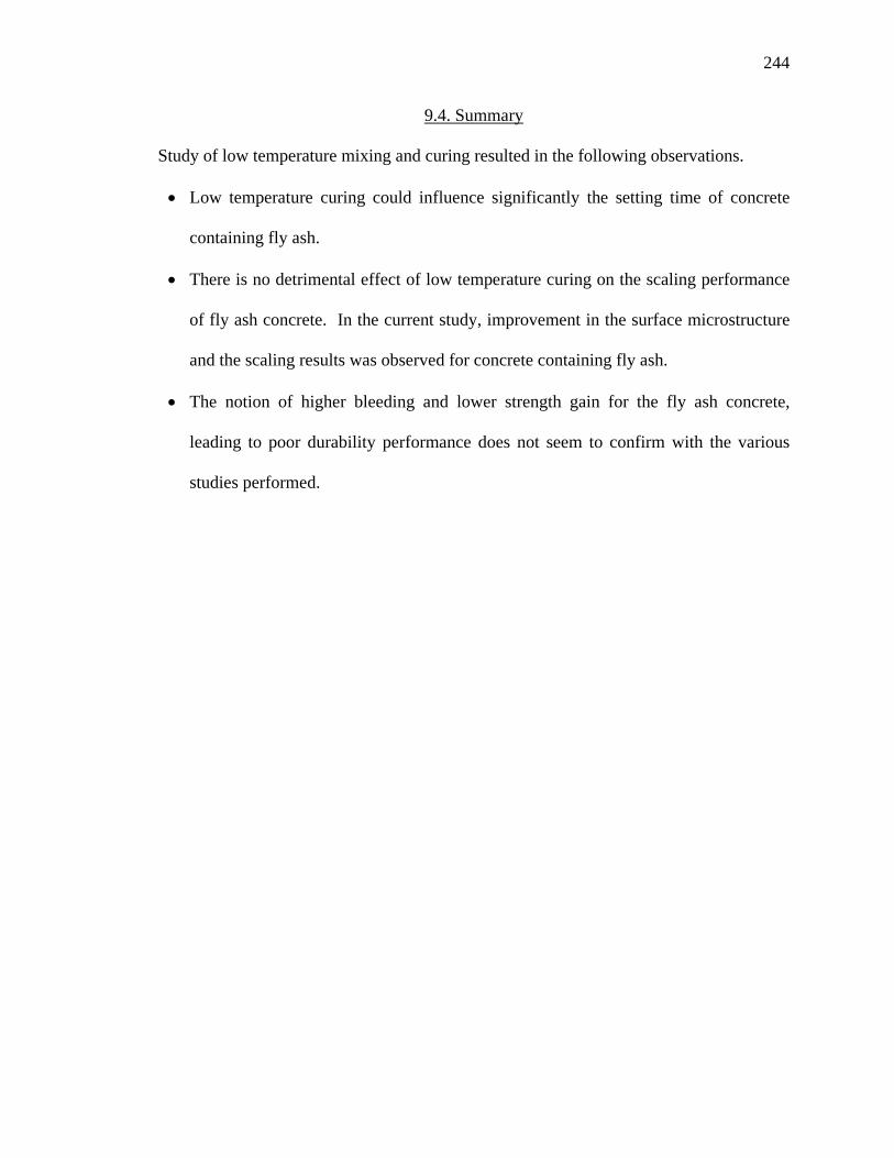
244

9.4. Summary

Study of low temperature mixing and curing resulted in the following observations.

• Low temperature curing could influence significantly the setting time of concrete

containing fly ash.

• There is no detrimental effect of low temperature curing on the scaling performance

of fly ash concrete. In the current study, improvement in the surface microstructure

and the scaling results was observed for concrete containing fly ash.

• The notion of higher bleeding and lower strength gain for the fly ash concrete,

leading to poor durability performance does not seem to confirm with the various

studies performed.

245

CHAPTER 10: DISCREPANCIES BETWEEN LABORATORY RESULTS AND FIELD OBSERVATIONS RELATING TO SCALING OF CONCRETE CONTAINING

SCM

10.1. Introduction

Chapter 9 concluded that there is no significant influence of curing temperature

on the scaling of concrete containing fly ash or SCM (Supplementary Cementitious

Materials). The laboratory tests on the influence of the conditioning periods on scaling

revealed that even after 56 days (i.e., 28 days of moist curing and 28 days of drying)

concrete containing fly ash can scale more than the control mixture. This would suggest

that the pavements containing fly ash even constructed before October 15th could be

prone to scaling damage. However, in reality, scaling of mixtures containing fly ash is

rarely observed in Indiana (Byers, 2003). In addition, studies on the scaling conducted in

the laboratory and the field indicate that the laboratory procedure is far more severe than

concrete may be exposed to in the field for the climatic conditions similar to state of

Indiana.

This chapter attempts to address the discrepancy between the laboratory results

and field performance of concrete containing SCM in regard to scaling and discusses

possible reasons for such discrepancy. To address the source of this discrepancy, first a

brief literature review was performed. In addition, a telephone survey was conducted to

ascertain the experience of the twelve neighboring states with respect to the scaling of

concrete containing SCM. Five parameters were suggested to be responsible for the

246

difference between the laboratory and field performance. Finally, risk analysis was used

to determine the probability of scaling in concrete for climatic conditions of Indiana.

10.2. Literature Review Expressing Discrepancy Between Laboratory and Field

Performance for Scaling of Concrete Containing SCM

Many researchers have determined that the scaling resistance of concrete

containing SCM is higher than that of plain OPC concrete, when studied in the laboratory

using standard laboratory procedure ASTM C 672. On the other hand, although many

concrete pavements in the United State contain SCM, no major case of scaling has been

reported in the field (at least for typical replacement levels of cement with fly ash). Very

little correlation was observed between the two data sets. Field scaling results obtained

by many researchers (Afrani and Rogers, 1994 and Hooton and Boyd, 1997) have shown

satisfactory performance despite poor laboratory results for concrete containing slag.

Despite severe scaling damage observed in laboratory, Bouzoubaâ (2002) reported

satisfactory performance of the side-walks made up of High Volume Fly ash concrete

(HVFA), after four winters with more than 400 cycles of freezing and thawing combined

with numerous applications of deicing salts. Thus, it can be concluded that ASTM C 672

is a very severe test that may underestimate deicing salt scaling resistance of HVFA

concrete in actual field applications. Thomas (1997) performed extensive field survey of

scaling resistance of fly ash concrete pavement to ascertain long term performance. The

results of this survey are summarized in Figure 10.1.

247

Figure 10.1: Results from field observation of scaling of concrete containing fly ash (Thomas, 1997)

It is evident that most concrete containing fly ash performed well in very severe

climates even after several years of exposure. Only a few pavements with very high

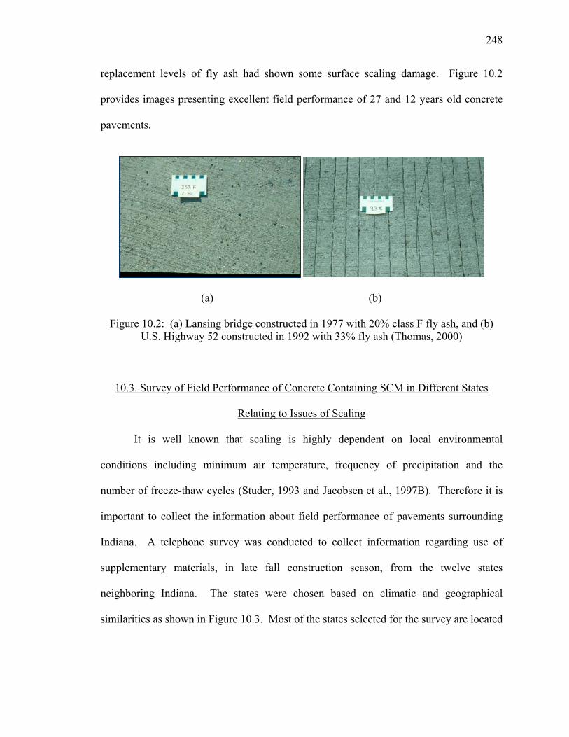
248

replacement levels of fly ash had shown some surface scaling damage. Figure 10.2

provides images presenting excellent field performance of 27 and 12 years old concrete

pavements.

(a) (b)

Figure 10.2: (a) Lansing bridge constructed in 1977 with 20% class F fly ash, and (b) U.S. Highway 52 constructed in 1992 with 33% fly ash (Thomas, 2000)

10.3. Survey of Field Performance of Concrete Containing SCM in Different States

Relating to Issues of Scaling

It is well known that scaling is highly dependent on local environmental

conditions including minimum air temperature, frequency of precipitation and the

number of freeze-thaw cycles (Studer, 1993 and Jacobsen et al., 1997B). Therefore it is

important to collect the information about field performance of pavements surrounding

Indiana. A telephone survey was conducted to collect information regarding use of

supplementary materials, in late fall construction season, from the twelve states

neighboring Indiana. The states were chosen based on climatic and geographical

similarities as shown in Figure 10.3. Most of the states selected for the survey are located

249

at the same or at higher latitudes from Indiana. Additionally, the state of Kansas was also

selected due to extensively reported scaling problems.

Figure 10.3: States selected for scaling problem survey

A brief summary of all the information collected is shown in Table 10.1.

Additionally, any specific measure taken by the state for construction during late fall/low

temperature season is also reported. This Table is not an exhaustive list of all the details

on scaling. However, in general most of the states that had the potential of having some

information about scaling were contacted and hence, the information collected should

give a good “average” indication of the problem.

250

Table 10.1: Summary of information on scaling obtained from 12 states surrounding Indiana

State & Contact

Person (see references for

details)

Restriction on use of fly

ash /slag

Scaling problem due to fly ash (reasons for

general scaling)

Report available

(type of the report)

Pavement Surface

Treatments for late fall

Indiana (Mr. Zink, E & B Paving)

Yes (October 15th-April 1st)

None

YES (one study done in late fall with fly ash)

Normal curing compound

Illinois (Mr. Dirks, IDOT) (Mr.Voigt, ACPA)

No (Removed since 2002)

None No

Application of 2 coats of linseed oil

Iowa (Mr. Henson, Iowa DOT)

No (Removed since 1997)

None (one problem mainly due to finishing issue)

No Normal curing compound

Kansas (Mr. Latorella, ACPA)

No

None (some problems with high volume slag concrete)

No Normal curing compound

Nebraska (Mr. Woolstrum, DOT)

No None No

Until 6 months after construction no salt application

South Dakota (Mr. Crow, ACPA)

No (replacement of 18% only)

None No Normal curing compound

Wisconsin (Mr. Parry, WisDOT)

No (Removed since 1994)

None (one major problem with high volume slag concrete constructed in summer)

No Normal curing compound

251

Table 10.1 continued

State & Contact

Person (see references for

details)

Restriction on use of fly

ash /slag

Scaling problem due to fly ash (reasons

for general scaling)

Report available

(type of the report)

Pavement Surface

Treatments for late fall

Minnesota (Mr. Snyder & Mr. Zeller, CPAM)

No

None (six year back one major problem due to aggregates)

Yes (showing effects of bad const. practices on scaling)

Application of 2 coats of linseed oil, during late fall replacement of fly ash 1:4/3rd

Michigan (Mr. Branch, DOT)

Yes (October 1st – April 1st)

None (Some problems due to improper curing)

No Normal curing compound

Ohio (Mr. Struble DOT)

Yes (October 15th - April 1st )

None (one problem on bridge deck with fly ash )

No Normal curing compound

Pennsylvania (Mr. Malashkie, DOT)

No None None

Linseed oil was being used but not any more

New York (Mr. Streeter, DOT)

No Yes (one major problem in fall 2003)

Yes (problems in most bridge decks)

Normal curing compound

The results obtained from individual states are discussed in more detail below.

Indiana: In Indiana, fly ash and ground granulated blast furnace slag (GGBFS)

are not allowed in pavements construction from October 15th to April 1st. Therefore,

hardly any documented evidence for the use of these materials in cold climates in

concrete pavement construction is available. One of such exception was a test segment

of US24 was constructed between Wabash and Huntington Indiana by E & B Paving

(1999), in which fly ash was used after October 15th. In this study related to maturity, fly

ash was used till November 10th and up to minimum temperatures of -1.5oC (29.3oF) and

252

rising. After four years of service, that pavement did not show any major signs of scaling

on that segment (Zink, 2004). As far as scaling of plain concrete is concerned, some

dusting and scaling was observed on US231 pavement constructed during late fall

(Nantung, 2003). The reason for the scaling was sudden drop in temperature (high rate of

freezing) during night time, which caused formation of weak surface layer. Therefore,

this was not the typical scaling generated due to application of deicer salts, but more like

dusting where weak surface layer came off quickly. It was extrapolated from this

experience that fly ash concrete would be more susceptible to this kind of problems due

to slower setting; however, previous chapter confirmed that there is no detrimental effect

of low temperature curing on concrete containing fly ash.

Illinois: In 2001 IDOT removed the restrictions on use of fly ash and GGBFS in

cold weather conditions. Even before that, fly ash was allowed to be used in a few

projects in Chicago during late fall season, but required with special permission. No

major problem of scaling has been reported with IDOT. As a precautionary measure, it is

specified that two coats of boiled linseed oil (50 yard2/l) shall be used on all the

pavements constructed in late fall season (October 15th -April 15th). It is strongly

believed that such treatment protects the pavement very well from freeze-thaw and

scaling damage for the first winter (Dircks, 2004).

Iowa: Since 1997 Iowa removed the restriction on the use of fly ash and GGBFS

during the late fall construction season. No major problem of scaling has been observed

in the state so far, (Henson, 2004). Normal white pigment based curing compound is

used for curing during late fall season.

253

Kansas: Due to abundance of highly reactive aggregates, state of Kansas has

major problems with alkali-silica reaction (ASR). To combat this issue, minimum 30%

to 40% of GGBFS is being used in normal pavement construction. This addition of high

volume of slag has created some problems of mortar flaking and scaling in last 5 to 6

years. Scaling has been observed for concrete constructed throughout the year,

irrespective of season of construction (Latorella, 2004). Hardly any case of scaling was

observed for concrete containing 20 - 25% SCM placed during late fall construction

season. It is reported that good finishing and curing practices had helped in improving

scaling resistance of concrete incorporating high volumes of GGBFS.

Nebraska: In Nebraska, it is common to use blended cement that contain class F

fly ash. Most of the pavements are being constructed with this type of cement since the

restriction on use of fly ash for late fall construction has been removed. As one of the

precautionary measures it is specified that salt should not be applied on newly

constructed pavement for at least 6 months after construction. If there is a serious safety

concern then salt can be applied earlier, but still no scaling has been observed in such

cases (Woolstrum, 2004). Normal white pigment based curing compound is being

applied on the pavement and no sealing of the pavement is done for the late fall season.

South Dakota: There is no restriction on the use of fly ash as far as the

construction season is concerned. The maximum replacement of fly ash by weight of

cement is 18% with 1:1 replacement. No major problems of scaling have been reported

in the state (Crow, 2004). No other specific measures are specified for concrete

protection during winter.

254

Minnesota: Fly ash is being used year round, however during the late fall

construction season the replacement level of fly ash is increased from 1:1 to 1:4/3. This

effectively increases the total cementitious material in concrete. Also, as an additional

precautionary measure, a Linseed oil based curing compound is specified for winter

construction. Regarding scaling observation, one major problem of scaling was observed

(on 28 slabs up to 3 years old) during the winter of 1996 - ‘97. A detailed study was

performed on these slabs by obtaining various field samples and acquiring construction

history through surveys. A report (Snyder, 1998) summarizing the results concluded that

along with unusual severity of winter, several other factors like non-durable aggregates,

air loss due to longer transit time, over finishing, retempering of mix and inadequate

curing were the major factors causing wide spread scaling problem. One of the minor

factors was the late fall construction season but there was no specific evidence of scaling

due to addition of fly ash in such case. Moreover, it should be noted that all scaling

incidents were observed for slabs thinner than 200 mm (8”). In general, however, even in

the severe climate of Minnesota the problem of scaling of pavement essentially does not

exist. One of the reasons for good scaling resistance of concrete pavement in that state

may be the use very low average w/cm of 0.37 specified by Minnesota DOT and the use

of low slump. Additionally, machine finishing of these pavements along with higher

thickness seem to help in improving scaling resistance.

Wisconsin: Wisconsin has no restriction on use of fly ash or slag since 1994,

when they started using maturity as a tool for strength predictions. Up to 30% fly ash is

being used in the field and no major problems of scaling have been observed relating late

fall construction season. One problem of scaling was reported on Loomis Road in

255

suburban Milwaukee for concrete containing GGBFS that was placed in summer. A

detailed study as to the reasons for this poor performance was conducted and submitted

by the ACPA (Voigt, 1999). This pavement was constructed in the summer of 1998 and

during the first winter most of the concrete with slag (50% replacement) scaled

significantly in comparison to plain concrete. GGBFS concrete had met 28 day strength

criteria and later petrography study showed that hardened concrete had air content within

specification. The main reasons for scaling were assumed to be lower control over slump

of mixture containing slag and improper finishing. Moreover, when almost all laboratory

studies have shown that high replacement of cement (50%) with fly ash or slag would

cause excessive scaling, it is not very surprising to have moderate scaling of high volume

slag concrete in the field when one or two other factors aggravated the situation.

Michigan: Similar to Indiana, Michigan also has restriction on use of fly ash/slag

during late fall construction season. The use of fly ash and slag is prohibited in the Upper

Peninsula starting from October 1st and in the Lower Peninsula starting from October 15th

until April 1st of the continuing year. A few cases of scaling have been observed which

are mainly attributed to poor construction practices. Not a single case has been attributed

to use of fly ash or slag (Branch, 2004). In the case of pavements, normal water based

curing compound is being used during winter for curing.

Ohio: Ohio is the third state other than Indiana and Michigan, in which there is

still a seasonal restriction on use of fly ash and slag. They also have limited experience

as far as use of fly ash or GGBFS during late fall is concerned. So far, scaling was

observed in one case on a bridge deck in which fly ash was used during late fall

construction season (Struble, 2004). Several other incidents of scaling were reported in

256

the Cleveland area, but all of them were normal concrete and they scaled mainly due to

late fall construction or insufficient air content.

Pennsylvania: In Pennsylvania, there are no restrictions on use of fly ash and slag

during late fall construction season. In the past there was a requirement of using linseed

oil for sealing of concrete during winter construction but now this restriction has been

removed (Malashkie, 2004). Specifications are mainly based on air temperature and

various curing guidelines are provided for various temperatures ranges. No major

problems of scaling have been reported thus far.

New York: There are no restrictions on the use of fly ash and slag during winter

construction and ternary blends of fly ash and silica fume are very common in the high

performance concrete mixtures placed during winter. During the winter of 2002 - ‘03

numerous cases of concrete scaling were observed in bridge decks, side-walks and other

flat works in western New York. This was one of the most extreme winters for western

New York with precipitation 33% higher than average and number of freeze-thaw cycles

60% higher than normal. A report submitted by Mr. Streeter (Streeter, 2003) points out

that one of the major reason for bridge deck scaling was late season placement, which did

not allow concrete to dry before it was exposed to de-icing salts, which caused scaling

even after sufficient curing of the bridge decks. However, not a single pavement showed

scaling. Attempt to provide explanations for this behavior is presented in section 10.5.1.

In summary, it can be said that overall a few problems of scaling of concrete

containing moderate (up to 30%) amounts of fly ash were actually observed in the field.

In cases where problems occurred they were mostly attributed to poor construction

practices or high volume replacement of cement by supplementary materials. It should

257

be noted that all four states which reported some problems of scaling (Minnesota,

Wisconsin, Michigan and New York) are situated at higher latitude than Indiana. These

states have average minimum temperature about 5 - 10oC lower than the average Indiana

temperature, which could be one of the reasons for higher instances of scaling.

Another important finding of this survey is that when scaling was observed, it was

mostly observed in the thin slabs and bridge decks, not in pavements. This implies that

thickness of the pavement and construction procedures would have strong influence on

scaling resistance.

10.4. Parameters Responsible for Discrepancy Related to Fresh Concrete

There are certain parameters, which can influence fresh properties of concrete.

Several parameters influencing properties of fresh concrete may be responsible for the

observed differences between scaling performance of concrete cast in the laboratory and

concrete placed in the field. The two major parameters suggested in this section are early

age evaporation and finishing of concrete. In the field, due to effect of wind and solar

radiation, rate of evaporation can be much higher then that in the corresponding

laboratory specimen. This can create significant difference in surface porosity of both

concretes. The other parameter is machine (slip form paver) finishing of concrete in

comparison to normal hand/trowel finishing in the laboratory. This finishing could also

change scaling resistance of surface significantly.

258

10.4.1. Influence of Early Age Evaporation on Scaling and Surface Porosity

The porosity of concrete surface could be dependent on the cumulative effect of

bleeding and evaporation. Specimens with higher amounts of bleeding and lower

evaporation loss can develop highly porous surface layer due to the high localized w/cm.

To understand the role of surface pore structure and porosity in scaling mechanism,

specimens with different amount of evaporation losses were studied.

10.4.1.1. Specimen Preparation and Experimental Procedure

The 1-in. (25-mm) slump mixture proportion shown in Table 7.1 was used to

prepare three slab specimens with the dimension of 380 mm x 190 mm x 75 mm (15” x

7.5” x 3”). The specimens were prepared following the same procedure as that used to

prepare the normal scaling specimens (section 8.2). After finishing, all specimens were

weighed and initial mass was recorded. After weighing, one of the slabs was stored

under the plastic lid until the time at which it was demolded (24 ± 2 hours after casting).

The other two specimens were placed in an environmentally controlled chamber for 6

hours. The temperature of the chamber was 30oC (86ºF) with an average humidity of

45%. Fans within the chamber aided in the evaporation of surface bleed water. One

specimen was subjected to an average wind velocity of 27.3 kph (17 mph) and the other

to 14.5 kph (9 mph) over the top surface. Details of specimen and water loss are given in

Table 10.2. After 6 hours they were kept under plastic sheet until they were demolded

(24 ± 2 hours).

At the end of 24 hours, all three specimens were weighed once again and loss of

water was determined. At the time of demolding each slab was weighed again and cut to

259

half using a diamond bladed saw to create two 75 mm x 190 mm x 250 mm (3” x 7.5” x

10”) test specimens. These specimens were then placed in moist curing room (98 ± 2%

RH), for two more days and following that they were kept for 3 more days in constant

humidity room (50 ± 5% RH) for drying. One half of each slab was used to perform

standard scaling test and the other half was used to prepare two SEM specimens for

microstructural study.

Table 10.2: Mass of specimens before and after evaporation

Specimen ID

Size of the specimens

(mm)

Wind speed at surface (kph)

Initial Mass (kg)

Final Mass (kg)

Loss of water in 24 hrs.

(kg)

Loss per area

(kg/m2)

No. of SEM

specimens

3-3-ah 250 x 190 x 75 27.3 31.59 31.16 0.43 4.53 2

3-3-am 250 x 190 x 75 14.5 33.74 33.32 0.42 4.47 1

3-3-an 250 x 190 x 75 0 31.96 31.97 0.01 -- 2

1 kg = 2.2 lb; 25.4 mm = 1”; 1 kph = 0.62 mph

Notation “3-3” represents moist curing and drying duration, respectively.

Additionally, the specimens were given the following suffixes: “ah” - high evaporation,

“am” - medium evaporation, and “an” - no evaporation. Scaling test was performed on

these specimens using the same test procedure as described in section 8.3.2.

10.4.1.2. Results from Scaling Study of Evaporation Samples

The results of scaling study for specimens exposed to different wind speeds (i.e.,

evaporation rates) at early ages are shown in Figure 10.4. It can be seen that with

increase in wind speed, the total scaled mass decreased significantly. This, once again,

260

confirms that for very short moist curing and drying period (i.e., at very early ages, less

than 10 days) the amount of moisture in the surface layer and the degree to which it

influences microstructure is an important parameter influencing scaling.

Figure 10.4: Total mass scaled for samples exposed to different wind velocities

Figures 10.5(a) and (b) show cumulative scaled mass versus wind velocity and

versus total water loss, respectively. From Figure 10.5(b) it seems that rate of

evaporation would have exceeded the bleeding rate for the specimen (3-3-ah) subjected to

27.3 km/h (17 mph) wind speed (as indicated by the vertical drop in the trend line), while

that may not be the case for specimen (3-3-am) subjected to 14.5 km/h (9 mph) wind

speed. It can be hypothesized that in specimen 3-3-ah high wind speed could have

caused quick water loss by the generation of higher capillary stresses. This higher

capillary stresses could have helped in generating a denser microstructure. Therefore,

water loss being the same, lower scaling was observed in the specimen 3-3-ah compared

to specimen 3-3-am. Thus effect of evaporation might provide a good explanation for the

absence of scaling observed in the actual pavements at early or later ages.

0

0.2

0.4

0.6

0.8

1

1.2

1.4

0 10 20 30 40 50

Number of Cycle

Cum

ulat

ive

Sca

led

Mas

s (k

g/m

2 )0 km/h16.66 km/h26.82 km/h

0.0 km/h 14.5 km/h 27.3 km/h

261

(a) (b)

Figure 10.5: (a) Scaled mass for different wind speeds and (b) scaled mass for different total water loss

Higher wind speed (i.e., higher rate of evaporation) at very early ages will create

changes in surface microstructure during plastic stage and could help in developing better

tensile strength at the surface. During this period, because of restraint provided by the

form or by the concrete below the surface, there are chances of plastic shrinkage cracking

occurring on the surface. At the same time, the continuous evaporation would help in

reducing capillary porosity. To confirm this hypothesis detailed microstructural analysis

was performed with evaporation samples as described in the next section.

10.4.1.3. Microstructural Study of Evaporation Samples

A series of SEM specimens (two for each evaporation rate) were prepared

following procedure described in section 8.2.2. Images of microstructure were collected

and analyzed to obtain porosity gradients. The values of individual porosities were

normalized against the minimum (or bulk porosity) and are plotted in Figure 10.6.

0

0.2

0.4

0.6

0.8

1

1.2

1.4

0 5 10 15 20 25 30

Wind Speed (km/h)

Cum

ulat

ive

Scal

ed M

ass

(kg/

m2 )

0

0.2

0.4

0.6

0.8

1

1.2

1.4

0 1 2 3 4 5

Water Loss (kg/m2)

Cum

ulat

ive

Sca

led

Mas

s (k

g/m

2 )

3-3-an

3-3-am

3-3-ah

3-3-an

3-3-am

3-3-ah

262

Surprisingly, for all three cases, the ratio of surface to bulk porosity was almost in the

same range.

Figure 10.6: Porosity gradient for evaporation specimens, normalized against minimum value

During image acquisition it was observed that higher amount of cracking was

presented in the samples subjected to high evaporation, while minimal or no cracking was

observed in the specimen without any evaporation losses. The crack widths were found

to be higher for the sample 3-3-ah than for sample 3-3-am. Since all these specimens

were exposed to similar sample preparation, it can be said that these cracks would not

have formed during oven drying or any other sample preparation procedures. In addition,

these cracks are only visible in the surface region of the specimen. Thus, it can be said

that these cracks are most likely plastic shrinkage cracks formed during evaporation from

the surface. To confirm these observations and to find true capillary porosity the

following procedure was adopted.

Dep

th fr

om to

p (m

m)

-10

-9

-8

-7

-6

-5

-4

-3

-2

-1

0

0.0 0.5 1.0 1.5 2.0 2.5 3.0 3.5Di t f t ( )

No evaporation(3-3-an)

High evaporation(3-3-ah)

Medium evaporation(3-3-am)

Porosity (Normalized against minimum value)

263

Figure 10.7: Segmentation of images at lower threshold

Figure 10.7 shows typical images obtained from three specimens. The images

were segmented at lower brightness threshold value (60 to 65) to distinguish the distinct

features. It can be easily seen that cracks are more pronounced in the case of specimen 3-

3-ah, than in the specimen 3-3-am. Moreover, in both of these specimens the matrix is

comparatively denser while in the case of specimen 3-3-an, no cracks are observed and

the matrix has more distributed pores (capillary porosity). It is believed that higher

capillary porosity and lower tensile strength of this matrix is responsible for higher F-T

and scaling damage. Thus, although total porosity would be similar for all the three

specimens, the strength of the matrix would be different, and therefore scaling

performance was different. To eliminate the effect of plastic shrinkage cracking and

3-3-ah - High Evaporation 3-3-am = Medium Evaporation 3-3-an = No evaporation

264

localized difference in air voids, porosities of the images were obtained by eliminating

these features with different filters and paint tools. This modified porosity gradients for

3-3-an and 3-3-ah specimens are plotted in Figure 10.8.

Figure 10.8: Modified porosity gradients for high and no evaporation specimens

Figure 10.8 shows that surface capillary porosity of the specimen 3-3-an is almost

twice the capillary porosity of the specimen 3-3-ah. Therefore, it can be hypothesized

that young field concrete exposed to wind and solar radiation would have higher

evaporation rates. This will result in removal of remove excess water from the surface

and will reduce potential for scaling damage as compared to laboratory specimens.

10.4.2. Finishing Operation- Hand Finishing Versus Machine Finishing

Based on the literature review and the survey of the DOT representatives, it was

realized that finishing could influence scaling results significantly. There is not much

difference in scaling results of concrete with different types of hand finishing (Luther et

al., 1994) but certainly, machine finishing seems to improve scaling resistance in

-10

-9

-8

-7

-6

-5

-4

-3

-2

-1

0

0.0 1.0 2.0 3.0 4.0

Porosity (Normalized against minimum value)

Dis

tanc

e fr

om to

p (m

m)

No evaporation(3-3-an)

High evaporation(3-3-ah)

265

comparison with manually-finished concrete (Thomas, 1997). It is difficult to assess this

influence experimentally, so data from literature review and survey was used.

Slip-form paving or machine finishing could help in improving scaling resistance

due to following reasons. For proper slip-form paving operation slump should be limited

to maximum of 2” (50 mm) and hence, the overall bleeding in the concrete could be

reduced. Additionally, due to machine finishing there are very few chances of

retempering of the surface with additional water thus, making the surface weaker due to a

local increase in the w/cm ratio. At the same time, in the case of manually-finished

concrete there are chances of over-finishing, which can influence air void structure of

concrete surface. Moreover, tines created in the actual pavement would additionally help

in increasing the evaporation rate and thereby could make the surface denser. The

microstructural study of the simulated field and laboratory samples confirmed that field

surface tend to be less porous than comparative laboratory specimen. To support these

reasoning three different finding in this regard are mentioned below.

As mentioned earlier, extensive study was carried out in Minnesota to determine

reasons for poor durability performance of exterior slabs during the winter of 1996-97

(Snyder, 1998). This study revealed that 85% of the total problems were scaling

problem. After detailed investigation it was realized that out of total scaling problems

61% problems were associated with improper finishing of the concrete. However, not a

single problem was in the pavement constructed with slip form paver. This shows

importance of finishing, and highlights the fact that poor manual finishing practices can

lead to increased scaling.

266

Pigeon (1996) studied the effects of surface microstructure on scaling resistance.

He studied different wooden trowel finished surface and compared them with sawed

surface. He consistently found wooden trowel finished surface more prone to scaling in

comparison to sawed surface. Microstructural study confirmed that there is a significant

layer of high porosity observed in the hand finished laboratory specimens. Based on this

study, it was concluded that poor finishing of the laboratory specimen is the main reason

for apparent discrepancies in scaling performance of field and laboratory concrete

containing SCM.

In field performance survey of fly ash concrete, Thomas (2000) investigated

various slabs and parking garages with scaling problems. He studied 20 different field

cases where he found scaling problems in concrete placed and finished by hand in

comparison to machine finished concrete. One such case (a parking slab in Wisconsin) is

shown in Figure 10.9.

Figure 10.9: Parking slab with differential scaling performance (Thomas, 2000)

Parking area in Wisconsin – placed in 1992

Placed & finished with a paving machine

Placed & finished by hand

40% Class F fly ash

267

From this Figure it is evident that the portion of the slab placed and finished

manually showed very poor resistance to scaling while machine finished segment did not

show any scaling. Thus, it can be concluded that the finishing operations conducted by

slip form paver is one of the important parameter in improving scaling resistance of

concrete, with and without SCM.

10.5. Parameters Responsible for Discrepancy Related to Hardened Concrete

There are several parameters which could influence the scaling performance of

concrete in the hardened stage. One of these parameters (already considered in the

previous chapter) is the size of the specimen. Second parameter is the number of

consecutive F-T cycles and intermittent drying. Third parameter is the actual procedure

for application of salt solution on the pavement, which is very much different from the

procedure followed in ASTM C 672. The influence of these parameters is discussed in

detail in the next section.

10.5.1. Influence of Size of the Specimen on Minimum Surface Temperature, Rate of

Freezing and Scaling

The size of specimen used in the laboratory study (75 mm x 190 mm x 250 mm)

is considerably smaller in comparison to actual pavement section. In previous chapter

using (300-mm deep specimens), it was shown that large thermal mass and single

direction heat flow could change scaling behavior. For large size specimens, the rate of

freezing and minimum surface temperature observed are different from that observed in

the corresponding small specimens even at the same ambient temperature. Therefore,

268

further study was performed with different sizes of specimens to determine the influence

of size of specimen on rate of freezing and scaling.

10.5.1.1. Specimen Preparation and Experimental Procedure

For this study, mold previously prepared for 300-mm deep specimens, were used.

Each mold was partitioned vertically (using 2-inch thick StyrofoamTM sheets) to create

total of three slabs. The area of the each slab was 11” x 11” (0.078m2), which is much

higher than minimum area (75 in2 or 0.048 m2) specified by ASTM C 672. A wooden

pole was installed at the center of the each slab and thermocouples were attached to it at

various depths. Figure 10.10 shows both molds with partitions and thermocouples pole

installed. To create slabs with different thicknesses (ranging from 55 to 245 mm), paper

waste was used to fill up the bottom portions of the molds so that the top of all the slabs

was at the same level, as shown in the section in Figure 10.10.

Figure 10.10: Partitioned mold for size effect study

269

After partitioning, all joints were sealed using duct tape. Three to nine

thermocouples (depending on the depth of the slab) were attached to each central pole

using duct tape to obtain the temperature profile at various locations within the slab. All

the thermocouple wires were “channeled” out from the mold and into one corner of each

slab. Details regarding the number and position of thermocouples for specimens of

various depths are shown in Table 10.3. The depth of the each partition was kept 1”

(25 mm) deeper than the specified specimen depth mentioned in the Table. The bottom

1” of each slab was filled with coarse aggregates (cooled to 1oC or 33.8ºF) to simulate

boundary conditions at the bottom of a field slab. Form release agent was applied on all

the sides. Figure 10.11 shows one of the molds, in its final stage before casting the

concrete.

The mixture proportions shown in Table 7.1 for 25 mm (1”) slump specimen were

used in this study. All aggregates were stored in 1oC room 48 hours prior mixing. The

mixing, casting and finishing was also identical to large size specimen study, as described

in section 9.2.6.2. Slabs were stored in the cold room (1oC), until they achieved maturity

equivalent to 550 psi (3.8 MPa) at which point they were moved to F-T chamber for 50

cycles of freezing and thawing with salt solution on the surface. Temperature data was

collected continuously throughout the test; two additional thermocouples were placed to

measure the room temperature.

270

Figure 10.11: Final mold before mixing, with 1” thick base of aggregates

Table 10.3: Summary of specimens and results of size effect study

Depth of specimen

(mm)

No. and positions of thermocouples from

top (mm)

Minimum temp. at 2 mm (oC)

Maximum temp. at 2 mm (oC)

Avg. rate of freezing (oC/hr)

Scaling results (kg/m2)

55 5 (2, 8, 20, 40 and 50) -11.5 15.2 -2.0 0.25 81 3 (2, 30 and 75) -10.1 15.1 -1.88 0.15 103 5 (2, 10, 30, 60 and 100) -8.6 12.5 -1.58 None 130 3 (2, 60 and 125) -7.2 12.0 -1.43 None 184 3 (2, 75 and 180) -6.9 11.0 -1.38 None

245 8 (2, 8, 20, 40, 75, 125, 180 and 240)

-6.6 11.3 -1.35 None

Room temp.

2 (near surface of the each specimen)

-15.9 22.4 -2.95 -----

Styrofoam sealing (2”)

Wooden frame, will act as a dam to pond solution

Densely packed Paper waste

Paper waste Paper waste

55 mm deep 103 mm deep

184 mm deep

Cross section of the mold

1” thick layer of aggregate

271

10.5.1.2. Results and Data Analysis - Laboratory Study

Figure 10.12 shows the temperature profiles (2 mm below the surface) for all six

lab specimens along with the temperature of the F-T room. Minimum and maximum

temperatures for all these slabs along with computed average rate of freezing are given in

Table 10.3. The scaling results after application of 50 F-T cycles for all the slabs are also

given in the same Table.

Figure 10.12: F-T cycle temperatures (room and 2 mm below surface of all six specimens)

It can be seen that for specimens with depths ranging from 55 mm to 245 mm

(2.5” x 9.5”), the minimum temperature of the surface region ranges from -11.5 to -6.6oC

(11.3 to 20.1ºF) for ambient minimum temperature of -15.9oC (3.4ºF). This confirms

previous observations that the difference between surface and air temperature increases

with the increase in size of the specimen. Moreover, results show that scaling (very

minor) was only observed in for the specimens in which surface temperature dropped

below than -10oC (14ºF). These results confirm the finding of Lindmark (1999) that

-20

-15

-10

-5

0

5

10

15

20

25

0 10 20 30 40 50

Time (hours)

Tem

pera

ture

(o c)

F-T Room Temperature

130 mm deep slab

103 mm deep slab

184 mm deep slab

81 mm deep slab

55 mm deep slab

245mm deep slab

272

scaling of the concrete is highly dependent on minimum temperature that surface attains,

and duration of time for which it attains this temperature. Therefore, size of the

pavement being very large in comparison to the laboratory specimen, chances of scaling

will be reduced in each case when the minimum surface temperature stay above -10oC.

The typical rate of freezing observed in the simulated pavement segment exposed to the

elements is further described in the next section dealing with the outdoor study.

One more important observation was made from analysis of the temperature data

from these slabs, instrumented with thermocouples. Figure 10.13 shows temperature

profile of thermocouples placed in 81-mm (3.2”) and 245-mm (9.6”) thick slab at 2 mm

and 75 mm from the surface for each specimen along with the temperature profile of the

F-T room.

Figure 10.13: Thermal massing effect of large size specimens

From the Figure it is evident that for a small size (81 mm) specimen the rates of

freezing at 2 mm and 75 mm are the same, while for large size (245 mm) specimen rates

of freezing at 2 and 75 mm are significantly different. Thus, because of higher heat

absorbing capacity of the large size specimen, differential rate of freezing is observed in

-20-15-10

-505

10152025

0 4 8 12 16 20 24

Time (hours)

Tem

pera

ture

(o c)

F-T Room Temperature

81 mm slab @ 2 mm

81 mm slab @ 75 mm

245 mm slab @ 75mm

245 mm slab @ 2mm

273

the surface region. Freezing front moves down slowly from top towards bulk of the

specimen. This could be another reason why scaling is observed in the laboratory

specimen, while field specimen of similar concrete does not scale.

It has been observed that presence of excess surface water on the surface is

essential to cause scaling problem. Verbeck and Klieger (1957) found that when samples

were frozen in damp condition, i.e., with no liquid present on the surface, there was no

scaling. Similar observation was made by Lindmark (1999). This is one of the very few

phenomena which has been observed and accepted by all researchers who studied

scaling. Fagerlund (1977) proposed that in sound concrete, moisture uptake during

freezing and increased degree of saturation is the major cause of scaling.

Based on above observations, in the case of small size specimen, similar rate of

freezing of bulk and surface regions may lead to higher moisture uptake. On the other

hand, for large size specimens, surface freezes much faster then the bulk of the concrete.

This phenomenon, even in the presence of salt solution provides less time for water

uptake. Moreover, freezing will progress downward with time, which can cause moisture

movement further downward and away from the surface. Thus, chances of having high

degree of saturation in the surface region, and thereby generating detrimental forces, are

much lower for larger specimens than for smaller specimens. In summary, the change in

rate of freezing is one another important parameter that can help in resolving the

discrepancy between laboratory and field scaling performance of concrete.

274

10.5.2. Study of the Cumulative F-T Cycles and Intermediate Drying

During conditioning period study and low temperature curing study, one common

observation was made from all different specimens. None of the specimens, including

those which experienced severe scaling showed any scaling damage until completion of

three continuous F-T cycles. This indicates that scaling does not happen in one F-T

cycle, but that it takes 2 - 3 continuous cycles to initiate scaling in well air entrained

concrete. This is consistent with other findings (Jacobsen et al., 1997A) that filling of air

voids with water during freezing is one of the major reasons for scaling of virgin

concrete. They suggested that due to pumping effect, degree of saturation of surface

region increases thus, making air voids inefficient in consecutive cycles that cause

damage to the surface. Fagerlund (1977) described the mechanisms of water uptake in

the air pores during freezing and has shown how the air pores are inactivated after long

period of continuous water storage. All these results provide indirect evidence that in

sound concrete scaling does not initiate in 1 - 2 cycles.

At this point it is important to know what kind of freezing temperatures are

observed for actual pavement when surface of the pavement is wet or has excessive

moisture. To determine time of wetness and number of corresponding freezing cycles,

following approach was used.

10.5.2.1. Number of Wetting Events and Freezing Temperature for Indiana

Information related to pavement wetness and corresponding temperature can be

useful to determine the probability of initiation of scaling process generation in the

climate of Indiana. The computer program “Conclife”, developed by National Institute of

275

Standards and Technology (NIST) was used to determine the number of wetting events

and corresponding subzero temperatures for four different locations in Indiana. The

model is based on a one-dimensional finite difference scheme and includes heat transfer

by conduction, convection, and radiation. Environmental conditions are varied by using

the Typical Meteorological Year (TMY2) data files available from the National

Renewable Energy Laboratory. Based on the weather data available in these files and the

developed heat transfer model, both the surface temperature and the time-of-wetness of

the concrete are computed for typical pavement and bridge deck structures. The time-of-

wetness includes both precipitation and condensation on the concrete surface. Wetting

may not represent all the times saturation but if there is no wetting there will not be any

saturation during that duration for pavement. Thus, this approach will represent the worst

case scenario for available data. The results for following four different locations are

obtained for Indiana: South Bend, Fort Wayne, Indianapolis and Evansville. Data for all

the locations is summarized in Table 10.4.

Table 10.4: Data for freezing and wetting event for a typical year

Location for Indiana

Total number of

wetting events

Total number of

freezing events

Total number of wetting event with sub zero pavement

temperature

Minimum temperature

while pavement was wet

South Bend 227 100 2 -0.96 Fort Wayne 220 100 10 -6.97 Indianapolis 221 90 11 -6.04 Evansville 254 69 4 -4.07

276

The data indicate that Fort Wayne is the location with maximum number of

possible freezing events and with the lowest minimum temperature. Therefore, more

complete set of data for Fort Wayne is plotted in Figure 10.14.

0 2000 4000 6000 8000

Time in hours for a typical year starting from January

0

10

20

30

40

Tota

l hou

rs o

f pa

rticu

lar w

ettin

g ev

ent

0

-2

-4

-6

-8

-10

Tem

pera

ture

(o C) b

elow

zer

o de

gree

for c

orre

spon

ding

wet

ting

even

ts

Total hours of wetting event at particular timeAll sub-zero temperatures for corresponding wetting events

Figure 10.14: Total hours of wetting event at each time with sub-zero temperature

From Figure 10.14, it can be said that lowest minimum surface temperature is

about -7ºC (19.4ºF), which based on the evidence presented earlier, might not be low

enough to initiate scaling in the pavement. It should be noted here that the Typical

Metrological Data represent normals over a period of 30 years, so the record minimum

277

temperatures might be significantly lower than the reported temperatures. For this

reason, the total time of wetness during the freezing events was given more importance in

this study. Analysis of the data indicates that the maximum duration of wetness observed

during freezing was 30 hours, which is less then 2 days. It is very unlikely to observe

more then 2 F-T cycles (with minimum air temperature being less then -12 to -15oC, i.e.,

10.4 to 5ºF) during this time frame.

Based on the above data it can be said that it is hardly possible that concrete will

undergo 2 - 3 continuous F-T cycles with salt solution on surface in the field and this

could be another reason for apparent discrepancy between laboratory and field scaling

performance. Thus, to substantiate this argument and see how concrete would perform in

laboratory in presence of realistic F-T cycles, study of intermittent drying was done.

Additionally, importance of early age evaporation was already described earlier in the

chapter. Therefore, to generate the most realistic F-T performance of 250 mm x 190 mm

x 75 mm (10” x 7.5” x 3”) specimens in laboratory, combined influence of both these

parameters was studied along with their individual effects as described in the next

section.

10.5.2.2. Preparation of the Specimens and Experimental Procedure

The mixture proportion used in this study was identical to the mixture proportion

of 25 mm (1”) slump concrete, shown in Table 7.1. As the original supply of cement and

fly ash was exhausted, new shipment of (nominally) same material was secured from the

same sources again. Total of four scaling slabs were prepared in this study following the

procedure described in section 8.2. Out of the four slabs, two were exposed to early age

278

evaporation, the same way as described in section 10.4.1.1 with wind speed of 9 mph on

the surface. All slabs were cut in to halves and eight scaling specimens were prepared

using the same procedure as described in section 8.2.

All eight slabs were conditioned in the laboratory for 3 days, during which period

they were covered with plastic lid and plastic sheets. They were then moved to F-T

chamber and ponded with salt solution. After two F-T cycles, four out of these eight

slabs (two slabs to be exposed to wind of 9 mph and two subjected to non-wind

evaporation) were removed from the F-T room during the thawing period. The solution

was removed and surfaces of the specimens were washed thoroughly. After washing the

specimens were moved back into the chamber. Two of these specimens were exposed to

constant wind effect of 9 mph (14.5 kmph) with the help of two fans for 24 hours.

Weight of the specimens was measured at the end of drying period. After one drying

cycle, once again 3% solution of sodium chloride was applied to the surface and again the

specimens were exposed to 2 continuous cycles of F-T with solution on the surface.

Thus, these four specimens were exposed to 1 dry cycle after 2 wet cycles for total of 75

cycles, while other four specimens were exposed to continuous 50 F-T cycles. To create

consistent drying effect, during each drying cycle specimens were exposed to wind for 24

to 28 hours until the mass of the specimen was close to the mass recorded earlier (within

± 10 grams). For intermittently dried specimens scaled mass after 75 cycles was

compared to scaled mass collected after 50 cycles of other four specimens. This helped

in comparing equivalent amount of wet cycles in all specimens. Results of this study are

reported below.

279

10.5.2.3. Results and Data Analysis

Surprisingly, for all eight specimens, significant reduction in scaled mass

(compared with earlier results) was observed, with maximum scaling of only 0.3 kg/m2.

This reduction can be attributed to variability in materials. Effect of variability of

materials on scaling was discussed in detail in Chapter 7. To study the effect of

intermittent drying and evaporation independent of materials parameters, the scaled mass

is normalized with respect to minimal value. Figure 10.15 below shows results of this

study.

Figure 10.15: Results of evaporation and intermittent drying study

From Figure 10.15 it can be said that the scaled mass of the specimens, with the

combined effect of intermittent drying and early age evaporation, is 11 times lower then

the scaled mass specimen exposed to continuous F-T cycles (normal scaling cycle),

prepared from the same mixture. Even just intermittent drying could reduce scaled mass

to 1/5th of normal scaling specimen. Thus, when laboratory specimens were exposed to

0

2

4

6

8

10

12

Evaporation+ intermittent drying

Intermittent dryingonly

Evaporation only No evaporation ordrying

Nor

mal

ized

val

ues

for s

cale

d m

ass

280

environmental conditions likely to be encountered in Indiana, significant reduction in

scaling was observed. This phenomenon could also be largely dependent on mixture

proportion or composition of materials. As the required number of cycles to initiate

scaling may vary (from 2 to 4), depending on type of air void structure formed in the

particular concrete.

10.5.3. Current Practices for the Use of De-icing Salts

In the literature summary (section 2.4.3), it was evident that maximum scaling can

be observed for salt concentration of 2 to 4%. Lindmark (1999) further studied this

aspect and mentioned that this pessimum solution is dependent on minimum surface

temperature and eutectic point of a particular salt. In our study, with minimum

temperature of F-T cycle being -15.9oC (3.4ºF), 5% was observed as the concentration

after which no freezing was observed in the solution and thereby no scaling could be

observed. This was evident from the study of high salt concentration effect in section

8.3.3. Also in Indiana, typical minimum temperatures are similar to that used in the

laboratory studies. This suggests that scaling in the field can only be expected when salt

concentration is in the range of 1 to 5%.

Based on current de-icing practices mentioned in the section 2.4.3, it is possible

that the salt concentrations used in the field may be higher than the pessimum

concentrations thus reducing the risk of scaling damage.

Having knowledge of these important parameters responsible for discrepancy

between laboratory and field scaling results, risk analysis (Monte Carlo simulations)

281

techniques can be used to calculate the probability of scaling in Indiana climate. The

results of such simulations are presented in the next section.

10.6. Determination of Probability of Scaling in the Field

From the experiments described earlier, it is clear that there are several

parameters which have influence on the scaling performance of concrete containing

SCM. All these parameters contribute to certain extent to scaling resistance or generation

of detrimental forces. Due to complex nature of scaling mechanism, most of these

parameters can not be combined mathematically to develop a model for scaling with

reasonable accuracy (Lindmark, 1999). In such situation, to assess the possibility of

scaling for field concrete pavement, risk analysis approach can be used. This approach

can give the probability of occurrence of an event that could initiate scaling in the

concrete pavement. Thus, first an event is defined which is responsible for causing

scaling and then effect of various parameters (salt concentration, surface finishing or

materials composition) is incorporated through various probability distribution functions.

10.6.1. Determination of Detrimental Event that Could Cause Scaling in Concrete

Pavement

Based on intermittent drying study it is clear that it takes 2 to 3 F-T cycles with

salt solution on surface to initiate scaling in the sound concrete. This study revealed that

for concrete exposed to only 2 consecutive wet cycles, scaling could be reduced 11 times,

but this can be dependent on type of materials and air void structure. To simulate the

worst case scenario, for purpose of this study it was assumed that only two cycles could

282

be required to initiate the scaling. Thus, selecting 2 days as the detrimental event not

only helped in representing the worst case scenario but also allowed to account for some

relaxation incorporation of any unforeseen parameters, which could contribute to scaling.

Other parameters associated with this modeling effort are described below.

Minimum surface temperature: It has been proved in the size effect study that

scaling in the concrete doesn’t happen until surface temperature drops below -10oC

(14ºF). To achieve surface temperature of -10oC, air temperature should be in the range

of -15oC (5ºF), (assuming lag of -5oC). In presence of high wind this lag might decrease

and hence to represent the worst case scenario the required minimum air temperature was

assumed to be -12oC (10.4ºF).

Maximum surface temperature: To develop pumping effect and to increase the

degree of saturation by progressive filling of air voids thawing is essential. Thus,

concrete surface temperature should be allowed to reach at least to 0oC (32ºF). Due to

solar radiation, the surface temperature might become higher than air temperature (3 to

5oC difference can be assumed as seen between the surface and the air temperatures).

Also, in presence of salt solutions concrete surface might thaw at temperature lower than

0oC. Thus, considering both these factors the maximum temperature during cycle was

assumed to be -6oC (21.2ºF).

Precipitation: Along similar lines and, with the above temperature requirement, it

is important for the pavement to have sufficient surface moisture. For the pavement on

which traffic is present, it is rarely possible that precipitation or snow that accumulated at

one time will remain present for two consecutive cycles. Either due to safety concern or

due to thawing, surface moisture of single precipitation won’t be available during the

283

second cycle. Thus, moisture needed for the second cycle must come in the form of new

precipitation (precipitation value during both freezing cycles should be higher than 0.0”).

Daily weather observations (minimum and maximum temperature and

precipitation) are collected at hundreds of locations or "stations" throughout Indiana.

Most of these data are edited, and then published several months later by the National

Climatic Data Center (NCDC). These data for all the locations of Indiana is available

online and can be downloaded freely from NCDC website (http://www.ncdc.noaa.gov) or

from local Purdue website http://shadow.agry.purdue.edu/sc.obs-geog.html. For this

study data from five locations in northwestern Indiana were selected. These five

locations were selected based on high precipitation and lower minimum temperature

values. Data for 30 years period (1963 to 1993) for all these locations was collected.

This data is available in a standard format, but to simplify the analysis and to isolate the

typical values, a data program was written using C++. This program helped in quick data

analysis by screening large database for specified minimum and maximum temperature

and precipitation values, which could be considered detrimental when scaling is

concerned. Figure 10.16 shows a window of this program along with input parameters

and results displayed for Lowell, Indiana. Using this program and parameters decided

above, number of detrimental events for all the five locations for over 30 years of period

were determined. Table 10.5 shows the data with month wise number of detrimental

events for all five locations considered.

284

Figure 10.16: Snapshot of the program prepared for data analysis for event determination

Table 10.5: Determination of number of events for different locations

Month wise observed number of detrimental events Definition:2 consecutive days during 1963 to 1993 having

Min. temp. ≤ -12oC, Max temp. ≥ -6oC, Precip. > 0.0” Location name County

Oct Nov Dec Jan Feb Mar Michigan city La Porte 0 2 1 3 0 1 Wanatah sand Porter 0 1 2 2 2 1

Lowell Lake 0 1 0 4 1 2 North Judson Starke 0 0 1 5 2 1

Winamac Pulaski 0 1 1 0 4 0 Monthly mean value 0 1 2 3 2 1

Note: The events counted are based on only the error free available data points in the database.

285

10.6.2. Monte Carlo Simulation and Risk Analysis for Scaling Probability Determination

For scaling to occur in the field, parameters (surface salt concentration, scaling

resistance of concrete) other than severe weather condition (occurrence of the detrimental

event) are also important. Thus, total of three different parameters were used to

determine the probability of scaling. Importance of severe weather (occurrence of

detrimental event) for determination of scaling is shown in above study. Based on

observed data for all the locations in Table 10.5, the probability distribution for this factor

is given in Table 10.6. For other two selected factors, reasoning is given below.

Salt concentration: It has been clear from literature review and study of current

practices that pessimum salt concentration, which could cause scaling, may not occur in

each case of application of salt. It has been proved that in no case scaling would initiate

when surface salt concentration is higher than 6 - 7% for Indiana climate. It is well

known that average application rate for different salts are in the range of 25 - 30%.

Therefore considering this factor and based on monthly average consumption of salts,

month wise probability distribution for pessimum concentration is given in Table 10.6.

To represent the worst case scenario, the mean values selected are higher then possible

mean values.

Scaling resistance: It has been shown that for concrete pavements, due to lower

slump and higher thickness (higher thermal mass), scaling resistance is substantially

higher than the resistance of a thin concrete section. To incorporate this aspect into risk

model, it is important to determine chances of having poor scaling resistance of concrete

even with such a large heat absorption capacity. For thick concrete pavement poor

scaling resistance can be attributed to the problems in air void structure due to improper

286

vibration, finishing or presence of deleterious materials. Probability of such cases in

typical pavement construction with good quality control is very rare. Therefore, a

uniform probability distribution of 0 to 0.2 is given to this factor. Table 10.6 gives

probability distribution parameters assigned to each factor for all the months studied.

Table 10.6: Probability distribution assigned to each factor under study

Month wise assigned probability distributions Factor (type of probability dist.)

Distribution parameters Oct. Nov. Dec. Jan. Feb. Mar.

Mean 0 1 2 3 2 1 (A) No. of events (Normal dist.) S.D. 0 0.33 0.67 1 0.67 0.33

Mean 0 0.3 0.5 0.5 0.5 0.25 (B) Pessimum salt conc. (Normal dist.) S.D. 0 0.1 0.16 0.16 0.16 0.08

Minimum 0 0 0 0 0 0 (C)Scaling resistance (Uniform dist.) Maximum 0.2 0.2 0.2 0.2 0.2 0.2

Using above parameters, risk analysis was performed to determine probability of

all these factors, occurring at the same time using simple probability multiplication rule.

Probability of scaling P(S) = P (A) x P (B) x P (C). Then using @Risk 4.5TM software,

risk analysis was performed by taking all the three factors as variable (A), (B) and (C).

The results of simulation for each month along with summary statistics, showing

probability in %, are shown in Figure 10.17. The simulation settings are shown in Table

10.7.

Table 10.7: Simulation settings for Monte Carlo simulation

Workbook Name

Number of Simulations

Number of Iterations

Number of Inputs

Number of Outputs Sampling Type

risk_analysis.xls 1 10000 25 14 Monte Carlo

287

Figure 10.17: Summary of simulation results, with % of probability for all months

Statistic Value Minimum 0.0000 Maximum 0.3880 Mean 0.0837 Std Dev 0.0665

Statistic Value Minimum 0.0000 Maximum 0.8476 Mean 0.1598 Std Dev 0.1259

Statistic Value Minimum 0.0000 Maximum 2.1935 Mean 0.5118 Std Dev 0.3942

Statistic Value Minimum 0.0000 Maximum 1.4541 Mean 0.3173 Std Dev 0.2609

Statistic ValueMinimum 0.0000 Maximum 0.3746 Mean 0.0827 Std Dev 0.0635

u = 0.32

X <=0.025%

X <=0.8395%

0

1

2

-0.2 0.25 0.7 1.15 1.6

u = 0.51

X <=1.2795%

X <=0.045%

0

0.4

0.8

1.2

-0.5 0.25 1 1.75 2.5

u = 0.16

X <=0.495%

X <=0.015%

0

2

4

-0.1 0.15 0.4 0.65 0.9

u= 8.4E-02

X <=0.2295%

X <=0.015%

0

3

6

9

-0.05 0.0625 0.175 0.2875 0.4

u =8.27E-02

X <=0.015%

X <=0.295%

0

3

6

-0.05 0.0625 0.175 0.2875 0.4

M

arch

D

ecem

ber

Nov

embe

r Ja

nuar

y Fe

brua

ry

µ = 0.084

µ = 0.16

µ = 0.51

µ = 0.32

µ = 0.083

288

Based on these results it can be said that maximum probability of occurring of one

event, which could initiate scaling in the concrete pavement, is 0.51% for the month of

January. Therefore it can be said that, statistically, only one out of 196 pavements would

have experienced conditions sufficient to initiate scaling. It should be noticed that this is

just the probability of initiation of scaling; there are chances are that such pavements will

never go through number of cycles required to cause substantial scaling damage.

Therefore, this risk model supports the finding of survey showing absence of scaling in

sound field pavements.

To see how well this model correlate to general scaling issue, the factor of high

scaling resistance (factor C), was eliminated from the analysis. Thus, this should

represent regular flat slab, being constructed with proper quality control. Once again

probability for all the months were determined and highest probability of month of

January is shown in Figure 10.18.

Statistic Value

Minimum -2.2985

Maximum 12.6049

Mean 5.0419

Std Dev 2.2773

Figure 10.18: Simulation results showing probability for scaling for flat works

u = 5.04

X <=1.655%

X <=9.1995%

0.00

0.05

0.10

0.15

0.20

-4 -2 0 2 4 6 8 10 12 14

µ = 5.04

289

From this Figure it is evident that for normal sections, even in outside weather

probability of scaling is high (one out of 20 concrete would show some scaling damage).

This sounds a reasonable number based on survey results. Thus, it seems that results of

risk analysis gave reasonable output, which can be used to determine probability of

scaling in the field for particular location.

10.7. Summary

In summary, it can be said that, based on literature review and survey, scaling of concrete

pavement is a rare phenomenon for low a replacement values of SCM. Therefore, the

laboratory procedure (ASTM C 672) is too severe to study the scaling performance of

concrete, specifically those containing fly ash or slag. A total of five major reasons were

identified, which could lead to discrepancy between laboratory and field performance.

• Early age evaporation in the field reduces surface porosity and ultimately, makes field

concrete more resistant to scaling.

• Finishing of pavement with slip-form paver and tinning operations reduces chances of

accumulation of water in the surface region and increases in its strength.

• High heat absorption capacity and differential rate of freezing likely to be present in

the large pavement sections, reduces potential for scaling.

• Short-duration of F-T cycles reduces chances achieving of high degree of saturation

in the surface region.

• Salt concentrations in the field are often higher than the pessimum scaling

concentration.

290

At the end, results of risk analysis confirmed that probability of scaling in

concrete pavement is very low. These results are mainly applicable to pavements with

maximum 20 - 25% replacement values of SCM.

291

CHAPTER 11: SUMMARY, CONCLUSIONS AND RECOMMENDATIONS

11.1. Introduction

This research addresses several issues raised concerning the scaling of concrete

containing fly ash and provides insight towards understanding the mechanism, and

scaling performance of concrete with and without fly ash.

This chapter provides an overall summary of the study including the result of an

extensive literature review, analysis of experimental results, and information gathered

during survey of several state agencies. Individual conclusions from each segment of the

study are described. Conclusions are linked together to determine the relative influence

of all parameters studied. Finally, overall conclusions are provided along with brief

guidelines for the various issues related to the low temperature construction season.

11.2. Summary and Conclusions from Experimental Studies

11.2.1. Materials Selection and its Influence on Scaling Performance

Chapter 7 summarized the experimental studies and observations on the influence

of various material parameters on the scaling performance of concrete. A study of pastes

containing different binders revealed that it is unlikely that excessive amounts of low

density fly ash particles will be present in the near-surface zone of typical pavement

mixtures. It was also confirmed that the presence of deleterious sand particles could

lower scaling resistance of concrete. In summary, a systematic detailed study should be

292

pursued in the future to develop better understanding of dependency of scaling

performance on material properties.

11.2.2. Studies of Different Conditioning Periods and Slumps

In Chapter 8 the influence of conditioning periods and slump on the scaling

results was studied. Based on the study of six different moist curing and six different

drying periods (36 specimens), it can be said that 7 days moist curing and 2-3 days of

drying are the optimum with respect to achieving the best scaling resistance. For 63 mm

slump specimens, 3 days of moist curing proved to be the most beneficial. The

microstructural study confirmed that at early ages the surface of the laboratory concrete

could have an increased porosity which can lead to scaling during in the first few F-T

cycles. A salt penetration study confirmed that the effect of salt concentration profile is

more important for specimens conditioned for a longer time.

11.2.3. Influence of Low Temperature Curing on Early Age Properties and Scaling

From the study on the influence of low temperature mixing and curing (Chapter

9), the following summary could be made: when cured at low temperature, the setting

time of concrete with and without fly ash, could increase as much as three times its initial

value. At low temperatures concrete containing fly ash exhibited longer period of

bleeding and a slower rate, which reduced the potential for water accumulation at the

surface. Therefore, no detrimental effect due to low temperature curing on the scaling

performance of fly ash concrete was observed. A large size (300-mm deep) specimen

study was important for the simulation of the field conditions. The notion of higher

293

bleeding and lower strength gain for fly ash concrete due to slower setting, and its

detrimental effects on durability performance, were not confirmed in the various studies

performed.

11.2.4. Discrepancy Between Laboratory Scaling Results and Field Observations

A literature review and survey of various DOT concluded that scaling of concrete

pavement rarely occurs for concrete with low replacement values of SCM. However,

several cases of scaling of laboratory concrete were also reported. Therefore, the

laboratory test procedure (ASTM C672) can be considered too severe to study the scaling

performance of concretes, especially, those containing fly ash or slag. There were five

major reasons identified, that could cause such a discrepancy between laboratory and

field performance. First, early age evaporation observed in the field reduces surface

porosity and makes field concrete more resistant to scaling. The second major parameter

is finishing of the pavement. The slip-form paving and the tinning operations can result

in the formation of a pavement with a stronger surface due to increased rate of

evaporation. The third and fourth parameters were high heat absorption capacity of

thicker sections and shorter durations of F-T cycles with the period of intermittent drying

occur in the field in comparison to laboratory exposure. Finally, the chances of attaining

a pessimum concentration of salts along with a quarter inch of water on the surface while

freezing are too low. The results of risk analysis confirmed that probability of scaling in

concrete pavement is very low.

294

11.2.5. Summary and Conclusion Derived from Linking Together all the Parameters

Studied

Figure 11.1 is presented to show relative importance of various parameters

studied on the scaling performance of concrete. This Figure shows the possible

percentage improvement in scaling resistance for each parameter studied. This schematic

was prepared by considering independent effect of that particular parameter, while

keeping everything else constant. For example, it was observed that with change in

conditioning periods alone, scaled mass of particular mixture was reduced by as much as

40%, therefore, in Figure 11.2, 40% improvement in scaling performance is suggested for

the conditioning periods. The percentage values obtained here are based on experimental

results; however, certain approximations were made to determine independent effect of a

few parameters.

10

85

60

25

55

1530

40

95

50

0

25

50

75

100

Mat

eria

lspa

ram

eter

s

Con

ditio

ning

perio

ds

S

lum

p

(2.5

to 1

")

Sal

t pro

file

insi

desp

ecim

ens

Low

tem

pera

ture

curin

g E

arly

age

dryi

ng a

t low

tem

pera

ture

Ear

ly a

geev

apor

atio

n

Mac

hine

finis

hing

Siz

e of

the

spec

imen

s(3

to 1

1")

Inte

rmitt

ent

dryi

ng

Impr

ovem

ent i

n

Sc

alin

g re

sist

ance

(%)

Figure 11.1: Relative importance of all parameters studied

As shown in the Figure 11.1, the most significant parameter influencing the

scaling performance of concrete was the type of cementitious materials. In the first part

Specific to field conditions

295

of this study (Chapters 1 - 5), it was shown that by changing the cement and fly ash

combination, the change in scaled mass varied from 0.3 to 3.0 kg/m2. The high

dependency of scaling on materials could be one of the reasons for reduced repeatability

(variability of 25%), of the test ASTM C 672 with even the same concrete (Marchand et

al., 1996).

The second most important parameter found based on the results of the entire

study is intermittent drying, which is also one of the major causes for the discrepancy

between laboratory and field performance. When concrete was exposed to one

intermittent drying cycle after two wetting cycles, 85% reduction in the scaled mass was

observed. This helped to explain the severity of laboratory study being too high in

comparison to observed field exposure conditions.

The third important parameter, the conditioning period, also changed the scaling

resistance. Moist curing could reduce the surface porosity by effectively filling the

capillary porosity with hydration products. Mild drying could help in drying of air voids

and increase the scaling resistance. Therefore, by selecting optimum periods of moist

curing and dryings, scaling resistance could be improved up to 70%. The optimum

period for 1” slump mixture studied was 7 days of moist curing and 2 - 3 days of drying.

Another parameter that was observed to influence the scaling behavior was the

ability of concrete to absorb heat, which was related to the size of the specimen. The

influence of size of the specimens was described in both Chapters 9 and 10. Study of

300-mm deep specimens illustrated that a change in thickness of the specimens from 75

mm to 300 mm, can result in a 60% improvement in scaling resistance.

296

The decrease in slump (63 to 25 mm) of the specimens and early age evaporation

can improve scaling resistance by 50 and 55%, respectively, which directly relates to the

amount of bleeding water accumulated in the surface region. The microstructural study

showed that a thin layer (0.7 to 1.0 mm) of high porosity could be created in high slump

specimens. Therefore, the surface region could be made more dense and more scaling

resistant by either decreasing the slump (and thereby reducing overall bleeding) or by

early age evaporation.

It is difficult to control the salt concentration front for any particular pavement but

in the case of laboratory studies with different drying periods, the salt penetration profile

can be changed, which can change the scaling results up to 30%.

The finishing of the concrete is also one of the most important parameters

influencing scaling. Based on literature review it can be said scaling resistance of the

concrete can be improved by 25% by proper finishing operations.

Early age drying was studied to determine the appropriate time of application of

curing compound. It was observed that drying of specimen until the surface moisture

evaporates is beneficial in scaling resistance (15% increase). The role of low temperature

curing was also found beneficial and improved scaling resistance by 10% for concrete

containing fly ash.

11.3. Overall Conclusions from the Research Project

Based on the study of scaling of concrete containing fly ash, it can be

recommended that the use of supplementary cementitious materials at current

replacement levels and using current INDOT temperature guidelines can be extended

297

throughout the year for climatic conditions of Indiana for pavement construction. The

reasons for this conclusion are evident in the entire study and are also briefly discussed

below.

• The first part of this study (Chapters 1 - 5) showed that adequate F-T resistance can

be obtained when concrete has a compressive strength of at least 3500 psi (24.1 MPa)

and has low amounts of freezable water in addition to minimum air contents of 6%

and air-void spacing less than 0.008” (0.203 mm).

• In regard to scaling, the ASTM C672 was found to be too severe and does not

represent the climatic conditions observed in Indiana. Risk analysis indicated that the

overall probability of scaling to initiate in any typical pavement in Indiana is very

low.

• The scaling resistance of concrete is likely to be higher in actual pavement in

comparison to the corresponding laboratory specimens. This can be attributed to low

slump, better finishing with slip form paver, and the more favorable temperature

profile developed during freezing due to a higher depth of specimens.

• Out of the total of seven different combinations of cementitious materials studied in

this research, only one combination showed a scaled mass higher than the specified

limit when studied as per ASTM C 672. Moreover, when the second shipment of the

same worst performing combination of materials was obtained from the same source,

no scaling was observed even in the laboratory study. This indicates that the

probability of getting the worst performing combination is very low.

298

• The worst performing combination that showed severe scaling damage in the

laboratory, did not show any scaling when attempt was done to simulate the actual

field conditions in the laboratory.

• Information obtained from the survey showed that out of 12 states having similar or

more sever climatic conditions than Indiana, 9 states allow the use of fly ash or slag

throughout the entire year. None of these states reported any major scaling problems

of in connection with late fall construction season in the case of concrete pavement.

Based on this study, it seems that present INDOT specification is adequate to

provide good F-T and scaling resistance for concrete pavement. However, a few more

guidelines are provided here that might help in ensuing even better performance of

concrete as far as F-T durability and scaling is concerned.

It should be noted here that this study exclusively addressed concrete pavements

only. Therefore, the recommendation and guideline is also exclusively for normal

pavement constructed with a slip-form paver.

11.3.1. Guidelines for Materials, Mixing and Slump of Concrete

The INDOT specification (Section 901) provides a guideline for selection of

various materials for PCC construction. These guidelines appear adequate for providing

good F-T and scaling resistance for concrete. In addition, the following few additional

precautions could help to improve concrete performance.

• Care should be taken to reduce the chances of variability in cementitious materials in

the same project, and adjustments should be made to avoid variability in air content

and other fresh properties due to changes in materials.

299

• With current limit for loss on ignition being 3%, concrete containing fly ash seem to

have similar air content as plain concrete. However, air content being one of the most

important parameter with respect to scaling and F-T resistance, careful observations

of air content in fresh concrete should be made, and unexpected air loss due to higher

carbon content in the fly ash should be strictly avoided.

• For low temperatures, care should be taken to maintain the desired low slump. It has

been observed that at low temperatures due to the increased effectiveness of the water

reducer the slump increases. Therefore, regular adjustments in the quantity of the

water reducer should be made to achieve consistently low slump values. This might

require trial batching at several temperatures.

• The current slump requirement for slip formed concrete is 30 mm (1.25”) to 75 mm

(3”) (Section 502.04), which seem to work fine for adequate F-T performance.

However, reducing the maximum slump requirement to 50 mm (2”) might help in

providing better scaling resistance and more consistency in the performance,

specifically for low temperature construction seasons.

11.3.2. Guidelines for Placement, Finishing and Curing

Section 504 of INDOT specification provides a guideline for finishing and curing

of concrete. Based on survey information, application of usual curing compound seems

to be working for even low temperature cured concrete with supplementary materials. In

addition, a few more guidelines are suggested below based on this study.

• The practice of “sprinkling” the surface with water to ensure better finishing should

be avoided, especially during the low temperature construction seasons. Hand

300

finishing and retempering of the surface should be avoided. Moreover, overworking

should be avoided to prevent formation of excessive layer of mortar and water at the

top surface.

• The best time for application of the curing compound would be as soon as the surface

moisture evaporates, or as soon as marring of the concrete does not occur. This time

for low temperature construction seasons for concrete containing fly ash could be

significantly longer than for plain concrete, depending on the wind speed and

temperature.

• The application rate of the curing compound (3.7 m2/l) seems to be satisfactory to

ensure good scaling resistance at early ages. Extra care should be taken to maintain

uniformity and flawless application, specifically for the late fall construction season.

11.3.3. Temperature Guidelines

Current INDOT weather limitations (502.11) seem to be adequate for low

temperature construction seasons. The following suggestions are offered based on this

study:

• When fly ash is used at very low temperature (2ºC - 5oC or 35.6º - 41ºF), the setting

time and time to attain a flexural strength equivalent to 550 psi (3.8 MPa) might

increases significantly in comparison to a mixture without fly ash. Therefore, careful

estimation will be required for saw cutting or opening the pavement to traffic.

• The use of SCM should not be allowed when the air temperature drops below 4oC

(39ºF) without consent of the engineer. In the special cases when concrete is placed

at lower than the specified temperature, the placing temperature should be raised to at

301

least 13oC or more (ACI 306). The ingredients may be heated to attain the desired

minimum placing temperature. When the aggregates are free of frozen water, it is

usually easier to heat only the mixing water, but when the air temperature is

consistently below 0oC (32ºF), aggregates should also be heated. Care should be

taken when water at temperature above 60oC (140ºF) is used as this may lead to the

formation of small cement clumps or flash setting. Detailed guidelines to achieve

different placing temperatures are provided in ACI 306 “Guide for Cold Weather

Concreting”.

• ACI 306 specifies that the concrete should be protected after placing such that

temperature of 10oC or more is maintained to achieve reasonable setting time and

strength gain. The maximum allowable temperature drop in the first 24 hours after

the end of protection should be 28oC (82.4ºF). This guideline can be useful to avoid

thermal cracking as well as being considered important for better F-T and scaling

resistance. Therefore, careful monitoring of the temperature should be done, and

protection should be removed only when drastic changes in ambient temperature are

not expected.

302

LIST OF REFERENCES ASTM Standard Designation C 1074, Standard Practice for Estimating Concrete Strength by the Maturity Method, The American Society for Testing and Materials, 1998. ASTM Standard Designation C 215, Standard Test Method for Fundamental Transverse, Longitudinal, and Torsional Frequencies for Concrete Specimens, The American Society for Testing and Materials, 1997. ASTM Standard Designation C 231, Standard Test Method for Air Content of Freshly Mixed Concrete by the Pressure Method, The American Society for Testing and Materials, 1997. ASTM Standard Designation C 305, Standard Practice for Mechanical Mixing of Hydraulic Cement Pastes and Mortars of Plastic Consistency, The American Society for Testing and Materials, 1999. ASTM Standard Designation C 39, Standard Test Method for Compressive Strength of Cylindrical Concrete Specimens, The American Society for Testing and Materials, 2001. ASTM Standard Designation C 457, Standard Test Method for Microscopical Determination of Parameters of the Air-Void System in Hardened Concrete, The American Society for Testing and Materials, 1998. ASTM Standard Designation C 618, Standard Specification for Coal Fly Ash and Raw or Calcined Natural Pozzolan for Use as a Mineral Admixture in Concrete, The American Society for Testing and Materials, 2001. ASTM Standard Designation C 666, Standard Test Method for Resistance of Concrete to Rapid Freezing and Thawing, The American Society for Testing and Materials, 1997. ASTM Standard Designation C 672, Standard Test Method for Scaling Resistance of Concrete Surfaces Exposed to Deicing Chemicals, The American Society for Testing and Materials, 1998. ASTM Standard Designation C 78, Standard Test Method for Flexural Strength of Concrete (Using Simple Beam with Third-Point Loading), The American Society for Testing and Materials, 2000.

303

Attiogobe, E. K., “Predicting Freeze-Thaw Durability of Concrete – A New Approach”, ACI Materials Journal, V.93, No.5, Sep – Oct 1996, pp. 457-464. Ballim, Y., “Curing and The Durability of OPC, Fly ash and Blast-Furnace Slag Concretes”, Materials and Structures, Vol.26, 1993, pp. 238-244. Barde, A. “Early Age Flexural Behavior of Cementitious Systems and Factors Affecting Maturity Based Predictions” M.S.C.E thesis, Purdue University, 2004 Baroghel-Bounty, “Durability of Concrete with 20 to 120 Mpa Strength”, Concrete under severe weather conditions, Vol 4, 1995. Barrow, R.S., Hadchiti, K.M., Carrasquillo, P.M., Carrasquillo, R.L., “Temperature Rise and Durability of Concrete Containing Fly Ash”, ACI Special Publication SP-114, pp.331-348. Edited by V. M. Malhotra. American Concrete Institute, Trondheim, Norway, 1989. Bentz, D.P., Ehlen, M.A., Ferraris, C.F., Garboczi, E.J., “Sorptivity-Based Service Life Predictions for Concrete Pavements”, 7th International Conference on Concrete Pavements – Orlando, FL, USA, Sep 2001. Berry, E.E., Hemmings, R.T., Zhang, M.H., Cornelius, B.J., Golden, D.M., “Hydration in High Volume Fly Ash Concrete Binders”, ACI Materials Journal, Vol.91, No.4, Jul – Aug 1994, pp. 382-388. Bilodeau, A., Carette, G.G., Malhotra, V.M., Langley, W.S., “Influence of Curing and Drying on the Salt Scaling Resistance of Fly Ash Concrete”, ACI Special Publication SP-126, pp.201-228. Edited by V.M. Malhotra. American Concrete Institute, Detroit, 1991. Bilodeau, A. and Malhotra, V.M. "Concrete Incorporating High Volumes of ASTM Class F Fly Ashes: Mechanical Properties and Resistance to De-Icing Salt Scaling and to Chloride- Ion Penetration" ACI Special Publication SP-132, Vol. 1, 1992, pp. 319-349 (ed.: V.M. Malhotra). Bilodeau A. Shivasundaram, V., Painter, K.E. and Malhotra V. M. “Durability of Concrete Containing High Volume of Fly Ash from Sources in The US”, ACI Materials Journal, January-February 1994, pp. 3-12 Bouzoubaâ, N., Zhang, M. H., and Malhotra, V. M., “Mechanical Properties and Durability of Concrete Made with High-Volume Fly Ash Blended Cements Using a Coarse Fly Ash”, Cement and Concrete Research, Vol.31, No.10, Oct 2001, pp. 1393-1402. Bouzoubaâ, N., Fournier B., Golden D. M. and Malhotra (2002), V. M. “Mechanical Properties and Durability of Concrete Made with High-Volume Fly Ash Blended Cement

304

Produced in Cement Plant” ACI Materials Journal, V. 99, No. 6, November-December 2002, pp.560-567. Branch, Douglas (Michigan Department of Transportation, 517 322 1652), “Personal Communication” February 2004. Browne, F. P. and Cady P. D.,” Deicer Scaling Mechanism in Concrete”, American Concrete Institute special publication SP-47, pp. 101-119, 1975. Butler, W., Baweja, D., “Long – Term Durability of Fly Ash Concretes in Civil Engineering Structures” Concrete Durability, ACI Special Publication SP 100, Vol. 1, pp. 519-540. Edited by John. M. Scanlon. American Concrete Institute, Detroit, 1987. Byres, M., “Personal Communication”, Study Advisory Committee Meeting, July 7, 2003. Nantung, Tommy, “Personal Communication”, Study Advisory Committee Meeting, July 7, 2003 Cable J. “Personal Communication”, Telephone conversations, February 2004. Carino, N.J, “The Maturity Method”, Handbook on Non Destructive Testing of Concrete, CRC Press, 1991, pp.101-146. Carino, N.J., Lew, H.S., “Temperature Effects on Strength-Maturity Relations of Mortar”, ACI Journal, Proceedings, V.80, No.3, May – Jun 1983, pp. 177-182. Carino, N.J., Lew, H.S., Volz, C.K., “Early Age Temperature Effects on Concrete Strength Prediction”, ACI Journal, Vol.80, No.10, Mar – Apr 1983, pp. 93-101. Chengju, G., “Maturity of Concrete: Method for Predicting Early-Age Strength”, ACI Materials Journal, Vol.86, No.4, Jul – Aug 1989, pp. 341-353. Cohen, M.D., Zhou, Y., Dolch, W.L., “Non-Air-Entrained High-Strength Concrete – Is it Frost Resistant? ”, ACI Materials Journal, Vol.89, No.2, Jul – Aug 1992, pp. 406-415. Cohen, M.D., Olek, J., “Silica fume in PCC: The Effects of Form on Engineering Performance”, Concrete International, Nov 1989, pp. 43-47. Collepardi, M., Marcialis, A., and Turriziani, R., "Penetration of Chloride Ions into Cement Pastes and Concretes", Journal of American Ceramic Society, V. 53, pp 534-535, 1972.

305

Diamond S., Sheng Qizhong and Olek J., (1989) “Evidence for Minimum Pozzolanic Reaction in a Fly ash Cement During the Period of Major Strength Development” Materials Research Society Symposium Proceedings, Volume-137, pp. 437-446. Dirks, D. A. (Concrete Engineer, Illinois Department of Transportation, 217 782 7208), “Personal Communication”, February 2004. Fagerlund, G., “Effect of Air Entraining and Other Admixtures on the Salt-scaling Resistance of Concrete” Paper presented at the International seminar on “Some aspects of admixtures and industrial by products on the durability of concrete” Goteburg, Sweden, 33p, 1986. Fagerlund, G., “Studies of Scaling, the Water Uptake and the Dilation of Mortar Specimens Exposed to Freezing and Thawing in NaCl Solution”, Proceedings of RILEM TC-117 Research Seminar, Lund, Sweden, Edited by G. Fagerlund and M. J. Setzer pp. 36-66, 1992. Fox, Thomas A.(2004), “Fly Ash in High-Performance Concrete in Transportation Structures” Presentation in TRB - Supplementary Cementing Materials Workshop, TRB 2004 Annual meeting. Gebler, S.H., Klieger, P., “Effect of Fly Ash on the Durability of Air-Entrained Concrete”, Research and Development Bulletin RD090, Portland Cement Association, http://www.portcement.org/pdf_files/RD090.pdf, 1986. Gifford, P.M., Gillot, J.E., “Freeze-Thaw Durability of Activated Blast Furnace Slag Cement Concrete”, ACI Materials Journal, Vol.93, No.3, May-Jun 1996. Girodet C., Bosc J. L., Chabannet M., Pera J., (1997) “Influence of Sand on the Freeze-thaw Resistance of the Mortar Phase of Concrete” Edited by M. J. Setzer and R. Auberg, RILEM Proceedings 34, E & FN Spon., pp. 53-60. Girodet C., Chabannet M., Bosc J. L., Pera J., (1997) “Influence of the Type of Cement on the Freeze-thaw Resistance of the Mortar Phase of Concrete” Edited by M. J. Setzer and R. Auberg, RILEM Proceedings 34, E & FN Spon., pp. 31-40. Gopalan, M. K., “ Sorptivity of Fly Ash Concretes”, Cement and Concrete Research, Vol. 26, No. 8, 1996, pp. 1189-1197 Graveen C., Barde, A., and Weiss, W.J., "Practical Use of Maturity Method: The Role of Variations in Mixture Proportions on Maturity Predictions", Presented at the American Concrete Institute (ACI), Vancouver, Canada, March 2003

306

Gunter, M., Bier, T. and Hilsdorf, H., Effects of Curing Type of Cement on the Resistance of Concrete to Freezing in Deicing Salt Solutions”, ACI Special Publication SP-100, Edited by J. Scanlon, pp. 877-899, 1987. Hall, C., Water Sorptivity of Mortars and Concrete: A Review”, Magazine of Concrete Research, Vol.41, No.147, 1989, pp. 51-61 Hall, C., Yau, M.H.R., “Water Movement in Porous Building Materials IX; The Water Absorption and Sorptivity of Concretes”, Building and Environment, Vol.22, 1987, pp.77-82. Hansen, W. C. (1954), “ Effect of Age of Concrete on its Resistance to Scaling Caused by Using Calcium Chloride for Ice Removal”, Journal of American Concrete Institute, Vol. 50, 1954, pp.341-351. Hadchiti Karim M., and Carrasquillo Ramon L., “Abrasion Resistance and Scaling Resistance of Concrete Containing Fly Ash” Research report 481-3, University of Texas at Austin, 1988. Harnik, A. B., Meier, U. and Rosli, A. (1980), “Combined influence of freezing and deicing salt on concrete- Physical aspects”, ASTM Special Technical Publication STP-691, Edited by P. J. Sereda and G. G. Litvan, pp. 474-484 Henson, Todd (PCC Materials Engineer, Iowa Department of Transportation, 515 239 1226), “Personal Communication” February 2004. Hong, K., Hooton, R.D., “Effects of Cyclic Chloride Exposure on Penetration of Concrete Cover”, Cement and Concrete Research, Vol. 29, 1999, pp.1379-1386. Hover, K., “Analytical Investigation of the Influence of Air Bubble Size on the Determination of the Air Content of Freshly Mixed Concrete”, Cement, Concrete, and Aggregates, Vol.10, No.1, pp.29-34, 1988. Indiana Climate Page “Website containing processed climatic data for Indiana” http://shadow.agry.purdue.edu/sc.index.html” INDOT Specifications “Indiana Department of Transportation Specifications for Contractors” http://www.in.gov/dot/div/contracts/standards/book/sep04/sep.htm, Section 500- Rigid Pavements, 1999 Standard Specification Book. Issa, Mohsen A., Issa, Mahmoud A., and Hammad, Ahmad M., “Investigation of Popout and Scaling in Concrete Driveways”, Concrete International, Vol. 16, pp. 63-66, Aug. 1994.

307

Isaac, Afrani and Chris, Rogers (1994), “The Effects of Different Cementing Materials and Curing on Concrete Scaling”, Cement Concrete and Aggregates, Vol. 16, No. 2, Dec. 1994, pp. 132-139. Jacobsen, S., Marchand, J., Boisvert, L., Pigeon, M., Sellevold, E.J., “Frost Deicer Salt Scaling Testing of Concrete: Effect of Drying and Natural Weathering”, Cement, Concrete and Aggregates, Vol.19, No.1, 1997, pp. 8-16. Jacobsen, S., Saether, D.H., Sellevold, E.J., “Frost Testing of High Strength Concrete: Frost/Salt Scaling at Different Cooling Rates”, Materials and Structures, Vol.30, pp. 33-42, Jan – Feb 1997. Jain, M.K., Pal, S.C., “Utilization of Industrial Slag in Making High Performance Concrete Composites”, The Indian Concrete Journal, Jun 1998, pp. 307-315. Jackson, F. H. (1958), “Long-Time Study of Cement Performance in Concrete- Chapter 11: Report on the Condition of Three Test Pavements after 15 Years of Service,” Journal of American Concrete Institute, 29[12] pp. 1017-1032. Janseen D. J., (1997) “The Influence of Material Parameters on Freeze-thaw Resistance With and Without Deicing Salt” Edited by M. J. Setzer and R. Auberg, RILEM Proceedings 34, E & FN Spon., pp. 3-10. Jansen, Daniel C., Palmquist Shane M., Swan Christopher, Al-Mufarrej Dalia, Arya Behnam, and D'Annunzio Christian O. “Physical Properties of Concrete with Vitrified Coarse Aggregate” ACI Materials Journal, V. 97, No. 3. May-June 2000, pp. 360-366 Kelham, S., “A Water Absorption Test for Concrete”, Magazine of Concrete Research, Vol.40, No.143, Jun 1988, pp. 106-110. Klieger P. (1955) “Effect of Atmospheric Conditions During the Bleeding Period and Time of Finishing on the Scale Resistance of Concrete” ACI Journal Proceedings, Vol. 52, Nov. 1955, pp. 309-326. Klieger P. (1957) “Curing Requirements for Scale Resistance of Concrete”, Portland Cement Association 1957, Research Department Bulletin No. 82, RX082. Klieger P. (2003) “Further Studies on the Effect of Entrained Air on Strength and Durability of Concrete with Various Sizes of Aggregates” Reprint from highway research board bulletin 128, Concrete International, November 2003, pp. 26-45. Klieger, P., Gebler, S., “Fly Ash and Concrete Durability”, Concrete Durability, ACI Special Publication SP 100, Vol. 1, pp. 1043-1069. Edited by John. M. Scalon. American Concrete Institute, Detroit, 1987.

308

Kosmatka, S.H., Kerkhoff, B., Panarese, W.C., “Design and Control of Concrete Mixtures”, Fourteenth Edition, Engineering Bulletin 001, Portland Cement Association. Lam, L., Wong, Y.L., Poon, C.S., “Degree of Hydration and Gel/Space Ratio of High-Volume Fly Ash/Cement Systems”, Cement and Concrete Research, Vol. 30, 2000, pp. 747-756. Lane, D.S., Ozyildirim, C., “Combinations of Pozzolans and Ground, Granulated, Blast Furnace Slag for Durable Hydraulic Cement Concrete”, Final Report, VTRC 00-R1, Aug 1999, pp. 1-18. Langan, B.W., Joshi, R.C., Ward, M.A., “Strength and Durability of Concretes Containing 50% Portland Cement Replacement by Fly Ash and Other Materials”, Canadian Journal of Civil Engineering, Vol. 17, 1990, pp. 19-27.

Langlois, M., Beaupré, D., Pigeon, M., Foy, C., “The Influence of Curing on the Salt Scaling Resistance of Concrete with and without Silica Fume”, ACI Special Publication SP-114, pp.971-990. Edited by V.M. Malhotra. American Concrete Institute, Detroit, 1989. Latorella, Todd (Director of engineering, Missouri Kansas chapter of ACPA, 913 381 2251), “Personal Communication” February 2004 Le Sage De Fontenay, C. and Sellevold E. J., “Ice Formation in Hardened Cement Paste”, ASTM Special Technical Publication STP-691, Edited by P. J. Sereda and G. G. Litvan, pp. 425-438, 1980. Lilkov, V., Dimitrova, E., Petrov, O.E., “Hydration Process of Cement Containing Fly Ash and Silica Fume: The First 24 Hours”, Cement and Concrete Research, Vol.27, No.4, 1997, pp. 577-588. Lindmark, Sture. “Mechanics of Salt Frost Scaling of Portland Cement-Bound Materials: Studies and Hypothesis” (Doctoral Thesis), Lund University, 1999. http://www.byggnadsmaterial.lth.se/pdf/TVBM-1017.pdf Litvan G. G. (1980), “Freeze Thaw Durability of Porous Building Materials, Durability of Building Materials and Components,” ASTM Special Technical Publication STP-691, Edited by P. J. Sereda and G. G. Litvan, pp. 455-463. Litvan G. G. and Meyer A. (1986), “Carbonation of Granulated Blast Furnace Slag Cement Concrete During Twenty Years of Field Exposure”, pp. 1445-1462, ACI Special Publication, SP-91, Edited by V. M. Malhotra, American Concrete Institute, Detroit. LTPP data “Long term pavement performance database- data for several pavements of United States and Canada” http://www.tfhrc.gov/pavement/ltpp/ltpp.htm, 2003.

309

Luther, M. D., Mikols, W. J., Demaio, A. J., and Whitlinger, J. E., “Scaling Resistance of Ground Granulated Blast Furnace Slag Concretes”, ACI Special Publication SP-145-2, pp. 47-84, 1994. Malashkie, Jerry (Chief of materials testing division, Pennsylvania Department of Transportation, 717 787 4246) “Personal Communication”, February 2004. Malhotra, V.M., “Mechanical Properties and Freezing and Thawing Resistance of Non-Air-Entrained, Air-Entrained and Air-Entrained Superplasticized Concrete Using ASTM Test C 666, Procedures A and B”, Cement, Concrete, and Aggregates, Vol.4, No.1, 1982, pp.3-23. Maltais, Y., Marchand, J., “Influence of Curing Temperature on Cement Hydration and Mechanical Strength Development of Fly Ash Mortars”, Cement and Concrete Research, Vol.27, No.7, 1997, pp.1009-1020. Manmohan, D., Mehta, P.K., “Influence of Pozzolanic, Slag, and Chemical Admixtures on Pore Size Distribution and Permeability of Hardened Cement Pastes”, Cement, Concrete and aggregates, Vol.3, No.1, pp 63-67, 1981. Marchand J., Maltais Y., Machabee Y., Talbot C., and Pigeon M., (1997) “Effects of Fly Ash on Microstructure and Deicer Salt Scaling Resistance of Concerete” Edited by M. J. Setzer and R. Auberg, RILEM Proceedings 34, E & FN Spon., pp. 11-20. Marchand, J., Pigeon, M., Boisvert, J., Isabelle. H.L., Houdusse, O., “Deicer Salt Scaling Resistance of Roller-Compacted Concrete Pavements Containing Fly Ash and Silica Fume”, ACI Special Publication SP 132, pp.151-178. Edited by V.M. Malhotra. American Concrete Institute, Istanbul, Turkey, 1992. Marchand, J., Pleau, R., Pigeon, M., “Precision of Tests for Assessment of Deicer Salt Scaling Resistance of Concrete”, Cement, Concrete and Aggregates, Vol.18, No.2, 1996, pp.85-91. Marchand, J., Pleau, R., Gagne, R., “Deterioration of Concrete Due to Freezing and Thawing”, Materials Science of Concrete IV, 2000, pp. 283-354. Marchand J., Sellevold E. J., Pigeon M., “The Deicer Salt Scaling Deterioration of Concrete an Overview.” ACI Special Publication SP-145, pp. 1-45, 1994. Martys, N.S., Ferraris, C.F., “Capillary Transport in Mortars and Concrete”, Cement and Concrete Research”, Vol. 27, No.5, 1997, 747-760. Marzouk, H.M., Hussein, A., “Properties of High Strength Concrete at Low Temperatures”, ACI Materials Journal, Vol.87, No.2, Mar – Apr 1990, pp. 167-171.

310

Marzouk, H.M., Hussein, A., “Effect of Curing Age on High-Strength Concrete at Low Temperatures”, Journal of Materials in Civil Engineering, Vol.7, No.3, Aug 1995, pp. 160-167. McCarter, W.J., “Influence of Surface Finish on Sorptivity of Concrete”, Journal of Materials in Civil Engineering, Vol. 5, No.1, Feb 1993, pp. 130-136. McIntosh, J.D., “The Effect of Low-Temperature Curing on the Compressive Strength of Concrete”, Proc. Rilem Symp. On Winter Concreting, Danish Institute for Building Research Copenhagen, Session BII, Copenhagen 1956 Mehta, P.K., “ Pozzolanic and Cementitious By-Products in Concrete- Another Outlook”, ACI Special Publication SP- 114, pp. 1-43, Edited by V. M. Malhotra, American Concrete Institute, Trondheim, Norway, 1989. Mehta, P.K., Monteiro, P.J.M., “Concrete, Microstructure, Properties and Materials”, Indian edition, 1997. Mehta, J. “Scaling Resistance of Fly Ash Concrete for Late Fall Paving Applications” M.S.Thesis., Purdue University, December 2004. Naik, T.R., Ramme, B.W., Tews, J.H., “Pavement Construction with High Volume Class C and Class F Fly Ash Concrete”, ACI Materials Journal, Vol. 92, March – April 1995, pp. 200-210. Naik, T.R., Ramme, B.W., Kraus R. N., and Siddique R.,(2003) “Long-Term Performance of High-Volume Fly Ash Concrete Pavements” ACI Materials Journal, V. 100, No. 2, March-April 2003, pp. 150-155. Naik, T.R., Singh, S.S., Hossain, M.M., “Abrasion Resistance of High-Strength Concrete Made with Class C fly ash”, ACI Materials Journal, Vol.92, No.67, Nov-Dec 1995, pp.649-659. Naik, T., Singh, S.S., “Influence of Fly Ash on Setting and Hardening Characteristics of Concrete Systems”, ACI Materials Journal, Vol.94, No.5, Sep – Oct 1997, pp. 355-360. Naik, T.R., Singh, S.S., and Ramme Bruce (1998) ”Mechanical Properties and Durability of Concrete Made with Blended Fly Ash” ACI Materials Journal, Vol. 95, No. 4, July-August 1998, pp. 454-462. Naik, T., Singh, S.S., “Superplasticized Structural Concrete Containing High Volumes of Class C Fly Ash”, Journal of Energy Engineering, Vol.117, No.2, Aug 1991, pp. 87-96.

311

Nasser, K.W., Lai, P.S.H., “Resistance of Fly Ash Concrete to Freezing and Thawing”, ACI Special Publication SP-132, pp.205-226. Edited by V.M. Malhotra. American Concrete Institute, Istanbul, Turkey, 1992. Neville, A.M., “Properties of concrete”, Fourth Edition, 1996. Neuwald A., Krishnan A., Weiss J., Olek J., Nantung T., “Concrete Curing and its Relationship to Measured Scaling in Concrete Containing Fly Ash” TRB 2003 Annual Meeting Presentation Okamoto, P.A., Whiting, D., “Use of Maturity Method and Pulse Velocity Techniques to Predict Strength Gain of Rapid Concrete Pavement Repairs During Curing Period”, Transportation Research Record 1458, 1994, pp. 85-90. Ozturan T., Bastopcu M. E., “Effects of Curing on Durability of Fly Ash Concrete” ACI Special Publication 212, June 2003, pp. 353-368. Ozyildirim, C., “Laboratory Investigation of Low-Permeability Concretes Containing Slag and Silica Fume”, ACI Materials Journal, Vol.91, No.2, Mar – Apr 1994, pp. 197-202. Parry, Jim, (Physical and chemical tests supervisor, Wisconsin Department of Transportation, 608 246 7939), “Personal Communication”, February 2004. Parsons, W. H., Johnson, W. H. (1944), “Factors Affecting the Thermal Expansion of Concrete Aggregate Materials,” Proceeding American Concrete Institute, Vol. 40, pp. 457-466. Pearson, J. C., “A Concrete Failure Attributed to Aggregate of Low Thermal Coefficient,” Proceedings, American Concrete Institute, Vol. 38, 1942, pp. 29-34. Pigeon, M., Pleau, R., Aitcin, P.C., “Freeze Thaw Durability of Concrete with and Without Silica Fume in ASTM C666 (Procedure A) Test Method: Internal Cracking Versus Scaling”, Cement, Concrete, and Aggregates, Vol. 8, No.2, 1976, pp. 76-85. Pigeon, M., Prevost, J., Simard, J.M., “Freeze-Thaw Durability vs. Freezing Rate”, Journal of American Concrete Institute, Vol.82, 1985, pp. 684-692. Pigeon, M., Gagne, R., Foy, C., “Critical Air-Void Spacing Factors with Low Water to Cement Ratio Concretes with and without Condensed Silica Fume”, Cement and Concrete Research, Vol.17, 1987, pp. 896-906. Pigeon, M., Talbot, C., Marchand, J., Hornain, H., “Surface Microstructure and Scaling Resistance of Concrete”, Cement and Concrete Research, Vol.26, No.10, 1996, pp. 1555-1566.

312

Pigeon, M., Perraton, D. and Pleau, R. “Scaling Test of Silica Fume Concrete and the Critical Spacing Factor Concept”, ACI Special Publication SP-100, Edited by J. Scanlon, pp.1155-1182, 1987. Pinto, R.C.A., Hover, K.C., “Application of Maturity Approach to Setting Times”, ACI Materials Journal, Vol.96, No.6, Nov-Dec 1999, pp. 686-691. Powers, T. C. (1945), “A Working Hypothesis for Further Studies of Frost Resistance of Concrete”, Proceeding American Concrete Institute, Vol. 41, 1945, pp. 245-272 Powers, T.C. (1949), “The Air Requirement of Frost-Resistant Concrete”, Proceedings, Highway Research Board, V.29, 1949, pp.184-202, and Discussion, pp.203-211. Powers, T.C. (1953), Helmuth, R. A. “Theory of Volume Changes in Hardened Portland-Cement Paste during Freezing”, Proceedings, Highway Research Board, V.32, 1953, PCA Bulletin 46, 1953. Ramezanianpour, A.A., Malhotra, V.M., “Effect of Curing on the Compressive Strength, Resistance of Chloride-Ion Penetration and Porosity of Concretes Incorporating Slag, Fly Ash or Silica Fume”, Cement and Concrete Composites, Vol.17, 1995, pp.125-133. Rodway, L.E., “Effect of Air-Entraining Agent on Air-Void Parameters of Low and High Calcium Fly Ash Concretes”, Cement, Concrete, and Aggregates, Vol. 10, No.1, 1998, pp.35-38. Rosli, A. and Hanrik A. B., “Improving the Durability of Concrete to Freezing and Deicing Salts”, Durability of building materials and components, ASTM Special Technical Publication STP-691, Edited by P. J. Sereda and G. G. Litvan, pp. 464-473, 1980. Roy, D.M., “Fly Ash and Silica Fume Chemistry and Hydration”, ACI Special Publication SP-114, pp.117-138. Edited by V. M. Malhotra. American Concrete Institute, Trondheim, Norway, 1989. Sarkar, S.L., Baalbaki, M., Aiticin, P.C., “Microstructural Development in High Strength Concrete Containing a Ternary Cementitious System” Cement Concrete and Aggregates, Vol.13, No.2, 1991, pp.81-87. Saucier, F., Pigeon, M., Cameron, J., “Air Void Stability-Part V: Temperature, General Analysis, and Performance Index”, ACI Materials Journal, Vol.88, 1991, pp.25-36. Sellevold, E. J. and Farstad, T., “Frost/Salt Testing of Concrete: Effect of Test Parameters and Concrete Moisture History”, Nordic Concrete Research, Vol. 10, pp. 121-138, 1991.

313

Setzer M. J., “Basic Phenomena of Frost Action”, Proceedings of RILEM TC-117 Research Seminar, Lund, Sweden, Edited by G. Fagerlund and M. Setzer pp. 5-17. Setzer M. J. “Action of Frost and Deicing Chemicals: Basic Phenomenon and Testing” freeze-Thaw durability of concrete, RILEM proceedings 30, 1997. Sharma, R.L., Pandey, S.P, “Influence of Mineral Additives on the Hydration Characteristics of Ordinary Portland Cement “, Cement and Concrete Research, Vol. 29, 1999, pp. 1525-1529. Slate, F. O., “Chemical Reactions of Indiana Aggregate in Disintegration of Concrete,” Proceedings American Society of Testing Materials, Vol. 49, 1949, pp. 954-961. Snyder, M. J., “Protective Coatings to Prevent Deterioration of Concrete by Deicing Chemicals”, National cooperative highway research program report 16, Highway Research board of the division of engineering and industrial research, National academy of science, national research council, 1965. Snyder, Mark, (Concrete Paving Association of Minnesota) “An Evaluation of Concrete Flatwork Durability Problems in Minnesota”, Aggregate and Ready-mix Association of Minnesota, April 1998. Streeter D. (Materials Bureau, New York State Department of Transportation, 518 457 5956), “Personal Communication” January 2004. Struble, Bryan, (Concrete Engineer, Ohio Department of Transportation, 614 275 1325), “Personal Communication”, February 2004. Studer W., “Internal Comparative Tests on Frost Deicing Salt Resistance” freeze-Thaw durability of concrete, RILEM proceedings 30, 1997. Sturrup, V.R., Hooton, D.R., Clendenning, T.G., “Durability of Fly Ash Concrete”, ACI Special Publication SP-79, pp.71-86. Edited by V.M. Malhotra. American Concrete Institute, Detroit, 1983. Stark David C., Kosmatka Steven H., Farny James A., and Tennis Paul D., (2002), “Performance of concrete specimen in the PCA outdoor test facility”, Research Development Bulletin No. RD 124. Stark J., Eckart A., Ludwig H. M., (1997) “Influence of C3A Content on Frost and Scaling Resistance of Concrete” Frost Resistance of Concrete, Edited by M. J. Setzer and R. Auberg, RILEM Proceedings 34, E & FN Spon., pp. 100-110.

314

Swenson, E.G., “CBD-116. Durability of Concrete Under Winter Conditions”, Canadian Building Digest, http://www.nrc.ca/irc/cbd/cbd116e.html, 1969. Tan, X., Pu, X., “Strengthening Effects of Finely Ground Fly ash, Granulated Blast Furnace Slag, and their Combination”, Cement and Concrete Research, Vol.28, No.12, 1998, pp. 1819-1825. Tank, R.C., Carino, N.J., “Rate Constant Functions for Strength Development of Concrete”, ACI Materials Journal, Vol.88, No.1, Jan – Feb 1991, pp. 74-83. Thomas, M.D.A. “Laboratory and Field Studies of Salt Scaling in Fly Ash Concrete” Frost Resistance of Concrete, Edited by M. J. Setzer and R. Auberg, RILEM Proceedings 34, E & FN Spon., pp. 21-30. Thomas, M.D.A, Mathews, J.D., “Effect of Curing on Durability of Fly Ash Concrete”, Transportation Research Record 1458, 1994, pp. 99-108. Thomas, M.D.A., Shehata, M.H., Shashiprakash, S.G., Hopkins, D.S., Cail, K., “Use of Ternary Cementitious Systems Containing Silica Fume and Fly Ash in Concrete”, Cement and Concrete Research, Vol.29, 1999, pp.1207-1214. Thomas, M.D.A. (2000), “Deicer Salt Scaling Resistance of Fly Ash Concrete- The Lab. vs. the Field”, Presentation in ACI fall 2000 convention. Uomoto, T., Kobayashi, K., “Effect of Curing Temperature and Humidity on Strength of Concrete Containing Blast Furnace Slag Admixture”, ACI Special Publication SP 114, pp. 1345-1364. Edited by V. M. Malhotra. American Concrete Institute, Trondheim, Norway, 1989. Verbeck, G. and Klieger, P. “Studies of “salt” scaling of concrete”, Highway Research Board Bulletin, No150, Washington D. C. 1957, pp. 1-17. Virtanen J., “ Field Study on the Effects of Additions on the Salt Scaling Resistance of Concrete” Nordic Concrete Research, Vol. 9, pp. 197-212 (1990). Voigt G. (Chief operating officer, Illinois Department of Transportation, 847 966 2272), “Personal Communication” January 2004 Wainwright and Ait-Aider H., “The Influence of Cement Source and Slag Additions on the Bleeding of Concrete” Cement and Concrete Research, Vol. 25, No. 7, pp. 1445-1456, 1995. Whiting, D., Dziedzic, W., “Chloride Permeability of Rigid Concrete Bridge Deck Overlays”, Transportation Research Record 1234, pp. 24-29.

315

Whiting David, “Strength and Durability of Residential Concretes Containing Fly Ash” Portland Cement Association, Research and Development Bulletin RD0099.01T, 1989 Whiting, D., “Deicer Scaling Resistance of Lean Concretes Containing Fly Ash”, ACI Special Publication SP-114, pp. 340-371, 1989. Wimpenny, D.E., Ellis, C., Reeves, C.M., Higgins, D.D., “The Development of Strength and Elastic Properties in Slag Cement Concretes Under Low Temperature Curing Conditions”, ACI Special Publication SP-114, pp.1283-1306. Edited by V. M. Malhotra. American Concrete Institute, Trondheim, Norway, 1989. Wong, Y.L., Lam, L., Poon, C.S., Zhou, F.P., “ Properties of Fly Ash-Modified Cement Mortar-Aggregate Interfaces”, Cement and Concrete Research, Vol.29, 1999, pp.1905-1913. Woolstrum, George (Portland Cement Concrete And Physical Test Engineer, Nebraska Department of Roads, 402 479 4791) “Personal Communication” February 2004. Zeller, M. (Director of Engineering services, Concrete Paving Association of Minnesota, 763-561-0402) “Personal Communication”, February 2004.

Zink R. (E & B Paving, Rochester, Indiana, 574 223 4644), “Cold Weather Concrete Field Study”, Submitted to INDOT Materials and Test Division, 2000.

APPENDIX A - MIXTURE PROPORTION FOR CONCRETE PREPARATION

Table A1: Mixture proportion for concrete preparation

Cement 515 lb/yd3 Water 226 lb/yd3 Fine Aggregate (SSD) 1485 lb/yd3 Coarse Aggregate (SSD) 1665 lb/yd3 Water Reducer 1256 ml Air Entraining Agent 134 ml Cement 515 lb/yd3

Note: 1. Water to cementitious (w/cm) ratio for mortar and paste mixtures = 0.41 2. Water to cementitious (w/cm) ratio for concrete mixtures = 0.44

APPENDIX B - STRENGTH DATA FOR MORTARS

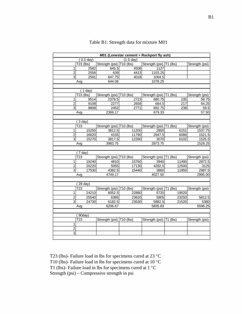
B1

Table B1: Strength data for mixture M01

T23 (lbs)- Failure load in lbs for specimens cured at 23 °C T10 (lbs)- Failure load in lbs for specimens cured at 10 °C T1 (lbs)- Failure load in lbs for specimens cured at 1 °C Strength (psi) – Compressive strength in psi

M01 (Lonestar cement + Rockport fly ash)( 0.5 day) (1.5 day)

T23 (lbs) Strength (psi) T10 (lbs) Strength (psi) T1 (lbs) Strength (psi)1 2582 645.5 4508 11272 2556 639 4413 1103.253 2591 647.75 4018 1004.5

Avg 644.08 1078.25

( 1 day)T23 (lbs) Strength (psi) T10 (lbs) Strength (psi) T1 (lbs) Strength (psi)

1 9514 2378.5 2723 680.75 235 58.752 9108 2277 2658 664.5 217 54.253 9808 2452 2771 692.75 238 59.5

Avg 2369.17 679.33 57.50

( 3 day)T23 Strength (psi) T10 (lbs) Strength (psi) T1 (lbs) Strength (psi)

1 15250 3812.5 11200 2800 6151 1537.752 16620 4155 11790 2947.5 6086 1521.53 15270 3817.5 12280 3070 6102 1525.5

Avg 3983.75 2873.75 1528.25

( 7 day)T23 Strength (psi) T10 (lbs) Strength (psi) T1 (lbs) Strength (psi)

1 19240 4810 15760 3940 11490 2872.52 20220 5055 17130 4282.5 12500 31253 17530 4382.5 15440 3860 11950 2987.5

Avg 4749.17 4027.50 2995.00

( 28 day)T23 Strength (psi) T10 (lbs) Strength (psi) T1 (lbs) Strength (psi)

1 24210 6052.5 22880 5720 190202 25540 6385 23620 5905 23250 5812.53 24730 6182.5 23530 5882.5 21520 5380

Avg 6206.67 5835.83 5596.25

( 90day)T23 Strength (psi) T10 (lbs) Strength (psi) T1 (lbs) Strength (psi)

123

B2

Table B2: Strength data for mixture M02

M02 (Lonestar cement + Clifty creek fly ash)( 0.5 day) (1.5 day)

T23 (lbs) Strength (psi) T10 (lbs) Strength (psi) T1 (lbs) Strength (psi)1 3072 768 5548 13872 2776 694 5086 1271.53 3030 757.5 5638 1409.5

Avg 739.83 1356.00

( 1 day)T23 (lbs) Strength (psi) T10 (lbs) Strength (psi) T1 (lbs) Strength (psi)

1 11900 2975 3513 878.25 259 64.752 11490 2872.5 3644 911 259 64.753 12440 3110 3697 924.25 291 72.75

Avg 2985.83 904.50 67.42

( 3 day)T23 Strength (psi) T10 (lbs) Strength (psi) T1 (lbs) Strength (psi)

1 18590 4647.5 12420 6700 16752 20840 5210 14840 3710 6720 16803 20930 5232.5 15250 3812.5 7048 1762

5030.00 3761.25 1705.67

( 7 day)T23 Strength (psi) T10 (lbs) Strength (psi) T1 (lbs) Strength (psi)

1 22200 5550 20340 5085 14810 3702.52 24200 6050 19590 4897.5 15020 37553 23780 5945 18290 4572.5 14790 3697.5

Avg 5848.33 4851.67 3718.33

( 28 day)T23 Strength (psi) T10 (lbs) Strength (psi) T1 (lbs) Strength (psi)

1 30340 7585 27650 6912.5 23530 5882.52 27570 6892.5 26890 6722.5 25030 6257.53 29470 7367.5 24210 22960 5740

Avg 7281.67 6817.50 5960.00

( 90day)T23 Strength (psi) T10 (lbs) Strength (psi) T1 (lbs) Strength (psi)

123

B3

Table B3: Strength data for mixture M03

M03 (Lonestar cement + Miami Fort fly ash)( 0.5 day) ( 0.5 day)T23 (lbs) Strength (psi) T10 (lbs) Strength (psi) T1 (lbs) Strength (psi)

1 3449 862.25 303 101.002 3334 833.50 272 90.673 3584 896.00 287 95.67

Avg 863.92 95.78

( 1 day)T23 (lbs) Strength (psi) T10 (lbs) Strength (psi) T1 (lbs) Strength (psi)

1 8152 2038 3535 1178.33 641 213.672 8790 2197.5 3408 1136.00 770 256.673 8763 2190.75 2882

Avg 2142.08 1157.17 235.17

( 3 day)T23 Strength (psi) T10 (lbs) Strength (psi) T1 (lbs) Strength (psi)

1 12150 3037.5 11570 2892.5 7537 1884.252 13190 3297.5 11730 2932.5 6465 1616.253 12620 3155 12420 3105 7663 1915.75

Avg 3167.5 2912.50 1805.42

( 7 day)T23 Strength (psi) T10 (lbs) Strength (psi) T1 (lbs) Strength (psi)

1 14440 3610 13820 3455 11810 2952.52 12820 14380 3595 11790 2947.53 14990 3747.5 17080 14140

Avg 3678.75 3525.00 2950.00

( 28 day)T23 Strength (psi) T10 (lbs) Strength (psi) T1 (lbs) Strength (psi)

1 20608 5152 21970 5492.5 20500 51252 20810 5202.5 21890 5472.5 20480 51203 20406 5101.5 22050 5512.5 20460 5115

Avg 5152.00 5492.50 5120.00

( 90day)T23 Strength (psi) T10 (lbs) Strength (psi) T1 (lbs) Strength (psi)

1 25490 22430 5607.5 23960 59902 22940 5735 23510 5877.5 203603 22940 5735 18880 23590 5897.5

Avg 5735.00 5742.50 5943.75

B4

Table B4: Strength data for mixture M04

M04 (Lonestar cement + Will county fly ash)( 0.5 day) ( 0.5 day)T23 (lbs) Strength (psi) T10 (lbs) Strength (psi) T1 (lbs) Strength (psi)

1 2559 639.75 81 20.252 2451 612.75 71 17.753 2513 628.25 56 14

Avg 626.92 17.33

( 1 day)T23 (lbs) Strength (psi) T10 (lbs) Strength (psi) T1 (lbs) Strength (psi)

1 8252 2063 3532 883.00 315 78.752 7903 1975.75 4305 1076.25 270 67.503 8768 2192 3226 806.50 342

Avg 2076.92 921.92 73.13

( 3 day)T23 Strength (psi) T10 (lbs) Strength (psi) T1 (lbs) Strength (psi)

1 13720 3430 11850 6007 1501.752 13460 3365 9174 2293.5 5378 1344.53 14390 3597.5 9068 2267 4561

Avg 3397.5 2293.50 1423.13

( 7 day)T23 Strength (psi) T10 (lbs) Strength (psi) T1 (lbs) Strength (psi)

1 13660 14110 3527.5 12700 31752 15040 3760 14610 3652.5 12120 30303 15880 3970 17590 13175 3293.75

Avg 3865.00 3590.00 3166.25

( 28 day)T23 Strength (psi) T10 (lbs) Strength (psi) T1 (lbs) Strength (psi)

1 19145 4786.25 20480 5120 19800 49502 19145 4786.25 20000 5000 19600 49003 19205 4801.25 20840 5210 19820 4955

Avg 4791.25 5110.00 4935.00

( 90day)T23 Strength (psi) T10 (lbs) Strength (psi) T1 (lbs) Strength (psi)

1 22510 5627.5 24000 6000 20040 50102 22530 5632.5 23320 5830 21650 5412.53 22510 5627.5 22085 5521.25 20070 5017.5

Avg 5629.17 5783.75 5146.67

B5

Table B5: Strength data for mixture M05

M05 (Lehigh cement + Rockport fly ash)( 0.5 day) ( 0.5 day)T23 (lbs) Strength (psi) T10 (lbs) Strength (psi) T1 (lbs) Strength (psi)

1 3004 751 127 31.752 2951 737.75 136 343 2989 747.25 149 37.25

Avg 745.33 34.33

( 1 day)T23 (lbs) Strength (psi) T10 (lbs) Strength (psi) T1 (lbs) Strength (psi)

1 9176 2294 2377 594.25 195 48.752 8315 2078.75 2552 638 209 52.253 8249 2062.25 2555 638.75 206 51.5

Avg 2145.00 623.67 50.83

( 3 day)T23 Strength (psi) T10 (lbs) Strength (psi) T1 (lbs) Strength (psi)

1 13050 3262.5 10160 2540 5582 1395.52 13400 3350 12410 3102.5 5335 1333.753 11320 2830 11020 2755 4809 1202.25

Avg 3147.50 2799.17 1310.50

( 7 day)T23 Strength (psi) T10 (lbs) Strength (psi) T1 (lbs) Strength (psi)

1 16770 4192.5 12930 3232.5 11630 2907.52 16540 4135 13310 3327.5 11360 28403 13520 15120 10810 2702.5

Avg 3902.50 3446.67 2816.67

( 28 day)T23 Strength (psi) T10 (lbs) Strength (psi) T1 (lbs) Strength (psi)

1 20050 5012.5 20590 5147.5 18040 45102 20330 5082.5 19770 4942.5 121003 19250 4812.5 19930 4982.5 18130 4532.5

Avg 4969.167 5024.167 4521.250

( 90day)T23 Strength (psi) T10 (lbs) Strength (psi) T1 (lbs) Strength (psi)

1 21860 5465 25870 6467.5 177302 23440 5860 20430 21310 5327.53 21630 5407.5 24410 6102.5 21790 5447.5

Avg 5577.50 6285 5387.5

B6

Table B6: Strength data for mixture M06

M06 (Lehigh cement + Clifty Creek fly ash)( 0.5 day) (1.5 day)

T23 (lbs) Strength (psi) T10 (lbs) Strength (psi) T1 (lbs) Strength (psi)1 3008 752 6547 1636.752 2975 743.75 6197 1549.253 3141 785.25

Avg 760.33 1593.00

( 1 day)T23 (lbs) Strength (psi) T10 (lbs) Strength (psi) T1 (lbs) Strength (psi)

1 12710 3177.5 2619 654.75 164 412 12920 3230 2551 637.75 175 43.753 13630 2806 701.5 161 40.25

Avg 3203.75 664.67 41.67

( 3 day)T23 Strength (psi) T10 (lbs) Strength (psi) T1 (lbs) Strength (psi)

1 18750 4687.5 14350 3587.5 5891 1472.752 20180 13160 3290 6901 1725.253 18390 4597.5 14040 3510 6436 1609

Avg 4642.50 3462.50 1602.33

( 7 day)T23 Strength (psi) T10 (lbs) Strength (psi) T1 (lbs) Strength (psi)

1 20010 5002.5 17380 4345 14680 36702 19920 4980 19400 4850 14780 36953 21350 5337.5 19690 4922.5 15940 3985

Avg 5106.67 4705.83 3783.33

( 28 day)T23 Strength (psi) T10 (lbs) Strength (psi) T1 (lbs) Strength (psi)

1 27920 6980 26280 6570 22620 56552 28270 7067.5 26010 6502.5 23030 5757.53 28740 7185 26510 6627.5 22280 5570

7077.50 6566.67 5660.83

( 90day)T23 Strength (psi) T10 (lbs) Strength (psi) T1 (lbs) Strength (psi)

123

B7

Table B7: Strength data for mixture M07

M07 (Lehigh cement + Miami Fort fly ash)( 0.5 day) ( 0.5 day)T23 (lbs) Strength (psi) T10 (lbs) Strength (psi) T1 (lbs) Strength (psi)

1 3613 903.25 288 722 3710 927.5 279 69.753 3304 826 276 69

Avg 885.58 70.25

( 1 day)T23 (lbs) Strength (psi) T10 (lbs) Strength (psi) T1 (lbs) Strength (psi)

1 9025 2256.25 2848 712 399 99.752 8491 2122.75 2675 668.75 370 92.53 9083 2270.75 2783 695.75 429 107.25

Avg 2216.58 692.17 99.83

( 3 day)T23 Strength (psi) T10 (lbs) Strength (psi) T1 (lbs) Strength (psi)

1 13830 3457.5 11760 2940 7083 1770.752 14190 3547.5 11550 2887.5 7780 19453 16150 13380 8214 2053.5

Avg 3502.50 2913.75 1923.08

( 7 day)T23 Strength (psi) T10 (lbs) Strength (psi) T1 (lbs) Strength (psi)

1 19590 4897.5 17350 4337.5 141502 19580 4895 18040 4510 12490 3122.53 17190 16400 4100 12000 3000

Avg 4896.25 4315.83 3061.25

( 28 day)T23 Strength (psi) T10 (lbs) Strength (psi) T1 (lbs) Strength (psi)

1 22940 5735 21710 5427.5 19650 4912.52 20670 5167.5 20710 5177.5 20440 51103 22380 5595 19930 4982.5 21240 5310

5499.17 5195.83 5110.83

( 90day)T23 Strength (psi) T10 (lbs) Strength (psi) T1 (lbs) Strength (psi)

1 24330 6082.5 24840 6210 24900 62252 24170 6042.5 24690 6172.5 23240 58103 26660 6665 23740 5935 23010 5752.5

Avg 6263.33 6105.83 5929.17

B8

Table B8: Strength data for mixture M08

M08 (Lehigh cement+ Will County fly ash)( 0.5 day) ( 0.5 day)

T23 (lbs) Strength (psi) T10 (lbs) Strength (psi) T1 (lbs) Strength (psi)1 2629 657.25 65 16.252 2827 706.75 65 16.253 2848 712

Avg 692.00 16.25

( 1 day)T23 (lbs) Strength (psi) T10 (lbs) Strength (psi) T1 (lbs) Strength (psi)

1 12020 3005 2993 748.25 193 48.252 10770 2692.5 2829 707.25 212 533 10700 2675 2872 718 278 69.5

Avg 2790.83 724.50 56.92

( 3 day)T23 Strength (psi) T10 (lbs) Strength (psi) T1 (lbs) Strength (psi)

1 18200 12880 3220 6905 1726.252 15390 3847.5 13280 3320 5546 1386.53 14060 3515 15850 8096 2024

Avg 3681.25 3270.00 1712.25

( 7 day)T23 Strength (psi) T10 (lbs) Strength (psi) T1 (lbs) Strength (psi)

1 19180 4795 17360 4340 12140 30352 19710 4927.5 18760 4690 13170 3292.53 19010 4752.5 17040 4260 13660 3415

Avg 4825.00 4430.00 3247.50

( 28 day)T23 Strength (psi) T10 (lbs) Strength (psi) T1 (lbs) Strength (psi)

1 24770 6192.5 21810 19570 4892.52 22830 23480 5870 17810 4452.53 25630 6407.5 24990 6247.5 19010 4752.5

6300.00 6058.75 4699.17

( 90day)T23 Strength (psi) T10 (lbs) Strength (psi) T1 (lbs) Strength (psi)

1 25490 6372.5 26750 6687.5 25780 64452 27860 6965 26240 6560 25330 6332.53 28280 7070 27630 6907.5

Avg 6802.5 6718.33 6388.75

B9

Table B9: Strength data for mixture M09

M09 (Essroc cement + Rockport fly ash)( 0.5 day) (1.5 day)

T23 (lbs) Strength (psi) T10 (lbs) Strength (psi) T1 (lbs) Strength (psi)1 2097 524.25 3743 935.752 2159 539.75 3703 925.753 2152 538 3857 964.25

Avg 534.00 941.92

( 1 day)T23 (lbs) Strength (psi) T10 (lbs) Strength (psi) T1 (lbs) Strength (psi)

1 10320 2580 2159 539.75 130 32.52 10770 2692.5 2183 545.75 144 363 9374 2343.5 2319 579.75 102 25.5

Avg 2538.67 555.08 31.33

( 3 day)T23 Strength (psi) T10 (lbs) Strength (psi) T1 (lbs) Strength (psi)

1 15940 3985 11350 2837.5 4407 1101.752 16290 4072.5 10960 2740 38693 15540 3885 12240 3060 4651 1162.75

Avg 3980.83 2879.17 1132.25

( 7 day)T23 Strength (psi) T10 (lbs) Strength (psi) T1 (lbs) Strength (psi)

1 17340 4335 15360 3840 11020 27552 15910 3977.5 13860 3465 11250 2812.53 16320 4080 15310 3827.5 12120 3030

Avg 4130.83 3710.83 2865.83

( 28 day)T23 Strength (psi) T10 (lbs) Strength (psi) T1 (lbs) Strength (psi)

1 19290 16000 19330 4832.52 21640 5410 19180 4795 17870 4467.53 22480 5620 19570 4892.5 20040 5010

Avg 5515.00 4843.75 4770.00

( 90day)T23 Strength (psi) T10 (lbs) Strength (psi) T1 (lbs) Strength (psi)

123

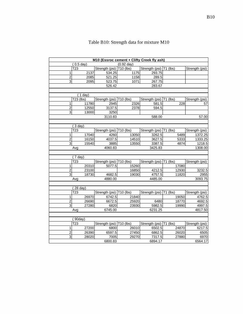
B10

Table B10: Strength data for mixture M10

M10 (Essroc cement + Clifty Creek fly ash)( 0.5 day) (0.92 day)T23 Strength (psi) T10 (lbs) Strength (psi) T1 (lbs) Strength (psi)

1 2137 534.25 1175 293.752 2085 521.25 1158 289.53 2095 523.75 1071 267.75

526.42 283.67

( 1 day)T23 (lbs) Strength (psi) T10 (lbs) Strength (psi) T1 (lbs) Strength (psi)

1 11780 2945 2326 581.5 228 572 12550 3137.5 2378 594.53 13000 3250

3110.83 588.00 57.00

( 3 day)T23 Strength (psi) T10 (lbs) Strength (psi) T1 (lbs) Strength (psi)

1 17040 4260 13050 3262.5 5489 1372.252 16150 4037.5 14510 3627.5 5333 1333.253 15540 3885 13550 3387.5 4874 1218.5

Avg 4060.83 3425.83 1308.00

( 7 day)T23 Strength (psi) T10 (lbs) Strength (psi) T1 (lbs) Strength (psi)

1 20310 5077.5 15260 170802 23100 16850 4212.5 12930 3232.53 18730 4682.5 19030 4757.5 11820 2955

Avg 4880.00 4485.00 3093.75

( 28 day)T23 Strength (psi) T10 (lbs) Strength (psi) T1 (lbs) Strength (psi)

1 26970 6742.5 21840 19050 4762.52 26690 6672.5 25920 6480 18770 4692.53 27280 6820 23930 5982.5 19990 4997.5

Avg 6745.00 6231.25 4817.50

( 90day)T23 Strength (psi) T10 (lbs) Strength (psi) T1 (lbs) Strength (psi)

1 27200 6800 26010 6502.5 24870 6217.52 26390 6597.5 27450 6862.5 26020 65053 28020 7005 29270 7317.5 27880 6970

6800.83 6894.17 6564.17

B11

Table B11: Strength data for mixture M11

M11 (Essroc cement + Miami Fort fly ash)( 0.5 day) ( 0.5 day)T23 (lbs) Strength (psi) T10 (lbs) Strength (psi) T1 (lbs) Strength (psi)

1 2333 583.25 4175 1043.752 2403 600.75 3809 952.253 2536 634 3798 949.5

606 981.83

( 1 day)T23 (lbs) Strength (psi) T10 (lbs) Strength (psi) T1 (lbs) Strength (psi)

1 10350 2587.5 2067 516.75 315 78.752 10560 2640 2109 527.253 10480 2620

Avg 2615.83 522.00 78.75

( 3 day)T23 Strength (psi) T10 (lbs) Strength (psi) T1 (lbs) Strength (psi)

1 13550 3387.5 8390 2097.5 3358 839.52 11200 7715 1928.75 3352 8383 13620 3405 9368 2342 3519 879.75

Avg 3396.25 2122.75 852.42

( 7 day)T23 (lbs) Strength (psi) T10 (lbs) Strength (psi) T1 (lbs) Strength (psi)

1 16090 4022.5 12960 3240 11850 2962.52 17350 4337.5 12530 3132.5 12240 30603 15150 3787.5 14010 3502.5 12040 3010

Avg 4049.17 3291.67 3010.83

( 28 day)T23 (lbs) Strength (psi) T10 (lbs) Strength (psi) T1 (lbs) Strength (psi)

1 21190 5297.5 19120 4780 19130 4782.52 21370 5342.5 21010 5252.5 17280 43203 21970 5492.5 21410 5352.5 17580 4395

5377.5 5128.33 4499.17

( 90day)T23 (lbs) Strength (psi) T10 (lbs) Strength (psi) T1 (lbs) Strength (psi)

1 23590 5897.5 20160 5040 21830 5457.52 25370 6342.5 23140 5785 22080 55203 24740 6185 21450 5362.5 21370 5342.5

Avg 6141.67 5395.83 5440.00

B12

Table B12: Strength data for mixture M12

M12 (Essroc cement + Will County fly ash)( 0.5 day) (1.5 day)T23 Strength (psi) T10 (lbs) Strength (psi) T1 (lbs) Strength (psi)

1 1460 365 3089 772.252 1555 388.75 3166 791.53 1563 390.75 3390 847.5

Avg 381.5 803.75

( 1 day)T23 (lbs) Strength (psi) T10 (lbs) Strength (psi) T1 (lbs) Strength (psi)

1 11230 2807.5 3589 897.25 323 80.752 11480 2870 3843 960.75 387 96.753 10580 2645 3838 959.5 377 94.25

Avg 2774.17 939.17 90.582193.75 494 23

( 3 day)T23 Strength (psi) T10 (lbs) Strength (psi) T1 (lbs) Strength (psi)

1 19250 4812.5 14910 3727.5 7981 1995.252 18200 4550 15340 3835 8204 20513 18520 4630 13790 3447.5 6847

Avg 4664.17 3670.00 2023.133792.5 3297.5 1373

( 7 day)T23 Strength (psi) T10 (lbs) Strength (psi) T1 (lbs) Strength (psi)

1 19010 4752.5 21800 5450 15810 3952.52 21620 5405 16480 41203 20250 5062.5 22200 5550 16600 4150

Avg 4907.50 5468.33 4074.175017.5 4960 3717.5

( 28 day)T23 Strength (psi) T10 (lbs) Strength (psi) T1 (lbs) Strength (psi)

1 23420 5855 25990 6497.5 23560 58902 22710 5677.5 19280 22290 5572.53 22990 5747.5 25710 6427.5 24320 6080

Avg 5760 6462.5 5847.5

( 90day)T23 Strength (psi) T10 (lbs) Strength (psi) T1 (lbs) Strength (psi)

1 24790 6197.5 26530 6632.5 26910 6727.52 27110 6777.5 28230 7057.5 26210 6552.53 26740 6685 23160 27150 6787.5

Avg 6553.33 6845.00 6689.17

B13

Table B13: Strength data for mixture M13

M13 (Lonestar cement-Type I)( 0.5 day) (1.5 day)

T23 (lbs) Strength (psi) T10 (lbs) Strength (psi) T1 (lbs) Strength (psi)1 4692 1173 6877 1719.252 4722 1180.5 6741 1685.253 4359 1089.75 6744 1686

Avg 1147.75 1696.83

( 1 day)T23 (lbs) Strength (psi) T10 (lbs) Strength (psi) T1 (lbs) Strength (psi)

1 12110 5767 1441.75 1154 288.52 14230 3557.5 5896 1474 1033 258.253 13580 3395 5793 1448.25 1026 256.5

Avg 3476.25 1454.67 267.75

(3 day)T23 (lbs) Strength (psi) T10 (lbs) Strength (psi) T1 (lbs) Strength (psi)

1 18930 4732.5 15360 3840 89932 17180 4295 16700 4175 10720 26803 17940 4485 16770 4192.5 9728 2432

Avg 4504.17 4069.17 2556.00

( 7 day)T23 (lbs) Strength (psi) T10 (lbs) Strength (psi) T1 (lbs) Strength (psi)

1 23840 21870 5467.5 15540 38852 20680 5170 18430 4607.5 16760 41903 22520 5630 21050 5262.5 16220 4055

Avg 5400.00 5112.50 4043.33

( 28 day)T23 (lbs) Strength (psi) T10 (lbs) Strength (psi) T1 (lbs) Strength (psi)

1 23770 5942.5 23260 5815 23290 5822.52 22030 5507.5 24590 6147.5 24970 6242.53 22210 5552.5 21490 5372.5 24370 6092.5

Avg 5667.5 5778.33 6052.50

( 90 day)T23 (lbs) Strength (psi) T10 (lbs) Strength (psi) T1 (lbs) Strength (psi)

1 24460 6115 28370 7092.5 26660 66652 24000 6000 28320 7080 27580 68953 25410 6352.5 27460 6865 27460 6865

Avg 6155.83 7012.50 6808.33

B14

Table B14: Strength data for mixture M14

M14 (Lehigh cement-Type I/II)( 0.5 day) (1.5 day)

T23 (lbs) Strength (psi) T10 (lbs) Strength (psi) T1 (lbs) Strength (psi)1 5017 1254.25 8180 20452 4776 1194 8086 2021.53 4792 1198 8215 2053.75

Avg 1215.42 2040.08

( 1 day)T23 (lbs) Strength (psi) T10 (lbs) Strength (psi) T1 (lbs) Strength (psi)

1 15620 3905 5633 1408.25 1080 2702 18260 6412 1603 1128 2823 16480 4120 5528 1382 1120 280

Avg 4012.50 1464.42 277.33

(3 day)T23 (lbs) Strength (psi) T10 (lbs) Strength (psi) T1 (lbs) Strength (psi)

1 21480 5370 20620 5155 12020 30052 16290 19670 4917.5 12500 31253 20960 5240 20750 5187.5 13270 3317.5

Avg 5305.00 5086.67 3149.17

( 7 day)T23 (lbs) Strength (psi) T10 (lbs) Strength (psi) T1 (lbs) Strength (psi)

1 22730 5682.5 22820 5705 22140 55352 23450 5862.5 20980 5245 18600 46503 22710 5677.5 23550 5887.5 21780 5445

Avg 5740.83 5612.50 5210.00

( 28 day)T23 (lbs) Strength (psi) T10 (lbs) Strength (psi) T1 (lbs) Strength (psi)

1 27190 6797.5 27410 6852.5 24490 6122.52 26970 6742.5 27190 6797.5 24900 62253 24650 28490 7122.5 27780 6945

Avg 6770 6924.17 6430.83

( 90 day)T23 (lbs) Strength (psi) T10 (lbs) Strength (psi) T1 (lbs) Strength (psi)

1 28650 7162.5 30760 7690 29000 72502 29150 7287.5 28000 7000 28360 70903 30630 7657.5 27760 6940 28680 7170

Avg 7369.17 7210.00 7170.00

B15

Table B15: Strength data for mixture M15

M15 (Essroc cement-TypeI)( 0.5 day) (1.5 day)

T23 (lbs) Strength (psi) T10 (lbs) Strength (psi) T1 (lbs) Strength (psi)1 4337 1084.25 6651 1662.752 4686 1171.5 6830 1707.53 4592 1148 6618 1654.5

Avg 1134.58 1674.92

( 1 day)T23 (lbs) Strength (psi) T10 (lbs) Strength (psi) T1 (lbs) Strength (psi)

1 15320 3830 4673 1168.25 516 1292 14040 3510 5002 1250.5 512 1283 16210 4052.5 5192 1298 576 144

Avg 3797.50 1238.92 133.67

(3 day)T23 (lbs) Strength (psi) T10 (lbs) Strength (psi) T1 (lbs) Strength (psi)

1 19850 4962.5 13560 120002 18570 4642.5 16270 4067.5 9727 2431.753 19180 4795 16820 4205 10230 2557.5

Avg 4800.00 4136.25 2494.63

( 7 day)T23 (lbs) Strength (psi) T10 (lbs) Strength (psi) T1 (lbs) Strength (psi)

1 22460 5615 21360 5340 20350 5087.52 23020 5755 19380 4845 175103 19960 21650 5412.5 19860 4965

Avg 5685.00 5199.17 5026.25

( 28 day)T23 (lbs) Strength (psi) T10 (lbs) Strength (psi) T1 (lbs) Strength (psi)

1 24510 6127.5 27060 6765 26110 6527.52 26710 6677.5 28680 7170 25840 64603 24350 6087.5 27560 6890 26500 6625

Avg 6297.50 6941.67 6537.50

( 90 day)T23 (lbs) Strength (psi) T10 (lbs) Strength (psi) T1 (lbs) Strength (psi)

1 26600 6650 30160 7540 30440 76102 27150 6787.5 33060 31820 79553 25460 6365 31800 7950 30770 7692.5

Avg 6600.83 7745.00 7752.50

B16

Table B16: Strength data for mixture M16

M16 (Lonestar cement-Type III)( 0.5 day) (0.5 day)

T23 (lbs) Strength (psi) T10 (lbs) Strength (psi) T1 (lbs) Strength (psi)1 10660 2665 1509 377.252 10470 2617.5 1437 359.253 10680 2670 1539 384.75

Avg 2650.83 373.75

( 1 day)T23 (lbs) Strength (psi) T10 (lbs) Strength (psi) T1 (lbs) Strength (psi)

1 18240 4560 10000 2500 3486 871.52 19200 4800 9700 2425 4053 1013.253 19000 4750 9559 2389.75

Avg 4703.33 2438.25 942.38

(3 day)T23 (lbs) Strength (psi) T10 (lbs) Strength (psi) T1 (lbs) Strength (psi)

1 24610 22680 5670 137802 23640 5910 26360 15640 39103 23750 5937.5 22020 5505 16290 4072.5

Avg 5923.75 5587.50 3991.25

( 7 day)T23 (lbs) Strength (psi) T10 (lbs) Strength (psi) T1 (lbs) Strength (psi)

1 25810 6452.5 24800 6200 23000 57502 26320 6580 24550 6137.5 23200 58003 23540 24450 6112.5 22800 5700

Avg 6516.25 6150.00 5750.00

( 28 day)T23 (lbs) Strength (psi) T10 (lbs) Strength (psi) T1 (lbs) Strength (psi)

1 29820 7455 35100 28760 71902 29040 7260 30860 7715 28370 7092.53 31360 7840 30600 7650 30490 7622.5

Avg 7518.33 7682.50 7301.67

( 90 day)T23 (lbs) Strength (psi) T10 (lbs) Strength (psi) T1 (lbs) Strength (psi)

1 32240 8060 34040 8510 33590 8397.52 32570 8142.5 30590 35990 8997.53 32760 8190 34130 8532.5 33320 8330

Avg 8130.83 8521.25 8575.00

B17

Table B17: Strength data for mixture M17

M17 (Lonestar cement-TypeIII + Rockport fly ash)( 0.5 day) ( 0.5 day)T23 Strength (psi) T10 (lbs) Strength (psi) T1 (lbs) Strength (psi)

1 6889 1722.25 440 1102 6892 1723 433 108.253 6726 1681.5

Avg 1708.92 109.13

( 1 day)T23 (lbs) Strength (psi) T10 (lbs) Strength (psi) T1 (lbs) Strength (psi)

1 17960 4490 6620 1655 811 202.752 16260 4065 7130 1782.5 825 206.253 15480 3870 6687 1671.75 825 206.25

Avg 4141.67 1703.08 205.08

( 3 day)T23 Strength (psi) T10 (lbs) Strength (psi) T1 (lbs) Strength (psi)

1 21150 5287.5 16390 4097.5 10710 2677.52 20760 5190 18220 10940 27353 22310 5577.5 15990 3997.5 11050 2762.5

Avg 5351.67 4047.50 2725.00

( 7 day)T23 Strength (psi) T10 (lbs) Strength (psi) T1 (lbs) Strength (psi)

1 23220 5805 19920 4980 17630 4407.52 22110 5527.5 22780 17840 44603 23720 5930 20930 5232.5 16530 4132.5

Avg 5754.17 5106.25 4333.33

( 28 day)T23 Strength (psi) T10 (lbs) Strength (psi) T1 (lbs) Strength (psi)

1 30600 7650 28590 7147.5 26650 6662.52 31120 7780 27790 6947.5 26950 6737.53 26390 26270 6567.5 26660 6665

Avg 7715 6887.50 6688.33

( 90day)T23 Strength (psi) T10 (lbs) Strength (psi) T1 (lbs) Strength (psi)

123

B18

Table B18: Strength data for mixture M18

M18 (Lonestar cement -TypeIII + Clifty Creek fly ash)( 0.5 day) ( 0.5 day)T23 (lbs) Strength (psi) T10 (lbs) Strength (psi) T1 (lbs) Strength (psi)

1 7712 1928 540 1352 7815 1953.75 513 128.253 8305 2076.25 523 130.75

Avg 1986.00 131.33

( 1 day)T23 (lbs) Strength (psi) T10 (lbs) Strength (psi) T1 (lbs) Strength (psi)

1 17590 4397.5 9532 2383 800 2002 18660 4665 8988 2247 800 2003 16380 4095 9180 2295

Avg 4385.83 2308.33 200.00

( 3 day)T23 (lbs) Strength (psi) T10 (lbs) Strength (psi) T1 (lbs) Strength (psi)

1 24450 6112.5 18400 4600 14500 36252 22700 5675 17880 4470 14200 35503 23510 5877.5 19590 4897.5 13300 3325

Avg 5888.33 4655.83 3500.00

( 7 day)T23 (lbs) Strength (psi) T10 (lbs) Strength (psi) T1 (lbs) Strength (psi)

1 28810 7202.5 25930 6482.5 20200 50502 28310 7077.5 26540 6635 19950 4987.53 27610 6902.5 26380 6595 19850 4962.5

Avg 7060.83 6570.83 5000.00

( 28 day)T23 (lbs) Strength (psi) T10 (lbs) Strength (psi) T1 (lbs) Strength (psi)

1 31870 7967.5 29100 7275 28480 71202 33710 8427.5 27720 6930 28070 7017.53 24350 32510 29390

Avg 8197.50 7102.50 7068.75

( 90day)T23 Strength (psi) T10 (lbs) Strength (psi) T1 (lbs) Strength (psi)

123

B19

Table B19: Strength data for mixture M19

M19 (Lonestar cement-TypeIII + Miami Fort fly ash)( 0.5 day) ( 0.5 day)T23 (lbs) Strength (psi) T10 (lbs) Strength (psi) T1 (lbs) Strength (psi)

1 7211 1802.75 573 143.252 6311 585 146.253 6914 1728.5 591 147.75

Avg 1765.63 145.75

( 1 day)T23 (lbs) Strength (psi) T10 (lbs) Strength (psi) T1 (lbs) Strength (psi)

1 15980 3995 7532 1883 1329 332.252 14990 3747.5 7010 1752.5 1439 359.753 16340 4085 7841 1960.25 1308 327

Avg 3942.50 1865.25 339.67

( 3 day)T23 (lbs) Strength (psi) T10 (lbs) Strength (psi) T1 (lbs) Strength (psi)

1 23270 5817.5 20390 5097.5 12200 30502 24150 6037.5 20080 5020 11360 28403 22010 5502.5 18970 4742.5 11750 2937.5

Avg 5785.83 4953.33 2942.50

( 7 day)T23 (lbs) Strength (psi) T10 (lbs) Strength (psi) T1 (lbs) Strength (psi)

1 24270 6067.5 24970 6242.5 17160 42902 22780 5695 22520 5630 19100 47753 22960 5740 24490 6122.5 19700 4925

Avg 5834.17 5998.33 4663.33

( 28 day)T23 (lbs) Strength (psi) T10 (lbs) Strength (psi) T1 (lbs) Strength (psi)

1 28080 7020 29640 7410 27730 6932.52 26460 29820 7455 26130 6532.53 28240 7060 28750 7187.5 27580 6895

7040 7350.83 6786.67

( 90day)T23 Strength (psi) T10 (lbs) Strength (psi) T1 (lbs) Strength (psi)

123

B20

Table B20: Strength data for mixture M20

M20 (Lonestar cement-TypeIII +Will county fly ash)( 0.5 day) ( 0.5 day)T23 Strength (psi) T10 (lbs) Strength (psi) T1 (lbs) Strength (psi)

1 7146 1786.5 372 932 7541 1885.25 405 101.253 6906 1726.5 411 102.75

Avg 1799.42 99.00

( 1 day)T23 (lbs) Strength (psi) T10 (lbs) Strength (psi) T1 (lbs) Strength (psi)

1 15320 3830 6927 1731.75 824 2062 15400 3850 7061 1765.25 821 205.253 16170 4042.5 7203 1800.75 855 213.75

Avg 3907.50 1765.92 208.33

( 3 day)T23 Strength (psi) T10 (lbs) Strength (psi) T1 (lbs) Strength (psi)

1 19650 4912.5 18750 4687.5 12200 30502 20220 5055 18910 4727.5 12470 3117.53 20490 5122.5 18870 4717.5 10940 2735

Avg 5030.00 4710.83 2967.50

( 7 day)T23 Strength (psi) T10 (lbs) Strength (psi) T1 (lbs) Strength (psi)

1 23230 5807.5 23340 5835 20790 5197.52 25300 6325 23610 5902.5 21620 54053 22350 5587.5 26750 21570 5392.5

5906.67 5868.75 5331.67

( 28 day)T23 Strength (psi) T10 (lbs) Strength (psi) T1 (lbs) Strength (psi)

1 28950 7237.5 27070 6767.5 27020 67552 26360 6590 29710 7427.5 28480 71203 26720 6680 24180 30460 7615

6835.83 7097.50 7163.33

( 90day)T23 Strength (psi) T10 (lbs) Strength (psi) T1 (lbs) Strength (psi)

123

B21

Table B21: Strength data for mixture M21

M21 (Lonestar cement + Holnam slag)( 0.5 day) 0.94 dayT23 (lbs) Strength (psi) T10 (lbs) Strength (psi) T1 (lbs) Strength (psi)

1 3886 971.5 2530 632.52 4091 1022.75 2551 637.753 4130 1032.5 2661 665.25

Avg 1008.92 645.17

( 1 day)T23 (lbs) Strength (psi) T10 (lbs) Strength (psi) T1 (lbs) Strength (psi)

1 11360 2840 4724 1181 965 241.252 10180 2545 4666 1166.5 956 2393 11480 2870 4829 1207.25 908 227

Avg 2751.67 1184.92 235.75

( 3 day)T23 (lbs) Strength (psi) T10 (lbs) Strength (psi) T1 (lbs) Strength (psi)

1 17890 4472.5 13260 3315 8068 20172 17910 4477.5 12370 3092.5 8224 20563 18060 4515 14200 8025 2006.25

Avg 4488.33 3203.75 2026.42

( 7 day)T23 (lbs) Strength (psi) T10 (lbs) Strength (psi) T1 (lbs) Strength (psi)

1 23030 5757.5 17660 4415 14630 3657.52 23680 5920 18550 4637.5 14210 3552.53 22330 5582.5 18780 4695 14330 3582.5

Avg 5753.33 4582.50 3597.50

( 28 day)T23 (lbs) Strength (psi) T10 (lbs) Strength (psi) T1 (lbs) Strength (psi)

1 28620 7155 28280 7070 21270 5317.52 25820 6455 27380 6845 23010 5752.53 27440 6860 27520 6880 22760 5690

Avg 6823.33 6931.67 5586.67

( 90day)T23 (lbs) Strength (psi) T10 (lbs) Strength (psi) T1 (lbs) Strength (psi)

1 28880 7220 28670 7167.5 29170 7292.52 30000 7500 30450 7612.5 27300 68253 29940 7485 29150 7287.5

Avg 7401.67 7355.83 7058.75

B22

Table B22: Strength data for mixture M22

M22 (Lehigh cement + Holnam slag)( 0.5 day) (0.93 day)

T23 (lbs) Strength (psi) T10 (lbs) Strength (psi) T1 (lbs) Strength (psi)1 4201 1050.25 2092 5232 4036 1009 2305 576.253 4307 1076.75 2322 580.5

Avg 1045.33 559.92

( 1 day)T23 (lbs) Strength (psi) T10 (lbs) Strength (psi) T1 (lbs) Strength (psi)

1 11070 2767.5 3595 898.75 353 88.252 11150 2787.5 3488 872 313 78.253 9724 2431 3403 850.75 397 99.25

Avg 2662.00 873.83 88.58

( 3 day)T23 (lbs) Strength (psi) T10 (lbs) Strength (psi) T1 (lbs) Strength (psi)

1 17870 4467.5 10490 2622.5 7102 1775.52 18850 4712.5 10910 2727.5 7215 1803.753 19170 4792.5 12260 6501 1625.25

Avg 4657.50 2675.00 1734.83

( 7 day)T23 (lbs) Strength (psi) T10 (lbs) Strength (psi) T1 (lbs) Strength (psi)

1 20850 5212.5 16870 4217.5 12750 3187.52 21310 5327.5 17450 4362.5 12770 3192.53 21670 5417.5 17960 4490 11810 2952.5

Avg 5319.17 4356.67 3110.83

( 28 day)T23 (lbs) Strength (psi) T10 (lbs) Strength (psi) T1 (lbs) Strength (psi)

1 30600 7650 23150 5787.5 20740 51852 30790 7697.5 24670 6167.5 19340 48353 30420 7605 24690 6172.5 21420 5355

Avg 7650.83 6042.50 5125.00

( 90day)T23 (lbs) Strength (psi) T10 (lbs) Strength (psi) T1 (lbs) Strength (psi)

123

Avg

B23

Table B23: Strength data for mixture M23

M23 (Essroc cement + Holnam slag)( 0.5 day) (0.94 day)T23 (lbs) Strength (psi) T10 (lbs) Strength (psi) T1 (lbs) Strength (psi)

1 3309 827.25 1890 472.52 2999 749.75 1858 464.53 3373 843.25 1952 488

Avg 806.75 475.00

( 1 day)T23 (lbs) Strength (psi) T10 (lbs) Strength (psi) T1 (lbs) Strength (psi)

1 9333 2333.25 2620 655 409 102.252 8083 2020.75 2784 696 419 104.753 8971 2242.75 2699 674.75 406 101.5

Avg 2198.92 675.25 102.83

( 3 day)T23 Strength (psi) T10 (lbs) Strength (psi) T1 (lbs) Strength (psi)

1 15560 3890 11960 2990 5283 1320.752 15890 3972.5 12400 3100 5589 1397.253 15010 3752.5 11830 5733 1433.25

Avg 3871.67 3045.00 1383.75

( 7 day)T23 Strength (psi) T10 (lbs) Strength (psi) T1 (lbs) Strength (psi)

1 20930 5232.5 16020 4005 12530 3132.52 21700 5425 16990 4247.5 11290 2822.53 20630 5157.5 17510 4377.5 11650 2912.5

Avg 5271.67 4210.00 2955.83

( 28 day)T23 Strength (psi) T10 (lbs) Strength (psi) T1 (lbs) Strength (psi)

1 24820 6205 24130 6032.5 21210 5302.52 26780 6695 23450 5862.5 18920 47303 22270 23930 5982.5 20880 5220

Avg 6450.00 5959.17 5084.17

( 90day)T23 Strength (psi) T10 (lbs) Strength (psi) T1 (lbs) Strength (psi)

123

Avg

B24

Table B24: Strength data for mixture M24

M24 (Lonestar cement - Type III + Holnam slag)

( 0.5 day) ( 0.5 day)T23 (lbs) Strength (psi) T10 (lbs) Strength (psi) T1 (lbs) Strength (psi)

1 8104 2026 1159 289.752 8106 2026.5 1177 294.253 8039 2009.75 1154 288.5

Avg 2020.75 290.83

( 1 day)T23 (lbs) Strength (psi) T10 (lbs) Strength (psi) T1 (lbs) Strength (psi)

1 16590 4147.5 9257 2314.25 2052 5132 16470 4117.5 8594 2148.5 2070 517.53 15010 3752.5 8758 2189.5 2062 515.5

Avg 4005.83 2217.42 515.33

( 3 day)T23 Strength (psi) T10 (lbs) Strength (psi) T1 (lbs) Strength (psi)

1 23320 5830 17360 4340 13310 3327.52 22460 5615 17550 4387.5 12610 3152.53 22560 5640 17980 4495 12370 3092.5

Avg 5695.00 4407.50 3190.83

( 7 day)T23 Strength (psi) T10 (lbs) Strength (psi) T1 (lbs) Strength (psi)

1 25950 6487.5 24360 6090 18270 4567.52 27570 6892.5 24450 6112.5 17690 4422.53 26030 6507.5 22400 18560 4640

Avg 6629.17 6101.25 4543.33

( 28 day)T23 Strength (psi) T10 (lbs) Strength (psi) T1 (lbs) Strength (psi)

1 31800 7950 30600 7650 27330 6832.52 33050 8262.5 31400 7850 26050 6512.53 30380 7595 29290 7322.5 27010 6752.5

Avg 7935.83 7607.50 6699.17

( 90day)T23 Strength (psi) T10 (lbs) Strength (psi) T1 (lbs) Strength (psi)

123

Avg

APPENDIX C - PICTURES OF SCALED SURFACES

C1

Table C1: Conditioning periods for concrete slabs subjected to salt scaling tests

Conditioning3 & 4 7 & 8 CC1 & CC2 CC5 & CC6

Drying (20 oC @ 50 % RH) 3 days 14 days 3 days 14 days

Specimen No.

Moist Curing (21oC @ 100 % RH) 3 days 14 days 3 days 14 days

C2

Figure C1: C01 (Lonestar cement) conditioned for 6 days

Figure C2: C02 (Lonestar cement + Rockport fly ash) conditioned for 6 days

C3

Figure C3: C03 (Lonestar cement + slag) conditioned for 6 days

Figure C4: C04 (Lehigh cement + Rockport fly ash) conditioned for 6 days

C4

Figure C5: C05 (Lehigh cement + Miami Fort fly ash) conditioned for 6 days

Figure C6: C06 (Essroc cement + Clifty Creek fly ash) conditioned for 6 days

C5

Figure C7: C01 (Lonestar cement) conditioned for 28 days

Figure C8: C02 (Lonestar cement + Rockport fly ash) conditioned for 28 days

C6

Figure C9: C03 (Lonestar cement + slag) conditioned for 28 days

Figure C10: C04 (Lehigh cement + Rockport fly ash) conditioned for 28 days

C7

Figure C11: C05 (Lehigh cement + Miami Fort fly ash) conditioned for 28 days

Figure C12: C06 (Essroc cement + Clifty Creek fly ash) conditioned for 28 days

C8

Figure C13: C01 (Lonestar cement) with curing compound conditioned for 6 days

Figure C14: C02 (Lonestar cement + Rockport fly ash) with curing compound conditioned for 6 days

C9

Figure C15: C03 (Lonestar cement + slag) with curing compound conditioned for 6 days

Figure C16: C04 (Lehigh cement + Rockport fly ash) with curing compound conditioned for 6 days

C10

Figure C17: C05 (Lehigh cement + Miami Fort fly ash) with curing compound conditioned for 6 days

Figure C18: C06 (Essroc cement + Clifty Creek fly ash) with curing compound conditioned for 6 days

C11

Figure C19: C01 (Lonestar cement) with curing compound conditioned for 28 days

Figure C20: C02 (Lonestar cement + Rockport fly ash) with curing compound conditioned for 28 days

C12

Figure C21: C03 (Lonestar cement + slag) with curing compound conditioned for 28 days

Figure C22: C04 (Lehigh cement + Rockport fly ash) with curing compound conditioned for 28 days

C13

Figure C23: C05 (Lehigh cement + Miami Fort fly ash) with curing compound conditioned for 28 days

Figure C24: C06 (Essroc cement + Clifty Creek fly ash) with curing compound conditioned for 28 days