Team Incentives and Bonus Floors in Relational

Contracts1

Jonathan Glover, Columbia University, Graduate School of Business

Hao Xue, New York University, Stern School of Business

February 26, 2018

1We thank Anil Arya, Tim Baldenius, Jeremy Bertomeu, Wouter Dessein, Marina Halac, JackHughes, Xiaojing Meng, Brian Mittendorf, Madhav Rajan, Stefan Reichelstein, and seminar partic-ipants at Ohio State, UCLA, Purdue, and Rutgers for helpful comments.

Abstract

“Team Incentives and Bonus Floors in Relational Contracts”

A common means of incorporating non-verifiable performance measures in compensation con-

tracts is via bonus pools. We study a principal-multi-agent relational contracting model in

which the optimal contract resembles a bonus pool. It specifies a minimum joint bonus floor

the principal is required to pay out to the agents and gives the principal discretion to use

non-verifiable performance measures to both increase the size of the pool and to allocate the

pool to the agents. The joint bonus floor is useful because of its role in motivating the agents

to mutually monitor each other (team incentives). In an extension section, we introduce a ver-

ifiable team performance measure. The broader message that emerges is that “paying for poor

performance” – either verifiable team performance or non-verifiable individual performance –

can be optimal in a relational (self-enforcing) contracting setting because it creates the trust

needed for the principal to tailor other promised payments to motivate mutual monitoring.

1 Introduction

This paper studies discretionary rewards based on non-verifiable performance measures. A

concern about discretionary rewards is that the evaluator must be trusted by the evaluatees

(Anthony and Govindarajan, 1998). In a single-period model, bonus pools are a natural

economic solution to the “trust” problem (MacLeod, 2003; Baiman and Rajan, 1995; Rajan

and Reichelstein, 2006; 2009; Ederhof, 2010). A bonus pool can be seen as a special case of a

relational contract. While explicit contracts are enforced by the courts, a relational (implicit)

contract must be self-enforcing. In a multi-period setting, relational contracts can be enforced

by threats of retaliation by one party when the other(s) renege on their promises (MacLeod

and Malcomson, 1989). In a single-period setting with multiple agents, the only self-enforcing

contract is a bonus pool, which leaves the principal discretion only in allocating the fixed pool

to the agents.

We study a multi-period relational contracting model in which the optimal contract resem-

bles a bonus pool with added discretion to increase the size of the bonus pool. It specifies a

minimum joint bonus (hereafter bonus floor) the principal is required to pay out to the agents

and gives the principal discretion to use non-verifiable performance measures to both increase

the size of the pool and to allocate the pool to the agents. Such discretion is fairly common

in practice. As an example, Gibbons and Henderson (2013) analyze the bonus pay at Lincoln

Electric. They find that the board of Lincoln Electric has complete discretion both in setting

the size of the firm-wide bonus and in determining individual payouts based on its subjective

evaluation of individual contributions such as ideas and cooperation. Similar discretion is

common in Wall Street firms as well.1 Empirically, Murphy and Oyer (2003) find that 42%

of their sample of 262 firms gave the compensation committee discretion in determining the

size of the executive bonus pool, while 70% had discretion in allocating the bonus pool to

individual executives.2 The related theoretical literature on bonus pools typically uses the

1See, for example, UBS Group AG 2015 Compensation Report and Eccles and Crane (1988).2For evidence on discretion in individual bonus plans, see Bushman, Indjejikian, and Smith (1996).

1

term bonus pool for bonus pools with a non-discretionary total payout, while our focus is

on repeated play and the role of trust in facilitating discretion in determining the size of the

bonus pool.

Our multi-period relationship not only facilitates trust between the principal and the

agents, it also creates the possibility of trust between the agents and, hence, opportunities

for relational contracts between the agents. Understanding the nature of relational contracts

between the agents is important because teamwork and team incentives are becoming increas-

ingly prevalent in modern organizations (Deloitte, 2016). Hamilton Nickerson, and Owan

(2003) study a manufacturing company and find that the introduction of team production

and team-based incentive pay significantly increase productivity. They interpret their ev-

idence as suggesting that mutual monitoring among the team members contributes to the

increases in productivity. Similarly, Knez and Simester (2001) examine the introduction of

team-based compensation system at Continental Airlines established in 1995. They find evi-

dence consistent with the argument that the use of teams at the firm increased the extent of

mutual monitoring, which improves the company’s on-time performance. Knez and Simester

also present anecdotal evidence of workers punishing each other for shirking as a way to sustain

team incentives.

The demand for mutual monitoring using relational contracts in our model is similar to

Arya, Fellingham, and Glover (1997) and Che and Yoo (2001).3 The agents work closely

enough that they observe each other’s actions, while the principal observes only individual

performance measures that imperfectly capture those actions. The key idea in those papers is

to replace the agents’ Nash incentive constraints with group incentive constraints. As Milgrom

and Roberts (1992, p. 416) write: “[g]roups of workers often have much better information

about their individual contributions than the employer is able to gather...[g]roup incentives

3There is an earlier related literature that assumes the agents can write explicit side-contracts with eachother (e.g., Tirole, 1986; Itoh, 1993). Itoh’s (1993) model of explicit side-contracting can be viewed as anabstraction of the implicit side-contracting that was later modeled by Arya, Fellingham, and Glover (1997)and Che and Yoo (2001). As Tirole (1992), writes: “[i]f, as is often the case, repeated interaction is indeedwhat enforces side contracts, the second approach [of modeling repeated interactions] is clearly preferablebecause it is more fundamentalist.”

2

then motivate the employees to monitor one another and to encourage effort provision.”

When organizations focus on team performance, they evaluate employees using different

metrics. For instance, Cisco, General Electric, and Google have invested substantially to

transform their performance evaluation systems from evaluating an individual employee’s

performance to gauging how effectively employees contribute to their teams (Deloitte, 2017).

Individual’s contributions to the team are often non-verifiable. (Gibbons and Henderson 2013

present examples of non-verifiable performance measures in both blue-color and white-color

settings.) By definition, non-verifiable measures cannot be explicated contracted on.

This paper studies relational contracts between a principal and two agents based on non-

verifiable performance measures in an infinitely repeated relationship. The non-verifiable

performance measures in our model can be interpreted as the principal’s imperfect assessment

of each agent’s contribution to the team. To analyze the relational contracts in the most

tractable setting, our main model does not include any verifiable performance measures (e.g.,

group, divisional, or firm-wide earnings). (We introduce such a verifiable measure as an

extension in Section 5.)

All players in our model share the same expected contracting horizon (discount rate).

Nevertheless, the players may differ in their relative credibility because of other features of the

model such as the loss to the principal of forgone productivity. In determining the optimal

incentive arrangement, both the common discount rate and the relative credibility of the

principal and the agents are important. In particular, when the principal’s ability to commit

is strong, the optimal contract emphasizes team incentives. Joint performance evaluation

(JPE ), which rewards the agents when both are judged to have supplied high effort, emerges

as an optimal means of setting the stage for the agents to mutually monitor each other. JPE

provides the agents with incentives to monitor each other and a means of disciplining each

other by creating a punishing equilibrium – a stage game (one shot) equilibrium with lower

payoffs than the agents obtain on the equilibrium path. As the principal’s reneging constraint

becomes a binding constraint, rewarding joint poor performance via a positive bonus floor can

3

be optimal because it helps the principal maintain a strategic complementarity in the agents’

payoffs, which is efficient in providing incentives for mutual monitoring.4 The alternative is

to use relative performance evaluation (RPE) to partially replace mutual monitoring/team

incentives with individual incentives.5 The problem with RPE is that it undermines mutual

monitoring by reducing the strategic complementarity in the agents’ payoffs. Therefore, if the

principal attempts to replace team incentives with individual incentives using RPE when her

credibility is limited, even more individual incentives are needed to makeup for the reduced

team incentives.

Discretionary increases to bonus pools are considerably more common than discretionary

decreases (Murphy and Oyer, 2006). A common criticism of this asymmetric treatment is that

managers get their bonuses too often – “pay for pulse” rather than “pay for performance.”

Our results suggest a different interpretation. Using a floor and allowing for discretionary

increases but not discretionary decreases can be optimal as part of an incentive structure that

fosters mutual monitoring/team incentives.

Mutual monitoring/team incentives are not always optimal (or even feasible). When in-

dividual rather than team incentives are optimal, the principal would use RPE if she did not

have to prevent tacit collusion between the agents. The unappealing feature of RPE is that

it creates a strategic substitutability in the agents’ payoffs that encourages them to collude

on an undesirable equilibrium that has them alternating between (work, shirk) and (shirk,

work).6 (We use the term mutual monitoring to refer to relational contracts that benefit

the principal and collusion to refer to the relational contracts between the agents that harm

the principal.) The collusion threat is severe if the agents’ ability to commit is strong, in

which case paying for poor performance via a bonus floor is again optimal because it creases a

4Strategic complementarities, which mean that each agent’s marginal return to his action is increasing inthe other agent’s action, have been widely studied in economics (e.g., Milgrom and Roberts, 1990).

5Here, the potential benefit of RPE is not in removing noise from the agents’ performance evaluation asin Holmstrom (1979) but rather in relaxing the principal’s reneging constraint, since RPE has the principalmaking payments to only one of the two agents.

6Even in one-shot principal-multi-agent contracting relationships, the agents may have incentives to colludeon an equilibrium that is harmful to the principal (Demski and Sappington, 1984; Mookherjee, 1984).

4

strategic independence in payoffs, which is a desirable property of collusion-proof incentives.

We then introduce a verifiable joint performance measure in an extension section. In

order to keep the analysis tractable, we assume that each agent’s marginal contribution to the

verifiable joint performance measure does not depend on the other agent’s effort choice. Here,

it is optimal to condition the bonus floor on the realized verifiable measure. When the binary

verifiable measure is low, the bonus floor is always zero. When the verifiable measure is high, a

positive bonus floor can arise to foster mutual monitoring or prevent collusion, demonstrating

the robustness of the role for bonus floors developed in our main model (without the verifiable

joint performance measure). It can also be optimal for the principal to reward the agents

even if the verifiable team measure is low in order to foster the agents’ mutual monitoring.

The broader message that emerges is that “paying for poor performance” – either verifiable

team performance or non-verifiable individual performance – can be optimal in a relational

(self-enforcing) contracting setting because it creates the trust needed for the principal to

tailor other promised payments to motivate mutual monitoring.

The existing relational contracting literature has explored the role repeated interactions

can have in facilitating trust and discretionary rewards based on non-verifiable performance

measures (e.g., Baker, Gibbons, and Murphy, 1994; Ederhof, Rajan and Reichelstein, 2011),

but this literature has mostly confined attention to single-agent settings.7 In this paper, we

explore optimal discretionary rewards based on non-verifiable individual performance measures

in a multi-period, principal-multi-agent model. Like our paper, Che and Yoo (2001) study an

infinitely repeated relationship in which two agents can mutually monitor each other’s effort.

The difference between our paper and Che and Yoo (2001) is that, since the performance

measures are non-verifiable in our model, the principal too has to rely on a relational contract.

Kvaløy and Olsen (2006) also study team incentives in a multi-agent relational contracting

setting. The most important difference between our paper and theirs is that they do not allow

7One exception is Levin (2002), which examines the role multilateral contracting can have in bolsteringthe principal’s ability to commit if the principal’s reneging on a promise to any one agent means she will loosethe trust of both agents. We make the same assumption. Levin does not study relational contracting betweenthe agents.

5

for a commitment to a joint bonus floor, which is the focus of our paper. While the principal

cannot write a formal contract on the non-verifiable performance measures, it seems difficult

to rule out contracts that specify a joint bonus floor. After all, this idea is at the heart of

bonus pools.8 In a single period version of our model, the principal’s ability to make promises

is so limited that she would renege on any promise to pay more than the minimum, so the joint

bonus floor becomes a non-discretionary total payout bonus pool (as in Macleod, 2003; Rajan

and Reichelstein 2006; 2009). Under repeated play, relational contracts allow the principal to

use discretion not only in allocating the bonus pool between the agents but also to increase

its size above the joint bonus floor.

Our paper is also closely related to Baldenius, Glover, and Xue (2016). In their model,

the principal perfectly observes the agents’ actions, while our non-verifiable performance mea-

sures are imperfect. Because the principal observes the agents’ actions, there is no role for

mutual monitoring in their model. In contrast, mutual monitoring/team incentives is the

primary focus of our paper. Their focus is on the agents’ productive interdependency through

a verifiable joint performance measure, while we have assumed away such productive interde-

pendency for tractability. In particular, they show that the optimal contract often converts

any productive interdependencies into overall strategic independency in payoffs to combat

agents’ collusion. When mutual monitoring is not optimal in our model, our results com-

plement theirs in that strategic independence emerges as an optimal response to the agents’

collusion threat even under imperfect non-verifiable performance measures (but without the

productive interdependency). We view this a secondary contribution of our study.

The remainder of the paper is organized as follows. Section 2 presents the model. Section

3 studies implicit side-contracting between the agents. Section 4 specifies the principal’s

optimization problem and characterizes the optimal contracts. Section 5 introduces a verifiable

joint performance measure and demonstrates the robustness of the main results. Section 6

8Umbrella plans or “inside/outside” bonus plans are often used in practice to ensure the incentive com-pensation is tax deductible per IRS Rule 162(m). Effectively, the inside plan can be used to specify a bonusfloor, while the board of a company has the discretion to raise the total bonus utill it reaches the outside plan– a bonus cap.

6

concludes.

2 Model

A principal contracts with two identical agents, i = A,B, to perform two independent and ex

ante identical projects (one project for each agent) in an infinitely repeated relationship, where

t is used to denote the period, t = 1, 2, 3, .... All parties are risk neutral. Each agent chooses

a personally costly effort ei ∈ {0, 1} in period t: the agent chooses either “work” (eit = 1) or

“shirk” (eit = 0). Each agent’s personal cost of shirk is normalized to be zero and of work

is normalized to one. Each agent’s effort eit generates a stochastic output xit ∈ {H,L} in the

current period, with q1 = Pr(xit = H|eit = 1), q0 = Pr(xit = H|eit = 0), and 0 < q0 < q1 < 1.

(Whenever it does not cause confusion, we drop sub- and superscripts.) The outputs (xit, xjt),

which are also the performance measures, are individual rather than joint measures in the

sense that agent i’s effort does not affect agent j’s probability of producing a high output.

Throughout the paper, we assume each agent’s effort is so valuable that the principal wants

to induce both agents to work (eit = 1) in every period. (Sufficient conditions are provided in

the appendix.) The principal’s problem is to design a contract that motives both agents to

work in every period at the minimum cost.

Because of their close interactions, the agents observe each other’s effort in each period. As

in Che and Yoo (2001), we assume that the communication from the agents to the principal

is blocked and, therefore, the outcome pair (xi, xj) is the only signal on which the agents’

wage payment can depend. As in Kvaløy and Olsen (2006), we assume the performance mea-

sures (xi, xj) are unverifiable. For example, the performance measures can be client relations

and business development for sales person or the balance between (long-term) research and

(short-term) drug hunting for researchers at a pharmaceutical company. The principal cannot

directly incorporate the performance measures into an explicit contract. Instead, the perfor-

mance measures can be used in determining compensation only via a self-enforcing relational

7

(implicit) contract. We will introduce a verifiable joint measure in Section 5.

The relational contract governs the parties’ entire relationship, specifying the agents’ ac-

tions in each period, the equilibrium payments the principal makes to the agents, and what the

parties will do in retaliation if any of them reneges on their promises. At the beginning of each

period, the principal promises the agents a wage scheme that depends on the non-verifiable

performance measures and, hence, must be self-enforcing. For tractability, we assume the ex

ante identical agents are offered the same wage schemes, i.e., symmetric contracts.9 In addi-

tion, because the production technology is stationary and the principal induces high efforts

in each period (a stationary effort policy), we know from Levin (2003) that the same wages

will be offered in each period on the equilibrium path.10 Since a stationary wage scheme is

optimal, we omit the time subscript from wages.

Denote by w ≡ {wLL, wLH , wHL, wHH} the relational contract the principal promises the

agents, where wmn is the wage agent i expects to receive according to the principal’s promise

if his (performance) outcome is xi = m and his peer’s outcome is xj = n, with m,n ∈ {H,L}.

(Recall that we can drop the agent superscript for symmetric contracts.) The agents are

protected by limited liability—the wage transfer from the principal to each agent must be

nonnegative:

wmn ≥ 0,∀m,n ∈ {H,L}. (Non-negativity)

9Confining attention to symmetric contracts is a restrictive assumption in that asymmetric contracts canbe preferred by the principal, as in Demski and Sappington’s (1984) single period model. As we will showin Section 4, restricting attention to symmetric contracts greatly simplifies our infinitely repeated contractingproblem by reducing the infinite set of possibly binding collusion constraints to two. Without the restric-tion to symmetric contracts, we know of no way to simplify the set of collusion constraints into a tractableprogramming problem.

10The basic idea is that the agent’s incentives come from two sources: performance measure contingentpayments in the current period and a (possible) change in continuation payoffs that depend on the current pe-riod’s performance measures. Because of the limited liability constraints, even the lowest of these continuationpayoffs must be nonnegative. Since all parties are risk neutral and have the same discount rate, any crediblepromise the principal makes to condition continuation payoffs on current period performance measures canbe converted into a change in current payments that replicates the variation in continuation payoffs withoutaffecting the principal’s incentives to renege on the promise or violating the limited liability constraints onpayments. The new continuation payoffs are functions of future actions and outcomes only, removing thehistory dependence. The new contract is a short-term one. If instead the effort level to be motivated is notstationary, then, of course, non-stationary contracts can be optimal.

8

We assume each agent’s best outside opportunity provides him with a payoff of 0 in each

period. Therefore, any contract that satisfies the limited liability constraints will also satisfy

the agents’ individual rationality constraints, since the cost of low effort is zero. The individual

rationality constraints are suppressed throughout our analysis.

In addition to the implicit promises w, we assume the parties can write an explicit contract

as long as the explicit contract does not depend on the non-verifiable performance measures

(xi, xj). This effectively limits the explicit contract to a bonus floor w ≥ 0 – a minimum

total bonus to be paid to both agents in the current period independent of the non-verifiable

performance measures. Given the multilateral nature of the contracting relationship, it seems

difficult to rule out such explicit contracts, since they require only that a court be able to

verify whether or not the contractual minimum w was paid out. It is easy to see that the

minimum joint bonus w satisfies w ≤ minm,n∈H,L{wm,n + wn,m} in any optimal contract.11

That is, the bonus floor/explicit contract is enforced by the courts only off the equilibrium

path.

Denote by π(k, l; w) the expected wage payment of agent i if he chooses an effort level

k ∈ {1, 0} while the other agent j chooses effort l ∈ {1, 0}, assuming the principal honors the

relational contract w ≡ {wLL, wLH , wHL, wHH}. The discussion above implies that

π(k, l; w) = qkqlwHH + qk(1− ql)wHL + (1− qk)qlwLH + (1− qk)(1− ql)wLL. (1)

To motivate the principal to honor her implicit promises w with the agents, we consider the

following (grim) trigger strategy played by the agents: both agents behave as if the principal

will honor the implicit promises w until the principal reneges, after which the employment

relationship reverts to punishment phase – the agents shirk in all future periods, and the

principal offers them a fixed salary of zero. Such a grim trigger strategy is without loss of

11Suppose by contradiction that w > wm,n + wn,m when the agents’ outcome pair is (m,n). Since thecourt will enforce w, it will allocate the difference ∆ =w−(wm,n + wn,m) between the two agents accordingto a certain allocation rule. The principal can directly give the agents the same payments the courts wouldimpose by increasing the payments so that (w′m,n + w′n,m) = w. The principal can do better by optimizingover possible (w′m,n + w′n,m) = w.

9

generality, since this is the harshest punishment the agents can impose on the principal. The

principal will not renege if

2 [q1H − π(1, 1; w)]− 2q0H

r≥ max

m,n∈{H,L}{wmn + wnm − w}. (Principal’s IC)

The Principal’s IC constraint ensures the principal will abide by the promised wage scheme

w rather than renege and payout the minimum joint bonus floor w. The left hand side is the

cost of reneging, which is the present value of the production loss in all future periods net

of wage payment. The right hand side of this constraint is the principal’s benefit of paying

out only the minimum joint bonus. If instead a bonus floor is not allowed, the right hand of

the principal’s incentive constraint becomes maxm,n{wmn + wnm − 0}, i.e., the principal can

always breach her promise and pay zero to both agents in the current period.

All parties in the model share a common discount rate r, capturing the time value of

money or the probability 11+r

the relationship will continue at the end of each period (the

contracting horizon). Denote by Ht the history of all actions and outcomes before period

t, including whether the principle has ever reneged her implicit promises. Denote by Pt the

public profile before period t, i.e., the history without the agents’ actions. The principal’s

strategy is a mapping from the public profile Pt to period t wages. Each agent’s strategy

maps the entire history Ht to his period t effort choice. The equilibrium concept is Perfect

Bayesian Equilibrium (PBE). Among the large set of PBE’s, we choose the one that is best

for the principal subject to collusion-proofness. To be collusion proof, there can be no self-

enforcing deviation the agents could adopt that improves their payoffs (at least strictly for

one of the agents) from the (work, work) equilibrium.

3 Relational Contracting between the Agents

The fact that agents observe each other’s effort choice, together with their multi-period rela-

tionship, gives rise to the possibility that they would use relational contracts to motivate each

10

other to work (mutual monitoring) as in Arya, Fellingham, and Glover (1997) and Che and

Yoo (2001). Consider the following trigger strategy used to enforce (work, work): both agents

play work until one agent i deviates by choosing shirk; thereafter, the agents play (shirk,

shirk):

1 + r

r[π(1, 1; w)− 1] ≥ π(0, 1; w) +

1

rπ(0, 0; w). (Mutual Monitoring)

Such mutual monitoring requires two conditions. First, each agent’s expected payoff from

playing (work, work) must be at least as high as from playing the punishment strategy (shirk,

shirk). In other words, both working must Pareto dominate both shirking from the agents’

point of view in order for (shirk, shirk) to be perceived as a punishment. That is,

π(1, 1; w)− 1 ≥ π(0, 0; w). (Pareto Dominance)

Second, the off-equilibrium punishment strategy (shirk, shirk) must be self-enforcing in that

playing (shirk, shirk) is a stage game Nash equilibrium. That is,

π(0, 0; w) ≥ π(1, 0; w)− 1. (Self-Enforcing Shirk)

As we will show in Section 4, contracts that motivate agents to mutually monitor each

other are already collusion proof. Despite its desirable properties, mutual monitoring is not

always optimal because of the Principal’s IC constraint. In this case, the principal must

instead ensure (work, work) is a stage game Nash equilibrium, i.e.,

π(1, 1; w)− 1 ≥ π(0, 1; w). (Static NE)

However, the Nash constraint may not be sufficient to motivate the agents to act as the

principal intends because they may find tacit collusion more desirable. To sustain a collusive

strategy, the agents would adopt a grim trigger strategy in which agent i punishes agent j for

deviating from the collusive strategy by playing the stage game equilibrium that gives j the

11

lowest payoff. As we show in the proof of Lemma 1, for any contract that satisfies (Static NE),

the grim trigger strategy calls for the agents to revert to the stage game equilibrium (work,

work) in all future periods if any agent deviates from the collusive strategy. That is, when

the principal chooses to provide individual incentives rather than using mutual monitoring,

playing (work,work) is the most severe punishment the agents can impose on each other for

deviating a collusive strategy.

The principal needs to prevent all collusive strategies. Given the infinitely repeated rela-

tionship, the space of potential collusions between the two agents is also infinite. Nonetheless,

Lemma 1 below shows that we can confine attention to two intuitive collusive strategies when

constructing collusion-proof contracts. First, the contract has to satisfy the following condi-

tion to prevent the “Joint Shirking” strategy in which agents collude on playing (shirk, shirk)

in all periods:

π(1, 0; w)− 1 +π(1, 1; w)− 1

r≥ 1 + r

rπ(0, 0; w). (No Joint Shirking)

In addition, the contract has to satisfy the following condition to prevent “Cycling” collusive

strategy in which agents collude on alternating between (work, shirk) and (shirk, work):

1 + r

r[π(1, 1; w)− 1] ≥ (1 + r)2

r(2 + r)π(0, 1; w) +

(1 + r)

r(2 + r)[π(1, 0; w)− 1] . (No Cycling)

The left hand side of the two constraints is the agent’s expected payoff if he unilaterally

deviates by choosing work when he is supposed to shirk in some period t and is then punished

indefinitely with the stage game equilibrium of (work, work). The right hand side is the

expected payoff the agent derives from the collusive strategy – either Joint Shirking or Cycling.

Lemma 1 provides necessary and sufficient conditions for any contract that provides individual

Nash incentives to be collusion proof. (Lemma 1 is borrowed from Baldenius, Glover, and

Xue (2016) but is repeated here for completeness.)

Lemma 1 For contracts that provide individual incentives and hence satisfy (Static NE), the

12

necessary and sufficient condition to be collusion proof is that: either both (No Joint Shirking)

and (No Cycling) are satisfied, or both (No Cycling) and (Pareto Dominance) are satisfied.

Proof. All proofs are provided in Appendix A.

The intuition for the lemma is that all other potential collusive strategies can only provide

some period t′ shirker with a higher continuation payoff than under Joint Shirking or Cycling

if some other period t′′ shirker has a lower continuation payoff than under Joint Shirking

or Cycling. Hence, if the contract motivates all potential shirkers under Joint Shirking and

Cycling to instead deviate to work, then so will the period t′′ shirker under the alternative

strategy.

4 The Principal’s Problem and Its Solution

4.1 The Principal’s Problem

The principal designs an explicit joint bonus floor w and an implicit wage scheme w =

{wLL, wLH , wHL, wHH} to ensure (work, work) in every period is a collusion-proof equilib-

rium. When designing the optimal contract, the principal can choose to motivate mutual

monitoring between agents if it is worthwhile (and feasible). Alternatively, she can implement

a static Nash equilibrium subject to collusion-proof constraints (which is always feasible).

The following integer program summarizes the principal’s problem. It is an integer program

because the variable T (short for team incentives) takes a value of either zero or one: T = 1

means the principal designs the contract to induce mutual monitoring, while T = 0 represents

individual incentives.

13

Program P: minT∈{0,1},w≥0,wmn≥0

π(1, 1)

s.t.

Principal’s IC

T ×Mutual Monitoring (2)

T × Pareto Dominance

T × Self-Enforcing Shirk

(1− T )× Static NE

(1− T )× No Joint Shirking

(1− T )× No Cycling

Two features of the program deserve further discussion. First, the team incentives case

(T = 1) does not include any collusion-proof constraints, which will be shown to be without

loss. The idea is, even without collusion-proof constraints, the solution under T = 1 is such

that playing (work, work) in the repeated game is Pareto optimal for the agents and, hence,

is collusion proof by definition. Second, while Lemma 1 specifies the necessary and sufficient

condition for contracts providing individual incentives (T = 0) to be collusion proof, once we

endogenize the choice of T , it is without loss of generality to incorporate only the sufficient

condition that both (No Joint Shirking) and (No Cycling) are satisfied. This is because, under

the alternative collusion proof condition shown in Lemma 1, that is, (Pareto Dominance) and

(No Cycling), the individual-incentive case T = 0 results in a strictly smaller feasible set than

the team-incentive case.12 Intuitively, if the contract already satisfies (Pareto Dominance), the

principal will be better-off by providing team incentives (T = 1) than by providing individual

incentives that requires additional collusion-proof conditions.

12To see this, note that (Pareto Dominance) and (Static NE) together imply (Mutual Monitoring). This,however, means the T = 0 case has more constraints than the T = 1 case. (Note that the (Self-EnforcingShirk) constraint never binds in the T = 1 case.)

14

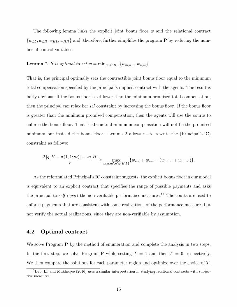
The following lemma links the explicit joint bonus floor w and the relational contract

{wLL, wLH , wHL, wHH} and, therefore, further simplifies the program P by reducing the num-

ber of control variables.

Lemma 2 It is optimal to set w = minm,n∈H,L{wm,n + wn,m}.

That is, the principal optimally sets the contractible joint bonus floor equal to the minimum

total compensation specified by the principal’s implicit contract with the agents. The result is

fairly obvious. If the bonus floor is set lower than the minimum promised total compensation,

then the principal can relax her IC constraint by increasing the bonus floor. If the bonus floor

is greater than the minimum promised compensation, then the agents will use the courts to

enforce the bonus floor. That is, the actual minimum compensation will not be the promised

minimum but instead the bonus floor. Lemma 2 allows us to rewrite the (Principal’s IC)

constraint as follows:

2 [q1H − π(1, 1; w)]− 2q0H

r≥ max

m,n,m′,n′∈{H,L}{wmn + wnm − (wm′,n′ + wn′,m′)}.

As the reformulated Principal’s IC constraint suggests, the explicit bonus floor in our model

is equivalent to an explicit contract that specifies the range of possible payments and asks

the principal to self-report the non-verifiable performance measures.13 The courts are used to

enforce payments that are consistent with some realizations of the performance measures but

not verify the actual realizations, since they are non-verifiable by assumption.

4.2 Optimal contract

We solve Program P by the method of enumeration and complete the analysis in two steps.

In the first step, we solve Program P while setting T = 1 and then T = 0, respectively.

We then compare the solutions for each parameter region and optimize over the choice of T .

13Deb, Li, and Mukherjee (2016) uses a similar interpretation in studying relational contracts with subjec-tive measures.

15

The following proposition presents the overall optimal contract as a function of the common

discount rate r. That is, we express the results as a function of discount rate cutoffs, which

are themselves functions of other exogenous parameters. Following the literature, we label

a wage scheme as joint performance evaluation (JPE ) if wHH ≥ wHL and wLH ≥ wLL and

relative performance evaluation (RPE ) if wHL ≥ wHH and wLL ≥ wLH (with one >). We say

that a contract has a bonus pool (BP) feature if it specifies a positive total bonus floor, i.e.,

w > 0. Our BP -type contracts can be thought of as discretionary bonus pools that allow the

principal to pay the agents more than the contractually agreed upon minimum w.

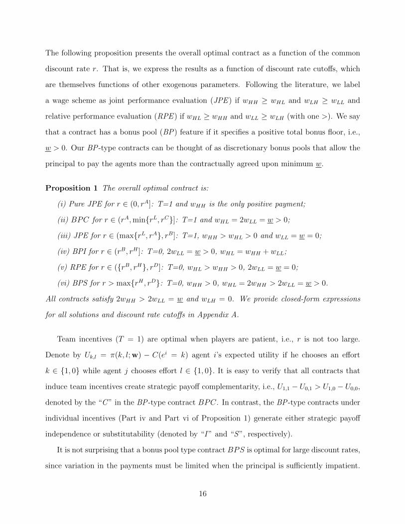
Proposition 1 The overall optimal contract is:

(i) Pure JPE for r ∈ (0, rA]: T=1 and wHH is the only positive payment;

(ii) BPC for r ∈ (rA,min{rL, rC}]: T=1 and wHL = 2wLL = w > 0;

(iii) JPE for r ∈ (max{rL, rA}, rB]: T=1, wHH > wHL > 0 and wLL = w = 0;

(iv) BPI for r ∈ (rB, rH ]: T=0, 2wLL = w > 0, wHL = wHH + wLL;

(v) RPE for r ∈ ({rB, rH}, rD]: T=0, wHL > wHH > 0, 2wLL = w = 0;

(vi) BPS for r > max{rH , rD}: T=0, wHH > 0, wHL = 2wHH > 2wLL = w > 0.

All contracts satisfy 2wHH > 2wLL = w and wLH = 0. We provide closed-form expressions

for all solutions and discount rate cutoffs in Appendix A.

Team incentives (T = 1) are optimal when players are patient, i.e., r is not too large.

Denote by Uk,l = π(k, l; w) − C(ei = k) agent i’s expected utility if he chooses an effort

k ∈ {1, 0} while agent j chooses effort l ∈ {1, 0}. It is easy to verify that all contracts that

induce team incentives create strategic payoff complementarity, i.e., U1,1 − U0,1 > U1,0 − U0,0,

denoted by the “C ” in the BP -type contract BPC. In contrast, the BP -type contracts under

individual incentives (Part iv and Part vi of Proposition 1) generate either strategic payoff

independence or substitutability (denoted by “I ” and “S”, respectively).

It is not surprising that a bonus pool type contract BPS is optimal for large discount rates,

since variation in the payments must be limited when the principal is sufficiently impatient.

16

In fact, BPS converges to a bonus pool with a fixed size as the discount rates r → ∞.

This coincides with the traditional view that bonus pools without discretion in determining

the total payout is the only self-enforcing compensation in a one-shot game. The repeated

relationship in our model gives the principal discretion to raise the size of the bonus pool

from the bonus floor. We next provide necessary and sufficient conditions for such BP -type

contracts to arise for intermediate discount rates.

Corollary 1 (i) The interval rA < r ≤ min{rL, rC} over which BPC is optimal is non-empty

if and only if H ≤ H∗ and q0 > 1 − q1. (ii) The interval rB < r ≤ rH over which BPI is

optimal is non-empty if and only if q1 >12

and H ≤ H∗∗, where H∗ and H∗∗ are characterized

in Appendix A.

To understand Part (i) of the corollary, it is helpful to analyze what the principal can

do upon loosing her credibility to promise Pure JPE. She can either set a positive bonus

floor w = 2wLL as in BPC, which allows her to foster team incentives by further increasing

wHH . Alternatively, the principal could substitute individual incentives for team incentives by

paying wHL > 0 and holding the bonus floor w = wLL at 0 (as in JPE ), i.e., she could increase

her reliance on relative performance evaluation. While rewarding joint poor performance

wLL through the positive bonus floor keeps the focus on team incentives, it has the cost of

rewarding for performance that has the lowest likelihood ratio q0q1

. The condition q0 > 1− q1

in the corollary above limits the opportunity cost of rewarding for poor performances, while

the condition H ≤ H∗ implies that the principal’s credibility is limited, creating a demand

for a BP -type contract. The discount rate region over which the principal can commit to

the ideal Pure JPE contract expands for higher H. If H is sufficiently large (H > H∗),

the principal’s credibility is so strong that by the time she looses her credibility at rA, the

agents have already lost their patience to mutually monitor each other. Without the benefit

of mutual monitoring, rewarding for poor performances wLL via a BP -type contract is not

optimal in the team incentive (T = 1) region of discount rates.

17

In the individual incentive region (T = 0) of discount rates, Corollary 1 - Part (ii) states

that using the bonus floor to create strategy payoff independence is optimal when the agents’

ability to enforce collusion is strong. The condition q1 >12

in Corollary 1 is intuitive: the

agents’ ability to collude on the Cycling collusive strategy is stronger for higher q1, because a

higher q1 increases the probability that the (only) working agent will collet the payment wHL.

As discussed previously, a higher output H strengthens the principal’s credibility relative to

the agents. If the condition H ≤ H∗∗ is violated, the principal’s credibility is so strong that

the agents’ ability to collude on the side-contract is weak by the time the principal looses her

credibility at rB, making RPE optimal instead.

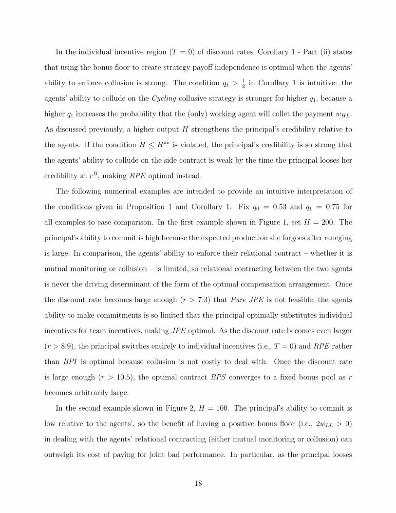
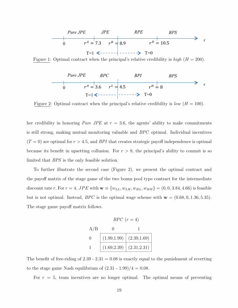
The following numerical examples are intended to provide an intuitive interpretation of

the conditions given in Proposition 1 and Corollary 1. Fix q0 = 0.53 and q1 = 0.75 for

all examples to ease comparison. In the first example shown in Figure 1, set H = 200. The

principal’s ability to commit is high because the expected production she forgoes after reneging

is large. In comparison, the agents’ ability to enforce their relational contract – whether it is

mutual monitoring or collusion – is limited, so relational contracting between the two agents

is never the driving determinant of the form of the optimal compensation arrangement. Once

the discount rate becomes large enough (r > 7.3) that Pure JPE is not feasible, the agents

ability to make commitments is so limited that the principal optimally substitutes individual

incentives for team incentives, making JPE optimal. As the discount rate becomes even larger

(r > 8.9), the principal switches entirely to individual incentives (i.e., T = 0) and RPE rather

than BPI is optimal because collusion is not costly to deal with. Once the discount rate

is large enough (r > 10.5), the optimal contract BPS converges to a fixed bonus pool as r

becomes arbitrarily large.

In the second example shown in Figure 2, H = 100. The principal’s ability to commit is

low relative to the agents’, so the benefit of having a positive bonus floor (i.e., 2wLL > 0)

in dealing with the agents’ relational contracting (either mutual monitoring or collusion) can

outweigh its cost of paying for joint bad performance. In particular, as the principal looses

18

0

r

Pure JPE JPE RPE BPS

T=1 T=0

𝑟! = 7.3 𝑟! = 8.9 𝑟! = 10.5

Figure 1: Optimal contract when the principal’s relative credibility is high (H = 200).

0

r

Pure JPE BPC BPI BPS

T=1 T=0 𝑟! = 3.6 𝑟! = 4.5 𝑟! = 8

Figure 2: Optimal contract when the principal’s relative credibility is low (H = 100).

her credibility in honoring Pure JPE at r = 3.6, the agents’ ability to make commitments

is still strong, making mutual monitoring valuable and BPC optimal. Individual incentives

(T = 0) are optimal for r > 4.5, and BPI that creates strategic payoff independence is optimal

because its benefit in upsetting collusion. For r > 8, the principal’s ability to commit is so

limited that BPS is the only feasible solution.

To further illustrate the second case (Figure 2), we present the optimal contract and

the payoff matrix of the stage game of the two bonus pool type contract for the intermediate

discount rate r. For r = 4, JPE with w ≡ {wLL, wLH , wHL, wHH} = (0, 0, 3.84, 4.66) is feasible

but is not optimal. Instead, BPC is the optimal wage scheme with w = (0.68, 0, 1.36, 5.35).

The stage game payoff matrix follows.

BPC (r = 4)

A/B 0 1

0 (1.99,1.99) (2.39,1.69)

1 (1.69,2.39) (2.31,2.31)

The benefit of free-riding of 2.39 - 2.31 = 0.08 is exactly equal to the punishment of reverting

to the stage game Nash equilibrium of (2.31 - 1.99)/4 = 0.08.

For r = 5, team incentives are no longer optimal. The optimal means of preventing

19

collusion is BPI with w = (1.09, 0, 5.82, 4.73). The payoff matrix follows.

BPI (r = 5)

A/B 0 1

0 (3.02,3.02) (2.78,3.06)

1 (3.06,2.78) (2.82,2.82)

The principal provides any shirking agent with a benefit of 0.04 for instead working and

upsetting collusion on either Joint Shirking or Cycling. It is easy to verify that the shirking

agent’s continuation payoff under Joint Shirking of 3.025

= 0.604 is the same as his continuation

payoff under Cycling. Under the equilibrium strategy (work,work), each agent’s continuation

payoff is 2.825

= 0.564. Therefore, the difference in continuation payoffs of 0.604−0.564 = 0.04

is exactly equal to the benefit an agent receives for upsetting collusion by playing work instead

of shirk in the current period. That is, both (No Joint Shirking) and (No Cycling) hold as

equality – a feature of the contract that creates payoff strategic independence.

4.3 Optimal contract without bonus floor

To better understand the importance of the bonus floor in our model, we also derive the

optimal contract assuming, as in Kvaløy and Olsen (2006), the principal cannot commit to a

joint bonus floor. That is, w = 0 by assumption. We present optimal contracts under this

alternative assumption in Proposition 2 and compare it to the optimal contracts in Proposition

1 in Corollary 2.

Proposition 2 When the principal cannot commit to a joint bonus floor, the optimal contract

is (i) Pure JPE for r ∈ (0, rA], (ii) JPE for r ∈ (rA, rB], (iii) RPE for r ∈ (rB, rD], and

infeasible otherwise.

Corollary 2 The ability to commit to a positive bonus floor w > 0 results in

(i) more relational contract in general:

20

• when w = 0 by assumption, there is no feasible solution for r > rD;

• when w ≥ 0, relational contract is feasible for all r otherwise.

(ii) more team incentives:

• when w = 0 by assumption, team incentives are optimal if and only if r < rB;

• when w ≥ 0, team incentives are optimal if and only if (1) r < rB or (2) r <

min{rL, rC} in the case of rL ≥ rB.

(iii) more strategic payoff independence ∆U = 0:

• when w = 0 by assumption, ∆U = 0 holds at the singular discount rate rB;

• when w ≥ 0, ∆U = 0 is optimal for a range of discount rates, all with w > 0.

The optimal contract essentially reproduces the results of Kvaløy and Olsen (2006).14 Part

(i) of Corollary 2 is straightforward, as the ability to commit to a joint bonus floor strengthens

the principal’s credibility. Inspecting Program P shows that the joint bonus floor relaxes the

(Principal’s IC) constraint in both the team incentive case and individual incentive case, it

is unclear, a priori, whether such a commitment results in more or less team incentives once

team incentives is a choice variable. Part (ii) of Corollary 2 shows that the region in which

team incentives are optimal expands once the bonus floor is introduced. Part (iii) highlights

the role of the bonus floor in combating the agents’ possible collusion. When the principal

cannot commit to such a bonus floor, JPE and RPE of Proposition 2 converge to independent

performance evaluation (i.e., wHH = wHL > 0, and wLH = wLL = 0) at the singular discount

rate rB, creating strategic independence ∆U = 0. As we have shown in Proposition 1 and

Corollary 1, when the principal can commit to a joint bonus floor, BPI (with a bonus floor)

creates ∆U = 0 and is optimal for a range of discount rates r even though contracts without

positive bonus floors could be used to prevent tacit collusion.

14We say “essentially” because they restrict attention to stationary strategies, while we do not.

21

In Appendix B, we study the other difference between our model and Kvaløy and Olsen

(2006) – their restriction to stationary collusion strategies. In sum, Appendix B and Proposi-

tion 2 (and its corollary) demonstrate that the important qualitative differences between our

results and theirs are due to the principal’s ability to commit to a bonus floor in our model.

5 Incorporating a Verifiable Joint Performance Mea-

sure

In a typical bonus pool arrangement, the size of the bonus pool is based, at least in part, on a

verifiable joint performance measure such as group, divisional, or firm-wide earnings (Eccles

and Crane, 1988). Suppose that such an objective measure y ∈ {H,L} exists and define

p1 = Pr(y = H|eA = eB = 1), p = Pr(y = H|eA 6= eB), and p0 = Pr(y = H|eA = eB = 0)

with p1 > p > p0. As before, agent j’s non-verifiable performance measure is xj ∈ {0, 1},

and q1 = Pr(xj = 1|ej = 1) and q0 = Pr(xj = 1|ej = 0). Denote by w ≡ {wymn} the

combined explicit/implicit contract the principal offers agent i, if the verifiable team measure

is y ∈ {H,L} and agent i and j’s non-verifiable individual measures are m and n, respectively.

The only possibility of the principal reneging is on the implicit contract that depends on the

non-verifiable individual measures. Assuming the principal honors her promise truthfully, we

can rewrite agent i’s expected wage payment if he chooses effort k and agent j chooses l as:

π(k, l; w) = Ey∈{H,L} [qkqlwyHH + qk(1− ql)wyHL + (1− qk)qlwyLH + (1− qk)(1− ql)wyLL] , (3)

where the expectation is taken over the team measure y given effort k, l.

The principal’s problem is same as Program P in the main model after substituting the

expected payment π(k, l; w) everywhere by (3) shown above. The other change to Program

22

P is to redefine the Principal’s IC for each realized team measure y as follows:

2[

p1min{p1−p, p−p0} − π(1, 1; w)

]r

≥ maxm,n∈{H,L}

{wymn + wynm − wym′n′ − w

yn′m′}, ∀y ∈ {H,L}.

(Principal’s new IC)

Introducing the objective team measure y qualitatively changes the fallback contract triggered

by the principal’s reneging. In the main model, the principal looses the agents’ trust upon

reneging and expects the agents to shirk in perpetuity off the equilibrium. With a verifiable

team measure, the reneging principal can continue to induce (work, work) off the equilibrium

by replying solely on the verifiable team measure. That is, the reneging principal can ensure

(work, work) as the unique stage game equilibrium, which requires paying p1min{p1−p, p−p0} to

each agent.15

Before we characterize the solution, we first demonstrate the robustness of our results in

the main model via a numerical example. We use the same parameters as in Figures 1 and 2 to

ease comparison: q0 = 0.53 and q1 = 0.75. The objective measure y satisfies p1 = 0.6, p = 0.5,

and p0 = 0.4 in Figure 3. In this example, the optimal contract satisfies wLmn = 0,∀m,n, i.e.,

the payment is zero whenever the team measure is low. Given the high team measure y = H,

the way the optimal contact varies with the discount rate r is qualitatively the same as in

Figure 2. The moment the principal cannot credibly commit to Pure JPE (only wH11 > 0) at

r = 0.8, she starts to pay for poor individual performances wH00 in order to continue raising

wH11, which has the benefit of fostering the agents’ mutual monitoring. Individual incentives

are optimal for higher discount rates r > 3.6, and BPI is optimal for r < 8 because it has the

benefit of creating strategic independence, a desirable feature in combating agents’ collusion.

We use the names developed in the main model to label contracts in Figure 3, not only to

facilitate comparison with Figure 2, but also because the optimal payments wHmn (i.e., given

the team output y = H) are qualitatively similar in terms of having a positive bonus floor

15We assume in this section that the agent’s effort is valuable enough so that, following reneging (out-of-equilibrium), the principal chooses to induce (work, work) by using the verifiable measure. Denote by X theincremental value that a working agent brings to the principal than a shirking agent. Our out-of-equilibriumspecification requires (q1 − q0)X ≥ p1

min{p1−p, p−p0} .

23

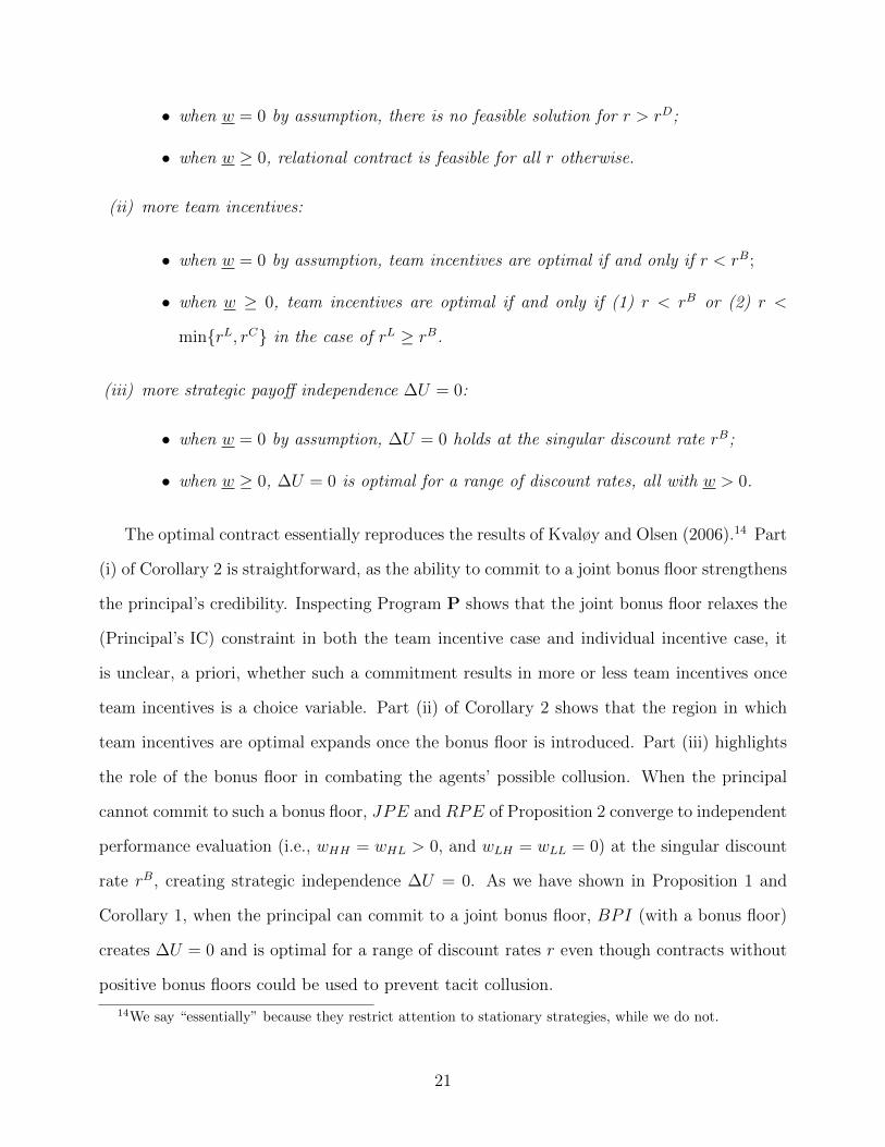
and their strategic payoff interdependencies.

0

r

𝑤!!! > 0 BPC:    𝑤!!! > 0 BPI BPS

T=1 T=0

𝑟 = 0.8 𝑟 = 3.6 𝑟! = 8

Figure 3: Optimal contract with a team measure (p0 = 0.4, p = 0.5, p1 = 0.6).

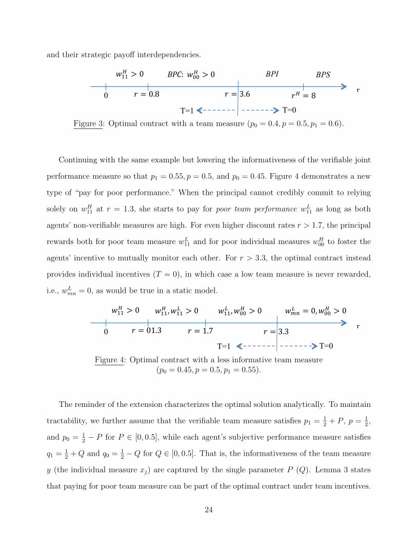
Continuing with the same example but lowering the informativeness of the verifiable joint

performance measure so that p1 = 0.55, p = 0.5, and p0 = 0.45. Figure 4 demonstrates a new

type of “pay for poor performance.” When the principal cannot credibly commit to relying

solely on wH11 at r = 1.3, she starts to pay for poor team performance wL11 as long as both

agents’ non-verifiable measures are high. For even higher discount rates r > 1.7, the principal

rewards both for poor team measure wL11 and for poor individual measures wH00 to foster the

agents’ incentive to mutually monitor each other. For r > 3.3, the optimal contract instead

provides individual incentives (T = 0), in which case a low team measure is never rewarded,

i.e., wLmn = 0, as would be true in a static model.

0

r

𝑤!!! > 0 𝑤!!! ,𝑤!!! > 0 𝑤!"! = 0,𝑤!!! > 0

T=1 T=0

𝑟 = 01.3 𝑟 = 3.3 𝑟 = 1.7

 𝑤!!! ,𝑤!!! > 0

Figure 4: Optimal contract with a less informative team measure(p0 = 0.45, p = 0.5, p1 = 0.55).

The reminder of the extension characterizes the optimal solution analytically. To maintain

tractability, we further assume that the verifiable team measure satisfies p1 = 12

+ P , p = 12,

and p0 = 12− P for P ∈ [0, 0.5], while each agent’s subjective performance measure satisfies

q1 = 12

+Q and q0 = 12−Q for Q ∈ [0, 0.5]. That is, the informativeness of the team measure

y (the individual measure xj) are captured by the single parameter P (Q). Lemma 3 states

that paying for poor team measure can be part of the optimal contract under team incentives.

24

Lemma 3 Given team incentives T=1, the optimal contract for r ≤ r1 has wH11 as the only

positive payment. As r increases from r1, there exists a unique P ∗ such that the principal

• pays for “poor team performance” (wL11 > 0) while keeping wH10 = 0 for P ≤ P ∗;

• increases wH10 without paying for poor team performance (i.e., wLmn = 0) for P > P ∗.

Part (ii) is at odds with the insights derived from standard single-period models of indi-

vidual incentives (e.g., Holmstrom, 1979). The standard informativeness argument suggests

that paying for wH10 provides stronger (individual) incentive than rewarding wL11 for any P > 0.

However, compared to paying wH10 > 0 (a form of RPE ), paying for “poor” team performance

wL11 has the benefit of fostering mutual monitoring. The principal trades off the benefit of fos-

tering mutual monitoring (via wL11) against the benefit of rewarding a measure with a higher

likelihood ratio (wH10). Since the advantage of wH10 in likelihood ratios is stronger when the

team measure y is more informative (higher P ), Part (ii) states that the benefit of focusing

on team incentives dominates if the likelihood ratio loss is not particularly strong. Given

Lemma 3 and our focus on mutual monitoring, we confine attention to P < ∆̄.= Q

2(1+Q),

which is sufficient to ensure that paying for poor team performance (i.e., Part ii of the lemma)

is always part of the optimal contract.16 Lemma 4 summarizes features of optimal contracts

given individual incentives T = 0.

Lemma 4 Given individual incentive T=0, the optimal contract

i. has neither the principal’s IC nor the agents’ collusion constraints binding for low r.

ii. creates strategic payoff independence ∆U = 0 for intermediate discount rates r ∈ [r, r̄],

which is a non-empty interval if and only if the fall-back objective measure is not too

noisy (hence the principal’s credibility is not too strong), i.e., P ≥ ∆.17

16We impose this sufficient condition to maintain tractability when we endogenize the choice between teamand individual incentives. Each program has 15 constraints (excluding 8 non-negativity constraints).

17The threshold ∆ is implicitly characterized in the Appendix. A sufficient condition is P > 0.025.

25

iii. creates payoff substitutability ∆U < 0 for large discount rates. As r →∞, the contract

converges to a conditional symmetric bonus pool: wLmn = 0 and wH11 = wH00 = 12wH10.

The condition P ≥ ∆ in Part (ii) of the lemma reinforces another finding in the main

model: the optimal contract depends on the principal’s credibility relative to agents’. To see

this, note that the principal’s credibility is stronger the lower P is because, upon reneging,

the principal’s off-equilibrium option of relying solely on the objective measure is costlier for

smaller P . The worse off-equilibrium contract, in turn, strengthens the principal’s credibility

to honor the subjective measures on equilibrium, echoing a result in Baker, Gibbons, and

Murphy (1994). If P ≥ ∆ is violated, the principal’s credibility will be so strong that by the

time she looses her credibility, the agents are already so impatient that their ability to collude

is weak; in this case, creating ∆U = 0 to combat collusion is unnecessary.

Proposition 3 endogenizes the choice of team incentives T = {0, 1} and characterizes the

optimal contract.

Proposition 3 Assuming ∆ ≤ P ≤ ∆̄, the overall optimal contract depends on r as follows:

(i) T = 1 for r ≤ r1, wH11 > 0 is the only positive payment, i.e., Pure JPE.

(ii) T = 1 for r ∈ (r1, r2]. As r increases, wH11 decreases while the payment for poor team

performance wL11 increases untill wL11 = wH11 at r = r2. All other payments are zero.

(iii) T = 1 for r ∈ (r2, r̃]. As r increases, wH10 increases from zero and wL11 decreases.

(iv) T = 0 for r ∈ (r̃, r3], the contract creates strategic payoff independence, and wH00 > 0.

(v) T = 0 for r > r3, the contract creates payoff strategic substitute ∆U < 0 and converges

to a conditional symmetric bonus pool as r →∞.

We characterize the r-cutoffs in Appendix A.

Comparing Proposition 3 to Proposition 1 confirms the insights derived without the team

measure. In both cases, team incentives are optimal if and only if the discount rate r is not

26

Discount Rate r1 r1=2.236 r2=3.614 4

Opt

imal

Pay

men

ts

0

1.25

2.5

wL11

wH11

wH10

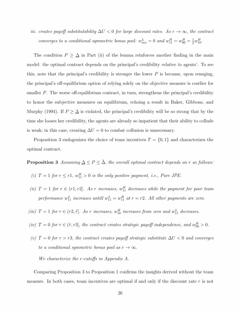
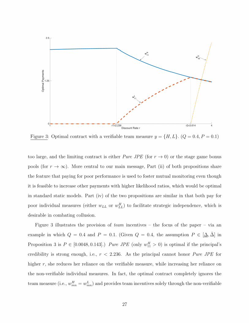
Figure 3: Optimal contract with a verifiable team measure y = {H,L}. (Q = 0.4, P = 0.1)

too large, and the limiting contract is either Pure JPE (for r → 0) or the stage game bonus

pools (for r → ∞). More central to our main message, Part (ii) of both propositions share

the feature that paying for poor performance is used to foster mutual monitoring even though

it is feasible to increase other payments with higher likelihood ratios, which would be optimal

in standard static models. Part (iv) of the two propositions are similar in that both pay for

poor individual measures (either wLL or wHLL) to facilitate strategic independence, which is

desirable in combating collusion.

Figure 3 illustrates the provision of team incentives – the focus of the paper – via an

example in which Q = 0.4 and P = 0.1. (Given Q = 0.4, the assumption P ∈ [∆, ∆̄] in

Proposition 3 is P ∈ [0.0048, 0.143].) Pure JPE (only wH11 > 0) is optimal if the principal’s

credibility is strong enough, i.e., r < 2.236. As the principal cannot honor Pure JPE for

higher r, she reduces her reliance on the verifiable measure, while increasing her reliance on

the non-verifiable individual measures. In fact, the optimal contract completely ignores the

team measure (i.e., wHmn = wLmn) and provides team incentives solely through the non-verifiable

27

measures at r = 3.614. For r > 3.614, the principal starts to increase wH10 because the agents’

ability to enforce mutual monitoring is weak when the discount rate is high. The principal

eventually tunes down team incentives for r ∈ [3.614, 4.13] by increasing wH10 and lowering wL11

and switches to individual incentives (T = 0) for r > r̃ = 4.13.

In summary, “paying for poor performance” – either a discretionary increase above the

zero floor when the verifiable measure is low but both non-verifiable measures are high or a

non-discretionary adherence to the positive bonus floor when the verifiable measure is high –

can be part of the optimal relational contract used to foster mutual monitoring. Again, there

is no role for mutual monitoring in Baldenius et al., so neither of these results arise in their

model.

6 Conclusion

Our model makes a number of simplifying assumptions: binary actions/performance mea-

sures, risk neutral agents, symmetric contracts, and communication from the agents to the

principal is blocked. Although these assumptions are standard in the relational contracting

literature, they are nonetheless limiting. Of these assumptions, we view the restriction to

symmetric contracts and blocked communication as most limiting. These limitations provide

opportunities for future research.

A natural starting point is to relax these assumptions in a model of explicit contracting

between the principal and the agents. With agents who have different roles such as top exec-

utives, static models predict the agents would be offered qualitatively different compensation

contracts. Yet, in practice, the compensation of executives are often similar. As an extreme

example, Apple pays the same base salary, annual cash incentive, and long-term equity award

28

to each of its executive officers other than its CEO.18 19 We conjecture that compensating

productively different agents similarly can be rationalized by a team-based model of dynamic

incentives (with a low discount rate/long expected tenure).

Another natural avenue for future research is peer evaluation (or 360-degree evaluation)

under relational side-contracting. We assumed communication from the agents to the principal

is blocked, as in Arya, Fellingham, and Glover (1997), Che and Yoo (2001), and Kvaløy

and Olsen (2006). Ma (1988) studies a single-period, multi-agent model of moral hazard

without side-contracting under unblocked communication (peer reports) from the agents to

the principal. In Ma (1988), if the agents perfectly observe each other’s actions and the

principal contracts on the agents’ peer reports, the principal can implement the first-best

if every action pair induces a unique distribution over performance measures.20 Baliga and

Sjostrom (1998) study a similar setting but allow for explicit side-contracting between the

agents and show that side-contracting greatly limits the role of peer reports. Deb, Li, and

Mookerherjee (2016) study peer evaluation under relational contracting between the principal

and the agents but without (relational or explicit) side-contracts between the agents, showing

that peer evaluations are sparingly incorporated in determining compensation. As far as we are

aware, there have been no studies of peer evaluation under implicit side-contracting/collusion.

Collusion between the principal and one of the agents may also arise.

If we apply the team-based model to thinking about screening, we might expect to see

compensation contracts that screen agents for their potential productive complementarity,

since productive complementarities reduce the cost of motivating mutual monitoring. A pro-

18According to Apple Inc.’s 2016 Proxy Statement: “Our executive officers are expected to operate as ateam, and accordingly, we apply a team-based approach to our executive compensation program, with internalpay equity as a primary consideration. This approach is intended to promote and maintain stability withina high performing executive team, which we believe is achieved by generally awarding the same base salary,annual cash incentive, and long-term equity awards to each of our executive officers, except [CEO] Mr. Cook.”

19For related observations about cash bonuses paid to CEOs that are similar to bonuses paid to otherexecutives, see Core, Guay, and Verrecchia (2003) and Guay, Kepler, and Tsui (2016), which finds that, forapproximately 75% of their sample, the CEO and the fifth-highest-paid executive have an identical set ofperformance targets for their cash bonuses.

20Towry (2003) initiated an important experimental literature that contrasted the Arya, Fellingham, andGlover (horizontal) and Ma (vertical) views of mutual monitoring, emphasizing the important role of teamidentity.

29

ductive substitutability (e.g., hiring an agent similar to existing ones when there are overall

decreasing returns to effort) is particularly unattractive, since the substitutability makes it

appealing for the agents to tacitly collude on taking turns working. We might also expect to

see agents screened for their discount rates. Patient agents would be more attractive, since

they are the ones best equipped to provide and receive mutual monitoring incentives. Are

existing incentive arrangements such as employee stock options with time-based rather than

performance-based vesting conditions designed, in part, to achieve such screening?

Even if screening is not necessary because productive complementarities or substitutabili-

ties are driven by observable characteristics of agents (e.g., their education or work experience),

optimal team composition is an interesting problem. For example, is it better to have one

team with a large productive complementarity and another with a small substitutability or

to have two teams each with a small productive complementarity?

30

References

[1] Anthony, R. and V. Govindarajan, 1998. Management Control Systems, Mc-Graw Hill.

[2] Arya, A., J. Fellingham, and J. Glover, 1997. Teams, Repeated Tasks, and Implicit

Incentives. Journal of Accounting and Economics, 23: 7-30.

[3] Baiman, S. and M. Rajan, 1995. The Informational Advantages of Discretionary Bonus

Schemes. The Accounting Review, 70: 557-579.

[4] Baker, G., R. Gibbons, and K. Murphy, 1994. Subjective Performance Measures in Op-

timal Incentive Contracts. Quarterly Journal of Economics, 109: 1125-1156.

[5] Baldenius, T., J. Glover, and H. Xue, 2016. Relational Contracts With and Between

Agents. Journal of Accounting and Economics, 61: 369-390.

[6] Baliga, S. and Sjostrom, T., 1998. Decentralization and collusion. Journal of Economic

Theory, 83, 196-232.

[7] Bushman, R.M., Indjejikian, R.J. and Smith, A., 1996. CEO compensation: The role of

individual performance evaluation. Journal of Accounting and Economics, 21, 161-193.

[8] Core, J.E., Guay, W.R. and Verrecchia, R.E., 2003. Price versus non-price performance

measures in optimal CEO compensation contracts. The Accounting Review, 78(4), 957-

981.

[9] Che, Y. and S. Yoo, 2001. Optimal Incentives for Teams. American Economic Review,

June: 525-541.

[10] Deloitte. 2016. Global Human Capital Trends: The New Organizational: Different by

Design. London: Deloitte University Press.

[11] Deloitte. 2017. Global Human Capital Trends: Rewriting the rules for the digital age.

London: Deloitte University Press.

31

[12] Demski, J. and D. Sappington, 1984. Optimal Incentive Contracts with Multiple Agents.

Journal of Economic Theory, 33: 152-171.

[13] Deb, J., J. Li, and A. Mukherjee, 2016. Relational contracts with subjective peer evalu-

ations. Rand Journal of Economics, 47: 3-28.

[14] Eccles, R.G. and D.B. Crane, 1988. Doing Deals: Investment Banks at Work. Harvard

Business School Press.

[15] Ederhof, M., 2010. Discretion in Bonus Plans. The Accounting Review, 85: 1921-1949.

[16] Ederhof, M., M. Rajan, and S. Reichelstein, 2011. Discretion in Managerial Bonus Pools.

Foundations and Trends in Accounting, 54: 243-316.

[17] Gibbons, R. and Henderson, R., 2013. What do managers do? Exploring persistent

performance differences amongst seemingly similar enterprises. The Handbook of Orga-

nizational Economics, 680-731.

[18] Guay, W., Kepler, J., and D. Tsui, 2016. Do CEO Bonus Plans Serve a Purpose. Working

Paper, The Wharton School.

[19] Hamilton, B.H., Nickerson, J.A. and Owan, H., 2003. Team incentives and worker hetero-

geneity: An empirical analysis of the impact of teams on productivity and participation.

Journal of Political Economy, 111: 465-497.

[20] Holmstrom, B., 1979. Moral Hazard and Observability. Bell Journal of Economics, 10:

74-91.

[21] Itoh, H., 1993. Coalitions, incentives, and risk sharing. Journal of Economic Theory, 60,

410-427.

[22] Knez, M. and Simester, D., 2001. Firm-wide incentives and mutual monitoring at Conti-

nental Airlines. Journal of Labor Economics, 19: 743-772.

32

[23] Kvaløy, Ola and Trond E. Olsen, 2006. Team Incentives in Relational Employment Con-

tracts. Journal of Labor Economics, 24: 139-169.

[24] Levin, J., 2002. Multilateral Contracting and the Employment Relationship. Quarterly

Journal of Economics, 117: 1075-1103.

[25] Levin, J., 2003. Relational Incentive Contracts. American Economic Review, 93: 835-847.

[26] Ma, C. T., 1988. Unique implementation of incentive contracts with many agents. Review

of Economic Studies, 55, 555-572.

[27] MacLeod, W. B., 2003. Optimal Contracting with Subjective Evaluation. American Eco-

nomic Review, 93: 216-240.

[28] MacLeod, W. B. and Malcomson, J.M., 1989. Implicit contracts, incentive compatibility,

and involuntary unemployment. Econometrica, 447-480.

[29] Milgrom, P. and Roberts, J., 1990. Rationalizability, learning, and equilibrium in games

with strategic complementarities. Econometrica, 1255-1277.

[30] Milgrom, P. and Roberts, J., 1992. Economics, Organization and Management, Prentice

Hall.

[31] Mookherjee, D., 1984. Optimal Incentive Schemes with Many Agents. Review of Economic

Studies, 51: 433–446.

[32] Murphy, K., and P. Oyer, 2001. Discretion in Executive Incentive Contracts: Theory and

Evidence. Working Paper, Stanford University.

[33] Rajan, M. and S. Reichelstein, 2006. Subjective Performance Indicators and Discretionary

Bonus Pools. Journal of Accounting Research, 44: 525-541.

[34] Rajan, M. and S. Reichelstein, 2009. Objective versus Subjective Indicators of Managerial

Performance. The Accounting Review, 84: 209-237.

33

[35] Tirole, J., 1986. Hierarchies and Bureaucracies: On the Role of Collusion in Organiza-

tions. Journal of Law, Economics and Organization, 2: 181-214.

[36] Tirole, J., 1992. Collusion and the theory of organizations. In J.-J. Laffont, ed., Advances

in economic theory: Invited papers for the sixth world congress of the Econometric Society

2. Cambridge: Cambridge University Press.

[37] Towry, K., 2003. Control in a teamwork environment-The impact of social ties on the

effectiveness of mutual monitoring contracts. The Accounting Review, 78: 1069–1095.

34

Appendix

Proof of Lemma 1. We start with a preliminary result that specifies the harshest punish-

ment supporting the collusion.

Claim: It is without loss of generality to restrict attention to collusion constraints that

have the agent punishing each other by playing (1, 1) (i.e., work, work) forever after a deviation

from the collusion strategy.

Proof. We first argue that the off-diagonal action profiles (0, 1) and (1, 0) cannot be punish-

ment strategies harsher than (1, 1). We illustrate the argument for (0, 1); similar logic applies

to (1, 0):

Agent B

L H

Agent AL U00, U00 U01, U10

H U10, U01 U11, U11

If playing (0, 1) were a harsher punishment for Agent A (i.e., U01 < U11), he would be able to

profitably deviate to (1, 1). That is, playing (0, 1) is not a stage-game equilibrium and thus

cannot be used as a punishment strategy. If (0, 1) were a harsher punishment for Agent B (i.e.,

U10 < U11), we would need U10 ≥ U00 to prevent Agent B from deviating from (0, 1) to (0, 0).

However, U10 < U11, U10 ≥ U00, and (Static NE) together imply U11 ≥ max{U10, U00, U01},

which means there is no scope for collusion because at least one of the agents is strictly worse

off under any potential collusive strategy than under the always working strategy.

To establish that (1, 1) is the (weakly) harshest punishment, it remains to show that

U11 ≤ U00. Suppose, by contradiction, U11 > U00. If the wage scheme w ≡ {wxmn}, x =

{0, 1}, m, n = {L,H}, creates strategic payoff substitutability, i.e., U10 − U00 > U11 − U01,

(Static NE) again implies that (0, 0) is not a stage-game equilibrium and thus cannot be

used as a punishment strategy in the first place. If instead w creates (weak) strategic payoff

complementarity, i.e., U11 − U01 ≥ U10 − U00, we have U10 + U01 ≤ U11 + U00 < 2U11, where

35

the last inequality is due to the assumption U11 > U00. But U00 < U11 and U10 + U01 < 2U11

together mean that at least one of the agents is strictly worse off under any potential collusive

strategy than under the always working strategy, meaning there is no scope for any collusion.

Let

V it (σ) ≡

∞∑τ=1

U it+τ (a

iτ , a

jτ )

(1 + r)τ

be agent i’s continuation payoff from t+ 1 and forwards, discounted to period t, from playing

{aAt+τ , aBt+τ}∞τ=1 specified in an action profile σ = {aAt , aBt }∞t=0, for aAt , aBt ∈ {0, 1}. We allow

any σ satisfying the following condition to be a potential collusive strategy:

∞∑t=0

U it (a

it, a

jt)

(1 + r)t≥ 1 + r

rU1,1, ∀i ∈ {A,B}, (4)

where U it (a

it, a

jt) is Agent i’s stage-game payoff at t given the action pair (ait, a

jt) specified in

σ, and 1+rrU1,1 is the agent’s payoff from always working.

The outline of the sufficiency part of the Lemma is as follows:

Step 1: Any collusive strategy that contains only (1, 1), (1, 0) and (0, 1) (i.e., without (0, 0)

in any period) is easier for the principal to upset than Cycling.

Step 2: Any collusive strategy that ever contains (0, 0) at some period t would be easier

for the principal to upset than either Joint Shirking or Cycling.

Step 1: The basic idea here is that, compared with Cycling, any reshuffling of (0, 1) and

(1, 0) effort pairs across periods and/or introducing (1, 1), can only leave some shirking agent

better off in some period if it also leaves another shirking agent worse off in another period,

in terms of their respective continuation payoffs.

In order for the agents to be better-off under the collusive strategy σ that contains only

(1, 1), (1, 0) and (0, 1) than under jointly work (1, 1)∞, condition (4) requires U1,0+U0,1 > 2U1,1.

36

Therefore, we know

VCY C

+ V CY C ≥ V it (σ) + V j

t (σ), ∀t, (5)

where VCY C

=∑

t=1,3,5,...

U1,0

(1+r)t+

∑t=2,4,6,...

U0,1

(1+r)tand V CY C =

∑t=1,3,5,...

U0,1

(1+r)t+

∑t=2,4,6,...

U1,0

(1+r)tare

the continuation payoffs (under Cycling) of the shirking agent and the working agent, respec-

tively. We drop the time index in VCY C

and V CY C because they’re time independent. Since

(Static NE) and U1,0 + U0,1 > 2U1,1 together imply U1,0 > U1,1 ≥ U0,1, simple algebra shows

VCY C

> max{V CY C , V ∗}, (6)

where V ∗.= U1,1

ris the continuation payoff from playing (1, 1)∞.

To prove the claim that the collusive strategy σ is easier for the principal to upset than

Cycling, it is sufficient to show the following:

∃ t|{(ait = 0, ajt = 1) ∧ V it (σ) ≤ V

CY C}. (7)

That is, there will be some period when the agents i is supposed to be the only “shirker”

in that period faces a weakly lower continuation payoff (hence stronger incentives to deviate

from shirking) under the collusive strategy σ than under Cycling. Suppose by contradiction

that (7) fails. That is,

V it (σ) > V

CY C, ∀ t|{(ait = 0, ajt = 1)}. (8)

We know from (5) that (8) implies the following for the other agent j:

V jt (σ) < V CY C , ∀ t|{(ait = 0, ajt = 1)}. (9)

Since one agent always playing 0 is not a sub-game perfect equilibrium, there must be a

switch from (0, 1) to (1, 0), possibly sandwiched by one or more (1, 1), in any strategy σ. We

pick any such block in σ, and denote τ and τ + 1 + n (n ∈ {0, 1, 2, 3, ...}) as the time (0, 1)

37

and (1, 0) are sandwiched by n period(s) of (1, 1).

We show below that, for all n, (8) leads to a contradiction, which then verifies (7) and

proves the claim. We name the first agent as Agent A throughout the analysis.

• If n = 0, i.e., (0, 1) is followed immediately by a (1, 0) at τ + 1. One can show the

following for Agent A’s continuation payoff at τ

V Aτ (σ) =

U1,0 + V Aτ+1(σ)

1 + r

<U1,0 + V CY C

1 + r

= VCY C

,

which contradicts (8). The inequality above applies (9) to t = τ + 1.

• If n is an even number (n = 2, 4, 6, ...), i.e., there are even numbers of (1, 1) sandwiched

between (0, 1) and (1, 0). We prove the case for n = 2 and same argument applies for

all even n.

... t = τ t = τ + 1 t = τ + 2 t = τ + 3 ...

σ ... (0, 1) (1, 1) (1, 1) (1, 0) ...

We can show the following for Agent A’s continuation payoff at τ :

V Aτ (σ) =

U1,1

1 + r+

U1,1

(1 + r)2+U1,0 + V A

τ+3(σ)

(1 + r)3

<U1,1

1 + r+

U1,1

(1 + r)2+U1,0 + V CY C

(1 + r)3

<U1,0

1 + r+

U0,1

(1 + r)2+U1,0 + V CY C

(1 + r)3

= VCY C

,

which again contradicts (8). The first inequality applies (9) to t = τ + 3. The second

38

inequality applies (6) and the fact that VCY C

> V ∗ if and only if U1,0

1+r+ U0,1

(1+r)2>

U1,1

1+r+ U1,1

(1+r)2.

• If n is an odd number (n = 1, 3, 5, ...). Consider, without loss of generality, the following

case for n = 1, i.e., there is one (1, 1) sandwiched between (0, 1) and (1, 0).

... t = τ t = τ + 1 t = τ + 2 ...

σ ... (0, 1) (1, 1) (1, 0) ...

We can show the following for Agent A’s continuation payoff at τ

V Aτ (σ) =

U1,1

1 + r+U1,0 + V A

τ+2(σ)

(1 + r)2

<U1,1

1 + r+U1,0 + V CY C

(1 + r)2

=rV ∗

1 + r+U1,0 + V CY C

(1 + r)2

=rV ∗

1 + r+VCY C

1 + r

< VCY C

,

which contradicts (8). The first inequality applies (9) to t = τ + 2, the second equalities

is from the definition of V ∗ = U1,1

r, and the last equality is by the definition of V CY C

and VCY C

so that VCY C

= U1,0+VCY C

1+r.

Step 2: Given any contract offered by the principal, one of the following must be true:

max{2U1,1, 2U0,0, U1,0 + U0,1} =

2U1,1 case 1

U1,0 + U0,1 case 2

2U0,0 case 3.

39

Case 1 is trivially collusion proof as no other action profile Pareto-dominates the equilib-

rium strategy {1, 1}∞t=0.

Case 2 has two sub-cases: sub-case 2.1 where U1,0+U0,1

2≥ U1,1 ≥ U0,0 and sub-case 2.2 in

which U1,0+U0,1

2≥ U0,0 > U1,1. In sub-case 2.1, first note that we can ignore collusive strategy

σ that contains (0, 0) at some period without loss of generality. The reason is that we can

construct a new strategy σ′ by replacing (0, 0) in σ by (1, 1), and σ′ is more difficult to upset

than σ because (a) both agents’ continuation payoffs are higher under σ′ and (b) σ′ does not

have the possibility of upsetting the collusive strategy at (0, 0). After ruling out collusive

strategies containing (0, 0), we can refer to Step 1 and show that any such collusive strategy

is deterred by the (No Cycling) constraint.

In sub-case 2.2 (i.e., U1,0+U0,1

2≥ U0,0 > U1,1), we argue that any collusive strategy σ that

contains (0, 0) at some point is easier to be upset than (thus implied by) the Cycling strategy.

The reason is clear by comparing the action profiles between σ and Cycling from any t̃ such

that at̃(σ) = (0, 0):

t = t̃ t = t̃+ 1, t̃+ 2, · · ·

σ (0, 0) {aA(σ), aB(σ)}∞t̃+1

Cycling (0, 1) {Cycle}∞t̃+1

U1,0+U0,1

2≥ U0,0 > U1,1 implies U1,0 − U0,0 > U1,1 − U0,1. That is, the benefit for either

Agent A or B to unilaterally deviate from (0, 0) at t̃ is higher than the benefit for A to deviate

from (0, 1) to (1, 1) at t̃ under the Cycling strategy. In addition, we know V At̃

(CY C) +

V Bt̃

(CY C) ≥ V At̃

(σ) +V Bt̃

(σ) holds under Case 2, and therefore either V At̃

(σ) ≤ V At̃

(CY C) or

V Bt̃

(σ) ≤ V Bt̃

(CY C). If V At̃

(σ) ≤ V At̃

(CY C) holds, then A has stronger incentive to deviate

at t̃ under σ than he would have under Cycling. If it is V Bt̃

(σ) ≤ V Bt̃

(CY C), we make use of

the observation that V Bt̃

(CY C) < V At̃

(CY C) to conclude V Bt̃

(σ) < V At̃

(CY C), which means

that B has stronger incentive to deviate at t̃ under σ than A would have under Cycling at t̃.

Again, once we rule out collusive strategies containing (0, 0), we can refer to Step 1 and show

that any such collusive strategy is deterred by the (No Cycling) constraint.

40

Case 3 implies V At (SHK) +V B

t (SHK) = maxσ VAt (σ) +V B

t (σ), ∀t. If a collusive strategy

σ contains aAt′ (σ) = aBt′ (σ) = 0 at some period t′, then either V At′ (σ) ≤ V A

t′ (SHK) or V Bt′ (σ) ≤

V Bt′ (SHK), which means at least one of the agents who is supposed to (jointly) shirk at t′ will

have a weakly stronger incentive to deviate than he would have under Joint Shirking strategy.

If the collusive strategy does not contain aAt = aBt = 0 in any period, we can refer to Step 1

and show that any such collusive strategy is deterred by the (No Cycling) constraint.

Having shown the sufficiency of the lemma, it remains to prove necessity. (No Joint Shirking)

is necessary for a contract to be collusion-proof unless playing (1, 1) indefinitely Pareto-

dominates Shirking in the sense of (Pareto Dominance) defined in the text (i.e., U11 ≥ U00).

Likewise, (No Cycling) is necessary unless (1, 1)∞ Pareto-dominates Cycling, which, according

to (Pareto Dominance) in the text, requires (1+r)U11

r≥

∑t=0,2,4,...

U01

(1+r)t+

∑t=1,3,5,...

U10

(1+r)t. Note that

this condition is identical to (No Cycling).

Proof of Lemma 2. Given any wage scheme w, denote M = minm,n∈H,L{wm,n + wn,m}.

We first show w ≤M . Suppose by contradiction that w > M , which means w > wm,n + wn,m

for some outcome pair (m,n). Since the court will enforce w, it will allocate the difference

∆ =w−(wm,n + wn,m) between the two agents according to a certain allocation rule. The

principal can directly give the agents the same payment as what they would have received

through the court’s enforcement by increasing the payments so that (w′m,n + w′n,m) = w and

allocating it appropriately. Label the new wage scheme as w′. It is easy to see that (i) w′

costs the same as w, and (ii) w′ is feasible as long as the original w is. Since the principal

can do better by optimizing over all possible (w′m,n + w′n,m) = w (as opposed to replicating

the court’s allocation rule), w′ is at least weakly better than w.

To further prove w = M , suppose instead w < M in a wage scheme w. We can construct

a new wage scheme w′ by increasing w (while keep the payment wm,n unchanged). It is easy

to see that (i) w′ and w yield the same objective value, and (ii) w′ is feasible as long as w is.

Since Principal’s IC is more relaxed in w′ than in w, it is optimal to set w ≥ M . We know

w = M as we already show w ≤M above.

41

Proof of the optimal contracts: We solve optimal contract by the method of enumeration

and complete the analysis in two steps. In Lemmas 5 and 6, we solve Program P while setting

T = 1 and then T = 0, respectively. We then compare the solutions for each parameter region

and optimize over the choice of T in Proposition 1. The following parameters will be useful

in the remainder of the appendix.

rA =1

2

(q0 − q1)2q1H − 1− q21+√((q0 − q1)2q1H − 1− q21)2 + 4(q0 − q1)2(q0 + q1)H − 4q21

,rB = (q0 − q1)2H − q1,

rC = (q0 − q1)2(q0 + q1)H − q0 − q21,

rD =1

2

(q0 − q1)2(2− q1)H − 1− 2q1 + q21+√((q0 − q1)2(2− q1)H − 1− 2q1 + q21)2 + 4(q1 − 2)q1 − 8(q0 − q1)2(q1 − 1)H

,rL =

q1 + q0 − 1

(1− q1)2,

rH =2q1 − 1

(1− q1)2.

Note that rA,rB,rC ,and rD increase in H, and we assume throughout the paper that H is

larger enough to assure that (i) rC > rB whenever q0 + q1 > 1, and (ii) rA < rB < rD and

rA < rC . In addition, the agent’s effort is assumed to be valuable enough (q1 − q0 is not too

small) such that rA >√

2 and (q0 − q1)2H ≥ max{1 + 1q1−q0 ,

q212q1−1 ,

q1(2−q1)2(1−q1) ,

q0−(1−q1)q1q0+q1−1 }.

Lemma 5 Given T = 1, the solution to Program P is one of the following (with wLH = 0

and wHH > 0 in all cases):

(i) Pure JPE: wHH is the only positive payment for r ∈ (0, rA] and it increases in r;

(ii) BPC: wHL = 2wLL = w > 0 for r ∈ (rA,min{rL, rC}];

(iii) JPE: wHH > wHL > 0, wLL = w = 0 for r ∈ (max{rL, rA}, rB];

(iv) BPC2: wHL > 2wLL = w > 0 for r ∈ (max{rL, rB}, rC ];

(v) infeasible otherwise.

42

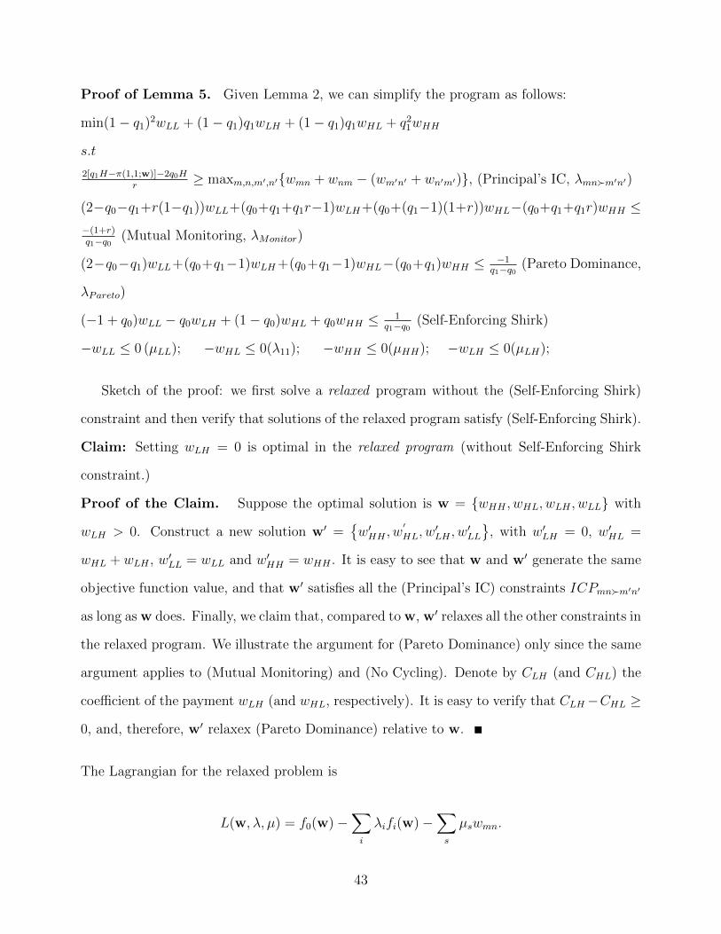
Proof of Lemma 5. Given Lemma 2, we can simplify the program as follows:

min(1− q1)2wLL + (1− q1)q1wLH + (1− q1)q1wHL + q21wHH

s.t

2[q1H−π(1,1;w)]−2q0Hr

≥ maxm,n,m′,n′{wmn + wnm − (wm′n′ + wn′m′)}, (Principal’s IC, λmn�m′n′)

(2−q0−q1+r(1−q1))wLL+(q0+q1+q1r−1)wLH+(q0+(q1−1)(1+r))wHL−(q0+q1+q1r)wHH ≤−(1+r)q1−q0 (Mutual Monitoring, λMonitor)

(2−q0−q1)wLL+(q0+q1−1)wLH+(q0+q1−1)wHL−(q0+q1)wHH ≤ −1q1−q0 (Pareto Dominance,

λPareto)

(−1 + q0)wLL − q0wLH + (1− q0)wHL + q0wHH ≤ 1q1−q0 (Self-Enforcing Shirk)

−wLL ≤ 0 (µLL); −wHL ≤ 0(λ11); −wHH ≤ 0(µHH); −wLH ≤ 0(µLH);

Sketch of the proof: we first solve a relaxed program without the (Self-Enforcing Shirk)

constraint and then verify that solutions of the relaxed program satisfy (Self-Enforcing Shirk).

Claim: Setting wLH = 0 is optimal in the relaxed program (without Self-Enforcing Shirk

constraint.)

Proof of the Claim. Suppose the optimal solution is w = {wHH , wHL, wLH , wLL} with

wLH > 0. Construct a new solution w′ ={w′HH , w

′HL, w

′LH , w

′LL

}, with w′LH = 0, w′HL =

wHL + wLH , w′LL = wLL and w′HH = wHH . It is easy to see that w and w′ generate the same

objective function value, and that w′ satisfies all the (Principal’s IC) constraints ICPmn�m′n′

as long as w does. Finally, we claim that, compared to w, w′ relaxes all the other constraints in

the relaxed program. We illustrate the argument for (Pareto Dominance) only since the same

argument applies to (Mutual Monitoring) and (No Cycling). Denote by CLH (and CHL) the

coefficient of the payment wLH (and wHL, respectively). It is easy to verify that CLH−CHL ≥

0, and, therefore, w′ relaxex (Pareto Dominance) relative to w.

The Lagrangian for the relaxed problem is

L(w, λ, µ) = f0(w)−∑i

λifi(w)−∑s

µswmn.

43

A contract w = {wmn} for m,n ∈ {H,L} is optimal if and only if one can find a pair (w, λ, µ)

that satisfies the following four conditions: (i) Primal feasible, i.e., constraints fi(w) ≥ 0

and wmn ≥ 0, (ii) Dual feasible, i.e., Lagrangian multiplier vectors λ ≥ 0 and µ ≥ 0,

(iii) Stationary condition, i.e., ∇wL(w, λ, µ) = 0, and (iv) Complementary slackness, i.e.

λifi(w) = µswmn = 0. The proof lists the optimal contract, in particular the pair (w, λ, µ),

as a function of the discount rate r.

For r < rA, the solution, denoted as as Pure JPE, is:

wLL = 0, wHL = 0, wHH = 1+r(q1−q0)(q0+q1+q1r) ;

λPareto = q1, λMonitor =q21

q0+q1+q1r, λCY C = 0, λHH�LL = 0,

λHL�LL = 0, λHH�HL = 0, λHH�HH = 0, λLL�HH = 0,

λLL�HL = 0, µLL = q0−2q0q1+q1(1+r−q1r)q0+q1+q1r

, µHL = q0q1q0+q1+q1r

, µHH = 0.

The ICPHH�LL constraint yields the upper bound on r under Pure JPE.

For rA < r ≤ min(rL, rC), the solution, denoted as BPC, is:

wLL =(q1−q0)2(q0+q1+q1r)H−(1+r)(q21+r)

(q1−q0)(q0+q1−(−1+q1)q1r−r2) , wHL = 2 ∗ wLL,

wHH =(q1−q0)2(q0+q1+(−1+q1)r)H−(1+r)(−1+q21+r)

(q1−q0)(q0+q1−(−1+q1)q1r−r2) ;

λPareto = 0, λMonitor = −rq0+q1+q1r−q21r−r2

, λCY C = 0, λHH�LL = q0−(q1−2)((q1−q)r−1)q0+q1+q1r−q21r−r2

,

λHL�LL = 0, λHH�HL = −2(q0−(q1−1)((q1−1)r−1))q0+q1+q1r−q21r−r2

, λHH�HH = 0, λLL�HH = 0,

λLL�HL = 0, µLL = 0, µHL = 0, µHH = 0.

Under BPC , the non-negativity of wLL and wHL requires r > rA, while (Pareto Dominance)

and λHH�HL ≥ 0 impose the upper bounds rC and rL, respectively.

For min{rL, rA} < r ≤ rB , the solution, denoted as JPE, is:

wLL = 0, wHL =(1+r)(q21+r)

q1−q0−(q1−q0)(q0+q1+q1r)H

(1−q1)r(1+r)−q0(q1+r) ,

wHH = (1−q1)q1(1+r)+(q1−q0)2(q0+(−1+q1)(q+r))H(q1−q0)((−1+q1)r(1+r)+q0(q1+r)) ;

λPareto = 0, λMonitor = (q1−1)q1r(q1−1)r(1+r)+q0(q1+r) , λCY C = 0, λHH�LL = −q0q1

(q1−1)r(1+r)+q0(q1+r) ,

λHL�LL = 0, λHH�HL = 0, λHH�HH = 0, λLL�HH = 0,

λLL�HL = 0, µLL = r(q0−(q1−1)((q1−q)r−1))(q1−1)r(1+r)+q0(q1+r) , µHL = 0, µHH = 0.

44

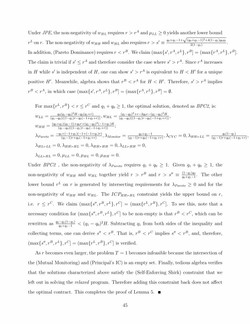
Under JPE, the non-negativity of wHL requires r > rA and µLL ≥ 0 yields another lower bound

rL on r. The non-negativity of wHH and wHL also requires r > s′ ≡ q0+q1−1+√

(q0+q1−1)2+4(1−q1)q0q12(1−q1) .

In addition, (Pareto Dominance) requires r < rB. We claim (max{s′, rA, rL}, rB] = (max{rA, rL}, rB].

The claim is trivial if s′ ≤ rA and therefore consider the case where s′ > rA. Since rA increases

in H while s′ is independent of H, one can show s′ > rA is equivalent to H < H ′ for a unique

positive H ′. Meanwhile, algebra shows that rB < rA for H < H ′. Therefore, s′ > rA implies

rB < rA, in which case (max{s′, rA, rL}, rB] = (max{rA, rL}, rB] = ∅.

For max{rL, rB} < r ≤ rC and q1 + q0 ≥ 1, the optimal solution, denoted as BPC2, is:

wLL = q0(q1−q0)2H−q0(q1+r)(q1−q0)((1−q1)r−q0(−1+q1+r)) , wHL = (q1−q0)2+r−2q0r−(q1−q0)3H

(q1−q0)((1−q1)r−q0(−1+q1+r)) ,

wHH = (q0+q1)(q1−1)+q0r+(q1−q0)2(−1+q1)H(q1−q0)((1−q1)r−q0(−1+q1+r)) ;

λPareto = −q0+(−1+q1)(−1+(−1+q1)r)(q1−1)r+q0(−1+q1+r) , λMonitor = q0+q1−1

(q1−1)r+q0(−1+q1+r) , λCY C = 0, λHH�LL = q0(1−q1)(q1−1)r+q0(−1+q1+r) ,

λHL�LL = 0, λHH�HL = 0, λHH�HH = 0, λLL�HH = 0,

λLL�HL = 0, µLL = 0, µHL = 0, µHH = 0.

Under BPC2 , the non-negativity of λPareto requires q1 + q0 ≥ 1. Given q1 + q0 ≥ 1, the

non-negativity of wHH and wHL together yield r > rB and r > s′′ ≡ (1−q1)q0q0+q1−1 . The other

lower bound rL on r is generated by intersecting requirements for λPareto ≥ 0 and for the

non-negativity of wHH and wHL. The ICPHH�HL constraint yields the upper bound on r,

i.e. r ≤ rC . We claim (max{s′′, rB, rL}, rC ] = (max{rL, rB}, rC ]. To see this, note that a

necessary condition for (max{s′′, rB, rL}, rC ] to be non-empty is that rB < rC , which can be

rewritten as q0−q1(1−q1)q0+q1−1 < (q1 − q0)2H. Subtracting q1 from both sides of the inequality and

collecting terms, one can derive s′′ < rB. That is, rB < rC implies s′′ < rB, and, therefore,

(max{s′′, rB, rL}, rC ] = (max{rL, rB}, rC ] is verified.

As r becomes even larger, the problem T = 1 becomes infeasible because the intersection of

the (Mutual Monitoring) and (Principal’s IC) is an empty set. Finally, tedious algebra verifies

that the solutions characterized above satisfy the (Self-Enforcing Shirk) constraint that we

left out in solving the relaxed program. Therefore adding this constraint back does not affect

the optimal contract. This completes the proof of Lemma 5.

45

Lemma 6 Given T = 0, the solution to the Program P is one of the following (wLH = 0 and

wHH > 0 in all cases):

(i) IPE: wHH = wHL = 1q1−q0 , wLL = w = 0 for r ∈ (0, rB];

(ii) BPI: 2wLL = w > 0, wHL = wHH + wLL.;

(iii) RPE: wHL > wHH > 0, wLL = w = 0 for r ∈ (max{rB, rH}, rD];

(iv) BPS: wHH > 0, wHL = 2wHH > 2wLL = w > 0 for r > max{rH , rD}.

Proof of Lemma 6. Similar argument as in the Proof of Lemma 5 shows that setting

wLH = 0 is optimal. Given wLH = 0, one can rewrite the program as follows.

min(1− q1)2wLL + (1− q1)q1wHL + q21wHH

s.t

2[q1H−π(1,1;w)]−2q0Hr

≥ max{wmn + wnm − (wm′n′ + wn′m′)}, (Principal’s IC, λmn�m′n′)

(1− q1)wLL − (1− q1)wHL − q1wHH ≤ −1q1−q0 (Static NE, λSNE)

((2− q1 − q0) + (1− q0)r)wLL + ((q0 − 1)(1 + r) + q1)wHL − (rq0 + q0 + q1)wHH ≤ −(1+r)q1−q0 (No

Joint Shirking, λSHK)

(1− q1)(2 + r)wLL + ((q1 − 1)(1 + r) + q1)wHL − q1(2 + r)wHH ≤ − 1+rq1−q0 (No Cycling, λCY C)

−wLL ≤ 0(µ00); −wHL ≤ 0(µ10); −wHH ≤ 0(µ11).

For r ≤ rB, the solution, denoted as IPE, is:

wLL = 0, wHL = wHH = 1q1−q0

λSNE = q1, λSHK = 0, λCY C = 0, λHH�LL = 0,

λHL�LL = 0, λHH�HL = 0, λHL�HH = 0, λLL�HH = 0,

λLL�HL = 0, µLL = 1− q1, µHL = 0, λ12 = 0.

Under IPE, the ICPHH�LL constraint imposes the upper bound rB on r.

For rB < r < rH , the solution, denoted as BPI, is:

wLL = (q1−q0)2(1+r)H−(1+r)(q1+r)(q1−q0)(q−r(−1+q1+r)) , wHL = wHH + wLL,

wHH = (q1−q0)2H−(1+r)(−1+q1+r)(q1−q0)(q−r(−1+q1+r)) ;

46

λSNE = 0, λSHK =r(1+r+q21r−2q1(q+r))

(q1−q0)(1+r)(−1+(−1+q1)r+r2) , λCY C =r(−1+q0+q1−r+q0r−q21r)

(q0−q1)(1+r)(−q+(−1+q1)r+r2) , λHH�LL =

1+r−q1r−1−(1−q1)r+r2 ,

λHL�LL = 0, λHH�HL = 0, λHL�HH = 0, λLL�HH = 0,

λLL�HL = 0, µLL = 0, µHL = 0, µHH = 0.

Under BPI, both the non-negativity of wLL and the (Static NE) constraints require r > rB,

and λSHK ≥ 0 requires r < rH .

For max{rH , rB} < r ≤ rD, the optimal solution, denoted as RPE, is:

wLL = 0, wHL =(q1−q0)q1(2+r)H−

(1+r)(q21+r)

q1−q0

q21−r(1+r)+q1r(2+r),

wHH = (1−q1)q1(1+r)+(q1−q0)2(−1−r+q1r(2+r))H(q1−q0)(q21−r(1+r)+q1r(2+r))

,

λSNE = 0, λSHK = 0, λCY C = (1−q1)q1rr(1+r)−q21−q1r(2+r)

, λHH�LL =q21

r(1+r)−q21−q1r(2+r),

λHL�LL = 0, λHH�HL = 0, λHL�HH = 0, λLL�HH = 0,

λLL�HL = 0, µLL =r(1+r+q21r−2q1(1+r))r(1+r)−q21−q1r(2+r)

, µHL = 0, µHH = 0.

Under RPE, the (Static NE) constraint and µLL ≥ 0 yields two lower bounds rB and rH on r.

ICPHL�LL and the non-negativity of wHH and wHL together require r ≤ rD. wHH ≥ 0 also re-

quires r > s ≡ 2q1−1+√

(2q1−1)2+4(1−q1)q212(1−q1) , and we claim (max{s, rB, rH}, rD] = (max{rB, rH}, rD].

Consider the case where s > rB (as the claim is trivial if instead s ≤ rB). Since rB increases

in H while s is independent of H, one can show that s > rB is equivalent to H < H∗ for

a unique positive H∗. Algebra shows that rD < rB for H < H∗. Therefore, in the case of

s > rB, we know rD < rB and hence (max{s, rB, rH}, rD] = (max{rB, rH}, rD] = ∅.

For r > max{rD, rH}, the optimal solution, denoted as BPS, is:

wLL = (1+r)((2−q1)q1+r)+(q1−q0)2(−2(1+r)+q1(2+r))H(q1−q0)(2q1+(3−q1)q1r+r2−2(1+r)) , wHL = 2wHH ,

wHH = (1+r)(−(1−q1)2+r)−(q1−q0)2(1−q1)(2+r)H(q1−q0)(2q1+(3−q1)q1r+r2−2(1+r)) ,

λSNE = q1, λSHK = 0, λCY C = r−2−2r−q21r+r2+q1(2+3r)

, λHH�LL = q1(−2+(−1+q1)r)2+2r+q21r−r2−q1(2+3r)

,

λHL�LL =2(1+r+q21r−2q1(1+r))−2−2r−q21r+r2+q1(2+3r)

, λHH�HL = 0, λHL�HH = 0, λ8 = 0,

λLL�HL = 0, µLL = 1− q1, µHL = 0, µHH = 0.

The two lower bounds rD and rH are derived from the non-negativity constraint of wLL and

47

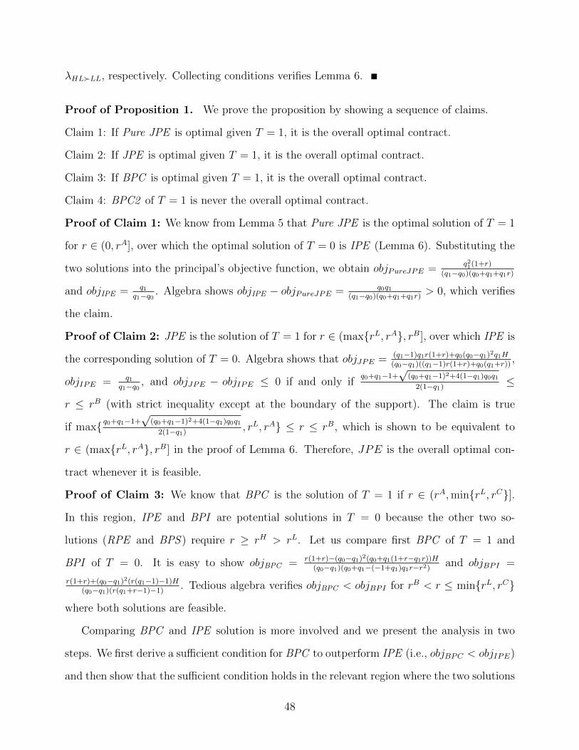
λHL�LL, respectively. Collecting conditions verifies Lemma 6.

Proof of Proposition 1. We prove the proposition by showing a sequence of claims.

Claim 1: If Pure JPE is optimal given T = 1, it is the overall optimal contract.

Claim 2: If JPE is optimal given T = 1, it is the overall optimal contract.

Claim 3: If BPC is optimal given T = 1, it is the overall optimal contract.

Claim 4: BPC2 of T = 1 is never the overall optimal contract.

Proof of Claim 1: We know from Lemma 5 that Pure JPE is the optimal solution of T = 1

for r ∈ (0, rA], over which the optimal solution of T = 0 is IPE (Lemma 6). Substituting the

two solutions into the principal’s objective function, we obtain objPureJPE =q21(1+r)

(q1−q0)(q0+q1+q1r)

and objIPE = q1q1−q0 . Algebra shows objIPE − objPureJPE = q0q1

(q1−q0)(q0+q1+q1r) > 0, which verifies

the claim.

Proof of Claim 2: JPE is the solution of T = 1 for r ∈ (max{rL, rA}, rB], over which IPE is

the corresponding solution of T = 0. Algebra shows that objJPE = (q1−1)q1r(1+r)+q0(q0−q1)2q1H(q0−q1)((q1−1)r(1+r)+q0(q1+r)) ,

objIPE = q1q1−q0 , and objJPE − objIPE ≤ 0 if and only if

q0+q1−1+√

(q0+q1−1)2+4(1−q1)q0q12(1−q1) ≤

r ≤ rB (with strict inequality except at the boundary of the support). The claim is true

if max{ q0+q1−1+√

(q0+q1−1)2+4(1−q1)q0q12(1−q1) , rL, rA} ≤ r ≤ rB, which is shown to be equivalent to

r ∈ (max{rL, rA}, rB] in the proof of Lemma 6. Therefore, JPE is the overall optimal con-

tract whenever it is feasible.

Proof of Claim 3: We know that BPC is the solution of T = 1 if r ∈ (rA,min{rL, rC}].

In this region, IPE and BPI are potential solutions in T = 0 because the other two so-

lutions (RPE and BPS ) require r ≥ rH > rL. Let us compare first BPC of T = 1 and

BPI of T = 0. It is easy to show objBPC = r(1+r)−(q0−q1)2(q0+q1(1+r−q1r))H(q0−q1)(q0+q1−(−1+q1)q1r−r2) and objBPI =

r(1+r)+(q0−q1)2(r(q1−1)−1)H(q0−q1)(r(q1+r−1)−1) . Tedious algebra verifies objBPC < objBPI for rB < r ≤ min{rL, rC}

where both solutions are feasible.

Comparing BPC and IPE solution is more involved and we present the analysis in two

steps. We first derive a sufficient condition for BPC to outperform IPE (i.e., objBPC < objIPE)

and then show that the sufficient condition holds in the relevant region where the two solutions

48

are optimal in their corresponding program, i.e., rA < r ≤ min{rL, rB, rC}. Given objBPC

and objIPE derived above, one can show that objBPC < objIPE if and only if r < δ, where

δ =1

2(1− q1)[((q1 − q0)2H − q1)q1(1− q1)− 1+√

(((q1 − q0)2H − q1)q1(1− q1)− 1)2 + 4(1− q1)((q1 − q0)2H − q1)(q1 + q0)].

We will show r < δ (hence objBPC < objIPE) satisfies over the relevant region rA < r ≤

min{rL, rB, rC} by considering two cases. First consider the case of δ ≥ rB, in which r < δ

satisfies trivially for rA < r ≤ min{rL, rB, rC}. Consider the second case in which δ < rB.

The remainder shows that δ < rB over the relevant region implies rL < δ, and, therefore,

r < δ again satisfies given rA < r ≤ min{rL, rB, rC}. One can show that δ < rB corresponds

to either r <1+√

1+4(1−q1)2(−1+q1(3+(q1−2)q1))H2(1−q1)2H or q1 −

√q1H< r < q1. We need only consider

r <1+√

1+4(1−q1)2(−1+q1(3+(q1−2)q1))H2(1−q1)2H as the latter condition r < q1 ≤ 1 is outside the relevant

region. Given r <1+√

1+4(1−q1)2(−1+q1(3+(q1−2)q1))H2(1−q1)2H , algebra shows rL < δ for any q0 ∈ [0, q1).

Proof of Claim 4: Recall that BPC2 of T = 1 is obtained by solving the following three

binding constraints: (Mutual Monitoring), (Pareto Dominance), and ICPHH�LL. When both

(Mutual Monitoring) and (Pareto Dominance) are biding, it is easy to prove U11 = U00 = U01.

Since BPC2 also creates strategic payoff complementarity (i.e., U11−U01 > U10−U00), we can

further show that the contract satisfies U11 = U00 = U01 > U10, which means that BPC2 would

have satisfied the (No Cycling) had the constraint been part of T = 1. In other words, BPC2

satisfies all the potentially binding constraints in the T = 0 program when the parameters

are such that either RPE or BPS is optimal given T = 0 (recall that (No Joint Shirking)

is not binding in these two solutions). Therefore, the optimality of RPE and BPS means

that objBPC2 ≥ objRPE and objBPC2 ≥ objBPS over the corresponding parameter spaces.

To see that BPI is more cost efficient than BPC2 (i.e., objBPC2 ≥ objBPI), note that RPE

is feasible over the region where BPI is optimal, and we know by revealed preference that

objRPE ≥ objBPI , and objBPC2 ≥ objRPE ≥ objBPI by transitivity.

49

BPS is optimal for sufficiently large r as team incentives T = 1 is infeasible in the region.

Proof of Corollary 1. For Part (i), it is easy to verify from Lemma 5 that the interval

over which BPC is optimal is non-empty if and only if rA < rL, which requires H ≤ H∗.=

(q1+(q1−1)q1)(q0+(q1−1)((q1−1)q21+1))(q1−1)2(q0−q1)2((q0−1)q21−q0q1+q0+q31)

and q0 > 1 − q1. Similarly, following Lemma 6, we know the

interval rB < r ≤ rH is non-empty if and only if q1 >12

and H ≤ H∗∗ ≡ q1(3−(2−q1)q1)−1(1−q1)2(q1−q0)2 .

Proof of Proposition 2. Given Lemma 5, it is easy to verify that, fixing T = 1 and w = 0,

the solution to Program P is: (i) Pure JPE for r ∈ (0, rA]; (ii) JPE for r ∈ (rA, rB]; and (iii)

infeasible otherwise. Similarly, given Lemma 6, one can verify that fixing T = 0 and w = 0,

the solution to Program P is: (i) IPE for r ∈ (0, rB]; (ii) RPE for r ∈ (rB, rD]; and (iii)

infeasible otherwise. Endogenizing the choice of T follows similar steps shown in Proposition

1 and is hence suppressed. Collecting the conditions yields the overall optimal contract stated

in the proposition.

Proof of Corollary 2. The corollary follows from comparing Propositions 1 and 2.

Proof of Lemma 3. Following Lemmas 5 and 6, we list positive payments and Lagrangian

multipliers of the binding constraints (µ for non-negativity constraints and λ for other con-

straints).

For r < r1.=

2P(2Q2+Q−2)+√

(2(P (2Q2+Q−2)+Q2)+Q)2+8P (2P+1)(P (1−2Q)2+4Q)+Q(2Q+1)

8P, the solu-

tion is: wH11 = 4(r+1)P (4Q(Q(r+2)+r)+r+2)+2Q(2Qr+r+2)

, λMonitor =4(P+ 1

2)(Q+ 12)

2

P (4Q(Q(r+2)+r)+r+2)+2Q(2Qr+r+2),

µH00 = − (2P+1)Q(4P(4Q2+1)+4Q2(r−2)−r−2)2P (4Q(Q(r+2)+r)+r+2)+4Q(2Qr+r+2)

, µH10 =(4P 2−1)Q(4Q2−1)

2P (4Q(Q(r+2)+r)+r+2)+4Q(2Qr+r+2),

µL00 =(4PQ2+P+2Q)(16PQ−4Q2(r−2)+r+2)4P (4Q(Q(r+2)+r)+r+2)+8Q(2Qr+r+2)

, µL10 =(4Q2−1)(P(4Q2−1)r−2(P+Q)(4PQ+1))4P (4Q(Q(r+2)+r)+r+2)+8Q(2Qr+r+2)

,

µL11 = − P (2Q−1)(2Q+1)2(2Q(r−2)+r+2)4P (4Q(Q(r+2)+r)+r+2)+8Q(2Qr+r+2)

.

ICPH11�H00 imposes the upper bound r < r1.

To prove Part (ii), note that for r1 < r ≤ min{r2,−2(P−Q)(4PQ−1)P (4Q2−1) }, the contract is

wH11 =2(−2P 2(1−2Q)2−P (4Q(3Q+r−1)+2r+3)+2Q(2Qr+r+2))

P(P((4Q(4Q(Q2+Q−2)−1)−9)r−2(1−4Q2)2−4(2Qr+r)2)+8Qr(2Qr+r+2)),

wL11 =2(2P 2(1−2Q)2+P(Q2(8r+4)+4Q(r+1)−8r(r+1)+1)+2Q(2Qr+r+2))

P(P((4Q(4Q(Q2+Q−2)−1)−9)r−2(1−4Q2)2−4(2Qr+r)2)+8Qr(2Qr+r+2)).

50

λMonitor = − 2(2P−1)(2Q+1)2r

P((4Q(4Q(Q2+Q−2)−1)−9)r−2(1−4Q2)2−4(2Qr+r)2)+8Qr(2Qr+r+2),

λH11�H00 = − P (2Q−1)(2Q+1)2(2Q(r−2)+r+2)

2P((4Q(4Q(Q2+Q−2)−1)−9)r−2(1−4Q2)2−4(2Qr+r)2)+16Qr(2Qr+r+2),

µH00 =2r((4Q2−1)r(4PQ2+2PQ+P−Q)+2(4Q2+1)(P−Q)(4PQ−1))

P((4Q(4Q(Q2+Q−2)−1)−9)r−2(1−4Q2)2−4(2Qr+r)2)+8Qr(2Qr+r+2),

µH10 = − (4Q2−1)r(P(8PQ+4Q2(r−2)−r−2)+2Q)P((4Q(4Q(Q2+Q−2)−1)−9)r−2(1−4Q2)2−4(2Qr+r)2)+8Qr(2Qr+r+2)

,

µL00 = − 2(2P−1)Qr(4P(4Q2+1)−4Q2(r−2)+r+2)P((4Q(4Q(Q2+Q−2)−1)−9)r−2(1−4Q2)2−4(2Qr+r)2)+8Qr(2Qr+r+2)

,

µL10 =2(4P 2−1)Q(4Q2−1)r

P((4Q(4Q(Q2+Q−2)−1)−9)r−2(1−4Q2)2−4(2Qr+r)2)+8Qr(2Qr+r+2).

wL11 > 0 requires r > r1, ICPL11�L00 requires

r < r2.=

4PQ2 − 5P + 4Q2 + 2Q+√

(4(P + 1)Q2 − 5P + 2Q)2 − 16P (P (1− 2Q)2 − 4Q)

8P,

and µH10 > 0 requires r < −2(P−Q)(4PQ−1)P (4Q2−1) . One can show that the interval r1 < r ≤

min{r2,−2(P−Q)(4PQ−1)P (4Q2−1) } is non-empty if and only if −2(P−Q)(4PQ−1)

P (4Q2−1) ≥ r1, which is equivalent

to P ≤ P ∗ for a unique threshold P ∗ implicitly characterized by −2(P−Q)(4PQ−1)P (4Q2−1) = r1.

The previous solution does not exist if, in contrast, P > P ∗ (hence r1 > −2(P−Q)(4PQ−1)P (4Q2−1) ).

As r increases from r1, the solution is

wH10 =(2P 2(1−2Q)2+P(Q2(8r+4)+4Q(r+1)−8r(r+1)+1)+2Q(2Qr+r+2))P ((4P 2−1)Q(4Q2−1)+4P (4Q2−1)r+2(2Q−1)r2(2(P+1)Q+P ))

,

wH11 = (2P+1)(2PQ+P+2Qr)P ((4P 2−1)Q(2Q+1)+2r2(2(P+1)Q+P )+4P (2Q+1)r)

; λMonitor = (2P+1)(2Q+1)r(4P 2−1)Q(2Q+1)+2r2(2(P+1)Q+P )+4P (2Q+1)r

,

λH11�H00 = − (4P 2−1)Q(2Q+1)

2(4P 2−1)Q(2Q+1)+4r2(2(P+1)Q+P )+8P (2Q+1)r, µH00 = − (2P+1)Q(2Q−1)r2

(4P 2−1)Q(2Q+1)+2r2(2(P+1)Q+P )+4P (2Q+1)r,

µL00 =r(2(2Q+1)(P+Q)(4PQ+1)−(2Q−1)r(4PQ2+P+2Q))2(4P 2−1)Q(2Q+1)+4r2(2(P+1)Q+P )+8P (2Q+1)r

, µL10 =P(4Q2−1)r(2Q(r−2)−r−2)

2(4P 2−1)Q(2Q+1)+4r2(2(P+1)Q+P )+8P (2Q+1)r,

µL11 = − (2Q+1)r(P(8PQ+4Q2(r−2)−r−2)+2Q)2(4P 2−1)Q(2Q+1)+4r2(2(P+1)Q+P )+8P (2Q+1)r

.

The non-negativity of wH10 and µL11 requires r > r1 and r > −2(P−Q)(4PQ−1)P (4Q2−1) , respectively;

while ICPH11�H00 and Self-Shirking impose an upper bound on r.

For Part (iii), note that the principal can always ignore the individual subjective measures

and set wHmn = (r+1)P (r+2)

and wLmn = 0 for all m,n ∈ {0, 1}, which is feasible for all r.

Proof of Lemma 4. For r < rA.= min{ (2P+1)Q2

P (2(P+1)Q−P ), (2P+1)Q(3−2Q)

4P}, the optimal solution

satisfies wH11 =4

2(P+1)Q+P+(2Q−1)wH

10

2Q+1. The principal can transfer between wH11 and wH10, subject

51

to the constraints. For instance, setting wH10 = 0 is optimal for r ≤ (2P+1)Q(2Q+1)4P

, and setting

wH10 = (2P+1)Q(2Q+1)−4rPP (2Q−1)r(2(P+1)Q+P )

is optimal for (2P+1)Q(2Q+1)4P

< r < rA. The two upper bounds of r

is required by No Cycling and ICPH10�H00, respectively.

To prove Part (ii), we will show that the statement holds for r.=

(2(P+1)Q−P )(4PQ2+P−2Q)4P (P−Q)

<

r < r̄.= − 4(P+2Q2)

(1−2Q)2(2P (Q+1)−Q). The optimal contract is

wH00 =(P 2(2−8Q2)−P(4Q2(r+2)−4Q(r+1)+r(4r+5))+4Q(r+1))

P (P (8Q3r−4Q2(r+2)+2Qr−(r+2)(4r+1))+2Q(−2Qr−2r2+r+2)),

wH10 = − 2(r(P(4Q2+5)−2Q)+2(P+1)(4PQ2+P−2Q)+4Pr2)P (P (8Q3r−4Q2(r+2)+2Qr−(r+2)(4r+1))+2Q(−2Qr−2r2+r+2))

,

wH11 = − (r(P(4Q2+5)−2Q)+2(P+1)(4PQ2+P−2Q)+4Pr2)P (P (8Q3r−4Q2(r+2)+2Qr−(r+2)(4r+1))+2Q(−2Qr−2r2+r+2))

,

wL11 = − 2(2P+1)(P+Qr)P (P (8Q3r−4Q2(r+2)+2Qr−(r+2)(4r+1))+2Q(−2Qr−2r2+r+2))

.

Substituting the payments verifies ∆U = 0. Given the maintaining assumption P < Q2(1+Q)

,

one can verify that r̄ > r is equivalent to P > ∆ for a uniquely determined ∆.

To prove Part (iii), note that for r > − 4(P+2Q2)(1−2Q)2(2P (Q+1)−Q)

, the solution is

wH00 =P(4((Q−2)Qr+Q(3Q−1)+r2)+7r+3)+2Q(2Q(r+2)−3r−2)

P (P (4Q2(r+2)−8Qr+(r+2)(4r+3))+Q(−4Q2r+8Q(r+1)+r(4r−3)−4)) ,

wH10 =2(4P 2+P(4Q2(r+3)−4Q(r+1)+r(4r+7)+5)+4Q(Q(r+2)−r−1))

P (P (4Q2(r+2)−8Qr+(r+2)(4r+3))+Q(−4Q2r+8Q(r+1)+r(4r−3)−4)) ,

wH11 =4P 2+P(4Q2(r+3)−4Q(r+1)+r(4r+7)+5)+4Q(Q(r+2)−r−1)

P (P (4Q2(r+2)−8Qr+(r+2)(4r+3))+Q(−4Q2r+8Q(r+1)+r(4r−3)−4)) ,

wL10 = 4(2P+1)(P+Qr)P (P (4Q2(r+2)−8Qr+(r+2)(4r+3))+Q(−4Q2r+8Q(r+1)+r(4r−3)−4)) ,

wL11 = 2(2P+1)(P+Qr)P (P (4Q2(r+2)−8Qr+(r+2)(4r+3))+Q(−4Q2r+8Q(r+1)+r(4r−3)−4)) .

λCY C = 2(r+2)(2Pr+r)P (4Q2(r+2)−8Qr+(r+2)(4r+3))+Q(−4Q2r+8Q(r+1)+r(4r−3)−4) ,

λH11�H00 = − (2P+1)Q(2Q+1)((2Q−1)r−4)4P (4Q2(r+2)−8Qr+(r+2)(4r+3))−4Q(4Q2r−8Q(r+1)+r(3−4r)+4)

,

λL11�L00 =(4Q2−1)r(2P (Q+1)−Q)+4(2Q+1)(Q−P )

4P (4Q2(r+2)−8Qr+(r+2)(4r+3))−4Q(4Q2r−8Q(r+1)+r(3−4r)+4),

λH10�H00 = (2P+1)Q(4Q((Q−1)r−2)+r)2(P (4Q2(r+2)−8Qr+(r+2)(4r+3))+Q(−4Q2r+8Q(r+1)+r(4r−3)−4)) ,

λL10�L00 = − (1−2Q)2r(2P (Q+1)−Q)+4P+8Q2

2(P (4Q2(r+2)−8Qr+(r+2)(4r+3))+Q(−4Q2r+8Q(r+1)+r(4r−3)−4)) ,

µL00 = 4Pr(−2Qr+r+2)P (4Q2(r+2)−8Qr+(r+2)(4r+3))+Q(−4Q2r+8Q(r+1)+r(4r−3)−4) .

Taking the limit shows that, as r →∞, wLmn = 0, wH11 = wH00 = 12wH10 = 1

P+Q.

Proof of Proposition 3. We list the complete optimal solutions, taking as given team

incentives (T = 1) or individual incentives (T = 0), separately. Endogenizing T = {0, 1} then

52

follows from comparing the expected payments across the two programs.

Solutions given T = 0:

SolA: the optimal contract for r ≤ (2P+1)Q2

P (2(P+1)Q−P )is shown in Part (i) of Lemma 4. The

maintaining assumption P < Q2(1+Q)

helps simplify the upper bound on r.

SolB: for (2P+1)Q2

P (2(P+1)Q−P )< r ≤ P 2(2Q(−4Q2+6Q+1)−3)+8PQ−8Q2

4P (2(P−1)Q+P ), the solution is wH10 = 1

Q,

wH11 = P 2(2Q+1)(1−2Q)2−4PQ+4Q2

PQ(P (2Q+1)(4Q2−4r−1)+8Qr), wL11 = −4(P 2r+(2P+1)Q2−2(P+1)PQr)

PQ(P (2Q+1)(4Q2−4r−1)+8Qr). The binding constraints

are wH00 = wL00 = wL10 = 0, Static NE, and ICPH11�H00. The non-negativity wL11 > 0 and

the constraint ICPH10�H00 impose the lower and upper bound on r, respectively. Note that

we identify the binding constrains (rather than listing each Lagrangian multipliers) in this

proposition for space considerations.

SolC: forP 2(2Q(−4Q2+6Q+1)−3)+8PQ−8Q2

4P (2(P−1)Q+P )< r ≤ −P 2(1−2Q)2(2Q−3)+4P (2Q−1)Q−8Q2

8(P−1)PQ−4P 2 , the solu-

tion is wH10 = 8(P−Q)P (P (2Q+1)(4(Q−2)Q+4r+3)−8Qr) , w

H11 = 4(P−Q)

P (P (2Q+1)(4(Q−2)Q+4r+3)−8Qr) , and wL10 =[4((2P+1)Q(2Q−3)+4Pr)

P (P (2Q+1)(4(Q−2)Q+4r+3)−8Qr) + 2QwL11 + wL11

]/(2Q−1). The solution is not unique: the princi-

pal can transfer between wL11 and wL10 subject to the constraints. For instance, setting wL10 = 0 is

optimal for r ≤ Q(1P−Q+ 1

)−1

4; while, for higher r, setting wL10 =

4(P((1−2Q)2+4r)−4Q)P (2Q−1)(P (2Q+1)(4(Q−2)Q+4r+3)−8Qr)

is optimal. The binding constraints are wH00 = wL00 = 0, Static NE, ICPH11�H00, and

ICPH10�H00. The upper bound of r is imposed by No Cycling constraint.

SolD: for −P2(1−2Q)2(2Q−3)+4P (2Q−1)Q−8Q2

8(P−1)PQ−4P 2 < r ≤ r̃.=

(2(P+1)Q−P )(4PQ2+P−2Q)4P (P−Q)

, the solution

is wH00 =(2Q+1)(P 2(2Q−1)(4(Q−2)Q+4r+3)−4PQ(2Q+2r−1)+8Q2)

2PQ(P (16Q2(Q2+r)−12r−1)−2Q(4Q(Q+2r)−1)) ,

wH10 =(P 2(2Q−1)(2Q(4Q2−2Q+4r+1)+4r−1)−2PQ(4Q(3Q+2r−1)+4r+3)+8Q2)

PQ(P (16Q2(Q2+r)−12r−1)−2Q(4Q(Q+2r)−1)) ,

wH11 =(P 2(2Q−1)(2Q(4Q2−2Q+4r+1)+4r−1)−2PQ(4Q(3Q+2r−1)+4r+3)+8Q2)

2PQ(P (16Q2(Q2+r)−12r−1)−2Q(4Q(Q+2r)−1)) ,

wL10 =2(P 2(8Q3−4Q2+2Q−4r−1)+4PQ(Q(2Q−1)+r+1)−4Q2)

PQ(P (16Q2(Q2+r)−12r−1)−2Q(4Q(Q+2r)−1)) , wL11 =(P 2(8Q3−6Q+2)+P (−4(Q−1)Q−5)Q−8Q3)

PQ(P (16Q2(Q2+r)−12r−1)−2Q(4Q(Q+2r)−1)) .

The binding constraints are wL00 = 0, Static NE, No Cycling, ICPH11�H00, ICPH10�H00, and

ICPL11�L00. The non-negativity constraints wH00 > 0 and wL10 > 0 imposes the lower and upper

bound of r, respectively.

SolE: for r̃ < r ≤ r3.= − 4(P+2Q2)

(1−2Q)2(2P (Q+1)−Q), the solution is the one shown in Lemma 4 -

Part (ii).

53

SolF: for r > r3, the solution is the one shown in Lemma 4 - Part (iii).

Solutions given T = 1:

Sol1: The optimal contract for r ≤ r1 is Pure JPE shown in Part (i) of Lemma 3.

Sol2: Part (ii) of Lemma 3 (the one with wL11 > 0) specifies the contract for r1 < r ≤ r2.=

4PQ2+√

(4(P+1)Q2−5P+2Q)2−16P (P (1−2Q)2−4Q)−5P+4Q2+2Q

8P. The maintaining assumption P < Q

2(1+Q)

assures the existence of the interval (r1, r2].

Sol3: for r2 < r ≤ −2(P−Q)(4PQ−1)P (4Q2−1) , the solution is

wH10 =4(P(−4Q2(r−1)−4Q+(r+1)(4r+1))−2Q(2Qr+r+2))

P (P (4Q2−1)(4Q2(r−2)−(r+2)(4r+1))+4Q(2Q−1)(2Q−2r2+1)),

wH11 = − 2(2P+1)(2PQ+P+2Qr)P (P (2Q+1)(4Q2(r−2)−(r+2)(4r+1))+4Q(2Q−2r2+1))

,

wL11 = − 2(2P+1)(2PQ+P+2Qr)P (P (2Q+1)(4Q2(r−2)−(r+2)(4r+1))+4Q(2Q−2r2+1))

. The binding constraints are wH00 =

wL00 = wL10 = 0, Mutual Monitoring, ICPH11�H00, and ICPL11�L00. The non-negativity wH10 > 0

and ICPH10�H00 impose the lower and upper bound of r, respectively.

Sol4: for −2(P−Q)(4PQ−1)P (4Q2−1) < r ≤ r̃, a feasible solution is

wH00 =P 2(2−8Q2)−P(4Q2(r+2)−4Q(r+1)+r(4r+5))+4Q(r+1)

P (P (8Q3r−4Q2(r+2)+2Qr−(r+2)(4r+1))+2Q(−2Qr−2r2+r+2)),

wH10 = − 2(r(P(4Q2+5)−2Q)+2(P+1)(4PQ2+P−2Q)+4Pr2)P (P (8Q3r−4Q2(r+2)+2Qr−(r+2)(4r+1))+2Q(−2Qr−2r2+r+2))

,

wH11 =r(2Q−P(4Q2+5))−2(P+1)(4PQ2+P−2Q)−4Pr2

P (P (8Q3r−4Q2(r+2)+2Qr−(r+2)(4r+1))+2Q(−2Qr−2r2+r+2)),

wL11 = − 2(2P+1)(P+Qr)P (P (8Q3r−4Q2(r+2)+2Qr−(r+2)(4r+1))+2Q(−2Qr−2r2+r+2))

.

wH00 > 0 and Pareto require r > r3 and r < r̃, respectively. The solution is optimal if the

parameters satisfy r̃ ≤ 4P (2Q+1)(2Q−1)(2P (Q+1)−Q)

(the binding constraints are wL00 = wL10 = 0, Mutual

Monitoring, ICPH11�H00, ICPL11�L00, and ICPH10�H00.) Setting wL10 = 0 is no longer optimal

if the condition is violated (i.e., r̃ > 4P (2Q+1)(2Q−1)(2P (Q+1)−Q)

), in which case, depending the value

of r, either wH00 or Self-Shirking replaces wL10 = 0 as the binding constraint in the optimal

solution. We verify that Part (iii) of the proposition holds for both cases as well.

Sol 5: for r̃ < r ≤ −P 2−4PQ3+4(P (3P+2)+1)Q2−3PQ4P (P−Q)

, the optimal solution is

wH00 =P 2(2Q−1)(12Q2+4r+1)+4PQ((1−2Q)2+2r)−8Q2

2PQ(2Q+1)(4PQ2+4Pr+P−2Q), wH11 = 2P+1

4PQ2+4Pr+P−2Q+wH00, wL11 = 2P+1

4PQ2+4Pr+P−2Q ,

wH10 =P 2(4Q2+1)(12Q2+4r+1)+2PQ(4Q(Q(4Q−3)+2r+1)−1)−16Q3

PQ(2Q+1)2(4PQ2+4Pr+P−2Q). The binding constraints are wL00 =

wL10 = 0, Self-Shirking, ICPH11�H00, ICPL11�L00, and Pareto. ICPH11�H10 and Mutual Mon-

54

itoring require the upper and lower bound on r, respectively.

Sol 6: for r > −P 2−4PQ3+4(P (3P+2)+1)Q2−3PQ4P (P−Q)

, the solution is wH00 =1− 2(2P+1)Q

4PQ2+4Pr+P−2Q

2P, wH01 =

(8P2−2)Q

4PQ2+4Pr+P−2Q−P

Q+1

2P, wH10 =

− 2(2PQ+Q)2

4PQ2+4Pr+P−2Q+P+Q

2PQ, wH11 = P (4P+4(Q−1)Q+4r+3)−4Q

2P (4PQ2+4Pr+P−2Q), wL11 = 2P+1

4PQ2+4Pr+P−2Q .

The binding constraints are wL00 = wL10 = wL01 = 0, Mutual Monitoring, ICPH11�H00, ICPL11�L00,

ICPH11�H10, and Pareto. The non-negativity of wH01 imposes the lower bound on r.

Endogenizing T = {0, 1}: Having solved the optimal solution given T = {0, 1}, endo-

genizing the choice of T is conceptually straightforward: comparing the expected payments

between the two program. We sketch the three main steps of the comparison and skip the

tedious algebra. First, the relevant solutions for r ≤ r̃ are SolA to SolD (given T = 0) and

Sol1 to Sol4 (given T = 1). Second, tedious but straightforward algebra shows that Sol1 to

Sol4 are overall optimal as long as they are optimal given T = 1. Finally, Sol5 and Sol6 of

T = 1 are never the overall optimal contract. The argument is similar to that in Claim 4

of the proof of Proposition 1: for parameters over which the two solutions are optimal given

T = 1, they satisfy all the potentially binding constraints of program with T = 0.

Proof of Corollary 3. Part (i) follows from the fact that the program of T = 1 does not

include No Cycling – the only difference from Lemma 5. One can verify that solutions in

Lemma 5 satisfy strategic complements, i.e., U(1, 1) − U(0, 1) > U(1, 0) − U(0, 0); and that

strategic complements and the Pareto Dominance together imply 2U(1, 1) > U(0, 1)+U(1, 0).

Therefore, agents will not collude on playing any strategies that involve only work and shirk.

For T = 0, it is straightforward to plug in the new cycling constraint, investigate the

Lagrangian, and verify the first part of Corollary 3 - (ii). The second part of (ii) follows from

the observation that the No Cycling constraint is more restrictive than the restated cycling

constraint. Note that the two agents are willing to collude on playing work and shirk only

if their joint payoff satisfies U(1, 0) + U(0, 1) > 2U(1, 1). Given T = 0, U(1, 0) + U(0, 1) >

2U(1, 1) implies U(1, 0) − U(1, 1) > U(1, 1) − U(0, 1) ≥ 0, where the last inequality follows

from the Static NE constraint that must hold if T = 0. The observation U(1, 0)− U(1, 1) >

55

U(1, 1)−U(0, 1) ≥ 0 further implies U(1, 0) > U(1, 1) > U(0, 1), which together with the time

value argument, suggests that our No Cycling constraint provides strictly higher continuation

payoff for the shirking agent in (0,1) (hence more costly for the principal to break) than any

collusive strategy having agents randomizes between work and shirk.

Part (iii) follows directly form parts (i) and (ii) of the Corollary.

56

Appendix B: Stationary Collusive Strategies

In addition to allowing for a joint bonus floor, another difference between our paper and

Kvaløy and Olsen (2006) is that they confine attention to stationary collusive strategies using a

correlation device, while we allow for non-stationary collusive strategies but in pure strategies.

In particular, stationary collusive strategies are characterized in Kvaløy and Olsen (2006)

as probabilities (a, b, b, 1 − a − 2b) on effort combinations of (1, 1), (1, 0), (0, 1), and (0, 0),

respectively. If we allow for such correlated strategies (while keeping the ability to commit

to a bonus floor), Program P will be intact except that (No Cycling) would be restated as

follows:

1 + r

r[π(1, 1;w)− 1] ≥ π(0, 1;w) +

[π(1, 0;w)− 1 + π(0, 1;w)]/2

r.

The second term of the right hand side of the equation is the continuation payoff for the

shirking agent from indefinitely playing either (1, 0) or (0, 1) with equal probability in each

period. Similar argument as Lemma 1 shows that a contract is collision proof if it satisfies both

the (No Joint Shirking) and the modified cycling constraint above. We also solve Program

P with the restated cycling constraint. The corollary below shows that the restated cycling

constraint does not qualitatively change the nature of the optimal contract studied in the

main model.

Corollary 3 If we confine attention to stationary collusive strategies,

(i) Given T = 1, the wage contract and the cutoffs are same as in Lemma 5.

(ii) Given T = 0, the wage contract and the cutoffs are characterized by the same binding

constraints as those in Lemma 6. The expected wage payment, π(1, 1), is weakly lower

than that in Lemma 6.

(iii) The overall optimal contract is same as Proposition 1 (the closed-form of cutoffs rD and

rH are different).

57

Part (i) shows that the way we formulate cycling constraint is irrelevant for the team

incentive case (T = 1). This is straightforward if we recall from Program P that team incentive

case does not include any collusion-proof constraint. For individual incentives (T = 0), the

restated No Cycling constraint only causes changes of a few cutoffs of the optimal contract.

As Corollary 3 - Part (iii) shows, the optimal contract is qualitatively unaffected by the

alternative way to formulate the cycling collusive strategies. In particular, the main insight is

that that having a positive bonus floor (wLL > 0) is still useful for the same reason as in the

main model, either to encourage mutual monitoring or to mitigate agents’ collusion problem.

Contrasting Corollary 3 with Proposition 2 makes it clear that the qualitative difference

of our paper and Kvaløy and Olsen (2006) is due the the principal’s ability to commit to

a positive bonus floor. Nonetheless, we find it more appealing to formulate the collusive

strategy as we did in the main model (without the correlated device) because the agents earns

more rent by colluding on it than on the stationary collusive strategy studied in Kvaløy and

Olsen (2006). This is shown in the second part of Corollary 3 - Part (ii), which suggests the

No Cycling constraint formulated in our main model is more restrictive than the correlated

cycling strategy above. Intuitively, because of the time value, the Cycle strategy formatted

in the text gives the shirking agent a higher continuation payoff (hence more difficult for the

principal to upset) than what he would receive under the correlated collusive strategy.

58