tcp performance analysis for lte and lte/wlan aggregation

TCP PERFORMANCE ANALYSIS FOR LTE AND LTE/WLAN AGGREGATION

A Master's Thesis Submitted to the Faculty of the

Escola Tècnica d'Enginyeria de Telecomunicació de Barcelona

Universitat Politècnica de Catalunya by

Sebastià Janer Cifre

In partial fulfilment of the requirements for the degree of

MASTER IN TELECOMMUNICATIONS ENGINEERING

Advisor: Ilker Demirkol

Barcelona, October 2018

Title of the thesis: TCP Performance Analysis for LTE and LTE/WLAN Aggregation

Author: Sebastià Janer Cifre

Advisor: Dr. Ilker Demirkol

Abstract

Nowadays, mobile IP data traffic is increasing exponentially and predictions tells that it will triplicate its actual value in 2020. A solution to this dare is LTE/WLAN Aggregation technique where cellular networks such as LTE and WLAN networks such as WiFi are combined to improve its performance. In this thesis, a prototype, based on very tight coupling between LTE and WiFi, is evaluated for their performance. There will be three policies assessed: No Offload policy, when data traffic is sent over LTE link; Full Offload, when data packets is sent over WiFi link and control packets through LTE link; and LWA with different techniques to split traffic through both links: Time division, Par/Impar, Low ICMP RTT and Port division.

In very tight coupling, eNB manages offloading and aggregation techniques, and does not require the core network in any case. PDCP layer, as common layer between both technologies, switches the traffic depending on the policy. Moreover, prioritizing reliability in front of throughput, an analysis of TCP flow control and default TCP congestion control method employed by Linux, namely CUBIC, theoretically and showing their functioning through physical experiments was performed.

1

Dedicated to my parents for their effort during years.

2

Acknowledgements.

My acknowledgments to my advisor Dr. Ilker Demirkol for his kindness, patience and valuable advices in this research work.

3

Revision history and approval record

Revision Date Purpose

0 15/09/2018 Document creation

1 08/10/2018 Document revision

2 10/10/2018 Document revision

Written by: Reviewed and approved by:

Date 10/10/2018 Date 10/10/2018

Name Sebastià Janer Name Ilker Demirkol

Position Project Author Position Project Supervisor

4

Table of contents

Abstract 1

Acknowledgements. 3

Revision history and approval record 4

Table of contents 5

List of Figures 6

List of Tables 12

1. Introduction 13

2. Background 20

3. State of the art of the technology used or applied in this thesis 34

4. Implementation 36

5. TCP Protocol Performance Evaluation 54

7. Conclusions and future development 87

Bibliography 88

Glossary 89

5

List of Figures

Figure 1.1 Global IP traffic growth 13

Figure 1.2 Mobile data traffic growth 13

Figure 1.3 Ericsson Mobile data traffic growth by application 14

Figure 1.4 Mobile data traffic offloaded in 2020 14

Figure 1.5 Scenario Architecture 16

Figure 1.6 Protocol stack 17

Figure 1.7 IP data packet through WiFi link 20

Figure 2.1 Evolved Packet System 21

Figure 2.2 E-UTRAN 22

Figure 2.3 E-UTRAN Protocol stack 23

Figure 2.4 3GPP network 26

Figure 2.5 high level software architecture 27

Figure 2.6 Combinations of available non overlapping WiFi channels

in 2.4 GHz band 31

Figure 2.7 Combinations of available 40 MHz WiFi channels

in 2.4 GHz band 31

Figure 2.8 CUBIC congestion avoidance growth function 33

Figure 3.1 LWA architecture 34

6

Figure 4.1 LTE link Architecture 37

Figure 4.2 USRP B210 on the left, USRP X310 on the right 37

Figure 4.3 VERT 900MHz and 2450 MHz antennas,

RG-58 coaxial cable and 20 dB attenuators 38

Figure 4.4 Return loss vs frequency of VERT 900 MHz and

VERT 2450 MHz 38

Figure 4.5 Ethernet interface configuration on eNB host 40

to connect with USRP X310

Figure 4.6 OAI eNB interfaces 41

Figure 4.7 enB.band.tm1.usrpx310 configuration file 43

Figure 4.8 OAI UE interfaces 45

Figure 4.9 Downlink scenario LTE Link using OAI software 48

Figure 4.10 Uplink scenario LTE Link using OAI software 49

Figure 4.11 WiFi Architecture 50

Figure 4.12 hostapd.conf file with all link layer settings 51

Figure 4.13 WiFi network configuration on OAI UE 52

Figure 4.14 WiFi interface features 53

Figure 5.1 LTE link 54

Figure 5.2 Iperf TCP test: Server terminal on the left,

Client terminal on the right 55

Figure 5.3 Wireshark capture of the first 18 packets of the iperf

7

downlink TCP test at the eNB 56

Figure 5.4 Packet structure of Linux “cooked” encapsulation

(LINKTYPE_LINUX_SLL) 57

Figure 5.5 Data packet and ACK packet corresponding a No Offload

TCP iperf test 57

Figure 5.6 TCP probe file corresponding to the first 17 ACK packets received

of the iperf downlink TCP test at the eNB 58

Figure 5.7 Rwnd (blue), Cwnd (red) and ssthr (green) evolution from the

corresponding TCP probe data file 59

Figure 5.8 Cwnd (red) and ssthr (green) evolution from the corresponding

TCP probe data file 59

Figure 5.9 Rwnd and Cwnd maximum values in bytes 61

Figure 5.10 Cwnd (red) and Ssthr (green) behaviour when there two

different packet losses 62

Figure 5.11 Fast retransmissions packets during the TCP test captured

with Wireshark 62

Figure 5.12 Bytes in flight (blue) and rwnd (green) of the iperf downlink

TCP test at the eNB 63

Figure 5.13 RTT of the iperf downlink TCP test at the eNB 64

Figure 5.14 Throughput of the iperf downlink TCP test at the eNB 64

Figure 5.15 RTT vs Bytes in Flight and Throughput vs Bytes in Flight with

two zones defined:

1) Buffer Size Limitation Zone. 2) Application Bandwidth Limitation Zone 65

8

Figure 5.16 Average Throughput (bps) of the following iperf TCP test:

No Offload policy, downlink with 25 RB without buffer size limitations 66

Figure 5.17 Rwnd (blue), Cwnd (red) and Ssthr (green) performance

of the following iperf TCP test: No Offload policy, downlinkwith 25 RB

without buffer size limitations 67

Figure 5.18 Rwnd (Bytes) in green and Bytes in Flight (Bytes) in blue

of the following iperf TCP test: No Offload policy, downlinkwith 25 RB

without buffer size limitations 67

Figure 5.19 RTT (ms) evolution of the following iperf TCP test:

No Offload policy, downlink with 25 RB without buffer size limitations 68

Figure 5.20 RTT (ms) evolution of the following iperf tests

1) No Offload policy, downlink with 25 RB with Snd_buffer_size = 25KB

2) No Offload policy, downlink with 25 RB with Snd_buffer_size = 50KB

3) No Offload policy, downlink with 25 RB with Snd_buffer_size = 75K 69


No Offload policy, downlink with 25 RB using BDP opt =86.88 KB 71

Figure 5.22 Cwnd, rwnd and ssthr of the following iperf TCP test:


Figure 5.23 RTT (ms) of the following iperf TCP test:


Figure 5.24 TCP Throughput vs TCP Snd_Buff_Size for No Offload

Downlink 25 RB (blue) and 50 RB (red) 72

Figure 5.25 UDP Throughput for No Offload Downlink 25 RB (blue) and

50 RB (red) 73

9

Figure 5.26 UDP Throughput for No Offload Uplink 25 RB (green)

and 50 RB (brown), TCP Throughput for No Offload Uplink 25 RB (blue)

and 50 RB (red) 73

Figure 5.27 WiFi Link. Enclosed with red circle the WiFi AP,

Ethernet interface of eNB and wifi interface of UE 74

Figure 5.28 ISM 2.4 GHz band with all operating WiFi networks with

its channel. Source: WiFi Explorer LITE application 74


Full Offload policy, downlink without buffer size limitations 75


of the following iperf TCP test: Full Offload policy, downlink without

buffer size limitations 76

Figure 5.31 RTT mean for iperf tests corresponding to No Offload policy

(blue) and Full Offload policy (red) 77

Figure 5.32 Throughput performance of Full Offload policy:

UDP downlink throughput (brown), UDP uplink throughput (green),

TCP downlink throughput (blue), TCP uplink throughput (red) 77

Figure 5.33 Time division LWA technique 78

Figure 5.34 Throughput performance for Time Division LWA technique

using 25 RB LTE link (blue) and using 50 RB on LTE link (red) 79


for Time Division LWA technique using 25 RB LTE link 79

10

Figure 5.36 Par/Impar LWA technique 80

Figure 5.37 Throughput performance for Par/Impar LWA technique



for Par/Impar LWA technique using 25 RB LTE link 81

Figure 5.39 Low RTT Ping LWA technique 82

Figure 5.40 Throughput performance for Low RTT Ping LWA technique



for Low RTT Ping LWA technique using 25 RB LTE link 73

Figure 5.42 Port division LWA technique 84

Figure 5.43 Throughput performance for Port division LWA technique

using 25 RB LTE link (blue) and using 50 RB on LTE link (red),

WiFi link (green), 25 RB LTE link + WiFi link (purple) and

25 RB LTE link + WiFi link (brown). 85

Figure 5.44 Rwnd (blue), Cwnd (red) and Ssthr (green) performance for

Port division LWA technique: WiFi link corresponding to port 5202 85

Figure 5.45 Rwnd (blue), Cwnd (red) and Ssthr (green) performance for

Port division LWA technique: LTE link using 25 RB corresponding

to port 5201 86

11

List of Tables

Table 1. Physical LTE layer main features 24

Table 2. 14 WiFi channels available in 2.4 GHz band 30

Table 3. LTE Band 7 features 42

Table 4. Bandwidth and Resource Block 46

Table 5. Relation between Tx gain and RB with the reference signal

power transmitter by the OAI eNB if we use USRP B210 47

Table 6. Relation between Tx gain and RB with the reference signal

power transmitter by the OAI eNB if we use USRP B210 47

12

1. Introduction

1.1. Motivation

The predicted global IP traffic, which includes managed IP, fixed Internet and mobile data, is increasing exponentially in terms of exabytes consumed per month. Several studies provides estimates of annual growing IP traffic. One of these studies was performed by Cisco and is described in [1]. In Figure 1.1, global traffic growth from 2015 to 2020 is represented.

Figure 1.1 Global IP traffic growth [1]

There is a 20% increase of traffic demand each year, which means that the Compound Annual Growth Rate (CAGR) exhibit a continuous incremental tendency. 1 EB unit is equivalent to 1 billion of GB and the total world population was 7.6 billion of people in 2017 , therefore it can conclude that during 2017 on average each person consumes 1

14.27 GB.

There is a fractional part of global IP traffic that is sent through mobile communications networks. According to Figure 1.2, in 2018 it was 17 EB which means that 12.8 % of total IP traffic is sent through mobile communications networks and demand will keep increasing every year, even faster. In 2020, predictions tells that mobile data traffic will triplicate its value obtained in 2018.

1 (2017, june 21). The World Population Prospects: 2017 Revision | Latest Major https://www.un.org/development/desa/publications/world-population-prospects-the-2017-revision.html

13

Figure 1.2 Mobile data traffic growth [1]

This growth of mobile data traffic is caused by the high number of application that appeared during last decade. In Figure 1.3, a description of mobile data traffic separated by application type is showed. This description is enclosed on the annually Mobility Report performed by Ericsson. In this case is from November 2017.

Figure 1.3 Ericsson Mobile data traffic growth by application 2

It is important to realise that Video consumption represents more than half of overall traffic and it will keep increasing next years. In 2020, approximately 60 % of all mobile data traffic will be Video consumption.

Nowadays, the exponentially increasing mobile data demand is one of the main challenges. Several studies have already been performed to develop solutions to fulfill these demands. An important one is exploit heterogeneous networks, which is achieved by aggregation of different access technologies such as WiFi. It is very important since most of traffic in cellular networks devices is created when these devices are not connected to the cellular network. Devices are also equipped with other interfaces such as WiFi and it is more economic for mobile network operators if their users download applications when their device is connected to a WiFi network.

According to this reflexion, in Figure 1.4, fraction of traffic consumed, when devices are connected to the cellular network and when WiFi interface is used, are represented.

2 Ericsson, “Ericsson Mobility Report,” November 2017

14

Figure 1.4 Mobile data traffic offloaded in 2020 [2]

The integration of two or more RATs seamlessly is expected to provide a scaled-up capacity expected from the future networks. Such aggregation is expected to be an enabler for 5G systems to efficiently use the limited RF spectrum. For this purpose, LTE/Wi-Fi Aggregation (LWA) was standardized in 3GPP Rel. 13. Talking about its standardization, LWA has been evaluated in a limited manner for its effect on the higher layer protocols such as TCP. In these few studies, it is shown that TCP performance is badly affected by such aggregation of multiple RATs. However, no detailed analysis of the reasons for this effect has been done in the literature. In this thesis, we analyze the TCP performance of LWA through physical experiments, using open-source LTE UE and eNB implementations with commodity hardware such as generic purpose processors (GPPs), software-defined radio (SDR) and Wi-Fi adapters. We provide insights on the TCP fundamentals in such practical scenario and how it is affected by the dynamics of the wireless channels and their aggregation.

1.2. Statement of purpose

Software Defined Radio (SDR) enables the execution of many hardware-based operations through software. With an open-source LTE software and a SDR, we are able to run a LTE base station on a PC or a portable low-cost device. At the same time, simple devices such as Raspberry Pi can be turned into WiFi APs. In this work, we will work on the developed LTE/WiFi integration solution using OpenAirInterface (OAI) software that implements the LTE eNB and the core network. In addition, we will evaluate and characterize TCP traffic performance on it.

Towards the target of more efficient LTE and WiFi coupling solutions using TCP protocol for data transfer, three main objectives are proposed:

- Analysis of the open power control loop used by OAI and the tunning of the LTE parameters to achieve a stable, more reliable LTE link.

- Analysis of default TCP congestion control method employed by Linux, namely CUBIC, theoretically and showing its functioning through physical experiments.

- Tuning CUBIC parameters for LTE, WiFi and LWA technologies. - Performance analysis of several packet scheduler methods for LWA to improve

the TCP performance.

1.3. Requirements and specifications

The LWA scenario is composed by two functional links which are implemented independently: the LTE link and the WiFi link. Both are between eNB and UE. In Figure 1.5, the LWA scenario is represented. The implementation is based on very tight coupling approach, i.e., where WiFi AP controlled directly by an LTE eNB. In consequence, the study can focus on E-UTRAN network since it is possible to send PDCP frames directly over WiFi. For this reason, we have used eNB implementation option “without S1 interface” from OAI, where all

15

processes performed by EPC network are emulated at eNB, without an actual EPC software.

Figure 1.5 Scenario Architecture

The LTE link connection between both SDR devices can be wireless or wired depending on the working frequency used since they allow to use antennas and coaxial cables, whereas the WiFi link connection is less flexible. WiFi AP is used in bridge mode to be as simple as possible. eNB is connected to a WiFi AP through Ethernet network and WiFi AP to UE through wireless network. In consequence, the eNB adapts all WiFi packets through Ethernet captures. We are interested in a fast implementation. In consequence, very tight coupling approach reduces delay since UE does not need to use WiFi security mechanisms such as authentication when it finds an available WiFi AP. Furthermore, UE is able to receive traffic separately or at the same time from both interfaces. As we want to offload data traffic through WiFi link, different policies has been implemented depending of the amount of offloaded traffic through WiFi interface:

- No Offload traffic: this policy implies a standard LTE transmission without

intervention of Wi-Fi, and is named No Offload. The protocol stack is a regular on: IP data packet is sent through PDCP layer and continue to RLC, MAC and PHY. The traffic follows Path 1 of the protocol stack shown in Figure 1.6.

- Full Offload traffic: radio bearer is switched to WiFi, which means that data traffic obtained in PDCP layer is sent only through WiFi interface. The data traffic changes the regular path followed and now an adaptation layer is required to identify each PDCP PDU, as it will be detailed later. After that, the data is sent through lower layers of WiFi link. The policy is named as Full Offload , and follows Path 2 of protocol stack shown in Figure 1.6. LTE sends and receives control plane traffic.

16

- LTE/WiFi Aggregation traffic: radio bearer is split between lower layers of LTE and

WiFi technologies. In this thesis, this policy has different techniques but in all of them both paths are used. LTE sends and receives control plane traffic.

Figure 1.6 Protocol stack

The protocol stack includes lower layers of both technologies LTE and Wi-Fi with PDCP layer as common layer. When an IP data packet arrives to PDCP layer, a PDCP header is added obtaining a PDCP PDU. If that PDU will be sent through WiFi, an adaptation header is added which is required to recognize each PDCP PDU. Adaptation layer adds four fields to frame:

- Radio Network Temporary Identifier (RNTI) is assigned when a UE has one or more active connections, it requires 2 bytes.

- rb_id is the radio bearer identification, it also requires 2 bytes. - module_id field identifies the UE, it has 1 byte. - eNB_index indicates the index of connected eNB and it has 1 byte.

In Figure 1.7, how an IP packet is transported over WiFi interface is represented.

Figure 1.7 IP data packet through WiFi link

The data packet continues to next layer where an Ethernet header is added with Ethernet type field “0x99ff”, then information is sent through Ethernet network to WiFi AP configured in bridge mode. With this configuration, Ethernet header is converted to WiFi header and finally data i sent by physical WiFi interface.

17

1.4. Methods and procedures The project is performed in the framework of research projects displayed by Wireless Networking Group from University Polytechnic of Catalonia. The group has different research areas such as protocols and architecture for wired and wireless networks, cellular, mobile ad hoc networks, sense networks, and heterogeneous networks; energy efficiency and cooperation of wireless networks; modeling, performance analysis and optimization protocols… The start of this project is from code inherited of the work “LTE/WIFI AGGREGATION IMPLEMENTATION AND EVALUATION” completed by Diego Patricio Ibarra Barreno on July 2017. All devices and material used in this project are provided by my advisor Dr. Ilker Demirkol as part of material used by the investigation group. Moreover, all software used in this project (Open Air Interface, Hostapd, Wireshark and TCP probe) was recommended by my advisor.

1.5. Work breakdown Structure

1. Background: a. LTE technology information review. b. WLAN technology information review. c. LWA technique information review. d. TCP protocol information review.

2. LTE link setup implementation. a. OpenAirInterface information review and configuration. b. LTE link power control analysis. c. LTE link setup testing

3. WiFi link setup implementation. a. Raspberry Pi and Hostapd review and configuration. b. Ethernet eNB interface and WiFi UE interface configuration. c. WiFi link setup testing.

4. Both links’ integration. a. Integration of WiFi part into Open Air Interface.

5. TCP data traffic analysis and evaluation. a. No Offload TCP data traffic analysis and evaluation. b. Full Offload TCP data traffic analysis and evaluation. c. LWA techniques implementation. d. LWA TCP data traffic analysis and evaluation

1.6. Incidences

During the project, all incidences appeared were at the beginning when we were setting up both links. Moreover, we have to comment that almost of them were related with

18

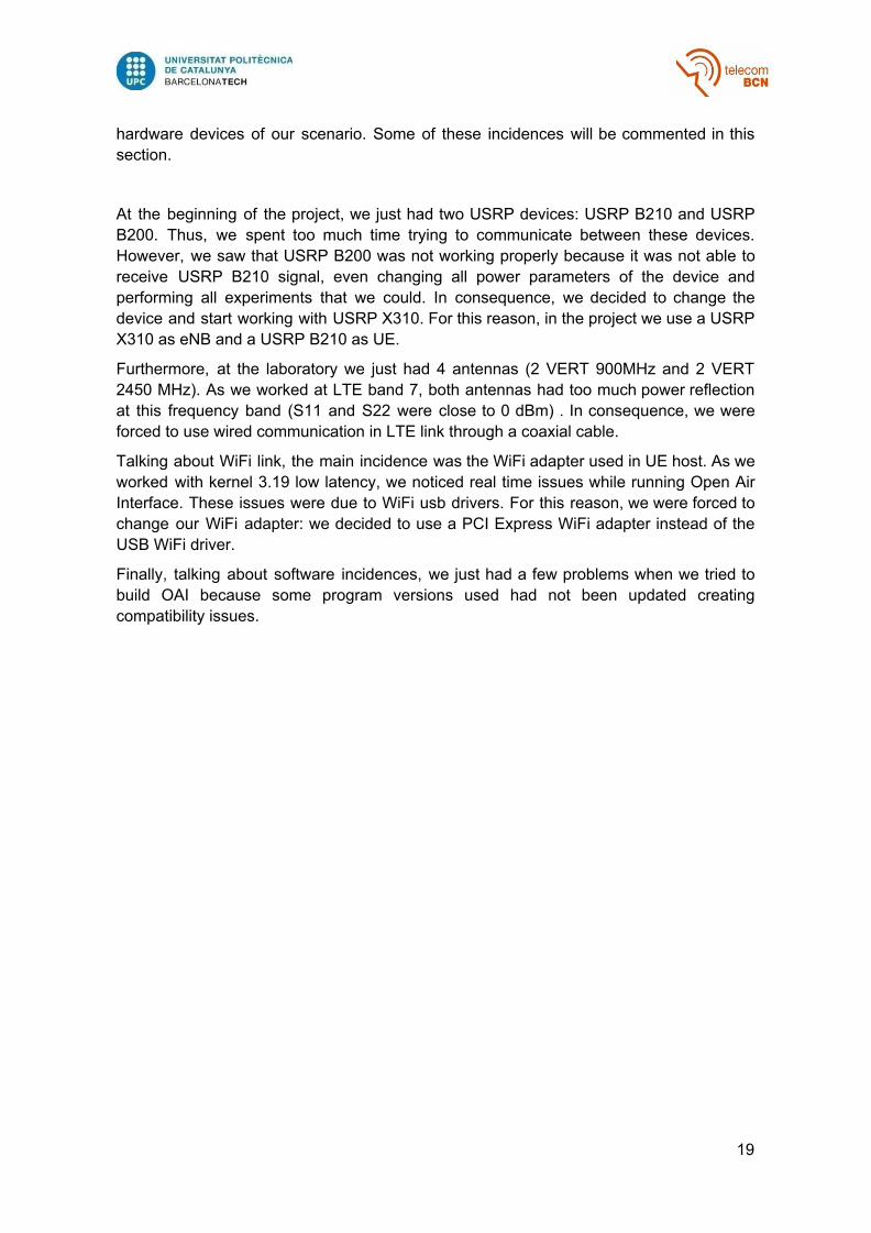
hardware devices of our scenario. Some of these incidences will be commented in this section.

At the beginning of the project, we just had two USRP devices: USRP B210 and USRP B200. Thus, we spent too much time trying to communicate between these devices. However, we saw that USRP B200 was not working properly because it was not able to receive USRP B210 signal, even changing all power parameters of the device and performing all experiments that we could. In consequence, we decided to change the device and start working with USRP X310. For this reason, in the project we use a USRP X310 as eNB and a USRP B210 as UE.

Furthermore, at the laboratory we just had 4 antennas (2 VERT 900MHz and 2 VERT 2450 MHz). As we worked at LTE band 7, both antennas had too much power reflection at this frequency band (S11 and S22 were close to 0 dBm) . In consequence, we were forced to use wired communication in LTE link through a coaxial cable.

Talking about WiFi link, the main incidence was the WiFi adapter used in UE host. As we worked with kernel 3.19 low latency, we noticed real time issues while running Open Air Interface. These issues were due to WiFi usb drivers. For this reason, we were forced to change our WiFi adapter: we decided to use a PCI Express WiFi adapter instead of the USB WiFi driver.

Finally, talking about software incidences, we just had a few problems when we tried to build OAI because some program versions used had not been updated creating compatibility issues.

19

2. Background

2.1 LTE

2.1.1 Evolved Packet System (EPS)

The Evolved Packet System (EPS) is the set of radio access and core network of LTE. It is composed by:

- An access network called Evolved Universal Terrestrial Radio Access Network (E-UTRAN).

- A core network called Evolved Packet Core (EPC).

At the beginning, Long Term Evolution (LTE) acronym was introduced to describe the new radio interface of 4G system developed by 3GPP. This term has remained but in specifications it is found as EPS network and this latter denomination is known as LTE network, which includes the radio part and the core part. In this document, it is adopted this terminology.

LTE provides IP connectivity between a UE (User equipment) and an external data network. It assigns to the UE an IP address that is valid in the external network. In consequence, traffic can be exchanged between external network and UE.

Long Term Evolution (LTE) was an acronym introduced at the beginning to describe the new radio interface of the 4G system developed by 3GPP. This term has remained but in specifications it is found as EPS network and this latter denomination is known as LTE network, which includes the radio part and the core part. In most of the books this terminology is used and in this document it is also adopted. The mobile terminal is named in the specifications as User Equipment (UE). In Figure 2.1, there is represented the EPS of LTE.

Figure 2.1 Evolved Packet System of LTE [3]

The deployment of a LTE network is not done in a decoupled way and have interface with others networks such as UTRAN, GERAN. The UE can move between networks without any additional action done by the user, which means that there exists continuity service.

20

For this reason, if a UE starts a connection to an external network in LTE and he decides to move to a HSPA network, it does not lose this connectivity. This integration with other networks is done through the core network.

These interfaces were designed to connect networks of the same family 3GPP, as well as, non-3GPP networks, allowing other technological families to converge to the use of LTE as the main mobile communication technology.

2.1.2 Access Network (E-UTRAN)

E-UTRAN network in LTE contains a single element called evolved NodeB (eNB). Several eNBs can compose E-UTRAN and may be interconnected with each other through X2 interface (optional). X2 supports enhanced mobility, inter-cell interference management… Moreover, each eNB is connected to the core network through the S1 interface. This interface connected to the core network is divided by:

- S1-U interface: user plane transport. - S1-MME interface: control plane transport.

In Figure 2.2, there is represented the E-UTRAN.

Figure 2.2 E-UTRAN [3]

In LTE network, there is no hierarchical structure with controller and base stations. All these radio interface functionalities are contained in the eNB. In consequence, each of these elements is autonomous and can provide access to core network, which means that the radio functionality is completely distributed.

The evolved NodeB (eNB) hosts the following functions:

- Radio Resource Management functions: Radio Bearer Control, Radio Admission Control, Connection Mobility Control, Dynamic allocation of resources to UEs in both uplink and downlink (scheduling).

- Measurement and measurement reporting configuration for mobility and scheduling.

21

- Access Stratum (AS) security.

- IP header compression and encryption of user data stream.

- Selection of an MME at UE attachment when no routing to an MME can be determined from the information provided by the UE.

- Routing of User Plane data towards Serving Gateway.

- Scheduling and transmission of paging messages (originated from the MME).

- Scheduling and transmission of broadcast information (originated from the MME or O&M).

2.1.3 LTE E-UTRAN protocol stack

The functionalities of LTE E-UTRAN are supported in the protocol stack represented in Figure 2.3. It is executed in the eNB and the UE. A user plane and a control plane are distinguished.

Figure 2.3 E-UTRAN protocol stack [3]

On the one hand, user plane refers to send IP packets. In this case E-UTRAN just carries IP packets. The circuit switched service cannot be provided through the LTE access network.

On the other hand, control plane refers to radio resource control RRC (radio signalling) and non-access stratum (NAS) protocols. NAS protocols appear are not executed in the eNB. They are sent through the eNB between UE and core network, encapsulated through the RRC protocol and finally in lower layers of the protocol stack. There is a unique physical layer and a link layer with three sublayers: a PDCP layer, an RLC layer, and a MAC layer.

22

2.1.4 Radio Resource Control protocol (RRC)

Radio Resource Control is the main protocol for handling the use of radio interface. Its functionalities are the following:

- Broadcast of System Information related to NAS and AS. - Establishment, maintenance and release of RRC connection. - Establishment, configuration, maintenance and release of Signalling and Data

Radio Bearers (SRBs and DRBs). - Security functions including key management. - Mobility functions including control of UE cell selection/reselection, Paging, UE

measurement configuration and reporting, and Handover. - QoS management. - Notification for ETWS (Earthquake and Tsunami Warning System), CMAS

(Commercial Mobile Alert System) and MBMS (Multimedia Broadcast Multicast Service).

- NAS direct message transfer between UE and NAS.

2.1.5 Link Layer

LTE Link layer is composed by three sublayers: PDCP, RLC and MAC. Most important functions of each sublayer are described in next subsections.

2.1.5.1 Packet Data Convergence Protocol (PDCP)

- Header compression using the Robust Header Compression (RoHC) protocol for user plane.

- In-sequence delivery and retransmission of PDCP SDUs for AM Radio Bearers at handover.

- Duplicate detection. - Ciphering. - Integrity protection.

2.1.5.2 Radio Link Control (RLC)

- Transfer of upper layer PDUs supporting acknowledge mode (AM), un-acknowledge mode (UM) and transparent mode (TM) data transference. In AM the sequence number is used for retransmission request in the event that a RLC message is missing. In UM a header is added with a sequence number but retransmission mechanism is not active, being very useful to know the order of delivery of the information. TM is equivalent to not using RLC layer.

- Error Correction through ARQ. - Segmentation according to the size of the transmission block. - Re-segmentation of PDUs that need to be retransmitted. - Concatenation of SDUs for the same radio bearer. - Protocol error detection and recovery. - In-sequence delivery.

23

2.1.5.3 Media Access Control (MAC)

- Scheduling Information reporting. - Multiplexing and demultiplexing of RLC PDUs. - Error correction through HARQ. - Logical Channel Prioritisation. - Padding.

2.1.5 Physical Layer

The physical layer of LTE is a highly efficient means of conveying both data and control information between an enhanced eNB and UE. It uses Orthogonal Frequency Division Multiple Access (OFDMA) on the downlink and Single Carrier - Frequency Division Multiple Access (SC-FDMA) on the uplink. OFDMA allows data to be directed to or from multiple users on a subcarrier-by-subcarrier basis for a specified number of symbol periods. Moreover, it only defines shared channels and there are no dedicated channels. LTE defines the concept of transport channel as the service that offers physical layer to upper layers. In consequence, an eNb distributes information to multiple users through the same transport channel.

In Table 1 there is exposed a summary of the main features of physical layer.

Table 1. Physical LTE layer main features [3]

2.2 Open-Source LTE

There are some efforts to implement software-based on 3GPP LTE specifications, with open source: Gr-LTE, srsLTE, Open Source Long-Term Evolution Deployment, Open Air Interface, and with software-license: Amarisoft LTE.

- Gr-LTE : GNU Radio LTE Receiver was developed in Communication 3

Engineering Lab at Karlsruhe Institute of Technology. The aim of this is to receive, synchronize and decode LTE signals, then Gr-LTE supplies all necessary elements for an LTE downlink receiver.

3 https://github.com/kit-cel/gr-lte/blob/master/README.md

24

- srsLTE : this project was developed by Software Radio System (SRS). Its 4

environment is composed of srsUE and srsENB with whole layers from physical to IP, so that represents a step further than gr-LTE.

- Open Source Long-Term Evolution Deployment (OSLD) : OSLD was developed 5

by FlexNets group, and offers a LTE library for building base stations and mobile terminals on general purposes processors.

- Open Air Interface : the nonprofit consortium OSA (OpenAirInterface Software 6

Alliance) is responsible for the project. OAI has a complete LTE environment, it includes E-UTRAN and EPC that have interoperability with LTE commercial devices.

- Amarisoft LTE : it has an important LTE ecosystem being release 13 compliant. 7

To be used, it requires the purchase of the license.

OAI is the most complete open source project of LTE system which can be found for the development of prototypes and academic projects.

2.2.1 Open Air Interface overview

The main goal of OAI is “to bring academia closer to complex real world systems with open source tools to ensure a common R&D and prototyping framework for rapid proof of concept designs . Open Air Interface (OAI) is an open source software, which puts into 8

operation LTE release 10, deploying the complete protocol stack of 3GPP standards.

In E-UTRAN side, eNB has been developed entirely, and a UE also. On the other hand, EPC side is composed of: mobility management entity (MME), serving gateway (SGW) and packet data network gateway (PGW), and home subscriber server (HSS). SGW and PGW are working together in a block called S+PGW.

Open source software works over Linux computing equipment in x86 platforms with different software defined radio (SDR) front ends like: ExpressMIMO2, USRP, BladeRF, LimeSDR.

Hardware and software let to get real time radio frequency experience and an emulation environment for practical proof of concept implementations.

2.2.2 Open Air Interface usage

Open air interface is capable of being used with commercial off-the-shelf hardware, for instance: UE such as smartphones and LTE dongles, namely Huawei E392, E398u-1,

4 https://github.com/srsLTE/srsLTE 5 https://sites.google.com/site/osldproject/ 6 http://www.openairinterface.org/ 7 https://www.amarisoft.com/software-enb-epc-ue-simulator/ 8 http://openairinterface.eurecom.fr

25

http://openairinterface.eurecom.fr/

Bandrich 500; eNB such as Ericsson com4Innov and commercial EPC. Figure 2.4 shows a traditional 3GPP network that is possible implement with OAI.

Figure 2.4 3GPP network

Open Air Interfaces has developed deployments to interact with OAI elements and commercial devices, for instance:

- Radio access network can be deployed with Open Air Interface eNB and a commercial UE, in core side Open Air Interface Evolved Packet Core is used.

- Other possible configuration in Radio access network is an Open Air Interface eNB and a commercial UE with a Commercial Evolved Packet Core.

- A commercial eNB can be configured in Radio access network with a commercial UE and an Open Air Interface Evolved Packet Core.

2.2.3 Open Air Interface source code organization

Source code of OAI is developed with regard to 3GPP LTE standard and it is systematized in separate folders depending of the layer implemented and its functionality. All source code is distributed through git repository. The software package contains some README documentation and scripts with helper information. It is systematized according to the following directory structure:

Openair5G: includes the software package for deployment of Open Air Interface radio access network.

- Openair1: Layer 1 code that consists of all signal processing related to physical layer procedures, physical radio frequency simulation testbenches, schedules several physical functions according to the use as well as UE and eNB.

- Openair2: Layer 2 code that contains: radio link control (RLC), medium access control (MAC), packet data convergence protocol (PDCP), radio resource control (RRC) and X2AP service.

- Openair3: Middleware code that includes S1AP, NAS GTPV1-U for both eNB and UE.

- Common: includes general utilities for all layers.

26

- Cmake_targets: This folder is to build system, it means specific code for executables with everything related to configurations and compilations.

OpenairCN: includes the software package for implementation of Open Air Interface Evolved Packet Core.

- Script: it contains the implementation of procedures as MME, HSS, S+P-GW. - Src: it is a folder that consists of code for GTP, NAS, and interfaces. - Docs: this folder includes documents and user guides. - Etc: some configuration files. - Test: scripts for testing and performance of the system.

2.2.4 High level software architecture

In Figure 2.5, the architecture corresponding to the OAI system is represented. The different interacting components are organized in three spaces, which are hardware space, kernel space, and user space.

Hardware space is the physical part responsible for transmitting/receiving radio frequency. These elements require a USB interface and can be as follows: USRP, BLADERF, and LMSDR.

In kernel space there are the RF drivers, as well as, the Linux network drivers. The RF driver has an Application Programming Interface (API) written in C language with which the driver is accessible to third-party programs. Linux network drivers are accessible to user space elements.

User space includes control and monitoring elements as well as control modem and synchronization called lte-softmodem whose operation depends on a low latency linux under x86 processors. lte-softmodem through RF API interacts with RF driver and through low latency linux interacts with linux driver network.

Figure 2.5 High level software architecture

27

2.2.5 Supported RF platforms

Open Air Interface can interact with several RF devices. nowadays it is possible to develop applications with the following platforms: EURECOM EXPRESSMIMO2 RF, NI/Ettus USRP B200 /B210 and X310 , BladeRF, and LimeSDR. 9 10 11

2.3 WLAN

In this thesis, there is a study of a system that coordinates either cellular network and wireless local area network for aggregation and offloading traffic process. For this reason, an overview of wireless local area network is also required.

Talking about topology, the main types of WLAN are: Ad hoc networks and infrastructure networks.

On the one hand, Ad hoc networks are usually used in short time period, where some nodes should share files and a WLAN with infrastructure is not deployed.

On the other hand, wireless local area networks with infrastructure has one or some wireless access points and nodes can transmit data through them. The wireless AP has a wired connection to establish communication towards Internet.

WiFi is aimed at use within unlicensed spectrum. This enables users to access the radio spectrum without the need for the regulations and restrictions that might be applicable elsewhere. The downside is that this spectrum is also shared by many other users and as a result the system has to be resilient to interference.

There are a number of unlicensed spectrum bands in a variety of areas of the radio spectrum. Often these are referred to as ISM bands - Industrial, Scientific and Medical, and they carry everything from microwave ovens to radio communications. Many of these bands, including the two used for Wi-Fi are global allocations, although local restrictions may apply for some aspects of their use.

2.3.1 Standard IEEE 802.11

There is a plethora of standards under the IEEE 802 LMSC (LAN / MAN Standards Committee). Of these even 802.11 has a variety of standards, each with a letter suffix. These cover everything from the wireless standards themselves, to standards for security aspects, quality of service and the like:

802.11

It was the first wireless standard published by IEEE in 1997. The transmissions are made in infrared signals with theoretical rates of 1 Mbps or 2 Mbps, over 2,4 GHz band. The spectrum modulation technique was Frequency-Hopping spread spectrum (FHSS) and Direct Sequence Spread Spectrum (DSSS). Nowadays, this version is currently obsolete.

9 https://www.ettus.com/product/details/UB200-KIT 10 https://www.ettus.com/product/details/UB210-KIT 11 https://www.ettus.com/product/details/X310-KIT

28

802.11b

IEEE ratified this standard in 1999. It works with a modulation known as High Rate direct sequence spread spectrum (HR/DSSS) over 2,4 Ghz band. 802.11b has a maximum transmission speed of 11 Mbps and both preambles (long and short) are defined.

Furthermore, it uses CSMA/CA protocol, which has an important overhead. This protocol is used to listen transmissions in the channel and to avoid collisions. In fact, the maximum rate with this standard is close to 5.9 Mbps over TCP and 7.1 Mbps over UDP.

802.11a

In this standard, 52 carriers of orthogonal frequency division multiple access (orthogonal frequency division multiplexing (OFDM)) is used, with BPSK, QPSK, 16-QAM or 64 QAM modulation. It has a maximum data rate of 54Mbps, and according to channel conditions the speeds can be adjusted to: 6, 9, 12, 18, 24, 36, 48, and 54Mbps.

The transmission band used is of 5 GHz, this makes it incompatible with 802.11b or 802.11g, and the higher frequency means shorter reach compared with counterparts that use 2.4Ghz band at the same power. FEC coding is used with a coding rate of 1/2, 2/3, or 3/4.

802.11g

802.11g is the “de facto” standard wireless networking protocol [7]. It is working in the same band with 802.11b over 2,4Ghz, with a different transmission technique. In this case, it uses Orthogonal Frequency Division Multiplexing (OFDM), using BPSK, QPSK, 16-QAM or 64 QAM.

It provides a maximum raw data throughput of 54 Mbps, although this translates to a real maximum throughput of just over 24 Mbps. FEC coding is used with a coding rate of 1/2, 2/3, or 3/4.

802.11n

It is High Throughput (HT) standard and can achieve until 600 Mbps in both bands, 2.4 GHz or 5GHz. The rates are obtained with more channel bandwidth, 20Mhz or 40Mhz. Transmission techniques used is OFDM with Multiple Input Multiple Output (MIMO) system.

802.11ac

The IEEE802.11ac standard has been developed to raise the data throughput rates attainable on WiFi networks up to a minimum of around 1 Gbps with speeds up to nearly 7 Gbps possible. The implementation of Gigabit WiFi is needed to ensure that WiFi standards keep up with the requirements of users. This will enable those wanting to

29

stream high definition video and many other files to be able to achieve this at the speeds they require.

2.3.2 WLAN Channels, Frequencies, Bands and Bandwidths

The main bands used for carrying WiFi are: 2.4 GHz and 5 GHz.

The 2.4 GHz band is a pretty crowded place, because it is used by more than just WiFi. Old cordless phones, garage doors openers and other devices tendo to use the 2.4 GHz band. The longer waves used by this band are better suited to longer ranges and transmission through walls and solid objects. However, because so many devices uses the 2.4 GHz band, the resulting congestion can cause dropped connections and slower-than-expected speeds.

The 5 GHz band is much less congested, which means you will likely get more stable connections. You will also see higher speeds. On the other hand, the shorter waves used by the 5 GHz band makes it less able to penetrate walls and solid objects. It has also got a shorter effective range than the 2.4 GHz band.

In Table 3, there are displayed the frequencies for the total of fourteen 802.11 WiFi channels that are available in 2. 4GHz band. Not all of these channels are available for use in all countries.

Table 2. 14 WiFi channels available in 2.4 GHz band

Channels used for WiFi are separated by 5 MHz in most cases but have a bandwidth of 22 MHz in 802.11b, 20 MHz in 802.11g and 20 or 40 MHz in 802.11n. As a result channels overlap and it can be seen that it is possible to find a maximum of three non-overlapping channels. Therefore if there are adjacent pieces of WLAN equipment that need to work on non-interfering channels, there is only a possibility of three. There are five combinations of available non overlapping channels are given in Figure 2.6:

30

Figure 2.6. Combinations of available non overlapping WiFi channels in 2.4 GHz band

As said, with the use of IEEE 802.11n, there is the possibility of using signal bandwidths of either 20 MHz or 40 MHz. When 40 MHz bandwidth is used to gain the higher data throughput, this obviously reduces the number of channels that can be used. In Figure 2.7, we represented the 40 MHz channel capacity for this standard:

Figure 2.7. Combinations of available 40 MHz WiFi channels in 2.4 GHz band

2.4 TCP protocol

2.4.1 Definition and control mechanisms

The Transmission Control Protocol (TCP) is one of the main protocols of the Internet Protocol suite. At its origins, it complemented the Internet Protocol (IP). For this reason, it usually known as TCP/IP. The most important feature of TCP in front of other important protocols such as UDP, is reliability. TCP provides apps a way to deliver (and receive) an ordered and error-checked stream of information packets over the network. Most of important applications such as email, remote administration and WWW (World Wide Web) and file transfer rely on TCP.

TCP operations may be divided into three phases:

- Connection establishment: to establish a connection, TCP uses a three-way handshake. Before a client tries to connect with a server, the server must first bind and listen at a port to open it up for connections. The three-way handshake happens:

- SYN: active open performed by client sending a SYN packet. - SYN-ACK: server replies with a SYN-ACK.

31

- ACK: finally, the client sends an ACK back to the server. With these, a full-duplex communication is established.

- Data transference. - Connection termination: to finish a connection there is a four-way handshake, with

each side of connection terminating. First the client and after the server, send a FIN packet to advertise that it stop its half of the connection. Of course both packets are acknowledged by the other side.

Talking about data transference, as it was commented, TCP most feature is reliability. To provide reliability, a set of control mechanism are required. They which will add overhead that will increase latency and reduce throughout compared with other protocols. Congestion control and flow control are the main control mechanisms on TCP. 12

Talking about congestion control mechanism, it is composed by two algorithms: slow start and congestion avoidance [4]. Before talk about this two algorithms, a few parameters should be commented:

- Congestion window (cwnd): value that limits the number of data that the server can send.

- Receiver window (rwnd): value that limits the number of data that the receiver can receive.

- Bytes in flight: number of bytes that have been sent but still have not been acknowledged by the sender.

- Slow start threshold (ssthr): threshold that limits slow start and congestion avoidance algorithms zones.

- Maximum segment size (MSS): maximum data allowed to transmit in a data packet.

- RTT: round trip time

Slow start algorithm is part of congestion control mechanism used by TCP. Even though it is called slow start, its cwnd growth is quite aggressive, even more aggressive than the congestion avoidance phase. It begins initially with a cwnd size of 1,2,4 or even 10 MSS depending of kernel version used in the deployment. Cwnd size will be increased by one with each ACK received, doubling the window size each each RTT. The transmission rate will be increased by slow start algorithm until either a loss is detected or ssthr is reached by cwnd.

When a loss happens, a fast retransmission is sent and cwnd and ssthr are decreased skipping slow start and going to the congestion avoidance algorithm. All this proceed is known as fast recovery.

There are several types of congestion avoidance algorithms: Veno, BIC, CUBIC, Westwood, Reno, BBR… In kernel 3.19 low latency, the default one is CUBIC. In consequence, it will be analysed deeper.

12 RFC 5681: https://tools.ietf.org/html/rfc5681

32

The window growth function of CUBIC [5] is a cubic function, whose shape is very similar to the growth function of BIC. CUBIC is designed to simplify and enhance the window control of BIC. More specifically, the congestion window of CUBIC is determined by the following function:

Wcubic = C(t − K)3 +Wmax

where C is a scaling factor, t is the elapsed time from the last window reduction, Wmax is the window size just before the last window reduction, and K = (3WmaxβC)^(1/2), where β is a constant multiplication decrease factor applied for window reduction at the time of loss event (i.e., the window reduces to βWmax at the time of the last reduction).

In Figure 2.8 , the growth function of CUBIC with the origin at Wmax is represented. The window grows very fast upon a window reduction, but as it gets closer to Wmax, it slows down its growth. Around Wmax, the window increment becomes almost zero. Above that, CUBIC starts probing for more bandwidth in which the window grows slowly initially, accelerating its growth as it moves away from Wmax. This slow growth around Wmax enhances the stability of the protocol, and increases the utilization of the network while the fast growth away from Wmax ensures the scalability of the protocol.

Figure 2.8. CUBIC congestion avoidance growth function [5]

In this work, iperf tool has been used to generate TCP data traffic between eNB and UE. 13

In addition, Wireshark and TCP probe have been used to capture TCP packets. 14 15

13 https://iperf.fr 14 https://www.wireshark.org/docs/wsug_html_chunked/ 15 https://wiki.linuxfoundation.org/networking/tcp_testing

33

3. State of the art of the technology used or applied in this

thesis

3.1 LTE/WLAN Aggregation (LWA)

LTE-WLAN Aggregation (LWA) is a feature of 3GPP Release-13 which allows a mobile device to be configured by the network so that it uses its LTE and WiFi links simultaneously. Unlike other LTE/WLAN internetworking networks such as S2b and LWIP, which also allow using LTE and WLAN simultaneously, LWA has the capability to split a single bearer (or a single IP flow) at sub-bearer granularity while accounting for channel conditions. This ability allows all applications such as video streaming and file download to use both LTE and WLAN links simultaneously without any application-level enhancements, thus promising significant performance gains. eNB decides through which interface data should be transmitted (LTE or both LTE and WiFi). It takes into account that WLAN was designed over unlicensed bands and LTE over licensed bands. In consequence, fairness and regulation problems are avoided. A LWA network is composed by an eNB, a UE, and a WiFi AP. Depending of the scenario to be implemented, eNB and WiFi AP may be collocated or non-collocated. When they are not integrated, data is delivered through WLAN Termination (WL) using Xw interface. In Figure 3.1, LWA user plane architecture is represented. Furthermore, more information about LWA technology can be found in [6]

Figure 3.1. LWA user plane architecture [4]

eNB transmits split/switch bearer, whereas UE receives packets over LTE and WiFi links, which are aggregated in PDCP layer. If data packets are transmitted over WiFi, PDCP packets are encapsulated in WiFi frames. In addition, LWA just works in downlink.

34

3.2. Related works

Several works are available about this topic:

- “Very tight coupling between LTE and WiFi: From theory to practice” present an interesting solution to offload LTE networks through WiFi AP. Moreover, it provides a unified LTE/WiFi access with three main levels of coupling of both technologies: Loose coupling, Tight coupling and Very tight coupling. In our project, we focus on very tight coupling implementation, so it is a good reference to understand it. More information can be found in [7].

- “Very tight coupling between LTE and WiFi for Advanced Offloading Procedures” present a very tight coupling solution between LTE and WiFi, which can be used to enhance the offloading procedures. It describes the entities of this solution, its protocol stack and how user packets are transmitted. More information can be found in [8].

- A review of 3GPP to the report “Study on small cells enhancements for e-utra and e-utran” could help to understand better the importance of small cells in near future. More information can be found in [9].

- “A Survey of Available Features for Mobile Traffic Offload” present another two main solutions used to alleviate traffic load on the Radio Access Network: femtocells and wifi networks. More information can be found in [10].

35

4. Implementation

4.1 LTE link The LTE link is based on Open Air Interface (OAI) which as it was commented is an open source platform developed by Eurecom. It proposes a complete implementation of the different elements of Release 10 LTE network (it implements an eNB and a UE, but also the different parts of the EPC). It will work on a real time mode using Radio Frequency (RF) cards as Ettus Universal Software Radio Peripheral (USRP) devices. It is important to remark the main difference between using real LTE equipment or using OAI is that using real LTE equipment, some layers of the protocol stack are implemented with the hardware (e.g. PDCP) which allows faster execution. However, in OAI the entire protocol stack is executed as a software by the operating system. It can increase the execution time and causes some limitations on the achievable throughput. In the next subsection, it is described the different components used in the LTE path for my experiments. 4.1.1 LTE Architecture overview The LTE link represents the E-UTRAN part of a LTE network and is composed by:

- OAI eNB: one Ubuntu machine and one RF USRP X310. - OAI UE: one Ubuntu machine and one RF USRP B210.

Both RF cards are connected through Uu Interface. The main objective is to make this interface as much as stable in order to have a very low number of packets loss (0-5%) when we transmit through this link. At the beginning, I just have in the laboratory two RF USRP devices: one USRP B200 and one USRP B210. During first tests I had to use a USRP B200 device as eNB part which leaded to some synchronization problems among both devices that forced to change it for a USRP X310. In Figure 4.1, there is represented the schematic of LTE link with its components.

36

Figure 4.1. LTE link Architecture

Once it is explained different components used, for OAI to LTE setup, there are some hardware and software requirements that has to be explained. 4.1.2 Hardware components requirements To implement a OAI eNB and a OAI UE, it is required at least Intel Core i5-6600 CPU @ 3.3 GHz x 4. Intel architecture based Personal computers are used in all project OAI due to utilization of complete SIMD instructions (SSE, SSE2, SSE3, and SSE4). With regard to support RF, USRP used (USRP B210 and USRP X310) requires:

- USRP B210: a free USB3 port to connect with PC. it is also allow to use power supply (5.9V 4A DC), even though it is enough with USB3 port connection.

- USRP X310: 1 Gigabit ethernet cable to connect with PC and power supply (12V).

Figure 4.2. USRP B210 on the left, USRP X310 on the right

USRP devices allow to connect different types of antennas and coaxial cable and their maximum transmission power allowed is 0 dBm. In this study, I only had two types of antennas (VERT 900 MHz and VERT 2450 MHz) and a coaxial cable (RG-58).

37

Figure 4.3. VERT 900 MHz and 2450 MHz antennas, RG-58 coaxial cable and 20 dB attenuators.

It will be explained deeper later but we decided to use fDOWNLINK=2.66 GHz as working frequency in downlink (note that is located in the center of Band 7). For this reason, I was obligated to use wired connexions through coaxial cable RG-58 because either VERT 900MHz and VERT 2450 MHz did not work properly at this frequency. Moreover, this LTE band is in licensed spectrum, which requires rights to use it wirelessly. One of the main parameters to analyse how an antenna works with frequency is return loss. In Figure 4.4, return loss of VERT 900MHz and VERT 2450 MHz is represented.

Figure 4.4. Return loss vs frequency of VERT 900MHz and VERT 2450 MHZ

38

S11 and S22 represents how much power is reflected from the antenna. See how at 2.66 MHz, VERT 900MHz has a S22 very close to 0 dBm, which implies than most of the power transmitted through this antenna is reflected. With VERT 2450 MHz, even though is not as worse as VERT 900 MHz, it has a S11 higher than -10 dBm which means that more than a 10th part of power transmitted is reflected. Finally, I also have some attenuators of 20 dB that can be used to manage the received signal and not saturate the devices as we will see later. 4.1.3 Software verifications Once we introduced the different hardware components, next we comment all software requirements to use OAI LTE setup. PCs use Ubuntu LTS 14.04.3 (64 bits) as OS with low latency Kernel version 3.19. In addition, since there is real time communications, it is necessary to disable power management features in the BIOS as p-states, c-states and CPU frequency control. Furthermore, i7z tool is used to verify that CPU does not change frequency, and just C0 state remains available. Finally, to get the repository for UE/eNB, a version control software called git should be installed. It can be found here: https://gitlab.eurecom.fr/oai/openairinterface5g/wikis/GetSources 4.1.4 LTE Link setup All software verifications commented in the section 4.1.3 are requirements to continue with the LTE link setup. To perform this setup, it was followed the noS1 interface guide of OAI, which can find in the following link: https://gitlab.eurecom.fr/oai/openairinterface5g/wikis/HowToConnectOAIENBWithOAIUEWithoutS1Interface All files corresponding to OAI eNB are stored in the debugmigradoeNB folder, whereas the ones corresponding to OAI UE are in the debugmigradoUE2 folder. As it has commented, both folders are heredated from previous people, so if you change your computer specifications, remember to adapt your new location path on both folders. The file where you should adapt your new location is: /openairinterface5g/cmake_targets/lte_noS1_build_oai/build/CMakeCache.txt OAI eNB setup First of all, in our case we must set up the USRP X310. On the eNB host, you need to edit the Ethernet connection between the host and USRP X310 since both are connected through an Ethernet cable of 1 Gigabit.

39

The IP address associated to USRP X310 is 192.168.10.2. In consequence, you should edit a wired Ethernet connection of eNB host to have an IP address of 192.168.10.1 with a subnet mask of 255.255.255.0 . In Figure 4.5, this edit is represented:

Figure 4.5 Ethernet interface configuration on eNB host to connect with USRP X310

Placing “uhd_usrp_probe” on the terminal, it can check if UHD driver has been installed properly. The oaienv script build_oai allows to build eNB without S1 interface. This script is located inside the folder debugmigradoeNB/openairinterface5g/cmake_targets. In oaienv file, some variable regard to actual working directory are contained. To build eNB without S1 interface: $ cd debugmigradoENB/openairinterface5g $ source oaienv $ cd cmake_targets $ sudo ./build_oai -w USRP --eNB --noS1 -x where -w defines the RF hardware used (in our case is USRP); --eNB is used to make the LTE softmodem; --noS1 is defined to compile eNB without S1 interface and -x generate the software oscilloscope features. At debugmigradoeNB/openairinterface5g/cmake_targets, there is a file called lte_noS1_build_oai where it can analyse all the procedure of building to find out possible errors. Once the eNB is builded, it is time to load the nasmesh Kernel Module (nasmesh.ko) to setup the radio bearer and providing the IP connectivity between eNB and attached UE: $ cd debugmigradoENB/openairinterface5g $ source oaienv $ ./cmake_targets/tools/init_nas_nos1 eNB

40

If namesh.ko is loaded due to a previous process, it will be removed and loaded again. Now, if we use the ifconfig command to check all the interfaces, we should have the oai0 interface with IP address 10.0.1.1 and netmask 255.255.255.0. In Figure 4.6, the different interfaces of the OAI eNB PC are represented.

Figure 4.6. OAI eNB interfaces

After loading the namesh.ko to provide connectivity with the attached UE, it is time to run the OAI enB. The command to run the eNb is: $ cd debugmigradoENB/openairinterface5g $ source oaienv $ cd cmake_targets $ sudo -E ./lte_noS1_build_oai/build/lte-softmodem-nos1 -d -O OPENAIR_TARGETS/PROJECTS/GENERIC-LTE-EPC/CONF/enb.band7.tm1.usrpx310.conf 2>&1 | tee ENB.log where -O defines the path to configuration file of eNB; -d enables soft scope and L1 and L2 stats (Xforms) and it can see that in this case we use the following configuration file: enb.band7.tm1.usrpb310.conf. At debugmigradoeNB/openairinterface5g/cmake_targets, there is a file called ENB.log where it can analyse all the procedure of running to find out possible errors with the link connection. To run an OAI eNB, there are set of configuration files that we can select and also modify depending of the simulations that we want to perform. All these configurations files are located in: debugmigradoENB/openairinterface5g/targets/projects/Generic-LTE-EPC/Conf.

41

There are a lot of parameters that we can configure in these files. In Figure 4.8, there is represented the file enb.band7.tm1.usrpx310.conf. All power and gain parameters will be commented later when we analyse power control, however one of the main parameter that needs to be configured before running eNB is the carrier frequency. Any LTE band can be used, in my case Band 7 is used. The Band 7 is a part of the FDD spectrum that is used in Europe and has different uplink and downlink frequencies. In Table X there is represented some features of this band.

Uplink Frequency 2500-2570 MHz

Downlink Frequency 2620-2690 MHz

Width Band 70 MHz

Duplex Spacing 120 MHz

Band Gap 50 MHz

Table 3. LTE Band 7 features

I decided to use fDOWNLINK=2.66 GHz as working frequency in downlink (note that is located in the center of Band 7). In consequence, the received frequency used by the eNB in the uplink will be fUPLINK=fDOWNLINK - Duplex Spacing = 2.66 GHz - 0.12 GHz = 2.54 GHz. OAI UE setup In the UE case, the connection setup between OAI UE host and USRP B210 is easier than if we use USRP X310 because it is a USB3 cable connection. To build the UE without S1 interface, the process is similar to the one explained for the eNB. In order to start the process: $ cd debugmigradoUE2/openairinterface5g $ source oaienv $ cd cmake_targets $ sudo ./build_oai -w USRP --eNB --UE --noS1 -x where parameters used in build_oai script are: -w defines the RF hardware used (in our case is USRP); --eNB is used to make the LTE softmodem; --UE makes the UE specific parts;--noS1 is defined to compile eNB without S1 interface and -x generate the software oscilloscope features.

42

As it was commented for eNb, at debugmigradoUE2/openairinterface5g/cmake_targets, there is a file called lte_noS1_build_oai (as it was commented for eNB) where it can analyse all the procedure of building to find out possible errors. Once the UE is builded and as in enB case, it is time to load the nasmesh Kernel Module (nasmesh.ko) to setup the radio bearer and providing the IP connectivity between eNB and attached UE: $ cd debugmigradoUE2/openairinterface5g $ source oaienv $ ./cmake_targets/tools/init_nas_nos1 UE As in the eNB part, if we use the ifconfig command to check all the interfaces, we should have the oai0 interface with IP address 10.0.1.9 and netmask 255.255.255.0. In Figure 4.7, the different interfaces of the OAI UE PC are represented.

Figure 4.7 OAI UE interfaces

After setting up the oai0 interface in UE to provide IP connectivity with the corresponding eNB, it is time to run the OAI eNB. The command to run the UE is: $ cd debugmigradoUE2/openairinterface5g $ source oaienv $ cd cmake_targets $ sudo -E ./lte_noS1_build_oai/build/lte-softmodem-nos1 -U -C(working frequency) -r (resourceblock value) --ue-scan-carrier --ue-txgain (txgain value) --ue-rxgain (rxgain value) -d >&1 | tee UE.log where -U set the lte softmodem as a UE; -C set the downlink working frequency for all component carriers; -r set the RB (Resource Block) value (possible values: 6, 25,50 ,100); --ue-scan_carrier set UE to scan around carrier; --ue-txgain set UE Tx gain; --ue-rxgain set UE Rx gain and -d enables soft scope and L1 and L2 stats (Xforms).

43

Notice that in the UE part, it is not use a configuration file to configure the UE but it is done with the running command, whereas in the eNB part, a configuration file is used. As we will analyse later, this will have an important impact on the power control study. Moreover, talking about working frequency, same eNB values are used: fDOWNLINK=2.66 GHz fUPLINK=2.54 GHz. In this case, in the running command we just need to add the fDOWNLINK because the software automatically calculate the fUPLINK. At debugmigradoUE2/openairinterface5g/cmake_targets, there is a file called UE.log where it can analyse all the procedure of running to find out possible errors with the link connection. 4.1.5 LTE Power Control analysis Before talking about LTE testing, it is important to introduce some theoretical concepts concerning power control and try to show them on a practical way with the OAI program. In wired communications, the amount of energy being sent from the transmitter reaches the receiver without much degradation (connecting two PC with a long ethernet cable). However, what happens if the transmitter and receiver is connected wirelessly? One can intuitively know that the energy drop will be higher. In mobile communications, the solution is more complex due to range and channel condition variations. Several mechanisms have been implemented to cope with these kind of issues. Closed Loop Power Control can be an option since the transmitter can change its output dynamically. However, this mechanism requires a feedback between eNB and UE. It can happen that the transmitter and the receiver is not in such a communication state, for example when a person just turned his mobile phone and it has to send some signal to the base station. In this case, how strong power the mobile phone has to transmit it’s first signal? This is so important since if the mobile phone transmit the signal in too low power, the base station would not detect it and if it transmits it in too high power, it can interfere with communication between other users and the base station. To handle this environment, there is a mechanism called Open Loop Power Control which do not require a feedback between eNB and UE and can migrate these kind of problems. Applied to our study, this mechanism works as:

1. OAI eNB is transmitting a certain reference signal with a fixed power value. 2. OAI eNB transmit the information about the reference signal it is transmitting. 3. OAI eNB also transmit the maximum allowable power that UE can transmit. 4. OAI UE decode the reference signal coming from the OAI eNB and measure the

power received. 5. OAI UE can figure out the path loss between OAI UE and OAI eNB by comparing

the result from step 2 and step 4. 6. From step 3, OAI UE knows how much power is allowed for it. 7. From step 5 and 6, OAI UE can figure out how much power it can really transmit.

44

In the previous section 4.1.4, it has said that there are a set of configuration files that we can select or modify depending of simulations that we want to perform. This is the most difference between OAI eNB configuration and OAI UE. In Figure 4.8, there is represented the configuration file enb.band7.tm1.usrpx310.conf.

Figure 4.8. enb.band7.tm1.usrpx310 configuration file

Analysing Figure 4.8, firstly, we have to select the transmission mode that we want to follow in the simulation. In our study, we always use transmission mode 1 (single-antenna port, port 0). In addition, we also have to add:

fDOWNLINK=2.66 GHz, duplex spacing=120 MHz and fUPLINK=2.54 GHz.

Secondly, concerning the power, there are a set of values that are very important:

- reference power signal: transmission power of the OAI eNB. - transmission gain: linked with the reference power value, corresponds to the

gain of the transmitter amplifier of the USRP. - number of resource block (RB). - Po_nominal_pusch: in the physical uplink shared channel, it is the minimum

power that the receiver (eNB) must receive to establish a connection. It is a very important information for the UE.

45

- Po_nominal_pucch: in the physical uplink control channel, it is the minimum power that the receiver (eNB) must receive to establish a connection. It is a very important information for the UE.

- α value (AL): indicates the type of control power that we want to perform in the test (total α=1 , fractional α=[0.2,0.8] or no control power α=0).

Talking about the RB value, it is important to remark the relation about the number of resource blocks and bandwidth. In Table X, the relation between both values is represented.

Bandwidth Resource Blocks

1.4 MHz 6

3 MHz 15

5 MHz 25

10 MHz 50

15 MHz 75

20 MHz 100

Table 4. Bandwidth and Resource Block Analysing Table X, it is clear that when for example it increases the RB from 25 to 50, it also increases the bandwidth (in this case both parameters are doubled). This also affects to the reference signal power transmitted by the OAI eNB since if the bandwidth is increased, the power should be reduced (if we double the transmission bandwidth, we will transmit the half of power per bandwidth, which is - 3dBm less). For this reason, it is important to have in mind these three values when we analyse the transmission in OAI. Furthermore, in OAI eNB configuration there is a complete relation between reference signal power and transmission gain of the amplifier. As it has said, we are able to tune both values in the configuration file, so it is important to know that both values must be modified at same time when we want to perform an experiment. In Table X, there is a complete set of the relation between the transmission gain, the number of resource block and the power transmitted by the OAI eNB.

Tx gain (dB) reference power RB = 25

reference power RB = 50


90 -24 dBm -27 dBm -30 dBm

46

85 -29 dBm -32 dBm -35 dBm

80 -34 dBm -37 dBm -40 dBm

75 -39 dBm -42 dBm -45 dBm

Table 5. Relation between Tx gain and RB with the reference signal power transmitter by the OAI eNB if we use a USRP B210.

Tx gain (dB) reference power RB = 25



38 -24 dBm -27 dBm -30 dBm

33 -29 dBm -32 dBm -35 dBm

28 -34 dBm -37 dBm -40 dBm

23 -39 dBm -42 dBm -45 dBm

Table 6. Relation between Tx gain and RB with the reference signal power transmitter by the OAI eNB if we use a USRP X310.

When a transmission starts, OAI eNB also provide information to the OAI UE concerning the minimum power that it needs to receive in the uplink transmission. These values can also be configured in the configuration file of the eNB and are the following: Po_nominal_pusch (physical uplink shared channel) and Po_nominal_pucch (physical uplink control channel). Once it has been explained different values that can be configured in OAI eNB configuration files, it is time to analyse either downlink and uplink performance. In Figure 4.9, there is represented the downlink scenario of the LTE link.

Figure 4.9. Downlink scenario LTE Link using OAI software

47

As it has explained before, OAI eNB broadcasts information regulary. One of these parameters is reference signal power. For this reason, OAI UE is able to figure out possible signal degradation during the channel according to:

Path Loss (PL) = RSRP - reference power signal. At the receiver, three parameters are important in terms of control power:

- The RSRP (Reference Signal Received Power) is the linear average of reference signal received power across the specified bandwidth. The value of the RSRP should be between -75 and -95 dBm. To reach this gain, it can calibrate the set of attenuation that you include in the channel.

- The RSSI (Reference Signal Strength Indicator) is the total power UE observes across the whole band. The value of the RSSI should be between -50 and -70 dBm.

- The level of Noise (No) at the receiver. The value of the No should be < -115 dBm.

All these ranges are a recommendation by Eurecom and can be found here: https://gitlab.eurecom.fr/oai/openairinterface5g/wikis/HowToCalibrateeNBandUE If we transmit with a reference power of -24 dBm, 40 dB of attenuation is not enough to reach a RSRP < -75 dBm . For this reason, it has used 60 dB. Using 60 dB, we obtain a RSRP = 84 dBm which is included in the range. It has tried to use just 40 dB of attenuation because it seems that if we receive a higher RSRP, the communication should work better. However, it is recommendable to fulfill this range of values provided by OAI program since it is very unstable system even if you receive higher values. Other possible option could have been decrease the reference power of OAI eNB instead of adding more attenuation. However, the experience tells that it is not recommendable to reduce a lot reference power of eNB. It should follow values displayed on Table X when we talk about reference power. Analysing Figure 4.9, it can be seen that receiver gain (Grx) just modify noise level at the receiver. Thus, increasing Grx, it will reduce No but we have to take care to not use a very high value since receiver can be saturated. So it is important to have in mind this trade off to select a suitable value depending of the test that we want to perform. Once it has explained the downlink, we can focus on the uplink. In Figure 4.10, there is represented the uplink scenario of the LTE link.

48

https://gitlab.eurecom.fr/oai/openairinterface5g/wikis/HowToCalibrateeNBandUE

Figure 4.10. Uplink scenario LTE Link using OAI software

First of all, it is important to remember two channels which are very important in LTE uplink communication:

- PUCCH: the Physical Uplink Control Channel is used to transfer just Uplink Control Information (UCI).

- PUSCH: the Physical Uplink Shared Channel is used to transfer RRC signalling messages, Application Data and Uplink Control Information.

In OAI UE, it is not possible to configure transmission power as in OAI eNB. However, one can modify both amplifiers’ gains. In consequence, it is important to know that the OAI UE will take into account the following parameters:

- Path Loss figured out from downlink study. - α parameter (AL) provided by OAI eNB. - Po_nominal values sent by OAI eNB. - Transmission gain of OAI UE. - Number of resource blocks (RB).

The PUSCH theoretically is defined as following:

PPusch=min (maximum_power, Pnominal_usch + PL*α). It is important to understand the influence of the path loss and the nominal power in the power control. As far as is the distance, the OAI UE will need to transmit higher power. In addition, as high as the Po_nominal sent by eNB is, it will also required a higher level of power transmission by the OAI UE to establish a connection. Furthermore, the PPUSCH theoretical equation does not take into account transmission gain of the receiver. In OAI program, we can set transmission gain at the OAI UE. It means that OAI UE will know its gain transmission before transmitting. In consequence it can adapt its PPusch value. In the PUCCH, it is the same behaviour but there are three differences regarding the PUSCH:

- Number of resource blocks do not modify power level. - Amplifier transmission gain (Gtx) do not modify power level. - g parameter: is the current PUCCH power control adjustment state.

49

PPucch=min (maximum_power, Pnominal_ucch - PL*α + g). Recommended values of PPUSCH and PPUCCH are:

- PPUSCH: [-20, -12] dBm. - PPUCCH: [-36, -28] dBm.

4.2 WiFi link 4.2.1 WiFi Architecture overview The WiFi link is composed by the following hardware components:

- eNB host: Ubuntu OS and one Ethernet interface (eth0). - UE host: Ubuntu OS and one WiFI adapter (wlan3). In our case, it has been used

a PCI Express WiFi Adapter, which supports standard 802.11b and 802.11g. - Hostapd AP: an intermediate device to bridge Ethernet interface (eth0) and WiFi

adapter (wlan3). In this case, computational requirements of AP device are not very important, hence any device that can run a Linux distribution is possible. I decided to use a Raspberry Pi device. In addition, WiFi adapters used need also to support Linux OS. In Figure 4.11, there is represented the WiFi link architecture.

Figure 4.11. WiFi link Architecture

4.2.2 Hostapd One main solution for WiFi AP solution is Hostapd. Hostapd is an open-source software with two principal functions: WiFi link layer and network configuration. WiFi link layer function means that is responsible of attaching wireless clients to access point and ensuring that they can transmit or receive IP packets. Network configuration goal is relaying IP packets among Ethernet and wireless interfaces of AP device.

50

The first step should be install the Hostapd in the Raspberry Pi device. It will work as host access point. $ sudo apt-get update $ sudo apt-get install hostapd $ apt-get install bridge-utils The goal is configure Hostapd as a bridge, so it is not necessary to install a DHCP server. In Figure 4.12, there are represented all WiFi link layer settings. The location is the following: /etc/hostapd/hostapd.conf file.

Figure 4.12. hostapd.conf file with all link layer settings

Secondly, talking about network configuration function, it is applied over Ethernet or Wireless interfaces. It can be done by two ways: NAT and bridge. NAT is a procedure used to interchange packets between two networks with incompatible addresses, in real time the addresses used are converted. If we use it, each interface (eth0, wlan3) has its corresponding subnet. In our scenario, as we want a network working in the same IP subnet, a bridge configuration will be used. In a bridge, network interface of the Raspberry Pi should be binded. At the beginning, a bridge interface is created, after ethernet interface (eth0) is added and wireless interface (wlan0) will be added by Hostapd. Below, settings to create a bridge are displayed: $ sudo ifdown eth0 $ sudo ifdown wlan0 $ sudo ifconfig eth0 0.0.0.0 $ sudo ifconfig wlan0 0.0.0.0 $ sudo brctl addbr br0

51

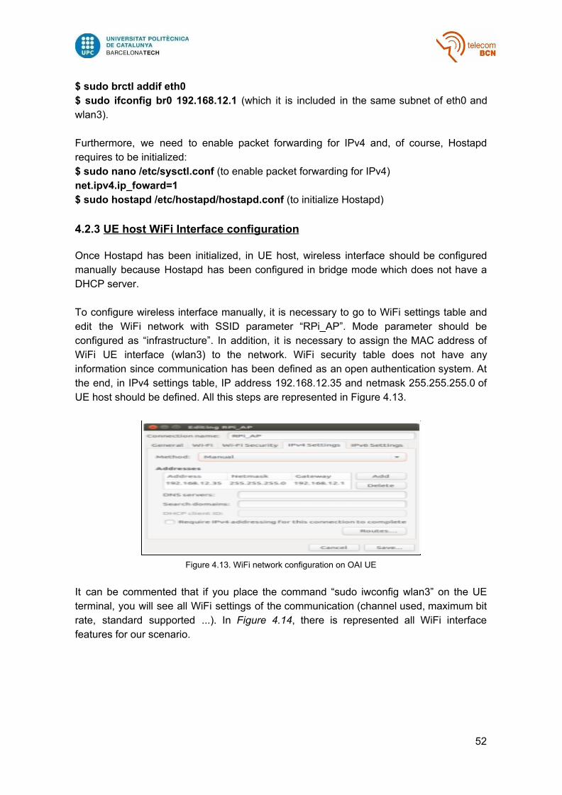
$ sudo brctl addif eth0 $ sudo ifconfig br0 192.168.12.1 (which it is included in the same subnet of eth0 and wlan3). Furthermore, we need to enable packet forwarding for IPv4 and, of course, Hostapd requires to be initialized: $ sudo nano /etc/sysctl.conf (to enable packet forwarding for IPv4) net.ipv4.ip_foward=1 $ sudo hostapd /etc/hostapd/hostapd.conf (to initialize Hostapd) 4.2.3 UE host WiFi Interface configuration Once Hostapd has been initialized, in UE host, wireless interface should be configured manually because Hostapd has been configured in bridge mode which does not have a DHCP server. To configure wireless interface manually, it is necessary to go to WiFi settings table and edit the WiFi network with SSID parameter “RPi_AP”. Mode parameter should be configured as “infrastructure”. In addition, it is necessary to assign the MAC address of WiFi UE interface (wlan3) to the network. WiFi security table does not have any information since communication has been defined as an open authentication system. At the end, in IPv4 settings table, IP address 192.168.12.35 and netmask 255.255.255.0 of UE host should be defined. All this steps are represented in Figure 4.13.

Figure 4.13. WiFi network configuration on OAI UE

It can be commented that if you place the command “sudo iwconfig wlan3” on the UE terminal, you will see all WiFi settings of the communication (channel used, maximum bit rate, standard supported ...). In Figure 4.14, there is represented all WiFi interface features for our scenario.

52

Figure 4.14. WiFi interface features

4.2.4 eNB host Ethernet Interface configuration As communication is done at Layer 2, routing is not required. It just necessary to define the eNB interface in the same subnet of WiFi link (192.168.12.0). For a permanent configuration of the interface: $ sudo nano /etc/network/interface auto eth0 iface eth0 inet static address 192.168.12.45 netmask 255.255.255.0

53

5. TCP Protocol Performance Evaluation

Once it has been described how we can initialize and how work different policies, we can start to test and analyse their performance.

As it has commented in the background, both protocols (UDP and TCP) has been used to analyse data transference. However, despite its control mechanism can increase the overhead reducing the throughput, we focused on the TCP since in most applications, the reliability has a huge importance.

Even though it has been focus on TCP, we can not forget that UDP can be a reference to check which is the limit of the throughput and it can helps when we analyse the traffic with TCP.

Furthermore, to generate either TCP and UDP traffic, it has used the iperf tool, whereas to capture the packets through the links it has used Wireshark and TCP probe. Remember that with just the Wireshark we do not have information of the cwnd, which it is important if we want to analyse the TCP protocol. In addition, to represent and analyse all files from TCP probe captures, it has used R program.

We are going to start with the No Offload policy, where there is no intervention of WiFi.

5.1 No Offload policy

In the No Offload policy, the transmission either downlink and uplink is through LTE application. OAI allows to use 25, 50 or 100 RB. We will perform a deeper analysis of traffic using 25 RB since the link is more stable than for 50 or 100. In Figure 5.1, there is represented the OAI link. Remember that the OAI link has a MTU= 1500 bytes.

Figure 5.1. LTE link

54

5.1.1 First test. Congestion control analysis First of all, we are going to perform an iperf TCP test in downlink to evaluate its parts of communication (connection establishment, data transfer ...), its variables (cwnd, rwnd, rtt, throughput ...) and its congestion and flow control algorithms. In consequence, we perform this test:

Dowlink test:

client (eNB): iperf -c 10.0.1.9 -t 60 -i 1 -w 125K

server (UE): iperf -s -t 60 -i 1 -w 150K

where Snd_buffer_size= 125KB and Rcv_buffer_size = 150KB. These values have been chosen randomly. In Figure 5.2, iperf commands on each terminal are represented.

Figure 5.2. Iperf TCP test: Server terminal on the left, Client terminal on the right

If we analyse Figure 5.2, we can see how we can set the receive buffer to 150KB using the -w option, but the kernel doubles the buffer size to 300KB to make sure there is space for both the received segments and information about the TCP connection stored by the kernel. If the kernel allocates 300KB for the received buffer, how much is reserved for receiving segments? Or what is the maximum advertised window that the receiver can send to the source? Some of these questions will be solved later. Note that it happens the same on the send buffer (kernel doubles its size to 250KB).

If we capture the traffic at the eNB using Wireshark, we can analyse the different parts of TCP protocol communication and evaluate its behaviour. In Figure 5.3, there is represented the Three Way Handshake and first data and ACK packets of this communication.

55

Figure 5.3. Wireshark capture of the first 18th packets of the iperf downlink TCP test at the eNB

The sender begins with a SYN packet that does not contain data (Len is 0). It advertises that the Maximum Segment Size (MSS) is 1460, and TCP SACK Permitted option is set to True, which indicates that the sender can receive and interpret the SACK option. It is also contains the initial size of the sender’s congestion window (cwnd) but the Wireshark does not provide this information.

The receiver responds with a SYN-ACK. It sends an increment of the sequence number received in the last segment, in its Acknowledgment field (A=1). The initial receiver window (rwnd) size is 28960 bytes. Notice that in Figure 5.3, this value is enclosed in red circle. As the SACK option is set to True, the MSS value is reduced to 1448 bytes since 12 bytes are destined to TCP options. In consequence, the initial value of the rwnd size is 20 times the MSS (20*1448=28960 bytes). In Figure 5.5, there is represented a TCP data packet.

Talking about data packet, we can see that its length is 1516 bytes. This 1516 bytes are distributed as follows:

- 1500 bytes of payload since LTE link MTU is 1500 bytes. - 16 of header corresponding to a link-layer header used in pcap capture files. In

our case, the type of header corresponds to Linux “cooked” capture encapsulation and it is defined as LINKTYPE_LINUX_SLL.

56

This encapsulation header is represented on Figure 5.5, on the bottom of Wireshark where encapsulations are displayed. The packet structure of LINKTYPE_LINUX_SLL is 16

represented in Figure 5.4.

Figure 5.4. Packet structure of Linux “cooked” encapsulation (LINKTYPE_LINUX_SLL)

Figure 5.5. Data packet and ACK packet corresponding a No Offload TCP iperf test

The sender receives the SYN-ACK and sends an ACK to notify that it has received the packet correctly and it is ready for starting data transfer.

Once the connection is established, TCP starts slowly to determine the bandwidth of the connection to avoid overflowing the receiver (Slow Start).

A single packet of size 92 bytes is sent by the sender with the PSH flag set. It indicates to the receiver that the contents of the receive buffer should be passed to the application layer.

From this moment, the eNB starts to sent data packets of size 1448. Notice how the bytes in flight starts to increase too. If we analyse the number of data packets transmitted, we can see how the eNB just send 9 data packets and then waits to receive the corresponding ACKs from the UE. The reason of just transmitting 9 data packets is due to the cwnd, which controls the data rate of the sender. Wireshark does not provide information about cwnd, however if we analyse the number of bytes in flight than it has been sent (13056 bytes) when the eNB sends the 9th data packet, we find out that the

16 http://www.tcpdump.org/linktypes

57

initial value of the cwnd should be the first multiple of MSS higher than 13056 bytes. As 9*1448= 13032 bytes < 13056 bytes, the initial value of cwnd should be 10*1448=14480 bytes. In fact, this corresponds to the recommendation through RFC 6928, and being the default initial window size of 10 MSS use by Linux kernels since 2.6.39. More information can be found in:

https://blog.apnic.net/2018/01/15/tcp-initial-window-configurations-wild/

Furthermore, it will be analysed deeper when we talk about TCP probe file, but we can see how the receiver advertises that the rwnd size increases 2*MSS=2896 bytes for every ACK. This increment of the rwnd is enclosed in red circle in Figure 5.3.

Using the TCP probe, as we saw in background it can obtain information of some interesting variables in TCP. In Figure 5.6 there is represented the TCP probe file for this test. Remember that this file provides us information at every ACK packet received from the receiver at the sender.

Figure 5.6. TCP probe file corresponding to the first 17 ACK packets received of the iperf downlink TCP test at the eNB

As it has said in the background, cwnd (7th column) and ssthr (8th column) values must be multiplied by MSS to obtain their correct value. We can see how, effectively, the initial cwnd is 10*MSS=14480 bytes and how it increments by 1 MSS for every ACK received (cwnd=cwnd+MSS). Moreover, note that the increment of the rwnd (9th column) is 2*MSS=2896 bytes as we found out in Figure 5.3. In Figure 5.7, there is represented the cwnd, rwnd and ssthr by the R program. If we compare packets provided by a TCP probe file and packets captured on Wireshark, we will see that exist a coincidence of all ACK packets received but now we can gather cwnd and ssthr information.

58

Figure 5.7. Rwnd (blue), Cwnd (red) and ssthr (green) evolution from the corresponding TCP probe data file

Analyzing Figure 5.7, there are a lot of things to comment regarding the congestion control mechanism of TCP.

Firstly, a zoom slow start zone is required to compare how is the increasing of the cwnd in slow start, and how it changes when ssthr is reached. In Figure 5.8, the evolution of cwnd and ssthr at the beginning of iperf test is represented.

Figure 5.8. Cwnd (red) and ssthr (green) evolution from the corresponding TCP probe data file

59

As we can see, during slow start zone (cwnd<=ssthr), cwnd increases by 1 MSS every time that an ACK is received. In consequence, for each RTT, cwnd will as much MSS as ACK are received. However, once cwnd reaches ssthr, cwnd enters in congestion avoidance zone and its increment starts to be less aggressive. During this zone, cwnd increases 1 MSS for each RTT instead of for each ACK received.

Furthermore, pay attention to the maximum values that are reached by the cwnd and rwnd. In Figure 5.9, there is a zoom of these values, where we can see how many part of both buffers is reserved for transmitting and receiving segments. In addition, in [11] it is commented that an update of TCP from 24/04/2012 says that overhead which is not used by TCP receiver buffer is defined as:

1/2^tcp_adv_win_scale where tcp_adv_win_scale = 2

It means that 100% - 25%= 75% of receiver buffer is reserved for receiving data packets. A new update from 16/01/2013 mentions that this value was changed to 1 as default value from Ubuntu 12.04 LTS and kernel 3.2.0. In consequence, for tcp_adv_win_scale=1, the reserved space for receiving data in receiver buffer is 50% of the whole size.

This answers the question that it has been asked at the beginning of this section. In consequence:

- Rcv_buffer_size=150KB, doubled by the kernel to 300KB, and a 50% approximately is reserved for receiving segments (152040 bytes since it must be a multiple of MSS).

- Snd_buffer_size=125KB, doubled by the kernel to 250KB, and a 33% approximately is reserved for sending segments (82536 bytes since it must be a multiple of MSS). This percentage has been obtained approximately from all iperf experiments performed during this work since in [11], it is just specified reserver space size for Rcv_buffer.

In short, it is important to have this relation in mind since it will have a huge importance when we analyse the flow control to find optimal capacity.

60

Figure 5.9. Rwnd and Cwnd maximum values in bytes.

Furthermore, analysing the three variables (cwnd, rwnd, ssthr), there are different ways to determine that it has been a packet loss. It just depends of the variable that you have to analyse:

- Ssthr: a decrement means that there is a packet loss or a RTO timeout (in this case, as CUBIC algorithm is used, ssthr decrements to cwnd*β). Notice that it always tries to be at a same distance from the cwnd, so when there is a loss it easy to detect it.

- Rwnd: a decrement higher than 5000 bytes approximately means that there is a packet loss or a timeout end.

- Cwnd: a decrement means that there is a packet loss (in this case, as CUBIC algorithm is used, cwnd decrements to cwnd*β). If the decrement is until 1 or 2 MSS, it can be a RTO timeout decrement.

In Figure 5.10, there are two zooms corresponding to the behaviour of cwnd and ssthr when there is a fast retransmission due to a packet loss. In this case, β=0.8 approximately.

61

Figure 5.10. Cwnd (red) and Ssthr (green) behaviour when there two different packet losses

It should be commented that with Wireshark it is easy to find out when there is a fast retransmission. In Figure 5.11, it has been filtered fast retransmission packets from our example using tcp.analysis.fast_retransmission as a filter on Wireshark. If we compare with Figure 5.3, we can see how they correspond with fast retransmissions detected on the TCP probe file with the cwnd, rwnd and ssthr variables.

Figure 5.11. Fast retransmission packets transmitted during the TCP test captured with Wireshark

One of the most important parameters in TCP is the bytes in flight, which informs about the number of bytes that has been sent but still has not been acknowledged by the receiver. The Wireshark provides us the evolution of this parameter during a TCP communication. In Figure 5.12, we can see represented the bytes in flight and the rwnd of our test.

62

Figure 5.12. Bytes in flight (blue) and rwnd (green) of the iperf downlink TCP test at the eNB

Analysing the evolution of the bytes in flight during the communication, one can see how they are limited by the cwnd and not by the rwnd. This is because in our test, the Rcv_buffer_size > Snd_buffer_size. In consequence, the cwnd will always limit the number of bytes in flight. In our tests, the limit of cwnd size will always be lower than the limit of the rwnd size since it does not make sense to transmit at a higher rate than the receiver is able to receive. However, it can happen that the rwnd limits the number of bytes in flight. Below there is a description of the different situations:

- Rcv_buffer_size > Snd_buffer_size: in this case the cwnd will be always lower than the rwnd. In consequence, the number of bytes in flight will be always limited by the cwnd.

- Rcv_buffer_size < Snd_buffer_size: in this case the cwnd will be higher than the rwnd. However, as we have seen before, every time that there is a packet loss in the communication, cwnd decreases to cwnd*β and it will be a fast retransmission by the sender. The cwnd will follow CUBIC congestion avoidance algorithm. For this reason, during this time the cwnd will limit the number of bytes in flight until it reaches the rwnd again.

Furthermore, in Figure 5.13 and Figure 5.14 there are represented the RTT and throughput of this iperf downlink TCP test. Note that when there is a packets loss or RTO timeout, it is easy to detect with RTT (there is an increase close to 30 ms of normal behaviour). In addition, analysing throughput we can see decreases of 2-3 Mbps on its performance due to packets loss or timeouts. This zones are enclosed with red circle.

63

Figure 5.13. RTT of the iperf downlink TCP test at the eNB

Figure 5.14. Throughput of the iperf downlink TCP test at the eNB

5.1.2 TCP Flow Control downlink analysis Once it has been described the behaviour of the congestion control mechanism on an example and its influence on the throughput, it is time to analyse which impact has on the throughput two important variables in communication: capacity and latency. Taking into account that in our tests the Rcv_buffer_size > Snd_buffer_size, one of the most interesting questions when we talk about optimal throughput from a flow control perspective in TCP is “what size should the sender buffer be to achieve the ideal sending rate?”. It should be greater than or equal to the path bandwidth multiplied by the RTT (maximum cwnd size >= bandwidth * RTT). This value is commonly referred to as the Bandwidth Delay Product (BDP): the product of the path bandwidth and the path RTT. During a TCP communication, we can differentiate two zones:

64

1. Communication limited by the capacity of the sender or receiver buffer sizes: in this case, we have not achieved the optimal throughput yet. We are using a lower capacity than the optimal, so the buffers will not be congested and the RTT will not increase. When we want to estimate the latency of a TCP communication, it is better to do it at this zone, when the RTT is still not influenced by the bandwidth limitation and buffers are not congested.

2. Communication limited by the bandwidth of the link: in this case we are using LTE link with 25 RB (5 MHz of bandwidth). During this zone, we have already reached the optimal throughput and despite we continue increasing the size of the sender buffer, the throughput will not increase because we are limited by the 5 MHz of bandwidth. In consequence, the RTT will start increasing because we use a higher capacity than the optimal, and buffers will start to be congested.

In Figure 5.15, there is a representation of both zones in a TCP flow control communication.

Figure 5.15. RTT vs Bytes in Flight and Throughput vs Bytes in Flight where can be represented the two

zones defined: 1) Buffer Size Limitation Zone. 2) Application Bandwidth Limitation Zone

The threshold that limits both zones is known as BDPopt. If the sender buffer is smaller than the BDPopt, the throughput will be lower than the optimal, and if the sender buffer is greater than or equal to the BDPopt then we will reach the optimal throughput. The BDPopt has an huge importance in any TCP communication. In consequence, we have followed the following path to estimate it:

65

1. Throughput calculation with no buffer limitation: the first step will be to evaluate the throughput without limitation on either buffer sizes. Notice that if we do not limit buffer sizes capacity, we assure to be in the zone limited by the bandwidth of the application, so we will reach the optimal throughput.

2. Latency estimation: once the optimal throughput is known, it will be time to estimate the latency. As it has been commented, the latency should be estimated in the first zone where buffers are not congested. When buffers start to be congested, the RTT starts to increase and it can lead to bad estimations.

3. BDPopt= throughput * latency: finally, we can compute the BDPopt. It is important to understand the importance of the latency when we try to estimate the BDPopt. In some applications such as WiFi, there is a high interference from other users and it is more difficult to estimate the latency than in LTE. The interference variates a lot the RTT of data packets and at the end, its mean variation is a high influence on the latency estimation. The lower the latency mean variance is, the better estimation of the BDPopt is. Once explained the method followed to compute the BDPopt, it going to start applying it in the No Offload policy. Firstly, we are going to perform an iperf TCP test without buffer limitation (which means without the -w option). In Figure 5.16, there is represented the throughput with Wireshark for this iperf test.

Figure 5.16. Average Throughput (bps) of the following iperf TCP test: No Offload policy, downlink with 25 RB

without buffer size limitations.

If we analyse the throughput, we can see how there is a mean of 16,6 Mbps as optimal throughout when we transmit with 5 MHz of bandwidth through LTE. It is quite good since is very close to the theoretical one, which is 21 Mbps as defined in [3]. Talking about behaviours, there are three perturbations. These perturbations appear when there is a packet loss or a RTO timeout occurs and can lead to a decrement of 3 or 5 Mbps. Notice that in this case there we do not limitate any of both buffer sizes, so rwnd and cwnd increase until reach their iperf default TCP limit of window. Every time that there is a

66

packet loss, the rwnd will increase aggressively its value if it still has not reached its iperf limit. If the loss happens when rwnd has reached its iperf limit, it will not increase more. In addition, notice that without buffer size limitation, the congestion avoidance evolution of the cwnd is closer to CUBIC. In Figure 5.17 and Figure 5.18 there are represented the rwnd, cwnd, ssthr and bytes in flight for this test where we can see these increments.

Figure 5.17. Rwnd (blue), Cwnd (red) and Ssthr (green) performance of the following iperf TCP test: No

Offload policy, downlink with 25 RB without buffer size limitations.

Figure 5.18. Rwnd (Bytes) in green and Bytes in Flight (Bytes) in blue of the following iperf TCP test: No

Offload policy, downlink with 25 RB without buffer size limitations.

Furthermore, in 5.19 there is represented the evolution of RTT. As we have got over BDPopt, throughput is limited by the bandwidth of the application (5 MHz). In consequence, an increase of buffer size (cwnd) must suppose an increase of RTT (capacity = throughput * RTT) because buffers are congested. For this reason, RTT follows a path similar to the cwnd and bytes in flight. We can see how either cwnd and RTT has a similar evolution due to the linear relation. Note that RTT reaches values higher than 450 ms, while in the previous test when we still have not reached the BDPopt

67

we had a constant evolution with variation between 15 - 45 ms. For this reason it is very important to estimate latency when you are not limited by bandwidth of links since you can have differences closer to 400 ms.

Figure 5.19. RTT (ms) evolution of the following iperf test: No Offload policy, downlink with 25 RB without

buffer size limitations. Once we know the optimal throughput (16.6 Mbps), we can focus on the estimation of latency. As it has commented before, the estimation of latency will be performed during time when buffers are still not congested (cwnd maximum value < BDPopt). For this reason, it has started to perform iperf TCP test with high limit of buffer sizes in order to assure that we do not reach the BDPopt. In Figure 5.20, there are represented the RTT for the corresponding sender buffer size limitation: 25 KB, 50 KB, 62.5 KB, 75KB.

68

Figure 5.20. RTT (ms) evolution of the following iperf tests

1) No Offload policy, downlink with 25 RB with Snd_buffer_size = 25KB 2) No Offload policy, downlink with 25 RB with Snd_buffer_size = 50KB 3) No Offload policy, downlink with 25 RB with Snd_buffer_size = 75KB

Notice that with these buffers size limitations on the sender, it seems that it has not reached the BDPopt and we have not achieved the optimal throughput yet. Even with a few loses, the path of RTT in different tests are very similar (a variation between 12 - 48 ms) and do not follow the cwnd path as when buffers are congested. This is an indicator that we are not limited by channel bandwidth. If we analyse the throughput of each iperf test, we will see that as far as we increase the capacity (less limitation on buffers size), the throughout keeps increasing until we reach the optimal one (BDPopt) since the RTT does not have a high variation. Remember that in this policy, there is a wired communication, so no interference will happen as opposed to if the communication was wireless. This affects directly to the latency and allows a better estimation. If we compute the RTT mean when buffers are not congested, we have obtained a mean range of 40 - 43 ms . The higher the interference is, the higher the latency estimation range is. In my case I estimate the latency as the middle value of the range RTT = 41.5 ms.

69

Finally, knowing the optimal throughput and the latency estimation, we are ready to compute the estimation of BDPopt. If we take into account the mean latency estimation range obtained:

BDPopt = [(16.6 Mbps * 40 ms) / 8, (16.6 Mbps * 43 ms) / 8] = [83 KB, 89.25 KB]

However, as we have seen before, the capacity should be a multiple of MSS. In consequence:

BDPopt = [ 83.984 KB, 89.776 KB ] where both limit values are the

first multiples of MSS = 1448 bytes higher than previous limit values. In my case, as I did before with the latency, I will estimate the BDPopt with the middle value of the range that is multiple of MSS which is BDPopt = 86.880 KB. Remember that this value are referred to the size of the buffer destined to transmitter. Previously we have seen that 50% of the Rcv_buffer_size was used for receiving segments and a 33% of the Snd_buffer_size for transmitting segments. In addition, the kernel doubles the size of buffers, so if we want to obtain the buffers size corresponding to the estimated BDPopt:

Rcv_buffer_sizeopt = ( BDPopt / 50 % ) / 2 = 86.88 KB Snd_buffer_sizeopt = ( BDPopt / 33 % ) / 2 = 131.64 KB

In Figure 21, Figure 22 and Figure 23, there are represented throughput; cwnd, rwnd and ssthr; and RTT of an iperf TCP test using the optimal capacity estimated. As you will see, it reaches optimal throughout and buffers are still not congested since RTT function does not follow cwnd path.

Figure 5.21. Average Throughput (bps) of the following iperf TCP test: No Offload policy, downlink with 25 RB

using BDPopt=86.88 KB

70

Figure 5.22. Cwnd, rwnd and ssthr of the following iperf TCP test: No Offload policy, downlink with 25 RB

using BDPopt=86.88 KB

Figure 5.23. RTT of the following iperf TCP test: No Offload policy, downlink with 25 RB using BDPopt=86.88 KB

5.1.3 Throughput evaluations results Now it is time to show some throughput results obtained from all study performed with this policy. In Figure 5.24, there is represented the throughput vs Snd_Buff_Size for Downlink and 25 RB and 50 RB which its corresponding Snd_buffer_sizeopt. Notice that with 50 RB in TCP, we are not able to reach the double optimal throughput of 25 RB; the throughput just increase by 8 Mbps. It can be because UE receives a high amount of out of order packets which it does not acknowledge, so eNB will not receive these ACK and cwnd decreases leading to reduce the throughput. In Figure 5.25, there is the downlink throughput reached when we use UDP with 25 and RB. It is important to observe that as in UDP there is no control mechanism, we reach the

71

double throughput when bandwidth is doubled. It confirms that poor stability can affect the protocols that prioritizes reliability reducing its throughput. Notice that with 50 RB, using UDP we reach 33 Mbps. Finally, in Figure 5.26, there is represented the throughput behaviour either TCP and UDP in uplink for 25 and 50 RB too.

Figure 5.24. TCP Throughput vs TCP Snd_Buff_Size for No Offload Downlink 25 RB (blue) and 50 RB (red).

Figure 5.25. UDP Throughput for No Offload Downlink 25 RB (blue) and 50 RB (red).

72

Figure 5.26. UDP Throughput for No Offload Uplink 25 RB (green) and 50 RB (brown).TCP Throughput for No Offload Uplink 25 RB (blue) and 50 RB (red).

5.2 Full Offload policy Once analysed deeply performance of No Offload policy, it is time to focus on Full Offload. In this policy all the traffic is offloaded through WiFi link. The transmission of data packets in downlink and uplink is transmitted through WiFi application. However, in the case of control packets, they are transmitted by LTE either uplink or downlink. In Figure 5.27, there is represented WiFi link. Remember that the WiFi link has a MTU = 1500 bytes.

Figure 5.27. WiFi Link. Enclosed with red circle the WiFi AP, Ethernet interface of eNB and wifi interface of UE.

In this case, we are not going to analyse as deeper as in the No Offload policy, since the TCP congestion control mechanism has the same behaviour for different applications. However, important parameters such as latency have a different behaviour due to interferences and it will affect the calculation of optimal throughput and BDPopt.

73

A few features about WiFi network should be remembered before starting with the TCP analysis. The WiFi network that it is been used has ESSID=”RPI_AP”, uses the channel 6 of 2.4 GHZ ISM BAND which corresponds with a central frequency of 2.437 GHz and has 20 MHz of bandwidth. It just supports 802.11b and 802.11g wifi standards which provides a maximum throughput of 54 Mbps in theory. In Figure 5.28, there is a representation of the ISM 2.4 GHz band with all operating WiFi networks with its corresponding channel.

Figure 5.28. ISM 2.4 GHz band with all operating WiFi networks with its channel. Source: WiFi Explorer LITE application.

As RPI_AP network is located at channel 6, it does not receive interference from channel 1 and channel 11 or above. However, a lot of WiFi networks are located in closer bands such as UPCguest in channel 5, ENTELBCN in channel 4, dd-wrt-306 in channel 3 …. It will lead to a high amount of interference that will affect our wireless communication. Once we commented different features about WiFi link, we can start analysing TCP flow control of this policy. We will start to analyse the downlink link. As we did in No Offload policy, the first step will be to find the optimal throughput that we can reach with WiFi link when a TCP communication is performed. As we want to assure that we are limited by the WiFi bandwidth (20 MHz), we are going to perform a test without limiting buffer sizes. In Figure 5.29, there is represented its throughput with Wireshark.

74

Figure 5.29. Average Throughput (bps) of the following iperf TCP test: Full Offload policy, downlink without buffer size limitations.

Analysing the throughput, we achieve a mean of 21 Mbps when we transmit with 20 MHz of bandwidth with standard 802.11g. We can realise that we are receiving a high amount of interference from other channels that reduces a lot our throughput and it seems that is not the optimal one. This can happen when we transmit in 2.4 GHz band (unlicensed band) since it is a very congested band that allows to transmit to higher ranges but with lower speeds. In our case it should have been better to use the 5 GHz band since despite it does not cover a long range, it would provide higher throughput values. Notice that in our scenario eNB and UE are separated just 1 meter. However, our devices do not support 802.11ac standard where 5 GHz band is included. Furthermore, it can see how every time that there is a loss, the rwnd adopts the same behaviour as in No Offload policy. It starts to increase aggressively if it has not achieved its iperf TCP limit yet. However, if the loss happens when rwnd has reached the limit, it will not increase more. For this reason we would not analyse deeper the congestion control since it works similar in different applications. In Figure 5.30, there are represented the rwnd, cwnd, ssthr and bytes in flight for this test where it can see the increments.

Figure 5.30. Rwnd (blue), Cwnd (red) and Ssthr (green) performance of the following iperf TCP test: Full

Offload policy, downlink without buffer size limitations. If we analyse cwnd, it can see the high amount of interference that exist in this link due to WiFi works on an unlicensed band. Every time that cwnd tries to increase its value higher than 120 KB approximately, fast retransmission situations appear. For this reason, we are just able to transmit at 21 Mbps instead of 54 Mbps using 20 MHz of bandwidth. In addition, medium access overhead can influence. If we try to increase the cwnd in order

75

to increase the throughput, the high amount of interference leads to packet losses or RTO timeouts because sender cannot receive corresponding ACK packet. If we compare cwnd limit of this link with No Offload link, notice that in this case we are just able to reach 115-125 KB, whereas in No Offload it is close to 1.2 MB which is very significative. In WiFi link, we are not limited by the bandwidth of the application (20 MHz), even if we perform iperf TCP tests without buffer limitation. The high interference avoid reach optimal throughput and it is more difficult to estimate a BDPopt. Moreover, interference not only affect on throughput. In these links, it is more difficult to estimate latency due to the high variance of RTT when we still are not limited by WiFi bandwidth. In Figure 5.31, there is a comparison of RTT mean for different iperf TCP test when it is Full Offload and when it is No Offload. This comparison was done when we still are not limited by link bandwidth.

Figure 5.31. RTT mean for iperf tests corresponding to No Offload policy (blue) and Full Offload policy (red).

To summarize, in WiFi link, the band used is very important depending of your goals. If you prefer a better throughput performance, 5 GHz band should be used. This study has been done in a university campus where a lot of students uses 2.4 GHz band every day. In consequence, interference is very high and has a huge impact on throughput reached (21 Mbps) which is lower than optimal one. Moreover, it also affects to latency estimation since it increase its variance aggressively. In Figure 5.32, throughput performance obtained for Full Offload policy is represented.

76

Figure 5.32. Throughput performance of Full Offload policy: UDP downlink throughput (brown), UDP uplink throughput (green), TCP downlink throughput (blue), TCP uplink throughput (red).

5.3 LTE/WiFi Aggregation policy Once we analysed No Offload policy and Full Offload policy, it is time to focus on LTE/WiFi Aggregation policy and try to perform some techniques in order to check if throughout performance of previous policies can be improved for TCP communications tests. In this policy, aggregation techniques are just performed for downlink communication, while in uplink all data packets will be transmitted through WiFi because throughput results were better than in LTE. Control packets will keep going through LTE link as in the other two policies.

In LWA policy, radio bearer is split between lower layer of LTE and WiFi in PDCP layer. In this work, on PDCP layer several techniques have been implemented and evaluated in order to improve TCP throughput results obtained from previous policies. All iperf test studied was without limiting both TCP buffers size in order to reach the optimal throughput even if we reach it with non-optimal TCP buffers sizes. 5.3.1 Time division technique The first technique implemented is called Time Division technique. As first technique implemented, we decided to implement a simple one where decision transmission link by PDCP layer depends on the time that we at. The OAI eNB decides to transmit during a period of time through LTE link and another period of time through WiFi. In this case, it can see that we are not transmitting for both links at same time. In Figure 5.33, first LWA technique is represented.

77

Figure 5.33. Time division LWA technique

In Figure 5.34, throughput performance of iperf Downlink TCP test. As we do not transmit through both links at the same time, there is not a high improvement if we compare with No Offload and Full Offload throughput results. On the one hand, during LTE intervals of time, using 25 RB we reach on average close to 16.5 Mbps which is quite similar to 16.6 Mbps obtained in No Offload policy. However, using 50 RB we are not able to double previous value, even there is an improvement of 9 Mbps approximately. It can be because there is a high amount of out of order packets that are not acknowledged by TCP receiver. In consequence, sender has to reduce its cwnd size, and, for this reason the throughout does not reach the optimal value. It is not a isolate case of this technique because it also happened in No Offload policy. During WiFi interval, there is a similar throughput performance as the one obtained in Full Offload policy with an average of 21 Mbps approximately.

Figure 5.34. Throughput performance for Time Division LWA technique using 25 RB LTE link (blue) and using

50 RB on LTE link (red)

78

Figure 5.35. Rwnd (blue), Cwnd (red) and Ssthr (green) performance for Time Division LWA technique using

25 RB LTE link In Figure 5.35, we can see rwnd, cwnd and ssthr for Time Division LWA technique. In this case, as is the simplest one, since we are transmitting an interval of time through a link and another interval through the other. Cwnd had a similar behaviour than in Full Offload policy. However, we can comment that during LTE interval, notice that cwnd does not reach a very high value as in No Offload policy. 5.3.2 Par/Impar technique The second technique implemented is called Par/Impar technique. In this case, the PDCP layer of OAI eNB decides to transmit par data packets through LTE link and impar data packets through WiFi. In consequence, the transmission will start through WiFi link, but it does not matter for which link the transmission starts. In Figure 5.36, second LWA technique is represented.

Figure 5.36. Para/Impar LWA technique

79

In Figure 5.37, throughput performance of iperf Downlink TCP test without buffer limitations is represented. Either using 25 RB and using 50 RB, there is an improvement of throughput performance compared with other policies results. Using 25 RB we obtain a throughout average of 26.5 Mbps and using 50 RB 30 Mbps approximately. One of the reasons of this improvement is due to the lower congestion of LTE and WiFi buffers compared with other policies because in this case we are transmitting half of data traffic through each link.

Figure 5.37. Throughput performance for Par/Impar LWA technique using 25 RB LTE link (blue) and using 50

RB on LTE link (red)

80

Figure 5.38. Rwnd (blue), Cwnd (red) and Ssthr (green) performance for Par/Impar LWA technique using 25

RB LTE link In Figure 5.38, we can see the evolution of rwnd, cwnd and ssthr during Par/Impar LWA technique. As we can see, cwnd reach higher values than in Full Offload policy (now it reaches values higher than 150KB), so this lead to an improve in throughput results as it is shown in Figure 5.37. 5.3.3 Low RTT Ping technique The third technique implemented is called Low Latency Ping technique. An external server thread is defined inside PDCP layer of OAI eNB. The external server strains 5 ICMP packets through each link continuously and calculates their mean RTT value. Once the RTT mean of each link is calculated, the server sends the information to PDCP layer and starts again the process. PDCP layer decides to transmit data packets through the link that has a lower RTT. There is an upper limit of 1000 ms for RTT of ICMP packets, so if mean RTT computation is higher than 1000 ms, information is not sent to PDCP layer. In Figure 5.39, third LWA technique is represented.

81

Figure 5.39. Low RTT Ping LWA technique

In Figure 5.40, throughput performance of iperf Downlink TCP test without buffer limitations is represented. When we started to perform this technique, we thought that using link with lower ICMP RTT, we will reach better results. However, perhaps the technique was not applied in the best efficient way. Notice that we have even worse throughput performance (14 Mbps when 25 RB is used in LTE link and 20 Mbps when 50 RB approximately) than in other policies. It can happen because it is not the best way to calculate the RTT through ICMP packets. The server takes too much time to calculate RTT means of each 5 ICMP packets sent, so when information arrives to PDCP layer and is updated, channel conditions may have already changed. This technique could reach better throughput performance but it has to find out a way to reduce the time of computing the RTT mean of each 5 ICMP sent in each link by external server.

Figure 5.40. Throughput performance for Low RTT Ping LWA technique using 25 RB LTE link (blue) and

using 50 RB on LTE link (red)

82

Figure 5.41. Rwnd (blue), Cwnd (red) and Ssthr (green) performance for Low RTT Ping LWA technique using

25 RB LTE link

In Figure 5.41, we can see the evolution of cwnd during Low RTT LWA technique. 5.3.4 Port division technique The last technique implemented is called Port division technique. The main difference from other techniques commented is that in this case we are transmitting through LTE and WiFi links at the same time using different ports (port 5201 for LTE link and port 5202 for WiFi link). With this technique, WiFi throughput performance can be added to the LTE one leading to better throughout performance. In Figure 5.42, fourth LWA technique is represented.

83

Figure 5.42. Port division LWA technique

In Figure 5.43, throughput performance of iperf Downlink TCP test without buffer limitations is represented. In first case, we are transmitting packets through LTE link with 25 RB using port 5201 and packets through WiFi link using port 5202. We can see how in both case, throughput results are lower than average values obtained in previous cases. We reach 15 Mbps on average in LTE link and 15.5 Mbps in WiFi link approximately. This reduction can happen because eNB is sending data packets through different ports at the same time, so it forces UE to receive packets from different ports with different latencies and it can lead to a high amount out of order packets that can reduce sender cwnd since ack packets will not be received. However, as we transmit through different ports, we can add WiFi throughput results to LTE results, resulting to a throughput average close to 30 Mbps using 25 RB in LTE link. Using 25 RB in LTE link, this is the best throughput performance of all techniques performed. Using 50 RB instead of 25 RB, we achieve a better throughput performance in average (33 Mbps approximately), but we are far from what is expected as it has happened during all tests performed with 50 RB.

84

Figure 5.43. Throughput performance for Port division LWA technique using 25 RB LTE link (blue) and using 50 RB on LTE link (red), WiFi link (green), 25 RB LTE link + WiFi link (purple) and 25 RB LTE link + WiFi link

(brown).

Figure 5.44. Rwnd (blue), Cwnd (red) and Ssthr (green) performance for Port division LWA technique: WiFi link corresponding to port 5202

In Figure 5.44 and Figure 5.45 there are represented rwnd, cwnd and ssthr of WiFi link and LTE link respectively. As we can see, in LTE link we reach a cwnd of 1 MB as in No Offload policy. In fact, in this technique LTE works quite well. However, in WiFi link we have a decrease of 6 Mbps approximately if we compare with results in Full Offload. It

85

can see that cwnd in WiFi link does not reach 100 KB. It seems that the most affected link due to this technique is WiFi link.

Figure 5.45. Rwnd (blue), Cwnd (red) and Ssthr (green) performance for Port division LWA technique: LTE

link using 25 RB corresponding to port 5201

86

7. Conclusions and future development

In this thesis, a very tight coupling approach between LTE and WiFi prototype has been implemented using Open Air Interface and Hostapd software. Moreover, three policies were developed and evaluated with TCP traffic by Wireshark and TCP probe capture programs. Some conclusion of this work should be commented:

A deep analysis and evaluation of TCP traffic through different links allows to contrast Wireshark information with TCP probe information. Adding information provided by each program, we learnt how to detect when a paquet loss or RTO timeout happens analysing rwnd, cwnd or ssthr parameters. A relation between Rcv_buff_size and maximum rwnd size value was found. Moreover, if we do not limit TCP buffer sizes, it detected a high difference between maximum cwnd value reached in no offload policy (close to 1.2 MB), where interference is very low, and maximum cwnd value reached in full offload policy (just 120 KB) due to interference. In addition, we were able to characterize all different parts of CUBIC congestion avoidance algorithm.

Talking about TCP flow control mechanism, we found out that we can split TCP data transfer test in two main zones depending of number of bytes in flight. The threshold that separate both zones was defined as BDPopt and we defined a method to estimate it through optimal throughput and RTT estimation. In first zone (bytes in flight < BDPopt ), TCP buffers are still not congested since we still not used all the bandwidth of our link and optimal throughput has not been reached yet. In second zone, we reach optimal throughput and TCP buffers start to be congested (bandwidth limit reached), which lead to a change in RTT behaviour since it starts to follow congestion window shape.

As future development, it could be interesting to perform different experiments changing the default congestion control algorithm CUBIC to BBR, Veno or another one that adapts better to our environment. Moreover, as 2.4 GHz WiFi band is very congested, it should be also interesting to use 5 GHz WiFI band or wired connection in WiFi link in order to reduce the interference. Remember that as we are not working with long distances, 5 GHz band should improve our results.

87

Bibliography

[1] CISCO, “Cisco Visual Networking Index: Forecast and Methodology , 2015 – 2020,” 2016.

[2] CISCO, “Cisco Visual Networking Index: Global Mobile Data Traffic Forecast Update, 2016 – 2021,” 2017.

[3] R. Agustí, F.B. Álvarez, F. Casadevall, R. Ferrús, J. Pérez, O. Sallent, “LTE: Nuevas Tendencias en Comunicaciones Móviles”, UPC, 2010

[4] Van Jacobson, Michael J. Karels, “Congestion Avoidance and Control,” November, 1988

[5] Injong Rhee, Lisong Xu, “CUBIC: A New TCP-Friendly High-Speed TCP Variant,” 2008

[6] Intel, “LTE-WLAN Aggregation (LWA): Benefits and Deployment Considerations” 2016.

[7] Y. Khadraoui, X. Lagrange, and A. Gravey, “Very Tight Coupling Between LTE and WiFi: From Theory to Practice” Wirel. Days, pp. 7-9, 2016.

[8] X. Lagrange, “Very tight Coupling between LTE and WiFi for advanced offloading procedures” in WCNC Workshop, Interference and design issues for future heterogeneous networks. IEEE, 2014.

[9] 3GPP, “Study on small cells enhancements for e-utra and e-utran” Release 12, Technical Report TR 36.842, Tecg. Rep., 2013.

[10] Y. Khadraoui, X. Lagrange, and A. Gravey, “A survey of available features for mobile traffic offload” in European Wireless 2014; 20th European Wireless Conference; Proceedings of. VDE, 2014, pp.1-4

[11] S. Gordon, “Impact of Bandwidth Delay Product on TCP Throughput”, Australia, 2013.

88

Glossary

cwnd: congestion window

rwnd: receiver window

ssthr: slow start threshold

MTU: maximum transmission unit

MSS: maximum segment size

Snd_buff_size: sended TCP buffer size

Rcv_buff_size: receiver TCP buffer size

BDP: bandwidth delay product

RTT: round trip time

TCP: transmission control protocol

UDP: user datagram protocol

IP: Internet protocol

ICMP: Internet control message protocol

RB: resource block

89

tcp performance analysis for lte and lte/wlan aggregation

Documents

Transcript of tcp performance analysis for lte and lte/wlan aggregation