Tax Britannica: Nineteenth Century Tariffsand British National Income∗

Sami DakhliaUniversity of Alabama

sami@ua.edu

John V.C. NyeWashington University in St.Louis

nye@wueconc.wustl.edu

November 1, 2001This version: August 1, 2003

Abstract

The literature on British economic history presumes that Britainwas a free trader after the repeal of the Corn Laws and that her tarifflevels were thus below those which were optimal for maximizing utility.Presumably, if the optimal British tariff had been positive and greaterthan the levels established by mid-century, a reduction to zero of alltariffs that remained would have lowered British welfare even further.In this paper, we use a simple computable general equilibrium model tosimulate a drop in all British tariffs to zero. The resulting substantialnet increase in British welfare suggests that British tariffs were muchhigher than would be consistent with an optimum tariff policy. Moreimportant, the size of British losses from her high tariff levels suggeststhat British policy was not consistent with the stance of an ideologicalfree trader.

∗Special thanks to Jean Mercenier (Monsieur GAMS) for his invaluable help. We alsowish to thank Sam Addy, David Bullock, Avner Greif, Deirdre McCloskey, Maria Craw-ford, Joel Mokyr, Erik O’Donoghue, Paul Pecorino, Akram Temimi, Dean Williamson,and an anonymous referee for very helpful comments.

1

1 Introduction

Traditional accounts of commercial history have treated nineteenth-centuryBritain as the lone European free trader in the decades following the re-peal of the Corn Laws (e.g. Kindleberger, 1975). Such a transformationwas important on both political and ideological grounds. It is said to haveencouraged reform in the institutions of international trade and in supportof free markets. However, British moves toward trade liberalization seemto have been especially anomalous because Britain might have stood to losefrom a move to lower tariffs. As the leader in world trade, Britain musthave had substantial market power and if so, would have gained more inthe short run by maintaining a positive optimal tariff. McCloskey first drewattention to this problem in a noted essay published some two decades ago(1980). Using purely hypothetical elasticity parameters and speculating asto the values of the most significant variables, McCloskey concluded that ifthe optimal British tariffs were positive, Britain would have paid a price formoving to free trade.However, the price was small in static terms, and what-ever welfare losses were incurred were undoubtedly offset by the dynamicgains from moving to freer trade. About a decade after McCloskey’s work,Irwin (1988) made much the same point with a simple model that sought tomeasure the welfare change associated with Britain’s trade reductions; he,too, concluded that in going to free trade, Britain was moving away fromthe optimal tariff and that the nation had therefore suffered a loss in utilityon the basis of static calculations.He conceded that his calculations seemed“to confirm the judgment that adverse terms of trade shifts would outweighefficiency gains from a British tariff reduction” (Irwin, 1988, p.1158), butrepeated McCloskey’s claim that these were static calculations that ignoredthe dynamic effects of free trade: in particular, the demonstration effect ofBritish tariff reduction in terms of spurring other nations to move to freetrade.

However, there are serious difficulties with the calculations on whichthese claims have been based. For one thing, more recent research pointsto Britain’s having had substantially higher tariffs than had hitherto beensuspected, tariffs which were not fully eradicated in the quarter-century afterPeel’s reforms had begun in the 1840s (Nye, 1991). For the most part, thesetook the form of extremely high tariffs on wine and brandy, coffee, tea, sugar,and tobacco. The persistence of these tariffs, especially on wine and brandy,is remarkable because these duties indicate a Britain unwilling to lower tariffs

1

on her prime imports. Furthermore, the duties on wine and brandy go backto the beginnings of English mercantilism and struggles with France as farback as the late seventeenth century. Arguably, they were designed to be notonly protective but indeed prohibitive. War with the French from 1689 to1713 led to temporary prohibitions and, subsequently, permanent high tar-iffs designed to limit the import of wine and spirits and favor domestic beerand liquor as well the production of friendly nations such as Portugal andSpain.This reduced the volume of French imports in the eighteenth centuryto five percent or less of their peak seventeenth century levels. (cf. Nye,1991, and elaborated in Nye, 2004). Thus, Britain may have lowered sometariffs, but she was not a free trader after the 1840s.

In this paper we simulate a drop in all British tariffs to zero and demon-strate that British tariffs, even after the repeal of the Corn Law, were notonly far too high to be consistent with the stance of a committed free trader,but even too high to be consistent with an optimum tariff policy.

Nineteenth-century Britain’s stance as the leading free trader in historyhas become so embedded in our received wisdom that whole literatures inhistory and political economy have been constructed based on Britain’s pre-sumed ideological purity. But more recent research (Anderson and Tollison,1985, and Nye, 1991 and 2004) suggests that the politics of trade reform wasmuch more consistent with the cynical view of self-professed reform typicalof work in public choice and the evolution of institutions. We speculate onthe importance of this work for further analysis of political economy. Thesize of welfare losses is large enough, especially when held against comparablefigures for France, that we are forced to reconsider the impact of these resultson the political economy of trade and the history of trade reform. Indeed,such an analysis forces a reinvestigation of the problems of strategic theoriesof hegemonic trade and raises difficulties because of the subtlety required tounderstand the course of all political economic reforms.

2 Measuring protection

Traditional tariff indices have usually focused on one of three measures: (1)the nominal level of tariffs per class of goods, (2) weighted measures of av-erage tariffs defined as total revenues divided by total value of imports (andvarious modifications to this basic idea) or (3) measures of effective protec-tion on an item-by-item basis, where nominal tariff levels are corrected for

2

tariffs on inputs used in production of these goods. All three suffer from avariety of theoretical and empirical problems. The first measure ignores therelative importance of a good in total trade, the second has serious problemswith respect to trade weights, given the problem that a nearly prohibitivetariff might add little to the revenues received, and the third is not only prob-lematic when used to create an overall index but also suffers because effectiveprotection measures ignore the costs of tariff restrictions to the consumer.

The most widely cited recent attempt to create a more universal tariffmeasure is the Trade Restrictiveness Index (TRI) first promoted by Andersonand Neary (1994) and adopted by O’Rourke (1997) in his own contributionto the debate on whether nineteenth century France, rather than Britain,was the freer trader. The TRI —which is calculated within a computablegeneral equilibrium (CGE) framework— is the first theoretically sound indexbecause it is directly derived from an economic objective, in this case welfaremaximization.

By explicitly modeling tariffs and trade in a general equilibrium frame-work, O’Rourke quantified and thereby clarified the terms of the debate. Hedemonstrated that the outcome of the debate hinges on the functional formsand calibration of preferences and technology; in particular, he showed thatthe degree of substitutability between beer and imported alcoholic beveragesturned out to have a remarkable impact on the welfare effects of British tar-iffs. The question, thus, is no longer whether beer and wine are substitutes(and thus whether tariffs on wine should be included in a tariff index), butrather for what range of elasticities of substitution between both types ofalcohol, France would indeed have been the freer trader.

Unfortunately, in order to compute a country’s TRI, one must ignore theissue of market power and assume a small country whose decisions have noeffect on world trade. As shown in the appendix, a large country’s TRI willbe either ambiguous or not defined at all. (See also Dakhlia, 2002.) Sincethe small-country assumption is evidently not ideal when studying how acountry that loomed large in international commerce might have benefitedfrom a positive economic tariff and its subsequent reduction, the TRI-basedmeasure must be abandoned. We should however be careful not to toss thebaby with the bath water: we preserve the CGE framework since it offersan unusually rich context in which to interpret our sparse data. While wecannot derive an index per se, the framework will still allow us to trackwelfare effects of protectionism.

Specifically, we track the national welfare effects of a progressive counter-

3

factual tariff reduction down to zero. This suffices for our purposes, since wemerely wish to know whether British tariffs were higher or lower than thosesuggested by static welfare maximization.

3 The Model

Our approach follows Anderson/Neary and O’Rourke by modeling the econ-omy in a general equilibrium framework. The general equilibrium frameworkprovides a particularly appropriate tool for performing comparative staticsexercises in trade and for studying the static effects of policy changes andtheir impact on trade flows, allocation of goods, and welfare effects on con-sumers, since the interdependence among the various markets is at the heartof the measurement problem: a tariff imposed on wine, for example, willaffect not only the demand for wine, but also the demand for beer and othergoods. A partial equilibrium approach would capture only bits and pieces ofa tariff’s intricate effects.

A model should be sufficiently rich to shield itself from the Fogel cri-tique (1967) and leave room for the data to matter. The downside of a richand flexible model, of course, is that it may be too complex to allow forsimple, closed-form solutions and comparative statics; thus the need for anumeric, computational approach. Moreover, the beauty of a computablegeneral equilibrium approach lies in its direct focus on the welfare or utilityof the representative consumer, thereby avoiding awkward approximationstypical of partial equilibrium welfare analysis.

As in Anderson and Neary, we assume that region i has a representa-tive consumer who values a large variety of imports as well as a generic,non-traded, domestic product. This specification conforms to the availablerecords, which are rich on import and export data, but scarce on non-tradedcommodities. Region i’s consumer is endowed with non-traded inputs andreceives all tariff revenue. Furthermore, she consumes her entire productionof the non-traded good, while none of the exportables are consumed at home.

As in O’Rourke, a two-level nested CES utility function allows us tospecify different elasticities of substitution within bundles of goods as wellas among bundles. The maleability of nested CES offers an attractive com-promise between realism on one hand and computational expediency on theother. The first utility level combines comparable consumption goods into

4

GB Utility

Dom. good

Textiles

Alcohol

Caffeine

Wool

Cotton

Rum/Brandy

Silk

Coffee

Tea

Wine

OtherOther

Other

FR Utility

Dom. good

Sugar Colonial

Non-colonial

Textiles Wool

Cotton

OtherOther

Other

Beer (dom.)

Figure 1: British two-level utility function

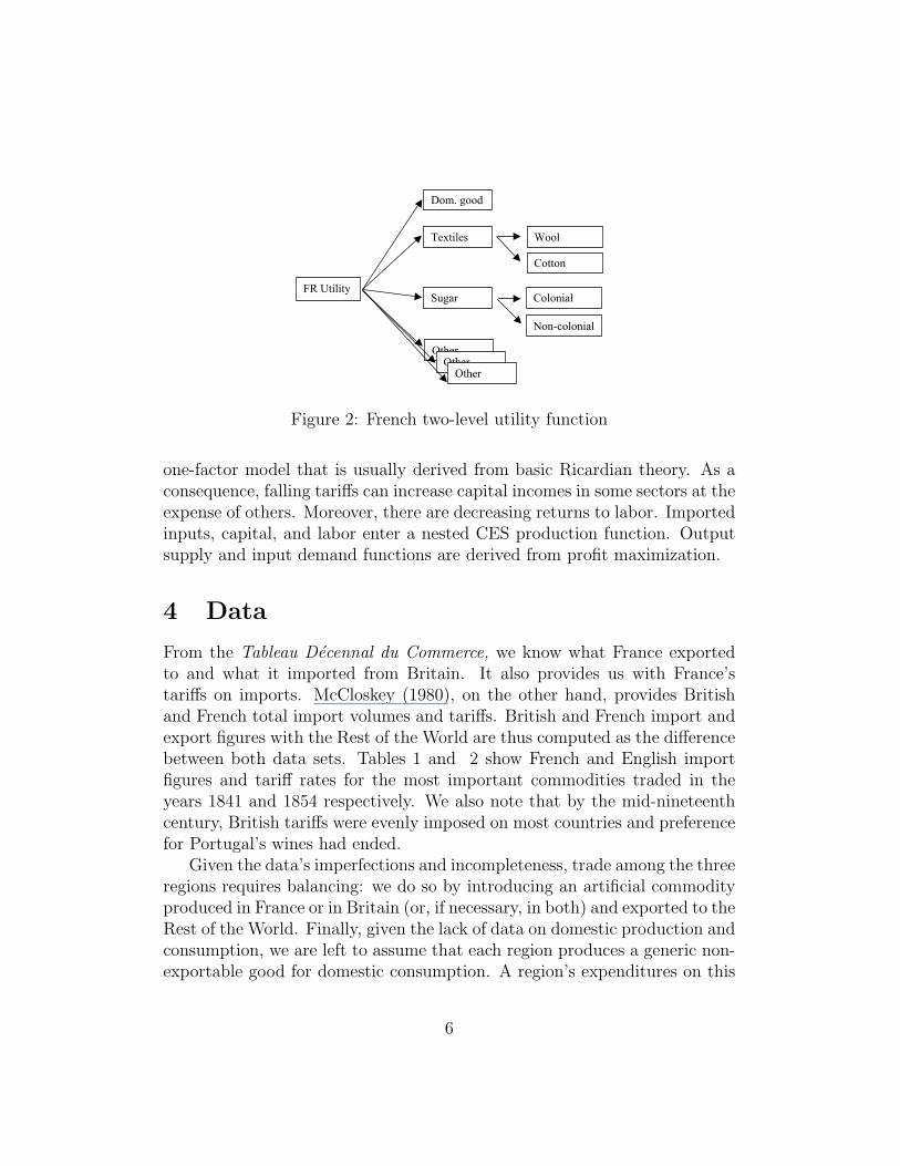
bundles. Wine and brandy, for instance, which can be considered close sub-stitutes, belong to the same bundle generically called alcohol. The secondutility level then combines the various bundles such as alcohol and textiles.The assumed preference structures for Britain and France are represented byFigures 1 and 2.

Our model differs from Anderson/Neary and O’Rourke in two essentialways:

(1) Our world economy consists of three finitely-sized regions (Britain,France, and the rest of the world) instead of a single, price-taking country(facing an infinitely large “rest of the world”). While this forces us to dropthe TRI as a convenient measure of protection, it also relaxes the assumptionof a zero optimal tariff vector, thus acknowledging the issue of market powerraised by McCloskey and Irwin.

(2) In addition to imported intermediate goods and a mobile, non-tradedinput, we include capital as a third type of input and assume that it is sector-specific: a brewery cannot be transformed into a steel mill. Our specific-factors model (Jones, 1971 and Samuelson, 1971) stands in contrast to the

5

GB Utility

Dom. good

Textiles

Alcohol

Caffeine

Wool

Cotton

Rum/Brandy

Silk

Coffee

Tea

Wine

OtherOther

Other

FR Utility

Dom. good

Sugar Colonial

Non-colonial

Textiles Wool

Cotton

OtherOther

Other

Beer (dom.)

Figure 2: French two-level utility function

one-factor model that is usually derived from basic Ricardian theory. As aconsequence, falling tariffs can increase capital incomes in some sectors at theexpense of others. Moreover, there are decreasing returns to labor. Importedinputs, capital, and labor enter a nested CES production function. Outputsupply and input demand functions are derived from profit maximization.

4 Data

From the Tableau Decennal du Commerce, we know what France exportedto and what it imported from Britain. It also provides us with France’stariffs on imports. McCloskey (1980), on the other hand, provides Britishand French total import volumes and tariffs. British and French import andexport figures with the Rest of the World are thus computed as the differencebetween both data sets. Tables 1 and 2 show French and English importfigures and tariff rates for the most important commodities traded in theyears 1841 and 1854 respectively. We also note that by the mid-nineteenthcentury, British tariffs were evenly imposed on most countries and preferencefor Portugal’s wines had ended.

Given the data’s imperfections and incompleteness, trade among the threeregions requires balancing: we do so by introducing an artificial commodityproduced in France or in Britain (or, if necessary, in both) and exported to theRest of the World. Finally, given the lack of data on domestic production andconsumption, we are left to assume that each region produces a generic non-exportable good for domestic consumption. A region’s expenditures on this

6

British Imports

from France

from RoW Tariff

French Imports

from Britain

from RoW Tariff

wool fab. 6.95 wool. text. 0.465 0.285 50.0%cotton fab. 2.7 270.5 cotton text. 19.47 50.0%coffee 45.32 96.0% coffee 26.3 100.8%sugar 318.5 67.0% for. sugar 10 156.4%cereals 7.91 204.9 6.5% col. sugar 83.9 71.9%wines 11.59 69.15 113.9% fats/lard 5.2rum/brandy 19.283 69.39 206.6% silk 7.79 52.21jewelry 0.56 wool 2 44.04 22.1%leather gds 4.58 raw cotton 1.62 106.7 12.1%eggs 4.89 coal 6.44 20.4 16.5%silk fabric 28.64 hides/pelts 1.697 25.62 2.2%tobacco 94.8 843.3% flax/linen 27.9tea 186.3 114.1% oleag. 2.79 34.77 3.3%wood 115.7 14.0% wood 39.2Other-FR 34.35 15.2% copper/iron 14.9 0.91Other-RW 842.2 15.2% livestock 10.6 21.8%

Other-BR 7.74 76.9%Other-RW 397.3 13.5%

Sources: Tableau Décennal du Commerce, McCloskey (1980), Nye (1991).

Table 1: Import/export data for 1841

British Imports

from France

from RoW Tariff

French Imports

from Britain

from RoW Tariff

coffee 22.18 52.8% silk 44.45 77.85 0.0%sugar 213.8 52.5% wool 16.78 35.72 17.9%wood 131.5 4.8% raw cotton 0.66 99.14 14.3%tobacco 24.95 479.0% wood 57.2 0.0%tea 100 119.5% coal 8.85 56.65 10.2%rum/brandy 8.94 24.26 201.8% hides/pelts 1.98 36.12 1.6%cereals 0.64 546.9 1.9% livestock 21.1 3.8%cotton fab. 9.92 437.6 0.0% coffee 23.3 78.5%wines 8.88 47.37 84.9% flax/linen 1.61 21.09 0.0%silk fabric 103.3 oleag. 1.85 15.95 14.6%wool fab. 33.45 wool. text. 0.14 0.56 50.0%leather gds 14.69 cotton text. 0.0018 0.7982 50.0%Other 90.7 1531 8.1% for. sugar 16.6 107.2%

col. sugar 48.7 62.2%fats/lard 6.2 0.0%Other 56.558 427.14 8.0%

Sources: Tableau Décennal du Commerce, McCloskey (1980), Nye (1991).

Table 2: Import/export data for 1854

7

generic domestic good is assumed to equal GDP plus intermediate imports(including tariff revenues) minus exports. Finally, we assume that the rest ofthe world produces and consumes the same goods as Britain and France andin proportional amounts. In our standard baseline calibration, we let Britainand France make up half the world’s economy, and thus purposely bias theirmarket power upwards.1

In empirical work, it is often assumed that final demand is elastic, whileintermediate demand is inelastic. Anderson’s (1995) calibration, just to citean example, specified elasticities of substitutions of 0.7 among input bundlesand 2.0 among bundles of consumption goods. We made the same numer-ical assumption for our base case. Within bundles, we typically chose 3.0among textiles, 5.0 between tea and coffee, 5.0 among various alcohols, and8.0 between foreign and colonial sugar.2 While these assumptions strike usas reasonable, we also ran our simulations over a wide range of alternativeelasticities assumptions: between 0.1 and 2.0 among input bundles and be-tween 0.5 and 4.0 among final consumption goods. We found that our resultsare rather robust to alternative specifications in the higher elasticity range.

A final caveat: despite the quantitative – or, rather, numerical – nature ofour simulations, we feel that their qualitative implications deserve most of theattention and interpretation. The shape of curves and their positions relativeto other curves are more significant than are their absolute magnitudes.

5 Results

5.1 The big picture

Over a wide range of alternative calibrations, calculations that simulate aunilateral drop in all British tariffs show a substantial net increase in British

1In 1854, for example, Britain imported 8.88 million francs (MF) worth of wine fromFrance and 47.37 MF worth of wine from the rest of the world. In our standard calibration,we would thus assume that the rest of the world also imported 8.88 MF worth of winefrom France and produced an additional 47.37 MF for its own consumption. Alternativespecifications of market shares are explored as part of our sensitivity analysis.

2Previous research based on partial equilibrium analysis specified price elasticities ofdemand, ε, rather than elasticities of substitution, σ. The two are, of course, related sincethe price elasticity depends on the CES elasticities of substitution as well as on a good’sexpenditure share s. The approximate relation is ε ≈ σ − s(1 + σ), also shown in Table 3in the appendix.

8

welfare, suggesting that British tariff levels were significantly higher thanwould be consistent with an optimum tariff policy.3 For our baseline case,we found that British tariffs in 1841 were roughly three times larger thanthe optimal tariff, leading to a static welfare loss for Britain of about 1.4%.For 1854, on the other hand, we find that while actual tariffs are significantlyreduced, they are still almost twice the size of optimal tariffs, this despite ourexaggerated assumptions on market power. Static welfare losses for Britain,however, have fallen to a negligible 0.13% of national income.4 Thus, whileBritain did indeed significantly reduce its tariffs, thereby greatly eliminatingassociated welfare losses, those tariffs were still too high to be consistent witha policy of free, unfettered, trade. Indeed the tariff levels still exceeded thosethat would have been consistent with an optimal tariff policy.

In comparison, French tariffs led to much smaller French static welfarelosses, which, in 1841, represented less than 1% of income. Those tariffs wereabout 10 times the magnitude of optimal tariffs, reflecting, in part, France’ssmaller market power. In 1854, French tariffs fell to a very negligible 0.06%loss of welfare, even though, here too, tariffs were still about twice the size ofoptimal tariffs. We note that the French results were robust to quite severerespecifications of the tariff equivalents on cotton and woolen textiles, giventhe relatively small share of French trade that was taxed.

Chart 1 summarizes these findings by plotting welfare (the utility of therepresentative consumer) against percentage of the original tariff vector. Thegraph is best read from right to left: we start with 100%, the full norm ofthe historic tariff vector, and then observe changes in welfare as we scale thenorm of the tariff vector down to 0%.

Issues of country size notwithstanding, readers familiar with O’Rourke’sspectacularly high uniform tariff equivalents might wonder how his results,which are based on similar data, can be reconciled with our relatively smallwelfare effects. We speculate that the explanation lies in the high variance ofBritish customs duties. In addition to having high levels of tariffs on a small

3It is important to point out that we restrict our attention to equi-proportional re-ductions of the historic tariff vector. Our computed “optimal tariffs” are thus not global,but rather constrained to the segment connecting zero tariffs to the historic tariffs. As aconsequence, we are likely to underestimate the welfare losses associated with protection.

4To use modern examples for comparison, Krugman and Obstfeld(1997) report welfarecosts of protection of 9.5% for Brazil 9.5%, 5.4% for Turkey, 5.2% for the Philippines, and0.26% for the U.S.

9

but important set of imports, the highly discriminatory nature of these dutieswould distort British trade beyond what would seem indicated by the highlevels alone. Hence, any uniform tax designed to mimic the welfare resultsof such a tariff profile would have to reflect both the effects of the tariffsthemselves and the welfare losses due to the uneven imposition of customsduties. Since a uniform tax has little distortionary effect, even less so if theproceeds are returned to the consumer, it takes a very high uniform tariffindeed to obtain a small change in welfare.

5.2 Sensitivity analysis

As expected, the simulation results are sensitive to calibration, in particularto the specified elasticities of substitution.

First, according to our data, Britain was mainly an importer of consump-tion goods, whereas France’s imports were dominated by inputs. Since wetypically assume an elasticity of substitution of 0.7 among inputs and 2.0among most consumption goods, this asymmetry clearly lowers Britain’s op-timal tariff relative to France. To see how much of our result rests on thisasymmetry, we performed simulations with identical calibrations for boththe supply and the demand side. Specifically, we assumed that both elas-ticities of substitution were equal to 1, which corresponds to Cobb-Douglasspecifications for both tastes and technology.

As can be seen in Chart 2, increasing the elasticity of substitution amonginputs from 0.7 to 1 and decreasing the elasticity of substitution amongconsumption goods from 2.0 to 1 somewhat diminishes Britain’s potentialgains from a counterfactual reduction of tariffs in 1841, even if those potentialgains are still higher than France’s potential gains. For comparison, the samechange in elasticity assumptions has an even larger effect on 1841 France,whose potential benefit of trade liberalization is reduced by 75%.

More remarkably, in 1854, while still being far from being free-traders,both Britain and France appear to be practicing near-optimal tariff policiesunder the new elasticity assumptions. While Britain’s tariffs are still slightlybeyond their optimal level, France actually displays a touch of magnanimity.

Second, we perform a sensitivity analysis on the elasticity of substitutionamong (bundles of) consumption goods. Chart 3 shows the static welfareeffects of a move to free trade for 1841 and 1854 Britain and for elasticities

10

ranging from 0.5 to 4.0.The graphs are very similar between the two years, the main difference

being the relative magnitude of welfare losses. As seen earlier, for an elastic-ity of substitution of 2.0 among consumption bundles, Britain’s high tariffscost her close to 1.4% of her static income in 1841, but only 0.13% in 1854.Increasing the elasticity of substitution from 2.0 to 4.0 dramatically increasesthe welfare cost of protection to over 2.4% of income in 1841 and to 0.35% in1854. Decreasing the elasticity also lowers the welfare losses, but the criticalresult here is that the consumer’s elasticity of substitution must be a low0.5 before it can be claimed that 1841 British tariffs were close to welfaremaximizing, but only below 1 to make the same claim for 1854. The premisebehind McCloskey’s argument thus begins to hold water if imports generallyfaced inelastic demands. We note furthermore that for an elasticity of sub-stitution of 0.5, a free-trade policy would have cost Britain 1.7% of its welfare.

Third, we vary the elasticity of substitution among inputs and find ourresults to be particularly sensitive to this parameter. As can be seen in Chart4, raising the elasticity from 0.7 (slightly inelastic) to 1.2 (slightly elastic)just about triples both 1841’s and 1854’s static welfare losses relative to op-timal tariffs. Raising the elasticity to 2.0 pushes the welfare losses to anenormous 9% of income in 1841 and a smaller loss of only 1% in 1854. Morefundamentally, even a reduction of that elasticity to an almost Leontief 0.1still places the optimal tariff below the historic tariff for either year.

Fourth, we vary the size of the rest of the world. Our baseline case tendsto exaggerate British (and French) market power by assuming that the restof the world makes up only a modest half of the world’s economy. By relaxingthis assumption and increasing market share of the rest of the world to 70, 90,and 99%, our central claim that British tariffs were too high to be consistentwith an optimal tariff policy is further reinforced. The simulation results arereported in Charts 5 and 6.

5.3 The revenue story

Irwin argued that Britain’s high tariffs on select goods such as wines, rum,and brandy were levied not for protection but for revenue alone. As such,he claimed, unless given a very small weight, their inclusion into a measureof protection such as a tariff index would be misleading. His rationale was

11

that those goods had no close domestic substitutes and, in particular, thateven high wine prices would have only a negligible effect on British beerconsumption. However, this ignores the prohibitive effects of the tariff oncertain classes of wine and spirits most likely to be in competition withdomestic production of alcoholic beverages.5

It is thus natural to ask whether 1841 tariffs of about 115% on wines andover 200% on rum and brandy could conceivably have been so high as to beexcessively prohibitive and not raise anywhere close to the potential revenues.Our simulations suggest, however, that for a range of plausible elasticities ofsubstitution, those high tariffs were indeed still on the reasonable side of theLaffer curve. In particular, for an elasticity of substitution of 2.0 amongalcohol imports and domestic beer, the vector of tariffs on alcohol was closeto revenue-maximizing: in Chart 7, the solid tariff revenue curve is flat andalmost reaches its maximum at 100% of historic tariffs on alcohols. Onlyfor higher elasticities of substitution would the historic tariffs have beenexcessive.

Chart 8, finally, shows the welfare effects of these simulations. At anelasticity of substitution of 2.0, for which the tariffs are close to revenue-maximizing, the welfare losses remain non-negligible. While we thus agreewith Irwin that tariffs –except for those on table wine– can be construedas revenue-maximizing, the associated utility loss suggests that the tariffscannot be exempted from a protective role.

6 Conclusion

This paper has been motivated by the desire to sort out the various claimsthat have been made about the status of British trade policy in the 1800s.The view of Britain as a magnanimous market liberal, willing to sacrificeshort-term static gains from higher tariffs in order to promote free trade at

5We should point out that these revenue maximization calculations are somewhat mis-leading for wine and spirits because these goods were uniquely taxed by volume ratherthan ad valorem. Thus, our calculations ignore the prohibitive effect of British tariffs onthe cheapest class of wines, which did not enter into British consumption at all after theeighteenth century. In contrast, the finest products of Burgundy and Bordeaux naturallyreceived much lower tariffs on an ad valorem basis for a fixed tariff. Our inability todeal with the problem of specific tariffs on wine and brandy therefore leaves out the veryimportant protective and distributional effects on the types of wines that were importedand on the specific protection of domestic beer.

12

home and abroad, has been examined and rejected.The use of a simple computable general equilibrium model has allowed

for more refined calculations than seen in earlier writing based on partialequilibrium models. We found that British tariff levels even a decade or moreafter the abolition of the Corn Laws were still high in absolute terms (andindeed were high relative to those of important rivals like France). Moreover,calculations that simulated a drop in all British tariffs showed a significant netincrease in British welfare - suggesting that British tariff levels were higherthan would be consistent with an optimum tariff policy. More important,the size of British losses from her high tariff levels makes it clear that Britishpolicy was not consistent with pure free trade. It confirms earlier work(Nye, 1991) that demonstrated how unusually high British tariff levels werecompared both to British rhetoric and to French tariffs. It lays to rest thepuzzle - examined by both McCloskey (1980) and Irwin (1988) - of a dominantBritain moving to a trade policy that was freer than that which would havebeen dictated by narrow self interest, a claim which served as the basis foran important subset of the work on hegemonic stability theory (cf. Keohane,1984). The actual policies employed were, in practice, far more damagingto the welfare of the nation than has been suggested in the magnanimousview of Britain originally advanced by McCloskey (1980), but are now mucheasier to reconcile with an interest group explanation whose origins partlylie in historical decisions made a century and a half earlier (Anderson andTollison, 1985, and Nye, 2004). Finally, our results are consistent with a tradepolicy aimed at revenue maximization, but only if we ignore the prohibitiveeffects of the tariff on wine and treat them as ad valorem rather than as thespecific tariffs they had always been in practice.

References

[1] Anderson, Gary M. and Robert D. Tollison, “Ideology, Interest Groups,and the Repeal of the Corn Laws,” Journal of Institutional and Theo-retical Economics 141 (1985) 197-212.

[2] Anderson, James E. and J. Peter Neary, “Measuring the restrictivenessof trade policy,” The World Bank Economic Review 8 (1994) 151–69.

[3] Anderson, James E., “Trade Restrictiveness Benchmarks,” Mimeo(1995).

13

[4] Dakhlia, Sami, “A generalized Trade Restrictiveness Index,” SSRNWorking Paper (2002).

[5] France, Administration des Douanes, Tableau Decennal du Commercede la France, 1847–56 (Paris, 1858).

[6] France, Administration des Douanes, Tableau Decennal du Commercede la France, 1867–76 (Paris, 1878).

[7] Irwin, Douglas A.,“Welfare Effects of British Free Trade: Debate andEvidence from the 1840s,” Journal of Political Economy 96 (1988) 1142–64.

[8] Irwin, Douglas A., “Free trade and protection in nineteenth-centuryBritain and France revisited: a comment on Nye,” Journal of EconomicHistory 51 (1993) 146–52.

[9] Jones, Ronald W., “A Three-Factor Model in Theory, Trade, and His-tory,” in Jagdish Bhagwati et al., eds., Trade, Balance of Payments, andGrowth (Amsterdam: North-Holland, 1971) 3–11.

[10] Keohane, Robert, After Hegemony: Cooperation and Discord in theWorld Political Economy (Princeton, New Jersey, 1984).

[11] Kindleberger, Charles P., “The Rise of Free Trade in Western Europe,1820–1875,” Journal of Economic History 35 (1975) 20–55.

[12] McCloskey, Donald N., “Magnanimous Albion: free trade and Britishnational income, 1841–1881,” Explorations in Economic History 17(1980) 303–20.

[13] Mercenier, Jean and Erinc Yeldan, “A Plea for Greater Attention on theData in Policy Analysis,” Journal of Policy Modeling 21 (1999) 851–73.

[14] Nye, John V., “The myth of free-trade Britain and fortress France: tar-iffs and trade in the nineteenth century,” Journal of Economic History51 (1991) 23–46.

[15] Nye, John V., War, Wine, Taxes. Manuscript in progress (2004).

[16] O’Rourke, Kevin, “Measuring protection: a cautionary tale,” Journalof Development Economics 53 (1997) 169–83.

14

[17] Samuelson, Paul, “Ohlin was right,” Swedish Journal of Economics 73(1971) 365–84.

Appendix 1: TRI and large country

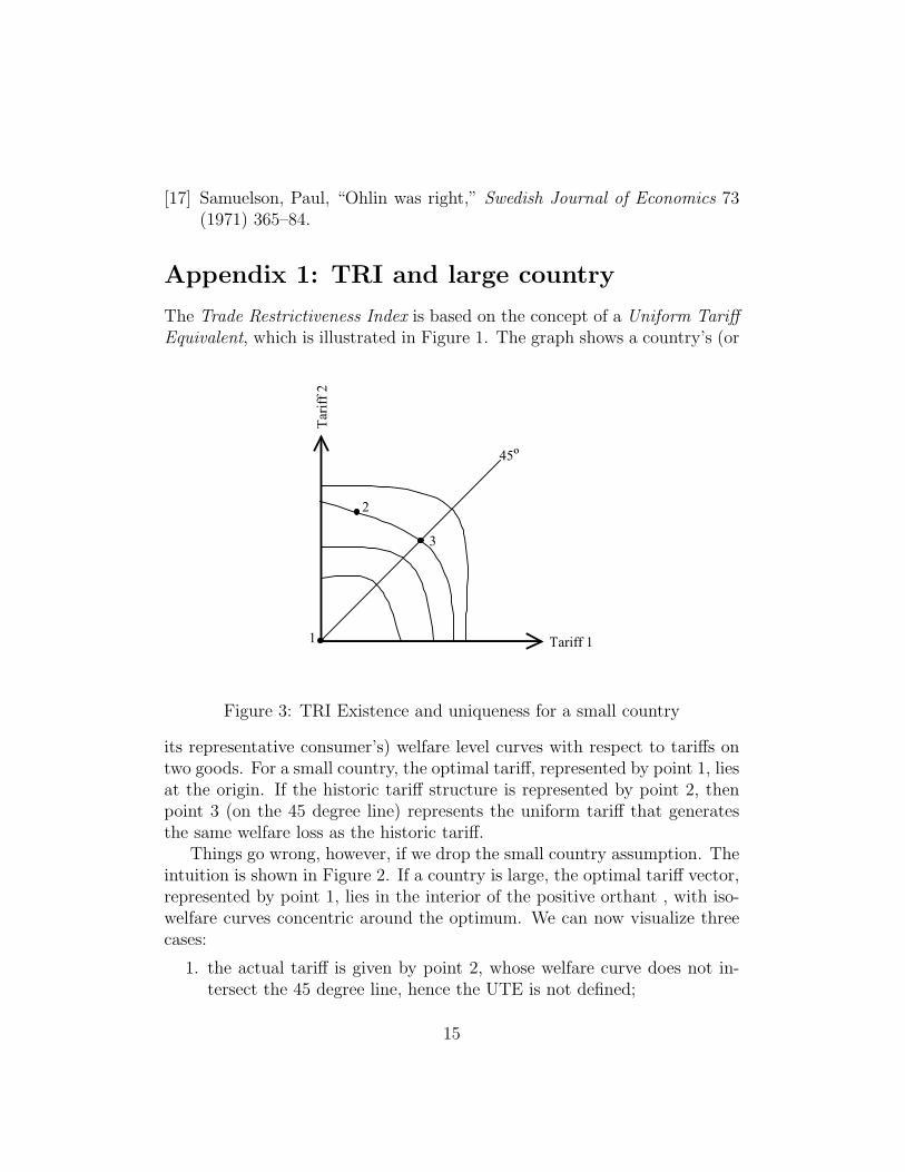
The Trade Restrictiveness Index is based on the concept of a Uniform TariffEquivalent, which is illustrated in Figure 1. The graph shows a country’s (or

Tariff 1

Tarif

f 2

2

3

1

45º

Figure 3: TRI Existence and uniqueness for a small country

its representative consumer’s) welfare level curves with respect to tariffs ontwo goods. For a small country, the optimal tariff, represented by point 1, liesat the origin. If the historic tariff structure is represented by point 2, thenpoint 3 (on the 45 degree line) represents the uniform tariff that generatesthe same welfare loss as the historic tariff.

Things go wrong, however, if we drop the small country assumption. Theintuition is shown in Figure 2. If a country is large, the optimal tariff vector,represented by point 1, lies in the interior of the positive orthant , with iso-welfare curves concentric around the optimum. We can now visualize threecases:

1. the actual tariff is given by point 2, whose welfare curve does not in-tersect the 45 degree line, hence the UTE is not defined;

15

Tarif

f 2

Tariff 1

1

3

4

5

45º

76

2

Figure 4: Nonexistence or non-uniqueness of a uniform tariff equivalent

2. the actual tariff is given by point 3, whose welfare curve intersects the45 degree line twice at points 4 and 5, thus the UTE is not uniquelydefined and hence ambiguous;

3. the actual tariff is given by point 6 with UTE at point 7. This lastcase, however, appears to be non-generic.

Appendix 2: Formal Model

The world economy consists of three regions, Britain, France, and the restof the world. We identify sectors of activity by indices s, t ∈ S, withS = {1, 2, . . . , S} representing the set of all industries. Regions are iden-tified by indices i, j ∈ W , with W = {Br, Fr, RW}. To keep track of tradeflows, we follow the usual practice that identifies the first two indices with,respectively, the region and the industry supplying the good and the nexttwo with the client region and industry. Production uses three types of in-put: fixed capital, mobile labor, and imported intermediate inputs. Outputconsists of the non-traded good and exported goods. None of the exportables

16

are consumed at home. Consumers are endowed with labor (a non-tradedinput) and receive all profits and tariff revenue. They consume importedfinal goods and their non-traded good.

6.1 Consumption

Each region i has a representative consumer who values a large variety of im-ports as well as a generic, non-traded, domestic product. This specification,also used by Anderson and Neary for their TRI computations, conforms tothe available records, which are rich on import and export data, but scarceon non-traded commodities.

A two-level nested CES utility function allows us to specify different elas-ticities of substitution within bundles of goods as well as among bundles. Themaleability of nested CES offers an attractive compromise between realismon one hand and computational expediency on the other. The first utilitylevel combines bundles of consumption goods cjsi into aggregates cki. Wineand brandy, for instance, which can be considered close substitutes, belong tothe same bundle generically called alcohol. Formally, we shall partition theset S into bundles or “nests” Sk, k ∈ K = {1, 2, . . . , K}, K ≤ S. The secondutility level determines the optimal composition of the consumption aggre-gates cki, such as alcohol and textiles. Formally, the consumer’s preferencesare thus:

Ci =

(∑k∈K

ρkicσi−1

σiki

) σiσi−1

where

cki =

(∑s∈Sk

∑j∈W

δjsicσk−1

σkjsi

) σkσk−1

,

and δjsi and ρki represent benchmark expenditure shares.The consumer maximizes Ci with respect to cjsi and subject to

pciCi ≥∑j∈W

∑s∈S

(1 + τjsi)pjsicjsi,

where τjsi are tariff rates, pjsi are prices, and σi and σk are elasticities ofsubstitution.

17

6.2 Production

The representative firm of region i, sector s owns fixed, sector specific capitalKis, while labor is assumed to be fully mobile. Hence, there are decreasingreturns to labor. Material inputs, all imported, along with capital and laborenter a nested CES production function along the same principle as in theconsumer’s utility function. Output supply and input demands result frommaximizing profit

Πis = pisQis −∑j∈W

∑t∈S

(1 + τjti)pjtixjtis − wiLis

subject toΠis ≥ 0,

and

Qis =

(αKisK

σis−1

σisis + αLisL

σis−1

σisis +

∑k∈K

αkisxσis−1

σiskis

) σisσis−1

,

where

xkis =

(∑t∈Sk

∑j∈W

βjtisxσk−1

σkjtis

) σkσk−1

.

18

Appendix 3: Tables and graphs

0% 5% 10% 20% 40% 60% 80% 100%0 0.00 -0.05 -0.10 -0.20 -0.40 -0.60 -0.80 -1.00

-0.1 -0.10 -0.15 -0.19 -0.28 -0.46 -0.64 -0.82 -1.00-0.5 -0.50 -0.53 -0.55 -0.60 -0.70 -0.80 -0.90 -1.00

-1 -1.00 -1.00 -1.00 -1.00 -1.00 -1.00 -1.00 -1.00-1.5 -1.50 -1.48 -1.45 -1.40 -1.30 -1.20 -1.10 -1.00

-2 -2.00 -1.95 -1.90 -1.80 -1.60 -1.40 -1.20 -1.00-5 -5.00 -4.80 -4.60 -4.20 -3.40 -2.60 -1.80 -1.00

-10 -10.00 -9.55 -9.10 -8.20 -6.40 -4.60 -2.80 -1.00

Expenditure ShareEla

stic

ity

of

Subst

itution

Table 3: Own-price elasticities of demand

CHART 1Base Case: Counterfactual unilateral reduction from 100% to 0%of a country's historical tariff vector. Effect on own Welfare.

Brit 41 Brit 54 Fra 41 Fra 54100% 0.000% 0.000% 0.000% 0.000%95% 0.136% 0.024% 0.042% 0.007%90% 0.267% 0.047% 0.089% 0.015%85% 0.398% 0.068% 0.140% 0.022%80% 0.526% 0.087% 0.191% 0.027%75% 0.651% 0.102% 0.243% 0.034%70% 0.774% 0.117% 0.303% 0.041%65% 0.888% 0.125% 0.359% 0.046%60% 0.996% 0.131% 0.425% 0.054%55% 1.097% 0.131% 0.485% 0.058%50% 1.186% 0.125% 0.550% 0.061%45% 1.261% 0.110% 0.620% 0.063%40% 1.319% 0.090% 0.686% 0.063%35% 1.355% 0.058% 0.756% 0.061%30% 1.364% 0.013% 0.816% 0.056%25% 1.336% -0.046% 0.872% 0.046%20% 1.255% -0.126% 0.919% 0.032%15% 1.097% -0.230% 0.947% 0.010%10% 0.813% -0.367% 0.952% -0.019%

5% 0.306% -0.550% 0.919% -0.056%0% -0.715% -0.806% 0.840% -0.107%

-0.5%

-0.3%

-0.1%

0.1%

0.3%

0.5%

0.7%

0.9%

1.1%

1.3%

1.5%

0% 20% 40% 60% 80% 100%

Brit41

Fra41

Brit54Fra54

19

CHART 2Using the same elasticities of substitutionin consumption and production. Effect on Welfare

1841 Br 1/1 Br 0.7/2.0 Fr 1/1 Fr 0.7/2.0100% 0.000% 0.000% 0.000% 0.000%95% 0.086% 0.136% 0.019% 0.042%90% 0.170% 0.267% 0.033% 0.089%85% 0.256% 0.398% 0.051% 0.140%80% 0.337% 0.526% 0.070% 0.191%75% 0.418% 0.651% 0.089% 0.243%70% 0.495% 0.774% 0.107% 0.303%65% 0.568% 0.888% 0.131% 0.359%60% 0.637% 0.996% 0.149% 0.425%55% 0.701% 1.097% 0.168% 0.485%50% 0.757% 1.186% 0.191% 0.550%45% 0.804% 1.261% 0.210% 0.620%40% 0.841% 1.319% 0.229% 0.686%35% 0.860% 1.355% 0.243% 0.756%30% 0.860% 1.364% 0.257% 0.816%25% 0.835% 1.336% 0.266% 0.872%20% 0.777% 1.255% 0.271% 0.919%15% 0.665% 1.097% 0.266% 0.947%10% 0.482% 0.813% 0.247% 0.952%

5% 0.167% 0.306% 0.210% 0.919%0% -0.423% -0.715% 0.149% 0.840%

1854 Br 1/1 Br 0.7/2.0 Fr 1/1 Fr 0.7/2.0100% 0.000% 0.000% 0.000% 0.000%95% 0.005% 0.024% -0.005% 0.007%90% 0.008% 0.047% -0.010% 0.015%85% 0.009% 0.068% -0.015% 0.022%80% 0.009% 0.087% -0.019% 0.027%75% 0.008% 0.102% -0.024% 0.034%70% 0.003% 0.117% -0.032% 0.041%65% -0.005% 0.125% -0.039% 0.046%60% -0.016% 0.131% -0.049% 0.054%55% -0.032% 0.131% -0.056% 0.058%50% -0.050% 0.125% -0.066% 0.061%45% -0.077% 0.110% -0.078% 0.063%40% -0.112% 0.090% -0.090% 0.063%35% -0.155% 0.058% -0.105% 0.061%30% -0.210% 0.013% -0.122% 0.056%25% -0.281% -0.046% -0.141% 0.046%20% -0.369% -0.126% -0.163% 0.032%15% -0.486% -0.230% -0.188% 0.010%10% -0.635% -0.367% -0.217% -0.019%

5% -0.837% -0.550% -0.251% -0.056%0% -1.112% -0.806% -0.290% -0.107%

-0.3%

-0.1%

0.1%

0.3%

0.5%

0.7%

0.9%

1.1%

1.3%

1.5%

0% 20% 40% 60% 80% 100%

Br 1/1

Br .7/2

Fr .7/2

Fr 1/1

-0.8%

-0.7%

-0.6%

-0.5%

-0.4%

-0.3%

-0.2%

-0.1%

0.1%

0.2%

0% 20% 40% 60% 80% 100%Fr 1/1

Br 1/1

Fr .7/2

Br .7/2

20

CHART 3Varying the elasticity of substitution among consumptionbundles for both Britain and France: Effect on Britain

1841 0.5 1.1 2.0 4.0100% 0.000% 0.000% 0.000% 0.000%95% -0.017% 0.070% 0.136% 0.206%90% -0.039% 0.134% 0.267% 0.409%85% -0.067% 0.195% 0.398% 0.612%80% -0.100% 0.253% 0.526% 0.816%75% -0.139% 0.309% 0.651% 1.013%70% -0.184% 0.356% 0.774% 1.211%65% -0.239% 0.398% 0.888% 1.403%60% -0.301% 0.431% 0.996% 1.587%55% -0.376% 0.454% 1.097% 1.765%50% -0.462% 0.468% 1.186% 1.932%45% -0.562% 0.465% 1.261% 2.085%40% -0.679% 0.445% 1.319% 2.218%35% -0.818% 0.406% 1.355% 2.327%30% -0.983% 0.342% 1.364% 2.402%25% -1.172% 0.245% 1.336% 2.433%20% -1.403% 0.103% 1.255% 2.394%15% -1.676% -0.097% 1.097% 2.252%10% -2.012% -0.387% 0.813% 1.929%

5% -2.435% -0.816% 0.306% 1.255%0% -2.992% -1.534% -0.715% -0.484%

1854 0.5 1.1 2.0 4.0100% 0.000% 0.000% 0.000% 0.000%95% -0.027% 0.003% 0.024% 0.047%90% -0.057% 0.005% 0.047% 0.093%85% -0.088% 0.005% 0.068% 0.137%80% -0.123% 0.002% 0.087% 0.178%75% -0.161% -0.003% 0.102% 0.216%70% -0.202% -0.011% 0.117% 0.252%65% -0.246% -0.024% 0.125% 0.282%60% -0.295% -0.039% 0.131% 0.309%55% -0.348% -0.061% 0.131% 0.330%50% -0.408% -0.087% 0.125% 0.344%45% -0.475% -0.120% 0.110% 0.350%40% -0.549% -0.161% 0.090% 0.345%35% -0.632% -0.211% 0.058% 0.330%30% -0.725% -0.273% 0.013% 0.298%25% -0.831% -0.347% -0.046% 0.249%20% -0.951% -0.438% -0.126% 0.175%15% -1.090% -0.550% -0.230% 0.071%10% -1.250% -0.688% -0.367% -0.077%

5% -1.441% -0.863% -0.550% -0.287%0% -1.668% -1.088% -0.806% -0.596%

-1.2%

-0.8%

-0.4%

0.0%

0.4%

0.8%

1.2%

1.6%

2.0%

2.4%

0% 20% 40% 60% 80% 100%

elas=4

elas=1

elas=2

elas=0.5

-0.8%

-0.6%

-0.4%

-0.2%

0.0%

0.2%

0.4%

0% 20% 40% 60% 80% 100%

elas=4

elas=2

elas=1

elas=0.5

21

CHART 4Varying the elasticity of substitution among input bundlesfor both Britain and France: Effect on Britain

1841 0.1 0.7 1.2 2.0 0.0 0.1100% 0.000% 0.000% 0.000% 0.000% 5341.48 341.48 5341.4895% 0.028% 0.136% 0.192% 0.251% 5340.95 324.59 5340.590% 0.047% 0.267% 0.390% 0.512% 5340.43 307.71 5339.585% 0.061% 0.398% 0.593% 0.788% 5339.92 290.82 5338.4980% 0.067% 0.526% 0.799% 1.077% 5339.41 273.92 5337.4575% 0.061% 0.651% 1.016% 1.383% 5338.91 257.02 5336.3870% 0.050% 0.774% 1.236% 1.709% 5338.41 240.11 5335.2965% 0.025% 0.888% 1.464% 2.054% 5337.92 223.2 5334.1860% -0.011% 0.996% 1.701% 2.419% 5337.43 206.27 5333.0355% -0.058% 1.097% 1.943% 2.811% 5336.95 189.33 5331.8450% -0.122% 1.186% 2.196% 3.229% 5336.46 172.37 5330.6245% -0.203% 1.261% 2.455% 3.682% 5335.98 155.38 5329.3440% -0.303% 1.319% 2.728% 4.169% 5335.49 138.37 5328.0235% -0.426% 1.355% 3.009% 4.701% 5335 121.33 5326.6330% -0.573% 1.364% 3.301% 5.286% 5334.5 104.24 5325.1725% -0.752% 1.336% 3.607% 5.929% 5333.98 87.1 5323.6320% -0.966% 1.255% 3.922% 6.644% 5333.44 69.89 5321.9815% -1.233% 1.097% 4.239% 7.440% 5332.86 52.61 5320.2110% -1.564% 0.813% 4.529% 8.300% 5332.23 35.22 5318.28

5% -1.996% 0.306% 4.679% 9.104% 5331.52 17.69 5316.150% -2.614% -0.715% 4.214% 9.177% 5330.71 0 5313.75

1854 0.1 0.7 1.2 2.0 0.0 0.1100% 0.000% 0.000% 0.000% 0.000% 5341.48 341.48 5341.4895% 0.011% 0.025% 0.036% 0.049% 5340.95 324.59 5340.590% 0.020% 0.049% 0.073% 0.101% 5340.43 307.71 5339.585% 0.028% 0.069% 0.110% 0.155% 5339.92 290.82 5338.4980% 0.032% 0.088% 0.147% 0.211% 5339.41 273.92 5337.4575% 0.033% 0.106% 0.183% 0.270% 5338.91 257.02 5336.3870% 0.032% 0.118% 0.219% 0.333% 5338.41 240.11 5335.2965% 0.027% 0.129% 0.254% 0.397% 5337.92 223.2 5334.1860% 0.017% 0.134% 0.287% 0.465% 5337.43 206.27 5333.0355% 0.003% 0.136% 0.320% 0.536% 5336.95 189.33 5331.8450% -0.014% 0.129% 0.350% 0.610% 5336.46 172.37 5330.6245% -0.038% 0.117% 0.377% 0.686% 5335.98 155.38 5329.3440% -0.066% 0.096% 0.399% 0.765% 5335.49 138.37 5328.0235% -0.102% 0.065% 0.416% 0.844% 5335 121.33 5326.6330% -0.143% 0.020% 0.424% 0.922% 5334.5 104.24 5325.1725% -0.194% -0.039% 0.421% 0.995% 5333.98 87.1 5323.6320% -0.254% -0.118% 0.401% 1.057% 5333.44 69.89 5321.9815% -0.325% -0.221% 0.355% 1.091% 5332.86 52.61 5320.2110% -0.408% -0.358% 0.271% 1.080% 5332.23 35.22 5318.28

5% -0.509% -0.542% 0.123% 0.976% 5331.52 17.69 5316.150% -0.634% -0.798% -0.140% 0.694% 5330.71 0 5313.75

-2.7%

-1.7%

-0.7%

0.3%

1.3%

2.3%

3.3%

4.3%

5.3%

6.3%

7.3%

8.3%

9.3%

0% 20% 40% 60% 80% 100%

elas=2.0

elas=1.2

elas=0.7

elas=0.1

elas=2.0

-0.7%

-0.3%

0.1%

0.5%

0.9%

0% 20% 40% 60% 80% 100%

elas=1.2

elas=0.7

elas=2.0

elas=0.1

22

CHART 5Varying the size of the Rest of the WorldEffect on Britain

1841 50% 70% 90% 99% 0.0 0.1100% 0.000% 0.000% 0.000% 0.000% 5341.48 341.48 5341.4895% 0.136% 0.156% 0.203% 0.317% 5340.95 324.59 5340.590% 0.267% 0.309% 0.409% 0.649% 5340.43 307.71 5339.585% 0.398% 0.462% 0.615% 0.988% 5339.92 290.82 5338.4980% 0.526% 0.612% 0.827% 1.342% 5339.41 273.92 5337.4575% 0.651% 0.763% 1.038% 1.706% 5338.91 257.02 5336.3870% 0.774% 0.907% 1.253% 2.082% 5338.41 240.11 5335.2965% 0.888% 1.049% 1.467% 2.472% 5337.92 223.2 5334.1860% 0.996% 1.183% 1.681% 2.870% 5337.43 206.27 5333.0355% 1.097% 1.311% 1.893% 3.279% 5336.95 189.33 5331.8450% 1.186% 1.425% 2.101% 3.696% 5336.46 172.37 5330.6245% 1.261% 1.528% 2.302% 4.117% 5335.98 155.38 5329.3440% 1.319% 1.614% 2.491% 4.537% 5335.49 138.37 5328.0235% 1.355% 1.678% 2.664% 4.949% 5335 121.33 5326.6330% 1.364% 1.712% 2.808% 5.344% 5334.5 104.24 5325.1725% 1.336% 1.706% 2.917% 5.700% 5333.98 87.1 5323.6320% 1.255% 1.645% 2.967% 5.993% 5333.44 69.89 5321.9815% 1.097% 1.500% 2.934% 6.179% 5332.86 52.61 5320.2110% 0.813% 1.227% 2.758% 6.179% 5332.23 35.22 5318.28

5% 0.306% 0.713% 2.330% 5.837% 5331.52 17.69 5316.150% -0.715% -0.337% 1.333% 4.757% 5330.71 0 5313.75

1854 50% 70% 90% 99% 0.0 0.1100% 0.000% 0.000% 0.000% 0.000% 5341.48 341.48 5341.4895% 0.044% 0.058% 0.080% 0.093% 5340.95 324.59 5340.590% 0.085% 0.115% 0.162% 0.189% 5340.43 307.71 5339.585% 0.125% 0.169% 0.244% 0.290% 5339.92 290.82 5338.4980% 0.161% 0.222% 0.326% 0.394% 5339.41 273.92 5337.4575% 0.194% 0.271% 0.408% 0.503% 5338.91 257.02 5336.3870% 0.224% 0.315% 0.487% 0.617% 5338.41 240.11 5335.2965% 0.248% 0.356% 0.566% 0.736% 5337.92 223.2 5334.1860% 0.266% 0.391% 0.639% 0.859% 5337.43 206.27 5333.0355% 0.279% 0.418% 0.708% 0.987% 5336.95 189.33 5331.8450% 0.285% 0.437% 0.768% 1.118% 5336.46 172.37 5330.6245% 0.282% 0.448% 0.820% 1.254% 5335.98 155.38 5329.3440% 0.268% 0.446% 0.858% 1.389% 5335.49 138.37 5328.0235% 0.243% 0.430% 0.880% 1.522% 5335 121.33 5326.6330% 0.202% 0.401% 0.883% 1.649% 5334.5 104.24 5325.1725% 0.145% 0.350% 0.859% 1.761% 5333.98 87.1 5323.6320% 0.066% 0.274% 0.806% 1.848% 5333.44 69.89 5321.9815% -0.043% 0.170% 0.711% 1.891% 5332.86 52.61 5320.2110% -0.186% 0.024% 0.563% 1.864% 5332.23 35.22 5318.28

5% -0.382% -0.178% 0.345% 1.727% 5331.52 17.69 5316.150% -0.654% -0.464% 0.022% 1.421% 5330.71 0 5313.75

-0.8%

0.2%

1.2%

2.2%

3.2%

4.2%

5.2%

6.2%

0% 20% 40% 60% 80% 100%

90%

70%

50%

elas=0.1

99%

-0.7%

-0.4%

0.0%

0.4%

0.7%

1.1%

1.4%

1.8%

0% 20% 40% 60% 80% 100%

50%

99%

90%

70%

23

CHART 6Varying the size of the Rest of the WorldEffect on France

1841 50% 70% 90% 99% 0.0 0.1100% 0.000% 0.000% 0.000% 0.000% 5341.48 341.48 5341.4895% 0.061% 0.061% 0.061% 0.061% 5340.95 324.59 5340.590% 0.126% 0.126% 0.126% 0.121% 5340.43 307.71 5339.585% 0.191% 0.196% 0.191% 0.182% 5339.92 290.82 5338.4980% 0.257% 0.266% 0.261% 0.247% 5339.41 273.92 5337.4575% 0.331% 0.336% 0.331% 0.313% 5338.91 257.02 5336.3870% 0.401% 0.411% 0.406% 0.383% 5338.41 240.11 5335.2965% 0.481% 0.490% 0.481% 0.457% 5337.92 223.2 5334.1860% 0.560% 0.569% 0.560% 0.527% 5337.43 206.27 5333.0355% 0.644% 0.653% 0.639% 0.602% 5336.95 189.33 5331.8450% 0.728% 0.742% 0.723% 0.676% 5336.46 172.37 5330.6245% 0.812% 0.830% 0.807% 0.751% 5335.98 155.38 5329.3440% 0.900% 0.914% 0.891% 0.826% 5335.49 138.37 5328.0235% 0.984% 1.003% 0.970% 0.896% 5335 121.33 5326.6330% 1.068% 1.082% 1.050% 0.961% 5334.5 104.24 5325.1725% 1.143% 1.162% 1.120% 1.017% 5333.98 87.1 5323.6320% 1.208% 1.222% 1.176% 1.054% 5333.44 69.89 5321.9815% 1.255% 1.274% 1.213% 1.073% 5332.86 52.61 5320.2110% 1.278% 1.297% 1.227% 1.064% 5332.23 35.22 5318.28

5% 1.264% 1.283% 1.204% 1.017% 5331.52 17.69 5316.150% 1.204% 1.222% 1.129% 0.910% 5330.71 0 5313.75

1854 50% 70% 90% 99% 0.0 0.1100% 0.000% 0.000% 0.000% 0.000% 5341.48 341.48 5341.4895% 0.015% 0.015% 0.017% 0.017% 5340.95 324.59 5340.590% 0.029% 0.029% 0.032% 0.034% 5340.43 307.71 5339.585% 0.044% 0.046% 0.049% 0.049% 5339.92 290.82 5338.4980% 0.058% 0.061% 0.066% 0.066% 5339.41 273.92 5337.4575% 0.073% 0.076% 0.080% 0.083% 5338.91 257.02 5336.3870% 0.088% 0.093% 0.097% 0.097% 5338.41 240.11 5335.2965% 0.100% 0.107% 0.112% 0.115% 5337.92 223.2 5334.1860% 0.115% 0.122% 0.127% 0.129% 5337.43 206.27 5333.0355% 0.127% 0.134% 0.141% 0.144% 5336.95 189.33 5331.8450% 0.139% 0.149% 0.156% 0.156% 5336.46 172.37 5330.6245% 0.151% 0.158% 0.166% 0.168% 5335.98 155.38 5329.3440% 0.158% 0.168% 0.175% 0.175% 5335.49 138.37 5328.0235% 0.166% 0.175% 0.183% 0.183% 5335 121.33 5326.6330% 0.171% 0.180% 0.188% 0.185% 5334.5 104.24 5325.1725% 0.171% 0.180% 0.188% 0.185% 5333.98 87.1 5323.6320% 0.166% 0.178% 0.183% 0.178% 5333.44 69.89 5321.9815% 0.156% 0.168% 0.173% 0.166% 5332.86 52.61 5320.2110% 0.136% 0.149% 0.154% 0.144% 5332.23 35.22 5318.28

5% 0.110% 0.122% 0.127% 0.112% 5331.52 17.69 5316.150% 0.071% 0.083% 0.085% 0.068% 5330.71 0 5313.75

0.0%

0.3%

0.5%

0.8%

1.0%

1.3%

0% 20% 40% 60% 80% 100%

90%

70%

50%

99%

0.00%

0.03%

0.05%

0.08%

0.10%

0.13%

0.15%

0.18%

0.20%

0% 20% 40% 60% 80% 100%

50%

99%

90%

70%

24

CHART 7Laffer Curves: Tariff on alcohols and effect on British Revenue

for various elasticities of substitution among alcohols, including domestic beer

1841 elas=1 elas=3 elas=5 elas=10200% 21.8% -14.4% -27.6% -40.3%190% 20.5% -12.7% -24.9% -37.1%180% 19.1% -10.9% -22.2% -33.7%170% 17.5% -9.2% -19.4% -30.1%160% 15.8% -7.4% -16.5% -26.2%150% 13.8% -5.8% -13.5% -22.1%140% 11.6% -4.2% -10.6% -17.7%130% 9.3% -2.8% -7.7% -13.2%120% 6.5% -1.6% -4.9% -8.7%110% 3.5% -0.6% -2.2% -4.2%100% 0.0% 0.0% 0.0% 0.0%90% -3.9% 0.2% 1.9% 3.7%80% -8.4% -0.4% 2.9% 6.5%70% -13.6% -1.9% 3.0% 8.2%60% -19.8% -4.6% 1.7% 8.2%50% -27.1% -9.1% -1.8% 5.7%40% -35.8% -15.9% -8.0% 0.0%30% -46.5% -26.2% -18.3% -10.4%20% -59.9% -41.6% -34.6% -27.7%10% -77.0% -64.7% -60.0% -55.4%

0% -100.0% -100.0% -100.0% -100.0%

1854 elas=1 elas=3 elas=5 elas=10200% 30.0% -11.3% -26.0% -40.2%190% 27.9% -9.6% -23.5% -37.1%180% 25.8% -8.1% -20.8% -34.0%170% 23.5% -6.7% -18.1% -30.4%160% 20.8% -5.2% -15.4% -26.7%150% 18.1% -4.0% -12.7% -22.5%140% 15.2% -2.7% -10.0% -18.3%130% 11.9% -1.5% -7.1% -13.8%120% 8.3% -0.6% -4.6% -9.0%110% 4.4% -0.2% -2.1% -4.4%100% 0.0% 0.0% 0.0% 0.0%90% -4.8% -0.2% 1.7% 4.0%80% -10.0% -1.3% 2.7% 7.1%70% -16.0% -3.3% 2.5% 9.0%60% -22.9% -6.5% 1.0% 9.2%50% -30.8% -11.3% -2.5% 6.9%40% -40.0% -18.3% -9.0% 1.3%30% -50.6% -28.8% -19.2% -9.0%20% -63.8% -44.0% -35.4% -26.3%10% -79.6% -66.3% -60.4% -54.4%

0% -100.0% -100.0% -100.0% -100.0%

-100%

-80%

-60%

-40%

-20%

0%

20%

0% 50% 100% 150% 200%

-100%

-80%

-60%

-40%

-20%

0%

20%

0% 50% 100% 150% 200%

elas=10

elas=5

elas=3

elas=1

elas=1

elas=3

elas=5

elas=10

25

CHART 8Tariff on alcohols and effect on British Welfare

for various elasticities of substitution among alcohols, including domestic beer

1841 elas=1 elas=3 elas=5 elas=10200% -1.033% -1.186% -1.253% -1.311%190% -0.932% -1.080% -1.150% -1.216%180% -0.832% -0.974% -1.041% -1.116%170% -0.732% -0.863% -0.927% -1.005%160% -0.629% -0.746% -0.807% -0.888%150% -0.523% -0.626% -0.682% -0.757%140% -0.420% -0.504% -0.551% -0.618%130% -0.315% -0.381% -0.418% -0.470%120% -0.209% -0.253% -0.278% -0.315%110% -0.103% -0.125% -0.139% -0.156%100% 0.000% 0.000% 0.000% 0.000%90% 0.103% 0.122% 0.136% 0.150%80% 0.200% 0.239% 0.259% 0.287%70% 0.292% 0.340% 0.367% 0.398%60% 0.373% 0.423% 0.445% 0.470%50% 0.443% 0.470% 0.484% 0.493%40% 0.490% 0.470% 0.456% 0.437%30% 0.509% 0.395% 0.337% 0.267%20% 0.482% 0.200% 0.070% -0.078%10% 0.384% -0.178% -0.431% -0.693%

0% 0.164% -0.874% -1.317% -1.762%

1854 elas=1 elas=3 elas=5 elas=10200% -0.265% -0.319% -0.341% -0.358%190% -0.240% -0.290% -0.312% -0.334%180% -0.213% -0.262% -0.284% -0.307%170% -0.188% -0.232% -0.252% -0.278%160% -0.161% -0.200% -0.221% -0.246%150% -0.134% -0.169% -0.186% -0.211%140% -0.107% -0.136% -0.151% -0.172%130% -0.080% -0.102% -0.114% -0.132%120% -0.054% -0.068% -0.077% -0.088%110% -0.027% -0.035% -0.038% -0.044%100% 0.000% 0.000% 0.000% 0.000%90% 0.025% 0.033% 0.036% 0.041%80% 0.050% 0.063% 0.071% 0.080%70% 0.074% 0.091% 0.101% 0.110%60% 0.096% 0.114% 0.123% 0.132%50% 0.115% 0.129% 0.136% 0.139%40% 0.129% 0.134% 0.131% 0.126%30% 0.140% 0.120% 0.104% 0.082%20% 0.142% 0.080% 0.041% -0.006%10% 0.131% -0.002% -0.077% -0.166%

0% 0.099% -0.155% -0.290% -0.443%

-1.2%

-0.8%

-0.4%

0.0%

0.4%

0% 50% 100% 150% 200%

-0.3%

-0.2%

-0.1%

0.0%

0.1%

0% 50% 100% 150% 200%

elas=1 elas=3 elas=5elas=10

elas=1 elas=3 elas=5elas=10

26