The Astrophysical Journal Supplement Series, 213:13 (48pp), 2014 July doi:10.1088/0067-0049/213/1/13C© 2014. The American Astronomical Society. All rights reserved. Printed in the U.S.A.

TADPOL: A 1.3 mm SURVEY OF DUST POLARIZATION IN STAR-FORMING CORES AND REGIONS

Charles L. H. Hull1, Richard L. Plambeck1, Woojin Kwon2, Geoffrey C. Bower1,3, John M. Carpenter4,Richard M. Crutcher5, Jason D. Fiege6, Erica Franzmann6, Nicholas S. Hakobian5, Carl Heiles1, Martin Houde7,8,

A. Meredith Hughes9, James W. Lamb4, Leslie W. Looney5, Daniel P. Marrone10, Brenda C. Matthews11,12,Thushara Pillai4, Marc W. Pound13, Nurur Rahman14,19, Goran Sandell15, Ian W. Stephens5,16, John J. Tobin17,20,

John E. Vaillancourt15, N. H. Volgenau18, and Melvyn C. H. Wright11 Astronomy Department & Radio Astronomy Laboratory, University of California, Berkeley, CA 94720-3411, USA; chat@astro.berkeley.edu

2 SRON Netherlands Institute for Space Research, Landleven 12, 9747 AD Groningen, The Netherlands3 ASIAA, 645 N. A’ohoku Place, Hilo, HI 96720, USA

4 Department of Astronomy, California Institute of Technology, 1200 E. California Blvd., MC 249-17, Pasadena, CA 91125, USA5 Department of Astronomy, University of Illinois at Urbana-Champaign, 1002 W Green Street, Urbana, IL 61801, USA

6 Department of Physics & Astronomy, University of Manitoba, Winnipeg, MB, R3T 2N2, Canada7 Department of Physics & Astronomy, University of Western Ontario, London, ON, N6A 3K7, Canada

8 Division of Physics, Mathematics, & Astronomy, California Institute of Technology, Pasadena, CA 91125, USA9 Van Vleck Observatory, Astronomy Department, Wesleyan University, 96 Foss Hill Drive, Middletown, CT 06459, USA

10 Steward Observatory, University of Arizona, 933 North Cherry Avenue, Tucson, AZ 85721, USA11 Department of Physics & Astronomy, University of Victoria, 3800 Finnerty Rd., Victoria, BC, V8P 5C2, Canada

12 National Research Council of Canada, 5071 West Saanich Rd., Victoria, BC, V9E 2E7, Canada13 Astronomy Department & Laboratory for Millimeter-wave Astronomy, University of Maryland, College Park, MD 20742, USA

14 Physics Department, University of Johannesburg, C1-Lab 140, P.O. Box 524, Auckland Park 2006, South Africa15 SOFIA Science Center, Universities Space Research Association, NASA Ames Research Center, Moffett Field, CA 94035, USA

16 Institute for Astrophysical Research, Boston University, Boston, MA 02215, USA17 National Radio Astronomy Observatory, 520 Edgemont Rd., Charlottesville, VA 22903, USA

18 Combined Array for Research in Millimeter-wave Astronomy, Owens Valley Radio Observatory, P.O. Box 968, Big Pine, CA 93513, USAReceived 2013 October 24; accepted 2014 March 11; published 2014 July 3

ABSTRACT

We present λ 1.3 mm Combined Array for Research in Millimeter-wave Astronomy observations of dust polarizationtoward 30 star-forming cores and eight star-forming regions from the TADPOL survey. We show maps of allsources, and compare the ∼2.′′5 resolution TADPOL maps with ∼20′′ resolution polarization maps from single-dishsubmillimeter telescopes. Here we do not attempt to interpret the detailed B-field morphology of each object.Rather, we use average B-field orientations to derive conclusions in a statistical sense from the ensemble of sources,bearing in mind that these average orientations can be quite uncertain. We discuss three main findings. (1) Asubset of the sources have consistent magnetic field (B-field) orientations between large (∼20′′) and small (∼2.′′5)scales. Those same sources also tend to have higher fractional polarizations than the sources with inconsistentlarge-to-small-scale fields. We interpret this to mean that in at least some cases B-fields play a role in regulatingthe infall of material all the way down to the ∼1000 AU scales of protostellar envelopes. (2) Outflows appear tobe randomly aligned with B-fields; although, in sources with low polarization fractions there is a hint that outflowsare preferentially perpendicular to small-scale B-fields, which suggests that in these sources the fields have beenwrapped up by envelope rotation. (3) Finally, even at ∼2.′′5 resolution we see the so-called polarization hole effect,where the fractional polarization drops significantly near the total intensity peak. All data are publicly available inthe electronic edition of this article.

Key words: ISM: magnetic fields – magnetic fields – polarization – stars: formation – stars: magnetic field –stars: protostars

Online-only material: color figures, supplemental data

1. INTRODUCTION

Magnetic fields have long been considered one of the keycomponents that regulate star formation (e.g., Shu et al. 1987;McKee et al. 1993). And indeed, observations of polarizationin regions of star formation have shown that magnetic fields(B-fields) often are well-ordered on scales from ∼100 pc (Heiles2000) down to ∼1 pc, which suggests that on large scalesB-fields are dynamically important. At smaller scales ambipolardiffusion (e.g., Mestel & Spitzer 1956; Fiedler & Mouschovias1993; Tassis et al. 2009) or turbulent magnetic reconnectiondiffusion (Lazarian 2005; Leao et al. 2013) are thought to allow

19 South Africa SKA Fellow.20 Hubble Fellow.

dense cores to become “supercritical” (see Crutcher 2012), atwhich point gravity overwhelms magnetic support and allowsthe formation of a central protostar. Alternatively, the corescould form as supercritical objects in a turbulent environment(e.g., Mac Low & Klessen 2004).

Under most circumstances, spinning dust grains align them-selves with their long axes perpendicular to the B-field (e.g.,Hildebrand 1988; Lazarian 2003, 2007; Hoang & Lazarian2009; Andersson 2012), so the thermal radiation from thesegrains is polarized perpendicular to the B-field. AmbientB-fields can be probed on scales of �1 pc using optical ob-servations of background stars (e.g., Heiles 2000), whose lightbecomes polarized after passing through regions of aligned dustgrains. However, this type of observation is not possible insidethe dense cores where the central protostars and their circum-

1

The Astrophysical Journal Supplement Series, 213:13 (48pp), 2014 July Hull et al.

stellar disks form; even at infrared wavelengths the extinctionthrough these dense regions is too great.

Mapping the polarized thermal emission from dust grains atmillimeter and submillimeter wavelengths is the usual meansof studying the B-fields in these regions. The 1.3 mm dual-polarization receiver system at the Combined Array for Re-search in Millimeter-wave Astronomy (CARMA; Bock et al.2006), described in Hull et al. (2011), has allowed us to mapthe dust polarization toward a sample of several dozen nearbystar-forming cores and a few star-forming regions (SFRs) as partof the TADPOL21 survey—a CARMA key project.

Previous results from the TADPOL survey have touched onseveral topics including the consistency of B-fields from largeto small scales (Stephens et al. 2013), the low levels of dustpolarization in the circumstellar disks around more evolvedClass II sources like DG Tau (Hughes et al. 2013; see Figure 15),and the misalignment of bipolar outflows and small-scaleB-fields in low-mass protostars (Hull et al. 2013). The latterresult has been used to place limits on the fraction of protostarsthat should harbor circumstellar disks (Krumholz et al. 2013).

Here we present the data from the full survey. We comparethese ∼2.′′5 resolution data with ∼20′′ resolution polarizationmaps from single-dish submillimeter telescopes to analyze theconsistency of B-field orientations down to the ∼1000 AU scaleof protostellar envelopes. We also revisit the correlation ofB-fields with bipolar outflows and see hints that sources withlow polarization fractions have outflows and small-scale B-fieldorientations that are preferentially perpendicular. Finally, evenat ∼2.′′5 resolution we see the so-called polarization hole effect,where the fractional polarization drops significantly near thetotal intensity peak.

2. SOURCE SELECTION AND OBSERVATIONS

We selected sources from catalogs of young stellar objects(e.g., Jørgensen et al. 2007; Matthews et al. 2009; Tobin et al.2010; Enoch et al. 2011). While several well known, high-massSFRs are included in the survey, we focus mainly on nearby(d � 400pc) Class 0 and Class I objects that are known tohave bipolar outflows, and that had been observed previouslywith the polarimeters on the James Clerk Maxwell Telescope(JCMT) and the Caltech Submillimeter Observatory (CSO), twosubmillimeter single-dish telescopes with ∼20′′ resolution. SeeAppendix B for source descriptions. Since the survey spannedfive observing semesters, sources were selected to cover a widerange of hour angles to allow most observations to be scheduledduring the more stable nighttime weather.

Observations were made with CARMA between 2011 Mayand 2013 April. Three different array configurations were used:C (26–370 m baselines, or telescope spacings), D (11–148 m),and E (8.5–66 m), which correspond to angular resolutions at1.3 mm of approximately 1′′, 2′′, and 4′′, respectively.

3. CALIBRATION AND DATA REDUCTION

The CARMA polarization system consists of dual-polarization receivers that are sensitive to right- (R) and left-circular (L) polarization, and a spectral-line correlator that mea-sures all four cross polarizations (RR, LL, LR, RL) on each ofthe 105 baselines connecting the 15 telescopes (6 with 10 mdiameters and 9 with 6 m diameters). Each receiver comprises asingle feed horn, a waveguide circular polarizer, an orthomode

21 TADPOL: Telescope Array Doing POLarization.

transducer (OMT), two heterodyne mixers, and two low-noiseamplifiers, all mounted in a cryogenically cooled dewar. The lo-cal oscillator (LO) and sky signals are combined using a mylarbeamsplitter in front of the dewar window.

The waveguide polarizer is a two-section design with half-wave and quarter-wave retarder sections rotated axially withrespect to one another to achieve broadband (210–270 GHz) per-formance; the retarders are sections of reduced-height, facetedcircular waveguide (Plambeck & Engargiola 2010). The polar-izer converts the R and L circularly polarized radiation fromthe sky into orthogonal X and Y linear polarizations, whichthen are separated by the OMT (Navarrini & Plambeck 2006).The mixers use Atacama Large Millimeter-submillimeter ArrayBand 6 SIS (superconductor–insulator–superconductor) tunneljunctions fabricated at the University of Virginia by ArthurLichtenberger. Although at ALMA these devices are used insideband-separating mixers (Kerr et al. 2013), at CARMA theyare used in double-sideband mixers that are sensitive to signalsin two bands, one 1–9 GHz above (upper sideband, or USB),and the other 1–9 GHz below (lower sideband, or LSB) the LOfrequency. A phase-switching pattern applied to the LO allowsthe LSB and USB signals to be separated in the correlator. The1–9 GHz intermediate frequency (IF) from each mixer is ampli-fied with WBA13 low-noise amplifiers (Weinreb 1998; Pandianet al. 2006).

For the TADPOL observations the LO frequency was223.821 GHz. The correlator was set up with three 500 MHzwide bands centered at IF values of 6.0, 7.5, and 8.0 GHz, andone 31 MHz wide band centered at 6.717 GHz.22,23 The cor-responding sky frequencies are equal to the difference (LSB)or the sum (USB) of the LO and the IF. The narrowbandsection allowed simultaneous spectral-line observations of theSiO(J = 5 → 4) line (217.105 GHz) in the LSB and theCO(J = 2 → 1) line (230.538 GHz) in the USB, with a chan-nel spacing of ∼0.2 km s−1. These lines were used to mapbipolar outflows.

In addition to the usual gain, passband, and flux calibra-tions, two additional calibrations are required for polarizationobservations: “XYphase” and leakage. The XYphase calibra-tion corrects for the phase difference between the L and R chan-nels on each telescope, caused by delay differences in the re-ceiver, underground cables, and correlator cabling. To calibratethe XYphase one must observe a linearly polarized source withknown position angle (P.A.). Since most astronomical sources atmillimeter wavelengths are weakly polarized and time-variable,CARMA uses artificial linearly polarized noise sources for thispurpose. The noise sources are created by inserting wire gridpolarizers into the beams of the 10 m telescopes. With the gridin place, one linear polarization reaching the receiver originatesfrom the sky, while the other originates from a room temperatureload. Since the room temperature load is much hotter than thesky, the receiver sees thermal noise that is strongly polarized.The L–R phase difference is then derived, channel by channel,from the L versus R autocorrelation spectrum obtained with the

22 Some or all of the data for the following six sources are from anotherCARMA project led by Kwon et al.: L1448 IRS 2, HH 211 mm, L1527,Ser-emb 1, HH 108 IRAS, and L1165. These observations had a differentcorrelator setup, with an LO frequency of 228.5988 GHz; three 500 MHz widebands centered at IF values of 1.9392, 2.4392, and 2.9392 GHz; and one31 MHz wide band centered at 1.9392 GHz. Dust continuum andCO(J = 2 → 1) data from these data sets are reported in this paper.23 The following sources have narrow-band windows with widths of 62 MHzand corresponding channel spacings of ∼0.4 km s−1: W3 Main, W3(OH),OMC3-MMS5/6, OMC2-FIR3/4, G034.43+00.24 MM1, and DR21(OH).

2

The Astrophysical Journal Supplement Series, 213:13 (48pp), 2014 July Hull et al.

grid in place. One of the 10 m telescopes is always used as thereference for the regular passband observations, thus transfer-ring the L–R phase calibration to all other telescopes.

The leakage corrections compensate for cross-coupling be-tween the L and R channels, caused by imperfections in thepolarizers and OMTs and by crosstalk in the analog electronicsthat precede the correlator. Leakages are calibrated by observ-ing a strong source (usually the gain calibrator) over a range ofparallactic angles. There are no moving parts in the CARMAdual polarization receivers, so the measured leakages are stablewith time. A typical telescope has a band-averaged leakage am-plitude (i.e., a voltage coupling from L into R, or vice versa)of 6%.

Observations of 3C286, a quasar known to have a very stablepolarization P.A. χ , yield χ = 41◦ ± 3◦ (measured counter-clockwise from north), consistent with recent measurementsby Agudo et al. (2012): χ = 37.◦3 ± 0.◦8 at λ 3 mm andχ = 33.◦1±5.◦7 at λ 1.3 mm. Our results also are consistent withALMA commissioning results at λ 1.3 mm (χ = 39◦; S. Corder2013, private communication), as well as with centimeter obser-vations compiled by Perley & Butler (2013), who showed thatthe polarization P.A. of 3C286 increases slowly from χ = 33◦at λ � 3.7 cm to χ = 36◦ at λ = 0.7 cm. The uncertainty of±3◦ in the CARMA value is the result of systematic errors inthe R–L phase correction, and is estimated from the scatter inthe χ values derived using different 10 m reference antennas.

To check for variations in the instrumental polarization acrossthe primary beams of the telescopes, we observed BL Lac(a bright, highly polarized quasar) at eight offset positions,each 12′′ from the field center. The deviations in P.A. andpolarization fraction from the field-center values were ±4◦ and±8%, respectively. Primary beam polarization will thereforehave a relatively small effect on the results presented here, sincemost of the sources in the TADPOL survey are less than 10′′across and are centered in the primary beam.

We perform calibration and imaging with the MIRIADdata reduction package (Sault et al. 1995). We calibrate thecomplex gains by observing a nearby quasar every 15 minutes;the passband by observing a bright quasar for 10 minutes;and the absolute flux using observations of Uranus, Mars,or MWC 349.24 Using multi-frequency synthesis and naturalweighting, we create dust-continuum maps of all four Stokesparameters (I,Q,U, V ) by inverting the calibrated visibilities,deconvolving the source image from the synthesized beampattern with CLEAN (Hogbom 1974), and restoring themwith a Gaussian fit to the synthesized beam. The typical beamsize is 2.′′5.

We produce polarization P.A. and intensity maps from theStokes I, Q, and U data. (Note that since we are searching forlinear dust polarization, we do not use the Stokes V maps, whichare measures of circular polarization.) The rms noise values inthe Q and U maps are generally comparable, such that we definethe rms noise σP in the polarization maps as σP ≈ σQ ≈ σU .The polarized intensity P is

P =√

Q2 + U 2 . (1)

However, polarization measurements have a positive bias be-cause the polarization P is always positive, even though the

24 CARMA absolute flux measurements at 1.3 mm are estimated to beuncertain by ±15%, due in part to uncertainties in planet models, pointing, andantenna focus. However, these uncertainties do not affect the conclusionsdrawn in this paper.

Stokes parameters Q and U from which P is derived can be ei-ther positive or negative. This bias has a significant effect in lowsignal-to-noise ratio (S/N) measurements (P � 3σP ) and canbe taken into account by calculating the bias-corrected polar-ized intensity Pc (e.g., Vaillancourt 2006; see also Naghizadeh-Khouei & Clarke 1993 for a discussion of the statistics of P.A.sin low S/N measurements).

All of the maps we present here have been bias-corrected.For polarization detections with P � 5σP , we calculated Pcby finding the maximum of the probability distribution function(i.e., the most probable value) of the true polarization Pc giventhe observed polarization P (see Vaillancourt 2006). For verysignificant polarization detections (P � 5σP ), we used the high-S/N limit:

Pc ≈√

Q2 + U 2 − σ 2P . (2)

The fractional polarization is

Pfrac = Pc

I. (3)

The P.A. χ and uncertainty δχ (calculated using standarderror propagation) of the incoming radiation are

χ = 1

2arctan

(U

Q

), (4)

δχ = 1

2

σP

Pc

. (5)

Note that polarization angles (and the B-field orientationsinferred from them) are not vectors, but are polars. A polar is a“headless” vector that has an orientation (not a direction) witha 180◦ ambiguity.

In good weather σP ≈ 0.4 mJy beam−1 for a single 6 hrobservation, and can be as low as ∼0.2 mJy beam−1 whenmultiple observations are combined. We consider it a detectionif Pc � 2σP (corresponding to δχ ≈ ±14◦) and if the locationof the polarized emission coincides with a detection of I � 2σI ,where σI is the rms noise in the Stokes I map. We alsogenerate maps of the red- and blueshifted CO(J = 2 → 1)and SiO(J = 5 → 4) line wings, but we do not attempt tomeasure polarization in the spectral-line data because of fine-scale frequency structure in the polarization leakages.

4. DATA PRODUCTS AND RESULTS

Maps of all sources are shown in Appendix A. Note that all ofthe polarization orientations have been rotated by 90◦ to showthe inferred B-field directions in the plane of the sky.

There are typically three plots per source:1. Small-scale (CARMA) B-fields, with outflows overlaid.

These plots include B-field orientations as well as red-and blueshifted outflow lobes, all overlaid on the totalintensity (Stokes I) dust emission in gray. The outflow dataare CO(J = 2 → 1) for all sources except for Ser-emb8 and 8(N) (Figure 26), which have more clearly definedoutflows in SiO(J = 5 → 4).

2. Small-scale B-fields overlaid on Stokes I dust contours. Inthese plots the B-field orientations are black for significantdetections (Pc > 3.5σP ) or gray for marginal detections(2σP < Pc < 3.5σP ), and are overlaid on total intensitydust emission contours. The B-field orientations are thesame as those plotted in (a). These plots zoom in on thesource to provide a clearer view of the small-scale B-fieldmorphology.

3

The Astrophysical Journal Supplement Series, 213:13 (48pp), 2014 July Hull et al.

Table 1Observations

Source α δ Ipka Pc,pk

a,b P frac χlg χsmb |χlg − χsm| χo Type d θbm

(J2000) (J2000) (mJy beam−1) (mJy beam−1) (%) (◦) (◦) (◦) (◦) (pc) (′′)

W3 Main 02:25:40.6 62:05:51.6 374 3.3 2.0 (0.5) 135 (49) 100 (36) 35 (60) . . . SFR 1950 2.9W3(OH) 02:27:03.9 61:52:24.6 2760 13.8 1.0 (0.4) 22 (25) 82 (53) 60 (58) . . . SFR 2040 2.7L1448 IRS 2 03:25:22.4 30:45:13.2 136 3.4 3.7 (0.9) 148 (12) 135 (43) 13 (44) 134∗ 0 232 3.8L1448N(B) 03:25:36.3 30:45:14.7 596 5.4 1.3 (0.2) 14 (33) 26 (37) 12 (49) 97∗ 0 232 2.5L1448C 03:25:38.9 30:44:05.3 186 <2.4 . . . 110 (39) 112 (32) 2 (50) 161 0 232 2.5L1455 IRS 1 03:27:39.1 30:13:03.0 43 <2.0 . . . 72 (19) 150 (24) 78 (30) 66 I 320 2.7NGC 1333-IRAS 2Ac 03:28:55.6 31:14:37.0 322 3.1 1.8 (0.4) 135 (56) 70 (23) 65 (60) 21∗ 0 320 3.5

98∗SVS 13 03:29:03.7 31:16:03.5 276 3.8 2.0 (0.5) 171 (24) 6 (24) 15 (33) . . . 0/I 235 3.3NGC 1333-IRAS 4A 03:29:10.5 31:13:31.3 1680 46.1 4.5 (0.5) 53 (25) 56 (20) 3 (32) 18∗ 0 320 2.4NGC 1333-IRAS 4B 03:29:12.0 31:13:08.1 866 9.7 1.7 (0.3) 55 (27) 84 (34) 29 (43) 0∗ 0 320 2.5NGC 1333-IRAS 4B2 03:29:12.8 31:13:07.1 244 <2.0 . . . 55 (27) 55 (20) 0 (33) 76 0 320 2.5HH 211 mm 03:43:56.8 32:00:50.0 196 4.8 4.1 (1.2) 168 (17) 164 (32) 4 (36) 116∗ 0 320 4.1DG Tau 04:27:04.5 26:06:15.9 296 <2.8 . . . . . . 84 (14) . . . . . . II 140 2.4L1551 NE 04:31:44.5 18:08:31.5 418 8.3 2.0 (0.3) 46 (32) 164 (15) 62 (35) 67∗ I 140 2.6L1527 04:39:53.9 26:03:09.6 161 3.4 2.2 (0.3) 38 (42) 3 (8) 35 (42) 92∗ 0/I 140 3.0CB 26 04:59:50.8 52:04:43.5 77 <1.8 . . . 81 (21) 87 (66) 6 (69) 147 I 140 2.5Orion-KL 05:35:14.5 −05:22:31.6 3270 91.7 5.3 (1.2) 119 (13) 140 (34) 21 (36) . . . SFR 415 2.7OMC3-MMS5 05:35:22.6 −05:01:16.5 123 5.2 4.4 (0.7) 49 (10) 59 (12) 10 (15) 80∗ 0 415 3.0OMC3-MMS6 05:35:23.4 −05:01:30.6 984 20.2 3.0 (0.3) 51 (12) 44 (8) 7 (14) 171∗ 0 415 3.0OMC2-FIR4 05:35:26.9 −05:09:55.8 57 2.2 7.9 (2.2) 43 (27) 146 (64) 77 (69) . . . SFR 415 3.0OMC2-FIR3 05:35:27.6 −05:09:34.2 76 2.8 5.8 (1.4) 50 (30) 166 (7) 64 (30) . . . 0 415 3.0CB 54 07:04:20.8 −16:23:22.2 93 <2.8 . . . 173 (38) 32 (42) 39 (56) 108 I 1100 3.0VLA 1623 16:26:26.4 −24:24:30.5 283 3.8 1.7 (0.4) 60 (32) 23 (48) 37 (57) 120∗ 0 125 3.3Ser-emb 17 18:29:06.2 00:30:43.3 156 <2.2 . . . . . . 73 (39) . . . . . . I 415 3.0Ser-emb 1 18:29:09.1 00:31:31.1 220 <1.6 . . . . . . 127 (52) . . . 12 0 415 3.3Ser-emb 8 18:29:48.1 01:16:43.6 165 3.5 3.0 (0.6) 94 (35) 7 (44) 87 (56) 129∗ 0 415 2.6Ser-emb 8 (N) 18:29:48.7 01:16:55.8 72 2.5 5.2 (1.2) 92 (31) 83 (15) 9 (34) 107∗ 0 415 2.6Ser-emb 6 18:29:49.8 01:15:20.3 1230 17.1 1.4 (0.2) 86 (29) 172 (33) 86 (43) 135∗ 0 415 2.7HH 108 IRAS 18:35:42.1 −00:33:18.4 198 <2.3 . . . . . . 4 (34) . . . 34 0/I 310 4.1G034.43+00.24 MM1 18:53:18.0 01:25:25.4 1160 12.6 1.9 (0.4) . . . 41 (22) . . . 47 SFR 1560 2.6G034.43+00.24 MM3 18:53:20.6 01:28:26.4 66 <2.4 . . . . . . 57 (41) . . . . . . SFR 1560 2.6B335 IRS 19:37:00.9 07:34:09.3 71 <3.0 . . . 18 (35) 123 (40) 75 (53) 99 0 150 3.5DR21(OH) 20:39:01.1 42:22:49.0 615 8.5 2.2 (0.4) 89 (22) 42 (37) 47 (43) . . . SFR 1500 2.6L1157 20:39:06.2 68:02:15.8 197 7.7 5.8 (1.2) 143 (23) 147 (29) 4 (37) 146∗ 0 250 2.2CB 230 21:17:38.7 68:17:32.4 104 2.1 5.4 (3.2) 113 (34) 96 (35) 17 (48) 172∗ 0/I 325 3.0L1165 22:06:50.5 59:02:45.9 128 <2.9 . . . . . . 113 (4) . . . 52 I 300 3.9NGC 7538-IRS 1 23:13:45.4 61:28:10.3 3230 11.6 1.7 (0.8) 145 (26) 52 (62) 87 (67) . . . SFR 2650 2.4CB 244 23:25:46.6 74:17:38.3 43 <1.5 . . . 168 (79) 170 (49) 2 (92) 42 0 200 2.7

Notes. Coordinates are fitted positions of dust emission peaks measured in the CARMA maps. Ipk and Pc,pk are the maximum total intensity and bias-correctedpolarized intensity, respectively. The polarization fraction P frac = P / I , where P and I are the unweighted averages of the polarization and total intensities inlocations where Pc > 3.5σP . The bipolar outflow orientations χo and the large- and small-scale B-field orientations χlg and χsm are measured counterclockwise fromthe north. Sources included in Figure 2 are marked with an asterisk (*) next to their outflow orientations. |χlg − χsm| is the angle difference between the large- andsmall-scale B-field orientations. The uncertainties in χlg and χsm are in parentheses; these numbers are the circular standard deviations of the B-field orientationsused in the averages, and thus reflect the dispersion of the B-field orientations in each source. The uncertainty in |χlg − χsm| is equal to the uncertainties in χsm andχlg added in quadrature. The B-field is assumed to be perpendicular to the position angle of the dust polarization. Source types are: 0 (Class 0 young stellar object(YSO)), I (Class I YSO), II (Class II YSO), and SFR (star-forming region). d is the distance to the source. θbm is the geometric mean of the major and minor axes ofthe synthesized beam.a Polarized and total intensity maxima do not necessarily coincide spatially.b Upper limits on the polarized intensity Pc,pk are given for sources with Pc,pk < 3.5σP . Because of low-level calibration artifacts, the small-scale B-field angles χsm

for such sources are not always reliable.c NGC 1333-IRAS 2A has two well-defined outflows. Both outflow orientations are listed here and both are included in Figure 2.

3. Comparison of large- and small-scale B-fields. These plotsinclude the same dust contours and small-scale B-fieldorientations as in (b), but zoomed out so that the large-scaleB-fields from the SCUBA (orange), Hertz (light blue), andSHARP (purple) polarimeters (see below) can be plotted.These plots show how the B-field morphology changes fromthe ∼0.1 pc scales probed by single-dish submillimetertelescopes to the ∼0.01 pc scales probed by CARMA.

To show the B-field morphologies as clearly as possible, wehave chosen to plot the lengths of the line segments on a square-root scale. For data from CARMA, from the SCUBA polarime-ter at the JCMT (Matthews et al. 2009), and from the Hertzpolarimeter (Dotson et al. 2010) and the SHARC-II (SHARP)polarimeter (Attard et al. 2009; Davidson et al. 2011; Chapmanet al. 2013) at the CSO, the segment lengths are proportional tothe square root of the polarized intensity.

4

The Astrophysical Journal Supplement Series, 213:13 (48pp), 2014 July Hull et al.

0 1 2 3 4 5 6 7 8P frac (%)

0

15

30

45

60

75

90

|χlg−

χsm|(

deg)

Figure 1. Large- vs. small-scale B-field orientation |χlg − χsm| as a function of polarization fraction P frac. Sources are included if they have (1) B-field detections atboth scales, (2) CARMA polarization detections Pc > 3.5σP , and (3) distances d � 400 pc. The plotted uncertainty in |χlg − χsm| is equal to the uncertainties inχsm and χlg added in quadrature, where those uncertainties reflect the dispersion of the B-field orientations in each source. The fractional polarization P frac = P / I ,where P and I are the unweighted averages of the polarized and total intensities in locations where Pc > 3.5σP . Points below the 45◦ line exhibit overall alignmentbetween large- and small-scale fields.

(A color version of this figure is available in the online journal.)

All maps from the TADPOL survey are publicly availableas FITS images and machine readable tables for each figure inAppendix A. For each figure we include maps of Stokes I, Q, andU; bias-corrected polarization intensity Pc; polarization fractionPfrac = Pc/I ; and inferred B-field orientation χsm. Additionally,we include FITS cubes of total intensity (Stokes I) spectral-linedata, as well as machine readable tables listing the R.A., decl., I,Pc, Pfrac, χsm, and associated uncertainties of each line segmentplotted in the figures. These files are available in a tar.gz packageavailable via the link in the figure caption.

The results for each source are summarized in Table 1. Wegive fitted coordinates of the dust emission peaks, maximumtotal intensity Ipk, maximum bias-corrected polarized intensityPc,pk, average polarization fraction P frac, average small-scaleB-field orientation χsm, outflow orientation χo, source type, dis-tance d to the source, and synthesized-beam size θbm (resolutionelement) of the maps.

We also tabulate the average large-scale B-field orientationχlg from the SCUBA, Hertz, and SHARP data. We averaged χlgvalues within a radius of ∼40′′ of the CARMA field center; allof these detections are shown in the figures in Appendix A.

The values P frac, χlg, and χsm are averages of quantitiesthat vary across each source, and hence are sensitive to theweighting schemes used to derive them. Since the locationsof the intensity and polarization peaks for each source are notnecessarily spatially coincident, we chose to calculate a measureof fractional polarization P frac using the mean polarized andtotal intensities across the entire source. To do this, we averageonly pixels where Pc > 3.5σP . We average I and Pc separatelyover this set of pixels, and define P frac = Pc / I . For the typicalsource Pc has a much flatter distribution than I over thesepixels, so that our average is biased toward the minimum of

the “polarization hole” in each source (see Section 5.3). Theuncertainty in the fractional polarization is calculated ratherdifferently: it is the median of the uncertainties in the fractionalpolarization in each pixel.

Note that when calculating P frac we average only the magni-tude of Pc (and not the orientation χ of the B-field) across thesource, which makes our measurements sensitive only to depo-larization along the line of sight (LOS) or in the plane of the skyat scales smaller than the resolution of our CARMA maps.

We should note that interferometric measurements of frac-tional polarization can be problematic because an interferometeracts as a spatial filter, and is insensitive to large scale structure.This makes direct comparisons of fractional polarization resultsfrom single dish telescopes and interferometers extremely dif-ficult. For example, in cases where polarized emission (StokesQ or U) is localized, but total intensity (Stokes I) is extended,it is possible to overestimate the polarization fraction with aninterferometer. The comparison of polarization angles should beless problematic, however, as it is unlikely that Stokes Q wouldbe very localized and U would be very extended, or vice versa.

To calculate χsm we performed a total-intensity-weightedaverage of each small-scale B-field orientation χ where Pc >2σP :

χsm =∑

χI∑I

. (6)

This method gives more weight to the B-field orientations in thehighest density regions of the source, and is the same methodused in Hull et al. (2013).

To calculate χlg we performed total-intensity-weighted aver-ages of the large-scale B-field orientations from SCUBA, Hertz,and/or SHARP. For sources that had detections from morethan one telescope, we weighted each of the averages by the

5

The Astrophysical Journal Supplement Series, 213:13 (48pp), 2014 July Hull et al.

0 15 30 45 60 75 90Projected angle between outflow and B-field (deg)

0.0

0.2

0.4

0.6

0.8

1.0

Cu

mu

lati

vedi

stri

buti

onfu

nct

ion

(CD

F)

Rando

m0− 45

◦

0−20◦

70− 90

◦Ran

dom0

− 45◦

0−20◦

70− 90

◦

Outflows vs. large-scale B-fields

High-polarizationLow-polarization

0 15 30 45 60 75 90Projected angle between outflow and B-field (deg)

0.0

0.2

0.4

0.6

0.8

1.0

Cu

mu

lati

vedi

stri

buti

onfu

nct

ion

(CD

F)

Rando

m0− 45

◦

0−20◦

70− 90

◦Ran

dom0

− 45◦

0−20◦

70− 90

◦

Outflows vs. small-scale B-fields

High-polarizationLow-polarization

Figure 2. Thick, stepped curves show the cumulative distribution functions(CDF) of the (projected) angles between the bipolar outflows and the meanlarge-scale (top) and small-scale (bottom) B-field orientations in the low-massprotostellar cores listed in Table 1. Sources included in the plot have an asterisk(*) next to their outflow orientation in the table. Large-scale B-fields are fromarchival CSO and JCMT data, and have ∼20′′ resolution; small-scale B-fields arefrom the CARMA data, and have ∼2.′′5 resolution. The dashed curves include the“high-polarization” sources, and the solid curves include the “low-polarization”sources (see Section 5.1 for a discussion of high- vs. low-polarization sources).Sources are included if they have (1) B-field detections at both large andsmall scales, (2) CARMA polarization detections Pc > 3.5σP , (3) distancesd � 400 pc, and (4) well-defined bipolar outflows. The dotted curves arethe CDFs from Monte Carlo simulations where the B-fields and outflows areoriented within 20◦, 45◦, and 70◦–90◦ of one another, respectively. The straightline is the CDF for random orientation. The two plots show that outflows appearto be randomly aligned with B-fields; although, in sources with low polarizationfractions there is a hint that outflows are preferentially perpendicular to small-scale B-fields, which suggests that in these sources the fields have been wrappedup by envelope rotation (see Section 5.2).

number of detections present in the map (i.e., for a source with40 SCUBA and 5 Hertz detections, more weight is given to theaverage of the SCUBA detections).

The dispersions in χsm and χlg are calculated using thecircular standard deviation of the B-field orientations acrosseach source. Note that these dispersions reflect the spread inB-field orientations in each source, not the uncertainty in themeasurements. For example, a source with complicated B-field

morphology such as NGC 7538-IRS 1 (see Figure 36) has a largescatter in χsm because of the widely varying B-field orientationsacross the source. Nevertheless, any given B-field orientationin the map has an uncertainty of �14◦, since we only plotdetections where Pc > 2σP .

The value |χlg − χsm| was used to characterize the consis-tency between large- and small-scale B-field orientations. Thedispersion in |χlg − χsm| is equal to the dispersions in χsm andχlg added in quadrature.

Generally the outflow angle χo is determined by connectingthe center of the continuum source and the intensity peaks of thered and blue outflow lobes, and taking the average of the twoP.A.s. Of course, this is somewhat arbitrary because it dependson the selected velocity ranges for the red and blue lobes, andbecause outflows can have complex morphology. We do notreport outflow orientations in sources where the morphology isextremely complex. The outflow orientation is indicated in thefirst panel of most plots in Appendix A.

Note that as a test, we performed polarized-intensity-weighted (as opposed to total-intensity-weighted) averages ofχlg and χsm and found that our main conclusions were un-changed. For the low-mass cores plotted in Figures 1 and 2,the two weighting schemes resulted in �20◦ differences in theconsistency angle |χlg − χsm|.

5. ANALYSIS AND DISCUSSION

In this paper, we do not attempt to interpret the detailed B-fieldmorphology of each object. Rather, our goal is to use averageB-field orientations to derive conclusions in a statistical sensefrom the ensemble of sources. The large uncertainties in χlg andχsm in Table 1 reflect the large dispersions in the B-field orienta-tions across each of these objects. The mean B-field orientationis necessarily determined by detections of polarization in loca-tions where the observations have sufficient signal-to-noise, andmay not reflect the B-field orientation across the entirety of thesource. Furthermore, the B-fields may have been distorted bycollapse, pinching, or outflows, and thus caution must be usedwhen interpreting the source-averaged values that we reportin Table 1.

5.1. Consistency of B-fields from Large to Small Scales

While ∼kpc-scale galactic B-fields do not seem to be cor-related with smaller-scale B-fields in clouds and cores (e.g.,Stephens et al. 2011), Li et al. (2009) did find evidence thatB-field orientations are consistent from the ∼100 pc scales ofmolecular clouds to the ∼0.1 pc scales of dense cores. We takethe next step by examining the consistency of B-field orienta-tions from the ∼0.1 pc core to ∼0.01 pc envelope scales.

In Figure 1 we plot |χlg−χsm| as a function of the polarizationfraction. This plot is limited to sources with (1) B-field detectionsat both scales, (2) CARMA polarization detections Pc > 3.5σP ,and (3) distances d � 400 pc.

The most notable feature of the plot is the relative ab-sence of star-forming cores in the upper-right quadrant,i.e., sources that are strongly polarized but have inconsis-tent large-to-small-scale B-field orientations. With the excep-tion of OMC2-FIR3 and Ser-emb 8, we see that the coreswith high CARMA polarization fractions (P frac � 3%) haveB-field orientations that are consistent from large to small scales.These “high-polarization” sources are L1448 IRS 2 (Figure 6),

6

The Astrophysical Journal Supplement Series, 213:13 (48pp), 2014 July Hull et al.

20h39m05.0s06.0s07.0s08.0s

Right Ascension (J2000)

+68◦02 10

15

20

25

Dec

linat

ion

(J20

00)

L1157

3.2

4.0

4.8

5.6

6.4

7.2

8.0

8.8

9.6

Pfr

ac(%

)

20h39m00.0s00.5s01.0s01.5s

Right Ascension (J2000)

+42◦22 40

45

50

55

23 00

Dec

linat

ion

(J20

00)

DR21(OH)

1

2

3

4

5

6

7

8

910

Pfr

ac(%

)

Figure 3. Sample maps of polarization fraction (grayscale), with dust continuum contours overlaid. The grayscale saturates at 10% in order to emphasize the lowpolarization fraction near the center of each object; however, the polarization fraction near the edge can be significantly higher. The dust continuum contours in alldust maps are −3, 2, 3, 5, 7, 10, 14, 20, 28, 40, 56, 79, 111, 155, 217 ×σI (see Appendix A). Polarization fraction has only been plotted in locations with significantpolarization detections (i.e., Pc > 3.5σP ).

NGC 1333-IRAS 4A (Figure 12), HH 211 mm (Figure 14),Orion-KL (Figure 19), OMC3-MMS5 and MMS6 (Figure 20),OMC2-FIR3 and 4 (Figure 21), Ser-emb 8 and 8(N) (Figure 26),L1157 (Figure 33), and CB 230 (Figure 34).

In these sources the consistency of the B-fields from largeto small scales suggests that the fields have not been twistedby turbulent motions as the material collapses to form theprotostellar cores. This is in turn consistent with the sources’higher fractional polarization, because more ordered B-fieldswould lead to less averaging of disordered polarization alongthe LOS. In this subset of sources the B-fields appear to bedynamically important, and may play a role in regulating theinfall of material down to ∼0.01 pc scales.

The remaining “low-polarization” sources (P frac < 3%) areL1448N(B) (Figure 7), NGC 1333-IRAS 2A (Figure 10), SVS13 (Figure 11), NGC 1333-IRAS 4B (Figure 13), L1551 NE(Figure 16), L1527 (Figure 17), VLA 1623 (Figure 23), andSer-emb 6 (Figure 27).

Unlike the high-polarization sources, these low-polarizationsources may have low ratios of magnetic to turbulent energy,which would result in more twisted small-scale B-fields andthus low CARMA polarization fractions. Note that straightB-fields with a high inclination angle relative to the LOS wouldalso result in low fractional polarization; however, the likelihoodof observing B-fields nearly pole-on is low.

Note that we are not asserting that higher polarization iscaused directly by stronger B-fields, or that weak polarizationoccurs because of weak B-fields or poor grain alignment. Wesimply assume that high and low polarization fractions arecaused by B-fields that are less or more twisted, respectively.

We have not yet discussed the more distant sources in oursample, which are all massive SFRs. Four of these have beenobserved previously by SCUBA, Hertz, and/or SHARP: W3Main (Figure 4), W3(OH) (Figure 5), DR21(OH) (Figure 32),and NGC 7538-IRS 1 (Figure 36). It is important to note that weare probing different structures in these objects than we are in thenearby star-forming cores: at the distances to the more distantSFRs, the angular resolution of our CARMA maps corresponds

to a spatial resolution of ∼0.1 pc. It is evident from our maps thatat these scales the B-fields in the SFRs have been twisted, mostlikely by dynamic processes, as high-mass SFRs are known tobe highly turbulent (Elmegreen & Scalo 2004). This suggeststhat for massive SFRs the ratio of magnetic to turbulent energyis low at ∼0.1 pc scales.

5.2. Misalignment of B-fields and Bipolar Outflows

We first addressed the question of B-field and outflow mis-alignment in Hull et al. (2013), where we found that bipolar out-flows were randomly aligned with—or perhaps preferentiallyperpendicular to—the small-scale B-fields in their associatedprotostellar envelopes. In this paper we use the same sample ofnearby (d � 400 pc) low-mass cores with well-defined outflowsused by Hull et al. (2013), minus IRAS 16293 A, which was nota TADPOL source.

The outflow angles are the same as those used in Hull et al.(2013); the values for χsm typically differ by a few degreesbecause of the inclusion of additional data. Note that we do notinclude SFRs in this analysis, nor do we include sources withcomplicated outflow structure such as SVS 13 (Figure 11) andOMC2-FIR3/4 (Figure 21). All sources included in Figure 2have an asterisk (*) next to their outflow orientation in Table 1.

In this paper we extend this analysis to include a comparisonof outflow orientations versus large-scale B-fields. Additionally,for each of these comparisons we split the sources into high-and low-polarization subsamples and plot a separate CDF foreach. The heavy dashed and solid curves in Figure 2 correspondto the high- and low-polarization subsamples, respectively.

As discussed in Hull et al. (2013), the B-field and outflowP.A.s we observe are projected onto the plane of the sky. Todetermine if the large scatter in P.A. differences could be dueto projection effects, we compare the results with Monte Carlosimulations where the outflows and B-fields are tightly aligned,somewhat aligned, preferentially perpendicular, or randomlyaligned.

For the tightly aligned case, the simulation randomly selectspairs of vectors in three dimensions that are within 20◦ of one

7

The Astrophysical Journal Supplement Series, 213:13 (48pp), 2014 July Hull et al.

another, and then projects the vectors onto the plane of the skyand measures their angular differences. The resulting CDF isshown in Figure 2. In this case projection effects are not asproblematic as one might think: to have a projected separationlarger than 20◦ the two vectors must point almost alongthe LOS.

For the somewhat-aligned and preferentially perpendicularcases the simulation randomly selects pairs of vectors that areseparated by 0◦–45◦ or 70◦–90◦, respectively. In these casesprojection effects are more important and result in CDFs thatare closer to that expected for random alignment, shown by thethin straight line (see Figure 2).

In all four cases in Figure 2 a Kolmogorov–Smirnov(K-S) test rules out the scenario where outflows and B-fieldsare tightly aligned (the K-S probabilities for all distributionsare <0.002). This is consistent with the results from Hull et al.(2013), who found that outflows and small-scale B-fields are nottightly aligned.

The K-S test also shows that all of the distributions areconsistent with random alignment. However, in low-polarizationsources the K-S test gives a probability of only 0.12 thatthe outflows and small-scale B-fields are randomly aligned,hinting25 that they may be preferentially perpendicular. (Notethat the K-S test does not take into account the dispersions inthe B-field orientations reported in Table 1.)

We speculate that the polarization fractions are low in thesesources because B-fields have be wrapped up toroidally byenvelope rotation. Rotation at ∼1000 AU scales has beendetected in at least two of the sources: see N2H+ observationsof CB 230 and CB 244 by Chen et al. (2007) using theOwens Valley Radio Observatory. The envelope rotation axesare roughly aligned with the outflow axes in both of thesesources.

This result could have important consequences for the for-mation of circumstellar disks within rotating envelopes, sincepreferential misalignment of the B-field and the rotation axisshould allow disks to form more easily (Hennebelle & Ciardi2009; Krasnopolsky et al. 2012; Joos et al. 2012; Li et al. 2013).Objects with misaligned B-fields and rotation axes are less sus-ceptible to the “magnetic braking catastrophe,” where magneticbraking prevents the formation of a rotationally supported Ke-plerian disk (Allen et al. 2003; Li et al. 2011). Indeed, thesemodels suggest that misalignment may be a necessary condi-tion for the formation of disks (see also Krumholz et al. 2013).

What about the high-polarization population? These could besources where we do not have the angular resolution to seeB-field twisting and instead are seeing a bright sheath ofpolarized material that has retained the “memory” of the globalB-field. Perhaps these are younger sources, or perhaps corescan form with a wide range of B-field strengths (e.g., Vazquez-Semadeni et al. 2011) and some are strong enough to resisttwisting.

It is important to emphasize that even if we are seeingwrapped small-scale B-fields in the low-polarization sample,the scales we are probing are ∼500–1000 AU envelope scales,not ∼100 AU disk scales. Consequently, the B-fields wouldhave been wrapped up by the envelopes and not by the disks.However, many simulations (e.g., Machida et al. 2006; Myerset al. 2013) expect the B-fields in a protostar to be wrapped up atdisk scales, regardless of the larger-scale B-field morphology in

25 We use the word “hint” because typically a K-S test is considered to bedefinitive only when the statistic is <0.1.

the envelope and the core. If this is the case, then with sufficientangular resolution ALMA should see perpendicular B-fields andoutflows even in our high-polarization sample.

One possible concern with this analysis is that outflows coulddisrupt the small-scale B-fields in the protostellar envelopes.And indeed, in a few sources we see hints that the fields arestretched along the direction of the outflow (e.g., NGC 1333-IRAS 2A (Figure 10), HH 211 mm (Figure 14), Ser-emb 6(Figure 27), and L1157 (Figure 33)). However, these detectionstend to be quite far from the central intensity peak, where theB-field orientation is usually different. This suggests that whileoutflows may drag B-fields along with them, the outflows donot disrupt the B-fields in the densest parts of the protostellarenvelope.

Another concern is that over time outflows could havechanged direction, and that deep in the core the outflows andB-fields could actually be aligned. However, many sources showbipolar ejections with consistent P.A.s over parsec scales. Someexamples of such sources from the TADPOL survey includeHH 211 mm (Lee et al. 2009), L1448 IRS 2 (Tobin et al. 2007;O’Linger et al. 1999), L1157 (Gueth et al. 1996; Bachiller &Perez Gutierrez 1997), L1527 (Hogerheijde et al. 1998), andVLA 1623 (Andre et al. 1990).

A source that helps dispel the above concerns is OMC3-MMS6, which has a very small bipolar outflow with a dynamicalage of only 100 years (Takahashi & Ho 2012), too young to haveeither perturbed the B-field or changed direction appreciably.As is clear in the maps in Figure 20, the outflow is not alignedwith either the large- or the small-scale fields around MMS6,suggesting that the orientation of the disk launching the outflowtruly is misaligned with the B-field in the envelope.

5.3. Fractional Polarization “Hole”

The “polarization hole” effect, where the fractional polariza-tion of protostellar cores drops near their dust emission peaks, isa well known phenomenon that has been seen in many previousobservations (e.g., Dotson 1996; Matthews et al. 2002; Girartet al. 2006; Liu et al. 2013). We see the same effect in all of ourmaps, for both nearby low-mass sources and distant high-masssources; this shows that the polarization hole effect is presentacross many size scales, although the reasons for the effect maybe different at different scales. See Figure 3 for sample mapsof polarization fraction in L1157 and DR21(OH); these mapsshow that in both cores and SFRs, the polarization fraction ishigher at the edges and lower near the total intensity peaks.

For low resolution maps (e.g., those with ∼20′′ resolutionfrom SCUBA, Hertz, and SHARP), a plausible explanation ofthe polarization holes was unresolved structure that was aver-aged across the beam. However, in some of the higher reso-lution (∼2.′′5 resolution) maps presented here and in previousinterferometric observations, these twisted plane-of-sky B-fieldmorphologies have been resolved, and yet the drop in fractionalpolarization persists.

There are multiple possible explanations. First, except fora very few LOSs through the densest parts of protostellardisks, millimeter-wavelength thermal dust emission is opticallythin, and thus we are integrating along the LOS. If the B-fieldorientation is not consistent along the LOS (due to turbulence orrotation, for example), averaging will result in reduced fractionalpolarization. Second, there could still be unresolved B-fieldstructure in the plane of the sky at scales smaller than the ∼2.′′5resolution of the CARMA data (e.g., Rao et al. 1998). And third,grains at the centers of cores could be poorly aligned because

8

The Astrophysical Journal Supplement Series, 213:13 (48pp), 2014 July Hull et al.

grain alignment is less efficient in regions with high extinction,or because collisions knock grains out of alignment at higherdensities. Simulations of polarized emission from turbulentcores that include the above effects show the polarization hole(e.g., Padoan et al. 2001; Lazarian 2005; Bethell et al. 2007;Pelkonen et al. 2009).

6. SUMMARY

We have presented polarization maps of low-mass star-forming cores and high-mass SFRs from the TADPOL survey.Using source-averaged B-field orientations and polarizationfractions, we have studied the statistical properties of theensemble of sources and have come to the following keyconclusions:

1. Sources with high CARMA polarization fractions also haveconsistent B-field orientations on large (∼20′′) and small(∼2.′′5) scales. We interpret this to mean that in at least somecases B-fields play a role in regulating the infall of materialall the way down to the ∼1000 AU scales of protostellarenvelopes.

2. Outflows appear to be randomly aligned with B-fields;although, in sources with low polarization fractions thereis a hint that outflows are preferentially perpendicular tosmall-scale B-fields, which suggests that in these sourcesthe fields have been wrapped up by envelope rotation.

3. Finally, even at ∼2.′′5 resolution we see the so-calledpolarization hole effect, where the fractional polarizationdrops significantly near the total intensity peak.

As the largest survey of low-mass protostellar cores to date,the TADPOL project sets the stage for observations with ALMA.ALMA’s unprecedented sensitivity will allow us to answer thequestion of what happens to magnetic fields in very young Class0 protostars between the ∼1000 AU scales we probe in this workand the ∼100 AU scales of the circumstellar disks. The additionof ALMA data to the TADPOL sample will also enable morerobust statistical analyses of the types done in both this work andin Hull et al. (2013), and will allow us to see trends in B-fieldmorphology with source mass, age, environment, multiplicity,envelope rotation, outflow velocity, and B-field strength.

We thank the referee for thorough and insightful comments,which improved the paper significantly.

C.L.H.H. acknowledges the advice and guidance of themembers of the Berkeley Radio Astronomy Laboratory andthe Berkeley Astronomy Department. In particular he thanksJames Gao and James McBride, as well as the authors of theAPLpy plotting package, for helping make the Python plots ofTADPOL sources a reality. He would also like to thank NicholasChapman for helping to compile the SHARP data.

C.L.H.H. acknowledges support from an NSF GraduateFellowship and from a Ford Foundation Dissertation Fellow-ship. J.D.F. acknowledges support from an NSERC Discoverygrant. J.J.T. acknowledges support provided by NASA throughHubble Fellowship grant no. HST-HF-51300.01-A awarded bythe Space Telescope Science Institute, which is operated by theAssociation of Universities for Research in Astronomy, Inc., forNASA, under contract NAS 5-26555. N.R. acknowledges sup-port from South Africa Square Kilometer Array (SKA) Post-doctoral Fellowship program.

Support for CARMA construction was derived from thestates of California, Illinois, and Maryland, the James S.

McDonnell Foundation, the Gordon and Betty Moore Foun-dation, the Kenneth T. and Eileen L. Norris Foundation, theUniversity of Chicago, the Associates of the California Instituteof Technology, and the National Science Foundation. OngoingCARMA development and operations are supported by the Na-tional Science Foundation under a cooperative agreement, andby the CARMA partner universities.

APPENDIX A

SOURCE MAPS

All maps from the TADPOL survey are publicly availableas FITS images and machine readable tables. For each figurebelow we include maps of Stokes I, Q, and U; bias-correctedpolarization intensity Pc; polarization fraction Pfrac = Pc/I ; andinferred B-field orientation χsm. Additionally, we include FITScubes of total intensity (Stokes I) spectral-line data, as well asmachine readable tables listing the R.A., decl., I, Pc, Pfrac, χsm,and associated uncertainties of each line segment plotted in thefigures. These files are available in a tar.gz package availablevia the link in the figure caption.

APPENDIX B

DESCRIPTION OF SOURCES

B.1. W3 Main

The W3 molecular cloud, located at a distance of 1.95 kpc(Xu et al. 2006), is one of the massive molecular clouds in theouter galaxy, with an estimated total gas mass of 3.8 × 105 M(Moore et al. 2007). It contains several young, massive star-forming complexes, the most active of which is W3 Main.Early thermal dust continuum observations identified threesources: W3 SMS1, SMS2, and SMS3 (Ladd et al. 1993). Ourpolarization observations are toward W3 SMS1 and are centeredon the luminous infrared source IRS 5 (2 × 105 L; Campbellet al. 1995).

Discovered by Wynn-Williams et al. (1972), IRS 5 is adouble infrared source (Howell et al. 1981); both sources areassociated with radio continuum emission that is consistent withvery young, hyper-compact H ii regions (van der Tak et al.2005). Millimeter interferometer observations have resolvedthe brightest dust continuum source associated with IRS 5 intoat least five compact cores (MM1–MM5; Rodon et al. 2008).Hubble Space Telescope observations also revealed seven near-IR sources within IRS 5 (Megeath et al. 2005). Multiple outflowsassociated with IRS 5 have also been observed in variousmolecular tracers (Rodon et al. 2008; Wang et al. 2012). It hasbeen proposed that IRS 5 is a Trapezium cluster in the makingand thus holds valuable clues to high mass cluster formation.

Low resolution infrared and submillimeter polarization obser-vations have revealed low polarization, with a notable declinetoward IRS 5 and a spread of values away from the dust peak(Schleuning et al. 2000; Matthews et al. 2009). Water-maser po-larization observations have revealed an hourglass-shaped fieldtoward IRS 5 (Imai et al. 2003).

The more extended structure to the west of IRS 5 observedin our TADPOL image is the free-free emission associated withthe H ii region W3 B, better known for its infrared associationIRS 3 (Wynn-Williams et al. 1972; Megeath et al. 1996). Theassociated stellar source (designated as IRS 3a) is consistentwith a star of spectral type O6 (Megeath et al. 1996; see Figure 4for maps).

9

The Astrophysical Journal Supplement Series, 213:13 (48pp), 2014 July Hull et al.

B.2. W3(OH)

W3(OH) is another active, high-mass star formation site in theW3 molecular cloud. H2O maser parallax measurements placethe complex at a distance of 2.04 kpc (Hachisuka et al. 2006).W3(OH) consists of two main regions: a young, limb-brightenedultra-compact (UC) H ii region with several OH masers, knownas W3(OH) (Dreher & Welch 1981), and a younger, massive hotcore with water masers ∼6′′ east of W3(OH) known as W3(H2O)or W3(TW) (Turner & Welch 1984). Both of these regions arewithin the TADPOL field of view. The UC H ii region is ionizedby a massive O9 star, and has a total luminosity of 7.1×104 L(Hirsch et al. 2012). High resolution observations have revealeddense gas in a massive protobinary system (∼22 M) towardW3(H2O), without any associated ionized emission from UCH ii region (Wilner et al. 1999; Wyrowski et al. 1999; Chenet al. 2006). Massive, collimated outflows and jets have beendetected toward the W3(H2O) system (Reid et al. 1995; Zapataet al. 2011).

SCUBA observations show significant polarization through-out the region (∼5%) with some evidence for depolarizationtoward the center (Matthews et al. 2009). Strong magneticfields are also implied by single-dish CN Zeeman measure-ments, which find a ∼1.1 mG field strength toward this region(Falgarone et al. 2008; see Figure 5 for maps).

B.3. L1448 IRS 2

L1448 IRS 2 is a Class 0 young stellar object (YSO; O’Lingeret al. 1999) located in the Perseus molecular cloud at a distanceof ∼230 pc (Hirota et al. 2011). Its well-collimated bipolaroutflow has been studied by CO mapping (e.g., Wolf-Chaseet al. 2000), Spitzer IRAC (Tobin et al. 2007), and molecularhydrogen mapping (e.g., Eisloffel 2000). It is also one of theobjects where Kwon et al. (2009) found that dust grains havegrown significantly even in the youngest protostellar stage.The surrounding flattened structure was studied by Spitzerobservations (Tobin et al. 2010). Recent SHARP observationsby Chapman et al. (2013) show magnetic fields that are alignedwith the bipolar outflow to within ∼10◦ (see Figure 6 for maps).

B.4. L1448N(B)

L1448N(B) is a Class 0 YSO at the center of the L1448 IRS 3core (also called L1448N and IRAS 03225+3034) (Bachiller &Cernicharo 1986), at a distance of ∼230 pc (Hirota et al. 2011).It was first detected at 6 cm (Anglada et al. 1989), althoughit is weaker at centimeter wavelengths that its companionL1448N(A), which lies ∼7′′ to the northeast (NE). L1448N(A)and L1448N(B) are suspected to be a gravitationally boundcommon-envelope binary (Kwon et al. 2006; Looney et al. 2000)with a separation of ∼2000 AU, even though they seem to be indifferent evolutionary stages. L1448N(B) is the stronger sourceat millimeter wavelengths (Terebey & Padgett 1997; Looneyet al. 2000); it appears to be younger and more embedded thanits companion (O’Linger et al. 2006).

CO observations of L1448N(B) show an outflow with a posi-tion angle (P.A.) estimated to be 129◦ on large (arcminute) scales(Wolf-Chase et al. 2000) and 105◦ on small scales (Kwon et al.2006). The redshifted lobe is easy to distinguish in channelmaps, but the blueshifted lobe overlaps, and may even inter-act with, the outflow from L1448C, ∼75′′ to the south. High-resolution (0.′′7 × 0.′′5) maps of the 2.7 mm continuum emis-sion from L1448N(B) show a protostellar envelope elongatedin a direction nearly perpendicular (P.A. ∼ 56◦) to the outflow

(Looney et al. 2000). Observations of the linear polarizationof 1.3 mm continuum emission made with the Berkeley Illi-nois Maryland Array (BIMA) interferometer at ∼4′′ resolution(Kwon et al. 2006) imply that the magnetic field through the en-velope is also approximately perpendicular to the outflow. Thisorientation is consistent with lower-resolution (10′′) 850 μmpolarization observations made with SCUPOL on the JCMT(Matthews et al. 2009; see Figure 7 for maps).

B.5. L1448C

L1448C is the collective name for the embeddedClass 0 YSOs located 75′′–80′′ southeast (SE) of L1448N, ata distance of 232 pc (Hirota et al. 2011). L1448C has been thetarget of numerous observations in the IR continuum (e.g., Tobinet al. 2007), in the (sub)millimeter continuum (e.g., Jørgensenet al. 2007), in CO line emission (e.g., Nisini et al. 2000), and inSiO line emission (e.g., Nisini et al. 2007) because it is the pointof origin of symmetrical, well-collimated, high-velocity, andrapidly evolving (Hirano et al. 2010) outflows. The blueshiftedoutflow lobe extends to the north; the westward bend in the out-flow at the point where it overlaps L1448N is strong evidencethat the L1448C and L1448N outflows interact (Bachiller et al.1995).

The multiplicity of YSOs in L1448C was revealed by obser-vations of millimeter continuum emission (Volgenau 2004). Thestrongest millimeter source, called L1448C(N) (Jørgensen et al.2006) or L1448mm A (Tobin et al. 2007), is the likely sourceof the outflows. A second source, ∼8′′ south of L1448mm A, isweaker in millimeter emission but prominent in maps of near-and mid-infrared emission made with IRAC and MIPS, respec-tively, on Spitzer. This source is called L1448C(S) (Jørgensenet al. 2006) or L1448mm B (Tobin et al. 2007).

SCUBA maps of linearly polarized 850 μm emission fromthe L1448 cloud only show significant polarization alongthe perimeter of the clump of 850 μm continuum emissioncoincident with L1448C. There is no obvious trend in theorientation of the magnetic field lines (see Figure 8 for maps).

B.6. L1455 IRS 1

The dark cloud L1455 is located ∼1◦ south of the active starformation region NGC 1333 at a distance of 320 pc (de Zeeuwet al. 1999). L1455 IRS 1 (also known as L1455 FIR and IRAS03245+3002) is the brightest far infrared source in the cloud.It is a low mass, Class I protostar, which was first detectedin the far infrared with the Kuiper Airborne Observatory(Davidson & Jaffe 1984). High velocity CO emission was firstdetected by Frerking & Langer (1982) and was first mappedin CO(J = 1 → 0) by Goldsmith et al. (1984), who foundextended blue- and redshifted emission over an area of morethan 10′, indicating the presence of more than one outflow, whichthey thought might be powered by RNO 15 and/or L1455 IRS1. More recent studies (Hatchell et al. 2007; Curtis et al. 2010)have identified four outflows in L1455, each associated with asubmillimeter core.

L1455 IRS 1 was first imaged in narrowband H2S(1) emissionby Davis et al. (1997), who found three compact H2 knots on thesymmetry axis of IRS 1, outlining a highly collimated outflowat a P.A. of 32◦, while Curtis et al. (2010) determined a P.A.of 42◦ from their CO(J = 3 → 2) imaging. This agrees wellwith the TADPOL CO(J = 2 → 1) imaging, which showsa well-defined bipolar molecular outflow. Although the dustpolarization is not very strong, it is still a case where the B-field

10

The Astrophysical Journal Supplement Series, 213:13 (48pp), 2014 July Hull et al.

appears to be perpendicular to the outflow (see Figure 9 formaps).

B.7. NGC 1333-IRAS 2A

The IRAS 2 (IRAS 03258+3104) core lies approximately11′ south–southwest (SW) of the center of the NGC 1333reflection nebula, at a distance of 320 pc (de Zeeuw et al. 1999).IRAS 2 hosts at least three deeply embedded YSOs (Sandell &Knee 2001). IRAS 2A, the strongest emitter at (sub)millimeterwavelengths, is a Class 0 object near the center of the core(Lefloch et al. 1998), at the intersection of nearly perpendicularCO outflows (Sandell et al. 1994; Engargiola & Plambeck 1999).One outflow (P.A. ∼104◦), with a blueshifted lobe that extends∼100′′ to the west and a redshifted lobe that extends ∼85′′ tothe east, is highly collimated and presumably young. The otheroutflow (P.A. ∼ 25◦), with blueshifted (south) and redshifted(north) lobes that extend at least 70′′ in either direction, is poorlycollimated and older. The coincidence of IRAS 2A with the pointof origin of the outflows suggests that IRAS 2A is an unresolved(<65 AU) binary system (e.g., Jørgensen et al. 2004).

The magnetic field across the IRAS 2 core, as mapped withthe SCUPOL on the JCMT (14′′ resolution), was describedas weak with a “random field pattern” (Curran et al. 2007).However, higher resolution (3′′) data obtained by Curran et al.with the BIMA interferometer shows magnetic field line with aroughly east–west (E–W) orientation across most of the emittingregion, which is consistent with the TADPOL observations (seeFigure 10 for maps).

B.8. SVS 13

SVS 13 was discovered as a near-infrared source by Stromet al. (1976) in the NGC 1333 star-forming region. Using verylong baseline interferometry (VLBI) observations of 22 GHzH2O masers, Hirota et al. (2008) found a distance of 235 pc.Observations at millimeter wavelengths reveal at least threecontinuum sources within SVS 13. These sources, which forma straight line in the plane of the sky from NE to SW, have beennamed as A, B, and C, respectively (Looney et al. 2000, andreferences therein). Source A is a Class 0/I source coincidentwith the infrared/optical counterparts of SVS 13; sources Band C are Class 0 sources. High resolution BIMA observationsrevealed a weak component of source A that is located 6′′ to theSW of the source and is coincident with centimeter continuumsource VLA3 (Rodriguez et al. 1997; Rodrıguez et al. 1999).TADPOL observations focus on sources A and B.

Observational evidence suggests that SVS 13 is poweringthe well-studied chain of Herbig–Haro (HH) objects HH 7–11(Bachiller et al. 2000; Looney et al. 2000). However, thereis some debate as to the main exciting source of the outflow,which could be either VLA3 or SVS 13 (Rodriguez et al. 1997).This object is known to be one of the brightest H2O masersources among the known low-mass YSOs (Haschick et al.1980; Claussen et al. 1996; Furuya et al. 2003; see Figure 11for maps).

B.9. NGC 1333-IRAS 4A

NGC 1333-IRAS 4A comprises two deeply embedded Class0 YSOs at the south end of the NGC 1333 reflection nebula,located at a distance of 320 pc (de Zeeuw et al. 1999). Thebinarity of IRAS 4A, first detected in 0.84 mm CSO–JCMTbaseline data (Lay et al. 1995), has been resolved interfero-metrically at millimeter (Looney et al. 2000), submillimeter

(Jørgensen et al. 2007), and centimeter (Reipurth et al. 2002)wavelengths. The two components are 1.′′8 apart (580 AU at320 pc) and share a common envelope with an estimated massof 2.9 M (Looney et al. 2003). High-resolution observations ofmolecular line emission from IRAS 4A have revealed both low-density (Jørgensen et al. 2007) and high-density (Di Francescoet al. 2001) tracers with inverse P-Cygni profiles, which havebeen interpreted as evidence that envelope material is fallingonto the central protostars.

The outflows emanating from IRAS 4A have been mapped inseveral CO transitions (e.g., Blake et al. 1995; Knee & Sandell2000; Jørgensen et al. 2007; Yıldız et al. 2012). The outflows arewell-collimated but are “bent” in the sky plane. Close (<0.′5) toIRAS 4A, the outflows are oriented north–south (N–S); furtherfrom the protostars, the outflows have a P.A. or ∼45◦. Theredshifted lobe extends northward, and the blueshifted lobeextends southward. The extent of the outflows on the sky (4′)and the large range of line-of-sight (LOS) velocities suggeststhat the outflow axis has an inclination <45◦.

Maps of linearly polarized dust emission from IRAS 4A havebeen made at 850 μm with the SCUBA polarimeter on the JCMT(Matthews et al. 2009). These maps imply a large-scale magneticfield that is fairly uniform in the NE–SW direction across theIRAS 4 core. Girart et al. (2006) also mapped IRAS 4A athigh resolution with the submillimeter array (SMA), revealingone of the first “hourglass” B-field morphologies ever seen in alow-mass protostar (see Figure 12 for maps).

B.10. NGC 1333-IRAS 4B and 4B2

NGC 1333-IRAS 4B and 4B2 are Class 0 sources in Perseusat a distance of 320 pc (de Zeeuw et al. 1999), and about 30′′ tothe SE of the well known Class 0 source NGC 1333-IRAS 4A.IRAS 4B hosts a slow (∼10 km s−1) bipolar molecular outfloworiented N–S. Single-dish maps from the SCUBA (Matthewset al. 2009) and Hertz (Dotson et al. 2010) polarimeters showpolarization consistent with the prominent polarization detectedby CARMA on the western edge of the core.

Strong water lines were detected toward IRAS 4B by theSpitzer infrared spectrograph (Watson et al. 2007) and HerschelHIFI (Herczeg et al. 2012). Watson et al. (2007) attributedthe emission to shocked material falling from the protostellarenvelope onto the dense surface of the circumstellar disk, whichrequires that the disk of IRAS 4B be oriented roughly face-on,thus allowing emission to escape from the cavity evacuated bythe bipolar outflow. That assumption was called into questionafter VLBI measurements of the proper motions of water masersin the outflow of IRAS 4B that suggest that the object is in factviewed edge-on (Marvel et al. 2008). The claim by Watson et al.(2007) that the water emission originates in the disk has beenchallenged by Herczeg et al. (2012), who argue that the emissionoriginates in shocks within the bipolar outflow cavity.

IRAS 4B2 (also called IRAS 4BE, IRAS 4B′, and IRAS 4BII)is the weaker binary companion 10′′ to the east of IRAS 4B.The source has been called IRAS 4C as well (e.g., Choi et al.1999; Looney et al. 2000), but 4C is generally used as the nameof a source ∼40′′ east-NE of IRAS 4A (e.g., Rodrıguez et al.1999; Smith et al. 2000; Sandell & Knee 2001). In their BIMAobservations, Choi et al. (1999) saw IRAS 4B2 as an unresolvedextension of continuum emission to the east of IRAS 4B. Sandell& Knee (2001) and Di Francesco et al. (2001) later resolved the10′′ IRAS 4B/IRAS 4B2 binary using the JCMT and the PdBI,respectively.

11

The Astrophysical Journal Supplement Series, 213:13 (48pp), 2014 July Hull et al.

While prior to the TADPOL survey no spectral-line emissionhad been detected toward IRAS 4B2, we see a small, faint E–Woutflow in CO(J = 2 → 1) (see Figure 13 for maps).

B.11. HH 211 mm

HH 211 mm is the Class 0 YSO (Froebrich 2005) launch-ing the well-known bipolar outflow HH 211. It is located inthe IC 348 cluster at the eastern part of the Perseus molec-ular cloud, at a distance of 320 pc (de Zeeuw et al. 1999).The jet HH 211 was relatively recently detected by near-IRH2 observations (McCaughrean et al. 1994). Gueth & Guil-loteau (1999) showed that the driving object is HH 211 mm,and they distinguished between the collimated jet and the slowextended outflow components using interferometric millimeter-continuum and CO observations. The bipolar outflow has beenstudied extensively in various molecular line transitions (e.g.,SiO(J = 1 → 0); Chandler & Richer 2001), and recentlySpitzer IRS observations showed that the bipolar outflow ma-terial is mostly molecular (Dionatos et al. 2010). Based on thebipolar outflow velocity and extension, the kinematic age is esti-mated to be only ∼1000 yr. (e.g., Gueth & Guilloteau 1999). Re-cent submillimeter interferometric observations have revealedthat the object is a protobinary system separated by about 0.′′3(Lee et al. 2009), and the kinematic structure of the envelopehas been studied by CARMA N2H+ observations (Tobin et al.2011). The SCUPOL map toward the HH 211 and IC 348 regionshowed polarization that is neither aligned with nor perpendic-ular to the bipolar outflow (Matthews et al. 2009; see Figure 14for maps).

B.12. DG Tau

DG Tau is a Class II, 0.67 M K5-M0 T Tauri star (Gudel et al.2007, and references therein) located at a distance of roughly140 pc in the Taurus-Auriga star-forming association (Kenyonet al. 1994; Torres et al. 2009). It is remarkable primarily forits well-collimated jet, HH 158, and was among the first TTauri stars known to exhibit such strong and clear accretion andoutflow activity (Mundt & Fried 1983). The literature on itsjet is correspondingly vast, as it has been studied extensivelyacross the electromagnetic spectrum (see, e.g., Schneider et al.2013; Rodrıguez et al. 2012b; Lynch et al. 2013, and referencestherein). DG Tau is properly known as DG Tau A, since it has acommon proper motion companion DG Tau B, a Class I sourcethat launches the HH 159 jet (e.g., Rodrıguez et al. 2012a).

The dust disk around DG Tau has the dubious distinctionof being the most frequently observed by (sub)millimeterpolarimeters. It was one of the first two T Tauri disks thatseemed to exhibit a tentative (3σ ) detection of unresolved850 μm polarization using the single-dish JCMT (Tamura et al.1999), apparently indicating a large-scale toroidal magneticfield threading the disk. Follow-up observations at 350 μm withthe CSO did not confirm the 3% polarization fraction, but thewavelengths were too widely separated to rule out a spectraldependence of the polarization fraction (Krejny et al. 2009). Aspart of the TADPOL survey the JCMT detection was followed upat 1.3 mm using the CARMA polarimeter, which again resultedin a sensitive non-detection (Hughes et al. 2013). The CARMAresults indicate that either the JCMT detection was spuriousor the polarization originates from large spatial scales that arefiltered out by the interferometer—an envelope, perhaps—ratherthan from the circumstellar disk itself (see Figure 15 for maps).

B.13. L1551 NE

L1551 NE is a low-mass Class I protostar first discoveredwith IRAS (Emerson et al. 1984) and located a few arcminutesfrom L1551 IRS 5 and at a distance of 140 pc (Kenyonet al. 1994). L1551 NE is a binary system with a bipolarmolecular outflow and a Keplerian circumbinary disk (Moriarty-Schieven et al. 1995; Rodriguez et al. 1995; Reipurth et al.2002; Takakuwa et al. 2012). SCUBA 850 μm measurementsshow polarization orientations in the extended dust envelopethat are mostly perpendicular to the outflow direction, with nopolarization detected at the continuum peak (Matthews et al.2009). Our TADPOL observations show a clear pattern ofpolarization across the continuum peak, with B-field orientationsperpendicular to the outflow direction (see Figure 16 for maps).

B.14. L1527

L1527 is a Class 0/I YSO located in the Taurus molecularcloud at a distance of about 140 pc (e.g., Andre et al. 2000).Its bipolar outflow is oriented in the E–W direction and isnearly in the plane of the sky, which makes the object an idealtarget for studying the disk and outflow structure at the earlieststage of low mass star formation (e.g., Jørgensen et al. 2007).Recently the disk was revealed to have Keplerian motion, and theprotostellar mass was estimated to be ∼0.2 M using CARMA13CO observations (Tobin et al. 2012). In addition, detailedmodeling of SMA and CARMA continuum observations foundthat the disk is large (about 125 AU in radius) and is thicker thanthe hydrostatic equilibrium case (Tobin et al. 2013b).

The source’s orientation is also beneficial for magneticfield studies. SCUPOL detected quite irregular polarization at850 μm, but at the center the B-field orientation is perpendic-ular to the bipolar outflow (Matthews et al. 2009), consistentwith the TADPOL observations. In contrast, SHARP detectedpolarization in the outer regions at 350 μm that was consistentwith B-fields that are aligned with the bipolar outflow (Davidsonet al. 2011; see Figure 17 for maps).

B.15. CB 26

CB 26 (Clemens & Barvainis 1988) is a Bok globule generallyaccepted to be associated with the Taurus-Auriga complex adistance of 140 pc (Launhardt & Sargent 2001; Henning et al.2001). The embedded YSO located near the edge of the globuleis a Class I source with a luminosity of 0.5 L (Stecklumet al. 2004). Millimeter interferometric observations of dustcontinuum and molecular spectral-line emission (Launhardt &Sargent 2001) show both an edge-on disk that sits at the center ofa near-infrared bipolar reflection nebula (Stecklum et al. 2004),as well as a bipolar outflow (Launhardt et al. 2009) perpendicularto the disk.

SCUBA 850 μm measurements show polarization orienta-tions both predominantly parallel to the disk (Henning et al.2001) and predominantly perpendicular to the disk (Matthewset al. 2009). Our TADPOL observations detect polarization nearthe dust peak that is consistent with the latter SCUBA results(see Figure 18 for maps).

B.16. Orion-KL

Orion-KL, the Kleinmann-Low Nebula in Orion, is thenearest region of high mass star formation, 415 pc away (Mentenet al. 2007). It lies inside Orion Molecular Cloud 1 (OMC1),which in turn forms part of an integral shaped filamentary cloud

12

The Astrophysical Journal Supplement Series, 213:13 (48pp), 2014 July Hull et al.

2h25m37.0s38.0s39.0s40.0s41.0s

Right Ascension (J2000)

+62◦05 35

40

45

50

55

06 00

05

10

Dec

linat

ion

(J20

00)

(a)

B field

2h25m37.0s38.0s39.0s40.0s41.0s

Right Ascension (J2000)

+62◦05 35

40

45

50

55

06 00

05

10

Dec

linat

ion

(J20

00)

W3 Main(b)

B field

2h25m34.0s36.0s38.0s40.0s42.0s44.0s

Right Ascension (J2000)

+62◦05 15

20

25

30

35

40

45

50

55

06 00

05

10

15

20

25

30

Dec

linat

ion

(J20

00)

(c)

B field

Figure 4. Maps of W3 Main. The line segments show the inferred magnetic field orientations; they have been rotated by 90◦ relative to the polarization orientations.Segments are plotted twice per synthesized beam (resolution element) in locations where I > 2σI and Pc > 2σP , where I is the total intensity of the dust emission,Pc is the bias-corrected polarized intensity, and σI and σP are the rms noise values in the total and polarized intensity maps, respectively. (a) The segment lengths areproportional to the square root of polarized intensity, not fractional polarization. The grayscale is proportional to the total intensity (Stokes I) dust emission. The blueand red contours are the blue- and redshifted spectral-line wings. The outflow orientation is indicated by a gray line for sources with outflows listed in Table 1. Thevelocity ranges of the CO(J = 2 → 1) emission in this map are −2.3 to −10.8 km s−1 (redshifted) and −67.9 to −80.6 km s−1 (blueshifted). The contour levels inall spectral-line maps are 4, 8, 12, 16 and 20, 25, 30 . . . 190, 195, 200 ×σSL, where σSL is the rms noise measured in the spectral-line moment maps. In this map,σSL = 0.50 K km s−1. (b) Line segments are black where Pc > 3.5σP and gray where 2σP < Pc < 3.5σP . The grid on which the line segments are plotted is centeredon the polarization intensity peak Pc,pk, which is not necessarily spatially coincident with the total intensity peak Ipk. The ellipses show the synthesized beams. Thedust continuum contours in all dust maps are −3, 2, 3, 5, 7, 10, 14, 20, 28, 40, 56, 79, 111, 155, 217 ×σI . In this map, σI = 8.8 mJy beam−1. (c) Same dust contoursand B-field orientations as in (b), with data from three submillimeter polarimeters overlaid: SCUBA (in orange, from Matthews et al. 2009), Hertz (in light blue, fromDotson et al. 2010), and SHARP (in purple, from Attard et al. 2009; Davidson et al. 2011; Chapman et al. 2013). For SCUBA, Hertz, and SHARP data the segmentlengths are proportional to the square root of the polarized intensity.

(A color version of this figure and associated FITS images and machine-readable tables are available in the online journal.)

13

The Astrophysical Journal Supplement Series, 213:13 (48pp), 2014 July Hull et al.

2h27m02.0s03.0s04.0s05.0s06.0s

Right Ascension (J2000)

+61◦52 10

15

20

25

30

35

40

Dec

linat

ion

(J20

00)

(a)

B field

2h27m02.0s03.0s04.0s05.0s06.0s

Right Ascension (J2000)

+61◦52 15

20

25

30

35

40

Dec

linat

ion

(J20

00)

W3(OH)(b)

B field

2h27m00.0s02.0s04.0s06.0s08.0s

Right Ascension (J2000)

+61◦51 50

55

52 00

05

10

15

20

25

30

35

40

45

50

55

53 00

05

Dec

linat

ion

(J20

00)

(c)

B field

Figure 5. W3(OH). Same as Figure 4. (a) The velocity ranges of the CO(J = 2 → 1) line wing emission are −13.4 to −34.5 km s−1 (redshifted) and −57.8 to−72.6 km s−1 (blueshifted). σSL = 1.97 K km s−1. (b) σI = 14.4 mJy beam−1.

(A color version of this figure and associated FITS images and machine-readable tables are available in the online journal.)

14

The Astrophysical Journal Supplement Series, 213:13 (48pp), 2014 July Hull et al.

3h25m21.0s21.5s22.0s22.5s23.0s23.5s

Right Ascension (J2000)

+30◦44 55

45 00

05

10

15

20

25

30

Dec

linat

ion

(J20

00)

(a)

B field

3h25m21.5s22.0s22.5s23.0s23.5s

Right Ascension (J2000)

+30◦45 00

05

10

15

20

25

Dec

linat

ion

(J20

00)

L1448 IRS 2(b)

B field

3h25m20.0s21.0s22.0s23.0s24.0s25.0s

Right Ascension (J2000)

+30◦44 35

40

45

50

55

45 00

05

10

15

20

25

30

35

40

45

50

Dec

linat

ion

(J20

00)

(c)

B field

Figure 6. L1448 IRS 2. Same as Figure 4. (a) The velocity ranges of the CO(J = 2 → 1) line wing emission are 18.0 to 7.5 km s−1 (redshifted) and 1.1 to −6.3 km s−1

(blueshifted). σSL = 1.39 K km s−1. (b) σI = 2.0 mJy beam−1.

(A color version of this figure and associated FITS images and machine-readable tables are available in the online journal.)

15

The Astrophysical Journal Supplement Series, 213:13 (48pp), 2014 July Hull et al.

3h25m35.5s36.0s36.5s37.0s37.5s

Right Ascension (J2000)

+30◦45 00

05

10

15

20

25

30

Dec

linat

ion

(J20

00)

(a)

B field

3h25m35.5s36.0s36.5s37.0s

Right Ascension (J2000)

+30◦45 05

10

15

20

25

Dec

linat

ion

(J20

00)

L1448N(B)(b)

B field

3h25m34.0s35.0s36.0s37.0s38.0s39.0s

Right Ascension (J2000)

+30◦44 35

40

45

50

55

45 00

05

10

15

20

25

30

35

40

45

50

Dec

linat

ion

(J20

00)

(c)

B field

Figure 7. L1448N(B). Same as Figure 4. (a) The velocity ranges of the CO(J = 2 → 1) line wing emission are 25.4 to 11.6 km s−1 (redshifted) and −0.0 to−11.7 km s−1 (blueshifted). σSL = 4.33 K km s−1. (b) σI = 4.5 mJy beam−1.

(A color version of this figure and associated FITS images and machine-readable tables are available in the online journal.)

16

The Astrophysical Journal Supplement Series, 213:13 (48pp), 2014 July Hull et al.

3h25m38.0s38.5s39.0s39.5s40.0s

Right Ascension (J2000)

+30◦43 50

55

44 00

05

10

15

20

Dec

linat

ion

(J20

00)

(a)

B field

3h25m38.0s38.5s39.0s39.5s40.0s

Right Ascension (J2000)

+30◦43 55

44 00

05

10

15

20

Dec

linat

ion

(J20

00)

L1448C(b)

B field

3h25m36.0s37.0s38.0s39.0s40.0s41.0s

Right Ascension (J2000)

+30◦43 30

35

40

45

50

55

44 00

05

10

15

20

25

30

35

40

45

Dec

linat

ion

(J20

00)

(c)

B field

Figure 8. L1448C. Same as Figure 4. (a) The velocity ranges of the CO(J = 2 → 1) line wing emission are 15.0 to 7.6 km s−1 (redshifted) and 1.3 to −12.5 km s−1

(blueshifted). σSL = 3.01 K km s−1. (b) σI = 1.2 mJy beam−1.

(A color version of this figure and associated FITS images and machine-readable tables are available in the online journal.)

17

The Astrophysical Journal Supplement Series, 213:13 (48pp), 2014 July Hull et al.

3h27m38.0s38.5s39.0s39.5s40.0s

Right Ascension (J2000)

+30◦12 50

55

13 00

05

10

15

Dec

linat

ion

(J20

00)

(a)

B field

3h27m38.6s38.8s39.0s39.2s39.4s39.6s

Right Ascension (J2000)

+30◦12 55

13 00

05

10

Dec

linat

ion

(J20

00)

L1455 IRS 1(b)

B field

3h27m37.0s38.0s39.0s40.0s41.0s42.0s

Right Ascension (J2000)

+30◦12 25

30

35

40

45

50

55

13 00

05

10

15

20

25

30

35

40

Dec

linat

ion

(J20

00)

(c)

B field

Figure 9. L1455 IRS 1. Same as Figure 4. (a) The velocity ranges of the CO(J = 2 → 1) line wing emission are 15.7 to 7.2 km s−1 (redshifted) and 3.0 to −2.3 km s−1

(blueshifted). σSL = 1.26 K km s−1. (b) σI = 0.6 mJy beam−1.

(A color version of this figure and associated FITS images and machine-readable tables are available in the online journal.)

18

The Astrophysical Journal Supplement Series, 213:13 (48pp), 2014 July Hull et al.

3h28m54.5s55.0s55.5s56.0s56.5s

Right Ascension (J2000)

+31◦14 25

30

35

40

45

50

Dec

linat

ion

(J20

00)

(a)

B field

3h28m54.5s55.0s55.5s56.0s56.5s

Right Ascension (J2000)

+31◦14 25

30

35

40

45

50

Dec

linat

ion

(J20

00)

NGC 1333-IRAS 2A(b)

B field

3h28m53.0s54.0s55.0s56.0s57.0s58.0s

Right Ascension (J2000)

+31◦14 00

05

10

15

20

25

30

35

40

45

50

55

15 00

05

10

15

Dec

linat

ion

(J20

00)

(c)

B field

Figure 10. NGC 1333-IRAS 2A. Same as Figure 4. (a) The velocity ranges of the CO(J = 2 → 1) line wing emission are 27.0 to 10.1 km s−1 (redshifted) and 2.6 to−5.8 km s−1 (blueshifted). σSL = 2.07 K km s−1. (b) σI = 2.4 mJy beam−1.

(A color version of this figure and associated FITS images and machine-readable tables are available in the online journal.)

19

The Astrophysical Journal Supplement Series, 213:13 (48pp), 2014 July Hull et al.

3h29m02.0s02.5s03.0s03.5s04.0s04.5s05.0s

Right Ascension (J2000)

+31◦15 35

40

45

50

55

16 00

05

10

15

Dec

linat

ion

(J20

00)

(a)

B field

3h29m02.5s03.0s03.5s04.0s04.5s

Right Ascension (J2000)

+31◦15 40

45

50

55

16 00

05

Dec

linat

ion

(J20

00)

SVS 13(b)

B field

3h29m01.0s02.0s03.0s04.0s05.0s06.0s

Right Ascension (J2000)

+31◦15 15

20

25

30

35

40

45

50

55

16 00

05

10

15

20

25

30

Dec

linat

ion

(J20

00)

(c)

B field

Figure 11. SVS 13. Same as Figure 4. (a) The velocity ranges of the CO(J = 2 → 1) line wing emission are 27.0 to 19.6 km s−1 (redshifted) and −6.9 to −12.2 km s−1

(blueshifted). σSL = 0.59 K km s−1. (b) σI = 3.6 mJy beam−1.

(A color version of this figure and associated FITS images and machine-readable tables are available in the online journal.)

20

The Astrophysical Journal Supplement Series, 213:13 (48pp), 2014 July Hull et al.

3h29m10.0s10.5s11.0s

Right Ascension (J2000)

+31◦13 20

25

30

35

40

Dec

linat

ion

(J20

00)

(a)

B field

3h29m10.0s10.5s11.0s

Right Ascension (J2000)

+31◦13 20

25

30

35

40

Dec

linat

ion

(J20

00)

NGC 1333-IRAS 4A(b)

B field

3h29m08.0s09.0s10.0s11.0s12.0s13.0s

Right Ascension (J2000)

+31◦12 55

13 00

05

10

15

20

25

30

35

40

45

50

55

14 00

05

10

Dec

linat

ion

(J20

00)

(c)

B field

Figure 12. NGC 1333-IRAS 4A. Same as Figure 4. (a) The velocity ranges of the CO(J = 2 → 1) line wing emission are 11.2 to 3.8 km s−1 (redshifted) and −4.6to −14.2 km s−1 (blueshifted). σSL = 2.41 K km s−1. (b) σI = 10.9 mJy beam−1.

(A color version of this figure and associated FITS images and machine-readable tables are available in the online journal.)

21

The Astrophysical Journal Supplement Series, 213:13 (48pp), 2014 July Hull et al.

3h29m11.5s12.0s12.5s13.0s

Right Ascension (J2000)

+31◦12 55

13 00

05

10

15

Dec

linat

ion

(J20

00)

(a)

B field

3h29m11.5s12.0s12.5s13.0s

Right Ascension (J2000)

+31◦12 55

13 00

05

10

15

Dec

linat

ion

(J20

00)

NGC 1333-IRAS 4B, 4B2

4B4B2

(b)

B field

3h29m10.0s11.0s12.0s13.0s14.0s15.0s

Right Ascension (J2000)

+31◦12 30

35

40

45

50

55

13 00

05

10

15

20

25

30

35

40

45

Dec

linat

ion

(J20

00)

(c)

B field

Figure 13. NGC 1333-IRAS 4B and 4B2. Same as Figure 4. (a) The velocity ranges of the CO(J = 2 → 1) line wing emission are 22.5 to 9.8 km s−1 (redshifted)and 3.4 to −12.5 km s−1 (blueshifted). σSL = 3.12 K km s−1. (b) σI = 7.3 mJy beam−1.

(A color version of this figure and associated FITS images and machine-readable tables are available in the online journal.)

22

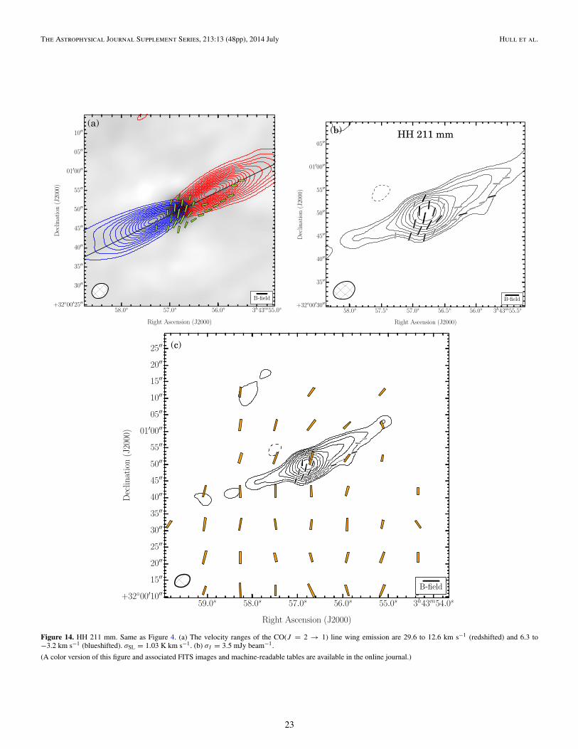
The Astrophysical Journal Supplement Series, 213:13 (48pp), 2014 July Hull et al.

3h43m55.0s56.0s57.0s58.0s

Right Ascension (J2000)

+32◦00 25

30

35

40

45

50

55

01 00

05

10

Dec

linat

ion

(J20

00)

(a)

B field

3h43m55.5s56.0s56.5s57.0s57.5s58.0s

Right Ascension (J2000)

+32◦00 30

35

40

45

50

55

01 00

05

Dec

linat

ion

(J20

00)

HH 211 mm(b)

B field

3h43m54.0s55.0s56.0s57.0s58.0s59.0s

Right Ascension (J2000)

+32◦00 10

15

20

25

30

35

40

45

50

55

01 00

05

10

15

20

25

Dec

linat

ion

(J20

00)

(c)

B field

Figure 14. HH 211 mm. Same as Figure 4. (a) The velocity ranges of the CO(J = 2 → 1) line wing emission are 29.6 to 12.6 km s−1 (redshifted) and 6.3 to−3.2 km s−1 (blueshifted). σSL = 1.03 K km s−1. (b) σI = 3.5 mJy beam−1.

(A color version of this figure and associated FITS images and machine-readable tables are available in the online journal.)

23

The Astrophysical Journal Supplement Series, 213:13 (48pp), 2014 July Hull et al.

4h27m03.5s04.0s04.5s05.0s05.5s

Right Ascension (J2000)

+26◦06 05

10

15

20

25

30D

eclinat

ion

(J20

00)

(a)

B field

4h27m04.2s04.4s04.6s04.8s05.0s

Right Ascension (J2000)

+26◦06 10

15

20

Dec

linat

ion

(J20

00)

DG Tau(b)

B field

Figure 15. DG Tau. Same as Figure 4. (a) The velocity ranges of the CO(J = 2 → 1) line wing emission are 13.3 to 8.0 km s−1 (redshifted) and 4.9 to 0.6 km s−1

(blueshifted). σSL = 0.85 K km s−1. (b) σI = 1.9 mJy beam−1. There is no (c) plot because there were no SCUBA, SHARP, or Hertz data to overlay.

(A color version of this figure and associated FITS images and machine-readable tables are available in the online journal.)

that is more than 7 pc long (Johnstone & Bally 1999). Our map,a mosaic of seven pointings, covers Orion-KL and its associatedhot core, and a piece of the more quiescent “northern ridge”about 25′′ to the NE.

At least two massive stars, Source I (SrcI) and theBecklin–Neugebauer (BN) object are associated with Orion-KL. Proper motion measurements show that these two stars arerecoiling from one another at 35–40 km s−1; they appear tohave been ejected from a multiple system just 500 years ago(Gomez et al. 2008; Goddi et al. 2011). This explosive eventalso is thought to have created a set of bow shocks and fingersthat form a poorly collimated, NW–SE high velocity outflow;a separate, lower velocity outflow emerges from SrcI in theperpendicular direction (Plambeck et al. 2009).

Extensive polarization maps from SCUBA, Hertz, and Stokes(Dotson et al. 2000) show that the large-scale magnetic field inOMC1 is perpendicular to the long axis of the molecular cloud,with evidence for an hourglass-shaped pinch centered on KL(Schleuning 1998). Higher resolution 345 GHz SMA observa-tions show a remarkable circularly symmetric polarization pat-tern centered between SrcI and BN, near the site of the putativeexplosive event; a possible interpretation is that the explosiondragged the magnetic field outward into a radial pattern (Tanget al. 2010). However, within 500 AU of SrcI the magnetic fielddeduced from SiO v = 0 maser26 polarization observations isrelatively straight. (Plambeck et al. 2003). The B-field orien-tation is highly uncertain because maser polarization may beeither parallel or perpendicular to the field, and because of pos-sible Faraday rotation by foreground plasma; Plambeck et al.argued that it is at P.A. 145◦, roughly perpendicular to the lowvelocity outflow from SrcI.

The TADPOL map shows the radial magnetic field patternpreviously detected with the SMA. Our map extends furthernorth, and shows that the magnetic field orientation in the

26 These masers, in the ground vibrational state, should not be confused withthe stronger v = 1 masers closer to the star; both the intensity and thepolarization of the v = 1 masers are time variable.

northern ridge cloud is consistent with the large scale field,except near the SW tip where it forms part of the radial pattern(see Figure 19 for maps).

B.17. OMC3-MMS5 and MMS6

MMS5 and MMS6 are condensations in Orion MolecularCloud 3 (OMC3)—a narrow ridge or filament about 1 pc longand at a distance of 415 pc (Menten et al. 2007). MMS6 isthe brightest millimeter continuum source in OMC3, with anestimated mass of 36 M (Chini et al. 1997b). It containsa compact core, MMS6-main, that probably is heated by anextremely young intermediate mass Class 0 protostar (Takahashiet al. 2012). A bipolar outflow, with a total length of only 4′′(2000 AU), emerges along an N–S axis from MM6-main; thedynamical age of the outflow is less than 100 years (Takahashi& Ho 2012). A more extended outflow emerges along an E–Waxis from MMS5.

The large scale magnetic field orientation in OMC3 inferredfrom SCUBA data is perpendicular to the long axis of the cloud.Matthews et al. (2001) argue that the pattern of depolarizationalong the central axis is best explained by a field toroidallywrapped around a filament, rather than by a straight fieldperpendicular to a sheet. The field orientations that we measurefor both the MMS5 and MMS6 cores are closely alignedwith the large-scale field. Our results for MMS6 agree wellwith previous 3.′′6 resolution observations of this source madewith BIMA (Matthews et al. 2005; see Figure 20 for maps).

B.18. OMC2-FIR3 and 4

OMC2 is an intermediate mass SFR located north of the mas-sive OMC1 complex in the so-called integral-shaped filament ofOrion A. Located at a distance of 415 pc (Menten et al. 2007), itis one of the brightest regions in the Orion Nebula and is know toharbor several protostellar objects and pre-main-sequence stars.Earlier continuum studies at (sub)millimeter wavelengths haveestablished it to be in a later evolutionary stage of star forma-tion than the OMC3 region neighboring it to the north (Chini

24

The Astrophysical Journal Supplement Series, 213:13 (48pp), 2014 July Hull et al.

4h31m43.5s44.0s44.5s45.0s45.5s

Right Ascension (J2000)

+18◦08 15

20

25

30

35

40

45

Dec

linat

ion

(J20

00)

(a)

B field

4h31m44.0s44.2s44.4s44.6s44.8s45.0s

Right Ascension (J2000)

+18◦08 25

30

35

40

Dec

linat

ion

(J20

00)

L1551 NE(b)

B field

4h31m42.0s43.0s44.0s45.0s46.0s47.0s

Right Ascension (J2000)

+18◦07 55

08 00

05

10

15

20

25

30

35

40

45

50

55

09 00

05

10

Dec

linat

ion

(J20

00)

(c)

B field

Figure 16. L1551 NE. Same as Figure 4. (a) The velocity ranges of the CO(J = 2 → 1) line wing emission are 22.5 to 15.0 km s−1 (redshifted) and 3.4 to −1.9 km s−1

(blueshifted). σSL = 0.75 K km s−1. (b) σI = 1.8 mJy beam−1.

(A color version of this figure and associated FITS images and machine-readable tables are available in the online journal.)

25

The Astrophysical Journal Supplement Series, 213:13 (48pp), 2014 July Hull et al.

4h39m53.0s53.5s54.0s54.5s

Right Ascension (J2000)

+26◦03 00

05

10

15

20

Dec

linat

ion

(J20

00)

(a)

B field

4h39m53.4s53.6s53.8s54.0s54.2s54.4s

Right Ascension (J2000)

+26◦03 05

10

15

Dec

linat

ion

(J20

00)

L1527(b)

B field

4h39m51.0s52.0s53.0s54.0s55.0s56.0s

Right Ascension (J2000)

+26◦02 30

35

40

45

50

55

03 00

05

10

15

20

25

30

35

40

45

Dec

linat

ion

(J20

00)

(c)

B field

Figure 17. L1527. Same as Figure 4. (a) The velocity ranges of the CO(J = 2 → 1) line wing emission are 12.9 to 9.7 km s−1 (redshifted) and 2.3 to −0.9 km s−1

(blueshifted). σSL = 0.32 K km s−1. (b) σI = 1.0 mJy beam−1.

(A color version of this figure and associated FITS images and machine-readable tables are available in the online journal.)

26

The Astrophysical Journal Supplement Series, 213:13 (48pp), 2014 July Hull et al.

4h59m49.5s50.0s50.5s51.0s51.5s52.0s

Right Ascension (J2000)

+52◦04 35

40

45

50

55

Dec

linat

ion

(J20

00)

(a)

B field

4h59m49.5s50.0s50.5s51.0s51.5s52.0s

Right Ascension (J2000)

+52◦04 30

35

40

45

50

55

Dec

linat

ion

(J20

00)

CB 26(b)

B field

4h59m48.0s50.0s52.0s54.0s

Right Ascension (J2000)

+52◦04 05

10

15

20

25

30

35

40

45

50

55

05 00

05

10

15

20

Dec

linat

ion

(J20

00)

(c)

B field

Figure 18. CB 26. Same as Figure 4. (a) The velocity ranges of the CO(J = 2 → 1) line wing emission are 11.4 to 8.3 km s−1 (redshifted) and 4.0 to −0.2 km s−1

(blueshifted). σSL = 0.46 K km s−1. (b) σI = 0.7 mJy beam−1.

(A color version of this figure and associated FITS images and machine-readable tables are available in the online journal.)

27

The Astrophysical Journal Supplement Series, 213:13 (48pp), 2014 July Hull et al.

5h35m13.0s14.0s15.0s16.0s

Right Ascension (J2000)

23 00

55

50

45

40

35

30

25

20

15

10

05

−5◦22 00D

eclinat

ion

(J20

00)

Orion-KL

Source IBN

(b)

B field

5h35m12.0s13.0s14.0s15.0s16.0s17.0s

Right Ascension (J2000)

10

05

23 00

55

50

45

40

35

30

25

20

15

10

05

22 00

−5◦21 55

Dec

linat

ion

(J20

00)

(c)

B field

Figure 19. Orion-KL. Same as above. (b) σI = 211.0 mJy beam−1. The full-width half-maximum of the seven mosaic pointings are plotted as gray, dottedcircles. Their diameters (∼44′′) reflect the average primary beam size of the 6and 10 m telescopes. There is no (a) plot because there were no spectral-linedata to plot.

(A color version of this figure and associated FITS images and machine-readabletables are available in the online journal.)

et al. 1997b; Lis et al. 1998). More recent studies have modeledseveral of its embedded sources as infalling protostars, youngstars with disks, and binaries comprising both types of objects(Adams et al. 2012). More specifically, although OMC2-FIR4 iswell-modeled as a Class 0 protostar of approximately 50 L and10−4M yr−1 mass infall rate (Adams et al. 2012), recent highresolution measurements have resolved three spatially distinctsources in its core (Lopez-Sepulcre et al. 2013).

The polarization of the OMC2 region and the FIR3 and 4sources was first investigated at 350 μm by Houde et al. (2004)with Hertz at the CSO (see also Dotson et al. 2010). This regionis characterized by extremely low polarization levels as wellas a strong depolarization with increasing total intensity. Forexample, OMC2-FIR4 was found to have a mean polarization of0.35% ± 0.08% within region of approximately ±0.′3 from its

peak (200 Jy within a beam of 20′′ full-width-half-maximum at350 μm), making it one of the most weakly polarized molecularcloud complexes ever observed at that wavelength. Althoughhigher polarization was measured at 850 μm, the relatively lowpolarization as compared with other sources within the integral-shaped filament was confirmed by Matthews et al. (2009) andPoidevin et al. (2010). OMC2-FIR4 was also observed to be aregion of transition in the orientation of the polarization. Themean polarization angle goes from ∼115◦ south of it to ∼175◦to the north at OMC2-FIR3, where the polarization angle isrelatively well-aligned with the filament. This transition regionis almost coincident with a location of intense outflow activityreported by Williams et al. (2003).

The aforementioned low levels of polarization obtained withsingle-dish measurements are in contrast with the results shownin Table 1 and Figure 21, where mean polarization fractionsof ∼6%–8% are detected with CARMA, making FIR 3 and 4two of the most polarized sources in our sample. This may bereconciled by the fact that the magnetic field, as measured atsmall scales with CARMA, significantly changes its orientationwithin just a few arcseconds toward the center of the map (i.e., atOMC2-FIR4). The change of nearly 90◦ observed could accountfor the exceedingly low polarization observed with Hertz, if thedata were combined within a single Hertz beam (see Figure 21for maps).

B.19. CB 54

CB 54 (LBN1042; Lynds 1965; Clemens & Barvainis 1988)is a Bok globule at a distance of 1.1 kpc (Henning et al.2001, and references therein). (Sub)millimeter and mid-infraredobservations reveal two Class I YSOs coincident with sourceIRAS 07020−1618, with strong dust continuum emission andone or two bipolar outflows (Yun & Clemens 1994; Zhouet al. 1996; Ciardi & Gomez Martın 2007; de Gregorio-Monsalvo et al. 2009; Launhardt et al. 2010). SCUBA 850 μmmeasurements show weak polarization across the continuumsource, with changing orientation and increased strength inthe envelope (Henning et al. 2001; Matthews et al. 2009; seeFigure 22 for maps).

B.20. VLA 1623

VLA 1623 is the prototypical Class 0 source, discovered byAndre et al. (1993). It is located in the southern edge of theOphiuchus A cloud at a distance of 125 pc (Loinard et al. 2008).It has a highly collimated outflow, as is typical of Class 0 sources,and this outflow extends over a large distance at a common P.A.(Andre et al. 1990). The polarization toward VLA 1623 wasmeasured by Holland et al. (1996) using the single bolometerUKT14, and the B-field was found to be perpendicular to theCO outflow. Holland et al. (1996) note that this alignment ofthe field implies that the large-scale field in the cloud cannottherefore collimate the outflow. The single dish polarization datafrom SCUBA (Matthews et al. 2009) and Hertz (Dotson et al.2010) are consistent with this early picture, as are the CARMAdata, which show that the central region has a preferred B-fieldorientation orthogonal to the outflow. This central region may bea flattened pseudo-disk, as discussed for other Class 0 sourcesby Davidson et al. (2011). The orientation of the field is alignedalong the major axis of this pseudo-disk and orthogonal to theoutflow, and even follows the emission extension to the NE.While the field orientation on small scales might alone suggesta toroidal field component, we note that in fact the CARMA

28

The Astrophysical Journal Supplement Series, 213:13 (48pp), 2014 July Hull et al.

5h35m21.8s22.0s22.2s22.4s22.6s22.8s23.0s23.2s

Right Ascension (J2000)

25

20

15

10

−5◦01 05

Dec

linat

ion

(J20

00)

(a)

B field

5h35m22.0s22.2s22.4s22.6s22.8s23.0s23.2s

Right Ascension (J2000)

25

20

15

−5◦01 10

Dec

linat

ion

(J20

00)

OMC3-MMS5(b)

B field

5h35m23.0s23.2s23.4s23.6s23.8s

Right Ascension (J2000)

35

30

−5◦01 25

Dec

linat

ion

(J20

00)

(a)

B field

5h35m22.8s23.0s23.2s23.4s23.6s23.8s24.0s

Right Ascension (J2000)

40

35

30

−5◦01 25

Dec

linat

ion

(J20

00)

OMC3-MMS6(b)

B field

5h35m21.0s22.0s23.0s24.0s25.0s

Right Ascension (J2000)

02 00

55

50

45

40

35

30

25

20

15

10

05

01 00

55

50

−5◦00 45

Dec

linat

ion

(J20

00)

(c)

B field

Figure 20. OMC3-MMS5 and MMS6. Same as Figure 4. (a) The velocity ranges of the CO(J = 2 → 1) line wing emission are 20.7 to 16.5 km s−1 (redshifted) and5.9 to 3.8 km s−1 (blueshifted). σSL = 0.24 K km s−1. (b) σI = 15.0 mJy beam−1.

(A color version of this figure and associated FITS images and machine-readable tables are available in the online journal.)

29

The Astrophysical Journal Supplement Series, 213:13 (48pp), 2014 July Hull et al.

5h35m25.0s26.0s27.0s28.0s29.0s

Right Ascension (J2000)

30

25

20

15

10

05

10 00

55

50

45

40

35

−5◦09 30

Dec

linat

ion

(J20

00)

(a)

B field

5h35m25.0s26.0s27.0s28.0s29.0s

Right Ascension (J2000)

30

25

20

15

10

05

10 00

55

50

45

40

35

−5◦09 30

Dec

linat

ion

(J20

00)

OMC2-FIR3, 4FIR3

FIR4

(b)

B field

5h35m25.0s26.0s27.0s28.0s29.0s30.0s

Right Ascension (J2000)

40

35

30

25

20

15

10

05

10 00

55

50

45

40

35

30

25

20

−5◦09 15

Dec

linat

ion

(J20

00)

(c)

B field

Figure 21. OMC2-FIR3 and 4. Same as Figure 4. (a) The velocity ranges of the CO(J = 2 → 1) line wing emission are 33.1 to 20.4 km s−1 (redshifted) and 1.4 to−11.3 km s−1 (blueshifted). σSL = 1.35 K km s−1. (b) σI = 3.5 mJy beam−1.

(A color version of this figure and associated FITS images and machine-readable tables are available in the online journal.)

30

The Astrophysical Journal Supplement Series, 213:13 (48pp), 2014 July Hull et al.

7h04m20.0s20.2s20.4s20.6s20.8s21.0s21.2s21.4s21.6s

Right Ascension (J2000)

30

25

20

−16◦23 15

Dec

linat

ion

(J20

00)

(a)

B field

7h04m20.2s20.4s20.6s20.8s21.0s21.2s21.4s

Right Ascension (J2000)

30

25

20

−16◦23 15

Dec

linat

ion

(J20

00)

CB 54(b)

B field

7h04m19.0s20.0s21.0s22.0s23.0s

Right Ascension (J2000)

24 00

55

50

45

40

35

30

25

20

15

10

05

23 00

55

50

−16◦22 45

Dec

linat

ion

(J20

00)

(c)

B field

Figure 22. CB 54. Same as Figure 4. (a) The velocity ranges of the CO(J = 2 → 1) line wing emission are 28.0 to 23.8 km s−1 (redshifted) and 14.3 to 9.0 km s−1

(blueshifted). σSL = 1.28 K km s−1. (b) σI = 1.3 mJy beam−1.

(A color version of this figure and associated FITS images and machine-readable tables are available in the online journal.)

31

The Astrophysical Journal Supplement Series, 213:13 (48pp), 2014 July Hull et al.

16h26m25.5s26.0s26.5s27.0s27.5s

Right Ascension (J2000)

45

40

35

30

25

20

−24◦24 15

Dec

linat

ion

(J20

00)

(a)

B field

16h26m25.5s26.0s26.5s27.0s

Right Ascension (J2000)

40

35

30

25

−24◦24 20

Dec

linat

ion

(J20

00)

VLA 1623(b)

B field

16h26m24.0s25.0s26.0s27.0s28.0s29.0s

Right Ascension (J2000)

10

05

25 00

55

50

45

40

35

30

25

20

15

10

05

24 00

−24◦23 55

Dec

linat

ion

(J20

00)

(c)

B field

Figure 23. VLA 1623. Same as Figure 4. (a) The velocity ranges of the CO(J = 2 → 1) line wing emission are 15.2 to 5.7 km s−1 (redshifted) and −1.7 to−9.1 km s−1 (blueshifted). σSL = 0.98 K km s−1. (b) σI = 3.8 mJy beam−1.

(A color version of this figure and associated FITS images and machine-readable tables are available in the online journal.)

32

The Astrophysical Journal Supplement Series, 213:13 (48pp), 2014 July Hull et al.

18h29m05.5s06.0s06.5s07.0s07.5s

Right Ascension (J2000)

+0◦30 25

30

35

40

45

50

55

31 00

Dec

linat

ion

(J20

00)

(a)

B field

18h29m05.5s06.0s06.5s07.0s

Right Ascension (J2000)

+0◦30 30

35

40

45

50

55

Dec

linat

ion

(J20

00)

Ser-emb 17(b)

B field

Figure 24. Ser-emb 17. Same as Figure 4. (a) The velocity ranges of the CO(J = 2 → 1) line wing emission are 15.4 to 12.2 km s−1 (redshifted) and −2.6 to−11.1 km s−1 (blueshifted). σSL = 1.13 K km s−1. (b) σI = 1.7 mJy beam−1. There is no (c) plot because there were no SCUBA, SHARP, or Hertz data to overlay.

(A color version of this figure and associated FITS images and machine-readable tables are available in the online journal.)

18h29m08.0s08.5s09.0s09.5s10.0s

Right Ascension (J2000)

+0◦31 15

20

25

30

35

40

45

Dec

linat

ion

(J20

00)

(a)

B field

18h29m08.5s09.0s09.5s10.0s

Right Ascension (J2000)

+0◦31 20

25

30

35

40

45

Dec

linat

ion

(J20

00)

Ser-emb 1(b)

B field

Figure 25. Ser-emb 1. Same as Figure 4. (a) The velocity ranges of the CO(J = 2 → 1) line wing emission are 27.0 to 13.3 km s−1 (redshifted) and 3.8 to−11.1 km s−1 (blueshifted). σSL = 2.16 K km s−1. (b) σI = 1.4 mJy beam−1. There is no (c) plot because there were no SCUBA, SHARP, or Hertz data to overlay.

(A color version of this figure and associated FITS images and machine-readable tables are available in the online journal.)

33

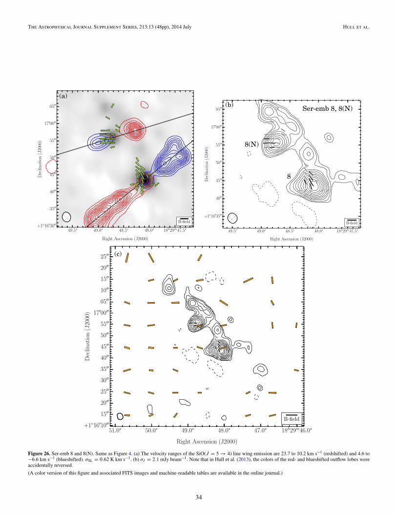
The Astrophysical Journal Supplement Series, 213:13 (48pp), 2014 July Hull et al.

18h29m47.5s48.0s48.5s49.0s49.5s

Right Ascension (J2000)

+1◦16 30

35

40

45

50

55

17 00

05

Dec

linat

ion

(J20

00)

(a)

B field

18h29m47.5s48.0s48.5s49.0s49.5s

Right Ascension (J2000)

+1◦16 35

40

45

50

55

17 00

05

Dec

linat

ion

(J20

00)

Ser-emb 8, 8(N)

8

8(N)

(b)

B field

18h29m46.0s47.0s48.0s49.0s50.0s51.0s

Right Ascension (J2000)

+1◦16 10

15

20

25

30

35

40

45

50

55

17 00

05

10

15

20

25

Dec

linat

ion

(J20

00)

(c)

B field

Figure 26. Ser-emb 8 and 8(N). Same as Figure 4. (a) The velocity ranges of the SiO(J = 5 → 4) line wing emission are 23.7 to 10.2 km s−1 (redshifted) and 4.6 to−6.6 km s−1 (blueshifted). σSL = 0.62 K km s−1. (b) σI = 2.1 mJy beam−1. Note that in Hull et al. (2013), the colors of the red- and blueshifted outflow lobes wereaccidentally reversed.

(A color version of this figure and associated FITS images and machine-readable tables are available in the online journal.)

34

The Astrophysical Journal Supplement Series, 213:13 (48pp), 2014 July Hull et al.

18h29m49.0s49.5s50.0s50.5s51.0s

Right Ascension (J2000)

+1◦15 05

10

15

20

25

30

35

Dec

linat

ion

(J20

00)

(a)

B field

18h29m49.2s49.4s49.6s49.8s50.0s50.2s50.4s50.6s

Right Ascension (J2000)

+1◦15 10

15

20

25

30

Dec

linat

ion

(J20

00)

Ser-emb 6(b)

B field

18h29m48.0s49.0s50.0s51.0s52.0s

Right Ascension (J2000)

+1◦14 45

50

55

15 00

05

10

15

20

25

30

35

40

45

50

55

16 00

Dec

linat

ion

(J20

00)

(c)

B field

Figure 27. Ser-emb 6. Same as Figure 4. (a) The velocity ranges of the CO(J = 2 → 1) line wing emission are 23.9 to 16.4 km s−1 (redshifted) and 1.6 to−11.1 km s−1 (blueshifted). σSL = 2.35 K km s−1. (b) σI = 6.2 mJy beam−1.

(A color version of this figure and associated FITS images and machine-readable tables are available in the online journal.)

35

The Astrophysical Journal Supplement Series, 213:13 (48pp), 2014 July Hull et al.

18h35m41.0s41.5s42.0s42.5s43.0s

Right Ascension (J2000)

35

30

25

20

15

10

−0◦33 05

Dec

linat

ion

(J20

00)

(a)

B field

18h35m41.4s41.6s41.8s42.0s42.2s42.4s42.6s42.8s43.0s

Right Ascension (J2000)

30

25

20

15

−0◦33 10

Dec

linat

ion

(J20

00)

HH 108 IRAS(b)

B field

Figure 28. HH 108 IRAS. Same as Figure 4. (a) The velocity ranges of the CO(J = 2 → 1) line wing emission are 22.3 to 13.8 km s−1 (redshifted) and 9.6 to2.2 km s−1 (blueshifted). σSL = 0.86 K km s−1. (b) σI = 2.6 mJy beam−1. There is no (c) plot because there were no SCUBA, SHARP, or Hertz data to overlay.

(A color version of this figure and associated FITS images and machine-readable tables are available in the online journal.)

18h53m17.0s17.5s18.0s18.5s19.0s

Right Ascension (J2000)

+1◦25 10

15

20

25

30

35

40

45

Dec

linat

ion

(J20

00)

(a)

B field

18h53m17.5s18.0s18.5s19.0s

Right Ascension (J2000)

+1◦25 15

20

25

30

35

40

Dec

linat

ion

(J20

00)

G034.43+00.24 MM1(b)

B field

Figure 29. G034.43+00.24 MM1. Same as Figure 4. (a) The velocity ranges of the CO(J = 2 → 1) line wing emission are 96.5 to 66.8 km s−1 (redshifted) and 49.9to 18.2 km s−1 (blueshifted). σSL = 5.81 K km s−1. (b) σI = 8.8 mJy beam−1. There is no (c) plot because there were no SCUBA, SHARP, or Hertz data to overlay.

(A color version of this figure and associated FITS images and machine-readable tables are available in the online journal.)

36

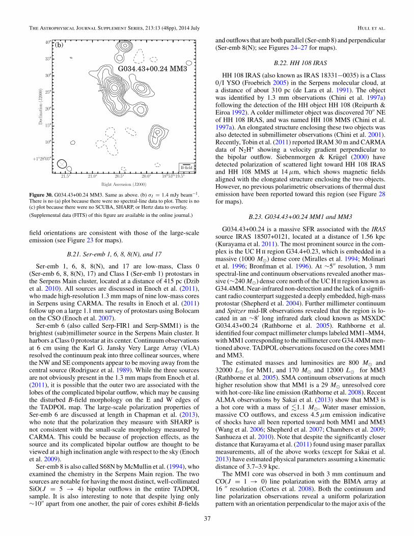
The Astrophysical Journal Supplement Series, 213:13 (48pp), 2014 July Hull et al.

18h53m19.5s20.0s20.5s21.0s21.5s

Right Ascension (J2000)

+1◦28 05

10

15

20

25

30

35

40D

eclinat

ion

(J20

00)

G034.43+00.24 MM3

(b)

B field

Figure 30. G034.43+00.24 MM3. Same as above. (b) σI = 1.4 mJy beam−1.There is no (a) plot because there were no spectral-line data to plot. There is no(c) plot because there were no SCUBA, SHARP, or Hertz data to overlay.

(Supplemental data (FITS) of this figure are available in the online journal.)

field orientations are consistent with those of the large-scaleemission (see Figure 23 for maps).

B.21. Ser-emb 1, 6, 8, 8(N), and 17

Ser-emb 1, 6, 8, 8(N), and 17 are low-mass, Class 0(Ser-emb 6, 8, 8(N), 17) and Class I (Ser-emb 1) protostars inthe Serpens Main cluster, located at a distance of 415 pc (Dzibet al. 2010). All sources are discussed in Enoch et al. (2011),who made high-resolution 1.3 mm maps of nine low-mass coresin Serpens using CARMA. The results in Enoch et al. (2011)follow up on a large 1.1 mm survey of protostars using Bolocamon the CSO (Enoch et al. 2007).

Ser-emb 6 (also called Serp-FIR1 and Serp-SMM1) is thebrightest (sub)millimeter source in the Serpens Main cluster. Itharbors a Class 0 protostar at its center. Continuum observationsat 6 cm using the Karl G. Jansky Very Large Array (VLA)resolved the continuum peak into three collinear sources, wherethe NW and SE components appear to be moving away from thecentral source (Rodriguez et al. 1989). While the three sourcesare not obviously present in the 1.3 mm maps from Enoch et al.(2011), it is possible that the outer two are associated with thelobes of the complicated bipolar outflow, which may be causingthe disturbed B-field morphology on the E and W edges ofthe TADPOL map. The large-scale polarization properties ofSer-emb 6 are discussed at length in Chapman et al. (2013),who note that the polarization they measure with SHARP isnot consistent with the small-scale morphology measured byCARMA. This could be because of projection effects, as thesource and its complicated bipolar outflow are thought to beviewed at a high inclination angle with respect to the sky (Enochet al. 2009).

Ser-emb 8 is also called S68N by McMullin et al. (1994), whoexamined the chemistry in the Serpens Main region. The twosources are notable for having the most distinct, well-collimatedSiO(J = 5 → 4) bipolar outflows in the entire TADPOLsample. It is also interesting to note that despite lying only∼10′′ apart from one another, the pair of cores exhibit B-fields

and outflows that are both parallel (Ser-emb 8) and perpendicular(Ser-emb 8(N); see Figures 24–27 for maps).

B.22. HH 108 IRAS

HH 108 IRAS (also known as IRAS 18331−0035) is a Class0/I YSO (Froebrich 2005) in the Serpens molecular cloud, ata distance of about 310 pc (de Lara et al. 1991). The objectwas identified by 1.3 mm observations (Chini et al. 1997a)following the detection of the HH object HH 108 (Reipurth &Eiroa 1992). A colder millimeter object was discovered 70′′ NEof HH 108 IRAS, and was named HH 108 MMS (Chini et al.1997a). An elongated structure enclosing these two objects wasalso detected in submillimeter observations (Chini et al. 2001).Recently, Tobin et al. (2011) reported IRAM 30 m and CARMAdata of N2H+ showing a velocity gradient perpendicular tothe bipolar outflow. Siebenmorgen & Krugel (2000) havedetected polarization of scattered light toward HH 108 IRASand HH 108 MMS at 14 μm, which shows magnetic fieldsaligned with the elongated structure enclosing the two objects.However, no previous polarimetric observations of thermal dustemission have been reported toward this region (see Figure 28for maps).

B.23. G034.43+00.24 MM1 and MM3

G034.43+00.24 is a massive SFR associated with the IRASsource IRAS 18507+0121, located at a distance of 1.56 kpc(Kurayama et al. 2011). The most prominent source in the com-plex is the UC H ii region G34.4+0.23, which is embedded in amassive (1000 M) dense core (Miralles et al. 1994; Molinariet al. 1996; Bronfman et al. 1996). At ∼5′′ resolution, 3 mmspectral-line and continuum observations revealed another mas-sive (∼240 M) dense core north of the UC H ii region known asG34.4MM. Near-infrared non-detection and the lack of a signifi-cant radio counterpart suggested a deeply embedded, high-massprotostar (Shepherd et al. 2004). Further millimeter continuumand Spitzer mid-IR observations revealed that the region is lo-cated in an ∼8′ long infrared dark cloud known as MSXDCG034.43+00.24 (Rathborne et al. 2005). Rathborne et al.identified four compact millimeter clumps labeled MM1–MM4,with MM1 corresponding to the millimeter core G34.4MM men-tioned above. TADPOL observations focused on the cores MM1and MM3.

The estimated masses and luminosities are 800 M and32000 L for MM1, and 170 M and 12000 L for MM3(Rathborne et al. 2005). SMA continuum observations at muchhigher resolution show that MM1 is a 29 M unresolved corewith hot-core-like line emission (Rathborne et al. 2008). RecentALMA observations by Sakai et al. (2013) show that MM3 isa hot core with a mass of �1.1 M. Water maser emission,massive CO outflows, and excess 4.5 μm emission indicativeof shocks have all been reported toward both MM1 and MM3(Wang et al. 2006; Shepherd et al. 2007; Chambers et al. 2009;Sanhueza et al. 2010). Note that despite the significantly closerdistance that Kurayama et al. (2011) found using maser parallaxmeasurements, all of the above works (except for Sakai et al.2013) have estimated physical parameters assuming a kinematicdistance of 3.7–3.9 kpc.

The MM1 core was observed in both 3 mm continuum andCO(J = 1 → 0) line polarization with the BIMA array at16 ′′ resolution (Cortes et al. 2008). Both the continuum andline polarization observations reveal a uniform polarizationpattern with an orientation perpendicular to the major axis of the

37

The Astrophysical Journal Supplement Series, 213:13 (48pp), 2014 July Hull et al.

19h37m00.0s00.5s01.0s01.5s02.0s

Right Ascension (J2000)

+7◦33 55

34 00

05

10

15

20

25

Dec

linat

ion

(J20

00)

(a)

B field

19h37m00.0s00.5s01.0s01.5s

Right Ascension (J2000)

+7◦33 55

34 00

05

10

15

20

Dec

linat

ion

(J20

00)

B335 IRS(b)

B field

19h36m59.0s37m00.0s01.0s02.0s03.0s

Right Ascension (J2000)

+7◦33 30

35

40

45

50

55

34 00

05

10

15

20

25

30

35

40

45

Dec

linat

ion

(J20

00)

(c)

B field

Figure 31. B335 IRS. Same as Figure 4. (a) The velocity ranges of the CO(J = 2 → 1) line wing emission are 19.7 to 12.3 km s−1 (redshifted) and 6.0 to −0.4 km s−1

(blueshifted). σSL = 1.33 K km s−1. (b) σI = 1.6 mJy beam−1.

(A color version of this figure and associated FITS images and machine-readable tables are available in the online journal.)

38

The Astrophysical Journal Supplement Series, 213:13 (48pp), 2014 July Hull et al.

20h38m59.5s39m00.0s00.5s01.0s01.5s02.0s

Right Ascension (J2000)

+42◦22 35

40

45

50

55

23 00

05

Dec

linat

ion

(J20

00)

(a)

B field

20h39m00.0s00.5s01.0s01.5s02.0s

Right Ascension (J2000)

+42◦22 40

45

50

55

23 00

Dec

linat

ion

(J20

00)

DR21(OH)(b)

B field

20h38m58.0s59.0s39m00.0s01.0s02.0s03.0s04.0s

Right Ascension (J2000)

+42◦22 10

15

20

25

30

35

40

45

50

55

23 00

05

10

15

20

25

Dec

linat

ion

(J20

00)

(c)

B field

Figure 32. DR21(OH). Same as Figure 4. (a) The velocity ranges of the CO(J = 2 → 1) line wing emission are 36.9 to 7.2 km s−1 (redshifted) and −24.5 to−41.4 km s−1 (blueshifted). σSL = 2.64 K km s−1. (b) σI = 8.6 mJy beam−1.

(A color version of this figure and associated FITS images and machine-readable tables are available in the online journal.)

39

The Astrophysical Journal Supplement Series, 213:13 (48pp), 2014 July Hull et al.

20h39m04.0s05.0s06.0s07.0s08.0s

Right Ascension (J2000)

+68◦02 05

10

15

20

25

Dec

linat

ion

(J20

00)

(a)

B field

20h39m05.0s06.0s07.0s08.0s

Right Ascension (J2000)

+68◦02 05

10

15

20

25

Dec

linat

ion

(J20

00)

L1157(b)

B field

20h39m02.0s04.0s06.0s08.0s10.0s

Right Ascension (J2000)

+68◦01 50

55

02 00

05

10

15

20

25

30

35

40

45

Dec

linat

ion

(J20

00)

(c)

B field

Figure 33. L1157. Same as Figure 4. (a) The velocity ranges of the CO(J = 2 → 1) line wing emission are 14.7 to 5.2 km s−1 (redshifted) and −2.2 to −14.9 km s−1

(blueshifted). σSL = 2.52 K km s−1. (b) σI = 1.7 mJy beam−1.

(A color version of this figure and associated FITS images and machine-readable tables are available in the online journal.)

40

The Astrophysical Journal Supplement Series, 213:13 (48pp), 2014 July Hull et al.

21h17m36.0s37.0s38.0s39.0s40.0s41.0s

Right Ascension (J2000)

+68◦17 15

20

25

30

35

40

45

50

Dec

linat

ion

(J20

00)

(a)

B field

21h17m37.0s38.0s39.0s40.0s41.0s

Right Ascension (J2000)

+68◦17 20

25

30

35

40

45

Dec

linat

ion

(J20

00)

CB 230(b)

B field

21h17m33.0s36.0s39.0s42.0s45.0s

Right Ascension (J2000)

+68◦16 55

17 00

05

10

15

20

25

30

35

40

45

50

55

18 00

05

10

Dec

linat

ion

(J20

00)

(c)

B field

Figure 34. CB 230. Same as Figure 4. (a) The velocity ranges of the CO(J = 2 → 1) line wing emission are 13.1 to 5.7 km s−1 (redshifted) and −1.8 to −16.6 km s−1

(blueshifted). σSL = 0.47 K km s−1. (b) σI = 0.7 mJy beam−1.

(A color version of this figure and associated FITS images and machine-readable tables are available in the online journal.)

41

The Astrophysical Journal Supplement Series, 213:13 (48pp), 2014 July Hull et al.

22h06m48.0s49.0s50.0s51.0s52.0s53.0s

Right Ascension (J2000)

+59◦02 30

35

40

45

50

55

03 00

05D

eclinat

ion

(J20

00)

(a)

B field

22h06m49.0s50.0s51.0s52.0s

Right Ascension (J2000)

+59◦02 35

40

45

50

55

03 00

Dec

linat

ion

(J20

00)

L1165(b)

B field

Figure 35. L1165. Same as Figure 4. (a) The velocity ranges of the CO(J = 2 → 1) line wing emission are 4.9 to −0.4 km s−1 (redshifted) and −2.5 to −7.8 km s−1

(blueshifted). σSL = 0.81 K km s−1. (b) σI = 1.2 mJy beam−1. There is no (c) plot because there were no SCUBA, SHARP, or Hertz data to overlay.

(A color version of this figure and associated FITS images and machine-readable tables are available in the online journal.)

filament. TADPOL observations reveal a much more complexpolarization pattern with significantly disturbed B-fields—andeven hints of hourglass morphology—in the densest parts of thecore (see Figures 29 and 30 for maps).

B.24. B335 IRS

B335 IRS (Barnard 335, also called CB 199 (Clemens &Barvainis 1988)) is an extremely isolated Bok globule harboringa low-mass Class 0 protostar. The distance to B335 is uncertain,but a recent estimate by Stutz et al. (2008) finds that itmay be as close as 150 pc. Stutz et al. (2008) also derivea luminosity for B335 of 1.2 L. The protostellar nature ofB335 was first uncovered by Keene et al. (1980, 1983) usingfar-infrared observations that were indicative of an embeddedsource. Frerking & Langer (1982) found evidence for an outflowin CO(J = 1 → 0); B335 also presents a convincing infallsignature with blue-asymmetric line profiles in optically thicktracers (Zhou et al. 1993). Harvey et al. (2003) found evidencefor a circumstellar disk with a radius <60 AU from modelingof interferometric visibilities. Kinematic data from ∼1000 AUscales shown little evidence for rapid inner envelope rotation(Yen et al. 2013; see Figure 31 for maps).

B.25. DR21(OH)

DR21(OH) is a massive star-forming clump located in theheart of the DR21 molecular ridge in Cygnus X. At a distanceof 1.5 kpc (Rygl et al. 2010), Cygnus X is one of the nearestmassive star-forming complexes in our galaxy (Schneider et al.2006; Motte et al. 2007). DR21(OH) has an estimated bolomet-ric luminosity of 1.7 × 104 L and a mass of 1800 M (Jakobet al. 2007). Millimeter observations have revealed two mas-sive millimeter sources, MM1 and MM2 (Mangum et al. 1991;Liechti & Walmsley 1997), each with masses of a few × 100 M.At sub-arcsecond resolution, these two cores are resolved intoa cluster of ∼10 compact massive cores between 5–24 M (Za-pata et al. 2012). DR21(OH) is rich in methanol, water and OHmaser features (Plambeck & Menten 1990; Liechti & Walmsley

1997; Kurtz et al. 2004; Araya et al. 2009). Infrared observationshave identified several deeply embedded YSOs in the region(Kumar et al. 2007; Davis et al. 2007). High-velocity bipolaroutflows from both MM1 and MM2 have been detected in COand other tracers (Lai et al. 2003; Zapata et al. 2012). Therefore,MM1/2 are excellent candidates for very young massive proto-stars. Our TADPOL observations encompass these two massivesources.

DR21(OH) has been part of several single-dish and inter-ferometric polarization studies. At low resolution, a uniformlarge scale magnetic field perpendicular to the DR21 filament isobserved (Vallee & Fiege 2006; Kirby 2009). At higher resolu-tion, a more complex polarization pattern, consistent with ourTADPOL observations, has been revealed toward DR21(OH)(Lai et al. 2003; Girart et al. 2013). The plane-of-sky compo-nent of the magnetic field is estimated to be 0.62 and 2.1 mGat scales of 0.34 and 0.08 pc respectively (Girart et al. 2013).These measurements are consistent with previous single-dishCN Zeeman measurements, which estimate the LOS magneticfield strength to be 0.36 and 0.71 mG for MM1 and MM2, re-spectively (Crutcher 1999; Falgarone et al. 2008; see Figure 32for maps).

B.26. L1157

L1157-mm (IRAS 20386+6751) is a Class 0 source locatedin the Cepheus flare region. The distance to L1157 is uncertain,with estimates between 250 pc and 440 pc (Viotti 1969;Straizys et al. 1992; Kun 1998; Kun et al. 2008); we adopta distance of 250 pc (Looney et al. 2007). L1157 has a large(∼20,000 AU) flattened envelope structure detected in 8 μmabsorption (Looney et al. 2007) and molecular tracers N2H+ andNH3 (Chiang et al. 2010; Tobin et al. 2011) that reveal complexkinematics from rotation, infall, and outflow. This large scalestructure is perpendicular to the well known outflow from thecentral source (Gueth et al. 1996), affording an edge-on viewof the system. The dust emission from the system has beenobserved at multiple wavelengths and resolutions at CARMA

42

The Astrophysical Journal Supplement Series, 213:13 (48pp), 2014 July Hull et al.

23h13m43.0s44.0s45.0s46.0s47.0s48.0s

Right Ascension (J2000)

+61◦27 55

28 00

05

10

15

20

25

30

Dec

linat

ion

(J20

00)

(a)

B field

23h13m43.0s44.0s45.0s46.0s47.0s

Right Ascension (J2000)

+61◦27 55

28 00

05

10

15

20

25

Dec

linat

ion

(J20

00)

NGC 7538 IRS 1(b)

B field

23h13m40.0s42.0s44.0s46.0s48.0s50.0s

Right Ascension (J2000)

+61◦27 35

40

45

50

55

28 00

05

10

15

20

25

30

35

40

45

50

Dec

linat

ion

(J20

00)

(c)

B field

Figure 36. NGC 7538-IRS 1. Same as Figure 4. (a) The velocity ranges of the CO(J = 2 → 1) line wing emission are −36.3 to −39.5 km s−1 (redshifted) and −69.1to −75.5 km s−1 (blueshifted). σSL = 3.2 K km s−1. (b) σI = 19.3 mJy beam−1.

(A color version of this figure and associated FITS images and machine-readable tables are available in the online journal.)

43

The Astrophysical Journal Supplement Series, 213:13 (48pp), 2014 July Hull et al.

23h25m44.0s45.0s46.0s47.0s48.0s49.0s50.0s

Right Ascension (J2000)

+74◦17 25

30

35

40

45

50

Dec

linat

ion

(J20

00)

(a)

B field

23h25m44.0s45.0s46.0s47.0s48.0s49.0s

Right Ascension (J2000)

+74◦17 30

35

40

45

Dec

linat

ion

(J20

00)

CB 244

(b)

B field

23h25m40.0s44.0s48.0s52.0s56.0s

Right Ascension (J2000)

+74◦17 00

05

10

15

20

25

30

35

40

45

50

55

18 00

05

10

15

Dec

linat

ion

(J20

00)

(c)

B field

Figure 37. CB 244. Same as Figure 4. (a) The velocity ranges of the CO(J = 2 → 1) line wing emission are 11.7 to 6.4 km s−1 (redshifted) and 2.2 to −3.1 km s−1

(blueshifted). σSL = 0.98 K km s−1. (b) σI = 0.6 mJy beam−1.

(A color version of this figure and associated FITS images and machine-readable tables are available in the online journal.)

44

The Astrophysical Journal Supplement Series, 213:13 (48pp), 2014 July Hull et al.

(Chiang et al. 2012) and was best modeled as an envelope witha unresolved disk (<40 AU). Recent high resolution (∼0.′′06)VLA 7.3 mm dust continuum observations have placed a limit onthe size of the disk component of <20 AU (Tobin et al. 2013b).The magnetic field was shown to have a well-defined hourglassshape and was estimated to have a plane-of-sky magnitude of1–4 mG (Stephens et al. 2013; see Figure 33 for maps).

B.27. CB 230

CB 230 (Clemens & Barvainis 1988) is an isolated globulelocated in the Cepheus flare region, at a distance of 325 pc(Straizys et al. 1992), although other more recent estimates rangefrom 270–515 pc (Kun et al. 2009). The protostellar system isclassified as Class 0/I (Launhardt et al. 2013). A large envelopeis detected in both N2H+ and ammonia and exhibits a velocitygradient suggestive of rotation (Chen et al. 2007; Tobin et al.2011). The protostellar source is also identified as a triple system(Yun 1996; Launhardt et al. 2013; Tobin et al. 2013a). The widecompanion (CB 230 IRS2) is located 10′′ from CB 230 IRS1 andis not observed at wavelengths longer than 24 μm (Launhardtet al. 2001; Massi et al. 2008; Launhardt et al. 2013); however,IRS 2 does seem to drive a CO outflow (Launhardt 2001). Theclose companion to IRS 1 (IRS 1B) was recently discovered byTobin et al. (2013a) and is separated from IRS 1 by 0.′′3 (100 AU)(see Figure 34 for maps).

B.28. L1165

The L1165 dark cloud has an L-shaped filament structure,and is located in the Cepheus region (e.g., Reipurth et al. 1997;Tobin et al. 2010). Two IRAS objects are in the kink of thefilamentary structure; however, only the southern object IRAS22051+5848 was detected at 850 μm and classified as a Class IYSO (Visser et al. 2002); this is the source we observe. Thedistance to the object is somewhat ambiguous in the literature:750 pc (e.g., Reipurth et al. 1997) and 300 pc (e.g., Dobashiet al. 1994). We adopt the latter 300 pc, which gives a reasonableluminosity for a low mass YSO and has been used in previous(sub)millimeter studies. The bipolar outflow has been mappedin CO(J = 2 → 1) by the JCMT (Visser et al. 2002; Parkeret al. 1991), and the near infrared nebula feature was imaged inK-band by the University of Hawaii 2.2 m telescope (Connelleyet al. 2007). It has been imaged in 350 μm continuum emissionby the SHARC-II camera at the CSO (Wu et al. 2007). Inaddition, Spitzer IRAC data have revealed that the bipolaroutflow cavity and the elongated envelope structure (imagedin 8 μm emission) are perpendicular to each other (Tobin et al.2010). Recently Tobin et al. (2011) detected a velocity gradientalong the elongated envelope structure using IRAM 30 mobservations in N2H+ and CARMA observations in N2H+ andHCO+; these observations showed that the HCO+ feature can beinterpreted as rotation around a 0.5 M central protostar. Therehave been no previous polarimetric observations toward thisobject (see Figure 35 for maps).

B.29. NGC 7538-IRS 1

The hyper-compact H ii region NGC 7538-IRS 1 was firstdiscovered in a 2 μm and 20 μm survey of NGC 7538 (Wynn-Williams et al. 1974), which lies at a distance of 2.65 kpc(Moscadelli et al. 2009). IRS1 is an extremely young high-mass star (type ∼O7), which powers an N–S ionized thermal jet(Gaume et al. 1995; Sandell et al. 2009), drives a molecularoutflow (Scoville et al. 1986; Zhu et al. 2013), and excites

a variety of molecular masers, including OH, H2O, H2CO,CH3OH, NH3, and 15NH3 (Johnston et al. 1989). It is stillheavily accreting with an accretion rate of ∼10−3 M yr−1,quenching the formation of an H ii region. All the observationalevidence suggests that IRS 1 should be surrounded by an E–Waccretion disk, which has yet to be confirmed. Imaging withthe SCUBA polarimeter at 850 μm indicates that the magneticfield is disturbed around IRS 1 (Momose et al. 2001). At theposition of IRS 1 the degree of polarization is 2%–3%, witha polarization (not B-field) P.A. of 90◦; however, immediatelyeast the P.A. is ∼ 50◦, similar to what Flett & Murray (1991)obtained at 800 μm. It is not surprising that the magnetic fieldaround IRS 1 is disturbed, because the molecular cloud core isforming a young cluster (Qiu et al. 2011). At least eight of thecluster members are seen as millimeter continuum sources andH2O masers, suggesting that they are surrounded by accretiondisks and are probably powering outflows (see Figure 36 formaps).

B.30. CB 244

CB 244 (L1262) is an isolated globule in the Cepheus regionwith an estimated distance of 200 pc, which is the distance of thenearby cloud L1235 (Snell 1981; Benson & Myers 1989; Stutzet al. 2010). CB 244 harbors both a Class 0 protostar drivingan outflow (Yun & Clemens 1994; Visser et al. 2002) and aneighboring starless core (Stutz et al. 2010). Chen et al. (2007)observed a filamentary distribution of N2H+ in the envelopesurrounding the protostar; the velocity structure of the line wassuggestive of rapid envelope rotation (see Figure 37 for maps).

REFERENCES

Adams, J. D., Herter, T. L., Osorio, M., et al. 2012, ApJL, 749, L24Agudo, I., Thum, C., Wiesemeyer, H., et al. 2012, A&A, 541, A111Allen, A., Li, Z.-Y., & Shu, F. H. 2003, ApJ, 599, 363Andersson, B.-G. 2012, in press (arXiv:1208.4393)Andre, P., Martin-Pintado, J., Despois, D., & Montmerle, T. 1990, A&A,

236, 180Andre, P., Ward-Thompson, D., & Barsony, M. 1993, ApJ, 406, 122Andre, P., Ward-Thompson, D., & Barsony, M. 2000, in Protostars and Planets

IV, ed. V. Mannings, A. P. Boss, & S. S. Russell (Tucson, AZ: Univ. ArizonaPress), 59

Anglada, G., Rodriguez, L. F., Torrelles, J. M., et al. 1989, ApJ, 341, 208Araya, E. D., Kurtz, S., Hofner, P., & Linz, H. 2009, ApJ, 698, 1321Attard, M., Houde, M., Novak, G., et al. 2009, ApJ, 702, 1584Bachiller, R., & Cernicharo, J. 1986, A&A, 168, 262Bachiller, R., Gueth, F., Guilloteau, S., Tafalla, M., & Dutrey, A. 2000, A&A,

362, L33Bachiller, R., Guilloteau, S., Dutrey, A., Planesas, P., & Martin-Pintado, J. 1995,

A&A, 299, 857Bachiller, R., & Perez Gutierrez, M. 1997, ApJL, 487, L93Benson, P. J., & Myers, P. C. 1989, ApJS, 71, 89Bethell, T. J., Chepurnov, A., Lazarian, A., & Kim, J. 2007, ApJ, 663, 1055Blake, G. A., Sandell, G., van Dishoeck, E. F., et al. 1995, ApJ, 441, 689Bock, D., Bolatto, A. D., Hawkins, D. W., et al. 2006, Proc. SPIE, 6267, 13Bronfman, L., Nyman, L.-A., & May, J. 1996, A&AS, 115, 81Campbell, M. F., Butner, H. M., Harvey, P. M., et al. 1995, ApJ, 454, 831Chambers, E. T., Jackson, J. M., Rathborne, J. M., & Simon, R. 2009, ApJS,

181, 360Chandler, C. J., & Richer, J. S. 2001, ApJ, 555, 139Chapman, N. L., Davidson, J. A., Goldsmith, P. F., et al. 2013, ApJ, 770, 151Chen, H.-R., Welch, W. J., Wilner, D. J., & Sutton, E. C. 2006, ApJ, 639, 975Chen, X., Launhardt, R., & Henning, T. 2007, ApJ, 669, 1058Chiang, H.-F., Looney, L. W., & Tobin, J. J. 2012, ApJ, 756, 168Chiang, H.-F., Looney, L. W., Tobin, J. J., & Hartmann, L. 2010, ApJ, 709, 470Chini, R., Reipurth, B., Sievers, A., et al. 1997a, A&A, 325, 542Chini, R., Reipurth, B., Ward-Thompson, D., et al. 1997b, ApJL, 474, L135Chini, R., Ward-Thompson, D., Kirk, J. M., et al. 2001, A&A, 369, 155Choi, M., Panis, J.-F., & Evans, N. J., II. 1999, ApJS, 122, 519Ciardi, D. R., & Gomez Martın, C. 2007, ApJ, 664, 377

45

The Astrophysical Journal Supplement Series, 213:13 (48pp), 2014 July Hull et al.

Claussen, M. J., Wilking, B. A., Benson, P. J., et al. 1996, ApJS, 106, 111Clemens, D. P., & Barvainis, R. 1988, ApJS, 68, 257Connelley, M. S., Reipurth, B., & Tokunaga, A. T. 2007, AJ, 133, 1528Cortes, P. C., Crutcher, R. M., Shepherd, D. S., & Bronfman, L. 2008, ApJ,

676, 464Crutcher, R. M. 1999, ApJ, 520, 706Crutcher, R. M. 2012, ARA&A, 50, 29Curran, R. L., Chrysostomou, A., & Matthews, B. C. 2007, in IAU Symp.

243, Star-Disk Interaction Young Stars, ed. J. Bouvier & I. Appenzeller(Cambridge: Cambridge Univ. Press), 63

Curtis, E. I., Richer, J. S., Swift, J. J., & Williams, J. P. 2010, MNRAS,408, 1516

Davidson, J. A., & Jaffe, D. T. 1984, ApJL, 277, L13Davidson, J. A., Novak, G., Matthews, T. G., et al. 2011, ApJ, 732, 97Davis, C. J., Kumar, M. S. N., Sandell, G., et al. 2007, MNRAS, 374, 29Davis, C. J., Ray, T. P., Eisloeffel, J., & Corcoran, D. 1997, A&A, 324, 263de Gregorio-Monsalvo, I., Gomez, J. F., Anglada, G., et al. 2009, AJ, 137, 5080de Lara, E., Chavarria-K., C., & Lopez-Molina, G. 1991, A&A, 243, 139de Zeeuw, P. T., Hoogerwerf, R., de Bruijne, J. H. J., Brown, A. G. A., & Blaauw,

A. 1999, AJ, 117, 354Di Francesco, J., Myers, P. C., Wilner, D. J., Ohashi, N., & Mardones, D.

2001, ApJ, 562, 770Dionatos, O., Nisini, B., Cabrit, S., Kristensen, L., & Pineau Des Forets, G.

2010, A&A, 521, A7Dobashi, K., Bernard, J.-P., Yonekura, Y., & Fukui, Y. 1994, ApJS, 95, 419Dotson, J. L. 1996, ApJ, 470, 566Dotson, J. L., Davidson, J., Dowell, C. D., Schleuning, D. A., & Hildebrand,

R. H. 2000, ApJS, 128, 335Dotson, J. L., Vaillancourt, J. E., Kirby, L., et al. 2010, ApJS, 186, 406Dreher, J. W., & Welch, W. J. 1981, ApJ, 245, 857Dzib, S., Loinard, L., Mioduszewski, A. J., et al. 2010, ApJ, 718, 610Eisloffel, J. 2000, A&A, 354, 236Elmegreen, B. G., & Scalo, J. 2004, ARA&A, 42, 211Emerson, J. P., Harris, S., Jennings, R. E., et al. 1984, ApJL, 278, L49Engargiola, G., & Plambeck, R. L. 1999, in Proc. of the 3rd cologne-Zermatt

Symp., The Physics and Chemistry of the Interstellar Medium, ed. V.Ossenkopf, J. Stutzki, & G. Winnewisser (GCA-Verlag Herdecke), 291

Enoch, M. L., Corder, S., Duchene, G., et al. 2011, ApJS, 195, 21Enoch, M. L., Corder, S., Dunham, M. M., & Duchene, G. 2009, ApJ, 707, 103Enoch, M. L., Glenn, J., Evans, N. J., II, et al. 2007, ApJ, 666, 982Falgarone, E., Troland, T. H., Crutcher, R. M., & Paubert, G. 2008, A&A,

487, 247Fiedler, R. A., & Mouschovias, T. C. 1993, ApJ, 415, 680Flett, A. M., & Murray, A. G. 1991, MNRAS, 249, 4Frerking, M. A., & Langer, W. D. 1982, ApJ, 256, 523Froebrich, D. 2005, ApJS, 156, 169Furuya, R. S., Kitamura, Y., Wootten, A., Claussen, M. J., & Kawabe, R.

2003, ApJS, 144, 71Gaume, R. A., Goss, W. M., Dickel, H. R., Wilson, T. L., & Johnston, K. J.

1995, ApJ, 438, 776Girart, J. M., Frau, P., Zhang, Q., et al. 2013, ApJ, 772, 69Girart, J. M., Rao, R., & Marrone, D. P. 2006, Sci, 313, 812Goddi, C., Humphreys, E. M. L., Greenhill, L. J., Chandler, C. J., & Matthews,

L. D. 2011, ApJ, 728, 15Goldsmith, P. F., Snell, R. L., Hemeon-Heyer, M., & Langer, W. D. 1984, ApJ,

286, 599Gomez, L., Rodrıguez, L. F., Loinard, L., et al. 2008, ApJ, 685, 333Gudel, M., Telleschi, A., Audard, M., et al. 2007, A&A, 468, 515Gueth, F., & Guilloteau, S. 1999, A&A, 343, 571Gueth, F., Guilloteau, S., & Bachiller, R. 1996, A&A, 307, 891Hachisuka, K., Brunthaler, A., Menten, K. M., et al. 2006, ApJ, 645, 337Harvey, D. W. A., Wilner, D. J., Myers, P. C., & Tafalla, M. 2003, ApJ, 596, 383Haschick, A. D., Moran, J. M., Rodriguez, L. F., et al. 1980, ApJ, 237, 26Hatchell, J., Fuller, G. A., Richer, J. S., Harries, T. J., & Ladd, E. F. 2007, A&A,

468, 1009Heiles, C. 2000, AJ, 119, 923Hennebelle, P., & Ciardi, A. 2009, A&A, 506, L29Henning, T., Wolf, S., Launhardt, R., & Waters, R. 2001, ApJ, 561, 871Herczeg, G. J., Karska, A., Bruderer, S., et al. 2012, A&A, 540, A84Hildebrand, R. H. 1988, QJRAS, 29, 327Hirano, N., Ho, P. P. T., Liu, S.-Y., et al. 2010, ApJ, 717, 58Hirota, T., Bushimata, T., Choi, Y. K., et al. 2008, PASJ, 60, 37Hirota, T., Honma, M., Imai, H., et al. 2011, PASJ, 63, 1Hirsch, L., Adams, J. D., Herter, T. L., et al. 2012, ApJ, 757, 113Hoang, T., & Lazarian, A. 2009, ApJ, 697, 1316Hogbom, J. A. 1974, A&AS, 15, 417

Hogerheijde, M. R., van Dishoeck, E. F., Blake, G. A., & van Langevelde, H. J.1998, ApJ, 502, 315

Holland, W. S., Greaves, J. S., Ward-Thompson, D., & Andre, P. 1996, A&A,309, 267

Houde, M., Dowell, C. D., Hildebrand, R. H., et al. 2004, ApJ, 604, 717Howell, R. R., McCarthy, D. W., & Low, F. J. 1981, ApJL, 251, L21Hughes, A. M., Hull, C. L. H., Wilner, D. J., & Plambeck, R. L. 2013, AJ,

145, 115Hull, C., Plambeck, R., & Engargiola, G. 2011, in General Assembly and

Scientific Symp., 2011 XXXth URSI (Istanbul, Turkey: IEEE), 1Hull, C. L. H., Plambeck, R. L., Bolatto, A. D., et al. 2013, ApJ, 768, 159Imai, H., Horiuchi, S., Deguchi, S., & Kameya, O. 2003, ApJ, 595, 285Jakob, H., Kramer, C., Simon, R., et al. 2007, A&A, 461, 999Johnston, K. J., Stolovy, S. R., Wilson, T. L., Henkel, C., & Mauersberger, R.

1989, ApJL, 343, L41Johnstone, D., & Bally, J. 1999, ApJL, 510, L49Joos, M., Hennebelle, P., & Ciardi, A. 2012, A&A, 543, A128Jørgensen, J. K., Bourke, T. L., Myers, P. C., et al. 2007, ApJ, 659, 479Jørgensen, J. K., Harvey, P. M., Evans, N. J., II, et al. 2006, ApJ, 645, 1246Jørgensen, J. K., Hogerheijde, M. R., van Dishoeck, E. F., Blake, G. A., &

Schoier, F. L. 2004, A&A, 413, 993Keene, J., Davidson, J. A., Harper, D. A., et al. 1983, ApJL, 274, L43Keene, J., Hildebrand, R. H., Whitcomb, S. E., & Harper, D. A. 1980, ApJL,

240, L43Kenyon, S. J., Dobrzycka, D., & Hartmann, L. 1994, AJ, 108, 1872Kerr, A. R., Pan, S.-K., Claude, S. M. X., et al. 2013, submitted

(arXiv:1306.6085)Kirby, L. 2009, ApJ, 694, 1056Knee, L. B. G., & Sandell, G. 2000, A&A, 361, 671Krasnopolsky, R., Li, Z.-Y., Shang, H., & Zhao, B. 2012, ApJ, 757, 77Krejny, M., Matthews, T. G., Novak, G., et al. 2009, ApJ, 705, 717Krumholz, M. R., Crutcher, R. M., & Hull, C. L. H. 2013, ApJL, 767, L11Kumar, M. S. N., Davis, C. J., Grave, J. M. C., Ferreira, B., & Froebrich, D.

2007, MNRAS, 374, 54Kun, M. 1998, ApJS, 115, 59Kun, M., Balog, Z., Kenyon, S. J., Mamajek, E. E., & Gutermuth, R. A.

2009, ApJS, 185, 451Kun, M., Kiss, Z. T., & Balog, Z. 2008, in Handbook of Star Forming Regions,

Vol. 1, ed. B. Reipurth (San Francisco, CA: ASP), 136Kurayama, T., Nakagawa, A., Sawada-Satoh, S., et al. 2011, PASJ, 63, 513Kurtz, S., Hofner, P., & Alvarez, C. V. 2004, ApJS, 155, 149Kwon, W., Looney, L. W., Crutcher, R. M., & Kirk, J. M. 2006, ApJ, 653, 1358Kwon, W., Looney, L. W., Mundy, L. G., Chiang, H.-F., & Kemball, A. J.

2009, ApJ, 696, 841Ladd, E. F., Deane, J. R., Sanders, D. B., & Wynn-Williams, C. G. 1993, ApJ,

419, 186Lai, S.-P., Girart, J. M., & Crutcher, R. M. 2003, ApJ, 598, 392Launhardt, R. 2001, in IAU Symp. 200, The Formation of Binary Stars, ed. H.

Zinnecker & R. Mathieu (Cambridge: Cambridge Univ. Press), 117Launhardt, R., Nutter, D., Ward-Thompson, D., et al. 2010, ApJS, 188, 139Launhardt, R., Pavlyuchenkov, Y., Gueth, F., et al. 2009, A&A, 494, 147Launhardt, R., Sargent, A., & Zinnecker, H. 2001, in ASP Conf. Ser. 235,

Science with the Atacama Large Millimeter Array, ed. A. Wootten (SanFrancisco, CA: ASP), 134

Launhardt, R., & Sargent, A. I. 2001, ApJL, 562, L173Launhardt, R., Stutz, A. M., Schmiedeke, A., et al. 2013, A&A, 551, A98Lay, O. P., Carlstrom, J. E., & Hills, R. E. 1995, ApJL, 452, L73Lazarian, A. 2003, JQSRT, 79, 881Lazarian, A. 2005, in AIP Conf. Ser. 784, Magnetic Fields in the Universe:

From Laboratory and Stars to Primordial Structures., ed. E. M. de Gouveiadal Pino, G. Lugones, & A. Lazarian (Melvoille, NY: AIP), 42

Lazarian, A. 2007, JQSRT, 106, 225Leao, M. R. M., de Gouveia Dal Pino, E. M., Santos-Lima, R., & Lazarian, A.

2013, ApJ, 777, 46Lee, C.-F., Hirano, N., Palau, A., et al. 2009, ApJ, 699, 1584Lefloch, B., Castets, A., Cernicharo, J., Langer, W. D., & Zylka, R. 1998, A&A,

334, 269Li, H.-b., Dowell, C. D., Goodman, A., Hildebrand, R., & Novak, G. 2009, ApJ,

704, 891Li, Z.-Y., Krasnopolsky, R., & Shang, H. 2011, ApJ, 738, 180Li, Z.-Y., Krasnopolsky, R., & Shang, H. 2013, ApJ, 774, 82Liechti, S., & Walmsley, C. M. 1997, A&A, 321, 625Lis, D. C., Serabyn, E., Keene, J., et al. 1998, ApJ, 509, 299Liu, H. B., Qiu, K., Zhang, Q., Girart, J. M., & Ho, P. T. P. 2013, ApJ, 771, 71Loinard, L., Torres, R. M., Mioduszewski, A. J., & Rodrıguez, L. F. 2008, ApJL,

675, L29Looney, L. W., Mundy, L. G., & Welch, W. J. 2000, ApJ, 529, 477

46

The Astrophysical Journal Supplement Series, 213:13 (48pp), 2014 July Hull et al.

Looney, L. W., Mundy, L. G., & Welch, W. J. 2003, ApJ, 592, 255Looney, L. W., Tobin, J. J., & Kwon, W. 2007, ApJL, 670, L131Lopez-Sepulcre, A., Taquet, V., Sanchez-Monge, A., et al. 2013, A&A,

556, A62Lynch, C., Mutel, R. L., Gudel, M., et al. 2013, ApJ, 766, 53Lynds, B. T. 1965, ApJS, 12, 163Mac Low, M.-M., & Klessen, R. S. 2004, RvMP, 76, 125Machida, M. N., Matsumoto, T., Hanawa, T., & Tomisaka, K. 2006, ApJ,

645, 1227Mangum, J. G., Wootten, A., & Mundy, L. G. 1991, ApJ, 378, 576Marvel, K. B., Wilking, B. A., Claussen, M. J., & Wootten, A. 2008, ApJ,

685, 285Massi, F., Codella, C., Brand, J., di Fabrizio, L., & Wouterloot, J. G. A.

2008, A&A, 490, 1079Matthews, B. C., Fiege, J. D., & Moriarty-Schieven, G. 2002, ApJ, 569, 304Matthews, B. C., Lai, S.-P., Crutcher, R. M., & Wilson, C. D. 2005, ApJ,

626, 959Matthews, B. C., McPhee, C. A., Fissel, L. M., & Curran, R. L. 2009, ApJS,

182, 143Matthews, B. C., Wilson, C. D., & Fiege, J. D. 2001, ApJ, 562, 400McCaughrean, M. J., Rayner, J. T., & Zinnecker, H. 1994, ApJL, 436, L189McKee, C. F., Zweibel, E. G., Goodman, A. A., & Heiles, C. 1993, in Protostars

and Planets III, ed. E. H. Levy & J. I. Lunine (Tucson, AZ: Univ. of ArizonaPress), 327

McMullin, J. P., Mundy, L. G., Wilking, B. A., Hezel, T., & Blake, G. A.1994, ApJ, 424, 222

Megeath, S. T., Herter, T., Beichman, C., et al. 1996, A&A, 307, 775Megeath, S. T., Wilson, T. L., & Corbin, M. R. 2005, ApJL, 622, L141Menten, K. M., Reid, M. J., Forbrich, J., & Brunthaler, A. 2007, A&A, 474, 515Mestel, L., & Spitzer, L., Jr. 1956, MNRAS, 116, 503Miralles, M. P., Rodriguez, L. F., & Scalise, E. 1994, ApJS, 92, 173Molinari, S., Brand, J., Cesaroni, R., & Palla, F. 1996, A&A, 308, 573Momose, M., Tamura, M., Kameya, O., et al. 2001, ApJ, 555, 855Moore, T. J. T., Bretherton, D. E., Fujiyoshi, T., et al. 2007, MNRAS, 379, 663Moriarty-Schieven, G. H., Butner, H. M., & Wannier, P. G. 1995, ApJL,

445, L55Moscadelli, L., Reid, M. J., Menten, K. M., et al. 2009, ApJ, 693, 406Motte, F., Bontemps, S., Schilke, P., et al. 2007, A&A, 476, 1243Mundt, R., & Fried, J. W. 1983, ApJL, 274, L83Myers, A. T., McKee, C. F., Cunningham, A. J., Klein, R. I., & Krumholz, M.

R. 2013, ApJ, 766, 97Naghizadeh-Khouei, J., & Clarke, D. 1993, A&A, 274, 968Navarrini, A., & Plambeck, R. 2006, ITMTT, 54, 272Nisini, B., Benedettini, M., Giannini, T., et al. 2000, A&A, 360, 297Nisini, B., Codella, C., Giannini, T., et al. 2007, A&A, 462, 163O’Linger, J., Wolf-Chase, G., Barsony, M., & Ward-Thompson, D. 1999, ApJ,

515, 696O’Linger, J. C., Cole, D. M., Ressler, M. E., & Wolf-Chase, G. 2006, AJ,

131, 2601Padoan, P., Goodman, A., Draine, B. T., et al. 2001, ApJ, 559, 1005Pandian, J., Baker, L., Cortes, G., et al. 2006, IMMag, 7, 74Parker, N. D., Padman, R., & Scott, P. F. 1991, MNRAS, 252, 442Pelkonen, V.-M., Juvela, M., & Padoan, P. 2009, A&A, 502, 833Perley, R. A., & Butler, B. J. 2013, ApJS, 206, 16Plambeck, R., & Engargiola, G. 2010, CARMA Memos, 54Plambeck, R. L., & Menten, K. M. 1990, ApJ, 364, 555Plambeck, R. L., Wright, M. C. H., Friedel, D. N., et al. 2009, ApJL, 704, L25Plambeck, R. L., Wright, M. C. H., & Rao, R. 2003, ApJ, 594, 911Poidevin, F., Bastien, P., & Matthews, B. C. 2010, ApJ, 716, 893Qiu, K., Zhang, Q., & Menten, K. M. 2011, ApJ, 728, 6Rao, R., Crutcher, R. M., Plambeck, R. L., & Wright, M. C. H. 1998, ApJL,

502, L75Rathborne, J. M., Jackson, J. M., Chambers, E. T., et al. 2005, ApJL, 630, L181Rathborne, J. M., Jackson, J. M., Zhang, Q., & Simon, R. 2008, ApJ, 689, 1141Reid, M. J., Argon, A. L., Masson, C. R., Menten, K. M., & Moran, J. M.

1995, ApJ, 443, 238Reipurth, B., Bally, J., & Devine, D. 1997, AJ, 114, 2708Reipurth, B., & Eiroa, C. 1992, A&A, 256, L1Reipurth, B., Rodrıguez, L. F., Anglada, G., & Bally, J. 2002, AJ, 124, 1045Rodon, J. A., Beuther, H., Megeath, S. T., & van der Tak, F. F. S. 2008, A&A,

490, 213Rodriguez, L. F., Anglada, G., & Curiel, S. 1997, ApJL, 480, L125Rodrıguez, L. F., Anglada, G., & Curiel, S. 1999, ApJS, 125, 427Rodriguez, L. F., Anglada, G., & Raga, A. 1995, ApJL, 454, L149Rodriguez, L. F., Curiel, S., Moran, J. M., et al. 1989, ApJL, 346, L85Rodrıguez, L. F., Dzib, S. A., Loinard, L., et al. 2012a, RMxAA, 48, 243Rodrıguez, L. F., Gonzalez, R. F., Raga, A. C., et al. 2012b, A&A, 537, A123

Rygl, K. L. J., Brunthaler, A., Reid, M. J., et al. 2010, A&A, 511, A2Sakai, T., Sakai, N., Foster, J. B., et al. 2013, ApJL, 775, L31Sandell, G., Goss, W. M., Wright, M., & Corder, S. 2009, ApJL, 699, L31Sandell, G., & Knee, L. B. G. 2001, ApJL, 546, L49Sandell, G., Knee, L. B. G., Aspin, C., Robson, I. E., & Russell, A. P. G. 1994,

A&A, 285, L1Sanhueza, P., Garay, G., Bronfman, L., et al. 2010, ApJ, 715, 18Sault, R. J., Teuben, P. J., & Wright, M. C. H. 1995, in ASP Conf. Ser., 77,

Astronomical Data Analysis Software and Systems IV, ed. R. A. Shaw,H. E. Payne, & J. J. E. Hayes (San Francisco, CA: ASP), 433

Schleuning, D. A. 1998, ApJ, 493, 811Schleuning, D. A., Vaillancourt, J. E., Hildebrand, R. H., et al. 2000, ApJ,

535, 913Schneider, N., Bontemps, S., Simon, R., et al. 2006, A&A, 458, 855Schneider, P. C., Eisloffel, J., Gudel, M., et al. 2013, A&A, 550, L1Scoville, N. Z., Sargent, A. I., Sanders, D. B., et al. 1986, ApJ, 303, 416Shepherd, D. S., Nurnberger, D. E. A., & Bronfman, L. 2004, ApJ,

602, 850Shepherd, D. S., Povich, M. S., Whitney, B. A., et al. 2007, ApJ, 669, 464Shu, F. H., Adams, F. C., & Lizano, S. 1987, ARA&A, 25, 23Siebenmorgen, R., & Krugel, E. 2000, A&A, 364, 625Smith, K. W., Bonnell, I. A., Emerson, J. P., & Jenness, T. 2000, MNRAS,

319, 991Snell, R. L. 1981, ApJS, 45, 121Stecklum, B., Launhardt, R., Fischer, O., et al. 2004, ApJ, 617, 418Stephens, I. W., Looney, L. W., Dowell, C. D., Vaillancourt, J. E., & Tassis, K.

2011, ApJ, 728, 99Stephens, I. W., Looney, L. W., Kwon, W., et al. 2013, ApJL, 769, L15Straizys, V., Cernis, K., Kazlauskas, A., & Meistas, E. 1992, BaltA, 1, 149Strom, S. E., Vrba, F. J., & Strom, K. M. 1976, AJ, 81, 314Stutz, A., Launhardt, R., Linz, H., et al. 2010, A&A, 518, L87Stutz, A. M., Rubin, M., Werner, M. W., et al. 2008, ApJ, 687, 389Takahashi, S., & Ho, P. T. P. 2012, ApJL, 745, L10Takahashi, S., Saigo, K., Ho, P. T. P., & Tomida, K. 2012, ApJ, 752, 10Takakuwa, S., Saito, M., Lim, J., et al. 2012, ApJ, 754, 52Tamura, M., Hough, J. H., Greaves, J. S., et al. 1999, ApJ, 525, 832Tang, Y.-W., Ho, P. T. P., Koch, P. M., & Rao, R. 2010, ApJ, 717, 1262Tassis, K., Dowell, C. D., Hildebrand, R. H., Kirby, L., & Vaillancourt, J. E.

2009, MNRAS, 399, 1681Terebey, S., & Padgett, D. L. 1997, in IAU Symp. 182, Herbig-Haro Flows and

the Birth of Stars, ed. B. Reipurth & C. Bertout (Cambridge: CambridgeUniv. Press), 507

Tobin, J. J., Chandler, C. J., Wilner, D. J., et al. 2013a, ApJ, 779, 93Tobin, J. J., Hartmann, L., Chiang, H.-F., et al. 2011, ApJ, 740, 45Tobin, J. J., Hartmann, L., Chiang, H.-F., et al. 2012, Natur, 492, 83Tobin, J. J., Hartmann, L., Chiang, H.-F., et al. 2013b, ApJ, 771, 48Tobin, J. J., Hartmann, L., Looney, L. W., & Chiang, H.-F. 2010, ApJ, 712, 1010Tobin, J. J., Looney, L. W., Mundy, L. G., Kwon, W., & Hamidouche, M.

2007, ApJ, 659, 1404Torres, R. M., Loinard, L., Mioduszewski, A. J., & Rodrıguez, L. F. 2009, ApJ,

698, 242Turner, J. L., & Welch, W. J. 1984, ApJL, 287, L81Vaillancourt, J. E. 2006, PASP, 118, 1340Vallee, J. P., & Fiege, J. D. 2006, ApJ, 636, 332van der Tak, F. F. S., Tuthill, P. G., & Danchi, W. C. 2005, A&A, 431, 993Vazquez-Semadeni, E., Banerjee, R., Gomez, G. C., et al. 2011, MNRAS,

414, 2511Viotti, R. 1969, Ap&SS, 5, 323Visser, A. E., Richer, J. S., & Chandler, C. J. 2002, AJ, 124, 2756Volgenau, N. H. 2004, PhD thesis, Univ. MarylandWang, Y., Beuther, H., Zhang, Q., et al. 2012, ApJ, 754, 87Wang, Y., Zhang, Q., Rathborne, J. M., Jackson, J., & Wu, Y. 2006, ApJL,

651, L125Watson, D. M., Bohac, C. J., Hull, C., et al. 2007, Natur, 448, 1026Weinreb, S. 1998, in Microwave Symp. Digest, 2 1998 IEEE MTT-S Interna-

tional (Baltimore, MD: IEEE), 673Williams, J. P., Plambeck, R. L., & Heyer, M. H. 2003, ApJ, 591, 1025Wilner, D. J., Reid, M. J., & Menten, K. M. 1999, ApJ, 513, 775Wolf-Chase, G. A., Barsony, M., & O’Linger, J. 2000, AJ, 120, 1467Wu, J., Dunham, M. M., Evans, N. J., II, Bourke, T. L., & Young, C. H. 2007, AJ,

133, 1560Wynn-Williams, C. G., Becklin, E. E., & Neugebauer, G. 1972, MNRAS,

160, 1Wynn-Williams, C. G., Becklin, E. E., & Neugebauer, G. 1974, ApJ, 187, 473Wyrowski, F., Schilke, P., Walmsley, C. M., & Menten, K. M. 1999, ApJL,

514, L43Xu, Y., Reid, M. J., Zheng, X. W., & Menten, K. M. 2006, Sci, 311, 54

47

The Astrophysical Journal Supplement Series, 213:13 (48pp), 2014 July Hull et al.

Yen, H.-W., Takakuwa, S., Ohashi, N., & Ho, P. T. P. 2013, ApJ, 772, 22Yıldız, U. A., Kristensen, L. E., van Dishoeck, E. F., et al. 2012, A&A,

542, A86Yun, J. L. 1996, AJ, 111, 930Yun, J. L., & Clemens, D. P. 1994, ApJS, 92, 145Zapata, L. A., Loinard, L., Su, Y.-N., et al. 2012, ApJ, 744, 86

Zapata, L. A., Rodrıguez-Garza, C., Rodrıguez, L. F., Girart, J. M., & Chen,H.-R. 2011, ApJL, 740, L19

Zhou, S., Evans, N. J., II, Koempe, C., & Walmsley, C. M. 1993, ApJ,404, 232

Zhou, S., Evans, N. J., II, & Wang, Y. 1996, ApJ, 466, 296Zhu, L., Zhao, J.-H., Wright, M. C. H., et al. 2013, ApJ, 779, 51

48