Systems Analysis and Control Lecture 16: Generalized Root Locus and Controlled Design
22
Systems Analysis and Control Matthew M. Peet Illinois Institute of Technology Lecture 16: Generalized Root Locus and Controlled Design
Transcript of Systems Analysis and Control Lecture 16: Generalized Root Locus and Controlled Design
Systems Analysis and Control
Matthew M. PeetIllinois Institute of Technology
Lecture 16: Generalized Root Locus and Controlled Design
Overview
In this Lecture, you will learn:
Generalized Root Locus?
• What about changing OTHER parameters
• TD, TI , et c.
• mass, damping, et c.
Compensation via Root-Locus
• Introduction
• Pole-Zero Compensation
• Lead-Lag
M. Peet Lecture 16: Control Systems 2 / 22
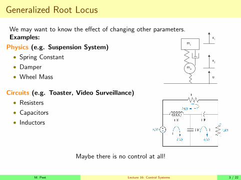
Generalized Root Locus
We may want to know the effect of changing other parameters.Examples:
Physics (e.g. Suspension System)
• Spring Constant
• Damper
• Wheel Mass
x1
x2
mc
mw
u
Circuits (e.g. Toaster, Video Surveillance)
• Resisters
• Capacitors
• Inductors
Maybe there is no control at all!
M. Peet Lecture 16: Control Systems 3 / 22
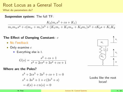
Root Locus as a General ToolWhat do parameters do?
Suspension system: The full TF:
K2(mcs2 + cs+K1)
mcmws4 + c(mw +mc)s3 + (K1mc +K1mw +K2mc)s2 + cK2s+K1K2
The Effect of Damping Constant: c
• No Feedback
• Only examine cI Everything else is 1.
G(s) =s2 + cs+ 1
s4 + 2cs3 + 3s2 + cs+ 1
Where are the Poles?
s4 + 2cs3 + 3s2 + cs+ 1 = 0
s4 + 3s2 + 1 + c (2s3 + s)
= d(s) + c n(s) = 0
x1
x2
mc
mw
u
Looks like the rootlocus!
M. Peet Lecture 16: Control Systems 4 / 22
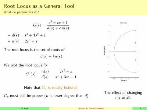
Root Locus as a General ToolWhat do parameters do?
G(s) =s2 + cs+ 1
d(s) + c n(s)
• d(s) = s4 + 3s2 + 1
• n(s) = 2s3 + s
The root locus is the set of roots of
d(s) + kn(s)
We plot the root locus for
Gc(s) =n(s)
d(s)=
2s3 + s
s4 + 3s2 + 1
Note that Gc is totally fictional!
Gc must still be proper (n is lower degree than d).
−1.5 −1 −0.5 0−2
−1.5
−1
−0.5
0
0.5
1
1.5
2
Root Locus
Real Axis
Imag
inar
y A
xis
The effect of changingc is small.
M. Peet Lecture 16: Control Systems 5 / 22
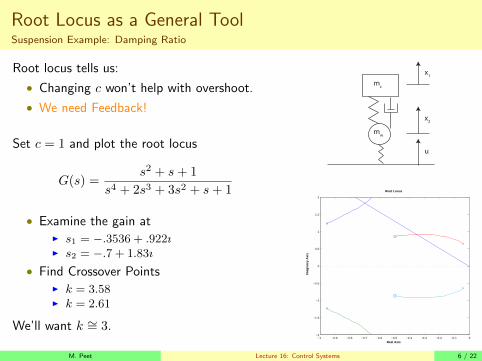
Root Locus as a General ToolSuspension Example: Damping Ratio
Root locus tells us:
• Changing c won’t help with overshoot.
• We need Feedback!
Set c = 1 and plot the root locus
G(s) =s2 + s+ 1
s4 + 2s3 + 3s2 + s+ 1
• Examine the gain atI s1 = −.3536 + .922ıI s2 = −.7 + 1.83ı
• Find Crossover PointsI k = 3.58I k = 2.61
We’ll want k ∼= 3.
x1
x2
mc
mw
u
−1 −0.9 −0.8 −0.7 −0.6 −0.5 −0.4 −0.3 −0.2 −0.1 0−2
−1.5
−1
−0.5
0
0.5
1
1.5
2
Root Locus
Real Axis
Imag
inar
y A
xis
M. Peet Lecture 16: Control Systems 6 / 22
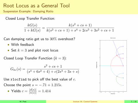
Root Locus as a General ToolSuspension Example: Damping Ratio
Closed Loop Transfer Function:
kG(s)
1 + kG(s)=
k(s2 + cs+ 1)
k(s2 + cs+ 1) + s4 + 2cs3 + 3s2 + cs+ 1
Can damping ratio get us to 30% overshoot?
• With feedback
• Set k = 3 and plot root locus
Closed Loop Transfer Function (k = 3):
Gkc(s) =s2 + cs+ 1
(s4 + 6s2 + 4) + c(2s3 + 3s+ s)
Use rlocfind to pick off the best value of c.
Choose the point s = −.71 + 1.215ı.
• Yields c = |d(s)||n(s)| = 1.414 −2.5 −2 −1.5 −1 −0.5 0
−3
−2
−1
0
1
2
3
Root Locus
Real Axis
Imag
inar
y A
xis
M. Peet Lecture 16: Control Systems 7 / 22
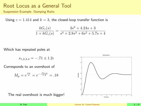
Root Locus as a General ToolSuspension Example: Damping Ratio
Using c = 1.414 and k = 3, the closed-loop transfer function is
kGc(s)
1 + kGc(s)=
3s2 + 4.24s+ 3
s4 + 2.8s3 + 6s2 + 5.7s+ 4
Which has repeated poles at
s1,2,3,4 = −.71± 1.2ı
Corresponds to an overshoot of
Mp = eπσω = e−
.71∗π1.2 = .18
The real overshoot is much bigger! 0 1 2 3 4 5 6 7 8 9 100
0.2
0.4
0.6
0.8
1
1.2
1.4
Step Response
Time (sec)
Am
plit
ud
e
M. Peet Lecture 16: Control Systems 8 / 22
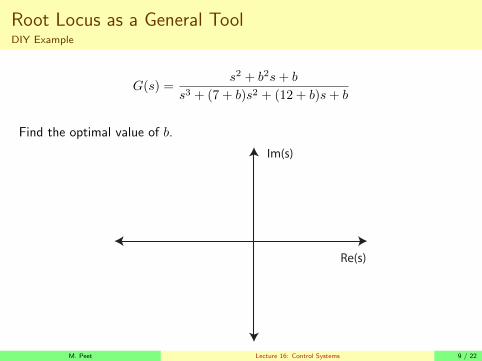
Root Locus as a General ToolDIY Example
G(s) =s2 + b2s+ b
s3 + (7 + b)s2 + (12 + b)s+ b
Find the optimal value of b.
Im(s)
Re(s)
M. Peet Lecture 16: Control Systems 9 / 22
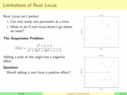
Limitations of Root Locus
Root Locus isn’t perfect
• Can only study one parameter at a time.
• What to do if root locus doesn’t go wherewe want?
The Suspension Problem:
G(s) =s2 + s+ 1
s4 + 2s3 + 3s2 + s+ 1
Adding a pole at the origin has a negativeeffect.
Question:
Would adding a zero have a positive effect?
−3 −2.5 −2 −1.5 −1 −0.5 0 0.5 1−2
−1.5
−1
−0.5
0
0.5
1
1.5
2
Root Locus
Real Axis
Imag
inar
y A
xis
−3 −2.5 −2 −1.5 −1 −0.5 0 0.5 1−2
−1.5
−1
−0.5
0
0.5
1
1.5
2
Root Locus
Real Axis
Imag
inar
y A
xis
M. Peet Lecture 16: Control Systems 10 / 22
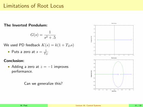
Limitations of Root Locus
The Inverted Pendulum:
G(s) =1
s2 + .5
We used PD feedback K(s) = k(1 + TDs)
• Puts a zero at s = 1TD
Conclusion:
• Adding a zero at z = −1 improvesperformance.
Can we generalize this?
−0.8 −0.6 −0.4 −0.2 0 0.2 0.4 0.6 0.8−0.8
−0.6
−0.4
−0.2
0
0.2
0.4
0.6
0.8
Root Locus
Real Axis
Imag
inar
y A
xis
−4 −3.5 −3 −2.5 −2 −1.5 −1 −0.5 0 0.5 1−0.8
−0.6
−0.4
−0.2
0
0.2
0.4
0.6
0.8
Root Locus
Real AxisIm
agin
ary
Axi
s
M. Peet Lecture 16: Control Systems 11 / 22
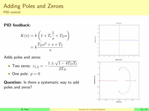
Adding Poles and ZeroesPID control
PID feedback:
K(s) = k
(1 + Ti
1
s+ TDs
)= k
TDs2 + s+ TIs
Adds poles and zeros:
• Two zeros: z1,2 = −1±√1− 4TDTI2TD
• One pole: p = 0
Question: Is there a systematic way to addpoles and zeros?
−0.8 −0.6 −0.4 −0.2 0 0.2 0.4 0.6 0.8−0.8
−0.6
−0.4
−0.2
0
0.2
0.4
0.6
0.8
Root Locus
Real Axis
Imag
inar
y A
xis
−2 −1.5 −1 −0.5 0 0.5 1−1.5
−1
−0.5
0
0.5
1
1.5
Root Locus
Real Axis
Imag
inar
y A
xis
M. Peet Lecture 16: Control Systems 12 / 22

Adding Poles and ZeroesHow?
How To Add a Pole/Zero?
• What does it mean?
Ku=Ke y=Gu
Input Output
G
Errore
Constraint: The plant is fixed.
• G(s) doesn’t change.
The pole/zero must come from the controller. e.g.What is a Controller?
• A systemI Maps e(t) to u(t)
M. Peet Lecture 16: Control Systems 13 / 22

Adding Poles and ZeroesZeros
Goal: Add a Zero
• Like PD control.
Controller:
K(s) = k(s+ z)
• Input to Controller: e(s)
• Output from Controller:
u(s) = k(s+ z)
= kse(s) + kze(s)
Time-Domain:
u(t) = k e′(t) + kz e(t)
Problem: Requires differentiation.
e′(t) ∼=e(t)− e(t− τ)
τ
M. Peet Lecture 16: Control Systems 14 / 22
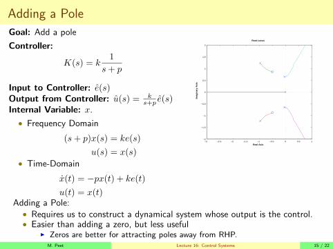
Adding a Pole
Goal: Add a pole
Controller:
K(s) = k1
s+ p
Input to Controller: e(s)Output from Controller: u(s) = k
s+p e(s)Internal Variable: x.
• Frequency Domain
(s+ p)x(s) = ke(s)
u(s) = x(s)• Time-Domain
x(t) = −px(t) + ke(t)
u(t) = x(t)
−3 −2.5 −2 −1.5 −1 −0.5 0 0.5 1−2
−1.5
−1
−0.5
0
0.5
1
1.5
2
Root Locus
Real Axis
Imag
inar
y A
xis
Adding a Pole:• Requires us to construct a dynamical system whose output is the control.• Easier than adding a zero, but less useful
I Zeros are better for attracting poles away from RHP.M. Peet Lecture 16: Control Systems 15 / 22
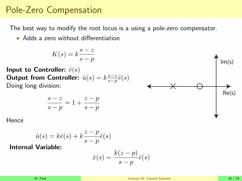
Pole-Zero Compensation
The best way to modify the root locus is a using a pole-zero compensator.
• Adds a zero without differentiation
K(s) = ks− zs− p
Input to Controller: e(s)Output from Controller: u(s) = k s−z
s−p e(s)Doing long division:
s− zs− p
= 1 +z − ps− p
Hence
u(s) = ke(s) + kz − ps− p
e(s)
Im(s)
Re(s)
Internal Variable:
x(s) =k(z − p)s− p
e(s)
M. Peet Lecture 16: Control Systems 16 / 22
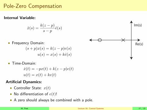
Pole-Zero Compensation
Internal Variable:
x(s) =k(z − p)s− p
e(s)
• Frequency Domain:
(s+ p)x(s) = k(z − p)e(s)u(s) = x(s) + ke(s)
• Time-Domain:
x(t) = −px(t) + k(z − p)e(t)u(t) = x(t) + ke(t)
Im(s)
Re(s)
Artificial Dynamics:
• Controller State: x(t)
• No differentiation of e(t)!
• A zero should always be combined with a pole.
M. Peet Lecture 16: Control Systems 17 / 22
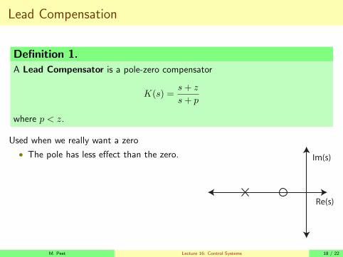
Lead Compensation
Definition 1.
A Lead Compensator is a pole-zero compensator
K(s) =s+ z
s+ p
where p < z.
Used when we really want a zero
• The pole has less effect than the zero. Im(s)
Re(s)
M. Peet Lecture 16: Control Systems 18 / 22
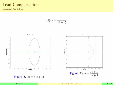
Lead CompensationInverted Pendulum
G(s) =1
s2 − .5
−4 −3.5 −3 −2.5 −2 −1.5 −1 −0.5 0 0.5 1−0.8
−0.6
−0.4
−0.2
0
0.2
0.4
0.6
0.8
Root Locus
Real Axis
Imag
inar
y A
xis
Figure: K(s) = k(s+ 1)
−4 −3.5 −3 −2.5 −2 −1.5 −1 −0.5 0 0.5 1−4
−3
−2
−1
0
1
2
3
4
Root Locus
Real Axis
Imag
inar
y A
xis
Figure: K(s) = ks+ 1
s+ 3
M. Peet Lecture 16: Control Systems 19 / 22
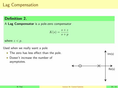
Lag Compensation
Definition 2.
A Lag Compensator is a pole-zero compensator
K(s) =s+ z
s+ p
where z < p.
Used when we really want a pole
• The zero has less effect than the pole.
• Doesn’t increase the number ofasymptotes.
Im(s)
Re(s)
M. Peet Lecture 16: Control Systems 20 / 22
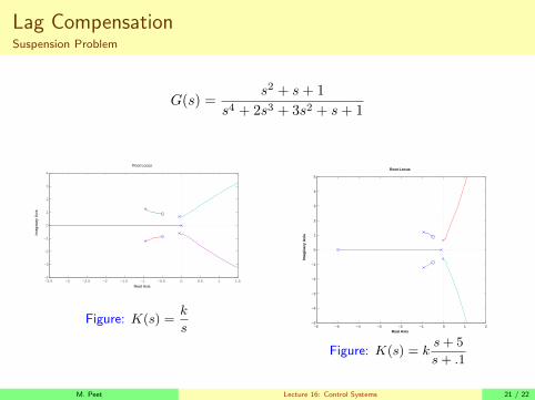
Lag CompensationSuspension Problem
G(s) =s2 + s+ 1
s4 + 2s3 + 3s2 + s+ 1
−3.5 −3 −2.5 −2 −1.5 −1 −0.5 0 0.5 1 1.5−4
−3
−2
−1
0
1
2
3
4
Root Locus
Real Axis
Imag
inar
y A
xis
Figure: K(s) =k
s −6 −5 −4 −3 −2 −1 0 1 2−5
−4
−3
−2
−1
0
1
2
3
4
5
Root Locus
Real Axis
Imag
inar
y A
xis
Figure: K(s) = ks+ 5
s+ .1
M. Peet Lecture 16: Control Systems 21 / 22
Summary
What have we learned today?
Generalized Root Locus?
• What about changing OTHER parameters
• TD, TI , et c.
• mass, damping, et c.
Compensation via Root-Locus
• Introduction
• Pole-Zero Compensation
• Lead-Lag
Next Lecture: Pole-Zero Compensation and Notch Filters
M. Peet Lecture 16: Control Systems 22 / 22