Mr. Munyaradzi Chawana*

Faculty of Finance & Investment Management, University of Johannesburg, Johannesburg 2006,

South Africa.

Tel: +2711 559 3856 Fax: +2711 559 3753

E-mail: dfimpostgrad@uj.ac.za

Prof. Riëtte Eiselen

Faculty of Finance & Investment Management, University of Johannesburg, Johannesburg 2006,

South Africa.

Tel: +2711 559 4349 Fax: +2711 559 3753

E-mail: rjeiselen@uj.ac.za

Working Paper 2012

*Corresponding Author

SYSTEMATIC RISK FACTORS AND THE SOUTH AFRICAN STOCK MARKET:

AN ARBITRAGE PRICING THEORY ASSESSMENT

Abstract

Based on the premise that there are multiple systematic risk factors that influence stock

returns, the Arbitrage Pricing Theory (APT) introduced by Ross (1976) has attracted a great

deal of attention in financial economics literature. In contrast to the voluminous research in

developed markets relating stock returns to more than one source of systematic risk, there is a

paucity of evidence from emerging markets. In the framework of the Arbitrage Pricing

theory, we investigated from a developing market perspective whether a set of pre-specified

macroeconomic variables originally proposed as influencing stock returns in the seminal

work of Chen, Roll and Ross (1986) are risk factors priced on the JSE Limited. The analysis

was conducted on monthly data from the South African stock market and aggregate economic

data for the period January 2000 to December 2009 (a period characterised by upswings and

downturns in the South African economy). Using the Fama-Macbeth (1973) two step

procedure, it was found that unlike the findings of Chen et al. (1986), macroeconomic

variables of economic activity, inflation and term structure are not significantly priced in

South Africa in the period 2000-2009. The study provides additional evidence in the ongoing

debate regarding the relationship between macroeconomic variables and stock returns

especially from an emerging economy perspective.

Keywords: Arbitrage Pricing Theory, Systematic Risk, Stock returns, Macroeconomic

Variables.

1. Introduction

One of the fundamental problems in financial economics is the need to explain stock returns

with events in the aggregate economy (Pitsillis, 2005). From the perspective of efficient-

market theory and rational expectations intertemporal asset pricing theory, stock prices

should depend on their exposures to state variables that describe the economy (Chen, Roll &

Ross 1986). Accordingly, researchers and investors alike have for a long time been intrigued

by the interaction (or lack thereof) that exists between stock returns and the aggregate

economy.

Motivated by the purported failure of the Capital Asset Pricing Model (CAPM) to explain

stock returns adequately, the Arbitrage Pricing Theory (APT) introduced by Ross (1976) has

attracted a great deal of attention in stock pricing literature. Based on the premise that

multiple systematic risk factors influence stock returns, the APT has resulted in a dense

volume of empirical evidence on how stock returns are related to the aggregate economy in

developed markets, especially the US. The evidence on stock pricing from the developed

economies has aided our understanding of how markets price risk. Despite this, much about

the way assets are priced still remains unclear, for example, on one hand studies by Chen et

al. (1986), Clare and Thomas (1994), Clare, Priestley and Thomas (1997), Antoniou, Garrett

and Priestley (1998), Groenewold and Fraser (1997) and Gunsel and Cukur (2007) affirm the

role of key macroeconomic variables in explaining the variations in stock returns and on the

other hand studies by Martinez and Rubio (1989), Poon and Taylor (1991), and Shanken

(1992) refute the influence of key macroeconomic variables on stock returns.

In comparison with the wealth of studies on asset pricing in developed economies, there is a

paucity of studies investigating the same issue in developing economies such as South Africa.

The question remains whether and to what extent macroeconomic risk factors are priced in

emerging stock markets The question is particularly pertinent if one considers the differences

in environmental factors between developed and developing markets in terms of market

sophistication, investor type, market rules and regulations and market maturity (Serra, 2002).

It may be argued that stock markets of developing economies are unique, and different from

those found in developed countries. Hence, how stocks are priced in emerging markets may

be different from developed markets.

Following Chen, Roll and Ross (1986), we sought to investigate from a developing market

perspective, whether a set of pre-specified macroeconomic variables (economic activity,

inflation, term structure and oil prices) originally proposed as influencing stock returns in the

seminal work of Chen, Roll and Ross (1986) are risk factors priced on the JSE Limited. Two

issues motivated us: (i) ascertaining the degree to which the findings reported by Chen et al.

(1986) for the US can be extended to an emerging economy like South Africa (ii)

ascertaining if previous studies of this nature, Van Rensburg (1996) for example, hold true in

another period, namely the 2000-2009 period. The second issue is important due to the fact

that APT empirical results in stock pricing studies have been found to be susceptible to the

choice of the study period.

The analysis was conducted using monthly data from the South African stock market and

aggregate macroeconomic variables for the period January 2000 to December 2009 (a period

characterised by upswings and downturns in the South African economic cycle). Using the

traditional Fama-Macbeth (1973) two step procedure, the findings of this study suggest that

none of the pre-specified risk factors were significantly priced in South Africa in the January

2000 to December 2009 period. Hence, no evidence was found to support the Chen et al.

(1986) risk factor set in influencing equilibrium returns on the JSE Limited.

2. Theoretical framework

2.1 The Arbitrage Pricing Theory

Through the APT, Ross (1976) introduced the idea that more than one systematic factor

influences stock returns and that other non-systematic sources of risk, impinging on stock

returns, are irrelevant in stock pricing since they can be removed in large and well diversified

portfolios (Lehmann & Modest, 1988). Thus, the return on the stock at time t, , can be

expressed as a linear combination of the return at time t on common factors ( :

where is the expected return on stock , is the total number of stocks and the

factors ( have a mean of zero ; is the sensitivity of the return on stock

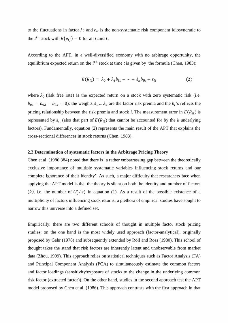
to the fluctuations in factor ; and is the non-systematic risk component idiosyncratic to

the stock with ( ) for all .

According to the APT, in a well-diversified economy with no arbitrage opportunity, the

equilibrium expected return on the stock at time t is given by the formula (Chen, 1983):

where (risk free rate) is the expected return on a stock with zero systematic risk (i.e.

); the weights are the factor risk premia and the ’s reflects the

pricing relationship between the risk premia and stock i. The measurement error in is

represented by (also that part of that cannot be accounted for by the k underlying

factors). Fundamentally, equation (2) represents the main result of the APT that explains the

cross-sectional differences in stock returns (Chen, 1983).

2.2 Determination of systematic factors in the Arbitrage Pricing Theory

Chen et al. (1986:384) noted that there is ‘a rather embarrassing gap between the theoretically

exclusive importance of multiple systematic variables influencing stock returns and our

complete ignorance of their identity’. As such, a major difficulty that researchers face when

applying the APT model is that the theory is silent on both the identity and number of factors

( ), i.e. the number of in equation (1). As a result of the possible existence of a

multiplicity of factors influencing stock returns, a plethora of empirical studies have sought to

narrow this universe into a defined set.

Empirically, there are two different schools of thought in multiple factor stock pricing

studies: on the one hand is the most widely used approach (factor-analytical), originally

proposed by Gehr (1978) and subsequently extended by Roll and Ross (1980). This school of

thought takes the stand that risk factors are inherently latent and unobservable from market

data (Zhou, 1999). This approach relies on statistical techniques such as Factor Analysis (FA)

and Principal Component Analysis (PCA) to simultaneously estimate the common factors

and factor loadings (sensitivity/exposure of stocks to the change in the underlying common

risk factor (extracted factor)). On the other hand, studies in the second approach test the APT

model proposed by Chen et al. (1986). This approach contrasts with the first approach in that

observable pre-specified macroeconomic variables are employed as the systematic factors in

the stock return generation process.

The use of purely statistically based procedures to determine the number of factors which

explain stock returns appears to be a source of contention and controversy (Brown, 1989).

With a bewildering variety of estimation methods and procedures that have been advocated

and used in the literature, the controversy and confusion to the issue of the ‘number of

factors’ is quite evident. For the US market the Roll and Ross (1980) versus Dhrymes, Friend

& Gultekin (1984) debate is a prime example. These studies impressively emphasise the

empirical inconsistency in APT studies that employ factor analytical techniques. Moreover,

the economic interpretation of factors derived by the factor analytical approach remains

problematic.

Due to the challenge posed by giving economic interpretation to APT factors derived from

the factor analytical approach, more recent empirical studies on APT have concentrated on

pre-specifying macroeconomic variables that compensate for the latent variable problem of

the factor analytical approach (Junttila, Larkomaa & Perttunen, 1997). Chen et al. (1986)

were the first to employ specific macroeconomic factors as proxies for the otherwise

theoretically undefined systematic variables in the APT (Poon & Taylor, 1991). This

innovation by Chen et al. (1986) provided an avenue for researchers to link economic activity

to stock market performance in a theoretically grounded framework. The approach provides a

researcher with an economic interpretation of sensitivities and risk premia in the relationship

between stock returns and systematic risk (Chen et al., 1986). According to Pitsillis (2005),

an interpretation of this nature is highly desirable given that one fundamental problem in both

macroeconomics and finance is to explain stock returns with events in the aggregate

economy.

Subsequent to the Chen et al. (1986) seminal study, a limited (comparative to developed

economy studies) number of studies have investigated the macroeconomic risk-stock return

relationship using the Chen et al. (1986) APT framework in an emerging market context. On

the one hand are studies that support the evidence of a significant relationship between stock

returns and macroeconomic variables. For example, Kandir (2008) for the Turkish market

pre-specified six macroeconomic variables and employing the Ordinary Least Squares (OLS)

methodology, Kandir (2008) found the consumer price index, exchange rate, interest rate and

the return on the MSCI World Equity Index significantly priced in the 1997 to 2005 period,

while macroeconomic variables of Industrial production, money supply and oil prices were

observed as having no significant impact on stock returns. Singh (2008) for the Indian market

employed the dollar exchange rate, wholesale price index, production index, gold price, call

money rate, 91 day T-bill rate and money supply. Using the Fama and MacBeth two step

regression technique, Singh (2008) discovered that the call rate and dollar rate were priced in.

Similar to Singh (2008), Nguyen (2010) employed the Fama and MacBeth two step

methodology to the Thai stock market data for the period 1987 to 1996 and discovered that

changes in exchange rates consistently explained Thai stock returns. Bundoo (2009) studying

data for Mauritius reported that macroeconomic variables of the consumer price index, oil

price, the exchange rate and the level of economic activity as proxied by electricity

consumption were statistically significant predictors of stock returns.

However, some studies have not found a significant relationship between stock returns and

macroeconomic variables. For example, Tursoy, Gunsel and Rjoub (2008) empirically tested

the APT on the Istanbul Stock Exchange for the period of February 2001 to September 2005.

Using the OLS technique, unlike Kandir (2008) cited above, Tursoy et al. (2008) observed

that none of the macroeconomic variables of: money supply, industrial production, crude oil

price, consumer price index, import, export, gold price, exchange rate, interest rate, gross

domestic product, foreign reserve, unemployment rate and a market pressure index could

significantly explain the return variation in 11 industry portfolios of the Istanbul Stock

Exchange. For India, Vipul and Gianchandani (1997) pre-specified the following

macroeconomic variables: the call money rate, dollar exchange rate, wholesale price index,

gold price and the national index. Using the Fama-Macbeth two step regression method they

found all of the five systematic variables to be insignificantly priced.

Prior research adopting the Chen et al. (1986) pre-specification variable approach to APT

factor identification in South Africa is limited to Van Rensburg (1996, 2000). Using iterated

non-linear seemingly unrelated regression (ITNLSUR) estimation techniques, and employing

unexpected movements in (rand) gold returns, (dollar) returns on the Dow-Jones Industrial

Index, the term structure of interest rates and inflation expectations together with the 'residual

market factor' of Burmeister and Wall (1986) as pervasive macroeconomic variables, Van

Rensburg (1996) discovered that unexpected movements in the Dow-Jones Industrial Index,

short-term interest rates, the term structure of interest rates and the 'residual market factor' of

Burmeister and Wall (1986) were associated with statistically significant risk premia over the

period 1980 to1989. In his conclusion Van Rensburg (1996) stated that his findings did not

preclude the possibility of other macroeconomic risk factors being found priced over the

same period as found in the US market by Chen et al. (1986) and McElroy and Burmeister

(1988). However, Van Rensburg (2000) argued that the pre-specified variable approach

adopted by him in an earlier study, (Van Rensburg, 1996) did not take account of the

dichotomy in the return generating processes underlying mining and industrial shares on the

JSE Limited. Consequently, a factor analytic augmentation to the pre-specified approach is

suggested in Van Rensburg (2000). Employing the Iterated Non-Linear Seemingly Unrelated

Regression (INLSUR) technique of McElroy and Burmeister (1988), Van Rensburg (2000)

discovered that the rand gold price, the rate on long bonds, the Dow-Jones Industrial Index

and the level of gold and foreign exchange reserves together with the Industrial and All-Gold

residual market factors represent priced sources of risk within the framework of the APT over

the period 1985 to 1995. In his conclusion, Van Rensburg (2000) noted that the findings of

the study implied that the influence of macroeconomic variables on the JSE Limited is most

parsimoniously expressed in the two factor analytical APT model of Van Rensburg and

Slaney (1997). As a consequence, the dominant position in the South African APT literature

points to the influence of two (unobservable) systematic factors on stock returns of JSE

Limited listed companies.

In general, studies in emerging markets employ more or less similar variables to Chen et al.

(1986). However, it is also evident from the literature that researchers in emerging markets

employ country specific variables with the industrial production index, exchange rate, money

supply, unemployment, oil price and gold price variables mainly used.

3. Data and methodology

3.1 Data

A quantitative approach utilising secondary data was followed where monthly data on stock

returns were combined with macroeconomic monthly data for the period January 2000 to

December 2009. Monthly macroeconomic data was sourced from the South African Reserve

Bank website (www.reservebank.co.za) and Statistics South Africa website

(www.statssa.gov.za). Data on stock returns were sourced from Macgregor/BFA website:

www.mcgregorbfa.co.za.

3.1.1 Sample of stocks

The population for this study was all the stocks that constituted the JSE All Share Index

during the period January 2000 to December 2009 (a total of 312 stocks). Due to issues of

delisting, suspension and thin trading, the criteria used in Van Rensburg (1996)1 to select a

stock sample were followed:

1. A stock should be listed for the entire period of the study (Jan 2000- Dec 2009):

Employing this criterion may typically induce the problem of survivorship bias: only

stocks that have ‘survived’ in the entire study period are analysed. According to Antoniou

et al. (1998), the potential impact of the survivorship bias is to make the estimated prices

of risk conservative (assuming that the non-surviving stocks carried greater risk than

surviving stocks). However, since the study period was only 10 years, survivorship bias

was not expected to pose a serious problem.

2. A stock should not be infrequently traded (infrequent trading threshold was set at two

consecutive months within a single trading year i.e. if a stock is not traded for more than

two consecutive months within a single trading year, the stock is left out of the sample);

3. All stocks chosen should represent more than 50% of the capitalisation of the JSE; and

4. Non-operational firms such as 'cash-shells' were excluded. A cash shell is a listed

company whose assets consist wholly or mostly of cash or shares because it has disposed

of all, or a substantial part, of its business (JSE Limited, 2010).

From the population of 312 stocks, 210 stocks satisfied the criteria above and constituted the

sample for this study.

3.1.1.1 Stock portfolio formation

Stock portfolio formation from the sample of 210 stocks was necessitated by (i) the need to

eliminate diversifiable risk and (ii) the need to reduce the Errors in Variables (EIV) problem:

the EIV problem arises when beta estimates ,which contain measurement errors rather

than true values of beta ( , which as unknown, are used to determine the risk-return

relationship. However, two challenges arose: a) how many stocks to include in a single

portfolio to achieve meaningful diversification and b) on what attribute to group the

1 Originally employed in an unpublished master’s dissertation by Reese (1993)

portfolios so as to minimise loss of information and eliminate estimation problems caused by

using portfolios rather than individual stocks (Fama & MacBeth, 1973).

As far as a) (the number of stocks in a portfolio) is concerned, Evans and Archer (1968)

argued that 10 stocks, Fama (1981) argued that 15 stocks while Stattman (1987) argued that

at least 30 stocks should be included in a well diversified portfolio. . Based on the notion

(Elton and Gruber, 1995) that the optimal number of stocks in a well diversified portfolio is

country specific, Neu-Ner and Firer (1997) concluded that between 10 and 30 stocks are

sufficient to achieve a well diversified portfolio on the JSE Limited. In this study, 14

portfolios, each containing 15 stocks were created to satisfy the requirement for

diversification and the requirement for an optimum number of portfolios for the second step

cross-section regressions.

In terms of b) (the method used to create portfolios) two methods are predominant in

empirical studies, namely market-beta and market-size based portfolios. Both methods are

aimed at grouping stocks according to a uniform attribute (either beta or size). For the

market-beta method, individual stock betas calculated from the relationship between returns

on the stock and returns on a market proxy are used to create portfolios. For the market-size-

based method, market capitalisation of individual stocks is used to form portfolios. Chen et

al. (1986) concluded in their study that market-size-based portfolios provide the smallest

variance of diversifiable risk. Market-size-based portfolios were also found to produce a wide

spread of average returns and betas by Chan and Chen (1988) and Fama and French (1992).

In this study, market-size-based portfolios were created as follows: For each of the years

2000 to 2009, 14 portfolios of 15 stocks each (14 x 15 = 210) were formed based on the

market capitalisation of the stocks at the end of the previous year. For each year portfolio 1

contained the stocks with the smallest market capitalisation and portfolio 14 the stocks with

the largest market capitalisation based on the market capitalisation at the end of the previous

year. The process of portfolio formation necessitated rebalancing the stocks according to

market capitalisation at the end of each year to form the portfolios for the next year. The

process resulted in ten sets (one for each year) of 14 portfolios where each portfolio

contained 15 stocks.

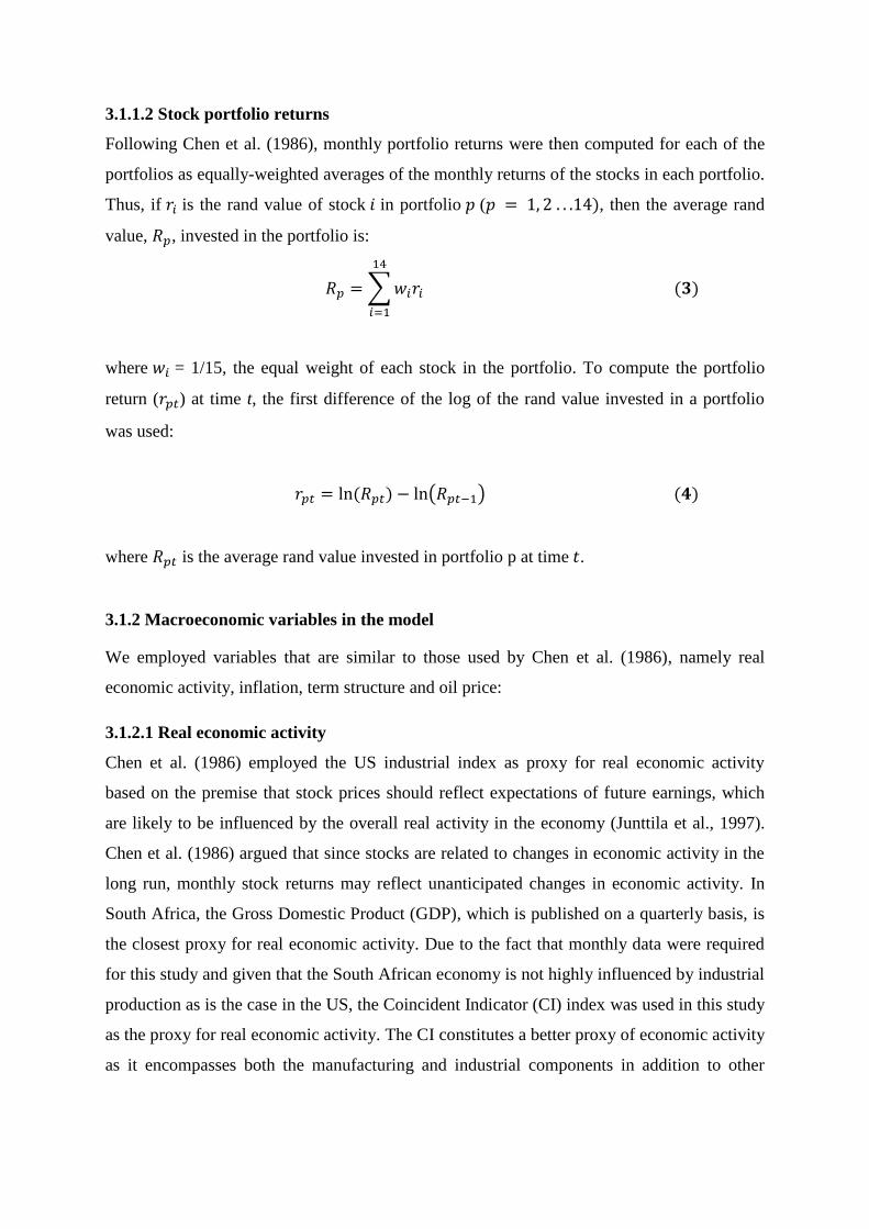
3.1.1.2 Stock portfolio returns

Following Chen et al. (1986), monthly portfolio returns were then computed for each of the

portfolios as equally-weighted averages of the monthly returns of the stocks in each portfolio.

Thus, if is the rand value of stock in portfolio ( , then the average rand

value, , invested in the portfolio is:

∑

where = 1/15, the equal weight of each stock in the portfolio. To compute the portfolio

return ( ) at time t, the first difference of the log of the rand value invested in a portfolio

was used:

( )

where is the average rand value invested in portfolio p at time .

3.1.2 Macroeconomic variables in the model

We employed variables that are similar to those used by Chen et al. (1986), namely real

economic activity, inflation, term structure and oil price:

3.1.2.1 Real economic activity

Chen et al. (1986) employed the US industrial index as proxy for real economic activity

based on the premise that stock prices should reflect expectations of future earnings, which

are likely to be influenced by the overall real activity in the economy (Junttila et al., 1997).

Chen et al. (1986) argued that since stocks are related to changes in economic activity in the

long run, monthly stock returns may reflect unanticipated changes in economic activity. In

South Africa, the Gross Domestic Product (GDP), which is published on a quarterly basis, is

the closest proxy for real economic activity. Due to the fact that monthly data were required

for this study and given that the South African economy is not highly influenced by industrial

production as is the case in the US, the Coincident Indicator (CI) index was used in this study

as the proxy for real economic activity. The CI constitutes a better proxy of economic activity

as it encompasses both the manufacturing and industrial components in addition to other

sectors of the South African economy. Two return series of growth in the proxy for economic

activity from time to were derived from the CI data series:

If denotes the level of the CI index in month , then the monthly growth rate of economic

activity, was computed as follows:

and the yearly growth rate was computed as:

The monthly growth rate, , measures the short term change in economic activity lagged

by at least a partial month (Chen et al., 1986) whereas the yearly growth rates, , reflect

changes in economic activity in the long run. Chen et al. (1986) argued that stock market

prices involve the valuation of cash flows over long periods in the future; thus monthly stock

returns may not be highly related to contemporaneous monthly changes in the economic

activity. To take account of the lagging effect, stock returns are thus influenced by the

monthly series of yearly growth rates . In their explanation, Chen et al. (1986) state that

this month's change in stock prices probably reflects changes in economic activity anticipated

many months into the future.

3.1.2.2 Inflation

Inflation affects sales revenue and borrowings of a firm through changes in nominal cash

flows and discount rate (Gunsel & Cukur, 2007; Clare and Thomas, 1994). According to

Gunsel and Cukur, (2007), anticipated inflation is already priced in the discount rate and sales

prices, hence, only unanticipated inflation will influence the market value of a stock. Thus,

similar to Chen et al. (1986), two macroeconomic variables were formed from the inflation

variable in this study: (i) expected inflation (DEI) and (ii) unexpected inflation (UI):

Change in expected inflation is proxied by the series of first differences of the

Bankers’ Acceptance rate ( , a market-determined rate that reflects conditions in the

money market (Van Rensburg, 1996) :

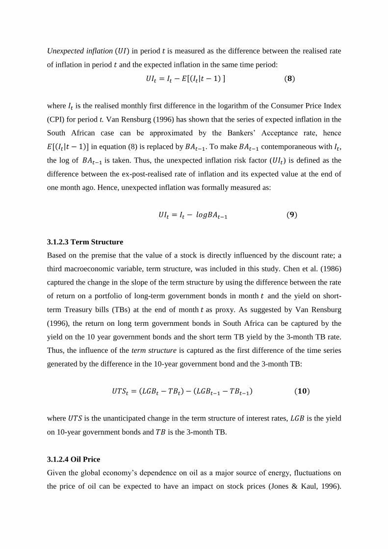
Unexpected inflation in period is measured as the difference between the realised rate

of inflation in period and the expected inflation in the same time period:

[ | ]

where is the realised monthly first difference in the logarithm of the Consumer Price Index

(CPI) for period t. Van Rensburg (1996) has shown that the series of expected inflation in the

South African case can be approximated by the Bankers’ Acceptance rate, hence

[ | ] in equation (8) is replaced by . To make contemporaneous with ,

the log of is taken. Thus, the unexpected inflation risk factor ( ) is defined as the

difference between the ex-post-realised rate of inflation and its expected value at the end of

one month ago. Hence, unexpected inflation was formally measured as:

3.1.2.3 Term Structure

Based on the premise that the value of a stock is directly influenced by the discount rate; a

third macroeconomic variable, term structure, was included in this study. Chen et al. (1986)

captured the change in the slope of the term structure by using the difference between the rate

of return on a portfolio of long-term government bonds in month and the yield on short-

term Treasury bills (TBs) at the end of month as proxy. As suggested by Van Rensburg

(1996), the return on long term government bonds in South Africa can be captured by the

yield on the 10 year government bonds and the short term TB yield by the 3-month TB rate.

Thus, the influence of the term structure is captured as the first difference of the time series

generated by the difference in the 10-year government bond and the 3-month TB:

where is the unanticipated change in the term structure of interest rates, is the yield

on 10-year government bonds and is the 3-month TB.

3.1.2.4 Oil Price

Given the global economy’s dependence on oil as a major source of energy, fluctuations on

the price of oil can be expected to have an impact on stock prices (Jones & Kaul, 1996).

Moreover, for an oil importing country like South Africa, an increase in oil price is believed

to lead to an increase in production costs and hence a decrease in future cash flows, leading to

a negative impact on the stock market (Ahmet, 2010). Chen et al. (1986) studied the influence

of oil price on US stock returns by forming an oil price series based on realised monthly first

difference in the logarithm of the Producer Price index/Crude Petroleum series. Following

Chen et al. (1986) the variable unanticipated changes in oil prices is included in this study:

where is the unanticipated change in oil is prices in month and and are

month end Brent crude oil prices.

Chen et al. (1986) used risk premium as the final variable in their model. It was our intention

in this study to include the risk premium macroeconomic variable (completing the set of

factors employed by Chen et al. 1986). Chen et al. (1986) captured the impact of changes in

risk premia on stock returns by using the difference between the return on government bonds

and that of low grade (Baa and under) bond portfolios. Unfortunately, there is no reliable data

on corporate bonds g in South Africa. For this reason the risk premium factor was excluded

from this study and the oil price variable included.

3.2 Empirical Methodology

Having formed 14 portfolios together with the monthly average returns and based on the set

of macroeconomic factors calculated, the two step regression procedure proposed by Fama

and MacBeth (1973) was employed to analyse the relationship between unanticipated

changes in macroeconomic factors and stock returns. We first determined the period of beta

estimation which ultimately influences the risk premium estimation. Following Chen et al.

(1986) and Shanken and Weinstein (2006) we based the calculation of the portfolio betas on

five-year (60 month) window periods as shown in Table 3.1.

[Insert Table 1 here]

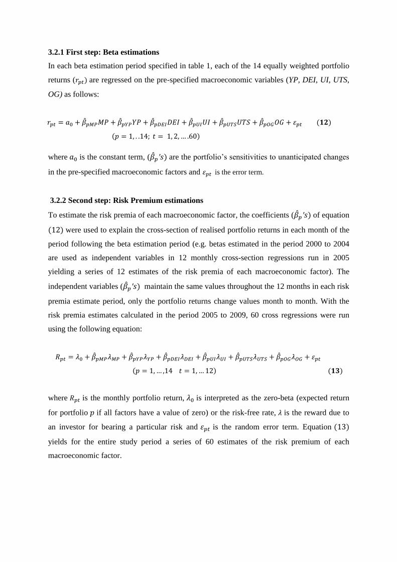
3.2.1 First step: Beta estimations

In each beta estimation period specified in table 1, each of the 14 equally weighted portfolio

returns ( are regressed on the pre-specified macroeconomic variables (YP, DEI, UI, UTS,

OG) as follows:

where is the constant term, ( are the portfolio’s sensitivities to unanticipated changes

in the pre-specified macroeconomic factors and is the error term.

3.2.2 Second step: Risk Premium estimations

To estimate the risk premia of each macroeconomic factor, the coefficients ( of equation

were used to explain the cross-section of realised portfolio returns in each month of the

period following the beta estimation period (e.g. betas estimated in the period 2000 to 2004

are used as independent variables in 12 monthly cross-section regressions run in 2005

yielding a series of 12 estimates of the risk premia of each macroeconomic factor). The

independent variables ( maintain the same values throughout the 12 months in each risk

premia estimate period, only the portfolio returns change values month to month. With the

risk premia estimates calculated in the period 2005 to 2009, 60 cross regressions were run

using the following equation:

where is the monthly portfolio return, is interpreted as the zero-beta (expected return

for portfolio if all factors have a value of zero) or the risk-free rate, is the reward due to

an investor for bearing a particular risk and is the random error term. Equation

yields for the entire study period a series of 60 estimates of the risk premium of each

macroeconomic factor.

3.2.3 Hypothesis Testing

We used the Fama and MacBeth (1973) t-statistic to test individually for each

macroeconomic factor the null hypothesis of a zero mean risk premia. The t-statistic was

calculated as follows:

( )

√

where is the mean value of the th estimated risk premium, : the number of months

from Jan 2005- Dec 2009, which is also the number of estimates of used to compute and

is the standard deviation of (Fama & MacBeth, 1973).

4. Results

4.1 Descriptive statistics

Tables 2 and 3 show the sample means, medians, maxima, minima, standard deviations,

skewness and kurtosis statistics for the 14 monthly market size-sorted stock portfolios and the

monthly macroeconomic variables respectively for the period 2000(1) to 2009(12).

[Insert Table 2 here]

Despite the fact that prior empirical research (Banz, 1981; Chan & Chen, 1991; Fama &

French, 1992) suggests that stock returns are related to firm size, with small stocks providing

a relatively higher return than large stocks, the results (Table 2) show that average returns on

the JSE Limited in the period 2000 to 2009 do not vary systematically with portfolio size. In

terms of skewness and kurtosis, the results are similar to those reported in previous South

African studies (Mangani, 2009): stock return distributions are characterised by being

asymmetrical and peaked and point to large departures from normality. In contrast, skewness

and kurtosis statistics of macroeconomic variables (Table 4.2) point to only moderate

departures from normality: four of the six variables have skewness values close to zero

(between -1 and +1) and kurtosis values not exceeding 3. Only one of the variables (UI) is

moderately positively distributed (skewness = 1.276) and is very peaked (kurtosis = 9.5),

while the variable DEI is moderately negatively distributed but not very peaked (kurtosis =

2.7). The fact that the macroeconomic variables tend to exhibit near normal distributions can

be attributed to the rate of change method used to generate unanticipated movements in

macroeconomic risk factors.

[Insert Table 3 here]

4.2 Diagnostic Tests

Diagnostic tests were run on the independent (macroeconomic) variables to ensure that the

variables satisfied classical linear regression assumptions: Firstly, the Augmented Dickey-

Fuller (ADF) test for stationarity was performed and the results showed that three of the five

macroeconomic variables were stationary and the other two variables were stationary after

first differencing. Secondly, multicollinearity among the macroeconomic variables was

assessed. Three sub-periods (Jan 2000- Dec 2009, Jan 2000 to Dec 2004 and Jan 2005 to Dec

2009) were used due to the fact that economic structural shifts alter the correlations of

macroeconomic variables across periods. Structural shifts in the South African economy

would thus be signified by different correlations in the sub-periods considered. Correlation

results showed that there were no strong correlations across the three sub-periods: absolute

values of the correlations did not exceed 0.70. Lastly, a Portmanteau test (proposed by Box

and Ljung (1978)) was used to test for autocorrelation between time and : the null

hypothesis of white noise series was accepted (at the 5% level of significance) only for the

variables UTS and OG while the series of MP and YP were found to be highly

autocorrelated. First differences of the MP and YP series, however, led to the acceptance of

the white noise hypothesis. For DEI and UI, mild autocorrelations were evidenced.

4.3 Macroeconomic variables and asset pricing

Due to the fact that the main aim of this study was to ascertain whether real economic

activity, inflation, term structure and oil price are macroeconomic risk factors priced on the

JSE Limited, results of the first step (beta estimations) regressions (14x5=70 regressions) are

not shown but are available from the authors. In general, results of the regressions showed

that the null hypothesis that all betas were zero could be rejected in nearly all of the 70 time

series regressions. In addition, the proportion of variation in portfolio stock returns explained

by the pre-specified macroeconomic variables is small across all the 14 portfolios and sub-

periods.

We present the results (Table 4.3) of the null-hypothesis that the mean risk premium of the

pre-specified macroeconomic factors (individually) is not significantly different from zero

using the Fama-Macbeth (1973) t-test for the whole sample period: (2005(1)-2009(12) and

for two sub periods: {(2005(1)-2007(6), 2007(7)-2009(12)}. Using the decision rule, |t( | >

1.96, to reject the null-hypothesis, not one of the coefficients of risk premium in the period

(January 2005 to December 2009) is statistically significantly different from zero. Thus, for

each of the macroeconomic risk factors, the null hypothesis that the risk premium is equal to

zero cannot be rejected and hence inference about their direction and magnitude serves no

purpose.

[Insert Table 4 here]

The reliability of the results obtained for the period January 2005 to December 2009 were

henceforth ascertained by creating two sub-periods of the risk premium estimates: January

2005-June 2007 and July 2007-December 2009. Employing the same testing methodology as

for the main period we established that the results for the sub-periods were consistent with

the results of the main period, namely, all macroeconomic risk factors were not statistically

significant.

5. Discussion and implications

We investigated from a developing market perspective whether a set of pre-specified

macroeconomic variables originally proposed as influencing stock returns in the seminal

work of Chen, Roll and Ross (1986) are risk factors priced on the JSE Limited. Employing

the two step regression technique of Fama-MacBeth (1973), the null hypothesis that these

economic risk factors are not priced against the alternative hypothesis that at least one of the

risk factors is priced could not be rejected. The results of this study provide a different

perspective for South Africa compared to that found for the US by Chen et al. (1986).

Consistent with Martinez and Rubio (1989) for Spain and Poon and Taylor (1991) for the

UK, the findings of this study suggest that none of the risk factors found to be significant in

Chen et al. (1986) are priced in the South African case. From a statistical point of view, there

are two plausible reasons why this result might have been obtained in this study:

i. Size-based portfolios used in the study might have failed to produce a good spread of

returns in a short span of time such as a single month. As acknowledged by Poon and

Taylor (1994), with the possibility of narrowly spread betas and returns fed into the

second stage regression, it might not be surprising that the results do not show a

systematic risk premium.

ii. The stock return-systematic risk relationships may not be captured within the

contemporaneous time lags used in this study. Since there are time lags to which the

announcement/publication of macroeconomic data filters to stock markets, the

lead/lag factors included in this study might have failed to capture the

contemporaneous relationships between stock returns and macroeconomic risk

factors.

A number of pre-test procedures were carried out in this study, and the result of one such test

deserves further discussion considering the results of this study. The majority of financial

empirical tests on stock returns rely on techniques that assume the underlying data generating

process is normally distributed, or at least approximately normally distributed (Fabozzi,

Focardi & Kolm, 2010). Consistent with empirical findings in international markets, results

in this study for the test of normality of stock returns show that the underlying data

generating processes show evidence of the well-known property of financial data series:

returns do not follow the normal distribution. Mangani (2009) also provides compelling

evidence that stock returns on the JSE limited are not normally distributed and are

characterised by ‘fat tails’. However, Chen et al. (1986) did not address the issue of non-

normal return distributions, largely relying on the assumption of returns being log-normally

distributed. A consequence of adopting such an assumption in this study, as noted by Fama

and MacBeth (1973) is that t-statistics employed in this study provide a bias towards rejecting

the significance of systematic factors, given the fact that empirical return distributions have

fat tails.

This study has important implications for both investors and researchers. From an investor’s

point of view, the most important implication of this study is on the identification of the true

sources of systematic risk in an emerging market framework. The findings of this study

suggest that stock returns in South Africa are not influenced by domestic factors, raising the

question of whether returns are influenced by global economic conditions or not. Since

investment decisions are based on the trade-off between risk and return, the implication for a

local or foreign investor is that in evaluating prospective investments, the sources of risk may

lie in external rather than local conditions. Simply focusing on South Africa’s domestic

conditions may lead to erroneous investment decisions.

From a research point of view, this study has highlighted the challenge in the specification of

a unified set of systematic factors influencing stock returns across market structures in the

developed and developing world. Thus, the implication for researchers is the need for further

research in the pursuit of a unified set of risk factors that influence stock returns in emerging

markets. Furthermore, the evidence in this study suggests that financial theories hypothesised

for developed economies should be used with caution, since the idealised conditions for

which they are theorised are less likely to exist in emerging markets.

Conclusion

Employing the widely used Fama-MacBeth two step procedure, the null hypothesis that there

is no relationship between the macroeconomic variables of economic activity, inflation, term

structure, oil prices and stock returns on the JSE Limited could not be rejected in this study.

Thus, the central conclusion in this study is that stock returns in South Africa, an emerging

market, are influenced by factors different from those suggested by Chen et al. (1986)..

Perhaps future research should focus on pin-pointing these systematic factors. The challenge

though for future research is twofold: (i) reducing the pool of possible systematic risk factors

to a well-defined set; and (ii) finding/defining a statistical methodology that yields this well-

defined set unambiguously.

References

Ahmet, B. (2010). The effects of macroeconomics variables on stock returns: Evidence from

Turkey, European Journal of Social Sciences, 14(3): 404-416.

Antoniou, A., Garrett, I. & Priestley, R. (1998). Macroeconomic variables as common

pervasive risk factors and the empirical content of the Arbitrage Pricing Theory, Journal of

Empirical Finance, 5(3): 221-240.

Banz, R.W. (1981). The relationship between returns and market values of common stocks,

Journal of Financial Economics, 9(1): 3-18.

Brown, S.J. (1989). The number of factors in security returns, The Journal of finance, 44(5):

1247-1262.

Box, G.E.P. & Ljung, G.M. (1978). On a measure of a lack of fit in time series models,

Biometrika, 65(2): 297-303.

Burmeister, E. & Wall, K.D (1986). The Arbitrage Pricing Theory and macroeconomic factor

measures, The Financial Review, 21(1): 1-20.

Bundoo, S.K. (2009). Testing the Arbitrage Pricing Theory in an emerging stock market: The

case of Mauritius, Afro-Asian Journal of Finance and Accounting, 1(4): 322-332.

Chan, K. & Chen, N. (1988). An unconditional asset-pricing test and the role of firm size as

an instrumental variable for risk, Journal of Finance, 43(2): 309-325.

Chan, K. & Chen, N. (1991). Structural and return characteristics of small and large firms,

Journal of Finance, 46(4): 1467-1484.

Chen, N. (1983). Some Empirical tests of the Theory of Arbitrage Pricing, Journal of

Finance, 38(5): 1393-1414.

Chen, N., Roll, R. & Ross, S.A. (1986). Economic factors and the stock market, Journal of

Business, 58(3): 383-403.

Clare, A.C. & Thomas, S.H. (1994). Macroeconomic factors, the APT and the UK Stock

market, Journal of Business, Finance and Accounting, 21(3): 309-330.

Clare, A.C., Priestley, R. & Thomas, S. (1997). The robustness of the APT to alternative

estimators, Journal of Business Finance and Accounting, 24(5): 645-655.

Dhrymes, P., Friend, V. & Gultekin, M. (1984). A Critical examination of the empirical

evidence on the Arbitrage Pricing Theory, Journal of Finance. 39(2): 323-346.

Elton, E.J. & Gruber, M.J. (1995). Modern Portfolio Theory and Investment Analysis. 5th

edition. New York: John Wiley & Sons.

Evans, J.L. & Archer, S.H. (1968). Diversification and the reduction of dispersion: An

empirical analysis, Journal of Finance, 7(1): 761-767.

Fabozzi, F.J., Focardi, P. &. Kolm, P.N. (2010). Quantitative equity investing: Techniques

and strategies. New Jersey: John Wiley & Sons, Inc.

Fama, E.F. (1981). Stock returns, real activity, inflation and money, American Economic

Review, 71(1): 545-565.

Fama, E.F. & French, K.R. (1992). The cross section of expected stock returns, Journal of

Finance, 47(2): 427-466.

Fama, E.F. & MacBeth, J.D. (1973). Risk, return and equilibrium: Empirical tests, Journal of

Political Economy, 81(3): 607-636.

Gehr, A. (1978). Some tests of Arbitrage Pricing Theory, Journal of Midwest Finance

Association, 7(4): 91-106.

Groenewold, N. & Fraser, P. (1997). Share prices and macroeconomic factors, Journal of

Business Finance and Accounting, 24(9): 1367-1383.

Gunsell, N. & Cukur, S. (2007). The effects of macroeconomic factors on the London stock

returns: A sectoral approach, International Research Journal of Finance and Economics, 10:

140-152.

Jones, C.M. & Kaul, G. (1996). Oil and the Stock Markets, Journal of Finance, 51(2): 463-

491.

JSE Limited (2010). How to list. [Online] URL:http://www.jse.co.za/How-To-List-On-

AltX.aspx.

Junttila, J., Larkomaa, P. & Perttunen, J. (1997). The Stock Market and Macroeconomy in

Finland in the APT-Framework, The Finnish Journal of Business Economics, 4: 454-473.

Kandir, Y.S. (2008). Macroeconomic variables, firm characteristics and stock returns:

Evidence from Turkey, International Research Journal of Finance and Economics, 16: 35-

45.

Lehmann, B.N. & Modest, D.M. (1988). The empirical Foundations of the Arbitrage Pricing

Theory, Journal of Financial Economics, 21(2): 213-254.

Mangani, R. (2009). Macroeconomic effects on individual JSE stocks, Investment Analysts

Journal, 69: 47-57.

Martinez, M.A. & Rubio, G. (1989). Arbitrage pricing with macroeconomic variables: An

empirical investigation using Spanish data, Working paper, Universidad del Pais Vasco.

McElroy, M.B. & Burmeister, E. (1988). Arbitrage Pricing Theory as a restricted nonlinear

multivariate regression model, Journal of Business & Economic Statistics, 6(1): 29-42.

Neu-Ner, M.A. & Firer, C. (1997). The benefits of diversification on the JSE, Investment

Analysts Journal, 46: 45-59.

Nguyen, D.T. (2010). Arbitrage Pricing Theory: Evidence from an emerging stock market,

Development and Policies Research Center, Working Paper Series No. 2010/03.

Pitsillis, M. (2005). Review of literature on multifactor asset pricing models. In Knight, J. &

Satchell, S. (Eds). Linear Factor Models in Finance. Oxford: Elsevier Ltd.

Poon, S. & Taylor, S.J. (1991). Macroeconomic factors and the UK stock market, Journal of

Business Finance and Accounting, 18(5): 619-636.

Reinganum, M.R. (1981). The Arbitrage Pricing Theory some empirical results, Journal of

Finance, 36(2): 313-321.

Roll, R. & Ross, S.A. (1980). An empirical investigation of the Arbitrage Pricing Theory,

Journal of Finance, 35(5):1073-1103.

Ross, S.A. (1976). The Arbitrage Theory of capital asset pricing, Journal of Economic

Theory, 13(1): 341-360.

Serra, A.P. (2002). The cross-sectional determinants of returns: Evidence from emerging

markets’ stocks, Working Papers DA FEP, 120.

Shanken, J. (1992). On the Estimation of Beta-pricing models, The Review of Financial

Studies, 5(1): 1-33.

Shanken, J. & Weinstein, M.I. (2006). Economic forces and the stock market revisited,

Journal of Empirical Finance, 13: 129-144.

Singh, R. (2008). CAPM vs. APT with macro economic variables: evidence from the Indian

stock market, Asia-Pacific Business Review, Jan-March.

Stattman, D. (1980). Book values and stock returns, The Chicago MBA: A Journal of Selected

Papers. 4: 25-45.

Tursoy, T., Gunsel, N. & Rjoub, H. (2008). Macroeconomic factors, the APT and the Istanbul

stock market, International Research Journal of Finance and Economics, 22: 49-57.

Van Rensburg, P. (1996). Macroeconomic identification of the priced APT factors on the

Johannesburg Stock Exchange, South African Journal of Business Management, 27(4): 104-

112.

Van Rensburg, P. (2000). Macroeconomic identification of candidate APT factors on the

Johannesburg Stock Exchange, Journal of Studies in Economics and Econometrics, 23(2):

27-53.

Van Rensburg, P. & Slaney, K.B.E. (1997). Market segmentation on the Johannesburg Stock

Exchange, Journal of Studies in Economics and Econometrics, 23(3): 1-23.

Vipul & Gianchandani, K. (1997). A test of APT in Indian market, Finance India, 11(2): 285-

304.

Zhou, G. (1999). Security factors as linear combination of economic variables, The Journal

of Financial Markets, 2(4): 403-432.

Tables

Table 1. Portfolio formation, estimation and testing periods

Period

1 2 3 4 5

Beta estimation period 2000-2004 2001-2005 2002-2006 2003-2007 2004-2008

Risk premium estimation period 2005 2006 2007 2008 2009

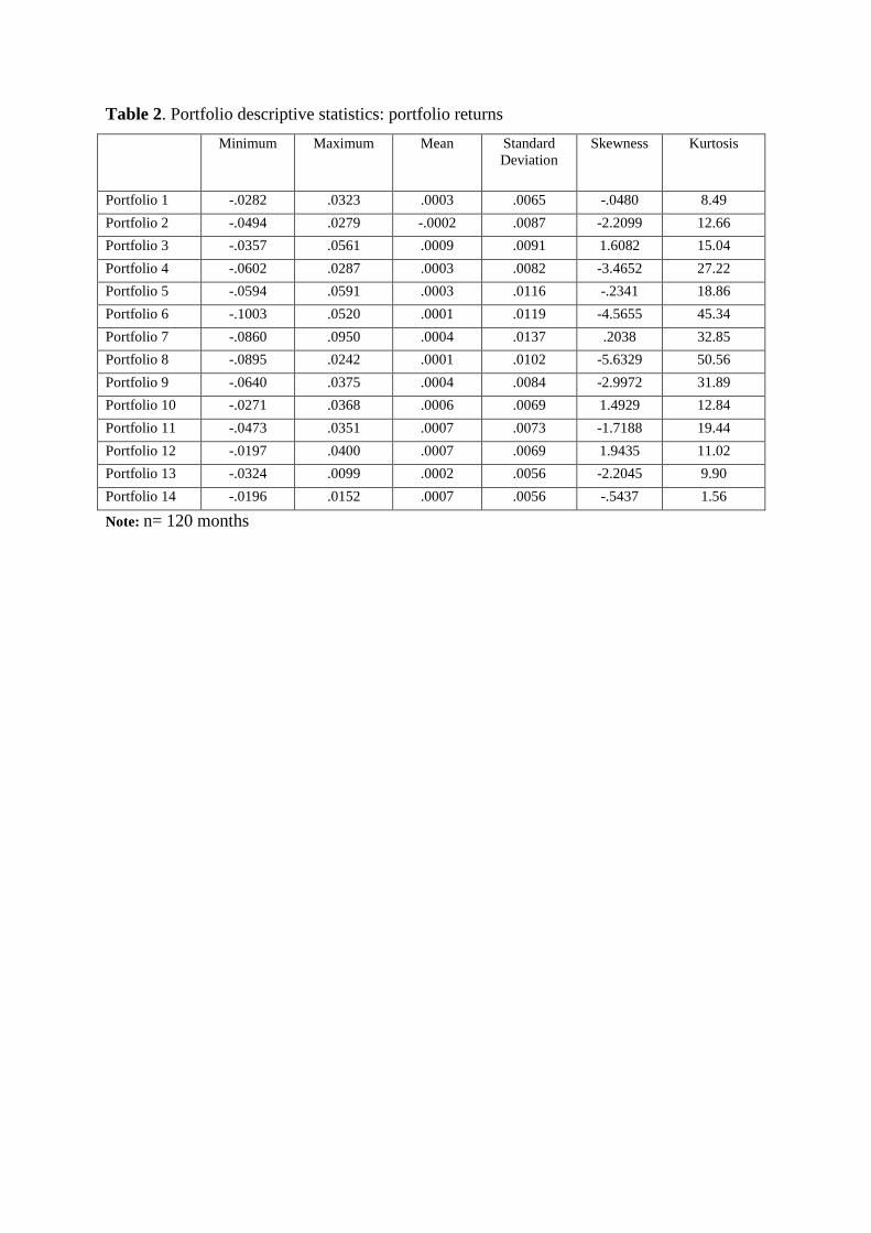
Table 2. Portfolio descriptive statistics: portfolio returns

Minimum Maximum Mean Standard

Deviation

Skewness Kurtosis

Portfolio 1 -.0282 .0323 .0003 .0065 -.0480 8.49

Portfolio 2 -.0494 .0279 -.0002 .0087 -2.2099 12.66

Portfolio 3 -.0357 .0561 .0009 .0091 1.6082 15.04

Portfolio 4 -.0602 .0287 .0003 .0082 -3.4652 27.22

Portfolio 5 -.0594 .0591 .0003 .0116 -.2341 18.86

Portfolio 6 -.1003 .0520 .0001 .0119 -4.5655 45.34

Portfolio 7 -.0860 .0950 .0004 .0137 .2038 32.85

Portfolio 8 -.0895 .0242 .0001 .0102 -5.6329 50.56

Portfolio 9 -.0640 .0375 .0004 .0084 -2.9972 31.89

Portfolio 10 -.0271 .0368 .0006 .0069 1.4929 12.84

Portfolio 11 -.0473 .0351 .0007 .0073 -1.7188 19.44

Portfolio 12 -.0197 .0400 .0007 .0069 1.9435 11.02

Portfolio 13 -.0324 .0099 .0002 .0056 -2.2045 9.90

Portfolio 14 -.0196 .0152 .0007 .0056 -.5437 1.56

Note: n= 120 months

Table 3. Descriptive statistics: macroeconomic variable

Minimum Maximum Mean Standard.

Deviation

Skewness Kurtosis

YP -.03 .03 .0027 .00833 -.811 1.960

MP -.09 .12 .0440 .04381 -.684 .568

DEI -1.42 .73 -.0319 .38911 -1.390 2.741

UI -1.50 .01 -.9605 .16959 1.276 9.532

UTS -1.24 1.59 -.0113 .46336 .638 1.064

OG -.14 .09 .0039 .04340 -.981 1.000

Note: MP= Monthly Economic Activity; YP= Yearly Economic Activity; DEI=Change in expected Inflation;

UI=Unanticipated Inflation; UTS=Unanticipated change in term structure; OG=Change in Oil price. n = 120

months

Table 4. Fama and MacBeth t-test results

A. 2005(1)-2009(12)

Period

-0.006 -0.003 0.002 -0.79 -0.393 0.280 -0.019

0.043 0.040 0.019 6.223 2.545 4.665 0.162

( ) (-1.056) (-0.544) (0.687) (-0.99) (-1.196) (0.465) (0.90)

B. 2005(1)-2007(6)

0.002 -0.004 0.004 -0.130 -0.132 0.065 -0.047

0.004 0.046 0.025 2.977 2.166 3.676 0.214

( ) (2.839) (-0.485) (0.851) (-0.240) (-0.335) (0.097) (-1.198)

C. 2007(7)-2009(12)

-0.014 -0.002 0.000 -1.461 -0.654 0.495 0.009

0.060 0.033 0.012 8.307 2.889 5.537 0.075

( ) (-1.281) (-0.250) (-0.174) (-0.963) (-1.239) (0.490) (0.667)

Note: MP= Monthly Economic Activity; YP= Yearly Economic Activity; DEI=Change in expected Inflation;

UI=Unanticipated Inflation; UTS=Unanticipated change in term structure; OG=Change in Oil price;

=constant; = mean risk premium; ( )= Fama and MacBeth t-statistic (one tail)