Edited by

Sustainable Tourism and Its Environmental and Human Ecological Effects

Luc Hens and An Thinh Nguyen

Printed Edition of the Special Issue Published in International Journal of Environmental Research and Public Health

www.mdpi.com/journal/ijerph

Sustainable Tourism and ItsEnvironmental and HumanEcological Effects

Sustainable Tourism and ItsEnvironmental and HumanEcological Effects

Editors

Luc Hens

An Thinh Nguyen

MDPI • Basel • Beijing • Wuhan • Barcelona • Belgrade • Manchester • Tokyo • Cluj • Tianjin

Editors

Luc Hens

Flemish Institute for

Technological Research (VITO)

Belgium

Department of Economics,

Entrepreneurship and

Business Administration,

Sumy State University

Sumy, Ukraine

An Thinh Nguyen

Faculty of Development

Economics, VNU University of

Economics and Business

Hanoi, Vietnam

Editorial Office

MDPI

St. Alban-Anlage 66

4052 Basel, Switzerland

This is a reprint of articles from the Special Issue published online in the open access journal

International Journal of Environmental Research and Public Health (ISSN 1660-4601) (available at: https:

//www.mdpi.com/journal/ijerph/special issues/sustainable tourism effects).

For citation purposes, cite each article independently as indicated on the article page online and as

indicated below:

LastName, A.A.; LastName, B.B.; LastName, C.C. Article Title. Journal Name Year, Volume Number,

Page Range.

ISBN 978-3-0365-2233-3 (Hbk)

ISBN 978-3-0365-2234-0 (PDF)

© 2021 by the authors. Articles in this book are Open Access and distributed under the Creative

Commons Attribution (CC BY) license, which allows users to download, copy and build upon

published articles, as long as the author and publisher are properly credited, which ensuresmaximum

dissemination and a wider impact of our publications.

The book as a whole is distributed byMDPI under the terms and conditions of the Creative Commons

license CC BY-NC-ND.

Contents

About the Editors . . . . . . . . . . . . . . . . . . . . . . . . . . . . . . . . . . . . . . . . . . . . . . vii

Preface to ”Sustainable Tourism and Its Environmental and Human Ecological Effects” . . . . ix

Quang Hai Truong, An Thinh Nguyen, Quoc Anh Trinh, Thi Ngoc Lan Trinh and Luc Hens

Hierarchical Variance Analysis: A Quantitative Approach for Relevant Factor Exploration andConfirmation of Perceived Tourism ImpactsReprinted from: Int. J. Environ. Res. Public Health 2020, 17, 2786, doi:10.3390/ijerph17082786 . . . 1

Luna Santos-Roldan, Ana Mª Castillo Canalejo, Juan Manuel Berbel-Pineda and Beatriz

Palacios-Florencio

Sustainable Tourism as a Source of Healthy TourismReprinted from: Int. J. Environ. Res. Public Health 2020, 17, 5353, doi:10.3390/ijerph17155353 . . . 21

Fen Zeng and Zhenjiang Shen

Study on the Impact of Historic District Built Environment and Its Influence on Residents’Walking Trips: A Case Study of Zhangzhou Ancient City’s Historic DistrictReprinted from: Int. J. Environ. Res. Public Health 2020, 17, 4367, doi:10.3390/ijerph17124367 . . . 35

Jinsoo Hwang, Hyunjoon Kim and Ja Young Choe

The Role of Eco-Friendly Edible Insect Restaurants in the Field of Sustainable TourismReprinted from: Int. J. Environ. Res. Public Health 2020, 17, 4064, doi:10.3390/ijerph17114064 . . . 51

Ni Wayan Masri, Jun-Jer You, Athapol Ruangkanjanases, Shih-Chih Chen and Chia-I Pan

Assessing the Effects of Information System Quality and Relationship Quality on ContinuanceIntention in E-TourismReprinted from: Int. J. Environ. Res. Public Health 2020, 17, 174, doi:10.3390/ijerph17010174 . . . 63

Aijun Liu, Taoning Liu, Xiaohui Ji, Hui Lu and Feng Li

The Evaluation Method of Low-Carbon Scenic Spots by Combining IBWM with B-DST andVIKOR in Fuzzy EnvironmentReprinted from: Int. J. Environ. Res. Public Health 2020, 17, 89, doi:10.3390/ijerph17010089 . . . . 79

Xiaowei Xu, Daxin Dong, Yilun Wang and Shiying Wang

The Impacts of Different Air Pollutants on Domestic and Inbound Tourism in ChinaReprinted from: Int. J. Environ. Res. Public Health 2019, 16, 5127, doi:10.3390/ijerph16245127 . . . 109

Yanchun Jin and Yoonseo Park

An Integrated Approach to Determining Rural Tourist Satisfaction Factors Using the IPA andConjoint AnalysisReprinted from: Int. J. Environ. Res. Public Health 2019, 16, 3848, doi:10.3390/ijerph16203848 . . . 125

Chun-Chu Yeh, Crystal Jia-Yi Lin, James Po-Hsun Hsiao and Chin-Huang Huang

The Effect of Improving Cycleway Environment on the Recreational Benefits of Bicycle TourismReprinted from: Int. J. Environ. Res. Public Health 2019, 16, 3460, doi:10.3390/ijerph16183460 . . . 141

Chao Bi and Jingjing Zeng

Nonlinear and Spatial Effects of Tourism on Carbon Emissions in China: A SpatialEconometric ApproachReprinted from: Int. J. Environ. Res. Public Health 2019, 16, 3353, doi:10.3390/ijerph16183353 . . . 153

v

Han-Shen Chen

Establishment and Application of an Evaluation Model for Orchid Island SustainableTourism DevelopmentReprinted from: Int. J. Environ. Res. Public Health 2019, 16, 755, doi:10.3390/ijerph16050755 . . . 171

vi

About the Editors

Luc Hens is a Belgian human ecologist who has been performing and supporting research

on sustainable development and climate change policy instruments in Vietnam for over 25 years.

He worked at the “Flemish Institute for Technological Research (VITO)”, which is Belgium’s

largest environmental research organization. Professor Hens has published over 130 papers in

international peer-reviewed journals. He has also published in local Belgian and Dutch scientific

journals, and (co-)edited over 40 books with international distribution. He is “Editor in Chief” of

“Environment, Development and Sustainability”, a journal paying ample attention to sustainable

tourism contributions.

An Thinh Nguyen is the Dean of the Faculty of Development Economics at VNU University

of Economics and Business, Hanoi, Vietnam. He also currently acts as the Vice-President of the

International Association of Landscape Ecology in the Vietnamese region (VN-IALE). His research

focuses include the geography of Vietnam, human geography, environmental economics, and tourism

economics.

vii

Preface to ”Sustainable Tourism and Its

Environmental and Human Ecological Effects”

The book “Sustainable Tourism and Its Environmental and Human Ecological Effects” addresses

the increasing interest in sustainable and related forms of tourism, with a focus on the environmental

and human ecological impacts. The social and economic impacts of sustainable tourism are

addressed, along with its effects on the physical environment. A series of case studies on the

friction between tourism development and environmental quality is presented. Specific topics

are: the development of sustainable tourism, sport tourism, e-travel services and e-tourism;

environmental and human ecological effects of tourism on island and inland destinations; impacts

of historic district built environment to recreation, leisure and sports; evaluation of low-carbon scenic

spots; current crisis experienced by the tourism industry caused by COVID-19. The book covers a

wide range of tourism destinations worldwide, mainly in Asia and Europe (Vietnam, Taiwan, China,

South Korea, and Spain). The book offers opportunities, including policy papers, not only focusing on

the instruments to alleviate environmental impacts, but also on methods for the efficient involvement

of stakeholders.

Luc Hens, An Thinh Nguyen

Editors

ix

International Journal of

Environmental Research

and Public Health

Article

Hierarchical Variance Analysis: A QuantitativeApproach for Relevant Factor Exploration andConfirmation of Perceived Tourism Impacts

Quang Hai Truong 1, An Thinh Nguyen 2,*, Quoc Anh Trinh 3, Thi Ngoc Lan Trinh 4 and

Luc Hens 5

1 Institute of Vietnamese Studies & Development Sciences, Vietnam National University (VNU),Hanoi 10000, Vietnam; truongquanghai.ivides@gmail.com

2 VNU University of Economics and Business, Vietnam National University (VNU), Hanoi 10000, Vietnam3 VNU University of Science, Vietnam National University (VNU), Hanoi 10000, Vietnam;

trinhquocanh@hus.edu.vn4 School of Economics and Management, Hanoi University, Hanoi 10000, Vietnam;

trinhngoclan181@gmail.com5 Vlaamse Instelling voor Technologisch Onderzoek (VITO), Boeretang 200, 2400 Mol, Belgium;

luchens51@gmail.com* Correspondence: anthinhhus@gmail.com

Received: 22 March 2020; Accepted: 16 April 2020; Published: 17 April 2020

Abstract: The issue of tourism impacts is one that has plagued the tourism industry. This studydevelops a quantitative approach using hierarchical variance analysis, which deals with the explorationof the relevant factors and the confirmation of their significant contribution to analyze the residents’perception of tourism impacts. Hierarchical variance analysis includes three mathematical procedures:Cronbach’s alpha tests, the exploration of relevant factors, and a hierarchical factor confirmation.Data are collected using a structured questionnaire completed by 452 surveyed residents living in LySon Island, Vietnam. The significant effects of socio-demographic variables on the overall impactassessment are observed. The bilateral and simultaneous relationships are analyzed using a one-factorANOVA. A two-factor ANOVA shows the significant contribution of each socio-demographic variableon the economic, socio-cultural, and environmental impacts. Interaction between factors such as“Education level”, “Type of work”, etc. are hierarchically confirmed. The findings allow a betterunderstanding of the residents’ perception of the effects of tourism on society, the economy, and theenvironment. This provides a scientific basis to help define problems and promote legal regulationsfor community participation in tourism planning in a small island destination.

Keywords: hierarchical variance analysis; residents’ perceptions; socio-demographic variables;ANOVA; linear regression model; perceived tourism impacts; overall impact assessment; Ly SonIsland; Vietnam

1. Introduction

Tourism development impacts the local economy and residents’ lives socially, economically, andenvironmentally [1,2]. A stakeholder approach is used to assess the impacts of tourism [3,4]. Localresidents link tourism development with the challenges of sustainable development, which affect theirsupport for further tourism development [5,6], more hospitality, and for the sustainability of tourism [7].Perceived environmental pollution reduces the support of residents for tourism development [5].Perceived economic benefits increase the support of residents towards tourism development [8–11]because it provides opportunities for employment for local residents in general, and for womenin particular. This enables them to be more independent, raises local land prices [1], and provides

IJERPH 2020, 17, 2786; doi:10.3390/ijerph17082786 www.mdpi.com/journal/ijerph1

IJERPH 2020, 17, 2786

increased income opportunities [11,12]. Perceived social impacts, such as changes in the life styles andcustoms of local residents, decrease local social moral standards [1]. The perceived environmentalimpacts include generating municipal solid waste and carbon dioxide, degenerating the quality ofthe environment, disturbing the regular life of residents, and destroying the peaceful character ofvillages [1,13,14]. Perceptions differ between households on the socio-demographic characteristics andon the stages of local tourism development [7,15,16]. A better balance between the socio-economicimpacts and environmental considerations in residents’ perceptions is needed [5].

2. Literature Review

Residents’ perception of tourism impacts has been quantitatively studied in depth. Combiningsocio-psychological theories with mathematic models such as Cronbach’s alpha tests, Fisher test,ANOVA, Structural Equation Modeling (SEM), multi-level factor, and regression analysis providestheoretical and practical insights allowing us to understand the impacts of the stressors and beneficiariesin tourism communities [17–21]. A series of aspects of residents’ support towards tourism developmentare quantified using a triple bottom line approach [22] involving the following: a two-dimensionalinformedness–involvement tourism grid [23], self-perception theory [24], social exchange theory [25–28],social exchange theory combined with identity theory [29], and the cognitive appraisal theory [30].Tourists’ safety is analyzed by the Rimal and Real’s risk perception attitude framework [31]. The itemresponse theory measures the sustainability perception of residents [32]. The du Cros model assessestourism potential [33]. A comprehensive resilience model assesses overall community resilience fortourism [34]. Structural Equation Modeling (SEM) has the advantage of being able to assess theoverall support of residents for tourism development [35,36]. The relationships between tourismimpacts, emotions, and stress are tested by the Partial Least Squares Structural Equation Modeling(PLS-SEM) [37].

This study develops the hierarchical variance analysis, a mathematical approach using Cronbach’salpha tests, ANOVA, and linear regression analysis to analyze the socio-demographic composition ofsurveyed residents according to their perception on tourism impacts. Socio-demographic compositionis expressed by variables such as gender, age, marital status, the condition of being native, foreignparticipants’ years of residence in the city, parental status, education level, participation in localassociations and neighborhood groups, and the type of work in relation to tourism [7]. Analyzingsocio-demographic variables supports research that recognizes existing conditions, needs, andexpectations of a given population [38–40]. Taking into account the impacts of tourism, a combinationof mathematics procedures is definitely worth additional empirical research. Pearson correlations,ANOVA analyses, and hierarchical multiple regression analyses using socio-demographic variablesshows significant variance in the overall attitudes [7]. Descriptive statistics was combined with a seriesof independent sample t-tests to assess statistically significant differences caused by socio-demographiccharacteristics of residents living in a tourism destination [41]. The two-level hierarchical linear modelusing the fixed effects model, random intercept empty model, random coefficients model, and Cook’sdistance test was used to assess the impacts of tourism conducted from perceptions of residents [42].However, there are still few quantitative studies which mix mathematics procedures to examine howsocio-demographic variables affect the residents’ perception on social, economic, and environmentalimpacts of tourism. The proposed hierarchical variance analysis is a vindication of our efforts to solvetwo main problems in the field of tourism impacts: the first is to examine the link between relevantfactors and the confirmation of their significant contribution; and the second is to analyze the residents’perception of tourism impacts according to each socio-demographic variable.

The paper is organized as follows: Section 2 introduces the mathematic procedures of thehierarchical variance analysis methodology; the results of a case analysis in a Vietnamese islanddestination are described in Section 3; and a conclusion and policy implication are drawn up inSection 4.

2

IJERPH 2020, 17, 2786

3. Methodology

3.1. Problem

The hierarchical variance analysis combines three mathematic procedures: Cronbach’s alpha tests(to assess the reliability of independent variables), the exploration of relevant factors (to measure theeffect of independent variables on the perceived impacts), and a hierarchical factor confirmation (tofind the one that explains most of the contribution of the relevant variables on the perceived impactsand to confirm the likely interaction). Perceived tourism impacts are expressed by dependent variables,while socio-demographic characteristics are expressed by independent variables. To process the model,dependent variables of tourism impacts Y were selected: Economic impacts (Y1), Socio-cultural impacts(Y2), and Environmental impacts (Y3) (Table 1). The six independent variables of socio-demographicare: Gender (X1), Marital status (X2), Education level (X3), Age (X4), Type of work (X5), and Socialnetwork (X6). In the first step, Cronbach’s Alpha test verifies the relevance of X for each tourism impactY. In the next steps, an ANOVA compares the positive, negative, and overall variance of each perceivedimpact on tourism development. A linear regression analysis measures the effect of socio-demographicvariables on three impacts confirming the result of the exploration step. By the end of the analysis,a two-factor ANOVA confirms the likely interaction between “Education level” and “Type of work”while predicting three impacts.

Table 1. Dependent variables of tourism impacts.

Economic Impacts (Y1) Socio-Cultural Impacts (Y2) Environmental Impacts (Y3)

Y+1 Y−1 Y1 Y+2 Y−2 Y2 Y+3 Y−3 Y3Positive Negative Overall Positive Negative Overall Positive Negative Overall

3.2. Cronbach Alpha’s Test

Cronbach Alpha’s test estimates the reliability of independent variables Xi in each question.Suppose that we are interested in the relevance of variables Xi, i = 1, K, let Z be the total test score ineach question:

Z = X1 + X2 + . . .+ XK (1)

The Cronbach Alpha is defined as [43]

α =K

K − 1

⎛⎜⎜⎜⎜⎜⎜⎝1−∑K

i=1 σ2Xi

σ2Z

⎞⎟⎟⎟⎟⎟⎟⎠ (2)

where σ2Z is the variance of the total observed test scores, and σ2

Xiis the variance of the variable Xi.

Cronbach Alpha varies from 0 to 1. The greater value of α, the more acceptable the internalconsistency among variables X (Table 2).

Table 2. The common usage of Cronbach Alpha [44].

Cronbach Alpha Internal Consistency

0.9 ≤ α Excellent0.8 ≤ α < 0.9 Good0.65 ≤ α < 0.8 Acceptable0.5 ≤ α < 0.65 Poorα < 0.5 Unacceptable

3

IJERPH 2020, 17, 2786

3.3. Exploration of Relevant Factors

A one-factor ANOVA is used to explore the relationship between an impact and a variable bymeasuring the effect of the socio-demographic background of the residents on the perceived economic,socio-cultural, the environmental impacts of tourism.

Suppose that the factor X consists of k treatments T1, . . . , Tk, and there are ni observationsYi1, . . . , Yini of the dependent variable Y with respect to the treatment Ti

(i = 1, k

). The following

denotations are used:μi. =

1ni

∑nij=1 Yij, is the treatment mean;

E(Yij

)= 1

n∑

i∑

j Yij = μ (n =∑

j nj), is the grand mean;

αi = μ− μi.

εi j: the error terms.The impact of X on variable Y is tested using the significant difference between the k

treatment means:H : μ1 = μ2 = . . . = μk vs. K : at least one mean differs.With the assumption that εi j are independent normally distributed random variables with

E(εi j

)= 0, Var

(εi j

)= σ2 (*), the random variables Yij can be written [45] as

Yij = μ+ αi + εi j, i = 1, k, j = 1, ni (3)

The deviation of Yij can be separated in the variation between the treatments (αi) and within thetreatments (εi j):

k∑i=1

ni∑j=1

(yij − μ

)2=

k∑i=1

ni(μi. − μ)2 +k∑

i=1

ni∑j=1

(yij − μi.

)2(4)

or

SSTotal (total sum of square) = SST (sum of squared treatment) + SSE (sum of squared errors)

The difference among the treatment means is tested as

H : αi = 0(∀i); K : At least one α � 0

Results from comparing SST with SSE, if the weight of SST is equal or less than that of SSE. Thereshould be no difference among k treatments, otherwise, there is a significant disparity among the kmeans, which results from an impact of factor F on the dependent variable Y.

Because the values of μ and μi are unknown, they are replaced by an estimation of y. (samplegrand mean) and yi (sample treatment mean):

k∑i=1

ni∑j=1

(yij − y

)2=

k∑i=1

ni(yi. − y

)2+

k∑i=1

ni∑j=1

(yij − yi.

)2(5)

By dividing SST and SSE by their corresponding degrees of freedom (ν1 = k− 1 and ν2 = n− k) toobtain MST (mean square of treatment) and MSE (mean square of error), the sampling distributionof the ratio F = MST/MSE is a Fisher distribution with ν1 and ν2 degrees of freedom. If F > Fα, thehypothesis H is rejected.

4

IJERPH 2020, 17, 2786

3.4. Hierarchical Factor Confirmation

3.4.1. Linear Regression Analysis

The multiple linear regression is

Y = β0 + β1X1 + β2X2 + . . .+ βpXp + ε

where ε is the random error, following the normal distribution with Eε = 0, Varε = σ2.The following linear regression equation is estimated:

EY = β0 + β1X1 + β2X2 + . . .+ βpXp

Using either the least square method or the maximum likelihood estimation, one finds theestimators of the p coefficient βi as bi, following the estimated linear regression equation:

Y = b0 + b1X1 + . . .+ bpXp

To further explore the bilateral relationship between a variable and an impact, a one-way ANOVAis used. Independent variables will be combined to find out about their simultaneous effect on theoutcome. As a result, several hierarchical models are considered to find the one that explains most ofthe contribution of the relevant variables on the impacts.

Suppose that p independent variables affect variable Y, p models are used with 1, 2, ..., p predictorswith respect to the largest R2 (adjusted R2). Particularly, among p. linear models containing 1 predictor,

i.e., Y = b0 + biXi, the one providing the largest R2 will be selected; among p(p−1)2 models containing

two predictors, i.e., Y = b0 + bi1 Xi1 + bi2Xi2 , the one with the largest R2 will be plotted, until the lastone containing all p variables are used. After that, the model providing the largest R2 is selected.

Suppose the dataset consists of n sets{(

yi, x1i, . . . , xpi)}

i=1,n. Using a similar option as the one in

Equation (5), the total sum of squared difference consists of two sources [40]:

n∑i=1

(yi − y)2 =n∑

i=1

(yi − yi)2 +

n∑i=1

(yi − y)2 (6)

where y is the sample grand mean of Y, and yi. are the estimated values of Y given the ith value of X.Denoting SSTotal =

∑ni=1(yi − y)2, SSE =

∑ni=1(yi − yi)

2, SSR =∑n

i=1(yi − y)2, Equation (6) canbe rewritten as SSTotal = SSE + SSR. SSE measures the lack of fit of the regression model, and SSRmeasures the variation that can be explained by the regression model. The determination coefficient ofR2 is defined by the ratio SSR/SSE; the larger R2 is, the better the model fits the data. However, whenincreasing the number of variables, R2 also increases; therefore, it is inappropriate to use this numberto assess how well the model fits the data. The adjusted R2 is introduced to deal with this problem:

R2adj = 1−

SSEd fe

SSTotald ft

= 1−(1−R2

)× n− 1

n− p− 1(7)

Taking into account the degrees of freedom (d fe = n− p− 1, d ft = n− 1), the adjusted R2 increaseswhen the increase in R2 is more than one would expect to see by chance.

Remarkably, the Fisher test is performed in a similar way to explore the relevant steps. Thefollowing test problem is considered:

H : β1 = . . . = βl = 0 (reduced model);K : at least one βi differs (full model).

5

IJERPH 2020, 17, 2786

Taking into account the Fisher test, the error between the estimators of coefficient and the observedvalues is evaluated [46]: the sum of the squared error of the two models: SSE(R) and SSE(F) (thereduced and the full one, respectively). While the estimator of yi is yi in the full model, deducing(F) =

∑ni=1(yi − yi)

2, the estimator in reduced model is y (∀i), deducing SSE(R) =∑n

i=1(yi − y)2.Because of Equation (6), SSE(R) ≥ SSE(F). The following cases are possible:

- In case SSE(F) is close to SSE(R), the full model does not reduce the total variance of SST and SSR(the variation explained by the regression model) is limited. The reduced model is selected;

- On the contrary, in case SSE(F) differs significantly from SSE(R), the full model reduces substantiallyand the total variance and the full model is selected.

The ratio (F) measures the difference between SSE(F) and SSE(R):

F =SSE(R) − SSE(F)

d fr − d f f:

SSE(F)d f f

(8)

In the case that the full model contains p variables, the degrees of freedom of SSE(F) is givenas n − p − 1, and of SSE(R) it is given as n − 1. Take notice that in Equation (6) SSE(R) − SSE(F) =

SSTotal− SSE(F) = SSR(F) can be rewritten as

F =SSR

p:

SSE(F)n− p− 1

=MSTMSE

(9)

If F > Fα, which means the difference is significant, H is rejected and the full model is used forthe prediction.

The Fisher test is used to compare the two models and allows the choice of the one with thesmallest variance.

3.4.2. Two-Factor ANOVA

Supposing one wants to see the effect of factor A containing a levels and factor B containing blevels on the outcome variable Y, the problem can be formulated using the following symbols [47]:

yijk are the observations to the ith level of factor A and jth level in factor B where k = 1, nij,∑

i, j nij = n(but nij are commonly assumed to be the same as n/ab);

μ = EY = 1n∑

i,i,k yijk is grand mean;μi j. =

1nij

∑k yijk is the mean at the ith level in factor A and jth level in factor B;

μi.. =1

b. nij

∑j,k yijk is the mean at the ith level of factor A, μ. j. =

1a.nij

∑i,k yijk is the mean of the jth

level in factor B;αi = μ− μi.. is the main effect of factor A, β j = μ− μ. j. is the main effect of factor B;εi jk are the random error variable satisfying E

(εi jk

)= 0, Var

(εi jk

)= σ2.

Along the same idea as the one-factor ANOVA, the two-factor ANOVA can be written as

yijk = μ+ αi + β j + (αβ)i j + εi jk (10)

where (αβ)i j is the effect of the interation between factor A and B. As a result, the total variance can bepartitioned as ∑

i, j,k

(yijk − μ

)2=

∑i, j,k

(yijk − μi j.

)2+

∑i, j

nij(μi j. − μ

)2(11)

of notice SSE =∑

i, j,k

(yijk − μi j.

)2and

∑i, j

nij(μi j. − μ

)2=

∑i

b.nij(μi.. − μ)2 +∑

j

a.nij(μ. j. − μ

)2+

∑i, j

nij(μi j. − μi.. − μ. j. + μ

)2(12)

6

IJERPH 2020, 17, 2786

Therefore,∑

i b.nij(μi.. − μ)2 = SSA,∑

j a.nij(μ. j. − μ

)2= SSB,

∑i, j nij

(μi j. − μi.. − μ. j. + μ

)2=

SS(AB), thenSS Total = SSA + SSB + SS(AB) + SSE (13)

This means the total sum of square of variance can be partitioned into one source from factor A,one from factor B, one from their interaction, and one from the random error. Replacing the estimatorsfor the unknown parameters in this model, Equation (14) can be written as

∑i, j,k

(yijk − y

)2=

∑i

b.nij(yi.. − y

)2+

∑j

a.nij(y. j. − y

)2+

∑i, j

nij(yij. − yi.. − y. j. + y

)2

+∑i, j,k

(yijk − yij.

)2= SSA + SSB + SS(AB) + SSE

(14)

At this point, the Fisher test assesses these sources of variance:Problem 1: test the hypothesis: H: μ1.. = μ2.. = . . . = μa.. vs. K: at least one mean differs. The

Fisher statistic is FA =SSA/d faSSE/d fe

= MSAMSE , d fa = a− 1;

Problem 2: test the hypothesis: H: μ.1. = μ.2. = . . . = μ.b. vs. K: at least one mean differs. TheFisher statistic is written as FB =

SSB/d fbSSE/d fe

= MSBMSE , d fb = b− 1;

Problem 3: test the hypothesis: H: there is no interaction between both factors and K: The Fisher

statistic is written as FAB =

SS(AB)d fabSSEd fe

, d fab = (a− 1)(b− 1), d fe = d ft − d fa − d fb − d fab.

This complex process is performed using the R software, in which the p-value allows one to decideabout the H. If the p-value is smaller than the critical value α, H is rejected.

4. The Case Analysis

4.1. The Ly Son Destination

Ly Son Island is the most attractive destination in Quang Ngai province, on the South CentralCoast, Vietnam. Ly Son has substantial biodiversity on the land and in the sea. The biodiversity iswell protected in the Ly Son Marine Protected Areas. The island can be categorized into four mainareas: mountainous forest, farms, residential areas, and the coast (Figure 1). The most attractive touristsites are the resorts in Hang Cau, Bac An Hai, and Nam An Vinh; other spots include the Sau volcaniccave, the garlic fields, and the beaches of Chua Duc, Bac An Hai, and Hang Cau. The island attractedabout 95,000 visitors in 2015, and over 230,000 visitors in 2018. Tourism development contributessignificantly to the local economy: the tourism revenue is estimated at USD 12 million in 2018. Someof the negative consequences of rapid tourism development on the island can be seen to have affectedthe master planning, fishing, social life, and environment. Massive motels and hotels have brokenwith the master plan and the overview of the total landscape. Near-shore seafood has been exhausteddue to over-fishing. A number of shops and spontaneous tourist stalls have sprung up around themonuments and natural landscapes, making the island appear unsightly. The overbalance of touristson the island at the weekend influences the normal life of residents. Environmental pollution hasbecome a problem due to the increase in water use, waste, and sewage [48].

7

IJERPH 2020, 17, 2786

(a)

(b)

(c)

(d)

(e)

Figure 1. The total landscape and tourism areas on Ly Son Island (photo by authors, 2018). (a) Overviewof Ly Son landscape; (b) mountainous forests; (c) farming tourism areas; (d) residential tourism recreations(R); (e) the sandy coasts of the island (C).

8

IJERPH 2020, 17, 2786

4.2. Data Collection

This study aimed to collect information on the socio-demographic background of residents andsurvey their perception of tourism impacts. The questionnaire was divided into two main parts: thefirst part entailed socio-demographic questions; the second part was about perceptions of the economic,socio-cultural, and environmental impacts of tourism. Finally, respondents were asked about theirsocial network in yes/no questions. The socio-demographic information dealt with gender, maritalstatus, education level, age, type of work, and social network. Marital status included two categories:“married” and “single”. Education levels were classified into four groups: “Primary education orbelow”, “Secondary school”, “High school” and “Beyond high-school level”. Four age groups wereinventoried: “18–25 years”, “26–42 years”, “43–55 years” and “Older than 55 years”. The type of workquestion included as alternatives: “Farmer”, “Fishermen”, “Trade and Tourism service”, and “Freelabor and Other”. The questionnaires were completed during a field trip in September 2018. Thesample includes 452 residents selected according to a stratified random sample design.

The perception scale used items on economic, socio-cultural, and environmental impacts, and anoverall assessment. The items were quantified using a 5-point Likert scale, which expressed ‘strongdisagreement’ as (1), ‘disagreement’ (2), ‘neutral’ (3), ‘agreement’ (4), and ‘strong agreement’ (5).

4.3. Descriptive Statistics

The Cronbach Alpha of the economic impacts group is 0.811, of the socio-cultural impacts groupis 0.785, and of the environmental impacts group is 0.823. The results show that the questions in eachgroup were relevant, and consequently, all questions could be used in the analysis.

4.3.1. Socio-Demographic Variables

Gender (X1): almost two thirds of surveyed respondents were male.Marital status (X2): a majority of respondents (94.5%) were married.Education levels (X3): there were equal percentages among the surveyed residents’ education

levels: primary or below, secondary, high school or beyond; while the number of cases holding highschool level and beyond high-school level were almost the same.

Age (X4): over half of the respondents were over 43 years old, while young laborers (between 18and 25 years old) accounted for 2%.

Types of work (X5): almost half of residents were farmers, while about 14% of them went fishingfor living; about 18% of cases worked in trade and tourism services, and a small proportion of residentswere officials.

Social participation (X6): a third of respondents admitted to participating in social activities inthe community.

4.3.2. Tourism Impacts

The scale means and standard deviations were calculated in the positive and negative assessmenton three impacts, and the mean of overall assessment was considered (Table 3).

Table 3. The (scale) mean and standard deviation of the assessment on three impacts.

Economic Impacts (Y1) Socio-Cultural Impacts (Y2) Environmental Impacts (Y3)

Y+1 Y−1 Y1 Y+2 Y−2 Y2 Y+3 Y−3 Y3

(Scale) mean 3.7 3.5 3.8 3.8 2.8 3.8 3.8 3.1 3.1Standard deviation 0.603 0.808 0.665 0.430 0.458 0.667 0.508 0.835 1.007

4.3.3. Correlations between Socio-Demographic Variables and Tourism Impacts

On the basis of the correlation coefficients, residents had a clear assessment of the negativeeconomic impacts (with more pessimism among single, higher educated, younger, and free labor

9

IJERPH 2020, 17, 2786

residents), and overall environmental satisfaction (with more pessimism among male, single, highereducated, farming–fishing, and non-participating residents) (Table 4).

Table 4. Correlations between socio-demographic variables and tourism impacts.

Economic Impact Socio-Cultural Impact Environmental Impact

Y+1 Y−1 Y1 Y+2 Y−2 Y2 Y+3 Y−3 Y3

X1 −0.062 0.052 0.026 −0.097 (.) −0.007 −0.022 0.003 −0.172 (***) 0.147 (**)X2 −0.058 0.159 (**) −0.078 −0.004 0.079 −0.078 −0.117 (*) 0.042 −0.117 (*)X3 0.03 0.15 (**) −0.032 −0.021 0.119 (*) −0.05 −0.088 (.) −0.103 (*) 0.133 (**)X4 −0.067 −0.118 (*) 0.037 0.014 −0.156 (**) 0.063 0.088 (.) 0.058 −0.053X5 0.047 0.115 (*) −0.038 −0.047 −0.034 −0.002 0.092 (.) −0.19 (***) 0.178 (***)X6 0.026 −0.04 −0.11 (*) −0.087 (.) 0.011 −0.086 (.) 0.063 −0.148 (**) 0.33 (***)

Note: (.) p < 0.10; (*) p < 0.05; (**) p < 0.01; (***) p < 0.001.

4.4. Socio-Demographic Effects on Attitudes and Tourism

4.4.1. Effects of gender

No marked effect of gender on economic impacts was found. Male residents were more optimisticthan the woman in terms of positive socio-cultural impacts (F = 3.79, p = 0.052). Men were moreworried than the women about negative environmental impacts (F = 12.35, p < 0.001) and less satisfiedin terms of the overall environmental impacts (F = 8.87, p < 0.01).

4.4.2. Effects of Marital Status

Economic impacts: married residents were more satisfied than singles ones about the positiveimpacts (F = 4.32, p < 0.05), less worried about negative impacts (F = 10.65, p < 0.01), and moreoptimistic in their overall assessment (F = 5.43, p < 0.05).

Socio-cultural impacts: married residents were more satisfied in their overall assessment than thesingle ones (F = 5.0, p < 0.05).

Environmental impacts: married residents were more satisfied than single ones on the positiveimpacts (F = 12.7, p < 0.001), and on the overall assessment (F = 8.13, p < 0.01).

4.4.3. Effect of Education Levels

Economic impacts: education levels had the main effects on negative economic impacts. Residentseducated to a higher level worried more about the negative impacts than others (F = 4.59, p < 0.01).Residents who studied to a high-school level worried most, and those with a primary level or belowworry least.

Socio-cultural impacts: education levels clearly affected negative socio-cultural impacts(F = 4.07, p < 0.01). Residents educated to a higher level worried more the ones educated to a lesserlevel, while the assessments of the others were not clear.

Environmental impacts: education levels affected the positive aspects most (F = 7.17, p < 0.001).The negative aspects (F = 11.26, p < 0.001) and the overall assessment (F = 14.45, p < 0.001) of theenvironmental impacts were less affected. Residents with primary level of education or below = andsecondary school levels were optimistic about the positive assessments, while those with higher schooleducations showed more pessimism. Regarding the negative assessment, the higher the educationlevel of the residents, the less they worry, except for those with a level above high school (who’sassessment was unclear). Overall, the satisfaction of residents increased along with their educationlevel regardless of the ideas from the group with the highest level of education.

4.4.4. Effects of Age

Economic impacts: age had significant effects on positive economic expectations from tourism(F = 3.64, p < 0.05). The youngest residents expressed less satisfaction while those between 26 and 42

10

IJERPH 2020, 17, 2786

year had the most positive expectations. The ideas of seniors were not as clear as those of the other agegroups, although they were less satisfied than the age group of 26–42 (t = 2.24, p < 0.05).

Socio-cultural impacts: the main effects of age on the negative and overall assessment werefound (F = 6.76, p < 0.001 and F = 5.82, p < 0.001, respectively). T-tests confirmed this effect: the mostpronounced negative assessments were found for the age groups 18–25 and 43–55 (t = 2.14, p < 0.05),group 26–42 and 43–55 (t = 4.14, p < 0.001), group 26–42 and 55–81 (t = 2.8, p < 0.01).

Environmental impacts: a significant effect of age on the positive assessment (F = 6.42, p < 0.001)and overall assessment (F = 4.52, p < 0.01) were found. The t-test results include in following: 26–42vs. 18–25 (t = 1.90, p < 0.05), 43–55 vs. 18–25 (t = 2.07, p < 0.05), over 55 vs. 18–25 (t = 1.96, p < 0.05).They show that the youngest residents expected the least positive aspects of environmental impacts,while residents between 43 and 54 years expected the most. No clear differences were found in termsof negative aspects. The overall satisfaction followed the same trend: the youngest group was lesssatisfied than the middle-aged group.

4.4.5. Effects of type of work

Economic impacts: a significant effect of the type of work on both the positive and negative aspectsof the economic impacts was found (F = 2.46, p < 0.05 and F = 5.82, p < 0.001, respectively). T-testsindicated that residents working in trade and tourism services had the most positive expectation: farmervs. trade and tourism (t = −2.37, p < 0.01), fishermen vs. trade and tourism (t = −2.26, p < 0.05), freelabor vs. trade and tourism (t = −2.56, p < 0.01). Free laborers demonstrated the most pessimismon the negative impacts: farmer vs. free labor (t = −4.13, p < 0.001), fishermen vs. free labor(t = −5.1, p < 0.001), trade and tourism vs. free labor (t = −4.22, p < 0.001).

Socio-cultural impacts: types of work influenced negative effects (F = 3.22, p < 0.05). The t-testresults showed that farmers are the most worried about the negative aspects of socio-cultural impacts:trade and tourism vs. farmer (t = −2.01, p < 0.05), fishermen vs. farmer (t = −1.78, p < 0.05), officialsvs. farmer (t = −1.34, p < 0.1).

Environmental impacts: significant effects on the positive, negative, and overall assessment werefound (F = 2.95, p < 0.05; F = 4, p < 0.01 and F = 4.43, p < 0.01, respectively). Results of the ANOVAand t-tests showed that farmers were the least satisfied in terms of the positive and overall assessmenton environmental impacts; free labors worried least about the negative impacts and were most satisfiedon the overall assessment.

4.4.6. Effects of Social Networks

Economic impacts: the ANOVA result showed a significant difference in the overall assessment(F = 5.58, p < 0.05): residents who participated in social organizations felt more satisfied.

Socio-cultural impacts: no effect was found.Environmental impacts: significant effects on the negative and overall assessment were found

(F = 10.17, p < 0.01 and F = 55.34, p < 0.001, respectively). Residents with a social network worriedmore and were less satisfied than those without a social network.

4.5. Socio-Demographic Effects Analyzed with a Linear Regression Model

The socio-demographic variables were put into the linear regression analysis to analyze theirsimultaneous effects on the perceptions of tourism development.

4.5.1. Economic Impacts

Table 5 shows the significant effects of some socio-demographic variables on the negative sidesand overall assessment of the economic impacts. In particular, marital status, education level, type ofwork, and social network contributed 7.91% to the variability of negative impacts explained by themodel. Single, higher educated, and socially participating residents felt more pessimistic about thesenegative impacts. Marital status, education level, type of work, and social network accounted for 2.7%

11

IJERPH 2020, 17, 2786

of the variability of the overall assessment score explained by the model. This shows that married,socially participating residents demonstrated a higher overall satisfaction in terms of economic impacts.

Table 5. Linear regression analysis for economic impacts and socio-demographic variables.

Impact Predictors β SEβ R2 Adjusted R2 F Test Value

Y+1

X1-Female −0.637 0.402

0.052 0.0273 2.102 (*)X2-Single −1.245 0.888

X3-Secondary 1.142 (*) 0.479X5-Trade and Tourism 0.982 (.) 0. 55

X6-Not participate −0.449 0.42

Y−1

X2-Single 2.176 (.) 1.172 0.1 0.0791 4.749 (***)X3-Secondary 1.446 (*) 0.631

X3-High school 2.731 (***) 0.809X3-Beyond high school 2.019 (*) 0.946

X5-Others 1.949 (*) 0.891X6-Not participate −1.399 (*) 0.553

Y1X2-Single −0.465 (**) 0.16 0.0575 0.0355 2.605 (**)

X6-Not participate −0.194 (*) 0.079

Note: (.) p < 0.10; (*) p < 0.05; (**) p < 0.01; (***) p < 0.001.

4.5.2. Socio-Cultural Impacts

Male and socially participating residents felt more optimistic about the positive aspects of tourismwhich contribute 2.24% to the variability of the positive scores explained by the model. Regarding thenegative aspects, higher educated residents worried more than fishermen, official agents, and thoseworking in trade and tourism. This explains the significant variance of 7.5% of the negative scores.Overall, married and socially participating residents were more satisfied in terms of the socio-culturalimpacts of tourism development (Table 6).

Table 6. Linear regression analysis for socio-cultural impacts and socio-demographic variables.

Predictors β SEβ R2 Adjusted R2 F Test Value

Y+2

X1. -Female −1.215 (*) 0.7660.0447 0.0224 1.998 (*)X5-Official Agent 2.721 (.) 1.615

X6. -Not participate −2.064 (**) 0.796

Y−2

X1-Female -0.727 0.707 0.0962 0.075 4.539 (***)X3-Beyond high school 5.733 (***) 1.24

X5-Fishermen −1.791 (.) 1.035X5-Official Agent −6.817 (***) 1.49

X5-Trade and Tourism −3.105 (**) 0.966

X6-Not participating in asocial organization 0.623 0.735

Y2X2-Single −0.36 (*) 0.161 0.0353 0.0229 2.839 (*)

X3 0.001 0.003

X6-Not participating in asocial organization −0.175 (*) 0.076

Note: (.) p < 0.10; (*) p < 0.05; (**) p < 0.01; (***) p < 0.001.

4.5.3. Environmental Impacts

Socio-demographic variables explain the significant variances of the assessment scores onenvironmental impacts. Marital status, education level, and type of work explain 7.82% of thevariability of positive scores; gender, education level, type of work, and social network explain 14.98%of the variability of negative scores; gender, marital status, education level, type of work, and socialnetwork explain 17.79% of the variability of overall scores. Married, lower educated residents, and

12

IJERPH 2020, 17, 2786

free laborers felt more satisfied in terms of the positive aspects; female, secondary- and high-schooleducated, free laborers, and others who did not participate in social activities worried less about thenegative aspects. In the overall assessment, female, married people, free laborers, and nonsociallyparticipating residents felt more optimistic about the environmental impacts of tourism development(Tables 7 and 8).

Table 7. Linear regression analysis for environmental impacts and socio-demographic variables.

Predictors β SEβ R2 Adjusted R2 F Test Value

Y+3

X2-Single −1.07 (***) 0.3710.0971 0.0782 5.147 (***)

X3-Beyond high school −0.721 (*) 0.3X5-Fishermen 0.481 (*) 0.031

X5-Others 0.757 (**) 0.281

X5-Trade and Tourism 0.428 (.) 0.224

Y−3X1-Female −3.1 (***) 0.752 0.1693 0.1498 8.694 (***)

X3-Secondary −2.824 (**) 0.894X3-High school −2.26 (***) 1.148

X5-Official Agent −2.709 (.) 1.585

X5-Others −3.305 (**) 1.228

X6-Non sociallyparticipating −3.156 (***) 0.781

Y3

X1-Female 0.377 (***) 0.101 0.1988 0.1779 9.506 (***)X2-Single −0.652 (**) 0.224

X3-High school 0.623 (**) 0.155

X5-Others 0.381 (*) 0.17

X6-Non sociallyparticipating 0.413 (***) 0.106

Note: (.) p < 0.10; (*) p < 0.05; (**) p < 0.01; (***) p < 0.001.

Table 8. Relevant factors influencing Ly Son residents’ perceptions on tourism’s impacts.

More Favorable Less Favorable

Economic impacts

MarriedSecondary

Trade and TourismSocial network

SingleHigh-school level or Beyond

Free laborNo Social network

Socio-cultural impacts

Male, MarriedSocial network

Trade – Tourism service, Officials,Fishermen

Female, SingleNo social network

Beyond High-school level

Environmental impacts

MarriedFemale

No social networkSecondary, High schoolFree labors, Fishermen

SingleMale

Social networkBeyond high-school level

4.6. Interaction Effects on Three Tourism Impacts Analyzed Using a Two-Factor ANOVA

Types of work and education levels are two important factors in predicting the satisfaction of theresidents. The two-factor ANOVA confirmed the interaction plots of the tourism attitude dimensionson education levels by different types of work, controlling the effects of the variables related to tourismattitudes (i.e., gender, marital status, age, social network). The two-factor ANOVA results show asignificant interaction for “Education level” × ”Type of work” and on negative and overall economic

13

IJERPH 2020, 17, 2786

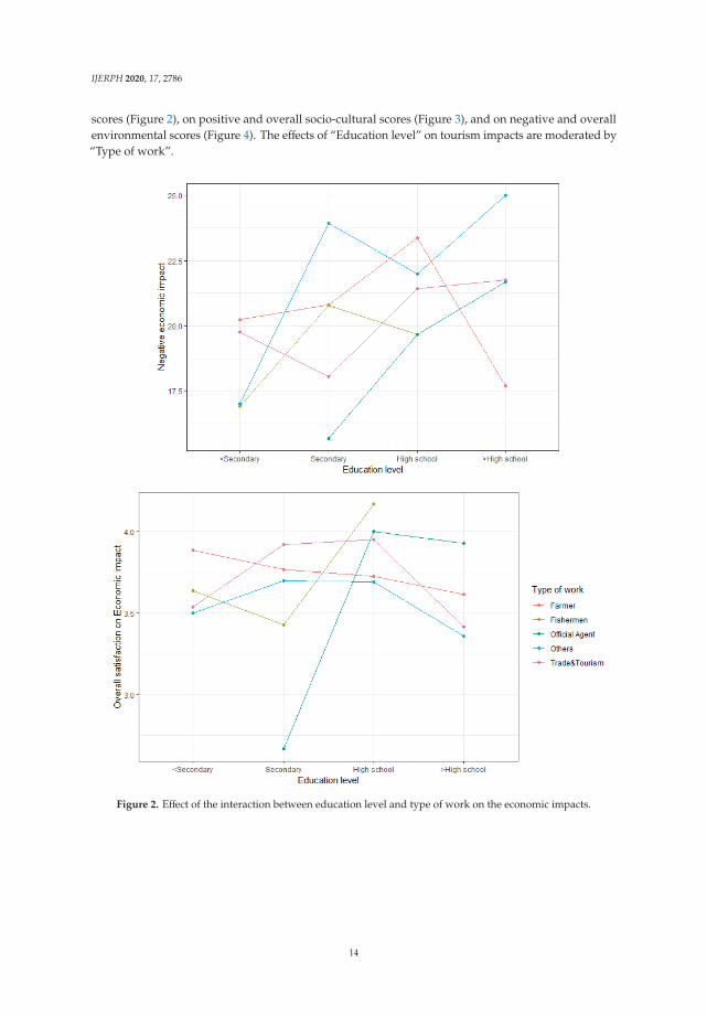
scores (Figure 2), on positive and overall socio-cultural scores (Figure 3), and on negative and overallenvironmental scores (Figure 4). The effects of “Education level” on tourism impacts are moderated by“Type of work”.

Figure 2. Effect of the interaction between education level and type of work on the economic impacts.

14

IJERPH 2020, 17, 2786

Figure 3. Effect of interaction between “Education level” and “Type of work” on the socio-cultural impacts.

15

IJERPH 2020, 17, 2786

Figure 4. Effect of interaction between “Education level” and “Type of work” on the environmental impacts.

Significant effects of the interaction between “Education level” and “Type of work” exist in termsof the negative economic impacts and overall assessment. For the negative economic impact, dramaticchanges were observed between the group of “Beyond high-school level” and “Primary level orbelow”; free laborers with primary level or below had the smallest negative scores, while those witha level above high school showed most pessimism. Farmers with a primary level of education orbelow showed the largest negative scores; on the contrary, those with the highest level of educationdemonstrated the smallest. On the overall assessment, fishermen and officials with secondary levelof education felt the least satisfied, but those with a high-school level of education felt most satisfiedcompared with the two others. Adding the interaction increases the adjusted R-squared to 10.76% inthe negative model (nearly 3% more than without interaction) and by 4.6% in the overall model (1%higher than without interaction).

16

IJERPH 2020, 17, 2786

The interaction between “Education level” and “Type of work” is a significant predictor of thepositive aspects and overall socio-cultural impact. Free laborers with primary level of education orbelow felt least pessimistic, while those with above a high-school level worried the most in terms of thesocio-cultural impacts of tourism. Farmers with a primary level of education or below ranked first inscores but those with highest educated level worried least. Officials worried more than other groups.In the overall socio-cultural satisfaction, a difference is seen between the “Secondary” group and the“High school” group: officials and fishermen with a secondary level of education were the two leastsatisfied groups, while those with a high-school level became the two most satisfied groups out of thefive. The interaction increases the adjusted R-squared in the positive model by 3.44% and confirms theadditive effect in the negative model.

A two-factor ANOVA showed the significant contribution of the interaction between “Educationlevel” and “Type of work” on the environmental impact. Regarding negative environmental scores, forresidents with primary level of education or below, farmers ranked first, free labors ranked second, andtrade and tourism services were the least. This comparison changes a lot for residents who obtained ahigher education level: farmers worried the least (together with officials), those belonging to trade andtourism services worried most, followed by free laborers. Regarding overall environmental scores, adifference was observed between the primary education or below group and the higher educationlevel: farmers in the first group felt least satisfied but most satisfied in the second one; those working inthe trade and tourism service ranked third for satisfaction but fell down to the last. The interaction andthese two factors explain 13.58% of the total variance in the negative model and 14.2% in the overallmodel, which is a substantial contribution to the whole model.

5. Discussion

Hierarchical variance analysis is a combination mathematical procedures that allows one toassess the perceived tourism impacts. It provides quantitative procedures to analyze the variancehierarchically, as well as explaining it using the factors or the regression model in the total variance,making it feasible and straightforward to apply. The approach entails two steps: (i) exploration of therelevant factors; and (ii) confirmation of their significant contribution and the effect of their interactionin explaining the residents’ assessment. The model is comprehensive and requires uncomplicatedcalculation compared with other mathematics models such as the Exploratory Factor Analysis (EFA)and Confirmation Factor Analysis (CFA). Hence, it is applicable to the data collected by structuredinterviews. However, this approach has some limitations. When the questionnaire is not well designed,the independence between factors is violated. As a result, the regression model does not follow theadditive rule. In other situations, the Fisher test does not produce a significant result, which meansthe linear regression model is invalid. Under these conditions, one has to apply other mathematicalmodels such as a Structural Equation Model (SEM), a Bayesian network, or others.

The study’s findings show that at the core of solving the negative impacts of tourism developmentis the promotion of sustainable tourism development. Particularly Vietnam, the findings suggestsignificant solutions for small islands, with their relative limited surface and their relatively limitednatural resources. Firstly, tourism should be managed in an interdisciplinary manner. The governmentshould plan to raise awareness of the noneconomic aspects of tourism development among thepublic, including environmental and socio-culture aspects. While tourism revenue continues be amost important priority, which can be improved by an increase in visitors and the development oftourism infrastructures, the control of natural resource degradation, environmental pollution, andsome negative changes in the socio-cultural life of residents should be taken into account in tourismmanagement and strategic tourism planning at both provincial and local levels. Secondly, communityparticipation (CP) in tourism planning and development should be brought to the forefront. Asocio-demographic survey provides the input data for the perception analysis of the local residents’support for tourism development, and their local participation in tourism planning. The findingsprovide a better understanding of residents’ perceptions of the local economy, and the perceived

17

IJERPH 2020, 17, 2786

impacts of tourism development on society, the economy, and environment. This offers a scientific basisto help deal with problems emerging during tourism development and also promote the participationof locals in tourism planning and development.

6. Conclusions

This study investigates the effects of socio-demographic variables on residents’ perception towardstourism development in Ly Son Island, Vietnam: the bilateral and simultaneous relationships wereassessed using a one-factor ANOVA to explore the relationships and then a linear regression analysisto confirm them. Furthermore, the interaction between two important factors (“Education level” and“Type of work”) is also explored by a hierarchical confirmation.

The results show that no marked effect of gender on the impacts of tourism is found, whilefarmers, younger, higher educated, and socially participating residents have negative assessments interms of tourism impacts. Married and socially participating residents demonstrate higher overallsatisfaction in terms of the economic impacts, and are more satisfied on the socio-cultural impacts oftourism development. Female, married people, free laborers, and nonsocially participating residentsfeel more optimistic about the environmental impacts of tourism development. The interactionbetween “Education level” and “Type of work” contributes significantly to the economic, socio-cultural,environmental impacts, and the overall impact.

Author Contributions: Conceptualization, Q.H.T. and A.T.N.; Formal analysis, T.N.L.T.; Investigation, Q.H.T.;Methodology, Q.A.T. and T.N.L.T.; Project administration, Q.H.T.; Software, Q.A.T. and T.N.L.T.; Writing—originaldraft, Q.H.T., A.T.N. and L.H.; Writing—review & editing, A.T.N. and L.H. All authors have read and agreed tothe published version of the manuscript.

Funding: This research was funded by the National Science Project: “Scientific rationale for spatial organization,model establishment and recommendations for sustainable tourism development in the coastal areas, sea andislands of Vietnam”, grant number KC.09.09/16-20.

Conflicts of Interest: The authors declare no conflict of interest.

References

1. Li, W.; Lin, L.; Shi-rong, T.; Song, L.; Zhao, Y.; Yong, W.; Dong-dong, L. Residents’ attitudes to tourismdevelopment in ancient village resorts Case study of World Cultural Heritage of Xidi and Hong villages.Chin. Geogr. Sci. 2004, 14, 170–178.

2. Sroypetch, S. The mutual gaze: Host and guest perceptions of socio-cultural impacts of backpacker tourism:A case study of the Yasawa Islands, Fiji. Mar. Isl. Cult. 2016, 5, 133–144. [CrossRef]

3. Ng, S.I.; Chia, K.W.; Ho, J.A.; Ramachandran, S. Seeking tourism sustainability—A case study of TiomanIsland, Malaysia. Tour. Manag. 2017, 58, 101–107. [CrossRef]

4. Lv, X.; Li, C.; McCabe, S. Expanding theory of tourists’ destination loyalty: The role of sensory impressions.Tour. Manag. 2020, 77, 104026. [CrossRef]

5. Robinson, D.; Newman, S.P.; Stead, S.M. Community perceptions link environmental decline to reducedsupport for tourism development in small island states: A case study in the Turks and Caicos Islands.Mar. Policy 2019, 108, 103671. [CrossRef]

6. Rasoolimanesh, S.M.; Ali, F.; Jaafar, M. Modeling residents’ perceptions of tourism development: Linearversus non-linear models. Destin. Mark. Manag. 2018, 10, 1–9. [CrossRef]

7. Almeida-García, F.; Peláez-Fernández, M.A.; Balbuena-Vázquez, A.; Cortés-Macias, R. Residents’ perceptionsof tourism development in Benalmádena (Spain). Tour. Manag. 2016, 54, 259–274. [CrossRef]

8. Sdrali, D.; Goussia-Rizou, M.; Kiourtidou, P. Residents’ perception of tourism development as a vital step forparticipatory tourism plan: A research in a Greek protected area. Environ. Dev. Sustain. 2015, 17, 923–939.[CrossRef]

9. Sita, S.E.D.; Nor, N.A.M. Degree of contact and local perceptions of tourism impacts: A case study ofhomestay programme in Sarawak. Procedia Soc. Behav. Sci. 2015, 211, 903–910. [CrossRef]

10. Naidoo, P.; Sharpley, R. Local perceptions of the relative contributions of enclave tourism and agritourism tocommunity well-being: The case of mauritius. Destin. Mark. Manag. 2016, 5, 16–25. [CrossRef]

18

IJERPH 2020, 17, 2786

11. Garau-Vadell, J.B.; Gutierrez-Taño, D.; Diaz-Armas, R. Economic crisis and residents’ perception of theimpacts of tourism in mass tourism destinations. Destin. Mark. Manag. 2018, 7, 68–75. [CrossRef]

12. Sun, Y.; Cruz, M.J.; Min, Q.; Liu, M.; Zhang, L. Conserving agricultural heritage systems through tourism:Exploration of two mountainous communities in China. Mt. Sci. 2013, 10, 962–975. [CrossRef]

13. Zhang, Y.; Zhang, J.; Zhang, H.; Zhang, R.; Wang, Y.; Guo, Y.; Wei, Z. Residents’ environmental conservationbehaviour in the mountain tourism destinations in China: Case studies of Jiuzhaigou and Mount Qingcheng.Mt. Sci. 2017, 14, 2555–2567. [CrossRef]

14. Diaz-Farina, E.; Díaz-Hernández, J.J.; Padrón-Fumero, N. The contribution of tourism to municipal solidwaste generation: A mixed demand-supply approach on the island of Tenerife. Waste Manag. 2020, 102,587–597. [CrossRef]

15. Chiu, H.Y.; Chan, C.S.; Marafa, L.M. Local perception and preferences in nature tourism in Hong Kong. Tour.Manag. Perspect. 2016, 20, 87–97. [CrossRef]

16. Lee, T.H.; Jan, F.H. Can community-based tourism contribute to sustainable development? Evidence fromresidents’ perceptions of the sustainability. Tour. Manag. 2019, 70, 368–380.

17. Liang, Z.X.; Hui, T.K. Residents’ quality of life and attitudes toward tourism development in China.Tour. Manag. 2016, 57, 56–67. [CrossRef]

18. Bimonte, S.; Faralla, V. Does residents’ perceived life satisfaction vary with tourist season? A two-step surveyin a Mediterranean destination. Tour. Manag. 2016, 55, 199–208.

19. Wassler, P.; Nguyen, T.H.H.; Mai, L.Q.; Schuckert, M. Social representations and resident attitudes: Amultiple-mixed-method approach. Ann. Tour. Res. 2019, 78, 102740. [CrossRef]

20. Zhang, H.; Xu, H. Impact of destination psychological ownership on residents’ “place citizenship behavior”.Destin. Mark. Manag. 2019, 14, 100391. [CrossRef]

21. Huang, K.; Pearce, P. Visitors’ perceptions of religious tourism destinations. Destin. Mark. Manag. 2019, 14, 100371.[CrossRef]

22. Stylidis, D.; Biran, A.; Sit, J.; Szivas, E.M. Residents’ support for tourism development: The role of residents’place image and perceived tourism impacts. Tour. Manag. 2014, 45, 260–274. [CrossRef]

23. Šegota, T.; Mihalic, T.; Kušcer, K. The impact of residents’ informedness and involvement on their perceptionsof tourism impacts: The case of bled. Destin. Mark. Manag. 2017, 6, 196–206. [CrossRef]

24. Woosnam, K.M.; Draper, J.; Jiang, J.K.; Aleshinloye, K.D.; Erul, E. Applying self-perception theory to explainresidents’ attitudes about tourism development through travel histories. Tour. Manag. 2018, 64, 357–368.[CrossRef]

25. Boley, B.B.; McGehee, N.G.; Perdue, R.R.; Long, P. Empowerment and resident attitudes toward tourism:Strengthening the theoretical foundation through a Weberian lens. Ann. Tour. Res. 2014, 49, 33–50. [CrossRef]

26. Vargas-Sánchez, A.; Oom do Valle, P.; da Costa Mendes, J.; Silva, J.A. Residents’ attitude and level ofdestination development: An international comparison. Tour. Manag. 2015, 48, 199–210. [CrossRef]

27. Kang, S.K.; Lee, J. Support of marijuana tourism in Colorado: A residents’ perspective using social exchangetheory. Destin. Mark. Manag. 2018, 9, 310–319. [CrossRef]

28. Choi, Y.H.; Song, H.; Wang, J.H.; Hwang, J. Residents’ perceptions of the impacts of a casino-based integratedresort development and their consequences: The case of the Incheon area in South Korea. Destin. Mark.Manag. 2019, 14, 100390. [CrossRef]

29. Nunkoo, R.; Gursoy, D. Residents’ support for tourism. Ann. Tour. Res. 2012, 39, 243–268. [CrossRef]30. Ouyang, Z.; Gursoy, D.; Sharma, B. Role of trust, emotions and event attachment on residents’ attitudes

toward tourism. Tour. Manag. 2017, 63, 426–438. [CrossRef]31. Wang, J.; Liu-Lastres, B.; Ritchie, B.W.; Pan, D.Z. Risk reduction and adventure tourism safety: An extension

of the risk perception attitude framework (RPAF). Tour. Manag. 2019, 74, 247–257. [CrossRef]32. Vincenzi, S.L.; Possan, E.; de Andrade, D.F.; Pituco, M.M.; de Santos, T.O.; Jasse, E.P. Assessment of

environmental sustainability perception through item response theory: A case study in Brazil. Clean. Prod.2018, 170, 1369–1386. [CrossRef]

33. Yan, L.; Gao, B.W.; Zhang, M. A mathematical model for tourism potential assessment. Tour. Manag. 2017,63, 355–365. [CrossRef]

34. Sheppard, V.A.; Williams, P.W. Factors that strengthen tourism resort resilience. Hosp. Tour. Manag. 2016, 28,20–30. [CrossRef]

19

IJERPH 2020, 17, 2786

35. Kim, K.; Uysal, M.; Sirgy, M.J. How does tourism in a community impact the quality of life of communityresidents? Tour. Manag. 2013, 36, 527–540. [CrossRef]

36. Moghavvemi, S.; Woosnam, K.M.; Paramanathan, T.; Musa, G.; Hamzah, A. The effect of residents’ personality,emotional solidarity, and community commitment on support for tourism development. Tour. Manag. 2017,63, 242–254. [CrossRef]

37. Jordan, E.J.; Spencer, D.M.; Prayag, G. Tourism impacts, emotions and stress. Ann. Tour. Res. 2019, 75,213–226. [CrossRef]

38. Blieszner, R.; Roberto, K.A.; Singh, K. The helping networks of rural elders: Demographic and socialpsychological influences on service use. Ageing Int. 2001, 27, 89. [CrossRef]

39. Fayos, G.T.; Gallarza, G.M.G.; Arteaga, M.F.; Elena, F.I. Measuring socio-demographic differences involunteers with a value-based index: Illustration in a mega event. Voluntas 2014, 25, 1345–1367. [CrossRef]

40. Mak, W.; Rosenblatt, A. Demographic influences on psychiatric diagnoses among youth served in Californiasystems of care. Child Fam. Stud. 2002, 11, 165–178. [CrossRef]

41. Van der Steina, A.; Rozite, M. Tourism development in Riga: Resident attitudes toward tourism. In Tourismin Transitions. Geographies of Tourism and Global Change; Müller, D., Wieckowski, M., Eds.; Springer: Cham,The Netherlands, 2018; pp. 137–155.

42. Yergeau, M.E. Tourism and local welfare: A multilevel analysis in Nepal’s protected areas. World Dev. 2020,127, 104744. [CrossRef]

43. Develles, R.F. Scale Development: Theory and Applications; Sage Publications: Southend Oaks, CA, USA, 1991;pp. 24–33.

44. Kline, P. The Hand$book of Psychological Testing, 2nd ed.; Routledge: London, UK; Abingdon, UK, 2000; p. 13.45. Pardoe, I. Multiple Linear Regression Model Evaluation (Lecture 6); In STAT 501 Online Course; Department

of Statistics, Eberly College of Science. Available online: https://online.stat.psu.edu/stat501/lesson/6/6.2(accessed on 22 March 2020).

46. Ramachandran, K.M.; Tsokos, C.P. Mathematical Statistics with Applications; Elsevier Academic Press:Amsterdam, The Netherlands, 2009; p. 503.

47. Zar, J.H. Two-factor analysis of variance. In Biostatistical Analysis; Lynch, D., O’Brien, C., Eds.; PearsonPrentice Hall: Upper New Jersey River, NJ, USA, 2010; pp. 251–253.

48. LSGOS (General Statistics Office of Ly Son). Statistical Yearbook of Ly Son District 2018; Statistics Publishing:Quang Ngai, Vietnam, 2018; 234p.

© 2020 by the authors. Licensee MDPI, Basel, Switzerland. This article is an open accessarticle distributed under the terms and conditions of the Creative Commons Attribution(CC BY) license (http://creativecommons.org/licenses/by/4.0/).

20

International Journal of

Environmental Research

and Public Health

Article

Sustainable Tourism as a Source of Healthy Tourism

Luna Santos-Roldán 1,*, Ana Mª Castillo Canalejo 1, Juan Manuel Berbel-Pineda 2 and

Beatriz Palacios-Florencio 2

1 Department of Statistics, Business Organization and Applied Economics, Faculty of Law and Business,University of Córdoba, 14071 Córdoba, Spain; acastillo@uco.es

2 Department of Business Organization and Marketing Faculty of Business Studies, University of Pablo deOlavide, CarreteraUtrera, Km.1, 41013 Seville, Spain; jmberpin@upo.es (J.M.B.-P.); bpalacios@upo.es (B.P.-F.)

* Correspondence: td1sarol@uco.es

Received: 26 June 2020; Accepted: 16 July 2020; Published: 24 July 2020

Abstract: Even though the World Tourism Organization described Sustainable Tourism as a tourismform that could contribute to the future survival of the industry, the current reality is quite different,since it has not been firmly established in society at expected levels. The present study analyzeswhich variables drive the consumption of this tourism type, taking tourist awareness as the keyelement. To this awareness, we must add the current crisis experienced by the tourism industrycaused by COVID-19, since it can benefit Sustainable Tourism development, promoting less crowdeddestinations that favor social distancing. For this, the existing literature on Sustainable Tourismhas been examined in order to create a model that highlights the relations among these variables.To determine the meaning of these relations, a sample of 308 tourists was analyzed through structuralequation models using Partial Least Squares. The results show that there is a clear attitude on thepart of the tourist to develop Sustainable Tourism, driven by the positive effects and motivation itentails, as well as the satisfaction the tourist perceives when consuming a responsible tourism type.

Keywords: sustainable tourism; attitude; positive effects; motivation; satisfaction

1. Introduction

The World Tourism Organization (UNWTO) in 2005 defined the concept of Sustainable Tourism as“one whose practices and principles can be applicable to all forms of tourism in all types of destinations,including mass tourism and the various niche tourism segments”. Sustainability principles referto the environmental, economic, and socio-cultural aspects of tourism development, and a suitablebalance must be established among these three dimensions to guarantee its long-term sustainability [1].In addition to international organizations, we also find many authors who have defined the concept ofsustainable tourism [2–6]. Conversely, despite the fact that sustainable tourism has been recognized inbusiness practice, the volume of academic research has not been as relevant as might be expected [7].From the start, the development of sustainable tourism is based on environmental preservation, culturalauthenticity and the profitability of the tourist activity in the destination [8]. In this tourism type,both social return and the reversed well-being index on the visited destinations are recognized, as wellas the economic return—in other words, whether the tourist activity generates enough income for thelocal population in terms of employment, wealth and available resources [9].

This study aims to establish the factors that allow sustainable tourism development, which isreally necessary for the industry in the context of the crisis caused by COVID-19. From a theoreticalpoint of view, motivational factors, economic impact and satisfaction are analyzed as attributes thatpotentially influence the intention and attitude of choosing this type of tourism.

Hence, one of the possible solutions the tourism industry can find to help the current crisis that itfaces as a consequence of COVID-19 could come from Sustainable Tourism. Finding solutions is more

IJERPH 2020, 17, 5353; doi:10.3390/ijerph17155353 www.mdpi.com/journal/ijerph21

IJERPH 2020, 17, 5353

than necessary in those countries where the tourism industry plays an important role in the economy.Thus, in the case of Spain, it must be considered that it is a country highly dependent on tourism.In 2019, it was the second world destination in terms of international tourist arrivals (83.3 millions),with EUR 92.5 billion in tourism revenue, 2.8 million direct jobs and a contribution to GDP of 14.2% [10].In this way, tourism is considered the main industry in the country. Therefore, in order to preserve thissituation, it is essential to promote developing a sustainable industry over time and, perhaps morenecessary than ever, this tourism type.

The contribution of this research is double-edged. Firstly, we present a model that relates a set ofvariables obtained from the literature and that must be considered for sustainable tourism developmentfrom the perspective of the tourist (applicant for tourist services). Secondly, we propose a hypothesisset that seeks to analyze both the level and strength of these relations as drivers of an attitude favorableto sustainable tourism development. The study begins with a review of the literature to considerthe relation among the variables considered in the study. Next, the methodology used in the datacollection is explained to later expose the results analysis, as well as the discussion and conclusions,which complete the final sections of this study.

2. Literature Review

2.1. Relation between Positive Impacts and Attitude towards Sustainable Tourism

According to [11], tourism impacts are the result of human behavior stemming from interactionsbetween tourists and the subsystems of the territory where they come into play. Throughout thepublications that take the study of sustainable tourism as a main topic, the doctrine that corroboratesthe effects of positive impacts is predominant, whose consequences affect residents, economy andenvironment [12]. Firstly, the main positive economic aspects are based on greater economicmovement, contribution to GDP, job creation and income distribution in other local economic activities.Secondly, regarding residents, the well-being of the local and tourist population is taken into accountmeticulously, in addition to the respect and preservation of the culture and heritage of the hostregion. Thirdly, as sustainable tourism is closely related to the environment, due to its use of naturalresources, it highly depends on having an attractive natural environment. This produces an increasedenvironmental awareness in society, as well as the revaluation of the natural environment through theapproval of environmental quality conservation, protection and improvement measures [13–16].

Sustainable tourism development is inherent to those tourists capable of showing a greaterawareness of the sustainability problem [17], who are averse to mass tourism development andseek to contribute to destination protection when choosing. Sensitive to the negative impacts oftourism, they support the development of respectful sustainable tourism from an economic, social andenvironmental perspective [18,19]. In accordance with [20], that the positive impacts of awareness ofthe protection of natural resources, cultural resources and the increase in local recreational facilitiesand resources were considered. From the study of these authors, the following hypothesis is proposed:

Hypothesis 1 (H1). The positive impact on tourists has a direct and positive influence on their attitude towardssustainable tourism development.

2.2. Relation between Satisfactory Experience and Attitude towards Sustainable Tourism

Customer motivation is identified as a determinant factor in the success of all industries [21] and,homogeneously, in the case of the tourism sector, influences future intentions of purchase and visitingof the same destination [22]. The success of a global model of sustainable tourism requires achievinghigh levels of tourist satisfaction, thus increasing their awareness of the problems that sustainabilityencompasses and promoting more respectful practices. This long-term maintenance of the applicant’ssatisfaction guarantees the consolidation of the destination in the market and, at the same time, it favors

22

IJERPH 2020, 17, 5353

an adequate demand according to its attractions [23]. This satisfaction is configured based on previousexpectations and evaluation after finishing the tourist experience [24,25].

Recent studies have analyzed this direct relation between both constructs, linked to a givengeographic environment [25–28]. This study covers a geographic area not detected in the literaturereview and, in line with the proposed authors, the second of the hypotheses is established:

Hypothesis 2 (H2). Experiential satisfaction has a direct and positive influence on the attitude towardssustainable tourism.

2.3. Motivation and Attitude Relation towards Sustainable Tourism

Motivation has been analyzed as an internal factor that guides and integrates the behavior of theindividual. It is a psychological factor that leads people to act in a certain way to satisfy their desiresand goals [29] and, therefore, a driver that motivates people to take vacations or visit destinations [4].Motivation is related to the attitudes and intentions of tourists when choosing a destination [30,31],and the experience gained in situ is crucial to satisfy that motivation and increase the loyalty to a touristdestination [32]. Hence, tourist motivation is not only useful to explain tourist behavior, but also actsas a predictor of the visit intention [33].

The customer’s profile of sustainable tourism involves a tourist committed to the environmentand who is aware of sustainability. As tourist motivation has positive effects on the visit intention,various studies [34–37] confirm that the experience is more attractive to tourists when they participatein activities entailing more responsible behavior and greater involvement with the environment,the local community and society. In this way, a direct relation between motivation and attitude towardssustainable tourism is established. From the reading of these authors, the third hypothesis is proposed:

Hypothesis 3 (H3). Motivation has a direct and positive influence on the attitude towards sustainable tourism.

2.4. Moderating Effect of Motivation in the Relation between Positive Impacts and Attitude towardsSustainable Tourism

Most research concludes that the three basic categories of benefits and costs that affecta community which receives tourists are economic, environmental, and social [5,38–43], although [2]also incorporate institutional sustainability. Likewise, the sustainability principles imply a balance ofthese three dimensions: environment, economy and society [32]. Most studies report a positive relationbetween the attitude towards sustainable tourism development and the perception of its positiveimpacts [2,5,26,44–46].

In the tourism context, motivation is one of the most important values regarding behavioralintentions among revisiting a place, word of mouth and the search for alternative destinations [47].This is why tourists more committed to the balance among sustainability dimensions show a highermotivation towards this tourism type and, on the other hand, there is a direct and positive relationbetween these two variables, as other authors have analyzed [36,37]. Therefore, research has focusedon the direct relation between positive impacts and motivation with an implication towards sustainabletourism (hypotheses 1 and 3 of the model); however, the moderating effect that motivation can have onpositive impacts and sustainable tourism has not been analyzed. Therefore, the following hypothesisis formulated:

Hypothesis 4 (H4). Motivation has a moderating effect on positive impacts and the attitude towardssustainable tourism.

23

IJERPH 2020, 17, 5353

2.5. Moderating Effect of Motivation in the Relation between Satisfaction and Attitude towardsSustainable Tourism

Understanding what factors influence tourist satisfaction is one of the most relevant researchtopics in the tourism sector, due to the impact it has on the success of any tourism product or service.Most tourists can compare the aspects of different destinations (such as services, attractions, etc.)according to their perceptions. A high level of tourist satisfaction fosters positive future behaviors,such as the intention to revisit and recommend a destination [48].

The relation of satisfaction and motivation with the attitude towards sustainable tourism hasbeen analyzed in the scientific literature by various studies [36,37,49–51] to refer to the tourists’general evaluations of their experiences with environment respect and their expectations regardingthe sustainable development of tourist destinations or services. Similarly, the moderating effect ofsatisfaction with sustainable tourism and other variables, such as the recommendation of a destinationand emotional value, have also been analyzed [32]. However, the moderating effect that motivationcan have on the relation between satisfaction and attitude towards sustainable tourism has not beenexamined. Consequently, we deduce from the collected studies that the higher the motivation ofa tourist to visit ecological and sustainable environments is, the greater the impact of said relation is.Therefore, the following model hypothesis is suggested:

Hypothesis 5 (H5). Motivation has a moderating effect between satisfaction and attitude towardssustainable tourism.

All hypothesis are represented in Figure 1:

Figure 1. Conceptual model. Source: Own elaboration. While H1, H2 and H3 consider a directinfluence between constructs, H4 and H5 include a moderator perspective.

3. Data and Methodology

3.1. Participants

The data were collected from tourists who visited the city of Córdoba (Spain) between the monthsof October and November 2019. Córdoba (a World Heritage city) is one of the main cities receivingtourism (both national and international). This means that one of the main challenges it faces is itsmassification and the problems associated. The measurement instrument was completed by a total of308 subjects.

Table 1 shows the main aspects related to the respondents’ profiles. It has to be emphasized thata relative equality is observed regarding the origin of the tourists surveyed. In general, these aretourists who came on holidays that they financed and, in a high percentage of cases, that were based ontheir own decisions. The questionnaire was personally distributed among the main tourist attractionslocated inside the old quarter. More than 60% of the travelers were 35 years old or more, had a stable

24

IJERPH 2020, 17, 5353

partner (married and living as a couple), lived in households based on two or more people and earneda monthly income of between EUR 1000 and 2000. Although the majority of the respondents statedthat they were visiting this city for the first time (62.7%), a high percentage (close to 40%) repeatedtheir destination. On average, the tourists who participated in the study stayed in the city for 2–3 days.

Table 1. Respondent characteristics.

Descriptive Variables Absolute Frequency Percentage

Sex

Male 142 46.1Female 166 53.9

Nationality

Spaniard 163 52.9Other 145 47.1

Visit purpose

Work 23 7.5Vacancy 150 48.7Visit friends 47 15.3Family event 25 8.1Independent journey 39 12.7Others 24 7.8

Person who paid for the visit

Myself 140 45.5My company 29 9.4My partner 63 20.5Friends 10 3.2Family 60 19.5Others 6 1.9

Person who proposed the destination

Myself 111 36.0My company 31 10.1My partner 55 17.9Friends 36 11.7Family 71 23.1Others 4 1.3

Professional status

Student 54 17.5Freelance 43 14.0Employed person 141 45.8Unemployed person 16 5.2Retired person 19 6.2Homemaker 28 9.1Lost 7 2.3

Age

65 years old or more 21 6.855–64 years old 45 14.645–54 years old 79 25.6

35–44 years old 57 18.526–34 years old 43 14.018–25 years old 62 20.1Lost 1 0.3

25

IJERPH 2020, 17, 5353

Table 1. Cont.

Descriptive Variables Absolute Frequency Percentage

Marital status

Single 78 25.3Married 135 43.8Common-law relationship 60 19.5Divorced 27 8.8Widow/er 7 2.3Lost 1 0.3

Household size

Individual 37 12.02 people 126 40.93 people 73 23.14 people 58 18.85 or more people 14 4.5Lost 2 0.6

Salary

Less than EUR 999 71 23.1EUR 1000–1499 96 31.2EUR 1500−1999 72 23.4EUR 2000 and over 60 19.5Lost 9 2.9

Source: Own elaboration.

3.2. Measurements

In relation to the instruments used, special interest was placed on translating the original versionsof the scales to the linguistic characteristics of the population. All variables were measured on a Likertscale from 1 to 5, where 1 = totally disagree and 5 = totally agree.

The items in the questionnaire were translated and adapted for the different constructs. The itemsof positive socio-cultural, economic and environmental impacts were extracted and adapted from [20].The items related to experiential satisfaction were obtained from the research carried out by [51].The items of Sustainable Tourism Development Attitude were adapted from the study of [26].Finally, the construct of motivation was extracted and adapted from [4].

3.3. Data Analysis

The relations among the variables, with special emphasis on the moderating effect of the satisfactionexperience, were analyzed with a structural equation model based on variance—the Partial LeastSquares (PLS). Furthermore, the recommendations of various authors were followed: [52] and [53].The computer software used was SmartPLS 3.2.8.

The use of a single instrument to collect data on constructs (latent variables) implies the need tocheck the existence of a common variance among them. Following the experts’ opinions [54,55] onthe design and execution process of questionnaires, we proceeded to separate the different measures,as well as to guarantee the anonymity of the respondents. The presence of common influence onresponses was analyzed using the [56]. The exploratory factor analysis recorded the existence of12 factors, where the largest of them explains 17% of the total variance. Therefore, there is no commonfactor of influence among the items included in the questionnaire [57].

The validation of the proposed model was carried out at a double level. Firstly, the measurementmodel. Once the validity of the model was checked, the structural model was validated.

26

IJERPH 2020, 17, 5353

4. Results and Discussion

4.1. Measurement Model

The mean and standard deviation values of each item, as well as the latent variables, are given inTable 2. In addition, this table includes the data required to perform the first step in the validation ofthe measurement model: determining the reliability of the individual items. It can be seen that thefactorial loads of most of the items exceed the minimum criterion of 0.707 [58]. Only one item witha lower value has been maintained, although it is very close (0.692). This item was not eliminatedafter checking its significance level via bootstrapping (5000 subsamples) and in accordance with thesuggestions of [59]. Finally, 22 elements of a total of 31 items related to the constructs of the modelanalyzed were removed.

Table 2. Mean, standard deviation, individual reliability, composed reliability and average varianceextracted for constructs and indicators.

Construct and Indicator Mean SD LoadingComposedReliability

AVE

Global positive impacts (GPI) 3.35 1.110 0.885 0.719

Tourism promotes awareness of theprotection of natural resources 3.13 1.237 0.807

Tourism promotes awareness of theprotection of cultural resources 3.44 1.324 0.877

Tourism increases local recreationalfacilities and resources 3.46 1.366 0.858

Sustainable Tourism DevelopmentAttitude (SUS) 3.43 0.991 0.800 0.668

I think the attitudes and behaviors oflocal tourists are satisfactory and donot disturb residents

3.25 1.106 0.743

I think that the positive aspects of thedevelopment of Sustainable Tourismare greater than their negative aspects

3.61 1.306 0.885

Experiential satisfaction (SAT) 4.02 0.803 0.765 0.622

It is worth visiting a sustainable city 4.07 1.062 0.692

I feel that I contribute to environmentprotection and Sustainable Tourism 3.97 0.941 0.875

Motivation (MOT) 4.46 0.585 0.749 0.600

I want to travel somewhere that offersan ecological environment 4.17 0.900 0.825

I want to experience different culturesfrom mine 4.75 0.574 0.720

Source: Own elaboration.

In order to set the construct’s reliability, the composite reliability index (�c) was used [60]. All itsvalues, included in Table 2, are above the minimum threshold: above 0.7 [61]. The previous tablealso shows the AVE value, which is used to determine the convergent validity, since it exceeds theminimum level of 0.5 in all latent variables [62].

To determine the discriminant validity of the model constructs, we used the Fornell–Larcker testand the corresponding values are shown in Table 3. These table data verify that all the constructsstrictly meet the Fornell–Larcker criterion. In short, this allows us to affirm the existence of discriminantvalidity among the latent variables and the way of measuring them.

27

IJERPH 2020, 17, 5353

Table 3. Constructs discriminant validity (Fornell–Larcker criterion).

Constructs GIP MOT SUS SAT

GIP 0.848

MOT 0.190 0.774

SUS 0.646 0.215 0.817

SAT 0.303 0.131 0.382 0.789

GIP: Global positive impacts; MOT: Motivation; SUS: Sustainable Tourism Development Attitude; SAT: Experientialsatisfaction. Diagonal elements (bold figures) are the square root of the variance shared between the constructs andtheir measures. Off-diagonal elements are the correlations among constructs. For discriminant validity, diagonalelements should be larger than off-diagonal.

After validating the measurement model, it is necessary to validate the structural model.

4.2. Structural Model

Following the opinion of [63], this study should start with the analysis of the sign, size andsignificance of the path coefficients, the values of R2 and the Q2 test. [59] recommend the use of thebootstrapping technique with 5000 samples to calculate the t statistics and the confidence intervals,which will allow for establishing the significance of the relations. The two-step technique has beenfollowed for the analysis of the moderating effects [59]. Table 4 shows the direct effects (path coefficients),the values of the t statistic, the corresponding confidence intervals (without bias) and the verificationof whether the proposed hypotheses have been supported, without forgetting the values of R2 and Q2.

Table 4. Direct effects on endogenous variables.

Effects onEndogenous Variables

Path (β)t Value

(Bootstrap)Confidence

IntervalExplainedVariance

Support

Sustainable TourismDevelopment AttitudeAdj R2 = 0.470/Q2 = 0.297)

H1: Global positive impacts 0.568 *** 14.393 (0.500; 0.627) Sig 36.69% Yes

H2: Experiential satisfaction 0.212 *** 4.957 (0.137; 0.279) Sig 8.09% Yes

H3: Motivation 0.064 ns 1.438 (−0.015; 0.133) 1.38% No

H4: Global positive impacts xMotivation (interaction term) −0.120 ** 2.640 (−0.195; −0.046) Sig Yes

H5: Experiential satisfaction xMotivation (interaction term) 0.073 * 1.872 (0.012; 0.140) Sig Yes

*** p < 0.001, ** p < 0.01, * p < 0.05; ns: not significant.; nd: not determined. t (0.05; 4999) = 1.645, t (0.01; 4999) = 2.327,t (0.001; 4999) = 3.092. One-tailed test.

In order to have a greater awareness of the attitude of the tourist (consumer of tourist services)towards sustainable tourism development, it is necessary to know what variables influence it. Based onprevious work on Sustainable Tourism, this study designs a model where a set of variables thatinfluence the attitude towards the development of Sustainable Tourism are described. The relationsamong them and the consistency of this relation have also been analyzed.

Not all the hypotheses presented have been validated. The hypothesis that relates positiveeconomic impacts to attitude presents higher parameters (β, T-Student) than other variables (GIP ATT;β = 0.568; t = 14.393). Furthermore, the relation with satisfaction for the experience had developingthis modality of tourism shows quite adequate levels (SAT ATT; β = 0.212; t = 4.957). This reveals theimportant role played by the tourist’s awareness and their contribution so that Sustainable Tourismcan be developed. Lower levels are found in the hypothesis that relates motivation to attitude(MOT ATT; β = 0.064; t = 1.438). This means that this relation is presented as “not significant”.

28

IJERPH 2020, 17, 5353

However, the variable “motivation” also has a moderating effect on the relations shown in the model,both the one we observe in positive impacts and the one that appears in satisfaction on the attitude forsustainable tourism development. Thus, we find that, as motivation increases, the satisfaction effect onattitude also grows (β = 0.073; t = 1.852). However, the moderating effect of the variable “motivation”is the opposite in the relation between positive impacts and attitude (β = −0.120; t = 2.640). In otherwords, the less motivation there is, the less the impact effect on the attitude will be reduced (Figure 2).

Figure 2. Structural model.

This study is in line with previous works that have highlighted the importance of tourist awarenessfor sustainable tourism development [12,24,25,28,37]. Similarly, it is in line with the recently publisheddocument “Covid-19: EU Guide to the progressive resumption of tourism services and health protocolsin hotels” [64]. It is essential to develop Covid-19-related protocols for hotel establishments [65–67].These protocols corroborate many of the guidelines that must be followed for sustainable tourismdevelopment, fundamentally related to environmental protection, based on a commitment to reducedestination massification in order to avoid tourist overcrowds. In this way, it will be possible to maintaina safe distance among people while consuming tourist services, which comprises the main concern ofthe health authorities. Nevertheless, we note that the health authorities have not clearly communicatedthese protocols yet. This lack of information will lead to a certain delay in the implementation ofmeasures in tourist offers, which could help sustainable tourism development.

We believe that, as health authorities establish the protocols to responsibly and safely developtourism, and as long as the tourists are aware of their implementation, it is quite probable that the levelof the different variables of the proposed model (positive impacts, satisfaction and motivation towardsthe attitude for sustainable tourism development) will increase due to a greater knowledge on the partof the tourist. A higher level of awareness, fundamentally supported by the security that tourists needin the current context, can lead them to consume tourist services.

5. Conclusions

The development of sustainable tourism requires, mainly, an awareness on the part of the touristservices applicant (the tourist). According to the analysis of the literature, we find a series of factorsthat can contribute to increasing positive attitudes towards sustainable tourism development from theperspective of demand. Through this analysis and a methodology focused on personal surveys carried

29

IJERPH 2020, 17, 5353

out on tourists using a questionnaire, the factors that make tourists have a favorable attitude towardssustainable tourism development have been determined. Based on this study and the results obtainedfrom the fieldwork, in addition to the analysis of the tourist-industry situation after the health crisis,a series of conclusions are drawn from both theoretical and empirical perspectives.

5.1. Theoretical Perspective

Firstly, in the literature, we find three factors that lead to a favorable attitude for sustainabletourism development from the tourist’s perspective. On the one hand are the positive effectsperceived by the tourist with the consumption of sustainable tourism, whose consequences affect theresident’s, economy and destination environment [12,16]. On the other hand, customer satisfactionis identified as a determinant of success in any industry [21] and, therefore, in the tourismindustry [28]. Finally, motivation is related to the attitudes and intentions of tourists when choosinga destination [30,31]. However, this motivation plays a moderating (and different) role in the relationbetween the positive effects and the attitude towards sustainable tourism development and in therelation between satisfaction and the attitude towards sustainable tourism. Thus, motivation harms thepositive impact and favors the satisfaction effects on the attitude of sustainable tourism development.

Secondly, after reviewing studies and reports on the current context of the tourism industry, it canbe affirmed that there is a need to develop protocols (based on the perspective that tourist servicesoffer) which reaffirm tourists’ commitments to consume sustainable tourism. This perspective is notincluded in the model (which only analyzes the demand perspective); however, from a theoreticalpoint of view, it does seem necessary to consider. In this scenario, the performance of the presentedempirical study is one more reference to contemplate that the tourist (applicant for tourist services)becomes a fundamental element for sustainable tourism development. Nevertheless, for their safety,the tourist will demand tourist services that take into account hygiene and health factors [65] andaspects related to social distancing [68,69].

5.2. Empirical Perspective

Firstly, only two of the three main hypotheses regarding the direct effects are supported.The attitude towards sustainable tourism development is positively influenced by the global positiveimpacts perceived by the tourist and by the satisfaction experienced with the consumption of thistourism type. The value of R2 indicates an appropriate predictive level for the “attitude towardssustainable tourism development” variable, which is reinforced by the value of Q2.

Secondly, it is important to highlight that the “motivation” variable plays a moderating roleregarding the impacts on the relations of the other two variables analyzed. In the case of positiveglobal impacts, the incidence of motivation is negative—in other words, the less motivated a subject is,the lower the effect of global positive impacts on the attitude towards sustainable tourism developmentwill be. On the other hand, motivation seems to increase the effect of the satisfaction experienced onthe attitude towards sustainable tourism development.

In summary, sustainable tourism can build on the momentum provided by this context of healthcrisis to increase a favorable attitude towards sustainable tourism development. Achieving thisattitude will allow for an increase in the tourist’s awareness, translated as the tourist’s perceptionof the positive impact and the satisfaction experienced with the consumption of this tourism type.Likewise, motivation is a factor that also favors the attitude towards sustainable tourism development.At the same time, a priori, the role played by the tourist offer (companies and authorities) to helpincrease this tourist awareness will also be important.

5.3. Limitations and Future Studies

The main limitation we find in the present work is that the study was carried out prior to the crisiscaused by COVID-19; therefore, aspects such as changes in attitudes, motivations and perceptionsrelated to and caused by this new situation were not considered at any time. However, the study

30

IJERPH 2020, 17, 5353

focused on analyzing the importance of sustainable tourism. Without doubt, this relevance will bedriven by this new situation. Therefore, it would be very convenient to replicate this work in the futurewhen total mobility within national territories begins to be allowed and the circulation of tourists isallowed internationally. Thus, for example, an aspect that was not supported in the present work is theimportance of positive impacts a destination could have, which did not suppose a motivation for itschoice. Thanks to the different government campaigns that are being recently launched with the aimof achieving positive impacts from visiting certain destinations, we think that this aspect could changedue to the increased sensitivity perceived by the tourist. In short, it is necessary to find formulas thatboost the tourism industry. The development of sustainable tourism can help to mitigate tourists’perceived fears of visiting destinations with a large concentration of people.

Therefore, it would also be interesting to launch a study that considers the actions carried out bythe tourism offer in order to verify its impact on the attitude towards sustainable tourism development.

Author Contributions: Conceptualization, A.M.C.C., J.M.B.-P. and L.S.-R.; methodology, B.P.-F.; formal analysisB.P.-F.; writing—original draft preparation, A.M.C.C., J.M.B.-P. and L.S.-R.; writing—review and editing, L.S.-R.All authors have read and agreed to the published version of the manuscript.

Funding: This research received no external funding.

Conflicts of Interest: The authors declare no conflict of interest.

References

1. UNWTO. 2005. Available online: https://www.unwto.org/sustainable-development (accessed on 26 June 2020).2. Hussain, K.; Ali, F.; Ari Ragavan, N.; Singh Manhas, P. Sustainable tourism and resident satisfaction at

Jammu and Kashmir, India. Worldw. Hosp. Tour. Themes 2015, 7, 486–499. [CrossRef]3. Zamfir, A.; Corbos, R.A. Towards Sustainable Tourism Development in Urban Areas: Case Study on

Bucharest as Tourist Destination. Sustainability 2015, 7, 12709–12722. [CrossRef]4. Mohaidin, Z.; Tze Wei, K.; Ali Murshi, M. Factors influencing the tourists’ intention to select sustainable

tourism destination: A case study of Penang, Malaysia. Int. J. Tour. Cities 2017, 3, 442–465. [CrossRef]5. Chi-Ming, H.; Chang, H.; Sung Hee, P. A study of two stakeholders’ attitudes toward sustainable tourism

development: A comparison model of Penghu Island in Taiwan. Pac. J. Bus. Res. 2017, 8, 2–28.6. Higgins-Desbiolles, F.; Carnicelli, S.; Krolikowski, C.; Wijesinghe, G.; Boluk, K. Degrowing tourism:

Rethinking tourism. J. Sust. Tour. 2019, 27, 1926–1944. [CrossRef]7. Ruhanen, L.; Weiler, B.; Moyle, B.D.; McLennan, C.L.J. Trends and patterns in sustainable tourism research:

A 25-year bibliometric analysis. J. Sust. Tour. 2015, 23, 517–535. [CrossRef]8. Crosby, A. Elementos Básicos para un Turismo Sostenible en las áreas Naturales; Centro Europeo de Formación

Ambiental y Turística: Madrid, Spain, 1996.9. Fernández Poncela, A.M. Turismo, Negocio o Desarrollo: El Caso de Huasca, México. Available online:

https://riull.ull.es/xmlui/handle/915/16470 (accessed on 26 June 2020).10. INE. 2020. Available online: https://www.ine.es/ (accessed on 26 June 2020).11. Ardahaey, F.T. Economic impacts of tourism industry. Int. J. Bus. Manag. 2011, 6, 206–216.12. Abdallah, A.; Al-Bakry, R. Advancing Towards Sustainable Economies: Examining Resident Attitudes and Perceptions

Towards Sustainable Tourism Development in Qatar; Development and Entrepreneurship Agency (VADEA):Varazdin, Croatia, 2019; Available online: https://search.proquest.com/docview/2188521461?accountid=14520(accessed on 26 June 2020).

13. Fullana, P.; Ayuso, S. Turismo Sostenible; Rubes: Barcelona, Spain, 2002.14. Meuser, T.; Von Peinen, C. Sustainable Tourism “Wish you Weren’t Here”. Available online: https:

//link.springer.com/chapter/10.1007/978-3-8349-7043-5_5 (accessed on 26 June 2020).15. Cardona, J.R.; Azpelicueta Criado, M.C.; Serra Cantallops, A. Proposal for general components of residents’

attitudes: Traditional society, development of tourism and evolution of attitudes. Revista Brasileira de Pesquisaem Turismo 2015, 9, 240–257. [CrossRef]

31

IJERPH 2020, 17, 5353

16. Santiago Escobar, D.M. Turismo Sostenible y Desarrollo: Análisis del Desarrollo Turístico Sostenible ColombianoMediante el Estudio de la Efectividad de Los Programas de Asistencia al Desarrollo Como Modelos de Ayuda ala Sostenibilidad Local; Universitat de Girona: Girona, Spain, 2018; pp. 1–345. Available online: https://www.tdx.cat/bitstream/handle/10803/667297/tdmse_20190307.pdf?sequence=2andisAllowed=y (accessed on26 June 2020).

17. Rivas García, J.; Díaz Magadán, M. Los indicadores de sostenibilidad en el turismo. Rev. Econ. Soc. Tur.Medio Ambiente 2007, 6, 27–62.

18. Cottrell, S.; Duim, R.; Ankersmid, P.; Kelder, L. Measuring the sustainability of tourism in Manuel Antonioand Texel: A tourist perspective. J. Sustain. Tour. 2004, 12, 409–431. [CrossRef]

19. Ohtman, N.; Anwar, N.A.M.; Kian, L.L. Sustainability analysis: Visitors’ impact on Taman Negara. J. Tour.Hosp. Culin. Arts 2010, 2, 67–79.

20. Pavlic, I.; Portolan, A.; Puh, B. (Un)supported current tourism development in UNESCO protected site: Thecase of old city of dubrovnik. Economies 2017, 5, 9.

21. Adetola, B.O.; Adewumi, I.B.; Olonimoyo, H.T. Tourist Satisfaction with Attractions of Idanre Hills, OndoState, Nigeria. Am. J. Tour. Manag. 2016, 5, 1–8.

22. Choo, H.; Ahn, K.; Petrick, J.F. An integrated model of festival revisit intentions. Theory of planned behaviorand festival quality/satisfaction. Int. J. Contemp. Hosp. Manag. 2016, 28, 818–838. [CrossRef]

23. Ritchie, J.R.B.; Crouch, G.I. The Competitive Destination: A Sustainable Tourism Perspective; CABI Publishing:Oxon, UK, 2003.

24. Chen, C.C.; Huang, W.J.; Petrick, J.F. Holiday recovery experiences, tourism satisfaction and lifesatisfaction—Is there a relationship? Tour. Manag. 2016, 53, 140–147. [CrossRef]

25. Le, C.C.; Dong, D.X. Factors affecting european tourists’ satisfaction in Nha Trang city: Perceptions ofdestination quality. Int. J. Tour. Cities 2017, 3, 350–362. [CrossRef]

26. Su, W.-S.; Chang, L.-F.; Yeh, M.-T. Developing sustainable tourism attitude in Taiwanese residents. Int. J.Organ. Innov. 2017, 10, 275–289.

27. Thao, H.D.P.; Thuy, V.T.N.; Dat, P.M. Service quality attributes in ecotourism: The incorporation of experiencialeffects. Int. J. Bus. Soc. 2019, 20, 1198–1217.

28. Anuwichanont, J.; Serirat, S.; Mechinda, P.; Archarungroj, P. Examining tourists’ attitude towards the religioustourism in thailand. Rev. Integr. Bus. Econ. Res. 2020, 9, 55–66.

29. Beerli, A.; Martin, J.D. Factors influencing destination image. Ann. Tour. Res. 2004, 31, 657–681. [CrossRef]30. Chee, X.; Yang, W. Understanding Tourist Motivation and Behavioural Intention to Visit a New Chinese

Beach Destination: A Case Study of Potential Swedish Tourists’ Intention to Travel to Nordic Village ofHainan Island, China. Master’s Thesis, University of Gothenburg, Gothenburg, Sweden, August 2011.

31. Chang, L.L.; Backman, K.F.; Huang, Y.C. Creative tourism: A preliminary examination of creative tourists’motivation, experience, perceived value and revisit intention. Int. J. Cult. Tour. Hosp. Res. 2014, 8, 401–419.[CrossRef]

32. Liu, C.-H.S.; Horng, J.-S.; Chou, S.-F. A critical evaluation of sustainable tourism from the integratedperspective: Conducting moderated-mediation analysis. Tour. Manag. Perspect. 2015, 16, 43–50. [CrossRef]

33. Huang, S.; Hsu, C. Travel motivation: Linking theory to practice. Int. J. Cult. Tour. Hosp. Res. 2009, 3,287–295. [CrossRef]

34. Park, D.B.; Yoon, Y.S. Segmentation by motivation in rural tourism: A Korean case study. Tour. Manag. 2009,30, 99–108. [CrossRef]

35. Ballantyne, R.; Packer, J.; Falk, J. Visitors’ learning for environmental sustainability: Testing short-andlong-term impacts of wildlife tourism experiences using structural equation modelling. Tour. Manag. 2011,32, 1243–1252. [CrossRef]

36. Zhang, H.; Lei, S.L. A structural model of residents’ intention to participate in ecotourism: The case ofa wetland community. Tour. Manag. 2012, 33, 916–925. [CrossRef]

37. Huang, Y.; Liu, C.S. Moderating and mediating roles of environmental concern and ecotourism experiencefor revisit intention. Int. J. Contemp. Hosp. Manag. 2017, 29, 1854–1872. [CrossRef]

38. Murphy, P.E. Tourism: A Community Approach; Routledge: New York, NY, USA, 1985.39. Gunn, C.A. Tourism Planning; Taylor and Francis: New York, NY, USA, 1988.40. Gee, C.Y.; Mackens, J.C.; Choy., D.J. The Travel Industry; Van Nostrand Reinhold: New York, NY, USA, 1989.

32

IJERPH 2020, 17, 5353

41. Gursoy, D.; Jurowsky, C.; Uysal, M. Resident attitudes: A Structural Modeling Approach. Ann. Tour. Res.2002, 29, 79–105. [CrossRef]

42. Vargas, A.; Plaza, M.; Porras, N. Desarrollo del turismo y percepción de la comunidad local: Factoresdeterminantes de su actitud hacia un mayor desarrollo turístico. In Proceedings of the XXI Congreso AnualAEDEM, Universidad Rey Juan Carlos, Madrid, Spain, 6–8 June 2007; p. 24.

43. Nunkoo, R.; So, K.K.F. Residents’ support for tourism: Testing alternative structural models. J. Travel Res. 2015.[CrossRef]

44. Andereck, K.L.; Voght, C.A. The relationship between residents’ attitudes toward tourism and tourismdevelopment options. J. Travel Res. 2000, 39, 27–36. [CrossRef]

45. Byrd, E.; Cardenan, D.; Dregalla, S. Differences in stakeholder attitudes of tourism development and thenatural environment. E-Rev. Tour. Res. 2009, 7, 72–81.

46. Ekanayake, E.; Long, A.E. Tourism development and economic growth in developing countries. Int. J. Bus.Financ. Res. 2012, 6, 61–63.

47. Hutchinson, J.; Lai, F.; Wang, Y. Understanding the relationships of quality, value, equity, satisfaction,and behavioral intentions among golf travelers. Tour. Manag. 2009, 30, 298–308. [CrossRef]

48. Castillo Canalejo, A.M.; Jimber Del Río, J.A. Quality, satisfaction and loyalty índices. J. Place Manag. Dev. 2018.[CrossRef]

49. Kao, Y.F.; Huang, L.S.; Wu, C.H. Effects of theatrical elements on experiential quality and loyalty intentionsfor theme parks. Asia Pac. J. Tour. Res. 2008, 13, 163–174. [CrossRef]

50. Chang, N.J.; Fong, C.M. Green product quality, green corporate image, green customer satisfaction, and greencustomer loyalty. Afr. J. Bus. Manag. 2010, 4, 2836–2844.

51. Wu, H.-C.; Ai, C.-H.; Cheng, C.-C. Synthesizing the effects of green experiential quality, green equity, greenimage and green experiential satisfaction on green switching intention. Int. J. Contemp. Hosp. Manag. 2016,28, 2080–2107. [CrossRef]

52. Roldán, J.; Sánchez-Franco, M. Variance-Based Structural Equation Modeling: Guidelines for Using PartialLeast Squares in Information Systems Research. In Research Methodologies, Innovations and Philosophies inSoftware Systems Engineering and Information Systems; IGI Global: Hershey, PA, USA, 2012.

53. Sarstedt, M.; Hair, J.F.; Ringle, C.M.; Thiele, K.O.; Gudergan, S.P. Estimation issues with PLS and CBSEM:Where the bias lies! J. Bus. Res. 2016, 69, 3998–4010. [CrossRef]

54. Podsakoff, P.M.; MacKenzie, S.B.; Lee, J.-Y.; Podsakoff, N.P. Common method biases in behavioral research:A critical review of the literature and recommended remedies. J. Appl. Psychol. 2003, 88, 879–903. [CrossRef]

55. Huber, G.P.; Power, D.J. Retrospective reports of strategic-level managers: Guidelines for increasing theiraccuracy. Strateg. Manag. J. 1985, 1, 171–180. [CrossRef]

56. Harman, H. Modern factor analysis. University of Chicago Press: Chicago, IL, USA, 1967.57. Podsakoff, P.M.; Organ, D.W. Self-Report in Organizational Research: Problems and prospects. J. Manag.

1986, 12, 531–544. [CrossRef]58. Carmines, E.G.; Zeller, R.A. Reliability and Validity Assessment; Sage publications: Thousand Oaks, CA,

USA, 1979.59. Hair, J.F.; Hult, G.T.M.; Ringle, C.; Sarstedt, M. A Primer on Partial Least Squares Structural Equation Modeling

(PLS-SEM), 2nd ed.; Sage Publications: Thousand Oaks, CA, USA, 2017.60. Werts, C.E.; Linn, R.L.; Joreskog, K.G. Interclass reliability estimates: Testing structural assumptions.

Educ. Psychol. Meas. 1974, 34, 25–33. [CrossRef]61. Nunnally, J.C. Psychometric Theory, 2nd ed.; McGraw-Hill: New York, NY, USA, 1978.62. Fornell, C.; Larcker, D.F. Evaluating structural equation models with unobservable variables and measurement

error. J. Mark. Res. 1981, 18, 39–50. [CrossRef]63. Carrión, C.C.; Nitzl, C.; Roldán, J.L. Mediation Analyses in Partial Least Squares Structural Equation Modeling:

Guidelines and Empirical Examples. In Partial Least Squares Path Modeling; Springer: Berlin/Heidelberg,Germany, 2017.

64. European Commission. COVID-19: EU Guidance for the Progressive Resumption of Tourism Servicesand for Health Protocols in Hospitality Establishments, Brussels. 2020, May, 13. 3251. Available online:https://ec.europa.eu/info/sites/info/files/communication_tourismservices_healthprotocols.pdf (accessed on26 June 2020).

33

IJERPH 2020, 17, 5353

65. World Health Organization (WHO). Available online: https://www.who.int/publicationsdetail/water-sanitation-hygiene-and-waste-management-for-the-covid-19-virusinterim-guidance (accessed on10 April 2020).

66. Salathé, M.; Althaus, C.L.; Neher, R.; Stringhini, S.; Hodcroft, E.; Fellay, J.; Zwahlen, M.; Senti, G.; Battegay, M.;Wilder-Smith, A.; et al. COVID-19 Epidemic in Switzerland: On the importance of testing, contact tracingand isolation. Swiss Med. Wkly. 2020, 150, 11–12. [CrossRef] [PubMed]

67. Weber, M.; Podnar Žarko, I. Regulatory view on smart city services. Sensors 2019, 19, 415. [CrossRef]68. Dalton, C.B.; Corbett, S.J.; Katelaris, A.L. Pre-emptive low cost social distancing and enhanced hygiene

implemented before local COVID19 transmission could decrease the number and severity of cases. Med. J. Aust.2020, 212, 1.

69. Dinarto, D.; Wanto, A.; Sebastian, L.C. Global Health Security—COVID-19: Impact on Bintan’s Tourism Sector.Available online: https://dr.ntu.edu.sg/bitstream/10356/137356/2/CO20033.pdf (accessed on 26 June 2020).

© 2020 by the authors. Licensee MDPI, Basel, Switzerland. This article is an open accessarticle distributed under the terms and conditions of the Creative Commons Attribution(CC BY) license (http://creativecommons.org/licenses/by/4.0/).

34

International Journal of

Environmental Research

and Public Health

Article

Study on the Impact of Historic District BuiltEnvironment and Its Influence on Residents’ WalkingTrips: A Case Study of Zhangzhou Ancient City’sHistoric District

Fen Zeng and Zhenjiang Shen *

International Joint SPSD Lab of Fuzhou University and Kanazawa University, Kanazawa 920-1192, Japan;zengfen186@163.com or zengfen186@stu.kanazawa-u.ac.jp* Correspondence: shenzhe@se.kanazawa-u.ac.jp; Tel.: +81-176-234-4560

Received: 14 May 2020; Accepted: 15 June 2020; Published: 18 June 2020

Abstract: Walking maintains an indisputable advantage as a simple transport mode over shortdistances. Various situations have shown that when staying in a walk-friendly built environment,people are more likely to walk and interact with their surroundings. Scholars have reported someevidence of the influence of neighbourhood environments on personal walking trips. Most existingstudies of the correlation between the built environment and walking, however, have been conductedin the West and are cross-sectional, which leaves a gap in addressing the causality between builtenvironments and walking under the intervention of regeneration measures. This study takes a historicdistrict of a mid-sized city in China as the research area and reports the changes in the traditionalresidential district’s built environment caused by the implementation of urban regeneration. In thispaper, we use physical and perceptual indicators to measure the walkability of the built environment.We identify the changed content of the built environment’s walkability and the change of residents’walking behaviour through longitudinal and quasi-longitudinal methods. The conclusion shows thatthe implementation of a regeneration project of the historic district has greatly changed perceivedwalkability, which has significantly promoted residents’ recreational walking trips, especially amongthe population of middle-aged and elderly people in the district. The conclusion that the builtenvironment’s change promotes recreational walking is contrary to the research performed insprawling Western contexts such as in the US, and it provides a meaningful supplement for researchon the topic in an Asian context.

Keywords: built environment; walking behaviour; neighbourhood walkability; regeneration project

1. Introduction

Compared with other modes of transportation, walking is a very simple transport mode.It can improve personal physical activity, increase opportunities for informal contact, and promoteneighbourhood relationships. Before the advent of major transformations in transport technologyin the nineteenth century, walking was the common and traditional form of urban transport [1].In contemporary society, especially within central areas, walking is also one of the fastest andmost time-reliable transport modes for short-distance trips. However, car dependence with thedevelopment of large-scale urban motorisation has brought pervasive criticism upon unfriendlywalking environments, such as single-function land, lack of service facilities, and poor sidewalkconnectivity. This status is not conducive to public life, health, liveability, or economic improvementand could also frustrate pedestrians [2–5]. Consequently, researchers have started attaching importanceto walkability, making the quality of the walking environment and the design of pedestrian precinctsan essential element of urban planning in the past decade.

IJERPH 2020, 17, 4367; doi:10.3390/ijerph17124367 www.mdpi.com/journal/ijerph35

IJERPH 2020, 17, 4367

Reviewing previous research, there is enough evidence to prove a correlation between the builtenvironment and walking behaviour [6–8]. The neighbourhood environment has been proven to atleast partially affect individuals’ physical activity and walking behaviour [9–15]. Pedestrian activitiescan be increased by the presence of a well-connected street, easily accessible facilities, varied landuses, and good experience in the neighbourhood environment [16,17]. As one of New Zealand’sgovernment entities, the New Zealand Transport Agency (NZTA) (2009) has offered an authoritativedefinition of walkability: “the extent to which the built environment is walking-friendly” [18]. In apedestrian-friendly community environment, pedestrians prefer to interact with the surroundingenvironment more frequently, which is beneficial to creating a closer community network and asafer neighbourhood.

However, quantitative studies on the correlation between the built environment and walkinghave been focused on cross-sectional and easily raised causal attributions [19]. There is much less workfocusing on longitudinal studies of built environments and walking behaviour under the influence ofimprovement measures. Besides this, on a neighbourhood environment scale, the sprawling Westerncontext is different from the high-density and compact Asian context; those reports may not beapplicable to Asia, including China [20]. Longitudinal research is helpful for improving the walkingenvironment in China [21].

This paper provides new evidence for a longitudinal study of the relationship between the builtenvironment and walking and helps to solve the problem of insufficient studies on this topic inAsian neighbourhood environments. The study measures “before” and “after” walkability of thebuilt environment by indicators of three components and uses a quasi-longitudinal method to collect“before” and “after” information about residents’ walking behaviour to clarify the built environment’simpact on walking. This longitudinal report may help to provide some information for plannersand managers who intend to optimise pedestrian environment quality to promote a more attractive,inclusive, and walking-oriented healthy city.

2. Literature Review

Reviewing the existing research, scholars have developed plentiful theoretical models to measurethe extent to which the built environment is walking-friendly. Thus, the walkability index wasgenerated [22,23]. The development of walkability measurement has gone through several stages.The earliest measurement indexes came from the 3Ds developed by Cervero and Kockelman (1997) [24].Ewing et al. (2009) further extended this to a 5D layout, which included density, diversity, design,destination accessibility, and transit distance [25]. Frank (2010) calculated walkability by four walkingindexes: intersection density, net residential density, retail floor area ratio, and land use mix [26].All their measurement indexes are physical indexes. Pikora et al. (2003) and Cerin (2006) furtherdeveloped the physical indexes, supplemented the measurement of aesthetics and pedestrian safety, anddeveloped the theory of a neighbourhood environment walkability scale (NEWS) [27,28]. Jun and Hur(2015) emphasised perception and the walking experience in their model [29]. Moura (2017) adaptedthe 5C theory, which was developed by the London Planning Advisory Committee and proposedthe latest 7C layout; “conspicuous” and “commitment” were added to the walkability indicatorsof “connected”, “convenient”, “comfortable”, and “convivial”, which makes the assessment morecomprehensive within the expansion of the walking experience and perception [30]. Walking safetyand experience indicators were also proved to be necessary and effective in measuring walkability [31].

In terms of types of research on correlations, scholars have provided multiple views to investigatethe association between the built environment and walking, but the majority are cross-sectional.The existence of a small quantity of longitudinal studies generally concerns two categories: impact ofevent intervention or time sequence. The former refers to the implementation of an improvement planor impact of a life event, such as a residential relocation or family or work changes, which involves achange of personal circumstances. The latter is based on the impact of different time periods at thesame site. Regarding the impact of time, Hirsch et al. (2014) took five built environment factors as the

36

IJERPH 2020, 17, 4367

measurement standard, inspected the same six locations in the United States four times over a decade,and found that the destination quantity and level of street connectivity were positively correlated withutilitarian walking. Rates of recreational walking increased under higher baseline levels of both landszoned for retail and walking destinations but had no association with built environment features [32].Regarding the impact of event intervention, based on changes in land use, bus support, pedestriannetwork, and population, which were caused by a natural experiment on Hong Kong’s universitycampus, Sun et al. (2014) measured the change of students’ walking behaviour. They found thatthe transformation of the campus environment led to a great change in students’ walking behaviour,and students’ walking distance and walking proportion were increased [33]. Carlson et al. (2019)studied the activity impact under a rapidly completed street-view improvement project in a northeastneighbourhood in Kansas City, MO. After recording “before” and “after” pedestrian activity at thesame site, they found that the intervention with the street view increased pedestrian numbers [34].Gao (2019) emphasised the impact of life-event induced change on walking. After collecting two-yeartravel records of 922 families in the Netherlands’ 87 cities, they analysed their walking behaviour andfound that life events were related to utilitarian walking but had no significant impact on recreationalwalking [35]. The majority of this longitudinal research is based on the case of Western countries,and these reports do not consider factors that can influence pedestrian perceptions and experienceswhen measuring the extent to which the built environment supports walking. At a community level,the social network in a neighbourhood is more closely connected with the environment than in generalareas [36–42]. As the majority of studies have been performed in Western countries, supplementationwith Asian cases is urgently needed.

3. Study Area

3.1. District Selection

The research area is the Zhangzhou ancient city’s historic district in Fujian Province, China,with an area of about 0.5 hm2 (Figure 1). According to the administrative division in Zhangzhou,the jurisdiction of the historic district belongs to the Xiqiao subdistrict, which includes four residentialneighbourhoods. Although motorisation in Zhangzhou has developed rapidly in recent years,the main travel modes of this medium-sized city are still nonmotorised vehicles and walking (Table 1).The study’s neighbourhood is a traditional living settlement located in an old urban area, with a highlybuilt footprint, low and continuous buildings, mixed land use and dense street networks. The existingstudies’ summary concluded that within 500 m is a comfortable walking distance for most people.The plane morphology of the study neighbourhood is basically a structured grid square, and thestraight-line distance from its geometric centre point to the boundary is at 300 to 500 m, which accordswith the comfortable walking distance range, making it suitable for research.

Table 1. References for travel modes of similar medium-sized cities in China.

CityWalkingRatio (%)

ElectricVehiclesRatio (%)

Bike Ratio(%)

PublicTransportation

Ratio (%)

Car Ratio(%)

Year

Zhangzhou 21.17 25.50 6.84 6.08 13.46 2013Huzhou a 24.20 33.70 5.00 4.40 26.10 2015Ningpo b 4.53 22.28 18.27 34.38 15.06 2008Fuzhou c 28.30 14.00 14.60 16.70 9.20 2008

Kunshan a 16.20 28.40 6.20 13.70 29.10 2017a From Bi and Luo (2018) [4]. b From Teng and Chen (2009) [43]. c From Lin T (2012) [27].

37

IJERPH 2020, 17, 4367

(a) (b)

Figure 1. Location of study area: (a) Position of Zhangzhou municipality in China; (b) study area inZhangzhou (2017 Google image).

3.2. Physical Intervention Descriptions of Phase I Regeneration Project

The ancient city’s historic district has implemented several local renovations since 1988, such asthe restoration and renewal of local building facades and some street pavements. The first phase of theregeneration project, started in 2015, is a comprehensive, integrated vision and action for the entirehistoric district. It aims to improve the economic, social, and environmental conditions of the districtand create a comprehensive community for life, culture, and tourism. The physical intervention ofPhase I of the project mainly included traffic system optimisation, environmental design, commercialplanning, and architectural renovation (Figure 2).

Figure 2. Photos of the historic district.

The traffic system optimisation included an adjustment of the internal traffic mode and parkingconfiguration. Previous vehicle lanes in the district were almost all adjusted to nonmotorised trafficuse for pedestrian and nonmotor vehicle access (Figure 3). At the same time, the construction of anunderground parking lot was carried out by using the idle land at the district boundary; a specialentrance for vehicles and special connecting facilities for pedestrians were set up.

38

IJERPH 2020, 17, 4367

(a) (b)

Figure 3. Neighbourhood traffic control (highlights show the streets are closed to motorised vehicles).(a) Before; (b) after.

The environmental design includes improvement of district infrastructure and green space,allocation of street furniture, design of three entrance squares, and restoration of historic open space.The restoration of historic open space provides more leisure and exercise locations for residentsand visitors.

Surrounding vacant lands were redesigned as commercial stores after the restoration of the historicopen space, and some style conflicts and declining buildings were renovated or rebuilt.

4. Research Design and Methods

4.1. Analysis Model Construction

4.1.1. Walkable Built Environment Model

This paper has summarised the development of measurement frameworks. As the physicalcalculation indexes were considered too incomprehensive to capture pedestrians’ walkability perceptionof the environment [30], the measurement index in this paper includes not only a developed physicalenvironment index but also pedestrians’ perception and interaction indexes based on the characteristicsof the built environment in the 7C index.

In the present case, we measured and collected 23 data sets to measure the “before” and “after”walkability. These data consist of three control components: Street Connectivity, Pedestrian Accessibility,and Perceived Walkability.

Street Connectivity. The measurement index was calculated by CAD based on the 1:2000topographic file provided by the local government’s surveying department in 2012 and supplementedby the field survey.

Pedestrian Accessibility. The measurement index was an extracted survey of land use anddestinations. The local government’s planning department’s status investigation files (before),delay images of Tencent and Baidu online street view (before), and the field survey (after) wereaggregated to form the distribution of destinations and the land use calculation. Generally, residents’pedestrian network in a neighbourhood incorporates formal and rich informal paths (in the studyarea, “informal paths” includes park paths that are used for transportation and other informal pathswithin the plot). Due to the accuracy of the topographic file, informal paths were able to be included inthe calculation. As for the classification of destinations, according to the characteristics of traditionalneighbourhood communities in Chinese cities, Yintao (2013) divided the neighbourhood destinationsof Shanghai communities into 20 classes for measurement [44–47]. Alternatively, according to TheShanghai Planning Guidance for 15-min Walkable Neighborhoods, Weng et al. (2019) divided these into six

39

IJERPH 2020, 17, 4367

categories and 15 subcategories, including education, medical care, municipal administration, financeand telecommunication, commercial service, and elderly care [45]. Considering the whole populationof all ages, destinations were divided into four categories and nine subdivisions in this research. Table 2shows the classification results of the trip destination statistics.

Table 2. Classification and statistics of nine types of trip destinations.

Destination Category Subdivision Rules Abbreviations

Commercial service destinationRetail store RSRestaurant R

Public facility destination

School SAmenity facility A

Culture and recreation facility CRClinic C

Transit destinationBus stop BS

Parking lot P

Green open space —— GS

Perceived Walkability. Perception represents the extent to which people feel comfortable andsafe walking. Although individuals have varied perceptions, there are also commonalities that can betracked. In this research, we combined subjective evaluation data and objective data calculation formeasurement. The aforementioned topographic file was used for the CAD calculation; questionnairesampling survey statistics were used for measurement of subjective evaluation results.

4.1.2. Survey and Sampling

In this paper, a quasi-longitudinal design was used to resolve the difficulties associated withprevious data. Respondents were asked about their walking experience before and after projectimplementation. This method is considered to be an effective way to improve causality between theenvironment and trip, and the control influence of variables like attitudes over time [18]. Differentpersonal demographic characteristics, like age or income, always produce variable neighbourhoodactivities. Demographic information and walking experience were obtained by the questionnaire.The sampling survey was conducted with the help of subdistrict staff from 16 to 26 November 2018.We conducted random interviews with families of community residents to ensure that respondentswere evenly distributed. Residents who relocated after project implementation were not eligible toparticipate, and all respondents were granted anonymous use of their data for academic purposes.Through the questionnaire, personal and family attributes were collected, including age, gender,education, career status, any children in the household, annual household income, and car and electricbicycle ownership.

Residents were also asked to review their walking experience, previous and present. Firstly, residentsneeded to report a self-assessment of the project implementation influence degree on the change ofpersonal walking behaviour and a multiple response assessment of the subjective evaluation of destinationsbased on their improved or reduced accessibility. Secondly, information about walking behaviour wasmeasured, including walking frequency per week before and after project implementation, “before” and“after” average single walking distance, and “before” and “after” walking frequency to destinations.

4.2. Calculation and Statistical Methods of Variables

4.2.1. Index Calculation

Calculation methods of the index measuring built environment walkability are as follows:Group 1: Street connectivity index. (1) Block density: Number of blocks per unit area, indirect data

were used to detect street connectivity; (2) Average length of street segments: Average length between

40

IJERPH 2020, 17, 4367

two adjacent street intersections; (3) Street network density: Street length (km) on neighbourhoodunit area (km2); (4) Connected Node Ratio (CNR) [11]: The ratio of the number of street intersectionsto the number of street intersections plus the number of cul-de-sacs. A CNR less than 0.5 should beavoided as much as possible; (5) Link-Node Ratio (LNR) [11]: The ratio of the number of road sectionsconnecting two nodes and the number of nodes. When the LNR is higher, the connectivity is better.On a block with good connectivity, the LNR value should be greater than 1.4.

Group 2: Pedestrian accessibility index. Average walking distance to the aforementioned ninedestinations and degree of district’s mixed land use, as follows.

(1) Average walking distance: Calculates the average walking distance of the nine classes’destinations. Because the research neighbourhood plan is regular and square, walking distancebetween the geometric centre and the boundary is within 300 to 500 m. Therefore, the distance is withinthe predetermined walking range, and the average shortest walking distance from the four communitygeometric centres to the nearest three of nine classes’ destinations in the neighbourhood is calculated

as follows to measure the average walking distance to a destination; the formula being Dj =∑3

i=1 Di3 .

(In the formula, Dj is the mean value of the shortest distance from each community geometriccentre to the nearest three destinations of class j.)

(2) Degree of land use mix: Proportion of each class of land area of the following five categorieswithin a unit area (km2): Residential, Retail commerce, Public facility, Road traffic, and Green openspace. Shannon’s (1948) [40] information entropy theory was used for reference to express land-usestructure and equilibrium degree by the results of entropy value (H) and equilibrium value (J), using the

formula H = − n∑i=1

pi ln pi, J = H/Hmax = −n∑

i=1pi ln pi/ ln n.

(In the formula, pi represents the proportion of class i land area, and n represents the calculatedland number.)

Group 3: Perceived walkability index. (1) Ratio of street walkable area: the ratio of walkable areato total neighbourhood area; (2) Proportion of green open space: the ratio between the area of greenopen space and total neighbourhood area; (3) Streetscapes’ suitability and walking safety: Evaluationresults of respondents (from 1 point being “very dissatisfied” to 5 points indicating “very satisfied”)are used to qualitatively measure the index before and after project implementation; (4) Landmarkvisibility: 0–2 points are used to measure the visibility of landmarks like historic sites, characteristicbuildings, squares, and parks, where 1 point is given to street segments that have a view of a landmark,2 points are given to a situation where landmarks are located on street segments; otherwise, 0 pointsare given; (5) Interaction degree: The ratio of street segments with communication space to all streetsegments. The communication space here refers to open shops, restaurants, activity rooms, and otherbuildings that can initiate an interaction at night; (6) Regulatory enforcement degree: the ratio of streetsegments that have implemented current pedestrian-friendly regulations to all street segments, such asstreet segments with vehicle control, pavement arrangements, or crossing guidance interventions.

Walkability score of the built environment: Seven indicators of the above three components wereweighted to get the results by weight function of an adult’s utilitarian walking following Moura’s 7Clayout. The formula being

Walkability score = [(0.17 * Connected node ratio) + (0.06 * Equilibrium degree) + (0.17 * Suitability ofstreetscape) + (0.17 * Interaction degree) + (0.11 * Landmarks visibility) + (0.22 * Walking safety) + (0.11 *Regulatory enforcement degree)

4.2.2. Methods

Statistical analyses of built environment variables and the survey were conducted in SPSS 22,and the significance level was set at p < 0.05. Univariate analysis examined the basic distributionof data for the primary calculation of descriptive statistics. The analysis method consists of twosteps. Firstly, we explored the built environment contexts before and after project implementation.A statistical test was used to compare the response distribution; a paired sample t-test examines

41

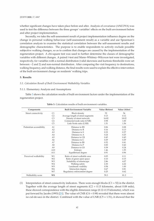
IJERPH 2020, 17, 4367

whether significant changes have taken place before and after. Analysis of covariance (ANCOVA) wasused to test the difference between the three groups’ variables’ effects on the built environment beforeand after project implementation.

Secondly, we take the self-assessment result of project implementation influence degree on thechange in personal walking behaviour (self-assessment result) as a variable and use Spearman’scorrelation analysis to examine the statistical correlation between the self-assessment results anddemographic characteristics. The purpose is to enable respondents to actively exclude possiblesubjective walking changes, so as to confirm that changes are caused by the implementation of theregeneration project. A chi-square test was used to further determine the classes of demographicvariables with different changes. A paired t-test and Mann–Whitney–Wilcoxon test were investigated,respectively, for variables with a normal distribution (valid skewness and kurtosis thresholds were setbetween −2 and 2) and non-normal distribution. After comparing the visit frequency to destinations,walking frequency, and walking distance, the final results were used to explain the effective interventionof the built environment change on residents’ walking trips.

5. Results

5.1. Calculation Result of Built Environment Walkability Variables

5.1.1. Elementary Analysis and Assumptions

Table 3 shows the calculation results of built environment factors under the implementation of theregeneration project.

Table 3. Calculation results of built environment variables.

Components Built Environment Variable Value (Before) Value (After)

Street connectivity C1 Block density 52 54C2 Average length of street segments 0.13 0.12C3 Density of street network 16.82 18.02C4 Connected node ratio (CNR) 0.98 1.00C5 Link-Node ratio (LNR) 1.51 1.56

Pedestrian accessibility A1 Distance to RS 0.06 0.08A2 Distance to R 0.16 0.13A3 Distance to S 0.32 0.37A4 Distance to A 0.24 0.25A5 Distance to CR 0.45 0.45A6 Distance to C 0.29 0.29A7 Distance to BS 0.52 0.41A8 Distance to P 0.00 0.42A9 Distance to GS 0.38 0.24A10 Entropy 1.46 1.55A11 Equilibrium degree 0.91 0.96

Perceived walkability W1 Ratio of street walkable area 0.05 0.11W2 Ratio of green open space 0.10 0.15W3 Suitability of streetscape 2.86 4.07W4 Walking safety 2.30 4.22W5 Landmark visibility 0.58 1.00W6 Interaction degree 0.67 0.81W7 Regulatory enforcement degree 0.25 0.62

Walkability score WS 59.3 81.2

(1) Interpretation of street connectivity indicators. There were enough blocks (C1 = 52) in the district.Together with the average length of street segments (C2 = 0.13 kilometre, about 0.08 mile),these showed correspondence with the eligible dimension range (0.12–0.15 kilometre), which wasput forward by Jacobs (1993) [21]. The value of CNR (C4 = 0.98) revealed that there were almostno cul-de-sacs in the district. Combined with the value of LNR (C5 = 1.51), it showed that the

42

IJERPH 2020, 17, 4367

district was composed of many small blocks and intersections with various paths between eachblock and consequently formed desirable street network connectivity.

(2) Interpretation of pedestrian accessibility indicators. Research points out that mixed-use of land isthe key component of walkability, is linked with health, traffic, and environmental consequences,and is convenient for people to access on foot [16]. The equilibrium degree (A11 = 0.91) wasclose to 1, indicating the high mixed degree of land use belonging to a high-density residentialneighbourhood. The distances between four centres of the research district grid and each of thenine types of facilities were almost all within 0.5 km. According to the international standardwalking speed, the range that adults can reach in 5 min is 0.25 miles (about 0.4 kilometre),which shows that the neighbourhood has ideal walking accessibility to facilities [1,2,36].

(3) Interpretation of perceived walkability. Benefitting from the large area of an urban historicalpark (about 0.05 square kilometres) on its north side, the historic district had a high ratio ofgreen open space. However, the walkable area outside the park was not desirable, and theengagement of local authorities in the pedestrian environment (W7 = 0.25) was insufficient.Therefore, the residents’ evaluation of streetscape suitability and walking safety (W3 = 2.86,W4 = 2.30) tended to be negative (median = 3). A large number of street segments with visiblelandmarks can improve street attractiveness and differentiation. The visibility of landmarks(W5 = 0.58) in the study area was unsatisfactory; otherwise, the street interaction degree wasacceptable because of the central location in the city.

5.1.2. Differences Analysis of Built Environment Variables among Groups

Table 4 reports the differences between “before” and “after” built environment variables. Both thecorrelation (p = 0.000) and t-test result (p = 0.032) were significant, which indicates that there is asignificance difference. An analysis of covariance was further conducted to examine the intensityamong three groups’ indicators, which led to the significance change (Tables 5 and 6). The result of thetest of homoscedasticity (F = 3.307, p = 0.059 > 0.05) was not significant, and there was no interaction(F = 0.359, p = 0.704 > 0.05). After removing the interaction terms, the result of tests of between-subjecteffects revealed a significant difference in the effects of three groups on the change of “before” and“after” built environment variables (Table 5). From the result of pairwise comparisons, we can confirmthat the perceived walkability group has a greater impact function than the street connectivity groupand pedestrian accessibility group (Table 6).

Table 4. Paired-samples test result of built environment walkability (before and after).

BuiltEnvironment

VariableMean SD SE t Df

Sig.(2-Tailed)

Before −0.221 a 0.7280.031 −2.3 21 0.032After −0.151 a 0.72

a Result of log transformation.

Table 5. Tests of between-subject effects from ANCOVA.

Dependent VariableType III Sum

of Squaresdf Mean Square F Sig.

Corrected Model 2923.003 a 3 974.334 5883.707 0.000Intercept 0.712 1 0.712 4.302 0.052

Three groups of builtenvironment variable 1.328 2 0.664 4.009 0.035

Before-After walkability 2146.077 1 2146.077 12,959.501 0.000a R-squared = 0.999 (adjusted R-squared = 0.999).

43

IJERPH 2020, 17, 4367

Table 6. Pairwise comparisons analysis among three groups from ANCOVA.

Group of Variable MD SE Sig b

95% Confidence Intervalfor Difference b

LowerBound

UpperBound

Group1 Group2 0.038 0.057 0.514 −0.082 0.159Group3 −0.212 * 0.059 0.002 −0.336 −0.088

Group2 Group1 −0.038 0.057 0.514 −0.159 0.082Group3 −0.250 * 0.045 0.000 −0.345 −0.156

Group3 Group1 0.212 * 0.059 0.002 0.088 0.336Group2 0.250 * 0.045 0.000 0.156 0.345

Based on estimated marginal means. * The mean difference is significant at the 0.05 level; b adjustment for multiplecomparisons: least significant difference (equivalent to no adjustments).

After weighting seven indexes of three components corresponding to the 7C framework,the walkability score before project implementation was 59.3, which belongs to a moderately walkabledistrict according to the Walkscore® standard. The walkability score (WS = 81.2) was greatly improvedafter project implementation. Based on the results of differences among the three groups of builtenvironment variables, it can be concluded that the improvement of the walkability score is mainlydue to the improvement of perceived walkability. Based on the above analysis results, we putforward a preliminary hypothesis that the changed built environment walkability mainly consistsof walking perception and experience in the environment, which may promote the occurrence ofrecreational walking.

5.2. Analysis of Respondents’ Walking Behaviour

5.2.1. The Report of All Respondents’ Samples

Table 7 displays the population characteristics of respondents. Results showed that the sampleswere mainly composed of middle-aged and elderly people with a low education level. Those with afull-time job and self-employed and retired respondents were homogeneously distributed, and thefamily income was mostly middle level. (According to the comparison of citizens’ income distributionfrom the National Bureau of Statistics and the economic indicators of personal capita income from theZhangzhou Statistical Yearbook 2017, individuals with an annual income of more than ¥120,000 areclassified as high-income citizens in the Zhangzhou municipality.) More than half of the families hadchildren living in the home, and the proportion of those with a household car was not high. The samplerepresents the typical residents of the Zhangzhou ancient city’s historic district, a long-standingresidential area with the highest ageing population of all subdistricts of the city (according to subdistrictstaff). Most modern young or middle-aged families with a high level of education separate from theirelders and move from the historic district to newly-built middle or upscale residential areas in the cityto live independently.

The walking frequency variable and the variable of visit frequency to destinations that reflectedthe walking behaviour of residents were investigated by measurement data. The walking distancevariable was reported as seven grades: 0.4, 0.4–0.8, 0.8–1.2, 1.2–2, 2–3, 3–4, 4–5, and above 5 km.A paired t-test was investigated to report the correlation of walking behaviours between “before” and“after”. The coefficient of correlation was significant (p = 0.000); the results of “before” and “after”walking frequency and walking distance were significantly different. The frequency of walking perweek (Mt = −0.939) increased significantly after project implementation (Table 8).

44

IJERPH 2020, 17, 4367

Table 7. Characterisation of surveyed residents and their families.

Personal Attributes N Frequency (%) Family Attributes N Frequency (%)

GenderMale 45 54.88

Family size

1 5 6.10

Female 37 45.12 2–3 43 52.44

Age

18–29 years old 4 4.88 4 or more 34 41.46

30–39 years old 16 19.51

Annualhousehold

income

Less than¥30,000 4 4.88

40–49 years old 21 25.61 ¥30,000–60,000 35 42.68

50–59 years old 18 21.95 ¥60,000–120,000 34 41.46

60 years old or older 23 28.05 More than¥120,000 9 10.98

Education

Basic first orsecond stage 39 47.56

Presence ofchildren

0 33 40.24

Secondaryeducation orhigh school

27 32.93 1 37 45.12

University 16 19.51 2 or more 12 14.63

Master and above 0 0.00Availability of

a car

0 57 69.51

Careerstatus

Student 3 3.66 1 or more 25 30.49

Full time job 21 25.61

Availability ofelectric bicycles

0 21 25.61

Self-employed 26 31.71 1 46 56.10

No job 4 4.882 or more 15 18.29

Retired 28 34.15

Table 8. “Before” and “after” paired-samples test results of residents’ walking behaviour.

WalkingBehaviourVariable

Before After Paired-Samples Test

Mean SD Mean SD Mean SE t sig

Walking frequencyper week 7.35 3.567 8.29 3.977 −0.939 0.200 −4.70 0.000

Average singlewalking distance 3.12 0.908 3.63 1.083 −0.512 0.072 −7.11 0.000

5.2.2. Subgroup Analysis Results

Self-assessment data was investigated to three levels: no impact, certain impact, and great impact.A Spearman correlation analysis was run to test for socio-demographic variables and self-assessmentdata. The self-assessment results of four population attribute categories (age group, education group,career group, and car group) showed differences (Table 9). After a further chi-square test, despite theinsignificant result on career groups, results were confirmed according to the adjusted residual (AR)value and the crosstab proportion of each class factor in the other three groups.

Table 9. “Before” and “after” correlation analysis between attribute variables and self-assessment variables.

Aspects Variables Correlation Coefficients Sig (2-Tailed)

Personal attributes Gender 0.002 0.987Age 0.363 0.001

Education −0.311 0.004Career status 0.281 0.011

Family attributes Family population −0.105 0.349Annual household income −0.164 0.142

Presence of children −0.097 0.385Availability of a car −0.248 0.025

Availability of electric bicycles −0.15 0.177

45

IJERPH 2020, 17, 4367

Residents aged 50 to 59 and over 60 in the age sub-group were more inclined to the followingconclusion than other age groups—project implementation had a greater impact on their walkingbehaviour. The same results could be found in the “less than high school” class of the education groupand the “no car” class of the car group.

Based on the above analysis conclusion, a paired t-test was run on subgroups to obtain resultsfor “before” and “after” walking frequency and the walking distance of 57 samples without acar, 41 middle-aged and elderly samples, and 38 samples with less than a high school educationbackground. Due to a large difference in the report result of each sample, the variable of visit frequencyto destinations did not meet the valid threshold of skewness and kurtosis. A Wilcoxon signed rank testwas consequently used to test the variables of the three subgroups. Only significant variables wereshown in the final statistical results (Tables 10 and 11).

Table 10. “Before” and “after” paired-samples test results of three sub-groups’ walking behaviours.

GroupBranch

VariableBefore After Paired-Samples Test

Mean SD Mean SD Mean SE t df sig

Middle-agedand Elderly

Walkingfrequency 8.44 3.905 9.07 4.274 −0.634 0.246 −2.57 40 0.000

Walkingdistance 3.17 1.052 3.66 1.146 −0.366 0.091 −4.03 40 0.000

No car

Walkingfrequency 7.44 3.784 8.05 4.121 −0.614 0.192 −3.20 56 0.002

Walkingdistance 3.21 0.940 3.61 1.161 −0.404 0.086 −4.68 56 0.000

Less thanhigh school

Walkingfrequency 8.13 4.408 8.79 4.515 −0.658 0.254 −2.56 37 0.015

Walkingdistance 3.34 0.994 3.63 1.195 −0.289 0.092 −3.16 37 0.003

Table 11. “Before” and “after” Wilcoxon test results of three sub-groups’ walking visits to destinations.

Group Branch VariableRelated Samples Wilcoxon Test

Mean SD SE z N * sig

Middle-agedand Elderly

Walkingfrequency to GS 3.82 2.46 5.852 2.392 38 0.017

No car

Walkingfrequency to RS 3.90 2.45 4.623 2.271 51 0.023

Walkingfrequency to R 2.08 1.46 5.690 2.460 38 0.014

Walkingfrequency to GS 2.83 1.91 15.652 3.354 48 0.001

Less thanhigh school

Walkingfrequency to R 1.86 1.28 4.500 2.333 22 0.020

Walkingfrequency to GS 3.97 2.58 5.852 2.392 31 0.017

* Samples with zero destination visits or no changes were removed.

(1) All three sub-groups reported increased walking frequency and walking distance. The increasein walking distance was significantly longer in the “no car” subgroup (M = −0.404), followedby the middle-aged and elderly subgroup (M = −0.366). The increase in walking frequency wassignificantly higher in the “less than high school” education subgroup (M = −0.658), followed bythe middle-aged and elderly subgroup (M = −0.634).

(2) The report on visit frequency to destinations revealed specific contents of significant differencesin the pedestrian behaviour of residents before and after project implementation. Among the

46

IJERPH 2020, 17, 4367

three destinations, only the differences in green open space have commonality. In summary,walking distance and travel frequency of middle-aged and elderly residents improved afterproject implementation, which is reflective of recreational walks to visit the green open space.Kim et al. (2014) [23] indicated that recreational walking is more sensitive to the walkingenvironment. The difference between built environment factors, however, was the comprehensiveresult of three group variables: street connectivity, pedestrian accessibility, and perceivedwalkability. From the specific content of respondents’ walking behaviour changes and thesignificant difference results of perceived walkability changes, at least one result could bemeasured: the change in the built environment brought about by the project has a significantrelationship with the recreational walking promotion of middle-aged and older residents.

6. Discussion and Conclusions

Based on the change in the built environment brought by the implementation of the regenerationproject, this study focuses on and evaluates the correlation of residents’ walking trips before and afterthe change through a quasi-longitudinal method. We adopt comprehensive indicators to evaluate builtenvironment walkability, including not only developed physical environment calculation indicatorsbut also perceived walkability and interaction indicators in the 7C layout. The results show that theproject has significantly improved perceived walkability in the environment, and residents have alsoreported a desirable walking safety and streetscape experience index. Although there may be someresidents with individual constraints or other objective factors, results can still be obtained from thispaper. As we assume the increase in recreational walking is significantly related to the implementationof this project, the preliminary assumption of the correlation between recreational walking and thebuilt environment is valid. For utilitarian walking, only positive changes in residents’ visits to retailvenues and restaurants were observed, while the other content did not receive a strong data responsein this study.

The first phase project of the Zhangzhou ancient city’s historic district retained the original formof its streets and alleys, mainly implementing environmental design and traffic system optimisation.The design of entrance squares and arrangement of landscape increased many open activity spaces;the optimisation of the traffic system reduced nuisances from vehicle traffic and enlarged pedestrianspace, broadening the visual field. Intervention in commercial areas and growth of the tourismindustry have turned many monotonous household-daily-necessity retail stores into featured localrestaurants and diversified commodity retail, which facilitates more visits. However, there are still somelimitations to this study. Even though scholars have been committed to providing reports on walkingbehaviour changes in built environments and discovering reasons for the changes via longitudinaldesign, subjective motivation, and triggers for walking are complex and uncertain. In addition toindividual constraints, trip purpose or preferences generally affect the choice of walking for a privatetrip. Besides this, the perceived indicators of BE, such as site quality, health, neighbourhood satisfaction,or social connectedness, also effect walking results. Especially for residents who are familiar withthe surrounding neighbourhood environment, even the captured changes may only be temporaryresults. The sustainability of the positive impact is still unknown; sometimes, social activities are moreinfluential than the built environment for residents’ pedestrian behaviour [21]. Another limitation canbe found in the content of pedestrian perception. Certain impacts on walking behaviour are foundamong the content of perceived walkability factors, but the specific pedestrian environment, communityawareness, and detail factors (such as the architectural visual impact on both sides, street furniture,and street scale) that affect visual quality are not further captured.

Nevertheless, although objective and perceived environment measures have been proven to beimportant environmental correlates of walking in adults, most studies in this field are still conductedin the West [3]. The sprawling Western context is different from the compact Asian context; relevantresearch in China holds great significance, especially the evidence reported in this study that change ofBE promotes the recreational walking of the middle-aged and elderly, which helps to improve their

47

IJERPH 2020, 17, 4367

physical function, reduce the economic and social burden of NCDs, and improve individual quality oflife [26].

The results support the hypothesis that changes in the built environment can effectively promoteleisure walking behaviour, especially for the middle-aged and elderly. We believe this research hasmade a meaningful contribution to the literature on this topic. As our study is a case study that mayinvolve the unique characteristics of a single city, this limits generalizability. More cross-sectionalcases, combined with longitudinal exploration, need further research and the assembly of a catalogue.In addition, future research will need to take into account other trip modes like driving or cycling tocontribute a comprehensive strategy of BE impact on travel behaviour.

Author Contributions: F.Z. put forward the idea, designed the study, performed the survey, collected data,analysed the data and wrote the draft; Z.S. reviewed and edited the paper. All authors have read and agreed tothe published version of the manuscript.

Funding: This research received no external funding.

Acknowledgments: We are indebted to the editor and the anonymous reviewers for their thorough reading of thepaper and for providing insightful comments that helped to improve the contents and the presentation.

Conflicts of Interest: The authors declare no conflict of interest.

References

1. Atash, F. Redesigning suburbia for walking and transit: Emerging concepts. J. Urban Plan. Dev. 1994, 120,48–57. [CrossRef]

2. Aultman-Hall, L.; Hall, F.L.; Baetz, B.B. Analysis of bicycle commuter routes using geographic informationsystems: Implications for bicycle planning. Transp. Res. Record 1997, 1578, 102–110. [CrossRef]

3. Bauman, A.E.; Bull, F.C. Environmental Correlates of Physical Activity and Walking in Adults and Children:A Review of Reviews; National Institute of Health and Clinical Excellence: London, UK, 2007.

4. Bi, X.; Luo, W. Analysis of travel characteristics and transportation improvement strategies of small andmedium-sized cities (in Chinese). Technol. Econ. Areas Commun. 2018, 20.

5. Brondeel, R.; Pannier, B.; Chaix, B. Associations of socioeconomic status with transport-related physicalactivity: Combining a household travel survey and accelerometer data using random forests. J. Transp.Health 2016, 3, 287–296. [CrossRef]

6. Carmona, M.; Tiesdell, S.; Heath, T.; Oc, T. Public Places Public Spaces: The Dimensions of Urban Design;Archtectural press: Oxford, UK, 2010.

7. Carlson, J.A.; Grimes, A.; Greend, M.; Morefield, T.; Steel, C.; Reddy, A.; Bejarano, C.; Shook, R.P.; Moore, T.;Steele, L.; et al. Impacts of temporary pedestrian streetscape improvements on pedestrian and vehicle activityand community perceptions. J. Transp. Health 2019, 15, 100791. [CrossRef]

8. Carr, L.J.; Dunsiger, S.I.; Marcus, B.H. Walk score™ as a global estimate of neighborhood walkability. Am. J.Prev. Med. 2010, 39, 460–463. [CrossRef] [PubMed]

9. Cerin, E.; Saelens, B.E.; Sallis, J.F.; Frank, L.D. Neighborhood Environment Walkability Scale: Validity anddevelopment of a short form. Med. Sci. Sports Exerc. 2006, 38, 1682–1691. [CrossRef]

10. Cervero, R.; Kockelman, K. Travel demand and the 3Ds: Density, diversity, and design. Transp. Res. Part DTransp. Environ. 1997, 2, 199–219. [CrossRef]

11. Dill, J. Measuring network connectivity for bicycling and walking. In 83rd Annual Meeting of the TransportationResearch Board; Environmental Protection Agency: Washington, DC, USA, 2004; pp. 11–15.

12. Ewing, R.; Handy, S. Measuring the unmeasurable: Urban design qualities related to walkability. J. UrbanDes. 2009, 14, 65–84. [CrossRef]

13. Ewing, R.; Greenwald, M.J.; Zhang, M.; Walters, J.; Feldman, M.; Cervero, R.; Thomas, J. Measuring the Impactof Urban form and Transit Access on Mixed Use Site Trip Generation Rates—Portland Pilot Study; US EnvironmentalProtection Agency: Washington, DC, USA, 2009.

14. Ewing, R.; Cervero, R. Travel and the built environment: A meta-analysis. J. Am. Plan. Assoc. 2010, 76,265–294. [CrossRef]

48

IJERPH 2020, 17, 4367

15. Fan, P.; Wan, G.; Xu, L.; Park, H.; Xie, Y.; Liu, Y.; Yue, W.; Chen, J. Walkability in urban landscapes:A comparative study of four large cities in China. Landsc. Ecol. 2018, 33, 323–340. [CrossRef]

16. Frank, L.D.; Sallis, J.F.; Saelens, B.E.; Leary, L.; Cain, K.; Conway, T.L.; Hess, P.M. The development of awalkability index: Application to the Neighborhood Quality of Life Study. Br. J. Sports Med. 2010, 44,924–933. [CrossRef] [PubMed]

17. Gao, J.; Kamphuis, C.B.M.; Ettema, D.; Helbich, M. Longitudinal changes in transport-related and recreationalwalking: The role of life events. Transp. Res. Part D Transp. Environ. 2019, 77, 243–251. [CrossRef]

18. Handy, S.; Cao, X.; Mokhtarian, P. Correlation or causality between the built environment and travel behavior?Evidence from Northern California. Transp. Res. Part D Transp. Environ. 2005, 10, 427–444. [CrossRef]

19. Handy, S.L.; Boarnet, M.G.; Ewing, R.; Killingsworth, R.E. How the built environment affects physicalactivity: Views from urban planning. Am. J. Prev. Med. 2002, 23, 64–73. [CrossRef]

20. Hirsch, J.A.; Moore, K.A.; Clarke, P.J.; Rodriguez, D.A.; Evenson, K.R.; Brines, S.J.; Zagorski, M.A.; Roux, A.V.D.Changes in the built environment and changes in the amount of walking over time: Longitudinal resultsfrom the multi-ethnic study of atherosclerosis. Am. J. Epidemiol. 2014, 180, 799–809. [CrossRef]

21. Jacobs, A.B. Great Streets; MIT Press: Cambridge, MA, USA, 1993.22. Jun, H.J.; Hur, M. The relationship between walkability and neighborhood social environment: The

importance of physical and perceived walkability. Appl. Geogr. 2015, 62, 115–124. [CrossRef]23. Kim, S.; Park, S.; Lee, J.S. Meso-or micro-scale? Environmental factors influencing pedestrian satisfaction.

Transp. Res. Part D Transp. Environ. 2014, 30, 10–20. [CrossRef]24. Leyden, K.M. Social capital and the built environment: The importance of walkable neighborhoods. Am. J.

Public Health 2003, 93, 1546–1551. [CrossRef]25. Lee, C.; Moudon, A.V. Physical activity and environment research in the health field: Implications for urban

and transportation planning practice and research. J. Plan. Liter. 2004, 19, 147–181. [CrossRef]26. Li, F.; Harmer, P.A.; Cardinal, B.J.; Bosworth, M.; Acock, A.; Johnson-Shelton, D.; Moore, J.M. Built environment,

adiposity, and physical activity in adults aged 50–75. Am. J. Prev. Med 2008, 35, 38–46. [CrossRef] [PubMed]27. Lin, T. Travel modes and age differentiation of Fuzhou residents (in Chinese). J. Shijiazhuang Univ. 2012, 14,

81–85, 128.28. Milakis, D.; Efthymiou, D.; Antoniou, C. Built environment, travel attitudes and travel behaviour:

Quasi-longitudinal analysis of links in the case of Greeks relocating from US to Greece. Sustainability2017, 9, 1774. [CrossRef]

29. Moudon, A.V.; Lee, C.; Cheadle, A.D.; Garvin, C.; Johnson, D.B.; Schmid, T.L.; Weathers, R.D. Attributes ofenvironments supporting walking. Am. J. Health Promot. 2007, 21, 448–459. [CrossRef]

30. Moura, F.; Cambra, P.; Gonçalves, A.B. Measuring walkability for distinct pedestrian groups with aparticipatory assessment method: A case study in Lisbon. Landsc. Urban Plan. 2017, 157, 282–296. [CrossRef]

31. Newman, P.; Kenworthy, J. Sustainability and Cities: Overcoming Automobile Dependence; Island Press:Washington, DC, USA, 1999.

32. NZTA (New Zealand Transport Agency). Pedestrian Planning and Design Guide; NZTA: Wellington, NZ, USA, 2009.33. Pikora, T.; Giles-Corti, B.; Bull, F.; Jamrozik, K.; Donovan, R. Developing a framework for assessment of the

environmental determinants of walking and cycling. Soc. Sci. Med. 2003, 56, 1693–1703. [CrossRef]34. Pliakas, T.; Wilkinson, P.; Tonne, C. Contribution of the physical environment to socioeconomic gradients in

walking in the Whitehall II study. Health Place 2014, 27, 186–193. [CrossRef] [PubMed]35. Putnam, R.D. Bowling Alone: The collapse and revival of American community; Simon and Schuster: New York,

NY, USA, 2001.36. Randall, T.A.; Baetz, B.W. Evaluating pedestrian connectivity for suburban sustainability. J. Urban Plan. Dev.

2001, 127, 1–15. [CrossRef]37. Rzotkiewicz, A.; Pearson, A.L.; Dougherty, B.V.; Shortridge, A.; Wilson, N. Systematic review of the use

of Google Street View in health research: Major themes, strengths, weaknesses and possibilities for futureresearch. Health Place 2018, 52, 240–246. [CrossRef] [PubMed]

38. Saelens, B.E.; Sallis, J.F.; Frank, L.D. Environmental correlates of walking and cycling: Findings from thetransportation, urban design, and planning literatures. Ann. Behave. Med. 2003, 25, 80–91. [CrossRef] [PubMed]

39. Sdoukopoulos, A.; Verani, E.; Nikolaidou, A.; Gavanas, N.; Pitsiava-Latinopoulou, M.; Mikiki, F.; Mademli, E.;Pallas, C. Development and implementation of walkability audits in Greek medium-sized cities: The case ofthe Serres’ city centre. Transp. Res. Procedia 2017, 24, 337–344. [CrossRef]

49

IJERPH 2020, 17, 4367

40. Shannon, C.E. A mathematical theory of communication. Bell Syst. Tech. J. 1948, 27, 379–423. [CrossRef]41. Su, S.; Zhou, H.; Xu, M.; Ru, H.; Wang, W.; Weng, M. Auditing street walkability and associated social

inequalities for planning implications. J. Transp. Geogr. 2019, 74, 62–76. [CrossRef]42. Sun, G.; Oreskovic, N.M.; Lin, H. How do changes to the built environment influence walking behaviors?

A longitudinal study within a university campus in Hong Kong. Int. J. Health Geogr. 2014, 13, 28. [CrossRef]43. Teng, H.; Chen, Z. Resident trip characteristics and transport development policies in Ningbo (in Chinese).

Traff. Saf. 2009, 31, 94–97.44. Tong, X.; Wang, Y.; Chan, E.H.W. International research trends and methods for walkability and their

enlightenment in China. Procedia Environ. Sci. 2016, 36, 130–137. [CrossRef]45. Weng, M.; Ding, N.; Li, J.; Jin, X.; Xiao, H.; He, Z.; Su, S. The 15-minute walkable neighborhoods: Measurement,

social inequalities and implications for building healthy communities in urban China. J. Transp. Health 2019,13, 259–273. [CrossRef]

46. Wang, H.; Yang, Y. Neighbourhood walkability: A review and bibliometric analysis. Cities 2019, 93, 43–61. [CrossRef]47. Yintao, L. Walkability Evaluation Based on People’s Use of Facilities by Walking (in Chinese). Urban Plan. Forum.

2013, 5, 113–118.

© 2020 by the authors. Licensee MDPI, Basel, Switzerland. This article is an open accessarticle distributed under the terms and conditions of the Creative Commons Attribution(CC BY) license (http://creativecommons.org/licenses/by/4.0/).

50

International Journal of

Environmental Research

and Public Health

Article

The Role of Eco-Friendly Edible Insect Restaurants inthe Field of Sustainable Tourism

Jinsoo Hwang 1, Hyunjoon Kim 2,* and Ja Young Choe 3

1 The College of Hospitality and Tourism Management, Sejong University, Seoul 143-747, Korea;jhwang@sejong.ac.kr

2 The Department of Tourism Management, The College of Business Administration, Dong-A University,Busan 49236, Korea

3 Faculty of Business Administration, University of Macau, Macau 853, China; jaceychoe@umac.mo* Correspondence: hyunjoon@dau.ac.kr

Received: 22 May 2020; Accepted: 4 June 2020; Published: 7 June 2020

Abstract: The purpose of this study is to apply the concept of a green image in order to explorehow to form behavioral intentions in the context of eco-friendly edible insect restaurants. This studyanalyzed 444 samples collected in South Korea in order to evaluate the theoretical model including12 hypotheses. The data analysis results showed that a green image has a positive influence on attitude.In addition, attitude helps to increase desire, which in turn positively affects two sub-dimensions ofbehavioral intentions, such as intentions to use and word-of-mouth intentions.

Keywords: edible insect restaurants; eco-friendly; green image; behavioral intentions; attitude; desire

1. Introduction

The world’s population is on a constant rise, and now it is approximately 7.7 billion, but willincrease to about 9.7 billion by 2050 [1]. Such an increase in population causes severe food shortagesbecause of limited resources [2]. Edible insects are receiving much attention as humans need newfood sources to replace current food sources [3]. The Food and Agriculture Organization (FAO)also suggested that edible insects are the future food of mankind that can solve world hunger [4].Edible insects are as high in protein, amino acids, and micronutrients, which are important nutrients forhumans, as the meat of livestock [5]. Edible insects also have the advantage of not having a high-levelentry barrier similar to that for livestock in terms of technology and monetary investment [6].

Green food can be defined as an organic and sustainable food in the restaurant industry [7], andprevious studies have indicated that green food is regarded as pivotal for the sustainable developmentof the regional tourism [8]. In particular, in terms of the environmental aspect, edible insects aid torecycle animal waste, which leads to the protection of the environment [9]. In addition, Megido et al.also argued that compared to raising livestock, raising edible insects can reduce greenhouse gas, soit can be said that edible insects are green food [10]. According to Gössling and his colleagues [11],restaurant managers and the sustainable tourism service sector need to cooperate extensively in termsof environmental issues and global climate changes, and the industry should find ways to reducecarbon and waste for restaurant managers. In this sense, the eco-friendly role of edible insects issignificantly related to the green image in the field of sustainable tourism since edible insect productionnot only has lower greenhouse gas emissions, but also higher feed-conversion efficiency because itrequires less land and water when compared to livestock [12].

In recent years, consumers have a lot of interest in protecting the environment, so they try topurchase eco-friendly products/services, which fulfills their environmental needs [13]. For example,tourists actively enjoy involving themselves in sustainable food consumption including edible insectsduring their ecotourism holidays [12]. For this reason, restaurant companies make an effort to make

IJERPH 2020, 17, 4064; doi:10.3390/ijerph17114064 www.mdpi.com/journal/ijerph51

IJERPH 2020, 17, 4064

their corporate image appear green to consumers [14]. If edible insect restaurants emphasize a greenimage based on their role of environmental protection, it will have a positive effect on consumerbehavior. Although a green image of an edible insect restaurant is important in the context of sustainabletourism, there has been no research done on this subject.

To sum up, this study tried to explain how to form behavioral intentions in the context ofeco-friendly edible insect restaurants. More specifically, this study examined the relationship betweengreen image and attitude. In addition, this study investigated the effect of attitude on desire and twosub-dimensions of behavioral intentions including intentions to use and word-of-mouth intentions.In this situation, the results of this study will provide edible insect restaurant managers with importantimplications for developing effective green marketing strategies.

2. Literature Review

2.1. Eco-Friendly Edible Insect Restaurants

Although entomophagy, which means human consumption of insects, was first introduced byBodenheimer [15], humans have been eating insects for thousands of years [16]. Currently, abouttwo billion people around the world eat 1900 species of insects, such as crickets, buffalo worms,grasshoppers, ants, and cicadas as part of their food culture [17]. In addition, the market for edibleinsects in 2018 was approximately U.S. $400 million, and it is predicted to be approximately threetimes larger in 2023 [18]. According to Pliner and Hobden [19], food neophobia refers to a personalinclination to reluctance to try novel/unique foods. Thus, food neophobia and edible insects are highlycorrelated because edible insects can also seem disgusting to consumers. However, Olabi et al. [20]suggested that fear/negative emotions of novel/unique foods may gradually decrease with constantexposure. Therefore, in order to reduce the food neophobia of consumers, insect restaurant ownersneed to continuously promote edible insects, highlighting their merits.

These edible insects also play an important role in the restaurant industry. In the past, a smallnumber of customers used edible insect restaurants, so they operated on a small scale. Nowadays, asmore and more customers are looking for edible insect restaurants, their growth is exponential, andedible insect restaurants are operating even in five-star hotels [21]. For example, Linger restaurant,located in Denver, USA, uses insects as ingredients to provide a variety of menus to customers, andSweet and Sour Crickets are the most popular [22]. In addition, Lardo, in Col. Condesa, an edible insectrestaurant located in Mexico, is known for providing its customers with original menus, especially“huevo en torta”, which means eggs on cake made using insects. In fact, Mexico has a number ofedible insect restaurants that provide an “exotic” experience to tourists [23]. In Thailand, “Insectsin the Backyard” serves food using insects such as crickets, grasshoppers, worms, and beetles [24].In particular, the restaurant emphasizes the nutritional aspects of insects, and suggests that insectsplay an important role in human future food. China has a long history of edible insects, especiallyinsect restaurants in Yunnan Province have become popular [25]. Furthermore, there are many edibleinsect restaurants in England, Japan, New Zealand, and Taiwan, and sales are increasing [12].

In recent years, as consumers’ interest in environmental protection has increased in the restaurantindustry, the eco-friendly role of edible insect restaurants has attracted attention [26]. Prior studieshave consistently claimed that edible insects can play an important role in protecting the environment.First, it is widely known that many resources, such as grass and water, are used to raise livestock,which causes desertification [27]. On the other hand, edible insects are considered to be environmentallyfriendly because they require far fewer resources than livestock [28]. Second, greenhouse gas emissionsfrom livestock have a negative impact on climate change [29], but edible insects have a very low levelof greenhouse gas emissions, making a significant contribution to environmental protection [30]. Third,in terms of global warming potential (GWP), edible insects have lower levels of GWP compared tolivestock such as beef and lamb [31].

52

IJERPH 2020, 17, 4064

In summary, edible insect restaurants are expected to play an important role in satisfying theeco-friendly needs of consumers, as edible insects are emerging as important new food sources thatcan replace traditional food sources in the environmental aspect. However, research on edible insectrestaurants is insufficient.

2.2. Green Image

Human life has been enriched through several industrial revolutions, but on the contrary, theserevolutions have caused environmental pollution [32]. In the late twentieth century, countries aroundthe world recognized the seriousness of problems caused by environmental pollution, such as resourcedepletion and desertification, and governments have made efforts such as enacting laws on theprotection of global environment [10]. As consumers’ awareness of environmental protection increases,they are willing to pay more to buy eco-friendly products that are more expensive than general productsin order to protect the environment [33]. For this reason, companies are making a lot of effort in variousforms, such as green marketing and green management to make their images green [34].

The concept of a green image refers to “a set of perceptions of a firm in a consumer’s mind thatis linked to environmental commitments and concerns” [35]. Green includes the concept of naturalenvironment and is also known as environmentally friendly or eco-friendly [36]. The green image of acompany that satisfies consumers’ environmental needs plays a major role in enhancing trust in thecompany, consequently creating strong brand equity [34]. In addition, green image helps to maximizeconsumers’ intention to use and minimize consumers’ switch intentions [37]. More importantly, since agreen image of a company has a symbolic meaning that can represent the overall characteristics of thecompany, the green image plays a critical role in differentiating it from other competitive brands [34].

Prior research has examined the outcome variables of a green image in diverse fields. For instance,Lee et al. [38] examined how a hotel’s green image affects behavioral intentions using 416 hotel guests.They found that the green image of the hotel favorably induces customers’ behavioral intentions.In addition, Yusof, Musa, and Rahman [39] developed a research model, which focused on therelationship between a green image and loyalty in the retail industry. Their data analysis resultsindicated that there is a positive relationship between a green image and loyalty. In other words, whenpeople have a green image of a certain brand, they have a high loyalty to that brand. Martínez [35]also explored the effect of a green image on loyalty and identified that a green image positively affectsloyalty. That is, people have high levels of brand loyalty if the brand has a green image.

2.3. Effect of Green Image on Attitude

First, this study proposes how a green image plays a role in forming attitude. Although manyscholars have suggested the definition of attitude, the definition proposed by Ajzen [40] is the mostfrequently cited. The author emphasized the importance of attitude in order to explain consumerbehavior through the theory of planned behavior (TPB), and defined attitude as “the degree to which aperson has a favorable or unfavorable evaluation or appraisal of the behavior” [40]. In other words,attitude is a personal subject of an object or person, so the attitude is formed based on the values orbeliefs that an individual seeks [41], which suggested that there is a positive association between greenimage and attitude. For instance, if consumers have strong beliefs about the protection of the naturalenvironment, they will have a favorable attitude toward using eco-friendly products/services.

Existing studies have also supported the effect of green image on attitude. For example, Han,Yu, and Kim [42] explored the relationship between green image and attitude in the tourism industry,and they suggested that a green image is a vital predictor of attitude. That is, people have a favorableattitude to a certain brand when the brand has a green image. In addition, Hwang and Lyu [43]developed a research model in order to identify how a green image aids to enhance attitude in theairline industry, and they suggested that when consumers perceive a green image from a certain airline,they have a favorable attitude toward using that airline. Hwang and Kim [33] also investigated therole of green image in forming attitudes in the context of eco-friendly drone food delivery services.

53

IJERPH 2020, 17, 4064

The authors showed that a green image helps to make consumer’s attitude favorable. Based on thetheoretical and empirical studies discussed above, this study presents the following hypothesis.

Hypothesis 1 (H1). Green image has a positive impact on attitude.

2.4. Effect of Attitude on Desire and Behavioral Intentions

Desire is defined as “a state of mind whereby an agent has a personal motivation to perform anaction or to achieve a goal” [44]. A particular behavior is formed by internal stimulation, which isknown as the state of desire [44]. Desire is heavily affected by a positive or negative appraisal,which aids to form behavioral intentions [45]. For example, when a consumer makes a positiveassessment of a certain product/service, they have a greater desire to use the product/service.

According to the model of goal-directed behavior (MGB), desire is a strong motivation forconsumers to do a certain behavior they aim for and is shaped by the attitude they have [45],which suggested that attitude is an important factor influencing desire. Existing studies have confirmedthe effect of attitude on desire. For example, Meng and Han [46] applied MGB to the field of bicycletourism, and they found that attitude was found to bear a significant impact on desire. In other words,when consumers have a positive attitude toward bicycle tourism, they would have a high level ofdesire to do bicycle tourism. Kim and Preis [47] also examined the relationship between attitude anddesire based on the extended MGB in the tourism industry. The authors indicated that when tourists’attitudes toward using mobile devices for tourism-related purposes are good, they are more likely tohave high levels of desire to use the devices. Based on the literature review above, this study proposedthe following hypothesis.

Hypothesis 2 (H2). Attitude has a positive impact on desire.

Next, this study hypothesizes the relationship between attitude and behavioral intentions.Behavioral intentions are the likelihood that a person will attempt a particular behavior [40,48], andthey consist of intentions to use and word-of-mouth intentions (e.g., Kim, Ng, and Kim, 2009; Maxham,2001) [49,50]. Intentions to use can be defined as “the degree to which a person has formulatedconscious plans to perform or not perform some specified future behavior” [51]. Consumers haveintentions to use through a positive appraisal of products or services, which has a direct impact ona company’s sales [52]. In addition, word-of-mouth refers to “informal communication directed atother consumers about the ownership, usage or characteristics of particular goods and services and/ortheir sellers” [53]. The effect of word-of-mouth has more influence on consumers than the commercialadvertisement of companies because people get information from acquaintances including family,friends, and relatives [54].

The relationship between attitude and behavioral intentions is theoretically supported by thetheory of reasoned action (TRA) and the theory of planned behavior (TPB) [48,55], which indicated thatattitude is an important factor that leads to behavioral intentions. The effect of attitude on behavioralintentions has been demonstrated in many fields. For instance, Alzahrani, Hall-Phillips, and Zeng [56]tried to find the relationship between attitude and behavioral intentions using the TRA, and theyshowed that when consumers have a favorable attitude toward using hybrid electric vehicles, theytend to have high levels of behavioral intentions. More recently, Yarimoglu and Gunay [57] employedthe extended TPB in the green hotel industry. They showed that attitude is a significant predictor ofbehavioral intentions.

Hypothesis 3 (H3). Attitude has a positive impact on intentions to use.

Hypothesis 4 (H4). Attitude has a positive impact on word-of-mouth intentions.

54

IJERPH 2020, 17, 4064

2.5. Effect of Desire on Behavioral Intentions

According to MGB, desire to take a particular action is a significant predictor of behavioralintentions [58]. Empirical studies have also supported the argument. For example, Han, Lee,and Kim [59] developed a research model in order to find the relationship between desire andbehavioral intentions. They showed that desire helps to enhance behavioral intentions. In addition,Hwang and Kim [33] examined the relationship between desire and behavioral intentions using inthe context of drone food delivery services. They found that when consumers have high levels ofdesire to use drone food delivery services, they are more likely to use the services. Hwang, Cho, andKim [60] also tried to investigate how desire affects behavioral intentions in the context of eco-friendlydrone food delivery services. They suggested that desire plays an important role in the formation ofbehavioral intentions. Based on the theoretical and empirical backgrounds, the following hypothesesare proposed.

Hypothesis 5 (H5). Desire has a positive impact on intentions to use.

Hypothesis 6 (H6). Desire has a positive impact on word-of-mouth intentions.

2.6. Research Model

Based on a total of six hypotheses, this study proposes the following research model (Figure 1).

Figure 1. Proposed conceptual model.

3. Methodology

3.1. Measurement

First, a green image was measured with three items cited from Hwang and Kim [33] andMartínez [35]. Second, three items regarding attitude were cited from Ajzen [40] and Han andHyun [61]. Third, desire was measured using three items adapted from Hwang and Kim [33] andPerugini and Bagozzi [58]. Fourth, in terms of behavioral intentions, three measurements for intentionsto use were cited from Zeithaml, Berry, and Parasuraman [62], while word-of-mouth intentions weremeasured with three measurements borrowed from Hennig-Thurau, Gwinner, and Gremler [63].

All measurement items were measured using a seven-point Likert type scale (1 = strongly disagree;7 = strongly agree). The survey was carefully reviewed by three expert groups including professors,graduate students, and restaurant employees in order to ensure content validity before finalizing thequestionnaire, and they identified that there is high levels of content validity.

55

IJERPH 2020, 17, 4064

3.2. Data Collection

Data collection was performed using an online survey company system in South Korea. Therewere few edible insect restaurants in South Korea, so this study provided respondents with twonewspaper articles and a video where anyone could easily understand the eco-friendly role of edibleinsect restaurants before beginning our survey. For example, the two newspaper articles and one videoshowed how to make insect foods and its important role in the protection of the environment. From the6479 questionnaires distributed, 450 responses were collected. Responses with extreme answers andmissing information were removed. As a result, 444 usable responses remained for further analysis.Prior studies including Hair et al. [64] and Weston and Gore [65] suggested that a sample size of 200is satisfactory for performing confirmatory factor analysis (CFA) and structural equation modeling(SEM) with the maximum-likelihood estimation method. This implies that there was no problem withthe representation of the sample.

4. Results

4.1. Profile of the Sample

The ratio of males and females in the sample was 50%. The mean age was 38.06 years, ranging from 20to 59 years of age. The number of respondents in their 30s was the highest. In terms of monthly householdincome, 130 respondents (29.3%) answered that their income was between U.S. $1001 and U.S. $2000.In addition, 52.3% of the respondents (n = 232) were married, and 55.9% had a bachelor’s degree (n = 248).

4.2. Confirmatory Factor Analysis

Table 1 showed the results of confirmatory factor analysis. The results indicated that the overall fitof the measurement model was acceptable. The factor loadings were equal to or greater than 0.843 andall factor loadings were significant at p < 0.001. As shown in Table 2, the values of average varianceextracted (AVE) were greater than 0.50 for all constructs, which is the threshold value [66]. Consideringthe high levels of factor loadings and also the values of AVE in the measurement model, convergentvalidity for all of the measurement items had been achieved [67].

Table 1. Confirmatory factor analysis: items and loadings.

Construct and Scale Items Standardized Loading a

Green image of an edible insect restaurantAn edible insect restaurant is more likely to be successful about its environmental protection. 0.843

An edible insect restaurant is more likely to solve environmental problems. 0.870An edible insect restaurant is more likely to have a strong environmental reputation. 0.888

Attitude toward using an edible insect restaurantUnfavorable—Favorable 0.922

Bad—Good 0.886Negative—Positive 0.929

DesireI desire to visit an edible insect restaurant. 0.936

My desire to visit an edible insect restaurant is strong. 0.970I want to visit an edible insect restaurant. 0.961

Intentions to useI will dine out at an edible insect restaurant. 0.953

I am willing to dine out at an edible insect restaurant. 0.957I am likely to dine out at an edible insect restaurant. 0.967

Word-of-mouth intentionsI am likely to say positive things about an edible insect restaurant to others. 0.887

I am likely to recommend an edible insect restaurant to others. 0.980I am likely to encourage others to dine out at an edible insect restaurant. 0.937

Goodness-of-fit statistics: χ2 = 211.179, df = 80, χ2 df −1 = 2.640, p < 0.001, NFI = 0.977, CFI = 0.986, TLI = 0.981, andRMSEA = 0.061

a All factors loadings are significant at p < 0.001; df = Degree Freedom; NFI = normed fit index; CFI = comparativefit index; TLI = Tucker–Lewis index; and RMSEA = root mean square error of approximation.

56

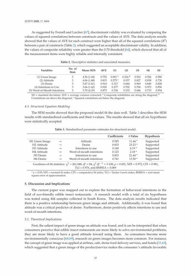
IJERPH 2020, 17, 4064

As suggested by Fornell and Larcker [67], discriminant validity was evaluated by comparing thevalues of squared correlations between constructs and the values of AVE. The data analysis resultsshowed that the values of AVE for each construct were higher than all of the squared correlations (R2)between a pair of constructs (Table 2), which suggested an acceptable discriminant validity. In addition,the values of composite reliability were greater than the 0.70 threshold [64], which showed that all ofthe measurement items were highly reliable and internally consistent.

Table 2. Descriptive statistics and associated measures.

VariablesNo. ofItem

Mean (SD) AVE (1) (2) (3) (4) (5)

(1) Green Image 3 4.56 (1.04) 0.752 0.901 a 0.524 b 0.563 0.526 0.580(2) Attitude 3 4.06 (1.48) 0.833 0.275 c 0.937 0.827 0.838 0.730(3) Desire 3 3.67 (1.41) 0.914 0.317 0.684 0.969 0.840 0.828

(4) Intentions to Use 3 3.66 (1.42) 0.920 0.277 0.702 0.706 0.972 0.856(5) Word-of-Mouth Intentions 3 3.78 (4.29) 0.875 0.336 0.533 0.686 0.733 0.954

SD = standard deviation; AVE = average variance extracted; a Composite reliabilities are along the diagonal; b

Correlations are above the diagonal; c Squared correlations are below the diagonal.

4.3. Structural Equation Modeling

The SEM results showed that the proposed model fit the data well. Table 3 describes the SEMresults with standardized coefficients and their t-values. The results showed that all six hypotheseswere statistically accepted.

Table 3. Standardized parameter estimates for structural model.

Coefficients t-Value Hypothesis

H1 Green Image → Attitude 0.545 11.44 * SupportedH2 Attitude → Desire 0.833 23.23 * SupportedH3 Attitude → Intentions to use 0.149 4.19 * SupportedH4 Attitude → Word-of-mouth intentions 0.123 2.18 * SupportedH5 Desire → Intentions to use 0.833 21.44 * SupportedH6 Desire → Word-of-mouth intentions 0.741 12.50 * Supported

Goodness-of-fit statistics: χ2 = 261.048, df = 84, χ2 df −1 = 3.108, p < 0.001, NFI = 0.972, CFI = 0.981,TLI = 0.976, and RMSEA = 0.069

* p < 0.05; NFI = normed fit index; CFI = comparative fit index; TLI = Tucker–Lewis index; RMSEA = root meansquare error of approximation.

5. Discussion and Implications

The current paper was mapped out to explore the formation of behavioral intentions in thefield of eco-friendly edible insect restaurants. A research model with a total of six hypotheseswas tested using 444 samples collected in South Korea. The data analysis results indicated thatthere is a positive relationship between green image and attitude. Additionally, it was found thatattitude was a critical predictor of desire. Furthermore, desire positively affects intentions to use andword-of-mouth intentions.

5.1. Theoretical Implications

First, the salient impact of green image on attitude was found, and it can be interpreted that whenconsumers perceive that edible insect restaurants are more likely to solve environmental problems,they are more likely to have a good attitude toward using them. As consumers become moreenvironmentally conscious [68,69], research on green images becomes more common. For instance,the concept of green image was applied at airlines, café, drone food delivery services, and hotels [33,43],which suggested that a green image of the product/service makes the consumer’s attitude favorable.

57

IJERPH 2020, 17, 4064

In this respect, the result of this study is consistent with previous studies. However, unlike previousstudies, this study applied the concept of green image and revealed the effect of green image onattitude for the first time in the field of edible insect restaurants, thereby providing importanttheoretical implications.

Second, the SEM results identified attitude as an important factor in the formation of desire.That is, when consumers have a favorable attitude toward using edible insect restaurants, their desireof using the restaurants is strong. The relationship between attitude and desire was theoreticallysupported by the MGB [45], and also the existing literature has consistently confirmed the relationship(e.g., Hwang, Kim et al., 2019; Kim and Preis, 2016; Meng and Han, 2016) [33,46,47], which indicatedthat attitude plays a vital role in the formation of desire. In addition, our analysis identified theprominent influence of attitude on two sub-dimensions of behavioral intentions including intentions touse and word-of-mouth intentions. That is, consumers tend to dine out at edible insect restaurants andsay positive things about them to others when they have a positive attitude. The theoretical evidencefor the relationship between attitude and behavioral intentions is through TRA and TPB [48,55].In addition, prior research has verified the relationship in many different fields (e.g., Alzahrani et al.,2019; Yarimoglu and Gunay, 2019) [56,57]. In this regard, the significant theoretical implication ofthis study is that we confirmed and extended the current literature by empirically identifying theeffect of attitude on desire, intentions to use, and word-of-mouth intentions in the context of edibleinsect restaurants.

5.2. Managerial Implications

First, the current study confirmed that a green image of edible insect restaurants induces apositive attitude toward using them, which in turn positively affects desire and two sub-dimensions ofbehavioral intentions. The findings suggested the importance of green image in the context of edibleinsect restaurants. In fact, many restaurant companies are making an effort to impress consumers withtheir green image. For instance, Starbucks, the world’s largest coffee brand, will stop using disposableplastic straws by 2020 and replace them with paper or compostable plastic straws [70]. In addition,McDonald’s produces more than 3000 tons of coffee peel each year during roasting. McDonald’splans to reduce the negative environmental impact by using the coffee peel as a vehicle material withFord [71]. The efforts of these companies play an important role in delivering their green image toconsumers. As explained earlier, edible insects are greener food sources than livestock when comparinggreenhouse gas emissions and GWP [28,29]. Thus, if edible insect restaurant owners emphasize theeco-friendly aspects of edible insects using advertising, which is considered a significant means thatcreate a green image (e.g., Ankit and Mayur, 2013; Yoon and Kim, 2016) [72,73], the consumers wouldhave a favorable attitude toward using them. Furthermore, as the results of our data analysis indicated,consumers are more likely to have a high level of behavioral intentions toward edible insect restaurants.

Second, from a sustainable tourism, destination marketing organizations can emphasize the greenrole of edible insect restaurants for their marketing strategies. It is important to educate tourists thatvisiting an edible insect restaurant can reduce carbon emissions, maintain sustainability from theperspective of food miles, and support the region’s growing sustainable agriculture movement. It isrecommended to provide menu books in an edible restaurant with a carbon footprint so that touristscan recognize to what extent they contribute to reduce the total greenhouse gas by their food choice.In addition, it is suggested that photos and promotional images include local farmers who sustainways of life with growing edible insects to enhance the image of sustainability in a destination.

6. Limitations and Future Research

There are some limitations that provide opportunities for future research. First, the data collectionwas performed only in South Korea. Therefore, it is recommended that generalizing our study findingsto other regions should be carefully done. Second, since edible insect restaurants are not activated inSouth Korea, the respondents in this study did not actually use the restaurants. In order to overcome

58

IJERPH 2020, 17, 4064

this issue, two newspaper articles and a video, which clearly explain edible insect restaurants, weregiven to respondents before the start of the survey. However, it is necessary to collect data from otherregions where edible insect restaurants are active in order to obtain data from people who actuallyuse the restaurants. Third, eco-friendly behavioral intentions vary according to the demographiccharacteristics of consumers [74]. Therefore, future studies need to use demographic characteristics(e.g., gender and age) as a moderator.

Author Contributions: Conceptualization: J.H.; methodology: J.H.; formal analysis: J.H.; investigation: H.K.;resources: J.Y.C.; data curation: J.H.; writing—original draft preparation: J.H., H.K., and J.Y.C.; writing—reviewand editing: J.H., H.K., and J.Y.C.; supervision: J.H. and H.K. All authors have read and agreed to the publishedversion of the manuscript.

Funding: This study is supported by a research grant from Dong-A University.

Conflicts of Interest: The authors declare no conflict of interest.

References

1. United Nations. Growing at a Slower Pace, World Population Is Expected to Reach 9.7 Billion in 2050 andCould Peak at Nearly 11 billion around 2100. Available online: https://www.un.org/development/desa/en/news/population/world-population-prospects-2019.html (accessed on 1 May 2020).

2. UNESCO (United Nations Educational, Scientific, and Cultural Organization). Water and Energy: Factsand Figures. Available online: https://unesdoc.unesco.org/images/0022/002269/226961E.pdf (accessed on1 May 2020).

3. Shelomi, M. The meat of affliction: Insects and the future of food as seen in Expo 2015. Trends Food Sci. Technol.2016, 56, 175–179. [CrossRef]

4. BBC. UN Urges People to Eat Insects to Fight World Hunger. Available online: https://www.bbc.com/news/world-22508439 (accessed on 1 May 2020).

5. Rumpold, B.A.; Schlüter, O.K. Nutritional Composition and Safety Aspects of Edible Insects. Mol. Nutr.Food Res. 2013, 57, 802–823. [CrossRef] [PubMed]

6. Yen, J. Edible insects: Traditional knowledge or western phobia? EÈntomol. Res. 2009, 39, 289–298. [CrossRef]7. LaVecchia, G. Green: The new gold-restaurants are facing public pressure to be more environmentally

responsible. Some forward-thinking operators are responding with creative solutions. Restaur. Hosp. 2008,92, 36–47.

8. Wang, Y.-F. Development and Validation of the Green Food and Beverage Literacy Scale. Asia Pac. J. Tour. Res.2015, 21, 1–37. [CrossRef]

9. Mitsuhashi, J. The future use of insects as human food. In Forest Insects as Food: Humans Bite Back; Food andAgricultural Organization of the United Nations: Bangkok, Thailand, 2010; pp. 115–122.

10. Megido, R.C.; Gierts, C.; Blecker, C.; Brostaux, Y.; Haubruge, É.; Alabi, T.; Francis, F. Consumer acceptanceof insect-based alternative meat products in Western countries. Food Qual. Preference 2016, 52, 237–243.[CrossRef]

11. Gössling, S.; Garrod, B.; Aall, C.; Hille, J.; Peeters, P. Food management in tourism: Reducing tourism’scarbon ‘foodprint’. Tour. Manag. 2011, 32, 534–543. [CrossRef]

12. Yen, A.L.; Hanboonsong, Y.; Van Huis, A. The role of edible insects in human recreation and tourism.In The Management of Insects in Recreation and Tourism; Cambridge University Press: Cambridge, UK, 2012;pp. 169–186.

13. Xu, Y.; Jeong, E. The effect of message framings and green practices on customers’ attitudes and behaviorintentions toward green restaurants. Int. J. Contemp. Hosp. Manag. 2019, 31, 2270–2296. [CrossRef]

14. Namkung, Y.; Jang, S. (Shawn) Are Consumers Willing to Pay more for Green Practices at Restaurants?J. Hosp. Tour. Res. 2016, 41, 329–356. [CrossRef]

15. Bodenheimer, F.S. A Chapter of the ecology of man. In Insects as Human Food; Springer: Dordrecht,The Netherlands, 1951; pp. 7–38.

16. Xiaoming, C.; Ying, F.; Hong, Z.; Zhiyong, C. Review of the nutritive value of edible insects. In Forest Insectsas Food: Humans Bite Back; Food and Agricultural Organization of the United Nations: Bangkok, Thailand,2010; pp. 85–104.

59

IJERPH 2020, 17, 4064

17. Van Huis, A.; Van Itterbeeck, J.; Klunder, H.; Mertens, E.; Halloran, A.; Muir, G.; Vantomme, P. Edible Insects:Future Prospects for Food and Feed Security; Food and Agriculture Organization of the United Nations: Rome,Italy, 2013; p. 171.

18. Sogari, G.; Liu, A.; Li, J. Understanding Edible Insects as Food in Western and Eastern Societies. In Disruptiveand Emerging Technology Trends across Education and the Workplace; IGI Global: Hershey, PA, USA, 2019;pp. 166–181.

19. Pliner, P.; Hobden, K. Development of a scale to measure the trait of food neophobia in humans. Appetite1992, 19, 105–120. [CrossRef]

20. Olabi, A.; Najm, N.E.O.; Baghdadi, O.K.; Morton, J.M. Food neophobia levels of Lebanese and Americancollege students. Food Qual. Preference 2009, 20, 353–362. [CrossRef]

21. Ramos-Elorduy, J. Anthropo-entomophagy: Cultures, evolution and sustainability. EÈntomol. Res. 2009, 39,271–288. [CrossRef]

22. USA Today. 2019 Food Trends: Cricket Powder, Edible Insect Start-Ups Spark Love for Bugs. Availableonline: https://www.usatoday.com/story/news/investigations/2018/12/21/2019-food-trends-cricket-powder-edible-insects-enter-us-diet/2351371002/ (accessed on 1 May 2020).

23. Gardner, A. The Ultimate Edible Insect Travel Guide—Mexico. CRICKSTER. Available online: https://www.eatcrickster.com/blog/insect-travel-guide-mexico (accessed on 1 May 2020).

24. Abbie, F.S. It’s Not Just a Bug, It’s a Fine-Dining Feature at This Thailand Restaurant. 2017. Available online:https://search.proquest.com/docview/1973649587?accountid=12206 (accessed on 1 May 2020).

25. Chen, X.; Feng, Y.; Chen, Z. Common edible insects and their utilization in China. EÈntomol. Res. 2009, 39,299–303. [CrossRef]

26. Hwang, J.; Choe, J.Y. How to enhance the image of edible insect restaurants: Focusing on perceived risktheory. Int. J. Hosp. Manag. 2020, 87, 102464. [CrossRef]

27. Norris, K.; Potts, S.G.; Mortimer, S.R. Chapter 3. Ecosystem Services and Food Production. Chem. Environ.2010, 30, 52–69. [CrossRef]

28. Halloran, A.; Hanboonsong, Y.; Roos, N.; Bruun, S. Life cycle assessment of cricket farming in north-easternThailand. J. Clean. Prod. 2017, 156, 83–94. [CrossRef]

29. Gamborg, C.; Röcklinsberg, H.; Gjerris, M. Sustainable Proteins? Values Related to Insects in Food Systems.In Edible Insects in Sustainable Food Systems; Springer International Publishing: Cham, Switzerland, 2018;pp. 199–211.

30. Makkar, H.P.; Tran, G.; Heuzé, V.; Ankers, P. State-of-the-art on use of insects as animal feed. Anim. Feed.Sci. Technol. 2014, 197, 1–33. [CrossRef]

31. Antoci, A.; Galeotti, M.; Sordi, S. Environmental pollution as engine of industrialization. Commun. NonlinearSci. Numer. Simul. 2018, 58, 262–273. [CrossRef]

32. Cherian, J.; Jacob, J. Green Marketing: A Study of Consumers’ Attitude towards Environment FriendlyProducts. Asian Soc. Sci. 2012, 8, 117. [CrossRef]

33. Hwang, J.; Kim, H. Consequences of a green image of drone food delivery services: The moderating role ofgender and age. Bus. Strat. Environ. 2019, 28, 872–884. [CrossRef]

34. Chen, Y.-S. The Drivers of Green Brand Equity: Green Brand Image, Green Satisfaction, and Green Trust.J. Bus. Ethics 2009, 93, 307–319. [CrossRef]

35. Martínez, P. Customer loyalty: Exploring its antecedents from a green marketing perspective. Int. J. Contemp.Hosp. Manag. 2015, 27, 896–917. [CrossRef]

36. Laroche, M.; Bergeron, J.; Barbaro-Forleo, G. Targeting consumers who are willing to pay more forenvironmentally friendly products. J. Consum. Mark. 2001, 18, 503–520. [CrossRef]

37. Wu, H.-C.; Ai, C.-H.; Cheng, C.-C. Synthesizing the effects of green experiential quality, green equity, greenimage and green experiential satisfaction on green switching intention. Int. J. Contemp. Hosp. Manag. 2016,28, 2080–2107. [CrossRef]

38. Lee, J.-S.; Hsu (Jane), L.-T.; Han, H.; Kim, Y. Understanding how consumers view green hotels: How a hotel’sgreen image can influence behavioural intentions. J. Sustain. Tour. 2010, 18, 901–914. [CrossRef]

39. Yusof, J.M.; Musa, R.; Rahman, S.A. The Effects of Green Image of Retailers on Shopping Value and StoreLoyalty. Procedia Soc. Behav. Sci. 2012, 50, 710–721. [CrossRef]

40. Ajzen, I.; Joyce, N.; Sheikh, S.; Cote, N.G. Knowledge and the Prediction of Behavior: The Role of InformationAccuracy in the Theory of Planned Behavior. Basic Appl. Soc. Psychol. 2011, 33, 101–117. [CrossRef]

60

IJERPH 2020, 17, 4064

41. Ajzen, I.; Fishbein, M. Attitudes and the Attitude-Behavior Relation: Reasoned and Automatic Processes.Eur. Rev. Soc. Psychol. 2000, 11, 1–33. [CrossRef]

42. Han, H.; Yu, J.; Kim, W. Airport shopping–An emerging non-aviation business: Triggers of traveler loyalty.J. Travel Tour. Mark. 2018, 35, 835–845. [CrossRef]

43. Hwang, J.; Lyu, S.O. Relationships among green image, consumer attitudes, desire, and customer citizenshipbehavior in the airline industry. Int. J. Sustain. Transp. 2019, 14, 437–447. [CrossRef]

44. Perugini, M.; Bagozzi, R.P. The distinction between desires and intentions. Eur. J. Soc. Psychol. 2004, 34,69–84. [CrossRef]

45. Leone, L.; Perugini, M.; Ercolani, A.P. Studying, Practicing, and Mastering: A Test of the Model ofGoal-Directed Behavior (MGB) in the Software Learning Domain. J. Appl. Soc. Psychol. 2004, 34, 1945–1973.[CrossRef]

46. Meng, B.; Han, H. Effect of environmental perceptions on bicycle travelers’ decision-making process:Developing an extended model of goal-directed behavior. Asia Pac. J. Tour. Res. 2016, 21, 1–14. [CrossRef]

47. Kim, M.J.; Preis, M.W. Why Seniors use Mobile Devices: Applying an Extended Model of Goal-DirectedBehavior. J. Travel Tour. Mark. 2015, 33, 404–423. [CrossRef]

48. Ajzen, I. From Intentions to Actions: A Theory of Planned Behavior. In Action Control; Springer Science andBusiness Media LLC: New York, NY, USA, 1985; pp. 11–39.

49. Kim, W.G.; Ng, C.Y.N.; Kim, Y.-S. Influence of institutional DINESERV on customer satisfaction, returnintention, and word-of-mouth. Int. J. Hosp. Manag. 2009, 28, 10–17. [CrossRef]

50. Maxham, J.G.; Iii, J.G.M. Service recovery’s influence on consumer satisfaction, positive word-of-mouth, andpurchase intentions. J. Bus. Res. 2001, 54, 11–24. [CrossRef]

51. Warshaw, P.R.; Davis, F.D. Disentangling behavioral intention and behavioral expectation. J. Exp. Soc. Psychol.1985, 21, 213–228. [CrossRef]

52. Han, H.; Yu, J.; Kim, W. Environmental corporate social responsibility and the strategy to boost the airline’simage and customer loyalty intentions. J. Travel Tour. Mark. 2019, 36, 371–383. [CrossRef]

53. Westbrook, R.A. Product/consumption based affective responses and postpurchase processes. J. Mark. Res.1987, 24, 258–270. [CrossRef]

54. Herr, P.M.; Kardes, F.R.; Kim, J. Effects of Word-of-Mouth and Product-Attribute Information on Persuasion:An Accessibility-Diagnosticity Perspective. J. Consum. Res. 1991, 17, 454. [CrossRef]

55. Hill, R.J.; Fishbein, M.; Ajzen, I. Belief, Attitude, Intention and Behavior: An Introduction to Theory andResearch. Contemp. Sociol. A J. Rev. 1977, 6, 244. [CrossRef]

56. Alzahrani, K.; Hall-Phillips, A.; Zeng, A.Z. Applying the theory of reasoned action to understandingconsumers’ intention to adopt hybrid electric vehicles in Saudi Arabia. Transp. 2017, 46, 199–215. [CrossRef]

57. Yarimoglu, E.; Gunay, T. The extended theory of planned behavior in Turkish customers’ intentions to visitgreen hotels. Bus. Strat. Environ. 2019, 29, 1097–1108. [CrossRef]

58. Perugini, M.; Bagozzi, R.P. The role of desires and anticipated emotions in goal-directed behaviours:Broadening and deepening the theory of planned behaviour. Br. J. Soc. Psychol. 2001, 40, 79–98. [CrossRef]

59. Han, H.; Lee, M.J.; Kim, W. Antecedents of Green Loyalty in the Cruise Industry: Sustainable Developmentand Environmental Management. Bus. Strat. Environ. 2017, 27, 323–335. [CrossRef]

60. Hwang, J.; Cho, S.-B.; Kim, W. Consequences of psychological benefits of using eco-friendly services in thecontext of drone food delivery services. J. Travel Tour. Mark. 2019, 36, 835–846. [CrossRef]

61. Han, H.; Hyun, S.S. Cruise travel motivations and repeat cruising behaviour: Impact of relationshipinvestment. Curr. Issues Tour. 2017, 22, 786–805. [CrossRef]

62. Zeithaml, V.A.; Berry, L.L.; Parasuraman, A. The behavioral consequences of service quality. J. Mark. 1996,60, 31–46. [CrossRef]

63. Hennig-Thurau, T.; Gwinner, K.; Gremler, D.D. Understanding Relationship Marketing Outcomes. J. Serv. Res.2002, 4, 230–247. [CrossRef]

64. Hair, J.F.; Black, W.C.; Babin, B.J.; Anderson, R.E.; Tatham, R.L. Multivariate Data Analysis, 6th ed.; Auflage:Upper Saddle River, NJ, USA, 2006.

65. Weston, R.; Gore, P.A. A Brief Guide to Structural Equation Modeling. Couns. Psychol. 2006, 34, 719–751.[CrossRef]

66. Bagozzi, R.P.; Yi, Y. On the evaluation of structural equation models. J. Acad. Mark. Sci. 1988, 16, 74–94.[CrossRef]

61

IJERPH 2020, 17, 4064

67. Fornell, C.; Larcker, D.F. Evaluating structural equation models with unobservable variables and measurementerror. J. Mark. Res. 1981, 18, 39–50. [CrossRef]

68. Chen, T.B.; Chai, L.T. Attitude towards the environment and green products: Consumers’ perspective.Manag. Sci. 2010, 4, 27–39.

69. Tang, C.S.; Zhou, S.X. Research advances in environmentally and socially sustainable operations. Eur. J.Oper. Res. 2012, 223, 585–594. [CrossRef]

70. The New York Time. Starbucks to Stop Using Disposable Plastic Straws by 2020. Available online:https://www.nytimes.com/2018/07/09/business/starbucks-plastic-straws.html (accessed on 1 May 2020).

71. BusinessInsider. McDonald’s Is Teaming up with Ford to Recycle Coffee Residue into Car Parts. Availableonline: https://www.businessinsider.com/mcdonalds-teaming-ford-recycle-coffee-residue-car-parts-2019-12(accessed on 1 May 2020).

72. Ankit, G.; Mayur, R. Green marketing: Impact of green advertising on consumer purchase intention.Adv. Manag. 2013, 6, 14–17.

73. Yoon, H.J.; Kim, Y.J. Understanding Green Advertising Attitude and Behavioral Intention: An Application ofthe Health Belief Model. J. Promot. Manag. 2016, 22, 49–70. [CrossRef]

74. Han, H.; Yu, J.; Kim, W. Investigating airline customers’ decision-making process for emergingenvironmentally-responsible electric airplanes: Influence of gender and age. Tour. Manag. Perspect.2019, 31, 85–94. [CrossRef]

© 2020 by the authors. Licensee MDPI, Basel, Switzerland. This article is an open accessarticle distributed under the terms and conditions of the Creative Commons Attribution(CC BY) license (http://creativecommons.org/licenses/by/4.0/).

62

International Journal of

Environmental Research

and Public Health

Article

Assessing the Effects of Information System Qualityand Relationship Quality on Continuance Intentionin E-Tourism

Ni Wayan Masri 1, Jun-Jer You 2, Athapol Ruangkanjanases 3,*, Shih-Chih Chen 4 and Chia-I Pan 5

1 College of Management, National Kaohsiung University of Science and Technology No. 1, University Rd.,Yanchao Dist., Kaohsiung City 824, Taiwan; anandamallika1@gmail.com

2 Department of Artificial Intelligence CTBC Business School No. 600, Sec. 3, Taijiang Blvd., Annan District,Tainan 709, Taiwan; youjunjer@ctbc.edu.tw

3 Chulalongkorn Business School, Chulalongkorn University, Bangkok 10330, Thailand4 Department of Information Management, National Kaohsiung University of Science and Technology No. 1,

University Rd., Yanchao Dist., Kaohsiung City 824, Taiwan; scchen@nkust.edu.tw5 Department of Business Management, National Sun Yat-sen University 70 Lienhai Rd., Kaohsiung 80424,

Taiwan; d004010008@student.nsysu.edu.tw* Correspondence: athapol@cbs.chula.ac.th

Received: 1 November 2019; Accepted: 22 December 2019; Published: 25 December 2019

Abstract: The advance of electronic commerce has resulted in successful e-travel services. Throughthe development of e-travel information, consumers can plan their trip without time and spacelimitations. This study proposes a model regarding the formation of the relationship quality (customersatisfaction and trust), information system quality, perceived value, and customers’ intention tocontinue in the e-tourism environment. The study is based on 351 e-travel users in Taiwan. The resultshows that customer satisfaction has a positive effect on continuance intention. Information systemquality has a positive relationship with customer satisfaction, trust, and customer continuanceintention. Furthermore, the perceived value has an effect on customer satisfaction and trust. However,the perceived value is partially related to customer continuance intention through customer satisfaction.The managerial implications of this study are discussed.

Keywords: e-tourism; information system quality; perceived value; relationship quality;continuance intention

1. Introduction

The success of electronic commerce (EC) is dependent on the internet infrastructure onlineservices [1]. A new model of communication via e-mail, internet, e-travel, web services, and socialmedia has increased in customer service, and the role of traditional communications such as thetelephone has decreased [2]. The high-tech environments enable transactions to take place throughvirtual channels, no longer requiring the physical presence between customers and service providers.The trend is away from face-to-face contact and toward online services [2,3].

A focus on developing online consumers is central to business models in electronic commerce [4].Travel agents and managers must learn how to maintain customer relationship quality and continuanceintention, and they must understand the influence of antecedent factors in the e-tourism environment.Specifically, e-tourism has been rapidly rising in competition around the globe, and therefore manyemerging agents have switched from business-to-business (B2B), business-to-consumer (B2C) andBusiness-to-Business-Consumer (B2BC) in order to sustain their existing customers.

Although the key role of relationship quality related to customer continuance intention has beenpreviously studied, many critical issues still require research, including the formation of relationship

IJERPH 2020, 17, 174; doi:10.3390/ijerph17010174 www.mdpi.com/journal/ijerph63

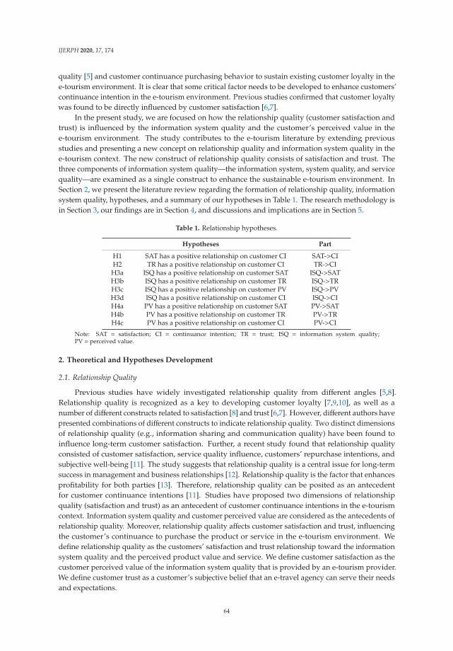
IJERPH 2020, 17, 174

quality [5] and customer continuance purchasing behavior to sustain existing customer loyalty in thee-tourism environment. It is clear that some critical factor needs to be developed to enhance customers’continuance intention in the e-tourism environment. Previous studies confirmed that customer loyaltywas found to be directly influenced by customer satisfaction [6,7].

In the present study, we are focused on how the relationship quality (customer satisfaction andtrust) is influenced by the information system quality and the customer’s perceived value in thee-tourism environment. The study contributes to the e-tourism literature by extending previousstudies and presenting a new concept on relationship quality and information system quality in thee-tourism context. The new construct of relationship quality consists of satisfaction and trust. Thethree components of information system quality—the information system, system quality, and servicequality—are examined as a single construct to enhance the sustainable e-tourism environment. InSection 2, we present the literature review regarding the formation of relationship quality, informationsystem quality, hypotheses, and a summary of our hypotheses in Table 1. The research methodology isin Section 3, our findings are in Section 4, and discussions and implications are in Section 5.

Table 1. Relationship hypotheses.

Hypotheses Part

H1 SAT has a positive relationship on customer CI SAT->CIH2 TR has a positive relationship on customer CI TR->CI

H3a ISQ has a positive relationship on customer SAT ISQ->SATH3b ISQ has a positive relationship on customer TR ISQ->TRH3c ISQ has a positive relationship on customer PV ISQ->PVH3d ISQ has a positive relationship on customer CI ISQ->CIH4a PV has a positive relationship on customer SAT PV->SATH4b PV has a positive relationship on customer TR PV->TRH4c PV has a positive relationship on customer CI PV->CI

Note: SAT = satisfaction; CI = continuance intention; TR = trust; ISQ = information system quality;PV = perceived value.

2. Theoretical and Hypotheses Development

2.1. Relationship Quality

Previous studies have widely investigated relationship quality from different angles [5,8].Relationship quality is recognized as a key to developing customer loyalty [7,9,10], as well as anumber of different constructs related to satisfaction [8] and trust [6,7]. However, different authors havepresented combinations of different constructs to indicate relationship quality. Two distinct dimensionsof relationship quality (e.g., information sharing and communication quality) have been found toinfluence long-term customer satisfaction. Further, a recent study found that relationship qualityconsisted of customer satisfaction, service quality influence, customers’ repurchase intentions, andsubjective well-being [11]. The study suggests that relationship quality is a central issue for long-termsuccess in management and business relationships [12]. Relationship quality is the factor that enhancesprofitability for both parties [13]. Therefore, relationship quality can be posited as an antecedentfor customer continuance intentions [11]. Studies have proposed two dimensions of relationshipquality (satisfaction and trust) as an antecedent of customer continuance intentions in the e-tourismcontext. Information system quality and customer perceived value are considered as the antecedents ofrelationship quality. Moreover, relationship quality affects customer satisfaction and trust, influencingthe customer’s continuance to purchase the product or service in the e-tourism environment. Wedefine relationship quality as the customers’ satisfaction and trust relationship toward the informationsystem quality and the perceived product value and service. We define customer satisfaction as thecustomer perceived value of the information system quality that is provided by an e-tourism provider.We define customer trust as a customer’s subjective belief that an e-travel agency can serve their needsand expectations.

64

IJERPH 2020, 17, 174

2.2. Relationship Quality and Continuance Intention in E-Tourism

According to the expectation disconfirmation model, a customer’s continuance intention isinfluenced by service quality and customer satisfaction [14]. In an e-commerce B2C model, it has beenshown that customer satisfaction influences consumers’ continuance intentions as the outcome ofcognitive, affective, and conative loyalty [15]. Furthermore, relationship quality has a positive influenceon repurchase intention in B2B e-commerce [16]. Satisfaction and trust have been examined as a singleentity, where the relationship quality was considered as a second-order construct [16]. The presentstudy shows that relationship quality consists of satisfaction and trust, which can predict a customer’scontinuance to purchase the product or service in the e-tourism environment. Customer satisfactionand trust are examined as separate entities to fit the advanced technology available. For instance, manycustomers may be satisfied with the information on a website, but this does not mean that the customerwill trust the product or service provided. Based on the above literature, our study hypotheses are:

Hypothesis 1 (H1). Customer satisfaction has a positive effect on continuance intention.

Hypothesis 2 (H2). Customer trust has a positive effect on continuance intention.

2.3. Information System Quality

The information system was proposed in [17]. The study introduced the model, which positsthree major dimensions: system quality, information quality, and user satisfaction in the context oforganizations. Ten years later, in an update to the original Information System literature, the authorsadded service quality to the information system model to evaluate the information system throughseven factors: information quality, system quality, service quality, information use, use, user satisfaction,and net benefits [18]. This develops a different definition regarding the information system [19]. Thesystem quality consists of response time, system reliability, and system availability, which have apositive impact on the perceived ease of use and usefulness of website [18,20].

Service quality is defined as the user’s perceptions regarding the service performance [21]. Servicequality measures the discrepancy between what the customer feels and needs and what is offeredaccordingly to fulfill the customer’s expectations [20,22]. For example, service quality on multicommunication mechanisms enables the user to have their complaints responded to in a timely manner.

Information system success has been measured in four dimensions: completeness, accuracy,format, and currency [23]. For information quality, the user-perceived effectiveness of system qualitymeasurements have included accuracy, relevance, adequacy, and included quality, timeliness, andsequencing [24]. Other studies have also shown that the information system quality has a significantrelationship with perceived usefulness [19]. However, the numbers of previous studies have developedthe information system quality in an e-commerce environment. This study adopts the model from thestudy in [18], as shown in Figure 1. We conceptualize three dimensions of system quality, informationquality, and service quality as information system quality to adopt the advanced technology in thee-tourism environment. The information system quality is defined as products or services that fitcustomer needs and expectations to complete their transaction in the e-tourism environment. Theproducts or services include itinerary services, reliable information, instant information, accurateoperation, and specific information with easy access at anytime and anyplace by the customer. Forinstant, low-cost travel, travel agencies provide interconnected systems, such as TripAdvisor, ezfly.com,or skyscanner.com.tw.

The value that a service involves is not only by the provider but also through the opportunity forcustomer satisfaction and a trust relationship. The information system quality accommodates the swiftcustomer mindset that has changed from traditional to online 24-h services. The travel agency reducesthe time and travel expense, which benefits both parties. Our model has shown that customer trust andsatisfaction are influenced by the information system quality and perceived value. The informationsystem quality enhances the mindset of the customer relationship through a single entity of the product

65

IJERPH 2020, 17, 174

and service in an e-travel environment. Perceived value is dependent on the consumer’s perceptionsof what is received and what is given [25]. The customer’s perceived value influences the customersatisfaction and trust regarding the product or service in the e-tourism environment. Based on thestudies above, we propose the following hypotheses:

Figure 1. Relationship quality research model. Note: H = hypothesis.

Hypothesis 3 (H3). Information system quality has an effect on customer (a) satisfaction, (b) trust, (c) perceivedvalue, and (d) continuance intention.

2.4. Perceived Value

The concept of value has constantly emerged from the different studies related to consumerbehavior [25,26]. Prior studies suggested that perceived value is a better predictor of repurchaseintentions than satisfaction, commitment, or trust [26]. Furthermore, the perceived value of the productand service could attract new consumers and result in benefits to the vendor [6,27,28]. Our model hasshown that customer satisfaction and trust relationships are influenced by the customer’s perceivedproduct and service value. The customer’s perceived value influences the customer’s continuanceintention. Based on this literature, we propose the following hypothesis:

Hypothesis 4 (H4). Perceived value has a positive effect on customer (a) satisfaction, (b) trust, and (c)continuance intention.

3. Research Methodology

3.1. Subjects: Instrument Development and MeasurementThe survey study was designed based on the previous study on the information system success and

IT development in an e-commerce environment, looking at service quality, system quality, perceivedquality, trust, satisfaction, and continuance of use. We developed and reworded the survey items tofit the present study. All the items in the questionnaire were modified from English, translated toChinese, and then translated back to English. The initial version of the survey study was pretestedby two Ph.D. students and one professor who is an expert in the field of questionnaire design fore-commerce studies. After obtaining feedback from the experts, we modified the questionnaires forthe final measurements of the model.

The constructs are measured using five-point Likert scales, ranging from 1–5, with 1 indicating“strongly disagrees” and 5 indicating “strongly agrees”. Information system quality was adoptedfrom [14,18], with seven items. Perceived value, with five items, was modified from [26,28], and threeitems were taken for further data analysis. Customer trust, with four items, was modified from [6,29].

66

IJERPH 2020, 17, 174

Satisfaction, with four items, was modified from [6]. Continuance intention was adapted from [30]with five items, and three items were taken for further data analysis, as the loading value was lowerthan the effective value.

3.2. Survey CollectionThe questionnaire was targeted to online travel users such as students, information technology

users, manufacturers, and customers in finance, public service, and medical fields, who have experiencebuying domestic or international travel itineraries such as air tickets, reservations, and car rentals,as well as experience booking hotels and other services in e-travel (e.g., Ezfly, Eztravel, Skyscanner,tripadvisor). We chose websites that were the most popular and where the systematic system can easilybe accessed by personal computer (PC) and cell phones, with flexible times and affordable prices foryoung or elderly people. The data were collected over two months in Taiwan. For more informationregarding the survey items, refer to Appendix A. To maximize the respondents’ awareness on thissurvey, we contacted the respondents by email or sent the questionnaire on personal Facebook chat,Line chat, group Facebook, or Line chat. We distributed 450 questionnaires, and 376 were returned,with a response rate of 83.5%. After data sterilization, 25 respondents were dropped due to incompleteresponses on the survey. The final sample employed in our study was 351 responses (93.4% of thetotal responses). We employed IBM SPSS 20 (Armonk, NY, USA) for descriptive analysis to assess thefrequency, and the percent range of populations is shown in Table 2.

Table 2. Demographics of the respondents.

Demographic Respondents (N = 351)

Characteristics Frequency Percent (%) Characteristics Frequency Percent (%)

Gender Occupation

MaleFemale

143208

40.759.3

StudentTechnology

ManufacturingFinanceServiceMedical

523875569337

14.810.821.416.026.510.5

Age MonthlyIncome

≤2021–3031–4041–5051–60>60

298956667833

8.325.416.018.822.29.4

≥1000$1001–2000$2001–3000$3001–4000$<4000

4516949682

12.848.114.01.723.4

Education Travel service

≥Senior high schoolUniversity/collegeGraduate above

70155126

19.944.235.9

hkexpressezfly

eztravelTripAdvisor

Others

7070

1038523

19.919.929.324.26.6

Instruments

PCSmartphone

114237

32.567.5

Note: PC = personal computer.

The majority of respondents used the online travel service itinerary for their travels, which showedthat 59.3% were female and 40.7% were male. The participants were mostly from the age groups of21–30 years old and 51–60 years old. The participants mostly work in manufacturing and public servicefrom different sectors. The highest monthly income was 1001–2000 USD. The participants searched forinformation using a smartphone 67.5% of the time. Further, eztravel (29.3%) and TripAdvisor (24.2%)

67

IJERPH 2020, 17, 174

were the most popular e-travel service websites for finding information and booking itineraries. Thedata samples were sufficient to identify the customers’ behavior and to accommodate further study onthe information system quality.

4. Data Analysis Results

4.1. Measurement Model Analysis

The measurement model and structural model was assessed with partial least squares (PLS) usingSmarts-PLS 3.2.8 [31]. First, PLS is not as restrictive on the sample size as that designed in the structuralequation model. The constructs in this study are all reflective. Therefore, a PLS modeling approachwas chosen in this study.

Second, for the data analysis, we started with the PLS algorithm that can obtain at convergence,satisfying fixed-point equations which include measurement reliability and model validity.

The third, the bootstrap procedure [32] was used to test the significance of various results such aspath coefficients, Cronbach’s alpha, and R2 values. As in bootstrapping, subsamples are randomlydrawn observations from the original set of data. This process was repeated until a large number ofrandom subsamples were created, which in the case of our study was 2000 subsamples. The estimationsfrom the bootstrap subsamples were used to derive standard errors for the PLS-SEM results. With thisinformation, t-values, p-values, and confidence intervals were calculated to assess the significance ofmodel studies.

Four, confirmatory factor analysis was conducted to assess the item loadings, discriminant validity,and internal consistency of the model. Item loading and internal consistencies greater than 0.70 wereconsidered acceptable [33,34]. Moreover, to assess convergent and discriminant validity, first, theindicators loaded should be stronger than corresponding ones on the other constructs. Second, thesquare root of the average variance extracted (AVE) should be greater than the internal-constructscorrelations shown in Appendix B, (cross-factor loading) which confirms the presence of a validdiscriminant. Furthermore, in Table 3, the Cronbach’s alpha values range from 0.91 to 0.98, and theAVE ranges from 0.79 to 0.96, indicating acceptability [33]. These results demonstrate that all themeasurements have an adequate acceptability level.

Table 3. Construct reliability and discriminant validity.

Constructs ItemsCronbach’s

AlphaCompositeReliability

AVE CI ISQ PV SAT TR

ContinuanceIntention CI 0.98 0.99 0.96 0.98

Informationsystem Quality ISQ 0.97 0.98 0.87 0.78 0.93

Perceived Value PV 0.95 0.97 0.91 0.67 0.66 0.96Satisfaction SAT 0.91 0.94 0.79 0.72 0.70 0.86 0.89

Trust TR 0.92 0.94 0.80 0.70 0.70 0.78 0.83 0.90

Note: AVE = average variance extracted.

Five, an exploratory factor analysis was conducted to determine the relationship factors in theSmart-PLS algorithms. The exploratory factor analysis results are shown in Table 4. Standard factorloading and the t-value on the measurements were significant at the level of 0.01–0.02. Table 5 showsall the items of latent variables correlations on their intended factors to determine if the survey study isadequate for further analysis.

68

IJERPH 2020, 17, 174

Table 4. Weight and loading.

Constructs Items Outer Loading Outer Weights Standard Deviation T Statistics

ContinuanceIntention

CI1 0.98 0.34 0.01 171.44CI2 0.98 0.34 0.01 161.33CI3 0.98 0.33 0.01 137.83

Informationsystem Quality

ISQ1 0.95 0.16 0.01 97.28ISQ2 0.94 0.16 0.02 62.09ISQ3 0.92 0.15 0.02 49.69ISQ4 0.92 0.15 0.01 67.88ISQ5 0.93 0.15 0.02 61.26ISQ6 0.94 0.15 0.01 101.48ISQ7 0.90 0.14 0.02 54.40

PerceivedValue

PV3 0.95 0.34 0.01 102.10PV4 0.96 0.35 0.01 134.48PV5 0.96 0.35 0.01 93.05

Satisfaction

SAT1 0.89 0.31 0.01 63.35SAT2 0.90 0.27 0.02 59.68SAT3 0.85 0.24 0.02 38.83SAT4 0.91 0.31 0.01 62.48

Trust

TR1 0.87 0.31 0.02 57.57TR2 0.88 0.27 0.02 52.50TR3 0.91 0.26 0.02 55.83TR4 0.92 0.28 0.01 69.56

Note: Both the standard deviation and t-value are for loading not for weighting.

Table 5. Latent variable correlations.

Constructs Items CI ISQ PV SAT TR

Continuance Intention CI 1.00 0.78 0.67 0.72 0.70Information System Quality ISQ 0.78 1.00 0.66 0.70 0.70

Perceived Value PV 0.67 0.66 1.00 0.86 0.78Satisfaction SAT 0.72 0.70 0.86 1.00 0.83

Trust TR 0.70 0.70 0.78 0.83 1.00

4.2. The Results of Structural Model

The results of the Smart-PLS part coefficients and significance values are shown in Figure 2.Table 6 shows the summary of our hypotheses testing. Seven of the nine hypotheses have positive andsignificant relationships. Customer satisfaction has a positive and significant effect on continuanceintention, which supports H1, SAT–CI (β = 0.20, t = 2.59, ** p < 0.01). However, the influence ofcustomer trust has no significant relationship with continuance intention. Thus, H2 is not supported,trust–continuance intention (TR–CI) (β = 0.13, t = 1.89, p < 0.05). The testing (H3a, H3b, H3c,and H3d) showed that information system quality has a positive and significant effect on customersatisfaction, trust, perceived value, and customer continuance intention. Thus, H3a, informationsystem quality–satisfaction (ISQ–SAT) (β = 0.12, t = 2.99, *** p < 0.001), H3b, ISQ–TR (β = 0.33, t = 5.82*** p < 0.001), H3c, ISQ–perceived value (PV) (β = 0.67, t = 17.0 *** p < 0.001), and H3d, ISQ–CI (β = 0.50,t = 7.50, *** p < 0.001) were supported. Consequently, the (H3a, H4b), customer perceived value has apositive and significant effect on customer satisfaction and customer trust. Thus, H4a and H4b weresupported (PV–SAT, β = 0.50, t = 8.30, *** p < 0.001, and PV–TR, β = 0.56, t = 10.1, *** p < 0.001).However, perceived value does not have a significant influence on customer continuance intention,and so H4c, PV–CI (β = 0.07, t = 0.97, p < 0.05) is not supported. The model also explains 67% of thevariance of customer continuance intention, 81% of the variance of customer satisfaction, 67% of thevariance of a customer trust relationship, and 44% of the variance of customer perceived value of theproduct or service on an e-tourism channel.

69

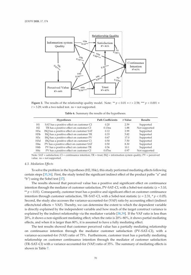
IJERPH 2020, 17, 174

Figure 2. The results of the relationship quality model. Note: ** p < 0.01 = t > 2.58; *** p < 0.001 =t > 3.29; with a two-tailed test. ns = not supported.

Table 6. Summary the results of the hypotheses.

Hypotheses Path Coefficients t-Value Results

H1 SAT has a positive effect on customer CI 0.20 2.59 SupportedH2 TR has a positive effect on customer CI 0.13ns 1.88 Not supportedH3a ISQ has a positive effect on customer SAT 0.12 2.99 SupportedH3b ISQ has a positive effect on customer TR 0.33 5.82 SupportedH3c ISQ has a positive effect on customer PV 0.67 17.0 SupportedH3d ISQ has a positive effect on customer CI 0.50 7.50 SupportedH4a PV has a positive effect on customer SAT 0.50 8.30 SupportedH4b PV has a positive effect on customer TR 0.56 10.1 SupportedH4c PV has a positive effect on customer CI 0.07ns 0.97 Not supported

Note: SAT = satisfaction; CI = continuance intention; TR = trust; ISQ = information system quality; PV = perceivedvalue. ns = not supported.

4.3. Mediation Effects

To solve the problem in the hypotheses (H2, H4c), this study performed mediating effects followingcertain steps [35,36]. First, the study tested the significant indirect effect of the product paths “a” and“b”) using the Sobel test [37].

The results showed that perceived value has a positive and significant effect on continuanceintention through the mediator of customer satisfaction, PV–SAT–CI, with a Sobel-test statistic (z = 3.10,** p < 0.01). Consequently, customer trust has a positive and significant effect on customer continuanceintention through customer satisfaction, TR–SAT–CI, with a Sobel-test statistic (z = 2.31, * p < 0.05).Second, the study also accesses the variance-accounted-for (VAF) ratio by accounting effect (indirecteffects/total effects = VAF). Thereby, we can determine the extent to which the dependent variableis directly explained by the independent variable and how much of the target construct variance isexplained by the indirect relationship via the mediator variable [38,39]. If the VAF ratio is less than20%, it shows a non-significant mediating effect; when the ratio is 20%–80%, it shows partial mediatingeffects, and when it is larger than 80%, it is assumed to have a fully mediating effect.

The test results showed that customer perceived value has a partially mediating relationshipon continuance intention through the mediator customer satisfaction (PV–SAT–CI), with avariance-accounted-for (VAF) ratio of 75%. Furthermore, customer trust has a partially mediatingrelationship on customer continuance intention through the mediator of customer satisfaction(TR–SAT–CI) with a variance-accounted-for (VAF) ratio of 35%. The summary of mediating effects isshown in Table 7.

70

IJERPH 2020, 17, 174

Table 7. Results of mediating effects.

Indirect Effect IV-MD MD-DV C c’ AB Total Effect Sobel VAF% Type

PV-SAT-CI 0.50 *** 0.20 ** 0.20 *** 0.67 *** 0.21 *** 0.28 *** 3.10 ** 75% PartialTR-SAT-CI 0.36 *** 0.20 ** 0.28 *** 0.70 *** 0.07 ** 0.20 *** 2.31 * 35% Partial

Note: IV = independent variable; MD =mediator; DV = dependent variable; VAF = variance-accounted-for; IV-MD= The IV significantly affects the mediator; MD-DV = the mediator has a significant unique effect on the DV; C= the effect of the IV on the DV shrinks upon the addition of the mediator to the model; c’ = The IV significantlyaffects the DV in the absence of the mediator; AB = the total indirect effect. * p < 0.05 = t > 1.96; ** p < 0.01 = t > 2.58;*** p < 0.001 = t > 3.29; with one-tailed test.

5. Discussion

5.1. Theoretical Implication

Several implications are obtained from this study. First, this study extends the previously study [18],and the findings support the research on information system quality by examining information quality,system quality, and service quality as a single entity.

Second, the prior study on customer relationship quality examined this quality as a single entityand showed a positive and significant effect on continuance intention [7]. In this study, relationshipquality was examined as two separate entities (customer satisfaction and customer trust). Customersatisfaction had a positive and significant effect on the continued use of the products or service in thee-tourism environment. Customers showed a continuance of trust in the products or service when thecustomer was satisfied with the product or service. The information system quality proved long-termusage investment on customer continuance intention, which differs from the existing studies [18] andsupports [30,40] customer relationship quality in the e-tourism environment.

Third, the customer-perceived value has a positive effect on customer satisfaction and trust.However, perceived value has no significant relationship on customer continuous intention.Furthermore, perceived value has a partial influence on customer continuance intention throughcustomer satisfaction. This means that without sufficient customer satisfaction, customers may nottend to purchase in the future or will be unable to retain long-term success in e-tourism. The travelagencies have to build existing customers through customer relationship quality, in particular, buildingcustomer satisfaction and trusting relationships.

The findings stated that the customer’s relationship qualities (e.g., trust and satisfaction) arethe main issues affecting the continuing usage intention in regard to information system quality.Providing a new model, such as a one-desk information service and improved relationship quality(customer satisfaction and trust) could enhance the impact of information system quality on thee-tourism environment.

Fourth, the study found that the majority of respondents who employ the online travel service fortheir travels were 59.3% female and 40.7% male. The mean gender show a similar benefit from theinformation system quality in e-tourism. Moreover, results also showed that the participants from ages21–30 and 51–60 years old who worked in manufacturing and the public service from different sectorswere more expected to continue to purchase the products or service.

Furthermore, the customers with income from 1001–2000 USD more frequently used theinformation and booking and were the most familiar with the websites Eztravel 29.3% and TripAdvisor24.2%. However, most customers used a smartphone as their preferred tool for booking travel plans.We conclude that these characteristic customer behaviors are shown to provide continuance successin the information system applications in this e-commerce environment, which is different from thefindings of previous studies [18].

5.2. Practical Implication

The practical implications for information system quality, perceived value, relationship quality,and customer’s continuance intention offer important implications for travel agencies and managers

71

IJERPH 2020, 17, 174

in e-tourism. To improve IS quality in the e-tourism environment, the travel agency and managerhas to upgrade the operational process infrastructure and delivery service transaction to matchreal-time customer expectations. Furthermore, they require software and hardware with an advancedinformation system that can prevent technical difficulties and transactions overloading [30].

Managers and practitioners can use these results as guidelines to develop websites, operations,and provide advance support to customers. The measurement of information system quality canenhance products and services to help managers and organizations provide better products andservices in the e-tourism environment. In addition, these results may apply a particularly powerfulbenchmark against competitors’ websites that can affect long-term development activities on e-tourism.Our findings not only support a viewpoint on information system quality development, but also onbuilding customer relationship quality through the application of customer satisfaction and trustprovided by the e-tourism provider. Service providers can provide an incentive program such aspurchasing a bundle program for customer travel planning. Furthermore, the study also demonstratedthe positive and significant influence of perceived value on customers’ continuance intention throughcustomer satisfaction, which enhances long-term customer success in adopting a new program suchas a package information service. This may suggest that enhancing information system quality isnot only to satisfying for the customers but also helps to build customer trust relationships in ane-tourism environment.

6. Conclusions and Future Study

This study has important implications for the researcher and practitioner. The study concludesthat customer relationship quality (satisfaction) has positive effects on customer continuance intentions.However, customer trust also has a partial relationship on continuance intention through customersatisfaction. In addition, information system quality has a significant relationship with customersatisfaction, trust, perceived value, and continuance intention. Furthermore, the customer-perceivedvalue is also significantly related to customer satisfaction and trust, but it is partially related to customercontinuance intention through the customer satisfaction relationship.

However, nowadays, e-tourism companies have greatly invested in training programs andadvertising campaigns to transform information system quality for the users. This study providedmore comprehensive findings on the information system and examined three dimensions (informationquality, system quality, and service quality) in a single entity as information system quality, but it alsoseparately examined the relationship quality that consists of customer satisfaction and trust in thee-tourism environment. We attempted to integrate perceived value and customer relationship qualitywith the model on customer continuance intention. Some interesting findings that were not discussedin previous studies are also covered in the current study. A large sample in this study is from themanufacturing and services sector, which is due to the customer trust and satisfaction in e-tourism.This study also provides meaningful implications on e-tourism continuance intention behavior.

A limitation in this study is using self-report instruments, as this may have the potential for acommon method bias in measuring the study variables [41]. Hence, we diminished the probabilityof common biases by segregating the instruments and motivating the participants in the study.Furthermore, study data were collected in Taiwan. The travel forum members have similar culture andconvenience traits. More research across countries and cultures will be required in order to generalizethe findings. Finally, future studies also have the possibility to investigate different factors that can beintegrated into the model.

Author Contributions: Funding acquisition, Writing—original draft, A.R.; Resources, C.-I.P.; Supervision, S.-C.C.;Writing—original draft, Data collection, Data analysis, N.W.M.; Writing—review and editing, J.-J.Y. All authorshave read and agreed to the published version of the manuscript.

Funding: This research received no external funding.

Conflicts of Interest: The authors declare no conflict of interest.

72

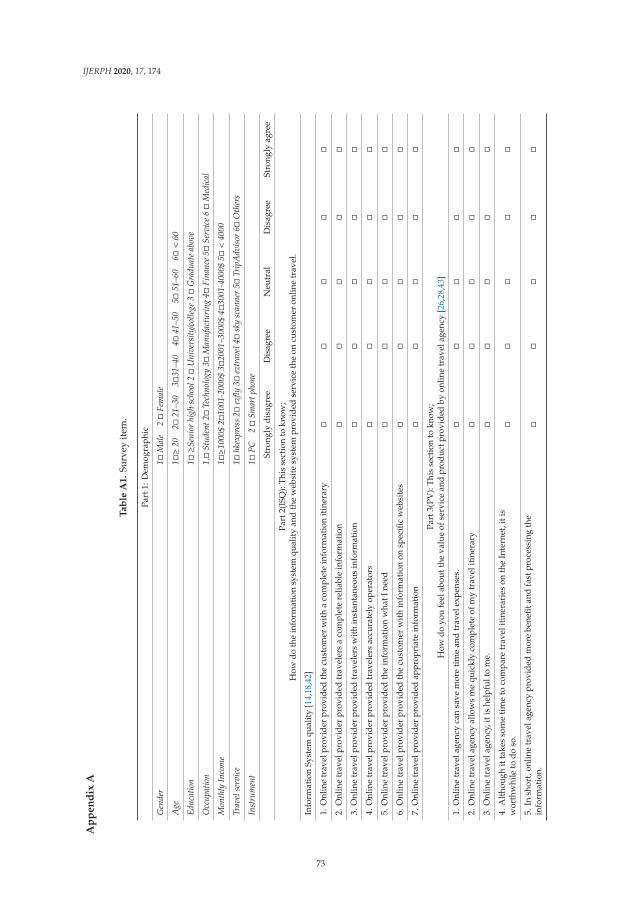
IJERPH 2020, 17, 174

Ap

pe

nd

ixA

Ta

ble

A1

.Su

rvey

item

.

Part

1:D

emog

raph

ic

Gen

der

1�M

ale

2�

Fem

ale

Age

1�≥2

02�

21–3

03�

31–4

04�

41–5

05�

51–6

06�<

60

Educ

atio

n1�≥S

enio

rhi

ghsc

hool

2�

Uni

vers

ity/co

llege

3�

Gra

duat

eab

ove

Occ

upat

ion

1.�

Stud

ent2�

Tech

nolo

gy3�

Man

ufac

turi

ng4�

Fina

nce

5�Se

rvic

e6�

Med

ical

Mon

thly

Inco

me

1�≥1

000$

2�10

01-2

000$

3�20

01–3

000$

4�30

01-4

000$

5�<

4000

Trav

else

rvic

e1�

hkex

pres

s2�

ezfly

3�ez

trav

el4�

sky

scan

ner

5�Tr

ipA

dvis

or6�

Oth

ers

Inst

rum

ent

1�PC

2�

Smar

tpho

ne

Stro

ngly

disa

gree

Dis

agre

eN

eutr

alD

isag

ree

Stro

ngly

agre

e

Part

2(IS

Q):

This

sect

ion

tokn

ow;

How

doth

ein

form

atio

nsy

stem

qual

ity

and

the

web

site

syst

empr

ovid

edse

rvic

eth

eon

cust

omer

onlin

etr

avel

.

Info

rmat

ion

Syst

emqu

alit

y[1

4,18

,42]

1.O

nlin

etr

avel

prov

ider

prov

ided

the

cust

omer

wit

ha

com

plet

ein

form

atio

nit

iner

ary

��

��

�

2.O

nlin

etr

avel

prov

ider

prov

ided

trav

eler

sa

com

plet

ere

liabl

ein

form

atio

n�

��

��

3.O

nlin

etr

avel

prov

ider

prov

ided

trav

eler

sw

ith

inst

anta

neou

sin

form

atio

n�

��

��

4.O

nlin

etr

avel

prov

ider

prov

ided

trav

eler

sac

cura

tely

oper

ator

s�

��

��

5.O

nlin

etr

avel

prov

ider

prov

ided

the

info

rmat

ion

wha

tIne

ed�

��

��

6.O

nlin

etr

avel

prov

ider

prov

ided

the

cust

omer

wit

hin

form

atio

non

spec

ific

web

site

s�

��

��

7.O

nlin

etr

avel

prov

ider

prov

ided

appr

opri

ate

info

rmat

ion

��

��

�

Part

3(PV

):Th

isse

ctio

nto

know

;H

owdo

you

feel

abou

tthe

valu

eof

serv

ice

and

prod

uctp

rovi

ded

byon

line

trav

elag

ency

[26,

28,4

3]

1.O

nlin

etr

avel

agen

cyca

nsa

vem

ore

tim

ean

dtr

avel

expe

nses

.�

��

��

2.O

nlin

etr

avel

agen

cyal

low

sm

equ

ickl

yco

mpl

ete

ofm

ytr

avel

itin

erar

y�

��

��

3.O

nlin

etr

avel

agen

cy,i

tis

help

fult

om

e.�

��

��

4.A

ltho

ugh

itta

kes

som

eti

me

toco

mpa

retr

avel

itin

erar

ies

onth

eIn

tern

et,i

tis

wor

thw

hile

todo

so.

��

��

�

5.In

shor

t,on

line

trav

elag

ency

prov

ided

mor

ebe

nefit

and

fast

proc

essi

ngth

ein

form

atio

n.�

��

��

73

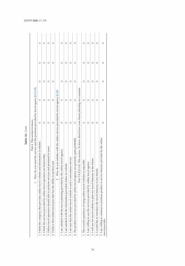
IJERPH 2020, 17, 174

Ta

ble

A1

.C

ont.

Part

4:Th

isse

ctio

nto

know

;1.

How

doyo

utr

ustt

hese

rvic

ean

dth

epr

oduc

tspr

ovid

edby

trav

elag

ency

[6,2

5,29

].

1.It

hink

the

com

pany

that

prov

ides

onlin

etr

avel

web

site

and

info

rmat

ion

isre

liabl

e.�

��

��

2.It

hink

the

serv

ices

prov

ided

byon

line

trav

elop

erat

ors

are

trus

twor

thy.

��

��

�

3.O

nlin

etr

avel

oper

ator

ssh

ould

able

tope

rfor

mse

rvic

esan

dpr

omis

edto

user

s�

��

��

4.Ib

elie

veth

aton

line

trav

elpr

ovid

erha

sth

eab

ility

topr

otec

tuse

r�

��

��

2.H

owdo

you

sati

sfies

wit

hth

eon

line

serv

ice

prov

ided

bytr

avel

agen

cy[6

,44]

1.Ia

msa

tisfi

edw

ith

the

trav

elpl

anni

ngpr

ovid

edby

the

onlin

etr

avel

agen

cy.

��

��

�

2.Ia

msa

tisfi

edw

ith

the

info

rmat

ion

prov

ided

onlin

eon

web

site

.�

��

��

3.Ia

msu

reth

atth

eon

line

trav

elw

ebsi

teis

such

aco

nven

ienc

ese

rvic

e�

��

��

4.Th

epr

oduc

tor

serv

ice

prov

ided

byon

line

trav

elag

ency

are

gene

rally

quit

epr

ofita

ble

��

��

�

Part

5(C

I)[9

,40]

:Thi

sse

ctio

n,To

know

abou

thow

your

futu

repl

anni

ngon

e-to

uris

m

1.Th

eov

eral

lexp

erie

nce

ofus

ing

onlin

etr

avel

web

site

sis

enjo

yabl

e.�

��

��

2.Ia

mw

illin

gto

use

the

serv

ices

prov

ided

byon

line

trav

elag

ency

��

��

�

3.Iw

illus

eth

etr

avel

web

site

topl

anm

ytr

avel

itin

erar

yin

the

futu

re.

��

��

�

4.Iw

ould

like

toin

trod

uce

the

trav

elit

iner

ary

tom

yfr

iend

s�

��

��

5.Ia

mw

illin

gto

cont

inue

topu

rcha

sepr

oduc

tor

serv

ice

itine

rary

prov

ided

byth

eon

line

trav

elpr

ovid

er.

��

��

�

74

IJERPH 2020, 17, 174

Appendix B

Table A2. The Result of cross loading.

Cross Loadings

Constructs Items CI ISQ PV SAT TR

ContinuanceIntention

CI1 0.98 0.76 0.68 0.71 0.70CI2 0.98 0.77 0.66 0.71 0.69CI3 0.98 0.75 0.64 0.69 0.67

Informationsystem Quality

ISQ1 0.76 0.95 0.66 0.68 0.67ISQ2 0.76 0.94 0.66 0.69 0.69ISQ3 0.72 0.92 0.59 0.63 0.62ISQ4 0.70 0.92 0.61 0.64 0.65ISQ5 0.71 0.93 0.62 0.66 0.66ISQ6 0.73 0.94 0.61 0.66 0.66ISQ7 0.68 0.90 0.58 0.61 0.60

Perceived ValuePV3 0.60 0.63 0.95 0.80 0.76PV4 0.66 0.64 0.96 0.82 0.75PV5 0.66 0.64 0.96 0.84 0.72

Satisfaction

SAT1 0.70 0.66 0.87 0.89 0.73SAT2 0.58 0.60 0.72 0.90 0.72SAT3 0.51 0.53 0.63 0.85 0.70SAT4 0.71 0.68 0.80 0.91 0.78

Trust

TR1 0.69 0.71 0.76 0.83 0.87TR2 0.59 0.59 0.66 0.73 0.88TR3 0.58 0.55 0.66 0.68 0.91TR4 0.63 0.63 0.69 0.71 0.92

References

1. Ponte, E.B.; Carvajal-Trujillo, E.; Escobar-Rodríguez, T. Influence of trust and perceived value on the intentionto purchase travel online: Integrating the effects of assurance on trust antecedents. Tour. Manag. 2015, 47,286–302. [CrossRef]

2. Chen, S.-C.; Li, S.-H. Consumer adoption of e-service: Integrating technology readiness with the theory ofplanned behavior. Afr. J. Bus. Manag. 2010, 4, 3556–3563.

3. Breidbach, C.F.; Kolb, D.G.; Srinivasan, A. Connectivity in service systems: Does technology-enablementimpact the ability of a service system to co-create value? J. Serv. Res. 2013, 16, 428–441. [CrossRef]

4. Li, X.; Wang, Y.; Yu, Y. Present and future hotel website marketing activities: Change propensity analysis. Int.J. Hosp. Manag. 2015, 47, 131–139. [CrossRef]

5. Wu, H.-C.; Cheng, C.-C. Relationships between technology attachment, experiential relationship quality,experiential risk and experiential sharing intentions in a smart hotel. J. Hosp. Tour. Manag. 2018, 37, 42–58.[CrossRef]

6. Su, L.; Hsu, M.K.; Swanson, S. The effect of tourist relationship perception on destination loyalty at a worldheritage site in China: The mediating role of overall destination satisfaction and trust. J. Hosp. Tour. Res.2017, 41, 180–210. [CrossRef]

7. Setó-Pamies, D. Customer loyalty to service providers: Examining the role of service quality, customersatisfaction and trust. Total Qual. Manag. Bus. Excell. 2012, 23, 1257–1271. [CrossRef]

8. Williams, P.; Ashill, N.J.; Naumann, E. Relationship quality and satisfaction: Customer-perceived successfactors for on-time projects. Int. J. Proj. Manag. 2015, 33, 1836–1850. [CrossRef]

9. Ou, W.-M.; Shih, C.M.; Chen, C.Y. Relationships among customer loyalty programs, service quality,relationship quality and loyalty: An empirical study. Chin. Manag. Stud. 2011, 5, 194–206. [CrossRef]

10. Liu, C.-T.; Guo, Y.M.; Lee, C.-H. The effects of relationship quality and switching barriers on customer loyalty.Int. J. Inf. Manag. 2011, 31, 71–79. [CrossRef]

75

IJERPH 2020, 17, 174

11. Su, L.; Swanson, S.R.; Chen, X. The effects of perceived service quality on repurchase intentions and subjectivewell-being of Chinese tourists: The mediating role of relationship quality. Tour. Manag. 2016, 52, 82–95.[CrossRef]

12. Gounaris, S.; Tzempelikos, N. Relational key account management: Building key account managementeffectiveness through structural reformations and relationship management skills. Ind. Mark. Manag. 2014,43, 1110–1123. [CrossRef]

13. Casidy, R.; Nyadzayo, M. Drivers and outcomes of relationship quality with professional service firms:An SME owner-manager perspective. Ind. Mark. Manag. 2017, 78, 27–42. [CrossRef]

14. Bhattacherjee, A. Understanding information systems continuance: An expectation-confirmation model.MIS Q. 2001, 25, 351–370. [CrossRef]

15. Yuksel, A.; Yuksel, F.; Bilim, Y. Destination attachment: Effects on customer satisfaction and cognitive,affective and conative loyalty. Tour. Manag. 2010, 31, 274–284. [CrossRef]

16. Zhang, Y.; Fang, Y.; Wei, K.K. Repurchase intention in B2C e-commerce—A relationship quality perspective.Inf. Manag. 2011, 48, 192–200. [CrossRef]

17. DeLone, W.H.; McLean, E.R. Information systems success: The quest for the dependent variable. Inf. Syst.Res. 1992, 3, 60–95. [CrossRef]

18. Delone, W.H.; McLean, E.R. The DeLone and McLean model of information systems success: A ten-yearupdate. J. Manag. Inf. Syst. 2003, 19, 9–30.

19. Chung, N.; Koo, C. The use of social media in travel information search. Telemat. Inf. 2015, 32, 215–229.[CrossRef]

20. Dedeke, A.N. Travel web-site design: Information task-fit, service quality and purchase intention. Tour.Manag. 2016, 54, 541–554. [CrossRef]

21. Wang, K. Determinants of mobile value-added service continuance: The mediating role of service experience.Inf. Manag. 2015, 52, 261–274. [CrossRef]

22. Walsh, G.; Hennig-Thurau, T.; Sassenberg, K. Does relationship quality matter in e-services? A comparisonof online and offline retailing. J. Retail. Consum. Serv. 2010, 17, 130–142. [CrossRef]

23. Rana, N.P.; Dwivedi, Y.K.; Williams, M.D. Investigating success of an e-government initiative: Validation ofan integrated IS success model. Inf. Syst. Front. 2015, 17, 127–142. [CrossRef]

24. Hosseini, S.; Barker, K.; Ramirez-Marquez, J.E. A review of definitions and measures of system resilience.Reliab. Eng. Syst. Saf. 2016, 145, 47–61. [CrossRef]

25. Kuo, Y.-F.; Wu, C.-M.; Deng, W.-J. The relationships among service quality, perceived value, customersatisfaction, and post-purchase intention in mobile value-added services. Comput. Hum. Behav. 2009, 25,887–896. [CrossRef]

26. Gallarza, M.G.; Saura, I.G. Value dimensions, perceived value, satisfaction and loyalty: An investigation ofuniversity students’ travel behaviour. Tour. Manag. 2006, 27, 437–452. [CrossRef]

27. Su, L.; Swanson, S.R.; Chen, X. The impact of perceived service fairness and quality on the behavioralintentions of chinese hotel guests: The mediating role of consumption emotions. J. Travel Tour. Mark. 2016,33 (Suppl. 1), 88–102. [CrossRef]

28. Lai, T.L. Service quality and perceived value’s impact on satisfaction, intention and usage of short messageservice (SMS). Inf. Syst. Front. 2004, 6, 353–368. [CrossRef]

29. Wang, L.; Law, R.; Guillet, B.D. Impact of hotel website quality on online booking intentions: eTrust as amediator. Int. J. Hosp. Manag. 2015, 47, 108–115. [CrossRef]

30. Hadji, B.; Degoulet, P. Information system end-user satisfaction and continuance intention: A unifiedmodeling approach. J. Biomed. Informat. 2016, 61, 185–193. [CrossRef]

31. Ringle, C.M.; Wende, S.; Becker, J.-M. SmartPLS 3. Boenningstedt: SmartPLS GmbH. Available online:http://www.smartpls.com (accessed on 30 July 2015).

32. Hair, J.; Hollingsworth, C.L.; Randolph, A.B. An updated and expanded assessment of PLS-SEM ininformation systems research. Ind. Manag. Data Syst. 2017, 117, 442–458. [CrossRef]

33. MacKenzie, S.B.; Podsakoff, P.M.; Podsakoff, N.P. Construct measurement and validation procedures in MISand behavioral research: Integrating new and existing techniques. MIS Q. 2011, 35, 293–334. [CrossRef]

34. Fornell, C.; Larcker, D.F. Structural equation models with unobservable variables and measurement error:Algebra and statistics. J. Mark. Res. 1981, 1, 382–388. [CrossRef]

76

IJERPH 2020, 17, 174

35. Hair, F.J., Jr.; Sarstedt, M.; Hopkins, L. Partial least squares structural equation modeling (PLS-SEM) Anemerging tool in business research. Eur. Bus. Rev. 2014, 26, 106–121. [CrossRef]

36. Nitzl, C.; Roldan, J.L.; Cepeda, G. Mediation analysis in partial least squares path modeling: Helpingresearchers discuss more sophisticated models. Ind. Manag. Data Syst. 2016, 116, 1849–1864. [CrossRef]

37. Soper, D. Sobel Test Calculator for the Significance of Mediation. Available online: https://www.danielsoper.com/statcalc/calculator.aspx?id=31 (accessed on 28 August 2019).

38. Baron, R.M.; Kenny, D.A. The moderator–mediator variable distinction in social psychological research:Conceptual, strategic, and statistical considerations. J. Pers. Soc. Psychol. 1986, 51, 1173. [CrossRef]

39. Carrión, G.C.; Nitzl, C.; Roldán, J.L. Mediation analyses in partial least squares structural equation modeling:Guidelines and empirical examples. In Partial Least Squares Path Modeling; Springer: Berlin/Heidelberg,Germany, 2017; pp. 173–195.

40. Kim, J.; Hong, S.; Min, J. Antecedents of application service continuance: A synthesis of satisfaction andtrust. Expert Syst. Appl. 2011, 38, 9530–9542. [CrossRef]

41. Jeyaraj, A.; Rottman, J.W.; Lacity, M.C. A review of the predictors, linkages, and biases in IT innovationadoption research. J. Inf. Technol. 2006, 21, 1–23. [CrossRef]

42. Kettinger, W.J.; Lee, C.C. Pragmatic perspectives on the measurement of information systems service quality.MIS Q. 1997, 21, 223–240. [CrossRef]

43. Moliner, M.A.; Sánchez, J.; Rodríguez, R.M.; Callarisa, L. Relationship quality with a travel agency: Theinfluence of the postpurchase perceived value of a tourism package. Tour. Hosp. Res. 2007, 7, 194–211.[CrossRef]

44. Liao, C.; Chen, J.-L.; Yen, D.C. Theory of planning behavior (TPB) and customer satisfaction in the continueduse of e-service: An integrated model. Comput. Hum. Behav. 2007, 23, 2804–2822. [CrossRef]

© 2019 by the authors. Licensee MDPI, Basel, Switzerland. This article is an open accessarticle distributed under the terms and conditions of the Creative Commons Attribution(CC BY) license (http://creativecommons.org/licenses/by/4.0/).

77

International Journal of

Environmental Research

and Public Health

Article

The Evaluation Method of Low-Carbon Scenic Spotsby Combining IBWM with B-DST and VIKOR inFuzzy Environment

Aijun Liu 1, Taoning Liu 1, Xiaohui Ji 1, Hui Lu 2 and Feng Li 3,*1 Department of Management Engineering, School of Economics & Management, Xidian University,

Xi’an 710071, China; ajliu@xidian.edu.cn (A.L.); tnliu@stu.xidian.edu.cn (T.L.); xhji@stu.xidian.edu.cn (X.J.)2 Tianhua College, Shanghai Normal University, Shanghai 201815, China; janetluck@126.com3 School of Information, Beijing Wuzi University, Beijing 101149, China* Correspondence: lifeng@bwu.edu.cn

Received: 26 November 2019; Accepted: 18 December 2019; Published: 21 December 2019

Abstract: With the concept of sustainability gaining popularity, low-carbon tourism has been widelyconsidered. In this paper, a multicriteria group decision making (MCGDM) process based on anuncertain environment is proposed to study the evaluation problem of low-carbon scenic spots (LSSs).In order to minimize the influence of subjective and objective factors, the traditional Vlse KriterjumskaOptimizacija I Kompromisno Resenje (VIKOR) method is expanded, using the improved best andworst method (IBWM) and Bayes approximation method, based on Dempster-Shafer Theory (B-DST).First, in order to make the evaluation process more professional, a number of evaluation criteriaare established as effective systems, followed by the use of triangular intuitionistic fuzzy numbers(TIFNs) to evaluate alternatives of LSSs. Next, according to the evaluation results, the weights ofthe criteria are determined by the IBWM method, and the weights of the expert panels (Eps) aredetermined by B-DST. Finally, a weighted averaging algorithm of TIFN is used to integrate the aboveresults to expand the traditional VIKOR and obtain the optimal LSS. The applicability of this methodis proven by example calculation. The main conclusions are as follows: tourist facilities and theeco-environment are the two most important factors influencing the choice of LSSs. Meanwhile, theroles of management and participant attitudes in LSS evaluations cannot be ignored.

Keywords: low-carbon scenic spots; multicriteria group decision making; IBWM; B-DST; VIKOR;low-carbon

1. Introduction

Low-carbon tourism was first proposed during the 2009 World Economic Forum “towardslow-carbon tourism” [1]. As a means of sustainable development, low-carbon tourism can promoteeconomic growth and social development. The study found that carbon dioxide emissions from tourismdevelopment account for 4.4% of total global carbon emissions. And by 2035, emissions are expectedto grow at an average rate of 3.2% per year [2]. Therefore, the role of tourism in the development ofa low-carbon economy cannot be ignored [3]. LSSs are an important carrier for low-carbon tourism.While on holidays, tourists generate a lot of carbon emissions, including through food, accommodation,traffic, visits, shopping, and entertainment. Therefore, more and more scenic spots are beginning toactively respond to the call for the implementation of low-carbon policies in the development process.Many tourist facilities in the Yanzigou Scenic Spot in Sichuan province are specially designed to meetlow carbon demands. For example, the garbage bins in the scenic area are humanized, and there areslogans which remind visitors to make an effort to maintain environmental sanitation.

However, academic research on LSSs has lagged behind. Therefore, it is necessary to understandthe connotation of LSS and establish an evaluation system as quickly as possible. This would provide

IJERPH 2020, 17, 89; doi:10.3390/ijerph17010089 www.mdpi.com/journal/ijerph79

IJERPH 2020, 17, 89

not only a scientific basis for macro carbon emission reduction decisions, but also theoretical guidancefor future LSS criteria verification, emission reduction project cooperation, and the establishment ofan emission compensation system. At present, most published studies have focused on qualitativeanalyses, while few quantitative analyses have been published. Moreover, studies of scenic spots haveonly focused on the construction of a system of criteria [4–6].

In this paper, the evaluation of LSSs is studied by combining TIFNs, IBWM, B-DST, and theexpanded VIKOR method (as shown in Figure 1). The IBWM is used to determine the criteria weightsof LSSs. BWM is a very effective multicriteria decision method (MCDM) which is used to determinecriteria weights. It was proposed in 2015 as a new approach [7], so it has some shortcomings, whichare mainly reflected in two aspects. On the one hand, in the process of using traditional BWM, thebest and worst criteria are determined only by the subjective decisions of experts. On the other hand,the 1–9 scale is insufficient to express the difference between the best and worst criteria [8]. In thispaper, an entropy weight method and TIFNs are used to make up for these shortcomings. The entropyweight method is introduced to modify the subjective weight. For the second deficiency, TIFNs is usedas the evaluation language to measure the deviation degree of the difference criterion. At present,there are many fuzzy languages; TIFNs was chosen because it can better express the hesitationdegree of decision-making problems in reality. In addition, due to the complexity of information inMCGDM, a single decision maker is often affected by subjective factors, and cannot represent thecomprehensiveness of the problem. In this case, multiple experts from different fields are required toparticipate in the decision. Therefore, the weight information determination of decision makers is aparticularly important research field. B-DST is an extension of Dempster-Shafer Theory (DST), whichis different from DST in terms of knowing the prior probability. In addition, it is a good way to expressthe difference between “uncertain” and “don’t know”, and the reasoning form is not complicated.Therefore, it is widely used in uncertain environments [9,10]. The criteria and expert weights can beobtained effectively through the above two methods; then, VIKOR is selected to determine the finalranking of alternative LSSs. VIKOR is actually a compromise sorting method, by maximizing thegroup benefits and minimizing the individual regret to compromise a sort limited decision scheme indifferent evaluation standards and complicated decision environments. Furthermore, it can effectivelyavoid subjectivity and uncertainty problems, and has high levels of reliability and rationality [11,12].Finally, some of the major findings are summarized as the following related management sciencepoint of view: (1) The development of low-carbon tourism is the inevitable trend of the sustainabledevelopment of scenic spots, which requires both managers and tourists to have a low-carbon thinking,to focus on the overall situation, and to actively participate in low-carbon construction, so as to makescenic spots develop in a sustainable manner. (2) The construction of LSS can be effectively combinedwith modern electronic information technology to promote the intelligent development of scenic spottourism. Scenic spots can start from the following points: Firstly, the construction of digital scenicspots, the integration of scenic spots planning, scenic spots protection, scenic spots services, and otherinformation. Secondly, electronic tour guides can be developed. Finally, scenic spots can use electronictickets. This is not only conducive to low-carbon management; low-carbon publicity can also play arole in increasing the level of enthusiasm of tourists. (3) Conditional scenic spots can use regional orethnic characteristics transport (such as horse-drawn cart, camel manned), and provide battery cars,bicycles, or feature low-carbon vehicles for the convenience of tourists.

80

IJERPH 2020, 17, 89

Figure 1. Steps of the evaluation method.

The structure of this paper is as follows: Section 2 presents a literature review including lowcarbon tourism and the methods used in the evaluation process. Section 3 establishes a criteriasystem for evaluating LSSs. Section 4 presents the proposed integrated framework for LSS criteriaevaluation. Section 5 presents an example on LSS criteria evaluation to validate the proposed model,and the different sorting results obtained by different parameters and methods are discussed. Section 6concludes the research process and puts forward some constructive suggestions.

2. Literature Review

Since this paper contains two major innovations, the literature review is divided into two aspects:The first presents a status analysis of LSS research, while the second presents an analysis of the MCDMused for the evaluation system.

The study of low-carbon tourism was first introduced in Europe and the United States [13]. Sincethe 1990s, with the emerging energy crisis and environmental pollution [14], several new types oftourism development have emerged, such as green tourism and eco-tourism. The general populationis also increasingly focused on the impact of tourism development on the environment [15], especiallywith regard to carbon emissions, which has also received a good deal of expert attention. With the riseof research on energy utilization and greenhouse gas emissions, research on low-carbon tourism hasmainly focused on the relationship between tourism and global climate change, investigating theirinteractions, as well as low-carbon tourism services. For example, the researchers investigated andcame up with a quantitative measure of carbon emissions from travel-related traffic [16,17]. Peetersand Dubois argued that international aviation and private cars are dominant factors in high-carbontourism [2]. Kuo and Chen used the LCA evaluation method to quantitatively study energy use,greenhouse gas emissions, wastewater, and solid waste related to tourism [18]. They concluded thatboth tourist consumption and waste emissions exceeded the daily usage of local residents. Beckenet al. reported that the energy consumption of tourism has a strong correlation with the behaviorof tourists [19]. Lin reported that the carbon emissions of private cars are more harmful to theenvironment than those of other traffic tools [20]. Tol suggested that a carbon tax affects the choiceof tourists regarding tourism destinations [21]. Therefore, its implementation can reduce emissionsto some extent. Similarly, current international research on low-carbon tourism services is focusedon resource conservation and the environmental friendliness of tourism services. Various tourism

81

IJERPH 2020, 17, 89

service models have been proposed that reflect the low-carbon concept, and which are based on theprotection of the ecological environment [22]. The practice model of low-carbon tourism services isconstantly being enriched, e.g. by Spain’s green energy-saving tourism, Germany’s comprehensivetourism, Japan’s environmental preservation tourism, Korea’s environmentally-friendly tourism, andIsrael’s water-saving rural tourism. In addition, research on the evaluation methods of tourismservice provision efficiency is becoming more substantive. Methods such as random value evaluation,the ecological effect method, the fuzzy comprehensive evaluation method, the ecological footprintmethod, and the multisector dynamic macroeconomic model have been used widely. For example,Blancas et al. used random value evaluation to analyze the efficiency of the utilization of resourcesin Spanish ecotourism [23]. Michalena et al. used the general equilibrium and multisector dynamicmacroeconomic models to analyze the efficiency of the tourism industry [24].

Few relevant studies on low-carbon tourism have been published. The LSS is a source oflow-carbon tourism, and also a key link in carbon emissions in tourism, which is of great significancefor low-carbon tourism. In addition, the existing literature on scenic spots has mainly focused onevaluation criteria [25]. Low-carbon tourism scenic spots cannot be simply equated with energyconservation and emissions reductions, but should be extended to the four stages of resources andthe environment, emission reduction technology, consumption management, and policy philosophy.Qian et al. divided the evaluation criteria for LSSs into four aspects which are relevant for theeco-environment, tourist facilities, management system, and participant attitudes using Delphi, andfurther expanded these aspects into two levels, thereby obtaining 27 four-level criteria [4]. The Xixiwetland was used as an example to verify the validity of the research. Among the existing studies,no evaluation method has been proposed for low-carbon tourist attractions. Therefore, this studyproposes a MCDM method for the evaluation of scenic spots which converts the demands of touristsregarding scenic spots into the criteria of a LSS construction. Moreover, the relationship betweenthe most important scenic spot criteria was also considered, which plays an important role in theconstruction of new scenic spots.

After a long period of development, the MCDM method has made some achievements. At present,common methods include the Analytic Hierarchy process (AHP), Network Analytic Hierarchy Process(ANP), Decision Experiment and Evaluation Experiment (DEMATEL), Technique for Order Preferenceby Similarity to an Ideal Solution (TOPSIS), Linear Programming (LP), and the Data Envelope-Analysismethod (DEA). In 1998, Opricovic proposed a VIKOR method which is applicable to MCDM technology,emphasizing the selection and ordering of alternative sets of conflict criteria [26,27]. It represents thedistance from the positive ideal solution, taking into account the relative importance of all criteria, andthe balance between overall satisfaction and individual satisfaction [28]. In order to effectively solvethe disadvantage of fuzzy uncertainty in MCDM, Tian introduced triangular fuzzy number (TFN)theory into the MCDM method for the evaluation of a smart bike-sharing program (BSP), and languagevariables were used to quantify the performance of the alternatives [29]. Li and Zhao proposed a fuzzyGRA-VIKOR assessment of an ecological industrial power plant, and combined fuzzy AHP with afuzzy entropy weight method to obtain subjective and objective comprehensive weights [30], whichcould be used to deal with the uncertainty in the decision-making process. Therefore, this paper appliesthe TIFN theory to effectively quantify fuzzy, subjective, objective, and uncertain linguistic variables.When using the MCDM method to evaluate LSSs, in addition to effectively quantifying the languagevariables, another issue that needs attention is determining the importance of different criteria anddifferent Eps, so appropriate methods should be taken to determine the weight [31]. Wan used theentropy weight method to calculate the weight values of many supplier attributes [32]. Xu combinedthe subjective weight obtained by the G1 method with the objective weight obtained by the entropymethod to determine the comprehensive weight of the attributes [33]. As a very effective multiattributedecision making method to gain the subjective weight, BWM was proposed by Rezaei in 2015, andwas extended in 2016 [34]. In this paper, through the BWM method, the subjective weights of theLSS evaluation criteria are obtained, and the entropy weight method is used to modify them, which

82

IJERPH 2020, 17, 89

will make the evaluation results more accurate. At the same time, due to the complexity of decisioninformation, it is often difficult for a single decision-maker to operate alone; Rather Eps from differentfields are required to make decisions together. Therefore, the determination of weight information ofdecision-makers has become a particularly important research field. DST was formally put forwardby Harvard University mathematician A.P.Dempster [35]. Subsequently, in 1976, his student Shaferfurther improved the theory [36]. Tang defined an aggregation operator within the framework ofintuitionistic fuzzy multicriteria [37]. Liu and Gao combined the intuitionistic fuzzy set (IFS) with theDST to obtain expert weights in decision making [38]. The main content of this study is to solve theevaluation problems related to LSSs through a new MCDM method. In addition, this paper pays moreattention to the establishment for a LSS criteria system in the evaluation process, which makes thedecision-making results more comprehensive and scientific.

3. LSSs Evaluation Criteria System

In order to comprehensively evaluate LSSs, a complete evaluation criteria system should beestablished. Therefore, the realization of LSS was mainly carried out from four aspects: eco-environment,tourism facilities, management system, and participant attitudes. The specific criteria system is shownin Figure 2.

Figure 2. Evaluation criteria for LSSs.

3.1. Eco-Environment

LSS is composed of natural resource-type scenic spots, such as wetlands and forests. There arethree main aspects to the evaluation for scenic resources: biological environment, water environmentand air quality. The unique low-carbon landscape in the scenic area is the premise for the developmentof low-carbon tourism, and it is also the key to attracting tourists [39]. The type and quantity ofvegetation affect the ecological environment of the scenic spot. The water environment, air quality, andthe environment around the scenic spot are important evaluation criteria for the eco-environment inthe scenic spot [40,41].

(1) Refers to the sum of all plant communities in a certain area. This criterion is usually used toreflect the green status in the scenic area.

(2) The quality of the ecological environment in the scenic spot is mainly reflected in themaintenance of species diversity in the scenic area.

(3) Refers to the surface water environmental quality standard of the People’s Republic of China(GB3838-2002); surface waters includes rivers, lakes, canals, channels, reservoirs, and so on.

83

IJERPH 2020, 17, 89

(4) The drainage of scenic spots must meet the national standard (GB8978-88) comprehensivesewage discharge standard.

(5) Simplifies the concentration of several air pollutants that are routinely monitored into a singleconceptual index value form.

(6) The air negative ion concentration is used as the basic observation index, and the air quality isevaluated by the unipolar and the air ion evaluation coefficients

3.2. Tourist Facilities

To build a LSS, the facilities inside the scenic spot should have low-carbon and environmentalprotection effects, mainly including two aspects: transportation facilities and waste disposal facilities.These two points play an important role in the construction for LSSs, and are also important criteria forevaluating the carbon level in the area [42]. In the process of transportation, huge carbon emissionswill be generated [43].

(1) Tourist attractions mainly choose green transportation modes such as battery cars and mountainbikes. At the same time, motor vehicles are prohibited from entering, reducing pollution and reducingcarbon emissions from scenic traffic.

(2) Road construction in the scenic area should select materials that are in harmony with thenatural environment, reduce the proportion of hardened roads, and set up animal passages andreminder signs.

(3) The road construction for scenic spots needs to increase the greening rate.(4) For the guidance information in the scenic area, original materials such as stones, wood, and

pebbles can be selected.(5) The scenic ecological parking lot generally uses shrub as the isolation line and should minimize

the area of the hardened parking lot.(6) Set up sorting bins in the scenic spot, and recycle and treat the recyclable garbage and

non-recyclable garbage separately.(7) The disposal of solid waste should be treated in such a way that it minimizes the impact on

the environment.

3.3. Management Level

Management level is a key factor by which to determine the quality of LSSs. Generally, managementlevels are divided into hard and soft management. Hard management mainly refers to some hardcriteria such as management target compliance rates, policy support, implementation intensity, travelcomplaints and feedback mechanisms, low-carbon operating systems, and supervision agencies [44].Software management mainly has two aspects: low-carbon publicity education and low-carbontourism penetration. Although the soft management method in this area is not as strict as the hardtarget requirements, the role is equally important. Through the slowly infiltrating method of makingbrochures, signboards, etc., the low-carbon concept is now deeply rooted in the hearts of the people [45].

(1) National policy support will help to stimulate scenic spots in accelerating the promotion oflow-carbon tourism and forming a cyclical model of the entire industrial chain.

(2) Reference to the people-oriented concept, i.e., one which is in line with the development needsof LSSs, and, at the same time, which is better able to protect the interests of travelers.

(3) The water and air quality of scenic spots are vital, and the corresponding detection mechanismsmust be established to sensitively detect environmental changes.

(4) Install a device that calculates the carbon emissions of tourists. Furthermore, and a tree fieldshould be set up for visitors. By purchasing planting seedlings, the “offset to carbon activities” oftourism can be achieved.

(5) Tourism products in the scenic spot can be more localized agricultural products, andtourism packaging is as ecological as possible, thereby avoiding the waste of resources causedby excessive packaging.

84

IJERPH 2020, 17, 89

(6) In order to maintain the ecological environment and maintain the low-carbon effect, the scenicspot must invest a certain amount of its resources every year into maintenance.

3.4. Participant Attitudes

The participants in low-carbon tourism include tourists and local residents. Tourists are theultimate consumers of low-carbon tourism products [46]. While visiting scenic spots, tourists’understanding of the low-carbon tourism concept will have an impact on their behavior regarding sixaspects: food, accommodation, traffic, travel, visits, and entertainment. At present, low-carbon tourismis being recognized by more and more tourists. Local residents enjoy a good ecological and livingenvironment brought about by low-carbon tourism resources. Their daily production and lifestyleshould also meet a low-carbon standard [41]. Otherwise, it may indirectly have a destructive impacton LSSs.

(1) The attitude and participation of local residents toward low-carbon and environmentalprotection have an impact on the low-carbon operation of the scenic spot.

(2) Through the dissemination of low-carbon knowledge, all employees in the scenic area willinfluence tourists regarding their own low-carbon environmental behavior.

(3) Advocate low-carbon tourism and green tourism. Publicize and introduce low-carbonknowledge in public information materials.

4. Methodology

A novel MCDM method is introduced in this paper which combines TIFN, extended BWM, B-DST,and the extended VIKOR approach. Among these, TIFN is the basic evaluation language; extendedBWM and combining evidence theory with Bayes approximation are mainly used to calculate thecriteria and group decision makers, respectively. Extended VIKOR is the main research method.

4.1. Fuzzy Set Theory

The fuzzy set theory proposed by Zadeh aims to simulate the ambiguity or inaccuracy of humancognitive processes [47]. A fuzzy number is a particular fuzzy set: a =

{(x.μa(x)).x ∈ R

}and μ(x) are a

consecutive mapping from R to the closed interval [0,1]. TIFN is an extension of the discourse spaceof an intuitionistic fuzzy number (IFN) from a discrete set to continuous set. Compared with thedefinition of IFS, TIFN relates the membership and non-membership degrees to the fuzzy conceptof “excellent” or “good” by adding triangular fuzzy number (TFN) (a, b, c), so that the decisioninformation of different dimensions can be expressed more accurately. It is possible to use TIFNs toprocess data under uncertain conditions. The functional distribution of TIFNs is shown in Figure 3.

au

a a a

av x

a xμ

aω

Figure 3. Functional distribution of TIFNs.

85

IJERPH 2020, 17, 89

Definition 1. Let a = ((a, a, a);ωa, ua) be a TIFNs on real number set R; its membership function andnon-membership function can be represented as follows:

μa(x) =

⎧⎪⎪⎪⎪⎪⎪⎪⎪⎪⎪⎪⎨⎪⎪⎪⎪⎪⎪⎪⎪⎪⎪⎪⎩

0, x < ax−aa−aωa, a ≤ x < a

ωa, x = aa−xa−aωa, a < x ≤ a

0 x ≥ a

(1)

va(x) =

⎧⎪⎪⎪⎪⎪⎪⎪⎪⎨⎪⎪⎪⎪⎪⎪⎪⎪⎩

a−x+(x−a)a−a ua, a ≤ x < a

ua, x = ax−a+(a−x)

a−a ua, a ≤ x ≤ a

1, x < a or x > a

(2)

As shown in Figure 3, whereωa and ua respectively represent the maximum membership degree and the minimumnon-membership degree, such that they satisfy the condition: 0 ≤ ωa ≤ 1, 0 ≤ ua ≤ 1 and ωa + ua ≤ 1.

Definition 2. The basic operation process of TIFN is described by Wan in detail [31].

Definition 3. For the TIFN ar =((

ar, ar, ar);ωr, ur

)(r = 1, 2, ..., k), the weighted averaging algorithm (WAA)

is defined as Equation (3) (The proof of Equation (3) is provided in Appendix A.1).

TI −WAA(a1, a2, ..., ak) =k∑

r=1

wrar =

⎛⎜⎜⎜⎜⎜⎝⎛⎜⎜⎜⎜⎜⎝

k∑r=1

wrar,k∑

r=1

wrar,k∑

r=1

wrar

⎞⎟⎟⎟⎟⎟⎠; minrωar, max

ruar

⎞⎟⎟⎟⎟⎟⎠ (3)

Definition 4. If ar =((

ar, ar, ar);ωr, ur

)(r = 1, 2, ..., k) is a set of TIFN. The weighted probability mean md is

calculated as follows:

md =1

12

(ar + 4ar + ar

)[(1− ur) +ωr] (4)

Definition 5. The similarity measurement between a1 =((

a1, a1, a1);ω1, u1

)and a2 =

((a2, a2, a2

);ω2, u2

)is calculated using the normalized Hamming distance and Euclidean distance, which are used to measure theshortest distance between two fuzzy numbers, as shown in Equations (5) and (6).

dh (a1, a2) =13

(∣∣∣a1 − a2

∣∣∣+ |a1 − a2|+∣∣∣a1 − a2

∣∣∣+ max(|ω1 −ω2|, |u1 − u2|))

(5)

de (a1, a2) =1√3

{((a1 − a2

)2+ (a1 − a2)

2 + (a1 − a2)2)+ max

(|ω1 −ω2|2, |u1 − u2|2

)} 12

(6)

The above two distance of TIFNs formulas have the following properties:

(1) d(a1, a2) ≥ 0(2) d(a1, a2) = d(a2, a1)

(3) If b =((

b, b, b);ωb, ub

)is any TIFN, then d

(a1, b

)≤ d

(a1, b

)+ d

(a2, b

)(The proof of property (3) is provided in Appendix A.2)

Definition 6. In TIFN, language terms can be effectively converted into TIFNs by transforming scales. Table 1lists the fuzzy BWM linguistic variables and consistency indices (CIs). Table 2 lists the linguistic variables for

86

IJERPH 2020, 17, 89

experts, rating the relationship between alternatives and criteria. Figure 4 shows the linguistic variables moreintuitively on the axis.

Table 1. Linguistic terms for fuzzy BWM.

Linguistic Term TIFNs Consistency Indices (CIs)

Equally Important(EI) [(1,1,1;0.6), (1,1,1;0.3)] 2.395Weakly Important(WI) [(2/3,1,3/2;0.6), (2/3,2,3/2;0.3)] 2.427

Fairly Important(FI) [(3/2,2,2/5;0.6), (3/2,2,2/5;0.3)] 3.120Important(I) [(5/2,3,7/2;0.6), (5/2,3,7/2;0.3)] 4.487

Very Important(VI) [(7/2,4,9/2;0.6), [(7/2,4,9/2;0.3)] 5.435Absolutely Important(AI) [(9/2,5,11/2;0.6), (9/2,5,11/2;0.3)] 6.348

Table 2. Linguistic variables for experts, rating the relationship between alternatives and criteria.

Linguistic Term TIFNs

Absolutely Low (AL) [(0,0,1;0.6), (0,0,1;0.3)]Low (L) [(0,1,3;0.6), (0,1,3;0.3)]

Fairly Low (FL) [(1,3,5;0.6), (1,3,5;0.3)]Medium (M) [(3,5,7;0.6), (3,5,7;0.3)]

Fairly High (FH) [(5,7,9;0.6), [(5,7,9;0.3)]High (H) [(7,9,10;0.6), (7,9,10;0.3)]

Absolutely High (AH) [(9,10,10;0.6), (9,10,10;0.3)]

Lin

guis

tic te

rms

for

fuzz

y B

WM

Lin

guis

tic te

rms

for

TIF

Ns

Figure 4. Linguistic terms.

4.2. The Proposed Framework

Suppose that there are p Eps{DM1, DM2, ..., DMp

}to evaluate m alternatives {B1, B2, ..., Bm}; each

alternative is composed of n criteria values CRj( j = 1, 2, ..., n). Let WkCR =

(wk

CR,1, wkCR,2, ..., wk

CR,n

)T

be the weight vector, where wkCR, j represents the weight of criterion CRj satisfying that wk

CR, j ∈[0, 1](k = 1, 2, ..., p) and

n∑j=1

wkCR, j = 1. Let O =

(o1, o2, ..., op

)Tbe the weight vector of the Eps, where ok

is the weight of Ep satisfying that ok ∈ [0, 1](k = 1, 2, ..., p) andp∑

k=1ok = 1.

Both WkCR =

(wk

CR,1, wkCR,2, ..., wk

CR,n

)Tand O =

(o1, o2, ..., op

)Tare unknown, and need to be

determined according to the decision information. The evaluation values of Eps on the programattributes are expressed by TIFNs. For example, the evaluation value of Ep DMk on attribute CRj of Bi

is a TIFN aki j =

((ak

ij, akij, ak

ij

);ωk

i j, ukij

). Thus, the problems with TIFNs can be expressed as multiattribute

decision matrix Nk =(nk

ij

)m×n

(k = 1, 2, ..., p).

87

IJERPH 2020, 17, 89

Phase 1. Determining the weight of the criteria (BWM-Entropy Weight Method).BWM was proposed by Rezaei in 2015 [7]. This method simplifies the comparison process by

selecting the best and the worst criteria among many, thus reducing the risk of inconsistency andreaching the accuracy of the judgment results. This method cannot fully reflect the information in thereal data; the entropy weight method as a method to calculate the objective weight makes up for thisdeficiency. So, the two methods in this paper are combined to form a new I-BWM. The specific stepsare as follows:

Step 1. Determine the criteria system.The system is the basis for evaluating alternatives; suppose there is n criteria CRj( j = 1, 2, ..., n)

and CRn represents the nth criterion.Step 2. Determine the best and worst criteria.In this step, the best and worst criteria are determined by the Eps, whereby CRb represents the

best criteria and CRw represents the worst.Step 3. Compare the best and worst criteria with other criteria.This step is divided into two parts: one is that the language variables in Table 1 are used by Eps to

determine the preference of the best criterion over all other criteria. The best-to-others vector would beχb = (xb1, xb2, ..., xbn), and the other is to determine the preference of the worst criterion over all othercriteria. Similarly, the best-to-others vector would be χw = (x1w, x2w, ..., xnw).

Step 4. The mathematical model will be established to calculate the target weight.The aim is to calculate the optimal weights of criteria in this step. For the mathematical

programming models, the optimal absolute difference is expressed as∣∣∣∣∣ wCR,b

wCR, j− xbj

∣∣∣∣∣. The worst absolute

difference∣∣∣∣∣ wCR, j

wCR,w− x jw

∣∣∣∣∣, φ represents a consistency ratio, and wCR,b, wCR, j, wCR,w represent the weight of

the criteria CRb, CRj, CRw respectively. The target weight can be obtained by Equation (6).

minφ⎧⎪⎪⎪⎪⎪⎪⎪⎪⎪⎪⎪⎨⎪⎪⎪⎪⎪⎪⎪⎪⎪⎪⎪⎩

∣∣∣∣∣ wCR,bwCR, j

− xbj

∣∣∣∣∣ ≤ φ f or all j∣∣∣∣∣ wCR, j

wCR,w− x jw

∣∣∣∣∣ ≤ φ f or all jn∑

k=1wCR, j = 1

wCR, j ≥ 0

(7)

In the traditional BWM method, 1–9 is usually used as the evaluation criteria to select the best andworst criteria according to the subjective attitude of experts, which is not science. Therefore, TIFNs isintroduced to replace the 1–9 scale, which can more accurately express the attitude of Eps. In this way,the above Equation (6) evolves into Equation (7).

minφ∗

s.t.

⎧⎪⎪⎪⎪⎪⎪⎪⎪⎪⎪⎪⎪⎪⎪⎪⎪⎪⎪⎪⎪⎨⎪⎪⎪⎪⎪⎪⎪⎪⎪⎪⎪⎪⎪⎪⎪⎪⎪⎪⎪⎪⎩

∣∣∣∣∣∣ (aCR,b,aCR,b,aCR,b;ωCR,b,uCR,b)(aCR, j,aCR, j,aCR, j;ωCR, j,uCR, j

) − (xbj, xbj, xbj, wbj, ubj

)∣∣∣∣∣∣ ≤ φ∗∣∣∣∣∣∣(aCR, j,aCR, j,aCR, j;ωCR, j,uCR, j

)(aCR,w,aCR,w,aCR,w;ωCR,w,uCR,w)

−(xjw, xjw, xjw,ω jw, ujw

)∣∣∣∣∣∣ ≤ φ∗n∑

k=1R(wCR, j

)= 1

aCR, j ≤ aCR, j ≤ aCR, j

ωCR, j ≤ uCR, jwCR, j ≥ 0

j = 1, 2, ..., n

(8)

88

IJERPH 2020, 17, 89

Next, supposed that:∣∣∣∣∣∣ (aCR,b,aCR,b,aCR,b;ωCR,b,uCR,b)(aCR, j,aCR, j,aCR, j;ωCR, j,uCR, j

) − (xbj, xbj, xbj, wbj, ubj

)∣∣∣∣∣∣ = α,∣∣∣∣∣∣(aCR, j,aCR, j,aCR, j;ωCR, j,uCR, j

)(aCR,w,aCR,w,aCR,w;ωCR,w,uCR,w)

−(xjw, xjw, xjw,ω jw, ujw

)∣∣∣∣∣∣ = β(9)

(1) When α > 0, β > 0

minφ∗

s.t.

⎧⎪⎪⎪⎪⎪⎪⎪⎪⎪⎪⎪⎪⎪⎪⎪⎪⎪⎪⎪⎨⎪⎪⎪⎪⎪⎪⎪⎪⎪⎪⎪⎪⎪⎪⎪⎪⎪⎪⎪⎩

(aCR,b,aCR,b,aCR,b;ωCR,b,uCR,b)(aCR, j,aCR, j,aCR, j;ωCR, j,uCR, j

) − (xbj, xbj, xbj, wbj, ubj

)≤ φ∗(

aCR, j,aCR, j,aCR, j;ωCR, j,uCR, j)

(aCR,w,aCR,w,aCR,w;ωCR,w,uCR,w)−

(xjw, xjw, xjw,ω jw, ujw

)≤ φ∗

n∑k=1

R(wCR, j

)= 1

aCR, j ≤ aCR, j ≤ aCR, j

ωCR, j ≤ uCR, jwCR, j ≥ 0

j = 1, 2, ..., n

(10)

(2) When α < 0, β < 0

minφ∗

s.t.

⎧⎪⎪⎪⎪⎪⎪⎪⎪⎪⎪⎪⎪⎪⎪⎪⎪⎪⎪⎪⎨⎪⎪⎪⎪⎪⎪⎪⎪⎪⎪⎪⎪⎪⎪⎪⎪⎪⎪⎪⎩

(xbj, xbj, xbj, wbj, ubj

)− (aCR,b,aCR,b,aCR,b;ωCR,b,uCR,b)(

aCR, j,aCR, j,aCR, j;ωCR, j,uCR, j) ≤ φ∗(

xjw, xjw, xjw,ω jw, ujw)−

(aCR, j,aCR, j,aCR, j;ωCR, j,uCR, j

)(aCR,w,aCR,w,aCR,w;ωCR,w,uCR,w)

≤ φ∗n∑

k=1R(wCR, j

)= 1

aCR, j ≤ aCR, j ≤ aCR, j

ωCR, j ≤ uCR, jwCR, j ≥ 0

j = 1, 2, ..., n

(11)

(3) When α > 0, β < 0

minφ∗

s.t.

⎧⎪⎪⎪⎪⎪⎪⎪⎪⎪⎪⎪⎪⎪⎪⎪⎪⎪⎪⎪⎨⎪⎪⎪⎪⎪⎪⎪⎪⎪⎪⎪⎪⎪⎪⎪⎪⎪⎪⎪⎩

(aCR,b,aCR,b,aCR,b;ωCR,b,uCR,b)(aCR, j,aCR, j,aCR, j;ωCR, j,uCR, j

) − (xbj, xbj, xbj, wbj, ubj

)≤ φ∗(

xjw, xjw, xjw,ω jw, ujw)−

(aCR, j,aCR, j,aCR, j;ωCR, j,uCR, j

)(aCR,w,aCR,w,aCR,w;ωCR,w,uCR,w)

≤ φ∗n∑

k=1R(wCR, j

)= 1

aCR, j ≤ aCR, j ≤ aCR, j

ωCR, j ≤ uCR, jwCR, j ≥ 0

j = 1, 2, ..., n

(12)

89

IJERPH 2020, 17, 89

(4) When α < 0, β > 0

minφ∗

s.t.

⎧⎪⎪⎪⎪⎪⎪⎪⎪⎪⎪⎪⎪⎪⎪⎪⎪⎪⎪⎪⎨⎪⎪⎪⎪⎪⎪⎪⎪⎪⎪⎪⎪⎪⎪⎪⎪⎪⎪⎪⎩

(xbj, xbj, xbj, wbj, ubj

)− (aCR,b,aCR,b,aCR,b;ωCR,b,uCR,b)(

aCR, j,aCR, j,aCR, j;ωCR, j,uCR, j) ≤ φ∗(

aCR, j,aCR, j,aCR, j;ωCR, j,uCR, j)

(aCR,w,aCR,w,aCR,w;ωCR,w,uCR,w)−

(xjw, xjw, xjw,ω jw, ujw

)≤ φ∗

n∑k=1

R(wCR, j

)= 1

aCR, j ≤ aCR, j ≤ aCR, j

ωCR, j ≤ uCR, jwCR, j ≥ 0

j = 1, 2, ..., n

(13)

The target weight value(w∗CR,1, w∗CR,2, ..., w∗CR,n

)can be obtained by solving Equation (7). The

consistency index obtained must not exceed the maximum possible CI. The maximum possible CI fordifferent linguistic variables of fuzzy TIFNs-BWM is listed in the Table 1.

As for the minimum consistency xbn = xnw = xbw,(xbj −φ

)×

(x jw −φ

)= (xbw + φ)

⇒(xbj −φ

)×

(xbj −φ

)= (xbk + φ)

⇒ φ2 −(1 + 2xbj

)φ+

(xbj

2 − xbj)= 0

(14)

The consistency ratio can be calculated by Consistency Ratio =φ∗CI . The closer to 0, the better the

consistency. Complete consistency is achieved when CI is zero.Step 5. The entropy weight method is used to determine the objective weight. The specific process

and the releated Equations (15) and (16) are shown in Figure 5.

ekj = −

1lnm

m∑i=1

vkij ln vk

ij( j = 1, 2, . . . , n, k = 1, 2, . . . , p) (15)

wkj =

(1− ek

j

)/

n∑j=1

(1− ek

j

)(16)

Step 6. The entropy weight method is used to modify BWM.In order to combine the BWM and the entropy weight methods, the entropy value variable is

introduced and the final weight value w∗CR, j is determined by Equation (17).

wkCR, j = w∗CR, je

kj + wk

j

(1− ek

j

), ( j = 1, 2, ..., n) (17)

where w∗CR, j is the weight value determined by BWM method and wkj is the weight value determined

by the entropy weight method. To ensure the final weight, the value must conform to the followingtwo properties:

(1) The final determined weight should be between the weights determined by the two methods.

(2) The entropy value ekj is relatively large:

(ek

j > 0.5), wk

CR,n is closer to w∗CR, j and ekj is relatively

small(ek

j < 0.5), wk

CR,n is closer to wkj .

90

IJERPH 2020, 17, 89

CR CR nCR −bCR wCR

bx

( )b nx − bwx

( )n wx −wx

wx

bx

( )k kij m n

N n×

=( )k k

ij m nM m

×=

( )k kij m n

V v×

=kje jCR

kijv

kijv = k k

ij ijv v = [ ]kje ∈

kjw

kNjCR

( ) ( )k k knw w w k p=

( ) ( )m

k k kj ij ij

ie v j n k p

m =

= − = =

( ) ( ) ( )n

k k kj j j

jw e e

=

= − −

Figure 5. Objective weight calculation steps.

Phase 2. B-DST is used to determine the weights of Eps.B-DST is an extension of DST, which can be used to deal with the uncertainty existing in things. It

decomposes the complex large evidence into simple, small pieces of evidence in a certain way. Afterthe relevant processing of small evidence, it uses combination rules to synthesize the processing results,and finally, obtains the solution to the problem [48,49]. In this part, a Bayes approximation methodbased on Dempster’s rule of evidence synthesis is used as the basis to obtain the weights of Eps.

For the TIFN multiattribute group decision matrix Nk =(nk

ij

)m×n

and normalized weighted

probability mean matrix Vk =(vk

ij

)m×n

, let ψ = {B1, B2, ..., Bm} be used as the identification framework.

Bi indicates the ith plan. All criteria values in Vk are the evidence body of the criteria. In other words,for the evaluation value of DMk on criteria attribute ai of plan Bi, vk

ij is the evidence body mkj(Ai),

as shown in Equation (18).

mkj(Bi)= vk

i j (i = 1, 2, ..., m; j = 1, 2, ..., n; k = 1, 2, ..., p) (18)

Step 1. Determine the attribute weighted evidence body.

91

IJERPH 2020, 17, 89

In the previous phase, the final criteria attribute weight modified by the entropy weight methodto BWM is wk

CR, j, and the attribute weight evidence body m′kj(Bi) of scheme Bi under CRj could beobtained by Equations (19) and (20), as shown in the matrix C∗.

m′kj(Bi) = wkCR, jm

kj(Bi) (19)

m′kj(ψ)= 1−m∑

i=1

m′kj(Bi) = 1−wkCR,n

m∑i=1

mkj(Bi) (20)

C∗ =

⎡⎢⎢⎢⎢⎢⎢⎢⎢⎢⎢⎢⎢⎢⎢⎢⎢⎢⎢⎢⎢⎢⎢⎢⎢⎢⎢⎢⎢⎢⎢⎢⎢⎢⎢⎢⎢⎢⎢⎢⎢⎢⎢⎢⎢⎢⎢⎢⎢⎢⎢⎢⎢⎢⎢⎢⎢⎢⎢⎢⎢⎢⎢⎢⎢⎢⎢⎢⎢⎢⎢⎢⎢⎢⎢⎢⎢⎢⎢⎢⎢⎢⎢⎢⎢⎣

DM1

m′1j (Bi) CR1 CR2 . . . CRn

B1 w1CR,1m1

1(B1) w1CR,2m1

2(B1) . . . w1CR,nm1

n(B1)

B2 w1CR,1m1

1(B2) w1CR,2m1

2(B2) . . . w1CR,nm1

n(B2)...

......

......

Bm w1CR,1m1

1(Bm) w1CR,2m1

2(Bm) . . . w1CR,nm1

n(B3)

ψ 1−w1CR,1

m∑i=1

m11(Bi) 1−w1

CR,2

m∑i=1

m12(Bi) . . . 1−w1

CR,n

m∑i=1

m1n(Bi)

· · ·

DMn

m′nj (Bi) CR1 CR2 . . . CRn

B1 wnCR,1mn

1(B1) wnCR,2mn

2(B1) . . . wnCR,nmn

n(B1)

B2 wnCR,1mn

1(B2) wnCR,2mn

2(B2) . . . wnCR,nmn

n(B2)...

......

......

Bm wnCR,1mn

1(Bm) wnCR,2mn

2(Bm) . . . wnCR,nmn

n(B3)

ψ 1−wnCR,1

m∑i=1

mn1(Bi) 1−wn

CR,2

m∑i=1

mn2(Bi) . . . 1−wn

CR,n

m∑i=1

mnn(Bi)

⎤⎥⎥⎥⎥⎥⎥⎥⎥⎥⎥⎥⎥⎥⎥⎥⎥⎥⎥⎥⎥⎥⎥⎥⎥⎥⎥⎥⎥⎥⎥⎥⎥⎥⎥⎥⎥⎥⎥⎥⎥⎥⎥⎥⎥⎥⎥⎥⎥⎥⎥⎥⎥⎥⎥⎥⎥⎥⎥⎥⎥⎥⎥⎥⎥⎥⎥⎥⎥⎥⎥⎥⎥⎥⎥⎥⎥⎥⎥⎥⎥⎥⎥⎥⎥⎦

(21)

Step 2. Calculate the Bayes approximation function value of the attribute weighted evidence body.By considering the credibility of the criteria in the weighted evidence body, the uncertainty

information provided by the criterion evidence with a low level of credibility will be reduced, andthe uncertainty information provided by the uncertain criterion element will be increased, therebyreducing the influence of the criterion evidence body with low levels of credibility on the wholedecision result.

The Bayes approximation function value m′kj(Bi) of attribution-weighted evidence body m′kj(Bi)

is calculated by Equation (22).

m′kj (Bi) =

wkCR,1mk

1(B1) +

(1−wk

CR,1

m∑i=1

mk1(Bi)

)

wkCR,1mk

1(B1) × 1 + wkCR,1mk

1(B2) × 1 + · · ·+ wkCR,1mk

1(Bm) × 1 +(1−wk

CR,1

m∑i=1

mk1(Bi)

)×m

(22)

Step 3. Determine the weight of comprehensive evidence.According to the Bayes approximate formula of evidence theory, the attribution weighted evidence

body m′kj(Bi) can be fused into comprehensive evidence weight body m′kj(Bi), which can be calculatedby Equation (23).

mk(Bi) =

[m1

1(B1) ×m12(B1) × · · · ×m1

n(B1)]

[mk

1(B1) × · · · ×mkn(B1)

]+

[mk

1(B2) × · · · ×mkn(B2)

]+ · · ·+

[mk

1(Bm) × · · · ×mkn(Bm)

] (23)

92

IJERPH 2020, 17, 89

where comprehensive weighted evidence body mk(Bi) represents DMk individual evaluation evidenceof scheme Bi.

Step 4. Calculate the distance and similarity between the sets of evidence.Let evidence set m

_

k be a set of comprehensive weighted evidence mk(Bi) (i = 1, 2, ..., m) for any

set of evidence m_

q and m_

k; the distance between them is calculated as Equation (24)

d(m_

q, m_

t)=

√[Mq, Mq]+[Mt,Mt] − 2[Mt, Mq]

2(q, t ∈ k) (24)

where Mk =(mk(B1), mk(B2), ..., mk(Bm)

)(k = q, t), [Mq, Mt] is defined as [Mq, Mt] =

z∑i=1

z∑j=1

[mq(Bi)mt

(Bj

)dij

], and dij =

∣∣∣Bi∩Bj∣∣∣∣∣∣Bi∪Bj∣∣∣ (i, j = 1, ..., 2z).

Similarity d(m_

q, m_

k)

and distance s(m_

q, m_

k)

are a pair of opposite concepts. The smaller the

distance of the evidence body, the greater their similarity. The similarity between m_

q and m_

k can be

calculated by Equations (25)–(27).

s(m_

q, m_

k)= 1− d

(m_

q, m_

k)(q, t = 1, 2, ..., p) (25)

DM =(d(m_

q, m_

k))

m×m=

m_

1 m_

2 m_

3 · · · m_

m

m_

1

m_

2

m_

3

...m_

m

⎡⎢⎢⎢⎢⎢⎢⎢⎢⎢⎢⎢⎢⎢⎢⎢⎢⎢⎢⎢⎢⎢⎢⎢⎢⎢⎢⎢⎢⎢⎢⎢⎣

0 d(m_

1, m_

2)

d(m_

1, m_

3)· · · d

(m_

1, m_

m)

d(m_

1, m_

2)

0 d(m_

2, m_

3)· · · d

(m_

2, m_

m)

d(m_

1, m_

3)

d(m_

2, m_

3)

0 · · · d(m_

3, m_

m)

......

......

...

d(m_

1, m_

m)

d(m_

2, m_

m)

d(m_

3, m_

m)· · · 0

⎤⎥⎥⎥⎥⎥⎥⎥⎥⎥⎥⎥⎥⎥⎥⎥⎥⎥⎥⎥⎥⎥⎥⎥⎥⎥⎥⎥⎥⎥⎥⎥⎦m×m

(26)

SM =(s(m_

q, m_

k))

m×m=

m_

1 m_

2 · · · m_

m

m_

1

m_

2

m_

3

...m_

m

⎡⎢⎢⎢⎢⎢⎢⎢⎢⎢⎢⎢⎢⎢⎢⎢⎢⎢⎢⎢⎢⎢⎢⎢⎢⎢⎢⎢⎢⎢⎢⎢⎣

1 1− d(m_

1, m_

2)· · · 1− d

(m_

1, m_

m)

1− d(m_

1, m_

2)

1 · · · 1− d(m_

2, m_

m)

1− d(m_

1, m_

3)

1− d(m_

2, m_

3)· · · 1− d

(m_

3, m_

m)

......

......

1− d(m_

1, m_

m)

1− d(m_

2, m_

m)· · · 1

⎤⎥⎥⎥⎥⎥⎥⎥⎥⎥⎥⎥⎥⎥⎥⎥⎥⎥⎥⎥⎥⎥⎥⎥⎥⎥⎥⎥⎥⎥⎥⎥⎦m×m

(27)

Step 5. Calculate the weight of Eps.If the similarity between the evidence is relatively large, it can be considered that the degree of

mutual support between the evidence is relatively high, that is, the evidences are mutually supportive.In general, the higher the degree to which an evidence is supported by other evidence, the more

credible that evidence. Let Sup(m_

k)

represents the support degree of other pieces of evidence to

evidence m_

k. The support degree function is calculated using Equation (28).

93

IJERPH 2020, 17, 89

Let the relative confidence crd(m_

k)

of m_

k be treated as the weight vk of m_

k.The weight vector of

the evidence is expressed as O =(o1, o2, ..., op

)T, which is obtained using Equation (29).

Sup(m_

k)=

p∑t=1,t�k

s(m_

q, m_

k)(k = 1, 2, ..., p) (28)

ok = crd(m_

k)/

p∑t=1

crd(m_

k)

(29)

Phase 3 Determine the ranking of suppliers and select the best LSSs.VIKOR is an optimal compromise solution sequencing method based on ideal solutions which

determines the positive ideal solution and negative ideal solution of the decision matrix, and then sortsthe solution according to the proximity between the attribute evaluation value of each alternative andthe ideal solution. It can consider both group utility maximization and individual regret minimization,and fully reflect the subjective preference of decision makers. On the basis of the above studies and theclassical VIKOR, this paper proposes an extension method of TIFNs multiattribute group decisionmaking to select the optimal LSS. The main steps are as follows:

Step 1. Calculate the attribute weight vector of comprehensive criteria.According to the research on criteria attribute weights Wk

CR =(wk

CR,1, wkCR,2, ..., wk

CR,n

)T, (k = 1, 2, ...p) in phase 1 and Eps weight O =

(o1, o2, ..., op

)Tin phase

2, Equation (30) can be used to calculate the comprehensive criteria attribute weight.

wj =

p∑k=1

okwkCR, j ( j = 1, 2, ..., n) (30)

Step 2. Construct the comprehensive decision matrix.According to the TIF-WAA operator in Definition 3, the following Equations (31) and (32) are

used to integrate a single decision matrix Nk =(nk

ij

)m×n

(k = 1, 2, ..., p) into a comprehensive weighted

matrix Z =(zij

)m×n

.

Z =(zij

)m×n

=

CR1 CR2 CR3 · · · CRn

B1

B2

B3...

Bm

⎡⎢⎢⎢⎢⎢⎢⎢⎢⎢⎢⎢⎢⎢⎢⎢⎢⎢⎢⎢⎣

z11 z12 z13 . . . z1nz21 z22 z23 . . . z2n

z31 z32 z33 . . . z3n...

......

......

zm1 zm2 zm3 . . . zmn

⎤⎥⎥⎥⎥⎥⎥⎥⎥⎥⎥⎥⎥⎥⎥⎥⎥⎥⎥⎥⎦(31)

zi j =((

z1i(nj

), z2i

(nj

), z3i

(nj

));ωzij , uzij

)= TIF−WAA

(n1

i j, n2i j, ..., np

i j

)=

p∑k=1

oknki j =

(( p∑k=1

oknkij,

p∑k=1

oknkij,

p∑k=1

oknkij

); min

1≤k≤p

{ωk

nij

}, max

{uk

nij

}) (32)

Step3. Determine the positive and negative ideal solutions, where the positive ideal solution isB+ =

{b+1 , b+2 , ..., b+n

}and the negative ideal solution is B− =

{b−1 , b−2 , ..., b−n

}.

b+ =((

max1≤i≤m

{z1i

(nj

)}),(

max1≤i≤m

{z2i

(nj

)}),(

max1≤i≤m

{z3i

(nj

)}); 1, 0

)(33)

b− =((

min1≤i≤m

{z1i

(nj

)}),(

min1≤i≤m

{z2i

(nj

)}),(

min1≤i≤m

{z3i

(nj

)}); 0, 1

)(34)

94

IJERPH 2020, 17, 89

Step 4. Calculate the group utility values, the individual regret values for each alternative, andthe approximation between the alternative solution and the ideal solution.

The Hamming distance of TIFN in Definition 4 is used in Equations (35) and (36) to calculate theabove group utility value S(Bi) and individual regret value R(Bi).

S(Bi) =n∑

j=1wj⎧⎪⎪⎪⎪⎨⎪⎪⎪⎪⎩(∣∣∣∣∣∣(

max1≤i≤m

{z1i(nj)

})−z

∣∣∣∣∣∣+∣∣∣∣∣∣(

max1≤i≤m

{z2i(nj)

})−z

∣∣∣∣∣∣+∣∣∣∣∣∣(

max1≤i≤m

{z3i(nj)

})−z

∣∣∣∣∣∣+max(|1−ωz|,|0−uz|))

3(∣∣∣∣∣∣(

max1≤i≤m

{z1i(nj)

})−(

min1≤i≤m

{z1i(nj)

})∣∣∣∣∣∣+∣∣∣∣∣∣(

max1≤i≤m

{z2i(nj)

})−(

min1≤i≤m

{z2i(nj)

})∣∣∣∣∣∣+∣∣∣∣∣∣(

max1≤i≤m

{z3i(nj)

})−(

min1≤i≤m

{z3i(nj)

})∣∣∣∣∣∣+1)⎫⎪⎪⎪⎪⎬⎪⎪⎪⎪⎭

(35)

R(Bi) = max1≤ j≤n⎧⎪⎪⎪⎪⎨⎪⎪⎪⎪⎩wj

(∣∣∣∣∣∣(

max1≤i≤m

{z1i(nj)

})−z

∣∣∣∣∣∣+∣∣∣∣∣∣(

max1≤i≤m

{z2i(nj)

})−z

∣∣∣∣∣∣+∣∣∣∣∣∣(

max1≤i≤m

{z3i(nj)

})−z

∣∣∣∣∣∣+max(|1−ωc|,|0−uc|))

3(∣∣∣∣∣∣(

max1≤i≤m

{z1i(nj)

})−(

min1≤i≤m

{z1i(nj)

})∣∣∣∣∣∣+∣∣∣∣∣∣(

max1≤i≤m

{z2i(nj)

})−(

min1≤i≤m

{z2i(nj)

})∣∣∣∣∣∣+∣∣∣∣∣∣(

max1≤i≤m

{z3i(nj)

})−(

min1≤i≤m

{z3i(nj)

})∣∣∣∣∣∣+1)⎫⎪⎪⎪⎪⎬⎪⎪⎪⎪⎭

(36)

Calculate the approximation between the alternative solution and the ideal solution Q(Bi) usingEquation (37)

Q(Bi) = θS(Bi) − Smax

Smin − Smax+ (1− θ)R(Bi) −Rmax

Rmin −Rmax(37)

where Smax = maxi

(Si), Smin = mini(Si), Rmax = max

i(Ri), and Rmin = min

i(Ri), θ represents the group

utility maximization coefficient. This paper takes θ = 0.5, which indicates that the decision result isdetermined by the majority for good evaluations and the minority for poor evaluations.

Step 5. The evaluation results are obtained by sorting the alternatives.According to Q(Bi)(i = 1, 2, ..., m), the alternatives are ranked from small to large, so as to obtain

the optimal one.

5. Case Analysis

In this section, five typical LSSs in area J are evaluated. Firstly, the background information ofthe five alternatives is given. Secondly, the proposed method was used to evaluate the five LSSs anddetermine the sorting order. Finally, the influence of different situations on the evaluation results wasobtained through sensitivity and comparative analyses.

5.1. Background Information

In the context of global climate change, it is the common aspiration of mankind to reducegreenhouse gas emissions and achieve sustainable economic development. Low-carbon economy hasbecome a trend of sustainable development for the global economy. As an important part of the globaleconomy, tourism has an unshirkable responsibility to respond to the call for low-carbon development.As the carrier of tourism, the construction for LSSs is of incomparable significance. In recent years,various types of LSSs have been springing up, but a series of problems such as ununified selectionsubjects and incomplete construction methods have become increasingly prominent. Therefore,systematically evaluating LSSs is a problem that needs to be solved by academia. Based on the objectivereality, and taking LSSs as the research object, this paper proposes a new MCDM to effectively solvethe problem of LSS evaluation.

5.2. Evaluate Process and Results

There were three Eps {DM1, DM2, DM3} to evaluate five LSSs {B1, B2, B3, B4, B5}. Each LSS iscomposed of twenty-two criteria CRj( j = 1, 2, ..., 22). Recommended by the competent departmentof tourist attractions and evaluated by experts on the spot in area J, the evaluator consisted of

95

IJERPH 2020, 17, 89

three panels, including tourism professors, scenic spot managers, and tourism-related governmentworkers. According to Definition 6, the expert selected appropriate language variables to evaluate thefive alternatives.

Phase 1. Determine the weight of the criteria.After consultation, the Eps determined the optimal criterion CR1 and the worst criterion CR11,

and obtained the optimal comparison vector χ1 = (1, x1,2, ..., x1,22) and the worst comparison vectorχ11 = (x1,11, x2,11, ..., x22,11) by referring to the language variables in Table 1. According to Equations(7)–(13), the subjective weights of the 22 criteria can be obtained as follows:

(w∗CR,1, w∗CR,2, w∗CR,3, ..., w∗CR,22

)=

⎛⎜⎜⎜⎜⎜⎝ 0.0842, 0.0385, 0.0842, 0.0436, 0.0842, 0.0385, 0.0516, 0.0430, 0.0375, 0.0334, 0.0334,

0.0400, 0.0467, 0.0430, 0.0430, 0.0334, 0.0375, 0.0334, 0.0334, 0.0400, 0.0400, 0.0375

⎞⎟⎟⎟⎟⎟⎠T

The consistency index φ∗ = (2.395, 2.427, 3.120, 4.487, 5.435, 6.348) can be obtained byEquation (14). According to Equation (4), the initial value of five alternatives LSSs was defuzzied andnormalized to obtain three sets of evaluation matrices, as shown in Tables 3–5. The subjective weightobtained by Equations (15)–(17) was modified by the objective weight obtained by the entropy weightmethod; the results were shown in Table 6.

Table 3. Evaluation matrix by DM1.

B1 B2 B3 B4 B5

CR1 0.1180 0.2449 0.2085 0.1966 0.2321CR2 0.2345 0.1427 0.2377 0.1998 0.1852CR3 0.2199 0.3089 0.1571 0.0366 0.2775CR4 0.2817 0.2988 0.0395 0.0395 0.3406CR5 0.0379 0.3781 0.2108 0.2108 0.1624CR6 0.2055 0.1468 0.2055 0.1468 0.2956CR7 0.1430 0.2287 0.2168 0.2168 0.1947CR8 0.1956 0.2177 0.1956 0.1956 0.1956CR9 0.1843 0.1981 0.1868 0.2327 0.1981CR10 0.2320 0.2576 0.0306 0.3057 0.1741CR11 0.2961 0.1676 0.0391 0.1676 0.3296CR12 0.2595 0.1749 0.1319 0.1749 0.2588CR13 0.2041 0.1832 0.2187 0.1970 0.1970CR14 0.0433 0.3397 0.0433 0.2460 0.3278CR15 0.1508 0.2111 0.2761 0.2111 0.1508CR16 0.0959 0.0959 0.2825 0.2120 0.3137CR17 0.2056 0.2056 0.1543 0.2289 0.2056CR18 0.2632 0.1778 0.1342 0.2370 0.1878CR19 0.1270 0.2244 0.2558 0.1684 0.2244CR20 0.3553 0.1087 0.2401 0.2536 0.0423CR21 0.2379 0.1210 0.2137 0.2137 0.2137CR22 0.1864 0.2125 0.2076 0.2070 0.1864

96

IJERPH 2020, 17, 89

Table 4. Evaluation matrix by DM2.

B1 B2 B3 B4 B5

CR1 0.1369 0.2839 0.0821 0.2279 0.2691CR2 0.0892 0.2625 0.2475 0.2080 0.1928CR3 0.1818 0.2554 0.0779 0.2554 0.2294CR4 0.2677 0.3335 0.0375 0.0375 0.3237CR5 0.0405 0.4044 0.2254 0.2254 0.1042CR6 0.2055 0.1468 0.2055 0.1468 0.2956CR7 0.0716 0.2477 0.2348 0.2348 0.2109CR8 0.2718 0.0923 0.2718 0.2718 0.0923CR9 0.2024 0.2176 0.2052 0.1724 0.2024CR10 0.2421 0.2252 0.0320 0.3190 0.1817CR11 0.0978 0.1630 0.3207 0.0978 0.3207CR12 0.1804 0.1708 0.1288 0.2673 0.2527CR13 0.2041 0.1832 0.2187 0.1970 0.1970CR14 0.0380 0.2982 0.0380 0.3380 0.2878CR15 0.1258 0.1761 0.2303 0.2610 0.2067CR16 0.1064 0.1064 0.3678 0.1064 0.3132CR17 0.2013 0.2013 0.2365 0.1595 0.2013CR18 0.2329 0.1574 0.2336 0.2098 0.1663CR19 0.1401 0.1961 0.2821 0.1857 0.1961CR20 0.2704 0.0827 0.1828 0.1930 0.2711CR21 0.2323 0.1181 0.2087 0.2087 0.2323CR22 0.1864 0.2125 0.2076 0.2070 0.1864

Table 5. Evaluation matrix by DM3.

B1 B2 B3 B4 B5

CR1 0.1794 0.3723 0.1076 0.2988 0.0419CR2 0.0892 0.2625 0.2475 0.2080 0.1928CR3 0.1708 0.2589 0.0790 0.2589 0.2325CR4 0.2082 0.2593 0.2517 0.0292 0.2517CR5 0.0391 0.3905 0.2349 0.2349 0.1007CR6 0.2523 0.1801 0.1801 0.1286 0.2590CR7 0.0743 0.2570 0.2436 0.2063 0.2188CR8 0.2214 0.1024 0.2389 0.3348 0.1024CR9 0.0775 0.2736 0.2150 0.1807 0.2532CR10 0.2320 0.2576 0.0306 0.3057 0.1741CR11 0.2251 0.1487 0.2089 0.2084 0.2089CR12 0.1478 0.1510 0.2414 0.2364 0.2234CR13 0.2128 0.1910 0.2280 0.1628 0.2054CR14 0.0308 0.2418 0.2200 0.2740 0.2333CR15 0.1317 0.1844 0.2411 0.1844 0.2584CR16 0.2353 0.1865 0.2764 0.0799 0.2219CR17 0.1942 0.2470 0.2419 0.0699 0.2470CR18 0.2214 0.1994 0.2219 0.1994 0.1580CR19 0.1286 0.1801 0.2590 0.1801 0.2523CR20 0.2129 0.2258 0.1694 0.1789 0.2129CR21 0.2323 0.1181 0.2087 0.2087 0.2323CR22 0.1864 0.2125 0.2076 0.2070 0.1864

97

IJERPH 2020, 17, 89

Table 6. The criteria weight after modified.

w1CR,j w2

CR,j w3CR,j

CR1 0.0831 0.0822 0.0906CR2 0.0382 0.0382 0.0384CR3 0.0845 0.0823 0.0826CR4 0.0632 0.0626 0.0476CR5 0.0858 0.0879 0.0911CR6 0.0381 0.0381 0.0382CR7 0.0512 0.0509 0.0513CR8 0.0429 0.0440 0.0445CR9 0.0374 0.0374 0.0379CR10 0.0384 0.0377 0.0395CR11 0.0394 0.0365 0.0333CR12 0.0396 0.0395 0.0396CR13 0.0467 0.0467 0.0466CR14 0.0611 0.0615 0.0467CR15 0.0425 0.0425 0.0426CR16 0.0356 0.0391 0.0338CR17 0.0373 0.0373 0.0380CR18 0.0331 0.0332 0.0333CR19 0.0331 0.0331 0.0332CR20 0.0471 0.0399 0.0398CR21 0.0396 0.0396 0.0396CR22 0.0375 0.0375 0.0375

Phase 2. Calculate the weights of Eps.According to Equations (19)–(22), the Eps comprehensive weighted body m1

j (Bi), m2j (Bi), m2

j (Bi)

of evidence for alternatives B1, B2, B3, B4, B5 on criteria attributes are CR1, CR2, ..., CR22, as is shown inTables 7–9. According to Equation (23), m1

j (Bi), m2j (Bi), m2

j (Bi) can be integrated into the individualcomprehensive evidence body of the Eps, as shown in Table 10. The evidence body similarity matrixobtained from Equations (24)–(27), as is shown in Equation (38).

SM =

⎛⎜⎜⎜⎜⎜⎜⎜⎜⎝1.00000 0.36734 0.367370.36734 1.00000 0.367320.36737 0.36732 1.00000

⎞⎟⎟⎟⎟⎟⎟⎟⎟⎠ (38)

Table 7. The comprehensive weighted body of evidence given by DM1.

m1j (Bi) B1 B2 B3 B4 B5

CR1 0.1985 0.2008 0.2002 0.1999 0.2006CR2 0.2003 0.1995 0.2003 0.2000 0.1999CR3 0.2004 0.2020 0.1992 0.1970 0.2014CR4 0.2011 0.2013 0.1979 0.1979 0.2019CR5 0.1970 0.2033 0.2002 0.2002 0.1993CR6 0.2000 0.1996 0.2000 0.1996 0.2008CR7 0.1994 0.2003 0.2002 0.2002 0.1999CR8 0.2000 0.2002 0.2000 0.2000 0.2000CR9 0.1999 0.2000 0.1999 0.2003 0.2000CR10 0.2003 0.2005 0.1987 0.2008 0.1998CR11 0.2008 0.1997 0.1987 0.1997 0.2011CR12 0.2005 0.1998 0.1994 0.1998 0.2005CR13 0.2000 0.1998 0.2002 0.2000 0.2000CR14 0.1980 0.2018 0.1980 0.2006 0.2016CR15 0.1996 0.2001 0.2007 0.2001 0.1996CR16 0.1992 0.1992 0.2006 0.2001 0.2008CR17 0.2000 0.2000 0.1996 0.2002 0.2000CR18 0.2004 0.1998 0.1996 0.2003 0.1999CR19 0.1995 0.2002 0.2004 0.1998 0.2002CR20 0.2015 0.1991 0.2004 0.2005 0.1985CR21 0.2003 0.1994 0.2001 0.2001 0.2001CR22 0.1999 0.2001 0.2001 0.2001 0.1999

98

IJERPH 2020, 17, 89

Table 8. The comprehensive weighted body of evidence given by DM2.

m2j (Bi) B1 B2 B3 B4 B5

CR1 0.1989 0.2015 0.1979 0.2005 0.2012CR2 0.1991 0.2005 0.2004 0.2001 0.1999CR3 0.1997 0.2010 0.1978 0.2010 0.2005CR4 0.2009 0.2018 0.1979 0.1979 0.2016CR5 0.1970 0.2039 0.2005 0.2005 0.1982CR6 0.2000 0.1996 0.2000 0.1996 0.2008CR7 0.1986 0.2005 0.2004 0.2004 0.2001CR8 0.2007 0.1990 0.2007 0.2007 0.1990CR9 0.2000 0.2001 0.2000 0.1998 0.2000CR10 0.2003 0.2002 0.1987 0.2009 0.1999CR11 0.1992 0.1997 0.2009 0.1992 0.2009CR12 0.1998 0.1998 0.1994 0.2005 0.2004CR13 0.2000 0.1998 0.2002 0.2000 0.2000CR14 0.1979 0.2013 0.1979 0.2018 0.2011CR15 0.1993 0.1998 0.2003 0.2005 0.2001CR16 0.1992 0.1992 0.2014 0.1992 0.2009CR17 0.2000 0.2000 0.2003 0.1997 0.2000CR18 0.2002 0.1997 0.2002 0.2001 0.1998CR19 0.1996 0.2000 0.2006 0.1999 0.2000CR20 0.2006 0.1990 0.1999 0.1999 0.2006CR21 0.2003 0.1993 0.2001 0.2001 0.2003CR22 0.1999 0.2001 0.2001 0.2001 0.1999

Table 9. The comprehensive weighted body of evidence given by DM3.

m3j (Bi) B1 B2 B3 B4 B5

CR1 0.1996 0.2034 0.1982 0.2019 0.1969CR2 0.1991 0.2005 0.2004 0.2001 0.1999CR3 0.1995 0.2010 0.1979 0.2010 0.2006CR4 0.2001 0.2006 0.2005 0.1983 0.2005CR5 0.1968 0.2037 0.2007 0.2007 0.1980CR6 0.2004 0.1998 0.1998 0.1994 0.2005CR7 0.1987 0.2006 0.2005 0.2001 0.2002CR8 0.2002 0.1991 0.2004 0.2012 0.1991CR9 0.1990 0.2006 0.2001 0.1998 0.2004CR10 0.2003 0.2005 0.1986 0.2009 0.1998CR11 0.2002 0.1996 0.2001 0.2001 0.2001CR12 0.1996 0.1996 0.2003 0.2003 0.2002CR13 0.2001 0.1999 0.2003 0.1996 0.2001CR14 0.1984 0.2004 0.2002 0.2007 0.2003CR15 0.1994 0.1999 0.2004 0.1999 0.2005CR16 0.2002 0.1999 0.2005 0.1992 0.2002CR17 0.2000 0.2004 0.2003 0.1990 0.2004CR18 0.2001 0.2000 0.2002 0.2000 0.1997CR19 0.1995 0.1999 0.2004 0.1999 0.2004CR20 0.2001 0.2002 0.1997 0.1998 0.2001CR21 0.2003 0.1993 0.2001 0.2001 0.2003CR22 0.1999 0.2001 0.2001 0.2001 0.1999

Table 10. The individual comprehensive evidence body of Eps.

B1 B2 B3 B4 B5

m1(Bi) 0.1966 0.2065 0.1942 0.1970 0.2056m2(Bi) 0.1915 0.2058 0.1953 0.2022 0.2052m3(Bi) 0.1915 0.2091 0.1995 0.2020 0.1979

99

IJERPH 2020, 17, 89

The weight O = (0.333343, 0.333321, 0.333336)T for DM1, DM2, DM3 is obtained byEquations (28)–(29).

Phase 3. Determine the ranking and select the best LSS.By combining the weights obtained by phase1 and phase2 through Equation (30), the final weights

for the 22 criteria can be obtained as shown in Table 11. Through Equations (31) and (32), the evaluationinformation of three Eps can be integrated into a comprehensive decision matrix, as shown in Table 12.Using Equations (33)–(37), the group utility value S(Bi) and individual regret value R(Bi) of eachscheme, as well as their proximity to the ideal solution Q(Bi), are shown in Table 13, and the rankingresults of the five alternative scenic spots can be obtained as follows: B1 > B3 > B4 > B2 > B5. B1

is the best alternative scenic area. Refer to Xu (2017) for θ = 0.5; the transformation of the resultcorresponding to θ transformation will be discussed in the following section.

The method proposed in this paper can consider the maximum value of group utility, theminimum value of majority regret, and the minimum value of individual regret. In addition, theweights proportion of scoring Eps are taken into account effectively through Bayesian distribution.The decision system chooses the decision mechanism θ = 0.5, meaning that the decision makers makedifferent decisions according to the consensus reached through negotiation. Therefore, the methodproposed in this paper is effective and flexible.

Table 11. The final weights of the 22 criteria.

Criteria Weight Subcriteria Subcriteria Weight

Eco-environment 0.3909 CR1 0.0853CR2 0.0383CR3 0.0831CR4 0.0578CR5 0.0883CR6 0.0381

Tourist facilities 0.2937 CR7 0.0511CR8 0.0438CR9 0.0376CR10 0.0385CR11 0.0364CR12 0.0396CR13 0.0466

Management level 0.2391 CR14 0.0564CR15 0.0425CR16 0.0362CR17 0.0375CR18 0.0332CR19 0.0331

Participant attitudes 0.1193 CR20 0.0423CR21 0.0396CR22 0.0375

100

IJERPH 2020, 17, 89

Ta

ble

12

.Th

eco

mpr

ehen

sive

deci

sion

mat

rix.

z ijB

1B

2B

3B

4B

5

CR

1((

3.0,

5.0,

7.0)

;0.6

,0.3

)((

6.3,

8.1,

8.9)

;0.8

,0.1

)((

3.00

01,5

.000

1,6.

6667

);0.

6,0.

3)((

6.7,

7.6,

9.3)

;0.6

,0.2

)((

6.0,

7.0,

7.66

67);

0.6,

0.3)

CR

2((

3.43

34,4

.966

7,6.

5);0

.6,0

.3)

((5.

6666

,7.6

666,

9.0)

;0.6

,0.3

)((

6.7,

7.6,

9.3)

;0.6

,0.2

)((

5.0,

7.0,

9.0)

;0.6

,0.3

)((

7.4,

8.5,

9.2)

;0.4

,0.4

)C

R3

((5.

8,7.

5,9.

0667

);0.

4,0.

4)((

9.0,

10.0

,10.

0);0

.6,0

.3)

((1.

6667

,3.6

667,

5.66

67);

0.6,

0.3)

((5.

9999

,6.9

999,

7.66

66);

0.6,

0.3)

((7.

0,9.

0,10

.0);

0.6,

0.3)

CR

4((

6.7,

7.6,

9.3)

;0.6

,0.2

)((

6.53

33,8

.4,9

.266

7);0

.8,0

.1)

((1.

9333

,3.2

667,

5.06

67);

0.8,

0.1)

((0.

0,1.

0,3.

0);0

.6,0

.3)

((5.

8,7.

8,9.

2);0

.8,0

.1)

CR

5((

0.0,

1.0,

3.0)

;0.6

,0.3

)((

8.3,

8.9,

9.5)

;0.8

,0.1

)((

6.6,

8.0,

9.13

33);

0.6,

0.3)

((6.

6,8.

0,9.

1333

);0.

6,0.

3)((

1.66

67,3

.666

7,5.

6667

);0.

6,0.

3)C

R6

((6.

0,7.

5,9.

0);0

.7,0

.2)

((3.

6667

,5.6

667,

7.66

67);

0.6,

0.3)

((5.

0,7.

0,9.

0);0

.6,0

.3)

((3.

0,5.

0,7.

0);0

.6,0

.3)

((5.

8,7.

8,9.

2);0

.8,0

.1)

CR

7((

3.13

34,4

.833

4,6.

4);0

.6,0

.3)

((6.

3,8.

1,8.

9);0

.8,0

.1)

((9.

0,10

.0,1

0.0)

;0.6

,0.3

)((

8.23

33,9

.2,9

.766

7);0

.6,0

.2)

((7.

0,9.

0,10

.0);

0.6,

0.3)

CR

8((

7.13

33,8

.833

3,9.

7333

);0.

4,0.

4)((

3.66

67,5

.333

4,6.

6667

);0.

6,0.

3)((

6.33

33,8

.333

3,9.

6667

);0.

6,0.

3)((

7.33

33,8

.833

3,9.

6667

);0.

7,0.

2)((

3.00

01,5

.000

1,6.

6667

);0.

6,0.

3)C

R9

((5.

8666

,6.9

333,

8.0)

;0.6

,0.3

)((

7.5,

9.06

67,9

.933

3);0

.7,0

.2)

((6.

7,7.

6,9.

3);0

.6,0

.2)

((5.

4333

,7.3

667,

8.96

67);

0.6,

0.3)

((7.

7667

,8.8

,9.5

);0.

7,0.

2)C

R10

((7.

0,9.

0,10

.0);

0.6,

0.3)

((8.

1,8.

6333

,9.1

667)

;0.7

,0.2

)((

0.0,

1.0,

3.0)

;0.6

,0.3

)((

8.3,

8.9,

9.5)

;0.8

,0.1

)((

6.0,

8.0,

9.0)

;0.5

,0.4

)C

R11

((5.

5001

,7.0

667,

8.26

67);

0.7,

0.2)

((3.

6667

,5.6

667,

7.66

67);

0.6,

0.3)

((5.

9999

,6.9

999,

7.66

66);

0.6,

0.3)

((4.

0,5.

5,7.

0);0

.7,0

.2)

((9.

0,10

.0,1

0.0)

;0.6

,0.3

)C

R12

((7.

1334

,8.5

,9.4

);0.

4,0.

4)((

6.0,

8.0,

9.0)

;0.5

,0.4

)((

4.83

33,6

.4,7

.933

3);0

.7,0

.2)

((6.

2,8.

0667

,8.9

333)

;0.8

,0.1

)((

8.0,

8.5,

9.0)

;0.7

,0.2

)C

R13

((7.

5,8.

5,9.

5);0

.6,0

.2)

((8.

3,8.

9,9.

5);0

.8,0

.6)

((8.

0,8.

5,9.

0);0

.7,0

.2)

((6.

3333

,8.3

333,

9.66

67);

0.6,

0.3)

((7.

0,9.

0,10

.0);

0.6,

0.3)

CR

14((

0.0,

1.0,

3.0)

;0.6

,0.3

)((

7.5,

8.5,

9.5)

;0.6

,0.2

)((

2.23

33,3

.2,5

.1);

0.6,

0.2)

((6.

2,8.

0667

,8.9

333)

;0.8

,0.1

)((

7.0,

9.0,

10.0

);0.

6,0.

3)C

R15

((3.

0,5.

0,7.

0);0

.6,0

.3)

((5.

0,7.

0,9.

0);0

.6,0

.3)

((7.

5,8.

5,9.

5);0

.6,0

.2)

((5.

4333

,7.3

667,

8.96

67);

0.6,

0.3)

((6.

4333

,7.4

666,

8.5)

;0.7

,0.2

)C

R16

((3.

0,5.

0,6.

6667

);0.

6,0.

3)((

2.33

33,4

.333

3,6.

3333

);0.

6,0.

3)((

6.53

33,8

.4,9

.266

7);0

.8,0

.1)

((2.

6667

,4.6

667,

6.33

34);

0.6,

0.3)

((7.

2333

,8.3

667,

9.43

33);

0.6,

0.2)

CR

17((

6.9,

8.53

33,9

.766

7);0

.6,0

.2)

((7.

5,9.

0667

,9.9

333)

;0.7

,0.2

)((

6.2,

8.06

67,8

.933

3);0

.8,0

.1)

((5.

0,6.

6667

,8.0

);0.

6,0.

3)((

7.5,

9.06

67,9

.933

3);0

.7,0

.2)

CR

18((

8.0,

8.5,

9.0)

;0.7

,0.2

)((

6.33

33,8

.333

3,9.

3333

);0.

6,0.

3)((

6.99

99,8

.333

3,9.

0);0

.6,0

.3)

((7.

0,9.

0,10

.0);

0.6,

0.3)

((5.

0,7.

0,9.

0);0

.6,0

.3)

CR

19((

3.0,

5.0,

7.0)

;0.6

,0.3

)((

5.66

67,7

.666

7,9.

3333

);0.

6,0.

3)((

5.8,

7.8,

9.2)

;0.8

,0.1

)((

5.66

67,7

.666

7,9.

0);0

.6,0

.3)

((6.

6667

,8.1

667,

9.33

33);

0.7,

0.2)

CR

20((

7.56

67,8

.2,9

.1);

0.6,

0.2)

((3.

0,5.

0,6.

6667

);0.

6,0.

3)((

6.0,

8.0,

9.0)

;0.5

,0.4

)((

5.0,

7.0,

9.0)

;0.6

,0.3

)((

5.23

32,6

.199

9,7.

4333

);0.

6,0.

2)C

R21

((9.

0,10

.0,1

0.0)

;0.6

,0.3

)((

3.0,

5.0,

7.0)

;0.6

,0.3

)((

7.0,

9.0,

10.0

);0.

6,0.

3)((

7.0,

9.0,

10.0

);0.

6,0.

3)((

8.33

33,9

.666

7,10

.0);

0.6,

0.3)

CR

22((

7.0,

9.0,

10.0

);0.

6,0.

3)((

5.8,

7.8,

9.2)

;0.8

,0.1

)((

9.0,

10.0

,10.

0);0

.6,0

.3)

((8.

0,8.

5,9.

0);0

.7,0

.2)

((7.

0,9.

0,10

.0);

0.6,

0.3)

101

IJERPH 2020, 17, 89

Table 13. The values S(Bi), R(Bi) and Q(Bi) of five alternatives.

S(Bi) R(Bi) Q(Bi) Final Ranking

B1 0.5701 0.9747 0.0128 1B2 0.3652 0.9600 0.6883 4B3 0.4734 0.9753 0.1765 2B4 0.4343 0.9720 0.3164 3B5 0.2961 0.9510 1.0000 5

5.3. Discussion

Due to the different selection of θ, the results are different. In this case, a sensitivity analysiswas conducted from the perspective of θ selection to explore the influence on the evaluation resultsof alternatives B1, B2, B3, B4, B5, thus verifying the robustness of the evaluation results. On this basis,other comparable MCDM methods, including the single entropy weight method and BWM, are usedto determine the weight of the first stage, so as to evaluate the LSSs. The results of different methodswill illustrate the feasibility and rationality of the proposed method.

5.3.1. Sensitive Analyses

In this section, the impact of the group utility maximization coefficient θ on the results is discussed.θ < 0.5 indicates that decision makers make decisions according to the decision mechanism thatmaximizes group utility; θ > 0.5 indicates that decision makers make decisions according to thedecision mechanism that minimizes individual regret. This paper assumes that θ = 0.5, which indicatesthat decision makers make decisions according to the decision mechanism that reaches consensusthrough consultation. The value of θ is set to 0.1, 0.2, 0.3, 0.4, 0.5, 0.6, 0.7, 0.8, and 0.9 respectively. Theresults of the ideal solution approximation Q(Bi) for the five alternatives and their rankings are shownin Table 14. In addition, in order to make the results more intuitive, two image representations wereselected to express the final rankings. In Figure 6a, the abscissa represents the value of the θ, and theordinate represents Q(Bi) under different θ. In Figure 6b, the outermost circle represents θ and thelines of different species colors represent five LSSs; the left and right lines correspond in color. In thefigures below, i = 1, 2, 3, 4, and 5 represent alternatives 1, 2, 3, 4, and 5. In addition, the left and rightlines correspond to each other. As shown in Figure 6, when θ = 0.1, the values of alternative scenicspot B1 and B3 are the closest, the gap between them becomes larger as θ increases, and the advantageof option B1 becomes more obvious. B5 is the most stable among all alternatives, and the change trendsof option B3 and B4 are similar. The ranking is B1 > B3 > B4 > B2 > B5. In summary, scenic spot B1 isthe optimal alternative.

Table 14. The ranking orders of alternatives with different θ.

θ Q(B1) Q(B2) Q(B3) Q(B4) Q(B5) Ranking Orders Best Candidates

0.1 0.0231 0.6405 0.0353 0.1732 1.0000 B1 > B3 > B4 > B2 > B5 B10.2 0.0205 0.6524 0.0706 0.2090 1.0000 B1 > B3 > B4 > B2 > B5 B10.3 0.0180 0.6644 0.1059 0.2448 1.0000 B1 > B3 > B4 > B2 > B5 B10.4 0.0154 0.6763 0.1412 0.2806 1.0000 B1 > B3 > B4 > B2 > B5 B10.5 0.0128 0.6883 0.1765 0.3164 1.0000 B1 > B3 > B4 > B2 > B5 B10.6 0.0103 0.7002 0.2118 0.3522 1.0000 B1 > B3 > B4 > B2 > B5 B10.7 0.0077 0.7122 0.2471 0.3881 1.0000 B1 > B4 > B3 > B2 > B5 B10.8 0.0051 0.7241 0.2824 0.4239 1.0000 B1 > B4 > B3 > B2 > B5 B10.9 0.0026 0.7361 0.3177 0.4597 1.0000 B1 > B4 > B3 > B2 > B5 B1

102

IJERPH 2020, 17, 89

Figure 6. Sensitivity analysis results. (a) Description of what is the trend of the alternatives on the axis;(b) Description of what is the trend of the alternatives on the ring chart.

5.3.2. Comparative Analysis.

In this paper, BWM is combined with the entropy weight method to obtain criteria weights.In order to demonstrate the scientific nature of the research results, this paper considers the comparisonbetween the single BWM method and the single entropy weight method to calculate the weights. BWMis a very effective MCDM for determining criteria weights; it simplifies the operation process effectivelyby pairwise comparisons to calculate the required results. Entropy, as a measure of informationuncertainty, can be used to determine the entropy weight of the criteria. The criteria weights aremainly determined according to the information contained in the evaluation value of the criteria,so as to avoid the influence of subjective factors. By comparison, the results obtained by the twomethods are less different from those obtained by the research method in this paper. Therefore, theoptimal multicriteria decision method of TIFNs proposed in this paper can effectively solve the MCDMproblem. In comparison, the method in this paper considers both objective weight and subjectiveweight, and combines them effectively to make the evaluation results more universal. The evaluationresults of the two methods are shown in Figures 7 and 8. The results show that θ � 0.1, 0.2, i.e., theresult calculated by entropy weight method deviates slightly from other methods; for the alternativescenic spot, B1 is the optimal LSS.

Figure 7. Result calculated by the entropy weight method. (a) Description of what is the trend of thealternatives on the axis; (b) Description of what is the trend of the alternatives on the ring chart.

103

IJERPH 2020, 17, 89

Figure 8. Result calculated by BWM. (a) Description of what is the trend of the alternatives on the axis;(b) Description of what is the trend of the alternatives on the ring chart.

6. Conclusions

This paper proposes a new MCGDM method by which to study evaluation methods for LSSs.IBWM and B-DST are used to improve the traditional VIKOR method. Considering the uncertainty ofthe decision-making environment, TIFN was chosen as the evaluation language. Finally, the followingconclusions are obtained.

(1) According to the comprehensive weight in Table 11, environmental factors and tourist facilitiesaccount for the largest proportion in the evaluation of LSSs. Therefore, build LSSs must carry outscientific planning. First of all, the construction of tourist attractions should use new technologies,new materials, and other energy-saving technologies to make the energy consumption levels of thescenic areas as low as possible; furthermore, it should prioritize integration and coordination with thesurrounding ecological environment. Secondly, the number of tourists should be controlled in order toensure low carbon emissions in the scenic area, according to reasonable limits. Third, the planning ofscenic areas should attempt to increase green areas. Finally, the treatment of waste in the scenic areashould be scientifically planned, e.g., by the separation and recovery of solid waste, wastewater andsewage treatment to be discharged into rivers, and so on.

(2) The operation of the scenic area is guided by low-carbon ideas. Scientific planning fortourist attractions is an important aspect of construction. The low-carbon concept should be put intoevery aspect of the operation of scenic spots, including strengthening the education of scenic areamanagement personnel and service personnel. At the same time, scenic area managers should activelyexchange and cooperate with foreign scenic spots to learn from their experience.

(3) LSSs should actively strengthen environmental protection education for tourists. Tourists arethe main body of tourism activities, and their behavior has a direct impact on the carbon emissionsof scenic spots. Therefore, it is necessary to actively strengthen environmental protection educationfor tourists.

The development of sustainable tourism and eco-tourism is a hot topic for experts and scholarsat home and abroad. However, there are few research papers on low-carbon tourism. The methodproposed in this paper can help select the best LSS and fill the academic gap in the LSS evaluationfield. Then, in the context of global warming, this paper studies low-carbon evaluation criteria systemsfor tourist attractions. It is not uncommon for evaluation criteria systems to be applied in tourism,but this paper innovatively applies an evaluation system to the low-carbon evaluation of scenic spots.However, this research has some shortcomings. First, in the research process, the selection of the expertgroup members was relatively limited, and their views were relatively concentrated, which may haveled to insufficient broadness of thought, i.e., making it too simple to reach consensus on issues. Second,the evaluation of alternative LSSs in this paper is expressed by TIFNs, and the evaluation value may be

104

IJERPH 2020, 17, 89

real numbers or other forms in practical application. Therefore, the MCGDM problem could be betterstudied when the decision information is of mixed language type.

Author Contributions: This paper presents collaborative research results written by A.L., T.L., and X.J. H.L. andF.L. conceived and designed the study. T.L. and X.J. performed the research and wrote the paper. H.L. and F.L.checked English language and style. A.L. provided revised advice. All authors have read and agreed to thepublished version of the manuscript.

Funding: The study was supported by “Shaanxi Natural Science Foundation Project” (2017JM7004), “CentralUniversity Science Research Foundation of China” (JB190606), “Major Theoretical and Practical ResearchProjects of Social Science in Shaanxi Province” (2019C068), “Beijing Intelligent Logistics System CollaborativeInnovation Center” (BILSCIC-2019KF-12), “Beijing Social Science Foundation” (17GLC066,18GLB022), “BeijingWuzi University Major Research Projects” (2019XJZD12), “Key Realm R&D Program of Guang Dong Province”(2019B020214002).

Acknowledgments: The authors especially thank the editors and anonymous referees for their kindly review andhelpful comments.

Conflicts of Interest: The authors declare no conflict of interest.

Appendix A

Appendix A.1. Proof Definition 3

Definition 3 can be proved by Mathematical inductionAssume that decision-maker weights are knownFirst, let n = 2, according to γa = ((γa,γa,γa);ωa, ua) (γ > 0)Where i = 1, 2.Therefore, we can obtain,

TI −WAA(a1, a2)

=((γ1a1 + γ2a2,γ1a1 + γ2a2,γ1a1 + γ2a2

); min{ω1,ω2}, max{u1, u2}

)Then, let n = k

TI −WAA(a1, a2, ..., ak)

=((γ1a1 + γ2a2+, ...,+γkak,γ1a1 + γ2a2+, ...,+γkak,γ1a1 + γ2a2, ...,+γkak

); min{ω1, ...,ωk}, max{u1, ..., uk}

)((

k∑r=1

wrar,k∑

r=1wrar,

k∑r=1

wrar

); min

k{ω1,ω2, ...,ωk}, max

k{ω1,ω2, ...,ωk}

)Finally, let n = k + 1

TI −WAA(a1, a2, ..., ak, ak+1)

=((γ1a1 + γ2a2+, ...,+γk+1ak+1,γ1a1 + γ2a2+, ...,+γk+1ak+1,γ1a1 + γ2a2, ...,+γk+1ak+1

); min

{ω1, ...,ωk+1

}, max

{u1, ..., uk+1

})=

((k+1∑r=1

wrar,k+1∑r=1

wrar,k+1∑r=1

wrar

); min

k+1

{ω1,ω2, ...,ωk,ωk+1

}, max

k+1

{ω1,ω2, ...,ωk,ωk+1

})

Appendix A.2. Proof Property (3){ |ω1 −ω2|+ |ω2 −ω3| ≥∣∣∣ω1 −ωb

∣∣∣|u1 − u2|+ |u2 − u3| ≥

∣∣∣u1 − ub

∣∣∣Thenmax{|ω1 −ω2|, |u1 − u2|}+ max

{|ω2 −ω3|,

∣∣∣ω1 −ωb

∣∣∣} ≥ {|u2 − u3|,

∣∣∣u1 − ub

∣∣∣}And because⎧⎪⎪⎪⎪⎨⎪⎪⎪⎪⎩

∣∣∣a1 − a2

∣∣∣+ ∣∣∣a2 − b∣∣∣ ≥ ∣∣∣a1 − b

∣∣∣|a1 − a2|+ |a2 − b| ≥ |a1 − b|∣∣∣a1 − a2

∣∣∣+ ∣∣∣∣a2 − b∣∣∣∣ ≥ ∣∣∣∣a1 − b

∣∣∣∣Hence dh

(a1, b

)≤ dh

(a1, b

)+ dh

(a2, b

)Similarly, de

(a1, b

)≤ de

(a1, b

)+ de

(a2, b

)can also be proved.

References

1. Gössling, S.; Scott, D.; Hall, C.M. Inter-market variability in CO2 emission-intensities in tourism: Implicationsfor destination marketing and carbon management. Tour. Manag. 2015, 46, 203–212. [CrossRef]

105

IJERPH 2020, 17, 89

2. Peeters, P.; Dubois, G. Tourism travel under climate change mitigation constraints. J. Transp. Geogr. 2010, 18,447–457. [CrossRef]

3. Jin, C.; Cheng, J.; Xu, J.; Huang, Z. Self-driving tourism induced carbon emission flows and its determinantsin well-developed regions: A case study of Jiangsu Province, China. J. Clean. Prod. 2018, 186, 191–202.[CrossRef]

4. Cheng, Q.; Su, B.; Tan, J. Developing an evaluation index system for low-carbon tourist attractions in China–Acase study examining the Xixi wetland. Tour. Manag. 2013, 36, 314–320. [CrossRef]

5. Prideaux, B.; Yin, P. The disruptive potential of autonomous vehicles (AVs) on future low-carbon tourismmobility. Asia Pac. J. Tour. Res. 2019, 24, 459–467. [CrossRef]

6. Chen, L.F. Green certification, e-commerce, and low-carbon economy for international tourist hotels. Environ.Sci. Pollut. Res. 2019, 1–9. [CrossRef]

7. Rezaei, J. Best-worst multi-criteria decision-making method. Omega 2015, 53, 49–57. [CrossRef]8. Liu, A.; Ji, X.; Lu, H.; Liu, H. The selection of 3PRLs on self-service mobile recycling machine: Interval-valued

pythagorean hesitant fuzzy best-worst multi-criteria group decision-making. J. Clean. Prod. 2019, 230,734–750. [CrossRef]

9. Wang, J.; Qiao, K.; Zhang, Z. An improvement for combination rule in evidence theory. Future Gener. Comput.Syst. 2019, 91, 1–9. [CrossRef]

10. Bappy, M.M.; Ali, S.M.; Kabir, G.; Paul, S.K. Supply chain sustainability assessment with Dempster-Shaferevidence theory: Implications in cleaner production. J. Clean. Prod. 2019, 237. [CrossRef]

11. Liang, W.Z.; Zhao, G.Y.; Hong, C.S. Performance assessment of circular economy for phosphorus chemicalfirms based on VIKOR-QUALIFLEX method. J. Clean. Prod. 2018, 196, 1365–1378. [CrossRef]

12. Awasthi, A.; Govindan, K.; Gold, S. Multi-tier sustainable global supplier selection using a fuzzy AHP-VIKORbased approach. Int. J. Prod. Econ. 2018, 195, 106–117. [CrossRef]

13. Lee, J.W.; Brahmasrene, T. Investigating the influence of tourism on economic growth and carbon emissions:Evidence from panel analysis of the European Union. Tour. Manag. 2013, 38, 69–76. [CrossRef]

14. García-Pozo, A.; Sánchez-Ollero, J.L.; Ons-CappaM, M. ECO-innovation and economic crisis: a comparativeanalysis of environmental good practices and labour productivity in the Spanish hotel industry. J. Clean.Prod. 2016, 196, 131–138. [CrossRef]

15. Juvan, E.; Dolnicar, S. Can tourists easily choose a low carbon footprint vacation? J. Sustain. Tour. 2014, 22,175–194. [CrossRef]

16. Dillimono, H.D.; Dickinson, J.E. Travel, tourism, climate change, and behavioral change: travelers’perspectives from a developing country, Nigeria. J. Sustain. Tour. 2015, 23, 437–454. [CrossRef]

17. Mostafanezhad, M.; Norum, R. The anthropocenic imaginary: Political ecologies of tourism in a geologicalepoch. J. Sustain. Tour. 2019, 27, 421–435. [CrossRef]

18. Kuo, N.W.; Chen, P.H. Quantifying energy use, carbon dioxide emission, and other environmental loadsfrom island tourism based on a life cycle assessment approach. J. Clean. Prod. 2009, 17, 1324–1330. [CrossRef]

19. Becken, S.; Simmons, D.G.; Frampton, C. Energy use associated with different travel choices. Tour. Manag.2003, 24, 267–277. [CrossRef]

20. Lin, T.P. Carbon dioxide emissions from transport in Taiwan’s national parks. Tour. Manag. 2010, 31, 285–290.[CrossRef]

21. Tol, R.S.J. The impact of a carbon tax on international tourism. Transp. Res. Part D Transp. Environ. 2007, 12,129–142. [CrossRef]

22. Higham, J.; Cohen, S.A.; Cavaliere, C.T.; Reis, A.; Finkler, W. Climate change, tourist air travel and radicalemissions reduction. J. Clean. Prod. 2016, 111, 336–347. [CrossRef]

23. Blancas, F.J.; González, M.; Lozano-Oyola, M.; Pérez, F. The assessment of sustainable tourism: Applicationto spanish coastal destinations. Ecol. Indic. 2010, 10, 484–492. [CrossRef]

24. Michalena, E.; Hills, J.; Amat, J.P. Developing sustainable tourism, using a multicriteria analysis on renewableenergy in mediterranean islands. Energy Sustain. Dev. 2009, 13, 129–136. [CrossRef]

25. Liu, B.; Li, T.; Tsai, S.B. Low carbon strategy analysis of competing supply chains with different powerstructures. Sustainability 2017, 9, 835.

26. Liu, A.; Zhu, Q.; Ji, X.; Lu, H.; Tsai, S.B. Novel Method for Perceiving Key Requirements of CustomerCollaboration Low-Carbon Product Design. Int. J. Environ. Res. Public Health 2018, 15, 1446. [CrossRef]

106

IJERPH 2020, 17, 89

27. Opricovic, S.; Tzeng, G.H. Compromise solution by MCDM methods: A comparative analysis of VIKOR andTOPSIS. Eur. J. Oper. Res. 2004, 156, 445–455. [CrossRef]

28. Çelikbilek, Y.; Tüysüz, F. An integrated grey based multi-criteria decision making approach for the evaluationof renewable energy sources. Energy 2016, 115, 1246–1258. [CrossRef]

29. Tian, Z.P.; Wang, J.Q.; Wang, J.; Zhang, H.Y. A multi-phase QFD-based hybrid fuzzy MCDM approach forperformance evaluation: A case of smart bike-sharing programs in Changsha. J. Clean. Prod. 2018, 171,1068–1083. [CrossRef]

30. Li, N.; Zhao, H. Performance evaluation of eco-industrial thermal power plants by using fuzzy GRA-VIKORand combination weighting techniques. J. Clean. Prod. 2016, 135, 169–183. [CrossRef]

31. Han, Y.; Deng, Y.; Cao, Z.; Lin, C.T. An interval-valued Pythagorean prioritized operator-based gametheoretical framework with its applications in multicriteria group decision making. Neural Comput. Appl.2019, 1–19. [CrossRef]

32. Wan, S.P.; Wang, Q.Y.; Dong, J.Y. The extended VIKOR method for multi-attribute group decision makingwith triangular intuitionistic fuzzy numbers. Knowl. Based Syst. 2013, 52, 65–77. [CrossRef]

33. Xu, F.; Liu, J.; Lin, S.; Yuan, J. A VIKOR-based approach for assessing the service performance of electricvehicle sharing programs: A case study in Beijing. J. Clean. Prod. 2017, 148, 254–267. [CrossRef]

34. Liu, A.; Ji, X.; Xu, L.; Lu, H. Research on the recycling of sharing bikes based on time dynamics series,individual regrets and group efficiency. J. Clean. Prod. 2019, 208, 666–687. [CrossRef]

35. Denoeux, T. A k-nearest neighbor classification rule based on Dempster-Shafer theory. IEEE Trans. Syst.Mancybern. 1995, 25, 804–813. [CrossRef]

36. Certa, A.; Hopps, F.; Inghilleri, R.; La Fata, C.M. A Dempster-Shafer Theory-based approach to the FailureMode, Effects and Criticality Analysis (FMECA) under epistemic uncertainty: Application to the propulsionsystem of a fishing vessel. Reliab. Eng. Syst. Saf. 2017, 159, 69–79. [CrossRef]

37. Tang, H. A novel fuzzy soft set approach in decision making based on grey relational analysis andDempster–Shafer theory of evidence. Appl. Soft Comput. 2015, 31, 317–325. [CrossRef]

38. Liu, P.; Gao, H. Some intuitionistic fuzzy power Bonferroni mean operators in the framework ofDempster–Shafer theory and their application to multicriteria decision making. Appl. Soft Comput. 2019.[CrossRef]

39. Su, J.; Ji, D.; Lin, M.; Chen, Y.; Sun, Y.; Huo, S.; Xi, B. Developing surface water quality standards in China.Resour. Conserv. Recycl. 2017, 117, 294–303. [CrossRef]

40. Rubino, L.; Capasso, C.; Veneri, O. Review on plug-in electric vehicle charging architectures integrated withdistributed energy sources for sustainable mobility. Appl. Energy 2017, 207, 438–464. [CrossRef]

41. Hsiao, T.Y. A study of the effects of co-branding between low-carbon islands and recreational activities. Curr.Issues Tour. 2018, 21, 529–546. [CrossRef]

42. Luo, F.; Becken, S.; Zhong, Y. Changing travel patterns in China and ‘carbon footprint’ implications for adomestic tourist destination. Tour. Manag. 2018, 65, 1–13. [CrossRef]

43. Wu, Y.; Wu, X.; Niu, B.; Zeng, Y.; Zhu, M.; Guo, H. Facile fabrication of Ag2 (bdc)@ Ag nano-composites withstrong green emission and their response to sulfide anion in aqueous medium. Sens. Actuators B: Chem. 2018,255, 3163–3169. [CrossRef]

44. Geels, F.W. Disruption and low-carbon system transformation: Progress and new challenges in socio-technicaltransitions research and the Multi-Level Perspective. Energy Res. Soc. Sci. 2018, 37, 224–231. [CrossRef]

45. Seles, B.M.R.P.; de Sousa Jabbour, A.B.L.; Jabbour, C.J.C.; de Camargo Fiorini, P.; Mohd-Yusoff, Y.;Thomé, A.M.T. Business opportunities and challenges as the two sides of the climate change: Corporateresponses and potential implications for big data management towards a low carbon society. J. Clean. Prod.2018, 189, 763–774. [CrossRef]

46. Büchs, M.; Bahaj, A.S.; Blunden, L.; Bourikas, L.; Falkingham, J.; James, P.; Wu, Y. Promoting low carbonbehaviours through personalised information? Long-term evaluation of a carbon calculator interview. EnergyPolicy. 2018, 120, 284–293. [CrossRef]

47. Khan, M.I. Evaluating the strategies of compressed natural gas industry using an integrated SWOT andMCDM approach. J. Clean. Prod. 2018, 172, 1035–1052. [CrossRef]

107

IJERPH 2020, 17, 89

48. Luo, Z.; Deng, Y. A matrix method of basic belief assignment’s negation in Dempster-Shafer theory. IEEETrans. Fuzzy Syst. 2019. [CrossRef]

49. Gao, X.; Liu, F.; Pan, L.; Deng, Y.; Tsai, S.B. Uncertainty measure based on Tsallis entropy in evidence theory.Int. J. Intell. Syst. 2019, 34, 3105–3120. [CrossRef]

© 2019 by the authors. Licensee MDPI, Basel, Switzerland. This article is an open accessarticle distributed under the terms and conditions of the Creative Commons Attribution(CC BY) license (http://creativecommons.org/licenses/by/4.0/).

108

International Journal of

Environmental Research

and Public Health

Article

The Impacts of Different Air Pollutants on Domesticand Inbound Tourism in China

Xiaowei Xu, Daxin Dong *, Yilun Wang and Shiying Wang

School of Business Administration, Southwestern University of Finance and Economics, Chengdu 611130, China;xiaoweix@swufe.edu.cn (X.X.); wangyilun@smail.swufe.edu.cn (Y.W.); sherringw@smail.swufe.edu.cn (S.W.)* Correspondence: dongdaxin@swufe.edu.cn

Received: 28 October 2019; Accepted: 6 December 2019; Published: 15 December 2019

Abstract: Previous studies have reported that air pollution negatively affects the tourism industry.This paper attempted to answer the following question: among different air pollutants, which one actsas the most adverse factor? The study was based on a sample of panel data covering 337 Chinese citiesfor the period between 2007 and 2016. Four pollutant indicators were inspected: PM2.5 (particulatematter 2.5 micrometers or less in size), PM10 (particulate matter 10 micrometers or less in size), SO2

(sulfur dioxide), and NO2 (nitrogen dioxide). It was found that PM2.5 had a significantly negativeimpact on both domestic and inbound tourist arrivals. Regarding the other three pollutant indicators,except for the negative influence of NO2 on inbound tourist arrivals, no statistically significant impactwas found. This study suggests that tourism policy makers should primarily focus on PM2.5, whenconsidering the nexus between air quality and tourism development. According to our estimates,the negative impact of PM2.5 on tourism is substantial. If the PM2.5 concentration in the ambientair increases by 1 μg/m3 (=0.001 mg/m3), domestic and inbound tourist arrivals will decline by0.482% and 1.227%, respectively. These numbers imply an average reduction of 81,855 person-timesin annual domestic tourist arrivals and 12,269 in inbound tourist arrivals in each city.

Keywords: air pollution; PM2.5; PM10; SO2; NO2; tourist arrivals

1. Introduction

In recent years, the tremendous industrial growth of the Chinese economy has caused high levelsof air pollution in some regions. Air pollution heavily affects public health. For instance, it wasreported that air pollution has caused an average of 1.1 million premature deaths in China annually [1].Moreover, air pollution also inhibits many economic and social activities. In particular, the adverseeffect of air pollution on tourism has received increasing attention. Pollution damages tourism’sdevelopment by evoking negative psychological states in tourists, reducing the aesthetics of scenicspots, harming the tourist experience, and decreasing tourism’s demand (e.g., [2–4]).

Prior studies have found that air pollution negatively influences tourism’s development andactivities. The air pollutants examined included PM (particulate matter), SO2 (sulfur dioxide), NO2

(nitrogen dioxide), and so on. Among them, PM is one of the most well-known types of air pollutants.PM with a diameter of 2.5 micrometers or less is known as PM2.5, while that with a diameter of10 micrometers or less is known as PM10. At present, given that social media and news agenciesfrequently associate PM2.5 with haze pollution, many people perceive PM2.5 and haze weather to beinterchangeable concepts [5]. Additionally, some people regard PM2.5 as the only pollutant necessaryfor measuring the air quality index (AQI). Although PM2.5 is a dominant pollutant in haze pollution,it should be noted that, according to the World Health Organization (WHO) Air Quality Guidelines,relevant pollutants also include PM10, NO2, SO2, and ozone (O3). Different air pollutants have beenused together to calculate AQI scores and have also been found to be associated with negative health

IJERPH 2019, 16, 5127; doi:10.3390/ijerph16245127 www.mdpi.com/journal/ijerph109

IJERPH 2019, 16, 5127

outcomes, such as hospital admissions, respiratory diseases, incidence of asthma symptoms, andcardiovascular disease (e.g., [6,7]). When SO2 and NO2 combine with water and sunlight, the maincomponent of acid rain results, which can cause deforestation and destroy cultural heritage, such asancient historical buildings and monuments.

Yan et al. [8] empirically examined the effects of different air pollutants on urban activities inChina using geotagged check-in records on a Chinese social media platform, indicating that SO2 hadthe largest impact, followed by PM2.5, NO2, and PM10. They further discovered that leisure-relatedactivities were much more sensitive to air pollution than work-related activities. To examine theimpact of air pollution on the tourism industry, a number of studies have used PM2.5, PM10, or AQI asindicative measures of air quality (e.g., [9–12]). However, how other major air pollutants (e.g., NO2,SO2) influence the tourism industry in China has seldom been explored. Given that these air pollutantscould all pose health threats to travelers [13] and destroy the attractiveness of destination cities topotential tourists, knowledge about how and to what extent major air pollutants exert impacts ontourism industry is required.

To address the above literature gap, this study aimed to examine the impact of air pollutionon the tourism industry by taking into account four major air pollutants: PM2.5, PM10, NO2, andSO2. More specifically, this study examined whether and to what extent the different air pollutantsrespectively impact domestic and inbound tourism. The study’s results are expected to help theChinese government formulate better air quality control strategies, in order to maintain a sustainabletourism industry. Additionally, the results of this study could help the public health sector betterunderstand how to issue travel advice on air pollution.

The rest of this paper proceeds as follows. Section 2 presents a literature review. Section 3discusses the empirical model and the data used in the analyses. The estimated results of the empiricalmodel are reported in Section 4. Section 5 discusses the implications of the results. Section 6 concludesand talks about the directions for future research.

2. Literature Review

2.1. Air Pollutants: Sources and Impacts

SO2 and NO2 are among the major causes of smog and acid rain. SO2 arises from industrialactivities that burn fossil fuels (e.g., coal, oil, and diesel) containing sulfur. Sources include butare not limited to power plants, metal processing and smelting facilities, and diesel vehicles andequipment [14,15]. Common effects of SO2 are respiratory problems and increased hospital admissionsfor cardiac disease [16]. NO2 is typically produced from combustion processes (e.g., heating, powergeneration, and engines in vehicles and ships). NO2 emissions are more likely to be clustered indensely populated urban areas and suburban industrial areas [17]. High levels of NO2 exposurecould cause respiratory infections and the prevalence of bronchitic symptoms in asthmatic childrenaged between 5 and 14 years old [6]. NO2 exposure has also been found to be associated with lungcancer [18], mortality, hospital admissions, and respiratory diseases across all ages [6]. In addition tothe health effects of SO2 and NO2, their environmental effects are largely due to the acid rain that formsfrom SO2 and NO2. It is well known that acid rain not only damages natural ecosystems, but alsoman-made materials, such as limestone, marble, and sandstone [19]. For example, the Giant Buddha atLeshan in Sichuan Province, the Longmen Grottoes in Henan Province, and the Dazu rock carvings inChongqing, which are famous tourist attractions in China, have been reported to be at a high risk ofrapid deterioration from acid rain [20].

110

IJERPH 2019, 16, 5127

Compared to SO2 and NO2, PM is more tangible and visible. Wang et al. [21] identified soil dust,vehicular emission, coal combustion, secondary aerosol, industrial emission, and biomass burningas six common sources of PM2.5 and PM10 in Beijing, China. A high concentration of PM directlyreduces the visibility of air. It is also well known that PM severely damages public health [22–24].For the Chinese population, Lu et al. [25] found that short exposures to PM2.5 and PM10 were positivelyassociated with increases in mortality due to cardiovascular and respiratory disease. Feng et al. [26]further suggested a strong association between PM2.5 and influenza-like illness counts in the flu season.

Among the above four air pollutants, PM2.5 has received the most widespread attention in recentyears. This may be due to the fact that PM2.5 is small enough to penetrate deep into the lungs, travelslong distances and transcends boundaries or regions, and largely contributes to the impairment ofvisibility [27]. However, ignoring the impacts of other pollutants could lead to increasing healthrisks and detrimental climate changes in the long run. From the perspective of the tourism industry,overlooking the impact of other pollutants could lower travelers’ satisfaction with respect to touristdestinations and expose travelers to more serious health threats.

2.2. The Impact of Air Pollution on Tourism

Two major streams of studies have examined the impacts of air pollution on tourism. One streamof literature relied on questionnaire survey tools to measure travelers’ subjectively perceived levelof air pollution, which is actually a psychological response to the actual air quality (e.g., [2,5,28,29]).Another stream of literature examined the impacts of actual air pollution on the tourism industry byapplying different scientifically measured indices of air pollution (e.g., [9–11,30]). Table 1 presents anon-exhaustive summary of previous studies. The table reports the area studied, the period covered,and the type of pollutants studied by each research. As shown in the table, the air pollution indicatorsthat were utilized to measure air quality varied across the different studies. It was found that PM2.5 andPM10 were two of the most frequently used air pollution indicators, followed by the comprehensiveindex of AQI, or the air pollution index (API). It was noticed that other air pollutants, such as SO2 andNO2, have been less focused on. Some studies also relied on the number of good or bad air-qualitydays within one year or the subjectively perceived level of air pollution reported in questionnairesurveys to measure air quality.

111

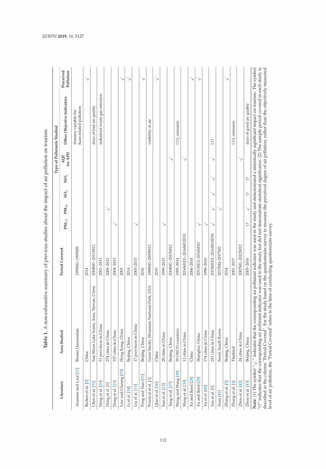
IJERPH 2019, 16, 5127

Ta

ble

1.

Ano

n-ex

haus

tive

sum

mar

yof

prev

ious

stud

ies

abou

tthe

impa

ctof

air

pollu

tion

onto

uris

m.

Lit

era

ture

Are

aS

tud

ied

Peri

od

Co

vere

d

Ty

pe

of

Po

llu

tan

tsS

tud

ied

PM

2.5

PM

10S

O2

NO

2A

QI

(or

AP

I)O

ther

Ob

ject

ive

Ind

icato

rsP

erc

eiv

ed

Po

llu

tio

n

Ana

man

and

Looi

[31]

Brun

eiD

arus

sala

m19

95M

1–19

99M

9du

mm

yva

riab

lefo

rha

ze-r

elat

edpo

lluti

on

Beck

enet

al.[

2]C

hina

2014

√

Che

net

al.[

32]

Sun

Moo

nLa

keSc

enic

Are

a,Ta

iwan

,Chi

na20

04M

1–20

11M

12da

ysof

bad

air

qual

ity

Den

get

al.[

30]

31pr

ovin

ces

inC

hina

2001

–201

3in

dust

rial

was

tega

sem

issi

on

Don

get

al.[

9]27

4ci

ties

inC

hina

2009

–201

2√

Don

get

al.[

10]

337

citi

esin

Chi

na20

04–2

013

√

Law

and

Che

ung

[33]

Hon

gK

ong,

Chi

na20

03√

Liet

al.[

34]

Beiji

ng,C

hina

2014

√

Liu

etal

.[11

]17

prov

ince

sin

Chi

na20

05–2

015

√

Peng

and

Xia

o[3

5]Be

ijing

,Chi

na20

16√

Poud

yale

tal.

[3]

Gre

atSm

oky

Mou

ntai

nN

atio

nalP

ark,

USA

1988

M3–

2009

M12

visi

bilit

yof

air

Qia

oet

al.[

36]

Chi

na20

15√

Sun

etal

.[12

]28

citi

esin

Chi

na19

99–2

015

√

Tang

etal

.[37

]Be

ijing

,Chi

na20

04M

1–20

15M

12√

Wan

gan

dW

ang

[38]

35O

ECD

coun

trie

s19

95–2

014

CO

2em

issi

on

Wan

get

al.[

39]

11ci

ties

inC

hina

2016

M1D

1–20

16M

12D

31√

Xu

and

Ree

d[2

8]C

hina

2006

–201

4√

Xu

and

Ree

d[2

9]Sh

angh

ai,C

hina

2011

M12

–201

6M10

√√

Xu

etal

.[40

]17

4ci

ties

inC

hina

1998

–201

6√

Yan

etal

.[8]

251

citi

esin

Chi

na20

15M

1D1–

2016

M10

D30

√√

√√

√C

O

Yoon

[41]

Seou

l,So

uth

Kor

ea20

15M

4–20

17M

2√

Zha

nget

al.[

5]Be

ijing

,Chi

na20

14√

Zha

nget

al.[

4]Th

aila

nd20

01–2

017

CO

2em

issi

on

Zho

uet

al.[

42]

24ci

ties

inC

hina

2007

M1–

2012

M12

√

Zho

uet

al.[

43]

Beiji

ng,C

hina

2005

–201

6O

√O

Oda

ysof

good

air

qual

ity

No

te:(

1)Th

esy

mbo

l“√

”in

dica

tes

that

the

corr

espo

ndin

gai

rpo

lluta

ntin

dica

tor

was

used

inth

est

udy

and

dem

onst

rate

da

stat

istic

ally

sign

ifica

ntim

pact

onto

uris

m.T

hesy

mbo

l“O

”in

dica

tes

that

the

corr

espo

ndin

gai

rpo

lluta

ntin

dica

tor

was

used

inth

est

udy

butd

idno

tdem

onst

rate

stat

isti

cals

igni

fican

ce.(

2)T

hesa

mpl

epe

riod

cove

red

inea

chst

udy

isde

scri

bed

inth

eco

lum

n"P

erio

dC

over

ed".

For

the

stud

yba

sed

onth

equ

estio

nnai

resu

rvey

tom

easu

reth

epe

rcei

ved

degr

eeof

air

pollu

tion,

rath

erth

anth

eob

ject

ivel

ym

easu

red

leve

lofa

irpo

lluti

on,t

he"P

erio

dC

over

ed"

refe

rsto

the

tim

eof

cond

ucti

ngqu

esti

onna

ire

surv

ey.

112

IJERPH 2019, 16, 5127

Overall, there was no consensus on the selection of air pollution indicators in the literature.The choice of air pollution indicator largely depended on the degree of convenience in data collection.Although different pollutants all reduce the quality of air, their respective impacts on tourist activitiesmay be different. Interestingly, Yan et al. [8] reported that PM2.5, PM10, SO2, and NO2 all depressedhumans’ leisure-relevant behaviors, while Zhou et al. [43] reported that only PM10 had a statisticallysignificant impact. As an extension of these two studies, our study also examined and comparedthe regression results for different pollutants. However, differently from Yan et al. [8] who usedgeotagged social media check-in data of “Weibo” covering 2015 and 2016, and Zhou et al. [43], whosolely concentrated on one city in China (the city of Beijing), this study used a city-level sample,including 337 Chinese cities and covering the period between 2007 and 2016. Based on a wider sample,this study was able to examine the impact of air pollution on both inbound and domestic tourism moreprecisely from an aggregate perspective.

3. Empirical Model and Data

3.1. Model

The study was based on a city-level sample with panel data structure, consisting of both temporaland spatial dimensions. Following the previous studies investigating the pollution-tourism nexus(e.g., [12,31,32,39]), it was assumed that the impacts of air pollution and other explanatory variableson tourism could be captured by a linear econometric regression model. To be precise, in this studythe following panel data econometric model was used:

yit = xitβ + si + ut + εit, (1)

where yit is the dependent variable in city i during period t. xit refers to a vector of explanatoryvariables. si is the section-fixed effect, and ut is the time-fixed effect. εit is the error term. β is a vectorof parameters to be estimated.

In this study, we investigated the impacts of air pollution on both domestic tourism and inboundtourism. Thus, we separately considered two dependent variables: Arrivalsdomestic, the domestictourist arrivals (in 10,000 person-times), and Arrivalsinbound, the inbound tourist arrivals (in 10,000person-times). As usual, in the econometric regressions, we used the logarithmic values of these twovariables to deal with the scaling problem. Accordingly, the variations of dependent variables areexpressed as percentage changes.

Among the explanatory variables, the core variable of interest was the air pollutant indicator.In this study, we inspected four important air pollution indicators: PM2.5, PM10, SO2, and NO2.These variables of air pollutants are expressed by their degrees of concentration density (mg/m3) inambient air.

A set of control variables was contained in the regressions: Scenic, Hotel, Road, GovSize,Population, and GDPpc. (i) The first control variable, Scenic, measures the abundance of local tourismendowment. It was calculated by the logarithmic value of the number of 4A- and 5A-rated scenicspots within each city. Since a 5A-rated scenic spot is typically considered as much more attractivethan a 4A spot [9,30], we assumed that one 5A spot equalled three 4A spots. To avoid the problemof logarithmic computation when a city has zero 4A and 5A spots, we assigned a value of 0.01 to thenumber of scenic spots when it was actually zero. (ii) The second control variable, Hotel, measuredthe availability of tourism-specific infrastructure. We used the star-rated hotels to proxy this, sincehotels are one of the most crucial tourism infrastructures. This variable was calculated by the ratioof the number of hotels divided by local population (in ten thousand). (iii) The third variable wasRoad, the length of road (km) per area (km2). This was an indicator of the transportation infrastructure.(iv) GovSize was the government size, measured by the ratio of local government expenditure toGDP. This variable was used to capture the impact of the government on local tourism’s development.(v) Population was the logarithmic value of the local population (in ten thousand), as a control variable

113

IJERPH 2019, 16, 5127

for the potential economies of scale in tourism development. (vi) The last control variable was GDPpc,the logarithmic value of real GDP per capita (RMB). The nominal GDP was deflated, taking 2000 as thebase year. Since previous studies have found that tourism might have impacts on economic and socialdevelopment, which are directly linked to the values of the control variables in the current period,we lagged these control variables for three periods to mitigate the potential endogeneity problem.The idea is that the three-period-lagged values of the control variables probably affect the currentvalue of the dependent variable (through their impacts on the current values of the control variables),but the current dependent variable has no effect on the past value of the control variables. That way,the potential endogeneity caused by reverse causality from the dependent variable to explanatoryvariables was mitigated. Definitely, one limitation of using the lagged values of control variables isthat the estimated coefficients of them may not accurately reflect the impacts of the variables in thecurrent period. However, given the large benefit of using this approach to mitigate the endogeneityissue, its limitation was deemed acceptable, and hence, it has been widely used in applied economicsresearch (e.g., [44,45]).

3.2. Data

The data of PM2.5 were collected from NASA’s Global Annual PM2.5 Grids data [46,47]. The dataof PM10, SO2, and NO2 were mainly extracted from a series of yearly published environmental qualityreports—“The Report on the State of the Environment of China” [48–50]. These reports were writtenby China’s Ministry of Environmental Protection (MEP), and later, by the Ministry of Ecology andEnvironment (MEE). These reports provided detailed official data of air quality in different areasof China since 2007. The reports did not offer city-level air pollution data for the years 2013 and2015. We checked the China Statistical Yearbook on Environment and several province-level statisticalyearbooks to supplement the missing data for some cities in 2013 and 2015, as well as some observationsin other years. It is worth mentioning that the MEP, and later, the MEE, have also reported the PM2.5

data in recent years. However, the available sample size was much smaller compared to that basedon NASA’s data. That is why we relied on the latter data source for PM2.5 in our empirical analysis.In fact, an examination of the overlapping sample of these two data sources would make it clear thatthey are both reliable and highly correlated, though the reported values are not directly comparable,due to the technological disparity in measurement. NASA’s PM2.5 data were constructed on the basisof the information supplied by the remote sensing measurements of satellites, whereas the data offeredby the MEP and MEE were from the direct measurements in local observation stations. Althoughthere were uncertainties associated with the remote sensing measurements (for example, affected byweather and the precision of the electrical instruments), the accuracy and reliability of the PM2.5 gridsdata have been highly appreciated. In fact, both data sources have been widely utilized in previousresearch (e.g., [8,9,11,12,42]). The data from the two data sources were highly correlated. For example,for the sample cities in the year of 2016, the Pearson correlation coefficient between PM2.5 values fromthe two data sources was 0.753, indicating a strong positive correlation.

The data of the dependent variables Arrivalsdomestic and Arrivalsinbound, and the control variablesHotel, Road, GovSize, Population, and GDPpc during the period 2007–2013 came from the ChinaStatistical Yearbook for Regional Economy. For the period covered, this yearbook provided city-leveldata for almost all Chinese cities above the prefecture-level, though with occasional missing values.The data between 2014 and 2016 were obtained from the EPS database, available at its website:http://www.epschinadata.com. In addition, we checked different province-level statistical yearbooksor utilized the linear interpolation method to supplement some missing observations. The data ofScenic were collected from the public information released by the tourism-relevant local governmentalsectors in different provinces.

Ultimately, our sample was comprised of unbalanced panel data covering 337 Chinese citiesfor the period between 2007 and 2016. This sample covered almost all regions in Mainland China,including all four province-level municipalities (Beijing, Tianjin, Shanghai, and Chongqing) and all

114

IJERPH 2019, 16, 5127

prefecture-level administrative districts except Sansha City and Danzhou City of Hainan Province.Sansha and Danzhou, which were respectively established in 2012 and 2015, were excluded due to lackof statistical data. Table 2 shows the summary statistics for the variables used in empirical analyses.It is clear from the table that there were rich heterogeneities among the sample cities. The samplecontained both less developed and well developed, small and large, and clean and severely pollutedcities. Some cities had highly developed tourism industries, but the tourism size in some cities wasquite small. Overall, our sample was highly representative and able to provide sufficient informationon the general situation of China.

It is notable that the different air pollutants are probably correlated. Indeed, since humanactivities often emit more than one kind of pollutant, a district may be polluted by multiple pollutantssimultaneously [51,52]. Moreover, since different pollutants may have complex chemical and physicalinteractions within the air, the degree of air pollution caused by one pollutant may be exacerbated byanother one. Considering this, we had a concern that if the correlation among different pollutantswas sufficiently high, there would be no way to distinguish different pollutants and use traditionaleconometric regressions to estimate their individual impacts on tourism. Table 3 shows the Pearsoncorrelation coefficients among the four pollutants. From the table, we see that different pollutants areindeed positively correlated, as expected. However, the correlation coefficients are not very high anddo not exceed 0.5. Thus, the indices of these four pollutants reflect different aspects of air pollution,and can be considered separately as different explanatory variables in the regression model.

Table 2. Summary statistics.

Variable Unit Obs Mean SD Min Max

DependentVariable

Arrivalsdomestic 104 person-times 2892 6.832 1.229 1.033 10.658Arrivalsinbound 104 person-times 2952 1.447 2.311 −9.210 7.106

AirPollutant

PM2.5 mg/m3 3364 0.033 0.018 0.002 0.087PM10 mg/m3 2376 0.083 0.033 0 0.436SO2 mg/m3 2379 0.033 0.018 0.002 0.148NO2 mg/m3 2379 0.030 0.012 0.002 0.069

ControlVariable

Scenic - 3367 −0.334 2.640 −4.605 4.331Hotel - 3367 0.143 0.226 0.003 4.338Road km/km2 3367 0.767 0.497 0.003 2.249GovSize - 3367 0.189 0.179 0.040 3.581Population 104 persons 3367 5.665 0.877 2.077 7.996GDPpc RMB 3367 9.720 0.731 7.613 11.874

Note: (1) The variables Scenic, Hotel, and GovSize have no unit. Scenic is the number of scenic spots. Hotel is the ratioof the number of hotels divided by local population (in ten thousand). GovSize is the ratio of government spendingto GDP. (2) The variables Arrivalsdomestic, Arrivalsinbound, Scenic, Population, and GDPpc were log-transformed. (3) Theabbreviations “Obs”, “SD”, “Min”, and “Max” in the first row denote “Observations”, “Standard Deviation”, “Minimum”,and “Maximum”, respectively.

Table 3. Correlation coefficients among the four pollutants.

PM2.5 PM10 SO2 NO2

PM2.5 1PM10 0.329 1SO2 0.309 0.403 1NO2 0.435 0.492 0.401 1

4. Results

The regression results for Equation (1) are reported in this section. Section 4.1 discusses theestimated impacts of air pollutants on domestic tourism. Section 4.2 discusses the circumstancesregarding inbound tourism.

115

IJERPH 2019, 16, 5127

4.1. Impacts of Air Pollutants on Domestic Tourism

Table 4 shows the estimated influences of different air pollutants on domestic tourism. First,we focused on PM2.5. As reported in column (1) of the table, the coefficient of PM2.5 was −4.815,statistically significant at the 1% level. This implies that if the PM2.5 density increased by 1 μg/m3

(=0.001 mg/m3), domestic tourist arrivals would decline by 0.482%. Given that the mean value ofannual domestic tourist arrivals among our sample cities was around 17 million person-times, thismagnitude corresponds to a decline of 81,855 person-times in tourist arrivals. This is indeed a hugeloss. Regarding the control variables, we found that the coefficients of Scenic and Hotel were bothsignificantly positive, consistent with the straightforward idea that more scenic spots and more tourisminfrastructure benefit tourism. Government size, GovSize, had a significant positive coefficient, perhapsbecause local government plays an important role in tourism development in China. The coefficient ofGDP per capita, GDPpc, was also positive, indicating that, on average, Chinese tourists consideredmore developed regions to be more attractive. The variables Road and Population did not showsignificant impacts on domestic tourism.

Table 4. The impacts of air pollutants on domestic tourism.

Variable

PM2.5PM10 SO2 NO2

AllPollutantsBaseline System

GMMSmallerSample

TourismReceipts

(1) (2) (3) (4) (5) (6) (7) (8)

PM2.5 −4.815 *** −2.136 * −5.304 *** −4.394 ** −5.376 ***PM10 0.558 0.817SO2 −0.589 −0.768NO2 0.001 0.070Scenic 0.016 *** 0.138 *** 0.011 ** 0.024 *** 0.012 ** 0.012 ** 0.012 ** 0.011 **Hotel 0.176 *** 0.068 0.147 *** 0.055 0.145 *** 0.149 *** 0.147 *** 0.146 ***Road −0.006 0.275 ** 0.091 * −0.199 *** 0.111 ** 0.111 ** 0.113 ** 0.084GovSize 0.539 *** −0.238 0.594 ** 0.313 0.569 ** 0.555 ** 0.551 ** 0.598**Population 0.310 0.805 *** 0.238 0.014 0.267 0.280 0.282 0.220GDPpc 0.192 ** 0.048 0.227 ** 0.298 *** 0.230 ** 0.227 ** 0.228 ** 0.231 **

Observations 2892 2892 2033 2783 2033 2036 2036 2033Cities 337 337 328 337 328 328 328 328R2 0.776 - 0.815 0.738 0.814 0.814 0.814 0.816

Statistical significance: * p < 10%, ** p < 5%, *** p < 1%.

To investigate the robustness of our finding on the harmful effect of PM2.5, we conducted threefurther robustness analyses on the result. (i) One concern is that air pollution and tourism might havecomplex reciprocal interactions [53], which might cause the endogeneity problem in the econometricestimation [9]. System GMM (general method of moments) estimation is a reliable approach to dealwith the endogeneity problem in a “short panel” with many individuals but a small number ofperiods like our data structure. Column (2) of the table reports the result of System GMM estimation,which shows a significant negative coefficient of −2.136. The magnitude was smaller than that of thecoefficient in column (1), but was still quite considerable. (ii) Comparing the number of observations ofPM2.5 and the other three pollutants, as previously reported in Table 2, we found that PM2.5 data hadmore observations than the other three pollutants. This raised the concern that the regression resultsregarding PM2.5 might not be fully comparative to those for the other pollutants, due to the differencein sample size. To address this concern, we deleted the sample points that had data for PM2.5 but not forthe other pollutants, and repeated the regression based on the smaller sample obtained. The estimatedcoefficient of PM2.5 was −5.304, as displayed in column (3). Clearly, our previous finding held.(iii) To date, we have only considered the impact of PM2.5 on tourist arrivals. In column (4), we reportthe estimate when the dependent variable was the logarithmic value of tourism receipts (in 100 millionRMB, deflated based on the year 2000 price), instead of tourist arrivals. The estimated coefficient was

116

IJERPH 2019, 16, 5127

−4.394, very close to that in column (1). Given that the mean annual domestic tourism receipt was 12billion RMB, the coefficient implies that, on average, a 1 μg/m3 increase in PM2.5 concentration wouldcause a reduction of 53 million RMB (approximately 8 million US dollars) in domestic tourism receiptsat the city level. In a nutshell, combining the results in columns (1)–(4) together, we are able to claimthat PM2.5 had a robust and significant negative impact on domestic tourism.

Next, we examined the effects of PM10, SO2, and NO2 on domestic tourism, respectively.As reported in column (5), the estimation did not detect a statistically significant impact from PM10.Column (6) reports the estimated coefficient of SO2, which was not significant either. Similarly, as canbe seen from column (7), NO2 did not significantly affect domestic tourism.

Lastly, we put all four pollutants into one regression equation and reported the estimates incolumn (8). The result still showed a significant negative coefficient for PM2.5, but not for PM10, SO2,or NO2. This result supported the findings from columns (1)–(7) when we checked the impacts of thefour pollutants one by one.

4.2. Impacts of Air Pollutants on Inbound Tourism

Table 5 demonstrates the impacts of air pollutants on inbound tourism. Column (1) reportsthe baseline estimates for PM2.5. The statistically significant coefficient was −12.269, indicating thatinbound tourist arrivals would decline by 1.227% in response to a 1 μg/m3 (=0.001 mg/m3) increasein PM2.5 concentration. Given that the mean value of annual inbound tourist arrivals in our samplecities was nearly 1 million person-times, this magnitude indicates a decline of 12,269 person-times intourist arrivals. This loss is indeed substantial. The control variables were generally not statisticallysignificant, indicating that inbound tourists were not sensitive to the economic and social characteristicsof destination cities.

Table 5. The impacts of air pollutants on inbound tourism.

Variable

PM2.5PM10 SO2 NO2

AllPollutantsBaseline System

GMMSmallerSample

TourismReceipts

(1) (2) (3) (4) (5) (6) (7) (8)

PM2.5 −12.269 *** −12.517 ** −7.185 * −8.259 * −7.359 *PM10 0.924 1.780SO2 −0.567 0.804NO2 −5.069 * −6.625 *Scenic 0.002 0.455 *** 0.011 0.046 *** 0.012 0.012 0.010 0.008Hotel 0.105 2.034 * 0.085 0.089 0.080 0.086 * 0.094 * 0.086 *Road −0.182 −1.071 ** −0.283 ** −0.198 −0.262 * −0.260 * −0.239 * −0.268 *GovSize −0.472 ** −11.859 *** 0.090 −0.656 ** 0.064 −0.024 −0.021 0.094Population −0.246 −0.306 −0.667 −1.150 −0.623 −0.643 −0.684 −0.733GDPpc 0.031 0.152 −0.052 0.034 −0.039 −0.053 −0.047 −0.033

Observations 2952 2952 2111 2941 2111 2114 2114 2111Cities 337 337 324 337 324 324 324 324R2 0.214 - 0.266 0.100 0.265 0.262 0.264 0.270

Statistical significance: * p < 10%, ** p < 5%, *** p < 1%.

Three robustness analyses on the impact of PM2.5 are reported in columns (2)–(4). (i) In column (2),the System GMM estimates are reported. The coefficient of PM2.5 was −12.517, very close to thatreported in column (1). (ii) In column (3), we relied on a smaller sample, in which all sample pointshad data for all four pollutants. The estimated coefficient of PM2.5 was −7.185. This coefficient was stillsignificantly negative, supporting the result in column (1). (iii) In column (4), we used the logarithmicvalue of inbound tourism receipts (in 100 million RMB, deflated based on the year 2000 price) as thedependent variable, instead of tourist arrivals. The estimated significant negative coefficient of −8.259supported the finding that PM2.5 harmed inbound tourism. The magnitude implies that inboundtourism receipts would decline by 7 million RMB (approximately 1 million US dollars) after PM2.5

117

IJERPH 2019, 16, 5127

concentration increased by 1 μg/m3, given that the average inbound tourism receipt of the samplecities was 893 million RMB per year.

Next, we checked the impacts of the other three air pollutant indices. The impacts of PM10 andSO2 were not significant, as reported in columns (5) and (6), respectively. From column (7), it wasfound that the impact of NO2 was negative and statistically significant at the 10% level. This impliesthat inbound tourists were responsive to the rise of NO2 pollution.

In column (8), we report the estimates after we put all four pollutants together within oneregression equation. The coefficient of PM2.5 was −7.359 and maintained statistical significance. PM10

and SO2 did not have significant impacts. The coefficient of NO2 was significantly negative, analogousto that in column (7).

5. Discussion and Implications

5.1. Discussion

The analyses in this study provide three important findings. Firstly, it was found that air pollution,measured by PM2.5, shows a harmful effect on both domestic and inbound tourism. This finding isconsistent with previous studies (e.g., [29–31,33]) that reported the negative impact of air pollution ontourism. As our sample covered a wide geographic area and a long time-span, this study supplementsthe prior literature by providing further evidence on the pollution-tourism nexus. As claimed inthe previous studies, policy makers should take actions to mitigate the air pollution problem for thepurpose of boosting tourism. Good air quality is a substantially attractive characteristic for touristdestination cities.

Secondly, different pollutants were found to exert different impacts on the tourism industry.According to our estimates, the most adverse pollutant indicator is PM2.5, which was compared toPM10, SO2, and NO2. The estimates demonstrate a robust, large, and statistically significant impact ofPM2.5 on tourism. Given that PM2.5 can be especially harmful, due to its relatively small size comparedto other air pollutants, it has attracted more public attention through microblogging platforms such asWeibo [54]. In addition, PM2.5 is more closely associated with the reduction of visibility than someother pollutants [55,56]. Travelers are highly concerned about the low visibility issue, as it can reducethe aesthetics of tourist attractions [5,57] and interrupt traffic by causing flight delays or cancellations,or highway closures [58]. Regarding the other three pollutants, PM10, SO2, and NO2, the estimationresults show that they do not have a similar impact to that of PM2.5. No statistically significant effectof PM10 and SO2 on tourism was detected. NO2 was found to negatively influence inbound tourism,but it does not significantly affect domestic tourism. This finding is novel and not consistent with someprevious studies, including Yan et al. [8], Yoon [41], and Zhou et al. [43], which reported a negativeeffect of PM10, SO2, or NO2 on tourism. The different impacts of NO2 on domestic and inboundtourism are especially interesting. There may be at least two plausible explanations. The first reasonis relevant to the degree of perception and concern about air pollution in different tourist groups.The previous studies have confirmed that people’s opinions about the severity of air pollution largelydepend on their sociodemographic status, including education, knowledge, income, and so on [59,60].For instance, tourists with higher income levels are typically more sensitive to air pollution than thosewith low income [39]. It is possible that, on average, the sociodemographic characteristics of inboundtourists make them more aware of the damage of NO2, compared to domestic tourists in China.The second reason is relevant to the differences in the health risks faced by inbound and domestictourists during the tourist activities. As the stay time of foreign tourists is usually longer than thatof domestic tourists, inbound tourists are potentially exposed to more NO2 when they visit pollutedcities. Therefore, inbound tourists might become more responsive to the variations of pollution.For example, Song et al. [61] demonstrated increasing prevalence trends of adult asthma in Asianregions, especially in Japan and South Korea, which are the top source countries of China’s inboundtourism. Given that exposure to NO2 could lead to asthma exacerbations [62], it is possible that people

118

IJERPH 2019, 16, 5127

with potential asthma or other respiratory diseases would stay away from travel destinations withhigh NO2 concentrations.

It is notable that, although our study did not report as significant a harmful impact of PM10, SO2,or NO2 on tourism as PM2.5, this does not necessarily mean that these three pollutants are trivial tosustainable tourism development in China. From the perspective of public health, the threats to tourists’health conditions posed by PM10, SO2, and NO2 should be noticed. It is also notable that, since theinference from our regressions reflects an average situation based on a sample of 337 Chinese cities,it does not rule out idiosyncratic properties in different areas. It is possible that, although PM2.5 is themost adverse pollutant on average, pollution problems in certain regions are majorly caused by otherpollutants. The unequal impacts of different pollutants on tourism detected by our study essentiallyindicate that tourism-relevant policy makers and researchers should pay attention to monitoringsuitable air pollution indictors. In particular, PM2.5 should not be ignored in tourism analysis.

The third finding was that domestic tourists and inbound tourists respond to air pollution atdifferent magnitudes. According to our estimates, if PM2.5 concentration rises by 1 μg/m3, domesticand inbound tourist arrivals will decline by 0.482% and 1.227%, respectively. Thus, in terms ofpercentage change, inbound tourists are more sensitive to the degradation of air quality. It is plausiblethat foreign travelers are more aware of the harmfulness of air pollution, compared to Chinese travelers.An earlier study by Law and Cheung [33] has signaled that travelers from Western countries were moresensitive to the air pollution in Hong Kong than Asian travelers. Our study extends the result of Lawand Cheung [33], which used Hong Kong as a case study, to a large geographic scope. In addition,it should be noticed that, as the aggregate size of domestic tourism is much larger than inboundtourism in China, in absolute values, the impact of air pollution on domestic tourism is much stronger.Our estimates imply a reduction of 81,855 person-times in annual domestic tourist arrivals and 12,269in inbound tourist arrivals, in response to a 1 μg/m3 increase in PM2.5. These estimates could helpthe tourism sectors predict the trends and variations of domestic and inbound tourism developmentassociated with varying air quality problems. Moreover, these estimates could not only exert pressureon policy makers to improve environmental outcomes, but also raise Chinese citizens’ awareness ofenvironmental protection to build a positive destination image.

5.2. Implications

From a theoretical perspective, this study made the following contributions. First, this studyempirically examined the impacts of four important components of air pollution (PM2.5, PM10, SO2,and NO2) on both the domestic and inbound tourism industries in China using a sample of 337 citiescovering the period between 2007 and 2016. The sample used in the study may generate more preciseand updated estimates, since it covers the period of recent years for a wide geographic range. Second,the findings enrich the air pollution–tourism nexus literature by confirming the finding from previousresearch that PM2.5 plays a vital role in depressing both domestic and inbound tourist numbers inChina, and by providing new insights into how NO2 exerts different effects on the domestic andinbound tourism industries. The study results remind researchers that air pollution might be moreaccurately studied from the perspective of different air pollutants.

Practically, the results indicate that the Chinese government should continue tackling air pollutionin China for the benefit of human health and for the sustainable development of the tourism industry.On the one hand, among the four common air pollutants considered, it seems that PM2.5 has receivedthe most attention from travelers over the last decade. Therefore, tourism policy makers shouldprimarily focus on PM2.5, concerning the nexus between air quality and the development of tourism.On the other hand, given the fact that other air pollutants could also result in negative health effects,emphasizing the importance of PM2.5 should not overshadow the threats posed by other air pollutants.It is suggested that great efforts should be made to raise travelers’ awareness of other air pollutants.Furthermore, although China’s outbound tourism market has attracted the attention of the world,its inbound tourism has been experiencing very slow growth [63]. As suggested by this study, NO2

119

IJERPH 2019, 16, 5127

pollution should also be tackled to attract more international travelers. The estimation results alsoreveal that inbound tourists are more sensitive to the air pollution issue in China. Given that Beijing,the capital of China with notorious air quality records, has attracted a lot of international attentionin recent years, inbound tourists may believe that the air quality in other Chinese cities is also poor.In fact, there are a number of Chinese tourist cities with air quality up to standard, including Haikou,Zhoushan, Lhasa, Fuzhou, Zhuhai, and Huizhou, among others [64]. Destination marketers in Chinacould strive to promote these cities to potential inbound tourists and design more haze-avoidance orsmog-free travel packages.

6. Conclusions and Directions for Future Research

To conclude, the present study utilized an econometric model to empirically investigate howfour atmospheric pollutants (PM2.5, PM10, SO2, and NO2) affected the tourism industry in China.The results of the analyses demonstrated that PM2.5 played a dominant role in negatively influencingChina’s inbound and domestic tourism industries. The results also revealed that NO2 reduced thenumber of inbound tourists.

This study was restricted by several limitations, which actually indicate promising directions forfuture research. Firstly, some other air pollutants, such as CO (carbon monoxide) and O3 (ozone), werenot investigated in this study due to the limitation of data availability. These two pollutants are alsomonitored and reported by the environmental sectors of the government in China. Unfortunately, dataare only available for a very small sample from our data sources. In the future, the impact of other airpollutants could also be inspected if more data can be collected.

Secondly, this study examined the effects of different air pollutants but did not consider anycomprehensive air pollution indices, such as AQI. Estimating the impact of AQI on tourism andcomparing it with the estimated impact of PM2.5 will provide more information for better decisionmaking. However, in this study, we were not able to do this because of the data availability problem.Given that AQI was not directly available from our data sources, in order to infer the values of AQI,we need to know the values of different pollutants, including PM2.5, PM10, SO2, NO2, CO, and O3.On the one hand, as mentioned previously, there were no sufficient data of CO and O3. On the otherhand, our PM2.5 data provided by NASA were constructed based on the remote sensing measurementsof satellites. The data are not directly comparable to those provided by the MEP and MEE based ondirect measurements in different local observation stations, though they are both reliable and highlycorrelated. Hence, we can investigate the correlation between AQI and tourism in the future, aftermore data are released.

Thirdly, this study inspected the actual level of air pollution measured by scientific instruments.It is notable that the objectively measured air pollution level might not be completely consistent withpeople’s perceived level of air pollution, since the perception of air pollution is subjective and affectedby a lot of social and individual factors, such as education and mass media. Future studies couldcollect data on the perceived air pollution level by potential tourists and examine whether the studyresults using subjective data match the results in this study.

Author Contributions: Conceptualization and funding acquisition, D.D. and X.X.; methodology, data curation,formal analysis, and original draft preparation, D.D.; literature review and review and editing, X.X.; software,validation, and supervision, Y.W. and S.W.

Funding: This research was funded by the Fundamental Research Funds for the Central Universities (grantnumbers JBK1801039 and JBK1809054).

Acknowledgments: The authors are grateful to the Editors and two anonymous referees for their commentsand suggestions.

Conflicts of Interest: The authors declare no conflict of interest.

120

IJERPH 2019, 16, 5127

References

1. Kao, E. Air pollution is killing 1 million people and costing Chinese economy 267 billion yuan a year,research from CUHK shows. South China Morning Post, 2 October 2018.

2. Becken, S.; Jin, X.; Zhang, C.; Gao, J. Urban air pollution in China: destination image and risk perceptions.J. Sustain. Tour. 2017, 25, 130–147. [CrossRef]

3. Poudyal, N.C.; Paudel, B.; Green, G.T. Estimating the Impact of Impaired Visibility on the Demand for Visitsto National Parks. Tour. Econ. 2013, 19, 433–452. [CrossRef]

4. Zhang, Y.; Khan, S.A.R.; Kumar, A.; Golpîra, H.; Sharif, A. Is tourism really affected by logistical operationsand environmental degradation? An empirical study from the perspective of Thailand. J. Clean. Prod. 2019,227, 158–166. [CrossRef]

5. Zhang, A.; Zhong, L.; Xu, Y.; Wang, H.; Dang, L. Tourists’ Perception of Haze Pollution and the PotentialImpacts on Travel: Reshaping the Features of Tourism Seasonality in Beijing, China. Sustainability 2015,7, 2397–2414. [CrossRef]

6. Héroux, M.E.; Anderson, H.R.; Atkinson, R.; Brunekreef, B.; Cohen, A.; Forastiere, F.; Hurley, F.; Katsouyanni,K.; Krewski, D.; Krzyzanowski, M.; et al. Quantifying the health impacts of ambient air pollutants:recommendations of a WHO/Europe project. Int. J. Public Health 2015, 60, 619–627. [CrossRef] [PubMed]

7. Khaniabadi, Y.O.; Goudarzi, G.; Daryanoosh, S.M.; Borgini, A.; Tittarelli, A.; De Marco, A. Exposure to PM10,NO2, and O3 and impacts on human health. Environ. Sci. Pollut. Res. 2017, 24, 2781–2789. [CrossRef]

8. Yan, L.; Duarte, F.; Wang, D.; Zheng, S.; Ratti, C. Exploring the effect of air pollution on social activity inChina using geotagged social media check-in data. Cities 2019, 91, 116–125. [CrossRef]

9. Dong, D.; Xu, X.; Wong, Y.F. Estimating the Impact of Air Pollution on Inbound Tourism in China:An Analysis Based on Regression Discontinuity Design. Sustainability 2019, 11, 1682. [CrossRef]

10. Dong, D.; Xu, X.; Yu, H.; Zhao, Y. The Impact of Air Pollution on Domestic Tourism in China: A SpatialEconometric Analysis. Sustainability 2019, 11, 4148. [CrossRef]

11. Liu, J.; Pan, H.; Zheng, S. Tourism Development, Environment and Policies: Differences between Domesticand International Tourists. Sustainability 2019, 11, 1390. [CrossRef]

12. Sun, J.; Zhang, J.H.; Wang, C.; Duan, X.; Wang, Y. Escape or stay? Effects of haze pollution on domestictravel: Comparative analysis of different regions in China. Sci. Total Environ. 2019, 690, 151–157. [CrossRef][PubMed]

13. Guindi, M.N.; Flaherty, G.T.; Byrne, M. Every breath you take: how does air pollution affect the internationaltraveller? J. Travel Med. 2018, 25, 1–3. [PubMed]

14. Emami, F.; Masiol, M.; Hopke, P.K. Air pollution at Rochester, NY: Long-term trends and multivariateanalysis of upwind SO2 source impacts. Sci. Total Environ. 2018, 612, 1506–1515. [CrossRef] [PubMed]

15. Lu, Q.; Zheng, J.; Ye, S.; Shen, X.; Yuan, Z.; Yin, S. Emission trends and source characteristics of SO2,NOx, PM10 and VOCs in the Pearl River Delta region from 2000 to 2009. Atmos. Environ. 2013, 76, 11–20.[CrossRef]

16. World Health Organizations. Ambient (Outdoor) Air Quality and Health. 2018. Available online: https://www.who.int/news-room/fact-sheets/detail/ambient-(outdoor)-air-quality-and-health (accessed on10 September 2019).

17. Liu, F.; Beirle, S.; Zhang, Q.; van der A, R.J.; Zheng, B.; Tong, D.; He, K. NOx emission trends over Chinesecities estimated from OMI observations during 2005 to 2015. Atmos. Chem. Phys. 2017, 17, 9261–9275.[CrossRef]

18. Hamra, G.B.; Laden, F.; Cohen, A.J.; Raaschou-Nielsen, O.; Brauer, M.; Loomis, D. Lung Cancer and Exposureto Nitrogen Dioxide and Traffic: A Systematic Review and Meta-Analysis. Environ. Health Perspect. 2015,123, 1107–1112. [CrossRef]

19. Mehta, P. Science behind Acid Rain: Analysis of Its Impacts and Advantages on Life and Heritage Structures.South Asian J. Tour. Heritage 2010, 3, 123–132.

20. Wong, E. Outlasting Dynasties, Now Emerging from Soot. The New York Times, 18 May 2014.21. Wang, H.; Zhuang, Y.; Wang, Y.; Sun, Y.; Yuan, H.; Zhuang, G.; Hao, Z. Long-term monitoring and source

apportionment of PM2.5/PM10 in Beijing, China. J. Environ. Sci. 2008, 20, 1323–1327. [CrossRef]

121

IJERPH 2019, 16, 5127

22. Agudelo-Castañeda, M.D.; Calesso Teixeira, E.; Alves, L.; Fernández-Niño, A.J.; Rodríguez-Villamizar, A.L.Monthly-Term Associations Between Air Pollutants and Respiratory Morbidity in South Brazil 2013–2016:A Multi-City, Time-Series Analysis. Int. J. Environ. Res. Public Health 2019, 16, 3787. [CrossRef]

23. Merklinger-Gruchala, A.; Jasienska, G.; Kapiszewska, M. Effect of Air Pollution on Menstrual CycleLength—A Prognostic Factor of Women’s Reproductive Health. Int. J. Environ. Res. Public Health 2017,14, 816. [CrossRef]

24. Shin, J.; Han, S.H.; Choi, J. Exposure to Ambient Air Pollution and Cognitive Impairment inCommunity-Dwelling Older Adults: The Korean Frailty and Aging Cohort Study. Int. J. Environ. Res.Public Health 2019, 16, 3767. [CrossRef] [PubMed]

25. Lu, F.; Xu, D.; Cheng, Y.; Dong, S.; Guo, C.; Jiang, X.; Zheng, X. Systematic review and meta-analysis of theadverse health effects of ambient PM2.5 and PM10 pollution in the Chinese population. Environ. Res. 2015,136, 196–204. [CrossRef] [PubMed]

26. Feng, C.; Li, J.; Sun, W.; Zhang, Y.; Wang, Q. Impact of ambient fine particulate matter (PM2.5) exposureon the risk of influenza-like-illness: a time-series analysis in Beijing, China. Environ. Health 2016, 15, 17.[CrossRef] [PubMed]

27. Lin, Y.; Zou, J.; Yang, W.; Li, C.Q. A Review of Recent Advances in Research on PM2.5 in China. Int. J.Environ. Res. Public Health 2018, 15, 438. [CrossRef]

28. Xu, X.; Reed, M. Perceived pollution and inbound tourism in China. Tour. Manag. Perspect. 2017, 21, 109–112.[CrossRef]

29. Xu, X.; Reed, M. Perceived pollution and inbound tourism for Shanghai: a panel VAR approach. Curr. IssuesTour. 2019, 22, 601–614. [CrossRef]

30. Deng, T.; Li, X.; Ma, M. Evaluating impact of air pollution on China’s inbound tourism industry: A spatialeconometric approach. Asia Pac. J. Tour. Res. 2017, 22, 771–780. [CrossRef]

31. Anaman, K.A.; Looi, C.N. Economic Impact of Haze-Related Air Pollution on the Tourism Industry in BruneiDarussalam. Econ. Anal. Policy 2000, 30, 133–143. [CrossRef]

32. Chen, C.M.; Lin, Y.L.; Hsu, C.L. Does air pollution drive away tourists? A case study of the Sun Moon LakeNational Scenic Area, Taiwan. Transp. Res. Part D Transp. Environ. 2017, 53, 398–402. [CrossRef]

33. Law, R.; Cheung, C. Air Quality in Hong Kong: A Study of the Perception of International Visitors. J. Sustain.Tour. 2007, 15, 390–401. [CrossRef]

34. Li, J.; Pearce, P.L.; Morrison, A.M.; Wu, B. Up in Smoke? The Impact of Smog on Risk Perception andSatisfaction of International Tourists in Beijing. Int. J. Tour. Res. 2016, 18, 373–386. [CrossRef]

35. Peng, J.; Xiao, H. How does smog influence domestic tourism in China? A case study of Beijing. Asia Pac. J.Tour. Res. 2018, 23, 1115–1128. [CrossRef]

36. Qiao, G.; Peng, S.; Prideaux, B.; Qiao, M. Identifying Causes for the Decline in International Arrivals toChina-Perspective of Sustainable Inbound Tourism Development. Sustainability 2019, 11, 1723. [CrossRef]

37. Tang, J.; Yuan, X.; Ramos, V.; Sriboonchitta, S. Does air pollution decrease inbound tourist arrivals? The caseof Beijing. Asia Pac. J. Tour. Res. 2019, 24, 597–605. [CrossRef]

38. Wang, M.C.; Wang, C.S. Tourism, the environment, and energy policies. Tour. Econ. 2018, 24, 821–838.[CrossRef]

39. Wang, L.; Fang, B.; Law, R. Effect of air quality in the place of origin on outbound tourism demand:Disposable income as a moderator. Tour. Manag. 2018, 68, 152–161. [CrossRef]

40. Xu, D.; Huang, Z.; Hou, G.; Zhang, C. The spatial spillover effects of haze pollution on inbound tourism:evidence from mid-eastern China. Tour. Geogr. 2019, pp. 1–22. [CrossRef]

41. Yoon, H. Effects of particulate matter (PM10) on tourism sales revenue: A generalized additive modelingapproach. Tour. Manag. 2019, 74, 358–369. [CrossRef]

42. Zhou, B.; Qu, H.; Du, X.; Yang, B.; Liu, F. Air Quality and Inbound Tourism in China. Tour. Anal. 2018,23, 159–164. [CrossRef]

43. Zhou, X.; Santana Jiménez, Y.; Pérez Rodríguez, J.V.; Hernández, J.M. Air pollution and tourism demand:A case study of Beijing, China. Int. J. Tour. Res. 2019, 21, 747–757. [CrossRef]

44. Stiebale, J. Do Financial Constraints Matter for Foreign Market Entry? A Firm-level Examination. World Econ.2011, 34, 123–153. [CrossRef]

45. Vergara, R. Taxation and private investment: evidence for Chile. Appl. Econ. 2010, 42, 717–725. [CrossRef]

122

IJERPH 2019, 16, 5127

46. van Donkelaar, A.; Martin, R.V.; Brauer, M.; Hsu, N.C.; Kahn, R.A.; Levy, R.C.; Lyapustin, A.; Sayer, A.M.;Winker, D.M. Global Estimates of Fine Particulate Matter Using a Combined Geophysical-Statistical Methodwith Information from Satellites. Environ. Sci. Technol. 2016, 50, 3762–3772. [CrossRef] [PubMed]

47. van Donkelaar, A.; Martin, R.V.; Brauer, M.; Hsu, N.C.; Kahn, R.A.; Levy, R.C.; Lyapustin, A.; Sayer, A.M.;Winker, D.M. Global Annual PM2.5 Grids from MODIS, MISR and SeaWiFS Aerosol Optical Depth (AOD) withGWR, 1998–2016; NASA Socioeconomic Data and Applications Center (SEDAC): Palisades, NY, USA, 2018.[CrossRef]

48. Ministry of Environmental Protection of the People’s Republic of China. The Report on the State ofthe Environment of China 2007, 2008, 2009, 2010, 2011; Published in Sequent Years, in Chinese; ChinaEnvironmental Science Press: Beijing, China, 2008–2012.

49. Ministry of Environmental Protection of the People’s Republic of China. The Report on the State of theEnvironment of China 2012, 2014; Published in Separate Years, In Chinese; China Environment Press: Beijing,China, 2013, 2015.

50. Ministry of Ecology and Environment of the People’s Republic of China. The Report on the State of theEnvironment of China 2016; China Environment Publishing Group: Beijing, China, 2018. (In Chinese)

51. Hu, J.; Ying, Q.; Wang, Y.; Zhang, H. Characterizing multi-pollutant air pollution in China: Comparison ofthree air quality indices. Environ. Int. 2015, 84, 17–25. [CrossRef]

52. Wesson, K.; Fann, N.; Morris, M.; Fox, T.; Hubbell, B. A multi–pollutant, risk–based approach to air qualitymanagement: Case study for Detroit. Atmos. Pollut. Res. 2010, 1, 296–304. [CrossRef]

53. Holden, A. The environment-tourism nexus: Influence of market ethics. Ann. Tour. Res. 2009, 36, 373–389.[CrossRef]

54. Kay, S.; Zhao, B.; Sui, D. Can Social Media Clear the Air? A Case Study of the Air Pollution Problem inChinese Cities. Prof. Geogr. 2015, 67, 351–363. [CrossRef]

55. Kim, Y.J.; Kim, K.W.; Oh, S.J. Seasonal Characteristics of Haze Observed by Continuous Visibility Monitoringin the Urban Atmosphere of Kwangju, Korea. Environ. Monit. Assess. 2001, 70, 35–46. [CrossRef]

56. Ge, W.; Chen, R.; Song, W.; Kan, H. Daily Visibility and Hospital Admission in Shanghai, China. Biomed.Environ. Sci. 2011, 24, 117–121. [CrossRef]

57. Kirillova, K.; Fu, X.; Lehto, X.; Cai, L. What makes a destination beautiful? Dimensions of tourist aestheticjudgment. Tour. Manag. 2014, 42, 282–293. [CrossRef]

58. Zhuang, P. Hundreds of flights cancelled in Beijing as thick smog lays siege to capital. South China MorningPost, 20 December 2016.

59. Guo, Y.; Liu, F.; Lu, Y.; Mao, Z.; Lu, H.; Wu, Y.; Chu, Y.; Yu, L.; Liu, Y.; Ren, M.; Li, N.; Chen, X.; Xiang, H.Factors Affecting Parent’s Perception on Air Quality—From the Individual to the Community Level. Int. J.Environ. Res. Public Health 2016, 13, 493. [CrossRef]

60. Reames, T.G.; Bravo, M.A. People, place and pollution: Investigating relationships between air qualityperceptions, health concerns, exposure, and individual- and area-level characteristics. Environ. Int. 2019,122, 244–255. [CrossRef] [PubMed]

61. Song, W.J.; Kang, M.G.; Chang, Y.S.; Cho, S.H. Epidemiology of adult asthma in Asia: toward a betterunderstanding. Asia Pac. Allergy 2014, 4, 75–85. [CrossRef] [PubMed]

62. Orellano, P.; Quaranta, N.; Reynoso, J.; Balbi, B.; Vasquez, J. Effect of outdoor air pollution on asthmaexacerbations in children and adults: Systematic review and multilevel meta-analysis. PLoS ONE 2017,12, e0174050. [CrossRef] [PubMed]

63. Cheng, S. Inbound tourism still rising. China Daily, 23 May 2018.64. Ministry of Environmental Protection of the People’s Republic of China. MEP Releases Air Quality of Key

Regions and 74 Cities in September and Q3 of 2013. Available online: http://english.mee.gov.cn/News_service/news_release/201310/t20131024_262189.shtml (accessed on 10 September 2019).

© 2019 by the authors. Licensee MDPI, Basel, Switzerland. This article is an open accessarticle distributed under the terms and conditions of the Creative Commons Attribution(CC BY) license (http://creativecommons.org/licenses/by/4.0/).

123

International Journal of

Environmental Research

and Public Health

Article

An Integrated Approach to Determining Rural TouristSatisfaction Factors Using the IPA andConjoint Analysis

Yanchun Jin 1,2 and Yoonseo Park 2,*

1 School of Management, Eastern Liaoning University, Dandong 118001, China; yanchunjin@hotmail.com2 Department of Business Administration, Jeonbuk National University, Jeonju 54896, Korea* Correspondence: yspark@jbnu.ac.kr; Tel.: +82-63-270-2990

Received: 5 September 2019; Accepted: 5 October 2019; Published: 11 October 2019

Abstract: Rural tourists satisfaction has a pivotal role in the development of sustainable rural tourism.As a method of identifying critical satisfaction factors, an importance and performance analysis (IPA)technique has attracted growing interest from academics due to it being able to deliver the importanceand performance of a product’s attributes from the standpoint of customers. However, IPA is basedon the presumption that a linear and symmetrical relationship exists between the performance andoverall satisfaction, which has been criticized by many researchers due to its deviation from the facts.On measurement of importance, researchers have not reached an agreement on whether direct orindirect approach should be applied. To measure satisfaction more effectively, this study presents arevised IPA method that integrates IPA, conjoint analysis and importance grid analysis. Based onmathematical psychology and psychometrics theory, the conjoint analysis method can be used toanalyze multi-attributes of various products and derive relative importance of attributes in customersatisfaction research. The importance grid analysis method has been applied to categorize attributesby many researchers. It can be used to measure the nonlinear relationship between the performanceof attributes and overall satisfaction. In this paper, an empirical study on rural tourists’ satisfactionwas undertaken using this integrated method. The results show that the integrated approach is moreresponsive to attribute performance, thus allowing for improvement of a certain target attribute inthe customer satisfaction enhancement process.

Keywords: importance-performance analysis; conjoint analysis; importance grid analysis method;sustainable rural tourism; tourist satisfaction

1. Introduction

Rural tourism has the potential as a development tool for rural areas [1]. As a dimension ofdeveloping sustainable tourism, satisfaction plays a critical role in the survival and future of tourismindustry. Regarding the conservation of rural nature and culture, it is important to find the criticalfactors that have direct impacts on satisfaction for achieving sustainable rural tourism development.Among various studies on customer satisfaction, identification of customer satisfaction factors isregarded as essential because it can affect resources allocation on different service attributes forsatisfaction improvement [2]. Product or service attributes are characteristics by which offerings areidentified or differentiated, which usually include features, functions, benefits, and uses [3]. Accordingto Lancaster [4], customers’ preferences are not on the product itself but on the characteristics orattributes of the product. Furthermore, product selection can be conceptualized as a process ofcomparing the main attributes of product or service. For this reason, investigating the critical attributesis a continuing concern within satisfaction research.

IJERPH 2019, 16, 3848; doi:10.3390/ijerph16203848 www.mdpi.com/journal/ijerph125

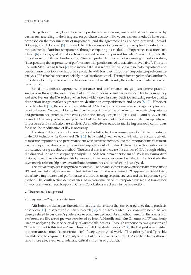
IJERPH 2019, 16, 3848

Using this approach, key attributes of products or service are generated first and then rated bycustomers according to their impacts on purchase decision. However, various methods have beenproposed on the measurement of importance, and the agreement has not been acquired. Jaccard,Brinberg, and Ackerman [5] indicated that it is necessary to focus on the conceptual foundations ofmeasurements of attributes importance through comparing six methods of importance measurements.Oliver [6] also suggested that customers should know “important for what” when they rate theimportance of attributes. Furthermore, Oliver suggested that, instead of measuring importance alone,“incorporating the importance of performance into predictions of satisfaction is available”. This is inline with Martilla and James [7], who indicate that it is more effective to examine both importance andperformance than focus on importance only. In addition, they introduced importance–performanceanalysis (IPA) that has been used widely in satisfaction research. Through investigation of an attribute’simportance before purchase and performance perception afterwards, the evaluation of satisfaction canbe acquired.

Based on attributes approach, importance and performance analysis can derive practicalsuggestions through the measurement of attribute importance and performance. Due to its simplicityand effectiveness, the IPA technique has been widely used in many fields for analyzing service quality,destination image, market segmentation, destination competitiveness and so on [8–12]. However,according to Oh [13], the revision of a traditional IPA technique is necessary considering conceptual andpractical issues. Conceptual issues involve the uncertainty of the criterion for measuring importanceand performance; practical problems exist in the survey design and grid scale. Until now, variousrevised IPA techniques have been provided, but the definition of importance and relationship betweenimportance and satisfaction are unclear. As an effective method in marketing research, continuousfocus on the modification of IPA is necessary.

The aims of this study are to present a novel solution for the measurement of attribute importancein the IPA technique. As Oliver and Oh [6,13] have highlighted, we use satisfaction as the same criteriato measure importance and performance but with different methods. For the importance measurement,we use conjoint analysis to acquire relative importance of attributes. Different from this, performanceis measured using the direct method. The second aim is to increase the utilities of IPA through addingthe diagonal line and discrepancy analysis. In addition, a major criticism of IPA is its assumptionthat a symmetric relationship exists between attribute performance and satisfaction. In this study, theasymmetric relationship between attribute performance and satisfaction is analyzed.

The rest of this paper is organized as follows. The second section reviews previous literature aboutIPA and conjoint analysis research. The third section introduces a revised IPA approach to identifyingthe relative importance and performance of attributes using conjoint analysis and the importance gridmethod. The fourth section demonstrates the implementation of this proposed revised IPA frameworkin two rural tourism scenic spots in China. Conclusions are drawn in the last section.

2. Theoretical Background

2.1. Importance–Performance Analysis

Attributes are defined as the determinant decision criteria that can be used to evaluate productsor services [14]. In Myers and Alpert’s research [15], attributes are identified as determinants that areclosely related to customer’s preference or purchase decision. As a method based on the analysis ofattributes, the IPA technique was introduced by John A. Martilla and John C. James in 1977 and firstlyused in analyzing the service quality of automobile dealers. Through response to two questions of“how important is this feature” and “how well did the dealer perform” [7], the IPA grid was dividedinto four areas named “concentrate here”, “keep up the good work”, “low priority” and “possibleoverkill” can be acquired. The analysis result of attributes derived from IPA can help firms allocatefunds more effectively on pivotal and critical attributes of products.

126

IJERPH 2019, 16, 3848

Due to its simplicity and effectiveness, IPA has enjoyed popularity. Its application has beenbroadened to a variety of areas, especially in research for identifying critical factors for productselection and evaluation of service quality and satisfaction [16]. As an extension, Sethna [17] hasa related IPA technique for customer satisfaction and provided a hypothesis that the greater thediscrepancy between importance and performance of a product on that attribute, the greater thecustomer’s dissatisfaction with the product. It has been proven to be an effective tool in research foridentifying determinants affecting overall satisfaction [18]. Moreover, IPA instead of SERVQUAL hasbeen suggested to measure service quality for limitations existed in the latter [9,19].

Although the ease of application and simplicity have led to the wide acceptance of the IPAresearch framework, researchers have disagreements on measurement of importance and asymmetricaleffects between attributes’ performance and satisfaction [13,20–22]. Importance, also termed as“value importance” or “salience”, reflects customer’s preference or stress on different attributes. Formeasurement of importance, it has been heavily criticized for its ambiguous, multidimensionaldefinitions in previous studies; in particular, both direct and indirect ratings of importance were usedin previous research. The direct method is a simple method. However, it has apparent problems.To date, a variety of revised IPA research frameworks using indirect or integrated methods hasbeen provided to avoid its disadvantages [23–26]. Multiple regression analysis, three factors theory,partial correlation analysis, and a back propagation neural network have been addressed for customerself-stated importance for avoiding problems such as incorrect interpretation of attributes’ importanceand changing evaluation in different purchase stages [23,27–29]. The second disagreement on attributeresearch is the relationship between attribute performance and satisfaction. It has been reportedthat attribute performance and satisfaction have a positive association [30]. Asymmetrical effects ofattribute-related performance on overall satisfaction have also been noticed [30,31]. The method ofcombining three-factor theory with the IPA technique for measuring asymmetrical effects has beenused in many research works [23,27,32].

Normally, two steps are required to apply the IPA method. First, the importance of attributesis measured prior to actual purchase experience. The same set of attributes is then used to evaluateperformance. However, if we use a random sampling method, it is impractical to make an investigationbefore and after the purchase on the same investigators. Therefore, some researchers have suggestedthat the investigation should be performed concerning the importance and performance at the sametime after purchase. Neslin [33] has suggested that a statistical method should be employed rather thana self-stated method for predictive validity. However, this also has problems. The main criticism raisedby other researchers is that, if these two factors (importance and performance) are evaluated at onetime, close relations between importance and performance would appear. Moreover, all attributes to beevaluated are likely to be important. This would bring about “ceiling effects”. For the multi-dimensionsof definition and measurement of the importance, Oliver [6] has also suggested the use of satisfactionas a measure criterion of importance and performance.

2.2. Conjoint Analysis in Satisfaction Research

Since being proposed by Green and Rao [34], the conjoint analysis method has been widely usedin the field of marketing research. The objective of conjoint analysis is to quantify the choice processon products or services based on experimental design and various data collecting methods includingranking, rating or choice-based methods. Historically, the compositional approach was utilized oncustomers’ choice processes, with more attention given to attributes or characteristics of products inthe 1970s and 1980s [35]. Different from this approach, conjoint analysis is a decompositional approach.It gets utilities of product attributes from alternatives or profiles that are made up of various attributesof products.

Because conjoint analysis method is more similar to a customer’s actual purchase decision orattribute evaluation, which is used in satisfaction research mainly on the measurement of attribute’srelative importance. Using the conjoint analysis method, attributes’ utilities and individual level utility

127

IJERPH 2019, 16, 3848

can be derived, and the percentage of utility range is defined as relative importance. This can be seen inprevious research [36]. Thus, the conjoint analysis technique is also applicable to drawing inference tothe importance of attributes that can provide useful information to explain why people make differentpurchase decisions [37]. It is thus well accepted that this approach is an objective and realistic way toobtain the relative importance of attributes.

The conjoint analysis method can be used in IPA research framework based on these reasons:first, relative importance of attributes can be measured using the conjoint analysis method. It can beseen that a measurement of relative importance rather than direct ratings was suggested in previousresearch [13,38]. Through designing the profile in conjoint analysis, a customer’s real attitude onattributes can be reflected. It will be not influenced by perception of the attribute’s importance andperformance. Second, orthogonal design is applied in the profile design of conjoint analysis, andthe relationship among attributes appears to have zero correlation. Additionally, conjoint analysis“depends on less restrictive assumptions than multiple regression analysis” [21], and the limitationsthat exist in the reported revised IPA technique can be minimized.

3. Methodology of Conjoint Analysis Based on Importance–Performance Analysis

3.1. Acquiring of Implicitly Derived Importance and Performance

The traditional IPA technique employs customer self-stated importance and the performanceapproach using Likert five-point or seven-point rating scale. Thus, it is considered as a simple andwell-understood method by both researchers and customers. However, various problems have arisenwith the wide application of the IPA technique. For instance, a linear relationship between importanceand performance was usually assumed, and every attribute was tended to be thought of as veryimportant [20]. More recently, related studies have focused on implicitly derived importance andthe performance approach. Matzler and Sauerwein [2] have provided the sensitivity of importanceweights through comparing the implicitly and explicitly derived importance approaches. In line withprevious research, this study analyzes the nonlinear relationship between attribute-level performanceand overall satisfaction based on the implicitly derived importance.

3.2. The Revised IPA Procedure

Based on previous research, this study provides a new approach to helping managers derivea more precise and simply applied marketing strategy by using the IPA technique. First, as bothself-stated importance and the implicitly derived method are questionable, this study employs theconjoint analysis method for deriving the relative importance of an attribute. Second, this study usessatisfaction ratings derived directly to acquire performance evaluation. The nonlinear relationshipbetween attribute-level performance and overall satisfaction can then be delivered using importancegrid analysis method. Finally, the attribute’s importance and performance will be plotted on theIPA grid.

3.2.1. Step 1: Conjoint Analysis Design

Experimental design of a conjoint study includes several steps. Some critical ones are theidentification of product attributes and levels, the determination of the analysis method such asratings-based and choice-based methods, and the design of profiles. Until now, four types ofmethods have been used in conjoint analysis: (1) a traditional method that uses stated preferences,(2) choice-based conjoint analysis that uses stated choices, (3) adaptive conjoint analysis, and (4)self-explicated conjoint analysis [35]. However, full profiles or a smaller set of full files usingstated preference are accepted widely due to a high applicative percentage in previous conjointanalysis studies.

For profile design, the orthogonal plan is supported by most researchers as it can avoid themulticollinearity among attributes effectively. In addition, it needs less profiles than the full-factorial

128

IJERPH 2019, 16, 3848

design. However, the orthogonal plan can only measure the main effects of attributes while interactiveeffects will be ignored. Thus, fractional factorial design that can measure both main effects andinteractive effects or higher-order effects is considered in this study. To satisfy all requirements,Box–Behnken design (BBD) is selected for data collection that will use 12 runs with three coded levels−1, 0 and 1 (Table 1).

Table 1. Experimental matrix of Box–Behnken design.

RunCoded Levels

X1 X2 X3

1 −1 −1 02 −1 1 03 1 −1 04 1 1 05 −1 0 −16 −1 0 17 1 0 −18 1 0 19 0 −1 −110 0 −1 111 0 1 −112 0 1 1

3.2.2. Step 2: Computation of Importance and Performance Values

One can compute the relative importance of the attribute by part-worth function that is specifiedas a piecewise linear function in dummy variables in conjoint analysis studies. According to Raoet al. [35], the component utility function for the t-th attribute can be written as:

Ut(xjt) = Ut1Dt1 + Ut2Dt2 + ... + Utrt−1 Dtrt−1 , (1)

where Utk is the component of the part-worth function for the k-th level of xt, xjt is the level for thej-th profile on the t-th attribute, rt is the number of discrete levels for the t-th attribute, and Dtk is thedummy variable taking the value 1 or 0. This formula can be used to calculate the utility of attribute.Its relative importance can also be determined.

The evaluation of performance can be acquired through asking customers to rate the satisfactionof attributes. In most of the previous research, the five-point Likert scale of 1 (very dissatisfied),2 (somewhat dissatisfied), 3 (neither dissatisfied nor satisfied), 4 (somewhat satisfied), and 5 (verysatisfied) was used to rate performance of attributes.

3.2.3. Step 3: Categorization of Attributes

Recent research supports the view that attributes have a nonlinear relationship with satisfaction.Depending on its impact on satisfaction, attributes can be categorized as basic attributes, excitementattributes, or performance attributes [39,40]. Basic attributes can respond to basic needs for the productor service. It will cause dissatisfaction if not fulfilled. However, it does not bring customer delightif exceeded. On the contrary, excitement attributes can increase customer satisfaction if delivered,although it does not cause dissatisfaction if not fulfilled [27]. Performance attributes will lead tosatisfaction if the attribute performance is high. It will cause dissatisfaction if its performance is low.

Vavra [41] firstly proposed that the importance grid could be used to identify the three satisfactionfactors (basic attributes, excitement attributes, and performance attributes). Importance grid isconstructed depending on whether the importance of attribute is derived explicitly or implicitly.A customer’s self-stated importance is identified as explicit importance. It is the indicator of anattribute’s dissatisfaction-generating potential. Different from explicit importance, as an indicator of

129

IJERPH 2019, 16, 3848

satisfaction-generating potential, implicit importance is obtained indirectly such as applying regressingattribute-level performance against overall satisfaction [2,42–44].

The assumption of importance grid analysis is that explicit importance and implicit importancemight differ in reflecting the importance-satisfaction relationship. In addition, it has been stated that acustomer’s self-stated importance cannot measure the relative importance of attribute adequately [45].Importance grid analysis combines attribute importance weights derived explicitly and implicitly in atwo-dimensional grid. The attribute can be plotted according to differences in importance weights(Figure 1).

Figure 1. Importance grid for attributes (Vavra [41]).

In terms of importance grid analysis, basic attributes are factors that have strong negativeimpact on overall satisfaction in low-level performance without having a significant positive impactwhen performance is high. It is a minimum requirement of product or service. Thus, it can beidentified as high importance in directly derived evaluation of attributes, but as low importancein indirectly derived evaluation. Different from basic attributes, exciting attributes are identifiedas not much important in directly derived evaluation but as highly important in indirectly derivedevaluation for its positive relationship with overall satisfaction on the high performance of attribute.For one-dimensional performance attributes, their corresponding changes can be shown betweenthe performance of attribute and overall satisfaction. An attribute with high explicit and implicitimportance can be considered high importance attributes. On the contrary, low importance attributesshow little importance both in explicit and implicit ways.

3.2.4. Step 4: Importance–Performance Grid Creation

Using importance and performance value derived from step 2, attributes can be plotted on theIPA matrix. For Importance–Performance (I–P) map partitioning, two types of quadrants approachesare mainly used. One is the “scale-centered quadrants approach”, suggested by Green and Rao [34].The other is the “data-centered quadrants approach”, which uses empirical means obtained from thedata as cross-points [46]. In addition, based on the traditional matrix, which divides the region intofour parts to analyze characteristics of attributes, some researchers have added a diagonal line on thematrix for representing high priority for improvement more clearly. This method has been proven tobe more effective than the traditional one [20].

130

IJERPH 2019, 16, 3848

In this study, the revised I–P matrix with data-centered quadrants approach and diagonal lineis employed. Combined with analysis results of attributes’ category, improvement suggestions forattributes will be derived.

4. Implementation of Revised IPA

4.1. Study Area

Two villages in China named Dalishu and Qingshan were selected for this study. Both of thesetwo villages are near the city and famous for rural tourism resources. However, tourist attractionin these two areas have their own characteristics. Zheng [47,48] evaluated the development ofmultifunctional agriculture in Dalishu village. Rural tourism was identified as an enhancementfoundation of multifunctional agriculture and rural sustainable tourism through outdoor activities,fruit picking and dining experiences. Compared to Dalishu village, rural tourism in Qingshan villageoffers natural and Manchu cultural landscape as tourist attractions. Rather than experienced activities,landscape appreciation is more concentrated in Qingshan village.

The two rural scenic spots are named after the village directly. With both similarities anddifferences existing in these two scenic spots, it can examine the revised IPA framework more effectivelyon the management focus on the attributes and the relationship between attribute performanceand satisfaction.

4.2. Questionnaire Design

According to the Organization of Economic Co-Operation and Development (OECD), rural tourismis defined as tourism taking place in the countryside: “rurality is the central and unique selling pointin the rural tourism package” [49]. Previous studies on rural tourism expectation and motivation weremainly concentrated on relaxation, socialization, learning, family togetherness, novelty, and excitement[50], functional factors (i.e., reservation system, service quality) and technical factors (i.e., room size,price level) [49], and access evaluation, lodgings availability, and price evaluation [51]. Based on theseprevious studies considering the characteristics of rural tourism in China, this study initially selected sixfactors (transportation, price level, rural lodging, rural eating facilities, rurality experience activity andrural tourism service quality) as expectation and satisfaction factors. However, after consulting withtourism researchers and travel agency managers, we decided to delete three factors: transportation, rurallodging and rural eating facilities. The reason to delete transportation is that transportation evaluationincludes many aspects, such as time, price, and comfortability that will make respondents feel that theyare difficult to evaluate. The reason to delete the other two factors is because the location of the surveyregion, one of which is very close to the city, and the majority of tourists will not have the experience ofrural eating or rural lodging experience. Therefore, the three factors determined in this study are ruraltourism price level, rurality experience activity and rural tourism service.

Regarding levels of attributes, we selected satisfaction as the measurement of the importance ofattributes based on Oliver’s suggestion [6] and Danaher’s research [38] as shown in Table 2.

This experiment design has three factors each with three levels, resulting in 33 = 27 treatmentswhich would be too many for respondents to evaluate. Different from previous research, this studyapplies Box–Behnken design that is evaluated as a very effective design method for researching therelationship among variables. For the case of three factors with three levels each, it needs 12 experimentruns. Therefore, we designed 12 questions according to the BBD method, and used five-point Likertscale (1 for “very dissatisfied” and 5 for “very satisfied”) to evaluate the satisfaction of the combinationof three attributes with different levels.

Holdout cases are generated randomly for checking the internal validity of the model. They arejudged by respondents but not used in the conjoint analysis. According to previous studies, we usedfour holdouts that were mixed into the 12 questions randomly. Consequently, each respondent wasasked to rank 16 alternatives.

131

IJERPH 2019, 16, 3848

Table 2. Rural tourism product attributes and levels.

Selected Attributes Levels Coding

Rural tourism price level Worse than expected −1About what expected 0Better than expected 1

Rurality experience activity Worse than expected −1About what expected 0Better than expected 1

Rural tourism service Worse than expected −1About what expected 0Better than expected 1

4.3. Data Collection and Respondents’ Profiles

The questionnaire was administrated online with a snowball sampling approach to residentsin Dandong City who had already participated in rural tourism in Dalishu and Qingshan scenicspots. This approach is chosen here since tourists mainly come from regions near the city. This surveyintegrated persons from those urban areas known to generate the most rural tourists in Dandong cityas well as tourist guides who were asked to invite tourists who had the experiences to these two scenicspots to participate in the survey. The award for this survey is the chance of a drawing in a lottery thatis supported by an online questionnaire design company.

The survey was conducted from October to November 2018. A total of 155 questionnaires werereceived. Questionnaires from respondents who finished this survey in less than three minutes orselected the same options for all of questions were deleted. Finally, 115 valid and usable questionnaireswere used for analysis. Demographic profiles of these respondents are summarized in Table 3.

Table 3. Demographic of the sample (n = 115).

Demographic Variables Frequency %

GenderMale 41 35.652Female 74 64.348

Ageup to 35 49 42.60936–44 39 33.913over 46 27 23.478

Monthly income (US dollar)below 450 41 35.652451–900 51 44.348above 901 23 20.000

Occupationtourism-related occupation 40 34.783tourism-unrelated occupation 51 44.348student in tourism-related major 9 7.826student in tourism-unrelated major 12 10.435retirement 3 2.609

4.4. Reliability and Validity Analysis

Although there have been disagreements on the reliability and validity evaluation of conjointanalysis, Pearson’s r and Kendall’s tau τ statistics based on holdout samples as simple and effectivemeasurement methods are widely used [52]. They are reported as indicators of fit between the modeland obtained data. Pearson’s r can be used to measure the degree of correlation between attribute

132

IJERPH 2019, 16, 3848

levels within a factor. Kendall’s tau is a measurement of the correlation between the observed and thepredicted preferences of rank order variables.

We analyzed the internal reliability of the two scenic spots, respectively. Results are shown inTable 4. Test results showed very high overall correlations with correlation coefficient r of 0.945 forDalishu scenic spots and 0.950 for Qingshan scenic spots. Kendall’s tau τ was 0.870 for Dalishu scenicspots and 0.818 for Qingshan scenic spots in all conjoint models, indicating a good and efficient modelfit. For the four holdouts cards, the Kendall’s tau τ statistics confirmed the model’s reliability both at0.333 in the two scenic spots. It showed cross-validity about the model’s ability to predict ratings ofhold-out profiles.

Table 4. Validity and reliability of the model.

Value Sig

Dalishu scenic spotPearson’s R 0.945 0.000Kendall’s tau 0.870 0.000Kendall’s tau for Holdouts 0.333 0.248

Qingshan scenic spotPearson’s R 0.950 0.000Kendall’s tau 0.818 0.000Kendall’s tau for Holdouts 0.333 0.248

4.5. Implicitly Derived Importance and Performance of Tourist Satisfaction Attributes and Dimensions

4.5.1. Conjoint Analysis of the Two Rural Tourism Destinations

Using SAS procedure Conjoint Analysis, we obtained relative importance values of the threeattributes, respectively. Relative importance values of the three attributes [rural tourism product pricelevel (price), rurality experience activity (activity), and rural tourism service (service)] were 0.303,0.418, 0.279 in Dalishu and 0.271, 0.396, 0.333 in Qingshan scenic spots (Figure 2). Furthermore, weanalyzed personal utility of attributes with different levels. Results are shown in Figures 3 and 4.

(a) (b)

Figure 2. Relative importance of attributes ((a) Dalishu scenic spots; (b) Qingshan scenic spots).

These attributes were coded as −1, 0, and 1 to represent “worse than expected”, “about whatwas expected” and “better than expected”, respectively. According to customers’ ratings, utilities ofattributes can be acquired. Changes of utilities with attributes’ ratings seem interesting as shown in thetwo figures. When ratings of attributes changed in “worse than expected”, “about what was expected”and “better than expected” three levels, utilities did not seem to increase continuously. Especially for

133

IJERPH 2019, 16, 3848

service attributes, it brought the same utility regardless of the “about what was expected” level or the"better than expected” level. Similar results were also seen in previous research that addressed anasymmetry relationship between service and overall satisfaction.

(a) (b) (c)

Figure 3. Utility plot of attributes in Dalishu scenic spots ((a) utility change with price rating; (b) utilitychange with activity rating; (c) utility change with service rating).

(a) (b) (c)

Figure 4. The utility plot of the attributes in Qingshan scenic spots ((a) utility change with price rating;(b) utility change with activity rating; (c) utility change with service rating).

4.5.2. Creation of Importance Grid

Using the importance grid analysis method, the classification of attributes can be obtained. First,the importance of attribute derived directly can be acquired from questionnaires such as explicitimportance and the relative importance obtained from conjoint analysis is used as implicit importance.Results are shown in Table 5.

Table 5. Mean implicit and explicit importance ratings of each attribute.

Attributes Implicit Importance Explicit Importance

Dalishu scenic spotRural tourism product price level 0.303 3.787Rurality experience activity 0.418 4.262Rural tourism service 0.279 4.295

Qingshan scenic spotRural tourism product price level 0.271 3.685Rurality experience activity 0.396 4.481Rural tourism service 0.333 4.315

134

IJERPH 2019, 16, 3848

Grand means of explicit and implicit attribute importance are used as the axis of the plot.Attributes are then plotted in the grid (Figure 5). The “service” attribute that has high explicitand low implicit importance is categorized as the basic attribute of overall customer satisfaction.“Price”, which has low explicit and implicit importance, is considered a low important attribute. On thecontrary, “activity”, which has high explicit importance and high importance, is categorized as a highimportance attribute.

Figure 5. Importance grid for attributes (D: Dalishu scenic spots; Q: Qingshan scenic spots).

Since “activity” is classified as a high importance attribute, it suggests that improvement ofefforts and special attention should be given to help enhance the satisfaction of tourism activity. Since“tourism service” is a basic factor, it suggests that business managers should pay more attention tokeeping the existing level and minimizing the cost of tourism service.

4.6. Creation of Importance–Performance Analysis Grid

The relative importance of attributes obtained from the conjoint analysis and the performancevalue obtained directly will be plotted on the IPA grid. Table 6 shows results of importance value,performance value, and corresponding values for discrepancy for Dalishu and Qingshan scenic spots.Corresponding values for discrepancy are obtained by calculating the difference between performanceand importance using their standardized value shown in the brackets. As shown in Table 6, "ruralityexperience activity” of Dalishu scenic spots and "rural tourism service” of Qingshan scenic spots hadthe biggest negative discrepancies. In contrast, the "rural tourism product price level” of the two scenicspots presented a clear positive discrepancy.

We then standardized the value of importance and performance to avoid problems existing in“scale-centered quadrants”. Point (0, 0) was used as the axis of the plot, and a diagonal line was addedto the plot. As shown in Figure 6, one of the three attributes is plotted in different areas of the twoscenic spots, while the other two attributes are plotted in the same areas.

135

IJERPH 2019, 16, 3848

Table 6. Importance and performance of rural tourism products attributes.

Attributes Performance Importance Discrepancy

Dalishu scenic spotRural tourism product price level 3.295 (0.520) 0.303 (−0.494) (1.014)Rurality experience activity 3.262 (−0.046) 0.418 (1.379) (−1.425)Rural tourism service 3.197 (−1.161) 0.279 (−0.885) (−0.276)

Qingshan scenic spotRural tourism product price level 3.352 (1.498) 0.271 (−1.015) (2.513)Rurality experience activity 3.278 (0.229) 0.396 (1.021) (−0.792)Rural tourism service 3.204 (−1.041) 0.333 (−0.005) (−1.035)

Average 3.265 0.388

Figure 6. Importance-performance grid for attributes (D: Dalishu scenic spots; Q: Qingshanscenic spots).

Since “rurality experience activity” is the most important attribute, as it is plotted in quadrant 1and quadrant 2 for the two scenic spots, it suggests that improvement of efforts and special attentionshould be given to Dalishu scenic spots while keeping up the good work for the Qingshan scenic spots.However, the attributes of rural tourism service could be characterized as low priority. According tothe discrepancy, improving rural tourism service should attract the attention of managers in Qingshanscenic spots. Finally, for the attribute of price level plotted in quadrant 4, it suggests that businessmanagers should pay more attention to keeping the existing level while minimizing the cost.

To compare the revised method with traditional IPA, we computed values of importance andperformance rated directly by customers (Table 7). Discrepancy was also acquired by computingstandardized value of importance and performance. Then, we plotted these values of importanceand performance derived directly on the IPA grid (Figure 7), which used point (0, 0) as the axis ofthe plot with diagonal line added. Attributes plotted in Figure 7 are distributed in three areas. In thisgrid, “rurality experience activity” and “rural tourism price level” are shown in the same area with therevised IPA grid. Different from the IPA grid using the revised method, the attribute “rural tourismservice” is plotted in the “concentrate here” area, suggesting that these attributes are good candidates

136

IJERPH 2019, 16, 3848

for improvement measures. Moreover, according to the results of discrepancy, services in both scenicplots need to be given high priority. This is also a little different from the results from the revisedIPA grid.

Table 7. Directly derived importance and performance of rural tourism products’ attributes.

Attributes Performance Importance Discrepancy

Dalishu scenic spotRural tourism product price level 3.295 (0.520) 3.787 (−1.090) (1.610)Rurality experience activity 3.262 (−0.046) 4.262 (0.387) (−0.433)Rural tourism service 3.197 (−1.161) 4.295 (0.490) (−1.650)

Qingshan scenic spotRural tourism product price level 3.352 (1.498) 3.685 (−1.407) (2.905)Rurality experience activity 3.278 (0.229) 4.481 (1.068) (−0.839)Rural tourism service 3.204 (−1.041) 4.315 (0.552) (−1.592)

Average 3.265 4.138

Figure 7. Traditional importance-performance grid (D: Dalishu scenic spots; Q: Qingshan scenic spots).

Considering the importance grid analysis results, “rural tourism service” is categorized as abasic attribute. It means that this attribute has an impact on the overall satisfaction when it is unmet,although it will not enhance its satisfaction when the needs are exceeded. For this reason, Figure 7seems to have similar plot of attributes with the revised IPA grid. However, according to results ofconjoint analysis and the importance grid, the importance of service in these two tourism sites is lessthan the activity. As a basic attribute, it is more accurately plotted in the third area of the IPA grid.

5. Conclusions

This paper presents a new method for measuring the importance and performance of ruraltourism products attributes. Instead of using ‘self-stated’ method to measure them directly, thisstudy applies the conjoint analysis method for analyzing the relative importance of attributes. Thisrevised IPA model is employed to identify the category of attributes of rural scenic spots to find

137

IJERPH 2019, 16, 3848

appropriate satisfaction enhancing strategies. The study results revealed two attributes on whichimprovement efforts should be made: “rurality experience activity” in Dalishu and “rural tourismservice” in Qingshan scenic spots. Beyond our initial thought, Dalishu scenic spots, which are famousfor agriculture experience activities, have a greater discrepant on activity attribute. Combined with theresults from importance grid analysis, the importance and utility of “rurality experience activity” needto be emphasized by managers. With respect to Qingshan scenic spots, “rural tourism service” needsto be more focused on by managers, although it is not the high-performance factor. It can be seen that,for the same type of leisure destinations, the improvement focus also appears to be different throughthis revised IPA approach.

Compared to the traditional IPA technique, the proposed IPA model better shows the importanceof attributes based on the conjoint analysis. Moreover, different from other importance measurementmethods that focus only on the importance for purchase decision or satisfaction, this study examines theattribute importance twofold: importance in product choice, and importance in delivering satisfaction.Therefore, these results enable managers to evaluate the improvement of attributes more accurately.Furthermore, this study supports previous studies in which a nonlinear relationship exists amongsatisfaction and attributes. Using the importance grid method, the category of attributes can beacquired, and the relationship among attributes and satisfaction can be obtained. Regarding the surveythat was conducted in rural settings, the better sustainable practices are necessary for the developmentof rural destinations. This study can provide managers of rural tourism destinations with a usefulguide on how to enhance overall satisfaction through identifying the factors that have a direct impacton satisfaction, thereby fostering destinations’ profitability and sustainable tourism.

With regard to its limitations, this study can be improved in three aspects. First, only threeattributes are used in this revised IPA technique. More attributes should be taken into account in theprocess of product selection. At the same time, managers also need to consider various factors whenseeking improvement. Future research therefore should select more attributes to analyze in orderto provide more practical suggestions. Regarding the conjoint analysis method, fractional factorialdesigns or partial profile design will be suggested for use with a large number of attributes. Second,samples of two rural scenic spots were selected in the present study. The number was not enoughfor representing the general rural tourism. A sample with a wider range of respondents and moreaccessible investigation methods are also needed in future studies. Finally, as an effective tool, IPA hasbeen used in tourism research for many years. However, tourist experience is a reflection of tourismproducts, and the revised IPA model needs to consider the characteristics of tourism products and beexamined in more fields for various products in future research.

Author Contributions: Conceptualization, Y.P.; Methodology, Y.J.; Software, Y.P.; Investigation, Y.J.;Writing—Original Draft Preparation, Y.J.; Writing—Review and Editing, Y.P.

Funding: This research received no external funding.

Acknowledgments: The authors wish to thank the anonymous referees for their valuable suggestion. Thanks arealso due to Bao, Kim and Lee, who gave us a lot of valuable advice in the early stages of this work.

Conflicts of Interest: The authors declare no conflict of interest.

References

1. Kastenholz, E.; Carneiro, M.J.; Marques, C.P.; Lima, J. Understanding and managing the rural tourismexperience—The case of a historical village in Portugal. Tour. Manag. Perspect. 2012, 4, 207–214. [CrossRef]

2. Matzler, K.; Sauerwein, E. The factor structure of customer satisfaction: An empirical test of the importancegrid and the penalty-reward-contrast analysis. Int. J. Serv. Ind. Manag. 2002, 13, 314–332. [CrossRef]

3. Poon, W.C.; Lock-Teng Low, K. Are travellers satisfied with Malaysian hotels? Int. J. Contemp. Hosp. Manag.2005, 17, 217–227. [CrossRef]

4. Lancaster, K.J. A new approach to consumer theory. J. Polit. Econ. 1966, 74, 132–157. [CrossRef]5. Jaccard, J.; Brinberg, D.; Ackerman, L.J. Assessing attribute importance: A comparison of six methods.

J. Consum. Res. 1986, 12, 463–468. [CrossRef]

138

IJERPH 2019, 16, 3848

6. Oliver, R.L. Satisfaction: A Behavioral Perspective on the Consume; Routledge: Abingdon, UK, 2010.7. Martilla, J.A.; James, J.C. Importance–Performance Analysis. J. Mark. 1977, 41, 77–79. [CrossRef]8. Ennew, C.T.; Reed, G.V.; Binks, M.R. Importance-performance analysis and the measurement of service

quality. Eur. J. Mark. 1993, 27, 59–70. [CrossRef]9. Ford, J.B.; Joseph, M.; Joseph, B. Importance-performance analysis as a strategic tool for service marketers:

The case of service quality perceptions of business students in New Zealand and the USA. J. Serv. Mark.1999, 13, 171–186. [CrossRef]

10. Baloglu, S.; Mangaloglu, M. Tourism destination images of Turkey, Egypt, Greece, and Italy as perceived byUS-based tour operators and travel agents. Tour. Manag. 2001, 22, 1–9. [CrossRef]

11. Wade, D.J.; Eagles, P.F. The use of importance–performance analysis and market segmentation for tourismmanagement in parks and protected areas: An application to Tanzania’s national parks. J. Ecotour. 2003,2, 196–212. [CrossRef]

12. Croes, R.; Kubickova, M. From potential to ability to compete: Towards a performance-based tourismcompetitiveness index. J. Destin. Mark. Manag. 2013, 2, 146–154. [CrossRef]

13. Haemoon, O. Revisiting importance-performance analysis. Tour. Manag. 2001, 22, 617–627.14. Louviere, J.J.; Hout, M. Analyzing Decision Making: Metric Conjoint Analysis; Number 67; Sage: Thousand

Oaks, CA, USA, 1988.15. Myers, J.H.; Alpert, M.I. Determinant buying attitudes: Meaning and measurement. J. Mark. 1968, 32, 13–20.

[CrossRef]16. Koh, S.N.; Yoo, J.E.J.; Boger, C.A.J. Importance-performance analysis with benefit segmentation of spa goers.

Int. J. Contemp. Hosp. Manag. 2010, 22, 718–735. [CrossRef]17. Sethna, B.N. Extensions and Testing of Importance–Performance Analysis. Bus. Econ. 1982, 20, 28–31.18. Lee, H.S. Measurement of visitors’ satisfaction with public zoos in Korea using importance-performance

analysis. Tour. Manag. 2015, 47, 251–260. [CrossRef]19. Kuo, N.T.; Chang, K.C.; Lai, C.H. Identifying critical service quality attributes for higher education in

hospitality and tourism: Applications of the Kano model and importance-performance analysis (IPA). Afr. J.Bus. Manag. 2011, 5, 12016–12024.

20. Bacon, D.R. A comparison of approaches to importance-performance analysis. Int. J. Mark. Res. 2003,45, 1–15. [CrossRef]

21. Azzopardi, E.; Nash, R. A critical evaluation of importance–performance analysis. Tour. Manag. 2013,35, 222–233. [CrossRef]

22. Sever, I. Importance-performance analysis: A valid management tool? Tour. Manag. 2015, 48, 43–53.[CrossRef]

23. Deng, W. Using a revised importance–performance analysis approach: The case of Taiwanese hot springstourism. Tour. Manag. 2007, 28, 1274–1284. [CrossRef]

24. Abalo, J.; Varela, J.; Manzano, V. Importance values for Importance–Performance Analysis: A formula forspreading out values derived from preference rankings. J. Bus. Res. 2007, 60, 115–121. [CrossRef]

25. Chen, K.Y. Improving importance-performance analysis: The role of the zone of tolerance and competitorperformance. The case of Taiwan’s hot spring hotels. Tour. Manag. 2014, 40, 260–272. [CrossRef]

26. Pak, R.J. Combination of importance-performance analysis and response surface methodology for enhancingsatisfaction. Int. J. Qual. Reliab. Manag. 2016, 33, 792–802. [CrossRef]

27. Matzler, K.; Bailom, F.; Hinterhuber, H.H.; Renzl, B.; Pichler, J. The asymmetric relationshipbetween attribute-level performance and overall customer satisfaction: A reconsideration of theimportance–performance analysis. Ind. Mark. Manag. 2004, 33, 271–277. [CrossRef]

28. Matzler, K.; Fuchs, M.; Schubert, A. Employee satisfaction: Does Kano’s model apply? Total Qual. Manag.Bus. Excell. 2004, 15, 1179–1198. [CrossRef]

29. Deng, W.J.; Chen, W.C.; Pei, W. Back-propagation neural network based importance–performance analysisfor determining critical service attributes. Expert Syst. Appl. 2008, 34, 1115–1125. [CrossRef]

30. Slevitch, L.; Oh, H. Asymmetric relationship between attribute performance and customer satisfaction:A new perspective. Int. J. Hosp. Manag. 2010, 29, 559–569. [CrossRef]

31. Mittal, V.; Ross, W.T., Jr.; Baldasare, P.M. The asymmetric impact of negative and positive attribute-levelperformance on overall satisfaction and repurchase intentions. J. Mark. 1998, 62, 33–47. [CrossRef]

139

IJERPH 2019, 16, 3848

32. Deng, W.J.; Kuo, Y.F.; Chen, W.C. Revised importance–performance analysis: Three-factor theory andbenchmarking. Serv. Ind. J. 2008, 28, 37–51. [CrossRef]

33. Neslin, S.A. Linking product features to perceptions: Self-stated versus statistically revealed importanceweights. J. Mark. Res. 1981, 18, 80–86. [CrossRef]

34. Green, P.E.; Rao, V.R. Conjoint measurement for quantifying judgmental data. J. Mark. Res. 1971, 8, 355–363.35. Rao, V.R. Applied Conjoint Analysis; Springer: Berlin/Heidelberg, Germany, 2014.36. Tamimi, N.; Sebastianelli, R. The relative importance of e-tailer website attributes on the likelihood of online

purchase. Internet Res. 2015, 25, 169–183. [CrossRef]37. Yen, K.H.; Chee, H.K.L. Empirical examination of AHP and conjoint analysis on casino attributes in Macau.

In Proceedings of the an International Conference on Public Welfare and Gaming Industry, Beijing, China,10–12 November 2010; pp. 327–350.

38. Danaher, P.J. Using conjoint analysis to determine the relative importance of service attributes measured incustomer satisfaction surveys. J. Retail. 1997, 73, 235–260. [CrossRef]

39. Matzler, K.; Hinterhuber, H.H.; Bailom, F.; Sauerwein, E. How to delight your customers. J. Prod. BrandManag. 1996, 5, 6–18. [CrossRef]

40. Noriaki, K. Life cycle and creation of attractive quality. In Proceedings of the 4th QMOD Conference,Linkoping, Sweden, 12–14 September 2001; pp. 18–36.

41. Vavra, T.G. Improving Your Measurement of Customer Satisfaction: A Guide to Creating, Conducting, Analyzing,and Reporting Customer Satisfaction Measurement Programs; ASQ Quality Press: Milwaukee, WI, USA, 1997.

42. Mikulic, J.; Prebežac, D. Rethinking the importance grid as a research tool for quality managers. Total Qual.Manag. Bus. Excell. 2011, 22, 993–1006. [CrossRef]

43. Mikulic, J.; Prebežac, D. A critical review of techniques for classifying quality attributes in the Kano model.Manag. Serv. Qual. Int. J. 2011, 21, 46–66. [CrossRef]

44. Jin, Y.; Park, Y.; Yu, J. An Assessment Model for Evaluating Asymmetric Effects of Attribute-LevelPerformance on Satisfaction. Sustainability 2019, 11, 4323. [CrossRef]

45. Matzler, K.; Sauerwein, E.; Heischmidt, K. Importance-performance analysis revisited: The role of the factorstructure of customer satisfaction. Serv. Ind. J. 2003, 23, 112–129. [CrossRef]

46. Lai, I.K.W.; Hitchcock, M. Importance–performance analysis in tourism: A framework for researchers.Tour. Manag. 2015, 48, 242–267. [CrossRef]

47. Zheng, L.; Liu, H. Evaluating multifunctional agriculture in Dalishu, China: A combined application ofSWOT analysis and the analytic network process method. Outlook Agric. 2013, 42, 103–108. [CrossRef]

48. Zheng, L.; Liu, H. Increased farmer income evidenced by a new multifunctional actor network in China.Agron. Sustain. Dev. 2014, 34, 515–523. [CrossRef]

49. Reichel, A.; Lowengart, O.; Milman, A. Rural tourism in Israel: Service quality and orientation. Tour. Manag.2000, 21, 451–459. [CrossRef]

50. Park, D.B.; Yoon, Y.S. Segmentation by motivation in rural tourism: A Korean case study. Tour. Manag. 2009,30, 99–108. [CrossRef]

51. Devesa, M.; Laguna, M.; Palacios, A. The role of motivation in visitor satisfaction: Empirical evidence inrural tourism. Tour. Manag. 2010, 31, 547–552. [CrossRef]

52. Kusumawati, A.R. Understanding Student Choice Criteria for Selecting an Indonesian Public University:A Conjoint Analysis Approach. In Proceedings of the SBS HDR Student Conference, Wollongong, Australia,30 September 2011; pp. 1–14.

© 2019 by the authors. Licensee MDPI, Basel, Switzerland. This article is an open accessarticle distributed under the terms and conditions of the Creative Commons Attribution(CC BY) license (http://creativecommons.org/licenses/by/4.0/).

140

International Journal of

Environmental Research

and Public Health

Article

The Effect of Improving Cycleway Environment onthe Recreational Benefits of Bicycle Tourism

Chun-Chu Yeh 1, Crystal Jia-Yi Lin 2, James Po-Hsun Hsiao 3 and Chin-Huang Huang 3,*

1 Department of Tourism and Hospitality, Transworld University, Yunlin 640, Taiwan; joyceyehh@gmail.com2 Department of Physical Education, National Taiwan University of Sport, Taichung 404, Taiwan;

lincrystal@ntupes.edu.tw3 Department of Sport Management, National Taiwan University of Sport, Taichung 404, Taiwan;

phhsiao@ntupes.edu.tw* Correspondence: hch55@ntupes.edu.tw; Tel.: +886-4-2221-3108 (ext. 2005)

Received: 7 August 2019; Accepted: 15 September 2019; Published: 17 September 2019

Abstract: Bicycle tourism is one of the popular physical activities for sport tourists. Since the physicalenvironment may affect bicycling behavior, it becomes an important determinant for cyclists to choosea cycleway. Exploratory factor analysis is performed to extract the perception of environmentalquality of cyclists into five main factors, including safety, light facilities, lane design, landscape, andenvironment cleanliness. The contingent behavior method (CBM) is adopted to measure the qualityimprovement projects in different scenarios of light facility and landscape improvement. The resultsshowed that the improvement projects increased the intended number of trips and the recreationalbenefits of cyclists.

Keywords: bicycle tourism; environment quality; recreational benefits; contingent behavior method

1. Introduction

Bicycle tourism has an important niche in the tourism market, and it is defined as ‘tourism thatinvolves watching or participating in a cycling event, or participating in independent or organizedcycle touring’ [1]. Taiwan’s bicycle industry is famous for the bicycle parts it produces and thebicycles it assembles. Due to Taiwan’s natural environment, bicycle routes in Taiwan are unique andunprecedented. For example, the course of the Taiwan KOM (King of the Mountain) Challenge climbsfrom 0 to 3275 meters above sea level for a total route length of about 105 kilometers. Participants ofTaiwan KOM are challenged by steep slopes and enjoy natural scenery. The environmental quality ofKOM’s bicycle routes includes smooth roads, climbing sections, and beautiful views of mountainswhich attract many international cyclists to the event. The environmental requirements for bicycletourism are rather different from those of city sightseeing and festival forms of tourism [2]. Cyclists needa special environment for cycleways [3]. An attractive environment can appeal to racing cyclists [4].They also strongly prefer scenery, cycling routes, and quiet roads [5]. The physical environment isan important determinant of consumers’ perceptions of chosen destinations [6]. However, there hasbeen little well-developed research on the environmental impacts of off-road cycling and there are fewquantitative studies on the impacts of mountain bike trails [7]. There is a lack of research estimatingthe monetary value of environment quality in terms of cycleways. This study estimates the effect ofenvironment quality on bike tourism.

Through cycling events, bicycle tourism can bring economic, social, and environmental impactsto the host communities and individual participants [2]. Studies on bicycle tourism often focuson motivations [8,9], general characteristics [10], bicycle road racing subculture [11], and genderdifferences [12,13] of competitive cyclists. Previous studies rarely look at the environment quality thatis needed for bicycle tourism [3], and it is difficult to evaluate the quality of the environment at a

IJERPH 2019, 16, 3460; doi:10.3390/ijerph16183460 www.mdpi.com/journal/ijerph141

IJERPH 2019, 16, 3460

recreation site [14]. Since the effect of environmental quality and recreation benefit cannot be estimatedby market price, they are considered nonmarket goods. This study adopted the contingent behaviormethod to estimate the effect of environmental quality improvement.

According to the Ministry of Transportation and Communications in Taiwan (2018) [15], thenumber of cyclists increased rapidly from 700,000 in 2008 to 2.45 million in 2013, and in 2017 thenumber of cyclists increased to 5.1 million. Around 80% of these cyclists cycle for recreational purposes,resulting in a greater demand for dedicated bicycle routes [16]. Most cyclists in Taiwan cycle for leisureor recreational bike tourism. Dong-Feng Cycleway, also known as the Green Corridor, is one of the mostpopular cycleways in central Taiwan. It was built along an abandoned railway, connecting Fengyuanand Dengshi districts in Taichung City. The cycleway stretches for 12 kilometers with a river on oneside and trees on both sides of the path, offering a great view to cyclists. Figure 1 shows a diagramof the site and pictures of Dong-Feng Cycleway. The built environment of Dong-Feng Cycleway issafe and comfortable and attracts many cyclists. This study focused on leisure bike tourism, andthe purpose of this study was to explore the influence of environmental quality on the demand forcycleways, and to estimate the effect of environmental improvement on recreational benefits.

Figure 1. Dong-Feng Cycleway map and pictures.

2. Literature Review.

Bicycling is recognized as a sustainable travel mode and an important form of physical activity [17].Bicycle tourism can be defined as ‘tourism that involves watching or participating in a cycling event,or participating in independent or organized cycle touring’ [1]. Lamont (2009) has expanded thedefinition to ‘the scope for investigating the relationship between cycling and tourism by justifyingthe inclusion of persons who travel for the purpose of engaging in competitive cycling, in addition topersons who travel specifically to observe cycling events’ [18].

Social and environmental factors affect cycling choice behavior, including demographic,environmental, and geographic variables [19]. For example, people’s perceptions of theenvironment—their awareness of the recreation site through their primary receptive senses—can havea direct and significant influence on bicycling behavior. In contrast, the objective environment mayonly affect bicycling behavior indirectly through influencing cyclists’ perceptions [20]. Previous studieshave identified that cyclists’ preference can be affected by the environment and bicycle facilities [21,22].

The main factors affecting recreational cyclists’ choices include bicycle route choice, basic bicyclefacilities, bicycle lane type, roadway grade, and scenery. Cycling routes can be divided into twotypes, commuting and recreational routes [21]. This study focused on recreational cycling. In Taiwan,recreational cyclists with higher skill levels prefer challenging routes and varied bicycle touringexperiences. Cyclists also prefer cycling routes that are near attractions, cycling facilities, information

142

IJERPH 2019, 16, 3460

centers, and bike-specific paths [16]. Road surface quality in particular is one important determinant indestination attractiveness [23]. With regard to safety on the road, bicycle lanes, bicycle slots, and widecurb lane are important factors; other factors include clean and smooth roads, route safety, diversescenery, length of ride, and route variety. Creating bicycle infrastructure can induce more bicycling,and can influence cyclists’ decisions to take on cycling touring [24,25]. Factors such as beautifulscenery or countryside were also reported to have a strong influence on sport tourism and customersatisfaction [26]. Based on previous research, cyclists’ perception of the cycleway’s environmentalquality is rather important.

Perceived environmental quality can influence tourists’ decisions [27]. Omitting the effect ofthe environmental quality from a demand model would result in underestimation of recreationalbenefits and lead to poor decision-making [28]. Therefore, to improve participants’ perceptions of theenvironment is as important as it is to improve the physical environment and cycling infrastructure,and should be seen as a way to complement the design of the built environment [20]. Since theenvironmental quality is the main factor determining the behavior of participants [29], and the effectof environment belongs to nonmarket value, scholars have applied contingent valuation (CVM) toestimate their willingness to pay (WTP) as a monetary value. However, CVM described a hypotheticalscenario that incurs hypothetical bias and the hypothetical WTP differs from actual WTP [30]. In orderto mitigate the hypothetical bias of CVM, Whitehead and Wicker (2018) performed willingness to travel(WTT) to revise the hypothetical bias of WTP [30]. They combined stated and revealed preference dataand asked respondents their intention of revisiting alternative distance projects for cycling events.The WTT is similar to the contingent behavior method (CBM) that Whitehead et al. (2000) hadsuggested to estimate the recreation benefits for the improvement of environmental quality [14]. Yeh,Hua, and Huang (2016) performed CBM to evaluate the improvement value of service quality forsports tourism [31]. Huang (2017) adopted CBM that combined actual and intended behavior data tomeasure the environmental effects of quality improvement [28]. Deely et al. (2019) combined actualand contingent behavior data to estimate the value of coarse fishing in Ireland [32]. This study alsoadopted CBM to estimate the improvement effect of environmental quality for cycleways.

3. Materials and Methods

3.1. Contingent Behavior Method

The environmental quality of recreation sites has been included in demand functions to estimateconsumers’ willingness to pay [33]. However, it is difficult to estimate the environment quality atthe same recreation site due to there being no variation in quality data [14]. The problem is how toevaluate the improvement effect and to identify the changes in quality variation that are associatedwith recreational benefits [14,34].

The most common approach to evaluate the quality improvement effect is to combine revealed andstated data, the so-called contingent behavior method [14,35–40]. This means a panel recreation demandmodel combining current data and expected hypothetical scenarios is used to measure consumerbenefits under different projects [36]. This study also adopted CBM to estimate the improvement effectof environmental quality for cycleways.

The estimation model of this study was based on the travel cost method. Then, the questionnairewas designed to ask respondents about their observed behavior from actual trips and their intendedbehavior with hypothetical changes under certain circumstances, such as improved environmentalquality. The contingent behavior question asked subjects whether they would increase the numberof their visits if the environmental quality of Dong-Feng cycleway were improved. Then, actual andintended data were combined to create a panel data set that was generated from one cross-sectionalsample survey. The advantage of combined data is its efficiency and reduction of sample sizes fromrepeated observations for each individual without incurring additional costs. The recreational benefits

143

IJERPH 2019, 16, 3460

can be measured by the change in consumer surplus between the demand function of actual trips andintended behavior trips.

This study followed previous research using CBM to estimate recreationalbenefits [28,31,32,35,37,39,41]. The CBM combined actual trips with contingent behavior dataregarding visit intentions given alternative projects. Panel data of the recreation demand model withpooled data of current and expected hypothetical scenarios was applied to measure consumer benefitsunder different projects [36]. The random effects Poisson model was employed to take into account theheterogeneity among individuals and structural changes in demand in different scenarios [31,42,43].The Poisson probability density function is as follows:

P(Xit = xit) =e−μtiμxit

itxit!

, xit = 0, 1, 2, . . . (1)

Assume xit is the number of times taken by individual i in a scenario t, and μit is the mean Poissondistribution, which depends on the explanatory variables and participant heterogeneity:

ln uit = αt + βtCOSTit + δtSCOSTit + ϕtINCOMEit + γtOTHERit + ui (2)

where t = 1, 2 and ui is a random effect for respondents i. Where t = 1 indicates the current level oflighting facilities and landscape and t = 2 represents the improvement scenario of lighting facility andlandscape. COST represents respondents’ travel costs, including immediate transportation costs andthe cost of round-trip travel time from their home to the destination, as well as time spent on-site.SCOST represents the travel cost associated with a visit to a substitute site. The substitution price ismeasured by the distance from the home of a visitor to an alternative site that offers similar attractionsand includes the same expenditure as the site under study. Respondents were asked where they wouldgo to make a trip if they did not go to Dong-Feng Cycleway (the Green Corridor). The most frequentchoice of the respondents for the substitute site is Kenting National Park in south Taiwan. INCOME ismonthly income of the respondents. OTHERS includes the main factors of environmental quality andAGE. In order to account for the potential structural change in trip demand across scenarios, this studycombined data from all trip scenarios. The dummy variable D = 1(t = 2), denotes the improvementprograms of lighting facilities and landscape; otherwise, D = 0 (t = 1). The definition of the variablesand descriptive statistics are listed in Table 1. A general recreation demand model uses pool data toincorporate the dummy variable into the mean μit.

lnμit = αt + βtCOSTit + δtSCOSTit + φtINCOMEit + γtOTHERSit+a2Ds + b2DsCOSTit + c2DsSCOSTit + d2DsINCOMEit + ui

(3)

where Ds represents the dummy variable for improving programs, s = 1, 2. When the coefficient ofthe dummy variable is significantly different to 0, it means that the visitors’ motivation to ride a bikewill be raised after the lighting facilities and landscape are improved. The differences of elasticityare represented by the interaction of the dummy variable and travel cost, substitute site travel cost,and income.

The consumer surplus of participants equals the area under the expected demand function foraccess to Dong-Feng Cycleway. The demand in Equation (3) is semi-log. Both the choke price ofcurrent and improved lighting facilities or landscape in the demand function are infinite. When thequality of the project improves, visitors’ recreational demand shifts rightward. The change of theconsumer surplus for the improvement of environmental quality can be measured as follows.

ΔCS =x′β′ −

xβ

(4)

144

IJERPH 2019, 16, 3460

where β and β′ are the coefficient of the price variable in the demand model, x is the number of tripswith current quality, and x′ is the number of trips with expected improvement of quality, respectively.

Table 1. Definition of the variables and descriptive statistics.

Variable Definition Mean SD

TRIPS1 The number of observed trips for individual visits to Dong-FengCycleway under the current quality. 3.38 5.67

TRIPS2The number of observed trips + intended trips for individualvisits to Dong-Feng Cycleway under quality improvement of

lighting facilities.6.11 7.37

TRIPS3The number of observed trips + intended trips for individual

visits to Dong-Feng Cycleway under quality improvement of thelandscape.

6.50 8.25

COST Total round trip travel costs to Dong-Feng Cycleway, the cost ismeasured in New Taiwan dollars (NT$). 692 947

SCOST Total round trip travel costs to a substitute site—Kenting NationalPark in Pingtung (NT$). 809 1,147

AGE Cyclist age. 31.15 10.44INCOME The monthly income of the respondent (NT$). 25,134 19,177

EQF1 The factor score of ‘safety’.(Origin Likert scale)

-(4.44)

-(0.53)

EQF2 The factor score of ‘lighting facility’.(Origin Likert scale)

-(4.22)

-(0.68)

EQF3 The factor score of ‘lane design’.(Origin Likert scale)

-(4.23)

-(0.60)

EQF4 The factor score of ‘landscape’.(Origin Likert scale)

-(3.84)

-(0.61)

EQF5 The factor score of ‘environment cleanliness’.(Origin Likert scale)

-(4.23)

-(0.63)

D1Dummy equal to 1 if the lighting facilities were improved in

Dong-Feng Cycleway, the respondents’ intention to ride a bikethere would change; 0, otherwise

0.93 0.27

D2Dummy equal to 1 if more trees were planted to improve the

landscape in Dong-Feng Cycleway, the respondents’ intention toride bike there would change; 0, otherwise.

0.92 0.27

3.2. Questionnaire and Sample

The questionnaire of environment quality items was designed from a number of sources andliterature reviews, including Bull (2006) [4], Chen and Chen (2013) [16], and Sener et al. (2009) [21].Cyclists’ answers to the questions in the questionnaire concerning environment quality were givenon a five-point Likert scale (1 = strongly disagree, 5 = strongly agree). The survey was conductedfrom July to August in 2016, and 420 cyclists were asked to fill out the questionnaire. Three hundredand seventy-two respondents completed the questionnaire, yielding a response rate of 88.57%. Oneof the advantages of CBM is data collection. The method can reduce sample sizes from repeatedobservations for each individual without incurring additional costs, and it can also increase estimationefficiency [44].

4. Results

4.1. Environmental Quality of Cycleways

This study adopted exploratory factor analysis to extract the major factorial dimension ofenvironmental quality for Dong-Feng Cycleway. Factor analysis was performed using the principalcomponent method and the Varimax rotation procedure. There were 27 items on environmental qualityin the questionnaire, and six items were dropped because their factor loading was smaller than 0.5.

145

IJERPH 2019, 16, 3460

Five major factorial dimensions were extracted out of 21 items. Table 2 lists the results of factor analysisthat show that the Eigenvalues exceed 1, explaining 62.98% of the total variance.

Table 2. Factor analysis of environmental quality for cyclists.

Items SafetyLightingFacility

LaneDesign

LandscapeEnvironmentCleanliness

Bicycle path pavement maintenance 0.733Guarantee the rights of cyclists 0.723Controlling steam locomotives into bicycle lanes 0.711Management and maintenance of public facilitiesaround bicycle lane 0.679

No parking for motors on bicycle lane 0.641Safety maintenance of the surroundings of bicyclepaths 0.633

Bicycle lane has enough lighting at night 0.805Bicycle lane night index visibility 0.764Bicycle lane night guardrail color visibility 0.757Bicycle lane lighting at night is bright enough 0.752The slope of the bicycle lane is appropriate 0.846Bicycle lane is properly curved 0.803The width of the bicycle lane is appropriate 0.795Bicycle lane guardrail setting 0.613Dispersion of landscape position 0.763Landscape is diversity 0.728The landscape is crowded 0.668Landscape has a famous specialty 0.657Appropriate location of toilets along the bicycle path 0.774Cleanliness of use of toilets along bicycle lanes 0.770There are enough trash bins along the bike path 0.749Eigenvalue 6.75 1.95 1.69 1.43 1.41Cumulative variation (%) 32.16 41.42 49.46 56.27 62.98Cronbach’s α 0.86 0.84 0.83 0.75 0.70

The first dimension of factor analysis was ‘safety’, which made up a large proportion ofenvironmental quality and accounted for 32.16% of the variation with a reliability of 0.86. The otherdimensions were ‘lighting facility’, ‘lane design’, ‘landscape’, and ‘environment cleanliness’, whichaccounted for a total variance of 9.26%, 8.04%, 6.81%, and 6.71%, respectively. The coefficient reliabilitiesfor ‘lighting facility’, ‘lane design’, ‘landscape’, and ‘environment cleanliness’ were 84%, 83%, 75%,and 70%, respectively. After factor analysis, five dimensions of environmental quality were introducedinto the CBM to estimate the monetary value of environment improvement for cyclists.

4.2. Contingent Behavior Model Estimates

This study adopted CBM, combining actual trips with intended trips to estimate the recreationalbenefits under the hypothetical scenarios of improved environmental quality. The improvementprograms included lighting facilities and landscape, which ranked the lowest among the environmentfactors in the pretest and formal survey (Table 1). The lighting facilities are insufficient for cycliststo ride at night and the landscape is damaged by a soil conservation project. Factors EQF1 to EQF5represent the factors of safety, lighting facility, lane design, landscape, and environment cleanliness,respectively. The contingent behavior model under the hypothetical scenarios includes the scenariosof improved lighting facility (model A) and landscape (model B). The definition of the variables anddescriptive statistics are listed in Table 1.

The goodness-of-fit of the evaluation models are revealed by Chi-squared measure, which wascalculated by likelihood ratio, and differed from 0 at the 0.01 significance level. The result indicatedthat the null hypothesis of all variables being equal zero was rejected. The signs of cost and substitutecost variables were consistent with the demand rule for both models and differ significantly from 0.The socioeconomic variables were positive and significantly related to participants’ age and income.Participants who are older and have higher income are more likely to ride a bike at Dong-FengCycleway. The older cyclists are more likely to choose bike tourism for leisure. For the perceptionfactors, in model A (improved lighting facility), ‘lighting facility’ (EQF2), ‘lane design’ (EQF3), and

146

IJERPH 2019, 16, 3460

‘environment cleanliness’ (EQF5) were significantly related to cyclists’ demand. In model B (improvedlandscape), apart from the aforementioned three factors, ‘landscape’ (EQF4) was also found to besignificantly related to the demand. Lighting facility and landscape were positively related to thedemand of cyclists. When the lighting facility and landscape factors are improved, the cyclists’ intentionto ride here increases. In contrast, lane design and environment cleanliness were negatively relatedto the demand because when the intended trips increased with in two hypothetical scenarios, thelane design and environment cleanliness factors remained constant. Thus, the relationship betweenthe demand and lane design and environment cleanliness factors changed from positive to negative.The quality improvement dummy variables (D1, D2) were significantly different from zero at the 0.01level, and demonstrated that the quality improvement would lead to an increase in the number of tripstaken. The coefficient of the interaction between dummy variables (D1, D2) and own-price, cross-price,and income was significantly different from zero. The results showed a shift in the elasticities of therecreation demand as the environmental quality improved. The results are consistent with the researchof Whitehead et al. (2000) [14]. The details of the results are listed in Table 3.

Table 3. Contingent behavior model for improvement effect.

Variable Model A Model B

Constant 0.0193(0.382)

0.4412(10.761)

COST −0.0003 ***(−16.416)

−0.0003 ***(−20.732)

SCOST 0.0003 ***(15.346)

0.0003 ***(18.190)

AGE 0.0252 ***(43.977)

0.0274 ***(57.751)

INCOME 0.00007 ***(11.047)

0.00008 ***(15.777)

EQF1 0.0049(0.585)

0.0004(0.340)

EQF2 0.2416 ***(28.012)

0.2449 ***(31.302)

EQF3 −0.0706 ***(−9.999)

−0.0691 ***(−10.448)

EQF4 0.0099(1.427)

0.0151 ***(2.606)

EQF5 −0.0913 ***(−13.286)

−0.0867 ***(−13.700)

D1 0.3948 ***(12.983) -

D1 COST 0.0001 ***(4.806) -

D1 SCOST −0.0002 ***(−13.001) -

D1 INCOME 0.00004 ***(3.860) -

D2 - 1.7936 ***(5.507)

D2 COST - 0.0004 ***(2.989)

D2 SCOST - −0.0002 ***(−13.353)

D2 INCOME - 0.0006 ***(6.118)

Chi-squared 984 *** 1138 ***Observation 784 784

Note: *** p < 0.01, t values in parentheses.

147

IJERPH 2019, 16, 3460

4.3. Elastic Estimates

The dummy variables, D1 and D2, were significantly different from 0 at the 0.01 level. Bothimprovement projects would lead to an increase in the number of trips taken. For the lighting facilityproject and the landscape project, the demand of trips increased from 3.38 to 6.11 and 6.50, respectively.The interaction coefficient between the dummy variables (D1, D2), own-price, and income was positiveand significantly different from zero at the 0.01 level. However, the interaction coefficient betweenthe dummy variable and cross-price was negative and significantly different from zero at the 0.01level. The results are presented in Table 4. In both projects, the elasticity of own-price, cross-price,and income were smaller than 1, and the elasticity of current quality was greater than the improvedquality. With the quality improvement project, price and income factors became inelastic, and demandfor the cycleway rose. The result is consistent with the research of Alberini et al. (2007) [35] andWhitehead et al. (2000) [14].

Table 4. Elasticity estimates.

Elasticity Lighting Facility Landscape

Current quality elasticityOwn-price −0.125953 −0.121762Cross-price 0.303048 0.273678

Income 0.512112 0.611752Improved quality elasticity

Own-price 0.026565 0.076216Cross-price −0.114006 −0.100279

Income 0.166571 0.232376

4.4. Estimating Recreational Benefits and Improving Effects

The recreational benefit was obtained from Equation (4). The average recreational benefit for aparticipant was NT$9796 for Model A and NT$10,133 for Model B. An increase was found in the lightingfacility improvement project; the consumer surplus was raised to NT$46,444. In contrast, an improvedlandscape raised the consumer surplus to NT$16,188 per person. With 250,000 cyclists in 2016, thefindings indicate that incremental recreational benefits could have increased to NT$ 9162.20 million ifthe lighting facilities were improved, and a gain of NT$1513.85 million could occur if the landscapeprogram was better than the current situation (see Table 5).

Table 5. Recreational benefits and programs effect.

Value (1000 NT$) Lighting Facility Landscape

Recreational benefits (average) 9.80 to 46.44 10.13 to 16.19Incremental of improvement effect 36.65 6.06

Total recreational benefits 11,611,120 4,047,072

5. Discussion

The empirical results showed that the exploratory factor analysis extracted the major factorialdimensions of environmental quality for Dong-Feng Cycleway, including ‘safety’, ‘lighting facility’,‘lane design’, ‘landscape’, and ‘environment cleanliness’. The scale of the lighting facilities and thelandscape quality were the lowest among the environment factors, and became the hypotheticalimprovement projects in this study. The results of CBM found that improving the lighting facilitiesand landscape factors would increase the number of intended trips and the recreational benefits forcyclists. The average recreational benefit for a rider with the current quality of lighting and landscapeis NT$9,796 and NT$10,133, respectively. After improving the quality of the lighting facilities and thelandscape, the recreational benefits could be increased to NT$46,444 and NT$16,188 for cyclists.

148

IJERPH 2019, 16, 3460

In order to examine the validity of the quality improvement projects, this study calculated theelasticity of own-price, cross-price, and income for the current and improved quality of lighting facilitiesand the landscape. The results revealed that the improved quality was less elastic than the currentquality. In other words, the demand for the cycleway became less elastic with the quality improvementprojects. This finding is the same as the findings of Alberini et al. (2007) [35] and Whitehead et al.(2000) [14]. Cyclists would not change their decision to visit Dong-Feng Cycleway after improvementof the environmental quality.

6. Conclusions

This study adopted the contingent behavior method to estimate the effect of improving theenvironmental quality of Dong-Feng Cycleway. The theoretical model was based on the travel costmethod, and the Poisson function was used in the empirical model. The respondents reported theirintention to ride a bike under hypothetical scenarios of improvement of the lighting facilities andlandscape. CBM, combining actual and intended behavior data, was used to measure the effect ofthe quality improvement projects and to calculate the recreational benefits with different scenariosof lighting facility and landscape improvement. The effect of environment quality improvement istremendous for cyclists. According to this result, public officials or managers should to improveenvironmental quality of cycleways.

The estimation of elasticity proved the validity of the quality improvement effect. This paper alsofound that the contingent behavior method contains more information than the traditional travel costmodel; the findings can assist officials to develop strategic policy concerning quality improvement tosustain bicycle tourism.

Based on the results, this study suggests that any efforts to improve existing cycleways should notneglect the importance of lighting facilities and the surrounding landscape; and for the planning offuture cycleways, efforts should be put into maximizing cyclists’ recreational benefits, and cyclewaydesign guides should provide designers information on how to achieve that. Information of thelighting facilities and surrounding landscape should be provided to cyclists in cycleway guides.

The limitation of this study is that the samples came from on-site cyclists only. According to thestructure used in the study of Whitehead et al. (2000) [14], nonparticipants should also be includedin the survey. As an effect on the demand function, higher environmental quality may attract newparticipants to the site. To elicit more information on attracting new cyclists to use the cycleway, furtherresearch should include nonvisitors’ opinions in the survey.

Author Contributions: C.-C.Y. contributed the conceptualization, investigation and supervision; C.J.-Y.L.writing—original draft preparation, review and editing; J.P.-H.H. investigation and data curation; C.-H.H.methodology, software, and formal analysis.

Funding: This research received no external funding.

Conflicts of Interest: The authors declare no conflict of interest.

References

1. Ritchie, B.W.; Tkaczynski, A.; Faulks, P. Understanding the motivation and travel behavior of cycle touristsusing involvement profiles. J. Trav. Tour. Mark. 2010, 27, 409–425. [CrossRef]

2. Dickinson, J.E.; Robbins, D. Other people, other times and special places: A social representations perspectiveof cycling in a tourism destination. Tour. Hosp. Plann. Dev. 2009, 6, 69–85. [CrossRef]

3. Fyall, A.; Jago, L. Sustainability in sport & tourism. J. Sport Tour. 2009, 14, 77–81.4. Bull, C.J. Racing cyclists as sports tourists: The experiences and behaviours of a case study group of cyclists

in East Kent, England. J. Sport Tour. 2006, 11, 259–274. [CrossRef]5. Downward, P.; Lumsdon, L. The development of recreational cycle routes: An evaluation of user needs.

Manag. Leis. 2001, 6, 50–60. [CrossRef]6. Hightower, R.; Brady, M.K.; Baker, T.L. Investigating the role of the physical environment in the hedonic

service consumption: An exploratory study of sporting events. J. Bus. Res. 2002, 55, 697–707. [CrossRef]

149

IJERPH 2019, 16, 3460

7. Hendricks, W.W.; Ramthun, R.; Chavez, D.J. The effects of persuasive message source and content onmountain bicyclists’ adherence to trail guidelines. J. Park Recreat. Admin. 2001, 19, 38–61.

8. Kulczyck, C.; Halpenny, E.A. Sport cycling tourists’ setting preferences, appraisals and attachments. J. SportTour. 2014, 19, 169–197. [CrossRef]

9. LaChausse, R.G. Motives of competitive and non-competitive cyclists. J. Sport Behav. 2006, 29, 304–314.10. Gat, I.; McWhirter, B.T. Personality characteristics of competitive and recreational cyclists. J. Sport Behav.

1998, 21, 408–420.11. Williams, T. Sport, hegemony and subcultural reproduction: The process of accommodation in bicycle road

racing. Int. Rev. Sociol. Sport 1989, 24, 315–333. [CrossRef]12. Brown, T.D.; O’Connor, J.P.; Barkatsas, A. Instrumentation and motivations for organized cycling: The

development of the cyclist motivation instrument (CMI). J. Sports Sci. Med. 2009, 8, 211–218. [PubMed]13. O’Connor, J.P.; Brown, T.D. Riding with the sharks: Serious leisure cyclist’s perceptions of sharing the road

with motorists. J. Sci. Med. Sport 2010, 13, 53–58. [CrossRef] [PubMed]14. Whitehead, J.C.; Haab, T.C.; Huang, J.C. Measuring recreation benefits of quality improvements with revealed

and stated behavior data. Resour. Energ. Econ. 2000, 22, 339–354. [CrossRef]15. Ministry of Transportation & Communications. Summary of Bicycle Use Survey. 2018. Available online:

https://www.motc.gov.tw/ch/home.jsp?id=55&parentpath=0%2C6&mcustomize=statistics101.jsp (accessedon 17 July 2019).

16. Chen, C.; Chen, P. Estimating recreational cyclists preferences for bicycle routes—Evidence from Taiwan.Transp. Pol. 2013, 26, 23–30. [CrossRef]

17. Pucher, J.; Buehler, R. City Cycling; MIT Press: Cambridge, UK, 2012; ISBN 9780262517812.18. Lamont, M. Reinventing the wheel: A definitional discussion of bicycle tourism. J. Sport Tour. 2009, 14, 5–23.

[CrossRef]19. Maldonado-Hinarejos, R.; Sivakumar, A.; Polak, J.W. Exploring the role of individual attitudes and perceptions

in predicting the demand for cycling: A hybrid choice modeling approach. Transportation 2014, 41, 1287–1304.[CrossRef]

20. Ma, L.; Dill, J.; Mohr, C. The objective versus the perceived environment: What matters for bicycling?Transportation 2014, 41, 1135–1152. [CrossRef]

21. Sener, N.I.; Eluru, N.; Bhat, C.R. An analysis of bicycle route choice preferences in Texas, US. Transportation2009, 36, 511–539. [CrossRef]

22. Stinson, M.A.; Bhat, C.R. Commuter bicyclist route: Choice analysis using a stated preference survey. Transp.Res. Rec. 2003, 1828, 107–115. [CrossRef]

23. Lee, C.; Huang, H. The attractiveness of Taiwan as a bicycle tourism destination: A supply side approach.Asia Pac. J. Tour. Res. 2014, 19, 273–299. [CrossRef]

24. Faulks, P.; Ritchie, B.; Fluker, M. Cycle Tourism in Australia: An Investigation Into its Size and Scope. 2007.Available online: http://www.researchgate.net/publication/237345906_Cycle_Tourism_in_Australia_An_investigation_into_its_size_and_scope (accessed on 17 July 2019).

25. Nickerson, N.P.; Jorgenson, J.; Berry, M.; Kwenye, J.; Kozel, D.; Schutz, J. Analysis of Touring Cyclists: Impacts,Needs and Opportunities for Montana. 2013. Available online: http://scholarworks.umt.edu/itrr_pubs/226/(accessed on 17 July 2019).

26. Kaplanidou, K.; Vogt, C. The meaning and measurement of a sport event experience among active sporttourists. J. Sport Manag. 2010, 24, 544–566. [CrossRef]

27. Mihaliˇc, T. Environmental management of a tourist destination- A factor of tourism competitiveness. Tour.Manag. 2000, 21, 65–78. [CrossRef]

28. Huang, C.H. Estimating the environmental effects and recreational benefits of cultivated flower land forenvironmental quality improvement in Taiwan. Agr. Econ. 2017, 48, 29–39. [CrossRef]

29. Han, J.H.; Nelson, C.M.; Kim, C. Pro-environmental behavior in sport event tourism: Roles of event attendeesand destinations. Tour. Geogr. 2015, 17, 719–737. [CrossRef]

30. Whitehead, J.C.; Wicker, P. Estimating willingness to pay for a cycling event using a willingness to travelapproach. Tour. Manag. 2018, 65, 160–169. [CrossRef]

31. Yeh, C.C.; Hua, K.T.; Huang, C.H. Service quality improving effects and recreational benefits for sporttourism. Tour. Econ. 2016, 22, 1332–1337. [CrossRef]

150

IJERPH 2019, 16, 3460

32. Deely, J.; Hynes, S.; Curtis, J. Combining actual and contingent behaviour data to estimate the value of coarsefishing in Ireland. Fish. Res. 2019, 215, 53–61. [CrossRef]

33. Loomis, J.B.; Walsh, R.G. Recreation Economic Decisions: Comparing Benefits and Costs; Venture Publishing Inc.:Andover, MA, USA, 1997.

34. Haab, T.C.; McConnell, K.E. Valuing Environmental and Natural Resources; Edward Elgar Publishing, Inc.:Northampton, MA, USA, 2002.

35. Alberini, A.; Zanatta, V.; Rosato, P. Combining actual and contingent behaviour to estimate the value ofsports fishing in the Lagoon of Venice. Ecol. Econ. 2007, 61, 530–541.

36. Bhat, M.G. Application of non-market valuation to the Florida Keys Marine reserve management. J. Environ.Manag. 2003, 67, 315–325. [CrossRef]

37. Eisworth, M.; Englin, J.; Fadali, E.; Shaw, W.D. The value of water levels in water-based recreation: A pooledrevealed preference/contingent behaviour model. Water Resour. Res. 2000, 36, 1079–1086. [CrossRef]

38. Richardson, R.B.; Loomis, J.B. Adaptive recreation planning and climate change: A contingent visitationapproach. Ecol. Econ. 2004, 50, 83–99. [CrossRef]

39. Prayaga, P.; Rolfe, J.; Stoeckl, N. The value of recreational fishing in the great barrier reef, Australia: A pooledrevealed preference and contingent behaviour model. Mar. Policy 2010, 34, 244–251. [CrossRef]

40. Jeon, H.; Herriges, J.A. Combining revealed preference data with stated preference data: A Latent classapproach. Environ. Resour. Econ. 2017, 68, 1053–1086. [CrossRef]

41. Lee, J.H. Incorporating users’ perceptions of site quality in a recreation travel cost model. J. Leis. Res. 2000,32, 406–414.

42. Lienhoop, N.; Ansmann, T. Valuing water level changes in reservoirs using two stated preference approaches:An exploration of validity. Ecol. Econ. 2011, 70, 1250–1258. [CrossRef]

43. Nanley, N.; Bell, D.; Alvarez-Farizo, B. Valuing the benefits of coastal water quality improvements usingcontingent and real behavior. Environ. Resour. Econ. 2003, 24, 273–285.

44. Englin, J.; Cameron, T.A. Augmenting travel cost models with contingent behaviour data. Environ. Resour.Econ. 1996, 7, 133–147. [CrossRef]

© 2019 by the authors. Licensee MDPI, Basel, Switzerland. This article is an open accessarticle distributed under the terms and conditions of the Creative Commons Attribution(CC BY) license (http://creativecommons.org/licenses/by/4.0/).

151

International Journal of

Environmental Research

and Public Health

Article

Nonlinear and Spatial Effects of Tourism on CarbonEmissions in China: A Spatial Econometric Approach

Chao Bi 1 and Jingjing Zeng 2,*

1 International Business School, Shaanxi Normal University, Xi’an 710119, China; bichao@snnu.edu.cn2 School of Public Administration, Zhongnan University of Economics and Law, Wuhan 430073, China* Correspondence: jjzeng@zuel.edu.cn

Received: 18 August 2019; Accepted: 9 September 2019; Published: 11 September 2019

Abstract: Reducing carbon emissions is crucial to the sustainable development of tourism. However,there are no consistent conclusions about the nexus between tourism and carbon emissions.Considering the possible nonlinear and spatial effects of tourism on carbon emissions, this paperemployed spatial econometric models combined with quadratic terms of explanatory variables toexplore the nexus between them using Chinese provincial panel data from 2003 to 2016. The mainresults are as follows: (1) There is a significant inverse U-shaped relationship between tourismdevelopment and carbon emissions. In the provinces whose tourism receipts are relatively low, theeffects of tourism on carbon emissions are positive but decrease gradually as the tourism receiptsincrease and then shifts to negative and continues decreasing gradually when the tourism receiptsbeyond the critical value. (2) For the geographical proximity and industrial relevance, one province’stourism development not only affects its carbon emissions but also affects its neighbors’ carbonemissions through spatial lag effect (indirect effect) which is also inverse U-shaped. (3) Carbonreduction policies, sustainable education, and transportation infrastructure all have significantmoderating effects on the relationship between tourism and carbon emissions, but the moderating effectof the management efficiency of tourism is not statistically significant. Furthermore, improvementsto the sustainable education and transportation infrastructure not only strengthen the direct negativeeffect of tourism on carbon emissions but also strengthen the indirect negative effect of tourism oncarbon emissions. This study not only advances the existing literature but is also of considerableinterest to policymakers.

Keywords: nonlinear effects; spatial lag effects; tourism industry; carbon emissions; spatialeconometric approach

1. Introduction

Tourism is highly vulnerable to climate change, in addition to contributing to it. Threats for thesector are diverse, including various impacts such as extreme weather events, increasing insurance costand safety concerns, biodiversity loss, and so on. At the same time, tourism is one of the key drivers tothe anthropogenic component of climate change [1,2], which is predicted to contribute approximately7.5% of global carbon emissions in 2035 [3]. Therefore, reducing carbon emissions from tourismnot only helps to offset global warming but is also conducive to the sustainable development of thetourism industry. The effective way of reducing carbon emissions is dependent on the linkage betweentourism and carbon emissions. Although the nexus between tourism and carbon emissions has beenwidely studied over time, a lack of tourism statistics and materials makes it difficult to quantify carbonemissions from tourism [4]. Tourism is not a traditional sector in the System of National Accounts,and as a result, the statistics of carbon emissions of the tourism industry on a national or regionalscale is difficult to calculate. Furthermore, it is also challenging to assess the other two kinds of

IJERPH 2019, 16, 3353; doi:10.3390/ijerph16183353 www.mdpi.com/journal/ijerph153

IJERPH 2019, 16, 3353

carbon emission effects of tourism: Income effect and infrastructure effect. The income effect meansthat tourism growth is helpful in increasing residents’ income, and then affecting carbon emissions,because existing studies have already confirmed that per capita income usually has a significant impacton carbon emissions [5,6]. The infrastructure effect means that the development of tourism usuallyrequires a large amount of infrastructure investment, which affect carbon emissions, because theinvestment on tourism infrastructure (e.g., transportation infrastructure, information infrastructure,and building infrastructure) usually has a significant impact on carbon emissions [7]. Therefore, acredible evaluation of the aggregated effects of tourism on carbon emissions will improve the ability tomanage the sustainable development of tourism.

Research on the carbon emissions of the tourism industry has been widely carried out anddiscussed, although it has been difficult to measure the carbon emissions from tourism for many years.Existing studies can be divided into two categories based on the data used in the research. The firstcategory of the research has mainly focused on the calculation of carbon emissions from tourism usingmethods such as a bottom–up approach, top–down approach, and a carbon footprint approach [4],and then they assessed the relationship between tourism development and carbon emissions withthe calculated emissions data [8–10]. Although this kind of literature has shed some light on therelationship between tourism and carbon emissions, ignoring the income effect and infrastructureeffect of tourism mentioned above may cause inaccurate results [11,12]. The second category of theliterature used econometric models with statistical data of national or regional carbon emissions toestimate the effects of tourism on carbon emissions [13]. As the statistical data of carbon emissionscontain the income effect and infrastructure effect of tourism, the overall effect of tourism on carbonemissions can be estimated easily using this kind of data. However, the latter kind of literature still hassome limitations, which may raise questions regarding the robustness and validity of the findings.Firstly, these studies typically explored the impact of tourism on carbon emissions based on linearregression models, and few studies have focused on the nonlinear connection between tourism andcarbon emissions. Secondly, this literature has not accounted for the spatial dependence of differentregions, while a region’s carbon emissions and tourism development are usually related to those of itsneighbors [14,15].

This paper aims to address the gaps by modeling the effects of tourism development on carbonemissions in the context of spatial dependence and nonlinear impact using the panel data of 30provinces in China from 2003 to 2016. There are two reasons to choose China’s provinces as theresearch samples in this study. To begin with, China’s tourism industry has developed rapidly in recentyears, and the induced environmental impacts are getting more and more attention [16]. However,the studies on the overall effect of tourism on carbon emissions are relatively scarce. Additionally,panel data of China’s 30 provinces from 2003 to 2016 provide the possibility to study the complicatedrelationship between tourism development and carbon emissions. The main contributions of thisstudy are threefold. Firstly, this study employed a quadratic polynomial model to test the nonlinearrelationship between tourism and carbon emissions. Secondly, a panel spatial econometric techniquewas used to take spatial dependence of carbon emissions into consideration. Finally, the moderatingeffects of the variables that affect the carbon efficiency of tourism subsectors were estimated to explorethe factors which affect the relationship between tourism and carbon emissions.

This paper is structured as follows: Following the introduction, the next section reviews the recentliterature on the calculation of the emissions from the tourism industry and the estimation of the effectsof tourism on carbon emissions. The third section introduces model specification, variables, and thedata description. Section 4 presents the results and discussion. Finally, we summarize the overallconclusions and policy implications.

154

IJERPH 2019, 16, 3353

2. Literature Review

2.1. Calculation of the Emissions from the Tourism Industry

Due to the lack of the census data on the carbon emissions from the tourism industry, scholarsusually measure carbon emissions data on tourism in a specific country, region or scenic spot asthe first step and then further evaluate the dynamic relationship between tourism development andcarbon emissions. For example, Becken et al. studied the carbon emissions of ecological hotels inthe Lamington National Park. The hotels had been granted the Green Globe 21 Certificate. Thestudy showed that after being certified, the hotels reduced carbon dioxide emissions by 189 tons peryear [8]. In another study, Wu and Shi estimated carbon emissions from China’s tourism sector in2008. According to their estimation, carbon emissions from tourism sector amounted to 51.34 milliontons, accounting for 0.86% of the total in China [9]. In a study by Xie et al., they measured the carbonemissions from the tourism of the Yangtze River Delta area. The results showed that there is a positiverelationship between carbon emissions from tourism and the gross income of tourism [10]. Finally, Wuet al. calculated the emissions from the tourism of five provinces in China from 2009 to 2011. The mainfinding of the study was that Beijing and Hainan saw their emissions per tourist dropped continuouslyduring 2009 and 2011. Zhejiang’s emissions from tourism showed a reverse U-shape trend, while thoseof Shandong and Hubei showed U-shape trends [4].

Among the above studies, methods of calculating the emissions from tourism have been oneof the main concerns. Since the first measurement proposed by Gossling [17], a variety of methodshave been explored, integrated, and applied on varied scales from national level down to local [18,19].There are three kinds of common methods used in the literature: A top–down method [20–24], abottom–up method [9,10,25–28], and a combination of other methods (e.g., carbon footprint, life cycleassessment, and environmental satellite accounts) [8,11,12,29–31]. Each of these approaches has itsadvantages. However, there are still some limitations when these methods are used to assess therelationship between carbon emissions and tourism. Firstly, this literature has ignored the additionalemission effects which can range from 30% to 110% of the basic effect [12]. Ignoring these effects wouldsubstantially underestimate the overall emission effect of tourism consumption [11]. Secondly, one ofthe key assumptions in these methods is the linearity between expenditure and emissions, implyingthat the influence of technological progress and management efficiency is not considered [21]. Thirdly,most of the literature typically provides a snapshot of the relationship between tourism and carbonemissions. Long-term evaluations of tourism emissions are scarce, so the environmental improvementor operational improvement of tourism services could not be identified [1].

2.2. Estimation of the Comprehensive Effect of Tourism on Carbon Emissions

In recent years, some scholars have attempted to use econometric techniques with the aggregatedlongitudinal carbon emissions data (e.g., total national carbon emissions and total regional carbonemissions), which include all types of emission effects of the tourism industry [13], to evaluate thelong-term comprehensive effects of tourism on carbon emissions. The literature can be divided intotwo categories based on the type of conclusions. The first kind of literature concluded that tourismhas a significant positive impact on carbon emissions. For example, Katircioglu et al. found that for asmall island like Cyprus, international tourism arrivals have a significant positive impact on carbonemissions [32]. Katircioglu investigated the long-run equilibrium relationship between tourism andenvironmental degradation as proxied by carbon emissions in Turkey. The findings reveal that tourismdevelopment has resulted in considerable carbon emissions [33]. Using the generalized method ofmoments model from panel data in 1998–2006, Leon et al. also confirmed the same findings in thecontext of both developed and less developed countries across the world [34]. In another study,Durbarry and Seetanah explored the dynamic relationship between tourism development and carbonemissions in the case of Mauritius from the period of 1978–2011 using the autoregressive distributedlag (ARDL) approach. The study also provided empirical evidence that an increase in the number

155

IJERPH 2019, 16, 3353

of tourists has a considerable and positive impact on carbon emissions [35]. Similar evidence wasprovided by Zaman et al. and Paramati et al. for developed and developing countries [6,36].

The second kind of literature concluded that the development of tourism has a significant adverseeffect on carbon emissions. For example, Lee and Brahmasrene investigated the influence of tourismon carbon emissions using panel data of European Union countries from 1988 to 2009. Results frompanel cointegration techniques and fixed-effects models indicated that tourism is inversely related tocarbon emissions in the EU [37]. In a different research study, Katircioglu found that tourist arrivalshave negatively significant effects on carbon dioxide emission levels both in the long-term and theshort-term periods in Singapore [5]. In Raza et al.’s study, they examined the relationship betweentourism and carbon emissions using US data. The findings of their study confirmed that tourismdevelopment can affect carbon emissions adversely [38]. Finally, using panel data of Western EuropeanUnion countries, Paramati et al. also found that the expansion of the tourism industry can decreasecarbon emissions [39].

According to the above conclusions, although most of the studies confirm the existence of anempirical relationship between carbon emissions and tourism development, the direction of causalitybetween them remains unclear. One of the main reasons for the inconsistent conclusions may bebecause they ignored the nonlinear effect of tourism on carbon emissions [40,41]. Additionally, ignoringthe spatial dependence among the regions may also cause inaccurate conclusions [14,42–44]. Therefore,with the end of taking both the spatial dependence and nonlinearity into consideration, this studyemploys a panel spatial econometric model containing a quadratic polynomial relationship to estimatethe total effects of tourism on carbon emissions.

3. Model Specification, Variables, and Data Description

3.1. Model Specification

3.1.1. Modeling of the Nonlinearity

This paper argues that there is an inverse U-shaped relationship between tourism and carbonemissions for the following two reasons. Firstly, tourism growth will increase carbon emissions.Tourism depends on a wide range of infrastructure services such as airports, ports, roads, railheads,resorts, and restaurants, as well as telecommunications and so on. Building the above ancillaryinfrastructure of tourism generates massive carbon emissions [45–48]. Furthermore, the transportationand hosting of increasing tourism consumers also induce more and more energy consumption andcarbon emissions. Secondly, well-managed tourism can play a positive role in the environment [3].With the growth of tourism, management efficiency of enterprises in the tourism subsectors will beimproved for the learning-by-doing effect [49]. Improved management leads to better fuel efficiency,lower energy intake per unit operation, and subsequently lower emission levels [50]. Further, carbonemissions can be reduced through technological progress and adopting clean energy, all of which willbe increased by the development of tourism [51].

In order to reveal the above nonlinear influence of tourism on carbon emissions, the model ispreliminarily set as follows:

Emissionit = β0 + β1Tourismit + β2Tourism2it + βkControls + ui + vt + εit (1)

where i and t represent region and year respectively; Emission is the carbon emission; Tourism is thedevelopment of tourism; Controls represents a series of control variables; ui and vt represent regionalfixed effect and time fixed effect respectively; ε is the error term; β0 is the constant item; and β1, β2, andβk are the coefficients to be estimated.

156

IJERPH 2019, 16, 3353

3.1.2. Modeling of the Spatial Dependence

There are usually similar economic structure and living customs among neighboring provinces sothat their energy consumption and induced carbon emissions are also correlated with each other [52].Furthermore, the economic development and induced carbon emissions of one province usually canincrease the same for its neighbors due to their close economic connections [53]. Additionally, tourismhas spatial effects in terms of carbon emissions, because the tourism growth of one province willcause the growth of related industries and the induced carbon emissions of adjacent provinces [14].To consider the above spatial effects, we can add the spatial relationships into Equation (1) by using aspatial Durbin model (SDM) as follows:

Emissionit = β0 + ρn∑

j=1wijEmissionjt + β1Tourismit + β2Tourism2

it + β3n∑

j=1wijTourismjt

+β4n∑

j=1wijTourism2

jt + βkControls + ui + vt + εit

(2)

In Equation (2), ρ denotes the regression coefficient of spatial lag of the explained variable, that is,the specific province’s carbon emission effect caused by its neighboring provinces; β3 and β4 denotethe regression coefficients of spatial lag of tourism and its quadratic form respectively, that is, thespecific province’s carbon emission effect caused by its neighbors’ tourism growth; wij denotes thespatial relationship between province i, and province j and is defined as follows:

wij =

{1, i f province i and province j are adjacent;0, other situations.

(3)

Although Equation (2) can describe the spatial dependence of carbon emissions, the spatialdependence may be caused by the spatial dependence of omitted unobservable variables (e.g., climateenvironment shared by neighboring provinces), which are included in the error term. Therefore, wecan use the spatial Durbin error model (SDEM) alternatively as follows:

Emissionit = β0 + β1Tourismit + β2Tourism2it + β3

n∑j=1

wijTourismjt

+ β4n∑

j=1wijTourism2

jt + βkControls + ui + vt + uit

uit = λn∑

j=1wijujt + εit

(4)

where u denotes the error term containing the spatial dependence, and λ denotes the regressioncoefficient of spatial impacts of the error terms.

To determine which model is more reliable, this paper used the likely ratio test (LR) with ageneral nested spatial model (GNSM), which can be reduced to SDM or SDEM. The GNSM is definedas follows:

Emissionit = β0 + ρn∑

j=1wijEmissionjt + β1Tourismit + β2Tourism2

it + β3n∑

j=1wijTourismjt

+β4n∑

j=1wijTourism2

jt + βkControls + ui + vt + uit

uit = λn∑

j=1wijujt + εit

(5)

3.1.3. Modeling of the Moderating Effects

The tourism industry consists of many subsectors such as transportation, accommodation, andreaction. Therefore, the variables which affect carbon emissions and carbon efficiency of these subsectors

157

IJERPH 2019, 16, 3353

will impact the strength of the relationship between the tourism industry and the aggregated carbonemissions. This kind of impact is called moderating effects and can be modeled through the interactionof these variables with the explanatory variables.

3.2. Variables

In this paper, carbon emissions are considered as the explained variable, which is denoted by the“emission” and measured using the amount of provincial total carbon emissions; tourism growth isthe explanatory variable and measured by the provincial tourism receipts. According to the existingliterature, energy consumption, energy mix, and gross domestic production (GDP) per capita are usedas the control variables in this paper [54–58].

In terms of the moderating variables, two kinds of variables are taken into consideration. Thefirst kind of moderating variable refers to the variables that affect the carbon efficiency of all thetourism subsectors. Carbon reduction policy, sustainable education, and tourism efficiency [59–63]are three such moderating variables used in this paper. Carbon reduction policy refers to policies topromote the carbon emission abatement and is denoted by “Reduction”, which is measured throughthe number of provincial carbon abatement policies. Sustainable education is denoted by “Education”and is measured through the average years of schooling. Tourism efficiency is denoted by “Toueff”and is measured using the ratio of tourism receipts to the number of employees. The second kind ofmoderating variables includes the variables that affect the carbon efficiency of one specific tourismsubsector, such as transportation infrastructure, which has a significant impact on the energy efficiencyand the induced carbon efficiency of the transportation industry [7]. Because the transportationindustry contributes approximately 75% of the carbon emissions from tourism, this paper mainlyexplored the moderating effects of the transportation infrastructure, which is measured by the intensityof the road networks [12,64] and is denoted by “Trans”.

3.3. Data Description

The panel dataset is yearly and covers the period from 2001 to 2016 for 30 Chinese provincialregions. Tibet, Hong Kong, Macau, and Taiwan are excluded due to data constraints. The data of theprovincial carbon emissions were taken from Shan et al. [65]; the data of provincial tourism receipts,GDP, population, average years of schooling, and the number of employees of the tourism industryin 30 provinces were taken from the China Statistical Yearbook [66]. Data on energy consumptionand energy mix of the 30 provinces were taken from the China Energy Yearbook [67]. Data on carbonreduction policy were taken from Zeng et al. [59]. Data on transportation infrastructure were takenfrom Bi et al. [7]. Table 1 reports the description and summary statistics for all variables.

Table 1. Description and summary statistics of the variables.

Variable Description Unit Mean Std. Dev. Min Max

Emission Carbon emissions million tons 281.90 234.99 7.55 1552.01Tourism Tourism receipts 10 billion CNY * 12.56 12.85 0.10 77.39Energy_con Energy consumption 104 tons tce ** 119.47 78.85 6.84 388.99Energy_mix Energy mix % 68.41 26.18 8.70 98.43PGDP GDP per capita 103 CNY 27.81 23.02 3.69 139.34Reduction Carbon reduction policy piece 18.39 20.33 1.00 133.00Education Sustainable education year 8.59 0.99 6.04 12.08Toueff Tourism efficiency 10 million CNY per employee 0.17 0.17 0.002 1.01

Trans Transportationinfrastructure

kilometers per 102 squarekilometers

4.34 4.83 0.08 26.01

* CNY represents Chinese Yuan, which is a unit of Chinese currency; ** tce means a ton of coal equivalent, which is aunit of energy.

158

IJERPH 2019, 16, 3353

4. Results and Discussion

4.1. Test of the Spatial Dependence of Carbon Emissions

To provide specific insight into the spatial pattern of carbon emissions, we used a visualizationtechnique to describe the spatial distribution of carbon emissions of China in 2003, 2008, 2012, and2016. The distribution maps are shown as follows.

Figure 1 indicates that the provinces with high carbon emissions tend to cluster together withthose with also high carbon emissions. In turn, provinces with low carbon emissions tend to clusterwith those with low carbon emissions. The above characteristic means that the distribution of carbonemissions in Chinese provinces is spatially dependent on each other. However, it seems that the spatialdependence of provinces with low carbon emissions in 2016 is not significant, so we further calculatedMoran’s I statistic of carbon emissions from 2003 to 2016. The results presented in Table 2 shows thatthere is significant spatial dependence of carbon emissions at the 10% significance level in all the yearsexcept 2006, 2007, and 2008. Therefore, it is necessary to consider the spatial dependence using thespatial econometric model.

(a)

(b)

(c)

(d)

Figure 1. Variation trend of spatial distribution of carbon emissions of China in (a) 2003, (b) 2008,(c) 2012, and (d) 2016.

159

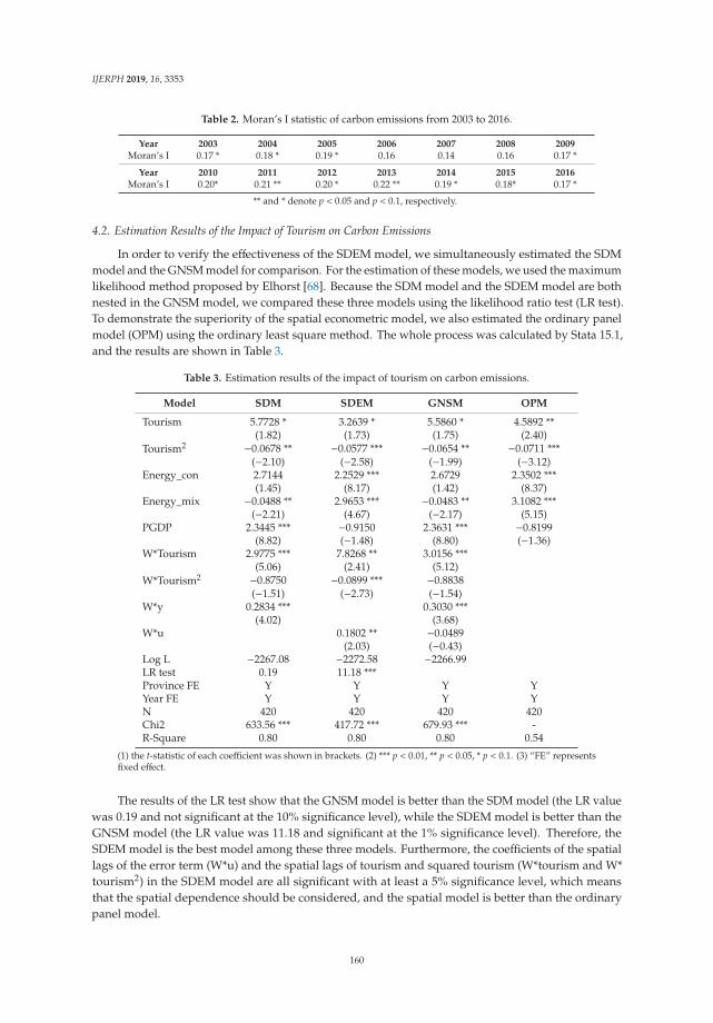
IJERPH 2019, 16, 3353

Table 2. Moran’s I statistic of carbon emissions from 2003 to 2016.

Year 2003 2004 2005 2006 2007 2008 2009Moran’s I 0.17 * 0.18 * 0.19 * 0.16 0.14 0.16 0.17 *

Year 2010 2011 2012 2013 2014 2015 2016Moran’s I 0.20* 0.21 ** 0.20 * 0.22 ** 0.19 * 0.18* 0.17 *

** and * denote p < 0.05 and p < 0.1, respectively.

4.2. Estimation Results of the Impact of Tourism on Carbon Emissions

In order to verify the effectiveness of the SDEM model, we simultaneously estimated the SDMmodel and the GNSM model for comparison. For the estimation of these models, we used the maximumlikelihood method proposed by Elhorst [68]. Because the SDM model and the SDEM model are bothnested in the GNSM model, we compared these three models using the likelihood ratio test (LR test).To demonstrate the superiority of the spatial econometric model, we also estimated the ordinary panelmodel (OPM) using the ordinary least square method. The whole process was calculated by Stata 15.1,and the results are shown in Table 3.

Table 3. Estimation results of the impact of tourism on carbon emissions.

Model SDM SDEM GNSM OPM

Tourism 5.7728 * 3.2639 * 5.5860 * 4.5892 **(1.82) (1.73) (1.75) (2.40)

Tourism2 −0.0678 ** −0.0577 *** −0.0654 ** −0.0711 ***(−2.10) (−2.58) (−1.99) (−3.12)

Energy_con 2.7144 2.2529 *** 2.6729 2.3502 ***(1.45) (8.17) (1.42) (8.37)

Energy_mix −0.0488 ** 2.9653 *** −0.0483 ** 3.1082 ***(−2.21) (4.67) (−2.17) (5.15)

PGDP 2.3445 *** −0.9150 2.3631 *** −0.8199(8.82) (−1.48) (8.80) (−1.36)

W*Tourism 2.9775 *** 7.8268 ** 3.0156 ***(5.06) (2.41) (5.12)

W*Tourism2 −0.8750 −0.0899 *** −0.8838(−1.51) (−2.73) (−1.54)

W*y 0.2834 *** 0.3030 ***(4.02) (3.68)

W*u 0.1802 ** −0.0489(2.03) (−0.43)

Log L −2267.08 −2272.58 −2266.99LR test 0.19 11.18 ***Province FE Y Y Y YYear FE Y Y Y YN 420 420 420 420Chi2 633.56 *** 417.72 *** 679.93 *** -R-Square 0.80 0.80 0.80 0.54

(1) the t-statistic of each coefficient was shown in brackets. (2) *** p < 0.01, ** p < 0.05, * p < 0.1. (3) “FE” representsfixed effect.

The results of the LR test show that the GNSM model is better than the SDM model (the LR valuewas 0.19 and not significant at the 10% significance level), while the SDEM model is better than theGNSM model (the LR value was 11.18 and significant at the 1% significance level). Therefore, theSDEM model is the best model among these three models. Furthermore, the coefficients of the spatiallags of the error term (W*u) and the spatial lags of tourism and squared tourism (W*tourism and W*tourism2) in the SDEM model are all significant with at least a 5% significance level, which meansthat the spatial dependence should be considered, and the spatial model is better than the ordinarypanel model.

160

IJERPH 2019, 16, 3353

According to the results of the SDEM model presented in Table 3, the coefficient of tourismis 3.2639 with a significance level of 10%, and the coefficient of squared tourism is −0.0577, with asignificance level of 1%. The positive effect of tourism and the negative effect of squared tourism showthat there is an inverse U-shaped relationship between tourism and carbon emissions. The inverseU-shaped relationship implies that one province’s carbon emissions will increase with its tourismgrowth, but a threshold will eventually be reached, after which the carbon emissions will decrease. Theabove effect of tourism is also called a direct effect in the context of spatial econometrics. At first glance,this finding is different from the existing literature. However, if the samples of this study are dividedinto two types, one that includes only the samples whose tourism receipts are on the left of the axis ofsymmetry of the inverse U-shape, and the other one that includes the samples whose tourism receiptsare on the right of the axis of symmetry, the result of the first type is consistent with the literature whichfound that tourism has a significant positive emissions effect in the countries (e.g., Cyprus, Turkey,and Mauritius) where tourism receipts are relatively low [32–36]. The result of the second type isconsistent with the literature which found that tourism has a significant negative emissions effect in thecountries (e.g., United States, Western European Countries, and Singapore) where tourism receipts arerelatively high [5,37,39]. Therefore, the nonlinear model used in this paper can include both positiveand negative effects in one model and is more realistic and appropriate than the existing linear models.

Among the estimation results of the SDEM model in Table 3, the coefficient of the spatial lagof tourism is 7.8268, with a significance level of 5%, and the coefficient of the spatial lag of squaredtourism is −0.0899, with a significance level of 1%. The results show that one province’s tourism notonly affects its carbon emissions but also affects its neighbors’ carbon emissions through the spatiallag effect, which is also called an indirect effect in the context of spatial econometrics. Although theindirect effect of tourism on carbon emissions turned out to be significant in this paper, it was rarelyconsidered in the existing studies. The geographic proximity of provinces and the mobility of economicresources (e.g., services, products, technologies, and funds) between provinces have increased thetransfer of carbon emissions among provinces [53]. From the perspective of tourism development, oneprovince’s tourism growth not only stimulates the growth of the tourism subsectors of the province butalso moves the related industry resources across the province. Thus, one province’s tourism-relatedindustry is driven by its neighbors’ tourism development, accompanied by carbon emissions generatedduring the process of undertaking industry growth. Therefore, one province will bear some carbonemissions for its neighbors’ tourism development and further expand the degree of interprovincialcarbon emissions [69,70]. Moreover, the negative coefficient of the spatial lag of squared tourism andthe positive coefficient of the spatial lag of tourism mean that there is a nonlinear relationship betweentourism and its indirect effect on carbon emissions. When one province’s tourism receipts beyond thecritical value, tourism development will not only eliminate carbon emissions of the province but alsoreduce the carbon emissions of its neighbors.

In order to describe the above nonlinear spatial relationships more clearly, we depicted the directand the indirect effects of tourism on carbon emissions in Figure 2. Additionally, the relationship oftourism on carbon emissions based on the OPM model is also depicted in Figure 2 for comparison.

Figure 2 illustrates the inverse U-shaped direct effect and indirect effect of tourism on carbonemissions more intuitively. The axis of symmetry of the inverse U-shaped curve is also depicted inFigure 2. According to the axis of symmetry, we can easily determine that when tourism receipts arelower than the critical value (283 billion Chinese Yuan (CNY)), the direct effect of tourism on carbonemissions is positive and then shifts to negative when the tourism receipts are beyond the above criticalvalue. In terms of indirect effect, when the tourism receipts are lower than 435 billion CNY, the effect oftourism on carbon emissions is positive and then shifts to negative when the tourism receipts increasebeyond the critical value (435 billion CNY under this situation). Moreover, compared to the SDEMmodel used in this paper, the inverse U-shape curve which describes the result of the OPM modelshows that the nonlinear OPM model overestimates the positive impact on carbon emissions from

161

IJERPH 2019, 16, 3353

tourism and underestimates the negative impact on carbon emissions from tourism by ignoring of theabovementioned indirect effect.

Figure 2. The nonlinear direct and indirect effects of tourism on carbon emissions.

The direct and indirect effects of tourism on carbon emissions of 30 provinces in 2016 are alsoshown in Figure 2. The provinces are divided into eastern provinces, which include Beijing, Tianjin,Hebei, Liaoning, Shanghai, Jiangsu, Zhejiang, Fujian, Shandong, Guangdong, and Hainan, middleprovinces which include Jilin, Heilongjiang, Shanxi, Henan, Anhui, Jiangxi, Hubei, and Hunan, andwestern provinces which include Inner Mongolia, Qinghai, Ningxia, Shaanxi, Sichuan, Chongqing,Guizhou, Yunnan, Guangxi, Gansu, and Xinjiang. According to Figure 2, in terms of the direct effect,there are 12 provinces whose tourism has already exceeded the critical value and has a negativeimpact on carbon emissions, and the tourism of the rest of the provinces still has a positive effect oncarbon emissions. Because most of the above 12 provinces are the relatively developed provinces andmost of the remaining provinces are less developed provinces in China, Figure 2 provides furtherevidence that the relationship between tourism and carbon emissions are consistent with the existingliterature [32–39]. In terms of the indirect effect, there are only three provinces whose tourism receiptshave exceeded the critical value, which means that most of the provinces in China still have a positiveeffect on their neighbors’ carbon emissions.

4.3. Estimation Results of the Moderating Effects

The SDEM model was used to estimate the moderating effects of reduction policy, sustainableeducation, tourism efficiency, and transportation infrastructure. The LR test was used to test whetherthe SDEM model should be reduced to the spatial error model (SEM), which does not contain thespatial lags of explanatory variables compared to the SDEM model. The results are presented in Table 4.

162

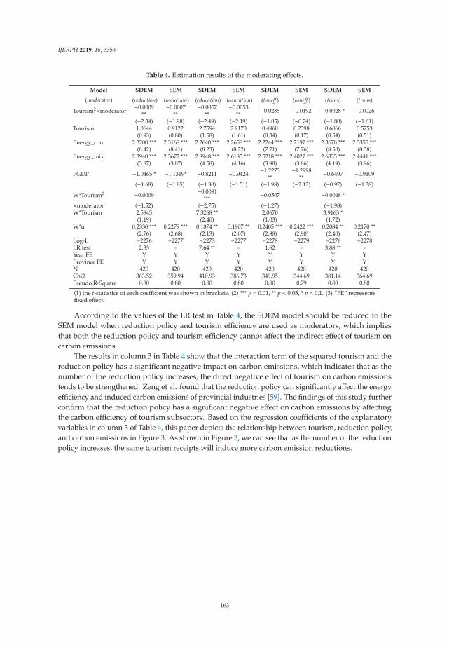
IJERPH 2019, 16, 3353

Table 4. Estimation results of the moderating effects.

Model SDEM SEM SDEM SEM SDEM SEM SDEM SEM

(moderator) (reduction) (reduction) (education) (education) (toueff ) (toueff ) (trans) (trans)

Tourism2×moderator−0.0009

**−0.0007

**−0.0057

**−0.0053

** −0.0285 −0.0192 −0.0028 * −0.0026

(−2.34) (−1.98) (−2.49) (−2.19) (−1.05) (−0.74) (−1.80) (−1.61)Tourism 1.0644 0.9122 2.7594 2.9170 0.4960 0.2398 0.6066 0.5753

(0.93) (0.80) (1.58) (1.61) (0.34) (0.17) (0.54) (0.51)Energy_con 2.3200 *** 2.3168 *** 2.2640 *** 2.2658 *** 2.2244 *** 2.2197 *** 2.3678 *** 2.3355 ***

(8.42) (8.41) (8.23) (8.22) (7.71) (7.76) (8.50) (8.38)Energy_mix 2.3940 *** 2.3672 *** 2.8948 *** 2.6185 *** 2.5218 *** 2.4027 *** 2.6335 *** 2.4441 ***

(3.87) (3.87) (4.58) (4.16) (3.98) (3.86) (4.19) (3.96)

PGDP −1.0465 * −1.1319* −0.8211 −0.9424 −1.2273**

−1.2998** −0.6497 −0.9109

(−1.68) (−1.85) (−1.30) (−1.51) (−1.98) (−2.13) (−0.97) (−1.38)

W*Tourism2 −0.0009 −0.0091*** −0.0507 −0.0048 *

×moderator (−1.52) (−2.75) (−1.27) (−1.98)W*Tourism 2.5845 7.3268 ** 2.0670 3.9163 *

(1.19) (2.40) (1.03) (1.72)W*u 0.2330 *** 0.2279 *** 0.1874 ** 0.1907 ** 0.2405 *** 0.2422 *** 0.2084 ** 0.2170 **

(2.76) (2.68) (2.13) (2.07) (2.88) (2.90) (2.40) (2.47)Log-L −2276 −2277 −2273 −2277 −2278 −2279 −2276 −2278LR test 2.33 - 7.64 ** - 1.62 - 3.88 ** -Year FE Y Y Y Y Y Y Y YProvince FE Y Y Y Y Y Y Y YN 420 420 420 420 420 420 420 420Chi2 363.52 359.94 410.93 386.73 349.95 344.69 381.14 364.69Pseudo.R-Square 0.80 0.80 0.80 0.80 0.80 0.79 0.80 0.80

(1) the t-statistics of each coefficient was shown in brackets. (2) *** p < 0.01, ** p < 0.05, * p < 0.1. (3) “FE” representsfixed effect.

According to the values of the LR test in Table 4, the SDEM model should be reduced to theSEM model when reduction policy and tourism efficiency are used as moderators, which impliesthat both the reduction policy and tourism efficiency cannot affect the indirect effect of tourism oncarbon emissions.

The results in column 3 in Table 4 show that the interaction term of the squared tourism and thereduction policy has a significant negative impact on carbon emissions, which indicates that as thenumber of the reduction policy increases, the direct negative effect of tourism on carbon emissionstends to be strengthened. Zeng et al. found that the reduction policy can significantly affect the energyefficiency and induced carbon emissions of provincial industries [59]. The findings of this study furtherconfirm that the reduction policy has a significant negative effect on carbon emissions by affectingthe carbon efficiency of tourism subsectors. Based on the regression coefficients of the explanatoryvariables in column 3 of Table 4, this paper depicts the relationship between tourism, reduction policy,and carbon emissions in Figure 3. As shown in Figure 3, we can see that as the number of the reductionpolicy increases, the same tourism receipts will induce more carbon emission reductions.

163

IJERPH 2019, 16, 3353

150

100ReductionPolicy

-14

-12

500

-10

-8

20

104

Tourism Receipts

-6

40

-4

-2

60

0

80 0100

Figure 3. Effect of tourism on carbon emissions using reduction policy as the moderator.

The results in column 4 in Table 4 show that the interaction term of the squared tourism andeducation has a significant negative effect on carbon emissions, which implies that the increase of thesustainable education tends to strengthen the negative effect of tourism on carbon emissions. Somescholars argue that the environmental protection awareness of tourists has an essential impact on thecarbon emissions induced from tourism [62], and this finding provides empirical evidence for theabove argument. The coefficient of the spatial lag of the interaction term is −0.0091 with a significancelevel of 1%, which indicates that the sustainable education not only strengthens the negative directeffect of tourism on carbon emissions but also strengthens the negative indirect effect of tourism oncarbon emissions. The direct and indirect effects of tourism on carbon emissions using sustainableeducation as the moderator are depicted in Figure 4, which shows the above findings more clearly.

(a) (b)

15

10-900 Sustainable

Education

-800

-700

0

-600

-500

520

-400

Car

bon

Emis

sion

s -300

Tourism Receipts

-200

40

-100

0

6080 0100

15

10-800

-600

0 SustainableEducation

-400

-200

0

20

Car

bon

Emis

sion

s 200

5

400

Tourism Receipts

40

600

800

6080 0100

Figure 4. (a) Direct and (b) indirect effect of tourism on carbon emissions using sustainable educationas the moderator.

According to the results in column 7 in Table 4, the coefficient of the squared tourism with themoderator is −0.0192, but it is not statistically significant, which means that the management efficiencyof the tourism industry cannot affect the direct effect of tourism on carbon emissions. This finding isdifferent from the arguments of the existing literature [49]. Therefore, although in theory, well-managedtourism could improve energy efficiency and the induced carbon efficiency [3,63], our above resultscould not provide the empirical evidence for this conclusion using Chinese samples, which indicates

164

IJERPH 2019, 16, 3353

that with the management efficiency improvement of the tourism industry, the energy efficiency oftourism is not necessarily improved.

The results presented in column 8 of Table 4 show that the coefficient of the interaction term ofthe squared tourism and the moderator is −0.0028 with a significance level of 10%, which indicatesthat the improvement of the transportation infrastructure is conducive to increasing carbon efficiencyand strengthens the negative effect of tourism on carbon emissions. Although the construction oftransportation facilities will increase carbon emissions, the improvement of transportation infrastructurewill improve the energy efficiency of the transportation industry and thus reduce carbon emissionsfrom tourism [45,46]. Our results show that the aggregated carbon emissions induced by theimprovement of transportation infrastructure are significantly negative, and therefore, the improvementof transportation infrastructure has a significant impact on the strength of the relationship betweentourism and carbon emissions. Moreover, the coefficient of the spatial lag of the interaction term is−0.0048, with a significance level of 10%, which indicates that the improvement of one province’stransportation infrastructure not only strengthens the negative effect of tourism on its carbon emissionsbut also strengthens the negative effect of tourism on its neighbors’ carbon emissions. The moderatingeffects of transportation infrastructure are depicted in Figure 5, from which we can see that with theimprovement of transportation infrastructure, both direct and indirect effects of tourism on carbonemissions tend to be strengthened.

(a) (b)

30

20TransportationInfrastructure

-900

-800

-700

100

-600

20

-500

Tourism Receipts

-400

40

-300

-200

60

-100

80

0

0100

30

20TransportationInfrastructure

-1200

-1000

0

-800

10

-600

20

-400

Tourism Receipts

40

-200

0

60

200

400

80 0100

Figure 5. (a) Direct and (b) indirect effect of tourism on carbon emissions using transportationinfrastructure as the moderator.

5. Conclusions and Policy Implications

Considering the possible nonlinear and spatial effects of tourism on carbon emissions, this paperemployed spatial econometric models combined with quadratic terms of explanatory variables toexplore the nexus between them. The main conclusions of the empirical analysis based on Chineseprovincial panel data from 2003 to 2016 are as follows: First, there is a significant inverse U-shapedrelationship between tourism development and carbon emissions. In the provinces whose tourismreceipts are relatively low, the effects of tourism on carbon emissions are positive but decrease graduallyas the tourism receipts increase and then become negative and continue decreasing gradually whenthe tourism receipts increase beyond the critical value. Second, there is a significant spatial lageffect (indirect effect) of tourism on carbon emissions, and the effect is also inverse U-shaped. Oneprovince’s tourism development not only affects its carbon emissions but also affects its neighbors’carbon emissions because of geographical proximity and industrial relevance. Finally, carbon reductionpolicy, sustainable education, and transportation infrastructure all have significant moderating effectson the relationship between tourism development and carbon emissions, but the moderating effect of

165

IJERPH 2019, 16, 3353

the management efficiency of tourism is not statistically significant. Furthermore, improvement ofthe sustainable education and transportation infrastructure not only strengthens the direct negativeeffect of tourism on carbon emissions but also strengthens the indirect negative effect of tourism oncarbon emissions.

Although the idea that increasing the emissions of carbon dioxide has a significant effect on globaltemperatures is not the topic of this study, it is one of the backgrounds of this paper. We noted that theabove idea is still controversial. Although the IPCC (Intergovernmental Panel on Climate Change)concluded that increasing carbon dioxide will increase global temperatures [71], some researchersconcluded that increases in carbon dioxide emissions have had no significant effects [72,73]. Ignoringthe controversy may misinform readers [74]. However, for this article, low-carbon development oftourism will also help to reduce environmental pollution caused by the consumption of fossil fuelsand will be conducive to the sustainable development of tourism, because fossil fuels currently stillaccount for roughly 85% of China’s energy mix [75]. Therefore, even considering the uncertainty ofthe relationship between carbon dioxide and climate change, the study on the nexus between carbondioxide emissions and tourism is still of great significance and has important policy implications.

Three main policy implications can be drawn from the above conclusions. First, in the regionswhere tourism receipts are below the critical value (283 billion CNY in China), it is still necessary toimprove the carbon efficiency of the tourism industry, because tourism can only be considered as alow carbon industry when its scale exceeds the critical value. Considering the lack of an endogenousdriving force to improve carbon efficiency, local government could take measures, such as increasing theinvestment in green public infrastructure and subsidizing tourism enterprises’ low-carbon initiatives,to improve energy efficiency and the induced carbon efficiency of the tourism industry. Second, localgovernments could improve the carbon efficiency in the upstream industries of the tourism industryto avoid the positive carbon emissions effect caused by their neighbors’ tourism growth. They couldalso improve tourism carbon efficiency through strengthening the connectivity between the upstreamindustry of tourism and the tourism industry of the neighboring regions because of the existing of thenegative indirect emissions effect of the tourism industry. Lastly, governments could strengthen thenegative effect of tourism on carbon emissions by increasing the number of carbon reduction policies,increasing the years of education, and improving transportation infrastructure. Moreover, tourismenterprises should be encouraged to improve energy efficiency and induced carbon efficiency whileimproving management efficiency.

Author Contributions: Conceptualization, C.B. and J.Z.; methodology, C.B.; software, C.B.; validation, C.B. andJ.Z.; formal analysis, C.B.; data curation, C.B.; writing—original draft preparation, C.B. and J.Z.; writing—reviewand editing, J.Z; visualization, C.B.

Funding: This research was funded by the National Social Science Foundation of China (CFA150151), the NationalNatural Science Foundation of China (Grant No: 71974203), the Fundamental Research Funds for the CentralUniversities from Zhongnan University of Economics and Law (Grant No: 2722019JCG061), Zhongnan universityof economics and law graduate education achievement award cultivation project (Grant No: CGPY201904),Interdisciplinary innovation research project (Grant No: 2722019JX002) and the Fundamental Research Funds forShannxi Normal University (16SZYB34).

Acknowledgments: The authors would like to acknowledge the many helpful comments of the anonymous peerreviewers. The views expressed in the article represent the views of the authors alone, however.

Conflicts of Interest: The authors declare no conflict of interest.

References

1. Gössling, S. National emissions from tourism: An overlooked policy challenge? Energy Policy 2013, 59,433–442. [CrossRef]

2. Gössling, S.; Buckley, R. Carbon labels in tourism: Persuasive communication? J. Clean. Prod. 2016, 111,358–369. [CrossRef]

3. UNWTO-UNEP-WMO. Climate Change and Tourism: Responding to Global Challenges[R]; The World TourismOrganization and The United Nations Environment Programme: Madrid, Spain, 2008.

166

IJERPH 2019, 16, 3353

4. Wu, P.; Han, Y.J.; Tian, M. The measurement and comparative study of carbon emissions from tourism intypical provinces in China. Acta Ecol. Sin. 2015, 35, 184–190. [CrossRef]

5. Katircioglu, S.T. Testing the tourism-induced EKC hypothesis: The case of Singapore. Econ. Model. 2014, 41,383–391. [CrossRef]

6. Zaman, K.; Shahbaz, M.; Loganathan, N.; Raza, S.A. Tourism development, energy consumption andEnvironmental Kuznets Curve: Trivariate analysis in the panel of developed and developing countries.Tour. Manag. 2016, 54, 275–283. [CrossRef]

7. Bi, C.; Jia, M.; Zeng, J.J. Nonlinear effect of public infrastructure on energy intensity in China: A panel smoothtransition regression approach. Sustainability 2019, 11, 629. [CrossRef]

8. Becken, S.; Simmons, D.G.; Frampton, C. Energy use associated with different travel choices. Tour. Manag.2003, 24, 267–277. [CrossRef]

9. Wu, P.; Shi, P.H. An estimation of energy consumption and CO2 emission in tourism sector of China.J. Geogr. Sci. 2011, 21, 733–745. [CrossRef]

10. Xie, Y.F.; Zhao, Y. Measuring carbon emissions from energy consumption by tourism in Yangtze River Delta.Geogr. Res. 2012, 31, 429–438.

11. Sun, Y.Y. A framework to account for the tourism carbon footprint at island destinations. Tour. Manag. 2014,45, 16–27. [CrossRef]

12. Filimonau, V.; Dickinson, J.; Robbins, D.; Reddy, M.V. The role of ‘indirect’ greenhouse gas emissions intourism: Assessing the hidden carbon impacts from a holiday package tour. Transp. Res. Part A Policy Pract.2013, 54, 78–91. [CrossRef]

13. Scott, D.; Gossling, S.; Hall, C.M.; Peeters, P. Can tourism be part of the decarbonized global economy? Thecosts and risks of alternate carbon reduction policy pathways. J. Sustain. Tour. 2016, 24, 52–72. [CrossRef]

14. Zhou, Y.N.; Huang, J.X.; Huang, M.X.; Lin, Y.C. The Driving Forces of Carbon Dioxide Equivalent EmissionsHave Spatial Spillover Effects in Inner Mongolia. Int. J. Environ. Res. Public Health 2019, 16, 1735. [CrossRef][PubMed]

15. Sun, H.; Sun, W.; Geng, Y.; Yang, X.; Bless Kofi, E. How does natural resource dependence affect publiceducation spending? Environ. Sci. Pollut. Res. 2019, 26, 3666–3674. [CrossRef] [PubMed]

16. Tang, C.C.; Zhong, L.S.; Ng, P. Factors that influence the tourism industry’s carbon emissions: A tourismarea life cycle model perspective. Energy Policy 2017, 109, 704–718. [CrossRef]

17. Gössling, S. Sustainable tourism development in developing countries: Some aspects of energy use. J. Sustain.Tour. 2000, 8, 410–425. [CrossRef]

18. Ram, Y.; Nawijn, J.; Peeters, P.M. Happiness and limits to sustainable tourism mobility: A new conceptualmodel. J. Sustain. Tour. 2013, 21, 1017–1035. [CrossRef]

19. Coles, T.; Dinan, C.; Warren, N. Energy practices among small- and medium-sized tourism enterprises:A case of misdirected effort? J. Clean. Prod. 2016, 111, 399–408. [CrossRef]

20. Patterson, M.G.; McDonald, G. How Clean and Green is New Zealand Tourism? Lifecycle and Future EnvironmentalImpacts; Landcare Research: Lincoln, New Zealand, 2004.

21. Becken, S.; Patterson, M. Measuring national carbon dioxide emissions from tourism as a key step towardsachieving sustainable tourism. J. Sustain. Tour. 2006, 14, 323–338. [CrossRef]

22. Dwyer, L.; Forsyth, P.; Spurr, R.; Hoque, S. Estimating the carbon footprint of Australian tourism.J. Sustain. Tour. 2010, 18, 355–376. [CrossRef]

23. Jones, C. Scenarios for greenhouse gas emissions reduction from tourism: An extended tourism satelliteaccount approach in a regional setting. J. Sustain. Tour. 2013, 21, 458–472. [CrossRef]

24. Tao, Y.G.; Huang, Z.F. Review of accounting for carbon dioxide emissions from tourism at different spatialscales. Acta Ecol. Sin. 2014, 34, 246–254. [CrossRef]

25. Kelly, J.; Williams, P.W. Modelling tourism destination energy consumption and greenhouse gas emissions:Whistler, British Columbia, Canada. J. Sustain. Tour. 2007, 15, 67–90. [CrossRef]

26. Kuo, N.W.; Chen, P.H. Quantifying energy use, carbon dioxide emission, and other environmental loadsfrom island tourism based on a life cycle assessment approach. J. Clean. Prod. 2009, 17, 1324–1330. [CrossRef]

27. Konan, D.E.; Chan, H.L. Greenhouse gas emissions in Hawaii: Household and visitor expenditure analysis.Energy Econ. 2010, 32, 210–219. [CrossRef]

28. Huebner, A. Public perceptions of destination vulnerability to climate change and implications for long-haultravel decisions to small island states. J. Sustain. Tour. 2012, 20, 939–951. [CrossRef]

167

IJERPH 2019, 16, 3353

29. Tabatchnaia-Tamirisa, N.; Loke, M.K.; Leung, P.S.; Tucker, K.A. Energy and tourism in Hawaii. Ann. Tour. Res.1997, 24, 390–401. [CrossRef]

30. Filimonau, V.; Dickinson, J.E.; Robbins, D.; Reddy, M.V. A critical review of methods for tourism climatechange appraisal: Life cycle assessment as a new approach. J. Sustain. Tour. 2011, 19, 301–324. [CrossRef]

31. Munday, M.; Turner, K.; Jones, C. Accounting for the carbon associated with regional tourism consumption.Tour. Manag. 2013, 36, 35–44. [CrossRef]

32. Katircioglu, S.T.; Feridun, M.; Kilinc, C. Estimating tourism-induced energy consumption and CO2 emissions:The case of Cyprus. Renew. Sustain. Energy Rev. 2014, 29, 634–640. [CrossRef]

33. Katircioglu, S.T. International tourism, energy consumption, and environmental pollution: The case ofTurkey. Renew. Sustain. Energy Rev. 2014, 36, 180–187. [CrossRef]

34. León, C.J.; Arana, J.E.; Alemán, A.H. CO2 emissions and tourism in developed and less developed countries.Appl. Econ. Lett. 2014, 21, 1169–1173. [CrossRef]

35. Durbarry, R.; Seetanah, B. The impact of long haul destinations on carbon emissions: The case of Mauritius.J. Hosp. Market. Manag. 2015, 24, 401–410. [CrossRef]

36. Paramati, S.R.; Alam, M.S.; Chen, C.F. The effects of tourism on economic growth and CO2 emissions:A comparison between developed and developing economies. J. Travel Res. 2017, 56, 712–724. [CrossRef]

37. Lee, J.W.; Brahmasrene, T. Investigating the influence of tourism on economic growth and carbon emissions:Evidence from panel analysis of the European Union. Tour. Manag. 2013, 38, 69–76. [CrossRef]

38. Raza, S.A.; Sharif, A.; Wong, W.K.; Karim, M.Z.A. Tourism development and environmental degradation inthe United States: Evidence from wavelet-based analysis. Curr. Issues Tour. 2017, 20, 1768–1790. [CrossRef]

39. Paramati, S.R.; Shahbaz, M.; Alam, M.S. Does tourism degrade environmental quality? A comparative studyof Eastern and Western European Union. Transp. Res. Part D Transp. Environ. 2017, 50, 1–13. [CrossRef]

40. Sun, Y.Y. Decomposition of tourism greenhouse gas emissions: Revealing the dynamics between tourismeconomic growth, technological efficiency, and carbon emissions. Tour. Manag. 2016, 55, 326–336. [CrossRef]

41. Li, F.; Zhang, J.D.; Liu, W.C.; Liu, J.A.; Huang, J.H.; Zeng, G.M. An exploration of an integrated stochastic-fuzzypollution assessment for heavy metals in urban topsoil based on metal enrichment and bioaccessibility.Sci. Total Environ. 2018, 644, 649–660. [CrossRef] [PubMed]

42. Yang, Y.; Zhou, Y.N.; Poon, J.; He, Z. China’s carbon dioxide emission and driving factors: A spatial analysis.J. Clean. Prod. 2019, 211, 640–651. [CrossRef]

43. Cheng, Y.P.; Wang, Z.Y.; Ye, X.Y.; Wei, Y.D. Spatiotemporal dynamics of carbon intensity from energyconsumption in China. J. Geogr. Sci. 2014, 24, 631–650. [CrossRef]

44. Li, F.; Qiu, Z.Z.; Zhang, J.D.; Liu, C.Y.; Cai, Y.; Xiao, M.S.; Zhu, L.Y. Temporal variation of major nutrients andprobabilistic eutrophication evaluation based on stochastic-fuzzy method in Honghu Lake, Middle China.Sci. China Techol. Sci. 2019, 62, 417–426. [CrossRef]

45. Black, W.R. Sustainable mobility and its implication for tourism. In Tourism and Transport: Issues and Agendafor the New Millennium; Lumsdon, L., Page, S., Eds.; Elsevier: Amsterdam, The Netherlands, 2004; pp. 57–68.

46. Gössling, S. Global environmental consequences of tourism. Glob. Environ. Chang. 2002, 12, 283–302.[CrossRef]

47. Gössling, S.; Hansson, C.B.; Hörstmeier, O.; Saggel, S. Ecological footprint analysis as a tool to assess tourismsustainability. Ecol. Econ. 2002, 43, 199–211. [CrossRef]

48. Høyer, K. Sustainable tourism or sustainable mobility? The Norwegian case. J. Sustain. Tour. 2000, 8, 147–159.[CrossRef]

49. Gössling, S. Carbon Management in Tourism; Routledge: Oxon, UK, 2011.50. Peeters, P.; Williams, V.; Haan, A. Technical and management reduction potential. In Climate Change and

Aviation: Issues, Challenges and Solutions; Gossling, S., Upham, P., Eds.; Earthscan: London, UK, 2009;pp. 293–307.

51. Upham, P.; Tomei, J.; Boucher, P. Biofuels, aviation and sustainability: Prospects and limits. In Climate Changeand Aviation: Issues, Challenges and Solutions; Gossling, S., Upham, P., Eds.; Earthscan: London, UK, 2009;pp. 309–328.

52. Cheng, Z.; Shi, X. Can industrial structural adjustment improve the total-factor carbon emission performancein China? Int. J. Environ. Res. Public Health 2018, 15, 2291. [CrossRef] [PubMed]

53. Zhou, Y.; Xu, Y.; Liu, C.; Fang, Z.; Guo, J. Spatial effects of technological progress and financial support onChina’s provincial carbon emissions. Int. J. Environ. Res. Public Health 2019, 16, 1743. [CrossRef]

168

IJERPH 2019, 16, 3353

54. Dietz, T.; Rosa, E.A. Effects of population and affluence on CO2 emissions. Proc. Natl. Acad. Sci. USA 1997,94, 175–179. [CrossRef]

55. Shi, A. The impact of population pressure on global carbon dioxide emissions, 1975-1996: Evidence frompooled cross-country data. Ecol. Econ. 2003, 44, 29–42. [CrossRef]

56. Fan, Y.; Liu, L.C.; Wu, G.; Wei, Y.M. Analyzing impact factors of CO2 emissions using the STIRPAT model.Environ. Impact Assess. Rev. 2006, 26, 377–395. [CrossRef]

57. Wang, S.J.; Li, Q.Y.; Fang, C.L.; Zhou, C.S. The relationship between economic growth, energy consumption,and CO2 emissions: Empirical evidence from China. Sci. Total Environ. 2016, 542, 360–371. [CrossRef][PubMed]

58. Sun, H.; Gulzara, T.; Haris, M.; Mohsin, M. Evaluating the environmental effects of economic openness:Evidence from SAARC countries. Environ. Sci. Pollut. Res. 2019, 26, 24542–24551. [CrossRef] [PubMed]

59. Zeng, J.J.; Liu, T.; Feiock, R.; Li, F. The impacts of China’s provincial energy policies on major air pollutants:A spatial econometric analysis. Energy Policy 2019, 132, 392–403. [CrossRef]

60. Tol, R.S.J. The impact of a carbon tax on international tourism. Transp. Res. Part D Transp. Environ. 2007, 12,129–142. [CrossRef]

61. Cheng, Z.H.; Li, L.S.; Liu, J. The emissions reduction effect and technical progress effect of environmentalregulation policy tools. J. Clean. Prod. 2017, 149, 191–205. [CrossRef]

62. Kachel, U.; Jennings, G. Exploring tourists’ environmental learning, values and travel experiences in relationto climate change: A postmodern constructivist research agenda. Tour. Hosp. Res. 2010, 10, 130–140.[CrossRef]

63. Lin, T.P. Carbon dioxide emissions from transport in Taiwan’s national parks. Tour. Manag. 2010, 31, 285–290.[CrossRef]

64. Thea, C. Towards a Low Carbon Travel & Tourism Sector[R]. In Proceedings of the World Business Summiton Climate Change, Copenhagen, Denmark, 24–26 May 2009.

65. Shan, Y.; Guan, D.; Zheng, H.; Ou, J.; Li, Y.; Meng, J.; Mi, Z.; Liu, Z.; Zhang, Q. China CO2 emission accounts1997–2015. Sci. Data 2018, 5, 170201. [CrossRef]

66. National Bureau of Statistics of China. China Statistical Yearbook; China Statistics Press: Beijing, China,2004–2017.

67. National Bureau of Statistics of China. China Energy Yearbook; China Statistics Press: Beijing, China, 2004–2017.68. Elhorst, J.P. Unconditional maximum likelihood estimation of linear and log-linear dynamic models for

spatial panels. Geogr. Anal. 2005, 37, 62–83. [CrossRef]69. Yao, L.; Liu, J. Research on carbon emission transfer among eight regional regions in China. China Popul.

Resour. Environ. 2010, 20, 16–19.70. Peng, L. An empirical analysis of inter-regional industrial linkages and spillover effects of economic growth

in China: Based on the perspective of inter-regional input-output analysis. J. Jishou Univ. (Soc. Sci. Ed.) 2008,3, 70–77.

71. United Nations, Intergovernmental Panel on Climate Change. Fourth Assessment Report (AR4); CambridgeUniversity Press: Cambridge, UK, 2007.

72. Segalstad, T.V. Carbon Cycle Modelling and the residence time of natural and anthropogenic atmosphericCO2: On the construction of the—Greenhouse effect global warming‖dogma. In Global Warming: TheContinuing Debate; Bate, R., Ed.; European Science and Environment Forum (ESEF): Cambridge, UK, 1998;pp. 184–219.

73. Essenhigh, R.E. Potential dependence of global warming on the residence time (RT) in the atmosphere ofanthropogenically sourced carbon dioxide. Energy Fuel 2009, 23, 2773–2784. [CrossRef]

74. Carlin, A. A Multidisciplinary, Science-Based Approach to the Economics of Climate Change. Int. J. Environ.Res. Public Health 2011, 8, 985–1031. [CrossRef] [PubMed]

75. Sun, H.; Clottey, S.A.; Geng, Y.; Fang, K.; Amissah, J.C.K. Trade Openness and Carbon Emission: Evidencefrom Belt and Road Countries. Sustainability 2019, 11, 2682. [CrossRef]

© 2019 by the authors. Licensee MDPI, Basel, Switzerland. This article is an open accessarticle distributed under the terms and conditions of the Creative Commons Attribution(CC BY) license (http://creativecommons.org/licenses/by/4.0/).

169

International Journal of

Environmental Research

and Public Health

Article

Establishment and Application of an EvaluationModel for Orchid Island SustainableTourism Development

Han-Shen Chen 1,2

1 Department of Health Diet and Industry Management, Chung Shan Medical University, No. 110, Sec. 1,Jianguo N. Rd., Taichung City 40201, Taiwan; allen975@csmu.edu.tw; Tel.: +886-4-2473-0022 (ext. 12225)

2 Department of Medical Management, Chung Shan Medical University Hospital, No. 110, Sec. 1,Jianguo N. Rd., Taichung City 40201, Taiwan

Received: 25 January 2019; Accepted: 1 March 2019; Published: 2 March 2019

Abstract: Global warming and climate change increase the likelihood of weather-related naturaldisasters that threaten ecosystems and consequently affect the tourism industry which thrives on thenatural attributes of island regions. Orchid Island, the study area, is home to the Yami (Tao) tribe—theonly indigenous people of Taiwan with a marine culture. The island possesses rich geological andtopographical features (such as coral reefs) and distinctive biological and ecological resources (such asthe green sea turtle, flying fish, and Orchid Island scops owl), and organizes traditional festivals andactivities (such as the flying fish festival) as well as tribal tourism activities. These factors contributeto its immense potential to become the new tourism hotspot. To study the factors enhancing touristexperiences, a random utility model was constructed using a choice experiment method (CEM) forthe tourist resort on Orchid Island. The study results demonstrated that: (1) Limiting tourists to600/day; employing professional tour guides; providing better recreational facilities; introducingadditional experience-enhancing activities; and lowering contributions towards the professionalecosystem conservation trust fund will improve the overall effectiveness of attracting tourists toOrchid Island. The evaluation results from both conditional logit and random parameter logit modelswere similar; (2) the analysis results from the latent class model demonstrated that island tourismhas significant market segmentation. The socioeconomic backgrounds of tourists, their experiences,and their preferences exhibit heterogeneity, with significant differences in willingness to pay forisland tourism.

Keywords: sustainable tourism; island destination; environmental impact; recreation economics

1. Introduction

According to the “Fourth Assessment Report (AR4) of the United Nations IntergovernmentalPanel on Climate Change (IPCC),” global warming and climate change have become increasinglyserious. The resulting rise in sea level from climate change can negatively impact water resources,ecological balance, and the environment. Climate change has a more severe impact on islands thatare surrounded by the sea. Relevant studies have pointed out that besides threatening ecosystems,natural disasters will also affect the operations of the tourism industry [1,2]. The UN World TourismOrganization (2011) mentioned that extreme weather conditions may affect 1.8 billion internationaltourists in 2030. The direct effects of climate change on the tourism industry include losses to manpowerand property. This also leads to a significant decrease in tourism as more and more tourists decide notto travel to such sites. Climate change will also indirectly affect the environment and culture of thetourist destination, the economic output of the tourism industry, and the damage infrastructure [3].The increasing demands for recreational tourism, changing tourist preferences, increasing awareness

IJERPH 2019, 16, 755; doi:10.3390/ijerph16050755 www.mdpi.com/journal/ijerph171

IJERPH 2019, 16, 755

on ecological conservation, and the rapid development in island tourism in recent years has attractedinternational researchers interested in island development to conduct relevant studies [4–6].

Dahlin et al. [7] pointed out that the development of island tourism will inevitably lead to somesigns of imbalance, including excessive coastal development, the destruction of ecological resources,pollution created by waste, etc. It may also lead to land encroachments to meet increasing demands foraccommodation and recreational water activities for tourists. Such changes may affect the traditionalcommunity system and gradually create an imbalance in the lifestyles of the locals. Therefore, whileislands may provide sightseeing and recreational services, they might simultaneously experience thenegative effects caused by the development in tourism on the environment, society, and local culturedue to their limited area and natural resources, vulnerability to disasters, compromised ability torecover from disasters, and economic dependence [8–10].

However, the development of the tourism industry is accompanied by increasingly prominentenvironmental problems. As the ultimate goal of sustainable tourism is still the sustainable managementof tourism destinations, the main application methods are still based on the environmental carryingcapacity, land division management, visitor impact management, and sustainable developmentindicators. Zhang et al. [11] suggested that, although existing sustainability evaluation methods can beused to assess the effects of human activities on ecosystem functions, they have a limited application inevaluating social economy. The use of this type of analysis to evaluate the economic benefits of tourismin that area can aid the concerned management in making related decisions on planning and utilizationand/or sustainable operation of local ecologic resources. In previous assessments of the benefits ofrecreational resources, many studies have employed the travel cost method and contingent valuationmethod (CVM) to assess the benefits of island tourism [12–14]. However, as travel cost methods andCVM methodologies have certain limitations in application, the CEM has gradually become a significantassessment method for conducting preference studies on the conservation of natural resources in recentyears. CEM is also an important assessment tool for measuring the value of nonmarket goods [15].

Liekens et al. [16] pointed out that besides the simultaneous assessment of use and nonuse values,CEM can also define the hypothetical market through questionnaire surveys to understand publicpreferences for landscape conservation and natural development. This will further reflect the valueof environmental goods (or services). As CEM has a multiattribute and multilevel assessment ability,different combinations of alternative programs are used to assess the important characteristics ofnonmarket goods or services. Choice sets of different hypothetical scenarios are used to enable therespondents to select appropriate alternative programs based on their preferences. This avoids anassessment bias [17]. Due to the aforementioned advantages, CEM has also been used to evaluatefactors with nonmarket value in recent years, including species conservation [15,18–20]; wetlandrehabilitation [21–23]; island tourism preferences [24–28]; and coastal region conservation [29–34].In addition, CEM was also employed to examine tourist preferences for land and environmentalfunctions in national parks [35,36]. Other studies that employed CEM focused on how to changespecific ecosystem services to affect economic benefits [37–40].

For empirical models, conditional logit (CL) models can be used to estimate the average preferenceof tourists from the multiple attributes of island tourism and to estimate the marginal willingnessto pay (MWTP) for these attributes [28,33]. The random parameter logit (RPL) model can reflect thedifferent responses of respondents from different backgrounds towards different attributes. This canbe used to examine the heterogeneous preferences of respondents and their willingness to pay forchanges in the levels of various attributes (such as folk and cultural experiences, ecologic experiences,and other attributes) [41–44].

To segment a clearer target market, the latent class model (LCM) can segregate respondentsinto different groups and examine and compare their preferences and group differences (such as theisland tourism preferences, attitudes, and socioeconomic background of interviewed tourists) [26].From the aforementioned studies, we can see that the empirical CEM models of CL, RPL, and LCM

172

IJERPH 2019, 16, 755

have been verified for use in the examination and evaluation of multiple attribute preferences at islandtourism sites.

Previous studies have shown that prior economic evaluation of nonmarket resources has mostlyfocused on the evaluation of forests, coastal areas, natural parks, and nature reserves. Only a fewstudies have evaluated the recreational value of island tourism. Therefore, this study used CEMto construct an island tourism attribute utility model and further employed CL and RPL modelsto estimate the utility function of island tourism. The socioeconomic background, awareness, andtourists’ attitudes towards island tourism were considered to examine the differences in MWTP forvarious attributes. LCM was used to test whether respondents had heterogeneous preferences forisland tourism so that they could select appropriate alternative programs based on their preferences.These will be used to evaluate the ecological environment, socioeconomic situation, and tribal tourismprograms on Orchid Island to determine their economic benefits and to create a system of sustainabledevelopment. The aforementioned methodology has representativeness and research originality andcan compensate for the current lack of studies on sustainable tourism development on islands inacademia. The research contribution made by studying the aforementioned problems can assist theworld, particularly the academic world, by providing a reference for economic evaluation models forsustainable island tourism and operation and management strategies.

The aim of this study is to evaluate the economic benefits of tourism for Orchid Island. A CEM isused to estimate the average preferences of tourists from the multiple attributes of island tourism and toestimate the WTP for these attributes. The study is divided into four parts. In Section 1, the motivationfor the study is discussed, and the study objective is proposed. In Section 2, we construct the preferenceutility model for island tourism and introduce preferred selection combinations for choice sets for theOrchid Island tourism site. In Section 3, we analyze the results of factors influencing multiple attributepreferences, along with their WTP. In Section 4, based on the results, countermeasures and suggestionsare proposed for the sustainable development of the Orchid Island environment, providing a referencefor policy makers to make more efficacious policies.

2. Literature Review

The CEM is a stated preference evaluation technique. Respondents are given multiple choices andforced to make trade-offs between them. Each option is described in terms of a bundle of attributesdescribing the good presented at various levels. The principle advantage of CEM is the ability to valueindividual characteristics of environmental goods and the marginal value of changes in characteristics.

In the past, economists try to assess people’s WTP for ecotourism preferences [24,25,33],species conservation [19,20], and, more recently, also the issue of WTP for ecosystem services wasexplored by many authors [37–39,45] but less frequent for evaluation of island tourism preferences [27,28].Remoundou et al. [31] employed CEM to evaluate the effects of climate change on the willingness topay for Santander’s coastal ecosystem. The study attributes included biodiversity, jellyfish blooms,days when the beaches were closed, sizes of the beaches, and annual additional household expenditure.Viteri Mejía and Brandt [33] employed CEM to interview tourists visiting the Galapagos Islands to assesstheir willingness to pay for protective measures against invasive species. The study attributes includeddepth of experience in the islands’ ecosystem, length of stay, level of protective measures taken againstinvasive species, and price of island tourism. The results of that study showed that tourists visitingthe Galapagos Islands highly valued the biodiversity on the island and were marginally willing to payUSD $2543 for better protective measures. Schuhmann et al. [32] employed CEM to evaluate touristpreferences and willingness to pay for coastal attributes in Barbados. The study attributes included price,type of accommodation, beach width, distance from beach, and beach litter.

Cazabon-Mannette et al. [29] employed CEM and CVM to evaluate the nonuse value andnonconsumptive value of sea turtles in Tobago. The study attributes included price, number ofsea turtle sightings, fish diversity (number of species), coral cover, and degree of congestion (number ofdivers). Xuan et al. [34] used a discrete choice experiment to evaluate tourists’ willingness to pay for

173

IJERPH 2019, 16, 755

boat tours in the marine protected area of Vietnam’s Nha Trang Bay. The study attributes included coralcover, environment quality, rate of unemployment of fishermen, and increase in ticket prices. Peng andOleson [30] employed a discrete choice experiment to evaluate beach recreationalists’ preferences andwillingness to pay to improve the water quality of Oahu beaches. The study attributes included waterquality, water turbidity, coral cover, fish diversity, and willingness to pay for motor vehicles. Park andSong [41] applied a latent profile analysis (LPA) and CEM to identify latent classes based on visitors’perceived place value and to estimate visitors’ willingness to pay (WTP) in an Urban Lake Park.

The above studies showed varying levels of WTP depended on factors such as where the studywas conducted, products and product attributes included and, data collection and analysis methodsused. In fact, through the questionnaire, the socioeconomic background (such as age, education, maritalstatus, and income) of respondents and respondents awareness and behavior (such as environmentalattitude, perceived value, and revisit intention) towards island tourism were used as perspectivesto examine the differences in WTP for various attributes. Halkos and Matsiori [46] pointed outthat the comparative study of residents’ and tourists’ WTP for improving the quality (protection) ofthe Pagasitikos coastal area in Greece found that income, education, environmental attitude are themost important factors affecting payment amount. Tonin [47] indicated, the previous knowledge orfamiliarity with coralligenous habitats and biodiversity issues, income, education, environmentalattitudes are main positive and significant determinants of WTP. The purpose of this study is theapplication of the CVM to the benefits of Orchid Island tourism management programs and thequantification of their value. In this case, it is not only the value of the island tourism that is calculated,but rather the economic benefits as a whole is evaluated through the respondents’ opinion of the goodsand services produced.

3. Materials and Methods

3.1. Description of the Study Area

Taiwan is surrounded by a coastline of 1141 km and has abundant marine resources.Island tourism in Taiwan has natural and ecological features as well as historical and cultural featuresand is an emerging tourist destination [48]. The study site, Orchid Island, which has a total area of48 km2 and 5069 residents, is located southeast of Taiwan and is surrounded by the sea (Figure 1).It is home to Taiwan’s only group of indigenous people with a marine culture—the Yami (Tao)tribe—and has rich geological and topographical features (coastal terrain, coral reefs); distinctivebiological and ecological resources (green sea turtle, flying fish, coconut crab, Orchid Island scops owl,and Arius (Podocarpus costalis)); traditional festivals and activities (launching ceremony, flying fishfestival); and aboriginal settlements. Orchid Island has witnessed a gradual development in diversetheme-based tours, which include natural ecology-based tours and relevant experience activities(snorkeling, whale watching, night observation of flying fish, and so forth). In recent years, supportedby government policies, island tourism and tribal tourism have become the new tourism trends inTaiwan and have significant developmental potential for the future.

However, the growth of the tourism industry is accompanied by a detrimental impact on theenvironment. The construction of coastal embankments and tetrapods causes severe damage to thecoastal environment and destroys biological habitats. In addition, tourism also indirectly affects theunique tatala boat culture of the Yami (Tao) people. The invasion of foreign culture causes a heritagecrisis in the traditional, cultural, and social structure of the Yami (Tao) people. As island ecosystemsare fragile, island development should emphasize the development of state land for environmentaland cultural conservation and protection while developing unique ecological and cultural experiencesto promote its tourism. The development of sightseeing resources must consider sustainable ecological,economic, and social development and try to minimize the impact of recreational activities on theenvironment. Therefore, development of the island tourism industry based on sustainable operating

174

IJERPH 2019, 16, 755

principles and conservation of the environment and its ecosystem are important topics to consider forthe sustainable development of island tourism.

Figure 1. Map of the study area.

3.2. Construction of Preference Utility Model for Island Tourism

3.2.1. Multi-Attribute WTP Valuation Model

First, CEM was used to construct an island tourism attribute utility model. Following that, CLand RPL models were used to estimate the utility function of island tourism. The socioeconomicbackgrounds of tourists and tourist awareness and behavior towards island tourism were used toexamine the differences in MWTP for various attributes. LCM was used to test whether there wereheterogeneous preferences for island tourism present in respondents. Lastly, the aforementionedempirical analysis results were used to estimate the economic benefits of island tourism.

CEM is a standard random utility model (RUM). Therefore, it was used to explore the MWTPfor all attributes and levels [49]. In the binary model, the utility of the nth respondent is assumed tobe the various options it faces (Uni), and the options are used to maximize the utility, as shown inEquation (1):

Uni = Vni + εni (1)

where Uni represents the attribute of the nth respondent facing the ith option, Vni represents theobservable part of the utility function, and εni represents the residual item, i.e., the unobservable part.

This study intended to explore differences in preferences and WTP between respondents ofdifferent social and economic backgrounds, considering various attributes and levels. The analysiswas conducted using a random parameters logit (RPL) model. The overall utility of the RPL modelwas determined as follows:

Uni = Vni(Xni, Sn) + I_ni (2)

where Vni is the utility coefficient of observable variable Xni and respondent characteristic Sn andrepresents the respondent’s preference, and εni is the residual item.

To estimate the relative importance of all attributes of the product in terms of value, it wasassumed that the degrees of various attributes in the alternative plan remained the same. Then,the marginal change in WTP for the kth attribute was determined by Equation (3):

WTP =−I2kI2c

(3)

175

IJERPH 2019, 16, 755

where I2k is the attribute k parameter and I2c is the payment tool parameter.

3.2.2. Introduction to Multiple Attributes and Levels of Orchid Island Tourism

Hanley et al. [50] pointed out that after defining the evaluation attributes to be included in CE,the evaluation of the levels of the attributes is a relatively important process. They also pointed outthat these levels should be specific and feasible for future application, and they can be formulatedthrough literature reviews and expert interviews. Therefore, besides conducting reviews of relevantliterature, this study also conducted interviews with five academics who were experts on the subject,two tour guides of the Orchid Island aboriginal tribe, and relevant staff from the public sector.Following that, four attributes, “limit on tourist numbers,” “tour guide system,” “recreational facilities,”and “experience activities”, were set up. In addition, an “ecosystem conservation trust fund” thatrepresents currency variables, was used as an expenditure tool attribute. We further delineated thecurrent status of various attributes (Table 1) for use as the basis for measuring changes in the levels ofattributes. After expert interviews, we obtained the following recommendations for level settings:

1. Tourist numbers should be controlled with the current level of 1000 tourists per day as the upperlimit. Further discussions with experts resulted in a recommendation of limiting numbers to nomore than 600 tourists per day as a principle;

2. Professional tour guides should be provided to offer guided tours;3. Recreational facilities with minimal environmental impact should be planned;4. Activities that enhance the experience of local characteristics/culture, such as “ecotourism,”

“tribal ceremonies,” and “cave and underground dwellings”, should be included in the scope ofexperience activities; and

5. Findings from the expert interviews should be used to set the evaluation levels for the ecosystemconservation trust fund. This study defined the various attributes and their levels for OrchidIsland tourism, as shown in Table 1 below:

Table 1. Attributes and levels of attributes of the Orchid Island tourism site.

Attributes Levels Variable Number of Levels

Limit on the number of visitors1. Maintaining the status quo: 1000 people per day LIM±

32. 800 people per day (20% reduction) LIM−3. 600 people per day (40% reduction) LIM−−

Tour guides1. Maintaining the status quo: professional tour guides notavailable GUI±

22. Introducing a guided tour facility GUI+

Recreation and facilities1. Maintaining the status quo REC±

22. Improving the quality of the recreation and facilities REC+

Experience activities

1. Maintaining the status quo: snorkeling, whale watching,night observation of flying fish EXP±

42. Addition of any one of the following activities:experiencing ecotourism, tribal ceremonies, or cave andunderground dwelling experience

EXP+

3. Addition of any two of the following three activities:experiencing ecotourism, tribal ceremonies, or cave andunderground dwelling experience

EXP+

4. Addition of the following three activities: experiencingecotourism, tribal ceremonies and or cave and undergrounddwelling experience

EXP+++

Ecosystem conservation trust fund

1. Maintaining the status quo: entrance free

FUND 6

2. TWD 200 per entry per person3. TWD 400 per entry per person4. TWD 600 per entry per person5. TWD 800 per entry per person6. TWD 1000 per entry per person

176

IJERPH 2019, 16, 755

3.3. Introduction to Preference Selection Combinations for Choice Sets for the Orchid Island Tourism Site

In order to understand the choices of tourists regarding multiple attribute preference programsfor the Orchid Island site, a more precise improvement plan and the preference for each attribute levelwill need to be more clearly defined. These attributes included “limit on tourist numbers,” “tour guidesystem,” “recreational facilities,” “experience activities,” and “ecosystem conservation trust fund.”Further information on these attributes are introduced and examined in Table 1 (attributes and levelsof attributes of the Orchid Island tourism site). The arrangement combinations of various attributesand their levels produced 288 possible factor combinations (3 × 2 × 2 × 4 × 6 = 288).

In actual operations, every respondent had to fill in their answers, i.e., select one of the threechoice sets (the two alternative programs and one status quo alternative). If the respondent was unableto make a decision, they could select “uncertain”, and this choice set was considered as a missingvalue. The researcher explained the various attributes of the Orchid Island tourism site and their levels(Table 2) and the content of the choice sets for Orchid Island preferences to each tourist respondent.This was in order to make the tourist respondents understand the content of the preference attributesof the Orchid Island tourism site before they selected their preferences. In terms of questionnairecontent presentation, the first part of the questionnaire, which was divided into “Orchid Islandtourism development awareness and behaviour”, and the third part, which included “basic personalinformation”, were identical in all five versions of the questionnaire.

Table 2. An example of the choice set of Orchid Island preferences and programs.

Program Attributes Current Program Program 1 Program 2

Limit on the number of visitors

Maintain The current situation 220% reduction 40% reduction

Uncertain

Tour guide

Not availableAvailable

Not available

Recreation and facilities

Maintaining the status quo Improved quality Improved quality

Experience activities

Maintaining the status quoThree additional activities One additional activity

Ecosystem conservation trustfund (TWD/entrance/person) Free TWD 600 TWD 1000

Please check(1 of 4) � Suggestions: � Suggestions: � Suggestions: � Suggestions:

3.4. Survey Design

This study employed purposive sampling and one-to-one interviews with 438 tourists in OrchidIsland, and, after factoring out the invalid questionnaires (i.e., those with omitted answers, incompleteanswers, or those in which answers to all the questions received the same scale points were all deemedas invalid and removed), a total of 385 valid ones were collected, giving a recovery rate of 87.9%.

177

IJERPH 2019, 16, 755

With regard to the socioeconomic backgrounds of tourists, there were more males (n of the total sample.In terms of age distribution, most people fell into the age groups of 31–40 years (n = 162%, 42.1%) and20–30 years (n = 129%, 33.5%). In terms of education level, tourists with university education (n = 162%,42.1%) made up the bulk of tourists. In terms of average personal monthly income, most tourists had anincome of TWD 30,000–40,000 (inclusive) (n = 169%, 43.9%), followed by TWD 20,000–30,000 (inclusive)(n = 101%, 26.2%). Recreational activities that tourists engaged in (multiple selection allowed) weremostly water activities (62.4%), tribal ceremonies (52.7%), and tasting of the local cuisine (28.7%).Expenditure on Orchid Island (including participating in activities, buying souvenirs, etc.) was TWD5000–10,000 (inclusive) (43.2%), followed by TWD 10,000–15,000 (inclusive) (32.7%). When askedwhether they would agree to pay a sum towards the ecosystem conservation trust fund to supportsustainable tourism development, most respondents were agreeable (n = 316%, 82.1%).

4. Results

4.1. Results of the Analysis of Factors Influencing Multiple Attribute Preferences for the Orchid Island Tourism Site

This study first used CL and RPL to estimate the utility functions of the multiple attributes of theOrchid Island tourism site and obtained the relevant factors that affected the functions. Table 3 showsthe empirical results. With the significance levels of the factors ranging from 1% to 9%, the evaluationmodel of this study passed the goodness of fit test (likelihood value was 614.6, which was significantlygreater than the threshold value of 21.7). From this, we can understand that the utility functions ofmultiple attributes of island tourism have good explanatory power [24,26,51]. The following sectionwill further describe the empirical analysis results of both models.

At a 5% significance level, the coefficient of LIM−− was positive and significant. From this,we understand that decreasing the current daily tourist limit from 1000 to 600 could increase the utilityvalue of island tourism for tourists. At a 1% significance level, GUI+ and REC+ t-values were alsovery significant. From this, we deduce that formulating and implementing a system of tour guidesand adding recreational facilities and improving the quality of the existing facilities will increasetourists’ preference for the Orchid Island tourism site. With regard to the ecosystem conservation trustfund, the t-value st a 1% significance level was negative and significant. From this, we can observethat the utility value of Orchid Island tourism will decrease for tourists by increasing the ecosystemconservation trust fund. RPL estimation results along with CL showed that only EXP+++ estimationresults were positive and achieved a significance level of 10%. From this, we understand that addingthree tourist activities to Orchid Island could significantly increase the utility levels for tourists.

Table 3. Results of the conditional logit model and random parameter logit model.

Conditional Logit Model Random Parameter Logit Model

Attributes and Levels Coefficient t-Value Coefficient t-Value S.E. t-Value

Constant −0.02 −0.05 −1.34 −3.73 c 3.56 8.46 c

LIM−− 0.08 1.12 0.11 0.79 0.49 1.77 a

LIM−− 0.15 2.33 b 0.18 1.24 1.24 6.11 c

GUI+ 0.12 2.71 c 0.12 1.23 0.89 4.66 c

REC+ 0.28 6.44 c 0.51 5.65 c 0.48 1.60EXP+ −0.02 −0.17 −0.05 −0.30 0.62 1.76 a

EXP++ −0.10 −1.31 −0.33 −2.12 b 1.16 4.28 c

EXP+++ 0.12 1.54 0.26 1.78 a 0.80 2.89 c

FUND −0.01 −7.21 c −0.01 −6.69 c

N of choice sets 1430 1430

Log-likelihood ratio −1476.54 −1254.62

X2(0.01,9) = 21.7 614.63 c

a 10% significance level; b 5% significance level; c 1% significance level.

178

IJERPH 2019, 16, 755

4.2. Examination and Analysis of Benefits of Island Tourism Management Programs

To analyze the benefits of island tourism management programs, this study used CL attributelevel parameters to estimate the WTP for various levels of attributes (as shown in Table 4). In Table 4,the WTP was calculated based on attribute coefficients in the CL model to represent the mean WTP ofall respondents. From the empirical analysis results, we can see that under the optimal program, eachtourist could generate TWD 1202 for every visit they participate in. Therefore, there will be a loss ofvalue if the status quo is maintained. The level of attributes in the optimal program could increasebenefits, i.e., an increase of TWD 2337 in WTP would occur with the optimal program comparedwith the status quo. Therefore, if the daily tourist limit can be decreased from the current number of1000 tourists to 600 tourists (LIM−−), the professional tour guide system could be implemented (GUI+),recreational facilities could be added, the facility quality of island tourism sites could be improved(REC+), and the experience activities available could be increased from snorkeling, whale watching, andnight observation of flying fish to include ecotourism, tribal ceremonies, and cave and undergrounddwelling experiences (EXP+++). This would be the most effective management program for improvingthe economic value of Orchid Island tourism. Thus, improving various attribute levels should prove tobe a more efficient management program as compared with the one being currently implemented.

Table 4. Willingness to pay (WTP) for attributes and levels and benefit evaluation of the managementprogram of Orchid Island Tourism.

Attributes and LevelsWTP

(TWD/Entrance/Person)Current Program

(TWD/Entrance/Person)Best Program

(TWD/Entrance/Person)Worst Program

(TWD/Entrance/Person)

LIM± −402.72 −402.72 −402.72LIM− 130.26

LIM−− 268.65 268.65GUI± −213.62 −213.62 −213.62GUI+ 213.62 213.62REC± −518.34 −518.34 −518.34REC+ 518.34 518.34EXP± −0.49 −0.49EXP+ −19.42EXP++ −180.32 −180.32EXP+++ 201.43 201.43

Total benefit −1135.17 1202.04 −1315.21

4.3. Examination of Willingness to Pay and Market Segmentation

The following section will further compare the socioeconomic backgrounds and behaviors oftourists in terms of their willingness to pay for the aforementioned levels of attributes. From Table 5,we can see that at a 10% significance level, the willingness to pay value for LIM is significantly differentamong individuals of different educational levels and is associated with intention to pay for theecosystem conservation trust fund. In addition, tourists with tertiary education and above and touristswho are willing to pay for the ecosystem conservation trust fund have a higher willingness to pay tobring down the daily tourist number from 1000 to 800. The willingness to pay value for GUI+ wassignificantly different between sexes and age groups. Females and respondents above 30 years oldindicated a higher willingness to pay for the implementation of the tour guide system. When examinedfor improving environmental and facility quality (REC+) at the 1% significance level, significantdifferences in tourist spending were identified. We can see that tourists who spend more have a higherwillingness to pay for improving the quality of recreational facilities at the Orchid Island tourism site.Finally, at the 1% significance level, the willingness to pay for EXP+++ was associated with significantdifferences in intention to pay for the ecosystem conservation trust fund. This shows that tourists whoare willing to pay for the ecosystem conservation trust fund have higher willingness to pay for threeadditional tourism activities. Previous studies utilizing RPL to examine the heterogeneous preferencesof tourists and market segmentation showed similar results to this study [24,26,51].

179

IJERPH 2019, 16, 755

Table 5. The differences in WTP of Orchid Island visitors from different socioeconomic backgrounds.

N Current LIM− LIM−− GUI+ REC+ EXP+ EXP++ EXP+++

Men 202 −1226 a 109 190 61 b 541 −46 −392 254

Women 183 −1738 102 191 164 563 −41 −348 263

Age > 30 256 −1602 103 196 162 a 542 −34 −312 b 265

Age ≤ 30 129 −1388 109 187 68 565 −52 −431 254

Tertiary 288 −1486 127 a 186 74 534 −56 −426 226

Secondary & primary 97 −1503 101 195 127 561 −40 −352 271

Income > TWD 30,000 281 −1491 109 164 96 544 −42 −387 261

Income ≤ TWD 30,000 104 −1504 105 211 127 562 −45 −361 262

Cost > TWD 10,000 198 −1786 b 117 224 116 583 c −28 a −350 280

Cost ≤ TWD 10,000 187 −1210 96 163 116 527 −62 −391 241

WTP Ecosystem conservationtrust fund 316 −1929 c 113 a 248 c 129 561 −26 c −344 a 289 c

Not WTP Ecosystemconservation trust fund 69 138 86 23 72 539 −102 −453 167

a 10% significance level; b 5% significance level; c 1% significance level.

Lastly, this study utilized LCM to construct a market segmentation model for Orchid Islandtourism based on the aforementioned background differences in order to examine the differences inisland tourism preferences and willingness to pay between different tourism groups. From Table 6,we can see that two potential market segmentation groups showed differences in island tourismpreferences. The first group of tourists showed preferences for “reducing the daily tourist limit to600 tourists”, “improving environment and facility quality”, and “increasing experience activitiesto three items”, and had lower preference for “ecosystem conservation trust fund”. In contrast,the option “increasing two experience activities” had a lower preference. The second group onlyshowed significant differences in the utility function for “improving environment and facility quality”and “ecosystem conservation trust fund”, and their WTP for “improving environment and facilityquality” was lower than that of the first group. The first categorical model included improvement inenvironment quality, and other attribute parameter preferences were relatively obvious. They can beclassified as tourists with obvious preferences (accounting for 79.5% of the sample). In comparison,the second group was only focused on the environment quality and can be classified as touristswith a single preference (accounting for 20.5% of the sample). A comparison of the socioeconomicbackgrounds and tourism behaviors of these two groups showed that tourists with obvious preferencesare mostly females, have higher education levels, higher spending capacities, and are willing to payfor the ecosystem conservation trust fund. This group obtains relatively higher island tourism benefitswithin a specific attribute combination. LCM was used for market segmentation of tourists to OrchidIsland to allow targeted market sales and self-positioning.

Table 6. Evaluation of latent class model (LCM) variables and WTP evaluation of Orchid Island.

Parameters of Attributes and LevelsCoefficient t-Value WTP

Category 1: Respondents with Strong Preference

Constant −0.70 −3.11 c -

LIM− −0.03 −0.46 -

LIM−− 0.26 3.51 c 542.00

GUI+ 0.04 1.05 -

REC+ 0.25 5.26 c 532.61

EXP+ −0.07 −0.93 -

EXP++ −0.15 −1.76 a −321.36

180

IJERPH 2019, 16, 755

Table 6. Cont.

Parameters of Attributes and LevelsCoefficient t-Value WTP

Category 1: Respondents with Strong Preference

EXP+++ 0.18 2.27 b 400.36

FUND −0.00 −5.69 c

Category 2: Respondents with a single preference

Constant 3.58 1.21 -

LIM− 0.76 1.24 -

LIM−− −0.93 −1.12 -

GUI+ 0.80 1.16 -

REC+ 0.77 1.67 a 395.00

EXP+ 0.76 0.76 -

EXP++ 0.94 0.97 -

EXP+++ −1.35 −0.83 -

FUND −0.00 −1.67 a

Category parameters: Category 1

Constant 0.41 0.69

Men −0.58 −1.82 a

Age >30 0.16 0.48

Tertiary 0.65 1.66 a

Income > TWD 30,000,000 −0.21 −0.65

Visited Orchid Island before −0.32 −0.83

Cost > TWD 2639 0.61 1.76 a

WTP Ecosystem conservation trust fund 2.54 4.53 c

N of choice sets 1430

Log-likelihood ratio −1563.47

X2(0.01,30) = 50.89 276.00 b

a 10% significance level; b 5% significance level; c 1% significance level.

5. Discussion

Regarding the empirical results, CL and RPL produced similar evaluation results for Orchid Islandtourists, and the tourists were shown to prefer a change in the status quo. In addition, RPL also reflecteda heterogeneous distribution pattern for tourists’ preferences for the various attribute parameters.The only preference that showed an identical effect on tourists’ choices was “improving recreationquality.” The two models showed that tourists’ preferences included having a system of professionaltour guides, improving the recreation and facility quality, adding three experience activities anddecreasing the charges towards the ecosystem conservation trust fund. The results of previous studieson Costa Rica tourists’ preferences for ecotourism [52] and preferences of tourists for the Barva VolcanoArea in Costa Rica [51] showed that tourists prefer improvements in infrastructure. These resultsare consistent with the results of this study that showed preferences for improved recreation andfacility quality.

In addition, tourists indicated that they would prefer to simultaneously experience threeactivities—ecotourism, tribal ceremonies, and cave and underground dwellings—on Orchid Island toexperience the natural, cultural, and ecologic landscapes. Tourists who were interviewed preferredthe most diverse ecotourism experience program. The results of the study by Chaminuka et al. [25]on tourists’ preferences for ecotourism in the villages adjacent to the Kruger National Park in South

181

IJERPH 2019, 16, 755

Africa also support the results of this study. They found that tourists have relatively high MWTP forvisits to villages and craft markets in these villages.

This study found that the socioeconomic background and tourism behavior of different touristswere associated with significant differences in the willingness to pay value for various attributes.Tourists with tertiary education and above who were willing to pay for the ecosystem conservationtrust fund indicated a greater preference for decreasing the daily limit of tourists than tourists withan education level lower than tertiary education and who were not willing to pay for the ecosystemconservation trust fund. The former showed a greater willingness to pay to restrict the number oftourists from 800 to 600. Tourists who are willing to pay for the ecosystem conservation trust fund weremore willing to pay value for the three experience activities than tourists who were not willing to payfor the ecosystem conservation trust fund. Tourists aged above 30 and females indicated preferencefor an explanatory tour guide system, while tourists who spend more were relatively more willingto pay for the improvement of recreation facilities. Previous studies have pointed out that there aredifferences in environmental attitude between residents and tourists, which vary according to gender,age, educational level, and other variables have similar results in this study [46,47].

The results of the analysis of preferred programs for developing island tourism in the areas ofOrchid Island natural, cultural, and ecological landscapes showed that, under the current program,the benefit for each tourist’s visit is TWD 1135. If the program with the highest value was used forestimation, each tourist could provide a benefit of TWD 1202 for every visit. Therefore, maintaining thestatus quo will decrease the economic value of island tourism development. In contrast, the tourists’willingness to pay value under the optimal program was increased by TWD 2337 compared withunder the current program. This optimal program involves decreasing the daily limit of tourists from1000 to 600 (TWD 269), implementing a system of professional tour guides (TWD 214), improvingthe environment and facility quality of the island tourism sites (TWD 518), and expanding thetourism experience activities available on Orchid Island from snorkeling, whale watching, and nightobservation of flying fish to include ecotourism, tribal ceremonies, and cave and underground dwellingexperiences (TWD 201). This is the best management program for developing island tourism for OrchidIsland. Lastly, this study used LCM to examine the market segmentation and heterogeneity in tourists’preferences for Orchid Island tourism and classified tourists into tourists with obvious preferencesand tourists with single preferences. The former accounted for 79.5% of the respondents and theseindividuals showed higher willingness to pay than the latter under the optimal program. This groupof people are the market segmentation subjects that operators should focus on. This segment consistsmostly of females who have a tertiary level education and above, who spend more (>TWD 10,000),and who are willing to pay for the ecosystem conservation trust fund. This LCM result reflects thatthe tourist group with obvious preferences has obvious preferences for “reducing the daily touristlimit to 600 tourists”, “improving recreation and facility quality”, and “increasing experience activitiesto three items” and has lower preference for the “ecosystem conservation trust fund” but does nothave a significant preference for “implementation of the tour guide system”. Overall, the interviewedtourist groups at the Orchid Island tourism site exhibited differences in preferences based on theirsocioeconomic backgrounds and tourism behaviors, and they demonstrated heterogeneity in islandtourism attribute preferences. The study by Juutinen et al. [26] on Oulanka National Park in Finlandalso supports this result.

In conclusion, The study show that CEM can be used to construct a multi-attribute utility functionfor natural resources and the environment to estimate economic values of goods and services. However,many other attributes could be included, such as ecosystem resilience, beach recreation, and landscapediversity. In this way, the preferences of tourists and local residents for environmental attributes couldbe better understood. Second, this study could consider local residents to generalize the findings infuture. A profound understanding of the determinant variables that affect residents’ attitudes towardtourism development could help community developers and practitioners build a suitably considerateand comprehensive program for future tourism development.

182

IJERPH 2019, 16, 755

6. Conclusions

The development of sustainable island tourism requires the integration of recreation, environment,and management information, which is further considered in the decision-making process for thedevelopment and management of sustainable tourism operations. This study used CE to constructa random utility model for the Orchid Island tourism site in Taiwan. To do so, it analyzed variousfactors, like recreation (such as experience activities), the environment (such as quality of recreationand facilities), systems (such as tourist limit system, tour guide system), and economic considerations(such as the ecosystem conservation trust fund), to construct an evaluation model for validation.

This study summarized five operation and management recommendations as references forthe management and operator units of Orchid Island and other relevant industries. This includedrestricting the daily number of visitors to Orchid Island to 600, implementing relevant measures toimprove the quality of recreation facilities, implementing a payment system for professional tourguides, and adding more than three experience activities for island tourism (such as ecotourism, tribalceremonies, and a cave and underground dwelling experience). These factors would not only increasethe overall utility for tourists who come to Orchid Island for island tourism but could also graduallyimplement an operation and management program for Orchid Island tourism. Secondly, the operatorsof island tourism should provide in-depth guided experience-tourism services for tourists who arehigh spenders, tourists aged above 30, and female tourists. Local tour guides could be trained toprovide professional guided tours for a target market.

Thirdly, if Orchid Island implements a pricing system, the economic benefits from theaforementioned programs could be combined with its corresponding operation and management costs,and improvements to experience service packages and measures could be included. This could be usedto plan specific content for the development of tourism in Orchid Island, which could be used as areference for determining the costs of island tourism packages. Fourth, it is suggested that, to effectivelymaintain biodiversity and achieve the goal of conservation and sustainable development, there shouldbe continued use of the Taiwanese National Scenic Area Act and other regulations on land planningand use. Additionally, a more explicit conservation program, geared towards Orchid Island’s regionalresource characteristics, should be formulated to realize the long-term preservation of the area’s naturalenvironment, flora, fauna, and historical relics. Moreover, the management of Orchid Island shouldapprove the demolition of illegal buildings or facilities and designate personnel to conduct patrols andinspections to maintain strict control of recreational activities within the park and to prevent improperbehavior that might damage or contaminate the environment. Lastly, relevant management units andisland tour operators should continue to understand the preferences and attitudes of tourists in thefuture to propose further operation and management strategies that conform to the concept of islandtourism and have more specific and feasible market positioning strategies. This will be more beneficialto the sustainable development of island tourism on Orchid Island.

Funding: This work was supported by the Ministry of Science and Technology (Republic of China, Taiwan)[grant number MOST 107-2410-H-040-008]. The funder had no role in study design; in the collection, analysis andinterpretation of data; in the writing of the report; and in the decision to submit the article for publication.

Acknowledgments: First of all, I would like to express my deepest gratitude to Chu-Wei Chen, who provided thestatistics used in my thesis. Second, I would like to express my heartfelt thanks to all the experts who have takenthe time to review this article and provide valuable comments.

Conflicts of Interest: The author declares no conflict of interest.

References

1. Buzinde, C.N.; Manuel-Navarrete, D.; Yoo, E.E.; Morais, D. Tourists’ perceptions in a climate of change:Eroding destinations. Ann. Tour. Res. 2010, 37, 333–354. [CrossRef]

2. Jopp, R.; DeLacy, T.; Mair, J. Developing a framework for regional destination adaptation to climate change.Curr. Issues Tour. 2010, 13, 591–605. [CrossRef]

183

IJERPH 2019, 16, 755

3. Scott, D.; Gössling, S.; Hall, C.M. International tourism and climate change. Wires Clim. Chang. 2012, 3,213–232. [CrossRef]

4. Arachchi, R.S.S.W.; Yajid, M.S.A.; Khatibi, A. Ecotourism practices in Sri Lankan eco resorts: A supplierperspective analysis. Tour. Hosp. Manag. 2015, 3, 169–180. [CrossRef]

5. Chen, C.C.; Lee, C.H. Economic benefits of improving the quality of cultural heritage sites. J. Econ. Manag.2017, 13, 241–264.

6. Volo, S. Eudaimonic well-being of islanders: Does tourism contribute? The case of the aeolian Archipelago.J. Destin. Mark. Manag. 2017, 6, 465–476. [CrossRef]

7. Dahlin, K.M.; Asner, G.P.; Field, C.B. Linking vegetation patterns to environmental gradients and humanimpacts in a Mediterranean-type island ecosystem. Landsc. Ecol. 2014, 29, 1571–1585. [CrossRef]

8. Benitez-Capistros, F.; Hugé, J.; Koedam, N. Environmental impacts on the Galapagos Islands: Identificationof interactions, perceptions and steps ahead. Ecol. Ind. 2014, 38, 113–123. [CrossRef]

9. Chi, Y.; Shi, H.; Wang, Y.; Guo, Z.; Wang, E. Evaluation on island ecological vulnerability and its spatialheterogeneity. Mar. Pollut. Bull. 2017, 125, 216–241. [CrossRef] [PubMed]

10. Hannak, J.S.; Kompatscher, S.; Stachowitsch, M.; Herler, J. Snorkelling and trampling in shallow-waterfringing reefs: Risk assessment and proposed management strategy. J. Environ. Manag. 2011, 92, 2723–2733.[CrossRef] [PubMed]

11. Zhang, Y.; Yang, Z.; Yu, X. Measurement and evaluation of interactions in complex urban ecosystem.Ecol. Model. 2006, 96, 77–89. [CrossRef]

12. Bertram, C.; Larondelle, N. Going to the woods is going home: Recreational benefits of a larger urban forestSite—A travel cost analysis for Berlin, Germany. Ecol. Econ. 2017, 132, 255–263. [CrossRef]

13. He, J.; Huang, A.; Xuc, L. Spatial heterogeneity and transboundary pollution: A contingent valuation (CV)study on the Xijiang River drainage basin in south China. China Econ. Rev. 2015, 36, 101–130. [CrossRef]

14. Perez-Verdin, G.; Sanjurjo-Rivera, E.; Galicia, L.; Hernandez-Diaz, J.C.; Hernandez-Trejo, V.;Marquez-Linares, M.A. Economic valuation of ecosystem services in Mexico: Current status and trends.Ecosyst. Serv. 2016, 21, 6–19. [CrossRef]

15. Rudd, M. National values for reginal aquatic species at risk in Canada. Endanger. Species Res. 2009, 6, 239–249.[CrossRef]

16. Liekens, I.; Schaafsma, M.; De Nocker, L.; Broekx, S.; Staes, J.; Aertsens, J.; Brouwer, R. Developing a valuefunction for nature development and land use policy in Flanders, Belgium. Land Use Policy 2013, 30, 549–559.[CrossRef]

17. Hoyos, D. The state of the art of environmental valuation with discrete choice experiments. Ecol. Econ. 2010,69, 1595–1603. [CrossRef]

18. Boxall, P.C.; Adamowicz, W.L.; Olar, M.; West, G.E.; Cantin, G. Analysis of the economic benefits associatedwith the recovery of threatened marine mammal species in the Canadian St. Lawrence Estuary. Mar. Policy2012, 36, 189–197. [CrossRef]

19. Lee, D.E.; Du Preez, M.D. Determining visitor preferences for rhinoceros conservation management at private,ecotourism game reserves in the Eastern Cape Province, South Africa: A choice modelling experiment.Ecol. Econ. 2016, 130, 106–116. [CrossRef]

20. Lew, D.K.; Wallmo, K. Temporal stability of stated preferences for endangered species protection from choiceexperiments. Ecol. Econ. 2017, 131, 87–97. [CrossRef]

21. Dias, V.; Belcher, K. Value and provision of ecosystem services from prairie wetlands: A choice experimentapproach. Ecosyst. Serv. 2015, 15, 35–44. [CrossRef]

22. Franzén, F.; Dinnétz, P.; Hammer, M. Factors affecting farmers’ willingness to participate in eutrophicationmitigation—A case study of preferences for wetland creation in Sweden. Ecol. Econ. 2016, 130, 8–15.[CrossRef]

23. Guimarães, M.H.; Madureira, L.; Nunes, L.C.; Santos, J.L.; Sousa, C.; Boski, T.; Dentinho, T. Using ChoiceModeling to estimate the effects of environmental improvements on local development: When the purposemodifies the tool. Ecol. Econ. 2014, 108, 79–90. [CrossRef]

24. Cerda, C.; Ponce, A.; Zappi, M. Using choice experiments to understand public demand for the conservationof nature: A case study in a protected area of Chile. J. Nat. Conserv. 2013, 21, 143–153. [CrossRef]

184

IJERPH 2019, 16, 755

25. Chaminuka, P.; Groeneveld, R.A.; Selomane, A.O.; Van Ierland, E.C. Tourist preferences for ecotourism inrural communities adjacent to Kruger National Park: A choice experiment approach. Tour. Manag. 2012, 33,168–176. [CrossRef]

26. Juutinen, A.; Mitani, Y.; Mäntymaa, E.; Shoji, Y.; Siikamäki, P.; Svento, R. Combining ecological andrecreational aspects in national park management: A choice experiment application. Ecol. Econ. 2011,70, 1231–1239. [CrossRef]

27. Romão, J.; Neuts, B.; Nijkamp, P.; Shikida, A. Determinants of trip choice, satisfaction and loyalty in aneco-tourism destination: A modelling study on the Shiretoko Peninsula, Japan. Ecol. Econ. 2014, 107, 195–205.[CrossRef]

28. Torres, C.; Faccioli, M.; Riera Font, A.R. Waiting or acting now? The effect on willingness-to-pay of deliveringinherent uncertainty information in choice experiments. Ecol. Econ. 2017, 131, 231–240. [CrossRef]

29. Cazabon-Mannette, M.; Schuhmann, P.W.; Hailey, A.; Horrocks, J. Estimates of the non-market value ofsea turtles in Tobago using stated preference techniques. J. Environ. Manag. 2017, 192, 281–291. [CrossRef][PubMed]

30. Peng, M.; Oleson, K.L.L. Beach Recreationalists’ Willingness to Pay and Economic Implications of CoastalWater Quality Problems in Hawaii. Ecol. Econ. 2017, 136, 41–52. [CrossRef]

31. Remoundou, K.; Diaz-Simal, P.; Koundouri, P.; Rulleau, B. Valuing climate change mitigation: A choiceexperiment on a coastal and marine ecosystem. Ecosyst. Serv. 2015, 11, 87–94. [CrossRef]

32. Schuhmann, P.W.; Bass, B.E.; Casey, J.F.; Gill, D.A. Visitor preferences and willingness to pay for coastalattributes in Barbados. Ocean Coast. Manag. 2016, 134, 240–250. [CrossRef]

33. Mejía, C.V.; Brandt, S. Managing tourism in the Galapagos Islands through price incentives: A choiceexperiment approach. Ecol. Econ. 2015, 117, 1–11. [CrossRef]

34. Xuan, B.B.; Sandorf, E.D.; Aanesen, M. Informing management strategies for a reserve: Results from adiscrete choice experiment survey. Ocean Coast. Manag. 2017, 145, 35–43. [CrossRef]

35. Ek, K.; Persson, L. Wind farms-where and how to place them? A choice experiment approach to measureconsumer preferences for characteristics of wind farm establishments in Sweden. Ecol. Econ. 2014, 105,193–203. [CrossRef]

36. León, C.J.; de León, J.; Araña, J.E.; González, M.M. Tourists’ preferences for congestion, residents’ welfareand the ecosystems in a national park. Ecol. Econ. 2015, 118, 21–29. [CrossRef]

37. Jaung, W.; Putzel, L.; Bull, G.Q.; Guariguata, M.R.; Sumaila, U.R. Estimating demand for certification of forestecosystem services: A choice experiment with Forest Stewardship Council certificate holders. Ecosyst. Serv.2016, 22, 193–201. [CrossRef]

38. Matthews, Y.; Scarpa, R.; Marsh, D. Using virtual environments to improve the realism of choice experiments:A case study about coastal erosion management. J. Environ. Econ. Manag. 2017, 81, 193–208. [CrossRef]

39. Oleson, K.L.L.; Barnes, M.; Brander, L.M.; Oliver, T.A.; van Beek, I.; Zafindrasilivonona, B.; van Beukering, P.Cultural bequest values for ecosystem service flows among indigenous fishers: A discrete choice experimentvalidated with mixed methods. Ecol. Econ. 2015, 114, 104–116. [CrossRef]

40. Sangha, K.K.; Russell-Smith, J.; Morrison, S.C.; Costanza, R.; Edwards, A.C. Challenges for valuing ecosystemservices from an Indigenous estate in northern Australia. Ecosyst. Serv. 2017, 25, 167–178. [CrossRef]

41. Park, C.; Song, H. Visitors’ Perceived Place Value and the Willingness to Pay in an Urban Lake Park. Int. J.Environ. Res. Public Health 2018, 15, 2518. [CrossRef] [PubMed]

42. Fujino, M.; Kuriyama, K.; Yoshida, K. An evaluation of the natural environment ecosystem preservationpolicies in Japan. J. For. Econ. 2017, 29, 62–67. [CrossRef]

43. Lyu, S.O. Which accessible travel products are people with disabilities willing to pay more? A choiceexperiment. Tour. Manag. 2017, 59, 404–412. [CrossRef]

44. Randrianarison, H.; Wätzold, F. Are buyers of forest ecosystem services willing to consider distributionalimpacts of payments to local suppliers? Results from a choice experiment in Antananarivo, Madagascar.Environ. Conserv. 2017, 44, 74–81. [CrossRef]

45. Cranford, M.; Mourato, S. Credit-based payments for ecosystem services: Evidence from a choice experimentin Ecuador. World Dev. 2014, 64, 503–520. [CrossRef]

46. Halkos, G.; Matsiori, S. Environmental attitudes and preferences for coastal zone improvements.Econ. Anal. Policy 2018, 58, 153–166. [CrossRef]

185

IJERPH 2019, 16, 755

47. Tonin, S. Economic value of marine biodiversity improvement in coralligenous habitats. Ecol. Indic. 2018, 85,1121–1132. [CrossRef]

48. Yu, C.P.; Huang, Y.C.; Yeh, P.F.; Chao, P.H. Residents’ attitudes toward island tourism development in Taiwan.Isl. Stud. J. 2017, 12, 159–176. [CrossRef]

49. Shoyama, K.; Managi, S.; Yamagata, Y. Public preferences for biodiversity conservation and climate-changemitigation: A choice experiment using ecosystem services indicators. Land Use Policy 2013, 34, 282–293.[CrossRef]

50. Hanley, N.; Mourato, S.; Wright, R.E. Choice modelling approaches: A superior alternative for environmentalvaluation? J. Econ. Surv. 2001, 15, 435–462. [CrossRef]

51. Hearne, R.; Santos, A. Tourists and locals preferences toward ecotourism development in the Maya BiosphereReserve, Guatemala. Environ. Dev. Sustain. 2005, 7, 303–318. [CrossRef]

52. Deshazo, J.R.; Fermo, G. Designing choice sets for stated preference methods: The effects of complexity onchoice consistency. J. Environ. Econ. Manag. 2002, 44, 123–143. [CrossRef]

© 2019 by the author. Licensee MDPI, Basel, Switzerland. This article is an open accessarticle distributed under the terms and conditions of the Creative Commons Attribution(CC BY) license (http://creativecommons.org/licenses/by/4.0/).

186

MDPISt. Alban-Anlage 66

4052 BaselSwitzerland

Tel. +41 61 683 77 34Fax +41 61 302 89 18

www.mdpi.com

International Journal of Environmental Research and Public Health Editorial OfficeE-mail: ijerph@mdpi.com

www.mdpi.com/journal/ijerph

MDPI

St. Alban-Anlage 66

4052 Basel

Switzerland

Tel: +41 61 683 77 34

Fax: +41 61 302 89 18

www.mdpi.com ISBN 978-3-0365-2233-3