Supplementary Materials Kitchen area air quality ... - MDPI

Supplementary Materials

Kitchen area air quality measurements in northern Ghana: evaluating the

performance of a low‐cost particulate sensor within a household energy

study

Authors

Evan R. Coffey1*

David Pfotenhauer1

Anondo Mukherjee2

Desmond Agao3

Ali Moro3

Maxwell Dalaba3

Taylor Begay1

Natalie Banacos4

Abraham Oduro3

Katherine L. Dickinson4

Michael Hannigan1

Affiliations *corresponding author 1University of Colorado Boulder College of Engineering and Applied Science. 427 UCB,

1111 Engineering Drive, Boulder, CO 80309 USA

2University of Colorado Boulder Atmospheric and Oceanic Sciences. 311 UCB, Boulder,

CO 80309 USA

3Navrongo Health Research Centre, Behind Navrongo War Memorial Hospital, Upper

East Region, Ghana, West Africa.

4Colorado School of Public Health, University of Colorado Anschutz Medical Campus.

13001 East 17th Place, Aurora, CO, 80045.

Baseline Correction algorithm %% P3 Ghana Cookstove Project HAPEx Analysis %Created by Anondo Murkerjee in Python and translated to Matlab by Taylor Begay tic % Clear workspace, command window, and close any open figures. clear all;close all; %% Begin Body of Code disp('-------------------------------------------------------') disp('-----------------HAPEx Analysis Code-------------------') disp('-------------------------------------------------------') %% User selects the folder with data for analysis % Ask the user for folder path and get the directory info disp('Select folder with dataset for analysis'); disp(' '); % Prompt the user to select the folder with HAPEx data folders hapexDir = uigetdir(pwd,'Select folder with dataset for analysis'); % Display an error if user hits "cancel" assert(~isequal(hapexDir,0),'No data folder selected!'); disp(['Analyzing files in folder: ' hapexDir '...']) disp(' ') %% User selects the subfolders within the selected HAPEx data folder % Ask user to pick 1 or more files with HAPEx data that NEEDS to be % baseline corrected disp('Select 1 or more folders for HAPEx baseline correction') IndivHAPEXdir = uigetfile_n_dir(hapexDir,'Choose 1 or more folders'); % Get the number of selected subfolders that are to be checked for DST % errors. nFolders = size(IndivHAPEXdir,2); %% User selects the folder for outputs to be saved % Ask the user for output folder path outFolderPath = uigetdir(pwd,'Select folder for outputs to be saved'); % Display an error if user hits "cancel" assert(~isequal(outFolderPath,0),'No output folder selected!'); %% Create a folder within the output folder to store all the files from each run finalFolder = ['Baseline Corrected ' 'Time-' datestr(now,'mm-dd-yy HHMMSS')]; mkdir(outFolderPath,finalFolder) outPath = fullfile(outFolderPath,finalFolder); % Store that file path for use later %% Create a pathway to the excel file that keeps track of skipped/bad HAPEx files %Prompt the user to select the 'Skipped HAPEx files.csv' file [SkippedFilesName,SkippedFilesPath] = uigetfile(('*.csv; *.CSV'),'Select ''Skipped HAPEx files.csv''','MultiSelect','off'); % Create the pathway to the excel file SkippedFilesdir = fullfile(SkippedFilesPath,SkippedFilesName); % Initialize a Count variable to keep track of baseline corrected files as % well as a current date variable Count = 0; currentDate = datetime(datestr(now,'dd/mm/yyyy HH:MM:ss')); % Gather the directories to all the HAPEx files in all the selected % subfolders. allHAPEXfiles = []; for n = 1:nFolders % for n = 1 % Create the folder name try indCatch = regexp(IndivHAPEXdir{n},'\d+.\d+.\d+'); folderName = IndivHAPEXdir{n}(indCatch(1):end); catch indCatch = regexp(IndivHAPEXdir{n},'\'); folderName = IndivHAPEXdir{n}(indCatch(end)+1:end); end % Get the filepaths to all the .csv files within the selected folder.S [~,message,~] = fileattrib([IndivHAPEXdir{n},'\*']); allExts = cellfun(@(s) s(end-2:end),{message.Name},'uni',0); % Get the extensions to every file and subfolder in the selected folder CSVidx = ismember(allExts,'csv'); % Search 'allExts' for files that have .csv extensions allHAPEXfiles = {message(CSVidx).Name}; % Use CSVidx to list all file paths to the .csv files % Display total number of .csv files within the selected folder. disp(' ') fprintf('Analyzing %i *.csv HAPEx files in folder: %s\n',numel(allHAPEXfiles),folderName) % Convert the list of hapex files to a table if it's not empty if isempty(allHAPEXfiles) allHAPEXfiles = table([],[],[],[],[],[],'VariableNames',{'name','folder','date','bytes','isdir','datenum'}); else allHAPEXfiles = cell2table(allHAPEXfiles','VariableNames',{'folder'}); end % %% Read columns of data as strings % formatSpec = '%s%s%s'; % delimiter = ','; %% Loop through all files in selected folders and correct the baseline for each set of data % for i = 1:size(allHAPEXfiles,1) for i = 27:size(allHAPEXfiles,1)

% Create the file name and file path filePath = char(allHAPEXfiles.folder(i)); filename = filePath(regexp(filePath,'HAPEX_\d+'):end-4); fprintf('-(%i/%i) Baseline correcting data in file: %s',i,numel(allHAPEXfiles),filename) % Call to the function importHAPExFiles to extract the data in each % file [TimeStamp,HAPEx,compliance] = importHAPExFiles(filePath); % Check for date issues if any(TimeStamp > currentDate) disp([' ---- File: ' filename ' has datetime issues']) output = cell2table(cellstr(filename)); output.Properties.VariableNames = {'Skipped_files'}; Table = readtable(SkippedFilesdir,'Delimiter',','); % If there's no previous table data, write our output row at the first % row in this table. if isempty(Table) writetable(output,SkippedFilesdir,'Delimiter',',') % Skipped_files = length(output); % If there's already data in the table, append our new data row to the % end of the old table, then rewrite the table into the csv file. else Table_all = [Table; output]; % Append new list to old list Table_new = unique(Table_all); % In case duplicate files were selected from last run, take only unique filenames Skipped_files = size(Table_new,1) - size(Table,1); writetable(Table_new,SkippedFilesdir,'Delimiter',',') end clear output Table Table_all Table_new continue end % Skip the file if no time data exists. Should be an empty HAPEx file. if isempty(TimeStamp) disp([' --- File: ' filename ' does not have a sufficient amount of data']) output = cell2table(cellstr(filename)); output.Properties.VariableNames = {'Skipped_files'}; Table = readtable(SkippedFilesdir,'Delimiter',','); % If there's no previous table data, write our output row at the first % row in this table. if isempty(Table) writetable(output,SkippedFilesdir,'Delimiter',',') % Skipped_files = length(output); % If there's already data in the table, append our new data row to the % end of the old table, then rewrite the table into the csv file. else Table_all = [Table; output]; % Append new list to old list Table_new = unique(Table_all); % In case duplicate files were selected from last run, take only unique filenames Skipped_files = size(Table_new,1) - size(Table,1); writetable(Table_new,SkippedFilesdir,'Delimiter',',') end clear output Table Table_all Table_new continue end % Merge the data into a table and convert to a timetable dat2 = table(TimeStamp,HAPEx,compliance); dat2timetable = table2timetable(dat2); % Take the minute average of the data using mean dat2min = retime(dat2timetable,'minutely','mean'); dat2shape = size(dat2min); dat2cols = dat2shape(1); % If there are only 5 data points, or less than 5 data points, skip the % file. if dat2shape(1) <= 6 % Less than or equal to 5 data points disp([' --- File: ' filename ' does not have a sufficient amount of data']) output = cell2table(cellstr(filename)); output.Properties.VariableNames = {'Skipped_files'}; Table = readtable(SkippedFilesdir,'Delimiter',','); % If there's no previous table data, write our output row at the first % row in this table. if isempty(Table) writetable(output,SkippedFilesdir,'Delimiter',',') % Skipped_files = length(output); % If there's already data in the table, append our new data row to the % end of the old table, then rewrite the table into the csv file. else Table_all = [Table; output]; % Append new list to old list Table_new = unique(Table_all); % In case duplicate files were selected from last run, take only unique filenames Skipped_files = size(Table_new,1) - size(Table,1); writetable(Table_new,SkippedFilesdir,'Delimiter',',') end clear output Table Table_all Table_new continue end % Get the column names of the data colnames = dat2min.Properties.VariableNames; hapex1name = colnames(1); hapex1_com_name = colnames(2); % Store the HAPEx and compliance data into the variable hapex1 hapex1 = dat2min; % Get the timetable and array format of hapex1 hapex1table = timetable2table(hapex1); hapex1array = table2array(hapex1table(:,[2,3])); % Initialize the array for the baseline mins = size(hapex1,1); hapex1_base = zeros(mins,2);

% Iterate through each minute (ii), using 80 minute windows from minute % (ii) to (ii + 80) to find baseline for ii = 1:mins-1 if ii < mins-81 win40 = hapex1(ii:ii+80,:); % Find 80 minute running window win40table = timetable2table(win40); win40array = table2array(win40table(:,[2,3])); elseif ii >= mins-81 win40 = hapex1(ii:mins-1,:); % Use the remaining data if less than 80 minutes exist after minute (ii) win40table = timetable2table(win40); win40array = table2array(win40table(:,[2,3])); end % Determine how many negative HAPEx values there are negwin = win40array(win40array(:,1) < 0); negcnt = length(negwin); % Replace negative HAPEx values with NaN, replacing compliance % values with NaN if it's corresponding hapex value is NaN. if negcnt < 5 && negcnt > 0 win40array(win40array(:,1) < 0) = NaN; win40array(any(isnan(win40array),2),:) = NaN; end % Sort the values based on the hapex values only [~,idx] = sort(win40array(:,1)); sortwin10 = win40array(idx,:); wincnt = length(win40array); if wincnt > 2 hapex1_base(ii,:) = sortwin10(3,:); elseif wincnt <= 2 win40min = nanmin(win40array); hapex1_base(ii,:) = win40min; end clear win40 win40table win40array end % Let the baseline go flat for the last 6 minutes (set last 5 values to % 6th to last value) last5valHap = hapex1_base(mins-6,1); last5valCom = hapex1_base(mins-6,2); hapex1_base(mins-5,1) = last5valHap; hapex1_base(mins-5,2) = last5valCom; hapex1_base(mins-4,1) = last5valHap; hapex1_base(mins-4,2) = last5valCom; hapex1_base(mins-3,1) = last5valHap; hapex1_base(mins-3,2) = last5valCom; hapex1_base(mins-2,1) = last5valHap; hapex1_base(mins-2,2) = last5valCom; hapex1_base(mins-1,1) = last5valHap; hapex1_base(mins-1,2) = last5valCom; hapex1_base(mins,1) = last5valHap; hapex1_base(mins,2) = last5valCom; hapex1_B_Cor = hapex1array - hapex1_base; % Subtract the baseline from the original common_val = mode(hapex1_B_Cor(:,1)); Mode = repmat(common_val,mins,1); % Most common value should be small (ideally near zero) fprintf(' -- Most common value in corrected HAPEx: %3.1f\n',common_val) hapex1_B_Cor(:,1) = hapex1_B_Cor(:,1) - common_val; % Combine data for the final output csv file. outTable = table(datestr(table2array(hapex1table(:,1))),hapex1array(:,1),hapex1array(:,2),... hapex1_base(:,1),Mode,hapex1_B_Cor(:,1),'VariableNames',{'datetime',... 'HAPEx','compliance','HAPEx_baseline','Mode','HAPEx_B_corrected'}); % Convert the table and create a csv file in the output folder filenameout = ['B_Cor_' filename]; writetable(outTable,[char(fullfile(outPath,filenameout)) '.csv']) % Plot the corrected data over the original figure(i) plot(table2array(hapex1table(:,1)),hapex1array(:,1),'k') hold on plot(table2array(hapex1table(:,1)),hapex1_B_Cor(:,1),'b') title([datestr(table2array(hapex1table(1,1))) ' ~ ' datestr(table2array(hapex1table(end,1)))]) xlabel('Date') ylabel('Pollutant Concentration') % Adjust the x-axis to show the proper date xlim([table2array(hapex1table(1,1)) table2array(hapex1table(end,1))]) xtickformat('MM/dd HH:mm') NumTicks = 4; L = get(gca,'XLim'); set(gca,'XTick',linspace(L(1),L(2),NumTicks)) % Adjust the legend to show the mode of the data Spacing_lines = 2; h = plot(nan(mins,Spacing_lines)); hold off set(h,{'Color'},{'w'}); hl = legend([{'Original','Corrected'} repmat({''},1,Spacing_lines)],'Box','Off'); annotation('textbox',hl.Position,'String',{['Mode = ' sprintf('%1.0f',common_val)]},... 'VerticalAlignment','Bottom','Edgecolor','none','FontSize',12); set(gca,'FontSize',12,'LineWidth',1.5) set(legend,'FontSize',12) % Save the image in the same folder as the created csv file imageFileOut = ['Image_' strrep(filename,'.csv','.jpeg')]; saveas(figure(i),char(fullfile(outPath,imageFileOut))) close(gcf) Count = Count + 1; end end fprintf('Total files: %i\n',size(allHAPEXfiles,1)) fprintf('Analyzed files: %i\n',Count) toc

Relative humidity corrections

Two pointwise RH corrections were tested on 1‐min baseline‐corrected HAPEx data. Equation

S1 is from Chakrabarti et al., 2004 [1] using RH as a decimal fraction. Equation S2 was derived

from sensitivity effects found by Wang et al., 2015 [2] (Figure S1) with data they provided with

RH as a percentage.

HAPEx . Equation S1

𝐻𝐴𝑃𝐸𝑥 𝐻𝐴𝑃𝐸𝑥 1.18𝐸 𝑅𝐻% . 0.859 Equation S2

Figure S1: Relative humidity effects on a) GP2Y1010 sensors (n=4) as measured by Wang et al., 2015 using a TSI

SidePak Personal Aerosol Monitor AM510 as reference. A power function best fit the data and correction coefficients

were determined relative to a RH of 50% and b) GP2Y1010 sensors as measured by Wang et al., 2015 using a scanning

mobility particle sizer (SMPS) as reference. A quadratic function best fit the data. This correction was not pursued

due to humidity effects on the reference instrument noted by the authors.

48ℎ𝑟 𝐻𝐴𝑃𝐸𝑥 𝑚𝑒𝑎𝑛 𝑚𝑒𝑎𝑠𝑢𝑟𝑒∑

∑

∑∑

Equation S3

a) b)

Figure S2: Classification of urban and rural kitchen descriptions from 60 study households visited. Urban kitchens

tend to have more walls and oftentimes a roof, relative to rural kitchens.

Figure S3: Absolute differences between paired 48hr mean HAPEx readings using a) no RH‐correction b) the

Chakrabarti et al. and c) Wang et al. pointwise RH corrections. Red lines show linear trend. HAPEx unit IDs are

shown.

a)

b)

c)

Figure S4: Mean (95% CI using bootstrapping) modified combustion efficiency (MCE) as measured by deployment‐

specific background‐subtracted CO and CO2 concentrations for all samples. Lower MCE (<1) is indicative of

combustion activity with depressions corresponding to typical mealtimes 7:00‐9:00 and 16:00‐19:00.

a) b)

Figure S5: Kitchen area 48hr mean HAPEx readings against gravimetric total PM2.5 mass concentration grouped by a) rural

and urban kitchens and b) season. Shaded areas represent 95% CI of linear model (*p<0.05. **p<0.01). Grouping the

regression analysis of mean 48hr HAPEx signal on gravimetric PM2.5 mass concentrations by urban and rural location and

by season, slopes and intercepts change slightly to reflect location‐specific particle properties and environments. Rural

samples have a slightly shallower slope (0.0706, 95% CI: 0.032, 0.109, p<0.05) than urban samples (0.106, 95% CI: 0.028,

0.185, p<0.05) yet have a larger intercept (9.17, p<0.05) compared to urban kitchens (2.88, p=0.37).

Figure S6: Scatterplot of particle coefficients by 48hr HAPEx‐weighted mean RH. The slope of the linear best fit was

not significantly different from zero (p=0.11) yet the intercept was significant (*p<0.01). These data were not

pointwise RH‐corrected. RH variation within 48hr periods were high and were likely washed‐out when averaged

over a 48hr period.

Figure S7: Boxplots of fraction of total PM2.5 mass as dust by season and urban/rural classification. ‘Dry’ and ‘Light

Rainy’ seasons have the highest median fractions of dust with more variation and lower fractions during the

‘Harmattan/bushburning’ and ‘Heavy Rainy’ seasons where urban/rural differences are most pronounced. ‘Other’ is

a transitional period of two weeks between ‘Light Rainy’ and the ‘Dry’ seasons.

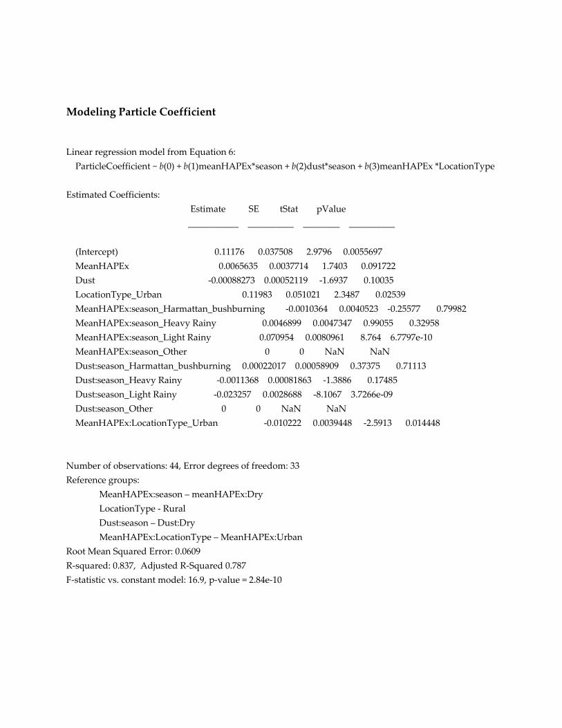
Modeling Particle Coefficient

Linear regression model from Equation 6:

ParticleCoefficient ~ b(0) + b(1)meanHAPEx*season + b(2)dust*season + b(3)meanHAPEx *LocationType

Estimated Coefficients:

Estimate SE tStat pValue

___________ __________ ________ __________

(Intercept) 0.11176 0.037508 2.9796 0.0055697

MeanHAPEx 0.0065635 0.0037714 1.7403 0.091722

Dust ‐0.00088273 0.00052119 ‐1.6937 0.10035

LocationType_Urban 0.11983 0.051021 2.3487 0.02539

MeanHAPEx:season_Harmattan_bushburning ‐0.0010364 0.0040523 ‐0.25577 0.79982

MeanHAPEx:season_Heavy Rainy 0.0046899 0.0047347 0.99055 0.32958

MeanHAPEx:season_Light Rainy 0.070954 0.0080961 8.764 6.7797e‐10

MeanHAPEx:season_Other 0 0 NaN NaN

Dust:season_Harmattan_bushburning 0.00022017 0.00058909 0.37375 0.71113

Dust:season_Heavy Rainy ‐0.0011368 0.00081863 ‐1.3886 0.17485

Dust:season_Light Rainy ‐0.023257 0.0028688 ‐8.1067 3.7266e‐09

Dust:season_Other 0 0 NaN NaN

MeanHAPEx:LocationType_Urban ‐0.010222 0.0039448 ‐2.5913 0.014448

Number of observations: 44, Error degrees of freedom: 33

Reference groups:

MeanHAPEx:season – meanHAPEx:Dry

LocationType ‐ Rural

Dust:season – Dust:Dry

MeanHAPEx:LocationType – MeanHAPEx:Urban

Root Mean Squared Error: 0.0609

R‐squared: 0.837, Adjusted R‐Squared 0.787

F‐statistic vs. constant model: 16.9, p‐value = 2.84e‐10

Modeling 48hr Gravimetric PM2.5 Mass Concentration

Linear regression model (Equation 7) with no RH correction:

log([PM2.5]) ~ b(0) + b(1)Mean_temp + b(2)Mean_rh + b(3)PercbyMCE + b(4)meanHAPEx + b(5)season +

CoverageClass*LocationTypeʹ (Equation 7)



_________ _________ ________ __________

(Intercept) 36.561 11.733 3.116 0.0066536

Mean_temp ‐0.10007 0.037208 ‐2.6895 0.016114

Mean_rh ‐0.041546 0.011735 ‐3.5404 0.0027213

PercbyMCE ‐0.36505 0.29336 ‐1.2444 0.23127

MeanHAPEx 0.046299 0.0089789 5.1565 9.5586e‐05

CoverageClass_No roof 2 walls ‐0.20722 0.29603 ‐0.69997 0.494


CoverageClass_No roof or walls ‐0.34027 0.65891 ‐0.51642 0.61262

CoverageClass_Roof 1 walls ‐0.4727 0.65707 ‐0.7194 0.48227

CoverageClass_Roof 3 walls 0.28139 0.47671 0.59027 0.56326


CoverageClass_Roof no walls ‐1.941 0.7464 ‐2.6005 0.019322

season_Harmattan_bushburning ‐0.59267 0.21883 ‐2.7083 0.015505

season_Heavy Rainy 1.3492 0.56858 2.3729 0.030517

Figure S8: Modeling particle coefficient using equation 6 a) residuals by fitted values and b) histogram

of residuals demonstrating normality.

a) b)

season_Light Rainy 0.1014 0.5285 0.19187 0.85026

season_Other 0 0 NaN NaN

LocationType_Urban 0.87859 0.53205 1.6513 0.11816

CoverageClass_No roof 2 walls:LocationType_Urban 0 0 NaN NaN


CoverageClass_No roof or walls:LocationType_Urban 0 0 NaN NaN

CoverageClass_Roof 1 walls:LocationType_Urban 0 0 NaN NaN


CoverageClass_Roof 4 walls:LocationType_Urban ‐2.5149 0.82064 ‐3.0646 0.0074098

CoverageClass_Roof no walls:LocationType_Urban 0 0 NaN NaN


Reference groups:

CoverageClass ‐ No roof and 1 wall

season – Dry


Mean_CO2:season – Mean_CO2:Dry

CoverageClass:LocationType ‐ no roof and 1 wall:Rural




Figure S9: Residuals of Equation 7 by fitted values. RMSE=0.42.

Linear regression model (Equation 8) with pointwise RH correction:

log([PM2.5]) ~ b(0) + b(1)Mean_temp + b(2)Mean_rh + b(3)PercbyMCE + b(4)meanHAPEx + b(5)cleanSD

+b(6)Mean_CO2*season + b(7)CoverageClass*LocationTypeʹ (Equation 8)



__________ _________ ________ __________

(Intercept) 41.366 11.69 3.5387 0.0053682

Mean_temp ‐0.099825 0.039135 ‐2.5508 0.028826

Mean_rh ‐0.032006 0.010831 ‐2.9551 0.014409

Mean_CO2 ‐0.0096285 0.0043357 ‐2.2207 0.050631

PercbyMCE ‐0.80014 0.30895 ‐2.5898 0.026958

MeanHAPExRH‐corr 0.076047 0.011466 6.6322 5.8379e‐05



CoverageClass_No roof or walls 2.497 0.67948 3.6748 0.0042831


CoverageClass_Roof 3 walls ‐0.053256 0.41547 ‐0.12818 0.90055


CoverageClass_Roof no walls 2.0579 0.84339 2.44 0.034846

season_Harmattan_bushburning ‐4.1741 1.9297 ‐2.1631 0.055818

season_Heavy Rainy ‐1.542 2.0825 ‐0.74047 0.47604

season_Light Rainy 30.205 11.919 2.5343 0.029653

season_Other 0 0 NaN NaN

LocationType_Urban ‐2.4353 0.5909 ‐4.1213 0.0020727

CleanSD ‐0.084713 0.032449 ‐2.6107 0.02601

Mean_CO2:season_Harmattan_bushburning 0.0074781 0.0040819 1.832 0.096856

Mean_CO2:season_Heavy Rainy 0.0059761 0.0041165 1.4517 0.17721

Mean_CO2:season_Light Rainy ‐0.069704 0.027166 ‐2.5658 0.028091

Mean_CO2:season_Other 0 0 NaN NaN

CoverageClass_No roof 2 walls:LocationType_Urban 3.3572 0.79594 4.2179 0.0017776


CoverageClass_No roof or walls:LocationType_Urban 0 0 NaN NaN




CoverageClass_Roof no walls:LocationType_Urban 0 0 NaN NaN


Reference groups:

CoverageClass ‐ No roof and 1 wall

season – Dry


Mean_CO2:season – Mean_CO2:Dry

CoverageClass:LocationType ‐ no roof and 1 wall:Rural




Figure S10: Residuals of Equation 8 by fitted values. RMSE=0.35.

References:

[1] Chakrabarti, B.; Fine, P.M.; Delfino, R.; Sioutas, C. Performance evaluation of the active‐flow personal

DataRAM PM2.5 mass monitor (Thermo Anderson pDR‐1200) designed for continuous personal

exposure measurements. Atmospheric Environment 2004, 38, 3329–3340.

[2] Wang, Y.; Li, J.; Jing, H.; Zhang, Q.; Jiang, J.; Biswas, P. Laboratory Evaluation and Calibration of

Three Low‐Cost Particle Sensors for Particulate Matter Measurement. Aerosol Science and Technology 2015,

49, 1063–1077

Supplementary Materials Kitchen area air quality ... - MDPI

Documents

Transcript of Supplementary Materials Kitchen area air quality ... - MDPI