arX

iv:1

902.

1089

0v2

[cs

.LG

] 9

Mar

202

21

Supervised ML Solution for Band Assignment in

Dual-Band Systems with Omnidirectional and

Directional AntennasDaoud Burghal, Rui Wang, Abdullah Alghafis and Andreas F. Molisch Fellow, IEEE

Abstract—Many wireless networks, including 5G NR (NewRadio) and future beyond 5G cellular systems, are expectedto operate on multiple frequency bands. This paper considersthe band assignment (BA) problem in dual-band systems, wherethe basestation (BS) chooses one of the two available frequencybands (centimeter-wave and millimeter-wave bands) to commu-nicate with the user equipment (UE). While the millimeter-wave band might offer higher data rate, there is a significantprobability of outage during which the communication shouldbe carried on the (more reliable) centimeter-wave band. Withmobility, the BA can be perceived as a sequential problem, wherethe BS uses previously observed information to predict the bestband for a future time step.

We formulate the BA as a binary classification problemand propose supervised Machine Learning (ML) solutions. Westudy the problem when both the BS and the UE use (i)omnidirectional antennas and (ii) both use directional antennas.In the omnidirectional case, we derive analytical benchmarksolutions based on the Gaussian Process (GP) assumption forthe inter-band shadow fading. In the directional case, where thelabeling is shown to be complex, we propose an efficient labelingapproach based on the Viterbi Algorithm (VA). We compare theperformances for two channel models: (i) a stochastic channeland (ii) a ray-tracing based channel.

Index Terms—Machine Learning, Side Information, DualMode base-station, Frequency Band Switching.

I. INTRODUCTION

The large available bandwidths in the millimeter-wave

(mmWave) frequency band can support the high data rates

required for many emerging applications in next generation

wireless networks (5G and beyond). However, the hostile

propagation conditions at high frequencies restrict its uti-

lization. Compared to the centimeter-wave (cmWave) band,1

signals in the mmWave band suffer from higher attenuation,

higher diffraction loss, and are more susceptible to blockage,

which reduces the reliability of the communication systems

[1], a required criterion for seamless user experience. The joint

utilization of the two bands enhances the coverage, system

reliability, and achievable data rates. This has been confirmed

with numerous research studies, where the outage probability

and throughput are shown to improve significantly [2]–[6].

Thus, due to these characteristics of the two bands, both are

D. Burghal, R. Wang, A. F. Molisch are at the Ming Hsieh Department ofElectrical Engineering and Computer, University of Southern California, LosAngeles, CA 90089, USA. ({burghal,wang78,molisch}@usc.edu).

A. Alghafis is with the Communication and Information TechnologyResearch Institute, KACST, Riyadh 11442, KSA (alghafis@kacst.edu.sa).

1In a slight abuse of notation, we call here the sub-6GHz band the cmWaveband, and 24-100 GHz the mmWave band. This is inspired by the current3GPP and WiFi frequency ranges.

indispensable components for future wireless networks [7]–

[10].

Communications exploiting dual bands can be realized in

different ways [11] [12]. For instance, the cmWave band can

be used for the control plane while the mmWave band is

used for the data plane. Alternatively, both bands can be used

for both planes. In fact, these scenarios were also among

the various possible architectures that were proposed for the

initial deployments of the non-stand alone (NSA) mode of the

5G mobile networks, i.e., through coexistence of the Long

Term Evolution (LTE) and the 5G NR [9]. However, the

simultaneous usage of the two bands might not be practical

due to a number of limitations at the network side and/or at the

UE side, such as limited processing capabilities, constraints on

transmission power, etc. Thus, depending on the underlying

BA scenario, the BS2 has to assign the UE to one of the

two bands based on the observed channels, such as in the

initial channel access scenario, or it has to sequentially switch

the communication between the two bands as the UE moves,

i.e., switching to the mmWave band whenever it is available

or to the cmWave band when the mmWave band suffers a

blockage or other bad propagation conditions. We refer to

the first problem as a one-shot BA, and the second as a

sequential BA. We here focus on the latter problem as it

can be viewed as a generalization of the one-shot, which was

addressed preliminary in our previous work [13].

In general, the BA problem is challenging because si-

multaneous observations of the two bands are not usually

available to the BS. One solution can be through using a

frequent ”measurement gap” to send training signals (e.g.,

Channel Status Information Reference Signal (CSI-RS) in

NR) over the two bands; however, the resulting overhead

and/or delays reduce the overall throughput of the system. The

problem is exacerbated with the needed signaling to schedule

the switching and perform the handover between frequency

bands, or when the UE and/or BS use multi-antennas, where

beam search is needed to align the beams. As an alternative

solution, the system could rely on the correlation and the

joint characteristics of the two bands [14], [15]. For the

sequential BA, where the goal is to choose the band for a

future time frame, the joint characteristics of the bands are

intricate, as the channel realizations and the relation between

2We use the term BS as a generic expression for the gNodeB in 3GPPNR, or an Access Point with both 802.11ac/ax and 802.11ad/ay in WiFi.Furthermore, the dual-band capabilities of the ”BS” here could be realizedwith co-located BSs.

2

the two bands change and decorrelate over time. Alternatively,

the BS can utilize partial information, such as the channel

state in one band or the UE’s location, together with some

”prior knowledge” of the cell environment to solve the BA

problem; this is a promising approach as the side information

could reveal the underlying structure of the environment.3

However, realizing this solution is challenging as it needs to

rely on the joint characterizations of the temporal evolution

of the two bands and the proper utilization of such (possibly)

non-homogeneous information. In this paper, we propose

solutions based on ML. For the extensive study of the joint

characterization of the channels, the readers are referred to

[17], [18], and the references therein.

ML provides powerful techniques that can capture complex

relations between the input data (features) and the output

values (labels). Motivated by the remarkable success of ML

in various fields, the wireless communication community has

shown an increased interest in ML-based solutions for channel

coding, estimation, channel modeling, to name a few, see,

e.g., [19]–[21] and references therein. The reported results

are promising; ML-based solutions are able to provide com-

petitive performance for problems where optimal solutions

are known, e.g., using multi-layer Neural Networks (NNs)

for decoding in AWGN channel [22], indicating that ML may

also be applied to problems where traditional methods have

failed or where the environment is too complex. For instance,

Ref. [23] demonstrated the efficacy of ML-based detection

over a molecular system where the channel characteristics are

difficult to model.

Similarly, for the simplified BA problems that can be

handled analytically (one-shot BA in a Gaussian stochastic

channel), ML solutions show comparative performance to the

optimum closed-form solutions [13]. Motivated by this, and

due to the complexity of the sequential BA, we propose to

solve the BA problem using supervised ML techniques with

various features combinations. The solutions are based on

feedforward NN and recurrent NN (the Long Short Term

Memory (LSTM)). We consider systems with omnidirectional

and directional antennas to capture different aspects of the

BA problem. We use the omnidirectional system to study

the basic problem and derive analytical benchmarks in a

synthesized stochastic environment. In particular, with the

common assumption that the shadow fading is normally

distributed (in decibel (dB) scale), the analytical solution

maps the observed GP to the BA decision (based on the

probabilities of the achieved rates). The directional systems

can be viewed as a generalization, where the system needs

to identify the best direction to use at the link ends, and

incorporate the increased overhead from band switching.

As we discuss below, acquiring labeled data when using

directional antennas is challenging. To solve this, we adopt

basic principles of the 5G-NR beam searching architecture,

and use the VA to propose an efficient (heuristic) labeling

algorithm that takes the accumulated rate into account. In

addition to the synthetic dataset that we use to compare

3Note that the same concepts have been used in different wireless ap-plications, such as localization, where the mapping between the channelinformation and location is used in fingerprinting approaches [16].

the ML-based to the analytical benchmark (GP) solutions

(in omnidirectional case), we utilize ray-tracing to generate

a dataset for omni- and directional cases. Finally, note that

in practice, directional communication is usually achieved

via analog beam-forming of multi-antennas (essential for

mmWave communication), thus in this paper, we also refer

to the directional case as Multi-Input Multi-Output (MIMO)

case, while for the omnidirectional one as Single-Input Single-

Output (SISO) case.

A. Prior Work

There have been recent studies that considered the interplay

between cmWave and mmWave bands. Refs. [15], [24], [25]

utilize the angular correlation in the two bands to provide a

coarse estimate of the Angle of Arrival (AoA) at mmWaves

based on the AoAs in the cmWave band, which can be used

to reduce the beam-forming complexity at the mmWave band.

Ref. [26] studied the covariance matrix translation between the

two bands. For joint communication in the two bands, [25]

proposes a two-queue model to assign data to each band such

that delay is minimized and throughput is maximized. Ref.

[27] considers the downlink resource allocation in a network

with a small cell BS, where the BS aims to assign the UE or

services to the resources in the two bands.

The BA can be viewed as a handover process between

two co-located BSs with different frequencies. Refs. [28]–[30]

used ML approaches to address the handover and switching

between BSs that may use different frequency bands. In

[29], the authors use ML to improve the success rate in the

handover between two co-located cells in different bands, their

implemented ML classifier uses the prior channel measure-

ments and handover decisions within a temporal window to

predict the success of the handover. Ref. [28] introduces an

uplink (ULink)/downlink (DLink) decoupling concept where

the central BS gathers measurements of the Rician K-factor

and the DLink reference signal received power for both bands,

and trains a non-linear ML algorithm that is then applied to

the cmWave band data to predict the target frequencies and

BS that can be used for the ULink and DLink. Ref. [30] uses a

gated recurrent NN to predict handover status at the next time

slot given the beam-sequence, where the BS uses the sequence

of previously used beam-forming vectors as input to the ML

scheme. Different from these works, we use various sets of

features and several ML algorithms for omnidirectional and

directional systems in two different environments, this help

identifying the limitations of the solutions and the impact of

the features. We also consider an analytical solution based on

GP for the BA problem, which allows us to benchmark the

ML solution. Furthermore, we propose an efficient labeling

scheme, i.e., providing a key enabler for the supervised ML-

based BA solutions.

Channel state prediction using GP or ML was considered

in several works such as [31]–[34], where Refs. [31], [34] use

GP to predict the shadowing values in the network based on

collected drive tests, while Refs. [31]–[33] use regression ML

techniques to predict the channel state. Using ML to predict

unobserved channel features was also considered in [35], [36];

3

in [36], the authors use NNs to predict the AoA, and in [35],

the authors utilize the observed channel state information in a

central BS to predict the optimal beam direction in local BSs.

In Ref. [37], the authors use beamformed CSI as input to a

recurrent NN to track the AoA. However, these works focus

on a single band and use mainly a regression framework, while

in this paper, we solve the BA in two bands as a classification

problem using several related feature combinations.

In our prior work [2], we utilize the GP assumption to

propose and analyze linear prediction based BA solution in an

omnidirectional communication system [2]. However, in this

work, the objective of the GP benchmark is to minimize the

misclassification probability. In [13], we discussed the one-

shot BA.

B. Contribution and Paper Structure

The contributions of this work span different aspects of the

BA problem, which can be summarized as follows.

• Formulate the BA in dual-band omnidirectional and

directional systems as binary classification problems and

propose supervised ML solutions based on recurrent NN

(LSTM) and different benchmarks.

• To enable supervised ML solutions, we study the labeling

techniques for the sequential BA. The labels are chosen

such that the sum rate is maximized.

– For a simplified SISO (omnidirectional communica-

tion), where the switching cost is ignored, the labels

can be based on the pairwise rates.

– For MIMO systems, where the multi-antenna are used

for beam-forming at both sides, we incorporate some

basic assumptions from 5G-NR to formulate the struc-

ture of the beam search and its periodicity. Then we

construct a trellis diagram to capture the switching

cost and propose a labeling scheme that captures the

sequential BAs.

• In the omnidirectional systems, we utilize the normal

distribution of the shadow fading (in a stochastic envi-

ronment) to propose an analytical benchmark solution

(dubbed as GP-based solution), and derive both exact

and approximate versions of the solution.

• For a fair assessment, we study the performance against

simpler ML solutions, and study the performance un-

der several features combinations in stochastic and ray-

tracing environments.

The remainder of the paper is organized as follows. Sec. II

introduces the basic system model, formulates the sequential

BA problem, and introduces the proposed solutions. Sec.

III highlights the two environments and the method used

to construct the sequences. A detailed discussion in the

section is dedicated to the proposed labeling method. Sec. IV

elaborates on the ML solution. Sec. V summarizes the GP-

based benchmark solution for omnidirectional SISO systems.

The performance of SISO systems in a stochastic environment

is studied in Sec. VI. The performance of the solutions for

the omnidirectional SISO and the directional MIMO systems

in a ray-tracing environment are studied in Sec. VII. Finally,

Sec. VIII provides concluding remarks and suggested future

directions.

II. PROBLEM AND SOLUTIONS OVERVIEW

A. Basic System Model

We consider a dual band cellular system, where the BS

and the UE can operate in two frequency bands with center

frequency fb and bandwidth ωb in band b ∈ {c,m}, where c

and m refer to the cmWave and the mmWave bands, respec-

tively. When using multi-antennas, without loss of generality,

in band b the BS and the UE use beamforming codebooks

Kb (of size Kb) and Mb (of size M b), respectively. Due

to a number of practical limitations of the UE, we assume

that data transmission occurs in a single frequency band at a

time. The BS controls the band selection process, using some

observations about the channel and prior knowledge to choose

the band that results in the highest data rate, more details about

the band selection metric are provided later in this section. To

focus on the basic problem, we consider a single user case,

i.e., no scheduling or interference is considered; the multi-user

case is left for future work.

It is well established that the small scale fading in the two

bands are independent due to the large frequency separation;

furthermore, modern diversity techniques mostly eliminate its

impact [38]. In contrast, large scale parameters vary relatively

slowly over time and maintain time and frequency correlation,

making it possible to utilize information over frequency

and time (space) and thus make switching decisions. Note

also that large-scale parameters are reciprocal in ULink and

DLink for both time-domain and frequency-domain duplexing

systems as long as the duplexing distance is smaller than the

stationarity time or bandwidth, respectively; this condition is

fulfilled for almost all practical systems. For this reason, the

subsequent discussion is valid for both link directions, and we

assume that the BS can acquire the channel state information

about the large-scale parameters without additional overhead.

Similar to [2] we define a time-frame as a sequence of T

time slots (data units), each time-frame is indexed with t, see

Fig. 1. On a dB scale, we can write the Signal to Noise Ratio

(SNR) of the received signal in band b, during time-frame t

[38]:

SNRbm,k(t) = P b

m,k + ζbm,k(t)−N bm, (1)

where we assumed the UE and the BS use the mth and the kth

beamforming codeword from Mb and Kb, respectively. P bm,k

is the Effective Isotropically Radiated Power (EIRP), N b is

the noise level, and ζb(t) captures the large scale variation

in band b that varies as the UE moves. Then using capacity-

achieving transmission, we can write the rate in band b as

Rbm,k(t) = ωb log

(

1 + 100.1SNRbm,k(t)

)

. (2)

The BA procedure and the detailed description of the obser-

vations and prior knowledge depend on the scheme and the

setup. In general, the BS used the observations to produce

the soft decision D ∈ [0, 1], which it then uses to make the

BA decision D ∈ {0, 1}, where ”0” and ”1” refer to the data

transmission in the cmWave and mmWave band, respectively.

4

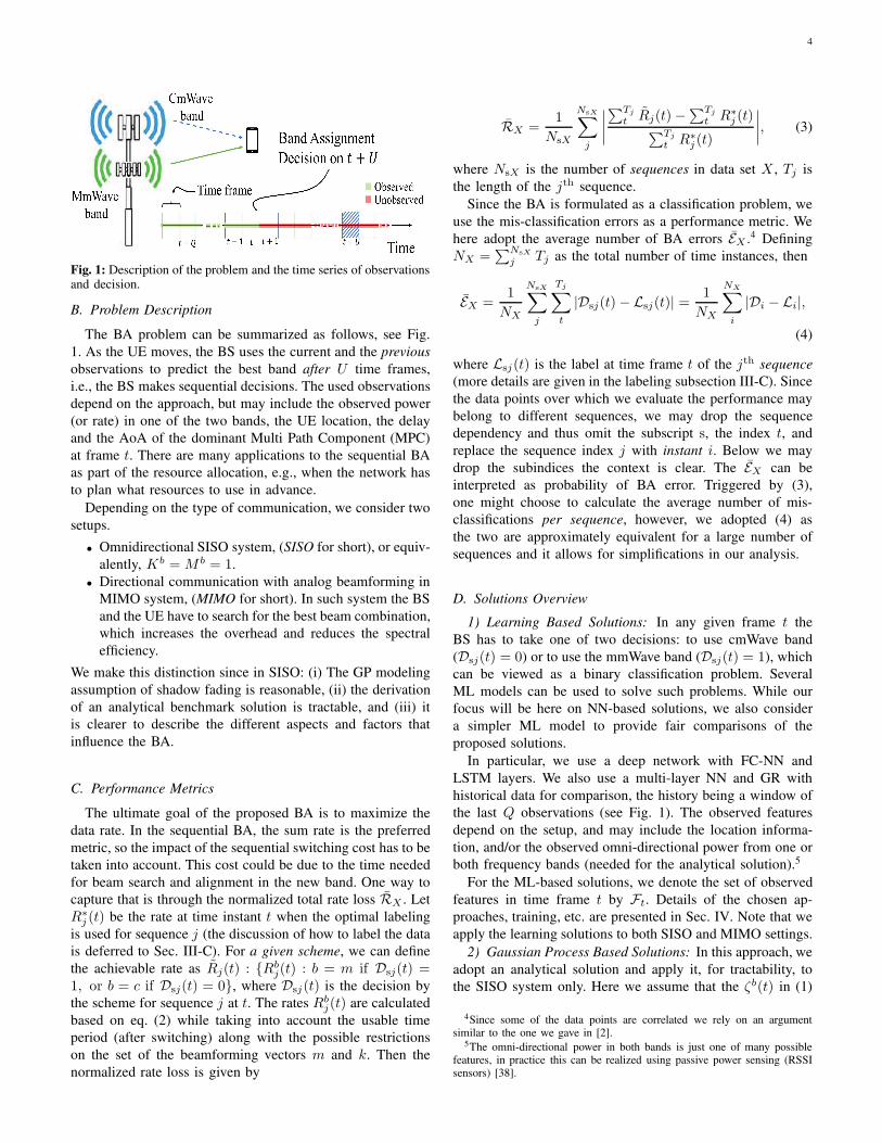
Fig. 1: Description of the problem and the time series of observationsand decision.

B. Problem Description

The BA problem can be summarized as follows, see Fig.

1. As the UE moves, the BS uses the current and the previous

observations to predict the best band after U time frames,

i.e., the BS makes sequential decisions. The used observations

depend on the approach, but may include the observed power

(or rate) in one of the two bands, the UE location, the delay

and the AoA of the dominant Multi Path Component (MPC)

at frame t. There are many applications to the sequential BA

as part of the resource allocation, e.g., when the network has

to plan what resources to use in advance.

Depending on the type of communication, we consider two

setups.

• Omnidirectional SISO system, (SISO for short), or equiv-

alently, Kb = M b = 1.

• Directional communication with analog beamforming in

MIMO system, (MIMO for short). In such system the BS

and the UE have to search for the best beam combination,

which increases the overhead and reduces the spectral

efficiency.

We make this distinction since in SISO: (i) The GP modeling

assumption of shadow fading is reasonable, (ii) the derivation

of an analytical benchmark solution is tractable, and (iii) it

is clearer to describe the different aspects and factors that

influence the BA.

C. Performance Metrics

The ultimate goal of the proposed BA is to maximize the

data rate. In the sequential BA, the sum rate is the preferred

metric, so the impact of the sequential switching cost has to be

taken into account. This cost could be due to the time needed

for beam search and alignment in the new band. One way to

capture that is through the normalized total rate loss RX . Let

R∗j (t) be the rate at time instant t when the optimal labeling

is used for sequence j (the discussion of how to label the data

is deferred to Sec. III-C). For a given scheme, we can define

the achievable rate as Rj(t) : {Rbj(t) : b = m if Dsj(t) =

1, or b = c if Dsj(t) = 0}, where Dsj(t) is the decision by

the scheme for sequence j at t. The rates Rbj(t) are calculated

based on eq. (2) while taking into account the usable time

period (after switching) along with the possible restrictions

on the set of the beamforming vectors m and k. Then the

normalized rate loss is given by

RX =1

NsX

NsX∑

j

∣

∣

∣

∣

∑Tj

t Rj(t)−∑Tj

t R∗j (t)

∑Tj

t R∗j (t)

∣

∣

∣

∣

, (3)

where NsX is the number of sequences in data set X , Tj is

the length of the jth sequence.

Since the BA is formulated as a classification problem, we

use the mis-classification errors as a performance metric. We

here adopt the average number of BA errors EX .4 Defining

NX =∑NsX

j Tj as the total number of time instances, then

EX =1

NX

NsX∑

j

Tj∑

t

|Dsj(t)− Lsj(t)| =1

NX

NX∑

i

|Di − Li|,

(4)

where Lsj(t) is the label at time frame t of the jth sequence

(more details are given in the labeling subsection III-C). Since

the data points over which we evaluate the performance may

belong to different sequences, we may drop the sequence

dependency and thus omit the subscript s, the index t, and

replace the sequence index j with instant i. Below we may

drop the subindices the context is clear. The EX can be

interpreted as probability of BA error. Triggered by (3),

one might choose to calculate the average number of mis-

classifications per sequence, however, we adopted (4) as

the two are approximately equivalent for a large number of

sequences and it allows for simplifications in our analysis.

D. Solutions Overview

1) Learning Based Solutions: In any given frame t the

BS has to take one of two decisions: to use cmWave band

(Dsj(t) = 0) or to use the mmWave band (Dsj(t) = 1), which

can be viewed as a binary classification problem. Several

ML models can be used to solve such problems. While our

focus will be here on NN-based solutions, we also consider

a simpler ML model to provide fair comparisons of the

proposed solutions.

In particular, we use a deep network with FC-NN and

LSTM layers. We also use a multi-layer NN and GR with

historical data for comparison, the history being a window of

the last Q observations (see Fig. 1). The observed features

depend on the setup, and may include the location informa-

tion, and/or the observed omni-directional power from one or

both frequency bands (needed for the analytical solution).5

For the ML-based solutions, we denote the set of observed

features in time frame t by Ft. Details of the chosen ap-

proaches, training, etc. are presented in Sec. IV. Note that we

apply the learning solutions to both SISO and MIMO settings.

2) Gaussian Process Based Solutions: In this approach, we

adopt an analytical solution and apply it, for tractability, to

the SISO system only. Here we assume that the ζb(t) in (1)

4Since some of the data points are correlated we rely on an argumentsimilar to the one we gave in [2].

5The omni-directional power in both bands is just one of many possiblefeatures, in practice this can be realized using passive power sensing (RSSIsensors) [38].

5

consists of path-loss P bL(t) and large scale fading (shadowing)

Sb(t), i.e.,

ζb(t) = −P bL(t) + Sb(t) (5)

We assume that the BS knows the channel model and statis-

tics, and it can estimate P bL(t), either using empirical models

or prior knowledge of the environment. Also we assume

that the shadowing is a stationary GP in space (time) and

frequency with mean µb = 0 and standard deviation σb in

band b, i.e., Sb(t) ∼ N (0, σ2b ), and Sb(t) and Sb′(t′) are

jointly normal with correlation function Cov(Sb(t), Sb′(t′)).An example of the correlation model and further discussion

is provided in Sec. V and in [18]. Note that assuming

Sb(t) is Gaussian on a dB scale matches many measurement

campaigns [38], but it may not always hold in practice. Still,

we rely on it along with the joint Gaussian assumption over

frequency for simplicity and mathematical tractability. To

emphasize the fact that the rate is a random quantity, we use

(5) to rewrite (1):

Rb(t) = ωb log(1 + 10(Pbtx−P b

L−Nb0)100.1S

b(t)). (6)

Note that the subscripts for beamforming codewords are not

used as this approach is used only for SISO systems. To

simplify the notation we sometimes omit the time index for

Sb and Rb when the meaning is clear from the context.

In time frame t the GP-based solution uses the SNR

observations in both bands (along with the path loss estimates)

of the current and the last Q time frames to extract Sb values,

then it predicts the BA decision in time frame t + U based

on the probability that Rb(t+ U) > Rb′(t+ U).

E. Remarks

Remark 1: In both solutions, when given a soft decision D(the output of the ML or probability in GP-based solution), the

BS can use a threshold γT ∈ [0, 1] to map D to D. We assume

that D = 1 when D > γT. We can, in general, choose the

γT that results in the best performance, however, we employ

γT = 0.5, more details are provided in the simulation sections.

Remark 2: In a simplified setting, for the one-shot problem,

the BS observes SNRb(t) to extract Sb(t) and then makes a

BA decision based on the probability that Rb(t) > Rb′(t).

Remark 3: For the GP-based solutions we refer to the set

of observations at time t as set Ht. In general, it is easy

to observe that this approach uses power (rate) and distance

information; it also uses previous measurements to acquire the

statistics of the environment. However, it is difficult to directly

incorporate other features. Thus we consider two different

environments, one of which matches the GP channel model.

Remark 4: Note the GP-based solution in this paper is

based on the classical wireless communication procedure,

estimating path-loss, covariance parameters, etc. Although, the

mathematical structure might resemble an ML algorithm, GP-

Classifier [39], the input features and the procedure to estimate

(train) the parameters are different, making them two distinct

approaches.

III. DATA ASPECTS

In this section we cover several aspects of the data. We

first highlight the different environments and features, then

we discuss the proposed methods to create the labels and the

sequences.

A. Environments and Features

We consider two environments, the first is a stochastic

environment that we use to compare the ML solution to the

GP-based benchmark for the SISO system, the second is a ray-

tracing based solution that we use for both SISO and MIMO

systems.

1) Stochastic Based Environment: In this synthetic envi-

ronment we generate the data such that it matches the GP

assumptions, which can be a reasonable assumption in some

scenarios [18]. In order to generate the channel realizations in

the two bands, we use a correlation model proposed in [18].

The covariance between shadowing values at time instants t

and t′ and in frequency bands b and b′ is

Cov(

Sb(t),Sb′(t′))

= (7)

ρb,b′√

C(

Sb(t), Sb(t′))

C(

Sb′(t), Sb′(t′))

,

where ρb,b′ is the inter-band correlation coefficient, and

C(

Sb(t), Sb(t′))

= exp−(

∆(t,t′)

dbdcor

)ν

σ2b , (8)

where ∆(t, t′) is the displacement (in meters) between the

location of the UE at times t and t′, dbdcor is the shadowing

decorrelation distance in band b (in meters), the real coeffi-

cient ν > 0 is a decay exponent [40], values for ν in (0, 2]have been previously used [40]. Note that with ν = 1 (8)

is equivalent to the popular Gudmundson correlation model

[18]; with this value, we observed that the schemes show

small dependency on prior observations, which may not reflect

practical environments, thus we consider two values of ν in

the sequential problem. We assume that the path-loss follows a

breakpoint path-loss model [38], with a break distance dbreakand a propagation exponent 2 for d ≤ dbreak and ǫ for

d > dbreak. Table I summarizes the values used for generating

the data sets.

The above generated shadowing realizations are jointly

normal over the two bands. However, due to spatial filtering

and the selection of the best beam, these assumptions are

not valid for MIMO systems, thus in Sec. VI we limit the

discussion to SISO systems. We consider four features (input

to the learning solutions): (f1) the distance from the BS to the

UE d in meters, (f2) the angular position of the UE θ in rad,

(f3) the received signal strength (or the SNR) in the cmWave

band in dBm (or dB), and (f4) is the received signal strength

(or the SNR) in the mmWave band in dBm (or dB).

2) Ray-tracing Based Environment: To assess the perfor-

mance in a more realistic setting, we simulate the propagation

channel in a campus environment by means of a commercial

ray-tracing tool, Wireless InSite [41]. The input to the ray-

tracer includes the 3D models of the buildings, the charac-

teristics of the building materials and models of foliage. The

output is a list of parameter vectors that contains the power,

6

Variable Band c/m

fb 2.5/28 GHz

Bandwidth ωb 10/100 MHz

P btx 15/22 dBm

ǫ 4

dbreak 50 m

ddcor 25/24

σb 5/7 dB

ρm,c 0.75

ν {1,1.9}

Noise Spectral Density -174 dBm/Hz

TABLE I: Stochastic channel simulation configurations

Variable Band c/m

fb 2.5/28 GHz

Ant. Pattern Isotropic

Ant. Polarization Vertical

P btx 15/30 dBm

BS height 45 m

MS height 2 m

Max. Diffraction 2/1

Max. Reflection 10

TABLE II: Ray-tracing simulation configurations.

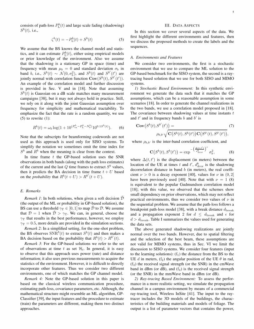
Fig. 2: Ray-tracing simulation environment. The co-located BSs areabove the rooftop. Gray objects represent the buildings. The green3D polygons denote foliage with different densities.

propagation delay, the Angle of Departure (AoD) and the

AoA, for each MPC. Simulation results have been compared

to measurements in a variety of settings and good agreements

were observed [41]. This simulation has been conducted based

on the model of the University Park Campus, University of

Southern California, which is shown in Fig. 2-(a). The detailed

simulation configurations are listed in Table II. The simulation

environment was also used in prior works, see references in

[13].

The dataset has about 1150 points, i.e., |A| = 1150. The

label that is associated with each point is whether the rate

in the mmWave band is larger than the one in the cmWave

band. To calculate the rate, we use the Shannon capacity with

bandwidth and noise spectral density that are shown in Table

I.

In Sec. VII we use this environment for SISO and MIMO

systems. In addition to the features (f1) to (f4) above, we here

use (f5) the delay of the dominant MPC in seconds, and (f6)

the AoA of the dominant MPC, where the dominant MPC is

the one with the highest power.

3) Feature Availability and Pre-processing: The availabil-

ity of the features depends on the system implementations.

For instance, (f1) and (f2), i.e., (d, θ) (which represent the

polar coordinates of the UE with respect to the BS), may

be estimated using signal processing techniques or acquired

by explicit feedback of the GPS data. To extract (f5) large

bandwidth might be required, for (f6) the use of antenna

arrays is necessary. Using both (f3) and (f4) may require

additional effort or equipment at the UE side. We consider

several combinations of the above features and discuss their

effectiveness for BA.

As typically done in ML, we perform pre-processing of the

features, in particular we standardize the input features such

that their mean is zero and the standard deviation is equal

to one. In addition, we utilize the prior knowledge about the

wireless propagation, for instance we use logarithmic scale

for distances and power, as this may linearize their relation

with one another.

B. Generating Sequences

In this problem the dataset consists of sequences of features

and labels that represent different UE trajectories and the

designated BA decisions; each sequence can be viewed as an

ordered subset of the available data points. The generation

of such a dataset is challenging, as we have to generate

correlated data points and reasonable trajectories. Note that

the points on different trajectories may still be correlated as

they belong to the same realization of the environment. As

a result, we restrict our environment to one realization with

several trajectories, i.e., we generate the trajectories over a

grid that represents the cell.

We use a Semi Markov Smooth mobility model (SMS) to

generate the motion trajectories [42]. In an SMS model, the

UE motion goes through cycles of four states until the end

of the simulation time; it starts with the acceleration state

with a random direction and a maximum ultimate speed, then

a steady motion state, next it decelerates to zero before it

stops in the last state, the UE can then go again to the first

state. The duration of each state is a design parameter and

can be set to random value. In our simulation, we omit the

repeated data points (the consecutive points on the trajectories

that correspond to the same location), and limit the number

of repeated crossings over the same grid point. This model

captures two important aspects of the realistic pedestrians’

mobility, the smooth speed and direction adaptation (during

the second state), and the possibility of changing the direction

and speed along the route (at the beginning of the first state).

C. Labeling

Labels are key components of supervised ML solutions.

They should capture the essential system model, they also

impact the solution quality and the overall performance. For

clarity and based on the discussion in Sec. II we distinguish

two cases.

7

1) SISO System: In this case, for simplicity, we neglect

the switching cost. As a result labeling is straightforward: at

t the system will assume Lsj(t) = 1 when Rm(t + U) ≥Rc(t+ U).6

2) MIMO System: For a realistic scenario with antenna

arrays in both frequency bands and switching cost, our goal

is to maximize the sum rate of the UE by the end of the

session (a mobility sequence). To quantify the beamforming

and switching cost, we propose a model based on the 3GPP

NR standard [9], where we assume that the BS will frequently

transmit beamformed reference signals (e.g., Synchronization

Signal Block (SSB) [9]) that the UE has to monitor to assess

the best beam that it should use. In that case, the achievable

rate in time t in band b is

Rbj(t) = Rb

j(t)Tf − T b

s

Tf

, (9)

where Tf is the duration of the time-frame and T bs is the

beam alignment cost in band b, which depends on the number

of directions (beams)/antennas and the search technique. In

practice, full beam sweep (”major” beam search) is not always

necessary as it is possible to do a ”minor” search within

a candidate list of beam combinations; this is especially

necessary for large number of antennas. Let Cb(t) be the list of

candidate beams in band b at time t, furthermore, let T bs = T b

M

and T bs = T b

m represent the time needed for major and minor

beam search, respectively. The list Cb(t) may include the past

successful beams and their neighbors.

For a given sequence of features and rates, we need to

find a good labeling technique. This is challenging as the

decision/label at t impacts (i) the possible candidate list for

future time instances, (ii) the set of observable features, and

(iii) the overall switching decisions as. For example, it is

reasonable to stay on one band if the UE needs to be switched

back to it later, i.e., to minimize the frequent switching cost.

One solution is to list all possible switching decisions and

their relative costs to create the labeled sequences. However,

this brute-force solution to the combinatorial problem is not

feasible for reasonable sequence lengths. Here we make a set

of simplification assumptions and propose an efficient labeling

solution.

While practically deployed methods to handle the required

frequent beam search are usually proprietary to the service

provider/vendors and depend on system design, we here

propose a method that in essence only depends on basic NR

assumption, where we utilize the periodic SSB to schedule

frequent beam search (or a periodic CSI-RS). Thus, the system

performs a periodic major search every N bp frames in band

b; in between the UE and BS do a minor search in Cb every

frame. Major searches could also be performed if the received

signal power is below a certain threshold (e.g., detectable

signal level), i.e., link failure, or when the UE switches to

a new band. Note that both the size of Cb and values of T bs

depend on the number of antennas/beams. We here set the

size Cb such that the device experiences an outage with a

6We here emphasize that the prediction at time frame t is for time framet+ U .

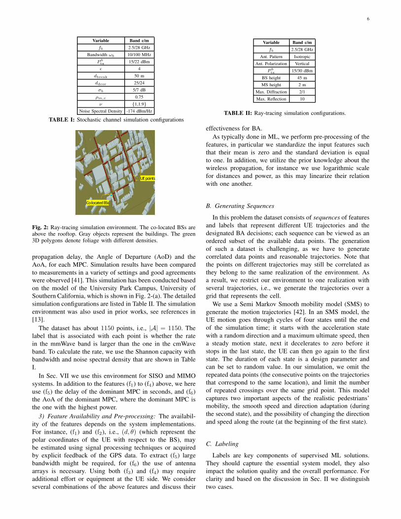
Fig. 3: A demonstration of the periodic major and minor beamsearches and candidate lists in mmWave band with Nm

p = 4, notethat C

m(t + 1) = Cm(t) after a minor search at t+1. Link failure

could trigger a major search.

probability of less than Z (e.g., outage with probability ≤0.1). Fig. 3 illustrates the idea of periodic beam search. More

implementation details are presented in Sec. VII-B1.

With the above assumptions in mind, we utilize the VA

to perform the sequence search and label the sequences.

We consider four states that represent the major and minor

searches in cmWave and mmWave, see Fig. 4. The edges

that connect the states represent the transition between them

over time. Whenever the UE switches between the bands, a

major search is triggered in the new band. The cost could

also be made to include additional delay due to the physical

layer (e.g., synchronization) or upper layer (e.g., protocol

procedures); nevertheless, the labeling process is the same,

but the value of T bM should be modified to include additional

delays for that particular edge. In addition to the periodic

major search and band switching, major search in the band

is also triggered in case of an outage (the power level of all

the beams in the available candidate list drops below a certain

threshold). We emphasize here that although the VA has four

states, the label could have one of two values {0, 1}, which is

determined based on the operating band after the transitions.

In appendix-C, we provide a worked-out labeling example for

demonstration.

Once the states are identified, we select the decisions

(labels) that maximize the sum rate for a given sequence.

Finally, we point out that the VA is a heuristic solution for

this problem, as it does not take into account the impact of

the future decisions during the selection process of the paths

at each state. However, VA provides a sequential decision tool

that can be used to identify the sequences and incorporate the

rates and losses. Other solutions, including algorithms that

consider forward and backward passes, are interesting future

study directions.

IV. MACHINE LEARNING SOLUTION

Before we dive into the details of the proposed ML archi-

tecture, we first briefly introduce of the used ML algorithms

and the datasets notations.

A. Preliminaries

1) Learning Techniques Overview: Three ML solutions are

considered in this paper: a solution that employs a recurrent

NN (LSTM layers), multi-layer FC-NN only as another so-

lution, and a simple GR (logistic regression) solution as a

8

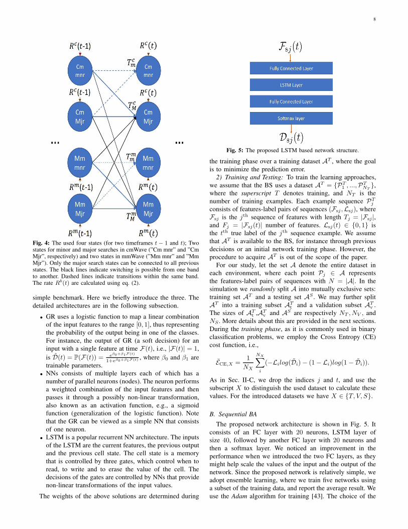
Fig. 4: The used four states (for two timeframes t− 1 and t); Twostates for minor and major searches in cmWave (”Cm mnr” and ”CmMjr”, respectively) and two states in mmWave (”Mm mnr” and ”MmMjr”). Only the major search states can be connected to all previousstates. The black lines indicate switching is possible from one bandto another. Dashed lines indicate transitions within the same band.The rate Rb(t) are calculated using eq. (2).

simple benchmark. Here we briefly introduce the three. The

detailed architectures are in the following subsection.

• GR uses a logistic function to map a linear combination

of the input features to the range [0, 1], thus representing

the probability of the output being in one of the classes.

For instance, the output of GR (a soft decision) for an

input with a single feature at time F(t), i.e., |F(t)| = 1,

is D(t) = P(F(t)) = eβ0+β1F(t)

1+eβ0+β1F(t) , where β0 and β1 are

trainable parameters.

• NNs consists of multiple layers each of which has a

number of parallel neurons (nodes). The neuron performs

a weighted combination of the input features and then

passes it through a possibly non-linear transformation,

also known as an activation function, e.g., a sigmoid

function (generalization of the logistic function). Note

that the GR can be viewed as a simple NN that consists

of one neuron.

• LSTM is a popular recurrent NN architecture. The inputs

of the LSTM are the current features, the previous output

and the previous cell state. The cell state is a memory

that is controlled by three gates, which control when to

read, to write and to erase the value of the cell. The

decisions of the gates are controlled by NNs that provide

non-linear transformations of the input values.

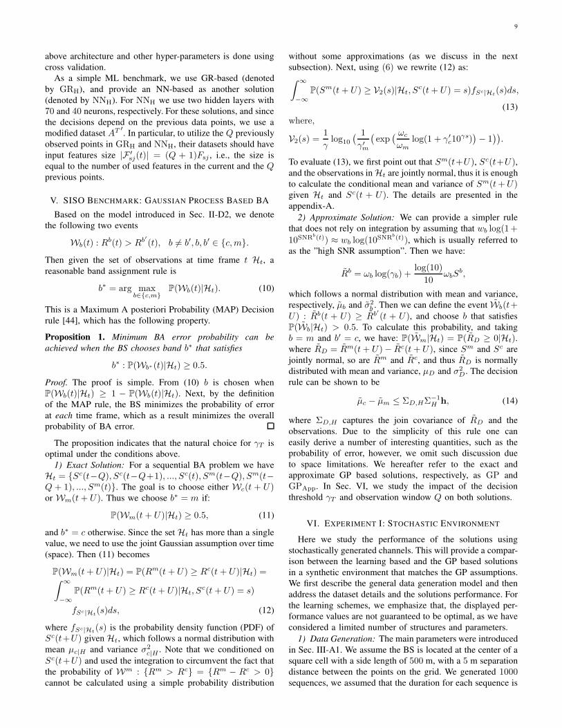
The weights of the above solutions are determined during

Fig. 5: The proposed LSTM based network structure.

the training phase over a training dataset AT , where the goal

is to minimize the prediction error.

2) Training and Testing: To train the learning approaches,

we assume that the BS uses a dataset AT = {PT1 , ...,P

TNT

},

where the superscript T denotes training, and NT is the

number of training examples. Each example sequence PTj

consists of features-label pairs of sequences (Fsj ,Lsj), where

Fsj is the jth sequence of features with length Tj = |Fsj |,and Fj = |Fsj(t)| number of features. Lsj(t) ∈ {0, 1} is

the tth true label of the jth sequence example. We assume

that AT is available to the BS, for instance through previous

decisions or an initial network training phase. However, the

procedure to acquire AT is out of the scope of the paper.

For our study, let the set A denote the entire dataset in

each environment, where each point Pj ∈ A represents

the features-label pairs of sequences with N = |A|. In the

simulation we randomly split A into mutually exclusive sets:

training set AT and a testing set AS . We may further split

AT into a training subset ATt and a validation subset AT

v .

The sizes of ATt ,AT

v and AS are respectively NT , NV , and

NS . More details about this are provided in the next sections.

During the training phase, as it is commonly used in binary

classification problems, we employ the Cross Entropy (CE)

cost function, i.e.,

ECE,X =1

NX

NX∑

i

(−Lilog(Di)− (1− Li)log(1− Di)).

As in Sec. II-C, we drop the indices j and t, and use the

subscript X to distinguish the used dataset to calculate these

values. For the introduced datasets we have X ∈ {T, V, S}.

B. Sequential BA

The proposed network architecture is shown in Fig. 5. It

consists of an FC layer with 20 neurons, LSTM layer of

size 40, followed by another FC layer with 20 neurons and

then a softmax layer. We noticed an improvement in the

performance when we introduced the two FC layers, as they

might help scale the values of the input and the output of the

network. Since the proposed network is relatively simple, we

adopt ensemble learning, where we train five networks using

a subset of the training data, and report the average result. We

use the Adam algorithm for training [43]. The choice of the

9

above architecture and other hyper-parameters is done using

cross validation.

As a simple ML benchmark, we use GR-based (denoted

by GRH), and provide an NN-based as another solution

(denoted by NNH). For NNH we use two hidden layers with

70 and 40 neurons, respectively. For these solutions, and since

the decisions depend on the previous data points, we use a

modified dataset AT ′. In particular, to utilize the Q previously

observed points in GRH and NNH, their datasets should have

input features size |F ′sj(t)| = (Q + 1)Fsj , i.e., the size is

equal to the number of used features in the current and the Q

previous points.

V. SISO BENCHMARK: GAUSSIAN PROCESS BASED BA

Based on the model introduced in Sec. II-D2, we denote

the following two events

Wb(t) : Rb(t) > Rb′(t), b 6= b′, b, b′ ∈ {c,m}.

Then given the set of observations at time frame t Ht, a

reasonable band assignment rule is

b∗ = arg maxb∈{c,m}

P(Wb(t)|Ht). (10)

This is a Maximum A posteriori Probability (MAP) Decision

rule [44], which has the following property.

Proposition 1. Minimum BA error probability can be

achieved when the BS chooses band b∗ that satisfies

b∗ : P(Wb∗(t)|Ht) ≥ 0.5.

Proof. The proof is simple. From (10) b is chosen when

P(Wb(t)|Ht) ≥ 1 − P(Wb(t)|Ht). Next, by the definition

of the MAP rule, the BS minimizes the probability of error

at each time frame, which as a result minimizes the overall

probability of BA error.

The proposition indicates that the natural choice for γT is

optimal under the conditions above.

1) Exact Solution: For a sequential BA problem we have

Ht = {Sc(t−Q), Sc(t−Q+1), ..., Sc(t), Sm(t−Q), Sm(t−Q + 1), ..., Sm(t)}. The goal is to choose either Wc(t + U)or Wm(t+ U). Thus we choose b∗ = m if:

P(Wm(t+ U)|Ht) ≥ 0.5, (11)

and b∗ = c otherwise. Since the set Ht has more than a single

value, we need to use the joint Gaussian assumption over time

(space). Then (11) becomes

P(Wm(t+ U)|Ht) = P(Rm(t+ U) ≥ Rc(t+ U)|Ht) =∫ ∞

−∞

P(Rm(t+ U) ≥ Rc(t+ U)|Ht, Sc(t+ U) = s)

fSc|Ht(s)ds, (12)

where fSc|Ht(s) is the probability density function (PDF) of

Sc(t+U) given Ht, which follows a normal distribution with

mean µc|H and variance σ2c|H . Note that we conditioned on

Sc(t+U) and used the integration to circumvent the fact that

the probability of Wm : {Rm > Rc} = {Rm − Rc > 0}cannot be calculated using a simple probability distribution

without some approximations (as we discuss in the next

subsection). Next, using (6) we rewrite (12) as:

∫ ∞

−∞

P(Sm(t+ U) ≥ V2(s)|Ht, Sc(t+ U) = s)fSc|Ht

(s)ds,

(13)

where,

V2(s) =1

γlog10

( 1

γ′m

(

exp( ωc

ωm

log(1 + γ′c10

γs))

− 1))

.

To evaluate (13), we first point out that Sm(t+U), Sc(t+U),and the observations in Ht are jointly normal, thus it is enough

to calculate the conditional mean and variance of Sm(t+U)given Ht and Sc(t + U). The details are presented in the

appendix-A.

2) Approximate Solution: We can provide a simpler rule

that does not rely on integration by assuming that wb log(1+

10SNRb(t)) ≈ wb log(10SNRb(t)), which is usually referred to

as the ”high SNR assumption”. Then we have:

Rb = ωb log(γb) +log(10)

10ωbS

b,

which follows a normal distribution with mean and variance,

respectively, µb and σ2b . Then we can define the event Wb(t+

U) : Rb(t + U) ≥ Rb′(t + U), and choose b that satisfies

P(Wb|Ht) > 0.5. To calculate this probability, and taking

b = m and b′ = c, we have: P(Wm|Ht) = P(RD ≥ 0|Ht).where RD = Rm(t+ U)− Rc(t+ U), since Sm and Sc are

jointly normal, so are Rm and Rc, and thus RD is normally

distributed with mean and variance, µD and σ2D . The decision

rule can be shown to be

µc − µm ≤ ΣD,HΣ−1H h, (14)

where ΣD,H captures the join covariance of RD and the

observations. Due to the simplicity of this rule one can

easily derive a number of interesting quantities, such as the

probability of error, however, we omit such discussion due

to space limitations. We hereafter refer to the exact and

approximate GP based solutions, respectively, as GP and

GPApp. In Sec. VI, we study the impact of the decision

threshold γT and observation window Q on both solutions.

VI. EXPERIMENT I: STOCHASTIC ENVIRONMENT

Here we study the performance of the solutions using

stochastically generated channels. This will provide a compar-

ison between the learning based and the GP based solutions

in a synthetic environment that matches the GP assumptions.

We first describe the general data generation model and then

address the dataset details and the solutions performance. For

the learning schemes, we emphasize that, the displayed per-

formance values are not guaranteed to be optimal, as we have

considered a limited number of structures and parameters.

1) Data Generation: The main parameters were introduced

in Sec. III-A1. We assume the BS is located at the center of a

square cell with a side length of 500 m, with a 5 m separation

distance between the points on the grid. We generated 1000sequences, we assumed that the duration for each sequence is

10

900 s with speed up to 1.5 m/s and a 4 s sampling period.7 To

generate the shadowing values we use the correlation model in

(7) for two different ν values, ν = 1 and ν = 1.9. We assume

that the observation window of GP-based and learning-based

solutions (other than LSTM-based) is Q = 5. We use 70% of

the sequences for training and 30% for testing. For the LSTM

based solution we use 50 sequences for cross validation.

2) Performance (ν = 1): The results are presented in Table

III. The first five rows show the feature combinations. We

notice that GPApp shows around 9% performance degradation

compared to GP. For learning schemes, we notice that all-

features combination (c-5) provides the best performance

followed by the combination of cmWave power and location

(c-4). One reason for (c-5)’s good performance seems to be the

location information. This conjecture is supported by the per-

formance of (c-1) compared to having cmWave and mmWave

powers (c-6). The importance of location information is intu-

itive, as it relates to trajectory prediction which in turn impacts

the channel conditions. The performance difference between

the LSTM-based solutions and NNH may be attributed to the

inherent ability of the LSTM layer for sequential learning.

Note that the cmWave and mmWave power combination (c-

6) still provides valuable information, and with it as the basis,

most of the learning schemes outperform GP, and all of them

outperform GPApp. This is important as both approaches, the

GP-based and the ML-based, may use cmWave and mmWave

power as input observations. Interestingly, we also observe

that using a cmWave only (c-7) learning scheme can outper-

form GPApp. Fig. 6 shows the performance as a function

of U for (c-5) and (c-6). It shows that the performance

of the proposed LSTM-based solution dominates the other

schemes for small U , but the probability of BA error increases

logarithmically as U increases.

The use of γT = 0.5 for GP was justified in Sec. V. In

Fig. 7 we present the impact of γT on the performance for

combinations (c-5) and (c-6), and show the performance for

the LSTM (as listed in the table) for comparison. We notice

that γT ≈ 0.5 is good for most of the schemes except GPApp,

indicating that GPApp can be improved with a judicious

choice of γT .

3) Performance (ν = 1.9): With ν = 1.9, the correlation

function decays faster than above, however, we noticed that

the impact of prior observations is more pronounced. The

results for several features observations are presented in Table

III. For GP-based, we observe that GP outperforms GPApp

by about 20%, and several learning schemes outperform the

GP with several features combinations. In addition, the all-

features combination (c-5) still has the least ES , but different

than above the performance gain is attributed to the power in

the two bands (c-6). Interestingly, the LSTM-based solution

using cmWave power (c-7) is as good as location (comparable

to GPApp) in this environment, which indicates that (c-7) is

a good BA predictor. The significance of (c-7) is also evident

for other learning schemes that use Q observations.

Based on the used pedestrians’ speed, grid points separation

7With the values of ddcor in Table I, the sampling period provides enoughshadowing samples based on Nyquist theorem.

Fig. 6: Misclassification error ES vs. U for two combination: (c-5)and (c-6) in Table III for in ν = 1.

Fig. 7: Misclassification error ES vs. the decision threshold γT withfor ν = 1 for features combinations: (c-5) and (c-6) in Table III.

and sampling interval we anticipate that observations outside

the used observation window, of size Q = 5, have small

influence on the BA at time frame t+U . However, considering

the adopted motion model, this may not be accurate, as an

old observation might be highly correlated (closely located)

to future value. This complicates the analysis of the impact of

Q. Instead we here restrict our attention to a simple circular

motion around the BS, where we consider 5000 sequences,

each corresponding to one circle around the BS and having

an independent shadowing realization; we here relax some of

the correlation assumptions since we consider only cmWave

and mmWave power information. The results are provided in

Fig. 8. The learning schemes achieve the same performance

compared to the optimal solution (GP in this case). Starting

with GP vs. GPApp, it is clear that the approximation

introduces an error floor for GPApp. The GPApp shows a

noticeable decrease in ES until Q = 4, as it may reduce

the uncertainty, however beyond that the error increases again

due to the model mismatch. The slow improvement for large

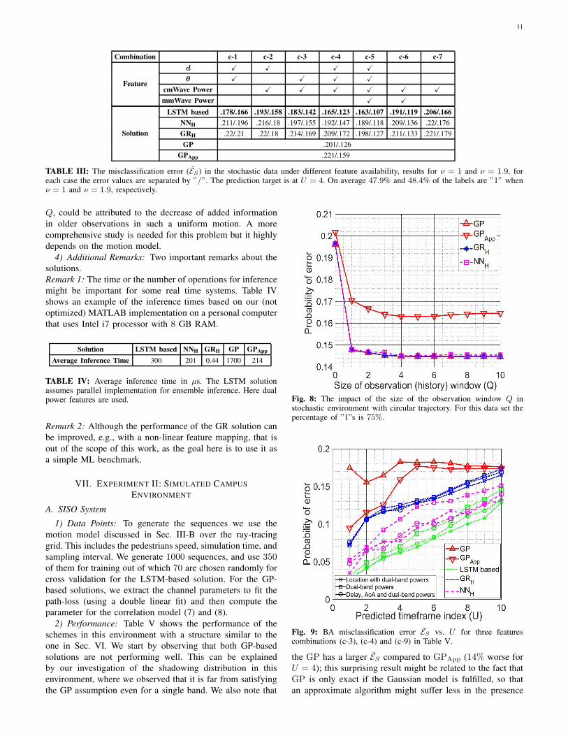
11

Combination c-1 c-2 c-3 c-4 c-5 c-6 c-7

Feature

d X X X X

θ X X X X

cmWave Power X X X X X X

mmWave Power X X

Solution

LSTM based .178/.166 .193/.158 .183/.142 .165/.123 .163/.107 .191/.119 .206/.166

NNH .211/.196 .216/.18 .197/.155 .192/.147 .189/.118 .209/.136 .22/.176

GRH .22/.21 .22/.18 .214/.169 .209/.172 .198/.127 .211/.133 .221/.179

GP .201/.126

GPApp .221/.159

TABLE III: The misclassification error (ES) in the stochastic data under different feature availability, results for ν = 1 and ν = 1.9, foreach case the error values are separated by ”/”. The prediction target is at U = 4. On average 47.9% and 48.4% of the labels are ”1” whenν = 1 and ν = 1.9, respectively.

Q, could be attributed to the decrease of added information

in older observations in such a uniform motion. A more

comprehensive study is needed for this problem but it highly

depends on the motion model.

4) Additional Remarks: Two important remarks about the

solutions.

Remark 1: The time or the number of operations for inference

might be important for some real time systems. Table IV

shows an example of the inference times based on our (not

optimized) MATLAB implementation on a personal computer

that uses Intel i7 processor with 8 GB RAM.

Solution LSTM based NNH GRH GP GPApp

Average Inference Time 300 201 0.44 1700 214

TABLE IV: Average inference time in µs. The LSTM solutionassumes parallel implementation for ensemble inference. Here dualpower features are used.

Remark 2: Although the performance of the GR solution can

be improved, e.g., with a non-linear feature mapping, that is

out of the scope of this work, as the goal here is to use it as

a simple ML benchmark.

VII. EXPERIMENT II: SIMULATED CAMPUS

ENVIRONMENT

A. SISO System

1) Data Points: To generate the sequences we use the

motion model discussed in Sec. III-B over the ray-tracing

grid. This includes the pedestrians speed, simulation time, and

sampling interval. We generate 1000 sequences, and use 350of them for training out of which 70 are chosen randomly for

cross validation for the LSTM-based solution. For the GP-

based solutions, we extract the channel parameters to fit the

path-loss (using a double linear fit) and then compute the

parameter for the correlation model (7) and (8).

2) Performance: Table V shows the performance of the

schemes in this environment with a structure similar to the

one in Sec. VI. We start by observing that both GP-based

solutions are not performing well. This can be explained

by our investigation of the shadowing distribution in this

environment, where we observed that it is far from satisfying

the GP assumption even for a single band. We also note that

Fig. 8: The impact of the size of the observation window Q instochastic environment with circular trajectory. For this data set thepercentage of ”1”s is 75%.

Fig. 9: BA misclassification error ES vs. U for three featurescombinations (c-3), (c-4) and (c-9) in Table V.

the GP has a larger ES compared to GPApp (14% worse for

U = 4); this surprising result might be related to the fact that

GP is only exact if the Gaussian model is fulfilled, so that

an approximate algorithm might suffer less in the presence

12

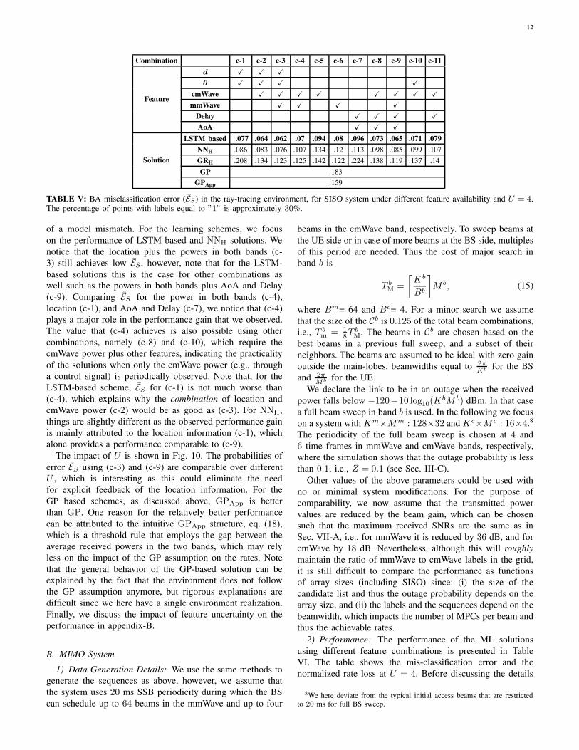
Combination c-1 c-2 c-3 c-4 c-5 c-6 c-7 c-8 c-9 c-10 c-11

Feature

d X X X

θ X X X X

cmWave X X X X X X X X

mmWave X X X X

Delay X X X X

AoA X X X

Solution

LSTM based .077 .064 .062 .07 .094 .08 .096 .073 .065 .071 .079

NNH .086 .083 .076 .107 .134 .12 .113 .098 .085 .099 .107

GRH .208 .134 .123 .125 .142 .122 .224 .138 .119 .137 .14

GP .183

GPApp .159

TABLE V: BA misclassification error (ES) in the ray-tracing environment, for SISO system under different feature availability and U = 4.The percentage of points with labels equal to ”1” is approximately 30%.

of a model mismatch. For the learning schemes, we focus

on the performance of LSTM-based and NNH solutions. We

notice that the location plus the powers in both bands (c-

3) still achieves low ES , however, note that for the LSTM-

based solutions this is the case for other combinations as

well such as the powers in both bands plus AoA and Delay

(c-9). Comparing ES for the power in both bands (c-4),

location (c-1), and AoA and Delay (c-7), we notice that (c-4)

plays a major role in the performance gain that we observed.

The value that (c-4) achieves is also possible using other

combinations, namely (c-8) and (c-10), which require the

cmWave power plus other features, indicating the practicality

of the solutions when only the cmWave power (e.g., through

a control signal) is periodically observed. Note that, for the

LSTM-based scheme, ES for (c-1) is not much worse than

(c-4), which explains why the combination of location and

cmWave power (c-2) would be as good as (c-3). For NNH,

things are slightly different as the observed performance gain

is mainly attributed to the location information (c-1), which

alone provides a performance comparable to (c-9).

The impact of U is shown in Fig. 10. The probabilities of

error ES using (c-3) and (c-9) are comparable over different

U , which is interesting as this could eliminate the need

for explicit feedback of the location information. For the

GP based schemes, as discussed above, GPApp is better

than GP. One reason for the relatively better performance

can be attributed to the intuitive GPApp structure, eq. (18),

which is a threshold rule that employs the gap between the

average received powers in the two bands, which may rely

less on the impact of the GP assumption on the rates. Note

that the general behavior of the GP-based solution can be

explained by the fact that the environment does not follow

the GP assumption anymore, but rigorous explanations are

difficult since we here have a single environment realization.

Finally, we discuss the impact of feature uncertainty on the

performance in appendix-B.

B. MIMO System

1) Data Generation Details: We use the same methods to

generate the sequences as above, however, we assume that

the system uses 20 ms SSB periodicity during which the BS

can schedule up to 64 beams in the mmWave and up to four

beams in the cmWave band, respectively. To sweep beams at

the UE side or in case of more beams at the BS side, multiples

of this period are needed. Thus the cost of major search in

band b is

T bM =

⌈

Kb

Bb

⌉

M b, (15)

where Bm= 64 and Bc= 4. For a minor search we assume

that the size of the Cb is 0.125 of the total beam combinations,

i.e., T bm = 1

8TbM. The beams in Cb are chosen based on the

best beams in a previous full sweep, and a subset of their

neighbors. The beams are assumed to be ideal with zero gain

outside the main-lobes, beamwidths equal to 2πKb for the BS

and 2πMb for the UE.

We declare the link to be in an outage when the received

power falls below −120−10 log10(KbM b) dBm. In that case

a full beam sweep in band b is used. In the following we focus

on a system with Km×Mm : 128×32 and Kc×M c : 16×4.8

The periodicity of the full beam sweep is chosen at 4 and

6 time frames in mmWave and cmWave bands, respectively,

where the simulation shows that the outage probability is less

than 0.1, i.e., Z = 0.1 (see Sec. III-C).

Other values of the above parameters could be used with

no or minimal system modifications. For the purpose of

comparability, we now assume that the transmitted power

values are reduced by the beam gain, which can be chosen

such that the maximum received SNRs are the same as in

Sec. VII-A, i.e., for mmWave it is reduced by 36 dB, and for

cmWave by 18 dB. Nevertheless, although this will roughly

maintain the ratio of mmWave to cmWave labels in the grid,

it is still difficult to compare the performance as functions

of array sizes (including SISO) since: (i) the size of the

candidate list and thus the outage probability depends on the

array size, and (ii) the labels and the sequences depend on the

beamwidth, which impacts the number of MPCs per beam and

thus the achievable rates.

2) Performance: The performance of the ML solutions

using different feature combinations is presented in Table

VI. The table shows the mis-classification error and the

normalized rate loss at U = 4. Before discussing the details

8We here deviate from the typical initial access beams that are restrictedto 20 ms for full BS sweep.

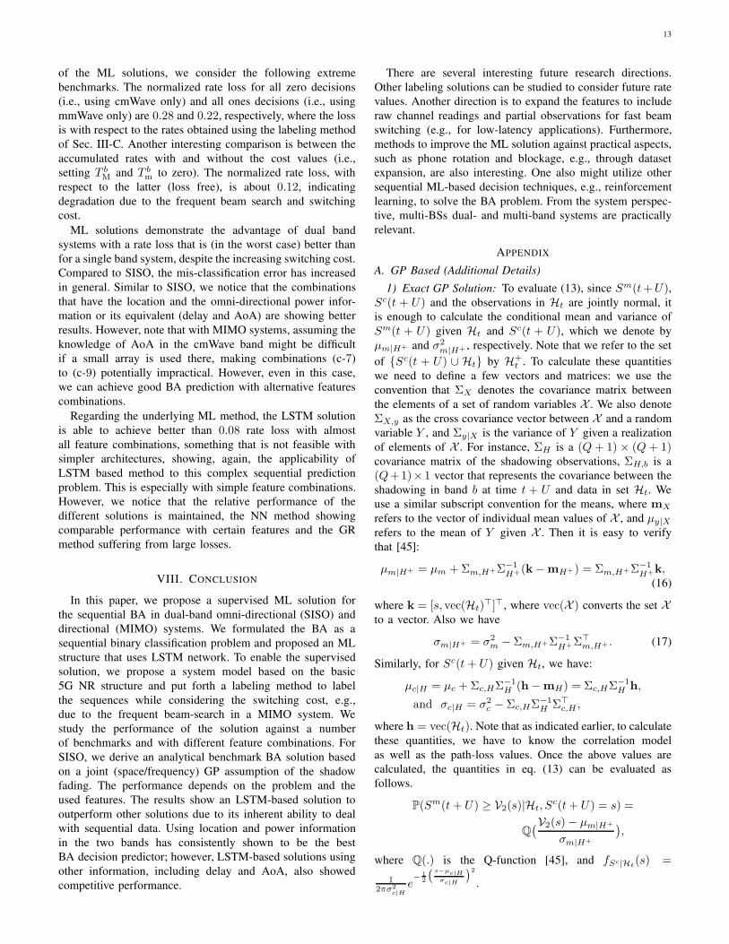
13

of the ML solutions, we consider the following extreme

benchmarks. The normalized rate loss for all zero decisions

(i.e., using cmWave only) and all ones decisions (i.e., using

mmWave only) are 0.28 and 0.22, respectively, where the loss

is with respect to the rates obtained using the labeling method

of Sec. III-C. Another interesting comparison is between the

accumulated rates with and without the cost values (i.e.,

setting T bM and T b

m to zero). The normalized rate loss, with

respect to the latter (loss free), is about 0.12, indicating

degradation due to the frequent beam search and switching

cost.

ML solutions demonstrate the advantage of dual band

systems with a rate loss that is (in the worst case) better than

for a single band system, despite the increasing switching cost.

Compared to SISO, the mis-classification error has increased

in general. Similar to SISO, we notice that the combinations

that have the location and the omni-directional power infor-

mation or its equivalent (delay and AoA) are showing better

results. However, note that with MIMO systems, assuming the

knowledge of AoA in the cmWave band might be difficult

if a small array is used there, making combinations (c-7)

to (c-9) potentially impractical. However, even in this case,

we can achieve good BA prediction with alternative features

combinations.

Regarding the underlying ML method, the LSTM solution

is able to achieve better than 0.08 rate loss with almost

all feature combinations, something that is not feasible with

simpler architectures, showing, again, the applicability of

LSTM based method to this complex sequential prediction

problem. This is especially with simple feature combinations.

However, we notice that the relative performance of the

different solutions is maintained, the NN method showing

comparable performance with certain features and the GR

method suffering from large losses.

VIII. CONCLUSION

In this paper, we propose a supervised ML solution for

the sequential BA in dual-band omni-directional (SISO) and

directional (MIMO) systems. We formulated the BA as a

sequential binary classification problem and proposed an ML

structure that uses LSTM network. To enable the supervised

solution, we propose a system model based on the basic

5G NR structure and put forth a labeling method to label

the sequences while considering the switching cost, e.g.,

due to the frequent beam-search in a MIMO system. We

study the performance of the solution against a number

of benchmarks and with different feature combinations. For

SISO, we derive an analytical benchmark BA solution based

on a joint (space/frequency) GP assumption of the shadow

fading. The performance depends on the problem and the

used features. The results show an LSTM-based solution to

outperform other solutions due to its inherent ability to deal

with sequential data. Using location and power information

in the two bands has consistently shown to be the best

BA decision predictor; however, LSTM-based solutions using

other information, including delay and AoA, also showed

competitive performance.

There are several interesting future research directions.

Other labeling solutions can be studied to consider future rate

values. Another direction is to expand the features to include

raw channel readings and partial observations for fast beam

switching (e.g., for low-latency applications). Furthermore,

methods to improve the ML solution against practical aspects,

such as phone rotation and blockage, e.g., through dataset

expansion, are also interesting. One also might utilize other

sequential ML-based decision techniques, e.g., reinforcement

learning, to solve the BA problem. From the system perspec-

tive, multi-BSs dual- and multi-band systems are practically

relevant.

APPENDIX

A. GP Based (Additional Details)

1) Exact GP Solution: To evaluate (13), since Sm(t+U),Sc(t + U) and the observations in Ht are jointly normal, it

is enough to calculate the conditional mean and variance of

Sm(t + U) given Ht and Sc(t + U), which we denote by

µm|H+ and σ2m|H+ , respectively. Note that we refer to the set

of {Sc(t + U) ∪ Ht} by H+t . To calculate these quantities

we need to define a few vectors and matrices: we use the

convention that ΣX denotes the covariance matrix between

the elements of a set of random variables X . We also denote

ΣX,y as the cross covariance vector between X and a random

variable Y , and Σy|X is the variance of Y given a realization

of elements of X . For instance, ΣH is a (Q + 1) × (Q + 1)covariance matrix of the shadowing observations, ΣH,b is a

(Q+1)× 1 vector that represents the covariance between the

shadowing in band b at time t + U and data in set Ht. We

use a similar subscript convention for the means, where mX

refers to the vector of individual mean values of X , and µy|X

refers to the mean of Y given X . Then it is easy to verify

that [45]:

µm|H+ = µm +Σm,H+Σ−1H+(k−mH+) = Σm,H+Σ−1

H+k,

(16)

where k = [s, vec(Ht)⊤]⊤, where vec(X ) converts the set X

to a vector. Also we have

σm|H+ = σ2m − Σm,H+Σ−1

H+Σ⊤m,H+ . (17)

Similarly, for Sc(t+ U) given Ht, we have:

µc|H = µc +Σc,HΣ−1H (h−mH) = Σc,HΣ−1

H h,

and σc|H = σ2c − Σc,HΣ−1

H Σ⊤c,H ,

where h = vec(Ht). Note that as indicated earlier, to calculate

these quantities, we have to know the correlation model

as well as the path-loss values. Once the above values are

calculated, the quantities in eq. (13) can be evaluated as

follows.

P(Sm(t+ U) ≥ V2(s)|Ht, Sc(t+ U) = s) =

Q(V2(s)− µm|H+

σm|H+

)

,

where Q(.) is the Q-function [45], and fSc|Ht(s) =

12πσ2

c|H

e− 1

2

(

s−µc|Hσc|H

)2

.

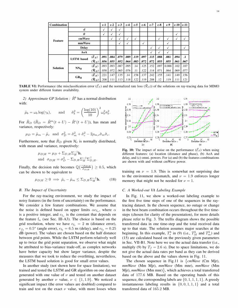
14

Combination c-1 c-2 c-3 c-4 c-5 c-6 c-7 c-8 c-9 c-10 c-11

Feature

d X X X

θ X X X X

cmWave X X X X X X X X

mmWave X X X X

Delay X X X X

AoA X X X

Solution

LSTM based(ES) .091 .084 .079 .089 .119 .097 .115 .088 .081 .094 .1

(RS) .056 .055 .052 .064 .083 .072 .072 .055 .055 .061 .067

NNH(ES) .093 .093 .087 .095 .14 .125 .152 .097 0.088 .102 .107

(RS) .058 .072 .065 .076 .11 .122 .114 .071 .064 .069 .077

GRH(ES ) .221 .147 .135 .14 .158 .137 .242 .155 .141 .149 .156

(RS) .208 .111 .113 .118 .122 .119 .208 .12 .119 .111 .121

TABLE VI: Performance (the misclassification error (ES) and the normalized rate loss (RS)) of the solutions on ray-tracing data for MIMOsystem under different feature availability.

2) Approximate GP Solution : Rb has a normal distribution

with:

µb = ωb log(γb), and σ2b =

(

log(10)

10

)2

ω2bσ

2b .

For RD (RD = Rm(t + U) − Rc(t + U)), has mean and

variance, respectively:

µD = µm − µc and σ2D = σ2

m + σ2c − 2ρm,cσmσc.

Furthermore, note that RD given Ht is normally distributed,

with mean and variance, respectively:

µD|H = µD +ΣD,HΣ−1H h,

and σD|H = σ2D − ΣD,HΣ−1

H Σ⊤D,H .

Finally, the decision rule becomes Q(−µD|H

σD|H

)

≥ 0.5, which

can be shown to be equivalent to

µD|H ≥ 0 =⇒ µc − µm ≤ ΣD,HΣ−1H h. (18)

B. The Impact of Uncertainty

For the ray-tracing environment, we study the impact of

noisy features (in the form of uncertainty) on the performance.

We consider a few feature combinations. We assume that

the noise is defined based on upper limits αefn , where α

is a positive integer, and efn is the constant that depends on

the feature fn (see Sec. III-A3). The choice is based on the

grid resolution, where we have ef1 = 2 m (distance error),

ef2 = 0.5o (angle error), ef5 = 6.5 ns (delay), and ef3 = 0.25dB (power). The values are chosen based on the half distance

between grid points. While the LSTM perform relatively well

up to twice the grid point separation, we observe what might

be attributed to bias-variance trade-off, as complex networks

have better capacity but show larger variance, despite the

measures that we took to reduce the overfitting, nevertheless,

the LSTM based solution is good for small error values.

In another study (not shown here for space limitation), we

trained and tested the LSTM and GR algorithm on one dataset

generated with one value of ν and tested on another dataset

generated by another ν value, ν ∈ {1, 1.9}. We noticed a

significant impact (the error values are doubled) compared to

train and test on the exact ν value, with more losses when

Fig. 10: The impact of noise on the performance (ES) when usingdifferent features: (a) location (distance and phase), (b) AoA anddelay, and (c) omni. powers. For (a) and (b) the features combinationsare shown with and without cmWave power.

training on ν = 1.9. This is somewhat not surprising due

to the environment mismatch, and ν = 1.9 enforces longer

memory that might not be needed for ν = 1.

C. A Worked-out VA Labeling Example

In Fig. 11, we show a worked-out labeling example to

the first five time steps of one of the sequences in the ray-

tracing dataset. In the chosen sequence, no outage or change

in the best beam combination occurs throughout the five time-

steps (chosen for clarity of the presentation), for more details

please refer to Fig. 3. The trellis diagram shows the possible

transferred data in one time-step and the total received data

up to that state. The solution assumes major searches at the

beginning. In this example, T bs in (9) (i.e., T b

M and T bm) and

(15) are calculated based on the previously given parameters

in Sec. VII-B1. Note here we use the actual data transfer (i.e.,

multiply (9) by Tf = 2.6 s). Due to space limitations, we do

not give the actual data rates per band as they can be derived

based on the above and the values shown in Fig. 11.

The chosen sequence in Fig.11 is{

cmWave (Cm Mjr),

mmWave (Mm Mjr), mmWave (Mm mnr), mmWave (Mm

Mjr), mmWave (Mm mnr)}

, which achieves a total transferred

data of 177.6 MB. Based on the operating bands of this

sequence, the corresponding labels are {0, 1, 1, 1, 1}. A greedy

instantaneous labeling results in {0, 0, 1, 1, 1} and a total

transferred data of 165.2 MB.

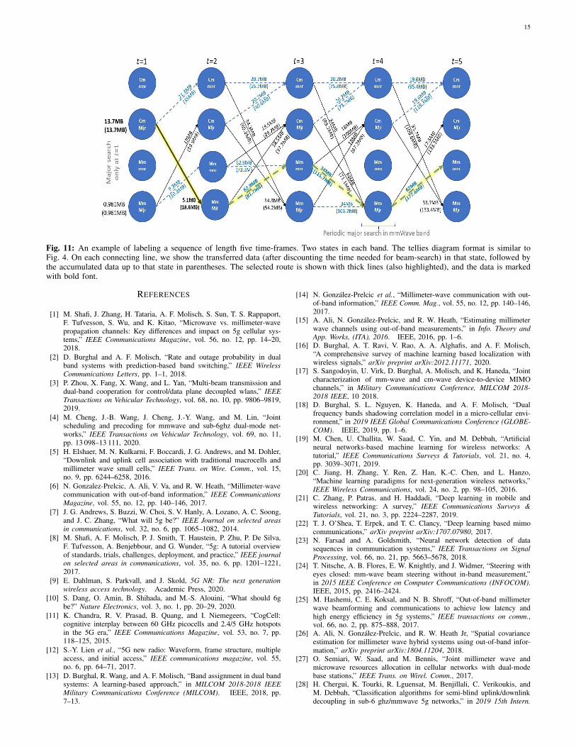
15

Fig. 11: An example of labeling a sequence of length five time-frames. Two states in each band. The tellies diagram format is similar toFig. 4. On each connecting line, we show the transferred data (after discounting the time needed for beam-search) in that state, followed bythe accumulated data up to that state in parentheses. The selected route is shown with thick lines (also highlighted), and the data is markedwith bold font.

REFERENCES

[1] M. Shafi, J. Zhang, H. Tataria, A. F. Molisch, S. Sun, T. S. Rappaport,F. Tufvesson, S. Wu, and K. Kitao, “Microwave vs. millimeter-wavepropagation channels: Key differences and impact on 5g cellular sys-tems,” IEEE Communications Magazine, vol. 56, no. 12, pp. 14–20,2018.

[2] D. Burghal and A. F. Molisch, “Rate and outage probability in dualband systems with prediction-based band switching,” IEEE Wireless

Communications Letters, pp. 1–1, 2018.

[3] P. Zhou, X. Fang, X. Wang, and L. Yan, “Multi-beam transmission anddual-band cooperation for control/data plane decoupled wlans,” IEEE

Transactions on Vehicular Technology, vol. 68, no. 10, pp. 9806–9819,2019.

[4] M. Cheng, J.-B. Wang, J. Cheng, J.-Y. Wang, and M. Lin, “Jointscheduling and precoding for mmwave and sub-6ghz dual-mode net-works,” IEEE Transactions on Vehicular Technology, vol. 69, no. 11,pp. 13 098–13 111, 2020.

[5] H. Elshaer, M. N. Kulkarni, F. Boccardi, J. G. Andrews, and M. Dohler,“Downlink and uplink cell association with traditional macrocells andmillimeter wave small cells,” IEEE Trans. on Wire. Comm., vol. 15,no. 9, pp. 6244–6258, 2016.

[6] N. Gonzalez-Prelcic, A. Ali, V. Va, and R. W. Heath, “Millimeter-wavecommunication with out-of-band information,” IEEE Communications

Magazine, vol. 55, no. 12, pp. 140–146, 2017.

[7] J. G. Andrews, S. Buzzi, W. Choi, S. V. Hanly, A. Lozano, A. C. Soong,and J. C. Zhang, “What will 5g be?” IEEE Journal on selected areas

in communications, vol. 32, no. 6, pp. 1065–1082, 2014.

[8] M. Shafi, A. F. Molisch, P. J. Smith, T. Haustein, P. Zhu, P. De Silva,F. Tufvesson, A. Benjebbour, and G. Wunder, “5g: A tutorial overviewof standards, trials, challenges, deployment, and practice,” IEEE journalon selected areas in communications, vol. 35, no. 6, pp. 1201–1221,2017.

[9] E. Dahlman, S. Parkvall, and J. Skold, 5G NR: The next generation

wireless access technology. Academic Press, 2020.

[10] S. Dang, O. Amin, B. Shihada, and M.-S. Alouini, “What should 6gbe?” Nature Electronics, vol. 3, no. 1, pp. 20–29, 2020.

[11] K. Chandra, R. V. Prasad, B. Quang, and I. Niemegeers, “CogCell:cognitive interplay between 60 GHz picocells and 2.4/5 GHz hotspotsin the 5G era,” IEEE Communications Magazine, vol. 53, no. 7, pp.118–125, 2015.

[12] S.-Y. Lien et al., “5G new radio: Waveform, frame structure, multipleaccess, and initial access,” IEEE communications magazine, vol. 55,no. 6, pp. 64–71, 2017.

[13] D. Burghal, R. Wang, and A. F. Molisch, “Band assignment in dual bandsystems: A learning-based approach,” in MILCOM 2018-2018 IEEE

Military Communications Conference (MILCOM). IEEE, 2018, pp.7–13.

[14] N. Gonzalez-Prelcic et al., “Millimeter-wave communication with out-of-band information,” IEEE Comm. Mag., vol. 55, no. 12, pp. 140–146,2017.

[15] A. Ali, N. Gonzalez-Prelcic, and R. W. Heath, “Estimating millimeterwave channels using out-of-band measurements,” in Info. Theory andApp. Works, (ITA), 2016. IEEE, 2016, pp. 1–6.

[16] D. Burghal, A. T. Ravi, V. Rao, A. A. Alghafis, and A. F. Molisch,“A comprehensive survey of machine learning based localization withwireless signals,” arXiv preprint arXiv:2012.11171, 2020.

[17] S. Sangodoyin, U. Virk, D. Burghal, A. Molisch, and K. Haneda, “Jointcharacterization of mm-wave and cm-wave device-to-device MIMOchannels,” in Military Communications Conference, MILCOM 2018-

2018 IEEE, 10 2018.[18] D. Burghal, S. L. Nguyen, K. Haneda, and A. F. Molisch, “Dual

frequency bands shadowing correlation model in a micro-cellular envi-ronment,” in 2019 IEEE Global Communications Conference (GLOBE-

COM). IEEE, 2019, pp. 1–6.[19] M. Chen, U. Challita, W. Saad, C. Yin, and M. Debbah, “Artificial

neural networks-based machine learning for wireless networks: Atutorial,” IEEE Communications Surveys & Tutorials, vol. 21, no. 4,pp. 3039–3071, 2019.

[20] C. Jiang, H. Zhang, Y. Ren, Z. Han, K.-C. Chen, and L. Hanzo,“Machine learning paradigms for next-generation wireless networks,”IEEE Wireless Communications, vol. 24, no. 2, pp. 98–105, 2016.

[21] C. Zhang, P. Patras, and H. Haddadi, “Deep learning in mobile andwireless networking: A survey,” IEEE Communications Surveys &

Tutorials, vol. 21, no. 3, pp. 2224–2287, 2019.[22] T. J. O’Shea, T. Erpek, and T. C. Clancy, “Deep learning based mimo

communications,” arXiv preprint arXiv:1707.07980, 2017.[23] N. Farsad and A. Goldsmith, “Neural network detection of data

sequences in communication systems,” IEEE Transactions on Signal

Processing, vol. 66, no. 21, pp. 5663–5678, 2018.[24] T. Nitsche, A. B. Flores, E. W. Knightly, and J. Widmer, “Steering with

eyes closed: mm-wave beam steering without in-band measurement,”in 2015 IEEE Conference on Computer Communications (INFOCOM).IEEE, 2015, pp. 2416–2424.

[25] M. Hashemi, C. E. Koksal, and N. B. Shroff, “Out-of-band millimeterwave beamforming and communications to achieve low latency andhigh energy efficiency in 5g systems,” IEEE transactions on comm.,vol. 66, no. 2, pp. 875–888, 2017.

[26] A. Ali, N. Gonzalez-Prelcic, and R. W. Heath Jr, “Spatial covarianceestimation for millimeter wave hybrid systems using out-of-band infor-mation,” arXiv preprint arXiv:1804.11204, 2018.

[27] O. Semiari, W. Saad, and M. Bennis, “Joint millimeter wave andmicrowave resources allocation in cellular networks with dual-modebase stations,” IEEE Trans. on Wirel. Comm., 2017.

[28] H. Chergui, K. Tourki, R. Lguensat, M. Benjillali, C. Verikoukis, andM. Debbah, “Classification algorithms for semi-blind uplink/downlinkdecoupling in sub-6 ghz/mmwave 5g networks,” in 2019 15th Intern.

16

Wireless Comm. & Mobile Comp. Conference (IWCMC). IEEE, 2019,pp. 2031–2035.

[29] F. B. Mismar and B. L. Evans, “Partially blind handovers for mmwavenew radio aided by sub-6 GHz LTE signaling,” in Proc. IEEE Int.

Conf. on Communications Work. Evolutional Tech. & Ecosystems for

5G Phase II, 2018.[30] A. Alkhateeb, I. Beltagy, and S. Alex, “Machine learning for reliable

mmwave systems: Blockage prediction and proactive handoff,” in 2018

IEEE Global Conf. on Signal and Information Processing (GlobalSIP).IEEE, 2018, pp. 1055–1059.

[31] J. Riihijarvi and P. Mahonen, “Machine learning for performance pre-diction in mobile cellular networks,” IEEE Computational Intelligence

Magazine, vol. 13, no. 1, pp. 51–60, 2018.[32] Y. Wang, M. Martonosi, and L.-S. Peh, “Predicting link quality using

supervised learning in wireless sensor networks,” ACM SIGMOBILE

Mobile Computing and Communications Review, vol. 11, no. 3, pp.71–83, 2007.

[33] J. Wang et al., “Spatiotemporal modeling and prediction in cellularnetworks: A big data enabled deep learning approach,” in INFOCOM

2017-IEEE Conference on Computer Communications, IEEE. IEEE,2017, pp. 1–9.

[34] L. S. Muppirisetty, T. Svensson, and H. Wymeersch, “Spatial wirelesschannel prediction under location uncertainty,” IEEE Trans. on Wireless

Comm., vol. 15, no. 2, pp. 1031–1044, 2016.[35] S. Chen, Z. Jiang, J. Liu, R. Vannithamby, S. Zhou, Z. Niu, and Y. Wu,

“Remote channel inference for beamforming in ultra-dense hyper-cellular network,” in GLOBECOM 2017-2017 IEEE Global Comm.Conf. IEEE, 2017, pp. 1–6.

[36] S. Navabi, C. Wang, O. Y. Bursalioglu, and H. Papadopoulos, “Pre-dicting wireless channel features using neural networks,” in 2018 IEEE

international conference on communications (ICC). IEEE, 2018, pp.1–6.

[37] D. Burghal, N. A. Abbasi, and A. F. Molisch, “A machine learningsolution for beam tracking in mmwave systems,” in 2019 53rd AsilomarConference on Signals, Systems, and Computers. IEEE, 2019, pp. 173–177.

[38] A. F. Molisch, Wireless Communications. IEEE Press - Wiley; 2edition, 2011.

[39] K. P. Murphy, Machine learning: a probabilistic perspective, 2012.[40] S. S. Szyszkowicz et al., “On the feasibility of wireless shadowing

correlation models,” IEEE Trans. on Veh.r Tech., vol. 59, no. 9, pp.4222–4236, 2010.

[41] W. I. Remcom, “https://www.remcom.com/wireless-insite-em-propagation-softwareinsite-wireless-em-propagation-more-info,” online,accessed: March 2017.

[42] M. Zhao and W. Wang, “WSN03-4: A Novel Semi-Markov SmoothMobility Model for Mobile Ad Hoc Networks,” in Global Telecommu-

nications Conference, 2006. GLOBECOM’06. IEEE. IEEE, 2006, pp.1–5.

[43] D. P. Kingma and J. Ba, “Adam: A method for stochastic optimization,”arXiv preprint arXiv:1412.6980, 2014.

[44] S. M. Kay, “Fundamentals of statistical signal processing, vol. ii:Detection theory,” Signal Processing. Upper Saddle River, NJ: Prentice

Hall, 1998.[45] A. Leon Garcia, Probability, statistics, and random processes for

electrical engineering. Pearson Education; 3rd ed., 2008.