
Maximizing Versus Satisficing: Happiness Is a Matter of Choice
Upload
khangminh22Category
view
2download
0
Journal of Artificial Intelligence Research 68 (2020) 691-752 Submitted 12/2019; published 08/2020
Subgoaling Techniques forSatisficing and Optimal Numeric Planning
Enrico Scala [email protected] di Brescia (Italy)The Australian National University (Australia)
Patrik Haslum [email protected] Thiebaux [email protected] Australian National University (Australia)
Miquel Ramirez [email protected]
University of Melbourne (Australia)
Abstract
This paper studies novel subgoaling relaxations for automated planning with proposi-tional and numeric state variables. Subgoaling relaxations address one source of complexityof the planning problem: the requirement to satisfy conditions simultaneously. The coreidea is to relax this requirement by recursively decomposing conditions into atomic sub-goals that are considered in isolation. Such relaxations are typically used for pruning, oras the basis for computing admissible or inadmissible heuristic estimates to guide optimalor satisficing heuristic search planners. In the last decade or so, the subgoaling principlehas underpinned the design of an abundance of relaxation-based heuristics whose formula-tions have greatly extended the reach of classical planning. This paper extends subgoalingrelaxations to support numeric state variables and numeric conditions. We provide boththeoretical and practical results, with the aim of reaching a good trade-off between accu-racy and computation costs within a heuristic state-space search planner. Our experimentalresults validate the theoretical assumptions, and indicate that subgoaling substantially im-proves on the state of the art in optimal and satisficing numeric planning via forwardstate-space search.
1. Introduction
Automated planning is the field of Artificial Intelligence that studies the development ofintelligent agents capable of choosing and organising a sequence of actions to achieve a givenset of objectives, ideally at minimal execution cost. Automated planning is model based;the planning model describes the conditions under which each action can be applied, andthe effects such an action has on the world if executed. Given a description of the initialstate and the goals that need to be achieved, a typical planning question asks whether thereexists a plan that is executable and brings the agent to a state where the goal is satisfied.
Over the past decades, research has shown that the high worst-case computational com-plexity of classical (propositional) planning (Bylander, 1994) can be effectively managed, byexploiting the structure of the problem, as captured by its representation (Geffner, 2011).The most prominent approach aimed at exploiting such a structure in a systematic way is
©2020 AI Access Foundation. All rights reserved.

Scala, Haslum, Thiebaux, & Ramirez
to relax the target problem into an easier problem to solve and use the relaxed solution costas a heuristic (Bonet & Geffner, 2001; Geffner, 2018; Pearl, 1984).
In the last two decades, several relaxations for propositional representations have beenproposed and explored (e.g., Bonet & Geffner, 2001; Haslum & Geffner, 2000; Helmert &Geffner, 2008; Helmert & Domshlak, 2009; Pommerening, Roger, Helmert, & Bonet, 2015;Domshlak, Hoffmann, & Katz, 2015), leading to planners that scale to instances of realisticsize. Less has been done to address more expressive problem classes, such as planning withnumeric information (Fox & Long, 2003). Since planning agents often have to deal withlimited resources or geometrical constraints, the ability to deal with this information isessential to address a wider class of real-world problems.
Numeric state variables were introduced into the de-facto standard planning language(PDDL) through the notion of numeric fluents (Fox & Long, 2003). A numeric fluentis a function mapping a tuple of objects to a rational number. Numeric fluents are aconvenient device to model quantitative properties of object(s), such as their position,their distance, their cost. Our main intuition is that, even though the introduction ofnumeric variables complicates planning substantially (numeric planning is undecidable ingeneral (Helmert, 2002) while classical planning is “only” PSPACE-complete), numericvariables and numeric conditions allow for more compact descriptions of certain planningproblems, which, if exploited properly, can lead to more powerful reasoning. For instance,imagine we wish to encode a domain involving a state variable x that models the positionof the agent through time. Let us assume that x ranges from 0 to 10 and we only wishto model its integer representation. In order to encode such knowledge using propositionalvariables we need to enumerate each of its possible values from 0 to 10, so having a totalof 11 propositional variables {P0, P1, ..., P10}. This not only causes a rapid explosion ofthe number of variables to consider, but also makes them orthogonal and incomparable.In particular, in a purely propositional representation, we would need to introduce furtherpropositions such as {lessP1P2 , lessP1P3 , ..., lessP8P9} to re-axiomatize the simple orderingrelation; therefore, any kind of reasoning that involves such information would require torebuild that structure. It is therefore only natural to study how to capture numeric aspectsdirectly, possibly using some kind of relaxation and heuristic approach. Our aim in thispaper is therefore to focus on the reasoning and algorithmic aspects of planning languagessupporting a numeric representation, so as to provide corresponding planners with novelrelaxation-based heuristics capable of delivering the same benefits that they have achievedin classical planning. Although, in principle, we could exclude propositional variables andconditions by compiling them into suitable numeric variables and numeric conditions, ourapproach will still consider propositional structures as such, alongside numeric ones. Thisis because, when certain aspects of the problem at hand are more conveniently modelledusing purely qualitative conditions, compilation into (infinite) numeric variables obscurestheir underlying structure, and reconstructing it requires additional reasoning effort.
Other researchers have investigated the solution of numeric planning problems throughrelaxation-based heuristic search before (e.g., Hoffmann, 2003; Coles, Coles, Fox, & Long,2012, 2013). However, in all of these approaches, the well-known interval-based relaxation(Hoffmann, 2003) underlies the heuristic. An exception is the work by Eyerich (2009),which is founded on the context-enhanced additive heuristic (Helmert & Geffner, 2008). Incontrast, we take inspiration from the h1 relaxation presented for classical planning (Haslum
692

Subgoaling Techniques for Satisficing and Optimal Numeric Planning
& Geffner, 2000), and use its underlying decomposition principle to capture the numericstructure of the problem. Rather than looking at sets of values that numeric variables mayattain (as in the interval-based relaxation), we start from the numeric subgoals, meaningelementary numeric conditions in formulae representing the goal and action preconditions,that need to be reached, and consider the operators that affect them. Differently fromclassical planning where atomic subgoals are propositional literals, numeric subgoals canconstrain sets of numeric state variables together; therefore even classical notions such asthat of an achiever (i.e. an action that contributes positively towards achieving a subgoal)need to be revised.
The techniques we investigate support mixed propositional–numeric reasoning: wherepropositional and numeric variables co-occur in the definition of the problem, the jus-tification for including actions in a relaxed solution may derive from both “quantitative”(numeric) and “qualitative” (propositional) subgoals. Numeric conditions in particular mayjustify the presence of some action, which takes the role of a possible achiever. How to defineand compute such possible achievers is not obvious, and we present a method to do so usinga closed-form arithmetic computation that is obtained in a number of steps, including aMixed Integer Program formulation and its continuous relaxation. This formulation appliesto what we call simple numeric conditions. Through possible achievers, we show how todevise a variety of heuristics for optimal and satisficing planning. Interestingly, even themost basic one proves superior to previous interval-based relaxations. Moving from atomicsubgoals to conjunctive subgoals, we also provide an extended version of possible achiev-ers that we call conjunctive achievers. Conjunctive achievers account for the simultaneousachievements of sets of subgoals, including mixed propositional and numeric conditions.They can be computed using a novel Mixed Integer Program formulation. The paper showshow to use this characterisation to get a novel lower bound that can be used as an admissibleheuristic.
We study these relaxations and heuristics both from a theoretical and practical view-point. Our theoretical analysis shows that the computational issues arising from the formu-lation can be tamed without loosing too much information nor compromising admissibility.From a practical perspective, our results over a number of numeric planning problems,taken from previous work on numeric planning and the from International Planning Com-petition suite, indicate that the presented heuristics often translate to great guidance andsubstantially extend the reach of forward search in numeric planning.
1.1 Contribution
This work extends our previous conference paper on the topic (Scala, Haslum, & Thiebaux,2016a) in a number of respects:
• We provide a more in-depth analysis of the subgoaling theoretical framework. Notonly proofs are extended, but also new theorems are reported to better analyse thecomplexities and the benefits of the new formulations.
• We report a novel, revised admissible estimate, which accounts for a limited formof assignment operations and is more informed because it considers a narrow set ofreachable actions.
693

Scala, Haslum, Thiebaux, & Ramirez
• We provide a novel relaxation schema based on the idea of subgoaling. Such a re-laxation makes heavy use of a Linear Program formulation to capture conjunctivereasoning. This leads to an expensive but quite informed admissible estimate that isevaluated on optimal planning tasks.
• We conduct an extended experimental analysis, with more insights and discussionsencompassing the implications of the novel conjunctive relaxation, with comparisonsnot only against numeric planning, but also against classical planning reformulationsof a bounded numeric planning problem.
• We extend our related work analysis, and consider in greater depth previous workon heuristic search, other approaches to numeric planning via Satisfiability ModuloTheory, and links to other research fields such as that of linear time systems.
1.2 Outline
In Section 2, we start by describing the language we use to model numeric planning prob-lems. Then our discussion proceeds through the following steps. First, in Section 3, weprovide the first formulation of a numeric h1 relaxation, and the computational conse-quences of a direct encoding via standard regression. In Section 4, we explain how this canbe made computable and then tractable in the case of what we call simple numeric condi-tions, and in Section 5, we use this novel formulation to obtain admissible and inadmissibleestimates. In Section 6 we compare the novel relaxation with the well-known interval-basedrelaxation in terms of reachability accuracy. In Section 7, we describe a transformationaimed at tightening the presented relaxation through redundant constraints. In Sections8 and 9, we then present a more systematic approach to tightening the relaxation using amuch more sophisticated (yet expensive) Linear Program based schema. The novel method-ological contribution of the paper ends with Sections 10 and 11, which show how to exploitdecomposition to also consider more general numeric constructs in the subgoaling schema;this requires a slight extension of the notion of possible achiever. Sections 12 and 13 reporton related work and on the experimental evaluation of our contributions, respectively.
2. Numeric Planning Problems
We are concerned with sequential numeric planning problems described in PDDL2.1 – level2; see (Fox & Long, 2003; Haslum, Lipovetzky, Magazzeni, & Muise, 2019) for a moredetailed presentation of the language and modelling examples.
2.1 Syntax
We work with the grounded problem representation, where a numeric planning problem isdescribed as a tuple Π = 〈F,X, I,G,C,A, γ〉1 consisting of the following elements:
F is a set of Boolean variables (the propositional variables). X is a set of rational-valuedvariables (the numeric variables). A state is a total mapping from F to {>,⊥} and from
1. We will in the remaining sections use the symbol ‘ = ’ to differentiate the equality by definition with thestandard equality ‘=’.
694

Subgoaling Techniques for Satisficing and Optimal Numeric Planning
X to Q ∪ {⊥} 2 Propositional variables assigned to ⊥ in a state are false in that statewhilst numeric variables assigned to ⊥ are referred to as undefined. I is the initial state. Gdescribes the goal that the final state of any solution plan must satisfy, and C the global stateconstraints that must be satisfied by all states reached at any step of a valid plan. Both Gand C are formally represented as formulae in Negation Normal Form (NNF), inductivelydefined as follows:
(i) a propositional condition v = >, such that v ∈ F , is a (atomic) formula;
(ii) a numeric condition 〈ξ,D, 0〉, where ξ is an arithmetical expression over X and D ∈{>,≥,=} is a comparison operator, is a (atomic) formula;
(iii) if ψ is a formula as defined by items (i) or (ii) above, ¬ψ is a formula;
(iv) if ψ and ψ′ are formulae, so are ψ ∧ ψ′ and ψ ∨ ψ′.
We use Greek letters (generally ψ) to indicate formulae, whether atomic or compound.When no confusion arises, we use the term literal in place of a propositional condition or itsnegation, and use v and ¬v as a shorthand for v = > and v = ⊥, respectively. Moreover,for convenience, we write c ∈ ψ when the formula ψ is either a conjunction or a disjunction,to indicate that the sub-formula c appears as a conjunct/disjunct of ψ.
A is the set of actions and γ is a function that associates each action with a non-negative rational cost. Each action a ∈ A is described by a tuple 〈name(a),pre(a), eff(a)〉,3where name(a) is the (unique) name of the action, pre(a) is the formula (as defined above)representing the precondition that must be true of the state for the action to be executable,and eff(a) is a set of assignments over F and X representing the effects of the action inthe resulting state. Assignments are defined as follows: an assignment to a propositionalvariable v ∈ F is of the form v:=> or v:=⊥; an assignment of a numeric variable x ∈ Xis of the form 〈x, op(e), ξ〉 where x ∈ X is the affected variable, ξ is a numeric expression,and op(e) is one of += (increase), −= (decrease) or := (assign).4 Given an effect e, weuse lhs(e) to refer to the affected variable and rhs(e) to the expression used to update thatvariable. We disallow the occurrence of conflicting effects, i.e. of two effects {e, e′} ⊆ eff(a)with e 6= e′ and lhs(e) = lhs(e′).5 In the following, we use subscripts to distinguish the
2. Other works (Fox & Long, 2003; Scala, Haslum, Thiebaux, & Ramırez, 2016b; Cashmore, Magazzeni, &Zehtabi, 2020) consider numeric variables that take real values. Note that, even though some conditionscan only be satisfied by real values (e.g. x ∗ x = 2), our formulation and PDDL2.1 preclude reachingstates satisfying such conditions: PDDL2.1 does not allow initial states with non-rational values (initialstate assignments must have final decimal expansions) nor does it allow writing action effects that willyield non-rational values in a finite number of steps. The situation would be different if we allowednon-rational value assignments in action effects, such as x:=
√2.
3. Later in the text we will often use actions as simple pair of precondition and effects when the name ofthe action is not important.
4. Note that, in principle, an increase or decrease operation can be defined in terms of assignment, e.g.,x+= ξ is equivalent to x:=x + ξ. However, this kind of transformation hides some structure, namelyadditivity, which we exploit to a great extent in this paper.
5. PDDL allows actions to have conflicting propositional effects, taking an interpretation called DeleteBefore Adding (DBA) where the positive statement (v:=>) prevails over the negative one (v:=⊥). Wedisallow the occurrence of such conflicting effects. Note that PDDL2.1 does not allow actions withconflicting effects on numeric variables.
695

Scala, Haslum, Thiebaux, & Ramirez
propositional and numeric parts of action effects, writing effprop(a) for the propositionaleffects and effnum(a) for the numeric effects of a.
2.2 Semantics
The semantics of numeric planning is defined as follows. We write [v]s for the value ofvariable v ∈ F ∪ X in state s and [ξ]s for the value of numeric expression ξ in state s.Any numeric expression containing an undefined numeric variable is undefined. A numericexpression of the form ξ/o is also undefined in s if [o]s = 0, i.e., division by zero is undefined.For a numeric condition, s |= 〈ξ,D, 0〉 iff [ξ]sD0 evaluates to true. A numeric condition,and the negation of a numeric condition, containing a numeric expression that is undefinedin state s is not satisfied in s. Given these building blocks, the evaluation of the rest of thelanguage describing formulae follows the usual semantics of propositional logic.
An action a is applicable in state s iff s |= pre(a) and all numeric expressions in eff(a)are defined in s. The state s′ = s[a] resulting from applying an (applicable) action a in s isdefined as follows. For all v ∈ F ∪X:
• [v]s′
= rhs(e) if ∃e ∈ effprop(a) with lhs(e) = v (Propositional Effect)
• [v]s′◦= [rhs(e)]s if ∃e ∈ effnum(a) with lhs(e) = v and op(e) = ◦= (Numeric Effect)
• [v]s′
= [v]s otherwise (Frame Axiom)
A plan is a finite sequence of actions 〈a0, a1, ..., an−1〉 such that for all i ∈ {0, . . . , n− 1}ai is applicable in si, where s0 = I and si+1 = si[ai]. A valid plan is one that satisfies theglobal constraints C throughout its execution, i.e., ∀i ∈ {0, . . . , n}si |= C; a solution planis a valid plan that also reaches the goal, i.e., such that sn |= G. We say that a state s isreachable if there exists some valid plan that leads from the initial state to s. We say that
a solution plan π is optimal if it minimises the overall cost∑|π|−1
i=0 γ(ai).
2.3 Small Example
To illustrate these definitions and as a running example for the rest of the paper, let usconsider a very simple Sailing navigation domain, which is however representative of avariety of domains featuring multi-variable numeric conditions.
There is a sailing boat whose task is to rescue people in an unbounded area of the ocean.The positions of the boat and people to be rescued are described by their x-y coordinates inQ2. Note that these coordinates are not bounded a priori, making a propositional represen-tation impossible. The boat can sail in 7 possible directionsDir={NE,E,SE,S,SW,W,NW}(see Figure 1; the boat cannot sail straight into the wind). To save a person, the boat mustreach an area described by one or more linear inequalities. Once the boat reaches any pointwithin this area, the boat can rescue the castaway.
A numeric planning formulation of the problem uses two numeric variables X = {x, y}to model the position of the sailing boat and actions A = {ad | d ∈ Dir} for each of the 7possible movements of the boat. These actions have an empty precondition, and numericeffects defined as a function of the direction that the action is modelling, that is:
eff(ad) =
{〈x, :=, x+ kd,x〉〈y, :=, y + kd,y〉
696

Subgoaling Techniques for Satisficing and Optimal Numeric Planning
Figure 1: Points of sail (https://en.wikipedia.org). There are 7 possible directions for theboat to move with respect to a stable wind. The goal is to cross the dotted lineto the side indicated by the red dot.
where kd,x, kd,y are constants associated with moving a certain distance in the particulardirection (d). Actions therefore model translations in Q2.
The initial state is an assignment to the numeric variables x, y, say 〈x = 1, y = 1〉, whilethe goal is defined as a target region, specified by a conjunction of linear constraints. Forinstance, the goal region depicted in Figure 1 may be defined by G = 〈x + y,≥, 10〉. If weassume that the translation coefficients of all actions (kd,x and kd,y for all d) are equal to1, an optimal plan for this problem is to apply action aNE five times.
The other structures of our numeric planning problem can be left empty for the taskof modelling the movement of the sailboat. The modelling of multiple rescues in differentregions O = r0, · · · , rm can be done by introducing an action ai for each such region, whoseprecondition is the numeric constraints defining the area of interest, i.e., pre(ai)=
∧c∈ri〈ξc,≥
, 0〉, and whose effect records the fact that the rescue in ri has been accomplished, i.e.,effprop(ai) = (rescued ri). The goal is then the conjunction of rescued propositions for allregions in O, that is G =
∧r∈O(rescued r).
Throughout this paper, we will investigate the structure of the computational prob-lem made explicit by the language of numeric planning just introduced in order to studyconditions for the development of informed but tractable heuristics. Analogously to thepropositional case, our analysis focuses on determining why certain actions are required,but also, additionally here in the numeric case, counting how many times they need to beexecuted. Later, we explain how the techniques we develop for a restricted class of prob-lems combines with more general cases, and how these can be used in well known searchalgorithms.
3. From Classical to Numeric Subgoaling Relaxation
We start our discussion with a generalised formulation of the hmax and hadd heuristics(Bonet & Geffner, 2001) for classical planning; in this formulation, action preconditions
697

Scala, Haslum, Thiebaux, & Ramirez
and goals are not restricted to sets of propositions, but can instead be arbitrary formulaein Negation Normal Form (NNF). Following this, we extend this reformulation to accountfor numeric information.
3.1 hmax for NNF formulae in Classical Planning
hmax can be extended to handle NNF subgoals directly, without rewriting by splittingactions (in the case of disjunctions) or introducing artificial propositions to capture negativeliterals via positive ones. Let ψ be a propositional condition, that is, either v or ¬v for somev ∈ F : ach(s, ψ) denotes the set of achievers of ψ in state s. In the classical case, theseare simply the actions that make ψ true, i.e., that add the variable if the literal is positiveor delete it if the literal is negative. This is independent of the state s. However, becausenumeric effects can be state-dependent, the set of achievers of a numeric condition – definedbelow – can depend on s, and for this reason we incorporate the state into ach(s, ψ) to makethe similarity between the two settings clearer. The hmax estimate for an arbitrary NNF ψin s can now be defined as follows: 6
hmax(s, ψ) =
0 if s |= ψ
mina∈ach(s,ψ)
(hmax(s, pre(a)) + γ(a)) if ψ is a literal
minψ′∈ψ
(hmax(s, ψ′)) if ψ is ∨
maxψ′∈ψ
(hmax(s, ψ′)) if ψ is ∧
(1)
Besides the base case which gives an estimate of zero when ψ is already satisfied in s,the reasoning implemented by Eq. 1 depends on whether ψ is a simple literal or a morecomplex conjunction or disjunction. In the former case, Eq. 1 recursively calls itself againstthe regression of ψ through each a ∈ ach(s, ψ), and as for the original hmax, selects theoption that leads to minimising the cost of executing the action plus the estimated cost(via hmax) of achieving its precondition. When instead the condition is complex, hmax callsitself recursively on each subgoal of ψ in isolation and either minimises or maximises overthe results, depending on whether ψ was a disjunction or a conjunction.
3.1.1 Properties
It is well known that the hmax formulation induces a relaxation of the problem beingsolved. Such a relaxation, which is known as the subgoaling relaxation (Haslum, Bonet,& Geffner, 2005), is based on the following decomposition principle: given a conjunctionor a disjunction of literals ψ, the achievement of a literal l ∈ ψ is considered as completelyindependent from the achievement of any other literal l′ ∈ ψ such that l′ 6= l. Becausethis is indeed a proper relaxation, it is safely pruning, meaning that the relaxed problemhas no solution only if the original planning problem has no solution. This also means
6. Rintanen (2006) also extends hmax to arbitrary preconditions and, additionally, to conditional effects.Our formulation and motivation are different: we build directly on the original recursive formulationproposed by Bonet and Geffner (2001) with the aim of focusing on the underlying decomposition powerof this framework and transferring it to the numeric context.
698

Subgoaling Techniques for Satisficing and Optimal Numeric Planning
that heuristics based on the relaxation, such as hmax and hadd, have infinite values only forgoals that are unreachable from the given state. Moreover, it is known that hmax, whichestimates the cost of a conjunction by that of the most costly subgoal, is an admissibleheuristic, meaning that hmax(s, ψ) ≤ h∗(s, ψ), where h∗(s, ψ) denotes the actual optimalcost of achieving ψ from s, for any s and ψ.
3.1.2 Computational Aspects
The solution to Eq. 1 can be computed in time polynomial in the number of conditionsand actions using an iterative procedure that updates the cost estimate associated witheach formula ψ involved in the problem, until a fix-point is reached (this can be seen easilyextending (Haslum & Geffner, 2000)). Such a fix-point is guaranteed to exist by the simpleobservation that each action needs to be considered at most once, when the estimatedcost of its precondition becomes known. A way to do this is by using a label-correctingalgorithm (for example, the Bellman-Ford Algorithm (Bellman, 1958)), or, more efficientlysince there are no negative costs, organising the updating process using a priority queuein a Uniform Cost Search (UCS). The priority queue keeps track of the cheapest conditionand the causal chain of actions needed to achieve it, following the update rules given byEq. 1. The procedure terminates when either the goal condition is popped from the priorityqueue or when the priority queue becomes empty. An obvious benefit of UCS over a purelabel correcting algorithm is that it restricts the iterations to those conditions belongingto actions that are relaxed reachable and relevant for the estimation of the final optimalcost associated with the goal. Because UCS guarantees optimality on expansion, the costassociated to the goal is guaranteed to be the minimal one when the goal is popped out ofthe queue.
3.2 hmaxhbd and haddhbd: hmax and hadd with numeric conditions
The recursion mina∈ach(s,ψ) hmax(s, pre(a))+γ(a) in the definition of hmax can be explained
as the result of regressing the condition ψ through possible actions and taking the leastcost of the resulting formulae (Haslum et al., 2005). The restriction of the minimisation toachievers only simply excludes regression through actions that have either no or a detrimen-tal effect on ψ and therefore will never attain the minimum. Thus, the first step towardsextending Eq. 1 to planning with numeric information is a definition of regression for numericconditions and action effects. Numeric regression can be formulated as the computation ofthe so called weakest precondition, and relies on a simple manipulation of the expressionsinvolved in the numeric condition against the effects of the action (see (Scala, 2013) ormore generally (Hoare, 1969)). Let ψ = 〈ξ,D, 0〉 be a numeric condition and a an action;the regression of ψ through a is computed by substitution (’[]’) of the affected variables:
Definition 1 (Effect Regressor). Given a numeric condition ψ = 〈ξ,D, 0〉 and an action a,the effect regressor ψr(a) transforms ψ into 〈ξ[x1/τ(a, x1), . . . , xk/τ(a, xk)],D, 0〉 where
τ(a, xi) =
ξ′ if ∃〈xi, :=, ξ′〉 ∈ effnum(a)
xi + ξ′ if ∃〈xi,+=, ξ′〉 ∈ effnum(a)
xi − ξ′ if ∃〈xi,−=, ξ′〉 ∈ effnum(a)
xi Otherwise
699

Scala, Haslum, Thiebaux, & Ramirez
and x1, . . . , xk are the numeric variables affected by a. The substitution (denoted by ‘/’symbol) of x1, . . . , xk in ψr(a) is simultaneous. Variables among x1, . . . , xk, indeed even xi,can appear in the right-hand side of the effect of a on xi, and in this case will appear inτ(a, xi), but these occurrences are not replaced.
ψr(a) represents the necessary and sufficient condition for ψ to be true in the state resultingfrom applying the effects of a. To complete the notion of regression requires only that thisstate is defined, i.e., that the actions precondition is also true:
Proposition 3.1 (Numeric Regression). Let a be an action and ψ a numeric condition.s[a] |= ψ iff s |= ψr(a) ∧ pre(a). ψr(a) ∧ pre(a) denotes the regression of ψ through a.
Proof. (Sufficiency). Because s |= pre(a), the successor state s[a] is well defined. s[a] isby definition created by substituting for each variable affected by a the right hand-side ofthe effect modifying it, if any – remember here that we cannot have conflicting effects, i.e.there is at most one effect affecting each variable. ψr(a) is by definition constructed bysubstitution: it contains, for each affected variable, the right-hand side of the effect of a onthat variable. Now, because s |= ψr(a) we can substitute the variable modified by a on bothsides yielding s[a] |= ψ.(Necessity). Because s[a] |= ψ, s[a] must be a well defined state which implies that s |=pre(a). That s |= ψr(a) follows from s[a] |= ψ follows an argument analogous to that usedfor the sufficiency part.
Having defined regression for numeric conditions, the introduction of numeric informationinto the subgoaling relaxation becomes straightforward: it suffices to distinguish proposi-tional conditions from numeric conditions in the recurrence relation of Eq. 1, and treateach of them with the proper regression. Eq. 2 and Eq. 3 formalise this hybrid case for theadmissible (analogous of hmax) and inadmissible and additive (analogous of hadd) settings.NCs stands for the set of numeric conditions and PCs for the set of propositional conditions.
hmaxhbd (s, ψ) =
0 if s |= ψ
mina∈ach(s,ψ)
(hmaxhbd (s, pre(a)) + γ(a)) if ψ ∈ PCs
mina∈A
(hmaxhbd (s, pre(a) ∧ ψr(a)) + γ(a)) if ψ ∈ NCs
minψ′∈ψ
hmaxhbd (s, ψ′) if ψ is ∨
maxψ′∈ψ
hmaxhbd (s, ψ′) if ψ is ∧
(2)
haddhbd(s, ψ) =
0 if s |= ψ
mina∈ach(s,ψ)
(haddhbd(s, pre(a)) + γ(a)
)if ψ ∈ PCs
mina∈A
(haddhbd(s, pre(a) ∧ ψr(a)) + γ(a)) if ψ ∈ NCs
minψ′∈ψ
haddhbd(s, ψ′) if ψ is ∨∑ψ′∈ψ
haddhbd(s, ψ′) if ψ is ∧
(3)
700

Subgoaling Techniques for Satisficing and Optimal Numeric Planning
Unfortunately, the introduction of numeric conditions makes the recurrence relation muchmore complicated from a computational standpoint. While there is an obvious fix-point fortasks involving only propositional variables, the existence of such a fix-point is not clear inthe numeric setting. This is due to the following facts:
First, numeric action effects may depend on the state in which the action is applied,which complicates the definition of which actions are achievers of a numeric condition. Ingeneral, we cannot look at actions in isolation to determine whether they contribute toachieving a numeric condition. For example, consider the question whether the conditionψ=〈x−10,≥, 0〉 can be achieved from from state s={x = 0, y = 0} using actions 〈a0, ∅, y +=10〉 and 〈a1, ∅, x += y〉. It is obvious that neither action, when applied in s, can make ψsatisfied; indeed neither action changes the value of x. Yet the condition is achieved by thesequence 〈a0, a1〉 of both actions.
In certain numeric planning domains, such as our Sailing domain for example, thissituation does not arise. Even though the numeric effects of actions are still state-dependent,in the sense that the value of a numeric variable after the application of an action’s effectscan depend on the value it had before, whether the action makes a positive or negativecontribution with respect to the numeric conditions they are affecting is not. Consideringagain the numeric condition x ≥ 10, it is clear that an action effect of the form 〈x,+=, 1〉makes a positive contribution towards achieving the condition, regardless of the currentstate, as long as it is not already satisfied. This is the type of property that we will exploitin the next section.
In difference to the propositional case, the regression of a numeric condition throughan action is not limited to the action’s precondition only, but carries the remaining partof the regressed condition into the recursive evaluation of hmaxhbd (and haddhbd). For example,regressing ψ=〈x−10,≥, 0〉 through the effect 〈x,+=, 1〉 results in ψr(a) = 〈(x+1)−10,≥, 0〉,and thus considering an action a with this effect as a possible achiever in hmaxhbd leads to therecursive estimation hmaxhbd (s, pre(a) ∧ 〈(x+ 1)− 10,≥, 0〉). In contrast, in the propositionalcase, the regression of a single literal through an action achieving it results in consideringonly the action precondition. This also means that any negative effect that the action mayhave on a conjunction that the literal is part of is ignored – that is the subgoaling relaxation– which is not always true in the numeric case.
The main implication of these two observations is computational; this is not completelysurprising, since numeric planning is undecidable even with planning problems involvingjust one goal (Helmert, 2002). To overcome this computational barrier, we will first analyseregression of linear conditions and effects in greater depth, and then focus our attention ona further restricted class of numeric planning problems.
4. Regression and Action Repetition for Simple Numeric Conditions
Unlike in classical planning, actions with numeric effects are not necessarily idempotent,meaning that the repeated application of an action in a state can, in general, result ina state different from that reached by a single application of the action.7 Dually, this isalso true of numeric regression: that s 2 ψr(a) does not imply that s 2 ψr(a)r(a) , or indeed
7. Though note that the same is true of actions with conditional effects in classical planning.
701

Scala, Haslum, Thiebaux, & Ramirez
that s 2 ψ
m times︷ ︸︸ ︷r(a)...
r(a)
for some m. This is particularly relevant since many numeric planningproblems feature accumulation of resources or translation in geometrical spaces (e.g., theSailing domain seen in Section 1). While the current state may not satisfy the result of aregressing a condition once, it is possible that it will eventually satisfy the condition aftera number of action repetitions.
Restricting the form of action effects and their relations to the conditions they areinteracting with allows us to formulate repeated regression in closed form. In this sectionwe present the relevant restriction, and conclude with a notion of possible achiever thatexploits the closed form to infer necessary conditions for the reachability of a numericcondition.
4.1 Intuition
To start with a specific example, consider the fully instantiated action aNE from the Sailingdomain. Say aNE’s precondition remains empty and that its effects are:
eff(aNE) =
{〈x,+=, 4〉〈y,+=, 3〉
Assume that the condition ψ = (x − y) − 3 ≥ 0 needs to be satisfied, and let us assess theconditions that must hold for achieving ψ via regression through aNE. Regressing ψ throughaNE once gives us:
ψr(aNE) = ((x+ 4)− (y + 3))− 3 ≥ 0
After a second regression we obtain:
ψr(aNE)r(aNE)= ((x+ 8)− (y + 6))− 3 ≥ 0 (4)
For a more general example, consider an action 〈a, ∅, xk =∑
x∈X wa,xk,xx+ ka,xk〉 andthe numeric condition ψ = 〈
∑x∈X wψ,xx+ kψ,D, 0〉. Note that expressions in the action
effect and the left-hand side of the condition are both linear. All coefficients w(·,·,·), w(·,·), k(·,·)and k(·) are rational constants and their subscripts refer to the objects the coefficients dependon. In the action effect coefficients wa,xk,x, the subscript includes the action a containingthe effect, the variable xk affected, and the variable x the coefficient relates to in the right-hand side of the effect. Similarly ka,xk denotes the constant contribution of the effect ofa on xk. For each condition coefficient wψ,x the subscript indicates the condition ψ thecoefficient relates to, and the variable the coefficient is associated with, and similarly kψis the constant in the condition expression. Note that, in the following, we intend indexedsummation (“
∑”) to take precedence over simple addition (“+”); that is, when we write∑n
i=1 ai+b it should be understood as (∑n
i=1 ai)+b. We explicitly parenthesise the summedterm when it is itself a sum, as in
∑ni=1 (ai + b).
Having defined precisely what these components are, we can see that regressing ψthrough a equates to:
ψr(a) = 〈∑
x∈X\{xk}
wψ,xx+ kψ + wψ,xk
(∑x∈X
wa,xk,xx+ ka,xk
),D, 0〉
702

Subgoaling Techniques for Satisficing and Optimal Numeric Planning
and that if we regress the regressed condition ψr(a) through the action again we obtain:
ψr(a)r(a) = 〈∑
x∈X\{xk}
wψ,xx+ kψ
+ wψ,xk
∑x∈X\{xk}
wa,xk,xx+ ka,xk + wa,xk,xk
(∑x∈X
wa,xk,xx+ ka,xk
) ,D, 0〉which is equivalent to:
ψr(a)r(a) = 〈∑
x∈X\{xk}
wψ,xx+ kψ
+ wψ,xk
(1 + wa,xk,xk)
∑x∈X\{xk}
wa,xk,xx+ ka,xk
+ w2a,xk,xk
xk
,D, 0〉 (5)
The conditions obtained in equations 4 and 5 can be used to determine whether ψ is achievedby two repetitions of the same action (aNE or a) from some state s. For instance, in theSailing example, if ψ is the condition (x−y)−3 ≥ 0 and s is the state 〈x = 0, y = 0〉, then
[ψr(aNE)r(aNE)]s evaluates to −1 ≥ 0 which is false. If, instead, the state s is 〈x = 2, y = 0〉
it evaluates to 1 ≥ 0, meaning that applying aNE twice in this state will satisfy ψ.
4.2 Possible Achievers of Numeric Conditions
The intuition underlying the above examples can be generalised to a variable number m ofaction repetitions. For the class of so called linear and self-interference free (LSF) actions,which we define now, we give a formula for the generalised repeated regression.
Definition 2 (Self-interfering effects). An action a is said to have self-interfering effectswhenever ∃ e, e′ ∈ effnum(a) : e 6= e′ and lhs(e) occurs in rhs(e′).
Definition 3 (Linear effects). An action has linear effects if ∀e ∈ effnum(a), e can be writtenas 〈x, :=,
∑y∈X wa,x,yy + ka,x〉, with wa,x,y, ka,x ∈ Q, where x is the variable modified by e.
An action is said to be LSF (Linear and Self-interference Free) if it has linear effects anddoes not have self-interfering effects.
We are now in a position to define the m-times effect regressor as the closed formexpression for the regression of a numeric condition through an indeterminate number ofrepetitions of the effects of an LSF action:
Definition 4 (m-times effect regressor). Given a linear numeric condition ψ=∑
x∈X wψ,xx+kψ D 0, where wψ,x, kψ ∈ Q, and an LSF action a, the m-times effect regressor for a and ψ,denoted by ψr(a,m) is
ψr(a,m) =
(∑x∈X
wψ,x(fx,a(m)) + kψ
)D 0
703

Scala, Haslum, Thiebaux, & Ramirez
where
fx,a(m) =m−1∑k=0
wka,x,x
∑y∈X\{x}
wa,x,yy + ka,x
+ wma,x,xx
is the value of x after applying action a m times.
Note that m appears in the exponent of the last term of fx,a(m); thus, the function isnon-linear if wa,x,x is different from 0 and 1.
Theorem 4.1 (Correctness of m-times effect regressor). The m-times effect regressor rep-resents m repetitions of the effect regressor . That is, for all states s:
s |= ψ
m times︷ ︸︸ ︷r(a)...
r(a)
⇔ s |= ψr(a,m)
Proof. To prove the theorem it is sufficient to show that the two conditions are equiva-
lent, i.e., that ψ
m times︷ ︸︸ ︷r(a)...
r(a)
≡ ψr(a,m). The proof is by induction on m. For the base case(m = 1), note that ψr(a,1) is the result of substituting fx,a(1) for x in ψ, and that fx,a(1) issimply the right-hand side of the effect of a on x. Thus, ψr(a,1) ≡ ψr(a). For the inductivecase let us assume that the equivalence holds for some m = z − 1 with z ≥ 2; by induc-
tive hypothesis we have that ψr(a,z−1) ≡ ψ
(z-1)times︷ ︸︸ ︷r(a)...
r(a)
. The proof reduces to showing that
ψr(a,z−1)r(a) ≡ ψr(a,z). Since the right-hand side and comparison of the condition is notchanged by regression, we only need to focus on the expression on left-hand side. Consider
fx,a(z) =
lx,a(z)︷ ︸︸ ︷z−1∑k=0
wka,x,x
∑y∈X\{x}
wa,x,yy + ka,x
+wza,x,xx; for convenience, we introduce the
abbreviation lx,a(z) for the left term of the formula. The left hand side of ψr(a,z−1) is
lhs(ψr(a,z−1)) =∑x∈X
wψ,x(lx,a(z − 1) + wz−1
a,x,xx)
704

Subgoaling Techniques for Satisficing and Optimal Numeric Planning
Since the action does not have self-interfering effects, any variable y with a non-zero coeffi-cient in the sum
∑y∈X\{x}wa,x,yy is unchanged by regression through a; hence,
lhs(ψr(a,z−1)r(a)) =
∑x∈X
wψ,x
lx,a(z − 1) + wz−1a,x,x(
∑y∈X
wa,x,yy + ka,x)
+ kψ
=∑x∈X
wψ,x
lx,a(z − 1) + wz−1a,x,x(
∑y∈X\{x}
wa,x,yy + ka,x) + wza,x,xx
+ kψ
=∑x∈X
wψ,x(lx,a(z) + wza,x,xx
)+ kψ
=∑x∈X
wψ,x(fx,a(z)) + kψ = lhs(ψr(a,z))
Proposition 4.1 (Sufficient and Necessary Condition for Reachability of a Condition). Anumeric condition ψ is reachable from a state s by repeated applications of an LSF action aonly if there exists an m ∈ N ∪ {0} such that s |= ψr(a,m) and s |= pre(a) (necessary part).This condition is also sufficient if the action does not modify any variable occurring in itsprecondition.
Proof. This is proved quite directly as a consequence of Theorem 4.1, and Proposition 3.1.Necessity. If the condition ψ is reachable through a from s this implies the existence of a
finite t for which s
t︷ ︸︸ ︷[a] · · · [a] |= ψ. This, in turn, implies that:
(i) s |= pre(a)
(ii) s
t−1︷ ︸︸ ︷[a] · · · [a] |= ψr(a) (using Proposition 3.1) till
(iii) s |=
t︷ ︸︸ ︷ψr(a)···r(a)
≡ ψr(a,t) (using Theorem 4.1)
In particular (iii) implies the existence of a m ∈ N ∪ {0} such that s |= ψr(a,m).Sufficiency under hypothesis that action a does not affect any variable in itsprecondition. s |= ψr(a,m) and s |= pre(a) implies that s[a] |= ψr(a,m−1); now, since
s[a] |= pre(a) we have that s[a][a] |= ψr(a,k−2) till s
m︷ ︸︸ ︷[a] · · · [a] |= ψr(a,0) ≡ ψ.
Definition 5 (Possible Achiever). An LSF action a is said to be a possible achiever of anumeric condition ψ from s whenever there exists an m ∈ N+ such that s |= ψr(a,m).
From Theorem 4.1 it follows that a is a possible achiever of ψ =∑
x∈X wψ,xx+kψD0 fromstate s iff there exists m such that[∑
x∈Xwψ,xfx,a(m) + kψ
]sD 0 (6)
705

Scala, Haslum, Thiebaux, & Ramirez
In the following, we use ach(s, ψ) to denote the set of possible achievers of ψ from s.
Even with the restriction to linear numeric effects, using the closed form requires rea-soning over an exponential function that can be non-monotonic in m (if the coefficient ofthe affected variable is negative). To overcome this complication, in the next section weintroduce simple numeric conditions, and in Section 5 show that, for this class, efficient,admissible but still informed heuristics can be devised.
4.3 The Simple Numeric Condition Case
We define simple numeric conditions as linear inequalities that are only affected by actionshaving constant increase and decrease effects:
Definition 6 (Simple Numeric Condition). Let ψ = 〈ξ,B, 0〉. ψ is said to be a simplenumeric condition (SC) if: (i) ∀e ∈ {e′|e′ ∈ effnum(a), a ∈ A, ξ ∩ lhs(e′) 6= ∅}, e can beequivalently written on the form 〈x,+=, ka,x〉 with ka,x a constant in Q; (ii) B ∈ {>,≥},i.e., ψ is not an equality condition; and (iii) ξ is linear.
In the following a simple numeric planning problem is one in which every numeric conditionis simple.
Note that the restriction on the effects of actions affecting variables appearing in asimple numeric condition is that they are equivalent to an increase by a constant (whichmay be negative); effects of the form 〈x,−=, ka,x〉 and 〈x, :=, x + ka,x〉 obviously satisfythis condition. Also note that while atomic simple numeric conditions are restricted toinequalities, an equality can be expressed as the conjunction 〈ξ,≥, 0〉 ∧ 〈ξ,≤, 0〉.
Despite the restrictions, the class of simple numeric planning problem is as hard as gen-eral numeric planning, viz. undecidable. Helmert (2002) proved the undecidability of severalrestricted classes of numeric planning by reductions from known undecidable problems, in-cluding for the case of planning with numeric preconditions of the forms 〈x, {<,=, >}, 0〉and effects of the forms 〈x,+=, 1〉 or 〈x,−=, 1〉 (Helmert, 2002, Theorem 12). With thereformulation of equality comparisons into conjunctions of two inequalities, his reductionresults in a simple numeric planning problem. The restriction to simple numeric conditionsis motivated by several useful properties that they have:
First, every action that affects a variable in ψ is LSF. Effects are clearly linear, andno variable other than the affected variable appears in the right-hand side of an effect.This implies that the m-times regression of ψ through the effects of any action a can becomputed in closed form: If a affects any variable appearing in ψ, then a is LSF and ψr(a,m)
is given by Definition 4. Moreover, the functions fx,a(m) in ψr(a,m) all have the simple formfx,a(m) = mka,x + x; since ψ is linear, the m-times regression ψr(a,m) is also linear. If, onthe other hand, a has no effect on any variable appearing in ψ, then clearly ψr(a,m) ≡ ψ.
Second, to determine if a is a possible achiever of an SC ψ = 〈∑
x∈X wψ,xx+kψ,B, 0〉 itsuffices to see whether the combined effect of all numeric effects of a will increase, decrease,or leave unchanged the left-hand side of ψ. The m-times regression of ψ is
ψr(a,m) ≡∑x∈X
wψ,x(mka,x + x) + kψ B 0
706
Subgoaling Techniques for Satisficing and Optimal Numeric Planning
Rearranging the terms, we have
ψr(a,m) ≡ m
Nψ,a︷ ︸︸ ︷ ∑x=lhs(e),e∈effnum(a)
wψ,xka,x
+
ξψ︷ ︸︸ ︷(∑x∈X
wψ,xx
)+ kψ B0 (7)
where the first term (Nψ,a) represents the net effect of each application of action a on theleft-hand side of ψ, and the second term (ξψ) is simply the left-hand side of ψ. Note thatNψ,a is a constant, and that ψr(a,m) is also a simple numeric condition.
If [ξψ]sB0, then ψ is already satisfied in state s. If that is not the case, since the numberof repetitions m is non-negative it follows that Eq. (7) has a solution – and, in other words,that a is a possible achiever of ψ, in the sense of Definition 5 – if and only if Nψ,a > 0.Recall, however, Proposition 4.1: this is a necessary, but not sufficient, condition for thereachability of ψ from s since it does not take into account whether a is in fact applicable(once or m times).
The number of repetitions that are needed depends on the value of ξψ in the currentstate (and the rate of change), but that a finite number exists does not. In this sense, theeffect of actions on SCs is state-independent. In fact, we can write a closed-form expressionfor the number of repetitions of the effects of a required to achieve ψ from state s:
rep(a, ψ, s) =
0 if s |= ψ⌈
−[ξψ ]s
Nψ,a
⌉else if a ∈ ach(ψ)
∞ otherwise
(8)
A consequence of the above properties is that the number of relevant numeric condi-tions that can be generated by the hmaxhbd (and haddhbd) recurrence is finite. Relevant numericconditions are those generated by regressing through possible achievers only.
Theorem 4.2 (Termination with SCs ). If numeric conditions are regressed only throughpossible achievers, then computation of hmaxhbd and haddhbd with only SCs terminates in a finitenumber of steps.
Proof. The number of numeric conditions that can be generated in the recursive evaluationof the heuristics is finite because it starts only from the finite number of conditions presentin the problem (action preconditions and goal) and only actions having a positive effect onthem are considered. Each regression through a possible achiever is in fact closing the gapw.r.t. the target of the condition, and, since the contribution is constant (we are dealingonly with simple numeric conditions), it does not get infinitesimal. Thus, if at least onepossible achiever exists, the base case in which the condition is satisfied will be reached (Eq.2, line 1) at some point. Otherwise the cost for that condition is infinity, and this can onlybe true if there is no possible achiever for the condition.
It also follows that ψ is relaxed reachable, i.e., that hmaxhbd (s, ψ) is finite, iff there existssome action a that has a positive effect on ψ such that hmaxhbd (s, pre(a)) is also finite. In otherwords, the relaxed reachability of a SC can be demonstrated by considering only a singleachiever. Finding the minimum relaxed cost, i.e., the value of hmaxhbd (s, ψ) (or haddhbd(s, ψ)),
707

Scala, Haslum, Thiebaux, & Ramirez
may however require considering a combination of achievers. To see why, consider twoactions 〈a0, ∅, x = x + 0.9〉 and 〈a1, ∅, x = x + 1.1〉, with costs γ(a0) = 1 and γ(a1) = 1.5,and the cost of achieving the condition ψ = 〈x − 2,≥, 0〉 from a state where x = 0. Theminimum cost using only repetitions of one action is 3 (either three times a0 or two timesa1), while the minimum cost of 2.5 is achieved using each action once. In general, anexponential number of regressions may be required to find the minimum cost combinationof achievers. Thus, the fact that hmaxhbd with SCs can be computed in finite time does notimply that the heuristic can be computed efficiently.
The next section shows how to obtain approximations of hmaxhbd and haddhbd that support ef-ficient reasoning over different combinations of actions. To do this, we exploit that them-times effect regression of an SC through different actions is commutative; that is,ψr(a,n)r(b,m) ≡ ψr(b,m)r(a,n) for any SC ψ and actions a and b affecting it. To see why,note that if a variable x is affected by both a and b, then the value of x after applying firstb m times and then a n times is mkb,x + fx,a(n) = mkb,x + nka,x + x, which is clearly thesame as nka,x + fx,b(m), or the value of x after first applying a n times and then b m times.
We characterise the above optimisation task using a Mixed Integer Program, and thenelaborate upon its continuous relaxation to devise tractable inadmissible and admissibleestimates, which are numeric analogues of hadd and hmax.
5. Tractable Heuristics via Explicit Regression
Although finite, a naive implementation of both hmaxhbd and haddhbd is not tractable. In thissection, we will derive approximations of both heuristics that can be computed in timepolynomial in the problem representation, i.e., the number of actions, propositions andnumeric conditions that appears in it. Our tractable approximation hmaxhbd of hmaxhbd is still
admissible, and our tractable approximation haddhbd of haddhbd is inadmissible but more informed.
5.1 An Inadmissible Estimate: haddhbd
The core of the intractability of haddhbd lies in the recursive minimisation over combinations ofpossible achievers of numeric conditions. To address it, we will first turn it into an explicitminimisation problem, and then relax that problem until it can be solved efficiently.
The commutativity of the m-times regressor makes it possible to formulate haddhbd usinga linear combination of each action’s contribution8:
Theorem 5.1 (Explicit Regression for haddhbd). Let ψ be a simple numeric condition.
haddhbd(s, ψ) = minm1,..,mn=|A|∈N
s|=ψr(a1,m1)..r(an,mn)
∑j=1..n
mj [haddhbd(s, pre(aj)) + γ(aj)]
Proof. Let P = 〈a0, · · · , az〉 be a sequence of actions whose combined effects achieve ψ, andlet c(P) =
∑a∈P(haddhbd(s, pre(a)) + γ(a)) be the associated cost. haddhbd(s, ψ) finds, among all
such finite sequences the one with minimum cost, i.e., P∗. Thus, haddhbd(s, ψ) = c(P∗). Notethat P∗ is such that:
8. This can be seen as lifting up the sequencing problem to action counting, drawing this way a nice relationwith the line of research on operator counting (Pommerening, Roger, Helmert, & Bonet, 2014)
708

Subgoaling Techniques for Satisficing and Optimal Numeric Planning
(i) the action effects on ψ are commutative with each other; and
(ii) the same action can be repeated a number ma ≥ 0 of times.
Therefore, let MS(P∗) be the set of pairs (a,ma) where a is an action in P∗ and ma thenumber of occurrences of this action in P∗; we can rewrite c(P∗) as follows:
c(P∗) =∑a∈P
(haddhbd(s, pre(a)) + γ(a)) =∑
(a,ma)∈MS(P∗)
(ma ·
(haddhbd(s, pre(a)) + γ(a)
))It is easy to see that the cost of the optimal sequence found by the explicit regression ofthe theorem is equivalent to the cost of the optimal sequence (i.e., c(P∗)) found solving therecursive regression.
Note that what Theorem 5.1 gives is a formula for calculating haddhbd(s, ψ) given the esti-mated costs haddhbd(s, pre(aj)) for all relevant actions. This formula can be used to performa single update-step in the computation of haddhbd, whether in a label-correcting algorithmor a uniform-cost search, as described in Subsection 5.3. However, this formula has twoproblems: First, the hybrid additive heuristic haddhbd suffers from over-counting, in the sameway as the classical hadd heuristic does, but in the numeric case this is exacerbated becausethe estimated cost of an action’s preconditions is added for every repetition of the action.Second, because it involves a minimisation problem over n = |A| integer variables, it can-not be solved efficiently. As we shall now show, the resolution of both problems is linked,through a process of two approximations to the original formula.
First, to reduce the overly pessimistic estimate that this results in, we consider a moreoptimistic variant where the estimated precondition cost of actions used in the solution arecounted only once. That is, we replace
∑j=1..nmj [h
addhbd(s, pre(aj)) + γ(aj)] with the more
optimistic estimate∑
j=1..ns.t. mj>0
[haddhbd(pre(aj)) + mjγ(aj)]. We denote this modified update
formula with update′(ψ):
update′(ψ) = minm1,..,mn=|A|∈N
s|=ψr(a1,m1)..r(an,mn)
∑j=1..n
s.t. mj>0
(haddhbd(s, pre(aj)) + γ(aj)mj)
The solution to update′(ψ) can be computed by solving the following Mixed Integer Pro-gram:
minimise∑a∈A
(haddhbd(s, pre(a)) · acta + γ(a)ma
)subject to
∑x∈X
wψ,x
(∑a∈A
maka,x + [x]s
)+ kψ B 0
ma ≤ acta ·Ma, ∀a ∈ Aacta ∈ {0, 1},ma ∈ N,∀a ∈ A
(9)
The decision (integer) variable ma, as before, represents the number of times that actiona is used in the optimal solution, while acta is a 0/1 variable that takes the value 1 iff
709

Scala, Haslum, Thiebaux, & Ramirez
ma > 0, i.e., iff a is used at all. The constants are taken from the condition (wψ,x, kψ), theactions (γ(a), ka,x) and the state s from which the heuristic is computed ([x]s). For theformulation to be correct, we have to choose the constant Ma to be a number greater orequal to the maximum number of repetitions of a that may be used in any optimal solution;as detailed in Section 4.3, we can simply find for each possible achiever a the number ofrepetitions needed to satisfy ψ from s using only a, rep(a, ψ, s), which is an upper boundon the number of times that a may be used in an optimal solution. If there is no achieverof ψ from s the MIP is infeasible; in this case update′(ψ) =∞.
However, solving the optimisation problem in Eq. 9 is NP-complete:
Theorem 5.2. Computing update′(ψ) is NP-complete.
Proof. The problem is in NP, as it can be formulated using Eq 9. The problem is also NP-hard as its decisional version is equivalent to the decisional variant of the famous unbounded-knapsack problem (Martello & Toth, 1990), as the following shows. Let us first formulateour optimisation problem as a decision problem. In the decision version we set an upper-bound K to the cost and use a lower-bound T to determine valid solutions. The decisionproblem asks whether there is a number of repetitions for each action in A such that thecost is within K, and the lower bound T still in check. Formally:
∀a ∈ A ∃ma ≥ 0 |∑a∈A
γ(a)ma ≤ K and∑a∈A
Nψ,ama ≥ T
where T = − [ξψ]s = − [(∑
x∈X wψ,xx)
+ kψ]s, and Nψ,a =∑
x∈X wψ,xka,x. (T is the targetvalue, obtained by separating the evaluation of the left-hand side expression of ψ on thestate s from the contribution of the action effects Nψ,a, and bringing the resulting value onthe right-hand side of the inequality.)
An unbounded-knapsack problem (which is a well known NP-complete problem) consistsin determining a subsets of non-negative integer variables S′ ⊆ S = {e0, ..., en} such thateach can be added an arbitrary number of times so as to maximise benefit (
∑vi(ei)) keeping
the overall weight in check (∑wi(ei) ≤ W ). It is straightforward to see that its decision
version can be solved using our machinery: it suffices to use one action to model the addingof a particular element. The benefit of this element corresponds to the action contribution(Nψ,a), and the weight to its cost (γ(a)). This proves the NP-hardness of our problem.
5.1.1 Relaxation of the MIP and its Implications
Because computing update′(ψ) is intractable, we further approximate it by allowing the ma
variables to take rational rather than integral values, i.e., replacing the constraint ma ∈ Nwith ma ≥ 0 for all a in MIP 9. We denote this relaxation with update′′(ψ), and theheuristic that results from replacing the right-hand side of the case for (simple) numericconditions in the haddhbd recurrence (3) with update′′(ψ) by haddhbd.
The resulting problem is still a MIP, because the acta variables remain integral. How-ever, as we will show in Theorem 5.3 below, there always exists an optimal solution tothe continuous relaxation of the MIP that uses only one achiever; in other words: thereis no need to look for combinations of actions to satisfy a given condition. This meansthat the optimum can be found in polynomial time, without invoking a MIP solver. Ourimplementation of haddhbd makes use of this.
710

Subgoaling Techniques for Satisficing and Optimal Numeric Planning
Theorem 5.3. An optimal solution to the relaxation of MIP 9 with fractional ma variablescan be found by minimising over each possible achiever in isolation:
update′′(ψ) =
0 if s |= ψ
mina∈ach(s,ψ),m∈Q≥0
s|=ψr(a,m)
(m · γ(a) + haddhbd(pre(a))) otherwise
Proof. If the condition is already satisfied in state s, the minimum in both the formulaabove and the relaxation of MIP 9 is zero. If there is no achiever of ψ in s, update′′(ψ) =∞by definition. Thus, suppose s 6|= ψ and ach(s, ψ) 6= ∅, and let f∗ be the minimum cost ofachieving the condition using a single achiever, that is:
f∗ = mina∈A{T
Nψ,a· γ(a) + haddhbd(pre(a))}
where T = − [ξ]s, i.e., the gap that needs to be closed to achieve the condition. A possibleachiever requires Nψ,a > 0; in that case, T
Nψ,a· γ(a) + haddhbd(pre(a)) represents the relaxed
minimum cost of achieving ψ with a alone. Let a∗ be the action that attains the minimum.Assume for contradiction that f∗ is not the optimal solution to MIP 9. This implies
the existence of some other action a′ contributing to the satisfaction of ψ. Let us refer tothis cheaper cost with f+. Suppose, for simplicity, that the solution with cost f+ uses twoactions, a∗ and a′. This means that
f+ =T − T ′
Nψ,a∗· γ(a∗) +
T ′
Nψ,a′· γ(a′) + haddhbd(pre(a′)) + haddhbd(pre(a∗))
where T ′ is the part of the gap that is closed by some fractional number of repetitions ofaction a′, and T − T ′ the part closed by a∗. Since the solution is optimal, we must haveT ′ ≤ T and T ′ > 0. Since f+ < f∗, we can deduce that:
T − T ′
Nψ,a∗·γ(a∗) +
T ′
Nψ,a′·γ(a′) + haddhbd(pre(a′)) + haddhbd(pre(a∗)) <
T
Nψ,a∗·γ(a∗) + haddhbd(pre(a∗))
which yields
T − T ′
Nψ,a∗· γ(a∗) +
T ′
Nψ,a′· γ(a′) + haddhbd(pre(a′)) <
T
Nψ,a∗· γ(a∗)
Subtracting the first term from both sides and simplifying the right-hand side, we candeduce that
T ′
Nψ,a′γ(a′) + haddhbd(pre(a′)) <
T ′
Nψ,a∗γ(a∗)
which, observing that the precondition cost of an action is always non-negative, implies
T
Nψ,a′γ(a′) + haddhbd(pre(a′)) <
T
Nψ,a∗γ(a∗) + haddhbd(pre(a∗))
for any non-negative T . This contradicts the assumption that f∗ is the minimum single-achiever solution cost. If the optimal solution uses more than two actions, we can simplyapply the same argument to show that all but one can be eliminated, since actions’ contri-butions are additive.
711

Scala, Haslum, Thiebaux, & Ramirez
Let us return to the the example of Section 4.3 with actions 〈a0, ∅, x = x + 0.9〉 and〈a1, ∅, x = x+1.1〉, with costs γ(a0) = 1 and γ(a1) = 1.5, and the condition ψ = 〈x−2,≥, 0〉.The optimal cost of achieving ψ from a state with x = 0 is 2.5, by applying each actiononce, while using either action alone results in a cost of 3 (either three times a0 or two timesa1). However, if we allow for fractional action repetitions, the optimal solution is to applyaction a0 2 + 2/9 times, for a cost of 2 + 2/9. Using action a1 requires 1 + 9/11 repetitions,for a cost of 2 + 8/11.
From now on, we will use rep(a, ψ, s) to denote the minimum fractional number ofrepetitions of the effects of an action a that are needed to satisfy ψ, starting from s. Thatis:
rep(a, ψ, s) =
0 if s |= ψ−[ξψ ]s
Nψ,aelse if a ∈ ach(ψ)
∞ otherwise
(10)
where ξψ is the expression on the left hand side of the condition. Note that this is the sameas Eq. 8 except that the fraction is not rounded up. After having gone through these steps,let us report the resulting haddhbd heuristic:
haddhbd(s, ψ) =
0 if s |= ψ
mina∈ach(s,ψ)
(haddhbd(s, pre(a)) + γ(a)
)if ψ ∈ PC
mina∈ach(s,ψ)
(rep(a, ψ, s) · γ(a) + haddhbd(pre(a))) if ψ ∈ SC
minψ′∈ψ
haddhbd(s, ψ′) if ψ is ∨∑ψ′∈ψ
haddhbd(s, ψ′) if ψ is ∧
(11)
Note that, haddhbd(s, ψ) will never give a greater estimate than that computed by its integral
and more pessimistic variant haddhbd(s, ψ). This is because haddhbd(s, ψ) only counts preconditionsof an action once (regardless of whether multiple repetitions of the same action are required),and uses the continuous relaxation of update′(ψ), i.e., update′′(ψ).
5.2 An Admissible Estimate: hmaxhbd
To get a practical and admissible version of hmaxhbd , we will go through three main steps.First, observe that a lower bound on the cost of achieving condition ψ is given by theoptimal solution to a slight reformulation of the MIP in Eq. 9 where we drop preconditioncost:
minimise∑
a∈ach(s,ψ)
γ(a)ma
subject to∑x∈X
wψ,x
(∑a∈A
maka,x + [x]s
)+ kψ B 0
ma ∈ N ∀a ∈ A
(12)
712

Subgoaling Techniques for Satisficing and Optimal Numeric Planning
Second, we take the continuous relaxation of the above problem. The relaxation is tractableand, as observed previously, lower bounds the integer version. Also in this case optimalsolutions to the continuous relaxation can be found by looking at actions in isolation (i.e.,ma > 0 for just one a ∈ ach(s, ψ)).
Third, we improve this estimate by considering only relaxed reachable actions and theirprecondition costs. Let A+ ⊆ A denote this set. However, to maintain admissibility we canonly add the smallest precondition cost among the possible achievers of the condition.
Combining these steps and letting s and ψ be a state and a simple numeric condition,we obtain the following expression for the cost update:
hmaxhbd (s, ψ) =
(min
a∈A+∩ach(s,ψ)rep(a, ψ, s) · γ(a)
)+
(min
a∈A+∩ach(s,ψ)hmaxhbd (s, pre(a))
)(13)
where A+ = {a ∈ A | hmaxhbd (s, pre(a)) <∞} is the set of relaxed reachable actions.
Theorem 5.4 (Admissibility). For simple numeric planning problems, hmaxhbd (s, ψ) ≤ h∗(s, ψ).
Proof. To prove the statement we consider the different cases that can arise:
1. ψ is already satisfied in s;
2. ψ is a single simple numeric condition;
3. ψ is a single propositional condition;
4. ψ is a conjunction.
When ψ is satisfied in s (case 1), hmaxhbd (s, ψ) = 0, which is a valid lower bound. Case 3 followsdirectly from the original formulation of hmax. Assuming that cases 2 and 3 are valid lowerbounds, maximising over a set of valid lower bounds (case 4) will also be a lower bound.The only slightly tricky case is 2. Let π∗ be an optimal plan to achieve ψ from s. We candecompose π∗ into several sub-sequences of actions. π∗ must contain a multi-set of achieversof ψ, whose combined effects are sufficient to make ψ true from s; call this sub-sequenceπ∗A, and let A be its total cost. Let a0 be the action in π∗A that appears first in π∗, let π∗Bbe the sub-sequence of actions in π∗ that are necessary for achieving the preconditions ofa0, and let B be its total cost. Since every action in π∗B appears before every action π∗A in
the plan, the two are disjoint and the total cost of π∗ is at least A+B. The hmaxhbd estimateis likewise made up of two terms. The first term in Eq. 13 lower-bounds the minimum costof any combination of actions that can achieve ψ from s, i.e., it lower-bounds A. (That theoptimal solution to the linear relaxation of MIP 12 is attained by considering at most oneachiever follows by the same reasoning as in the proof of Theorem 5.3.) The second termin Eq. 13 lower-bounds the cost of achieving the preconditions of the first achiever of ψ inan optimal plan, i.e., it lower-bounds B. Hence, hmaxhbd (s, ψ) ≤ A+B ≤ γ(π∗).
However, Eq. 13 is too optimistic, in that it allows the minimum in the first term touse any possible achiever a whose current precondition cost estimate is finite, even whenthe estimated precondition cost hmaxhbd (s, pre(a)) is greater than what the minimum of thefirst term over actions excluding a would be. This is caused by the decoupling of the twominimisation problems.
713

Scala, Haslum, Thiebaux, & Ramirez
To overcome this issue we restrict the set of actions considered in both minimisationproblems to only those ones whose precondition cost does not exceed the cost of achievingthe numeric condition at hand without using them. Let hmaxhbd (A′, s, ψ) denote the heuristicestimate taken using only the set of actions A′ ⊆ A. We define the set
R(A, s, ψ) = {a | a ∈ A+ ∩ ach(s, ψ), hmaxhbd (A \ {a}, s, pre(a)) < hmaxhbd (A \ {a}, s, ψ)}
and redefine the heuristic update equation as follows:
hmaxhbd (s, ψ) =
(min
a∈R(A,s,ψ)rep(a, ψ, s) · γ(a)
)+
(min
a∈R(A,s,ψ)hmaxhbd (s, pre(a))
)(14)
It is important to observe that this restriction does not violate admissibility of the heuristic.The revised formulation only makes sure that we do not consider actions that make theestimate unnecessary low. The only actions discarded from the minimisation are thosehaving an estimated precondition cost which is at least as high as the cost of achieving thetarget condition without them. Of course, this restriction of the set of actions makes thenew estimate more accurate than its original formulation. Now we are ready to summarisethe hmaxhbd heuristic:
hmaxhbd (s, ψ) =
0 if s |= ψ
mina∈ach(s,ψ)
(hmaxhbd (s, pre(a)) + γ(a)
)if ψ ∈ PC
mina∈R(A,s,ψ)
rep(a, ψ, s) · γ(a) + mina∈R(A,s,ψ)
hmaxhbd (s, pre(a)) if ψ ∈ SC
minψ′∈ψ
hmaxhbd (s, ψ′) if ψ is ∨
maxψ′∈ψ
hmaxhbd (s, ψ′) if ψ is ∧
(15)
5.3 Computational Aspects of hmaxhbd and haddhbd
The approximations introduced in the previous two sections provide tractable ways of com-puting best achievers, without generating new numeric conditions that do not appear inthe problem (either as preconditions or goals). As in the case of the propositional hmax andhadd heuristics, this enables us to use a Uniform Cost Search procedure to compute theseheuristics in polynomial time.
Theorem 5.5 (Tractability). hmaxhbd and haddhbd can be computed in time polynomial in thesize of the problem.
Alg. 1 shows a polynomial algorithm proving the previous. The procedure is basicallya blind search over the relaxed reachable actions of the problem. η(a) denotes the currentestimate for satisfying precondition of action a. ω(ψ) denotes the cost of achieving a singleterminal ψ. Each condition in ψ gets an estimate of 0 or ∞ depending on whether it issatisfied or not in the state. The priority queue, Q, serves the purpose of organising theexpansion of the reachable actions according to their heuristic cost given by function η.
714

Subgoaling Techniques for Satisficing and Optimal Numeric Planning
Algorithm 1: hmax/addhbd computation
1 computeCost(ψ- Formula):2 if ψ is literal then3 return ω(ψ)
4 if ψ is ∨ then5 return minc∈ψ computeCost(c)
6 if ψ is ∧ then7 if max setting then8 return maxc∈ψ computeCost(c)
9 return∑
c∈ψ computeCost(c)
10 Main(A - Actions, G - Goals):11 ω, η = init costs(A,G)12 Q = PriorityQueue({(a, 0)|a ∈ A, η(a) = 0});13 A = A ∪ {Ga} ;14 closed = ∅15 poss = ∅;16 while Q 6= ∅ do17 a = pull(Q);18 if Ga == a then19 return η(Ga)
20 closed = closed ∪ {a}21 foreach ψ | rep(a, ψ, s) <∞, ψ ∈ NCs do22 k = rep(a, ψ, s);23 if Admissible then24 poss = poss ∪ (a, ψ);25 ω(ψ) = min(ω(ψ), k · γ(a) + min(a′,ψ)∈poss(η(a′));
26 else27 ω(ψ) = min(ω(ψ), k · γ(a) + η(a))
28 foreach ψ | a ∈ ach(ψ), ψ ∈ PCs do29 ω(ψ) = min(ω(ψ), γ(a) + η(a))
30 foreach a ∈ A do31 η(a) = computeCost (pre(a));
32 A′ = {a ∈ A | η(a) 6=∞, a /∈ closed};33 update queue(Q,A′,η);34 return ∞
Alg. 1 makes use of a dummy action Ga having the goal as precondition and emptyeffects. This is a simple expedient to have homogeneous elements in the priority queue.Every time a new action is pulled from Q, unless it is Ga (in which case the algorithmcan terminate with the cost associated to it), the algorithm updates the η cost for every
715

Scala, Haslum, Thiebaux, & Ramirez
action of the problem. This is triggered in case the action a just pulled from Q has indeedaffected at least a meaningful condition. This can be made efficient by carefully triggeringonly those actions whose preconditions have been touched by the action. Then, routineupdate queue updates the queue for all those reachable actions that have not being closedyet. The procedure eventually terminates as the queue will empty (actions are never re-added). However, the procedure may also end earlier, as soon as Ga is pulled from Q9 . Note that the update of the cost of a condition needs to take into account actionsalready expanded that are though achievers of the condition object of the update (line25). The additive version and the admissible version are obtained switching appropriatelybetween maximising and summing in the computeCost routine, which explores the actionprecondition formula using the cases defined for the two cases as for Equations 11 and 15,but considering the recursive calls as updates instead of actual recursions. The recursionwithin the computeCost function only serves the purpose of properly exploring the formula,which for simplicity is hereby represented as a tree.
Because the algorithm is an optimal search over the heuristic cost of each action, when-ever an action is popped out from the priority queue, its associated cost will be the minimumpossible cost according to the update rule defined by the specific setting (admissible or ad-ditive).
The computational complexity of the procedure is bounded polynomially by the numberof actions in A, and the number of conditions in C. The intuition is that the main loop(the priority queue) needs to iterate at most |A| times; once an action is popped out fromthe priority queue, it will never be re-inserted again. This is ensured by using the “closed”set in the algorithm; then, at most there are |C| updates to be performed, and relativeactions to be added in the priority queue if it is necessary. The small minimisation taskperformed for action preconditions of possible achievers of numeric condition (line 25) canalso be optimised by using another map that keeps track of the precondition contribution.
6. Over-Approximation Guarantees and Relation with IBR
We conclude this first part by observing that all the heuristics presented so far are safe-pruning heuristics, meaning that they give infinite values only for problems that are actuallyunsolvable. This holds under the condition that all the subgoals of the problems are simplenumeric conditions.
Theorem 6.1. For simple numeric planning problems, hmaxhbd and haddhbd are safe-pruning
heuristics, i.e. hmax/addhbd =∞⇒ h∗ =∞
Proof. First, note that both hmaxhbd and haddhbd are based on the same 1-subgoaling relaxationh1hbd, so have the same pruning power. Let Π be a numeric planning task, with initial stateI and goal G, and π a solution plan. Regressing the goal G through π yields a conditionthat is satisfied in the initial state I (cf. Proposition 3.1). Likewise each precondition ofeach action appearing in π regressed through the preceding segment of π yields a conditionsatisfied in I. Thus hmaxhbd (I,G) and haddhbd(I,G) are both finite.
9. The algorithm is similar to Liu’s implementation (2002), yet in this version we also include the numericeffects and their implication on the numeric conditions of the problem, and we iterate over actions insteadof iterating over conditions.
716

Subgoaling Techniques for Satisficing and Optimal Numeric Planning
We now turn our attention to the relationship between h1hbd (the relaxation underlying
both hmaxhbd and haddhbd) and the interval-based relaxation of Π (Scala et al., 2016b; Aldinger,Mattmuller, & Gobelbecker, 2015), denoted Π+. It is easy to see that problems that aresolvable in h1
hbd are also solvable in Π+: The set of achievers that is used in the solutionto the h1
hbd equation can be used to solve Π+ in an obvious way: achievers can be appliedto extend state intervals up to the point where all the conditions they can possibly achievebecome satisfied. Thus, any problem detected as unsolvable by Π+ is also detected asunsolvable by h1
hbd. However, the converse is not true: there are problems solvable in Π+
that are detected as unsolvable by h1hbd. This is because internal interactions within an
action are relaxed in Π+, but some are considered by h1hbd. Consider the following example:
the initial state is I = 〈x = 0, y = 0〉, the goal is G = x+ y > 0, and there is a single actiona = 〈∅, {x = x+1, y = y−1}〉. The interval-based relaxation Π+ of this problem is solvable.The initial state in Π+ is I = 〈x = [0, 0], y = [0, 0]〉. Applying action a (trivially executablein the initial state) generates the relaxed state I[a] = 〈x = [0, 1], y = [−1, 0]〉. Followingterminology from Scala et al. (2016b), we have that [lhs(G)]I[a] : [−1, 1], which implies thatI[a] |=+ G. With h1
hbd, the problem is instead trivially unsolvable because the action a isnot a possible achiever of G.
Our Sailing domain instance shown in Figure 1 (Section 2.3), presents another example:the rescue requires satisfying x + y ≥ 10 starting from position 〈x = 1, y = 1〉. In theinterval-based relaxation, any action that increases at least one of the variables x or y canbe used to achieve the goal, and therefore is considered helpful by heuristics based on thisrelaxation. This includes the two actions aNE and aW, but also the two misleading actionsaNW and aSE. The latter two actions increase either x or y but decrease the other by thesame amount, and thus fail to bring the state any closer to satisfying x + y ≥ 10. Thus,ignoring the interaction of action effects not only leads to weaker heuristic estimates butalso can make irrelevant actions appear helpful.
However, even though the h1hbd subgoaling relaxation captures some of the interactions
among actions’ effects, it still considers satisfaction of multiple conditions in conjunctionindependently. In the next three sections of the paper we describe two ways of remedyingthis issue. The first is a simple technique based on the adoption of redundant constraints(Section 7). The second is a more sophisticated approach that revises the notion of possibleachievers to better account for conjunctive constraints (Sections 8–9).
7. Redundant Constraints
The subgoaling relaxation, as presented thus far, assumes and exploits strong independenceamong subgoals appearing in conjunctions. Depending on whether we are interested inadmissibility or informativeness, we maximise or sum (respectively) the contribution ofeach conjunct. It is by reasoning over those basic elements that, for the admissible case,we obtain a numeric equivalent of the so called critical-paths necessary to achieve eachgoal. However, even though this form of reasoning gives us a way to devise admissible andtractable estimates, it ignores interactions between subgoals.
To illustrate the consequences, imagine a planning problem modelling an agent taskedwith pouring a given amount L of water into an empty bucket in less than T seconds. Theagent has a single action, pour : each time it is executed, it increases the level of water
717

Scala, Haslum, Thiebaux, & Ramirez
by one unit and increases the time spent by one second. Consider an instance with goal(T ≤ 10) ∧ (L ≥ 11), and initial state 〈T = 0, L = 0〉. Clearly, the problem is unsolvable:there is no way of filling the bucket in less than 11 seconds. The pouring action has apositive effect on the second goal (it is one of its possible achievers), but has an irreversiblenegative side effect on the time constraint. However, the subgoaling relaxation of the taskis solvable. A relaxed plan for this problem is to execute 11 times the refilling action. Therelaxation monotonically assumes that once a subgoal is satisfied, as T ≤ 10 is in the initialstate, then this subgoal remains satisfied at all future steps.
In order to overcome this problem in some situations, we propose a simple problemreformulation technique whose aim is to make some of the hidden numeric structure ofthe problem explicit. More precisely, let c be a precondition or a goal, we modify c byintroducing redundant constraints that are implied by the simultaneous satisfaction of eachpair of (numeric) conditions in any conjunction set in c. Let c1 = 〈ξ,B, 0〉 and c2 = 〈ξ′,B′, 0〉be two SCs appearing in a conjunction. The implied redundant constraint that we addto the conjunction is 〈ξ + ξ′, weaker(B,B′), 0〉, where weaker(B,B′) denotes the less strictof the two relations B and B′; that is, if one of them is strict inequality and the othera non-strict inequality, the redundant constraint uses the non-strict relation. This is toensure that the implied constraints remain a necessary condition for the satisfiability of theconjunction of its implicants. We denote the redundant constraint implied by two SCs ψand ψ′ with red(ψ,ψ′). Note that the implied constraint is also an SC.
In the example above, the conjunction of the two inequalities −T+10 ≥ 0 and L−11 ≥ 0imply the constraint L− T − 1 ≥ 0. Because the pouring action has no net effect on L− T(it increases both variables by 1), applying the m-times effect regressor to this constraintresults in m−m−1 ≥ 0, which is not satisfiable. Thus, the pouring action is not a possibleachiever of the implied constraint, and therefore also not of the original conjunctive goal.Situations like this are quite frequent in numeric planning problems.
We define variants of our heuristics by reformulating the problem with the addition ofredundant constraints for each pair of numeric conditions in conjunctions: we denote withhrmaxhbd the extended admissible estimate (the ’r’ stands for redundant constraints), and with
hraddhbd the inadmissible version. Eq. 16 and 17 below formalise hrmaxhbd and hhraddhbd . red(ψ′, ψ′′)denotes the redundant condition implied by ψ′ and ψ′′, as defined above.
hrmaxhbd (s, ψ) =
0 if s |= ψ
mina∈ach(s,ψ)
(hrmaxhbd (s, pre(a)) + γ(a)
)if ψ ∈ PC
mina∈R(A,s,ψ)
rep(a, ψ, s) · γ(a) + mina∈R(A,s,ψ)
hrmaxhbd (s, pre(a)) if ψ ∈ SC
minψ′∈ψ
hrmaxhbd (s, ψ′) if ψ is ∨
max
maxψ′∈ψ
hrmaxhbd (s, ψ′), maxψ′,ψ′′∈ψ∩NC,
ψ′ 6=ψ′′
hrmaxhbd (s, red(ψ′, ψ′′))
if ψ is ∧
(16)
718

Subgoaling Techniques for Satisficing and Optimal Numeric Planning
hraddhbd (s, ψ) =
0 if s |= ψ
mina∈ach(s,ψ)
(hraddhbd (s, pre(a)) + γ(a)
)if ψ ∈ PC
mina∈ach(s,ψ)
(rep(a, ψ, s) · γ(a) + hraddhbd (pre(a))) if ψ ∈ SC
minψ′∈ψ
hraddhbd (s, ψ′) if ψ is ∨∑ψ′∈ψ
hraddhbd (s, ψ′) +∑
ψ′,ψ′′∈ψ∩NC,ψ′ 6=ψ′′
hraddhbd (s, red(ψ′, ψ′′)) if ψ is ∧
(17)
The reformulation could be further strengthened in certain cases by including redundantconstraints over conjunctions that are implied by more complex formulae. For example,(¬b∨d)∨(b∧c) implies c∧d and therefore also red(c, d), if c and d are both SC. We could alsocreate redundant constraints from conjunctions of numeric and propositional conditions, byaugmenting the problem with a numeric encoding of propositions and propositional actioneffects that parallels the original formulation, similar to van den Briel et al. (2007), Coleset al. (2013) and others.
From a practical perspective, Alg. 1 can be modified to account for redundant con-straints. In our implementation, we compute the redundant constraints for each action’spreconditions upfront, then treat them as regular numeric conditions.
It is very easy to see that hrmaxhbd dominates hmaxhbd , as the redundant constraints simplyextend the set of conditions that are maximised over in Eq. 15. There is, however, acomputational overhead: the number of conditions to evaluate, and therefore the numberof updates to consider in Alg. 1, is potentially much larger. Finally, it is also easy tosee that hrmaxhbd remains admissible: since the redundant constraints are implied by thesatisfaction of the original conjunction, making them explicit does not reduce the space ofpossible solutions. However, in the inadmissible heuristic hraddhbd , the addition of redundantconstraints may again worsen the problem of over-counting, and unnecessarily inflate theheuristic estimate.
Redundant constraints have proven useful to prune the search space of invalid partialsolutions in areas such as constraint-based scheduling (Getoor, Ottosson, Fromherz, & Carl-son, 1997). Our experimental analysis will show that their use in numeric planning can bebeneficial as well.
In the following two sections we introduce a different way of tackling conjunctive goals.This new method uses a different formulation of our notion of a possible achiever, consid-ering sets of actions as achievers of conjunctions of (numeric) conditions. In Section 9 wefurther extend this notion to hybrid achievers of conjunctions of numeric and propositionalconditions.
8. Generalised Subgoaling: From Atoms to Conjunctions
To show the limits of what can be accomplished with redundant constraints, we extend the“filling the bucket” example from the previous section. Suppose that the agent is not only
719

Scala, Haslum, Thiebaux, & Ramirez
constrained by a time limit, but also needs to satisfy a constraint on total cost, C ≤ 10. Theslow pouring action has no cost (i.e., does not increase C). There is also a quicker but moreexpensive action fill, fills the whole bucket (i.e., L = L+ 11) in just one second (T = T + 1)but at a cost of 11 (C = C + 11). The problem remains unsolvable, but the introduction ofpair-wise redundant constraints shown in the previous section fails to capture this situation:The filling action can achieve the constraint red(L ≥ 11, T ≤ 10) = L− T − 1 ≥ 0, and thepouring action is an achiever of red(L ≥ 11, C ≤ 10) = L − C − 1 ≥ 0. Even combing allthree subgoals yields the redundant constraint L− T − C + 9 ≥ 0, which is satisfied in theinitial state. Therefore, even equipped with redundant constraints, the relaxation fails todetect that the problem is unsolvable. Again, the problem lies in the difficulty of predictingwhether and how a set of conditions can all be simultaneously satisfied in some future state.
Previous work in propositional planning proposed to deal with conjunctive reasoningthrough mutex relations (Blum & Furst, 1997), and through higher-order versions of thesubgoaling relaxation, such as the hm family (Haslum, 2009). In this section, we introduce amethod that shares the objective of strengthening the relaxed reasoning over conjunctions,but focusing on the numeric components of numeric planning problems and exploiting,as much as possible, the numeric properties underlying the formulation. We propose aformulation that can be implemented in a tractable algorithm. Intuitively, we achieve theseobjectives by capturing simultaneous validity within a constraint-based representation thatstill adopts the decomposition principle given by the subgoaling relaxation. The key idea isto lift the subgoaling principle from the single atomic subgoals to conjunction of subgoals.To achieve that, rather than seeking optimal values by minimising over different regressionsaction by action (Haslum, 2009), we propose to bundle several m-times effect regressorstogether into a single mathematical formulation that can be delegated to an LP solver.Intuitively, our formulation approximates the cost of achieving a conjunction, such as anaction’s preconditions, and it is used in an incremental fashion. Each time a new actionis made reachable because its preconditions become relaxed satisfied, this action will beused, together with the actions already reached, in order to reach new preconditions atpotentially lesser cost. As we will see, this yields a tighter, but computationally moreexpensive, relaxation than those we have presented so far. In the following subsections, wedevelop this idea through the notion of conjunctive achiever, which we then use to design anew admissible heuristic.
For ease of presentation, in the rest of this section we consider only conjunctions of simplenumeric conditions. We extend this to conjunctions of mixed numeric and propositionalconditions in Section 9. In the same way as we have shown earlier in the paper, the moregeneral case of arbitrary NNF formulae can be dealt with recursively, by minimising eachformula in a disjunction separately.
8.1 Conjunctive Achievers
Intuitively, a conjunctive achiever is a set of actions that can be used to achieve a conjunc-tion of numeric conditions. Formally:
Definition 7 (Conjunctive Achiever). Given a conjunction ψ = ψ1 ∧ ψ2 ∧ . . . ∧ ψn anda state s, the set A = {a1, .., ak} is said to be a conjunctive achiever of ψ iff there exists
m1, ...,mk ∈ N such that for all i, s |= ψr(a1,m1)...
r(ak,mk)
i
720

Subgoaling Techniques for Satisficing and Optimal Numeric Planning
The crucial difference w.r.t. the notion of a possible achiever (Def. 5) is that a con-junctive achiever set considers not only what (and how many) actions are needed to achieveeach condition, but also how these actions affect the other conjuncts via negative and/orpositive side-effects. As it can be seen from the definition, the statement asks for valuesfor the action counters such that the m-times effect regressor of each conjunct throughall actions, with the given repetitions, is satisfied. This means each conjunct is regressedthrough not only those actions that are needed for that specific condition, but also thosethat are necessary to achieve some other conjunct. However, the existence of a conjunctiveachiever is still a relaxation of the reachability of the conjunction, since the regression doesnot consider whether there is any order that allows the multi-set of actions that make upthe conjunctive achiever to be executed without violating any action’s precondition. Wewill use Ξ(A′, s, ψ) to denote the set of possible conjunctive achievers of ψ from a givenstate s using only the set of actions A′. (We will use conjunctive achievers obtained from arestricted set of actions in the definition of the heuristic and incrementally add to this setnew actions found to be relaxed reachable - see later Algorithm 2.)
Because we are still focusing on the simple numeric condition case and are not consid-ering action preconditions, the order in which the regressions are applied is irrelevant:
Proposition 8.1. Let A = {a1, .., ak} be a conjunctive achiever of ψ = ψ1 ∧ ψ2∧, ...,∧ψn.The order in which actions are regressed does not matter, i.e., given m1, ...,mk ∈ N:
ψr(a1,m1)r(a2,m2)
...r(ak,mk)
i ≡ ψr(a2,m2)r(a1,m1)...r(ak,mk)
i ≡ ψr(ak,mk)r(ak−1,mk−1)...r(a1,m1)
i ≡ ...
Proof. This is a direct consequence of pair-wise action commutativity shown in Section4.3.
Our interest is not only in determining the existence of conjunctive achievers, but alsoin determining optimal conjunctive achievers, that is those minimising the sum of actioncosts; the computation of this cost is crucial for getting valid lower bounds. For this taskalso, we formulate a Mixed Integer Program, Eq. 18 below. Input to the MIP formulationis the set of conditions, ψi, in the conjunction, the set of actions A′ that may be part of theconjunctive achiever (this may be the entire set of actions, or a subset), and the state s fromwhich it is computed. The solution to the MIP determines the action counters {ma}a∈A′ ,and implicitly also the subset of actions that make up the conjunctive achiever (those forwhich ma > 0).
minimise∑a∈A′
γ(a)ma
subject to∑x∈X
wψ1,x
(∑a∈A′
maka,x + [x]s
)+ kψ1 B 0
...∑x∈X
wψn,x
(∑a∈A′
maka,x + [x]s
)+ kψn B 0
ma ∈ N ∀a ∈ A′
(18)
721
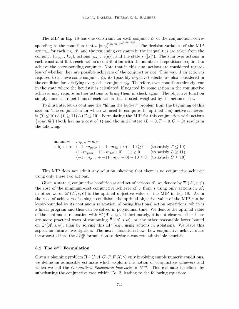
Scala, Haslum, Thiebaux, & Ramirez
The MIP in Eq. 18 has one constraint for each conjunct ψi of the conjunction, corre-
sponding to the condition that s |= ψr(a1,m1)...
r(ak,mk)
i . The decision variables of the MIPare ma, for each a ∈ A′, and the remaining constants in the inequalities are taken from theconjunct (wψi,x, kψi), actions (ka,x, γ(a)), and the state s ([x]s). The sum over actions ineach constraint links each action’s contribution with the number of repetitions required toachieve the corresponding conjunct. Note that in this sum, actions are considered regard-less of whether they are possible achievers of the conjunct or not. This way, if an action isrequired to achieve some conjunct ψj , its (possibly negative) effects are also considered inthe condition for satisfying every other conjunct ψk. Therefore, even conditions already truein the state where the heuristic is calculated, if negated by some action in the conjunctiveachiever may require further actions to bring them in check again. The objective functionsimply sums the repetitions of each action that is used, weighted by the action’s cost.
To illustrate, let us continue the “filling the bucket” problem from the beginning of thissection. The conjunction for which we need to compute the optimal conjunctive achieversis (T ≤ 10) ∧ (L ≥ 11) ∧ (C ≤ 10). Formulating the MIP for this conjunction with actions{pour,fill} (both having a cost of 1) and the initial state 〈L = 0, T = 0, C = 0〉 results inthe following:
minimise mpour +mfill
subject to (−1 ·mpour +−1 ·mfill + 0) + 10 ≥ 0 (to satisfy T ≤ 10)(1 ·mpour + 11 ·mfill + 0)− 11 ≥ 0 (to satisfy L ≥ 11)(−1 ·mpour +−11 ·mfill + 0) + 10 ≥ 0 (to satisfy C ≤ 10)
This MIP does not admit any solution, showing that there is no conjunctive achieverusing only these two actions.
Given a state s, conjunctive condition ψ and set of actions A′, we denote by Ξ∗(A′, s, ψ)the cost of the minimum-cost conjunctive achiever of ψ from s using only actions in A′;in other words Ξ∗(A′, s, ψ) is the optimal objective value of the MIP in Eq. 18. As inthe case of achievers of a single condition, the optimal objective value of the MIP can belower-bounded by its continuous relaxation, allowing fractional action repetitions, which isa linear program and thus can be solved in polynomial time. We denote the optimal valueof the continuous relaxation with Ξ∗(A′, s, ψ). Unfortunately, it is not clear whether thereare more practical ways of computing Ξ∗(A′, s, ψ), or any other reasonable lower boundon Ξ∗(A′, s, ψ), than by solving this LP (e.g., using actions in isolation). We leave thisaspect for future investigation. The next subsection shows how conjunctive achievers areincorporated into the hmax
hbd formulation to devise a concrete admissible heuristic.
8.2 The hgen Formulation
Given a planning problem Π=〈I, A,G,C, F,X, γ〉 only involving simple numeric conditions,we define an admissible estimate which exploits the notion of conjunctive achievers andwhich we call the Generalised Subgoaling heuristic or hgen. This estimate is defined bysubstituting the conjunctive case within Eq. 2, leading to the following equation:
722

Subgoaling Techniques for Satisficing and Optimal Numeric Planning
hgen(s, ψ) =
0 if s |= ψ
Ξ∗(A+, s, ψ) + mina∈A
∃ψ′∈ψ|a∈ach(s,ψ′)
hgen(s, pre(a)) if ψ is ∧ (19)
The first term lower-bounds the cost of satisfying formula ψ, and is the optimal objectivevalue of the continuous relaxation of the MIP in Eq. 18. Same as in the definition of hmax
hbd ,the action set A+ is the set of actions that have a finite estimated precondition cost, i.e.,A+ = {a ∈ A | hgen(s, pre(a)) <∞}. The second term in Eq 19 strengthens the bound byincluding the lowest precondition cost among all achiever actions for the conditions in ψ.
Theorem 8.1 (Admissibility). For simple numeric planning problems, hgen is an admissibleheuristic. Let s be a state and ψ an NNF formula. Then hgen(s, ψ) ≤ h∗(s, ψ).
Proof.
We first consider the case when ψ is a conjunction of SCs, by induction on cost. (Weassume for simplicity that action costs are strictly positive; to account for zero-cost actions,the induction order can be modified by tie-breaking on plan size.) Consider an optimal planfor achieving ψ from s, and let M be the multi-set of actions appearing in this plan. LetM ′ ⊆ M be the multi-set of actions whose effects are necessary and sufficient to achieveψ, disregarding the achievement of actions’ preconditions. Unless s |= ψ (in which casehgen(s, ψ) = h∗(s, ψ) = 0), M ′ is non-empty. The set of actions in M ′, with action countersset to the number of repetitions of each action in the plan, is a conjunctive achiever of ψ,and therefore its total cost, C ′ is greater than or equal to the optimal solution, C, to thecontinuous relaxation of the corresponding MIP 18. Every action a that has a non-zerocount ma in the optimal solution to MIP 18 is an achiever of some ψi ∈ ψ; if it were not,the action count could be removed from the conjunctive achiever (i.e., ma set to 0) withoutviolating any of the constraints, resulting in a conjunctive achiever with lower cost. LetB = mina∈A:∃ψ′∈ψ,a∈ach(s,ψ′) h
gen(s, pre(a)). If M ′ = M , i.e., there are no actions in theoptimal plan other than those in the conjunctive achiever M ′, then at least one of these isapplicable in s; hence B = 0. Otherwise, there is some action a′ in M ′ such that one or moreof the actions in M \M ′ are necessary to achieve pre(a′); since h∗(s, pre(a′)) < h∗(s, ψ) wehave hgen(s, pre(a′)) ≤ h∗(s, pre(a′)) by inductive assumption, and since a′ is an achiever ofsome ψi ∈ ψ, B ≤ hgen(s, pre(a′)). Thus, hgen(s, ψ) = C +B ≤ h∗(s, ψ).
The case of an NNF formula with SCs as atomic conditions follows simply from the factthat hgen (like hmax
hbd ) minimises cost over disjunctions.
We can strengthen the hgen estimate in the same way as we did hmaxhbd , by further restrict-
ing the action set A+ used in Ξ∗(A+, s, ψ) to include only those actions a whose preconditioncost does not exceed the cost of achieving ψ without using a. This is obtained by updatingthe cost of each conjunction in an incremental fashion.
8.3 Computing hgen
Algorithm 2 presents a modified version of the blind search schema in Algorithm 1 thatcomputes hgen. Again, we use a priority queue to explore actions according to their esti-mated cost η. The search starts with the actions applicable in the state; these are initially
723

Scala, Haslum, Thiebaux, & Ramirez
pushed in the queue with an associated cost of 0. Each action pulled from the priority queueQ enlarges the set of relaxed reachable actions A′. For each non-expanded action a′ whose(conjunctive) precondition can be achieved using actions in A′, the algorithm computesΞ∗(A′, s,pre(a)), the lower bound on the cost of a conjunctive achiever pf pre(a) obtainedfrom the LP-relaxation of MIP 18. Then the action with this associated cost is pushed ontoQ and a new iteration starts. The algorithm terminates when the priority queue empties(the problem is not solvable) or when the goal action ga is pulled out from the queue.
Algorithm 2: Computing hgen(s,G)
1 Closed = ∅2 A′ = ∅3 foreach a ∈ A ∪ {ga} do4 if s |= pre(a) then5 η(a) = 0
6 else7 η(a) =∞
8 Q = PriorityQueue({(a, 0)|a ∈ A, η(a) = 0});9 while Q 6= ∅ do
10 a = pull(Q);11 if a == ga then12 return η(a)
13 A′ = A′ ∪ {a};14 Closed = Closed ∪ {a};15 foreach a′ : a′ /∈ Closed do
16 η(a′) = Ξ∗(A′, s, pre(a′)) + mina′′∈A(η(a′′)));17 if a′ ∈ Q then18 update queue(Q,a′,η(a′));
19 else20 push(Q,a′,η(a′));
21 return ∞
The algorithm is guaranteed to terminate as the number of actions is finite. The com-putational cost is polynomially bounded by the number of actions and by the resolution ofthe LP, which is also polynomial. More formally:
Theorem 8.2. The computational complexity of hgen is polynomial in the problem size.
Proof. Note that there will be at most |A| iterations (each action is popped out from thequeue at most once), and each iteration i solves an LP at most (|A| − i) times, hence thecomputational complexity is bounded by O(|A|2 · LP ). Moreover, because the generatedLP contains a number of variables that is linear in the number of actions of the problemand a number of constraints that is linear in the size of the conjunctive formula, the overallcomplexity is polynomial in the size of the problem.
724

Subgoaling Techniques for Satisficing and Optimal Numeric Planning
The next section shows how the heuristic can be combined with propositional variablesand global constraints.
9. Hybridisation with Propositional Conditions: Conjunctive HybridAchievers
In this section, we extend the notion of conjunctive achievers and the generalised subgoal-ing heuristic to the hybrid case, where the subgoals in a conjunction can be both simplenumeric and propositional conditions. Furthermore, we show how the heuristic integratesin a beneficial way with global constraints, which are conditions that must be satisfied inevery state traversed by a plan.
9.1 Conjunctive Hybrid Achievers
The extension of conjunctive achievers to hybrid propositional conditions and numeric con-ditions is straightforward:
Definition 8 (Conjunctive Hybrid Achiever). Given a conjunction ψ =ψ1∧ψ2∧, ...,∧ψn ofliterals and simple numeric conditions, and a state s, the set A = {a1, .., ak} is said to be aconjunctive hybrid achiever, or simply a hybrid achiever of ψ iff there exists m1, ...,mk ∈ Nsuch that for every ψi ∈ ψ
• if ψi is a numeric condition, then s |= ψr(a1,m1)...
r(ak,mk)
i
• if ψi is a literal, and s 2 ψi then∑
j|aj∈ach(s,ψi)mj ≥ 1
Intuitively, a hybrid achiever must contain actions whose effects, if executed a sufficientnumber of times, are sufficient to satisfy each conjunct, numeric and propositional. Forpropositional conditions we only require that they are achieved by at least one action, if notalready satisfied in the current state. We use Ξhbd(A
′, s, ψ) to represent the set of hybridachievers for ψ from a given state s, using actions from set A′.
The existence of a conjunctive hybrid achiever is a necessary, but not sufficient, conditionfor ψ being reachable: It does not take into account whether the actions’ preconditions arereachable, or if some actions in the achiever have negative effects on the precondition ofothers. There is a certain asymmetry, in that negative side-effects on numeric subgoalsare considered, but not on propositional conditions. For example, consider the conjunctionp ∧ (x ≥ 0): if the action achieving p also decreases x (below 0), a hybrid achiever for theconjunction will be forced to also include actions that restore x ≥ 0. This way, some of thenegative interference will be taken into account. On the other hand, if the action requiredto increase x deletes p, this is not considered. The reason for this is that effects on simplenumeric conditions commute, but propositional effects, which are assignments, do not.
Given the conjunction ψ = ψ1 ∧ . . .∧ ψn ∧ . . .∧ l1 ∧ . . .∧ lt where ψi are simple numericconditions and lj propositional literals, the least-cost hybrid achiever can be computed by
725

Scala, Haslum, Thiebaux, & Ramirez
the following slight revision of the MIP formulation from Eq. 18:
minimise∑a∈A′
γ(a) ·ma
subject to∑x∈X
wψ1,x
(∑a∈A′
maka,x + [x]s
)+ kψ1 B 0
...∑x∈X
wψn,x
(∑a∈A′
maka,x + [x]s
)+ kψn B 0
∑a∈A′∩ach(s,l1)
ma ≥{
1 if [l1]s = ⊥0 otherwise
... ∑a∈A′∩ach(s,lt)
ma ≥{
1 if [lt]s = ⊥
0 otherwise
ma ∈ N ∀a ∈ A′
(20)
The only difference between this MIP and the earlier is the presence of the constraintsensuring that for each propositional literal li that is not already satisfied in state s, atleast one achiever is executed at least once (i.e., ma ≥ 1). Synergies between achieversare accounted for automatically, since the decision variables (action counters) are sharedbetween all constraints. That is, if some action contributes to achieving multiple conjuncts,whether propositional or numeric, the optimal solution to the MIP still determines theminimum number of repetitions of the action that is needed.
Again, we denote the cost of a minimum-cost hybrid achiever, i.e., the optimal objectivevalue of the MIP in Eq. 20, with Ξ∗hbd(A
′, s, ψ), and the optimal objective value of the
continuous relaxation of the MIP with Ξhbd∗(A′, s, ψ). With this in hand, the hybrid version
of hgen, denoted hgenhbd , is defined analogously:
hgenhbd(s, ψ) =
0 if s |= ψ
Ξhbd∗(A+, s, ψ) + min
a∈A∃ψ′∈ψ|a∈ach(s,ψ′)
hgenhbd(s, pre(a)) if ψ is ∧ (21)
This equation is identical to Eq. 19 but for the fact that we replace Ξ∗(A+, s, ψ) with
Ξhbd∗(s, ψ); in practice, this means that the minimum-cost hybrid achiever is computed
using the LP-relaxation of MIP 20. Note also that the minimum precondition cost in thesecond term is over all achievers of any subgoal in ψ, propositional as well as numeric. Itis easy to see that hgenhbd is also admissible, and that its computation is polynomial in theproblem size.
9.2 Enforcing Global Constraints
Global constraints are conditions that must be satisfied in every state traversed by the plan.In other words, they act as additional preconditions of every action, and as a conjunct to the
726

Subgoaling Techniques for Satisficing and Optimal Numeric Planning
goal. Global constraints are a convenient way to express, for example, bounds on variablesthat model resources, or plan safety constraints.
Global constraints are neglected in the standard h1 relaxation because they are alreadysatisfied in each state where the heuristic is computed. However, because conjunctive hybridachievers support conjunctions of numeric conditions, and take into account some negativeinteractions, it suffices to adjoin the global constraints (assuming these also are conjunc-tions of simple numeric conditions) with any conjunctive condition that is evaluated. Theestimated cost of achieving the condition will then also account for any additional cost ofkeeping the global constraint satisfied. Formally, only a small change to the hgenhbd equationis needed:
hgen,Chbd (s, ψ) =
0 if s |= ψ
Ξhbd∗(A+, s, ψ ∧ C) + min
a∈A∃ψ′∈ψ|a∈ach(s,ψ′)
hgen,Chbd (s, pre(a)) if ψ is ∧ (22)
where C is the global constraint, a conjunction of simple numeric constraints. The onlychange from Eq. 21 is that instead of an estimate of the cost of a hybrid achiever of ψ, weuse the estimated cost of a hybrid achiever of ψ ∧ C, the conjunction of the condition andthe global constraint. The heuristic remains admissible: The addition of global constraintsis equivalent to a problem reformulation where each action’s precondition and the goal arereplaced with their conjunction with C.
10. Handling Assignment Operations in Subgoaling
The restriction to simple numeric conditions does not allow for action effects that assigna numeric variable a constant value. To be simple, a condition can only be affected byconstant increases and decreases. This can be a limitation of the heuristic for domainshaving even very simple assignments. For instance, consider the case in which one wants tomodel the action of replenishing a water tank to its full capacity T . This can be modelledin numeric planning with an action, “refill”, that sets the amount v of water in the tankwith the constant numeric effect 〈v, :=, T 〉.
Let us focus on the case where each action has at most one effect that interacts with alinear numeric condition, and this effect is an assignment with a constant right-hand side.In this situation it is possible to use the Effect-Regressor ψr(a) to infer whether action aachieves ψ or not. More precisely, let e = 〈xk, :=, ka,xk〉 be the numeric effect of a. Theregression of the linear condition ψ = 〈
∑x∈X wψ,xx+kψ,B, 0〉 through a yields a condition:
ψr(a) = 〈∑
x∈X\{xk}
wψ,xx+ kψ + wψ,xkka,xk ,B, 0〉 (23)
Since in this case the action a is idempotent, we can say that a is an achiever of ψ in a states iff s |= ψr(a). Moreover, noting that B ∈ {≥, >}, we can also observe that a necessary (butinsufficient) state-independent condition for a to be an achiever for ψ is that wψ,xkka,xk ≥ 0.When this holds we will say, with a slight abuse of terminology, that a is an assignmentachiever for ψ. Similarly to what we did for Simple Numeric Conditions, this notion can be
727

Scala, Haslum, Thiebaux, & Ramirez
used in a relaxation schema, extending the subgoaling heuristics seen so far to also accountfor what we call Direct Assignment Conditions:
Definition 9 (Direct Assignment Condition.). Let ψ = 〈∑
x∈X wψ,xx+ kψ,B, 0〉. ψ is saidto be a Direct Assignment Condition (DC) if there is only one achiever of it, and thisachiever has a single numeric effect which is an assignment with a constant value.
Direct Assignment Conditions can be used in the recursive schema of hmaxhbd and haddhbd,by devising a specific treatment that differs from that used for Simple Numeric Conditions.More precisely, when a Direct Assignment Condition ψ is not satisfied in a state s, wecheck the satisfaction of the regressed condition through its assignment achiever ach(ψ)(which is unique given Def. 9) and use the recursive call to get an estimate of the achiever’sprecondition cost. For convenience, we report the extended formulation in Equation 24,where bold is used for highlighting the new supported case. The additive heuristic isextended in the analogous manner.
hmaxhbd (s, ψ) =
0 if s |= ψ
mina∈ach(s,ψ)
(hmaxhbd (s, pre(a)) + γ(a)
)if ψ ∈ PCs
mina∈R(A,s,ψ)
rep(a, ψ, s) · γ(a) + mina∈R(A,s,ψ)
hmaxhbd (s, pre(a)) if ψ ∈ SCs
hmaxhbd (s, pre(ach(ψ))) + γ′(ach(ψ), ψ, s) if ψ ∈ DCsminψ′∈ψ
hmaxhbd (s, ψ′) if ψ is ∨
maxψ′∈ψ
hmaxhbd (s, ψ′) if ψ is ∧
(24)
In this formulation, γ′(a, ψ, s) is a function that given the condition of interest and a state,returns the cost γ(a) of the action if s |= ψr(a), and∞ otherwise. In other words, the actualachievement of a direct condition is determined when the recurrence relation is solved.
Proposition 10.1. If all numeric conditions of the problem are either Direct AssignmentConditions or Simple Numeric Conditions, hmaxhbd provides an admissible estimate. Likewise,
haddhbd is safe-pruning.
Proof. The optimal plan to achieve a Direct Assignment Condition is lower-bounded by thecost of its achiever (which is unique) plus the lower bound on the cost of its precondition.As matter of fact, if we take as inductive hypothesis in hmaxhbd that the precondition costof each action is indeed a lower bound, it is easy to prove the lower bound for the DirectAssignment Condition. This can in fact be either (i) supported by the state where theheuristic is computed, or is supported (ii) by at least one execution of its unique achiever.For case (i) we get the obvious lower bound of 0; for case (ii) we know that since theprecondition cost of each action computed by hmaxhbd is a valid lower bound to get to thisprecondition, the sum of this cost plus the cost of executing the achiever for a DirectAssignment Condition is a lower bound for achieving the Direct Assignment Condition too.There is in fact no alternative path to get to it. Finally, as haddhbd is equivalent to hmaxhbd inreachability, it will always be safe-pruning.
728

Subgoaling Techniques for Satisficing and Optimal Numeric Planning
It is very likely that more general conditions could be handled by extending the theoryproposed in this section. For instance, one can think of generalising to the case in whichthe achiever set is not a singleton, but where each action in this set is restricted to affectthe same variable (but may have quite different preconditions and effects). We leave thisand other extensions as future work.
11. Integration with AIBR for More General Action Models
By integrating our results with other relaxation schema, it is possible to handle more gen-eral numeric conditions, even when these are affected by actions with non-constant additiveeffects. In the following definition, we further partition the numeric condition set to differ-entiate between simple, direct assignment and Hard Numeric Conditions (HC). HCs denotesthe set of numeric conditions that are neither Simple Numeric Conditions (Def. 6) nor Di-rect Assignment Conditions (Def. 9). We handle HCs using the relaxed solution given bythe interval-based relaxation (Scala et al., 2016b).
haddhbd+(s, ψ) =
0 if s |= ψ
mina∈ach(ψ)
(haddhbd+(s, pre(a)) + γ(a)) if ψ ∈ PCs
mina∈A+
(rep(a, ψ, s) · γ(a) + haddhbd+(s, pre(a))) if ψ ∈ SCs
haddhbd(s, pre(ach(ψ))) + γ′(ach(ψ), ψ, s) if ψ ∈ DCs∑a∈π′
π′∈sol(<s+,A+,G,X>)
(haddhbd+(s, pre(a)) + γ(a)) if ψ ∈ HCs
∑ψ′⊂ψ:|ψ′|=1
haddhbd+(s, ψ′) if |ψ| > 1
(25)
The subscript hbd+ denotes the support for HCs. Each subgoal type (PCs, SCs, DCs,HCs) is treated using the appropriate specialised reasoning, independently of other subgoals.
The implementation of the interval-based relaxation follows our previous work (Scalaet al., 2016b). The procedure is split into a reachability and a plan computation phase.The former performs a fix-point analysis using actions reachable for haddhbd+ (A+), whichreturns the actions sufficient to reach each complex condition, and then preconditions arerecursively evaluated using haddhbd+.10 There is no extraction of a relaxed plan so the heuristiccan be less accurate than Metric-FF-like heuristics (Hoffmann, 2003; Coles et al., 2012).Note that, in this formulation different relaxations can interleave in computing the cost ofa subgoal; if in fact an action includes some simple numeric precondition, the evaluation isdone with the more accurate estimate.
From a computational standpoint, the integration of the AIBR is achieved by callingthe relaxation and its estimate whenever an action contributing (indirectly or directly) tothe condition is popped out from the queue in Alg. 1. This can be expensive and we leavemore efficient implementation as object of study for future work.
10. As a difference w.r.t. previous work in this context (Aldinger et al., 2015; Hoffmann, 2003), the reachabil-ity analysis in (Scala et al., 2016b) does not require the transitive closure of the action effects dependencyrelation.
729

Scala, Haslum, Thiebaux, & Ramirez
Also note here that the formulation hereby presented does not consider the notionof conjunctive achievers. Although possible from a theoretical standpoint, we have notimplemented this aspect yet and it is not clear how efficient and practical it could be.
An admissible formulation (hmaxhbd+) can be obtained by using any admissible approxima-tion of the interval-based relaxation for HCs – the simplest one being to just assign them anestimate of zero – while using the lower bound hmaxhbd for SCs and maxing over subgoals. Allthe above heuristic variants provide safe pruning, giving infinite values only for unsolvableproblems.
12. Related Work
Planning with numeric information has been tackled by others using different approaches,two of which have gained the majority of the attention: heuristic search, and compilation toother models. Our related work discusses thoroughly the heuristic search approach whichis the closest to our method. We then draw connections with compilation approaches thathave been used in other contexts, but share similarities with our techniques. We concludewith a discussion of other, less similar approaches.
12.1 Numeric Planning via Heuristic Search
Heuristic search is a well established approach to solving planning problems (Pearl, 1984;Geffner & Bonet, 2013), which underlies the majority of the top performer planners atthe International Planning Competitions (Vallati, Chrpa, Grzes, McCluskey, Roberts, &Sanner, 2015). One of the powerful ideas behind previous and current approaches is todevise heuristics from a computationally effective relaxation or abstraction of the targetedproblem. In particular, the solution of the relaxed problem can be used as a means toestimate the actual distance or cost to the problem goal
Pioneered by Hoffman (2003), the interval-based relaxation (Aldinger et al., 2015; Gre-gory, Long, Fox, & Beck, 2012) has been the principle most used to extract such a heuristicinformation in the numeric extension to classical planning. These heuristics come in differ-ent flavours, including as metric extensions of the relaxed planning graph (Koehler, 1998;Hoffmann, 2003; Gerevini, Saetti, & Serina, 2008; Coles et al., 2012, 2013).
The interval-based relaxation approximates the value of each numeric state variableusing an interval enclosing all the possible values that this variable may eventually reach.Intervals for expressions are calculated using Interval Analysis (Moore, Kearfott, & Cloud,2009), and a numeric condition is satisfied if at least one value in the expression’s intervalsatisfies the condition. Applicable action effects monotonically widen the bounds of theintervals, hence a relaxed solution can be computed by extending intervals until the goal isreached, and then extracting from these intervals a set of relaxed actions. Monotonicity isachieved taking the convex union between the interval representing the possible values ofthe variable before the action execution, and the interval representing the effect expression.It follows that any condition previously satisfied will also be satisfied in the successor state.
Aldinger et al. (2015) showed that termination and safe pruning can be ensured whenthe dependency relation between numeric variables in the planning task is acyclic. For suchtasks, the set of reachable states are the fixed point intervals computed by executing appli-cable actions as many times as necessary, in the order defined by the dependency relation
730

Subgoaling Techniques for Satisficing and Optimal Numeric Planning
between numeric variables. Scala et al. (2016b) subsequently removed this restriction andextended the interval-based relaxation to numeric planning tasks with cyclic dependencies,as long as numeric effects are additive. In addition, they observed that any planning taskcan be transformed to have only additive effects, at the price of a further relaxation of statedependent assignment operations.
Our approach differs from this relaxation in a very substantial way. The subgoalingtechnique we present here reasons about relevant subgoals, by regression, instead of reachablevalues. As Keyder and Geffner (2008) point out regarding the classical case, cost-sensitiveadditive and inadmissible estimates can be obtained this way without a planning graph. Byapproaching the problem using a decomposition approach, the present work has been thefirst to provide a heuristic design leading to admissible estimates for numeric planning.
Analogously to the classical delete-relaxation, the interval-based relaxation fails to cap-ture any negative interactions between numeric variables. Coles et al. (2013) proposedthe use of a Mixed-Integer Program (MIP) to tighten the bounds on intervals for problemsthat model resources as numeric variables and feature only specific patterns of interac-tion between preconditions and effects (actions are consumers or producers of resources).This addresses one important weakness of interval-based heuristics, by forcing intervals tocapture changes to resource variables. However, this does not account for other kinds ofnegative interactions, such as those illustrated by the Sailing domain. The heuristic andthe planner developed by Coles et al., namely LPRPG, demonstrates good performanceover this specific class of numeric planning problems, which is a subclass of simple numericplanning. It is, however, not applicable to any problem outside of the producer–consumerclass. It is an open and interesting question how resource-flow reasoning can be effectivelyintegrated into our subgoaling relaxation; a possible way to do so would be by injecting theresource flow constraints arising from the producer–consumer pattern in the constraints ofthe hgen formulation. We leave this aspect as a future work.
Eyerich et al. (2009) proposed another approach to devising heuristics for numeric plan-ning, which extends the context-enhanced additive heuristic. In this approach, numericconditions are justified only qualitatively, completely abstracting away from the countingproblem. While this can be powerful in domains where only one repetition of numeric ac-tions is necessary (e.g., in ZenoTravel the refuelling action only needs to be executed once),in many other domains this abstraction is too coarse and looses all numeric information inthe problem. Temporal fast downward, which is the heuristic search planner employing thisheuristic, was not able to solve any of the instances of our Sailing problem. Illanes andMcIlraith (2017) also use a qualitative abstraction of the numeric aspects of the problem.They construct a classical planning problem by replacing numeric conditions with proposi-tions and use a classical planner to devise a partial policy, which is used to guide the searchfor a plan in the numeric planning problem. Our subgoaling approach captures numericstructures, enabling inferences that would be difficult to do with only propositional vari-ables. However, it should be possible to integrate our heuristics with abstraction approachesso as to accelerate even further the search. This is an aspect definitely worth exploring infuture work.
Regression – the ability to find sufficient and necessary conditions under which an actionachieves a given goal – has been widely used in many areas of planning (McDermott, 2003;Fikes, Hart, & Nilsson, 1972; Hoare, 1969; Rintanen, 2008; Scala, 2014). The very first
731

Scala, Haslum, Thiebaux, & Ramirez
heuristic that makes use of regression to estimate goal distance is due to McDermott (1996);this idea has been used extensively in the work by Bonet and Geffner (2001) and in the workby Haslum and Geffner (2000). Our approach builds on the declarative and decomposition-based formulation of heuristics of the latter two.
12.2 SMT Based Approaches
Another successful approach to numeric planning is based on the compilation of the planningproblem into the problem of finding a model satisfying a given SMT formula (Scala, Ramırez,Haslum, & Thiebaux, 2016c; Hoffmann, Gomes, Selman, & Kautz, 2007; Shin & Davis,2005). As for SAT-based planning in the classical planning case (Kautz & Selman, 1999;Rintanen, 2012), SMT-based planning stems from the idea of capturing all the possibletrajectories for a bounded version of the planning problem in a quantifier-free formula havingnumeric and propositional conditions as terms. Such a formula is responsible for capturingall those transitions that are consistent with the dynamics of the system (represented inthe actions), the initial state and the goals to be achieved. A challenging aspect for thisapproach is to find a compact representation of such possible trajectories; this is usuallyobtained by allowing multiple actions to share the same timepoint, and reconstructing thesequence of operations only when a model for the formula is found. To achieve this objective,previous work has exploited different ways of decomposing the problem, e.g. through theidentification of independent actions, or encodings that encapsulate ordered sequences ofactions (Wehrle & Rintanen, 2007). Whilst this has been a fruitful line of work in classicalplanning that has led to efficient SAT-based planning systems (Rintanen, 2012), less hasbeen done, relatively speaking, in the context of numeric planning.
There are two exceptions worth mentioning. In our previous work (Scala et al., 2016c),we have used the same m-times regressor as in this paper to capture unbounded sequencesof actions within a single time step, and found conditions under which these sequences ofactions represent valid transitions. Devising powerful heuristics can also be beneficial in theframework of compilation into other theories. This has been shown elsewhere (Rintanen,2012).
Looking into the potential of integrating planning as satisfiability, optimisation andmathematical programming is an old idea, of which two early examples are the LPSATplanner, due to Wolfman and Weld’s (2001), and Shin and Davis’s (2005) TMLPSAT.Both planners are built around “proto”-SMT solvers, based on a decision procedure, eitherDPLL (Davis, Logemann, & Loveland, 1962) or CDCL (Zhang, Madigan, Moskewicz, &Malik, 2001), suitably modified so that some clauses are not represented in propositionallogic, but in an auxiliary theory, and still able to take advantage of both unit propagationand conflict-directed clause learning. Both planners are strictly more expressive than any ofthe planners we propose in this paper, as we consciously trade-off expressiveness for perfor-mance. A “second wave” of approaches based on this integration followed the formalisationof SMT into abstract decision procedures (Nieuwenhuis, Oliveras, & Tinelli, 2006; Kroening& Strichman, 2008) and the availability of powerful, scalable implementations of impor-tant fragments of first-order logic such as linear constraints and difference logic (Dutertre& de Moura, 2006). Examples of these later systems, which all use slight reformulationsof Shin and Davies’ encoding, are dReal (Bryce, Gao, Musliner, & Goldman, 2015) and
732

Subgoaling Techniques for Satisficing and Optimal Numeric Planning
SMTPLAN (Cashmore et al., 2020). Parallel to these, other planning systems exist whichdepart significantly from this line of research, that also support in limited, incidental ways,numeric effects like the ones discussed in this paper. Inspired by well-established practicesin Optimisation (Hooker, 2003), there is the work due to Rintanen (2017) on clock-basedSMT encodings for temporal planning with numeric and propositional resources. Also, fol-lowing up the notion of chronicles (Ghallab, Nau, & Traverso, 2004), Bit-Monnot (2018)puts forward a very efficient SMT encoding that compares very favourably with other SMT-based approaches. Note that most of these systems address temporal, as well as numeric,planning. All, though, ultimately struggle with problems where there is a strong interactionbetween the subproblem of achieving individual goals separatedly, and that of determiningtheir ordering so as to avoid interference between temporal actions and minimise makespan.This was addressed via the integration of domain-independent heuristics into the process ofcompiling temporal problems into Constraint Programming (CP) (Vidal & Geffner, 2006).In this paper we address directly the problem of goal ordering, or subgoaling, in the contextof numeric planning, and propose effective heuristic methods that could be used to enhancethe capabilities of existing SMT-based temporal-numeric planners in an analogous way asVidal & Geffner did.
SMT-based planning approaches suffer from the same limitations as SAT-based planningapproaches. First, encodings based on Kautz and Selman’s (1999) seminal contribution,have trouble dealing with unsolvable planning problems, as they need to test satisfiabilityfor an upper bound on plan length or makespan. Finding a tight upper bound is as hard assolving the planning task itself (Bylander, 1994), and naive upper bounds lead to SAT en-codings with huge numbers of variables and clauses. Recent work on alternative SAT-basedapproaches (Suda, 2014; Eriksson & Helmert, 2020), that rely on Bradley’s (2011) notionof Property Directed Reachability (PDR), overcome the limitations inherent in Kautz &Selman’s encoding on completeness with respect to refutation, and propose practical algo-rithms to produce certificates of unsolvability for propositional planning. Second, and forsimilar reasons, controlling the quality of solution along arbitrary finite horizons while pro-ducing succinct SAT encodings is not trivial, as noted by Rintanen (2012). Our formulationcan guarantee admissible estimates to find optimal plans also in the numeric setting. Notethat the admissible estimates presented in this paper are the first of their kind.
12.3 Similar Problems and Methods
Analysis of discrete, linear time invariant systems. The notion of planning operatorsto abstract the behaviour 11 of a dynamical system has a long history in planning. Anearly example, which is closely related to the methods discussed in this paper, is the ideaby E. P. D. Pednault (1987) to associate with action effects an integral equation thatdescribes successor states after a set amount of time. In this work we limit ourselves tolinear dynamics, and therefore, established results from the theory of discrete-linear systems(Edward, 1996; Borrelli, Bemporad, & Morari, 2017) are particularly relevant to our work.Given a formulation of how a variable evolves given in terms of a linear function of some othervariables, the future of this variable is given by the exponentiation of the matrix formed
11. A behaviour in control is the set of trajectories that are compatible with a set of differential pathconstraints.
733

Scala, Haslum, Thiebaux, & Ramirez
by the coefficients in the linear functions given. However, a) computing such a matrixexponentiation is computationally expensive, b) the number of possible configurations, andtherefore, behaviours of the system, depend on how actions are ordered in plans. Theclosed-form expression presented in this paper is valid for simple numeric conditions, and inparticular the m-times effect regressor , as it exploits the factored representation of numericplanning problems. We see this as a special case of the general setting of discrete-linearsystems with variables that only change because of actions, and do not interfere (the self-interference effect free assumption). In terms of the theory developed by Borrelli et al. onModel Predictive Control (MPC) for linear systems, this corresponds to having the naturalresponse always set to 1 for each variable. We believe that this special case can still capturevery interesting problems with guarantees such as computational cost and admissibilityif desired. Once this connection has been drawn, we look forward to further refine ourunderstanding of the relationship between the contributions reported in this paper andwell-established results from Systems and Optimal Control theory.
Heuristics for classical planning The problem of capturing the number of times anaction has to appear in the solution plan is well known in the purely classical planning liter-ature. State of the art heuristics for optimal classical planning are based on the frameworkof operator counting (Pommerening et al., 2015). Our heuristic can be seen as an exten-sion of this framework to the numeric case. Interestingly, it seems that the combinationof our heuristic hmaxhbd with the generalised form hgen captures information in a similar waythe lm-cut and the state equations combine with each other (Helmert & Domshlak, 2009;Bonet & Helmert, 2010).Understanding the expressive power of our formulation againstthe classical planning version, together with understanding how to benefit from the variouscharacterisations in a comprehensive way are however all object of interesting future work.
13. Experimental Analysis
Our experimental analysis has been conducted to evaluate the usefulness of the heuristicspresented in this paper for both satisficing and optimal planning. We employed such heuris-tics in a forward state space search planner guided by two different informed search algo-rithms: Greedy Best First Search (GBFS) for the satisficing setting, and A∗ for the optimalsetting. In the satisficing setting ties are broken to favour nodes with lower g-values; in theoptimal setting ties are broken to favour nodes with higher g-values. The implementationis part of the ENHSP planning system (https://sites.google.com/view/enhsp/),which is a JAVA implementation containing all the necessary functionalities developed. Forsolving the linear programs in the hgenhbd formulation we used CPLEX 12.6.3.
The impact of heuristics on the planner is measured along two main dimensions: CPU-time to produce a valid (or optimal) solution, and length of the produced plans (for satis-ficing planning). Since we assess our heuristics in a state-space planner, we also report thenumber of node expansions as the number of times a node is popped out from the priorityqueue. Intuitively, the smaller the number of expansions, the less search was required tofind a solution. We seek an understanding of whether and when fewer expansions translateinto a faster convergence to the solution. Moreover, we want to understand how the inad-missible heuristics behave in terms of plan length. In our experiments, all actions have unitcost, therefore the optimal plans are those with the shortest length.
734
Subgoaling Techniques for Satisficing and Optimal Numeric Planning
For comparison, we ran experiments on heuristics based on the Interval Based Relaxation(IBR) and with a simple (yet much faster) goal sensitive heuristic. In the satisficing setting,we take MetricFF (Hoffmann, 2003) as representative of IBR based heuristic search numericplanners. In the optimal setting, the goal sensitive heuristic giving 0 to goal states and1 to non-goal states is run with our A∗ implementation. In our experiments we do notcompare with the LPRPG planner (Coles et al., 2013) because its heuristic is designed onlyfor handling producer–consumer resource problems (a subclass of simple numeric planning,see Section 12), and we assume that it will be more effective than search with any of themore general heuristics that we consider for problems that fall within that specific class.Therefore, since the results of an experimental comparison are quite predictable, we do notsee it as necessary to carry out that comparison.
Our experiments were run under Ubuntu on an Intel(R) Xeon(R) CPU E3-1240 v3 @3.40GHz and 8Gb of Ram with a timeout of 1800 secs. per problem.
In the following, we first introduce the domains used for our experiments; then we discussthe results obtained in the satisficing and optimal planning settings.
13.1 Domains
Our evaluation is carried out i) on a variety of standard numeric domains from the In-ternational Planning Competition (IPC)12 and the LPRPG benchmark suite (Coles et al.,2013), ii) on numeric planning reformulations of Functional STRIPS problems (Frances &Geffner, 2015) (F-STRIPS), and iii) on two sequential numeric domains called Sailingand Farmland introduced in our previous work (Scala et al., 2016a).
From the IPC, we only include domains where numeric variable(s) are included in atleast one action precondition or goal.
F-STRIPS’s domains, Sailing and Farmland are heavily numeric domains and ourevaluation puts a greater emphasis on them. This is to better understand the role played byour heuristics in dealing with the numeric structure of the problem. A detailed descriptionof these domains follow.
13.1.1 F-STRIPS Domains
Counters. This domain revolves around the idea of controlling the values of a set ofcounters {X1, ..., Xn} in order to satisfy a set of constraints. The domain of each countergoes from 0 to a MAX value that changes depending on the number of counters, and is set inorder to make the problem solvable. The domain comes with three sets of instances, whosegoals always require a total order among the counters i.e.: {X1 < X2, ..., Xn−1 < Xn}. Inthe first set of instances (Counters), counters are all initially set to 0, in the second set(Count-Rnd), their values are set randomly, while in the last set of instances (Count-Inv)the values are set in such a way that they all need to be reversed in order for the goal to besatisfied. For the first set we have 11 instances; for the random variant we have 33 instances;for the reversed variant 11 instances. Differently to the original formulation, our counters arerepresented using numeric fluents, and the domains of such counters are encoded either viaappropriate action preconditions, or via global constraints. We will study the two differentversions. Even though the domain is very simple, the number of actions in the optimal
12. http://icaps-conference.org/index.php/main/competitions
735

Scala, Haslum, Thiebaux, & Ramirez
plan grows quadratically with the number of counters, and common heuristics based on theInterval Based Relaxation (IBR) do not capture even the simplest interactions between theactions that are needed to set the counters. In the IBR, the goal is reached after one stepof parallel execution. This unfortunately happens also in our subgoaling relaxation, but notin our extended formulations (i.e., using redundant constraints or conjunctive achievers).
Gardening. This domain models an agent in a 2D grid. This agent is tasked to watera number of plants scattered within the grid. The agent can carry water with a bucket;however, as this bucket has limited capacity, the agent may need to refill it multiple timesto water all the plants. The goal specifies which plants need to be watered and, for eachof them, the amount of water that has to be poured. In our formulation, both the positionof the agent in the 2-D space and the amount of water carried are represented by numericstate variables. Optimal plans for this problem are the ones where the agent maximises theuse of the bucket while she is moving, and at the same time minimises the number of movesto get to the plants and to the tap position for refilling. A greedy solution would be toconsider each plant in isolation, refilling the bucket sufficiently to water a plant, and thengoing back to refill the bucket for the next plant. A greedy solution would however makethe plans unnecessarily longer; it is in fact much better to reason over multiple plants atonce, and therefore to refill the bucket with more water each time. In this domain, instancesscale up to grids of size 20× 20, and three plants to water.
Grouping. Finally, Grouping is the problem of pushing boxes in a grid-based domainwhich is entirely represented using numeric variables to denote boxes’ position. The agent’sgoal is to group subsets of these boxes together; the goal formula makes heavy use ofdisjunctions to compactly representing the allowed and disallowed configurations. Instancesscale on the number of boxes to be moved (from 2 to 10) and size of the grid (from 5 × 5to 100× 100).
13.1.2 Sailing and Farmland
These two domains were originally introduced by Scala et al. (2016a).
Sailing. This is the domain presented in Section 2.3, and depicted in Figure 1. Goals in ourinstances are given as a set of sites to be reached. As we have seen before, we have an actionfor each person to rescue, and the difficult part of this problem is to get the preconditionof these actions satisfied. The satisfaction of a precondition implies that the sailing boatis close enough to rescue the castaway. Instances generated for this domain scale on thenumber of boats (from 1 to 4) and the number of people to rescue (from 1 to 10). Sincethe positions to be reached by the boats can be quite far away, plans in this problem canbe quite long (we measured plans up to 1000 actions). An optimal plan corresponds tothe fastest possible tour reaching all the designed locations; in this regards this problem issimilar to the Travelling Salesperson Problem (Flood, 1956).
Farmland. The Farmland domain models the problem of allocating manpower to farms,with a hard constraint on a metric measuring benefit. The contribution of each farm to thebenefit is a function of the number of workers assigned. In our instances, each farm requiresat least one worker. The number of workers ranges from 100 to 1000, and the number offarms from 2 to 10. In this domain plans can be quite long; each action models the single
736

Subgoaling Techniques for Satisficing and Optimal Numeric Planning
movement of each worker. The accuracy of the heuristic becomes crucial to deal with sucha problem.
13.2 Satisficing Planning
We evaluate three GBFS planners, differing from each other on the particular heuristicemployed13:
• GBFS(haddhbd+): GBFS with the optimistic variant of the inadmissible heuristic givenin Eq. 11.
• GBFS(hraddhbd+): GBFS with the previous heuristic plus redundant constraints. Aredundant constraint is added to approximate the conjunctive satisfaction of eachpair of numeric conditions in the goal and in any action precondition, following theschema given in Section 7.
• GBFS(IBR). This has been obtained by using the best-first-search implemented inMetricFF with helpful actions disabled. This configuration yields quite a distilledversion of the planner against with we can compare the heuristic proposed in thispaper. For simplicity, we will use the term IBR to refer to this particular configurationof MetricFF.
Note that the two implementations with the h1 based heuristic pay some handicap in that:i) unlike MetricFF, they do not transform the task into a LNF (the LNF transformationinduces a better analysis of the state spaces by avoiding the exploration of states which aredominated by other states already seen) ii) they are implemented in ENHSP, which is inJAVA, while MetricFF is written in C.
13.2.1 Subgoaling Heuristics Analysis
Table 1 reports the data obtained using the two satisficing heuristics presented in thispaper. Redundant constraints help capture action interactions (e.g, Counters) but havetwo main drawbacks: overestimation and computational cost. In the variants of Counters,heuristic that incorporates redundant constraints largely dominates its rival due to the highnumber of interacting goals: redundant constraints do capture those interactions to someextent, whereas the pure additive version does not. The result is a substantial reduction ofthe number of expanded nodes, which overcomes hraddhbd+’s higher computational cost. Planlength is comparable, although it seems that adding redundant constraints tends to favourdeeper solutions. This is not surprising however, as the hraddhbd+’s estimate could be highly
inadmissible, much more than haddhbd+.
The situation in the Sailing domain is more interesting; here GBFS(hraddhbd+) solves just29 problems, yet there are instances where it expands fewer nodes. A deeper analysis on theraw data revealed that the adoption of redundant constraint was particular beneficial onthe instances involving only a single boat. For these instances, the reduction of expandednode is substantial: the configuration with redundant constraints expands on average 4225.9
13. Note here that other search engines can be used. Yet, our analysis is restricted to GBFS with the purposeof deepening our understanding on the informativeness of our relaxation and derived heuristics.
737

Scala, Haslum, Thiebaux, & Ramirez
nodes, while haddhbd+ expands 20640.8 and still obtains plans of slightly worse quality. Redun-dant constraints in this domain are generated starting from the convex set of constraintsdelimiting zones to be reached. In the instances with more than one boat, a large number ofthe generated constraints turned out to be dominated by the cost of the others. Summingthem together results in a higher estimation that misled the planner when navigating thesearch space in many situations.
In the IPC domains, redundant constraints are only generated for ZenoTravel andTPP. In particular, in ZenoTravel, redundant constraints lead to the generation of nonsimple numeric conditions, causing a substantial drop in performance of the planner. Al-though this signals the potential harm of redundant constraints, it has to be noted that itcan be easily avoided by not enforcing redundant constraints between constraints that areaffected by assignment operations. In that case, the performance of ZenoTravel wouldequate again the performance obtained by haddhbd+. In the other domains (Rovers, Satel-lite, Depots) there are no redundant constraint so the minor differences are only due tosmall perturbations in the running of the experiments.
Redundant constraints are also generated for most of the resource-flow domains, i.e.,HydroPower, MarketTrader, Pathways, Sugar, Pathways. However, apart froma small advantage in node expansion in Settlers and Pathways, their contribution seemsto only bring overhead. It is likely that other forms of redundant constraints should begenerated in order to better capture the numeric flows arising from these domains.
Coverage Planning Time Expanded Nodes Plan Length
Domain haddhbd+ hraddhbd+ haddhbd+ hraddhbd+ haddhbd+ hraddhbd+ haddhbd+ hraddhbd+
Counters (11) 6 8 71.64 15.95 74653.17 2373.00 68.50 80.17Grouping(192) 179 97 9.09 329.49 83.09 84.73 82.08 82.15Count-Inv (11) 6 9 101.56 3.60 99094.00 339.67 110.50 120.50Count-Rnd (33) 25 28 71.73 18.32 37156.24 1175.84 180.84 185.60Gardening(51) 51 29 2.03 98.70 11080.52 30379.90 329.90 226.79Sailing (40) 38 29 85.94 69.91 109441.04 115581.89 803.61 847.64Farmland(50) 50 50 1.25 3.09 308.64 303.98 301.74 302.44ZenoTravel(23) 18 7 1.15 116.51 14.57 14.57 11.29 11.29Rovers(20) 10 10 25.94 25.86 14155.80 14155.80 22.60 22.60Depots(22) 5 5 17.66 13.57 230.00 230.00 18.80 18.80Satellite(20) 10 11 120.63 102.13 9569.40 9569.40 45.80 45.80TPP(40) 9 7 128.97 291.56 40.57 46.57 18.71 18.86Settlers(20) 4 2 39.24 155.91 5706.50 2973.00 40.00 41.50Mprime(30) 26 26 66.51 99.76 214.38 214.38 7.50 7.50HydroPower(30) 5 5 566.88 578.02 8602977.00 8602977.00 41.20 41.20MarketTrader(20) 6 6 872.58 1224.61 457140.33 457120.33 5384.83 5384.83Sugar(20) 5 4 32.40 131.37 19686.00 19686.67 29.33 30.00Pathways(30) 3 3 208.41 45.11 488764.67 61423.67 32.67 36.00
Total 456 336
Table 1: In-Depth comparison of our heuristics along 3 different dimensions: PlanningTime, Plan Length and number of Expanded Nodes. The data is averaged overinstances solved by all configurations.
738

Subgoaling Techniques for Satisficing and Optimal Numeric Planning
13.2.2 Subgoaling VS Interval Based Relaxation
Table 2 compares the haddhbd+ heuristic with the IBR obtained using MetricFF.
Coverage Planning Time Expanded Nodes Plan Length
Domain haddhbd+ IBR haddhbd+ IBR haddhbd+ IBR haddhbd+ IBR
Counters (11) 6 11 71.64 0.11 74653.17 87.00 68.50 86.00Grouping(192) 179 10 0.87 13.42 14.80 19.30 13.80 18.30Count-Inv (11) 6 2 0.83 0.05 8.50 10.50 7.50 9.50Count-Rnd (33) 25 4 0.66 0.07 3.75 3.75 2.75 2.75Gardening(51) 51 0 NA NA NA NA NA NASailing (40) 38 0 NA NA NA NA NA NAFarmland(50) 50 0 NA NA NA NA NA NAZenoTravel(23) 18 6 1.10 0.02 16.00 15.67 13.17 14.67Rovers(20) 10 2 0.65 299.72 11.00 350337.00 9.00 14.00Satellite(20) 5 1 1.48 0.03 12.00 12.00 11.00 11.00Depots(22) 10 2 119.57 1.10 130.00 17.50 34.00 NATPP(40) 9 6 50.00 0.02 29.67 12.67 13.83 11.67Settlers(20) 4 1 2.82 0.01 222.00 1.00 26.00 NAMprime(30) 26 11 2.82 0.11 94.09 9.09 6.64 8.09HydroPower(30) 5 0 NA NA NA NA NA NAMarketTrader(20) 6 0 NA NA NA NA NA NASugar(20) 5 0 NA NA NA NA NA NAPathways(30) 3 0 NA NA NA NA NA NA
Total 456 56
Table 2: Experimental analysis comparing haddhbd+ with IBR. The data is averaged over in-stances solved by all configurations. NAs report situations where the intersectionof instances solved by all configurations is empty.
Apart from the first set of instances of Counters and instances from TPP, the sub-goaling heuristic developed largely outperforms the classical interval based relaxation im-plemented by MetricFF. There are however a number of interesting findings.
It is in fact not only the different relaxations employed by the two heuristics (haddhbd+
vs IBR) that affect the performance, but also the way the heuristic estimate is actuallycalculated. On the one hand, haddhbd+ pessimistically sums the contribution of each (sub)goal,thus neglecting any positive interactions among the actions needed to achieve them; Onthe other hand, IBR used in MetricFF is based on a plan-extraction mechanism that, asit happens for the propositional setting, alleviates the additive pessimistic assumption byusing sometimes the same action to achieve multiple conditions. We have also observed sometechnical issues, with MetricFF showing unexpected behaviour over some of the numeric-flowinstances. In particular for MarketTrader, MetricFF wrongly claims some of the instancesto be unsolvable.
In problems like ZenoTravel, assuming complete independence between subgoals (asfor haddhbd+) pays off, and it is also beneficial in Sailing and Farmland. These two domainsare particularly interesting. Indeed, only the subgoaling based heuristics are able to capturesome of the internal interferences occurring among the actions. Several conditions in thesetwo domains encompass more than one variable, a situation for which, as we have seenin our motivating example, the subgoaling relaxation is provably tighter than the interval
739

Scala, Haslum, Thiebaux, & Ramirez
Plan Length Planning Time
Instance IBR haddhbd+ IBR haddhbd+
2 1 1 0.01 0.574 11 6 0.01 0.598 41 28 0.01 0.8412 87 66 0.03 2.2816 149 120 0.10 20.4720 227 190 0.41 311.6424 321 NA 1.21 TO28 431 NA 3.03 TO32 557 NA 6.91 TO36 699 NA 15.04 TO40 857 NA 25.88 TO
Table 3: IBR vs haddhbd+ on Counters
based one, since it reasons on regressed subgoals rather than on reachable values. Therefore,haddhbd+ will likely results more accurate than IBR. As it is possible to observe from the table,none of the instances is solved using MetricFF.
The situation in the Gardening domain is more intricate. It seems that MetricFF getsstuck quite immediately. To understand this behaviour, we also tried to run it with thestandard configuration (enforced hill climbing plus helpful actions pruning), and it solvedall the instances. We ascribe the reason for this behaviour to the very specific way tiesare broken in MetricFF. The data for Counters, and in particular the subset of instanceswhere all counters are initially set to zero, is also somewhat difficult to explain. MetricFFseems to dominate in terms of coverage, even if it produces longer plans on average. Table3 shows the results for individual instances.
To investigate this behaviour more in depth we studied the effect of tie breaking in thesearch of our planner. More precisely, we changed the tie breaking to favour higher g-valuesalso in the satisficing setting. In the Counters domain there are no dead-ends so beinggreedy cannot harm too much in terms of the ability to find some plan, but it could in termsof the ability to find short plans. Table 4 reports the data collected with this setting, and thecomparison with MetricFF. This data partly justifies our intuition about the possible causesof the discrepancies between the two systems, but not fully. It seems in fact that MetricFFis not using a deterministic tie-breaking strategy, as sometimes it acts more conservativelyresulting in plans slightly longer than those produced by our implementation.
Our experimental analysis for the satisficing setting concludes with another experimentwhere we measure the performance of our best heuristic against MetricFF with all the func-tionalities enabled (enforced hill climbing plus helpful actions). This experimental settingwas meant to understand to what extent a tighter relaxation influences the overall system.The analysis focuses on the Sailing domain. In Sailing we have evidence that the relax-ation is actually tighter. Out of 40 instances submitted, MetricFF was able to solve just 5 ofthem within a 1800 secs timeout. This shows the great importance of a careful exploitationof numeric structures in the heuristic.
740

Subgoaling Techniques for Satisficing and Optimal Numeric Planning
Plan Length Planning Time
# Counters IBR haddhbd+ + LGTB IBR haddhbd+ + LGTB
2 1 1 0.01 0.814 11 6 0.01 0.678 41 28 0.01 0.9812 87 66 0.03 1.4216 149 120 0.10 1.6420 227 190 0.41 2.1724 321 276 1.21 2.2628 431 378 3.03 2.4732 557 496 6.91 3.1236 699 630 15.04 4.0540 857 780 25.88 6.23
Table 4: IBR vs haddhbd+ with modified tie-breaking on Counters
13.3 Optimal Planning
We evaluate 3 planners based on A∗ which differ by the heuristics they are equipped with:
• A∗ (hmaxhbd+): A∗ with the admissible heuristic described in Eq. 15
• A∗ (hrmaxhbd+ ): A∗ with the admissible heuristic plus redundant constraints, Eq. 16
• A∗ (hgenhbd): A∗ with the generalised subgoaling procedure presented in Eq. 22.
As a baseline, we run A∗ with a blind goal-sensitive heuristic that gives 0 to goal states,and the value of 1 to non-goal states.
Experiments focus on a selection of domains, namely Gardening, Counters, Farm-land and Sailing. For some of these, we also introduce a variant where we make useof global constraints (see next subsection). For this optimal setting, Counters instancesconsist of 2 up to 9 counters, for a total of 8 instances. This lets us analyse the experimentswith a finer level of granularity. We refer to this new set with SmallCounters. For theother domains, we use the same set of instances as Scala et al. (2016a).
Coverage Planning Time Expanded Nodes
hmaxhbd+ hrmaxhbd+ hgenhbd Blind hmaxhbd+ h
rmaxhbd+ hgenhbd Blind hmaxhbd+ hrmaxhbd+ hgenhbd Blind
SmallCounters(8) 7 7 7 7 14.6 19.5 29.7 96.5 582670 242926 18946.7 2685633.7Count-Inv (11) 2 2 11 2 0.7 0.5 0.5 1 415 160.5 8.5 1373.5
Count-Rnd (33) 6 7 32 6 0.5 0.4 0.5 0.8 13.3 5.5 5.5 280.3Gardening(63) 63 63 62 63 2.6 2.7 108.8 1.9 35786.8 25959 32620.9 135477.5
Sailing (40) 6 17 7 6 5.5 0.9 152.1 88.3 92349.2 3114.8 94201 4512638Farmland(50) 30 30 30 12 0.6 0.6 1.9 24.2 430.5 426.8 359.1 1495061.8
Total 114 126 149 96
Table 5: Coverage for the different heuristics. In parenthesis the number of instances foreach domain.
741

Scala, Haslum, Thiebaux, & Ramirez
Table 5 gives an overview of the performance of each heuristic when the planner is runon the original domain definition (without global constraints). The coverage of the variousheuristics differ for Sailing, Count-Inv and Count-Rnd. In Sailing the formulationusing redundant constraints dominates the other heuristics quite considerably, includingthe sophisticated generalised subgoaling formulation hgenhbd . The issue with hgenhbd is due to aninteresting phenomenon occurring in the Sailing domain, which we call the preconditionhiding phenomenon. In this domain, each goal predicate needs a goal marking action whichhas a single propositional effect, but quite complex precondition. In fact, its executionis only possible when a set of numeric constraints is satisfied. The generalised form hgenhbddoes capture the simultaneous satisfaction of the conditions, but only adds the minimumprecondition cost over all the possible achievers of every condition present in the goals G.In Sailing, the cost of each goal g ∈ G will always be one plus the cheapest cost of theprecondition of some action that is achieving any goal g′ in G, even if g′ 6= g. Therefore,the action precondition cost that is actually needed may be actually hidden by the costof some less expansive action. This phenomenon is somehow less evident in the hmaxhbd+
case. Considering subgoals in isolation enables us to add the lower bound of the minimumprecondition cost of the possible achievers of only a single condition (cf. Eq. 14). Lookingat the raw data for Sailing, it emerges that for the problem where there is a large numberof boats, hgenhbd performs better than hmaxhbd+. However, in problems where the number of
propositional goals is higher, hmaxhbd+, but in particular hrmaxhbd+ estimates much better thanhgenhbd . In SmallCounters, hgenhbd expands much fewer nodes than the other heuristics onaverage; however, this does not translate into an overall speed up. With the exceptionof one Count-Rnd instance, neither hmaxhbd+ nor its extension with redundant constraints
(i.e., hrmaxhbd+ ) outperform the blind heuristic in terms of coverage. Yet, they both reduce thenumber of expanded nodes.
The performance of hgenhbd on Count-Rnd and Count-Inv is magnificent. Considering
the results obtained by both hmaxhbd+ and hrmaxhbd+ for all the versions of Counters, it is clear
that, although hrmaxhbd+ expands fewer nodes, hmaxhbd+ is generally faster.This suggests us that the redundant constraints that we generate do not bring enough
information in this domain. It is possible that more powerful forms of redundant constraintscould be constructed, possibly by exploiting more directly the structure of the problem.Studying how to do this systematically is an interesting research direction.
13.3.1 Experiments with Global Constraints
Global constraints have been added in the following two domains:
• Counters. Each counter has de-facto a domain of possible values; global constraintsmake this explicit.
• Gardening. The agent cannot cross the boundary of the grid. Moreover, the agentcannot carry a negative amount of water nor one that exceeds the actual capacity ofthe bucket. Both conditions are encoded using conjunctive global constraints.
We did not come up with any interesting global constraint for either the Sailing or theFarmland problem. We leave this as future work, as well as the exploitation of such global
742

Subgoaling Techniques for Satisficing and Optimal Numeric Planning
constraints automatically (which is what we would need here when such global constraintsare not so easy to formulate).
Global constraints can play two roles in our planners. The first is in the actual searchas they can prune away portions of the search space which are not interesting. The secondis in the heuristic, whenever such a heuristic actually includes them in its reasoning. Weimplemented constraints that do not prune any reachable state; they just make the structureof our problem more explicit. Note that both hmaxhbd+ and hrmaxhbd+ ignore global constraints,thus the only goal of this experimental evaluation is to measure the impact of hgenhbd .
Table 6 reports the results for Gardening (using the same problem instances as forthe previous analysis) and SmallCounters. There is nothing surprising here, apart fromthe exceptional performance of the hgenhbd formulation in SmallCounters. The heuristicperfectly estimates the optimal cost for all the instances provided. We have also evaluatedthis with larger instances, and hgenhbd is indeed perfect with this domain. Table 7 reports theresults instance by instance.
hgenhbd performs also quite well in Gardening. The tighter relaxation behind hgenhbd , andin particular the intersection with global constraints is highly beneficial to the overall time,bringing its coverage in line with that of the other heuristics. Table 9 presents raw data forGardening. Interestingly hgenhbd almost always reduces (up to an order of magnitude) thenumber of expanded nodes. However, this almost never translates into an overall speed up.We only observed hgenhbd outperforming hrmaxhbd+ on 4 out of 63 instances (instances ’9 2 3’, ’53 1’, ’7 1 2’, and ’7 3 3’). It is only when the reduction of node expansions is prominentthat hgenhbd performs better than hrmaxhbd+ also in terms of planning time. Otherwise hgenhbd ’sreasoning benefits are nullified by its computational cost. A careful analysis of the rawdata reveals that there could even be situations where the less sophisticated hrmaxhbd+ resultsin more informed estimates (e.g., instance ’8 1 2’). The issue here can be tracked down tothe fact that hgenhbd can be dominated by hrmaxhbd+ .
Coverage Planning Time Expanded Nodes
hrmaxhbd+ hgenhbd hrmaxhbd+ hgenhbd hrmaxhbd+ hgenhbdSmallCounters(8) 7 8 21.5 0.7 242926 13
Gardening(63) 63 63 4.2 32.2 34443.7 6379
Table 6: Analysis with Global Constraints
13.3.2 Numeric vs Classical Planning
Our experimental analysis concludes with an experiment where we tried to answer thefollowing question: to what extent a sophisticated heuristic such as hgenhbd can make ENHSPcompetitive with highly optimised classical planners? To this end we encoded Countersin propositional planning. Each integer number in this propositional encoding has beenmodelled with an object, and arithmetic axiomatized using actions and further predicates.Table 8 reports a comparison between hgenhbd and Fast-Downward (Helmert, 2006) with theLM-CUT heuristic configuration14. Surprisingly, despite the huge number of expandednodes, LM-CUT is competitive in the first 6 instances. However, while hgenhbd ’s run-time
14. The code has been obtained from http://www.fast-downward.org/IpcPlanners
743

Scala, Haslum, Thiebaux, & Ramirez
Planning Time Expanded Nodes
# Counters hgenhbd hrmaxhbd+ Blind hgenhbd hrmaxhbd+ Blind
2 0.64 0.62 0.50 2 2 23 0.70 0.64 0.52 4 4 64 0.73 0.62 0.51 7 19 915 0.85 0.91 0.70 11 231 13326 0.92 1.32 2.19 16 3752 279637 0.97 6.69 13.07 22 71980 6708598 1.23 141.16 TO 29 1624494 TO9 1.33 TO TO 37 TO TO
Table 7: Focus on smaller instances of the Counters domain
Planning Time Expanded Nodes
hgenhbd LM-Cut hgenhbd LM-Cut
2 0.39 5× 10⁻⁵ 2 33 0.38 0.001 4 84 0.39 0.003 7 305 0.45 0.029 11 2736 0.57 0.836 16 39627 1.42 37.494 22 712148 0.89 1435.98 29 1× 10⁶
9 1.08 TO 37 TO
Table 8: LM-Cut vs hgenhbd on a selection of instances from the Counters domain. In theseinstances all Counters are initially set to 0 and should be ordered such thatc1 ≤ c2 ≤ ... ≤ cn, where n is the number of counters considered.
remain almost constant across the instances, LM-CUT run-time grows exponentially. Infact, LM-CUT only scales up to instance number 8.
14. Conclusion and Future Work
We have presented decomposition techniques based on the subgoaling principle previouslydeveloped for classical planning. These decompositions induce safe relaxations of numericplanning problems, which can be used to obtain both admissible and inadmissible yet moreinformed heuristics estimates. The key ideas behind the notions presented in this paperderive from a more direct exploitation of some of the numeric properties that arise in numericplanning problems, with a particular emphasis on those problems where only simple numericconditions occur. Even though we investigate them in the context of the development ofheuristics, these ideas may have a wider influence on all those reasoning tasks involvinga real-world problem modelled at a greater level of detail. For instance, one can think ofadopting the same relaxations to speed up SMT-based planning (Scala et al., 2016c; Bofill,
744

Subgoaling Techniques for Satisficing and Optimal Numeric Planning
Planning Time Expanded Nodes
S P V hrmaxhbd+ hgenhbd hrmaxhbd+ hgenhbd
4 1 1 0.59 1.41 67 404 1 2 0.81 1.11 477 664 1 3 0.62 0.99 166 304 2 1 0.75 0.95 267 264 2 2 1.58 3.70 4926 1364 2 3 1.88 2.99 2675 2304 3 1 2.66 7.89 9097 6204 3 2 4.79 16.90 51531 37604 3 3 6.81 15.78 61176 7355 1 1 0.54 0.83 27 305 1 2 0.76 1.39 529 2245 1 3 0.83 1.48 416 1995 2 1 1.23 8.30 1875 11105 2 2 2.42 9.25 8649 19745 2 3 1.26 3.66 2250 7045 3 1 9.19 6.41 84418 5155 3 2 1.15 4.91 782 7305 3 3 4.01 7.63 18530 7446 1 1 0.82 1.37 815 1396 1 2 0.91 1.55 837 2156 1 3 0.58 0.84 39 246 2 1 0.64 1.00 69 526 2 2 1.71 6.19 5055 15876 2 3 1.03 3.11 1103 4516 3 1 17.82 181.01 204185 511246 3 2 11.59 40.63 110120 54586 3 3 2.42 19.58 5845 4339
Planning Time Expanded Nodes
S P V hrmaxhbd+ hgenhbd hrmaxhbd+ hgenhbd
7 1 1 0.49 0.82 6 227 1 2 1.64 1.43 705 517 1 3 0.79 2.01 557 4717 2 1 1.41 2.98 3134 3577 2 2 1.94 3.89 5498 2877 2 3 1.08 6.59 1172 12807 3 1 1.86 12.15 3369 19587 3 2 1.29 4.79 1120 4707 3 3 13.81 10.33 168119 17118 1 1 0.67 1.05 239 378 1 2 0.61 0.78 7 338 1 3 0.98 1.01 1131 318 2 1 1.38 3.04 1797 3368 2 2 2.07 16.05 3883 49478 2 3 0.79 1.91 244 1698 3 1 2.81 30.25 8724 32848 3 2 10.88 104.25 105328 220478 3 3 7.16 124.24 59227 264409 1 1 1.08 1.78 264 819 1 2 1.00 1.57 16 1009 1 3 0.54 0.84 12 499 2 1 3.08 36.72 21782 115039 2 2 1.82 20.91 5540 46569 2 3 2.36 1.74 2871 979 3 1 1.41 12.29 1997 24949 3 2 8.86 194.34 81558 397679 3 3 14.67 48.87 142269 562410 1 1 0.86 1.01 696 2910 1 2 0.84 1.32 755 11610 1 3 0.71 1.28 334 14710 2 1 2.11 3.37 6672 27010 2 2 4.26 62.97 37106 1874010 2 3 3.32 18.98 14474 655310 3 1 52.33 334.31 560494 5253210 3 2 1.65 10.76 2088 137410 3 3 32.62 596.37 350839 118552
Table 9: Data on Gardening, optimal planning instances. S, P and V in the table standfor size of the grid, number of plants and specific ’variant’. For each pair S and Vwe generated 3 random instances where we vary the structure of the problem.
Espasa, & Villaret, 2017), much as delete-free relaxations have helped in providing shorterencodings in SAT-based planning (Rintanen, 2012) through existential semantics.
The paper discusses these novel techniques theoretically, and also practically in combi-nation with informed search strategies such as A∗ and GBFS. Results report a substantialadvancement on the state of the art. Some of the notions presented here, and in partic-ular the notion of possible achievers of numeric conditions have provided the foundationsof other heuristics and relaxations recently discussed in the literature, such as hybrid land-marks (Scala, Haslum, Magazzeni, & Thiebaux, 2017) and LP- and IP-based heuristics
745

Scala, Haslum, Thiebaux, & Ramirez
(Piacentini, Castro, Cire, & Beck, 2018). These new techniques, which extend the reach ofnumeric planning even further, would not have been possible without the notions presentedin this paper.
This work can be extended in many ways. First, the notion of possible achiever can beextended to consider more complex formalisms. That could start a completely new relax-ation framework aimed at better exploiting the actual structure of certain mathematicalfunctions natively (differently from compilation-based techniques, such as that by Li, Scala,Haslum, & Bogomolov, 2018). One of this extension could be the support for non-linearfunctions, such as quadratic functions. Second, the restriction on assignment operations inthis paper is also very conservative and can be relaxed to account for multiple assignmentsto the same variable; we do not know however the implications of this relaxation. Theproblem of estimating numeric condition cost is already NP-complete with additive effectsonly, so it is likely to be at least as hard for assignments. Moreover, it is not clear whethera continuous relaxation of the underlying computational problem will be as informed as itis for additive effects. Third, the conjunctive relaxation investigated in this paper opens theway to much more powerful heuristics, however with a more unbalanced trade-off betweencomputational cost and time. New forms of helpful actions and incrementality should beexplored in order for such novel heuristics to be informed and effective at the same time.
Acknowledgments
This work was supported by ARC project DP140104219, ‘Robust AI Planning for HybridSystems’. We also want to thank the anonymous reviewers for their useful feedback andcomments.
746

Subgoaling Techniques for Satisficing and Optimal Numeric Planning
References
Aldinger, J., Mattmuller, R., & Gobelbecker, M. (2015). Complexity of interval relaxednumeric planning. In Holldobler, S., Krotzsch, M., Penaloza, R., & Rudolph, S. (Eds.),KI 2015: Advances in Artificial Intelligence - 38th Annual German Conference on AI,Dresden, Germany, September 21-25, 2015, Proceedings, Vol. 9324 of Lecture Notesin Computer Science, pp. 19–31. Springer.
Bellman, R. (1958). On a routing problem. Quarterly of applied mathematics, 16 (1), 87–90.
Bit-Monnot, A. (2018). A constraint-based encoding for domain-independent temporalplanning. In International Conference on Principles and Practice of Constraint Pro-gramming.
Blum, A., & Furst, M. L. (1997). Fast planning through planning graph analysis. ArtificialIntelligence, 90 (1-2), 281–300.
Bofill, M., Espasa, J., & Villaret, M. (2017). Relaxed exists-step plans in planning as SMT.In Sierra, C. (Ed.), Proceedings of the Twenty-Sixth International Joint Conferenceon Artificial Intelligence, IJCAI 2017, Melbourne, Australia, August 19-25, 2017, pp.563–570. ijcai.org.
Bonet, B., & Geffner, H. (2001). Planning as heuristic search. Artificial Intelligence, 129,5–33.
Bonet, B., & Helmert, M. (2010). Strengthening landmark heuristics via hitting sets. InCoelho, H., Studer, R., & Wooldridge, M. (Eds.), ECAI 2010 - 19th European Confer-ence on Artificial Intelligence, Lisbon, Portugal, August 16-20, 2010, Proceedings, Vol.215 of Frontiers in Artificial Intelligence and Applications, pp. 329–334. IOS Press.
Borrelli, F., Bemporad, A., & Morari, M. (2017). Predictive control for linear and hybridsystems. Cambridge University Press.
Bradley, A. R. (2011). Sat-based model checking without unrolling. In Jhala, R., & Schmidt,D. A. (Eds.), Verification, Model Checking, and Abstract Interpretation - 12th Inter-national Conference, VMCAI 2011, Austin, TX, USA, January 23-25, 2011. Proceed-ings, Vol. 6538 of Lecture Notes in Computer Science, pp. 70–87. Springer.
Bryce, D., Gao, S., Musliner, D. J., & Goldman, R. P. (2015). Smt-based nonlinear PDDL+planning. In Proceedings of the Twenty-Ninth AAAI Conference on Artificial Intelli-gence, January 25-30, 2015, Austin, Texas, USA., pp. 3247–3253.
Bylander, T. (1994). The computational complexity of propositional strips planning. Arti-ficial Intelligence, 69 (1-2), 165–204.
Cashmore, M., Magazzeni, D., & Zehtabi, P. (2020). Planning for hybrid systems viasatisfiability modulo theories. Journal of Artificial Intelligence Research, 67, 235–283.
Coles, A. J., Coles, A., Fox, M., & Long, D. (2012). COLIN: planning with continuouslinear numeric change. Journal of Artificial Intelligence Research, 44, 1–96.
Coles, A. J., Coles, A., Fox, M., & Long, D. (2013). A hybrid LP-RPG heuristic for modellingnumeric resource flows in planning. Journal of Artificial Intelligence Research, 46,343–412.
747

Scala, Haslum, Thiebaux, & Ramirez
Davis, M., Logemann, M., & Loveland, D. (1962). A machine program for theorem-proving.Communications of the ACM, 5 (7), 394–397.
Domshlak, C., Hoffmann, J., & Katz, M. (2015). Red-black planning: A new systematicapproach to partial delete relaxation. Artificial Intelligence, 221, 73–114.
Dutertre, B., & de Moura, L. (2006). A fast linear-arithmetic solver for DPLL(T). In 18thInternational Conference on Computer Aided Verification (CAV), pp. 81–94. Springer.
Edward, R. S. (1996). Invitation to dynamical systems. Prentice Hall, Inc. A Simon &Schuster Company, Upper Saddle River, New Jersey, 7458, 231–316.
Eriksson, S., & Helmert, M. (2020). Certified unsolvability for SAT planning with propertydirected reachability. In Beck, J. C., Buffet, O., Hoffmann, J., Karpas, E., & Sohrabi, S.(Eds.), Proceedings of the Thirtieth International Conference on Automated Planningand Scheduling, Nancy, France, October 26-30, 2020, pp. 90–100. AAAI Press.
Eyerich, P., Mattmuller, R., & Roger, G. (2009). Using the context-enhanced additiveheuristic for temporal and numeric planning. In Proceedings of the 19th Interna-tional Conference on Automated Planning and Scheduling, ICAPS 2009, Thessaloniki,Greece, September 19-23, 2009.
Fikes, R., Hart, P. E., & Nilsson, N. J. (1972). Learning and executing generalized robotplans. Artificial Intelligence, 3 (1-3), 251–288.
Flood, M. M. (1956). The traveling-salesman problem. Operations research, 4 (1), 61–75.
Fox, M., & Long, D. (2003). Pddl2.1: An extension to pddl for expressing temporal planningdomains. Journal of Artificial Intelligence Research, 20, 61–124.
Frances, G., & Geffner, H. (2015). Modeling and computation in planning: Better heuristicsfrom more expressive languages. In Proceedings of the Twenty-Fifth InternationalConference on Automated Planning and Scheduling, ICAPS 2015, Jerusalem, Israel,June 7-11, 2015., pp. 70–78.
Geffner, H. (2011). The model-based approach to autonomous behavior: Prospects andchallenges. Intelligenza Artificiale, 5 (2), 163–169.
Geffner, H. (2018). Model-free, model-based, and general intelligence. In Lang, J. (Ed.),Proceedings of the Twenty-Seventh International Joint Conference on Artificial Intel-ligence, IJCAI 2018, July 13-19, 2018, Stockholm, Sweden, pp. 10–17. ijcai.org.
Geffner, H., & Bonet, B. (2013). A Concise Introduction to Models and Methods for Auto-mated Planning. Synthesis Lectures on Artificial Intelligence and Machine Learning.Morgan & Claypool Publishers.
Gerevini, A., Saetti, I., & Serina, A. (2008). An approach to efficient planning with numericalfluents and multi-criteria plan quality. Artificial Intelligence, 172 (8-9), 899–944.
Getoor, L., Ottosson, G., Fromherz, M. P. J., & Carlson, B. (1997). Effective redundantconstraints for online scheduling. In Proceedings of the Fourteenth National Conferenceon Artificial Intelligence and Ninth Innovative Applications of Artificial IntelligenceConference, AAAI 97, IAAI 97, July 27-31, 1997, Providence, Rhode Island., pp.302–307.
748

Subgoaling Techniques for Satisficing and Optimal Numeric Planning
Ghallab, M., Nau, D. S., & Traverso, P. (2004). Automated planning - theory and practice.Elsevier.
Gregory, P., Long, D., Fox, M., & Beck, J. C. (2012). Planning modulo theories: Extendingthe planning paradigm. In McCluskey, L., Williams, B. C., Silva, J. R., & Bonet,B. (Eds.), Proceedings of the Twenty-Second International Conference on AutomatedPlanning and Scheduling, ICAPS 2012, Atibaia, Sao Paulo, Brazil, June 25-19, 2012.AAAI.
Haslum, P. (2009). hm(P) = h1(Pm): Alternative characterisations of the generalisationfrom hmax to hm. In Gerevini, A., Howe, A. E., Cesta, A., & Refanidis, I. (Eds.), Pro-ceedings of the 19th International Conference on Automated Planning and Scheduling,ICAPS 2009, Thessaloniki, Greece, September 19-23, 2009. AAAI.
Haslum, P., Bonet, B., & Geffner, H. (2005). New admissible heuristics for domain-independent planning. In Proceedings, The Twentieth National Conference on Artifi-cial Intelligence and the Seventeenth Innovative Applications of Artificial IntelligenceConference, July 9-13, 2005, Pittsburgh, Pennsylvania, USA, pp. 1163–1168.
Haslum, P., & Geffner, H. (2000). Admissible heuristics for optimal planning. In Chien,S. A., Kambhampati, S., & Knoblock, C. A. (Eds.), Proceedings of the Fifth Inter-national Conference on Artificial Intelligence Planning Systems, Breckenridge, CO,USA, April 14-17, 2000, pp. 140–149. AAAI.
Haslum, P., Lipovetzky, N., Magazzeni, D., & Muise, C. (2019). An Introduction to thePlanning Domain Definition Language. Synthesis Lectures on Artificial Intelligenceand Machine Learning. Morgan & Claypool Publishers.
Helmert, M. (2002). Decidability and undecidability results for planning with numericalstate variables. In Ghallab, M., Hertzberg, J., & Traverso, P. (Eds.), Proceedings ofthe Sixth International Conference on Artificial Intelligence Planning Systems, April23-27, 2002, Toulouse, France, pp. 44–53. AAAI.
Helmert, M. (2006). The fast downward planning system. Journal of Artificial IntelligenceResearch, 26, 191–246.
Helmert, M., & Domshlak, C. (2009). Landmarks, critical paths and abstractions: What’sthe difference anyway?. In Gerevini, A., Howe, A. E., Cesta, A., & Refanidis, I.(Eds.), Proceedings of the 19th International Conference on Automated Planning andScheduling, ICAPS 2009, Thessaloniki, Greece, September 19-23, 2009. AAAI.
Helmert, M., & Geffner, H. (2008). Unifying the causal graph and additive heuristics.In Rintanen, J., Nebel, B., Beck, J. C., & Hansen, E. A. (Eds.), Proceedings of theEighteenth International Conference on Automated Planning and Scheduling, ICAPS2008, Sydney, Australia, September 14-18, 2008, pp. 140–147. AAAI.
Hoare, C. A. R. (1969). An axiomatic basis for computer programming. Commun. ACM,12 (10), 576–580.
Hoffmann, J. (2003). The metric-ff planning system: Translating ”ignoring delete lists” tonumeric state variables. Journal of Artificial Intelligence Research, 20, 291–341.
Hoffmann, J., Gomes, C. P., Selman, B., & Kautz, H. A. (2007). SAT encodings of state-space reachability problems in numeric domains. In IJCAI 2007, Proceedings of the
749

Scala, Haslum, Thiebaux, & Ramirez
20th International Joint Conference on Artificial Intelligence, Hyderabad, India, Jan-uary 6-12, 2007, pp. 1918–1923.
Hooker, J. N. (2003). Planning and scheduling by logic-based benders decomposition. Op-erations Research, 55 (3), 588–602.
Illanes, L., & McIlraith, S. A. (2017). Numeric planning via abstraction and policy guidedsearch. In Sierra, C. (Ed.), Proceedings of the Twenty-Sixth International Joint Con-ference on Artificial Intelligence, IJCAI 2017, Melbourne, Australia, August 19-25,2017, pp. 4338–4345. ijcai.org.
Kautz, H. A., & Selman, B. (1999). Unifying sat-based and graph-based planning. In Dean,T. (Ed.), Proceedings of the Sixteenth International Joint Conference on ArtificialIntelligence, IJCAI 99, Stockholm, Sweden, July 31 - August 6, 1999. 2 Volumes,1450 pages, pp. 318–325. Morgan Kaufmann.
Keyder, E., & Geffner, H. (2008). Heuristics for planning with action costs revisited. InGhallab, M., Spyropoulos, C. D., Fakotakis, N., & Avouris, N. M. (Eds.), ECAI 2008 -18th European Conference on Artificial Intelligence, Patras, Greece, July 21-25, 2008,Proceedings, Vol. 178 of Frontiers in Artificial Intelligence and Applications, pp. 588–592. IOS Press.
Koehler, J. (1998). Planning under resource constraints. In Prade, H. (Ed.), 13th EuropeanConference on Artificial Intelligence, Brighton, UK, August 23-28 1998, Proceedings.,pp. 489–493. John Wiley and Sons.
Kroening, D., & Strichman, O. (2008). Decision Procedures: An Algorithmic Point of View(2nd edition). Springer.
Li, D., Scala, E., Haslum, P., & Bogomolov, S. (2018). Effect-abstraction based relaxationfor linear numeric planning. In Lang, J. (Ed.), Proceedings of the Twenty-SeventhInternational Joint Conference on Artificial Intelligence, IJCAI 2018, July 13-19,2018, Stockholm, Sweden., pp. 4787–4793. ijcai.org.
Liu, Y., Koenig, S., & Furcy, D. (2002). Speeding up the calculation of heuristics forheuristic search-based planning. In Proceedings of the Eighteenth National Conferenceon Artificial Intelligence and Fourteenth Conference on Innovative Applications ofArtificial Intelligence, July 28 - August 1, 2002, Edmonton, Alberta, Canada., pp.484–491.
Martello, S., & Toth, P. (1990). Knapsack Problems: Algorithms and Computer Implemen-tations. John Wiley & Sons, Inc., New York, NY, USA.
McDermott, D. V. (1996). A heuristic estimator for means-ends analysis in planning. InProceedings of the Third International Conference on Artificial Intelligence PlanningSystems, Edinburgh, Scotland, May 29-31, 1996, pp. 142–149.
McDermott, D. V. (2003). Reasoning about autonomous processes in an estimated-regression planner. In Giunchiglia, E., Muscettola, N., & Nau, D. S. (Eds.), Proceedingsof the Thirteenth International Conference on Automated Planning and Scheduling(ICAPS 2003), June 9-13, 2003, Trento, Italy, pp. 143–152. AAAI.
Moore, R. E., Kearfott, R. B., & Cloud, M. J. (2009). Introduction to Interval Analysis.SIAM.
750

Subgoaling Techniques for Satisficing and Optimal Numeric Planning
Nieuwenhuis, R., Oliveras, A., & Tinelli, C. (2006). Solving SAT and SAT modulo theories:From an abstract davis-putnam-logemann-loveland procedure to dpll(t). Journal ofthe ACM, 53 (6), 937–977.
Pearl, J. (1984). Heuristics - intelligent search strategies for computer problem solving.Addison-Wesley series in artificial intelligence. Addison-Wesley.
Pednault, E. P. (1987). Formulating multiagent, dynamic-world problems in the classicalplanning framework. In Reasoning about actions & plans, pp. 47–82. Elsevier.
Piacentini, C., Castro, M. P., Cire, A. A., & Beck, J. C. (2018). Linear and integerprogramming-based heuristics for cost-optimal numeric planning. In McIlraith, S. A.,& Weinberger, K. Q. (Eds.), Proceedings of the Thirty-Second AAAI Conference onArtificial Intelligence, (AAAI-18), the 30th innovative Applications of Artificial Intel-ligence (IAAI-18), and the 8th AAAI Symposium on Educational Advances in Artifi-cial Intelligence (EAAI-18), New Orleans, Louisiana, USA, February 2-7, 2018, pp.6254–6261. AAAI Press.
Pommerening, F., Roger, G., Helmert, M., & Bonet, B. (2014). Lp-based heuristics forcost-optimal planning. In Chien, S. A., Do, M. B., Fern, A., & Ruml, W. (Eds.),Proceedings of the Twenty-Fourth International Conference on Automated Planningand Scheduling, ICAPS 2014, Portsmouth, New Hampshire, USA, June 21-26, 2014.AAAI.
Pommerening, F., Roger, G., Helmert, M., & Bonet, B. (2015). Heuristics for cost-optimalclassical planning based on linear programming. In Yang, Q., & Wooldridge, M.(Eds.), Proceedings of the Twenty-Fourth International Joint Conference on ArtificialIntelligence, IJCAI 2015, Buenos Aires, Argentina, July 25-31, 2015, pp. 4303–4309.AAAI Press.
Rintanen, J. (2006). Unified definition of heuristics for classical planning. In Brewka, G.,Coradeschi, S., Perini, A., & Traverso, P. (Eds.), ECAI 2006, 17th European Confer-ence on Artificial Intelligence, August 29 - September 1, 2006, Riva del Garda, Italy,Including Prestigious Applications of Intelligent Systems (PAIS 2006), Proceedings,Vol. 141 of Frontiers in Artificial Intelligence and Applications, p. 600. IOS Press.
Rintanen, J. (2008). Regression for classical and nondeterministic planning. In ECAI 2008 -18th European Conference on Artificial Intelligence, Patras, Greece, July 21-25, 2008,Proceedings, pp. 568–572.
Rintanen, J. (2012). Planning as satisfiability: Heuristics. Artificial Intelligence, 193, 45–86.
Rintanen, J. (2017). Temporal planning with clock-based SMT encodings. In Sierra, C.(Ed.), Proceedings of the Twenty-Sixth International Joint Conference on ArtificialIntelligence, IJCAI 2017, Melbourne, Australia, August 19-25, 2017, pp. 743–749.ijcai.org.
Scala, E. (2013). Numeric kernel for reasoning about plans involving numeric fluents. InBaldoni, M., Baroglio, C., Boella, G., & Micalizio, R. (Eds.), AI*IA 2013: Advancesin Artificial Intelligence - XIIIth International Conference of the Italian Associationfor Artificial Intelligence, Turin, Italy, December 4-6, 2013. Proceedings, Vol. 8249 ofLecture Notes in Computer Science, pp. 263–275. Springer.
751

Scala, Haslum, Thiebaux, & Ramirez
Scala, E. (2014). Plan repair for resource constrained tasks via numeric macro actions. InChien, S. A., Do, M. B., Fern, A., & Ruml, W. (Eds.), Proceedings of the Twenty-Fourth International Conference on Automated Planning and Scheduling, ICAPS2014, Portsmouth, New Hampshire, USA, June 21-26, 2014. AAAI.
Scala, E., Haslum, P., Magazzeni, D., & Thiebaux, S. (2017). Landmarks for numericplanning problems. In Sierra, C. (Ed.), Proceedings of the Twenty-Sixth InternationalJoint Conference on Artificial Intelligence, IJCAI 2017, Melbourne, Australia, August19-25, 2017, pp. 4384–4390. ijcai.org.
Scala, E., Haslum, P., & Thiebaux, S. (2016a). Heuristics for numeric planning via subgoal-ing. In Proceedings of the Twenty-Fifth International Joint Conference on ArtificialIntelligence, IJCAI 2016, New York, NY, USA, 9-15 July 2016, pp. 3228–3234.
Scala, E., Haslum, P., Thiebaux, S., & Ramırez, M. (2016b). Interval-based relaxation forgeneral numeric planning. In ECAI 2016 - 22nd European Conference on ArtificialIntelligence, 29 August-2 September 2016, The Hague, The Netherlands - IncludingPrestigious Applications of Artificial Intelligence (PAIS 2016), pp. 655–663.
Scala, E., Ramırez, M., Haslum, P., & Thiebaux, S. (2016c). Numeric planning with dis-junctive global constraints via SMT. In Proceedings of the Twenty-Sixth InternationalConference on Automated Planning and Scheduling, ICAPS 2016, London, UK, June12-17, 2016., pp. 276–284.
Shin, J., & Davis, E. (2005). Processes and continuous change in a sat-based planner.Artificial Intelligence, 166 (1-2), 194–253.
Suda, M. (2014). Property directed reachability for automated planning. Journal of Arti-ficial Intelligence Research, 50, 265–319.
Vallati, M., Chrpa, L., Grzes, M., McCluskey, T. L., Roberts, M., & Sanner, S. (2015). The2014 international planning competition: Progress and trends. AI Magazine, 36 (3),90–98.
van den Briel, M., Benton, J., Kambhampati, S., & Vossen, T. (2007). An LP-based heuristicfor optimal planning. In Proc. 13th Int. Conf. on Principles and Practice of ConstraintProgramming (CP), pp. 651–665.
Vidal, V., & Geffner, H. (2006). Branching and pruning: An optimal temporal POCLplanner based on constraint programming. Artif. Intell., 170 (3), 298–335.
Wehrle, M., & Rintanen, J. (2007). Planning as satisfiability with relaxed $-step plans.In AI 2007: Advances in Artificial Intelligence, 20th Australian Joint Conference onArtificial Intelligence, Gold Coast, Australia, December 2-6, 2007, Proceedings, pp.244–253.
Wolfman, S. A., & Weld, D. S. (2001). Combining linear programming and satisfiabilitysolving for resource planning. The Knowledge Engineering Review, 16 (1), 85–99.
Zhang, L., Madigan, C. F., Moskewicz, M. H., & Malik, S. (2001). Efficient conflict drivenlearning in a boolean satisfiability solver. In IEEE/ACM International Conference onComputer Aided Design (ICCAD), pp. 279–285. IEEE.
752
Copyright © 2022 FDOKUMEN