1

Induction of decision trees in numeric domains using set-valued attributes

Dimitrios Kalles, Athanasios Papagelis, Eirini NtoutsiComputer Technology Institute

PO Box 1122, GR-261 10, Patras, Greece{kalles,papagel,ntoutsi}@cti.gr

AbstractConventional algorithms for decision tree induction use an attribute-value representation scheme forinstances. This paper explores the empirical consequences of using set-valued attributes. This simplerepresentational extension, when used as a pre-processor for numeric data, is shown to yield significant gainsin accuracy combined with attractive build times. It is also shown to improve the accuracy for the secondbest classification option, which has valuable ramifications for post-processing. To do so an intuitive andpractical version of pre-pruning is employed. Moreover, the implementation of a simple pruning schemeserves as an example of pruning applicability over the resulted trees and also as an indication that theproposed discretization absorbs much of pruning potential. Finally, we construct several versions of thebasic algorithm to examine the value of every component that comprises it.

KeywordsDecision trees, discretization, set-values, post-processing.

1 Introduction

Describing instances using attribute-value pairs is a widely used practice in the machine learningand pattern recognition literature. In this paper we aim to explore the extent to which using such arepresentation for decision tree learning is as good as one would hope for. Specifically, we willmake a departure from the attribute-single-value convention and deal with set-valued attributes.

We will use set-valued attributes to enhance our ability to effectively pre-process numeric variables.Pre-processing attributes will also enhance the capability of deploying promising post-processingschemes: by reporting the second best choice during classification (with increased confidence), onecan evaluate alternatives in a sophisticated fashion. In doing so, we face all guises of decision treelearning problems. First of all, we re-define splitting criteria. Then, we argue on the value of pre-pruning, as a viable and reasonable pruning strategy with the set-valued attribute approach. Weproceed by altering the classification task to suit the new concepts.

The first and foremost characteristic of set-valued attributes is that during splitting, an instance maybe instructed to follow both paths of a (binary) decision tree, thus ending up in more than one leaf.Such instance replication across tree branches should improve the quality of the splitting process assplitting decisions are based on larger instance samples. The idea is, then, that classificationaccuracy should increase. This increase will be effected not only by more educated splits duringlearning but also because instances follow more than one path during testing too. This results in acombined decision on class membership.

Such instance proliferation, across and along tree branches can look like a problem. At some nodes,it may be that attributes are not informative enough for splitting and that the overlap in instancesbetween children nodes may be excessive. Defining what may be considered excessive has been aline of research in this work and it has turned out that very simple pre-pruning criteria suffice tocontain this excessiveness.

2

As probabilistic classification has inspired this research, we would like to give credit, for some ofthe ideas that come up in this paper, to the work carried out by Quinlan [16]. However, weemphasize that the proposed approach does not relate to splitting using feature sets, as employed byC4.5 [18].

Option decision trees -as they were modified by Kohavi and Clayton [10]- are quite close to ourwork. Kohavi and Clayton use a single structure for voting that is easier to interpret than bagging[3] and boosting [7] which use a set of unrelated trees. Still, our view of the problem is quitedifferent, adopting set-values as the main reason for uncertainty, during both tree creation andclassification.

Kohavi and Sahami [9] compared different global discretization methods that used error-based andentropy-based criteria. They stated “naïve discretization of the data can be potentially disastrous fordata mining as critical information may be lost due to the formation of inappropriate binboundaries”. We believe that the set-valued approach offers better boundaries for the discretizationproblem by carefully introducing a fuzziness factor.

An earlier attempt to capitalize on these ideas appeared in [8]. Probably due to the immaturity ofthose results and to the awkwardness of the terminology used therein, the potential has not beenfully explored. Of course, this research flavor has been apparent in [13], who discuss overlappingconcepts, in [1] and in [12]; the latter two are oriented towards the exploitation of multiple models.

Our short review would be incomplete without mentioning RIPPER [5], a system that exploits set-valued features to solve categorization problems in the linguistic domain. Cohen emphasized onsymbolic set-valued attributes, while we mainly concentrate on artificially created set-values fornumeric attributes. Nevertheless, our approach is readily adaptable to symbolic set-valued domains.

The rest of this paper is organized in six sections. The next section elaborates on the intuitionbehind the set-valued approach and how it leads to the heuristics employed. The actualmodifications to the standard decision tree algorithms come next, including descriptions of splitting,pruning and classifying. We then demonstrate via an extended experimental session that theproposed heuristics indeed work and identify potential pitfalls. The next two sections deal withmodifications to the standard algorithm so as to ensure the value of every one of its building blocks.The first one presents variations that use set-values just for training or testing while the secondbuilds on the idea of weighted distribution of multiple instances. Finally, we put all the detailstogether and discuss lines of research that have been deemed worthy of following.

2 An Overview of the Problem

Symbolic attributes are usually described by a single value (“Ford is the make of this car”). Asymbolic attribute may be characterized by a specific value as a result of the discrete nature of thedomain. On the other hand, numeric values are drawn from a continuum of values, where errors orvariation may turn up in different guises of the same underlying phenomenon: noise. Note that thiscan hold of seemingly symbolic values too; colors correspond to a de facto discretization offrequencies. It would be plausible that for some discretization, for a learning problem, we wouldlike to be able to make a distinction between values such as green, not-so-green, etc. but drawingthe line could be really difficult. This explains why discretizing numeric values is a practice thateasily fits the set-valued attributes context.

A casual browsing of the data sets in the Machine Learning repository [2] shows that there are nodata sets where the concept of set-valued attributes could apply in a purely symbolic domain. Itcomes as no surprise that such experiments are limited and the only practically justifiable ones haveappeared in a linguistic context (in robust or predictive parsing, for example, where a word can becategorized both as a verb and a noun, and only semantic context can make the difference) [14].

3

One of the typical characteristics of decision trees is that their divide-and-conquer approach quicklytrims down the availability of large instance chunks near the tree fringe. The splitting processcalculates some level of (some type of) information gain and splits the tree accordingly. In doing so,it forces instances that are near a splitting threshold to follow one path. The other one, even ifmissed by some small Äå is a loser. This amounts to a reduced sample in the losing branch. Bytreating numeric attributes as set-valued ones we artificially enlarge the learning population atcritical nodes. This transformation can be done with a discretization step, before any splitting starts.It also means that threshold values do not have to be re-calculated using the actual values but thesubstituted discrete ones (actually, set of values, where applicable).

During testing, the same rule applies and test instances may end up in more than one leaf. Based onthe assumption that such instance replication will only occur where there is doubt about theexistence of a single value for an attribute, it follows that one can determine class membership of aninstance by considering all leaves it has reached. This delivers a more educated classification as it isbased on a larger sample and, conceptually, resembles an ensemble of experts.

3 Learning with Set Valued Attributes

To obtain set-valued attributes we have to discretize raw data. The discretization step producesinstances that have (integer) set-valued attributes. Our algorithm uses these normalized instances tobuild the tree. Every attribute’s values are mapped to integers. Instances sharing an attribute valueare said to belong to the same bucket, which is characterized by that integer value. Each attributehas as many buckets as distinct values.

For all continuous (numeric) attributes we split the continuum of values into a small number of non-overlapping intervals with each interval assigned to a bucket (one-to-one correspondence). Aninstance’s value (a point) for a specific attribute may then belong to more that one of these buckets.Buckets may be merged when values so allow. Missing values are directed by default to the firstbucket for the corresponding attribute.1

We use the classic information gain [15] metric to select which attribute value will be the test on aspecific node. An attribute’s value that has been used is excluded from being used again in any sub-tree. Every instance follows at least one path from the root of the tree to some leaf. An instance canfollow more than one branch of a node when the attribute being examined at that node has twovalues that direct it to different branches. Thus, the final number of instances on leaves may belarger than the starting number of instances.

An interesting side-effect of having instances following both branches of a tree is that a child nodecan have exactly the same instances with its father. Although this is not necessarily a disadvantage–since more instances can lead to a better splitting decision- a repeating pattern of this behavioralong a path can cause a serious overhead due to the size of the resulting tree.

These considerations lead to a simple pre-pruning technique. We prune the tree at a node (we makethat node a leaf) when that node shares the same instance set with some predecessors (see Figure 1).Quantifying the some term is an ad hoc policy, captured by the notion of the pruning level (and thusallowing flexibility). So, for example, with a pruning level of 1 we will prune the tree at a node thatshares the same instance set with its father but not with its grandfather. We expect that anyinformation (lost) is likely contained in some of the surviving (replicated) instance sets.

1 Admittedly this approach is counterintuitive, yet quite straightforward. Our research agenda suggests that missingvalues instance should be directed to all buckets.

4

Quite clearly, using the proposed method may well result in testing instances that assign their valuesto more than one bucket. Thus, the classification stage requires an instance to be able to followmore than one branch of a node ending up, maybe, in more than one leaf. Classification is thenstraightforward by averaging the instance classes available at all the leaves reached by an instance.

An algorithm that uses the ÷2 metric, ChiMerge [11], has been used to discretize continuousattributes. ChiMerge employs a ÷2-related threshold to find the best possible points to split acontinuum of values.

The value for ÷2-threshold is determined by selecting a desired significance level and then using atable to obtain the corresponding ÷2 value (obtaining the ÷2 value also requires specifying thenumber of degrees of freedom, which will be 1 less than the number of classes). For example, whenthere are 3 classes (2 degrees of freedom) the ÷2 value at the .90 percentile level is 4.6. The meaningof ÷2-threshold is that among cases where the class and attribute are independent there is a 90%probability that the computed ÷2 value will be less than 4.6; ÷2 values in excess of this thresholdimply that the attribute and the class are not independent. Choosing higher values for ÷2-thresholdcauses the merging process to continue longer, resulting in fewer and larger intervals (buckets). Theuser can override ÷2-threshold by setting a max-buckets parameter, thus specifying an upper limit onthe number of intervals to create.

During this research we extended the use of the ÷2 metric to create left and right margins extendingfrom a bucket’s boundaries. Every attribute’s value belonging to a specific bucket but alsobelonging to the left (right) margin of that bucket, was also considered to belong to the previous(next) bucket respectively.

To define a margin’s length -for example a right margin- we start by constructing a test bucket,which initially has only the last value of the current bucket and test it with the next bucket as awhole using the ÷2 metric. While the result does not exceed ÷2-threshold, we extend the right marginto the left, thus enlarging the test bucket. We know (from the initial bucket construction) that theright margin will increase finitely and within the bucket’s size.

150Instances

150Instances

80Instances

150Instances

30Instances

Stop expanding thetree from that nodewhen pre-pruning is

set to 2 levels

Insta

nce R

eplic

atio

n

Figure 1: Pre-pruning example

5

For example, suppose we have an attribute named whale-size, which represents the length of, say,50 whales. To create buckets we sort the values of that attribute in ascending order and we useChiMerge to split the continuum of values to buckets (see Figure 2).

We then move to find the margins. The first bucket has only a right margin and the last has only aleft margin. Consider bucket 2 on the figure below; its boundary values are 13 and 23 and its leftand right margin are at values 16 and 22 correspondingly.

To obtain the right margin we start by testing value 23 with bucket 3 as a whole using the ÷2 metric.Suppose that the first test returns a value lower than ÷2-threshold; we set 23 as the right margin ofbucket 2 and combine 23 with 22 (the next-to-the-left value of bucket 2) to a test bucket.2 This testbucket is tested again with bucket 3 using the ÷2-statistic. Suppose that, once more, the returnedvalue does not exceed ÷2-threshold; we extend bucket's 2 right margin to 22. If the next attempt toextend the margin fails, because ÷2-threshold is exceeded, from then on, when an instance has thevalue 22 or 23 for its whale-size attribute, this value is mapped to both buckets 2 and 3.

4 Experimental Validation

Experimentation consisted by using several databases from the Machine Learning Repository [2].We compared the performance of the proposed approach to the results obtained by experimentingwith ITI [19] as well. ITI is a decision tree learning program that is freely available for researchpurposes. All databases were chosen to have continuous valued attributes to demonstrate thebenefits of our approach. Experimentation took place on a PentiumII 233 running Linux.

The main goal during this research was to observe how the proposed modifications, compared withexisting algorithms, would affect (hopefully increase) the accuracy over unseen data. A parallel

2 If the very first test were unsuccessful we would set the left margin to be the mid-point between bucket's 3 firstnumber (25) and bucket's 2 last number (23), which is 24.

Figure 3: Getting margins for every bucket

Figure 2: Splitting the continuum of values to buckets

4 6 7 8 9 10 11 12 13 14 16 19 21 22 23 25 27 28 30 31 32

Bucket 1 Bucket 2 Bucket 3

4 6 7 8 9 10 11 12 13 14 16 19 21 22 23 25 27 28 30 31 32

Bucket 1 Bucket 2 Bucket 3

R

Bucket-2Left Margin

Bucket-2Right Margin

L R L

6

goal was to build a time-efficient algorithm that outputs reasonably sized -and thus comprehensible-decision trees.

As the algorithm depends on a particular configuration of ÷2-thresholds, maximum number ofbuckets and pruning level, we conducted our testing for various combinations of those parameters.During the experimental section we chose to ‘lock’ maximum number of buckets to 15, becausemore buckets produced significant increase in time spent for the program to execute withoutshowing any accuracy increase3. On the other hand less buckets tended to produce unpredictableresults; sometimes better and sometimes worse. Furthermore, Kerber suggests that his algorithmshould be used with a moderate number of buckets, in the range of [5,15].

Specifically, every database was tested using ÷2-threshold values of 0.90, 0.95, 0.975 and 0.99, witha pruning level of 1, 2, 3, and 4, thus resulting in 16 different tests for every database.

These tests would be then compared to a single run of ITI. Note that each such test is the outcomeof a 10-fold cross-validation process.

The following databases were used:

Database Characteristics ClassesAbalone 4177 instances, 8 attributes (one nominal), no missing values 3Adult 48842 instances, 14 attributes (8 nominal), missing values exist 2Crx 690 instances, 15 attributes (6 nominal), no missing values 2Ecoli 336 instances, 8 attributes (one nominal), no missing values 8Glass 214 instances, 9 attributes (all numeric), no missing values 6Pima 768 instances, 8 attributes (all numeric), no missing values 2Wine 178 instances, 13 attributes (all numeric), no missing values 3Yeast 1484 instances, 8 attributes (one nominal), no missing values 10

Minimum-error-pruning (MEP) was adopted, in order to demonstrate the applicability of post-pruning over the resulted trees. This pruning method suffers from a series of disadvantages, themost important one being the dependence of pruning extent on the number of classes. Furthermore,it is not clear yet, whether a pruning algorithm should be used at its original form, due to thecomplicated maths that are induced by the replicated instances. Nevertheless, MEP’s simplicitycombined with our intention not to embark –for the time being- to a full pruning research projectconvinced us to adopt it.

Therefore, due to the immaturity of the pruning implementation, the proposed algorithm has to becompared mainly with un-pruned ITI. Our pre-pruning method ought to be viewed as a slightlycomplicated way to stop building the tree – almost every decision tree algorithm uses such stoppingcriteria, usually when possible test attributes are exhausted. Yet, the proposed algorithm surpassesun-pruned ITI while at the same time being very competitive to its pruned version.

Two metrics were recorded: accuracy and size. The results are presented at the Appendices.Accuracy is the percentage of the correctly classified instances, and size is the number of leaves ofthe resulting decision tree. Although speed -the time that the algorithm spends to create the tree- isnot reported, it was proportional to the time spent by ITI. Our algorithm recouped the time spentduring the discretization step through less expensive manipulations of integers during tree creationand classification. It has been noted by Catlett [4] that for very large data sets (as is common in real-world data mining applications) discretizing continuous features can often vastly reduce the timenecessary to induce a classifier. 3 In fact, most datasets’ accuracy slightly decreased with unlimited number of buckets.

7

As stated earlier in this paper, one of the goals was to demonstrate that the proposed modificationsimprove not only accuracy in the conventional sense, but also our ability to generate good second-or third-place alternatives, for use in post-processors. We term this extension Coverage: reportingfor a coverage of 2 means that we report the accuracy when we allow the real class to be among thebest 2 returned by the classifier. ITI had to be modified to report Coverage; this way we were ableto compare its outcomes with the set-valued results.

Although experiments were conducted both for Coverage-2 and Coverage-3 we chose to presentonly Coverage-2 outcomes due to their more valuable repercussions. Note that coverage k resultsfor data sets of k classes is necessarily 100%. Experiments have not been conducted when this wasthe case (Adult, Crx).

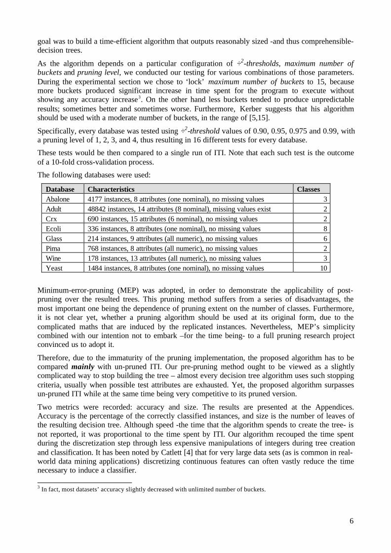
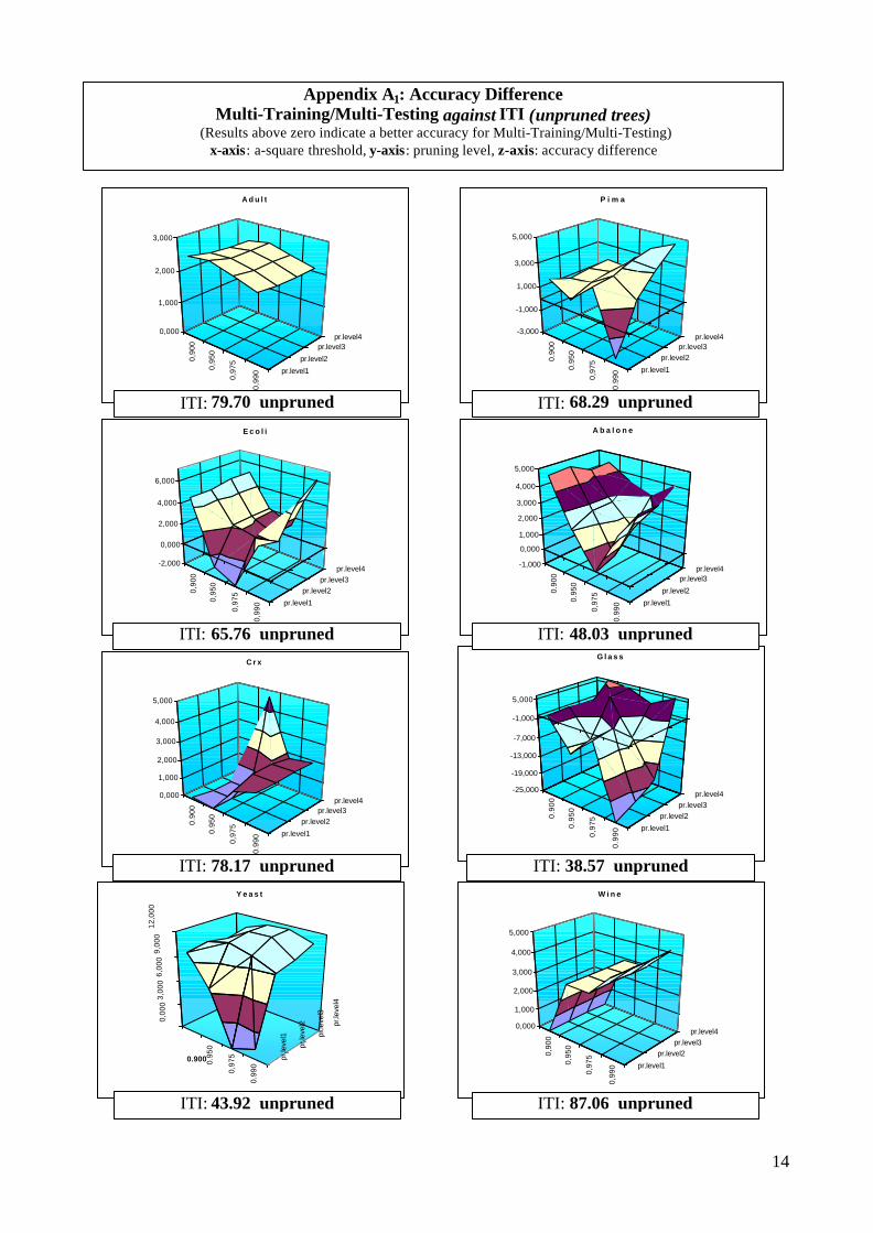
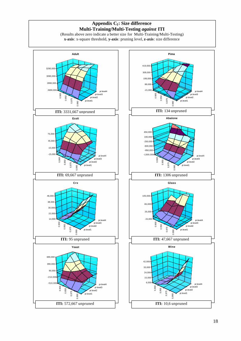
We felt that a graphical representation of the relative superiority of the one or the other algorithmwould be more emphatic, so we chose a three-dimensional method for presenting them. This waywe were hoping to unveil hidden characteristics of the whole approach; identifying good points orpossible pitfalls. Throughout the experiments, x-axis represents ÷2-threshold and y-axis representsthe pruning level. On the other hand, z-axis represents accuracy or size differences between the twodifferent algorithms, noted at the top of each page.

We first present the accuracy results (Appendix A). The comparison of un-pruned trees gives a clearwinner; with the exception of Glass database the proposed approach outperforms ITI by acomfortable margin. It is interesting to note that under-performance (regardless of whether this isobserved against ITI with or without pruning) is usually associated with high ÷2-threshold valuescombined with small pruning levels – that is the case for Glass, Pima and Yeast. Worse results forsmall pruning levels are an indication that instance replication is actually beneficial. Furthermore,increasing ÷2-threshold tends to produce steeper lines in conjunction with pruning level. The ÷2-threshold metric alone does not seem to produce consistent results throughout the experiments. Itrather seems that every database, depending on its idiosyncrasy, prefers more or less fuzzinessduring the creation of buckets. Finding a specific combination of these parameters under which ourapproach does best for all circumstances is a difficult task and, quite surely, theoreticallyintractable.

It is interesting to compare our un-pruned trees with ITI’s pruned ones. This comparisonindicates a better performance for our approach under Abalone, Ecoli, Wine and Yeast and a worseone under Adult, Glass, Pima and Crx. This is extremely promising regarding the possibilities of theproposed heuristic; we believe that a sophisticated pruning scheme, such as ITI’s approach which isbased on minimum-description-length principle (MDL) [17], can produce even better results.

The simple pruning strategy currently in use gave ambiguous results, compared to the results of theunpruned trees- with the exception of Glass database where pruning results are clear worse4. Still,the differences are not great indicating that this kind of pruning just did not offer much to thedirection of trees generalization. We conjecture that our algorithm absorbed much of the pruningpotential.

Coverage results (see Appendix B) are almost throughout consistent indicating a higher accuracyfor the proposed approach. Pima database was the only one to return a higher accuracy for ITI.Recall that, ITI stops building the tree when all instances at a node belong to the same class. Thus,un-pruned ITI could not show any improvement for Coverage-2 – it simply did not have any otherclass to return. Pruning changes that, since a newly created leaf originates from a node and thus itsinstances should belong to more than one class.

4 Recall that, Glass database has only 214 instances. Furthermore, Glass has six possible problem classes, somethingthat does not favor minimum-error-pruning.

8

The main drawback of the algorithm is the size of the trees that it constructs (see Appendix C). Allgraphs show a clear increase of trees size in conjunction with pruning level. On the other hand,results for ÷2-threshold are not –for once more- consistent throughout the experiments. Havinginstances replicate themselves can result in extremely large, difficult to handle trees. Two things canprevent this from happening: discretization reduces the size of the data that the algorithmmanipulates and pre-pruning reduces the unnecessary instance proliferation along tree branches. Wehave seen that both approaches seem to work well, yet none is a solution per se. Pruning helps onthis direction too. Pruned trees are of reasonable size ; sometimes even smaller than the pruned treesof ITI. Still, adult database produced a significant bigger tree, even when we had it pruned.

5 Training and Testing Policies

The cautious reader may question the effectiveness of the set-valued approach. The observedaccuracy increase could be due to the discretization step itself and thus it could be attributed just tothe ÷2 metric and not to the set-values extension. Other questions could be raised as well, such as,why not to use set-valued instances just during training or testing – and thus preserve computingresources. Our research would be surely incomplete without taking these questions intoconsideration.

For those reasons we devised several training and testing policies. The first one uses the ÷2 metric tocreate buckets but avoids the formation of margins. This way, every attribute-value is mapped to asingle bucket, and that stands for both training and testing instances (we call it single-training/single-testing in contrast to our main multi-training/multi-testing algorithm). The derivedalgorithm can be considered as a standard decision tree creation algorithm -not very different inphilosophy from ITI- that uses ChiMerge to discretize data.

The second derived algorithm does form margins, but uses them just for training instances. Alltesting instances have their attribute-values assigned to only one bucket. We call this version multi-training/single-testing. Using the same line of thought, we derive the third version of the algorithmwhich is the exact dual of the previous one - it uses margins just for testing instances. This versionis called single-training/multi-testing.

The derived algorithms produce different classes of solutions for the build/use of decision trees,with most of the known algorithms (like ID3, C4.5, ITI) belonging to the single-training/singletesting class. An easy way to distinguish between those classes is to draw the paths that an instancefollows during training and testing (Figure 4).

Having introduced the modified algorithms we embark into an introspection journey through theiradvantages and disadvantages. When we compare ITI with our single-training/single-testingalgorithm5 (Appendix D1) we come up with a higher accuracy for the ÷2 discretization method forthe majority of ÷2-thresholds and databases. This is a strong experimental evidence in favour ofChiMerge. Still, as we shall see, we can do even better.

The comparison between the single-training/single-testing and multi-training/multi-testingalgorithm (Appendix D2) provide us with a clear indication that the set-valued approach addssomething to the learning process that can be exploited towards higher accuracy levels. Thisexploitation can be achieved using the notion of pruning level. It is clear, under every ÷2-thresholdlevel, that an increase in the pruning is associated with some increase in accuracy. It is also clearthat when an increase in the introduced fuzziness (by increasing ÷2-threshold) destabilizes thesystem (and thus, produces bad accuracy results) the pruning level reacts as a stabilising factor(producing steeper improvement lines) which quickly fills the performance gap. It seems likely that

5 All comparisons are between unpruned version of trees.

9

where standard algorithms achieve an accuracy of a%, the set-valued approach has a potential rangeof performance between [a-å1, a+å2]. It is the pruning level that gets us closer to the right limit.

Appendix D3 presents the accuracy comparison between the multi-training/multi-testing and themulti-training/single-testing algorithms. It is obvious that when we avoid set-values during testing(and thus reach only one leaf) we come up with bad results. This can be attributed to the absence ofthe majority scheme vote, which seems to make good use of the introduced fuzziness.

The results of Appendix D4 (multi-training/multi-testing vs single-training/multi-testing) weresomewhat unexpected. Those results indicate a higher accuracy, over half of the tested databases,for the version of the heuristic that uses margins just during testing. Recall that this version can beviewed as an algorithm that uses a fuzzy-thresholds-technique to guide test-instances; suchtechniques are widely used in current algorithms. The fact that this algorithm does well wasexpected, although not to such a degree. Still, there are databases (Wine, Ecoli, Glass) where themulti-training/multi-testing heuristic surpasses the single-training/multi-testing algorithm by a morethan marginal accuracy difference. Further experiments have to be conducted towards this direction,in order to establish the class of problems/databases that can be assisted more by the multi-training/multi-testing than by the single-training/multi-testing algorithm.

Single Training - Single Testing

Multi Training - Single Testing

SingleTraining - Multi Testing

Multi Training - Multi Testing

During training

Figure 4: The paths a specific instance follows under different classes ofsolutions for the build/use of decision trees

During testing

10

6 Weight-Based Instance Replication

Another interesting extension to our basic algorithm is the balanced distribution of replicatedinstances. That is, rather than replicating instances every time they have to follow both branches ofa sub-tree, we feed them to lower nodes using a weighting technique. When an instance isdiscretized, a number is attached to every discretized value of it. Those numbers indicate theweights with which initial values belong to disretized ones. Using the weights of the discretizedvalues in conjunction with the splitting tests at each node we can calculate the total weight withwhich an instance arrives at a specific leaf. The sum of weights for every two newly createdinstances is equal with the weight of their father. This way, the sum of weights of instances atleaves is exactly the number of instances at root. The whole procedure does not affect the tree sizeor the paths from which instances traverse the tree. It only affects the majority scheme we use todecide the class of a testing instance.

We extended the basic algorithm with two different weighting techniques. The first one (half-weighted) assigns equal weights to the discretized values and thus, when it finds an instance that hasto follow both branches of a node, it divides that instance’s weight half to the right and half to theleft subtree. Subsequent divisions of that instance result in further reduction of its weight overfurther nodes. The second technique (weighted) assigns weights to discretized values according tothe distance of their initial value from the margins of the bucket that value belongs to.

Figure 5 depicts this procedure. An ellipse represents an instance and its area represents thatinstance’s weight. Suppose that the buckets’ line corresponds to a dscretized attribute (say B) andthat a random instance has the value 2.5 at its B attribute. The original algorithm would discretizeattribute B by giving it the values 1, 2 assuming that the weights for those values are both equal toone.

The half-weighted algorithm would also produce the values 1, 2 but with weights ½ and ½ for eachone of them. Building on the same idea, the weighted algorithm computes the distance of 2.5 fromthe margins 2.3 and 4.5 and bears a higher weight for value 1 than for value 2 (as shown by thelarger area for the discretized value B=1). That is because the value 2.5 is closer to 2.3 than to 4.5.

To calculate the weight for the left discretized value we use the function: LRxR

−−

where R indicates

the right and L the left margin (as in Figure 5); x indicates the value that is to be discretized. In the

same manner, the weight for the right value can be computed using the function:LR

Lx

−− .

B = 2.5

B=1B=2

L = 2.3

R =

4.53

Bucket 1 Bucket 2 Bucket 3

BWeight = 9/10

Weight = 1/10

Figure 5: Discretization using the weighted algorithm

11

Now, suppose that a decision node has installed value 1 of attribute B as its test value. When theabovementioned instance arrives at that node it satisfies both branches and thus it has to follow bothsubtrees. On doing so, it uses the weights that derived at the discretization step (Figure 6).

The comparison between the weighting techniques and our main algorithm is presented inAppendix E. It is clear that the weighted variant (although more promising at first glance) producesworse results than our basic algorithm. On the other hand, the half-weighted outcomes arecomparable with the main algorithm. Still, they do nït justify the implementation overhead.

From a theoretical point of view, the proposed modifications absorb some of the set-valuesfuzziness by trying to reduce the effect of instance replication. Still, the introduced fuzziness is thevery heart of the heuristic and the struggle to reduce (or control) it is somewhat premature at thispoint of the algorithm. This effect is more evident in the weighted variant, which minimizesfuzziness too soon and thus produces the worst results.

7 Discussion

We have proposed a modification to the classical decision tree induction approach in order tohandle set-valued attributes with relatively straightforward conceptual extensions to the basicmodel. Our experiments have demonstrated that by employing a simple pre-processing stage, theproposed approach can handle efficiently numeric attributes (for a start) and yet yield significantaccuracy improvements.

As we speculated in the introductory sections, the applicability of the approach to numeric attributesseemed all too obvious. Although numeric attributes have values that span a continuum, it is notdifficult to imagine that conceptual groupings of similar objects would also share neighboringvalues. The instance space along any particular (numerical) axes usually demonstrates clusters ofobjects; these clusters are captured by the proposed discretization step. We view this as an exampleof everyday representation bias; we tend to favor descriptions that make it easier for us to groupobjects rather than allow fuzziness. This bias can be captured in a theoretical sense by theobservation that entropy gain is maximized at class boundaries for numeric attributes [6].

When numeric attributes truly have values that make it difficult to identify class-related ranges,splitting will be "terminally" affected by the observed values and testing is affected too. Ourapproach serves to offer a second chance to near-misses and as the experiments show, near-missesdo survive. The ÷2 approach to determine secondary bucket preference ensures that neighboringinstances are allowed to be of value longer than the classical approach would allow. For themajority of cases this interaction has proved beneficial.

As far as the experiments are concerned, both pruning level and ÷2-threshold value have beenproved important. There have been cases, where increasing ÷2-threshold decreased the accuracy

B=1

Weight = 1

Weight = 1

Weight = 1/10Weight = 9/10

Figure 6: An instance’s weights along the used paths

12

(compared to lower ÷2-threshold values). We attribute such a behavior to the fact that thecorresponding data sets do demonstrate a non-easily-separable class property. In such cases,increasing ÷2-threshold, thus making buckets more rigid, imposes an artificial clustering whichdeteriorates accuracy. That our approach still over-performs un-pruned ITI is a sign that the fewinstances which are directed to more than one bucket compensate for the non-flexibility of the“few” buckets available.

The proposed algorithm can also find a potential application area wherever instances with symbolicset-valued attributes are the case. Natural language processing serves as an example. Orphanos etal. [14] exemplified the use of decision trees on Part-Of-Speech tagging for Modern Greek, anatural language which, from the computational perspective, has not been widely investigated.Orphanos et al. used three different algorithms (included the proposed one) that were able to handlesymbolic set-valued attributes, a requirement posed by the nature of the linguistic datasets. Theproposed algorithm outperformed the other two by a comfortable margin, demonstrating the valueof pre-pruning too.

Scheduled improvements to the proposed approach for handling set-valued attributes span a broadspectrum. It is interesting to note that using set-valued attributes naturally paves the way fordeploying more effective post-processing schemes for various tasks (character recognition is anobvious example). By following a few branches, one need not make a guess about the second bestoption based on only one node, as is usually the case. Our coverage results show that significantgains can be materialized.

Another important line of research concerns the development of a suitable post-pruning strategy.Instance replication complicates the maths involved in estimating error, and standard approachesneed to be better studied (for example, it is not at all obvious how minimum-description-lengthpruning might be readily adapted to set-valued attributes). Furthermore, we need to explore theextent to which instance replication does (or, hopefully, does not) seriously affect the efficiency ofincremental decision tree algorithms.

Recall that the algorithm depends on various parameters (÷2, max-buckets, pruning-level) that often

need special tuning -over a specific database- so as to obtain optimal results regarding accuracy andsize. It seems worthy to build on a meta-learner scheme where the algorithm would self-decide (viaexperiments) the values for its parameters. We are envisioning such a scheme that uses geneticalgorithms to evolve the parameters.

We feel that the proposed approach opens up a range of possibilities for decision tree induction. Bybeefing it up with the appropriate mathematical framework we may be able to say that a little bit ofcarefully introduced fuzziness improves the learning process.

References

1. Ali, K.M. and Pazzani, M.J., Error Reduction through Learning Multiple Descriptions, MachineLearning, 24, 173-202, 1996.

2. Blake, C., Keogh, E. and Merz, J., UCI Repository of machine learning databases[http://www.ics.uci.edu/~mlearn/MLRepository.html]. Irvine, CA: University of California,Department of Information and Computer Science, 1999.

3. Breiman, L., Bagging Predictors, Machine Learning 24, 123-140, 1996.

4. Catlett, J., On changing continuous attributes into ordered discrete attributes, In proceedings ofthe European Working Session on Learning, 164-178, 1991.

5. Cohen, W., Learning Trees and Rules with Set-valued Features, In Proceedings of AAAI-96,1996.

13

6. Fayyad, U.M. and Irani, K.B., On the Handling of Continuous-Valued Attributes on DecisionTree Generation, Machine Learning, 8, 87-102, 1992.

7. Freund, Y., Boosting a Weak Learning Algorithm by Majority. Information and Computation,121(2), 256-285, 1996.

8. Kalles, D., Decision trees and domain knowledge in pattern recognition, PhD Thesis, Universityof Manchester, 1994.

9. Kohavi, R. and Sahami, M., Error-Based and Entropy-Based Discretization of ContinuousFeatures, In Proceedings of the second International Conference of Knowledge Discovery and DataMining, 1996.

10. Kohavi, R. and Clayton, K., Option Decision Trees with Majority Votes. In proceedings ofICML97, 1997.

11. Kerber, R., Chimerge: Discretization of numeric attributes. In proceedings of the 10th NationalConference on Artificial Intelligence, San Jose, CA. MIT Press. 123-128, 1992.

12. Kwok, S.W. and Carter, C., Multiple Decision Trees. In Proceedings of the Uncertainty inArtificial Intelligence 4, (R.D. Shachter, T.S. Levitt, L.N. Kanal, and J.F. Lemmer, eds.), 1990.

13. Martin, J.D. and Billman, D.O., Acquiring and Combining Overlapping Concepts. MachineLearning, 16, 121-160, 1994.

14. Orphanos, G., Kalles, D., Papagelis, A. and Christodoulakis, D., Decision trees and NLP: ACase Study in POS Tagging, In proceedings of ACAI’99, 1999.

15. Quinlan, J.R., Induction of Decision Trees, Machine Learning, 1, 81-106, 1986.

16. Quinlan, J.R., Decision trees as probabilistic classifiers. In Proceedings of the 4th InternationalWorkshop on Machine Learning, Irvine, CA, 31-37, 1987.

17. Quinlan, J.R., Rivest, R.L., Infering Decision Trees Using the Minimum Description LengthPrinciple, In proceedings of the 10th International Conference on Machine Learning, Amherst, MA,252-259, 1993.

18. Quinlan, J.R., C4.5, Programs for machine learning, San Mateo, CA, Morgan Kaufmann, 1993.

19. Utgoff, P.E., Decision Tree Induction Based on Efficient Tree Restructuring, MachineLearning, 29, 5-44, 1997.

14

Appendix A1: Accuracy DifferenceMulti-Training/Multi-Testing against ITI (unpruned trees)

(Results above zero indicate a better accuracy for Multi-Training/Multi-Testing)x-axis: a-square threshold, y-axis: pruning level, z-axis: accuracy difference

0,9

00

0,9

50

0,9

75

0,9

90 pr.level1

pr.level2

pr.level3

pr.level40,000

1,000

2,000

3,000

A d u l t

0.9

00

0.9

50

0,9

75

0.9

90 pr.level1

pr.level2

pr.level3

pr.level4-3,000

-1,000

1,000

3,000

5,000

P i m a0

,90

0

0,9

50

0,9

75

0,9

90 pr.level1

pr.level2

pr.level3

pr.level4-2,000

0,000

2,000

4,000

6,000

E c o l i

0.9

00

0.9

50

0,9

75

0.9

90 pr.level1

pr.level2

pr.level3

pr.level4-1,000

0,000

1,000

2,000

3,000

4,000

5,000

A b a l o n e

0.9

00

0.9

50

0,9

75

0.9

90 pr.level1

pr.level2

pr.level3

pr.level40,000

1,000

2,000

3,000

4,000

5,000

C r x

0.9

00

0.9

50

0,9

75

0.9

90 pr.level1

pr.level2

pr.level3

pr.level4-25,000

-19,000

-13,000

-7,000

-1,000

5,000

G l a s s

0.900 0.9

50

0,9

75

0.9

90

pr.

leve

l1

pr.

leve

l2

pr.

leve

l3

pr.

leve

l4

0,0

00

3,0

00

6,0

00

9,0

00

12

,00

0

Y e a s t

0,9

00

0,9

50

0,9

75

0,9

90 pr.level1

pr.level2

pr.level3

pr.level40,000

1,000

2,000

3,000

4,000

5,000

W i n e

ITI: 79.70 unpruned ITI: 68.29 unpruned

ITI: 65.76 unpruned ITI: 48.03 unpruned

ITI: 78.17 unpruned ITI: 38.57 unpruned

ITI: 43.92 unpruned ITI: 87.06 unpruned

15

0,9

00

0,9

50

0,9

75

0,9

90 pr.level1

pr.level2

pr.level3

pr.level40,000

1,000

2,000

3,000

A d u l t

Appendix A2: Accuracy DifferenceMulti-Training/Multi-Testing against ITI (pruned trees)

(Results above zero indicate a better accuracy for Multi-Training/Multi-Testing)x-axis: a-square threshold, y-axis: pruning level, z-axis: accuracy difference

0.9

00

0.9

50

0,9

75

0.9

90 pr.level1

pr.level2

pr.level3

pr.level4-5,000

-4,000

-3,000

-2,000

-1,000

0,000

P i m a

ITI: 73.68 pruned

0,9

00

0,9

50

0,9

75

0,9

90

pr.

leve

l1

pr.

leve

l2

pr.

leve

l3

pr.

leve

l4

-3,000

-1,000

1,000

3,000

5,000

E c o l i

0.9

00

0.9

50

0,9

75

0.9

90 pr.level1

pr.level2

pr.level3

pr.level4-3,000

-2,000

-1,000

0,000

1,000

2,000

A b a l o n e

0.9

00

0.9

50

0,9

75

0.9

90 pr.level1

pr.level2

pr.level3

pr.level4-3,000

-2,000

-1,000

0,000

Crx

0.9

00

0.9

50

0,9

75

0.9

90 pr.level1

pr.level2

pr.level3

pr.level4-15,000

-11,000

-7,000

-3,000

1,000

5,000

G l a s s

0.9

00

0.9

50

0,9

75

0.9

90 pr.level1

pr.level2

pr.level3

pr.level4-4,000

-2,000

0,000

2,000

4,000

6,000

Y e a s t

0,900 0,9

50

0,9

75

0,9

90

pr.

leve

l1

pr.

leve

l2

pr.

leve

l3

pr.

leve

l4

-3,0

00-2,0

00-1

,00

0 0,0

001

,00

02,0

003

,00

0

W i n e

ITI: 66.37 pruned ITI: 50.60 pruned

ITI: 83.33 pruned ITI: 36.67 pruned

ITI: 47.70 pruned ITI: 88.24 pruned

ITI: 82.42 pruned

16

0.9

00

0.9

50

0,9

75

0.9

90 pr.level1

pr.level2

pr.level3

pr.level411,000

15,000

19,000

23,000

27,000

31,000

P i m a

0,900 0,9

50

0,9

75

0,9

90

pr.

leve

l1

pr.

leve

l2

pr.

leve

l3

pr.

leve

l4

18

,00

019

,00

020

,00

021

,00

02

2,0

00

E c o l i

0.9

00

0.9

50

0,9

75

0.9

90 pr.level1

pr.level2

pr.level3

pr.level434,000

35,000

36,000

37,000

38,000

A b a l o n e

0.9

00

0.9

50

0,9

75

0.9

90 pr.level1

pr.level2

pr.level3

pr.level424,000

27,000

30,000

33,000

36,000

39,000

G l a s s

0.9

00

0.9

50

0,9

75

0.9

90 pr.level1

pr.level2

pr.level3

pr.level430,000

32,000

34,000

36,000

38,000

Y e a s t

0,9

00

0,9

50

0,9

75

0,9

90 pr.level1

pr.level2

pr.level3

pr.level42,000

3,000

4,000

5,000

6,000

7,000

8,000

9,000

W i n e

Appendix B1: Accuracy Difference for Coverage2Multi-Training/Multi-Testing against ITI (unpruned trees)

(Results above zero indicate a better accuracy for Multi-Training/Multi-Testing)x-axis: a-square threshold, y-axis: pruning level, z-axis: accuracy difference

ITI: 79.70 unpruned ITI: 65.76 unpruned

ITI: 48.03 unpruned ITI: 43.92 unpruned

ITI: 87.06 unpruned ITI: 38.57 unpruned

17

0.9

00

0.9

50

0,9

75

0.9

90 pr.level1

pr.level2

pr.level3

pr.level4-12,000

-8,000

-4,000

0,000

P i m a

0,9

00

0,9

50

0,9

75

0,9

90 pr.level1

pr.level2

pr.level3

pr.level4-2,000

0,000

2,000

4,000

E c o l i

0.9

00

0.9

50

0,9

75

0.9

90 pr.level1

pr.level2

pr.level3

pr.level42,000

3,000

4,000

5,000

6,000

A b a l o n e

0.9

00

0.9

50

0,9

75

0.9

90 pr.level1

pr.level2

pr.level3

pr.level410,000

13,000

16,000

19,000

22,000

G l a s s

0.9

00

0.9

50

0,9

75

0.9

90 pr.level1

pr.level2

pr.level3

pr.level43,000

5,000

7,000

9,000

11,000

Y e a s t

0,9

00

0,9

50

0,9

75

0,9

90

pr.

leve

l1

pr.

leve

l2

pr.

leve

l3

pr.

leve

l4

1,000

2,000

3,000

4,000

5,000

6,000

7,000

W i n e

Appendix B2: Accuracy difference for Coverage2Multi-Training/Multi-Testing against ITI (pruned trees)

(Results above zero indicate a better accuracy for Multi-Training/Multi-Testing)x-axis: x-square threshold, y-axis: pruning level, z-axis: accuracy difference

ITI: 97.50 pruned ITI: 81.51 pruned

ITI: 80.86 pruned ITI: 52.86 pruned

ITI: 70.07 pruned ITI: 92.94 pruned

18

Appendix C1: Size differenceMulti-Training/Multi-Testing against ITI

(Results above zero indicate a better size for Multi-Training/Multi-Testing)x-axis: x-square threshold, y-axis: pruning level, z-axis: size difference

0.9

00

0.9

50

0,9

75

0.9

90 pr.level1

pr.level2

pr.level3

pr.level42690,000

2890,000

3090,000

3290,000

Adult

0.9

00

0.9

50

0,9

75

0.9

90 pr.level1

pr.level2

pr.level3

pr.level4-21,000

89,000

199,000

309,000

419,000

Pima

0,9

00

0,9

50

0,9

75

0,9

90 pr.level1

pr.level2

pr.level3

pr.level4-15,000

15,000

45,000

75,000

Ecoli

0.9

00

0.9

50

0,9

75

0.9

90 pr.level1

pr.level2

pr.level3

pr.level4-1300,000

-950,000

-600,000

-250,000

100,000

450,000

Abalone

0.9

00

0.9

50

0,9

75

0.9

90 pr.level1

pr.level2

pr.level3

pr.level4-15,000

25,000

65,000

105,000

Glass

0.9

00

0.9

50

0,9

75

0.9

90 pr.level1

pr.level2

pr.level3

pr.level414,000

22,000

30,000

38,000

46,000

Crx

0.9

00

0.9

50

0,9

75

0.9

90 pr.level1

pr.level2

pr.level3

pr.level4-510,000

-210,000

90,000

390,000

690,000

Yeast

0,9

00

0,9

50

0,9

75

0,9

90 pr.level1

pr.level2

pr.level3

pr.level46,000

15,000

24,000

33,000

42,000

Wine

ITI: 3331,667 unpruned ITI: 134 unpruned

ITI: 1306 unpruned

ITI: 95 unpruned ITI: 47,667 unpruned

ITI: 572,667 unpruned ITI: 10,6 unpruned

ITI: 69,667 unpruned

19

Appendix C2: Size differenceMulti-Training/Multi-Testing against ITI

(Results above zero indicate a better size for Multi-Training/Multi-Testing)x-axis: x-square threshold, y-axis: pruning level, z-axis : size difference

0.9

00

0.9

50

0,9

75

0.9

90 pr.level1

pr.level2

pr.level3

pr.level42450,000

2550,000

2650,000

2750,000

2850,000

A d u l t

0.9

00

0.9

50

0,9

75

0.9

90 pr.level1

pr.level2

pr.level3

pr.level435,000

125,000

215,000

305,000

P i m a

0,9

00

0,9

50

0,9

75

0,9

90 pr.level1

pr.level2

pr.level3

pr.level4-13,000

-8,000

-3,000

2,000

7,000

E c o l i

0.900 0.9

50

0,9

75

0.9

90

pr.

leve

l1

pr.

leve

l2

pr.

leve

l3

pr.

leve

l4

-37

0,0

00

-13

0,0

00

11

0,0

0035

0,0

0059

0,0

00

A b a l o n e

0.9

00

0.9

50

0,9

75

0.9

90 pr.level1

pr.level2

pr.level3

pr.level4-7,000

-1,000

5,000

11,000

17,000

G l a s s

0.9

00

0.9

50

0,9

75

0.9

90

pr.

leve

l1

pr.

leve

l2

pr.

leve

l3

pr.

leve

l4

53,000

56,000

59,000

62,000

65,000

C r x

0.9

00

0.9

50

0,9

75

0.9

90 pr.level1

pr.level2

pr.level3

pr.level4-200,000

-172,000

-144,000

-116,000

Y e a s t

0,9

00

0,9

50

0,9

75

0,9

90 pr.level1

pr.level2

pr.level3

pr.level44,000

7,000

10,000

13,000

W i n e

ITI: 665 pruned ITI: 32 pruned

ITI: 26,67 pruned ITI: 371,67 pruned

ITI: 16,33 pruned ITI: 22,333 pruned

ITI: 202,67 pruned ITI: 5,8 pruned

20

Appendix D1: Accuracy Difference Single-Training/Single-Testing against ITI

( Results above zero indicate better accuracy for Single-Training/Single-Testing)x-axis: x-square threshold, y-axis : pruning level, z-axis: accuracy difference

0,9

00

0,9

50

0,9

75

0,9

90 pr.level1

pr.level2

pr.level3

pr.level4-1,000

0,000

1,000

2,000

3,000

Adult

0.9

00

0.9

50

0,9

75

0.9

90 pr.level1

pr.level2

pr.level3

pr.level4-1,000

0,000

1,000

2,000

3,000

P i m a0

,90

0

0,9

50

0,9

75

0,9

90 pr.level1

pr.level2

pr.level3

pr.level4-1,000

1,000

3,000

5,000

7,000

E c o l i

0.900 0.9

50

0,9

75

0.9

90

pr.

leve

l1

pr.

leve

l2

pr.

leve

l3

pr.

leve

l4

-1,0

00

0,0

00

1,0

00

Crx

0.900 0.9

50

0,9

75

0.9

90

pr.

leve

l1

pr.

leve

l2

pr.

leve

l3

pr.

leve

l4

-1,0

00 1

,00

03,0

00

5,0

007

,00

09

,00

0

G l a s s

0.9

00

0.9

50

0,9

75

0.9

90 pr.level1

pr.level2

pr.level3

pr.level4-1,000

1,000

3,000

5,000

7,000

Y e a s t

0,9

00

0,9

50

0,9

75

0,9

90 pr.level1

pr.level2

pr.level3

pr.level4-2,000

-1,000

0,000

1,000

2,000

W i n e

ITI: 79.70 unpruned

ITI: 78.17 unpruned

ITI: 43.92 unpruned

ITI: 68.29 unpruned

ITI: 87.06 unpruned

0.900 0.9

50

0,9

75

0.9

90

pr.

leve

l1

pr.

leve

l2

pr.

leve

l3

pr.

leve

l4

-1,000

0,000

1,000

2,000

3,000

A b a l o n e

ITI: 38.57 unpruned

ITI: 65.76 unpruned ITI: 48.03 unpruned

21

Appendix D2: Accuracy Difference Multi-Training/Multi-Testing against Single-Training/Single-Testing

(Results above zero indicate better accuracy for Multi-Training/Multi-Testing) x-axis: a-square threshold, y-axis: pruning level, z-axis: accuracy difference

0,9

00

0,9

50

0,9

75

0,9

90 pr.level1

pr.level2

pr.level3

pr.level4-1,000

0,000

1,000

Adult

0.9

00

0.9

50

0,9

75

0.9

90 pr.level1

pr.level2

pr.level3

pr.level4-6,000

-3,000

0,000

3,000

Pima

0,9

00

0,9

50

0,9

75

0,9

90 pr.level1

pr.level2

pr.level3

pr.level4-10,000

-6,000

-2,000

2,000

Ecoli

0.9

00

0.9

50

0,9

75

0.9

90 pr.level1

pr.level2

pr.level3

pr.level4-1,000

1,000

3,000

5,000

Crx

0.9

00

0.9

50

0,9

75

0.9

90 pr.level1

pr.level2

pr.level3

pr.level4-31,000

-24,000

-17,000

-10,000

-3,000

Glass

0.9

00

0.9

50

0,9

75

0.9

90 pr.level1

pr.level2

pr.level3

pr.level4-7,000

-4,000

-1,000

2,000

5,000

Yeast

0,9

00

0,9

50

0,9

75

0,9

90 pr.level1

pr.level2

pr.level3

pr.level4-1,000

1,000

3,000

5,000

Wine

0.9

00

0.9

50

0,9

75

0.9

90 pr.level1

pr.level2

pr.level3

pr.level4-3,000

-1,000

1,000

3,000

Abalone

22

Appendix D3: Accuracy Difference Multi-Training/Multi-Testing against Multi-Training/Single-Testing

(Results above zero indicate better accuracy for Multi-Training/Multi-Testing) x-axis: a-square threshold, y-axis: pruning level, z-axis: accuracy difference

0,9

00

0,9

50

0,9

75

0,9

90 pr.level1

pr.level2

pr.level3

pr.level40,000

1,000

2,000

Adult

0,9

0

0,9

5

0,9

75

0,9

9 pr.level1

pr.level2

pr.level3

pr.level40,000

2,000

4,000

6,000

8,000

10,000

12,000

Pima

0,9

00

0,9

50

0,9

75

0,9

90 pr.level1

pr.level2

pr.level3

pr.level40,000

2,000

4,000

6,000

8,000

10,000

12,000

Ecoli

0,9

0

0,9

5

0,9

75

0,9

9 pr.level1

pr.level2

pr.level3

pr.level40,000

2,000

4,000

6,000

8,000

10,000

Abalone

0,9

0

0,9

5

0,9

75

0,9

9 pr.level1

pr.level2

pr.level3

pr.level4-1,000

0,000

1,000

2,000

3,000

4,000

5,000

Crx

0,9

0

0,9

5

0,9

75

0,9

9 pr.level1

pr.level2

pr.level3

pr.level4-11,000

-6,000

-1,000

4,000

9,000

Glass

0,9

0,9

5

0,9

75

0,9

9 pr.level1

pr.level2

pr.level3

pr.level4-5,000

-2,000

1,000

4,000

7,000

10,000

13,000

Yeast

0,9

00

0,9

50

0,9

75

0,9

90 pr.level1

pr.level2

pr.level3

pr.level40,000

2,000

4,000

6,000

8,000

10,000

Wine

23

Appendix D4: Accuracy Difference Multi-Training/Multi-Testing against Single-Training/Multi-Testing

(Results above zero indicate better accuracy for Multi-Training/Multi-Testing) x-axis: a-square threshold, y-axis: pruning level, z-axis: accuracy difference

0,9

00

0,9

50

0,9

75

0,9

90 pr.level1

pr.level2

pr.level3

pr.level4-3,000

-2,000

-1,000

0,000

1,000

Adult

0.9

00

0.9

50

0,9

75

0.9

90 pr.level1

pr.level2

pr.level3

pr.level4-10,000

-8,000

-6,000

-4,000

-2,000

0,000

Pima0

,90

0

0,9

50

0,9

75

0,9

90 pr.level1

pr.level2

pr.level3

pr.level4-3,000

-2,000

-1,000

0,000

1,000

2,000

3,000

4,000

Ecoli

0.9

00

0.9

50

0,9

75

0.9

90 pr.level1

pr.level2

pr.level3

pr.level4-6,000

-4,000

-2,000

0,000

2,000

Abalone

0.9

00

0.9

50

0,9

75

0.9

90 pr.level1

pr.level2

pr.level3

pr.level4-2,000

-1,000

0,000

1,000

2,000

3,000

4,000

5,000

Crx

0.9

00

0.9

50

0,9

75

0.9

90 pr.level1

pr.level2

pr.level3

pr.level4-20,000

-15,000

-10,000

-5,000

0,000

5,000

10,000

Glass

0.9

00

0.9

50

0,9

75

0.9

90 pr.level1

pr.level2

pr.level3

pr.level4-10,000

-7,000

-4,000

-1,000

Yeast

0,9

00

0,9

50

0,9

75

0,9

90 pr.level1

pr.level2

pr.level3

pr.level4-3,000

0,000

3,000

6,000

9,000

Wine

24

0,9

00

0,9

50

0,9

75

0,9

90 pr.level1

pr.level2

pr.level3

pr.level4-1,000

0,000

1,000

A d u l t

0.9

00

0.9

50

0,9

75

0.9

90 pr.level1

pr.level2

pr.level3

pr.level4-2,000

-1,000

0,000

1,000

P i m a

0,9

00

0,9

50

0,9

75

0,9

90 pr.level1

pr.level2

pr.level3

pr.level4-4,000

-3,000

-2,000

-1,000

0,000

1,000

E c o l i

0.9

00

0.9

50

0,9

75

0.9

90 pr.level1

pr.level2

pr.level3

pr.level4-1,000

0,000

1,000

Crx

0.9

00

0.9

50

0,9

75

0.9

90 pr.level1

pr.level2

pr.level3

pr.level4-1,000

0,000

1,000

2,000

Y e a s t

0,9

00

0,9

50

0,9

75

0,9

90

pr.

leve

l1

pr.

leve

l2

pr.

leve

l3

pr.

leve

l4

-1,0

00

0,0

00

1,0

00

W i n e

0.9

00

0.9

50

0,9

75

0.9

90

pr.

leve

l1

pr.

leve

l2

pr.

leve

l3

pr.

leve

l4

-12,000

-8,000

-4,000

0,000

4,000

8,000

12,000

G l a s s

0.9

00

0.9

50

0,9

75

0.9

90 pr.level1

pr.level2

pr.level3

pr.level4-1,000

0,000

1,000

A b a l o n e

Appendix E1: Accuracy Difference Multi-Training/Multi-Testing against Multi-Training/Multi-Testing (Half-Weighted)

( Results above zero indicate better accuracy for Multi-Training/Multi-Testing)x-axis: a-square threshold, y-axis: pruning level, z-axis : accuracy difference

ITI: 79.70 unpruned ITI: 68.29 unpruned

ITI: 65.76 unpruned ITI: 48.03 unpruned

ITI: 78.17 unpruned ITI: 38.57 unpruned

ITI: 43.92 unpruned ITI: 87.06 unpruned

25

0,9

00

0,9

50

0,9

75

0,9

90 pr.level1

pr.level2

pr.level3

pr.level4-1,000

0,000

1,000

2,000

3,000

A d u l t

0.9

00

0.9

50

0,9

75

0.9

90 pr.level1

pr.level2

pr.level3

pr.level4-1,000

0,000

1,000

2,000

P i m a0

,90

0

0,9

50

0,9

75

0,9

90 pr.level1

pr.level2

pr.level3

pr.level4-7,000

-4,000

-1,000

2,000

E c o l i

0.9

00

0.9

50

0,9

75

0.9

90 pr.level1

pr.level2

pr.level3

pr.level4-1,000

0,000

1,000

2,000

3,000

4,000

C r x

0.9

00

0.9

50

0,9

75

0.9

90 pr.level1

pr.level2

pr.level3

pr.level4-3,000

1,000

5,000

9,000

13,000

G l a s s

0.9

00

0.9

50

0,9

75

0.9

90 pr.level1

pr.level2

pr.level3

pr.level4-4,000

-1,000

2,000

5,000

8,000

Y e a s t

0,9

00

0,9

50

0,9

75

0,9

90 pr.level1

pr.level2

pr.level3

pr.level4-1,000

0,000

1,000

W i n e

Appendix E2: Accuracy Difference Multi-Training/Multi-Testing against Multi-Training/Multi-Testing (Weighted)

(Results above zero indicate better accuracy for Multi-Training/Multi-Testing)x-axis: a-square threshold, y-axis: pruning level, z-axis: accuracy difference

0.9

00

0.9

50

0,9

75

0.9

90 pr.level1

pr.level2

pr.level3

pr.level4-1,000

1,000

3,000

5,000

A b a l o n e

ITI: 79.70 unpruned ITI: 68.29 unpruned

ITI: 65.76 unpruned ITI: 48.03 unpruned

ITI: 78.17 unpruned ITI: 38.57 unpruned

ITI: 43.92 unpruned ITI: 87.06 unpruned