Studying Hunter-Gatherer Mobility Using Isotopic and Trace Elemental Analysis
414
University of Alberta STUDYING HUNTER-GATHERER MOBILITY USING ISOTOPIC AND TRACE ELEMENTAL ANALYSIS by Ian Fraser-Shapiro A thesis submitted to the Faculty of Graduate Studies and Research in partial fulfillment of the requirements for the degree of Doctor of Philosophy Department of Anthropology ©Ian Fraser-Shapiro Spring 2012 Edmonton, Alberta Permission is hereby granted to the University of Alberta Libraries to reproduce single copies of this thesis and to lend or sell such copies for private, scholarly or scientific research purposes only. Where the thesis is converted to, or otherwise made available in digital form, the University of Alberta will advise potential users of the thesis of these terms. The author reserves all other publication and other rights in association with the copyright in the thesis and, except as herein before provided, neither the thesis nor any substantial portion thereof may be printed or otherwise reproduced in any material form whatsoever without the author's prior written permission.
Transcript of Studying Hunter-Gatherer Mobility Using Isotopic and Trace Elemental Analysis

University of Alberta
STUDYING HUNTER-GATHERER MOBILITY USING ISOTOPIC AND TRACE ELEMENTAL ANALYSIS
by
Ian Fraser-Shapiro
A thesis submitted to the Faculty of Graduate Studies and Research in partial fulfillment of the requirements for the degree of
Doctor of Philosophy
Department of Anthropology
©Ian Fraser-Shapiro
Spring 2012 Edmonton, Alberta
Permission is hereby granted to the University of Alberta Libraries to reproduce single copies of this thesis and to lend or sell such copies for private, scholarly or scientific
research purposes only. Where the thesis is converted to, or otherwise made available in digital form, the University of Alberta will advise potential users of the thesis of these
terms.
The author reserves all other publication and other rights in association with the copyright in the thesis and, except as herein before provided, neither the thesis nor any substantial portion thereof may be printed or otherwise reproduced in any material form
whatsoever without the author's prior written permission.

ABSTRACT
This research comprises a series of papers to address the methodology of
studying hunter-gatherer mobility in prehistoric populations. As a laboratory for this
research, middle Holocene hunter-gatherer groups from Cis-Baikal, Siberia were
analyzed as part of ongoing research by the Baikal Archaeology Project. Paper no. 1
focuses on theoretical considerations of how researchers approach the concept of
mobility with regard to hunter-gatherers along with regional background information and
discussions on the specifics of using geochemical techniques to track human mobility in
the archaeological record. Paper no. 2 presents the methodology to enable laser ablation
ICP-MS analysis of teeth for strontium isotopic research with specific focus on correction
procedures for known interferences encountered using laser ablation as a sampling
method. The paper also presents groundwork for a new approach in trace element
analysis of teeth for provenancing purposes. Paper no. 3 presents the technique of micro-
sampling of skeletal materials for laser ablation with specific focus on long bones. The
purpose of micro-sampling is to target bone micro-structures to access diagenetically
resistant portions of the bones and to recover biogenic strontium isotopic and trace
elemental data. Paper no. 4 presents the results of extensive regional geochemical
mapping including plants, water sources and faunal remains throughout the Cis-Baikal
region. Coupled with this map is an analysis of molars from 16 individuals recovered
from small cemeteries distributed across the Cis-Baikal region. General characteristics of
the geochemical environment and mobility patterns elucidated through further
provenance analysis are discussed too. Finally, in paper no. 5, a summary of all new
findings is presented along with the assessment of the methods employed in this research.
As theoretical and analytical considerations intertwine, the resultant inferences can
provide astounding revelations about prehistoric populations. For the middle Holocene
hunter-gatherers of Lake Baikal, Siberia, this approach provides valuable new insights
and research directions.

TABLE OF CONTENTS
Chapter 1: Introduction ................................................................................. 1
Overview...................................................................................................... 1
Regional Background .................................................................................. 3
Culture History ............................................................................................ 6
Thesis Content ............................................................................................. 9
Works Cited ................................................................................................. 11
Chapter 2: Mobility patterns during the middle Holocene of Cis-Baikal: theoretical and methodological considerations ............................................ 16
Introduction .................................................................................................. 17
Hunter-Gatherer Mobility ............................................................................ 23
Terminology ......................................................................................... 24
Local Signals and Migration ................................................................ 26
Principles of Strontium Catchment ...................................................... 28
Cis-Baikal Geology ..................................................................................... 32
Hunter-Gatherer Mobility in Cis-Baikal ...................................................... 37
Bone and Tooth Formation and Alteration .................................................. 42
Tooth Mineralization ........................................................................... 42
Bone Formation ................................................................................... 46
Taphonomy and Diagenesis of Bone ................................................... 55
Research Goals ............................................................................................ 67
Dietary Averaging and Biases ............................................................. 68
Bone Consumption by Humans ........................................................... 70
Methodological Improvements ............................................................ 71
Laboratory Methods ..................................................................................... 72
Background .......................................................................................... 72
Interferences and Corrections .............................................................. 73

Analytical Methods ...................................................................................... 76
Mapping Biogeochemical Variability .................................................. 77
Reference Materials ............................................................................. 78
Summary ...................................................................................................... 80
Works Cited ................................................................................................. 82
Chapter 3: Assessing hunter-gatherer mobility in Cis-Baikal, Siberia using LA-ICP-MS: Methodological correction for laser interactions with calcium phosphate matrices and the potential for integrated LA-ICP-MS sampling of archaeological skeletal materials ................................................................... 98
Introduction .................................................................................................. 99
Hunter-Gatherer Mobility in Cis-Baikal ...................................................... 100
Khuzhir-Nuge XIV Cemetery ...................................................................... 104
Principles of Strontium Catchment .............................................................. 106
Tooth Mineralization ................................................................................... 107
Laser Ablation of Teeth ............................................................................... 111
Materials and Methods ................................................................................ 113
Results and Discussion ................................................................................ 118
Conclusion ................................................................................................... 136
Works Cited ................................................................................................. 138
Chapter 4: Micro-sampling of human bones for mobility studies: diagenetic impacts and potentials for elemental and isotopic research ........................ 145
Introduction .................................................................................................. 146
Hunter-Gatherer Mobility in Cis-Baikal ...................................................... 149
Khuzhir-Nuge XIV Cemetery ...................................................................... 151
Microbial Biodeterioration .......................................................................... 155
Materials and Methods ................................................................................ 157
Results and Discussion ................................................................................ 161
Elemental Composition ........................................................................ 161

Microbial Action .................................................................................. 171
Correction Methods ............................................................................. 174
Conclusion ................................................................................................... 177
Works Cited ................................................................................................. 179
Chapter 5: Spatial variability of biologically available 87Sr/86Sr, rare earth and trace elements in the Cis-Baikal region, Siberia: Evidence from modern environmental samples and small Neolithic and Early Bronze Age cemeteries .................................................................................... 183
Introduction .................................................................................................. 184
Cis-Baikal Resources ................................................................................... 185
Cis-Baikal Geology ..................................................................................... 186
Tooth Mineralization ................................................................................... 189
Laser Ablation on Teeth .............................................................................. 191
Materials: Environmental Samples .............................................................. 193
Materials: Human Samples .......................................................................... 197
Borki, Manzurka, and Obkhoi (upper Lena) and Ostrov Zhiloi (Angara) ... 198
Khotoruk and Shamanskii Mys (Little Sea) ................................................ 199
Sample Preparation and Analysis ................................................................ 200
Statistical Methods ....................................................................................... 201
Environmental Results ................................................................................. 202
Human Results ............................................................................................. 207
Borki ........................................................................................................... 214
Manzurka ..................................................................................................... 214
Obkhoi ......................................................................................................... 214
Ostrov Zhiloi ................................................................................................ 215
Khotoruk ...................................................................................................... 215
Shamanskii Mys ........................................................................................... 216
Discussion .................................................................................................... 218

Conclusion ................................................................................................... 224
Works Cited ................................................................................................. 226
Chapter 6: Synthesis and Conclusion ........................................................... 234
Individual Life History Approach ................................................................ 234
Technical Impacts ........................................................................................ 235
Laser Ablation Correction Factors ....................................................... 236
Micro-sampling of Human Molars ...................................................... 240
Micro-sampling of Long Bones ........................................................... 243
Diagenetic Research ............................................................................ 246
Reference Materials ............................................................................. 247
Overall Methodological Contribution .................................................. 251
Relevance for Subsistence, Mobility, and Beyond ...................................... 253
Mobility ............................................................................................... 253
Kinship ................................................................................................. 255
New Frontiers of Research: Beyond Cis-Baikal .......................................... 257
Final Remarks .............................................................................................. 263
Works Cited ................................................................................................. 264

List of Tables
1-1: Cultural History Chronology ..................................................................... 8
2-2: Histological index values for diagenetic changes ...................................... 63
4-1: Averaged laser ablation and solution mode 87Sr/86Sr ratios ....................... 155
5-1: Location, cultural, and chronological data for cemeteries ......................... 197
5-2: Micro-regional comparisons for 87Sr/86Sr data ......................................... 202
5-3: Provenance determinations for individual skeletal elements analyzed ..... 211
Appendix A ....................................................................................................... 269
Appendix B ....................................................................................................... 270
Appendix C ....................................................................................................... 290
Appendix D ....................................................................................................... 292
Appendix E ....................................................................................................... 294
Appendix F ....................................................................................................... 306
Appendix G ....................................................................................................... 309
Appendix H ....................................................................................................... 318
Appendix I ........................................................................................................ 364

List of Figures
1-1: Cis-Baikal regional map with geological and cultural areas ..................... 4
2-1: Cis-Baikal regional map with geological and cultural areas ..................... 33
2-2: Schematic representation of microbial destruction in bone ....................... 61
3-1: Cis-Baikal regional map with geological and cultural areas ..................... 102
3-2: Sampling scheme used on sectioned teeth ................................................. 116
3-3: Rubidium values by spot size .................................................................... 120
3-4: Strontium values by spot size .................................................................... 120
3-5: Effects of Laser Power on Elemental Concentrations ............................... 121
3-6: Strontium and zinc bivariate plot for molar formation .............................. 123
3-7: Barium and manganese bivariate plot showing geographic change .......... 123
3-8: Strontium and calcium correlations ........................................................... 124
3-9: Variability in the phosphorus values ......................................................... 124
3-10: Rubidium replicates Sr isotope groupings ............................................... 126
3-11: Cesium values notes internal variability for “local” groupings ............... 127
3-12: Barium values notes variability in “nonlocal” groupings ........................ 127
3-13: Grouping via rheniuim replicates Sr isotope groupings .......................... 128
3-14: Rhenium values illustrate sub-regional mobility ..................................... 130
3-15: 90Zr/91Zr comparing solution and laser ablation ICP-MS ........................ 132
3-16: Zirconium difference extrapolated from strontium concentrations and compared with observed laser ablation– and solution mode–MC-ICP-MS differences for Simonetti et al.2008 data. ......................................................... 133
3-17: Corrected 87Sr/86Sr ratios SM, LA, and LA ............................................. 134
4-1: Lake Baikal, Siberia showing the location of the KN XIV cemetery........ 152
4-2: Site plan of Khuzhir Nuge XIV cemetery ................................................. 153
4-3: Laser ablation scars from analysis ............................................................. 160
4-4: Calcium distribution of six osteons of K14_1999.045 .............................. 162

4-5: Strontium distribution of six osteons of K14_1999.045 ............................ 164
4-6: Strontium to calcium ratio of six osteons of K14_1999.045 ..................... 165
4-7: Barium distribution of all individuals analyzed ........................................ 167
4-8: Iron distribution of six osteons of K14_1999.045 ..................................... 168
4-9: Rhenium distribution of all individuals analyzed ...................................... 169
4-10: Cesium distribution of all individuals analyzed ...................................... 170
4-11: Solution mode and laser ablation 87Sr/86Sr ratios compared with diagenetically-impacted portions of bone ......................................................... 175
5-1: Cis-Baikal regional map with geological and cultural areas ..................... 187
5-2: Map of the Cis-Baikal region, locations of cemeteries (named), and sites of environmental (water, plant) sampling used in this study ............................ 194
5-3: Map of expected bioavailable 87Sr/86Sr isotopic values ............................. 204
5-4: Principal Components Analysis using complete isotopic and trace element data grouped by micro-region ............................................................. 205
5-5: Discriminant Function Analysis employing complete isotopic and trace element data grouped by micro-region ............................................................. 206
5-6: Discriminant Function Analysis employing complete isotopic and trace element data grouped by micro-regional subclasses ........................................ 208
5-7: Discriminant Function Analysis employing trace element data grouped by micro-region within the 87Sr/86Sr range of 0.708–0.710 .............................. 209
5-8: Bivariate plot showing for MZN_1974.013 projected with the results of Discriminant Function Analysis employing trace element data grouped by micro-regional subclass .................................................................................... 212
5-9: Bivariate plots for KHO_Grave on the mountain (1978), OBK_1971.005, OBK_1971.007, and SHM_1973.003 demonstrating the provenancing of human samples ....................................................................... 213

1
Chapter 1: Introduction
OVERVIEW
Siberia has played an important role in the development of humans as a species
(Reich, et al., 2010) and the distribution of human populations throughout Eurasia and
into the New World (Erlandson, et al., 2007, Schurr, 2004), as well as the historical
processes that have led to the establishment of modern world (Anthony, 2007, Jordan,
2008). The full extent to which a region regarded as marginal or wilderness through
much of the 20th century, has impacted the narrative of recorded history and prehistory is
still largely underappreciated in the realm of Western scholarship. Language and
geopolitical barriers have limited the exposure of the global audience to materials and
research conducted in Siberia, leaving an area with a deep and rich history outside of
many anthropological, ethnographic and historical discussions. Russian archaeologists
have noted that perhaps the highest priority for research groups is the publication,
discussion and general dissemination of previously excavated materials and research to
non-Russians (Bazaliiski, 2003, Goriunova, et al., 2004).
The Baikal Archaeology Project (BAP), an international multidisciplinary
research program aimed at investigating long-term culture change and continuity among
Holocene boreal forest hunter-gatherers of the Lake Baikal region of Siberia, is part of a
growing effort to elucidate the long and rich history of scholastic work conducted over
the past 100 years. Results from this ongoing research program have demonstrated an
intriguing ‘biocultural discontinuity’ in which two distinct periods of formal cemetery
use, perhaps indicative of significant social complexity, dating to the Early (EN) and Late
Neolithic (LN)–Early Bronze Age (EBA) periods are separated by an interval of
approximately 1000 years with no archaeologically visible mortuary record (Weber,

2
1995, Weber and Bettinger, 2010, Weber, et al., 2002). These two intervals of formal
cemetery use represent groups that are genetically dissimilar and show evidence for
differences in dietary preferences, mobility patterns, population size and distribution, and
aspects of mortuary ritual (e.g., Ezzo, et al., 2003, Katzenberg and Weber, 1999, Lam,
1994, Lieverse, 2005, 2010, Lieverse, et al., 2008, Lieverse, et al., 2007a, Lieverse, et al.,
2007b, Link, 1999, Mooder, et al., 2003, Mooder, et al., 2006, Mooder, et al., 2005,
Schurr, 2003, Stock, et al., 2010, Weber, et al., 2010a, Weber, et al., 2002). The
mechanisms underlying the development and abandonment of large formal cemeteries in
Cis-Baikal during the Early Neolithic and Late Neolithic–Early Bronze Age are still
under investigation and have thus far been attributed primarily to social processes.
Mobility patterns are integral to the understanding of social processes in general
and how groups can react to internal or external pressures. Russian scholars, particularly
followers of A.P. Okladnikov (1950, 1955)– the founder of Baikal Neolithic archaeology
–have not, to date, addressed matters of mobility in prehistoric populations during the
Neolithic and Early Bronze Age, attributing changes in material culture to in situ cultural
processes rather than any significant intra- or inter-regional population movements.
Growing evidence based on different archaeometric data, has suggested that such a
localized view of prehistoric cultural interaction, development, and mobility is not an
accurate view in Cis-Baikal. However, inferences and interpretations of this evidence
have yet to build a strong case against this established picture (Haverkort, et al., 2010,
Haverkort, et al., 2008, Weber, et al., 2003, Weber, et al., 2002, Weber, et al., 2011b).
The archaeological data have been described using a best-fit approach to
integrating archaeometric evidence with general understanding of hunter-gatherer diet,
mobility, social and political relations (Weber, et al., 2002, Weber, et al., 2011a). The
veracity of theories regarding hunter-gatherer mobility, either in the Cis-Baikal region, or

3
elsewhere in similar boreal forest environmental settings, is still open to question thus
adding uncertainty to conclusions employing them. Archaeometric data have the
potential to provide sharpened understanding of past hunter–gatherer mobility. Given the
uncertain relationship between data gathered to date and the actual human mobility
inferred from such data, a reexamination of the nature of the analytical tools and
explanatory structures employed is warranted to ensure that data gathered are answering
the research questions being asked. This thesis is therefore focused on the analytical
methods used to address questions of prehistoric mobility during the middle Holocene
around Lake Baikal, Siberia.
REGIONAL BACKGROUND
Archaeological research in the Lake Baikal region in Eastern Siberia (between
52º and 58ºN in latitude and 99º and 110ºE in longitude) distinguishes between its two
main subregions – Cis- and Trans-Baikal – in addition to the typical temporal and
thematic divisions (Figure 1-1). Cis-Baikal includes the western and northern shores of
the lake itself, the Little Sea, Ol’khon Island, the Lena River, the Angara River,
associated drainages and mountain ranges and as far north as Ust’-Ilimsk. Trans-Baikal
includes the eastern shore, the Upper Angara, Selenga and Barguzin rivers and associated
drainages and mountain ranges (Michael, 1958, Weber, 1995). The southern tip of the
lake itself and the Tunka Region are frequently included in the Cis-Baikal region due to
their proximity to the Angara and due to archaeological similarities of cemeteries and
artifacts recovered in the region (e.g., Shamanka II). Similarities in the archaeological
record between the Cis- and Trans-Baikal have been noted by a number of researchers

4
Figure 1-1: Cis-Baikal regional map with the age of dominant geologic formations and archaeological micro-regions

5
(see Weber, 1995); however, no systematic work attempting to compare the two
subregions has yet been attempted.
The Cis-Baikal region has received more archaeological attention than the Trans-
Baikal region because of the numerous modern large-scale construction projects along
the Angara River. The Trans-Siberian Railway runs through the Cis-Baikal region,
connecting Irkutsk to Moscow and Vladivostok and the cities in between. Irkutsk itself
expanded greatly during the second half of the 19th century due to increased trade through
the region and a population influx composed largely of exiles (including nobles, scholars
and artists) from other parts of Russia resulting from the Decembrist Revolt, but also
associated with greater exploratory interest in Siberia.
Excavations by N. Vitkovskii at the mouth of the Kitoi river in 1880-81
(Vitkovskii, 1880, 1881, 1882, 1889) and later in Irkutsk by many people near the
“Lokomotiv” stadium (in conjunction with the construction of Trans-Siberian Railway in
1897) revealed graves later to be viewed collectively as the Kitoi mortuary tradition
(Bazaliiski and Savel’ev, 2003). E.B. Petri conducted further archaeological fieldwork in
1912 and 1913 at Ulan-Khada on Lake Baikal, leading to the first attempt to synthesize
the region’s Neolithic prehistory which inspired later researchers such as Okladnikov,
whose numerous works have had the most influential impact on regional studies in
Siberia (Chard, 1958, 1974, Michael, 1958, 1992a, b, Weber, 1995).
Coinciding with the construction of three hydroelectric power plants on the
Angara River (Irkutsk, Bratsk, and Ilimsk), the pace of archaeological excavations
increased to a scale previously unknown in the region, and in much of the boreal world
(Vasil'evskii, 1978). The entire coast of Lake Baikal and the banks of the Angara from
Baikal to Ilimsk, as well as the shores of other smaller rivers (Ilim, Belaia), were
subjected to archaeological reconnaissance, with the most promising sites excavated

6
(Weber, 1995). All identified endangered sites were at least tested, though this ranged
from minimal testing to the excavation of thousands of square meters. Although salvage
archaeology is a less than ideal approach to collecting archaeological materials
systematically, it did at least grant a window into the recognizable archaeological remains
along Lake Baikal and the Angara River.
This approach greatly advanced knowledge about regional archaeological
materials, although it clearly produced a biased picture, as any site not in immediate
danger from construction activities would have received little or no attention while lower
lying areas in close proximity to Irkutsk, along the rivers and the Little Sea area received
a great deal of attention. Based on available reports, this seems to indicate that there was
little to no habitation or burial sites on the Trans-Baikal coast of the lake during the
Neolithic or Early Bronze Age, although it seems unlikely that hunter–gatherer presence
concentrated so much on one side of Lake Baikal (Weber, 1995). At present there is not
enough archaeological evidence from the eastern coastline, or Trans-Baikal, for any
useful interpretation.
Concerns for biased sampling of the region aside, there is a wealth of
archaeological material, clearly showing that the inhabitants of the Cis-Baikal region
during the middle Holocene were likely unique in their level of complexity and
interactions with their environment. Again, it is possible that this is merely a
misrepresentation due to the generally poor preservation conditions in boreal
environments.
CULTURE HISTORY
The culture history of the Cis-Baikal region has been the driving force behind
archaeological research in the region. Okladnikov (1950, 1955) provided the most

7
influential synthesis of regional archaeological materials and noted significant variability
in the archaeological record, enabling him to create his cultural historical chronology of
the region consisting of the following stages: Khin (Mesolithic), Isakovo (Neolithic),
Serovo (Neolithic), Kitoi (Neolithic), and Glazkovo (EBA). Technological innovations
are the primary means by which cultural historical groups are distinguished in this model
(Weber, 1995, Weber, et al., 2010a, Weber, et al., 2002). Technological improvements
and changes in economy (progressively more fishing) and social and political
organization (from matriarchal to patriarchal according to Okladnikov) identify
transitions between Okladnikov’s stages (Okladnikov, 1950, 1955). The Neolithic is
identified by presence of the bow and arrow, ground stone tools, and ceramics rather than
by the introduction of animal and plant domesticates as these did not arrive in Cis-Baikal
until the Iron Age and historical times, respectively. Copper and bronze objects mark the
beginning of the Early Bronze Age.
Although several Russian researchers challenged it (see Weber, 1995),
Okladnikov’s culture history model stood largely unchanged until the application of
radiocarbon dating (Weber, 1995). With radiocarbon evidence, the differences between
cultures became a confusing puzzle. Technological differences, particularly relating to
fishing, had been important in the development of Okladnikov’s model. With
radiocarbon evidence, however, it was demonstrated that the highly advanced Kitoi
culture was far older than previously believed, now placed at the beginning of the
Neolithic, creating a discontinuity in the technological progression of Okladnikov’s
model (Weber, 1995).
Based on craniometric evidence, Gerasimov (1955) recommended that Isakovo
and Serovo be combined into a single cultural unit. Radiocarbon dating showed very few
Isakovo graves, which combined with similarities in the material culture to Serovo, led

8
the BAP to drop Isakovo as a separate chronological group (Weber, 1995). The Serovo
and Glazkovo had been placed at the middle and after the Neolithic, respectively, by
Okladnikov (1950, 1955). Radiocarbon dates for Serovo and Glazkovo, however,
overlap, suggesting they represent a continuous timespan bridging the LN and EBA
(Weber, 1995). Therefore, in some studies BAP scholars (e.g., Weber, 1995, Weber, et
al., 2010a, Weber, et al., 2002) have treated Serovo and Glazkovo as a single culture
historical groups. However, it is more correct to view them as separate cultural and
temporal units as emphasized recently (Weber, et al., 2011b). Continued research into
the chronology of Cis-Baikal has led to revisions of the cultural history chronology,
identified a significant discontinuity between mortuary traditions and raised further
questions about the differences noted between the traditions (see Table 1-1) (Weber,
1995, Weber, 2011, Weber, et al., 2006, Weber, et al., 2010a, Weber, et al., 2002, Weber,
et al., 2008, 2010b, Weber, et al., 2005b). While continued radiocarbon dating may result
in further refinements, the larger picture is unlikely to change.
Table 1-1: Table of archaeological record after Weber et al. 2010a, b Period Mortuary Tradition Angara and South
Baikal (cal BP) Upper Lena (cal BP)
Little Sea (cal BP)
Late Mesolithic
Lack of archaeologically visible mortuary sites
8800–8000 8800–8000 8800–8000
Early Neolithic
Kitoi and other 8000–7000/6800 8000–7200 8000–7200
Middle Neolithic
Lack of archaeologically visible mortuary sites
7000/6800–6000/5800
7200–6000/5800
7000/6800–6000/5800
Late Neolithic
Isakovo, Serovo 6000/5800–5200 6000/5800–5200/5000
6000/5800–5200/5000
Early Bronze Age
Glazkovo 5200/5000–4000 5200/5000–3400
5200/5000–4000
The Middle Neolithic (MN) has been defined by Weber and colleagues (e.g.,
Weber, et al., 2005a, Weber, 1995, Weber and Bettinger, 2010, Weber, et al., 2010a,
Weber, et al., 2002) primarily by negative evidence. The formal cemeteries which were
in use during the EN, LN, and EBA, were not in use during the MN. A formal cemetery

9
is defined, for the purpose of Cis-Baikal (e.g., Weber, 1995, Weber and Bettinger, 2010,
Weber, et al., 2002), as an area used repeatedly and more or less exclusively for the
disposal of a group’s dead (Goldstein, 1981). This contrasts with informal mortuary
practices and isolated graves that can involve various kinds of disposal practices and
patterns scattered widely over the landscape (e.g., bodies buried in earth alone,
abandoned and exposed to the elements, tossed into water courses or crevices), or the use
of otherwise functional structures (refuse pits, middens, ditches, dwellings, temples, etc.)
(Weber and Bettinger, 2010). The length of the MN is perhaps still longer, and each of
the three mortuary traditions defining the EN, LN, and EBA somewhat shorter than
indicated by Table 1-1, due to the statistical errors inherently associated with radiocarbon
dating, with ongoing work to clarify the duration of each cultural period or mortuary
tradition (Weber, et al., 2005a, Weber, et al., 2006, Weber, et al., 2010a, Weber, et al.,
2008, 2010b).
THESIS CONTENT
The body of this thesis is focused on experimental development of new methods
for the geochemical analysis of hunter-gatherers particularly with regard to individual
migrations, mobility, and travel. Chapter 2 provides background to the analytical work
on bone chemistry presented in the main body of the thesis. This includes some brief
theoretical considerations of how researchers approach the concept of mobility with
regard to hunter-gatherers, distinctions between related terms, Cis-Baikal geology, bone
and tooth formation processes, and bone and tooth diagenesis along with discussion of
geochemical techniques used to track human mobility in the archaeological record.
Chapter 3 presents the methodology to enable laser ablation ICP-MS analysis of
teeth for strontium isotopic research using correction procedures for known interferences
encountered using laser ablation as a sampling method. The paper also presents

10
groundwork for a new approach in trace element analysis of teeth for provenancing
purposes.
Chapter 4 presents the technique of micro-sampling of long bones for laser
ablation. The purpose of micro-sampling is to target bone micro-structures to access
diagenetically resistant portions of the bones and to recover biogenic strontium isotopic
and trace elemental data.
Chapter 5 presents the results of extensive regional geochemical mapping,
including plants, water sources and faunal remains throughout the Cis-Baikal region.
Coupled with this map is an analysis of molars from 16 individuals recovered from small
cemeteries distributed across the Cis-Baikal region. General characteristics of the
geochemical environment and mobility patterns elucidated through further provenance
analysis are discussed too.
Finally, in Chapter 6, a summary of all new findings is presented along with the
assessment of the methods employed in this research. As theoretical and analytical
considerations intertwine, the resultant inferences can provide new important insights
about prehistoric populations. For the middle Holocene hunter-gatherers of Lake Baikal,
Siberia, this approach provides valuable new information and research directions.

11
WORKS CITED
Anthony, D.W., 2007. The horse, the wheel, and language: How bronze-age riders from the eurasian steppes shaped the modern world, Princeton University Press, Princeton.
Bazaliiski, V.I., 2003. The neolithic of the baikal region on the basis of mortuary
materials, in: Weber, A.W., McKenzie, H. (Eds.), Prehistoric foragers of the cis-baikal, siberia, Canadian Circumpolar Institute Press, Edmonton, pp. 37-50.
Bazaliiski, V.I., Savel’ev, N.A., 2003. The wolf of baikal: The "Lokomotiv" Early
neolithic cemetery in siberia (russia), Antiquity 77, 20-30. Chard, C.S., 1958. Outline of the prehistory of siberia: Part 1. The pre-metal periods,
Southwestern Journal of Anthropology 14, 1-33. Chard, C.S., 1974. Northeast asia in prehistory, University of Wisconsin Press, Madison. Erlandson, J.M., Graham, M.H., Bourque, B.J., Corbett, D., Estes, J.A., Steneck, R.S.,
2007. The kelp highway hypothesis: Marine ecology, the coast migation theory, and the peopling of the americas, Journal of Island and Coastal Archaeology 2, 161-174.
Ezzo, J.A., Weber, A.W., Goriunova, O.I., Bazaliiski, V.I., 2003. Fish, flesh, or fowl: In
pursuit of a diet-mobility-climate continuum model in the cis-baikal, in: Weber, A.W., McKenzie, H. (Eds.), Prehistoric foragers of the cis-baikal, siberia: Proceedings of the first conference of the baikal archaeology project, Canadian Circumpolar Institute Press, Edmonton, pp. 123-132.
Gerasimov, M.M., 1955. Osnovy vosstanovleniia litsa po cherepu, Trudy lnstituta
Etnografii. Goldstein, L., 1981. One-dimensional archaeology and multi-dimensional people: Spatial
organisation and mortuary analysis, in: Chapman, R., Kinnes, I., Randsborg, K. (Eds.), The archaeology of death, Cambridge University Press, Cambridge, pp. 53-69.
Goriunova, O.I., Novikov, A.G., Ziablin, L.P., Smotrova, V.I., 2004. Drevnie pogrebeniia
mogil'nika uliarba na baikale, Izd-vo IAE SO RAN, Novosibirsk. Haverkort, C.M., Bazaliiski, V.I., Savel’ev, N.A., 2010. Identifying hunter-gatherer
mobility patterns using strontium isotopes, in: Weber, A.W., Katzenberg, M.A., Schurr, T.G. (Eds.), Prehistoric hunter-gatherers of the baikal region, siberia: Bioarchaeological studies of past lifeways., University of Pennsylvania Museum of Archaeology and Anthropology, Philadelphia, pp. 217-239.
Haverkort, C.M., Weber, A.W., Katzenberg, M.A., Goriunova, O.I., Simonetti, A.,
Creaser, R.A., 2008. Hunter-gatherer mobility strategies and resource use based on strontium isotope (87sr/86sr) analysis: A case study from middle holocene lake baikal, siberia, Journal of Archaeological Science 35, 1265-1280.

12
Jordan, P., 2008. Ceramics before farming: The origins and dispersal of pottery amongst
hunter-gatherers of northern eurasia and the north pacific rim from 16,000 bp, Baikal Archaeology Project Workshops: Hunter-Gatherer Archaeology of the Northern Pacific Rim, Edmonton.
Katzenberg, M.A., Weber, A.W., 1999. Stable isotope ecology and palaeodiet in the lake
baikal region of siberia, Journal of Archaeological Science 26, 651-659. Lam, Y.M., 1994. Isotopic evidence for change in dietary patterns during the baikal
neolithic, Current Anthropology 35, 185-190. Lieverse, A.R., 2005. Bioarchaeology of the cis-baikal: Biological indicators of mid-
holocene hunter-gatherer adaptation and cultural change, PhD, Cornell University, Ithaca.
Lieverse, A.R., 2010. Health and behavior in the mid-holocene cis-baikal: Biological
indicators of hunter-gatherer adaptation and cultural change, in: Weber, A.W., Katzenberg, M.A., Schurr, T.G. (Eds.), Prehistoric hunter-gatherers of the baikal region, siberia: Bioarchaeological studies of past lifeways, University of Pennsylvania Museum of Archaeology and Anthropology, Philadelphia, pp. 135-174.
Lieverse, A.R., Bazaliiskiy, V.I., Goriunova, O.I., Weber, A.W., 2008. Upper limb
musculoskeletal stress markers among middle holocene foragers of siberia's cis-baikal region, American Journal of Physical Anthropology 9999, NA.
Lieverse, A.R., Link, D.W., Bazaliiskiy, V.I., Goriunova, O.I., Weber, A.W., 2007a.
Dental health indicators of hunter-gatherer adaptation and cultural change in siberia's cis-baikal, American Journal of Physical Anthropology 134, 323-339.
Lieverse, A.R., Weber, A.W., Bazaliiskiy, V.I., Goriunova, O.I., Savel'ev, N.A., 2007b.
Osteoarthritis in siberia's cis-baikal: Skeletal indicators of hunter-gatherer adaptation and cultural change, American Journal of Physical Anthropology 132, 1-16.
Link, D.W., 1999. Boreal forest hunter-gatherer demography and health during the
middle holocene of the cis-baikal, siberia, Arctic Anthropology 36, 51. Michael, H.N., 1958. The neolithic age in eastern siberia, Transactions of the American
Philosophical Society 48, Part 2. Michael, H.N., 1992a. The neolithic cultures of siberia and the soviet far east, in: Ehrich,
W. (Ed.), Chronologies in old world archaeology, vol. 1, Chicago University Press, Chicago, pp. 416-429.
Michael, H.N., 1992b. Siberia and the soviet far east, in: Ehrich, W. (Ed.), Chronologies
in old world archaeology, vol. 2, Chicago University Press, Chicago, pp. 405-417.

13
Mooder, K., Schurr, T., Bamforth, F.J., Bazaliiskii, V., 2003. Mitochondrial DNA and archaeology: The genetic characterization of prehistoric siberian hunter-gatherers, in: Weber, A.W., McKenzie, H. (Eds.), Prehistoric foragers of the cis-baikal, siberia - proceedings of the first conference of the baikal archaeology project, Canadiam Circumpolar Institute Press, pp. 187-196.
Mooder, K.P., Schurr, T.G., Bamforth, F.J., Bazaliiski, V.I., Savel’ev, N.A., 2006.
Population affinities of neolithic siberians: A snapshot from prehistoric lake baikal, American Journal of Physical Anthropology 129, 349-361.
Mooder, K.P., Weber, A.W., Bamforth, F.J., Lieverse, A.R., Schurr, T.G., Bazaliiski,
V.I., Savel’ev, N.A., 2005. Matrilineal affinities and prehistoric siberian mortuary practices: A case study from neolithic lake baikal, Journal of Archaeological Science 32, 619-634.
Okladnikov, A.P., 1950. Neolit i bronzovyi vek pribaikal'ia (chast' i i ii), Materialy i
issledovaniia po arkheologii sssr, Izdatel'stvo Akademii nauk SSSR, Moscow. Okladnikov, A.P., 1955. Neolit i bronzovyi vek pribaikal'ia (chast' iii) Materialy i
issledovaniia po arkheologii sssr, Izdatel'stvo Akademii nauk SSSR, Moscow. Reich, D., Green, R.E., Kircher, M., Krause, J., Patterson, N., Durand, E.Y., Viola, B.,
Briggs, A.W., Stenzel, U., Johnson, P.L.F., Maricic, T., Good, J.M., Marques-Bonet, T., Alkan, C., Fu, Q., Mallick, S., Li, H., Meyer, M., Eichler, E.E., Stoneking, M., Richards, M., Talamo, S., Shunkov, M.V., Derevianko, A.P., Hublin, J.-J., Kelso, J., Slatkin, M., Paabo, S., 2010. Genetic history of an archaic hominin group from denisova cave in siberia, Nature 468, 1053-1060.
Schurr, T., 2003. Molecular genetic diversity of siberian populations: Implications for
ancient DNA studies of archaeological populations from the cis-baikal region, in: Weber, A.W., McKenzie, H. (Eds.), Prehistoric foragers of the cis-baikal, siberia: Proceedings of the 1st conference of the baikal archaeological project, Canadian Circumpolar Institute, Edmonton, pp. 155-186.
Schurr, T., 2004. The peopling of the new world: Perspectives from molecular
anthropology, Annual Review of Anthropology 33, 551-583. Stock, J., Bazaliiski, V.I., Goriunova, O.I., Savel’ev, N.A., Weber, A.W., 2010. Skeletal
morphology, climatic adaptation, and habitual behavior among mid-holocene cis-baikal populations, relative to other hunter-gatherers, in: Weber, A.W., Katzenberg, M.A., Schurr, T.G. (Eds.), Prehistoric hunter-gatherers of the baikal region, siberia: Bioarchaeological studies of past lifeways, University of Pennsylvania Museum of Archaeology and Anthropology, Philadelphia, pp. 193-216.
Vasil'evskii, R.S., 1978. Predislovie [introduction], in: Vasil'evskii, R.S. (Ed.), Drevnie
kul'tury priangar'ia, Nauka, Novosibirsk, pp. 3-6.

14
Vitkovskii, N.I., 1880. Kratkii otchet o raskopke mogily kamennogo perioda v irkutskoi gub. [a short report on the excavation of a stone age cemetery in irkutsk province], Izvestia VSORGO XI(3-4), 1-12.
Vitkovskii, N.I., 1881. O rezul'tatakh raskopok drevnikh mogil prindadlezhashchikh
kamennomu veku [results of the excavation of early graves belonging to the stone age], Izvestia VSORGO XII(1).
Vitkovskii, N.I., 1882. Otchet o raskopkakh mogil kamennogo veka v irkutskoi gub., na
levom beregu angary, proizvedennykh letom 1881 g. (s katoiu i tremia tablitsami risunkov) [report on the excavation of stone age graves in irkutsk province, on the left bank of the angara, carried out in the summer of 1881 (with a map and three plates of drawings)], Izvestia VSORGO XIII(1-2), 1-36.
Vitkovskii, N.I., 1889. Sledy kamennogo veka v doline r. Angary [remains of the stone
age in the angara valley], Izvestia VSORGO XX, 1-42. Weber, A., McKenzie, H.G., Beukens, R., Goriunova, O.I., 2005a. Evaluation of
radiocarbon dates from the middle holocene hunter-gatherer cemetery khuzhir-nuge xiv, lake baikal, siberia, Journal of Archaeological Science 32, 1481-1500.
Weber, A.W., 1995. The neolithic and early bronze age of the lake baikal region: A
review of recent research, Journal of World Prehistory 9, 99-165. Weber, A.W., 2011. Bayesian approach to the examination of radiocarbon dates, in:
Weber, A.W., Goriunova, O.I., McKenzie, H., Lieverse, A.R. (Eds.), Kurma xi, a middle holocene hunter-gatherer cemetery on lake baikal, siberia, Canadian Circumpolar Institute Press, University of Alberta, Edmonton.
Weber, A.W., Bettinger, R.L., 2010. Middle holocene hunter-gatherers of cis-baikal,
siberia: An overview for the new century, Journal of Anthropological Archaeology 29, 491-506.
Weber, A.W., Beukens, R., Bazaliiski, V.I., Goriunova, O.I., Savel’ev, N.A., 2006.
Radiocarbon dates from neolithic and bronze age hunter-gatherer cemeteries in the cis-baikal region of siberia, Radiocarbon 48, 1-40.
Weber, A.W., Creaser, R.A., Goriunova, O.I., Haverkort, C.M., 2003. Strontium isotope
tracers in enamel of permanent human molars provide new insights into prehistoric hunter-gatherer procurement and mobility patterns: A pilot study of a middle holocene group from cis-baikal, in: Weber, A.W., McKenzie, H. (Eds.), Prehistoric foragers of the cis-baikal, siberia, proceedings of the first conference of the baikal archaeology project, Canadian Circumpolar Institute Press, Edmonton, pp. 133-153.
Weber, A.W., Katzenberg, M.A., Schurr, T.G., 2010a. Prehistoric hunter-gatherers of the
baikal region, siberia: Bioarchaeological studies of past life ways, University of Pennsylvania Museum of Archaeology and Anthropology, Pennsylvania.

15
Weber, A.W., Link, D.W., Katzenberg, M.A., 2002. Hunter-gatherer culture change and continuity in the middle holocene of the cis-baikal, siberia, Journal of Anthropological Archaeology 21, 230-299.
Weber, A.W., McKenzie, H., Beukens, R., 2008. Relative and radiocarbon dating:
Cemetery use and regional patterns, in: Weber, A.W., Goriunova, O.I., McKenzie, H. (Eds.), Khuzhir-nuge xiv, a middle holocene hunter-gatherer cemetery on lake baikal, siberia: Archaeological materials, Canadian Circumpolar Institute Press, Edmonton, pp. 185-212.
Weber, A.W., McKenzie, H., Beukens, R., 2010b. Radiocarbon dating of middle
holocene culture history in the cis-baikal, in: Weber, A.W., Katzenberg, M.A., Schurr, T.G. (Eds.), Prehistoric hunter-gatherers of the baikal region, siberia: Bioarchaeological studies of past lifeways, University of Pennsylvania Museum of Archaeology and Anthropology, Philadelphia, pp. 27-50.
Weber, A.W., McKenzie, H., Beukens, R., Goriunova, O.I., 2005b. Evaluation of
radiocarbon dates from the middle holocene hunter-gatherer cemetery khuzhir-nuge xiv, lake baikal, siberia, Journal of Archaeological Science 32, 1481-1500.
Weber, A.W., White, D., Bazaliiskii, V.I., Goriunova, O.I., Savel'ev, N.A., Anne
Katzenberg, M., 2011a. Hunter-gatherer foraging ranges, migrations, and travel in the middle holocene baikal region of siberia: Insights from carbon and nitrogen stable isotope signatures, Journal of Anthropological Archaeology In Press, Corrected Proof.
Weber, A.W., White, D., Bazaliiskii, V.I., Goriunova, O.I., Savel'ev, N.A., Anne
Katzenberg, M., 2011b. Hunter-gatherer foraging ranges, migrations, and travel in the middle holocene baikal region of siberia: Insights from carbon and nitrogen stable isotope signatures, Journal of Anthropological Archaeology 30, 523-548.

16
Chapter 2. Hunter–gatherer mobility patterns during the middle Holocene of Cis-
Baikal: theoretical and methodological considerations
By: Ian Scharlotta

17
INTRODUCTION
This thesis is focused on archaeological science, or on the application of
scientific laboratory techniques to examination of archaeological materials of all kinds.
This is a rapidly growing and dynamic subfield of archaeology. Bone chemistry is one
aspect of archaeological science that relates osteology and bioarchaeology with analytical
methods used to study skeletal tissues and the explanatory frameworks used to translate
raw geochemical data into behavioral information. Bone chemistry has a well-
established focus on diet, subsistence, and mobility as broadly defined concepts (e.g.,
Ambrose and Krigbaum, 2003, Bentley, 2006, Bowen, 1979a, Boyde, 1972, Bratter, et
al., 1977, Caley, 1951, 1967, Goffer, 1980, Hare, 1980, Katzenberg and Harrison, 1997,
Price, 1989, Price, et al., 1992, Price, et al., 2002, Price, et al., 1985). Strontium (Sr)
isotope analysis is a method most frequently used to study migration or mobility patterns,
primarily on agropastoral groups (e.g., Beard and Johnson, 2000, Bentley, 2006, Bentley,
et al., 2002, Cabrera, et al., 1999, Conlee, et al., 2009, Evans, et al., 2006, Grupe, et al.,
1997, Knudson and Buikstra, 2007, Price, et al., 2002, Price, et al., 1994). The goal of
this thesis is to modify the Sr method in such a way that it is more directly applicable to
studying hunter-gatherer’s mobility.
Assessment of mobility, whether of past human populations or herds of modern
fauna, begins with the assumption that there is an event that can be observed, quantified
and used to explain the behavior of the individual or population. For example, variation
in the migration distance and direction of a hypothetical roe deer population corresponds
to a behavioral shift that can be explained in light of internal or external factors (e.g.,
predation pressure). When applied to extant populations (human or animal), the concept
of mobility does not present any immediate challenges. Movements or migrations occur
(phenomena) and can be observed and quantified to build explanations of behavior. The

18
same is not true in the context of archaeological populations particularly when such
vague concepts as “lifetime mobility” are used (Pollard, et al., 2007: 188).
The difficulty, not readily apparent in studies of extant animals, is that mobility is
used in archaeological and ethnographic literature as a typological (essentialist) concept
(e.g., Binford, 1980, 1990, Delagnes and Rendu, 2011, Grupe, et al., 1997, Kelly, 1990,
1992, Lightfoot, 2008) that serves to document variation but contains no behavioral
information without specific temporal boundaries. For example, a seasonally mobile
group could be said to be sedentary for the majority of the year, moving on a seasonal
basis between base camps located near resources or social contacts. As such, behavioral
information such as how mobile the group is will be determined by the temporal
boundary (e.g., annual, sub-annual, seasonal, etc.). These temporal boundaries are
selected to reflect appropriately fine resolution to be able to speak to the behaviors being
explained. Observations made while following a hypothetical deer population from point
A to point B, beginning at time X and ending at time Y, can be compared between
various legs of the observed journey and with other recorded movement events. Mobility
as observed from monitoring this hypothetical population is the average of a series of
single movements, or more specifically a statistical description of events observed. The
annual or lifetime “mobility” assumed to exist is merely a statistical description of an
abstract concept. The “mobility” that we reconstruct was experienced differently by each
individual analyzed. Mobility is an active process or the quality of being in motion and
has limited value as a behavioral measure without reference to external conditions.
The situation gets more complicated when researchers are reconstructing
mobility events using proxy measures, e.g., various geochemical signatures. For
example, this hypothetical roe deer population could be making the same number and
distance of moves each year. If this population is moving across a homogenous

19
geochemical region, proxy data for this mobility will show equally that there could have
been movement within a homogenous region or no movement at all. If this population is
moving across a varied geochemical region, proxy data will reflect interaction with
numerous different geochemical areas and so clearly distinguish between large or small
movements. To put this in the context of Cis-Baikal research, preliminary geochemical
data suggest that the upper Lena micro-region is fairly homogeneous in its Sr isotopic
ratios (0.709–0.711, mean=0.7096), thus similar data are expected throughout the entire
micro-region. Data from the Angara drainage show much greater heterogeneity, but
produce a similar mean Sr isotopic ratio to the upper Lena (0.707–0.716, mean=0.7098).
Therefore, the same deer (or human) population could travel extensively throughout both
regions and yield similar average Sr isotopic ratios in spite of vastly different
experiences. Long-term average values are thus not necessarily good correlates for
behavioral actions.
The concept of climate is another useful example of limited use of phenomena
described in statistical terms. Nobody experiences regional or global climate, only
localized weather conditions: the specific temperature, precipitation, cloud cover etc.,
present in the immediate proximity of the observer. Climate is an abstract concept
formed by collecting data from broad regions and establishing statistical descriptions of
similar areas and changing conditions over a set period of time. Variation in these
descriptions is systematically removed to provide simplified explanations of dominant
conditions through spans of time and space. Thus, high level abstractions such as lifetime
mobility and climate do not provide an accurate view of the behavior or the
environmental setting, respectively, pressures that are central to explanations of
environmental or population changes.

20
Behavior is a variable concept. Variation in the essentialist view is primarily
noise clouding understanding of which kind is at hand and playing no role in the process
of change. Essentialism assumes that kinds exist objectively and that they transform
(change or evolve) wholly into new kinds of (for example) subsistence strategies, pottery
styles, stone tools, settlement systems and so forth. Materialism, in contrast, holds that
kinds do not exist (they are merely high level abstractions). Rather, it is the variants that
are real; evolutionary change is understood in terms of changes in population
characteristics over time or, in other words, differential persistence of variation over time
(Dunnell, 1971, Lyman and O'Brien, 1998, O'Brien and Holland, 1990). Using
essentialist units of analysis for a concept that is varied and so materialist in nature is
prone to problems such as circular reasoning, limited inquiry, and a lack of parsimony in
explanations (Lyman and O'Brien, 1998, Palmer and Donahoe, 1992). Problems
associated with using essentialist units are frequently the result of differences between
starting or implicit assumptions of the units employed and the goals of the research.
Materialist and essentialist units are not inherently good or bad; they are differentially
flexible instruments designed for a specific job that may lack the precision to handle new
questions effectively. Therefore, consideration of the units of analysis can play a major
in how variation is documented and ultimately how change is explained in the
examination of how things work.
Variation is what selection acts upon, initiating change in the average population
values of mobility. Before researchers can claim that change has occurred in the pattern
of mobility in a given population (i.e., middle Holocene populations in Cis-Baikal), it is
necessary to establish a good understanding of the range of variation present in the
population. If the range of variation differs between different micro-regions or temporal
groups, then an argument can be made for change over time or space. In order to refine
21
understanding of the range of variation, it is practical to move away from concepts such
as lifetime mobility and instead develop and employ terminology that can provide data on
events with the greatest possible geographic and temporal resolution. For proxy
measures of mobility patterns, this means generating accurate provenance information for
as many different spans of time in a given individual’s life as possible.
The use of multiple skeletal elements to approximate different time spans is a
good start (e.g., Cox and Sealy, 1997, Sealy, et al., 1995), but can provide biased results
that are difficult to interpret. For example, Haverkort et al. (2008) sampled multiple
human teeth near the cingulum, providing data for the tail end of the growth period of
each tooth crown. Anything short of major movement events in between the growth
periods of the teeth analyzed will thus not be visible. Consequently, while the authors
could argue for the timing of mobility events with fairly good precision, the nature of
these events was uncertain and no smaller scale events could be elucidated. For hunter-
gatherer (h-g) populations suspected of making numerous annual or sub-annual
movements, these data do not provide adequate resolution to support arguments for
change through time or space or explanations of behavioral activities reliant upon such an
assertion. What is needed is the means to micro-sample skeletal elements and to generate
data with finer temporal and spatial resolution.
Concurrent with a goal of improving the technological capabilities used to gather
data, is the explanatory frameworks associated with these data. There is a great deal of
variation between the conditions and experiences of individuals during their lives.
Analytical methods used in archaeology frequently focus on cultural and biological
conditions of large groups of people rather than individuals and so may be missing
aspects of the varied individual experiences during life. The approach known as
bioarchaeology of individual life histories combines different aspects of bio- and

22
archaeological sciences, human osteology to employ a suite of methods that provide
insight into the variability of past human behavior at the individual level (Meiklejohn and
Zvelebil, 1991). Central to developing individual life histories is the use of multiple lines
of evidence (e.g., osteological, dental, genetic, mortuary and geochemical) to develop
long strings of information from as many points during the life of specific persons as
possible (Corr, et al., 2009, Haak, et al., 2008, Sealy, et al., 1995, Smits, et al., 2010,
Zvelebil and Weber, In preparation). Life history is a process, so reconstructing it
requires micro-data from as many different stages of life as possible. Micro-sampling of
multiple skeletal elements provides insight into intra- and inter-individual variation,
which is necessary for the development of individual life histories. One problem that
hinders accurate assessment of provenance using chemical analysis is bone diagenesis.
Changes in the chemical composition of archaeological bone in the burial environment
can cloud the accuracy of provenance determinations or even yield compromised and
useless data. Thus in pursuit of precise knowledge of variation in mobility patterns, we
also contend with possible alterations of the skeletal materials being analyzed.
Diagenesis is a microscopic scale process of physical and chemical changes to materials.
As with the use of abstractions like lifetime mobility, individual analytical results should
not be treated as averaged data for materials assumed to be homogenous. Skeletal
materials are not homogenous in life and will be unevenly altered by diagenesis and will
thus have internally variable sample quality. If possible, any alterations that have
impacted a sample should be precisely identified and corrected for. As diagenetic
changes are microscopic in scale, the identification and correction of these changes must
operate on the microscopic scale. The subject of bone and tooth diagenesis is discussed
in more detail later in this chapter.

23
Similarly, attempts to assess human mobility patterns need to operate on the
microscopic scale rather than rely on essentialist assumptions of sample homogeneity.
Meaningful behavioral information should be drawn from effective characterization of
variation present, rather than from spans of time reflecting lifetime or multi-year
averages.
HUNTER-GATHERER MOBILITY
“When I’m a kid we’re always moving. Never stay around one place for long.
We got to move, otherwise we find no food. Even then sometimes there’s no
food for a while, so people in camp go hungry. Wherever there’s food, well, we
got to move to that place.” Kutchin man (Nelson, 1986: 273)
Mobility is a key element of h-g adaptations and exerts a strong influence on
other elements of people’s lives (Kelly, 1995). Proxy measures (e.g., geochemical
analysis) are utilized in order to reconstruct mobility patterning as behaviorally
meaningful information. Provided that analytical data do provide meaningful behavioral
information, understanding of mobility patterns offers insight into other aspects of the
economic, social, and cultural world of h-g groups. Many of the dimensions of the
concept of mobility as discussed by Kelly (1995) cannot be explored using Sr analysis,
thus I am interested in more specific questions. For example:
Where people were moving within the Baikal region?
Is it possible to determine how large prehistoric mobility ranges were?
Is there any evidence of migrations or routine interaction between the micro-
regions and perhaps areas outside of the Cis-Baikal region?
What is the range of inter- and intra-individual variation in mobility?
Are the traditional methods appropriate to address these questions?

24
Terminology
Terms such as mobility, travel, movement, and migration are used in
archaeological and ethnographic literature with inadequate precision and frequently have
different intended meanings. In archaeological usage, terms like travel and movement are
often interchangeable. Travel, as used here, refers to a specific event in which a
particular actor (e.g., a human) transgresses from point A to point B. Movement, as used
here, refers to the same event in which an object is transported from point A to point B,
however, the actor need not be one and the same as the material or person said to have
moved. Travel implies that movement has occurred, but movement can occur without the
subject having travelled (i.e., artifacts being traded or a dead human body transported to
its final resting location). Mobility, on the other hand, is an expression of the ability to be
mobile, or the capability to be moved and so is not interchangeable with travel or
movement. Mobility implies that movement or travel has occurred as a singular event
from place to place, or as a series of events within a given span of time. Thus, while
mobility is specifically the capacity for movement, in general application it is a measure
of the relative frequency and distance of movements over a set amount of time. Mobility,
in this way, is a covering term, or shorthand to indicate that a sequence or series of events
has occurred without having to repeat the details of the action at every instance. For
example, lifetime mobility refers to the total number of movements incurred during a
lifetime while logistical and residential mobility relate more closely to the amount of
travel occurring in a population for economic reasons; yet both approaches invoke a
capacity for movement and a record of series of events. Mobility is necessary in order to
travel/move/migrate. One cannot travel/move/migrate without a degree of mobility. To
what degree one needs to be mobile in order to travel/move/migrate is a question of scale.
Not much mobility is required to move around a single camp, however, a higher degree

25
of mobility is necessary to travel longer distances from site A to B. One needs a yet
higher degree of mobility to ‘migrate’ as this incorporates more travel and the
transportation of one or more individuals and their possessions in order to inhabit a new
location. Travel and movement do not express this aspect of scale ranging from
individual actions to those including entire populations and their material goods.
Migration is intrinsically different from mobility or movement because it
incorporates an element of permanence. Discussions over the nature of migration as a
concept and its identification in archaeological remains are ongoing and have noted
numerous details (e.g., population backflow and visiting) that can make separating
movement from migration difficult (e.g., Anthony, 1990, 1992, Chapman and
Dolukhanov, 1992, Lee, 1966, Lightfoot, 2008, Manning, 2005, Ravenstein, 1885,
1889). For example, ‘seasonal migration’ to a winter camp on Ol’khon Island, would be
a valid term denoting semi-permanence, a change in locale and the intention to return the
following year. However, repeated, sub-annual migrations would be more easily
explained as part of a cyclical annual mobility pattern, though as defined here could be
viewed as both a movement sequence and as a fine resolution migration (cf. Sealy and
van der Merwe, 1986). This is different from events such as a single purpose movement
of individuals for economic, social, or ritual purposes to Ol’khon Island from which they
would return once the purpose was fulfilled. Archaeologically, the difference should be
visible from evidence of reuse of the site over an extended period of time, as opposed to a
site with similar materials, but no chronological evidence for extended usage. Thus the
difference is in the permanence of the action and the intention to return, or not, that
distinguishes the formation of a temporary camp from a migration.
Differentiating movement from mobility from migration in mobile archaeological
populations (h-g or pastoralists) without permanent sedentary communities is a difficult

26
problem. In order to approach this problem, we first need to grasp the dynamics of
mobility at large and within a specific population to ascertain next where and how often
people are in motion. From this we can identify patterning that could suggest periodic
major shifts in a base of operations, or the establishment of a new community indicative
of a migration.
Local Signals and Migration
The difficulty in emphasizing the usefulness of geochemical methods for
examination of h-g mobility is that most approaches focus on the identification of a
“local” signal and then identification of individuals as either local or nonlocal, (Bentley,
2006, Price, et al., 2002). Nonlocal individuals may or may not be ascribed provenance
depending on the scale of regional comparisons available. This effectively limits
discussion of mobility within a population to the details of a migration or kinship
structures involving long-distance exchange (cf. Grupe, et al., 1997).
The concept of a “local” signal and the focus on migration have been integral to
the development of Sr isotopic research since Price et al.’s (1994) landmark pilot study at
Grasshopper Pueblo. The focus of this study was on migration and residential mobility
practices; however, the integral ideas of how to establish a local population signal and
then identify outliers, have since become standard operating procedure whether or not a
given piece of research has the same goals. The two key elements of this standard
method are: 1) a local signal is established, from which outliers beyond 2 standard
deviations can be identified; and 2) differences between bone and tooth values relative to
this local signal can be used to further identify migration or mobility events. Many
researchers have adopted these central tenets of Sr research (e.g., Bentley, 2006, Ezzo, et
al., 1997, Ezzo and Price, 2002, Grupe, et al., 1997, Wright, 2005), with some recently

27
stating specifically that 2σ boundaries is the standard method for identifying outliers
(Conlee, et al., 2009, Thornton, 2011). The 2σ method does not work equally well in all
environments. Geochemically homogenous regions can mask the movement of people,
leaving only individuals originating from outside the region, at potentially great
distances, being identified as outliers.
One important development to this method has been the implementation of
bioavailable Sr data based on faunal, floral or soil values (e.g., Beard and Johnson, 2000,
Evans and Tatham, 2004, Ezzo, et al., 1997, Haverkort, et al., 2010, Haverkort, et al.,
2008, Hodell, et al., 2004, Hoppe, et al., 1999, Kusaka, et al., 2009, Kusaka, et al., 2011,
Montgomery, et al., 2007, Price, et al., 2002, Price, et al., 2008, Weber, et al., 2003,
Wright, 2005). This focus on the geochemistry of the local foraging range from an
identified settlement (i.e., within 10 km) rather than interpreting a “local” signal from a
proxy source such as bone data, normally distributed or mean population values, provides
a more accurate picture of the localized bioavailable Sr environment. The research goal
of identifying immigrants in a sedentary localized population remains the same.
In order to apply methods clearly established to answer questions of migration to
more specific questions of mobility, researchers also answer the additional question of
where populations are going. Effective provenancing for the development of patterns of
mobility can be conducted using the methods described above as long as suitable matches
for different “local” populations or areas are available (e.g., Balasse, et al., 2002, Burton,
et al., 2002, Chenery, et al., 2010, Nehlich, et al., 2009, Sealy and van der Merwe, 1986,
Tafuri, et al., 2006, Towers, et al., 2010, Viner, et al., 2010). The range of possible
mobility patterns that can be effectively identified using this method is limited to those
that operate on sufficiently large scales of time to mimic the effects of migration or long-
term mobility events.

28
This presents a problem for attempts to use Sr isotopic ratios for the study of h-g
mobility. Barring cases where significant annual or seasonal resources are repeatedly
accessed (e.g., salmon, reindeer, pine nuts), the consistent or predictable dietary intake
and physical provenance of h-g groups over time cannot be certain. Mixing models can
only effectively resolve mobility between known regions if they are chemically distinct
(e.g., Balasse, et al., 2002). Thus, to develop understanding of mobility patterns in
situations where permanent resources or settlements cannot be assumed, these methods
should be reexamined.
Principles of Strontium Catchment
Sr ratios in herbivore bone reflect the isotopic signatures in the plants that these
animals eat and the water that they drink. Thus these signatures are a direct reflection of
their bioavailable geochemical environment. An herbivore foraging range will therefore
roughly equate to its Sr-catchment (Bentley and Knipper, 2005, Price, et al., 2002).
Herbivores will be mobile within their foraging range primarily due to the availability or
accessibility of forage (e.g., new growth, free of snow, and so forth). The situation is
slightly different for carnivores as their Sr-catchment will reflect their dietary intake
rather than simply their geographical territory. The territory of a predator, human or
otherwise, will intersect and contain portions of the territories of numerous prey animals,
though it will likely not encompass the full procurement ranges of these species.
Therefore the Sr ratios of their prey animals may derive from geological regions outside
of the predator’s geographic territory. This highlights the important concept of effective
geochemical background as a step beyond bioavailable geochemical signatures.
Herbivores provide direct translations of bioavailable geochemical values in plants, thus
whatever portion of soil geochemistry can be mobilized into the food chain. Carnivores

29
subsist largely or solely on other animals, thus their bioavailable geochemical values will
not directly translate into either their actual movements on the landscape or their bounded
procurement territory. The only evidence to relate carnivores directly with their physical
territory is the water that they drink, any vegetal matter they may consume (e.g., berries),
or small animals (e.g., rodents, lizards, etc.) whose entire range will be much limited in
scale and thus contained within the carnivore’s territory. Thus, both human and animal
predatory Sr signatures may reflect procurement ranges both larger and different from
their actual territories.
In geologically diverse regions, interpretation of bioavailable geochemical
signatures can be complicated by the fact that animals with small home ranges (e.g.,
suslik) may have adjacent geographical territories but exist on different bedrock
formations thus displaying different Sr ratios. Larger species, such as moose and red deer
frequently cross geologic boundaries during the course of an annual foraging cycle and
will average the 87Sr/86Sr ratios in their tissues. Thus interpretation of the bioavailable
geochemical data can be unintentionally biased during field collection based on sample
availability.
As noted in many studies (e.g., Beard and Johnson, 2000, Bentley, 2006, Bentley
and Knipper, 2005, Ezzo, et al., 1997, Ezzo and Price, 2002, Haverkort, et al., 2008,
Hodell, et al., 2004, Price, et al., 2002, Weber, et al., 2003), understanding of human
geochemical signatures (from bones or teeth) is best achieved in the context of the
biologically available geochemical environment. Regardless of the actual geochemical
properties of the rocks and soils, all that scientific analysis will show is the interaction
between human consumer and the biologically available geochemical environment. That
is, aspects of the rocks and soils that can be dissolved, absorbed by plants and become
part of the food chain. Understanding of the water sources is premier as the fundamental

30
vector for both plants’ and animals’ interactions with their environment, and thus the
compositional signatures that will be imparted upon their human consumers.
Modern surface water may not reflect compositional characteristics of the same
water source throughout prehistory as erosion factors can alter the geological interaction
or contribution to the water’s composition through time. Sampling of smaller water
courses and geochemical contributions to the larger rivers as well as identification of
localized geologic features can help address this matter. In the Baikal region, small (e.g.,
Bugul’deika, Manzurka, etc.) and medium (e.g., Irkut) rivers provide important
information for the development of regional distribution maps of geochemical signatures,
corresponding to very specific geographical areas as opposed to the averaged total of
entire drainages represented by large rivers (e.g., Lena). Consequently, in this research,
the longer the bodies of water, the more samples were collected for analysis.
Water that is consumed directly is an important interaction vector for all living
animals, is not the primary contributor of geochemical signals imparted on skeletal
tissues. Biologically available chemical components are present in far higher
concentrations in plants (approximately 10 times higher for elements such as Sr), than in
water (cf. Bentley, 2006). In a boreal forest environment, plant foods are likely not great
contributors to the human diet, but do comprise the majority or entirety of the diets of
animals that humans would have had subsisted on. Animals eat a variety of plants that
are inedible to humans and so will have a much broader interaction with the geochemical
environment. To track the range of potential inputs into animal’s diets, sampling of
plants is necessary throughout the archaeological micro-regions of Cis-Baikal. If
possible species with different root structures (i.e., depths; see species collected for
analysis in Chapter 5) should be collected in order to assess better the possible range of

31
biologically available geochemical values in both direct consumable plant matter and in
contribution towards local soil production.
Haverkort et al. (2008) noted that the majority of their Baikal faunal samples did
not have exact provenience and could only be attributed to regions or micro-regions.
Each individual animal will have its own foraging range which may overlap entirely or
not at all. This leaves the potential for great disparity between the geographic
coordinates of the sampling location (i.e., modern find or archaeological site) and the
location of the foraging range (i.e., geochemical interactions with the environment) the
animal experienced in life. Archaeological faunal materials present an additional
problem in that the animals could have been transported quite long distances from
hunting grounds to processing sites. The utility of large, frequently migratory, fauna –
modern or archaeological – as source of reference materials is thus compromised by the
missing information about the location of the animals’ foraging ranges. For example, a
sample of roe deer recovered from the Little Sea may actually come from an animal that
spent most of its life on the Upper Lena.
Small animals are the preferred choice for reference samples, at least for studies
involving agro-pastoral groups, as they generally have limited and spatially rather fixed
foraging ranges that are thus more conducive to the understanding of the distribution of
the biologically available geochemical tracers. The problem here is that in regions where
large fauna are available, small fauna usually does not contribute much to the general diet
and likely did not contribute much in the case of hunter–gatherer groups examined here.
There is currently no evidence to support significant usage of small fauna for food in Cis-
Baikal. In the Baikal region, small fauna from archaeological sites is rarely available for
sampling and collection of modern specimens is rather impractical. Furthermore, the
terrain of the Cis-Baikal region is highly variable, much of it not conducive to systematic

32
sampling of small fauna within the time frame available for fieldwork which would result
in a reference dataset biased towards a few pockets with more open taiga-steppe terrain
and close to the excavated archaeological sites (e.g., Little Sea).
Since plant and water samples have fixed and confirmed provenience and reflect
bioavailable geochemical data with greater chronological stability, they provide a more
accurate picture of prehistoric bioavailability of geochemical tracers than modern or
archaeological fauna can provide. In sum, for this research plants and water are materials
of choice for reference purposes.
CIS-BAIKAL GEOLOGY
Geochemical analysis for research into mobility can only be effective in regions
where the environment is geologically and geochemically diverse and relatively stable in
time and space. If there is no variation in the geochemical background of the region,
geochemical results will be homogenous and thus will not provide any useful behavioral
information. Luckily, the Baikal region is geologically and geochemically diverse.
Within Cis-Baikal there are four main geological zones that roughly correspond to
archaeological micro-regions (Figure 2-1): (1) the Baikal basin; (2) the drainage of the
upper and middle Angara River; (3) the basin of the upper Lena River; and (4) the Tunka
region.
In the Angara drainage, bounded by the Eastern Sayan Mountains to the west and
the Central Siberian Plateau to the east and extending north towards Bratsk, the bedrock
are of Archaean–Proterozoic age. Bedrock consist of granites, metamorphic schists and
porphyritic volcanics at a depth of 2.3 km. Covering the basement are Cambrian
sediments that consist mainly of dolomites with layers of limestones, rock, anhydrites,
clays, sandstones, argillites, gritstones, marls and gypsum. The Cambrian material is

33
Figure 2-1: Cis-Baikal regional map with the age of dominant geologic formations and archaeological micro-regions (following Haverkort et al., 2008; Galazii 1993).

34
covered by 100 m of Jurassic sediments made up of sandstones, siltstones and coal beds.
Adding to this variability are the valleys connecting with the Eastern Sayan Mountains
(e.g., Kitoi and Belaia Rivers) drawing from mixed metamorphic, unmetamorphosed and
magmatic complexes of Archaean and Early Proterozoic ages (Donskaya, et al., 2008,
Gladkochub, et al., 2006). Various exposures of these bedrock and Quaternary sediments,
primarily clays, are expected to yield 87Sr/86Sr values in the range of 0.705–0.712 (Fagel
and Boës, 2008, Haverkort, et al., 2008, Shouakar-Stash, et al., 2007).
The Upper Lena watershed cutting through the Central Siberian Plateau as the
river heads northwards and the surrounding plateau are underlain by Archaean–
Proterozoic basement at around 2.2 km depth overlain by Cambrian and Precambrian
sediments. These sediments consist primarily of dolomites interlayered with evaporites of
gypsum, anhydrite and halite rocks and beds of limestone and sandstone at different
depths and beds of limestone and sandstone (Donskaya, et al., 2008, Gladkochub, et al.,
2006). The thickness of the covering sediments and the relative geochemical
homogeneity of the plateau yield expected 87Sr/86Sr values fairly tightly clustered around
0.709 (Haverkort, et al., 2008, Huh, et al., 1994, Huh, et al., 1998b). Values for Lake
Baikal water are reported as 0.7085 (Kenison Falkner, et al., 1992).
The Baikal basin includes the lake itself, the coastal areas as well as the Little
Sea area enclosed by Ol’khon Island, the Baikal uplift zone, the Primorskii and Baikalskii
mountain ranges and is characterized by relatively high 87Sr/86Sr (~0.720–0.735) values
due to the presence of Archean and Proterozoic granites (Donskaya, et al., 2008, Galazii,
1993, Gladkochub, et al., 2006).
The Tunka region, covering the Irkut River valley running south of the Eastern
Sayan Mountains and connecting the southwestern tip of Lake Baikal with Lake
Khovsgol in Mongolia, consists of basement rock from the Sayan-Baikal fold belt, also of

35
Archaean and Proterozoic age. The Sharizhalgay uplift zone in the Eastern Sayan
Mountains and bordering the Siberian Plateau includes metamorphic and magmatic
complexes of similar age (Donskaya, et al., 2008, Gladkochub, et al., 2006). There is a
diffuse zone of Cenozoic volcanism to the south and west of the southwest end of Lake
Baikal, spanning from the East Sayan and Tuva to the Gobi and Mongolian Altai
(Johnson, et al., 2005, Rasskazov, 1994, Rosen, et al., 1994). Furthermore, the area also
features an essentially non-volcanic Late Oligocene–Quaternary sedimentary basin
composing much of the eastern portion of the valley (Rasskazov, 1994). All this yields a
complex range and distribution of expected 87Sr/86Sr values in the Tunka micro-region,
likely overlapping both values seen in the Angara drainage and the Baikal basin.
Fluvial geochemical results available for Siberian rivers emphasize different
compositional data than those frequently employed in either biogeochemical or in artifact
provenance studies. Previous examinations of radiogenic isotopes in Cis-Baikal have
focused solely on 87Sr/86Sr ratios (Haverkort, et al., 2010, Haverkort, et al., 2008, Weber,
et al., 2003). 87Sr/86Sr data for Siberian rivers and Lake Baikal have been published as
part of the fluvial geochemistry, encouraging the usage of this approach for studying h-g
mobility (Huh, et al., 1994, Huh, et al., 1998a, Kenison Falkner, et al., 1992). These data
also contain information for Na, K, Mg, Ca, Cl, Si and 87Sr/86Sr values for Siberian
drainages and Cr, V, and Sr for Lake Baikal. In stable isotope studies, these elements are
generally not mentioned as they do not have isotopes that exhibit natural fractionation,
however in terms of general compositional studies such data provide a more complete
geochemical picture and invaluable insight into the forthcoming human data.
While the four geological zones constitute a useful general framework of
reference, the biologically available Sr isotope ratios in various animals provide more
direct guidelines and models for analysis and interpretation of the human data (Beard and

36
Johnson, 2000, Bentley, 2006, Bentley and Knipper, 2005, Ezzo, et al., 1997, Ezzo and
Price, 2002, Hodell, et al., 2004, Price, et al., 2002). Because Holocene foragers used
terrestrial as well as aquatic resources, analyses have been conducted on both ecosystems
(Haverkort, et al., 2008, Katzenberg and Weber, 1999). On a regional scale the terrestrial
samples display a wide range of Sr isotope ratios and a few interesting patterns can be
observed.
First, the size of the animal Sr-catchment and proximity to geological formations
with high 87Sr/86Sr appear to be the main factors controlling 87Sr/86Sr in terrestrial
animals. For example, the specimens from the Little Sea micro-region produced the most
variable, highest, 87Sr/86Sr ratios. Furthermore, animals with very small Sr-catchment
(suslik, mouse) clearly have more variable 87Sr/86Sr than the animals with large
catchments (red deer, roe deer) even in the areas where the background geological
87Sr/86Sr is quite uniform and low (e.g., on the upper Lena). The lowest 87Sr/86Sr
(0.70882) was recorded for a mouse in the upper Lena basin and the highest (0.74330) for
a suslik found near the entrance to the Sarma Canyon in the Little Sea area. The large
herbivores also seem to conform to this pattern: in the Little Sea area, the moose, whose
procurement range is relatively small (Franzmann, 2007), produced 87Sr/86Sr much more
variable than found in the roe deer which is known for its very long treks (Clutton-Brock,
1982). And lastly, the Angara valley evinced some additional spatial differences between
the areas to the east and to the west of the river (Haverkort, et al., 2008).
The overall variability in 87Sr/86Sr ratios for the aquatic specimens is limited,
with the exception of three pike specimens from the Little Sea region. In this micro-
region the pike with the highest 87Sr/86Sr of all aquatic samples came from the same area
as the highest result for the suslik. Perch and dace are the only two fishes that were
analyzed for both the Lena and Angara Rivers with the mean values of 0.70884 and

37
0.71023, respectively (Haverkort, et al., 2008). The differences observed in the Sr
isotope ratios clearly show that these two river systems have different geochemical
characteristics of the Angara valley (mean 0.70836, SD 0.000332, n=10) differs from the
west side (mean 0.70985, SD 0.002569, n=5) in terms of 87Sr/86Sr, a pattern also visible
in the data obtained for the terrestrial species.
Overall, these data demonstrate that in Cis-Baikal the biologically available
87Sr/86Sr is sufficiently variable to be useful for archaeological applications (Haverkort, et
al., 2008). These differences consider not only the terrestrial ecosystem, but also the
aquatic. The Little Sea area on Lake Baikal is clearly distinguishable from the rest of
Cis-Baikal with its much higher on average 87Sr/86Sr and also, rather unexpectedly, much
more variable values on the intra- and inter-species levels compared to the rest of Cis-
Baikal. Interestingly, biologically available Sr in the eastern and western parts of the
Angara drainage appears to be distinguishable too. The upper Lena, however, turned out
to be similar to the eastern part of the Angara valley.
HUNTER–GATHERER MOBILITY IN CIS-BAIKAL
The study of h-g mobility during the Middle Holocene in the Cis-Baikal region
of Siberia only recently has begun in spite of a long history of archaeological research
that goes back to the 19th century. As noted above, Okladnikov (1950, 1955) identified
different hunting and fishing toolsets amongst the graves of the different cultural stages.
He believed that the Neolithic began with the Isakovo culture and that their extensive use
of wooden bows supported their place as terrestrial hunters within the Lake Baikal region
(Lam, 1994, Weber, 1995). The Serovo culture had a similar egalitarian system of burial
and grave goods with a tool inventory dominated by compound bows and hunting gear
showing a dependence on terrestrial hunting, but with clear use of riverine resources

38
including harpoons, fishhooks, net sinkers, polished stone figurines carved in the image
of different fish species, and fish bones (Weber, 1995). Okladnikov (1950) noted
significant variation in the quantity of Kitoi grave goods associated with individuals and
graves containing multiple individuals. Burial materials included relatively more fishing
gear than arrow heads, the nearly ubiquitous composite “Kitoi” fishhooks, and the
consistent use of red ochre to cover the deceased, indicating a heavy reliance on fishing
and likely evidence for social stratification (Weber, 1995). The Glazkovo culture
continued this progression of increased reliance on fishing and decline in terrestrial
hunting further diversifying the h-g society of the region. Based on the environmental
shifts at the Pleistocene/Holocene transition, this progression from terrestrial hunting to
fishing seemed perfectly logical (Lam, 1994).
In 1994, Lam published the first, relatively small, set of carbon and nitrogen
stable isotope data that could be used to test the veracity of the economic progression as
described in Okladnikov’s (1950) cultural-history model. These initial results were
somewhat surprising given the general acceptance of the Okladnikov’s model, as stable
isotope data did not support them at all; high δ15N (change in 15N/14N ratio) values
demonstrated a clear reliance on aquatic resources for all groups; the δ13C (change in
13C/12C ratio) values were ambiguous, but clearly did not support the fishing/hunting
dichotomy Okladnikov proposed. This work was the first to show serious flaws in
Okladnikov’s economic model, however, it still did not discuss mobility.
Katzenberg and Weber (1999), expanding on Lam’s preliminary work, with later
elaboration in Weber et al. (2002), conducted a larger scale stable isotope analysis on
human and faunal bone from the Neolithic and Early Bronze Age periods of Cis-Baikal
for carbon and nitrogen; in order to study regional and temporal variation in diet and
subsistence. Results for prehistoric diet in the Cis-Baikal suggest both regional and

39
temporal variation in diet and subsistence, with groups living closest to Lake Baikal
differing from groups living along the Upper Lena and the Angara River, sites more
distant from the lake. All indicators suggest reliance on the fish and seals of Lake Baikal
and minimal usage of terrestrial resources for the bulk diet while people further down the
Angara River and along the Upper Lena River appear to have relied mainly on terrestrial
herbivores for their protein source, with less reliance on riverine fish species. This
argued for subsistence behavior relying on food resources close to home.
Mobility and migration were not discussed prior to the Weber et al. (2002) study
where subsistence, population density and distribution were first linked directly to
mobility patterns. Okladnikov attributed all cultural changes to in situ developments and
limited intra- or inter-regional movements of people during the middle Holocene. Weber
et al. (2002) changed this by tying stable isotope data into theoretical models of h-g
subsistence and mobility. Using the revised model of cultural history (Table 1-1) and
incorporating dietary isotopic data with subsistence and mobility models allowed for
direct comparisons among regional and temporal groups. Dietary focus had clear
implications for the potential movements of individuals and groups. This linkage
between diet and mobility was effectively the beginning of mobility research in the Cis-
Baikal region.
Similarities in patterns of subsistence, settlement, and mobility to the
ethnographic models developed by Binford (1980), provided the first hypothetical picture
of regional variation in mobility during the Holocene. Some elements of the logistical
and residential mobility models were visible in archaeological data and working
hypotheses for the EN and LN–EBA groups were developed to suggest that the in the EN
groups relied on logistical mobility to provision groups while the during the LN–EBA,
groups made more frequent residential moves with less logistical travel.

40
These typological classifications showed a number of similarities with cultural
groups but were not ideal fits for the archaeological record. Ethnographic overviews
from other parts of the world (Kelly, 1995, Metcalfe and Burlow, 1992) demonstrated
that single groups could change strategies depending on a number of circumstances (e.g.,
season, type and location of resource, weather patterns). A better fit was found with the
travelers and processors model developed by Bettinger and Baumhoff (1982). This
model included variables such as subsistence, camp use, diet, demography, and mobility
that all served to be useful in distinguishing between the EN and LN–EBA adaptive
strategies. The contrasts and parallels between the EN and LN–EBA Cis-Baikal h-g
groups and the travelers/processors dichotomy provided the working model for mobility
prior to the implementations of geochemical techniques.
Mobility and territorial behavior, as addressed using dietary isotopic (C, N)
analysis proved to be a more direct measure of mobility patterns than could be drawn
from the travelers and processors model (Ezzo, et al., 2003, Katzenberg and Weber,
1999, Lam, 1994). Preliminary results suggested that EN individuals and groups pursued
a restricted range of resources within spatially limited annual ranges. Dietary evidence in
particular suggested well defined and fixed annual territories centered on the upper
Angara and Irkut valleys.
Geochemical data for Lokomotiv (EN) and Ust’-Ida I (LN and EBA), in the
Angara Valley, and Khuzhir-Nuge XIV, on the Little Sea (Figure 2-1), suggested that
groups associated with these cemeteries all used different home ranges (Haverkort, et al.,
2010). For LN and EBA mobility, two hypotheses were suggested: one invoked groups
traveling to pursue the most abundant resources available in diverse settings across the
whole of the Cis-Baikal area, the other a less regionally mobile pursuit of a broader range
of resources within specific micro-regions.

41
Weber et al. (2003) published a pilot study of the potential for the application of
Sr isotope analysis to provide new insights into the mobility and subsistence patterns of
the Neolithic h-g groups of Cis-Baikal. To test the applicability of this technique, tooth
enamel and femur samples were analyzed representing six adult individuals from the
EBA Khuzhir-Nuge XIV cemetery on Lake Baikal. In contrast to studies involving
sedentary farming groups, the goal was to assess changes in subsistence patterns over the
life span of an individual, rather than to identify places of residence during early
childhood and adulthood. Results from this study seemed to show that the long-term
foraging ranges of adults in the region were fairly limited, focusing on the Little Sea area.
In a later study, Haverkort et al. (2008) expanded the pilot investigation by
applying the Sr technique to a sample of 25 individuals from Khuzhir-Nuge XIV. The
main goal of this study was to differentiate between two alternative models formulated
from the results of the pilot study. A secondary goal of this study was to explore inter-
individual variation in Sr ratios, and potential sociocultural correlates. The results
showed a significant degree of intra- and inter-individual variation in Sr isotope ratios
and long-term foraging territories focusing on the west coast of Lake Baikal (i.e., Little
Sea) but including other parts of the Baikal region.
Recently, Weber and colleagues (Weber and Goriunova, 2012, Weber, et al.,
2011b), have further analyzed dietary and mobility data produced for the Cis-Baikal
region (Sr isotopes; C and N characteristics of river systems) to refine and enhance
understanding of mobility and subsistence. Two different diets were identified: one
including seal consumption (game–fish–seal) and one with much less or no seal at all
(game–fish), even in the Little Sea micro-region where seal intake is to be expected.
During the Early Bronze Age, the Little Sea and upper Lena micro-regions appear to be
exchanging individuals through seasonal travel (i.e., annual foraging range) or some other

42
type of routine interaction. The dietary difference could either have been the result of
cultural practices separating inhabitants of the two regions, or suggest multiple rounds of
seasonal interaction where some individuals were not near the lake when seal were
available for harvesting. Subsistence and mobility studies complement one another as
has been demonstrated by these and many other studies.
BONE AND TOOTH FORMATION AND ALTERATION
Demonstrating that a region has suitable bioavailable geochemical variation is
one part of the puzzle. Obtaining behaviorally meaningful information requires
additional consideration of the formation processes of the biological material being
analyzed. Background information on how bone and tooth tissues develop is central to
generating data with the best possible chronological resolution.
Tooth Mineralization
Teeth are dynamic mineral structures whose complexities are still being
unraveled. It has long been recognized that the incremental striae of Retzius represented
some aspect of matrix deposition but that there is a disconnect between this matrix
deposition and the final mineralization that will finalize the mineral matrix (e.g., Brown,
et al., 1960). At the time, micro-sampling of individual striae was not practical, thus the
matter was largely ignored. There has recently however been a resurgence of interest in
the formation process of the incremental growth lines as reflections of the circadian
rhythm of enamel matrix secretion with the advent of micro-sampling techniques such as
laser ablation and micro-drilling that could theoretically sample the enamel at such
pertinent scales (e.g., Hillson, 2002, Horstwood, et al., 2008, Kang, et al., 2004,
Prohaska, et al., 2002, Richards, et al., 2008).

43
Numerous hypotheses have been developed regarding the pattern and progression
of enamel mineralization, however the common theme amongst all works is that the
progression of mineralization of layers and/or maturation of matrices is patchy and
effectively non-linear thus making the chronological relationship between incremental
lines and geochemical signals rather tenuous (Bentley, 2006, Dolphin, et al., 2003,
Fincham, et al., 1999, Hillson, 2002, 2005, Kang, et al., 2004, Montgomery and Evans,
2006, Suga, 1982, 1989, Tafforeau, et al., 2007). Broad trends whereby mineralization
begins at the tooth cusp and finishes at the cingulum are still present, though the
intermediate pathways are debatable.
Montgomery and Evans, (2006) and Fincham et al., (1999) provide excellent
discussion of the biomineralization of tooth enamel with respect to Sr isotope analysis.
The process of mineralization spans a series of five distinct phases wherein an organic gel
or protein superstructure is transformed into a mineral matrix: 1) secretion; 2) assembly;
3) matrix formation; 4) resorption prior to maturation; and 5) maturation (see Fincham et
al. (1999), Fig. 8; Bentley (2006), Fig. 18). Following assembly, nanospheres of apatite
will remain largely intact until maturation; however, although these individual crystal
structures are reflexive of their formation environment, they will mingle with other
crystals to form a heterogeneous lattice of crystals in the mature matrix. Effectively, at
all stages prior to maturation, the enamel matrix remains an open chemical system
vulnerable to alteration, overprinting, or simply averaging of the matrix at the scale of
modern recovery techniques.
The practical ramifications of this open chemical system is that while the
formation of tooth crowns progresses at a well-known rate and there are incremental
growth lines to further support the logical conception of enamel matrix as a continuous
linear formation, all work to date demonstrates that there is a disjunction between enamel

44
formation and matrix maturation. So while we know that calcification of M1 begins at
birth and ends with maturation and root formation between 3 – 4 years of age, we are left
with nearly three years of that molar remaining an open chemical system and subject to
potential averaging effects (Avery, 1992, Hillson, 2002). In spite of this difficulty, there
is still some promise to the concept of micro-sampling tooth enamel. That incremental
growth lines do not mineralize in a similar incremental fashion has been well
demonstrated, however there are still some broad guidelines that remain true: 1) the
crown of a tooth will fully mineralize before the root; and 2) though accomplished in a
patchy or wave-like fashion, there are still broadly linear trends in mineralization
progressing from crown to cingulum.
Ongoing research into this problem with herbivore teeth has demonstrated that
there are long-term mixing effects in action during the formation and maturation of tooth
enamel (Balasse, 2003, Balasse, et al., 2002, Britton, et al., 2009, Brown, et al., 1960,
Hoppe, et al., 1999, 2003, 2004, Koch, et al., 1995, Montgomery, et al., 2010, Tafforeau,
et al., 2007). Such research has highlighted a secondary problem with efforts to access
the micro-structure of teeth and thus provenance their formational period. Formation of
enamel proceeds using available mineral components within the body that come from the
diet; however, there is a gap between intake of the raw ionic components of the mineral
structure and their incorporation into mineral tissues. Specifically, this is the problem of
residence time in the body for different elements.
Controlled feeding experiments have provided critical understanding of the
incorporation and utilization of trace elemental and isotopic components in mammalian
physiology (e.g., Ambrose, 1990, Ambrose and DeNiro, 1987, Ambrose and Katzenberg,
1998, Ambrose and Norr, 1993, Burton and Price, 1990, 1991, 1994, Burton and Wright,
1995, Lambert and Weydert-Homeyer, 1993a, b, Tieszen and Fagre, 1993). From such

45
studies, we can infer generalized expectations for presence, retention, and concentration
of different elements throughout skeletal and body tissues. Water has a short residence
time in the body of only 14 days while bone-seeking elements such as strontium, calcium,
and lead can remain in the body for 800–1600 days, with 10% of traceable doses
remaining active after 400 days (Bowen, 1979b, Dahl, et al., 2001, Montgomery, et al.,
2010).
Recent works (e.g., Britton, et al., 2009, Montgomery, et al., 2007, 2010) have
demonstrated that this residence time in the body has an intriguing effect on isotopic
signatures of a linearly-sampled herbivore tooth. Namely, an abrupt change in
geochemical geography and/or diet will not manifest as a sharp transition in isotopic
signals, but rather that there will be a gradual sloping change as contributions from
different geochemical end-members vary within the body-water average being accessed
for ionic component material in enamel formation.
At face value, this combination of lag time in mineral formation and maturation
with body-water averaging of over a year should render moot discussions of micro-
sampling human teeth for interim provenance information between the crown and
cingulum. It should however be noted that there is an important difference between
herbivore and human teeth. While it is quite likely that the same mineralization primers
are in effect for both human and herbivore teeth and that the non-linear progression of
mineral maturation is effectively the same, the time spans involved are different. For
example, each bovine molar will form and fully mineralize over a span of 12–18 months
(Montgomery, et al., 2010).
Each human molar, however, can theoretically span a time of 24–48 months
between initial calcification and final mineral maturation, though it will likely occur in
less than 36 months. Thus, there is a gap in comparative volumes and chronologies in

46
discussing the differences between herbivore and human teeth. While many herbivore
teeth are not good candidates for micro-sampling because their tooth formation rates will
not outstrip uncertainties about residence time and mineralization rates, human teeth will
likely exhibit some aspects of useful variability in isotopic signatures through formation
time and thus through the enamel mineral structure. It is useful to keep in mind that
while at present it is impossible to overcome the issue of residence time of dietary
components and maturation time for the mineral matrix, it may still well be worth
pursuing micro-sampling of human teeth in between cusp and cingulum.
Bone Formation
Serious consideration of the nature and effects of diagenesis on bone begin with
considerations of the process by which bone is formed and terminology used. There are
two histological types of mammalian bone, woven (non-lamellar, primary) and lamellar
(secondary, mature). Bone, or bone matrix, in general discussion refers entirely to
lamellar or secondary structures. Primary or woven bone develops during prenatal life
and characterizes the embryonic skeleton, sites of fracture repair, and a variety of bone
tumors (Cooper, et al., 1966). Forming rapidly, it lacks the structure and density
characteristic of lamellar bone, and barring illness or abnormal development, represents
only a temporary form of bone in humans. Woven bone is the more phylogenetically
primitive bone type in evolutionary terms, with bundles of collagen fibers arranged in a
non-oriented, random pattern; it is coarse and fibrous in microscopic appearance (Cooper,
et al., 1966, White, 2000).
In functional terms, primary and secondary bone structures are linked processes
in formation, differing primarily in form (structure) rather than in function (associated
processes and/or composition). The point of distinction is that lamellar bone is

47
essentially a replacing and not a primary tissue (Currey, 1960). Replacement begins with
postnatal growth and most woven bone is fully replaced by the age of four years in
humans, seen only in adults in instances of injury or illness (Cooper, et al., 1966). The
ratio of bone cells to bone matrix, or rather living cells to inorganic matrix is higher in
woven bone and the mineral content throughout the bone is more variable. However,
beyond the differences in blood supply to different types of bone and how this can dictate
mineralization, some uncertainty remains as to why this variability is present (Cooper, et
al., 1966, White, 2000).
The structure of mature lamellar bone was first described in a treatise entitled
Osteologia Nova in 1691 by Clopton Havers; with the observed structure depicted as
consisting of longitudinal, parallel plates or laminae pierced by both transverse and
longitudinal pores (Cooper, et al., 1966). This initial description focused on long bones,
yet both compact (cortical, non-spongy) and trabecular (cancellous, spongy) bone are
composed of lamellar bone tissue exhibiting this orderly, organized structure produced by
the repeated addition of uniform lamellae during appositional growth. Havers noted
“nutritious arteries,” within this bone tissue, referring to the passages (blood vessels) that
run longitudinally within bone, for which the term Haversian canal was given (Cooper, et
al., 1966). Lamellar bone is a later step in bone formation, linked to the formation of
compacted bone of such structure and thickness that it is unable to acquire adequate
amounts of nutrients and dispose of waste via diffusion from neighboring blood vessels.
The maturation of woven bone, termed laminar bone, forms a series of concentrically
arranged laminae, separated by a net-like system of blood vessels (Currey, 1960). A
notable feature of laminar bone is that the relative simplicity of the system allows for
rapid growth, providing a way of increasing the thickness of bones quickly, developing a

48
substantial framework of woven bone, that can then be replaced more slowly by lamellar
bone.
Related to this formation process are hypercalcified (‘bright line’) lines that are
correlated with the formation of new laminae. They seem to act as formation primers
(Currey, 1960, Dhem, et al., 1976, Mori, et al., 2007, Mori, et al., 2003) and appear
differently in animals (e.g., cows and horses) than they do in humans. Furthermore, the
extent to which laminar is replaced by lamellar bone and the rate at which this occurs can
vary greatly between species (Currey, 1960, Dhem, et al., 1976). Taken alone, this may
seem like an academic detail, but these hypercalcified lines have notably different
compositional traits including higher Ca and P content, lower crystallization and
significantly lower physical and chemical resistances, that can have great import when
considered in light of sampling concerns, diagenetic alterations and the laboratory
handling procedures employed in compositional analysis (Mori, et al., 2007, Mori, et al.,
2003).
For bone samples of concern to archaeologists and analytical chemical concerns
relating to archaeology, lamellar or Haversian bone will be the dominant type of bone
encountered. Haversian bone consists of a network of osteons aligned parallel to the
diaphysis long axis and running a slightly spiral course (Cohen and Harris, 1958,
Jaworski, 1991, Tappen, 1977). The formation of Haversian bone begins in humans early
during postnatal growth and is the product of discrete spatially (circumscribed) and
temporally (transient) coupled activity of osteoclast and osteoblast populations, forming
the basic multicellular units, generally termed Haversian systems or osteons (Jaworski,
1991). Some texts (e.g., Ham and Harris, 1956, Maximov and Bloom, 1957) assert that
Haversian systems are the unit of structure within bone, though this is an overarching
claim as they are much more related to the age of an organism and the process of bone

49
turnover than to any structural unit. Any useful discussion of the structural units of bone
needs to focus on the collagen/bone crystal scale, as all larger units are strictly limited to
the formation and remodeling of these structures (Currey, 1960).
The formation of lamellar bone begins in non-lamellar bone, with layers of bone
being deposited within the space that contains vessels, marrow elements and loose
connective tissue (Cooper, et al., 1966). As layers of bone build on the walls of this
space, vessels become trapped as an island within lamellae of bone, giving rise to primary
osteons (Cooper, et al., 1966, Enlow, 1963, Frost, 1963, White, 2000). After the initial
formation of primary osteons, the process of remodeling takes over as the primary
process involved in bone formation and ultimately bone mineralization.
The formation of the cavities noted by Clopton Havers is that of the formation of
individual Haversian systems, or secondary osteons. The cavities are the blood vessels or
vascular canals that are generally termed Haversian canals when they run parallel to the
long axis of the bone and Volkmann’s canal when they either connect these larger
vascular canals or simply run perpendicular to the long axis of the bone (i.e., Cohen and
Harris, 1958, Jaworski, 1991, White, 2000). There is some debate (e.g., Cohen and
Harris, 1958, Cooper, et al., 1966) whether this differentiation is appropriate or accurate,
though this matter is beyond the scope of this paper.
Individual osteons are approximately 200–300 microns (µm) in diameter and
only make up a fraction of the total length of any given bone, generally only traceable
over the course of several (3–5) millimeters (Cohen and Harris, 1958). The biggest
difference between primary and secondary osteons is that secondary osteons are, by
definition, cut through preexisting bone (cf. Jaworski, 1991), thus forming discrete but
connected bone units that are separated from the surrounding bone tissues they replaced,
by a thin protein-aceous membrane frequently referred to as a cement or reversal line

50
(Cohen and Harris, 1958, Currey, 1960, Jaworski, 1991). This cement line prevents the
passage of material between osteons except via the Haversian and Volkmann canals, thus
bone matrix within an osteon remains unchanged until the process of bone turnover
ruptures/replaces the osteon itself and thus has some implications for the penetration of
diagenetic effects.
Within the Haversian system there is the main blood vessel, lacunae (each
harboring a living osteocyte), canaliculi connecting the lacunae and providing nutrients to
the osteocytes and lamellae, or concentric rings of bone matrix (Jaworski, 1991, White,
2000). During the lifespan of an osteon, bone formation is ongoing, but not constant,
creating rings of lamellae with high and low density collagen fibers, visible as light
(bifringent, dense fibers) and dark (loose fibers) under polarizing light (Jaworski, 1991,
Marotti and Muglia, 1988). Each lamella is between 2 and 7 µm thick, representing a
period of growth. Thus, older osteons have more lamellae and younger osteons have
fewer (Cohen and Harris, 1958, Cooper, et al., 1966, Jaworski, 1991). While the
depositional process is ongoing, the mineralization of lamellae is not constant and does
not proceed in a uniform fashion, even within an osteon (Cohen and Harris, 1958,
Cooper, et al., 1966).
Mineralization involves individual fibrils and can include fibrils crossing
lamellae, however, this only applies to the lamellae in close proximity to the Haversian
canal, and the mineral density of mineralized matrix (once it occurs) does increase with
depositional age (Cohen and Harris, 1958, Cooper, et al., 1966). Thus, moving away
from the Haversian canal, mineralized lamellae will reflect increasing time depth, though
the caveat remains that each lamella may not have mineralized before the younger
neighboring lamella. This leaves useful discussion about the depositional chronology of
lamellae within an osteon needing comparable lamellae to be separated by at least 3 µm

51
in between lamellae under consideration. The distance of a full lamella is necessary
before one can reasonably assume that mineralization has occurred prior to the formation
of the next lamella.
Lamellae within an osteon are the useful unit of discussion with regard to
mineralization and deposition as the only relatively homogenous mineralized unit within
bones as a whole and even within the osteons of Haversian bone. As noted by Cooper et
al. (1966), the mineralization process begins with the individual fibrils of collagen, with
crystals forming both within and on the fibrils that form the mineralized region, which
then proceed to gradually enlarge and coalesce to form a fully mineralized matrix. This
operation only characterizes the basic mineralization of Type I collagen and not Type II
collagen found in the epiphyseal cartilage associated with growth plates, or any other
types of collagen (Hunter, 1991, Revell, 1986). Given that Haversian bone becomes the
dominant form of bone by the approximate age of five years, this should not be a point of
concern for archaeologists, except for studies focusing on infants, as the details of bone
formation and mineralization are different during this early period in life (Cooper, et al.,
1966).
The actual process of mineralization is somewhat complex, relying on a number
of interrelated factors and mechanisms. The local elevation of calcium and phosphate ion
levels to levels that would enable spontaneous precipitation of mineral; the presence of
substances which would provide sites for the nucleation of mineral (e.g., collagen fibers);
and finally the presence of substances preventing mineral formation and their removal or
inactivation to allow subsequent calcification (Hunter, 1991, Revell, 1986). The
biochemistry involved in the signaling for necessary mineral ions, the availability of such
ions and the presence or absence of substances guiding the actual mineral formation are

52
important, however, as they do not alter the composition of the bone matrix, are not vital
to the discussion here.
Most of the mineral present in normal lamellar bone is located within the
collagen fibrils; the volume present outside the collagen fibrils is only 5–10% (Boyde,
1972, Glimcher, 1976, Revell, 1986). Collagen molecules secreted into the extra-cellular
space by the osteoblasts are assembled into fibrils in a three-dimensional array prior to
impregnation with mineral (Revell, 1986). There is, therefore, a stage in the calcification
of bone in which the collagen fibrils in the extracellular tissue space are free of solid-
phase calcium and phosphate. Furthermore, the current best model of the array of
collagen molecules within a fibril has them overlapping about 9% of their length and
linear aggregates are staggered laterally to form a fibril in which there are spaces between
the ends of molecules, generally referred to as holes, with the overlapping ends and
spaces region being the hole zone (Glimcher, 1976, Hodge and Petruska, 1963, Revell,
1986).
The deposition of a mineral phase within and on the surface of the fibrils occurs
preferentially in the hole zone of the fibril, and there continues to be a preferential
distribution of the mass of the mineral phase at this site as against the overlap zone, at
least until full mineralization of the fibril occurs (Glimcher, 1976). After the
impregnation of fibrils with solid-phase mineral, a number of rate-dependent processes
occur concurrently within the fibril, including: heterogeneous nucleation of new
amorphous calcium phosphate, and the growth of amorphous calcium phosphate particles
and transition of these to poorly crystalline bioapatite with nucleation onto the surfaces of
amorphous calcium phosphate, with most of the additional material being deposited by
secondary nucleation (Glimcher, 1976). Although mineral is preferentially deposited in
the hole zone, solid-phase calcium and phosphate particles are deposited in pores in both

53
the hole zone and the overlap region, and the mass of mineral and number and size of
particles increases with time so that eventually larger particles will completely fill the
holes and pores (Glimcher, 1976, Revell, 1986).
While the form of the mineralization is reasonably well understood, there still
remains a certain amount of biochemical magic underlying the actual process that
governs this action within bones and the various proteins, or other substances, that
activate and inhibit this process at various points. This being said, it is important to take
a step back from this level of detail, as this description of the mineral matrix leaves open
the penetration of numerous diagenetic agents that, if introduced to all but the fully
mineralized portions of osteons, could destroy or alter the incomplete mineral crystals
within this structure. In some respects this renders the issue into terms of either fully
crystallized or not and thus dangerously exposed to alteration, though this also grants the
means to easily identify significant diagenetic alteration and the underlying structure that
makes the crystallinity index a useful measure of degradation (Weiner and Bar-Yosef,
1990).
The mineral structures of bone are primarily a calcium phosphate mineral
structure termed bioapatite, similar in structure and composition to hydroxylapatite,
though with some significant differences. General understanding has the mineral phase
of bones and teeth in humans being likened to the mineral hydroxylapatite
(Ca5(PO4)3(OH) or Ca10(PO4)6(OH)2), though there is reason to believe that this has been
in error. The physical structure of a mineral as well as its growth morphology is to some
degree controlled by its composition, just as the formation process of the crystalline solid
apatite controls the density and strength of the bone. The formation process of the
mineral is not merely governed by the flow and availability of individual elements; all the
necessary components (calcium, phosphorus, oxygen, and the appropriate channel-filling

54
ions (Cl-, F-, or OH-)) have to be present in the proper proportions to operate within the
protein/substance triggers that dictate the biomechanical process of bone mineralization
(Glimcher, 1976, Wopenka and Pasteris, 2005).
Apatite is one of the flexible mineral structures, so the exact composition and
structure of the apatite mineral is somewhat variable. As a flexible mineral, apatite is
very accommodating of chemical substitutions (e.g., carbonate replacing phosphate or
strontium replacing calcium). Carbonate substitution, yielding either carbonate-
hydroxylapatite (Ca10(PO4)5(CO3)(OH)2 or Ca5(PO4,CO3)3(OH)) or calcium carbonate
(CaCO3 and generally precipitated along with H2O from Ca(OH)2+CO2) are quite
common, though quickly stretch the limits of flexible hydroxylapatite, requiring the term
bioapatite as a more general category to incorporate the variable composition and
structure of apatite crystals found in teeth and bones (Millard, 2001, Weiner and Wagner,
1998, Wopenka and Pasteris, 2005).
The appropriateness of the classification as apatite is not in question, whatever
the ultimate form of the apatite. Concern has been raised about the appropriateness of
calling any portion of bone or tooth mineral hydroxylapatite in any form, as the mineral
in the skeleton frequently appears not to be hydroxylated, measuring as deficient in OH-
much of the time (Wopenka and Pasteris, 2005). The substitution of carbonate ions into
hydroxylapatite changes its growth morphology from needles to platelets and alters the
crystal lattice causing structural distortions at the surfaces of minute particles, possibly
constraining the compositional range of the bulk solid by inhibiting the incorporation of
OH- into nanocrystalline apatite (Wopenka and Pasteris, 2005). From a quick
examination of the mineral structures and the available ionic reactions that can occur, it
seems likely that a significant amount of calcium carbonate that is generally interpreted
as contamination, is actually produced as part of the mineralization process, particularly

55
in light of the importance of H2O to bone mechanical functioning, and potentially should
be investigated further (Weiner and Wagner, 1998).
Taphonomy and Diagenesis of Bone
Having been formed and mineralized, the bone becomes part of the
archaeological record of the dead person of animal before being excavated. Via the
processes studied by taphonomy, alteration is essentially a given and can occur at all
scales, from molecular loss and substitution, through to crystallite reorganization,
porosity and microstructural changes and, in many cases, to the disintegration of the
complete unit (Lyman, 1994, Nielsen-Marsh and Hedges, 1999, Nielsen-Marsh and
Hedges, 2000a, Weiner and Bar-Yosef, 1990).
The study of taphonomy is concerned with any changes that can occur between
the time of death and the recovery of a bone, or more generally the transition of organic
matter from the biosphere into the geologic record (Lyman, 1994). The process of
taphonomy can be broken down into two general categories, biostratinomy, or the
preburial effects and diagenesis, or post-depositional effects. As this discussion is
focused on the compositional changes that might result from such processes, it is useful
for a brief thought about the potential effects of the recognized potential impacts. The
impacts of biostratinomy can include, but are not limited to digestion, trampling,
exposure, butchering and defleshing, cooking, burning, excarnation and deliberate burial
(Millard, 2001).
The majority of these impacts are physical, breaking down the bone structure into
smaller pieces and/or penetrating the structure of the bone as a whole, exposing
previously protected portions of bones to environmental effects. It is not to say that this
physical impact does not alter significantly the composition of the bone, but rather that

56
most samples that have undergone substantial physical alteration and/or deterioration are
generally not good candidates for compositional analysis. This is due to the increased
alteration of the fragments, the ever present concerns about the archaeological context,
and the uncertainty that any given fragment of bone may or may not belong to the
organism about which researchers are asking questions.
Several of the biostratinomic effects do have notable potential compositional
effects. Digestion exposes bones to a caustic digestive tract of variable intensity
depending on the particular animal species involved, which immerses the bone in organic
acids. This leaves samples that survive the digestive tract etched, stripped of many lipid
and/or protein barriers and exposed to a solution capable of at least partially dissolving
the bone matrix itself, and then vulnerable to further changes after excretion (Andrews
and Armour-Chelu, 1998, Lyman, 1994).
Cooking and burning will have similar effects depending on exposure to heat,
though cooking will have effects more similar to digestion. Simply put, heated liquids
often have similar degradation effects as do acids, though ultimately, unless the heat is
high enough to alter the mineral matrix of the bone, any compositional alterations will be
a combination of the dissolution of soluble minerals, degradation of collagen fibers, and
deposition/precipitation from the mixed solution of the liquid in contact with the bone
and any soluble minerals already dissolved into solution, though this strongly resembles
the effects of exposure and diagenesis (Bada, et al., 1989, Millard, 2001, Roberts, et al.,
2002, Sillen, 1989, Sillen and LeGeros, 1991, Sillen and Morris, 1996, Sillen and
Parkington, 1996, Sillen and Sealy, 1995).
Finally, bones can also be exposed to the elements such as ambient heat, solar
radiation, mechanical weathering through wind, sand, water, ice/freeze-thaw cycles. All
of these actions, except for the heat, will either deposit extraneous material or will tend to

57
dissolve the mineral matrix of the bone. Natural exposure to heat (rarely above about 80
degrees Celsius) cannot alter the mineral matrix of bone alone, leaving its impacts on the
collagen fibers running amidst the mineral matrix. Bone is strong and resistant to heat
due to its combination of organic and mineral phases. However, if the collagen fibers
become dried, warped, altered or destroyed, then the remaining mineral is relatively
fragile and will likely succumb to mechanical effects or be drawn into solution by liquid
contact.
In sum, biostratinomic effects certainly impact the integrity and potentially the
composition of any given bone even before it enters a buried context and is forced to
contend with diagenetic effects, though many of the same processes are repeated in
diagenesis. The largest alterations of biostratinomic effects are the physical fracturing of
the bone matrix, thus exposing the matrix to greater potential chemical interactions upon
deposition as mentioned already in the late 19th century:
“The nature of the bones, that of the soil, its dryness or humidity, its
permeability by air and water, the more or less ancient date of burial, the depth
at which they lie, have a considerable effect of the condition of the bones.”
(Joly, 1887: 88)
Diagenesis for skeletal tissues is affected by intrinsic factors of the tissue
specimen, such as its size, porosity, chemical and molecular structure and by extrinsic
factors such as sediment pH, water and temperature regimes, and bacterial actions (Von
Endt and Ortner, 1984). Diagenesis is strictly concerned with the impacts on
archaeological materials after deposition has occurred and can be divided along a number
of different lines, with diagenetic impact/attack being the most important factors.

58
Three different types of diagenetic impact can be broadly identified: organic
diagenesis, inorganic diagenesis and microbial attack. However, Martill’s (1990: 285-
287) suggestion of viewing diagenesis as a process that takes place in three
“environments” – the bone tissue itself, the pore spaces and cavities within the bones, and
the sediment surrounding the bone – is also relevant. This combination of foci on the
nature of diagenesis highlights the key points of the entire complex interactions involved;
namely, what is changing, how is it changing, and where these changes are occurring.
In terms of “environments,” the first is governed by ionic substitution of apatite
minerals with other minerals; the second focuses on how pore spaces and trabeculae are
filled with diagenetic minerals that can be compared with the sedimentary matrix of the
burial context to look for changes in burial location and/or changes in the sedimentary
matrix of the burial during the interment period; and finally, the sedimentary matrix in
which vertebrate remains are buried affects the outer surface of the bone, the nature of
ground water (both its chemical makeup and transportability), and whether buried
vertebrate remains are crushed or deformed based on the presence or absence of
diagenetic cements in the sediments (Lyman, 1994, Martill, 1990). To address how these
diagenetic changes impact each of these environments, it is useful to return our attention
to the processes of diagenesis and their impact on archaeological materials.
Microbial attack begins very shortly after death, frequently taking over a body
within hours (Millard, 2001). Including fungi and bacteria, microbial attack begins with
soft tissues, but rapidly progresses to bones, with evidence of histological changes within
three months in some cases (Bell, 1990, Bell, et al., 1991, 1996, Hackett, 1981, Jackes, et
al., 2001, Jans, 2008, Jans, et al., 2004). The first descriptions of microbial attack on
mineralized tissue were published in 1864 by C. Wedl, who found tunnels of
approximately 8 µm in diameter in sections of teeth exposed to untreated well water and

59
in fossil reptile teeth; this type of tunneling was thus defined as Wedl or centrifugal
tunneling by Hackett (1981). These tunnels range in diameter from 5–10 µm and appear
empty with well-defined calcified walls, implying that collagen and mineral are both
resorbed by the fungi (Jans, et al., 2004).
Three other types of microbial attack described by Hackett (1981) as “linear
longitudinal,” “budded,” and “lamellate,” all appear to be caused by bacteria, though the
species responsible is unknown (Jans, et al., 2004). These types of microscopically focal
destruction can be distinguished histologically by morphology (size and shape), the
presence of hypermineralized rim and the presence of a lamellate content (Hackett, 1981,
Jans, et al., 2004). While a significant agent of alteration under most environmental
conditions, Hedges et al. (1995) showed that waterlogged terrestrial sites yielded very
well preserved bone, indicating that the agents of change require an aerobic environment.
The upside of microbial attack is that it leaves very distinct traces within the bone matrix
and the changes are discrete and visible (Hedges, 2002).
Organic diagenesis involves mainly the decay and loss of collagen, though any
attempt at radiocarbon dating (Hassan, et al., 1977), aDNA (Handt, et al., 1994, Richards,
et al., 1995), amino acid racemization dating (Collins, et al., 1999, Pollard and Heron,
1996), or lipid survival (Evershed, et al., 1995, Stott, et al., 1997) will inevitably entail
assessment of organic diagenesis. Microbial attack on collagen also falls under organic
diagenesis as it targets the organic portion of the bone (Hedges, 2002). Collagen survival
is greatly dependent upon temperature, thus in cool northern Europe, microbial attack is
the main concern, while for older bones and in hotter climates, a temperature-sensitive
loss mechanisms seem to be prevalent (Collins, et al., 1999, Hedges, 2002).
Detailed physical chemical models centering on hydrolytic mechanisms of
collagen loss (e.g., Collins, et al., 1999) have been proposed, and proven useful in

60
suggesting other chemical aspects involved in the process. For example, these models
have suggested that where collagen becomes strongly cross-linked (as in tanning
processes, but also through condensation reactions with soluble soil organics such as
humic acids) it may be stabilized to hydrolytic loss (Hedges, 2002). It remains to be
shown whether any significant collagen loss processes other than hydrolysis or microbial
action routinely operate.
Organic diagenesis is an interesting area because of both its complexity and
potential to access the body of information contained in the non-mineralized portion of
the body. The ability to remove proteins and/or collagen from archaeological samples is
not that difficult; the problem is determining what is it that is left, and what useful
information it contains. Several studies have focused specifically on this problem and
tried to understand the decomposition history of extractable proteins (Ambrose, 1993,
Collins, et al., 1999, Nielsen-Marsh, et al., 2000, Nielsen-Marsh, et al., 2009, Turner-
Walker, 2008). In terms of compositional alteration, the biggest source of diagenetic
effects are humic substances moving from soil to bone during burial where these
substances can chemically link to collagen, affecting its isotopic composition (Millard,
2001).
van Klinken and Hedges (1992) investigated the collagen–humic reaction and
whether purified collagen could be recovered from its products. They found that humic
acids react rapidly with collagen in vitro, and that some standard chemical treatments do
not entirely remove them. Likely the most useful application of the study of organic
diagenesis has been the discovery that some of the changes that alter collagen to the
extent of providing unreliable isotopic measurements are subtle and can only be detected
by a combination of measurements (i.e., C/N ratio, amino-acid composition, and infra-red
spectroscopy) (Deniro and Weiner, 1988a, b).

61
Inorganic phase diagenesis can be divided into three processes: loss, gain and
internal changes (Millard, 2001). Dissolution is the primary operator for any mineral loss
in a bone, though much of weight loss (~20%) and porosity increase (~50%) can be
attributed to loss of collagen (Hedges, 2002). Hydrological models assume that internal
pore waters to be saturated and that no significant exchange of water occurs, but that
diffusion between the pore waters and the surrounding soil water governs the rate of loss
of bone minerals, mediated by a Nernst layer around the bone’s surface with the
environment (Hedges, 2002, Hedges and Millard, 1995).
The rate at which this diffusion occurs can be calculated based on the hydrologic
activity at the site and the concentration gradient around the bone, which is dependent on
the soil water composition (Hedges, 2002). As a result, the most dissolution takes place
when conditions change and become greatly under saturated, either due to a reduction in
pH, or through recharging with fresh water.
Uptake of groundwater solutes also occurs through diffusion, with a diffusive
adsorption model (e.g., Hedges and Millard, 1995) adequate to explain, in many cases,
both the concentration gradient and the uranium daughter product isotopic distribution
observed from the external surface to the center of cortical bone (Hedges, 2002). This
same approach works with other minerals (e.g., Sr) as it takes much less time for other
minerals to reach equilibrium, barring issues with recrystallization within the bone matrix
(Hedges, 2002, Hedges and Millard, 1995, Tuross, et al., 1989). It also seems that once
any collagen is lost from bone, charged species of endogenous and exogenous origin are
likely to take up residence and that the brown staining often found extending inwards for
only a short distance from the periosteal surface of buried bone is a similar kind of
diffusion-reaction effect (Hedges, 2002).
62
Crystallinity generally increases with diagenetic alteration and with increased
time in the same conditions, although the precise mechanisms involved are not well
defined as most indications of crystallinity are from the infra-red splitting factor (IRSF)
(Hedges, 2002, Weiner and Bar-Yosef, 1990) or the X-ray diffraction (XRD) line width
(Bartsiokas and Middleton, 1992). Crystallinity is also affected by chemical changes,
especially uptake of F- of or CO3-, or the transformation of bioapatite to brushite in acidic
environments (Molleson, 1990). Changes to the actual crystallite size, and strain, can be
detected through either IRSF or XRD (Hedges, 2002).
The presence of collagen ensures the stability of the mineral matrix, thus the
ultimate source of crystallinity change is in the microbial and organic diagenetic effects
that impact collagen, yet the resulting changes are part of inorganic diagenesis. On
theoretical grounds, the expectation is for crystallinity to increase once substantial
collagen has been lost. There is usually enough adsorbed water in bone to keep bone
pores filled and to maintain equilibrium with the crystal phase, so the process can
continue at a rate that is essentially internally buffered and not very responsive to most
ambient environmental conditions, this being complicated by chemical changes in the
bioapatite and by microbial reconstitution of the micromorphology (Hedges, 2002).
Based on crystallinity changes, investigations of micro-regions within the bone should
provide much more helpful data than simply reporting an averaged value (Hedges, 2002).
In order to quantify the effects of diagenesis, a number of different approaches
have been developed. Widely used is Hedges et al.’s (1995) histological index (Table 2-
1) that provides a means of gauging the impact of microbial attacks on the structure of a
given bone sample and a tool to examine changes in preservation relating to geography,
stratigraphy and chronology. To determine the extent of porosity changes, mercury

63
intrusion porosimetry is frequently used in diagenetic studies (e.g., Nielsen-Marsh and
Hedges, 1999).
Table 2-1: Histological index values assigned to summarize the degree of diagenetic change (after Hedges et al. 1995) Index Approx. % of
intact bone Description
0 <5 No original features identifiable other than Haversian canals
1 <15 Small areas of well-preserved bone present, or some lamellar structure preserved by pattern of destructive foci
2 <33 Clear lamellate structure preserved between destructive foci
3 >67 Clear preservation of some osteocyte lacunae
4 >85 Only minor amounts of destructive foci, otherwise generally well preserved
5 >95 Very well preserved, virtually indistinguishable from fresh bone
Porosity measurements on archaeological bones have revealed close relationships
between changes in the porosity, remaining protein content and mineral alterations, as the
different types of degradation tend to happen concurrently if not directly correlated
(Nielsen-Marsh and Hedges, 1999). Mercury intrusion is also invaluable in helping to
define the changes to surface area and hydrological conductance of a bone sample, as
these are the determinants of the degree of alteration to bone in its burial environment
(Nielsen-Marsh and Hedges, 1999). Coupled with the suite of techniques developed in
tandem with attempts to ascertain organic diagenesis effects (e.g., C/N ratio, amino-acid
composition, and infra-red spectroscopy), these techniques allow for preliminary results
to be gathered for potential bone samples, ascertain the level of diagenetic impact for new
sites, and grant a foundation for presentation of results once the analysis is completed.
Regardless of the form of diagenesis, the number of ways in which the various
factors can alter the composition of the bone matrix is limited. Microbial attacks are
generally discrete intrusions that may or may not target collagen. Organic diagenesis is
the process of how collagen decays and is lost, though the ability of certain humic
substances to penetrate bone and attach to collagen is somewhat worrisome. Diffusion

64
reactions and internal remodeling dictate inorganic diagenesis. Interestingly, with all of
the research and work conducted on the nature of diagenetic effects, virtually no attention
has been paid to how this will specifically manifest in the details of bone matrix.
As noted earlier, newer lamellae are present in all living osteons, and these
newest lamellae will likely not be fully mineralized, still highly soluble and closest to the
cavities that were Haversian canals until the organisms’ death. With specific note that
the internal bone water is generally sufficient to maintain a closed system that require the
diffusion of ions either in or out, it does not require very much imagination to deduce that
the remaining liquid-phase minerals on free-floating collagen fibrils will dissolve the
partially mineralized structures of the young lamellae to create the saturated solution and
the base material for any recrystallization.
Linked to this is the idea of liquid penetration, for while caniculi connect all
living osteocytes, the diffusion capabilities through these caniculi will be limited,
particularly so given that they lead to the secluded and fully mineralized bioapatite
portions of older lamellae and the inherent difficulty of either a saturated or partially
saturated solution in dissolving a largely insoluble mineral crystal rather than either
diffusional contact with the external environment or the preferential dissolution of
decaying mineral structures. Thus, even if in diffusion equilibrium with the external
environment, diagenetic ions will have a difficult time reaching the mature mineral
structures until microbial attack can break down the matrix and eliminate the collagen
fibrils holding everything together. Furthermore, as specifically noted, no materials cross
the cement lines of osteons even when the systems are alive, thus it will be difficult to
penetrate the cement line even if the protein structure does not grant any buffering
effects.

65
Osteocytes have a limited life span (~25 years), and their mineralized structures
are replaced as new osteons cut through the existing bone. As a result, the interstitial
lamellae (bone matrix between the cement lines of living osteons) is mineralized material
from dead osteons, thus any remaining matrix is not connected to any active caniculi and
will be very hard pressed to be in dissolution contact with bone fluids post-mortem.
Given the nature of the post-mortem bone liquid solution, it is unlikely that the ideal
balance of ionic raw materials will be present to enable the precipitation of largely
insoluble bioapatite mineral crystals rather than the precipitation of more soluble mineral
forms, especially in the absence of guidance from nucleation or any of the
protein/substance signals that control bone formation and mineralization during life.
Finally, depending on the age and species of the organism, different proportions
of available poorly mineralized bioapatite crystals for dissolution (i.e., hypercalfied
bright lines and laminar bone) and/or the effects of the different bone structures and how
they are in contact with the bone liquid. Thus there are number of reasons to believe that
there will be significant variability within the bone matrix in terms of the impact and
effects of diagenesis, regardless of the form(s) in operation over any given period of time.
The true impacts of these details come in the standard sampling practices
employed by analysts. Basic procedure is to either cut a section of bone out of a long
bone (e.g., femur section) or preparing a bone powder from whatever element is to be
sampled and wash this material with Millipore water and likely involving some step of
acid leaching (e.g., acetic acid as described in Nielsen-Marsh and Hedges, 2000b) to
remove diagenetic formations. After a number of steps and repeated cleaning, the
prepared sample will either be powdered for introduction via TIMS (thermal ionization
mass spectrometry) or put into solution for IRMS (isotope ratio mass spectrometry).

66
There are other laboratory protocols involved in the process, but all methods
currently introduce an averaged/homogenized sample of skeletal material to be viewed as
a single point value. If this were done using the material immediately beneath the
periosteum, or from a child under the age of 5, then the bone being sampled would not be
fully formed Haversian bone and would have significantly different compositional traits
(for analysis and in regard to interaction with diagenetic effects) as would a sample taken
from an adult. Likewise, for studies trying to compare the effects of diagenesis for
humans and faunal materials, some thought should be given as to the bone structure of
the animals used as reference samples so that the results will actually be comparable
rather than simply a study in how different bone forms were affected by the same
process; unless, that is the main research question.
To prevent this bulk sampling of complex bone matrix and interpretive
limitations inherent to this approach, point sampling (LA-ICP-MS) or backscatter
scanning electron microscopy (SEM) should be employed. SEM can map the layout of
different minerals, however its detection limits prevent its use in identifying the location
of many trace elements and thus might not accurately map the full extent, distribution,
and penetration of diffusion diagenetic effects within a bone or tooth sample. The
advantage to the SEM method is it allows distinguishing visually the elements or units
within the bone matrix and obtaining some compositional data that can be overlaid with
the visual images to gain a better understanding of the nature of diagenetic attack and its
compositional impacts.
Another option is multiple point samples taken with a laser ablation system
attached to a multi-collector-inductively-coupled-plasma-mass-spectrometer (MC-ICP-
MS). The laser ablation system can sample points as small as 5 µm in diameter and
through the MC-ICP-MS, get detailed compositional data including trace elements and

67
isotopic ratios for that point. This system could be used to point-sample along the edges
of cement lines, sampling both older lamellae in recent osteons and interstitial lamellae
representing a previous generation of bone growth and then compare these points to each
other, to other lamellae in other osteons, and to younger lamellae in the same and other
osteons. The result would be a great deal of compositional data, taken at a scale currently
unused in skeletal compositional studies and in such a manner that the effects of
diagenesis could either be recorded and removed mathematically (modeling) or avoided
altogether by choosing stable sample sites within the bone matrix.
Generating behaviorally meaningful data is challenging in light of the ever
present uncertainties about removing all diagenetic effects from a bone sample and the
limited interpretive value of geochemical signals provided by testing homogenized
samples of bone. This study employs the method of micro-sampling as the primary
means of avoiding diagenetic effects and obtaining data that are meaningful for the
examination of h-g mobility patterns at the individual level. Remaining chemical
alterations from diagenesis can be identified and corrected for with greater precision in
this fashion.
RESEARCH GOALS
Incorporating the formation processes of skeletal tissues with the concept of
mobility to yield behaviorally meaningful information for the Cis-Baikal region is an
important aspect of answering research questions like those noted above. There are a
number of intermediate steps necessary to provide adequate understanding of the
interactions linking the target behavioral information with the analytical results and the
ultimate explanations of prehistoric actions. The first step is consideration of the
formation and anthropogenic processes occurring prior to analysis.

68
Dietary Averaging and Biases
One unique aspect of the Baikal Archaeology Project is the availability of a
variety of data and research specialists, resources that are rather unique in their focus on
examination of the same collections. Having multiple types of data on the same
individuals enables consideration of analytical methods otherwise generally impossible to
employ. That biogeochemistry is heavily influenced, or biased, by dietary patterns is no
surprise as the entirety of our physicality and life history is essentially a record of what
we have eaten, drunk, or inhaled. Mobility studies and dietary stable isotope analyses
generally run on parallel trajectories but frequently are not integrated with each other to
their full potential. It is understandable that in the formative literature regarding
compositional analysis for mobility purposes, agricultural populations were the most
frequent subjects. Perhaps this is why the vagaries of dietary variability were not
discussed in much detail. A similar tacit acceptance of roughly equal dietary patterns
playing into h-g studies through the guise of timescale and dietary averaging has
remained and is not without logical power. Dietary averaging, however, should not be
assumed, particularly in light of recent studies suggesting significant dietary differences
that are tied to seasonal activities (Nielsen-Marsh and Hedges, 2000a, Weber, et al.,
2011a).
Human teeth do not mineralize in a strictly linear fashion as a bounded timespan
of formation equating to a year or more, the type of formation that would make micro-
scale analysis of dietary or mobility data much more straightforward. Long bones, in
current methods are understandably treated as long-term averages of either dietary or
mobility behavior. Given such timescales, dietary variation can easily seem unimportant
as the approximate yearly average diet will likely be roughly the same throughout an

69
individuals’ life barring drastic changes in subsistence practices, locality or external
factors. Further research will be necessary in order to test the possible impacts of dietary
variation. Seasonal patterns and significant dietary differences present within the same,
or contemporary, populations serve as a major impetus to try to access smaller timespans
within an individual’s life.
Light isotope studies rely on fractionation to yield explanations, a factor that
dominates concerns about isotopic sources. Each animal carries its own isotopic
signature that will be partially imparted onto the person who consumes the animal. This
being said, the distribution of elements within the body of humans and animals is not
homogeneous. Heavier elements such as copper, lead and strontium are bone-seeking
elements (strontium much more strongly seeking than copper and lead) (Cabrera, et al.,
1999, D'Haese, et al., 1999, Pors Nielsen, 2004, Wilson, et al., 1981). The largest
remaining fraction of these heavy elements is contained within the blood, frequently
leaving the content of all remaining body tissues at less than 0.5% of the total elemental
presence in the body.
Outside of well-documented bone cominution or grease rendering activities,
bones, and often blood, generally are not a major part of the human diet (e.g., Brink,
1997). As bone seeking elements, the concentrations of elements in the bones are many
orders of magnitude higher than in the tissues generally sought for food, thus if any bone
is ingested, it will significantly bias the resulting concentrations. Small variations (e.g.,
5–10%) in the dietary contributions of terrestrial or aquatic animals, or of individual
animals (e.g., red deer versus moose) could significantly alter or bias the final elemental
concentrations and the associated isotopic ratios and thus the results of the analysis.
Dietary and mobility analyses use similar chemical processes to address different aspects
of the interaction between organisms and their chemical environment. However, specific

70
discussion of the extent of potential dietary biasing of mobility data, or more broadly,
correlations between dietary and mobility data have been conspicuously absent in the
literature.
Bone Consumption by Humans
Cooking weakens the mineral structure of the bone and will prompt increased
release of bone minerals. Any significant amount of bone stripped or cut off in meat
processing could bias the results of dietary analysis relative to the expected contributions.
Fish bones and bone marrow processing and grease soup production are likely the
greatest sources of potential bias in this respect as the most likely means by which bones
will be cooked or ingested with the animal tissues. Other subarctic and arctic groups with
a heavy dependence on fish do not always remove the bones before smoking or salting
and storing the fish. A prime example of this is a study of pottery residues showing the
practice of cooking fish whole, including scales and bones (Koch, 1998), which is similar
to a Norse practice of preserving cod (a large-boned fish) with the bones and then boiling
the entire preserved fish into a porridge.
Fish generally are hard to fully de-bone without wasting a significant amount of
edible tissue. With increasing cooking temperature (beginning at 60 C), the heat quickly
breaks down the bone structure, essentially gelatinizing the entire bone (Richter, 1986).
So, it may be reasonable to expect a significant amount of bones to have been directly
consumed by any given individual, particularly given the ubiquitous nature of fish
consumption amongst Cis-Baikal inhabitants (Weber, et al., 2011a). This will
undoubtedly bias the strontium, copper and lead signals towards the aquatic environment
from which the fish came.

71
It is realistic, however, to assume that all individuals in a group will be equally
exposed to such biasing factors. If we assume that all aquatic foods stemmed from the
same source or that groups were not imbibing foods from different aquatic micro-regions,
then there is no reason for concern. The difficulty arises if hypotheses regarding seasonal
movements are substantiated by mobility data. Then the question of what aquatic
resources are consumed, and where are they from becomes very important. Statistical
modeling could be performed to analyze and model the biasing impacts of dietary
changes relative to hypothesized seasonal locations.
Methodological Improvements
Steps to improve the data quality would aid in efforts to elaborate explanations
about prehistoric h-g mobility patterns, and are quite plausible. Examining formational
overprinting is an effort that combines both laboratory analysis and data handling
procedures. Diagenetic factors have received a great deal of attention in the
bioarchaeological literature (e.g., Hedges, 2002, Hedges and Millard, 1995, Hedges, et
al., 1995, Lyman, 1994, Von Endt and Ortner, 1984), however consensus has erred on the
side of caution and developed measurements to ensure that samples are suitably unaltered
and thus good candidates for analytical rigor as opposed to using samples that require
significant efforts to remove diagenetic effects. Again, this is logically sound, any
sample that has not been significantly altered by post-depositional processes is easier to
analyze and understand than one that might include mitigating factors attached to the
explanation. On the other hand, it is safe to assume that most archaeological bones are
diagenetically affected to some degree, which stresses the importance of developing new
methods, for example micro-sampling, to address this matter.

72
Since diagenetic alteration of bone progresses via specified biological and
chemical interactions and predictable vectors (i.e., water contact), it is possible, at least in
theory, to target diagenetically resistant portions of osteological materials. Thus,
modification of analytical methods is indeed a viable option for current and future
research and should take a place of prominence not only due to the potential impacts on
the remainder of compositional bioarchaeological research but also due to new
interpretive potentials such data would offer. Development and testing such methods is,
therefore, among the most important goals of this research.
LABORATORY METHODS
Following understanding of the formation, taphonomic, and diagenetic processes,
consideration turns to the laboratory methods used in light of such processes. Analytical
data provide very specific information, thus improvements in laboratory methods can
have significant impacts on the effective resolution of analyses performed.
Background
Since detailed discussion of the laboratory methods and analytical protocols used
for isotope tests or compositional analysis of biological materials is provided in Chapters
3, 4 and 5 and the literature cited therein (e.g., Beard and Johnson, 2000, Bentley, 2006,
Bentley and Knipper, 2005, Brothwell and Pollard, 2001, Cucina, et al., 2007, Ezzo, et
al., 1997, Ezzo and Price, 2002, Haverkort, et al., 2008, Hodell, et al., 2004, Pollard, et
al., 2007, Pollard and Heron, 1996, Price, et al., 2002, Weber, et al., 2003), only a
summary of this information will be presented here.
Older academic work relied upon thermal ionization mass spectrometry (TIMS)
which have developed into more recent studies relying upon solution-mode analysis

73
using multi-collector inductively-coupled-plasma mass-spectrometry (MC-ICP-MS).
Numerous studies have demonstrated the comparability of these methods, thus proof of
interoperability between the analytical approaches is no longer necessary.
Previous h-g mobility studies in Cis-Baikal (Haverkort, et al., 2010, Haverkort, et
al., 2008, Weber, et al., 2003) have been conducted using a combination of TIMS and
solution-mode MC-ICP-MS. The logic behind altering the analytical approach is to make
the best use of limited resources including archaeological materials, project funding, and
analytical time. Usage of TIMS is rather expensive in terms of time, materials, and
money, thus the conversion to solution-mode MC-ICP-MS technique. Solution-mode
MC-ICP-MS is generally limited in terms of analytical time to approximately 20 samples
per working day, not counting the time necessary to prepare the samples for analysis.
Laser-ablation (LA) introduction drastically improves this analytical time and can vastly
reduce the potential damage to tooth samples, assuming, of course, that LA data are
consistent and interoperable with results produced by other methods.
Interferences and Corrections
Several recent studies (Cucina, et al., 2007, Horstwood, et al., 2008, Richards, et
al., 2008, Simonetti, et al., 2008) have examined the potential and methodological
approaches necessary for usage of this technique. The main problems associated with the
increased speed and reduced physical impacts to archaeological materials associated with
laser-ablation technique is that the way in which the laser interacts with tooth enamel
causes interference to occur at mass 87 (via CaPO formation), an important part for
87Sr/86Sr ratio studies. Horstwood et al. (2008) and Simonetti et al. (2008) have
separately reached the conclusion that for human tooth enamel samples, the impact of this
interference is relative to the total Sr concentration in the materials, with far greater data

74
comparability and reproducibility for samples containing more than 200 ppm Sr. The
protocols and correction procedures presented in these works provide valuable foundation
to begin assessment of the sample introduction method for usage in the present studies.
There is no logical reason to pursue an analytical approach if the data will be
incompatible with past studies, regardless of internal comparability or speed of analysis.
Examination of the studies conducted to date highlights a potential area for
improvement in this regard. Standardization techniques play an important role in data
acquisition and subsequent data handling procedures. The usage of prepared bioapatite
standards is notably absent in the published works, which have relied instead upon more
common standards such as Durango apatite and NIST SRM glass standards, both
frequently used in archaeological provenance and geological studies. Cucina et al. (2007)
outlines the usage of prepared apatite standards as an important element in matrix-
matched standardization efforts. Laser-ablation works via the lasers’ ability to vaporize
efficiently the sample material for introduction into the ICP-MS instrument. The laser
couples differently with different surfaces and concerns about texture and material
composition weigh heavily in concerns about the accuracy and precision of the analytical
results via ICP-MS (Scharlotta, 2010, Scharlotta, et al., 2011, Speakman and Neff, 2005).
Thus testing with prepared apatite standards could help to monitor the formation of the
isobaric interference at mass 87. Another aspect of this approach would be the ability to
monitor mass 91 (91Zr), any offset of which should occur through a similar process of
interference from CaPO formed using 44Ca as opposed to the much more common 40Ca.
The key to the two aspects are the standards used and comparison with samples analyzed
employing well-tested methods.
Another potential area to improve the existing analytical methods based on laser-
ablation regards bone sampling. In past and present studies there has been much debate

75
about the usage of long bones for either dietary or mobility studies. The controversy lies
in the tendency for slow turnover of long bone material in a somewhat unpredictable
manner. Unlike rib bones that completely turnover their contents in fewer than 5 years,
long bones can retain mineral structures in excess of 20 years. For analysis via TIMS or
solution-mode MC-ICP-MS, the bone material is sectioned and homogenized, thus the
resulting data reflect an averaged value for up to 20 years or so. Unlike tooth enamel,
bone experiences natural turnover during the organisms’ life and diagenetic alteration
after deposition. This can pose a problem for any method that relies on a homogenized
view of the sample material. In cases of diagenetic overprinting, the bone values would
reflect a combination of lifetime averages and the overprinted soil values. Thus many
researchers regard bone Sr data with suspicion at best. For Cis-Baikal samples,
diagenetic overprinting seems unlikely at a broad scale simply because of the nature of
differences between soil values and the bone values (Ezzo, et al., 2003, Haverkort, et al.,
2008).
The potential for improvement lies in better understanding of the nature of
diagenetic impact on bones. Taphonomic processes in general and diagenetic alteration
of compositional signatures in particular occur through the vector of water contact. All
interaction and exchange between the depositional environment and the buried material
occurs through this vector and no other. What this means is that any portion of the bone
that is not in active or complete water contact with the circulation system of the bone and
thus the depositional environment will logically be more resistant to any changes that do
occur. The advantage of laser-ablation over solution-mode analysis is the potential for
micro-sampling of materials at scales as small as 5 µm in diameter.
This is significantly different from the scale of 1–2 mm sectioned and put into
solution for TIMS or solution-mode analysis. The nature of bone remodeling,

76
particularly in long bones, is that of secondary osteon formation and maintenance.
Osteons form by cutting through existing bone mineral structure and then by laying down
new materials. As new layers are deposited through time, they are increasingly removed
from the water contact that occurs via the circulation system. Likewise, previously
formed osteons, that are cut into are completely removed from water contact through
blood replenishment or water contact in a depositional environment. Therefore, sampling
of older sections of osteons, or osteons composing older bone matrix should either reflect
unadulterated portions of the bone, or at least less-altered portions of the bone matrix.
ANALYTICAL APPROACH
There are many considerations that can impact the explanatory power of
analytical data. Improved understanding of formation processes of samples analyzed and
the laboratory methods employed will not in themselves guarantee answers to research
questions. The reference data used to interpret these results crucially limit or,
alternatively, empower the results from analyzing skeletal materials. Some information
in the following sections was covered previously in a generalized capacity and is
revisited here in context, as it applies to the analytical methods employed in this study.
Mapping Biogeochemical Variability
As noted in many studies (e.g., Beard and Johnson, 2000, Bentley, 2006, Bentley
and Knipper, 2005, Ezzo, et al., 1997, Ezzo and Price, 2002, Haverkort, et al., 2008,
Hodell, et al., 2004, Price, et al., 2002, Weber, et al., 2003), calibration and making sense
of reference data for human bone samples is best achieved with materials that reflect the
biologically available geochemical environment. Regardless of the geochemical
properties of the rocks and soils, all that scientific analysis will show is the interaction

77
between human consumer and the biologically available geochemical environment. For
the majority of isotopic mobility studies, understanding of the water sources is premier.
This is due to the fact that this is the fundamental vector for both plants’ and animals’
interaction with their environment, and thus the compositional signatures that will be
imparted upon their human consumers.
Understanding of the biologically available geochemical environment can come
through a variety of sample types; however, all share certain criteria to be regarded as
effective reference samples. For example, studies involving small animals frequently
assume that these animals will reflect the local water signatures and thus render direct
sampling of the water sources redundant. This may have some consequences for
interpretation of the data; however, with analytical time and expense being limited, it is a
reasonable compromise. Ideally, a study will use data on both the local animals and on
current surface water sources. Such surface water may not reflect compositional
characteristics of the same water source throughout prehistory as erosion factors can alter
the geological interaction or contribution to the water’s composition through time. While
this is an important consideration, the only real means to avoid this is to have a host of
archaeological faunal samples to construct the comparison map. Such a situation would
be preferable, but rather unrealistic given that the limitations of the archaeological record.
For studies of sedentary populations, analysis of local small animals can provide
a good alternative approach to building a model of the local signature. However, for
more mobile h-g groups, an assumption that the burial context reflects the habitation
range may be deceiving. For studies in areas like Cis-Baikal, modern reference samples
are essential because of the uncertain spatial relationship between cemeteries and
habitation sites through both time and space. The usage of modern plant and animal
samples in conjunction with modern water sources provides a valuable link between

78
geochemical and biogeochemical backgrounds. If possible, water samples should be
drawn from an even larger region than biological reference samples, in order to best
represent the potential for identification of the source of outlier samples. Many animals
have ranges that could bring them in contact with water sources from areas such as Lake
Khovsgol in northern Monogolia and west of Lake Baikal, or the source waters of the
Eastern Sayan Mountains, even though the animals themselves may be recovered within
the Tunka Region (e.g., red and roe deer). Better understanding of the water composition
would help to identify outlier contributors to the bulk composition of the animals and
humans, such as the source of the very high Sr values noted by Haverkort et al. (2008).
Reference Materials
The usage of animal domesticates from developed agricultural contexts is risky.
The compositional signals could reflect anything from the pasture signatures, to imported
feed and water, nutritional supplements, or even imported animals. This is a rather
serious concern in the majority of the modern world. Many regions have been populated
by agricultural groups for a very long time, such that it is virtually impossible to find
animal samples that are not impacted by anthropogenic factors. Ironically enough, the
isolation of Siberia, both past and present, provides a boon for compositional research.
Outside of the most developed areas of the Angara Valley, modern agricultural practices
employing imported feed and nutritional supplements are limited.
For example, the Tunka region is primarily rangeland where the majority of
village animal domesticates roam freely throughout the region, with fencing intended
only to keep animals separated from crops reserved for human consumption. This does
not invalidate concerns over the usage of domesticated or anthropogenically influenced
faunal samples. What it does provide is an interesting condition of inversely related

79
animal size and value as a reference sample. The larger domesticates, that would
frequently be regarded as poor reference samples, appear to be relatively better samples
than smaller animals.
The reasoning is fairly straightforward. With sedentary human populations,
small animals such as rodents are generally drawn toward stored food sources, regardless
of the relative abundance of the environment. In effect this virtually guarantees that any
small animals recovered in association with human settlement to have a biased
compositional signal reflecting the human food or trash biogeochemical values rather
than that of the environment. Whereas the same argument for domesticated livestock not
eating imported food could potentially be made, the likelihood that a rodent will consume
some element of imported human food/food waste (i.e., bread made from non-local grain,
or canned foods) is significantly higher. Weber et al. (2011) noted several cases of
modern fauna with elevated nitrogen values.
For domesticated livestock to show a significantly altered biogeochemical
signature, the fields from which they feed would need to have been heavily fertilized
and/or supplemented by non-local fodder during the winter months. The majority of
village residents lack the means to purchase significant amounts of either fodder or
fertilizers (Metzo, 2001). The massive agricultural production efforts of the Soviet era
frequently involved fertilizers, herbicides and pesticides, though these were generally
focused on agricultural lands rather than rangelands and have drastically declined since
1991 (Gamzikof and Nosov, 2010). Agricultural practices generally preclude significant
efforts to fertilize grazing lands for either captive or free-range livestock, even in North
America where fertilization is extremely common.
In light of concerns about finding suitable faunal samples from either modern or
archaeological sources, the studies presented here rely on reference geochemical

80
signatures provided primarily by plant and water samples. Large and small modern and
archaeological fauna were collected and analyzed where possible, however, provide only
secondary geochemical background information. More detail on the protocol of
collecting reference samples is provided in Ch. 5.
SUMMARY
The dominant theme in past h-g mobility studies is the usage of proxy measures
to attempt to address the unknown dimensions of mobility. Examinations of the concept
of mobility and associated attempts to integrate this concept into explanatory frameworks
of individual life histories have highlighted several interesting factors. Taken at a broad
scale, the trends in both research and conceptual development highlight the main
elements of the concept of mobility as a process that is difficult to address with site-based
analyses. Taken more specifically in regard to h-g groups, this integration provides an
excellent framework with which to interpret the often ambiguous results of geochemical
analyses. Laboratory data are essentially useless without an appropriate theoretical
framework, thus there is a need to develop an integrated explanatory framework that
speaks directly to the archaeological context being examined, h–g in this case. The
theoretical concepts developed here can be coupled with the life history approach to
enhance the explanatory capacity of mobility as a concept and provide insights into Cis-
Baikal h-g mobility that would otherwise have remained unexplored. Coupled with
analytical improvements to demonstrate accurately and precisely contact and duration of
interaction with different geochemical environments, we can now attempt to answer a
host of new research questions including the nature and range of physical mobility,
diagenetic impacts on analytical data, effects of dietary patterns on correlated
explanations (i.e., mobility, kinship), kinship patterning through time and space, and

81
perhaps most importantly, a means for establishing the impacts of human agency on
isotopic analyses. Improving laboratory techniques to generate data with the desired
analytical precision and with an appropriate theoretical framework in mind are essential
components in order to assess working hypotheses regarding mobility and subsistence
and to develop the next generation of research questions in Cis-Baikal.

82
WORKS CITED Ambrose, S.H., 1990. Preparation and characterization of bone and tooth collagen for
isotopic analysis, Journal of Archaeological Science 17, 431-451. Ambrose, S.H., 1993. Isotopic analysis of paleodiets: Methodological and interpretive
considerations, in: Sandford, M.K. (Ed.), Investigations of ancient human tissue. Chemical analyses in anthropology, Gordon and Breach, Langhorne, pp. 59-130.
Ambrose, S.H., DeNiro, M.J., 1987. Bone nitrogen isotope composition and climate,
Nature 325, 201. Ambrose, S.H., Katzenberg, M.A., 1998. Close to the bone: Biogeochemical approaches
to paleodietary analysis in archaeology, Advances in archaeological and museum science, Plenum Press, New York.
Ambrose, S.H., Krigbaum, J., 2003. Bone chemistry and bioarchaeology, Journal of
Anthropological Archaeology 22, 193-199. Ambrose, S.H., Norr, L., 1993. Experimental evidence for the relationship of the carbon
isotope ratios of whole diet and dietary protein to those of bone collagen and carbonate, in: Lambert, J.B., Grupe, G. (Eds.), Prehistoric human bone: Archaeology at the molecular level, Springer-Verlag, Berlin, pp. 1-37.
Andrews, P., Armour-Chelu, M., 1998. Taphonomic observations on a surface bone
assemblage in a temperate environment, Bulletin de la Société Géologique de France 169, 433-442.
Anthony, D.W., 1990. Migration in archaeology: The baby and the bathwater, American
Anthropologist 92, 895-914. Anthony, D.W., 1992. The bath refilled: Migration in archaeology again, American
Anthropologist 94, 174-176. Avery, J.K., 1992. Essentials of oral histology and embryology - a clinical approach,
Mosby-Year Book, Inc., St. Louis. Bada, J.L., Herrmann, B., Payan, T.L., Man, E.H., 1989. Man, amino acid racemization
in bone and the boiling of the german emperor lothar i, Applied Geochemistry 4, 325-327.
Balasse, M., 2003. Potential biases in sampling design and interpretation of intra-tooth
isotope analysis, International Journal of Osteoarchaeology 13, 3-10. Balasse, M., Ambrose, S.H., Smith, A.B., Price, T.D., 2002. The seasonal mobility model
for prehistoric herders in the south-western cape of south africa assessed by isotopic analysis of sheep tooth enamel, Journal of Archaeological Science 29, 917-932.

83
Bartsiokas, A., Middleton, A.P., 1992. Characterization and dating of recent and fossil bone by x-ray diffraction, Journal of Archaeological Science 19, 62-72.
Beard, B.L., Johnson, C.M., 2000. Strontium isotope composition of skeletal material can
determine the birth place and geographic mobility of humans and animals, Journal of Forensic Sciences 45, 1049-1061.
Bell, L.S., 1990. Paleopathology and diagenesis; a sem evaluation of structural changes
using backscattered electron imaging, Journal of Archaeological Science 17, 86-102.
Bell, L.S., Boyde, A., Jones, S.J., 1991. Diagenetic alteration to teeth in situ illustrated by
backscattered electron imaging, Scanning 13, 173-183. Bell, L.S., Boyde, A., Jones, S.J., 1996. The speed of post mortem change to the human
skeleton and its taphonomic significance, Forensic Science International 82, 129-140.
Bentley, R.A., 2006. Strontium isotopes from the earth to the archaeological skeleton: A
review, Journal of Archaeological Method and Theory 13, 135-187. Bentley, R.A., Knipper, C., 2005. Geographical patterns in biologically available
strontium, carbon and oxygen isotope signatures in prehistoric sw germany, Archaeometry 47, 629-644.
Bentley, R.A., Price, T.D., Luning, J., Gronenborn, D., Wahl, J., Fullagar, Paul D., 2002.
Prehistoric migration in europe: Strontium isotope analysis of early neolithic skeletons, Current Anthropology 43, 799-804.
Bettinger, R.L., Baumhoff, M.A., 1982. The numic spread: Great basin cultures in
competition, American Antiquity 47, 485-503. Binford, L., 1980. Willow smoke and dogs' tails: Hunter-gatherer settlement systems and
archaeological site formation, American Antiquity 45, 4-20. Binford, L.R., 1990. Mobility, housing, and environment: A comparative study, Journal
of Anthropological Research 46, 119-152. Bowen, H.J.M., 1979a. Environmental chemistry of the elements, Academic Press,
London. Bowen, H.J.M., 1979b. Evnironmental chemistry of the elements, Academic Press,
London. Boyde, A., 1972. Scanning electron microscope studies of bone, in: Bourne, G.H. (Ed.),
The biochemistry and physiology of bone, 2nd ed., Academic, New York, pp. 259-310.

84
Bratter, P., Gawlik, D., Lausch, J., Rosick, U., 1977. On the distribution of trace elements in human skeletons, Journal of Radioanalytical and Nuclear Chemistry 37, 393-403.
Brink, J.W., 1997. Fat content in leg bones of bison bison, and applications to
archaeology, Journal of Archaeological Science 24, 259-274. Britton, K., Grimes, V., Dau, J., Richards, M.P., 2009. Reconstructing faunal migrations
using intra-tooth sampling and strontium and oxygen isotope analyses: A case study of modern caribou (rangifer tarandus granti), Journal of Archaeological Science 36, 1163-1172.
Brothwell, D.R., Pollard, A.M., 2001. Handbook of archaeological sciences, John Wiley
& Sons, LTD,, Chichester. Brown, W.A.B., Christoffersen, P.V., Massler, M., Weiss, M.B., 1960. Postnatal tooth
development in cattle, American Journal of Veternary Research XXI, 7-34. Burton, J.H., Price, T.D., 1990. The ratio of barium to strontium as a paleodietary
indicator of consumption of marine resources, Journal of Archaeological Science 17, 547-557.
Burton, J.H., Price, T.D., 1991. Paleodietary applications of barium values in bone, in:
Pernicka, E., Wagner, G.A. (Eds.), Proceedings of the 27th international symposium on archaeometry, 1990 heidelberg, Birkhauser Verlag, Basel, pp. 787-795.
Burton, J.H., Price, T.D., 1994. Barium and strontium: Recent results from the laboratory
for archaeological chemistry, Paper presented at the Fourth Advanced Seminar on Paleodiet, Banff, Alberta.
Burton, J.H., Wright, L.E., 1995. Nonlinearity in the relationship between bone sr/ca and
diet: Paleodietary implications, American Journal of Physical Anthropology 96, 273-282.
Burton, R.K., Gifford-Gonzalez, D., Snodgrass, J.J., Koch, P.L., 2002. Isotopic tracking
of prehistoric pinniped foraging and distribution along the central california coast: Preliminary results, International Journal of Osteoarchaeology 12, 4-11.
Cabrera, W.E., Schrooten, I., De Broe, M.E., D'Haese, P.C., 1999. Strontium and bone,
Journal of Bone and Mineral Research 14, 661-668. Caley, E.R., 1951. Early history and literature of archaeological chemistry, Journal of
Chemical Education 28, 64-66. Caley, E.R., 1967. The early history of chemistry in the service of archaeology, Journal
of Chemical Education 44, 120-123. Chapman, J., Dolukhanov, P.M., 1992. The baby and the bathwater: Pulling the plug on
migrations, American Anthropologist 94, 169-174.

85
Chenery, C., Müldner, G., Evans, J., Eckardt, H., Lewis, M., 2010. Strontium and stable
isotope evidence for diet and mobility in roman gloucester, uk, Journal of Archaeological Science 37, 150-163.
Clutton-Brock, T.H., 1982. Red deer: Behavior and ecology of two sexes, University of
Chicago Press, Chicago. Cohen, J., Harris, W.B., 1958. Three dimensional anatomy of haversian systems, Journal
of Bone and Joint Surgery 40A, 419-434. Collins, M.J., Waite, E.R., van Duin, A.C.T., 1999. Predicting protein decomposition:
The case of aspartic-acid racemization kinetics, Philosophical Transactions of the Royal Society of London. Series B: Biological Sciences 354, 51-64.
Conlee, C.A., Buzon, M.R., Gutierrez, A.N., Simonetti, A., Creaser, R.A., 2009.
Identifying foreigners versus locals in a burial population from nasca, peru: An investigation using strontium isotope analysis, Journal of Archaeological Science 36, 2755-2764.
Cooper, R.R., Milgram, J.W., Robinson, R.A., 1966. Morphology of the osteon: An
electron microscopic study, Journal of Bone and Joint Surgery 48, 1239-1271. Corr, L.T., Richards, M.P., Grier, C., Mackie, A., Beattie, O., Evershed, R.P., 2009.
Probing dietary change of the kwädąy dän ts'ìnchį individual, an ancient glacier body from british columbia: Ii. Deconvoluting whole skin and bone collagen δ13c values via carbon isotope analysis of individual amino acids, Journal of Archaeological Science 36, 12-18.
Cox, G., Sealy, J., 1997. Investigating identity and life histories: Isotopic analysis and
historical documentation of slave skeletons found on the cape town foreshore, south africa, International Journal of Historical Archaeology 1, 207-224.
Cucina, A., Dudgeon, J., Neff, H., 2007. Methodological strategy for the analysis of
human dental enamel by la-icp-ms, Journal of Archaeological Science 34, 1884-1888.
Currey, J.D., 1960. Differences in the blood-supply of bone of different histological
types, Quarterly Journal of Microscopical Science 101, 351-370. D'Haese, P.C., Couttenye, M.-M., Lamberts, L.V., Elseviers, M.M., Goodman, W.G.,
Schrooten, I., Cabrera, W.E., De Broe, M.E., 1999. Aluminum, iron, lead, cadmium, copper, zinc, chromium, magnesium, strontium, and calcium content in bone of end-stage renal failure patients Clinical Chemistry 45, 1548-1556.
Dahl, S.G., Allain, P., Marie, P.J., Mauras, Y., Boivin, G., Ammann, P., Tsouderos, Y.,
Delmas, P.D., Christiansen, C., 2001. Incorporation and distribution of strontium in bone, Bone 28, 446-453.

86
Delagnes, A., Rendu, W., 2011. Shifts in neandertal mobility, technology and subsistence strategies in western france, Journal of Archaeological Science 38, 1771-1783.
Deniro, M.J., Weiner, S., 1988a. Organic matter within crystalline aggregates of
hydroxyapatite: A new substrate for stable isotopic and possibly other biogeochemical analyses of bone, Geochimica et Cosmochimica Acta 52, 2415-2423.
DeNiro, M.J., Weiner, S., 1988b. Use of collagenase to purify collagen from prehistoric
bones for stable isotopic analysis, Geochimica et Cosmochimica Acta 52, 2425-2431.
Dhem, A., Piret, N., Nicaise, M., Nusgens, B., 1976. Bone in dermatosparaxis i.
Morphological analysis, Calcified Tissue International 21, 29-36. Dolphin, A.E., Kang, D., Goodman, A.H., Amarasiriwardena, D., 2003. Microspatial
analyses of intra- and intertooth variations in the distribution of trace elements, American Journal of Physical Anthropology Supplement 36, 90.
Donskaya, T., Bibikova, E., Gladkochub, D., Mazukabzov, A., Bayanova, T., De Waele,
B., Didenko, A., Bukharov, A., Kirnozova, T., 2008. Petrogenesis and age of the felsic volcanic rocks from the north baikal volcanoplutonic belt, siberian craton, Petrology 16, 422-447.
Dunnell, R.C., 1971. Systematics in prehistory, The Free Press, New York. Enlow, D.H., 1963. Principles of bone remodeling: An account of post-natal growth and
remodeling processes in long bones and the mandible, C.C. Thomas, Springfield. Evans, J.A., Chenery, C.A., Fitzpatrick, A.P., 2006. Bronze age childhood migration of
individuals near stonehenge, revealed by strontium and oxygen isotope tooth enamel analysis, Archaeometry 48, 309-321.
Evans, J.A., Tatham, S., 2004. Defining 'local signature' in terms of sr isotope
composition using a tenth- to twelfth-century anglo-saxon population living on a jurassic clay-carbonate terrain, rutland, uk, Geological Society, London, Special Publications 232, 237-248.
Evershed, R.P., Turner-Walker, G., Hedges, R.E.M., Tuross, N., Leiden, A., 1995.
Preliminary results for the analysis of lipids in ancient bone, Journal of Archaeological Science 22, 277-290.
Ezzo, J.A., Johnson, C.M., Price, T.D., 1997. Analytical perspective on prehistoric
migration: A case study from east-central arizona, Journal of Archaeological Science 24, 447-466.
Ezzo, J.A., Price, T.D., 2002. Migration, regional reorganization, and spatial group
composition at grasshopper pueblo, arizona, Journal of Archaeological Science 29, 499-520.

87
Ezzo, J.A., Weber, A.W., Goriunova, O.I., Bazaliiski, V.I., 2003. Fish, flesh, or fowl: In pursuit of a diet-mobility-climate continuum model in the cis-baikal, in: Weber, A.W., McKenzie, H. (Eds.), Prehistoric foragers of the cis-baikal, siberia: Proceedings of the first conference of the baikal archaeology project, Canadian Circumpolar Institute Press, Edmonton, pp. 123-132.
Fagel, N., Boës, X., 2008. Clay-mineral record in lake baikal sediments: The holocene
and late glacial transition, Palaeogeography, Palaeoclimatology, Palaeoecology 259, 230-243.
Fincham, A.G., Moradian-Oldak, J., Simmer, J.P., 1999. The structural biology of the
developing dental enamel matrix, Journal of Structural Biology 126, 270-299. Franzmann, A.W., 2007. Ecology and management of the north american moose,
University Press of Colorado. Frost, H.M., 1963. Principles of bone remodeling, C.C. Thomas, Springfield. Galazii, G.I., 1993. Baikal atlas, Russian Academy of Sciences, Moscow. Gamzikof, G., Nosov, V., 2010. Role of crop nutrition in narrowing the yield gap for
spring wheat in siberia, Better Crops 94, 9-11. Gladkochub, D., Pisarevsky, S., Donskaya, T., Natapov, L., Mazukabzov, A., Stanevich,
A., Sklyarov, E., 2006. The siberian craton and its evolution in terms of the rodinia hypothesis, Episodes 29, 169-173.
Glimcher, M.J., 1976. Composition, structure, and organization of bone and other
mineralized tissues and the mechanisms of calcification, in: Aurbach, G.D. (Ed.), Handbook of physiology-endocrinology vii, Williams and Wilkins, Baltimore, pp. 25-116.
Goffer, Z., 1980. Analytical chemistry: A sourcebook on the applications of chemistry to
archaeology, Wiley-Interscience Publication, New York. Grupe, G., Price, T.D., Schröter, P., Söllner, F., Johnson, C.M., Beard, B.L., 1997.
Mobility of bell beaker people revealed by strontium isotope ratios of tooth and bone: A study of southern bavarian skeletal remains, Applied Geochemistry 12, 517-525.
Haak, W., Brandt, G., de Jong, H.N., Meyer, C., Ganslmeier, R., Heyd, V.,
Hawkesworth, C., Pike, A.W.G., Meller, H., Alt, K.W., 2008. Ancient DNA, strontium isotopes, and osteological analyses shed light on social and inship organization of the later stone age, Proceedings of the National Academy of Sciences U.S.A. 105, 18226-18231.
Hackett, C.J., 1981. Microscopical focal destruction (tunnels) in exhumed human bones,
Medicine, Science, and the Law 21, 243-265.

88
Ham, A.W., Harris, W.R., 1956. Repair and transplantation of bone, in: Bourne, G.H. (Ed.), The biochemistry and physiology of bone, Academic, New York, pp. 476-520.
Handt, O., Richards, M.B., Trommsdorff, M., Kilger, C., Simanainen, J., Georgiev, O.,
Bauer, K., Stone, A., Hedges, R.E.M., Schaffer, W., Utermann, G., Sykes, B., Pääbo, S., 1994. Molecular genetic analyses of the tyrolean ice man, Science 264, 1775-1778.
Hare, P.E., 1980. Organic geochemistry of bone and its relation to the survival of bone in
the natural environment, in: Behrensmeyer, A.K., Hill, A.P. (Eds.), Fossils in the making: Vertebrate taphonomy and paleoecology, University of Chicago Press, Chicago, pp. 208-219.
Hassan, A.A., Termine, J.D., Haynes, V.C., 1977. Mineralogical studies on bone apatite
and their implications for radiocarbon dating, Radiocarbon 19, 364-374. Haverkort, C.M., Bazaliiski, V.I., Savel’ev, N.A., 2010. Identifying hunter-gatherer
mobility patterns using strontium isotopes, in: Weber, A.W., Katzenberg, M.A., Schurr, T.G. (Eds.), Prehistoric hunter-gatherers of the baikal region, siberia: Bioarchaeological studies of past lifeways., University of Pennsylvania Museum of Archaeology and Anthropology, Philadelphia, pp. 217-239.
Haverkort, C.M., Weber, A.W., Katzenberg, M.A., Goriunova, O.I., Simonetti, A.,
Creaser, R.A., 2008. Hunter-gatherer mobility strategies and resource use based on strontium isotope (87sr/86sr) analysis: A case study from middle holocene lake baikal, siberia, Journal of Archaeological Science 35, 1265-1280.
Hedges, R.E.M., 2002. Bone diagenesis: An overview of processes, Archaeometry 44,
319-328. Hedges, R.E.M., Millard, A.R., 1995. Bones and groundwater: Towards the modeling of
diagenetic processes, Journal of Archaeological Science 22, 155-164. Hedges, R.E.M., Millard, A.R., Pike, A.W.G., 1995. Measurements and relationships of
diagenetic alteration of bone from three archaeological sites, Journal of Archaeological Science 22, 201-209.
Hillson, S., 2002. Dental anthropology, 2nd ed., Cambridge University Press, Cambridge. Hillson, S., 2005. Teeth, 2nd ed., Cambridge University Press, Cambridge. Hodell, D.A., Quinn, R.L., Brenner, M., Kamenov, G., 2004. Spatial variation of
strontium isotopes (87sr/86sr) in the maya region: A tool for tracking ancient human migration, Journal of Archaeological Science 31, 585-601.
Hodge, A.J., Petruska, J.A., 1963. Recent studies with the electron microscope on
ordered aggregates of the tropocollagen macromolecule, in: Ramachandran, G.N. (Ed.), Aspects of protein structure, Academic, New York, pp. 289-300.

89
Hoppe, K.A., Koch, P.L., Carlson, R.W., Webb, D.S., 1999. Tracking mammoths and mastodons: Reconstruction of migratory behavior using strontium isotope ratios, Geology 27, 439-442.
Hoppe, K.A., Koch, P.L., Furutani, T.T., 2003. Assessing the preservation of biogenic
strontium in fossil bones and tooth enamel, International Journal of Osteoarchaeology 13, 20-28.
Hoppe, K.A., Stover, S.M., Pascoe, J.R., Amundson, R., 2004. Tooth enamel
biomineralization in extant horses: Implications for isotopic microsampling, Palaeogeography, Palaeoclimatology, Palaeoecology 206, 355-365.
Horstwood, M.S.A., Evans, J.A., Montgomery, J., 2008. Determination of sr isotopes in
calcium phosphates using laser ablation inductively coupled plasma mass spectrometry and their application to archaeological tooth enamel, Geochimica et Cosmochimica Acta 72, 5659-5674.
Huh, Y., Coleman, D., Edmond, J., 1994. 87sr/86sr in siberian rivers, eos, Transactions
of the American Geophysical Union 75, 142. Huh, Y., Mai-yin, T., Zaitsev, A., Edmond, J., 1998a. The fluvial geochemistry of th
rivers of eastern siberia: I. Tributaries of the lena river draining the sedimentary platform of the siberian craton, Geochimica et Cosmochimica Acta 62, 1657-1676.
Huh, Y., Tsoi, M.-Y., Zaitsev, A., Edmond, J.M., 1998b. The fluvial geochemistry of the
rivers of eastern siberia: I. Tributaries of the lena river draining the sedimentary platform of the siberian craton, Geochimica et Cosmochimica Acta 62, 1657-1676.
Hunter, G.K., 1991. In vitro studies on matrix-mediated mineralization, in: Hall, B.K.
(Ed.), Bone, volume 4: Bone metabolism and mineralization, CRC Press, London, pp. 225-247.
Jackes, M., Sherburne, R., Lubell, D., Barker, C., Wayman, M., 2001. Destruction of
microstructure in archaeological bone: A case study from portugal, International Journal of Osteoarchaeology 11, 415-432.
Jans, M.M.E., 2008. Microbial bioerosion of bone - a review, in: Wisshak, M., Tapanila,
L. (Eds.), Current developments in bioerosion, Springer-Verlag, Heidelberg, pp. 397-413.
Jans, M.M.E., Nielsen-Marsh, C.M., Smith, C., Collins, M.J., Kars, H., 2004.
Characterisation of microbial attack on archaeological bone, Journal of Archaeological Science 33, 87-95.
Jaworski, Z.F.G., 1991. Haversian systems and haversian bone, in: Hall, B.K. (Ed.),
Bone, volume 4: Bone metabolism and mineralization, CRC Press, London, pp. 21-46.

90
Johnson, J.S., Gibson, S.A., Thompson, R.N., Nowell, G.M., 2005. Volcanism in the vitim volcanic field, siberia: Geochemical evidence for a mantle plume beneath the baikal rift zone, Journal of Petrology 46, 1309-1344.
Joly, N., 1887. Man before metals, Kegan Paul, Trench, London. Kang, D., Amarasiriwardena, D., Goodman, A.H., 2004. Application of laser ablation–
inductively coupled plasma-mass spectrometry (la–icp–ms) to investigate trace metal spatial distributions in human tooth enamel and dentine growth layers and pulp, Analytical and Bioanalytical Chemistry 378, 1608-1615.
Katzenberg, M., Harrison, R., 1997. What's in a bone? Recent advances in archaeological
bone chemistry, Journal of Archaeological Research 5, 265-293. Katzenberg, M.A., Weber, A.W., 1999. Stable isotope ecology and palaeodiet in the lake
baikal region of siberia, Journal of Archaeological Science 26, 651-659. Kelly, R., 1990. Marshes and mobility in the western great basin, in: Janetski, J., Madsen,
D. (Eds.), Wetlands adaptations in the great basin, Brigham Young University, Provo, pp. 259-276.
Kelly, R., 1992. Mobility/sedentism: Concepts, archaeological measures, and effects.,
Annual Review of Anthropology 21, 43-66. Kelly, R., 1995. The foraging spectrum, Smithsonian Institute Press, Washington D.C. Kenison Falkner, K., Lebaron, G., Thouron, D., Jeandel, C., Minster, J.-F., 1992. Cr, v
and sr in lake baikal, eos, Transactions of the American Geophysical Union 73, 140.
Knudson, K.J., Buikstra, J.E., 2007. Residential mobility and resource use in the
chiribaya polity of southern peru: Strontium isotope analysis of archaeological tooth enamel and bone, International Journal of Osteoarchaeology 17, 563-580.
Koch, E., 1998. Neolithic bog pots from zealand, møn, lolland and falster, Copenhagen. Koch, P.L., Heisinger, J., Moss, C., Carlson, R.W., Fogel, M.L., Behrensmeyer, A.K.,
1995. Isotopic tracking of change in diet and habitat use in african elephants, Science 267, 1340-1343.
Kusaka, S., Ando, A., Nakano, T., Yumoto, T., Ishimaru, E., Yoneda, M., Hyodo, F.,
Katayama, K., 2009. A strontium isotope analysis on the relationship between ritual tooth ablation and migration among the jomon people in japan, Journal of Archaeological Science 36, 2289-2297.
Kusaka, S., Nakano, T., Yumoto, T., Nakatsukasa, M., 2011. Strontium isotope evidence
of migration and diet in relation to ritual tooth ablation: A case study from the inariyama jomon site, japan, Journal of Archaeological Science 38, 166-174.

91
Lam, Y.M., 1994. Isotopic evidence for change in dietary patterns during the baikal neolithic, Current Anthropology 35, 185-190.
Lambert, J.B., Weydert-Homeyer, J.M., 1993a. Dietary inferences from elemental
analysis of bone, in: Lambert, J.B., Grupe, G. (Eds.), Prehistoric human bone: Archaeology at the molecular level, Springer-Verlag, Berlin, pp. 217-228.
Lambert, J.B., Weydert-Homeyer, J.M., 1993b. The fundamental relationship between
ancient diet and the inorganic constituents of bone as derived from feeding experiments, Archaeometry 35, 279-294.
Lee, E.S., 1966. A theory of migration, Demography 3, 47-57. Lightfoot, E., 2008. Movement, mobility and migration, Archaeological Review from
Cambridge 23.2. Lyman, R.L., 1994. Vertebrate taphonomy, Cambridge University Press, Cambridge. Lyman, R.L., O'Brien, M.J., 1998. The goals of evolutionary archaeology: History and
explanation, Current Anthropology 39, 615-652. Manning, P., 2005. Migration in world history, Routledge, New York. Marotti, G., Muglia, M.A., 1988. A scanning electron microscope study of human bony
lamellae: Proposal for a new model of collagen lamellar organization, Archivio Italiano di Anatomia e di Embriologia 93, 163-175.
Martill, D.M., 1990. Bones as stones: The contribution of vertebrate remains to the
lithologic record, in: Donovan, S.K. (Ed.), The processes of fossilization, Columbia University Press, New York, pp. 270-292.
Maximov, A.A., Bloom, W., 1957. A textbook of histology, Saunders, Philadelphia. Meiklejohn, C., Zvelebil, M., 1991. Health status of european popultaions at the
agricultural transition and the implications for the adoption of farming, in: Bush, H., Zvelebil, M. (Eds.), Health in past societies. Biocultural interpretations of human skeletal remains in archaeological contexts, British Archaeological Reports, International, Oxford, pp. 129-145.
Metcalfe, D., Burlow, K.R., 1992. A model for exploring the optimal trade-off between
field processing and transport, American Anthropologist 94, 340-356. Metzo, K., 2001. Adapting capitalism: Household plots, forest resources, and
moonlighting in post-soviet siberia<sup>1</sup>, GeoJournal 55, 549-556.
Millard, A.R., 2001. The deterioration of bone, in: Brothwell, D.R., Pollard, A.M. (Eds.),
Handbook of archaeological sciences, John Wiley and Sons, New York, pp. 637-647.

92
Molleson, T.I., 1990. The accumulation of trace metals in bone during fossilization, in: Priest, N.D., Van der Vyver, F.L. (Eds.), Trace metals and fluoride in bone and teeth, CRC Press, Boca Raton, pp. 341-365.
Montgomery, J., Evans, J.A., 2006. Immigrants on the isle of lewis - combining
traditional funerary and modern isotope evidence to investigate social differentiation, migration and dietary change in the outer hebrides of scotland, in: Gowland, R., Knüsel, C. (Eds.), The social archaeology of funerary remains, Oxbow, Oxford, pp. 122-142.
Montgomery, J., Evans, J.A., Cooper, R.E., 2007. Resolving archaeological populations
with sr-isotope mixing models, Applied Geochemistry 22, 1502-1514. Montgomery, J., Evans, J.A., Horstwood, M.S.A., 2010. Evidence for long-term
averaging of strontium in bovine enamel using tims and la-mc-icp-ms strontium isotope intra-molar profiles, Environmental Archaeology 15, 32-42.
Mori, R., Hirayama, A., Kodaka, T., Nakamura, M., 2007. Histological and
physiochemical studies of hypercalcified primear lines in the laminar bone of young calves, Anatomical Science International 82, 108-115.
Mori, R., Kodaka, T., Sano, T., Yamagishi, N., Asari, M., Naito, Y., 2003. Comparative
histology of the laminar bone between young calves and foals, Cells, Tissues, Organs 175, 43-50.
Nehlich, O., Montgomery, J., Evans, J., Schade-Lindig, S., Pichler, S.L., Richards, M.P.,
Alt, K.W., 2009. Mobility or migration: A case study from the neolithic settlement of nieder-mörlen (hessen, germany), Journal of Archaeological Science 36, 1791-1799.
Nelson, R., 1986. Hunters of the northern forest, Second ed., University of Chicago
Press, Chicago. Nielsen-Marsh, C.M., Hedges, R.E.M., 1999. Bone porosity and the use of mercury
intrusion porosimetry in bone diagenesis studies, Archaeometry 41, 165-174. Nielsen-Marsh, C.M., Hedges, R.E.M., 2000a. Patterns of diagenesis in bone i: The
effects of site environments, Journal of Archaeological Science 27, 1139-1150. Nielsen-Marsh, C.M., Hedges, R.E.M., 2000b. Patterns of diagenesis in bone ii: Effects
of acetic acid treatment and removal of diagenetic co2-3, Journal of Archaeological Science 27, 1151-1159.
Nielsen-Marsh, C.M., Hedges, R.E.M., Mann, T., Collins, M.J., 2000. A preliminary
investigation of the application of differential scanning calorimetry to the study of collagen degradation in archaeological bone, Thermochimica Acta 365, 129-139.
Nielsen-Marsh, C.M., Stegemann, C., Hoffmann, R., Smith, T., Feeney, R., Toussaint,
M., Harvati, K., Panagopoulou, E., Hublin, J.-J., Richards, M.P., 2009.
93
Extraction and sequencing of human and neanderthal mature enamel proteins using maldi-tof/tof ms, Journal of Archaeological Science 36, 1758-1763.
O'Brien, M.J., Holland, T.D., 1990. Variation, selection, and the archaeological record,
Archaeological Method and Theory 2, 31-79. Okladnikov, A.P., 1950. Neolit i bronzovyi vek pribaikal'ia (chast' i i ii), Materialy i
issledovaniia po arkheologii sssr, Izdatel'stvo Akademii nauk SSSR, Moscow. Okladnikov, A.P., 1955. Neolit i bronzovyi vek pribaikal'ia (chast' iii) Materialy i
issledovaniia po arkheologii sssr, Izdatel'stvo Akademii nauk SSSR, Moscow. Palmer, D.C., Donahoe, J.W., 1992. Essentialism and selectionism in cognitive science
and behavior analysis, American Psychologist 47, 1344-1358. Pollard, A.M., Batt, C., Stern, B., Young, S.M.M., 2007. Analytical chemistry in
archaeology, Cambridge University Press, Cambridge. Pollard, A.M., Heron, C., 1996. Archaeological chemistry, Royal Society of Chemistry,
Cambridge. Pors Nielsen, S., 2004. The biological role of strontium, Bone 35, 583-588. Price, T.D., 1989. The chemistry of prehistoric bone, Cambridge University Press,
Cambridge, p. 289. Price, T.D., Blitz, J., Burton, J., Ezzo, J.A., 1992. Diagenesis in prehistoric bone:
Problems and solutions, Journal of Archaeological Science 19, 513-529. Price, T.D., Burton, J.H., Bentley, R.A., 2002. The characterization of biologically
available strontium isotope ratios for the study of prehistoric migration, Archaeometry 44, 117-135.
Price, T.D., Burton, J.H., Fullagar, P.D., Wright, L.E., Buikstra, J.E., Tiesler, V., 2008.
Strontium isotopes and the study of human mobility in ancient mesoamerica.(report), Latin American Antiquity 19, 167(114).
Price, T.D., Connor, M., Parsen, J.D., 1985. Bone chemistry and the reconstruction of
diet: Strontium discrimination in white-tailed deer, Journal of Archaeological Science 12, 419-442.
Price, T.D., Johnson, C.M., Ezzo, J.A., Ericson, J.E., Burton, J.H., 1994. Residential
mobility in the prehistoric southwest united states: A preliminary study using strontium isotope analysis, Journal of Archaeological Science 21, 415-330.
Prohaska, T., Latkoczy, C., Schultheis, G., Teschler-Nicola, M., Stingeder, G., 2002.
Investigation of sr isotope ratios in prehistoric human bones and teeth using laser ablation icp-ms and icp-ms after rb/sr separation, Journal of Analytical Atomic Spectrometry 17, 887-891.

94
Rasskazov, S.V., 1994. Magmatism related to the eastern siberia rift systems and the geodynamics (magmatisme associé au rift de sibérie orientale: Implications géodynamiques), Bulletin des Centres de Recherches Exploration-Production Elf-Aquitaine 18, 437-452.
Ravenstein, E.G., 1885. The laws of migration, Journal of the Statistical Society of
London 48, 167-235. Ravenstein, E.G., 1889. The laws of migration, Journal of the Royal Statistical Society
52, 241-305. Revell, P.A., 1986. Pathology of bone, Springer-Verlag, Berlin. Richards, M.B., Sykes, B., Hedges, R.E.M., 1995. Authenticating DNA extracted from
ancient skeletal remains, Journal of Archaeological Science 22, 291-300. Richards, M.P., Harvati, K., Grimes, V., Smith, C., Smith, T., Hublin, J.-J., 2008.
Strontium isotope evidence of neanderthal mobility at the site of lakonis, greece using laser-ablation pimms, Journal of Archaeological Science 35, 1251-1256.
Richter, J., 1986. Experimental study of heat induced morphological changes in fish bone
collagen, Journal of Archaeological Science 13, 477-481. Roberts, S.J., Smith, C.I., Millard, A., Collins, M.J., 2002. The taphonomy of cooked
bone: Characterizing boiling and its physico–chemical effects, Archaeometry 44, 485-494.
Rosen, O.M., Condie, K.C., Natapov, L., Nozhkin, A.D., 1994. Archean and early
proterozoic evolution of the siberian craton: A preliminary assessment, in: Condie, K.C. (Ed.), Archean crustal evolution, Elsevier, Amsterdam, pp. 411-459.
Scharlotta, I., 2010. Groundmass microsampling using laser ablation time-of-flight
inductively coupled plasma mass spectrometry (la-tof-icp-ms): Potential for rhyolite provenance research, Journal of Archaeological Science 37, 1929-1941.
Scharlotta, I., Gilstrap, W., Neff, H., 2011. No stone unburned: A compositional analysis
of obsidian microdebitage by laser ablation tof–icp–ms, Archaeometry 53, 873-889.
Sealy, J., Armstrong, R., Schire, C., 1995. Beyond lifetime averages: Tracing life
histories through isotopic analysis of different calcified tissues from archaeological human skeletons, Antiquity 69, 290-300.
Sealy, J., van der Merwe, N.J., 1986. Isotope assessment and the seasonal-mobility
hypothesis in the southwestern cape of south africa, Current Anthropology 27, 135-150.
Shouakar-Stash, O., Alexeev, S.V., Frape, S.K., Alexeeva, L.P., Drimmie, R.J., 2007.
Geochemistry and stable isotopic signatures, including chlorine and bromine

95
isotopes, of the deep groundwaters of the siberian platform, russia, Applied Geochemistry 22, 589-605.
Sillen, A., 1989. Diagenesis of the inorganic phase of cortical bone, in: Price, T.D. (Ed.),
The chemistry of prehistoric human bone, Cambridge University Press, Cambridge, pp. 211-229.
Sillen, A., LeGeros, R., 1991. Solubility profiles of synthetic apatites and of modern and
fossil bones, Journal of Archaeological Science 18, 385-397. Sillen, A., Morris, A., 1996. Diagenesis of bone from border cave: Implications for the
age of the border cave hominids, Journal of Human Evolution 31, 499-506. Sillen, A., Parkington, J., 1996. Diagenesis of bones from eland's bay cave, Journal of
Archaeological Science 23, 535-542. Sillen, A., Sealy, J.C., 1995. Diagenesis of strontium in fossil bone: A reconsideration of
nelsonet al.(1986), Journal of Archaeological Science 22, 313-320. Simonetti, A., Buzon, M.R., Creaser, R.A., 2008. In-situ elemental and sr isotope
investigation of human tooth enamel by laser-ablation-(mc)-icp-ms: Successes and pitfalls, Archaeometry 50, 371-385.
Smits, E., Millard, A.R., Nowell, G.M., Pearson, D.G., 2010. Isotopic investigation of
diet and residential mobility in the neolithic of the lower rhine basin, European Journal of Archaeology 13, 5-31.
Speakman, R.J., Neff, H., 2005. The application of laser-ablation-icp-ms to the study of
archaeological materials-an introduction, in: Speakman, R.J., Neff, H. (Eds.), Laser ablation-icp-ms in archaeological research, University of New Mexico Press, Albuquerque, pp. 1-16.
Stott, A.W., Evershed, R.P., Tuross, N., 1997. Compound-specific approach to the δ13c
analysis of cholesterol in fossil bones, Organic Geochemistry 26, 99-103. Suga, S., 1982. Progressive mineralization pattern of developing enamel during the
maturation stage, Journal of Dental Research 61, 1532-1542. Suga, S., 1989. Enamel hypomineralization viewed from the pattern of progressive
mineralization of human and moneky developing enamel, Advances in Dental Research 3, 188-198.
Tafforeau, P., Bentaleb, I., Jaeger, J.-J., Martin, C., 2007. Nature of laminations and
mineralization in rhinoceros enamel using histology and x-ray synchrotron microtomography: Potential implications for palaeoenvironmental isotopic studies, Palaeogeography, Palaeoclimatology, Palaeoecology 246, 206-227.
Tafuri, M.A., Bentley, R.A., Manzi, G., di Lernia, S., 2006. Mobility and kinship in the
prehistoric sahara: Strontium isotope analysis of holocene human skeletons from

96
the acacus mts. (southwestern libya), Journal of Anthropological Archaeology 25, 390-402.
Tappen, N.C., 1977. Three-dimensional studies of resorption spaces and developing
osteons, American Journal of Anatomy 149, 301-332. Thornton, E.K., 2011. Reconstructing ancient maya animal trade through strontium
isotope (87sr/86sr) analysis, Journal of Archaeological Science 38, 3254-3263. Tieszen, L.L., Fagre, T., 1993. Effect of diet quality and composition on the isotopic
composition of respiratory co2, bone collagen, bioapatite and soft tissues, in: Lambert, J.B., Grupe, G. (Eds.), Prehistoric human bone: Archaeology at the molecular level, Springer-Verlag, Berlin, pp. 121-155.
Towers, J., Montgomery, J., Evans, J., Jay, M., Pearson, M.P., 2010. An investigation of
the origins of cattle and aurochs deposited in the early bronze age barrows at gayhurst and irthlingborough, Journal of Archaeological Science 37, 508-515.
Turner-Walker, G., 2008. The chemical and microbial degredation of bones and teeth, in:
Pinhasi, R., Mays, S. (Eds.), Advances in human palaeopathology, John Wiley & Sons, Hoboken, pp. 3-30.
Tuross, N., Behrensmeyer, A.K., Eanes, E.D., 1989. Strontium increases and crystallinity
changes in taphonomic and archaeological bone, Journal of Archaeological Science 16, 661-672.
van Klinken, G.J., Hedges, R.E.M., 1992. Experiments on collagen-humic interactions:
Speed of humic uptake and effects of diverse chemical treatments, Journal of Archaeological Science 22, 263-270.
Viner, S., Evans, J., Albarella, U., Pearson, M.P., 2010. Cattle mobility in prehistoric
britain: Strontium isotope analysis of cattle teeth from durrington walls (wiltshire, britain), Journal of Archaeological Science 37, 2812-2820.
Von Endt, D.W., Ortner, D.J., 1984. Experimental effects of bone size and temperature
on bone diagenesis, Journal of Archaeological Science 11, 247-253. Weber, A.W., 1995. The neolithic and early bronze age of the lake baikal region: A
review of recent research, Journal of World Prehistory 9, 99-165. Weber, A.W., Creaser, R.A., Goriunova, O.I., Haverkort, C.M., 2003. Strontium isotope
tracers in enamel of permanent human molars provide new insights into prehistoric hunter-gatherer procurement and mobility patterns: A pilot study of a middle holocene group from cis-baikal, in: Weber, A.W., McKenzie, H. (Eds.), Prehistoric foragers of the cis-baikal, siberia, proceedings of the first conference of the baikal archaeology project, Canadian Circumpolar Institute Press, Edmonton, pp. 133-153.
Weber, A.W., Goriunova, O.I., 2012. Hunter-gatherer migrations, mobility and social
relations: A case study from the early bronze age baikal region, siberia, in:

97
Weber, A.W., Zvelebil, M. (Eds.), Human bioarchaeology: Group identity and individual life histories (journal of anthropological archaeology, special issue).
Weber, A.W., Link, D.W., Katzenberg, M.A., 2002. Hunter-gatherer culture change and
continuity in the middle holocene of the cis-baikal, siberia, Journal of Anthropological Archaeology 21, 230-299.
Weber, A.W., White, D., Bazaliiski, V.I., Goriunova, O.I., Savel’ev, N.A., Katzenberg,
M.A., 2011a. Hunter-gatherer foraging ranges, migrations, and travel in the middle holocene baikal region of siberia: Insights from carbon and nitrogen stable isotope signatures, Journal of Anthropological Archaeology In Press.
Weber, A.W., White, D., Bazaliiskii, V.I., Goriunova, O.I., Savel'ev, N.A., Anne
Katzenberg, M., 2011b. Hunter-gatherer foraging ranges, migrations, and travel in the middle holocene baikal region of siberia: Insights from carbon and nitrogen stable isotope signatures, Journal of Anthropological Archaeology 30, 523-548.
Weiner, S., Bar-Yosef, O., 1990. States of preservation of bones from prehistoric sites in
the near east: A survey, Journal of Archaeological Science 17, 187-196. Weiner, S., Wagner, H.D., 1998. The material of bone: Structure-mechanical function
relations, Annual Review of Materials Science 28, 271-298. White, T., 2000. Human osteology, Academic, London. Wilson, T., Katz, J.M., Gray, D.H., 1981. Inhibition of active bone resorption by copper,
Calcified Tissue International 33, 35-39. Wopenka, B., Pasteris, J.D., 2005. A mineralogical perspective on the apatite in bone,
Materials Science and Engineering C 25, 131-143. Wright, L.E., 2005. Identifying immigrants to tikal, guatemala: Defining local variability
in strontium isotope ratios of human tooth enamel, Journal of Archaeological Science 32, 555-566.
Zvelebil, M., Weber, A.W., In preparation. Human bioarchaeology: Group identity and
individual life histories, Journal of Anthropological Archaeology (Special Issue).

98
Chapter 3: Assessing hunter-gatherer mobility in Cis-Baikal, Siberia using LA-ICP-
MS: Methodological correction for laser interactions with calcium phosphate
matrices and the potential for integrated LA-ICP-MS sampling of archaeological
skeletal materials1
By: Ian Scharlotta; Andrzej Weber; and Olga I. Goriunova
1 A version of this chapter has been published. Scharlotta I, Weber A, Goriunova O I. 2011. Assessing hunter-gatherer mobility in Cis-Baikal, Siberia using LA-ICP-MS: Methodological correction for laser interactions with calcium phosphate matrices and the potential for integrated LA-ICP-MS sampling of archaeological skeletal materials. In Laser Ablation: Effects and Applications, S. E. Black, ed., Nova Publishers.
Additional authors provided access to research materials and facilities and editorial feedback.

99
INTRODUCTION
Strontium isotope analysis has traditionally relied on thermal ionization mass
spectrometry (TIMS) due to its reliability and analytical precision. The advent of multi-
collector inductively-coupled-plasma mass-spectrometry (MC-ICP-MS) as an alternative
to TIMS coupled with either a laser micro-drill or a laser ablation (LA) unit for micro-
sampling greatly expanded the possibilities for archaeometric research of Sr isotopes.
Both laser micro-drills and laser ablation are far less destructive and enable higher spatial
resolution for analysis than traditional TIMS and MC-ICP-MS methodologies, however
micro-sampling for solution preparation still requires significant lab handling for sample
preparation whereas laser ablation requires virtually no special handling (Horstwood, et
al., 2008, Nowell and Horstwood, 2009). In spite of several studies using LA on human
bone and high-Sr apatites (Bizarro, et al., 2003, Prohaska, et al., 2002), analysis of
phosphate minerals by LA has not figured prominently in the scientific literature until
recently (Cucina, et al., 2007, Horstwood, et al., 2008, Horstwood, et al., 2006, Richards,
et al., 2008, Simonetti, et al., 2008, Vroon, et al., 2008, Woodhead, et al., 2005).
The goal of this study is to examine problems associated with the application of
laser ablation as a sample introduction method for MC-ICP-MS on human skeletal
materials. Previous research(Horstwood, et al., 2008, Simonetti, et al., 2008, Woodhead,
et al., 2005) has indicated a number of potential problems in gathering accurate strontium
isotopic data from calcium phosphate matrices using LA-MC-ICP-MS. In addition to
interference from rubidium (87Rb), doubly charged rare earth elements (Paton, et al.,
2007), and calcium dimers (Woodhead, et al., 2005), there is the production of a
polyatomic species of CaPO that interferes with the 87Sr (Horstwood, et al., 2008,
Simonetti, et al., 2008, Vroon, et al., 2008). This polyatomic species is apparently unique

100
to laser ablation as it is not apparent with solution mode (SM) MC-ICP-MS. The exact
source of this polyatomic species is uncertain; however it is a relatively minor contributor
of isobaric mass 87 to most geological samples. Unfortunately, many archaeological
skeletal samples have very low concentrations of Sr and are thus susceptible to
significant error terms as a result of this polyatomic species while using LA-MC-ICP-
MS.
Traditional Sr isotopic research has focused primarily on sedentary agrarian
groups. With such groups, the focus of research is on identifying the local signature so
that nonlocals (people, animals, etc.) can be recognized. Such an approach is perhaps of
only limited utility for the broader study of hunter-gatherers, as many groups utilized
large ranges of territory and would thus have more complex (averaged over larger areas)
isotopic signatures reflecting their lifetime mobility. Such complexity drives interest in
micro-sampling of skeletal materials to access greater chronologically refined insight into
mobile individuals. However, further research is needed to fully understand the dynamic
interaction between direct chemical interaction with the biologically available strontium,
the formation of skeletal tissues, and data recovery from these tissues. This study is
focused on the data recovery side of this problem, examining the range of variability in
strontium isotope ratios and trace element composition found within human teeth.
HUNTER GATHERER MOBILITY IN CIS-BAIKAL
The Cis-Baikal region of Siberia denotes the geographic region including the
western coast of Lake Baikal, the upper sections of the Angara and Lena river drainages,
and the Tunka region adjacent to the southwestern tip of Lake Baikal (approximately
between 52° and 58° N and 101° and 110° E). The topographic complexity of the rift

101
valley that formed Lake Baikal led to the formation of a large number of micro-habitats,
with a variety of seasonally available resources (Galazii, 1993, Weber, 2003, Weber, et
al., 2002). The thermal capacity of Lake Baikal itself moderates the local climate,
resulting in generally milder temperatures during the winter and cooler temperatures
during the summer. As a result, the Angara River Valley remains relatively free of snow
during the long winter which attracts various species of ungulates looking for forage and
less restricted mobility (Haverkort, et al., 2010). There is a variety of large game found
in the region including moose (Alces alces), red deer (Cervus elaphus), roe deer
(Capreolus capreolus pygarus), reindeer (Rangifer tarandus), and mountain goat (Capra
sibirica). Smaller species such as hare (Lepus sp.), suslik (Spermophilus citellus), wild
boar (Sus scrofa sibiricus), marmot (Marmota sibirica), geese, and other waterfowl are
also abundant in many areas around the lake. During the summer, large runs of black
grayling (Thymallus arcticus) are found in the first section of the Angara River, and
several fish species enter the tributaries of the Angara in large numbers to spawn. The
shallow coves and bays in the Little Sea region of Lake Baikal, between Ol’khon Island
and the west coast of the lake, also provide excellent opportunities for fishing and during
the late winter when the lake is frozen, nerpa, the Lake Baikal seal (Phoca sibirica) can
be hunted (Levin and Potapov, 1964, Losey, et al., 2008, Weber, 1995, Weber, et al.,
1998). Ethnographic studies of boreal forest populations highlight the use of mushrooms,
berries, and pine nuts as other non-medicinal resources (Haverkort, et al., 2010,
Katzenberg and Weber, 1999, Lam, 1994). There is very limited evidence for plant use
during the Neolithic, however there is sufficient ethnographic evidence for the role that
plants play in boreal forager subsistence systems around the world to speculate upon their
usage.

102
Figure 3-1: Lake Baikal, Siberia showing the location of the KN XIV cemetery, cultural micro-regions, and the age of the dominant bedrock formations (following Haverkort et al., 2008; Galazii 1993).

103
Within the Cis-Baikal region there are four main geological zones that roughly overlap
with archaeological micro-regions (Figure 3-1). The main zones are 1) the
Baikal basin, including the lake itself, the coastal areas as well as the Little Sea
area enclosed by Ol’khon Island; 2) the drainage of the upper and middle Angara River
bounded by the Eastern Sayan Mountains to the west and the Central Siberian Plateau to
the east and extending north towards Bratsk; 3) the upper Lena river basin cutting
through the Central Siberian Plateau as it heads northwards; and 4) the Tunka region
covering a sizeable valley running south of the Eastern Sayan Mountains and broadly
connecting the southwestern tip of Lake Baikal to Lake Khovsgol in Mongolia. The
upper and middle sections of the Angara River flow through Mesozoic and Quaternary
deposits, with expected 87Sr/86Sr values in the range of 0.705-0.712. The upper Lena
watershed and the surrounding Central Siberian Plateau are dominated by Cambrian and
Precambrian limestones, with expected values fairly tightly clustered around 0.709
(Haverkort, et al., 2008, Huh, et al., 1994). Overall values for Lake Baikal water are
reported as 0.7085 (Kenison Falkner, et al., 1992). The Baikal basin includes the
Primorskii and Baikalskii mountain ranges and is characterized by relatively high
87Sr/86Sr (~0.720-0.735) due to the presence of Archean and Proterozoic granites (Galazii,
1993). Bedrock of similar ages occur around the southwestern shores of Lake Baikal and
drainages adjacent to the Eastern Sayan Mountains, however our preliminary data for
environmental sampling of biologically available strontium isotopes in the Cis-Baikal
region indicate that these two regions have quite different 87Sr/86Sr values (Scharlotta,
2010). Both zones overlap 87Sr/86Sr ranges of neighboring regions (e.g., Angara
Drainage), while only the Little Sea area exhibits values above 0.720. Further

104
clarifications of the distinction between these two zones of similar age will be possible
upon completion of regional sampling efforts.
KHUZHIR-NUGE XIV CEMETERY
The KN XIV cemetery is located on the west coast of the Little Sea micro-region
of the Lake Baikal basin, near the southern end of Ol’khon Island and c. 3 km southwest
of the mouth of the Sarma River (53°04’58” N, 106°48’21” E). It occupies the southeast
slope of a hill rising from a shallow bay. With 79 graves and a total of 89 individuals
unearthed, KN XIV is the largest Early Bronze Age hunter-gatherer cemetery ever
excavated in the entire Cis-Baikal region (Weber et al. 2007). All the graves were only c.
30-60 cm deep sub-rectangular pits filled with rocks and loamy sand, and covered by
surface structures built of stone slabs still visible on the surface prior to archaeological
excavation. Most graves contained single inhumations, seven were double, and two were
triple interments.
The north-south orientation of Grave 7 is consistent with the Late Neolithic
Serovo culture of the Ol’khon region, while all the other graves show clear similarities
with the mortuary tradition of the Early Bronze Age Glazkovo culture (Haverkort, et al.,
2008, Weber, et al., 2003, Weber, et al., 2007). The most diagnostic EBA characteristics
include the generally west-east orientation of the burials and such grave goods as copper
or bronze objects (rings, knives, needles, and bracelets), kaolinite beads, and rings and
discs made of white nephrite or calcite (Weber, et al., 2008). A recent analysis of
approximately 80 14C dates indicates that the KN XIV cemetery was used continuously
by EBA peoples for a maximum of 700 years between ~4650 and 3950 cal. BP but the
majority of the burials (70%) date to between ~4450 and 4250 cal. BP (Weber, et al.,

105
2005). Since the analysis did not reveal any obvious temporal trends in mortuary
attributes, it seems to be justified to treat the cemetery with the exception of the much
earlier Grave 7, as one analytical unit (McKenzie 2006; Weber et al. 2005).
In previous studies (Haverkort, et al., 2010, Haverkort, et al., 2008, Weber, et al.,
2003) a sample of 25 individuals from KN XIV were analyzed for strontium isotope
ratios and compared with 79 faunal samples collected throughout Lake Baikal and the
Cis-Baikal region. Of these samples, there were 20 adult individuals for which all three
molars and a femur sample were available, 5 subadult burials with only M1 and M2
crowns completed were included too. For the latter individuals (Burials 16, 35.2, 37.2,
39 and 45) the M3 was either not yet formed, or still forming. Partly developed crowns
were not examined because such crowns are incompletely mineralized and this could
have affected the isotope ratios. The five molar samples used for this research came from
this pool of previously studied materials. Teeth from Burials 7, 12, 16, 35.1, and 35.2
were used in this study to provide continuity and comparability with previous studies on
KN XIV.
This previous work has helped to expand the possible applications of strontium
isotope research and helped to identify an interesting general pattern with several
mobility profiles within KN XIV individuals. Broadly speaking, it appears that there was
a significant amount of movement of individuals during their lifetime, whereby people
buried at KN XIV were frequently not born in the Little Sea region, but only migrated
there as subadults or adults (Haverkort, et al., 2010, Haverkort, et al., 2008). There was
significant variability within the cemetery itself as to the origin and age of migration to
the Little Sea with indications of correlated mortuary patterning that is the subject of
ongoing research.

106
PRINCIPLE OF STRONTIUM CATCHMENT
Strontium ratios in herbivore bone reflect the isotopic signatures in the plants that
these animals eat and the water that they drink thus are a direct reflection of their
bioavailable geochemical environment. An herbivore foraging range will therefore
roughly equate to its Sr-catchment (Bentley and Knipper, 2005, Price, et al., 2002). The
situation is slightly different for carnivores as their Sr-catchment will reflect their dietary
intake rather than simply their geographical territory. The territory of a predator, human
or otherwise, will intersect and contain portions of the territories of numerous prey
animals, though will likely not encompass the full procurement ranges of these species.
Therefore the strontium ratios of their prey animals may derive from geological regions
outside of the predator’s geographic territory. This highlights the important concept of
effective geochemistry as a step beyond bioavailable geochemical signatures. Herbivores
provide direct translations of bioavailable geochemical values in plants, thus whatever
portion of soil geochemistry can be mobilized into the food chain. Carnivores subsist
largely or solely on other animals, thus their bioavailable geochemical values will not
directly translate into either their actual movements on the landscape or their bounded
procurement territory. The only evidence to directly relate carnivores with their physical
territory is the water that they drink, any vegetal matter they may consume (e.g., berries),
or small animals (e.g., rodents, lizards, etc.) whose entire range will be limited in scale
and thus contained with the carnivore’s territory. Thus both human and animal predatory
strontium signatures may reflect procurement ranges both larger and different from their
actual territories.

107
In geologically diverse regions, interpretation of bioavailable geochemistry can
be complicated by the fact that animals with small home ranges (e.g., suslik) may have
adjacent geographical territories but exist on different bedrock formations and thus have
different strontium ratios. Larger species, such as moose and red deer frequently cross
geologic boundaries during the course of an annual foraging cycle; averaging the 87Sr/86Sr
ratios in their tissues. Thus interpretation of the bioavailable geochemistry can be
unintentionally biased during sampling based on sample availability.
TOOTH MINERALIZATION
Teeth are dynamic mineral structures whose complexities are still being
unraveled. It has long been recognized that the incremental striae of Retzius represented
some aspect of matrix deposition but that there is a disconnect between this matrix
deposition and the final mineralization that will finalize the mineral matrix (e.g., (Brown,
et al., 1960)). At the time, micro-sampling of individual striae was not practical, thus the
matter was largely ignored. However, there has recently been a resurgence of interest in
the formation process of the incremental growth lines as reflections of the circadian
rhythm of enamel matrix secretion with the advent of micro-sampling techniques such as
laser ablation and micro-drilling that could theoretically sample the enamel at such
pertinent scales (e.g., (Hillson, 2002, Horstwood, et al., 2008, Kang, et al., 2004,
Prohaska, et al., 2002, Richards, et al., 2008)). Numerous hypotheses have been
forwarded regarding the pattern and progression of enamel mineralization, however the
common theme amongst all works is that the progression of mineralization of layers
and/or maturation of matrices is patchy and effectively non-linear thus making the
chronological relationship between incremental lines and geochemical signals rather

108
tenuous (Bentley, 2006, Dolphin, et al., 2003, Fincham, et al., 1999, Hillson, 2002, 2005,
Kang, et al., 2004, Montgomery and Evans, 2006, Suga, 1982, 1989, Tafforeau, et al.,
2007). Broad trends whereby mineralization begins at the tooth cusp and finishes at the
cingulum are still present, though the intermediate pathways are debatable. Montgomery
and Evans, (Montgomery and Evans, 2006) and Fincham et al., (Fincham, et al., 1999)
provide excellent discussion of the biomineralization of tooth enamel with respect to Sr
isotope analysis. The process of mineralization spans a series of five distinct phases
wherein an organic gel or protein superstructure is transformed into a mineral matrix: 1)
secretion; 2) assembly; 3) matrix formation; 4) resorption prior to maturation; and 5)
maturation (see Fincham et al. (Fincham, et al., 1999) Fig. 8; Bentley (Bentley, 2006)
Fig. 18). Following assembly, nanospheres of apatite will remain largely intact until
maturation, however although these individual crystal structures are reflexive of their
formation environment, they will mingle with other crystals to form a heterogeneous
lattice of crystals in the mature matrix. Effectively, at all stages prior to maturation, the
enamel matrix remains an open chemical system vulnerable to alteration, overprinting, or
simply averaging of the matrix at the scale of modern recovery techniques.
The practical ramifications of this open chemical system is that while the
formation of tooth crowns progresses at a well-known rate and there are incremental
growth lines to further support the logical conception of enamel matrix as a progressive
linear formation, all work to date demonstrates that there is a disjunction between enamel
formation and matrix maturation. So while we know that calcification of M1 begins at
birth and ends with maturation and root formation between 3 – 4 years of age, we are left
with nearly three years of that molar remaining an open chemical system and a potential
averaging effect (Avery, 1992, Hillson, 2002). In spite of this theoretical difficulty, there

109
is still some promise to the concept of micro-sampling tooth enamel. That incremental
growth lines do not mineralize in a similar incremental fashion has been well
demonstrated, however we still have some broad guidelines that remain true: 1) the
crown of a tooth will fully mineralize before the root; and 2) though accomplished in a
patchy or wave-like fashion, there are still broadly linear trends in mineralization
progressing from crown to cingulum.
Ongoing research into this problem with herbivore teeth has demonstrated that
there are long-term mixing effects in action during the formation and maturation of tooth
enamel (Balasse, 2003, Balasse, et al., 2002, Britton, et al., 2009, Brown, et al., 1960,
Hoppe, et al., 1999, Hoppe, et al., 2003, Hoppe, et al., 2004, Koch, et al., 1995,
Montgomery, et al., 2010, Tafforeau, et al., 2007). Such research has highlighted a
secondary problem with efforts to access the micro-structure of teeth and thus provenance
their formational period, that while formation of enamel proceeds using available mineral
components within the body and that available components come from the diet, there is a
gap between intake of the raw ionic components of the mineral structure and their
incorporation into mineral tissues. Specifically this is the problem of residence time in
the body for different elements. Water has a short residence time in the body of only 14
days; however strontium, calcium, and lead can remain in the body for 800–1600 days,
with 10% of traceable doses remaining active after 400 days (Bowen, 1979, Dahl, et al.,
2001, Montgomery, et al., 2010). Recent works (e.g., (Britton, et al., 2009, Montgomery,
et al., 2007, Montgomery, et al., 2010)) have demonstrated that this residence time in the
body has an intriguing effect on isotopic signatures of a linearly-sampled herbivore tooth.
Namely that an abrupt change in geochemical geography and/or diet will not manifest as
a sharp transition in isotopic signals, but rather that there will be a gradual sloping change

110
as contributions from different geochemical end-members vary within the body-water
average being accessed for ionic component material in enamel formation. At face value,
this combination of lag time in mineral formation and maturation with body-water
averaging of over a year should render discussions of micro-sampling human teeth for
interim provenance information between the crown and cingulum, however it should be
noted that there is an important difference between herbivore and human teeth. While it
is quite likely that the same mineralization primers are in effect for both human and
herbivore teeth and that the non-linear progression of mineral maturation is effectively
the same, the time spans involved are different. For example, each bovine molar will
form and fully mineralize over a span of 12–18 months (Montgomery, et al., 2010).
However, each human molar can theoretically span a time of 24–48 months between
initial calcification and final mineral maturation, though it will likely occur in less than
36 months. Thus, we have a gap in comparative volumes and chronologies in discussing
the differences between herbivore and human teeth. While many herbivore teeth are not
good candidates for micro-sampling because their tooth formation rates will not outstrip
uncertainties about residence time and mineralization rates, human teeth will likely
exhibit some aspects of useful variability in isotopic signatures through formation time
and thus through enamel mineral volume/geography. We still must keep in mind that at
present it is impossible to overcome residence time for intake and maturation time for the
mineral matrix, it may well be worth pursuing micro-sampling of human teeth in between
cusp and cingulum.

111
LASER ABLATION OF TEETH
The coupling of a laser ablation unit to either an ICP-MS or a MC-ICP-MS is no
longer a novel concept to the fields of analytical chemistry and archaeology, and is
rapidly becoming a mainstream tool for ongoing research and a key player in the
advancement of micro-analytical techniques (cf. (Gratuze, 1999, Russo, et al., 2002,
Speakman and Neff, 2005, Tykot and Young, 1996)). Studies involving skeletal
materials were fairly late additions to the field, in part due to latent concerns about the
materials being analyzed and their potential for diagenetic alteration at the proposed scale
of analysis. However, in the last decade or so, ICP-MS studies on teeth and bones have
picked up significantly and are now part of a healthy academic field of research (Bizarro,
et al., 2003, Budd, et al., 1998, Copeland, et al., 2008, Copeland, et al., 2010, Cucina, et
al., 2007, Horstwood, et al., 2008, Montgomery, et al., 2010, Prohaska, et al., 2002,
Richards, et al., 2008, Simonetti, et al., 2008, Trotter and Eggins, 2006). Numerous
studies have demonstrated the reliability of ICP-MS and MC-ICP-MS as compared to
TIMS and INAA (cf. (Christensen, et al., 1995, James, et al., 2005, Kin, et al., 1999,
Revel and Ayrault, 2000, Speakman and Neff, 2005)) using both laser ablation and
solution mode sample introduction for both elemental composition and numerous isotopic
series. ICP-MS and MC-ICP-MS are generally faster and less labor intensive than
traditional analytical methods, however one of the trade-offs is the tacit recognition of the
need for corrections for a variety of interferences. The identification of and correction
for the seemingly endless string of interferences across the mass spectrum is an extremely
important part of researchers ability to use confidently ICP-MS as an analytical tool. For
single radiogenic isotopic series such as strontium, the list of potential problems includes
known isobaric interferences (87Rb), doubly-charge rare earth ions (Paton, et al., 2007),

112
polyatomic species such as calcium dimers (Woodhead, et al., 2005), calcium phosphate
(CaPO) (Horstwood and Evans, 2002, Horstwood, et al., 2008, Horstwood and Nowell,
2005, Richards, et al., 2008, Simonetti, et al., 2008, Vroon, et al., 2008), and other
molecular species yet to be identified. While daunting and providing a divergence from
the seemingly parsimonious relationship linking artifact and data via traditional analytical
methodologies, identifying possible problems and monitoring for data quality are
important parts of any analytical process and so should not be avoided. For Sr analysis,
the largest if not most pernicious problems are isobaric interference from 87Rb and a
recently identified polyatomic interference from calcium phosphate, though an important
distinction between the two should be made. Rubidium corrections are necessary for all
ICP-MS and MC-ICP-MS analyses as the charged 87Rb will carry the same mass-charge
ratio as its 87Sr counterpart, though this can be countered with accurate mass-bias
calculations. This is not a problem associated with sample introduction methodology.
On the other hand, polyatomics such as Ca dimers and calcium phosphate species are
notably absent in solution-mode analysis as sample ions are held in acid and thus
prevented from recombining as they are free to do in the carrier-gas environment of laser
ablation chambers. From the perspective of an end-user, that such interference only
manifest, or are only apparent at significant levels via laser ablation introduction both
with and without aspirated acids introduced, is both interesting and discouraging for
micro-sampling potentials. It is intriguing that complex molecules manifest in the highly
charged plasma environment when introduced by a carrier gas but not as an aspirated
solution, as both are theoretically entering into the plasma chamber as ionized particles.
Woodhead et al. (2005), Simonetti et al. (2008), Horstwood et al. (2008), and
Vroon et al. (2008) have all discussed the presence of significant interference on mass 87

113
from a previously unidentified source, thus impinged on researchers’ ability to accurately
assess the 87Sr/86Sr ratios of phosphate matrices with laser ablation. As all mammalian
skeletal tissues are varieties of phosphate mineral matrices, this is a major problem for
efforts to access the life signals contained therein and thus in archaeologists’ and
paleontologists’ ability to accurately interpret these signals and thus reconstruct the
movement histories of these animals. It appears that the root of the problem is the excess
of Ca and P present in the charged environment coupling with the oxide production rates
within the MC-ICP-MS. In theory, Ca and P levels should be proportional in all parts of
skeletal tissues, thus mineral replacements such as Sr, Ba, and the incorporation of other
trace elements should be proportional as well, and interferences will be related to the
oxide operational conditions of the instrument itself. This leaves us with several
important points to consider: do we have reason to question any of these starting
assumptions? Can we monitor the formation of CaPO during analysis and thus correct
for it in ways other than those outlined in previous works? Can we recover useful
geochemical information from skeletal tissues using laser ablation as a micro-sampling
technique?
MATERIALS AND METHODS
Tooth enamel samples consist of five human molars from the KN XIV cemetery
that have previously been used for analytical work by the Baikal Archaeology Project.
Samples included 4 second molars from graves 7 (Sample #1997.211), 16 (1997.217),
35-1 (1998.355), and 35-2 (1998.359), as well as 1 third molar from grave 12 (1997.225).
All samples were previously analyzed by Haverkort et al. (Haverkort, et al., 2008) and
several were also analyzed via TIMS by Weber et al.(Weber, et al., 2003). All samples

114
were analyzed for elemental composition using both SM-ICP-MS and LA-ICP-MS and
likewise for 87Sr/86Sr ratios using SM-MC-ICP-MS and LA-MC-ICP-MS. All
preparation and analyses were conducted at the Radiogenic Isotope Facility of the
Department of Earth and Atmospheric Sciences at the University of Alberta.
Solutions were prepared by extracting fragments of enamel (between ~0.020-
0.060 g) as close to the cingulum as possible to provide comparability between teeth with
various levels of wear. Fragments were mechanically removed using a diamond cutting
disk (NTI Diamond disc, Interflex-double sided, 8 mm diameter, 0.15 mm thickness)
fitted to a Dremel tool. If necessary, samples were abraded with the disk to remove any
adhering dentine. Sample locations were not side-specific as these teeth have been
previously sampled, thus samples were taken where adequate materials remained, though
largely stemming from areas immediately adjacent to previous sampling locations.
Sample preparation occurred in a Class 100 clean room facility and followed procedures
outlined in Simonetti et al. (Simonetti, et al., 2008) and Haverkort et al.(Haverkort, et al.,
2008). Samples were sonicated for 15 min in milliQ (MQ) de-ionized water and then in
5% acetic acid for 15 min. After an overnight leaching in 5% acetic acid, the acid was
removed and samples were rinsed with MQ prior to transfer to clean Teflon vial. A
known amount of 87Rb–84Sr spike was added, followed by 4 mL of 16 N HNO3 and 1 mL
of 12 N HCl and capped to digest on an 80 C hotplate overnight. Digested samples were
then dried overnight on the hotplate. Dried samples were dissolved in 3 mL of 0.75 N
HCl and loaded into syringes with disposable filters. Filtered samples were loaded onto
10 cm cation exchange columns containing 1.42 mL of 200-400 mesh AG50W-X8 resin.
Columns were rinsed with 3x1 mL of 0.75 N HCl, 3x1 mL of 2.5 N HCl and washed with
17 mL of 2.5 N HCl. Samples of 5 mL of 2.5 N HCl containing the purified Sr were

115
collected into clean Teflon vials and left to dry overnight on the hotplate. Dried samples
were dissolved with 1 mL of 2% HNO3 prior to necessary dilution for MC-ICP-MS
analysis. Analysis was conducted on a Nu Plasma HR MC-ICP-MS with a DSN-100
nebulizer. Strontium isotope data were acquired in static, multicollection mode using
five Faraday collectors for a total of 400 s, consisting of 40 scans of 10 s integrations.
The ‘wash-out’ period following the analysis of a sample was approximately 5 min.
Prior to the aspiration of a sample, a 30 s measurement of the gas (+acid) blank was
conducted to correct for 86Kr and 84Kr isobaric interferences. The isobaric interference of
87Rb was monitored and corrected online using the 85Rb signal. Accuracy and
reproducibility of the analytical protocol based on long-term repeated analysis of a 100
ppb solution of the NIST SRM 987 strontium isotope standard 0.710242 ± 0.000041
(certified value 0.71034±0.00026).
Elemental samples of similar size underwent similar handing, though without the
87Rb–84Sr spike, and not loaded onto cation exchange columns. Digested samples were
simply dissolved in 2% HNO3 prior to quadrupole-ICP-MS analysis. Sample solutions
were analyzed for 57 elements (Li, Be, B, Na, Mg, Al, P, Ca, Ti, V, Cr, Mn, Fe, Cu, Zn,
Ga, Ge, As, Rb, Sr, Y, 90Zr, 91Zr, Nb, Mo, Ru, Pd, Ag, Cd, Sn, Sb, Cs, Ba, La, Ce, Pr, Nd,
Sm, Eu, Gd, Tb, Dy, Ho, Er, Tm, Yb, Lu, Hf, Ta, W, Re, Os, Pt, Au, Tl, Pb, Th, and U)
using a Perken Elmer Elan6000 quadrupole ICP-MS, and instrument operating conditions
as follows: RF power = 1200 W; dual detector mode; blank subtraction performed
subsequent to internal standard correction; unit of measurement is cps (counts per
second); auto lens on; use of 4-point calibration curves (0, 0.25, 0.50, and 1.00 ppm for
Ca, Mg, and Fe; 0.005, 0.010, and 0.020 ppm for the remaining elements); sample uptake
rate (using a peristaltic pump) was ~1 mL; sample analysis consisted of 35

116
sweeps/reading, 1 reading/replicate and 3 replicates; dwell times were 10 ms for Al, Mn,
and U, and 20 ms for the remaining elements; total intergration times (dwell time x
number of sweeps) were 350 ms for Al, Mn, and U, and 700 ms for the remaining
elements (Appendix A). External reproducibility, based on repeated analysis of
international whole rock standards is 5-10% (2σ level) for most elements.
Laser ablation for elemental analysis of samples was conducted using the Perken
Elmer Elan6000 quadrupole ICP-MS coupled to a UP213 nm laser ablation system (New
Wave Research, USA). The instrument was optimized using the NIST SRM 612
international glass standard reference material (RF power 1200 W, peak hopping
acquisition, 50 ms dwell time).
Figure 3-2: Sampling scheme used on sectioned teeth. Enlargement – laser ablation scars representing one sampling group.
Teeth were serially sampled (Figure 3-2) using LA-ICP-MS to examine the
nature and extent of useful intra-tooth geochemical variability in tandem with attempts to
monitor the formation of the CaPO polyatomic species. This sampling included 8
sampling locations or groups on each tooth, offset but approximately equally spaced
between the bottom of the crown and the cingulum. Groups consisted of 5 lines each
with a combination of laser spot size and laser power settings were employed to assess
the impact of potential laser-matrix effects. Half of the sampling groups were conducted
using 50% laser power, while the other half was run at 100% laser power. Line groups

117
consisted of reducing laser spot sizes of 100, 80, 55, 40 and 25 µm in sequence, with a
repetition rate of 20Hz and an energy density of ~13 J cm-2. Experiments were conducted
in a mixed He/Ar atmosphere (ratio of 0.5:0.1 L min-1) within the ablation cell, and
mixed with Ar (1.03 L min-1) prior to entering the torch assembly. The laser ablation cell
was flushed with a higher flow rate of He (up to 0.9 L min-1) for approximately 1 min in-
between laser ablation runs to ensure adequate particle washout. The NIST SRM 612
glass standard was used as the external calibration standard. Quantitation for 57 elements
(Li, Be, B, Na, Al, Si, P, Ca, Sc, Ti, V, Cr, Mn, Fe, Co, Cu, Zn, Ga, Ge, As, Rb, Sr, Y,
90Zr, 91Zr, Nb, Mo, Ag, Cd, In, Sn, Sb, Cs, Ba, La, Ce, Pr, Nd, Sm, Eu, Gd, Tb, Dy, Ho,
Er, Tm, Yb, Lu, Hf, Ta, W, Re, Au, Tl, Pb, Bi, Th, and U) were obtained and normalized
to 24Mg, as measured by solution analysis, as the internal standard using the GLITTER®
(XP version, Macquarie University) laser ablation software (Appendix B). Mg was used
instead of Ca in order to assess variability in calcium in these teeth.
Laser ablation for isotopic analysis was conducted using a UP213 nm laser
system coupled to the Nu Plasma HR MC-ICP-MS with the sample-out line from the
desolvating nebulizing introduction system (DSN-100 from Nu Instruments) to allow for
simultaneous aspiration of a 2% HNO3 solution. At the beginning of each analytical
session, parameters for the introduction system and the ion optics were optimized by
aspirating a 100 ppb solution of the NIST SRM 987 Sr isotope standard. Based on the
results of the elemental laser ablation analysis, a full replication of the line groups was
not done. Instead, overlying each full powered elemental sampling site, three parallel
lines were analyzed using 100 µm laser spot size; 100% laser power; 20 Hz repetition
rate; ~15 J cm-2 energy density (Appendix C). Half powered elemental sampling sites
were not sampled for isotopic data as the elemental data were deemed to be of poor

118
quality. Strontium isotope data were acquired in static, multicollection mode using five
Faraday collectors for a total of 400 s, consisting of 40 scans of 10 s integrations, for data
reported. Testing for potential collector setups included attempts at using eight collectors
in order to extend the monitored mass range to include masses 90 and 91. Similar efforts
were also attempted using dual-acquisition, static analysis to similar effect following
Horstwood et al. (Horstwood, et al., 2008). Laser data were partially monitored by
repeated analysis of a specimen of Durango Apatite with a reported value of 0.706327 ±
0.000724 by TIMS (Horstwood, et al., 2008). In one analytical session, an average value
of 0.706118 ± 0.000035 were observed, and in a second, 0.706244 ± 0.000028. This
sample is currently being intensively sampled for its ongoing use as a mineral standard
for strontium analysis at the Radiogenic Isotopic Facility, however at present has been
analyzed fewer than fifty times and thus can only be viewed with moderate confidence.
As such, no attempts were made to standardize data for enamel samples to apatite values.
Quantification of the oxide levels during analyses using UO+/U+ demonstrated levels of
approximately 0.7%.
RESULTS AND DISCUSSION
This research included a number of different aspects, beginning with efforts to
demonstrate the value in trace element analysis of human teeth for provenance and/or
mobility purposes. The treatment of organic minerals in a similar fashion to complex
inorganic minerals for the purposes of provenance analysis is a fairly new and expanding
area of research within the realm of provenance analysis (cf. (Cucina, et al., 2007,
Cucina, et al., 2005, Dudgeon, 2008)). The underlying concept is the same for any
geochemical sourcing study, in that the range of variability must meet the strictures of the

119
“Provenance Postulate” (Weigand, et al., 1977). Though this has been demonstrated for
populations on Rapa Nui (Dudgeon, 2008), and in distinguishing African immigrants in a
Mexican cemetery (Cucina, et al., 2007, Cucina, et al., 2005); the range of useful
variability in trace element composition must be determined for each geographical
region. Thus, for cemeteries in Cis-Baikal, a new database of locally useful elemental
variability must be generated. This research consisted of only 5 samples, however still
presents a beginning to the formation of such a database.
We must first establish the veracity of hypothesized expectations for Cis-Baikal
inhabitants. Within each sampling group, five lines of different sizes: 100, 80, 55, 40,
and 25 µm, were drawn to demonstrate the impact that sample size has within a micro-
sampling environmental. Figures 3-3 and 3-4 show the tooth results of different laser
spot sizes being used on strontium and rubidium at full laser power; rubidium being
representative of elements of low concentration (below 20 ppm) and strontium of
elements of higher concentration. The results are not surprising as the direct relationship
between the physical amounts of sample introduced into the ICP-MS is integral to the
functioning of the equipment; however it does provide a reminder that mass ranges with
low concentrations are subject to significantly larger error terms as beam size is reduced.
As such, the use of low concentration mass ranges (i.e., rubidium or zirconiuim) for
correction factors must be taken carefully as the sampling methodology can have a major
impact on the effectiveness of such a correction factor. The difference in variability is
strictly the results of resultant signal strength, which can be equally altered by changes in
the spot size and the laser power. This variability viewed as confidence ellipses on
bivariate plots will yield relatively larger or smaller ellipses.

120
Figure 3-4: Strontium values by spot size.
Figure 3-3: Rubidium values by spot size.

121
Figure 3-5: Impact of laser effects shown by groups’ variability clustering by laser power rather than by internal variability.
Figure 3-5 demonstrates this as a compounded effect of both laser power and spot size as
each ellipse represents one group of five laser lines of different size.
The extent of variability related to laser effects was somewhat surprising, not in
that the concentrations were more variable, but rather that these data formed significantly
different shapes in statistical space. This could be interpreted as reflecting significant
internal variability within a single tooth, greater than may actually be present, simply as
an effect of the laser power. As these data came from prehistoric hunter-gatherer teeth, it
is possible that such variability is reflective of provenance shifts during the life of the

122
individual, however with the neat divide between groups measured with 50% and 100%
laser power, it is reasonable to assume that the ranges seen are in fact the result of the
laser settings and not fully reflective of internal variability within the enamel matrix.
The next question is whether there is adequate variability reflected in the
geochemical data from serial sampling of a tooth to potentially address the underlying
concern of the disjunction between enamel matrix formation and the supposed dietary
source of these signals. Figures 3-6 and 3-7 demonstrate that there is significant
variability within the span of a single tooth. As noted by Britton et al. (Britton, et al.,
2009) and Montgomery et al.(Montgomery, et al., 2010), the incorporation of a sudden
change in geochemical input signal will lead to a moderately sloped interchange
reflecting both the old and new end-members of the geochemical signal, so any
significant change in the elemental data is likely outstripping the visibility of this effect,
or showing snapshots along the transition slope still reflecting different values and
statistical morphology. This is highly suggestive of the presence of useful variability in
trace element composition in the hunter-gatherer population of Cis-Baikal comparable to
effects noted in agrarian groups by Cucina et al. (Cucina, et al., 2007, Cucina, et al.,
2005) and Dudgeon (Dudgeon, 2008). However, one interest aspect of the range of
variability within a single tooth raises some concerns about the extent of the validity of
the assumption that the hydroxyapatite matrix contains relatively stable quantities of Ca
and P. Figures 3-8 and 3-9, show calcium and phosphorous projected against strontium,
two elements that are supposed to be present in a fairly constant ratio throughout the
tooth, should show similar patterning. The predictable nature of calcium phosphate
matrices is the primary feature that enables geochemical research to be conducted on
skeletal tissues.

123
Figure 3-6: Strontium and zinc bivariate plot, suggests a transitional period during the early period of molar formation followed by a period of relative stability in geography and diet and the beginning of another transition towards the end of molar formation.
Figure 3-7: Barium and manganese bivariate plot shows an intriguing separation between paired groups A-B and C-D demonstrating a clear shift in geography or diet between the first and second half of the molar growth period.

124
Figure 3-8: Strontium and calcium are strongly correlated as expected as interchangeable mineral components.
Figure 3-9: Surprising variability in the phosphorus values both in extent and direction with correlation not following suit of Sr/Ca ratios as is generally hypothesized.

125
The range of variability visible in this one sample is still within the ranges to be
expected for normal Ca:P ratios of teeth not significantly altered by diagenetic processes,
however the distribution and differences in statistical morphology is intriguing.
After establishing that trace element analysis is a useful tool for analyzing hunter-
gatherers from Cis-Baikal, we must identify elements that may mirror or enhance
provenance information acquired from 87Sr/86Sr ratios. Strontium isotope ratio is a well-
developed analytical approach for provenancing skeletal tissues, however it has one
major caveat in its ability to elucidate either origins or mobility of an individual; that it
can only operate on the scale of the dominant bedrock formation and/or geologic zone.
In some areas of the world, this is more than adequate to answer all of the current
research questions relating to available cemetery populations. This is particularly true for
agrarian groups, where questions are dominated by a local/nonlocal dichotomy where the
primary goal is to establish the local signal and thus identify immigrants in a population,
with the provenancing of the immigrants falling to secondary level of investigation.
Geologically complex areas such as Cis-Baikal are broadly speaking, quite amenable to
such a research approach as there are geologic formations spanning three major epochs in
fairly well defined and non-overlapping geography, however we encounter several
problems in this situation. Previous studies in Cis-Baikal have demonstrated that the
87Sr/86Sr technique works in the region, but also that there are two situations that cannot
be clarified without further research: that there are some individuals who, though likely
mobile, stayed within a single geological zone; and that there are two major zones of
similar age and thus theoretically indistinguishable, leaving a rather difficult scenario
where hypotheses regarding regional population exchange will inevitably be hampered by
an inability to separate out individuals from these two regions. Two potential solutions to

126
this problem are intensive environmental sampling in order to improve the comparison
map available for samples, and the addition of another elemental and/or isotopic series to
provide statistical depth to the data and enable multivariate analyses. Within Cis-Baikal,
four elements appeared to meet the criteria for their ability to enhance the 87Sr/86Sr data:
rubidium (Figure 3-10), cesium (Figure 3-11), barium (Figure 3-12), and rhenium (Figure
3-13). That Rb concentrations can mimic 87Sr/86Sr ratios is not too surprising as most
radiogenic formations also contain higher levels of Rb and Sr, however this does not
inhibit its value as an elemental signal in helping to elucidate further provenancing of
samples within a radiogenic zone as there is still considerable variability in the raw
concentrations of the element encountered in the environment. Rhenium functions in a
similar fashion. Barium and cesium do not replicate 87Sr/86Sr data as effectively,
demonstrating instead their usefulness in discriminating between groups within a single
zone (Cs) or between individuals who all come from an area with similar 87Sr/86Sr values,
Figure 3-10: Rubidium replicates Sr isotope groupings.

127
Figure 3-11: Cesium values largely replicate Sr isotope groupings, however suggest greater internal variability for “local” groupings than is suggested by isotopic analysis.
Figure 3-12: Barium values suggest greater variability in “nonlocal” interpretation than is indicated by Sr isotope values.

128
Figure 3-13: Grouping via rheniuim replicates Sr isotope groupings.
but markedly different Ba concentrations, and thus likely from different areas within
another zone. Barium has been suggested to reflect differences in trophic position for
dietary contributions as well as geographical differences, though in either case significant
behavioral differences are reflected by both Ba abundances and Ba/Sr ratios (Burton and
Price, 1990, 1991, 1994, Burton, et al., 2003, Burton, et al., 1999, Gilbert, et al., 1994,
Knudson and Price, 2007, Knudson and Tung, 2011). Examined more closely, rhenium
and zinc values, for example, show a fair amount of variability throughout the geography
of a single tooth (Figure 3-14), illustrating this individual’s continual presence within a
single geologic zone, in this case the Little Sea; however, also showing that they had
notable variability in their interaction with rhenium through their environment via either
dietary or mobility changes. It is always possible that a portion of the data was
diagenetic rather than anthropogenic, however, significant patterning in statistical data

129
speaks to either non-diagenetic processes, or sufficiently strong and microscopically
focused diagenetic alteration as to be equally intriguing for ongoing research.
Discussions over methodological approaches to obtaining accurate 87Sr/86Sr data using
laser ablation frequently include debates over diagenetic alterations and the presence of
various interferences. Doubly-charged rare earth elements frequently fall within the mass
ranges monitored for 87Sr/86Sr analysis. Thus, their presence is of great concern.
Theoretically, the presence of elements unable to make direct replacements in the mineral
matrix strongly supports proponents of the view that all rare earth elements are diagenetic
in origin and thus represent both contaminated samples and a dead end avenue for
geochemical research. However, there are very often anomalies within any mineral
matrix, especially so in organic matrices such as calcium hydroxyapatite, and these areas
of imperfect mineral matrix are effectively traps for other mineral constituents, including
trace elements in general. Furthermore, studies demonstrating the utility of trace
elemental analysis on human teeth tend to overshadow concerns of diagenetic
overprinting or alteration of samples preventing the recovery of useful compositional data
from teeth. Following in light of this debate, we attempted to see if there were significant
correlations between the strontium and barium values. Sr2+ replaces calcium within
enamel at a rate not exceeding 1 in 10 ions, and so has a limited capability for
accumulation within skeletal tissues even if abundant in the body water supply at the time
of enamel formation. Similarly, Ba2+ sometimes substitutes strontium in the same
position, again at a fraction of the potentially available positions in the matrix. So,
significant shifts in the Sr:Ba ratios should hypothetically be a signal that there is
diagenetic alterations that could render normal interference calculations for rare earth
elements or other interferences inaccurate. However, in the teeth analyzed for this

130
Figure 3-14: Rhenium values for a single “local” individual illustrate their continued residence within a geologic region, though with some smaller scale mobility. Ellipse notations match tooth sampling locations in Fig. 3-2
research, no significant correlations could be found linking Sr:Ba ratios with other forms
of interference in 87Sr/86Sr analyses.
The last major goal of this research was to generate adequate data to test the
potential for an online or in situ measurement of interference on mass 87 from the
polyatomic molecule 40Ca31P16O. Previous research has demonstrated that the formation
of this polyatomic species is the source of significant interference for laser ablation
analyses of strontium isotopes at such a scale that interpretations can be biased through
methodological fault. As the 40Ca31P16O is the result of interactions between the enamel

131
surface, the laser and the charged oxidation environment of the plasma, however it
remains unclear which element in the system is primarily responsible for this
interference, or if it is truly an unavoidable consequence of having excess amounts of Ca,
P and O in a charged environment. There are several uncertain variables in this
equations, thus the easiest way to measure 40Ca31P16O production during analysis would
be to measure the related species 44Ca31P16O that will skew values of mass 91 in relative
proportion to the level of interference on mass 87. In order to measure the interference at
mass 91, we need to compare the mass peaks of zirconium 90 and 91. A comparison of
90Zr and 91Zr between solution mode and laser ablation quadrupole-ICP-MS clearly
shows the presence of the hypothesized offset between the two masses of Zr (Figure 3-
15). The LA values include the data from small laser spot sizes as well as larger ones, so
there is significantly more variability in the laser data than the solution data, though there
is still a readily apparent offset and linear trend in the offset that can be used for a
correction. Such a correction follows the logic that the visible offset in Zr values will
correlate with the 87Sr/86Sr differences between laser and solution data.
As a test of this concept, we first utilized the published dataset from Simonetti et
al.(Simonetti, et al., 2008) to see if using reported Sr concentrations we could “correct”
the LA data and get results within the original error terms of the analysis. The published
data contained Sr concentrations, but no information on Zr, so an added step was needed
in this experiment. A linear relationship between the concentrations of Sr and Zr were
drawn from the KN XIV analyses and applied to the reported Sr values in order to
generate the expected offset of 91Zr. This offset was then compared to the differences in
87Sr/86Sr data to gain a second linear relationship for the expected error from 40Ca31P16O
based on the levels of Sr and Zr (Figure 3-16). The dataset lacked information on

132
specific corrections used, however the laboratory protocols from the time did not
incorporate REE or Ca-dimer corrections, so additional blanket correction values were
included in the process, however the correction procedure largely followed that outlined
by Horstwood et al. (Horstwood, et al., 2008).
Figure 3-15: Comparison between 90Zr/91Zr between solution mode and laser ablation ICP-MS for KN XIV teeth.

133
Figure 3-16: Zirconium difference extrapolated from strontium concentrations and compared with observed laser ablation– and solution mode–MC-ICP-MS differences for Simonetti et al.2008 data.
Due to the number of variables missing, there is a fair amount of uncertainty in the
accuracy of the final “corrected” data, yet the new LA data largely fall on or near the SM
data reported (Figure 3-17). Several of the values did not end within the original error
terms, showing the difficulties in applying corrections to data with significant amounts of
uncertainty attached and compounding concerns over the comparability of micro-
sampling locations with the masses of enamel homogenized for solutions. The fact that
the majority of samples fell surprisingly close to the SM values strongly supports the
potential for this avenue of online correction. The difficulty with this situation is that

134
Figure 3-17: 87Sr/86Sr ratios by sample for SM, LA, and LA corrected for REE, calcium dimer and CaPO.
these data were drawn from quadrupole-ICP-MS analysis that is equipped with different
electron-multipliers and will have different operating oxide conditions than both another
quadrupole-ICP-MS and a MC-ICP-MS. This problem could theoretically be overcome
if the quadrupole-ICP-MS and the MC-ICP-MS were connected to the same ablation
chamber and online correlations could be drawn between 87Sr/86Sr values and Zr
concentrations, however the RIF laboratory is not set up in such a fashion.

135
In order to enable in situ correction of mass 87 using mass 91 for 87Sr/86Sr
analysis, the same machine must monitor both masses simultaneously. Unfortunately, the
MC-ICP-MS used for this research was not sensitive enough to measure peaks at masses
90 or 91 without special tuning. It remains theoretically possible that this machine could
be effectively used for LA 87Sr/86Sr analysis using a Zr offset correction; however the
special tuning would render the procedure impractical and likely interfere with regular
operations of the instrument. Thus at present, efforts to correct 87Sr/86Sr data for
40Ca31P16O interference remain most ably demonstrated with the procedures used by
Horstwood et al. (Horstwood, et al., 2008). Without the same depth of suitable reference
materials and sample runs, we can still examine new data, but must approach it with
some measure of caution. Taking the LA data for the Cis-Baikal samples and applying
several different approaches to correction, we find a significant amount of variability.
Applying the correction equation used for the Simonetti et al. (2008) directly, but with
measured Zr concentrations, we clearly have an overcorrection (Appendix D). There is
likely to be a significant divergence of the laser data from the single solution datum as we
realize the disconnect between internal variability of a tooth’s formation and the
homogenizing effects of solution preparation, however are overcorrected by a 87Sr/86Sr
ratio of approximately 0.002. A second attempt at using zirconium differences as a
correction yield better results, which are well within the realm of uncertainty regarding
internal variability relative to the solution data available. We find similar results from a
correction drawn directly from strontium concentrations and bypassing zirconium offsets
altogether. These later two corrections are difficult to assess without a coupled set of
micro-sampled set of solutions. Given the added uncertainty of drawing these data from
a different instrument, we were inclined to have greater faith in the strontium corrected

136
laser data in this case. The strontium data are likely to be more similar between the two
instruments and thus less prone to measurement errors within the scope of this
experiment. These data also highlight a fair amount of internal variability regardless of
which correction is used. Of the five teeth sampled, there is an average deviation of
0.000773 for 87Sr/86Sr ratios, with some individuals exhibiting significantly more
variability than others. This is strongly suggestive of 87Sr/86Sr ratios indicative of
mobility across geologic zones and/or changes in dietary geochemical interactions of
these individuals.
CONCLUSION
Micro-sampling of complex minerals is a delicate balance between micro-
sampling methodology, analytical precision and the formation events responsible for the
initial complexity. This will be true whether the mineral matrix is organic or inorganic.
For skeletal materials, there is greater uncertainty attached to the formation process and
the contributing ionic pool of resources used to form the final matrix. Dietary intakes
will be averaged within the body, for over a year for elements such as strontium, and the
forming mineral structure remains an open chemical system for weeks or months after the
formation of the structures visible as Retzius lines. This makes progress difficult to
impossible for efforts to generate useful provenance and/or dietary data for individuals at
a temporal scale smaller than a tooth as a whole. Evidence from herbivore teeth strongly
suggest that lag times can outstrip effective mineralization rates, making intensive micro-
sampling an unnecessary effort as the same trend lines can be generated with a fraction of
the total analyses involved in intensive micro-sampling. The same may or may not be
true for human teeth as they take longer to form and in a smaller volume than herbivore

137
teeth, thus potentially incorporating geochemical information at a temporal scale either
within the body residence time of heavy elements or sufficiently long that changes in
body averages can become visible using mixing models to interpret such data effectively.
The data generated for this research strongly support two conclusions: 1) that trace
element analysis can provide a useful contribution to understanding provenance/mobility
data for skeletal tissues; and 2) that micro-sampling of human teeth is a worthwhile
effort, with laser ablation being a reasonable option with appropriate corrections applied.

138
WORKS CITED
Avery, J.K., 1992. Essentials of oral histology and embryology - a clinical approach, Mosby-Year Book, Inc., St. Louis.
Balasse, M., 2003. Potential biases in sampling design and interpretation of intra-tooth
isotope analysis, International Journal of Osteoarchaeology 13, 3-10. Balasse, M., Ambrose, S.H., Smith, A.B., Price, T.D., 2002. The seasonal mobility model
for prehistoric herders in the south-western cape of south africa assessed by isotopic analysis of sheep tooth enamel, Journal of Archaeological Science 29, 917-932.
Bentley, R.A., 2006. Strontium isotopes from the earth to the archaeological skeleton: A
review, Journal of Archaeological Method and Theory 13, 135-187. Bentley, R.A., Knipper, C., 2005. Geographical patterns in biologically available
strontium, carbon and oxygen isotope signatures in prehistoric sw germany, Archaeometry 47, 629-644.
Bizarro, M., Simonetti, A., Stevenson, R.K., Kurszlaukis, S., 2003. In situ 87sr/86sr
investigations of igneous apatites and carbonates using laser-ablation mc-icp-ms, Geochimica et Cosmochimica Acta 67, 289-302.
Bowen, H.J.M., 1979. Evnironmental chemistry of the elements, Academic Press,
London. Britton, K., Grimes, V., Dau, J., Richards, M.P., 2009. Reconstructing faunal migrations
using intra-tooth sampling and strontium and oxygen isotope analyses: A case study of modern caribou (rangifer tarandus granti), Journal of Archaeological Science 36, 1163-1172.
Brown, W.A.B., Christoffersen, P.V., Massler, M., Weiss, M.B., 1960. Postnatal tooth
development in cattle, American Journal of Veternary Research XXI, 7-34. Budd, P., Montgomery, J., Cox, A., Krause, P., Barreiro, B., Thomas, R.G., 1998. The
distribution of lead within ancient and modern human teeth: Implications for long-term and historical exposure monitoring, The Science of the Total Environment 220, 121-136.
Burton, J.H., Price, T.D., 1990. The ratio of barium to strontium as a paleodietary
indicator of consumption of marine resources, Journal of Archaeological Science 17, 547-557.
Burton, J.H., Price, T.D., 1991. Paleodietary applications of barium values in bone, in:
Pernicka, E., Wagner, G.A. (Eds.), Proceedings of the 27th international symposium on archaeometry, 1990 heidelberg, Birkhauser Verlag, Basel, pp. 787-795.

139
Burton, J.H., Price, T.D., 1994. Barium and strontium: Recent results from the laboratory
for archaeological chemistry, Paper presented at the Fourth Advanced Seminar on Paleodiet, Banff, Alberta.
Burton, J.H., Price, T.D., Cahue, L., Wright, L.E., 2003. The use of barium and strontium
abundances in human skeletal tissues to determine their geographic origins, International Journal of Osteoarchaeology 13, 88-95.
Burton, J.H., Price, T.D., Middleton, W.D., 1999. Correlation of bone ba/ca and sr/ca due
to biological purification of calcium, Journal of Archaeological Science 26, 609-616.
Christensen, J.N., Halliday, A.N., Lee, D.-C., Hall, C.M., 1995. In situ sr isotopic
analysis by laser ablation, Earth and Planetary Science Letters 136, 79-85. Copeland, S.R., Sponheimer, M., le Roux, P.J., Grimes, V., Lee-Thorp, J.A., de Ruiter,
D.J., Richards, M.P., 2008. Strontium isotope ratios (87sr/86sr) of tooth enamel: A comparison of solution and laser ablation multicollector inductively coupled plasma mass spectrometry methods, Rapid Communications in Mass Spectrometry 22, 3187-3194.
Copeland, S.R., Sponheimer, M., Lee-Thorp, J.A., Le Roux, P.J., De Ruiter, D.J.,
Richards, M.P., 2010. Strontium isotope ratios in fossil teeth from south africa: Assessing laser ablation mc-icp-ms analysis and the extent of diagenesis, Journal of Archaeological Science 37, 1437-1446.
Cucina, A., Dudgeon, J., Neff, H., 2007. Methodological strategy for the analysis of
human dental enamel by la-icp-ms, Journal of Archaeological Science 34, 1884-1888.
Cucina, A., Neff, H., Tiesler, V., 2005. Provenance of african-born individuals from the
colonial cemetery of campeche (mexico) by means of trace element analysis, Dental Anthropology 17, 65-69.
Dahl, S.G., Allain, P., Marie, P.J., Mauras, Y., Boivin, G., Ammann, P., Tsouderos, Y.,
Delmas, P.D., Christiansen, C., 2001. Incorporation and distribution of strontium in bone, Bone 28, 446-453.
Dolphin, A.E., Kang, D., Goodman, A.H., Amarasiriwardena, D., 2003. Microspatial
analyses of intra- and intertooth variations in the distribution of trace elements, American Journal of Physical Anthropology Supplement 36, 90.
Dudgeon, J., 2008. The genetic architecture of the late prehistoric and protohistoric rapa
nui, University of Hawai'i, Manoa, p. 301. Fincham, A.G., Moradian-Oldak, J., Simmer, J.P., 1999. The structural biology of the
developing dental enamel matrix, Journal of Structural Biology 126, 270-299.

140
Galazii, G.I., 1993. Baikal atlas, Russian Academy of Sciences, Moscow. Gilbert, C., Sealy, J., Sillen, A., 1994. An investigation of barium, calcium and strontium
as palaeodietary indicators in the southwestern cape, south africa, Journal of Archaeological Science 21, 173-184.
Gratuze, B., 1999. Obsidian characterization by laser ablation icp-ms and its application
to prehistoric trade in the mediterranean and the near east: Sources and distribution of obsidian within the aegean and anatolia, Journal of Archaeological Science 26, 869-881.
Haverkort, C.M., Bazaliiski, V.I., Savel’ev, N.A., 2010. Identifying hunter-gatherer
mobility patterns using strontium isotopes, in: Weber, A.W., Katzenberg, M.A., Schurr, T.G. (Eds.), Prehistoric hunter-gatherers of the baikal region, siberia: Bioarchaeological studies of past lifeways., University of Pennsylvania Museum of Archaeology and Anthropology, Philadelphia, pp. 217-239.
Haverkort, C.M., Weber, A.W., Katzenberg, M.A., Goriunova, O.I., Simonetti, A.,
Creaser, R.A., 2008. Hunter-gatherer mobility strategies and resource use based on strontium isotope (87sr/86sr) analysis: A case study from middle holocene lake baikal, siberia, Journal of Archaeological Science 35, 1265-1280.
Hillson, S., 2002. Dental anthropology, 2nd ed., Cambridge University Press, Cambridge. Hillson, S., 2005. Teeth, 2nd ed., Cambridge University Press, Cambridge. Hoppe, K.A., Koch, P.L., Carlson, R.W., Webb, D.S., 1999. Tracking mammoths and
mastodons: Reconstruction of migratory behavior using strontium isotope ratios, Geology 27, 439-442.
Hoppe, K.A., Koch, P.L., Furutani, T.T., 2003. Assessing the preservation of biogenic
strontium in fossil bones and tooth enamel, International Journal of Osteoarchaeology 13, 20-28.
Hoppe, K.A., Stover, S.M., Pascoe, J.R., Amundson, R., 2004. Tooth enamel
biomineralization in extant horses: Implications for isotopic microsampling, Palaeogeography, Palaeoclimatology, Palaeoecology 206, 355-365.
Horstwood, M.S.A., Evans, J.A., 2002. Complications of la-mc-icp-ms sr isotope analysis
of phosphate matrices, Eighth International Conference on Plasma Source Mass Spectrometry, University of Durham, UK.
Horstwood, M.S.A., Evans, J.A., Montgomery, J., 2008. Determination of sr isotopes in
calcium phosphates using laser ablation inductively coupled plasma mass spectrometry and their application to archaeological tooth enamel, Geochimica et Cosmochimica Acta 72, 5659-5674.

141
Horstwood, M.S.A., Nowell, G.M., 2005. Multi-collector devices, in: Nelms, S. (Ed.), Icp-ms handbook, Blackwell Scientific Publications, Oxford, pp. 54-68.
Horstwood, M.S.A., Parrish, R.R., Condon, D.J., Pashley, V., 2006. Laser ablation
acquisition protocols and non-matrix matched standardisation of u-pb data, Geochimica et Cosmochimica Acta 70, A264-A264.
Huh, Y., Coleman, D., Edmond, J., 1994. 87sr/86sr in siberian rivers, eos, Transactions
of the American Geophysical Union 75, 142. James, W.D., Dahlin, E.S., Carlson, D.L., 2005. Chemical compositional studies of
archaeological artifacts: Comparison of la-icp-ms to inaa measurements, Journal of Radioanalytical and Nuclear Chemistry 263, 697-702.
Kang, D., Amarasiriwardena, D., Goodman, A.H., 2004. Application of laser ablation–
inductively coupled plasma-mass spectrometry (la–icp–ms) to investigate trace metal spatial distributions in human tooth enamel and dentine growth layers and pulp, Analytical and Bioanalytical Chemistry 378, 1608-1615.
Katzenberg, M.A., Weber, A.W., 1999. Stable isotope ecology and palaeodiet in the lake
baikal region of siberia, Journal of Archaeological Science 26, 651-659. Kenison Falkner, K., Lebaron, G., Thouron, D., Jeandel, C., Minster, J.-F., 1992. Cr, v
and sr in lake baikal, eos, Transactions of the American Geophysical Union 73, 140.
Kin, F.D., Prudêncio, M.I., Gouveia, M.Â., Magnusson, E., 1999. Determination of rare
earth elements in geological reference materials: A comparative study by inaa and icp-ms, Geostandards and Geoanalytical Research 23, 47-58.
Knudson, K.J., Price, T.D., 2007. Utility of multiple chemical techniques in
archaeological residential mobility studies: Case studies from tiwanaku- and chiribaya-affiliated sites in the andes, American Journal of Physical Anthropology 132, 25-39.
Knudson, K.J., Tung, T.A., 2011. Investigating regional mobility in the southern
hinterland of the wari empire: Biogeochemistry at the site of beringa, peru, American Journal of Physical Anthropology 145, 299-310.
Koch, P.L., Heisinger, J., Moss, C., Carlson, R.W., Fogel, M.L., Behrensmeyer, A.K.,
1995. Isotopic tracking of change in diet and habitat use in african elephants, Science 267, 1340-1343.
Lam, Y.M., 1994. Isotopic evidence for change in dietary patterns during the baikal
neolithic, Current Anthropology 35, 185-190. Levin, M.G., Potapov, L.P., 1964. The peoples of siberia, University of Chicago Press,
Chicago.

142
Losey, R.J., Nomokonova, T., Goriunova, O.I., 2008. Fishing ancient lake baikal, siberia:
Inferences from the reconstruction of harvested perch (perca fluviatilis) size, Journal of Archaeological Science 35, 577-590.
Montgomery, J., Evans, J.A., 2006. Immigrants on the isle of lewis - combining
traditional funerary and modern isotope evidence to investigate social differentiation, migration and dietary change in the outer hebrides of scotland, in: Gowland, R., Knüsel, C. (Eds.), The social archaeology of funerary remains, Oxbow, Oxford, pp. 122-142.
Montgomery, J., Evans, J.A., Cooper, R.E., 2007. Resolving archaeological populations
with sr-isotope mixing models, Applied Geochemistry 22, 1502-1514. Montgomery, J., Evans, J.A., Horstwood, M.S.A., 2010. Evidence for long-term
averaging of strontium in bovine enamel using tims and la-mc-icp-ms strontium isotope intra-molar profiles, Environmental Archaeology 15, 32-42.
Nowell, G.M., Horstwood, M.S.A., 2009. Comments on richards et al. Journal of
archaeological science, 35, 2008. Strontium isotope evidence of neanderthal mobility at the site of lakonis, greece using laser-ablation pimms., Journal of Archaeological Science 36, 1334-1341.
Paton, C., Woodhead, J.D., Hergt, J., Phillips, D., Shee, S., 2007. Sr-isotope analysis of
kimberlitic groundmass perovskite via la-mc-icp-ms, Geostandard Geoanalytical Research 31, 321-330.
Price, T.D., Burton, J.H., Bentley, R.A., 2002. The characterization of biologically
available strontium isotope ratios for the study of prehistoric migration, Archaeometry 44, 117-135.
Prohaska, T., Latkoczy, C., Schultheis, G., Teschler-Nicola, M., Stingeder, G., 2002.
Investigation of sr isotope ratios in prehistoric human bones and teeth using laser ablation icp-ms and icp-ms after rb/sr separation, Journal of Analytical Atomic Spectrometry 17, 887-891.
Revel, G., Ayrault, S., 2000. Comparative use of inaa and icp-ms for environmental
studies, Journal of Radioanalytical and Nuclear Chemistry 244, 73-80. Richards, M.P., Harvati, K., Grimes, V., Smith, C., Smith, T., Hublin, J.-J., 2008.
Strontium isotope evidence of neanderthal mobility at the site of lakonis, greece using laser-ablation pimms, Journal of Archaeological Science 35, 1251-1256.
Russo, R.E., Mao, X., Liu, H., Gonzalez, J., Mao, S.S., 2002. Laser ablation in analytical
chemistry - a review, Talanta 57, 425-451. Scharlotta, I., 2010. Spatial variability of biologically available 87sr/86sr, rare earth and
trace elements in the cis baikal region, siberia: Evidence from environmental

143
samples and small cemeteries, 38th International Symposium on Archaeometry, Tampa, Florida.
Simonetti, A., Buzon, M.R., Creaser, R.A., 2008. In-situ elemental and sr isotope
investigation of human tooth enamel by laser-ablation-(mc)-icp-ms: Successes and pitfalls, Archaeometry 50, 371-385.
Speakman, R.J., Neff, H., 2005. Laser ablation-icp-ms in archaeology research,
University of New Mexico Press, Santa Fe. Suga, S., 1982. Progressive mineralization pattern of developing enamel during the
maturation stage, Journal of Dental Research 61, 1532-1542. Suga, S., 1989. Enamel hypomineralization viewed from the pattern of progressive
mineralization of human and moneky developing enamel, Advances in Dental Research 3, 188-198.
Tafforeau, P., Bentaleb, I., Jaeger, J.-J., Martin, C., 2007. Nature of laminations and
mineralization in rhinoceros enamel using histology and x-ray synchrotron microtomography: Potential implications for palaeoenvironmental isotopic studies, Palaeogeography, Palaeoclimatology, Palaeoecology 246, 206-227.
Trotter, J.A., Eggins, S.M., 2006. Chemical systematics of conodont apatite determined
by laser ablation icp-ms, Chemical Geology 233, 196-216. Tykot, R.H., Young, S.M.M., 1996. Archaeological applications of inductively coupled
plasma - mass spectrometry, in: Pollard, A.M., Heron, C. (Eds.), Archaeological chemistry, Royal Society of Chemistry, Cambridge, pp. 116-130.
Vroon, P.Z., van der Wagt, B., Koornneef, J.M., 2008. Problems in obtaining precise and
accurate sr isotope analysis from geological materials using laser ablation mc-icpms, Analytical and Bioanalytical Chemistry 390.
Weber, A., McKenzie, H.G., Beukens, R., Goriunova, O.I., 2005. Evaluation of
radiocarbon dates from the middle holocene hunter-gatherer cemetery khuzhir-nuge xiv, lake baikal, siberia, Journal of Archaeological Science 32, 1481-1500.
Weber, A.W., 1995. The neolithic and early bronze age of the lake baikal region: A
review of recent research, Journal of World Prehistory 9, 99-165. Weber, A.W., 2003. Biogeographic profile of the lake baikal region, siberia, in: Weber,
A.W., McKenzie, H. (Eds.), Prehistoric foragers of the cis-baikal, siberia, proceedings of the first conference of the baikal archaeology project, Canadian Circumpolar Institute Press, Edmonton, pp. 51-66.
Weber, A.W., Creaser, R.A., Goriunova, O.I., Haverkort, C.M., 2003. Strontium isotope
tracers in enamel of permanent human molars provide new insights into prehistoric hunter-gatherer procurement and mobility patterns: A pilot study of a

144
middle holocene group from cis-baikal, in: Weber, A.W., McKenzie, H. (Eds.), Prehistoric foragers of the cis-baikal, siberia, proceedings of the first conference of the baikal archaeology project, Canadian Circumpolar Institute Press, Edmonton, pp. 133-153.
Weber, A.W., Goriunova, O.I., McKenzie, H., 2008. Khuzhir-nuge xiv, a middle
holocene hunter-gatherer cemetery on lake baikal: Archaeological materials, Northern hunter-gatherer research series no. 4, CCI Press and the Baikal Archaeology Project, Edmonton.
Weber, A.W., Katzenberg, M.A., Goriunova, O.I., 2007. Khuzhir-nuge xiv, a middle
holocene hunter-gatherer cemetery on lake baikal, siberia: Osteological materials, Northern hunter-gatherers research series no. 3, CCI Press and the Baikal Archaeology Project, Edmonton.
Weber, A.W., Link, D.W., Goriunova, O.I., Konopatskii, A.K., 1998. Patterns of
prehistoric procurement of seal at lake baikal: A zooarchaeological contribution to the study of past foraging economies in siberia, Journal of Archaeological Science 25, 215-227.
Weber, A.W., Link, D.W., Katzenberg, M.A., 2002. Hunter-gatherer culture change and
continuity in the middle holocene of the cis-baikal, siberia, Journal of Anthropological Archaeology 21, 230-299.
Weigand, P.C., Harbottle, G., Sayre, E.V., 1977. Turquoise sources and source analysis:
Mesoamerica and the southwestern u.S.A., in: Earle, T.K., Ericson, J.E. (Eds.), Exchange systems in prehistory, Academic Press, New York, pp. 15-34.
Woodhead, J.D., Swearer, S., Hergt, J., Maas, R., 2005. In situ sr-isotope analysis of
carbonates by la-mc-icp-ms: Interference corrections, high spatial resolution and an example from otolith studies, Journal of Analytical Atomic Spectrometry 20, 22-27.

145
Chapter 4: Micro-sampling of human bones for mobility studies: diagenetic
impacts and potentials for elemental and isotopic research1
By Ian Scharlotta, Andrzej Weber, Olga I. Goriunova
1 A version of this chapter has been prepared for submission to Journal of Science. Scharlotta I, Weber A, Goriunova O I. Microsampling of human bones for mobility studies: diagenetic impacts and potentials for elemental and isotopic research. Additional authors provided access to research materials and facilities and editorial feedback.

146
INTRODUCTION
Sampling and selection of analytical protocols are always important aspects of
any geochemical analysis. For geological specimens, these choices often reflect the
specific research question being pursued. The situation is rather more involved with
complex and organic mineral structures for there are frequent difficulties in accessing the
desired target data. In attempts at the analysis of archaeological human skeletal
materials, important considerations include selection of an appropriate analytical
technique, assessment of the kind and extent of diagenetic alteration of the samples, and
the formation process and history of the analyzed skeletal material itself. For skeletal
materials, the relationship between the formation process of the physical sample and the
chemical interactions occurring during life being reconstructed via analysis can be
complicated and open to interpretation.
Strontium (Sr) isotope analysis traditionally has relied on thermal ionization mass
spectrometry (TIMS) due to its reliability and analytical precision. The advent of multi-
collector inductively-coupled-plasma mass-spectrometry (MC-ICP-MS) as an alternative
to TIMS, coupled with either a laser micro-drill or a laser ablation (LA) unit for micro-
sampling, greatly expanded the possibilities for archaeometric measurement of Sr
isotopes. Both laser micro-drills and laser ablation are far less destructive and enable
higher spatial resolution for analysis than traditional TIMS and MC-ICP-MS techniques;
however, micro-sampling for solution preparation still requires a significant amount of
laboratory preparation whereas laser ablation requires virtually no special handling
(Copeland, et al., 2008, Horstwood, et al., 2008, Nowell and Horstwood, 2009, Prohaska,
et al., 2002). Although the use of LA for human teeth, bone and high-Sr apatites is
relatively well established (Bizarro, et al., 2003, Prohaska, et al., 2002), adoption of the

147
method to measure Sr isotope ratios in phosphate minerals is quite recent (Copeland, et
al., 2010, Cucina, et al., 2007, Horstwood, et al., 2008, Horstwood, et al., 2006, Richards,
et al., 2008, Simonetti, et al., 2008, Vroon, et al., 2008, Woodhead, et al., 2005).
A significant amount of research has been devoted to the subject of diagenesis of
archaeological bone materials, highlighting both the importance and the complexity of
the matter. The majority of archaeological bone is likely to be biologically altered to
some extent (Jans, et al., 2004). Microbial attack is a significant factor of diagenetic
alteration with a growing body of work focusing on the specific causes, processes and
effects of this alteration (e.g., Jans, 2008, Jans, et al., 2004, Smith, et al., 2007). Such
research has shed light on changes in the porosity, bone mineral (i.e., crystallinity
changes), the decreases and ultimate loss of bone collagen and the relationship of many
active agents involved in biodeterioration, though it has largely left unanswered questions
regarding the potential for utilizing unaltered portions of bone for geochemical research
(Jans, 2008, Smith, et al., 2007, Trueman, et al., 2008).
The goal of this study is to examine the applicability of laser ablation as a sample
introduction method for MC-ICP-MS on human skeletal materials and its potential for
providing useful insights on human mobility. Previous research (Copeland, et al., 2008,
Horstwood, et al., 2008, Simonetti, et al., 2008, Woodhead, et al., 2005) has indicated a
number of potential problems in gathering accurate Sr isotopic data from calcium
phosphate matrices using LA-MC-ICP-MS. In addition to interference from rubidium
(87Rb), doubly charged rare earth elements (Paton, et al., 2007), and calcium dimers
(Woodhead, et al., 2005), there is the production of a polyatomic species of CaPO that
interferes with the 87Sr (Horstwood, et al., 2008, Scharlotta, et al., 2011, Simonetti, et al.,
2008, Vroon, et al., 2008). This polyatomic species is apparently unique to the laser
ablation technique as it is not apparent with solution mode (SM) MC-ICP-MS.

148
The problem of CaPO polyatomic interference is limited to certain matrix types.
For archaeological teeth, a method to correct for this interference is necessary in order to
obtain accurate data from samples with low concentrations of Sr (Scharlotta, et al., 2011);
however, for bone samples, there does not appear to be any significant offset in isotopic
values resulting from this polyatomic species. Thus, confirmation that this problem is not
a factor would ease the pathways of analysis and interpretation. Bones themselves
provide enough ambiguity regarding structural formation, reformation, and subsequent
alteration to cause concerns about sampling method without additional concerns
regarding the use of micro-sampling. A long bone can reflect well over 20 years of an
individual’s life. Individual osteons generally have a lifespan of no more than 20–25
years and form themselves by cutting through and replacing old bone material (Frost,
1963). However, this does not necessarily translate to a simple age of the bone as
equivalent to that of the current osteons; remnants of the old bone are frequently visible
in histological analysis. These old portions are also represented in the homogenized
powders and solutions of conventional sampling methods. Direct micro-sampling can
alleviate this uncertainty by providing a clear link between what is being sampled and the
target analytical data.
Previous Sr isotopic research has focused primarily on sedentary agrarian groups
(e.g., Bentley and Knipper, 2005, Grupe, et al., 1997, Price, et al., 2002, Price, et al.,
2008, Price, et al., 2007, Price, et al., 1994). With such groups, the focus of research is
on identifying the local Sr signature so that organisms of nonlocal origin (people and
animals) can be recognized. Such an approach is of only limited utility for the study of
hunter-gatherers, as many groups utilized large territories and would thus have less
localized (i.e., averaged over larger areas) isotopic signatures reflecting their lifetime
mobility. This circumstance drives interest in micro-sampling of skeletal materials to

149
access insights into mobile individuals with greater chronological resolution. However,
further research is needed to understand better the dynamic interaction between the direct
chemical contact of living organisms with the biologically available Sr, the formation of
skeletal tissues, and data recovery from these tissues. This study is focused on the data
recovery side of this problem, examining the range of variability in Sr isotope ratios and
trace element composition found within human femur samples.
HUNTER GATHERER MOBILITY IN CIS-BAIKAL
The Cis-Baikal region of Siberia refers to the area including the western coast of
Lake Baikal, the upper sections of the Angara and Lena river drainages, and the Tunka
region adjacent to the southwestern tip of Lake Baikal (approximately between 52° and
58° N and 101° and 110° E). The topographic complexity of the rift valley that formed
Lake Baikal led to the formation of a large number of micro-habitats, with a variety of
seasonally available resources (Galazii, 1993, Weber, 2003, Weber, et al., 2002). The
thermal capacity of Lake Baikal itself moderates the local climate immediately along its
coastline, resulting in generally milder temperatures during the winter and cooler
temperatures during the summer. As a result, the Angara River Valley remains relatively
free of snow during the long winter which attracts various species of ungulates looking
for forage and less restricted mobility (Formozov, 1964). There is a variety of large and
medium-size game found in the region including moose (Alces alces), red deer (Cervus
elaphus), roe deer (Capreolus capreolus pygargus), reindeer (Rangifer tarandus), and
mountain goat (Capra sibirica). Smaller species such as wild boar (Sus scrofa sibiricus),
hare (Lepus sp.), marmot (Marmota sibirica), suslik (Spermophilus citellus), and
waterfowl such as geese are also abundant in many areas around the lake. During the
summer, large runs of black grayling (Thymallus arcticus baicalensis) are found in the

150
uppermost section of the Angara River near its source at Lake Baikal, and several fish
species enter the tributaries of the Angara in large numbers to spawn. The shallow coves
and bays in the Little Sea region of Lake Baikal, between Ol’khon Island and the west
coast of the lake, also provide excellent opportunities for fishing and during the late
winter when the lake is frozen, nerpa, the Lake Baikal seal (Phoca sibirica) can be
hunted (Bagenal, 1972, Bronte, et al., 1999, Khlobystin, 1963, Khozhova and Izmest'eva,
1998, Levin and Potapov, 1964, Losey, et al., 2008, Weber, 1995, Weber, et al., 1998).
Dietary studies of boreal forest populations report the use of mushrooms, berries, and
pine nuts as other food resources (Haverkort, et al., 2010, Katzenberg and Weber, 1999,
Lam, 1994, Marles, 2000). While there is limited archaeological evidence for plant use
during the Baikal’s middle Holocene, there is sufficient ethnographic information about
the use of plants for food by foragers in similar boreal settings around the world to
believe that at Baikal they were used to some extent too (e.g., Kelly, 1983, Marles, 2000,
Winterhalder, 1981, 1982).
Within the Cis-Baikal region there are four main geological zones that roughly
correspond to archaeological micro-regions (Figure 4-1): 1) the Baikal basin, including
the lake itself, the coastal areas as well as the Little Sea area enclosed by Ol’khon Island;
2) the drainage of the upper and middle Angara River bounded by the Eastern Sayan
Mountains to the west and the Central Siberian Plateau to the east and extending north
towards Bratsk; 3) the upper Lena river basin cutting through the Central Siberian Plateau
as the river heads northwards; and 4) the Tunka region covering a sizeable valley running
south of the Eastern Sayan Mountains and connecting the southwestern tip of Lake
Baikal to Lake Khovsgol in Mongolia. The upper and middle sections of the Angara
River flow through Mesozoic and Quaternary deposits, with expected 87Sr/86Sr values in
the range of 0.705–0.712. The upper Lena watershed and the surrounding Central

151
Siberian Plateau are dominated by Cambrian and Precambrian limestones, with expected
values fairly tightly clustered around 0.709 (Haverkort, et al., 2008, Huh, et al., 1994).
Overall values for Lake Baikal water are reported as 0.7085 (Kenison Falkner, et al.,
1992). The Baikal basin includes the Primorskii and Baikalskii mountain ranges
characterized by relatively high 87Sr/86Sr ratios (~0.720–0.735) due to the presence of
Archean and Proterozoic granites (Galazii, 1993). Bedrock of similar ages occurs around
the southwestern shores of Lake Baikal and drainages adjacent to the Eastern Sayan
Mountains; however our preliminary results of environmental sampling of biologically
available Sr isotopes in the Cis-Baikal region indicate that these two regions have quite
different 87Sr/86Sr values. Both Archean and Proterozoic zones (Little Sea and Tunka
Region) overlap 87Sr/86Sr ranges of neighboring regions (e.g., Angara drainage), while
only the Little Sea area exhibits values above 0.720. Further clarifications of the
distinction between these two zones of similar geological age will be possible upon
completion of the regional sampling project which is in progress.
KHUZHIR-NUGE XIV CEMETERY
The KN XIV cemetery is located on the west coast of the Little Sea micro-region
of the Lake Baikal basin, near the southern end of Ol’khon Island and c. 3 km southwest
of the mouth of the Sarma River (53°04’58” N, 106°48’21” E). It occupies the southeast-
facing slope of a hill rising from a shallow bay (Figure 4-2). With 79 graves and a total
of 89 individuals unearthed, KN XIV is the largest Early Bronze Age hunter-gatherer
cemetery excavated in the Cis-Baikal region (Weber, et al., 2008, Weber, et al., 2007).

152
Figure 4-1: Lake Baikal, Siberia showing the location of the KN XIV cemetery, cultural micro regions, and the age of the dominant bedrock formations regions (following Haverkort et al., 2008; Galazii 1993).

153
Figure 4-2: Site plan of Khuzhir Nuge XIV cemetery.

154
All the graves were no more than c. 30–60 cm deep sub-rectangular pits filled
with rocks and loamy sand, and covered by surface structures built of stone slabs still
visible on the surface prior to archaeological excavation. Most graves contained single
inhumations, seven were double, and two were triple interments.The north-south
orientation of Grave 7 is consistent with the Late Neolithic Serovo culture of the Ol’khon
region, while all the other graves show clear similarities with the mortuary tradition of
the Early Bronze Age Glazkovo culture (Goriunova and Mamonova, 1994, Konopatskii,
1982, Weber, et al., 2002). The most diagnostic EBA characteristics include the
generally SW–NE orientation of the burials and such grave goods as copper or bronze
objects (rings, knives, needles, and bracelets), kaolinite beads, and rings and discs made
of white nephrite or calcite (Weber, et al., 2008). Analysis of approximately 80 14C dates
indicates that the KN XIV cemetery was used continuously by EBA peoples for a
maximum of 700 years between ~4650 and 3950 cal. BP but the majority of the burials
(70%) date to between ~4450 and 4250 cal. BP (Weber, et al., 2005). However, more
recent reassessment of the radiocarbon evidence suggests much shorter use of the
cemetery, perhaps not exceeding 100 years (Weber, 2011). Since the analysis did not
reveal any obvious temporal trends in mortuary attributes, it seems justified to treat the
cemetery, with the exception of the much earlier Grave 7, as one analytical unit
(McKenzie, 2006, Weber, et al., 2005).
In previous geochemical studies (Haverkort, et al., 2010, Haverkort, et al., 2008,
Weber, et al., 2003) a sample of 25 individuals from KN XIV were analyzed for Sr
isotope ratios and compared with 79 faunal samples collected throughout Lake Baikal
and the Cis-Baikal region. The human materials included 20 adult individuals for which
three molars (M1, M2 and M3) and a femur sample were available and 5 subadult burials

155
with only M1 and M2 crowns completed. The six femur samples used for the current
study came from this pool of previously tested individuals (Table 4-I). The work
conducted previously has helped to expand the possible applications of Sr isotope
research and to identify an interesting general pattern with several mobility profiles
within KN XIV individuals.
Table 4-1: Averaged laser ablation and solution mode 87Sr/86Sr ratios of long bones. Master_ID: cemetery name in abbreviated form, excavation year, grave number, and the individual number when more than one interment was present.
Burial Master ID Sample ID
Avg. Laser
87Sr/86Sr 2σ
error Soln.
87Sr/86Sr 2σ error2 14C age
BP
B.27.1 K14_1998.027.01 1998.304 0.710273 0.0007 0.71037 0.000013 4060 ± 120
B.35-1 K14_1998.035.01 1998.312 0.710882 0.0013 0.71012 0.000019 4030 ± 70
B.35-2 K14_1998.035.02 2003.597 0.710177 0.0018 0.71036 0.000027 3770 ± 140
B.39 K14_1999.039 2003.591 0.710305 0.0012 0.71066 0.000022 3930 ± 180
B.45 K14_1999.045 2003.623 0.710948 0.0013 0.71056 0.000021 4820 ± 90
B.57-2 K14_1999.057.02 1999.175 0.711272 0.0016 0.71096 0.000018 4080 ± 550
There was a significant amount of movement of individuals during their lifetime,
whereby people buried at KN XIV were frequently not born in the Little Sea region, but
only migrated there as subadults or adults (Haverkort, et al., 2010, Haverkort, et al., 2008,
Weber and Goriunova, 2012) also significant variability within the cemetery itself as to
the origin of individuals, the time in life of migration to the Little Sea, dietary
preferences, mortuary protocols, and spatial organization that is the subject of ongoing
research (cf. Weber, 2011, Weber and Goriunova, 2012).
MICROBIAL BIODETERIORATION
Microbial attacks can be either fungal or bacterial in nature, however, fungal and
bacterial attacks only rarely co-occur in the same bone (Jans, et al., 2004). Marchiafava
et al. (1974) noted that invading fungal hyphae contained mineral in solution, whilst the

156
tunnels they created held no redeposited minerals, suggesting that the dissolved mineral
was likely transported out of the bone. Fungal alteration of bones forms tunnels up to
250 µm in diameter, dissolving and removing mineral from the bone, and can cross
cement lines without apparent difficulty (Hackett, 1981). Yet, it is unclear whether this is
the process of harvesting nutrients directly from the bone or if the fungi are using the
bone as a medium while drawing nutrients from another source (Hackett, 1981, Jans,
2008). Cement lines have a high sulphur content and low calcium and phosphorous
content, though a high Ca/P ratio, making them different enough in content and structure
to inhibit bacterial progression (de Ricqles, et al., 1991, Jackes, et al., 2001, Martin and
Burr, 1989). Bacteria appear to produce pores in bone, causing substantial degradation as
they spread from blood vessels and fill osteons until they reach a cement line or another
area already invaded by bacteria (Bell, 1990, Hackett, 1981, Hedges, 2002). This
produces biodeterioration with a complex morphology while mineral is dissolved to
expose collagen and redeposited as a hypermineralized rim at the edge of bacterial foci,
reorganized rather than removed (Jans, 2008). It is unknown whether the rarity of co-
occurrence of fungal and bacterial attacks is due to competition between the organisms, a
lack of remaining nutrients after an initial alteration, or if such alteration creates
environmental incompatibility for further alteration (e.g., intrusive phosphate minerals
such as francolite or brushite deposited by bacteria cannot support fungi as a nutrient
source or as a medium) (Child, 1995, Hedges, 2002, Jackes, et al., 2001, Jans, 2008, Jans,
et al., 2004, Smith, et al., 2007).
Trace element assay has long been an important aspect of research on diagenesis
in archaeological bone (e.g., Gilbert, 1975, Hedges, 2002, Nielsen-Marsh and Hedges,
2000, Pate, et al., 1989, Price, 1989, Radosevich, 1993, Trueman, et al., 2008, Tuross, et
al., 1989). Much of the discussion has focused on what are the expected “normal” and

157
“diagenetic” values for human skeletal tissues in a fashion similar to the use of C/N ratios
as a measure of data integrity in dietary isotope studies (e.g., Burton, et al., 2003, Grün, et
al., 2008, Grupe, 1998, Hedges, 2002, Lappalainen, et al., 1981, Maurer, et al., 2011,
Molleson, 1988, Price, et al., 2002, Stojanowski and Knudson, 2011, Tütken, et al., 2008,
Vrbic, et al., 1987). Clear relationships remain between the biogeochemical environment
of an individual’s lifetime and frequently also the diagenetic environment of their burial,
however many researchers have written off the potential utility of trace element data as
reflecting anthropogenic information (e.g., mobility; see Cucina, et al., 2007, Cucina, et
al., 2004, Cucina, et al., 2011, Knudson and Price, 2007) in favor of the use of trace
element data strictly for identification and removal of possibly diagenetically altered
tissues. Debates over whether trace element compositional data reflects diagenetic or
anthropogenic information have quieted in recent years as improved laboratory
techniques (e.g., Garvie-Lok, et al., 2004, Koch, et al., 1997, Nielsen-Marsh and Hedges,
2000, Pate, et al., 1989) have enabled researchers to understand the nature of chemical
changes and remove any mineral structures resulting from diagenetic alterations. Two
caveats, however, remain to be addressed: first, sample pretreatments may not remove all
diagenetic alterations and/or overcorrect for hypothesized alterations and thus bias the
resultant data; and second, such approaches operate on the assumption that sample
homogenization is an appropriate means to obtain anthropogenic geochemical
information. One possible approach to alleviate both of these problems is to micro-
sample bone structure, thus avoiding bone structures that exhibit bio-deterioration.
MATERIALS AND METHODS
As mentioned, femur samples included in this study represent six individuals
from the KN XIV cemetery all of which previously have been examined (Table 4-1)

158
(Haverkort, et al., 2008). Femur samples were mounted in epoxy, thin-sectioned,
mounted on slides and ground to a thickness of ~100µm to enable observation of internal
structures. All samples were analyzed for elemental composition using LA-ICP-MS and
for 87Sr/86Sr ratios using LA-MC-ICP-MS. All sample preparation and analyses were
conducted at the Radiogenic Isotope Facility of the Department of Earth and Atmospheric
Sciences at the University of Alberta, Edmonton.
Laser ablation for the elemental analysis was conducted using the Perken Elmer
Elan6000 quadrupole ICP-MS coupled to a UP213 nm laser ablation system (New Wave
Research, USA). The instrument was optimized using the NIST SRM 612 international
glass standard reference material (RF power 1200 W, peak hopping acquisition, 50 ms
dwell time). Individual osteons were sampled in a serial fashion using a 6µm beam, with
a repetition rate of 20 Hz and an energy density of ~13 J cm-2, beginning at the Haversian
canal and progressing outwards towards the cement line to examine the nature and extent
of useful intra-osteon geochemical variability (Figure 4-3). Osteons appearing intact and
those showing variable levels of alteration were both sampled in this manner to observe
the compositional changes associated with microbial deterioration. During bone
remodeling, osteoid will be deposited at a rate of approximately 0.3–1.0µm per day
(Frost, 1963, Parfitt, 1979, 1984). This is followed by a minimum lag time of one week
before mineralization will begin. Thus, each laser ablation line could reflect less than a
month during the individual’s life. This is difficult to gauge precisely given numerous
factors that can impact the growth and size of individual osteons (Parfitt, 1979, 1984). It
is more likely that a given ablation line will approximate closer to a span of six months to
one year within the last ten years of the individual’s life.
Experiments were conducted in a mixed He/Ar atmosphere (ratio of 0.5:0.1 L
min-1) within the ablation cell, and mixed with Ar (1.03 L min-1) prior to entering the

159
torch assembly. The laser ablation cell was flushed with a higher flow rate of He (up to
0.9 L min-1) for approximately 1 min. between laser ablation runs to ensure adequate
particle washout. The NIST SRM 612 glass standard was used as the external calibration
standard. Quantitative results for 58 elements (Li, Be, B, Na, Al, Si, P, K, Ca, Sc, Ti, V,
Cr, Mn, Fe, Ni, Co, Cu, Zn, Ga, Ge, As, Rb, Sr, Y, 90Zr, 91Zr, Nb, Mo, Ag, Cd, In, Sn, Sb,
Cs, Ba, La, Ce, Pr, Nd, Sm, Eu, Gd, Tb, Dy, Ho, Er, Tm, Yb, Lu, Hf, Ta, Re, Au, Tl, Pb,
Bi, Th, and U) were obtained and normalized to 24Mg, as measured by solution analysis,
as the internal standard using the GLITTER® (XP version, Macquarie University) laser
ablation software (Appendix E). Mg was used instead of Ca in order to assess variability
in calcium in these samples.
Laser ablation for isotopic analysis was conducted using a UP213 nm laser
system coupled to the Nu Plasma HR MC-ICP-MS with the sample-out line from the
desolvating nebulizing introduction system (DSN-100 from Nu Instruments) to allow for
simultaneous aspiration of a 2% HNO3 solution. At the beginning of each analytical
session, parameters for the introduction system and the ion optics were optimized by
aspirating a 100 ppb solution of the NIST SRM 987 Sr isotope standard.
Experimentation with the laser size and power quickly highlighted a problem with a
replication of the analyses conducted for elemental composition. Similar spot sizes were
unable to yield high enough Sr signals to gain useable 87Sr/86Sr ratios. In order to
determine the minimum spot size that could be effectively used on these bone samples, a
size range experiment was conducted on Durango Apatite.
The results of this showed that a spot size as small as 60 µm, yielding signal
strengths of 1–1.5V on 88Sr, (100% laser power; 20 Hz repetition rate; ~15 J cm-2 energy
density) could be effectively used; however, more reliable signals (3+ V) were gained

160
Figure 4-3: Laser ablation scars from analysis. Biodeterioration appears to progress from cracks and hypermineralized areas as has been noted in SEM studies (e.g., Bell 1990; Jackes et al. 2001). Letters denote osteon and data series. Scale = 100µm.

161
from analyses using sizes greater than 100µm. Sr levels are lower in most human
samples than in Durango Apatite, so stable signals as low as 0.5V were accepted.
Analyses with questionable signals were repeated to ensure stability. Not all
osteons are large enough to be able to hold a 100+ µm laser beam, so the majority of
analyses were conducted using an 80 µm beam, with 100 µm being used on select large
osteons. This large beam size limits temporal assessment within the bone to the age of a
given osteon, thus the last several years of life of the individual. For each sample, nine
intact osteons were analyzed along with five osteons that were suspected to have been
impacted by diagenetic processes in order to assess the direction of and potential extent
of diagenetic alteration of intact osteons (Appendix F).
RESULTS AND DISCUSSION
Elemental Composition
A number of conclusions can be drawn from the elemental and isotopic results.
Areas of bone visually assessed as deteriorated or altered showed marked changes in
trace element and isotopic profiles. That obvious signs of deterioration are coupled with
skewed chemical data is less surprising than the observation of this progress. It appears
that chemical changes precede the visual changes and that the chemical data are a better
indicator of the bone mineral integrity as well as of the nature and extent of diagenetic
alteration already in progress in any given sample. Foremost, the femur samples appear
to suffer primarily from bacterial attack as opposed to fungal attack. Biodeteriorated
regions are visible and show the characteristics described for bacterial attack in the
literature such as mineral redistribution and redeposited phosphate with significantly
lower Ca levels (e.g., Jackes, et al., 2001, Jans, 2008, Jans, et al., 2004). Also note that
analyses begin at the Haversian canal with lower Ca values and that where the laser

162
Figure 4-4: Calcium distribution (in ppm. concentrations) of six osteons of 2003.623 (K14_1999.045) beginning at the Haversian canal and ending at or past the cement line. Shorter series came close to, but did not cross the cement line at their ends. Longer series crossed the cement line approximately where noted.

163
approaches or crosses the cement line, Ca values spike down. Data series presented
correspond with osteons shown in Figure 4-3 and are of six osteons within a single
individual sample (Figure 4-4). Although the majority of the osteon appears to be intact,
Series C shows where the biodeterioration begins (whitish discoloration in Figure 4-3):
an intrusive phosphate mineral is already being formed and the cement line is no longer
visible in the compositional data, though the laser’s entry into the hypermineralized
intrusive phosphate looks very similar. The presence of intrusive material is clearly
visible in the Ca content of series D. It is important to be able to identify the type of
microbial action and/or other diagenetic processes in a given sample to ensure that
appropriate measures are taken prior to interpretation of the results.
Sr values display an interesting pattern, being present as a structural component
and a trace element (i.e., floating in mineral traps within the matrix). Fully
biodeteriorated portions demonstrate a loss of Sr in addition to a redistribution of the
remaining portion present in the intrusive phosphates (Figure 4-5). Along with the stable
Sr:Ca values (Figure 4-6), this suggests that the form of the intrusive phosphate is more
akin to brushite than to francolite (Garvie-Lok, et al., 2004, Prohaska, et al., 2002),
though this is difficult to assess conclusively (or with more certainty) from a limited
sampling area. Prior to complete dissolution, Sr does appear to be resistant to diagenetic
effects (cf. Radosevich, 1993). Ba shows an interesting aspect of trace element uptake
within the osteon (Figure 4-7). Ba can act as a mineral replacement for Ca or Sr, yet
those points closest to the Haversian canal suggest diagenetic Ba values (e.g., Burial 45)
and that trace elements were not secured into the mineral matrix at the time of death and
that the Ba of the most recently deposited bone matrix remained soluble upon burial.
Other nonstructural elements (i.e., Fe) show marked redistribution associated with
biodeterioration (Figure 4-8).

164
Figure 4-5: Strontium distribution (in ppm. concentrations) of six osteons of 2003.623 (K14_1999.045) beginning at the Haversian canal and ending at or past the cement line.

165
Figure 4-6: Strontium to calcium ratio distribution of six osteons of 2003.623 (K14_1999.045) beginning at the Haversian canal and ending at or past the cement line.

166
It is difficult to tell whether trace elements were deposited in the bone from the
soil or if alteration lowered the Mg values used to calibrate the data. Analysis of trace
elements and 87Sr/86Sr on teeth from the six individuals analyzed herein and several other
individuals from Khuzhir-Nuge demonstrated a relationship between some trace elements
and the mobility data traditionally provided by isotope analysis (Haverkort, et al., 2008,
Scharlotta, et al., 2011).
In this population, rhenium (Re) replicated Sr isotope data (Scharlotta, et al.,
2011). That similar patterning is seen across multiple osteons of the same individual
suggest this to be anthropogenic and not diagenetic alteration. To see such duplication in
diagenetic processes in multiple locations, each with unique history of preservation and
potential alteration would be highly unlikely. Thus, variability, as well as repeated
patterns between osteons, in Re values for Burial 45 suggest that there were at least three
major movement events in this individual’s life within the Little Sea region; into, out of,
and returning to an area with higher Re (circled, Figure 4-9). The preservation of Re
signatures is somewhat easier to see in other individuals, with Burials 35-2, 39, and 57-2
also likely showing three, and Burial 35-1 showing two major movement events during
their lives. Individual 27-1 does not appear to have moved between geologic zones, or
was possibly more contaminated than other samples, and would require further analysis
to clarify the matter based on Re data alone.
Another element that showed strong promise for anthropogenic data was cesium
(Cs). Individual 27-1 does appear to have made three major movements in his life
(Figure 4-10). Based on Cs data, individuals 35-1, and 57-2 appear to have only made
two major movements and so likely occupied area with a more even geochemical

167
Figure 4-7: Barium distribution (in ppm. concentrations) of all six individuals beginning at the Haversian canal and ending at or past the cement line, each data series (A-F) reflects one osteon
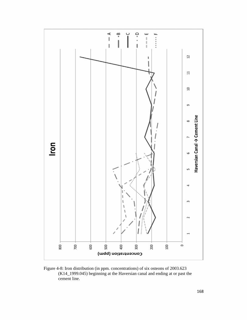
168
Figure 4-8: Iron distribution (in ppm. concentrations) of six osteons of 2003.623 (K14_1999.045) beginning at the Haversian canal and ending at or past the cement line.

169
Figure 4-9: Rhenium distribution (in ppm. concentrations) of six individuals beginning at the Haversian canal and ending at or past the cement line, each data series (A-F) reflects one osteon.

170
Figure 4-10: Cesium distribution (in ppm. concentrations) of six individuals beginning at the Haversian canal and ending at or past the cement line, each data series (A-F) reflects one osteon.

171
gradient as opposed to the sharp shifts noted in Re. Individuals 35-2, 39, and 45 still
suggest three major movements, though with varying degrees of clarity. Cesium does not
precisely replicate Sr isotopic values, but rather suggests greater degrees of mobility
within geological areas with similar signatures, thus requiring further mapping for
effective discussion of individual provenance.
Elemental compositional data are thus able to provide insight into the nature and
extent of diagenetic alteration within samples that may appear visually intact and/or
identical in preservation. These data also enable discussion of the role and manifested
nature of different elements within primary bone structure and diagenetic mineral
counterparts in archaeological bone samples. Finally, and most importantly from the
perspective of this study, the elemental results can provide additional information on
provenance and mobility of individuals during the later portions of their lives as well as
locality and dietary contributions in adult individuals during the years immediately prior
to death, both aspects generally extending beyond the accessible record of molar enamel
formation. Further work with bone samples of young adults could help to elucidate
problems or uncertainties with residence time of difference elements within the body
system as a whole and within specific tissues as there would be overlapping records of
bone and teeth, accessible in micro-scale.
Microbial Action
One additional point of interest with micro-sampling bones is that with the
progression of microbial alterations, based upon observation of slides prepared for this
research and locating intact osteons therein, there appears to be strong evidence that the
periosteum harbors a disproportionate number of intact osteons in spite of the seemingly
more direct contact with the burial environment. Consideration of this matter highlights

172
one important aspect of bones, that they contain water themselves, and that their post-
depositional alteration progresses with water contact (Hedges, 2002, Hedges and Millard,
1995). Regardless of the form of diagenesis, there are a limited number of ways in which
the various effects can alter the composition of the bone matrix.
Microbial attacks are generally discrete intrusions that may or may not target
collagen (Child, 1995a, b, Hedges, 2002, Hedges and Millard, 1995, Jans, 2008, Jans, et
al., 2004). Organic diagenesis involves processes by which collagen decays and is lost,
though the ability of certain humic substances to penetrate bone and attach to collagen is
somewhat worrisome. Diffusion reactions and internal remodeling dictate inorganic
diagensis. Newer lamellae are present in all living osteons, and will likely not be fully
mineralized, still highly soluble and closest to the cavities that were Haversian canals
until the organisms’ death. With specific note that the internal bone water is generally
sufficient to maintain a closed system that requires the diffusion of ions either in or out;
the remaining liquid-phase minerals on free-floating collagen fibrils will dissolve the
partially mineralized structures of the young lamellae to create the saturated solution and
the base material for any recrystallization (Hedges, 2002).
Caniculi connect all living osteocytes, however the diffusion capabilities, or
liquid penetration, through these caniculi will be limited (Wang, et al., 2005). Caniculi
generally lead to secluded and fully mineralized bioapatite portions of older lamellae.
Saturated or partially saturated solutions will have difficulty in dissolving a largely
insoluble mineral crystal through such limited pathways (Sillen, 1989). As such, the
liquid penetration of diagenetic solutions will be limited within the complex
microstructure of bones and there will be preferential dissolution of decaying mineral
structures. Thus, even if in diffusion equilibrium with the external environment,
diagenetic ions will have a difficult time reaching the mature mineral structures until

173
microbial attack can break down the matrix and eliminate the collagen fibrils holding
everything together (Hedges, 2002, Millard, 2001, Nielsen-Marsh and Hedges, 2000a,
Sillen, 1989).
Furthermore, no materials cross the cement lines of osteons even when the
systems are alive, thus penetration of the cement line will be difficult even if the protein
structure does not grant any buffering effects (Schaffler, et al., 1987). Osteocytes have a
limited life span (~25 years), and their mineralized structures are replaced as new osteons
cut through the existing bone (Frost, 1963, Maximov and Bloom, 1957). As a result, the
interstitial lamellae (bone matrix between the cement lines of living osteons) is
mineralized material from dead osteons, thus any remaining matrix is not connected to
any active caniculi and will be very hard pressed to be in dissolution contact with bone
fluids post-mortem. Given the nature of the post-mortem bone liquid solution, it is
unlikely that the ideal balance of ionic raw materials will be present to enable the
precipitation of largely insoluble bioapatite mineral crystals rather than the precipitation
of more soluble mineral forms, especially in the absence of guidance from nucleation or
any of the protein/substance signals that control bone formation and mineralization
during life (Hedges, 2002, Millard, 2001, Sillen, 1989).
Finally, proportions of available poorly mineralized bioapatite crystals available
for dissolution (i.e. hypercalcified bright lines and laminar bone) will be different for
specific bone structures depending on how they are in contact with the bone liquid and
depend on the age and species of the organism (Mori, et al., 2007, Mori, et al., 2003).
Thus there are number of reasons to believe that there will be significant variability
within the bone matrix as it relates to the impact and effects of diagenesis, regardless of
the form(s) in operation over any given period of time.

174
Correction Methods
There is an ongoing debate in archaeology and geochemistry regarding problems
with isotopic analysis of Sr in calcium phosphate matrices using laser ablation as an
introduction method, for some aspect of the laser ablation sample introduction leads to
the formation of a polyatomic species that interferes with mass 87 and thus interpretation
of Sr isotope ratios (Horstwood, et al., 2008, Prohaska, et al., 2002, Scharlotta, et al.,
2011, Simonetti, et al., 2008, Woodhead, et al., 2005).
Strangely enough, even though there is great similarity in the mineral matrices
that form teeth and long bones, there is no evidence for significant alteration of isotopic
signals from bones. Looking at the elemental data, there appear to be similar formations
of the related polyatomic species at mass 91, though with fairly high error terms and low
concentrations all around, yet there is no clear interference as a result. This can be seen
in Figure 4-11; for each individual, the average 87Sr/86Sr value for the nine unaltered
osteons falls close to that obtained for the same individual using solution-mode analysis.
The values for the diagenetically altered osteons are, in contrast, clearly aberrant
(Appendix F).
As these samples were recovered from a high-87Sr/86Sr region, it is entirely
possible that diagenetic contaminants were not fully removed from samples during
solution preparation and purification, thus leaving an elevated result that could mask the
presence of interference resulting from laser ablation. This seems unlikely in this
particular case as several of the samples’ diagenetic portions yielded lower Sr isotope
ratios, and only one burial (Burial 35-1) was suspected of having partial alteration on
even intact osteons, and thus was likely to be almost completely compromised.
There are a few possible explanations for this, and likely others not considered
here. First, the problem may be with the solution data masking the presence of

175
Figure 4-11: Solution mode and laser ablation 87Sr/86Sr ratios compared with diagenetically-impacted portions of bone.
176
interference in the laser data. Second, perhaps there is enough difference in the structure
of the mineral matrices that the laser interaction does not actually create the polyatomic
interference noted in tooth analysis and the elemental data are simply the result of large
error factors on low concentrations. Third, what is being seen is actually a large
coincidence, with a homogenized complex life history coming up with similar numbers
as an altered laser averaging.
Solution preparation procedures are intended to remove diagenetic overprinting
by eliminating the most soluble portions of the bone structure, namely those that were
mobilized in the burial environment rather than life. However, there remains a degree of
uncertainty as to what is being removed, what the true target data are (i.e., remaining
solids after n leaches, or the nth leachate) and whether an efficient leaching has been
achieved. This difficulty is further confounded by the complexity of bone structure and
formation processes. Any long bone is a combination of material from potentially well
over 30 years of an individual’s life. The lifespan of any given Haversian system is
generally no more than 20–25 years; however, remnant portions of old Haversian
systems, not fully removed by the cutting actions of visible osteons, frequently remain
visible in histological slides. The true age of these remnants is often uncertain and they
could thus contribute intact, diagenetically resistant bone material to the analytical result
without much regard as to what its contribution is truly telling us about the individual as
we do not have a good fix on the chronology of such portions. This matter is the focus of
continued investigation to assess the intriguing source of this confusion.

177
CONCLUSION
Numerous laboratory procedures and a series of checks have been implemented
to assess the quality of a bone sample and counteract or remove the effects of
biodeterioration on bone sections or powders (e.g., Garvie-Lok, et al., 2004, Koch, et al.,
1997, Nielsen-Marsh and Hedges, 2000). Such methods have proven effective and
necessary, given the prevalence of biodeterioration, in accessing bio- and geochemical
data obtained from archaeological bone. The downside of these techniques is that they
all rely on homogenized sample tissue which makes impossible to identify important
movement or dietary events within individual life histories.
While microscopic observations of biodeterioration are not new (e.g., Bell, 1990,
Jackes, et al., 2001, Nielsen-Marsh and Hedges, 2000b), our data show that many
chemical alterations reported in the literature can be avoided and/or monitored in tandem
with chemical analyses of bones. Micro-sampling (i.e., laser ablation, micro-drilling)
provides an avenue towards obtaining anthropogenic chemical data and, most
importantly, individual life history events. Areas of biodeterioration can be avoided or
corrections for specific alterations observed can be applied with greater finesse than bulk
sampling approaches and potentially enable further use of archaeological materials that
hold detailed data on diet, mobility, and health, all critical aspects of individual life
history.
In the Cis-Baikal region, microsampling of individual osteons supports the
hypothesis that these hunter-gatherers made numerous major movements during their
lives from one area to another. Without more detailed geochemical mapping of the
region it is difficult to speculate as to their exact locations during life, it certainly does
appear that numerous individuals were moving into and out of the Little Sea region of
Lake Baikal. Furthermore, that individuals were undertaking major travel to the Little

178
Sea either shortly before their death, or were transported to the area post-mortem,
suggests a strong cultural importance of either the area, or the Khuzhir-Nuge XIV
cemetery in particular.
In terms of general application, the tandem use of Sr isotope and elemental
compositional analysis using LA-ICP-MS seems very feasible and effective. At present,
the isotopic signatures of whole osteons can be observed and micro-sampling can be
conducted using elemental data for further enhancement of provenance determination.
Perhaps with future improvements in equipment, a more direct approach may become
possible, but with the equipment available today, major progress in the amount and
nature of information available from bone samples is already possible.

179
WORKS CITED Bell, L.S., 1990. Paleopathology and diagenesis; a sem evaluation of structural changes
using backscattered electron imaging, Journal of Archaeological Science 17, 86-102.
Bizarro, M., Simonetti, A., Stevenson, R.K., Kurszlaukis, S., 2003. In situ 87sr/86sr
investigations of igneous apatites and carbonates using laser-ablation mc-icp-ms, Geochimica et Cosmochimica Acta 67, 289-302.
Child, A.M., 1995a. Microbial taphonomy of archaeological bone, Studies in
Conservation 40, 19-30. Child, A.M., 1995b. Towards an understanding of the microbial decomposition of
archaeological bone in the burial environment, Journal of Archaeological Science 22, 165-174.
Formozov, A.N., 1964. Snow cover as an integral factor of the environment and its
importance in the ecology of mammals and birds, University of Alberta, Edmonton.
Frost, H.M., 1963. Principles of bone remodeling, C.C. Thomas, Springfield. Galazii, G.I., 1993. Baikal atlas, Russian Academy of Sciences, Moscow. Garvie-Lok, S.J., Varney, T.L., Katzenberg, M.A., 2004. Preparation of bone carbonate
for stable isotope analysis: The effects of treatment time and acid concentration, Journal of Archaeological Science 31, 763-776.
Hackett, C.J., 1981. Microscopical focal destruction (tunnels) in exhumed human bones,
Medicine, Science, and the Law 21, 243-265. Haverkort, C.M., Bazaliiski, V.I., Savel’ev, N.A., 2010. Identifying hunter-gatherer
mobility patterns using strontium isotopes, in: Weber, A.W., Katzenberg, M.A., Schurr, T.G. (Eds.), Prehistoric hunter-gatherers of the baikal region, siberia: Bioarchaeological studies of past lifeways., University of Pennsylvania Museum of Archaeology and Anthropology, Philadelphia, pp. 217-239.
Haverkort, C.M., Weber, A.W., Katzenberg, M.A., Goriunova, O.I., Simonetti, A.,
Creaser, R.A., 2008. Hunter-gatherer mobility strategies and resource use based on strontium isotope (87sr/86sr) analysis: A case study from middle holocene lake baikal, siberia, Journal of Archaeological Science 35, 1265-1280.
Hedges, R.E.M., 2002. Bone diagenesis: An overview of processes, Archaeometry 44,
319-328. Hedges, R.E.M., Millard, A.R., 1995. Bones and groundwater: Towards the modeling of
diagenetic processes, Journal of Archaeological Science 22, 155-164.

180
Huh, Y., Coleman, D., Edmond, J., 1994. 87sr/86sr in siberian rivers, eos, Transactions of the American Geophysical Union 75, 142.
Jackes, M., Sherburne, R., Lubell, D., Barker, C., Wayman, M., 2001. Destruction of
microstructure in archaeological bone: A case study from portugal, International Journal of Osteoarchaeology 11, 415-432.
Jans, M.M.E., 2008. Microbial bioerosion of bone - a review, in: Wisshak, M., Tapanila,
L. (Eds.), Current developments in bioerosion, Springer-Verlag, Heidelberg, pp. 397-413.
Jans, M.M.E., Nielsen-Marsh, C.M., Smith, C., Collins, M.J., Kars, H., 2004.
Characterisation of microbial attack on archaeological bone, Journal of Archaeological Science 33, 87-95.
Kenison Falkner, K., Lebaron, G., Thouron, D., Jeandel, C., Minster, J.-F., 1992. Cr, v
and sr in lake baikal, eos, Transactions of the American Geophysical Union 73, 140.
Marchiafava, V., Bonucci, L., Ascenzi, A., 1974. Fungal osteoclasia: A model of dead
bone resorption, Calcified Tissue Research 14, 195-210. Maximov, A.A., Bloom, W., 1957. A textbook of histology, Saunders, Philadelphia. McKenzie, H., 2006. Mortuary variability among middle holocene hunter-gatherers in the
lake baikal region of siberia, russia, Department of Anthropology, University of Alberta, Edmonton.
Millard, A.R., 2001. The deterioration of bone, in: Brothwell, D.R., Pollard, A.M. (Eds.),
Handbook of archaeological sciences, John Wiley and Sons, New York, pp. 637-647.
Mori, R., Hirayama, A., Kodaka, T., Nakamura, M., 2007. Histological and
physiochemical studies of hypercalcified primear lines in the laminar bone of young calves, Anatomical Science International 82, 108-115.
Mori, R., Kodaka, T., Sano, T., Yamagishi, N., Asari, M., Naito, Y., 2003. Comparative
histology of the laminar bone between young calves and foals, Cells, Tissues, Organs 175, 43-50.
Nielsen-Marsh, C.M., Hedges, R.E.M., 2000a. Patterns of diagenesis in bone i: The
effects of site environments, Journal of Archaeological Science 27, 1139-1150. Nielsen-Marsh, C.M., Hedges, R.E.M., 2000b. Patterns of diagenesis in bone ii: Effects
of acetic acid treatment and removal of diagenetic co2-3, Journal of Archaeological Science 27, 1151-1159.
Parfitt, A.M., 1979. The quantum concept of bone remodeling and turnover. Implications
for the pathogenesis of osteoporosis., Calcified Tissue International 28, 1-5.

181
Parfitt, A.M., 1984. The cellular basis of bone remodeling: The quantum concept reexamined in light of recent advances in the cell biology of bone, Calcified Tissue International 36, S37-S45.
Paton, C., Woodhead, J.D., Hergt, J., Phillips, D., Shee, S., 2007. Sr-isotope analysis of
kimberlitic groundmass perovskite via la-mc-icp-ms, Geostandard Geoanalytical Research 31, 321-330.
Prohaska, T., Latkoczy, C., Schultheis, G., Teschler-Nicola, M., Stingeder, G., 2002.
Investigation of sr isotope ratios in prehistoric human bones and teeth using laser ablation icp-ms and icp-ms after rb/sr separation, Journal of Analytical Atomic Spectrometry 17, 887-891.
Radosevich, S.C., 1993. The six deadly sins of trace element analysis: A case of wishful
thinking in science, in: Sandford, M.K. (Ed.), Investigations of ancient human tissue: Chemical analyses in anthropology, Gordon and Breach Science Publishers, pp. 269-332.
Schaffler, M.B., Burr, D.B., Frederickson, R.G., 1987. Morphology of the osteonal
cement line in human bone, The Anatomical Record 217, 223-228. Scharlotta, I., Weber, A.W., Goriunova, O.I., 2011. Assessing hunter-gatherer mobility in
cis-baikal, siberia using la-icp-ms: Methodological corrections for laser interactions with calcium phosphate matrices and the potential for integrated la-icp-ms sampling of archaeological skeletal materials, in: Black, S.E. (Ed.), Laser ablation: Effects and applications, Nova Publishers.
Sillen, A., 1989. Diagenesis of the inorganic phase of cortical bone, in: Price, T.D. (Ed.),
The chemistry of prehistoric human bone, Cambridge University Press, Cambridge, pp. 211-229.
Wang, L., Wang, Y., Han, Y., Henderson, S.C., Majeska, R.J., Weinbaum, S., Schaffler,
M.B., 2005. In situ measurement of solute transport in the bone lacunar-canalicular systems, Proceedings of the National Academy of Sciences U.S.A. 102, 11911-11916.
Weber, A., McKenzie, H.G., Beukens, R., Goriunova, O.I., 2005. Evaluation of
radiocarbon dates from the middle holocene hunter-gatherer cemetery khuzhir-nuge xiv, lake baikal, siberia, Journal of Archaeological Science 32, 1481-1500.
Weber, A.W., 2011. Bayesian approach to the examination of radiocarbon dates, in:
Weber, A.W., Goriunova, O.I., McKenzie, H., Lieverse, A.R. (Eds.), Kurma xi, a middle holocene hunter-gatherer cemetery on lake baikal, siberia, Canadian Circumpolar Institute Press, University of Alberta, Edmonton.
Weber, A.W., Goriunova, O.I., 2012. Hunter-gatherer migrations, mobility and social
relations: A case study from the early bronze age baikal region, siberia, in: Weber, A.W., Zvelebil, M. (Eds.), Human bioarchaeology: Group identity and individual life histories (journal of anthropological archaeology, special issue).

182
Weber, A.W., Goriunova, O.I., McKenzie, H., 2008. Khuzhir-nuge xiv, a middle holocene hunter-gatherer cemetery on lake baikal: Archaeological materials, Northern hunter-gatherer research series no. 4, CCI Press and the Baikal Archaeology Project, Edmonton.
Weber, A.W., Katzenberg, M.A., Goriunova, O.I., 2007. Khuzhir-nuge xiv, a middle
holocene hunter-gatherer cemetery on lake baikal, siberia: Osteological materials, Northern hunter-gatherers research series no. 3, CCI Press and the Baikal Archaeology Project, Edmonton.
Woodhead, J.D., Swearer, S., Hergt, J., Maas, R., 2005. In situ sr-isotope analysis of
carbonates by la-mc-icp-ms: Interference corrections, high spatial resolution and an example from otolith studies, Journal of Analytical Atomic Spectrometry 20, 22-27.

183
Chapter 5: Spatial variability of biologically available 87Sr/86Sr, rare earth and
trace elements in the Cis-Baikal region, Siberia: Evidence from modern
environmental samples and small Neolithic and Early Bronze Age cemeteries.1
By Ian Scharlotta and Andrzej Weber
1A version of this chapter has been prepared for submission to Journal of Archaeological Science. Scharlotta I, Weber A. Spatial variability of biologically available 87Sr/86Sr, rare earth and trace elements in the Cis-Baikal region, Siberia: Evidence from modern environmental samples and small Neolithic and Early Bronze Age cemeteries. Additional authors provided access to research materials and facilities and editorial feedback.

184
INTRODUCTION
Strontium isotope ratios (87Sr/86Sr) of human and animal bones and teeth are a
useful technique in determining migration and mobility patterns in past populations.
Strontium isotope ratios broadly reflect the underlying bedrock geology, manifested in
biologically available portions of the source materials (e.g., soils, plants, water, animals).
Taken a step further, the question is whether a technique based roughly on differences
between rather large geologic zones can be effective for tracking individual or group
mobility on the landscape with resolution finer than evidence for major migrations
between geologic zones. Such information would greatly benefit studies of prehistoric
mobility, allowing for better informed discussions of where an individual came from and
reaching beyond the question of whether they were born, lived and buried in the same
locale.
The analysis of 87Sr/86Sr isotope systems in skeletal tissues, while rather robust as
a technique, is complicated in that the processes by which strontium is transferred from
the ground to the diet to the skeleton are susceptible to influence and alteration by subtle
changes in diet and localized mobility (Bentley, 2006). These concerns are potentially
less significant in the context of agrarian populations, or even pastoral groups which
follow relatively fixed annual cycles, than in hunter-gatherers that can potentially
experience diverse physical mobility and multiple dietary changes over the period of a
single or several years.
In the Cis-Baikal region of Siberia, it has been hypothesized that hunter–gatherer
groups formed centers with higher population densities near reliable food resources such
as the productive fisheries on the Angara River and the Little Sea areas featuring a
combination of cove-and-lagoon and littoral fishes, and the Baikal seal, the latter

185
available pretty much everywhere along the open coast (Weber, et al., 2011). It appears
that the mobility of such groups was largely limited to those relatively small areas. Long-
distance relocation of individuals took place as well but in a fashion that appeared to be
somewhat asymmetrical: some micro-regions attracting more individuals than others.
These insights come from examination of 87Sr/86Sr values as well as carbon and nitrogen
stable isotope signatures in a few large Neolithic and Early Bronze Age (EBA)
cemeteries on the coast of Baikal (Khuzhir-Nuge XIV, Kurma XI), in the Angara valley
(Lokomotiv and Ust’-Ida), the Shamanka II cemetery on the southern coast of Baikal and
several other small cemeteries scattered around entire Baikal region (Weber, et al., 2011).
The current study focuses on mapping the distribution of the biologically
available 87Sr/86Sr ratios and rare earth and trace element concentrations throughout much
of the Cis-Baikal region and on examination of these geochemical tracers in human
samples from several of small cemeteries. The skeletal samples examined here represent
a few locations from the upper Lena valley, an area not tested previously but implicated
as an important contact zone with groups on the coast of Lake Baikal (Little Sea) and to a
lesser extent also in the Angara valley (Weber, et al., 2011). It is expected that both the
environmental data and the results from small cemeteries will provide useful guidelines
for the more comprehensive interpretations facilitated by the large cemeteries.
CIS-BAIKAL RESOURCES
The Cis-Baikal region of Siberia refers to the area including the western coast of
Lake Baikal, the upper sections of the Angara and Lena river drainages, and the Tunka
region adjacent to the southwestern tip of Lake Baikal (approximately between 52° and
58° N and 101° and 110° E). The topographic complexity of the rift valley that formed
Lake Baikal led to the formation of a large number of micro-habitats, with a variety of
seasonally available resources (Galazii, 1993, Weber, 2003, Weber, et al., 2002). The

186
thermal capacity of Lake Baikal moderates the local climate immediately along its
coastline, resulting in milder temperatures during the winter and cooler temperatures
during the summer. As a result, the Angara River Valley remains relatively free of snow
during the long winter which attracts various species of ungulates looking for forage and
less restricted mobility (Formozov, 1964). There is a variety of large and medium-size
game found in the region including moose (Alces alces), red deer (Cervus elaphus), roe
deer (Capreolus capreolus pygargus), reindeer (Rangifer tarandus), and mountain goat
(Capra sibirica). Smaller species such as wild boar (Sus scrofa sibiricus), hare (Lepus
sp.), marmot (Marmota sibirica), suslik (Spermophilus citellus), and waterfowl are also
abundant in many areas around the lake. During the summer, large runs of black grayling
(Thymallus arcticus baicalensis) are found in the uppermost section of the Angara River
near its source at Lake Baikal, and several fish species enter the tributaries of the Angara
in large numbers to spawn. The shallow coves and bays in the Little Sea region of Lake
Baikal, between Ol’khon Island and the west coast of the lake, also provide excellent
fisheries and during the late winter and early spring, the Lake Baikal seal (Phoca
sibirica) can be hunted on the ice along the open coast of the lake (Levin and Potapov,
1964, Weber, 1995, Weber, et al., 1998). Dietary studies of boreal forest populations
report the use of mushrooms, berries, and pine nuts as vegetarian foods (Haverkort, et al.,
2010, Katzenberg and Weber, 1999, Lam, 1994, Marles, 2000), however, to date there is
very limited archaeological evidence for the use of such foods during the Baikal’s middle
Holocene.
CIS-BAIKAL GEOLOGY
Within Cis-Baikal there are four main geological zones that roughly correspond
to archaeological micro-regions (Figure 5-1): (1) the Baikal basin; (2) the drainage of the

187
Figure 5-1: Map of the Cis-Baikal, Siberia region, dominant geological formations, and archaeological micro-regions (following Haverkort et al., 2008; Galazii 1993).

188
upper and middle Angara River; (3) the basin of the upper Lena River; and (4) the Tunka
region.
In the Angara drainage, bounded by the Eastern Sayan Mountains to the west and
the Central Siberian Plateau to the east and extending north towards Bratsk, the bedrocks
are of Archaean–Proterozoic age consisting of granites, metamorphic schists and
porphyritic volcanics at a depth of 2.3 km. Covering the basement are Cambrian
sediments that consist mainly of dolomites with layers of limestones, rock, anhydrites,
clays, sandstones, argillites, gritstones, marls and gypsum. The Cambrian material is
covered by 100 m of Jurassic sediments made up of sandstones, siltstones and coal beds.
Adding to this variability are the valleys connecting with the Eastern Sayan Mountains
(e.g., Irkut, Kitoi and Belaia Rivers) drawing from mixed metamorphic,
unmetamorphosed and magmatic complexes of Archaean and Early Proterozoic ages
(Donskaya, et al., 2008, Gladkochub, et al., 2006). Various exposures of these bedrocks
and Quaternary sediments, primarily clays, are expected to yield 87Sr/86Sr values in the
range of 0.705–0.712 (Fagel and Boës, 2008, Haverkort, et al., 2008, Shouakar-Stash, et
al., 2007).
The Upper Lena watershed, cutting through the Central Siberian Plateau as the
river heads northwards, and the surrounding Central Siberian Plateau are underlain by
Archaean–Proterozoic basement at around 2.2 km depth overlain by Cambrian and
Precambrian sediments. These sediments consist primarily of dolomites interlayered
with evaporites of gypsum, anhydrite and halite rocks and beds of limestone and
sandstone at different depths and beds of limestone and sandstone (Donskaya, et al.,
2008, Gladkochub, et al., 2006). The thickness of the covering sediments and the relative
geochemical homogeneity of the plateau yield expected 87Sr/86Sr values fairly tightly
clustered around 0.709 (Haverkort, et al., 2008, Huh, et al., 1994, Huh, et al., 1998).
Values for Lake Baikal water are reported as 0.7085 (Kenison Falkner, et al., 1992).

189
The Baikal basin includes the lake itself, the coastal areas as well as the Little
Sea area enclosed by Ol’khon Island, the Baikal uplift zone, the Primorskii and Baikalskii
mountain ranges. This basin is characterized by relatively high 87Sr/86Sr (~0.720–0.735)
values due to the presence of Archean and Proterozoic granites (Donskaya, et al., 2008,
Galazii, 1993, Gladkochub, et al., 2006).
The Tunka micro-region, covering the middle Irkut River valley running south of
the Eastern Sayan Mountains and connecting the southwestern tip of Lake Baikal with
Lake Khovsgol in Mongolia, consists of basement rock from the Sayan-Baikal fold belt,
also of Archaean and Proterozoic age. The Sharizhalgay uplift zone in the Eastern Sayan
Mountains and bordering the Siberian Plateau includes metamorphic and magmatic
complexes of similar age (Donskaya, et al., 2008, Gladkochub, et al., 2006). There is a
diffuse zone of Cenozoic volcanism to the south and west of the southwest end of Lake
Baikal, spanning from the East Sayan and Tuva to the Gobi and Mongolian Altai
(Johnson, et al., 2005, Rasskazov, 1994, Rosen, et al., 1994). Furthermore, the area also
features an essentially non-volcanic Late Oligocene–Quaternary sedimentary basin
composing much of the eastern portion of the valley (Rasskazov, 1994). All this yields a
complex range and distribution of expected 87Sr/86Sr values in the Tunka micro-region,
likely overlapping both values seen in the Angara drainage and the Baikal basin.
TOOTH MINERALIZATION
Teeth are dynamic mineral structures whose complexities are still being
unraveled. It has long been recognized that the incremental striae of Retzius represent
some aspect of matrix deposition complicated however by the delay between this matrix
deposition and the final mineralization of the matrix (e.g., Brown, et al., 1960). With the
advent of micro-sampling techniques such as laser ablation and micro-drilling, there has
been a resurgence of interest in the formation process of the incremental growth lines and

190
the meaning of the information that can be recovered from these materials (e.g., Hillson,
2002, Horstwood, et al., 2008, Kang, et al., 2004, Prohaska, et al., 2002, Richards, et al.,
2008, Scharlotta, et al., 2011). Numerous hypotheses have been forwarded regarding the
pattern and progression of enamel mineralization, however the common theme amongst
all works is that the progression of mineralization of layers and/or maturation of matrices
is patchy and effectively non-linear thus making the chronological relationship between
incremental lines and geochemical signals tenuous (Bentley, 2006, Dolphin, et al., 2003,
Fincham, et al., 1999, Hillson, 2002, 2005, Kang, et al., 2004, Montgomery and Evans,
2006, Suga, 1982, 1989, Tafforeau, et al., 2007). Nevertheless, the broad trend whereby
mineralization begins at the tooth cusp and finishes at the cingulum is still present,
though the intermediate pathways are uncertain.
Montgomery and Evans (2006) and Fincham et al. (1999) provide
comprehensive discussion of the biomineralization of tooth enamel with respect to Sr
isotope analysis. The process of mineralization spans a series of five distinct phases
wherein an organic gel or protein superstructure is transformed into a mineral matrix: (1)
secretion; (2) assembly; (3) matrix formation; (4) resorption prior to maturation; and (5)
maturation (see Fincham, et al., 1999 Fig. 8; Bentley 2006 Fig. 18). Effectively, during
all stages prior to maturation, the enamel remains an open chemical system vulnerable to
alteration, overprinting, or averaging of the mineral matrix. Modern recovery techniques
(e.g., laser ablation) can sample volumes of material small enough to be significantly
biased by micro-scale heterogeneity in the sample. In spite of difficulties with a
disjunction between enamel formation and maturation and potential averaging effects
(Avery, 1992, Hillson, 2002), there is still promise to the method of micro-sampling tooth
enamel. That the various growth layers in human teeth lines do not mineralize in a
similar fashion of linear accretion has been well demonstrated, however, as mentioned,
there are a few general principles that remain valid: 1) the crown of a tooth will fully

191
mineralize before the root; and 2) though accomplished in a patchy or wave-like fashion,
there is broadly linear trend in mineralization progressing from crown to cingulum.
Ongoing research into this matter using herbivore teeth has demonstrated that
there are long-term mixing effects in action during the formation and maturation of tooth
enamel (Balasse, 2003, Balasse, et al., 2002, Britton, et al., 2009, Brown, et al., 1960,
Hoppe, et al., 1999, Hoppe, et al., 2003, Hoppe, et al., 2004, Koch, et al., 1995,
Montgomery, et al., 2010, Tafforeau, et al., 2007). This research has identified a
secondary problem, namely the differences of residence time in the body for different
elements and compounds. Water-soluble materials have a short residence time in the
body of only 14 days; however strontium, calcium, and lead can remain in the body for
800–1600 days, with 10% of traceable doses remaining active after 400 days (Bowen,
1979, Dahl, et al., 2001, Montgomery, et al., 2010). Recent works (e.g., Britton, et al.,
2009, Montgomery, et al., 2007, Montgomery, et al., 2010) have demonstrated that this
residence time in the body has an intriguing effect on isotopic signatures of a linearly-
sampled herbivore tooth. Namely, an abrupt change in geochemical geography and/or
diet will not manifest as a sharp transition in isotopic signals, rather there will be a
gradual sloping change as contributions from different geochemical end-members vary
within the body–water average signal.
LASER ABLATION ON TEETH
Laser ablation studies involving skeletal materials began only recently, in part
due to latent concerns about the risk of diagenetic alteration at microscopic scales of
analysis. In the last decade or so, ICP-MS tests on teeth and bones have increased (e.g.,
Bizarro, et al., 2003, Budd, et al., 1998, Copeland, et al., 2008, Copeland, et al., 2010,
Cucina, et al., 2007, Horstwood, et al., 2008, Montgomery, et al., 2010, Prohaska, et al.,
2002, Richards, et al., 2008, Scharlotta, et al., 2011, Simonetti, et al., 2008, Trotter and

192
Eggins, 2006). ICP-MS and MC-ICP-MS are generally faster and less labor intensive
than traditional analytical methods, however one of the trade-offs is the need for
corrections for a variety of interferences. For Sr analysis, the largest, if not most
pernicious problems are isobaric interference from 87Rb (rubidium) and a recently
identified polyatomic interference from calcium phosphate (CaPO4). Rubidium
corrections are necessary for all ICP-MS and MC-ICP-MS analyses as the charged 87Rb
will carry the same mass-charge ratio as its 87Sr counterpart, though this can be countered
with accurate mass-bias calculations. This is not a problem associated with sample
introduction method. On the other hand, polyatomics such as Ca dimers and calcium
phosphate species are notably absent in solution-mode analysis as sample ions are held in
acid and thus prevented from recombining as they are free to do in the carrier-gas
environment of laser ablation chambers.
Woodhead et al. (2005), Simonetti et al. (2008), Horstwood et al. (2008), Vroon
et al. (2008) and Scharlotta et al. (2011) have all discussed the presence of significant
interference on mass 87 from a previously unidentified source, thus impinging
researchers’ ability to assess accurately the 87Sr/86Sr ratios of phosphate matrices with
laser ablation. As all mammalian skeletal tissues are varieties of phosphate mineral
matrices, this is a major problem in accessing the life signals contained therein. This also
affects data analysis and reconstruction of the movement of such animals. At the root of
the problem may be the excess of Ca and P present in the charged environment coupling
with the oxide production rates within the MC-ICP-MS. In theory, Ca and P levels
should be proportional in all parts of skeletal tissues, thus mineral replacements such as
Sr and Ba (barium), and the incorporation of other trace elements should be proportional
too, and interferences should be related to the oxide operational conditions of the
instrument itself. Horstwood et al. (2008, 2011) and Scharlotta et al. (2011)
demonstrated the close relationship between Sr concentration in samples and the resultant

193
error in 87Sr/86Sr ratios and examined the nature of this relationship and the effectiveness
of several correction factors to eliminate the adverse effects of polyatomic interferences.
MATERIAL: ENVIRONMENTAL SAMPLES
As noted in many studies (e.g., Beard and Johnson, 2000, Bentley, 2006, Bentley
and Knipper, 2005, Ezzo, et al., 1997, Ezzo and Price, 2002, Haverkort, et al., 2008,
Hodell, et al., 2004, Price, et al., 2002, Weber, et al., 2003), understanding of human
geochemical signatures (from bones or teeth) is best achieved in the context of the
biologically available geochemical environment. Regardless of the actual geochemical
properties of the rocks and soils, all that scientific analysis will show is the interaction
between human consumer and the biologically available geochemical environment. That
is, of the water sources as the fundamental vector for both plants’ and animals’
interactions with their environment, and thus understanding of the water is central to the
compositional signatures that will be imparted upon their human consumers.
Modern surface water may not reflect compositional characteristics of the same
water source throughout prehistory as erosion factors can alter the geological interaction
or contribution to the water’s composition through time. Sampling of smaller water
courses and geochemical contributions to the larger rivers as well as identifying localized
geologic features can help address this matter. Small (e.g., Bugul’deika, Manzurka, etc.)
and medium (e.g., Irkut) rivers provide important information for the development of
regional distribution maps of geochemical signatures, corresponding to very specific
geographical areas as opposed to the averaged total of entire drainages represented by
large rivers (e.g., Lena). Therefore, water samples were taken from accessible rivers (i.e.,
flowing at the time of sampling; Appendix G, Figure 5-2). Only one water sample was
collected per each sampling location, with an effort to sample each river at consistent
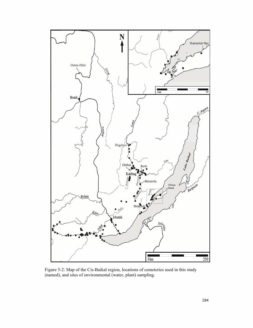
194
Figure 5-2: Map of the Cis-Baikal region, locations of cemeteries used in this study (named), and sites of environmental (water, plant) sampling.

195
intervals (c. 50 km). Consequently, the longer the body of water, the more samples
collected for analysis. Water while an important interaction vector for all living animals,
it does not comprise the primary contribution to geochemical signals imparted on skeletal
tissues. Biologically available chemical components are present in far higher
concentrations in plants (approximately 10 times higher for elements such as strontium),
than in water. As noted, plant foods are likely not great contributors to the human diet
here, but do however, comprise the majority or entirety of the diets of animals that
humans would have had subsisted on. Animals eat a variety of plants that are inedible to
humans and so will have a much broader interactions with the geochemical environment.
To track the range of potential inputs into animal’s diets, sampling of plants was
conducted throughout the archaeological micro-regions of Cis-Baikal. A few plant
samples were collected at each location and at intervals of 15 km. Additional plant
specimens were frequently collected adjacent to water samples locations. If possible
species with different root structures (i.e., depths) were collected in order to assess better
the possible range of biologically available interactions in both direct consumable plant
matter and in contribution towards local soil production.
Haverkort et al. (2008) noted that the majority of Baikal faunal samples available
at the time did not have exact provenience and could only be attributed to regions or
micro-regions. Each individual animal will have its own foraging range which may
overlap entirely or not at all with the micro-region from which it was recovered. This
leaves the potential for disparity between the geographic coordinates of the sampling
location (i.e., modern find or archaeological site) and the location of the foraging range
(i.e., geochemical interactions with the environment) the animal experienced in life.
Archaeological faunal materials have an additional problem in that the animals could
have been transported quite long distances from hunting grounds to processing sites. The
utility of large, frequently migratory, fauna – modern or archaeological – as source of

196
reference materials is thus compromised by the lack of information about the location of
the animal foraging range. For example, a sample of roe deer recovered from the Little
Sea may actually come from an animal that spent most of its life on the Upper Lena.
Small animals are the preferred choice for reference samples, at least for studies
involving agro-pastoral groups, as they generally have limited and spatially rather fixed
foraging ranges that are thus more conducive to the understanding of the distribution of
the biologically available geochemical tracers. The problem here is that small fauna
usually does not contribute much to the general diet and there is currently no evidence to
support their dietary contribution in the case of hunter–gatherer groups examined here.
Small fauna is rare at archaeological sites in the area and collection of modern specimens
rather impractical (e.g., Novikov, et al., 2007, 2008). Furthermore, the terrain of the Cis-
Baikal region is highly variable, much of it not conducive to systematic sampling of
small fauna within the time frame available for fieldwork resulting in a reference dataset
biased towards a few pockets with more open taiga-steppe terrain and close to the
archaeological sites excavated over several years (e.g., Little Sea). These samples are
included in the study only for general comparative purposes.
Since plant and water samples have fixed and confirmed provenience and reflect
bioavailable geochemistry with greater chronological stability, they provide a more
accurate picture of prehistoric bioavailability of geochemical tracers than modern or
archaeological fauna can provide. In sum, plants and water are our materials of choice
for reference purposes.
Assessment of biologically available 87Sr/86Sr and elemental data was conducted
using a combination of plant (n = 179) and water (n = 60) samples, and faunal bone and
teeth (n = 124) for a total of 363 samples (Figure 5-2, Appendix G). Faunal samples
included those used by Haverkort et al. (2008) and 51 new specimens taken from areas
not sampled before (e.g., Tunka region). Sampled areas focused on archaeological

197
micro-regions in order to examine the nature and extent of movement both within and
between micro-regions.
MATERIALS: HUMAN SAMPLES
As mentioned, the main reason this study focuses on individuals from small
cemeteries is that the geochemical research on Baikal materials conducted to date created
a geographic and cultural bias toward large cemeteries in the Angara valley (e.g.,
Lokomotiv and Ust’-Ida) and Little Sea area (e.g., Khuzhir-Nuge XIV). Integration of
the new human data with the information already available in the context of the much
larger, spatially and quantitatively, set of environmental background values will provide
for a more comprehensive and balanced regional framework of reference data with which
to assess human movement across entire Baikal region. Six small cemeteries
representing three out of four main archaeological micro-regions were available for
analysis: Borki 1, Manzurka, and Obkhoi from the upper Lena valley, Ostrov Zhiloi from
the Angara valley, and Khotoruk, and Shamanskii Mys from the Little Sea area (Figure 5-
2, Table 5-1). No materials were available from the Tunka valley for this study as the
only Neolithic–Bronze Age cemetery known to date in proximity to the Tunka valley is
Shamanka II, subject of a separate large scale examination.
Table 5-1: General location, cultural, and chronological data for analyzed cemeteries.
Site Chronology Region Individuals Teeth Ostrov Zhiloi Neolithic Angara 1 1 Khotoruk Early Neolithic Little Sea 7 20 Shamanskii Mys Early Bronze Age Little Sea 3 8 Borki 1 Early Bronze Age Upper Lena 1 3 Manzurka Early Bronze Age Upper Lena 1 3 Obkhoi Early Bronze Age Upper Lena 3 8

198
Human samples consisted of 43 molars from 16 following individuals: Borki 1 (n
= 1), Manzurka (n = 1) and Obkhoi (n = 3) from the upper Lena; Khotoruk (n = 7) and
Shamanskii Mys (n = 3) from the Little Sea; and Ostrov Zhiloi (n = 1) from the Angara
valley (Figure 5-2). For 11 individual, where possible, each individual was represented
by 3 molars (M1, M2, M3), but for 5 individuals, not all molars were available for
analysis. Molars grow in specific, well known sequential time spans, covering the range
of juvenile growth from infancy to sub-adulthood (Hillson, 2002, 2005). Analysis of all
three molar teeth from an individual provides detailed information about their movement
during the full course of their childhood. Since each molar reflects several years of
growth, every tooth was sampled at four points between the crown and the cingulum.
The exact relationship between uptake, deposition and mineralization of tooth enamel is
still unclear, however, given the span of time reflected by each tooth, 4 evenly spaced
sampling locations should reflect ~6–10 months of temporal separation between final
mineralization.
BORKI, MANZURKA, AND OBKHOI (UPPER LENA) AND OSTROV ZHILOI
(ANGARA)
The three upper Lena cemeteries were excavated in the 1970s and are known
only from the Russian fieldwork reports (Okladnikov, 1971) or a short preliminary
publication (Konopatskii, 1977). While Borki and Obkhoi produced only EBA graves, 3
and 12 respectively, 1 Early Neolithic (EN) and 4 Early Bronze Age (EBA) graves were
found at Manzurka. All individuals examined here date to the EBA. Although carbon
and nitrogen stable rations for some of these individuals are known (Weber, et al., 2002),
so far no geochemical tests have been carried out on materials from the upper Lena.
Ostrov Zhiloi, located on the middle Angara and excavated in the 1960–1970s,
has been only very briefly described by Vasil’evskii (1978). Three graves were found

199
and classified as Neolithic (i.e., EN or Late Neolithic – LN). Even though hundreds of
Neolithic and EBA burials have been excavated in the Angara valley before and after the
World War II, most have been lost and only the collections acquired since the 1980s are
available for continuous examination. These, however, are strongly biased toward the
large cemeteries of Lokomotiv and Ust’-Ida, both located on the upper section of the
Angara. Hence the value of the Ostrov Zhiloi single skeleton.
KHOTORUK AND SHAMANKSKII MYS (LITTLE SEA)
Khotoruk is an EN cemetery located near the mouth of the Anga River on the
northwest coast of Lake Baikal, about 50 km southwest of Ol’khon Island (Konopatskii,
1982, Mamonova and Sulerzhitskii, 1989, Weber, et al., 2006). Based on morphological
properties of some of the grave goods, the cemetery has been dated to the EN which is
consistent with the available radiocarbon dates (Mamonova and Sulerzhitskii, 1989,
Weber, et al., 2006).
Shamanskii Mys, located on the west coast of Ol’khon Island (Goriunova and
Novikov, 2010, Konopatskii, 1982, Okladnikov and Konopatskii, 1974/1975, Weber, et
al., 2006), produced 11 graves. Based on the morphological properties of grave
accoutrements, one grave was classified as EN, three as LN, and seven as EBA, which is
also consistent with the available radiocarbon dates (Weber et al. 2006). Only the EBA
individuals are examined in this study.
EN graves are generally very rare in the Little Sea area. Khotoruk is the only
such cemetery tested to date outside of the Angara valley (Lokomotiv). The island
location of Shamanskii Mys contrasts with the mainland EBA cemeteries in the Little Sea
area (KNXIV). Both samples expand temporal and spatial scales of comparison between
data sets. Carbon and nitrogen stable isotope results are also available for these materials
(Weber et al. 2002).

200
SAMPLE PREPARATION AND ANALYSIS
Sample pretreatment varied depending on the material analyzed. For water
samples, 10 mL was filtered through a 0.2µ fiber filter and evaporated to dryness prior to
transport in polypropylene vials, rehydrated with milliQ (MQ) de-ionized water and
evaporated to dryness in Teflon beakers under a laminar flow hood. Dried plant leaves or
needles were ashed in a muffle furnace for 18 hours at 650º C prior to further processing.
Sample solution preparation occurred in a Class 100 clean room facility and
followed procedures outlined in Haverkort et al. (2008) and Scharlotta et al. (2011).
Plant, water and faunal samples were analyzed for elemental composition using solution
mode-ICP-MS and for 87Sr/86Sr ratios using multi collector-ICP-MS. Dried strontium
isotopic samples were dissolved with 1 mL of 2% HNO3 prior to necessary dilution for
MC-ICP-MS analysis. Analysis was conducted on a Nu Plasma HR MC-ICP-MS with a
DSN-100 nebulizer. Accuracy and reproducibility of the analytical protocol based on
long-term repeated analysis of a 100 ppb solution of the NIST SRM 987 strontium
isotope standard 0.710242 ± 0.000041.
Elemental samples underwent similar handling, though not loaded onto cation
exchange columns. Digested samples were dissolved in 2% HNO3 prior to ICP-MS
analysis. Sample solutions were analyzed for 49 elements (Li, Na, Mg, Al, P, Ca, Ti, V,
Cr, Mn, Fe, Co, Ni, Cu, Zn, Ga, As, Rb, Sr, Y, Zr, Nb, Mo, Ag, Cd, Sn, Sb, Cs, Ba, La,
Ce, Pr, Nd, Sm, Eu, Gd, Tb, Dy, Ho, Er, Tm, Yb, Lu, Ta, Au, Tl, Pb, Th, and U) using a
Perken Elmer Elan6000 quadrupole ICP-MS. External reproducibility, based on repeated
analysis of international whole rock standards is 5–10% (2σ level) for most elements
(Supp. Mat. I).
Laser ablation for elemental analysis of human tooth samples was conducted
using the Perken Elmer Elan6000 quadrupole ICP-MS coupled to a UP213 nm laser

201
ablation system (New Wave Research, USA). Quantitative results for the same 49
elements analyzed in solution, were obtained and normalized to 24Mg, as the internal
standard using the GLITTER® (XP version, Macquarie University) laser ablation
software.
Laser ablation for isotopic analysis of human teeth was conducted using a UP213
nm laser system coupled to the Nu Plasma HR MC-ICP-MS with the sample-out line
from the desolvating nebulizing introduction system (DSN-100 from Nu Instruments) to
allow for simultaneous aspiration of a 2% HNO3 solution. At the beginning of each
analytical session, parameters for the introduction system and the ion optics were
optimized by aspirating a 100 ppb solution of the NIST SRM 987 Sr isotope standard.
Machine drift was monitored using a Durango Apatite reference material (Supp. Mat. II).
All laboratory work was conducted at the Radiogenic Isotope Facility of the Department
of Earth and Atmospheric Sciences at the University of Alberta, Edmonton.
STATISTICAL METHODS
A combination of statistical techniques developed specifically for the unique
needs of chemical sourcing were employed to analyze the resulting geochemical data,
following established approaches described by Baxter (1994a, b), Baxter and Buck
(2000), Davis (1986), Glascock (1992), Glascock et al. (1994), Hoard et al. (1992), and
Truncer et al. (1998). Analyses of regional variance and means were conducted.
Following this, in order to explore the data further and assess to what extent cultural
regions could be separated in multivariate space, exploration using bivariate plots,
principal components analysis and canonical discriminant analysis were conducted on a
combination of 87Sr/86Sr isotopic data and elemental concentration data.

202
ENVIRONMENTAL RESULTS
Preliminary examination of 87Sr/86Sr variability in faunal material associated with
archaeological micro-regions by Haverkort et al. (2010, 2008) demonstrated promising
results. As the sample size was expanded to include more animal specimens, water and
plant samples, the range of 87Sr/86Sr variability proved to be quite large (Table 5-2).
Analysis of regional variance and means successfully exhibited differences; however the
extent of overlap between micro-regions rendered moot effective correlations between
geological, geochemical and archaeological areas as previously described. Rather than
effectively mimicking bedrock geology with some attenuation for translating bedrock
geology to biologically available Sr, there was a confounding overlap in the ranges of
87Sr/86Sr values through all micro-regions.
Table 5-2: Range and variance results of micro-regional comparisons for 87Sr/86Sr data grouped by sample type.
Descriptive Statistics
All Samples N Minimum Maximum Mean Range Std. Error Std. Deviation Variance
Angara 60 .70791 .71680 .7098197 .0088940 .00017288 .00133916 1.79E-06
Little_Sea 103 .70694 .77350 .7174613 .0665570 .00116915 .01186556 1.41E-04
Tunka 121 .70673 .71812 .7101078 .0113880 .00018092 .00194856 3.80E-06
Upper Lena 79 .70814 .71191 .7096936 .0037700 .00010883 .00096731 9.36E-07
Faunal N Minimum Maximum Mean Range Std. Error Std. Deviation Variance
Angara 39 .70811 .71680 .7096641 .0086900 .00023565 .00147160 2.17E-06
Little_Sea 54 .70694 .74614 .7151879 .0392030 .00123168 .00905094 8.19E-05
Upper Lena 14 .70849 .71112 .7097906 .0026320 .00022928 .00085790 7.36E-07
Tunka 17 .70881 .71097 .7094852 .0021600 .00018333 .00075589 5.71E-07
Water N Minimum Maximum Mean Range Std. Error Std. Deviation Variance
Angara 7 .70791 .71169 .7095367 .0037840 .00043510 .00115115 1.33E-06
Little_Sea 11 .70877 .77350 .7276372 .0647260 .00610954 .02026306 4.11E-04
Tunka 26 .70711 .71373 .7096870 .0066220 .00028721 .00146450 2.14E-06
Upper Lena 16 .70814 .70917 .7085601 .0010230 .00007369 .00029476 8.69E-08
Plants N Minimum Maximum Mean Range Std. Error Std. Deviation Variance
Angara 14 .70951 .71220 .7103945 .0026860 .00022765 .00085180 7.26E-07
Little_Sea 38 .70783 .75225 .7177463 .0444220 .00178740 .01101824 1.21E-04
Tunka 81 .70673 .71812 .7103102 .0113880 .00025282 .00220403 4.86E-06
Upper Lena 46 .70875 .71191 .7101648 .0031620 .00012243 .00083037 6.90E-07

203
Furthermore, even groups of similarly aged geologic formations (i.e., Archean and
Proterozoic areas along the western coast of Baikal and Tunka) exhibited different
87Sr/86Sr values (Figure 5-1). The clear exception to this overlap is the Little Sea area
which featured distinctly higher 87Sr/86Sr values making any contact with bioavailable Sr
from this micro-region apparent. Previous work indicated a spike in both terrestrial and
aquatic 87Sr/86Sr values associated specifically with the Sarma drainage adjacent to the
KNXIV cemetery; however, this effect appears now to be more widespread through the
micro-region (Figures 5-1, 5-3). Figure 5-3 provides a visual approximation of the
expected bioavailable isotopic values throughout the major archaeological micro-regions
based upon analysis of environmental samples and expanded to dominant topographic
features of the landscape. The great variation in strontium isotopic values observed
through environmental sampling highlights the important distinction between the
dominant geological formations as the source of bioavailable radiogenic materials and the
actual bioavailable isotopic values in the environment (cf. Sillen, et al., 1998).
Due to the complexity of the situation, multivariate statistical approaches were
employed to enable geochemical group discrimination. Samples collected have varied
elemental concentrations on orders of magnitude of difference. Data were converted to
ratios relative to internal Mg concentrations in order to make the different sample types
comparable. Ratios to all available elements were attempted, but none provided a better
marriage of different sample types (water, plants, and human or animal skeletal
materials). Faunal materials were excluded from the analysis at this point as the nature of
the provenience information, as discussed above, frequently made individual
archaeological micro-regional group or arbitrary geochemical sub-group membership
uncertain. Remaining environmental comparisons were made on all plant and water
samples. Principal component analysis (Figure 5-4) and discriminant function analysis

204
Figure 5-3: Approximate map of expected bioavailable 87Sr/86Sr isotopic distributions throughout the Cis-Baikal region based on water and plant sampling, and sites of environmental (water, plant) sampling.

205
Figure 5-4: Bivariate plot showing the results of Principal Components Analysis employing complete isotopic and trace element data grouped by micro-region.

206
Figure 5-5: Bivariate plot showing the results of Discriminant Function Analysis employing complete isotopic and trace element data grouped by micro-region.

207
(Figure 5-5) were attempted on geochemical micro-regional groups reflecting the Middle
Angara, Tunka, Baikal coast/Little Sea, and the upper Lena micro-regions.
Following this, micro-regional groups were subdivided into 2–4 groups each
based on combinations of 87Sr/86Sr and elemental values for a total of 11 subgroups
(Figure 5-6). These multivariate data are presented only as the 2 sigma confidence
ellipses to improve visibility. Unfortunately, 87Sr/86Sr ratios presented the dominant
vector of variability in these groups and the complexity in multivariate space does not
support effective regional provenancing of individuals.
Given the observed geochemical complexity, a different approach was taken to
discriminate the geological micro-regional groups. The entire data set was broken down
into subclasses reflecting limited ranges of 87Sr/86Sr variability and then re-divided by
micro-region; in this case, taking the whole range of Cis-Baikal 87Sr/86Sr values and
dividing them into 8 subclasses (<0.708, 0.708–0.710,…, 0.718–0.720, and >0.720), and
then within each of these geochemical subclasses, comparing the 87Sr/86Sr isotopic and
elemental data between micro-regions. Geochemical subclasses do not correlate to
specific geography, reflecting similarities present only in statistical space. This
effectively moderates the dominant effect of the 87Sr/86Sr values within multivariate
space. 87Sr/86Sr values are still crucial for accurate categorization within appropriate
subclasses, but subsequently micro-regions are compared primarily based on elemental
data. Conducted in this fashion, comparison between geochemical subclasses reveals
rather distinct micro-regional differences (Figure 5-7).
HUMAN RESULTS
Human results were transformed using the same discriminant function matrix as
environmental data and compared to established micro-regional subclasses groups to
establish their provenance (Table 5-3). Strontium isotope ratios were directly comparable

208
Figure 5-6: Bivariate plot showing the results of Discriminant Function Analysis employing complete isotopic and trace element data grouped by micro-regional subclasses as determined by cluster analysis.

209
Figure 5-7: Bivariate plot showing the results of Discriminant Function Analysis employing trace element data grouped by micro-region within the 87Sr/86Sr range of 0.708–0.710.

210
across the different reference sample types, but trace elemental data had to be converted
prior to comparisons. With disparate comparative materials, archaeological micro-
regional group classifications were difficult and could not be verified by techniques such
as Mahalanobis distance measurements. Instead, human samples were tested for their
hypothesized group membership by a visual version of jackknifing. Samples added to a
micro-regional subclass group would either cluster closely with the group, or stretch the
group in the direction of the appropriate group membership. All samples were tested as
members of all available groups before provenance determination and final group
membership were established. Once classified by micro-regional subclass, samples were
compared both visually to the reference samples in multivariate biplots (e.g., Figures 5-8
and 5-9) and through hierarchical cluster analysis to verify the geographic sampling site
with the greatest affinity to the human sample analyzed.
Previous geochemical work in the Cis-Baikal region supported the feasibility of
mobility research and suggested significant patterning of the 87Sr/86Sr values likely
indicating different mobility or migration patterns. With an expanded environmental
reference dataset, better understanding of the geological complexity in the region has
come to light. As such, it is difficult to input the results for individuals recovered from
small cemeteries (discussed here) into the interpretive framework presented by Haverkort
et al. (2008). Discussion of this framework in light of new knowledge about 87Sr/86Sr
ratio variability throughout the region is beyond the scope of this paper. Instead,
qualitative discussion of the 16 individuals analyzed in this study will be provided in light
of the new data. Table 5-3 contains provenance information for each examined molar.

211
Table 5-3: Provenance determinations for individual skeletal elements analyzed.
HSAMP_ID MASTER_ID SITE ELEMENT PROVENANCE
2000.220 BO1_1971.001 Borki 1 M1 Upper Lena/Little Sea
2000.221 BO1_1971.001 Borki 1 M2 Upper Lena/Little Sea
2000.222 BO1_1971.001 Borki 1 M3 Upper Lena/Little Sea
2000.190 KHO_1977.002 Khotoruk M1 Little Sea
2000.191 KHO_1977.002 Khotoruk M2 Little Sea
2000.192 KHO_1977.002 Khotoruk M3 Little Sea
2000.194 KHO_1978.004.01 Khotoruk M1 Little Sea
2000.195 KHO_1978.004.01 Khotoruk M2 Little Sea
2000.197 KHO_1978.004.01 Khotoruk M3 Little Sea
2000.171 KHO_1978.004.02 Khotoruk M1 Little Sea
2000.172 KHO_1978.004.02 Khotoruk M2 Little Sea
2000.173 KHO_1978.004.02 Khotoruk M3 Little Sea
2000.187 KHO_1978.004.03 Khotoruk M1 Little Sea
2000.188 KHO_1978.004.03 Khotoruk M2 Little Sea
2000.179 KHO_1978.004.04 Khotoruk M1 Little Sea
2000.180 KHO_1978.004.04 Khotoruk M2 Little Sea
2000.181 KHO_1978.004.04 Khotoruk M3 Little Sea
2000.183 KHO_1978.007 Khotoruk M1 Little Sea
2000.184 KHO_1978.007 Khotoruk M2 Little Sea
2000.185 KHO_1978.007 Khotoruk M3 Little Sea
2000.175 KHO_Grave on the mountain (1978) Khotoruk M1
Little Sea/Angara Drainage
2000.176 KHO_Grave on the mountain (1978) Khotoruk M2
Little Sea/Angara Drainage
2000.177 KHO_Grave on the mountain (1978) Khotoruk M3 Little Sea
2000.201 SHM_1975.001 Shamanskii Mys M1 Upper Lena/Little Sea
2000.202 SHM_1975.001 Shamanskii Mys M2 Upper Lena/Little Sea
2000.203 SHM_1975.001 Shamanskii Mys M3 Upper Lena/Little Sea
2000.205 SHM_1972.002 Shamanskii Mys M1 Little Sea
2000.206 SHM_1972.002 Shamanskii Mys M2 Little Sea
2000.207 SHM_1972.002 Shamanskii Mys M3 Little Sea
2000.198 SHM_1973.003 Shamanskii Mys M2 Upper Lena
2000.199 SHM_1973.003 Shamanskii Mys M3 Upper Lena
2000.224 MNZ_1974.002 Manzurka M1 Upper Lena
2000.225 MNZ_1974.002 Manzurka M2 Upper Lena
2000.226 MNZ_1974.002 Manzurka M3 Upper Lena
2000.212 OBK_1971.013 Obkhoi M1 Upper Lena
2000.213 OBK_1971.013 Obkhoi M2 Upper Lena
2000.214 OBK_1971.013 Obkhoi M3 Upper Lena
2000.216 OBK_1971.005 Obkhoi M1 Upper Lena
2000.217 OBK_1971.005 Obkhoi M2 Upper Lena
2000.218 OBK_1971.005 Obkhoi M3 Upper Lena
2000.209 OBK_1971.007 Obkhoi molar Upper Lena
2000.210 OBK_1971.007 Obkhoi molar Upper Lena
1997.284 OZH_000.006 Ostrov Zhiloi molar Little Sea

212
Figure 5-8: Bivariate plot showing for MZN_1974.013 projected with the results of Discriminant Function Analysis employing trace element data grouped by micro-regional subclass.

213
Figure 5-9: Bivariate plots for KHO_Grave on the mountain (1978), OBK_1971.005, OBK_1971.007, and SHM_1973.003 demonstrating the provenancing of human samples. Shaded areas include the majority of human samples.

214
BORKI 1
The one EBA individual (BO1_1971.001) from Borki had results for three
molars that were fairly tightly clustered suggesting spatially limited mobility as a
subadult within an area that was not covered by current geochemical survey and one
where the body was buried. Provenance data showed equal affinity to both the Upper
Lena and the Little Sea regions, likely indicating fairly stable residence in or near the
mountains of the Primorskii Range upstream along the Lena River. This individual was
interred near Kachug, an area well represented by the environmental data set, yet
apparently did not enter it until adulthood.
MANZURKA
The geochemical results for the EBA individual (MZN_1974.013) from
Manzurka are rather surprising for they suggest that this person spent significant portions
of childhood in both the Manzurka and Khodontsa Valleys, both in close proximity to its
final resting place. This is one of the few individuals who could be easily classified as
“local”, i.e., buried in the same area where they were born and spent much of their
subadulthood. Data from the later portions of M1 and much M2 suggest interactions with
regions of the Upper Lena not sampled yet.
OBKHOI
One individual (OBK_1971.005) stayed firmly within the Upper Lena region,
was born near the Manzurka Valley, moved to the Khodontsa Valley by the age of ~5
years, moved next to areas not covered by the current map, and finally returned to the
vicinity of Obkhoi as an adult or after death. One individual (OBK_1971.013) lived their
life in areas in the vicinity of the confluence of the Kulenga and Lena Rivers (Kachug),
however, also appears to have lived in areas of the upper Lena not sampled in this study.

215
These two individuals suggest fairly significant mobility within the upper Lena micro-
region. The third individual (OBK_1971.007) lived most of their sub-adult life in the
upper Lena region as well, likely in proximity to the Manzurka Valley. This individual
was different, however, with a geochemical influence coming from the Little Sea region,
slightly skewing results prior to moving finally closer to the Little Sea near the end of
either M2 or M3 mineralization. This individual was in contact with and suggests
broader connections between the Upper Lena and Little Sea micro-regions.
OSTROV ZHILOI
Based on available comparative data, this individual (OZH_000.006) appears to
have grown up in the Little Sea micro-region. If so, this is very surprising given the
substantial distance separating these two locations and the lack of waterways other than
the Angara providing direct lines of movement between them. As such, this individual
appears to have travelled quite significantly through their life, either joining with a local
group, or died far afield from their birthplace, but still granted a formal burial.
KHOTORUK
Seven EN individuals from Khotoruk were analyzed and all appear to have lived
their sub- and young adult lives within either the Little Sea micro-region or the Baikal
Basin. Two individuals (KHO_1978.004.02 and KHO_1978.004.04) lived their lives on
the southern and western shores of the Little Sea, staying within fairly high 87Sr/86Sr ratio
zones indicative of the granitic rocks of Sarma Canyon and surrounding areas. Two
individuals (KHO_1977.002 and KHO_1978.004.03) were born and spent their early
childhood in similarly high 87Sr/86Sr ratio zones, but moved to areas with lower 87Sr/86Sr
ratios earlier in their lifetime, by around age 5. It is possible that this shift could indicate
the effects of weaning foods and a different diet for children and their mothers, though

216
this remains speculative. Two individuals (KHO_1978.004.01 and KHO_1978.007)
demonstrated some variability in their geochemical signatures and lived their sub-adult
lives in an area of the Baikal Basin not sampled in this study. Lower 87Sr/86Sr ratios and
trace element signatures suggest the area between the Kuda Valley and the shores of Lake
Baikal as likely candidates for their provenance.
The final individual from Khotoruk (KHO_Grave on the Mountain) showed a
rather surprising history of mobility. This individual was born in a rather low 87Sr/86Sr
ratio zone (0.709) and gradually moved into progressively 87Sr/86Sr ratio zones as they
grew up. There are small pockets of low 87Sr/86Sr ratios to be found within the Little Sea
and neighboring Upper Lena regions, however the trace element data suggest instead that
this individual was born not within the Angara drainage, but in an area fairly close to the
boundary between the two (e.g., within the Kuda Valley). Initial movement likely took
place while the individual was an infant, given the variability in M1 values. Another
major movement took place before the beginning of mineralization of M3, likely around
the age of 8 years. This was a series of movements, showing fairly small changes during
the first half of crown formation, and then followed by a major movement to a higher
87Sr/86Sr ratio zone by the completion of M3 formation. Final values for this individual
likely put them in the vicinity of Khotoruk as a sub-adult and remaining (or returning)
there until death.
SHAMANSKII MYS
Each individual from the Shamanskii Mys cemetery exhibited a different
mobility history, though all date to the EBA. Individuals analyzed included both those
local to the Little Sea micro-region, and as well as non-local, or not-Little Sea, perhaps
Upper Lena micro-region, childhood locale. This evidence includes both geochemical
provenance, as well as stable isotope dietary information, showing individuals eating

217
Baikal seals and others subsisting on terrestrial and riverine, but not lake resources (see
below; Weber, et al., 2011). The mix of Little Sea and other micro-regional geochemical
and dietary signatures is intriguing evidence for the interment of individuals with varied
backgrounds in a single cemetery. One individual (SHM_1972.002), showed relatively
minor variations in their molar geochemical data, thus most likely stayed on Ol’khon
Island. One individual (SHM_1973.003) appears to have grown up in the Upper Lena, in
an area not heavily sampled, with tightly clustered 87Sr/86Sr ratios. This is somewhat
surprising given dietary data for this individual that indicates significant consumption of
aquatic resources, including seal, as an adult. Thus while this person lived their sub-adult
life in the Upper Lena, they must have come to the Little Sea, and Ol’khon Island
specifically for some significant amount of time prior to their death. And the third
individual from Shamanskii Mys (SHM_1975.001), showed a significant amount of
geochemical variability. Provenance determination was to a region somewhere between
the Little Sea and the Upper Lena. The strongest affinity is for the region around
Zhigalovo, but with much time spent in areas not sampled in this study. At some points
in their development, this person was in greater or lesser contact with relatively high
87Sr/86Sr ratio zones (above 0.717 around age 7–8) that are only found near the Little Sea,
and equally in contact with lower regions (0.709 around age 9–10 years). It is possible
that the lack of clear provenance for this individual is the result of significant travel
between the Upper Lena and Little Sea regions yielding averaging effects. Unfortunately
no dietary information is available for this individual to help confirm the duration of final
habitation on Ol’khon Island prior to death; however all other individuals from this site
examined for carbon and nitrogen stable isotope ratios show consumption of the local
aquatic foods (fish and Baikal seal; Weber et al. 2011).

218
DISCUSSION
These new results lead to a number of interesting inferences. First, there is a
high level of agreement between the insights on mobility generated by this study and the
insights gained via the most recent assessment of the regional dietary patterns (Weber et
al. 2011) as well as the more detailed study of the various geochemical signatures
assembled for the KN XIV cemetery in the Little Sea micro-region (Weber, et al., 2011).
Given that the archaeological record is often incomplete or corrupted by diagenetic and
taphonomic factors, to find individuals from several sites, frequently separated by a large
distance that provide corroborating evidence is very encouraging as a form of
verification. This generally supports the utility of geochemical data for mobility
inferences and provides additional justification to continue this line of investigation and
develop more comprehensive models of hunter-gatherer mobility and travel.
There is an asymmetry in the patterning of hunter-gatherer movement between
various micro-regions in Cis-Baikal. The mobility of individuals was heavily focused on
movement and interaction between groups residing in the Little Sea and on the upper
Lena. Only one individual (KHO_Grave on the mountain) from the individuals
representing the Little Sea area analyzed in this study or previously (i.e., 25 persons from
KNXIV) by Haverkort and colleagues (2008), shows any contact with the Angara
Drainage. This contact was marginal (e.g., Kuda Valley rather than Angara River itself).
While there was a large EBA population living along the Angara and the southern coast
of Lake Baikal, there is no evidence for significant movements of people between the
Angara and the other three micro-regions (i.e., Tunka, upper Lena, and Little Sea).
Weber and colleagues hypothesized the presence of just such an asymmetrical pattern of
movement that is also supported by this new geochemical data (Weber and Goriunova,
2012, Weber, et al., 2011).

219
The data from Khotoruk support the notion that asymmetrical patterns of
movement were also present during the EN. This data set also suggests that different
patterns of movement and cultural contact were present during the EN and the LN–EBA.
This inference is, however, based a very small sample of individuals from a single
cemetery, additional evidence is greatly needed to verify it. The only demonstrable
contact with the Angara was during the EN and the samples analyzed show significantly
less mobility overall during the EN. This is intriguing given the geography, with the
Kuda Valley providing a direct travel route between the Angara Drainage and the Little
Sea and over relatively easy terrain. In contrast, overland movement between the Little
Sea and the upper Lena is more challenging. The relative difficulty in travel could
support the lack of movement between some micro-regions (e.g., upper Lena) but cannot
explain the overall lack of movement, so some other factor must be responsible for this
pattern.
Returning to the matter of EBA patterns, Shamanskii Mys data contribute further
to the very interesting picture of mobility during this period. Based upon dietary
evidence (Weber, et al., 2011), there are two distinct diet types within the Little Sea EBA
population: GF (game-fish) and GFS (game-fish-seal). Sealing is predominantly a
seasonal activity conducted on Lake Baikal from late winter to early spring (Weber, et
al., 1998). Weber and colleagues (Weber and Goriunova, 2012, Weber, et al., 2011),
based on the examination of the large KNXIV data set, hypothesized the movement of
significant numbers of individuals between the upper Lena and Little Sea micro-regions
on a seasonal basis. The seasonal nature of this movement produced two cycles of inter-
regional mobility, one that brought people from the upper Lena to the Little Sea during
the narrow window when seal meat is available for consumption and possibly to
participate directly in the hunting of seals, and another pattern that brought non-locals to
the Little Sea outside of the sealing season. Shamanskii Mys individuals (1973.003 and

220
1975.001) support the hypothesis that such interregional movements were not a unique
feature of the KNXIV cemetery, but a broader phenomenon connecting the upper Lena
with the Little Sea as part of regular travel and interactions. What is interesting,
however, and worth further research, is that at Shamanskii Mys there are no individuals
with the GF diet, while all mainland Little Sea cemeteries analyzed have people with
both the GFS and GF diets.
Even more exciting is the correlation between inter-regional mobility and the
presence of certain artifacts as grave goods. All three Shamanskii Mys individuals
analyzed in this study were buried with nephrite artifacts, SHM_1973.003 and
SHM_1975.001 each with white nephrite disks and SHM_1972.002 with a green nephrite
knife (Konopatskii, 1982). This is very interesting considering the likely provenance of
these artifacts. Green nephrite comes from the Angara micro-region or the Eastern Sayan
mountains while white nephrite comes from northern Trans-Baikal in the Vitim volcanic
fields (Johnson, et al., 2005, Sekerin and Sekerina, 2000). It has been suggested that
there are far more sources of nephrite in the Baikal region (R. Losey, personal
communication), however this research is still in progress and will hopefully elucidate
the exact number of geochemically distinct nephrite sources and their provenance. It is
intriguing that the local individual was buried with numerous grave goods and a green
nephrite knife that was likely acquired indirectly through trade or through a specific trek
to procure raw material to make such an object that only occurred during adulthood. This
individual had no connection with the Angara Drainage during their childhood, remaining
firmly within the Little Sea, yet was buried with an exotic artifact from a region that
groups in both the upper Lena and the Little Sea had little direct contact. The other two
individuals (SHM_1973.003 and SHM_1975.00) were of non-local birth and childhood,
but were buried in the Little Sea and consumed seal during their adult lives. Both of
these individuals were buried with white nephrite objects likely from Trans-Baikal.

221
The highly seasonal seal hunt is an excellent candidate for contact across the lake
with the people from Trans-Baikal including the Vitim volcanic fields with the white
nephrite and/or other mineral resources. Modern Buryat residents of Ol’khon Island and
the Little Sea are noted to have close kinship ties to groups around Barguzin in Trans-
Baikal and retain contacts across the ice (R. Losey, personal communication). This
cross-ice movement could explain the presence of white nephrite from northern Trans-
Baikal in the Little Sea. Seal hunts could also function as trading excursions involving
contacts with groups living on the eastern coast of the lake or further into Trans-Baikal.
Having a highly prestigious item (white nephrite) would go a long way towards
explaining the nature of social contacts between the upper Lena and the Little Sea. It is
quite plausible that long distance trade of valuables functioned as a strong draw-factor to
make the trek across the taiga from as far as Ust’-Ilimsk (Ostrov Zhiloi) or vice versa
relative to the subsistence or prestige value of the seal hunt itself. Rather trekking across
the lake during the annual seal hunt, provides an avenue for goods to flow, the sharing of
seal meat along with other exchanges providing a measure of hospitality or pretext for the
exchange of goods. The individuals who never ate a seal in their last years of life could
either have been individuals arriving outside of the sealing season or individuals
returning from long distance treks inland (i.e., apart from Lake Baikal and possible seal
consumption for multiple years, thus yielding a GF dietary signature).
The individual from Ostrov Zhiloi may be a good example of this kind of long
distance trek though Ostrov Zhiloi has uncertain chronology (simply Neolithic), so it
could represent an earlier phase of the patterns that become more evident during the
EBA, or a rather unique EN individual. It is perhaps quite meaningful that only the two
Shamanskii Mys individuals with a history of extensive movements also have exotic
artifacts among their grave goods. This could be suggestive of differing cultural attitudes
towards the value of long-distance travel and acquisition of exotic artifacts and their role

222
in prestige building. Unfortunately the individuals in this study do not provide large
enough a sample to verify such propositions.
Given how incomplete the archaeological record is, it is intriguing however that
we have managed to clearly identify several individuals involved in now confirmed inter-
regional movements between the upper Lena and the Little Sea. As such, the combined
use of strontium and trace-element geochemical markers has the potential to provide
many new insights on the broad regional scale facilitated by the large Cis-Baikal
cemeteries such as Lokomotiv, Ust’-Ida, Shamanka II, KNXIV and Kurma XI.
Research and prehistoric mobility attempts to identify cultural patterning within
the scientific data. In some cases, there is only circumstantial evidence to support the
specific pattern (e.g., seasonal mobility, logistical foraging, and exogamous kinship
structures). The data fit the proposed models only in most general terms but are often not
paired with explicit discussion of the model expectation and possible disparities from
such expectations. For example, identification of individuals that were not born within
the local community is frequently used to posit the existence of exogamous kinship
structures (e.g., Bentley, et al., 2002, Grupe, et al., 1997, Haverkort, et al., 2008). Such
an assumption may not be warranted in the context of hunter-gatherers for at least two
reasons. First, whether an extended kin group is exogamous or endogamous has no
impact on where individual families actually live. It is generally observed and so widely
assumed that endogamous groups tend not to travel as far away from their core
community, however, there is no restriction against having members of the same kin
group living in different geochemical regions. And second, there are a host of
possibilities that would also explain an individuals' movement during life and residence
near the burial community other than kinship without clear evidence of a specific
exogamous structure. For example, if only non-local males or females were found in a
cemetery population then the likelihood of an exogamous structure is high. If, as in the

223
case of Cis-Baikal materials, individuals cannot be clearly sexed in all cases and those
that can be, include both males and females of non-local birth, then further evidence is
necessary to support the hypothesis of exogamy.
The first molar presents as much information about an individual's mother while
nursing as it does about the given individual. Thus an individual suspected of non-local
birth or childhood could have also been the child of a woman, together or individually
joining the local group for a number of reasons such as having been taken as a captive or
refugee and without standing in the new community. It is also possible that the same
cemeteries were used by many hunter–gatherer groups that were culturally related at least
by burial custom but with different subsistence and mobility patterns. As such, it seems
the presence of non-local in a cemetery population is not enough to suggest exogamous
marriage patterns. KNXIV individuals appeared to be fairly mobile (Haverkort, et al.,
2008) in a complex geochemical environment, a pattern borne out in greater detail with
the data from small cemeteries examined here. There seems to be far greater movement
within archaeological micro-regions than between micro-regions. While the data set is
still rather limited, the travel did not follow a clear pattern of revisiting specific locations
(rivers, valleys, etc.) through time and suggests the residential movement of relatively
small groups of people in an ad hoc pattern. Kinship structures have real ramifications
for the individual, sub-group and core group subsistence and mobility decisions.
Exogamous group membership is quite fluid, and Ives (1990) noted that exogamous
hunter–gatherer groups were significantly smaller in terms of individual group size even
though the extended kin networks were far greater in both geographic size and number of
people involved. The kind of frequent residential movements with great variability in
locale suggests just such small and fluid group movements during the EBA on the upper
Lena and in the Little Sea. Combined with the clear long distance movement of some
individuals (e.g., SHM_1973.003 and SHM_1975.001), this strongly suggests EBA

224
groups had an exogamous kin structure as well as seasonal contacts with outsiders in
conjunction with seal hunting activities on Lake Baikal.
CONCLUSION
Employment of geochemical tracers in studies of past hunter-gatherer mobility
and migrations presents unique challenges. Cis-Baikal is uniquely situated in having a
long history of hunter-gatherers who maintained formal cemeteries which consistently
yield well-preserved human skeletal remains, in an environment with significant
geological and thus geochemical variation. Many other areas of the world do not have
this combination of materials and environment in which to address questions of mobility
with geochemical methods. Foragers are frequently highly mobile and can have
seasonally diverse diets. This makes methods developed for sedentary agrarian
populations not applicable directly and calls for new approaches. Previous application of
strontium isotopes to track mobility in Cis-Baikal hunter-gatherer groups showed promise
and the adoption of the local v. nonlocal distinction quite suitable to monitor the
movements of people throughout the region. Upon further investigation however, the
highly variable distribution of biologically available strontium ratios (87Sr/86Sr) reveal a
very complex geochemical environment that prehistoric Baikal foragers were in contact
with. Consequently, to track human mobility more effectively the original approach
required augmentation using trace element analysis. This tandem geochemical approach
proved highly effective tool for discriminating regions with overlapping 87Sr/86Sr ratios as
well as for provenancing prehistoric people. Our ability to track hunter-gatherer mobility
is entirely dependent on the resolution of geochemical surveys. The greater the
resolution of regional environmental sampling, the better the chance that interpretation of
individual provenance data can reach beyond broad geologic zones and enters discussions
about inter-regional movements. Individual mobility patterns appear to be quite variable

225
supporting the notion that Neolithic and EBA Baikal hunter-gatherers outside were quite
mobile and not tied firmly to the very productive fisheries on the Angara or in the Little
Sea area. Several individuals show evidence of significant movement throughout much
of the Cis-Baikal region, with predominant interactions occurring between the Upper
Lena and the Little Sea micro-regions as opposed to significant intermixing of groups
from the Little Sea and the Angara River as frequently implicitly assumed previously.

226
WORKS CITED Avery, J.K., 1992. Essentials of oral histology and embryology - a clinical approach,
Mosby-Year Book, Inc., St. Louis. Balasse, M., 2003. Potential biases in sampling design and interpretation of intra-tooth
isotope analysis, International Journal of Osteoarchaeology 13, 3-10. Balasse, M., Ambrose, S.H., Smith, A.B., Price, T.D., 2002. The seasonal mobility model
for prehistoric herders in the south-western cape of south africa assessed by isotopic analysis of sheep tooth enamel, Journal of Archaeological Science 29, 917-932.
Baxter, M.J., 1994a. Exploratory multivariate analysis in archaeology, Edinburgh
University Press, Edinburgh. Baxter, M.J., 1994b. Stepwise discriminant analysis in archaeometry: A critique, Journal
of Archaeological Science 21, 659-666. Baxter, M.J., Buck, C.E., 2000. Data handling and statistical analysis, in: Ciliberta, E.,
Spoto, G. (Eds.), Modern analytical methods in art and archaeology, Wiley and Sons, New York, pp. 681-746.
Beard, B.L., Johnson, C.M., 2000. Strontium isotope composition of skeletal material can
determine the birth place and geographic mobility of humans and animals, Journal of Forensic Sciences 45, 1049-1061.
Bentley, R.A., 2006. Strontium isotopes from the earth to the archaeological skeleton: A
review, Journal of Archaeological Method and Theory 13, 135-187. Bentley, R.A., Knipper, C., 2005. Geographical patterns in biologically available
strontium, carbon and oxygen isotope signatures in prehistoric sw germany, Archaeometry 47, 629-644.
Bentley, R.A., Price, T.D., Luning, J., Gronenborn, D., Wahl, J., Fullagar, Paul D., 2002.
Prehistoric migration in europe: Strontium isotope analysis of early neolithic skeletons, Current Anthropology 43, 799-804.
Bizarro, M., Simonetti, A., Stevenson, R.K., Kurszlaukis, S., 2003. In situ 87sr/86sr
investigations of igneous apatites and carbonates using laser-ablation mc-icp-ms, Geochimica et Cosmochimica Acta 67, 289-302.
Bowen, H.J.M., 1979. Evnironmental chemistry of the elements, Academic Press,
London. Britton, K., Grimes, V., Dau, J., Richards, M.P., 2009. Reconstructing faunal migrations
using intra-tooth sampling and strontium and oxygen isotope analyses: A case study of modern caribou (rangifer tarandus granti), Journal of Archaeological Science 36, 1163-1172.

227
Brown, W.A.B., Christoffersen, P.V., Massler, M., Weiss, M.B., 1960. Postnatal tooth development in cattle, American Journal of Veternary Research XXI, 7-34.
Budd, P., Montgomery, J., Cox, A., Krause, P., Barreiro, B., Thomas, R.G., 1998. The
distribution of lead within ancient and modern human teeth: Implications for long-term and historical exposure monitoring, The Science of the Total Environment 220, 121-136.
Copeland, S.R., Sponheimer, M., le Roux, P.J., Grimes, V., Lee-Thorp, J.A., de Ruiter,
D.J., Richards, M.P., 2008. Strontium isotope ratios (87sr/86sr) of tooth enamel: A comparison of solution and laser ablation multicollector inductively coupled plasma mass spectrometry methods, Rapid Communications in Mass Spectrometry 22, 3187-3194.
Copeland, S.R., Sponheimer, M., Lee-Thorp, J.A., Le Roux, P.J., De Ruiter, D.J.,
Richards, M.P., 2010. Strontium isotope ratios in fossil teeth from south africa: Assessing laser ablation mc-icp-ms analysis and the extent of diagenesis, Journal of Archaeological Science 37, 1437-1446.
Cucina, A., Dudgeon, J., Neff, H., 2007. Methodological strategy for the analysis of
human dental enamel by la-icp-ms, Journal of Archaeological Science 34, 1884-1888.
Dahl, S.G., Allain, P., Marie, P.J., Mauras, Y., Boivin, G., Ammann, P., Tsouderos, Y.,
Delmas, P.D., Christiansen, C., 2001. Incorporation and distribution of strontium in bone, Bone 28, 446-453.
Davis, J.C., 1986. Statistics and data analysis in geology, John Wiley and Sons, New
York. Dolphin, A.E., Kang, D., Goodman, A.H., Amarasiriwardena, D., 2003. Microspatial
analyses of intra- and intertooth variations in the distribution of trace elements, American Journal of Physical Anthropology Supplement 36, 90.
Donskaya, T., Bibikova, E., Gladkochub, D., Mazukabzov, A., Bayanova, T., De Waele,
B., Didenko, A., Bukharov, A., Kirnozova, T., 2008. Petrogenesis and age of the felsic volcanic rocks from the north baikal volcanoplutonic belt, siberian craton, Petrology 16, 422-447.
Ezzo, J.A., Johnson, C.M., Price, T.D., 1997. Analytical perspective on prehistoric
migration: A case study from east-central arizona, Journal of Archaeological Science 24, 447-466.
Ezzo, J.A., Price, T.D., 2002. Migration, regional reorganization, and spatial group
composition at grasshopper pueblo, arizona, Journal of Archaeological Science 29, 499-520.
Fagel, N., Boës, X., 2008. Clay-mineral record in lake baikal sediments: The holocene
and late glacial transition, Palaeogeography, Palaeoclimatology, Palaeoecology 259, 230-243.

228
Fincham, A.G., Moradian-Oldak, J., Simmer, J.P., 1999. The structural biology of the developing dental enamel matrix, Journal of Structural Biology 126, 270-299.
Formozov, A.N., 1964. Snow cover as an integral factor of the environment and its
importance in the ecology of mammals and birds, University of Alberta, Edmonton.
Galazii, G.I., 1993. Baikal atlas, Russian Academy of Sciences, Moscow. Gladkochub, D., Pisarevsky, S., Donskaya, T., Natapov, L., Mazukabzov, A., Stanevich,
A., Sklyarov, E., 2006. The siberian craton and its evolution in terms of the rodinia hypothesis, Episodes 29, 169-173.
Glascock, M.D., 1992. Neutron activation analysis, in: Neff, H. (Ed.), Chemical
characterization of ceramic pastes in archaeology, Prehistory Press, Madison, pp. 11-26.
Glascock, M.D., Neff, H., Stryker, K.S., Johnson, T.N., 1994. Sourcing archaeological
obsidian by an abbreviated naa procedure, Journal of Radioanalytical and Nuclear Chemistry 180, 29-35.
Goriunova, O.I., Novikov, A.G., 2010. The bronze age in the cis-baikal: A review of
research and future prospects, in: Weber, A.W., Katzenberg, M.A., Schurr, T.G. (Eds.), Prehistoric hunter-gatherers of the baikal region, siberia: Bioarchaeological studies of past life ways, University of Pennsylvania Museum of Archaeology and Anthropology, Philadelphia, pp. 239-256.
Grupe, G., Price, T.D., Schröter, P., Söllner, F., Johnson, C.M., Beard, B.L., 1997.
Mobility of bell beaker people revealed by strontium isotope ratios of tooth and bone: A study of southern bavarian skeletal remains, Applied Geochemistry 12, 517-525.
Haverkort, C.M., Bazaliiski, V.I., Savel’ev, N.A., 2010. Identifying hunter-gatherer
mobility patterns using strontium isotopes, in: Weber, A.W., Katzenberg, M.A., Schurr, T.G. (Eds.), Prehistoric hunter-gatherers of the baikal region, siberia: Bioarchaeological studies of past lifeways., University of Pennsylvania Museum of Archaeology and Anthropology, Philadelphia, pp. 217-239.
Haverkort, C.M., Weber, A.W., Katzenberg, M.A., Goriunova, O.I., Simonetti, A.,
Creaser, R.A., 2008. Hunter-gatherer mobility strategies and resource use based on strontium isotope (87sr/86sr) analysis: A case study from middle holocene lake baikal, siberia, Journal of Archaeological Science 35, 1265-1280.
Hillson, S., 2002. Dental anthropology, 2nd ed., Cambridge University Press, Cambridge. Hillson, S., 2005. Teeth, 2nd ed., Cambridge University Press, Cambridge. Hoard, R.J., Bozell, J.R., Holen, S.R., Glascock, M.D., Neff, H., Elam, J.M., 1992.
Source determination of white river group silicates from two archaeological sites in the great plains, American Antiquity 58, 698-710.

229
Hodell, D.A., Quinn, R.L., Brenner, M., Kamenov, G., 2004. Spatial variation of strontium isotopes (87sr/86sr) in the maya region: A tool for tracking ancient human migration, Journal of Archaeological Science 31, 585-601.
Hoppe, K.A., Koch, P.L., Carlson, R.W., Webb, D.S., 1999. Tracking mammoths and
mastodons: Reconstruction of migratory behavior using strontium isotope ratios, Geology 27, 439-442.
Hoppe, K.A., Koch, P.L., Furutani, T.T., 2003. Assessing the preservation of biogenic
strontium in fossil bones and tooth enamel, International Journal of Osteoarchaeology 13, 20-28.
Hoppe, K.A., Stover, S.M., Pascoe, J.R., Amundson, R., 2004. Tooth enamel
biomineralization in extant horses: Implications for isotopic microsampling, Palaeogeography, Palaeoclimatology, Palaeoecology 206, 355-365.
Horstwood, M.S.A., Evans, J.A., Montgomery, J., 2008. Determination of sr isotopes in
calcium phosphates using laser ablation inductively coupled plasma mass spectrometry and their application to archaeological tooth enamel, Geochimica et Cosmochimica Acta 72, 5659-5674.
Huh, Y., Coleman, D., Edmond, J., 1994. 87sr/86sr in siberian rivers, eos, Transactions
of the American Geophysical Union 75, 142. Huh, Y., Tsoi, M.-Y., Zaitsev, A., Edmond, J.M., 1998. The fluvial geochemistry of the
rivers of eastern siberia: I. Tributaries of the lena river draining the sedimentary platform of the siberian craton, Geochimica et Cosmochimica Acta 62, 1657-1676.
Ives, J.W., 1990. A theory of northern athapaskan prehistory, University of Calgary
Press, Calgary. Johnson, J.S., Gibson, S.A., Thompson, R.N., Nowell, G.M., 2005. Volcanism in the
vitim volcanic field, siberia: Geochemical evidence for a mantle plume beneath the baikal rift zone, Journal of Petrology 46, 1309-1344.
Kang, D., Amarasiriwardena, D., Goodman, A.H., 2004. Application of laser ablation–
inductively coupled plasma-mass spectrometry (la–icp–ms) to investigate trace metal spatial distributions in human tooth enamel and dentine growth layers and pulp, Analytical and Bioanalytical Chemistry 378, 1608-1615.
Katzenberg, M.A., Weber, A.W., 1999. Stable isotope ecology and palaeodiet in the lake
baikal region of siberia, Journal of Archaeological Science 26, 651-659. Kenison Falkner, K., Lebaron, G., Thouron, D., Jeandel, C., Minster, J.-F., 1992. Cr, v
and sr in lake baikal, eos, Transactions of the American Geophysical Union 73, 140.
Koch, P.L., Heisinger, J., Moss, C., Carlson, R.W., Fogel, M.L., Behrensmeyer, A.K.,
1995. Isotopic tracking of change in diet and habitat use in african elephants, Science 267, 1340-1343.

230
Konopatskii, A.K., 1977. Drevnii mogil'nik u sela manzurka [an ancient cemetery at the
manzurka settlement], Izvestia SO AN SSSR, Seriia obshchestvennykh nauk 1, 71-76.
Konopatskii, A.K., 1982. Drevnie kul'tury baikala (o. Ol'khon) [early cultures of baikal
(ol'khon island), Nauka [In Russian], Novosibirsk. Lam, Y.M., 1994. Isotopic evidence for change in dietary patterns during the baikal
neolithic, Current Anthropology 35, 185-190. Levin, M.G., Potapov, L.P., 1964. The peoples of siberia, University of Chicago Press,
Chicago. Mamonova, N.N., Sulerzhitskii, L.D., 1989. Opyt datirovaniia po 14c pogrebenii
pribaikal'ia epokhi golotsena., Sovetskaia arkheologiia 1, 19-32. In Russian. Marles, R.J., 2000. Aboriginal plant use in canada's northwest boreal forest, UBC Press,
Vancouver. Montgomery, J., Evans, J.A., 2006. Immigrants on the isle of lewis - combining
traditional funerary and modern isotope evidence to investigate social differentiation, migration and dietary change in the outer hebrides of scotland, in: Gowland, R., Knüsel, C. (Eds.), The social archaeology of funerary remains, Oxbow, Oxford, pp. 122-142.
Montgomery, J., Evans, J.A., Cooper, R.E., 2007. Resolving archaeological populations
with sr-isotope mixing models, Applied Geochemistry 22, 1502-1514. Montgomery, J., Evans, J.A., Horstwood, M.S.A., 2010. Evidence for long-term
averaging of strontium in bovine enamel using tims and la-mc-icp-ms strontium isotope intra-molar profiles, Environmental Archaeology 15, 32-42.
Novikov, A.G., Goriunova, O.I., Vorob'eva, G.A., 2007. Arkheologicheskie raboty v
bukhte saga-zaba letom 2006 g. (ol'khonskii raion irkutskoi oblasti, rossiia), Archives of the Institute of Archaeology of the Russian Academy of Sciences, p. 168.
Novikov, A.G., Goriunova, O.I., Vorob'eva, G.A., 2008. Arkheologicheskie raboty v
bukhte saga-zaba letom 2007 g. (ol'khonskii raion irkutskoi oblasti, rossiia), Archives of the Institute of Archaeology of the Russian Academy of Sciences, p. 248.
Okladnikov, A.P., 1971. Arkheologicheskie issledovaniia v verkhov'iakh r. Leny v 1971
[archaeological fieldwork on the upper lena in 1971], LOIA USSR Academy of Sciences, Leningrad.
Okladnikov, A.P., Konopatskii, A.K., 1974/1975. Hunters for seal on the baikal lake in
the stone and bronze ages., Folk 16-17, 299-308.

231
Price, T.D., Burton, J.H., Bentley, R.A., 2002. The characterization of biologically available strontium isotope ratios for the study of prehistoric migration, Archaeometry 44, 117-135.
Prohaska, T., Latkoczy, C., Schultheis, G., Teschler-Nicola, M., Stingeder, G., 2002.
Investigation of sr isotope ratios in prehistoric human bones and teeth using laser ablation icp-ms and icp-ms after rb/sr separation, Journal of Analytical Atomic Spectrometry 17, 887-891.
Rasskazov, S.V., 1994. Magmatism related to the eastern siberia rift systems and the
geodynamics (magmatisme associé au rift de sibérie orientale: Implications géodynamiques), Bulletin des Centres de Recherches Exploration-Production Elf-Aquitaine 18, 437-452.
Richards, M.P., Harvati, K., Grimes, V., Smith, C., Smith, T., Hublin, J.-J., 2008.
Strontium isotope evidence of neanderthal mobility at the site of lakonis, greece using laser-ablation pimms, Journal of Archaeological Science 35, 1251-1256.
Rosen, O.M., Condie, K.C., Natapov, L., Nozhkin, A.D., 1994. Archean and early
proterozoic evolution of the siberian craton: A preliminary assessment, in: Condie, K.C. (Ed.), Archean crustal evolution, Elsevier, Amsterdam, pp. 411-459.
Scharlotta, I., Weber, A.W., Goriunova, O.I., 2011. Assessing hunter-gatherer mobility in
cis-baikal, siberia using la-icp-ms: Methodological corrections for laser interactions with calcium phosphate matrices and the potential for integrated la-icp-ms sampling of archaeological skeletal materials, in: Black, S.E. (Ed.), Laser ablation: Effects and applications, Nova Publishers.
Sekerin, N.V., Sekerina, N.V., 2000. Nefrity i ikh rasprostranenie v yuzhnoi sibiri
[nephrite and their distributions in southern siberia], Baikal’skaia sibir’ v drevnosti, Irkutskii Gosudarstvennyi Pedagogicheskii Universitet [IGPU], Irkutsk. [In Russian], pp. Vypusk 2, Chast’ 2: 146-160.
Shouakar-Stash, O., Alexeev, S.V., Frape, S.K., Alexeeva, L.P., Drimmie, R.J., 2007.
Geochemistry and stable isotopic signatures, including chlorine and bromine isotopes, of the deep groundwaters of the siberian platform, russia, Applied Geochemistry 22, 589-605.
Sillen, A., Hall, G., Richardson, S., Armstrong, R., 1998. 87sr/86sr ratios in modern and
fossil food-webs of the sterkfontein valley: Implications for early hominid habitat preference, Geochimica et Cosmochimica Acta 62, 2463-2473.
Simonetti, A., Buzon, M.R., Creaser, R.A., 2008. In-situ elemental and sr isotope
investigation of human tooth enamel by laser-ablation-(mc)-icp-ms: Successes and pitfalls, Archaeometry 50, 371-385.
Suga, S., 1982. Progressive mineralization pattern of developing enamel during the
maturation stage, Journal of Dental Research 61, 1532-1542.

232
Suga, S., 1989. Enamel hypomineralization viewed from the pattern of progressive mineralization of human and moneky developing enamel, Advances in Dental Research 3, 188-198.
Tafforeau, P., Bentaleb, I., Jaeger, J.-J., Martin, C., 2007. Nature of laminations and
mineralization in rhinoceros enamel using histology and x-ray synchrotron microtomography: Potential implications for palaeoenvironmental isotopic studies, Palaeogeography, Palaeoclimatology, Palaeoecology 246, 206-227.
Trotter, J.A., Eggins, S.M., 2006. Chemical systematics of conodont apatite determined
by laser ablation icp-ms, Chemical Geology 233, 196-216. Truncer, J., Glascock, M.D., Neff, H., 1998. Steatite source characterization in eastern
north america: New results using instrumental neutron activation analysis, Archaeometry 40, 23-44.
Vasil'evskii, R.S., 1978. Arkheologicheskie issledovaniia na srednei angare (nekotorye
predvaritel'nye rezul'taty rabot angaro-ilimskoi ekspeditsii 1967-1974 gg.) [archaeological fieldwork on the middle angara (some preliminary results of the angara-ilim expedition in 1967-1974)], in: Vasil'evskii, R.S. (Ed.), Drevnie kul-tury priangar-ia, Nauka, Novosibirsk, pp. 131-151.
Vroon, P.Z., van der Wagt, B., Koornneef, J.M., 2008. Problems in obtaining precise and
accurate sr isotope analysis from geological materials using laser ablation mc-icpms, Analytical and Bioanalytical Chemistry 390.
Weber, A.W., 1995. The neolithic and early bronze age of the lake baikal region: A
review of recent research, Journal of World Prehistory 9, 99-165. Weber, A.W., 2003. Biogeographic profile of the lake baikal region, siberia, in: Weber,
A.W., McKenzie, H. (Eds.), Prehistoric foragers of the cis-baikal, siberia, proceedings of the first conference of the baikal archaeology project, Canadian Circumpolar Institute Press, Edmonton, pp. 51-66.
Weber, A.W., Beukens, R., Bazaliiski, V.I., Goriunova, O.I., Savel’ev, N.A., 2006.
Radiocarbon dates from neolithic and bronze age hunter-gatherer cemeteries in the cis-baikal region of siberia, Radiocarbon 48, 1-40.
Weber, A.W., Creaser, R.A., Goriunova, O.I., Haverkort, C.M., 2003. Strontium isotope
tracers in enamel of permanent human molars provide new insights into prehistoric hunter-gatherer procurement and mobility patterns: A pilot study of a middle holocene group from cis-baikal, in: Weber, A.W., McKenzie, H. (Eds.), Prehistoric foragers of the cis-baikal, siberia, proceedings of the first conference of the baikal archaeology project, Canadian Circumpolar Institute Press, Edmonton, pp. 133-153.
Weber, A.W., Goriunova, O.I., 2012. Hunter-gatherer migrations, mobility and social
relations: A case study from the early bronze age baikal region, siberia, in: Weber, A.W., Zvelebil, M. (Eds.), Human bioarchaeology: Group identity and individual life histories (journal of anthropological archaeology, special issue).

233
Weber, A.W., Link, D.W., Goriunova, O.I., Konopatskii, A.K., 1998. Patterns of prehistoric procurement of seal at lake baikal: A zooarchaeological contribution to the study of past foraging economies in siberia, Journal of Archaeological Science 25, 215-227.
Weber, A.W., Link, D.W., Katzenberg, M.A., 2002. Hunter-gatherer culture change and
continuity in the middle holocene of the cis-baikal, siberia, Journal of Anthropological Archaeology 21, 230-299.
Weber, A.W., White, D., Bazaliiskii, V.I., Goriunova, O.I., Savel'ev, N.A., Anne
Katzenberg, M., 2011. Hunter-gatherer foraging ranges, migrations, and travel in the middle holocene baikal region of siberia: Insights from carbon and nitrogen stable isotope signatures, Journal of Anthropological Archaeology 30, 523-548.
Woodhead, J.D., Swearer, S., Hergt, J., Maas, R., 2005. In situ sr-isotope analysis of
carbonates by la-mc-icp-ms: Interference corrections, high spatial resolution and an example from otolith studies, Journal of Analytical Atomic Spectrometry 20, 22-27.

234
Chapter 6: Synthesis and Conclusion
INDIVIDUAL LIFE HISTORY APPROACH
The development and growth of bio- and archaeological sciences have proceeded
rapidly in the last 10 – 15 years. This recent focus on scientific methods can, however,
be deceptive for scientific archaeology has been a driving factor in research, minimally,
since the 1960’s with the rise of New Archaeologists emphasizing scientific rigor as the
foundation for archaeological research. Decades of discussion followed regarding the
role of science in archaeology, how explanations based in new theoretical paradigms
were able to elucidate aspects of prehistory and material culture, and whether anything
had been gained by the academic community. Analytical data, like science in general,
provide very specific information for a particular question. Understanding and drawing
inferences from this data require an explanatory structure, namely archaeological theory.
The seeming recent increase in archaeological science has, perhaps, as much to
do with the development and implementation of evolutionary archaeology as it does with
technological developments that have opened new analytical opportunities (Zvelebil and
Weber, In preparation). One specific approach, the bioarchaeology of individual life
histories, perhaps best exemplifies this relationship. Modern Darwinian evolutionary
theory differs from most other anthropological approaches foremost in a focus on
individual actions and how variation in individual strategies can generate the group or
population level changes that are frequently discussed in archaeology (O'Brien and
Lyman, 2004, Shennan, 2002).
Hunter-gatherer mobility traditionally has been approached as a site-level
concept (e.g. seasonal, temporary, transient, semi-permanent, permanent sites), rather
than at the individual- or group-level (e.g., logistical or residential mobility; Binford,
235
1980). Archaeological materials provide insight into how long and when a site was used,
for what purpose, or as an expanded concept including also demographic aspects of the
archaeological sites encountered (traveler/processor; Bettinger and Baumhoff, 1982).
Explanations drawn from these approaches are not geared to individual actions and may
not provide details and insights into individual behavior. Current technology has
outstripped the explanatory capabilities of traditional approaches and underscores need to
incorporate historical narratives of individual action and life history generated using
Darwinian evolutionary approaches.
Archaeological science, mobility research in particular, is very technologically
driven with pressure to generate finer resolution data for individuals as traditional
methods (e.g., site based analyses) cannot provide adequate data to answer the research
questions posed by the theoretical perspectives of the life history approach. This thesis
has focused on the methodological refinements associated with generating provenance
data with resolution fine enough to differentiate between movement and migration
patterns in prehistory. Querying the exact provenance of individuals during different
intervals in their life has been a research goal for longer than it has been analytically
possible to determine. Yet the improvement of technology has not altered research goals,
but rather continually sharpens the contextualization possible with mobility data available
and encourages further developments.
TECHNICAL IMPACTS
As mentioned above, the primary focus of research presented in this thesis has
been on technical aspects of the methods used to assess chemically prehistoric h-g
mobility and migrations. This focus has been prompted by the identification of an
explanatory gap between the goals of theoretical frameworks, such as the life history

236
approach, and the data being gathered to develop the story of individual lives. Hunter-
gatherers pose additional challenges (see Chapter 2) for scientific analyses as many
starting assumptions, such as static relationships with specific geographic ranges that are
perhaps valid for agro-pastoralist populations cannot be confidently asserted for foraging
populations. BAP scholars have completed much work on Middle Holocene cemetery
populations within Cis-Baikal, providing ample data to support rich explanations of
prehistoric activities and cultural patterns. The inclusion of multiple data types (e.g.,
dietary, osteological, mobility) and representative samples within each type greatly
improves knowledge of and insights into any given individual; however, further
improvements are possible.
Laser Ablation Correction Factors
The first goal of this dissertation research was to establish the feasibility of
conducting geochemical research on a regional level with a large cemetery population.
Given the constraints of conducting large-scale analyses using the TIMS method, this
would not be a viable option. Thus, the question reverts to what methods are available
that can provide geochemical data with sufficient precision and accuracy for
archaeological purposes, as opposed to the best possible precision and accuracy, for a
much more competitive overall cost (money, labor, and time) per sample. The 2003 pilot
study came at a time when comparisons between solution mode (SM) MC-ICP-MS and
TIMS were still under debate. A growing body of evidence suggested that the two
analytical methods could provide compatible data at least for reference materials but at
significantly lower costs and less physical damage to the sample (see Chapter 3 for more
details). SM-MC-ICP-MS could be conducted for approximately ¼ the per-sample cost
as compared with TIMS. The difference in data precision and reproducibility of

237
strontium isotopic standard NBS-987 measured over several months is statistically
significant; averaging 0.5 – 1 epsilon units (0.00005 – 0.0001) for SM-MC-ICP-MS and
0.3 – 0.5 epsilon units (0.00003 – 0.00005) for TIMS. Data precision and reproducibility
is therefore separated by a factor of 2 between the two methods, however this level of
uncertainty is negligible when considering archaeological samples. If the data produced
by SM-MC-ICP-MS are adequate for the needs of archaeologists and can be used for ¼
the price, then researchers have the option of analyzing either four times as many samples
for the same money, or to conduct a study for ¼ of the cost. In either case, this difference
brings large scale geochemical research within reach of more archaeological research
programs. BAP (Haverkort, et al., 2008, Weber, et al., 2003) began its research in this
middle period when TIMS was still the standard method but SM-MC-ICP-MS was
becoming an acceptable alternative technique, and so the study employed a combination
approach where samples previously analyzed using TIMS were repeated using SM-MC-
ICP-MS along with a large portion of individuals from the KNXIV cemetery. The study
demonstrated the practicality of using new techniques and was one of the first large scale
geochemical studies that focused on hunter-gatherers.
Solution preparation for strontium isotope analysis is a time consuming and labor
intensive process spurring interest in alternative means of sample introduction and
analysis. MC-ICP-MS analysis does not require the preparation of solutions, as would
TIMS analysis and laser ablation (LA) provides additional advantages. The technique
has existed on the peripheries of geochemical analysis for many years now, with periodic
spikes in general interest specifically related to its ability to sample materials in a
virtually non-destructive fashion. The primary caveat is that samples must be able to fit
inside a sample chamber. For skeletal materials, this requires the removal of teeth from
the mandible or skull and the removal of portions of bone small enough to fit inside this

238
chamber. Sample preparation for SM-MC-ICP-MS or TIMS requires similarly
destructive initial sample collection, though also completely compromises the removed
sample in solution preparation. LA provides two critical benefits in this regard, allowing
samples to remain intact for repeat analysis or for future studies, and enabling micro-
sampling of skeletal materials.
Researchers gathered very promising early results (see references in Chapter 3),
but soon realized that there were additional complications in using LA on skeletal
materials. Two kinds of problems were identified: lack of adequate reference materials
and unexpected interferences. Lasers couple differently with samples depending on
various aspects of texture and density. Ideal reference materials are those with similar
properties to the samples being analyzed. Most standard reference materials are
developed for geochemistry rather than archaeology and often come in the form of
impregnated glasses, clays, or mineral structures that make poor analogies to skeletal
materials. Solutions to this problem can include the development of new reference
materials such as faunal teeth or bone, or the growth of analogous minerals to the
composition of tooth enamel and bone. Each of these approaches takes considerable time
and expertise in development and maintenance, so they are generally beyond the scope of
individual research projects and must be produced by labs that frequently deal with
archaeological materials. The second problem, interferences, can often be compounded
by the choice of reference materials. ICP-MS data are determined as relative intensities
compared to known materials, i.e., reference samples.
Many reference samples do not have similar isotopic or elemental composition as
the archaeological skeletal collections being analyzed. Without reference materials of
similar matrix and chemical composition, any unknown interference encountered during
the analysis can have undue effect on the results obtained for archaeological samples.

239
For example, Durango Apatite is a well characterized naturally occurring phosphate
mineral that has been used in multiple geochemical labs as a reference material for
archaeological and geochemical research. Unfortunately, Durango Apatite has relatively
high Sr content (>400 ppm) and so it makes a poor comparison for skeletal materials that
may have <100 ppm Sr. The high Sr content of reference materials like Durango Apatite
also masks the presence of interferences that may only impact samples with much lower
Sr content. This is the case for many archaeological skeletal materials, hence the
problem with the polyatomic molecule (CaPO) was not easy to identify.
Several research groups successfully pointed out this molecule as that responsible
for errant Sr isotope ratios in phosphate matrices like those that comprise teeth and bones.
The independent conclusion of two research groups (Horstwood, et al., 2008, Simonetti,
et al., 2008) was that this polyatomic molecule would only present a significant offset
when analyzing materials with Sr content below 200 – 300 ppm. Understanding the
analytical limitations of any method is critical to the progression and implementation of
research programs; however, this identified cutoff poses a major challenge for hunter-
gatherer research.
Sr is a bone-seeking element, with over 99% of the Sr found in bones of any
human or animal being. Sr is available in plant foods at concentrations averaging 10
times higher than in human or animal bones. As a result, a diet high in animal protein
will be generally low in Sr content. In areas such as the Subarctic and Arctic where there
are few edible plants capable of large dietary contributions, individuals will quite often
have very low Sr content in their teeth and bones. This poses a serious methodological
hurdle for researchers working with hunter-gatherers, regardless of geographical region
but compounded at higher latitudes where animal products necessarily contribute
significantly to the average diet.

240
The results of Chapter 3 demonstrate that correction factors can be effectively
applied to LA data for human teeth. By correlating the correction factor directly to the Sr
content, the low-Sr content limitation is effectively neutralized. This removes the hurdle
of Sr content to LA analysis of skeletal materials and allows for hunter-gatherer
collections, like those from Cis-Baikal, to be analyzed timely and efficiently. Two
different research labs identified the presence of polyatomic interference that limited
effective LA analysis on human teeth to high-Sr samples. It remains unclear why neither
group proposed a similar solution to this problem. Perhaps more important than the value
of correction factors for Sr isotope ratio analysis, are the preliminary data supporting both
micro-sampling as a useful avenue of research for human teeth and the tandem use of Sr
isotope ratio analysis with trace element tests.
Micro-sampling of Human Molars
Micro-sampling has been another distinct focus of this dissertation research.
Laser-guided micro-drills are an alternative to LA for micro-sampling of skeletal
materials. As a sampling method, it has largely been limited to geochemical research
focusing on the composition of single crystals within heterogeneous mineral matrices.
Micro-sampling for geochemical research of this type involves goals and challenges that
are similar to those involved in attempts at refining methods of analysis for
archaeological skeletal materials. Micro-drills are a fairly new addition to geochemical
laboratories and so are not very common. Once samples are removed, they are prepared
as solutions for analysis via TIMS or SM-MC-ICP-MS.
As noted in Chapter 3, LA is significantly cheaper and faster to employ than SM
analysis, with virtually no prior preparation necessary and frequently faster analysis time
and throughput. Thus, micro-drills are certainly a suitable option for micro-sampling

241
research, but will present the same types of hurdles for time and labor as will traditional
solution-based sample preparations. As time and cost are frequently the deciding factors
in archaeometric research, micro-drills present a capable but frequently unfeasible
alternative to LA for any sort of micro-sampling research.
The main limitation of the traditional methods, from the perspective of the
individual life history approach, is that they homogenize the sample material in a few
ways. Foremost is the concern about the inclusion of diagenetic materials with the
desired skeletal material (target data). Second is the inclusion of sample materials that
correspond to quite different time intervals in the life of a particular person. For
example, as bone remodels, portions can be entirely removed from the vascular system
and remain isolated for many years before new bone formation eliminates this part of the
bone (see Chapter 4). Teeth do not remodel, so this is not a concern, however the
accidental inclusion of dentine or root material can equally bias the results. Third, and
more generally, homogenization does not allow access to any potentially useful micro-
structure within the samples. The entirety of the sample is averaged to generate a single
datum that becomes representative of the full chronological extent that an element could
represent. For example, a molar is reduced to a one datum point for the entire growth and
mineralization span of many years and any discussion of behavioral changes occurring
within that span are not possible based in this kind of information.
Thus, micro-sampling is crucial to the development or refinement of analytical
techniques for research on hunter-gatherer in general and specifically to build individual
life histories for prehistoric populations. As such, until the development of new sample-
introduction or analytical techniques capable of providing a better combination of being
virtually non-destructive, fast and economical, continued research into LA in pursuit of
biogeochemical data from hunter-gatherers is the best course of action.

242
One caveat for implementing micro-sampling approaches to analyses is the
possibility that sampling may be occurring at scales beyond the rate of formation. Teeth
form and mineralize over an extended span of time with daily depositional bands visible
under magnification. If these bands reflected mature enamel, then micro-sampling
should aim to collect data from individual bands. If this is not the case, then further
consideration of the mineralization process is necessary. Research into the mineralization
and progression pattern of mammalian teeth has provided some perplexing results.
Faunal samples, such as herbivore teeth, were initially thought to mineralize in a linear
fashion following a similar pattern to eruption and use-wear. Recent research has
increasingly suggested that this may not provide an accurate picture of mineralization
(e.g., Britton, et al., 2009, Montgomery, et al., 2010).
Tooth mineralization appears to follow a patchy pattern where entire segments of
teeth will complete their mineralization at the same time rather than following the linear
progression of initial deposition. These researchers have suggested that micro-sampling
of teeth may not be practical for this reason. The Sr data from Chapter 3 would suggest a
similar type of averaging effect in human teeth. This result is not surprising considering
the long residence time of Sr in the body (400+ days). Any major movements within this
timespan will be averaged and masked to a certain extent unless crossing major
geochemical zones.
Several human tooth samples analyzed in Chapter 5 do in fact show this pattern
and further support the preliminary conclusions drawn from the work presented in
Chapter 3. Sr isotope ratios considered alone do not provide much support for micro-
sampling, showing little evidence for movement of individuals across geochemical
boundaries. However, examination of trace elemental compositional data for the same
individuals changes this picture entirely and highlights the limitations of using a single

243
line of evidence (single element, single isotopic series, etc.). Thus, elemental data
demonstrate useful variability present within micro-sampled portions of human molars.
This suggests significant dietary or geographic changes that occurred during molar
formation experienced within the bounds of a single geological or geochemical zone and
also demonstrates the validity of pursuing micro-sampling of human teeth.
Micro-sampling of Long Bones
Bones and teeth are composed of very similar mineral structures, both of which
are generally referred to as calcium hydroxylapatite. The difference is that bone is
composed of a loose mineral matrix while tooth enamel is made of compact matrix;
therefore bone is significantly more susceptible to chemical alteration in the burial
environment than teeth. This risk of diagenetic alteration has long plagued chemical
research involving bone, with results being questionable. Stable isotope analysis (e.g.,
carbon and nitrogen) has focused on data quality indices that can enable researchers to
determine samples that will provide reliable data and those that are too degraded or are
likely impacted by diagenetic factors. These indices, however, are not applicable to
strontium isotope and trace element tests. Studies of mobility generally take one of two
approaches: 1) avoiding bone altogether, assuming that it has been altered; or 2)
attempting to measure bone values as well as local soil values to check for diagenetic
impacts. The first approach cannot benefit researchers. The second approach assumes
that potential diagenetic alterations are limited to overprinting and so will be readily
apparent in the results with significantly divergent values. Chapter 4 discusses in detail
the several diagenetic alterations and vectors to be concerned about.
The results of Chapter 4 highlight an interesting aspect of previous BAP
research. Haverkort et al. (2008) noted that Sr bone data, examined at a group level, were
244
less variable than any of the three molars. This limited variation called into the question
the veracity of the data as diagenetic alteration would produce a similar pattern. Without
further work, solving this dilemma seemed difficult. My own results validate the correct
application of purification procedures in preparation of the original samples. The data
generated in 2008 were closely duplicated by the LA technique for individuals analyzed
in both studies. This leaves the question open as to why the bone data are so much less
variable. Was adult mobility lower than sub-adult mobility? Or, are these data telling us
of significant mobility averaged over long time and large area?
Bones are complicated structures, particularly long bones that undergo constant
remodeling and include materials old and new. Bones reflect the recent and living
history of the individual up until their death, so long as special care is taken into what
portions of bones are being sampled. Standard sampling methods for chemical analysis
convert all portions of the bone into a homogenized powder or solution. Chemical
purification methods will help to eliminate diagenetic overprinting by removing the most
soluble portions of the sample, but will leave the remaining bone material largely intact.
Thus, the sample includes isolated portions of bone that can be over 20 years old, as well
as newer material that will be less than 10 years old. The result is assumed to reflect the
final 5-10 years of life, but can be biased by older portions of bone as well as those that
were altered by diagenesis but not removed entirely. In cases such as Cis-Baikal where
there are geological zones of very old rock with high Sr isotope ratios, the inclusion of
this material for an individual who had not lived in this region for many years would alter
their apparent adult provenance. As such, special care should be taken when assessing
bones for chemical analyses to ensure that the desired target data are actually being
obtained. Individual bone cells have limited lifespans, and the successful use of LA on

245
tooth enamel suggests that these internal structures could be sampled in a direct and
precise fashion.
Individual osteons can effectively be used for geochemical research (see Chapter
4). Micro-sampling of these osteons provides access to a wealth of data regarding the
final years of life. If isolated, partially remodeled portions or islands of old bone can be
identified within a sample, then a larger portion of the adult life can be analyzed.
Osteons that were alive at the time of death have a maximum age of about 25 years,
though are likely on average about 10 years old. As these mature cells have cut into and
through older, dead osteons, remnants of these dead cells reflect a portion of life on
average more than 10 years before the death of the individual. Analyzing osteons of
different age and longevity within a bone sample can potentially provide a detailed record
of an individual’s sub-adult and adult life, depending on the age of death of the
individual.
Trace elemental analysis can be conducted at a scale of 5-10 microns, while,
current LA units cannot provide adequate signal strength below approximately 80
microns to micro-sample individual osteons for strontium isotopic ratios, but can micro-
sample osteons as a whole cell. This allows researchers to check for diagenetic
alterations as part of the analysis as opposed to assuming that purification procedures
have achieved the desired effect. Sampling of multiple osteons within a single piece of
bone enables for a data quality check, identification of localized diagenetic alteration and
values, and provides internal validation for target data reproduced between multiple
osteons of similar age. Sr isotopic results and patterns in trace element concentrations are
repeated between multiple osteons to ensure that no one datum is biased by analytical
error or sample deterioration.

246
Diagenetic Research
Changing the effective resolution, from macro- to micro-sampling for chemical
analysis on teeth and bones has implications beyond the groundbreaking impacts on the
spatial and temporal resolution of archaeological mobility studies. Entering into
microscopic analysis of skeletal materials opens an entire new domain of diagenetic
research. Microscopic examination of skeletal materials has long been a staple of
osteological research and provided the foundational understanding of diagenetic
processes operating within bones.
Histological thin sections and sections of bone prepared for examination using
scanning electron microscopy have elucidated many aspects of the physical changes
occurring within diagenetically altered samples; however, the nature of chemical changes
associated with observed physical changes has remained underexplored (e.g., Boyde,
1972, Child, 1995, Hackett, 1981, Hedges and Millard, 1995, Jackes, et al., 2001,
Millard, 2001). That chemical changes occur as the result of microbial action and contact
with the burial environment, is well established (cf. Jans, 2008, Jans, et al., 2004,
Nielsen-Marsh and Hedges, 2000a, Nielsen-Marsh and Hedges, 2000b); however,
systematic work focusing on the study of chemical changes and their progression relative
to different diagenetic processes have been rare. Bone micro-sampling appears to have
much to offer to significantly improve understanding of bone diagenesis.
Combining microscopic chemical analysis with the study of microbial
biodeterioration provides the opportunity to track the progress of known diagenetic
agents and the chemical changes that precede and are correlated with observable physical
changes, providing a more complete (or comprehensive) understanding of the diagenetic
process. Such precise knowledge on diagenetic alteration could lead to improved means

247
of treatment and removal of diagenetic portions of samples and ensure sample hygiene
and thus analytical data quality.
Reference materials
Establishing effective means of data recovery is one other important aspect of
this dissertation research in that it provides the necessary context for archaeological
interpretation of the chemical data. The greatest challenge that researchers studying
hunter-gatherers face when trying to develop individual life histories using geochemical
techniques involves availability of suitable reference materials. The dietary inferences
that have shaped understanding of prehistoric subsistence, and to a lesser extent mobility
patterns, are only possible through the characterization of possible foods within the
region. Mobility inferences drawn from dietary isotopic data (carbon and nitrogen) are
limited to identification of individuals who were subsisting on foods different from the
local resources. For example, identifying individuals interred in the Little Sea micro-
region who had diets consisting of terrestrial game and fish from mountain streams as
opposed to deep water systems suggests that they spent the bulk of their final years away
from lake resources.
Developing reference samples and ultimately the reference map necessary to
provenance prehistoric individuals is a difficult task. Ideally, reference materials should
be of the same kind as the archaeological specimens (i.e., teeth or bones) to be analyzed
in order to provide a useful distribution map of bioavailable geochemical tracers in the
landscape. Small animals are frequently considered as the best candidates for this
purpose, having limited foraging ranges that provide accurate geographical information
about local biogeochemical background. Unfortunately geologic formations are often not
homogenous at the scale of small animal foraging ranges and the data obtained for small

248
fauna can exhibit significantly geochemical variation over short distances. Any given
small animal’s geochemical data can thus be misleading; they could reflect the larger
geological formation or they could just be a sub-localized anomaly with very different
characteristics from the surrounding area. To counter uncertainties related to sub-local
geochemical data, small animals representing systematic intervals covering the entire
research area would be required. However, the requisite number of small animals renders
such sampling strategy quite impractical.
Furthermore, small animals are not expected to constitute significant portions of
the diet under circumstances where larger game or more economical resources are
available. Hypothetically, it would be preferable to pursue reference materials that would
be analogous to the actual foods encountered in prehistory. This, however, presents
several challenges including uncertain linkages between the geographic locale of life and
location of death for animals and possible changes in the biogeochemical environment
since prehistory. Chapter 5 discusses the problems of using faunal materials for reference
samples in mobility research in more detail. Briefly, where an animal lives and where it
dies or where it becomes food for humans, and thus enters into the bioavailable
geochemical equation and the location where it is sampled are frequently not one and the
same.
Many large fauna (e.g., deer) have large foraging ranges and experience
migrations of varying scope during their lives depending on the species. Migration
patterns and foraging ranges are not static through individual life spans and over
generations even with species such as reindeer that do tend to follow predictable patterns
over numerous years. Simply put, there is no guarantee that the geographic location of
the sample collection site is representative of the location of the animal’s actual foraging
range. In this regard, modern faunal materials hold exactly the same risks as

249
archaeological materials, thus limiting their use as source of geochemical reference data.
Such reference materials can be used if the effective geochemical resolution were limited
to regions or micro-regions large enough to fully contain the foraging ranges of these
species. Unfortunately, spatial correlations between archaeological micro-regions and
animal or human foraging ranges are unknown and the goals of mobility research in Cis-
Baikal aim to provenance individuals throughout their lives with geographical resolution
on the scale of individual river valleys or similarly discrete formations.
If researchers are unable to use confidently either small or large fauna for
reference materials, what environmental samples can be collected that will hold more
spatially and chronologically stable provenience information (i.e., will be the same today
as it was in the Middle Holocene)? Water and plants represent relatively static features in
terms of bioavailable geochemical tracers. Barring major events such as volcanic
eruptions or earthquakes, water courses will interact with the same or similar rocks and
soils through many thousands of years and produce relatively stable bioavailable
geochemical compositions. Plants are indicative of the soils that they grow in and are
similarly resistant to alteration. Shifting wind patterns and the deposition of loess or the
removal of finer sediments can alter the soil content in a relatively rapid fashion, but the
overall geochemical composition of the soil will change rather slowly.
Therefore plant and water samples were used as reference materials. Sr isotope
ratios are constant and can be compared between plants, water, animals, and humans
without modification. Trace element data, however, require further consideration prior to
use. Many elements, including Sr, are present in higher concentrations in plants by an
order of magnitude relative to human samples. Similarly, water contains elements in
concentrations roughly an order of magnitude lower than human bone or tooth samples.
To make these materials comparable, data were examined as ratios to internal controls.

250
For this study, ratios to measured Mg concentrations were found to provide the best
results for comparative analysis in multivariate statistical space. Using reference
materials of different chemical composition presents technical challenges, but also
provides valuable new insights.
The results of Chapter 5 would not have been possible using traditional sampling
methods or reference materials. This work also provides a reference map that can be
used for all future mobility studies in Cis-Baikal. To explore the potential of this
biogeochemical reference map, individuals from several smaller cemeteries in the region
were analyzed using the new methods. Original plans had been to develop individual life
histories of mobility for 16 individuals and correlate them with the mobility patterns
identified by Haverkort et al. (2008). With the completion of the reference map; it
became apparent that more detailed conclusions were possible than a local/nonlocal
determination in the fashion of the earlier study. Thus, the research direction shifted to
generating provenancing results for individual life segments based on the reference map
and human geochemical data.
Correlating geochemistry with specific geologic formations or sites is the driving
force behind provenance analysis for artifacts as well as skeletal analysis. Vagaries of
archaeological preservation and geochemical analysis have long made it easier to
provenance artifacts than to provide similar inferences about human mobility. This
demonstration of effective mobility tracking for prehistoric individuals with resolution
finer than at the micro-regional level alters the types of research questions that can be
addressed, opens up new avenues of research on Cis-Baikal hunter-gatherers, and
provides a methodological framework for researchers studying hunter-gatherers
elsewhere in the world.

251
Overall Methodological Contribution
Many of the analytical techniques underlying the research conducted here are not
new, often employing equipment that has been available to chemical researchers for
many years. For example, in spite of early interest in trace element studies of skeletal
materials (e.g., Bratter, et al., 1977, Gilbert, 1980, Keeley, et al., 1977, Lambert, et al.,
1979, Sowden and Stitch, 1957), much of this work was discredited as providing errant or
inconclusive data on prehistoric diet and trophic position (Burton, et al., 1999, Hancock,
et al., 1989, Price, et al., 1992). With dietary reconstructions proving ineffectual, the
technique fell out of favor. The most notable results of the attempted use of trace
element analysis for dietary reconstruction was the identification of diagenetic factors
interfering with analytical results and so providing stronger evidence for diagenetic
alteration of a sample than for any dietary signatures.
The potential for using trace elemental composition or abundances as a
provenance technique rather than a dietary technique, has only surfaced relatively
recently (e.g., Burton, et al., 2003, Cucina, et al., 2004, Cucina, et al., 2011, Knudson and
Torres-Rouff, 2009, Knudson and Tung, 2011). Demonstrating that trace element
signatures provide anthropogenic rather than diagenetic information is the largest hurdle
to this avenue of research. Combining the trace elemental biogeochemical groups with
an established isotopic technique used for migration research has proved invaluable in
demonstrating useful (i.e., non-diagenetic) chemical variation within both teeth and bones
at a microscopic level of analysis.
Providing a systematic assessment of the potentials for analysis of
microstructures present within bones and teeth matrix, my research has demonstrated that
this approach holds great potential for the future of migration and mobility research.
Furthermore, changing the resolution from single skeletal elements to micro-sampling

252
each element for analysis of individual life history has provided a major breakthrough in
the types of research questions that can be effectively answered using chemical
techniques. These include answers to such queries as those outlined in Chapter 2.
Namely, that even with a limited sample size, there is evidence of two general patterns of
mobility during the EBA; one involving regular, short-distance residential movements
but without significant long-distance movement; and another in which individuals were
trekking between the Little Sea, the Upper Lena, and possibly to regions such as
Barguzin and the middle Angara. With this window into mobility patterns, it is likely
that prehistoric mobility ranges were potentially quite large for some individuals or
groups, though some individuals were not particularly mobile and may have lived their
lives within the range of a few valleys. This suggests either a large range of variation in
inter- and intra-individual mobility, or the presence of multiple mobility strategies within
the regional population that could possibly reflect different social or cultural groups
within Cis-Baikal. Further analysis will be needed to clarify if such patterning reflects
migration rather than movement events. With a limited sample size of primarily teeth, it
remains possible that individuals analyzed thus far represent migrants, who were
permanent residents in the area they were interred (e.g., Little Sea); however, aside from
interment location the results do not provide evidence for permanent relocation, and so
are likely individuals who died during social or economic excursions, but were not
permanent residents. This is in contrast with the interpretations generally drawn from Sr
isotopic data. Traditional inferences would suggest that nonlocal individuals had
migrated to the region of their death based on their designation as having been born
elsewhere. There are myriad reasons why an individual could end up far from their birth
location, migration being only one. Micro-sampled skeletal materials provide sufficient
resolution to address questions of mobility rather than simply migration. This is the

253
beginning of an entirely new avenue of research into diagenesis, skeletal microstructure,
mobility, and other potential topics.
RELEVANCE FOR SUBSISTENCE, MOBILITY, AND BEYOND
Chemical analysis provides insight into materials (e.g., pottery, lithic, etc.) and
prehistoric activities (e.g., mobility) that cannot be determined using such approaches as
typological analysis. New and important aspects of h-g adaptions, including dietary
patterns, have been elucidated. Based on representative evidence (i.e., carvings) and
artifacts, Okladnikov postulated that moose was an important food item, and that Isakovo
groups subsisted entirely on game, yet modern dietary analysis demonstrated this to be
false (Katzenberg, et al., 2009, Katzenberg and Weber, 1999, Weber, et al., 2002). Stable
isotope analysis revealed numerous additional insights and demonstrated that terrestrial
and aquatic fauna contributed significantly to the diets of all Neolithic and Bronze Age
hunter-gatherers in Cis-Baikal (Katzenberg, et al., 2009, Katzenberg and Weber, 1999,
Lam, 1994, Weber, et al., 2002, Weber, et al., 2011). The remarkable discovery was the
identification of two dietary patterns among contemporary individuals within the same
cemetery (Weber, et al., 2011). Seal bones recovered from habitation sites along the
coast of Lake Baikal speak to the harvesting and consumption of seals through multiple
cultural phases, yet provide no evidence that individuals interred nearby may not have
eaten seal during their adult life (Novikov, et al., 2007, 2008). Chemical analysis was
necessary to identify this cultural pattern tied to mobility.
Mobility
Mobility research has experienced similar changes and new insights. Mobility
and migrations were not discussed for the Cis-Baikal region during the Neolithic and

254
Bronze Age, neither by Okladnikov nor by his Russian followers until BAP scholars
brought this important matter into research focus. Russian scholars argued that cultural
changes were the result of in situ developments and the homogeneity of the material
culture suggested limited exchange of people within and between regions. Limited
evidence of changing burial practices and prestige goods (e.g., nephrite) that frequently
traveled great distances provided the only clues that people, goods, or ideas were moving
around. Thus the identification of numerous individuals at KNXIV who were born
outside of the micro-region was rather surprising.
Based primarily on dietary data, Weber hypothesized the movement of people
between the Little Sea and Upper Lena regions (Weber, et al., 2011). Multiple
individuals analyzed in Chapter 5 were identified as being involved in this movement.
Given the nature of the archaeological record, this is was a critical discovery. The
geochemical research on mobility conducted for this dissertation (Chapter 5) confirmed
the movement between these micro-regions and further supported the asymmetry of this
pattern. In spite of similar material culture and burial practices throughout the micro-
regions, thus far, no evidence supports significant population movement and exchange
occurring between the Angara–Upper Lena, Angara–Little Sea, and from the Little Sea to
the Upper Lena (Haverkort, et al., 2010, Haverkort, et al., 2008, Weber, et al., 2003,
Weber, et al., 2011). One individual from Khotoruk (Chapter 5; KHO_Grave on the
Mountain) appears to have lived in a region bordering both the Angara and Little Sea
micro-regions and represents the only individual to have moved from anywhere near the
Angara drainage to the Little Sea.
This research has focused on a relatively small number of individuals. The
overall goal of the methodological improvements outlined and tested herein, is to study
mobility patterns in prehistory. Unfortunately, with a small sample size, it is difficult to

255
draw general conclusions regarding prehistoric mobility patterns. Thus, while detailed
understanding of the movements of select individuals has been established, further work
involving larger cemeteries will be necessary prior to significant discussions of mobility
patterns in a regional context.
Kinship
The potential resolution of the new mobility data is such that inferences on
kinship patterns could be addressed with larger datasets, a topic that has been very
challenging to address archaeologically. The sample size of individuals from small
cemeteries (Chapter 5) is limited, so clear conclusions cannot be drawn; however, the
results are very intriguing. Exogamous kinship structures appear to be omnipresent
during the EBA and likely during the LN as well. The few individuals analyzed so far
from the EN appear to be significantly less mobile than those from the EBA. Further
research is necessary, but it seems plausible that this is the first evidence to support
differences in kinship structure between EN and LN–EBA populations. Weber and
colleagues (2002, 2011) suggested differences in population density, distribution, and
their provisioning, so reduced individual mobility during the EN confined within a micro-
region further supports the likelihood that EN groups had an endogamous kinship
structure.
Chapter 4 provides a first look at adult mobility patterns, and the possibility of
bone data overlapping with sub-adult molar data for some individuals (e.g., individuals
under age 30). Geochemical analysis of human molars limits discussions of mobility to
sub-adulthood. Adult mobility patterns can be inferred using M1 (~0-3 years) as a proxy
measure for the nursing mother, but are otherwise beyond direct reach. Children can
generally be assumed to not travel alone, but will be accompanied by adults. M2 (~2-7

256
years) could be viewed as a proxy of the family group as the child will likely not yet be
old enough to participate in major movements without family members. Furthermore,
M3 (~7-12 years) could be viewed as a proxy of apprentice/adult (e.g., son/father)
relationships and movements as the individual will be old enough to be an adult-in-
training (participating in hunts), whether the learning pattern is through peers or through
adult teachers. This allows for possible inferences to be drawn about different aspects of
group movement relative to a single individual, but will not provide direct data on these
matters.
Analyzing bone is full of potentials and pitfalls, providing the sole direct source
of adult activities and misleading data if not carefully handled. Individuals from KNXIV
analyzed in the bone micro-sampling pilot study showed multiple movements. The
estimated timeframes reflected by individual osteons suggests that these were residential
movements. Individuals remained in geochemically similar areas for long enough to
completely shift their body water composition and bone composition. The frequency of
these moves supports the results for EBA mobility patterns demonstrated in Chapter 5
namely that small residential groups were quite mobile and did not always remain close
to productive fisheries (e.g., Angara, Little Sea).
The patterns of movement identified throughout these studies have also
highlighted the importance of explanatory structure. As mentioned, the bioarchaeology
of individual life history has been a strongly technologically driven approach to
archaeological sciences; however, it is becoming increasingly evident that equal attention
needs to be given to theoretical developments to ensure that adequate explanatory
frameworks are available to interpret these entirely new kinds of data sets. Using new
results to verify previous hypotheses is a laudable goal, but the power of these data seems

257
to go far beyond this and to inform on previously unattainable aspects of past human
behavior and interactions.
NEW FRONTIERS OF RESEARCH: BEYOND CIS-BAIKAL
The impact of the geochemical examination of the relatively few individuals
from several middle Holocene cemeteries belies the great relevance and importance of
continuing this avenue of research and extending it to the larger cemeteries that have
received greater attention from BAP scholars (e.g., KNXIV, Kurma XI, Ust’-Ida,
Lokomotiv, Shamanka II). The cumulative nature of scientific research will certainly
yield worthwhile dividends as vastly increased understanding of prehistoric mobility and
migration patterns becomes available for large numbers of individuals. This fact has
already been demonstrated with the intensive dietary and chronological research
conducted for Cis-Baikal and will hopefully yield equally intriguing actions within Cis-
Baikal during the Middle Holocene including, perhaps, interactions with the greater
Siberian and pan-Asian world.
Suggestions that Cis-Baikal was integrated into larger spheres of influence and
cultural exchange have been made at various times since Okladnikov first published his
comprehensive synthesis in the 1950s. Noted most often, have been similarities in
stylistic artifacts (pottery, lithics, and metal). Authors such as Anthony (2007), Bobrov
(1988), Chernykh (1992), Koryakova and Epimakhov (2007), and Vajda (2001, 2009)
have specifically noted similarities between various Cis-Baikal “cultures” and those
further west. The most observable connection has been through the recovery of nephrite
artifacts as far away as Omsk, West Siberia, and the Borodino hoard in the Carpathian
Mountains west of the Black Sea.

258
Nephrite is the most obvious of artifacts to be associated with inter-regional
connections, due to its limited availability in specific locales near Lake Baikal, China and
Central Asia. Scholars have mentioned a Nephrite, or Jade, Road that connected China
with parts of Eurasia during the Bronze Age as a precursor to the later Silk Road,
however this East-West movement is likely different from the connections linking Lake
Baikal to other regions. Nephrites in Borodino (Moldavia) and Rostovka (Omsk, Siberia)
were specifically attributed to Lake Baikal rather than other potential sources and were
contemporaneous with EBA groups in Cis-Baikal. Interestingly, from the descriptions,
axes/adzes at Borodino were likely green nephrite from the Eastern Sayan Mountains
(west of Lake Baikal) while those at Rostovka and nearby Lebedi II were likely white
nephrite from the Vitim volcanic fields in Trans-Baikal (northeast of Lake Baikal)
(Anthony, 2007, Chernykh, 1992, Chernykh, et al., 2004, Koryakova and Epimakhov,
2007, Sekerin and Sekerina, 2000).
There is some discussion that as many as five or more nephrite sources are
located within Cis- and Trans-Baikal (R. Losey, personal communication). Multiple
distinct materials sources would greatly aid in identifying the origins and movement of
artifacts both within the Lake Baikal region and areas abroad, however this will require
further research. Without directly sourcing of these nephrite objects, it is difficult to be
certain of their origins and the pathways that brought them to their archaeological sites.
Nevertheless, these finds still present some interesting questions. As noted in Chapter 5,
there were people moving between the Little Sea and the Upper Lena, possibly as far
from Lake Baikal as Ust’-Ilimsk on the Angara or further, some of whom were buried
with white nephrite. Thus, it is plausible that individuals from within northern and
western Cis-Baikal were in contact with contemporary groups such as the Afanasevo to
the west in Tuva, Minusinsk, and the confluence of the Angara and Yenisei Rivers. What

259
is intriguing about this flow of goods is that thus far there is no solid evidence for
significant movement of people between the Lower Angara or South Baikal on one side
and either the Upper Lena or the Little Sea on the other. Green nephrite from the Lower
Angara micro-region may not have been exchanged northward or following the Angara
River. If the movement of nephrite followed the movement of people, then perhaps green
nephrite objects from southern Cis-Baikal were exiting the region through Mongolia.
Weber et al. (2011) suggested possible contacts between South Baikal and the
lower Selenga River in Trans-Baikal or Lake Khovs’gol in Northern Mongolia. The
Selenga flows out of Northern Mongolia, into Southern Trans-Baikal and into Lake
Baikal. During the EN, it appeared that multiple individuals from both Lokomotiv and
Shamanka II had grown up on well-developed rivers much like the Selenga. Further
mobility research will test this argument, but current evidence provides circumstantial
evidence for contacts with Trans-Baikal and ultimately with Mongolia and the northern
peripheries of what would later be the Xiongnu and Chinese spheres of influence. The
postulated existence of trade networks connecting China to Western Asia and Eastern
Europe through the deserts of Mongolia and Central Asia during the Bronze Age could
indicate a second avenue of inter-regional contact with Lake Baikal.
Current evidence suggesting contact between the Selenga with Cis-Baikal during
the EBA is limited to genetic evidence linking EBA burials at Ust’-Ida most closely to a
Mongolian (Xiongnu era) necropolis located in Northern Mongolia on the Egyin Gol
River, approximately 10 km from its confluence with the Selenga River (Keyser-Tracqui,
et al., 2003). This suggests a measure of continuity in genetic population and inter-
regional contacts between Northern Mongolia, the Selenga River and the Angara River,
minimally beginning in the EBA and extending towards the Iron Age. The hypothesized
contacts during the EN would suggest a far earlier beginning of this inter-regional contact

260
and the possible interaction between populations that would later become the Serovo and
Glazkovo in Cis-Baikal and the earlier morphologically, genetically and probably
linguistically different Kitoi populations. Demonstration of this contact and movement
seems likely given the verification of previous arguments proposed by Weber using
geochemical data (Weber, et al., 2011). Aside from all archaeological data, there is, of
course, no reason why such contacts should not exist at any point of the region’s long
prehistory.
Genetic evidence has also suggested that the Kitoi were most closely related to
the extant Ket of Central/Northern Siberia (Mooder, 2008, Mooder, et al., 2003, 2006,
2005). Oral traditions for the Ket hold that they once lived further south, near the
confluence of the Angara and Yenisei Rivers, but were driven northwards by hostile
settlers with horses (likely Turkic speaking groups) (Vajda, 2001, 2008, 2009).
Linguistic relics of populations ancestral to the Ket can be found in river and place names
far south of their historical range. In the 16th Century, when Cossack troops, followed
later by Russian traders, entered Central and Eastern Siberia, even in areas populated by
Turkic speaking groups, Ket or Yeniseic linguistic markers were present in areas near the
middle and lower reaches of the Angara and immediately west of the boundaries of Cis-
Baikal (Vajda, 2009). Thus, it seems plausible that the population known as Kitoi while
in Cis-Baikal continued to inhabit areas of the middle and lower Angara drainage after
ending their cemetery traditions within Cis-Baikal.
Further evidence of contact between Kitoi descendants and agro-pastoral steppe
groups can be found in the material cultures of the Afanasevo and Seima-Turbino
Cultures in the Minusinsk Basin and the Altai Mountains. Metalworking in Siberia has
an uncertain start date, with some of the earliest instances found in Cis-Baikal and in the
Altai roughly contemporary with Afanasevo groups (Anthony, 2007, Chernykh, 1992,

261
Chernykh, et al., 2004, Koryakova and Epimakhov, 2007). The likely source for these
technologies is in the southern Altai, slightly earlier than cases found further north and
east. Afanasevo groups previously had been attributed as the technological source due to
similarities between their material culture and other steppe-pastoralist groups in northern
Eurasia.
The odd part of collections were the lithic technologies that were dissimilar to
any other steppe group known from Europe, Central Asia, Western Siberia or the
Eurasian steppe zone. The closest similarities were found in Lake Baikal with
Okladnikov’s (1950, 1955) descriptions of primarily Kitoi material culture which he
dated, erroneously, to the LN rather than the EN, the chronological position firmly
established by extensive radiocarbon dates. Projectile points, compound lithic tools
utilizing hafted micro-blades, wooden and bone socketing styles, unique composite
fishhooks, as well as extremely rare bone plate armor were found in conjunction with
nephrite rings and beads at sites like Lebedi II (Chernykh, 1992, Chernykh, et al., 2004).
Also found at Lebedi II were numerous moose head carvings on pendants and on bone
tools and bear-tooth pendants reminiscent of Kitoi grave goods in South Baikal.
Given that similarities were drawn predominantly from Okladnikov’s work with
Kitoi material culture cited as analogous but with errant chronological determinations, it
seems quite likely that Afanasevo, or related, groups were in contact with the descendants
of the Kitoi living either along the Angara or Yenisei Rivers and surrounding areas. The
majority of technological similarities relate to widely available materials, but the working
of and access to nephrite raises a few questions: Did populations related to the Kitoi
continue to access nephrite sources near Lake Baikal? Were they in contact with new
populations in Cis-Baikal? Or, were objects found in the Altai and further away on the

262
steppes hoarded or conserved goods brought by Kitoi groups and subsequently
exchanged or taken by new neighbors?
The exchange of goods and ideas was not simply an outflow from Cis-Baikal to
surrounding regions, overland, following the Angara, or possibly following the Selenga
into Mongolia. New burial practices show up in LN–EBA (Serovo-Glazkovo), for
example at the KNXIV cemetery. Burials 7, 24, 34, and 51 all appear to have been
interred with their knees elevated, a style without local precursors and nearly identical to
burial practices seen throughout the steppes in kurgans and other Neolithic and Bronze
Age cemeteries from Eastern Europe and eventually far into Trans-Baikal and Eastern
Siberia (Anthony, 2007, Weber, et al., 2008, Weber, et al., 2007). Burials 9, 22, 55, and
58 may also have been interred in this fashion, but with less certainty of the elevation of
the knees. Burials 7, 51, and 55 have dietary and Sr data from previous analyses.
Individual 7 has GF diet and Sr indicative of residence in the Upper Lena. Individuals 51
and 55 both had GFS diet and Sr values suggestive of being native to Ol’khon Island or a
part of the Little Sea not adjacent to the KNXIV cemetery or the southern half of the
Little Sea coast that has extremely high Sr isotope ratios values. Even moderated by
consumption of aquatic resources, the exceptionally high Sr values from these areas
would not be masked. Burials 9 and 24 both contained nephrite artifacts that can be
linked to intra- and inter-regional movements of people though the significance of these
artifacts is uncertain. Finally, there is evidence of metallurgy, likely not an in situ
development, rather an imported technology in the form of finished artifacts or the
production methods themselves. Certainly, by the later portion of the EBA and the
Middle Bronze Age, Cis- and Trans- Baikal would become involved in the technological
development and production of metal goods; however, the early vestiges of this are
uncertain at present.

263
FINAL REMARKS
While many of the connections, contacts and research directions mentioned
above may prove difficult to follow up or verify, the methods outlined and tested in this
thesis certainly provide the means to establish where the people themselves were moving.
This research has demonstrated the correction methods necessary to enable effective laser
ablation micro-sampling of tooth enamel, effectiveness and promising results of micro-
sampling of bone micro-structures, and that these methods are effective in provenancing
individuals relative to the new geochemical reference map. This can be combined with
systematic geochemical research on human materials and provenancing of different
artifact types (i.e., nephrite and metal objects) to provide clearer linkages between
different groups at different points in time and space. With the tools to track human
movement and artifact movement, researchers can better assess whether materials are
being carried and exchanged directly or indirectly via inter-regional networks.
Establishing the nature of local trade and cultural exchange networks, and the chronology
of these networks is crucial to understanding how groups in Cis-Baikal may have
interacted in the larger Pan-Asian world during the Neolithic and Bronze Age. Questions
such as these will be addressed in part as larger cemeteries are analyzed using the new
methods. The impacts of new technological developments (e.g., examination of H, S,
and O isotopes), chemical analysis of different artifact classes and further examination of
links to cultural groups and regions outside of Cis-Baikal will likely be as important as
the impacts of BAP research have been to date.
264
WORKS CITED
Anthony, D.W., 2007. The horse, the wheel, and language: How bronze-age riders from the eurasian steppes shaped the modern world, Princeton University Press, Princeton.
Bettinger, R.L., Baumhoff, M.A., 1982. The numic spread: Great basin cultures in
competition, American Antiquity 47, 485-503. Binford, L., 1980. Willow smoke and dogs' tails: Hunter-gatherer settlement systems and
archaeological site formation, American Antiquity 45, 4-20. Bobrov, V.V., 1988. On the problem of interethnic relations in south siberia in the third
and second millenium bc, Arctic Anthropology 25, 30-46. Boyde, A., 1972. Scanning electron microscope studies of bone, in: Bourne, G.H. (Ed.),
The biochemistry and physiology of bone, 2nd ed., Academic, New York, pp. 259-310.
Bratter, P., Gawlik, D., Lausch, J., Rosick, U., 1977. On the distribution of trace elements
in human skeletons, Journal of Radioanalytical and Nuclear Chemistry 37, 393-403.
Britton, K., Grimes, V., Dau, J., Richards, M.P., 2009. Reconstructing faunal migrations
using intra-tooth sampling and strontium and oxygen isotope analyses: A case study of modern caribou (rangifer tarandus granti), Journal of Archaeological Science 36, 1163-1172.
Burton, J.H., Price, T.D., Cahue, L., Wright, L.E., 2003. The use of barium and strontium
abundances in human skeletal tissues to determine their geographic origins, International Journal of Osteoarchaeology 13, 88-95.
Burton, J.H., Price, T.D., Middleton, W.D., 1999. Correlation of bone ba/ca and sr/ca due
to biological purification of calcium, Journal of Archaeological Science 26, 609-616.
Chernykh, E.N., 1992. Ancient metallurgy in the ussr, Cambridge University Press,
Cambridge. Chernykh, E.N., Kuz'minykh, E.V., Orlovskaya, L.B., 2004. Ancient metallurgy of
northeast asia: From the urals to the saiano-altai, in: Linduff, K.M. (Ed.), Metallurgy in ancient eastern eurasia from the urals to the yellow river, Edwin Mellen, Lewiston, pp. 15-36.
Child, A.M., 1995. Towards an understanding of the microbial decomposition of
archaeological bone in the burial environment, Journal of Archaeological Science 22, 165-174.
Cucina, A., Neff, H., Tiesler, V., 2004. Provenance of african-born individuals from the
colonial cemetery of campeche (mexico) by means of trace elements analysis, Dental Anthropology 17, 65-69.

265
Cucina, A., Tiesler, V., Sierra Sosa, T., Neff, H., 2011. Trace-element evidence for
foreigners at a maya port in northern yucatan, Journal of Archaeological Science 38, 1878-1885.
Gilbert, R.I., 1980. Trace elements in human hair and bone, in: Brown, A.C., Crounse,
R.G. (Eds.), Hair, trace elements, and human illness, Praeger, New York, pp. 35-44.
Hackett, C.J., 1981. Microscopical focal destruction (tunnels) in exhumed human bones,
Medicine, Science, and the Law 21, 243-265. Hancock, R.G.V., Grynpas, M.D., Pritzker, K.P.H., 1989. The abuse of bone analyses for
archaeological dietary studies, Archaeometry 31, 169-179. Haverkort, C.M., Bazaliiski, V.I., Savel’ev, N.A., 2010. Identifying hunter-gatherer
mobility patterns using strontium isotopes, in: Weber, A.W., Katzenberg, M.A., Schurr, T.G. (Eds.), Prehistoric hunter-gatherers of the baikal region, siberia: Bioarchaeological studies of past lifeways., University of Pennsylvania Museum of Archaeology and Anthropology, Philadelphia, pp. 217-239.
Haverkort, C.M., Weber, A.W., Katzenberg, M.A., Goriunova, O.I., Simonetti, A.,
Creaser, R.A., 2008. Hunter-gatherer mobility strategies and resource use based on strontium isotope (87sr/86sr) analysis: A case study from middle holocene lake baikal, siberia, Journal of Archaeological Science 35, 1265-1280.
Hedges, R.E.M., Millard, A.R., 1995. Bones and groundwater: Towards the modeling of
diagenetic processes, Journal of Archaeological Science 22, 155-164. Horstwood, M.S.A., Evans, J.A., Montgomery, J., 2008. Determination of sr isotopes in
calcium phosphates using laser ablation inductively coupled plasma mass spectrometry and their application to archaeological tooth enamel, Geochimica et Cosmochimica Acta 72, 5659-5674.
Jackes, M., Sherburne, R., Lubell, D., Barker, C., Wayman, M., 2001. Destruction of
microstructure in archaeological bone: A case study from portugal, International Journal of Osteoarchaeology 11, 415-432.
Jans, M.M.E., 2008. Microbial bioerosion of bone - a review, in: Wisshak, M., Tapanila,
L. (Eds.), Current developments in bioerosion, Springer-Verlag, Heidelberg, pp. 397-413.
Jans, M.M.E., Nielsen-Marsh, C.M., Smith, C., Collins, M.J., Kars, H., 2004.
Characterisation of microbial attack on archaeological bone, Journal of Archaeological Science 33, 87-95.
Katzenberg, M.A., Goriunova, O., Weber, A., 2009. Paleodiet reconstruction of bronze
age siberians from the mortuary site of khuzhir-nuge xiv, lake baikal, Journal of Archaeological Science 36, 663-674.

266
Katzenberg, M.A., Weber, A.W., 1999. Stable isotope ecology and palaeodiet in the lake baikal region of siberia, Journal of Archaeological Science 26, 651-659.
Keeley, H.C.M., Hudson, G.E., Evans, J., 1977. Trace element contents of human bones
in various states of preservation 1. The soil silhouette, Journal of Archaeological Science 4, 19-24.
Keyser-Tracqui, C., Crubezy, E., Ludes, B., 2003. Nuclear and mitochondrial DNA
analysis of a 2,000 year-old necropolis in the egyin gol valley of mongolia, American Journal of Human Genetics 73, 247-260.
Knudson, K.J., Torres-Rouff, C., 2009. Investigating cultural heterogeneity in san pedro
de atacama, northern chile, through biogeochemistry and bioarchaeology, American Journal of Physical Anthropology 138, 473-485.
Knudson, K.J., Tung, T.A., 2011. Investigating regional mobility in the southern
hinterland of the wari empire: Biogeochemistry at the site of beringa, peru, American Journal of Physical Anthropology 145, 299-310.
Koryakova, L., Epimakhov, A.V., 2007. The urals and western siberia in the bronze and
iron ages, Cambridge University Press, Cambridge. Lam, Y.M., 1994. Isotopic evidence for change in dietary patterns during the baikal
neolithic, Current Anthropology 35, 185-190. Lambert, J.B., Szpunar, C.B., Buikstra, J.E., 1979. Chemical analysis of excavated
human bone from middle and late woodland sites, Archaeometry 21, 115-129. Millard, A.R., 2001. The deterioration of bone, in: Brothwell, D.R., Pollard, A.M. (Eds.),
Handbook of archaeological sciences, John Wiley and Sons, New York, pp. 637-647.
Montgomery, J., Evans, J.A., Horstwood, M.S.A., 2010. Evidence for long-term
averaging of strontium in bovine enamel using tims and la-mc-icp-ms strontium isotope intra-molar profiles, Environmental Archaeology 15, 32-42.
Mooder, K., 2008. The ties that bind: A model for gene flow along the yenesei river basin
and beyond, Baikal Archaeology Project Workshops - "Hunter-Gatherer Archaeology of the Northern Pacific Rim", Edmonton.
Mooder, K., Schurr, T., Bamforth, F.J., Bazaliiskii, V., 2003. Mitochondrial DNA and
archaeology: The genetic characterization of prehistoric siberian hunter-gatherers, in: Weber, A.W., McKenzie, H. (Eds.), Prehistoric foragers of the cis-baikal, siberia - proceedings of the first conference of the baikal archaeology project, Canadiam Circumpolar Institute Press, pp. 187-196.
Mooder, K.P., Schurr, T.G., Bamforth, F.J., Bazaliiski, V.I., Savel’ev, N.A., 2006.
Population affinities of neolithic siberians: A snapshot from prehistoric lake baikal, American Journal of Physical Anthropology 129, 349-361.

267
Mooder, K.P., Weber, A.W., Bamforth, F.J., Lieverse, A.R., Schurr, T.G., Bazaliiski, V.I., Savel'ev, N.A., 2005. Matrilineal affinities and prehistoric siberian mortuary practices: A case study from neolithic lake baikal, Journal of Archaeological Science 32, 619-634.
Nielsen-Marsh, C.M., Hedges, R.E.M., 2000a. Patterns of diagenesis in bone i: The
effects of site environments, Journal of Archaeological Science 27, 1139-1150. Nielsen-Marsh, C.M., Hedges, R.E.M., 2000b. Patterns of diagenesis in bone ii: Effects
of acetic acid treatment and removal of diagenetic co2-3, Journal of Archaeological Science 27, 1151-1159.
Novikov, A.G., Goriunova, O.I., Vorob'eva, G.A., 2007. Arkheologicheskie raboty v
bukhte saga-zaba letom 2006 g. (ol'khonskii raion irkutskoi oblasti, rossiia), Archives of the Institute of Archaeology of the Russian Academy of Sciences, p. 168.
Novikov, A.G., Goriunova, O.I., Vorob'eva, G.A., 2008. Arkheologicheskie raboty v
bukhte saga-zaba letom 2007 g. (ol'khonskii raion irkutskoi oblasti, rossiia), Archives of the Institute of Archaeology of the Russian Academy of Sciences, p. 248.
O'Brien, M.J., Lyman, R.L., 2004. History and explanation in archaeology,
Anthropological Theory 4, 173-197. Okladnikov, A.P., 1950. Neolit i bronzovyi vek pribaikal'ia (chast' i i ii), Materialy i
issledovaniia po arkheologii sssr, Izdatel'stvo Akademii nauk SSSR, Moscow. Okladnikov, A.P., 1955. Neolit i bronzovyi vek pribaikal'ia (chast' iii) Materialy i
issledovaniia po arkheologii sssr, Izdatel'stvo Akademii nauk SSSR, Moscow. Price, T.D., Blitz, J., Burton, J., Ezzo, J.A., 1992. Diagenesis in prehistoric bone:
Problems and solutions, Journal of Archaeological Science 19, 513-529. Sekerin, N.V., Sekerina, N.V., 2000. Nefrity i ikh rasprostranenie v yuzhnoi sibiri
[nephrite and their distributions in southern siberia], Baikal’skaia sibir’ v drevnosti, Irkutskii Gosudarstvennyi Pedagogicheskii Universitet [IGPU], Irkutsk. [In Russian], pp. Vypusk 2, Chast’ 2: 146-160.
Shennan, S., 2002. Genes, memes and human history: Darwinian archaeology and
cultural evolution, Thames and Hudson, London. Simonetti, A., Buzon, M.R., Creaser, R.A., 2008. In-situ elemental and sr isotope
investigation of human tooth enamel by laser-ablation-(mc)-icp-ms: Successes and pitfalls, Archaeometry 50, 371-385.
Sowden, E.M., Stitch, S.R., 1957. Estimation of the concentrations of stable strontium
and barium in human bone, Trace Elements in Human Tissue 67, 104-109.

268
Vajda, E., 2001. Yeniseian peoples and languages: A history of yeniseian studies with an annoted bibliography and source guide, Curzon Press, Surrey.
Vajda, E., 2008. Yeniseic and na-dene peoples: Linguistic, genetic and archaeological
perspectives, Baikal Archaeology Project Workshops - "Hunter-Gatherer Archaeology of the Northern Pacific Rim", Edmonton.
Vajda, E., 2009. Loanwords in ket, in: Haspelmath, M., Tadmor, U. (Eds.), Loanwords in
the world's languages: A comparative handbook, De Grutyer, Mouton, pp. 471-495.
Weber, A.W., Creaser, R.A., Goriunova, O.I., Haverkort, C.M., 2003. Strontium isotope
tracers in enamel of permanent human molars provide new insights into prehistoric hunter-gatherer procurement and mobility patterns: A pilot study of a middle holocene group from cis-baikal, in: Weber, A.W., McKenzie, H. (Eds.), Prehistoric foragers of the cis-baikal, siberia, proceedings of the first conference of the baikal archaeology project, Canadian Circumpolar Institute Press, Edmonton, pp. 133-153.
Weber, A.W., Goriunova, O.I., McKenzie, H., 2008. Khuzhir-nuge xiv, a middle
holocene hunter-gatherer cemetery on lake baikal: Archaeological materials, Northern hunter-gatherer research series no. 4, CCI Press and the Baikal Archaeology Project, Edmonton.
Weber, A.W., Katzenberg, M.A., Goriunova, O.I., 2007. Khuzhir-nuge xiv, a middle
holocene hunter-gatherer cemetery on lake baikal, siberia: Osteological materials, Northern hunter-gatherers research series no. 3, CCI Press and the Baikal Archaeology Project, Edmonton.
Weber, A.W., Link, D.W., Katzenberg, M.A., 2002. Hunter-gatherer culture change and
continuity in the middle holocene of the cis-baikal, siberia, Journal of Anthropological Archaeology 21, 230-299.
Weber, A.W., White, D., Bazaliiskii, V.I., Goriunova, O.I., Savel'ev, N.A., Anne
Katzenberg, M., 2011. Hunter-gatherer foraging ranges, migrations, and travel in the middle holocene baikal region of siberia: Insights from carbon and nitrogen stable isotope signatures, Journal of Anthropological Archaeology 30, 523-548.
Zvelebil, M., Weber, A.W., In preparation. Human bioarchaeology: Group identity and
individual life histories, Journal of Anthropological Archaeology (Special Issue).

Appendix A: Solution mode 87Sr/86Sr ratios and elemental data for KN XIV teeth. Local/Nonlocal determinations from Haverkort et al. 2008.
Burial Sample # Tooth 87Sr/86Sr 2σ error Li Be B Na Mg Al P Ca Ti V Cr Mn7 1997.211 M2 0.71075 0.000023 0.63 0.05 4.10 4701.5 1637.3 73.8 100564 219178 2.82 4.47 0.38 8.68
12 1997.217 M2 0.71320 0.000026 0.57 0.02 10.51 6572.0 2077.0 69.4 167574 340542 3.23 3.70 0.55 5.37
16 1997.225 M3 0.71329 0.000019 0.49 0.00 9.37 8344.9 3085.5 16.2 174015 342816 2.57 3.25 0.94 41.14
35.1 1998.355 M2 0.71080 0.000023 0.72 0.01 7.19 7667.8 2617.2 36.9 192947 407889 2.99 3.30 0.77 7.66
35.2 1998.359 M2 0.71054 0.000031 0.57 0.00 4.57 6431.1 2176.9 13.0 161437 342590 2.89 1.33 0.25 4.35
Burial Fe Cu Zn Ga Ge As Rb Sr Y Zr90 Zr91 Nb Mo Ru Pd Ag
7 1070.68 0.36 81.90 0.57 0.01 0.57 0.02 114.65 1.83 0.08 0.07 0.01 0.09 0.22 0.03 0.01
12 1493.29 0.54 105.14 0.74 0.01 0.09 0.10 167.86 0.44 0.19 0.19 0.15 0.29 0.26 0.08 0.04
16 1449.09 0.89 59.29 0.75 0.01 0.08 0.13 190.18 0.51 0.33 0.39 0.12 0.37 0.22 0.06 0.03
35.1 1737.76 0.52 89.10 0.81 0.01 0.06 0.03 193.02 0.74 0.15 0.15 0.08 0.23 0.26 0.05 0.02
35.2 1414.44 0.34 97.90 0.73 0.01 0.06 0.03 103.17 0.18 0.07 0.08 0.03 0.21 0.14 0.02 0.01
Burial Cd Sn Sb Cs Ba La Ce Pr Nd Sm Eu Gd Tb Dy Ho Er
7 0.04 0.03 0.02 0.00 18.52 4.55 25.23 0.60 2.02 0.29 0.07 0.28 0.03 0.14 0.03 0.08
12 0.03 0.18 0.34 0.01 174.01 0.49 0.41 0.09 0.32 0.05 0.06 0.05 0.01 0.03 0.01 0.02
16 0.04 0.38 0.18 0.00 172.40 0.45 0.21 0.07 0.26 0.04 0.06 0.05 0.01 0.03 0.01 0.02
35.1 0.03 0.09 0.12 0.00 193.71 0.80 0.48 0.13 0.52 0.08 0.07 0.08 0.01 0.05 0.01 0.03
35.2 0.01 0.06 0.05 0.00 76.75 0.17 0.15 0.03 0.11 0.02 0.03 0.02 0.00 0.01 0.00 0.01
Burial Tm Yb Lu Hf Ta W Re Os Pt Au Tl Pb Th U Little Sea Origin
7 0.01 0.06 0.01 0.02 0.01 0.03 0.00 0.01 0.00 0.06 0.00 0.27 2.34 0.07 Nonlocal
12 0.00 0.01 0.00 0.12 0.12 0.38 0.01 0.04 0.01 0.30 0.07 0.08 0.21 0.02 Local
16 0.00 0.01 0.00 0.17 0.11 0.28 0.01 0.03 0.01 0.25 0.04 0.14 0.20 0.02 Local
35.1 0.00 0.02 0.00 0.09 0.07 0.17 0.00 0.03 0.01 0.19 0.02 0.05 0.09 0.01 Nonlocal
35.2 0.00 0.01 0.00 0.03 0.03 0.08 0.00 0.01 0.00 0.08 0.01 0.06 0.03 0.00 Nonlocal
269

Appendix B: Laser ablation elemental data for KN XIV teeth (Sample ID_Laser Spot Size_Sample Group).
Sample ID Li Be B Na Al Si P Ca Sc Ti V Cr Mn Fe Co Cu97211_100_A 0.36 0.21 1.08 3650 241.2 207.2 64028 222294 0.09 4.27 2.88 1.01 35.3 112.8 0.33 0.5397211_80_A 0.49 0.60 1.22 3548 43.9 117.7 63295 237604 0.16 1.69 2.99 0.72 9.6 57.9 0.08 0.3497211_55_A 0.65 2.02 1.23 3653 6.41 104.6 61442 236212 0.38 4.81 3.11 1.62 4.2 42.4 0.12 0.6997211_40_A 0.30 1.05 3.77 3716 47.9 146.6 64487 234468 0.44 5.07 2.47 2.11 12.8 52.5 0.12 0.9397211_25_A 1.08 7.14 7.20 3815 18.7 403.1 65676 264531 1.99 21.4 3.50 9.87 9.9 44.1 0.82 4.1097211_100_B 0.45 0.46 0.79 3658 21.5 104.3 58902 218526 0.08 0.85 2.60 0.88 5.8 55.8 0.07 0.2497211_80_B 0.41 0.20 1.58 3725 25.7 55.4 61789 233482 0.16 1.47 2.39 1.00 6.0 58.2 0.07 0.2597211_55_B 0.44 1.37 1.06 3742 39.4 120.3 59195 230186 0.33 4.78 2.81 1.52 9.3 50.6 0.13 0.6197211_40_B 0.28 2.56 2.36 3569 75.0 83.0 59179 225281 0.45 5.90 1.69 2.12 14.6 66.0 0.16 0.9197211_25_B 1.44 2.68 4.11 3175 265.4 476.9 53285 195904 1.37 15.2 1.90 7.14 31.6 128.4 0.61 3.0997211_100_C 0.50 0.05 1.31 3650 14.9 101.7 55783 214246 0.08 0.66 2.25 1.05 5.9 54.4 0.04 0.2197211_80_C 0.36 0.25 1.11 3642 21.5 69.4 57419 228728 0.15 1.82 2.37 1.44 7.6 53.5 0.20 0.3097211_55_C 0.40 2.56 1.09 3608 35.9 135.8 55749 210288 0.26 2.65 2.11 1.18 11.7 50.5 0.11 0.4197211_40_C 0.67 3.48 1.83 3416 43.0 129.5 54202 203894 0.45 4.25 2.10 2.28 16.7 59.8 0.16 0.9397211_25_C 0.19 3.63 3.78 3474 95.0 287.0 55328 210874 1.48 17.6 1.53 7.03 23.6 78.3 0.33 2.6897211_100_D 0.34 0.36 1.01 4132 19.1 101.3 51667 201906 0.10 0.82 2.20 0.93 10.0 51.1 0.13 0.1697211_80_D 0.52 1.04 0.83 4204 37.8 95.7 58098 225548 0.19 1.53 1.94 0.75 9.8 49.5 0.12 0.2597211_55_D 0.32 0.18 1.56 4010 51.8 129.6 55034 214956 0.29 2.74 1.94 1.70 15.9 65.9 0.16 0.5297211_40_D 0.60 2.17 1.15 4147 63.0 156.8 56970 223171 0.43 4.14 2.28 2.25 43.3 83.7 0.33 0.9397211_25_D 1.56 6.97 4.17 4207 148.6 272.6 55209 202297 1.41 17.1 2.01 6.81 214.2 161.5 2.09 2.7897211_100_E 1.10 7.93 3.15 3895 10.1 154.1 48036 199831 0.88 8.08 3.12 4.24 1.5 41.3 0.39 1.3997211_80_E 1.37 11.9 5.69 4216 392.2 403.7 49274 190208 1.95 15.3 1.96 8.88 26.4 122.1 0.83 2.8997211_55_E 3.13 33.7 17.6 3802 1018.7 850.4 49334 169428 4.42 33.2 4.45 22.4 444.5 247.1 4.88 6.9597211_40_E 5.44 23.8 22.8 4827 1198.3 1125.6 43453 166217 5.23 57.2 5.80 26.8 205.1 194.0 10.1 7.2997211_25_E 26.0 160.2 59.5 5311 2086.0 4583.9 48566 190663 20.4 242.1 23.4 116.4 829.5 611.9 13.3 41.097211_100_F 0.35 2.80 1.20 3804 273.2 75.3 41279 155721 0.44 4.44 3.33 1.91 12.2 99.0 0.19 0.5197211_80_F 1.20 2.12 3.89 3780 190.4 323.5 41964 167565 1.28 18.3 2.60 7.42 48.8 126.3 0.59 2.2497211_55_F 1.81 0.00 9.57 3236 452.1 434.7 36926 147314 2.18 14.3 3.06 11.3 16.0 283.8 0.96 2.1597211_40_F 1.78 5.31 6.65 2219 460.7 452.4 25899 100775 2.15 25.2 2.39 12.0 16.7 144.9 0.94 3.1797211_25_F 4.18 17.9 12.3 1287.2 357.7 739.6 12963 44550 4.64 32.4 4.11 19.4 7.0 97.0 1.33 5.0597211_100_G 0.51 1.31 1.58 3620 176.8 54.2 37093 147174 0.25 2.54 3.73 1.44 115.2 82.6 0.72 0.4697211_80_G 0.30 0.45 1.18 2541 275.9 214.8 25103 100286 0.44 4.43 1.99 2.98 20.6 137.2 1.14 0.7697211_55_G 2.77 12.9 6.89 2854 332.0 281.5 31469 129221 1.35 16.7 4.33 7.94 33.6 191.6 0.79 1.9397211_40_G 1.84 0.00 6.83 2511 281.7 438.2 31200 117070 2.03 25.3 2.49 11.8 81.7 165.5 2.73 3.0797211_25_G 0.00 19.0 6.33 2013 1399.9 535.6 16875 56438 2.56 30.7 2.81 14.3 238.6 309.8 4.20 4.3197211_100_H 0.57 0.28 1.17 4637 262.3 84.2 46826 184186 0.39 5.41 3.66 1.95 353.3 171.4 10.1 0.5797211_80_H 0.63 5.88 3.18 5196 692.5 354.3 53934 205958 1.08 9.20 2.70 5.62 315.0 193.5 7.32 1.7397211_55_H 2.43 12.4 10.2 5194 833.2 450.1 54287 207797 2.14 23.2 3.04 12.6 504.3 388.3 7.08 3.3997211_40_H 3.53 67.2 42.2 4132 946.7 3006.5 46712 206639 13.4 150.5 12.7 71.7 174.5 324.3 4.31 22.897211_25_H 21.2 92.1 72.7 3926 2336.83 3143.4 39578 170792 14.0 184.6 14.0 86.0 67.1 1350.0 8.11 24.697217_100_A 0.30 0.05 1.25 5323 4.03 87.9 73633 288065 0.10 1.05 1.29 1.17 1.2 86.8 0.52 0.4497217_80_A 0.23 0.25 1.30 5153 2.83 75.3 78360 301801 0.19 1.32 1.11 0.89 1.2 81.1 0.13 0.2797217_55_A 0.16 2.23 2.63 5178 0.84 188.5 76339 301185 0.39 4.09 0.83 2.03 1.4 68.0 0.16 0.6297217_40_A 0.76 4.03 3.13 5337 1.83 131.7 78018 310309 0.82 5.57 0.67 3.75 0.9 77.8 0.29 1.05
270

Appendix B: Laser ablation elemental data for KN XIV teeth (Sample ID_Laser Spot Size_Sample Group).
Sample ID Zn Ga Ge As Rb Sr Y Zr90 Zr91 Nb Mo Ag Cd In Sn Sb97211_100_A 111.0 0.29 0.06 0.26 0.11 97.8 0.64 0.12 0.20 0.01 0.13 0.05 0.12 0.01 0.17 0.0397211_80_A 87.4 0.28 0.12 0.59 0.10 99.1 0.20 0.03 0.03 0.01 0.19 0.03 0.12 0.02 0.13 0.0397211_55_A 78.3 0.21 0.35 1.08 0.26 99.7 0.03 0.06 0.77 0.09 0.31 0.04 0.35 0.02 0.16 0.1097211_40_A 86.5 0.23 0.43 1.33 0.29 99.8 0.25 0.10 0.53 0.05 0.47 0.15 0.65 0.06 0.32 0.1197211_25_A 82.7 1.40 2.42 8.53 1.53 113.0 0.21 0.45 3.81 0.31 2.68 0.69 0.76 0.32 1.14 0.9897211_100_B 58.7 0.16 0.06 0.25 0.05 98.9 0.10 0.02 0.09 0.01 0.13 0.03 0.05 0.01 0.10 0.0397211_80_B 54.6 0.20 0.18 0.51 0.12 99.7 0.09 0.06 0.21 0.04 0.16 0.03 0.14 0.02 0.23 0.0497211_55_B 45.2 0.23 0.36 1.21 0.23 99.6 0.14 0.02 0.22 0.06 0.27 0.13 0.23 0.02 0.22 0.1397211_40_B 61.2 0.36 0.37 1.29 0.32 98.1 0.47 0.14 0.36 0.03 0.42 0.11 0.43 0.03 0.29 0.2797211_25_B 63.2 0.99 1.82 4.97 1.10 90.6 1.46 0.40 2.61 0.28 2.98 0.51 2.47 0.06 0.95 0.7697211_100_C 46.0 0.17 0.07 0.30 0.05 94.5 0.07 0.02 0.08 0.02 0.12 0.03 0.10 0.01 0.11 0.0297211_80_C 50.7 0.16 0.11 0.54 0.09 93.4 0.12 0.02 0.11 0.03 0.14 0.06 0.10 0.02 0.12 0.0597211_55_C 47.5 0.23 0.31 1.02 0.16 89.7 0.27 0.05 0.35 0.03 0.35 0.06 0.38 0.03 0.16 0.1197211_40_C 56.5 0.25 0.50 1.46 0.28 88.4 0.56 0.04 0.44 0.06 0.30 0.11 0.65 0.07 0.25 0.2397211_25_C 63.1 0.67 1.15 5.52 0.95 91.6 1.29 0.54 1.63 0.26 2.09 0.34 1.78 0.26 0.92 0.5897211_100_D 31.9 0.18 0.06 0.23 0.04 95.0 0.15 0.03 0.10 0.01 0.11 0.03 0.03 0.01 0.16 0.0397211_80_D 36.8 0.15 0.16 0.69 0.09 98.3 0.10 0.03 0.34 0.01 0.11 0.04 0.20 0.01 0.18 0.0597211_55_D 49.0 0.33 0.24 1.07 0.19 94.4 0.30 0.11 0.50 0.04 0.19 0.04 0.36 0.06 0.19 0.0897211_40_D 63.0 0.26 0.51 1.42 0.31 100.4 0.37 0.09 0.41 0.06 0.59 0.16 0.76 0.08 0.32 0.1497211_25_D 88.5 0.86 1.58 4.82 0.85 98.2 1.08 0.29 1.85 0.14 1.00 0.64 1.88 0.25 0.98 0.1997211_100_E 22.1 0.44 0.69 2.20 0.50 115.8 0.11 0.16 1.47 0.11 1.26 0.29 1.22 0.09 0.66 0.3497211_80_E 25.3 1.32 2.24 6.29 1.14 114.9 1.93 0.34 1.56 0.47 1.20 0.76 2.23 0.27 0.97 1.0297211_55_E 68.4 2.29 5.01 13.0 2.81 108.6 3.74 1.76 5.07 0.77 3.88 1.01 2.96 0.43 2.11 2.3497211_40_E 59.3 2.61 5.47 19.0 3.94 102.1 4.43 2.36 7.56 0.94 4.73 2.77 6.23 0.83 3.45 1.0997211_25_E 145.6 11.0 25.9 93.0 15.2 124.9 7.6 10.2 20.7 5.4 22.4 10.2 24.0 2.5 13.3 11.697211_100_F 29.7 0.45 0.42 0.86 0.27 98.8 1.07 0.18 0.72 0.02 0.55 0.15 0.66 0.02 0.28 0.0897211_80_F 17.5 0.74 0.93 4.22 0.81 110.8 2.20 0.29 2.98 0.50 1.03 0.76 1.54 0.26 1.24 0.4397211_55_F 17.8 0.84 2.42 5.82 1.50 111.9 3.57 0.44 1.99 0.43 0.47 0.57 3.26 0.42 1.48 0.9197211_40_F 22.7 1.49 2.28 6.60 1.54 88.0 2.89 0.77 2.75 0.30 1.94 0.55 2.24 0.24 1.98 1.4097211_25_F 28.1 2.29 4.00 13.6 2.81 65.2 1.75 0.52 4.32 0.84 4.07 2.24 2.60 0.39 2.14 1.4597211_100_G 21.5 0.27 0.26 1.37 0.16 103.6 1.18 0.10 0.23 0.09 0.31 0.08 0.19 0.03 0.20 0.0797211_80_G 15.1 0.34 0.42 2.25 0.32 83.6 1.93 0.11 0.83 0.07 0.64 0.14 0.55 0.11 0.38 0.0597211_55_G 11.7 0.98 1.58 4.60 0.96 108.3 3.67 0.42 1.30 0.34 1.74 0.53 1.41 0.19 1.26 0.4297211_40_G 19.1 1.45 2.56 6.75 1.38 102.3 1.60 0.31 3.33 0.41 1.64 0.78 4.02 0.33 1.39 1.0697211_25_G 19.3 1.30 2.43 9.05 1.86 92.3 3.72 1.11 3.31 0.30 1.80 0.67 1.89 0.35 2.22 1.0597211_100_H 24.3 0.35 0.41 1.45 0.25 101.6 1.25 0.11 0.51 0.08 0.55 0.15 0.41 0.06 0.33 0.1197211_80_H 28.9 0.77 1.19 3.52 0.70 108.5 2.75 0.22 1.75 0.34 1.56 0.41 0.52 0.15 0.88 0.5597211_55_H 55.7 1.13 2.39 5.99 1.56 108.6 3.88 1.23 2.76 0.32 4.31 1.06 1.70 0.11 2.50 0.9497211_40_H 88.1 7.62 15.7 43.8 8.79 131.1 5.01 2.52 11.5 1.74 8.83 4.69 15.9 1.39 7.67 3.6197211_25_H 106.7 9.6 14.7 65.9 10.0 199.9 23.3 4.6 14.8 2.3 19.8 7.0 11.9 2.5 11.7 4.797217_100_A 54.8 0.62 0.08 0.22 0.11 113.4 0.01 0.04 0.11 0.01 0.10 0.03 0.07 0.01 0.23 0.0497217_80_A 60.3 0.47 0.18 0.70 0.10 113.6 0.02 0.02 0.22 0.03 0.24 0.03 0.13 0.02 0.14 0.0797217_55_A 61.8 0.43 0.37 1.27 0.28 113.7 0.10 0.08 0.64 0.10 0.29 0.19 0.51 0.04 0.33 0.2997217_40_A 52.9 0.38 0.79 2.15 0.40 113.5 0.03 0.15 1.16 0.14 0.73 0.34 1.19 0.12 0.57 0.42
271

Appendix B: Laser ablation elemental data for KN XIV teeth (Sample ID_Laser Spot Size_Sample Group).
Sample ID Cs Ba La Ce Pr Nd Sm Eu Gd Tb Dy Ho Er Tm Yb Lu97211_100_A 0.01 31.9 2.48 2.59 0.39 1.35 0.18 0.05 0.13 0.02 0.11 0.02 0.03 0.00 0.04 0.0197211_80_A 0.02 27.7 1.11 0.47 0.13 0.54 0.09 0.02 0.06 0.01 0.05 0.01 0.02 0.01 0.05 0.0197211_55_A 0.04 26.2 0.08 0.06 0.02 0.10 0.28 0.04 0.08 0.02 0.15 0.05 0.11 0.03 0.02 0.0297211_40_A 0.05 29.1 1.06 0.45 0.19 0.38 0.33 0.05 0.13 0.03 0.19 0.05 0.08 0.04 0.09 0.0697211_25_A 0.26 28.3 0.47 0.19 0.15 0.67 1.39 0.37 0.41 0.21 0.23 0.13 0.27 0.16 0.86 0.2397211_100_B 0.01 26.2 0.38 0.30 0.06 0.13 0.07 0.01 0.02 0.00 0.03 0.01 0.01 0.01 0.02 0.0197211_80_B 0.03 25.9 0.45 0.32 0.09 0.23 0.15 0.03 0.05 0.01 0.07 0.01 0.02 0.01 0.03 0.0197211_55_B 0.03 27.1 0.78 0.40 0.12 0.39 0.12 0.03 0.07 0.03 0.10 0.03 0.07 0.02 0.08 0.0397211_40_B 0.06 28.4 1.90 1.36 0.28 1.10 0.31 0.07 0.27 0.02 0.17 0.04 0.12 0.03 0.11 0.0297211_25_B 0.16 32.3 6.98 3.72 1.45 4.66 1.25 0.25 0.55 0.11 0.58 0.08 0.42 0.03 0.39 0.1597211_100_C 0.01 23.1 0.48 0.30 0.07 0.15 0.05 0.02 0.02 0.00 0.03 0.01 0.02 0.01 0.02 0.0197211_80_C 0.01 23.2 0.57 0.30 0.08 0.36 0.12 0.02 0.06 0.01 0.06 0.02 0.05 0.01 0.07 0.0197211_55_C 0.02 25.2 1.10 0.51 0.11 0.45 0.17 0.03 0.08 0.02 0.09 0.02 0.04 0.03 0.10 0.0297211_40_C 0.04 25.5 1.96 0.95 0.35 0.63 0.51 0.04 0.16 0.04 0.20 0.06 0.10 0.03 0.20 0.0497211_25_C 0.15 28.1 3.11 1.41 0.49 1.62 1.29 0.22 0.78 0.16 0.31 0.19 0.23 0.13 0.51 0.1197211_100_D 0.01 23.2 0.76 0.38 0.11 0.40 0.11 0.01 0.03 0.00 0.03 0.01 0.02 0.01 0.02 0.0197211_80_D 0.01 23.9 0.39 0.19 0.06 0.21 0.12 0.03 0.04 0.01 0.05 0.02 0.03 0.01 0.04 0.0197211_55_D 0.04 26.0 1.44 0.72 0.20 0.77 0.26 0.04 0.08 0.02 0.09 0.02 0.05 0.02 0.04 0.0397211_40_D 0.04 29.8 2.28 1.02 0.51 1.42 0.39 0.04 0.12 0.05 0.15 0.06 0.13 0.03 0.12 0.0397211_25_D 0.24 33.6 6.87 6.91 0.96 3.91 1.25 0.19 0.58 0.14 0.19 0.14 0.18 0.02 0.22 0.1297211_100_E 0.14 27.6 0.27 0.14 0.06 0.36 0.48 0.11 0.46 0.06 0.33 0.12 0.20 0.10 0.31 0.1097211_80_E 0.24 35.4 5.16 2.97 1.26 4.82 1.88 0.17 0.76 0.09 0.80 0.13 0.42 0.17 0.20 0.1897211_55_E 0.51 49.2 9.96 6.19 1.51 5.06 4.03 0.75 1.42 0.37 2.24 0.68 0.68 0.39 0.49 0.5397211_40_E 0.82 46.2 9.84 8.43 2.60 11.0 4.54 0.79 1.73 0.37 1.93 0.64 0.82 0.54 2.58 0.4197211_25_E 3.15 81.8 18.3 23.6 2.48 24.1 16.2 1.52 5.80 1.23 6.48 2.27 1.37 1.81 6.10 2.3597211_100_F 0.05 33.1 3.90 1.91 0.81 2.70 0.57 0.13 0.25 0.06 0.20 0.05 0.09 0.04 0.14 0.0697211_80_F 0.26 38.0 6.80 3.12 1.22 4.08 1.54 0.20 0.59 0.11 0.48 0.08 0.50 0.02 0.39 0.1297211_55_F 0.34 39.0 12.3 4.90 2.28 7.68 1.69 0.42 1.03 0.20 1.71 0.25 0.52 0.21 1.17 0.2397211_40_F 0.31 36.3 13.5 4.43 1.98 8.70 2.32 0.37 0.44 0.16 1.10 0.30 0.48 0.21 0.28 0.1397211_25_F 0.42 38.6 16.0 4.56 2.37 9.83 2.70 0.33 1.26 0.27 1.62 0.57 0.60 0.28 1.04 0.3697211_100_G 0.03 32.9 5.22 1.48 0.69 2.82 0.31 0.08 0.43 0.03 0.28 0.05 0.10 0.03 0.12 0.0497211_80_G 0.06 32.0 9.71 2.42 1.52 6.63 0.67 0.20 0.64 0.08 0.24 0.06 0.18 0.05 0.31 0.0497211_55_G 0.12 40.6 13.1 4.24 2.35 9.97 1.23 0.49 1.01 0.20 0.47 0.18 0.52 0.14 0.25 0.1597211_40_G 0.23 34.9 10.1 3.46 1.81 4.67 2.69 0.28 0.93 0.11 0.85 0.16 0.36 0.07 0.98 0.0797211_25_G 0.33 52.3 17.4 6.80 2.94 11.2 2.78 0.37 1.30 0.22 0.84 0.30 0.47 0.14 0.44 0.3997211_100_H 0.05 34.3 3.87 2.89 0.55 2.39 0.34 0.09 0.22 0.05 0.20 0.05 0.14 0.02 0.13 0.0497211_80_H 0.12 42.0 5.68 2.80 1.36 5.26 1.20 0.30 0.52 0.15 0.51 0.14 0.24 0.13 0.30 0.1397211_55_H 0.25 53.9 10.9 8.85 1.86 5.20 1.26 0.31 1.01 0.15 1.07 0.13 0.40 0.19 0.99 0.2897211_40_H 1.5 54.4 17.6 13.2 5.7 12.4 11.8 1.2 2.0 1.0 4.1 0.9 3.0 1.2 2.1 1.597211_25_H 2.4 178.6 64.7 31.8 14.8 55.4 13.9 2.2 8.2 1.5 4.6 1.6 5.6 0.9 2.3 2.497217_100_A 0.01 85.8 0.01 0.04 0.01 0.04 0.05 0.01 0.03 0.01 0.03 0.00 0.01 0.01 0.02 0.0197217_80_A 0.02 78.5 0.01 0.02 0.01 0.09 0.19 0.02 0.02 0.00 0.07 0.01 0.03 0.00 0.05 0.0197217_55_A 0.05 71.9 0.03 0.03 0.04 0.12 0.27 0.09 0.01 0.05 0.27 0.05 0.12 0.02 0.11 0.0297217_40_A 0.09 73.4 0.05 0.05 0.05 0.32 0.93 0.07 0.32 0.04 0.17 0.07 0.13 0.04 0.34 0.04
272

Appendix B: Laser ablation elemental data for KN XIV teeth (Sample ID_Laser Spot Size_Sample Group).
Sample ID Hf Ta W Re Au Tl Pb Bi Th U97211_100_A 0.02 0.01 0.03 0.02 0.03 0.02 0.34 0.01 0.01 0.0397211_80_A 0.03 0.02 0.08 0.05 0.12 0.06 0.12 0.02 0.01 0.0197211_55_A 0.03 0.05 0.10 0.04 0.30 0.10 0.09 0.04 0.05 0.0197211_40_A 0.15 0.06 0.18 0.12 0.45 0.16 0.11 0.07 0.03 0.0697211_25_A 0.70 0.18 0.84 0.39 1.32 0.77 0.67 0.38 0.12 0.2197211_100_B 0.02 0.01 0.04 0.02 0.03 0.02 0.07 0.01 0.01 0.0197211_80_B 0.04 0.01 0.04 0.05 0.11 0.05 0.05 0.02 0.01 0.0197211_55_B 0.10 0.06 0.05 0.11 0.30 0.11 0.08 0.06 0.01 0.0397211_40_B 0.13 0.05 0.17 0.11 0.56 0.14 0.12 0.06 0.03 0.0397211_25_B 0.28 0.17 0.62 0.44 1.66 0.50 0.35 0.22 0.10 0.3397211_100_C 0.02 0.01 0.03 0.01 0.04 0.02 0.06 0.01 0.01 0.0197211_80_C 0.04 0.01 0.09 0.03 0.09 0.05 0.07 0.02 0.01 0.0197211_55_C 0.04 0.03 0.07 0.07 0.13 0.10 0.09 0.04 0.02 0.0297211_40_C 0.12 0.07 0.13 0.08 0.34 0.18 0.21 0.05 0.04 0.0497211_25_C 0.26 0.02 0.41 0.42 0.41 0.51 0.48 0.26 0.13 0.0697211_100_D 0.03 0.01 0.03 0.01 0.06 0.02 0.10 0.01 0.01 0.0197211_80_D 0.03 0.02 0.02 0.04 0.09 0.05 0.04 0.02 0.02 0.0097211_55_D 0.11 0.04 0.12 0.05 0.15 0.10 0.07 0.05 0.03 0.0297211_40_D 0.09 0.07 0.31 0.07 0.25 0.18 0.13 0.08 0.04 0.0497211_25_D 0.49 0.03 0.44 0.31 0.80 0.47 0.40 0.18 0.12 0.1097211_100_E 0.28 0.09 0.35 0.22 0.63 0.29 0.19 0.06 0.04 0.0397211_80_E 0.34 0.31 0.74 0.53 0.94 0.58 0.57 0.28 0.17 0.1297211_55_E 1.54 0.39 1.19 0.85 1.52 1.59 1.25 0.85 0.38 0.3297211_40_E 1.44 0.67 0.22 1.47 1.85 2.35 1.13 1.03 0.33 0.2497211_25_E 11.7 4.5 13.7 4.3 15.1 9.9 5.0 2.8 3.1 0.797211_100_F 0.11 0.03 0.06 0.09 0.34 0.11 0.17 0.07 0.03 0.0497211_80_F 0.29 0.24 0.25 0.27 0.97 0.44 0.60 0.27 0.10 0.0797211_55_F 1.05 0.25 0.66 0.53 0.83 0.75 0.73 0.21 0.15 0.1797211_40_F 0.42 0.30 0.91 0.52 0.81 0.82 0.77 0.37 0.14 0.1797211_25_F 1.18 0.40 1.06 0.93 3.97 1.40 0.97 0.57 0.24 0.1697211_100_G 0.12 0.05 0.08 0.05 0.17 0.10 0.05 0.05 0.02 0.0497211_80_G 0.14 0.01 0.22 0.10 0.39 0.16 0.15 0.07 0.05 0.0897211_55_G 0.28 0.23 0.28 0.51 0.93 0.45 0.39 0.15 0.10 0.1597211_40_G 0.58 0.29 0.64 0.88 1.11 0.91 0.62 0.43 0.05 0.0997211_25_G 0.71 0.09 1.73 0.83 2.75 0.83 0.95 0.31 0.24 0.1297211_100_H 0.08 0.08 0.12 0.10 0.21 0.11 0.16 0.06 0.03 0.0697211_80_H 0.31 0.20 0.58 0.21 0.92 0.41 0.26 0.17 0.07 0.1997211_55_H 0.78 0.26 1.21 0.43 1.21 0.74 0.65 0.32 0.22 0.3397211_40_H 4.23 1.42 2.33 4.06 7.97 4.53 4.30 1.53 0.83 0.7997211_25_H 4.46 1.84 8.46 4.29 5.93 4.25 3.75 3.57 0.75 1.7697217_100_A 0.02 0.01 0.01 0.01 0.03 0.02 0.04 0.01 0.01 0.0097217_80_A 0.03 0.02 0.05 0.05 0.11 0.06 0.04 0.02 0.01 0.0197217_55_A 0.21 0.06 0.02 0.08 0.33 0.12 0.09 0.06 0.01 0.0297217_40_A 0.25 0.08 0.38 0.16 0.59 0.26 0.18 0.08 0.05 0.06
273

Appendix B: Laser ablation elemental data for KN XIV teeth (Sample ID_Laser Spot Size_Sample Group).
Sample ID Li Be B Na Al Si P Ca Sc Ti V Cr Mn Fe Co Cu97217_25_A 1.30 9.30 4.74 5416 4.69 445.3 79131 312387 2.45 21.3 1.88 13.6 3.1 97.9 0.80 2.1497217_100_B 0.27 0.57 1.55 5165 4.97 119.2 75014 295279 0.08 0.88 0.90 1.27 2.1 74.7 0.03 0.7897217_80_B 0.42 1.03 1.61 5246 5.00 134.6 79826 316606 0.18 1.58 1.00 1.63 1.3 73.8 0.05 0.3297217_55_B 0.39 3.77 1.87 5330 13.1 119.8 80310 311098 0.38 2.95 0.84 2.30 2.4 58.9 0.22 0.4797217_40_B 0.67 5.33 3.21 5352 8.40 122.1 81216 313227 0.59 6.23 0.60 3.35 1.2 61.3 0.40 1.0997217_25_B 2.38 3.59 7.52 5516 6.80 425.5 84019 322510 2.05 13.8 2.09 11.4 2.7 108.3 0.53 2.5697217_100_C 0.33 0.51 1.20 5361 7.60 101.6 72693 287984 0.10 0.69 0.98 1.31 1.5 67.5 0.05 0.1497217_80_C 0.42 1.81 2.14 5489 21.4 103.2 80017 315531 0.20 1.83 1.33 2.01 3.0 72.6 0.12 0.1997217_55_C 0.75 2.20 1.95 5539 27.0 160.3 79543 305732 0.40 3.86 1.25 1.94 2.8 54.6 0.11 0.4997217_40_C 0.75 0.55 1.75 5788 42.7 177.4 84829 335817 0.63 6.61 1.40 3.62 6.1 97.0 0.23 0.6797217_25_C 2.44 5.37 9.74 5344 70.3 491.6 83480 322326 1.82 24.7 1.82 11.2 12.0 64.6 0.74 2.3597217_100_D 0.25 0.15 1.16 5928 17.5 147.3 77480 304196 0.10 0.94 1.47 1.31 2.2 62.8 0.05 0.1797217_80_D 0.29 1.12 0.83 6053 17.3 121.2 82094 330689 0.18 1.46 1.51 1.76 2.2 67.8 0.09 0.3297217_55_D 0.45 2.44 3.84 6359 49.1 153.0 84395 331942 0.41 4.45 1.85 2.50 4.0 97.9 0.13 0.4897217_40_D 0.73 3.93 1.30 6339 43.1 177.0 83431 331381 0.58 8.74 1.78 3.22 4.6 93.6 0.22 2.9997217_25_D 2.22 7.97 8.81 5876 25.4 554.2 80796 310825 1.88 15.2 1.55 9.78 4.3 55.4 0.31 1.9197217_100_E 1.35 0.73 3.36 4875 1.95 157.6 74659 288323 0.85 7.20 0.84 4.14 1.0 64.5 0.39 1.0597217_80_E 3.37 12.6 8.40 4940 4.08 385.7 66046 272802 1.79 15.9 1.75 11.1 2.5 80.0 0.83 2.7297217_55_E 5.58 29.3 13.9 4384 8.34 716.3 62153 253802 3.52 22.6 3.24 20.0 4.6 102.3 1.12 5.2297217_40_E 12.5 46.1 38.0 5118 18.5 1674.9 72107 255347 8.62 76.4 7.03 45.0 11.9 233.4 3.91 11.697217_25_E 29.4 341.0 89.2 6594 46.4 5197.1 73007 252952 29.5 268.9 24.4 141.7 30.0 750.5 7.1 45.197217_100_F 0.51 5.72 3.36 5447 1.32 131.5 61558 238079 0.76 7.09 0.89 3.55 0.9 23.2 0.22 0.9097217_80_F 0.34 11.5 9.56 4987 8.92 344.7 56685 229623 1.68 17.4 1.59 9.32 2.2 51.4 0.61 1.9297217_55_F 3.48 25.1 13.6 6080 96.2 594.8 62864 221898 3.43 21.8 2.40 22.4 3.8 100.1 1.33 8.1797217_40_F 7.50 38.1 15.2 5934 15.4 1192.4 59770 229635 6.21 65.8 6.56 34.6 6.2 219.6 3.17 9.3897217_25_F 25.4 90.6 53.9 6417 30.5 2850.36 54529 229070 15.1 145.7 12.4 76.6 17.4 403.7 5.81 22.297217_100_G 0.67 4.74 1.63 5205 1.22 112.1 61292 230307 0.70 2.87 0.62 3.12 0.7 21.4 0.20 0.8797217_80_G 1.20 21.0 10.4 5310 5.06 431.0 63336 257117 1.91 30.5 1.87 11.3 2.3 72.1 0.77 3.0997217_55_G 6.13 9.41 12.9 5368 7.75 701.6 63516 232397 3.02 31.5 2.97 19.4 4.1 98.5 2.23 5.7197217_40_G 15.1 60.7 25.9 4478 19.2 1402.9 55760 209295 7.0 57.1 5.9 37.3 9.3 189.9 1.6 10.497217_25_G 11.7 185.8 112.5 5051 65.1 6015.0 71602 211325 27.5 291.2 18.7 167.0 34.6 847.8 9.5 49.097217_100_H 1.45 5.01 2.94 5566 1.24 145.5 62848 245832 0.76 6.60 1.14 4.02 0.9 39.0 0.26 1.2097217_80_H 4.18 28.6 15.9 4953 8.03 654.9 64016 269741 3.04 33.5 2.67 17.6 3.9 82.8 1.03 5.7197217_55_H 3.73 23.3 11.7 4308 6.13 752.3 56823 217050 3.64 33.3 3.20 20.4 4.5 99.0 1.67 7.1697217_40_H 15.9 43.9 27.0 6458 16.5 1401.3 63018 239038 6.55 57.0 5.23 37.4 8.1 211.2 2.33 10.897217_25_H 15.8 49.9 73.0 5397 54.8 4588.98 56169 254953 19.8 203.7 16.2 128.9 25.4 710.1 7.25 42.197225_100_A 0.14 0.21 2.15 7010 11.7 236.1 118421 547999 0.20 2.50 2.63 2.29 22.6 164.7 0.27 0.5497225_80_A 0.36 0.81 2.79 6991 5.80 203.4 117616 533001 0.33 3.72 1.90 1.42 19.5 92.3 0.20 0.4197225_55_A 1.27 0.88 2.69 7209 11.5 115.6 115828 534020 0.64 8.39 1.45 2.84 30.7 79.3 0.29 0.7497225_40_A 1.30 8.14 5.23 7091 23.0 406.3 116400 528097 1.06 15.8 2.51 5.28 51.5 105.6 0.34 1.6297225_25_A 2.10 32.2 12.0 7299 30.4 969.6 115523 538233 3.77 49.6 3.75 19.6 70.6 115.7 0.91 6.0997225_100_B 0.26 1.40 1.70 7111 11.3 188.0 105481 486559 0.23 3.32 1.52 2.09 72.1 89.8 0.36 0.4097225_80_B 0.39 1.66 2.26 7102 27.7 173.4 107869 500983 0.46 4.60 1.73 1.84 116.7 101.4 0.57 0.6797225_55_B 0.53 4.56 2.74 7213 2.87 221.8 103344 493218 0.61 6.87 1.37 3.04 41.4 72.5 0.24 0.72
274

Appendix B: Laser ablation elemental data for KN XIV teeth (Sample ID_Laser Spot Size_Sample Group).
Sample ID Zn Ga Ge As Rb Sr Y Zr90 Zr91 Nb Mo Ag Cd In Sn Sb97217_25_A 39.5 1.34 2.38 6.35 1.73 110.9 0.23 0.71 3.23 0.49 1.90 1.17 3.63 0.20 1.75 0.3897217_100_B 80.9 0.55 0.07 0.25 0.08 120.1 0.02 0.03 0.12 0.01 0.09 0.03 0.05 0.01 0.22 0.0397217_80_B 87.5 0.68 0.19 0.43 0.11 123.2 0.02 0.05 0.32 0.05 0.11 0.02 0.13 0.01 0.14 0.0797217_55_B 109.4 0.84 0.35 0.89 0.22 122.1 0.06 0.11 0.50 0.13 0.33 0.12 0.07 0.04 0.26 0.1697217_40_B 101.1 0.51 0.77 2.05 0.37 124.1 0.06 0.14 0.86 0.19 0.49 0.25 0.96 0.07 0.42 0.2797217_25_B 124.5 1.31 2.43 6.35 1.49 121.9 0.12 0.47 3.04 0.33 1.66 1.10 1.37 0.19 1.49 1.1497217_100_C 75.4 0.73 0.07 0.36 0.05 126.7 0.01 0.02 0.17 0.01 0.07 0.03 0.07 0.01 0.19 0.0397217_80_C 128.6 0.78 0.15 0.38 0.11 129.0 0.02 0.05 0.29 0.03 0.12 0.05 0.19 0.00 0.21 0.0597217_55_C 140.0 0.97 0.33 1.26 0.21 128.4 0.05 0.11 0.33 0.05 0.27 0.15 0.27 0.03 0.23 0.1597217_40_C 162.0 1.38 0.61 1.89 0.43 138.3 0.11 0.02 0.65 0.07 0.50 0.33 0.61 0.10 0.61 0.2897217_25_C 225.5 1.27 2.18 5.65 1.14 124.9 0.14 0.25 3.62 0.71 1.62 0.88 2.31 0.36 1.64 0.4397217_100_D 89.7 1.24 0.10 0.33 0.10 142.7 0.01 0.03 0.09 0.00 0.13 0.04 0.07 0.01 0.23 0.0597217_80_D 133.3 1.12 0.20 0.43 0.12 147.0 0.02 0.07 0.18 0.03 0.19 0.07 0.24 0.04 0.22 0.1197217_55_D 161.5 1.21 0.46 1.43 0.22 150.1 0.02 0.14 0.10 0.02 0.41 0.20 0.34 0.06 0.27 0.1697217_40_D 171.3 1.51 0.50 1.35 0.35 148.6 0.03 0.07 0.86 0.03 0.47 0.25 1.05 0.05 0.39 0.2697217_25_D 213.6 1.11 1.98 5.93 1.00 141.2 0.26 0.11 3.15 0.28 2.00 0.54 2.82 0.31 1.11 0.5597217_100_E 18.0 0.54 1.03 1.87 0.46 108.0 0.11 0.17 0.77 0.03 0.60 0.33 1.04 0.07 0.47 0.2397217_80_E 15.4 1.13 2.54 5.05 1.02 99.0 0.12 0.42 1.45 0.50 2.96 0.57 2.08 0.43 1.22 0.3697217_55_E 31.8 1.99 3.68 14.7 2.10 94.7 0.15 1.17 3.37 0.48 3.44 0.94 6.83 0.60 2.45 1.0197217_40_E 44.9 4.95 11.7 22.4 4.47 84.1 1.22 1.53 6.92 0.77 10.8 3.60 9.24 1.46 7.33 4.1497217_25_E 157.5 15.9 29.5 84.8 15.3 133.4 3.27 5.03 32.2 6.03 17.8 16.8 24.8 1.96 19.3 9.6297217_100_F 30.0 0.77 0.80 2.13 0.32 121.7 0.09 0.22 0.60 0.16 0.46 0.18 0.65 0.10 0.48 0.3697217_80_F 39.5 1.08 1.92 2.56 1.10 106.3 0.42 0.53 4.16 0.52 2.96 0.31 1.84 0.25 1.25 0.7197217_55_F 30.3 2.71 3.94 8.82 1.64 109.1 0.53 5.20 6.15 0.69 4.56 0.76 2.83 0.39 3.50 0.9797217_40_F 63.3 4.11 6.78 16.8 2.79 121.9 0.00 1.59 9.65 1.70 12.3 3.77 7.39 0.48 3.56 2.3497217_25_F 77.9 8.42 18.1 44.2 8.29 131.0 1.34 1.59 13.2 0.83 17.8 3.27 10.1 1.61 10.9 1.6097217_100_G 27.6 1.11 0.82 1.45 0.28 108.1 0.13 0.02 0.97 0.15 0.76 0.21 0.64 0.07 0.36 0.1497217_80_G 16.2 1.36 2.12 4.51 0.98 127.4 0.38 0.47 2.13 0.46 1.67 0.65 2.82 0.18 1.62 0.6397217_55_G 22.1 2.16 3.75 7.95 1.96 117.1 0.63 1.36 3.08 0.47 4.17 0.82 4.06 0.59 2.34 1.8197217_40_G 41.3 3.50 7.68 20.3 3.52 103.0 0.40 2.70 10.6 1.32 6.76 3.22 9.28 0.91 5.16 1.7997217_25_G 147.0 11.5 37.9 103.2 17.6 131.4 3.79 5.82 45.6 4.03 15.8 11.3 20.0 1.40 18.8 10.997217_100_H 25.6 1.35 0.67 2.45 0.35 118.9 0.14 0.31 1.41 0.03 0.55 0.22 0.76 0.15 0.39 0.2997217_80_H 20.1 1.82 3.45 9.34 1.65 115.0 0.13 0.89 4.00 0.07 4.43 1.22 4.28 0.35 2.02 1.4397217_55_H 24.3 1.87 3.82 7.56 2.13 95.3 0.47 1.61 4.60 0.99 4.41 1.72 3.47 0.40 2.39 2.1297217_40_H 39.3 3.91 8.13 20.0 3.55 91.2 0.30 1.78 6.09 1.87 6.75 1.22 6.50 1.05 4.89 3.0797217_25_H 127.9 12.8 22.5 74.2 12.3 100.2 0.70 4.39 39.8 2.63 15.6 8.62 13.0 2.98 12.7 10.097225_100_A 233.4 1.81 0.22 0.45 0.23 206.7 0.32 0.06 0.18 0.02 0.29 0.06 0.43 0.02 0.35 0.0697225_80_A 197.7 1.53 0.27 0.76 0.34 196.2 0.14 0.14 0.34 0.03 0.52 0.76 0.26 0.01 0.33 0.1497225_55_A 180.0 1.55 0.62 2.12 0.70 205.1 0.20 0.14 1.05 0.05 0.39 0.23 0.53 0.06 0.32 0.1297225_40_A 148.6 1.63 1.00 2.64 1.15 198.4 0.61 0.37 0.20 0.16 0.84 0.23 1.31 0.16 0.59 0.3097225_25_A 160.1 3.32 4.37 8.97 4.40 194.2 1.29 1.13 5.12 0.64 3.29 0.87 7.81 0.44 2.24 2.3997225_100_B 110.5 1.40 0.13 0.30 0.16 193.9 0.18 0.04 0.23 0.02 0.39 0.06 0.25 0.01 0.32 0.0497225_80_B 133.4 1.59 0.29 0.83 0.29 194.5 0.32 0.09 0.30 0.02 0.31 0.09 0.16 0.03 0.30 0.1297225_55_B 136.7 1.09 0.60 1.36 0.55 189.4 0.06 0.18 0.58 0.14 0.53 0.18 0.74 0.07 0.46 0.15
275

Appendix B: Laser ablation elemental data for KN XIV teeth (Sample ID_Laser Spot Size_Sample Group).
Sample ID Cs Ba La Ce Pr Nd Sm Eu Gd Tb Dy Ho Er Tm Yb Lu97217_25_A 0.36 64.2 0.19 0.09 0.18 1.08 2.53 0.33 0.89 0.27 1.00 0.29 0.60 0.28 1.77 0.2197217_100_B 0.01 87.3 0.03 0.03 0.01 0.02 0.08 0.01 0.00 0.01 0.02 0.01 0.03 0.01 0.02 0.0197217_80_B 0.02 94.5 0.03 0.03 0.02 0.08 0.16 0.03 0.05 0.01 0.11 0.02 0.05 0.02 0.07 0.0297217_55_B 0.06 101.7 0.03 0.04 0.03 0.12 0.39 0.05 0.07 0.01 0.18 0.04 0.03 0.02 0.18 0.0497217_40_B 0.09 104.4 0.05 0.06 0.03 0.35 0.67 0.03 0.17 0.04 0.22 0.07 0.05 0.01 0.25 0.0797217_25_B 0.28 99.1 0.12 0.10 0.21 0.10 1.79 0.44 1.32 0.10 1.33 0.30 0.57 0.05 0.25 0.2497217_100_C 0.01 102.6 0.02 0.03 0.01 0.04 0.09 0.01 0.05 0.00 0.03 0.01 0.03 0.01 0.02 0.0197217_80_C 0.03 123.1 0.07 0.06 0.01 0.06 0.17 0.01 0.04 0.01 0.09 0.02 0.04 0.01 0.07 0.0197217_55_C 0.05 137.9 0.08 0.06 0.03 0.12 0.25 0.03 0.10 0.02 0.15 0.05 0.11 0.02 0.15 0.0597217_40_C 0.05 177.4 0.16 0.07 0.05 0.21 0.47 0.09 0.25 0.01 0.33 0.04 0.11 0.04 0.19 0.0797217_25_C 0.31 160.0 0.17 0.26 0.16 0.98 1.23 0.14 0.81 0.12 0.55 0.26 0.39 0.13 1.37 0.2797217_100_D 0.01 154.6 0.01 0.02 0.00 0.04 0.08 0.01 0.03 0.00 0.05 0.01 0.03 0.01 0.02 0.0197217_80_D 0.02 160.9 0.03 0.02 0.00 0.04 0.21 0.01 0.07 0.02 0.04 0.01 0.03 0.01 0.04 0.0297217_55_D 0.06 179.7 0.05 0.04 0.04 0.18 0.47 0.05 0.10 0.04 0.16 0.05 0.07 0.02 0.16 0.0297217_40_D 0.06 184.3 0.08 0.04 0.04 0.20 0.35 0.11 0.07 0.04 0.30 0.07 0.11 0.05 0.18 0.0997217_25_D 0.30 191.4 0.15 0.13 0.07 0.60 1.50 0.19 0.27 0.06 0.64 0.30 0.09 0.03 1.18 0.0297217_100_E 0.13 93.5 0.03 0.08 0.06 0.25 1.01 0.11 0.03 0.08 0.43 0.12 0.25 0.05 0.23 0.0997217_80_E 0.24 82.7 0.22 0.13 0.04 0.63 2.08 0.10 0.73 0.11 0.83 0.12 0.18 0.12 0.56 0.1797217_55_E 0.59 86.5 0.25 0.22 0.24 1.78 2.58 0.64 1.70 0.26 2.35 0.52 0.82 0.19 0.91 0.2097217_40_E 1.08 90.6 1.23 0.97 0.38 2.27 8.57 0.99 1.88 0.40 4.59 0.61 2.57 0.60 1.09 0.4597217_25_E 3.12 127.0 2.56 2.26 1.77 13.0 29.7 2.31 6.20 2.30 8.07 2.84 4.23 1.39 9.38 1.4797217_100_F 0.09 140.7 0.05 0.02 0.03 0.10 0.61 0.09 0.16 0.08 0.37 0.05 0.22 0.06 0.25 0.0797217_80_F 0.15 143.8 0.14 0.04 0.09 0.56 1.56 0.03 0.07 0.17 0.74 0.26 0.45 0.10 0.08 0.1997217_55_F 0.36 376.5 0.21 0.25 0.35 1.21 2.64 0.37 0.29 0.13 1.13 0.23 0.13 0.23 1.32 0.4597217_40_F 0.71 193.6 0.44 0.55 0.31 3.16 5.13 0.22 2.62 0.32 3.12 0.60 1.46 0.34 0.84 0.8897217_25_F 1.80 195.5 1.04 2.99 1.02 1.77 10.8 1.33 5.05 0.31 3.49 0.98 3.45 1.61 2.62 1.7097217_100_G 0.05 119.4 0.07 0.03 0.03 0.27 0.60 0.10 0.13 0.04 0.32 0.03 0.22 0.03 0.24 0.0397217_80_G 0.38 152.9 0.17 0.26 0.17 0.28 1.24 0.30 1.00 0.07 0.79 0.33 0.40 0.18 0.25 0.2097217_55_G 0.45 141.9 0.49 0.30 0.10 1.42 2.53 0.31 1.44 0.25 1.33 0.19 1.14 0.19 1.79 0.3497217_40_G 0.77 124.8 0.48 0.43 0.58 2.82 3.55 0.30 1.65 0.35 3.05 0.66 2.26 0.53 1.78 0.3997217_25_G 4.49 165.2 3.59 1.83 1.44 12.1 30.5 0.82 10.1 2.64 9.29 3.66 10.9 2.78 7.65 2.4097217_100_H 0.07 157.4 0.08 0.05 0.07 0.32 0.71 0.07 0.27 0.04 0.30 0.08 0.19 0.02 0.35 0.0697217_80_H 0.38 115.3 0.22 0.20 0.31 0.71 3.48 0.49 1.32 0.16 1.41 0.47 0.74 0.30 0.38 0.3697217_55_H 0.41 105.0 0.36 0.04 0.22 1.06 3.52 0.65 0.88 0.27 1.40 0.45 0.85 0.20 0.94 0.5197217_40_H 0.83 113.3 0.31 0.60 0.33 0.32 2.49 1.06 2.32 0.35 3.04 0.54 1.13 0.53 1.77 0.5597217_25_H 3.05 88.9 2.43 1.38 2.16 12.9 16.1 2.00 5.35 1.19 8.57 2.14 3.67 2.71 9.98 1.8197225_100_A 0.02 163.9 0.45 0.36 0.06 0.39 0.11 0.01 0.05 0.01 0.04 0.02 0.04 0.01 0.04 0.0197225_80_A 0.04 148.6 0.27 0.18 0.05 0.18 0.21 0.02 0.04 0.02 0.07 0.03 0.04 0.01 0.08 0.0297225_55_A 0.08 171.9 0.46 0.35 0.09 0.44 0.43 0.07 0.11 0.03 0.24 0.03 0.18 0.04 0.13 0.0597225_40_A 0.15 165.0 0.71 0.50 0.13 0.54 0.62 0.08 0.21 0.05 0.46 0.10 0.20 0.07 0.06 0.0797225_25_A 0.45 182.3 1.00 1.25 0.25 0.95 3.18 0.20 0.85 0.17 1.04 0.32 1.09 0.25 1.71 0.0897225_100_B 0.12 142.5 0.28 0.34 0.05 0.19 0.13 0.02 0.04 0.01 0.05 0.01 0.02 0.00 0.03 0.0197225_80_B 0.04 159.0 0.54 0.42 0.10 0.48 0.23 0.02 0.08 0.01 0.11 0.03 0.09 0.01 0.06 0.0297225_55_B 0.05 136.6 0.09 0.17 0.02 0.23 0.44 0.09 0.17 0.02 0.30 0.06 0.13 0.03 0.21 0.00
276

Appendix B: Laser ablation elemental data for KN XIV teeth (Sample ID_Laser Spot Size_Sample Group).
Sample ID Hf Ta W Re Au Tl Pb Bi Th U97217_25_A 0.84 0.53 0.41 0.60 1.56 0.68 0.57 0.37 0.16 0.0797217_100_B 0.02 0.01 0.03 0.02 0.05 0.03 0.07 0.01 0.01 0.0197217_80_B 0.06 0.01 0.06 0.02 0.07 0.04 0.03 0.03 0.02 0.0297217_55_B 0.13 0.07 0.12 0.09 0.20 0.13 0.12 0.03 0.01 0.0297217_40_B 0.07 0.01 0.11 0.14 0.53 0.21 0.14 0.10 0.07 0.0397217_25_B 0.64 0.33 1.00 0.67 1.18 0.80 0.59 0.17 0.06 0.0397217_100_C 0.03 0.01 0.03 0.02 0.01 0.03 0.06 0.01 0.00 0.0197217_80_C 0.04 0.01 0.06 0.05 0.09 0.05 0.06 0.02 0.00 0.0197217_55_C 0.09 0.04 0.28 0.06 0.13 0.10 0.07 0.03 0.02 0.0297217_40_C 0.19 0.05 0.21 0.13 0.50 0.19 0.22 0.11 0.06 0.0297217_25_C 0.44 0.37 0.68 0.65 1.79 0.56 0.57 0.36 0.21 0.1497217_100_D 0.03 0.01 0.02 0.03 0.03 0.03 0.03 0.01 0.00 0.0097217_80_D 0.06 0.03 0.08 0.04 0.09 0.05 0.05 0.03 0.01 0.0197217_55_D 0.16 0.07 0.12 0.08 0.25 0.12 0.09 0.07 0.02 0.0297217_40_D 0.18 0.07 0.28 0.14 0.28 0.22 0.12 0.03 0.06 0.0497217_25_D 0.21 0.16 0.84 0.37 1.93 0.67 0.45 0.31 0.12 0.2097217_100_E 0.33 0.07 0.36 0.18 0.41 0.28 0.24 0.07 0.09 0.0897217_80_E 0.40 0.29 0.88 0.50 0.71 0.53 0.55 0.30 0.13 0.0997217_55_E 0.66 0.21 1.02 0.63 2.33 1.14 1.08 0.68 0.30 0.2597217_40_E 2.06 0.85 2.04 1.62 5.75 2.60 2.51 1.01 0.81 0.4597217_25_E 9.59 1.98 7.42 4.61 11.9 9.24 7.05 4.44 1.54 1.7997217_100_F 0.13 0.10 0.32 0.11 0.38 0.19 0.20 0.04 0.04 0.0597217_80_F 0.62 0.15 0.78 0.34 1.40 0.56 0.28 0.33 0.11 0.1797217_55_F 1.10 0.28 0.85 1.01 1.66 0.92 0.81 0.38 0.25 0.1297217_40_F 2.03 0.44 1.81 1.45 1.32 2.03 1.56 0.88 0.37 0.3597217_25_F 4.80 2.80 1.76 3.44 4.82 4.19 3.51 2.69 0.88 0.5997217_100_G 0.14 0.05 0.22 0.13 0.35 0.19 0.11 0.09 0.03 0.0297217_80_G 0.63 0.41 0.65 0.43 0.78 0.73 0.46 0.28 0.14 0.1097217_55_G 1.29 0.38 2.24 0.67 1.93 0.98 1.00 0.49 0.35 0.1997217_40_G 3.39 0.53 2.80 1.01 2.21 2.34 1.14 1.11 0.70 0.3897217_25_G 7.80 3.22 8.54 7.51 13.4 9.52 9.85 4.48 3.48 1.1797217_100_H 0.26 0.01 0.32 0.22 0.36 0.26 0.09 0.08 0.08 0.0197217_80_H 0.59 0.35 1.83 0.57 1.76 1.02 0.61 0.28 0.26 0.1397217_55_H 0.96 0.40 1.05 0.53 1.64 1.06 0.86 0.36 0.21 0.1497217_40_H 2.21 0.74 2.57 1.00 4.35 2.13 1.60 0.87 0.13 0.4697217_25_H 8.31 2.97 9.09 3.60 7.07 6.01 3.69 3.11 0.22 1.7497225_100_A 0.04 0.01 0.03 0.03 0.09 0.03 0.09 0.02 0.01 0.0297225_80_A 0.08 0.03 0.10 0.06 0.16 0.06 0.06 0.03 0.01 0.0197225_55_A 0.20 0.08 0.14 0.12 0.15 0.14 0.15 0.09 0.04 0.0297225_40_A 0.27 0.11 0.24 0.28 0.45 0.24 0.23 0.14 0.07 0.0597225_25_A 0.87 0.44 0.38 0.45 2.29 1.14 0.77 0.46 0.19 0.1397225_100_B 0.04 0.01 0.03 0.03 0.08 0.03 0.05 0.01 0.01 0.0197225_80_B 0.08 0.04 0.10 0.07 0.13 0.07 0.07 0.04 0.02 0.0197225_55_B 0.12 0.08 0.23 0.13 0.24 0.15 0.11 0.06 0.04 0.03
277

Appendix B: Laser ablation elemental data for KN XIV teeth (Sample ID_Laser Spot Size_Sample Group).
Sample ID Li Be B Na Al Si P Ca Sc Ti V Cr Mn Fe Co Cu97225_40_B 0.35 0.00 4.40 7263 50.8 334.5 102751 452288 0.89 22.0 1.63 4.32 139.2 129.4 0.36 1.2997225_25_B 6.26 4.97 10.0 6867 144.9 1187.4 99077 433928 2.96 32.2 2.44 16.0 191.5 255.4 1.72 14.697225_100_C 0.21 0.76 2.66 6903 29.3 245.5 94365 429419 0.23 1.82 1.91 2.16 90.3 108.1 0.94 0.5997225_80_C 0.14 2.50 3.65 6901 62.8 240.1 96928 447873 0.27 4.24 2.29 1.63 114.6 195.9 0.62 1.1697225_55_C 0.82 3.33 2.59 7092 40.2 166.9 102026 446394 0.58 5.72 2.15 2.63 117.7 124.7 0.34 0.7097225_40_C 0.94 5.58 3.44 6972 90.9 330.9 98885 439993 0.85 9.97 1.55 4.42 133.5 246.6 0.61 1.1697225_25_C 5.34 21.3 14.5 6918 313.0 1007.4 110472 451093 3.48 40.8 3.03 17.0 165.9 284.8 1.11 3.9997225_100_D 0.34 0.78 2.64 7044 45.8 252.4 87574 407171 0.28 2.47 1.75 2.08 66.2 155.0 1.71 0.5697225_80_D 0.12 1.76 3.04 7369 61.5 193.1 95664 454880 0.31 2.81 1.48 1.38 71.3 104.7 0.43 0.5397225_55_D 1.63 0.00 2.82 7250 97.8 324.9 95804 437473 0.56 5.18 1.56 2.79 96.5 162.9 0.82 0.6397225_40_D 1.23 6.65 6.96 6012 1168.1 2203.63 81549 354900 0.65 199.4 3.84 3.44 198.5 1195.9 1.45 2.2997225_25_D 1.83 15.0 13.5 6206 1193.8 1523.9 81773 382410 2.30 41.4 3.00 12.1 317.9 1467.9 4.88 4.5297225_100_E 2.38 5.64 7.22 7142 154.0 717.1 86554 394904 1.44 67.7 2.46 6.60 25.1 183.5 0.69 24.297225_80_E 6.32 23.4 21.4 6579 124.8 729.2 80614 377898 3.66 32.6 3.34 17.9 56.0 122.7 2.54 12.797225_55_E 0.00 108.2 25.6 6919 315.6 1919.7 78710 390870 7.92 129.8 6.66 48.2 418.0 525.8 10.7 28.697225_40_E 54.4 241.3 81.3 7744 621.3 4511.08 102583 454515 20.1 287.9 17.2 112.7 47.3 554.8 7.48 49.397225_25_E 65.0 233.0 216.3 7593 1749.5 7438.72 84279 319535 35.1 436.9 26.8 185.5 252.2 1294.3 14.4 166.297225_100_F 2.36 8.36 10.2 6720 112.9 329.5 78546 347284 1.24 11.3 2.58 6.04 215.4 147.6 2.67 5.6697225_80_F 5.63 19.7 14.9 8881 485.3 631.8 73909 324531 2.91 31.3 2.70 14.9 324.3 479.4 3.26 22.697225_55_F 14.0 48.2 35.3 7745 780.7 1512.0 85002 358737 7.42 134.2 5.78 36.9 5554 1667.2 111.1 34.797225_40_F 20.9 11.6 75.9 7111 855.3 2208.14 76997 312071 11.4 308.3 7.37 55.2 983.3 465.5 18.1 23.197225_25_F 41.9 0.00 104.4 13477 1660.2 7062.54 73522 303867 38.1 324.2 28.4 181.3 4584 3465 94.5 63.497225_100_G 2.66 1.36 24.1 6694 449.0 196.8 64490 288154 0.72 30.9 4.19 3.44 995.2 661.7 10.7 7.4997225_80_G 6.55 21.5 18.5 6381 1021.3 1335.8 67508 292433 2.07 61.3 4.61 11.3 1122.0 1626.3 28.3 9.7497225_55_G 22.5 51.6 27.7 6193 859.1 1466.1 70271 350032 8.38 77.0 5.45 36.0 146.3 811.2 3.06 7.5097225_40_G 22.8 51.4 58.9 5364 1316.6 1545.3 53422 238861 7.78 75.2 5.16 39.9 587.9 1544.9 22.8 10.597225_25_G 97.5 306.8 192.1 7697 2135.23 6449.39 58507 299052 29.7 357.1 23.1 157.6 76.0 1325.5 11.1 31.297225_100_H 3.32 14.6 9.17 6894 1161.7 905.2 80839 352330 1.44 51.2 2.65 6.74 714.5 1753.7 15.3 5.7397225_80_H 7.57 3.35 27.5 6837 1539.0 1612.1 87672 401447 3.35 61.6 4.48 17.0 2162 2539 76.2 8.4497225_55_H 13.7 28.1 50.9 8865 1908.9 2008.06 96972 391857 5.97 110.9 16.2 30.0 7760 4277 141.9 11.897225_40_H 13.9 41.0 26.4 5652 3108.64 3307.72 65683 304643 5.25 211.5 18.9 32.3 11867 5616 249.4 26.897225_25_H 13.3 88.8 70.6 5005 5094.67 9918.99 75494 264446 10.1 224.3 10.3 61.1 4544 8638 238.8 16.598355_100_A 0.54 1.24 5.76 5716 47.5 160.4 76667 416773 0.22 1.21 8.08 2.16 30.8 96.5 0.34 0.7398355_80_A 1.01 1.92 5.56 5623 73.4 147.5 78834 431454 0.24 2.12 7.73 1.35 27.1 65.6 0.15 0.3898355_55_A 2.44 4.42 4.37 5664 32.1 171.8 77085 409924 0.51 3.64 7.25 2.52 20.2 74.6 0.18 0.8198355_40_A 2.97 2.14 5.01 5670 26.4 237.2 80196 426649 0.84 6.64 7.12 4.53 15.8 48.7 0.18 0.9698355_25_A 14.2 3.61 15.1 4686 28.9 588.8 75902 387291 2.92 29.5 5.07 15.5 13.3 85.7 0.88 3.7098355_100_B 1.19 0.91 3.20 5657 3.01 148.0 68497 364693 0.11 0.94 5.11 1.96 10.5 48.7 0.12 0.5098355_80_B 0.98 1.25 3.23 5615 0.49 126.5 68329 369037 0.22 1.51 4.19 1.97 5.3 34.5 0.08 0.2598355_55_B 1.47 5.58 2.88 5372 1.08 191.9 65910 343271 0.44 4.07 3.48 2.24 3.4 45.3 0.09 0.4598355_40_B 3.55 6.75 5.29 5249 1.60 142.1 68870 350840 0.68 6.01 3.06 3.78 4.1 43.2 0.31 0.6898355_25_B 1.27 25.4 10.2 6174 7.56 527.6 72705 368006 2.38 22.6 4.81 14.0 4.2 64.7 0.58 3.2098355_100_C 0.60 1.03 2.48 5582 1.09 105.9 62837 323982 0.11 0.91 2.82 1.58 2.9 58.5 0.06 0.2198355_80_C 0.90 1.71 2.96 5446 0.45 57.2 64233 333070 0.16 0.81 2.62 1.57 3.2 30.3 0.10 0.16
278

Appendix B: Laser ablation elemental data for KN XIV teeth (Sample ID_Laser Spot Size_Sample Group).
Sample ID Zn Ga Ge As Rb Sr Y Zr90 Zr91 Nb Mo Ag Cd In Sn Sb97225_40_B 137.3 1.66 1.02 1.95 0.83 178.9 0.68 0.34 0.97 0.15 0.22 0.37 0.41 0.12 0.44 0.2897225_25_B 121.9 2.33 2.53 5.66 2.98 161.1 1.67 1.15 4.01 0.50 1.83 1.78 1.15 0.45 1.70 0.6597225_100_C 63.1 1.44 0.12 0.35 0.14 186.1 0.53 0.05 0.10 0.01 0.24 0.04 0.65 0.02 0.26 0.0497225_80_C 83.9 1.45 0.21 0.62 0.23 184.6 1.09 0.15 0.22 0.05 0.32 0.07 0.16 0.02 0.31 0.0997225_55_C 100.1 1.76 0.58 1.47 0.43 180.4 0.57 0.09 0.41 0.03 0.61 0.02 0.43 0.07 0.27 0.2397225_40_C 127.3 1.93 0.99 1.92 0.76 181.4 0.83 0.22 1.19 0.15 0.77 0.20 0.87 0.10 0.55 0.3897225_25_C 159.7 2.50 3.47 9.58 2.67 180.8 1.82 1.00 5.19 0.40 2.90 0.82 1.90 0.32 2.07 1.4597225_100_D 50.9 1.09 0.13 0.34 0.85 177.9 0.64 0.03 0.10 0.01 0.22 0.06 0.07 0.02 0.38 0.0397225_80_D 82.2 1.06 0.28 0.47 0.22 186.8 0.73 0.11 0.21 0.03 0.17 0.13 0.27 0.04 0.44 0.1097225_55_D 110.0 1.47 0.48 1.13 0.44 185.4 0.60 0.19 0.76 0.05 0.32 0.14 0.45 0.10 0.32 0.2197225_40_D 147.1 2.10 0.61 1.98 0.83 159.8 1.90 0.21 0.79 0.17 1.17 0.25 0.86 0.08 0.47 0.2297225_25_D 209.4 3.04 2.31 6.26 1.72 160.6 6.99 0.88 1.78 0.27 1.73 0.98 1.83 0.22 1.26 0.7097225_100_E 44.2 1.41 1.14 2.89 0.94 162.0 1.08 1.80 2.10 0.16 0.83 1.27 1.79 0.13 1.91 0.1197225_80_E 43.2 2.54 3.87 9.25 2.57 154.0 2.06 1.40 1.59 0.31 3.07 0.87 11.0 0.24 2.01 1.5297225_55_E 46.1 6.74 9.46 20.0 6.25 167.7 6.31 3.23 7.28 1.58 8.15 3.28 9.13 1.41 5.16 2.0197225_40_E 191.9 12.2 22.2 49.4 15.9 193.6 9.23 5.85 28.0 1.72 18.1 4.46 23.3 2.43 14.8 7.7297225_25_E 175.6 25.3 43.1 97.0 24.6 199.9 15.1 23.8 46.5 3.81 21.3 14.9 33.6 5.21 23.5 10.597225_100_F 32.9 2.36 1.09 2.77 0.85 151.3 2.82 0.37 0.96 0.21 0.76 0.33 0.98 0.14 0.71 0.2697225_80_F 38.3 2.66 3.31 6.48 1.89 157.1 9.13 1.22 3.17 0.49 1.78 1.02 0.84 0.44 1.42 0.8797225_55_F 45.0 12.2 7.50 15.7 4.86 173.8 12.6 2.60 10.9 1.45 6.12 3.03 6.80 1.06 4.46 2.9997225_40_F 58.9 7.62 10.4 28.8 6.98 155.5 12.2 2.52 9.16 2.47 6.38 2.99 8.67 1.40 6.23 3.8197225_25_F 166.3 20.7 35.4 69.0 24.4 152.5 16.0 6.04 54.5 8.38 30.6 15.2 33.9 2.75 18.6 7.4597225_100_G 49.9 2.93 0.58 1.56 0.57 155.8 10.7 0.82 0.70 0.17 0.42 0.32 0.76 0.10 0.48 0.1397225_80_G 52.6 2.72 2.42 4.80 1.45 156.4 11.0 1.16 2.91 0.27 2.31 1.08 2.94 0.15 1.35 0.1397225_55_G 48.9 4.08 6.68 20.9 4.56 181.9 15.1 1.78 6.10 1.23 4.50 3.66 4.05 1.10 4.39 1.5497225_40_G 34.0 4.71 7.50 14.1 4.63 132.6 14.2 2.63 9.72 1.49 4.46 2.56 8.01 1.20 4.69 1.5397225_25_G 128.1 15.0 32.3 80.4 19.1 148.6 21.7 9.03 23.5 6.27 18.7 6.59 16.8 4.10 17.2 7.7497225_100_H 112.8 3.09 1.56 2.57 0.85 186.2 12.9 0.95 1.11 0.24 1.53 0.95 1.12 0.22 0.70 0.3097225_80_H 174.0 6.39 3.66 8.10 1.88 201.3 21.8 0.95 3.50 0.38 1.97 1.39 3.05 0.37 2.26 1.5097225_55_H 386.1 12.6 5.16 14.9 3.39 208.0 18.2 1.92 6.19 1.73 3.48 2.01 5.39 0.38 3.19 1.6797225_40_H 181.6 18.5 4.94 10.8 3.50 208.2 44.5 5.02 7.52 0.76 3.46 2.00 3.08 0.93 3.07 1.1797225_25_H 194.8 11.9 9.31 19.6 6.67 222.2 55.3 5.62 10.8 1.66 7.44 3.04 6.62 1.41 7.80 5.6398355_100_A 112.5 2.32 0.11 0.25 0.09 164.3 0.04 0.04 0.14 0.02 0.15 0.04 0.25 0.01 0.25 0.0498355_80_A 85.2 2.47 0.21 0.59 0.18 168.3 0.04 0.10 0.26 0.05 0.19 0.09 0.20 0.02 0.16 0.0498355_55_A 67.6 2.78 0.51 0.98 0.38 168.1 0.07 0.13 0.41 0.09 0.13 0.17 0.17 0.07 0.29 0.1898355_40_A 56.6 1.71 0.89 1.88 0.59 170.1 0.08 0.23 1.29 0.23 0.31 0.21 0.80 0.12 0.40 0.1298355_25_A 45.5 1.46 3.10 5.17 2.26 155.8 0.14 0.54 3.54 0.53 0.78 1.00 2.21 0.20 1.64 0.8798355_100_B 32.0 2.03 0.09 0.24 0.07 167.1 0.01 0.05 0.19 0.01 0.10 0.01 0.08 0.01 0.16 0.0498355_80_B 25.2 1.99 0.21 0.41 0.16 160.3 0.02 0.08 0.34 0.02 0.19 0.09 0.15 0.04 0.13 0.0698355_55_B 22.5 2.11 0.47 1.24 0.26 152.2 0.05 0.08 0.36 0.08 0.56 0.18 0.32 0.03 0.30 0.1398355_40_B 22.8 1.60 0.75 1.76 0.52 151.9 0.09 0.13 0.62 0.04 0.48 0.14 0.39 0.07 0.32 0.1598355_25_B 19.4 2.01 3.59 4.46 2.10 160.8 0.23 1.13 2.33 0.61 1.80 0.67 1.46 0.20 1.54 0.8198355_100_C 30.3 1.69 0.07 0.20 0.05 146.8 0.01 0.01 0.15 0.01 0.09 0.03 0.06 0.00 0.24 0.0398355_80_C 35.1 1.80 0.22 0.40 0.11 145.8 0.02 0.06 0.35 0.02 0.12 0.09 0.14 0.01 0.15 0.08
279

Appendix B: Laser ablation elemental data for KN XIV teeth (Sample ID_Laser Spot Size_Sample Group).
Sample ID Cs Ba La Ce Pr Nd Sm Eu Gd Tb Dy Ho Er Tm Yb Lu97225_40_B 0.06 156.8 1.15 1.05 0.07 0.74 0.67 0.12 0.32 0.06 0.30 0.10 0.22 0.06 0.19 0.0697225_25_B 0.23 160.3 2.37 2.81 0.41 1.67 1.62 0.33 0.87 0.13 0.93 0.25 0.43 0.24 0.67 0.2197225_100_C 0.01 163.4 0.83 0.93 0.17 0.65 0.14 0.02 0.09 0.01 0.06 0.02 0.06 0.01 0.06 0.0197225_80_C 0.02 174.7 1.94 1.40 0.40 1.36 0.29 0.04 0.26 0.02 0.20 0.03 0.08 0.02 0.11 0.0297225_55_C 0.06 166.8 0.98 1.03 0.23 0.60 0.47 0.07 0.13 0.03 0.18 0.07 0.13 0.05 0.12 0.0597225_40_C 0.13 180.6 1.63 1.49 0.30 1.12 0.55 0.12 0.26 0.10 0.45 0.07 0.31 0.04 0.03 0.0497225_25_C 0.37 179.2 3.14 2.86 0.71 2.79 3.14 0.26 0.69 0.21 0.91 0.23 0.32 0.22 0.75 0.2497225_100_D 0.01 123.5 0.78 1.74 0.18 0.64 0.13 0.03 0.10 0.01 0.08 0.01 0.04 0.01 0.04 0.0097225_80_D 0.02 126.0 1.03 0.70 0.17 0.71 0.26 0.04 0.11 0.02 0.08 0.04 0.06 0.01 0.06 0.0197225_55_D 0.06 131.0 0.72 0.97 0.20 0.43 0.46 0.06 0.12 0.03 0.24 0.03 0.11 0.03 0.13 0.0697225_40_D 0.07 159.8 4.38 3.84 0.78 3.30 0.64 0.10 0.52 0.05 0.34 0.07 0.15 0.03 0.23 0.0597225_25_D 0.27 264.1 12.9 13.3 2.72 10.0 1.76 0.32 1.01 0.27 1.08 0.30 0.75 0.15 0.87 0.2097225_100_E 0.16 190.4 1.40 1.23 0.20 1.30 0.84 0.18 0.28 0.10 0.37 0.09 0.27 0.06 0.30 0.1097225_80_E 0.51 192.4 2.40 2.20 0.62 1.74 2.47 0.47 1.03 0.07 1.35 0.38 0.87 0.07 0.79 0.1897225_55_E 0.89 217.4 6.41 5.17 1.57 5.90 5.85 0.72 3.33 0.72 1.79 1.00 2.66 0.76 2.09 0.8097225_40_E 2.28 268.6 9.73 9.64 2.00 11.7 19.4 1.59 3.68 1.84 5.81 1.72 4.17 1.38 10.4 1.4597225_25_E 1.89 375.6 18.3 16.7 4.18 19.6 26.4 1.22 7.07 2.16 11.4 4.66 4.52 2.29 7.71 3.4297225_100_F 0.15 177.8 2.25 2.75 0.71 2.39 0.87 0.15 0.53 0.08 0.48 0.12 0.32 0.12 0.30 0.0997225_80_F 0.22 227.8 6.31 9.10 2.13 7.60 2.20 0.57 1.70 0.26 1.46 0.34 0.58 0.14 1.33 0.3297225_55_F 0.81 737.8 9.57 56.1 2.05 5.05 7.57 0.54 2.48 0.31 3.28 0.67 2.30 0.47 1.45 0.6097225_40_F 1.44 276.5 7.38 14.3 2.86 6.30 8.51 0.64 4.72 1.21 4.84 0.85 2.93 1.08 4.61 0.3397225_25_F 3.03 742.6 13.7 104.2 6.49 14.9 24.7 3.79 10.1 1.34 13.4 2.89 8.60 1.64 1.13 2.4597225_100_G 0.07 307.1 10.3 10.9 2.51 10.6 1.21 0.52 1.61 0.23 1.10 0.31 0.84 0.11 0.54 0.1097225_80_G 0.22 354.2 13.4 25.8 3.47 9.99 3.60 0.39 1.81 0.25 1.07 0.40 0.73 0.15 0.77 0.1597225_55_G 0.60 250.4 12.1 5.77 2.63 12.6 4.52 0.79 2.10 0.64 2.35 0.75 1.43 0.32 2.30 0.6297225_40_G 0.96 256.6 15.9 10.8 3.54 17.1 5.48 1.35 2.08 0.42 3.37 0.77 1.00 0.76 3.67 0.5097225_25_G 4.04 274.7 14.4 16.7 5.86 20.5 23.0 4.61 6.16 1.33 9.99 2.49 3.71 1.42 11.7 1.4997225_100_H 0.13 249.6 18.4 19.0 3.55 13.9 3.01 0.58 1.84 0.36 1.62 0.26 1.07 0.11 0.76 0.1297225_80_H 0.25 437.4 26.9 52.4 6.68 21.2 2.97 0.88 3.83 0.31 2.48 0.72 2.74 0.30 1.64 0.2797225_55_H 0.43 1199.3 26.8 163.6 6.77 25.1 6.02 1.41 2.23 0.52 2.40 0.61 1.38 0.36 1.37 0.2897225_40_H 0.71 1671.1 58.0 186.6 12.4 42.9 9.13 1.33 9.46 0.89 6.25 0.68 2.99 0.39 2.88 0.4897225_25_H 1.13 1419.9 72.0 301.3 17.5 57.2 9.83 3.70 9.75 0.91 5.92 2.11 4.15 0.65 3.78 0.8698355_100_A 0.01 250.4 0.43 0.21 0.04 0.13 0.10 0.01 0.02 0.01 0.03 0.01 0.02 0.01 0.02 0.0198355_80_A 0.02 262.7 0.52 0.11 0.02 0.13 0.12 0.02 0.07 0.01 0.11 0.02 0.03 0.01 0.07 0.0298355_55_A 0.07 252.2 0.11 0.03 0.03 0.18 0.36 0.06 0.09 0.02 0.14 0.04 0.11 0.02 0.02 0.0498355_40_A 0.10 245.6 0.14 0.05 0.04 0.32 0.76 0.12 0.08 0.04 0.26 0.12 0.24 0.05 0.09 0.0598355_25_A 0.32 224.0 0.26 0.16 0.18 1.51 2.38 0.41 1.13 0.09 0.86 0.43 0.65 0.21 0.73 0.2398355_100_B 0.01 238.7 0.05 0.43 0.02 0.04 0.09 0.01 0.01 0.01 0.04 0.01 0.02 0.01 0.00 0.0198355_80_B 0.02 230.6 0.02 0.01 0.02 0.05 0.12 0.02 0.06 0.01 0.08 0.01 0.03 0.01 0.05 0.0298355_55_B 0.02 216.9 0.03 0.02 0.03 0.11 0.35 0.02 0.19 0.04 0.09 0.03 0.07 0.02 0.11 0.0298355_40_B 0.08 215.0 0.06 0.04 0.06 0.19 0.59 0.08 0.32 0.05 0.26 0.07 0.16 0.05 0.18 0.0498355_25_B 0.36 221.3 0.17 0.26 0.12 1.00 2.02 0.31 0.61 0.23 0.80 0.20 0.29 0.04 0.46 0.0298355_100_C 0.01 202.4 0.04 0.20 0.01 0.02 0.06 0.01 0.00 0.00 0.03 0.00 0.01 0.01 0.03 0.0198355_80_C 0.02 200.0 0.03 0.03 0.01 0.07 0.16 0.01 0.04 0.02 0.07 0.02 0.05 0.02 0.06 0.01
280

Appendix B: Laser ablation elemental data for KN XIV teeth (Sample ID_Laser Spot Size_Sample Group).
Sample ID Hf Ta W Re Au Tl Pb Bi Th U97225_40_B 0.20 0.10 0.22 0.16 0.33 0.16 0.22 0.06 0.06 0.0497225_25_B 0.48 0.44 1.05 0.53 0.79 0.75 1.17 0.58 0.25 0.1797225_100_C 0.03 0.01 0.03 0.03 0.05 0.03 0.13 0.01 0.01 0.0397225_80_C 0.06 0.04 0.07 0.04 0.02 0.05 0.14 0.02 0.01 0.0797225_55_C 0.12 0.08 0.26 0.07 0.24 0.11 0.11 0.06 0.03 0.0397225_40_C 0.25 0.10 0.12 0.19 0.61 0.21 1.13 0.10 0.06 0.0597225_25_C 0.76 0.54 0.83 0.42 0.82 0.63 0.77 0.51 0.23 0.1697225_100_D 0.01 0.01 0.04 0.02 0.04 0.03 0.12 0.01 0.01 0.0397225_80_D 0.09 0.04 0.10 0.02 0.12 0.06 0.06 0.03 0.01 0.0497225_55_D 0.13 0.06 0.14 0.07 0.29 0.12 0.10 0.05 0.06 0.0397225_40_D 0.12 0.11 0.18 0.20 0.26 0.22 0.20 0.09 0.12 0.0897225_25_D 0.64 0.21 1.14 0.61 0.59 0.48 0.54 0.29 0.10 0.3797225_100_E 0.31 0.13 0.13 0.30 0.26 0.31 1.79 0.09 0.13 0.0697225_80_E 1.13 0.33 0.88 0.45 1.29 0.88 0.70 0.34 0.17 0.1897225_55_E 0.00 0.88 3.29 1.87 3.13 2.15 1.49 0.83 0.32 0.6397225_40_E 4.71 1.94 7.28 4.14 13.0 6.29 5.01 2.24 0.99 0.9297225_25_E 13.6 2.46 8.56 8.14 17.7 10.5 10.0 6.14 1.64 2.2097225_100_F 0.20 0.12 0.12 0.22 0.21 0.28 0.31 0.12 0.02 0.1397225_80_F 0.58 0.27 1.24 0.51 2.20 0.66 1.24 0.37 0.24 0.5297225_55_F 1.12 0.93 1.74 1.25 4.72 2.02 1.38 0.67 0.47 1.0997225_40_F 1.65 1.36 2.56 2.60 3.70 2.64 2.19 1.65 0.49 0.9697225_25_F 9.72 3.27 12.3 6.97 19.8 9.51 7.93 2.38 1.65 1.5697225_100_G 0.18 0.06 0.17 0.18 0.23 0.21 0.34 0.05 0.04 0.5797225_80_G 0.35 0.14 0.75 0.38 0.54 0.31 0.84 0.23 0.14 0.7297225_55_G 2.02 0.48 2.55 1.45 1.41 1.79 1.70 0.70 0.34 0.6797225_40_G 1.15 1.06 3.09 1.43 1.81 1.77 1.72 0.69 0.48 0.9997225_25_G 11.8 3.45 12.9 5.37 18.6 5.95 8.68 4.09 1.41 0.9897225_100_H 0.32 0.16 0.28 0.25 0.50 0.43 0.79 0.12 0.13 0.7697225_80_H 0.51 0.36 0.79 0.89 1.78 0.72 1.10 0.50 0.26 1.0897225_55_H 0.90 0.35 2.41 1.32 3.13 1.38 3.57 0.38 0.37 0.8997225_40_H 1.78 0.52 2.75 0.86 3.67 1.50 1.43 0.53 0.59 2.2497225_25_H 1.94 1.12 0.86 1.51 6.65 2.48 3.15 1.40 0.95 3.3998355_100_A 0.05 0.02 0.03 0.02 0.03 0.02 0.06 0.01 0.00 0.0098355_80_A 0.05 0.01 0.06 0.04 0.06 0.04 0.04 0.02 0.01 0.0298355_55_A 0.09 0.06 0.13 0.12 0.13 0.10 0.10 0.06 0.04 0.0298355_40_A 0.22 0.13 0.03 0.27 0.25 0.20 0.20 0.16 0.01 0.0898355_25_A 0.75 0.37 0.00 0.40 1.57 0.78 0.77 0.33 0.15 0.1098355_100_B 0.03 0.01 0.03 0.02 0.05 0.03 0.11 0.01 0.01 0.0098355_80_B 0.07 0.03 0.08 0.03 0.09 0.04 0.05 0.02 0.01 0.0098355_55_B 0.11 0.03 0.12 0.05 0.16 0.13 0.09 0.04 0.01 0.0198355_40_B 0.23 0.08 0.11 0.14 0.28 0.16 0.14 0.07 0.07 0.0498355_25_B 0.49 0.28 0.76 0.42 1.28 0.72 0.72 0.18 0.14 0.0998355_100_C 0.02 0.01 0.03 0.01 0.04 0.02 0.04 0.01 0.00 0.0098355_80_C 0.03 0.02 0.05 0.04 0.12 0.04 0.04 0.01 0.01 0.01
281

Appendix B: Laser ablation elemental data for KN XIV teeth (Sample ID_Laser Spot Size_Sample Group).
Sample ID Li Be B Na Al Si P Ca Sc Ti V Cr Mn Fe Co Cu98355_55_C 1.93 6.37 3.75 5575 1.44 191.6 63542 319095 0.35 1.88 2.20 1.99 2.7 39.5 0.13 0.3498355_40_C 2.61 6.53 2.63 5515 3.48 132.9 65849 335529 0.61 6.21 3.02 3.56 3.1 36.1 0.30 0.5598355_25_C 2.72 0.00 10.4 5779 7.16 483.1 71633 355946 2.04 16.0 3.83 13.3 4.1 67.8 1.51 2.3798355_100_D 0.95 0.98 1.91 6429 237.5 1193.9 59014 323913 0.09 10.9 4.06 3.30 28.2 245.8 0.46 10.298355_80_D 1.58 0.75 2.22 6421 323.4 1267.4 60991 341152 0.14 16.1 3.78 4.59 54.9 370.0 0.72 11.798355_55_D 1.29 1.07 2.31 6820 273.3 1211.9 62857 344754 0.30 8.05 4.16 3.56 30.3 306.3 0.19 12.298355_40_D 3.25 12.4 3.08 7765 729.3 943.4 70267 347507 0.77 23.8 3.95 5.72 23.0 456.2 0.39 1.8698355_25_D 7.48 28.6 10.1 7227 816.4 1445.2 60617 327555 2.04 34.5 3.85 11.1 15.7 523.3 0.78 1.7898355_100_E 2.65 7.15 7.09 7003 451.6 304.9 73560 387677 0.65 7.17 7.29 3.96 281.8 159.9 3.34 1.2398355_80_E 8.41 12.2 9.70 6643 164.1 450.8 72134 389539 1.99 22.8 6.89 11.8 187.6 70.3 1.95 2.2498355_55_E 5.53 7.48 27.8 6572 110.8 1095.8 77796 403901 5.13 39.2 8.59 29.6 783.7 138.1 13.7 4.1398355_40_E 45.6 123.5 43.7 6222 51.5 1935.4 73094 390653 7.73 81.4 9.83 52.7 376.9 244.4 5.11 6.4898355_25_E 135.4 518.4 106.1 7630 80.3 7652.89 67619 390670 32.8 223.3 25.2 204.9 328.1 907.7 8.08 33.398355_100_F 2.76 2.74 4.80 6357 17.8 183.2 65251 346685 0.60 4.91 4.88 3.35 20.6 39.9 0.48 0.5298355_80_F 0.00 34.5 10.3 6531 31.9 370.0 69648 371499 1.82 8.55 4.90 9.88 3.8 56.9 0.85 1.8098355_55_F 14.9 57.0 26.2 6483 29.8 899.1 75103 386510 4.56 44.5 4.45 24.3 6.0 112.0 2.16 3.6498355_40_F 35.1 67.4 43.9 5455 49.3 1417.6 57715 302612 5.73 52.6 5.27 37.6 9.2 217.8 2.08 6.0898355_25_F 116.6 206.3 159.8 10722 100.7 6978.81 79516 406200 37.1 220.3 16.2 181.6 44.8 844.3 12.0 30.898355_100_G 0.32 1.72 4.20 6637 9.56 145.9 62605 323536 0.70 3.14 3.57 3.23 2.0 32.8 0.14 0.5298355_80_G 8.75 16.8 9.83 6358 14.6 327.3 62026 320332 1.38 13.0 3.90 8.88 2.9 46.4 0.36 1.0798355_55_G 17.4 33.4 21.9 6489 12.4 688.1 59559 312781 3.14 30.6 3.25 18.3 5.7 81.6 1.77 3.4698355_40_G 14.4 55.6 23.0 6861 16.2 852.4 67327 279489 3.21 30.3 3.39 22.4 5.1 129.1 1.47 3.2198355_25_G 68.3 0.00 44.6 6310 74.9 2313.80 61648 272751 9.56 110.9 8.52 60.6 15.5 283.9 3.27 10.498355_100_H 2.35 6.39 3.47 6866 233.9 124.1 60993 314304 0.54 6.67 2.68 3.34 8.3 188.0 0.34 0.7098355_80_H 2.86 27.3 8.03 6626 472.4 370.9 61651 316834 1.46 13.2 2.72 9.55 47.3 383.1 0.92 1.3398355_55_H 4.17 23.3 18.1 6972 577.8 1629.4 56880 281299 2.29 27.1 2.87 13.2 642.7 736.9 18.4 2.5798355_40_H 12.3 21.9 8.09 5529 2086.60 2253.96 48220 201172 3.38 79.2 5.01 19.4 35.1 1438.3 1.24 2.7398355_25_H 13.1 0.00 90.9 5899 9426.62 16379.57 28832 120601 9.06 438.6 20.4 63.9 3839 7596 127.5 12.698359_100_A 0.89 0.28 1.97 5156 83.9 295.1 71508 375569 0.11 1.96 3.85 2.30 7.4 87.1 0.16 0.3998359_80_A 0.64 3.05 2.62 5219 41.3 134.2 73028 389421 0.20 2.63 3.50 1.70 8.2 53.1 0.16 2.3498359_55_A 2.01 6.43 2.34 5112 1.61 152.6 69484 366453 0.45 4.35 3.32 2.34 2.9 27.4 0.24 1.9698359_40_A 5.07 5.39 5.68 5250 1.49 148.7 70842 372659 0.62 6.05 2.29 3.91 1.4 26.5 0.14 3.3398359_25_A 14.4 7.48 18.5 4524 5.66 532.8 69691 341600 2.70 21.0 3.02 13.7 3.3 69.3 0.58 8.1098359_100_B 0.87 0.28 1.78 4936 24.0 152.4 61189 321110 0.10 2.07 3.65 1.80 1.8 73.7 0.04 0.2198359_80_B 0.74 2.87 1.58 5005 2.60 97.7 64118 331139 0.33 1.52 3.04 1.19 1.0 28.8 0.06 0.3898359_55_B 0.85 6.15 1.84 4997 0.90 193.7 62666 320117 0.40 3.85 2.83 2.30 1.1 21.0 0.16 0.5298359_40_B 2.72 1.00 2.62 5108 1.48 138.3 65434 336027 0.70 6.11 2.60 3.71 1.1 41.7 0.13 0.6598359_25_B 9.34 36.3 17.2 4932 4.83 536.5 65241 323575 1.89 19.1 3.12 12.4 3.0 57.8 0.75 2.2398359_100_C 0.35 0.97 1.70 4903 1.42 131.9 57372 297025 0.08 9.34 2.68 1.44 5.6 25.1 0.03 0.1498359_80_C 0.28 0.76 1.93 4943 0.40 75.5 59334 307362 0.21 1.40 2.65 0.96 0.7 28.2 0.08 0.2898359_55_C 2.13 4.14 2.50 4978 0.78 174.1 60394 307603 0.35 1.94 2.83 2.03 0.9 27.2 0.05 0.6098359_40_C 2.44 9.48 4.40 4940 1.26 160.2 60888 308997 0.49 5.86 2.47 3.95 0.9 27.8 0.07 1.0698359_25_C 8.56 40.8 7.12 4686 4.62 424.1 60645 302051 1.90 15.5 2.84 12.1 2.6 48.3 0.68 2.7698359_100_D 0.85 0.87 1.82 5349 0.37 108.9 56438 289110 0.07 0.40 2.44 1.68 0.5 26.3 0.04 0.15
282

Appendix B: Laser ablation elemental data for KN XIV teeth (Sample ID_Laser Spot Size_Sample Group).
Sample ID Zn Ga Ge As Rb Sr Y Zr90 Zr91 Nb Mo Ag Cd In Sn Sb98355_55_C 48.5 1.60 0.25 0.76 0.26 137.4 0.05 0.10 0.88 0.01 0.26 0.14 0.30 0.03 0.24 0.0398355_40_C 72.3 1.83 0.67 1.53 0.70 137.3 0.08 0.13 0.40 0.09 0.92 0.17 0.64 0.12 0.43 0.1598355_25_C 78.2 2.53 2.52 3.90 1.44 139.5 0.29 0.44 2.85 0.31 0.26 0.82 2.19 0.28 1.37 0.8798355_100_D 35.9 1.84 0.07 0.20 0.62 210.6 0.45 0.29 0.20 0.02 0.08 0.04 0.10 0.01 0.17 0.0398355_80_D 49.3 1.75 0.16 0.32 1.50 221.7 0.43 0.40 0.28 0.08 0.16 0.05 0.10 0.02 0.32 0.0898355_55_D 58.8 1.55 0.36 0.77 0.69 217.3 0.44 0.48 0.48 0.05 0.26 0.16 0.34 0.06 0.20 0.1498355_40_D 74.3 1.43 0.89 1.18 0.42 165.4 0.77 0.37 0.78 0.15 0.75 0.23 0.78 0.08 0.37 0.1198355_25_D 82.6 1.84 3.00 4.17 1.12 145.4 0.75 0.39 2.06 0.39 1.40 0.90 1.60 0.25 1.44 0.6398355_100_E 36.0 2.73 0.72 1.93 0.43 192.1 1.05 0.24 1.27 0.04 0.40 0.26 0.80 0.09 0.45 0.1698355_80_E 30.4 2.44 1.62 6.13 1.18 194.3 0.20 0.45 0.27 0.16 1.57 0.82 0.34 0.28 1.42 0.4198355_55_E 26.0 3.09 6.52 9.67 3.32 214.2 0.49 2.37 6.91 1.05 3.82 2.83 4.35 0.69 3.13 1.7498355_40_E 50.5 5.39 11.0 29.6 5.97 195.3 0.77 4.07 10.8 1.65 6.00 0.72 10.8 0.88 6.57 2.2098355_25_E 124.6 16.6 43.9 90.1 25.0 186.2 3.23 12.1 32.0 0.71 10.9 22.8 20.2 2.60 21.3 8.0798355_100_F 19.6 2.30 0.57 1.48 0.38 183.4 0.08 0.11 0.46 0.04 0.89 0.19 0.41 0.07 0.37 0.2398355_80_F 19.1 3.29 2.01 4.83 1.16 201.3 0.15 0.16 1.50 0.23 1.18 0.97 1.34 0.24 1.12 0.3898355_55_F 23.8 2.46 4.15 10.8 2.70 206.1 0.50 1.52 6.04 0.75 2.74 1.44 4.41 0.49 3.23 1.2598355_40_F 36.4 4.01 6.70 13.8 3.98 161.8 0.15 3.10 8.22 1.25 4.15 2.40 2.86 0.82 4.36 1.4798355_25_F 159.2 21.0 38.4 73.5 23.5 257.5 3.88 10.3 47.2 5.87 21.5 7.94 24.3 3.60 20.8 12.098355_100_G 25.1 2.01 0.74 1.98 0.42 192.0 0.06 0.12 0.29 0.12 0.43 0.16 0.49 0.06 0.34 0.2898355_80_G 28.3 2.13 1.26 2.66 0.85 199.7 0.25 0.31 1.44 0.03 1.14 0.94 0.91 0.17 0.93 0.3798355_55_G 21.3 2.48 3.84 10.0 1.83 172.2 0.17 0.62 4.03 0.38 3.18 1.18 2.55 0.33 2.19 1.0398355_40_G 21.6 2.37 3.58 8.03 2.23 173.5 0.48 1.45 8.17 0.08 0.41 0.98 3.66 0.54 2.48 1.2098355_25_G 58.7 5.64 10.9 26.2 6.47 170.8 1.30 3.96 12.9 1.96 10.2 4.61 9.98 1.28 7.01 4.6498355_100_H 28.2 2.15 0.58 1.56 0.35 147.3 0.89 0.12 0.76 0.04 0.43 0.22 0.59 0.06 0.34 0.2098355_80_H 40.5 2.78 2.08 2.58 1.13 153.5 1.85 0.61 1.62 0.35 1.82 0.95 2.06 0.26 1.28 0.1198355_55_H 33.4 3.18 2.90 5.67 1.40 138.4 0.97 0.74 1.95 0.19 2.19 0.37 2.47 0.23 1.59 0.8798355_40_H 29.2 2.05 4.79 8.97 2.43 110.6 2.69 1.30 4.58 0.35 0.73 1.43 1.78 0.46 2.12 1.2598355_25_H 63.1 12.5 7.97 20.0 7.77 116.7 4.21 4.87 9.68 0.46 15.4 2.85 8.69 0.79 7.67 4.3198359_100_A 99.1 1.40 0.08 0.25 0.09 110.0 0.34 0.04 0.09 0.01 0.12 0.04 0.08 0.01 0.19 0.0398359_80_A 64.8 1.48 0.19 0.49 0.11 113.4 0.14 0.04 0.18 0.04 0.17 0.05 0.16 0.03 0.22 0.0598359_55_A 50.9 1.06 0.44 0.92 0.27 110.5 0.05 0.16 0.53 0.06 0.42 0.25 0.19 0.05 0.31 0.1098359_40_A 41.5 0.90 1.01 1.50 0.40 111.1 0.07 0.14 1.14 0.10 0.74 0.20 0.84 0.08 0.50 0.2498359_25_A 29.9 1.56 1.89 3.69 1.57 103.0 0.06 0.07 1.84 1.55 1.82 0.95 2.90 0.19 1.53 0.5998359_100_B 54.9 1.18 0.12 0.21 0.10 100.0 0.02 0.04 0.12 0.03 0.13 0.03 0.06 0.01 0.23 0.0198359_80_B 42.4 1.10 0.24 0.41 0.10 99.3 0.03 0.04 0.23 0.02 0.13 0.05 0.11 0.01 0.14 0.0498359_55_B 37.5 0.94 0.40 1.15 0.23 99.1 0.05 0.03 0.10 0.08 0.40 0.13 0.23 0.02 0.25 0.1698359_40_B 38.1 1.22 0.80 0.99 0.34 104.1 0.06 0.09 0.85 0.13 0.84 0.05 0.54 0.06 0.53 0.2798359_25_B 32.9 1.45 1.95 5.88 1.49 95.8 0.21 0.45 3.58 0.21 1.66 1.38 1.32 0.34 1.44 0.5498359_100_C 32.6 1.04 0.11 0.22 0.16 99.4 0.01 0.03 0.08 0.01 0.09 0.02 0.09 0.01 0.18 0.0398359_80_C 30.9 1.07 0.17 0.35 0.08 98.4 0.00 0.03 0.21 0.00 0.12 0.06 0.08 0.02 0.24 0.0698359_55_C 33.5 1.22 0.33 0.89 0.17 100.8 0.03 0.15 0.33 0.05 0.38 0.17 0.09 0.03 0.25 0.0998359_40_C 34.8 1.03 0.63 1.02 0.33 98.4 0.05 0.17 0.53 0.06 0.35 0.23 0.28 0.06 0.48 0.0898359_25_C 46.7 1.95 2.21 3.11 1.23 95.3 0.19 0.66 1.87 0.29 1.22 0.79 1.20 0.46 1.22 0.9898359_100_D 39.8 0.91 0.06 0.19 0.04 97.5 0.00 0.02 0.07 0.00 0.10 0.04 0.09 0.01 0.22 0.04
283

Appendix B: Laser ablation elemental data for KN XIV teeth (Sample ID_Laser Spot Size_Sample Group).
Sample ID Cs Ba La Ce Pr Nd Sm Eu Gd Tb Dy Ho Er Tm Yb Lu98355_55_C 0.05 183.5 0.05 0.03 0.02 0.14 0.26 0.05 0.12 0.02 0.14 0.02 0.14 0.04 0.10 0.0298355_40_C 0.08 192.4 0.06 0.04 0.03 0.25 0.40 0.06 0.15 0.03 0.38 0.07 0.11 0.05 0.07 0.0798355_25_C 0.32 199.1 0.21 0.20 0.10 1.05 1.56 0.28 0.09 0.20 1.47 0.17 0.83 0.12 0.58 0.1898355_100_D 0.03 197.2 0.66 0.60 0.14 0.53 0.11 0.03 0.06 0.01 0.06 0.01 0.03 0.01 0.04 0.0198355_80_D 0.04 199.4 1.02 1.15 0.19 0.65 0.11 0.02 0.08 0.01 0.06 0.02 0.04 0.01 0.07 0.0198355_55_D 0.03 182.8 0.77 0.79 0.14 0.73 0.36 0.04 0.12 0.02 0.11 0.03 0.08 0.01 0.06 0.0398355_40_D 0.08 211.5 1.55 1.48 0.41 1.13 0.44 0.05 0.19 0.03 0.25 0.08 0.12 0.05 0.19 0.0498355_25_D 0.28 198.7 1.76 1.98 0.39 2.10 1.39 0.30 0.47 0.14 0.62 0.11 0.47 0.11 0.30 0.1698355_100_E 0.07 369.4 6.69 1.81 0.45 1.54 0.55 0.09 0.31 0.02 0.38 0.06 0.17 0.03 0.18 0.0698355_80_E 0.22 348.9 0.21 0.18 0.04 0.08 2.05 0.43 0.52 0.11 0.84 0.17 0.64 0.12 0.16 0.2698355_55_E 0.82 399.6 0.62 0.45 0.13 0.20 4.23 0.46 0.17 0.04 2.91 0.52 0.48 0.29 0.19 0.2998355_40_E 1.24 358.2 0.56 1.00 0.77 2.32 5.13 0.73 1.30 0.43 3.72 0.54 3.44 1.13 0.72 1.2098355_25_E 3.12 328.9 2.33 2.08 3.24 4.21 32.8 5.28 2.42 2.53 15.6 4.78 3.40 1.92 4.03 2.0498355_100_F 0.06 276.0 0.05 0.03 0.02 0.24 0.56 0.08 0.21 0.03 0.22 0.08 0.19 0.03 0.19 0.0398355_80_F 0.27 296.1 0.15 0.02 0.13 0.91 1.30 0.20 0.68 0.07 0.73 0.26 0.55 0.09 0.43 0.1098355_55_F 0.48 325.8 0.16 0.39 0.25 1.06 3.02 0.33 0.91 0.48 0.85 0.43 0.64 0.16 0.62 0.2298355_40_F 0.70 250.6 0.42 0.69 0.29 0.46 3.90 1.11 2.62 0.29 2.45 0.87 1.07 0.35 1.68 0.5298355_25_F 3.52 302.2 2.80 0.58 1.38 11.7 21.1 3.66 7.09 2.63 17.5 3.32 7.05 2.31 6.42 2.2698355_100_G 0.10 279.2 0.06 0.05 0.03 0.23 0.56 0.02 0.14 0.05 0.27 0.03 0.10 0.05 0.04 0.0698355_80_G 0.17 292.0 0.11 0.16 0.07 0.44 0.96 0.14 0.53 0.08 0.18 0.15 0.26 0.09 0.32 0.1398355_55_G 0.37 273.5 0.21 0.19 0.20 0.86 2.91 0.47 1.48 0.16 1.39 0.49 0.74 0.10 1.43 0.0398355_40_G 0.46 267.9 0.22 0.23 0.24 0.93 2.88 0.55 1.23 0.32 1.99 0.20 0.56 0.40 1.93 0.3098355_25_G 1.41 299.0 2.16 1.06 0.22 3.89 8.61 1.22 3.35 1.13 2.56 0.96 2.88 1.09 2.14 1.1698355_100_H 0.08 217.4 1.27 0.95 0.37 1.61 0.63 0.04 0.24 0.05 0.29 0.07 0.14 0.05 0.17 0.0198355_80_H 0.21 244.3 2.30 1.75 0.55 1.30 1.40 0.22 0.44 0.09 0.79 0.14 0.42 0.10 0.47 0.1098355_55_H 0.29 323.0 2.29 6.69 0.53 1.95 2.38 0.41 0.72 0.19 0.95 0.20 0.62 0.29 0.37 0.1298355_40_H 0.44 289.2 3.85 3.44 0.95 5.68 3.26 0.31 1.04 0.22 1.37 0.30 0.51 0.24 1.15 0.1898355_25_H 1.17 941.3 10.7 57.3 2.63 10.8 9.16 1.42 5.64 0.54 3.26 1.18 1.77 1.01 1.29 0.6298359_100_A 0.02 149.3 1.34 0.95 0.24 1.02 0.16 0.02 0.10 0.01 0.06 0.01 0.05 0.01 0.03 0.0198359_80_A 0.03 157.5 0.73 0.29 0.06 0.31 0.12 0.02 0.05 0.01 0.09 0.02 0.05 0.02 0.07 0.0198359_55_A 0.05 157.7 0.04 0.04 0.00 0.16 0.21 0.01 0.20 0.04 0.13 0.03 0.10 0.00 0.03 0.0498359_40_A 0.08 160.4 0.04 0.06 0.03 0.28 0.72 0.11 0.17 0.04 0.28 0.08 0.17 0.06 0.05 0.0498359_25_A 0.23 140.3 0.37 0.15 0.20 0.46 1.52 0.31 0.59 0.13 1.11 0.20 0.42 0.14 0.66 0.1598359_100_B 0.01 136.6 0.01 0.04 0.00 0.02 0.05 0.01 0.02 0.01 0.04 0.01 0.02 0.01 0.02 0.0198359_80_B 0.01 134.5 0.01 0.01 0.01 0.05 0.18 0.02 0.04 0.01 0.09 0.02 0.06 0.01 0.02 0.0398359_55_B 0.04 139.1 0.05 0.01 0.03 0.07 0.36 0.03 0.09 0.03 0.15 0.02 0.06 0.00 0.10 0.0298359_40_B 0.10 142.2 0.04 0.04 0.03 0.18 0.23 0.02 0.02 0.03 0.26 0.06 0.05 0.01 0.25 0.0598359_25_B 0.29 137.8 0.15 0.02 0.10 0.89 1.38 0.11 0.29 0.16 0.50 0.10 0.53 0.18 0.08 0.1998359_100_C 0.01 131.5 0.02 0.04 0.00 0.03 0.05 0.01 0.02 0.00 0.00 0.01 0.01 0.00 0.01 0.0198359_80_C 0.02 131.7 0.02 0.02 0.01 0.02 0.17 0.01 0.01 0.00 0.01 0.01 0.02 0.01 0.04 0.0198359_55_C 0.05 140.1 0.06 0.00 0.02 0.00 0.22 0.01 0.09 0.01 0.11 0.03 0.09 0.03 0.06 0.0298359_40_C 0.03 132.4 0.06 0.02 0.04 0.09 0.68 0.01 0.02 0.03 0.18 0.05 0.10 0.02 0.15 0.0398359_25_C 0.29 127.1 0.14 0.12 0.09 0.98 1.25 0.36 0.49 0.15 0.46 0.11 0.48 0.11 0.00 0.2798359_100_D 0.01 108.4 0.01 0.00 0.00 0.04 0.05 0.01 0.02 0.00 0.02 0.01 0.00 0.01 0.02 0.01
284

Appendix B: Laser ablation elemental data for KN XIV teeth (Sample ID_Laser Spot Size_Sample Group).
Sample ID Hf Ta W Re Au Tl Pb Bi Th U98355_55_C 0.10 0.05 0.11 0.08 0.11 0.10 0.09 0.04 0.01 0.0198355_40_C 0.13 0.07 0.33 0.10 0.15 0.11 0.12 0.05 0.07 0.0498355_25_C 0.60 0.30 0.66 0.39 0.11 0.50 0.65 0.40 0.20 0.0598355_100_D 0.01 0.01 0.03 0.01 0.04 0.02 0.30 0.01 0.03 0.0198355_80_D 0.02 0.01 0.07 0.02 0.04 0.04 0.24 0.02 0.03 0.0298355_55_D 0.06 0.03 0.10 0.09 0.03 0.09 0.21 0.04 0.02 0.0298355_40_D 0.12 0.09 0.26 0.14 0.18 0.18 0.17 0.05 0.06 0.0398355_25_D 0.38 0.27 0.59 0.35 0.82 0.58 0.37 0.19 0.10 0.1098355_100_E 0.23 0.05 0.21 0.18 0.35 0.14 0.17 0.08 0.05 0.0298355_80_E 0.42 0.34 0.66 0.46 1.12 0.58 0.62 0.27 0.12 0.0898355_55_E 2.06 0.93 0.65 0.80 0.64 1.57 1.33 0.77 0.12 0.2798355_40_E 2.10 0.65 2.51 1.78 2.88 2.46 1.77 0.91 0.45 0.0598355_25_E 11.7 2.73 10.7 5.39 20.8 9.60 8.75 4.27 0.54 1.8098355_100_F 0.14 0.04 0.15 0.14 0.21 0.14 0.13 0.07 0.03 0.0398355_80_F 0.32 0.22 0.73 0.58 0.98 0.47 0.35 0.18 0.09 0.0698355_55_F 1.27 0.30 1.15 0.81 2.28 0.77 1.08 0.29 0.20 0.1498355_40_F 1.11 0.86 3.32 1.35 4.26 1.87 1.34 0.49 0.89 0.2398355_25_F 0.93 5.18 8.97 4.13 17.9 10.4 6.29 3.25 1.58 2.4298355_100_G 0.16 0.02 0.26 0.06 0.31 0.15 0.16 0.07 0.05 0.0298355_80_G 0.23 0.03 0.18 0.29 0.82 0.32 0.30 0.15 0.03 0.0198355_55_G 1.04 0.34 0.94 0.66 1.33 0.89 0.59 0.45 0.17 0.0598355_40_G 1.57 0.28 1.69 0.87 1.10 1.39 0.98 0.56 0.19 0.0698355_25_G 1.87 1.09 5.20 2.38 2.94 2.39 1.63 1.63 0.91 0.5198355_100_H 0.16 0.07 0.25 0.11 0.18 0.09 0.11 0.09 0.03 0.0798355_80_H 0.68 0.24 0.14 0.38 0.76 0.41 0.34 0.22 0.19 0.0998355_55_H 0.82 0.17 1.12 0.45 0.86 0.49 0.53 0.39 0.13 0.1998355_40_H 0.59 0.48 0.93 0.74 1.87 0.74 0.71 0.34 0.23 0.1398355_25_H 2.03 1.17 4.54 1.61 2.98 2.91 3.01 1.42 0.77 0.5998359_100_A 0.03 0.01 0.04 0.01 0.01 0.03 0.14 0.02 0.00 0.0198359_80_A 0.07 0.01 0.02 0.04 0.03 0.05 0.05 0.02 0.01 0.0198359_55_A 0.14 0.03 0.25 0.12 0.36 0.10 0.10 0.04 0.01 0.0298359_40_A 0.28 0.08 0.03 0.16 0.31 0.20 0.15 0.13 0.04 0.0398359_25_A 0.39 0.05 0.76 0.66 1.33 0.83 0.58 0.19 0.02 0.0398359_100_B 0.03 0.01 0.03 0.01 0.03 0.02 0.05 0.01 0.00 0.0098359_80_B 0.04 0.02 0.08 0.03 0.08 0.05 0.04 0.02 0.01 0.0098359_55_B 0.18 0.00 0.12 0.10 0.21 0.08 0.05 0.05 0.04 0.0198359_40_B 0.18 0.07 0.20 0.12 0.24 0.13 0.09 0.06 0.05 0.0298359_25_B 0.43 0.18 1.19 0.49 0.70 0.55 0.43 0.33 0.02 0.2298359_100_C 0.02 0.01 0.05 0.02 0.06 0.02 0.02 0.01 0.01 0.0098359_80_C 0.07 0.03 0.03 0.03 0.05 0.05 0.05 0.02 0.01 0.0198359_55_C 0.14 0.03 0.16 0.07 0.16 0.07 0.11 0.05 0.03 0.0198359_40_C 0.11 0.05 0.36 0.14 0.18 0.15 0.06 0.07 0.03 0.0398359_25_C 0.68 0.16 0.51 0.31 1.11 0.54 0.55 0.28 0.11 0.0598359_100_D 0.01 0.01 0.02 0.01 0.03 0.02 0.04 0.01 0.00 0.00
285

Appendix B: Laser ablation elemental data for KN XIV teeth (Sample ID_Laser Spot Size_Sample Group).
Sample ID Li Be B Na Al Si P Ca Sc Ti V Cr Mn Fe Co Cu98359_80_D 0.96 2.60 2.04 5499 0.41 74.4 59836 313634 0.14 1.35 2.76 2.29 0.7 26.0 0.04 0.2098359_55_D 1.37 3.78 2.29 5397 0.83 138.8 57692 298639 0.32 2.48 2.76 2.41 0.7 16.7 0.11 0.3598359_40_D 1.94 6.63 3.11 5637 2.74 119.2 62416 315019 0.48 3.42 2.13 3.43 1.6 18.0 0.27 0.6298359_25_D 1.06 5.84 13.2 5009 8.41 385.3 60288 296061 1.41 10.0 3.11 12.0 2.6 51.9 0.62 2.1598359_100_E 2.28 6.70 4.99 5694 1.73 120.8 61014 294052 0.60 5.77 0.87 3.19 0.8 22.7 0.24 0.9798359_80_E 2.68 26.0 7.94 5704 3.71 359.4 59934 293452 1.48 8.44 1.07 8.70 2.0 37.9 0.64 2.4898359_55_E 27.7 44.3 19.6 6336 8.38 845.0 65397 319324 2.87 24.9 2.47 22.6 4.7 85.3 2.19 4.8898359_40_E 4.03 91.1 34.2 5890 12.7 1292.6 58709 274252 5.54 46.6 3.59 35.7 8.5 184.3 1.29 5.9398359_25_E 88.6 0.00 199.4 6135 52.5 4619.15 51783 220297 19.9 209.5 12.5 125.2 28.9 612.7 6.96 26.998359_100_F 0.34 6.06 11.2 5376 2.45 117.3 54855 270489 0.56 3.38 1.33 4.39 0.7 22.6 0.17 0.5698359_80_F 10.4 20.5 10.9 5545 4.28 369.2 56081 283891 1.75 11.4 1.43 9.97 2.2 49.1 0.41 1.8798359_55_F 12.9 4.96 16.2 5018 7.04 777.7 56913 285266 2.89 25.7 2.92 19.0 4.5 74.0 1.43 4.1198359_40_F 36.3 71.3 38.2 5155 18.9 1514.0 61955 298125 7.33 39.5 4.40 41.9 9.4 169.8 2.83 8.5298359_25_F 132.9 261.1 213.9 4990 54.4 5214.77 88965 299013 20.1 128.2 24.2 140.9 34.7 693.7 10.3 24.998359_100_G 0.99 1.84 7.84 6065 1.48 122.6 58370 283877 0.62 5.77 2.29 3.19 0.9 35.1 0.11 0.6798359_80_G 5.82 22.9 7.43 6486 3.49 306.4 61152 304762 1.24 11.5 2.48 8.59 1.7 60.0 0.11 5.6498359_55_G 16.3 8.32 21.1 6367 8.73 607.2 64143 284996 2.74 22.8 3.24 16.2 3.5 69.3 0.25 4.1298359_40_G 13.0 36.2 25.2 7365 11.4 721.1 68626 258390 2.63 32.4 3.48 19.7 4.1 99.6 1.00 5.2198359_25_G 26.6 20.5 23.1 6517 14.1 1466.4 54682 183067 6.14 46.8 3.69 39.6 9.2 167.0 2.90 9.4798359_100_H 3.75 2.99 4.01 6225 12.5 207.9 58702 285997 0.60 6.59 2.59 3.50 1.7 45.4 0.20 3.0098359_80_H 2.82 0.00 9.87 6295 7.55 238.6 61310 263536 0.98 9.00 1.89 6.58 1.4 32.4 0.50 1.6198359_55_H 6.31 38.2 16.9 6217 47.8 711.1 59535 281567 3.06 59.0 2.67 18.7 4.3 83.3 1.28 5.5098359_40_H 22.0 43.5 20.4 12534 79.0 857.8 71561 280557 3.93 27.2 5.46 86.3 5.8 109.7 1.69 17.298359_25_H 0.00 74.3 23.4 7189 52.0 1536.6 42253 179132 6.78 51.9 4.79 41.2 10.3 199.9 3.52 10.1
SRM612 Avg. 42.38 38.18 35.81 105192 11276 336656 60.70 85519 41.36 48.13 39.59 40.27 38.75 56.69 32.42 37.16
286

Appendix B: Laser ablation elemental data for KN XIV teeth (Sample ID_Laser Spot Size_Sample Group).
Sample ID Zn Ga Ge As Rb Sr Y Zr90 Zr91 Nb Mo Ag Cd In Sn Sb98359_80_D 54.8 0.83 0.15 0.42 0.10 97.7 0.01 0.03 0.15 0.02 0.12 0.04 0.09 0.02 0.12 0.0598359_55_D 68.8 0.72 0.43 0.95 0.16 92.0 0.03 0.07 0.42 0.08 0.42 0.15 0.19 0.02 0.25 0.0898359_40_D 95.4 0.99 0.70 1.59 0.34 95.9 0.08 0.11 1.47 0.03 0.17 0.22 0.47 0.04 0.27 0.1498359_25_D 143.8 1.16 1.86 4.03 0.91 87.4 0.21 0.37 0.91 0.26 1.94 0.14 1.02 0.14 1.32 0.7798359_100_E 18.4 1.26 0.55 1.97 0.31 114.7 0.02 0.08 0.74 0.11 0.60 0.22 0.47 0.06 0.31 0.0498359_80_E 23.4 1.97 1.43 3.11 0.97 114.1 0.25 0.31 2.47 0.24 1.16 0.43 0.91 0.17 0.97 0.5398359_55_E 28.2 2.12 4.50 7.50 2.29 123.1 0.30 1.06 4.84 0.75 2.79 2.06 4.40 0.63 2.16 0.9198359_40_E 24.8 2.95 6.90 17.6 2.91 109.5 0.26 2.18 9.93 0.77 4.04 1.50 3.19 0.71 3.48 2.2898359_25_E 78.4 11.2 24.8 41.5 11.2 102.3 3.83 5.85 32.6 5.77 21.7 9.85 17.1 2.20 16.5 7.0898359_100_F 23.3 1.33 0.59 1.12 0.32 113.2 0.08 0.08 0.46 0.07 0.93 0.20 0.09 0.08 0.35 0.2198359_80_F 16.4 0.97 1.65 4.63 0.88 120.1 0.09 0.19 2.70 0.24 1.27 0.67 1.42 0.26 1.02 0.5998359_55_F 35.5 2.32 4.86 5.40 2.10 126.3 0.55 1.20 2.73 0.42 4.45 1.43 3.04 0.50 1.97 1.2698359_40_F 35.4 3.56 7.75 14.2 3.57 130.9 0.53 1.68 12.1 0.84 7.66 3.66 4.93 0.45 3.80 1.1198359_25_F 110.4 13.0 26.1 39.3 13.2 102.0 2.01 4.34 19.7 3.05 16.2 8.47 9.78 3.26 18.7 6.5098359_100_G 24.7 1.43 0.60 1.15 0.35 111.3 0.01 0.12 0.73 0.04 0.60 0.22 0.33 0.07 0.38 0.0998359_80_G 25.5 0.83 1.83 3.65 0.86 112.5 0.02 0.46 1.22 0.33 1.00 0.37 1.36 0.30 0.91 0.4698359_55_G 26.7 1.49 2.68 4.83 1.51 103.1 0.35 0.34 1.87 0.37 2.79 1.03 2.20 0.21 1.85 0.6598359_40_G 36.1 1.52 3.79 10.5 1.75 101.6 0.48 0.84 4.67 0.72 0.92 1.84 1.21 0.39 1.65 1.0398359_25_G 62.6 3.65 9.72 20.0 3.66 63.2 1.12 2.10 5.51 1.48 9.06 2.38 7.12 1.02 4.23 2.5798359_100_H 60.1 0.76 0.59 1.57 0.25 91.2 0.08 0.28 0.86 0.15 0.36 0.17 0.50 0.05 0.41 0.1598359_80_H 104.3 1.15 1.33 1.92 0.64 84.6 0.10 0.83 1.02 0.15 0.24 0.29 0.61 0.09 0.62 0.4498359_55_H 133.6 1.87 3.52 7.56 1.85 88.8 0.57 4.86 4.87 0.07 3.28 1.49 2.57 0.23 2.11 0.7698359_40_H 239.3 1.99 4.00 9.20 1.97 83.5 0.14 8.82 6.39 0.99 4.56 2.19 0.57 0.46 5.73 0.8698359_25_H 117.3 3.50 9.31 11.1 3.98 65.7 0.78 70.2 10.9 0.52 4.49 2.88 6.10 0.64 5.17 2.55
SRM612 Avg. 38.37 36.36 34.87 38.29 31.96 76.54 38.61 36.66 36.22 38.14 35.90 22.06 28.72 43.09 38.26 38.52
287

Appendix B: Laser ablation elemental data for KN XIV teeth (Sample ID_Laser Spot Size_Sample Group).
Sample ID Cs Ba La Ce Pr Nd Sm Eu Gd Tb Dy Ho Er Tm Yb Lu98359_80_D 0.01 105.3 0.01 0.01 0.01 0.04 0.18 0.02 0.03 0.00 0.05 0.02 0.05 0.00 0.04 0.0198359_55_D 0.04 101.3 0.03 0.00 0.02 0.09 0.23 0.04 0.11 0.02 0.07 0.04 0.02 0.02 0.04 0.0298359_40_D 0.07 106.2 0.05 0.08 0.02 0.06 0.35 0.01 0.19 0.05 0.31 0.08 0.10 0.00 0.21 0.0698359_25_D 0.22 95.9 0.12 0.11 0.15 0.51 1.46 0.11 0.88 0.13 0.92 0.21 0.31 0.10 0.20 0.1598359_100_E 0.06 168.9 0.03 0.03 0.05 0.22 0.35 0.03 0.19 0.01 0.18 0.03 0.10 0.03 0.15 0.0798359_80_E 0.13 186.3 0.15 0.03 0.14 0.43 0.78 0.36 0.53 0.11 0.60 0.15 0.37 0.15 0.71 0.0998359_55_E 0.54 189.5 0.50 0.03 0.30 0.15 4.18 0.24 0.13 0.19 0.85 0.21 0.27 0.06 2.20 0.2298359_40_E 0.36 174.4 0.72 0.06 0.22 1.50 6.35 0.67 1.83 0.39 0.63 0.74 1.28 0.16 2.86 0.4598359_25_E 2.11 135.5 1.38 2.14 1.90 9.89 10.3 1.79 4.92 1.05 7.96 1.15 3.44 0.62 2.22 2.4098359_100_F 0.04 177.4 0.02 0.06 0.03 0.14 0.40 0.04 0.24 0.04 0.20 0.05 0.12 0.04 0.13 0.0498359_80_F 0.21 177.5 0.23 0.07 0.08 0.47 1.20 0.26 0.71 0.15 0.15 0.05 0.49 0.16 0.45 0.1498359_55_F 0.27 209.4 0.28 0.10 0.20 1.17 2.97 0.37 0.71 0.34 0.67 0.33 0.50 0.16 1.57 0.3098359_40_F 0.94 189.6 0.56 0.71 0.61 2.84 5.11 0.30 2.00 0.60 3.23 0.74 2.20 0.46 2.69 0.6998359_25_F 3.83 190.9 1.33 1.30 1.41 3.68 18.6 1.88 5.16 1.10 4.82 1.30 9.51 2.37 8.02 1.7798359_100_G 0.05 147.2 0.03 0.03 0.04 0.16 0.28 0.07 0.14 0.03 0.22 0.03 0.09 0.00 0.21 0.0698359_80_G 0.11 155.1 0.04 0.11 0.09 0.64 1.24 0.23 0.00 0.07 0.51 0.06 0.31 0.01 0.12 0.0898359_55_G 0.34 143.3 0.25 0.22 0.17 0.73 2.27 0.46 1.09 0.04 0.59 0.29 0.88 0.14 0.98 0.1998359_40_G 0.38 144.5 0.34 0.18 0.19 0.82 1.80 0.57 1.00 0.26 1.47 0.37 0.98 0.16 1.10 0.1798359_25_G 0.78 109.5 0.40 0.63 0.39 1.67 2.13 0.52 1.44 0.43 1.90 0.48 1.74 0.66 1.58 0.5098359_100_H 0.08 94.6 0.10 0.21 0.03 0.13 0.52 0.10 0.14 0.02 0.19 0.03 0.04 0.02 0.16 0.0298359_80_H 0.13 93.2 0.27 0.09 0.07 0.29 0.89 0.09 0.08 0.12 0.23 0.10 0.17 0.01 0.38 0.1298359_55_H 0.37 81.3 0.16 0.19 0.14 1.21 3.07 0.04 1.04 0.41 0.97 0.17 0.72 0.17 0.25 0.3698359_40_H 0.53 86.5 0.10 0.30 0.23 0.13 2.46 0.30 1.18 0.18 1.56 0.39 0.16 0.16 1.83 0.2098359_25_H 0.78 51.0 0.56 0.62 0.48 0.34 4.19 0.52 2.46 0.61 1.88 0.37 1.71 0.46 2.70 0.85
SRM612 Avg. 42.00 37.87 35.98 38.36 37.34 35.32 37.14 34.59 37.22 36.13 36.24 38.15 37.85 37.81 40.22 38.00
288

Appendix B: Laser ablation elemental data for KN XIV teeth (Sample ID_Laser Spot Size_Sample Group).
Sample ID Hf Ta W Re Au Tl Pb Bi Th U98359_80_D 0.05 0.01 0.05 0.03 0.07 0.04 0.03 0.01 0.01 0.0098359_55_D 0.09 0.01 0.20 0.05 0.18 0.07 0.06 0.03 0.02 0.0198359_40_D 0.11 0.06 0.07 0.06 0.25 0.12 0.14 0.06 0.04 0.0198359_25_D 0.61 0.25 0.57 0.35 1.01 0.45 0.25 0.15 0.10 0.0498359_100_E 0.11 0.05 0.30 0.12 0.31 0.13 0.13 0.08 0.00 0.0298359_80_E 0.42 0.21 0.83 0.42 0.70 0.45 0.21 0.19 0.12 0.0898359_55_E 0.10 0.41 0.17 0.41 1.68 0.81 0.51 0.29 0.28 0.2098359_40_E 1.80 0.42 1.67 0.84 2.44 1.55 1.16 0.43 0.28 0.3598359_25_E 6.83 3.21 6.35 6.76 16.0 3.86 3.41 3.24 1.87 1.3298359_100_F 0.12 0.06 0.22 0.14 0.32 0.11 0.12 0.08 0.02 0.0498359_80_F 0.33 0.11 0.14 0.37 0.77 0.37 0.33 0.21 0.13 0.0698359_55_F 0.81 0.33 0.92 0.57 1.65 0.91 0.81 0.33 0.16 0.1698359_40_F 3.20 1.30 3.16 1.30 2.69 1.57 1.70 0.49 0.30 0.3898359_25_F 10.1 1.03 6.67 4.10 12.0 5.72 5.06 3.80 1.96 1.3898359_100_G 0.15 0.02 0.30 0.09 0.19 0.12 0.11 0.10 0.00 0.0298359_80_G 0.25 0.10 0.41 0.29 0.74 0.27 0.31 0.15 0.14 0.0798359_55_G 0.87 0.35 0.32 0.71 0.85 0.83 0.71 0.36 0.14 0.1498359_40_G 0.98 0.40 1.29 0.56 1.90 0.70 0.85 0.23 0.31 0.1198359_25_G 1.99 0.47 1.87 1.48 3.37 2.06 1.21 0.83 0.32 0.3998359_100_H 0.16 0.03 0.19 0.13 0.19 0.13 0.40 0.08 0.04 0.0298359_80_H 0.28 0.11 0.15 0.16 0.75 0.31 0.30 0.10 0.05 0.0598359_55_H 1.02 0.26 0.59 0.59 1.00 0.53 1.77 0.34 0.10 0.2098359_40_H 0.94 0.77 1.08 0.86 1.61 0.75 2.30 0.44 0.18 0.1398359_25_H 1.60 0.80 1.85 1.97 3.87 1.88 2.64 0.74 0.54 0.22
SRM612 Avg. 35.08 40.09 0.00 8.26 5.21 14.08 39.72 30.70 37.56 37.79
289

Appendix C: Laser ablation 87Sr/86Sr ratio data for KN XIV teeth (Sample ID_Sample Group).
Sample ID total Sr (V) 88Sr (V) 85Rb (V) 87Sr/86Sr 2σ error 84Sr/86Sr 2σ error 97.211_A1 0.51551 0.45867 2.89E-04 0.712374 0.000181 0.05592 0.00018197.211_A2 0.51609 0.45335 2.41E-04 0.712508 0.000168 0.05652 0.00020297.211_A3 0.49531 0.42887 2.70E-04 0.712539 0.000204 0.05615 0.00019297.211_B1 0.52372 0.43622 2.80E-04 0.712277 0.000198 0.05598 0.00018297.211_B2 0.50026 0.41559 1.92E-04 0.712029 0.000162 0.05665 0.00011597.211_B3 0.48724 0.40481 2.08E-04 0.712610 0.000141 0.05542 0.00027297.211_C1 0.50601 0.42038 1.77E-04 0.711635 0.000157 0.05709 0.00011297.211_C2 0.43079 0.35789 1.41E-04 0.711531 0.000202 0.05717 0.00011697.211_C3 0.50637 0.42081 1.77E-04 0.711771 0.000164 0.05518 0.00019197.211_D1 0.49949 0.41508 2.26E-04 0.712428 0.000172 0.05474 0.00040497.211_D2 0.46193 0.38379 1.12E-04 0.711917 0.000189 0.05678 0.00010997.211_D3 0.54054 0.44921 1.67E-04 0.711483 0.000214 0.05620 0.000262
97.217_A1 0.41158 0.34178 3.00E-04 0.715898 0.000197 0.05696 0.00017597.217_A2 0.40418 0.33555 3.99E-04 0.717021 0.000274 0.05822 0.00011497.217_A3 0.40042 0.33247 4.29E-04 0.717213 0.000200 0.05708 0.00011297.217_B1 0.33228 0.27592 2.38E-04 0.716345 0.000320 0.05777 0.00019697.217_B2 0.34036 0.28257 2.91E-04 0.716882 0.000130 0.05858 0.00014797.217_B3 0.36801 0.30552 3.38E-04 0.717450 0.000204 0.05726 0.00012997.217_C1 0.29886 0.24818 2.15E-04 0.715361 0.000214 0.05796 0.00015597.217_C2 0.43354 0.36000 2.94E-04 0.715857 0.000240 0.05738 0.00014597.217_C3 0.42691 0.35448 2.86E-04 0.715117 0.000204 0.05758 0.00010297.217_D1 0.36271 0.30120 1.91E-04 0.715128 0.000234 0.05827 0.00016797.217_D2 0.37763 0.31354 2.07E-04 0.715732 0.000195 0.05777 0.00013197.217_D3 0.37921 0.31475 2.35E-04 0.716022 0.000236 0.05895 0.000150
97.225_A1 0.25591 0.21245 3.16E-04 0.714416 0.000294 0.05955 0.00022297.225_A2 0.23264 0.19311 2.65E-04 0.716152 0.000312 0.05906 0.00019097.225_A3 0.26784 0.22227 3.13E-04 0.716326 0.000208 0.05988 0.00023297.225_B1 0.22018 0.18276 3.03E-04 0.715584 0.000296 0.05915 0.00016697.225_B2 0.23487 0.19493 3.21E-04 0.716525 0.000252 0.05998 0.00020897.225_B3 0.24834 0.20608 3.51E-04 0.716107 0.000300 0.05992 0.00021697.225_C1 0.21049 0.17468 3.30E-04 0.715738 0.000300 0.06010 0.00024697.225_C2 0.25908 0.21497 3.62E-04 0.715356 0.000252 0.06026 0.00015997.225_C3 0.25338 0.21027 3.90E-04 0.715987 0.000280 0.05950 0.00016997.225_D1 0.18731 0.15546 2.53E-04 0.715001 0.000320 0.06019 0.00026097.225_D2 0.21800 0.18086 3.44E-04 0.716650 0.000348 0.06077 0.00023097.225_D3 0.13213 0.10972 1.64E-04 0.715232 0.000672 0.05441 0.000842
98.355_A1 0.20930 0.17431 5.31E-05 0.713216 0.000366 0.03779 0.00175498.355_A2 0.19146 0.15974 5.37E-05 0.715299 0.000420 0.02282 0.00132898.355_B1 0.17089 0.14191 5.08E-05 0.712612 0.000450 0.06042 0.00036098.355_B2 0.19550 0.16235 5.24E-05 0.712071 0.000302 0.05999 0.00019298.355_B3 0.22082 0.18339 6.25E-05 0.711960 0.000278 0.05934 0.00024098.355_C1 0.17003 0.14126 4.84E-05 0.711643 0.000414 0.05909 0.00024098.355_C2 0.16434 0.13654 6.00E-05 0.712180 0.000448 0.05918 0.00022698.355_C3 0.17493 0.14530 6.72E-05 0.712650 0.000346 0.05840 0.00028898.355_D1 0.14176 0.11771 5.70E-05 0.713514 0.000632 0.05988 0.00034298.355_D2 0.17101 0.14200 1.05E-04 0.713680 0.000390 0.05869 0.00027898.355_D3 0.15444 0.12822 6.71E-05 0.714696 0.000464 0.05890 0.000240
290

Appendix C: Laser ablation 87Sr/86Sr ratio data for KN XIV teeth (Sample ID_Sample Group).
Sample ID total Sr (V) 88Sr (V) 85Rb (V) 87Sr/86Sr 2σ error 84Sr/86Sr 2σ error98.359_A1 0.08856 0.07353 3.41E-05 0.711740 0.000690 0.06180 0.00049098.359_A2 0.09535 0.07919 3.17E-05 0.712716 0.000660 0.05925 0.00047098.359_A3 0.09603 0.07978 3.54E-05 0.711875 0.000672 0.05881 0.00040298.359_B1 0.07894 0.06555 2.82E-05 0.711754 0.000710 0.06094 0.00044498.359_B2 0.08500 0.07059 2.74E-05 0.712941 0.000916 0.06025 0.00050498.359_B3 0.09881 0.08204 2.92E-05 0.712905 0.000712 0.06003 0.00044098.359_C1 0.07775 0.06455 2.07E-05 0.714185 0.001052 0.05964 0.00050498.359_C2 0.09139 0.07587 1.97E-05 0.713401 0.000680 0.05945 0.00045698.359_C3 0.09690 0.08046 2.68E-05 0.713736 0.000610 0.05919 0.00035298.359_D1 0.07844 0.06514 1.65E-05 0.713330 0.000860 0.06142 0.00048498.359_D2 0.08522 0.07079 2.26E-05 0.712387 0.000880 0.06143 0.00047298.359_D3 0.08934 0.07420 3.15E-05 0.712620 0.000800 0.06016 0.000414
NBS-987 3.09790 3.82E-05 0.710253 0.000027 0.05648 0.000021
291

Appendix D: Laser ablation 87Sr/86Sr ratio data for KN XIV teeth with correction results.
Sample ID 87Sr/86Sr Zr Corrected # Zr Corrected # Sr Corrected 2σ error97.211_A1 0.71237430 0.70821408 0.71108833 0.71056915 0.000180697.211_A2 0.71250770 0.70823243 0.71122170 0.71071835 0.000168497.211_A3 0.71253930 0.70824821 0.71140698 0.71075663 0.000204097.211_B1 0.71227740 0.70816728 0.71100795 0.71048493 0.000198097.211_B2 0.71202850 0.70810714 0.71077471 0.71024595 0.000162297.211_B3 0.71261000 0.70825984 0.71136671 0.71082603 0.000141497.211_C1 0.71163530 0.70799253 0.71036271 0.70978755 0.000157297.211_C2 0.71153080 0.70796321 0.71026708 0.70966876 0.000202097.211_C3 0.71177110 0.70803503 0.71055889 0.70985657 0.000164097.211_D1 0.71242800 0.70821164 0.71115754 0.71058669 0.000171897.211_D2 0.71191690 0.70807137 0.71069914 0.71011702 0.000188897.211_D3 0.71148250 0.70796882 0.71028614 0.70963369 0.0002140
Standard Deviation 0.00011341 0.00041561 0.00044487
97.217_A1 0.71589830 0.70916331 0.71462579 0.71425862 0.000197497.217_A2 0.71702070 0.70946692 0.71577390 0.71538276 0.000274097.217_A3 0.71721260 0.70953035 0.71603309 0.71557575 0.000200097.217_B1 0.71634480 0.70928272 0.71507506 0.71476320 0.000320097.217_B2 0.71688150 0.70943396 0.71564234 0.71532475 0.000130297.217_B3 0.71744970 0.70959904 0.71623286 0.71588370 0.000204097.217_C1 0.71536060 0.70901162 0.71409974 0.71383020 0.000214097.217_C2 0.71585720 0.70915276 0.71461090 0.71434325 0.000240097.217_C3 0.71511730 0.70895875 0.71386866 0.71359879 0.000204097.217_D1 0.71512840 0.70894867 0.71385162 0.71370219 0.000234097.217_D2 0.71573200 0.70911950 0.71446194 0.71433012 0.000195097.217_D3 0.71602160 0.70920874 0.71472953 0.71463623 0.0002360
Standard Deviation 0.00022346 0.00083040 0.00076318
97.225_A1 0.71441630 0.70875527 0.71314311 0.71324599 0.000294097.225_A2 0.71615180 0.70923948 0.71488803 0.71495085 0.000312097.225_A3 0.71632610 0.70928631 0.71513680 0.71515129 0.000208097.225_B1 0.71558430 0.70907414 0.71432001 0.71437625 0.000296097.225_B2 0.71652500 0.70933733 0.71526199 0.71531867 0.000252097.225_B3 0.71610680 0.70923198 0.71486652 0.71488428 0.000300097.225_C1 0.71573800 0.70911716 0.71445760 0.71450444 0.000300097.225_C2 0.71535630 0.70902323 0.71407876 0.71411776 0.000252097.225_C3 0.71598720 0.70919037 0.71473958 0.71473358 0.000280097.225_D1 0.71500120 0.70891396 0.71372276 0.71373858 0.000320097.225_D2 0.71665020 0.70937318 0.71537663 0.71541911 0.000348097.225_D3 0.71523210 0.70899393 0.71401245 0.71399631 0.0006720
Standard Deviation 0.00018410 0.00067363 0.00066716
NBS-987 0.7102531 0.0000268
292

Appendix D: Laser ablation 87Sr/86Sr ratio data for KN XIV teeth with correction results.
Sample ID 87Sr/86Sr Zr Corrected # Zr Corrected # Sr Corrected 2σ error98.355_A1 0.71321610 0.70842549 0.71194423 0.71189847 0.000366098.355_A2 0.71529940 0.70900309 0.71403402 0.71399903 0.000420098.355_B1 0.71261160 0.70826177 0.71134340 0.71130582 0.000450098.355_B2 0.71207140 0.70811765 0.71082020 0.71073572 0.000302098.355_B3 0.71196010 0.70808717 0.71071416 0.71058561 0.000278098.355_C1 0.71164310 0.70799212 0.71037700 0.71023980 0.000414098.355_C2 0.71218040 0.70814531 0.71093771 0.71077170 0.000448098.355_C3 0.71265020 0.70828057 0.71148712 0.71119181 0.000346098.355_D1 0.71351400 0.70852977 0.71221852 0.71235422 0.000632098.355_D2 0.71368010 0.70858320 0.71238294 0.71254837 0.000390098.355_D3 0.71469610 0.70886989 0.71341020 0.71355363 0.0004640
Standard Deviation 0.00032814 0.00115463 0.00124365
98.359_A1 0.71173970 0.70802341 0.71046317 0.71006817 0.000690098.359_A2 0.71271620 0.70829094 0.71145679 0.71107688 0.000660098.359_A3 0.71187540 0.70808271 0.71066127 0.71020853 0.000672098.359_B1 0.71175440 0.70802811 0.71048662 0.70997575 0.000710098.359_B2 0.71294070 0.70835282 0.71169777 0.71115279 0.000916098.359_B3 0.71290470 0.70834199 0.71163271 0.71111523 0.000712098.359_C1 0.71418450 0.70869238 0.71290906 0.71239862 0.001052098.359_C2 0.71340080 0.70847836 0.71215470 0.71160299 0.000680098.359_C3 0.71373560 0.70859164 0.71248943 0.71196584 0.000610098.359_D1 0.71332960 0.70845532 0.71205540 0.71152037 0.000860098.359_D2 0.71238730 0.70820050 0.71112639 0.71058079 0.000880098.359_D3 0.71262010 0.70827165 0.71141785 0.71073830 0.0008000
Standard Deviation 0.00021411 0.00077966 0.00075921
293

Appendix E: Raw elemental data for individual osteons (i.e., ‘1’ Haversian canal —> ‘5’ cement line).
Analysis ID Li Be B Na Al Si P K Ca Sc Ti V Cr Mn Fe Ni Co Cu Zn Ga GeK14_1998.027.01 (Sample: 1998.304)98304_a1 7.17 3.64 30.45 2447 846.7 2510 65514 60.55 3E+05 10.69 110.5 29.71 72.74 211.1 419.6 16.24 13.13 8.26 118 7.81 11.8498304_a2 4.28 26.7 22.11 2499 751.9 4643 63889 45.35 3E+05 5.24 46.31 22.4 46.08 141.8 203.2 13.61 6.44 8.45 73.47 8.27 5.4498304_a3 1.37 79.6 46.55 2146 806.9 8174 62300 37.21 3E+05 10.14 84.8 28.65 65.72 118.2 372.4 16.36 19.44 11.26 93.98 7.81 11.4498304_a4 3.28 20.73 9.89 2119 678.4 2841 61756 40.33 3E+05 5.39 25.33 21.84 37.6 102.4 374 14.42 5.12 7.76 107.2 6.12 6.4398304_a5 12 4.38 36.17 2268 607.7 3162 64471 37.04 3E+05 16.44 21.37 25.3 94.76 92.09 407.4 13.61 13.44 15.18 62.83 6.54 8.8998304_b1 7.41 46.95 22.33 2607 1239 3580 68111 79.46 3E+05 8.78 94.08 14.03 83.18 385.4 633.1 20.57 11.72 14.82 77.01 8.65 10.9798304_b2 1.55 32.01 26.33 2653 1183 5193 70526 24.55 3E+05 7.7 54.95 17.43 69.2 433.6 553.6 16.7 15.18 9.03 120.8 6.42 9.1498304_b3 1.55 9.86 38.01 2563 955.9 2329 67839 51.83 3E+05 6.81 77.66 20.32 67.47 356.5 356 24.16 10.41 12.63 72.63 10.76 12.7798304_b4 5.09 12.34 26.64 2814 1188 5689 74332 72.37 3E+05 9.39 55.51 25.19 55.63 347.1 795.8 17.32 13.45 9.15 92.44 5.74 6.5498304_b5 9.86 14.52 21.08 2712 1619 2567 76107 59.57 3E+05 9.84 53.76 17.52 72.44 460.2 1188 17.89 16.42 12.55 93.63 11.78 8.9598304_c1 0 30.16 14.25 2053 421.3 2199 56142 25.23 3E+05 5.1 51.35 26.97 44.34 86.52 383.4 10.68 8.15 3.26 50.57 3.61 7.4198304_c2 9.38 33.08 9.76 2191 417.9 4035 64016 27.75 3E+05 9.9 19.87 13.9 64.02 87.07 277.6 15.04 14.28 5.98 57.02 10.26 13.9298304_c3 1.07 44.54 11.3 2157 386.9 2302 64696 26.65 3E+05 8.21 8.22 24.49 61.85 100.2 309.8 15.71 8.75 6.26 73.52 4.97 5.1498304_c4 2.26 7.26 3.42 2133 380.1 2752 62770 39.1 3E+05 8.33 69.29 22.8 51.71 88.92 251.3 15.57 13.32 8.13 47.85 6.47 4.7298304_c5 8.31 37.91 3.43 2100 348.7 1958 61933 31.24 3E+05 6.03 45.27 24.96 50 97.56 318.2 11.53 13.27 250.1 78.25 4.87 9.7598304_d1 7.44 16.28 15.96 1102 20.32 3968 39041 36.74 2E+05 5.4 40.54 10.9 58.65 7.74 299.2 22.32 12.04 8.26 47.56 7.26 8.2998304_d2 6.19 4.8 11.25 1368 20.25 2435 62416 47.71 2E+05 9.94 47.71 18.82 63.34 10.6 150.3 22.2 8.35 7.95 43.94 7.5 8.6198304_d3 7 11.53 26.03 1040 26.72 1954 50623 23.53 2E+05 8.47 38.11 9.22 52.3 8.82 190 14.84 6.78 8.07 26.35 9.5 7.898304_d4 5.64 36.7 34.3 1409 23.94 4216 61353 25.87 3E+05 7.09 68.71 9.06 51.56 7.25 256.6 15 7.87 9.6 27.3 9.11 7.2698304_d5 0 31.14 25.17 3412 14.86 4893 63174 23.15 3E+05 6.74 18.12 12.99 53 12.3 246.6 17.13 9.59 7.54 21.5 11.73 10.36
K14_1998.035.01 (Sample: 1998.312)98312_a1 9.17 4.81 2.18 2020 72.1 6236 57206 25.04 3E+05 9.93 27.13 18.44 61.65 9.25 322.2 29.43 4.87 1.32 35.02 9.83 6.8798312_a2 0.47 9.69 11.86 1952 74.96 3755 55348 30.57 3E+05 5.58 29.55 19.4 43.92 7.58 224 9.75 18.2 7.2 29.82 4.42 5.3998312_a3 0 4013 0 0 1819 0 0 804.6 2E+05 0 0 0 1665 0 0 0 953.1 0 2617 0 098312_a3 0.98 25.82 11.64 1952 65.92 1881 54416 22.08 3E+05 5.76 28.95 24.51 43.39 6.54 178.3 10.46 9.46 3.54 22.64 6.41 6.3198312_a4 1.65 30.7 27.64 1942 53.8 1657 49715 22.41 2E+05 5.07 48.58 18.28 46.21 7.58 222.8 11.33 5.34 8.41 20.54 4.21 9.1798312_a5 4.19 28.85 25.94 2162 64.14 2418 55440 34.09 3E+05 6.57 45.56 18.27 44.8 13.37 181.1 12.58 7.24 5.53 20.27 5.57 3.8598312_b1 7.02 9.41 15.37 2100 70.47 2962 51962 393.1 2E+05 6.01 38.15 22.27 40.8 7.64 151.8 11.94 23.73 6.62 19.04 8.01 4.1698312_b2 1.5 13.82 30.19 2179 83.07 6815 55897 24.78 3E+05 8.17 19.21 24.19 68.81 9.01 344.4 19.15 48.19 9.2 20.15 4.92 10.3498312_b3 1.75 12.15 29.46 2072 82.52 6844 51426 22.88 3E+05 7.27 13.48 20.95 62.38 9.5 336.2 15.24 28.08 8.99 28.93 5.67 8.7498312_b4 0.97 34.66 18.98 2219 95.52 2460 53905 27.55 3E+05 6.04 29.69 16.98 39.99 7.77 187.6 13.88 7.4 5.79 30.65 6.88 7.7398312_b5 3 36.2 5.74 2057 90.88 1829 52009 29.69 3E+05 4.83 51.64 19.47 35.86 6.1 176.6 12.76 16.55 4.93 14.24 5.25 5.2998312_c1 2.88 39.09 11.92 2200 98.89 3225 54855 35.67 2E+05 6.37 86.21 23.09 48.01 6.84 222.5 12.73 6.34 9.22 27.71 5.03 6.6698312_c2 0.51 44.39 27.94 2399 128.9 3822 55119 41.98 3E+05 8.7 69.07 21.61 56.6 13.38 148 12.49 5.31 3.42 8.93 5.37 6.7698312_c3 3.71 36.76 11.55 2454 146.9 3150 51979 37.54 2E+05 6.61 57.08 18.11 41.29 14.53 228.7 9.42 23.06 5 17.64 4.16 4.4298312_c4 2.88 16.86 24.76 2255 136.3 2631 50243 30.08 2E+05 6.39 61.13 16.17 48.54 24.68 245.1 11.68 7.2 9.29 15.23 4.45 8.4698312_c5 10.8 7.79 6.9 2297 163.6 6827 52629 40.5 3E+05 9.07 83.14 16.75 61.6 17.89 236 19.42 8.68 12.65 29.45 7.26 8.1498312_d1 0.8 26.27 8.76 1614 363.8 1740 53430 27.87 2E+05 4.24 57.32 14.8 38.9 25.49 247.5 8.34 15.32 6.17 38.19 4.18 6.2898312_d2 8.14 6.24 35.9 2037 400.5 3272 55372 20.09 2E+05 8.81 16.98 14.68 58.31 40.59 324.7 18.48 60.85 5.5 27.67 7.64 7.5198312_d3 3.58 30.96 11.16 1817 344 1094 49471 30.79 2E+05 3.24 38.84 17.88 29.43 53.9 215.3 9.07 22.99 2.42 15.83 6.18 4.6698312_d4 8.05 8.77 7.73 1980 395.6 2805 53466 28.99 2E+05 9.54 61.82 10.53 53.32 45.11 287.7 20.42 7.93 7.72 22.41 6.39 8.5798312_d5 3.73 18.72 8.24 1967 368.5 1148 54678 47.13 2E+05 4.33 35.07 13.22 31.12 60.39 141.5 8.98 30 8 21.71 7.4 3.97
294

Appendix E: Raw elemental data for individual osteons (i.e., ‘1’ Haversian canal —> ‘5’ cement line).
Analysis ID Li Be B Na Al Si P K Ca Sc Ti V Cr Mn Fe Ni Co Cu Zn Ga GeK14_1998.035.02 (Sample: 2003.597)03597_a1 0.7 4.02 18.68 3023 1749 5710 52780 390.1 3E+05 7.58 49.48 18.75 53.65 159.4 1005 19.69 4.25 10.78 51.99 9.52 5.7103597_a2 3.72 3.87 23.43 2433 1625 17599 63194 106.3 3E+05 7.64 41.35 15.06 46.99 145.5 766.3 15.77 6.61 7.41 61.02 8.14 7.1803597_a3 3.21 32.2 31.75 2292 1491 3659 59916 107.3 3E+05 7.68 42.97 16.7 43.38 137.6 593.9 12.04 4.35 8.99 47.48 8.16 5.9603597_a4 4.51 26.18 18.66 2296 1441 2904 59072 82.04 3E+05 6.63 24.65 19.62 41.75 112.4 462.2 12.16 4.69 7.63 39.32 6.76 6.5703597_a5 9.96 2.7 20.86 2371 1472 8191 56486 113 3E+05 11.04 94.35 16.77 54.58 107.9 449.1 13.81 3.21 11.93 28.74 5.69 8.903597_b1 0 17.16 23.89 1879 292.6 4114 49097 22.84 3E+05 5.61 39.43 28.76 37.63 110.2 159.3 11.05 4.42 7.06 26.82 4.25 6.2603597_b2 2.27 13.25 24.46 1972 269.2 7176 50142 26.48 2E+05 6.99 91.22 28.2 59.27 113.6 333.6 12.84 4.15 10.02 52.74 5.32 8.6103597_b3 1.49 26.68 18.92 2070 314.6 4974 50825 22.91 3E+05 7.48 61.05 20.47 48.87 136 247.1 15.48 4.58 9.49 40.46 6.96 5.2603597_b4 6.62 5.03 19.43 2206 323.1 7442 52408 27.82 3E+05 7.84 51.16 23.94 56.5 187.3 242.1 14.98 4 11.27 29.18 8.25 5.9203597_b5 2.21 5.2 18.3 2036 300.9 7095 47215 27.11 2E+05 7.38 17.1 17.5 55.71 169.2 306 17.53 7.81 7.51 16.13 6.08 9.103597_c1 9.31 0 25.28 1956 464.7 10318 56764 72.01 3E+05 9.56 72 12.71 67.1 49.9 305.4 27.91 9.63 11.24 42.96 9.99 13.6203597_c2 5.2 30.67 21.63 1999 442.3 6137 56631 36.32 3E+05 8.15 37.09 18.7 58.51 53.72 225.6 11.77 7.68 9.93 32.42 7.47 8.503597_c3 0 68.68 23.92 1994 483.1 4863 54995 53.4 3E+05 9.32 89.79 25.68 59.91 62.68 357 14.11 10.62 9.94 25.58 6.23 8.503597_c4 4.62 8.33 23.56 1952 450.5 3328 52939 60.08 3E+05 4.47 50.45 19.59 38.83 52.77 178 9.78 6.03 6.25 33.16 5.84 5.0703597_c5 8.15 4.46 25.5 1882 495.3 5835 54473 48.28 3E+05 8.81 26.15 18.9 61.03 52.27 245.4 20.63 6.2 12.1 33.18 8.24 5.9603597_d1 7.12 77.8 61.03 1822 2308 3237 53579 96.5 3E+05 13.8 21.99 18.74 90.45 586.7 1313 28.2 21.35 22.47 43.61 10.02 11.7303597_d2 4.06 42 34.4 1957 2108 6101 55266 78.11 3E+05 8.69 44.38 13.27 49.35 672.4 1329 20.49 17.21 4.95 60.45 12.41 7.8703597_d3 8.25 34.91 34.51 2254 2312 2014 59564 106.1 3E+05 6.92 45.09 14.6 57.9 653.4 1285 18.98 17.11 10.06 45.43 8.95 6.7603597_d4 5.22 22.14 31.2 2123 2243 4540 55760 91.05 3E+05 6.45 49.43 15.65 39.55 736 1401 13.23 16.97 6.38 33.46 10.18 6.3503597_d5 5.67 34.08 30.67 2439 2227 1753 54096 155.7 3E+05 7.52 43.83 17.23 48.76 629.5 993.9 14.37 19.26 8.5 26.13 8.78 7.21
K14_1999.039 (Sample: 2003.591)03591_a1 1.52 4.57 25.84 1800 89.97 1996 50942 47.01 3E+05 7.61 67.37 12.85 53.58 24.36 144.5 17.11 0.62 10.68 39.19 7.65 9.0503591_a2 8.32 2.89 24.67 1791 92.94 10087 52547 62.36 3E+05 9 64.27 13.14 61.49 16.04 239 16.33 1.99 7.21 38.89 7.47 9.6603591_a3 0.93 2.82 24.35 1768 93.19 1543 48311 49.42 3E+05 7.03 49.32 12.02 43.2 18.16 173.1 15.63 3.09 6.4 19.87 4 4.6903591_a4 4.8 29.03 16.52 1849 87.59 3266 48696 61.28 3E+05 5.44 45.36 10.35 41.78 17.84 149.1 9.41 1.97 7.22 32.43 5.35 6.3503591_a5 2.34 0 21.6 1724 102.8 2385 46971 56.52 2E+05 6.44 30.08 9.31 41.68 19.06 305.6 9.08 4.86 6.04 28.69 7.2 4.6603591_b1 0.57 0 36.65 1946 208.5 6797 53355 45.85 3E+05 5.97 67.32 14.68 64.87 40.02 251.4 26.13 1 7.01 26.5 10.41 14.3303591_b2 1.31 73.27 19.47 1973 186.9 8681 54370 62.76 3E+05 8.73 65.69 7.21 64.67 37.85 347.2 16.69 1.53 3.04 26.84 5.8 8.8503591_b3 1.06 33.1 19.32 1871 167.4 1454 52767 49.73 3E+05 6.56 51.29 11.36 40.58 37.25 171.3 11.5 2.2 7.49 33.13 8.19 5.6403591_b4 2.71 20.9 16.49 1881 201.7 2722 52165 54.37 3E+05 7.12 26.39 10.17 38.68 32.4 189.3 9.49 0.7 4.23 27.27 6.3 5.6203591_b5 1.56 43.87 21.34 1886 195.1 4075 51057 51.21 3E+05 7.75 15.03 11.35 51.78 39.37 119.7 11.47 2.12 6.27 81.79 5.75 3.7303591_c1 3.65 33.5 13.89 1875 1393 2779 55641 29.07 3E+05 6.05 51.59 11.81 47 787.2 401.8 16.87 15.37 8.95 53.24 7.99 6.3503591_c2 11.3 69.68 29.65 1915 1406 8599 52958 67.27 3E+05 15.98 123.7 16.34 87.94 785 424.1 25.67 20.11 6.88 44.31 8.04 16.6903591_c3 0.76 13.97 34.22 2040 1456 9628 53035 65.39 3E+05 10.38 88.44 12.47 79.79 811.5 451.6 18.36 15.27 10.07 41.96 12.27 8.4403591_c4 15.5 7.37 32.84 2056 1351 2917 50683 63.66 3E+05 13.03 50.65 9.91 84.6 734.2 319.3 21.57 23.33 9.67 20.14 7.9 9.3303591_c5 6.23 4.56 18.64 1827 1324 2664 49180 59.91 3E+05 7.07 83.29 7.4 58.42 782.7 344.3 9.99 15.67 9.51 31.11 10.4 11.2603591_d1 2.18 13.5 28.83 2140 3383 2261 71306 69.35 3E+05 8.3 42.91 22.94 64.67 1183 1072 15.44 26.02 10.97 89.37 9.8 7.103591_d2 2.18 54.51 30.18 2302 3479 4229 71258 69.51 3E+05 7.36 100.2 21.11 54.88 1378 1077 41.68 37.36 10.01 61.46 7.97 6.9903591_d3 3.36 12.54 29.11 2088 3697 5181 67094 39.11 3E+05 8.15 31.07 22.73 62.11 1656 1303 41.18 41.76 8.59 57.83 10.54 9.7103591_d3 81 505.4 971.8 2938 1891 1E+06 18171 3086 2E+05 1196 8125 213.6 7468 1463 25106 1688 1514 1319 1938 530.6 777.603591_d4 6.97 43.54 28.77 2041 3505 5714 70168 70.12 3E+05 7.54 75.99 20.63 63.87 1616 1271 39.37 60.08 6.18 62.95 12.01 8.1303591_d5 2.17 54.2 25.99 1930 3233 5259 64675 66.57 3E+05 7.65 41.86 13.13 48.25 1688 1350 23.98 46.08 4.44 66.69 7.32 9.04
295

Appendix E: Raw elemental data for individual osteons (i.e., ‘1’ Haversian canal —> ‘5’ cement line).
Analysis ID Li Be B Na Al Si P K Ca Sc Ti V Cr Mn Fe Ni Co Cu Zn Ga GeK14_1999.045 (Sample: 2003.623)03623_a1 55.8 156.8 87.08 1963 43.37 3162 49949 155.5 3E+05 18.27 143.7 36.28 81.52 22.27 451.1 94.41 4.19 23.34 143.2 10.53 18.1503623_a2 48.1 135.3 115 3560 32.47 2559 75275 700.7 4E+05 12.92 154.3 26.15 66.58 16.41 367.5 25.25 3.42 19.6 119.1 11.26 8.8403623_a3 68.4 64.18 52.74 4203 35.94 2868 76885 90.25 4E+05 15.33 111.5 23.97 71.07 19.83 388.5 23.14 6.16 16.31 118.8 7.97 15.1103623_a4 23.2 87.17 101.5 4382 34.45 3116 76534 528 4E+05 16.29 143.3 24.21 82.41 23.17 394 35.37 4.17 17.29 62.86 8.25 18.803623_a5 34.4 137.3 44.34 4004 22.86 1906 71707 59.54 4E+05 10.26 124.7 33.67 69.24 13.79 220.2 18.14 3.63 12.01 78.93 5.31 8.9103623_b1 15.5 21.9 50.67 2972 25.46 2191 69540 72.84 4E+05 13.38 94.61 27.05 54.22 14.69 289.4 44.18 3.58 12.66 86.92 6.17 12.1503623_b2 53.3 56.61 39.84 2824 20.67 1679 69952 57.21 4E+05 9.21 82.83 22.65 43.68 21.98 277.6 14.69 2.8 7.01 70.1 7.62 10.503623_b3 4.18 85.26 27.7 3670 19.7 1635 73904 51.49 4E+05 8.4 67.85 24.01 43.59 11.06 241.9 13.45 2.74 9.71 49.09 4.53 8.2403623_b4 29.2 12.68 65.69 3526 16.06 1575 69427 56.98 4E+05 7.61 60.58 23.58 38.71 11.28 251.1 17.13 3.05 9.37 40.97 4.27 8.7803623_b5 83 148.5 12.64 3899 21.23 1900 69570 60.67 4E+05 10.12 94.3 14.24 47.46 13.41 204.2 16.67 2.03 8.43 59.91 5.67 8.0603623_b6 30.5 86.4 48.89 3864 16.73 1640 72921 53.74 4E+05 8.31 68.29 22.11 41.75 11.13 201.6 13.28 2.76 8.48 35.85 7.23 7.9403623_b7 0 36.81 42.71 3988 14.61 1426 72002 50.92 4E+05 7.3 55.01 24.06 37.27 10.35 200.6 14.73 1.96 7.38 43.97 5 6.1303623_b8 39.5 25.79 25.96 3831 17.61 1498 67730 46.84 4E+05 7.58 52.64 24.5 37.62 15.63 209.6 13.54 1.45 5.16 36.36 6.36 8.1703623_b9 40.1 80.36 45.74 3698 15.53 1507 70689 47.45 4E+05 7.48 92.37 26.44 37.51 10.3 186.4 15.03 2.55 7.4 32.19 7.55 8.6603623_b10 41.2 67.5 31.43 3036 16.48 1336 54812 41.84 3E+05 6.93 52.88 21.16 33.99 9.37 167.8 54.97 1.74 6.2 30.89 5.55 5.2403623_b11 31.9 128.3 73.3 3705 18.82 1692 62797 93.91 4E+05 9.01 53.61 30.9 44.21 11.95 217.5 56.63 2.86 11.04 38.86 4.03 9.5203623_b12 12 163.5 54.04 4000 15.08 1515 65659 104 4E+05 7.12 83.47 23.91 37.85 9.47 221.7 22.12 3.93 8.78 39.06 4.79 7.5203623_c1 9.54 88.17 29.2 2476 37.5 1674 55171 142.2 3E+05 9.46 73.35 31.07 42.15 13.14 225 90.28 3.19 13.59 53.97 5.7 9.8103623_c2 10.3 19.62 33.24 2985 18.8 1324 67868 130.6 4E+05 6.52 47.01 30.1 33.97 13.07 174.7 51.81 1.81 7.77 63.31 4.06 5.8903623_c3 30.8 152.1 58.41 3331 16.8 1543 71907 120.9 4E+05 6.85 72.73 25.38 39.64 11.19 223.3 32.23 2.74 9.8 37.95 4.53 7.7803623_c4 30.5 123.1 41 3514 17.27 1602 71546 128.4 4E+05 8.41 62.27 22.48 40.19 16.89 183.1 13.07 3.13 8.02 46.38 3.78 9.0203623_c5 25.8 73.52 54.88 3407 14.57 1432 70492 47.15 4E+05 7.2 47.92 23.29 37.5 21.37 191.9 14.05 2.28 7.07 31.66 5.98 7.0703623_c6 30.7 123.9 50.76 3630 13.75 1606 69785 104.5 4E+05 8.42 76.42 23.56 40.63 20.25 183.5 15.91 2.22 10.12 73.88 6.52 7.8603623_c7 52.9 26.83 29.23 3714 15.18 1589 74873 173.5 4E+05 6.66 50.59 32.56 40.07 16.33 245.8 12.17 1.92 8.36 83.21 4.82 7.6503623_c8 31.5 127.3 90.67 4047 19.61 1631 72528 173.8 4E+05 7.21 68.92 20.89 41.11 22.46 211.8 14.59 2.27 7.6 53.75 4.74 5.9103623_c9 40.7 22.8 61.98 3785 14.29 1483 66303 160.9 4E+05 6.96 67.27 26.21 38.42 17 200.2 13.32 2.53 9.46 38.16 6.22 6.9703623_c10 44.1 154.6 60.21 3739 18.79 1609 70866 102.2 4E+05 7.92 68.05 19.88 41.16 12.98 237.3 12.8 3.16 8.52 48.42 6.08 5.8403623_c11 64.4 92.22 62.34 4375 15.57 1656 79648 135 4E+05 7.76 64.95 27.98 43.45 10.98 182.4 16.71 2.82 9.26 75.09 4.81 7.7703623_c12 122 246.2 166.8 4567 45.44 4408 83821 140.5 3E+05 19.78 157.9 15.64 111 26.89 669.7 35.14 6.14 19.11 122 8.37 22.0203623_d1 17.4 192.7 130.8 4290 32.41 3287 72942 110.7 3E+05 16.49 165.5 29.45 81.54 22.62 398 24.54 1.76 18.29 194 7.16 17.1903623_d2 45.2 129.7 76.41 3803 23.35 2318 74159 76.72 3E+05 10.49 104.8 20.16 59.04 15.25 301.6 15.78 3.22 15.86 76.1 5 10.103623_d3 38.5 110.6 7.54 5195 22.77 2426 74342 83.83 3E+05 12.59 86.54 19.91 62.09 14.39 315.3 21.67 4.12 9.38 127.5 5.02 10.9503623_d4 49.2 141.2 68.23 6317 23.63 2510 104742 191.5 4E+05 11.63 80.3 22.7 65.77 16.74 410.1 22.48 0.4 10.89 163.8 10.29 13.9103623_d5 53.6 154 74.55 5018 29.89 2714 85749 151.9 3E+05 10.72 97.66 21.81 69.34 15.86 456.2 24.45 2.68 6.84 93.61 6.12 11.903623_d6 26.1 106 36.36 4874 10.82 1317 57488 124.4 2E+05 6.84 63.62 12.84 33.58 13.71 184.8 10.55 1.84 6.65 56.82 4.31 5.7803623_d7 37.5 62.2 64.32 5127 14.77 1342 58823 282.8 2E+05 6.64 21.56 10.65 34.43 8.09 175.8 11.07 2.65 6.76 78.54 2.91 7.2903623_d8 15.2 0.001 15.13 3632 8.93 768 58187 57.82 2E+05 3.62 32.72 13.47 20.15 4.86 157.2 7.46 1.52 4.75 95.43 2.16 2.6403623_e1 55.9 80.55 73.6 3832 16.63 1549 71887 50.68 4E+05 7.74 59.89 22.79 38.16 12.37 231.5 15.41 1.39 7.54 33.75 4.15 5.9303623_e2 56.4 81.3 13.67 4110 17.29 1520 72547 136.6 4E+05 7.09 50.98 22.05 38.79 13.54 253.5 17.68 2.42 6.2 35.38 3.72 9.2803623_e3 0 70.39 54.98 4680 20.29 1604 75534 56.87 4E+05 8.82 88.68 20.9 40.47 10.3 209 13.55 2.22 6.97 58 6.63 6.5503623_e4 44 89.82 44.16 4101 18.45 1575 68471 51.05 4E+05 7.8 61.41 28.9 40.34 11.67 256.6 12.04 1.54 7.37 65.3 8.44 8.2603623_e5 44.6 91.14 55.01 4133 18.39 1590 67441 113.7 4E+05 7.2 50.76 24.65 41.53 9.76 175.2 13.43 1.88 8.92 40.81 4.35 7.4303623_e6 14.6 91.2 71.23 4033 15 1589 68328 153.2 4E+05 8.03 56.66 31.66 39.8 10.28 247.4 12.6 2.69 10.16 35.84 4.02 8.3403623_f1 56 19.85 56.77 3271 35.45 2008 78817 119 4E+05 8.27 89.92 29.42 49.64 12.95 268.8 17.78 5.51 7.08 126.3 6.49 8.9603623_f2 32.5 94 32.98 3430 17.22 1616 68435 57.59 4E+05 8.46 58.13 24.51 39.99 9.82 260.2 17.09 2.25 7.09 84.05 6.26 7.35
296

Appendix E: Raw elemental data for individual osteons (i.e., ‘1’ Haversian canal —> ‘5’ cement line).
Analysis ID Li Be B Na Al Si P K Ca Sc Ti V Cr Mn Fe Ni Co Cu Zn Ga Ge03623_f3 49.2 142.5 35.43 4252 17.67 1731 73756 59.1 4E+05 8.73 68.09 20.71 42.87 10.89 227.2 13.82 1.7 10.27 62.16 6.27 6.6403623_f4 39.3 114.1 56.89 4075 19.09 1943 74711 348.5 4E+05 9.11 83.12 22.12 49.83 12.66 343.3 15.61 1.92 9.91 48.3 5.06 10.6103623_f5 39.9 115.9 91.56 3875 20.26 1971 75179 69.99 4E+05 10 63.66 30.72 51.32 11.82 278.3 16.4 2.76 12.3 42.41 5.05 11.0103623_f6 61.6 126.4 48.22 3601 23.45 2157 75760 73.64 4E+05 9.71 97.99 42.89 54.81 13.14 303 21.13 2.12 9.47 111.4 9.76 13.34
K14_1999.057.02 (Sample: 1999.175)99175_a1 2.45 50.49 33.28 2181 15.79 1694 43147 21.72 2E+05 4.95 72.92 6.74 44.65 8.71 210.5 12.4 3.54 7.05 17.79 4.25 4.9899175_a2 5.25 7.94 22.63 2293 31.79 1617 44699 31.82 2E+05 3.74 70.08 8.26 42.59 6.21 271.7 10.32 2.38 6.78 22.01 6.19 4.8999175_a3 0.42 2.72 19.79 2372 19.39 1550 45652 27.13 2E+05 5.44 35.35 13.09 42.13 8.01 158.4 9.02 2.49 5.94 17.49 4.55 5.9299175_a4 1.4 13.04 7.41 2394 21.98 732.9 45359 32.53 2E+05 3.29 10.81 10.66 19.91 3.08 80.69 5.74 1.44 1.76 16.25 3.49 3.6299175_a5 4.07 15.47 10.14 2341 21.72 1933 44620 20.7 2E+05 3.11 36.18 9.93 26.41 5.12 99.47 8.83 3 3.73 28.73 2.63 4.199175_b1 3.44 30.09 24.12 2388 143.7 1948 47591 41.61 2E+05 7.96 35.11 13.01 49.3 6.07 249.5 16.35 3.12 4.18 57.89 7.96 7.699175_b2 9.69 3.11 10.07 2310 34.29 6939 49374 29.28 2E+05 10.49 74.58 7.19 71.12 11.43 290.6 26.91 15.69 4.76 32.54 7.22 8.8499175_b3 2.8 32.1 14.82 2199 26.9 1170 45035 23.55 2E+05 4.06 30.46 11.75 34.88 4.43 168 8.97 6.54 4.46 25.11 2.86 4.1799175_b4 1.49 18.76 14.98 2228 69.12 2933 43810 26.45 2E+05 3.75 43.51 13.02 31.17 4.49 155.1 8.48 6.74 5.21 13.07 6.02 5.5899175_b5 2.44 16.2 21.09 2212 79.89 1979 44378 25.08 2E+05 4 49.61 10.55 30.1 3.35 126.9 8.29 5.94 5.5 29.22 4.55 4.4599175_c1 2 0 6.11 2117 241.9 3286 45905 39.05 2E+05 4.45 50 6.12 38.07 667.8 178.6 11.5 8.09 2.46 40.11 5.8 4.299175_c2 0.34 4.49 4.12 2296 198 3229 46486 29.41 2E+05 5.29 23.28 9.32 36.78 1071 164.6 12.39 3.63 3.42 28.64 7.75 7.0699175_c3 2.13 4.07 2.8 2333 189.8 3050 48564 27.86 2E+05 4.14 11.7 9.55 33.73 1021 149 13.79 9.09 6.47 29.38 5.49 6.999175_c4 0.26 22.33 10.22 2270 186.9 1669 44579 30.3 2E+05 3.02 7.89 5.11 26.53 222.4 116.1 6.54 6.27 3.09 22.35 6.37 5.5699175_c5 0.8 7.17 13.56 2443 233.4 2013 45777 27.89 2E+05 4.66 24.02 3.72 28.79 229.6 163.4 10.01 10.41 4.1 30.89 6.07 6.1799175_d1 5.96 12.84 5.86 2222 246.7 1387 46769 50.8 2E+05 5 45.86 10.42 37.13 53.66 293.1 7.87 4.51 6.03 41.01 6.01 4.4699175_d2 3.14 21.19 16.73 2406 38.45 1217 45547 40.06 2E+05 4.56 41.85 9.61 34.02 4.98 164.7 10.08 10.99 5.06 29.51 5.56 5.2599175_d3 2.18 14.71 11.6 2295 15.02 951.1 44775 32.01 2E+05 3.49 19.87 8.85 31.63 3.7 113.8 7.81 7.81 4.97 23.3 6.41 3.4599175_d4 2.94 4.87 12.8 2252 19.74 1433 45299 41.58 2E+05 3.7 15.98 8.41 25.9 2.95 102.9 8.5 6.25 4.36 21.84 3.77 2.9199175_d5 2.04 11.09 20.07 2593 15.22 1540 47351 76.5 2E+05 4.45 28.93 12.11 35.89 4.62 197.8 12.28 8.2 4.26 19.85 6.69 7.1899175_d5 32.9 0 0 1874 160.2 0 30885 0 1E+05 59.09 1075 0 102.7 55.35 0 0 0 0 203.9 51.28 26.11
SRM612 Avg. 42.38 38.181 35.814 105192 11276 3E+05 60.697 76.54 85519 41.36 48.13 39.59 40.27 38.75 56.6 38.72 32.42 37.16 38.37 36.36 34.87
297

Appendix E: Raw elemental data for individual osteons (i.e., ‘1’ Haversian canal —> ‘5’ cement line).
continued As Rb Sr Y90Zr 91Zr Nb Mo Ag Cd In Sn Sb Cs Ba La Ce Pr Nd Sm Eu
1998.304 Burial 27-198304_a1 16.9 0.69 374.8 1.39 0.52 14.06 3.71 9.63 0.61 6.25 1.04 7.92 4.08 0.53 556.1 2.8 0.9 0.96 4.04 5.07 1.6798304_a2 8.65 1.27 398.4 0.57 0.32 11.78 1.79 9.59 1.51 7.4 0.62 4.34 1.71 0.35 549.6 0.87 0.64 0.47 2.41 3 1.2198304_a3 23.5 1.89 404.9 1.79 0.31 2.69 1.03 2.35 4.72 1.8 0.5 9.5 0.28 0.34 703.3 1.84 1.2 0.59 1.55 6.31 0.3498304_a4 9.46 0.85 371.2 1.14 0.53 3.46 1.39 11.38 2.45 1.03 0.68 3.82 1.87 0.55 588.4 1.82 0.52 0.33 2.62 4.02 0.9498304_a5 7.33 3.59 396.2 0.97 0.94 23.51 0 7.31 6.34 1.81 1.75 11.19 4.83 1.41 667.3 2.47 0.69 1.14 6.76 8.48 1.9798304_b1 17.4 1.56 386.5 6.56 1.27 7.35 2.21 26.44 5.53 9.13 0.68 10.24 2.98 1.07 697 14.26 3.81 1.92 13.73 12.8 1.2298304_b2 17.8 1.68 376.8 6.19 1.39 7.58 1.5 31.63 1.23 6.21 0.68 7.27 2.03 1.02 651.3 11.71 3.86 0.95 5.67 6.15 1.0298304_b3 16.6 0.94 374.4 2.32 0.7 12.31 0.69 17.11 1.63 5.48 0.79 6.93 4.39 0.52 555.2 7.31 1.74 1.03 3.54 7.68 2.5398304_b4 18 0.76 400.6 5.47 2.28 14.08 1.15 32.96 4.65 4.43 1.28 5.99 2.05 0.94 638.4 13.35 3.98 1.74 9.06 5.07 1.1898304_b5 9.96 1.47 447.3 6.34 4.42 13.63 0.45 70.07 5.2 13.58 2.26 6.48 3.97 1 754.2 18.68 3.77 1.79 9.01 8.5 1.9898304_c1 9.61 0 353.2 1.51 0.81 9.2 1.4 0 0 0 1.18 4.79 0 0.39 464 0.53 0.59 0 2.65 4.69 0.7798304_c2 17.5 2.61 383.8 1.15 2.97 22.43 1.97 26.02 4.94 5.77 1.92 6.18 3.78 1.23 500.6 0.96 0.82 0.63 3.72 6.8 0.6398304_c3 21.6 1.03 364.4 1.59 0.24 6.24 0.32 27.63 0.28 0.46 1 8.14 0.86 0.57 544.8 1.42 0.93 0.65 1.79 4.87 0.2698304_c4 8.65 1.09 386.2 1.03 2.32 10.13 2.18 21.05 0.3 6.39 0.75 6.46 2.09 1.13 527.8 0.75 0.91 0.21 1.26 3.65 0.3798304_c5 12 0.87 343.3 0.67 2.62 2.2 1.74 34.27 0.89 5.11 0.57 5.45 2.37 1.08 485.7 0.85 0.28 0.78 3.29 3.57 0.9698304_d1 17.5 0.78 329.1 0.25 0.84 2.45 0.75 18.5 2.77 4.57 0.46 6.17 2.12 0.75 659.1 0.76 0.078 0.18 2.95 4.16 1.2298304_d2 16.3 1.84 459.1 1.23 0.66 4.33 0.88 52.9 6.52 5.38 0.89 8.31 2.49 1.02 962 0.86 1.08 1.17 1.25 9.71 1.0198304_d3 8.25 1.04 369 0.98 0.4 9.63 0.79 37.26 2.6 0.77 0.71 5.42 1.99 0.58 649.4 1.24 0.61 0.81 0.5 4.9 0.8198304_d4 9.77 0.59 434.3 0.79 1.23 7.76 1.67 24.98 2.97 0.6 0.81 6.18 2.27 0.46 779.5 0.58 1.1 0.38 1.93 7.39 1.1398304_d5 14.9 0.35 411 0.78 1.04 4.58 1.99 37.32 4.35 4.15 0.69 6.25 1.92 0.68 814 1.19 0.19 0.63 3.78 6.69 1.35
1998.312 Burial 35-198312_a1 21.7 1.35 235.2 1.8 0.92 4.08 4.62 21.32 0.37 7.93 1.85 9.19 0.28 0.23 435.7 1.31 0.34 0.2 5.09 6.35 1.4898312_a2 7.88 0.57 250.5 0.75 0.41 19.58 1.12 29.93 4.01 5.76 1.23 5.77 1.55 0.31 485 0.34 0.47 0.132 1.31 5.31 0.8898312_a3 2082 0 0 0 0 376.3 170.47 7858 0 845 0 282.3 0 0 0 0 95.23 0 0 0 098312_a3 11.8 0.78 261 1.47 1.48 14.49 1.09 44.23 1.97 1.69 0.42 4.74 1.52 0.43 481.7 0.54 0.46 0.35 0.81 6.37 0.8698312_a4 11.8 0.24 247.3 0.56 0.89 2.38 1.3 31.88 1.51 3.86 0.64 5.47 2.55 0.51 459.1 1.27 0.77 0.59 3.5 4.36 0.298312_a5 11.1 1.07 281.7 0.44 0.59 4.34 1.72 37.26 0.24 5.12 0.84 5.41 1.69 0.75 500.5 1.03 0.88 0.39 0.25 2.49 0.5898312_b1 8.31 0.89 250.6 0.69 2.15 2.62 0.26 64.67 0 3.03 0.87 4.96 0 0.63 488.7 0.5 0.43 0.33 0.25 4.84 0.5798312_b2 20 0.51 282.9 0.098 0.43 0.96 0.43 47.79 5.08 3.02 0.071 9.31 0.61 0.78 505.8 0.28 0.24 0.093 0.28 6.72 1.5798312_b3 27.6 1.4 272.7 1.86 0.76 1.68 4.77 8.72 0.91 8.21 2.34 5.47 0.53 0.141 518 0.31 0.106 0.163 0.97 11.34 1.5398312_b4 9.36 0.73 266.7 0.19 1.53 9.58 1.45 51.66 2.6 4.31 0.5 4.31 1.43 0.49 527 0.5 0.43 0.33 3.38 3.44 0.8198312_b5 8.72 1.17 272.8 0.59 1.3 12.89 0.87 32.41 2.71 5.8 0.43 4.81 1.72 0.48 516.9 0.74 0.36 0.39 2.35 2.92 0.6898312_c1 6.65 1.65 227.9 1.09 3.42 10.76 0.28 109.4 2.92 4.84 0.41 6.65 0.77 0.27 369.7 0.068 0.35 0.73 0 7.72 0.998312_c2 19.9 0.93 243 0.4 3.87 17.23 1.84 48.51 0.54 5.48 0.37 42.46 1.45 0.41 437.4 0.37 1.33 0.83 0.85 6.18 0.4198312_c3 5.87 0.77 249.8 1.02 2.26 1.46 1.07 64.89 1.19 3.2 0.75 4.89 0.62 0.66 451.6 0.75 0.46 0.34 2.05 3.61 0.8598312_c4 14.9 1.43 232.8 0.28 0.21 9.21 0.42 103.3 2.93 6.86 0.8 4.57 2.27 0.78 429.2 0.2 0.058 0.52 3.1 6.69 0.5498312_c5 20.3 1.95 264.2 0.22 3.29 14.65 0.16 60.61 8.9 6.6 1.09 7.61 5.35 0.44 490.9 1.54 0.93 0 1.83 9.1 2.4698312_d1 10.8 0.55 259.9 0.7 2.78 7.14 0.69 107.8 0.21 4.55 1.18 3.86 1.51 0.51 560.4 0.23 0.29 0.34 0.89 4.43 0.8598312_d2 9.66 0.58 267.7 3.17 5.88 6.77 0.76 176.2 0.23 0.38 1.15 6.6 3.29 0.28 507.3 1.63 0.98 0.122 0.24 5.58 0.2198312_d3 6.71 0.98 243.3 0.85 1.08 2.98 1.03 58.19 0.4 1.34 0.36 4.58 2.04 0.45 476.4 0.36 0.33 0.144 1.97 4.24 0.798312_d4 9.55 1.67 280.6 0.16 0.71 1.58 3.28 71.71 0 1.07 1.14 4.61 0.83 0.64 572 1.14 0.97 0.038 4.43 5.51 0.3398312_d5 7 1.16 265.5 0.72 1.13 8.73 0.63 85.07 0.95 3.21 0.75 3.69 0 0.47 516.5 0.53 0.55 0.42 1.45 2.64 0.18
298

Appendix E: Raw elemental data for individual osteons (i.e., ‘1’ Haversian canal —> ‘5’ cement line).
continued As Rb Sr Y90Zr 91Zr Nb Mo Ag Cd In Sn Sb Cs Ba La Ce Pr Nd Sm Eu
2003.597 Burial 35-203597_a1 11.8 0.69 360 0.93 3.02 9.05 2.41 9.3 3.42 1.22 1.17 4.74 4.05 0.78 955.8 5.79 0.82 0.44 1.6 7.34 1.0703597_a2 8.69 0.8 353.8 1.32 1.75 12.9 0.41 7.73 3.98 3.28 0.3 5.03 1.49 0.46 821 4.96 0.69 0.45 1.15 5.4 0.6303597_a3 7.49 1.09 312.4 0.66 2.32 6.41 0.99 3.1 2.97 4.89 0.48 3.87 2.57 0.73 727.3 4.98 0.95 0.48 1.13 2.32 0.7603597_a4 11.2 0.68 312.5 0.92 1.5 1.65 0.63 2.62 2.41 5.61 0.67 4.08 2.21 0.39 650.2 5.19 0.67 0.46 4.09 5.16 1.203597_a5 20.2 1.07 287.8 1.44 3.31 14.07 0.29 21.28 3.77 6.19 0.21 5.2 0.74 1.05 565.8 3.81 0.91 0.18 2.4 1.34 1.1803597_b1 9.73 0.63 271.2 0 0.49 8.31 0.32 6.35 3.52 3.66 0.62 5.4 1.67 0.67 558.1 0.62 0 0.4 2.92 3.69 0.703597_b2 13.8 1.55 268.2 1.2 0.64 16.64 1.11 12.85 3.15 5.18 0.4 8.34 2.36 0.86 536.4 0.87 0.76 0.57 3.38 6.03 0.3803597_b3 9.23 0.69 299.5 1.31 0.93 1.97 0.61 3.27 1.32 8.01 1.79 4.34 1.83 0.68 607.2 1.17 0.58 0.76 2.61 4.66 0.7603597_b4 10.9 1 292.3 1.35 3.09 13.19 0.13 2.86 5 8.22 0.32 6.9 3.75 0.147 653.1 0.38 0.055 0.124 0.49 8.27 1.1103597_b5 7.28 0.33 264 0.09 0.83 0.88 0.14 13.98 0 0.39 0.2 4.96 2.5 0.53 633.1 0.46 0.17 0.6 0.51 6.35 003597_c1 15.4 0.31 312.7 0.51 0.94 18.55 0 21.12 4.97 8.18 1.38 6.86 3.73 0.43 659 1.38 1.68 0.9 5.32 6.71 1.5603597_c2 17.2 0.79 321.2 0 2.42 10.35 1.59 11.9 1.46 2.41 0.2 4.94 2.08 0.77 646.6 0.77 0.66 0.71 5.14 5.3 0.8703597_c3 16.6 0.41 299.3 0 5.41 0 2.51 19.01 1.73 0.48 1.72 6.53 3.29 0.7 626.5 3.84 0.41 1.58 0.62 2.34 1.3703597_c4 10.8 1.63 302.4 0.66 1.52 6.49 1 7.63 3.89 4.05 0.84 5.79 1.31 0.48 595.3 0.31 0.27 0.44 2.63 5.25 0.7703597_c5 3.96 0.28 306.6 2.87 1.05 2.24 0.46 4.44 0.8 3.63 0.33 4.89 0.15 0.225 635.5 0.166 0.144 0.072 0.21 0.54 1.3603597_d1 26.5 0.32 355.1 1.88 0 2.83 2.82 38.26 1.52 0.62 0.21 7.84 0.29 0.79 998.5 7.03 1.9 0.82 5.28 0.51 1.5403597_d2 6.72 0.61 376 1.43 3.26 10.05 1.75 14.01 3.06 5.04 1.04 5.57 2.82 0.77 1060 8.76 1.38 0.68 3.6 2.92 0.6803597_d3 13.7 0.99 357.1 1.33 1.39 7.12 0.36 1.48 1.59 7.23 1.22 5.79 2.34 1.11 979.8 7.76 1.9 0.46 3.32 5.92 1.3703597_d4 7.49 0.53 351.3 1.3 1.71 10.02 1.94 9.21 1.97 1.16 0.77 4.55 1.24 0.31 925.5 10.61 2.21 0.61 2.1 2.65 0.07403597_d5 6.65 1.48 367.2 0.94 4.54 3.69 2.43 14.3 3.02 2.04 0.27 5.62 0.75 0.84 979.5 10.7 1.2 0.94 1.59 9.09 1.34
2003.591 Burial 3903591_a1 16.2 2.08 339.2 0.31 1.05 12.22 0.69 0 2.02 5.4 0.45 6.64 2.48 0.52 527.9 0.91 0.58 0.84 3.51 9.88 0.6303591_a2 13.8 1.77 346.2 1.68 1.33 16.48 0.15 2.48 6.26 2.1 0.21 6.09 0.58 0.204 527.3 0.28 1.05 0.184 4.73 3.09 1.9603591_a3 8.06 0.55 336.1 0.76 0.43 7.3 0.85 3.65 2.77 4.57 0.77 4.92 0.75 0.44 508 0.34 0.47 0.134 2.1 3.73 0.3903591_a4 11.2 1.14 356.9 0.37 2.08 6.71 2.51 12.65 1.8 2.97 0.41 4.29 2.72 0.41 533.9 0.5 0.059 0.46 1.93 3.43 1.3803591_a5 12.4 0.59 324.4 0.39 0.36 7.93 1.21 3.12 2.13 0 0.29 5.21 2.28 0.68 483.3 0.83 0.049 0.186 2.28 3.29 0.6703591_b1 2.7 1.85 342.3 0.23 0.53 24.37 3.72 23.54 1.22 2.01 1.28 9.72 3.5 0.74 546.7 1.28 0.22 1.18 4.95 1.64 1.4503591_b2 9.98 0.131 350.1 1.72 1.8 1.72 0 2.38 4.52 7.44 0.26 7.6 6.83 1.02 542.5 0.19 0.28 0.25 2.23 8.59 0.2203591_b3 7.79 1 342.5 0.21 1.76 10.71 0.11 10.61 0.75 3.35 0.56 4.42 1.54 0.65 508.7 0.31 0.48 0.37 2.18 6.12 0.6403591_b4 10.6 0.89 362.3 0.69 2.21 6.75 0.35 3.25 0.41 2.99 0.5 4.31 0.62 0.41 521.3 0.114 0.098 0.33 1.94 1.38 0.9803591_b5 13.3 0.76 357.5 1.02 2.32 9.99 1.53 14.35 0.62 4.43 0.171 5.63 2.03 0.74 547 0.74 0.9 0.41 2.87 5.1 0.8403591_c1 9.06 1.16 351.9 2.5 1.34 1.44 1.4 6.29 2.05 4.77 0.57 4.73 2.68 0.65 730.9 0.53 0.49 0.28 2.19 6.14 0.6403591_c2 23 0.78 397.5 1.05 1.67 22.33 0.16 10.63 1.94 1.83 1.66 8.9 0.84 1.35 833.1 1.66 0.59 0.45 0.59 11.4 0.6903591_c3 19 3.84 438.2 0.91 2.07 22.57 3.45 2.22 2 0 1.68 10.75 0.3 0.63 875.3 1.68 1.44 0.22 6.49 2.15 0.7503591_c4 18.3 0.36 409.6 0.96 2.72 21.64 0.54 32.74 1.58 1.56 0.44 7.98 0.48 1.6 868.6 1.61 0.22 0.23 6.22 7.81 0.303591_c5 22 0.93 406.2 0.59 4.91 12.27 1.87 32.58 1.17 1.93 1.82 6.4 0.89 1.38 853.9 0.91 0.093 0.84 0.83 4.43 1.0303591_d1 16 1.18 368.3 8.18 3.58 15.47 0.65 29.46 2.94 0.95 1.41 6.17 3.16 0.73 604.7 20.28 2.5 1.44 4.45 5.58 1.303591_d2 11.9 1.31 426 6.42 1.65 9.96 0.44 27.18 2.68 4.42 1.05 6.71 4.07 0.6 780.2 20.8 3.35 1.1 8.51 3.59 0.8403591_d3 17.4 2.06 430.1 6.25 3.6 15.59 0.8 2.11 4.2 1.17 1.16 9.09 3.19 0.66 920.8 22.11 3.94 0.92 10.24 1.9 1.8503591_d3 2144 72.75 25.94 16.24 146.9 159.2 48.52 3353 557.2 353.5 153.6 763.2 65.14 124.5 10.61 0 20.3 15.39 91.49 746.4 173.703591_d4 18.3 1.04 411.9 6.44 3.15 13.68 2.95 31.79 1.79 2.95 2.03 7.13 2.8 0.52 907.4 18.51 3.98 1.18 5.16 4.93 1.1503591_d5 11.8 1.49 396.9 4.38 2.99 7.46 1.49 8.88 0.86 2.84 0.73 5.91 2.01 0.42 854.8 10.29 2.58 0.67 4.29 7.91 0.82
299
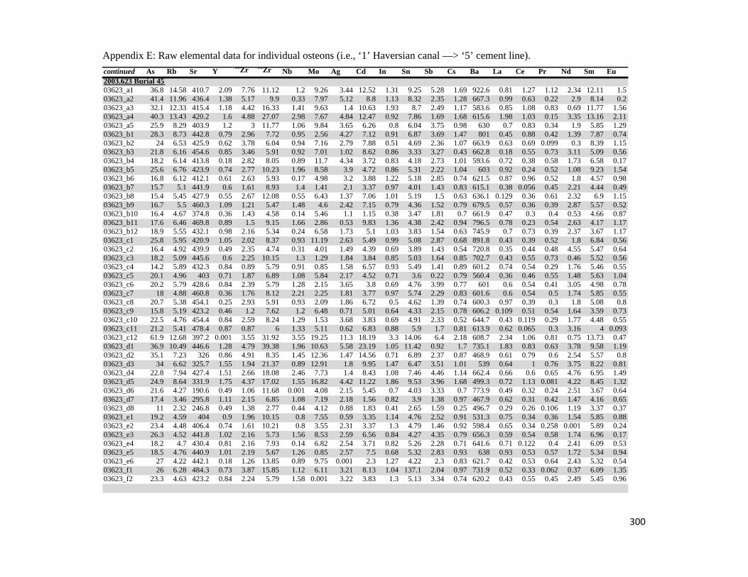
Appendix E: Raw elemental data for individual osteons (i.e., ‘1’ Haversian canal —> ‘5’ cement line).
continued As Rb Sr Y90Zr 91Zr Nb Mo Ag Cd In Sn Sb Cs Ba La Ce Pr Nd Sm Eu
2003.623 Burial 4503623_a1 36.8 14.58 410.7 2.09 7.76 11.12 1.2 9.26 3.44 12.52 1.31 9.25 5.28 1.69 922.6 0.81 1.27 1.12 2.34 12.11 1.503623_a2 41.4 11.96 436.4 1.38 5.17 9.9 0.33 7.97 5.12 8.8 1.13 8.32 2.35 1.28 667.3 0.99 0.63 0.22 2.9 8.14 0.203623_a3 32.1 12.33 415.4 1.18 4.42 16.33 1.41 9.63 1.4 10.63 1.93 8.7 2.49 1.17 583.6 0.85 1.08 0.83 0.69 11.77 1.5603623_a4 40.3 13.43 420.2 1.6 4.88 27.07 2.98 7.67 4.84 12.47 0.92 7.86 1.69 1.68 615.6 1.98 1.03 0.15 3.35 13.16 2.1103623_a5 25.9 8.29 403.9 1.2 3 11.77 1.06 9.84 3.65 6.26 0.8 6.04 3.75 0.98 630 0.7 0.83 0.34 1.9 5.85 1.2903623_b1 28.3 8.73 442.8 0.79 2.96 7.72 0.95 2.56 4.27 7.12 0.91 6.87 3.69 1.47 801 0.45 0.88 0.42 1.39 7.87 0.7403623_b2 24 6.53 425.9 0.62 3.78 6.04 0.94 7.16 2.79 7.88 0.51 4.69 2.36 1.07 663.9 0.63 0.69 0.099 0.3 8.39 1.1503623_b3 21.8 6.16 454.6 0.85 3.46 5.91 0.92 7.01 1.02 8.62 0.86 3.33 3.27 0.43 662.8 0.18 0.55 0.73 3.11 5.09 0.5603623_b4 18.2 6.14 413.8 0.18 2.82 8.05 0.89 11.7 4.34 3.72 0.83 4.18 2.73 1.01 593.6 0.72 0.38 0.58 1.73 6.58 0.1703623_b5 25.6 6.76 423.9 0.74 2.77 10.23 1.96 8.58 3.9 4.72 0.86 5.31 2.22 1.04 603 0.92 0.24 0.52 1.08 9.23 1.5403623_b6 16.8 6.12 412.1 0.61 2.63 5.93 0.17 4.98 3.2 3.88 1.22 5.18 2.85 0.74 621.5 0.87 0.96 0.52 1.8 4.57 0.9803623_b7 15.7 5.1 441.9 0.6 1.61 8.93 1.4 1.41 2.1 3.37 0.97 4.01 1.43 0.83 615.1 0.38 0.056 0.45 2.21 4.44 0.4903623_b8 15.4 5.45 427.9 0.55 2.67 12.08 0.55 6.43 1.37 7.06 1.01 5.19 1.5 0.63 636.1 0.129 0.36 0.61 2.32 6.9 1.1503623_b9 16.7 5.5 460.3 1.09 1.21 5.47 1.48 4.6 2.42 7.15 0.79 4.36 1.52 0.79 679.5 0.57 0.36 0.39 2.87 5.57 0.5203623_b10 16.4 4.67 374.8 0.36 1.43 4.58 0.14 5.46 1.1 1.15 0.38 3.47 1.81 0.7 661.9 0.47 0.3 0.4 0.53 4.66 0.8703623_b11 17.6 6.46 469.8 0.89 1.5 9.15 1.66 2.86 0.53 9.83 1.36 4.38 2.42 0.94 796.5 0.78 0.23 0.54 2.63 4.17 1.1703623_b12 18.9 5.55 432.1 0.98 2.16 5.34 0.24 6.58 1.73 5.1 1.03 3.83 1.54 0.63 745.9 0.7 0.73 0.39 2.37 3.67 1.1703623_c1 25.8 5.95 420.9 1.05 2.02 8.37 0.93 11.19 2.63 5.49 0.99 5.08 2.87 0.68 891.8 0.43 0.39 0.52 1.8 6.84 0.5603623_c2 16.4 4.92 439.9 0.49 2.35 4.74 0.31 4.01 1.49 4.39 0.69 3.89 1.43 0.54 720.8 0.35 0.44 0.48 4.55 5.47 0.6403623_c3 18.2 5.09 445.6 0.6 2.25 10.15 1.3 1.29 1.84 3.84 0.85 5.03 1.64 0.85 702.7 0.43 0.55 0.73 0.46 5.52 0.5603623_c4 14.2 5.89 432.3 0.84 0.89 5.79 0.91 0.85 1.58 6.57 0.93 5.49 1.41 0.89 601.2 0.74 0.54 0.29 1.76 5.46 0.5503623_c5 20.1 4.96 403 0.71 1.87 6.89 1.08 5.84 2.17 4.52 0.71 3.6 0.22 0.79 560.4 0.36 0.46 0.55 1.48 5.63 1.0403623_c6 20.2 5.79 428.6 0.84 2.39 5.79 1.28 2.15 3.65 3.8 0.69 4.76 3.99 0.77 601 0.6 0.54 0.41 3.05 4.98 0.7803623_c7 18 4.88 460.8 0.36 1.76 8.12 2.21 2.25 1.81 3.77 0.97 5.74 2.29 0.83 601.6 0.6 0.54 0.5 1.74 5.85 0.5503623_c8 20.7 5.38 454.1 0.25 2.93 5.91 0.93 2.09 1.86 6.72 0.5 4.62 1.39 0.74 600.3 0.97 0.39 0.3 1.8 5.08 0.803623_c9 15.8 5.19 423.2 0.46 1.2 7.62 1.2 6.48 0.71 5.01 0.64 4.33 2.15 0.78 606.2 0.109 0.51 0.54 1.64 3.59 0.7303623_c10 22.5 4.76 454.4 0.84 2.59 8.24 1.29 1.53 3.68 3.83 0.69 4.91 2.33 0.52 644.7 0.43 0.119 0.29 1.77 4.48 0.5503623_c11 21.2 5.41 478.4 0.87 0.87 6 1.33 5.11 0.62 6.83 0.88 5.9 1.7 0.81 613.9 0.62 0.065 0.3 3.16 4 0.09303623_c12 61.9 12.68 397.2 0.001 3.55 31.92 3.55 19.25 11.3 18.19 3.3 14.06 6.4 2.18 608.7 2.34 1.06 0.81 0.75 13.73 0.4703623_d1 36.9 10.49 446.6 1.28 4.79 39.38 1.96 10.63 5.58 23.19 1.05 11.42 0.92 1.7 735.1 1.83 0.83 0.63 3.78 9.58 1.1903623_d2 35.1 7.23 326 0.86 4.91 8.35 1.45 12.36 1.47 14.56 0.71 6.89 2.37 0.87 468.9 0.61 0.79 0.6 2.54 5.57 0.803623_d3 34 6.62 325.7 1.55 1.94 21.37 0.89 12.91 1.8 9.95 1.47 6.47 3.51 1.01 539 0.64 1 0.76 3.75 8.22 0.8103623_d4 22.8 7.94 427.4 1.51 2.66 18.08 2.46 7.73 1.4 8.43 1.08 7.46 4.46 1.14 662.4 0.66 0.6 0.65 4.76 6.95 1.4903623_d5 24.9 8.64 331.9 1.75 4.37 17.02 1.55 16.82 4.42 11.22 1.86 9.53 3.96 1.68 499.3 0.72 1.13 0.081 4.22 8.45 1.3203623_d6 21.6 4.27 190.6 0.49 1.06 11.68 0.001 4.08 2.15 5.45 0.7 4.03 3.33 0.7 773.9 0.49 0.32 0.24 2.51 3.67 0.6403623_d7 17.4 3.46 295.8 1.11 2.15 6.85 1.08 7.19 2.18 1.56 0.82 3.9 1.38 0.97 467.9 0.62 0.31 0.42 1.47 4.16 0.6503623_d8 11 2.32 246.8 0.49 1.38 2.77 0.44 4.12 0.88 1.83 0.41 2.65 1.59 0.25 496.7 0.29 0.26 0.106 1.19 3.37 0.3703623_e1 19.2 4.59 404 0.9 1.96 10.15 0.8 7.55 0.59 3.35 1.14 4.76 2.52 0.91 531.3 0.75 0.34 0.36 1.54 5.85 0.8803623_e2 23.4 4.48 406.4 0.74 1.61 10.21 0.8 3.55 2.31 3.37 1.3 4.79 1.46 0.92 598.4 0.65 0.34 0.258 0.001 5.89 0.2403623_e3 26.3 4.52 441.8 1.02 2.16 5.73 1.56 8.53 2.59 6.56 0.84 4.27 4.35 0.79 656.3 0.59 0.54 0.58 1.74 6.96 0.1703623_e4 18.2 4.7 430.4 0.81 2.16 7.93 0.14 6.82 2.54 3.71 0.82 5.26 2.28 0.71 641.6 0.71 0.122 0.4 2.41 6.09 0.5303623_e5 18.5 4.76 440.9 1.01 2.19 5.67 1.26 0.85 2.57 7.5 0.68 5.32 2.83 0.93 638 0.93 0.53 0.57 1.72 5.34 0.9403623_e6 27 4.22 442.1 0.18 1.26 13.85 0.89 9.75 0.001 2.3 1.27 4.22 2.3 0.83 621.7 0.42 0.53 0.64 2.43 5.32 0.5403623_f1 26 6.28 484.3 0.73 3.87 15.85 1.12 6.11 3.21 8.13 1.04 137.1 2.04 0.97 731.9 0.52 0.33 0.062 0.37 6.09 1.3503623_f2 23.3 4.63 423.2 0.84 2.24 5.79 1.58 0.001 3.22 3.83 1.3 5.13 3.34 0.74 620.2 0.43 0.55 0.45 2.49 5.45 0.96
300

Appendix E: Raw elemental data for individual osteons (i.e., ‘1’ Haversian canal —> ‘5’ cement line).
continued As Rb Sr Y90Zr 91Zr Nb Mo Ag Cd In Sn Sb Cs Ba La Ce Pr Nd Sm Eu
03623_f3 19.1 5.63 430.8 0.64 1.95 6.19 1.38 5.35 2.81 5.8 0.74 5.82 2.53 0.64 623.9 0.25 0.41 0.173 3.26 3.36 1.0203623_f4 18.2 6.71 438.1 0.72 3.82 9.88 0.32 8.54 3.18 9.26 0.84 4.2 4.04 1.15 623 1.03 0.34 0.61 3 7.1 0.9403623_f5 23.4 5.84 461.7 0.73 2.73 7.83 1.12 6.12 3.94 4.69 1.59 7.02 2.05 1.04 642.7 0.52 0.47 0.148 3.73 6.08 1.3503623_f6 32.5 6.02 476.3 1.37 2.43 13.32 2.43 9.42 3.5 7.21 1.6 6.54 3.15 0.98 708.9 1.13 1.03 1.1 5.23 7.82 1.04
1999.175 Burial 57-299175_a1 11.2 1.41 216.7 1.08 0.27 10.63 2.28 25.12 2.87 0.53 0.18 6.19 2.2 0.63 421.6 0 0.95 0.29 4.32 3.42 0.8999175_a2 10.7 1.1 228.2 1.04 0.72 10.21 1.55 24.61 4.78 4.56 0.76 4.6 3.67 0.75 423 0.058 0.05 0.038 2.94 6.36 0.299175_a3 13.3 0.68 248.9 0.91 0.37 3.23 0.24 31.01 0.44 1.44 1.15 4.83 3.2 0.238 448.6 0.66 0 0.078 3.63 3.21 0.13699175_a4 4.68 0.42 236.4 0.48 1.08 0.91 0.72 6.84 1.47 1.72 0.53 2.24 0.8 0.199 440 0.35 0.24 0.132 0.78 1.7 0.499175_a5 4.8 0.35 229.9 0.66 0.28 4.56 1.69 28.61 2.47 2.88 0.76 3.06 1.64 0.33 438.3 0.59 0.5 0.151 1.31 4.02 0.15799175_b1 10.8 0.68 263.8 0.39 4.03 8.85 0.58 32.73 2.39 1.28 0.93 5.64 2.6 0.74 513.4 1.14 0.18 0.74 2.55 6.36 1.0499175_b2 19.8 1.44 242.1 0.37 4.27 1.83 2.85 12.2 0.74 0 0.2 7.98 1.14 1.12 457.9 0.135 0.23 0.044 0.53 2.63 0.5499175_b3 8.09 0.83 257.1 0.78 0.28 5.42 1.16 13.26 1.47 4.85 0.8 3.74 0 0.32 464.8 0.7 0.34 0.37 2.21 4.78 0.7999175_b4 8.83 0.84 242.8 0.29 2.49 5.48 0.73 15.29 2.96 0.43 0.7 4.03 1.14 0.4 463.5 0.29 0.35 0.53 1.58 3.41 0.4699175_b5 5.75 1.25 243.4 0.48 1.52 6.67 0.71 13.48 2.21 2.99 0.49 3.25 0.98 0.28 497.8 0.49 0.21 0.079 1.36 2.94 0.5699175_c1 7.67 1.18 232.6 0.52 0.88 1.93 1.35 36.77 2.41 3.98 0.095 5 1.85 0.53 558 0.81 0.6 0.155 0.93 1.16 1.0699175_c2 11.2 0.81 233.6 0.4 1.33 3.9 1.6 11.68 2.86 0.87 0.78 4.49 2.2 0.77 621.6 0.39 0.67 0.72 0.75 5.37 0.16499175_c3 5.84 0.73 243.2 0.97 0.53 2.94 0.44 29.31 0.16 1.32 0.174 4.06 0.37 0.57 569.8 0.71 0.41 0.46 0.68 0.85 0.09999175_c4 3.94 0.98 206.2 0.101 1.46 3.47 1.38 7.79 1.74 2.88 0.83 2.9 0.72 0.27 481.4 0.48 0.251 0.167 1.85 2.31 0.12599175_c5 7.38 0.65 238.1 0.87 0.7 8.53 0.47 19.45 1.63 0.46 0.153 2.22 0.54 0.36 523.6 0.89 0.38 0.05 0.3 3.07 0.04399175_d1 7.05 1.08 237.5 0.22 0.33 16.28 0.56 26.94 3.12 0.66 1.05 3.67 0.31 0.68 473.6 0.49 0.73 0.56 2.34 6.54 0.6899175_d2 9.1 0.8 219.3 0.62 1.94 6.06 0.46 35.69 1.64 2.72 0.45 4.07 0.16 0.44 432.9 0.64 0.146 0.41 2.47 3.08 0.7299175_d3 3.64 0.72 220.9 0.085 0.95 5.94 0.64 25.41 1.61 1.12 0.62 2.44 2.48 0.3 419 0.123 0.266 0.203 2.7 3.37 0.2199175_d4 6.95 0.61 224.6 0.41 0.91 4.01 0.1 14.39 1.88 3.11 0.3 3.24 1.45 0.29 420.3 0.3 0.44 0.034 0.2 2.74 0.6799175_d5 2.9 1.11 228.5 0.24 2.84 3.15 1.9 26.79 3.4 0.35 0 3.61 3.03 0.43 418.2 0.76 0.8 0.61 0.23 4.51 0.8699175_d5 233 0 124.7 0 0 0 0 0 17.18 0 0 0 0 0 109.7 0 0 0.77 0 0 5.32
SRM612 Avg 38.3 31.96 76.54 38.61 36.66 36.22 38.137 35.9 22.06 28.72 43.09 38.26 38.52 42 37.87 35.98 38.36 37.34 35.32 37.14 34.59
301

Appendix E: Raw elemental data for individual osteons (i.e., ‘1’ Haversian canal —> ‘5’ cement line).
continued Gd Tb Dy Ho Er Tm Yb Lu Hf Ta Re Au Tl Pb Bi Th U1998.304 Burial 27-198304_a1 4.89 0.7 4.19 0.48 1.23 0.71 3.33 0.71 2.37 1.05 0.61 4.08 1.95 2.65 0.9 0.82 0.4798304_a2 3.55 0.72 2.48 0.15 1.82 0.73 1.97 0.14 1.4 0.62 0.75 4.18 2.03 1.28 0.38 0.15 0.04798304_a3 0.66 0.87 3.69 0.071 2.71 0.89 4.14 0.89 0.45 0.1 2.71 1.17 0.38 1.34 0.79 0.075 0.5898304_a4 1.58 0.115 1.36 0.48 0.99 0.46 2.15 0.117 0 0.83 0.81 2.63 1.86 0.62 0.65 0 0.11698304_a5 5.78 0.34 0.86 1.23 0.21 0.137 5.56 0.138 0.46 0.2 0.24 1.57 4.89 2.54 1.06 0.15 0.4198304_b1 3.57 1.02 2.71 1.32 3.17 0.73 0.87 0.74 0.92 1.53 0.33 4.19 3.06 1.11 0.75 0.3 0.6898304_b2 3.43 0.3 2.94 0.9 2.64 0.86 4.03 0.077 1.65 0.73 1.52 2.85 2.11 1.06 1 0.54 0.3598304_b3 1.49 0.61 4.49 0.91 1.9 0.88 1.07 0.077 0.76 1.83 0.14 3.56 3.79 1.88 0.62 0.68 0.4198304_b4 2.45 0.19 3.63 0.33 2.17 0.71 1.79 0.5 1.67 0.37 0.89 4.97 2.69 1.06 0.78 0.42 0.2998304_b5 1.46 0.29 4.06 1.24 1.6 0.15 3.22 0.3 0.5 1.43 1.21 3.93 3.75 1.04 1.23 0.75 0.5998304_c1 0 0.35 2.74 0.84 2.46 0 2.17 0.47 2.67 0.68 1.16 0 4.2 0.99 0.41 0 0.1298304_c2 0.93 0.19 2.12 0.68 0.39 0.93 0.89 0.66 2.17 1.36 0.22 3.73 3 1.96 1.17 0.71 0.4398304_c3 3.32 0.67 1.53 1 0.48 0.68 0.98 0.47 2.26 0.31 0.18 6.74 0.52 1.02 0.86 0.115 0.03498304_c4 2.49 0.87 3.69 0.35 2.21 0.22 0.52 0.51 0.18 0.33 0.9 2.91 3.43 1.88 1.02 0.18 0.14698304_c5 3.98 0.22 1.85 0.115 1.77 0.39 0.52 0.58 1.91 0.85 1.02 3.29 4.42 1.22 0.89 0.63 0.3898304_d1 0.9 0.51 2.16 0.26 1.58 0.73 0.29 0.73 1.71 1.07 1.29 4.17 1.8 1.34 0.8 0.57 0.08198304_d2 2.96 0.85 1.22 0.63 0.45 0.86 2.84 0.61 2.85 0.43 0.51 2.07 4.81 1.57 0.77 0.94 0.5698304_d3 0.85 0.086 0.73 0.87 0.53 0.69 2.27 0.49 2.27 1.01 1.21 4.79 2.48 1.26 0.43 0.53 0.3298304_d4 2.7 0.38 2.83 0.35 1.69 0.39 1.26 0.39 1.83 0.57 0.69 4.45 2.87 0.91 0.7 0.44 0.2698304_d5 2.28 0.46 2.77 0.97 2.03 0.94 3.79 0.66 2.68 0.69 1.42 4.61 2.33 0.82 0.93 1.14 0.2
1998.312 Burial 35-198312_a1 0.33 0.87 0.86 0.21 0.42 1.26 0.64 0.55 0.9 0.4 1.54 0 9.54 1.29 0.78 0.074 0.5898312_a2 1.81 0.135 0.38 0.86 1.61 0.37 2.45 0.37 0.45 0.54 0.64 5.54 6.28 0.54 0.73 0.149 0.0398312_a3 92.2 0 0 0 173.5 94.82 0 94.66 61.92 0 0 0 124.5 0 0 0 098312_a3 1.77 0.093 2.15 0.53 0 0.37 1.69 0.63 1.19 0.75 0.63 2.9 2.47 1.06 0.78 0.79 0.3398312_a4 2.1 0.42 0.67 0.45 0.37 0.61 2.01 0.43 3.74 0.116 0.75 3.43 3.03 1.08 0.54 0.47 0.3998312_a5 1.97 0.043 2.39 0.42 1.24 0.41 1.88 0.57 2.29 0.44 1.21 4.55 4.15 1.02 0.5 0.88 0.5298312_b1 2.33 0.043 3.17 0.182 1.04 0.68 1.57 0.68 0.57 0.49 0.59 1.9 5.68 0.69 0.59 0.37 0.05798312_b2 0.23 0.24 3.93 0.1 0.74 0.097 4.37 1.33 4.35 0.35 0.25 1.62 1.5 0.42 0.82 0.26 0.06298312_b3 6.32 1.27 5.42 0.22 3.96 1.3 6.02 0.212 0.69 0.31 0.073 1.42 1.7 0.37 0.8 1 0.5998312_b4 1.66 0.23 1.42 0.5 1.8 0.34 1.58 0.14 2.22 0.5 0.56 0.52 4.93 1.1 0.79 0.37 0.3898312_b5 2 0.28 1.71 0.3 1.25 0.58 1.9 0.29 1.34 0.26 0.5 2.3 3.56 0.59 0.51 0.31 0.18798312_c1 0.67 0.53 3.19 0.79 0.56 0.139 0 0.54 0 1.11 0.93 3.03 3.76 0.53 0.47 0.83 0.08998312_c2 0.24 0.6 3.61 0.9 1.87 0.3 2.84 0.099 2 1.26 0.34 1.11 8.17 1.24 0.48 0.108 0.3998312_c3 1.74 0.35 2.59 0.076 1.54 0.59 1.02 0.62 1.17 0.52 0.87 2.83 3.53 0.51 0.7 0.67 0.04798312_c4 0.23 0.92 3.2 0.79 0.57 0.23 2.51 0.185 2.49 0.2 0.32 5.25 7.9 1.34 0.47 0.59 0.3598312_c5 2.08 1.02 3.07 0.055 0 0.107 7.63 0.74 0.35 0.23 1.26 0.89 7.97 1.05 0.186 0.17 0.6798312_d1 3.49 0.152 2.12 0.2 1.55 0.36 1.66 0.36 0.38 0.52 0.2 2.84 7.07 1.26 0.44 0.042 0.3398312_d2 0.21 0.084 4.62 0.088 0.52 0.78 0.79 0.042 0.14 0.062 0.073 0.95 9.38 1.94 0.185 0.85 0.13698312_d3 0.55 0.58 1.01 0.5 0.34 0.112 1.12 0.242 1.37 0.35 0.93 1.36 5.33 0.49 0.47 0.26 0.2298312_d4 0.96 0.76 1.49 0.164 2.36 0.079 0.92 0.77 0.64 1.94 1.32 1.55 14.69 0.23 1.16 0.129 0.598312_d5 0.85 0.249 1.49 0.64 1.34 0.36 0 0.36 1.16 0.52 0.87 0.59 5.12 0.36 0.49 0.55 0.281
302

Appendix E: Raw elemental data for individual osteons (i.e., ‘1’ Haversian canal —> ‘5’ cement line).
continued Gd Tb Dy Ho Er Tm Yb Lu Hf Ta Re Au Tl Pb Bi Th U2003.597 Burial 35-203597_a1 0 0.28 1.92 0.22 1.41 0.65 2.17 0.29 1.56 1.19 0 2.7 1.33 0.74 0.85 0.72 003597_a2 1.84 0.53 2.23 0.49 1.16 0.66 0.64 0.66 2.57 0.1 0.69 3.14 1.11 0.86 0.61 0.42 0.2603597_a3 1.59 0.098 2.35 0.48 1.41 0.73 1.42 0.57 1.91 1.38 0.84 2.7 1.11 1.28 0.52 0.33 0.22103597_a4 1.57 0.32 1.35 0.82 0.26 0.32 0 0.127 1.1 0.5 0.59 2.68 1.12 1.16 0.52 0.36 0.05703597_a5 0 0.23 2.98 0.147 0 0.72 3.37 0.72 0.48 0.07 2.25 4.18 1.76 1.98 0.26 0.104 0.22303597_b1 0.51 0.29 1.76 0.44 1.58 0.42 0.99 0.43 0.71 0.77 0.19 1.75 1.17 1.06 0.73 0.33 0.1403597_b2 2.91 0.83 1.15 0.62 0.56 0.6 0.65 1.05 2.02 0.89 1.08 1.61 1.5 1.65 0.95 0.051 0.5703597_b3 0.73 0.45 1.88 1.27 1.41 0.101 0.24 0 1.56 0.97 0 2.7 2.03 1.04 0.42 0.111 0.3103597_b4 4.61 0.66 3.95 0.99 0.53 0.67 3.15 0.96 3.92 0.065 2.1 0.76 2.1 0.62 0.28 0.24 0.05903597_b5 0 0.62 1.12 0.093 1.93 0.045 0.21 0.9 3.69 0.2 1.14 3.68 0.16 1.41 0.205 0.197 0.12103597_c1 0.25 0.151 1.28 0.98 0.16 1.89 0.72 0.21 0.17 0.15 2.41 1.19 1.74 1.49 1.5 1.04 0.06903597_c2 0.67 0.27 0.87 0.55 2.27 0.21 0.33 0.49 1.77 1.11 0.13 6.12 1.04 1.18 0.83 0.58 0.1403597_c3 0.53 0.107 3.46 0.114 0.33 0.165 0.51 0.055 2.8 0.16 1.5 1.59 0.31 1.85 1.52 0.121 0.5603597_c4 2.27 0.32 1.94 0.34 1.75 0.33 0.67 0.58 1.92 0.69 0.59 3.83 0.89 0.73 0.6 0.36 0.3803597_c5 0.74 0.34 0.32 0.85 3.56 0.82 0.71 0.27 0.77 1.73 0.21 1.54 3.18 1.08 1.06 0.91 0.10203597_d1 6.41 1.29 3.59 0.6 0.88 0.22 4.38 0.94 4.44 1.96 0.39 5.42 5.16 2.54 1.21 0.79 0.14403597_d2 1.99 0.57 1.7 0.6 0.49 0.58 2.72 0.41 0.89 1.36 0.74 3.36 2.16 0.97 0.83 0.35 0.3203597_d3 4.95 0.58 2.45 0.61 1.8 0.59 2.76 0.59 0.2 0.87 0.32 4.82 2.06 1.3 1.31 0.2 0.6803597_d4 1.81 0.26 1.93 0.55 0.68 0.37 1.75 0.179 1.25 0.55 0.94 2.16 1.32 0.82 0.34 0.098 0.4303597_d5 0.46 0.79 0.19 0.59 0.43 0.57 0.44 0.047 0.47 0.85 0.25 3.31 1.06 0.59 0.52 0.63 0.38
2003.591 Burial 3903591_a1 4.26 0.86 0.95 0.64 1.89 0.23 0 0.88 0.26 1.3 1.57 0.44 1.3 1.37 0.98 0.68 0.4103591_a2 0.7 0.047 3.48 1.23 2.56 0.24 0.23 0.146 0.16 0.36 1.5 1.12 1.77 1.3 0.76 0.159 0.16103591_a3 2.54 0.046 2.18 0.77 1.13 0.83 3.01 0.65 1.24 0.42 0.25 3.71 1.12 0.63 0.67 0.41 0.24703591_a4 2.34 0.137 2.83 0.5 0.28 0.23 0.87 0.59 1.14 0.5 1.22 1.97 1.04 0.53 0.62 0.37 0.2303591_a5 1.95 0.192 0.65 0.32 0.24 0.078 1.89 0.7 0.26 1.03 0.14 3.29 2.33 0.61 0.52 0.44 0.4603591_b1 1.12 0.28 0.24 0.91 2.67 1.52 1.08 0.88 0.19 0 0.41 1.66 1.28 1.35 0.21 0.96 0.8203591_b2 0.21 0.214 0.91 0.27 2.6 0.85 0.2 0.86 2.85 0.129 1.52 6.96 1.91 1.87 1.34 0.94 0.5703591_b3 1.87 0.38 0.44 0.56 1.17 0.071 2.54 0.55 0.59 0.105 0.97 2.22 0.87 0.33 0.49 0.233 0.3603591_b4 2.35 0.27 1.13 0.5 0.36 0.69 0.54 0.49 1.98 0.51 0.21 1.79 1.93 0.53 0.82 0.128 0.22803591_b5 0.76 0.5 4.71 0.53 1.19 0.234 2.37 0.51 1.69 1.06 0.9 5.05 1.67 0.78 0.79 0.56 0.15503591_c1 1.87 0.76 1.61 0.4 1.67 0.39 2.55 0.55 1.29 0.57 0.97 3.85 2.41 1.33 0.92 0.51 0.3603591_c2 5.5 0.2 4.71 1.66 4.89 0.052 1.47 0.21 0.35 0.23 2.01 1.2 1.75 1.74 1.02 0.23 0.7503591_c3 2.57 1.59 4.76 1.19 0.23 0.23 0.71 1.15 5.4 0.33 2.88 6.58 2.77 1.76 1.79 1.25 0.4503591_c4 0.58 1.08 1.49 0.25 1.27 1.1 1.39 0.12 0.2 0.26 0.42 3.42 4.66 1.68 0.43 1.2 0.2803591_c5 1.07 0.14 1.84 0.31 0.45 1.08 0 0.074 0.74 0.92 1.1 5.05 1.55 1.65 0.79 0.081 0.4103591_d1 2.64 0.54 3.26 1.15 0.99 0.96 2.59 0.79 1.85 0.82 1.39 6.37 2.42 0.66 0.86 0.86 0.9203591_d2 3.52 0.99 2.1 0.53 1.54 0.51 2.36 0.88 2.38 0.74 1.55 4.1 2.23 1.89 1.2 0.55 0.903591_d3 2.71 0.55 4.03 0.82 1.84 0.56 2.61 0.97 2.63 1.43 1.4 5.55 3.23 1.48 0.5 0.37 0.703591_d3 509 102.8 201.4 25.09 0 8.07 489.93 16.2 53.65 154.5 185.8 1041 275.1 12.29 133.2 35.29 15.9903591_d4 1.64 0.5 4.08 0.72 4.23 0.168 4.58 1.2 2.3 1.44 1.74 2.89 3.19 1.02 1.08 0.76 0.7403591_d5 4.83 0.32 2.92 0.89 1.32 0.7 2.32 0.5 1.65 0.73 0.88 2.85 2.32 1.07 0.63 0.24 0.64
303

Appendix E: Raw elemental data for individual osteons (i.e., ‘1’ Haversian canal —> ‘5’ cement line).
continued Gd Tb Dy Ho Er Tm Yb Lu Hf Ta Re Au Tl Pb Bi Th U2003.623 Burial 4503623_a1 1.34 0.29 4.71 1.36 2.02 0.94 3.19 1.22 2.32 1.34 2.34 4.02 2.95 3.89 2.82 0.29 0.7903623_a2 3.54 0.53 5.23 0.58 3.89 0.99 2.74 0.27 1.99 0.81 2.31 6 2.27 2.25 1.44 0.12 0.5503623_a3 3.02 0.91 2.82 0.28 2.1 0.98 8.1 1.04 2.41 2.2 2.43 3.28 3.49 1.72 0.56 0.66 0.00103623_a4 2.89 0.62 4.68 2.24 2.84 0.94 1.31 0.99 3.26 2.1 3.3 5.68 2.78 2.02 1.67 1.09 0.6403623_a5 2.52 0.76 4.07 0.83 1.23 0.71 3.37 0.96 3.74 0.58 1.66 3.49 2.13 1.54 0.94 0.39 0.2803623_b1 2.86 0.75 3.78 1.25 2.43 0.8 3.13 0.49 2.28 1.14 2.11 4.87 2.43 2 0.95 0.17 0.5503623_b2 3.88 0.75 2.09 0.37 1.55 0.63 1.73 0.125 0.41 0.89 1.65 3.82 1.6 1.28 1.12 0.69 0.3503623_b3 2.19 0.57 2.89 1.14 1.52 0.5 0.23 0.84 0.34 0.87 1.91 4.32 1.57 1.53 1.59 0.58 0.2403623_b4 2.11 0.32 3.11 0.6 0.95 0.001 1.63 0.51 2.9 1.19 1.71 4.17 1.51 1.04 0.93 0.32 0.2303623_b5 1.89 0.4 3.06 0.76 2.27 0.75 2.07 0.46 2.13 0.87 2.5 2.77 1.82 1.87 0.63 0.41 0.4203623_b6 2.2 0.47 1.45 0.42 1.08 0.066 1.7 0.65 3.02 1.01 1.62 4.35 1.58 1.4 0.64 0.48 0.5403623_b7 2.34 0.29 3.99 0.7 0.61 0.001 2.55 0.57 2.15 0.29 1.26 2.68 1.73 1.34 0.71 0.29 0.303623_b8 2 0.74 3.96 0.47 0.98 0.56 2.18 0.112 2.25 1.12 0.94 1.99 1.88 0.99 0.75 0.001 0.2203623_b9 2.02 0.61 2.32 0.58 1.98 0.46 0.51 0.6 0.56 0.46 1.64 2.85 2 1.16 0.83 0.051 0.3203623_b10 1.7 0.44 1.58 0.48 2.35 0.053 0.5 0.29 1.65 0.55 1.48 2.93 1.39 1.88 0.69 0.45 0.14503623_b11 2.78 0.142 2.12 0.65 0.92 0.37 2.48 0.67 2.55 0.52 2.26 3.93 2.12 2.05 0.85 0.6 0.4403623_b12 1.44 0.43 2.69 0.48 1 0.183 1.57 0.34 2.56 0.81 1.17 2.88 1.13 0.82 1.02 0.31 0.22703623_c1 2.19 0.33 2.51 0.51 1.52 0.5 1.56 0.53 2.13 0.87 1.45 6.59 1.32 1.25 1.04 0.34 0.3403623_c2 3.04 0.46 1.45 0.5 1.49 0.49 0.19 0.52 1.97 0.4 1.01 2.49 1.59 1.1 0.88 0.38 0.3503623_c3 2.17 0.46 2.03 0.62 1.06 0.182 0.43 0.98 1.72 0.5 1.25 3.78 1.84 1.39 0.63 0.043 0.3403623_c4 2.63 0.112 0.74 0.61 1.05 0.78 2.34 0.52 0.83 0.98 1.74 3.73 1.09 1.23 1.02 0.33 0.4103623_c5 1.28 0.132 2.39 0.6 1.53 0.65 1.39 0.44 1.43 1.1 1.7 4.07 1.3 1.27 0.68 0.276 0.403623_c6 1.52 0.56 1.42 0.5 0.61 0.35 1.65 0.73 2.41 0.7 2.14 3.75 1.76 1.5 1.08 0.57 0.23903623_c7 2.13 0.32 3.14 0.5 1.47 0.49 0.76 0.52 3.16 1.46 1.73 3.72 1.37 1.06 0.51 0.15 0.2403623_c8 2.68 0.33 1.45 0.2 1.52 0.35 1.69 0.75 2.13 0.5 1.46 3.83 2.17 1.25 0.9 0.33 0.2403623_c9 0.59 0.52 1.87 0.57 0.54 0.32 1.54 0.59 1.58 0.79 1.49 4.52 1.5 1.62 1.01 0.43 0.3903623_c10 1.53 0.32 2.02 0.8 1.83 0.35 2.35 0.52 1.71 0.7 1.76 4.38 1.55 1.24 0.81 0.66 0.3403623_c11 1.57 0.22 2.08 0.9 0.89 0.62 2.42 0.54 1.76 0.88 1.05 3.91 1.13 2.3 0.92 0.59 0.3503623_c12 5.92 0.68 3.91 1.95 4.09 1.35 9.11 0.78 3.31 2.35 3.95 10.42 3.55 2.94 1.72 0.9 0.6603623_d1 7.3 0.69 6.1 1.32 2.26 0.58 0.001 1.37 3.66 1.06 3.45 10.51 3.63 1.89 1.74 1 0.5203623_d2 2.19 0.52 3.54 1.35 1.51 0.71 2.38 0.92 2.45 0.66 1.46 7.74 2.11 2.18 1.12 0.67 0.3503623_d3 3.23 0.97 3.7 1.19 3.16 0.34 2.49 0.55 3.14 1.05 2.86 4.3 2.54 2.07 1.33 0.7 0.4103623_d4 2.37 0.5 6.64 0.78 2.84 0.54 3.65 0.47 3.25 0.5 1.28 2.23 2.64 2.72 1.38 0.001 0.3703623_d5 1.26 1.22 4.17 1.59 2.52 0.19 3.96 1.25 5 0.83 3.22 3.04 2.74 3.47 0.87 0.78 0.5803623_d6 2.17 0.38 2.02 0.58 0.86 0.29 1.92 0.3 1.98 0.81 1.32 4.05 1.27 1.13 0.67 0.269 0.3403623_d7 1.27 0.27 2.37 0.66 0.57 0.29 1.38 0.53 1 0.41 1.2 3.19 1.22 1.03 0.61 0.045 0.203623_d8 0.73 0.154 0.68 0.24 0.5 0.166 0.79 0.249 1.41 0.119 0.69 1.06 0.66 0.81 0.35 0.158 0.11503623_e1 3.26 0.28 3.04 0.44 0.92 0.53 2.05 0.46 2.35 0.75 1.55 2.74 1.6 1.95 0.84 0.4 0.22903623_e2 0.87 0.57 1.77 0.62 1.85 0.31 1.46 0.37 2.12 0.43 0.95 2.56 1.29 0.89 0.64 0.23 0.3703623_e3 3.01 0.32 3.14 0.93 1.47 0.158 3.27 0.51 2.66 0.49 1.24 4.39 1.18 1.36 0.72 0.46 0.03703623_e4 1.47 0.62 2.38 0.34 1.76 0.34 0.26 0.058 1.16 0.82 1.56 4.3 1.64 1.03 0.86 0.71 0.403623_e5 2.1 0.32 1.5 0.85 0.71 0.41 2.8 0.36 1.66 0.83 2 3.08 1.51 1.28 1.12 0.45 0.4103623_e6 1.48 0.31 3.1 0.77 1.02 0.83 1.61 0.72 2.03 0.48 1.22 3.08 1.85 1.04 0.71 0.32 0.2403623_f1 3.22 0.39 2.46 0.75 1.81 0.95 2.86 0.78 1.47 0.6 1.53 5.46 2.15 1.85 1.26 0.56 0.2903623_f2 1.52 0.32 1.18 0.94 2.1 0.49 1.65 0.73 1.33 0.27 1.91 2.23 1.69 1.51 0.63 0.33 0.48
304
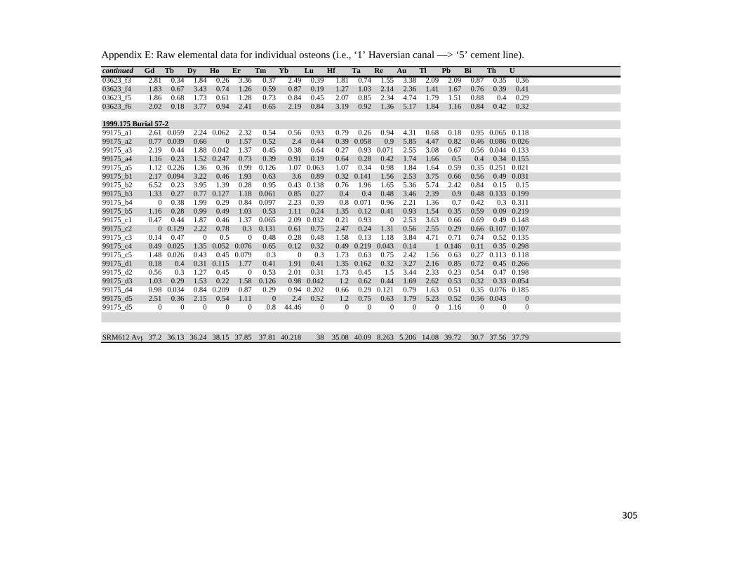
Appendix E: Raw elemental data for individual osteons (i.e., ‘1’ Haversian canal —> ‘5’ cement line).
continued Gd Tb Dy Ho Er Tm Yb Lu Hf Ta Re Au Tl Pb Bi Th U03623_f3 2.81 0.34 1.84 0.26 3.36 0.37 2.49 0.39 1.81 0.74 1.55 3.38 2.09 2.09 0.87 0.35 0.3603623_f4 1.83 0.67 3.43 0.74 1.26 0.59 0.87 0.19 1.27 1.03 2.14 2.36 1.41 1.67 0.76 0.39 0.4103623_f5 1.86 0.68 1.73 0.61 1.28 0.73 0.84 0.45 2.07 0.85 2.34 4.74 1.79 1.51 0.88 0.4 0.2903623_f6 2.02 0.18 3.77 0.94 2.41 0.65 2.19 0.84 3.19 0.92 1.36 5.17 1.84 1.16 0.84 0.42 0.32
1999.175 Burial 57-299175_a1 2.61 0.059 2.24 0.062 2.32 0.54 0.56 0.93 0.79 0.26 0.94 4.31 0.68 0.18 0.95 0.065 0.11899175_a2 0.77 0.039 0.66 0 1.57 0.52 2.4 0.44 0.39 0.058 0.9 5.85 4.47 0.82 0.46 0.086 0.02699175_a3 2.19 0.44 1.88 0.042 1.37 0.45 0.38 0.64 0.27 0.93 0.071 2.55 3.08 0.67 0.56 0.044 0.13399175_a4 1.16 0.23 1.52 0.247 0.73 0.39 0.91 0.19 0.64 0.28 0.42 1.74 1.66 0.5 0.4 0.34 0.15599175_a5 1.12 0.226 1.36 0.36 0.99 0.126 1.07 0.063 1.07 0.34 0.98 1.84 1.64 0.59 0.35 0.251 0.02199175_b1 2.17 0.094 3.22 0.46 1.93 0.63 3.6 0.89 0.32 0.141 1.56 2.53 3.75 0.66 0.56 0.49 0.03199175_b2 6.52 0.23 3.95 1.39 0.28 0.95 0.43 0.138 0.76 1.96 1.65 5.36 5.74 2.42 0.84 0.15 0.1599175_b3 1.33 0.27 0.77 0.127 1.18 0.061 0.85 0.27 0.4 0.4 0.48 3.46 2.39 0.9 0.48 0.133 0.19999175_b4 0 0.38 1.99 0.29 0.84 0.097 2.23 0.39 0.8 0.071 0.96 2.21 1.36 0.7 0.42 0.3 0.31199175_b5 1.16 0.28 0.99 0.49 1.03 0.53 1.11 0.24 1.35 0.12 0.41 0.93 1.54 0.35 0.59 0.09 0.21999175_c1 0.47 0.44 1.87 0.46 1.37 0.065 2.09 0.032 0.21 0.93 0 2.53 3.63 0.66 0.69 0.49 0.14899175_c2 0 0.129 2.22 0.78 0.3 0.131 0.61 0.75 2.47 0.24 1.31 0.56 2.55 0.29 0.66 0.107 0.10799175_c3 0.14 0.47 0 0.5 0 0.48 0.28 0.48 1.58 0.13 1.18 3.84 4.71 0.71 0.74 0.52 0.13599175_c4 0.49 0.025 1.35 0.052 0.076 0.65 0.12 0.32 0.49 0.219 0.043 0.14 1 0.146 0.11 0.35 0.29899175_c5 1.48 0.026 0.43 0.45 0.079 0.3 0 0.3 1.73 0.63 0.75 2.42 1.56 0.63 0.27 0.113 0.11899175_d1 0.18 0.4 0.31 0.115 1.77 0.41 1.91 0.41 1.35 0.162 0.32 3.27 2.16 0.85 0.72 0.45 0.26699175_d2 0.56 0.3 1.27 0.45 0 0.53 2.01 0.31 1.73 0.45 1.5 3.44 2.33 0.23 0.54 0.47 0.19899175_d3 1.03 0.29 1.53 0.22 1.58 0.126 0.98 0.042 1.2 0.62 0.44 1.69 2.62 0.53 0.32 0.33 0.05499175_d4 0.98 0.034 0.84 0.209 0.87 0.29 0.94 0.202 0.66 0.29 0.121 0.79 1.63 0.51 0.35 0.076 0.18599175_d5 2.51 0.36 2.15 0.54 1.11 0 2.4 0.52 1.2 0.75 0.63 1.79 5.23 0.52 0.56 0.043 099175_d5 0 0 0 0 0 0.8 44.46 0 0 0 0 0 0 1.16 0 0 0
SRM612 Avg 37.2 36.13 36.24 38.15 37.85 37.81 40.218 38 35.08 40.09 8.263 5.206 14.08 39.72 30.7 37.56 37.79
305

Appendix F: Raw strontium isotope results for individual osteons.
Burial Total Sr (V)87Sr/86Sr 2σ error 84Sr/86Sr 2σ error
K14_1998.027.01
Intact-1 1.03 0.710664 0.00057 0.056743 0.00014
Intact-2 1.36 0.710550 0.00025 0.056652 0.00010
Intact-3 1.44 0.710515 0.00026 0.056803 0.00005
Intact-4 1.12 0.709436 0.00045 0.056275 0.00015
Intact-5 1.01 0.710160 0.00037 0.056376 0.00012
Intact-6 1.30 0.710140 0.00032 0.056274 0.00009
Intact-7 1.38 0.710461 0.00034 0.056267 0.00006
Intact-8 1.30 0.710390 0.00026 0.056302 0.00007
Intact-9 1.50 0.710141 0.00031 0.056493 0.00007
Diagenetic-1 1.41 0.711112 0.00020 0.056815 0.00006
Diagenetic-2 1.23 0.711441 0.00024 0.056856 0.00008
Diagenetic-3 1.69 0.710975 0.00023 0.056624 0.00005
Diagenetic-4 1.42 0.710920 0.00020 0.056449 0.00008
Diagenetic-5 1.45 0.710674 0.00023 0.056500 0.00008
K14_1998.035.01
Intact-1 0.92 0.710227 0.00028 0.055419 0.00015
Intact-2 0.79 0.710674 0.00032 0.054155 0.00023
Intact-3 0.63 0.710653 0.00043 0.053240 0.00059
Intact-4 0.70 0.711823 0.00058 0.056539 0.00016
Intact-5 0.61 0.712002 0.00072 0.056230 0.00019
Intact-6 0.75 0.710928 0.00040 0.056326 0.00014
Intact-7 0.73 0.710549 0.00040 0.056439 0.00014
Intact-8 0.71 0.710233 0.00037 0.056640 0.00014
Intact-9 0.60 0.710852 0.00055 0.056722 0.00020
Diagenetic-1 0.26 0.717124 0.00394 0.057195 0.00072
Diagenetic-2 0.50 0.713042 0.00166 0.056344 0.00038
Diagenetic-3 0.43 0.713551 0.00175 0.056118 0.00043
Diagenetic-4 0.76 0.709987 0.00047 0.056970 0.00015
Diagenetic-5 0.72 0.709661 0.00057 0.057015 0.00018
306

Appendix F: Raw strontium isotope results for individual osteons.
Burial Total Sr (V)87Sr/86Sr 2σ error 84Sr/86Sr 2σ error
K14_1998.035.02
Intact-1 0.44 0.711867 0.00127 0.053728 0.00100
Intact-2 0.47 0.710200 0.00151 0.054214 0.00084
Intact-3 0.47 0.710127 0.00103 0.053236 0.00108
Intact-4 0.50 0.709541 0.00102 0.056439 0.00027
Intact-5 0.51 0.708952 0.00104 0.056749 0.00025
Intact-6 0.55 0.709380 0.00063 0.056916 0.00038
Intact-7 0.60 0.711022 0.00039 0.056745 0.00025
Intact-8 0.44 0.710124 0.00130 0.055967 0.00055
Intact-9 0.42 0.710383 0.00081 0.055754 0.00058
Diagenetic-1 0.51 0.706062 0.00194 0.057846 0.00079
Diagenetic-2 0.50 0.707067 0.00129 0.057923 0.00052
Diagenetic-3 0.48 0.703660 0.00332 0.058432 0.00114
Diagenetic-4 0.57 0.709698 0.00094 0.058219 0.00068
Diagenetic-5 0.39 0.707243 0.00226 0.058927 0.00092
K14_1999.039
Intact-1 0.82 0.710023 0.00036 0.057456 0.00023
Intact-2 0.83 0.709940 0.00035 0.057370 0.00014
Intact-3 0.98 0.710684 0.00030 0.056128 0.00009
Intact-4 0.90 0.710015 0.00031 0.056579 0.00016
Intact-5 0.93 0.709531 0.00039 0.056671 0.00009
Intact-6 0.94 0.710463 0.00041 0.056273 0.00012
Intact-7 0.92 0.711014 0.00039 0.056112 0.00014
Intact-8 0.84 0.709833 0.00041 0.057040 0.00024
Intact-9 0.98 0.711244 0.00053 0.056170 0.00014
Diagenetic-1 0.78 0.712520 0.00090 0.056108 0.00021
Diagenetic-2 0.64 0.712921 0.00104 0.056217 0.00022
Diagenetic-3 0.61 0.714094 0.00172 0.057733 0.00054
Diagenetic-4 0.71 0.712651 0.00088 0.057027 0.00019
Diagenetic-5 0.75 0.712178 0.00061 0.056626 0.00026
307

Appendix F: Raw strontium isotope results for individual osteons.
Burial Total Sr (V)87Sr/86Sr 2σ error 84Sr/86Sr 2σ error
K14_1999.045
Intact-1 1.02 0.710794 0.00069 0.057295 0.00032
Intact-2 0.58 0.711944 0.00140 0.057212 0.00042
Intact-3 0.71 0.711907 0.00085 0.057173 0.00030
Intact-4 0.66 0.710800 0.00034 0.055969 0.00014
Intact-5 1.19 0.710754 0.00049 0.056357 0.00010
Intact-6 1.10 0.710465 0.00052 0.056178 0.00013
Intact-7 0.63 0.711429 0.00074 0.055748 0.00024
Intact-8 0.63 0.710353 0.00086 0.055476 0.00036
Intact-9 0.60 0.710083 0.00078 0.055501 0.00033
Diagenetic-1 0.65 0.707400 0.00108 0.056776 0.00032
Diagenetic-2 0.89 0.709474 0.00053 0.056587 0.00012
Diagenetic-3 0.69 0.707060 0.00172 0.056476 0.00030
Diagenetic-4 0.78 0.710675 0.00086 0.057410 0.00034
Diagenetic-5 0.79 0.711184 0.00047 0.057102 0.00030
K14_1999.057.02
Intact-1 0.78 0.710234 0.00048 0.055832 0.00016
Intact-2 0.87 0.710433 0.00044 0.055905 0.00016
Intact-3 0.75 0.710328 0.00058 0.055377 0.00033
Intact-4 0.58 0.711643 0.00098 0.056602 0.00042
Intact-5 0.90 0.711309 0.00041 0.056475 0.00014
Intact-6 0.74 0.711146 0.00047 0.056469 0.00013
Intact-7 0.83 0.711812 0.00032 0.056063 0.00015
Intact-8 0.71 0.712509 0.00066 0.055552 0.00029
Intact-9 0.73 0.712036 0.00040 0.055360 0.00033
Diagenetic-1 0.53 0.714669 0.00182 0.055312 0.00051
Diagenetic-2 0.46 0.714494 0.00127 0.056269 0.00048
Diagenetic-3 0.51 0.714701 0.00156 0.056303 0.00026
Diagenetic-4 0.45 0.712510 0.00135 0.055570 0.00045
Diagenetic-5 0.07 0.716986 0.00292 0.054349 0.00154
NBS-987 3.10 0.710253 0.00003 0.056476 0.00002
308

Appendix G: Environmental samples used in the study.
Sample ID Site Latin Name English Name Russian Name Element Latitude Longitude
E 2008.008 Arshan Martes zibellina sable sobol tooth 51°53'52" 102°26'08"E 2008.013 Arshan Apodemus peninsulae mouse mysh tooth 51°54'54" 102°23'23"E 2008.014 Tunka Valley Citelius parryi ground squirrel suslik longbone 51°42'23" 102°35'50"E 2008.015 Tunka Valley Bos taurus cow korova tooth 51°45'32" 102°33'41"E 2008.016 Tunka Valley Bos taurus cow korova longbone 51°54'91" 102°23'37"E 2008.017 Tunka Valley Bos taurus cow korova tooth 51°41'56" 102°33'49"E 2008.018 Tunka Valley Bos taurus cow korova tooth 51°41'57" 102°25'34"E 2008.019 Tunka Valley Bos taurus cow korova tooth 51°41'57" 102°25'34"E 2008.020 Tunka Valley Bos taurus cow korova tooth 51°41'57" 102°25'34"E 2008.021 Tunka Valley Bos taurus cow korova tooth 51°41'57" 102°25'34"E 2008.030 Tunka Valley Equus callabus horse loshad tooth 51°41'57" 102°25'34"E 2008.035 Tunka Valley Equus callabus horse loshad longbone 51°41'57" 102°25'34"E 2008.039 Tunka Valley Equus callabus horse loshad longbone 51°41'57" 102°25'34"E 2008.040 Tunka Valley Equus callabus horse loshad tooth 51°41'57" 102°25'34"E 2008.051 Little Sea Cervidae deer olen pedal element 53°05'54" 106°48'09"E 2008.056 Little Sea Citelius parryi ground squirrel suslik tooth 53°04'98" 106°46'62"E 2008.057 Little Sea Citelius parryi ground squirrel suslik vertebra 53°04'29" 106°46'62"E 2008.061 Ol'khon Island Lepus hare zajac longbone 53°00'87" 106°56'20"E 2008.065 Ol'khon Island Citelius parryi ground squirrel suslik tooth 53°00'92" 106°56'14"E 2008.068 Ol'khon Island Citelius parryi ground squirrel suslik tooth 53°01'74" 106°56'28"E 2008.069 Ol'khon Island Citelius parryi ground squirrel suslik longbone 53°01'75" 106°56'30"E 2008.070 Ol'khon Island Citelius parryi ground squirrel suslik tooth 53°01'75" 106°56'30"E 2008.071 Ol'khon Island Citelius parryi ground squirrel suslik tooth 53°01'76" 106°56'30"E 2008.072 Ol'khon Island Citelius parryi ground squirrel suslik tooth 53°01'77" 106°56'32"E 2008.074 Ol'khon Island Citelius parryi ground squirrel suslik inominate 53°01'78" 106°56'35"E 2008.075 Ol'khon Island Citelius parryi ground squirrel suslik longbone 53°01'80" 106°56'36"E 2008.076 Ol'khon Island Citelius parryi ground squirrel suslik tooth 53°01'80" 106°56'36"E 2008.080 Ol'khon Island Citelius parryi ground squirrel suslik tooth 53°01'56" 106°56'40"E 2008.082 Sagan-Zaba Capreolus pygargus roe deer kosulya tooth 52°41'60" 106°27'76"E 2008.085 Sagan-Zaba Capreolus pygargus roe deer kosulya pedal element 52°41'32" 106°29'21"E 2008.086 Sagan-Zaba Capreolus pygargus roe deer kosulya tooth 52°41'29" 106°29'18"E 2008.088 Sagan-Zaba Capreolus pygargus roe deer kosulya tooth 52°41'39" 106°29'26"
309

Appendix G: Environmental samples used in the study.
Sample ID Site Latin Name English Name Russian Name Element Latitude LongitudeE 2008.089 Sagan-Zaba Cervus elaphus red deer blagorodnii olen tooth 52°41'40" 106°29'15"E 2008.091 Sagan-Zaba Cervidae deer olen longbone 52°41'46" 106°29'10"E 2008.092 Sagan-Zaba Capreolus pygargus roe deer kosulya tooth 52°41'47" 106°29'10"E 2008.094 Sagan-Zaba Capreolus pygargus roe deer kosulya tooth 52°41'48" 106°29'06"E 2008.095 Sagan-Zaba Phoca sibirica baikal seal Baikalskaya nerpa rib 52°38'82" 106°26'06"E 2008.105 Sagan-Zaba Cervus elaphus red deer blagorodnii olen longbone 52°40'89" 106°25'48"E 2008.112 Sagan-Zaba Citelius parryi ground squirrel suslik longbone 52°43'56" 106°31'62"E 2008.115 Sagan-Zaba Capreolus pygargus roe deer kosulya tooth 52°43'56" 106°31'24"E 2008.117 Sagan-Zaba Capreolus pygargus roe deer kosulya tooth 52°43'54" 106°31'18"E 2008.118 Sagan-Zaba Citelius parryi ground squirrel suslik tooth 52°43'49" 106°31'05"E 2008.122 Sagan-Zaba Capreolus pygargus roe deer kosulya tooth 52°43'48" 106°30'96"E 2008.126 Sagan-Zaba Capreolus pygargus roe deer kosulya tooth 52°42'51" 106°29'33"E 2008.128 Sagan-Zaba Citelius parryi ground squirrel suslik tooth 52°41'33" 106°29'07"E 2008.129 Sagan-Zaba Apodemus peninsulae mouse mysh tooth 52°41'53" 106°28'00"E 2008.130 Sagan-Zaba Citelius parryi ground squirrel suslik tooth 52°41'37" 106°28'26"E 2008.131 Sagan-Zaba Citelius parryi ground squirrel suslik tooth 52°41'32" 106°26'36"E 2009.001 Baiandai Betula sp. birch bereza leaves 53°07'13" 105°38'31"E 2009.002 Baiandai Betula sp. birch bereza leaves 53°07'13" 105°38'31"E 2009.007 Khogot Picea sp. spruce el' needles 53°13'40" 105°51'04"E 2009.008 Khogot Picea sp. spruce el' needles 53°13'40" 105°51'04"E 2009.018 Khogot Betula sp. birch bereza leaves 53°16'56" 105°54'18"E 2009.019 Khogot Abies sp. larch listvennitsa needles 53°16'56" 105°54'18"E 2009.023 Khodontsa R. n/a n/a n/a water 53°22'33" 106°00'24"E 2009.029 Manzurka Betula sp. birch bereza leaves 53°30'26" 106°01'37"E 2009.030 Manzurka Abies sp. larch listvennitsa needles 53°30'26" 106°01'37"E 2009.034 Manzurka R. n/a n/a n/a water 53°43'24" 105°59'37"E 2009.040 Kharbatovo Betula sp. birch bereza leaves 53°48'31" 105°58'47"E 2009.041 Kharbatovo Pinus sp. pine sosna needles 53°48'31" 105°58'47"E 2009.050 Ilikta Betula sp. birch bereza leaves 53°49'25" 106°24'54"E 2009.051 Ilikta Picea sp. spruce el' needles 53°49'25" 106°24'54"E 2009.055 Ilikta R. n/a n/a n/a water 53°49'25" 106°24'54"E 2009.056 Lena R. n/a n/a n/a water 53°50'22" 106°20'41"
310

Appendix G: Environmental samples used in the study.
Sample ID Site Latin Name English Name Russian Name Element Latitude LongitudeE 2009.057 Biriulka R. n/a n/a n/a water 53°51'54" 106°20'18"E 2009.061 Makrushina Betula sp. birch bereza leaves 53°52'50" 106°15'40"E 2009.062 Makrushina Pinus sp. pine sosna needles 53°52'50" 106°15'40"E 2009.073 Malye Goly Betula sp. birch bereza leaves 53°54'38" 106°09'29"E 2009.074 Malye Goly Pinus sp. pine sosna needles 53°54'38" 106°09'29"E 2009.078 Anga R. n/a n/a n/a water 53°56'14" 106°02'49"E 2009.079 Tutura R. n/a n/a n/a water 54°47'23" 105°14'06"E 2009.082 Zhigalovo Betula sp. birch bereza leaves 54°46'07" 105°08'39"E 2009.083 Zhigalovo Pinus sp. pine sosna needles 54°46'07" 105°08'39"E 2009.086 Lena R. n/a n/a n/a water 54°39'54" 105°13'05"E 2009.088 Vorob'eva Betula sp. birch bereza leaves 54°34'38" 105°14'48"E 2009.089 Vorob'eva Pinus sp. pine sosna needles 54°34'38" 105°14'48"E 2009.094 Zapleskino Betula sp. birch bereza leaves 54°21'58" 105°15'00"E 2009.095 Zapleskino Pinus sp. pine sosna needles 54°21'58" 105°15'00"E 2009.099 Gul'ma R. n/a n/a n/a water 54°12'53" 105°27'08"E 2009.101 Verkholensk Betula sp. birch bereza leaves 54°06'44" 105°34'06"E 2009.102 Verkholensk Pinus sp. pine sosna needles 54°06'44" 105°34'06"E 2009.108 Magdan Betula sp. birch bereza leaves 53°37'34" 105°17'56"E 2009.109 Magdan Abies sp. larch listvennitsa needles 53°37'34" 105°17'56"E 2009.112 Magdan R. n/a n/a n/a water 53°37'34" 105°17'56"E 2009.114 Magdan Betula sp. birch bereza leaves 53°37'41" 105°17'21"E 2009.115 Magdan Pinus sp. pine sosna needles 53°37'41" 105°17'21"E 2009.119 Kulenga R. n/a n/a n/a water 53°40'41" 105°19'16"E 2009.120 Inei R. n/a n/a n/a water 53°43'12" 105°20'03"E 2009.123 Ikhinagui Betula sp. birch bereza leaves 53°44'32" 105°19'53"E 2009.124 Ikhinagui Abies sp. larch listvennitsa needles 53°44'32" 105°19'53"E 2009.128 Obkhoi Betula sp. birch bereza leaves 53°58'34" 105°26'47"E 2009.129 Obkhoi Pinus sp. pine sosna needles 53°58'34" 105°26'47"E 2009.134 Shemetovo Betula sp. birch bereza leaves 54°01'03" 105°26'47"E 2009.135 Shemetovo Pinus sp. pine sosna needles 54°01'03" 105°26'47"E 2009.139 Shemetovo Bos taurus cow korova molar 54°01'03" 105°26'47"E 2009.140 Shemetovo Bos taurus cow korova molar 54°01'03" 105°26'47"
311

Appendix G: Environmental samples used in the study.
Sample ID Site Latin Name English Name Russian Name Element Latitude LongitudeE 2009.141 Tal'ma R. n/a n/a n/a water 54°01'12" 105°29'57"E 2009.142 Kulenga R. n/a n/a n/a water 54°06'01" 105°35'05"E 2009.145 Kartukhai Betula sp. birch bereza leaves 54°02'17" 105°37'17"E 2009.146 Kartukhai Pinus sp. pine sosna needles 54°02'17" 105°37'17"E 2009.150 Shyshkino Betula sp. birch bereza leaves 54°00'07" 105°43'48"E 2009.151 Shyshkino Pinus sp. pine sosna needles 54°00'07" 105°43'48"E 2009.155 Mys Betula sp. birch bereza leaves 54°01'55" 106°24'15"E 2009.157 Mys Picea sp. spruce el' needles 54°01'55" 106°24'15"E 2009.161 Anga R. n/a n/a n/a water 53°58'41" 106°11'15"E 2009.163 Kachug Betula sp. birch bereza leaves 53°58'53" 105°51'41"E 2009.164 Kachug Abies sp. larch listvennitsa needles 53°58'53" 105°51'41"E 2009.168 Lena R. n/a n/a n/a water 53°56'38" 105°53'04"E 2009.169 Polovinka Betula sp. birch bereza leaves 53°07'07" 105°40'44"E 2009.170 Polovinka Betula sp. birch bereza leaves 53°07'07" 105°40'44"E 2009.172 Oloi Betula sp. birch bereza leaves 52°55'09" 105°10'37"E 2009.173 Oloi Betula sp. birch bereza leaves 52°55'09" 105°10'37"E 2009.175 Kuda R. n/a n/a n/a water 52°55'56" 104°51'25"E 2009.176 Sosnovyi Bor Betula sp. birch bereza leaves 52°39'01" 104°30'59"E 2009.177 Sosnovyi Bor Betula sp. birch bereza leaves 52°39'01" 104°30'59"E 2009.182 Irkut R. n/a n/a n/a water 52°04'34" 103°53'34"E 2009.185 Moty Betula sp. birch bereza leaves 52°04'24" 103°54'14"E 2009.186 Moty Pinus sp. pine sosna needles 52°04'24" 103°54'14"E 2009.191 Andrianovskaia Betula sp. birch bereza leaves 51°48'34" 103°47'18"E 2009.192 Andrianovskaia Pinus sp. pine sosna (kedr) needles 51°48'34" 103°47'18"E 2009.197 Angaselka Betula sp. birch bereza leaves 51°43'21" 103°42'02"E 2009.198 Angaselka Pinus sp. pine sosna needles 51°43'21" 103°42'02"E 2009.203 Kultuk Betula sp. birch bereza leaves 51°44'04" 103°38'12"E 2009.204 Kultuk Betula sp. birch bereza leaves 51°44'04" 103°38'12"E 2009.207 Kultuchnaia R n/a n/a n/a water 51°44'04" 103°38'12"E 2009.208 Bol'shaia Bystraia R. n/a n/a n/a water 51°43'51" 103°23'13"E 2009.211 Bystroe Betula sp. birch bereza leaves 51°43'56" 103°25'57"E 2009.212 Bystroe Pinus sp. pine sosna (kedr) needles 51°43'56" 103°25'57"
312

Appendix G: Environmental samples used in the study.
Sample ID Site Latin Name English Name Russian Name Element Latitude LongitudeE 2009.215 Sredniaia Tibelti R. n/a n/a n/a water 51°45'41" 103°15'17"E 2009.216 Irkut R. n/a n/a n/a water 51°46'39" 103°14'41"E 2009.219 Tibelti Betula sp. birch bereza leaves 51°46'45" 103°13'19"E 2009.220 Tibelti Pinus sp. pine sosna needles 51°46'45" 103°13'19"E 2009.225 Zun-Murino Betula sp. birch bereza leaves 51°44'07" 102°52'41"E 2009.226 Zun-Murino Pinus sp. pine sosna needles 51°44'07" 102°52'41"E 2009.229 Zun-Murino R. n/a n/a n/a water 51°43'56" 102°51'40"E 2009.232 Shabartaika Betula sp. birch bereza leaves 51°43'01" 102°43'43"E 2009.233 Shabartaika Pinus sp. pine sosna needles 51°43'01" 102°43'43"E 2009.236 Irkut R. n/a n/a n/a water 51°43'03" 102°35'13"E 2009.239 Guzhiry Betula sp. birch bereza leaves 51°47'42" 102° 4' 3"E 2009.240 Guzhiry Pinus sp. pine sosna needles 51°47'42" 102° 4' 3"E 2009.245 Dalakhai Betula sp. birch bereza leaves 51°48'01" 102°58'31"E 2009.246 Dalakhai Betula sp. birch bereza leaves 51°48'01" 102°58'31"E 2009.248 Tsagan-Ugun R. n/a n/a n/a water 51°48'01" 102°58'31"E 2009.251 Nikol'sk Picea sp. spruce el' needles 51°43'06" 102°35'23"E 2009.252 Nikol'sk Pinus sp. pine sosna needles 51°43'06" 102°35'23"E 2009.257 Tagarkhai Betula sp. birch bereza leaves 51°52'32" 102°26'41"E 2009.258 Tagarkhai Abies sp. larch listvennitsa needles 51°52'32" 102°26'41"E 2009.261 Kitoi R. n/a n/a n/a water 52°02'56" 101°05'53"E 2009.262 Il'chir Lake Abies sp. larch listvennitsa needles 52° 0' 2" 101°01'17"E 2009.263 Il'chir Lake Abies sp. larch listvennitsa needles 52° 0' 2" 101°01'17"E 2009.265 Ch. Irkut R. n/a n/a n/a water 51°57'23" 100°56'35"E 2009.266 Il'chir Lake Abies sp. larch listvennitsa needles 51°57'39" 100°57'05"E 2009.267 Il'chir Lake Abies sp. larch listvennitsa needles 51°57'39" 100°57'05"E 2009.269 Suser R. n/a n/a n/a water 51°54'20" 100°45'27"E 2009.270 Ch. Irkut Abies sp. larch listvennitsa needles 51°54'04" 100°45'30"E 2009.271 Ch. Irkut Abies sp. larch listvennitsa needles 51°54'04" 100°45'30"E 2009.273 Ch. Irkut R. n/a n/a n/a water 51°54'04" 100°45'30"E 2009.274 Ch. Irkut Betula sp. birch bereza leaves 51°47'54" 100°42'32"E 2009.275 Ch. Irkut Betula sp. birch bereza leaves 51°47'54" 100°42'32"E 2009.277 B. Irkut Betula sp. birch bereza leaves 51°46'12" 100°42'33"
313

Appendix G: Environmental samples used in the study.
Sample ID Site Latin Name English Name Russian Name Element Latitude LongitudeE 2009.278 B. Irkut Betula sp. birch bereza leaves 51°46'12" 100°42'33"E 2009.280 B. Irkut R. n/a n/a n/a water 51°46'12" 100°42'33"E 2009.281 Irkut Abies sp. larch listvennitsa needles 51°44'58" 100°43'56"E 2009.282 Irkut Abies sp. larch listvennitsa needles 51°44'58" 100°43'56"E 2009.284 Irkut R. n/a n/a n/a water 51°44'58" 100°43'56"E 2009.286 Aerkhan Abies sp. larch listvennitsa needles 51°41'50" 100°52'18"E 2009.287 Aerkhan Pinus sp. pine sosna needles 51°41'50" 100°52'18"E 2009.289 Aerkhan R. n/a n/a n/a water 51°41'50" 100°52'18"E 2009.290 Irkut R. n/a n/a n/a water 51°40'26" 101°01'06"E 2009.293 B. Khara-Gol Betula sp. birch bereza leaves 51°39'16" 101°15'05"E 2009.294 B. Khara-Gol Pinus sp. pine sosna (kedr) needles 51°39'16" 101°15'05"E 2009.297 B. Khara-Gol R. n/a n/a n/a water 51°39'16" 101°15'05"E 2009.300 Khalagan Betula sp. birch bereza leaves 51°37'56" 101°33'23"E 2009.301 Khalagan Abies sp. larch listvennitsa needles 51°37'56" 101°33'23"E 2009.304 Khalagan R. n/a n/a n/a water 51°37'56" 101°33'23"E 2009.307 Nilovka Betula sp. birch bereza leaves 51°40'45" 101°40'46"E 2009.308 Nilovka Pinus sp. pine sosna needles 51°40'45" 101°40'46"E 2009.311 Ekhe-Ukhgun' R. n/a n/a n/a water 51°40'45" 101°40'46"E 2009.314 Turan Betula sp. birch bereza leaves 51°38'55" 101°41'12"E 2009.315 Turan Pinus sp. pine sosna needles 51°38'55" 101°41'12"E 2009.318 Irkut R. n/a n/a n/a water 51°38'55" 101°41'12"E 2009.321 B. Zangisan Betula sp. birch bereza leaves 51°40'00" 101°49'43"E 2009.322 B. Zangisan Pinus sp. pine sosna needles 51°40'00" 101°49'43"E 2009.325 B. Zangisan R. n/a n/a n/a water 51°40'00" 101°49'43"E 2009.326 Arshan Pinus sp. pine sosna needles 51°55'02" 102°25'34"E 2009.327 Arshan Pinus sp. pine sosna needles 51°55'02" 102°25'34"E 2009.329 Kyngarga R. n/a n/a n/a water 51°55'02" 102°25'34"E 2009.330 Arshan Abies sp. larch listvennitsa needles 51°55'06" 102°25'25"E 2009.331 Arshan Abies sp. larch listvennitsa needles 51°55'06" 102°25'25"E 2009.335 Arshan Betula sp. birch bereza leaves 51°52'06" 102°30'14"E 2009.336 Arshan Pinus sp. pine sosna needles 51°52'06" 102°30'14"E 2009.339 Tunka R. n/a n/a n/a water 51°44'24" 102°31'53"
314

Appendix G: Environmental samples used in the study.
Sample ID Site Latin Name English Name Russian Name Element Latitude LongitudeE 2009.342 Tunka Betula sp. birch bereza leaves 51°44'20" 102°30'11"E 2009.343 Tunka Pinus sp. pine sosna needles 51°44'20" 102°30'11"E 2009.346 Ulan-Gorkhon Betula sp. birch bereza leaves 51°41'23" 102°30'41"E 2009.347 Ulan-Gorkhon Betula sp. birch bereza leaves 51°41'23" 102°30'41"E 2009.349 Ulan-Gorkhon R. n/a n/a n/a water 51°41'23" 102°30'41"E 2009.352 Okhor-Shibir Betula sp. birch bereza leaves 51°37'55" 102°21'50"E 2009.353 Okhor-Shibir Larix sp. larch listvennitsa needles 51°37'55" 102°21'50"E 2009.356 Okhor-Shibir R. n/a n/a n/a water 51°37'55" 102°21'50"E 2009.357 Irkut R. n/a n/a n/a water 51°42'49" 102°25'50"E 2009.360 Kiren Betula sp. birch bereza leaves 51°40'34" 102°08'49"E 2009.361 Kiren Pinus sp. pine sosna needles 51°40'34" 102°08'49"E 2009.364 Kultuk Betula sp. birch bereza leaves 51°41'15" 103°41'37"E 2009.365 Kultuk Betula sp. birch bereza leaves 51°41'15" 103°41'37"E 2009.367 Bezymiannaia Betula sp. birch bereza leaves 51°35'42" 103°54'34"E 2009.368 Bezymiannaia Betula sp. birch bereza leaves 51°35'42" 103°54'34"E 2009.370 Bezymiannaia R. n/a n/a n/a water 51°35'42" 103°54'34"E 2009.373 Sukhoi Ruchei Betula sp. birch bereza leaves 51°37'37" 103°47'45"E 2009.374 Sukhoi Ruchei Pinus sp. pine sosna needles 51°37'37" 103°47'45"E 2009.379 Gramatukha Pinus sp. pine sosna needles 51°56'46" 103°48'42"E 2009.380 Gramatukha Abies sp. fir pikhta needles 51°56'46" 103°48'42"E 2009.385 Bulga Betula sp. birch bereza leaves 52°58'04" 105°44'18"E 2009.386 Bulga Larix sp. larch listvennitsa needles 52°58'04" 105°44'18"E 2009.391 Kosaia Step Betula sp. birch bereza leaves 52°52'03" 106°01'55"E 2009.392 Kosaia Step Larix sp. larch listvennitsa needles 52°52'03" 106°01'55"E 2009.395 Bugul'deika R. n/a n/a n/a water 52°50'27" 106°04'58"E 2009.396 Bugul'deika R. n/a n/a n/a water 52°32'52" 106°03'49"E 2009.399 Dolon-Bogot Betula sp. birch bereza leaves 52°36'23" 106°08'42"E 2009.400 Dolon-Bogot Pinus sp. pine sosna needles 52°36'23" 106°08'42"E 2009.403 Dolon-Bogot R. n/a n/a n/a water 52°36'23" 106°08'42"E 2009.406 Popovo Betula sp. birch bereza leaves 52°43'49" 106°17'28"E 2009.407 Popovo Larix sp. larch listvennitsa needles 52°43'49" 106°17'28"E 2009.412 Petrovo Betula sp. birch bereza leaves 52°44'59" 106°21'01"
315

Appendix G: Environmental samples used in the study.
Sample ID Site Latin Name English Name Russian Name Element Latitude LongitudeE 2009.413 Petrovo Pinus sp. pine sosna needles 52°44'59" 106°21'01"E 2009.416 Anga R. n/a n/a n/a water 52°47'57" 106°30'59"E 2009.419 Khotoruk Larix sp. larch listvennitsa needles 52°47'50" 106°30'50"E 2009.420 Khotoruk Pinus sp. pine sosna needles 52°47'50" 106°30'50"E 2009.423 Gorkhon R. n/a n/a n/a water 52°51'01" 106°28'51"E 2009.426 Narim-Kurei Larix sp. larch listvennitsa needles 52°50'43" 106°29'16"E 2009.427 Narim-Kurei Pinus sp. pine sosna needles 52°50'43" 106°29'16"E 2009.432 Shamanskii Mys Larix sp. larch listvennitsa needles 53°12'11" 107°20'36"E 2009.433 Shamanskii Mys Larix sp. larch listvennitsa needles 53°12'11" 107°20'36"E 2009.436 Baikal Lake n/a n/a n/a water 53°12'11" 107°20'36"E 2009.437 Khuzhir Larix sp. larch listvennitsa needles 53°10'40" 107°20'03"E 2009.438 Khuzhir Larix sp. larch listvennitsa needles 53°10'40" 107°20'03"E 2009.440 Khadai Larix sp. larch listvennitsa needles 53°03'52" 107°03'54"E 2009.441 Khadai Larix sp. larch listvennitsa needles 53°03'52" 107°03'54"E 2009.443 Baikal Lake n/a n/a n/a water 53°01'05" 106°53'47"E 2009.444 Kurkut Bay Larix sp. larch listvennitsa needles 53°00'39" 106°48'15"E 2009.445 Kurkut Bay Larix sp. larch listvennitsa needles 53°00'39" 106°48'15"E 2009.447 Kurma Larix sp. larch listvennitsa needles 53°10'59" 106°58'27"E 2009.448 Kurma Larix sp. larch listvennitsa needles 53°10'59" 106°58'27"E 2009.450 Kurma Lake n/a n/a n/a water 53°10'59" 106°58'27"E 2009.451 Sarma Pinus sp. pine sosna needles 53°08'28" 106°53'32"E 2009.452 Sarma Pinus sp. pine sosna needles 53°08'28" 106°53'32"E 2009.454 Baikal Lake n/a n/a n/a water 53°08'28" 106°53'32"E 2009.455 Sarma Pinus sp. pine sosna needles 53°08'36" 106°53'27"E 2009.456 Sarma Pinus sp. pine sosna needles 53°08'36" 106°53'27"E 2009.460 Sarma Betula sp. birch bereza leaves 53°06'48" 106°50'21"E 2009.461 Sarma Larix sp. larch listvennitsa needles 53°06'48" 106°50'21"E 2009.464 Sarma R. n/a n/a n/a water 53°06'48" 106°50'21"E 2009.467 Khuzhir-Nuge Betula sp. birch bereza leaves 53°05'09" 106°47'24"E 2009.468 Khuzhir-Nuge Larix sp. larch listvennitsa needles 53°05'09" 106°47'24"E 2009.473 Kulura Larix sp. larch listvennitsa needles 53°01'01" 106°44'25"E 2009.474 Kulura Larix sp. larch listvennitsa needles 53°01'01" 106°44'25"
316

Appendix G: Environmental samples used in the study.
Sample ID Site Latin Name English Name Russian Name Element Latitude LongitudeE 2009.477 Kulura n/a n/a n/a water 53°01'01" 106°44'25"E 2009.478 Tazhyren' Steppe Pinus sp. pine sosna needles 52°53'42" 106°37'10"E 2009.479 Tazhyren' Steppe Pinus sp. pine sosna needles 52°53'42" 106°37'10"E 2009.483 Listvianka Betula sp. birch bereza leaves 51°51'38" 104°51'11"E 2009.484 Listvianka Larix sp. larch listvennitsa needles 51°51'38" 104°51'11"E 2009.487 Listvianka n/a n/a n/a water 51°51'38" 104°51'11"E 2009.490 Bol'shaia Rechka Betula sp. birch bereza leaves 51°57'06" 104°44'50"E 2009.491 Bol'shaia Rechka Pinus sp. pine sosna needles 51°57'06" 104°44'50"E 2009.494 Bol'shaia Rechka n/a n/a n/a water 51°57'06" 104°44'50"E 2009.495 Karolok R. n/a n/a n/a water 52°08'08" 104°34'42"E 2009.498 Karolok Betula sp. birch bereza leaves 52°08'18" 104°34'14"E 2009.499 Karolok Pinus sp. pine sosna needles 52°08'18" 104°34'14"E 2009.504 Central Park Betula sp. birch bereza leaves 52°16'25" 104°17'40"E 2009.505 Central Park Larix sp. larch listvennitsa needles 52°16'25" 104°17'40"E 2009.508 Ushakovka R. n/a n/a n/a water 52°17'48" 104°17'43"E 2009.511 Lokomotiv Betula sp. birch bereza leaves 52°17'15" 104°15'13"E 2009.512 Lokomotiv Betula sp. birch bereza leaves 52°17'15" 104°15'13"E 2009.515 Irkut R. n/a n/a n/a water 52°17'46" 104°14'23"E 2009.518 Ershi Betula sp. birch bereza leaves 52°13'22" 104°19'27"E 2009.519 Ershi Pinus sp. pine sosna needles 52°13'22" 104°19'27"E 2009.523 Tunka Betula sp. birch bereza leaves 51°44'33" 102°26'01"E 2009.524 Tunka Betula sp. birch bereza leaves 51°44'33" 102°26'01"E 2009.525 Tunka Pinus sp. pine sosna needles 51°44'33" 102°26'01"E 2009.526 Tunka Pinus sp. pine sosna needles 51°44'33" 102°26'01"E 2009.527 Tunka Pinus sp. pine sosna needles 51°44'33" 102°26'01"E 2009.528 Mondy Betula sp. birch bereza leaves 51°41'53" 100°52'28"E 2009.529 Mondy Betula sp. birch bereza leaves 51°41'53" 100°52'28"E 2009.530 Mondy Betula sp. birch bereza leaves 51°41'53" 100°52'28"E 2009.531 Mondy Larix sp. larch listvennitsa needles 51°41'53" 100°52'28"E 2009.536 Zun-Murino Betula sp. birch bereza leaves 51°44'30" 102°47'14"E 2009.537 Zun-Murino Pinus sp. pine sosna (kedr) needles 51°44'30" 102°47'14"E 2009.542 Tory Betula sp. birch bereza leaves 51°46'30" 103°01'25"E 2009.543 Tory Pinus sp. pine sosna needles 51°46'30" 103°01'25"
317

Appendix H: 87Sr/86Sr ratios and trace element concentrations (ppm) for environmental samples.
Plants
Sample ID 87Sr/86Sr Li Na Mg Al P Ca Ti V Cr FeE2009.001 0.709952 25.422 5158.4 122560.4 391.720 35396.7 250105.2 22.554 2.739 4.891 2989.2E2009.002 0.710224 48.688 6468.7 64575.5 479.768 19957.5 267427.8 38.221 2.336 7.771 3852.9E2009.007 0.709011 52.315 4704.2 26995.1 2131.997 23141.5 232334.9 171.684 8.535 15.510 5227.2E2009.008 0.708929 69.472 6407.4 30292.3 1911.524 27396.0 226075.4 154.387 6.559 13.167 4563.7E2009.018 0.708891 14.377 2200.7 29962.1 258.679 18705.2 157236.7 29.573 1.569 3.460 2873.2E2009.019 0.708960 207.888 16631.4 49253.2 2677.871 62123.3 110816.1 117.629 10.216 18.695 4411.1E2009.029 0.709780 162.091 5476.5 72640.9 775.508 53789.1 206581.5 64.849 2.908 4.621 3086.9E2009.030 0.709945 284.893 25114.8 56912.8 2410.230 81673.6 98445.8 52.432 4.045 15.902 2675.2E2009.040 0.710573 33.448 3783.2 67865.7 697.571 48828.8 227172.8 40.820 1.882 4.996 3006.9E2009.041 0.709897 73.930 6567.7 39219.7 5514.541 36402.5 296074.7 173.782 7.881 14.106 5348.1E2009.050 0.711422 40.438 6148.4 93486.6 2697.950 42985.2 293334.7 174.210 6.652 9.156 6052.2E2009.051 0.711192 72.998 10242.7 33688.6 3057.300 56939.3 211605.9 176.121 7.957 11.971 4532.3E2009.061 0.710731 28.239 4628.4 63704.2 1086.776 52101.0 330820.9 65.328 2.942 7.649 4329.8E2009.062 0.711043 67.231 7687.6 32035.8 6948.570 37942.7 286097.0 300.090 15.960 26.260 9781.1E2009.073 0.710312 11.707 1607.7 41658.1 874.138 24040.6 241653.3 60.765 2.593 3.919 3593.4E2009.074 0.710546 95.192 5240.8 36869.8 12957.964 31457.5 243340.7 348.978 31.157 37.603 18651.6E2009.082 0.711487 70.667 14554.6 189334.5 760.985 115665.6 408702.1 39.658 4.326 2.918 4657.3E2009.083 0.711883 384.224 57674.0 142007.5 6709.369 148001.9 259975.9 228.169 9.530 11.428 7080.5E2009.088 0.709874 100.645 18723.2 152088.4 6186.425 111522.5 495276.1 418.717 13.881 14.356 9167.7E2009.089 0.710792 451.104 45138.3 80752.4 21088.247 107726.5 449428.0 671.046 46.958 51.216 20629.9E2009.094 0.710142 60.644 14017.6 195505.2 2454.587 110844.2 553549.1 121.492 6.440 6.560 6968.2E2009.095 0.710459 206.806 15655.5 32696.5 12865.650 35811.7 255983.6 402.377 31.904 29.369 15520.2E2009.101 0.709100 49.709 7702.9 102081.5 1905.723 37155.2 298021.8 114.067 5.018 5.096 4198.6E2009.102 0.710748 216.808 19451.3 52742.1 5082.179 58967.4 253391.7 202.751 12.986 13.375 6959.6E2009.108 0.709258 72.579 13735.8 61575.2 873.355 77610.2 221051.5 51.746 2.734 2.301 3187.9E2009.109 0.708889 223.399 15674.2 56913.5 682.590 53835.3 133196.1 17.640 2.552 2.504 2311.5E2009.114 0.709252 45.140 8252.2 75521.9 268.573 116629.2 159701.0 18.177 1.344 1.009 1985.7E2009.115 0.708751 186.021 19213.4 38831.2 3661.567 60690.5 342961.2 138.748 8.346 10.258 5819.6E2009.123 0.709809 42.888 9317.3 46928.3 286.103 84189.2 200832.9 18.270 1.501 0.947 2511.4E2009.124 0.709184 315.273 25329.3 23666.1 608.153 90431.6 90394.1 13.377 2.116 11.521 1884.3E2009.128 0.710131 33.291 8126.3 63809.9 770.101 35419.5 251134.1 51.032 1.782 2.175 2996.6E2009.129 0.709934 78.647 6910.4 32766.4 4349.621 33073.0 390479.3 204.805 11.130 11.169 6813.1E2009.134 0.709883 16.129 3487.0 73459.5 402.350 44906.2 298725.2 25.584 1.175 1.368 3512.3E2009.135 0.709992 132.362 15473.0 48593.6 5966.786 53402.7 311227.4 299.646 15.118 18.073 8185.6E2009.145 0.710993 53.314 9156.2 81018.4 6718.672 44663.7 240305.1 337.854 15.467 12.996 9364.3E2009.146 0.711913 27.215 3084.6 14822.8 5795.085 13482.4 77694.8 205.303 13.406 12.976 7385.7E2009.150 0.710488 23.114 4712.9 84236.0 616.576 52216.9 227086.1 31.651 2.091 1.856 2880.9E2009.151 0.710735 60.756 8224.3 33021.0 10896.616 35069.5 256910.4 372.107 26.831 25.054 16002.9E2009.155 0.711096 542.427 11907.7 63167.4 1261.089 55896.8 255890.7 70.895 3.263 4.815 4049.1E2009.157 0.711151 66.413 8527.1 39412.1 2358.769 39840.9 227856.1 80.658 5.165 6.122 4539.9E2009.163 0.709212 30.878 7467.5 61760.9 953.808 48822.5 253664.5 57.297 2.751 2.869 3623.5
318

Appendix H: 87Sr/86Sr ratios and trace element concentrations (ppm) for environmental samples.
Sample ID Mn Co Ni Cu Zn Ga As Se Rb Sr YE2009.001 2232.314 1.128 17.279 94.834 289.097 0.401 1.830 6.517 59.154 1492.768 0.237E2009.002 5214.006 1.976 22.078 98.419 180.806 0.527 0.934 2.701 74.269 1760.337 0.411E2009.007 761.818 2.002 14.726 78.642 2186.604 1.893 2.142 3.172 42.734 2475.973 1.937E2009.008 858.275 1.716 11.519 85.850 1745.890 1.425 1.446 1.530 47.350 2570.193 1.562E2009.018 1847.358 1.484 25.844 76.389 173.515 0.396 0.569 1.763 176.309 2436.609 0.230E2009.019 1433.432 2.707 29.284 193.114 466.644 1.462 2.835 6.513 127.046 2320.278 1.270E2009.029 4943.575 2.904 49.678 86.939 2602.232 0.874 1.328 2.907 73.699 796.089 1.310E2009.030 17511.472 4.813 38.319 121.531 234.808 1.154 1.300 2.555 139.454 456.274 0.734E2009.040 8218.702 2.394 49.653 71.084 170.452 0.700 0.785 1.508 64.678 660.298 0.470E2009.041 9991.575 3.087 17.833 73.612 2105.897 1.478 2.147 4.121 38.777 498.978 1.281E2009.050 5831.437 6.071 14.387 99.512 973.074 1.144 1.171 2.505 65.048 244.386 1.137E2009.051 1181.560 1.738 9.614 58.480 1663.341 1.213 1.454 3.537 86.757 365.862 1.161E2009.061 940.851 1.711 21.245 84.979 892.923 0.784 0.619 1.132 26.296 667.563 0.588E2009.062 1022.417 3.390 18.141 75.368 1144.901 2.482 2.150 1.497 37.131 448.053 2.819E2009.073 2599.706 2.026 12.542 38.194 91.156 0.587 0.541 0.928 48.586 725.031 0.601E2009.074 1933.509 7.048 29.563 79.762 495.007 4.617 3.283 1.347 79.737 605.037 5.771E2009.082 8558.649 4.437 162.200 210.630 1807.832 0.925 6.426 10.068 112.098 387.914 0.583E2009.083 14441.983 3.183 70.070 420.528 4836.300 2.597 1.788 3.600 183.812 101.287 1.610E2009.088 8801.453 5.939 35.354 205.263 1867.373 2.476 2.343 4.327 54.383 718.845 3.226E2009.089 19693.252 11.830 45.805 369.461 4167.721 7.505 7.179 12.708 77.113 477.795 11.562E2009.094 2923.491 2.784 22.356 196.856 3520.620 1.381 1.833 4.851 81.637 1164.595 1.677E2009.095 1366.447 5.617 20.877 123.365 952.023 4.106 4.178 3.678 28.954 343.378 8.010E2009.101 637.287 1.922 27.651 125.415 1630.456 0.738 1.578 4.163 38.575 2159.010 0.830E2009.102 3372.983 2.512 8.898 138.514 1932.895 1.922 2.829 5.863 29.397 364.222 2.079E2009.108 5456.274 2.112 61.997 189.805 1511.189 0.714 0.883 2.689 99.569 528.417 0.343E2009.109 12422.427 1.901 8.596 155.819 338.724 0.696 1.012 3.428 105.168 952.083 0.268E2009.114 4609.011 0.868 72.195 96.745 2248.697 0.762 0.679 2.232 36.390 272.071 0.227E2009.115 5556.530 1.353 7.586 147.334 2050.670 1.489 2.469 5.327 30.635 271.704 1.468E2009.123 7158.792 1.742 10.192 134.856 1659.924 0.636 0.870 2.575 41.931 373.275 0.320E2009.124 9848.243 1.588 11.352 163.105 184.732 0.776 1.131 2.644 35.493 263.784 0.182E2009.128 3265.831 1.437 19.334 82.009 135.824 0.464 0.497 1.430 74.885 617.632 0.385E2009.129 1932.007 1.866 9.118 101.491 1206.959 1.541 2.838 6.720 11.585 739.196 1.795E2009.134 1980.860 0.985 10.064 86.574 194.334 0.402 0.655 1.489 23.801 741.929 0.221E2009.135 3102.471 2.898 12.828 121.482 1494.447 2.270 3.258 4.903 42.997 414.918 2.487E2009.145 1468.884 3.845 20.369 130.199 430.503 2.045 2.023 1.493 25.789 375.829 3.573E2009.146 473.205 2.588 9.055 31.482 424.954 1.785 1.499 0.412 9.669 66.626 2.565E2009.150 1346.600 1.206 16.085 83.664 331.771 0.522 0.973 2.019 20.826 404.576 0.427E2009.151 1144.133 5.034 19.350 61.706 1025.586 3.635 4.847 5.444 31.989 375.420 5.984E2009.155 3678.940 2.315 28.018 236.723 1215.721 0.716 0.971 2.400 66.418 623.343 0.776E2009.157 2375.185 1.713 12.172 66.168 519.163 1.024 0.803 0.515 87.256 1239.782 1.224E2009.163 912.695 1.519 20.266 125.978 2909.779 0.602 0.917 2.063 39.672 723.889 0.531
319

Appendix H: 87Sr/86Sr ratios and trace element concentrations (ppm) for environmental samples.
Sample ID Zr Nb Mo Ru Pd Ag Cd Sn Sb Cs BaE2009.001 0.001 0.056 1.064 0.890 0.081 0.157 0.560 0.370 0.129 0.270 709.636E2009.002 0.001 0.081 2.177 1.256 0.068 0.078 0.808 1.420 0.162 0.495 525.230E2009.007 0.001 0.115 1.869 1.445 0.114 0.161 0.150 1.059 0.499 0.573 2828.832E2009.008 0.001 0.095 2.277 1.126 0.091 0.145 0.001 0.604 0.317 0.583 1623.147E2009.018 0.001 0.065 1.272 0.962 0.048 0.110 0.264 0.177 0.107 0.749 486.234E2009.019 0.001 0.138 1.758 0.654 0.094 0.474 0.317 0.375 0.283 1.235 1035.162E2009.029 0.001 0.149 11.110 0.803 0.073 0.319 1.061 0.362 0.103 1.215 803.041E2009.030 0.001 0.121 1.097 0.148 0.080 0.345 0.281 0.374 0.128 1.447 335.767E2009.040 0.001 0.101 1.325 0.752 0.055 0.085 0.895 0.177 0.072 0.334 449.978E2009.041 0.001 0.193 1.285 0.761 0.097 0.300 0.526 0.388 0.185 0.392 202.340E2009.050 0.001 0.181 1.617 0.847 0.065 0.084 0.922 0.332 0.125 0.269 367.911E2009.051 0.001 0.109 1.081 0.569 0.062 0.095 0.092 0.256 0.098 0.467 1051.612E2009.061 0.001 0.112 1.523 1.012 0.056 0.055 0.181 0.198 0.102 0.222 771.921E2009.062 0.001 0.194 1.279 1.017 0.079 0.322 0.154 0.611 0.339 0.532 125.850E2009.073 0.001 0.071 2.266 0.834 0.039 0.032 0.231 0.118 0.055 0.277 588.510E2009.074 0.202 0.153 2.313 0.999 0.106 0.270 1.382 0.732 0.267 1.713 246.071E2009.082 0.128 0.221 3.061 0.730 0.194 0.422 0.559 0.418 0.112 1.034 1439.055E2009.083 0.138 0.413 5.379 0.576 0.133 1.378 0.780 0.864 0.352 0.840 129.818E2009.088 0.472 0.439 2.826 1.180 0.133 0.367 0.883 0.453 0.134 0.783 2247.290E2009.089 0.133 0.183 3.090 0.981 0.255 1.688 0.521 2.428 0.420 1.318 375.692E2009.094 0.199 0.169 2.430 1.236 0.106 0.180 0.598 0.189 0.081 0.754 1153.260E2009.095 0.091 0.189 1.613 0.453 0.234 0.520 0.205 1.411 0.219 0.840 269.776E2009.101 0.086 0.160 11.077 0.894 0.107 0.258 0.114 0.190 0.085 0.416 666.997E2009.102 0.397 0.075 1.878 0.555 0.142 0.383 0.157 0.481 0.210 0.508 123.089E2009.108 0.097 0.070 2.038 0.556 0.065 0.189 0.262 0.076 0.096 0.329 844.754E2009.109 0.126 0.001 0.800 0.367 0.048 0.542 0.285 0.094 0.012 1.146 1323.047E2009.114 0.065 0.026 1.132 0.302 0.050 0.117 0.433 0.067 0.042 0.381 880.117E2009.115 0.075 0.065 4.241 1.015 0.100 0.293 0.558 0.399 0.204 0.289 232.077E2009.123 0.042 0.011 1.614 0.351 0.042 0.108 0.548 0.085 0.044 0.225 580.039E2009.124 0.070 0.001 1.005 0.028 0.037 0.141 0.370 0.084 0.018 0.542 353.565E2009.128 0.057 0.050 1.209 0.485 0.028 0.120 0.154 0.062 0.045 0.488 976.827E2009.129 0.099 0.072 1.038 0.940 0.089 0.786 0.124 0.395 0.150 0.313 241.405E2009.134 0.123 0.128 0.858 0.687 0.075 0.098 0.152 0.146 0.045 0.311 1489.149E2009.135 0.099 0.365 1.382 0.684 0.168 0.259 0.563 0.712 0.310 0.564 227.193E2009.145 0.173 0.200 5.133 0.522 0.071 0.106 0.084 0.448 0.100 0.338 675.368E2009.146 0.038 0.064 0.935 0.181 0.041 0.070 0.070 0.399 0.096 0.370 60.053E2009.150 0.029 0.076 2.484 0.459 0.040 0.080 0.124 0.098 0.050 0.231 980.211E2009.151 0.072 0.168 1.868 0.822 0.119 0.295 0.270 0.865 0.313 0.869 183.310E2009.155 0.065 0.095 1.491 0.657 0.049 1.735 0.811 0.155 0.054 0.142 1029.648E2009.157 0.158 0.037 0.619 0.666 0.043 0.184 0.044 0.217 0.080 0.936 1161.377E2009.163 0.120 0.095 1.371 0.684 0.064 0.084 0.091 0.120 0.064 0.268 964.152
320

Appendix H: 87Sr/86Sr ratios and trace element concentrations (ppm) for environmental samples.
Sample ID La Ce Pr Nd Sm Eu Gd Tb Dy Ho ErE2009.001 0.379 0.658 0.074 0.291 0.064 0.320 0.064 0.001 0.046 0.001 0.001E2009.002 0.748 1.272 0.145 0.558 0.117 0.262 0.112 0.001 0.081 0.001 0.047E2009.007 3.254 5.994 0.691 2.660 0.586 1.457 0.462 0.061 0.359 0.072 0.207E2009.008 2.472 4.604 0.537 2.076 0.414 0.832 0.388 0.049 0.299 0.059 0.161E2009.018 0.447 0.832 0.094 0.360 0.073 0.237 0.064 0.001 0.044 0.001 0.001E2009.019 2.218 4.095 0.484 1.913 0.364 0.535 0.337 0.043 0.242 0.046 0.129E2009.029 2.148 2.815 0.469 1.771 0.348 0.422 0.389 0.045 0.254 0.048 0.113E2009.030 1.046 1.756 0.230 0.868 0.166 0.173 0.190 0.001 0.135 0.028 0.074E2009.040 0.773 1.270 0.151 0.550 0.102 0.220 0.139 0.001 0.085 0.001 0.047E2009.041 2.033 3.645 0.442 1.682 0.326 0.147 0.324 0.041 0.235 0.049 0.137E2009.050 1.751 3.486 0.417 1.591 0.310 0.220 0.316 0.038 0.241 0.046 0.130E2009.051 1.936 3.750 0.428 1.564 0.313 0.508 0.333 0.043 0.240 0.047 0.140E2009.061 0.896 1.745 0.207 0.777 0.159 0.377 0.189 0.001 0.128 0.026 0.071E2009.062 5.096 10.017 1.176 4.418 0.863 0.236 0.819 0.099 0.575 0.111 0.297E2009.073 0.936 1.893 0.221 0.869 0.179 0.304 0.198 0.001 0.131 0.026 0.071E2009.074 10.503 20.764 2.458 9.212 1.792 0.496 1.700 0.206 1.188 0.224 0.608E2009.082 0.920 1.410 0.179 0.671 0.145 0.522 0.151 0.020 0.106 0.025 0.056E2009.083 2.691 5.078 0.578 2.142 0.436 0.123 0.438 0.056 0.334 0.070 0.171E2009.088 4.341 8.634 1.053 4.144 0.841 0.925 0.867 0.111 0.657 0.127 0.338E2009.089 15.570 31.139 3.869 14.794 3.020 0.826 2.943 0.391 2.203 0.420 1.157E2009.094 2.182 4.429 0.557 2.130 0.426 0.505 0.459 0.057 0.352 0.066 0.177E2009.095 10.441 21.697 2.737 10.837 2.217 0.611 1.926 0.271 1.554 0.301 0.749E2009.101 1.124 2.216 0.264 1.036 0.191 0.264 0.194 0.026 0.164 0.031 0.081E2009.102 3.388 6.613 0.794 3.033 0.580 0.166 0.512 0.066 0.399 0.072 0.210E2009.108 0.549 1.016 0.121 0.418 0.103 0.292 0.079 0.011 0.064 0.012 0.037E2009.109 0.419 0.781 0.095 0.350 0.070 0.454 0.058 0.007 0.041 0.008 0.024E2009.114 0.391 0.549 0.077 0.280 0.054 0.304 0.050 0.006 0.036 0.006 0.015E2009.115 2.223 4.444 0.526 1.976 0.369 0.168 0.359 0.046 0.281 0.053 0.136E2009.123 0.323 0.501 0.088 0.367 0.075 0.222 0.078 0.009 0.053 0.011 0.031E2009.124 0.307 0.532 0.061 0.250 0.054 0.125 0.044 0.006 0.030 0.006 0.021E2009.128 0.535 1.022 0.118 0.454 0.094 0.369 0.080 0.011 0.066 0.013 0.036E2009.129 2.574 5.000 0.586 2.277 0.456 0.172 0.431 0.056 0.333 0.064 0.185E2009.134 0.312 0.576 0.073 0.265 0.073 0.585 0.062 0.011 0.043 0.012 0.029E2009.135 4.170 7.812 0.928 3.634 0.683 0.236 0.645 0.090 0.520 0.100 0.281E2009.145 5.179 10.462 1.263 4.949 1.007 0.459 1.050 0.134 0.795 0.155 0.426E2009.146 4.539 9.008 1.073 4.058 0.794 0.188 0.744 0.092 0.551 0.105 0.272E2009.150 0.616 1.205 0.142 0.545 0.120 0.388 0.115 0.014 0.091 0.018 0.048E2009.151 9.918 19.817 2.358 8.694 1.673 0.431 1.640 0.198 1.217 0.229 0.652E2009.155 1.040 2.097 0.253 0.976 0.191 0.438 0.198 0.024 0.152 0.028 0.081E2009.157 1.801 3.751 0.430 1.682 0.358 0.508 0.323 0.042 0.251 0.046 0.121E2009.163 0.843 1.649 0.187 0.706 0.141 0.393 0.148 0.020 0.109 0.021 0.063
321

Appendix H: 87Sr/86Sr ratios and trace element concentrations (ppm) for environmental samples.
Sample ID Tm Yb Lu Ta Au Tl Pb Th UE2009.001 0.001 0.001 0.001 0.001 0.161 0.475 5.834 0.051 0.001E2009.002 0.007 0.001 0.001 0.001 0.078 0.258 5.262 0.118 0.057E2009.007 0.027 0.185 0.001 0.001 0.129 0.553 8.938 0.569 0.345E2009.008 0.024 0.148 0.001 0.001 0.071 0.591 8.085 0.511 0.263E2009.018 0.001 0.001 0.001 0.001 0.055 0.233 3.006 0.081 0.001E2009.019 0.017 0.113 0.001 0.001 0.199 0.129 17.385 0.410 0.419E2009.029 0.013 0.078 0.001 0.001 0.100 0.619 5.078 0.164 0.058E2009.030 0.011 0.059 0.001 0.052 0.365 0.127 11.654 0.327 0.079E2009.040 0.006 0.001 0.001 0.027 0.129 0.420 3.672 0.148 0.001E2009.041 0.018 0.112 0.001 0.030 0.206 0.400 5.916 0.442 0.110E2009.050 0.019 0.107 0.001 0.001 0.111 0.494 7.697 0.450 0.108E2009.051 0.019 0.125 0.001 0.001 0.123 0.363 4.379 0.533 0.115E2009.061 0.010 0.062 0.001 0.001 0.046 0.320 5.421 0.212 0.049E2009.062 0.041 0.249 0.001 0.001 0.048 0.608 10.846 0.997 0.227E2009.073 0.010 0.061 0.001 0.001 0.025 0.194 2.694 0.198 0.042E2009.074 0.078 0.482 0.066 0.001 0.027 0.588 17.072 1.843 0.359E2009.082 0.012 0.049 0.012 0.092 1.383 0.718 7.592 0.294 0.044E2009.083 0.034 0.165 0.028 0.125 0.652 1.086 18.049 0.717 0.199E2009.088 0.049 0.296 0.045 0.027 0.335 0.769 14.620 0.889 0.275E2009.089 0.151 0.961 0.130 0.001 0.827 1.053 34.018 2.485 0.851E2009.094 0.026 0.140 0.023 0.006 0.184 0.555 12.097 0.375 0.123E2009.095 0.110 0.674 0.096 0.029 1.193 0.671 16.336 2.031 0.513E2009.101 0.011 0.077 0.013 0.001 0.478 0.445 7.179 0.302 0.091E2009.102 0.031 0.185 0.023 0.001 0.535 0.617 10.701 0.646 0.207E2009.108 0.006 0.033 0.004 0.001 0.184 0.476 4.402 0.131 0.033E2009.109 0.002 0.022 0.004 0.001 0.246 0.071 4.756 0.057 0.022E2009.114 0.002 0.014 0.002 0.001 0.094 0.173 3.077 0.060 0.016E2009.115 0.017 0.118 0.016 0.001 0.499 0.688 10.333 0.267 0.139E2009.123 0.004 0.024 0.004 0.001 0.103 0.283 2.299 0.048 0.019E2009.124 0.002 0.014 0.002 0.001 0.088 0.017 3.502 0.050 0.015E2009.128 0.006 0.037 0.005 0.001 0.025 0.370 3.806 0.078 0.031E2009.129 0.025 0.157 0.022 0.001 0.342 0.662 7.072 0.380 0.159E2009.134 0.009 0.026 0.007 0.059 0.403 0.285 3.476 0.231 0.024E2009.135 0.036 0.229 0.031 0.066 0.863 0.657 9.899 0.845 0.244E2009.145 0.054 0.354 0.049 0.031 0.170 0.380 9.018 1.211 0.269E2009.146 0.037 0.236 0.033 0.001 0.065 0.151 4.592 1.025 0.216E2009.150 0.007 0.045 0.006 0.017 0.192 0.192 5.323 0.164 0.034E2009.151 0.081 0.518 0.068 0.001 0.388 0.562 10.938 2.160 0.494E2009.155 0.011 0.068 0.010 0.001 0.124 1.190 7.565 0.211 0.056E2009.157 0.016 0.093 0.013 0.001 0.023 0.370 4.489 0.337 0.082E2009.163 0.008 0.056 0.009 0.001 0.121 0.474 6.687 0.188 0.054
322

Appendix H: 87Sr/86Sr ratios and trace element concentrations (ppm) for environmental samples.
Sample ID 87Sr/86Sr Li Na Mg Al P Ca Ti V Cr FeE2009.164 0.709836 185.084 16960.5 54734.2 2241.292 47150.9 179359.7 80.352 7.027 6.669 4580.9E2009.169 0.710089 26.427 5020.3 85879.8 320.991 56470.2 250131.0 20.380 1.439 1.115 3706.6E2009.170 0.709924 28.734 5133.4 74796.0 447.835 52394.2 284831.4 27.946 1.771 1.254 3443.9E2009.172 0.709744 29.247 4641.9 77034.9 531.472 29726.4 265887.4 31.744 1.647 21.832 3536.9E2009.173 0.709818 35.175 4403.8 71746.7 1069.152 32942.8 251994.1 65.350 2.470 13.978 4000.8E2009.176 0.709648 33.118 6176.7 74256.6 1863.507 39354.1 188051.3 136.019 3.887 5.033 3910.8E2009.177 0.709514 55.441 7679.4 74649.8 2963.794 30478.5 262909.5 171.117 5.815 6.815 6473.5E2009.185 0.710747 23.265 4330.8 80503.9 1793.111 39033.4 181485.6 98.898 3.799 5.368 3832.6E2009.186 0.712200 254.554 26769.3 56463.5 13938.094 73536.5 168253.3 523.108 19.251 36.529 11545.1E2009.191 0.714414 53.585 8219.4 76790.7 1413.850 41900.7 214183.3 116.638 3.460 6.572 4524.3E2009.192 0.713661 155.031 17042.2 71355.6 10915.198 56850.2 215483.3 411.722 13.432 19.865 8808.4E2009.197 0.711874 24.547 4725.3 49960.2 775.029 37713.0 157332.1 70.180 3.154 6.124 6014.0E2009.198 0.716004 392.620 35240.1 44613.9 19448.077 72339.0 74446.3 404.905 21.232 31.730 20407.7E2009.203 0.711531 31.725 6323.4 86329.2 1898.186 27321.4 212012.8 140.921 5.410 7.332 6217.2E2009.204 0.710690 36.319 5113.3 91059.6 1114.249 43982.4 251212.0 81.332 3.342 4.585 4950.3E2009.211 0.711031 27.720 5385.2 71110.8 1420.464 43097.3 176757.2 113.517 3.508 5.428 3944.9E2009.212 0.710951 131.358 11022.8 59289.4 12154.697 60833.9 198179.7 68.996 3.051 6.954 3853.7E2009.219 0.709721 49.253 7483.4 64743.2 1122.866 55693.2 190846.6 73.699 2.731 3.794 4166.2E2009.220 0.709569 225.584 23925.4 57685.7 10335.835 78483.6 183568.2 115.475 4.958 7.557 4327.8E2009.225 0.709737 17.729 3412.1 61934.4 2224.713 50774.2 124775.3 85.376 6.031 5.944 5489.6E2009.226 0.709855 127.170 16049.2 62179.5 8090.773 76226.3 114487.6 193.109 6.005 8.247 4498.0E2009.232 0.710365 19.442 4700.6 71895.3 718.950 33018.6 283122.1 64.744 2.004 2.931 4501.6E2009.233 0.709700 65.081 7365.9 48152.1 13073.742 51337.4 218482.7 245.333 10.555 15.853 7465.9E2009.239 0.710190 14.530 2247.6 26675.2 429.990 24171.5 124712.7 30.738 1.287 2.723 2120.9E2009.240 0.711257 207.814 22730.4 53716.6 12514.657 67966.8 110044.5 154.256 4.465 13.162 3979.2E2009.245 0.710757 27.132 6343.5 60109.2 748.971 55174.1 186340.8 57.523 2.421 2.685 3373.5E2009.246 0.710669 65.082 12232.2 53476.3 3336.987 85941.3 168513.0 238.216 8.449 12.783 5946.7E2009.251 0.708958 72.875 11754.6 29960.9 4415.541 47014.1 159833.6 426.908 12.062 14.663 9128.6E2009.252 0.708475 171.450 20344.3 42015.5 11484.081 51270.3 72563.3 1004.37 25.481 33.561 15333.9E2009.257 0.709891 29.913 5638.1 73035.1 1126.266 17177.1 252339.0 92.463 3.953 5.163 4364.6E2009.258 0.709719 168.536 23848.4 40900.6 3113.674 40635.5 85960.8 216.289 9.360 18.642 4897.0E2009.262 0.713761 249.207 21682.8 81374.5 5984.986 50275.7 115489.3 185.150 17.039 40.525 10455.9E2009.263 0.713422 166.425 22917.9 61253.9 5452.080 54669.8 138294.0 221.671 15.663 35.585 9426.2E2009.266 0.717476 202.227 16545.2 40648.9 12682.338 44246.4 67168.9 296.174 35.775 61.817 22160.1E2009.267 0.718116 170.725 12451.6 44802.8 9045.970 38612.1 83099.7 249.019 27.382 47.710 17696.2E2009.270 0.709765 122.989 12225.0 46265.6 10737.397 69247.6 79588.4 342.930 23.257 40.571 17381.0E2009.271 0.709778 84.020 10721.9 30184.1 14331.971 47374.0 51662.7 578.925 35.205 59.970 21094.2E2009.274 0.706728 25.400 4950.8 35479.1 1128.635 12945.3 265841.0 127.932 4.429 4.815 4011.4E2009.275 0.706904 200.720 8556.1 24618.1 881.595 12263.3 258122.4 113.179 3.796 6.570 3842.6E2009.277 0.709739 20.165 4555.2 62750.7 1102.032 38659.6 190003.9 106.247 4.931 8.117 3910.5E2009.278 0.710665 26.747 4653.1 69305.5 1416.106 31656.0 242154.2 133.990 5.725 9.258 4620.0
323

Appendix H: 87Sr/86Sr ratios and trace element concentrations (ppm) for environmental samples.
Sample ID Mn Co Ni Cu Zn Ga As Se Rb Sr YE2009.164 392.873 1.389 7.303 192.773 358.888 0.971 1.791 3.885 37.858 1034.632 1.027E2009.169 5718.033 1.487 20.574 97.663 368.373 0.578 0.794 2.264 58.863 1854.485 0.280E2009.170 2882.486 1.290 22.503 90.688 592.778 0.525 1.119 3.337 46.286 1765.065 0.321E2009.172 9580.138 5.946 38.716 104.206 1451.759 0.528 0.717 2.504 257.570 1475.142 0.330E2009.173 14069.783 4.460 60.743 111.037 1136.686 0.803 0.584 1.614 255.418 1124.525 0.514E2009.176 25763.757 15.815 82.353 93.635 1765.180 1.355 0.908 1.612 76.953 896.857 1.170E2009.177 27305.412 9.765 45.221 115.084 3275.656 1.751 1.326 2.621 40.613 1347.538 1.502E2009.185 10197.965 5.155 86.271 86.003 1782.770 1.206 0.782 1.765 116.670 1148.936 0.933E2009.186 11158.309 6.202 98.609 201.129 1053.427 5.508 2.120 2.543 56.409 378.149 4.257E2009.191 17024.547 6.596 29.963 128.582 3482.162 1.094 0.769 1.404 58.097 930.098 0.723E2009.192 8073.706 12.567 38.845 166.754 1447.974 3.266 3.882 2.005 31.156 347.319 2.634E2009.197 15500.144 7.765 63.101 103.412 929.627 0.845 0.548 1.048 75.507 1225.636 0.514E2009.198 9241.271 9.613 106.615 226.912 1345.899 3.454 2.703 2.375 153.615 315.316 3.883E2009.203 3857.841 4.170 30.708 126.821 831.980 0.985 0.923 2.068 113.451 1060.355 0.985E2009.204 13338.599 18.293 121.798 187.898 2558.789 0.930 0.925 2.618 264.520 1572.386 0.767E2009.211 11102.972 3.996 31.809 104.808 4912.401 1.033 0.696 1.616 171.837 1142.189 0.660E2009.212 S 3.836 38.334 144.121 2903.543 1.777 0.841 2.526 157.643 502.543 0.600E2009.219 27371.777 4.242 52.424 120.499 947.986 1.261 0.678 1.570 169.881 1217.451 0.556E2009.220 13971.956 4.623 57.788 238.091 1540.483 1.513 1.028 2.677 87.516 595.588 0.930E2009.225 11845.912 11.682 71.733 107.807 2133.333 1.370 0.438 0.892 150.749 796.431 0.868E2009.226 35284.223 4.255 69.240 133.241 1563.217 2.085 0.699 1.740 202.520 207.109 0.900E2009.232 5035.259 8.664 39.126 113.865 1531.063 0.608 0.474 1.752 52.288 1102.356 0.501E2009.233 29722.613 9.570 39.487 108.484 1133.228 2.642 1.888 3.315 33.709 339.350 2.112E2009.239 8896.967 8.133 45.925 66.445 363.931 0.458 0.423 1.268 96.998 389.157 0.271E2009.240 16992.019 3.605 95.032 172.177 1044.020 1.604 0.666 1.417 126.198 98.612 1.008E2009.245 1351.456 1.766 14.151 105.984 2181.850 0.748 0.612 1.764 56.249 763.544 0.355E2009.246 748.165 4.470 21.786 145.312 1603.126 1.986 0.873 1.222 70.747 755.617 1.298E2009.251 12702.143 5.809 21.331 88.122 1255.164 2.150 0.971 2.192 112.629 941.577 2.045E2009.252 1746.638 7.361 30.301 181.150 1036.221 3.726 1.466 2.992 72.517 194.946 4.343E2009.257 1156.459 2.919 75.955 98.994 2862.692 0.553 1.180 3.693 102.212 976.188 0.511E2009.258 2392.163 1.817 16.770 193.313 428.007 1.307 1.701 4.419 138.702 924.948 1.253E2009.262 12641.322 8.722 77.819 153.883 391.820 1.697 1.591 2.320 78.080 659.283 1.230E2009.263 7919.103 7.392 116.834 174.289 412.400 1.602 1.259 1.763 72.854 974.617 1.511E2009.266 12881.723 13.918 63.014 106.433 321.177 3.262 3.789 1.590 44.090 979.257 4.278E2009.267 8190.526 10.087 40.404 70.196 467.080 2.547 3.056 1.290 37.621 474.045 2.967E2009.270 6984.935 10.421 53.852 97.685 429.982 3.185 1.208 1.716 208.342 339.684 2.070E2009.271 2703.951 12.945 62.436 102.394 331.568 5.556 2.138 2.773 97.122 408.601 3.530E2009.274 758.819 1.368 5.671 100.993 1223.035 0.654 1.102 3.060 82.688 1085.709 1.202E2009.275 885.509 1.471 7.363 136.163 857.949 0.590 0.857 2.188 103.362 975.087 1.115E2009.277 2816.689 7.130 50.047 183.305 2136.902 0.910 1.278 3.859 118.104 488.911 0.968E2009.278 6217.957 8.127 50.395 107.488 527.967 1.088 1.476 4.084 50.773 717.098 1.137
324

Appendix H: 87Sr/86Sr ratios and trace element concentrations (ppm) for environmental samples.
Sample ID Zr Nb Mo Ru Pd Ag Cd Sn Sb Cs BaE2009.164 0.041 0.016 0.530 0.394 0.047 0.291 0.053 0.678 0.077 0.653 1076.671E2009.169 0.063 0.142 1.137 0.797 0.092 0.217 0.298 0.172 0.055 0.286 978.684E2009.170 0.053 0.094 1.335 0.656 0.065 0.289 0.199 0.153 0.038 0.213 474.418E2009.172 0.030 0.084 2.119 0.781 0.055 0.148 0.361 0.127 0.051 0.850 242.667E2009.173 0.020 0.123 2.164 0.717 0.055 0.149 0.803 0.126 0.067 0.491 586.190E2009.176 0.113 0.179 2.322 0.562 0.055 0.084 1.188 0.247 0.106 0.467 710.892E2009.177 0.923 0.434 1.511 0.665 0.129 0.277 1.031 0.320 0.177 0.438 239.943E2009.185 0.362 0.261 1.252 0.521 0.063 0.102 1.167 0.347 0.196 0.503 322.364E2009.186 0.215 0.484 2.295 0.385 0.118 0.944 0.584 1.878 1.051 0.919 253.452E2009.191 0.137 0.154 1.265 0.568 0.099 0.247 1.303 0.406 0.173 0.328 980.873E2009.192 0.215 0.370 1.937 0.617 0.101 0.605 0.452 1.305 12.305 0.412 286.464E2009.197 0.177 0.127 2.234 0.389 0.057 0.113 0.577 0.475 0.573 0.473 244.400E2009.198 0.433 0.413 2.625 0.193 0.101 0.702 0.331 1.837 1.661 1.054 293.370E2009.203 0.103 0.131 1.646 0.558 0.048 0.181 0.385 0.398 0.198 0.504 342.271E2009.204 0.150 0.156 5.112 0.733 0.079 0.183 0.952 0.348 0.213 0.474 1152.232E2009.211 0.137 0.174 1.596 0.444 0.098 0.342 1.945 0.405 0.133 0.597 815.462E2009.212 0.164 0.160 2.055 0.395 0.083 0.329 2.098 0.353 0.139 0.507 300.123E2009.219 0.198 0.162 1.983 0.589 0.077 0.267 1.256 0.306 0.124 0.418 361.191E2009.220 0.451 0.230 1.996 0.451 0.101 0.579 0.690 0.602 0.203 0.397 202.798E2009.225 0.238 0.130 1.961 0.343 0.053 0.093 1.011 0.179 0.041 0.720 355.954E2009.226 0.468 0.483 2.068 0.184 0.080 0.464 0.439 0.453 0.148 0.598 126.393E2009.232 0.082 0.175 6.209 0.889 0.093 0.132 0.479 0.239 0.079 0.334 773.541E2009.233 0.169 0.335 1.708 0.362 0.101 0.831 1.868 0.805 0.476 0.947 277.710E2009.239 0.131 0.068 1.029 0.310 0.041 0.102 0.648 0.162 0.040 0.317 789.640E2009.240 0.402 0.321 1.601 0.247 0.135 0.620 0.486 0.607 0.155 0.590 80.003E2009.245 0.227 0.129 10.048 0.541 0.082 0.107 0.155 0.187 0.057 0.366 907.348E2009.246 0.397 0.325 37.206 0.448 0.063 0.273 0.668 0.330 0.106 0.491 598.052E2009.251 0.355 0.431 2.437 0.436 0.069 0.275 0.229 0.406 0.128 0.869 790.064E2009.252 0.507 0.745 20.819 0.185 0.106 0.604 0.389 0.718 0.247 0.821 122.893E2009.257 0.257 0.182 21.505 0.624 0.095 0.129 0.207 0.232 0.082 0.495 471.101E2009.258 1.835 0.103 2.735 0.322 0.119 0.831 0.630 0.375 0.143 0.921 573.985E2009.262 0.261 0.220 1.019 0.318 0.115 0.763 0.571 0.355 0.322 1.181 487.545E2009.263 0.150 0.169 0.900 0.527 0.062 0.572 0.767 0.242 0.222 0.660 672.119E2009.266 0.828 0.299 1.891 0.179 0.086 0.358 0.436 0.324 0.282 0.808 223.385E2009.267 0.502 0.193 1.237 0.224 0.055 0.228 0.177 0.259 0.250 0.768 114.514E2009.270 0.439 0.256 0.771 0.133 0.044 0.200 0.375 0.250 0.122 2.128 645.358E2009.271 2.413 0.379 2.019 0.160 0.110 0.191 0.165 0.412 0.152 1.473 414.675E2009.274 0.001 0.151 4.274 1.212 0.066 0.436 0.090 0.293 0.114 0.575 1112.025E2009.275 0.001 0.155 5.048 1.187 0.049 1.160 0.121 0.337 0.112 0.640 1581.158E2009.277 0.094 0.183 5.351 0.973 0.064 0.137 0.317 0.259 0.353 0.654 1210.957E2009.278 0.001 0.195 2.094 1.074 0.051 0.120 1.375 0.265 0.375 0.462 1241.926
325

Appendix H: 87Sr/86Sr ratios and trace element concentrations (ppm) for environmental samples.
Sample ID La Ce Pr Nd Sm Eu Gd Tb Dy Ho ErE2009.164 1.612 3.357 0.386 1.490 0.292 0.487 0.274 0.035 0.204 0.038 0.122E2009.169 0.363 0.611 0.078 0.286 0.070 0.401 0.077 0.011 0.050 0.013 0.030E2009.170 0.417 0.752 0.091 0.370 0.075 0.210 0.081 0.011 0.061 0.012 0.035E2009.172 0.505 0.914 0.104 0.408 0.083 0.111 0.093 0.011 0.064 0.011 0.033E2009.173 0.830 1.505 0.182 0.640 0.132 0.275 0.140 0.018 0.106 0.020 0.059E2009.176 2.027 3.639 0.412 1.465 0.283 0.345 0.308 0.037 0.231 0.044 0.119E2009.177 2.379 4.497 0.509 1.903 0.352 0.171 0.414 0.048 0.296 0.061 0.166E2009.185 2.096 4.346 0.401 1.420 0.277 0.181 0.293 0.033 0.200 0.036 0.102E2009.186 9.112 16.096 1.929 7.032 1.302 0.318 1.260 0.158 0.900 0.170 0.446E2009.191 1.579 2.732 0.288 1.028 0.189 0.451 0.218 0.027 0.140 0.031 0.088E2009.192 4.885 9.123 0.993 3.673 0.672 0.231 0.689 0.096 0.521 0.113 0.306E2009.197 1.199 1.928 0.232 0.795 0.145 0.130 0.154 0.024 0.108 0.025 0.057E2009.198 5.572 10.263 1.234 4.544 0.927 0.290 0.961 0.121 0.749 0.167 0.429E2009.203 1.858 3.317 0.383 1.397 0.266 0.194 0.288 0.038 0.218 0.048 0.121E2009.204 1.363 2.347 0.260 0.971 0.182 0.543 0.203 0.030 0.149 0.031 0.085E2009.211 1.225 2.240 0.252 0.921 0.172 0.371 0.191 0.025 0.136 0.030 0.076E2009.212 0.921 1.635 0.187 0.669 0.138 0.150 0.148 0.024 0.110 0.028 0.067E2009.219 1.006 1.862 0.199 0.738 0.149 0.188 0.164 0.023 0.118 0.025 0.063E2009.220 1.477 2.718 0.309 1.119 0.237 0.133 0.240 0.039 0.198 0.047 0.092E2009.225 2.003 3.880 0.438 1.671 0.321 0.207 0.324 0.040 0.210 0.041 0.103E2009.226 1.669 3.086 0.344 1.284 0.237 0.106 0.272 0.043 0.192 0.047 0.121E2009.232 1.482 2.430 0.262 0.914 0.166 0.375 0.171 0.025 0.105 0.027 0.056E2009.233 4.831 8.088 0.944 3.446 0.611 0.228 0.684 0.091 0.462 0.104 0.261E2009.239 0.540 0.812 0.096 0.354 0.072 0.354 0.078 0.012 0.055 0.013 0.029E2009.240 1.682 2.825 0.345 1.269 0.240 0.084 0.256 0.041 0.202 0.051 0.122E2009.245 0.732 1.340 0.147 0.548 0.109 0.409 0.113 0.017 0.076 0.016 0.046E2009.246 3.303 6.058 0.694 2.508 0.443 0.345 0.465 0.055 0.308 0.058 0.154E2009.251 4.530 8.606 1.011 3.801 0.709 0.488 0.782 0.091 0.514 0.096 0.242E2009.252 8.581 15.975 1.846 7.072 1.372 0.348 1.638 0.201 1.073 0.202 0.544E2009.257 0.799 1.453 0.170 0.600 0.124 0.233 0.131 0.022 0.106 0.026 0.063E2009.258 1.885 3.311 0.394 1.453 0.285 0.313 0.375 0.060 0.297 0.067 0.152E2009.262 2.379 4.455 0.516 1.885 0.361 0.256 0.407 0.053 0.286 0.059 0.159E2009.263 2.715 5.255 0.594 2.243 0.429 0.347 0.489 0.057 0.343 0.067 0.188E2009.266 5.933 11.495 1.366 5.175 1.043 0.286 1.207 0.158 0.940 0.186 0.520E2009.267 4.156 8.174 0.964 3.697 0.734 0.190 0.812 0.105 0.610 0.120 0.335E2009.270 8.417 15.007 1.798 6.589 1.175 0.461 1.025 0.102 0.501 0.089 0.250E2009.271 14.191 27.409 2.940 10.639 1.914 0.521 1.890 0.181 0.936 0.160 0.442E2009.274 1.626 2.886 0.349 1.333 0.271 0.448 0.315 0.040 0.244 0.050 0.135E2009.275 1.603 2.745 0.343 1.289 0.276 0.651 0.290 0.036 0.213 0.044 0.121E2009.277 1.569 2.863 0.331 1.228 0.265 0.479 0.265 0.033 0.194 0.037 0.108E2009.278 2.220 4.044 0.480 1.727 0.350 0.528 0.358 0.041 0.244 0.049 0.122
326

Appendix H: 87Sr/86Sr ratios and trace element concentrations (ppm) for environmental samples.
Sample ID Tm Yb Lu Ta Au Tl Pb Th UE2009.164 0.014 0.088 0.015 0.001 0.195 0.112 7.870 0.355 0.104E2009.169 0.007 0.028 0.008 0.053 0.514 0.357 3.263 0.272 0.029E2009.170 0.005 0.036 0.006 0.026 0.209 0.244 2.778 0.154 0.028E2009.172 0.005 0.030 0.005 0.021 0.112 0.301 3.122 0.145 0.033E2009.173 0.008 0.056 0.007 0.001 0.187 0.410 2.141 0.218 0.063E2009.176 0.018 0.112 0.017 0.001 0.113 0.364 5.221 0.419 0.126E2009.177 0.025 0.162 0.021 0.034 0.140 0.424 6.610 0.638 0.166E2009.185 0.014 0.084 0.013 0.023 0.084 0.242 4.596 0.425 0.120E2009.186 0.070 0.395 0.060 0.001 0.258 0.588 18.486 2.335 0.760E2009.191 0.014 0.071 0.013 0.001 0.239 0.668 8.360 0.487 0.110E2009.192 0.052 0.282 0.054 0.007 0.257 0.917 18.344 1.556 0.379E2009.197 0.011 0.051 0.010 0.004 0.108 0.342 3.494 0.322 0.061E2009.198 0.068 0.396 0.066 0.001 0.215 0.435 13.486 1.848 0.461E2009.203 0.020 0.122 0.020 0.001 0.118 0.551 10.791 0.570 0.131E2009.204 0.017 0.079 0.016 0.024 0.118 0.506 7.871 0.450 0.083E2009.211 0.014 0.058 0.013 0.001 0.085 0.471 5.568 0.432 0.083E2009.212 0.017 0.067 0.015 0.001 0.152 0.348 5.166 0.459 0.062E2009.219 0.012 0.052 0.009 0.007 0.182 0.528 6.672 0.383 0.072E2009.220 0.026 0.095 0.025 0.001 0.228 0.887 11.703 0.749 0.118E2009.225 0.014 0.087 0.015 0.002 0.054 0.253 2.679 0.657 0.114E2009.226 0.022 0.093 0.022 0.014 0.141 0.578 5.043 0.745 0.107E2009.232 0.015 0.046 0.013 0.016 0.255 0.552 4.732 0.433 0.062E2009.233 0.048 0.210 0.042 0.001 0.391 0.367 15.232 1.401 0.270E2009.239 0.007 0.033 0.008 0.001 0.112 0.285 2.682 0.284 0.026E2009.240 0.026 0.120 0.028 0.019 0.185 0.661 4.448 0.856 0.109E2009.245 0.009 0.039 0.009 0.021 0.133 0.490 5.320 0.451 0.058E2009.246 0.027 0.138 0.025 0.001 0.101 0.504 10.696 1.330 0.219E2009.251 0.035 0.184 0.030 0.001 0.133 0.550 6.225 1.197 0.176E2009.252 0.076 0.448 0.063 0.001 0.199 0.509 8.825 2.001 0.340E2009.257 0.015 0.058 0.013 0.009 0.143 0.625 7.226 0.356 0.071E2009.258 0.036 0.153 0.035 0.001 0.217 0.483 12.846 0.862 0.183E2009.262 0.024 0.141 0.001 0.001 0.516 0.382 12.325 0.820 0.163E2009.263 0.026 0.172 0.001 0.001 0.233 0.329 13.926 0.596 0.150E2009.266 0.074 0.480 0.075 0.001 0.112 0.099 8.449 2.288 0.666E2009.267 0.050 0.314 0.050 0.001 0.087 0.077 7.575 1.439 0.408E2009.270 0.034 0.228 0.001 0.001 0.094 0.125 6.648 2.049 0.265E2009.271 0.060 0.382 0.056 0.001 0.129 0.162 8.573 3.425 0.420E2009.274 0.019 0.113 0.001 0.001 0.064 0.467 10.265 0.386 0.104E2009.275 0.016 0.106 0.001 0.001 0.044 1.032 12.979 0.335 0.101E2009.277 0.016 0.089 0.001 0.001 0.083 0.782 7.136 0.357 0.079E2009.278 0.017 0.103 0.001 0.001 0.073 0.452 10.282 0.434 0.109
327

Appendix H: 87Sr/86Sr ratios and trace element concentrations (ppm) for environmental samples.
Sample ID 87Sr/86Sr Li Na Mg Al P Ca Ti V Cr FeE2009.281 0.709765 133.988 10525.2 60929.6 6200.337 29262.3 145297.4 218.788 15.359 20.654 11302.9E2009.282 0.710119 167.415 15038.3 65158.9 5654.371 35525.6 125878.7 244.061 14.494 16.595 10514.5E2009.286 0.708671 15.898 2940.7 74173.6 1259.756 26483.4 245927.4 107.085 3.927 5.725 3838.9E2009.287 0.708716 66.398 9700.8 52120.0 6961.077 29062.8 139335.3 392.461 18.647 27.548 13028.8E2009.293 0.710034 296.588 8211.8 52563.2 546.085 24728.1 220835.1 42.151 1.959 2.523 2745.7E2009.294 0.710003 181.263 20066.2 74714.6 2389.943 64340.4 152473.0 96.311 4.739 9.560 3366.9E2009.300 0.709494 36.819 4943.0 83472.1 1035.469 31396.3 260262.0 73.455 3.142 8.525 3549.4E2009.301 0.709476 121.336 11934.3 31585.0 892.962 39831.6 57404.6 47.726 3.430 25.368 2140.5E2009.307 0.709600 50.808 8798.1 67663.8 6063.035 49100.8 245473.3 527.858 15.276 20.142 10990.7E2009.308 0.709358 317.045 26687.0 63378.0 9821.442 71507.4 166940.1 607.704 16.214 26.089 9341.3E2009.314 0.708391 24.738 4643.2 74884.7 1199.578 27466.0 259486.6 107.819 3.701 4.344 3342.8E2009.315 0.708264 110.035 9354.3 60407.4 4780.857 20034.7 344671.1 378.529 11.560 23.532 7714.7E2009.321 0.709353 39.274 8000.3 58979.9 8011.087 22753.3 203438.0 388.939 19.520 21.819 11584.5E2009.322 0.709570 217.493 17872.9 60267.1 13612.992 47449.2 219522.4 944.742 26.896 35.187 16135.8E2009.326 0.709551 253.005 24777.1 60421.9 3259.051 73609.1 171769.9 228.930 7.374 13.226 4349.8E2009.327 0.709587 263.934 33647.7 41547.6 2690.707 61062.9 151311.7 198.030 6.491 13.641 3896.2E2009.330 0.709368 114.366 13373.5 31954.9 6089.217 63916.9 110971.8 336.074 11.520 14.178 6049.0E2009.331 0.709424 250.167 21239.2 56187.6 4586.006 62904.4 163155.1 263.284 10.293 12.803 5825.3E2009.335 0.709167 12.581 2643.1 39718.6 336.158 25086.7 300737.7 30.959 1.648 2.198 2881.8E2009.336 0.707136 143.613 12102.0 51081.5 3779.867 55412.3 218901.6 185.175 8.493 11.120 5014.7E2009.342 0.708471 211.082 11560.2 82913.9 1495.189 51641.8 247532.1 152.603 3.650 4.519 3677.6E2009.343 0.708951 373.280 31138.9 67996.1 8968.130 84308.1 159858.3 593.158 16.650 25.679 9638.1E2009.346 0.712028 34.051 6494.6 76655.7 721.456 35138.5 268757.1 46.178 2.595 6.046 2996.9E2009.347 0.712059 24.335 3817.2 64486.4 554.000 43114.4 233564.1 43.985 2.375 4.813 2976.2E2009.352 0.711535 19.871 3626.2 55864.9 2087.177 24245.6 238130.9 180.343 5.038 6.240 3984.5E2009.353 0.714250 134.289 13459.6 35023.9 1507.106 60448.0 115986.1 81.833 3.718 5.795 2689.9E2009.360 0.708765 19.174 3986.2 63898.6 706.802 36106.7 292870.0 59.488 2.406 3.102 3211.6E2009.361 0.708986 125.573 12810.5 66164.0 8669.027 68854.4 209061.3 585.248 18.457 30.042 10128.9E2009.364 0.707739 29.367 4753.2 90020.5 1136.074 55116.4 220833.5 76.394 3.873 8.776 5925.9E2009.365 0.707639 48.420 4864.5 121482.8 995.758 32659.8 317164.1 67.055 3.857 9.913 5642.6E2009.367 0.711125 42.517 5797.8 77533.0 1355.123 46087.5 242573.2 91.567 3.482 6.888 4236.2E2009.368 0.710069 27.573 4890.5 68333.2 896.427 58921.8 196168.8 58.868 2.092 5.615 3679.8E2009.373 0.708605 31.092 4495.4 89134.2 1455.383 33834.8 248416.4 124.741 5.150 12.243 6145.4E2009.374 0.711905 166.063 17729.4 49675.3 18782.117 64723.3 108797.9 258.064 14.848 22.045 10939.6E2009.379 0.714123 59.977 9626.2 44805.0 10723.777 55681.8 268582.1 410.705 12.674 17.385 7800.1E2009.380 0.714298 233.963 16605.6 41864.5 12046.666 61696.2 129418.7 126.828 4.252 12.191 3610.1E2009.385 0.710596 163.358 8369.6 64109.4 261.904 41955.5 237389.1 21.045 0.946 2.291 5222.0E2009.386 0.710573 96.250 9741.3 41661.3 1282.210 48774.6 129561.3 39.926 2.558 13.852 3672.4E2009.391 0.712669 22.962 3393.0 91371.9 459.322 38247.3 260801.8 34.498 2.071 5.852 3174.2E2009.392 0.709140 167.866 19078.0 49141.1 2000.530 52857.4 98250.2 86.612 5.332 6.816 3433.5E2009.399 0.712124 11.915 2204.7 48705.8 551.123 29811.3 224807.6 48.899 2.032 2.634 4755.8
328

Appendix H: 87Sr/86Sr ratios and trace element concentrations (ppm) for environmental samples.
Sample ID Mn Co Ni Cu Zn Ga As Se Rb Sr YE2009.281 3255.134 5.629 28.623 119.210 321.547 2.087 2.207 3.199 39.323 466.483 3.784E2009.282 2801.451 4.593 23.298 155.235 322.111 1.946 1.907 2.795 52.973 407.379 3.526E2009.286 2431.815 1.884 9.812 87.377 809.842 0.640 0.916 2.699 53.701 465.899 0.761E2009.287 6976.376 6.265 24.906 72.199 243.937 2.715 1.482 3.169 96.411 358.709 4.096E2009.293 5008.384 1.724 8.725 124.536 3098.270 0.424 0.703 2.162 234.068 485.478 0.261E2009.294 7013.660 0.970 6.249 176.289 970.748 1.186 1.103 2.222 220.271 94.958 0.612E2009.300 5284.454 3.399 32.572 113.166 1347.360 0.611 1.104 3.223 54.226 851.344 0.443E2009.301 3161.141 1.987 29.329 60.799 195.784 0.562 0.813 2.572 120.513 519.549 0.323E2009.307 9335.226 9.420 82.950 154.209 2127.963 2.364 1.088 1.923 63.938 1143.416 3.011E2009.308 6881.836 7.198 47.582 215.211 2026.358 2.490 1.398 2.687 62.720 416.962 2.765E2009.314 829.534 2.054 25.316 94.650 2222.084 0.593 1.278 3.130 72.259 590.990 0.629E2009.315 2239.148 3.114 28.268 91.414 3425.547 1.845 1.978 2.658 43.744 1033.769 2.354E2009.321 1266.757 5.434 39.635 99.178 900.045 2.678 1.865 5.218 54.704 878.787 4.018E2009.322 10978.509 6.602 27.542 145.938 464.345 4.159 1.768 4.868 58.415 296.467 5.151E2009.326 798.445 1.991 13.696 196.627 2421.737 1.769 2.342 1.983 109.582 437.658 1.853E2009.327 381.946 1.712 8.871 187.237 1063.633 1.387 4.554 2.364 87.672 279.181 1.669E2009.330 8931.881 7.322 36.595 145.063 707.063 2.547 1.994 1.950 80.193 1102.121 3.491E2009.331 9263.357 3.540 17.609 177.853 587.860 2.174 2.026 2.614 54.402 1460.562 2.693E2009.335 1828.703 1.307 41.100 81.840 422.470 0.353 1.012 3.358 45.371 1139.233 0.245E2009.336 7046.962 3.084 18.254 154.661 2417.157 1.585 1.744 4.023 66.718 801.034 1.082E2009.342 1505.246 5.136 7.047 95.322 2671.367 0.744 0.830 0.819 83.891 854.822 0.728E2009.343 5676.054 3.805 14.517 195.812 1489.465 2.852 2.127 3.170 127.528 217.960 2.707E2009.346 3277.118 2.668 15.403 136.374 1274.632 0.466 1.027 3.378 50.779 914.068 0.437E2009.347 1907.404 2.572 16.362 107.278 1617.426 0.465 0.926 2.839 51.420 562.719 0.308E2009.352 5704.118 2.666 139.021 93.103 1138.530 0.913 1.098 2.652 99.913 834.979 1.329E2009.353 21620.612 2.726 15.619 120.327 401.882 1.024 0.833 2.145 86.890 1573.452 0.557E2009.360 1653.299 1.245 13.634 103.366 374.721 0.486 0.815 2.486 56.599 785.872 0.315E2009.361 1660.936 4.283 14.945 128.408 1303.008 3.546 2.874 3.172 68.615 323.293 3.184E2009.364 9515.760 10.161 82.833 149.248 1099.043 0.921 0.875 1.546 95.302 1025.818 0.767E2009.365 8624.134 10.212 53.144 140.803 2527.689 0.783 1.239 3.019 83.979 1560.357 0.738E2009.367 9491.173 8.197 50.055 126.516 3576.825 0.878 0.830 1.223 164.237 887.402 0.764E2009.368 14481.710 8.116 58.353 133.895 3380.786 0.855 0.602 0.878 195.049 834.494 0.571E2009.373 7291.915 17.409 68.323 107.654 2408.973 0.995 0.892 0.901 88.538 547.310 1.184E2009.374 11943.628 16.893 318.456 201.435 952.642 2.384 2.215 0.508 595.073 55.239 2.172E2009.379 60308.752 8.385 52.900 190.240 3145.491 3.855 2.251 2.924 250.799 983.304 3.560E2009.380 73334.346 3.423 28.554 123.820 2030.486 2.122 0.999 1.881 148.821 134.201 0.835E2009.385 12050.335 2.497 26.951 137.533 2244.672 0.583 0.436 1.189 99.265 492.999 0.227E2009.386 23723.488 4.635 16.691 89.719 364.012 0.985 0.860 2.193 88.619 491.414 0.401E2009.391 7106.679 6.373 7.641 88.030 3518.711 0.549 1.075 2.696 39.831 1023.526 0.298E2009.392 29400.321 6.134 9.108 327.589 472.646 1.507 1.563 3.361 105.502 1081.448 1.060E2009.399 11591.271 4.374 26.930 76.216 1630.263 0.632 0.487 0.899 117.532 1298.925 0.742
329
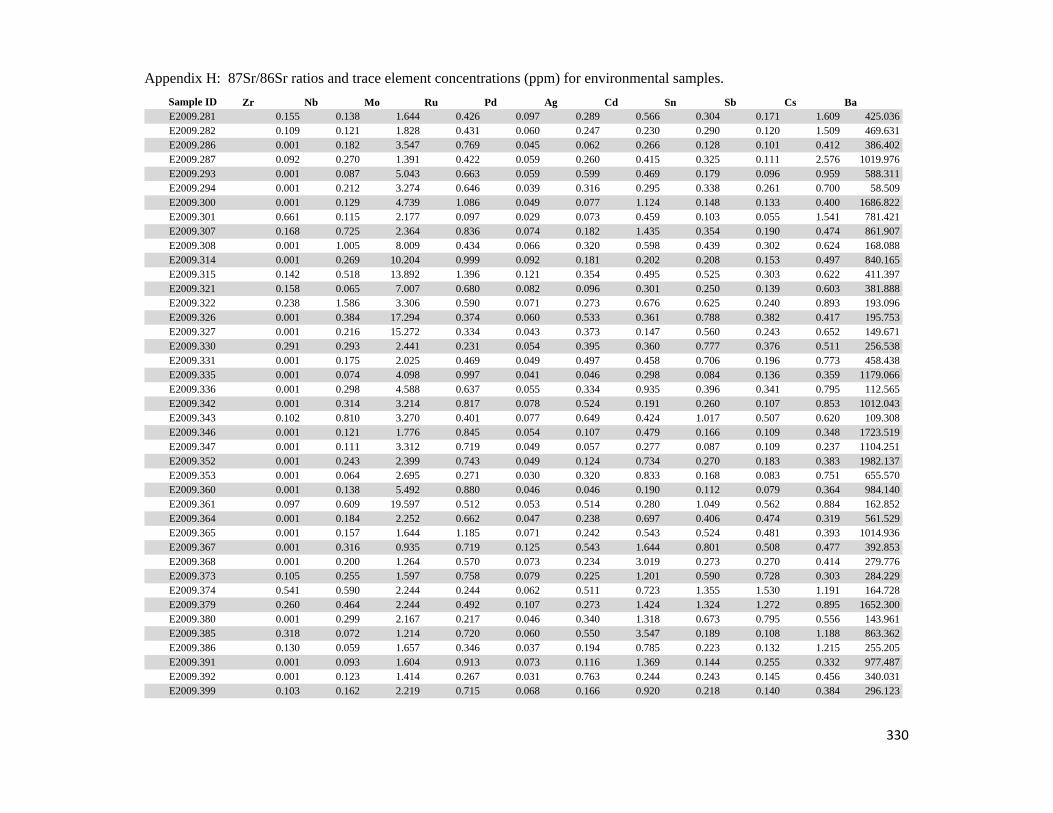
Appendix H: 87Sr/86Sr ratios and trace element concentrations (ppm) for environmental samples.
Sample ID Zr Nb Mo Ru Pd Ag Cd Sn Sb Cs BaE2009.281 0.155 0.138 1.644 0.426 0.097 0.289 0.566 0.304 0.171 1.609 425.036E2009.282 0.109 0.121 1.828 0.431 0.060 0.247 0.230 0.290 0.120 1.509 469.631E2009.286 0.001 0.182 3.547 0.769 0.045 0.062 0.266 0.128 0.101 0.412 386.402E2009.287 0.092 0.270 1.391 0.422 0.059 0.260 0.415 0.325 0.111 2.576 1019.976E2009.293 0.001 0.087 5.043 0.663 0.059 0.599 0.469 0.179 0.096 0.959 588.311E2009.294 0.001 0.212 3.274 0.646 0.039 0.316 0.295 0.338 0.261 0.700 58.509E2009.300 0.001 0.129 4.739 1.086 0.049 0.077 1.124 0.148 0.133 0.400 1686.822E2009.301 0.661 0.115 2.177 0.097 0.029 0.073 0.459 0.103 0.055 1.541 781.421E2009.307 0.168 0.725 2.364 0.836 0.074 0.182 1.435 0.354 0.190 0.474 861.907E2009.308 0.001 1.005 8.009 0.434 0.066 0.320 0.598 0.439 0.302 0.624 168.088E2009.314 0.001 0.269 10.204 0.999 0.092 0.181 0.202 0.208 0.153 0.497 840.165E2009.315 0.142 0.518 13.892 1.396 0.121 0.354 0.495 0.525 0.303 0.622 411.397E2009.321 0.158 0.065 7.007 0.680 0.082 0.096 0.301 0.250 0.139 0.603 381.888E2009.322 0.238 1.586 3.306 0.590 0.071 0.273 0.676 0.625 0.240 0.893 193.096E2009.326 0.001 0.384 17.294 0.374 0.060 0.533 0.361 0.788 0.382 0.417 195.753E2009.327 0.001 0.216 15.272 0.334 0.043 0.373 0.147 0.560 0.243 0.652 149.671E2009.330 0.291 0.293 2.441 0.231 0.054 0.395 0.360 0.777 0.376 0.511 256.538E2009.331 0.001 0.175 2.025 0.469 0.049 0.497 0.458 0.706 0.196 0.773 458.438E2009.335 0.001 0.074 4.098 0.997 0.041 0.046 0.298 0.084 0.136 0.359 1179.066E2009.336 0.001 0.298 4.588 0.637 0.055 0.334 0.935 0.396 0.341 0.795 112.565E2009.342 0.001 0.314 3.214 0.817 0.078 0.524 0.191 0.260 0.107 0.853 1012.043E2009.343 0.102 0.810 3.270 0.401 0.077 0.649 0.424 1.017 0.507 0.620 109.308E2009.346 0.001 0.121 1.776 0.845 0.054 0.107 0.479 0.166 0.109 0.348 1723.519E2009.347 0.001 0.111 3.312 0.719 0.049 0.057 0.277 0.087 0.109 0.237 1104.251E2009.352 0.001 0.243 2.399 0.743 0.049 0.124 0.734 0.270 0.183 0.383 1982.137E2009.353 0.001 0.064 2.695 0.271 0.030 0.320 0.833 0.168 0.083 0.751 655.570E2009.360 0.001 0.138 5.492 0.880 0.046 0.046 0.190 0.112 0.079 0.364 984.140E2009.361 0.097 0.609 19.597 0.512 0.053 0.514 0.280 1.049 0.562 0.884 162.852E2009.364 0.001 0.184 2.252 0.662 0.047 0.238 0.697 0.406 0.474 0.319 561.529E2009.365 0.001 0.157 1.644 1.185 0.071 0.242 0.543 0.524 0.481 0.393 1014.936E2009.367 0.001 0.316 0.935 0.719 0.125 0.543 1.644 0.801 0.508 0.477 392.853E2009.368 0.001 0.200 1.264 0.570 0.073 0.234 3.019 0.273 0.270 0.414 279.776E2009.373 0.105 0.255 1.597 0.758 0.079 0.225 1.201 0.590 0.728 0.303 284.229E2009.374 0.541 0.590 2.244 0.244 0.062 0.511 0.723 1.355 1.530 1.191 164.728E2009.379 0.260 0.464 2.244 0.492 0.107 0.273 1.424 1.324 1.272 0.895 1652.300E2009.380 0.001 0.299 2.167 0.217 0.046 0.340 1.318 0.673 0.795 0.556 143.961E2009.385 0.318 0.072 1.214 0.720 0.060 0.550 3.547 0.189 0.108 1.188 863.362E2009.386 0.130 0.059 1.657 0.346 0.037 0.194 0.785 0.223 0.132 1.215 255.205E2009.391 0.001 0.093 1.604 0.913 0.073 0.116 1.369 0.144 0.255 0.332 977.487E2009.392 0.001 0.123 1.414 0.267 0.031 0.763 0.244 0.243 0.145 0.456 340.031E2009.399 0.103 0.162 2.219 0.715 0.068 0.166 0.920 0.218 0.140 0.384 296.123
330

Appendix H: 87Sr/86Sr ratios and trace element concentrations (ppm) for environmental samples.
Sample ID La Ce Pr Nd Sm Eu Gd Tb Dy Ho ErE2009.281 6.025 11.140 1.298 4.938 0.981 0.356 1.192 0.151 0.869 0.172 0.467E2009.282 5.976 11.086 1.291 4.844 0.973 0.371 1.157 0.140 0.843 0.152 0.430E2009.286 1.638 3.014 0.344 1.278 0.244 0.191 0.254 0.030 0.176 0.032 0.089E2009.287 10.621 18.973 2.127 7.722 1.403 0.649 1.487 0.170 0.981 0.179 0.487E2009.293 0.502 0.830 0.096 0.366 0.069 0.251 0.078 0.001 0.058 0.001 0.001E2009.294 1.180 2.054 0.239 0.891 0.161 0.050 0.167 0.001 0.136 0.025 0.071E2009.300 0.821 1.441 0.161 0.575 0.129 0.718 0.133 0.001 0.085 0.001 0.046E2009.301 0.871 1.594 0.182 0.678 0.126 0.311 0.099 0.001 0.064 0.001 0.001E2009.307 6.846 12.333 1.418 5.334 1.020 0.538 1.127 0.132 0.731 0.133 0.370E2009.308 5.893 10.780 1.238 4.576 0.884 0.232 0.977 0.118 0.661 0.122 0.324E2009.314 1.186 2.213 0.257 0.962 0.190 0.356 0.211 0.001 0.143 0.030 0.082E2009.315 4.765 8.854 1.011 3.761 0.719 0.291 0.748 0.089 0.501 0.096 0.270E2009.321 9.137 17.233 1.913 6.948 1.282 0.386 1.434 0.168 0.958 0.180 0.494E2009.322 13.362 24.344 2.625 9.292 1.671 0.375 1.763 0.205 1.183 0.222 0.616E2009.326 2.354 4.386 0.502 1.851 0.363 0.123 0.428 0.062 0.389 0.075 0.222E2009.327 2.023 3.810 0.430 1.641 0.312 0.103 0.370 0.052 0.333 0.070 0.194E2009.330 3.451 7.097 0.897 3.454 0.702 0.201 0.828 0.111 0.701 0.142 0.432E2009.331 3.465 6.563 0.798 3.043 0.595 0.264 0.660 0.091 0.552 0.111 0.332E2009.335 0.545 0.761 0.093 0.354 0.075 0.465 0.078 0.001 0.047 0.001 0.023E2009.336 2.167 3.846 0.483 1.718 0.312 0.101 0.296 0.038 0.225 0.044 0.124E2009.342 1.231 2.293 0.259 0.958 0.198 0.430 0.237 0.001 0.168 0.033 0.089E2009.343 5.066 9.310 1.091 4.095 0.772 0.186 0.837 0.101 0.592 0.112 0.319E2009.346 0.749 1.032 0.124 0.448 0.103 0.670 0.110 0.001 0.078 0.001 0.055E2009.347 0.497 0.836 0.097 0.347 0.074 0.421 0.086 0.001 0.062 0.001 0.001E2009.352 2.446 4.241 0.476 1.761 0.356 0.835 0.382 0.048 0.277 0.052 0.136E2009.353 1.280 2.058 0.246 0.896 0.161 0.269 0.169 0.001 0.114 0.001 0.057E2009.360 0.587 1.057 0.122 0.441 0.087 0.401 0.093 0.001 0.062 0.001 0.001E2009.361 6.546 12.068 1.388 5.079 0.942 0.238 0.965 0.122 0.696 0.135 0.371E2009.364 1.069 1.967 0.219 0.839 0.169 0.237 0.192 0.001 0.162 0.031 0.093E2009.365 1.087 1.879 0.223 0.812 0.175 0.427 0.192 0.001 0.144 0.027 0.076E2009.367 1.337 2.324 0.265 0.981 0.181 0.160 0.182 0.001 0.155 0.030 0.083E2009.368 0.858 1.531 0.185 0.686 0.123 0.111 0.139 0.001 0.107 0.020 0.060E2009.373 1.590 3.068 0.357 1.369 0.256 0.140 0.293 0.038 0.240 0.048 0.132E2009.374 2.881 5.413 0.633 2.400 0.472 0.139 0.469 0.066 0.407 0.082 0.233E2009.379 6.164 10.585 1.209 4.520 0.837 0.669 0.811 0.105 0.643 0.124 0.348E2009.380 1.654 2.925 0.339 1.208 0.232 0.079 0.187 0.001 0.145 0.027 0.078E2009.385 0.334 0.556 0.071 0.261 0.054 0.288 0.053 0.001 0.001 0.001 0.001E2009.386 0.620 1.206 0.141 0.539 0.097 0.097 0.106 0.001 0.085 0.001 0.043E2009.391 0.507 0.948 0.105 0.407 0.082 0.341 0.084 0.001 0.058 0.001 0.001E2009.392 2.052 4.055 0.458 1.686 0.314 0.162 0.310 0.038 0.218 0.043 0.117E2009.399 1.571 2.405 0.286 0.996 0.165 0.133 0.193 0.001 0.131 0.028 0.076
331

Appendix H: 87Sr/86Sr ratios and trace element concentrations (ppm) for environmental samples.
Sample ID Tm Yb Lu Ta Au Tl Pb Th UE2009.281 0.063 0.394 0.058 0.001 0.298 0.184 9.250 1.810 0.444E2009.282 0.057 0.358 0.051 0.001 0.154 0.229 14.214 1.680 0.424E2009.286 0.012 0.076 0.001 0.001 0.073 0.305 4.204 0.440 0.081E2009.287 0.063 0.403 0.055 0.001 0.108 0.239 11.504 3.060 0.431E2009.293 0.001 0.001 0.001 0.001 0.060 0.796 7.625 0.140 0.030E2009.294 0.010 0.066 0.001 0.001 0.083 0.783 11.926 0.347 0.088E2009.300 0.007 0.001 0.001 0.001 0.071 0.543 8.704 0.189 0.051E2009.301 0.001 0.001 0.001 0.001 0.058 0.070 4.280 0.204 0.056E2009.307 0.049 0.306 0.041 0.001 0.050 0.561 10.457 1.249 0.294E2009.308 0.044 0.266 0.001 0.001 0.102 0.412 13.845 1.416 0.284E2009.314 0.013 0.073 0.001 0.001 0.361 0.603 8.310 0.341 0.090E2009.315 0.034 0.233 0.001 0.001 0.207 1.072 17.594 0.982 0.328E2009.321 0.064 0.413 0.057 0.001 0.141 0.612 7.892 2.162 0.381E2009.322 0.079 0.507 0.071 0.001 0.157 0.809 18.613 3.933 0.633E2009.326 0.031 0.193 0.001 0.001 0.086 0.764 15.012 0.863 0.324E2009.327 0.031 0.194 0.001 0.001 0.089 0.175 10.095 0.700 0.260E2009.330 0.064 0.418 0.062 0.001 0.073 0.101 10.110 1.014 0.547E2009.331 0.044 0.301 0.045 0.001 0.088 0.137 17.561 0.987 0.425E2009.335 0.004 0.001 0.001 0.001 0.038 0.239 3.411 0.100 0.021E2009.336 0.015 0.105 0.001 0.001 0.101 0.434 16.632 0.463 0.155E2009.342 0.013 0.077 0.001 0.001 0.225 0.935 8.261 0.387 0.064E2009.343 0.042 0.275 0.001 0.001 0.402 0.756 23.177 1.320 0.309E2009.346 0.008 0.053 0.001 0.001 0.172 0.618 6.413 0.152 0.040E2009.347 0.001 0.001 0.001 0.001 0.104 0.354 4.828 0.132 0.035E2009.352 0.017 0.116 0.001 0.001 0.084 0.424 7.540 0.527 0.119E2009.353 0.009 0.053 0.001 0.001 0.089 0.122 7.863 0.294 0.073E2009.360 0.001 0.001 0.001 0.001 0.051 0.392 3.991 0.165 0.040E2009.361 0.049 0.325 0.052 0.001 0.088 0.783 19.511 1.706 0.491E2009.364 0.013 0.082 0.001 0.001 0.043 0.537 10.157 0.289 0.087E2009.365 0.013 0.073 0.001 0.001 0.059 0.522 10.897 0.269 0.076E2009.367 0.013 0.073 0.001 0.074 0.361 0.660 6.915 0.413 0.090E2009.368 0.009 0.001 0.001 0.037 0.138 0.341 3.487 0.221 0.053E2009.373 0.019 0.123 0.001 0.028 0.101 0.434 6.146 0.398 0.140E2009.374 0.034 0.210 0.001 0.025 0.055 0.402 13.162 1.030 0.270E2009.379 0.049 0.314 0.048 0.027 0.202 0.863 28.571 1.311 0.525E2009.380 0.011 0.069 0.001 0.021 0.121 0.216 8.508 0.409 0.197E2009.385 0.001 0.001 0.001 0.001 0.058 0.591 5.389 0.083 0.001E2009.386 0.006 0.001 0.001 0.001 0.097 0.001 4.817 0.143 0.046E2009.391 0.001 0.001 0.001 0.001 0.083 0.418 7.314 0.104 0.001E2009.392 0.017 0.103 0.001 0.001 0.095 0.061 8.224 0.379 0.125E2009.399 0.011 0.064 0.001 0.028 0.139 0.270 2.409 0.251 0.055
332

Appendix H: 87Sr/86Sr ratios and trace element concentrations (ppm) for environmental samples.
Sample ID 87Sr/86Sr Li Na Mg Al P Ca Ti V Cr FeE2009.400 0.709535 92.117 10677.9 41707.8 4972.934 55299.8 167987.3 244.008 11.641 13.513 5542.9E2009.406 0.716746 25.906 4453.6 46633.7 4520.792 44740.3 167257.2 316.081 9.279 10.676 7469.2E2009.407 0.717134 71.844 8047.4 19502.9 12281.169 37062.1 58746.8 290.668 25.617 26.033 18188.7E2009.412 0.707832 20.184 3821.5 65228.1 601.394 38065.5 230977.7 44.098 2.000 3.894 3160.2E2009.413 0.709014 68.777 7061.2 43779.8 3960.814 31226.6 276740.6 220.332 9.774 14.856 6465.6E2009.419 0.712528 287.057 29838.1 78869.4 7331.625 75468.3 157035.4 115.358 6.611 6.451 4224.4E2009.420 0.716140 196.591 17870.6 53916.9 4560.860 58989.7 284148.6 166.485 9.803 9.168 6048.6E2009.426 0.715368 520.161 31137.5 99749.6 9376.350 54599.2 100680.2 454.878 21.979 19.011 10823.9E2009.427 0.716263 189.874 14095.9 66333.4 22279.947 49626.1 150058.8 829.402 41.041 39.763 16809.3E2009.432 0.710569 172.877 8541.4 56915.8 29680.364 40175.4 104369.0 234.260 64.752 49.857 26716.0E2009.433 0.712683 167.547 10127.3 57260.4 20456.951 48060.6 91051.5 672.786 40.927 32.514 19489.0E2009.437 0.713666 1170.70 33709.0 54601.1 12900.600 53089.7 155593.8 399.187 13.157 15.856 6545.8E2009.438 0.713234 32.703 2073.0 59552.2 13081.267 12125.4 315161.8 409.421 21.519 22.839 12155.3E2009.440 0.713131 330.268 18088.0 56187.0 2419.506 67229.9 135783.6 69.382 5.061 5.817 3359.3E2009.441 0.715448 218.215 15990.9 42061.8 2502.448 55233.2 205120.0 84.816 5.705 7.946 3724.3E2009.444 0.715100 214.760 16705.9 62281.7 16140.501 47237.2 110497.2 481.106 31.346 42.475 13582.3E2009.445 0.716693 117.454 12091.5 60426.3 10381.117 43564.9 127184.7 442.721 23.330 27.064 11101.3E2009.447 0.712968 38.620 1989.7 39085.9 3574.348 42550.8 118495.7 199.985 11.599 11.285 5796.1E2009.448 0.712076 320.105 20666.4 32939.0 3815.168 52718.6 106952.6 156.544 11.169 14.093 5218.1E2009.451 0.712026 333.713 22678.6 67199.4 12978.982 62252.1 151502.3 662.809 27.018 23.625 14363.7E2009.452 0.712385 356.397 31899.1 48590.8 9823.439 63167.3 195538.8 579.039 23.462 24.689 12008.8E2009.455 0.714079 475.485 46174.0 72452.7 7057.178 81315.7 98048.9 287.686 11.095 23.499 5854.3E2009.456 0.716878 235.264 27440.3 56533.9 6831.559 66184.8 120022.1 393.872 14.782 15.497 7261.2E2009.460 0.748496 70.962 8170.7 103411.8 1252.320 52197.2 238556.3 89.795 4.285 5.721 3750.9E2009.461 0.750199 89.419 8216.9 68456.2 2184.961 52653.9 209541.0 116.297 6.035 9.836 4533.4E2009.467 0.726098 79.030 8658.2 77135.0 2640.146 71807.8 216817.1 32.970 6.374 8.660 5149.0E2009.468 0.730220 183.543 21582.8 91792.3 7462.415 50624.9 130861.0 322.603 15.349 18.152 9559.6E2009.473 0.722925 312.932 9938.8 39817.5 13051.999 26986.9 64864.6 280.909 18.450 46.270 9185.7E2009.474 0.717705 236.395 19925.8 47151.8 19179.206 41090.5 94997.4 579.810 30.940 52.069 15011.2E2009.478 0.711935 174.231 19781.8 58311.2 23238.013 48728.4 138599.4 899.286 45.096 40.309 22127.1E2009.479 0.711699 182.019 17150.0 63501.2 12708.481 49465.2 204821.6 608.830 24.579 33.310 12368.2E2009.483 0.732844 183.723 15940.2 105806.5 1967.506 61295.2 234623.6 128.469 5.591 9.975 4667.0E2009.484 0.752254 484.599 36206.9 64516.7 8606.575 55830.6 114160.5 504.343 22.976 28.533 10963.6E2009.490 0.712507 147.603 16531.4 79955.6 2014.697 66968.6 185247.8 126.558 5.763 9.863 4008.0E2009.491 0.712047 266.281 24109.8 52309.0 12428.613 56483.8 202853.3 299.766 14.470 34.349 7314.9E2009.498 0.710242 80.945 9404.9 58519.0 1030.744 45156.9 204305.5 76.780 3.457 5.681 3664.8E2009.499 0.710399 559.668 49409.8 56356.6 16059.301 76804.8 111616.9 236.331 9.925 28.278 5049.1E2009.504 0.709915 336.987 25113.1 55466.7 18032.235 34495.4 130824.6 234.988 53.677 44.083 22060.7E2009.505 0.709861 197.569 14201.4 47289.8 7308.027 29498.3 199462.1 242.613 20.579 22.443 10533.3E2009.511 0.709930 342.556 18631.5 79222.7 6156.735 44179.6 262748.5 132.051 16.322 21.266 10752.5E2009.512 0.710209 235.723 19104.8 70629.7 3144.487 53113.3 264941.1 235.207 9.853 15.865 6504.0
333

Appendix H: 87Sr/86Sr ratios and trace element concentrations (ppm) for environmental samples.
Sample ID Mn Co Ni Cu Zn Ga As Se Rb Sr YE2009.400 3043.288 2.885 21.705 104.905 1862.310 1.796 1.563 2.297 78.217 978.912 2.428E2009.406 22951.731 5.836 104.839 81.436 1965.847 2.899 1.115 2.462 69.183 878.639 4.855E2009.407 18995.760 8.864 34.820 45.915 320.435 7.102 1.753 2.021 85.269 501.580 16.710E2009.412 9585.022 6.195 33.904 124.205 297.538 0.684 0.929 1.452 107.154 2045.099 0.433E2009.413 4829.442 3.147 15.809 99.024 899.412 1.792 1.600 1.874 68.295 1694.370 2.131E2009.419 1879.449 1.973 5.423 399.603 357.933 1.658 1.771 3.945 51.915 1733.520 0.802E2009.420 6617.150 2.735 10.140 231.040 1642.501 1.695 2.432 2.158 22.455 636.645 1.473E2009.426 3937.095 5.563 25.665 434.318 349.953 3.011 2.154 3.672 49.727 1113.082 3.261E2009.427 1965.899 7.837 37.652 168.778 1053.304 5.788 1.803 2.117 52.717 249.299 6.271E2009.432 4035.639 17.563 54.496 234.958 461.923 7.604 2.684 3.106 109.457 854.205 19.538E2009.433 7450.211 22.172 64.437 143.136 348.716 5.722 2.201 2.885 77.249 1099.292 11.604E2009.437 20170.055 8.814 57.444 274.097 1390.951 2.567 1.560 3.460 149.440 678.913 3.211E2009.438 21117.772 11.331 31.336 105.838 1471.943 3.762 2.481 3.348 19.969 1101.555 6.812E2009.440 5825.581 6.145 36.753 251.785 339.709 1.250 1.144 2.742 35.430 1898.601 2.040E2009.441 4515.214 9.611 25.271 392.384 291.780 1.018 1.265 3.794 33.092 1714.364 1.503E2009.444 9752.703 13.632 68.464 214.941 355.639 3.493 1.522 3.164 46.620 1021.829 3.298E2009.445 8794.368 13.434 71.657 158.086 301.727 2.767 1.488 3.253 37.411 1188.702 3.056E2009.447 52364.141 15.993 68.688 94.091 238.433 2.403 1.539 4.855 49.828 3003.874 2.667E2009.448 14599.056 14.821 130.104 191.260 183.768 1.676 1.244 3.419 103.968 1734.284 1.573E2009.451 3296.213 7.625 16.880 210.374 1095.033 4.200 2.127 2.837 39.132 397.156 6.906E2009.452 1040.776 5.142 19.320 177.196 784.795 3.602 2.092 3.476 45.168 451.972 5.805E2009.455 7233.174 8.022 24.752 296.185 828.950 2.008 1.162 2.745 103.920 150.294 2.397E2009.456 4421.132 5.181 15.222 220.620 1006.851 2.468 1.622 2.977 67.092 241.866 3.234E2009.460 13863.826 8.607 60.816 151.931 1170.972 0.997 1.402 4.865 68.991 640.790 1.045E2009.461 15450.739 7.671 28.927 147.616 542.137 1.403 1.693 4.813 134.392 2503.398 1.558E2009.467 24253.477 14.616 53.108 136.996 1891.760 2.093 1.665 4.902 48.005 1081.354 3.125E2009.468 4451.551 5.876 67.312 225.655 475.027 3.387 1.770 5.277 77.496 1649.816 5.101E2009.473 1152.939 5.805 40.505 84.135 110.993 2.492 1.049 2.384 136.634 734.882 1.848E2009.474 8656.420 11.662 60.988 224.540 328.195 4.332 1.705 3.045 46.055 579.337 4.536E2009.478 6628.462 12.312 37.416 150.813 893.106 7.057 2.565 3.808 59.116 493.126 11.323E2009.479 10744.204 13.149 40.129 310.655 1251.730 4.135 2.108 5.391 40.581 706.161 5.909E2009.483 12389.038 6.970 32.314 287.196 811.898 1.861 1.373 3.265 77.609 789.824 1.278E2009.484 4863.371 7.595 80.337 379.577 528.108 4.806 2.542 2.975 84.243 796.323 4.667E2009.490 22667.945 47.103 447.353 301.489 4220.539 2.108 1.272 2.244 93.417 1365.856 2.001E2009.491 42516.361 11.066 138.000 171.960 1788.151 6.127 2.844 4.385 58.600 931.404 5.664E2009.498 14727.380 11.061 147.098 182.601 1892.383 1.351 0.985 1.179 148.519 2223.523 1.085E2009.499 14977.828 5.293 285.031 389.916 1257.308 3.262 1.671 3.129 169.564 391.041 3.088E2009.504 1253.295 10.715 56.672 247.723 420.106 7.906 6.083 3.416 108.860 739.598 11.403E2009.505 960.845 3.881 55.858 210.419 1392.223 3.284 2.530 4.195 64.869 685.906 4.505E2009.511 9170.619 7.474 116.470 257.683 2223.307 3.005 2.890 5.449 57.154 1245.297 4.294E2009.512 3011.774 5.513 80.443 326.160 2279.815 1.833 2.335 5.529 78.424 1309.010 2.096
334

Appendix H: 87Sr/86Sr ratios and trace element concentrations (ppm) for environmental samples.
Sample ID Zr Nb Mo Ru Pd Ag Cd Sn Sb Cs BaE2009.400 0.001 0.426 2.851 0.565 0.071 0.393 0.348 0.743 0.256 0.631 780.758E2009.406 0.343 0.612 2.089 0.492 0.078 0.172 1.935 0.891 0.172 0.496 331.038E2009.407 1.328 0.248 1.417 0.123 0.153 0.102 0.213 1.043 0.146 1.643 155.947E2009.412 0.001 0.101 3.075 0.814 0.040 0.081 0.611 0.173 0.169 0.322 548.791E2009.413 0.001 0.285 2.606 1.044 0.066 0.453 1.597 0.664 0.275 0.784 614.593E2009.419 0.001 0.105 1.684 0.670 0.042 1.779 0.069 0.270 0.097 0.650 483.047E2009.420 0.001 0.296 1.772 0.967 0.063 1.275 0.913 0.675 0.508 0.582 190.951E2009.426 0.195 0.258 1.123 0.418 0.054 1.594 0.171 0.564 0.108 1.453 919.323E2009.427 0.120 0.402 4.092 0.561 0.077 1.763 0.205 1.273 0.227 1.786 159.136E2009.432 0.285 0.109 2.148 0.344 0.173 0.684 0.454 0.894 0.171 2.289 323.247E2009.433 0.205 0.345 1.881 0.292 0.103 0.765 0.309 0.851 0.291 1.610 236.758E2009.437 0.001 0.480 6.658 0.403 0.055 0.863 3.729 0.597 0.387 2.253 499.644E2009.438 0.211 0.307 2.649 0.852 0.098 0.629 3.105 0.830 0.703 1.008 790.362E2009.440 0.001 0.079 0.514 0.471 0.048 1.050 0.064 0.221 0.148 0.781 238.424E2009.441 0.001 0.043 0.499 0.663 0.041 0.897 0.121 0.177 0.098 0.212 357.241E2009.444 0.001 0.131 0.689 0.474 0.047 0.743 0.127 0.363 0.131 0.979 425.589E2009.445 0.001 0.146 0.709 0.526 0.045 0.820 0.153 0.301 0.093 0.888 497.101E2009.447 0.126 0.143 2.611 0.494 0.052 0.598 4.031 0.687 0.137 0.622 519.224E2009.448 0.142 0.175 1.961 0.373 0.037 0.702 0.677 0.358 0.081 1.274 293.796E2009.451 0.199 0.629 9.273 0.498 0.148 1.031 0.125 1.052 0.230 1.044 123.676E2009.452 0.160 0.546 5.290 0.524 0.100 1.167 0.071 0.898 0.222 0.866 135.259E2009.455 0.189 0.498 1.730 0.244 0.062 0.588 0.340 0.514 0.186 0.726 60.075E2009.456 0.228 0.478 6.325 0.304 0.062 0.712 0.215 0.606 0.239 1.064 84.456E2009.460 0.001 0.232 2.869 0.820 0.055 0.140 1.415 0.157 0.065 0.434 481.338E2009.461 0.001 0.091 1.067 0.852 0.058 0.412 0.362 0.261 0.061 1.923 718.470E2009.467 0.211 0.001 2.535 0.652 0.076 0.312 3.745 0.149 0.036 0.698 715.101E2009.468 0.345 0.289 1.043 0.634 0.081 0.620 0.087 0.734 0.107 1.049 939.046E2009.473 0.166 0.091 4.054 0.305 0.033 0.421 0.254 0.287 0.114 2.760 397.693E2009.474 0.318 0.269 1.550 0.314 0.065 0.597 0.114 0.497 0.148 1.123 593.883E2009.478 0.230 0.513 3.162 0.423 0.157 0.874 0.516 1.150 0.365 1.509 328.842E2009.479 0.167 0.560 8.349 0.724 0.109 1.279 0.399 0.884 0.380 0.523 241.646E2009.483 0.593 0.278 1.076 0.825 0.083 0.428 0.544 0.471 0.310 0.383 652.059E2009.484 0.285 0.270 1.625 0.422 0.071 0.677 0.201 1.749 1.104 1.249 575.946E2009.490 0.146 0.254 1.769 0.720 0.068 0.506 4.631 0.427 0.288 0.476 941.142E2009.491 0.117 0.416 2.076 0.548 0.100 1.350 0.942 1.607 1.136 0.598 169.457E2009.498 0.148 0.192 3.461 0.843 0.072 0.265 0.939 0.384 0.268 0.392 310.308E2009.499 0.174 0.417 2.180 0.252 0.062 1.554 0.252 1.397 0.668 0.676 244.836E2009.504 0.407 0.049 3.934 0.442 0.128 0.691 0.326 5.860 3.126 2.135 405.099E2009.505 0.146 0.001 2.532 0.752 0.084 0.157 0.144 1.869 0.841 0.423 528.377E2009.511 0.161 0.098 2.462 0.836 0.119 0.216 0.677 1.841 1.349 0.515 324.189E2009.512 0.201 0.386 3.030 0.846 0.080 0.211 0.317 1.257 1.196 0.315 440.543
335

Appendix H: 87Sr/86Sr ratios and trace element concentrations (ppm) for environmental samples.
Sample ID La Ce Pr Nd Sm Eu Gd Tb Dy Ho ErE2009.400 5.161 9.226 1.061 3.775 0.665 0.376 0.630 0.077 0.453 0.092 0.268E2009.406 16.574 32.244 3.266 10.949 1.721 0.349 1.625 0.183 1.046 0.196 0.549E2009.407 69.028 136.423 13.486 46.527 7.122 1.028 6.822 0.717 3.987 0.711 1.875E2009.412 0.829 1.487 0.164 0.586 0.112 0.220 0.114 0.001 0.083 0.001 0.044E2009.413 5.389 8.745 0.989 3.587 0.611 0.338 0.628 0.075 0.432 0.085 0.238E2009.419 1.643 2.992 0.349 1.254 0.224 0.202 0.228 0.001 0.167 0.034 0.093E2009.420 3.038 5.367 0.630 2.318 0.421 0.148 0.405 0.046 0.282 0.054 0.150E2009.426 6.028 9.857 1.276 4.727 0.899 0.513 0.961 0.120 0.689 0.133 0.370E2009.427 11.931 17.593 2.343 8.649 1.630 0.436 1.710 0.217 1.275 0.250 0.714E2009.432 23.884 36.528 5.492 20.878 4.089 0.967 5.413 0.690 4.205 0.865 2.456E2009.433 17.150 29.788 3.803 14.121 2.684 0.588 3.024 0.382 2.343 0.463 1.292E2009.437 6.131 11.698 1.271 4.525 0.819 0.342 0.887 0.111 0.666 0.131 0.383E2009.438 14.446 28.687 3.060 10.988 1.902 0.648 1.832 0.213 1.253 0.248 0.688E2009.440 3.717 4.453 0.677 2.444 0.416 0.170 0.489 0.061 0.358 0.068 0.178E2009.441 5.378 7.944 0.847 2.697 0.399 0.204 0.454 0.051 0.281 0.052 0.141E2009.444 12.933 18.586 1.935 6.199 0.933 0.337 1.103 0.122 0.727 0.145 0.403E2009.445 13.623 17.025 1.984 6.338 0.913 0.342 1.042 0.110 0.644 0.126 0.365E2009.447 5.294 11.823 1.140 4.133 0.763 0.310 0.759 0.093 0.548 0.105 0.294E2009.448 3.212 7.331 0.703 2.486 0.452 0.173 0.485 0.057 0.339 0.064 0.186E2009.451 15.543 31.212 3.310 11.587 2.036 0.354 1.972 0.230 1.383 0.270 0.749E2009.452 13.483 27.297 2.849 9.966 1.729 0.310 1.627 0.191 1.137 0.219 0.611E2009.455 5.414 10.553 1.121 3.907 0.692 0.130 0.633 0.076 0.480 0.093 0.262E2009.456 7.120 13.786 1.463 5.172 0.922 0.183 0.934 0.110 0.663 0.133 0.383E2009.460 2.236 4.137 0.446 1.596 0.286 0.229 0.290 0.032 0.192 0.037 0.102E2009.461 4.118 6.996 0.768 2.636 0.461 0.356 0.488 0.054 0.298 0.057 0.159E2009.467 14.401 19.888 2.536 8.365 1.309 0.445 1.224 0.124 0.643 0.113 0.297E2009.468 24.670 41.581 4.440 14.658 2.285 0.658 2.251 0.218 1.163 0.208 0.557E2009.473 4.278 7.773 0.798 2.777 0.496 0.247 0.535 0.065 0.378 0.076 0.209E2009.474 11.631 19.925 2.100 7.231 1.262 0.457 1.397 0.160 0.942 0.181 0.514E2009.478 27.752 51.139 5.599 19.867 3.441 0.745 3.584 0.406 2.359 0.455 1.305E2009.479 14.326 25.982 2.901 10.272 1.770 0.424 1.723 0.204 1.167 0.227 0.648E2009.483 2.145 3.859 0.424 1.574 0.295 0.333 0.306 0.039 0.232 0.046 0.136E2009.484 8.163 15.453 1.756 6.536 1.246 0.445 1.287 0.154 0.936 0.185 0.510E2009.490 2.839 5.096 0.574 2.099 0.400 0.477 0.427 0.052 0.307 0.059 0.174E2009.491 7.071 12.581 1.435 5.370 1.035 0.270 1.071 0.138 0.854 0.178 0.525E2009.498 1.565 2.522 0.305 1.110 0.225 0.170 0.230 0.031 0.178 0.034 0.105E2009.499 4.560 7.986 0.934 3.479 0.679 0.223 0.698 0.093 0.536 0.109 0.317E2009.504 21.838 40.105 4.545 16.538 3.078 0.718 3.308 0.396 2.355 0.456 1.302E2009.505 8.245 14.699 1.714 6.263 1.178 0.428 1.211 0.148 0.885 0.177 0.517E2009.511 6.643 11.571 1.346 4.909 0.915 0.311 1.073 0.134 0.809 0.165 0.474E2009.512 3.543 6.180 0.718 2.633 0.503 0.290 0.557 0.067 0.402 0.081 0.232
336

Appendix H: 87Sr/86Sr ratios and trace element concentrations (ppm) for environmental samples.
Sample ID Tm Yb Lu Ta Au Tl Pb Th UE2009.400 0.038 0.227 0.001 0.043 0.284 0.366 10.515 1.069 0.260E2009.406 0.072 0.446 0.062 0.001 0.101 0.359 7.558 3.587 0.327E2009.407 0.238 1.481 0.203 0.001 0.060 0.170 16.953 12.163 1.089E2009.412 0.007 0.001 0.001 0.001 0.055 0.398 4.475 0.272 0.099E2009.413 0.034 0.211 0.001 0.001 0.208 1.117 11.330 1.011 0.225E2009.419 0.014 0.081 0.001 0.001 0.102 0.283 9.728 0.572 0.196E2009.420 0.021 0.139 0.001 0.021 0.080 0.465 14.572 0.670 0.202E2009.426 0.050 0.316 0.048 0.001 0.095 0.081 15.672 1.659 0.389E2009.427 0.102 0.631 0.096 0.001 0.064 0.358 12.595 2.987 0.879E2009.432 0.342 2.185 0.323 0.037 0.391 0.411 23.150 5.689 1.698E2009.433 0.181 1.150 0.173 0.024 0.190 0.142 8.345 5.154 1.043E2009.437 0.052 0.352 0.053 0.035 0.209 0.852 18.362 2.730 0.394E2009.438 0.097 0.609 0.089 0.041 0.131 0.360 30.455 2.600 0.508E2009.440 0.023 0.130 0.001 0.001 0.090 0.001 7.432 0.327 0.125E2009.441 0.019 0.109 0.001 0.001 0.078 0.001 5.976 0.332 0.109E2009.444 0.057 0.342 0.052 0.001 0.067 0.200 6.250 2.240 0.220E2009.445 0.047 0.303 0.045 0.001 0.067 0.102 7.029 1.721 0.198E2009.447 0.039 0.250 0.001 0.001 0.069 0.063 4.263 1.977 0.632E2009.448 0.027 0.151 0.001 0.001 0.062 0.136 9.146 1.424 0.392E2009.451 0.106 0.670 0.098 0.091 0.595 0.468 11.614 5.037 0.662E2009.452 0.086 0.537 0.079 0.047 0.269 0.473 12.148 5.112 0.791E2009.455 0.035 0.212 0.001 0.046 0.149 0.677 13.654 1.752 0.233E2009.456 0.052 0.339 0.048 0.028 0.129 0.302 13.345 2.148 0.319E2009.460 0.014 0.092 0.001 0.001 0.099 0.498 6.593 0.534 0.171E2009.461 0.021 0.132 0.001 0.001 0.083 0.149 7.479 0.856 0.338E2009.467 0.036 0.235 0.001 0.001 0.074 0.189 6.899 0.831 0.181E2009.468 0.073 0.454 0.064 0.001 0.119 0.266 13.895 7.425 0.550E2009.473 0.029 0.180 0.001 0.001 0.053 0.001 2.592 1.418 0.868E2009.474 0.067 0.430 0.066 0.001 0.061 0.129 9.337 2.926 0.684E2009.478 0.181 1.187 0.181 0.057 0.455 0.348 14.116 6.599 0.934E2009.479 0.089 0.590 0.088 0.048 0.267 0.233 12.399 3.285 2.223E2009.483 0.019 0.123 0.001 0.029 0.124 0.342 13.564 0.476 0.154E2009.484 0.073 0.466 0.068 0.001 0.113 0.075 25.554 2.395 0.591E2009.490 0.023 0.142 0.001 0.020 0.078 0.211 10.466 0.510 0.153E2009.491 0.070 0.474 0.070 0.036 0.148 0.548 24.992 1.348 0.518E2009.498 0.014 0.092 0.001 0.001 0.070 0.329 8.075 0.236 0.103E2009.499 0.046 0.279 0.045 0.029 0.156 0.502 20.347 0.972 0.354E2009.504 0.180 1.149 0.168 0.001 0.129 0.102 50.232 5.732 1.624E2009.505 0.070 0.452 0.066 0.001 0.076 0.474 27.785 1.968 0.562E2009.511 0.066 0.413 0.060 0.038 0.289 0.520 26.468 1.507 0.450E2009.512 0.032 0.214 0.001 0.031 0.147 0.850 17.378 0.899 0.261
337

Appendix H: 87Sr/86Sr ratios and trace element concentrations (ppm) for environmental samples.
Sample ID 87Sr/86Sr Li Na Mg Al P Ca Ti V Cr FeE2009.518 0.711526 223.167 14530.4 68500.9 7767.220 31511.1 245914.0 552.430 18.337 23.182 8681.5E2009.519 0.711770 466.810 45054.2 70770.7 14193.276 74171.4 123771.5 404.087 14.769 22.253 6602.8E2009.523 0.708581 94.239 7522.6 92847.4 519.031 61930.1 241541.3 47.341 3.063 7.169 3405.3E2009.524 0.708973 305.315 26716.9 65541.8 4331.747 68990.0 176474.4 325.091 11.077 21.492 5766.1E2009.525 0.708529 121.909 12364.3 93237.8 1189.362 28542.0 287439.8 113.052 3.849 11.280 4627.9E2009.526 0.707794 103.548 10204.6 63400.8 6816.851 35864.6 177314.1 497.162 19.866 24.561 11897.0E2009.527 0.709776 112.515 9686.1 95348.9 588.332 44801.5 297709.8 54.058 3.268 8.600 4529.2E2009.528 0.709878 119.862 10544.9 62049.7 16714.230 56969.8 229107.6 14.630 4.784 21.972 4526.9E2009.529 0.709641 241.004 18033.9 64123.4 1395.815 78076.9 188361.0 18.746 3.520 11.904 3887.5E2009.530 0.709435 281.931 22945.0 64273.5 13585.422 70138.8 205502.0 629.984 19.377 39.820 11050.2E2009.531 0.707794 103.548 10204.6 63400.8 6816.851 35864.6 177314.1 497.162 19.866 24.561 11897.0E2009.536 0.709776 112.515 9686.1 95348.9 588.332 44801.5 297709.8 54.058 3.268 8.600 4529.2E2009.537 0.709878 119.862 10544.9 62049.7 16714.230 56969.8 229107.6 14.630 4.784 21.972 4526.9E2009.542 0.709641 241.004 18033.9 64123.4 1395.815 78076.9 188361.0 18.746 3.520 11.904 3887.5E2009.543 0.709435 281.931 22945.0 64273.5 13585.422 70138.8 205502.0 629.984 19.377 39.820 11050.2
NBS-987 Avg. 0.710253SRM612 Avg. 42.376 105192 77.440 11276 60.697 85518.580 48.134 39.6 40.268 56.603
Sample ID Mn Co Ni Cu Zn Ga As Se Rb Sr YE2009.518 9851.861 12.445 144.884 180.375 1555.096 3.766 2.748 5.735 92.356 1956.603 5.056E2009.519 7565.145 6.244 170.992 330.619 1388.275 3.223 2.025 4.525 80.522 400.643 3.549E2009.523 1341.739 1.377 9.383 146.804 2122.941 0.681 1.195 4.040 30.718 641.913 0.298E2009.524 1170.470 2.040 11.318 380.561 1160.295 1.856 2.260 6.009 46.426 373.768 1.301E2009.525 427.473 1.415 15.621 230.535 1717.174 0.667 0.936 2.791 45.238 641.142 0.680E2009.526 1937.336 4.708 20.991 118.770 477.568 2.698 2.302 5.930 92.796 1253.586 3.447E2009.527 10605.855 7.573 70.803 240.889 448.950 0.853 1.375 5.014 72.601 1125.056 0.406E2009.528 35091.233 3.825 32.433 80.341 213.313 2.108 1.561 5.639 49.785 273.285 0.961E2009.529 17502.067 6.919 35.385 259.644 1318.790 1.607 0.705 1.904 92.569 1005.205 0.837E2009.530 10285.572 7.749 25.695 196.569 1040.303 3.665 1.906 5.074 99.620 750.204 2.858E2009.531 1937.336 4.708 20.991 118.770 477.568 2.698 2.302 5.930 92.796 1253.586 3.447E2009.536 10605.855 7.573 70.803 240.889 448.950 0.853 1.375 5.014 72.601 1125.056 0.406E2009.537 35091.233 3.825 32.433 80.341 213.313 2.108 1.561 5.639 49.785 273.285 0.961E2009.542 17502.067 6.919 35.385 259.644 1318.790 1.607 0.705 1.904 92.569 1005.205 0.837E2009.543 10285.572 7.749 25.695 196.569 1040.303 3.665 1.906 5.074 99.620 750.204 2.858
SRM612 Avg. 38.745 32.417 38.724 37.156 38.372 36.364 34.874 38.288 31.963 76.543 38.6
338

Appendix H: 87Sr/86Sr ratios and trace element concentrations (ppm) for environmental samples.
Sample ID Zr Nb Mo Ru Pd Ag Cd Sn Sb Cs BaE2009.518 0.226 0.375 1.444 0.878 0.093 0.289 1.261 1.092 0.658 0.318 482.712E2009.519 0.241 0.493 2.273 0.398 0.071 0.771 0.248 1.012 0.675 0.461 100.530E2009.523 0.001 0.116 4.430 0.807 0.066 0.072 0.091 0.105 0.069 0.258 1142.030E2009.524 0.148 0.469 13.405 0.598 0.058 0.658 0.115 0.427 0.215 0.248 99.058E2009.525 0.065 0.198 6.556 1.027 0.060 0.066 0.001 0.192 0.078 0.221 1852.303E2009.526 0.223 0.300 1.533 0.746 0.073 0.263 0.112 0.420 0.090 1.998 976.585E2009.527 0.001 0.112 2.466 1.028 0.052 0.193 1.276 0.132 0.072 0.342 1559.839E2009.528 0.139 0.001 1.161 0.517 0.042 0.180 0.406 0.001 0.030 0.695 210.434E2009.529 0.144 0.114 1.424 0.692 0.074 0.138 0.798 0.142 0.034 0.254 2569.346E2009.530 0.121 0.793 2.051 0.844 0.097 0.530 0.558 1.071 0.288 1.075 296.427E2009.531 0.223 0.300 1.533 0.746 0.073 0.263 0.112 0.420 0.090 1.998 976.585E2009.536 0.001 0.112 2.466 1.028 0.052 0.193 1.276 0.132 0.072 0.342 1559.839E2009.537 0.139 0.001 1.161 0.517 0.042 0.180 0.406 0.001 0.030 0.695 210.434E2009.542 0.144 0.114 1.424 0.692 0.074 0.138 0.798 0.142 0.034 0.254 2569.346E2009.543 0.121 0.793 2.051 0.844 0.097 0.530 0.558 1.071 0.288 1.075 296.427
SRM612 Avg. 36.662 36.216 38.137 35.898 22.057 28.715 43.095 38.257 38.519 41.997 37.872
Sample ID La Ce Pr Nd Sm Eu Gd Tb Dy Ho ErE2009.518 8.622 14.612 1.774 6.558 1.225 0.453 1.347 0.166 0.973 0.187 0.536E2009.519 5.439 9.863 1.145 4.072 0.767 0.193 0.846 0.108 0.629 0.134 0.373E2009.523 0.488 0.916 0.104 0.395 0.085 0.542 0.088 0.001 0.057 0.001 0.001E2009.524 2.498 4.685 0.541 1.984 0.385 0.125 0.401 0.047 0.271 0.051 0.161E2009.525 1.045 1.891 0.215 0.797 0.174 0.930 0.187 0.001 0.131 0.026 0.072E2009.526 7.294 13.697 1.538 5.698 1.059 0.684 1.171 0.133 0.739 0.140 0.395E2009.527 0.816 1.306 0.139 0.504 0.100 0.789 0.115 0.001 0.062 0.001 0.001E2009.528 1.767 3.221 0.370 1.329 0.243 0.144 0.242 0.001 0.162 0.032 0.093E2009.529 1.657 2.804 0.325 1.186 0.253 1.326 0.226 0.001 0.145 0.028 0.076E2009.530 6.484 12.373 1.372 5.058 0.966 0.316 0.953 0.110 0.599 0.107 0.296E2009.531 7.294 13.697 1.538 5.698 1.059 0.684 1.171 0.133 0.739 0.140 0.395E2009.536 0.816 1.306 0.139 0.504 0.100 0.789 0.115 0.001 0.062 0.001 0.001E2009.537 1.767 3.221 0.370 1.329 0.243 0.144 0.242 0.001 0.162 0.032 0.093E2009.542 1.657 2.804 0.325 1.186 0.253 1.326 0.226 0.001 0.145 0.028 0.076E2009.543 6.484 12.373 1.372 5.058 0.966 0.316 0.953 0.110 0.599 0.107 0.296
SRM612 Avg. 35.984 38.363 37.342 35.321 37.138 34.588 37.225 36.127 36.239 38.149 37.848
339
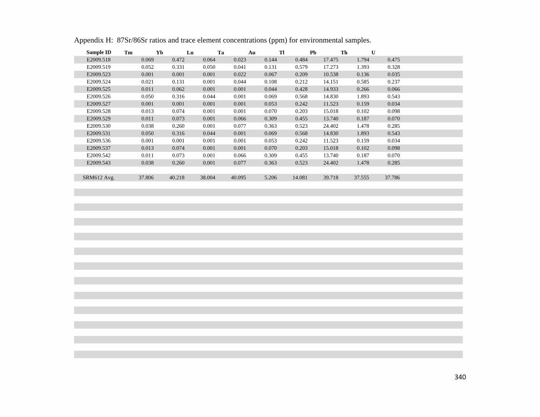
Appendix H: 87Sr/86Sr ratios and trace element concentrations (ppm) for environmental samples.
Sample ID Tm Yb Lu Ta Au Tl Pb Th UE2009.518 0.069 0.472 0.064 0.023 0.144 0.484 17.475 1.794 0.475E2009.519 0.052 0.331 0.050 0.041 0.131 0.579 17.273 1.393 0.328E2009.523 0.001 0.001 0.001 0.022 0.067 0.209 10.538 0.136 0.035E2009.524 0.021 0.131 0.001 0.044 0.108 0.212 14.151 0.585 0.237E2009.525 0.011 0.062 0.001 0.001 0.044 0.428 14.933 0.266 0.066E2009.526 0.050 0.316 0.044 0.001 0.069 0.568 14.830 1.893 0.543E2009.527 0.001 0.001 0.001 0.001 0.053 0.242 11.523 0.159 0.034E2009.528 0.013 0.074 0.001 0.001 0.070 0.203 15.018 0.102 0.098E2009.529 0.011 0.073 0.001 0.066 0.309 0.455 13.740 0.187 0.070E2009.530 0.038 0.260 0.001 0.077 0.363 0.523 24.402 1.478 0.285E2009.531 0.050 0.316 0.044 0.001 0.069 0.568 14.830 1.893 0.543E2009.536 0.001 0.001 0.001 0.001 0.053 0.242 11.523 0.159 0.034E2009.537 0.013 0.074 0.001 0.001 0.070 0.203 15.018 0.102 0.098E2009.542 0.011 0.073 0.001 0.066 0.309 0.455 13.740 0.187 0.070E2009.543 0.038 0.260 0.001 0.077 0.363 0.523 24.402 1.478 0.285
SRM612 Avg. 37.806 40.218 38.004 40.095 5.206 14.081 39.718 37.555 37.786
340

Appendix H: 87Sr/86Sr ratios and trace element concentrations (ppm) for environmental samples.
Faunal SamplesSample ID 87Sr/86Sr Li Na Mg Al P Ca Ti V Cr FeF2008.088 0.706941 2.129 4748.0 1897.2 5.994 138250.7 329175.6 2.677 1.501 0.968 2099.7F2008.115 0.707908 2.917 4770.5 3281.5 28.770 143399.0 331529.0 4.167 1.027 0.687 2236.0F2002.452 0.708110 0.353 3329.5 4680.1 5.497 111045.4 193056.9 1.735 3.813 0.694 1674.7F2008.082 0.708127 2.489 4161.8 3576.9 12.190 119040.4 273315.8 3.405 1.016 2.700 1614.4F2002.450 0.708130 0.001 2409.5 4392.1 8.676 111876.7 190062.5 1.843 0.480 1.401 1667.2F1998.013 0.708180 0.001 2768.6 2183.0 11.173 95696.8 165062.8 1.445 1.727 1.080 1409.8F2002.449 0.708240 0.001 3649.2 3272.2 2.297 96622.6 168478.2 1.655 2.777 0.870 1511.9F2008.126 0.708280 2.591 3899.5 3886.1 5.803 118810.2 268983.5 2.259 1.334 0.406 1858.3F2002.445 0.708310 0.001 2332.1 3018.4 3.171 94941.9 168834.1 1.476 1.404 1.038 1449.5F2008.016 0.708492 1.175 8296.5 4331.2 3.426 129372.0 190886.7 1.906 0.859 0.795 1518.1F2002.444 0.708560 0.331 4708.5 4230.5 1.724 114514.4 208756.0 1.729 1.249 0.771 1755.8F1998.014 0.708570 0.315 2708.0 2298.9 6.499 98855.2 162806.3 1.322 1.374 0.905 1374.5F2008.008 0.708593 0.001 3648.0 6920.3 117.030 163399.3 240318.0 6.138 2.481 2.578 2501.4F2008.095 0.708742 0.408 6727.1 4648.8 97.477 139093.9 211464.4 3.083 0.898 0.584 1832.7F2008.013 0.708754 0.532 1994.1 5611.5 24.691 142987.0 257647.5 2.937 0.861 0.767 2403.6F2002.307 0.708780 0.408 2627.5 3986.8 15.495 115095.5 216263.4 1.681 0.638 0.943 1321.3F2002.451 0.708790 0.374 2831.5 4422.9 6.044 117334.7 204747.0 1.770 0.404 1.037 1793.3F2001.765 0.708800 0.001 5620.6 1835.8 5.114 78998.5 126736.2 1.612 0.378 0.607 1226.0F2002.309 0.708800 0.531 2498.9 2807.2 50.341 121813.0 209205.8 2.279 0.611 0.474 1307.6F2002.345 0.708810 0.799 1872.8 2917.8 25.305 125955.6 201362.8 1.972 0.402 0.663 1320.9F2002.357 0.708820 0.545 2185.9 4458.3 16.169 113425.5 217867.9 2.073 1.528 5.942 1428.9F2002.358 0.708820 0.902 2413.5 7267.4 10.638 128026.0 221509.2 1.897 0.308 1.275 1643.5F2008.015 0.708841 4.244 9896.2 3572.6 8.108 216857.8 407102.7 4.001 1.359 0.718 3854.7F2002.346 0.708870 0.800 3556.8 4409.4 12.050 106193.7 176757.2 1.776 0.560 1.764 1151.9F2001.766 0.708880 0.001 7949.7 1963.6 6.340 96907.0 142164.7 1.574 0.372 0.549 822.5F2002.354 0.708880 1.422 2990.0 4401.0 21.615 124723.8 202319.2 1.763 1.397 1.460 1332.8F2001.671 0.708890 0.454 4382.1 8234.5 1.827 150112.1 250577.9 2.013 0.001 0.280 2165.7F2002.347 0.708890 0.794 3016.9 4333.6 6.675 118256.2 204838.3 1.729 0.405 1.920 1364.8F2002.342 0.708950 1.250 2274.6 2541.7 15.478 123866.4 227686.1 1.810 1.179 0.605 1457.0F2002.343 0.708950 1.046 2416.1 2377.4 13.742 115394.7 204488.7 1.766 1.120 0.613 1315.2F2002.308 0.709000 0.435 2614.5 2384.4 15.590 116285.2 197129.1 1.698 0.805 0.499 1160.4F2002.417 0.709060 1.034 5012.6 4164.6 3.801 125257.0 233306.4 1.829 0.188 1.438 1897.4F2002.400 0.709070 0.686 3643.0 5132.2 20.171 130900.2 219277.1 1.859 0.643 1.009 1695.1F2002.419 0.709070 0.613 4183.2 4289.2 50.541 118351.2 225109.2 2.951 0.341 15.006 1871.4F2002.427 0.709090 2.985 2795.0 3092.8 40.385 133048.8 246498.5 2.545 1.563 0.820 2070.0F2001.774 0.709130 0.792 6035.4 3663.2 5.632 116870.6 217935.6 1.595 0.159 0.818 1248.9F2008.094 0.709140 3.125 4560.6 3496.6 7.108 151190.9 326506.4 2.801 1.148 0.775 2066.6F2001.669 0.709170 0.783 3335.5 2451.2 33.283 137985.9 221571.6 2.994 0.001 0.752 2129.6F2001.773 0.709200 0.623 4524.0 2762.0 9.522 114677.7 194197.4 1.650 0.334 0.417 1121.3F2002.362 0.709270 2.642 3259.4 2453.8 428.375 126410.9 271625.8 12.173 1.921 2.039 2581.1F2002.410 0.709280 0.403 1173.3 3654.4 74.276 111593.9 198631.3 4.953 0.756 1.198 1700.8
341

Appendix H: 87Sr/86Sr ratios and trace element concentrations (ppm) for environmental samples.
Sample ID Mn Co Ni Cu Zn Ga As Se Rb Sr YF2008.088 15.096 0.257 2.759 0.552 59.090 0.947 1.453 5.706 0.181 382.673 0.001F2008.115 7.501 0.350 1.616 0.379 60.185 1.019 1.215 4.661 0.160 529.004 0.037F2002.452 54.089 0.227 0.823 2.155 113.441 0.646 0.122 0.737 0.215 683.585 0.001F2008.082 5.220 0.152 0.001 0.267 71.237 0.789 1.098 4.322 0.088 388.997 0.001F2002.450 53.393 0.238 1.149 4.605 117.880 0.640 0.330 0.943 0.306 501.518 0.001F1998.013 59.221 0.247 1.809 0.559 79.831 0.693 0.222 1.193 0.072 463.854 0.001F2002.449 90.138 0.199 0.818 2.405 136.739 0.541 0.220 0.729 0.291 560.941 0.001F2008.126 16.470 0.264 1.543 0.336 72.058 0.878 1.346 5.216 0.137 236.522 0.001F2002.445 22.379 0.199 0.700 2.142 98.564 0.526 0.341 0.911 0.277 571.297 0.001F2008.016 0.499 0.281 3.963 0.190 58.746 0.781 0.708 2.549 0.249 209.258 0.001F2002.444 25.425 0.222 0.430 1.335 95.627 0.609 0.134 0.763 0.207 617.517 0.001F1998.014 58.774 0.225 1.474 1.734 84.626 0.683 0.142 0.941 0.065 470.743 0.001F2008.008 11.070 0.595 8.449 0.642 136.118 1.246 1.497 4.984 0.349 225.517 0.001F2008.095 2.468 0.168 0.163 0.441 156.539 0.593 0.580 2.052 0.127 92.502 0.001F2008.013 113.516 0.425 5.268 1.814 171.669 1.068 0.819 3.013 0.070 604.766 0.001F2002.307 56.114 0.069 0.001 5.076 124.948 0.492 0.235 0.948 0.052 437.670 0.001F2002.451 26.540 0.235 0.867 2.821 122.416 0.678 0.193 0.818 0.143 525.396 0.001F2001.765 70.061 0.271 0.643 1.423 64.914 0.531 0.145 1.050 0.425 307.756 0.001F2002.309 52.582 0.098 0.001 14.714 134.997 0.522 0.198 0.720 0.001 446.789 0.001F2002.345 44.629 0.085 0.001 9.547 129.734 0.520 0.232 1.181 0.001 1080.367 0.001F2002.357 87.967 0.118 0.001 10.594 167.190 0.375 0.380 1.673 0.001 901.557 0.031F2002.358 9.246 0.108 0.001 29.604 119.103 0.499 0.235 0.923 0.114 614.716 0.001F2008.015 2.273 0.868 14.049 0.327 37.551 1.849 1.736 5.712 0.224 358.429 0.001F2002.346 31.563 0.060 0.001 4.313 122.058 0.423 0.289 1.733 0.146 820.478 0.001F2001.766 91.485 0.034 0.001 6.702 96.779 0.428 0.208 1.068 0.376 338.095 0.001F2002.354 125.007 0.106 0.001 5.456 99.852 0.486 0.150 0.851 0.056 730.957 0.001F2001.671 21.595 0.365 0.677 1.237 107.877 1.269 0.149 0.799 0.160 430.396 0.001F2002.347 53.756 0.094 0.001 4.156 111.058 0.467 0.207 1.179 0.229 1103.020 0.001F2002.342 138.470 0.135 0.001 8.020 134.099 0.537 0.150 0.795 0.001 777.810 0.001F2002.343 239.371 0.107 0.001 6.734 116.199 0.501 0.189 0.998 0.001 670.454 0.001F2002.308 71.921 0.090 0.001 6.196 114.959 0.481 0.181 0.680 0.001 386.741 0.001F2002.417 0.763 0.222 0.341 2.451 234.020 0.647 0.147 0.598 0.227 441.878 0.001F2002.400 56.322 0.162 0.001 2.466 123.982 0.594 0.188 0.793 0.097 492.127 0.001F2002.419 8.652 0.218 0.001 1.426 106.906 0.633 0.166 0.622 0.169 152.803 0.001F2002.427 42.339 0.285 0.314 1.786 73.931 0.716 0.338 0.604 0.001 455.254 0.001F2001.774 19.986 0.056 0.001 1.494 73.304 0.498 0.144 0.446 0.078 204.839 0.001F2008.094 17.815 0.269 1.279 0.390 49.435 0.945 1.130 4.377 0.113 308.027 0.001F2001.669 30.081 0.436 3.193 2.586 330.488 0.996 0.108 0.650 0.001 410.971 0.001F2001.773 10.738 0.001 0.001 3.332 92.348 0.479 0.252 0.928 0.001 158.805 0.001F2002.362 61.616 0.652 0.001 1.642 75.456 0.647 0.821 0.593 0.347 631.744 0.416F2002.410 41.982 0.253 0.072 6.341 123.942 0.607 0.264 0.947 0.127 461.204 0.001
342

Appendix H: 87Sr/86Sr ratios and trace element concentrations (ppm) for environmental samples.
Sample ID Zr Nb Mo Ru Pd Ag Cd Sn Sb Cs BaF2008.088 0.001 0.001 0.104 0.101 0.014 0.001 0.001 0.001 0.001 0.001 105.402F2008.115 0.001 0.001 0.098 0.099 0.013 0.001 0.001 0.001 0.001 0.001 189.681F2002.452 0.001 0.001 0.026 0.067 0.013 0.001 0.001 0.001 0.001 0.001 58.516F2008.082 0.001 0.001 0.073 0.071 0.001 0.001 0.001 0.001 0.001 0.001 325.367F2002.450 0.001 0.001 0.027 0.039 0.017 0.014 0.001 0.062 0.001 0.001 13.326F1998.013 0.001 0.001 0.001 0.038 0.011 0.025 0.001 0.001 0.001 0.001 44.817F2002.449 0.200 0.001 0.117 0.055 0.032 0.024 0.001 0.163 0.001 0.001 40.861F2008.126 0.001 0.001 0.034 0.044 0.001 0.001 0.001 0.001 0.001 0.001 249.484F2002.445 0.001 0.001 0.029 0.052 0.001 0.001 0.001 0.001 0.001 0.001 24.132F2008.016 0.001 0.001 0.481 0.038 0.013 0.001 0.001 0.001 0.001 0.001 153.684F2002.444 0.001 0.001 0.055 0.050 0.011 0.001 0.001 0.001 0.001 0.001 23.221F1998.014 0.001 0.001 0.001 0.038 0.001 0.001 0.178 0.058 0.001 0.001 39.860F2008.008 0.001 0.058 0.147 0.055 0.026 0.013 0.001 0.077 0.013 0.001 40.250F2008.095 0.001 0.001 0.047 0.023 0.024 0.001 0.001 0.001 0.001 0.001 11.194F2008.013 0.001 0.001 0.257 0.110 0.022 0.001 0.001 0.001 0.033 0.001 224.047F2002.307 0.001 0.001 0.056 0.019 0.001 0.001 0.001 0.001 0.013 0.001 32.714F2002.451 0.001 0.001 0.001 0.034 0.001 0.001 0.001 0.001 0.001 0.001 12.614F2001.765 0.001 0.043 0.054 0.016 0.015 0.001 0.001 0.075 0.001 0.001 23.059F2002.309 0.001 0.001 0.045 0.017 0.001 0.001 0.001 0.001 0.001 0.001 45.496F2002.345 0.176 0.001 0.099 0.066 0.027 0.026 0.062 0.332 0.017 0.001 37.234F2002.357 0.170 0.001 0.001 0.001 0.058 0.031 0.001 0.115 0.012 0.001 26.552F2002.358 0.001 0.001 0.083 0.032 0.012 0.001 0.001 0.001 0.001 0.001 38.837F2008.015 0.001 0.001 4.399 0.208 0.019 0.001 0.001 0.001 0.001 0.001 117.102F2002.346 0.001 0.001 0.059 0.040 0.015 0.010 0.001 0.060 0.001 0.001 42.093F2001.766 0.143 0.001 0.050 0.001 0.026 0.020 0.001 0.079 0.024 0.001 25.726F2002.354 0.001 0.001 0.073 0.041 0.011 0.001 0.001 0.001 0.001 0.001 26.432F2001.671 0.001 0.001 0.080 0.087 0.001 0.001 0.001 0.001 0.001 0.001 252.888F2002.347 0.001 0.001 0.053 0.067 0.013 0.001 0.001 0.001 0.001 0.001 29.352F2002.342 0.001 0.001 0.106 0.036 0.013 0.001 0.001 0.073 0.014 0.001 29.953F2002.343 0.001 0.001 0.056 0.030 0.001 0.001 0.001 0.001 0.013 0.001 32.477F2002.308 0.001 0.001 0.043 0.001 0.001 0.001 0.001 0.001 0.017 0.001 48.397F2002.417 0.001 0.001 0.034 0.046 0.001 0.001 0.001 0.001 0.001 0.001 49.117F2002.400 0.001 0.001 0.075 0.023 0.001 0.001 0.067 0.001 0.001 0.001 20.736F2002.419 0.001 0.001 0.024 0.015 0.001 0.001 0.001 0.001 0.001 0.001 12.676F2002.427 0.001 0.001 0.883 0.045 0.001 0.001 0.001 0.001 0.144 0.001 168.438F2001.774 0.001 0.001 0.001 0.001 0.013 0.001 0.001 0.001 0.001 0.001 231.693F2008.094 0.001 0.001 0.167 0.090 0.014 0.001 0.001 0.001 0.001 0.001 243.631F2001.669 0.001 0.001 0.037 0.040 0.014 0.011 0.065 0.001 0.001 0.001 128.712F2001.773 0.001 0.001 0.001 0.001 0.016 0.001 0.001 0.001 0.001 0.001 205.632F2002.362 0.450 0.001 0.237 0.108 0.031 0.012 0.001 0.001 0.074 0.001 252.056F2002.410 0.001 0.001 0.055 0.029 0.012 0.001 0.001 0.001 0.001 0.001 22.418
343

Appendix H: 87Sr/86Sr ratios and trace element concentrations (ppm) for environmental samples.
Sample ID La Ce Pr Nd Sm Eu Gd Tb Dy Ho ErF2008.088 0.001 0.044 0.005 0.001 0.001 0.032 0.001 0.001 0.001 0.001 0.001F2008.115 0.052 0.115 0.012 0.045 0.001 0.063 0.001 0.001 0.001 0.001 0.001F2002.452 0.001 0.001 0.001 0.001 0.001 0.001 0.001 0.001 0.001 0.001 0.001F2008.082 0.001 0.001 0.001 0.001 0.001 0.095 0.001 0.001 0.001 0.001 0.001F2002.450 0.001 0.001 0.001 0.001 0.001 0.001 0.001 0.001 0.001 0.001 0.001F1998.013 0.001 0.001 0.001 0.001 0.001 0.001 0.001 0.001 0.001 0.001 0.001F2002.449 0.001 0.001 0.001 0.001 0.001 0.001 0.001 0.001 0.001 0.001 0.001F2008.126 0.001 0.001 0.001 0.001 0.001 0.084 0.001 0.001 0.001 0.001 0.001F2002.445 0.001 0.001 0.001 0.001 0.001 0.001 0.001 0.001 0.001 0.001 0.001F2008.016 0.001 0.001 0.001 0.001 0.001 0.078 0.001 0.001 0.001 0.001 0.001F2002.444 0.001 0.001 0.001 0.001 0.001 0.001 0.001 0.001 0.001 0.001 0.001F1998.014 0.001 0.001 0.001 0.001 0.001 0.001 0.001 0.001 0.001 0.001 0.001F2008.008 0.001 0.001 0.001 0.001 0.001 0.001 0.001 0.001 0.001 0.001 0.001F2008.095 0.001 0.001 0.001 0.001 0.001 0.001 0.001 0.001 0.001 0.001 0.001F2008.013 0.040 0.001 0.001 0.001 0.001 0.106 0.001 0.001 0.001 0.001 0.001F2002.307 0.001 0.001 0.001 0.001 0.001 0.001 0.001 0.001 0.001 0.001 0.001F2002.451 0.001 0.001 0.001 0.001 0.001 0.001 0.001 0.001 0.001 0.001 0.001F2001.765 0.001 0.001 0.001 0.001 0.001 0.001 0.001 0.001 0.001 0.001 0.001F2002.309 0.001 0.001 0.001 0.001 0.001 0.001 0.001 0.001 0.001 0.001 0.001F2002.345 0.001 0.001 0.001 0.001 0.001 0.001 0.001 0.001 0.001 0.001 0.001F2002.357 0.001 0.001 0.001 0.001 0.001 0.001 0.001 0.001 0.001 0.001 0.001F2002.358 0.001 0.001 0.001 0.001 0.001 0.001 0.001 0.001 0.001 0.001 0.001F2008.015 0.001 0.001 0.001 0.001 0.001 0.069 0.001 0.001 0.001 0.001 0.001F2002.346 0.001 0.001 0.001 0.001 0.001 0.001 0.001 0.001 0.001 0.001 0.001F2001.766 0.001 0.001 0.001 0.001 0.001 0.001 0.001 0.001 0.001 0.001 0.001F2002.354 0.001 0.001 0.001 0.001 0.001 0.001 0.001 0.001 0.001 0.001 0.001F2001.671 0.001 0.001 0.001 0.001 0.001 0.097 0.001 0.001 0.001 0.001 0.001F2002.347 0.001 0.001 0.001 0.001 0.001 0.001 0.001 0.001 0.001 0.001 0.001F2002.342 0.001 0.001 0.001 0.001 0.001 0.001 0.001 0.001 0.001 0.001 0.001F2002.343 0.001 0.001 0.001 0.001 0.001 0.001 0.001 0.001 0.001 0.001 0.001F2002.308 0.001 0.001 0.001 0.001 0.001 0.001 0.001 0.001 0.001 0.001 0.001F2002.417 0.001 0.001 0.001 0.001 0.001 0.001 0.001 0.001 0.001 0.001 0.001F2002.400 0.001 0.001 0.001 0.001 0.001 0.001 0.001 0.001 0.001 0.001 0.001F2002.419 0.001 0.001 0.001 0.001 0.001 0.001 0.001 0.001 0.001 0.001 0.001F2002.427 0.001 0.001 0.001 0.001 0.001 0.056 0.001 0.001 0.001 0.001 0.001F2001.774 0.001 0.001 0.001 0.001 0.001 0.001 0.001 0.001 0.001 0.001 0.001F2008.094 0.001 0.032 0.001 0.001 0.001 0.078 0.001 0.001 0.001 0.001 0.001F2001.669 0.001 0.001 0.001 0.001 0.001 0.050 0.001 0.001 0.001 0.001 0.001F2001.773 0.001 0.001 0.001 0.001 0.001 0.001 0.001 0.001 0.001 0.001 0.001F2002.362 0.425 0.806 0.111 0.448 0.095 0.104 0.097 0.001 0.070 0.001 0.001F2002.410 0.001 0.001 0.001 0.001 0.001 0.001 0.001 0.001 0.001 0.001 0.001
344

Appendix H: 87Sr/86Sr ratios and trace element concentrations (ppm) for environmental samples.
Sample ID Tm Yb Lu Ta Au Tl Pb Th UF2008.088 0.001 0.001 0.001 0.001 0.045 0.001 0.184 0.001 0.001F2008.115 0.001 0.001 0.001 0.020 0.035 0.001 0.143 0.031 0.001F2002.452 0.001 0.001 0.001 0.033 0.001 0.001 0.559 0.001 0.037F2008.082 0.001 0.001 0.001 0.001 0.028 0.001 0.146 0.001 0.001F2002.450 0.001 0.001 0.001 0.092 0.001 0.001 0.092 0.001 0.001F1998.013 0.001 0.001 0.001 0.045 0.017 0.001 0.175 0.001 0.199F2002.449 0.001 0.001 0.001 0.189 0.001 0.001 0.158 0.001 0.040F2008.126 0.001 0.001 0.001 0.001 0.029 0.001 0.129 0.015 0.001F2002.445 0.001 0.001 0.001 0.023 0.001 0.001 0.069 0.001 0.001F2008.016 0.001 0.001 0.001 0.058 0.063 0.001 3.129 0.032 0.001F2002.444 0.001 0.001 0.001 0.022 0.001 0.001 0.230 0.001 0.001F1998.014 0.001 0.001 0.001 0.036 0.012 0.001 0.240 0.001 0.195F2008.008 0.001 0.001 0.001 0.205 0.122 0.001 5.112 0.086 0.001F2008.095 0.001 0.001 0.001 0.051 0.094 0.001 0.047 0.020 0.042F2008.013 0.001 0.001 0.001 0.032 0.044 0.001 0.342 0.046 0.283F2002.307 0.001 0.001 0.001 0.034 0.001 0.001 0.262 0.001 0.141F2002.451 0.001 0.001 0.001 0.053 0.001 0.001 0.077 0.001 0.001F2001.765 0.001 0.001 0.001 0.204 0.043 0.001 0.066 0.144 0.084F2002.309 0.001 0.001 0.001 0.001 0.001 0.001 0.912 0.001 0.212F2002.345 0.001 0.001 0.001 0.160 0.001 0.001 0.280 0.001 0.001F2002.357 0.001 0.001 0.001 0.138 0.001 0.001 0.633 0.001 0.050F2002.358 0.001 0.001 0.001 0.042 0.001 0.001 0.663 0.001 0.001F2008.015 0.001 0.001 0.001 0.001 0.051 0.001 0.124 0.012 0.001F2002.346 0.001 0.001 0.001 0.077 0.001 0.001 0.115 0.001 0.035F2001.766 0.001 0.001 0.001 0.141 0.001 0.001 0.092 0.001 0.001F2002.354 0.001 0.001 0.001 0.029 0.001 0.001 0.141 0.001 0.001F2001.671 0.001 0.001 0.001 0.063 0.010 0.001 0.464 0.019 0.001F2002.347 0.001 0.001 0.001 0.051 0.001 0.001 0.090 0.001 0.001F2002.342 0.001 0.001 0.001 0.040 0.001 0.001 0.767 0.001 0.001F2002.343 0.001 0.001 0.001 0.001 0.001 0.001 0.193 0.001 0.001F2002.308 0.001 0.001 0.001 0.001 0.001 0.001 2.166 0.001 0.309F2002.417 0.001 0.001 0.001 0.026 0.001 0.001 0.379 0.001 0.001F2002.400 0.001 0.001 0.001 0.001 0.001 0.001 0.094 0.001 0.001F2002.419 0.001 0.001 0.001 0.035 0.001 0.001 0.098 0.001 0.001F2002.427 0.001 0.001 0.001 0.001 0.001 0.001 0.245 0.001 0.001F2001.774 0.001 0.001 0.001 0.031 0.001 0.001 0.255 0.001 0.001F2008.094 0.001 0.001 0.001 0.021 0.044 0.001 0.093 0.034 0.001F2001.669 0.001 0.001 0.001 0.033 0.020 0.001 0.750 0.011 0.001F2001.773 0.001 0.001 0.001 0.035 0.001 0.001 0.363 0.001 0.001F2002.362 0.005 0.001 0.001 0.022 0.001 0.001 0.680 0.001 0.314F2002.410 0.001 0.001 0.001 0.046 0.001 0.001 0.196 0.001 0.085
345

Appendix H: 87Sr/86Sr ratios and trace element concentrations (ppm) for environmental samples.
Sample ID 87Sr/86Sr Li Na Mg Al P Ca Ti V Cr FeF2002.423 0.709330 3.241 3023.7 2655.3 44.935 139052.5 259461.8 2.842 1.690 0.703 2159.3F2008.092 0.709371 2.807 4678.3 3667.0 28.043 141942.9 300868.2 4.661 1.277 1.068 1943.3F2008.118 0.709442 0.302 1777.3 3487.7 106.138 113984.4 235459.7 6.626 1.546 0.630 1710.9F2002.364 0.709500 0.972 5609.2 4436.2 11.841 119209.8 203506.1 2.033 0.256 1.082 1500.3F2002.403 0.709510 0.665 4794.2 5280.3 9.638 133259.5 231917.1 2.107 0.583 1.372 1817.8F2009.139 0.709526 1.810 5392.5 3152.6 6.917 148152.8 331983.4 2.420 1.442 0.600 2408.9F2009.140 0.709553 0.916 4895.0 5274.1 0.999 128211.9 250744.9 1.678 0.492 0.463 1804.8F2001.760 0.709570 0.855 2919.0 2803.5 34.259 107989.5 186097.8 2.393 0.191 0.622 1783.5F2002.390 0.709580 2.435 5002.9 5459.2 21.237 122741.7 209266.7 2.157 0.304 1.221 1670.8F2008.014 0.709618 0.878 3411.8 6967.1 105.618 162739.5 251535.8 5.789 1.309 1.139 2378.4F2002.429 0.709630 2.950 2833.4 4273.5 39.943 140785.3 267209.4 2.663 1.774 0.670 2263.0F2008.128 0.709634 0.001 4162.8 2940.9 14.949 120786.6 273984.1 3.079 1.443 0.445 1955.8F2001.767 0.709680 0.001 5575.0 2117.3 7.749 93806.2 139393.5 1.594 0.600 0.561 805.9F1991.013 0.709690 1.398 3044.6 1077.6 72.918 107305.0 234062.0 5.753 5.911 1.852 2066.8F2002.383 0.709730 4.464 5838.6 12494.6 2.331 160386.2 282571.8 2.004 0.114 0.934 2095.5F2002.384 0.709730 2.154 5393.2 13933.5 3.032 156834.0 261451.1 2.088 0.160 0.899 2027.0F2001.697 0.709740 1.870 3180.2 2593.0 157.332 105312.9 184642.8 4.267 0.328 0.569 1810.8F2008.019 0.709769 2.076 9200.4 3283.8 11.579 207470.8 454719.9 4.788 1.187 1.950 6965.9F2002.401 0.709830 0.460 1251.4 4512.4 54.860 122209.4 215284.0 3.880 0.608 1.025 1754.6F2000.546 0.709850 0.001 2394.6 1958.3 32.071 124020.8 178079.2 2.714 0.109 1.059 1690.6F2008.017 0.709866 2.321 8545.7 3000.5 13.445 199756.1 400108.3 4.171 0.864 0.954 4177.0F2008.030 0.709877 1.880 6224.2 2730.1 11.164 192080.4 424738.6 5.429 2.400 1.138 5710.2F2001.777 0.709910 1.867 7280.5 3971.9 25.388 117398.8 244495.9 1.987 0.217 1.094 1574.2F2001.691 0.709940 0.001 3939.4 2883.8 17.466 109978.2 193159.4 2.254 0.369 0.373 1777.5F2002.406 0.710040 0.001 1708.2 4709.6 19.843 113056.7 232791.2 2.088 1.247 1.724 1928.1F2008.021 0.710097 1.560 8468.2 4219.7 3.558 191168.6 408003.7 4.300 1.554 1.612 5273.4F2008.018 0.710199 1.754 8339.2 3605.0 6.800 192338.9 395197.3 3.807 0.938 0.940 4321.9F2008.040 0.710209 0.937 6790.9 3430.2 2.899 188064.6 408432.1 4.488 2.090 1.140 6027.6F2008.091 0.710228 0.435 5860.5 4449.5 15.064 130163.0 187948.5 2.178 0.711 0.404 1073.1F2002.361 0.710270 0.001 5223.1 4254.0 8.482 134965.1 229192.4 1.862 0.181 0.961 1625.7F2003.704 0.710350 2.742 3349.0 2970.2 2726.613 112429.6 262872.4 133.151 28.375 12.740 6202.9F2008.130 0.710512 0.818 2011.6 2819.3 350.742 91153.1 231275.5 39.095 7.996 1.780 2437.6F2008.131 0.710541 1.420 3154.3 3633.7 148.283 134439.5 289932.1 19.661 3.750 5.193 2409.4F2008.112 0.710547 0.001 2662.4 3443.9 145.369 117854.2 238061.1 10.606 1.627 1.573 2523.7F2002.370 0.710560 2.868 3073.1 4298.8 21.108 124274.9 224366.9 1.989 0.313 1.061 1701.4F2008.035 0.710575 0.310 3870.4 3065.6 25.574 132947.8 206915.0 2.752 0.721 1.133 1684.9F1993.081 0.710660 1.152 1523.6 1402.6 699.307 114900.4 263901.6 29.960 5.543 6.253 3079.2F2008.117 0.710717 2.649 3962.1 3636.3 19.093 131408.3 285129.0 2.826 0.940 0.834 1987.2F2001.757 0.710730 0.001 4320.9 1851.3 14.252 90455.2 179856.2 1.969 0.213 0.434 1711.7F2002.397 0.710820 0.001 4620.0 5489.9 9.316 107354.6 171705.7 1.667 0.459 1.392 1439.8F2002.366 0.710920 2.757 5957.6 5379.4 3.438 139709.9 261946.4 1.937 0.213 1.091 1932.7
346
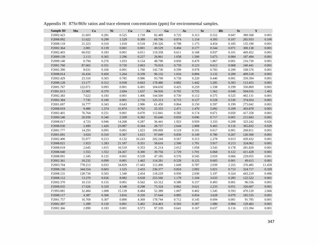
Appendix H: 87Sr/86Sr ratios and trace element concentrations (ppm) for environmental samples.
Sample ID Mn Co Ni Cu Zn Ga As Se Rb Sr YF2002.423 21.603 0.281 0.525 1.718 82.489 0.725 0.313 0.552 0.047 389.568 0.001F2008.092 11.622 0.298 1.529 0.389 69.796 0.874 1.154 4.393 0.107 265.933 0.100F2008.118 21.323 0.310 1.018 0.518 230.326 0.798 1.173 4.454 0.185 135.190 0.001F2002.364 2.081 0.139 0.001 0.001 49.529 0.494 0.177 0.544 0.071 300.138 0.001F2002.403 60.032 0.183 0.001 6.011 119.358 0.611 0.168 0.937 0.101 469.452 0.001F2009.139 2.113 0.365 2.296 0.227 26.861 1.058 1.500 5.673 0.084 187.494 0.001F2009.140 0.794 0.276 1.033 0.154 48.790 0.850 0.470 1.867 0.001 216.730 0.001F2001.760 87.665 0.351 0.720 2.063 76.024 0.759 0.123 0.612 0.068 240.441 0.001F2002.390 8.631 0.160 0.001 1.760 142.736 0.599 0.978 0.783 0.200 168.576 0.001F2008.014 16.434 0.450 5.264 0.339 96.132 1.016 0.894 3.132 0.200 409.518 0.001F2002.429 23.310 0.303 0.785 0.986 93.790 0.758 0.220 0.440 0.001 359.394 0.001F2008.128 13.177 0.312 0.938 0.663 178.480 0.882 1.442 5.285 0.303 113.455 0.001F2001.767 122.071 0.093 0.001 6.491 104.650 0.425 0.259 1.338 0.199 350.869 0.001F1991.013 12.905 0.370 2.694 1.637 94.926 0.702 0.755 1.562 0.048 504.016 1.463F2002.383 7.622 0.183 0.001 1.406 144.500 0.730 0.112 0.575 0.525 402.131 0.001F2002.384 7.745 0.180 0.001 2.716 125.313 0.715 0.127 0.528 0.530 374.024 0.001F2001.697 16.777 0.343 0.643 2.986 61.450 0.864 0.150 0.597 0.199 273.042 0.001F2008.019 9.480 1.374 31.874 0.762 25.355 2.471 1.470 5.092 0.209 303.878 0.001F2002.401 76.764 0.251 0.001 6.070 112.841 0.582 0.174 0.671 0.050 417.358 0.001F2000.546 20.939 0.340 2.509 0.382 93.646 0.859 0.096 0.717 0.001 212.843 0.001F2008.017 4.723 0.946 14.268 0.287 36.441 1.923 0.959 3.333 0.208 323.242 0.026F2008.030 2.490 1.426 23.087 0.344 28.757 2.644 2.808 9.465 0.116 365.832 0.029F2001.777 14.293 0.095 0.001 1.023 109.069 0.519 0.191 0.617 0.001 268.811 0.001F2001.691 3.024 0.310 0.367 1.615 97.049 0.830 0.149 0.780 0.267 120.500 0.001F2002.406 55.977 0.213 0.132 16.243 202.244 0.567 0.313 1.278 0.013 439.432 0.001F2008.021 1.923 1.283 21.187 0.351 58.616 2.500 1.701 5.917 0.213 324.062 0.001F2008.018 2.645 1.015 16.510 0.353 31.214 2.012 1.058 3.543 0.178 281.829 0.001F2008.040 1.553 1.552 24.267 0.300 39.756 2.729 1.701 6.068 0.122 411.428 0.001F2008.091 1.345 0.125 0.001 0.539 47.185 0.576 0.545 2.010 0.066 229.055 0.001F2002.361 10.232 0.099 0.001 1.462 114.281 0.528 0.125 0.605 0.001 49.615 0.001F2003.704 778.213 6.033 34.829 17.443 112.496 1.649 0.787 2.039 2.355 376.485 11.459F2008.130 344.554 0.603 1.525 2.433 236.377 0.824 2.002 5.021 0.713 324.717 0.359F2008.131 128.734 0.503 1.540 2.454 118.229 0.950 2.030 5.197 0.324 443.219 0.496F2008.112 13.270 0.656 8.082 0.658 253.566 1.178 1.104 3.633 0.285 122.522 0.001F2002.370 10.153 0.155 0.001 0.562 63.312 0.580 0.157 0.493 0.001 96.556 0.001F2008.035 17.626 0.329 4.548 0.298 73.324 0.862 0.621 2.233 0.051 326.607 0.001F1993.081 32.484 1.008 15.139 8.484 52.389 1.007 0.402 1.545 0.593 470.120 2.666F2008.117 4.387 0.306 3.816 0.320 57.644 0.885 0.854 3.628 0.079 182.535 0.001F2001.757 16.769 0.307 0.800 4.369 178.744 0.712 0.145 0.694 0.001 91.785 0.001F2002.397 1.289 0.120 0.001 5.402 214.463 0.503 0.287 1.080 0.984 129.483 0.001F2002.366 2.899 0.183 0.001 0.573 97.339 0.641 0.167 0.637 0.116 123.394 0.001
347

Appendix H: 87Sr/86Sr ratios and trace element concentrations (ppm) for environmental samples.
Sample ID Zr Nb Mo Ru Pd Ag Cd Sn Sb Cs BaF2002.423 0.001 0.001 0.826 0.056 0.001 0.001 0.001 0.001 0.126 0.001 214.785F2008.092 0.001 0.001 0.211 0.089 0.021 0.012 0.001 0.001 0.001 0.001 312.705F2008.118 0.001 0.001 0.059 0.037 0.001 0.001 0.001 0.001 0.001 0.001 73.982F2002.364 0.001 0.001 0.059 0.001 0.010 0.001 0.001 0.001 0.010 0.001 285.872F2002.403 0.001 0.001 0.072 0.032 0.001 0.001 0.353 0.001 0.001 0.001 24.521F2009.139 0.001 0.001 0.530 0.083 0.015 0.001 0.001 0.001 0.001 0.001 176.938F2009.140 0.001 0.001 0.381 0.032 0.001 0.001 0.001 0.001 0.001 0.001 242.205F2001.760 0.185 0.119 0.085 0.013 0.025 0.032 0.001 0.130 0.118 0.001 484.259F2002.390 0.001 0.001 0.055 0.001 0.001 0.010 0.001 0.094 0.031 0.001 232.599F2008.014 0.001 0.074 0.089 0.083 0.027 0.018 0.001 0.001 0.001 0.001 71.401F2002.429 0.001 0.001 0.475 0.053 0.010 0.001 0.001 0.001 0.214 0.001 277.724F2008.128 0.001 0.001 0.284 0.044 0.011 0.001 0.001 0.001 0.018 0.001 77.202F2001.767 0.001 0.001 0.031 0.001 0.016 0.001 0.001 0.001 0.001 0.001 33.407F1991.013 2.416 0.062 0.051 0.060 0.108 0.001 0.001 0.001 0.110 0.001 444.565F2002.383 0.001 0.001 0.066 0.055 0.018 0.001 0.001 0.001 0.001 0.001 141.727F2002.384 0.001 0.001 0.001 0.052 0.011 0.001 0.001 0.001 0.001 0.001 107.775F2001.697 0.001 0.001 0.070 0.024 0.001 0.001 0.001 0.001 0.001 0.001 110.383F2008.019 0.001 0.001 0.832 0.189 0.017 0.001 0.001 0.082 0.001 0.001 120.568F2002.401 0.001 0.001 0.149 0.029 0.013 0.001 0.001 0.001 0.001 0.001 31.937F2000.546 0.001 0.001 0.027 0.011 0.001 0.011 0.001 0.082 0.014 0.001 7.490F2008.017 0.001 0.001 1.441 0.189 0.015 0.001 0.001 0.001 0.038 0.001 121.119F2008.030 0.001 0.001 0.648 0.219 0.020 0.001 0.001 0.001 0.001 0.001 31.340F2001.777 0.001 0.001 0.001 0.012 0.014 0.001 0.001 1.799 0.010 0.001 376.666F2001.691 0.001 0.001 0.020 0.021 0.001 0.001 0.001 0.001 0.001 0.001 10.940F2002.406 0.455 0.001 0.183 0.019 0.049 0.049 0.118 0.352 0.016 0.001 41.001F2008.021 0.001 0.001 0.817 0.165 0.015 0.001 0.001 0.001 0.001 0.001 185.892F2008.018 0.001 0.001 1.118 0.162 0.014 0.001 0.001 0.001 0.001 0.001 120.642F2008.040 0.001 0.001 0.128 0.289 0.024 0.001 0.001 0.001 0.001 0.001 29.006F2008.091 0.001 0.058 0.078 0.020 0.041 0.014 0.001 0.001 0.001 0.001 323.548F2002.361 0.001 0.001 0.001 0.001 0.012 0.001 0.001 0.176 0.001 0.001 25.277F2003.704 3.805 0.400 0.066 0.101 0.272 0.128 0.381 0.087 0.255 0.214 202.298F2008.130 0.254 0.070 0.422 0.056 0.023 0.001 0.001 0.001 0.028 0.042 170.123F2008.131 0.280 0.070 0.278 0.079 0.035 0.024 0.001 0.001 0.019 0.001 73.185F2008.112 0.001 0.001 0.057 0.055 0.001 0.001 0.001 0.001 0.001 0.001 88.940F2002.370 0.001 0.001 0.071 0.001 0.015 0.021 0.001 0.001 0.032 0.001 222.425F2008.035 0.001 0.001 0.074 0.053 0.012 0.001 0.001 0.001 0.012 0.001 65.747F1993.081 3.117 0.123 0.082 0.080 0.141 0.022 0.228 0.001 0.067 0.041 253.205F2008.117 0.001 0.001 0.072 0.060 0.001 0.001 0.001 0.001 0.001 0.001 217.651F2001.757 0.001 0.001 0.001 0.001 0.001 0.001 0.001 0.107 0.025 0.001 92.406F2002.397 0.001 0.001 0.174 0.001 0.013 0.023 0.001 0.001 0.001 0.001 26.492F2002.366 0.182 0.001 0.085 0.024 0.030 0.032 0.001 0.140 0.017 0.001 192.562
348

Appendix H: 87Sr/86Sr ratios and trace element concentrations (ppm) for environmental samples.
Sample ID La Ce Pr Nd Sm Eu Gd Tb Dy Ho ErF2002.423 0.001 0.001 0.001 0.001 0.001 0.075 0.001 0.001 0.001 0.001 0.001F2008.092 0.136 0.274 0.032 0.122 0.001 0.105 0.001 0.001 0.001 0.001 0.001F2008.118 0.001 0.001 0.001 0.001 0.001 0.001 0.001 0.001 0.001 0.001 0.001F2002.364 0.001 0.001 0.001 0.001 0.001 0.091 0.001 0.001 0.001 0.001 0.001F2002.403 0.001 0.001 0.001 0.001 0.001 0.001 0.001 0.001 0.001 0.001 0.001F2009.139 0.001 0.001 0.001 0.001 0.001 0.062 0.001 0.001 0.001 0.001 0.001F2009.140 0.001 0.001 0.001 0.001 0.001 0.085 0.001 0.001 0.001 0.001 0.001F2001.760 0.001 0.001 0.001 0.001 0.001 0.173 0.001 0.001 0.001 0.001 0.001F2002.390 0.001 0.001 0.001 0.001 0.001 0.075 0.001 0.001 0.001 0.001 0.001F2008.014 0.001 0.001 0.001 0.001 0.001 0.033 0.001 0.001 0.001 0.001 0.001F2002.429 0.001 0.001 0.001 0.001 0.001 0.106 0.001 0.001 0.001 0.001 0.001F2008.128 0.001 0.001 0.001 0.001 0.001 0.001 0.001 0.001 0.001 0.001 0.001F2001.767 0.001 0.001 0.001 0.001 0.001 0.001 0.001 0.001 0.001 0.001 0.001F1991.013 0.674 1.227 0.179 0.860 0.205 0.224 0.282 0.038 0.233 0.052 0.146F2002.383 0.001 0.001 0.001 0.001 0.001 0.043 0.001 0.001 0.001 0.001 0.001F2002.384 0.001 0.001 0.001 0.001 0.001 0.034 0.001 0.001 0.001 0.001 0.001F2001.697 0.001 0.001 0.001 0.001 0.001 0.038 0.001 0.001 0.001 0.001 0.001F2008.019 0.001 0.035 0.001 0.001 0.001 0.082 0.001 0.001 0.001 0.001 0.001F2002.401 0.001 0.001 0.001 0.001 0.001 0.001 0.001 0.001 0.001 0.001 0.001F2000.546 0.001 0.001 0.001 0.001 0.001 0.001 0.001 0.001 0.001 0.001 0.001F2008.017 0.036 0.050 0.007 0.028 0.001 0.075 0.001 0.001 0.001 0.001 0.001F2008.030 0.001 0.054 0.006 0.030 0.001 0.001 0.001 0.001 0.001 0.001 0.001F2001.777 0.001 0.001 0.001 0.001 0.001 0.001 0.001 0.001 0.001 0.001 0.001F2001.691 0.001 0.001 0.001 0.001 0.001 0.001 0.001 0.001 0.001 0.001 0.001F2002.406 0.001 0.001 0.001 0.001 0.001 0.001 0.001 0.001 0.001 0.001 0.001F2008.021 0.001 0.001 0.001 0.001 0.001 0.140 0.001 0.001 0.001 0.001 0.001F2008.018 0.001 0.030 0.001 0.001 0.001 0.079 0.001 0.001 0.001 0.001 0.001F2008.040 0.001 0.001 0.001 0.001 0.001 0.001 0.001 0.001 0.001 0.001 0.001F2008.091 0.001 0.001 0.001 0.001 0.001 0.001 0.001 0.001 0.001 0.001 0.001F2002.361 0.001 0.001 0.001 0.001 0.001 0.001 0.001 0.001 0.001 0.001 0.001F2003.704 23.905 16.407 3.981 15.119 2.549 0.570 2.747 0.308 1.775 0.353 0.957F2008.130 0.460 0.855 0.112 0.447 0.086 0.076 0.089 0.001 0.066 0.001 0.001F2008.131 0.448 0.552 0.103 0.408 0.082 0.044 0.090 0.001 0.071 0.001 0.044F2008.112 0.001 0.001 0.001 0.001 0.001 0.050 0.001 0.001 0.001 0.001 0.001F2002.370 0.001 0.001 0.001 0.001 0.001 0.069 0.001 0.001 0.001 0.001 0.001F2008.035 0.001 0.001 0.001 0.001 0.001 0.032 0.001 0.001 0.001 0.001 0.001F1993.081 4.716 2.375 0.859 3.419 0.601 0.199 0.621 0.070 0.403 0.085 0.241F2008.117 0.001 0.001 0.001 0.001 0.001 0.076 0.001 0.001 0.001 0.001 0.001F2001.757 0.001 0.001 0.001 0.001 0.001 0.036 0.001 0.001 0.001 0.001 0.001F2002.397 0.001 0.001 0.001 0.001 0.001 0.001 0.001 0.001 0.001 0.001 0.001F2002.366 0.001 0.001 0.001 0.001 0.001 0.057 0.001 0.001 0.001 0.001 0.001
349

Appendix H: 87Sr/86Sr ratios and trace element concentrations (ppm) for environmental samples.
Sample ID Tm Yb Lu Ta Au Tl Pb Th UF2002.423 0.001 0.001 0.001 0.001 0.001 0.001 0.194 0.001 0.001F2008.092 0.001 0.001 0.001 0.035 0.059 0.001 0.168 0.065 0.001F2008.118 0.001 0.001 0.001 0.001 0.027 0.001 0.507 0.012 0.001F2002.364 0.001 0.001 0.001 0.001 0.001 0.001 0.302 0.001 0.043F2002.403 0.001 0.001 0.001 0.001 0.001 0.001 0.349 0.001 0.001F2009.139 0.001 0.001 0.001 0.028 0.046 0.001 0.154 0.058 0.001F2009.140 0.001 0.001 0.001 0.035 0.030 0.001 0.125 0.046 0.001F2001.760 0.001 0.001 0.001 0.196 0.068 0.001 1.060 0.278 0.001F2002.390 0.001 0.001 0.001 0.028 0.001 0.001 1.260 0.001 0.039F2008.014 0.001 0.001 0.001 0.091 0.136 0.001 0.287 0.107 0.001F2002.429 0.001 0.001 0.001 0.001 0.001 0.001 0.965 0.001 0.001F2008.128 0.001 0.001 0.001 0.001 0.028 0.001 0.690 0.001 0.001F2001.767 0.001 0.001 0.001 0.080 0.001 0.001 0.114 0.001 0.001F1991.013 0.020 0.129 0.001 0.196 0.066 0.001 0.344 0.103 1.856F2002.383 0.001 0.001 0.001 0.046 0.001 0.001 0.192 0.001 0.001F2002.384 0.001 0.001 0.001 0.028 0.001 0.001 0.232 0.001 0.001F2001.697 0.001 0.001 0.001 0.044 0.011 0.001 0.239 0.001 0.001F2008.019 0.001 0.001 0.001 0.001 0.029 0.001 0.272 0.001 0.001F2002.401 0.001 0.001 0.001 0.001 0.001 0.001 0.186 0.001 0.132F2000.546 0.001 0.001 0.001 0.049 0.025 0.001 0.068 0.037 0.082F2008.017 0.001 0.001 0.001 0.001 0.033 0.001 0.135 0.010 0.001F2008.030 0.001 0.001 0.001 0.001 0.038 0.001 0.074 0.018 0.001F2001.777 0.001 0.001 0.001 0.059 0.001 0.001 0.999 0.001 0.001F2001.691 0.001 0.001 0.001 0.041 0.013 0.001 0.079 0.001 0.001F2002.406 0.001 0.001 0.001 0.465 0.001 0.001 0.751 0.001 0.082F2008.021 0.001 0.001 0.001 0.030 0.030 0.001 0.278 0.001 0.001F2008.018 0.001 0.001 0.001 0.001 0.030 0.001 0.185 0.010 0.001F2008.040 0.001 0.001 0.001 0.001 0.046 0.001 0.080 0.001 0.001F2008.091 0.001 0.001 0.001 0.077 0.161 0.001 0.133 0.051 0.001F2002.361 0.001 0.001 0.001 0.001 0.001 0.001 0.730 0.001 0.001F2003.704 0.123 0.779 0.116 0.001 0.001 0.055 1.604 0.820 3.079F2008.130 0.001 0.001 0.001 0.001 0.029 0.001 0.351 0.079 1.127F2008.131 0.001 0.001 0.001 0.039 0.094 0.001 0.125 0.166 9.717F2008.112 0.001 0.001 0.001 0.001 0.026 0.001 0.489 0.001 0.001F2002.370 0.001 0.001 0.001 0.057 0.001 0.001 0.230 0.001 0.001F2008.035 0.001 0.001 0.001 0.029 0.039 0.001 0.395 0.013 0.001F1993.081 0.034 0.230 0.038 0.058 0.015 0.001 0.367 0.191 16.881F2008.117 0.001 0.001 0.001 0.024 0.030 0.001 0.097 0.014 0.001F2001.757 0.001 0.001 0.001 0.038 0.001 0.001 1.211 0.001 0.001F2002.397 0.001 0.001 0.001 0.033 0.001 0.001 0.298 0.001 0.001F2002.366 0.001 0.001 0.001 0.162 0.001 0.001 0.129 0.001 0.001
350

Appendix H: 87Sr/86Sr ratios and trace element concentrations (ppm) for environmental samples.
Sample ID 87Sr/86Sr Li Na Mg Al P Ca Ti V Cr FeF2002.360 0.710970 0.001 6419.6 4302.0 10.663 132972.2 232301.2 1.906 0.164 1.220 1626.6F2008.122 0.711013 1.318 4116.6 2427.0 20.434 138758.3 337015.0 3.907 1.652 0.666 2351.1F2008.039 0.711055 0.567 3513.2 2743.5 14.301 116396.6 196926.6 2.963 1.418 1.020 2068.6F2008.086 0.711122 5.414 4488.6 3039.6 3.598 125969.1 301174.3 2.533 1.119 0.717 1812.4F2008.020 0.711124 1.737 7401.8 3243.8 10.159 188545.4 398705.8 4.712 1.613 1.275 4920.3F2008.069 0.711171 0.365 2280.8 3646.2 351.225 133508.1 237639.8 16.012 2.224 1.547 2472.2F2002.396 0.711280 0.001 4158.1 5098.0 7.250 117179.4 192863.8 1.816 0.446 1.599 1554.7F2002.409 0.711370 0.001 2234.8 5399.9 30.730 118160.3 209198.9 1.843 0.823 0.986 1660.9F2000.547 0.711410 0.001 1632.2 1723.6 78.483 114022.8 176811.5 3.599 0.254 1.405 1783.0F1991.109 0.711630 1.207 2412.2 1468.5 982.581 118753.2 264828.5 25.884 9.483 3.790 3028.1F1991.104 0.711760 0.854 2642.8 1878.1 314.556 122778.4 260455.4 8.990 4.646 1.369 2288.8F1993.079 0.711830 1.098 1459.9 1587.1 306.625 126588.4 280326.1 10.884 6.894 5.320 2870.9F2008.105 0.712162 1.401 7117.8 5809.0 6.738 149992.0 223564.3 2.172 1.194 0.529 1314.3F1991.108 0.712180 0.902 2400.6 1734.3 672.867 124767.6 271214.4 20.967 7.776 2.601 2800.3F2000.230 0.712200 0.404 2413.5 2439.6 561.740 145012.1 241864.6 36.691 1.500 1.793 2857.5F2008.057 0.712423 0.001 3816.1 3965.2 145.025 137620.9 221093.9 5.600 1.225 0.754 2098.2F2000.229 0.712540 0.001 1740.4 2211.9 11.228 130027.5 182237.8 1.698 0.128 1.066 1660.8F2008.074 0.713391 0.480 1625.4 2084.8 623.894 118056.2 203773.0 20.257 2.366 1.599 2444.4F2008.085 0.714851 1.406 5145.1 4739.8 12.169 133254.9 220141.5 3.040 1.609 0.725 2349.4F2008.061 0.714852 0.481 2067.5 3181.3 400.308 124978.5 230578.7 18.993 2.270 1.739 2399.0F1993.151 0.715020 1.556 2231.1 1138.6 76.431 123479.8 280497.5 5.490 2.609 2.739 2495.0F2008.129 0.715576 0.317 4245.6 5587.3 35.663 137188.0 205520.3 3.278 1.757 2.142 2573.8F1993.094 0.716800 1.177 1406.8 1142.9 223.029 134241.9 280159.6 6.324 2.628 3.369 2670.4F2008.070 0.718725 0.361 2150.9 2770.4 534.728 128270.3 246748.6 27.158 2.548 1.853 2822.6F2008.080 0.719088 1.235 2202.9 3013.4 547.527 101172.9 229547.7 43.300 3.796 2.162 2169.7F2008.068 0.719449 0.931 2420.4 2719.9 493.739 119035.5 237821.4 6.651 1.239 1.326 1422.5F2008.076 0.720703 0.537 2102.0 2960.5 119.591 109879.7 233249.8 8.002 1.770 0.975 1508.9F2008.075 0.720794 0.358 2217.1 3225.7 539.863 124619.0 258768.5 22.610 2.714 1.472 2996.1F2008.065 0.721118 1.132 2260.3 2913.5 352.433 108508.4 215043.5 26.478 1.684 1.592 1532.6F2008.072 0.722528 0.001 4023.0 2484.0 75.948 94335.0 189140.6 8.340 1.309 0.640 1183.1F2008.071 0.722575 1.043 2188.2 3016.8 320.553 110874.8 219818.3 16.529 1.765 0.869 1471.4F2001.707 0.728290 1.851 2200.8 1187.0 27.506 105756.6 244721.4 3.174 2.786 0.690 2314.5F1991.054 0.731420 1.138 1940.2 1084.6 145.841 114521.0 235484.6 2.658 10.899 2.473 1972.5F2008.056 0.734373 1.578 2855.7 4079.1 28.689 114959.8 215326.4 2.356 0.722 0.695 1002.4F2008.089 0.739337 3.599 4927.7 2027.0 7.945 164000.0 349110.0 2.927 0.607 0.510 2145.6F1998.238 0.743300 1.785 2378.2 1997.2 720.493 113958.6 236471.8 16.545 1.079 2.008 2916.8F2008.051 0.746144 1.098 2554.1 4103.6 76.956 112435.0 173592.8 4.488 1.169 1.102 1908.7F1993.098 0.708570 0.001 2093.9 2030.9 34.948 98310.5 183914.8 1.461 0.276 1.028 1616.8F1993.100 0.708580 0.001 3126.1 2710.7 130.729 121742.3 230785.5 1.508 0.535 0.706 1943.5F1993.101 0.708580 0.001 3565.6 2606.2 19.259 126206.6 264372.2 1.594 0.580 0.792 2236.0F1997.068 0.713290 0.001 2336.4 2279.4 51.186 87918.0 190215.2 4.579 0.203 1.170 1762.9F1997.059 0.713730 0.393 2303.1 2254.9 110.614 118538.6 245679.7 9.906 0.350 1.079 2219.4
351

Appendix H: 87Sr/86Sr ratios and trace element concentrations (ppm) for environmental samples.
Sample ID Mn Co Ni Cu Zn Ga As Se Rb Sr YF2002.360 2.733 0.110 0.001 0.058 110.707 0.532 0.117 0.439 0.139 43.395 0.001F2008.122 17.303 0.366 4.724 0.379 62.519 1.042 1.763 6.772 0.078 355.878 0.042F2008.039 4.524 0.437 6.245 0.363 65.268 1.056 0.934 3.508 0.054 392.176 0.001F2008.086 10.420 0.195 0.254 0.267 60.321 0.896 1.444 5.832 0.242 291.289 0.001F2008.020 2.353 1.223 19.865 0.295 48.959 2.342 1.780 6.052 0.120 240.249 0.001F2008.069 49.587 0.698 6.231 0.886 153.375 1.112 1.306 4.283 0.597 354.856 0.001F2002.396 1.082 0.164 0.001 4.773 247.779 0.549 0.247 1.137 0.268 147.171 0.001F2002.409 76.768 0.204 0.001 5.218 205.024 0.613 0.210 0.886 0.056 391.515 0.001F2000.547 25.409 0.398 3.076 0.651 89.107 0.769 0.190 0.958 0.289 199.009 0.001F1991.109 255.930 2.130 13.321 6.840 58.948 1.095 0.287 1.255 0.472 659.098 5.045F1991.104 29.045 1.068 4.707 1.475 73.778 0.903 0.202 1.032 0.306 426.485 2.300F1993.079 368.308 3.626 22.497 6.824 66.276 1.024 0.710 1.746 0.125 627.503 7.717F2008.105 3.733 0.150 0.468 0.295 71.344 0.676 1.078 3.993 0.001 277.354 0.001F1991.108 74.736 1.212 8.458 2.716 78.745 1.008 0.189 0.818 0.529 471.107 2.366F2000.230 61.505 0.806 4.734 0.840 219.674 1.142 0.148 0.500 0.985 214.165 0.352F2008.057 34.207 0.460 5.418 0.551 300.564 0.983 0.841 2.847 0.177 162.647 0.001F2000.229 4.548 0.321 2.753 0.958 270.984 0.822 0.158 0.864 0.001 191.426 0.001F2008.074 44.803 0.750 6.529 0.943 159.437 1.172 0.862 2.684 1.061 180.827 0.001F2008.085 7.558 0.502 6.848 0.420 90.748 1.169 1.219 4.303 0.185 255.430 0.001F2008.061 262.822 0.905 6.549 0.830 117.111 1.033 1.292 4.300 0.880 493.693 0.031F1993.151 251.106 0.742 3.855 2.331 117.645 0.958 0.451 0.620 0.078 399.135 0.179F2008.129 20.151 0.584 6.976 1.605 221.412 1.087 1.063 3.837 0.211 132.762 0.001F1993.094 10.311 0.679 9.982 5.220 96.768 1.025 0.285 1.481 0.147 319.934 0.059F2008.070 47.580 0.879 7.499 1.038 209.313 1.237 1.173 3.787 0.931 199.848 0.001F2008.080 26.430 0.549 0.234 1.807 214.602 0.882 1.542 5.442 1.531 285.785 0.104F2008.068 58.704 0.855 0.001 1.023 216.198 0.738 0.879 3.339 0.347 286.237 0.001F2008.076 47.706 0.225 0.001 0.690 317.295 0.701 1.446 5.507 0.278 274.152 0.025F2008.075 184.089 1.073 8.596 0.880 364.558 1.276 1.352 4.449 0.670 236.778 0.054F2008.065 51.062 0.325 0.001 0.786 233.127 0.724 0.855 2.998 1.332 194.172 0.001F2008.072 7.612 0.119 0.001 0.755 266.219 0.531 1.016 3.937 0.272 135.292 0.023F2008.071 161.593 0.385 0.001 1.406 296.499 0.703 1.124 4.291 0.737 193.025 0.075F2001.707 60.895 0.867 2.179 7.407 74.023 0.876 0.663 0.669 0.093 468.495 0.001F1991.054 151.155 1.596 12.706 9.031 54.759 0.794 1.247 1.250 0.076 408.692 0.001F2008.056 27.346 0.064 0.001 0.648 232.932 0.610 0.881 3.374 0.183 153.546 0.001F2008.089 3.750 0.279 0.942 0.465 43.257 0.992 0.680 2.695 0.179 340.248 0.001F1998.238 52.415 0.886 4.626 1.384 255.519 1.032 0.267 0.651 0.795 85.078 1.090F2008.051 10.416 0.437 5.721 0.586 74.453 0.998 0.623 2.346 0.154 161.827 0.001F1993.098 7.328 0.287 2.103 0.437 143.610 0.667 0.172 0.914 0.050 86.687 0.001F1993.100 5.851 0.339 2.325 0.491 168.610 0.887 0.123 0.755 0.040 182.475 0.001F1993.101 1.519 0.413 3.122 0.645 156.862 0.922 0.096 0.608 0.100 188.457 0.001F1997.068 11.663 0.383 2.370 1.403 242.743 0.661 0.105 0.608 0.205 205.284 0.079F1997.059 29.909 0.446 2.630 1.454 272.010 0.902 0.121 0.719 0.230 207.537 0.001
352

Appendix H: 87Sr/86Sr ratios and trace element concentrations (ppm) for environmental samples.
Sample ID Zr Nb Mo Ru Pd Ag Cd Sn Sb Cs BaF2002.360 0.001 0.001 0.001 0.001 0.010 0.001 0.001 0.001 0.001 0.001 26.193F2008.122 0.001 0.001 4.129 0.109 0.013 0.001 0.001 0.001 0.001 0.001 303.335F2008.039 0.124 0.064 0.194 0.082 0.023 0.019 0.001 0.001 0.001 0.001 74.250F2008.086 0.001 0.001 0.115 0.070 0.010 0.001 0.001 0.001 0.043 0.001 234.625F2008.020 0.001 0.001 1.556 0.185 0.017 0.001 0.001 0.001 0.001 0.001 133.602F2008.069 0.001 0.065 0.107 0.079 0.012 0.023 0.001 0.001 0.012 0.020 101.317F2002.396 0.001 0.001 0.080 0.001 0.012 0.025 0.001 0.001 0.001 0.001 34.731F2002.409 0.001 0.001 0.073 0.021 0.012 0.001 0.076 0.001 0.001 0.001 45.136F2000.547 0.001 0.001 0.001 0.001 0.011 0.001 0.001 0.001 0.042 0.001 6.967F1991.109 0.737 0.049 0.264 0.092 0.067 0.061 0.586 0.001 0.026 0.030 459.954F1991.104 0.191 0.001 0.127 0.066 0.027 0.001 0.154 0.076 0.001 0.001 321.552F1993.079 2.095 0.087 0.127 0.085 0.133 0.023 0.330 0.001 0.095 0.001 321.565F2008.105 0.001 0.001 0.070 0.042 0.027 0.001 0.001 0.001 0.001 0.001 259.330F1991.108 0.380 0.046 0.254 0.074 0.039 0.014 0.323 0.069 0.015 0.023 450.633F2000.230 0.225 0.082 0.301 0.033 0.025 0.018 0.001 0.001 0.001 0.040 227.717F2008.057 0.001 0.001 0.161 0.042 0.013 0.001 0.001 0.001 0.001 0.001 87.359F2000.229 0.173 0.117 0.180 0.001 0.027 0.032 0.001 0.137 0.022 0.001 101.507F2008.074 0.001 0.093 0.057 0.033 0.010 0.012 0.001 0.001 0.018 0.045 146.252F2008.085 0.001 0.001 0.043 0.059 0.011 0.001 0.001 0.001 0.001 0.001 382.930F2008.061 0.001 0.095 0.435 0.109 0.015 0.001 0.072 0.001 0.020 0.034 705.023F1993.151 0.623 0.001 0.743 0.078 0.035 0.001 0.001 0.001 0.025 0.001 487.168F2008.129 0.141 0.108 0.194 0.031 0.039 0.031 0.001 0.157 0.082 0.001 121.388F1993.094 0.198 0.160 0.073 0.053 0.029 0.038 0.133 0.123 0.046 0.001 274.765F2008.070 0.001 0.095 0.059 0.069 0.013 0.001 0.001 0.001 0.022 0.040 125.765F2008.080 0.001 0.165 0.111 0.061 0.013 0.022 0.001 0.001 0.021 0.062 217.417F2008.068 0.001 0.054 0.057 0.042 0.013 0.010 0.102 0.001 0.034 0.022 217.136F2008.076 0.001 0.001 0.082 0.064 0.013 0.001 0.001 0.001 0.025 0.001 162.137F2008.075 0.001 0.068 0.074 0.094 0.015 0.020 0.068 0.001 0.020 0.024 148.498F2008.065 0.001 0.211 0.071 0.031 0.019 0.018 0.001 0.001 0.044 0.059 196.328F2008.072 0.001 0.044 0.063 0.034 0.014 0.001 0.001 0.001 0.001 0.001 159.530F2008.071 0.142 0.121 0.080 0.048 0.027 0.019 0.081 0.063 0.026 0.032 209.779F2001.707 0.001 0.001 6.325 0.072 0.001 0.001 0.001 0.001 0.028 0.001 286.463F1991.054 0.001 0.069 0.059 0.038 0.015 0.052 0.064 0.001 0.089 0.001 165.636F2008.056 0.001 0.103 0.070 0.017 0.028 0.019 0.001 0.001 0.060 0.001 67.787F2008.089 0.001 0.047 0.117 0.087 0.024 0.018 0.001 0.001 0.001 0.001 295.704F1998.238 0.890 0.042 0.175 0.022 0.047 0.001 0.001 0.001 0.029 0.090 92.771F2008.051 0.001 0.040 0.063 0.033 0.011 0.001 0.001 0.001 0.001 0.001 373.515F1993.098 0.001 0.001 0.053 0.001 0.013 0.010 0.001 0.068 0.001 0.001 6.552F1993.100 0.001 0.001 0.024 0.019 0.001 0.001 0.001 0.001 0.001 0.001 13.258F1993.101 0.001 0.001 0.289 0.037 0.012 0.001 0.001 0.001 0.001 0.001 16.741F1997.068 0.001 0.001 0.224 0.001 0.014 0.014 0.129 0.062 0.115 0.001 139.957F1997.059 0.001 0.001 0.443 0.022 0.001 0.011 0.177 0.001 0.024 0.001 115.276
353

Appendix H: 87Sr/86Sr ratios and trace element concentrations (ppm) for environmental samples.
Sample ID La Ce Pr Nd Sm Eu Gd Tb Dy Ho ErF2002.360 0.001 0.001 0.001 0.001 0.001 0.001 0.001 0.001 0.001 0.001 0.001F2008.122 0.047 0.074 0.011 0.044 0.001 0.104 0.001 0.001 0.001 0.001 0.001F2008.039 0.001 0.001 0.001 0.001 0.001 0.037 0.001 0.001 0.001 0.001 0.001F2008.086 0.001 0.001 0.001 0.001 0.001 0.072 0.001 0.001 0.001 0.001 0.001F2008.020 0.001 0.001 0.001 0.001 0.001 0.096 0.001 0.001 0.001 0.001 0.001F2008.069 0.036 0.001 0.001 0.001 0.001 0.055 0.001 0.001 0.001 0.001 0.001F2002.396 0.001 0.001 0.001 0.001 0.001 0.001 0.001 0.001 0.001 0.001 0.001F2002.409 0.001 0.001 0.001 0.001 0.001 0.001 0.001 0.001 0.001 0.001 0.001F2000.547 0.001 0.001 0.001 0.001 0.001 0.001 0.001 0.001 0.001 0.001 0.001F1991.109 2.241 3.074 0.486 2.256 0.542 0.345 0.789 0.112 0.764 0.172 0.510F1991.104 0.837 0.813 0.201 0.969 0.224 0.186 0.311 0.041 0.265 0.060 0.174F1993.079 17.348 7.521 2.887 10.899 1.814 0.439 1.903 0.207 1.171 0.239 0.682F2008.105 0.001 0.001 0.001 0.001 0.001 0.001 0.001 0.001 0.001 0.001 0.001F1991.108 1.324 1.563 0.265 1.215 0.282 0.253 0.394 0.053 0.334 0.077 0.225F2000.230 1.010 1.715 0.172 0.642 0.113 0.112 0.095 0.001 0.057 0.001 0.032F2008.057 0.001 0.001 0.001 0.001 0.001 0.045 0.001 0.001 0.001 0.001 0.001F2000.229 0.001 0.001 0.001 0.001 0.001 0.041 0.001 0.001 0.001 0.001 0.001F2008.074 0.057 0.001 0.001 0.001 0.001 0.082 0.001 0.001 0.001 0.001 0.001F2008.085 0.001 0.001 0.001 0.001 0.001 0.207 0.001 0.001 0.001 0.001 0.001F2008.061 0.166 0.084 0.005 0.001 0.001 0.365 0.001 0.001 0.001 0.001 0.001F1993.151 0.145 0.306 0.030 0.121 0.001 0.203 0.034 0.001 0.001 0.001 0.001F2008.129 0.001 0.001 0.001 0.001 0.001 0.068 0.001 0.001 0.001 0.001 0.001F1993.094 0.442 0.151 0.013 0.038 0.001 0.111 0.001 0.001 0.001 0.001 0.001F2008.070 0.096 0.051 0.001 0.001 0.001 0.070 0.001 0.001 0.001 0.001 0.001F2008.080 0.462 0.384 0.033 0.094 0.001 0.067 0.001 0.001 0.001 0.001 0.001F2008.068 0.170 0.083 0.001 0.001 0.001 0.059 0.001 0.001 0.001 0.001 0.001F2008.076 0.180 0.152 0.009 0.001 0.001 0.046 0.001 0.001 0.001 0.001 0.001F2008.075 0.620 0.494 0.030 0.072 0.001 0.087 0.001 0.001 0.001 0.001 0.001F2008.065 0.142 0.063 0.001 0.001 0.001 0.052 0.001 0.001 0.001 0.001 0.001F2008.072 0.059 0.067 0.008 0.031 0.001 0.048 0.001 0.001 0.001 0.001 0.001F2008.071 0.200 0.251 0.025 0.087 0.018 0.060 0.001 0.001 0.001 0.001 0.001F2001.707 0.033 0.001 0.001 0.001 0.001 0.110 0.001 0.001 0.001 0.001 0.001F1991.054 0.184 0.001 0.001 0.001 0.001 0.057 0.001 0.001 0.001 0.001 0.001F2008.056 0.001 0.001 0.001 0.001 0.001 0.001 0.001 0.001 0.001 0.001 0.001F2008.089 0.001 0.001 0.001 0.001 0.001 0.092 0.001 0.001 0.001 0.001 0.001F1998.238 2.023 2.615 0.437 1.691 0.315 0.093 0.311 0.035 0.192 0.036 0.102F2008.051 0.001 0.001 0.001 0.001 0.001 0.194 0.001 0.001 0.001 0.001 0.001F1993.098 0.001 0.001 0.001 0.001 0.001 0.001 0.001 0.001 0.001 0.001 0.001F1993.100 0.001 0.001 0.001 0.001 0.001 0.001 0.001 0.001 0.001 0.001 0.001F1993.101 0.001 0.001 0.001 0.001 0.001 0.001 0.001 0.001 0.001 0.001 0.001F1997.068 0.088 0.156 0.017 0.064 0.001 0.057 0.001 0.001 0.001 0.001 0.001F1997.059 0.064 0.068 0.006 0.001 0.001 0.042 0.001 0.001 0.001 0.001 0.001
354

Appendix H: 87Sr/86Sr ratios and trace element concentrations (ppm) for environmental samples.
Sample ID Tm Yb Lu Ta Au Tl Pb Th UF2002.360 0.001 0.001 0.001 0.001 0.001 0.001 0.085 0.001 0.001F2008.122 0.001 0.001 0.001 0.001 0.032 0.001 0.267 0.001 0.001F2008.039 0.001 0.001 0.001 0.129 0.073 0.001 0.307 0.042 0.001F2008.086 0.001 0.001 0.001 0.001 0.028 0.001 0.727 0.001 0.001F2008.020 0.001 0.001 0.001 0.024 0.033 0.001 0.192 0.001 0.001F2008.069 0.001 0.001 0.001 0.001 0.039 0.001 0.606 0.001 0.047F2002.396 0.001 0.001 0.001 0.026 0.001 0.001 0.333 0.001 0.001F2002.409 0.001 0.001 0.001 0.055 0.001 0.001 0.193 0.001 0.032F2000.547 0.001 0.001 0.001 0.109 0.032 0.001 0.355 0.046 0.040F1991.109 0.073 0.463 0.074 0.001 0.022 0.001 0.317 0.066 17.276F1991.104 0.023 0.140 0.023 0.091 0.029 0.001 0.112 0.037 1.102F1993.079 0.091 0.592 0.090 0.028 0.017 0.001 0.689 0.325 12.098F2008.105 0.001 0.001 0.001 0.035 0.098 0.001 0.240 0.001 0.063F1991.108 0.031 0.192 0.031 0.061 0.022 0.001 0.209 0.052 3.356F2000.230 0.001 0.025 0.001 0.105 0.036 0.001 0.674 0.231 0.032F2008.057 0.001 0.001 0.001 0.029 0.043 0.001 3.560 0.011 0.033F2000.229 0.001 0.001 0.001 0.239 0.093 0.001 0.135 0.281 0.040F2008.074 0.001 0.001 0.001 0.021 0.029 0.001 0.928 0.001 0.001F2008.085 0.001 0.001 0.001 0.059 0.050 0.001 0.208 0.010 0.001F2008.061 0.001 0.001 0.001 0.037 0.046 0.001 0.358 0.010 0.001F1993.151 0.001 0.001 0.001 0.070 0.016 0.001 0.130 0.039 6.448F2008.129 0.001 0.001 0.001 0.218 0.179 0.058 0.296 0.205 0.001F1993.094 0.001 0.001 0.001 0.216 0.075 0.001 0.200 0.268 11.952F2008.070 0.001 0.001 0.001 0.025 0.034 0.001 0.843 0.001 0.001F2008.080 0.001 0.001 0.001 0.021 0.033 0.001 0.361 0.016 0.074F2008.068 0.001 0.001 0.001 0.026 0.043 0.001 1.077 0.021 0.001F2008.076 0.001 0.001 0.001 0.001 0.036 0.001 0.631 0.015 0.038F2008.075 0.001 0.001 0.001 0.001 0.030 0.001 1.126 0.001 0.068F2008.065 0.001 0.001 0.001 0.073 0.064 0.001 0.517 0.056 0.033F2008.072 0.001 0.001 0.001 0.050 0.045 0.001 0.697 0.045 0.001F2008.071 0.001 0.001 0.001 0.073 0.078 0.001 0.844 0.121 0.001F2001.707 0.001 0.001 0.001 0.046 0.001 0.001 0.075 0.001 0.418F1991.054 0.001 0.001 0.001 0.062 0.050 0.001 0.501 0.016 0.404F2008.056 0.001 0.001 0.001 0.058 0.090 0.001 0.373 0.078 0.001F2008.089 0.001 0.001 0.001 0.045 0.078 0.001 0.132 0.115 0.001F1998.238 0.013 0.079 0.001 0.055 0.001 0.001 0.982 0.240 0.881F2008.051 0.001 0.001 0.001 0.106 0.051 0.001 0.348 0.023 0.001F1993.098 0.001 0.001 0.001 0.183 0.048 0.001 3.106 0.101 0.001F1993.100 0.001 0.001 0.001 0.053 0.024 0.001 0.188 0.028 0.001F1993.101 0.001 0.001 0.001 0.092 0.021 0.001 2.955 0.033 0.001F1997.068 0.001 0.001 0.001 0.077 0.020 0.001 0.658 0.018 0.039F1997.059 0.001 0.001 0.001 0.079 0.121 0.001 2.741 0.020 0.042
355

Appendix H: 87Sr/86Sr ratios and trace element concentrations (ppm) for environmental samples.
WaterSample ID 87Sr/86Sr Li Na Mg Al P Ca Ti V Cr FeW2009.023 0.708508 0.021 4.9 21.4 0.009 0.5 54.9 0.003 0.002 0.006 0.3W2009.034 0.708692 0.038 11.6 29.4 0.005 0.4 77.8 0.005 0.003 0.006 0.4W2009.055 0.709166 0.012 51.7 15.1 0.027 0.4 40.2 0.002 0.002 0.006 0.3W2009.056 0.708926 0.013 22.4 14.9 0.009 0.4 39.7 0.002 0.002 0.006 0.2W2009.057 0.708852 0.027 23.6 21.5 0.009 0.4 50.6 0.003 0.002 0.006 0.3W2009.078 0.708360 0.008 6.0 15.9 0.027 0.5 53.1 0.002 0.003 0.006 0.6W2009.079 0.708485 0.019 309.6 20.8 0.009 0.4 58.6 0.004 0.007 0.006 0.3W2009.086 0.708653 0.017 14.4 20.0 0.009 0.5 48.9 0.002 0.003 0.006 0.2W2009.099 0.708143 0.008 6.9 18.1 0.010 0.5 65.1 0.002 0.004 0.005 0.3W2009.112 0.708409 0.005 4.7 12.5 0.010 0.6 54.5 0.001 0.003 0.006 0.3W2009.119 0.708305 0.004 3.4 9.8 0.007 0.5 63.3 0.001 0.003 0.005 0.3W2009.120 0.708550 0.004 3.2 10.8 0.016 0.5 50.9 0.001 0.003 0.006 0.2W2009.141 0.708145 0.005 4.3 11.2 0.010 0.5 67.3 0.002 0.003 0.008 0.3W2009.142 0.708222 0.005 4.2 12.2 0.009 0.5 59.0 0.002 0.003 0.005 0.3W2009.161 0.708729 0.010 4.0 14.3 0.009 0.5 52.8 0.002 0.003 0.006 0.2W2009.168 0.708816 0.016 11.6 17.2 0.006 0.4 48.3 0.002 0.002 0.007 1.8W2009.207 0.710194 0.002 2.6 7.5 0.029 0.5 23.2 0.001 0.002 0.006 0.2W2009.208 0.709803 0.001 1.3 2.0 0.034 0.4 7.7 0.001 0.001 0.008 0.1W2009.215 0.710130 0.001 1.3 4.3 0.032 0.5 10.9 0.001 0.001 0.005 0.1W2009.216 0.709274 0.002 2.4 5.3 0.033 0.5 24.4 0.001 0.001 0.001 0.1W2009.229 0.709900 0.001 1.7 3.7 0.058 0.4 17.7 0.001 0.001 0.001 0.1W2009.236 0.708856 0.003 2.6 7.1 0.020 0.5 31.3 0.001 0.002 0.001 0.1W2009.248 0.712292 0.001 1.4 3.7 0.015 0.5 16.9 0.001 0.001 0.001 0.1W2009.261 0.710705 <DL 3.4 7.5 0.011 0.5 19.8 0.001 0.001 0.001 0.1W2009.265 0.713728 0.000 0.9 9.5 0.009 0.5 31.9 0.001 0.001 0.001 0.1W2009.269 0.709777 0.001 0.8 3.7 0.027 0.5 11.0 0.001 0.001 0.001 0.1W2009.273 0.709639 0.001 0.8 5.5 0.023 0.5 17.6 0.001 0.001 0.001 0.1W2009.280 0.707106 0.001 1.0 5.8 0.018 0.5 20.6 0.001 0.001 0.001 0.1W2009.284 0.708778 0.001 0.8 5.9 0.018 0.5 24.8 0.001 0.001 0.001 0.1W2009.289 0.707332 0.005 3.3 12.5 0.012 0.5 41.0 0.001 0.001 0.001 0.1W2009.290 0.708622 0.002 1.1 7.2 0.016 0.6 29.1 0.001 0.001 0.001 0.1W2009.297 0.709827 0.002 1.2 7.0 0.029 0.5 35.8 0.001 0.001 0.001 0.1W2009.304 0.709100 0.003 1.8 5.6 0.027 0.5 39.7 0.001 0.001 0.002 0.1W2009.311 0.709145 0.007 1.6 5.5 0.017 0.5 31.4 0.001 0.001 0.003 0.1W2009.318 0.708823 0.003 1.6 7.4 0.020 0.5 37.5 0.001 0.001 0.001 0.1W2009.325 0.709610 0.002 1.8 5.5 0.030 0.5 28.5 0.001 0.000 0.001 0.1W2009.329 0.709181 0.003 1.0 11.3 0.018 0.5 36.5 0.001 0.001 0.001 0.1W2009.339 0.708783 0.002 3.6 9.5 0.018 0.6 28.6 0.001 0.001 0.001 0.2W2009.349 0.712939 0.002 3.5 4.8 0.056 0.6 12.9 0.001 0.000 0.001 0.1W2009.356 0.709540 0.001 1.5 2.7 0.068 0.6 20.4 0.001 0.000 0.001 0.1W2009.357 0.708816 0.007 3.9 7.4 0.065 0.6 34.5 0.001 0.001 0.001 0.1
356

Appendix H: 87Sr/86Sr ratios and trace element concentrations (ppm) for environmental samples.
Sample ID Mn Co Ni Cu Zn Ga As Se Rb Sr YW2009.023 0.002 0.000 0.002 0.002 0.013 <DL 0.001 0.002 0.000 1.127 0.000W2009.034 0.014 0.000 0.002 0.001 0.012 <DL 0.001 0.002 0.000 2.320 0.000W2009.055 0.002 0.000 0.002 0.002 0.006 <DL 0.001 0.002 0.000 0.662 0.000W2009.056 0.002 0.000 0.002 0.001 0.006 <DL 0.001 0.002 0.000 0.833 <DLW2009.057 0.004 0.000 0.002 0.001 0.006 <DL 0.001 0.002 0.000 1.018 <DLW2009.078 0.006 0.000 0.003 0.001 0.005 <DL 0.001 0.002 0.000 0.607 0.000W2009.079 0.002 0.000 0.002 0.002 0.006 <DL 0.003 0.009 0.001 0.699 0.000W2009.086 0.003 0.000 0.002 0.001 0.005 <DL 0.001 0.001 0.000 0.982 0.000W2009.099 0.001 0.000 0.002 0.001 0.005 <DL 0.001 0.002 0.000 0.904 0.000W2009.112 0.007 0.000 0.002 0.001 0.003 <DL 0.001 0.002 0.000 0.382 0.000W2009.119 0.006 0.000 0.002 0.011 0.009 <DL 0.001 0.002 0.000 0.364 0.000W2009.120 0.004 0.000 0.002 0.001 0.005 <DL 0.001 0.002 0.000 0.283 0.000W2009.141 0.002 0.000 0.002 0.001 0.005 <DL 0.001 0.002 0.000 0.581 0.000W2009.142 0.002 0.000 0.002 0.001 0.004 <DL 0.001 0.002 0.000 0.523 0.000W2009.161 0.005 0.000 0.002 0.001 0.003 <DL 0.001 0.002 0.000 0.337 0.000W2009.168 0.010 0.000 0.003 0.003 0.007 <DL 0.001 0.001 0.000 1.054 <DLW2009.207 0.008 0.000 0.003 0.002 0.003 <DL 0.000 0.000 0.000 0.204 0.000W2009.208 0.001 0.000 0.003 0.001 0.002 <DL 0.000 <DL 0.001 0.049 0.000W2009.215 0.004 0.000 0.002 0.001 0.002 <DL 0.000 0.000 0.000 0.043 0.000W2009.216 0.001 0.000 0.001 0.001 0.002 <DL 0.000 0.000 0.001 0.123 0.000W2009.229 0.002 0.000 0.001 0.001 0.003 <DL 0.000 <DL 0.001 0.080 0.000W2009.236 0.006 0.000 0.001 0.001 0.002 <DL 0.000 0.001 0.001 0.184 <DLW2009.248 0.001 0.000 0.000 0.000 0.002 <DL 0.000 <DL 0.000 0.072 <DLW2009.261 0.005 0.000 0.002 0.001 0.003 <DL 0.000 0.000 0.000 0.048 <DLW2009.265 0.004 0.000 0.002 0.001 0.003 <DL 0.000 <DL 0.000 0.092 <DLW2009.269 0.003 0.000 0.001 0.001 0.002 <DL 0.000 <DL 0.000 0.034 0.000W2009.273 0.002 <DL 0.001 0.001 0.002 <DL 0.000 0.000 0.000 0.056 0.000W2009.280 0.001 <DL 0.001 0.001 0.002 <DL 0.000 <DL 0.002 0.175 0.000W2009.284 0.001 0.000 0.001 0.001 0.002 <DL 0.000 0.000 0.001 0.096 0.000W2009.289 0.001 <DL 0.000 0.001 0.002 <DL 0.000 0.001 0.001 0.211 0.000W2009.290 0.001 0.000 0.001 0.001 0.002 <DL 0.000 <DL 0.001 0.120 <DLW2009.297 0.001 0.000 0.001 0.002 0.003 <DL 0.000 0.001 0.002 0.121 0.000W2009.304 0.001 0.000 0.004 0.001 0.004 <DL 0.000 0.001 0.002 0.164 0.000W2009.311 0.001 0.000 0.001 0.001 0.002 <DL 0.000 0.001 0.001 0.232 0.000W2009.318 0.001 0.000 0.001 0.001 0.002 <DL 0.000 0.001 0.002 0.151 <DLW2009.325 0.001 0.000 0.002 0.001 0.005 <DL 0.000 <DL 0.002 0.125 0.000W2009.329 0.001 0.000 0.000 0.000 0.003 <DL 0.000 0.000 0.002 0.300 0.000W2009.339 0.009 0.000 0.001 0.000 0.003 <DL 0.000 0.000 0.001 0.220 <DLW2009.349 0.028 0.000 0.002 0.001 0.003 <DL 0.000 <DL 0.001 0.063 0.000W2009.356 0.002 0.000 0.001 0.001 0.003 <DL 0.000 <DL 0.001 0.068 0.000W2009.357 0.004 <DL 0.001 0.001 0.003 <DL 0.000 0.000 0.002 0.184 0.000
357

Appendix H: 87Sr/86Sr ratios and trace element concentrations (ppm) for environmental samples.
Sample ID Zr Nb Mo Ru Pd Ag Cd Sn Sb Cs BaW2009.023 <DL <DL 0.002 0.000 0.000 <DL <DL <DL 0.000 <DL 0.020W2009.034 <DL <DL 0.002 0.000 0.000 <DL <DL <DL 0.000 <DL 0.031W2009.055 <DL <DL 0.001 0.000 0.000 <DL <DL <DL 0.000 <DL 0.018W2009.056 <DL <DL 0.001 0.000 0.000 <DL <DL <DL 0.000 <DL 0.030W2009.057 <DL <DL 0.002 0.000 0.000 <DL <DL <DL 0.000 <DL 0.027W2009.078 0.000 <DL 0.001 0.000 0.000 <DL <DL <DL 0.000 <DL 0.064W2009.079 <DL <DL 0.001 0.000 0.000 <DL <DL 0.000 0.000 <DL 0.080W2009.086 <DL <DL 0.001 0.000 0.000 <DL <DL <DL 0.000 <DL 0.046W2009.099 0.000 <DL 0.001 0.000 0.000 <DL <DL <DL 0.000 <DL 0.066W2009.112 <DL <DL 0.000 0.000 0.000 <DL <DL 0.000 0.000 <DL 0.135W2009.119 <DL <DL 0.001 0.000 0.000 <DL <DL <DL 0.000 <DL 0.132W2009.120 <DL <DL 0.000 0.000 0.000 <DL <DL <DL 0.000 <DL 0.103W2009.141 <DL <DL 0.000 0.000 0.000 <DL <DL <DL 0.000 <DL 0.092W2009.142 <DL <DL 0.001 0.000 0.000 <DL <DL <DL 0.000 <DL 0.095W2009.161 <DL <DL 0.001 0.000 0.000 <DL <DL <DL 0.000 <DL 0.066W2009.168 <DL <DL 0.001 0.000 0.000 <DL <DL 0.000 0.000 <DL 0.034W2009.207 <DL <DL 0.001 0.000 0.000 <DL <DL <DL <DL <DL 0.016W2009.208 <DL <DL 0.000 0.000 0.000 <DL <DL <DL <DL <DL 0.006W2009.215 <DL <DL 0.001 0.000 0.000 <DL <DL <DL 0.000 <DL 0.009W2009.216 <DL <DL 0.001 0.000 0.000 <DL <DL <DL 0.000 <DL 0.022W2009.229 <DL <DL 0.000 0.000 0.000 <DL <DL <DL 0.000 <DL 0.011W2009.236 <DL <DL 0.001 0.000 0.000 <DL <DL <DL 0.000 <DL 0.036W2009.248 0.000 <DL 0.001 0.000 0.000 <DL <DL <DL 0.000 <DL 0.009W2009.261 <DL <DL 0.000 0.000 0.000 <DL <DL <DL 0.000 <DL 0.010W2009.265 <DL <DL 0.000 0.000 0.000 <DL <DL <DL 0.000 <DL 0.008W2009.269 <DL <DL 0.000 0.000 0.000 <DL <DL <DL 0.000 <DL 0.007W2009.273 <DL <DL 0.000 0.000 0.000 <DL <DL <DL 0.000 <DL 0.012W2009.280 <DL <DL 0.002 0.000 0.000 <DL <DL <DL 0.000 <DL 0.042W2009.284 <DL <DL 0.001 0.000 0.000 <DL <DL <DL 0.000 <DL 0.030W2009.289 <DL <DL 0.001 0.000 0.000 <DL <DL <DL 0.000 <DL 0.060W2009.290 <DL <DL 0.001 0.000 0.000 <DL <DL <DL 0.000 <DL 0.040W2009.297 <DL <DL 0.001 0.000 0.000 <DL <DL <DL <DL <DL 0.027W2009.304 <DL <DL 0.000 0.000 0.000 <DL <DL <DL <DL <DL 0.027W2009.311 <DL <DL 0.002 0.000 0.000 <DL <DL <DL <DL <DL 0.030W2009.318 <DL <DL 0.001 0.000 0.000 <DL <DL <DL 0.000 <DL 0.048W2009.325 <DL <DL 0.000 0.000 0.000 <DL <DL <DL <DL <DL 0.020W2009.329 <DL <DL 0.002 0.000 0.000 <DL <DL <DL 0.000 <DL 0.047W2009.339 <DL <DL 0.003 0.000 0.000 <DL <DL <DL <DL <DL 0.029W2009.349 <DL <DL 0.001 0.000 0.000 <DL <DL <DL 0.000 <DL 0.016W2009.356 <DL <DL 0.000 0.000 0.000 <DL <DL <DL <DL <DL 0.011W2009.357 <DL <DL 0.001 0.000 0.000 <DL <DL <DL 0.000 <DL 0.040
358

Appendix H: 87Sr/86Sr ratios and trace element concentrations (ppm) for environmental samples.
Sample ID La Ce Pr Nd Sm Eu Gd Tb Dy Ho ErW2009.023 <DL <DL <DL <DL <DL <DL <DL <DL <DL <DL <DLW2009.034 <DL <DL <DL <DL <DL <DL <DL <DL <DL <DL <DLW2009.055 <DL <DL <DL <DL <DL <DL <DL <DL <DL <DL <DLW2009.056 <DL <DL <DL <DL <DL <DL <DL <DL <DL <DL <DLW2009.057 <DL <DL <DL <DL <DL <DL <DL <DL <DL <DL <DLW2009.078 <DL <DL 0.000 0.000 <DL <DL <DL <DL <DL <DL <DLW2009.079 <DL <DL <DL <DL <DL <DL <DL <DL <DL <DL <DLW2009.086 <DL <DL <DL <DL <DL <DL <DL <DL <DL <DL <DLW2009.099 <DL <DL 0.000 <DL <DL <DL <DL <DL <DL <DL <DLW2009.112 <DL 0.000 0.000 <DL <DL 0.000 <DL <DL <DL <DL <DLW2009.119 <DL 0.000 0.000 <DL <DL 0.000 <DL <DL <DL <DL <DLW2009.120 <DL <DL 0.000 0.000 <DL 0.000 <DL <DL <DL <DL <DLW2009.141 <DL <DL 0.000 <DL <DL <DL <DL <DL <DL <DL <DLW2009.142 <DL <DL 0.000 <DL <DL <DL <DL <DL <DL <DL <DLW2009.161 <DL <DL 0.000 0.000 <DL <DL <DL <DL <DL <DL <DLW2009.168 <DL <DL <DL <DL <DL <DL <DL <DL <DL <DL <DLW2009.207 0.000 0.000 0.000 0.000 <DL <DL <DL <DL <DL <DL <DLW2009.208 0.000 0.000 0.000 0.000 <DL <DL <DL <DL <DL <DL <DLW2009.215 0.000 0.000 0.000 0.000 <DL <DL <DL <DL <DL <DL <DLW2009.216 0.000 0.000 0.000 0.000 <DL <DL <DL <DL <DL <DL <DLW2009.229 0.000 0.000 0.000 0.000 <DL <DL <DL <DL <DL <DL <DLW2009.236 <DL <DL <DL <DL <DL <DL <DL <DL <DL <DL <DLW2009.248 <DL <DL 0.000 <DL <DL <DL <DL <DL <DL <DL <DLW2009.261 <DL <DL <DL <DL <DL <DL <DL <DL <DL <DL <DLW2009.265 <DL <DL <DL <DL <DL <DL <DL <DL <DL <DL <DLW2009.269 0.000 0.000 0.000 0.000 <DL <DL <DL <DL <DL <DL <DLW2009.273 0.000 0.000 0.000 0.000 <DL <DL <DL <DL <DL <DL <DLW2009.280 0.000 <DL 0.000 0.000 <DL <DL <DL <DL <DL <DL <DLW2009.284 0.000 0.000 0.000 0.000 <DL <DL <DL <DL <DL <DL <DLW2009.289 0.000 0.000 0.000 0.000 <DL <DL <DL <DL <DL <DL <DLW2009.290 <DL <DL 0.000 <DL <DL <DL <DL <DL <DL <DL <DLW2009.297 0.000 0.000 0.000 0.000 <DL <DL 0.000 <DL <DL <DL <DLW2009.304 0.000 0.000 0.000 0.000 <DL <DL <DL <DL <DL <DL <DLW2009.311 0.000 <DL 0.000 0.000 <DL <DL <DL <DL <DL <DL <DLW2009.318 <DL <DL 0.000 <DL <DL <DL <DL <DL <DL <DL <DLW2009.325 0.000 <DL 0.000 0.000 <DL <DL <DL <DL <DL <DL <DLW2009.329 <DL <DL 0.000 <DL <DL <DL <DL <DL <DL <DL <DLW2009.339 <DL <DL <DL <DL <DL <DL <DL <DL <DL <DL <DLW2009.349 0.000 0.000 0.000 0.000 <DL <DL 0.000 <DL <DL <DL <DLW2009.356 0.000 0.000 0.000 0.000 <DL <DL <DL <DL <DL <DL <DLW2009.357 0.000 0.000 0.000 0.000 <DL <DL <DL <DL <DL <DL <DL
359

Appendix H: 87Sr/86Sr ratios and trace element concentrations (ppm) for environmental samples.
Sample ID Tm Yb Lu Ta Au Tl Pb Th UW2009.023 <DL <DL <DL <DL 0.000 <DL 0.000 <DL 0.001W2009.034 <DL <DL <DL <DL 0.000 <DL 0.000 <DL 0.001W2009.055 <DL <DL <DL <DL 0.000 <DL <DL <DL 0.000W2009.056 <DL <DL <DL <DL 0.000 <DL 0.000 <DL 0.000W2009.057 <DL <DL <DL <DL 0.000 <DL 0.000 <DL 0.001W2009.078 <DL <DL <DL <DL 0.000 <DL 0.000 <DL 0.001W2009.079 <DL <DL <DL <DL 0.000 <DL 0.000 <DL 0.001W2009.086 <DL <DL <DL <DL 0.000 <DL 0.000 <DL 0.001W2009.099 <DL <DL <DL <DL 0.000 <DL 0.000 <DL 0.001W2009.112 <DL <DL <DL <DL 0.000 <DL 0.000 <DL 0.001W2009.119 <DL <DL <DL <DL 0.000 <DL 0.001 <DL 0.001W2009.120 <DL <DL <DL <DL 0.000 <DL <DL <DL 0.001W2009.141 <DL <DL <DL <DL 0.000 <DL 0.000 <DL 0.001W2009.142 <DL <DL <DL <DL 0.000 <DL <DL <DL 0.001W2009.161 <DL <DL <DL <DL 0.000 <DL <DL <DL 0.001W2009.168 <DL <DL <DL <DL 0.000 <DL 0.000 <DL 0.000W2009.207 <DL <DL <DL <DL 0.000 <DL <DL <DL 0.000W2009.208 <DL <DL <DL <DL 0.000 <DL <DL <DL 0.000W2009.215 <DL <DL <DL <DL 0.000 <DL <DL <DL 0.000W2009.216 <DL <DL <DL <DL 0.000 <DL <DL <DL 0.000W2009.229 <DL <DL <DL <DL 0.000 <DL <DL <DL 0.000W2009.236 <DL <DL <DL <DL 0.000 <DL 0.000 <DL 0.001W2009.248 <DL <DL <DL <DL 0.000 <DL <DL <DL 0.001W2009.261 <DL <DL <DL <DL 0.000 <DL <DL <DL 0.000W2009.265 <DL <DL <DL <DL 0.000 <DL <DL <DL 0.000W2009.269 <DL <DL <DL <DL 0.000 <DL <DL <DL 0.000W2009.273 <DL <DL <DL <DL 0.000 <DL <DL <DL 0.000W2009.280 <DL <DL <DL <DL 0.000 <DL <DL <DL 0.002W2009.284 <DL <DL <DL <DL 0.000 <DL <DL <DL 0.001W2009.289 <DL <DL <DL <DL 0.000 <DL <DL <DL 0.003W2009.290 <DL <DL <DL <DL 0.000 <DL <DL <DL 0.001W2009.297 <DL <DL <DL <DL 0.000 <DL <DL <DL 0.001W2009.304 <DL <DL <DL <DL 0.000 <DL <DL <DL 0.001W2009.311 <DL <DL <DL <DL 0.000 <DL <DL <DL 0.001W2009.318 <DL <DL <DL <DL 0.000 <DL <DL <DL 0.001W2009.325 <DL <DL <DL <DL 0.000 <DL 0.000 <DL 0.000W2009.329 <DL <DL <DL <DL 0.000 <DL <DL <DL 0.002W2009.339 <DL <DL <DL <DL 0.000 <DL <DL <DL 0.001W2009.349 <DL <DL <DL <DL 0.000 <DL 0.000 <DL 0.000W2009.356 <DL <DL <DL <DL 0.000 <DL 0.000 <DL 0.000W2009.357 <DL <DL <DL <DL 0.000 <DL <DL <DL 0.001
360

Appendix H: 87Sr/86Sr ratios and trace element concentrations (ppm) for environmental samples.
Sample ID 87Sr/86Sr Li Na Mg Al P Ca Ti V Cr FeW2009.370 0.709962 0.001 1.2 4.1 0.027 0.5 15.1 0.000 0.001 0.005 0.1W2009.395 0.708772 0.003 5.0 14.0 0.045 0.6 32.9 0.001 0.001 0.001 0.2W2009.396 0.712713 0.015 2.6 25.2 0.016 0.6 51.7 0.001 0.001 0.001 0.2W2009.403 0.747744 0.011 6.7 8.2 0.014 0.6 32.5 0.001 0.001 0.006 0.1W2009.416 0.773498 0.012 4.2 7.5 0.015 0.6 19.8 0.000 0.001 0.001 0.1W2009.423 0.721274 0.002 5.4 13.2 0.024 0.6 47.4 0.001 0.001 0.001 0.2W2009.436 0.709215 0.003 4.0 4.2 0.014 0.5 16.9 0.000 0.001 0.000 0.1W2009.443 0.709018 0.002 3.6 3.3 0.006 0.4 15.4 0.001 0.001 0.001 0.1W2009.450 0.725122 0.003 2.8 3.8 0.033 0.4 11.3 0.000 0.001 0.001 0.1W2009.454 0.738304 0.003 3.7 3.8 0.013 0.4 15.9 0.001 0.001 0.001 0.1W2009.464 0.738351 0.004 1.6 6.7 0.016 0.4 14.2 0.001 0.000 0.001 0.1W2009.477 0.719998 0.002 2.9 7.4 0.011 0.4 33.4 0.001 0.001 0.001 0.1W2009.175 0.707906 0.026 13.3 21.0 0.010 0.4 84.9 0.005 0.003 0.008 0.4W2009.182 0.709821 0.003 2.2 5.5 0.030 0.5 22.4 0.001 0.001 0.005 0.1W2009.487 0.708946 0.003 3.9 4.0 0.026 0.4 16.3 0.000 0.001 0.001 0.0W2009.494 0.711690 0.002 4.3 4.3 0.010 0.4 8.1 0.001 0.000 0.001 0.0W2009.495 0.709119 0.002 3.6 4.4 0.023 0.4 9.8 0.000 0.000 0.001 0.2W2009.508 0.709761 0.003 5.6 8.5 0.017 0.4 20.6 0.001 0.000 0.001 0.1W2009.515 0.709514 0.002 2.8 6.2 0.025 0.4 26.1 0.001 0.001 0.001 0.4
Sample ID Mn Co Ni Cu Zn Ga As Se Rb Sr YW2009.370 0.001 0.000 0.001 0.000 0.002 <DL 0.000 <DL 0.001 0.056 <DLW2009.395 0.037 0.000 0.001 0.001 0.003 <DL 0.000 0.000 0.000 0.165 0.000W2009.396 0.002 0.000 0.000 0.000 0.004 <DL 0.001 0.001 0.000 0.209 0.000W2009.403 0.001 0.000 0.001 0.001 0.003 <DL 0.000 0.000 0.000 0.110 0.000W2009.416 0.006 <DL 0.000 0.000 0.003 <DL 0.000 <DL 0.000 0.071 0.000W2009.423 0.003 0.000 0.000 0.000 0.004 <DL 0.000 0.000 0.000 0.187 0.000W2009.436 0.001 <DL 0.000 0.000 0.002 <DL 0.000 <DL 0.001 0.110 <DLW2009.443 0.001 <DL 0.000 0.000 0.001 <DL 0.000 <DL 0.001 0.104 <DLW2009.450 0.001 0.000 0.000 0.000 0.001 <DL 0.000 <DL 0.000 0.072 <DLW2009.454 0.001 <DL 0.000 0.000 0.001 <DL 0.000 <DL 0.001 0.105 <DLW2009.464 0.001 <DL 0.000 0.000 0.002 <DL 0.000 <DL 0.000 0.044 <DLW2009.477 0.003 <DL <DL 0.000 0.004 <DL 0.000 <DL 0.000 0.147 0.000W2009.175 0.015 0.000 0.002 0.001 0.009 <DL 0.001 0.002 0.000 1.195 0.000W2009.182 0.003 0.000 0.003 0.002 0.003 <DL 0.000 <DL 0.001 0.126 0.000W2009.487 0.001 <DL 0.000 0.000 0.002 <DL 0.000 <DL 0.001 0.108 <DLW2009.494 0.012 0.000 0.001 0.001 0.003 <DL 0.000 <DL 0.000 0.057 0.000W2009.495 0.055 0.000 0.001 0.001 0.004 <DL 0.000 <DL 0.000 0.076 0.000W2009.508 0.026 <DL 0.001 0.001 0.003 <DL 0.000 <DL 0.000 0.118 <DLW2009.515 0.015 0.000 0.001 0.001 0.002 <DL 0.000 <DL 0.001 0.132 <DL
361

Appendix H: 87Sr/86Sr ratios and trace element concentrations (ppm) for environmental samples.
Sample ID Zr Nb Mo Ru Pd Ag Cd Sn Sb Cs BaW2009.370 <DL <DL 0.000 0.000 0.000 <DL <DL <DL <DL <DL 0.014W2009.395 <DL <DL 0.000 0.000 0.000 <DL <DL <DL 0.000 <DL 0.013W2009.396 <DL <DL 0.001 0.000 0.000 <DL <DL <DL 0.000 <DL 0.016W2009.403 <DL <DL 0.003 0.000 0.000 <DL <DL <DL 0.000 <DL 0.015W2009.416 <DL <DL 0.001 0.000 0.000 <DL <DL <DL <DL <DL 0.012W2009.423 <DL <DL 0.001 0.000 0.000 <DL <DL <DL <DL <DL 0.026W2009.436 <DL <DL 0.001 0.000 0.000 <DL <DL <DL 0.000 <DL 0.011W2009.443 <DL <DL 0.002 0.000 0.000 <DL <DL <DL 0.000 <DL 0.010W2009.450 <DL <DL 0.003 0.000 0.000 <DL <DL <DL 0.000 <DL 0.008W2009.454 <DL <DL 0.001 0.000 0.000 <DL <DL <DL 0.000 <DL 0.010W2009.464 <DL <DL 0.000 0.000 0.000 <DL <DL <DL <DL <DL 0.008W2009.477 <DL <DL 0.001 0.000 0.000 <DL <DL <DL <DL <DL 0.015W2009.175 <DL <DL 0.002 0.000 0.000 <DL <DL <DL 0.000 <DL 0.079W2009.182 <DL <DL 0.001 0.000 0.000 <DL <DL <DL 0.000 <DL 0.021W2009.487 <DL <DL 0.001 0.000 <DL <DL <DL <DL 0.000 <DL 0.010W2009.494 <DL <DL 0.000 0.000 0.000 <DL <DL <DL 0.000 <DL 0.006W2009.495 <DL <DL 0.000 0.000 0.000 <DL <DL <DL 0.000 <DL 0.006W2009.508 <DL <DL 0.000 0.000 0.000 <DL <DL <DL 0.000 <DL 0.011W2009.515 <DL <DL 0.001 0.000 0.000 <DL <DL <DL <DL <DL 0.022
Sample ID La Ce Pr Nd Sm Eu Gd Tb Dy Ho ErW2009.370 <DL <DL <DL <DL <DL <DL <DL <DL <DL <DL <DLW2009.395 <DL 0.000 0.000 <DL <DL <DL <DL <DL <DL <DL <DLW2009.396 <DL <DL 0.000 <DL <DL <DL <DL <DL <DL <DL <DLW2009.403 0.000 0.000 0.000 0.000 <DL <DL 0.000 <DL <DL <DL <DLW2009.416 <DL <DL 0.000 <DL <DL <DL <DL <DL <DL <DL <DLW2009.423 <DL <DL 0.000 <DL <DL <DL <DL <DL <DL <DL <DLW2009.436 <DL <DL <DL <DL <DL <DL <DL <DL <DL <DL <DLW2009.443 <DL <DL <DL <DL <DL <DL <DL <DL <DL <DL <DLW2009.450 <DL <DL <DL <DL <DL <DL <DL <DL <DL <DL <DLW2009.454 <DL <DL <DL <DL <DL <DL <DL <DL <DL <DL <DLW2009.464 <DL <DL <DL <DL <DL <DL <DL <DL <DL <DL <DLW2009.477 <DL <DL <DL <DL <DL <DL <DL <DL <DL <DL <DLW2009.175 <DL <DL <DL <DL <DL <DL <DL <DL <DL <DL <DLW2009.182 <DL 0.000 0.000 0.000 <DL <DL <DL <DL <DL <DL <DLW2009.487 <DL <DL <DL <DL <DL <DL <DL <DL <DL <DL <DLW2009.494 <DL 0.000 0.000 0.000 <DL <DL <DL <DL <DL <DL <DLW2009.495 0.000 0.000 0.000 0.000 <DL <DL <DL <DL <DL <DL <DLW2009.508 <DL <DL <DL <DL <DL <DL <DL <DL <DL <DL <DLW2009.515 <DL <DL <DL <DL <DL <DL <DL <DL <DL <DL <DL
362

Appendix H: 87Sr/86Sr ratios and trace element concentrations (ppm) for environmental samples.
Sample ID Tm Yb Lu Ta Au Tl Pb Th UW2009.370 <DL <DL <DL <DL 0.000 <DL 0.000 <DL 0.000W2009.395 <DL <DL <DL <DL 0.000 <DL 0.000 <DL 0.000W2009.396 <DL <DL <DL <DL 0.000 <DL 0.000 <DL 0.001W2009.403 <DL <DL <DL <DL 0.000 <DL 0.000 <DL 0.006W2009.416 <DL <DL <DL <DL 0.000 <DL 0.000 <DL 0.002W2009.423 <DL <DL <DL <DL 0.000 <DL <DL <DL 0.002W2009.436 <DL <DL <DL <DL 0.000 <DL <DL <DL 0.001W2009.443 <DL <DL <DL <DL 0.000 <DL <DL <DL 0.001W2009.450 <DL <DL <DL <DL 0.000 <DL <DL <DL 0.001W2009.454 <DL <DL <DL <DL 0.000 <DL <DL <DL 0.001W2009.464 <DL <DL <DL <DL 0.000 <DL <DL <DL 0.000W2009.477 <DL <DL <DL <DL 0.000 <DL <DL <DL 0.001W2009.175 <DL <DL <DL <DL 0.000 <DL 0.000 <DL 0.001W2009.182 <DL <DL <DL <DL 0.000 <DL <DL <DL 0.000W2009.487 <DL <DL <DL <DL 0.000 <DL <DL <DL 0.001W2009.494 <DL <DL <DL <DL 0.000 <DL <DL <DL <DLW2009.495 <DL <DL <DL <DL 0.000 <DL <DL <DL <DLW2009.508 <DL <DL <DL <DL 0.000 <DL <DL <DL 0.000W2009.515 <DL <DL <DL <DL <DL <DL <DL <DL 0.001
363

Appendix I: 87Sr/86Sr ratios and trace element concentrations (ppm) for human tooth samples.
Ostrov Zhiloi (OZH_000.006)
Sample ID Tooth 87Sr/86Sr Li Na Al P Ca Ti V Cr Mn1997.284a molar 0.710004 0.420 3029.6 17.39 70896.2 316394.4 0.950 0.450 1.680 62.8501997.284b molar 0.710000 0.860 3078.5 305.40 84505.8 371636.3 19.470 3.500 3.680 185.9101997.284c molar 0.709672 1.030 2212.8 389.21 67129.7 298066.8 23.830 4.800 4.140 242.3701997.284d molar 0.709965 0.530 2109.0 165.93 64860.5 291554.9 7.280 2.940 1.560 128.060
Sample ID Fe Ni Co Cu Zn Ga As Rb Sr Y Zr1997.284a 171.910 1.760 0.276 0.860 541.510 0.322 0.600 0.169 117.230 0.110 0.0281997.284b 727.180 6.010 0.540 1.270 812.700 0.680 0.500 0.870 134.220 4.390 0.6201997.284c 892.720 10.160 0.339 1.270 604.180 0.860 0.850 1.110 128.970 8.480 0.4931997.284d 308.760 4.650 0.281 0.630 624.020 0.520 0.390 0.430 121.140 2.640 0.264
Sample ID Nb Mo Ag Cd Sn Sb Cs Ba La Ce Pr1997.284a 0.020 0.230 0.010 0.140 0.410 0.028 0.010 24.640 0.238 0.335 0.0471997.284b 0.023 0.390 0.039 0.473 0.440 0.041 0.038 41.140 10.260 9.530 1.7301997.284c 0.052 0.270 0.035 0.483 0.280 0.037 0.043 54.520 15.730 18.470 3.0901997.284d 0.110 0.156 0.029 0.317 0.248 0.019 0.032 43.420 5.130 6.060 0.829
Sample ID Nd Sm Eu Gd Tb Dy Ho Er Tm Yb Lu1997.284a 0.164 0.048 0.012 0.040 0.013 0.037 0.009 0.019 0.006 0.017 0.0061997.284b 6.110 1.240 0.201 0.886 0.123 0.767 0.150 0.356 0.051 0.307 0.0521997.284c 10.760 1.910 0.392 1.560 0.234 1.420 0.255 0.700 0.106 0.552 0.0721997.284d 3.120 0.494 0.097 0.453 0.060 0.396 0.067 0.205 0.021 0.201 0.023
Sample ID Ta Au Tl Pb Th U1997.284a 0.019 0.077 0.013 0.233 0.009 0.0141997.284b 0.030 0.089 0.022 3.100 0.655 0.0141997.284c 0.012 0.062 0.029 3.700 1.280 0.0361997.284d 0.007 0.037 0.015 1.790 0.106 0.026
364

Appendix I: 87Sr/86Sr ratios and trace element concentrations (ppm) for human tooth samples.
Khotoruk 4a (KHO_1978.004.02)
Sample ID Tooth 87Sr/86Sr Li Na Al P Ca Ti V Cr Mn2000.171a M1 0.724742 0.700 2543.4 83.780 63914.9 267207.3 8.310 0.780 1.790 54.1302000.171b M1 0.727553 1.230 2976.4 94.320 90443.1 377301.8 3.200 0.820 4.480 54.3502000.171c M1 0.728499 1.120 3070.9 52.430 97581.5 410911.8 4.210 1.320 2.000 72.4002000.171d M1 0.726334 1.100 2881.5 29.320 90359.9 375473.7 1.130 0.690 1.630 82.4802000.172a M2 0.727164 0.800 2830.1 25.840 61347.6 250416.2 1.990 0.520 1.290 45.0302000.172b M2 0.725378 0.810 2548.4 35.840 67744.9 274661.2 1.860 0.710 2.180 45.9302000.172c M2 0.727937 1.480 3127.1 58.670 97529.3 412024.8 7.980 1.120 2.990 56.7302000.172d M2 0.726489 1.120 2813.8 120.440 82388.5 350329.8 9.330 1.460 3.140 64.3802000.173a M3 0.728053 0.880 3559.6 21.750 62217.9 249190.8 2.360 0.620 2.120 34.2202000.173b M3 0.727675 1.120 3282.6 110.280 128168.2 523150.1 8.340 2.670 6.070 112.7202000.173c M3 0.728111 1.370 3828.4 88.200 124113.9 501383.7 8.110 1.750 6.250 47.7702000.173d M3 0.729911 1.140 3864.7 15.200 112087.5 449437.2 1.400 0.810 3.330 42.280
Sample ID Fe Ni Co Cu Zn Ga As Rb Sr Y Zr2000.171a 262.970 2.410 0.251 1.770 362.860 0.375 0.260 0.370 84.250 2.020 0.2262000.171b 230.750 1.630 0.105 1.470 637.720 0.357 0.310 0.490 107.780 4.580 0.1102000.171c 254.680 2.830 0.119 1.510 534.810 0.440 0.680 0.123 125.470 9.190 0.3712000.171d 94.440 0.770 0.133 1.020 475.900 0.240 0.500 0.048 100.510 2.190 0.0752000.172a 163.230 1.900 0.306 0.860 330.920 0.260 0.320 0.125 101.680 1.030 0.0972000.172b 234.320 2.220 0.241 0.990 396.980 0.268 0.460 0.186 93.990 1.090 0.2932000.172c 353.490 3.040 0.830 1.090 644.570 0.453 1.040 0.380 130.980 6.230 0.4752000.172d 483.760 5.130 0.261 1.660 423.460 0.480 0.860 0.340 121.630 11.360 0.2872000.173a 144.050 1.460 0.125 0.850 242.040 0.232 0.204 0.071 80.530 1.610 0.1422000.173b 952.440 9.500 0.500 2.690 642.140 0.760 1.230 0.062 209.530 6.480 1.4902000.173c 410.560 3.920 0.401 1.460 671.670 0.540 0.880 0.340 164.060 4.210 0.8802000.173d 102.130 1.190 0.364 1.240 588.780 0.349 0.690 0.023 129.340 1.660 0.254
365

Appendix I: 87Sr/86Sr ratios and trace element concentrations (ppm) for human tooth samples.
Khotoruk 4a (KHO_1978.004.02)Sample ID Nb Mo Ag Cd Sn Sb Cs Ba La Ce Pr
2000.171a 0.020 0.470 0.054 0.186 0.232 0.018 0.007 16.780 5.230 6.320 0.8392000.171b 0.038 0.650 0.065 0.189 0.410 0.043 0.015 17.720 12.640 13.410 2.0902000.171c 0.067 0.860 0.056 0.214 0.390 0.053 0.009 27.290 26.870 23.820 4.3802000.171d 0.048 0.600 0.053 0.382 0.307 0.029 0.006 17.950 7.870 5.900 1.1142000.172a 0.026 0.400 0.025 0.135 0.286 0.011 0.018 14.540 2.840 2.820 0.3582000.172b 0.015 0.400 0.031 0.083 0.271 0.145 0.012 18.700 3.480 2.900 0.4052000.172c 0.051 0.520 0.074 0.161 0.510 0.077 0.021 29.440 15.720 15.570 2.2802000.172d 0.016 0.500 0.068 0.328 0.470 0.134 0.064 20.880 34.130 28.170 5.0302000.173a 0.025 0.360 0.030 0.154 0.249 0.026 0.009 12.220 4.960 3.710 0.6602000.173b 0.033 0.580 0.121 0.580 0.580 0.064 0.012 56.050 17.510 16.660 2.1902000.173c 0.082 0.570 0.111 0.235 0.490 0.071 0.012 30.750 8.260 7.690 1.1562000.173d 0.035 0.510 0.064 0.157 0.490 0.043 0.018 22.180 3.700 3.060 0.468
Sample ID Nd Sm Eu Gd Tb Dy Ho Er Tm Yb Lu2000.171a 3.210 0.521 0.076 0.507 0.061 0.343 0.064 0.161 0.028 0.156 0.0292000.171b 7.570 1.140 0.219 1.090 0.104 0.694 0.134 0.359 0.045 0.266 0.0522000.171c 16.100 2.630 0.408 2.070 0.233 1.320 0.266 0.800 0.100 0.545 0.1022000.171d 3.990 0.620 0.103 0.499 0.069 0.328 0.055 0.156 0.012 0.084 0.0212000.172a 1.320 0.154 0.028 0.138 0.021 0.113 0.022 0.062 0.010 0.070 0.0112000.172b 1.420 0.165 0.037 0.251 0.018 0.114 0.027 0.068 0.014 0.089 0.0102000.172c 8.110 1.280 0.223 1.130 0.153 0.819 0.155 0.414 0.072 0.421 0.0712000.172d 17.880 2.660 0.417 2.500 0.261 1.370 0.283 0.860 0.109 0.687 0.1012000.173a 2.150 0.241 0.055 0.293 0.027 0.211 0.027 0.076 0.014 0.093 0.0162000.173b 8.100 1.190 0.222 0.980 0.143 0.680 0.153 0.494 0.066 0.432 0.0652000.173c 3.730 0.489 0.077 0.695 0.053 0.388 0.098 0.264 0.040 0.258 0.0332000.173d 1.810 0.233 0.032 0.233 0.046 0.156 0.042 0.148 0.017 0.082 0.015
366

Appendix I: 87Sr/86Sr ratios and trace element concentrations (ppm) for human tooth samples.
Khotoruk 4a (KHO_1978.004.02)Sample ID Ta Au Tl Pb Th U
2000.171a 0.012 0.034 0.016 0.790 0.308 0.2042000.171b 0.008 0.116 0.047 1.290 0.502 0.1022000.171c 0.025 0.054 0.023 1.590 1.000 0.1832000.171d 0.000 0.042 0.027 1.210 0.105 0.1032000.172a 0.025 0.035 0.018 0.740 0.080 0.1972000.172b 0.000 0.055 0.020 1.290 0.067 0.3302000.172c 0.019 0.074 0.024 1.750 0.690 0.4302000.172d 0.015 0.041 0.023 2.220 0.630 0.4602000.173a 0.004 0.058 0.008 0.350 0.097 0.1212000.173b 0.007 0.067 0.031 1.400 0.437 1.5202000.173c 0.030 0.074 0.020 1.260 0.163 1.0802000.173d 0.004 0.111 0.040 0.720 0.060 0.490
367

Appendix I: 87Sr/86Sr ratios and trace element concentrations (ppm) for human tooth samples.
Khotoruk (KHO_Grave on the Mountain (1978))
Sample ID Tooth 87Sr/86Sr Li Na Al P Ca Ti V Cr Mn2000.175a M1 0.709544 0.470 3152.3 14.520 72575.5 287196.7 1.470 0.810 1.880 27.7202000.175b M1 0.709824 0.470 2763.0 17.390 82194.7 325086.2 1.230 0.550 1.630 57.9602000.175c M1 0.710288 0.760 3618.7 33.390 117530.8 471479.2 2.870 2.780 3.390 23.1102000.175d M1 0.710202 0.800 3131.9 15.650 105755.2 424470.6 1.010 1.340 4.800 22.6102000.176a M2 0.709320 0.650 3160.0 6.710 56717.2 211546.9 0.470 0.185 1.060 8.7902000.176b M2 0.710086 0.600 2766.4 22.870 80299.3 306836.7 0.940 0.195 1.700 7.1402000.176c M2 0.710274 0.910 3185.1 10.110 101527.7 404080.3 2.350 0.330 1.980 4.6002000.176d M2 0.710292 0.770 3223.4 48.370 105446.9 416727.1 3.270 0.660 2.850 21.8202000.177a M3 0.712029 0.450 2830.0 14.520 70340.5 279151.9 1.270 0.940 2.420 14.0202000.177b M3 0.712323 0.610 3109.7 12.500 86577.9 355374.1 2.810 0.670 1.580 29.9102000.177c M3 0.713038 0.880 3512.7 27.980 105723.4 432174.3 1.060 1.040 2.700 22.8302000.177d M3 0.715202 0.730 2803.0 61.990 90608.4 369082.7 3.600 1.010 2.500 26.060
Sample ID Fe Ni Co Cu Zn Ga As Rb Sr Y Zr2000.175a 184.350 1.380 2.270 1.620 517.900 0.412 0.256 0.320 132.330 0.106 0.0252000.175b 108.220 1.450 1.650 1.140 602.260 0.191 0.320 0.092 105.650 0.046 0.0362000.175c 272.270 1.440 0.238 4.010 945.690 0.470 0.440 0.040 172.870 1.790 0.1022000.175d 237.500 1.200 0.184 1.500 872.730 0.293 0.490 0.136 141.670 1.860 0.0662000.176a 56.450 0.209 0.070 0.240 317.370 0.223 0.228 0.035 104.210 0.077 0.0142000.176b 190.670 0.320 0.091 0.350 636.750 0.096 0.210 0.027 103.100 0.036 0.0402000.176c 129.760 0.360 0.078 0.640 848.760 0.161 0.340 0.054 121.870 0.041 0.0612000.176d 255.430 0.990 0.730 1.290 975.200 0.145 0.360 0.430 137.940 0.464 0.1722000.177a 97.880 1.000 0.275 3.570 363.290 0.172 0.330 0.038 110.020 0.453 0.0492000.177b 98.950 0.380 0.200 1.130 471.130 0.145 0.430 0.133 112.900 0.079 0.0332000.177c 203.200 1.010 0.391 1.700 594.960 0.160 0.300 0.050 110.400 0.640 0.0482000.177d 193.510 2.940 0.215 0.840 661.700 0.089 0.420 0.480 94.370 0.167 0.040
368

Appendix I: 87Sr/86Sr ratios and trace element concentrations (ppm) for human tooth samples.
Khotoruk (KHO_Grave on the Mountain (1978))Sample ID Nb Mo Ag Cd Sn Sb Cs Ba La Ce Pr
2000.175a 0.024 0.129 0.038 0.099 0.323 0.017 0.037 31.580 0.614 0.950 0.0972000.175b 0.028 0.300 0.091 0.124 0.400 0.028 0.009 18.580 0.643 1.780 0.0912000.175c 0.031 0.179 0.064 0.171 0.470 0.014 0.018 43.000 6.840 1.470 0.6532000.175d 0.045 0.172 0.067 0.153 0.470 0.056 0.009 27.170 7.010 1.220 0.6322000.176a 0.020 0.120 0.006 0.061 0.274 0.006 0.004 14.330 0.272 0.164 0.0382000.176b 0.041 0.165 0.045 0.036 0.369 0.014 0.007 11.000 0.215 0.258 0.0192000.176c 0.064 0.300 0.094 0.116 0.560 0.019 0.015 9.080 0.187 0.230 0.0702000.176d 0.061 0.210 0.068 0.149 3.900 0.039 0.026 15.520 1.780 1.480 0.3232000.177a 0.043 0.149 0.019 0.093 0.363 0.046 0.005 16.570 1.830 0.780 0.2402000.177b 0.024 0.300 0.048 0.083 0.510 0.033 0.011 10.880 0.322 0.211 0.0592000.177c 0.042 0.310 0.042 0.193 0.600 0.038 0.015 11.870 3.480 1.200 0.3052000.177d 0.058 0.310 0.006 0.198 0.530 0.053 0.026 11.750 0.754 0.501 0.097
Sample ID Nd Sm Eu Gd Tb Dy Ho Er Tm Yb Lu2000.175a 0.211 0.078 0.010 0.020 0.006 0.020 0.008 0.010 0.002 0.005 0.0052000.175b 0.189 0.084 0.012 0.030 0.005 0.026 0.004 0.019 0.007 0.011 0.0032000.175c 2.190 0.200 0.026 0.329 0.016 0.169 0.038 0.088 0.017 0.063 0.0152000.175d 2.490 0.243 0.055 0.288 0.035 0.174 0.034 0.063 0.015 0.040 0.0152000.176a 0.169 0.039 0.009 0.023 0.004 0.033 0.004 0.010 0.000 0.026 0.0052000.176b 0.066 0.106 0.016 0.029 0.005 0.020 0.005 0.005 0.002 0.007 0.0052000.176c 0.106 0.136 0.019 0.011 0.009 0.113 0.011 0.030 0.012 0.048 0.0202000.176d 0.950 0.114 0.034 0.087 0.021 0.060 0.013 0.032 0.010 0.047 0.0142000.177a 0.906 0.191 0.032 0.142 0.015 0.076 0.012 0.033 0.004 0.070 0.0072000.177b 0.181 0.080 0.014 0.039 0.004 0.053 0.008 0.009 0.013 0.034 0.0072000.177c 1.230 0.279 0.024 0.128 0.019 0.071 0.019 0.066 0.009 0.034 0.0092000.177d 0.414 0.116 0.020 0.076 0.005 0.030 0.008 0.008 0.007 0.012 0.010
369

Appendix I: 87Sr/86Sr ratios and trace element concentrations (ppm) for human tooth samples.
Khotoruk (KHO_Grave on the Mountain (1978))Sample ID Ta Au Tl Pb Th U
2000.175a 0.012 0.031 0.017 3.420 0.004 0.1002000.175b 0.019 0.050 0.029 6.760 0.003 0.1002000.175c 0.042 0.034 0.025 10.880 0.018 1.0202000.175d 0.004 0.080 0.021 13.700 0.013 0.3012000.176a 0.009 0.020 0.012 0.950 0.006 0.0282000.176b 0.010 0.066 0.021 6.080 0.003 0.0212000.176c 0.044 0.049 0.026 8.070 0.020 0.0392000.176d 0.032 0.127 0.023 11.690 0.018 0.0752000.177a 0.016 0.039 0.020 1.270 0.013 0.3702000.177b 0.020 0.080 0.023 2.220 0.008 0.1272000.177c 0.013 0.111 0.030 3.710 0.013 0.1642000.177d 0.040 0.081 0.023 3.700 0.008 0.056
370

Appendix I: 87Sr/86Sr ratios and trace element concentrations (ppm) for human tooth samples.
Khotoruk 4a-3 (KHO_1978.004.04)
Sample ID Tooth 87Sr/86Sr Li Na Al P Ca Ti V Cr Mn2000.179a M1 0.721043 0.520 2533.1 40.670 59681.6 233718.1 0.890 0.610 1.270 15.8802000.179b M1 0.723558 0.720 2680.8 7.630 74656.7 296306.5 0.920 0.400 1.910 18.9902000.179c M1 0.722146 0.860 3123.4 23.850 94052.8 374928.4 1.800 1.070 2.230 18.8502000.179d M1 0.721673 0.720 2693.4 19.890 78131.5 319207.2 1.860 0.570 1.910 22.2802000.180a M2 0.724552 0.580 3020.3 41.360 51568.5 200804.3 2.200 0.850 1.460 20.7802000.180b M2 0.726758 0.680 2338.0 31.760 62268.3 252835.6 1.630 0.710 1.350 16.4902000.180c M2 0.724777 0.550 2418.6 18.790 79310.7 318679.5 1.810 0.460 1.200 10.1302000.180d M2 0.729078 0.920 2824.3 23.780 97133.2 400814.8 1.510 0.560 2.620 20.4502000.181a M3 0.722831 0.700 3726.7 48.200 65502.6 260077.0 4.210 0.890 1.990 20.3402000.181b M3 0.726381 0.370 2520.7 33.330 58618.0 222392.3 1.540 0.860 1.490 33.5002000.181c M3 0.724364 0.580 2685.9 31.720 75850.2 292528.3 4.130 1.490 1.890 12.5302000.181d M3 0.726782 0.870 2988.9 43.880 101651.7 406952.9 3.370 2.400 2.300 23.230
Sample ID Fe Ni Co Cu Zn Ga As Rb Sr Y Zr2000.179a 235.720 1.960 0.152 1.200 272.330 0.215 0.214 0.520 74.000 0.290 0.0802000.179b 154.650 0.690 0.356 0.720 423.590 0.187 0.320 0.022 82.210 1.110 0.0802000.179c 171.470 2.040 0.110 0.770 505.570 0.124 0.240 0.330 111.030 0.800 0.0582000.179d 170.480 1.670 0.116 0.530 376.030 0.079 0.350 0.420 83.030 0.457 0.0292000.180a 331.010 2.640 0.171 1.520 251.320 0.231 0.309 0.097 101.930 1.220 0.1712000.180b 218.710 2.200 0.323 0.430 283.990 0.105 0.169 0.350 70.840 0.170 0.0882000.180c 246.550 1.290 0.120 1.100 429.850 0.129 0.280 0.086 91.050 0.160 0.0672000.180d 239.590 2.950 0.091 0.930 481.760 0.136 0.490 0.240 109.200 0.880 0.0822000.181a 319.600 2.390 0.158 2.150 328.000 0.265 0.360 0.146 96.660 2.270 0.4012000.181b 240.880 2.700 2.520 1.570 267.910 0.168 0.213 0.049 63.690 0.770 0.2632000.181c 286.250 2.550 0.093 1.960 423.720 0.136 0.177 0.039 76.770 0.477 0.1682000.181d 320.790 2.940 0.158 1.650 640.650 0.121 0.680 0.122 85.910 0.690 0.073
371

Appendix I: 87Sr/86Sr ratios and trace element concentrations (ppm) for human tooth samples.
Khotoruk 4a-3 (KHO_1978.004.04)Sample ID Nb Mo Ag Cd Sn Sb Cs Ba La Ce Pr
2000.179a 0.013 0.210 0.039 0.101 0.280 0.027 0.068 12.100 1.024 0.920 0.1372000.179b 0.019 0.460 0.013 0.140 0.370 0.047 0.014 12.010 3.510 2.800 0.4962000.179c 0.030 0.540 0.043 0.276 0.610 0.031 0.014 13.480 2.430 2.130 0.2972000.179d 0.012 0.380 0.045 0.194 0.360 0.021 0.014 10.060 1.530 1.340 0.2192000.180a 0.007 0.203 0.027 0.182 0.242 0.009 0.009 17.690 3.210 3.740 0.4872000.180b 0.010 0.360 0.040 0.144 0.335 0.029 0.010 7.650 0.423 0.587 0.0842000.180c 0.021 0.250 0.031 0.142 0.420 0.037 0.015 11.250 0.462 0.509 0.0842000.180d 0.041 0.370 0.028 0.162 0.470 0.041 0.008 13.570 2.990 2.340 0.4142000.181a 0.020 0.207 0.040 0.335 0.334 0.028 0.009 24.450 6.880 6.330 0.9242000.181b 0.018 0.230 0.065 0.271 0.200 0.006 0.010 13.930 1.970 2.260 0.3142000.181c 0.007 0.410 0.049 0.452 0.390 0.019 0.011 16.560 1.270 1.430 0.1942000.181d 0.028 0.860 0.025 0.309 0.610 0.056 0.020 12.830 1.880 2.020 0.230
Sample ID Nd Sm Eu Gd Tb Dy Ho Er Tm Yb Lu2000.179a 0.533 0.045 0.011 0.066 0.012 0.058 0.011 0.028 0.006 0.033 0.0072000.179b 1.910 0.209 0.040 0.258 0.027 0.155 0.029 0.095 0.013 0.076 0.0192000.179c 1.020 0.119 0.022 0.238 0.032 0.106 0.022 0.065 0.011 0.070 0.0092000.179d 0.769 0.106 0.028 0.068 0.014 0.100 0.013 0.030 0.007 0.031 0.0092000.180a 1.870 0.327 0.048 0.338 0.035 0.189 0.046 0.099 0.019 0.092 0.0132000.180b 0.228 0.070 0.012 0.048 0.012 0.027 0.011 0.028 0.005 0.034 0.0062000.180c 0.262 0.073 0.012 0.035 0.006 0.044 0.011 0.021 0.005 0.043 0.0052000.180d 1.350 0.213 0.020 0.145 0.027 0.132 0.023 0.072 0.013 0.096 0.0132000.181a 3.660 0.437 0.070 0.618 0.049 0.332 0.054 0.194 0.028 0.159 0.0272000.181b 1.130 0.167 0.025 0.263 0.019 0.124 0.028 0.075 0.009 0.066 0.0112000.181c 0.750 0.089 0.018 0.151 0.017 0.065 0.019 0.039 0.008 0.030 0.0132000.181d 1.000 0.098 0.016 0.160 0.012 0.078 0.018 0.033 0.011 0.045 0.012
372

Appendix I: 87Sr/86Sr ratios and trace element concentrations (ppm) for human tooth samples.
Khotoruk 4a-3 (KHO_1978.004.04)Sample ID Ta Au Tl Pb Th U
2000.179a 0.013 0.063 0.013 0.330 0.023 0.1292000.179b 0.006 0.065 0.015 0.470 0.039 0.0962000.179c 0.018 0.050 0.026 0.680 0.040 0.1142000.179d 0.009 0.089 0.017 0.390 0.019 0.0752000.180a 0.011 0.016 0.010 0.370 0.090 0.3202000.180b 0.023 0.055 0.020 0.480 0.013 0.0792000.180c 0.025 0.086 0.014 0.920 0.022 0.0802000.180d 0.020 0.106 0.019 1.060 0.034 0.1832000.181a 0.009 0.037 0.010 0.720 0.191 0.4802000.181b 0.014 0.042 0.017 0.400 0.030 0.2532000.181c 0.017 0.067 0.009 0.980 0.043 0.2992000.181d 0.006 0.090 0.021 1.270 0.061 0.340
373

Appendix I: 87Sr/86Sr ratios and trace element concentrations (ppm) for human tooth samples.
Khotoruk 7 (KHO_1978.007)
Sample ID Tooth 87Sr/86Sr Li Na Al P Ca Ti V Cr Mn2000.183a M1 0.712577 0.970 3869.6 16.010 60876.7 234512.7 2.850 1.360 2.050 5.6502000.183b M1 0.712718 2.190 3741.9 58.120 151248.5 601134.2 11.610 5.700 5.920 16.4202000.183c M1 0.712424 2.490 4458.0 129.780 188494.0 736732.8 17.830 7.280 5.890 53.7502000.183d M1 0.712643 2.350 4284.8 143.370 173706.0 673040.1 15.140 7.850 7.150 39.8202000.184a M2 0.713888 1.030 3243.2 29.140 99061.9 379160.1 5.060 2.020 2.310 11.1402000.184b M2 0.714696 1.300 3797.2 22.010 139048.2 539053.1 10.620 3.970 4.150 21.6602000.184c M2 0.715165 0.760 3052.7 15.110 100704.5 390018.6 3.000 0.820 1.930 7.4402000.184d M2 0.715560 2.230 3998.7 54.030 154814.5 598112.9 9.830 4.360 4.000 39.1002000.185a M3 0.711964 1.090 3521.6 41.520 86827.8 337138.5 9.740 2.730 1.710 19.2902000.185b M3 0.712074 1.720 4013.1 52.800 158089.0 614321.1 13.040 5.790 3.090 23.0402000.185c M3 0.712130 1.640 4521.5 41.450 170184.9 647450.8 12.040 6.190 3.670 22.7302000.185d M3 0.712472 2.610 4884.7 56.020 196026.9 764720.3 15.300 6.320 3.920 62.230
Sample ID Fe Ni Co Cu Zn Ga As Rb Sr Y Zr2000.183a 134.050 1.970 0.096 0.650 130.100 0.276 1.010 0.092 178.820 7.630 0.1792000.183b 421.830 6.660 0.307 2.010 673.740 0.720 3.040 1.630 394.310 35.590 0.6902000.183c 648.080 10.460 1.730 3.210 805.150 0.780 3.450 0.184 475.300 43.860 1.2602000.183d 626.870 9.520 1.230 3.590 724.380 0.810 2.980 0.790 426.350 31.640 1.1702000.184a 350.680 2.870 0.191 0.990 487.680 0.415 2.020 0.097 227.320 29.450 0.3192000.184b 265.290 3.530 0.348 1.840 607.160 0.520 2.760 0.112 317.990 39.660 0.5102000.184c 235.510 2.210 0.139 0.560 552.370 0.237 1.080 0.134 174.470 8.470 0.0812000.184d 628.850 4.850 0.830 1.950 786.590 0.490 2.660 0.550 307.730 43.920 0.4142000.185a 416.600 3.890 1.060 1.770 285.290 0.360 1.640 0.178 247.730 36.400 0.2982000.185b 631.430 7.170 0.303 2.260 652.690 0.860 2.360 0.185 399.610 63.710 0.8702000.185c 491.500 5.370 0.600 2.140 663.140 0.540 2.330 0.124 381.540 27.990 0.6502000.185d 672.710 7.880 1.040 2.430 925.100 0.820 2.380 0.650 437.390 68.130 0.730
374
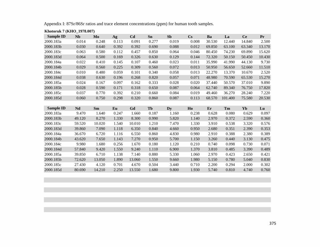
Appendix I: 87Sr/86Sr ratios and trace element concentrations (ppm) for human tooth samples.
Khotoruk 7 (KHO_1978.007)Sample ID Nb Mo Ag Cd Sn Sb Cs Ba La Ce Pr
2000.183a 0.014 0.248 0.113 0.091 0.277 0.019 0.008 30.530 12.440 14.840 2.5002000.183b 0.030 0.640 0.392 0.392 0.690 0.088 0.012 69.850 63.100 63.340 13.1702000.183c 0.063 0.580 0.112 0.457 0.850 0.064 0.046 80.450 74.230 69.890 15.6202000.183d 0.064 0.500 0.169 0.326 0.630 0.129 0.144 72.320 50.150 50.450 10.4302000.184a 0.022 0.410 0.145 0.107 0.460 0.023 0.011 35.990 41.990 44.130 9.7302000.184b 0.029 0.560 0.225 0.309 0.560 0.072 0.013 50.950 56.650 52.660 11.5102000.184c 0.010 0.480 0.059 0.101 0.340 0.058 0.013 22.270 13.370 10.670 2.5202000.184d 0.038 0.630 0.196 0.268 0.820 0.057 0.071 48.980 70.590 65.530 15.2702000.185a 0.024 0.167 0.097 0.162 0.333 0.028 0.020 37.440 50.570 37.010 9.8902000.185b 0.028 0.590 0.171 0.318 0.650 0.087 0.064 62.740 89.340 76.750 17.8202000.185c 0.037 0.770 0.392 0.210 0.660 0.084 0.019 49.460 36.270 28.240 7.2202000.185d 0.060 0.750 0.298 0.320 0.860 0.087 0.113 68.570 101.400 75.580 20.530
Sample ID Nd Sm Eu Gd Tb Dy Ho Er Tm Yb Lu2000.183a 9.470 1.640 0.247 1.660 0.187 1.160 0.238 0.628 0.080 0.629 0.0972000.183b 49.120 8.270 1.330 8.300 0.990 5.820 1.140 2.970 0.372 2.590 0.3602000.183c 59.520 10.020 1.540 10.010 1.210 7.470 1.330 3.910 0.538 3.320 0.5762000.183d 39.860 7.090 1.118 6.350 0.840 4.660 0.950 2.680 0.351 2.390 0.3532000.184a 36.670 6.720 1.116 6.550 0.860 4.830 0.980 2.910 0.388 2.380 0.3892000.184b 43.620 7.650 1.143 7.270 0.950 5.700 1.150 3.260 0.440 3.130 0.4752000.184c 9.980 1.680 0.256 1.670 0.180 1.120 0.210 0.740 0.098 0.730 0.0712000.184d 57.840 9.420 1.550 9.240 1.110 6.900 1.370 3.810 0.485 3.390 0.4892000.185a 39.850 6.710 1.138 7.140 0.880 5.330 1.060 2.970 0.423 2.650 0.4212000.185b 72.620 13.050 1.890 13.060 1.550 9.660 1.980 5.150 0.780 5.040 0.8302000.185c 27.430 4.120 0.701 4.670 0.504 3.440 0.710 2.200 0.294 2.000 0.3022000.185d 80.690 14.210 2.250 13.550 1.680 9.800 1.930 5.740 0.810 4.740 0.760
375

Appendix I: 87Sr/86Sr ratios and trace element concentrations (ppm) for human tooth samples.
Khotoruk 7 (KHO_1978.007)Sample ID Ta Au Tl Pb Th U
2000.183a 0.009 0.020 0.012 0.670 0.283 0.7202000.183b 0.030 0.096 0.035 3.020 1.170 1.6802000.183c 0.037 0.072 0.033 3.310 2.260 2.8002000.183d 0.023 0.085 0.025 3.020 1.130 2.1802000.184a 0.031 0.061 0.021 1.090 1.780 1.1902000.184b 0.029 0.092 0.021 1.750 1.130 2.0302000.184c 0.029 0.128 0.044 0.980 0.224 0.7702000.184d 0.040 0.088 0.020 2.800 1.510 1.7102000.185a 0.006 0.044 0.008 0.920 0.854 1.4602000.185b 0.049 0.124 0.032 4.700 2.320 2.5502000.185c 0.033 0.100 0.035 1.860 0.290 2.3802000.185d 0.041 0.089 0.046 4.780 2.320 2.760
376

Appendix I: 87Sr/86Sr ratios and trace element concentrations (ppm) for human tooth samples.
Khotoruk 4a-2 (KHO_1978.004.03)
Sample ID Tooth 87Sr/86Sr Li Na Al P Ca Ti V Cr Mn2000.187a M1 0.723371 0.480 2190.8 25.980 64760.3 219567.8 2.110 0.760 0.920 43.8802000.187b M1 0.721660 0.760 2651.6 23.440 102258.0 348025.5 2.070 1.590 1.310 71.6602000.187c M1 0.721904 0.590 2538.7 33.280 77719.3 270461.6 1.530 1.660 1.520 80.3202000.187d M1 0.726820 0.440 2611.4 6.520 66223.3 223152.9 0.550 0.410 1.450 34.9502000.188a M2 0.717408 0.530 2222.2 12.980 57352.9 208734.2 0.620 0.650 1.480 45.8902000.188b M2 0.717792 0.580 2560.3 22.390 80653.2 293560.3 2.780 1.560 2.630 65.4502000.188c M2 0.717142 1.060 3121.7 70.550 108443.0 390687.6 5.920 2.160 3.250 140.1702000.188d M2 0.717817 1.180 3771.2 139.800 142483.1 530905.3 16.510 4.220 6.180 167.470
Sample ID Fe Ni Co Cu Zn Ga As Rb Sr Y Zr2000.187a 107.310 1.110 0.158 0.470 257.140 0.267 0.285 0.118 63.730 2.180 0.3422000.187b 154.900 1.790 0.234 1.750 355.140 0.410 0.590 0.042 102.270 15.700 0.3672000.187c 144.020 1.240 0.283 0.370 212.400 0.146 0.470 0.145 69.770 3.600 0.1052000.187d 87.090 0.690 0.074 0.210 79.760 0.091 0.194 0.037 60.060 1.470 0.0192000.188a 79.940 0.540 0.178 0.360 179.330 0.131 0.176 0.027 73.080 0.780 0.0562000.188b 156.960 1.390 0.226 0.970 302.260 0.231 0.340 0.080 91.980 5.420 0.2192000.188c 273.800 2.440 0.298 1.330 416.010 0.322 0.520 0.086 124.450 31.700 0.7402000.188d 718.170 6.730 1.600 2.870 505.330 0.530 1.660 0.035 178.290 49.950 1.880
Sample ID Nb Mo Ag Cd Sn Sb Cs Ba La Ce Pr2000.187a 0.012 0.228 0.012 0.123 0.263 0.024 0.005 9.400 7.460 4.650 1.0382000.187b 0.022 0.310 0.068 0.215 0.309 0.024 0.010 25.460 50.610 17.890 6.2702000.187c 0.005 0.300 0.086 0.348 0.420 0.011 0.010 12.940 13.670 10.300 1.7302000.187d 0.015 0.147 0.021 0.045 0.227 0.015 0.008 9.520 5.950 3.880 0.8492000.188a 0.007 0.231 0.027 0.105 0.223 0.022 0.008 10.530 2.820 1.950 0.5222000.188b 0.013 0.290 0.050 0.199 0.340 0.033 0.013 19.220 18.020 9.520 2.4202000.188c 0.020 0.380 0.056 0.383 0.490 0.074 0.007 33.360 106.190 50.920 15.2202000.188d 0.013 0.470 0.087 0.550 0.530 0.071 0.013 51.490 181.610 84.850 22.130
377

Appendix I: 87Sr/86Sr ratios and trace element concentrations (ppm) for human tooth samples.
Khotoruk 4a-2 (KHO_1978.004.03)Sample ID Nd Sm Eu Gd Tb Dy Ho Er Tm Yb Lu
2000.187a 3.970 0.596 0.072 0.595 0.059 0.316 0.063 0.189 0.022 0.143 0.0322000.187b 22.660 3.140 0.503 3.130 0.373 2.160 0.390 1.050 0.145 1.040 0.1912000.187c 6.660 0.820 0.164 0.870 0.086 0.482 0.098 0.283 0.027 0.205 0.0362000.187d 2.930 0.504 0.044 0.323 0.046 0.201 0.046 0.125 0.015 0.096 0.0182000.188a 1.820 0.341 0.049 0.242 0.030 0.146 0.033 0.077 0.007 0.067 0.0092000.188b 8.160 1.120 0.165 1.110 0.110 0.604 0.120 0.374 0.048 0.270 0.0412000.188c 54.560 9.330 1.300 8.160 0.920 4.610 1.060 2.430 0.283 2.070 0.3412000.188d 80.850 11.060 1.590 11.070 1.080 6.320 1.290 3.760 0.496 2.860 0.546
Sample ID Ta Au Tl Pb Th U2000.187a 0.012 0.007 0.010 0.320 0.164 0.1242000.187b 0.022 0.047 0.019 0.600 0.680 0.4402000.187c 0.021 0.079 0.011 0.680 0.241 0.0682000.187d 0.003 0.051 0.007 0.660 0.207 0.0422000.188a 0.016 0.029 0.011 0.330 0.126 0.2322000.188b 0.025 0.065 0.015 0.810 0.222 0.4802000.188c 0.049 0.059 0.025 1.570 2.210 1.0602000.188d 0.034 0.060 0.014 3.030 2.300 2.150
378

Appendix I: 87Sr/86Sr ratios and trace element concentrations (ppm) for human tooth samples.
Khotoruk 2a (KHO_1977.002)
Sample ID Tooth 87Sr/86Sr Li Na Al P Ca Ti V Cr Mn2000.190a M1 0.723373 1.160 2847.1 392.970 92700.0 354301.9 33.570 1.720 4.490 75.4702000.190b M1 0.725763 1.320 3048.4 235.400 94930.5 365098.9 11.880 1.070 4.650 112.2902000.190c M1 0.727223 1.260 2881.1 294.140 95265.1 355155.1 16.070 1.470 3.410 172.8802000.190d M1 0.725699 1.050 2790.4 238.020 90470.2 336906.3 8.440 1.510 3.630 173.7902000.191a M2 0.718936 1.290 3445.5 47.310 123469.5 453858.0 8.630 2.110 4.860 57.3502000.191b M2 0.720439 1.160 2978.7 204.210 100254.3 365769.3 17.850 1.330 4.480 66.5702000.191c M2 0.719150 1.270 3577.4 80.650 133844.4 470907.5 6.920 1.890 5.210 97.5002000.191d M2 0.720119 0.560 2927.5 260.190 110047.8 408595.7 7.120 1.600 3.320 146.2502000.192a M3 0.717808 0.770 2862.8 46.430 80401.2 304202.3 1.870 0.840 2.660 84.3802000.192b M3 0.719647 1.160 2643.3 366.840 88942.8 338307.8 16.730 1.700 4.040 85.6402000.192c M3 0.717841 0.800 2703.6 59.300 93958.5 353675.0 5.050 1.380 2.810 140.6802000.192d M3 0.719041 1.170 2789.2 46.040 99774.0 385352.5 2.640 0.990 4.230 238.120
Sample ID Fe Ni Co Cu Zn Ga As Rb Sr Y Zr2000.190a 530.220 5.930 0.335 2.010 379.280 0.540 0.520 0.760 134.940 9.960 0.5202000.190b 411.690 3.750 0.325 1.090 402.750 0.460 0.590 0.230 139.310 3.320 0.3102000.190c 497.170 6.070 0.189 1.320 325.210 0.680 0.470 0.220 149.570 10.920 0.4322000.190d 412.490 5.520 0.220 1.720 331.230 0.410 0.340 0.178 138.010 16.450 0.5402000.191a 373.120 4.840 0.290 2.500 434.960 0.560 0.610 0.129 245.410 22.120 0.8002000.191b 441.760 4.740 0.420 1.290 454.970 0.268 0.260 0.610 142.880 7.450 0.2192000.191c 363.300 4.840 0.304 1.950 517.940 0.380 0.540 0.112 202.290 13.780 0.7302000.191d 473.890 4.910 0.251 1.020 472.690 0.520 0.810 0.100 163.420 14.900 0.5002000.192a 187.020 1.990 0.125 0.580 361.280 0.177 0.490 0.043 123.770 0.480 0.2482000.192b 704.260 6.600 0.370 1.360 497.750 0.390 0.390 0.670 124.360 3.650 0.5402000.192c 209.280 2.410 0.250 0.490 507.770 0.237 0.480 0.097 133.350 7.370 0.5102000.192d 177.160 1.550 0.121 0.760 521.870 0.287 0.670 0.076 134.410 7.290 0.580
379

Appendix I: 87Sr/86Sr ratios and trace element concentrations (ppm) for human tooth samples.
Khotoruk 2a (KHO_1977.002)Sample ID Nb Mo Ag Cd Sn Sb Cs Ba La Ce Pr
2000.190a 0.036 0.640 0.045 0.187 0.400 0.018 0.063 33.270 27.540 30.940 3.9202000.190b 0.014 1.150 0.084 0.210 0.420 0.036 0.013 34.730 10.470 12.130 1.6702000.190c 0.038 0.460 0.045 0.370 0.330 0.032 0.018 47.300 40.890 44.480 5.3002000.190d 0.031 0.540 0.036 0.383 0.440 0.051 0.012 44.940 54.840 62.690 7.5802000.191a 0.022 0.760 0.063 0.378 0.420 0.055 0.011 59.000 60.260 72.960 9.3402000.191b 0.040 0.410 0.060 0.318 0.274 0.040 0.043 29.800 19.300 22.630 3.0502000.191c 0.019 0.840 0.056 0.530 0.350 0.021 0.018 50.170 35.610 42.750 5.6302000.191d 0.007 0.840 0.100 0.520 0.330 0.030 0.015 51.760 42.150 50.510 6.7102000.192a 0.016 0.750 0.033 0.191 0.380 0.038 0.012 17.590 1.160 1.620 0.1632000.192b 0.034 0.760 0.050 0.175 0.360 0.022 0.045 26.230 10.280 12.680 1.5202000.192c 0.012 0.660 0.050 0.252 0.340 0.067 0.017 29.170 16.330 12.000 2.1802000.192d 0.036 0.810 0.052 0.550 0.470 0.053 0.012 25.210 16.540 10.710 2.190
Sample ID Nd Sm Eu Gd Tb Dy Ho Er Tm Yb Lu2000.190a 13.990 1.860 0.355 2.040 0.196 1.120 0.264 0.670 0.092 0.495 0.0942000.190b 6.050 1.160 0.147 0.763 0.081 0.510 0.099 0.191 0.027 0.169 0.0422000.190c 19.600 2.720 0.477 2.620 0.281 1.500 0.285 0.790 0.109 0.580 0.0972000.190d 29.150 4.020 0.666 4.150 0.457 2.400 0.540 1.250 0.184 1.120 0.2002000.191a 33.960 5.140 0.871 4.930 0.583 3.390 0.650 1.810 0.260 1.640 0.2612000.191b 11.800 1.810 0.238 1.690 0.187 1.050 0.228 0.630 0.093 0.570 0.0792000.191c 20.900 3.330 0.580 2.970 0.379 2.040 0.402 1.150 0.154 1.060 0.1782000.191d 25.410 3.800 0.497 3.720 0.374 2.020 0.426 1.230 0.155 0.990 0.1372000.192a 0.669 0.101 0.012 0.117 0.009 0.092 0.012 0.030 0.006 0.025 0.0112000.192b 5.440 0.940 0.148 0.800 0.087 0.528 0.120 0.365 0.029 0.257 0.0352000.192c 8.250 1.200 0.196 1.320 0.149 0.840 0.213 0.480 0.074 0.486 0.0752000.192d 7.770 1.060 0.194 1.180 0.128 0.820 0.187 0.492 0.061 0.416 0.072
380

Appendix I: 87Sr/86Sr ratios and trace element concentrations (ppm) for human tooth samples.
Khotoruk 2a (KHO_1977.002)Sample ID Ta Au Tl Pb Th U
2000.190a 0.035 0.072 0.029 1.690 1.080 0.3202000.190b 0.030 0.062 0.014 1.380 0.589 0.2722000.190c 0.023 0.047 0.019 1.440 0.529 0.6402000.190d 0.018 0.046 0.018 1.240 1.450 0.7202000.191a 0.023 0.046 0.015 1.500 3.130 1.2502000.191b 0.036 0.059 0.019 1.590 1.170 0.4102000.191c 0.015 0.039 0.014 1.940 2.400 0.8502000.191d 0.007 0.071 0.023 2.130 1.340 0.9302000.192a 0.017 0.059 0.004 0.650 0.055 0.3702000.192b 0.048 0.077 0.018 1.900 0.483 0.6202000.192c 0.013 0.055 0.015 1.340 0.423 0.5302000.192d 0.046 0.052 0.021 1.510 0.356 0.650
381

Appendix I: 87Sr/86Sr ratios and trace element concentrations (ppm) for human tooth samples.
Khotoruk 4 (KHO_1978.004.01)
Sample ID Tooth 87Sr/86Sr Li Na Al P Ca Ti V Cr Mn2000.194a M1 0.713782 0.730 2677.0 22.150 64596.3 247191.5 1.800 1.250 0.780 37.2202000.194b M1 0.713321 0.690 2986.0 29.870 92008.6 363581.7 1.640 1.460 1.430 46.6402000.194c M1 0.713642 0.820 2749.9 11.040 91324.2 363411.8 2.830 1.150 1.160 32.6502000.194d M1 0.714091 0.790 2939.0 16.520 104794.4 414540.0 1.880 1.190 2.130 29.4102000.195a M2 0.714575 1.220 2748.2 10.930 51230.7 199821.3 2.710 1.090 0.860 12.1102000.195b M2 0.713156 0.720 2275.0 25.750 56035.8 226573.2 4.120 1.130 2.070 10.5102000.195c M2 0.713464 0.740 2204.1 63.350 59659.8 233033.3 13.920 1.320 1.740 54.3402000.195d M2 0.714603 0.680 1984.0 71.150 55688.3 212125.7 5.430 1.220 2.340 10.6902000.197a M3 0.711040 0.240 2414.7 246.050 46749.7 165925.4 12.750 1.160 1.930 12.3802000.197b M3 0.712633 0.230 1998.9 85.170 59961.4 218344.5 1.120 1.560 2.320 58.0702000.197c M3 0.711337 0.260 2268.1 36.240 70467.3 259579.8 4.200 0.650 2.400 9.7902000.197d M3 0.712821 0.330 2036.6 267.950 73724.5 266445.6 39.400 1.570 1.520 19.210
Sample ID Fe Ni Co Cu Zn Ga As Rb Sr Y Zr2000.194a 127.430 1.280 0.112 0.650 205.360 0.234 0.232 0.090 107.800 5.440 0.2012000.194b 138.720 1.270 0.106 0.980 259.360 0.191 0.600 0.029 125.430 10.560 0.2382000.194c 111.280 0.330 0.260 0.720 309.110 0.174 0.330 0.075 113.000 15.920 0.1812000.194d 164.780 2.630 0.126 1.180 397.420 0.254 0.340 0.096 127.620 2.630 0.2122000.195a 151.420 2.820 0.242 1.970 51.650 0.116 0.480 0.105 91.090 0.258 0.1142000.195b 134.020 2.870 0.280 3.550 93.700 0.066 0.380 0.069 92.660 0.440 0.3682000.195c 197.250 4.670 4.530 3.550 140.070 0.284 0.600 0.210 79.730 1.340 0.4902000.195d 197.770 3.430 0.265 3.240 145.700 0.176 0.540 0.192 72.260 1.660 0.3372000.197a 258.140 2.450 0.210 0.940 126.090 0.420 0.124 0.089 152.620 3.410 0.3152000.197b 260.150 3.920 0.234 0.920 235.280 0.480 0.190 0.033 195.250 2.100 0.2972000.197c 150.110 0.480 0.068 0.650 278.520 0.340 0.250 0.050 149.750 10.630 0.4402000.197d 303.800 2.270 0.380 1.670 312.260 0.690 0.340 0.152 224.740 19.930 0.740
382

Appendix I: 87Sr/86Sr ratios and trace element concentrations (ppm) for human tooth samples.
Khotoruk 4 (KHO_1978.004.01)Sample ID Nb Mo Ag Cd Sn Sb Cs Ba La Ce Pr
2000.194a 0.012 0.165 0.047 0.150 0.291 0.017 0.007 12.170 16.030 8.700 2.2202000.194b 0.020 0.350 0.054 0.131 0.510 0.055 0.017 13.820 32.640 18.290 4.4202000.194c 0.014 0.250 0.071 0.104 0.360 0.062 0.016 17.090 42.500 13.830 6.1602000.194d 0.045 0.360 0.049 0.093 0.480 0.065 0.021 24.310 7.180 5.810 0.8922000.195a 0.001 0.192 0.031 0.065 0.242 0.065 0.010 19.500 1.120 2.040 0.1532000.195b 0.006 0.223 0.040 0.097 0.211 0.029 0.008 13.430 1.650 3.690 0.3282000.195c 0.008 0.142 0.034 0.080 0.220 0.121 0.020 17.240 3.960 10.770 0.8122000.195d 0.022 0.146 0.008 0.094 0.182 0.056 0.021 13.730 5.400 10.250 1.1282000.197a 0.013 0.350 0.031 0.091 0.143 0.013 0.008 23.630 0.689 2.610 0.2382000.197b 0.011 0.440 0.085 0.128 0.162 0.016 0.008 35.630 0.401 2.560 0.1222000.197c 0.011 0.300 0.022 0.130 0.340 0.054 0.009 29.440 1.290 5.560 0.3972000.197d 0.031 0.510 0.040 0.168 0.244 0.029 0.014 46.300 2.890 11.210 0.846
Sample ID Nd Sm Eu Gd Tb Dy Ho Er Tm Yb Lu2000.194a 8.060 1.290 0.199 1.310 0.132 0.758 0.154 0.470 0.057 0.299 0.0622000.194b 17.100 2.280 0.366 2.400 0.258 1.560 0.305 0.900 0.119 0.666 0.1292000.194c 24.120 3.600 0.583 3.710 0.444 2.570 0.475 1.310 0.166 1.260 0.1772000.194d 3.050 0.630 0.073 0.424 0.063 0.331 0.066 0.266 0.015 0.196 0.0472000.195a 0.623 0.109 0.011 0.096 0.011 0.081 0.011 0.032 0.005 0.017 0.0042000.195b 1.080 0.244 0.029 0.158 0.013 0.129 0.016 0.038 0.007 0.056 0.0112000.195c 2.720 0.560 0.053 0.410 0.059 0.218 0.062 0.162 0.016 0.126 0.0192000.195d 3.680 0.620 0.108 0.530 0.062 0.351 0.076 0.178 0.026 0.149 0.0272000.197a 1.160 0.283 0.110 0.415 0.046 0.393 0.102 0.286 0.044 0.286 0.0572000.197b 0.657 0.197 0.044 0.238 0.025 0.268 0.062 0.192 0.040 0.306 0.0562000.197c 2.160 0.550 0.221 1.010 0.148 1.260 0.312 1.090 0.143 1.080 0.1762000.197d 4.720 1.340 0.474 1.850 0.285 2.450 0.580 1.770 0.305 2.070 0.344
383

Appendix I: 87Sr/86Sr ratios and trace element concentrations (ppm) for human tooth samples.
Khotoruk 4 (KHO_1978.004.01)Sample ID Ta Au Tl Pb Th U
2000.194a 0.021 0.041 0.009 0.720 0.292 0.4602000.194b 0.040 0.094 0.022 0.710 0.366 0.4202000.194c 0.023 0.061 0.024 0.450 0.990 0.5802000.194d 0.027 0.028 0.024 0.530 0.232 0.7102000.195a 0.012 0.031 0.011 0.370 0.069 1.5002000.195b 0.015 0.049 0.009 0.450 0.211 1.8002000.195c 0.018 0.034 0.014 0.540 0.277 1.9402000.195d 0.011 0.000 0.007 0.390 0.274 1.7202000.197a 0.012 0.025 0.006 0.270 0.037 6.1002000.197b 0.014 0.021 0.005 0.400 0.011 7.2602000.197c 0.045 0.042 0.010 0.390 0.069 5.0602000.197d 0.037 0.010 0.009 0.900 0.204 7.620
384

Appendix I: 87Sr/86Sr ratios and trace element concentrations (ppm) for human tooth samples.
Shamanskii Mys 3 (SHM_1973.003)
Sample ID Tooth 87Sr/86Sr Li Na Al P Ca Ti V Cr Mn2000.198a M2 0.711119 0.400 2038.7 88.580 45429.8 159868.1 4.070 1.010 2.420 64.8902000.198b M2 0.711643 0.230 2082.0 58.960 57284.9 204495.4 6.550 0.780 1.320 62.8802000.198c M2 0.711696 0.380 2171.1 36.010 71613.4 257266.8 1.650 1.260 1.780 148.6502000.198d M2 0.711839 0.290 2045.7 190.940 75766.6 273416.6 11.540 1.800 2.250 159.2102000.199a M3 0.712498 0.136 2222.8 84.410 61689.8 202577.4 19.000 0.610 1.250 11.1702000.199b M3 0.711999 0.190 2350.0 102.570 68590.9 227266.2 3.510 0.650 1.330 14.6602000.199c M3 0.711851 0.240 1908.7 104.060 67768.0 227166.1 1.650 1.810 1.690 79.6402000.199d M3 0.711798 0.410 2257.5 108.570 82752.0 281345.8 11.010 2.180 2.130 57.270
Sample ID Fe Ni Co Cu Zn Ga As Rb Sr Y Zr2000.198a 196.220 3.180 0.420 1.070 139.870 0.460 0.103 0.165 154.530 3.290 0.2272000.198b 159.740 1.870 0.307 0.730 201.620 0.320 0.160 0.200 119.230 5.440 0.1452000.198c 143.450 1.490 0.204 0.720 298.090 0.530 0.168 0.185 178.070 22.220 0.3582000.198d 382.150 4.540 0.820 1.040 377.290 0.460 0.290 0.210 202.790 11.520 0.4072000.199a 206.650 2.170 0.201 0.510 269.770 0.208 0.138 0.104 103.490 2.340 0.1072000.199b 187.880 2.820 0.263 0.760 278.270 0.287 0.215 0.130 104.650 1.050 0.1362000.199c 282.680 3.180 0.167 1.300 278.270 0.440 0.162 0.059 228.950 2.270 0.4202000.199d 334.060 3.990 0.420 0.670 400.630 0.350 0.320 0.177 135.030 4.370 0.179
Sample ID Nb Mo Ag Cd Sn Sb Cs Ba La Ce Pr2000.198a 0.014 0.640 0.112 0.125 0.233 0.008 0.012 22.110 0.749 3.700 0.2482000.198b 0.014 0.690 0.047 0.122 0.201 0.036 0.007 22.420 1.560 6.060 0.3972000.198c 0.012 0.750 0.053 0.249 0.300 0.030 0.008 39.870 3.240 9.680 0.9542000.198d 0.034 0.690 0.064 0.163 0.350 0.009 0.012 36.120 1.860 5.500 0.6102000.199a 0.014 0.220 0.038 0.063 0.200 0.012 0.022 13.640 0.553 1.970 0.1642000.199b 0.018 0.350 0.047 0.077 0.239 0.034 0.024 12.880 0.243 1.430 0.1312000.199c 0.012 0.560 0.085 0.204 0.222 0.025 0.005 39.750 0.565 2.420 0.1642000.199d 0.055 1.470 0.021 0.129 0.224 0.019 0.031 23.950 1.060 5.980 0.342
385

Appendix I: 87Sr/86Sr ratios and trace element concentrations (ppm) for human tooth samples.
Shamanskii Mys 3 (SHM_1973.003)Sample ID Nd Sm Eu Gd Tb Dy Ho Er Tm Yb Lu
2000.198a 1.510 0.369 0.116 0.459 0.063 0.416 0.112 0.356 0.041 0.328 0.0442000.198b 2.400 0.650 0.187 0.850 0.120 0.970 0.220 0.630 0.097 0.652 0.0982000.198c 5.380 1.790 0.440 2.180 0.329 2.250 0.550 1.760 0.274 1.690 0.2932000.198d 3.310 0.850 0.260 1.350 0.197 1.340 0.334 1.080 0.145 1.030 0.1792000.199a 0.920 0.289 0.059 0.310 0.057 0.301 0.075 0.187 0.035 0.187 0.0342000.199b 0.476 0.167 0.057 0.123 0.014 0.163 0.028 0.116 0.021 0.096 0.0212000.199c 0.822 0.268 0.074 0.290 0.039 0.301 0.086 0.229 0.031 0.207 0.0332000.199d 1.790 0.720 0.160 0.590 0.092 0.600 0.125 0.448 0.057 0.347 0.064
Sample ID Ta Au Tl Pb Th U2000.198a 0.014 0.027 0.010 0.420 0.076 5.2602000.198b 0.014 0.010 0.009 0.520 0.059 2.0502000.198c 0.013 0.052 0.005 0.710 0.144 3.2002000.198d 0.020 0.039 0.014 0.600 0.107 6.9902000.199a 0.005 0.020 0.006 0.780 0.028 1.3202000.199b 0.018 0.012 0.015 0.390 0.020 1.5002000.199c 0.019 0.023 0.008 0.510 0.029 7.0702000.199d 0.030 0.020 0.012 1.030 0.076 2.580
386

Appendix I: 87Sr/86Sr ratios and trace element concentrations (ppm) for human tooth samples.
Shamanskii Mys 1 (SHM_1975.001)
Sample ID Tooth 87Sr/86Sr Li Na Al P Ca Ti V Cr Mn2000.201a M1 0.711689 0.138 1748.8 6.510 44537.4 181557.2 0.950 0.106 1.710 14.7402000.201b M1 0.710516 0.082 1393.7 22.830 44056.8 182432.8 1.540 0.247 0.830 25.9302000.201c M1 0.711827 0.108 1326.9 6.710 42215.0 165963.1 0.450 0.163 1.010 15.8402000.201d M1 0.713526 0.096 1818.1 23.190 58497.1 238454.7 3.170 0.479 1.340 12.3802000.202a M2 0.714667 0.124 1826.4 4.330 45632.3 181989.1 0.620 0.119 0.970 4.0302000.202b M2 0.713010 0.137 1733.9 50.700 55877.8 224581.5 0.980 0.599 1.180 13.1102000.202c M2 0.710841 0.204 2065.2 12.040 61100.2 257829.7 0.750 0.136 0.870 10.6302000.202d M2 0.717315 0.332 2621.9 13.710 80575.8 321736.3 0.700 0.153 1.490 13.5102000.203a M3 0.709939 0.180 826.980 18.040 19020.5 65208.6 0.696 0.337 1.030 24.1202000.203b M3 0.712945 0.155 1807.6 8.440 49757.5 186756.9 0.780 0.216 1.300 31.6902000.203c M3 0.712485 0.117 1285.4 13.990 44635.6 169894.6 1.160 0.425 1.460 12.1602000.203d M3 0.711714 0.175 2155.1 31.920 78038.0 298673.3 0.690 0.382 1.990 6.420
Sample ID Fe Ni Co Cu Zn Ga As Rb Sr Y Zr2000.201a 77.430 0.700 0.033 0.264 189.860 0.197 0.087 0.067 77.460 0.006 0.0122000.201b 113.040 1.240 0.598 0.750 212.020 0.248 0.098 0.046 141.480 0.513 0.0722000.201c 43.740 0.296 0.079 0.195 193.040 0.177 0.088 0.023 70.800 0.061 0.0242000.201d 88.250 0.410 0.148 0.277 334.160 0.267 0.126 0.040 115.920 0.640 0.0372000.202a 69.230 0.208 0.061 0.157 161.730 0.112 0.095 0.031 69.150 0.020 0.0172000.202b 160.030 1.480 0.180 0.619 202.490 0.294 0.153 0.013 179.100 0.885 0.1172000.202c 45.260 0.280 0.057 0.340 196.810 0.188 0.215 0.055 71.200 0.014 0.0312000.202d 80.010 0.370 0.176 0.248 333.940 0.079 0.161 0.126 102.290 0.208 0.0312000.203a 40.300 1.040 0.148 0.633 51.950 0.590 0.053 0.072 160.580 0.064 0.0742000.203b 59.690 0.507 0.095 0.484 219.340 0.323 0.116 0.053 112.660 0.104 0.0292000.203c 92.090 0.850 0.076 0.545 183.080 0.239 0.980 0.028 149.000 0.596 0.0982000.203d 93.130 0.345 0.158 0.290 382.420 0.195 0.128 0.037 157.390 0.266 0.054
387

Appendix I: 87Sr/86Sr ratios and trace element concentrations (ppm) for human tooth samples.
Shamanskii Mys 1 (SHM_1975.001)Sample ID Nb Mo Ag Cd Sn Sb Cs Ba La Ce Pr
2000.201a 0.008 0.069 0.123 0.032 0.174 0.011 0.003 10.040 0.003 0.030 0.0032000.201b 0.002 0.161 0.035 0.059 0.171 0.017 0.004 16.350 0.269 0.661 0.0472000.201c 0.016 0.048 0.024 0.060 0.176 0.013 0.012 13.160 0.058 0.169 0.0162000.201d 0.009 0.179 0.032 0.060 0.242 0.028 0.006 16.440 0.395 0.685 0.0802000.202a 0.010 0.103 0.083 0.032 0.176 0.008 0.006 10.380 0.025 0.123 0.0052000.202b 0.016 0.083 0.030 0.114 0.175 0.015 0.005 26.050 0.584 1.327 0.1262000.202c 0.006 0.105 0.011 0.114 0.237 0.039 0.006 17.090 0.017 0.103 0.0072000.202d 0.005 0.209 0.013 0.109 0.211 0.030 0.009 15.760 0.145 0.302 0.0202000.203a 0.002 0.066 0.225 0.044 0.052 0.010 0.005 49.150 0.057 0.159 0.0182000.203b 0.004 0.119 0.131 0.074 0.179 0.014 0.006 27.460 0.090 0.225 0.0232000.203c 0.013 0.090 0.010 0.056 0.125 0.018 0.005 22.580 0.375 0.827 0.0702000.203d 0.025 0.140 0.036 0.126 0.240 0.027 0.010 19.390 0.168 0.308 0.023
Sample ID2000.201a Nd Sm Eu Gd Tb Dy Ho Er Tm Yb Lu2000.201b 0.023 0.028 0.003 0.002 0.004 0.016 0.006 0.009 0.005 0.003 0.0032000.201c 0.181 0.077 0.008 0.058 0.007 0.053 0.012 0.037 0.012 0.045 0.0052000.201d 0.031 0.046 0.006 0.026 0.004 0.006 0.006 0.022 0.003 0.018 0.0082000.202a 0.345 0.096 0.014 0.076 0.011 0.097 0.024 0.049 0.014 0.049 0.0152000.202b 0.032 0.065 0.010 0.018 0.006 0.015 0.004 0.006 0.000 0.002 0.0052000.202c 0.569 0.081 0.054 0.136 0.019 0.129 0.024 0.067 0.018 0.091 0.0152000.202d 0.039 0.071 0.001 0.022 0.004 0.040 0.005 0.022 0.006 0.032 0.0072000.203a 0.092 0.077 0.013 0.036 0.007 0.031 0.014 0.022 0.011 0.032 0.0082000.203b 0.065 0.014 0.003 0.014 0.003 0.013 0.003 0.006 0.001 0.004 0.0012000.203c 0.077 0.040 0.007 0.012 0.003 0.012 0.005 0.011 0.004 0.001 0.0032000.203d 0.309 0.039 0.022 0.075 0.012 0.078 0.014 0.044 0.004 0.074 0.012
0.145 0.062 0.008 0.033 0.009 0.034 0.010 0.025 0.003 0.006 0.005
388

Appendix I: 87Sr/86Sr ratios and trace element concentrations (ppm) for human tooth samples.
Shamanskii Mys 1 (SHM_1975.001)Sample ID Ta Au Tl Pb Th U
2000.201a 0.013 0.020 0.008 0.237 0.001 0.1792000.201b 0.007 0.022 0.007 0.770 0.002 0.4952000.201c 0.001 0.014 0.011 0.204 0.003 0.2112000.201d 0.014 0.022 0.015 0.438 0.004 0.2962000.202a 0.008 0.027 0.008 0.167 0.000 0.1292000.202b 0.013 0.005 0.005 0.334 0.008 0.7512000.202c 0.000 0.081 0.020 0.123 0.011 0.0882000.202d 0.025 0.055 0.016 0.290 0.008 0.1982000.203a 0.003 0.003 0.002 0.146 0.009 1.9502000.203b 0.009 0.006 0.008 1.130 0.006 0.6432000.203c 0.008 0.004 0.004 0.393 0.005 0.7212000.203d 0.031 0.025 0.010 0.496 0.005 0.378
389

Appendix I: 87Sr/86Sr ratios and trace element concentrations (ppm) for human tooth samples.
Shamanskii Mys 2 (SHM_1972.002)
Sample ID Tooth 87Sr/86Sr Li Na Al P Ca Ti V Cr Mn2000.205a M1 0.712315 0.359 3531.8 27.990 80438.6 301196.4 0.650 0.192 2.070 58.1002000.205b M1 0.713115 0.530 3158.1 44.130 81465.3 302276.6 4.150 0.800 2.830 82.8702000.205c M1 0.713841 0.630 3889.9 2.370 93966.5 354750.6 1.190 0.600 1.810 51.1702000.205d M1 0.713268 0.800 3933.4 231.370 96913.5 370907.3 47.480 0.910 2.180 138.3502000.206a M2 0.712511 0.255 3250.0 28.520 62240.2 390760.4 1.590 0.591 1.640 59.5202000.206b M2 0.712215 0.286 2261.2 459.480 49716.6 314740.3 30.650 2.150 2.930 173.1702000.206c M2 0.713147 0.650 2849.9 52.650 93695.6 343659.7 2.050 0.398 1.820 62.3102000.206d M2 0.715585 0.450 2349.1 67.220 74477.8 267265.2 5.320 0.278 1.450 44.8702000.207a M3 0.712173 0.356 3054.8 92.470 71947.1 270371.3 4.660 0.476 1.910 74.3602000.207b M3 0.712752 0.280 2794.2 30.590 67696.2 255297.4 15.620 0.264 1.630 46.6202000.207c M3 0.712890 0.400 2883.0 11.950 90536.4 348457.4 2.970 0.232 2.450 56.2402000.207d M3 0.713795 0.360 2809.7 9.170 94294.9 365489.9 0.940 0.237 2.690 50.790
Sample ID Fe Ni Co Cu Zn Ga As Rb Sr Y Zr2000.205a 166.630 0.600 0.085 0.677 331.970 0.461 0.127 0.047 83.380 0.409 0.0362000.205b 231.330 1.480 0.109 0.626 383.990 0.590 0.155 0.267 79.830 0.424 0.0332000.205c 88.150 0.980 0.497 0.228 469.740 0.237 0.144 0.042 77.330 0.014 0.0002000.205d 332.070 4.640 0.138 1.200 559.940 0.632 0.204 0.226 91.450 1.920 0.1482000.206a 161.090 0.571 0.077 0.311 298.850 0.130 0.100 0.065 127.140 0.298 0.0652000.206b 862.980 9.410 0.587 2.790 279.520 0.780 0.110 0.546 125.680 8.620 0.2872000.206c 144.790 1.870 0.084 0.333 444.260 0.437 0.139 0.084 87.640 0.197 0.0132000.206d 104.310 1.010 0.186 0.163 322.000 0.294 0.127 0.075 79.340 0.599 0.0192000.207a 178.910 1.060 0.195 0.517 284.360 0.272 0.126 0.111 103.850 1.077 0.0752000.207b 131.450 0.510 0.094 0.650 294.310 0.268 0.104 0.089 83.910 0.626 0.0332000.207c 85.700 0.495 0.120 0.164 426.910 0.219 0.150 0.158 110.160 0.442 0.0402000.207d 94.580 0.450 0.249 0.230 345.550 0.254 0.147 0.028 118.110 0.318 0.048
390

Appendix I: 87Sr/86Sr ratios and trace element concentrations (ppm) for human tooth samples.
Shamanskii Mys 2 (SHM_1972.002)Sample ID Nb Mo Ag Cd Sn Sb Cs Ba La Ce Pr
2000.205a 0.005 0.356 0.032 0.041 0.279 0.007 0.006 20.180 0.133 0.327 0.0442000.205b 0.013 0.600 0.035 0.073 0.242 0.017 0.008 26.320 0.117 0.522 0.0352000.205c 0.012 0.660 0.030 0.096 0.372 0.016 0.005 18.500 0.008 0.315 0.0082000.205d 0.027 0.480 0.029 0.056 0.419 0.017 0.013 29.500 0.808 1.880 0.1802000.206a 0.018 0.680 0.028 0.046 0.441 0.014 0.009 19.980 0.132 0.583 0.0782000.206b 0.039 0.810 0.081 0.203 0.415 0.016 0.034 65.520 2.870 10.350 0.7072000.206c 0.005 0.400 0.034 0.055 0.385 0.009 0.010 22.530 0.066 0.317 0.0502000.206d 0.010 0.305 0.033 0.109 0.229 0.030 0.009 20.470 0.243 0.587 0.0542000.207a 0.008 0.374 0.023 0.064 0.231 0.007 0.006 17.720 0.335 1.346 0.0822000.207b 0.012 0.312 0.022 0.069 0.196 0.016 0.005 16.020 0.271 0.817 0.0582000.207c 0.004 0.670 0.030 0.071 0.337 0.010 0.007 17.630 0.154 0.494 0.0352000.207d 0.004 0.670 0.007 0.105 0.353 0.035 0.008 20.290 0.100 0.404 0.025
Sample ID Nd Sm Eu Gd Tb Dy Ho Er Tm Yb Lu2000.205a 0.220 0.087 0.023 0.111 0.013 0.096 0.013 0.040 0.007 0.041 0.0062000.205b 0.154 0.086 0.010 0.047 0.004 0.039 0.014 0.032 0.007 0.041 0.0052000.205c 0.022 0.049 0.017 0.019 0.005 0.032 0.007 0.017 0.004 0.000 0.0082000.205d 0.992 0.322 0.053 0.216 0.027 0.254 0.059 0.134 0.015 0.190 0.0132000.206a 0.108 0.071 0.008 0.036 0.007 0.025 0.007 0.030 0.006 0.039 0.0082000.206b 3.250 0.856 0.176 1.040 0.126 0.930 0.186 0.502 0.065 0.492 0.0732000.206c 0.044 0.063 0.010 0.052 0.013 0.036 0.008 0.014 0.008 0.022 0.0082000.206d 0.340 0.057 0.024 0.058 0.013 0.087 0.016 0.044 0.004 0.043 0.0052000.207a 0.382 0.094 0.042 0.140 0.020 0.145 0.027 0.097 0.009 0.095 0.0192000.207b 0.316 0.071 0.014 0.122 0.017 0.132 0.025 0.064 0.006 0.073 0.0092000.207c 0.143 0.088 0.010 0.084 0.011 0.062 0.012 0.030 0.006 0.026 0.0082000.207d 0.114 0.077 0.008 0.059 0.009 0.039 0.007 0.035 0.012 0.047 0.009
391

Appendix I: 87Sr/86Sr ratios and trace element concentrations (ppm) for human tooth samples.
Shamanskii Mys 2 (SHM_1972.002)Sample ID Ta Au Tl Pb Th U
2000.205a 0.006 0.016 0.011 0.416 0.013 0.0532000.205b 0.020 0.005 0.013 0.640 0.008 0.0422000.205c 0.022 0.035 0.014 0.317 0.004 0.0262000.205d 0.009 0.030 0.013 0.810 0.143 0.0322000.206a 0.023 0.041 0.015 0.850 0.008 0.0632000.206b 0.014 0.022 0.012 2.140 0.222 0.1872000.206c 0.015 0.023 0.014 0.506 0.005 0.0182000.206d 0.020 0.032 0.007 0.294 0.013 0.0152000.207a 0.022 0.020 0.007 0.489 0.040 0.0942000.207b 0.013 0.030 0.009 0.512 0.025 0.0522000.207c 0.002 0.003 0.012 0.527 0.019 0.0772000.207d 0.041 0.042 0.017 0.352 0.009 0.073
392

Appendix I: 87Sr/86Sr ratios and trace element concentrations (ppm) for human tooth samples.
Obkhoi 7 (OBK_1971.007)
Sample ID Tooth 87Sr/86Sr Li Na Al P Ca Ti V Cr Mn2000.209a molar 0.711363 0.680 2850.9 43.410 98511.1 356769.3 3.550 1.030 2.140 17.4902000.209b molar 0.709328 0.480 2199.9 14.350 88527.3 316319.9 0.670 0.268 1.460 39.0102000.209c molar 0.710761 0.660 2058.4 10.180 85852.0 307860.0 0.590 0.140 2.050 10.6402000.209d molar 0.711537 0.460 1949.3 12.130 76808.8 274096.0 0.510 0.064 1.600 4.8402000.210a molar 0.709441 0.730 2821.9 40.380 95798.7 355799.6 3.380 1.740 2.510 15.4402000.210b molar 0.709772 0.970 2998.5 47.580 129410.5 480788.5 3.590 3.150 3.200 34.5102000.210c molar 0.710054 0.740 2862.7 183.920 118503.3 426910.2 1.920 2.020 3.470 48.4902000.210d molar 0.711698 0.480 2049.4 12.480 79317.1 288461.8 0.730 0.096 1.880 3.140
Sample ID Fe Ni Co Cu Zn Ga As Rb Sr Y Zr2000.209a 191.220 2.030 0.150 0.290 625.190 1.370 0.267 0.103 128.220 3.910 0.2632000.209b 68.130 0.600 0.069 0.248 519.640 0.415 0.150 0.029 54.250 0.234 0.0362000.209c 103.530 0.870 0.050 0.084 474.070 0.224 0.126 0.170 48.200 0.044 0.0332000.209d 74.160 0.430 0.059 0.086 432.130 0.231 0.110 0.064 42.460 0.041 0.0092000.210a 248.770 1.590 0.156 0.527 513.990 0.830 0.395 0.245 142.750 7.090 0.4332000.210b 251.780 1.370 0.177 0.365 627.930 1.450 0.610 0.030 250.530 19.830 1.4502000.210c 367.050 2.450 0.304 0.588 793.320 1.470 0.690 0.131 244.570 2.780 0.4962000.210d 85.490 0.400 0.048 0.075 474.900 0.101 0.223 0.061 43.810 0.046 0.016
Sample ID Nb Mo Ag Cd Sn Sb Cs Ba La Ce Pr2000.209a 0.007 0.205 0.022 0.073 0.259 0.027 0.013 64.490 1.980 6.160 0.5372000.209b 0.004 0.208 0.024 0.040 0.256 0.025 0.006 21.850 0.158 0.651 0.0522000.209c 0.017 0.206 0.016 0.054 0.329 0.029 0.004 15.970 0.052 0.277 0.0132000.209d 0.014 0.283 0.035 0.085 0.255 0.032 0.008 14.650 0.020 0.102 0.0082000.210a 0.016 0.228 0.028 0.083 0.317 0.021 0.021 56.440 4.590 7.140 1.1172000.210b 0.010 0.420 0.049 0.107 0.388 0.034 0.009 108.230 13.070 18.620 2.9402000.210c 0.015 0.257 0.029 0.239 0.303 0.034 0.028 113.780 2.040 2.820 0.5202000.210d 0.003 0.203 0.008 0.048 0.264 0.008 0.004 8.080 0.044 0.215 0.021
393

Appendix I: 87Sr/86Sr ratios and trace element concentrations (ppm) for human tooth samples.
Obkhoi 7 (OBK_1971.007)Sample ID Nd Sm Eu Gd Tb Dy Ho Er Tm Yb Lu
2000.209a 2.370 0.467 0.160 0.492 0.089 0.500 0.110 0.308 0.041 0.295 0.0532000.209b 0.262 0.068 0.015 0.053 0.008 0.036 0.010 0.034 0.006 0.029 0.0032000.209c 0.043 0.060 0.010 0.014 0.004 0.055 0.006 0.014 0.002 0.027 0.0062000.209d 0.038 0.074 0.008 0.039 0.004 0.038 0.003 0.008 0.005 0.022 0.0052000.210a 4.910 0.931 0.285 1.120 0.139 0.866 0.190 0.547 0.061 0.434 0.0752000.210b 13.100 2.640 0.713 2.890 0.424 2.660 0.534 1.450 0.173 1.130 0.2012000.210c 2.210 0.373 0.093 0.429 0.054 0.351 0.076 0.216 0.023 0.166 0.0312000.210d 0.077 0.045 0.006 0.035 0.006 0.010 0.005 0.008 0.001 0.007 0.001
Sample ID Ta Au Tl Pb Th U2000.209a 0.014 0.029 0.007 0.990 0.063 0.0492000.209b 0.013 0.020 0.009 0.401 0.014 0.0042000.209c 0.025 0.022 0.011 0.276 0.010 0.0032000.209d 0.031 0.034 0.010 0.248 0.005 0.0032000.210a 0.017 0.039 0.009 0.840 0.066 0.0752000.210b 0.008 0.062 0.010 1.530 0.152 0.1652000.210c 0.009 0.026 0.006 1.520 0.015 0.2092000.210d 0.012 0.019 0.012 0.256 0.005 0.016
394

Appendix I: 87Sr/86Sr ratios and trace element concentrations (ppm) for human tooth samples.
Obkhoi 13 (OBK_1971.013)
Sample ID Tooth 87Sr/86Sr Li Na Al P Ca Ti V Cr Mn2000.212a M1 0.712875 0.530 2146.0 13.550 83873.3 299026.2 0.910 0.157 1.260 10.4202000.212b M1 0.711832 0.630 2060.6 25.620 78412.0 274310.0 1.990 0.238 1.230 5.2402000.212c M1 0.712782 0.240 1840.9 17.100 66325.3 233829.6 0.480 0.129 2.050 8.1402000.212d M1 0.714384 0.520 1895.0 9.000 76805.4 275634.5 1.850 0.105 1.330 4.2202000.213a M2 0.709524 0.640 2041.1 10.540 82711.2 290821.4 5.340 0.172 1.060 41.2502000.213b M2 0.711175 0.470 1826.7 3.070 74127.0 258163.2 0.710 0.185 1.560 9.0502000.213c M2 0.710063 0.420 1878.8 2.890 64317.1 222303.1 0.320 0.047 1.020 5.3302000.213d M2 0.709678 0.490 1704.6 0.936 67490.3 237886.6 0.210 0.042 1.170 2.9602000.214a M3 0.709459 0.303 2127.1 5.570 47891.2 271321.4 0.330 0.421 0.990 4.5102000.214b M3 0.711185 0.420 2351.0 58.760 75977.6 441322.8 3.630 0.830 1.890 17.3102000.214c M3 0.710882 0.440 2207.5 23.540 70385.1 415524.8 4.020 0.210 1.590 8.4702000.214d M3 0.711380 0.410 2006.9 44.220 62686.3 364301.8 5.120 0.655 1.840 9.620
Sample ID Fe Ni Co Cu Zn Ga As Rb Sr Y Zr2000.212a 76.870 0.840 0.074 0.121 465.170 0.314 0.121 0.248 53.870 0.021 0.0132000.212b 121.620 0.520 0.151 0.121 394.960 0.166 0.210 0.071 44.800 0.041 0.0102000.212c 98.390 0.340 0.015 0.050 328.730 0.191 0.205 0.093 33.550 0.106 0.0232000.212d 88.590 0.168 0.041 0.111 378.910 0.218 0.118 0.051 36.140 0.002 0.0162000.213a 81.390 0.224 0.042 0.161 424.820 0.356 0.116 0.044 55.390 0.474 0.0192000.213b 45.670 0.229 0.106 0.065 366.090 0.246 0.148 0.011 50.810 2.300 0.0322000.213c 46.710 0.131 0.020 0.064 205.540 0.154 0.149 0.021 38.540 0.122 0.0092000.213d 47.250 0.114 0.026 0.027 280.070 0.168 0.075 0.028 35.810 0.009 0.0212000.214a 78.470 0.158 0.045 0.192 271.360 0.216 0.080 0.018 76.320 0.014 0.0482000.214b 199.140 0.770 0.079 0.163 489.000 0.253 0.133 0.488 101.680 4.830 0.4162000.214c 128.360 0.405 0.053 0.086 438.530 0.139 0.159 0.075 76.700 2.880 0.1242000.214d 216.310 0.900 0.083 0.186 352.420 0.094 0.251 0.212 61.640 0.872 0.038
395

Appendix I: 87Sr/86Sr ratios and trace element concentrations (ppm) for human tooth samples.
Obkhoi 13 (OBK_1971.013)Sample ID Nb Mo Ag Cd Sn Sb Cs Ba La Ce Pr
2000.212a 0.014 0.148 0.025 0.055 0.280 0.000 0.013 15.740 0.018 0.105 0.0082000.212b 0.014 0.217 0.045 0.056 0.246 0.003 0.010 12.700 0.029 0.069 0.0062000.212c 0.007 0.090 0.026 0.041 0.199 0.249 0.004 10.630 0.011 0.037 0.0042000.212d 0.023 0.164 0.019 0.045 0.203 0.014 0.004 12.090 0.006 0.012 0.0052000.213a 0.008 0.234 0.021 0.046 0.234 0.022 0.006 20.070 0.250 0.224 0.0572000.213b 0.001 0.148 0.005 0.057 0.215 0.013 0.005 19.040 1.565 1.503 0.4552000.213c 0.010 0.170 0.010 0.032 0.168 0.020 0.005 12.160 0.093 0.095 0.0292000.213d 0.002 0.225 0.009 0.026 0.186 0.011 0.005 11.450 0.008 0.020 0.0322000.214a 0.006 0.163 0.013 0.056 0.330 0.011 0.003 41.270 0.005 0.045 0.0012000.214b 0.026 0.300 0.030 0.050 0.478 0.027 0.013 39.170 2.700 2.820 0.6202000.214c 0.013 0.250 0.023 0.079 0.457 0.020 0.007 20.230 1.516 1.500 0.4192000.214d 0.010 0.340 0.026 0.081 0.533 0.034 0.012 16.770 0.471 0.658 0.121
Sample ID Nd Sm Eu Gd Tb Dy Ho Er Tm Yb Lu2000.212a 0.026 0.014 0.004 0.023 0.005 0.023 0.005 0.014 0.006 0.022 0.0002000.212b 0.039 0.022 0.020 0.015 0.008 0.048 0.002 0.036 0.000 0.011 0.0012000.212c 0.016 0.040 0.007 0.030 0.000 0.010 0.003 0.010 0.004 0.015 0.0042000.212d 0.008 0.056 0.016 0.024 0.001 0.032 0.004 0.015 0.001 0.016 0.0012000.213a 0.328 0.087 0.018 0.091 0.011 0.067 0.007 0.026 0.005 0.029 0.0042000.213b 1.950 0.451 0.120 0.469 0.060 0.385 0.083 0.210 0.024 0.177 0.0232000.213c 0.124 0.026 0.009 0.024 0.004 0.030 0.004 0.012 0.004 0.013 0.0052000.213d 0.034 0.048 0.013 0.014 0.003 0.011 0.006 0.000 0.001 0.005 0.0012000.214a 0.011 0.028 0.004 0.007 0.003 0.025 0.003 0.004 0.003 0.002 0.0022000.214b 3.100 0.598 0.183 0.820 0.105 0.671 0.132 0.389 0.058 0.377 0.0452000.214c 1.780 0.384 0.082 0.621 0.068 0.398 0.084 0.232 0.026 0.145 0.0282000.214d 0.606 0.100 0.025 0.154 0.012 0.100 0.015 0.068 0.008 0.063 0.007
396

Appendix I: 87Sr/86Sr ratios and trace element concentrations (ppm) for human tooth samples.
Obkhoi 13 (OBK_1971.013)Sample ID Ta Au Tl Pb Th U
2000.212a 0.002 0.017 0.009 0.454 0.005 0.0052000.212b 0.000 0.008 0.025 0.207 0.009 0.0092000.212c 0.015 0.024 0.007 0.094 0.004 0.0012000.212d 0.006 0.026 0.011 0.469 0.005 0.0042000.213a 0.007 0.013 0.012 0.566 0.003 0.0082000.213b 0.015 0.016 0.008 0.330 0.032 0.0142000.213c 0.008 0.026 0.007 0.047 0.003 0.0032000.213d 0.009 0.020 0.006 0.075 0.002 0.0022000.214a 0.009 0.018 0.005 0.313 0.003 0.0472000.214b 0.026 0.042 0.012 0.670 0.066 0.0282000.214c 0.020 0.023 0.012 0.535 0.099 0.0242000.214d 0.016 0.036 0.008 0.560 0.018 0.018
397

Appendix I: 87Sr/86Sr ratios and trace element concentrations (ppm) for human tooth samples.
Obkhoi 5 (OBK_1971.005)
Sample ID Tooth 87Sr/86Sr Li Na Al P Ca Ti V Cr Mn2000.216a M1 0.709504 0.830 3340.2 52.380 118505.5 397861.2 1.030 1.220 3.050 61.2002000.216b M1 0.709900 0.670 2674.6 30.390 108568.1 377787.7 0.990 1.610 2.370 74.1202000.216c M1 0.708014 0.520 2860.2 7.700 82398.0 290781.9 1.370 0.445 2.300 25.8002000.217a M2 0.709923 0.620 2710.7 24.490 122607.2 401557.7 0.970 0.612 2.710 17.7102000.217b M2 0.709852 1.160 3654.0 126.390 210009.1 680475.9 4.130 4.090 5.600 77.4302000.217c M2 0.710532 0.820 3021.4 68.830 154187.2 505136.0 2.090 1.800 4.070 160.2002000.217d M2 0.710796 1.070 3692.7 97.010 193401.6 646066.3 3.810 4.080 5.770 60.0502000.218a M3 0.710495 0.500 3185.6 27.190 88862.9 305582.6 1.370 0.880 2.310 63.4102000.218b M3 0.709360 0.440 2465.3 39.230 105306.8 360225.9 1.000 1.010 3.120 172.3902000.218c M3 0.711193 0.580 2452.6 9.600 114225.5 388254.2 1.350 0.221 2.630 55.5502000.218d M3 0.710778 0.820 3173.7 62.880 138684.9 478541.6 12.950 1.600 3.990 317.070
Sample ID Fe Ni Co Cu Zn Ga As Rb Sr Y Zr2000.216a 168.550 0.990 0.152 0.155 672.690 0.990 0.540 0.111 138.560 5.470 0.6792000.216b 158.910 0.820 0.100 0.262 483.070 1.070 0.395 0.061 135.420 1.980 0.7142000.216c 95.640 0.970 0.212 0.342 230.340 0.301 0.201 0.088 61.160 1.170 0.0692000.217a 82.950 0.590 0.105 0.252 700.260 0.568 0.328 0.027 113.590 0.900 0.2362000.217b 355.980 4.190 0.329 0.700 1168.6 1.900 0.650 0.348 277.540 15.160 2.4102000.217c 189.910 1.090 0.140 0.218 784.520 0.740 0.340 0.070 135.230 11.300 0.8002000.217d 370.630 2.790 0.190 0.540 1269.8 1.660 0.780 0.190 257.260 18.560 2.7302000.218a 106.380 0.640 0.196 0.218 383.190 0.622 0.219 0.447 115.790 1.310 0.3782000.218b 112.940 0.960 0.129 0.131 570.270 0.740 0.154 0.029 114.530 1.770 0.6512000.218c 82.030 0.260 0.246 0.146 624.120 0.414 0.155 0.080 83.510 1.430 0.1512000.218d 198.500 4.710 0.354 0.860 783.770 1.260 0.240 0.760 134.180 15.180 0.800
Sample ID Nb Mo Ag Cd Sn Sb Cs Ba La Ce Pr2000.216a 0.013 0.117 0.034 0.075 0.275 0.020 0.013 61.600 3.920 5.160 0.8532000.216b 0.014 0.154 0.025 0.072 0.367 0.015 0.007 71.910 1.390 1.740 0.2732000.216c 0.023 0.191 0.021 0.371 0.219 0.016 0.006 25.800 0.974 1.053 0.1642000.217a 0.004 0.440 0.030 0.166 0.334 0.022 0.009 33.820 0.733 0.788 0.1592000.217b 0.009 0.670 0.027 0.181 0.502 0.054 0.014 117.390 10.930 14.250 2.8102000.217c 0.017 0.670 0.132 0.138 0.454 0.049 0.012 49.060 7.880 6.250 1.6602000.217d 0.024 0.720 0.020 0.149 0.563 0.053 0.007 111.470 13.150 13.570 3.100
398

Appendix I: 87Sr/86Sr ratios and trace element concentrations (ppm) for human tooth samples.
Sample ID Nb Mo Ag Cd Sn Sb Cs Ba La Ce Pr2000.218a 0.017 0.195 0.005 0.051 0.210 0.011 0.008 37.650 0.884 1.011 0.2082000.218b 0.023 0.168 0.009 0.131 0.293 0.011 0.007 48.520 1.033 0.840 0.2612000.218c 0.011 0.400 0.019 0.143 0.269 0.039 0.008 28.580 0.788 0.935 0.1302000.218d 0.037 0.210 0.013 0.266 0.412 0.047 0.010 61.800 11.270 9.470 2.570
Obkhoi 5 (OBK_1971.005)Sample ID Nd Sm Eu Gd Tb Dy Ho Er Tm Yb Lu
2000.216a 4.360 0.879 0.177 0.870 0.093 0.699 0.123 0.330 0.044 0.280 0.0542000.216b 1.223 0.148 0.055 0.248 0.030 0.169 0.043 0.104 0.016 0.094 0.0252000.216c 0.888 0.190 0.042 0.163 0.022 0.161 0.029 0.092 0.011 0.071 0.0172000.217a 0.567 0.150 0.038 0.167 0.023 0.067 0.025 0.059 0.006 0.072 0.0062000.217b 11.320 2.330 0.622 2.460 0.303 2.000 0.381 1.060 0.129 0.853 0.1332000.217c 7.770 1.460 0.324 1.610 0.189 1.300 0.265 0.732 0.100 0.591 0.0552000.217d 14.300 2.530 0.691 2.740 0.362 2.320 0.482 1.340 0.184 1.090 0.1702000.218a 0.953 0.123 0.050 0.153 0.030 0.144 0.035 0.075 0.015 0.068 0.0152000.218b 1.226 0.197 0.036 0.191 0.037 0.155 0.034 0.088 0.015 0.071 0.0142000.218c 0.567 0.152 0.033 0.181 0.012 0.203 0.023 0.092 0.012 0.070 0.0182000.218d 10.820 1.820 0.586 2.480 0.354 1.990 0.396 1.110 0.061 1.010 0.115
Sample ID Ta Au Tl Pb Th U2000.216a 0.016 0.013 0.008 1.210 0.062 0.0552000.216b 0.015 0.024 0.009 0.670 0.013 0.0582000.216c 0.009 0.012 0.009 0.770 0.008 0.0072000.217a 0.018 0.051 0.016 0.600 0.001 0.0382000.217b 0.036 0.041 0.009 3.210 0.111 0.1942000.217c 0.008 0.037 0.018 1.110 0.084 0.0762000.217d 0.038 0.085 0.017 2.540 0.158 0.1532000.218a 0.013 0.021 0.005 0.348 0.017 0.0442000.218b 0.011 0.029 0.009 0.550 0.011 0.0422000.218c 0.035 0.019 0.008 0.620 0.011 0.0152000.218d 0.031 0.050 0.019 7.610 0.066 0.094
399

Appendix I: 87Sr/86Sr ratios and trace element concentrations (ppm) for human tooth samples.
Borki 1 (BO1_1971.001)
Sample ID Tooth 87Sr/86Sr Li Na Al P Ca Ti V Cr Mn2000.220a M1 0.710598 0.283 2168.6 4.630 61993.1 206976.8 2.620 0.115 1.070 3.2102000.220b M1 0.711830 0.316 2155.2 21.110 76836.3 251260.2 0.640 0.107 1.180 12.9302000.220c M1 0.710561 0.640 1975.5 26.090 105507.9 351974.3 0.610 0.256 1.980 25.2802000.220d M1 0.710087 0.460 1854.5 24.610 98101.9 324719.1 1.130 0.304 2.240 9.6102000.221a M2 0.708861 0.440 1939.6 27.960 59741.1 200850.0 11.490 0.194 1.180 11.7902000.221b M2 0.709485 0.710 1675.7 76.690 82606.7 274413.3 7.270 0.382 2.320 25.9802000.221c M2 0.710564 0.500 1908.2 8.570 92643.0 302326.2 0.730 0.066 1.650 16.9402000.221d M2 0.711000 0.660 2094.3 87.530 112185.2 359749.1 1.150 0.536 2.670 251.6902000.222a M3 0.709804 0.450 2156.7 21.800 64023.1 208174.9 1.070 0.242 1.240 12.5202000.222b M3 0.709897 0.450 1796.2 17.160 76624.6 247250.8 0.800 0.340 1.030 24.5202000.222c M3 0.710381 0.490 2067.0 21.820 103410.3 327114.1 0.770 0.506 1.730 39.2302000.222d M3 0.710026 0.800 2431.4 242.240 138930.1 454872.2 3.340 2.510 3.830 149.500
Sample ID Fe Ni Co Cu Zn Ga As Rb Sr Y Zr2000.220a 37.940 0.163 0.022 0.068 266.650 0.135 0.070 0.068 41.900 0.079 0.0352000.220b 81.850 0.338 0.073 0.140 340.290 0.203 0.096 0.051 47.860 0.153 0.0392000.220c 130.330 0.780 0.100 0.205 533.190 0.216 0.132 0.137 51.870 0.065 0.0202000.220d 71.010 0.231 0.091 0.206 463.300 0.320 0.201 0.013 51.870 0.376 0.0832000.221a 71.530 0.568 0.319 0.086 298.140 0.209 0.072 0.102 58.340 0.243 0.0642000.221b 158.800 1.300 0.081 0.265 442.990 0.323 0.156 0.177 55.030 0.687 0.1212000.221c 61.490 0.860 0.051 0.114 466.390 0.066 0.108 0.078 49.820 0.022 0.0272000.221d 204.430 1.650 0.360 0.304 549.300 0.760 0.313 0.093 69.510 1.340 0.2712000.222a 56.860 0.530 0.223 0.325 273.580 0.245 0.156 0.023 63.570 0.515 0.1132000.222b 63.010 0.193 0.032 0.188 332.320 0.357 0.096 0.037 54.700 0.033 0.0332000.222c 87.730 0.770 0.082 0.221 525.550 0.488 0.179 0.024 60.350 0.232 0.1462000.222d 465.050 3.010 0.198 0.680 758.820 1.480 0.510 0.146 105.150 14.250 1.620
400

Appendix I: 87Sr/86Sr ratios and trace element concentrations (ppm) for human tooth samples.
Borki 1 (BO1_1971.001)Sample ID Nb Mo Ag Cd Sn Sb Cs Ba La Ce Pr
2000.220a 0.001 0.169 0.012 0.029 0.187 0.010 0.004 5.740 0.079 0.088 0.0292000.220b 0.008 0.166 0.010 0.039 0.168 0.011 0.003 8.030 0.104 0.117 0.0282000.220c 0.013 0.150 0.034 0.049 0.225 0.007 0.007 10.060 0.090 0.162 0.0242000.220d 0.013 0.160 0.009 0.077 0.298 0.018 0.006 21.350 0.290 0.192 0.0572000.221a 0.002 0.171 0.028 0.041 0.155 0.009 0.016 9.830 0.247 0.276 0.0652000.221b 0.013 0.284 0.010 0.040 0.181 0.035 0.011 15.000 0.629 0.685 0.2122000.221c 0.009 0.181 0.022 0.080 0.241 0.024 0.010 5.750 0.026 0.025 0.0092000.221d 0.010 0.251 0.026 0.092 0.289 0.019 0.007 35.650 1.010 0.748 0.2052000.222a 0.008 0.126 0.023 0.039 0.162 0.007 0.008 9.150 0.383 0.265 0.1012000.222b 0.005 0.186 0.026 0.030 0.184 0.033 0.003 12.070 0.060 0.149 0.0232000.222c 0.020 0.156 0.013 0.058 0.240 0.005 0.008 21.550 0.183 0.411 0.0382000.222d 0.006 0.202 0.059 0.366 0.376 0.045 0.007 60.900 11.620 5.360 2.660
Sample ID Nd Sm Eu Gd Tb Dy Ho Er Tm Yb Lu2000.220a 0.099 0.020 0.006 0.017 0.003 0.016 0.003 0.012 0.005 0.012 0.0032000.220b 0.102 0.039 0.009 0.025 0.003 0.019 0.007 0.018 0.003 0.010 0.0042000.220c 0.084 0.055 0.013 0.009 0.005 0.019 0.008 0.020 0.005 0.011 0.0122000.220d 0.285 0.065 0.010 0.047 0.007 0.033 0.009 0.024 0.010 0.020 0.0052000.221a 0.347 0.053 0.011 0.051 0.009 0.042 0.009 0.020 0.005 0.025 0.0052000.221b 0.796 0.119 0.045 0.150 0.022 0.121 0.023 0.063 0.010 0.057 0.0062000.221c 0.025 0.030 0.006 0.020 0.006 0.002 0.002 0.006 0.002 0.020 0.0042000.221d 0.891 0.162 0.046 0.214 0.025 0.136 0.030 0.076 0.009 0.055 0.0122000.222a 0.471 0.101 0.021 0.089 0.008 0.064 0.016 0.017 0.004 0.037 0.0042000.222b 0.088 0.024 0.014 0.019 0.002 0.011 0.010 0.021 0.001 0.016 0.0052000.222c 0.111 0.058 0.011 0.043 0.009 0.051 0.007 0.029 0.005 0.029 0.0072000.222d 11.850 2.200 0.542 2.600 0.301 1.870 0.412 1.070 0.110 0.805 0.117
401

Appendix I: 87Sr/86Sr ratios and trace element concentrations (ppm) for human tooth samples.
Borki 1 (BO1_1971.001)Sample ID Ta Au Tl Pb Th U
2000.220a 0.005 0.007 0.007 0.100 0.002 0.0022000.220b 0.001 0.025 0.006 0.228 0.007 0.0032000.220c 0.009 0.041 0.010 0.413 0.004 0.0042000.220d 0.011 0.032 0.007 0.340 0.011 0.0042000.221a 0.008 0.017 0.005 0.221 0.007 0.0032000.221b 0.025 0.023 0.005 0.540 0.022 0.0072000.221c 0.002 0.031 0.008 0.252 0.005 0.0032000.221d 0.016 0.036 0.012 0.590 0.013 0.0242000.222a 0.015 0.023 0.005 0.251 0.004 0.0072000.222b 0.000 0.002 0.007 0.231 0.003 0.0052000.222c 0.000 0.024 0.012 0.272 0.004 0.0142000.222d 0.030 0.058 0.007 1.820 0.048 0.072
402

Appendix I: 87Sr/86Sr ratios and trace element concentrations (ppm) for human tooth samples.
Manzurka 2 (MNZ_1971.002)
Sample ID Tooth 87Sr/86Sr Li Na Al P Ca Ti V Cr Mn2000.224a M1 0.708568 1.220 2430.7 22.680 94267.6 299136.5 2.400 1.010 1.990 24.9402000.224b M1 0.708408 0.850 2072.8 10.460 100297.5 317135.8 1.080 0.880 2.240 21.6702000.224c M1 0.708643 0.940 2260.0 34.040 121926.8 382940.2 2.850 1.470 3.030 42.9202000.224d M1 0.708674 1.000 2236.1 40.550 123656.6 391879.9 1.970 2.590 2.710 21.0002000.225a M2 0.708169 0.700 1787.4 2.680 90395.2 284858.9 0.420 0.232 1.330 3.9002000.225b M2 0.708771 1.150 2247.8 38.980 119743.5 377983.7 3.470 1.440 2.590 9.5702000.225c M2 0.708484 0.920 2273.6 19.500 132492.1 433754.3 4.850 2.810 3.490 20.5702000.225d M2 0.708840 1.220 2540.5 30.740 139916.2 459593.9 2.930 2.630 3.590 39.3802000.226a M3 0.709735 1.040 2134.4 12.160 89976.9 289955.3 1.220 0.604 2.030 10.8302000.226b M3 0.709468 1.120 2313.5 30.310 116964.4 381905.8 1.930 1.830 2.110 16.8202000.226c M3 0.709126 1.130 2446.8 26.470 133689.7 432516.4 3.070 1.960 2.940 43.0502000.226d M3 0.709445 0.930 1917.8 7.010 105454.6 328958.1 0.780 0.489 1.920 9.810
Sample ID Fe Ni Co Cu Zn Ga As Rb Sr Y Zr2000.224a 73.650 0.432 0.076 0.436 416.940 0.563 0.307 0.040 305.300 11.670 0.6112000.224b 63.990 0.480 0.042 0.420 487.830 0.499 0.312 0.099 327.850 16.380 0.4052000.224c 95.330 0.600 0.074 1.310 590.400 0.830 1.010 0.028 360.110 55.330 1.2402000.224d 107.420 0.840 0.047 1.070 576.450 0.800 0.540 0.033 345.690 37.110 1.0202000.225a 43.140 0.253 0.064 0.097 468.110 0.125 0.183 0.021 294.950 0.019 0.0472000.225b 189.180 1.400 0.082 0.371 598.990 0.780 0.510 0.126 443.380 14.520 0.7122000.225c 261.760 1.690 0.104 0.630 673.770 1.240 0.650 0.050 558.100 47.100 2.0602000.225d 254.480 2.070 0.178 0.421 700.060 1.080 0.700 0.037 592.840 37.740 1.7102000.226a 79.270 1.010 0.073 0.253 466.430 0.297 0.148 0.048 183.730 1.820 0.1472000.226b 209.740 0.920 0.060 0.403 659.540 0.600 0.500 0.115 242.390 24.990 0.9202000.226c 132.510 0.980 0.079 0.301 656.500 0.700 0.590 0.029 263.480 39.770 1.2002000.226d 56.680 0.159 0.048 0.093 623.890 0.226 0.126 0.016 184.250 6.600 0.162
403

Appendix I: 87Sr/86Sr ratios and trace element concentrations (ppm) for human tooth samples.
Manzurka 2 (MNZ_1971.002)Sample ID Nb Mo Ag Cd Sn Sb Cs Ba La Ce Pr
2000.224a 0.007 0.273 0.013 0.051 0.214 0.014 0.004 27.030 11.450 12.670 2.4402000.224b 0.003 0.390 0.013 0.055 0.184 0.023 0.002 26.990 14.740 16.340 3.6102000.224c 0.007 0.290 0.026 0.128 0.229 0.039 0.006 47.860 58.620 49.350 14.8302000.224d 0.004 0.420 0.037 0.079 0.221 0.025 0.007 50.290 39.710 39.160 9.5602000.225a 0.011 0.169 0.009 0.033 0.220 0.022 0.008 7.870 0.009 0.077 0.0082000.225b 0.015 0.240 0.037 0.088 0.210 0.025 0.007 39.120 14.230 19.370 3.1102000.225c 0.009 0.450 0.036 0.146 0.240 0.057 0.010 78.110 46.570 55.120 9.5402000.225d 0.014 0.330 0.025 0.151 0.244 0.023 0.007 66.750 36.500 44.500 8.0402000.226a 0.012 0.269 0.030 0.083 0.450 0.023 0.018 16.320 1.309 1.650 0.2672000.226b 0.018 0.620 0.045 0.121 0.162 0.024 0.008 39.550 22.510 25.140 4.9702000.226c 0.007 0.450 0.048 0.091 0.314 0.051 0.007 48.170 37.110 35.800 8.2002000.226d 0.013 0.370 0.033 0.056 0.185 0.031 0.006 16.570 5.640 5.280 1.268
Sample ID Nd Sm Eu Gd Tb Dy Ho Er Tm Yb Lu2000.224a 10.300 1.960 0.440 2.220 0.287 1.700 0.347 0.939 0.109 0.774 0.1182000.224b 14.820 2.880 0.707 3.150 0.424 2.650 0.524 1.420 0.179 1.190 0.1862000.224c 60.540 11.700 2.690 11.810 1.590 9.570 1.790 4.880 0.609 3.870 0.5262000.224d 39.610 7.430 1.800 7.560 1.002 6.140 1.170 3.150 0.407 2.610 0.3832000.225a 0.030 0.003 0.006 0.018 0.004 0.022 0.004 0.020 0.005 0.025 0.0052000.225b 12.780 2.500 0.559 2.700 0.352 2.330 0.444 1.160 0.175 1.030 0.1522000.225c 40.740 7.600 1.750 8.420 1.120 6.710 1.360 3.610 0.494 2.960 0.4762000.225d 34.010 6.870 1.500 6.760 0.936 5.820 1.110 3.100 0.387 2.390 0.4022000.226a 1.183 0.190 0.048 0.242 0.035 0.217 0.053 0.136 0.016 0.131 0.0212000.226b 21.140 4.160 0.944 4.400 0.565 3.630 0.778 2.070 0.234 1.720 0.2302000.226c 34.870 6.820 1.560 6.870 0.952 5.700 1.170 3.160 0.405 2.670 0.3792000.226d 5.630 1.120 0.259 1.140 0.182 0.825 0.189 0.479 0.065 0.513 0.066
404

Appendix I: 87Sr/86Sr ratios and trace element concentrations (ppm) for human tooth samples.
Manzurka 2 (MNZ_1971.002)Sample ID Ta Au Tl Pb Th U
2000.224a 0.008 0.019 0.006 1.790 0.315 0.0412000.224b 0.006 0.027 0.007 1.330 0.456 0.0352000.224c 0.018 0.013 0.008 3.750 2.850 0.1032000.224d 0.013 0.045 0.008 3.700 1.650 0.0862000.225a 0.012 0.002 0.004 0.399 0.006 0.0042000.225b 0.023 0.013 0.006 2.070 0.454 0.0682000.225c 0.031 0.030 0.010 4.710 1.560 0.1052000.225d 0.016 0.035 0.003 3.840 1.360 0.1192000.226a 0.029 0.002 0.009 0.640 0.018 0.0142000.226b 0.028 0.014 0.015 3.090 0.750 0.0562000.226c 0.036 0.019 0.015 3.280 1.080 0.1272000.226d 0.015 0.025 0.009 1.050 0.138 0.043
405