processes

Article

Study on the Nonlinear Dynamics of the ContinuousStirred Tank Reactors

Liangcheng Suo 1, Jiamin Ren 2, Zemeng Zhao 1 and Chi Zhai 2,*1 China Coal Energy Research Institute Co., Ltd., Xi’an 710054, China; suoliangc@chinacoal.com (L.S.);

hunter_zzm@163.com (Z.Z.)2 Faculty of Chemical Engineering, Kunming University of Science and Technology, Kunming 765000, China;

18761601966@163.com* Correspondence: zhaichi@kmust.edu.cn

Received: 23 September 2020; Accepted: 6 November 2020; Published: 10 November 2020 �����������������

Abstract: Chemical processes often exhibit nonlinear dynamics and tend to generate complex statetrajectories, which present challenging operational problems due to complexities such as outputmultiplicity, oscillation, and even chaos. For this reason, a complete knowledge of the static anddynamic nature of these behaviors is required to understand, to operate, to control, and to optimizecontinuous stirred tank reactors (CSTRs). Through nonlinear analysis, the possibility of outputmultiplicity, self-sustained oscillation, and torus dynamics are studied in this paper. Specifically,output multiplicity is investigated in a case-by-case basis, and related operation and control strategiesare discussed. Bifurcation analysis to identify different dynamic behaviors of a CSTR is alsoimplemented, where operational parameters are identified to obtain self-oscillatory dynamics andpossible unsteady-state operation strategy through designing the CSTR as self-sustained periodic.Finally, a discussion on codimension-1 bifurcations of limits cycles is also provided for the explorationof periodic forcing on self-oscillators. Through this synergistic study on the CSTRs, possible outputmultiplicity, oscillatory, and chaotic dynamics facilitates the implementation of novel operation/controlstrategies for the process industry.

Keywords: bifurcation analysis; process intensification; output multiplicity; torus dynamics

1. Introduction

It is well recognized that the natural world is complex, presenting an environment with chemicaland ecological networks that interact on a global scale. Elements of many such systems always exhibitnonlinear dynamics, and continuous stirred tank reactors (CSTRs) are typical process units that exhibitnonlinear dynamics, presenting challenging operational problems due to complex behavior such asoutput multiplicities, oscillations, and even chaos [1]. For this reason, a complete knowledge of thestatic and dynamic nature of these behaviors is required to understand, to operate, to control, and tooptimizea CSTR [2].

The presence of multiple steady states necessitates handy design of an efficient control system toregulate the operation states, and information about the transitions from state to state is critical [3].Challenges would also arise when it is desirable to operate CSTRs under open-loop unstable conditions,where the reaction rate may yield good productivity while the reactor temperature is proper to preventside reactions or catalyst degradation. Hence, it is important to consider the open/closed loop stabilityof the CSTRs, with analysis of output multiplicity providing practical guidelines for process designand operation.

Moreover, many studies show that CSTRs may exhibit a rich behavior in dynamic phenomena [4,5],with oscillation being the factor that has been subjected to intense research activity by both

Processes 2020, 8, 1436; doi:10.3390/pr8111436 www.mdpi.com/journal/processes

Processes 2020, 8, 1436 2 of 18

mathematicians and chemical engineers. The exploration of self-oscillatory CSTRs has evolvedinto two distinct dictions: one is the elimination of the oscillations and the other is to take advantageof the process dynamics for unsteady-state operation [6–8]. When the factor of time-evolution istaken into account, optimal design paradigm would extend beyond the conventional steady-stateoptimization, which offers opportunities for potential process improvement by periodic operation.

Oscillations may stem from fluctuations in input components or due to generation of instabilityin the CSTR itself. For the former, a matter of primary concern is whether perturbation on the inputparameters deliberately could outperform the steady operation. To address this point, nonlinearfrequency analysis through π-criterion [9], higher-order corrections of the π-criterion [10], Carlemanlinearization [11], Volterra series [12], and Laplace–Borel transform [13] has been implemented onthe CSTRs. Since an optimal scenario can be obtained by optimal periodic control (OPC) in termsof an oscillatory input profile, the problem of OPC is realized by using economic- model predictivecontrol (eMPC) [14], differential flatness [15], or extreme seeking [16]. For the latter, the route toself-sustained oscillations due to Hopf bifurcations has been studied from process intensificationperspectives, and analysis on τ-delayed Hopf bifurcations; detection of Hopf points and numericalsolution of the limit cycles have also been discussed.

Chaotic behavior could be generated through coupling of two oscillatory CSTRs or CSTRforced [17–19]. Bifurcation analysis studies dynamic complexities by using only steady-state informationof the CSTRs, and can be used not only to analyze the unforced system, but also to evaluate thedynamic changes when periodic forcing is introduced. Typical analytical tools include stroboscopicPoincaré maps and codimension-1 bifurcations of limit cycles [20], with the route to chaos throughperiod doubling (PD) and Neimark–Sacker (NS) bifurcations being commonly observable in the CSTRs.

It appears that there is a need for a comprehensive and synergistic study of the dynamics of CSTRs.In detail, output multiplicity, oscillation, and chaotic dynamics in CSTRs were investigated throughbifurcation analysis, and related topics on design, operation, and control of the CSTRs are discussed,which may facilitate the implementation of novel operation/control strategies for the process industry.

The remainder of the paper is arranged as follows. The CSTR model and classic stability analysisis briefed. Then, multiplicity, oscillation, and chaotic dynamics generated in CSTRs are analyzedconsecutively, where bifurcation analysis is conducted to identify the limit points, Hopf bifurcation,and NS bifurcation points. After that, the outcomes of forced inputs in chemical oscillators arecomputed and a critical guideline for unsteady state operation on chemical oscillators is presented.We finally offer concluding remarks.

2. Preliminaries

2.1. Model Formulation and Analysis

To investigate the dynamics of the lumped system, we introduce a simple first-order, irreversiblereaction A→B occurring at a jacket CSTR; the governing equations for mass and energy balance areprovided as follows:

V dCAdt = q(CA0 −CA) − kVCA

VρcpdTdt = qρcp(T f 0 − T) −Ua(T − T j) + (−∆H)kVCA

V jρ jcpjdT jdt = q jρ jcpj(T j0 − T j) + Ua(T − T j)

(1)

The jacket outlet temperature Tj represents the characteristic temperature of the jacket for heatconvection, and is assumed uniform in the jacket. This holds true when the jacket volume V is hugeand well mixed and the thermal inertia of the metal walls is considered negligible.

For analytical purposes, further simplification steps could be applied to make the CSTR modeltwo-dimensional, which is satisfied only when the dynamics related to the jacket temperature aremuch faster than that related to the reactor temperature. Then, the jacket temperature time constant is

Processes 2020, 8, 1436 3 of 18

negligible and Tj can be derived by setting the right-hand side of the third formula at Equation (1)to zero:

T j =q jρ jcpjT j0 + UaT

Ua + q jρ jcpj(2)

Substituting Equation (2) into Equation (1), and the dimensionless form of the model is given by

dZ1dt =

qV (1−Z1) − kZ1

dZ2dt =

qV (Z f 0 −Z2) −

UaKq j(Z2−Z j0)

Vρcp(1+Kq j)+ kZ1

whereZ1 = CA/CA0; Z2 = Tρcp/(−∆H)CAZ f 0 = T f 0ρcp/(−∆H)CA; Z j0 = T j0ρcp/(−∆H)CAK = ρ jcpj/Ua; k = k0 exp(−E/RT)

(3)

Setting the right-hand side of Equation (3) to zero obtains the equilibrium solutions: Z1 = q/(q + kV)

Z2 =q(1+Kq j)ρcp/(qZ f 0+kV+kVZ f 0)+q jKUaZ j0(q+kV)

(q(1+Kq j)ρcp+q jKUa)(q+kV)

(4)

Note that the solutions in Equation (4) may not be stable and stability analysis could be performedusing the Jacobian matrix of Equation (3), which is provided as follows:

J|(Z1,Z2) =

(a11 a12

a21 a22

)=

−q/V − k0

eEZj0/RTjZ2

−k0EZ1Z j0

RT jZ22eEZj0/RTjZ2

k0

eEZj0/RTjZ2

k0EZ1Z j0

RT jZ22eEZj0/RTjZ2−

KUaqccPρ(1+KUa)V

− q/V

(5)

Since all eigenvalues of Equation (5) need to be negative to meet the stability criterion,{a11a22 − a12a21 > 0a11 + a22 < 0

(6)

Other than the conditions prescribed in Equation (6), the CSTR is unstable. Singularity wouldcause complex dynamics to emerge, e.g., the necessary condition for self-oscillation, which is providedas follows: {

a11a22 − a12a21 > 0a11 + a22 = 0

(7)

However, a general analytical investigation of instabilities of the CSTR would be infeasible becausecomplexity of the terms in Equation (5). The presence of multiple solutions of a CSTR model indicatesthat each solution may have potentially different stability properties. One can expect that a multitudeof coexisting steady states with a diversity of stability properties could lead to a complex globalbehavior. Moreover, when the rigorous three-dimensional model is considered, the analysis could becomplicated further. Therefore, numerical bifurcation analysis is adopted to study the dynamics ofCSTRs in a case-by-case manner, and on the basis of the analysis, related design, operation, and controlissues are detailed.

2.2. Numerical Bifurcation Analysis Tools

For an effective illustration of the nonlinear dynamics in CSTRs, we sketch basics of bifurcationtheory in this section. Consider a lumped system represented by ordinary differential equations (ODEs)depending on a parameter vector α,

x′ = f (x,α) (8)

Processes 2020, 8, 1436 4 of 18

where f : Rn× R→Rn is smooth and nonlinear. The stability criterion is based on the equilibrium

manifold f (x) = 0 with given parameter vector α. Numerical bifurcation analysis is implementedthrough (1) draw equilibriu mcurves with variation ofα; a numerical continuation algorithm, e.g.,arch-length continuation, is available for solving such a problem; (2) detect bifurcation points alongwith these curves, where the qualitative or topological structure may change, leading the manifold toalso change significantly.

Limit point is correlative to the production of output multiplicity, which is identified as theJacobian matrix being singular:

A =

(∂ fi(α)∂x j

)∣∣∣∣∣∣i, j=1,2...,n

(9)

where as Hopf bifurcation emerges when a pair of pure imaginary eigenvalues are detected, and Hopfbifurcation is related to the production of self-oscillatory behavior. A Hopf point can be viewed asamplitude zero limit cycle, and periodic forcing of a self-oscillator can bifurcate out complex dynamictrajectories such as torus. Hence, codimension-1 bifurcation of limit cycles, i.e., Hopf bifurcation of thelimit cycles, is adopted to identify the generation of complex dynamics in CSTRs.

Stemming from the fact that a rich dynamic behavior is observed in CSTRs, which disturbs thegood development of the process, a complete knowledge of static and dynamic behavior is required tounderstand, to operate, to control, and to optimize the CSTRs. In the following sections, bifurcationanalysis is implemented on the CSTRs, and for this purpose, we propose the analysis strategy shownin Figure 1. On the basis of the analytics, we discuss topics on periodic operation and optimization ofthe processes.

Processes 20xx, x, x FOR PEER REVIEW 4 of 19

2.2. Numerical Bifurcation Analysis Tools

For an effective illustration of the nonlinear dynamics in CSTRs, we sketch basics of bifurcation theory in this section. Consider a lumped system represented by ordinary differential equations (ODEs) depending on a parameter vector α,

' ( , )x f x α= (8)

where f: Rn × R→Rn is smooth and nonlinear. The stability criterion is based on the equilibrium manifold f(x) = 0 with given parameter vector α. Numerical bifurcation analysis is implemented through (1) draw equilibriu mcurves with variation ofα; a numerical continuation algorithm, e.g., arch-length continuation, is available for solving such a problem; (2) detect bifurcation points along with these curves, where the qualitative or topological structure may change, leading the manifold to also change significantly.

Limit point is correlative to the production of output multiplicity, which is identified as the Jacobian matrix being singular:

, 1,2...,

( )= i

j i j n

fAxα

=

∂ ∂

(9)

where as Hopf bifurcation emerges when a pair of pure imaginary eigenvalues are detected, and Hopf bifurcation is related to the production of self-oscillatory behavior. A Hopf point can be viewed as amplitude zero limit cycle, and periodic forcing of a self-oscillator can bifurcate out complex dynamic trajectories such as torus. Hence, codimension-1 bifurcation of limit cycles, i.e., Hopf bifurcation of the limit cycles, is adopted to identify the generation of complex dynamics in CSTRs.

Stemming from the fact that a rich dynamic behavior is observed in CSTRs, which disturbs the good development of the process, a complete knowledge of static and dynamic behavior is required to understand, to operate, to control, and to optimize the CSTRs. In the following sections, bifurcation analysis is implemented on the CSTRs, and for this purpose, we propose the analysis strategy shown in Figure 1. On the basis of the analytics, we discuss topics on periodic operation and optimization of the processes.

f(x·α)=0

CSTR Processes

Establish dynamic models

modeling

Numerical bifurcation analysis

Periodic operationStable control

Equilibria Limit cycles

Limit point

Branch point

Output multiplicity

Saddle node

Hopf bifurcation

NS bifurcation PD bifurcation

Generation of chaos(periodic forcing of a limit cycle)

Generation of oscillations

Figure 1. Schematic of the strategy for analyzing continuous stirred tank reactor (CSTR) dynamic behaviors. Figure 1. Schematic of the strategy for analyzing continuous stirred tank reactor (CSTR)dynamic behaviors.

3. Control of Output Multiplicity

One interesting feature of nonlinear systems is their multiplicity behavior. For the case of inputmultiplicity [21], different feed flow rate q may lead to the same outcomes, which will affect CSTR

Processes 2020, 8, 1436 5 of 18

control strategy because the “zero dynamics” are unstable. Hence, CSTRs are generally not controlledusing q as the manipulate variable, and to attenuate the disturbances of q, feedward control is frequentlyapplied. Output multiplicity in the CSTR is because the curve of generated heat and the line of removedheat versus temperature can intersect with multiple points.

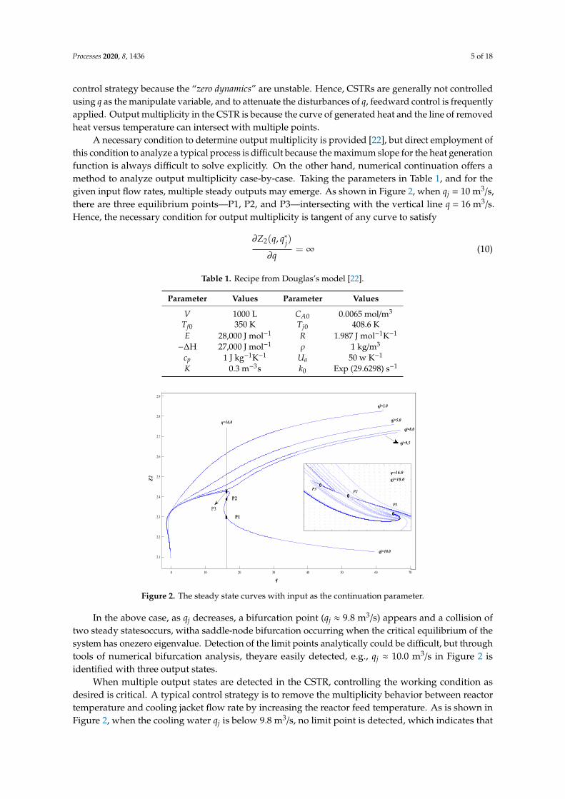
A necessary condition to determine output multiplicity is provided [22], but direct employment ofthis condition to analyze a typical process is difficult because the maximum slope for the heat generationfunction is always difficult to solve explicitly. On the other hand, numerical continuation offers amethod to analyze output multiplicity case-by-case. Taking the parameters in Table 1, and for thegiven input flow rates, multiple steady outputs may emerge. As shown in Figure 2, when qj = 10 m3/s,there are three equilibrium points—P1, P2, and P3—intersecting with the vertical line q = 16 m3/s.Hence, the necessary condition for output multiplicity is tangent of any curve to satisfy

∂Z2(q, q∗j)

∂q= ∞ (10)

Table 1. Recipe from Douglas’s model [22].

Parameter Values Parameter Values

V 1000 L CA0 0.0065 mol/m3

Tf0 350 K Tj0 408.6 KE 28,000 J mol−1 R 1.987 J mol−1K−1

−∆H 27,000 J mol−1 ρ 1 kg/m3

cp 1 J kg−1K−1 Ua 50 w K−1

K 0.3 m−3s k0 Exp (29.6298) s−1

Processes 20xx, x, x FOR PEER REVIEW 5 of 19

3. Control of Output Multiplicity

One interesting feature of nonlinear systems is their multiplicity behavior. For the case of input multiplicity [21], different feed flow rate q may lead to the same outcomes, which will affect CSTR control strategy because the “zero dynamics” are unstable. Hence, CSTRs are generally not controlled using q as the manipulate variable, and to attenuate the disturbances of q, feedward control is frequently applied. Output multiplicity in the CSTR is because the curve of generated heat and the line of removed heat versus temperature can intersect with multiple points.

A necessary condition to determine output multiplicity is provided [22], but direct employment of this condition to analyze a typical process is difficult because the maximum slope for the heat generation function is always difficult to solve explicitly. On the other hand, numerical continuation offers a method to analyze output multiplicity case-by-case. Taking the parameters in Table 1, and for the given input flow rates, multiple steady outputs may emerge. As shown in Figure 2, when qj = 10 m3/s, there are three equilibrium points—P1, P2, and P3—intersecting with the vertical line q = 16 m3/s. Hence, the necessary condition for output multiplicity is tangent of any curve to satisfy

*2 ( , )jZ q qq

∂= ∞

∂ (10)

Figure 2. The steady state curves with input as the continuation parameter.

In the above case, as qj decreases, a bifurcation point (qj ≈ 9.8 m3/s) appears and a collision of two steady statesoccurs, witha saddle-node bifurcation occurring when the critical equilibrium of the system has onezero eigenvalue. Detection of the limit points analytically could be difficult, but through tools of numerical bifurcation analysis, theyare easily detected, e.g., qj ≈ 10.0 m3/s in Figure 2 is identified with three output states.

Table 1. Recipe from Douglas’s model [22].

Parameter Values Parameter ValuesV 1000 L CA0 0.0065 mol/m3 Tf0 350 K Tj0 408.6 K E 28,000 J mol−1 R 1.987 J mol−1K−1 −ΔH 27,000 J mol−1 ρ 1 kg/m3

cp 1 J kg−1K−1 Ua 50 w K−1

K 0.3 m−3s k0 Exp (29.6298) s−1

0 10 20 30 40 50 60 70

2.1

2.2

2.3

2.4

2.5

2.6

2.7

2.8

2.9

q

Z2

qj=10.0

qj=9.5

qj=8.0

qj=5.0

qj=3.0

q=16.0

P2

P1P3

P1

P2P3

q=16.0qj=10.0

Figure 2. The steady state curves with input as the continuation parameter.

In the above case, as qj decreases, a bifurcation point (qj ≈ 9.8 m3/s) appears and a collision oftwo steady statesoccurs, witha saddle-node bifurcation occurring when the critical equilibrium of thesystem has onezero eigenvalue. Detection of the limit points analytically could be difficult, but throughtools of numerical bifurcation analysis, theyare easily detected, e.g., qj ≈ 10.0 m3/s in Figure 2 isidentified with three output states.

When multiple output states are detected in the CSTR, controlling the working condition asdesired is critical. A typical control strategy is to remove the multiplicity behavior between reactortemperature and cooling jacket flow rate by increasing the reactor feed temperature. As is shown inFigure 2, when the cooling water qj is below 9.8 m3/s, no limit point is detected, which indicates that

Processes 2020, 8, 1436 6 of 18

no output multiplicity is generated. However, the dynamics may offer more information than thetraditional steady state control. From the phase plot (qj = 10 m3/sand q = 16 m3/s), the convergent ridge(red arrow) of P2 separates the whole (Z1, Z2) domain into opposite trajectory directions, where theleft-bottom zone is attracted to P1 point, but not all the initial points from the top-right zone convergesto the P3 point because the red arrow almost crosses the P3 point. The stale zone that is attracted to P3point is limited, and one can identify P3 stable criterion by the following equation:

∂z2(q, q∗j)

∂q< 0 as (z1, z2) around P3 (11)

From Figure 3, the condition satisfying Equation (11) obtains a very small stable window, and thereis a high possibility to converge at the P1 point. When q = 16 m3/s and holds constant, qj shifts across9.8 m3/s (the limit point) can realize operation change between P1 and P3, approximately. Different qjwould lead to different steady state, and the industry may expect different operational states at specificcircumstances, i.e., failure to control the reactor properly would restrain it at P1, which has a lowerconversion rate thanP3.Therefore, the following split-ranging control strategy shown in Figure 4 isadopted—at the start-up stage, steam valve B is opened to heat the reactor to around the P3 point.When the reaction heat is released, valve B is gradually closed and valve A is opened to remove thereaction heat, while at the shutdown stage, more heat is removed to force the working point to shift toP1. Therefore, on the basis of the phase dynamics, the CSTR operation/control could work at multiplestates for different production load specification.

Processes 20xx, x, x FOR PEER REVIEW 6 of 19

When multiple output states are detected in the CSTR, controlling the working condition as desired is critical. A typical control strategy is to remove the multiplicity behavior between reactor temperature and cooling jacket flow rate by increasing the reactor feed temperature. As is shown in Figure 2, when the cooling water qj is below 9.8 m3/s, no limit point is detected, which indicates that no output multiplicity is generated. However, the dynamics may offer more information than the traditional steady state control. From the phase plot (qj = 10 m3/sand q = 16 m3/s), the convergent ridge (red arrow) of P2 separates the whole (Z1, Z2) domain into opposite trajectory directions, where the left-bottom zone is attracted to P1 point, but not all the initial points from the top-right zone converges to the P3 point because the red arrow almost crosses the P3 point. The stale zone that is attracted to P3 point is limited, and one can identify P3 stable criterion by the following equation:

*2 ( , )

0 ( 1, 2) P3jz q qas z z around

q∂

<∂

(11)

From Figure 3, the condition satisfying Equation (11) obtains a very small stable window, and there is a high possibility to converge at the P1 point. When q = 16 m3/s and holds constant, qj shifts across 9.8 m3/s (the limit point) can realize operation change between P1 and P3, approximately. Different qj would lead to different steady state, and the industry may expect different operational states at specific circumstances, i.e., failure to control the reactor properly would restrain it at P1, which has a lower conversion rate thanP3.Therefore, the following split-ranging control strategy shown in Figure 4 is adopted—at the start-up stage, steam valve B is opened to heat the reactor to around the P3 point. When the reaction heat is released, valve B is gradually closed and valve A is opened to remove the reaction heat, while at the shutdown stage, more heat is removed to force the working point to shift to P1. Therefore, on the basis of the phase dynamics, the CSTR operation/control could work at multiple states for different production load specification.

Figure 3. The phase plot for output multiplicity, where qj = 10m3/sand q = 16 m3/s.

0.3 0.4 0.5 0.6 0.7 0.8

2.25

2.3

2.35

2.4

2.45

2.5

Z1

Z2

P1

P2P3

q=16.0qj=10.0

Figure 3. The phase plot for output multiplicity, where qj = 10m3/sand q = 16 m3/s.

Processes 20xx, x, x FOR PEER REVIEW 6 of 19

When multiple output states are detected in the CSTR, controlling the working condition as desired is critical. A typical control strategy is to remove the multiplicity behavior between reactor temperature and cooling jacket flow rate by increasing the reactor feed temperature. As is shown in Figure 2, when the cooling water qj is below 9.8 m3/s, no limit point is detected, which indicates that no output multiplicity is generated. However, the dynamics may offer more information than the traditional steady state control. From the phase plot (qj = 10 m3/sand q = 16 m3/s), the convergent ridge (red arrow) of P2 separates the whole (Z1, Z2) domain into opposite trajectory directions, where the left-bottom zone is attracted to P1 point, but not all the initial points from the top-right zone converges to the P3 point because the red arrow almost crosses the P3 point. The stale zone that is attracted to P3 point is limited, and one can identify P3 stable criterion by the following equation:

*2 ( , )

0 ( 1, 2) P3jz q qas z z around

q∂

<∂

(11)

From Figure 3, the condition satisfying Equation (11) obtains a very small stable window, and there is a high possibility to converge at the P1 point. When q = 16 m3/s and holds constant, qj shifts across 9.8 m3/s (the limit point) can realize operation change between P1 and P3, approximately. Different qj would lead to different steady state, and the industry may expect different operational states at specific circumstances, i.e., failure to control the reactor properly would restrain it at P1, which has a lower conversion rate thanP3.Therefore, the following split-ranging control strategy shown in Figure 4 is adopted—at the start-up stage, steam valve B is opened to heat the reactor to around the P3 point. When the reaction heat is released, valve B is gradually closed and valve A is opened to remove the reaction heat, while at the shutdown stage, more heat is removed to force the working point to shift to P1. Therefore, on the basis of the phase dynamics, the CSTR operation/control could work at multiple states for different production load specification.

Figure 3. The phase plot for output multiplicity, where qj = 10m3/sand q = 16 m3/s.

0.3 0.4 0.5 0.6 0.7 0.8

2.25

2.3

2.35

2.4

2.45

2.5

Z1

Z2

P1

P2P3

q=16.0qj=10.0

Figure 4. The control schematic of the exothermic reactor working at the P3 point.

Processes 2020, 8, 1436 7 of 18

4. Unsteady State Operation through Periodic Disturbance

4.1. Periodic Exciting of the Inputs

Conventionally, a process is designed and operated at a desired steady state, and oscillations aretaken as disturbances, which are not desirable; thus, attempts have been made to eliminate sourcesof variation by modifying process design specifications to ensure stability, or by adding a controlsystem or a surge tank [23–28]. Recently, topics about designing for periodic operation began toresonate within the process systems engineering community, and nonlinearity of process systems mayallow for τ-time averaged performance enhancement with periodic forcing of external parameters.The operation of CSTRs with time-varying feed conditions is an appealing prospect for the industrydue to its relative ease in implementation. One can expect an optimal periodic operation problem thataims to maximize a scalar objective function as follows:

J = 1τ

∫ τ0 g(x,u)dt

s.t. x′ = f (x,u); x(0) = x(τ)(12)

where g(x, u) is the performance index, such as the profit. Let there be a stable state x0 for a stationaryinput u0, and the corresponding scalar objective function is J0, which is equal to g(x0, u0). Set the inputin the form of

u = u0 + δu (13)

where δu represents any continuous zero-mean τ-period perturbation vector, and the time-averagedobjective function is given as J. If J > J0, then, the forced periodic operation performance surpasses thatof the stationary operation. Essentially, the input perturbation δu, the dynamic system Equation (8),and the performance index g(x,u) all together determine performance of the periodic operation.

The case introduced is the cascade-parallel reaction occurring in the adiabatic CSTR; industrialinterest is to maximize the intermediate P, as well as to minimize the by-production R. The reactionkinetics is presented as follows:

A + B→ P, r1 = k1CACB

B + P→ R, r2 = k2CBCP(14)

Assume the reaction volume is constant dV/dt = 0, the lumped model is provided as follows:V dCA

dt = qACAF − (qA + qB)CA −Vk1CACB

V dCBdt = qBCBF − (qA + qB)CB −Vk1CACB −Vk2CBCP

V dCPdt = −(qA + qB)CP + Vk1CACB −Vk2CBCP

V dCRdt = −(qA + qB)CR + Vk2CBCP

(15)

where the flow rate is q, the concentration is C, and the subscript F represents the input condition.The objective is to maximize P production, but the separation cost of by-product R and reactants cost Aand B are also taken into account, which are scaled by σ, σ1, and σ2, respectively.

J =1τ

∫ τ

0[(qA + qB)(CP − σCR) − σ1qACAF − σ2qBCBF]dt (16)

The steady state performance is correlative to the extent of the reaction, ηi = riV (i = 1,2).The corresponding objective J0 can be given as follows, where θB is the mole ratio of B to A:

J0 = η1 − (w + 1)η2 − FA0(w1 + w2θB)

where :

η2 =k2η

21/k1

1/(qACAF)+(ζ+1)η1

(17)

Processes 2020, 8, 1436 8 of 18

When the design specifications σ, σ1, σ2, qACAF, and qBCBF are held constant, the steady stateoperational problem becomes maximizing J0 (criterion: ∂J0/∂x = 0, ∂2J0/∂x2 < 0), which is providedas follows:

J0(max) = 1/(√

1 + σ(k2/k1) +√(k2/k1) + σ(k2/k1))

2(18)

Set σ = 0, k2/k1 = 0.1, θB = 1/0.82, qA/V = 0.1, and k1 = 1 [29], then, the optimal outputs areCA0 = 0.3270, CB0 = 1.238, CP0 = 0.2083.

From an unsteady state operation viewpoint, one may inspect the overall performance if the inputconcentration CA and CB are excited by, say, cosine disturbances,

δCAF =(

11−iω1x0

+ 11+iω1x0

)Am1

δCBF =(

11−i(ω2+θ)x0

+ 11−i(ω2+θ)x0

)Am2

(19)

where i2 = −1, ω is the angular frequency, θ is the phase shift between two cosine disturbances, and Amis the amplitude. Therefore, the optimal periodic operation problem is to find proper ω and Am suchthat the τ-average objective function Equation (15) is maximized. Through Laplace–Borel [13] transformanalysis, relation of the output concentrations with varying parameters are presented as follows:

δCA =A2

m20.004438(0.1128+θ2+2θω+ω2)

[(ω+θ)2+0.17962][(ω+θ)2+0.7152][(ω+θ)2+0.31392]

+A2

m1(0.001329ω2)

0.001624+0.07ω2+0.642ω4+ω6

δCB =A2

m20.006149(0.0256+θ2+2θω+ω2)

[(ω+θ)2+0.17962][(ω+θ)2+0.7152][(ω+θ)2+0.31392]

+A2

m1(0.000123+0.003722ω2)

0.001624+0.07ω2+0.642ω4+ω6

δCP =−A2

m20.008922(0.03818+θ2+2θω+ω2)

[(ω+θ)2+0.17962][(ω+θ)2+0.7152][(ω+θ)2+0.31392]

+A2

m1(−0.0014−0.004238ω2)

0.001624+0.07ω2+0.642ω4+ω6

(20)

When the separation cost σ is neglected, Equation (15) retreats to the simple τ-time averagedproduction concentration δP. It is unfortunate that in the current case, periodic operation causes δP todecrease. As is shown in Figure 5, for different θ, J decreases with ω decrease. Hence, surge tanks areinserted before the reactor to eliminate possible oscillations of CA and CB.

Processes 20xx, x, x FOR PEER REVIEW 8 of 19

0 1 2 0 1 2

22 1 1

21

( 1) ( ):

/1 / ( ) ( 1)

A B

A AF

J w F w wwhere

k kq C

η η θ

ηηζ η

= − + − +

=+ +

(17)

When the design specifications σ, σ1, σ2, qACAF, and qBCBF are held constant, the steady state operational problem becomes maximizing J0 (criterion: ∂J0/∂x = 0, ∂2J0/∂x2 < 0), which is provided as follows:

20 2 1 2 1 2 1(max) 1/ ( 1 ( / ) ( / ) ( / ))J k k k k k kσ σ= + + + (18)

Set σ = 0, k2/k1 = 0.1, θB = 1/0.82, qA/V = 0.1, and k1 = 1 [29], then, the optimal outputs are CA0 = 0.3270, CB0 = 1.238, CP0 = 0.2083.

From an unsteady state operation viewpoint, one may inspect the overall performance if the input concentration CA and CB are excited by, say, cosine disturbances,

1 0 1 0

2 0 2 0

1 1 11 1

1 1 21 ( ) 1 ( )

AF

BF

C Ami x i x

C Ami x i x

δω ω

δω θ ω θ

= + − +

= + − + − +

(19)

where i2 = −1, ω is the angular frequency, θ is the phase shift between two cosine disturbances,and Am is the amplitude. Therefore, the optimal periodic operation problem is to find proper ω and Am such that the τ-average objective function Equation (15) is maximized. Through Laplace–Borel [13] transform analysis, relation of the output concentrations with varying parameters are presented as follows:

2 2 22

2 2 2 2 2 2

2 21

2 4 6

2 2 22

2 2 2 2 2

0.004438(0.1128 2 )[( ) 0.1796 ][( ) 0.715 ][( ) 0.3139 ]

(0.001329 )0.001624 0.07 0.642

0.006149(0.0256 2 )[( ) 0.1796 ][( ) 0.715 ][( ) 0.3

mA

m

mB

AC

A

AC

θ θω ωδω θ ω θ ω θ

ωω ω ω

θ θω ωδω θ ω θ ω θ

+ + +=+ + + + + +

++ + +

+ + +=+ + + + + + 2

2 21

2 4 6

2 2 22

2 2 2 2 2 2

2 21

2 4 6

139 ](0.000123 0.003722 )

0.001624 0.07 0.6420.008922(0.03818 2 )

[( ) 0.1796 ][( ) 0.715 ][( ) 0.3139 ]( 0.0014 0.004238 )

0.001624 0.07 0.642

m

mP

m

A

AC

A

ωω ω ω

θ θω ωδω θ ω θ ω θ

ωω ω ω

+++ + +− + + +=

+ + + + + +− −+

+ + +

(20)

When the separation cost σ is neglected, Equation (15) retreats to the simple τ-time averaged production concentration δP. It is unfortunate that in the current case, periodic operation causes δP to decrease. As is shown in Figure 5, for different θ, J decreases with ω decrease. Hence, surge tanks are inserted before the reactor to eliminate possible oscillations of CA and CB.

Figure 5. The first order offset of product concentration P with varying forcing amplitude and frequency, where the left hand side subplot is θ = 0 and the right hand side subplot is θ = π/2.

00.1

0.20.3

0.4

00.1

0.20.3

0.40.5

-0.04

-0.03

-0.02

-0.01

0

θ = 0

δCp

ω=2π/τAm1=Am2 0

0.10.2

0.30.4

00.1

0.20.3

0.40.5-2

-1.5

-1

-0.5

0x 10-4

δCp

Am1=Am2ω=2π/τ

θ = π/2

Figure 5. The first order offset of product concentration P with varying forcing amplitude and frequency,where the left hand side subplot is θ = 0 and the right hand side subplot is θ = π/2.

4.2. Generation of Self-Sustained Oscillations

It is well known that a CSTR without control can generate self-sustained oscillations, and outputsfrom such a process vary periodically even if there is no disturbance in input streams. It is interestingto analyze the conditions under which oscillations arise in a CSTR, and Hopf bifurcations can givebirth to limit cycles, when the equilibrium changes stability via a pair of purely imaginary eigenvalues. Suppose f(x, u) is a general vector field on Rn and satisfies f (0, u0) = 0 for some constant inputu0, and J(u0) denotes the associated Jacobian matrix evaluated at x = 0. For a neighborhood of u0,the eigenvalues of J(u) split invariantly into three disjoint eigen spaces Ws, Wc, and Wu containing

Processes 2020, 8, 1436 9 of 18

stable, central, and unstable eigenvalues, respectively. Hopf bifurcation is generated by a pair ofimaginary eigenvalues (c = ±iω(u)), and by central manifold theorem, f(x, u) can be reduced to atwo-dimensional equivalence along with the zero manifold. Therefore, the study ofHopf bifurcationscan be reduced to a two-dimensional form,{ .

x1 = α(u)x1 +ω(u)x2 + O(|x|2).x2 = −ω(u)x1 + α(u)x2 + O(|x|2)

(21)

where α(u0) = 0 and the residual is the 2-norm. Equation (10) can be transformed to the normal formHopf bifurcation as follows:( .

y1.y2

)=

(β −11 β

)(y1

y2

)± (y2

1 + y22)

(y1

y2

)+ O(|x|4) (22)

where β(u = 0) = 0. One can verify that the quadratic terms will not affect the structural properties ofthe dynamic system and can be truncated off. By introducing the complex variables z = y1 + iy2 andz* = y1 − iy2, Equation(11) is re-formulated as the following complex form:

.z = (β+ i)z− z|z|2 (23)

Using z = ρeiϕ and substituting to Equation (12) gives the polar form:{ .ρ = ρ(β− ρ2).ϕ = 1

(24)

The first formula of Equation (13) has the equilibrium point ρ= 0 for all values of β. The equilibriumis linearly stable if β < 0; it remains stable at β = 0 but nonlinearly, and the rate of solution convergenceto zero is no longer exponential; for β > 0, the equilibrium becomes linearly unstable. Moreover,there is an additional stable equilibrium point ρ0(β) = sqrt(β) for β > 0. The Hopf bifurcation can besupercritical or subcritical due to the stability criterion of the limit cycles, which is evaluated by theLyapunov function, as is detailed in Appendix A.

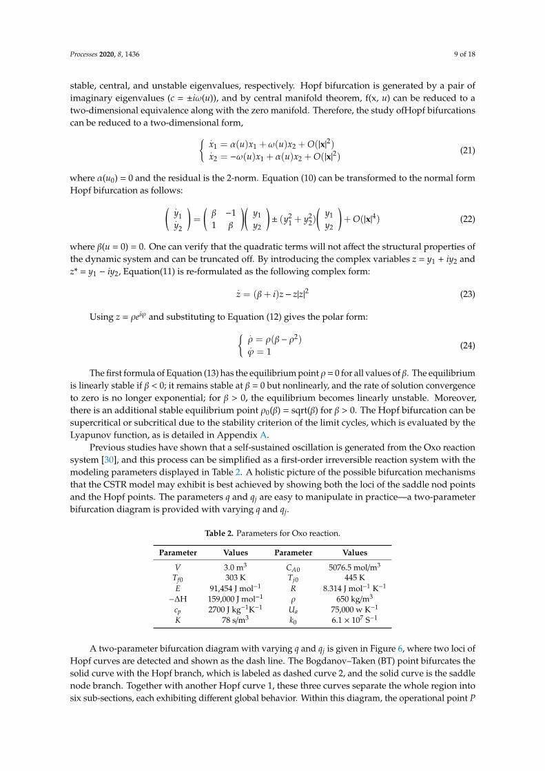
Previous studies have shown that a self-sustained oscillation is generated from the Oxo reactionsystem [30], and this process can be simplified as a first-order irreversible reaction system with themodeling parameters displayed in Table 2. A holistic picture of the possible bifurcation mechanismsthat the CSTR model may exhibit is best achieved by showing both the loci of the saddle nod pointsand the Hopf points. The parameters q and qj are easy to manipulate in practice—a two-parameterbifurcation diagram is provided with varying q and qj.

Table 2. Parameters for Oxo reaction.

Parameter Values Parameter Values

V 3.0 m3 CA0 5076.5 mol/m3

Tf0 303 K Tj0 445 KE 91,454 J mol−1 R 8.314 J mol−1 K−1

−∆H 159,000 J mol−1 ρ 650 kg/m3

cp 2700 J kg−1K−1 Ua 75,000 w K−1

K 78 s/m3 k0 6.1 × 107 S−1

A two-parameter bifurcation diagram with varying q and qj is given in Figure 6, where two loci ofHopf curves are detected and shown as the dash line. The Bogdanov–Taken (BT) point bifurcates thesolid curve with the Hopf branch, which is labeled as dashed curve 2, and the solid curve is the saddlenode branch. Together with another Hopf curve 1, these three curves separate the whole region intosix sub-sections, each exhibiting different global behavior. Within this diagram, the operational point P

Processes 2020, 8, 1436 10 of 18

mentioned above falls into section B, as represented by the large sized dot, meaning that a uniquestable limit cycle is generated.

Processes 20xx, x, x FOR PEER REVIEW 10 of 19

A two-parameter bifurcation diagram with varying q and qj is given in Figure 6, where two loci of Hopf curves are detected and shown as the dash line. The Bogdanov–Taken (BT) point bifurcates the solid curve with the Hopf branch, which is labeled as dashed curve 2, and the solid curve is the saddle node branch. Together with another Hopf curve 1, these three curves separate the whole region into six sub-sections, each exhibiting different global behavior. Within this diagram, the operational point P mentioned above falls into section B, as represented by the large sized dot, meaning that a unique stable limit cycle is generated.

Figure 6. Two-parameter bifurcation diagram of the Oxo reaction model. BT stands for a Bogdanov–Taken point, and CP stands for a cusp point. Any points in section A generate a unique stable point thatcoverts to the low conversion region; points in section E generate three equilibriums, the high and low conversion ones are stable while the middle one is a saddle; points in section B generate one stable limit cycle; points in section C generate a unique stable point thatcoverts to the low conversion region; points in section D generate three equilibriums, the high conversion region is a stable limit cycle, then a saddle, and a stable point at the low conversion region; points in section F generate a saddle that is incorporated by a limit cycle.

From the analysis diagram provided in Figure 6, one can find that designing at q = 0.004923 m3s−1 and qj = 0.01 m3s−1 generates oscillatory dynamics. If the oscillation is not desirable, one can redesign the operation point to, say, q = 0.01 m3s−1 and qj = 0.01 m3s−1, which falls into section E. If self-oscillation is on demand, i.e., the steady-state operating point is set as q = 0.004923 m3s−1 and qj = 0.01 m3s−1, a stable limit cycle with frequency 0.00167 s−1 is generated, as is shown in Figure 7 (black line). Since points in section E generate three equilibriums, and the high and low conversion ones are stable while the middle one is a saddle, the phase portrait obtained is similar to the subplot in Figure 2. One can implement the strategy provided in Figure 4 to control the CSTR at a high conversion equilibrium point. Because the mean value of the process output of a process operating at oscillatory state will not be the same as that of a steady state process output at the mean values of operating variables, one can also utilize the oscillatory dynamics for process intensification purpose, which is incorporated in the following section.

0 0.005 0.01 0.0150

0.01

0.02

0.03

0.04

0.05

0.06

0.07

0.08

0.09

0.1

q

qj

BT

CP

D

E

A

12

F

C

B

P

0 500 1000 1500 2000 2500 3000 3500 40000

0.02

0.04

0.06

0.08

0.1

0.12

0.14

0.16

0.18

t

Z1

No Forcing

f=0.003

f=0.006

Figure 6. Two-parameter bifurcation diagram of the Oxo reaction model. BT stands for aBogdanov–Taken point, and CP stands for a cusp point. Any points in section A generate a uniquestable point thatcoverts to the low conversion region; points in section E generate three equilibriums,the high and low conversion ones are stable while the middle one is a saddle; points in section Bgenerate one stable limit cycle; points in section C generate a unique stable point thatcoverts to thelow conversion region; points in section D generate three equilibriums, the high conversion region is astable limit cycle, then a saddle, and a stable point at the low conversion region; points in section Fgenerate a saddle that is incorporated by a limit cycle.

From the analysis diagram provided in Figure 6, one can find that designing at q = 0.004923 m3s−1

and qj = 0.01 m3s−1 generates oscillatory dynamics. If the oscillation is not desirable, one can redesignthe operation point to, say, q= 0.01 m3s−1 and qj = 0.01 m3s−1, which falls into section E. If self-oscillationis on demand, i.e., the steady-state operating point is set as q = 0.004923 m3s−1 and qj = 0.01 m3s−1,a stable limit cycle with frequency 0.00167 s−1 is generated, as is shown in Figure 7 (black line).Since points in section E generate three equilibriums, and the high and low conversion ones are stablewhile the middle one is a saddle, the phase portrait obtained is similar to the subplot in Figure 2.One can implement the strategy provided in Figure 4 to control the CSTR at a high conversionequilibrium point. Because the mean value of the process output of a process operating at oscillatorystate will not be the same as that of a steady state process output at the mean values of operatingvariables, one can also utilize the oscillatory dynamics for process intensification purpose, which isincorporated in the following section.

Processes 20xx, x, x FOR PEER REVIEW 10 of 19

A two-parameter bifurcation diagram with varying q and qj is given in Figure 6, where two loci of Hopf curves are detected and shown as the dash line. The Bogdanov–Taken (BT) point bifurcates the solid curve with the Hopf branch, which is labeled as dashed curve 2, and the solid curve is the saddle node branch. Together with another Hopf curve 1, these three curves separate the whole region into six sub-sections, each exhibiting different global behavior. Within this diagram, the operational point P mentioned above falls into section B, as represented by the large sized dot, meaning that a unique stable limit cycle is generated.

Figure 6. Two-parameter bifurcation diagram of the Oxo reaction model. BT stands for a Bogdanov–Taken point, and CP stands for a cusp point. Any points in section A generate a unique stable point thatcoverts to the low conversion region; points in section E generate three equilibriums, the high and low conversion ones are stable while the middle one is a saddle; points in section B generate one stable limit cycle; points in section C generate a unique stable point thatcoverts to the low conversion region; points in section D generate three equilibriums, the high conversion region is a stable limit cycle, then a saddle, and a stable point at the low conversion region; points in section F generate a saddle that is incorporated by a limit cycle.

From the analysis diagram provided in Figure 6, one can find that designing at q = 0.004923 m3s−1 and qj = 0.01 m3s−1 generates oscillatory dynamics. If the oscillation is not desirable, one can redesign the operation point to, say, q = 0.01 m3s−1 and qj = 0.01 m3s−1, which falls into section E. If self-oscillation is on demand, i.e., the steady-state operating point is set as q = 0.004923 m3s−1 and qj = 0.01 m3s−1, a stable limit cycle with frequency 0.00167 s−1 is generated, as is shown in Figure 7 (black line). Since points in section E generate three equilibriums, and the high and low conversion ones are stable while the middle one is a saddle, the phase portrait obtained is similar to the subplot in Figure 2. One can implement the strategy provided in Figure 4 to control the CSTR at a high conversion equilibrium point. Because the mean value of the process output of a process operating at oscillatory state will not be the same as that of a steady state process output at the mean values of operating variables, one can also utilize the oscillatory dynamics for process intensification purpose, which is incorporated in the following section.

0 0.005 0.01 0.0150

0.01

0.02

0.03

0.04

0.05

0.06

0.07

0.08

0.09

0.1

q

qj

BT

CP

D

E

A

12

F

C

B

P

0 500 1000 1500 2000 2500 3000 3500 40000

0.02

0.04

0.06

0.08

0.1

0.12

0.14

0.16

0.18

t

Z1

No Forcing

f=0.003

f=0.006

Figure 7. Oscillatory behavior for different forcing frequencies, where forcing amplitude is constant,A = 0.006 m3/s.

Processes 2020, 8, 1436 11 of 18

5. Forced Periodic Inputs on the Self-Sustained Oscillations

From process intensification viewpoint, regulating the set point as periodic may achieve betterperformance than controlling at steady state, but monitoring delay or process model mismatch maycause interference between manipulate and control variables. Hence, it is necessary to study thedynamics through external forcing of the chemical oscillator.

In current study, qj is excited rather than q on two reasons: (1) for a typical operational problem,varying the reactant inlet flow rate in large scale is not easy to realize in practice; (2) q is linearlycorrelated with state variable Z1 in the dynamic system, while nonlinearity is the reason for τ-timeaveraged performance improvement. On the other hand, varying qj is advisable because coolant iseasy to manipulate, and because the flow rate of qj usually determines heat removal from the reactor.For example, a deviation of qj by 10% will have an impact up to 5.5% for the heat removal term inEquation (1), hence havinga direct influence on the process itself.

Taking qj as forced oscillation variable, with the form of shown as follows:

q j = q j0 + A sin(2π f t) (25)

where qj0 is the nominal coolant flow rate, A is the forcing amplitude, f is the forcing frequency.A sinusoidal function by itself is an orbit if it is cast to polar coordinate plane. Setting u = sin(2πft + ϕ),where the derivative is du/dt = cos(2πft + ϕ) 2πf, then defining v = cos(2πft + ϕ), for analyticalconvenience, Equation (22) is written in the formal form of the two dimensional Hopf bifurcation;the sinusoidal forcing of the chemical oscillator is presented as follows:

dZ1dt =

qV (1−Z1) − kZ1

dZ2dt =

qV (Z f 0 −Z2) −

UaK(q j0+Au)(Z2−Z j0)

Vρcp(1+K(q j0+Au)) + kZ1dudt = u + 2πv f − (u2 + v2)udvdt = −2πu f + v− (u2 + v2)v

(26)

For the system above, the first two formulas in combined forms is a limit cycle while the remainingtwo forms are the other; how the two orbits correlate with each other to intensify overall behavior ofthe process system is the focus of this discussion.

As the intrinsic frequency affects the dynamics of the studied process, it can be calculatedaccording to the forcing rotation velocity by casting the normal form of the unforced process to thepolar coordinates. The method chosen in this work is to integrate Equation (3) at the nominal state bya fourth-order Runge–Kutta algorithm, and a frequency of 0.00167 s−1 is extracted from its trajectory.Apparently, when the difference between the forcing frequency f and the intrinsic frequency f 0 is large,the influence of an oscillation with a lower frequency would fade away; when f ≈ f 0, resonance takesplace. Neither scenario is expected from the process intensification point of view. Therefore, the forcingfrequencies in the range 0.1 < f/f 0 < 1 plus 1 < f/f 0 < 10 are of interest [31], and f/f 0 = 3 would be apreferable choice.

The impact of process inlet flow rate forcing on state variables is expected to be insignificant whenthe forcing amplitude is very small. Yet reasonably large forcing amplitudes provide an opportunity tomodify the dynamics of the process. As shown in Figure 7, with A = 0.006 m3/s, f = 0.006 s−1, the outputfrequency shifts from the intrinsic frequency to the forcing frequency of 0.006 s−1. Complex dynamicswould emerge because of codimension-1 bifurcations, i.e., bifurcation of the limit cycles, as is shown inFigure 8a periodic doubling (PD) and Figure 8b Neimark–Sacker (NS) bifurcation.

Processes 2020, 8, 1436 12 of 18

Processes 20xx, x, x FOR PEER REVIEW 12 of 19

Taking amplitude as the bifurcation parameter for Equation (15), the continuation diagram of the limit cycle is provided in Figure 9. A supercritical NS point is generated when the amplitude is about 0.00266 s−1, with the normal form coefficient of this NS point being negative. One can find the analytical solution of PD and NS bifurcations in Appendix B, and from Equation (A2), it is obvious that μ > 0 causes Equation (A1) to diverge, while for μ< 0 it shrinks to a point. Periodic or pseudo-periodic solutions are obtained when Re(μ) = 0, which is the singular point that may causecodimension-1 bifurcation of limit cycles. NS bifurcation emerges when μ1,2 = 0 ± iφ, where a two-dimensional invariant torus appears, while the fixed point changes stability by a Hopf bifurcation, as is shown in Figure 8b.

0L 0L 0L1L

0u > 0u = 0u<

a

0L

0u> 0u = 0u<

0L

0L

b

Figure 8. Codimension-1 bifurcation of limit cycles. (a) Periodic doubling bifurcation; (b) Neimark–Sacker bifurcation.

Figure 9. Continuation of limit cycle with forcing amplitude as bifurcation parameter.

0.06 0.062 0.064 0.066 0.068 0.07 0.072 0.074 0.076 0.078

1.095

1.1

1.105

1.11

1.115

Z1

Z2

NS

A=0.006 m3/s

f =0.002 s-1

Figure 8. Codimension-1 bifurcation of limit cycles. (a) Periodic doubling bifurcation; (b) Neimark–Sacker bifurcation.

Taking amplitude as the bifurcation parameter for Equation (15), the continuation diagram ofthe limit cycle is provided in Figure 9. A supercritical NS point is generated when the amplitude isabout 0.00266 s−1, with the normal form coefficient of this NS point being negative. One can find theanalytical solution of PD and NS bifurcations in Appendix B, and from Equation (A2), it is obvious thatµ > 0 causes Equation (A1) to diverge, while for µ< 0 it shrinks to a point. Periodic or pseudo-periodicsolutions are obtained when Re(µ) = 0, which is the singular point that may causecodimension-1bifurcation of limit cycles. NS bifurcation emerges when µ1,2 = 0 ± iϕ, where a two-dimensionalinvariant torus appears, while the fixed point changes stability by a Hopf bifurcation, as is shown inFigure 8b.

Processes 20xx, x, x FOR PEER REVIEW 12 of 19

Taking amplitude as the bifurcation parameter for Equation (15), the continuation diagram of the limit cycle is provided in Figure 9. A supercritical NS point is generated when the amplitude is about 0.00266 s−1, with the normal form coefficient of this NS point being negative. One can find the analytical solution of PD and NS bifurcations in Appendix B, and from Equation (A2), it is obvious that μ > 0 causes Equation (A1) to diverge, while for μ< 0 it shrinks to a point. Periodic or pseudo-periodic solutions are obtained when Re(μ) = 0, which is the singular point that may causecodimension-1 bifurcation of limit cycles. NS bifurcation emerges when μ1,2 = 0 ± iφ, where a two-dimensional invariant torus appears, while the fixed point changes stability by a Hopf bifurcation, as is shown in Figure 8b.

0L 0L 0L1L

0u > 0u = 0u<

a

0L

0u> 0u = 0u<

0L

0L

b

Figure 8. Codimension-1 bifurcation of limit cycles. (a) Periodic doubling bifurcation; (b) Neimark–Sacker bifurcation.

Figure 9. Continuation of limit cycle with forcing amplitude as bifurcation parameter.

0.06 0.062 0.064 0.066 0.068 0.07 0.072 0.074 0.076 0.078

1.095

1.1

1.105

1.11

1.115

Z1

Z2

NS

A=0.006 m3/s

f =0.002 s-1

Figure 9. Continuation of limit cycle with forcing amplitude as bifurcation parameter.

Processes 2020, 8, 1436 13 of 18

Therefore, when the orbits are on the left-hand side of NS (A > ANS), the output is a stable limitcycle with the same frequency as the forcing frequency. When the orbits are on the right-hand sideof NS (A < ANS), an invariant two-dimensional torus is generated in the corresponding phase space,as shown in the subplot of Figure 10. The emergence of torus is viewed as coexistence of two cyclingwith different frequency, but torus is to be avoided from apractical perspective because the dynamicsof the torus are complicated, the large area of working states makes it difficult to control, and loweraverage conversion ratio is obtained in this process. Therefore, forcing amplitude should be larger thanthe NS point, and application constrains such as operation cost should also be considered to decideproper forcing amplitude. When the periodic forcing is A = 0.006, f = 0.006, better outcome is generatedin at least three aspects: (1) the process itself is dominated by forcing frequency, which means as longas the forcing input is controlled, the objective is well controlled, irrelevant of the internal oscillation;(2) the process is intensified by periodic forcing; (3) smaller output amplitude in comparison with theinternal oscillation makes the system more robust to various disturbances.

Processes 20xx, x, x FOR PEER REVIEW 13 of 19

Therefore, when the orbits are on the left-hand side of NS (A > ANS), the output is a stable limit cycle with the same frequency as the forcing frequency. When the orbits are on the right-hand side of NS (A < ANS), an invariant two-dimensional torus is generated in the corresponding phase space, as shown in the subplot of Figure 10. The emergence of torus is viewed as coexistence of two cycling with different frequency, but torus is to be avoided from apractical perspective because the dynamics of the torus are complicated, the large area of working states makes it difficult to control, and lower average conversion ratio is obtained in this process. Therefore, forcing amplitude should be larger than the NS point, and application constrains such as operation cost should also be considered to decide proper forcing amplitude. When the periodic forcing is A = 0.006, f = 0.006, better outcome is generated in at least three aspects: (1) the process itself is dominated by forcing frequency, which means as long as the forcing input is controlled, the objective is well controlled, irrelevant of the internal oscillation; (2) the process is intensified by periodic forcing; (3) smaller output amplitude in comparison with the internal oscillation makes the system more robust to various disturbances.

Figure 10. Bifurcation of forcing amplitude for different forcing frequencies.

To numerically show how the periodic forcing can improve the performance of a process, the performance index calculated as follows:

0

1 ( , )y g Z u dtτ

τ= (27)

where τ is the forcing period; g(x,u) is the performance function, whose unforced equivalence is represented as ys = g(xs); Z is the state variable vector; and u is the forcing input. In this case, the state variable vector is [Z1, Z2], with the performance function g(Z(u)) as the outlet concentration Z1. For the case where the forcing is given by A = 0.006 m3/s, f = 0.006 s−1, the average outlet concentration is Z1forced = 0.067, compared with the unforced average value of Z1unforced = 0.078, thus showing an increase in conversion of 16.4%. As shown in Figure9, the center of the orbit would move left as the forcing amplitude A increases, but A cannot be increased in an unbounded manner, i.e., the jacket volume, coolant control valve, or the reactor itself would restrict the upper limit of A. The same situation happens with the forcing frequency f; when f is too high, even the feasibility of the process model, especially the assumption of remark 2, is questionable. For different f values, the location of the NS point does not migrate significantly, as shown in Figure 4, indicating that, for various f values, the dynamics of the process system is about to change when A decreases to NS point.

The periodic forcing parameters in Equation (26) are recommended to be A = 0.006 m3/s, f = 0.006 s−1, and better outcome is obtained in at least three aspects: (1) the process itself is dominated by the forcing frequency, which means that the objective is well controlled as long as the forcing input is controlled, regardless of its internal oscillation; (2) the process is intensified by periodic forcing; (3) a smaller output amplitude in comparison with the internal oscillation makes the system more robust to various disturbances.

0 1 2 3 4 5 6x 10-3

2

4

6

8

10

12

14

x 10-3

A

f

NS

NS

NS

NS

Figure 10. Bifurcation of forcing amplitude for different forcing frequencies.

To numerically show how the periodic forcing can improve the performance of a process,the performance index calculated as follows:

y =1τ

∫ τ

0g(Z, u) dt (27)

where τ is the forcing period; g(x,u) is the performance function, whose unforced equivalence isrepresented as ys = g(xs); Z is the state variable vector; and u is the forcing input. In this case, the statevariable vector is [Z1, Z2], with the performance function g(Z(u)) as the outlet concentration Z1. For thecase where the forcing is given by A = 0.006 m3/s, f = 0.006 s−1, the average outlet concentrationis Z1

forced = 0.067, compared with the unforced average value of Z1unforced = 0.078, thus showing an

increase in conversion of 16.4%. As shown in Figure 9, the center of the orbit would move left as theforcing amplitude A increases, but A cannot be increased in an unbounded manner, i.e., the jacketvolume, coolant control valve, or the reactor itself would restrict the upper limit of A. The samesituation happens with the forcing frequency f ; when f is too high, even the feasibility of the processmodel, especially the assumption of remark 2, is questionable. For different f values, the location of theNS point does not migrate significantly, as shown in Figure 4, indicating that, for various f values,the dynamics of the process system is about to change when A decreases to NS point.

The periodic forcing parameters in Equation (26) are recommended to be A = 0.006 m3/s,f = 0.006 s−1, and better outcome is obtained in at least three aspects: (1) the process itself is dominatedby the forcing frequency, which means that the objective is well controlled as long as the forcing inputis controlled, regardless of its internal oscillation; (2) the process is intensified by periodic forcing; (3) asmaller output amplitude in comparison with the internal oscillation makes the system more robust tovarious disturbances.

Processes 2020, 8, 1436 14 of 18

6. Conclusions

The nonlinear dynamics discussed above shows that the design, operation, and control of a CSTRcould be very complicated. The presence of the multiple steady states necessitates handy design of anefficient control system to regulate the operational conditions to desired states. The exploration onoscillatory CSTRs has evolved into two distinct directions: one is the elimination of the oscillationsand the other is to take advantage of the process dynamics. Chaotic dynamics would also generatethrough coupling of two oscillatory CSTRs or CSTR forced. Therefore, a complete knowledge of staticand dynamic behavior of these behaviors is required to understand, to operate, to control, and tooptimize CSTRs.

Author Contributions: Conceptualization, C.Z., L.S. and Z.Z.; methodology, L.S.; software, L.S.; validation, C.Z.and J.R.; formal analysis, C.Z.; investigation, L.S. and J.R.; resources, L.S.; data curation, L.S.; writing—originaldraft preparation, L.S. and C.Z.; writing—review and editing, C.Z.; visualization, L.S. and J.R.; supervision, C.Z.;project administration, C.Z.; funding acquisition, C.Z. All authors have read and agreed to the published versionof the manuscript.

Funding: The authors gratefully acknowledge the following institutions for support: Basic Yunnan (China)Research program (202001AU070048), and The National Natural Science Foundation of China (grant no.21878012).

Conflicts of Interest: The authors declare no conflict of interest.

Appendix A Stability Analysis of the Self-Oscillator

Any a Hopf bifurcation can simplified to a 2-dimentional domain, and the associated Jacobianmatrix is as summed as follows:

J(0;u) =

[α(u) ω(u)−ω(u) α(u)

](A1)

where the bifurcation parameter u sets as any real number and is independent of α or ω, and ω , 0 forall u, while α(u) < 0 if u < 0 and α(u) > 0 if u < 0.We want to construct a Lyapunov function V to teststability of the origin and the quartic terms are chosen,

V = 12

(x2

1 + x22

)+ 1

3 ax31 + bx2

1x2 + cx1x22 +

13 dx3

2+ 1

4 ex41 + gx3

1x2 +12 hx2

1x22 + jx1x3

2 +14 kx4

2

(A2)

and try to identify the constants a, b, . . . , k to be of O(1) for small µ and to give dV/dt the propertiesneeded. Applying Equation (A1), one obtains the time derivative of V,

dV/dt = α(u)(x2

1 + x22

)+ O

(|x|3

)(A3)

It follows Equation (A3) that for small y, Equation (A1) is negative definite when α(u) < 0 butpositive definite when α(u) > 0, independent of the coefficients a, b, . . . , k above. Hence, it only remainsto examine the case α(u) = 0.

Expand the two-dimensional system up to third-order,.x1 = α(u)x1 +ω(u)x2 +

12 f 1

11x21 + f 1

12x1x2 +12 f 1

22x22 +

16 f 1

111x31

+ 12 f 1

112x21x2 +

12 f 1

122x1x22 +

16 f 1

222x32 + O

(|x|4

).x2 = −ω(u)x1 + α(u)x2 +

12 f 2

11x21 + f 2

12x1x2 +12 f 2

22x22 +

16 f 2

111x31

+ 12 f 2

112x21x2 +

12 f 2

122x1x22 +

16 f 2

222x32 + 0

(|x|4

)where :

f ipq ,

∂2 fi∂xp∂xq

∣∣∣∣x=0

and f ipqr ,

∂3 fi∂xp∂xq∂xr

∣∣∣∣x=0

(A4)

Processes 2020, 8, 1436 15 of 18

Equation (A4) is generally functions of µ. The corresponding expression for.

V is given by

.V = α(x2

1 + x22) +

(−ωb + 1

2 f 111

)x3

1 +(ωc + 1

2 f 222

)x3

2 +(ω(a− 2c) + f 1

12 +12 f 2

11

)x2

1x2

+(ω(2b− d) + 1

2 f 122 + f 2

12

)x1x2

2 +(−ωg + 1

2 a f 111 +

12 b f 2

11 +16 f 1

111

)x4

1+

(ω(e− h) + b f 1

11 + a f 112 + c f 2

11 + b f 212 +

12 f 1

112 +16 f 2

111

)x3

1x2

+(3ω(g− j) + 1

2 c f 111 + 2b f 1

12 +12 a f 1

22 +12 d f 2

11 + 2c f 212 +

12 b f 2

22 +12 f 1

122 +12 f 2

112

)x2

1x22

+(ω(h− k) + c f 1

12 + b f 122 + d f 2

12 + c f 222 +

16 f 1

222 +12 f 2

122

)x1x3

2+

(ω j + 1

2 c f 122 +

12 d f 2

22 +16 f 2

222

)x4

2 + O(α)O(|x|3) + O(|x|5).

(A5)

To make the derivative of V definitely positive or negative, coefficients should be set so that theodd-order terms x1

3, x23, x1 x2

2, and x12 x2 are zeroes, which determines a, b, c and d uniquely.

a = −(

f 222 + f 1

12 +12 f 2

11

)/ω(u)

b = 12 f 1

11/ω(u)c = − 1

2 f 222/ω(u)

d =(

f 111 + f 2

12 +12 f 1

22

)/ω(u)

(A6)

Likewise, x1 x23 and x1

3 x2 can vanish to make Equation (A5) simpler. This determines e and k,which are functions of a, b, c, d, and h, while h can be arbitrary. Since the rest of the deduction does notinclude e and k, their explicit expression will not be included here.

From Equation (A3), dV/dt is sign definite when α(u) , 0. However, when α(u) = 0, conditions fordV/dt being positive definite are determined by parameters of x1

4, x24, and x1

2 x22,

β1 −ω(u)g < 0β2 + 3ω(u)(g− j) < 2δβ3 +ω(u) j < 0

(A7)

where β1 = 1

2 a f 111 +

12 b f 2

11 +16 b f 1

111β2 = 1

2 c f 111 + 2b f 2

12 +12 a f 1

22 +12 d f 2

11 + 2c f 212 +

12 b f 2

22 +12 f 1

122 +12 d f 2

112β3 = 1

2 c f 122 +

12 d f 2

22 +16 b f 2

222δ =

√(β1 −ω(u)g)(β3 +ω(u) j < 0)

(A8)

Observe that β1, β2, and β3 are independent of g and j, while g and j are confidents need to bedetermined. Instead of determining these two confidents, we introduce σ (x1

2 + x22)2, which makes

the sign of σ < 0 equal to Equation (A7) when Equation (A9) is satisfied,β1 −ω(u)g = σβ2 + 3ω(u)(g− j) = 2σβ3 +ω(u) j = σ

(A9)

Solving Equation (A9) and the Lyapunov coefficient, σ, is obtained,

σ|u=0 =1

16ω0

(f 111( f 2

11 − f 112) + f 2

22( f 212 − f 1

22) + ( f 211 f 2

12 − f 112 f 1

22)

+( f 1111 + f 1

122 + f 2112 + f 2

122)

)(A10)

Then, σ in Equation (A10) determines the stability of an internal oscillation.

Processes 2020, 8, 1436 16 of 18

Appendix B Bifurcaitons of the Limit Cycles

To study bifurcations of limit cycles, we introduce the Floquet theory. Considering Equation (3)in vector form dx/dt = f(x) with x = [Z1, Z2]T, there is a periodic solution x(t) = η(t) with period T0 atf = 0.00266 s−1. The system perturbed about ηwith an additional term vobtains,

v′ = J(t)v

where : Ji j(t) =∂fi∂x j

∣∣∣∣η(t)

(A11)

Floquet theorem provides solution structure for Equation (A11), which can be used to studybifurcations; when oscillatory qj at Equation (11) is included, one can verify that the solution v ofEquation (A11) need not to be periodic, but should be the form as follows:

eµtp(t) (A12)

where p(t) has period T0, and µi is the ith-Floquet exponents, plus ρi(T0) = eµiT0 is the Floquetmultiplier, satisfying

n∏i=1

ρi(T0) = exp

n∑i=1

µiT

= exp(∫ T0

0tr(J(s))ds

)(A13)

Proof. Suppose vi is n solutions of Equation (A11), and if the solution vectors are linearly independent,V = {vi} is called a fundamental matrix. It is easy to verify that for a given non-singular matrix B∈Rn×n,V(t + T0) = V(t)B is also a fundamental matrix of Equation (A11), where T0 is the period of the originalsystem, and the determinant, det, can be computed as follows:

det(B) = exp(∫ T0

0tr(J(s))ds

)(A14)

To prove Equation (A14), the determinant of V(t) needs to be computed.

V(t) = V(t0) + (t− t0)V′

(t0) + O((t− t0)

2)

= V(t0) + (t− t0)J(t0)V(t0) + O((t− t0)

2)

=(I + (t− t0)J(t0)

)V(t0) + O

((t− t0)

2) (A15)

where t0 is some initial time. Since

det(I + εC) = 1 + εtr(C) + O(ε2) (A16)

the determinant of the fundamental matrix satisfies

det(V(t)) = det(I + (t− t0)J(t0)

)det

(V(t0)

)= det

(V(t0)

)(1 + (t− t0)tr

(J(t0)

)) (A17)

Taylor expansion of Equation (A17) obtains

det(V(t)) = det(V(t0)

)+ (t− t0)

[det

(V(t0)

)]′+ O

((t− t0)

2)

where :[det

(V(t0)

)]′= det

(V(t0)

)tr(J(t0)

) (A18)

Processes 2020, 8, 1436 17 of 18

Then,

det(V(t)) = det(V(t0)

)exp

∫ t

t0

trJ(s)ds

(A19)

Now, introduce the period T0,

det(V(t + T0)) = det(V(t0)

)exp

(∫ tt0

trJ(s)ds +∫ t+T0

t trJ(s)ds)

= det(V(t)

)exp

(∫ t+T0

t trJ(s)ds)

= det(V(t)

)exp

(∫ T0

0 trJ(s)ds) (A20)

since V(t + T0) = V(t)B. The initial state is arbitrary, so assume V(0) = I; thus, Equation (A15) is proven.The eigenvalues ρ1, ρ2, . . . , ρn of B are called Floquet multipliers, and µi is the Floquet exponents,

satisfying ρi(T0) = eµiT0. Let b be an eigenvector of B corresponding to an eigenvalue ρ, then, one canobtain the following relations,

v(t + T0) = V(t + T0)b= V(t)Bb= ρV(t)b= ρv(t)

(A21)

Let Equation (A12) be satisfied and one obtains

p(t + T0) = v(t + T0)e−µ(t+T0)

= ρv(t)e−µ(t+T0)

=ρ

eµT0v(t)e−µt

= v(t)e−µt

= p(t)

(A22)

where inanalytics of the limit cycle are provided. �

References

1. Russo, L.P.; Bequette, B.W. Impact of process design on the multiplicity behavior of a jacketed exothermicCSTR. AIChE J. 1995, 41, 135–147. [CrossRef]

2. Astudillo, I.C.P.; Alzate, C.A.C. Importance of stability study of continuous systems for ethanol production.J. Biotechnol. 2011, 15, 43–55. [CrossRef] [PubMed]

3. Ajbar, A. Classification of static behavior of a class of unstructured models of continuous bioprocesses.Biotechnol. Prog. 2001, 17, 597–605. [CrossRef]

4. Uppal, A.; Ray, W.H.; Poore, A.B. On the dynamic behavior of continuous stirred tank reactors. Chem. Eng. Sci.1974, 29, 967–985. [CrossRef]

5. Uppal, A.; Ray, W.H.; Poore, A.B. The classification of the dynamic behavior of continuous stirred tankreactors—Influence of reactor residence time. Chem. Eng. Sci. 1976, 31, 205–214. [CrossRef]

6. Mahecha-Botero, A.; Garhyan, P.; Elnashaie, S.S.E.H. Nonlinear characteristics of a membrane fermentor forethanol production and their implications. Nonlinear Anal. Real World Appl. 2006, 7, 432–457. [CrossRef]

7. Sridhar, L.N. Elimination of oscillations in fermentation processes. AIChE J. 2011, 57, 2397–2405. [CrossRef]8. Zhang, N.; Seider, W.D.; Chen, B. Bifurcation control of high-dimensional nonlinear chemical processes using

an extended washout-filter algorithm. Comput. Chem. Eng. 2016, 84, 458–481. [CrossRef]9. Sterman, L.E.; Ydstie, B.E. Periodic forcing of the CSTR: An application of the generalized II-criterion.

AIChE J. 1991, 37, 986–996. [CrossRef]10. Kravaris, C.; Dermitzakis, I.; Thompson, S. Higher-order corrections to the pi criterion using center manifold

theory. Eur. J. Control 2012, 18, 5–19. [CrossRef]

Processes 2020, 8, 1436 18 of 18

11. Hatzimanikatis, V.; Lyberatos, G.; Pavlou, S.; Svoronos, S.A. A method for pulsed periodic optimization ofchemical reaction systems. Chem. Eng. Sci. 1993, 48, 789–797. [CrossRef]

12. Zuyev, A.; Seidel-Morgenstern, A.; Benner, P. An isoperimetric optimal control problem for a non-isothermalchemical reactor with periodic inputs. Chem. Eng. Sci. 2017, 161, 206–214. [CrossRef]

13. Zhai, C.; Sun, W.; Palazoglu, A. Analysis of periodically forced bioreactors using nonlinear transfer functions.J. Process Control 2017, 58, 90–105. [CrossRef]

14. Matthias, M.A.; Grüne, L. Economic model predictive control without terminal constraints for optimalperiodic behavior. Automatica 2016, 70, 128–139.

15. Varigonda, S.; Georgiou, T.T.; Daoutidis, P. Numerical solution of the optimal periodic control problem usingdifferential flatness. IEEE Trans. Autom. Control 2004, 49, 271–275. [CrossRef]

16. Guay, M.; Dochain, D.; Perrier, M.; Hudon, N. Flatness-Based Extremum-Seeking Control over PeriodicOrbits. IEEE Trans. Autom. Control 2007, 52, 2005–2012. [CrossRef]

17. Gómez-Pérez, C.A.; Espinosa, J. Design method for continuous bioreactors in series with recirculation andproductivity optimization. Chem. Eng. Res. Des. 2018, 137, 544–552. [CrossRef]

18. Zhao, X.; Marquardt, W. Wolfgang Marquardt, Reactor network synthesis with guaranteed robust stability.Comput. Chem. Eng. 2016, 86, 75–89. [CrossRef]

19. Zhai, C.; Palazoglu, A.; Wang, S.; Sun, W. Strategies for the Analysis of Continuous Bioethanol Fermentationunder Periodical Forcing. Ind. Eng. Chem. Res. 2017, 56, 3958–3968. [CrossRef]

20. Abashar, M.E.E.; Elnashaie, S.S.E.H. Multistablity, bistability and bubbles phenomena in a periodically forcedethanol fermentor. Chem. Eng. Sci. 2011, 66, 6146–6158. [CrossRef]

21. Sistu, P.B.; Bequette, B.W. Model predictive control of processes with input multiplicities. Chem. Eng. Sci.1995, 50, 921–936. [CrossRef]

22. Regenass, W.; Aris, R. Stability estimates for the stirred tank reactor. Chem. Eng. Sci. 1965, 20, 60–66.[CrossRef]

23. Swartz, C.L.; Kawajiri, Y. Design for dynamic operation: A review and new perspectives for an increasinglydynamic plant operating environment. Comput. Chem. Eng. 2019, 128, 329–339. [CrossRef]

24. Gu, S.; Liu, L.; Zhang, L. Optimization-based framework for designing dynamic flexible heat exchangernetworks. Ind. Eng. Chem. Res. 2018, 58, 6026–6041. [CrossRef]

25. Tsay, C.; Pattison, R.C.; Baldea, M. A pseudo-transient optimization framework for periodic processes:Pressure swing adsorption and simulated moving bed chromatography. AIChE J. 2018, 64, 2982–2996.[CrossRef]

26. Gelhausen, M.G.; Yang, S.; Cegla, M. Cyclic mass transport phenomena in a novel reactor for gas-liquid-solidcontacting. AIChE J. 2017, 63, 208–215. [CrossRef]

27. Muller, P.; Hermans, I. Applications of modulation excitation spectroscopy in heterogeneous catalysis.Ind. Eng. Chem. Res. 2017, 56, 1123–1136. [CrossRef]

28. Silveston, P.L.; Hudgins, R.R. Periodic Operation of Chemical Reactors; Butterworth-Heinemann, Elsevier:Amsterdam, The Netherlands, 2012.

29. Parulekar, S.J. Systematic performance analysis of continuous processes subject to multiple input cycling.Chem. Eng. Sci. 2003, 58, 5173–5194. [CrossRef]

30. Ray, A.K. Performance improvement of a chemical reactor by non-linear natural oscillations. Chem. Eng. J.1995, 59, 169–175. [CrossRef]

31. Ajbar, A. On the improvement of performance of bioreactors through periodic forcing. Comput. Chem. Eng.2011, 35, 1164–1170. [CrossRef]

Publisher’s Note: MDPI stays neutral with regard to jurisdictional claims in published maps and institutionalaffiliations.

© 2020 by the authors. Licensee MDPI, Basel, Switzerland. This article is an open accessarticle distributed under the terms and conditions of the Creative Commons Attribution(CC BY) license (http://creativecommons.org/licenses/by/4.0/).